Electricity and Magnetism, Second Edition
For 40 years, Edward M. Purcell's classic textbook has introduced
students to the wonders of electricity and magnetism.
With profound physical insight, Purcell covers all the standard introductory
topics, such as electrostatics, magnetism, circuits, electromagnetic
waves, and electric and magnetic fields in matter. Taking a non-traditional
approach, the textbook focuses on fundamental questions from different
frames of reference. Mathematical concepts are introduced in parallel with
the physics topics at hand, making the motivations clear. Macroscopic
phenomena are derived rigorously from microscopic phenomena.
With hundreds of illustrations and over 300 end-of-chapter problems, this
textbook is widely considered the best undergraduate textbook on
electricity and magnetism ever written.
edward m. purcell (1912-1997) was the recipient of many awards for
his scientific, educational, and civic work. In 1952 he shared the Nobel
Prize for Physics for his independent discovery of nuclear magnetic
resonance in liquids and in solids, an elegant and precise way of determining
chemical structure and properties of materials which is widely used today.
During his career he served as science advisor to Presidents Dwight D.
Eisenhower, John F. Kennedy, and Lyndon B.Johnson.

SECOND EDITION
ELECTRICITY
AND MAGNETISM
EDWARD M. PURCELL
Hi CAMBRIDGE
^W UNIVERSITY PRESS

CAMBRIDGE UNIVERSITY PRESS
Cambridge, New York, Melbourne, Madrid, Cape Town,
Singapore, Sao Paulo, Delhi, Dubai, Tokyo, Mexico City
Cambridge University Press
The Edinburgh Building, Cambridge CB2 8RU, UK
Published in the United States of America by Cambridge University Press, New York
www.cambridge.org
Information on this title: www.cambridge.org/9781107013605
© Dennis and Frank Purcell 2011
This edition is not for sale in India
Previously published by McGraw-Hill, Inc 1985
First edition published by Education Development Center, Inc 1963, 1964, 1965
First published by Cambridge University Press 2011
Printed in the United Kingdom at the University Press, Cambridge
A catalog record for this publication is available from the British Library
ISBN 978-1-107-01360-5 Hardback
Cambridge University Press has no responsibility for the persistence or
accuracy of URLs for external or third-party internet websites referred to in
this publication, and does not guarantee that any content on such websites is,
or will remain, accurate or appropriate.

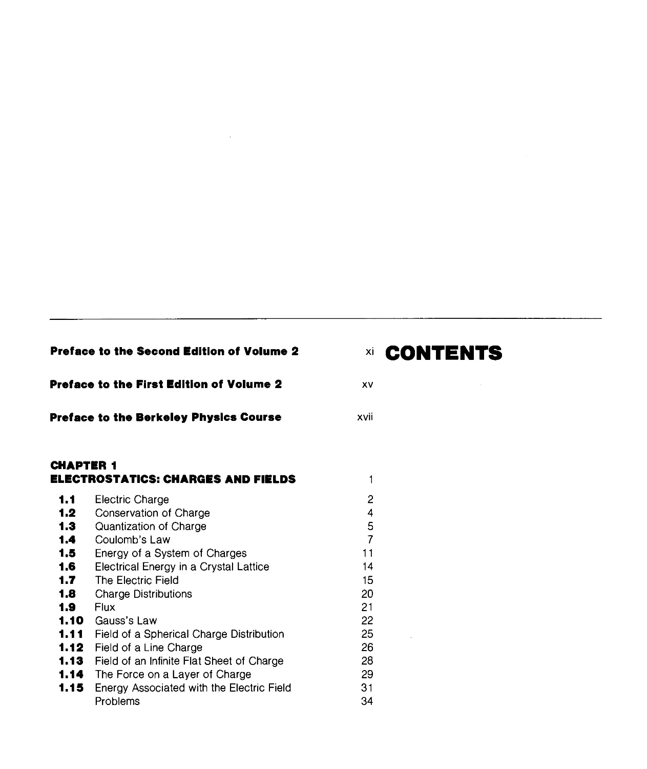
Preface to the Second Edition of Volume 2 xi CONTENTS
Preface to the First Edition of Volume 2 xv
Preface to the Berkeley Physics Course xvii
CHAPTER 1
ELECTROSTATICS: CHARGES AND FIELDS
1.1
1.2
1.3
1.4
1.5
1.6
1.7
1.8
1.9
1.10
1.11
1.12
1.13
1.14
1.15
Electric Charge
Conservation of Charge
Quantization of Charge
Coulomb's Law
Energy of a System of Charges
Electrical Energy in a Crystal Lattice
The Electric Field
Charge Distributions
Flux
Gauss's Law
Field of a Spherical Charge Distribution
Field of a Line Charge
Field of an Infinite Flat Sheet of Charge
The Force on a Layer of Charge
Energy Associated with the Electric Field
Problems
2
4
5
7
11
14
15
20
21
22
25
26
28
29
31
34

VI
CONTENTS
CHAPTER 2
THE ELECTRIC POTENTIAL 41
2.1 Line Integral of the Electric Field 42
2.2 Potential Difference and the Potential Function 44
2.3 Gradient of a Scalar Function 46
2.4 Derivation of the Field from the Potential 48
2.5 Potential of a Charge Distribution 49
Potential of Two Point Charges 49
Potential of a Long Charged Wire 50
2.6 Uniformly Charged Disk 51
2.7 Divergence of a Vector Function 56
2.8 Gauss's Theorem and the Differential Form
of Gauss's Law 58
2.9 The Divergence in Cartesian Coordinates 59
2.10 The Laplacian 63
2.11 Laplace's Equation 64
2.12 Distinguishing the Physics from the Mathematics 66
2.13 The Curl of a Vector Function 68
2.14 Stokes' Theorem 70
2.15 The Curl in Cartesian Coordinates 71
2.16 The Physical Meaning of the Curl 74
Problems 80
CHAPTER 3
ELECTRIC FIELDS AROUND CONDUCTORS 87
3.1 Conductors and Insulators 88
3.2 Conductors in the Electrostatic Field 89
3.3 The General Electrostatic Problem;
Uniqueness Theorem 94
3.4 Some Simple Systems of Conductors 97
3.5 Capacitance and Capacitors 103
3.6 Potentials and Charges on Several Conductors 107
3.7 Energy Stored in a Capacitor 110
3.8 Other Views of the Boundary-Value Problem 111
Problems 113
CHAPTER 4
ELECTRIC CURRENTS 123
4.1 Electric Current and Current Density 124
4.2 Steady Currents and Charge Conservation 126
4.3 Electrical Conductivity and Ohm's Law 128
4.4 The Physics of Electrical Conduction 133
4.5 Conduction in Metals 142

CONTENTS
4.6 Semiconductors 144
4.7 Circuits and Circuit Elements 148
4.8 Energy Dissipation in Current Flow 153
4.9 Electromotive Force and the Voltaic Cell 154
4.10 Networks with Voltage Sources 157
4.11 Variable Currents in Capacitors and Resistors 159
Problems 161
CHAPTER 5
THE FIELDS OF MOVING CHARGES 169
5.1
5.2
5.3
5.4
5.5
5.6
5.7
5.8
5.9
From Oersted to Einstein
Magnetic Forces
Measurement of Charge in Motion
Invariance of Charge
Electric Field Measured in Different Frames
of Reference
Field of a Point Charge Moving with
Constant Velocity
Field of a Charge That Starts or Stops
Force on a Moving Charge
Interaction between a Moving Charge and
Other Moving Charges
Problems
170
171
174
176
178
182
187
190
193
200
CHAPTER 6
THE MAGNETIC FIELD 207
6.1 Definition of the Magnetic Field 208
6.2 Some Properties of the Magnetic Field 214
6.3 Vector Potential 220
6.4 Field of Any Current-Carrying Wire 223
6.5 Fields of Rings and Coils 226
6.6 Change in B at a Current Sheet 231
6.7 How the Fields Transform 235
6.8 Rowland's Experiment 241
6.9 Electric Conduction in a Magnetic Field:
The Hall Effect 241
Problems 245
CHAPTER 7
ELECTROMAGNETIC INDUCTION 255
7.1 Faraday's Discovery 256
7.2 A Conducting Rod Moving through a Uniform
Magnetic Field 258

VIII
CONTENTS
7.3 A Loop Moving through a Nonuniform
Magnetic Field 262
7.4 A Stationary Loop with the Field Sources Moving 269
7.5 A Universal Law of Induction 271
7.6 Mutual Inductance 276
7.7 A Reciprocity Theorem 279
7.8 Self-inductance 281
7.9 A Circuit Containing Self-inductance 282
7.10 Energy Stored in the Magnetic Field 285
Problems 286
CHAPTER 8
ALTERNATING-CURRENT CIRCUITS 297
8.1
8.2
8.3
8.4
8.5
A Resonant Circuit
Alternating Current
Alternating-Current Networks
Admittance and Impedance
Power and Energy in Alternating-Current
Circuits
Problems
298
303
310
313
315
318
CHAPTER 9
MAXWELL'S EQUATIONS
AND ELECTROMAGNETIC WAVES 323
9.1 "Something Is Missing" 324
9.2 The Displacement Current 328
9.3 Maxwell's Equations 330
9.4 An Electromagnetic Wave 331
9.5 Other Waveforms; Superposition of Waves 334
9.6 Energy Transport by Electromagnetic Waves 338
9.7 How a Wave Looks in a Different Frame 341
Problems 343
CHAPTER 10
ELECTRIC FIELDS IN MATTER 347
10.1
10.2
10.3
10.4
10.5
10.6
Dielectrics
The Moments of a Charge Distribution
The Potential and Field of a Dipole
The Torque and the Force
on a Dipole in an External Field
Atomic and Molecular Dipoles; Induced Dipole
Moments
Permanent Dipole Moments
348
352
356
358
360
363

CONTENTS ix
10.7
10.8
10.9
10.10
10.11
10.12
10.13
10.14
10.15
The Electric Field Caused by Polarized Matter
Another Look at the Capacitor
The Field of a Polarized Sphere
A Dielectric Sphere in a Uniform Field
The Field of a Charge in a Dielectric Medium,
and Gauss's Law
A Microscopic View of the Dielectric
Polarization in Changing Fields
The Bound-Charge Current
An Electromagnetic Wave in a Dielectric
Problems
365
371
373
378
379
382
386
387
389
391
CHAPTER 11
MAGNETIC FIELDS IN MATTER 397
11.1 How Various Substances Respond to a
Magnetic Field 398
11.2 The Absence of Magnetic "Charge" 402
11.3 The Field of a Current Loop 405
11.4 The Force on a Dipole in an External Field 411
11.5 Electric Currents in Atoms 413
11.6 Electron Spin and Magnetic Moment 418
11.7 Magnetic Susceptibility 421
11.8 The Magnetic Field Caused by
Magnetized Matter 423
11.9 The Field of a Permanent Magnet 428
11.10 Free Currents, and the Field H 431
11.11 Ferromagnetism 437
Problems 442
Appendix A:
A Short Review of Special Relativity 451
Appendix B:
Radiation by an Accelerated Charge 459
Appendix C:
Superconductivity 465
Appendix D:
Magnetic Resonance 469
Appendix E:
Exact Relations among SI and CGS Units 473
index
477

This revision of "Electricity and Magnetism," Volume 2 of the
Berkeley Physics Course, has been made with three broad aims in mind.
First, I have tried to make the text clearer at many points. In years of
use teachers and students have found innumerable places where a
simplification or reorganization of an explanation could make it easier to
follow. Doubtless some opportunities for such improvements have still
been missed; not too many, I hope.
A second aim was to make the book practically independent of
its companion volumes in the Berkeley Physics Course. As originally
conceived it was bracketed between Volume 1, which provided the
needed special relativity, and Volume 3, "Waves and Oscillations," to
which was allocated the topic of electromagnetic waves. As it has
turned out, Volume 2 has been rather widely used alone. In
recognition of that I have made certain changes and additions. A concise
review of the relations of special relativity is included as Appendix A.
Some previous introduction to relativity is still assumed. The review
provides a handy reference and summary for the ideas and formulas
we need to understand the fields of moving charges and their
transformation from one frame to another. The development of Maxwell's
equations for the vacuum has been transferred from the heavily loaded
Chapter 7 (on induction) to a new Chapter 9, where it leads naturally
into an elementary treatment of plane electromagnetic waves, both
running and standing. The propagation of a wave in a dielectric
medium can then be treated in Chapter 10 on Electric Fields in
Matter.
A third need, to modernize the treatment of certain topics, was
most urgent in the chapter on electrical conduction. A substantially
rewritten Chapter 4 now includes a section on the physics of homo-
TO THE
SECOND EDITION
OF VOLUME 2

XII
PREFACE TO THE SECOND EDITION OF VOLUME 2
geneous semiconductors, including doped semiconductors. Devices are
not included, not even a rectifying junction, but what is said about
bands, and donors and acceptors, could serve as a starting point for
development of such topics by the instructor. Thanks to solid-state
electronics the physics of the voltaic cell has become even more
relevant to daily life as the number of batteries in use approaches in order
of magnitude the world's population. In the first edition of this book I
unwisely chose as the example of an electrolytic cell the one cell—the
Weston standard cell—which advances in physics were soon to render
utterly obsolete. That section has been replaced by an analysis, with
new diagrams, of the lead-acid storage battery—ancient, ubiquitous,
and far from obsolete.
One would hardly have expected that, in the revision of an
elementary text in classical electromagnetism, attention would have to
be paid to new developments in particle physics. But that is the case
for two questions that were discussed in the first edition, the
significance of charge quantization, and the apparent absence of magnetic
monopoles. Observation of proton decay would profoundly affect our
view of the first question. Assiduous searches for that, and also for
magnetic monopoles, have at this writing yielded no confirmed events,
but the possibility of such fundamental discoveries remains open.
Three special topics, optional extensions of the text, are
introduced in short appendixes: Appendix B: Radiation by an Accelerated
Charge; Appendix C: Superconductivity; and Appendix D: Magnetic
Resonance.
Our primary system of units remains the Gaussian CGS system.
The SI units, ampere, coulomb, volt, ohm, and tesla are also
introduced in the text and used in many of the problems. Major formulas
are repeated in their SI formulation with explicit directions about
units and conversion factors. The charts inside the back cover
summarize the basic relations in both systems of units. A special chart in
Chapter 11 reviews, in both systems, the relations involving magnetic
polarization. The student is not expected, or encouraged, to memorize
conversion factors, though some may become more or less familiar
through use, but to look them up whenever needed. There is no
objection to a "mixed" unit like the ohm-cm, still often used for resistivity,
providing its meaning is perfectly clear.
The definition of the meter in terms of an assigned value for the
speed of light, which has just become official, simplifies the exact
relations among the units, as briefly explained in Appendix E.
There are some 300 problems, more than half of them new.
It is not possible to thank individually all the teachers and
students who have made good suggestions for changes and corrections. I
fear that some will be disappointed to find that their suggestions have
not been followed quite as they intended. That the net result is a
substantial improvement I hope most readers familiar with the first edi-

PREFACE TO THE SECOND EDITION OF VOLUME 2
XIII
tion will agree. Mistakes both old and new will surely be found.
Communications pointing them out will be gratefully received.
It is a pleasure to thank Olive S. Rand for her patient and
skillfull assistance in the production of the manuscript.
Edward M. Purceii

The subject of this volume of the Berkeley Physics Course is electricity
and magnetism. The sequence of topics, in rough outline, is not
unusual: electrostatics; steady currents; magnetic field;
electromagnetic induction; electric and magnetic polarization in matter.
However, our approach is different from the traditional one. The difference
is most conspicuous in Chaps. 5 and 6 where, building on the work of
Vol. I, we treat the electric and magnetic fields of moving charges as
manifestations of relativity and the invariance of electric charge. This
approach focuses attention on some fundamental questions, such as:
charge conservation, charge invariance, the meaning of field. The only
formal apparatus of special relativity that is really necessary is the
Lorentz transformation of coordinates and the velocity-addition
formula. It is essential, though, that the student bring to this part of the
course some of the ideas and attitudes Vol. I sought to develop—
among them a readiness to look at things from different frames of
reference, an appreciation of invariance, and a respect for symmetry
arguments. We make much use also, in Vol. II, of arguments based
on superposition.
Our approach to electric and magnetic phenomena in matter is
primarily "microscopic," with emphasis on the nature of atomic and
molecular dipoles, both electric and magnetic. Electric conduction,
also, is described microscopically in the terms of a Drude-Lorentz
model. Naturally some questions have to be left open until the student
takes up quantum physics in Vol. IV. But we freely talk in a matter-
of-fact way about molecules and atoms as electrical structures with
size, shape, and stiffness, about electron orbits, and spin. We try to
treat carefully a question that is sometimes avoided and sometimes
PREFACE
TO THE
FIRST EDITION
OF VOLUME 2

XVI
PREFACE TO THE FIRST EDITION OF VOLUME 2
beclouded in introductory texts, the meaning of the macroscopic fields
E and B inside a material.
In Vol. II, the student's mathematical equipment is extended by
adding some tools of the vector calculus—gradient, divergence, curl,
and the Laplacian. These concepts are developed as needed in the
early chapters.
In its preliminary versions, Vol. II has been used in several
classes at the University of California. It has benefited from criticism
by many people connected with the Berkeley Course, especially from
contributions by E. D. Commins and F. S. Crawford, Jr., who taught
the first classes to use the text. They and their students discovered
numerous places where clarification, or something more drastic, was
needed; many of the revisions were based on their suggestions.
Students' criticisms of the last preliminary version were collected by
Robert Goren, who also helped to organize the problems. Valuable
criticism has come also from J. D. Gavenda, who used the preliminary
version at the University of Texas, and from E. F. Taylor, of Wesleyan
University. Ideas were contributed by Allan Kaufman at an early
stage of the writing. A. Felzer worked through most of the first draft
as our first "test student."
The development of this approach to electricity and magnetism
was encouraged, not only by our original Course Committee, but by
colleagues active in a rather parallel development of new course
material at the Massachusetts Institute of Technology. Among the latter,
J. R. Tessman, of the MIT Science Teaching Center and Tufts
University, was especially helpful and influential in the early formulation
of the strategy. He has used the preliminary version in class, at MIT,
and his critical reading of the entire text has resulted in many further
changes and corrections.
Publication of the preliminary version, with its successive
revisions, was supervised by Mrs. Mary R. Maloney. Mrs. Lila Lowell
typed most of the manuscript. The illustrations were put into final
form by Felix Cooper.
The author of this volume remains deeply grateful to his friends
in Berkeley, and most of all to Charles Kittel, for the stimulation and
constant encouragement that have made the long task enjoyable.
Edward M. Purceii

This is a two-year elementary college physics course for students
majoring in science and engineering. The intention of the writers has
been to present elementary physics as far as possible in the way in
which it is used by physicists working on the forefront of their field.
We have sought to make a course which would vigorously emphasize
the foundations of physics. Our specific objectives were to introduce
coherently into an elementary curriculum the ideas of special
relativity, of quantum physics, and of statistical physics.
This course is intended for any student who has had a physics
course in high school. A mathematics course including the calculus
should be taken at the same time as this course.
There are several new college physics courses under
development in the United States at this time. The idea of making a new
course has come to many physicists, affected by the needs both of the
advancement of science and engineering and of the increasing
emphasis on science in elementary schools and in high schools. Our own
course was conceived in a conversation between Philip Morrison of
Cornell University and C. Kittel late in 1961. We were encouraged by
John Mays and his colleagues of the National Science Foundation and
by Walter C. Michels, then the Chairman of the Commission on
College Physics. An informal committee was formed to guide the course
through the initial stages. The committee consisted originally of Luis
Alvarez, William B. Fretter, Charles Kittel, Walter D. Knight, Philip
Morrison, Edward M. Purcell, Malvin A. Ruderman, and Jerrold R.
Zacharias. The committee met first in May 1962, in Berkeley; at that
time it drew up a provisional outline of an entirely new physics course.
Because of heavy obligations of several of the original members, the
committee was partially reconstituted in January 1964, and now con-
PREFACE
TO THE
BERKELEY
PHYSICS COURSE

XVIII
PREFACE TO THE BERKELEY PHYSICS COURSE
sists of the undersigned. Contributions of others are acknowledged in
the prefaces of the individual volumes.
The provisional outline and its associated spirit were a powerful
influence on the course material finally produced. The outline covered
in detail the topics and attitudes which we believed should and could
be taught to beginning college students of science and engineering. It
was never our intention to develop a course limited to honors students
or to students with advanced standing. We have sought to present the
principles of physics from fresh and unified viewpoints, and parts of
the course may therefore seem almost as new to the instructor as to
the students.
The five volumes of the course as planned will include:
1. Mechanics (Kittel, Knight, Ruderman)
2. Electricity and Magnetism (Purcell)
3. Waves and Oscillations (Crawford)
4. Quantum Physics (Wichmann)
5. Statistical Physics (Reif)
The authors of each volume have been free to choose that style and
method of presentation which seemed to them appropriate to their
subject.
The initial course activity led Alan M. Portis to devise a new
elementary physics laboratory, now known as the Berkeley Physics
Laboratory. Because the course emphasizes the principles of physics,
some teachers may feel that it does not deal sufficiently with
experimental physics. The laboratory is rich in important experiments, and
is designed to balance the course.
The financial support of the course development was provided
by the National Science Foundation, with considerable indirect
support by the University of California. The funds were administered by
Educational Services Incorporated, a nonprofit organization
established to administer curriculum improvement programs. We are
particularly indebted to Gilbert Oakley, James Aldrich, and William
Jones, all of ESI, for their sympathetic and vigorous support. ESI
established in Berkeley an office under the very competent direction
of Mrs. Mary R. Maloney to assist the development of the course and
the laboratory. The University of California has no official connection
with our program, but it has aided us in important ways. For this help
we thank in particular two successive Chairmen of the Department of
Physics, August C. Helmholz and Burton J. Moyer; the faculty and
nonacademic staff of the Department; Donald Coney, and many
others in the University. Abraham Olshen gave much help with the early
organizational problems.

PREFACE TO THE BERKELEY PHYSICS COURSE xix
Your corrections and suggestions will always be welcome.
Eugene D. Commins
Frank S. Crawford, Jr.
Walter D. Knight
Philip Morrison
Alan M. Portis
Edward M. Purcell
Frederick Reif
Malvin A. Ruderman
Eyvind H. Wichmann
Berkeley, California Charles Kittel, Chairman

L
1.1 Electric Charge 2
1.2 Conservation of Charge 4
1.3 Quantization of Charge 5
1.4 Coulomb's Law 7
1.5 Energy of a System of Charges 11
1.6 Electrical Energy in a Crystal Lattice 14
1.7 The Electric Field 15
1.8 Charge Distributions 20
1.9 Flux 21
1.10 Gauss's Law 22
1.11 Field of a Spherical Charge Distribution 25
1.12 Field of a Line Charge 26
1.13 Field of an Infinite Flat Sheet of Charge 28
1.14 The Force on a Layer of Charge 29
1.15 Energy Associated with the Electric Field 31
Problems 34
ELECTROSTATICS:
CHARGES
AND FIELDS
1

2
CHAPTER ONE
ELECTRIC CHARGE
1.1 Electricity appeared to its early investigators as an
extraordinary phenomenon. To draw from bodies the "subtle fire," as it was
sometimes called, to bring an object into a highly electrified state, to
produce a steady flow of current, called for skillful contrivance. Except
for the spectacle of lightning, the ordinary manifestations of nature,
from the freezing of water to the growth of a tree, seemed to have no
relation to the curious behavior of electrified objects. We know now
that electrical forces largely determine the physical and chemical
properties of matter over the whole range from atom to living cell. For
this understanding we have to thank the scientists of the nineteenth
century, Ampere, Faraday, Maxwell, and many others, who
discovered the nature of electromagnetism, as well as the physicists and
chemists of the twentieth century who unraveled the atomic structure
of matter.
Classical electromagnetism deals with electric charges and
currents and their interactions as if all the quantities involved could be
measured independently, with unlimited precision. Here classical
means simply "nonquantum." The quantum law with its constant h is
ignored in the classical theory of electromagnetism, just as it is in
ordinary mechanics. Indeed, the classical theory was brought very nearly
to its present state of completion before Planck's discovery. It has
survived remarkably well. Neither the revolution of quantum physics nor
the development of special relativity dimmed the luster of the
electromagnetic field equations Maxwell wrote down 100 years ago.
Of course the theory was solidly based on experiment, and
because of that was fairly secure within its original range of
application—to coils, capacitors, oscillating currents, and eventually radio
waves and light waves. But even so great a success does not guarantee
validity in another domain, for instance, the inside of a molecule.
Two facts help to explain the continuing importance in modern
physics of the classical description of electromagnetism. First, special
relativity required no revision of classical electromagnetism.
Historically speaking, special relativity grew out of classical electromagnetic
theory and experiments inspired by it. Maxwell's field equations,
developed long before the work of Lorentz and Einstein, proved to be
entirely compatible with relativity. Second, quantum modifications of
the electromagnetic forces have turned out to be unimportant down to
distances less than 10"'° centimeters (cm), 100 times smaller than the
atom. We can describe the repulsion and attraction of particles in the
atom using the same laws that apply to the leaves of an electroscope,
although we need quantum mechanics to predict how the particles will
behave under those forces. For still smaller distances, a fusion of
electromagnetic theory and quantum theory, called quantum
electrodynamics, has been remarkably successful. Its predictions are confirmed
by experiment down to the smallest distances yet explored.

ELECTROSTATICS: CHARGES AND FIELDS
3
It is assumed that the reader has some acquaintance with the
elementary facts of electricity. We are not going to review all the
experiments by which the existence of electric charge was
demonstrated, nor shall we review all the evidence for the electrical
constitution of matter. On the other hand, we do want to look carefully at
the experimental foundations of the basic laws on which all else
depends. In this chapter we shall study the physics of stationary
electric charges—electrostatics.
Certainly one fundamental property of electric charge is its
existence in the two varieties that were long ago named positive and
negative. The observed fact is that all charged particles can be divided
into two classes such that all members of one class repel each other,
while attracting members of the other class. If two small electrically
charged bodies A and B, some distance apart, attract one another, and
if A attracts some third electrified body C, then we always find that
B repels C. Contrast this with gravitation: There is only one kind of
gravitational mass, and every mass attracts every other mass.
One may regard the two kinds of charge, positive and negative,
as opposite manifestations of one quality, much as right and left are
the two kinds of handedness. Indeed, in the physics of elementary
particles, questions involving the sign of the charge are sometimes linked
to a question of handedness, and to another basic symmetry, the
relation of a sequence of events, a, then b, then c, to the temporally
reversed sequence c, then b, then a. It is only the duality of electric
charge that concerns us here. For every kind of particle in nature, as
far as we know, there can exist an antiparticle, a sort of electrical
"mirror image." The antiparticle carries charge of the opposite sign.
If any other intrinsic quality of the particle has an opposite, the
antiparticle has that too, whereas in a property which admits no opposite,
such as mass, the antiparticle and particle are exactly alike. The
electron's charge is negative; its antiparticle, called a positron, has a
positive charge, but its mass is precisely the same as that of the electron.
The proton's antiparticle is called simply an antiproton; its electric
charge is negative. An electron and a proton combine to make an
ordinary hydrogen atom. A positron and an antiproton could combine in
the same way to make an atom of antihydrogen. Given the building
blocks, positrons, antiprotons, and antineutrons,t there could be built
up the whole range of antimatter, from antihydrogen to antigalaxies.
There is a practical difficulty, of course. Should a positron meet an
electron or an antiproton meet a proton, that pair of particles will
quickly vanish in a burst of radiation. It is therefore not surprising that
even positrons and antiprotons, not to speak of antiatoms, are
exceedingly rare and short-lived in our world. Perhaps the universe contains,
t Although the electric charge of each is zero, the neutron and its antiparticle are not
interchangeable. In certain properties that do not concern us here, they are opposite.

4
CHAPTER ONE
FIGURE 1.1
Charged particles are created in pairs with equal and
opposite charge
somewhere, a vast concentration of antimatter. If so, its whereabouts
is a cosmological mystery.
The universe around us consists overwhelmingly of matter, not
antimatter. That is to say, the abundant carriers of negative charge
are electrons, and the abundant carriers of positive charge are protons.
The proton is nearly 2000 times heavier than the electron and very
different, too, in some other respects. Thus matter at the atomic level
incorporates negative and positive electricity in quite different ways.
The positive charge is all in the atomic nucleus, bound within a
massive structure no more than I0_l2 cm in size, while the negative charge
is spread, in effect, through a region about 104 times larger in
dimensions. It is hard to imagine what atoms and molecules—and all of
chemistry—would be like, if not for this fundamental electrical
asymmetry of matter.
What we call negative charge, by the way, could just as well
have been called positive. The name was a historical accident. There
is nothing essentially negative about the charge of an electron. It is
not like a negative integer. A negative integer, once multiplication has
been defined, differs essentially from a positive integer in that its
square is an integer of opposite sign. But the product of two charges
is not a charge; there is no comparison-
Two other properties of electric charge are essential in the
electrical structure of matter: Charge is conserved, and charge is
quantized. These properties involve quantity of charge and thus imply a
measurement of charge. Presently we shall state precisely how charge
can be measured in terms of the force between charges a certain
distance apart, and so on. But let us take this for granted for the time
being, so that we may talk freely about these fundamental facts.
,%
'^
•!/"•.:■!!»». ■ ■ :■!>". ■ •.•fwam
7)mm»>.rm''m"i»wr.rr*A
Before
T2ZZZ5Z2Z2ZSZ2Z
e
—-o t
After
CONSERVATION OF CHARGE
1.2 The total charge in an isolated system never changes. By
isolated we mean that no matter is allowed to cross the boundary of the
system. We could let light pass into or out of the system, since the
"particles" of light, called photons, carry no charge at all. Within
the system charged particles may vanish or reappear, but they always
do so in pairs of equal and opposite charge. For instance, a thin-walled
box in a vacuum exposed to gamma rays might become the scene of
a "pair-creation" event in which a high-energy photon ends its
existence with the creation of an electron and a positron (Fig. I. I). Two
electrically charged particles have been newly created, but the net
change in total charge, in and on the box, is zero. An event that would
violate the law we have just stated would be the creation of a positively
charged particle without the simultaneous creation of a negatively
charged particle. Such an occurrence has never been observed.
Of course, if the electric charges of an electron and a positron

ELECTROSTATICS: CHARGES AND FIELDS
5
were not precisely equal in magnitude, pair creation would still violate
the strict law of charge conservation. That equality is a manifestation
of the particle-antiparticle duality already mentioned, a universal
symmetry of nature.
One thing will become clear in the course of our study of elec-
tromagnetism: Nonconservation of charge would be quite
incompatible with the structure of our present electromagnetic theory. We may
therefore state, either as a postulate of the theory or as an empirical
law supported without exception by all observations so far, the charge
conservation law:
The total electric charge in an isolated system, that is, the
algebraic sum of the positive and negative charge present at any
time, never changes.
Sooner or later we must ask whether this law meets the test of
relativistic invariance. We shall postpone until Chapter 5 a thorough
discussion of this important question. But the answer is that it does,
and not merely in the sense that the statement above holds in any
given inertial frame but in the stronger sense that observers in
different frames, measuring the charge, obtain the same number. In other
words the total electric charge of an isolated system is a relativistically
invariant number.
QUANTIZATION OF CHARGE
1.3 The electric charges we find in nature come in units of one
magnitude only, equal to the amount of charge carried by a single electron.
We denote the magnitude of that charge by e. (When we are paying
attention to sign, we write — e for the charge on the electron itself.)
We have already noted that the positron carries precisely that amount
of charge, as it must if charge is to be conserved when an electron and
a positron annihilate, leaving nothing but light. What seems more
remarkable is the apparently exact equality of the charges carried by
all other charged particles—the equality, for instance, of the positive
charge on the proton and the negative charge on the electron.
That particular equality is easy to test experimentally. We can
see whether the net electric charge carried by a hydrogen molecule,
which consists of two protons and two electrons, is zero. In an
experiment carried out by J. G. King,t hydrogen gas was compressed into
fJ. G. King, Phys. Rev. Lett. 5:562 (1960). References to previous tests of charge
equality will be found in this article and in the chapter by V. W. Hughes in
"Gravitation and Relativity," H. Y. Chieu and W. F. Hoffman (eds.), W. A. Benjamin, New
York, 1964, chap. 13.

6
CHAPTER ONE
a tank that was electrically insulated from its surroundings. The tank
contained about 5 X 1024 molecules [approximately 17 grams (gm)]
of hydrogen. The gas was then allowed to escape by means which
prevented the escape of any ion—a molecule with an electron missing or
an extra electron attached. If the charge on the proton differed from
that on the electron by, say, one part in a billion, then each hydrogen
molecule would carry a charge of 2 X 10~9e, and the departure of the
whole mass of hydrogen would alter the charge of the tank by 1016e,
a gigantic effect. In fact, the experiment could have revealed a
residual molecular charge as small as 2 X 10"20e, and none was observed.
This proved that the proton and the electron do not differ in
magnitude of charge by more than 1 part in 1020.
Perhaps the equality is really exact for some reason we don't yet
understand. It may be connected with the possibility, suggested by
recent theories, that a proton can, very rarely, decay into a positron
and some uncharged particles. If that were to occur, even the slightest
discrepancy between proton charge and positron charge would violate
charge conservation. Several experiments designed to detect the decay
of a proton have not yet, as this is written in 1983, registered with
certainty a single decay. If and when such an event is observed, it will
show that exact equality of the magnitude of the charge of the proton
and the charge of the electron (the positron's antiparticle) can be
regarded as a corollary of the more general law of charge
conservation.
That notwithstanding, there is now overwhelming evidence that
the internal structure of all the strongly interacting particles called
hadrons—a class which includes the proton and the neutron—involves
basic units called quarks, whose electric charges come in multiples of
e/3. The proton, for example, is made with three quarks, two of
charge %e and one with charge — He. The neutron contains one quark
of charge %e and two quarks with charge — %e.
Several experimenters have searched for single quarks, either
free or attached to ordinary matter. The fractional charge of such a
quark, since it cannot be neutralized by any number of electrons or
protons, should betray the quark's presence. So far no fractionally
charged particle has been conclusively identified. There are theoretical
grounds for suspecting that the liberation of a quark from a hadron is
impossible, but the question remains open at this time.
The fact of charge quantization lies outside the scope of classical
electromagnetism, of course. We shall usually ignore it and act as if
our point charges q could have any strength whatever. This will not
get us into trouble. Still, it is worth remembering that classical theory
cannot be expected to explain the structure of the elementary
particles. (It is not certain that present quantum theory can either!) What
holds the electron together is as mysterious as what fixes the precise
value of its charge. Something more than electrical forces must be

ELECTROSTATICS: CHARGES AND FIELDS
7
involved, for the electrostatic forces between different parts of the
electron would be repulsive.
In our study of electricity and magnetism we shall treat the
charged particles simply as carriers of charge, with dimensions so
small that their extension and structure is for most purposes quite
insignificant. In the case of the proton, for example, we know from
high-energy scattering experiments that the electric charge does not
extend appreciably beyond a radius of 10"'3 cm. We recall that
Rutherford's analysis of the scattering of alpha particles showed that even
heavy nuclei have their electric charge distributed over a region
smaller than 10"n cm. For the physicist of the nineteenth century a
"point charge" remained an abstract notion. Today we are on familiar
terms with the atomic particles. The graininess of electricity is so
conspicuous in our modern description of nature that we find a point
charge less of an artificial idealization than a smoothly varying
distribution of charge density. When we postulate such smooth charge
distributions, we may think of them as averages over very large numbers
of elementary charges, in the same way that we can define the
macroscopic density of a liquid, its lumpiness on a molecular scale
notwithstanding.
COULOMB'S LAW
1.4 As you probably already know, the interaction between electric
charges at rest is described by Coulomb's law: Two stationary electric
charges repel or attract one another with a force proportional to the
product of the magnitude of the charges and inversely proportional to
the square of the distance between them.
We can state this compactly in vector form:
Here qx and q2 are numbers (scalars) giving the magnitude and sign
of the respective charges, r2, is the unit vector in the direction! from
charge 1 to charge 2, and F2 is the force acting on charge 2. Thus Eq.
1 expresses, among other things, the fact that like charges repel and
unlike attract. Also, the force obeys Newton's third law; that is, F2 =
-F,.
The unit vector r21 shows that the force is parallel to the line
joining the charges. It could not be otherwise unless space itself has
some built-in directional property, for with two point charges alone in
empty and isotropic space, no other direction could be singled out.
fThe convention we adopt here may not seem the natural choice, but it is more
consistent with the usage in some other parts of physics and we shall try to follow it
throughout this book.

e
CHAPTER ONE
FIGURE 1.2
Coulomb's law expressed in CGS electrostatic umis
(lop) and in SI units (boltom). The conslanl «0 and line
factor relating coulombs to esu are connected, as we
snail learn later, with the speed of light. We have
rounded ofl the conslanls in the figure to lour-digit
accuracy. The precise values are given in Appendix E
F = 10dvnes
1 newtmi = lO-1 dynes
1 coulomb = 2.998 x ]()b' esu
e = 4 802 x 10"10 esu = 1.R02 x 10~w wuilimib
F = 8.988 x 10s nrwtom
2 tuulombs
5 coulombs ^**j>'ili
/•' = 8.988x10* new urns
coulomb
/I
'i.'U
8.988 x 1(T
If the point charge itself had some internal structure, with an
axis defining a direction, then it would have to be described by more
than the mere scalar quantity q. It is true that some elementary
particles, including the electron, do have another property, called spin.
This gives rise to a magnetic force between two electrons in addition
to their electrostatic repulsion. This magnetic force does not, in
general, act in the direction of the line joining the two particles. It
decreases with the inverse fourth power of the distance, and at atomic
distances of I0~8 cm the Coulomb force is already about 104 times
stronger than the magnetic interaction of the spins. Another magnetic
force appears if our charges are moving—hence the restriction to
stationary charges in our statement of Coulomb's law. We shall return
to these magnetic phenomena in later chapters.
Of course we must assume, in writing Eq. 1, that both charges
are well localized, each occupying a region small compared with r2l.
Otherwise we could not even define the distance r2l precisely.
The value of the constant k in Eq. 1 depends on the units in
which r, F, and q are to be expressed. Usually we shall choose to
measure r2l in cm, F in dynes, and charge in electrostatic units (esu). Two
like charges of 1 esu each repel one another with a force of 1 dyne
when they are 1 cm apart. Equation 1, with k = 1, is the definition
of the unit of charge in CGS electrostatic units, the dyne having
already been defined as the force that will impart an acceleration of
one centimeter per second per second to a one-gram mass. Figure 1.2a
is just a graphic reminder of the relation. The magnitude of e, the
fundamental quantum of electric charge, is 4.8023 X 10"10esu.
We want to be familiar also with the unit of charge called the
coulomb. This is the unit for electric charge in the Systeme
Internationale (SI) family of units. That system is based on the meter,
kilogram, and second as units of length, mass, and time, and among its
electrical units are the familiar volt, ohm, ampere, and watt.
The SI unit of force is the newton, equivalent to exactly 105
dynes, the force that will cause a one-kilogram mass to accelerate at
one meter per second per second. The coulomb is defined by Eq. I with
F in newtons, r2l in meters, charges q, and q2 in coulombs, and k =
8.988 X I09. A charge of 1 coulomb equals 2.998 X 10* esu. Instead
of k, it is customary to introduce a constant t0, which is just (4irA:)~',
with which the same equation is written
F =
1 glg2f2l
47T(0 r\t
00
«„ - 8.854 x 10 K
Refer to Fig. \.2b for an example. The constant «o will appear in
several SI formulas that we'll meet in the course of our study. The exact
value of <0 and the exact relation of the coulomb to the esu can be
found in Appendix E. For our purposes the following approximations
are quite accurate enough: k = 9 X I09; 1. coulomb = 3 X 10? esu.

ELECTROSTATICS: CHARGES AND FIELDS
9
Fortunately the electronic charge e is very close to an easily
remembered approximate value in either system: e = 4.8 X 10~loesu = 1.6
X 10-'9 coulomb.
The only way we have of detecting and measuring electric
charges is by observing the interaction or charged bodies. One might
wonder, then, how much of the apparent content of Coulomb's law is
really only definition. As it stands, the significant physical content is
the statement of inverse-square dependence and the implication that
electric charge is additive in its effect. To bring out the latter point,
we have to consider more than two charges. After all, if we had only
two charges in the world to experiment with, qt and q2, we could never
measure them separately. We could verify only thai F is proportional
to 1/Hi- Suppose we have three bodies carrying charges qit <?2. and
qz. We can measure the force on q, when q2 is 10 cm away from qt
and g3 is very far away, as in Fig. 1.3a. Then we can take q2 away,
bring 03 into q2s former position, and again measure the force on q,.
Finally, we bring q2 and o3 very close together and locate the
combination 10 cm from qY. We find by measurement that the force on q,
is equal to the sum of the forces previously measured. This is a
significant result that could not have been predicted by logical arguments
from symmetry like the one we used above to show that the force
between two point charges had to be along the line joining them. The
force with which two charges interact is not changed by the presence
of a third charge.
No matter how many charges we have in our system. Coulomb's
law (Eq. 1) can be used to calculate the interaction of every pair. This
is the basis of the principle of superposition, which we shall invoke
again and again in our study of electromagnetism. Superposition
means combining two sets of sources into one system by adding the
second system "on top oF' the first without altering the configuration
of either one. Our principle ensures that the force on a charge placed
at any point in the combined system will be the vector sum of the
forces that each set of sources, acting alone, causes to act on a charge
at that point. This principle must not be taken lightly for granted.
There may well be a domain of phenomena, involving very small
distances or very intense forces, where superposition no longer holds.
Indeed, we know of quantum phenomena in the electromagnetic field
which do represent a failure of superposition, seen from the viewpoint
of the classical theory.
Thus the physics of electrical interactions comes into full view
only when we have more than two charges. We can go beyond the
explicit statement of Eq. 1 and assert that, with the three charges in
Fig. 1.3 occupying any positions whatever, the force on any one of
them, such as q3, is correctly given by this equation:
(«)
9i
\o
(2°
Great
distance
%
(b)
,-*«3
-fc
C*
Great
distance
<fc
"i
(c)
93
1i
'%«
^
FIGURE 1.3
The force en q, in (c) is the sum of the forces on q, in
(a) and (fc).
t3 - —5—h
rl,
rh
(2)

10
CHAPTER ONE
The experimental verification of the inverse-square law of
electrical attraction and repulsion has a curious history. Coulomb himself
announced the law in 1786 after measuring with a torsion balance the
force between small charged spheres. But 20 years earlier Joseph
Priestly, carrying out an experiment suggested to him by Benjamin
Franklin, had noticed the absence of electrical influence within a
hollow charged container and made an inspired conjecture: "May we not
infer from this experiment that the attraction of electricity is subject
to the same laws with that of gravitation and is therefore according to
the square of the distances; since it is easily demonstrated that were
the earth in the form of a shell, a body in the inside of it would not be
attracted to one side more than the other."! The same idea was the
basis of an elegant experiment in 1772 by Henry Cavendish.
Cavendish charged a spherical conducting shell which contained within it,
and temporarily connected to it, a smaller sphere. The outer shell was
then separated into two halves and carefully removed, the inner sphere
having been first disconnected. This sphere was tested for charge, the
absence of which would confirm the inverse-square law. Assuming
that a deviation from the inverse-square law could be expressed as a
difference in the exponent, 2 + 5, say, instead of 2, Cavendish
concluded that 5 must be less than 0.03. This experiment of Cavendish
remained largely unknown until Maxwell discovered and published
Cavendish's notes a century later (1876). At that time also Maxwell
repeated the experiment with improved apparatus, pushing the limit
down to 5 < 10"6. The latest of several modern versions of the
Cavendish experiment.^ if interpreted the same way, yielded the
fantastically small limit 8 < 10"15.
During the second century after Cavendish, however, the
question of interest changed somewhat. Never mind how perfectly
Coulomb's law works for charged objects in the laboratory—is there a
range of distances where it completely breaks down? There are two
domains in either of which a breakdown is conceivable. The first is the
domain of very small distances, distances less than 10~14 cm where
electromagnetic theory as we know it may not work at all. As for very
large distances, from the geographical, say, to the astronomical, a test
of Coulomb's law by the method of Cavendish is obviously not
feasible. Nevertheless we do observe certain large-scale electromagnetic
phenomena which prove that the laws of classical electromagnetism
work over very long distances. One of the most stringent tests is
provided by planetary magnetic fields, in particular, the magnetic field of
the giant planet Jupiter, which was surveyed in the mission of Pioneer
tJoseph Priestly, "The History and Present State of Electricity," vol. II, London,
1767.
JE. R. Williams, J. G. Faller, and H. Hill. Phys. Rev. Lett. 26:721 (1971).

ELECTROSTATICS: CHARGES AND FIELDS
11
10. The spatial variation of this field was carefully analyzedt and
found to be entirely consistent with classical theory out to a distance
of at least 103 kilometers (km) from the' planet. This is tantamount to
a test, albeit indirect, of Coulomb's law over that distance.
To summarize, we have every reason for confidence in
Coulomb's law over the stupendous range of 24 decades in distance, from
10"14 to I010 cm, if not farther, and we take it as the foundation of
our description of electromagnetism.
*£
Great
distance
ENERGY OP A SYSTEM OF CHARGES
1.9 In principle. Coulomb's law is all there is to electrostatics.
Given the charges and their locations we can find all the electrical
forces. Or given that the charges are free to move under the influence
of other kinds of forces as well, we can find the equilibrium
arrangement in which the charge distribution will remain stationary. In the
same sense, Newton's laws of motion are all there is to mechanics. But
in both mechanics and electromagnetism we gain power and insight
by introducing other concepts, most notably that of energy.
Energy is a useful concept here because electrical forces are
conservative. When you push charges around in electric fields, no energy
is irrecoverably lost. Everything is perfectly reversible. Consider first
the work which must be done on the system to bring some charged
bodies into a particular arrangement. Let us start with two charged
bodies or particles very far apart from one another, as indicated at the
top of Fig. 1.4, carrying charges g, and^2. Whatever energy may have
been needed to create these two concentrations of charge originally we
shall leave entirely out of account. Bring the particles slowly together
until the distance between them is rn. How much work does this take?
It makes no difference whether we bring q, toward q2 or the
other way around. In either case the work done is the integral of the
product: force times displacement in direction of force. The force that
has to be applied to move one charge toward the other is equal to and
opposite the Coulomb force.
W
-\
force X distance
J r-a, r
-dr)
.2
§J$2
rt2
(3)
Because r is changing from co to rl2, the increment of displacement
is — dr. We know the work done on the system must be positive for
charges of like sign; they have to be pushed together. With q, and q2
in esu, and rl2 in cm, Eq. 3 gives the work in ergs.
tL. Davis. Jr., A. S. Goldhaber, M. M. Melo. Phys. Rev, Letl. 35:1402 (1975). For
a review of the history of the exploration or the outer limit of classical electromagne-
lism, see A. S. Goldhaber and M. M. Nieto, Rev. Mod. Phys. 43:277 (1971).
(fl>
•9„
21-
(fcj
rEl.
"if-.
1 "—^
I r31
•f "*B
1*32
i j- Final
~~y position
/ ofg3
V1, -
transit ■
(«)
FIGURE 1.4
Three charges are brought near one another. First q, is
brought in; then with q, and q2 fixed, q3 is brought in.

12
CHAPTER ONE
FIGURE 1.3
Because the force is central, the sections ot different
paths between r + dr and r require the same amount
ol won\.
This work is the same whatever the path of approach. Let's
review the argument as it applies to the two charges gT and q2 in Fig.
1.5. There we have kept gt fixed, and we show q2 moved to the same
final position along two different paths. Every spherical shell such as
the one indicated between r and r + dr must be crossed by both paths.
The increment of work involved, —F ■ rfs in this bit of path, is the
same for the two paths.t The reason is that F has the same magnitude
at both places and is directed radially from qu while ds = dr/cos 0;
hence F - ds = F dr. Each increment of work along one path is
matched by a corresponding increment on the other, so the sums must
be equal. Our conclusion holds even for paths that loop in and out, like
the dotted path in Fig. 1.5. (Why?)
Returning now to the two charges as we left them in Fig. 1.4ft,
let us bring in from some remote place a third charge q3 and move it
to a point P3 whose distance from charge 1 is fj| cm, and from charge
2, r32 cm. The work required to effect this will be
*=-!**■
ds
(4)
Thanks to the additivity of electrical interactions, which we have
already emphasized,
-J*
ds
= -J(F),+ Fi2) -ds
= — J F3, ■ dr — J F3:
dr
(5)
That is, the work required to bring q3 to P$ is the sum of the work
needed when qx is present alone and that needed when q2 is present
alone.
W, =
9l$3 , 9293
r*i
ryi
(6)
The total work done in assembling this arrangement of three charges,
which we shall call U, is therefore
ij = 5i?i _i_ 2i$i _i_ 9*k
rn
rn
'23
(7)
We note that qt, q2, and q3 appear symmetrically in the
expression above, in spite of the fact that q} was brought up last. We would
have reached the same result if q3 had been brought in first. (Try it.)
Thus V is independent of the order in which the charges were assem-
tHere we use for the first lime the scalar product, or "dot product." of two vectors. A
reminder: the scalar product of two vectors A and B, written A B, is the number
A B cos ft. A and B are the magnitudes of the vectors A and B, and 8 is the angle
between them. Expressed in terms of cartesian components of the two vectors, A - B
= A,B, + A,Bt + A&.

ELECTROSTATICS: CHARGES AND FIELDS
13
bled. Since it is independent also of the route by which each charge
was brought in, V must be a unique property of the final arrangement
of charges. We may call it the electrical potential energy of this
particular system. There is a certain arbitrariness, as always, in the
definition of a potential energy. In this case we have chosen the zero of
potential energy to correspond to the situation with the three charges
already in existence but infinitely far apart from one another. The
potential energy belongs to the configuration as a whole. There is no
meaningful way of assigning a certain fraction or it to one of the
charges.
It is obvious how this very simple result can be generalized to
apply to any number of charges. If we have N different charges, in
any arrangement in space, the potential energy of the system is
calculated by summing over all pairs, just as in Eq. 7. The zero of
potential energy, as in that case, corresponds to all charges far apart.
As an example, let us calculate the potential energy of an
arrangement of eight negative charges on the corners of a cube of side
b, with a positive charge in the center of the cube, as in Fig. 1.6a.
Suppose each negative charge is an electron with charge —e, while
the central particle carries a double positive charge, 2e. Summing over
all pairs, we have
12c2
u = 8<-2gi> + IJg2 +
(V3/2)fc * V2b \fib
4e2 A.yie1
(8)
Figure \.6b shows where each term in this sum comes from. The
energy is positive, indicating that work had to be done on the system
lo assemble it. That work could, of course, be recovered if we let the
charges move apart, exerting forces on some external body or bodies.
Or if the electrons were simply to fly apart from this configuration,
the total kinetic energy of all the particles would become equal to V.
This would be true whether they came apart simultaneously and
symmetrically, or were released one at a time in any order. Here we see
the power of this simple notion of the total potential energy of the
system. Think what the problem would be like if we had to compute
the resultant vector force on every particle at every stage of assembly
of the configuration! In this example, to be sure, the geometrical
symmetry would simplify that task; even so, it would be more complicated
than the simple calculation above.
One way of writing the instruction for the sum over pairs is this:
-9" -
— e
—e
?-—-J---J,
>?
I •
— e
*■* —e
'b
— e
M
12 such pairs
4 such pairs ^8 such pairs
(fc)
FIGURE 1.6
(a) The potential energy of this arrangement ol nine
point charges is given by Eq. 9. (fc) Four types of pairs
are involved in the sum.
z y-i *nj *i*
(9)
The double-sum notation, E£|E*„i» says: Take./" = I and sum over
k = 2, 3, 4,..., TV; then takey" = 2 and sum over k = 1, 3,4,...,
TV; and so on, through j = N. Clearly this includes every pair twice,
and to correct for that we put in front the factor %.

14
CHAPTER ONE
■*. ;&
*K ;
Jfr
Sft- j
(c)
r^%Ur°
zB
4IJ
3
* ^*-r^
e-" ■
(fc)
FIGURK 1.7
A poriion of a sodium chloride crystal, with the ions
Na+ and C1 ~ shown in about the right relative
proportions (a), and replaced by equivalent poinl
charges (£)■
ELECTRICAL ENERGY IN A CRYSTAL LATTICE
1.6 These ideas have an important application in the physics of
crystals. We know that an ionic crystal like sodium chloride can be
described, to a very good approximation, as an arrangement of positive
ions (Na+) and negative ions (Cl~) alternating in a regular three-
dimensional array or lattice. In sodium chloride the arrangement is
that shown in Fig. 1.7c. Of course the ions are not point charges, but
they are nearly spherical distributions of charge and therefore (as we
shall presently prove) the electrical forces they exert on one another
are the same as if each ion were replaced by an equivalent point
charge at its center. We show this electrically equivalent system in
Fig. 1.76. The electrostatic potential energy of the lattice of charges
plays an important role in the explanation of the stability and cohesion
of the ionic crystal. Let us see if we can estimate its magnitude.
We seem to be faced at once with a sum that is enormous, if not
doubly infinite, for any macroscopic crystal contains 10zo atoms at
least. Will the sum converge? Now what we hope to find is the
potential energy per unit volume or mass of crystal. We confidently expect
this to be independent of the size of the crystal, based on the general
argument that one end of a macroscopic crystal can have little
influence on the other. Two grams of sodium chloride ought to have twice
the potential energy of I gm, and the shape should not be important
so long as the surface atoms are a small fraction of the total number
of atoms. We would be wrong in this expectation if the crystal were
made out of ions of one sign only. Then, 1 gm of crystal would carry
an enormous electric charge, and putting two such crystals together
to make a 2-gm crystal would take a fantastic amount of energy. (You
might estimate how much!) The situation is saved by the fact that the
crystal structure is an alternation of equal and opposite charges, so
that any macroscopic bit of crystal is very nearly neutral.
To evaluate the potential energy we first observe that every
positive ion is in a position equivalent to that of every other positive ion.
Furthermore, although it is perhaps not immediately obvious from
Fig. 1.7, the arrangement of positive ions around a negative ion is
exactly the same as the arrangement of negative ions around a positive
ion, and so on. Hence we may take one ion as a center, it matters not
which kind, sum over its interactions with all the others, and simply
multiply by the total number of ions or both kinds. This reduces the
double sum in Eq. 9, to a single sum and a factor N; we must still
apply the factor % to compensate for including each pair twice. That
is, the energy of a sodium chloride lattice composed of a total of JV
ions is
2 f=i rlk
(10)

ELECTROSTATICS: CHARGES AND FIELDS
15
Taking the positive ion at the center as in Fig. 1 .lb, our sum runs over
all its neighbors near and far. The leading terms start out as follows:
1 / 6e2 Me1 Se2 \
U=-N[ + -= =-+■■■ (11)
2 \ a \fla V^a J
The first term comes from the 6 nearest chlorine ions, at distance a,
the second from the 12 sodium ions on the cube edges, and so on. It
is clear, incidentally, that this series does not converge absolutely; if
we were so foolish as to try to sum all the positive terms first, that sum
would diverge. To evaluate such a sum, we should arrange it so that
as we proceed outward, including ever more distant ions, we include
them in groups which represent nearly neutral shells of material. Then
if the sum is broken off, the more remote ions which have been
neglected will be such an even mixture of positive and negative
charges that we can be confident their contribution would have been
small. This is a crude way to describe what is actually a somewhat
more delicate computational problem. The numerical evaluation of
such a series is easily accomplished with a computer. The answer in
this example happens to be
U = ^™^ (12)
a
Here N, the number of ions, is twice the number of NaCl molecules.
The negative sign shows that work would have to be done to take
the crystal apart into ions. In other words, the electrical energy helps
to explain the cohesion of the crystal. If this were the whole story,
however, the crystal would collapse, for the potential energy of the
charge distribution is obviously lowered by shrinking all the distances.
We meet here again the familiar dilemma of classical—that is, non-
quantum—physics. No system of stationary particles can be in stable
equilibrium, according to classical laws, under the action of electrical
forces alone. Does this make our analysis useless? Not at all.
Remarkably, and happily, in the quantum physics of crystals the electrical
potential energy can still be given meaning, and can be computed very
much in the way we have learned here.
THE ELECTRIC FIELD
1.7 Suppose we have some arrangement of charges, q\, q2,..., q^,
fixed in space, and we are interested not in the forces they exert on
one another but only in their effect on some other charge q0 which
might be brought into their vicinity. We know how to calculate the

16
CHAPTER ONE
92= —lesu
y
q1= 2 esu
FIGURE 1.B
The field at a point is the vector sum of the fields ol
each of the ctiarges in the system.
resultant force on this charge, given its position which we may specify
by the coordinates x, y, z. The force on the charge g0 is
(13)
where r0; is the vector from the jlh charge in the system to the point
(x, y, z). The force is proportional to g0, so if we divide out q0 we
obtain a vector quantity which depends only on the structure of our
original system of charges, qlt , qN, and on the position of the point
(x, y, z). We call this vector function of x, y, z the electric field
arising from the qt, , qN and use the symbol E for it. The charges
?t< - - -1 4jv we call sources of the field. We may take as the definition
of the electric field E of a charge distribution, at the point (x, y, z)
E(x, y, z)
Ft
dj
(14)
Figure 1.8 illustrates the vector addition of the field of a point charge
of 2 esu to the field of a point charge of — 1 esu, at a particular point
in space. In the CGS system of units, electric field strength is
expressed in dynes per unit charge, that is, dynes/esu.
In SI units with the coulomb as the unit of charge and the new-
ton as the unit of force, the electric field strength E can be expressed
in newtons/coulomb, and Eq. 14 would be written like this:
(14')
each distance r0j being measured in meters.
After the introduction of the electric potential in the next
chapter, we shall have another, and completely equivalent, way of
expressing the unit of electric field strength; namely, statvolts/cm in the CGS
system of units and volts/meter in SI units.
So far we have nothing really new. The electric field is merely
another way of describing the system of charges; it does so by giving
the force per unit charge, in magnitude and direction, that an
exploring charge q0 would experience at any point. We have to be a little
careful with that interpretation. Unless the source charges are really
immovable, the introduction of some finite charge q0 may cause the
source charges to shift their positions, so that the field itself, as defined
by Eq. 14, is different. That is why we assumed fixed charges to begin
our discussion. People sometimes define the field by requiring qa to be
an "infinitesimal" test charge, letting E be the limit of F/qa as qa -—
0. Any flavor of rigor this may impart is illusory. Remember that in
the real world we have never observed a charge smaller than el
Actually, if we take Eq. 14 as our definition of E, without reference
to a test charge, no problem arises and the sources need not be fixed.

ELECTROSTATICS: CHARGES AND FIELDS
17
If the introduction of a new charge causes a shift in the source
charges, then it has indeed brought about a change in the electric field,
and if we want to predict the force on the new charge, we must use
the new electric field in computing it.
Perhaps you still want to ask, what fa an electric field? Is it
something real, or is it merely a name for a factor in an equation
which has to be multiplied by something else to give the numerical
value of the force we measure in an experiment? Two observations
may be useful here. First, since it works, it doesn't make any
difference. That is not a frivolous answer, but a serious one. Second, the
fact that the electric field vector at a point in space is all we need know
to predict the force that will act on any charge at that point is by no
means trivial. It might have been otherwise! If no experiments had
ever been done, we could imagine that, in two different situations in
which unit charges experience equal force, test charges of strength 2
units might experience different forces, depending on the nature of the
other charges in the system. If that were true, the field description
wouldn't work. The electric field attaches to every point in a system a
local properly, in this sense: If we know E in some small
neighborhood, we know, without further inquiry, what will happen to any
charges in that neighborhood. We don't need to ask what produced
the field.
To visualize an electric field, you need to associate a vector, that
is, a magnitude and direction, with every point in space. We shall use
various schemes, none or them wholly satisfactory, to depict vector
fields in this book.
It is hard to draw in two dimensions a picture of a vector func-
FIOURB 1.B
(a) Field of a charge q, = 3. {b) Field ol a charge <&
— — 1. Both representations are necessarily crude and
only roughly quantitative.
(«>
• Charge + 3
o Charge - 1 (b)

18
CHAPTER ONE
\'
E=Ohere
• Charge+ 3
o Charge - 1
FIGURE 1.10
The field in the vicinity ot two ctiatges. q, = + 3, q2
= — 1, is the superposition ol Ihe fields in Fig. 1 .Ss
and b.
tion in three-dimensional space. We can indicate the magnitude and
direction of E at various points by drawing little arrows near those
points, making the arrows longer where E is larger.! Using this
scheme, we show in Fig. 1.9a the field of an isolated point charge of
3 units and in Fig. 1.9b the field of a point charge of — 1 unit. These
pictures admittedly add nothing whatever to our understanding of the
field of an isolated charge; anyone can imagine a simple radial inverse-
square field without the help of a picture. We show them in order to
combine the two fields in Fig. 1.10, which indicates in the same
manner the field of two such charges separated by a distance a. All that
Fig. 1.10 can show is the field in a plane containing the charges. To
get a full three-dimensional representation one must imagine the fig-
tSuch a representation is rather clumsy ai best. It is hard to indicate the point in space
to which a particular vector applies, and the range of magnitudes of £ is usually so
large that it is impracticable to make the lengths or the arrows proportional to E.

ELECTROSTATICS: CHARGES AND FIELDS
19
ure rotated around the symmetry axis. In Fig. 1.10 there is one point
in space where E is zero. How far from the nearest charge must this
point lie? Notice also that toward the edge of the picture the field
points more or less radially outward all around. One can see that at a
very large distance from the charges the field will look very much like
the field from a positive point charge. This is to be expected because
the separation of the charges cannot make very much difference for
points far away, and a point charge of 2 units is just what we would
have left if we superimposed our two sources at one spot.
Another way to depict a vector field is to draw field lines. These
are simply curves whose tangent, at any point, lies in the direction of
the field at that point. Such curves will be smooth and continuous FIGURE 1.11
Some field lines in the electric fiela around two
charges, q, = + 3. a2 = — 1.
• o
• Charge+ 3
oCharge-1

20
CHAPTER ONE
except at singularities such as point charges, or points like the one in
the example of Fig. 1.10 where the field is zero. A field line plot does
not directly give the magnitude of the field, although we shall see that,
in a general way, the field lines converge as we approach a region of
strong field and spread apart as we approach a region of weak field.
In Fig. I.I 1 are drawn some field lines for the same arrangement of
charges as in Fig. 1.10, a positive charge of 3 units and a negative
charge of I unit. Again, we are restricted by the nature of paper and
ink to a two-dimensional section through a three-dimensional bundle
of curves.
FIGURE 1.12
Each element of the charge distribution p(x*, y*. z')
makes a contribution to the electric field E at this point
(a. y. z). The total field at this point is the sum ol all
such contnbuticns (Eq. 15).
ebWji)
CHARGE DISTRIBUTIONS
1.8 This is as good a place as any to generalize from point charges
to continuous charge distributions. A volume distribution or charge is
described by a scalar charge-density function p, which is a function of
position, with the dimensions charge/volume. That is, p times a volume
element gives the amount of charge contained in that volume element.
The same symbol is often used for mass per unit volume, but in this
book we shall always give charge per unit volume first call on the
symbol p. If we write p as a function of the coordinates jc, y, z, then p{x,
y, z) dx dy dz is the charge contained in the little box, of volume dx
dy dz, located at the point (je, v, z).
On an atomic scale, of course, the charge density varies
enormously from point to point; even so, it proves to be a useful concept in
that domain. However, we shall use it mainly when we are dealing
with large-scale systems, so large that a volume element dv = dx dy
dz can be quite small relative to the size of our system, although still
large enough to contain many atoms or elementary charges. As we
have remarked before, we face a similar problem in defining the
ordinary mass density of a substance.
If the source of the electric field is to be a continuous charge
distribution rather than point charges, we merely replace the sum in
Eq. 14 with the appropriate integral. The integral gives the electric field
at {x, y, z), which is produced by charges at other points (x\ y, z').
nx,y,z)= j
p(x", f, z*)f dx? dy dz1
(15)
(***)"
This is a volume integral. Holding (x, y, z) fixed we let the variables
or integration, x", y, and z1, range over all space containing charge,
thus summing up the contributions of all the bits of charge. The unit
vector f points from {x*, y, z1) to (jc, y, z)—unless we want to put a
minus sign before the integral, in which case we may reverse the
direction of f. It is always hard to keep signs straight. Let's remember that
the electric field points away from a positive source (Fig. 1.12).
In the neighborhood of a true point charge the electric field

ELECTROSTATICS: CHARGES AND FIELDS
21
grows infinite like I fr2 as we approach the point. It makes no sense to
talk about the field at the point charge. As our ultimate physical
sources of field are not, we believe, infinite concentrations of charge in
zero volume but instead finite structures, we simply ignore the
mathematical singularities implied by our point-charge language and rule
out of bounds the interior of our elementary sources. A continuous
charge distribution p (x\ y, zO which is nowhere infinite gives no
trouble at all. Equation 15 can be used to find the field at any point within
the distribution. The integrand doesn't blow up at r = 0 because the
volume element in the numerator is in that limit proportional to r2 dr.
That is to say, so long as p remains finite, the field will remain finite
everywhere, even in the interior or on the boundary of a charge
distribution.
FLUX
1.9 The relation between the electric field and its sources can be
expressed in a remarkably simple way, one that we shall find very
useful. For this we need to define a quantity called flux.
Consider some electric field in space and in this space some
arbitrary closed surface, like a balloon of any shape. Figure 1.13 shows
such a surface, the field being suggested by a few field lines. Now
divide the whole surface into little patches which are so small that over
any one patch the surface is practically flat and the vector field does
not change appreciably from one part of a patch to another. In other
words, don't let the balloon be too crinkly, and don't let its surface
pass right through a singularityt of the field such as a point charge.
The area of a patch has a certain magnitude in cm2, and a patch
defines a unique direction—the outward-pointing normal to its
surface. (Since the surface is closed, you can tell its inside from its
outside; there is no ambiguity.) Let this magnitude and direction be
represented by a vector. Then for every patch into which the surface has
been divided, such as patch number j, we have a vector a, giving its
area and orientation. The steps we have just taken are pictured in Fig.
1.136 and c. Note that the vector a, does not depend at all on the shape
of the patch; it doesn't matter how we have divided up the surface, as
long as the patches are small enough.
Let E, be the electric field vector at the location of patch number
j. The scalar product E, a, is a number. We call this number the
flux through that bit of surface. To understand the origin of the name.
tBy a singularity of the field we would ordinarily mean not only a point source where
the field approaches infinity, but any place where the field changes magnitude or
direction discontinuously, such as an infinites'imally thin layer of concentrated charge.
Actually this latter, milder, kind of singularity would cause no difficulty here unless
our balloon's surface were to coincide with the surface of discontinuity over some finite
area.
w
(c)
FIGURE 1.13
(a) A closed surlace in a vector field is divided (fc) into
small elements of area, (c) Each element of area is
represented by an outward vector

22
CHAPTER ONE
Flux = va Flux = ■ — it .■"— I
FIGURE 1.14
The flux through the frame ol area a is v ■ a, where v
is the velocity ol the fluid The flux is the volume of fluid imagine a vector function which represents the velocity of motion in a
passing through the frame, per unrt time fluid—say in a river, where the velocity varies from one place to
another but is constant in time at any one position. Denote this vector
field by v, measured, say, in meters/sec. Then, if a is the oriented area
in square meters of a frame lowered into the water, v - a is the rate
of flow of water through the frame in cubic meters per second (Fig.
1.14). We must emphasize that our definition of fiux is applicable to
any vector function, whatever physical variable it may represent.
Now let us add up the flux through all the patches to get the
flux through the entire surface, a scalar quantity which we shall
denote by $■
* - £ V »j (16)
Ally
Letting the patches become smaller and more numerous without limit,
we pass from the sum in Eq. 16 to a surface integral:
* = Lin E - <fc (17)
J surface
A surface integral of any vector function F, over a surface 5, means
just this: Divide S into small patches, each represented by a vector
outward, of magnitude equal to the patch area; at every patch, take
the scalar product of the patch area vector and the local F; sum all
these products, and the limit of this sum, as the patches shrink, is the
surface integral. Do not be alarmed by the prospect of having to
perform such a calculation for an awkwardly shaped surface like the one
in Fig. 1.13. The surprising property we are about to demonstrate
makes that unnecessary!
GAUSS'S LAW
1.10 Take the simplest case imaginable; suppose the field is that of
a single isolated positive point charge q and the surface is a sphere of

ELECTROSTATICS: CHARGES AND FIELD5
23
radius r centered on the point charge (Fig. 1.15). What is the flux $
through this surface? The answer is easy because the magnitude of E
at every point on the surface is q/r2 and its direction is the same as
that of the outward normal at that point. So we have
* = E X total area = -j X 4wr = Avq
(18)
The flux is independent of the size of the sphere.
Now imagine a second surface, or balloon, enclosing the first,
but not spherical, as in Fig. 1.16. We claim that the total flux through
this surface is the same as that through the sphere. To see this, look
at a cone, radiating from q, which cuts a small patch a out of the
sphere and continues on to the outer surface where it cuts out a patch
A at a distance R from the point charge. The area of the patch A is
larger than that of the patch a by two factors: first, by the ratio of the
distance squared (Rfr)1; and second, owing to its inclination, by the
factor 1 /cos ft. The angle 6 is the angle between the outward normal
and the radial direction (see Fig. 1.16). The electric field in that
neighborhood is reduced from its magnitude on the sphere by the factor
{r/R)2 and is still radially directed. Letting E,R, be the field at the
outer patch and E^ be the field at the sphere, we have
Flux through outer patch = EtR) ■ A = EiRiA cos 0 (]9)
Flux through inner patch = Eiri - a = £(rta
1
E(mA cos
-h(s)]|'(7
cost?
cos ft = Eir)o
This proves that the flux through the two patches is the same.
Now every patch on the outer surface can in this way be put into
correspondence with part of the spherical surface, so the total flux
must be the same through the two surfaces. That is, the flux through
the new surface must be just 4irq. But this was a surface of arbitrary
shape and size.t We conclude: The flux of the electric field through
any surface enclosing a point charge q is 4irq. As a corollary we can
say that the total flux through a closed surface is zero if the charge
lies outside the surface. We leave the proof of this to the reader, along
with Fig. 1.17 as a hint of one possible line of argument.
There is a way of looking at all this which makes the result seem
obvious. Imagine at q a source which emits particles—such as bullets
or photons—in all directions at a steady rate. Clearly the flux of
particles through a window of unit area will fall off with the inverse
square of the window's distance from q. Hence we can draw an
analogy between the electric field strength E and the intensity of particle
FIGURE 1.13
In the field E of a point charge q, what is the outward
flux over a sphere surroundmg cp
V
FIGURE 1.16
Showing that the flux through any closed surlsce
qround q is the same as the flux througn the sphere
tTo be sure, we had the second surface enclosing the sphere, but it didn't have to,
really. Besides, the sphere can be taken as small as we please.

24
CHAPTER ONE
(«)
FIGURE 1.17
To show that the flux through the closed surface in (a)
is zero, you can make use of (b).
flow in bullets per unit area per unit time. It is pretty obvious that the
flux or bullets through any surface completely surrouding q is
independent of the size and shape of that surface, for it is just the total
number emitted per unit time. Correspondingly, the flux of E through
the closed surface must be independent of size and shape. The
common feature responsible for this is the inverse-square behavior of the
intensity.
The situation is now ripe for superposition! Any electric field is
the sum of the fields of its individual sources. This property was
expressed in our statement, Eq. 13, of Coulomb's law. Clearly flux is
an additive quantity in the same sense, for if we have a number of
sources, 9i,fl2i ,4jv, the fields of which, if each were present alone,
would be E], E2... , Ew, the flux $ through some surface S in the
actual field can be written
*
= J E ■ rfa = f (E, + E2 + - ■ - + E„) ■ da (20)
We have just learned that I E^ -da equals 4xq„ if the charge
q„ is inside S and equals zero otherwise. So every charge q inside the
surface contributes exactly 4ir^ to the surface integral of Eq. 20 and
all charges outside contribute nothing. We have arrived at Gauss's
law:
The flux of the electric field E through any closed
surface, that is. the integral I E ■ da over the
surface, equals 4tt times the total charge enclosed by
the surface:
I E ■ da = 4>r ^~] qt = 4ir I p
dv
(21)
We call the statement in the box a law because it is equivalent
to Coulomb's law and it could serve equally well as the basic law of
electrostatic interactions, after charge and field have been defined.
Gauss's law and Coulomb's law are not two independent physical laws,
but the same law expressed in different ways.t
tThere is one difference, inconsequential here, but relevant to our later study of the
fields of moving charges. Gauss' law is obeyed by a wider class of fields than those
represented by the electrostatic field. In particular, a field that is inverse-square in t
but not spherically symmetrical can satisfy Gauss' law. In other words. Gauss' law
alone does not imply the symmetry of the field of a point source which is implicit in
Coulomb's law.

ELECTROSTATICS: CHARGES AND FIBLD5
25
Looking back over our proof, we see that it hinged on the
inverse-square nature of the interaction and of course on the additivity
of interactions, or superposition. Thus the theorem is applicable to any
inverse-square field in physics, for instance, to the gravitational field.
It is easy to see that Gauss's law would not hold if the law of
force were, say, inverse-cube. For in that case the flux of electric field
from a point charge q through a sphere of radius R centered on the
charge would be
*
"J
R3 R
-^ (22)
By making the sphere large enough we could make the flux through
it as small as we pleased, while the total charge inside remained
constant.
This remarkable theorem enlarges our grasp in two ways. First,
it reveals a connection between the field and its sources that is the
converse of Coulomb's law. Coulomb's law tells us how to derive the
electric field if the charges are given; with Gauss's law we can
determine how much charge is in any region if the field is known. Second,
the mathematical relation here demonstrated is a powerful analytic
tool; it can make complicated problems easy, as we shall see.
FIGURE 1.18
A charge distribution with spherical symmetry
FIELD OF A SPHERICAL CHARGE DISTRIBUTION
1.11 We can use Gauss's law to find the electric field of a
spherically symmetrical distribution of charge, that is, a distribution in
which the charge density p depends only on the radius from a central
point. Figure 1.18 depicts a cross section through some such
distribution. Here the charge density is high at the center, and is zero
beyond rD. What is the electric field at some point such as P, outside
the distribution, or P2 inside it (Fig. 1.19)? If we could proceed only
from Coulomb's law, we should have to carry out an integration which
would sum the electric field vectors at P, arising from each elementary
volume in the charge distribution. Let's try a different approach which
exploits both the symmetry of the system and Gauss's law.
Because of the spherical symmetry, the electric field at any point
must be radially directed—no other direction is unique. Likewise, the
field magnitude E must be the same at all points on a spherical surface
S, of radius r,, for all such points are equivalent. Call this field
magnitude Et. The flux through this surface S, is therefore simply 4irr?£|,
and by Gauss's law this must be equal to 4jt times the charge enclosed
by the surface. That is, 4irr^E, = 4tt (charge inside S|) or
E, =
charge inside St
r]
(23)
FIGURE 1.19
The electric field of a spherical charge distribution
/
w—
y\
V
-"So
\
\
\
\
I
I
\
\
/
X
/

26
CHAPTER ONE
FIGURI 1.20
The field is zero inside a spherical shell ot charge.
Comparing this with the field of a point charge, we see that the
field at all points on 5, is the same as if all the charge within Si were
concentrated at the center. The same statement applies to a sphere
drawn inside the charge distribution. The field at any point on Sj is
the same as if all charge within S2 were at the center, and all charge
outside S2 absent. Evidently the field inside a "hollow" spherical
charge distribution is zero (Fig. 1.20).
The same argument applied to the gravitational field would tell
us that the earth, assuming it is spherically symmetrical in its mass
distribution, attracts outside bodies as if its mass were concentrated
at the center. That is a rather familiar statement. Anyone who is
inclined to think the principle expresses an obvious property of the
center of mass must be reminded that the theorem is not even true, in
general, for other shapes. A perfect cube of uniform density does not
attract external bodies as if its mass were concentrated at its
geometrical center.
Newton didn't consider the theorem obvious. He needed it as the
keystone of his demonstration that the moon in its orbit around the
earth and a falling body on the earth are responding to similar forces.
The delay of nearly 20 years in the publication of Newton's theory of
gravitation was apparently due, in part at least, to the trouble he had
in proving this theorem to his satisfaction. The proof he eventually
devised and published in the Principia in 1686 (Book I, Section XII,
Theorem XXXI) is a marvel of ingenuity in which, roughly speaking,
a tricky volume integration is effected without the aid of the integral
calculus as we know it. The proof is a good bit longer than our whole
preceding discussion of Gauss's law, and more intricately reasoned.
You see, with all his mathematical resourcefulness and originality,
Newton lacked Gauss's theorem—a relation which, once it has been
shown to us, seems so obvious as to be almost trivial.
FIELD OF A LINE CHARGE
1.12 A long, straight, charged wire, if we neglect Us thickness, can
be characterized by the amount of charge it carries per unit length.
Let X, measured in esu/cm, denote this linear charge density. What is
the electric field of such a line charge, assumed infinitely long and with
constant linear charge density A? We'll do the problem in two ways,
first by an integration starting from Coulomb's law.
To evaluate the field at the point P, shown in Fig. 1.21, we must
add up the contributions from all segments of the line charge, one of
which is indicated as a segment of length dx. The charge dq on this
element is given by dq = X dx. Having oriented our x axis along the
line charge, we may as well let the y axis pass through P, which is r
cm from the nearest point on the line. It is a good idea to take
advantage of symmetry at the outset. Obviously the electric field at P must

■LBCTROSTATICS: CHARMS AND FHLDS
27
cos6 = ^
FIGURE 1.21
(a) The field al Pis the vector sum of contributions
from each element ol the line charge, (b) Detail ol
(appoint in the y direction, so that Ex and Ez are both zero. The
contribution of the charge dq to the y component of the elearic field at P
is
dq X dx
flfc„ = 3; cos 8 = —z$- cos 0
R<
Rz
(24)
where 8 is the angle the vector field of dq makes with the y direction.
The total y component is then
Ey - \ d£y " \
Xcosfl
dx
(25)
It is convenient to use 8 as the variable of integration. Since R =
/■/cos 8 and dx = R <ft?/cos 6, the integral becomes
r*/2 \cos8de x r-/2 J 2\
E. = = - cos 8 dd = —
J-w/i r r J-./2 r
(26)
We see that the field of an infinitely long, uniformly dense line charge
is proportional to the reciprocal of the distance from the line. Its
direction is of course radially outward if the line carries a positive charge,
inward if negative.
Gauss' law leads directly to the same result. Surround a segment

28
CHAPTER ONI
FIGURE 1.22
Using Gauss' law to find the field of a line ctiarge
of the line charge with a closed circular cylinder of length L and radius
r, as in Fig. 1.22, and consider the flux through this surface. As we
have already noted, symmetry guarantees that the field is radial, so
the flux through the ends of the "tin can" is zero. The flux through
the cylindrical surface is simply the area, 2irrL, times Er, the field at
the surface. On the other hand, the charge enclosed by the surface is
just XL, so Gauss's law gives us 2irrLEr — 4irXL or
r
(27)
in agreement with Eq. 26.
FIELD OF AN INFINITE FLAT SHEET OF CHARGE
1.13 Electric charge distributed smoothly in a thin sheet is called
a surface charge distribution. Consider a flat sheet infinite in extent,
with the constant surface charge density a. The electric field on either
side of the sheet, whatever its magnitude may turn out to be, must
surely point perpendicular to the plane of the sheet; there is no other
unique direction in the system. Also because of symmetry, the field
must have the same magnitude and the opposite direction at two
points P and f equidistant from the sheet on opposite sides. With
these facts established. Gauss's law gives us at once the field intensity,
as follows: Draw a cylinder, as in Fig. 1.23, with P on one side and /"
on the other, of cross-section area A. The outward flux is found only
at the ends, so that if EP denotes the magnitude of the field at P, and
EP. the magnitude of F, the outward flux is AEP + AEP. = 2AEF.
The charge enclosed is oA. Hence 2AEP = 4-aaA, or
Ep = 2.TTO
(28)
We see that the field strength is independent of r, the distance from
the sheet. Equation 28 could have been derived more laboriously by
calculating the vector sum of the contributions to the field at P from
all the little elements of charge in the sheet.
The field of an infinitely long line charge, we found, varies
inversely as the distance from the line, while the field of an infinite
sheet has the same strength at all distances. These are simple
consequences of the fact that the field of a point charge varies as the inverse
square of the distance. If that doesn't yet seem compellingly obvious,
look at it this way: Roughly speaking, the part of the line charge that
is mainly responsible for the field at P, in Fig. 1.21, is the near part—
the charge within a distance of order of magnitude r. If we lump all
this together and forget the rest, we have a concentrated charge of
magnitude q « \r, which ought to produce a field proportional to
q/r3, or X/r. In the case of the sheet, the amount of charge that is
"effective," in this sense, increases proportionally to r2 as we go out

ELECTROSTATICS: CHARGES AND FIELDS
29
ctesu/cm )
from the sheet, which just offsets the 1/r2 decrease in the field from
any given element of charge
FIGURE 1.23
Using Gauss' law to find the field of an infinite fiai sheet
of charge
THE FORCE ON A LAYER OF CHARGE
1.14 The sphere in Fig. 1.24 has a charge distributed over its
surface with the uniform density c, in esu/cm2. Inside the sphere, as we
have already learned, the electric field of such a charge distribution is
zero. Outside the sphere the field is Q/r2, where Q is the total charge
on the sphere, equal to 4irr},c. Just outside the surface of the sphere
the field strength is 4tt<t. Compare this with Eq. 28 and Fig. 1.23. In
both cases Gauss* law is obeyed: The change in E, from one side of
the layer to the other, is equal to Aira.
What is the electrical force experienced by the charges that
make up this distribution? The question may seem puzzling al first
because the field E arises from these very charges. What we must
think about is the force on some small element of charge dq, such as
a small patch of area dA with charge dq = a dA. Consider,
separately, the force on dq due to all the other charges in the distribution.
FIGURE 1.24
A spherical surface with uniform charge density a

30
CHAPTER ONE
Vi
1=0-
J-" = 477CT
p&r a
On
i -i)
/'" 4 7T(T
• • •-•
■ I" 4tt(T
/ -0-
FIGURE 1.23
The net change in Held at a charge layer depends only
on Ihe total charge per unit area.
and the force on the patch due to the charges within the patch itself.
This latter force is surely zero. Coulomb repulsion between charges
within the patch is just another example of Newton's third law; the
patch as a whole cannot push on itself. That simplifies our problem,
for it allows us to use the entire electric field E, including the field due
to all charges in the patch, in calculating the force d¥ on the patch of
charge dq\
d¥ = E dq = E a dA (29)
But what E shall we use, the field E = 4ir<r outside the sphere or the
field E = 0 inside? The correct answer, as we shall prove in a moment,
is the average of the two fields.
dF = JS(4mr + 0) a dA = l-nt? dA (30)
To justify this we shall consider a more general case, and one
that will introduce a more realistic picture of a layer of surface charge.
Real charge layers do not have zero thickness. Figure 1.25 shows some
ways in which charge might be distributed through the thickness of a
layer. In each example the value of a, the total charge per unit area
of layer, is the same. These might be cross sections through a small
portion of the spherical surface in Fig. 1.24 on a scale such that the
curvature is not noticeable. To make it more general, however, we
have let the field on the left be £\ (rather than 0, as it was inside the
sphere), with E2 the field strength on the right. The condition imposed
by Gauss's law, for given a, is in each case
E2 — E, = 4-na
(31)
Now let us look carefully within the layer where the field is
changing continuously from E\ to E2 and there is a volume charge
density p{x) extending from x = 0 to x = x0, the thickness of the
layer (Fig. 1.26). Consider a much thinner slab, of thickness dx « xo,
which contains per unit area an amount of charge p dx. The force on
it is
dF = Ep dx
Thus the total force per unit area of our charge layer is
-r
Ep dx
(32)
(33)
But Gauss's law tells us that dE, the change in E through the thin
slab, is just 4srp dx. Hence p dx in Eq. 33 can be replaced by dEjAic,
and the integral becomes
- - r
4ir Je\
EdE = —(E\- E\)
(34)

ELECTROSTATICS: CHARGES AND FIELDS
31
Since E2 — Et = 4tt<t, the result in Eq. 34, after being factored, can
be expressed as
F = J4(E, + E2)a
(35)
We have shown, as promised, that for given a the force per unit area
on a charge layer is determined by the mean of the external field on
one side and that on the other, f This is independent of the thickness
of the layer, as long as it is small compared to the total area, and of
the variation p{x) in charge density within the layer
The direction of the electrical force on an element of the charge
on the sphere is, of course, outward whether the surface charge is
positive or negative. If the charges do not fly off the sphere, that outward
force must be balanced by some inward force, not included in our
equations, which can hold the charge carriers in place. To call such a
force "nonelectrical" would be misleading, for electrical attractions
and repulsions are the dominant forces in the structure of atoms and
in the cohesion of matter generally. The difference is that these forces
are effective only at short distances, from atom to atom, or from
electron to electron. Physics on that scale is a story of individual particles.
Think of a charged rubber balloon, say, 10 cm in radius, with 20 esu
of negative charge spread as uniformly as possible on its outer surface.
It forms a surface charge of density o = 20/400ir = 0.016 esu/cm2.
The resulting outward force, per cm2 of surface charge, is
27titz, or 0.0016 dynes/cm2. In fact our charge consists of about 4 X
1010 electrons attached to the rubber film. As there are about 30
million extra electrons per cm2, "graininess" in the charge distribution is
hardly apparent. However, if we could look at one of these extra
electrons, we would find it roughly 10~4 cm—an enormous distance on an
atomic scale—from its nearest neighbor. This electron would be stuck,
electrically stuck, to a local molecule of rubber. The rubber molecule
would be attached to adjacent rubber molecules, and so on. If you pull
on the electron, the force is transmitted in this way to the whole piece
of rubber. Unless, of course, you pull hard enough to tear the electron
loose from the molecule to which it is attached. That would take an
electric field many thousands of times stronger than the field in our
example.
ENERGY ASSOCIATED WITH THE ELECTRIC FIELD
1.15 Suppose our spherical shell of charge is compressed slightly,
from an initial radius of rD to a smaller radius, as in Fig. 1.27. This
requires that work be done against the repulsive force, lira2 dynes for
tNole that this is not necessarily the same as the average field within the layer, a
quantity of no special interest or significance.
-H U-<b:
F =
Jtf?
E =E,
= 0
FIGURE 1.26
Within the charge layer of aensity pfx). E(*
E(x) = 4irp dx.
+ dx)-
FIGURE 1.27
Shrinking a spherical shell or charged balloon.

32
CHAPTER ONE
each square centimeter of surface. The displacement being dr, the
total work done is (47r/o)(27rcr2) dr, or 87T2/-2,o2 dr. This represents an
increase in the energy required to assemble the system of charges, the
energy (/we talked about in Section 1.5:
dU = %Tp-rW dr (36)
Notice how the electric field E has been changed. Within the shell of
thickness dr the field was zero and is now Aire. Beyond r0 the field is
unchanged. In effect we have created a field of strength E = Aire
filling a region of volume Aitr\ dr. We have done so by investing an
amount of energy given by Eq. 36 which, if we substitute E/Air for
<j, can be written like this:
E2
dU = — Aizrl dr (37)
This is an instance of a general theorem which we shall not prove
now: The potential energy V of a system of charges, which is the total
work required to assemble the system, can be calculated from the
electric field itself simply by assigning an amount of energy (E2/Sir) dv
to every volume element dv and integrating over all space where there
is electric field.
(38)
E2 is a scalar quantity, of course: E2 = E • E.
One may think of this energy as "stored" in the field. The system
being conservative, that amount of energy can of course be recovered
by allowing the charges to go apart; so it is nice to think of the energy
as "being somewhere" meanwhile. Our accounting comes out right if
we think of it as stored in space with a density of E2/%ir, in ergs/cm3.
There is no harm in this, but in fact we have no way of identifying,
quite independently of anything else, the energy stored in a particular
cubic centimeter of space. Only the total energy is physically
measurable, that is, the work required to bring the charge into some
configuration, starting from some other configuration. Just as the concept of
electric field serves in place of Coulomb's law to explain the behavior
of electric charges, so when we use Eq. 38 rather than Eq. 9 to express
the total potential energy of an electrostatic system, we are merely
using a different kind of bookkeeping. Sometimes a change in
viewpoint, even if it is at first only a change in bookkeeping, can stimulate
new ideas and deeper understanding. The notion of the electric field
as an independent entity will take form when we study the dynamical
behavior of charged matter and electromagnetic radiation.

ELECTROSTATICS: CHARGES AND FIELDS
33
We run into trouble if we try to apply Eq. 38 to a system that
contains a point charge, that is, a finite charge q of zero size. Locate
q at the origin of the coordinates. Close to the origin E2 will approach
q1/^. With dv = 4-irr2 dr, the integrand E1 dv will behave like dr/
r2, and our integral will blow up at the limit r = 0. That simply tells
us that it would take infinite energy to pack finite charge into zero
volume—which is true but not helpful. In the real world we deal with
particles like electrons and protons. They are so small that for most
purposes we can ignore their dimensions and think of them as point
charges when we consider their electrical interaction with one another.
How much energy it took to make such a particle is a question that
goes beyond the range of classical electromagnetism. We have to
regard the particles as supplied to us ready-made. The energy we are
concerned with is the work done in moving them around.
The distinction is usually clear. Consider two charged particles,
a proton and a negative pion, for instance. Let Ep be the electric field
of the proton, Ex that of the pion. The total field is E = Ep + Ex,
and E • E is E2P + El + 2EP • Ex. According to Eq. 38 the total
energy in the electric field of this two-particle system is
The value of the first integral is a property of any isolated proton. It
is a constant of nature which is not changed by moving the proton
around. The same goes for the second integral, involving the pion's
electric field alone. It is the third integral that directly concerns us,
for it expresses the energy required to assemble the system given a
proton and a pion as constituents.
The distinction could break down if the two particles interact so
strongly that the electrical structure of one is distorted by the presence
of the other. Knowing that both particles are in a sense composite (the
proton consisting of three quarks, the pion of two), we might expect
that to happen during a close approach. In fact, nothing much
happens down to a distance of 10-13 cm. At shorter distances, for strongly
interacting particles like the proton and the pion, nonelectrical forces
dominate the scene anyway.
That explains why we do not need to include "self-energy" terms
like the first two integrals in Eq. 39 in our energy accounts for a
system of elementary charged particles. Indeed, we want to omit them.
We are doing just that, in effect, when we replace the actual
distribution of discrete elementary charges (the electrons on the rubber
balloon) by a perfectly continuous charge distribution.

34
CHAPTER ONE
PROBLEMS
PROBLEM 1.3
W/A.t//,ft
U-0.5m-»!
1.1 In the domain of elementary particles, a natural unit of mass is
the mass of a nucleon, that is, a proton or a neutrcm, the basic massive
building blocks of ordinary matter. Given the nucleon mass as 1.6 X
10-M gm and the gravitational constant G as 6.7 X 10~B cm3/gm-
sec2, compare the gravitational attraction of two protons with their
electrostatic repulsion. This shows why we call gravitation a very weak
force. The distance between the two protons in the helium nucleus
could be at one instant as much as 10~n cm. How large is the force
of electrical repulsion between two protons at that distance? Express
it in newtons, and in pounds. Even stronger is the nuclear force that
acts between any pair of hadrons (including neutrons and protons)
when they are that close together.
1.2 On the utterly unrealistic assumption that there are no other
charged particles in the vicinity, at what distance below a proton
would the upward force on an electron (electron mass = 10"27 gm)
equal the electron's weight?
1.3 Two volley balls, mass 0.3 kilogram (kg) each, tethered by
nylon strings and charged with an electrostatic generator, hang as
shown in the diagram. What is the charge on each in coulombs,
assuming the charges are equal? (Reminder; the weight of a 1-kg
mass on earth is 9.8 newtons, just as the weight of a 1-gm mass is 980
dynes.)
1.4 At each corner of a square is a particle with charge g. Fixed at
the center of the square is a point charge of opposite sign, of
magnitude Q. What value must Q have to make the total force on each of
the four particles zero? With Q set at that value, the system, in the
absence of other forces, is in equilibrium. Do you think the
equilibrium is stable?
Arts. Q = 0.9579.
1.5 A thin plastic rod bent into a semicircle of radius R has a
charge of Q, in esu, distributed uniformly over its length. Find the
strength of the electric field at the center of the semicircle.
1.6 Three positive charges. A, B, and C, of 3 X 10"*, 2 X 10"6,
and 2 X 10~6 coulombs, respectively, are located at the corners of an
equilateral triangle of side 0.2 meter.
{a) Find the magnitude in newtons of the force on each charge.
(fc) Find the magnitude in newtons/coulomb of the electric field
at the center of the triangle.
Ans. (a) 2.34 newtons on A, 1.96 newtons on B and C;
(fc) 6.74 X 10s newtons/coulomb.

ELECTROSTATICS: CHARGES AND FIELDS
35
1.7 Find a geometrical arrangement of one proton and two
electrons such that the potential energy of the system is exactly zero. How
many such arrangements are there with the three particles on the
same straight line?
1.8 Calculate the potential energy, per ion, for an infinite one-
dimensional ionic crystal, that is, a row of equally spaced charges of
magnitude e and alternating sign. [Hint: The power-series expansion
of In (1 + x) may be of use.]
1.9 A spherical volume of radius a is filled with charge of uniform
density p. We want to know the potential energy U of this sphere of
charge, that is, the work done in assembling it. Calculate it by building
the sphere up layer by layer, making use of the fact that the field
outside a spherical distribution of charge is the same as if all the
charge were at the center. Express the result in terms of the total
charge Q in the sphere.
Arts. U = %{Q1la).
1.10 At the beginning of the century the idea that the rest mass of
the electron might have a purely electrical origin was very attractive,
especially when the equivalence of energy and mass was revealed by
special relativity. Imagine the electron as a ball of charge, of constant
volume density out to some maximum radius r0. Using the result of
Problem 1.9, set the potential energy of this system equal to mc2 and
see what you get for r0. One defect of the model is rather obvious:
Nothing is provided to hold the charge together!
1.11 A charge of 1 esu is at the origin. A charge of —2 esu is at x
= 1 on the x axis.
(a) Find a point on the x axis where the electric field is zero.
(b) Locate, at least approximately, a point on the y axis where
the electric field is parallel to the x axis. [A calculator should help
with (b).]
1.12 Another problem for your calculator: Two positive ions and
one negative ion are fixed at the vertices of an equilateral triangle.
Where can a fourth ion be placed so that the force on it will be zero?
Is there more than one such place?
1.13 The passage of a thundercloud overhead caused the vertical
electric field strength in the atmosphere, measured at the ground, to
rise to 0.1 statvolt/cm.
(a) How much charge did the thundercloud contain, in esu per
cm2 of horizontal area?
(b) Suppose there was enough water in the thundercloud in the
form of 1-millimeter (mm)-diameter drops to make 0.25 cm of
rainfall, and that it was those drops which carried the charge. How large
was the electric field strength at the surface of one of the drops?

36
CHAPTER ONI
PROBLBM 1.16
PROBLBM 1.19
1.14 A charge Q is distributed uniformly around a thin ring of
radius b which lies in the xy plane with its center at the origin. Locate
the point on the positive r axis where the electric field is strongest.
1.15 Consider a spherical charge distribution which has a constant
density p from r = 0 out to r = a and is zero beyond. Find the electric
field for all values of r, both less than and greater than a. Is there a
discontinuous change in the field as we pass the surface of the charge
distribution at r = til Is there a discontinuous change at r = 0?
1.16 The sphere of radius a was filled with positive charge at
uniform density p. Then a smaller sphere of radius a/2 was carved out,
as shown in the figure, and left empty. What are the direction and
magnitude of the electric field at A1 At Bl
1.17 (a) A point charge q is located at the center of a cube of edge
length d. What is the value of I E ■ da over one face of the cube?
{b) The charge q is moved to one corner of the cube. What is
now the value of the flux of E through each of the faces of the cube?
1.18 Two infinite plane sheets of surface charge, of density a = 6
esu/cm2 and a = —4 esu/cm2, are located 2 cm apart, parallel to one
another. Discuss the electric field of this system. Now suppose the two
planes, instead of being parallel, intersect at right angles. Show what
the field is like in each of the four regions into which space is thereby
divided.
1.19 An infinite plane has a uniform surface charge distribution a
on its surface. Adjacent to it is an infinite parallel layer of charge of
thickness d and uniform volume charge density p. All charges are
fixed. Find E everywhere.
1.20 Consider a distribution of charge in the form of a circular
cylinder, like a long charged pipe. Prove that the field inside the pipe is
zero. Prove that the field outside is the same as if the charge were all
on the axis. Is either statement true for a pipe of square cross section
on which the charge is distributed with uniform surface density?
1.21 The neutral hydrogen atom in its normal state behaves in
some respects like an electric charge distribution which consists of a
point charge of magnitude e surrounded by a distribution of negative
charge whose density is given by —p(,r) = Cc"2'/D°. Here a0 is the
Bohr radius, 0.53 X 10~8 cm, and C is a constant with the value
required to make the total amount of negative charge exactly e. What
is the net electric charge inside a sphere of radius a0? What is the
electric field strength at this distance from the nucleus?
1.22 Consider three plane charged sheeis. A, B, and C. The sheets
are parallel with B below A and C below B. On each sheet there is

■LECTROSTATICS: CHARGIS AND FIELDS
37
surface charge of uniform density: —4 esu/cm2 on A, 7 esu/cm2 on
B, and — 3 esu/cm3 on C. (The density given includes charge on both
sides of the sheet.) What is the magnitude of the electrical force on
each sheet, in dynes/cm2? Check to see that the total force on the
three sheets is zero.
Ans. 32jt dynes/cm2 on A; 14* dynes/cm2 on B; 18ir dynes/cm2 on C.
1.23 A sphere of radius R has a charge Q distributed uniformly
over its surface. How large a sphere contains 90 percent of the energy
stored in the electrostatic field of this charge distribution?
Ans. Radius: lOfi.
1.24 A thin rod 10 cm long carries a total charge of 8 esu uniformly
distributed along its length. Find the strength of the electric field at
each of the two points A and B located as shown in the diagram.
1.25 The relation in Eq. 27 expressed in SI units becomes
4xe0 r
with r in meters, \ in coulombs/meter, and E in newtons/coulomb.
Consider a high-voltage direct current power line which consists of
two parallel conductors suspended 3 meters apart. The lines are
oppositely charged. If the electric field strength halfway between them is
15,000 newtons/coulomb, how much excess positive charge resides on
a I-km length of the positive conductor?
Ans. 6.26 X 10~4 coulomb.
1.26 Two long, thin parallel rods, a distance lb apart, are joined
by a semicircular piece of radius b, as shown. Charge of uniform linear
density \ is deposited along the whole filament. Show that the field E
of this charge distribution vanishes at the point C. Do this by
comparing the contribution of the element at A to that of the element at
B which is defined by the same values or 6 and dd.
1.27 An infinite chessboard with squares of side s has a charge e
at the center of every white square and a charge — e at the center of
every black square. We are interested in the work W required to
transport one charge from its position on the board to an infinite distance
from the board, along a path perpendicular to the plane of the board.
Given that W is finite (which is plausible but not so easy to prove), do
you think it is positive or negative? To calculate an approximate value
for W, consider removing the charge from the central square of a 7 X
7 board. (Only 9 different terms are involved in that sum.) Or write a
program and compute the work to remove the central charge from a
much larger array, for instance a 101 X 101 board. Comparing the
result for the 101 X 101 board with that for a 99 X 99 board, and
for a 103 X 103 board, should give some idea of the rate of
convergence toward the value for the infinite array.
PROBLEM 1.24
-lOtrm-
3 cm
n
A
PROBLEM 1.26

38
CHAPTER ONE
1.28 Three protons and three electrons are to be placed at the
vertices of a regular octahedron of edge length a. We want to find the
energy of the system, that is, the work required to assemble it starting
with the particles very far apart. There are two essentially different
arrangements. What is the energy of each?
Arts. -3.879e*/a; -2.121^/a.
1.29 The figure shows a spherical shell of charge, of radius a and
surface density a, from which a small circular piece of radius b <£. a
has been removed. What is the direction and magnitude of the field
^ '~~-~~..fm at the midpoint of the aperture? There are two ways to get the answer.
~~~---X You can integrate over the remaining charge distribution to sum the
contributions of all elements to the field at the point in question. Or,
remembering the superposition principle, you can think about the
PROBLBM 1.29 effect of replacing the piece removed, which itself is practically a little
disk. Note the connection of this result with our discussion of the force
on a surface charge—perhaps that is a third way in which you might
arrive at the answer.
1.30 Concentric spherical shells of radius a and b, with b > a,
carry charge Q and —Q, respectively, each charge uniformly
distributed. Find the energy stored in the electric field of this system.
1.31 Like the charged rubber balloon described on page 31, a
charged soap bubble experiences an outward electrical force on every
bit of its surface. Given the total charge Q on a bubble of radius R.
what is the magnitude of the resultant force tending to pull any
hemispherical half of the bubble away from the other half? (Should this
force divided by 2irR exceed the surface tension of the soap film
interesting behavior might be expected!)
Aits. Q2I%R7
1.32 Suppose three positively charged particles are constrained to
move on a fixed circular track. If the charges were all equal, an
equilibrium arrangement would obviously be a symmetrical one with the
particles spaced 120 * apart around the circle. Suppose that two of the
charges are equal and the equilibrium arrangement is such that these
two charges are 90 * apart rather than 120'. What is the relative
magnitude of the third charge?
Ans. 3.154
1.33 Imagine a sphere of radius a filled with negative charge of
uniform density, the total charge being equivalent to that of two
electrons. Imbed in this jelly of negative charge two protons and assume
that in spite of their presence the negative charge distribution remains
uniform. Where must the protons be located so that the force on each
of them is zero? (This is a surprisingly realistic caricature of a hydro-

ELECTROSTATICS: CHARGES AND FIELDS
39
gen molecule; the magic that keeps the electron cloud in the molecule
from collapsing around the protons is explained by quantum
mechanics!)
1.34 Four positively charged bodies, two with charge Q and two ,/[
with charge q, are connected by four unstretchable strings of equal *^-.
length. In the absence of external forces they assume the equilibrium
configuration shown in the diagram. Show that tan3 8 = q2/^. This
can be done in two ways. You could show that this relation must hold
if the total force on each body, the vector sum of string tension and
electrical repulsion, is zero. Or you could write out the expression for PROBLEM 1.34
the energy U of the assembly (like Eq. 7 but for four charges instead
of three) and minimize it.
1.35 Consider the electric field of two protons b cm apart.
According to Eq. 1.38 (which we stated but did not prove) the potential
energy of the system ought to be given by
where E, is the field of one particle alone and E2 that of the other.
The first of the three integrals on the right might be called the
"electrical self-energy" of one proton; an intrinsic property of the particle,
it depends on the proton's size and structure. We have always
disregarded it in reckoning the potential energy of a system of charges, on
the assumption that it remains constant; the same goes for the second
integral. The third integral involves the distance between the charges.
The third integral is not hard to evaluate if you set it up in spherical
polar coordinates with one of the protons at the origin and the other
on the polar axis, and perform the integration over r first. Thus, by
direct calculation, you can show that the third integral has the value
e2/b, which we already know to be the work required to bring the two
protons in from an infinite distance to positions a distance b apart. So
you will have proved the correctness of Eq. 38 for this case, and by
invoking superposition you can argue that Eq. 38 must then give the
energy required to assemble any system of charges.

6 -
„-2
4- = 0.4
*.
B &
0,
0.3,
V \
31
II
—o—
r
PROBLEM 1.35

2.1 Line Integral of the Electric Field 42
2.2 Potential Difference and the Potential Function 44
2.3 Gradient of a Scalar Function 46
2.4 Derivation ot the Field from the Potential 48
2.5 Potential of a Charge Distribution 49
Potential of Two Point Charges 49
Potential of a Long Charged Wire 50
2.6 Uniformly Charged Disk 51
2.7 Divergence of a Vector Function 56
2.6 Gauss's Theorem and the Differential Form of Gauss's
Law 58
2.9 The Divergence in Cartesian Coordinates 59
2.10 The Laplacian 63
2.11 Laplace's Equation 64
2.12 Distinguishing the Physics from the Mathematics 66
2.13 The Curl of a Vector Function 68
2.14 Stokes" Theorem 70
2.15 The Curl in Cartesian Coordinates 71
2.16 The Physical Meaning of the Curl 74
Problems 80
THE ELECTRIC
POTENTIAL

42
CHAPTER TWO
LINE INTEGRAL OF THE ELECTRIC FIELD
•*b 2.1 Suppose that E is the field of some stationary distribution of
electric charges. Let Pi and P2 denote two points anywhere in the field.
f
V-
The line integral of E between the two points is I E ■ ds,
taken along some path that runs from Pi to P2, as in Fig. 2.1. This
means: Divide the chosen path into short segments, each segment
being represented by a vector connecting its ends; take the scalar
product of the path-segment vector with the field E at that place; add these
ds\f products up for the whole path. The integral as usual is to be regarded
as the limit of this sum as the segments are made shorter and more
numerous without limit.
Let's consider the field of a point charge q and some paths
running from point Pj to point P2 in that field. Two different paths are
shown in Fig. 2.2. It is easy to compute the line integral of E along
path A, which is made up of a radial segment running outward from
P, and an arc of radius r2. Along the radial segment of path A, E and
ds are parallel, the magnitude of E is q/r2, and E - ds is simply
Sh™g"lhe drvscn of the path ,nto pair, elements <fe. fa/*2) ds- Thus the line inte£ral on that ««ment is
The second leg of path A, the circular segment, gives zero because E
is perpendicular to ds everywhere on that arc. The entire line integral
is therefore
^i
FIGURI 2.1
rv*-s(i-i)
(2)
Now look at path B. Because E is radial with magnitude qfi2,
E - ds = {q/f2) dr even when ds is not radially oriented. The
corresponding pieces of path A and path B indicated in the diagram make
identical contributions to the integral. The part of path B that loops
beyond r2 makes a net contribution of zero; contributions from
corresponding outgoing and incoming parts cancel. For the entire line
integral, path B will give the same result as path A. As there is nothing
special about path B, Eq. 1 must hold for any path running from P,
toP2.
Here we have essentially repeated, in different language, the
argument in Section 1.5, illustrated in Fig. 1.5, concerning the work
done in moving one point charge near another. But now we are
interested in the total electric field produced by any distribution of charges.
One more step will bring us to an important conclusion. The line
integral of the sum of fields equals the sum of the line integrals of the

THE ELECTRIC POTENTIAL
43
Pith*
s*
FIGURE 2.2
The electric field E is that of a positive point charge Q.
The line integral ol E from Pi to P2 along path A has
the value o(t/r, — Vd). It will have exactly the same
value if calculated for path B, or for any other path
from P, to P2.
fields calculated separately. Or, stated more carefully, if E = E, +
E2 + - ., then
cPi J-F2 rPi
E - rfs = E, ■ ds + \ E2 ■ ds + ■ ■ ■
J Pi J Pi J Pi
(3)
where the same path is used for all the integrations. Now any
electrostatic field can be regarded as the sum of a number (possibly
enormous) of point-charge fields, as expressed in Eq. 1.14 or 1.15.
Therefore if the line integral from P, to P2 is independent of path for each
of the point-charge fields E,, E2,..., the total field E must have this
property:
The line integral 1 E - ds for any
J Pi
field E has the same value for all paths
Pi
electrostatic
from Pi to
(4)

44
CHAPTER TWO
The points P2 and Pj may coincide. In that case the paths are
all closed curves, among them paths of vanishing length. This leads to
the corollary:
The line integral E • ds around any closed path
in an electrostatic field is zero
(5)
By electrostatic field is meant, strictly speaking, the electric field
of stationary charges. Later on, we shall encounter electric fields in
which the line integral is not path-independent. Those fields will
usually be associated with rapidly moving charges. For our present
purposes we can say that, if the source charges are moving slowly enough,
the field E will be such that E • ds is practically path-independent.
Of course, if E itself is varying in time, the E in E • ds must be
understood as the field that exists over the whole path at a given
instant of time. With that understanding we can talk meaningfully
about the line integral in a changing electrostatic field.
POTENTIAL DIFFERENCE AND
THE POTENTIAL FUNCTION
2.2 Because the line integral in the electrostatic field is
path-independent, we can use it to define a scalar quantity 02i> without
specifying any particular path:
<t>2\ = —
J Pi
E • ds (6)
Thus 02i is the work per unit charge done in moving a positive charge
from Pi to P2 in the field E. Thus 021 is a single-valued scalar function
of the two positions Pj and P2. We call it the electric potential
difference between the two points.
In our CGS system of units, potential difference is measured in
erg/esu. This unit has a name of its own, the statvolt ("stat" comes
from "electrostatic"). The volt is the unit of potential difference in SI
units, the system in which the coulomb is the unit of charge and the
joule the unit of energy. One joule (107 ergs) of work is required to
move a charge of one coulomb through a potential difference of one
volt. The exact relations between CGS and SI electrical units are
given in Appendix E, taking into account the very recent official redef-

THE ELECTRIC POTENTIAL
45
inition of the meter in terms of the speed of light. Those exact relations
need not concern us now. Two approximate relations are all we shall
usually need: One coulomb is equivalent to 3 X 10^ esu. One volt is
equivalent to Moo statvolt. These are accurate to better than 0.1
percent, thanks to the accident that c is that close to 3 X 10s meters/sec.
Suppose we hold P, fixed at some reference position. Then <J>2i
becomes a function of P2 only, that is, a function of the spatial
coordinates x, y, z. We can write it simply ${x, y, z), without the
subscript, if we remember that its definition still involves agreement on a
reference point P,. We can say that t}> is the potential associated with
the vector field E. It is a scalar function of position, or a scalar field
(they mean the same thing). Its value at a point is simply a number
(in units of work per unit charge) and has no direction associated with
it. Once the vector field E is given, the potential function tf> is
determined, except for an arbitrary additive constant allowed by the
arbitrariness in our choice of Pi.
As an example, let us find the potential associated with the
electric field described in Fig. 2.3, the components of which are: Ex = Ky,
Ey = Kx, Ez = 0, with K a constant. This is a possible electrostatic
field. Some field lines are shown. Since Ez = 0, the potential will be
independent of z and we need consider only the xy plane. Let xt, yt
be the coordinates of />,, and x2, y2 the coordinates of P2. It is
convenient to locate P, at the origin: xt = 0,yt = 0. To evaluate
-J'
ds from this reference point to a general point {x2, yi) it is easiest to
use a path like the dotted path ABC in Fig. 2.3.
4(x2,y2)= - \ E- ds
J (0.0
1(0.0)
= - Et dx - \ Eydy (7)
J (0.0) J txi,a)
The first of the two integrals on the right is zero because Ex is zero
along the x axis. The second integration is carried out at constant x,
with Ey = Kx2:
r(*2.>j) ry-i
Eydy = — \ Kx2 dy = —Kx2y2
J(*1,0) JO
(8)
There was nothing special about the point (x2, y2) so we can drop the
subscripts:
$ = -Kxy (9)
for the potential at any point (x, y) in this field, with zero potential at
the origin. Any constant could be added to this. That would only mean
that the reference point to which zero potential is assigned had been
located somewhere else.
2-
1 -
C
T
-l
= Kx
FIGURE H.3
(a) A pariicuiat path. ABC, in the electric field E,
Ky. E, = Kx. Some Held lines are shown.

46
CHAPTER TWO
We must be careful not to confuse the potential 0 associated
with a given field E with the potential energy of a system of charges.
The potential energy of a system of charges is the total work required
to assemble it, starting with all the charges far apart. In Eq. 1.8, for
example, we expressed U, the potential energy of the charge system
in Fig. 1.6. The electric potential cj>(x, y, z) associated with the field
in Fig. 1.6 would be the work per unit charge required to move a unit
positive test charge from some chosen reference point to the point (x,
y, z) in the field of that structure of eight charges.
GRADIENT OF A SCALAR FUNCTION
2.3 Given the electric field, we can find the electric potential
function. But we can also proceed in the other direction; from the potential
we can derive the field. It appears from Eq. 6 that the field is in some
sense the derivative of the potential function. To make this idea
precise we introduce the gradient of a scalar function of position. Let/(x,
y, z) be some continuous, differentiable function of the coordinates.
With its partial derivatives df/dx, df/dy, and df/dz we can construct
at every point in space a vector, the vector whose x, y, z components
are equal to the respective partial derivatives.! This vector we call the
gradient off, written "grad/" or V/
V/=x—+ y—+ z— (10)
ox ay dz
V/is a vector that tells how the function/varies in the neighborhood
of a point. Its x component is the partial derivative of/with respect
to x, a measure of the rate of change of/as we move in the x direction.
The direction of the vector V/ at any point is the direction in which
one must move from that point to find the most rapid increase in the
function / Suppose we were dealing with a function of two variables
only, x and y, so that the function could be represented by a surface
in three dimensions. Standing on that surface at some point, we see
the surface rising in some direction, sloping downward in the opposite
direction. There is a direction in which a short step will take us higher
than a step of the same length in any other direction. The gradient of
|We remind the reader that a partial derivative with respect to x, of a function of x,
y, z, written simply df/dx, means the rate of change of the function with respect to x
with the other variables y and z held constant. More precisely,
df ,. f(x + Ax,y,z) -f(x,y,z)
— = hm
ox a*-o Ax
As an example, if / = x2yzi,
& = 2xyz> & = *V & = 3*V
ox oy dz

THE ELECTRIC POTENTIAL
47
(fc)
FIGURE S.4
The scalar function fjx, y) is represented by the surface
in (a). The arrows in (£>) represent the vector function,
grad I.
the function is a vector in that direction of steepest ascent, and its
magnitude is the slope measured in that direction.
Figure 2.4 may help you to visualize this. Suppose some
particular funaion or two coordinates x and y is represented by the surface
f{x,y) sketched in Fig. 2.4a. At the location (jci, j?i) the surface rises
most steeply in a direction that makes an angle of about 80° with the
positive x direction. The gradient of f{x, y), V/, is a vector function
of x and y. Its character is suggested in Fig. 2.4i"by a number oF
vectors at various points in the two-dimensional space, including the
point (j(|, V|) The vector function Vf defined in Eq. 10 is simply an
extension of this idea to three-dimensional space. [Be careful not to

48
CHAPTIRTWO
confuse Fig. 2.4a with real three-dimensional xyz space; the third
coordinate there is the value of the function/"(jc, y).]
As one example of a function in three-dimensional space,
suppose/is a function of r only, where r is the distance from some fixed
point O. On a sphere of radius r0 centered about 0,f = /(/"0) is
constant. On a slightly larger sphere of radius r0 + dr it is also constant,
with the value/ = f{r0 + dr). If we want to make the change from
f(r0) to f(ra + dr), the shortest step we can make is to go radially (as
from A to B) rather than from A to C, in Fig. 2.5. The "slope" of/is
thus greatest in the radial direction, so Vf at any point is a radially
pointing vector. In fact V/ = i {df/dr) in this case, f denoting, for
any point, a unit vector in the radial direction.
FIGURE S.5
The shortest step for a given change in f is the radial
step AB, it f is a function of ronly.
DERIVATION OF THE FIELD FROM THE POTENTIAL
2.4 It is now easy to see that the relation of the scalar function/to
the vector function V/ is the same, except for a minus sign, as the
relation of the potential tp to the field E. Consider the value of ip at
two nearby points, (x, y, z) and (x + dx, y + dy, z + dz). The
change in tp, going from the first point to the second, is in first-order
approximation
A ^f A _1_ Sf A _1_ **f A
dip = — dx + —dy + —dz
dx ay dz
(11)
On the other hand, from the definition of <p, the change can also be
expressed as
d<p = -E ■ rfs (12)
The infinitesimal vector displacement ds is just x dx + y dy + % dz.
Thus if we identify E with — Vipt Eqs. 11 and 12 become identical.
So the electric field is the negative of the gradient of the potential:
E = ~VV (13)
The minus sign came in because the electric field points from a region
of positive potential toward a region of negative potential, whereas the
vector V<p is defined so that it points in the direction of increasing tp.
To show how this works, we go back to the example of the field
in Fig. 2.3. From the potential given by Eq. 9. <p = — Kxy, we can
recover the electric field we started with:
E= - V{-Kxy)
'. d .a
= -[Xdx + },Sy
(-Kxy) = Kfry + yx) (14)

THI ■LICTRIC POTIHTIAL
49
POTENTIAL OF A CHARGE DISTRIBUTION
2.5 We already know the potential that goes with a single point
charge, because we calculated the work required to bring one charge
into the neighborhood of another in Eq. 3 of Chapter 1. The potential
at any point, in the field of an isolated point charge q, is just qfr,
where r is the distance from the point in question to the source q, and
where we have assigned zero potential to points infinitely far from the
source.
Superposition must work for potentials as well as fields. If we
have several sources, the potential function is simply the sum of the
potential functions that we would have for each of the sources present
alone—providing we make a consistent assignment of the zero of
potential in each case. If all the sources are contained in some finite
region, it is always possible, and usually the simplest choice, to put
zero potential at infinite distance. If we adopt this rule, the potential
of any charge distribution can be specified by the integral:
p(jc. y, z)
-J.
p(x',y',z')dx'dy'dz'
All
sources
(15)
where r is the distance from the volume element dx' dyf dz' to the
point (x, y, z) at which the potential is being evaluated (Fig. 2.6).
That is, r = [(x - xf + (y - /)2 + (z - z')2]l/2. Notice the
difference between this and the integral giving the electric field of a
charge distribution (Eq. 15 of Chapter I). Here we have r in the
denominator, not r2, and the integral is a scalar not a vector. From the
scalar potential function <p(x, y, z) we can always find the electric field
by taking the negative gradient of <p. according to Eq. 13.
'Field" point
FIGUM S.6
Each element ol the charge distribution p (*". y\ z')
contributes to the potential <J> at the point (x, y, z). The
potential at this point is the sum ol all such
contributions (Eq. 15).
Potential off two point charges. Consider a very simple
example, the potential of the two point charges shown in Fig. 2.7. A
positive charge of 12 esu is located 3 cm away from a negative charge,
—6 esu. The potential at any point in space is the sum of the potentials
due to each charge alone. The potentials for some selected points in
space are given in the diagram. No vector addition is involved here,
only the algebraic addition of scalar quantities. For instance, at the
point on the far right which is 6 cm from the positive charge and 5
cm from the negative charge, the potential has the value '% +
(—%) = 0.8. The unit here comes out esu/cm, which is the same as
erg/esu, or stotvohs. The potential approaches zero at infinite
distance. It would take 0.8 erg of work to bring a unit positive charge in
from infinity to a point where >p = 0.8 statvolt. Note that two of the
points shown on the diagram have v = 0. The net work done in
bringing in any charge to one of these points would be zero. You can see
that there must be an infinite number of such points, forming a surface
in space surrounding the negative charge. In fact the locus of points

50
CHAPTER TWO
'|V = 0
FICURE 2.7
The electric potential * at various points in a system ol
two point charges. <j> goes to zero at infinite distance. 4,
is given in units ol statvolts, or ergs per unit charge.
with any particular value of <p is a surface—an equipolential
surface—which would show on our two-dimensional diagram as a curve.
Potential of a long charged wire. There is one restriction on
the use of Eq. 15: It may not work unless all sources are confined to
some finite region of space. A simple example of the difficulty that
arises with charges distributed out to infinite distance is found in the
long charged wire whose field E we studied in Section 1.12. If we
attempt to carry out the integration over the charge distribution
indicated in Eq. 15, we find that the integral diverges—we get an infinite
result. No such difficulty arose in finding the electric field of the
infinitely long wire, because the contributions of elements of the line
charge to the field decrease so rapidly with distance. Evidently we had
better locate the zero of potential somewhere close to home, in a
system which has charges distributed out to infinity. Then it is simply a
matter of calculating the difference in potential p2i. between the
general point (x, y, z) and the selected reference point, using the
fundamental relation, Eq. 6.
To see how this goes in the case of the infinitely long charged
wire, let us arbitrarily locate the reference point Pt at a distance r,
from the wire. Then to carry a charge from Pi to any other point P2
at distance r2 requires the work per unit charge
<P2l
= -2\lnr2 + 2\lnr,
(16)

THE ELECTRIC POTENTIAL
51
This shows that the electrical potential for the charged wire can be
taken as
<P
= — 2\ In r + const
(17)
The constant, 2X In r( in this case, has no effect when we take
—grad tp to get back to the field E. In this case
_ d<p _ 2Af
dr r
(18)
UNIFORMLY CHARGED DISK
2.6 Let us study, as a concrete example, the electric potential and
field around a uniformly charged disk. This is a charge distribution
like that discussed in Section 1.13, except that it has a limited extent.
The flat disk of radius a in Fig. 2.8 carries a positive charge spread
over its surface with the constant density a, in esu/cmz. (This is a
single sheet of charge of infinitesimal thickness, not two layers
of charge, one on each side. That is, the total charge in the system is
iraV) We shall often meet surface charge distributions in the future,
especially on metallic conductors. However, the object just described
is not a conductor; if it were, as we shall soon see, the charge could
not remain uniformly distributed but would redistribute itself,
crowding more toward the rim of the disk. What we have is an insulating
disk, like a sheet of plastic, upon which charge has been "sprayed" so
that every square centimeter of the disk has received, and holds fixed,
the same amount of charge.
As a start, let's find the potential at some point P, on the axis of
symmetry, which we have made the y axis. All charge elements in a
thin, ring-shaped segment of the disk lie at the same distance from Py.
If s denotes the radius of such an annular segment and ds is its width,
its area is 2tts ds. The amount of charge it contains, dq, is therefore
dq — a 2-irs ds. All parts of this ring are the same distance away from
Pi, namely, r = y/y2 + s1, so the contribution of the ring to the
potential at Pi is dqjr, or 2iras dsj \Iy2 + s\ To get the potential
due to the whole disk, we have to integrate over all such rings:
<i>W>
"-/*-£
2iras ds
\/y2 + s'
= 2™ I VP^T? I (19)
The integral happened to be an elementary one; on substituting u =
y2 + s2 it takes the form I u~,/2 du. Putting in the limits, we obtain
*>(0, y, 0) = 2ir<f ( V/ + a2 - y) for y > 0 (20)
FIGURE 2.B
Finding the potential at a point P, on the axis ol a
uniformly charged disk.

52
CHAPTER TWO
FICURI 2.9
A graph of the potenlial on the axis. The dashed curve
is the potential ot a point charge q = r^a
A minor point deserves a comment: The result we have written
down in Eq. 20 holds for all points on the positive y axis. It is obvious
from the physical symmetry of the system (there is no difference
between one face of the disk and the other) that the potential must
have the same value for negative and positive y, and this is reflected
in Eq. 19, where only y2 appears. But in writing Eq. 20 we made a
choice of sign in taking the square root of y2, with the consequence
that it holds only for positive y. The correct expression for y < 0 is
obtained by the other choice of root and is
*>(0,.y,0) = 2ira(y/y2 + a2 + v) forjxO (21)
In view of this, we should not be surprised to find a singularity in ^(0,
y, 0) at y = 0. Indeed, the function has an abrupt change of slope
there, as we see in Fig. 2.9, where we have plotted as a function of y
the potential on the axis. The potential at the center of the disk is <p
(0, 0,0) = "hraa. That much work would be required to bring a unit
positive charge in from infinity, by any route, and leave it sitting at
the center of the disk.
The behavior of v>(0, v, 0) for very large y is interesting. For y
» a we can approximate Eq. 20 as follows:
V7T7-v = ,[(i+^) -i]
-HS)--K
(22)

THE ■LICTMC POTENTIAL
53
Hence
<p{0, y, 0) «
TOV
for y » a
(23)
Now ttcV is the total charge q on the disk, and Eq. 23 is just the
expression for the potential due to a point charge of this magnitude.
As we should expect, at a considerable distance from the disk (relative
to its diameter), it doesn't matter much how the charge is shaped; only
the total charge matters, in first approximation. In Fig. 2.9 we have
drawn, as a dotted curve, the function ira2a/y. You can see that the
axial potential function approaches its asymptotic form pretty quickly.
It is not quite so easy to derive the potential for general (points
away from the axis of symmetry, because the definite integral isn't so
simple. It proves to be something called an elliptic integral. These
functions are well-known and tabulated, but there is no point in
pursuing here mathematical details peculiar to a special problem. One
further calculation, which is easy enough, may be instructive. We can
find the potential at a point on the very edge of the disk, such as P2 in
Fig. 2.10.
To calculate the potential at Pj we can consider first the thin
wedge of length R and angular width dd in Fig. 2.10. An element of
the wedge, the black patch at distance r from P2, contains an amount
of charge or d$ dr. Its contribution to the potential at P2 is therefore
f*
just a dd dr. The contribution of the entire wedge is then o d6 \ dr
Jo
= oR dd. Now R is la cos 6 from the geometry of the right triangle,
and the whole disk is swept out as 0 ranges from —jt/2 to jt/2. Thus
we find the potential at P2:
J-/2
laa cos 8 dd = Aaa
FIGURI 2.10
(24) Finding the potential at a point P2 on the rim ol a
Comparing this with liraa, the potential at the center of the
disk, we see that, as we should expect, the potential falls off from the
center to the edge of the disk. The electric field, therefore, must have
an outward component in the plane of the disk. That is why we
remarked earlier that the charge, if free to move, would redistribute
itself toward the rim. To put it another way, our uniformly charged
disk is not a surface of constant potential, which any conducting
surface must be unless charge is moving.!
The electric field on the symmetry axis can be computed directly
from the potential function:
Ey =
dip
dy
d_
dy
liraiVy1
+ a2-y)
(25)
unitormly charged disk.
tThe fact that conducting surfaces have to be equipolentials will be discussed
thoroughly in Chapter 3.

54
CHAPTER TWO
giving
FIGURE 2.11
(Facing page.) The electric field of the uniformly
charged disk. Solid curves are field lines. Dashed
curves are intersections, with the plane of the figure,
of surfaces of constant potential.
Ey = 2izo
l
V7T7
y > 0
(26)
(To be sure, it is not hard to compute Ey directly from the charge
distribution, for points on the axis.)
As y approaches zero from the positive side, Ey approaches
lira. On the negative y side of the disk, which we shall call the back,
E points in the other direction and its y component Ey is — lira. This
is the same as the field of an infinite sheet of charge of density a,
derived in Section 1.13. It ought to be, for at points close to the center
of the disk, the presence or absence of charge out beyond the rim can't
make much difference. In other words, any sheet looks infinite if
viewed from close up. Indeed, Ey has the value 2tt<t not only at the
center but all over the disk.
In Fig. 2.11 we show some field lines for this system and also,
plotted as dashed curves, the intersections on the yz plane of the
surfaces of constant potential. Near the center of the disk these are
lenslike surfaces, while at distances much greater than a they approach
the spherical form of equipotential surfaces around a point charge.
Figure 2.11 illustrates a general property of field lines and
equipotential surfaces. A field line through any point and the equipotential
surface through that point are perpendicular to one another, just as,
on a contour map of hilly terrain, the slope is steepest at right angles
to a contour of constant elevation. This must be so, because if the field
at any point had a component parallel to the equipotential surface
through that point, it would require work to move a test charge along
a constant-potential surface.
The energy associated with this electric field could be expressed
as the integral over all space of E2 dv/Zir. It is equal to the work done
in assembling this distribution, starting with infinitesimal charges far
apart. In this particular example, as Problem 2.27 will demonstrate,
that work is not hard to calculate directly if we know the potential at
the rim of a uniformly charged disk.
There is a general relation between the work U required to
assemble a charge distribution p(x, y, z) and the potential <j>{x, y, z)
of that distribution:
U
= \\ rtdv
(27)
Equation 9 of Chapter 1, for the energy of a system of discrete point
charges, could have been written in this way:
1 N
ik
7=1
k+i rjk
(28)

THE ELECTRIC POTENTIAL
55
S*1
tfi** rf c°nStant ™^,
^
.-?>
«*
1

56
CHAPTER TWO
Sj includes D
-S„ includes D
FIGUM 2.19
(a) A volume V enclosed by a surface S is divided (b)
into two pieces enclosed by S, and S^. No matter how
lat this is carried, as in (c) and (d). the sum of the
surface integrals over all the pieces equals the cncpnal
surface integral over S, for any vector function F.
The second sum is the potential at the location of the jtb charge, due
to all the other charges. To adapt this to a continuous distribution we
merely replace qj with p dv and the sum over j by an integral, thus
obtaining Eq. 27.
DIVERGENCE OF A VECTOR FUNCTION
2.7 The electric held has a definite direction and magnitude at
every point. It is a vector function of the coordinates, which we have
often indicated by writing E(x, y, z). What we are about to say can
apply to any vector function, not just to the electric field; we shall use
another symbol, F(x, y, z), as a reminder of that. In other words, we
shall talk mathematics rather than physics for a while and call F
simply a general vector function. We shall keep to three dimensions,
however.
Consider a finite volume V of some shape, the surface of which
we shall denote by S. We are already familiar with the notion of the
total flux * emerging from 5. It is the value of the surface integral of
F extended over the whole of 51:
"I
F ■ da
(29)
In the integrand da is the infinitesimal vector whose magnitude is the
area or a small element of S and whose direction is the
outward-pointing normal to that little patch of surface, indicated in Fig. 2.12a.
Now imagine dividing V into two parts by a surface, or a
diaphragm, D that cuts through the "balloon" S, as in Fig. 2.1 lb. Denote
the two parts of Kby V, and V2 and, treating them as distinct volumes,
compute the surface integral over each separately. The boundary
surface S, of Vx includes D, and so does S2. It is pretty obvious that the
sum of the two surface integrals
F • da, + F ■ da2
J Si JSi
(30)
will equal the original integral over the whole surface expressed in Eq.
29. The reason is that any given patch on D contributes with one sign
to the first integral and the same amount with opposite sign to the
second, the "outward" direction in one case being the "inward"
direction in the other. In other words, any flux out of V\, through this
surface D, is flux into V2. The rest of the surface involved is identical to
that of the original entire volume.
We can keep on subdividing until our internal partitions have
divided V into a large number of parts, Vu . . , Vh . . , V^, with

THE ELECTRIC POTENTIAL
57
surfaces S\, ■ •. , Sh ... , SN. No matter how far this is carried we
can still be sure that
iL*'d*-L*-d*-*
(31)
What we are after is this: In the limit as N becomes enormous
we want to identify something which is characteristic of a particular
small region—and ultimately, of the neighborhood of a point. Now
the surface integral
I
F • d&i (32)
Si
over one of the small regions, is not such a quantity, for if we divide
everything again, so that N becomes 27V, this integral divides into two
terms, each smaller than before since their sum is constant. In other
words, as we consider smaller and smaller volumes in the same
locality, the surface integral over one such volume gets steadily smaller.
But we notice that, when we divide, the volume is also divided into two
parts which sum to the original volume. This suggests that we look at
the ratio of surface integral to volume for an element in the subdivided
space:
J Si
F ■ d»,
— (33)
It seems plausible that for N large enough, that is, for
sufficiently fine-grained subdivision, we can halve the volume every time
we halve the surface integral so that we shall find that with continuing
subdivision of any particular region this ratio approaches a limit. If
so, this limit is a property characteristic of the vector function F in
that neighborhood. We call it the divergence of F, written div F. That
is, the value of div F at any point is defined as
div F = lim -^ | F d*, (34)
Kj-0 Vj J Si
where Vt is a volume including the point in question, and Sh over
which the surface integral is taken, is the surface of Vt. We must
include the proviso that the limit exists and is independent of our
method of subdivision. For the present we shall assume that this is
true.
The meaning of div F can be expressed in this way: div F is the
flux out of Vh per unit of volume, in the limit of infinitesimal Vh It is
a scalar quantity, obviously. It may vary from place to place, its value
at any particular location (x, y, z) being the limit of the ratio in Eq.

58
CHAPTER TWO
34 as Vj is chopped smaller and smaller while always enclosing the
point (x, y, z). So div F is simply a scalar function of the coordinates.
GAUSS'S THEOREM AND
THE DIFFERENTIAL FORM OF GAUSS'S LAW
2.8 If we know this scalar function of position div F, we can work
our way right back to the surface integral over a large volume: We
first write Eq. 31 in this way:
r N r N
f F • rfa,
J Si
(35)
In the limit N -» oo, Vt — 0, the term in brackets becomes the
divergence of F and the sum goes into a volume integral:
F ■ da = div F dv
(36)
Equation 36 is called Gauss's theorem, or the divergence theorem. It
holds for any vector field for which the limit involved in Eq. 34 exists.
Let us see what this implies for the electric field E. We have
Gauss's law which assures us that
I
E • da = An p dv
s Jv
L-
(37)
If the divergence theorem holds for any vector field, it certainly holds
forE:
E ■ da = div E dv
(38)
Both Eq. 37 and Eq. 38 hold for any volume we care to choose—of
any shape, size, or location. Comparing them, we see that this can only
be true if at every point,
div E = 4irp
(39)
If we adopt the divergence theorem as part of our regular
mathematical equipment from now on, we can regard Eq. 39 simply as an alter-

THE ELECTRIC POTENTIAL
59
native statement of Gauss's law. It is Gauss's law in differential form,
that is, stated in terms of a local relation between charge density and
electric field.
THE DIVERGENCE IN CARTESIAN COORDINATES
2.9 While Eq. 34 is the fundamental definition of divergence,
independent of any system of coordinates, it is useful to know how to
calculate the divergence of a vector function when we are given its
explicit form. Suppose a vector function F is expressed as a function
of cartesian coordinates x, y, and z. That means that we have three
scalar functions, Fx (x, y, z), Fy (x, y, z), and Fz (x, y, z). We'll take
the region V{ in the shape of a little rectangular box, with one corner
at the point (x, y, z) and sides Ax, Ay, and Az, as in Fig. 2.13a.
Whether some other shape will yield the same limit is a question we
must face later.
Consider two opposite faces of the box, the top and bottom for
instance, which would be represented by the vectors £ Ax Ay and
— z Ax Ay. The flux through these faces involves only the z component
of F, and the net contribution depends on the difference between Fz at
the top and Fz at the bottom or, more precisely, on the difference
between the average of Fz over the top face and the average of Fz over
the bottom face of the box. To the first order in small quantities this
difference is (dFz/dz) Az. Figure 2.13ft will help to explain this. The
average value of Fz on the bottom surface of the box, if we consider
only first-order variations in Fz over this small rectangle, is its value
at the center of the rectangle. That value is, to first orderj in Ax and
to,
„ , , AxdFz AydFz
Fz(x,y, z +— -rs + ^-T1 40
2 dx 2 ay
For the average of Fz over the top face we take the value at the center
of the top face, which to first order in the small displacements is
„ , , AxdFz AydFz A dFz
Fz(x,y,z)+—-^ + ^-^ + Az-^ (41)
2 ox 2 dy az
tThis is nothing but the beginning of a Taylor expansion of the scalar function F„ in
the neighborhood of (x, y, z). That is, Fz[x + a, y + b, z + c) = Fz(x, y, z) +
( d a d\ (\
{a8-x + b3-y + CS-zjF'+---+b.
derivatives are all to be evaluated at (x, y, z)
0, and we drop the higher-order terms in the expansion.
d
dx
dy
. In our case a =
ci)
■■ Ax/2,
F,
,b
+ ■ ■ :
= Ay/2,
The
c =

60
CHAPTER TWO
FIGURI 2.13
Calculation ot flux from the box of volume Ax Ay Az
(*,r/.z)
(x + ¥-v+ ¥■* + **)
, , at , iii; ,
(b)
The net flux out or the box through these two faces, each of which has
the area of Ax Ay, is therefore
Ax Ay
\
. AxdF; AydF; 3FZ1
F, (x. y, z) + — —* + -f —± + Az —-M
2 dx 2 By dz \
(flux out of box al top)
_a^[f,(w)+^ + f^] (42)
(flux into box at bottom)

THE ELECTRIC POTENTIAL
61
FIGURE 2.14
The limit of the flux/volume ratio is independent ol tne
shape of the box.
which reduces to Ax Ay Az (dFzfdz). Obviously, similar statements
must apply to the other pairs of sides. That is, the net flux out of the
box through the sides parallel to the yz plane is Ay Az Ax (dFx/dx).
Notice that the product Ax Ay Az occurs here too. Thus the total flux
out of the little box is
* = A*A,Az(^ + ^ + ^l (43)
\ dx ay oz J
The volume of the box is A* Ay Az, so the ratio of flux to volume
is dFx/dx + dFy/dy + dFJdz, and as this expression does not
contain the dimensions of the box at all, it remains as the limit when
we let the box shrink. [Had we retained terms proportional to (Ax)2,
(Ax Ay), etc., in the calculation or the flux, they would of course
vanish on going to the limit.]
Now we can begin to see why this limit is going to be
independent of the shape of the box. Obviously it is independent or the
proportions of the rectangular box, but that isn't saying much. It is easy
to see that it will be the same for any volume that we can make by
sticking together little rectangular boxes of any size and shape.
Consider the two boxes in Fig. 2.14. The sum of the flux 3>i out of box 1
and 4>2 out of box 2 is not changed by removing the adjoining walls to
make one box, for whatever flux went through that plane was negative
flux for one and positive for the other. So we could have a bizarre
shape like Fig. 2.14c without affecting the result. We leave it to the
reader to generalize further. Tilted surfaces can be taken care of if
you will first prove that the vector sum of the four surface areas of the
tetrahedron in Fig. 2.15 is zero.
We conclude that, assuming only that the functions Fx, Fy, and
Fz are differentiable, the limit does exist and is given by
divF =
dFx , dFy , 6FZ
dx
+
dy
+
dz
(44)
If div F has a positive value at some point, we find—thinking of
F as a velocity field—a net "outflow" in that neighborhood. For
instance, if all three partial derivatives in Eq. 44 are positive at a point
P, we might have a vector field in that neighborhood something like
that suggested in Fig. 2.16. But the field could look quite different and
still have positive divergence, for any vector function G such that
div G = 0 could be superimposed. Thus one or two of the three partial
derivatives could be negative, and we might still have div F > 0. The
divergence is a quantity that expresses only one aspect of the spatial
variation of a vector field.
FIGURE 2.13
You can prove that a,
+ a2 + a3 + a, = 0

62
CHAPTER TWO
FIGURE 2.18
Showing a field which in the neighborhood of the point
Phas nonzero divergence.
Let's apply this to an electric field that is rather easy to visualize.
An infinitely long circular cylinder of radius a is filled with a
distribution of positive charge of density p. Outside the cylinder the electric
field is the same as that of a line charge on the axis. It is a radial field
with magnitude proportional to \jr. The field inside is found by
applying Gauss' law to a cylinder of radius r < a. You can do this as an
easy problem. You will find that the field inside is directly proportional
to r, and of course it is radial also. The exact values are:
E =
lirpa2
E = 2irpr
for r
for r < a
(45)
Figure 2.17 is a section perpendicular to the axis of the cylinder.
Rectangular coordinates aren't the most natural choice here, but we'll use
them anyway to get some practice with Eq. 44. With r =
V*! + y2, the field components are expressed as follows:
2irpa2x
x2 + y2
= 2irpx
_ M 2irpa2y
_W *» + /
= 2irpy
for r >■ a
for r < a
f or r > a
for r < a
(46)
FIGURE 2.17
The field inside and ouisioe a uniform cylindrical
distribution of charge.
JE = 2irpr inside
Ez is zero, of course.
Outside the cylinder of charge, div E has the value given by
dE.dEj, 2 r i
2x2
x2 + y2)
2\2
+ ?T7-(?fW]=0 (4?)
Inside the cylinder, div E is
^ + ^ = 21*1 + 1) = 47TP
dx ay
(48)
We expected both results. Outside the cylinder where there is no
charge, the net flux emerging from any volume—large or small—is
zero, so the limit of the ratio flux/volume is certainly zero. Inside the
cylinder we get the result required by the fundamental relation Eq.
39.

THE ELECTRIC POTENTIAL
63
THE LAPLACIAN
2.10 We have now met two scalar functions related to the electric
field, the potential function <p and the divergence, div E. In cartesian
coordinates the relationships are expressed as
"--—--(*£+»S+»£) w
Equation 49 shows that the x component of E is Ex = — dtp/dx.
Substituting this and the corresponding expressions for Ey and Ez into
Eq. 50, we get a relation between div E and <p:
divE= -div grad, = -^ + ^ + ^) (51)
The operation on <p which is indicated by Eq. 51 except for the minus
sign we could call "div grad," or "taking the divergence of the gradient
of...." The symbol used to represent this operation is V2, called the
Laplacian operator, or just the Laplacian. The expression
_*! il il
dx2 + dy2 + dz2
is the prescription for the Laplacian in cartesian coordinates.
The notation V2 is explained as follows. The gradient operator
is often symbolized by V, called "del." Writing it out in cartesian
coordinates,
v = *^- + yj- + if (52)
dx dy dz
If we handle this as a vector, then its square would be
dx2 + dy2 + dz2
(53)
the same as the Laplacian in cartesian coordinates. So the Laplacian
is often called "del squared," and we say "del squared <p," meaning
"div grad <p." Warning: In other coordinate systems, spherical polar
coordinates, for instance, the explicit forms of the gradient operator
and the Laplacian operator are not so simply related. It is well to
remember that the fundamental definition of the Laplacian operation
is "divergence of the gradient of."
We can now express directly a local relation between the charge
density at some point and the potential function in that immediate

64
CHAPTER TWO
neighborhood. From Gauss' law in differential form, div E = 4irp, we
have
VV = -4ttp (54)
Equation 54, sometimes called Poisson's equation, relates the charge
density to the second derivatives of the potential. Written out in
cartesian coordinates it is
^ + ^+3?=-4^ (55)
One may regard this as the differential expression of the relationship
expressed by an integral in Eq. 15, which tells us how to find the
potential at a point by summing the contributions of all sources near
and far.j
LAPLACE'S EQUATION
2.11 Wherever p = 0, that is, in all parts of space containing no
electric charge, the electric potential <p has to satisfy the equation
VV = 0 (56)
This is called Laplace's equation. We run into it in many branches of
physics. Indeed one might say that from a mathematical point of view
the theory of classical fields is mostly a study of the solutions of this
equation. The class of functions that satisfy Laplace's equation are
called harmonic functions. They have some remarkable properties, one
of which is this: If <p(x, y, z) satisfies Laplace's equation, then the
average value of <p over the surface of any sphere (not necessarily a
small sphere) is equal to the value of<p at the center of the sphere. We
can easily prove that this must be true of the electric potential 0 in
regions containing no charge. Consider a point charge q and a
spherical surface S over which a charge q' is uniformly distributed. Let the
charge q be brought in from infinity to a distance R from the center
of the charged sphere, as in Fig. 2.18. The electric field of the sphere
being the same as if its total charge q' were concentrated at its center,
tin fact, it can be shown that Eq. 55 is the mathematical equivalent of Eq. 15. This
means, if you apply the Laplacian operator to the integral in Eq. 15, you will come
out with — 4-rp. We shall not stop to show how this is done; you'll have to take our
word for it or figure out how to do it.

THE ELECTRIC POTENTIAL
65
the work required is qq'/R. Now suppose, instead, that the point
charge q was there first and the charged sphere was later brought in
from infinity. The work required for that is the product of q" and the
average over the surface S1 of the potential due to the point charge q.
Now the work is surely the same in the second case, namely, qq'/R,
so the average over the sphere of the potential due to q must be q/R.
That is indeed the potential at the center of the sphere due to the
external point charge q. That proves the assertion for any single point
charge outside the sphere. But the potential of many charges is just
the sum of the potentials due to the individual charges, and the
average of a sum is the sum of the averages. It follows that the assertion
must be true for any system of sources lying wholly outside the sphere
S.
This property of the potential, that its average over an empty
sphere is equal to its value at the center, is closely related to a fact
that you may find disappointing: You can't construct an electrostatic
field that will hold a charged particle in stable equilibrium in empty
space. This particular "impossibility theorem," like others in physics,
is useful in saving fruitless speculation and effort. Let us see why it is
true. Suppose we have an electric field in which, contrary to the
theorem, there is a point P at which a positively charged particle would
be in stable equilibrium. That means that any small displacement of
the particle from P must bring it to a place where an electric field acts
to push it back toward P. But that means that a little sphere around
P must have E pointing inward everywhere on its surface. That
contradicts Gauss's law, for there is no negative source charge within the
region. (Our charged test particle doesn't count; besides, it's positive.)
In other words, you can't have an empty region where the electric field
points all inward or all outward, and that's what you would need for
stable equilibrium. To express the same fact in terms of the electric
potential, a stable position for a charged particle must be one where
the potential <p is either lower than that at all neighboring points (if
the particle is positively charged) or higher than that at all
neighboring points (if the particle is negatively charged). Clearly neither is
possible for a function whose average value over a sphere is always
equal to its value at the center.
Of course one can have a charged particle in equilibrium in an
electrostatic field, in the sense that the force on it is zero. The point
where E = 0 in Fig. 1.10 is such a location. The position midway
between two equal positive charges is an equilibrium position for a
third charge, either positive or negative. But the equilibrium is not
stable. (Think what happens when the third charge is slightly
displaced from its equilibrium position.) It is possible, by the way, to trap
and hold stably an electrically charged particle by electric fields that
vary in time.
,<&
*>»'
iff
*&
Aiere
FIGURE S.16
The work required to bring in </ and distribute it over
the sphere is cf times the average, over the sphere, of
the potential 4> due to q.

66
CHAPTER TWO
DISTINGUISHING THE PHYSICS
FROM THE MATHEMATICS
2.12 In the last few sections we have been concerned with
mathematical relations and new ways of expressing familiar facts. It may
help to sort out physics from mathematics, and law from definition, if
we try to imagine how things would be if the electric force were not a
pure inverse-square force but instead a force with a finite range, for
instance, a force varying like
(57)
FIGURE 2.19
In a non-iriverse-square field, the flux through 8 closed
surface is rot zero.
Then Gauss's law in the integral form expressed in Eq. 37 would
surely fail, for by taking a very large surface enclosing some sources,
we would find a vanishingly small field on this surface. The flux would
go to zero as the surface expanded, rather than remain constant.
However, we could still define a field at every point in space. We could
calculate the divergence of that field, and Eq. 38, which describes a
mathematical properly of any vector field, would still be true. Is there
a contradiction here? No, because Eq. 39 would also fail- The
divergence of the field would no longer be the same as the source density.
We can understand this by noting that a small volume empty of
sources could still have a net flux through it owing to the effect of a
source outside the volume, if the field has finite range. As suggested
in Fig. 2.19, more flux would enter the side near the source than would
leave the volume.
Thus we may say that Eqs. 37 and 39 express the same physical
law. the inverse-square law that Coulomb established by direct
measurement of the forces between charged bodies, while Eq. 38 is an
expression of a mathematical theorem which enables us to translate
our statement of this law from differential lo integral form or the
reverse. The relations that connect E, p, and <ft are gathered together
in Fig. 2.20 and 2.20'.
How can we justify these differential relations between source
and field in a world where electric charge is really not a smooth jelly
but is concentrated on particles whose interior we know very little
about? Actually, a statement like Eq. 54, Poisson's equation, is
meaningful on a macroscopic scale only. The charge density p is to be
interpreted as an average over some small but finite region containing
many particles. Thus the function p cannot be continuous in the way
a mathematician might prefer. When we let our region Vt shrink down
in the course of demonstrating the differential form of Gauss's law,
we know as physicists that we musn't let it shrink too far. That is
awkward perhaps, but the fact is that we make out very well with the
continuum model in large-scale electrical systems. In the atomic world
we have the elementary particles, and vacuum. Inside the particles.

THE ELECTRIC POTENTIAL
67
Electric field
E
V4
P-e0T-E
*= —#l'-rfs
CIiujjs- p
density
<P
Electric
potential
P = eu^ >
* 4^/**' =
FIGURE 3.90
How electric charge density, electric potential, and
electric field are related. The integral relations involve
the line integral and trie volume integral. The differential
relations involve the gradient, the divergence, and div ■
grad or Vs, the Laplacian operator. Charge density p is
in esu/cm3, potential <p is in statvolts, field E is in
st at volt/cm, and all lengths in cm.
Fl din irld
I I
5 E /4f
(2.15)
(2.54) p = C*l
fl -rfs (2 T
C'lini^r
densitv
Ekvtric
potential
"—c^
(2.69)
4 ffr
.2.17)
FIGURE 2.20'
The same relations in SI units. Charge density p is in
coulomb/m3, potential * is in volts, field E is in volt/
meter, and all lengths are in meters. (cD = 8.654 x
10~12 coulomb/volt-meter)
even if Coulomb's law turns out to have some kind of meaning, much
else is going on. The vacuum, so far as electrostatics is concerned, is
ruled by Laplace's equation. Still, we cannot be sure that, even in the
vacuum, passage to a limit of zero size has physical meaning.

66
CHAPTER TWO
FIGURE S.21
For the subdivided loop, the sum of all the circulations-
r, around the sections is equal to the circulation r
around the original curve C.
(«)
(M
THE CURL OF A VECTOR FUNCTIONt
2.13 We developed the concept of divergence, a local property of a
vector field, by starting from the surface integral over a large closed
surface. In the same spirit, let us consider the line integral of some
vector field F(x, y, r), taken around a closed path, some curve C which
comes back to join itself. The curve C can be visualized as the
boundary of some surface S which spans it. A good name for the magnitude
of such a closed-path line integral is circulation; we shall use T (capital
gamma) as its symbol:
"Jc
F- ds
(58)
In the integrand ds is the element of path, an infinitesimal vector
locally tangent to C (Fig. 2.2 lc). There are two senses in which C
could be traversed; we have to pick one to make the direction of ds
unambiguous. Incidentally, the curve C need not lie in a plane—it can
be as crooked as you like.
Now bridge C with a new path B, thus making two loops, C\
and Cj, each of which includes B as part of itself (Fig. 2.21fc). Take
the line integral around each of these, in the same directional sense.
It is easy to see that the sum of the two circulations, Tt and r2, will
be the same as the original circulation around C: The reason is that
the bridge is traversed in opposite directions in the two integrations,
leaving just the contributions which made up the original line integral
around C. Further subdivision into many loops. C\, Q. Cjv,
leaves the sum unchanged:
L
F- ds
N r
I-1 J c'
or
r = Ir, (59)
Here, too, we can continue indefinitely to subdivide, by adding
new bridges, seeking in the limit to arrive at a quantity characteristic
of the field F in a local neighborhood. When we subdivide the loops,
we make loops with smaller circulation, but also with smaller area. So
it is natural to consider the ratio of loop circulation to loop area, just
as we considered in Section 2.7 the ratio of flux to volume. However,
things are a little different here, because the area a, of the bit of
surface that spans a small loop C, is really a vector; a surface has an
orientation in space. In fact, as we make smaller and smaller loops in
some neighborhood, we can arrange to have a loop oriented in any
direction we choose. (Remember, we are not committed to any
particle)
tStudy of this section and the remainder of Chapter 2 can be postponed until Chapter
6 is reached. Until then our only application of this vector derivative will be the
demonstration that an electrostatic field is characterized by curl E = 0, as explained in
Section 2.16.

THI ■LBCTRIC POTENTIAL
69
ular surface over the whole curve C.) Thus we can pass to the limit in
essentially different ways, and we must expect the result to reflect this.
Let us choose some particular orientation for the patch as it goes
through the last stages of subdivision. The unit vector A will denote
the normal to the patch, which is to remain fixed in direction as the
patch surrounding a particular point P shrinks down toward zero size.
The limit of the ratio of circulation to patch area will be written this
way:
lim —
ar-0 fl,-
or
lim
L<
F- ds
(60)
The rule for sign is that the direction of A and the sense in which C,
is traversed in the line integral shall be related by a right-hand-screw
rule, as in Fig. 2.22. The limit we obtain by this procedure is a scalar
quantity which is associated with the point P in the vector field F, and
with the direction A. We could pick three directions, such as x, y, and
i, and get three different numbers. It turns out that these numbers
can be considered components of a vector. We call the vector curl F.
That is to say, the number we get for the limit with A in a particular
direction is the component, in that direction, of the vector curl F. To
state this in an equation,
(curl F) - A = lim — = lim
or-0 Of Dj-0
I
F- ds
(61)
For instance, the x component of curl F is obtained by choosing
A = x, as in Fig. 2.23. As the loop shrinks down around the point P,
we keep it in a plane perpendicular to the x axis. In general, the vector
curl F will vary from place to place. If we let the patch shrink down
around some other point, the ratio of circulation to area may have a
different value, depending on the nature of the vector function F. That
is, curl F is itself a vector function of the coordinates. Its direction at
each point in space is normal to the plane through this point in which
the circulation is a maximum. Its magnitude is the limiting value of
circulation per unit area, in this plane, around the point in question.
The last two sentences might be taken as a definition of curl F.
Like Eq. 61 they make no reference to a coordinate frame. We have
not proved that the object so named and defined is a vector; we have
only asserted it. Possession of direction and magnitude is not enough
to make something a vector. The components as defined must behave
like vector components. Suppose we have determined certain values
for the x, y, and z components of curl F by applying Eq. 61 with A
C,
FIGURI 2.22
Right-hand-screw relation between the surface normal
and the direction in which the circulation line integral is
taken.
FIQURI fi.fiS
The patch shrinks around P. keeping its normal pointing
in the x drecBori

70 CHAPTER TWO
chosen, successively, as x, y, and z. If curl F is a vector, it is uniquely
determined by these three components. If some fourth direction is now
chosen for ft, the left side of Eq. 61 is fixed and the quantity on the
right, the circulation in the plane perpendicular to the new ft, had
better agree with it! Indeed, until one is sure that curl F is a vector, it is
not even obvious that there can be at most one direction for which the
circulation per unit area at P is maximum—as was tacitly assumed in
the latter definition. In fact, Eq. 61 does define a vector, but we shall
not give a proof of that.
STOKES' THEOREM
2.14 From the circulation around an infinitesimal patch of surface
we can now work back to the circulation around the original large loop
C:
r= f F ds = f^Tt = £«,(-) <62)
In the last step we merely multiplied and divided by a,-. Now observe
what happens to the right-hand side as N is made enormous and all
the a,'s shrink. The quantity in parentheses becomes (curl F) • ft,-,
where ft,- is the unit vector normal to the ith patch. So we have on the
right the sum, over all patches that make up the entire surface S
spanning C, of the product "patch area times normal component of (curl
F)." This is nothing but the surface integral, over S, of the vector curl
F:
II a' (-) = II a> (curl F) • A/ — [ «f» • curl F (63)
We thus find that
I F • ds = I curl F • da (64)
Jc Js
The relation expressed by Eq. 64 is a mathematical theorem
called Stokes' theorem. Note how it resembles Gauss's theorem, the
divergence theorem, in structure. Stokes' theorem relates the line
integral of a vector to the surface integral of the curl of the vector. Gauss's
theorem (Eq. 36) relates the surface integral of a vector to the volume
integral of the divergence of the vector. Stokes' theorem involves a
surface and the curve that bounds it. Gauss' theorem involves a
volume and the surface that encloses it.

THE ELECTRIC POTENTIAL
71
THE CURL IN CARTESIAN COORDINATES
2.IS Equation 61 is the fundamental definition of curl F, stated
without reference to any particular coordinate system. In this respect
it is like our fundamental definition of divergence, Eq. 34. As in that
case, we should like to know how to calculate curl F when the vector
function F(x, y, z) is explicitly given. To find the rule, we carry out
the integration called for in Eq. 61, but we do it over a path of very
simple shape, one that encloses a rectangular patch of surface parallel
to tne xy plane (Fig. 2.24). That is, we are taking n = z. In agreement
with our rule about sign, the direction of integration around the rim
FIGURE 2-24
Circulation around a rectangular patch with n = z.
JO
\
FIGURE S.2S
Looking down on the patch in Fig. 2.24.

72
CHAPTER TWO
must be clockwise as seen by someone looking up in the direction of
&. In Fig. 2.25 we look down onto the rectangle from above.
The line integral of A around such a path depends on the
variation of Ax with y and the variation of Ay with x. For if Ax had the
same average value along the top of the frame, in Fig. 2.25, as along
the bottom of the frame, the contribution of these two pieces of the
whole line integral would obviously cancel. A similar remark applies
to the side members. To the first order in the small quantities Ax and
Ay, the difference between the average of Ax over the top segment of
path at y + Ay and its average over the bottom segment at y is
The argument is like the one we used with Fig. 2.13b.
a - a i \ 4. — Ml ( at midpoint of \
Ax Ax (x, y) + 2 dx ^bottom of frame J (66)
. , , . Ax dAx dAx fat midpoint of\
Ax = Ax (x, y) + — — h Ay —— /.
2 dx dy \ top of frame J
These are the average values referred to, to first order in the Taylor's
expansion. It is their difference, times the length of the path segment
Ax, which determines their net contribution to the circulation. This
contribution is —Ax Ay (dAx/dy). The minus sign comes in because
we are integrating toward the left at the top, so that if Ax is more
positive at the top, it results in a negative contribution to the
circulation. The contribution from the sides is Ay Ax (dAy/dx), and here the
sign is positive, because if Ay is more positive on the right, the result
is a positive contribution to the circulation.
Thus, neglecting any higher powers of Ax and Ay, the line
integral around the whole rectangle is
L
A • ds = (-Ax) (j^j Ay + (Ay) {^j Ax
a a (dAy dA*
= AxAy^—- —
Now Ax Ay is the magnitude of the area of the enclosed
rectangle which we have represented by a vector in the z direction. Evidently
the quantity
T* - °-r (68)
ox ay

THE ELECTRIC POTENTIAL
73
FIGURE 2.26
For each orientation, the limit ot ttie ratio circulation/
area deterrnires a component of curl A at that point.
To determine all components of the vector curl A at
any point, the patches should all cluster around that
point: here they are separated for clarity.
is the limit of the ratio
Line integral around patch
Area of patch
(69)
as the patch shrinks to zero size. If the rectangular frame had been
oriented with its normal in the positive v direction, we would have
found the expression
dz
6A;
dx
(70)
for the limit of the corresponding ratio, and if the frame had been
oriented with its normal in the x direction, like the frame on the right
in Fig. 2.26, we would have obtained
dy
6Ay
dz
(71)
Although we have considered only rectangles, our result is
actually independent of the shape of the little patch and its frame, for
reasons much the same as in the case of the integrals involved in the
divergence theorem. For instance, it is clear that we can freely join
different rectangles to form other figures, because the line integrals
along the merging sections of boundary cancel one another exactly
(Fig. 2.27).
We conclude that, for any of these orientations, the limit of the
ratio of circulation to area is independent of the shape of the patch we

74
CHAPTIRTWO
FIGUM 2.27
The circulation in the loop at the right is the sum of the
circulations in the rectangles, and the area on the right
is the sum oT the rectangular areas. This diagram
shows why the circulation/ area ratio is independent ol
shape.
choose. Thus we obtain as a general formula for the components of
the vector curl F, when F is given as a function of x, y, and z:
. _ . (dFl dFy\ „ (dFx dFM\
curlF = x(___^ + y(___j
, . (3F. dFx\
(72)
You may find the following rule easier to remember than the formula
itself: Make up a determinant like this:
S y z
AAA
dx dy dz
F F F
(73)
Expand it according to the rule for determinants, and you will get curl
F as given by Eq. 72. Notice that the x component of curl F depends
on the rate of change of Fr in the y direction and the negative of the
rate of change of Fy in the z direction, and so on.
The symbol V X. read as "del cross." where V is interpreted as
the "vector"
. d ^„ d
ox dy
d_
'dz
(74)
is often used in place of the name curl. If we write V X F and follow
the rules for forming the components of a vector cross product, we get
automatically the vector, curl F. So curl F and V x F mean the same
thing.
THE PHYSICAL MEANING OF THE CURL
2.16 The name curl reminds us that a vector held with a nonzero
curl has circulation, or vorticity. Maxwell used the name rotation, and
in German a similar name is still used, abbreviated rot. Imagine a

THE ELECTRIC POTENTIAL
75
velocity vector field G, and suppose that curl G is not zero. Then the
velocities in this field have something of this character: 1 t or t 1
superimposed, perhaps, on a general flow in one direction. For
instance, the velocity field of water flowing out of a bathtub generally
acquires a circulation. Its curl is not zero over most of the surface.
Something floating on the surface rotates as it moves along. In the
physics of fluid flow, hydrodynamics and aerodynamics, this concept
is of central importance.
To make a "curlmeter" for an electric field—at least in our
imagination—we could fasten positive charges to a hub by insulating
spokes, as in Fig. 2.28. Exploring an electric field with this device, we
would find, wherever curl E is not zero, a tendency for the wheel to
turn around the shaft. With a spring to restrain rotation, the amount
of twist could be used to indicate the torque, which would be
proportional to the component of the vector curl E in the direction of the
+ +
+- +
+
+
+ +
FIGURE 2.28
The curlmeter.
+ 1

76
CHAPTER TWO
(«)
R
(fc)
shaft. If we can find the direction of the shaft for which the torque is
maximum, and clockwise, that is the direction of the vector curl E
(Of course, we cannot trust the curlmeter in a field which varies
greatly within the dimensions of the wheel itself.)
What can we say, in the light of all this, about the electrostatic
field E? The conclusion we can draw is a simple one: The curlmeter
will always read zero! That follows from a fact we have already
learned; namely, in the electrostatic field the line integral of E around
any closed path is zero. Just to recall why this is so, remember that
the line integral of E between any two points such as P\ and P2 in Fig.
2.29 is independent of the path. As we bring the two points Pj and P2
close together, the line integral over the shorter path in the figure
obviously vanishes—unless the final location is at a singularity such as a
point charge, a case we can rule out. So the line integral must be zero
over the closed loop in Fig. 2.29*/. But now, if the circulation is zero
around any closed path, it follows from Stokes' theorem that the
surface integral of curl E is zero over a patch of any size, shape, or
location. But then curl E must be zero everywhere, for if it were not zero
somewhere we could devise a patch in that neighborhood to violate the
conclusion. All this leads to the simple statement that in the
electrostatic field E
A
ic)
curl E = 0 (everywhere)
(75)
The converse is also true. If curl E is known to be zero everywhere,
then E must be describable as the gradient of some potential function;
it could be an electrostatic field.
This test is easy to apply. When the vector function in Fig. 2.3
was first introduced, it was said to represent a possible electrostatic
field. The components were specified by Ex = Ky and Ey = Kx, to
which we should add Ez = 0 to complete the description of a field in
three-dimensional space. Calculating curl E we find
1p2<
(<*>
FIGURE 2.2»
If the line integral between P, and Pj is independent ol
path, the line integral around a closed loop must be
zero.
BEZ
(curl E)* = —— -
dy
, , vx dE*
(curl E),, = — ■
(curlE),^-
dx
BEy
dz
dE,
dx
dEf
dy
= 0
-==* = 0
(76)
= K-K = 0
This tells us that E is the gradient of some scalar potential.
Incidentally, this particular field E happens to have zero divergence also:
dE, + dE1
dx By
dz
(77)
It therefore represents an electrostatic field in a charge-free region.

THE ELECTRIC POTENTIAL
77
/
l i I
/>
/
FIGURE S.30
Four ol these vecior fields
have zero divergence in the
region shown. Three have
zero curl. Can you spot
them?

78
CHAPTER TWO
FIGURE 2.31
Some vector relations summarized.
On the other hand, the equally simple vector function defined by
Fx = Ky; Fy = —Kx; F, = 0, does not have zero curl. Instead,
(curlF), = -IK
(78)
Hence no electrostatic field could have this form. If you will sketch
roughly the form of this field, you will see at once that it has
circulation
You can develop some feeling for these aspects of vector
functions by studying the two-dimensional fields pictured in Fig. 2.30. In
four of these fields the divergence of the vector function is zero
throughout the region shown. Try to identify the four. Divergence
implies a net flux into, or out of, a neighborhood. It is easy to spot in
certain patterns. In others you may be able to see at once that the
divergence is zero. In three of the fields the curl of the vector function
is zero throughout that portion of the field which is shown. Try to
identify the three by deciding whether a line integral around any loop
GAUSS
A»"
Surface encloses volume
Curve encloses surface
GRAD
Cur ye.
Point
Points enclose curve
Point
JF-da = jdlvFdv lAds = JcurlA-da ip — tpl = Igiadip-ds
surface /volume /curve Jsurface ./curve
IN CARTESIAN COORDINATES
a- p- dF* j_ Pfy _l aF* .a *(dA* dAy\
= V-F
\dx dy )
. « fdAy dA
= VXA
= v<p
dx dy dz

THE ELECTRIC POTENTIAL
79
would or would not be zero in each picture. That is the essence of curl.
After you have studied the pictures, think about these questions before
you compare your reasoning and your conclusions with the
explanation given later in Fig. 2.32.
The curl of a vector field will prove to be a valuable tool later
on when we deal with electric and magnetic fields whose curl is not
zero. We have developed it at this point because the ideas involved are
so close to those involved in the divergence. We may say that we have
met two kinds of derivatives of a vector field. One kind, the divergence,
involves the rate of change of a vector component in its own direction,
dFJdx, and so on. The other kind, the curl, is a sort of "sideways
derivative," involving the rate of change of Fx as we move in the y or
z direction.
The relations called Gauss's theorem and Stokes' theorem are
summarized in Fig. 2.31. The connection between the scalar potential
function and the line integral of its gradient can also be looked on as
a member of this family of theorems and is included in the third
column.
PROBLEMS
2.1 The vector function which follows represents a possible
electrostatic field:
Ex = 6xy Ey = 3x2 — 3y2 Ez = 0
Calculate the line integral of E from the point (0, 0, 0) to the point
(xu yu 0) along the path which runs straight from (0, 0, 0) to (xu 0,
0) and thence to (xu yu 0). Make a similar calculation for the path
which runs along the other two sides of the rectangle, via the point (0,
yu 0). You ought to get the same answer if the assertion above is true.
Now you have the potential function cj>(x, y, z). Take the gradient of
this function and see that you get back the components of the given
field.
2.2 Consider the system of two charges shown in Fig. 2.7. Let z be
the coordinate along the line on which the two charges lie, with z =
0 at the location of the positive charge. Make a plot of the potential 0
along this line, plotting 0 in statvolts against z in cm, from z = — 5
toz = 15.

80
CHAPTER TWO
2.3 A charge of 2 esu is located at the origin. Two charges of — 1
esu each are located at the point with x, y, z coordinates 1,1,0 and
— 1, 1, 0. It is easy to see that the potential 0 is zero at the point (0,
1, 0) if it is zero at infinity. It follows that somewhere on the y axis
beyond (0, 1, 0) the function 0(0, y, 0) must have a minimum or a
maximum. At that point the electric field E must be zero. Why?
Locate the point, at least approximately.
Ans.y = 1.6207.
2.4 Describe the electric field and the charge distribution that go
with the following potential:
x2 + y2 + z2 for x2 + y2 + z2 < a2
1 3
~fl2 + , 2 _x_ 2 , 2M/2 fOT02<X2 + y2 + Z2
{xl + y + zly'1
2.5 A sphere the size of a basketball is charged to a potential of
— 1000 volts. About how many extra electrons are on it, per cm2 of
surface?
Ans. 3 X 107.
2.6 A sphere the size of the earth has 1 coulomb of charge
distributed evenly over its surface. What is the electric field strength just
outside the surface, in volts/meter? What is the potential of the
sphere, in volts, with zero potential at infinity?
Ans. 2.5 X 10"4 volt/meter; 1500 volts.
2.7 Designate the corners of a square, 5 cm on a side, in clockwise
order, A, B, C, D. Put a charge 2 esu at A, — 3 esu at B. Determine
the value of the line integral of E, from point C to point D. (No actual
integration needed!)
2.8 For the cylinder of uniform charge density in Fig. 2.17:
(a) Show that the expression there given for the field inside the
cylinder follows from Gauss's law.
(b) Find the potential 0 as a function of r, both inside and
outside the cylinder, taking 0 = 0 at r = 0.
2.9 For the system in Fig. 2.10 sketch the equipotential surface that
touches the rim of the disk. Find the point where it intersects the
symmetry axis.
2.10 A thin rod extends along the z axis from z = — d to z = d.
The rod carries a charge uniformly distributed along its length with
linear charge density X. By integrating over this charge distribution
calculate the potential at a point Px on the z axis with coordinates 0,
0, 2d. By another integration find the potential at a point P2 on the x
0 =
0 =

il
Note that the vector remains
constant as you advance in the
direction in which it points. That is.
dF/d y = 0. with F, = 0. Hence
div F = 0. Note that the line integral
around the ___
dotted path
is not zero.
□
Note that there is no change m the
magnitude oF F. to first order, as you
advance in the direction F points.
That is enough to ensure zero
divergence
that the
could he
tlie path
is weaker
u
It appears
circulation
zero around
shown, for F
on the long
divF=0 curlF^O
leg than on the short leg. Actually,
this is a possible electrostatic field,
with F proportional to 1/r, where r
is the distance to a point outside
the picture.
divF=0 curlF = 0
/>
Tins is a central field. \
Tliat is, F is radial V*
and for given r, its magnitude is
constant. Any central field has zero
curl; the circulation is zero around
the dotted path, and any other path.
But the divergence is obviously not
zero.
\
For the same reason as above, we
deduce that div F is zero. Here the
magnitude of F is the same
everywhere, so f"-—^.—, the line
integral i ■ over the
long leg of J i the path
shown is L—— not canceled
by the integral over the short leg,
and the circulation is not zero.
/
divF^O curlF=0
divF = 0 curlF#l)
The circulation evidently could he
zero around the paths shown
Actually, this is the same field as that
in Fig. 2.2 and y.
is a possible elec- jf \„.
trostatic field. .' \ —
■—■ \ /
V.y
I
—- It is not obvious that
div F = 0 from this picture alone,
but you can see that it too could
be zero.
Clearly the circulation around the
dotted path is not zero. There
appears also to be a nonzero
divergence, since we see vectors
converging toward the center from all
directions.
*
1
I
I
.J
div F= 0 curl F = 0
divF^t) curlF^O
FIGURE 2.32
Discussion of Fig. 2 30.

82
CHAPTER TWO
PROBLEM 2.12
axis and locate this point to make the potential equal to the potential
atP,.
Arts. \ In 3; x = \ftd.
2.11 The points Pi and P2 in the preceding problem happen to lie
on an ellipse which has the ends of the rod as its foci, as you can
readily verify by comparing the sums of the distances from Pt and
from P2 to the ends of the rod. This suggests that the whole ellipse
might be an equipotential. Test that conjecture by calculating the
potential at the point Qd/2, 0, d) which lies on the same ellipse.
Indeed it is true, though there is no obvious reason why it should be,
that the equipotential surfaces of this system are a family of confocal
prolate spheroids. See if you can prove that. You will have to derive a
formula for the potential at a general point (x, 0, z) in the xz plane.
Then show that, if x and z are related by the equation x2/(a2 — d2)
+ z*/a2 = 1, which is the equation for an ellipse with foci at z =
±d, the potential will depend only on the parameter a, not on x or z.
2.12 The right triangle with vertex P at the origin, base b, and
altitude a has a uniform density of surface charge a. Determine the
potential at the vertex P. First find the contribution of the vertical
strip of width dx at x. Show that the potential at P can be written as
<I>p = ab ln[(l + sin 0)/cos 6].
2.13 By explicitly calculating the components of V X E,showthat
the vector function specified in Problem 2.1 is a possible electrostatic
field. (Of course, if you worked that problem, you have already proved
it in another way by finding a scalar function of which it is the
gradient.) Evaluate the divergence of this field.
2.14 Does the function J(x, y) = x2 + y2 satisfy the
two-dimensional Laplace's equation? Does the function gfx, y) = x2 — ylr>.
Sketch the latter function, calculate the gradient at the points (x =
0,y = ]);(x = \,y = 0);(x = 0,y = -l);and(x = -\,y =
0) and indicate by little arrows how these gradient vectors point.
2.15 Calculate the curl and the divergence of each of the following
vector fields. If the curl turns out to be zero, try to discover a scalar
function <t> of which the vector field is the gradient:
(a) Fx = x + y;Fy= —x+y;F,= —2z.
(fc) Gx = 2y; Gy = 2x + 3z; C, = 3y.
{c) Hx = x2 - z\ Hy = 2\BI = 2xz.
2.16 If A is any vector field with continuous derivatives, div (curl
A) = 0 or, using the "del" notation, V ■ (V X A) = 0. We shall need
this theorem later. The problem now is to prove it. Here are two
different ways in which that can be done:
(a) (Uninspired straightforward calculation in a particular coor-

THE ELECTRIC POTENTIAL
63
dinate system): Using the formula for V in cartesian coordinates, work
out the string of second partial derivatives that V - (V X A) implies.
(b) (With the divergence theorem and Stokes' theorem, no
coordinates are needed): Consider the surface S in the figure, a balloon
almost cut in two which is bounded by the closed curve C. Think about
the line integral, over a curve like C, of any vector field. Then invoke
Stokes and Gauss with suitable arguments.
2.17 Use the identity V (0V<&) = (V$F + 0 V2^ and the
divergence theorem to prove that Eq. 38 of Chapter 1 and Eq. 27 of
Chapter 2 are equivalent for any charge distribution of finite extent.
2.18 A hollow circular cylinder, of radius a and length b, with open
ends, has a total charge Q uniformly distributed over its surface. What
is the difference in potential between a point on the axis at one end
and the midpoint of the axis? Show by sketching some field lines how
you think the field of this thing ought to look.
2.19 We have two metal spheres, of radii R, and R2, quite far apart
from one another compared with these radii. Given a total amount of
charge Q which we have to divide between the spheres, how should it
be divided so as to make the potential energy of the resulting charge
distribution as small as possible? To answer this, first calculate the
potential energy of the system for an arbitrary division of the charge,
q on one and Q — q on the other. Then minimize the energy as a
function of q. You may assume that any charge put on one of these
spheres distributes itself uniformly over the sphere, the other sphere
being far enough away so that its influence can be neglected. When
you have found the optimum division of the charge, show that with
that division the potential difference between the two spheres is zero.
(Hence they could be connected by a wire, and there would still be no
redistribution. This is a special example of a very general principle we
shall meet in Chapter 3: on a conductor, charge distributes itself so as
to minimize the total potential energy of the system.)
2.20 As a distribution of electric charge, the gold nucleus can be
described as a sphere of radius 6 X 10"l3cm with a charge Q = 19e
distributed fairly uniformly through its interior. What is the potential
$o at the center of the nucleus, expressed in megavolts? (First derive
a general formula for 0o for a sphere of charge Q and radius a. Do
this by using Gauss's law to find the internal and external electric field
and then integrating to find the potential.)
Am. $ = !Q/2a = 95,000 statvolls = 28.5 megavolts.
2.21 Suppose eight protons are permanently fixed at the corners of
a cube. A ninth proton floats freely near the center of the cube. There
are no other charges around, and no gravity. Is the ninth proton
trapped? Can it find an escape route that is all down hitl in potential
Ss
'V
¥*
7
PROBLEM 2.16

84
CHAPTER TWO
PROBLEM 2.25
energy? Test it with your calculator. Many-digit accuracy will be
needed!
2.22 An interstellar dust grain, roughly spherical with a radius of
3 X 10-7 meters, has acquired a negative charge such that its
potential is —0.15 volt. How many extra electrons has it picked up? What
is the strength of the electric field at its surface, expressed in volts/
meter?
2.23 By means of a van de Graaff generator, protons are
accelerated through a potential difference of 5 X 106 volts. The proton beam
then passes through a thin silver foil. The atomic number of silver is
47, and you may assume that a silver nucleus is so massive compared
with the proton that its motion may be neglected. What is the closest
possible distance of approach, of any proton, to a silver nucleus? What
will be the strength of the electric field acting on the proton at that
position?
2.24 Which of the two boxed statements in Section 2.1 we regard
as the corollary of the other is arbitrary. Show that, if the line integral
E • ds is zero around any closed path, it follows that the line
integral between two different points is path-independent.
2.25 Two point charges of strength 2 esu each, and two point
charges of strength — 1 esu each are symmetrically located in the xy
plane as follows: The two positive charges are at (0, 2) and (0, — 2),
the two negative charges at (1, 0) and (—1, 0). Some of the equipo-
tentials in the xy plane have been plotted in the figure. (Of course
these curves are really the intersection of some three-dimensional
equipotential surfaces with the xy plane.) Study this figure until you
understand its general appearance. Now find the value of the potential
0 on each of the curves A, B, and C, as usual taking 0 = 0 at infinite
distance. Do this by calculating the potential at some point on the
curve, a point chosen to make the calculation as easy as possible.
Roughly sketch in some intermediate equipotentials.
2.26 Use the result for Problem 2.12 to answer this question: If a
square with surface charge density a and side s has the same potential
at its center as a disk with the same surface charge density and
diameter d, what must be the ratio s/dl Is your answer reasonable?
2.27 Use the result stated in Eq. 24 to calculate the energy stored
in the electric field of the charged disk described in Section 2.6. (Hint:
Consider the work done in building the disk of charge out from zero
radius to radius a by adding successive rings of width dr. Express the
total energy in terms of radius a and total charge Q = ira2<j.)
Ans. 8g2/3ira-

THE ELECTRIC POTENTIAL
85
2.28 A thin disk, radius 3 cm, has a circular hole of radius 1 cm in
the middle. There is a uniform surface charge of —4 esu/cm2 on the
disk.
(a) What is the potential in statvolts at the center of the hole?
(Assume zero potential at infinite distance.)
(b) An electron, starting from rest at the center of the hole,
moves out along the axis, experiencing no forces except repulsion by
the charges on the disk. What velocity does it ultimately attain?
(Electron mass = 9 X 10~28 gm.)
2.29 One of two nonconducting spherical shells of radius a carries
a charge Q uniformly distributed over its surface, the other a charge
—Q, also uniformly distributed. The spheres are brought together
until they touch. What does the electric field look like, both outside
and inside the shells? How much work is needed to move them far
apart?
2.30 Consider a charge distribution which has the constant density
p everywhere inside a cube of edge b and is zero everywhere outside
that cube. Letting the electric potential 0 be zero at infinite distance
from the cube of charge, denote by 0o the potential at the center of
the cube and <j>\ the potential at a corner of the cube. Determine the
ratio 0o/0i- The answer can be found with very little calculation by
combining a dimensional argument with superposition. (Think about
the potential at the center of a cube with the same charge density and
with twice the edge length.)
2.31 A flat nonconducting sheet lies in the xy plane. The only
charges in the system are on this sheet. In the half-space above the
sheet, z > 0, the potential is 0 = 0O e~kz cos kx, where 0O and k are
constants.
(a) Verify that <j> satisfies Laplace's equation in the space above
the sheet.
(b) What do the electric field lines look like?
(c) Describe the charge distribution on the sheet.
2.32 To show that it takes more than direction and magnitude to
make a vector, let's try to define a vector which we'll name squrl F by
a relation like Eq. 61 with the right-hand side squared:
(squrl F) • A =
1
F • ds
C,
lim
at- o Oi
Prove that this does not define a vector. {Hint: Consider reversing the
direction of n.)

3.1 Conductors and Insulators 88
3.2 Conductors in the Electrostatic Field 89
3.3 The General Electrostatic Problem; Uniqueness
Theorem 94
3.4 Some Simple Systems of Conductors 97
3.9 Capacitance and Capacitors 103
3.6 Potentials and Charges on Several Conductors 107
3.7 Energy Stored in a Capacitor 110
3.6 Other Views of the Boundary-Value Problem 111
Problems 113
ELECTRIC
FIELDS
AROUND
CONDUCTORS

88
CHAPTER THREE
CONDUCTORS AND INSULATORS
3.1 The earliest experimenters with electricity observed that
substances differed in their power to hold the "Electrick Vertue." Some
materials could be easily electrified by friction and maintained in an
electrified state; others, it seemed, could not be electrified that way, or
did not hold the Vertue if they acquired it. Experimenters of the early
eighteenth century compiled lists in which substances were classified
as "electricks" or "nonelectricks." Around 1730, the important
experiments of Stephen Gray in England showed that the Electrick Vertue
could be conducted from one body to another by horizontal string,
over distances of several hundred feet, provided that the string was
itself supported from above by silk threads.! Once this distinction
between conduction and nonconduction had been grasped, the
electricians of the day found that even a nonelectrick could be highly
electrified if it were supported on glass or suspended by silk threads. A
spectacular conclusion of one of the popular electric exhibitions of the
time was likely to be the electrification of a boy suspended by many
silk threads from the rafters; his hair stood on end and sparks could
be drawn from the tip of his nose.
After the work of Gray and his contemporaries the elaborate
lists of electricks and non-electricks were seen to be, on the whole, a
division of materials into electrical insulators and electrical
conductors. This distinction is still one of the most striking and extreme
contrasts that nature exhibits. Common good conductors like ordinary
metals differ in their electrical conductivity from common insulators
like glass and plastics, by factors on the order of 1020. To express it in
a way the eighteenth-century experimenters like Gray or Benjamin
Franklin would have understood, a metal globe on a metal post can
lose its electrification in a millionth of a second; a metal globe on a
glass post can hold its Vertue for many years. (To make good on the
last assertion we would need to take some precautions beyond the
capability of an eighteenth-century laboratory. Can you suggest some
of them?)
The electrical difference between a good conductor and a good
insulator is as vast as the mechanical difference between a liquid and
a solid. That is not entirely accidental. Both properties depend on the
mobility of atomic particles: in the electrical case, the mobility of the
carriers of charge, electrons or ions; in the case of the mechanical
properties, the mobility of the atoms or molecules that make up the
structure of the material. To carry the analogy a bit further, we know
of substances whose fluidity is intermediate between that of a solid and
|The "pack-thread" he used for his string was doubtless a rather poor conductor
compared to metal wire, but good enough for transferring charge in electrostatic
experiments. Gray found, too, that fine copper wire was a conductor, but mostly he used the
pack-thread for the longer distances.

ELECTRIC FIELDS AROUND CONDUCTORS
89
that of a liquid—substances such as tar or ice cream. Indeed some
substances—glass is a good example—change gradually and
continuously from a mobile liquid to a very permanent and rigid solid with
a few hundred degrees' lowering of the temperature. In electrical
conductivity, too, we find examples over the whole wide range from good
conductor to good insulator, and some substances that can change
conductivity over nearly as wide a range, depending on conditions such
as their temperature. A fascinating and useful class of materials called
semiconductors, which we shall meet in Chapter 4, have this property.
Whether we call a material solid or liquid sometimes depends
on the time scale, and perhaps also on the scale of distances involved.
Natural asphalt seems solid enough if you hold a chunk in your hand.
Viewed geologically, it is a liquid, welling up from underground
deposits and even forming lakes. We may expect that, for somewhat similar
reasons, whether a material is to be regarded as an electrical insulator
or a conductor will depend on the time scale of the phenomenon we
are interested in.
CONDUCTORS IN THE ELECTROSTATIC FIELD
3.2 We shall look first at electrostatic systems involving conductors.
That is, we shall be interested in the stationary state of charge and
electric field that prevails after all redistributions of charge have taken
place in the conductors. Any insulators present are assumed to be
perfect insulators. As we have already mentioned, quite ordinary
insulators come remarkably close to this idealization, so the systems we shall
discuss are not too artificial. In fact, the air around us is an extremely
good insulator. The systems we have in mind might be typified by
some such example as this: Bring in two charged metal spheres,
insulated from one another and from everything else. Fix them in positions
relatively near one another. What is the resulting electric field in the
whole space surrounding and between the spheres, and how is the
charge that was on each sphere distributed? We begin with a more
general question: After the charges have become stationary, what can
we say about the electric field inside conducting matter?
In the static situation there is no further motion of charge. You
might be tempted to say that the electric field must then be zero within
conducting material. You might argue that, if the field were not zero,
the mobile charge carriers would experience a force and would be
thereby set in motion, and thus we would not have a static situation
after all. Such an argument overlooks the possibility of other forces
which may be acting on the charge carriers, and which would have to
be counterbalanced by an electric force to bring about a stationary
state. To remind ourselves that it is physically possible to have other
than electrical forces acting on the charge carriers we need only think
of gravity. A positive ion has weight; it experiences a steady force in

90
CHAPTER THREE
a gravitational field and so does an electron; also, the forces they
experience are not equal. This is a rather absurd example. We know that
gravitational forces are utterly negligible on an atomic scale. There
are other forces at work, however, which we may very loosely call
"chemical." In a battery and in many, many other theaters of
chemical reaction, including the living cell, charge carriers sometimes move
against the general electric field; they do so because a reaction may
thereby take place which yields more energy than it costs to buck the
field. One hesitates to call these forces nonelectrical, knowing as we
do that the structure of atoms and molecules and the forces between
them can be explained in terms of Coulomb's law and quantum
mechanics. Still, from the viewpoint of our classical theory of
electricity, they must be treated as quite extraneous. Certainly they
behave very differently from the inverse-square force upon which our
theory is based. The general necessity for forces that are in this sense
nonelectrical was already foreshadowed by our discovery in Chapter
2 that inverse-square forces alone cannot make a stable, static
structure.
The point is simply this: We must be prepared to find, in some
cases, unbalanced, non-Coulomb forces acting on charge carriers
inside a conducting medium. When that happens, the electrostatic
situation is attained when there is a finite electric field in the conductor
that just offsets the influence of the other forces, whatever they may
be.
Having issued this warning, however, we turn at once to the very
familiar and important case in which there is no such force to worry
about, the case of a homogeneous, isotropic conducting material. In
the interior of such a conductor, in the static case, we can state
confidently that the electric field must be zero.t If it weren't, charges
would have to move. It follows that all regions inside the conductor,
including all points just below its surface, must be at the same
potential. Outside the conductor, the electric field is not zero. The surface
of the conductor must be an equipotential surface of this field.
Imagine that we could change a material from insulator to
conductor at will. (It's not impossible—glass becomes conducting when
heated; any gas can be ionized by x-rays.) In Fig. 3.1a is shown an
uncharged nonconductor in the electric field produced by two fixed
layers of charge. The electric field is the same inside the body as
outside. (A dense body such as glass would actually distort the field, an
tin speaking of the electric field inside matter, we mean an average field, averaged
over a region large compared with the details of the atomic structure. We know, of
course, that very strong fields exist in all matter, including the good conductors, if we
search on a small scale near an atomic nucleus. The nuclear electric field does not
contribute to the average field in matter, ordinarily, because it points in one direction
on one side of a nucleus and in the opposite direction on the other side. Just how this
average field ought to be defined, and how it could be measured, are questions we'll
consider in Chapter 10.

ELECTRIC FIELDS AROUND CONDUCTORS
91
effect well study in Chapter 10, but that is not important here.) Now,
in one way or another, let mobile charges (or ions) be created, making
the body a conductor. Positive ions are drawn in one direction by the
field, negative ions in the opposite direction, as indicated in Fig. 3.1b.
They can go no farther than the surface of the conductor. Piling up
there, they begin themselves to create an electric field inside the body
which tends to cancel the original field. And in fact the movement goes
on until that original field is precisely canceled. The final distribution
of charge at the surface, shown in Fig. 3.1 c, is such that its field and
the field of the fixed external sources combine to give zero electric field
in the interior of the conductor. Because this "automatically" happens
in every conductor, it is really only the surface of a conductor that we
need to consider when we are concerned with the external fields.
With this in mind, let us see what can be said about a system of
conductors, variously charged, in otherwise empty space. In Fig. 3.2
we see some objects Think of them, if you like, as solid pieces of
metal. They are prevented from moving by invisible
insulators—perhaps by Stephen Gray's silk threads. The total charge of each object,
by which we mean the net excess of positive over negative charge, is
fixed because there is no way for charge to leak on or off. We denote
it by <?*, for the £th conductor. Each object can also be characterized
by a particular value <pk of the electric potential function ip. We say
that conductor 2 is "at the potential v>2." With a system like the one
shown, where no physical objects stretch out to infinity, it is usually
convenient to assign the potential zero to points infinitely far away. In
that case <p2 is the work per unit charge required to bring an
infinitesimal test charge in from infinity and put it anywhere on conductor 2.
(Notice, by the way, that this is just the kind of system in which the
test charge needs to be kept small, a point raised in Section 1.7.)
+
+
+
+
+
+
+
+
+
+
+
+
+
+
+
+
+
+
+
+
0
\h
+
+
+
+
+
+
+
+
+
+
FIGURE 3.1
The obiect in (s) is a neuiral nonconductor The charges in it, both positive and
negative, are mncUe. In (fc) the charges have been released and begin to move.
They will move until the final condition, shown in (c), is attained.
+
+

92
CHAPTER THREE
<P,
FIGURE 3.3
A system ol three conductors. O, is the charge on
conductor 1. tf>, is its potential, etc.
Because the surface of a conductor in Fig. 3.2 is necessarily a
surface of constant potential, the electric field, which is —grad ip,
must be perpendicular to the surface at every point on the surface.
Proceeding from the interior of the conductor outward, we find at the
surface an abrupt change in the electric field; E is not zero outside the
surface, and it is zero inside. The discontinuity in E is accounted for
by the presence of a surface charge, of density a, which we can relate
directly to E by Gauss's law. We can use a flat box enclosing a patch
of surface (Fig. 3.3) like the one we used in analyzing the charged
disk in Section 2.6. Here, there is no flux through the "bottom" of the
box, which lies inside the conductor, and we conclude that £„ =
4jt<7, where E„ is the component of electric field normal to the surface.
As we have already seen, there is no other component in this case, the
field being always perpendicular to the surface. The surface charge
must account for the whole charge Qk. That is, the surface integral of
a over the whole conductor must equal Qk. In summary, we can make
the following statements about any such system of conductors,
whatever their shape and arrangement:
FIGURE 3.3
(a) Gauss' law relates the electric field strength at the
surface of a conductor to the density of surface charge
(Eq. 2). (fc) Cross section through surlace of conductor
and box.
<p = ipk at all points on the surface
of the ftth conductor
At any point just outside the conductor, E is
perpendicular to the surface, and E = 4ira, where a is the
local density of surface charge
Qk = I a da = — I E • dz
(1)
(2)
(3)
(o)
(b)
E is the total field arising from all the charges in the system, near and
far, of which the surface charge is only a part. The surface charge on
a conductor is obliged to "readjust itself until relation (2) is fulfilled.
That the conductor presents a special case, in contrast to other surface
charge distributions, is brought out by the comparison in Fig. 3.4.
Figure 3.5 shows the field and charge distribution for a simple
system like the one mentioned earlier. There are two conducting
spheres, a sphere of unit radius carrying a total charge of + 1 unit,
the other a somewhat larger sphere with total charge zero. Observe
that the surface charge density is not uniform over either of the
conductors. The sphere on the right, with total charge zero, has a negative
surface charge density in the region which faces the other sphere, and
a positive surface charge on the rearward portion of its surface. The
dashed curves in Fig. 3.S indicate the equipotential surfaces or, rather,
their intersection with the plane of the figure. If we were to go a long
way out, we would find the equipotential surfaces becoming nearly

ELECTRIC FIELDS AROUND CONDUCTORS
93
E = 2irc
4
4
+
+
+
+
4
4
4
+
(a)
*■»>
E = 2ttv
+
+
M
id)
+
4
4
+
+
4
+
4
+
4
+
4
spherical and the field lines nearly radial, and the field would begin to
look very much like that of a point charge of magnitude 1 and positive,
which is the net charge on the entire system.
Figure 3.5 illustrates, at least qualitatively, all the features we
anticipated, but we have an additional reason for showing it. Simple
as the system is, the exact mathematical solution for this case cannot
be obtained in a straightforward way. Our Fig. 3.5 was constructed
from an approximate solution. In fact, the number of
three-dimensional geometrical arrangements of conductors which permit a
mathematical solution in closed form is lamentably small. One does not
learn much physics by concentrating on the solution of the few neatly
soluble examples. Let us instead try to understand the general nature
of the mathematical problem such a system presents.
E = o
E = 4x<t
+
+
+
+
4
+
4
+
+
4
4
FIGURE 3.4
(a) An isolated sheet of surface charge with nothing
else in the system. This was treated in Fig. 1.23. The
f eld was determined as 2iro on each side of the sheet
by the assumption of symmetry, (b) II there are other
charges in the system, we can say only that the change
in Ex at the surface must be 4sro. with zero change m
Ey Many fields other than the field of (s) above could
have this properly. Two such are shown in (b) and (c).
(d) If we know thai the medium on one side of the
surlace is a conductor, we know that on the olher side
E must be perpendicular to the surface, with magnitude
E = 4t<t E could not have a component parallel to the
surface without causing charge to move-

94
CHAPTER THREE
tf>= 0.25
Positive
surface charge
Negative
surface charge
FIGURE 3.3
The electric field around two spherical conductors, one
with total charge 1, and one wilh total charge zero.
Dashed curves are intersections ol equipotential
surlaces with the plane of the figure. Zero potential is
at infinity.
THE GENERAL ELECTROSTATIC PROBLEM;
UNIQUENESS THEOREM
3.3 We can state the problem in terms of the potential function <p,
for if >p can be found, we can at once get E from it. Everywhere outside
the conductors tp has to satisfy the partial differential equation we met
in Chapter 2, Laplace's equation: Vy = 0. Written out in cartesian
coordinates, Laplace's equation reads.
dx2
dy*
ay
dz2
= o
(4)
The problem is Lo find a function that satisfies Eq. 4 and also meets
the specified conditions on the conducting surfaces. These conditions
might have been set in various ways. It might be that the potential of
each conductor ^ is fixed or known. (In a real system the potentials
may be fixed by permanent connections to batteries or other constant-

ELECTRIC FIELDS AROUND CONDUCTORS
95
potential "power supplies.") Then our solution <p(x, y, z) has to
assume the correct value at all points on each of the surfaces. These
surfaces in their totality bound the region in which <p is defined, if we
include a large surface "at infinity," where we require <p to approach
zero. Sometimes the region of interest is totally enclosed by a
conducting surface; then, .we can assign this conductor a potential and
ignore anything outside it. In either case, we have a typical boundary-
value problem, in which the value the function has to assume on the
boundary is specified for the entire boundary.
One might, instead, have specified the total charge on each
conductor, Qk. (We could not specify arbitrarily all charges and
potentials; that would overdetermine the problem.) With the charges
specified, we have in effect fixed the value of the surface integral of grad
<p over the surface of each conductor. This gives the mathematical
problem a slightly different aspect. Or one can "mix" the two kinds of
boundary conditions.
A general question of some interest is this: With the boundary
conditions given in some way, does the problem have no solution, one
solution, or more than one solution? We shall not try to answer this
question in all the forms it can take, but one important case will show
how such questions can be dealt with and will give us a useful result.
Suppose the potential of each conductor, <pk, has been specified,
together with the requirement that <p approach zero at infinite
distance, or on a conductor which encloses the system. We shall prove
that this boundary-value problem has no more than one solution. It
seems obvious, as a matter of physics, that it has a solution, for if we
should actually arrange the conductors in the prescribed manner,
connecting them by infinitesimal wires to the proper potentials, the system
would have to settle down in some state. However, it is quite a
different matter to prove mathematically that a solution always exists, and
we shall not attempt it. Instead, we assume that there is a solution
<p(x, y, z) and show that it must be unique. The argument, which is
typical of such proofs, runs as follows.
Assume there is another function \p(x, y, z) which is also a
solution meeting the same boundary conditions. Now Laplace's equation
is linear. That is, if <p and ^ satisfy Eq. 4, then so does <p + \p or any
linear combination such as c\<p + c2\p, where C\ and c2 are constants.
In particular, the difference between our two solutions, <p — \p, must
satisfy Eq. 4. Call this function W:
W{x, y, z) = <p(x, y, z) - ^(x, y, z) (5)
Of course, W does not satisfy the boundary conditions. In fact, at the
surface of every conductor W is zero, because \p and <p take on the
same value, <pk, at the surface of a conductor k. Thus W is a solution
of another electrostatic problem, one with the same conductors but
with all conductors held at zero potential. We can now assert that, if

96
CHAPTER THREE
this is so, W must be zero at all points in space. For if it is not, it must
have either a maximum or a minimum somewhere—remember that
W is zero at infinity as well as on all the conducting boundaries. If W
has an extremum at some point P, consider a sphere centered on that
point. As we saw in Chapter 2, the average over a sphere of a function
that satisfies Laplace's equation is equal to its value at the center. This
could not be true if the center is a maximum or minimum. Thus W
cannot have a maximum or minimum; it must therefore be zero
everywhere. It follows that ip = <f everywhere, that is, there can be only
one solution of Eq. 4 that satisfies the prescribed boundary conditions.
We can now demonstrate easily another remarkable fact. In the
space inside a hollow conductor of any shape whatever, if that space
itself is empty of charge, the electric field is zero. This is true whatever
the field may be outside the conductor. We are already familiar with
the fact that the field is zero inside an isolated uniform spherical shell
of charge, just as the gravitational field inside the shell of a hollow
spherical mass is zero. The theorem we just stated is, in a way, more
surprising. Consider the closed metal box shown partly cut away in
Fig. 3.6. There are charges in the neighborhood of the box, and the
external field is approximately as depicted. There is a highly
nonuniform distribution of charge over the surface of the box. Now the field
everywhere in space, including the interior of the box, is the sum of
the field of this charge distribution and the fields of the external
sources. It seems hardly credible that the surface charge has so
cleverly arranged itself on the box that its field precisely cancels the field
of the external sources at every point inside the box. Yet this must
have happened, as we can prove in a few sentences.
The potential function inside the box, <p(x, y, z), must satisfy
Laplace's equation. The entire boundary of this region, namely, the
box, is an equipotential, so we have <p = <p0, a constant everywhere on
the boundary. One solution is obviously <p = <p0 throughout the
volume. But there can be only one solution, according to our uniqueness
theorem, so this is it. 'V = constant" implies E = 0, because E =
-grad <p.
The absence of electric field inside a conducting enclosure is
useful, as well as theoretically interesting. It is the basis for electrical
shielding. For most practical purposes the enclosure does not need to
be completely tight. If the walls are perforated with small holes, or
made of metallic screen, the field inside will be extremely weak except
in the immediate vicinity of a hole. A metal pipe with open ends, if it
is a few diameters long, very effectively shields the space inside that
is not close to either end. We are considering only static fields of
course, but for slowly varying electric fields these remarks still hold.
(A rapidly varying field can become a wave that travels through the

ELECTRIC FIELDS AROUND CONDUCTORS
97
e
e
pipe. Rapidly means here "in less time than light takes to travel a pipe
diameter.")
SOME SIMPLE SYSTEMS OF CONDUCTORS
3.4 In this section we shall investigate a few particularly simple
arrangements of conductors. We begin with two concentric metal
spheres, of radii Rx and Rlt carrying total charges Qi and Q2,
respectively (Fig. 3.7). This situation presents no new challenge. It is obvious
from symmetry that the charge on each sphere must be distributed
uniformly, so our example really belongs back in Chapter 1! Outside
the larger sphere the field is that of a point charge of magnitude Q\
+ Q2, so tfii, the potential of the outer sphere, is
FIGURE 3.6
The field is zero everywhere inside a closed conducting
box.
FIGURE 3.7
With given charges Q, and Q2 on the spherical shells,
the potential ol the inner shell is given by Eq. 6
Metal
spheres

98
CHAPTER THREE
(«/
The potential of the inner sphere is given by
Q !
Conducting
plane
(tt
Conductor
(n
/
^r+e
-e
Vz =
*i
R, R2
+
Jr, r1 R, R, R2 Ri
(6)
ip2 is also the potential at all points inside the inner sphere. We could
have found <p2 = Qi/Ri + Q1/R2 by simple superposition: QijR\ is
the potential inside the larger sphere if it alone is present, Q2/R1 the
potential inside the inner sphere if it alone is present. If the spheres
carried equal and opposite charges, Q} = —Qi, only the space
between them will have a nonvanishing electric field.
About the simplest system in which the mobility of the charges
in the conductor makes itself evident is the point charge near a
conducting plane. Suppose the xy plane is the surface of a conductor
extending out to infinity. Let's assign this plane the potential zero.
Now bring in a positive charge Q and locate it h cm above the plane
on the z axis, as in Fig. 3.8o. What sort of field and charge distribution
can we expect? We expect the positive charge Q to attract negative
charge, but we hardly expect the negative charge to pile up in an
infinitely dense concentration at the foot of the perpendicular from Q.
Why not? Also, we remember that the electric field is always
perpendicular to the surface of a conductor, at the conductor's surface. Very
near the point charge Q, on the other hand, the presence of the
conducting plane can make little difference; the field lines must start out
from Q as if they were leaving a point charge radially. So we might
expect something qualitatively like Fig. 3.8fc, with some of the details
still a bit uncertain. Of course the whole thing is bound to be quite
symmetrical about the z axis.
But how do we really solve the problem? The answer is, by a
trick, but a trick that is both instructive and frequently useful. We
find an easily soluble problem whose solution, or a piece of it, can be
made to fit the problem at hand. Here the easy problem is that of two
equal and opposite point charges, Q and —Q. On the plane which
bisects the line joining the two charges, the plane indicated in cross
section by the line AA in Fig. 3.8c, the electric field is everywhere
perpendicular to the plane. If we make the distance of Q from the
plane agree with the distance h in our original problem, the upper half
of the field in Fig. 3.8f meets all our requirements: The field is per-
FICURE 3.8
(a) A point charge O above an infinite plane conductor
ib) The Held must look something like Ihis. (c) The field
of a pair of opposile charges.

ELECTRIC FIELDS AROUND CONDUCTORS
99
pendicular to the plane of the conductor, and in the neighborhood of
Q it approaches the field of a point charge.
The boundary conditions here are not quite those that figured in
our uniqueness theorem in the last section. The potential of the
conductor is fixed, but we have in the system a point charge at which the
potential approaches infinity. We can regard the point charge as the
limiting case of a small, spherical conductor on which the total charge
Q is fixed. For this mixed boundary condition—potentials given on
some surfaces, total charge on others—a uniqueness theorem also
holds. If our "borrowed" solution fits as well as this, it must be the
solution.
Figure 3.9 shows the final solution for the field above the plane,
with the density of the surface charge suggested. We can calculate the
field strength and direction at any point by going back to the two-
charge problem. Fig. 3.8<~, and using Coulomb's law. Consider a point
on the surface, a distance R from the origin. The square of its distance
from Q is r2 + A2, and the z component of the field of Q, at this point,
is —Q cos 6f(r2 + h2). The "image charge," —Q, below the plane
contributes an equal z component. Thus the electric field here is given
by:
£,=
-2Q
f2 + h>
cosfl =
2Qh
-2Q A ^____
r2 + h2' (r2 + A2)"2 ~ (r2 + A2)3'2
(7)
FIGURE 3.9
Some field lines for the charge above the plane. The
field strength at the surlace. given by Eq. 7. determines
the surface charge density o

100
CHAPTER THREE
This tells us the surface charge density a:
E, -Qh
4t 2K{r2 + h2)m
(8)
Let us calculate the total amount of charge on the surface by
integrating over the distribution:
Jo
2irrdr = -Q
f
Jo
hrdr
(h2 + rz)
2\3/2
= -Q
(9)
That result was to be expected. It means that all the flux leaving the
charge Q ends on the conducting plane.
There is one puzzling point. What if the plane conductor had
been completely uncharged before the charge Q was put in place
above it? How can the conductor now exhibit a net charge — Ql The
answer is that a compensating positive charge, +Q in amount, must
be distributed over the whole plane. To see what is going on here,
imagine that the conducting plane is actually a metal disk, not infinite
but finite and with a radius R » h. I f a charge + Q were to be spread
uniformly over this disk, on both sides, the resulting surface density
II
/
V-Rilivi chaise on tup
suriaw tifdisk. Trial: — i,)
FIGURE 3.10
The distribution of charge on a conducting disk with
total charge zero, in the presence ot a positive point
charge Oat height/? above the center of the disk. The
actual surface charge density at any point is of course
the algebraic sum of the positive and negative densities
shown.
- Positive th.irgf oil top and
Ixittom disk. Trial: + Q

ELECTRIC FIELDS AROUND CONDUCTORS
101
would be Q/2-kR2, which would cause an electric field of strength
2Q/R2 normal to the plane of the disk. Since our disk is a conductor,
on which charge can move, the charge density and the resulting field
strength will be even less than 2Q/R2 near the center of the disk
because of the tendency of the charge to spread out toward the rim.
In any case the field of this distribution is smaller in order of
magnitude by a factor h2/R2 than the field described by Eq. 7. As long as
R » h we were justified in ignoring it, and of course it vanishes
completely for an unbounded conducting plane. Figure 3.10 shows in
separate plots the surface charge density a, given by Eq. 8, and the
distribution of the compensating charge Q on the upper and lower
surfaces of the disk. Here we have made R not very much larger than
h, in order to show both distributions clearly in the same diagram.
Notice that the compensating positive charge has arranged itself in
exactly the same way on the top and bottom surfaces of the disk, as if
it were utterly ignoring the pile of negative charge in the middle of
the upper surface! Indeed, it is free to do so, for the field of that
negative charge distribution plus that of the point charge Q that induced
it has horizontal component zero at the surface of the disk, hence has
no influence whatever on the distribution of the compensating positive
charge.
The isolated conducting disk mentioned above belongs to
another class of soluble problems, a class which includes any isolated
conductor in the shape of a spheroid, an ellipsoid of revolution.
Without going into the mathematics! we show in Fig. 3.11 some electric
field lines and equipotential surfaces around the conducting disk. The
field lines are hyperbolas. The equipotentials are oblate ellipsoids of
revolution enclosing the disk. The potential 0 of the disk itself, relative
to infinity, turns out to be
* - <^ 00.
a
where Q is the total charge of the disk and a is its radius. Compare
this picture with Fig. 2.11, the field of a uniformly charged noncon-
ducting disk. In that case the electric field at the surface was not
normal to the surface; it had a radial component outward. If you could
make that disk in Fig. 2.11 a conductor, the charge would flow
outward until the field in Fig. 3.11 was established. According to the
mathematical solution on which Fig. 3.11 is based, the charge density
at the center of the disk would then be just half as great as it was at
the center of the uniformly charged disk.
Figure 3.11 shows us the field not only of the conducting disk,
tMathematically speaking, this class of problems is soluble because a spheroidal
coordinate system happens to be one of those systems in which Laplace's equation takes
on a particularly simple form.

102
CHAPTER THREE
0 = O.3<fto
0 = 0.40,
v
*=0.7tf„
* = O.80„
*=o.y0„
■ V = u.y0„ _
/■
FIGURE 3.11
Equipoientiais and field lines for a charged conducting but of any isolated oblate spheroidal conductor. To see that, choose
disk. one of the equipotential surfaces of revolution—say the one whose
trace in the diagram is the ellipse marked t$> — O.60o. Imagine that
we could plate this spheroid with copper and deposit charge Q on it.
Then the field shown outside it already satisfies the boundary
conditions: electric field normal to surface; total flux 4-xQ. It is a solution,
and in view of the uniqueness theorem it must be the solution for an
isolated charged conductor of that particular shape. All we need to do
is erase the field lines inside the conductor. Or imagine copperplating
two of the spheroidal surfaces, putting charge Q on the inner surface,
— Q on the outer. The section of Fig. 3.11 between these two equipo-
tentials shows us the field between two such concentric spheroidal
conductors.
This suggests a general strategy. Given the solution for any
electrostatic problem with the equipotentials located, we can extract from
it the solution for any other system made from the first by copper-
plating one or more equipotential surfaces. Perhaps we should call the
method "a solution in search of a problem." The situation was well
described by Maxwell: "It appears, therefore, that what we should

ELECTRIC FIELDS AROUND CONDUCTORS
103
naturally call the inverse problem of determining the forms of the
conductors when the expression for the potential is given is more
manageable than the direct problem of determining the potential when the
form of the conductors is given", t
If you worked Problem 2.11, you already possess the raw
material for an important example. You found that a uniform line charge
of finite length has equipotential surfaces in the shape of prolate
ellipsoids of revolution. This solves the problem of the potential and field
of any isolated charged conductor of prolate spheroidal shape,
reducing it to the relatively easy calculation of the potential due to a line
charge. You can try it in Problem 3.22.
CAPACITANCE AND CAPACITORS
3.5 An isolated conductor carrying a charge Q has a certain
potential 4>o, with zero potential at infinity. Q is proportional to <f>o. The
constant of proportionality depends only on the size and shape of the
conductor. We call this factor the capacitance of that conductor and
denote it by C.
Q=C<t>0 (11)
Obviously the units for C depend on the units in which Q and 0O are
expressed. Let us continue to measure Q in esu and <t>0 in statvolts. For
an isolated spherical conductor of radius a we know that <t>0 = Q/a.
Hence the capacitance of the sphere, defined by Eq. 11, must be
c = i = a (12)
For an isolated conducting disk of radius a, according to Eq. 10, Q =
(2/w)a<t>0, so the capacitance of such a conductor is C = (2/ir)a. It is
somewhat smaller than the capacitance of a sphere of the same radius,
which seems reasonable. The CGS electrostatic unit of capacitance is
the centimeter; it needs no other name. Since capacitance has the
dimensions of length, for conductors of a given shape capacitance
scales as a linear dimension of the object.
That applies to single, isolated conductors. The concept of
capacitance is useful whenever we are concerned with charges on and
potentials of conductors. By far the most common case of interest is
that of two conductors oppositely charged, with Q and — Q, respec-
fJames Clerk Maxwell, "Treatise on Electricity and Magnetism," vol. I, 3d ed.,
Oxford University Press, 1891, chap. VII; reprinted by Dover, New York, 1954. Every
student of physics ought sometime to look into Maxwell's book. Chapter VII is a good
place to dip in while we are on the present subject. At the end of Volume I you will
find some beautiful diagrams of electric fields, and shortly beyond the quotation we
have just given, Maxwell's reason for presenting these figures. One may suspect that
he also took delight in their construction and their elegance.

101
CHAPTER THREE
{a) A parallel-plate capacitor
V,
V,
FIGURE 3.12
(b) Cross section of (n) showing field lines.
tively. Here the capacitance is defined as the ratio of the charge Q to
the potential difference between the two conductors. The object itself,
comprising the two conductors, insulating material to hold the
conductors apart, and perhaps electrical terminals or leads, is called a
capacitor. Most electronic circuits contain numerous capacitors. The
parallel-plate capacitor is the simplest example.
Two similar flat conducting plates arc arranged parallel to one
another, separated by a distance s, as in Fig. 3.12a. Let the area of
each plate be A and suppose that there is a charge Q on one plate and
—Q on the other. ip{ and <p2 arc the values of the potential at each of
the plates. Figure 3.126 shows in cross section the field lines in this
system. Away from the edge, the field is very nearly uniform in the
region between the plates. When it is treated as uniform, its
magnitude must be {ip, — fiijs. The corresponding density of the surface
charge on the inner surface of one of the plates is
Vi
<Pl
4tt
4-irs
(13)
If we may neglect the actual variation of E and therefore of a which

ELECTRIC FIELDS AROUND CONDUCTORS
105
occurs principally near the edge of the plates, we can write a simple
expression for the total charge on one plate:
Q= A
>P\
<Pi
4irs
(neglecting edge effects)
(14)
We should expect Eq. 14 to be more nearly accurate the smaller
the ratio of the plate separation s to the lateral dimension of the plates.
Of course, if we were to solve exactly the electrostatic problem, edge
and all, for a particular shape of plate, we could replace Eq. 14 by an
exact formula. To show how good an approximation Eq. 14 is, there
are listed in Fig. 3.13 values of the correction factor/"by which the
charge Q given in Eq. 14 differs from the exact result, in the case of
two conducting disks at various separations. The total charge is always
a bit greater than Eq. 14 would predict. That seems reasonable as we
look at Fig. 3.126, for there is evidently an extra concentration of
charge at the edge, and even some charge on the outer surfaces near
the edge.
We are not concerned now with the details of such corrections
but with the general properties of a two-conductor system, the
capacitor. We are interested in the relation between the charge Q on one of
the plates and the potential difference between the two plates. For the
particular system to which Eq. 14 applies, the quotient @/(vi — ^>2)
is A/4irs. Even if this is only approximate, it is clear that the exact
formula will depend only on the size and geometrical arrangement of
the plates. That is, for a fixed pair of conductors, the ratio of charge
to potential difference will be a constant. We call this constant the
capacitance of the capacitor and denote it usually by C.
Q = C(tpi — ¥>2)
(15)
Thus the capacitance of the parallel-plate capacitor, with edge fields
neglected, is given by
C =
A (in cm2)
4tts (in cm)
(16)
Often, especially when we are concerned with electrical circuits,
we shall want to measure charge in coulombs and potentials in volts.
Then the capacitance, C in Eq. 14, will be measured in farads. If a
capacitor has a capacitance of one farad, the charge Q is equal to one
coulomb when the potential difference between the plates is one volt.
Figure 3.14 summarizes the formulas for capacitance in both CGS
and SI units. Refer to it when in doubt. As usual, the difference stems
from a factor 4ir^ in any expression involving charge. The farad
happens to be a gigantic unit; the capacitance of an isolated sphere the
size of the earth is less than a tenth of a farad. But that causes no
trouble. We deal on more familiar terms with the microfarad (jiF),
V,
<£
FIGURE 3.13
The true capacitance ot parallel circular plates,
compated to the prediction of Eq. 14. for various ratios
□t separation to plate radius. The effect of the edge
correction can be represenled by writing the charge O
as
Q _ AW>, - fe) f
4irS
For circular plates, the factor /depends on s/ff as
follows:
s/fl
0.2
0.1
0.05
0.02
0.01
t
1.286
1.167
1.094
1.042
1.023

106
CHAPTER THREE
CCS i mils
(C^
II
U
tin
-cm
*liit volts
1 *
coulombs -
SI units
- farads
y = r<b——",lts
r 47re0H
■ ii.-l-
!V.
«,, HKvlxlO l2 fiimd/miti i
FIGURE 3.14
Summary of units associated with capacrtance.
1
10"6 farad, and the picofarad (pF), 10"12 farad. One picofarad is
roughly equivalent to 1 cm. With the farad defined as one coulomb
per volt, the dimension of the constant eo can be conveniently
expressed as farads/meter.
Any pair of conductors, regardless of shape or arrangement, can
be considered a capacitor. It just happens that the parallel-plate
capacitor is a common arrangement and one for which an
approximate calculation of the capacitance is very easy. Figure 3.15 shows
two conductors, one inside the other. We can call this arrangement,
too, a capacitor. As a practical matter, some mechanical support for
the inner conductor would be needed, but that does not concern us.
Also, to convey electric charge to or from the conductors we would
need leads which are themselves conducting bodies. Since a wire
leading out from the inner body, numbered 1, necessarily crosses the space
between the conductors, it is bound to cause some perturbation of the
electric field in that space. To minimize this we may suppose the lead

ELECTRIC FIELDS AROUND CONDUCTORS
107
wires to be extremely thin. Or we might imagine the leads removed
before the potentials are determined.
In this system we can distinguish three charges: Q\, the total
charge on the inner conductor; @p, the amount of charge on the inner
surface of the outer conductor; Qjf9, the charge on the outer surface
of the outer conductor. Observe first that Q\^ must equal —Q\. We
know this because a surface such as S in Fig. 3.15 encloses both these
charges and no others and the flux through this surface is zero. The
flux is zero because on the surface S, lying, as it does, in the interior
of a conductor, the electric field is zero.
Evidently the value of Q, will uniquely determine the electric
field within the region between the two conductors and thus will
determine the difference between their potentials, ^i — tp2. For that reason,
if we are considering the two bodies as "plates" or a capacitor, it is
only Q,, or its counterpart ($', that is involved in determining the
capacitance. The capacitance is:
C =
<Pi
f2
(17)
Q¥}, on which <f>2 itself depends, is here irrelevant. In fact, the
complete enclosure of one conductor by the other makes the capacitance
independent of everything outside.
POTENTIALS AND CHARGES
ON SEVERAL CONDUCTORS
3.6 We have been skirting the edge of a more general problem, the
relations among the charges and potentials or any number of
conductors of some given configuration. The two-conductor capacitor is just
a special case. It may surprise you that anything useful can be said
about the general case. In tackling it, about all we can use is the
uniqueness theorem and the superposition principle. To have
something definite in mind, consider three separate conductors, all enclosed
by a conducting shell, as in Fig. 3.16. The potential of this shell we
may choose to be zero; with respect to this reference the potentials of
the three conductors, for some particular state of the system, are vi-
ip2, and v>3- The uniqueness theorem guarantees that, with <p,, ip2, and
ipi given, the electric field is determined throughout the system. It
follows that the charges Q,, Q2, and ft on the individual conductors are
likewise uniquely determined.
We need not keep account of the charge on the inner surface of
the surrounding shell, since it will always be —(Q, + Qi + ft). If
you prefer, you can let "infinity" take over the role of this shell,
imagining the shell to expand outward without limit. We have kept it in
the picture because it makes the process of charge transfer easier to
follow, for some people, if we have something to connect to.
FIGURE 3.15
A capacitor in which one conductor is enclosed by the
other.

108
CHAPTER THREE
a ta
fc)St
(c) State III
d) Superposition
FIGURE 3.16
A general slate ol this system can be analyzed as the
superposition (d) oT three states (a-c) in each of which
all conductors but one are at zero potential.
Among the possible states of this system are ones with tp2 and
ipi both zero. We could enforce this condition by connecting
conductors 2 and 3 to the zero-potential shell, as indicated in Fig. 3.16a. As
before, we may suppose the connecting wires are so thin that any
charge residing on them is negligible. Of course, we really do not care
how the specified condition is brought about. In such a state, which
we shall call state I, the electric field in the whole system and the
charge on every conductor is determined uniquely by the value or <pt.
Moreover, if ip, were doubled, that would imply a doubling of the field
strength everywhere, and hence a doubling of each of the charges Q},
Q2, and Q3. That is, with ip2 = >p3 = 0, each of the three charges must
be proportional to <p,. Stated mathematically:
State I
G. = C„Pl; Q2 = C2lVl; Q3 = C3lVl (18)
The three constants, CM, C2i, and C3i, can depend only on the shape
and arrangement of the conducting bodies.

ELECTRIC FIELDS AROUND CONDUCTORS
109
In just the same way we could analyze states in which <pt and
tp-s are zero, calling such a condition state // (Fig. 3.16ft). Again, we
must first find a linear relation between the only nonzero potential,
<p2 in this case, and the various charges:
_ _ n \ Qi = Cn<P2l Qi = C22<P2, Q3 = Cn<p2 (19)
Finally, when <p{ and <p2 are held at zero, the field and the charges are
proportional to ^3:
State III
<Pi = <Pi = 0
Q\ = Cl3<p3; Q2 = C23^3; Qi = C33933 (20)
Now the superposition of three states like /, //, and /// is also a
possible state. The electric field at any point is the vector sum of the
electric fields at that point in the three cases, while the charge on a
conductor is the sum of the charges it carried in the three cases. In
this new state the potentials are <pi, <p2, and <p2, none of them
necessarily zero. In short, we have a completely general state. The relation
connecting charges and potentials is obtained simply by adding Eqs.
18 through 20:
Q\ = Cn<pi + Cn<P2 + Cu<p3
Q2 = C2l<Pl + C22<Pl + C23<P3 (21)
63 = Csi<Pi + Ci2<P2 + C33933
It appears that the electrical behavior of this system is
characterized by the nine constants Cn, Cn, • • • , C33. In fact only six
constants are necessary, for it can be proved that in any system C12 =
C21. Cn = C31, and C23 = C32. Why this should be so is not obvious.
Problem 3.27 will suggest a proof based on conservation of energy, but
for that purpose you will need an idea developed in Section 3.7. The
C's in Eqs. 21 are called the coefficients of capacitance. It is clear that
our argument would extend to any number of conductors.
A set of equations like (21) can be solved for the <p's in terms of
the Q's. That is, there is an equivalent set of linear relations of the
form:
<P\ = J'nGi + ^1262 + P13Q3
<Pi = P21Q1 + P22Q2 + P23Q3 (22)
<P3 = ^igl + ^3202 + ^3363
The P's are called the potential coefficients; they could be computed
from the C's, or vice versa.
We have here a simple example of the kind of relation we can
expect to govern any linear physical system. Such relations turn up in

110
CHAPTER THREE
the study of mechanical structures (connecting the strains with the
loads), in the analysis of electrical circuits (connecting voltages and
currents), and generally speaking, wherever the superposition
principle can be applied.
ENERGY STORED IN A CAPACITOR
3.7 Consider a capacitor of capacitance C, with a potential
difference <pn between the plates. The charge Q is equal to Cp12. There is
a charge Q on one plate and — Q on the other. Suppose we increase
the charge from Q to Q + dQ by transporting a positive charge dQ
from the negative to the positive plate, working against the potential
difference <pl2. The work that has to be done is dW = <pn dQ = Q
dQ/C. Therefore to charge the capacitor starting from the uncharged
state to some final charge Qf requires the work
1 [Of Qj
C J g-o 2C
This is the energy U which is "stored" in the capacitor. It can also be
expressed by
U = %Gp212 (24)
For the parallel-plate capacitor with plate area A and separation
s we found the capacitance C = A/4ws and the electric field E =
<Pn/s. Hence Eq. 24 is also equivalent to
t/=K£)(^)2=£-^=l'voiume (25)
This agrees with our general formula, Eq. 38 in Chapter 1 for the
energy stored in an electric field, t
Equation 24 applies as well to the isolated charged conductor,
which can be thought of as the inner plate of a capacitor, enclosed by
an outer conductor of infinite size and potential zero. For the isolated
sphere of radius a, we found C = a, so that U = %a<t>2 or, equivalently,
U = %Q2/a, agreeing with our earlier calculation of the energy stored
in the electric field of the charged sphere.
The oppositely charged plates of a capacitor will attract one
another; some mechanical force will be required to hold them apart.
This is obvious in the case of the parallel-plate capacitor, for which
we could easily calculate the force on the surface charge. But we can
make a more general statement based on Eq. 23, which related stored
fAll this applies to the vacuum capacitor consisting of conductors with empty space
in between. As you know from the laboratory, most capacitors used in electric circuits
are filled with an insulator or "dielectric." We are going to study the effect that has
in Chapter 10.

ELECTRIC FIELDS AROUND CONDUCTORS
111
energy to charge Q and capacitance C. Suppose that C depends in
some manner on a linear coordinate x which measures the
displacement of one "plate" of a capacitor, which might be a conductor of any
shape, with respect to the other. Let F be the magnitude of the force
that must be applied to each plate to overcome their attraction and
keep x constant. Now imagine the distance x is increased by an
increment Ax with Q remaining constant and one plate fixed. The external
force F on the other plate does work F Ax and, if energy is to be
conserved, this must appear as an increase in the stored energy
Q2/2C. That increase at constant Q is
AU,fAx,<£*(L)Ax (26)
dx 2 dx \C) '
Equating this to the work F Ax we find
OTHER VIEWS OF THE BOUNDARY-VALUE PROBLEM
3.8 It would be wrqng to leave the impression that there are no
general methods for dealing with the Laplacian boundary-value problem.
Although we cannot pursue this question much further, we shall
mention some useful and interesting approaches which you are likely to
meet in future study of physics or applied mathematics.
First, an elegant method of analysis, called conformal mapping,
is based on the theory of functions of a complex variable.
Unfortunately it applies only to two-dimensional systems. These are systems
in which <p depends only on x and y, for example, all conducting
boundaries being cylinders (in the general sense) with elements
running parallel to z. Laplace's equation then reduces to
d2<p d2<p
a? + ^ = 0 (28)
with boundary values specified on some lines or curves in the xy plane.
Many systems of practical interest are like this or sufficiently like this
to make the method useful, quite apart from its intrinsic mathematical
interest. For instance, the exact solution for the potential around two
long parallel strips is easily obtained by the method of conformal
mapping. The field lines and equipotentials are shown in a cross-section
plane in Fig. 3.17. This provides us with the edge field for any parallel-
plate capacitor in which the edge is long compared with the gap. The
field shown in Fig. 3.12ft was copied from such a solution. You will be
able to apply this method after you have studied in more advanced
mathematics functions of a complex variable.
Second, we mention a numerical method for finding approxi-

112
CHAPTER THREE
FIGURE 3.17
Field lines and equipotentials for two infinitely long
conducting strips.
mate solutions of the electrostatic potential with given boundary
values. Surprisingly simple and almost universally applicable, this
method is based on that special property of harmonic functions with
which we are already familiar: The value of the function at a point is
equal to its average over the neighborhood of the point. In this method
the potential function %p is represented by values at an array of discrete
points only, including discrete points on the boundaries. The values at
nonboundary points are then adjusted until each value is equal to the
average of the neighboring values. In principle one could do this by
solving a large number of simultaneous linear equations—as many as
there are interior points. But an approximate solution can be obtained
by the following procedure, called a relaxation method. Start with the
boundary points of the array, or grid, set at the values prescribed.
Assign starting values arbitrarily to the interior points. Now visit, in
some order, all the interior points. At each point reset its value to the
average of the values at the four (for a square grid) adjacent grid

ELECTRIC FIELDS AROUND CONDUCTORS
113
points. Repeat again and again, until all the changes made in the
course oF one sweep over the network of interior points are acceptably
small. If you want to see how this method works. Problems 3.30 and
3.31 will provide an introduction. Whether convergence of the
relaxation process can be ensured, or even hastened, and whether a
relaxation method or direct solution of the simultaneous equations is the
better strategy for a given problem are questions in applied
mathematics that we cannot go into here. It is the high-speed computer, of
course, that makes both methods feasible.
PROBLEMS
3.1 A spherical conductor A contains two spherical cavities. The
total charge on the conductor itself is zero. However, there is a point
charge qt, at the center of one cavity and qc at the center of the other.
A considerable distance r away is another charge qj. What force acts
on each of the four objects, A, qt, gr, qj! Which answers, if any, are
only approximate, and depend on r being relatively large?
3.2 What is wrong with the idea of a gravity screen, something that
will "block" gravity the way a metal sheet seems to "block" the
electric field. Think about the difference between the gravitational source
and electrical sources. Note that the walls of the box in Fig. 3.6 do
not block the field of the outside sources but merely allow the surface
charges to set up a compensating field. Why can't something of this
sort be contrived for gravity? What would you need to accomplish it?
3.3 In the field of the point charge over the plane (Fig. 3.9), if you
follow a field line that starts out from the point charge in a horizontal
direction, that is, parallel to the plane, where does it meet the surface
of the conductor? (You'll need Gauss's law and a simple integration.)
3.4 A positive point charge Q is fixed 10 cm above a horizontal
conducting plane. An equal negative charge — Q is to be located
somewhere along the perpendicular dropped from Q to the plane. Where
can — Q be placed so that the total force on it will be zero?
Ans. y = 3.06 cm.
PROBLEM 3.1

114
CHAPTER THREE
3.5 A charge Q is located h cm above a conducting plane, just as
in Fig. 3.8a. Asked to predict the amount of work that would have to
be done to move this charge out to infinite distance from the plane,
one student says that it is the same as the work required to separate
to infinite distance two charges Q and — Q which are initially 2ft cm
apart, hence W = Q2/2h. Another student calculates the force that
acts on the charge as it is being moved and integrates F dx, but gets
a different answer. What did the second student get, and who is right?
3.6 By solving the problem of the point charge and the plane
conductor we have, in effect, solved every problem that can be constructed
from it by superposition. For instance, suppose we have a straight wire
200 meters long uniformly charged with 10J esu per centimeter of
length, running parallel to the earth at a height of 5 meters. What is
the field strength at the surface of the earth, immediately below the
wire? (For steady fields the earth behaves like a good conductor.)
What is the electrical force acting on the wire?
3.7 The two metal spheres in (a) are connected by a wire; the total
charge is zero. In (fc) two oppositely charged conducting spheres have
been brought into the positions shown, inducing charges of opposite
sign in A and in B. If now C and D are connected by a wire as in (f),
it could be argued that something like the charge distribution in (fc)
ought to persist, each charge concentration being held in place by the
attraction of the opposite charge nearby. What about that? Can you
prove it won't happen?
3.8 Three conducting plates are placed parallel to one another as
shown. The outer plates are connected by a wire. The inner plate is
PROBLEM 3.7
H3
M3©
H3©
^QGr
(w

ELECTRIC FIELDS AROUND CONDUCTORS
115
isolated and carries a charge amounting to 10 esu per square centi- PROBLEM 3.8
meter of plate. In what proportion must this charge divide itself into
a surface charge o, on one face of the inner plate and a surface charge
a2 on the other side of the same plate?
3.9 Locate two charges q each and two charges —q each on the
corners of a square, with like charges diagonally opposite one another.
Show that there are two equipotential surfaces that are planes. In this
way obtain, and sketch qualitatively, the field of a single point charge
located symmetrically in the inside corner formed by bending a metal
sheet through a right angle. Which configurations of conducting
planes and point charges can be solved this way and which can't? How
about a point charge located on the bisector of a 120° dihedral angle
between two conducting planes?
3.10 What is the capacitance Cof a capacitor that consists of two
concentric spherical metal shells? The inner radius of the outer shell
is a; the outer radius of the inner shell is b. Check your result by
considering the limiting case with the gap between the conductors, a —
b, much smaller than b. In that limit the formula for the capacitance
of the flat parallel-plate capacitor ought to be applicable.
3.11 A 100-pF capacitor is charged to 100 volts. After the charging
battery is disconnected, the capacitor is connected in parallel to
another capacitor. If the final voltage is 30 volts, what is the
capacitance of the second capacitor. How much energy was lost, and what
happened to it?
3.12 Two aluminized optical flats 15 cm in diameter are separated
by a gap of 0.04 mm, forming a capacitor. What is the capacitance in
pF?
3.13 Make a rough estimate of the capacitance of an isolated
human body. Hint: It must lie somewhere between that of an inscribed
sphere and that of a circumscribed sphere. By shuffling over a nylon
rug on a dry winter day you can easily charge yourself up to a couple
of kilovolts—as shown by the length of the spark when your hand
comes too close to a grounded conductor. How much energy would be
dissipated in such a spark?
3.14 Given that the capacitance of an isolated conducting disk of
radius a is 2a fir, what is the energy stored in the electric field of such
a disk when the net charge on the disk is Ql Compare this with the
energy in the field of a nonconducting disk of the same radius which
has an equal charge Q distributed with uniform density over its
surface. (See Problem 2.27.) Which ought to be larger? Why?
3.15 Two coaxial aluminum tubes are 30 cm long. The outer diam-
~f5cm
~f8cm

116
CHAPTER THREE
PROBLEM 3.18
PROBLEM 3.19
»V=0
..n v.
Ion soum*
= V„
eter of the inner tube is 3 cm, the inner diameter of the outer tube is
4 cm. When these are connected to a 45-volt battery, how much
energy is stored in the electric field between the tubes?
3.16 Calculate the electrical force which acts on one plate of a
parallel-plate capacitor. The potential difference between the plates is 10
statvolts, and the plates are squares 20 cm on a side with a separation
of 3 cm. If the plates are insulated so the charge cannot change, how
much external work could be done by letting the plates come
together? Does this equal the energy that was initially stored in the
electric field?
3.17 We want to design a spherical vacuum capacitor with a given
radius a for the outer sphere, which will be able to store the greatest
amount of electrical energy subject to the constraint that the electric
field strength at the surface of the inner sphere may not exceed E0.
What radius b should be chosen for the inner spherical conductor, and
how much energy can be stored?
Arts. %a; ("A^a'Eg.
3.18 The aluminum sheet A is suspended by an insulating thread
between the surfaces formed by the bent aluminum sheet B. The
sheets are oppositely charged; the difference of potential, in statvolts,
is V. This causes a force F, in addition to the weight of A, pulling A
downward. If we can measure F and know the various dimensions, we
should be able to infer V. As an application of Eq. 27, work out a
formula giving V in terms of F and the relevant dimensions.
3.19 In the apparatus shown, ions are accelerated through a
potential difference V0 and then enter the space between the semicylindrical
electrodes A and B. Show that an ion will follow the semicircular path
of radius r0 if the potentials of the outer and inner electrodes are
maintained, respectively, at 2F0 In (b/r0) and 2Fo In (a/r0). (The
cylindrical electrodes A and B are assumed to be long, in the direction
perpendicular to the diagram, compared with the space between
them.)
3.20 Here is the exact formula for the capacitance C of a
conductor in the form of a prolate spheroid of length la and diameter lb.
C =
2ae
In
1 + t
1 -<
where e =
1 -
b2
First verify that the formula reduces to the correct expression for the
capacitance of a sphere if b = a. Now imagine that the spheroid is a
charged water drop. If this drop is deformed at constant volume and
constant charge Q from a sphere to a prolate spheroid, will the energy

ELECTRIC FIELDS AROUND CONDUCTORS
117
stored in the electric field increase or decrease? (The volume of the
prolate spheroid is proportional to ab2.)
3.21 Imagine the xy plane, the xz plane, and the>z plane all made
of metal and soldered together at the intersections. A single point
charge Q is located a distance d from each of the planes. Describe by
a sketch the configuration of image charges you need to satisfy the
boundary conditions. What is the direction and magnitude of the force
that acts on the charge Ql
3.22 If you worked Problem 2.11, you should be able to derive from
that result the formula given in Problem 3.20 for the capacitance of
an isolated conductor of prolate spheroidal shape.
3.23 (a) Find the capacitance of a capacitor that consists of two
coaxial cylinders, of radii a and b, and length L. Assume i» b — a,
so that end corrections may be neglected. Check your results by
showing that, if the gap between the cylinders, b — a, is very small
compared with the radius, your formula reduces to one that could have
been obtained by using the formula for the parallel-plate capacitor.
(fc) A cylinder of 2.00-inch outer diameter hangs, with its axis
vertical, from one arm of a beam balance. The lower portion or the
hanging cylinder is surrounded by a stationary cylinder, coaxial, with
inner diameter 3.00 inches. Calculate the magnitude of the force
tending to pull the hanging cylinder further down when the potential
difference between the two cylinders is 5 kilovolts.
3.24 Two parallel plates are connected by a wire so that they
remain at the same potential. Let one plate coincide with the xz plane
and the other with the plane y = s. The distance s between the plates
is much smaller than the lateral dimensions of the plates. A point
charge Q is located between the plates at y = b (see figure). What is
the magnitude of the total surface charge on the inner surface of each
plate? The total surface charge on the inner surface of both plates
must of course be — Q (why?), and we can guess that a larger fraction
of it will be found on the nearer plate. If the charge were very close
to the left plate, b <£ s, the presence of the plate on the right couldn't
make much difference. However, we want to know exactly how the
charge divides. If you try to use an image method you will discover
that you need an infinite chain of images, rather like the images you
see in a barbershop with mirrors on both walls. It is not easy to
calculate the resultant field at any point on one of the surfaces.
Nevertheless, the question we asked can be answered by a very simple
calculation based on superposition. {Hint: Adding another charge Q
anywhere on the plane would just double the surface charge on each
plate. In fact the total surface charge induced by any number of
charges is independent of their position on the plane. If only we had a
PROBLEM 3.94

118
CHAPTER THREE
sheet or uniform charge on this plane the electric fields would be
simple, and we could use Gauss's law. Take it from there.)
3.25 (a) Show that the square of a potential difference (d>2 — fa)2
has the same dimensions as force. This tells us that the electrostatic
forces between bodies will largely be determined, as to order of
magnitude, by the potential differences involved. Dimensions will enter
only in ratios, and there may be some constants like A-k. What is the
order of magnitude of force you expect with 1 statvolt potential
difference between something and something else?
(fc) Practically achievable potential differences are rather
severely limited, for reasons having to do with the structure of matter.
The highest man-made difference of electric potential is about 10T
volts, achieved by a Van de Graaff electrostatic generator operating
under high pressure. (Billion-volt accelerators do not involve potential
differences that large.) How many pounds force are you likely to find
associated with a "square megavolt"? These considerations may
suggest why electrostatic motors have not found much application.
3.26 The figure shows in cross section a flat metal box in which
there are two flat plates, 1 and 2, each of area A. The various distances
\ — - ■ ,j separating the plates from each other and from the top and bottom of
f T i2 the box, labeled r, s, and (in the figure, are to be assumed small
compared with the width and length of the plates, so that it will be a good
approximation to neglect the edge fields in estimating the charges on
the plates. In this approximation, work out the capacitance
coefficients, C]|, C22, and C12- You might also workout C21 directly, to see
that it comes out equal to Ci2 as asserted by the general theorem
discussed in Problem 3.27.
3.27 Here are some suggestions which should enable you to
construct a proof that Cl2 must always equal C2\. We know that, when
an element of charge dQ is transferred from zero potential to a
conductor at potential fa some external agency has to supply an amount
of energy $ dQ. Consider a two-conductor system in which the two
conductors have been charged so that their potentials are, respectively,
fa/ and 4>2f (f for "final"). This condition might have been brought
about, starting from a state with all charges and potentials zero, in
many different ways. Two possible ways are of particular interest:
(a) Keep 02 at zero while raising fa gradually from zero to fa/,
then raise fa from zero to $y while holding fa constant at faj.
(b) Carry out a similar program with the roles of 1 and 2
exchanged, that is, raise fa from zero to faj first, and so on.
Compute the total work done by external agencies, for each of
the two charging programs. Then complete the argument.
3.28 A typical two-dimensional boundary-value problem is that of
two parallel circular conducting cylinders, such as two metal pipes, of

ELICTRIC FIELD5 AROUND CONDUCTORS
119
infinite length and at different potentials. These two-dimensional
problems happen to be much more tractable than three-dimensional
problems, mathematically. In fact, the key to all problems of the "two-
pipe" class is given by the field around two parallel line charges of
equal and opposite linear density All equipotential surfaces in this
field are circular cylinders! And all field lines are circular too. See if
you can prove this. It is easiest to work with the potential, but you
must note that one cannot set the potential zero at infinity in a two-
dimensional system. Let zero potential be at the line midway between
the two line charges, that is, at the origin in the cross-sectional
diagram. The potential at any point is the sum of the potentials calculated
for each line charge separately. This should lead you quickly to the
discovery that the potential is simply proportional to In (r2//"i) and is
therefore constant on a curve traced by a point whose distances from
two points are in a constant ratio. Make a sketch showing some of the
equipotentials.
3.29 Let ip(x, y, z) be any function that can be expanded in a
power series around a point (x0, yo, z0). Write a Taylor series
expansion for the value of >p at each of the six points (x0 + 6, y0, z0),
{x0 - i>, y0, z0), (x0, yo + $> zo)* (*o. yo - 5, zo\ (*o. -Vo- *c + S),
(*o. .Vo> zo — 5). which symmetrically surround the point (jc0i y0, z0)
at a distance fi. Show that, if <p satisfies Laplace's equation, the
average of these six values is equal to y{x0, y0, z0) through terms of the
third order in b.
3-30 Here's how to solve Laplace's equation approximately, for
given boundary values, using nothing but arithmetic. The method is
the relaxation method mentioned in Section 3.8, and it is based on the
result of Problem 3.29. For simplicity we take a two-dimensional
example. In the figure there are two square equipotential boundaries,
one inside the other. This might be a cross section through a capacitor
made of two sizes of square metal tubing. The problem is to find, for
an array of discrete points, numbers which will be a good
approximation to the values at those points of the exact two-dimensional
potential function 0(jc, y). For this exercise, we'll make the array
rather coarse, to keep the labor within bounds. Let us assign,
arbitrarily, potential 100 to the inner boundary and zero to the outer. All
points on these boundaries retain those values. You could start with
any values at the interior points, but time will be saved by a little
judicious guesswork. We know the correct values must lie between 0
and 100, and we expect that points closer to the inner boundary will
have higher values than those closer to the outer boundary. Some
reasonable starting values are suggested in the figure. Obviously, you
should take advantage of the symmetry of the configuration: Only
seven different interior values need to be computed. Now you simply
go over these seven interior lattice points in some systematic manner.
Line charge
density — A
PROBLEM 3.28
Line charge
density A

120
CHAPTER THREE
ob' ofl1
0 ofc oe
0 od oc
/
/
100
/
*
100
0 of oe od
0 Og of
/
o o
o o
o o
45 = 100
o o *-
o o
o o
Boundary point
o Interior point
<p = C
PROBLEM 3.30
Replace value at an interior point by ft x sum ol its
four neighbors: c -» ft (100 + a + d + e); keep a'
a. tf = b, if = v, and f = I. Suggested starling
values-
a = SO e = 50
b = 25 / = 25
c = 50 e = 25
tf= 25
replacing the value at each interior point by the average of its four
neighbors. Repeat until all changes resulting from a sweep over the
array are acceptably small. For this exercise, let us agree that it will
be time to quit when no change larger in absolute magnitude than one
unit occurs in the course of the sweep. The relaxation of the values
toward an eventually unchanging distribution is closely related to the
physical phenomenon of diffusion. If you start with much too high a
value at one point, it will "spread" to its nearest neighbors, then to its
next nearest neighbors, and so on, until the bump is smoothed out.
Enter your final values on the array, and sketch the approximate
course two equipotentials, for $ = 25 and tf> = 50, would have in the
actual continuous 4>(jc, y).
3.31 The relaxation method is clearly well adapted to machine
computation Write a program that will deal with the concentric
square boundary problem on a finer mesh—say, a grid with four times
as many points and half the spacing. It might be a good idea to utilize

ELECTRIC FIELDS AROUND CONDUCTORS
121
a coarse-mesh solution in assigning starting values for the relaxation
on the finer mesh.
3.32 A capacitor consists of two concentric spherical shells. Call
the inner shell, of radius a, conductor 1, and the outer shell, of radius
b, conductor 2. For this two-conductor system, find Cn, C22, and C12.
Ans. Cn = ab/(b - a); C22 = b2/(b - a); C21 = -ab/(b - a).

4.1 Electric Current and Current Density 124
4.2 Steady Currents and Charge Conservation 126
4.3 Electrical Conductivity and Ohm's Law 128
4.4 The Physics of Electrical Conduction 133
4.5 Conduction in Metals 142
4.6 Semiconductors 144
4.7 Circuits and Circuit Elements 148
4.6 Energy Dissipation in Current Flow 153
4.9 Electromotive Force and the Voltaic Cell 154
4.10 Networks with Voltage Sources 157
4.11 Variable Currents in Capacitors and Resistors 159
Problems 161
ELECTRIC
CURRENTS

124
CHAPTER FOUR
FIGURE 4.1
{a) A swarm of charged particles all moving with the
same velocity v. The frame has area a. The particles
which will pass through the frame in the nexl ir sec
are those row contained in the oblique prism (b). The
prism has base area a and altitude u At cos 8. hence
its volume issuAf cosflor a u At
ELECTRIC CURRENT AND CURRENT DENSITY
4.1 An electric current is charge in motion. The carriers of the
charge can be physical particles like electrons or protons, which may
or may not be attached to larger objects, atoms or molecules. Here we
are not concerned with the nature of the charge carriers but only with
the net transport of electric charge their motion causes. The electric
current in a wire is the amount of charge passing a fixed mark on the
wire in unit time. In CGS units current will be expressed in esu/sec.
The SI unit is coulombs/sec, or amperes (amps). A current of 1
ampere is the same as a current of 2.998 X 10' esu/sec, which is
equivalent to 6.24 X 10IK elementary electronic charges per second.
It is the net charge transport that counts, with due regard to
sign. Negative charge moving east is equivalent to positive charge
moving west. Water flowing through a hose could be said to involve
the transport of an immense amount of charge—about 3 X 10"
electrons per gram of water! But since an equal number of protons move
along with the electrons (every water molecule contains 10 of each),
the electric current is zero. On the other hand, if you were to charge
negatively a nylon thread and pull it steadily through a nonconducting
tube, that would constitute an electric current, in the direction
opposite the motion of the thread.
We have been considering current along a well-defined path, like
a wire. If the current is steady—that is, unchanging in time—it must
be the same at every point along the wire, just as with steady traffic
the same number of cars must pass, per hour, different points along
an unbranching road.
A more general kind of current, or charge transport, involves
charge carriers moving around in three-dimensional space. To
describe this we need the concept of current density. We have to
consider average quantities, for charge carriers are discrete particles. We
must suppose, as we did in defining the charge density p, that our scale
of distances is such that any small region we wish to average over
contains very many particles of any class we are concerned with.
Consider first a special situation in which there are n particles
per cm3, on the average, all moving with the same vector velocity u
and carrying the same charge q. Imagine a small frame of area a fixed
in some orientation, as in Fig. 4.1a. How many particles pass through
the frame in a time interval A/? If A/ begins the instant shown in Fig.
4.1 a and b, the particles destined to pass through the frame in the next
A< sec will be just those now located within the oblique prism in Fig.
4.16. This prism has the frame area as its base and an edge length u
At, which is the distance any particle will travel in a time At. Particles
outside this prism will either miss the window or fail to reach it. The
volume of the prism is the product base X altitude, or au At cos 6,

ELECTRIC CURRENTS
125
which can be written a • u At. On the average, the number of particles
found in such a volume will be «a • uAt. Hence the average rate at
which charge is passing through the frame, that is, the current
through the frame, which we shall call Ia, is
q{n& • u At)
h = -£ = nqa. ■ u (1)
Suppose we had many classes of particles in the swarm, differing
in charge q, in velocity vector u, or in both. Each would make its own
contribution to the current. Let us tag each kind by a subscript k. The
fcth class has charge qk on each particle, moves with velocity vector
uk, and is present with an average population density of nk such
particles per cubic centimeter. The resulting current through the frame
is then
Ia = n,9,a ■ u, + n2q2fL u2 + • = a • J^ nk<Jk»k (2)
On the right is the scalar product of the vector a with a vector quantity
that we shall call the current density J:
J = J^ "klkUk (3)
The magnitude of the current density J can be expressed in esu/sec-
cm2. In SI units current density is expressed in amperes per square
meter (amp/m2).t
Let's look at the contribution to the current density J from one
variety of charge carriers, electrons say, which may be present with
many different velocities. In a typical conductor, the electrons will
have an almost random distribution of velocities, varying widely in
direction and magnitude. Let Ne be the total number of electrons per
unit volume, of all velocities. We can divide the electrons into many
groups, each of which contains electrons with nearly the same speed
and direction. The average velocity of all the electrons, like any
average, would then be calculated by summing over the groups, weighting
each velocity by the number in the group, and dividing by the total
number. That is,
« = TT H nkuk (4)
ne k
We use the bar over the top, as in u, to mean the average over a dis-
fSometimes one encounters current density expressed in amps/cm2. Nothing is wrong
with that; the meaning is perfectly clear as long as the units are stated. (Long before
SI was promulgated, two or three generations of electrical engineers made out quite
well with amperes per square inch!)

126
CHAPTER FOUR
tribution. Comparing Eq. 4 with Eq. 3, we see that the contribution
of the electrons to the current density can be written simply in terms
of the average electron velocity. Remembering that for the electron q
= —e, and using subscript e to show that all quantities refer to this
one type of charge carrier, we can write
ie = —eNeue (5)
This may seem rather obvious, but we have gone through it step
by step to make clear that the current through the frame depends only
on the average velocity of the carriers, which often is only a tiny
fraction, in magnitude, of their random speeds.
STEADY CURRENTS AND CHARGE CONSERVATION
4.2 The current / flowing through any surface S is just the surface
integral
/ = J J • da (6)
We speak of a steady or stationary current system when the
current density vector J remains constant in time everywhere. Steady
currents have to obey the law of charge conservation. Consider some
region of space completely enclosed by the balloonlike surface S. The
surface integral of J over all of S gives the rate at which charge is
leaving the volume enclosed. Now if charge forever pours out of, or
into, a fixed volume, the charge density inside must grow infinite,
unless some compensating charge is continually being created there.
But charge creation is just what never happens. Therefore, for a truly
time-independent current distribution, the surface integral of J over
any closed surface must be zero. This is completely equivalent to the
statement that, at every point in space:
divJ = 0 (7)
To appreciate the equivalence, recall Gauss's theorem and our
fundamental definition of divergence in terms of the surface integral over
a small surface enclosing the location in question.
We can make a more general statement than Eq. 7. Suppose the
current is not steady, J being a function of t as well as of x, y, and z.
Then since J • da is the instantaneous rate at which charge is
leaving the enclosed volume, while p dv is the total charge inside the
volume at any instant, we have
Lwa = -|J/^ (8)

ELECTRIC CURRENTS
127
Letting the volume in question shrink down around any point {x, y,
z), the relation expressed in Eq. 8 becomes:t
divJ =
dp
dt
(time-dependent charge distribution) (9)
The time derivative of the charge density p is written as a partial
derivative since p will usually be a function of spatial coordinates as
well as time. Equations 8 and 9 express the conservation of charge: No
charge can flow away from a place without diminishing the amount
of charge that is there.
An instructive example of a stationary current distribution
occurs in the plane diode, a two-electrode vacuum tube. One electrode,
the cathode, is coated with a material that emits electrons copiously
when heated. The other electrode, the anode, is simply a metal plate.
By means of a battery the anode is maintained at a positive potential
with respect to the cathode. Electrons emerge from this hot cathode
with very low velocities and then, being negatively charged, are
accelerated toward the positive anode by the electric field between cathode
and anode. In the space between the cathode and anode the electric
current consists of these moving electrons. The circuit is completed by
the flow of electrons in external wires, possibly by the movement of
ions in a battery, and so on, with which we are not here concerned. In
this diode, p, the local density of charge in any region, is simply — ne,
where n is the local density of electrons, in electrons per cubic
centimeter. The local current density J is of course pvy where v is the
velocity of electrons in that region. In the plane-parallel diode we may
assume J has no y or z components (Fig. 4.2). If conditions are steady,
it follows then that Jx must be independent of jc, for if div J = 0 as
Eq. 7 says, dJJdx must be zero if Jy = Jz = 0. This is belaboring
the obvious; if we have a steady stream of electrons moving in the x
direction only, the same number per second have to cross any
intermediate plane between cathode and anode. We conclude that pv is
constant. But observe that v is not constant; it varies with x because
the electrons are accelerated by the field. Hence p is not constant
either. Instead, the negative charge density is high near the
cathode, low near the anode, just as the density of cars on an
expressway is high near a traffic slowdown, low where traffic is moving at
high speed.
-Anode
_E
r
Cathode
FIGURE 4.2
A vacuum diode wilh plane-parallel cathode and
anode.
tlf the step between Eqs. 8 and 9 is not obvious, look back at our fundamental
definition of divergence in Chapter 2. As the volume shrinks, we can eventually lake p
outside the volume integral on the right. The volume integral is to be carried out at
one imiani of time. Its time derivative thus depends on the difference between the
volume integral at I and at I + dt. The only difference is due to the change of p there,
since the boundary of the volume remains in the same place.

128
CHAPTER FOUR
ELECTRICAL CONDUCTIVITY AND OHM'S LAW
4.3 There are many ways of causing charge to move, including
what we might call "bodily transport" of the charge carriers. In the
Van de Graaff electrostatic generator (see Problem 4.3) an insulating
belt is given a surface charge, which it conveys to another electrode
for removal, much as an escalator conveys people. That constitutes a
perfectly good current. In the atmosphere, charged water droplets
falling because of their weight form a component of the electric current
system of the earth. In this section we shall be interested in a more
common agent of charge transport, the force exerted on a charge
carrier by an electric field. An electric field E pushes positive charge
carriers in one direction, negative charge carriers in the opposite
direction. If either or both can move, the result is an electric current in the
direction of E. In most substances, and over a wide range of electric
field strengths, we find that the current density is proportional to the
strength of the electric field that causes it. The linear relation between
current density and field is expressed by
J = o-E (10)
The factor a is called the conductivity of the material. Its value
depends on the material in question; it is very large for metallic
conductors, extremely small for good insulators. It may depend too on the
physical state of the material—on its temperature, for instance. But
with such conditions given, it does not depend on the magnitude of E.
If you double the field strength, holding everything else constant, you
get twice the current density.
In Eq. 10 a may be considered a scalar quantity, implying that
the direction of J is always the same as the direction of E. That is
surely what we would expect within a material whose structure has no
"built-in" preferred direction. Materials do exist in which the
electrical conductivity itself depends on the angle the applied field E makes
with some intrinsic axis in the material. One example is a single
crystal of graphite which has a layered structure on an atomic scale. For
another example, see Problem 4.7. In such cases J may not have the
direction of E. But there still are linear relations between the
components of J and the components of E, relations expressed by Eq. 10 with
a a tensor quantity instead of a scalar, t From now on we'll consider
only isotropic materials, those within which the electrical conductivity
is the same in all directions.
fThe most general linear relation between the two vectors J and E would be expressed
as follows. In place of the three equations equivalent to Eq. 10, namely, Jx = aEx, Jy
= oEy, and J2 = aE2, we would have Jx = axxEx + axyEy + aX2E„ Jy = ayxEx +
OyyEy + ay2E'„ and J2 = a2XEx + a2yEy + a22E2. The nine coefficients axx, axy, etc.,
make up a tensor. (In this case because of a symmetry requirement, it would turn out
that axy = oyx, ay2 = a2y, aX2 = a2X. Furthermore by a suitable orientation of the x,
y, z axes, all the coefficients could be rendered zero except axx, ayy, and a22.)

ELECTRIC CURRENTS
129
Equation 10 is a statement of Ohm's law. It is an empirical law,
a generalization derived from experiment, not a theorem that must be
universally obeyed. In fact, Ohm's law is bound to fail in the case or
any particular material if the electric field is too strong. And wc shall
meet some interesting and useful materials in which "nonohmic"
behavior occurs in rather weak fields. Nevertheless, the remarkable
fact is the enormous range over which, in the large majority of
materials, current density is proportional to electric field. Later in this
chapter we'll explain why this should be so. But now, taking Eq. 10
for granted, we want to work out its consequences. We are interested
in the total current / flowing through a wire or a conductor of any
other shape with well-defined ends, or terminals, and the difference in
potential between those terminals, for which we'll use the symbol V
(for voltage) rather than fa — <fr2 or $12- If J is proportional to E
everywhere inside the conductor, then / must surely be proportional
to V. For I is the integral of J over a cross section of the conductor,
while V is the line integral of E on a path through the conductor from
one terminal to the other. The relation of V to / is therefore another
expression of Ohm's law, which we'll write this way:
V = RI (11)
The constant R is the resistance of the conductor between the
two terminals. R depends on the size and shape of the conductor and
the conductivity o of the material. The simplest example is a solid rod
of cross section area A and length L between its ends. A steady current
/ flows through this rod from one end to the other (Fig. 4.3). Of course
there must be conductors to carry the current to and from the rod. We
FIGURE 4.3
The resistance ol a conductor of length L, uniform
cross section area A, and condudivily a.

130
CHAPTER FOUR
consider the terminals of the rod to be the points where these
conductors are attached. Inside the rod the current density is
/
J=A
and the electric field strength is
*-z
(12)
(13)
The resistance R in Eq. 11 is V/I. Using Eqs. 10.12. and 13 wc easily
find thai
« = - = — = —
/ A3 Aa
(14)
On the way to this simple formula we made some tacit
assumptions. First, we assumed the current density is uniform over the cross
section of the bar. To see why that must be so, imagine that J is
actually greater along one side of the bar than on the other. Then E
must also be greater along that side. But then the line integral of E
from one terminal to the other would be greater for a path along one
side than for a path along the other, and that cannot be true for an
electrostatic field. A second assumption was that J kept its uniform
magnitude and direction right out to the end of the bar. Whether that
is true or not depends on the external conductors that carry current to
and from the bar and how they arc attached. Compare Fig. 4.4a with
Fig. 4.46. Suppose that the terminal in (fc) is made of material with a
conductivity much higher than that of the bar. That will make the
plane of the end of the bar an equipotential surface, creating the
current system to which Eq. 14 applies exactly. But all we can say in
FIGURE 4.4
Different ways in which the current / might be
introduced into the conducting bar. In (a) it has to
spread out before the current density J becomes
uniform. In (fc) if the external conductor has much
higher conductivity than the bar. Ihe end of the bar will
be an equipotential and the current density will be
uniform from the beginning. For long thin conductors
like ordinary wires, the difference is negligible.
<f>)
Q
<h)

ELECTRIC CURRENTS
131
general about such "end effects" is that Eq. 14 will give R to a good
approximation if the width of the bar is small compared with its
length.
A. third assumption is that the bar is surrounded by an
electrically nonconducting medium. Without that, we could not even define
an isolated current path with terminals and talk about the current /
and the resistance R. In other words, it is the enormous difference in
conductivity between good insulators, including air, and conductors
that makes wires, as we know them, possible. Imagine the conducting
rod of Fig. 4.3 bent into some other shape, as in Fig. 4.5. Because it
is embedded in a nonconducting medium into which current cannot
leak, the problem presented in Fig. 4.5 is for all practical purposes the
same as the one in Fig. 4.3 that wc have already solved. Equation 14
applies to a bent wire as well as a straight rod, if we measured L along
the wire.
In a region where the conductivity a is constant, the steady
current condition div J = 0 (Eq. 7) together with Eq. 10 implies that
div E = 0 also. This tells us that the charge density is zero within that
region. On the other hand, if c varies from one place to another in the
conducting medium, steady current flow may entail the presence of
static charge within the conductor. Figure 4.6 shows a simple
example, a bar made of two materials of different conductivity, a, and a2.
The current density J must be the same on the two sides of the
interface; otherwise charge would continue to pile up there. It follows that
the electric field E must be different in the two regions, with an abrupt
jump in value at the interface. As Gauss's law tells us, such a discon-
FIGURE 4.3
As long as our conductors are surrounded by a
nonconducting medium (air. oil. vacuum, etc.) the
resistance P between the terminals doesn't depend on
the shape, only on the length of trie conductor and its
cross-sectional area

132
CHAPTER FOUR
°"i>0"e
E,
/
- Layerofpositivechaige
FIGURE 4.6
When current flows through this composite conductor.
a layer of static charge appears at the interface
between the two materials, so as to provide the
necessary jump in the electric field E. In this example
d < di. hence E2 must be greater than E,.
Vi
E,
tinuity in E must reflect the presence of a layer of static charge at the
interface. Problem 4.5 looks further into this example.
As defined by Eq. 10, conductivity is current density divided by
electric field strength. The CGS unit of current density is esu/sec-cm2.
The CGS unit for electric field strength can be expressed as esu/cm2.
Therefore the CGS unit for conductivity a is just sec"'.
Instead of the conductivity a we could have used its reciprocal,
resistivity p, in stating the relation between electric field and current
density:
(15)
It is customary to use p as the symbol for resistivity and o as the
symbol for conductivity in spite of their use in some of our other equations
for volume charge density and surface charge density. In the rest of
this chapter p will always denote resistivity and c conductivity.
Equation 14 written in terms of resistivity becomes
R =
PL
(16)
The CGS unit for resistivity p is simply the second. This
association of a resistivity with a time has a natural interpretation which
will be explained in Section 4.11. The corresponding SI units are
expressed by using a unit of resistance, the ohm, which is defined by
Eq. 11 as one volt per ampere. If resistance R is in ohms, it is evident
from Eq. 16 that p must have dimensions ohms X length. The official
SI unit for p would therefore be the ohm-meter. But another unit of
length can be used with perfectly clear meaning. In fact the unit most
commonly used for resistivity, in both the physics and technology of
electrical conduction, is the ohm-centimeter (ohm-cm). If one chooses
to measure resistivity in ohm-cm, the corresponding unit for
conductivity is written as ohm-1 cm-1, or (ohm-cm)-1, and called "reciprocal
ohm-cm." It should be emphasized that Eqs. 10 through 16 are valid
for any self-consistent choice of units.
In Table 4.1 the conductivity and resistivity of a few materials
are given in different units for comparison. The key conversion factor
is also given.

ELECTRIC CURRENTS
133
TABLE 4.1
Resistivity and its reciprocal, conductivity, for a few
materials
Material
Resistivity p
Conductivity a
Pure copper, 273 K
Pure copper, 373 K
Pure germanium, 273 K
Pure germanium, 500 K
Pure water, 291 K
Seawater (varies with
salinity)
1.56 X 10"6 ohm-cm
1.73 X 10"l8sec
2.24 X 10-6 ohm-cm
2.47 X 10"18 sec
200 ohm-cm
2.2 X 10-l0sec
0.12 ohm-cm
1.3 X 10"l3sec
2.5 X 107 ohm-cm
2.8 X 10"5 sec
25 ohm-cm
2.8 X 10"" sec
6.4 X 105 (ohm-cm)-1
5.8 X 1017 sec"1
4.5 X 105 (ohm-cm)"1
4.0 X 1017sec_1
0.005 (ohm-cm)-1
4.5 X 109sec_l
8.3 (ohm-cm)"1
7.7 X lO^sec'1
4.0 X 10"8(ohm-cm)-
3.6 X 10" sec-1
0.04 (ohm-cm)-1
3.6 X 10'° sec"1
Note: 1 ohm-meter = 100 ohm-cm = 1.11 X 10"l0sec.
THE PHYSICS OF ELECTRICAL CONDUCTION
4.4 To explain electrical conduction we have to talk first about
atoms and molecules. Remember that a neutral atom, one that
contains as many electrons as there are protons in its nucleus, is precisely
neutral (Section 1.3). On such an object the net force exerted by an
electric field is exactly zero. And even if the neutral atom were moved
along by some other means, that would not be an electric current. The
same holds for neutral molecules. Matter which consists only of
neutral molecules ought to have zero electrical conductivity. Here one
qualification is in order: We are concerned now with steady electric
currents, that is, direct currents, not alternating currents. An
alternating electric field could cause periodic deformation of a molecule,
and that displacement of electric charge would be a true alternating
electric current. We shall return to that subject in Chapter 10. For a
steady current we need mobile charge carriers, or ions. These must be
present in the material before the electric field is applied, for the
electric fields we shall consider are not nearly strong enough to create ions
by tearing electrons off molecules. Thus the physics of electrical
conduction centers on two questions: How many ions are there in a unit
volume of material, and how do these ions move in the presence of an
electric field?
In pure water at room temperature approximately two H20 mol-

134
CHAPTER FOUR
ecules in a billion are, at any given moment, dissociated into negative
ions, OH", and positive ions, H+. (Actually the positive ion is better
described as OH3", that is, a proton attached to a water molecule.)
This provides approximately 6 X 1013 negative ions and an equal
number of positive ions in a cubic centimeter of water, t The motion
of these ions in the applied electric field accounts for the conductivity
of pure water given in Table 4.1. Adding a substance like sodium
chloride whose molecules easily dissociate in water can increase
enormously the number of ions. That is why seawater has electrical
conductivity nearly a million times greater than that of pure water. It
contains something like 1020 ions per cm3, mostly Na+ and CI".
In a gas like nitrogen or oxygen at ordinary temperatures there
would be no ions at all except for the action of some ionizing radiation
such as ultraviolet light, x-rays, or nuclear radiation. For instance,
ultraviolet light might eject an electron from a nitrogen molecule,
leaving N^, a molecular ion with a positive charge e. The electron thus
freed is a negative ion. It may remain free or it may eventually stick
to some molecule as an "extra" electron, thus forming a negative
molecular ion. The oxygen molecule happens to have an especially
high affinity for-an extra electron; when air is ionized, Nj and O^ are
common ion types. In any case, the resulting conductivity of the gas
depends on the number of ions present at any moment, which depends
in turn on the intensity of the ionizing radiation and perhaps other
circumstances as well. So we cannot find in a table the conductivity
of a gas. Strictly speaking, the conductivity of pure nitrogen shielded
from all ionizing radiation would be zero.t
Given a certain concentration of positive and negative ions in a
material, how is the resulting conductivity, a in Eq. 10, determined?
Let's consider first a slightly ionized gas. To be specific, suppose its
density in molecules per cubic centimeter is like that of room air—
about 1019 per cm3. Here and there among these neutral molecules are
positive and negative ions. Suppose there are N positive ions in unit
volume, each of mass M+ and carrying charge e, and an equal number
of negative ions, each with mass A/_ and charge — e. The number of
ions in unit volume, 2N, is very much smaller than the number of
neutral molecules. When an ion collides with anything it is almost
fStudents of chemistry may recall that the concentration of hydrogen ions in pure
water corresponds to a pH value of 7.0, which means the concentration is 10~7 ° mole/
liter. That is equivalent to 10"100 mole/cm3. A mole of anything is 6.02 X 10"
things—hence the number 6 X 1013 given above.
JBut what about thermal energy? Won't that occasionally lead to the ionization of a
molecule? In fact, the energy required to ionize, that is, to extract an electron from,
a nitrogen molecule is several hundred times the mean thermal energy of a molecule
at 300 K. You would not expect to find even one ion so produced in the entire earth's
atmosphere!

ELECTRIC CURRENTS
135
always a neutral molecule rather than another ion. Occasionally a
positive ion does encounter a negative ion and combine with it to form a
neutral molecule. Such recombinationt would steadily deplete the
supply of ions if ions were not being continually created by some other
process. But in any case the rate of change of N will be so slow that
we can neglect it here.
Imagine now the scene, on a molecular scale, before an electric
field is applied. The molecules, and the ions too, are flying about with
random velocities appropriate to the temperature. The gas is mostly
empty space, the mean distance between a molecule and its nearest
neighbor being about 10 molecular diameters. The mean free path of
a molecule, which is the average distance it travels before bumping
into another molecule, is much larger, perhaps 10~5 cm, or several
hundred molecular diameters. A molecule or an ion in this gas spends
99.9 percent of its time as a free particle. If we could look at a
particular ion at a particular instant, say t = 0, we would find it moving
through space with some velocity u. What will happen next? The ion
will move in a straight line at constant speed until, sooner or later, it
chances to come close to a molecule, close enough for strong short-
range forces to come into play. In this collision the total kinetic energy
and the total momentum of the two bodies, molecule and ion, will be
conserved, but the ion's velocity will be rather suddenly changed in
both magnitude and direction to some new velocity u'. It will then
coast along freely with this new velocity until another collision
changes its velocity to u", and so on. After at most a few such
collisions the ion is as likely to be moving in any direction as in any other
direction. The ion will have "forgotten" the direction it was moving at
t = 0. To put it another way, if we picked 10,000 cases of ions moving
horizontally south, and followed each of them for r seconds, their final
velocity directions would be distributed impartially over a sphere. It
may take several collisions to wipe out most of the direction memory
or only a few, depending on whether collisions involving large
momentum changes or small momentum changes are the more common, and
this depends on the nature of the interaction. An extreme case is the
collision of hard elastic spheres, which turns out to produce a
completely random new direction in just one collision. We need not worry
about these differences. The point is that, whatever the nature of the
collisions, there will be some time interval t, characteristic of a given
system, such that the lapse of t seconds leads to substantial loss of
fin calling the process recombination we of course do not wish to imply that the two
"recombining" ions were partners originally. Close encounters of a positive ion with a
negative ion are made somewhat more likely by their electrostatic attraction.
However, that effect is generally not important when the number of ions per unit volume
is very much smaller than the number of neutral molecules.

136
CHAPTER FOUR
correlation between the initial velocity direction and the final velocity
direction of an ion in that system.f This characteristic time t will
depend on the ion and on the nature of its average environment; it will
certainly be shorter the more frequent the collisions, since in our gas
nothing happens to an ion between collisions.
Now we are ready to apply a uniform electric field E to the
system. It will make the description easier if we imagine the loss of
direction memory to occur completely at a single collision, as we have said
it does in the case of hard spheres. Our main conclusion will actually
be independent of this assumption. Immediately after a collision an
ion starts off in some random direction. We will denote by uc the
velocity immediately after a collision. The electric force on the ion Ee
imparts momentum to the ion continuously. After time t it will have
acquired from the field a momentum increment Eet, which simply
adds vectorially to its original momentum Muc. Its momentum is now
Muc + Ee?. If the momentum increment is small relative to Muc, that
implies that the velocity has not been affected much, so we can expect
the next collision to occur about as soon as it would have in the
absence of the electric field. In other words the average time between
collisions, which we shall denote by 1, is independent of the field E if
the field is not too strong.
The momentum acquired from the field is always a vector in the
same direction. But it is lost, in effect, at every collision, since the
direction of motion after a collision is random, regardless of the
direction before.
What is the average momentum of all the positive ions at a given
instant of time? This question is surprisingly easy to answer if we look
at it this way: At the instant in question, suppose we stop the clock
and ask each ion how long it has been since its last collision. Suppose
we get the particular answer t\ from positive ion 1. Then that ion must
have momentum eEtx in addition to the momentum Mv\ with which
it emerged from its last collision. The average momentum of all N
positive ions is therefore
Mu+ = j-Y, {Mu) + eEtj) (17)
i
Here \y) is the velocity the y'th ion had just after its last collision. These
velocities u) are quite random in direction and therefore contribute
zero to the average. The second part is simply Ee times the average
of the tj, that is, times the average of the time since the last collision.
fit would be possible to define t precisely for a general system by giving a quantitative
measure of the correlation between initial and final directions. It is a statistical
problem, like devising a measure of the correlation between the birth weights of rats and
their weights at maturity. However, we shall not need a general quantitative definition
to complete our analysis.

ELECTRIC CURRENTS
137
That must be the same as the average of the time until the next
collision, and both are the samet as the average time between collisions,
t. We conclude that the average velocity of a positive ion, in the
presence of the steady field E, is
This shows that the average velocity of a charge carrier is proportional
to the force applied to it. If we observe only the average velocity, it
looks as if the medium were resisting the motion with a force
proportional to the velocity. That is the kind of frictional drag you feel if you
try to stir thick syrup with a spoon, a "viscous" drag. Whenever
charge carriers behave like this, we can expect something like Ohm's
law.
In Eq. 18 we have written ~t+ because the mean time between
collisions may well be different for positive and negative ions. The
negative ions acquire velocity in the opposite direction, but since they
carry negative charge their contribution to the current density J adds
to that of the positives. The equivalent of Eq. 4.5, with the two sorts
of ions included is now
J = Ne(^yNe(z^yNe,(^+^E (19)
Our theory predicts that the system will obey Ohm's law, for Eq.
19 expresses a linear relation between J and E, the other quantities
being constants characteristic of the medium. Compare Eq. 19 with
Eq. 10. The constant Ne2 {'t+/M+ + ?_/A/_) appears in the role of
<r, the conductivity.
We made a number of rather special assumptions about this
system, but looking back, we can see that they were not essential so far
as the linear relation between E and J is concerned. Any system
containing a constant density of free charge carriers, in which the motion
of the carriers is frequently "rerandomized" by collisions or other
interactions within the system, ought to obey Ohm's law if the field E
is not too strong. The ratio of J to E, which is the conductivity a of
the medium, will be proportional to the number of charge carriers and
to the characteristic time t, the time for loss of directional correlation.
fYou may think the average time between collisions would have to be equal to the
sum of the average time since the last collision and the average time to the next.
That would be true if collisions occurred at absolutely regular intervals, but they don't.
They are independent random events, and for such the above statement, paradoxical
as it may seem at first, is true. Think about it. The question does not affect our main
conclusion, but if you unravel it you will have grown in statistical wisdom. (Hint: If
one collision doesn't affect the probability of having another—that's what independent
means—it can't matter whether you start the clock at some arbitrary time, or at the
time of a collision.)

138
CHAPTER FOUR
FIGURE 4.7
{a) A random distribution ot electrons and positive ions
with about equal numbers of each. Electron velocities
are shown as vectois and in (a) are completely
random. In (6) a drift toward the right, represemed by
the velocity vector -», has been introduced. This
velocity was added to each of the original electron
velocities, as shown in the case of the electron in the
lower left corner
It is only through this last quantity that all the complicated details of
the collisions enter the problem. The making or a detailed theory of
the conductivity of any given system, assuming the number of charge
carriers is known, amounts to making a theory forr. In our particular
example this quantity was replaced by 7, and a perfectly dehnite result
was predicted for the conductivity c. Introducing the more general
quantity t, and also allowing for the possibility or different numbers
of positive and negative carriers, we can summarize our theory as
follows:
\ M+ M_ J
(20)
We use the sign « to acknowledge that we did not give t a precise
definition. That could be done, however.
To emphasize the fact that electrical conduction ordinarily
involves only a slight systematic drift superimposed on the random
motion of the charge carriers, we have constructed Fig. 4.7 as an
artificial microscopic view of the kind of system we have been talking
about. Positive ions are represented by white dots, negative ions by
circles. We assume the latter are electrons and hence, because of their
small mass, so much more mobile than the positive ions that we may
*
*
(«)

ELECTRIC CURRENTS
139
neglect the motion of the positives altogether. In Fig. 4.7a we see a
wholly random distribution of particles and of electron speeds. To
make the diagram, the location and sign of a particle were determined
by a random-number table. The electron velocity vectors were likewise
drawn from a random distribution, one corresponding to the "max-
wellian" distribution of molecular velocities in a gas. In Fig. 4.1b we
have used the same positions, but now the velocities all have a small
added increment to the right. That is, Fig. 4.7 b is a view of an ionized
material in which there is a net flow of negative charge to the right,
equivalent to a positive current to the left. Figure 4.7a illustrates the
situation with zero average current.
Obviously we should not expect the actual average of the
velocities of the 46 electrons in Fig. 4.7a to be exactly zero, for they are
statistically independent quantities. One electron doesn't affect the
behavior of another. There will in fact be a randomly fluctuating
electric current in the absence of any driving field, simply as a result of
statistical fluctuations in the vector sum of the electron velocities. This
spontaneously fluctuating current can be measured. It is a source of
noise in all electric circuits, and often determines the ultimate limit of
sensitivity of devices for detecting weak electric signals.
With these ideas in mind, consider the materials whose electrical
conductivity is plotted, as a function of temperature, in Fig. 4.8. Glass
at room temperature is a good insulator. Ions are not lacking in its
internal structure, but they are practically immobile, locked in place.
As a glass is heated, its structure becomes somewhat less rigid. An ion
is able to move now and then, in the direction the electric field is
pushing it. That happens in a sodium chloride crystal, too. The ions, in that
case, Na+ and CI", move by infrequent short jumps.f Their average
rate of progress is proportional to the electric field strength at any
given temperature, so Ohm's law is obeyed. In both these materials,
the main effect of raising the temperature is to increase the mobility
of the charge carriers rather than their number.
Silicon and germanium are called semiconductors. Their
conductivity, too, depends strongly on the temperature, but for a different
reason. At zero absolute temperature, they would be perfect
insulators, containing no ions at all, only neutral atoms. The effect of
thermal energy is to create charge carriers by liberating electrons from
some of the atoms. The steep rise in conductivity around room
temperature and above reflects a great increase in the number of mobile
electrons, not an increase in the mobility of an individual electron. We
shall look more closely at semiconductors in Section 4.6.
The metals, exemplified by copper and lead in Fig. 4.8, are even
better conductors. Their conductivity generally decreases with
fThis involves some disruption of the perfectly orderly array of ions depicted in Fig.
1.7.

1000 K
FIGURE 4.8
The electrical conductivity of some representative
substances. Notice that logarithmic scales are used for
both conductivity and absolute temperature.
Pure lead
(superconducting
below 7.3 K)
Sea water
Pure water
Pure copper
(residual resistance
below 20 K due to
lattice defects)
Pure germanium
Pure silicon
Sodium chloride
crystal
Glass
10 100
Temperature
1000 K

ELECTRIC CURRENTS
141
increasing temperature. In fact, over most of the range plotted, the
conductivity of a pure metal like copper or lead is inversely
proportional to the absolute temperature, as can be seen from the 45 ° slope
of our logarithmic graph. Were that behavior to continue as copper
and lead are cooled down toward absolute zero, we could expect an
enormous increase in conductivity. At 0.001 K, a temperature now
readily attainable in the laboratory, we should expect the conductivity
of each metal to rise to 300,000 times its room temperature value. In
the case of copper, we would be sadly disappointed. As we cool copper
below about 20 K, its conductivity ceases to rise and remains constant
from there on down. We'll try to explain that in the next section. In
the case of lead, normally a somewhat poorer conductor than copper,
something far more surprising happens. As a lead wire is cooled below
7.2 K, its resistance abruptly and completely vanishes. The metal
becomes superconducting. This means, among other things, that an
electric current, once started flowing in a circuit of lead wire, will
continue to flow indefinitely (for years, even!) without any electric field to
drive it. The conductivity may be said to be infinite, though the
concept really loses its meaning in the superconducting state. Warmed
above 7.2 K, the lead wire recovers its normal resistance as abruptly
as it lost it. Many metals can become superconductors, including more
than 20 elements and numerous metallic compounds. The
temperature at which the transition from the normal to the superconducting
state occurs depends on the material. The highest transition
temperature yet observed is 21 K.
Our model of ions accelerated by the electric field, their progress
being continually impeded by collisions, utterly fails us here.
Somehow, in the superconducting state all impediment to the electrons'
motion has vanished. Not only that, magnetic effects just as profound
and mysterious are manifest in the superconductor. At this stage of
our study we cannot fully describe, let alone explain, the phenomena
of superconductivity. More will be said in Appendix C, which should
be intelligible after our study of magnetism.
Superconductivity aside, all these materials obey Ohm's law.
Doubling the electric field doubles the current if other conditions,
including the temperature, are held constant. At least that is true if
the field is not too strong. It is easy to see how Ohm's law could fail
in the case of a partially ionized gas. Suppose the electric field is so
strong that the additional velocity an electron acquires between
collisions is comparable to its thermal velocity. Then the time between
collisions will be shorter than it was before the field was applied, an
effect not included in our theory and one that will cause the observed
conductivity to depend on the field strength.
A more spectacular breakdown of Ohm's law occurs if the
electric field is further increased until an electron gains so much energy
between collisions that in striking a neutral atom it can knock another

142
CHAPTER FOUR
electron loose. The two electrons can now release still more electrons
in the same way. Ionization increases explosively, quickly making a
conducting path between the electrodes. This is a spark. It's what
happens when a sparkplug fires, and when you touch a doorknob after
walking over a rug on a dry day. There are always a few electrons in
the air, liberated by cosmic rays if in no other way. Since one electron
is enough to trigger a spark, this sets a practical limit to field strength
that can be maintained in a gas. Air at atmospheric pressure will
break down at roughly 30 kilovolts/cm or 100 statvolts/cm. In a gas
at low pressure, where an electron's free path is quite long, as within
the tube of an ordinary fluorescent lamp, a steady current can be
maintained with a modest field, with ionization by electron impact
occurring at a constant rate. The physics is fairly complex, and the
behavior far from ohmic.
CONDUCTION IN METALS
4.5 The high conductivity of metals is due to electrons within the
metal that are not attached to atoms but are free to move through the
whole solid. Proof of this is the fact that electric current in a copper
wire—unlike current in an ionic solution—transports no chemically
identifiable substance. A current can flow steadily for years without
causing the slightest change in the wire. It could only be electrons that
are moving, entering the wire at one end and leaving it at the other.
We know from chemistry that atoms of the metallic elements
rather easily lose their outermost electrons.t These would be bound to
the atom if it were isolated, but become detached when many such
atoms are packed close together in a solid. The atoms thus become
positive ions, and these positive ions form the rigid lattice of the solid
metal, usually in an orderly array. The detached electrons, which we
shall call the conduction electrons, move through this
three-dimensional lattice of positive ions.
The number of conduction electrons is large. The metal sodium,
for instance, contains 2.5 X 1022 atoms in 1 cm3, and each atom
provides one conduction electron. No wonder sodium is a good conductor!
But wait, there is a deep puzzle here. It is brought to light by applying
our simple theory of conduction to this case. As we have seen, the
mobility of a charge carrier is determined by the time r during which
it moves freely without bumping into anything. If we have 2.5 X 1022
electrons per cubic centimeter of mass me, we need only the
experimentally measured conductivity of sodium to calculate an electron's
fThis could even be taken as the property that defines a metallic element, making
somewhat tautological the statement that metals are good conductors.

ELECTRIC CURRENTS
143
mean free time t. The conductivity of sodium at room temperature, in
CGS units, is 1.9 X 1017 sec"1. Solving Eq. 20 for t_, with N+ = 0
as there are no mobile positive carriers, we find
ame (1.9 X 1017) X (9 X 1028) 4
Ne2 (2.5 X 1022) X (23 X 1020)
This seems a surprisingly long time for an electron to move through
the lattice of sodium ions without suffering a collision. The thermal
speed of an electron at room temperature ought to be about 107 cm/
sec, according to kinetic theory, which in that time should carry it a
distance of 3 X 10"7 cm. Now the ions in a crystal of sodium are
practically touching one another. The centers of adjacent ions are only
3.8 X 10~8 cm apart, with strong electric fields and many bound
electrons filling most of the intervening space. How could an electron
travel nearly 10 lattice spaces through these obstacles without being
deflected? Why is the lattice of ions so easily penetrated by the
conduction electrons?
This puzzle baffled physicists until the wave aspect of the
electrons' motion was recognized and explained by quantum mechanics.
Here we can only hint at the nature of the explanation. It goes
something like this. We should not now think of the electron as a tiny
charged particle deflected by every electric field it encounters. It is not
localized in that sense. It behaves more like a spread-out wave
interacting, at any moment, with a larger region of the crystal. What
interrupts the progress of this wave through the crystal is not the regular
array of ions, dense though it is, but an irregularity in the array. (A
light wave traveling through water can be scattered by a bubble or a
suspended particle, but not by the water itself; the analogy has some
validity.) In a geometrically perfect and flawless crystal the electron
wave would never be scattered, which is to say that the electron would
never be deflected; our time t would be infinite. But real crystals are
imperfect in at least two ways. For one thing, there is a random
thermal vibration of the ions, which makes the lattice at any moment
slightly irregular geometrically, and the more so the higher the
temperature. It is this effect which makes the conductivity of a pure metal
decrease as the temperature is raised. We see it in the sloping portions
of the graph of <x for pure copper and pure lead in Fig. 4.8. A real
crystal can have irregularities, too, in the form of foreign atoms, or
impurities, and lattice defects—flaws in the stacking of the atomic
array. Scattering by these irregularities limits the free time r whatever
the temperature. Such defects are responsible for the residual
temperature-independent resistivity seen in the plot for copper in Fig. 4.8.
In metals Ohm's law is obeyed exceedingly accurately up to
current densities far higher than any that can be long maintained. No
deviation has ever been clearly demonstrated experimentally. Accord-

144
CHAPTER FOUR
ing to one theoretical prediction, departures on the order of 1 percent
might be expected at a current density of 10' amps/cm2. That is more
than a million times the current density typical of wires in ordinary
circuits.
FIGURE 4.9
The structure of trie silicon crystal. The balls are Si
atoms. A rod represents a covalent bond between
neighboring atoms, made by snaring a pair ol
electrons. This requires four valence electrons pei
atom. Diamond has this structure, and so does
germanium.
SEMICONDUCTORS
4.6 In a crystal of silicon each atom has four near neighbors. The
three-dimensional arrangement of the atoms is shown in Fig. 4.9. Now
silicon, like carbon which lies directly above it in the periodic table,
has four valence electrons, just the number needed to make each bond
between neighbors a shared electron pair—a covalent bond as it is
called in chemistry. This neat arrangement makes a quite rigid
structure. In fact, it is the way the carbon atoms are arranged in diamond,
the hardest known substance. With its bonds all intact, the perfect
silicon crystal is a perfect insulator; there are no mobile electrons. But
imagine that we could extract an an electron from one of these bond
pairs and move it a few hundred lattice spaces away in the crystal.
This would leave a net positive charge at the site of the extraction and
c .0

ELECTRIC CURRENTS
145
would give us a loose electron. It would also cost a certain amount of
energy. We'll take up the question of energy in a moment. But first
let us note that we have created two mobile charges, not just one. The
freed electron is mobile. It can move like a conduction electron in a
metal, like which it is spread out, not sharply localized. The quantum
state it occupies we call a state in the conduction band. The positive
charge left behind is also mobile. If you think of it as an electron
missing in the bond between atoms A and B in Fig. 4.9, you can see that
this vacancy among the valence electrons could be transferred to the
bond between B and C, thence to the bond between C and D and so
on, just by shifting electrons from one bond to another. Actually, the
motion of the hole, as we shall call it henceforth, is even freer than
this would suggest. It sails through the lattice like a conduction
electron. The difference is that it is a positive charge. An electric field E
accelerates the hole in the direction of E, not the reverse. The hole
acts as if it had a mass comparable with an electron's mass. This is
really rather mysterious, for the hole's motion results from the
collective motion of many valence electrons.! Nevertheless, and fortunately,
it acts so much like a real positive particle that we may picture it as
such from now on.
The minimum energy required to extract an electron from a
valence state in silicon and leave it in the conduction band is 1.8 X
10~12 erg, or 1.12 electron-volts (ev). (One electron-volt is the work
done in moving one electronic charge through a potential difference of
one volt.) This is the energy gap between two bands of possible states,
the valence band and the conduction band. States of intermediate
energy for the electron simply do not exist. This energy ladder is
represented in Fig. 4.10. Two electrons can never have the same quantum
state—that is a fundamental law of physics. States ranging up the
energy ladder must therefore be occupied even at absolute zero. As it
happens, there are exactly enough states in the valence band to
accommodate all the electrons. At T = 0, as shown in Fig. 4.10a, all of
these valence states are occupied, and none of the conduction band
states.
If the temperature is high enough, thermal energy can raise
some electrons from the valence band to the conduction band. The
effect of temperature on the probability that electron states will be
occupied is expressed by the exponential factor e~^E/kT, called the
Boltzmann factor. Suppose that two states labeled 1 and 2 are avail-
tThis mystery is not explained by drawing an analogy, as is sometimes done, with a
bubble in a liquid. In a centrifuge, bubbles in a liquid would go in toward the axis;
the holes we are talking about would go out. A cryptic but true statement, which only
quantum mechanics will make intelligible, is this: The hole behaves dynamically like
a positive charge with positive mass because it is a vacancy in states with negative
charge and negative mass.

146
CHAPTER FOUR
c
NutU-t-lniiis
are in the:*;
energy states
No states
exist in this
meisy range
\blence electrons
(2 x10s3 per cm3)
fill all these
energy states
Conduction
band
-is
10 conduction
electrons per cm3
Eneigy
1.12 e-v
\alente
band
0,0 O O O
Cm's
I013 mobile
holes per cm3
i=0
«x = 0
FIGURE 4.10
A schematic representation of the energy bands in
silicon, which are all the possible states for the
electrons, arranged in order ol energy. Two electrons
cant riave the same state. At temperature zero the
valence band is full; an electron occupies every
available state. The conduction band is empty. At T =
500 K there are 10IS electrons m the lowest conduction
band slates, leaving 101S holes in the valence band, in
1 cm3 ot the crystal.
r = 500K
a — 0.3 (ohm-cm)
able for occupation by an electron and that the electron's energy in
state 1 would be E|, while its energy in state 2 would be E2. Let pi be
the probability that the electron will be found occupying state 1, p2
the probability that it will be found in state 2. In a system in thermal
equilibrium at temperature T the ratio pi/pi depends only on the
energy difference. AE = E2 — E\.\\ is given by
Pj = e-*tlkT
Pi
(21)
The constant k, Boltzmann's constant, has the value 1.38 X 10"'*
erg/kelvin, or 1.38 X 10~21 joule/kelvin. This relation holds for any
two states. It governs the population of available states on the energy
ladder. To predict the resulting number of electrons in the conduction
band at a given temperature we would have to know more about the
number of states available. But this shows why the number or
conduction electrons per unit volume depends so strongly on the
temperature. For T = 300 K the energy kT is about 0.025 ev. The Boltz-
mann factor relating states 1 cv apart in energy would be e~A0, or

ELECTRIC CURRENTS
147
4 X 10-18. In silicon at room temperature the number of electrons in
the conduction band, per cubic centimeter is approximately 1010. At
500 K one finds about 1015 electrons per cm3 in the conduction band,
and the same number of holes in the valence band (Fig. 4.106). Both
holes and electrons contribute to the conductivity, which is 0.3 (ohm-
cm) _1 at that temperature. Germanium behaves like silicon, but the
energy gap is somewhat smaller, 0.7 ev. At any given temperature it
has more conduction electrons and holes than silicon, consequently
higher conductivity, as is evident in Fig. 4.8. Diamond would be a
semiconductor, too, if its energy gap weren't so large (5.5 ev) that
there are no electrons in the conduction band at any attainable
temperature.
With only 1010 conduction electrons and holes per cubic
centimeter, the silicon crystal at room temperature is practically an
insulator. But that can be changed dramatically by inserting foreign atoms
into the pure silicon lattice. This is the basis for all the marvelous
devices of semiconductor electronics. Suppose that some very small
fraction of the silicon atoms—for example, 1 in 107—are replaced by
phosphorus atoms. (This "doping" of the silicon can be accomplished
in various ways.) The phosphorus atoms, of which there are now about
5 X 1015 per cm3, occupy regular sites in the silicon lattice. A
phosphorus atom has five valence electrons, one too many for the four-bond
structure of the perfect silicon crystal. The extra electron easily comes
loose. Only 0.044 ev of energy is needed to boost it to the conduction
band. What is left behind in this case is not a mobile hole, but an
immobile positive phosphorus ion. We now have nearly 5 X 1015
mobile electrons in the conduction band, and a conductivity of nearly
1 (ohm-cm)-1. There are a very few holes as well, the number that
would be there in the pure crystal at room temperature. Because
nearly all the charge carriers are negative, we call this "phosphorus-
doped" crystal an n-type semiconductor (Fig. 4.1 la).
Now let's dope a pure silicon crystal with aluminum atoms as
the impurity. The aluminum atom has three valence electrons, one too
few to construct four covalent bonds around its lattice site. That is
cheaply remedied if one of the regular valence electrons joins the
aluminum atom permanently, completing the bonds around it. The cost
in energy is only 0.05 ev, much less than the 1.2 ev required to raise
a valence electron up to the conduction band. This promotion creates
a vacancy in the valence band, a mobile hole, and makes of the
aluminum atom a fixed negative ion. Thanks to the holes thus created—
at room temperature nearly equal in number to the aluminum atoms
added—the crystal becomes a much better conductor. Of course there
are also a few electrons in the conduction band, as there would be in
the pure undoped silicon at the same temperature. But the
overwhelming majority of the mobile charge carriers are positive, and we call
this material a p-type semiconductor (Fig. 4.1 lb).

148
CHAPTIR FOUR
n-type
semiconductor
p-type
semiconductor
Conduction
band
Electrons from
phosphorus
impurity atoms
pxlO'-'cm-3]
> Electrons and holes
as in pure silicon [10ll'cm_1]
Valence
hand
B£L
Electrons and holes
as in pure silicon [10 cm ]
oo ooooooo
\r
Holes left by electrons
attaching to aluminum
impurity atoms
[5xlOlscm3]
<fl)
FIGURE 4.11
In an n-type semrcenductor most of the charge carriers
ate electrons released from pentavalent impurity atoms
such as phosphorus. In the p-type semiconductor the
majority of the charge carriers are holes. A hole is
created when a bivalent Impurity atom like aluminum
grabs an electron to complete the covalent bonds to its
four silicon neighbors. A few carriers of the opposite
sign exist in each case, as they would in a pure silicon
crystal at the same temperature. The number densities
in brackets refer to our example of 5 X 1015 impurity
atoms per cm3, and room temperature. Under these
conditions the nuiriber of majority charge carriers is
practically equal to the number ot impurity atoms, while
the number of minority carriers is very much smaller.
Once the number of mobile charge carriers has been established,
whether electrons or holes or both, the conductivity depends on their
mobility, which is limited, as in metallic conduction, by scattering
within the crystal. A single homogeneous semiconductor obeys Ohm's
law. The spectacularly nonohmic behavior of semiconductor devices—
as in a rectifier or a transistor—is achieved by combining «-type
material with p-type material in various arrangements.
CIRCUITS AND CIRCUIT ELEMENTS
4.7 Electrical devices usually have well-defined terminals to which
wires can be connected. Charge can flow into or out of the device over
these paths. In particular, if two terminals, and only two, are
connected by wires to something outside, and if the current flow is steady
with constant potentials everywhere, then obviously the current must
be equal and opposite at the two terminals.! In that case we can speak
oF the current / which flows through the device, and of the voltage V
"between the terminals" or "across the terminals," which means their
difference in electric potential. The ratio Vfl for some given / is a
tit is perfectly possible to have 4 amps flowing into one terminal of a two-terminal
object with 3 amps flowing out at the other terminal. But then the object is
accumulating positive charge at the rate of I coulomb/sec. Its potential must be changing
very rapidly—and that can't go on for long. Hence this cannot be a steady, or time-
independent, current.

■LECTRIC CURRENTS
149
(a) 28-cm length of No. 40 nichrome wire.
I «rJ
(b) J-lb spool of No. 28 enameled coppe
magnet wire (1030 ft).
+- 4
L
(e) Two 70-ohm resistors and one 30-ohm
resistor.
(d) 25-watt US-volt tungsten light bulb
(cold).
\->
-
- .J
(e) 0.5/v" KC1 solution with electrodes of
certain size and s'acini.
FIGURE 4.1 S
Various devices lhat are equivalent, for direct current,
to a 65-ohm resistor
certain number of resistance units (ohms, if V is in volts and / in amp).
If Ohm's law is obeyed in all parts of the object through which current
flows, that number will be a constant, independent of the current. This
one number completely describes the electrical behavior of the object,
for steady current flow (dc) between the given terminals. With these
rather obvious remarks we introduce a simple idea, the notion of a
circuit element.
Look at the five boxes in Fig. 4.12. Each has two terminals, and
inside each box there is some stuff, different in every box. If any one
of these boxes is made part of an electrical circuit by connecting wires
to the terminals, the ratio of the potential difference between the
terminals to the current flowing in the wire that we have connected to
the terminal will be found to be 65 ohms. We say the resistance
between the terminals, in each box, is 65 ohms. This statement would

150
CHAPTER FOUR
cL-VWV\r
25 Si
b,{—'SAAAAr—
60 il
120 n A£
r-WMn |—AA/WV
65 £2 57.6 Si
A„ B,
M
<<*)
%
FIGURE 4.IS
Some resistors connected together (a), the circuit
diagram (b). and the equivalent resistance between
certain pairs of terminals (c) and (d).
surely not be true for all conceivable values of the current or potential
difference. As the potential difference or voltage between the
terminals is raised, various things might happen, earlier in some boxes than
in others, to change the voltage/current ratio. You might be able to
guess which boxes would give trouble first. Still, there is some limit
below which they all behave linearly, and within that range, for steady
currents, the boxes are alike. They are alike in this sense: If any circuit
contains one of these boxes, which box it is makes no difference in the
behavior of that circuit. The box is equivalent to a 65-ohm resistor.t
We" represent it by the symbol -^^AA and in the description of the
circuit of which the box is one component, we replace the box with
this abstraction. An electrical circuit or network is then a collection of
such circuit elements joined to one another by paths of negligible
resistance.
Taking a network consisting of many elements connected
together and selecting two points as terminals, we can regard the
whole thing as equivalent, as far as these two terminals are concerned,
to a single resistor. We say that the physical network of objects in Fig.
4.13a is represented by the diagram of Fig. 4.13fc and for the termi-
tWe use the term resistor for the actual object designed especially for that function.
Thus a "200-ohm, IO-watt, wire-wound resistor" is a device consisting of a coil of wire
on some insulating base, with terminals, intended to be used in such a way that the
average power dissipated in it is not more than 10 watts.

ELECTRIC CURRENTS
151
nals A,A2 the equivalent circuit is Fig. 4.13c. The equivalent circuit
for the terminals at B,B2 is given in Fig. 4.13d. If you put this
assembly in a box with only that pair of terminals accessible, it will be
indistinguishable from a resistor of 57.6 ohms resistance. There is one very
important rule—only direct-current measurements are allowed! All
that we have said depends on the current and electric fields being
constant in time; if they are not, the behavior of a circuit element may
not depend on its resistance alone. The concept of equivalent circuit
can be extended from these dc networks to systems in which current
and voltage vary with time. Indeed, that is where it is most valuable.
We are not quite ready to explore that domain.
Little time will be spent here on methods for calculating the
equivalent resistance of a network of circuit elements. The cases of
series and parallel groups are easy. A combination like thai in Fig.
4.14 is two resistors, of value R, and R2, in scries. The equivalent
resistance is
R = Rx + R2
(22)
A combination like that in Fig. 4.15 is two resistors in parallel. By an
argument that you should be able to give, the equivalent resistance R
is found as follows:
R
R, R2
or
R =
RiRi
Rt
Ry
(23)
That is all that is needed to handle a circuit like the one shown
in Fig. 4.16, which, complicated as it looks, can be reduced, step by
step, to series or parallel combinations. However, the simple network
of Fig. 4.17 cannot be so reduced, so a more general method is
required. Any conceivable network of resistors in which a constant
current is flowing has to satisfy these conditions:
1. The current through each element must equal the voltage across
that element divided by the resistance of the element.
2- At a node of the network, a point where three or more
connecting wires meet, the algebraic sum of the currents into the node must
be zero. (This is our old charge-conservation condition, Eq. 7, in
circuit language.)
3. The sum of the potential differences taken in order around a
loop of the network, a path beginning and ending at the same node,
is zero. (This is network language for the general property of the static
1
electric field: I E - ds = 0 for any closed path.)
The algebraic statement of these conditions for any network will
provide exactly the number of independent linear equations needed to
R,
B=R1 + R2
Re
FIGURE 4.14
Resistances in series
FIGURE 4.15
Resistances in parallel.
flo> =
■R = -^'-
fii + R2

152
CHAPTER FOUR
~ l/W—]
AAAr-i
M/V\n
FIGURE 4.16
Reduction of a network that consists of series and
parallel combinations only.
FIGURE 4.17
A simple bridge nelwork. It can't be reduced in the
manner of Fig. 4.16.
ensure that there is one and only one solution for the equivalent
resistance between two selected nodes. We assert this without proving it.
It is interesting to note that the structure of a dc network problem
depends only on the topology of the network, that is, on those features
of the diagram of connections that are independent of any distortion
of the lines of the diagram.
A dc network of resistances is a linear system—the voltages and
currents are governed by a set of linear equations, the statements of
the conditions 1, 2, and 3. Therefore the superposition of different
possible states of the network is also a possible state. Figure 4.18 shows
a section of a network with certain currents, I\, /2,..., flowing in the
wires and certain potentials, V,, V2, , at the nodes. If some other
set of currents and potentials, say /( V[ is another possible
state of affairs in this section of network, then so is the set (/i + I\),
... ,(V, + V[), .... These currents and voltages corresponding to
the superposition will also satisfy the conditions 1,2, and 3. Some
general theorems about networks, interesting and useful to the electrical
engineer, are based on this.

ELECTRIC CURRENTS
153
FIGURE 4.18
Currents and potentials at the nodes of a nelwork.
ENERGY DISSIPATION IN CURRENT FLOW
4.8 The flow of current in a resistor involves the dissipation of
energy. If it takes a force F to push a charge carrier along with
average velocity v, any agency that accomplishes this must do work at the
rate F - v. If an electric held E is driving the ion of charge q. then F
= qE, and the rate at which work is done is qE - i. The energy thus
expended shows up eventually as heat. In our model of ionic
conduction the way this comes about is quite clear. The ion acquires some
extra kinetic energy, as well as momentum, between collisions. A
collision, or at most a few collisions, redirects its momentum at random
but does not necessarily restore the kinetic energy to normal. For that
to happen the ion has to transfer kinetic energy to the obstacle that
deflects it. Suppose the charge carrier has a considerably smaller mass
than the neutral atom it collides with. The average transfer of kinetic
energy is small when a billiard ball collides with a bowling ball.
Therefore the ion (billiard ball) will continue to accumulate extra energy
until its average kinetic energy is so high that its average loss of energy
in a collision equals the amount gained between collisions. In this way,
by first "heating up" the charge carriers themselves, the work done by
the electrical force driving the charge carriers is eventually passed on
to the rest of the medium as random kinetic energy, or heat.
Suppose a steady current /, in amperes, flows through a resistor
of R ohms. In every second, / coulombs of charge are transferred
through a potential difference of V volts, where V = IR. Hence the
work done in 1 sec is I2R, in joules. (1 coulomb X 1 volt = 1 joule
= I07 ergs.) The watt, or volt-ampere, is the corresponding unit of
power P (rate of doing work) (1 watt = joule/sec).
P = I2R (24)

154
CHAPTER FOUR
Naturally the steady flow of current in a dc circuit requires some
source of energy capable of maintaining the electric field that drives
the charge carriers. Until now we have avoided the question of the
electromotive force by studying only parts of entire circuits; we kept
the "battery" out of the picture. In Section 4.9 we shall discuss some
sources of electromotive force.
FIGURE 4.19
In the Van de Gtaatf generator, charge carriers are
mechanically transported in a direction opposite that in
which the electric field would move them
v = v0
ELECTROMOTIVE FORCE AND THE VOLTAIC CELL
4.9 The origin of the electromotive force in a direct-current circuit
is some mechanism that transports charge carriers in a direction
opposite that in which the electric field is trying to move them. A Van de
Graaff electrostatic generator (Fig. 4.19) is an example on a large
scale. With everything running steadily, we find current in the
external resistance flowing in the direction of the electric field E, and
energy being dissipated there (appearing as heat) at the rate IV0, or
/" R. Inside the column of the machine, too. there is a downward-
direcied electric field. Here charge carriers can be moved against the
field if they are stuck to a nonconducting belt. They are stuck so
tightly that they can't slide backward along the belt in the generally
downward electric field. (They can still be removed from the belt by
a much stronger field localized al the brush in the terminal. We need
not consider here the means for putting charge on and off the belt near
the pulleys.) The energy needed to pull the belt is supplied from
elsewhere—usually by an electric motor connected to a power line, but it
could be a gasoline engine, or even a person turning a crank. This Van
de Graaff generator is in effect a battery with an electromotive force,
under these conditions, of Vc volts.
In ordinary batteries it is chemical energy that makes the charge
carriers move through a region where the electric field opposes their
motion. That is, a positive charge carrier may move to a place of
higher electric potential if by so doing it can engage in a chemical
reaction that will yield more energy than it costs to climb the electrical
hill.
To see how this works, let us examine one particular voltaic cell.
Voltaic cell is the generic name for a chemical source of electromotive
force. In the experiments of Galvani around 1790 the famous
twitching frogs* legs had signaled the chemical production of electric
current. It was Volta who proved that the source was not "animal
electricity," as Galvani maintained, but the contact of dissimilar metals
in the circuit. Volta went on to construct the first battery, a stack of
elementary cells, each of which consisted of a zinc disk and a silver
disk separated by cardboard moistened with brine. The battery that
powers your transistor radio comes in a tidier package, but the
principle of operation is the same. Several kinds of voltaic cells are in use,
differing in their chemistry but having common features: two elec-

ELECTRIC CURRENTS
155
trodes of different material immersed in an ionized fluid, or
electrolyte.
As an example, we'll describe the lead-sulfuric acid cell which
is the basic element of the automobile battery. This cell has the
important property that its operation is readily reversible. With a storage
battery made of such cells, which can be charged and discharged
repeatedly, energy can be stored and recovered electrically.
A fully charged lead-sulfuric acid cell has positive plates which
hold lead dioxide, Pb02, as a porous powder, and negative plates
which hold pure lead of a spongy texture. The mechanical framework,
or grid, is made of a lead alloy. All the positive plates are connected
together and to the positive terminal of the cell. The negative plates,
likewise connected, are interleaved with the positive plates, with a
small separation. The schematic diagram in Fig. 4.20 shows only a
small portion of a positive and a negative plate. The sulfuric acid
electrolyte fills the cell, including the interstices of the active material, the
porosity of which provides a large surface area for chemical reaction.
The cell will remain indefinitely in this condition if there is no
external circuit connecting its terminals. The potential difference
between its terminals will be close to 2.1 volts. This open-circuit
potential difference is established "automatically" by the chemical
interaction of the constituents. This is the electromotive force of the cell,
for which the symbol & will be used. Its value depends on the
concentration of sulfuric acid in the electrolyte, but not at all on the size,
number, or separation of the plates.
Now connect the cell's terminals through an external circuit
with resistance R. If R is not too small, the potential difference V
between the cell terminals will drop only a little below its open-circuit
value <a, and a current / = V/R will flow around the circuit (Fig.
4.20b). Electrons flow into the positive terminal; other electrons flow
out of the negative terminal. At each electrode chemical reactions are
proceeding, the overall effect of which is to convert lead, lead dioxide,
and sulfuric acid into lead sulfate and water. For every molecule of
lead sulfate thus made, one charge e is passed around the circuit and
an amount of energy e& is released. Of this energy the amount eV
appears as heat in the external resistance R. The difference between
& and V is caused by the resistance of the electrolyte itself, through
which the current / must flow inside the cell. If we represent this
internal resistance by Rt, the system can be quite well described by the
equivalent circuit in Fig. 4.21.
As discharge goes on and the electrolyte becomes more diluted
with water, the electromotive force & decreases somewhat. Normally,
the cell is considered discharged when <£ has fallen below 1.75 volts.
To recharge the cell, current must be forced around the circuit in the
opposite direction by connecting a voltage source greater than <£
across the cell's terminals. The chemical reactions then run backward

156
CHAPTER FOUR
External circuit
Lead dioxide PW),
f
Sulfuric Hid
and water
■■* © * *
Sponfi. Ie;tc] Pli
Lead alloy ijrid
<£? Bisulfate inn HS<)4
^, MvdroKcn Mm II
(/dCIianjcd cell.
FIGURE 4.SO
A schematic diagram, nol lo scale, showing how the
lead-sulfuric acid cell works. The electrolyte, sulfuric
acid solution, permeates the lead dioxide granules in
the positive plate and the spongy lead in the negative
plate. The potential difference between the positive and
negative terminals is 2.1 volts. With the external circuit
closed, chemical reactions proceed at the solid-liquid
interlaces in both plates, the depletion ol sulfuric acid
in the electrolyte, and the transfer of electrons through
the external circuit ftorn negative terminal lo positive
terminal, which constitutes the current /. To recharge
the cell, replace the load F by a source with
electromotive force greater than 2.1 volts, thus forcing
current to flow through the cell in Ihe opposite direction
and reversing both reactions
9
3> <a-
%hr&
©- 0-
Electrons to ciiciiit
pi> + nso4 —-Pbso. + h" + a-
pboa + iisii;+3ii+ + a-
| Electrons from cirt nit |
-Pl>S04 + 2H,O
(b) Disi-liai^ingcvll
until all the lead sulfate is turned back into lead dioxide and lead. The
investment of energy in charging the cell is somewhat more than the
cell will yield on discharge, for the internal resistance R, causes a
power loss /2K, whichever way the current is flowing.

ELECTRIC CURRENTS
157
Notice in Fig. 4.20b that the current / in the electrolyte is
produced by a net drift of positive ions toward the positive plate.
Evidently the electric field in the electrolyte points toward, not away
from, the positive plate. Nevertheless, the line integral of E around
the whole circuit is zero, as it must be for any electrostatic field. The
explanation is this: There are two very steep jumps in potential at the
interface of the positive plate and the electrolyte and at the interface
of the negative plate and the electrolyte. That is where the ions are
moved against a strong electric field by forces arising in the chemical
reactions. It is this region that corresponds to the belt in a Van de
GraafT generator.
Every kind of voltaic cell has its characteristic electromotive
force, falling generally in the range of 1 to 3 volts. The energy
involved, per molecule, in any chemical reaction is essentially the gain
or loss in the transfer of an outer electron from one atom to a different
atom. That is never more than a few electron volts. We can be pretty
sure that no one is going to invent a voltaic cell with a 12-volt
electromotive force. The 12-volt automobile battery consists of six separate
lead-sulfuric acid cells connected in series.
*,
T
(o)
/=
H+.R-
V
V=E- IR_.
NETWORKS WITH VOLTAGE SOURCES
4.10 A network of resistors could contain more than one
electromotive force, or voltage source. The circuit in Fig. 4.22 contains two
batteries with electromotive force € \ and g°2, respectively. The positive
terminal of each battery is indicated next to the conventional battery
symbol. Assume that R, includes the internal resistance of one
battery, Ri that of the other. Supposing the resistances given, let us find
the currents in this network. Having assigned directions arbitrarily to
FIGURE 4.21
(a) Trie equivalent circuit for a voltaic cell is simply a
resistance R, in series with an electromotive force & ot
fixed value. (£>) Calculation of the current in a circuit
containing a voltaic cell.
.1
.Ri
/,
i—VW\r—,
R,
s,
FIGURE 4.22
A network with two voltage sources

158
CHAPTER FOUR
FIGURE 4.23
Make ffgq equal to the resistance thai would be
measured between the terminals in (a) if all
electromotive forces were zero. Wake F„ equal to the
voltage observed between the terminals in (a) with the
external circuit open. Then the circuit below is
equivalent io the circuit above. You can't tell the
difference by any direct-current measurement at those
terminals.
(<>)
-V\An
n.
•iu
■£,
-e.
IS
iijuk.ilt-iil
lit
*'
the currents I,, I2, and /3 in the branches, we impose the requirements
stated in Section 4.7 and obtain three independent equations:
/, - h - h = 0
6, - rt,J, - Rih = 0
62 + ^3's - fyh = 0
(25)
To check the signs, note that in writing the two loop equations we have
gone around each loop in the direction current would flow from the
battery in that loop. The three equations can be solved for I,, I2, and
/3 with the result:
/, =
h =
/, =
V}\I\2 ~T 6j/?3 T 62/^3
i?|/?2 ~l~ ^2^3
t)2"l T 02^3
R,R2 + R2Rj
+ R,R3
+ 61R1
+ /?l«3
&\R2 — ©2^1
(26)
R,R2 + R2R3 + R]Ri
I f in a particular case the value of /j turns out to be negative, it simply
means that the current in that branch flows opposite to the direction
we had assigned to positive current.
Suppose that a network such as this forms part of some larger
system, to which it is connected at two of its nodes. For example, let
us connect wires to the two nodes A and B and enclose the rest in a
"black box" with these two wires as the only external terminals, as in
Fig. 4.23a. A general theorem called Thevenin's theorem assures us
that this two-terminal box is completely equivalent, in its behavior in
any other circuit to which it may be connected, to a single voltage
source fjeq with an internal resistance Rtq. This holds for any network
of voltage sources and resistors, no matter how complicated. The
values of £eq and R^ are easily determined. ^ is the voltage between
the two terminal wires when nothing is connected to them outside the
box. In our example that is just I^Rj, with /3 given by Eq. 26. The
resistance RCii is the resistance that would be measured between the
two terminals with all the internal electromotive forces made zero. In
our example that would be the resistance of Ru R2, and R* all in
parallel, which is R&Rs/iR^! + R2Ri + R,Rj).
What if we didn't know what was in the box? We could
determine Gcq and R^ experimentally by two measurements: Measure the
open-circuit voltage with a voltmeter that draws negligible current;
that is €eq. Now connect the terminals together through an ammeter
of negligible resistance; this measures the short-circuit current /M.
Then
R =**
* xr
(27)

ELECTRIC CURRENTS
159
In analyzing a complicated circuit it sometimes helps to replace a two-
terminal section by its equivalent £„, and Req. Thevenin's theorem
assumes the linearity of all circuit elements, including the reversibility
of currents through batteries. If one of our batteries is a nonrecharge-
able dry cell with the current through it backward, caution is
advisable!
VARIABLE CURRENTS
IN CAPACITORS AND RESISTORS
4.11 Let a capacitor of capacitance C be charged to some potential
K0 and then discharged by suddenly connecting it across a resistance
R. Figure 4.24 shows the capacitor indicated by the conventional
symbol -||-, the resistor R, and a switch which we shall imagine to be
closed at time t = 0. It is obvious that as current flows the capacitor
will gradually lose its charge, the voltage across the capacitor will
diminish, and this in turn will lessen the flow of current. To see exactly
what happens we need only write down the conditions that govern the
circuit. Let Q be the charge on the capacitor at any instant, V the
potential difference between the plates which is also the voltage across
the resistance R. Let / be the current, considered positive if it flows
away from the positive side of the capacitor. These quantities, all
functions of the time, must be related as follows:
V dQ
6=CV I=R ~-% = !
(28)
Eliminating / and V, we obtain the equation which governs the time
variation of Q:
Writing this in the form
dQ
dt
dQ
Q
_Q_
RC
dt
RC
we can integrate both sides, obtaining
In Q = — + const
(29)
(30)
(3D
The solution of our differential equation is therefore
Q = (another constant) X e~'/KC (32)
We said that at t = 0, V = V0, so that Q = CV0 for t = 0.
FIGURE 4.24
Charge and current in an PC circuit. Charge decays by
the lactor t/e in time PC.
-RC—J
V
Switch closed

160
CHAPTER FOUR
This determines the constant, and we now have the exact behavior of
Q after the switch is closed:
Q = CV0e-'lRC (33)
The behavior of the current / is found directly from this:
>=-di-Vii<-"c «<>
At the closing of the switch the current rises at once to the value
V0/R and then decays exponentially to zero. The time that
characterizes this decay is the constant RC. We should not be surprised to find
that the product of resistance and capacitance has the dimensions of
time, for we know that C has the dimensions of length, and we have
already remarked that resistance X length, when it appears as ohm-
cm, the unit of resistivity, has the dimensions of time. People often
speak of the "RC time constant" associated with a circuit or part of a
circuit.
In SI units the unit of capacitance is the farad. A capacitor of
1-farad capacitance has a charge of 1 coulomb for a potential
difference of 1 volt. With R in ohms and C in farads, the product RC is a
time in sec. Just to check this, note that ohm = volts/amp = volt-
sec/coulomb, while farad = coulombs/volt. If we make the circuit of
Fig. 4.24 out of a 0.05-microfarad capacitor and a 5-megohm resistor,
both of which are reasonable objects to find around any laboratory,
we would have RC = 5 X 106 X 0.05 X 10-6 or 0.25 sec.
Quite generally, in any electrical system made up of charged
conductors and resistive current paths, one time scale—perhaps not
the only one—for processes in the system is set by some resistance-
capacitance product. This has a bearing on our earlier observation
about the dimensions of resistivity. Imagine a capacitor with plates of
area A and separation s. Its capacitance C is A/A-ks. Now imagine
the space between the plates suddenly filled with a conductive medium
of resistivity p. To avoid any question of how this might affect the
capacitance, let us suppose that the medium is a very slightly ionized
gas; a substance of that density will hardly affect the capacitance at
all. This new conductive path will discharge the capacitor as
effectively as did the external resistor in Fig. 4.24. How quickly will this
happen? The resistance of the path, R, is ps/A. Hence the time
constant RC is just (ps/A)(A/4irs) = p/4ir. For example, if our weakly
ionized gas had a resistivity of 108 ohm-cm, the time constant for
discharge of the capacitor would be about 10 microseconds. It does not
depend on the size or shape of the capacitor.
What we have here is simply the time constant for the relaxation
of an electric field in a conducting medium by redistribution of charge.
We really don't need the capacitor plates to describe it. Imagine that
we could suddenly imbed two sheets of charge, a negative sheet and a

ELECTRIC CURRENTS
161
positive sheet, opposite one another in a conductor—for instance, in
an n-type semiconductor (Fig. 4.25c). What will make these charges
disappear? Do negative charge carriers move from the sheet on the
left across the intervening space, neutralizing the positive charges
when they arrive at the sheet on the right? Surely not—if that were
the process, the time required would be proportional to the distance
between the sheets. What happens instead is this. The entire
population of negative charge carriers that fills the space between the sheets
is caused to move by the electric held. Only a very slight displacement
of this cloud of charge suffices to remove excess negative charge on
the left, while providing on the right the extra negative charge needed
to neutralize the positive sheet, as indicated in Fig. 4.25b. Within a
conductor, in other words, neutrality is restored by a small
readjustment of the entire charge distribution, not by a few charge carriers
moving a long distance. That is why the relaxation time can be
independent of the size of the system.
For a metal with resistivity typically 10_s ohm-cm, p/4sr is
about 10~18 sec, orders of magnitude shorter than the mean free time
or a conduction electron in the metal. As a relaxation time this makes
no sense. Our theory, at this stage, can tell us nothing about events on
a time scale as short as that.
PROBLEMS
4.1 We have 5 X I010 doubly charged positive ions per cm3, all
moving west with a speed of 1U7 cm/sec. In the same region there are
10" electrons per cm3 moving northeast with a speed of 10s cm/sec.
(Don't ask how we managed it!) What is the direction of J? What is
its magnitude in esu/sec-cmz? In amps/meter2?
Ans. 48.8° west of south; 5.14 X 10'esu/sec-cmJ;
1.71 X 104 amps/meter1.
4.2 In a 6-gigaelectron-volt (GeV) electron synchrotron, electrons
travel around the machine in an approximately circular path 240
meters long. It is normal to have about 10" electrons circling on this
path during a cycle of acceleration. The speed or the electrons is
practically that of light. What is the current? We give this very simple
problem to emphasize that nothing in our definition of current as rate
of transport requires the velocities of the charge carriers to be nonre-
lativistic and that there is no rule against a given charged particle
getting counted many times during a second as part of the current.
Ans. 0.020 amp.
Neutral background of
positive ions plus mobile
negative
r
©
©
©
©
®
©
©
V
charge carriers -v.
r
E
/
Fixed charge sheets S
r
e
e
e
e
e
G
e
(ft)
>
©
©
©
©
©
©
©
/
This block of negative
charge has mo\ed to
/" therigh
E = 0
- Net charge
density zero
1
t
©
©
©
©
©
©
ii
m
FIGURE 4.SS
In a conducting medium, here represented by an n-type
conductor, two fixed sheets of charge, one negative
and one positive, can be neutralized by a slight motion
of the entire block ot mobile charge carriers lying
between them, (a) Before the block of negative charge
has moved, (b) After the net charge density has been
reduced to zero at each sheet.

162
CHAPTER FOUR
4.3 In a Van de Graaff electrostatic generator, a rubberized belt 30
cm wide travels at a velocity of 20 meters/sec. The belt is given a
surface charge at the lower roller, the surface charge density being
high enough to cause a field of 40 statvolts/cm on each side of the
belt. What is the current in milliamperes (milliamps)?
4.4 The first telegraphic messages crossed the Atlantic in 1858, by
a cable 3000 km long laid between Newfoundland and Ireland. The
conductor in this cable consisted of seven copper wires, each of
diameter 0.73 mm, bundled together and surrounded by an insulating
sheath.
(a) Calculate the resistance of the conductor. Use 3 X 10"6
ohm-cm for the resistivity of the copper, which was of somewhat
dubious purity.
(b) A return path for the current was provided by the ocean
itself. Given that the resistivity of seawater is about 25 ohm-cm, see
if you can show that the resistance of the ocean return would have
been much smaller than that of the cable.
4.5 Show that the total amount of charge at the junction of the two
materials in Fig. 4.6 is (7/4tt)(1/(T2 — 1/<ti), where I is the current
flowing through the junction, in esu/sec, and the conductivities <s\ and
ff2 are expressed in CGS units of sec-1.
4.6 A wire of pure tin is drawn through a die, reducing its diameter
by 25 percent and increasing its length. By what factor will its
resistance be increased? Then it is flattened into a ribbon by rolling, which
results in a further increase in its length, which is now twice the
original length. What has been the overall change in resistance? Assume
the density and resistivity remain constant throughout.
4.7 A laminated conductor was made by depositing, alternately,
layers of silver 100 angstroms thick and layers of tin 200 angstroms
thick. The composite material, considered on a larger scale, may be
considered a homogeneous but anisotropic material with an electrical
conductivity aL for currents perpendicular to the planes of the layers,
and a different conductivity o-y for currents parallel to that plane.
Given that the conductivity of silver is 7.2 times that of tin, find the
ratio <ti/(T||.
Arts. 0.457.
4.8 A copper wire 1 km long is connected across a 6-volt battery.
The resistivity of the copper is 1.7 X 10"6 ohm-cm; the number of
conduction electrons per cubic centimeter is 8 X 1022 What is the
drift velocity of the conduction electrons under these circumstances?
How long does it take an electron to drift once around the circuit?

ELECTRIC CURRENTS
163
4.9 Normally in the earth's atmosphere the greatest density of free
electrons (liberated by ultraviolet sunlight) amounts to 106 per cm3
and is found at an altitude of about 100 km where the density of air
is so low that the mean free path of an electron is about 10 cm. At
the temperature which prevails there an electron's mean speed is
107 cm/sec. What is the conductivity in sec ' and in (ohm-cm)"1?
Arts. 2 X 108 sec"1; 2 X 10"4 (ohm-cm)"1
4.10 An ion in a liquid is so closely surrounded by neutral
molecules that one can hardly speak of a "free time" between collisions.
Still, it is interesting to see what value of r is implied by Eq. 20 if we
take the observed conductivity of pure water from Table 4.1 and the
values given for N+ and AL, 1013 per cm3. A typical thermal speed
for a water molecule is 5 X 104 cm/sec. How far would it travel in
that time r?
Ans. 2.5 X 10"8 cm.
4.11 The resistivity of seawater is about 25 ohm-cm. The charge
carriers are chiefly Na+ and Cl~ ions, and of each there are about 3
X 1020 per cm3. If we fill a plastic tube 2 meters long with seawater
and connect a 12-volt battery to the electrodes at each end, what is
the resulting average drift velocity of the ions, in cm/sec?
4.12 Use the figures given in Section 4.6 for the conductivity of
pure silicon at 500 K and the density of conduction electrons and holes
at that temperature to deduce the mean free time between collisions,
assuming it is the same for electrons and holes.
4.13 In a silicon junction diode the region of the planar junction
between n-type and p-type semiconductors can be approximately
represented as two adjoining slabs of charge, one negative and one
positive. Away from the junction, outside these charge layers, the potential
is constant, its value being $„ in the n-type material and <t>p in the p-
type material. Given that the difference between <f>p and $„ is 0.3 volt,
and that the thickness of each of the two slabs of charge is 0.01 cm,
find the charge density in each of the two slabs, and make a graph of
the potential cj> as a function of position x through the junction. What
is the strength of the electric field at the midplane?
4.14 Refer to Eq. 20 and Fig. 4.10. Assume that r+ = r_ and M+
= A/_ = me, the electron mass. If a conductivity of 0.3 (ohm-cm)"1
results from the presence of 1015 electrons per cm3 in the conduction
band and the same number of holes, what must be the value of the
mean free time r? The rms speed of an electron at 500 K is 1.5 X 107
cm/sec. Compare the mean free path with the distance between
neighboring silicon atoms, which is 2.35 X 10"8 cm.

164
CHAPTER FOUR
PROBLEM 4.16
°° 15
H 1 r—»—i r-
0 10 20 30 40
0 ohms
-\
50 imcroiiinps
PROBLEM 4.19
4.15 Suppose that each of the resistors in the circuit at the left in
Fig. 4.16 has the value 100 ohms. What is the resistance of the single
equivalent resistor at the far right?
4.16 In the circuit, if Ra is given, what value must R, have in order
that the input resistance between the terminals shall be equal to R$
4.17 I r the voltage at the terminals of an automobile battery drops
from 12.3 to 9.8 volts when a 0.5-ohm resistor is connected across the
battery, what is the internal resistance?
4.18 Show that, if a battery of fixed emf S and internal resistance
Ri is connected to a variable external resistance R, the maximum
power is delivered to the external resistor when R = Rj.
4.19 You have a microammeter which reads 50 microamps at full-
scale deflection, and the coil in the meter movement has a resistance
of 20 ohms. By adding two resistors, R, and R2, and a 1.5-volt battery
you can convert this into an ohmmeter. When the two outcoming leads
of this ohmmeter are connected together, the meter is to register 0
ohms by giving exactly full-scale deflection. When the leads are
connected across an unknown resistance R, the deflection will indicate the
resistance value if the scale is appropriately marked. In particular, we
want half-scale deflection to indicate 15 ohms. What values of R, and
R2 are required, how should the connections be made, and where on
the ohm scale will the marks be (with reference to the old
microammeter calibration) for 5 ohms and for 50 ohms?
4.20 A black box with three terminals, a. b. and c. contains nothing
but three resistors and connecting wire. Measuring the resistance
between pairs of terminals, we find R^ = 30 ohms, Rac = 60 ohms,
and Rfr = 70 ohms. Show that the contents of the box could be either
Is there any other possibility? Are the two boxes completely
equivalent, or is there an external measurement that would distinguish
between them?

ELECTRIC CURRENTS
165
4.21 In the circuit, all five resistors have the same value, 100 ohms,
and each cell has an electromotive force of 1.5 volts. Find the open-
circuit voltage and the short-circuit current for the terminals A, B.
Then find £0 and Rq for the Thevenin equivalent circuit.
PROBLEM 4.31
4.22 A resistor R is to be conneaed across the terminals A, B, of
the circuit on the right. For what value of R will the power dissipated
in the resistor be greatest? To answer this, construct the Thevenin
equivalent circuit and then invoke the result for Problem 4.18. How
much power will be dissipated in R?
4.23 Suppose the conducting medium in Fig. 4.25 is /i-type silicon
with 10'* electrons per cm3 in the conduction band. Assume the initial
density of charge on the sheets is such that the electric field strength
is 1 statvolt/cm. By what distance must the intervening distribution
of electrons be displaced to restore neutrality and reduce the electric
field to zero?
4.24 As an illustration of the point made in the first footnote in
Section 4.7 consider a black box which is approximately a 10-cm cube
with two binding posts. Each of these terminals is connected by a wire
to some external circuits. Otherwise, the box is well insulated from
everything. A current of approximately 1 amp flows through this
circuit element. Suppose now that the current in and the current out
differ by one part in a million. About how long would it take, unless
something else happens, for the box to rise in potential by 1000 volts?
4.25 Return to the example of the capacitor C discharging through
the resistor R which was worked out in the text and show that the
total energy dissipated in the resistor agrees with the energy originally
stored in the capacitor. Suppose someone objects that the capacitor is
never really discharged because Q only becomes zero for ( = co. How
would you counter this objection? You might find out how long it
would take the charge to be reduced to one electron, with some
reasonable assumptions.
4.26 Two graphite rods are of equal length. One is a cylinder of
radius a. The other is conical, tapering linearly from radius a at one
end to radius b at the other. Show that the end-to-end electrical
resistance of the conical rod is a/b times that of the cylindrical rod. Hint:
Consider the rod made up of thin, disklike slices, all in series.
PROBLEM 4.32

166
CHAPTER FOUR
PROBLEM 4.27
Rea —
4.27 This concerns the equivalent resistance R^ between terminals
T] and T2 for the network of five resistors. One way to derive a
formula for Rtq would be to solve the network for the current / that flows
in at T, for a given voltage difference V between T, and T2, then R^
= V/I. The solution involves rather tedious algebra in which it is easy
to make a mistake, so we'll tell you most of the answer:
R}R2Rj + R,R2R4 + ? + R&Rt + Rj(R,R3 + R2R3 + ? + R2fU)
RiR2 + R,R4 + ? + ftjR, + Rs(Ri + R2 + R3 + RJ
By considering the symmetry of the network you should be able to fill
in the missing terms. Now check the formula by directly calculating
R^ in three special cases: (o) R$ = 0, (b) fis = co, and (c) R, = R3
= 0, and comparing your results with what the the formula gives.
4.28 A 12-volt lead-acid storage battery with a 20 ampere-hour
capacity rating has a mass of 10 kg.
(a) How many kilograms of lead sulfate is formed when this
battery is discharged. (Molecular weight or PbS04 is 303.)
(&) How many kilograms of batteries of this type would be
required to store the energy derived from 1 kg of gasoline by an engine
of 20 percent efficiency? (Heat of combustion of gasoline: 4.5 X lCf
joules/gm.)
4.29 The common 1.5-volt dry cell used in flashlights and
innumerable other devices releases its energy by oxidizing the zinc can
which is its negative electrode, while reducing manganese dioxide,
Mn02, to Mn203 at the positive electrode, (it is called a carbon-zinc
cell, but the carbon rod is just an inert conductor.) A cell of size D,
weighing 90 gm, can supply 100 milliamps for about 30 hours.
(a) Compare its energy storage, in joules/kg, with that of the

ELECTRIC CURRENTS
167
lead-acid battery described in Problem 4.28. Unfortunately the cell is
not rechargeable.
{b) How high could you lift yourself with one D cell powering a
50 percent efficient winch?
4.30 The result for Problem 3.24 can help us to understand the flow
of current in a circuit, part of which consists of charged particles
moving through space between two electrodes. The question is, what is the
nature of the current when only one particle traverses the space? (If
we can work that out, we can easily describe any flow involving a
larger number arriving on any schedule.) Consider the simple circuit
in the figure, which consists of two electrodes in vacuum connected by
a short wire. Suppose the electrodes are 2 mm apart. A rather slow
alpha particle, of charge 2c, is emitted by a radioactive nucleus in the
left plate. It travels directly toward the right plate with a constant
speed of 10s cm/sec and stops in this plate. Make a quantitative graph
of the current in the connecting wire, plotting current against time.
Do the same for an alpha particle that crosses the gap moving with
the same speed but at an angle of 45" to the normal. (Actually for
pulses as short as this the inductance of the connecting wire, here
neglected, would affect the pulse shape.) Suppose we had a cylindrical
arrangement of electrodes, with the alpha particles being emitted from
a thin wire on the axis of a small cylindrical electrode. Would the
current pulse have the same shape?
4.31 All networks can be drawn flat if we adopt a conventional way problem 4.30
of representing a "crossing without touching" such as yC ■
Suppose a cube has a resistor along each edge. At each corner the leads
from three resistors are soldered together. Flatten this network out
into a circuit diagram. Find the equivalent resistance between two
nodes that represent diagonally opposite corners of the cube, in the
case where all resistors have the same value R0. For this you do not
need to solve a number of simultaneous equations; instead use
symmetry arguments. Now find the equivalent resistance between two
nodes that correspond to diagonally opposite corners of one face of the
cube. Here again, considerations of symmetry will reduce the problem
to a very simple one. For both these calculations, a sketch of the
structure as a cube, rather than flattened out, will help you to spot the
necessary symmetries in the currents.
4.32 Some important kinds of networks are infinite in extent. The
figure shows a chain or series and parallel resistors stretching off
endlessly to the right. The line at the bottom is the resistanceless return
wire for all of them. This is sometimes called an attenuator chain, or
a ladder network. The problem is to find the "input resistance," that
is, the equivalent resistance between terminals A and B. Our interest
V'
<r.

168
CHAPTER FOUR
PROBLEM 4.32
Tr
■fl.
in this problem mainly concerns the method of solution, which takes
an odd twist and which can be used in other places in physics where
we have an iteration of identical devices (even an infinite chain of
lenses, in optics). The point is that the input resistance which we do
not yet know—call it R—will not be changed by adding a new set of
resistors to the front end of the chain to make it one unit longer. But
now, adding this section, we see that this new input resistance is just
Rx in series with the parallel combination of R2 and R. We get
immediately an equation that can be solved for R. Show that, if voltage V0
is applied at the input to such a chain, the voltage at successive nodes
decreases in a geometric series. What ratio is required for the resistors
to make the ladder an attenuator that halves the voltage at every step?
Obviously a truly infinite ladder would not be practical. Can you
suggest a way to terminate it after a few sections without introducing any
error in its attenuation?
4.33 The figure shows two resistors in parallel, with values Rt and
R2. The current /0 divides somehow between them. Show that the
condition that I, + I2 = /c> together with the requirement of minimum
power dissipation, leads to the same current values that we would
calculate with ordinary circuit formulas. This illustrates a general
variational principle that holds for direct current networks: The
distribution of currents within the network, for given input current /0, is
always that which gives the least total power dissipation.

5.1 From Oersted to Einstein 170 THE FIELDS
5.2 Magnetic Forces 171 m#mmm#»
5.3 Measurement of Charge in Motion 174 OP MOVING
5.4 Invariance of Charge 176 CHARGES
5.5 Electric Field Measured in Different Frames of
Reference 178
5.6 Field of a Point Charge Moving with Constant Velocity 182
5.7 Field of a Charge That Starts or Stops 187
5.8 Force on a Moving Charge 190
5.9 Interaction between a Moving Charge and Other Moving
Charges 193
Problems 200

170
CHAPTER FIVE
FROM OERSTED TO EINSTEIN
5.1 In the winter of 1819-1820 Hans Christian Oersted was
lecturing on electricity, galvanism, and magnetism to advanced students
at the University of Copenhagen. Electricity meant electrostatics;
galvanism referred to the effects produced by continuous currents from
batteries, a subject opened up by Galvani's chance discovery and the
subsequent experiments of Volta; magnetism dealt with the already
ancient lore of lodestones, compass needles, and the terrestrial
magnetic field. It seemed clear to some that there must be a relation
between galvanic currents and electric charge, although there was
little more direct evidence than the fact that both could cause shocks.
On the other hand, magnetism and electricity appeared to have
nothing whatever to do with one another. Still Oersted had a notion, vague
perhaps, but tenaciously pursued, that magnetism like the galvanic
current might be a sort of "hidden form" of electricity. Groping for
some manifestation of this, he tried before his class the experiment of
passing a galvanic current through a wire which ran above and at right
angles to a compass needle. It had no effect. After the lecture,
something impelled him to try the experiment with a wire running parallel
to the compass needle. The needle swung wide—and when the
galvanic current was reversed it swung the other way!
The scientific world was more than ready for this revelation. A
ferment of experimentation and discovery followed as soon as the word
reached other laboratories. Before long Ampere, Faraday, and others
had worked out an essentially complete and exact description of the
magnetic action of electric currents. Faraday's crowning discovery of
electromagnetic induction came less than 12 years after Oersted's
experiment. In the previous two centuries since the publication in 1600
of William Gilbert's great work De Magnete, man's understanding of
magnetism had advanced not at all. Out of these experimental
discoveries there grew the complete classical theory of electromagnetism.
Formulated mathematically by Maxwell, it was triumphantly
corroborated by Hertz's demonstration of electromagnetic waves in 1888.
Special relativity has its historical roots in electromagnetism.
Lorentz, exploring the electrodynamics of moving charges, was led
very close to the final formulation of Einstein. And Einstein's great
paper of 1905 was entitled not "Theory of Relativity," but rather "On
the Electrodynamics of Moving Bodies." Today we see in the
postulates of relativity and their implications a wide framework, one that
embraces all physical laws and not solely those of electromagnetism.
We expect any complete physical theory to be relativistically
invariant. It ought to tell the same story in all inertial frames of reference.
As it happened, physics already had one relativistically invariant
theory—Maxwell's electromagnetic theory—long before the significance
of relativistic invariance was recognized. Whether the ideas of special
relativity could have evolved in the absence of a complete theory of

THE FIELDS OF MOVING CHARGES
171
the electromagnetic field is a question for the historian of science to
speculate about; probably it can't be answered. We can only say that
the actual history shows rather plainly a path running from Oersted's
compass needle to Einstein's postulates.
Still, relativity is not a branch of electromagnetism, nor a
consequence of the existence of light. The central postulate of special
relativity, which no observation has yet contradicted, is the equivalence
of reference frames moving with constant velocity with respect to one
another. Indeed, it is possible, without even mentioning light, to derive
the formulas of special relativity from nothing more than that
postulate and the assumption that all spatial directions are equivalent.* The
universal constant c then appears in these formulas as a limiting
velocity, approached by an energetic particle but never exceeded. Its value
can be ascertained by an experiment that does not involve light or
anything else (such as neutrinos) which are believed to travel at
precisely that speed. In other words, we would have special relativity even
if electromagnetic waves could not exist.
Later in this chapter we are going to follow the historical path
from Oersted to Einstein almost in reverse. We'll take special
relativity as given, and ask how an electostatic system of charges and fields
looks in another reference frame. In this way we shall find the forces
that act on electric charges in motion, including the force that acts
between electric currents. Magnetism, seen from this viewpoint, is a
relativistic aspect of electricity.! But first, let's review some of the
phenomena we shall be trying to explain.
MAGNETIC FORCES
5.2 Two wires running parallel to one another and carrying
currents in the same direction are drawn together. The force on one of
the wires, per unit length of wire, is inversely proportional to the dis-
*See N. David Mermin, "Relativity Without Light," American Journal of Physics,
52:119 (1984), in which it is shown that the most general law for the addition of
velocities which is consistent with the equivalence of inertial frames must have the
form v = (i>i + i>2)/0 + ViVi/c1), identical to our Eq. 6 in Appendix A. To discover
the value of the constant c in our universe we need only measure with adequate
accuracy three lower speeds v, u,, and i^- For references to other articles on the same
theme see also N.D. Mermin, American Journal of Physics, 52, 967 (1984).
tThe earliest exposition of this approach, to my knowledge, is the article by L. Page,
A Derivation of the Fundamental Relations of Electrodynamics from Those of
Electrostatics, American Journal of Science, XXXIV: 57 (1912). It was natural for Page,
writing only 7 years after Einstein's revolutionary paper, to consider relativity more
in need of confirmation than electrodynamics. His concluding sentence reads: "Viewed
from another standpoint, the fact that we have been able, by means of the principle
of relativity, to deduce the fundamental relations of electrodynamics from those of
electrostatics, may be considered as some confirmation of the principle of relativity."

172
CHAPTER FIVE
FIGURE 5.1
(a) Parallel wires caityaig currents in the same direction
are pulled together (£>) Parallel wires carrying currents
in opposite directions are pushed apart (c) These
forces are not affected by putting a metal plate
between the wires.
tance between the wires (Fig. 5.1c). Reversing the direction of one of
the currents changes the force to one of repulsion. Thus the two
sections of wire in Fig. 5.1b, which are part of the same circuit, tend to
fly apart. There is some sort of "action at a distance" between the two
filaments of steady electric current. It seems to have nothing to do
with any static electric charge on the surface of the wire. There may
be some such charge and the wires may be at different potentials, but
the force we are concerned with depends only on the charge movement
in the wires, that is, on the two currents. You can put a sheet of metal
between the two wires without affecting this force at all (Fig. 5.1c).
These new forces that come into play when charges are moving are
called magnetic.
Oersted's compass needle (Fig. 5.2a) doesn't look much like a
direct-current circuit. We now know, however, as Ampere was the first
to suspect, that magnetized iron is full of perpetually moving
charges—electric currents on an atomic scale. A slender coil of wire
with a battery to drive current through it (Fig. 5.2b) behaves just like
the compass needle under the influence of a nearby current.
Observing the motion of a free charged particle, instead of a
wire carrying current, we find the same thing happening. In a cathode
ray tube, electrons that would otherwise follow a straight path are
deflected toward or away from an external current-carrying wire,
depending on the relative direction of the current in that wire (Fig.
5.3). You are already familiar with this from the laboratory, and you
know that this interaction of currents and other moving charges can

THE FIELDS OF MOVING CHARGES
173
*
be described by introducing a magnetic field. (The electric field,
remember, was simply a way of describing the action at a distance
between stationary charges that is expressed in Coulomb's law.) We
say that an electric current has associated with it a magnetic field
which pervades the surrounding space. Some other current, or any
moving charged particle which finds itself in this field, experiences a
force proportional to the strength of the magnetic field in that locality.
The force is always perpendicular to the velocity, for a charged
particle. The entire force on a particle carrying charge q is given by
F=<?E + -vXB
c
(1)
where B is the magnetic field, t
We shall take Eq. 1 as the definition of B. The inclusion of a
factor 1 jc in the second term appears, at this stage, quite arbitrary.
We are free to include it since we have not previously specified the
units for B. Wc shall deal with the question of units at the beginning
of the next chapter. All that concerns us now is that the magnetic field
strength is a vector which determines the velocity-proportional part of
the force on a moving charge. In other words, the command, "Mea-
fHere for the first time we make use of the vector product, or cross product, of two
vectors. A reminder: The vector v X B is a vector perpendicular to both t and B and
of magnitude vB sin 8, where 8 is the angle between the directions of w and B. A right-
hand rule determines the sense or the direction of the vector v X B. In our Cartesian
coordinates *Xy = !and*XB = *<!),«, - v,Br) + HvA - vA) + &iv„By
FIGURE 5.2
A compass needle (a) and a coil ol wire carrying
current (fc) are similarly influenced by current in a
nearby conductor. The drection of the current / is
understood to be that in which positive ions would be
moving f? they were the carriers of Ihe current In the
earth's magnetic field the black end of the compass
needle would point north.
FIGURE 5.3
An example of the attraction of currents in the same
direction. Compare with Fig. 5.1a. We can also
describe it as the deflection of an electron beam by a
magnetic field.

174
CHAPTER FIVE
FIGURE a.4
(a) The magnrlude of a charge at rest is determined by
the force on a test charge at rest and Coulomb's law
[b) In the case ol a moving charge, the force, for all we
know now, may depend on the position ol the test
charge. If so, we can't use procedure (a), (c) At the
instant O passes through the center of the spherical
array ol test charges, measure the radial force
component on each, and use the average value of F, to
determine O. This is equivalent to measuring the
surface integral ol E.
(o)
Charge at rest
*" Test charge
at rest
(*)
V
y
\
v
\ /
(o
Moving charge
..•„./'
/
i>-- Test
charge at rest
-Test charge
at rest
V '
sure the direction and magnitude of the vector B at such and such a
place," calls for the following operations: Take a panicle of known
charge q. Measure the force on q at rest, to determine E. Then
measure the force on the particle when its velocity is v; repeat with v in
some other direction. Now find a B that will make Eq. 1 tit all these
results; that is the magnetic field at the place in question.
Clearly this doesn't explain anything- Why does Eq. 1 work?
Why can we always find a B that is consistent with this simple
relation, for all possible velocities? We want to understand why there is a
velocity-proportional force. It is really most remarkable that this force
is strictly proportional to v, and that the effect of the electric field does
not depend on v at all! In the following pages we'll see how this comes
about. It will turn out that a field B with these properties must exist
if the forces between electric charges obey the postulates of special
relativity. Seen from this point or view, magnetic forces are a relativ-
istic aspect of charge in motion.
A review of the essential ideas and formulas of special relativity
is provided in Appendix A. This would be a good time to read through
it.
MEASUREMENT OF CHARGE IN MOTION
5.3 How are we going to measure the quantity of electric charge on
a moving particle? Until this question is settled, it is pointless to ask
what effect motion has on charge itself. A charge can only be
measured by the effects it produces. A point charge Q which is at rest can
be measured by determining the force that acts on a test charge q a
certain distance away (Fig. 5.4a). That is based on Coulomb's law.
But if the charge we want to measure is moving, we are on uncertain
ground. There is now a special direction in space, the instantaneous
direction of motion. It could be that the force on the test charge q
depends on the direction from Q to q, as well as on the distance
between the two charges. For different positions of the test charge, as
in Fig. 5.4i, we would observe different forces. Putting these into
Coulomb's law would lead to different values for the same quantity Q.
Also we have as yet no assurance that the force will always be in the
direction of the radius vector r.
To allow for this possibility, let's agree to define Q by averaging
over all directions. Imagine a large number of infinitesimal lest
charges distributed evenly over a sphere (Fig. 5.4c). At the instant the
moving charge passes the center of the sphere, the radial component
of force on each test charge is measured, and the average of these
force magnitudes is used to compute Q. Now this is just the operation
that would be needed to determine the surface integral of the electric
field over that sphere, at time t. The test charges here are all at rest,

THE FIELDS OF MOVING CHARGES
175
remember; the force on q per unit charge gives, by definition, the
electric field at that point. This suggests that Gauss's law, rather than
Coulomb's law, offers the natural wayt to define quantity of charge
for a moving charged particle, or for a collection of moving charges.
We can frame such a definition as follows.
The amount of electric charge in a region is defined by the
surface integral of the electric field E over a surface S enclosing the
region. This surface S is fixed in some coordinate frame F The field
E is measured, at any point {x, y, z) and at time * in F, by the force
on a test charge at rest in F. at that time and place. The surface
integral is to be determined for a particular lime /. That is, the field values
used are those measured simultaneously by observers deployed all over
S. (This presents no difficulty, for S is stationary in the frame F.) Let
us denote such a surface integral, over S at time t, by
J sin
E- da
(2)
We define the amount of charge inside S as 1/4tt times this integral:
Q
Ait J sw
I da
(3)
It would be embarrassing if the value of Q so determined
depended on the size and shape of the surface S. For a stationary
charge it doesn't—that is Gauss's law. But how do we know that
Gauss's law holds when charges are moving? Fortunately it does. We
can take that as an experimental fact. This fundamental property of
the electric field of moving charges permits us to define quantity of
charge by Eq. 3 From now on we can speak of the amount of charge
in a region or on a particle, and that will have a perfectly definite
meaning even if the charge is in motion.
Figure 5.5 summarizes these points in an example. Two protons
and two electrons are shown in motion, at a particular instant of time.
It is a fact that the surface integral of the electric field E over the
surface S, is precisely equal to the surface integral over S2 evaluated
at the same instant, and we may use this integral, as we always have
used Gauss's law in electrostatics, to determine the total charge
enclosed. Figure 5.6 raises a new question. What if the same particles
had some other velocities? For instance, suppose the two protons and
two electrons combine to form a hydrogen molecule. Will the total
charge appear exactly the same as before?
S,
Electron
FIGURE S.S
Gauss' law remains valid for the field of moving
charges. The flux ol E through £: is equal to the flux of
E through S,. evaluated at the same instant of time.
FIGURE S.6
Does the flux of E through S depend on the state of
motion of the charged particles' Is the surface integral
of E over S the same as in Fig. 5.5? Here the particles
are bound togelher as a hydrogen molecule.
tit is not the only possible way. You could, for instance, adopt tlie arbitrary rule that
the test charge musl always be placed directly ahead (in the direction of motion) of
the charge lo be measured Charge so defined would not have the simple properties
we are about to discuss, and your theory would prove clumsy and complicated

176
CHAPTER FIVE
INVARIANCE OF CHARGE
5.4 There is conclusive experimental evidence that the total charge
in a system is not changed by the motion of the charge carriers. We
are so accustomed to taking this for granted that we seldom pause to
think how remarkable and fundamental a fact it is. For proof, we can
point to the exact electrical neutrality of atoms and molecules. We
have already described in Chapter 1 the experimental test of the
neutrality of the hydrogen molecule, which proved that the electron and
proton carry charges equal in magnitude to better than 1 part in 1020
A similar experiment was performed with helium atoms. Now the
helium atom contains two protons and two electrons, the same charged
particles that make up the hydrogen molecule. In the helium atom
their motion is very different. The protons, in particular, instead of
revolving slowly 0.7 angstrom apart, are tightly bound into the helium
nucleus where they move with kinetic energies in the range of 1
million ev. If motion had any effect on the amount of charge, we could
not have exact cancellation of nuclear and electronic charge in both
the hydrogen molecule and the helium atom. In fact, the helium atom
was shown to be neutral with nearly the same experimental accuracy.
Another line of evidence comes from the optical spectra of
isotopes of the same element, atoms with different nuclear masses but,
nominally at least, the same nuclear charge. Here again we find a
marked difference in the motion of the protons within the nucleus, but
comparison of the spectral lines of the two species shows no
discrepancy that could be attributed to even a slight difference in total
nuclear charge.
Mass is not invariant in the same way. We know that the mass
of a particle is changed by its motion, by the factor 1/(1 — u2/c2)]/2.
To emphasize the difference, we show in Fig. 5.7 an imaginary
experiment. In the box on the right the two massive charged particles,
which are fastened to the end of a pivoted rod, have been set revolving
with speed v. The entire mass on the right is greater than the mass on
the left, as demonstrated by weighing the box on a spring balance or
by measuring the force required to accelerate it.f The total electric
charge, however, is unchanged. A real experiment equivalent to this
can be carried out with a mass spectrograph, which can reveal quite
plainly a mass difference between an ionized deuterium molecule (two
protons, two neutrons, one electron) and an ionized helium atom (also
two protons, two neutrons, and one electron). These are two very
different structures, within which the component particles are whirling
tThe difference in mass depends not only on the kinetic energy of the particles, but
also on any change in potential energy, as in the elastic strain in the rod that holds
the particles. If the rod is fairly stiff, this contribution will be small compared with
the v2/c2 term. See if you can show why.

THE FIELDS OF MOVING CHARGES
177
// .// . // . /
Total mass — mass of box + 2m
Total charge = 2ij
around with very different speeds. The difference in energy shows up
as a measurable difference in mass. There is no detectable difference,
to very high precision, in the electric charge of the two ions.
This in variance of charge lends a special significance to the fact
of charge quantization. We emphasized in Chapter 1 the
importance—and the mystery—of the fact that every elementary charged
panicle has a charge equal in magnitude to that of every other such
particle. We now observe that this precise equality holds not only for
two particles at rest with respect to one another, but for any state of
relative motion.
The experiments wc have described, and many others, show that
the value of our Gauss's law surface integral I E ■ da depends only
on the number and variety of charged particles inside S. and not on
Total mass = mass of box +-
2m
Vl-«,V
Total charge = 2q
FIGURE 5.7
An imaginary experiment to show the mvarrance of
charge. The charge in the box is to be measured by
measuring the electric field all around the box or,
equivalently. by measuring the force on a distant test
charge

178
CHAPTER FIVE
how they are moving. According to the postulate of relativity, such a
statement must be true for any inertia! frame of reference if it is true
for one. Therefore if F is some other inertial frame, moving with
respect to F, and if 5" is a closed surface in that frame which at time
t' encloses the same charged bodies that were enclosed by S at time /,
we must have
I E - d» = I E' - da' (4)
J Sir) Jsm
The field E' is of course measured in F, that is, it is defined bj
the force on a test charge at rest in F. The distinction between t and
i' must not be overlooked. As we know, events that are simultaneous
in F need not be simultaneous in F. Each of the surface integrals in
Eq. 4 is to be evaluated at one instant in its frame. If charges lie on
the boundary of S, or of S\ one has to be rather careful about
ascertaining that the charges within S at t are the same as those within S'
at /'. If the charges are well away from the boundary, as in Fig. 5.8
which is intended to illustrate the relation in Eq. 4. there is no problem
in this respect.
Equation 4 is a formal statement of the relativistic invariance of
charge. We can choose our gaussian surface in any inertial frame; the
surface integral will give a number independent of the frame.
Invariance of charge is not the same as charge conservation, which was
discussed in Chapter 4 and is expressed mathematically in the equation
d,vJ = —
Charge conservation implies that, if we take a closed surface fixed in
some coordinate system and containing some charged matter, and if
no particles cross the boundary, then the total charge inside that
surface remains constant. Charge invariance implies that, if we look al
this collection of stuff from any other frame of reference, we will
measure exactly the same amount of charge. Energy is conserved, but
energy is not a relativistic invariant. Charge is conserved, and charge
is a relativistic invariant. In the language of relativity theory, energy
is one component of a four-vector, while charge is a scalar, an
invariant number, with respect to the Lorentz transformation. This is an
observed fact with far-reaching implications. It completely determines
the nature of the field of moving charges.
ELECTRIC FIELD MEASURED IN
DIFFERENT FRAMES OF REFERENCE
9.5 If charge is to be invariant under a Lorentz transformation, the
electric field E has to transform in a particular way. "Transforming
FIGURE 5.8
The surface integral of E over S is equal to the integral
of E' over S". The charge is ihe same in all frames of
reference.

THE FIELDS OF MOVING CHARGES
179
— b-
-i
++++++++++++++++++
i
r
E" means answering a question like this: If an observer in a certain
inertial frame F measures an electric field E as so-and-so-many stat-
volts/cm, at a given point in space and time, what field will be
measured at the same space-time point by an observer in a different
inertial frame Fl For a certain class of fields, we can answer this question
by applying Gauss's law to some simple systems.
In the frame F (Fig. 5.9a) there are two stationary sheets of
charge of uniform density o and —a esu/cm2, respectively. They are
squares b cm on a side lying parallel to the xy plane, and their
separation is supposed to be so small compared with their extent that the
field between them can be treated as uniform. The magnitude of this
field, as measured by an observer in F, is of course just 4xit. Now
consider an inertial frame F which moves toward the left, with respect
to F, with velocity v. To an observer in F, the charged "squares" are
no longer square. Their x' dimension is contracted from b to
fcVl — P\ where fi stands for v/c, as usual. But total charge is
invariant, that is, independent of reference frame, so the charge density
measured in F must be greater than c in the ratio 7, that is,
1/Vl — 01- Figure 5.9 shows the system in cross section, (b) as seen
in F and (c) as seen in F'. What can we say about the electric field in
F if all we know about the electric field of moving charges is
contained in Eq. 4?
For one thing, we can be sure that the electric field is zero
outside the sandwich, and uniform between the sheets, at least in the limit
as the extent of the sheets becomes infinite. The field of an infinite
uniform sheet could not depend on the distance from the sheet, nor on
position along the sheet. There is nothing in the system to fix a position
along the sheet. But for all we know at this point, the field of a single
moving sheet of positive charge might look like Fig. 5.10a. However,
even if it did, the field of a sheet of negative charge moving with the
same velocity would have to look like Fig. 5.106, and the superposition
of the two fields would still give zero field outside our two charged
sheets and a uniform perpendicular field between them, as in Fig.
fcVn^5
|F_—
FIGURE S.9
(a) Two square sheets ol suriace density +0 and — c.
stationary in an inertial frame F. [b) A cross-section
view in the F frame. F' is a different frame moving in
the — It direction with respect to F. (c) Cross section of
the charge sheets as seen in frame P. Same charge is
on shorter sheet, so charge density is greater: a' = ya.

180
CHAPTER FIVE
\ \ \
*")
(C)
—+ ++++++++++ ++++++++++ -
•■+++++-H+ + ++1+ + +++I4- + + + +-
X., 1 a-
^Box stationary in f"
FIGURE 5. lO
(a) Perhaps the field of a single moving sheet ol
positive charge looks like this. (II really doesn't, but we
haven't proved that yet.) (b) If the field of the positive
sheet looked like Fig. 5.10a. the field ot a moving
negative sheet would look like this, (c) The
superposition ot the fields of the positive and negative
sheets would look like this, even if Fig. 5.10a and b
were correct.
5.10c. (Actually, as we shall prove before long, the field of a single
sheet of charge moving in its own plane is perpendicular to the sheet,
unlike the hypothetical fields pictured in Fig. 5.10a and b.)
Wc can apply Gauss's law to a box stationary in frame F', the
box shown in cross section in Fig. 5.10c. The charge content is
determined by u', and the field is zero outside the sandwich. Gauss's law
tells us that the magnitude of E'z, which is the only field component
inside, must be 4ir<7', or Awaj Vl — &1-
E'z =
Ez
w=w
= yEz
(5)
Now imagine a different situation with the stationary charged
sheets in the frame F oriented perpendicular to the x axis, as in Fig.
5.11. The observer in F now reports a field in the x direction of
magnitude Et = Aicu. In this case, the surface charge density observed in
the frame F' is the same as that observed in F. The sheets are not
contracted; only the distance between them is contracted, but that
doesn't enter into the determination of the field. This time we find by
applying Gauss's law to the box stationary in F':
E' = 47r</ = 4w<r = E,
(6)
That is all very well for the particularly simple arrangement of
charges here pictured; do our conclusions have more general validity?
This question takes us to the heart of the meaning of field. If the
electric field E at a point in space-time is to have a unique meaning, then
the way E appears in other frames of reference, in the same space-
time neighborhood, cannot depend on the nature of the sources,
wherever they may be, that produced E. In other words, the observer in F,
having measured the field in his neighborhood at some time, ought to
be able to predict from these measurements alone what observers in
other frames of reference would measure at the same space-time
point. Were this not true, field would be a useless concept. The evi-

THE FIELDS OF MOVING CHARGES
181
dence that it is true is the eventual agreement of our field theory with
experiment.
Seen in this light, the relations expressed in Eqs. 5 and 6 take
on a significance beyond the special case of charges on parallel sheets.
Consider any charge distribution, all parts of which are at rest with
respect to the frame F. If an observer in F measures a field E2 in the
z direction, then an observer in the frame F will report, for the same
space-time point, a field E'z = yE,. That is, he will get a number, as
the result of his E'. measurement, which is larger by the factor 7 than
the number the F observer got in his Ez measurement. On the other
hand, if the observer in F measures a field Ex in the x direction, the
direction of the velocity of F with respect to F, then the observer in
F reports a field E'x equal to Ex. Obviously the y and the z directions
are equivalent, both being transverse to the velocity v. Anything we
have said about E'z applies to E'y too. Whatever the direction of E in
the frame F, we can treat it as a superposition of fields in the x, the
y, and the z directions, and from the transformation of each of these
predict the vector field E' at that point in P. Let's summarize this in
words appropriate to relative motion in any direction: Charges at rest
in frame F are the source of a field E. Let frame F' move with speed
* relative to F. At any point in F, resolve E into a longitudinal
component En parallel to v and a transverse component £± perpendicular
to the direction of v. At the same space-time point in F, the field E'
is to be resolved into E'n and E\, E' ■ being parallel to * and £'j_
perpendicular thereto. We have now learned that
(7)
Our conclusion holds only for fields that arise from charges
stationary in F. As we shall see presently, if charges in F are moving, the
prediction of the electric field in F involves knowledge of two fields in
F, the electric and the magnetic. But we already have a useful result,
one that suffices whenever we can find any incrtial frame of reference
in which all the charges remain at rest. We shall use it now to study
the electric field of a point charge moving with constant velocity.
FIELD OF A POINT CHARGE
MOVING WITH CONSTANT VELOCITY
5.6 In the frame F the point charge Q remains at rest at the origin
(Fig. 5.12a). At every point the electric field E has the magnitude
Qjt2 and is directed radially outward. In the xz plane its components
at any point (x, z) are
*L -1
+
4
b4
+
1 t '
+
+
Box stationary
inF
-j.—4__1 x
(61
FIGURES. 11
The elecbic field in anothei frame of reference (relative
velocity parallel to field direction), (a) In reference
Irame F. (fc) Cross-sectional view in reference frame
F.

182
CHAPTER FIVI
Q . « G*
(8)
Consider another frame F which is moving in the negative x
direction, with speed v, with respect to frame F. We need the relation
between the coordinates of an event in the two frames, for which we
turn to the Lorentz transformation given in Eq. 2 of Appendix A. It
simplifies the description to assume, as we are free to do, that the
origins of the two frames coincide at time zero according to observers
in both frames. In other words that event, the coincidence of the
origins, can be the event A referred to by Eq. 2, with coordinates xA
= 0, yA = 0, zA = 0, tA = 0 in frame F and x'A = 0, yA =
0, zi = 0, f£ = 0 m frame F'. Then event B is the space-time point
we are trying to locate. We can omit the tag B and call its coordinates
in Fjust x, y, z, t, and its coordinates in F just x", y', z*, t'. Then Eq.
2 of Appendix A would become
jr/ = yx — ypct y' = y
zJ = z
t' = yt-
70X
FIGURE 5.12
The electric field of a point charge (a) in a frame in
which the charge is af res!, and (C) in a frame in which
the charge moves with constant velocity.
However, that transformation was for an F frame moving in the
positive x direction with respect to F., as one can quickly verify by noting
that, with increasing time /, x1 gets smaller. To construct the Lorentz
transformation for our problem, in which the F frame moves in the
opposite direction, we must either reverse the sign of 0 or switch the

THE FIELDS OF MOVING CHARGES
183
primes. We'll choose to do the latter because we want to express x and
z in terms of x' and z'. The Lorentz transformation we need is
therefore
x = yx' - y(3ct' y = / z = z' t = yt' - -^— (9)
c
According to Eqs. 5 and 6, E'z = yE2 and E'x = Ex. Using Eqs.
8 and 9, we can express the field components E'2 and E'x in terms of
the coordinates in F. For the instant t' = 0, when Q passes the origin
in F, we have
E' = E = yQX'
E'z = yEz =
[(yx')2 + z'2)3'2 (io)
[(yx')2 + z'2)
■'21 3/2
Note first that E'2/E'x = z'/x'. This tells us that the vector E'
makes the same angle with the x' axis as does the radius vector r'.
Hence E' points radially outward along a line drawn from the
instantaneous position of Q, as in Fig. 5A2b. Pause a moment to let this
conclusion sink in! It means that, if Q passed the origin of the primed
system at precisely 12:00 noon, "prime time," an observer stationed
anywhere in the primed system will report that the electric field in his
vicinity was pointing, at 12:00 noon, exactly radially from the origin.
This sounds at first like instantaneous transmission of information!
How can an observer a mile away know where the particle is at the
same instant? He can't. That wasn't implied. This particle, remember,
has been moving at constant speed forever, on a "flight plan" that calls
for it to pass the origin at noon. That information has been available
for a long time. It is the past history of the particle that determined
the field observed, if you want to talk about cause and effect. We'll
inquire presently into what happens when there is an unscheduled
change in the flight plan.
To find the strength of the field, we compute E'2 + E'2, which
is the square of the magnitude of the field, E'2.
y2Q2(x'2 + z'2) = Q\x'2 + z'2)
[{yx')2 + z'2]3 ~ y\x'2 + z'2 - /32z/2]3
Q2{\ - /32)2
E'2 = E'2 + E'2 =
(Here, for once, it was neater with /3 worked back into the expression.)
Let r' denote the distance from the charge Q, which is momentarily
at the origin, to the point (x',z') where the field is measured: r' =
(x'2 + z'2yi2. Let 6' denote the angle between this radius vector and

184
CHAPTER FIVE
FIGURE S.13
The intensity in various directions of the field ot a
moving charge. At this instant, the charge is passing
the origin of the *yy frame. The numbers give the
field strength relative to O/r"1
FIGURE S.14
Another representation of the field of a uniformly
moving charge.
K
D
the velocity of the charge Q, which is moving in the positive x'
direction in the frame F*. Then since z' = r' sin 8\ the magnitude of the
field can be written as
£' =
l-p>
r'2(l - j82 sin2 0')3/2
(12)
There is nothing special about the origin of coordinates, nor about the
x'z' plane as compared with any other plane through the x' axis.
Therefore we can say quite generally that the electric field of a charge
which has been in uniform motion is at a given instant of time directed
radially from the instantaneous position of the charge, while its
magnitude is given by Eq. 12 with 6' the angle between the direction of
motion of the charge and the radius vector from the instantaneous
position of the charge to the point of observation.
For low speeds the field reduces simply to E' =» Q/r'\ and is
practically the same, at any instant, as the held of a point charge
stationary in F at the instantaneous location of Q. But if 02 is not
negligible, the field is stronger at right angles to the motion than in the
direction of the motion, at the same distance from the charge. If we
were to indicate the intensity of the field by the density of field lines,
as is often done, the lines tend to concentrate in a pancake
perpendicular to the direction of motion. Figure 5.13 shows the density of lines
as they pass through a unit sphere, from a charge moving in the x'
direction with a speed vjc = 0.866. A simpler representation of the
field is shown in Fig. S.14, a cross section through the field with some
field lines in the x'z' plane indicated.t
This is a remarkable electric field. It is not spherically
symmetrical, which is not surprising because in this frame there is a preferred
direction, the direction of motion of the charge. However, the field is
symmetrical about a plane perpendicular to the direction of motion of
the charge. That, by the way, is sufficient to prove that the field of a
uniform sheet of charge moving in its own plane must be
perpendicular to the sheet. Think of that field as the sum of the fields of charge
elements spread uniformly over the sheet. Since each of these
individual fields has the fore-and-aft symmetry of Fig. 5.14 with respect to
the direction of motion, their sum could only be perpendicular to the
sheet. It could not look like Fig. 5.10a
The field in Fig. 5.14 is a field that no stationary charge
distribution, whatever its form, could produce. For in this field the line
integral of E' is not zero around every closed path. Consider, for example.
tA two-dimensional diagram like Fig, 5.14 cannot faithfully represent the field
intensity by the density of field lines. Unless we arbitrarily break off some of the lines, the
density oflines in the picture will fall ofT as l/r\ whereas the intensity of the field we
are trying to represent falls off as l/r'1. So Fig. 5.14 gives only a qualitative indication
of the variation of £' with r' and &.

THE FIELDS OF MOVING CHARGES
185
the closed path ABCD in Fig. 5.14. The circular arcs contribute
nothing to the line integral, being perpendicular to the field; on the radial
sections, the field is stronger along BC than along DA, so the
circulation of E' on this path is not zero. But remember, this is not an
electrostafr'c field. In the course of time the electric field E' at any
point in the frame F changes as the source charge moves.
Figure 5.15 shows the electric field at certain instants of time
observed in a frame of reference through which an electron is moving
at constant velocity in the x direction.! In Figure 5.15, the speed of
the electron is 0.33c, its kinetic energy therefore about 30,000 ev [30
kiloelectron-volts (kev)]. The value of 01 is %, and the electric field
does not differ greatly from that of a charge at rest. In Fig. 5.16, the
speed is 0.8c, corresponding to a kinetic energy of 335 kev. If the time
unit for each diagram is taken as 1.0 X 10~10 sec, the distance scale
is life-size, as drawn. Of course, the diagram holds equally well for
any charged particle moving at the specified fraction of the speed of
light. We mention the equivalent energies for an electron merely to
remind the reader that relativistic speeds are nothing out of the
ordinary in the laboratory.
FIELD OF A CHARGE THAT STARTS OR STOPS
5.7 It must be clearly understood that uniform velocity, as we have
been using the term, implies a motion at constant speed in a straight
line that has been going on forever. What if our electron had not been
traveling in the distant past along the negative x axis until it came
into view in our diagram at t = 0? Suppose it had been sitting quietly
at rest at the origin, waiting for the clock to read t = 0. Just prior to
t = 0, something gives the electron a sudden large acceleration, up to
the speed v, and it moves away along the positive x axis at this speed.
Its motion from then on precisely duplicates the motion of the electron
for which Fig. 5.16 was drawn. But Fig. 5.16 does not correctly
represent the field of the electron whose history was just described. To
see that it cannot do so, consider the field at the point marked P, at
time t = 2, which means 2 X 10"'° sec. In 2 X 10"'° sec a light
signal travels 6 cm. Since this point lies more than 6 cm distant from
the origin, it could not have received the news that the electron had
started to move at t = 0! Unless there is a gross violation of
relativity—and we are taking the postulates of relativity as basis for this
whole discussion—the field at the point P at time t = 2, and indeed
at all points outside the sphere of radius 6 cm centered on the origin,
must be the field of a charge at rest at the origin.
On the other hand, close to the moving charge itself, what hap-
tPreviously we had the charge at rest in the unprimed frame, moving in the primed
frame. Here we adopt xyz for the frame in which the charge is moving, to avoid
cluttering the subsequent discussion with primes.

186
CHAPTER FIVE
t =
= 0
t = 4
t = B
V _ 1
c — S
Time unit: 10— sec
FIGURE S.15
The electric field ol a moving charge, shown for three
instants ol time; vie = Va.
pened in the remote past can't make any difference. The field must
somehow change, as we consider regions farther and farther from the
charge, at the given instant t — 2, from the held shown in the second
diagram of Fig. 5.16 to the field of a charge at the origin. We can't
deduce more than this without knowing how fast the news does travel.
Suppose—just suppose—it travels as fast as it can without conflicting
with the relativity postulates. Then if the period of acceleration is
neglected, we should expect the field within the entire 6-cm-radius
sphere, at I = 2, to be the field of a uniformly moving point charge.
If that is so, the field of the electron which starts from rest, suddenly
acquiring the speed v at ( = 0, must look something like Fig. 5.17.
There is a thin spherical shell (whose thickness in an actual case will
depend on the duration of the interval required for acceleration)
within which the transition from one type of field to the other takes
place. This shell simply expands with speed c, its center remaining at
x = 0. The arrowheads on the field lines indicate the direction of the
field when the source is a negative charge, as we have been assuming.
Figure 5.18 shows the field of an electron which had been
moving with uniform velocity until t = 0, at which time it reached x =
0 where it was abruptly stopped. Now the news that it was stopped
cannot reach, by time t, any point farther than it from the origin. The
field outside the sphere of radius R = ct must be that which would
have prevailed if the electron had kept on moving at its original speed.
Thai is why we see the "brush" of field lines on the right in Fig. 5.18

THE FIELDS OF MOVING CHARGES
187
>
( = 0
\
r = 2
1 = 4
o _4
7-5
Time unit: 10 sec
pointing precisely down to the position where the electron would be if
it hadn't stopped. (Note that this last conclusion does not depend on
the assumption we introduced in the previous paragraph, that the
news travels as fast as it can.) The field almost seems to have a life of
its own!
It is a relatively simple matter to conneci the inner and outer
field lines. There is only one way it can be done that is consistent with
Gauss's law. Taking Fig. 5.18 as an example, from some point such
as A on the radial field line making angle 8a with the x axis, follow
the field line wherever it may lead until you emerge in the outer field
on some line making an angle that we may call <p0 with the x axis.
(This line of course is radial from the extrapolated position of the
charge, the apparent source of the outer field.) Connect A and D to
the x axis by circular arcs, arc AE centered on the source of the inner
field, arc DF centered on the apparent source of the outer field. Rotate
the curve EABCDF around the x axis to generate a surface of
revolution. As the surface encloses no charge, the surface integral of E
over the entire surface must be zero. The only contributions to the
FIGURE 5.16
The electric field of a moving charge, shown for three
instants ol time; vie = Vs.

188
CHAPTER FIVE
t = 2
kr
Charge started moving
at x = 0, at time ( = 0
x = 0
FIGURE 5.1 T
An electron initially at rest in the laboratory Irame is
suddenly accelerated at I = 0 and moves with
constant velocity thereafter This is how the electric
field looks at the instant / = 2 all over the laboratory
frame.
integral come from the spherical caps, for the surface generated by
ABCD is parallel to the field by definition. The field over the inner cap
is that of a point charge at rest at the origin. The field over the outer
cap is the field, as given by Eq. 12, of a point charge moving with
constant speed which would have been located, at this moment, at x
= 2v. If you work Problem 5.11, you will find that the condition "flux
in through one cap equals flux out through the other" requires
tan 0o — 7 tan f)0
(13)
The presence of -y in this formula is not surprising. We had
already noticed the "rclativistic compression" of the field pattern of a
rapidly moving charge, illustrated in Fig. 5.14. The important new
feature in Fig. 5.18 is the zigzag in the field line ABCD. The cause of
this is not the 7 in Eq. 13, but the fact that the apparent source of the
outer field is displaced from the source of the inner field. If AB and
CD belong to the same field line, the connecting segment BC has to
run nearly perpendicular to a radial vector. We have a transverse
electric field there, and one that, to judge by the crowding of the field lines,
is relatively intense compared with the radial field. As time goes on,
the zigzag in the field lines will move radially outward with speed c.
But the thickness of the shell of transverse field will not increase, for
that was determined by the duration of the deceleration process.
The ever-expanding shell of transverse electric field would keep
on going even if at some later time—at / = 3, say—we suddenly
accelerated the electron back to its original velocity. That would only

THE FIELDS OF MOVING CHARGES
169
( = 2
Charge stopped
moving at x = 0, at ( = 0
launch a new outgoing shell, this one looking very much like the field
in Fig. 5.17. The field does have a life of its own! What has been
created here before our eyes is an electromagnetic wave. The magnetic
field that is also part of it was not revealed in this view. Later, in
Chapter 9, we shall learn how the electric and magnetic fields work together
in propagating an electrical disturbance through empty space. What
we have discovered here is that such waves must exist if nature
conforms to the postulates of special relativity and if electric charge is a
relativistic invariant.
More can be done with our "zigzag-in-the-field-line" analysis.
Appendix B shows how to derive, rather simply, an accurate and
simple formula for the rate of radiation of energy by an accelerated
electric charge. We must return now to the uniformly moving charge,
which has more surprises in store.
FIGURE 5.18
An electron thai has been moving with constant
velocity reaches the origin at ( = 0, is abruptly
slopped, and remains at rest thereafter. This is how the
field looks in the laboratory frame at the instant t = Z.
The dashed outline follows a field line from A to D
Rotating the whole outline EABCDF around the x axis
generates a closed surface, the total flux through which
must be zero. The flux in through the spherical cap FD
must equal the flux out through the spherical cap EA.
This condition suffices to determine the relation
between PD and $g.
FORCE ON A MOVING CHARGE
5.8 Equation 12 tells us the force experienced by a stationary
charge in the field of another charge that is moving at constant
velocity. We now ask a different question: What is the force that acts on a
moving charge, one that moves in the field of some other charges?
We shall look first into the case of a charge moving through the
field produced by stationary charges. It might be an electron moving
between the charged plates of an oscilloscope, or an alpha particle
moving through the Coulomb field around an atomic nucleus. The

190
CHAPTER FIVE
sources of the field, in any case, are all at rest in some frame of
reference which we shall call the "lab frame." At some place and time
in the lab frame we observe a particle carrying charge q which is
moving, at that instant, with velocity v through the electrostatic field.
What force appears to act on ql
Force means rate of change of momentum, so we are really
asking, What is the rate of change of momentum of the particle, dp/dt,
at this place and time, as measured in our lab frame of reference?
(That is all we mean by the force on a moving particle.) The answer
is contained, by implication, in what we have already learned. Let's
look at the system from a coordinate frame F moving, at the time in
question, along with the particle. In this "particle frame" the particle
will be, at least momentarily, at rest. It is the other charges that are
now moving. This is a situation we know how to handle. The charge
q has the same value; charge is invariant. The force on the stationary
charge q is just E'q, where E' is the electric field observed in the frame
F. We have learned how to find E' when E is given; Eq. 7 provides
our rule. Thus knowing E, we can find the rate of change of
momentum of the particle as observed in F. All that remains is to transform
this quantity back to F. So our problem hinges on the question, How
does force, that is, rate of change of momentum, transform from one
inertial frame to another?
The answer to that question is worked out later and is expressed
in Eqs. 12 and 13 of Appendix A. The force component parallel to the
relative motion of the two frames has the same value in the moving
frame as it does in the rest frame of the particle. A force component
perpendicular to the relative frame velocity is always smaller, by
1 /y, than its value in the particle's rest frame. Let us summarize this
in Eq. 14 using subscripts || and _L to label momentum components,
respectively, parallel to and perpendicular to the relative velocity of F
and F, as we did in Eq. 7.
dPw = dp\
dt dt' (14)
dp i _ I dp'i
dt y dt'
Note that this is not a symmetrical relation between the primed and
unprimed quantities. The rest frame of the particle, which we have
chosen to call F in this case, is special. In it the magnitude of the
transverse force component is greater than in any other frame.
Equipped with the force transformation law, Eq. 14, and the
transformation law for electric field components, Eq. 7, we return now
to our charged particle moving through the field E, and we discover
an astonishingly simple fact. Consider first Etl, the component of E
parallel to the instantaneous direction of motion of our charged par-

THE FIELDS OF MOVING CHARGES
191
£ii — E|,
at
dP'n
Eji
foil
dt
= 9£„
"PARTICLE" FRAME F
"TAB" FRAME F
*=;
Ei
[
EY = TEi
«Fl _ 1 "/>! ■* «I>1 _ -,
tide. Transform to a frame /•"' moving, at that instant, with the
particle. In that frame the longitudinal electric field is E\, and according
to Eq. 7, £' = E„. So the force dp' /dt' is
d£
dt
--^ = gE\=gE
(15)
Back in frame F, observers are measuring the longitudinal force, that
is, the rate of change of the longitudinal momentum component,
dpjdt. According to Eq. 14, dpjdt = dp'Jdt', so in frame F the
longitudinal force component they find is
4eii = w_ = qE
dt dt' H
(16)
At
FIGURE 5.19
In a frame in which the charges pcoducrtg the field E
are at rest, the force on a charge q moving with any
velocity is simply qE
Of course ihe particle does not remain at rest in F as time goes on. It
will be accelerated by the field E', and v', the velocity of the particle

192
CHAPTER FIVE
in the inertial frame F, will gradually increase from zero. However,
as we are concerned with the instantaneous acceleration, only
infinitesimal values of v' are involved anyway, and the restriction on
Eq. 14 is rigorously fulfilled. For E±, the transverse field component
in F, the transformation is E\ = yEL, so that dp'\/dt' = qE' L =
qyE]_. But on transforming the force back to frame F we have
dpi/dt = (l/y)(dp'i/dt'), so the y drops out after all:
% = - (yEig) = qEL (17)
dt y
The message of Eqs. 16 and 17 is simply this: The force on a charged
particle in motion through F is q times the electric field E in that
frame, Strictly independent of the velocity of the particle. Figure 5.19
is a reminder of this fact, and of the way we discovered it.
You have already used this result earlier in the course, where
you were simply told that the contribution of the electric field to the
force on a moving charge is qE. Because this is familiar and so simple,
you may think it is obvious and we have been wasting our time proving
it. Now we could have taken it as an empirical fact. It has been
verified over an enormous range, up to velocities so close to the speed of
light, in the case of electrons, that the factor y is 104. From that point
of view it is a most remarkable law. Our discussion in this chapter has
shown that this fact is also a direct consequence of charge invariance.
INTERACTION BETWEEN A MOVING CHARGE
AND OTHER MOVING CHARGES
5.9 We know that there can be a velocity-dependent force on a
moving charge. That force is associated with a magnetic field, the
sources of which are electric currents, that is, other charges in motion.
Oersted's experiment showed that electric currents could influence
magnets, but at that time the nature of a magnet was totally
mysterious. Soon Ampere and others unraveled the interaction of electric
currents with each other, as in the attraction observed between two
parallel wires carrying current in the same direction. This led Ampere
to the hypothesis that a magnetic substance contains permanently
circulating electric currents. If so, Oersted's experiment could be
understood as the interaction of the galvanic current in the wire with the
permanent microscopic currents which gave the compass needle its
special properties. Ampere gave a complete and elegant mathematical
formulation of the interaction of steady currents, and of the
equivalence of magnetized matter to systems of permanent currents. His
brilliant conjecture about the actual nature of magnetism in iron had
to wait a century, more or less, for its ultimate confirmation.
Whether the magnetic manifestations of electric currents arose
from anything more than the simple transport of charge was not clear

THE FIELDS OF MOVING CHARGES
193
to Ampere and his contemporaries. Would the motion of an
electrostatically charged object cause effects like those produced by a
continuous galvanic current? Later in the century Maxwell's theoretical
work suggested the answer should be yes. The first direct evidence was
obtained by Henry Rowland, to whose experiment we shall return at
the end of Chapter 6.
From our present vantage point, the magnetic interaction of
electric currents can be recognized as an inevitable corollary to
Coulomb's law. If the postulates of relativity are valid, if electric charge
is invariant, and if Coulomb's law holds, then, as we shall now show,
the effects we commonly call "magnetic" are bound to occur. They
will emerge as soon as we examine the electric interaction between a
moving charge and other moving charges. A very simple system will
illustrate this.
In the lab frame of Fig. 5.20a, with spatial coordinates x, y, z,
there is a line of positive charges, at rest and extending to infinity in
both directions. We shall call them ions for short. Indeed, they might
represent the copper ions that constitute the solid substance of a
copper wire. There is also a line of negative charges that we shall call
electrons. These are all moving to the right with speed u0. In a real
wire the electrons would be intermingled with the ions; we've
separated them in the diagram for clarity. The linear density of positive
charge is X0 in esu/cm. It happens that the linear density of negative
charge along the line of electrons is exactly equal in magnitude. That
is, any given length of "wire" contains at a given instant the same
number of electrons and protons.t The net charge on the wire is zero.
Gauss' law tells us there can be no flux from a cylinder that contains
no charge, so the electric field must be zero everywhere outside the
wire. A test charge q at rest near this wire experiences no force
whatever.
Suppose the test charge is not at rest in the lab frame but is
moving with speed v in the x direction. Transform to a frame moving
with the test charge, the x', y' frame in Fig. 5.206. The test charge q
is here at rest, but something else has changed: The wire appears to
be charged! There are two reasons for that: The positive ions are closer
together, and the electrons are farther apart. Because the lab frame
in which the positive ions are at rest is moving with speed v, the
distance between positive ions as seen in the test charge frame is
contracted by Vl — v2/c2, or \/y. The linear density of positive charge
in this frame is correspondingly greater; it must be 7X0. The density
of negative charge takes a little longer to calculate, for the electrons
were already moving with speed v0 in the lab frame. Hence their linear
density in the lab frame, which was —Xq, had already been increased
tit doesn't have to, but that equality can always be established, if we choose, by
adjusting the number of electrons per unit length. We assume that has been done.

194
CHAPTER FIVE
Positive ihargt-
\efiative charge
Ions mewing
-/^
Charge density y\^
A
Electrons moving
Charge density - 7(1 - 00,,)^
:.__2X'_2^A ft = f
, «n ft," P
Test charge at rest I q
9
I
Force on test charge = qE't
1-Pft
?; = ->%<■ "Oft)
Ions ;it if si
Klcc trans moving
Current: J = — \)i'0
| E=0
Test ciiarpe nun ing , >\ f.
1 • »■
I
Foite on t< st charge = -y- — —j-

THE FIELDS OF MOVING CHARGES
195
by a Lorentz contraction. In the electrons' own rest frame the negative
charge density must have been — A0/yo> where 70 is the Lorentz factor
that goes with u0-
Now we need the speed of the electrons in the test charge frame
in order to calculate their density there. To find that velocity (i>6 in
Fig. 5.206) we must add the velocity — v to the velocity v0,
remembering to use the relativistic formula for the addition of velocities (Eq.
6 in Appendix A). Let 06 = v'0/c, 0O = v0/c, and 0 = v/c. Then
06 =
flo-fl
1 -ftSo
(18)
The corresponding Lorentz factor 76, obtained from Eq. 18 with a
little algebra, is
76 = (1 - 062)-'/2 = 77od - 00o) (19)
This is the factor by which the linear density of negative charge in the
electrons' own rest frame is enhanced when it is measured in the test
charge frame. The total linear density of charge in the wire in the test
charge frame, X', can now be calculated:
A' = 7X0 - -,77o(l - 00o) = 700oAo
7o y "
(20)
factor for
transformation
to test charge
frame
positive charge
density in
ions' rest
frame
negative charge
density in
electrons'
rest frame
factor for
transformation
to test charge
frame
FIGURE 5.20
A test charge q moving parallel to a current in a wire,
(a) In the lab frame the wire, in which the positive
charges are fixed, is at rest. The current consists of
electrons moving to the right with speed v0. The net
charge on the wire is zero. There is no electric field
outside the wire, (b) In a frame in which the test charge
is at rest the positive ions are moving to the left with
speed v and the electrons are moving to the right with
speed vd. The linear density of a positive charge is
greater than the linear density of negative charge. The
wire appears positively charged, with an external field
P, which causes a force qEr on the stationary test
charge q. (c) That force transformed back to the lab
frame has the magnitude qE',ly, which is proportional
to the product of the speed v of the test charge and
the current in the wire, —X0v0.
The wire is positively charged. Gauss's law guarantees the existence
of a radial electric field E'r given by our familiar formula for the field
of any infinite line charge:
K =
2X' 270/3oXo
(21)
At the location of the test charge q this field is in the —y' direction.
The test charge will experience a force
F'y = qE'y= -
2<7700OAO
(22)
Now let's return to the lab frame, pictured again in Fig. 5.20c.
What is the magnitude of the force on the charge q as measured
there? If its value is qE'y in the rest frame of the test charge, observers
in the lab frame will report a force smaller by the factor 1 /y. Since r
= r', the force on our moving test charge, measured in the lab frame,
is

196
CHAPTER FIVE
Now — XqUo or — X0/30c is just the total current / in the wire, in the lab
frame, for it is the amount of charge flowing past a given point per
second. We'll call current positive if it is equivalent to positive charge
flowing in the positive x direction. Our current in this example is
negative. Our result can be written this way:
2/
Fy 21"* (24)
re
We have found that in the lab frame the moving test charge
experiences a force in the y direction which is proportional to the current in
the wire, and to the velocity of the test charge in the x direction.
It is a remarkable fact that the force on the moving test charge
does not depend separately on the velocity or density of the charge
carriers but only on the product, /30X0 in our example, that determines
the charge transport. If we have a certain current /, say 107 esu/sec
which is the same as 3.3 milliamps, it does not matter whether this
current is composed of high-energy electrons moving with 99 percent
of the speed of light, of electrons in a metal executing nearly random
thermal motions with a slight drift in one direction, or of charged ions
in solution with positive ions moving one way, negatives the other. Or
it could be any combination of these, as Problem 5.18 will
demonstrate. Furthermore, the force on the test charge is strictly
proportional to the velocity of the test charge v, Our derivation was in no
way restricted to small velocities, either for the charge carriers in the
wire or for the moving charge q. Equation 24 is exact, with no
restrictions,
Let's see how this explains the mutual repulsion of conductors
carrying currents in opposite directions, as shown in Fig, 5,\b at the
beginning of this chapter. Two such wires are represented in the lab
frame in Fig. 5.21a. Assume the wires are uncharged in the lab frame,
Then there is no electrical force from the opposite wire on the positive
ions which are stationary in the lab frame, Transferring to a frame in
which one set of electrons is at rest (Fig. 5,2\b), we find that in the
other wire the electron distribution is Lorentz-contracted more than
the positive ion distribution, Because of that the electrons at rest in
this frame will be repelled by the other wire, But when we transfer to
the frame in which those other electrons are at rest (Fig, 5,21c), we
find the same situation. They too will be repelled, These repulsive
forces will be observed in the lab frame as well, modified only by the
factor y. We conclude that the two streams of electrons will repel one
another in the lab frame. The stationary positive ions, although they
feel no direct electrical force from the other wire, will be the indirect
bearers of this repulsive force if the electrons remain confined within

THE FIELDS OF MOVING CHARGES
197
the wire. So the wires will be pushed apart, as in Fig. 5.16, until some
external force balances the repulsion.
Moving parallel to a current-carrying conductor, the charged
particle experienced a force perpendicular to its direction of motion.
What if it moves, instead, al right angles to the conductor? A velocity
perpendicular to the wire will give rise to a force parallel to the wire—
again, a force perpendicular to the particle's direction of motion. To
see how this comes about, let us return to the lab frame of that system
and give the test charge a velocity v in the y direction, as in Fig. 5.22a.
Transferring to the rest frame of the test charge (Fig. 5.226), we find
the positive ions moving vertically downward. Certainly they cannot
cause a horizontal held at the test-charge position. The x' component
of the field from an ion on the left will be exactly cancelled by the x'
component of the field of a symmetrically positioned ion on the right.
The effect we are looking for is caused by the electrons. They are all
moving obliquely in this frame, downward and toward the right.
Consider the two symmetrically located electrons e, and e2. Their electric
fields, relativistically compressed in the direction of the electrons'
motion, have been represented by a brush of field lines in the manner
of Fig. 5.14. You can see that, although £| and ei arc equally far away
FIGURE 5.21
(a) Lab frame with two wires carrying current in
opposite directions- As in melal wire, current is due to
notion of negative ions (electrons) only (b) Best frame
of electrons in wire 1. Note that in wire 2 positive ions
are compressed, but electron distribution is contracted
even more, (c) Rest frame of electrons in wire 2 Just
as in (b). the other wire appears to these electrons at
rest to be negatively charged.
Wirel
Current
Wire 2
At rest
Current
- At rest
f
At rest
(«
<<■)

198
CHAPTER FIVE
FIGURE 5.22
(a) The "wire" with its current of moving negative
charges, or "electrons." is the same as in Fig. 5.20.
but now the test charge is moving toward the wire, {b)
In the rest frame ol the test charge the positive
charges, or "ions." are moving in the —J direction.
The electrons are moving obliquely Because the field
of a moving charge is stronger in (fractions more
nearly perpendicular to its velocity, an electron on the
right, such as e;, causes a stronger field at the position
of the test charge than does a symmetrically located
electron on the left. Therefore the vector sum of the
fields has in this frame a component in the *" direction.
from the test charge, the field of electron e-i will be stronger than the
field of electron e, at that location. That is because the line from e2 to
the test charge is more nearly perpendicular to the direction of motion
of e2. In other words, the angle 6' that appears in the denominator of
Eq. 12 is here different for ex and e2, so that sin2 6'2 > sin2 0',. That
will be true for any symmetrically located pair of electrons on the line,
as you can verify with the aid of Fig. 5.23. The electron on the right
always wins. Summing over all the electrons is therefore bound to
yield a resullant field E' in the x direction. The y component of the
electrons* field will be exactly cancelled by the field of the ions. That
E'y. is zero is guaranteed by Gauss's law, for the number of charges
per unit length of wire is the same as it was in the lab frame. The wire
is uncharged in both frames.
bins al n st
Electrons moving
"o
Test change miiving
1
E=0
(«
-i-p^H-m-p-m
Ions moving
Ekvtnnis moving^
Test chiujje at rest "• ■
*•

THE FIELDS OF MOVING CHARGES
199
The force on our test charge, qE'x, when transformed back into
the lab frame, will be a force proportional to v in the x direction,
which is the direction of v X B if B is a vector in the z direction,
pointing at us out of the diagram. We could show that the magnitude
of this velocity-dependent force is given here also by Eq. 24: F =
2qul/rc2. The physics needed is all in Eq. 12, but the integration is
somewhat laborious and will not be undertaken here.
In this chapter we have seen how the fact of charge invariance
implies forces between electric currents. That does not oblige us to
look on one fact as the cause of the other. These are simply two aspects
of electromagnetism whose relationship beautifully illustrates the
more general law: Physics is the same in all inertial frames of
reference.
If we had to analyze every system of moving charges by
transforming back and forth among various coordinate systems, our task
would grow both tedious and confusing. There is a better way. The
overall effect of one current on another, or of a current on a moving
., , .... , - FIGURE 5.23
charge, can be described completely and concisely by introducing a A closer |ook al the geome,rj, ol Rg. b22b, showing
new field, the magnetic field. that. for any pa,r C( electrons equidistant from the test
charge, the one on the right will have a larger value of
sir^fl' Hence, according loEq. 5.12. it will produce the
slronger Held at the test charge.
sin 8' sin(<fr — a) sm flj sin(<2> + a)
sin'Ws—sin'flj — 4sin tf> vn,^>sinoiimt 3=0 if

200
CHAPTER FIVE
PROBLEMS
5.1 A capacitor consists of two parallel rectangular plates with a
vertical separation of 2 cm. The east-west dimension of the plates is
20 cm, the north-south dimension is 10 cm. The capacitor has been
charged by connecting it temporarily to a battery of 300 volts (1 stat-
volt). How many excess electrons are on the negative plate? What is
the electric field strength between the plates? Now give the following
quantities as they would be measured in a frame of reference which
is moving eastward, relative to the laboratory in which the plates are
at rest, with speed 0.6c: the three dimensions of the capacitor; the
number of excess electrons on the negative plate; the electric field
strength between the plates, Answer the same questions for a frame
of reference which is moving upward with speed 0,6c,
5.2 On a nylon filament 0.01 cm in diameter and 4 cm long there
are 5,0 X 108 extra electrons distributed uniformly over the surface,
What is the electric field strength at the surface of the filament:
(a) In the rest frame of the filament?
(b) In a frame in which the filament is moving at a speed 0.9c
in a direction parallel to its length?
5.3 A beam of 9.5-megaelectron-volt (Mev) electrons (7 = 20)
amounting as current to 0.05 microamperes, is traveling through
vacuum. The transverse dimensions of the beam are less than 1 mm, and
there are no positive charges in or near it.
(a) In the lab frame, what is approximately the electric field
strength 1 cm away from the beam, and what is the average distance
between an electron and the next one ahead of it, measured parallel
to the beam?
(b) Answer the same questions for the electron rest frame.
5.4 Consider the trajectory of a charged particle which is moving
with a speed 0.8c in the x direction when it enters a large region in
which there is a uniform electric field in the y direction. Show that
the x velocity of the particle must actually decrease. What about the
x component of momentum?
5.5 Fixed in the frame F is a sheet of charge, of uniform surface
density a, which bisects the dihedral angle formed by the xy and the
yz planes. The electric field of this stationary sheet is of course
perpendicular to the sheet. How will this be described by observers in a
frame F that is moving in the x direction with velocity 0.6c with
respect to Ft What is the surface charge density & and what is the
direction and strength of the electric field in Ft Is it perpendicular to
the sheet?
5.6 In a colliding beam storage ring an antiproton going east passed
a proton going west, the distance of closest approach being 10"8 cm.

THE FIELDS OF MOVING CHARGES
201
The kinetic energy of each particle in the lab frame was 93 Gev,
corresponding to 7 = 100. In the rest frame of the proton, what was the
maximum intensity of the electric field at the proton due to the charge
on the antiproton? For about how long, approximately, did the field
exceed half its maximum intensity?
5.7 The most extremely relativistic charged particles we know
about are cosmic rays which arrive from outer space. Occasionally one
of these particles has so much kinetic energy that it can initiate in the
atmosphere a "giant shower" of secondary particles, dissipating, in
total, as much as 1019 ev of energy (more than 1 joule!). The primary
particle, probably a proton, must have had y ~ 1010. How far away
from such a proton would the field rise to 1 volt/meter as it passes?
Roughly how thick is the "pancake" of field lines at that distance?
Arts. 4 meters; 4 X 10"l0 meter.
5.8 In the laboratory frame a proton is at rest at the origin at t =
0. At that instant a negative pion which has been traveling in along
the x axis at a speed of 0.6c has reached the point x = 0.01 cm. There
are no other charges around. What is the magnitude of the force on
the pion? What is the magnitude of the force on the proton? What
about Newton's third law?
5.9 The deflection plates in a high-voltage cathode ray oscilloscope
are two rectangular plates, 4 cm long and 1.5 cm wide, spaced 0.8 cm
apart. There is a difference in potential of 6000 volts between the
plates. An electron which has been accelerated through a potential
difference of 250 kilovolts enters this deflector from the left, moving
parallel to the plates and halfway between them, initially. We want to
find the position of the electron and its direction of motion when it
leaves the deflecting field at the other end of the plates. We shall
neglect the fringing field and assume the electric field between the
plates is uniform right up to the end. The rest mass of the electron
may be taken as 500 kev. First carry out the analysis in the lab frame
by answering these questions: y = ? ; /3 = ? ; px, in units of mc, =
? ; time spent between the plates = ? (Neglect the change in
horizontal velocity discussed in Problem 5.4); transverse momentum
component acquired, in units of mc, = ? ; transverse velocity at exit = ?
; vertical position at exit = ? ; direction of flight at exit? Now describe
this whole process as it would appear in an inertial frame which moved
with the electron at the moment it entered the deflecting region: What
do the plates look like? What is the field between them? What
happens to the electron in this coordinate system? Your main object in
this exercise is to convince yourself that the two descriptions are
completely consistent.
5.10 In the rest frame of a particle with charge q\ another particle
with charge q2 is approaching, moving with velocity v not small
compared with c. If it continues to move in a straight line, it will pass a

202
CHAPTIR FIVK
PROBLEMS. 13
/ =0.0
distance d from the position of the first particle. It is so massive that
its displacement from the straight path during the encounter is small
compared with d. Likewise, the first particle is so massive that its
displacement from its initial position while the other particle is nearby is
also small compared with d.
(a) Show that the increment in momentum acquired by each
particle as a result of the encounter is perpendicular to v and in
magnitude 2q,q2Jvd. (Gauss's law can be useful here.)
(£>) Expressed in terms or the other quantities, how large must
the masses of the particles be to justify our assumptions?
5.11 Derive Eq. 13 by performing the integration to find the flux
of E through each of the spherical caps described in the legend of Fig.
5.18. On the inner cap the field strength is constant, and the element
of surface area may be taken as 2JT/"2 sin 6 dO. On the outer cap the
field is described by Eq. 12 with the appropriate changes in symbols,
and the element of surface area is 2-ki2 sin $ d<t>. The integral you will
need is
I
dx
(a2 + x2)*'2 a\a2 + x2)1'2
5.1 2 In the field of the moving charge Q, given by Eq. 12, we want
to find an angle 5 such that half of the total flux from Q is contained
between the two conical surfaces 6' = 7r/2 + d and 6' — jt jl — h. If
you have done Problem 5.11 you have already done most of the work.
You should find that, for *y » I, the angle between the two cones is
roughly l/-y.
5.13 In the figure you see an electron at time i = 0.0 and the
associated electric field at that instant. Distances in centimeters are given.
- 15 12 9 6 3 3 6 y 12 15 18

THE FIELDS OF MOVING CHARGES
203
in the diagram.
(a) Describe what has been going on. Make your description as
complete and quantitative as you can.
(fc) Where was the electron at the time t = —7.5 X 10"10 sec?
(c) What was the strength of the electric field at the origin at
that instant?
5.14 The figure shows a highly relativistic positive particle
approaching the origin from the left and a negative particle
approaching with equal speed from the right. They collide at the origin at / =
0, find some way to dispose of their kinetic energy, and remain there
as a neutral entity. What do you think the electric field looks like at
some time t > 0? Sketch the field lines. How does the field change as
time goes on?
5.15 In Fig. 5.20 the relative spacing of the black and white dots
was designed to be consistent with 7 = 1.2 and fi0 = 0.8. Calculate
(So. Find the value, as a fraction of \>, of the net charge density X' in
the test-charge frame.
5.16 Suppose that the velocity of the test charge in Fig. 5.20 is
made equal to that of the electrons, v0. What would then be the linear
densities of positive charge, and of negative charge, in the test-charge
frame?
5.17 Two protons are moving parallel to one another a distance r
apart, with the same velocity fie in the lab frame. According to Eq.
12, at the instantaneous position of one of the protons the electric field
E caused by the other, as measured in the lab frame, is ye/r2. But the
force on the proton measured in the lab frame is not -ye^fr1. Verify
that by finding the force in the proton rest frame and transforming
PROBLEM 5.14
Situation for f<0
m
+f
—e
x = 0

204
CHAPTER FIVE
that force back to the lab frame. Show that the discrepancy can be
accounted for if there is a magnetic field /3 times as strong as the
electric field, accompanying this proton as it travels through the lab frame.
5.18 Consider a composite line charge consisting of several kinds
of carriers, each with its own velocity. For one kind, k, the linear
density of charge measured in frame F is A* and the velocity is @kc
parallel to the line. The contribution of these carriers to the current in F
is then Ik = A^c. How much do these A>type carriers contribute to
the charge and current in a frame F which is moving parallel to the
line at velocity — /3c with respect to F? By following the steps we took
in the transformations in Fig. 5.20, you should be able to show that
A'* = 7 (a* + ^J I'k = y(h + Pc\k)
If each component of the linear charge density and current transforms
in this way, then so must the total A and /:
A' = 7 (A + y) I' = y(I + /3cA)
You have now derived the Lorentz transformation to a
parallel-moving frame for any line charge and current, whatever its composition.
5.19 A proton moves in along the x axis toward the origin at a
velocity vx = —c/2. At the origin it collides with a massive nucleus,
rebounds elastically and moves outward on the x axis with nearly the
same speed. Make a sketch showing approximately how the electric
field of which the proton is the source looks at an instant 10~10 sec
after the proton reached the origin.
5.20 A stationary proton is located on the z axis at z = a. A
negative muon is moving with speed 0.8c along the x axis. Consider the
total electric field of these two particles, in this frame, at the time
when the muon passes through the origin. What are the values at that
instant of Ex and Ez at the point (a, 0, 0) on the x axis?
Arts. Ex = -0.00645 e/a2; Ez = -0.354 e/a2.
5.21 In a high-voltage oscilloscope the source of electrons is a
cathode at potential —125 kilovolts with respect to the anode and the
enclosed region beyond the anode aperture. Within, this region there
is a pair of parallel plates 5 cm long in the x-direction (the direction
of the electron beam) and 8 mm apart in the ^-direction. An electron
leaves the cathode with negligible velocity, is accelerated toward the
anode, and subsequently passes between these deflecting plates at a
time when the potential of the lower plate is —120 volts, that of the
upper plate +120 volts.
Fill in the blanks. Use rounded-off constants: electron rest mass

THE FIELDS OF MOVING CHARGES 205
= 5 X 105 ev, etc. When the electron arrives at the anode, its kinetic
energy is ev, its mass has increased by a factor of ,
and its velocity is c. Its momentum is
gm-cm/sec in the x direction. Beyond the anode the electron passes
between parallel metal plates. The field between the plates is
statvolts/cm; the force on the electron is dynes upward.
The electron spends sec between the plates and
emerges, having acquired y momentum of magnitude py =
gm cm/sec. Its trajectory now slants upward at an angle 0 =
radians.
A fast neutron which just happened to be moving along with the
electron when it passed through the anode reported subsequent events
as follows: "We were sitting there when this capacitor came flying at
us at cm/sec. It was cm long, so it
surrounded us for sec. That didn't bother me, but the
electric field of statvolts/cm accelerated the electron so
that after the capacitor left us the electron was moving away from me
at cm/sec."

6.1 Definition of the Magnetic Field 208
6.2 Some Properties of the Magnetic Field 214
6.3 Vector Potential 220
6.4 Field of Any Current-Carrying Wire 223
6.5 Fields of Rings and Coils 226
6.6 Change in B at a Current Sheet 231
6.7 How the Fields Transform 235
6.8 Rowland's Experiment 241
6.9 Electric Conduction in a Magnetic Field:
The Hall Effect 241
Problems 245
THE
MAGNETIC
FIELD

208
CHAPTER SIX
DEFINITION OF THE MAGNETIC FIELD
6.1 A charge which is moving parallel to a current of other charges
experiences a force perpendicular to its own velocity. We can see it
happening in the deflection of the electron beam in Fig. 5.3. We
discovered in Section 5.9 that this is consistent with—indeed, is required
by—Coulomb's law with charge invariance and special relativity. And
we found that a force perpendicular to the charged particle's velocity
also arises in motion at right angles to the current-carrying wire. For
a given current the magnitude of the force, which we calculated for
the particular case in Fig. 5.20a, is proportional to the product of the
particle's charge q and its speed v in our frame. Just as we defined the
electric field E as the vector force on unit charge at rest, so we can
define another field B by the velocity-dependent part of the force that
acts on a charge in motion. The defining relation was introduced at
the beginning of Chapter 5. Let us state it again more carefully.
At some instant t a particle of charge q passes the point (x, y,
z) in our frame, moving with velocity v. At that moment the force on
the particle (its rate of change of momentum) is F. The electric field
at that time and place is known to be E. Then the magnetic field at
that time and place is defined as the vector B which satisfies the vector
equation
F = ?El^vXB (1)
c
Of course, F here includes only the charge-dependent force and
not, for instance, the weight of the particle carrying the charge. A
vector B satisfying Eq. 1 always exists. Given the values of E and B
in some region, we can with Eq. 1 predict the force on any other
particle moving through that region with any other velocity. For fields
that vary in time and space Eq. 1 is to be understood as a local relation
among the instantaneous values of F, E, v, and B. Of course, all four
of these quantities must be measured in the same inertial frame.
In the case of our "test charge" in the lab frame of Fig. 5.20a,
the electric field E was zero. With the charge q moving in the positive
x direction, v = xv, we found that the force on it was in the negative
y direction, with magnitude 2Iqv/rc2:
F=-y^f (2)
re
In this case the magnetic field must be
2/
B = z— (3)
re
for then Eq. 1 becomes

THE MAGNETIC FIELD
209
gauss
c su-sei
—cm
-mi-set
amp
civile csu gauss
F ,,—-
"meter
meter-M:c
'-f'*-'***®®--^
FIGURE 6.1
The magnetic field ol a current in a long straight wire
arid the force on a charged particle moving through
(4) thai field.
in agreement with Eq. 2.
The relation of B to v and to the current / is shown in Fig. 6.1.
Three mutually perpendicular directions are involved: the direction of
B at the point of interest, the direction of a vector r from that point
to the wire, and the direction of current flow in the wire. Here
questions of handedness arise for the first time in our study. Having
adopted Eq. 1 as the definition of B and agreed on the conventional
rule for the vector product, that is, x X y = z, etc., in coordinates
like those of Fig. 6.1, we have determined the direction of B. That
relation has a handedness, as you can see by imagining a particle that

210
CHAPTER SIX
RH
LH
FIGURE 6.2
A reminder. The helix in (e) is called a nght-nanaed
helix, that in (b) a left-handed helix.
moves along the wire in the direction of the current while circling
around the wire in the direction of B. Its trail, no matter how you look
at it, would form a right-hand helix, like that in Fig. 6.2a, not a left-
hand helix like that in Fig. 6.2b.
Consider an experiment like Oersted's, as pictured in Fig. 5.2a.
The direction of the current was settled when the wire was connected
to the battery. Which way the compass needle points can be stated if
we color one end of the needle and call it the head of the arrow. By
tradition long antedating Oersted the "north-seeking" end of the
needle is so designated, and that is the black end of the needle in Fig.
5.2a.t If you compare that picture with Fig. 6.1 you will see that we
have defined B so that it points in the direction of "local magnetic
north." Or to put it another way, the current arrow and the compass
needle in Fig. 5.2a define a right-handed helix (see Fig. 6.2), as do the
current direction and the vector B in Fig. 6.1. This is not to say that
there is anything intrinsically right-handed about electromagnetism.
It is only the self-consistency of our rules and definitions that concerns
us here. Let us note, however, that a question of handedness could
never arise in electrostatics. In this sense the vector B differs in
character from the vector E. In the same way, a vector representing an
angular velocity, in mechanics, differs from a vector representing a
linear velocity.
As for the units in which magnetic field strength is to be
expressed, notice that our defining equation, Eq. 1, gives B the same
dimensions as E, the factor v/c being dimensionless. With force F in
dynes and charge q in esu, unit magnetic field strength is 1 dyne/esu.
This unit has a name, the gauss. There is no special name for the unit
dyne/esu when it is used as a unit of electric field strength. It is the
same as 1 statvolt/cm, which is the term we shall usually use for unit
electric field strength in our CGS system. When we use Eq. 3 to
calculate the strength of the magnetic field at distance r caused by a
current / in the straight wire, B will be in gauss (or dynes/esu) if / is
in esu/sec, r in cm, and c in cm/sec.
In SI units the equations look a bit different because the force
equation equivalent to our Eq. I denning B is written like this:
F = qE+ qvXB
(10
F is in newtons, q in coulombs, E in volts/meter, and v in meters/sec.
Notice that c does not appear. In a magnetic field of unit strength a
charge of one coulomb moving with a velocity of one meter/sec
perpendicular to the field experiences a force of one newton. The unit of
B so defined is called the tesla. One tesla is equivalent to precisely 104
tWe now know that the earth's magnetic field has reversed many times in geologic
history. See page 296 and the reference there given.

THE MAGNETIC FIELD
211
gauss. The relation between field and current, the equivalent of our
Eq. 3, now takes the following form in SI units:
B = %
Vol
2*r
(30
where B is in teslas, / is in amps, and r is in meters. The constant ti$,
like the constant eo we met in electrostatics, is a fundamental constant
in the SI unit system. Its value is exactly 4x X I0"7.
Let us use Eqs. 1 and 3 to calculate the magnetic force between
parallel wires carrying current. Let r be the distance between the
wires, and let l\ and l2 be the currents which we'll assume are flowing
in the same direction, as shown in Fig. 6.3. The wires are assumed to
be infinitely long—a fair assumption in a practical case if they are
very long compared with the distance r between them. We want to
predict the force that acts on some finite length / of one of the wires.
The current in wire 1 causes a magnetic field of strength
B, =
21,
cr
(5)
at the location of wire 2. Within wire 2 there are n2 moving charges
per centimeter length of wire, each with charge q2 and speed v2. They
constitute the current /2:
h = n2q2v2
(6)
According to Eq. 1 the force on each charge is g^fli/c.t The force
on each centimeter length of wire is therefore n2q2D2Bifc, or simply
hBifc, in dynes/cm. In view of Eq. 4, the force on a length / of wire
2 is
F =
2I,l2l
(7)
Obviously the force on an equal length of wire I caused by the
field of wire 2 must be given by the same formula. We have not
bothered to keep track of signs because we knew already that currents in
the same direction attract one another.
The same exercise carried out in SI units, with Eqs. 1' and 3',
will lead to
F =
2tt d
(70
FIGURE 6.3
Current /, produced magnetic field 6, at conductor 2.
The force on a length / ol conductor 2 is given by Eq.
7 or 7'
tfl| is the field inside wire 2, caused by the current in wire 1. When we study magnetic
fields inside matter in Chapter 11, we'll Find that most conductors, including copper
and aluminum, but not including iron, have very little influence on a magnetic field.
For the present, let us agree to avoid tilings like iron, ferromagnetic materials. Then
we can safely assume that the magnetic field inside the wire is practically what it
would be in vacuum with the same currents flowing.

212
CHAPTER SIX
i 0.3 un/stf
FIGURE 6.4
(a) The current in each copper wire is 9.5 X 10'° esu/
sec. and the torce Fon the 20-cm length ol conductor
is 80 dynes. (£>) One way to measure the force on a
length of conductor. The section BCDE swings like a
pendulum below the conducting pivots. The force on
the length CD due to the field of the straight conductor
GH is the only force deflecting the pendulum from the
vertical.
1 mill diameter
Here F is in newtons, while I\ and 1% are in amps. As the factor
//rf which appears in both Eqs. 7 and 7' is dimensionless. / and d could
be in any units, t
Let's apply Eq. 6 to the pair of wires in Fig. 6.4a. They are
copper wires 1 mm in diameter and 5 cm apart. In copper the number or
conduction electrons per cubic centimeter, already mentioned in
Chapter 4, is 8.45 X 1022, so there are (jt/4)(0.01)(8.45 X 1022) or
6.6 X 1020 conduction electrons in a 1-cm length of this wire. Suppose
t Equation T has usually been regarded as the primary definition of the ampere in the
SI system, fi$ being assigned the value 4ir X 10~7. That is to say, one ampere is that
current which, flowing in each of two infinitely long parallel wires a distance d apart,
will cause a force of exactly 2 X 10~' newton on a length d of one of the wires. The
other SI electrical units are then defined in terms of the ampere. Thus a coulomb is
one ampere-second, a volt is one joule/coulomb, and an ohm is one volt/ampere. See
Appendix E.

THE MAGNETIC FIELD
213
their mean drift velocity u is 0.3 cm/sec. (Of course their random
speeds are vastly greater.) The current in each wire is then
/ = nqv = (6.6 X 1020 cm_1)(4.80 X 1(T10 esu)(0.3 cm/sec)
= 9.5 X 1010esu/sec (8)
The attractive force on a 20-cm length of wire is
2/2/ _ 2(9.5 X 1010)2 X 20
c2d ~ (3 X 1010)2 X 5
F = ~n= „vm.M„c =80 dynes (9)
Now 80 dynes is not an enormous force, but it is easily
measurable. Figure 6.4b shows how the force on a given length of conductor
could be observed. The c2 in the denominator of Eq. 9 reminds us that,
as we discovered in the last chapter, this is a relativistic effect, strictly
proportional to u2/c2 and traceable to a Lorentz contraction. And here
with v less than the speed of a healthy ant, it is causing a quite
respectable force! The explanation is the immense amount of negative charge
the conduction electrons represent, charge which ordinarily is so
precisely neutralized by positive charge that we hardly notice it. To
appreciate that, consider the force with which our wires in Fig. 6.3
would repel one another if the charge of the 6.6 X 1020 electrons per
cm were not neutralized. You will find that the force is just c2/v2 times
the force we calculated above, or roughly 40 trillion tons per
centimeter of wire. So full of electricity is all matter! If the electrons in one
raindrop were removed from the earth, the whole earth's potential
would rise by several million volts.
Matter in bulk, from raindrops to planets, is almost exactly
neutral. You will find that any piece of it much larger than a molecule
contains nearly the same number of electrons as protons. If it didn't,
the resulting electric field would be so strong that the excess charge
would be irresistibly blown away. That would happen to electrons in
our copper wire even if the excess of negative charge were no more
than 10~10 of the total. A magnetic field, on the other hand, cannot
destroy itself in this way. No matter how strong it may be, it exerts
no force on a stationary charge. That is why forces that arise from the
motion of electric charges can dominate the scene. The second term
on the right in Eq. 1 can be much larger than the first. Thanks to that
second term, an electric motor can start your car. In the atomic
domain, however, where the coulomb force between pairs of charged
particles comes into play, magnetic forces do take second place
relative to electrical forces. They are weaker, generally speaking, by just
the factor we should expect, the square of the ratio of the particle
speed to the speed of light.

214
CHAPTER SIX
Inside atoms we find magnetic fields as large as 105 gauss. The
strongest large-scale fields easily produced in the laboratory are on
that order of magnitude too, although fields up to several million gauss
have been created for short times. In ordinary electrical machinery,
electric motors for instance, 104 gauss (or 1 teslaf) would be more
typical. The strength of the earth's magnetic field is a few tenths of a
gauss at the earth's surface, and presumably many times stronger
down in the earth's metallic core where the currents that cause the
field are flowing. We see a spectacular display of magnetic fields on
and around the sun. A sunspot is an eruption of magnetic field with
local intensity of a few thousand gauss. Some other stars have stronger
magnetic fields. Strongest of all is the magnetic field at the surface of
a neutron star, or pulsar, where the intensity is believed to reach the
hardly conceivable range of 1012 gauss. On a vaster scale, our galaxy
is pervaded by magnetic fields which extend over thousands of light
years of interstellar space. The field strength can be deduced from
observations in radioastronomy. It is a few microgauss—enough to
make the magnetic field a significant factor in the dynamics of the
interstellar medium.
SOME PROPERTIES OF THE MAGNETIC FIELD
6.2 The magnetic field, like the electric field, is a device for
describing how charged particles interact with one another. If we say that the
magnetic field at the point (4.5, 3.2, 6.0) at 12:00 noon points
horizontally in the negative y direction and has a magnitude of 5 gauss,
we are making a statement about the acceleration a moving charged
particle at that point in space-time would exhibit. The remarkable
thing is that a statement of this form, giving simply a vector quantity
B, says all there is to say. With it one can predict uniquely the
velocity-dependent part of the force on any charged particle moving with
any velocity. It makes unnecessary any further description of the other
charged particles which are the sources of the field. In other words, if
two quite different systems of moving charges happen to produce the
same E and B at a particular point, the behavior of any test particle
at the point would be exactly the same in the two systems. It is for
this reason that the concept of field, as an intermediary in the
interaction of particles, is useful. And it is for this reason that we think of
the field as an independent entity.
Is the field more, or less, real than the particles whose
interaction, as seen from our present point of view, it was invented to
describe? That is a deep question which we would do well to set aside
tNikola Tesla (1856-1943) inventor and electrical engineer for whom the SI unit was
named, invented the alternating-current induction motor and other useful
electromagnetic devices. Gauss's work in magnetism was concerned mainly with the earth's
magnetic field. Perhaps this will help you to remember which is the larger unit.

THE MAGNETIC FIELD
215
for the time being. People to whom the electric and magnetic fields
were vividly real—Faraday and Maxwell, to name two—were led
thereby to new insights and great discoveries. Let's view the magnetic
held as concretely as they did and learn some of its properties.
So far we have studied only the magnetic field of a straight wire
or filament of steady current. The field direction, we found, is
everywhere perpendicular to a plane containing the filament and the point
where the field is observed. The magnitude of the field is proportional
to l/r. The field lines are circles surrounding the filament, as shown
in Fig. 6.5. The sense of direction of B is determined by our previously
adopted convention about the vector cross-product, by the (arbitrary)
decision to write the second term in Eq. 1 as {qfc)v X B, and by the
physical fact that a positive charge moving in the direction of a
positive current is attracted to it rather than repelled. These are all
consistent if we relate the direction of B to the direction of the current
that is its source in the manner shown in Fig. 6.5. Looking in the
direction of positive current, we see the B lines curling clockwise. Or you
may prefer to remember it as a right-hand-thread relation.
Let's look at the line integral of B around a closed path in this
field. (Remember that a similar inquiry in the case of the electric field
or a point charge led us to a simple and fundamental property of all
electrostatic fields.) Consider first the path ABCD in Fig. 6.6a. This
lies in a plane perpendicular to the wire; in fact, we need only work in
this plane, for B has no component parallel to the wire. The line
integral of B around the path shown is zero, for the following reason.
Paths BC and DA are perpendicular to B and contribute nothing.
Along AB, B is stronger in the ratio r2/r, than it is along CD; but CD
is longer than AB by the same factor, for these two arcs subtend the
same angle at the wire. So the two arcs give equal and opposite
contributions, and the whole integral is zero.
It follows that the line integral is also zero on any path that can
be constructed out of radial segments and arcs, such as the path in
Fig. 6.6b. From this it is a short step to conclude that the line integral
is zero around any path that does not enclose the wire. To smooth out
the corners we would only need to show that the integral around a
little triangular path vanishes. The same step was involved in the case
of the electric field.
A path which does not enclose the wire is one like the path in
Fig. 6.6c. which, if it were made of string, could be pulled free. The
line integral around any such path is zero.
Now consider a circular path that encloses the wire, as in Fig.
6.6d. Here the circumference is 2irr and the field is lifer and
everywhere parallel to the path, so the value of the line integral around this
particular path is (2tit)(2//«■). or 4*7/r. We now claim that any path
looping once around the wire must give the same value. Consider, for
instance, the crooked path C in Fig. 6.6e. Let us construct the path C"
B
.--■^
FIGURE 6.5
Magnetic field lines around a straight wire carrying
current.

216
CHAPTER SIX
(a) Path lying in plane
perpendicular to wire
(fc) Path constructed of
radial segments and arcs.
(c) Path which does not
enclose the wire.
FIGURI 6.6
The line integral of the magnetic field B over any
closed path depends only on the current enclosed.
(d) Circular path
enclosing wire.
(e) Crooked path
enclosing wire.
(J) Circular and
crooked path not
enclosing wire.
(g) Loop of N turns
enclosin ■ wire.
in Fig. 6.6/ made of a path like C and a circular path, but not
enclosing the wire. The line integral around C must be zero, and therefore
the integral around C must be the negative of the integral around the
circle, which we have already evaluated as 4n7/c in magnitude. The
sign will depend in an obvious way on the sense of traversal of the
path. Our general conclusion is:
J
B ■ ds — — X current enclosed by path
c
(10)
Equation I0 holds when the path loops the current filament once.
Obviously a path which loops it A' times, like the one in Fig. 6.6g. will
give just N times as big a result for the line integral.

THE MAGNETIC FIELD
217
-350 kV
Van de Graaff generator;
negative charge carrier! up,
positive charge down,
v- 2000cm/sec
Pure water; negative ions moving
right at 3.5 cm/sec; positive ions
moving left at 2 cm/sec
-300 kV
Copper wire; conduction electrons
drifting to left with average
velocity ~ 10 cm/sec
High-voltage electron beam
in vacuum; electron velocity
-2.4X 1010 cm/sec
The magnetic field, as we have emphasized before, depends only
on the rate of charge transport, the number of units of charge passing
a given point in the circuit, per second. Figure 6.7 shows a circuit with
a current of 5 milliamperes, equivalent to 15 X 106 esu/sec. The
average velocity of the charge carriers ranges from 10-4 cm/sec in one
part of the circuit to 0.8 times the speed of light in another. The line
integral of B over a closed path has the same value around every part
of this circuit, namely:
J
B ■ ds =
4tI 4ir X (15 X 106 esu/sec)
3 X 1010 cm/sec
= 0.00628 gauss-cm
on
What we have proved for the case of a long straight filament of
current clearly holds, by superposition, for the field of any system of
straight filaments. In Fig. 6.8 several wires are carrying currents in
different directions. If Eq. 10 holds for the magnetic field of one of
these wires, it must hold for the total field which is the vector sum, at
every point, of the fields of the individual wires. That is a pretty
complicated field. Nevertheless, we can predict the value of the line inte-
FIGURE 6.T
The line integral of B nas precisely the same value
around every pari ol this circuit, although the velocity
ol the charge carriers is quite different in different parls.

218
CHAPTER SIX
FIGURE 6.8
A superposition of straight current filaments. The line
integral of B around Ihe dosed path, in trie direction
indicated by the arrowhead, is equal to[4jr/c)(—I, +
«■
FIGURE 6.9
J is the local current density The surface integral of J
over S is the current enclosed by Ihe curve C.
gral of B around the closed path in Fig. 6.8 merely by noting which
currents the path encircles, and in which sense.
However, we are interested in other things than long straight
wires. We want to understand the magnetic field of any sort of current
distribution—for example, that of a current flowing in a closed loop,
a circular ring of current, to take the simplest case. Perhaps we can
derive this field too from the fields of the individual moving charge
carriers, properly transformed. A ring of current could be a set of
electrons moving at constant speed around a circular path. But here that
strategy fails us. The trouble is that an electron moving on a circular
path is an accelerated charge, whereas the magnetic fields we have
rigorously derived are those of charges moving with constant velocity.
We shall therefore abandon our program of derivation at this point
and state the remarkably simple fact: These more general fields obey
exactly the same law, Eq. 10. The line integral of B around a bent
wire is equal to that around a long straight wire carrying the same
current. As this goes beyond anything we have so far deduced, we
must look on it here as a postulate confirmed by the experimental tests
of its implications.
To state the law in the most general way, we must talk about
volume distributions of current. A general steady current distribution
is described by a volume current density J{x, y, z) which varies from
place to place but is constant in time. A current in a wire is merely a
special case in which J has a large value within the wire but is zero
elsewhere. Wc discussed volume distribution of current in Chapter 4,
where we noted that, for time-independent currents, J has to satisfy
the continuity equation, or conservation-of-charge condition.
div J = 0
(12)
Take any closed curve C in a region where currents are flowing.
The total current enclosed by C is the flux of J through the surface
spanning C, that is, the surface integral I J ■ da over this surface S
(see Fig. 6.9). A general statement of the relation in Eq. 10 is
therefore
f B - ds = — f J ■ rfa
Jc c Js
(13)
Let us compare this with Stokes' theorem, which we developed in
Chapter 2:
J F • ds = | (curl F) • da
(14)
We see that a statement equivalent to Eq. 13 is this:

THE MAGNETIC FIELD
219
curl B =
4jtJ
(15)
This is the simplest and most general statement of the relation
between the magnetic field and the moving charges which are its
source.
However, Eq. 15 is not enough to determine B(x, y, z), given
J(x, y, z), for many different vector fields could have the same curl.
We need to complete it with another condition. We had better think
about the divergence of B. Going back to the magnetic field of a single
straight wire, we observe that the divergence of that field is zero. You
can't draw a little box anywhere, even one enclosing the wire, which
will have a net outward or inward flux. It is enough to note that the
boxes V\ and V2 in Fig. 6.10 have no nel flux and can shrink to zero
without developing any. For this field then, div B = 0, and hence also
for all superpositions of such fields. Again we postulate that the
principle can be extended to the field of any distribution of currents, so
that a companion to Eq. 12 is the condition
FIGURE 6.10
There is zero ret flux of B from either box.
div B = 0
(16)
In SI units the relation of magnetic field B in teslas to current
density J in amps/m2 is
curl B = no3
(15')
We are concerned with fields whose sources lie within some
finite region. We won't consider sources that are infinitely remote and
infinitely strong. With that proviso, Eqs. 15 and 16 together determine
B uniquely if J is given. For suppose both equations are satisfied by
two different fields B, and B2. Their difference, the vector field D =
B| — B2, is a field with zero divergence and zero curl everywhere.
What could it be like? Having zero curl, it must be the gradient of
some potential function/(x, y, z): D = V/. But V ■ D = 0, too, so
V - V/ or V2f = 0 everywhere. Over a sufficiently remote enclosing
boundary f must take on some constant value fc. Since f satisfies
Laplace's equation everywhere inside that boundary, it cannot have a
maximum or a minimum anywhere in that region (Section 2.11) and

220
CHAPTER SIX
so it must have the value f0 everywhere. Hence D = V/ = 0, and B,
= B2.
In the case of the electrostatic field the counterpart of Eqs. 15
and 16 was
divE = 47rp and curl E = 0 (17)
In the case of the electric field, however, we could begin with
Coulomb's law, which expressed directly the contribution of each
charge to the electric field at any point. Here we shall have to work
our way back to some relation of that type.t We shall do so by means
of a potential function.
VECTOR POTENTIAL
6.3 We found that the scalar potential function tp(x, y, z) gave us
a simple way to calculate the electrostatic field of a charge
distribution. If there is some charge distribution p(x, y, z), the potential at
any point (xu y\, z\) is given by the volume integral
, , f p(*2, yi, zi) dv2
<p(x\, yu z\) = (18)
The integration is extended over the whole charge distribution, and rn
is the magnitude of the distance from (x2, y2, z2) to (x{, yiy z\). The
electric field E is obtained as the negative of the gradient of tp:
E = -grad <p (19)
The same trick won't work here, because of the essentially
different character of B. The curl of B is not necessarily zero, so B can't,
in general, be the gradient of a scalar potential. However, we know
another kind of vector derivative, the curl. It turns out that we can
usefully represent B, not as the gradient of a scalar function but as
the curl of a vector function, like this:
B = curl A
(20)
By obvious analogy, we call A the vector potential. It is not
obvious, at this point, why this tactic is helpful. That will have to
emerge as we proceed. It is encouraging that Eq. 16 is automatically
tThe student may wonder why we couldn't have started from some equivalent of
Coulomb's law for the interaction of currents. The answer is that a piece of a current
filament, unlike an electric charge, is not an independent object that can be physically
isolated. You cannot perform an experiment to determine the field from part of a
circuit; if the rest of the circuit isn't there, the current can't be steady without violating
the continuity condition.

THE MAGNETIC FIELD
221
satisfied, since div curl A = 0, for any A.f Or to put it another way,
the fact that div B = 0 presents us with the opportunity to represent
B as the curl of another vector function. Our job now is to discover
how to calculate A, when the current distribution J is given, so that
Eq. 20 will indeed yield the correct magnetic field. In view of Eq. 15,
the relation between J and A is
curl (curl A) (21)
c
Equation 21, being a vector equation, is really three equations.
We shall work out one of them, say the x-component equation. The x
component of curl B is dBz/dy — dBy/dz. The z and y components of
B are, respectively,
dAv dAx „ dAx dAz
dx dy dz ox
Thus the x component part of Eq. 21 reads
d (dAy dAx\ d (dAx dAz\ ^irJx
dy \dx dy J dz \ dz dx
(23)
We assume our functions are such that the order of partial
differentiation can be interchanged. Taking advantage of that and
rearranging a little, we can write Eq. 23 in this way:
_^Ax_d^Ax+d_ fdAA + d_ fdA,\ = 4^
dy2 dz2 dx\dy J dx\dz J c
To make the thing more symmetrical, let's add and subtract the same
term, d2Ax/dx2, on the left:
_^A1_^A1_^AX, A (*d* ,H,H) = H ,
dx2 dy2 dz2 dx\dx dy dz J c ( '
We can now recognize the first three terms as the negative of
the Laplacian of Ax. The quantity in parentheses is the divergence of
A. Now we have a certain latitude in the construction of A. All we
care about is its curl; its divergence can be anything we like. Let us
require that$
div A = 0 (26)
In other words, among the various functions which might satisfy our
tlf you are not familiar with this fact, refer back to Problem 2.16.
JTo see why we are free to do this, suppose we had an A such that curl A = B, but
div A = f(x, y, z) ¥= 0. Treating /like the charge density p in an electrostatic field,
we obviously can find a field F, the analog of the electrostatic E, such that div F = /
But we know that the curl of such a field will be zero. Hence we could add — F to A,
making a new field with the correct curl and zero divergence.

222
CHAPTER SIX
requirement that curl A = B, let us consider as candidates only those
which also have zero divergence. Then that part of Eq. 25 drops away
and we are left simply with
d2A,
dx2
d2Ax
dy2
+
dz2
*r/x
(27)
/, is a known scalar function of x. y. z. Let us compare Eq. 27
with Poisson's equation, Eq. 2.54, which reads
dtp dtp dip
d^ + a7 + dT2 = -4*p
(28)
The two equations are identical in form. We already knew how to find
a solution to Eq. 28. The volume integral in Eq. 18 is the prescription.
Therefore a solution to Eq. 27 must be given by
AAxt,yi, z,) =-
c J rl2
z2) dv2
(29)
The other components must satisfy similar formulas. They can all be
combined neatly in one vector formula:
FIGURE 6.11
Some field lines around a current filament. Current
flows toward you (out of the plane of the paper)
- Current flowing
in z direction
A(JC,, j/,, Z|)
= 'J
J(jc2, y2, z2) dv2
rt2
(30)
There is only one snag. We stipulated that div A = 0, in order
to gel Eq. 27. How do we know the A given by Eq. 30 will have this
special property? Fortunately, it can be shown that it does.
As an example of a vector potential, consider a long straight wire
carrying a current /. In Fig. 6.11 we see the current coming toward
us out of Ihe page, flowing along the positive z axis. We know what
the magnetic held of the straight wire looks like. The field lines are
circles, as sketched already in Fig. 6.5. A few are shown in Fig. 6.11
The magnitude of B is lifer. Using a unit vector !p in the
"circumferential" direction we can write the vector B as
B =
21$
cr
(31)
Noting that the unit vector £ is —sin &% + cos <py, we can write this
in terms of x and y as follows:
2f(-sin yox + cosyy) 2/ f—yi + xy\
B = cV*3 + y A** + y* ) (32)

THE MAGNETIC FIELD
223
One vector function A(x, y, z) that will satisfy V X A = B is the
following:
A z-ln(x2 + /) (33)
c
To verify this, we calculate the components of V X A:
dAx dAz _ 2Ix
dz dx c(x2 + y2)
,_ . .. uS*x US1, LIX
(VXA), = —^-—£ = -_—- {=By) (34)
dx dy
Of course, this is not the only function that could serve as the vector
potential for this particular B. To the A of Eq. 33 could be added any
vector function with zero curl. This all holds for the space outside the
wire. Inside the wire, B is different, so A must be different also. It is
not hard to find the appropriate vector potential function for the
interior of a solid round wire—see Problem 6.26.
Incidentally, the A for our particular example above could not
have been obtained by Eq. 30. The integral would diverge owing to
the infinite extent of the wire. This may remind you of the difficulty
we encountered in Chapter 2 in setting up a scalar potential for
the electric field of a charged wire. Indeed the two problems are
very closely related, as we should expect from their identical
geometry and the similarity of Eqs. 30 and 18. We found (Eq. 17 of
Chapter 2) that a suitable scalar potential for the line charge problem is
—X In (x2 + y2) + arbitrary constant. This assigns zero potential to
some arbitrary point which is neither on the wire nor an infinite
distance away. Both that scalar potential and the vector potential of
Eq. 33 are singular at the origin and at infinity.
FIELD OF ANY CURRENT-CARRYING WIRE
6.4 Figure 6.12 shows a loop of wire carrying current /. The vector
potential A at the point (xiy yu z{) is given according to Eq. 30 by the
integral over the loop. For current confined to a thin wire we may take
as the volume element du2 a short section of the wire of length dl. The
current density J is I/a, where a is the cross-section area, and dv2 =
adl. Hence J dv2 = / dl, and if we make the vector dl point in the
direction of positive current, we can simply replace J dv2 by / dl. Thus

224
CHAPTER SIX
:// r>2
FIGURE 6.12
Each element ol trie current loop contributes to the
vector potential A at the point {x,,y,,z$.
for a thin wire or filament, we can write Eq. 30 as a line integral over
the circuit:
c J rl2
(35)
To calculate A everywhere and then find B by taking the curl of
A might be a long job. It will be more useful to isolate one contribution
to the line integral for A, the contribution from the segment of wire
at the origin, where the current happens to be flowing in the x
direction (Fig. 6.13). We shall denote the length of this segment by dl. Let
dA be the contribution of this part of the integral to A. Then at the
point (x, y, 0) in the xy plane, dA, which points in the positive x
direction, is
dA = x-
V*2 + y7
(36)
It is clear from symmetry that the contribution of this part of A to
curl A must be perpendicular to the xy plane. Denoting the
corresponding part of B by dB we have
dB = curl (dA)
-(-?)
(37)
= z
Clc) dly
_ „(//c)<//sinv>

THE MAGNETIC FIELD
225
With this result we can free ourselves at once from a particular
coordinate system. Obviously all that matters is the relative
orientation of the element dl and the radius vector r from that element to the
point where the field B is to be found. The contribution to B from any
short segment of wire dl can be taken to be a vector perpendicular lo
the plane containing dl and r, of magnitude / dl sin <p/r2c, where y is
the angle between dl and r. This can be written compactly using the
cross-product and is illustrated in Fig. 6.14.
dB =
(38)
If you are familiar with the rules of the vector calculus, you can take
a short cut from Eq. 35 to Eq. 38. Writing JB=Vx dA, with dA
= I dl/cr, we treat V as a vector, reversing the order of the cross-
product and changing the sign. Here dl is a constant, so that V
operates only on 1/r, otherwise we couldn't get away with this! We recall
FIGURE 6.13
If we find dA. the contribution to A of the particular
element shown, ils contribution to B can be calculated
using B = curl A
FIGURE 6.14
The field of any circuit can be calculated by using this
relation for the contribution of each circuit element.

226
CHAPTER SIX
that V(l/r) = — r/r2 (as in going from the Coulomb potential to the
Coulomb field). Thus:
m „ I dl I , „(l\
dB = V X = - - «7 X V -
cr c \rj (39)
/ _,, / f \ I dlXr
c \ r J cr
Historically, Eq. 38 is known as the Biot-Savart law. The
meaning of Eq. 38 is that, if B is computed by integrating over the complete
circuit, taking the contribution from each element to be given by this
formula, the resulting B will be correct. As we remarked in the
footnote at the end of Section 6.2, the contribution of part of a circuit is
not physically identifiable. In fact, Eq. 38 is not the only formula that
could be used to get a correct result for B—to it could be added any
function which would give zero when integrated around a closed path.
We seem to have discarded the vector potential as soon as it
performed one essential service for us. Indeed, it is often easier, as a
practical matter, to calculate the field of a current system directly,
now that we have Eq. 38, than to find the vector potential first. We
shall practice on some examples in the next section. However, the
vector potential is important for deeper reasons. For one thing, it has
revealed to us a striking parallel between the relation of the
electrostatic field E to its sources, electric charges, and the relation of the
magnetic field B to steady currents. Its greatest usefulness lies ahead,
in the study of time-varying fields, and electromagnetic radiation.
FIELDS OF RINGS AND COILS
6.5 A current filament in the form of a circular ring of radius b is
shown in Fig. 6.15a. We could predict without any calculation that
the magnetic field of this source must look something like Fig. 6.15b,
where we have sketched some field lines in a plane through the axis of
symmetry. The field as a whole must be rotationally symmetrical
about this axis, the z axis in Fig. 6.15a, and the field lines themselves
must be symmetrical with respect to the plane of the loop, the xy
plane. Very close to the filament the field will resemble that near a
long straight wire, since the distant parts of the ring are there
relatively unimportant.
It is easy to calculate the field on the axis, using Eq. 38. Each
element of the ring of length dl contributes a dB perpendicular to r.
We need only include the z component of dB, for we know the total
field on the axis must point in the z direction,
I dl n Idlb
dBz = —T cos 6 = —T - (40)
cr cr r

THE MAGNETIC FIELD
227
(«)
fh)
Integrating over the whole ring, we have simply I dl = 2-nb, so the
held on the axis at any point z is
2irb2I 2irb2I
B,=
(field on axis)
cr3 c{b2 + z2)3'2
At the center of the ring, z = 0, the magnitude of the field is
2tt/
B,=
cb
(field at center)
(41)
(42)
The cylindrical coil of wire shown in Fig. 6.16a is usually called
a solenoid. We assume the wire is closely and evenly spaced so that
the number of turns in the winding, per centimeter length along the
cylinder, is a constant, n. Now the current path is actually helical, but
if the turns are many and closely spaced, we can ignore this and regard
the whole solenoid as equivalent to a stack of current rings. Then we
can use Eq. 41 as a basis for calculating the fiekj at any point, such
as the point z, on the axis of the coil. Take first the contribution from
the current ring included between radii from the point z making
angles 8 and 8 + dd with the axis. The length of this segment of the
solenoid, shaded in Fig. 6.16b. is r ddf sin 8, and it is therefore equiv-
FIGUM 6.15
The magnetic field ol a ring ol current (a) Calculation
ol field on the axis, {b) Some field lines.

228
CHAPTER SIX
n turns/cm
r
rdd
sin 6
-fc^
\
>y
V
d6
(fc)
FIGURE 6.16
(a) Solenoid, (b) Calculation of the field on the axis of a
solenoid.
alent to a ring carrying a current Inr d8/sin 6. Since r = fr/sin fl, we
have, for the contribution of this ring to the axial field:
dB2 =
2wb2 Inr dB _ 2irln
cr* sin 6 c
sin 6 d8
(43)
Carrying out the integration between the limits 0, and 8Z gives
b, . ™ r
c Jbi
sin 6 dd = -^ (cos 6, - cos 62) (44)
We have used Eq. 44 to make a graph, in Fig. 6.17, of the field
strength on the axis of a coil the length of which is four times its
diameter. The ordinate is the field strength Bz relative to the field strength
in a coil of infinite length with the same number of turns per
centimeter and the same currents in each turn. For the infinite coil, 6, =
0 and #2 = jt, so
B,=
4x/«
(infinitely long solenoid)
(45)
At the center of the "four-to-one" coil the field is very nearly as large
as this, and it stays pretty nearly constant until we approach one of
the ends.
Figure 6.18 shows the magnetic field lines in and around a coil
of these proportions. Note that some field lines actually penetrate the

THE MAGNETIC FIELD
229
1.0
B-, relative to field of co3
of infinite length
0.8
0.6
0.4
0.2
-End of coil
-5 -4 -
8-2-10 1 2 8
z distance alon: axis in units of coil radius
FIGURE 6.17
Field strength B£ on the axis, tor the solenoid shown in
Fig. 6 18
/
IE G.18
tes in and around a solenoid.

230
CHAPTER SIX
FIGURE 6.19
A solenoid formed by a single cylindrical conducting
sheet. Inset shows how the field lines change direction
inside the current-carrying conductor.
winding. The cylindrical sheath of current is a surface of discontinuity
for the magnetic field. Of course, if we were to examine the field very
closely in the neighborhood of the wires, we would not find any
infinitely abrupt kinks, but we would find a very complicated, ripply
pattern around and through the individual wires.
It is quite possible to make a long solenoid with a Single turn of
a thin wide ribbonlike conductor, as in Fig. 6.19. To this our
calculation and the diagram in Fig. 6.18 apply exactly, the quantity nl being
merely replaced by the current per centimeter flowing in the sheet.
Now the change in direction of a field line that penetrates the wall
occurs entirely within the thickness of the sheet, as suggested in the
inset in Fig. 6.19.
In calculating the field of the solenoid in Fig. 6.16 we treated it
as a stack of rings, ignoring the longitudinal current which must exist
in any coil in which the current enters at one end and leaves at the
other. Let us see how the field is modified if that is taken into account.
The helical coil in Fig. 6.20c is equivalent, so far as its external field
is concerned, to the superposition of the stack of current rings in Fig.
6.20a and a single axial conductor in Fig. 6.20b. Adding the field of

THE MAGNETIC FIELD
231
B'
/
&
the latter, B', to the field B of the former, we get the external field of
the coil. It has a helical twist. Some field lines have been sketched in
Fig. 6.20c. As for the field inside the solenoid, the longitudinal current
/ flows, in effect, on the cylinder itself. Such a current distribution, a
uniform hollow tube of current, produces zero field inside the
cylinder—leaving unmodified the interior field we calculated before. If you
follow a looping field line from inside to outside to inside again, you
will discover that it does not close on itself. Field lines generally don't.
You might find it interesting to figure out how this picture would be
changed if the wire that leads the current / away from the coil were
brought down along the axis of the coil to emerge at the bottom.
FIGURE 6.S0
The helical coil (c) is equivalent to a stack 01 circular
rings, each carrying curreni /and shown in (a), plus a
curreni / parallel to the axis of the coil. A path around
the coil encloses the current /. the field ot which. B',
musl be added to the field B of the rings to form the
external field of the helical coil.
CHANGE IN B AT A CURRENT SHEET
6.6 I n the example of Fig. 6.19 we had a solenoid constructed from
a single curved sheet of current. Let's look at something even simpler,
a flat, unbounded current sheet. You may think of this as a sheet of

232
CHAPTER SIX
FIGURE 6.S1
At a sheet of surface current there must be a charge in
the parallel component of B from one side to the other
copper of uniform thickness in which a current flows with constant
density and direction everywhere within the metal. In order to refer to
directions, let us locate the sheet in the xz plane and let the current
flow in the x direction. As the sheet is supposed to be of infinite extent
with no edges, it is hard to draw a picture of it! We show a broken-
out fragment of the sheet in Fig. 6.21, in order to have something to
draw; you must imagine the rest of it extending over the whole plane.
The thickness of the sheet will not be very important, finally, but we
may suppose that it has some definite thickness /. If the current
density inside the metal is J in esu/sec-cm2, then every centimeter of
height, in the z direction, includes a ribbon of current amounting to
Jt esu/sec. We call this the surface current density or sheet current
density and use the symbol d to distinguish it from the volume current
density J. The units of d are esu/sec-cm. If we are not concerned with
what goes on inside the sheet itself, d is a useful quantity. It is d that
determines the change in the magnetic field from one side of the sheet
to the other, as we shall see.
The field in Fig. 6.21 is not merely that due to the sheet alone.
Some other field in the z direction was present, from another source.
The total field, including the effect of the current sheet, is represented
by the B vectors drawn in front of and behind the sheet.
Consider the line integral of B around the rectangle 12341 in
Fig. 6.21. One of the long sides is in front of the surface, the other
behind it, with the short sides piercing the sheet. Let B* denote the z
component of the magnetic field immediately in front of the sheet,
Bj the z component of the field immediately behind the sheet. We
mean here the field of all sources that may be around, including the
sheet itself. The line integral of B around the long rectangle is simply
l(Bt — Bj). (Even if there were some other source which caused a
field component parallel to the short legs of the rectangle, these legs
themselves can be kept much shorter than the long sides, since we
assume the sheet is thin, in any case, compared with the scale or any
field variation.) The current enclosed by the rectangle is just Id.
Hence we have the relation l(B* — BJ) = 4irdl/c, or
B? - B~ =
W
(46)
A current sheet of density d gives rise to a jump in that component
of B which is parallel to the surface and perpendicular to d. This may
remind you of the change in electric field at a sheet of charge. There,
the perpendicular component of E is discontinuous, the magnitude of
the jump depending on the density of surface charge.
If the sheet is the only current source we have, then of course
the field is symmetrical about the sheet. Bt is 2-xdjc, and B~ is
— Ivdjc. This is shown in Fig. 6.22a. Some other situations, in which
the effect of the current sheet is superposed on a field already present

THE MAGNETIC FIILD
233
(»)
■ Current sheet
(c)
^
II II
from another source, are shown in Fig. 6.22b and c. Suppose there are
two sheets carrying equal and opposite surface currents, as shown in
cross section in Fig. 6.23, with no other sources around. The direction
of current flow is perpendicular to the plane of the paper, out on the
left and in on the right. The field between the sheets is Airtf/c, and
there is no field at all outside. Something like this is found when
current is carried by two parallel ribbons or slabs, close together
compared with their width, as sketched in Fig. 6.24. Often bus bars for
distributing heavy currents in power stations are of this form.
The change in B takes place within the sheet, as we already
remarked in connection with Fig. 6.19. For the same 3, the thinner
the sheet, the more abrupt the transition We looked at a situation
very much like this in Chapters 1 and 2 when we examined the
discontinuity in the perpendicular component of E that occurs at a sheet
of surface charge. It was instructive then to ask about the force on the
surface charge, and we shall ask a similar question here.
Consider a square portion of the sheet, 1 cm on a side. The cur-
FIGURE 6.22
Some possible forms of the total magnetic field neat a
current sheet. Current flows in the it direction (out ot
the page), (a) The field ct the sheet alone, (b)
Superposed on a uniform field in the z direction (this is
like the situation in Fig. 6.21). (c) Superposed on a
uniform field in another direction. In every case the
component Exchanges by 4jrrf/c. on passing through
the sheet, with no change in Bv.
FIGURE 6.23
The magnetic field Between plane-parallel curreni
sheets.
B = 0
3
III
B
_ 4-irS
S = 0
s
I

234
CHAPTER SIX
Z'
0
0
FICURI 6.24
The magnetic field of a pair ot copper bus bars, stiown
in cross section, carrying current in opposite directions.
V
rent included is equal to 3, the length of current path is 1 cm, and the
average field that acts on this current, assuming the current is
uniformly distributed through the thickness of the sheet, is %.B\ + B~).
Therefore the force on this portion or the current distribution is
Force on 1 cm2 of sheet = - (B? + BJ) — (47)
2 c
In view of Eq. 46, we can substitute (B* — B~)f4x for r?/c, so that
the force per square centimeter can be expressed in this way:
2 (Bt + B~\fBt - B~\
Force per cm - ^—^—j^—^—j
(48)
= r,1^2
(B7)2]
The force is perpendicular to the surface and proportional to the
area, like the stress caused by hydrostatic pressure. To make sure of
the sign, we can figure out the direction of the force in a particular
case, such as that in Fig. 6.23. The force is outward on each
conductor. It is as if the high-field region were the region of high pressure.
The repulsion of any two conductors carrying current in opposite
directions, as in Fig. 6.24, can be seen as an example of that.

THE MAGNETIC FIELD
235
We have been considering an infinite flat sheet, but things are
much the same in the immediate neighborhood of any surface where
there is a change in B. Wherever the component of B parallel to the
surface changes from B, to B2, from one side of the surface to the
other, we may conclude not only that there is a sheet of current
flowing in the surface, but that the surface must be under a perpendicular
stress of (Bj — B\ )/%ir, measured in dynes/cm2. This is one of the
controlling principles in magnetohydrodynamks. the study of
electrically conducting fluids, a subject of interest both to electrical
engineers and to astrophysicists.
HOW THE FIELDS TRANSFORM
6.7 A sheet of surface charge, if it is moving parallel to itself,
constitutes a surface current. If we have a uniform charge density of a on
the surface, with the surface itself sliding along at speed v, the surface
current density is just 3 = ov. This simple idea will help us to see
how the electric and magnetic field quantities must change when we
transform from one inertia! frame of reference to another.
Let's imagine two plane sheets of surface charge, parallel to the
xz plane as in Fig. 6.25. Again, we show fragments of surfaces only
in the sketch; the surfaces are really infinite in extent. In the inertia!
frame F, with coordinates x, y. and z, the density of surface charge is
<r on one sheet and — a on the other. Here a means the amount of
charge within unit area when area is measured by observers stationary
in F. (It is not the density of charge in the rest frame of the charges
themselves, which would be smaller by I/7-) In the frame F the uni-
FIGURE 6.2S
As observed in the Itame F on the left, the surlace
charge density is c and the surface current density is
nvD. Frame P on the right moves in the x direction with
speed cas seen from F. In P the surlace charge
density is o* and the current density is c'cj.

236
CHAPTER SIX
form electric field E points in the positive y direction, and Gauss' law
assures us, as usual, that its strength is
Ey = 4ir<r (49)
In this frame F the sheets are both moving in the positive x
direction with speed v0, so that we have a pair of current sheets. The
density of surface current is <fx = au0 in one sheet, the negative of
that in the other. As in the arrangement in Fig. 6.23, the field between
two such current sheets is
= 4^ = 4^
c c
The inertial frame F is one that moves, as seen from F, with a
speed v in the positive x direction. What fields will an observer in F
measure? To answer this we need only find out what the sources look
like in F.
In F the x' velocity of the charge-bearing sheets is u'Q, given by
the velocity addition formula
, Vq ~ V Pq - P
v« = T^I?=cT^pTp (51)
There is a different Lorentz contraction of the charge density in this
frame, exactly as in our earlier example of the moving line charge in
Section 5.9. We can repeat the argument we used then: The density
in the rest frame of the charges themselves is a(l — vl/c2)l/2, or
ff/70, and therefore the density of surface charge in the frame F is
a = a — (52)
To
As usual, Yo stands for (1 — u'Q2/c2)~]/2. By means of Eq. 51 we can
eliminate 70, expressing it in terms of p0 and p, or 70 and 7. When we
do this, the result is
a' = 07(1 " PoP) (53)
The surface current density in the frame F is charge density X charge
velocity:
#> = a'Uo = ffT(l - PoP)c (f° ~fl = ay\v0 - v) (54)
1 PoP
We now know how the sources appear in frame F, so we know what
the fields in that frame must be. In saying this, we are again invoking
the postulate of relativity. The laws of physics must be the same in all
inertial frames, and that includes the formulas connecting electric
field with surface charge density, and magnetic field with surface cur-

THE MAGNETIC FIELD
237
rent density. It follows then that
cv A , - (4ir<rv0\(v
Ey = A-ko = 7
4ir
B'z d' = 7
c
4lT(T
\ c J \c
c \c
(55)
(56)
If we look back at the values of Ey and Bz in Eqs. 49 and 50, we see
that our result can be written as follows:
E'y = 7 (Ey - /3BZ) (57)
B'z = y(Bz-pEy)
If the sandwich of current sheets had been oriented parallel to
the xy plane, instead of the xz plane, we would have obtained relations
connecting E'z with Ez and By, and B'y with By and E2. Of course they
would have the same form as the relations above, but if you trace the
directions through, you will find that there are differences in sign,
following from the rules for the direction of B.
Now we must learn how the field components in the direction of
motion change. We discovered in Section 5.5 that a longitudinal
component of E has the same magnitude in the two frames. That this is
true also of a longitudinal component of B can be seen as follows.
Suppose a longitudinal component of B, a Bx component in the
arrangement in Fig. 6.25, is produced by a solenoid around the x axis
in frame F. The field strength inside a solenoid, as we know, depends
only on the current in the wire, /, which is charge per second, and n,
the number of turns of wire per centimeter of axial length. In the
frame F the solenoid will be Lorentz-contracted, so the number of
turns per centimeter in that frame will be greater. But the current, as
reckoned by the observer in F, will be reduced, since from his point
of view, the F observer who measured the current by counting the
number of electrons passing a point on the wire, per second, was using
a slow-running watch. The time dilation just cancels the length
contraction in the product nl. Indeed any quantity of the dimensions
(longitudinal length)"' X (time)-1 is unchanged in a Lorentz
transformation. So B'x = Bx.
Remember the point made early in Chapter 5, in the discussion
following Eq. 5.6: The transformation properties of the field are local
properties. The values of E and B at some space-time point in one
frame must uniquely determine the field components observed in any
other frame at that same space-time point. Therefore the fact that we
have used an especially simple kind of source (the parallel uniformly
charged sheets) in our derivation in no way compromises the
generality of our result. We have in fact arrived at the general laws for the
transformation of all components of the electric and magnetic field, of
whatever origin or configuration.

238
CHAPTER SIX
*^x E x
B'x = Bx
E'y = y(Ey-l3B2)
B'y = y(By + pE2)
E'z = y (Ez + /3By)
B'z = y (B2 - /3Ey)
We give below the full list of transformations. All primed
quantities are measured in the frame F', which is moving in the positive x
direction with speed v as seen from F. Unprimed quantities are the
numbers which are the results of measurement in F. As usual, /3 stands
for v/c and 7 for (1 - /32)"l/2.
(58)
The equations in the box confront us with an astonishing fact,
their symmetry with respect to E and B. If the printer had mistakenly
interchanged E's with B's, and y's with z's, the equations would come
out exactly the same! Yet our previous view was that magnetism is a
kind of "second-order" effect arising from relativistic changes in the
electric fields of moving charges. Certainly magnetic phenomena as
we find them in Nature are distinctly different from electrical
phenomena. The world around us is by no means symmetrical with
respect to electricity and magnetism. Nevertheless, with the sources
out of the picture, we find that the fields themselves, E and B, are
connected to one another in a highly symmetrical way.
It appears too that the electric and magnetic fields are in some
sense aspects, or components, of a single entity. We can speak of the
electromagnetic field, and we may think of Ex, Ey, Ez, Bx, By, and Bz
as six components of the electromagnetic field. The same field viewed
in different inertial frames will be represented by different sets of
values for these components, somewhat as a vector is represented by
different components in different coordinate systems rotated with respect
to one another. However, the electromagnetic field so conceived is not
a vector, mathematically speaking, but rather something called a
tensor. The totality of the equations in the box forms the prescription for
transforming the components of such a tensor when we shift from one
inertial frame to another. We are not going to develop that
mathematical language here. In fact, we shall return now to our old way of
talking about the electric field as a vector field, and the magnetic field
as another vector field coupled to the first in a manner to be explored
further in Chapter 7. To follow up on this brief hint of the unity of
the electromagnetic field as represented in four-dimensional space-
time, you will have to wait for a more advanced course.
We can express the transformation of the fields, Eq. 58, in a
more elegant way which is often useful. Let Be be the velocity of a
frame F as seen from a frame F. We can always resolve the fields in
both F and F' into vectors parallel to and perpendicular to, respec-

THE MAGNETIC FIELD
239
tively, the direction of 0. Thus, using an obvious notation:
E = E,| + E±
B = B, + B±
E' = E'h + E'±
B' = B'h + B'±
Then the transformation can be written like this:
(59)
E'h - E,|
B'n = By
E'x = T(Ei +j8XBi)
B'± = T(B± - 0 X EJ
(60)
In the special case that led us to Eq. 59, 0 was 0\, E± was A-way, and
Bi was A-kovqz/c. The symmetry of the transformation is even more
striking in the more general form, Eq. 60.
In SI units, with E in volts/meter and B in teslas, the Lorentz
transformation of the fields reads as follows:
E'|,
B'n
=
=
E„
B,i
E'x
B'i
= T(Ei
= T(B±
+ -
1
V«oMo
Y^oMo
/3XB±)
/3XEJ
(60')
In this system, unfortunately, the use of different units for E and B
tends to obscure the essential electromagnetic symmetry of the
vacuum. The electric and magnetic fields are after all components of one
tensor. The Lorentz transformation is something like a rotation,
turning E partly into B', and B partly into E'. It seems quite natural and
appropriate that the only parameter in Eq. 60 is the dimensionless
ratio 0. To draw an analogy which is not altogether unfair, imagine
that it has been decreed that east-west displacement components must
be expressed in centimeters while north-south components are to be in
inches. The transformation effecting a rotation of coordinate axes
would be, to say the least, aesthetically unappealing. Nor is symmetry
restored to Eq. 60' when B is replaced, as is often done, by a vector
H, which we shall meet in Chapter 11, and which in the vacuum is simply
B/mo-
There is a remarkably simple relation between the electric and
magnetic field vectors in a special but important class of cases.
Suppose a frame exists—let's call it the umprimed frame—in which B is
zero in some region. Then in any other frame F which moves with

240
CHAPTER SIX
FIGURE 6.S6
The electric and magnetic fields, at one instant of time,
of a charge in uniform motion.
velocity /3c relative to that special frame, we have according to Eq. 60
E'H = E E'± = ■)*! B' = 0 B\ y0 X EL (61)
But 0 X E|| = 0 in any case, for EN is parallel to jfl by definition.
Hence the relation between E' and B' reduces simply to
B' = -0X E'
(62)
This holds in every frame if B = 0 in one frame. Remember that jflc
is the velocity of the frame in question with respect to the special
frame in which B = 0.
In the same way, we can deduce from Eq. 60 that, if there exists
a frame in which E = 0, then in any other frame
E'-jSXB-
(63)
As before, fie is the velocity or the frame F with respect to the special
frame F in which, in this case, E = 0.
Because Eqs. 62 and 63 involve only quantities measured in the
same frame of reference, they are easy to apply, whenever the
restriction is met, to fields that vary in space. A good example is the field of
a point charge q moving with constant velocity, the problem studied
in Chapter 5. Take the unprimed frame to be the frame in which the
charge is at rest. In this frame, of course, there is no magnetic field.
Equation 61 tells us that in the lab frame, where we find the charge
moving with speed v, there must be a magnetic field perpendicular to
the electric field and to the direction of motion. We have already
worked out the exact form of the electric field in this frame: We know
the field is radial from the instantaneous position of the charge, with
a magnitude given by Eq. 12 of Chapter 5. The magnetic field lines
must be circles around the direction of motion, as indicated crudely in
Fig. 6.26. When the velocity of the charge is high, so that -y » l.the
radial "spokes" which are the electric field lines are folded together
into a thin disk. The circular magnetic field lines are likewise
concentrated in this disk. The magnitude of B is then nearly equal to the
magnitude of E. That is, the magnitude of the magnetic field in gauss
is almost exactly the same as the magnitude of the electric field, at
the same point and instant of time, in statvolts/cm.
We have come a long way from Coulomb's law in the last two
chapters. Yet with each step we have only been following out
consistently the requirements of relativity and of the invariance of electric
charge. We can begin to see that the existence of the magnetic field
and its curiously symmetrical relationship to the electric field is a
necessary consequence of these general principles. We remind the reader
again that this was not at all the historical order of discovery and
elucidation of the laws of electromagnetism. One aspect of the coupling
between the electric and magnetic fields which is implicit in Eq. 58
came to light in Michael Faraday's experiments with changing elec-

THE MAGNETIC FIELD
241
trie currents, which will be described in Chapter 7. That was 75 years
before Einstein, in his epochal paper of 1905, first wrote out our Eq.
58.
ROWLAND'S EXPERIMENT
6.8 As we remarked in Sec. 5.9, it was not obvious 100 years ago
that a current flowing in a wire and a moving electrically charged
object are essentially alike as sources of magnetic field. The unified
view of electricity and magnetism which was then emerging from
Maxwell's work suggested that any moving charge ought to cause a
magnetic field, but experimental proof was hard to come by.
That the motion of an electrostatically charged sheet produces
a magnetic field was first demonstrated by Henry Rowland, the great
American physicist renowned for his perfection of the diffraction
grating. Rowland made many ingenious and accurate electrical
measurements, but none that taxed his experimental virtuosity as severely as
the detection and measurement of the magnetic field of a rotating
charged disk. The field to be detected was something like 10~5 of the
earth's field in magnitude—a formidable experiment, even with
today's instruments! In Fig. 6.27, you will see a sketch of Rowland's
apparatus and a reproduction of the first page of the paper in which
he described his experiment. Ten years before Hertz' discovery of
electromagnetic waves, Rowland's result gave independent, if less
dramatic, support to Maxwell's theory of the electromagnetic field.
ELECTRIC CONDUCTION IN A MAGNETIC FIELD:
THE HALL EFFECT
6.9 When a current flows in a conductor in the presence of a
magnetic field, the force (q/c)\ X B acts directly on the moving charge
carriers. Yet we observe a force on the conductor as a whole. Let's see
how this comes about. Figure 6.28a shows a section of a metal bar in
which a steady current is flowing. Driven by a field E, electrons are
drifting to the left with average speed u, which has the same meaning
as the u in our discussion of conduction in Chapter 4. The conduction
electrons are indicated, very schematically, by the white dots. The
black dots are the positive ions which form the rigid framework of the
solid metal bar. Since the electrons are negative, we have a current in
the y direction. The current density J and the field E are related by
the conductivity of the metal, a, as usual: J = aE. There is no
magnetic field in Fig. 6.28a except that of the current itself, which we shall
ignore. Now an external field B in the x direction is switched on. The
state of motion immediately thereafter is shown in Fig. 6.28ft. The
electrons are being deflected downward. But since they cannot escape
at the bottom of the bar, they simply pile up there, until the surplus

FIGURE 6.27
The essential parts of Rowland's apparatus. In the
tube at the left two short magnetized needles are
suspended horizontally.
\
ON THE MAGNETIC EFFECT OF ELECTEIC CONVECTION 1
[American Journal of Science L3], XV, 30-38, 1878]
The experiments described in this paper were made with a view of
determining whether or not an electrified hody in motion produces
magnetic effects. There seems to he no theoretical ground upon which
we can settle the question, seeing that the magnetic action of a
conducted electric current may he ascribed to some mutual action between
the conductor and the current. Hence an experiment is of value.
Professor Maxwell, in his ' Treatise on Electricity,' Art. 770, has computed
the magnetic action of a moving electrified surface, but that the action
exists has not yet been proved experimentally or theoretically.
The apparatus employed consisted of a vulcanite disc 21 1
centimetres in diameter and -5 centimetre thick which could be made to
revolve around a vertical axis with a velocity of 61- turns per second.
On either side of the disc at a distance of -6 cm. were fixed glass plates
having a diameter of 38-9 cm. and a hole in the centre of 7-8 cm. The
vulcanite disc was gilded on both sides and the glass plates had an
annular ring of gilt on one side, the outside and inside diameters being
24-0 cm. and 8-9 cm. respectively. The gilt sides could be turned
toward or from the revolving disc but were usually turned toward it so
that the problem might be calculated more readily and there should
be no uncertainty as to the electrification. The outside plates were
usually connected with the earth; and the inside disc with an electric
battery, by means of a point which approached within one-third of a
millimetre of the edge and turned toward it. As the edge was broad,
the point would not discharge unless there was a difference of potential
between it and the edge. Between the electric battery and the disc,
1 The experiments described were made in the laboratory of the Berlin University
through the kindness of Professor Helmholtz, to whose advice they are greatly
indebted for their completeness. The idea of the experiment first occurred to me in
1S6S and was recorded in a note book of that date.

THE MAGNETIC FIELD
243
of negative charge at the bottom of the bar and the corresponding
excess of positive charge at the top create an electric field E, in which
(o)
Excess negative charge
FIGURE 6.26
{a) A currenl (lows in a metal bar. Only a short section
of the bar is shown. Conduction electrons are indicated
(not in true size and number') by while dots, positive
ions of the crystal lattice by black dots. The arrows
indicate the average velocity vol the electrons, {b) A
magnetic field is applied to the x direction, causing (at
first) a downward deflection ol the moving electrons, {dj
The altered charge distribution makes a transverse
electric field E, In this field the stationary positive ions
experience a downward force.

244
CHAPTER SIX
the upward force, of magnitude eE„ exactly balances the downward
force {e/c)vB. In the steady state (which is attained very quickly!) the
average motion is horizontal again, and there exists in the interior of
the metal this transverse electric field E„ as observed in coordinates
fixed in the metal lattice (Fig. 6.28c). This field causes a downward
force on the positive ions. That is how the force, (—efc)\ X B, on the
electrons is passed on to the solid bar. The bar, oF course, pushes on
whatever is holding it.
The condition for zero average transverse force on the moving
charge carriers is
E,
XB = 0
(64)
FIGURE 6.29
The Hall effect. When a magnetic field is applied
perpendrcular to a conductor carrying current, a
potential difference is observed between points on
opposite sides of the bar—points which, in the
absence of the field, would be at the same potential
This is consistent with the existence of the field E,
inside the bar. By measuring the "Hall voltage" one
can determme Ihe number o! charge carriers per cubic
centimeter, and their sign
Suppose there are m mobile charge carriers per cm3 and, to be
more general, denote the charge of each by q. Then the current density
J is nqy. If we now substitute Sjnq for v in Eq. 64, we can relate the
transverse field E, to the directly measurable quantities J and B:
E, =
-JX B
nqc
(65)
For electrons q = — e, so E, has in that case the direction or J X B.
as it does in Fig. 6.28c.
The existence of the transverse field can easily be demonstrated.
Wires are connected to points P} and P2 on opposite edges of the bar
(Fig. 6.29), the junction points being carefully located so that they are
at the same potential when current is flowing in the bar and B is zero:
The wires are connected to a voltmeter. After the field B is turned on
P, and P2 are no longer at the same potential. The potential difference
is E, times the width of the bar, and in the case illustrated Px is
positive relative to P2. A steady current will flow around the external cir-
--~To galvanometer

THE MAGNETIC FIELD
245
cuit from P\ to P2, its magnitude determined by the resistance of the
voltmeter. Notice that the potential difference would be reversed if the
current J consisted of positive carriers moving to the right rather than
electrons moving to the left. Here for the first time we have an
experiment that promises to tell us the sign of the charge carriers in a
conductor.
The effect was discovered in 1879 by E. H. Hall who was
studying under Rowland at Johns Hopkins. In those days no one understood
the mechanism of conduction in metals. The electron itself was
unknown. It was hard to make much sense of the results. Generally
the sign of the "Hall voltage" was consistent with conduction by
negative carriers, but there were exceptions even to that. A complete
understanding of the Hall effect in metallic conductors came only with
the quantum theory of metals, about 50 years after Hall's discovery.
The Hall effect has proved to be especially useful in the study
of semiconductors. There it fulfills its promise to reveal directly both
the concentration and the sign of the charge carriers. The n-type and
p-type semiconductors described in Chapter 4 give Hall voltages of
opposite sign, as we should expect. As the Hall voltage is proportional
to B, an appropriate semiconductor in the arrangement of Fig. 6.29
can serve, once calibrated, as a simple and compact device for
measuring an unknown magnetic field. An example is described in
Problem 6.35.
PROBLEMS
6.1 Suppose the current / that flows in the circuit in Fig. 5.1b is 6
X 1010 esu/sec, or 20 amperes. The distance between the wires is 5
cm. How large is the force, per centimeter of length, that pushes
horizontally on one of the wires?
6.2 A current of 8000 amperes flows through an aluminum rod 4
cm in diameter. Assuming the current density is uniform through the
cross section, find the strength of the magnetic field at 1 cm, at 2 cm,
and at 3 cm from the axis of the rod.
6.3 Consider the magnetic field of a circular current ring, at points
on the axis of the ring, given by Eq. 41. Calculate explicitly the line
integral of the field along the axis from -co to oo, to check the
general formula
J B • * = -
Why may we ignore the "return" part of the path which would be
necessary to complete a closed loop?

246
CHAPTER SIX
PROBLEM 6.4
PROBLEM 6.S
6-4 A long wire is bent into the hairpinlike shape shown in the
figure. Find an exact expression for the magnetic field at the point P
which lies at the center of the half-circle.
6.5 Three long straight parallel wires are located as shown in the
diagram. One wire carries current 11 into the paper; each of the others
carries current / in the opposite direction. What is the strength of the
magnetic field at the point Pl and at the point P-p.
6.6 Suppose that the current 12 in Fig. 6.4b is equal to /, but
reversed, so that CD is repelled by GH. Suppose also that AB and EF
lie vertically above GH, that the lengths BC and CD are 30 and 15
cm, respectively, and that the conductor BCDE, which is 1 -mm-diam-
eter copper wire as in {a), has a weight of 8 dynes/cm. In equilibrium
the deflection of the hanging frame from the vertical is such that r =
1.5 cm. How large is the current in esu/sec and in amperes? Is the
equilibrium stable?
6.7 The earth's metallic core extends out to 3000 km, about half
the earth's radius. Imagine that the field we observe at the earth's
surface, which has a strength of roughly 0.5 gauss at the north
magnetic pole, is caused by a current flow around the "equator" of the
core. How big would that current be, in amperes?
""'' amps.
Ans. 3 X 10' ■
6.8 A wire carrying current / runs down the y axis to the origin,
thence out to infinity along the positive x axis. Show that the magnetic
field in the quadrant x > 0, y > 0 oF the xy plane is given by
c\x
+
I
y\Jx2 + y1
x^/x2 + y2)
6.9 Describing the experiment in which he discovered the influence
of an electric current on a nearby compass needle, H. C. Oersted
wrote: "If the distance of the connecting wire does not exceed three-
quarters or an inch from the needle, the declination of the needle
makes an angle of about 45°. If the distance is increased the angle
diminishes proportionally. The declination likewise varies with the
power of the battery." About how large a current, in amperes, must
have been flowing in Oersted's "connecting wire"? Assume the
horizontal component of the earth's field in Copenhagen in 1820 was the
same as it is today, 0.2 gauss.
6.10 A 50-kilovolt direct-current power line consists of two
conductors 2 meters apart. When this line is transmitting 10 megawatts,
how strong is the magnetic field midway between the conductors?
6.11 A solenoid is made by winding two layers of No. 14 copper
wire on a cylindrical form 8 cm in diameter. There are four turns per

THE MAGNETIC FIELD
247
centimeter in each layer, and the length of the solenoid is 32 cm. From
the wire tables we find that No. 14 copper wire, which has a diameter
of 0.163 cm, has a resistance of 0.010 ohm/meter at 75°C. (The coil
will run hot!) If the solenoid is connected to a 50-volt generator, what
will be the magnetic field strength at the center of the solenoid in
gauss and what is the power dissipation in watts?
6.12 Current / flows around the wire frame in the figure.
(a) What is the direction of the magnetic field at P, the centei
of the cube?
(fc) Show by using superposition that the field at P is the same
as if the frame were replaced by the single square loop shown on the
right.
PROBLEM 6.12
PROBLEM 6.14
6.13 One way to produce a very uniform magnetic field is to use a
very long solenoid and work only in the middle section of its interior.
This is often convenient, wasteful of space and power. Can you suggest
ways in which two short coils or current rings might be arranged to
achieve good uniformity over a limited region? Hint: Consider two
coaxial current rings of radius a, separated axially by a distance b.
Investigate the uniformity of the held in the vicinity of the point on
the axis midway between the two coils. Determine the magnitude of
the coil separation b which for given coil radius a will make the field
in this region as nearly uniform as possible.
6.14 A coil is wound evenly on a torus of rectangular cross section.
There are N turns of wire in all. Only a few are shown in the figure.
2fc-
2a-
1
h
A

248
CHAPTER SIX
PROBLEM 6.1«
"1
II
I
lb
H '
PROBLEM 6.17
With so many turns, we shall assume that the current on the surface
of the torus flows exactly radially on the annular end faces, and
exactly longitudinally on the inner and outer cylindrical surfaces. First
convince yourself that on this assumption symmetry requires that the
magnetic field everywhere should point in a "circumferential"
direction, that is, that all field lines are circles about the axis or the torus.
Second, prove that the field is zero at all points outside the torus,
including the interior of the central hole. Third, find the magnitude of
the field inside the torus, as a function of radius.
6.15 For a delicate magnetic experiment, a physicist wants to
cancel the earth's field over a volume roughly 30 X 30 X 30 cm in size,
so that the residual field in this region will not be greater than 10
milligauss at any point. The strength of the earth's field in this location
is 0.5S gauss, making an angle of 30° with the vertical. It may be
assumed constant to a milligauss or so over the volume in question.
(The earth's field itself would hardly vary that much over a foot or so,
but in a laboratory there are often local perturbations.) Suggest an
arrangement of coils suitable for the task, and estimate the number of
ampere turns required in your compensating system.
6.16 A long copper rod 8 cm in diameter has an off-center
cylindrical hole, as shown in the diagram, down its full length. This
conductor carries a current of 900 amps flowing in the direction "into the
paper." We want to know the direction, and strength in gauss, of the
magnetic field at the point P which lies on the axis of the outer
cylinder.
6.17 A number of simple facts about the fields of solenoids can be
found by using superposition. The idea is that two solenoids of the
same diameter, and length L, if joined end to end, make a solenoid of
length 2L. Two semi-infinite solenoids butted together make an
infinite solenoid, and so on. (A semi-infinite solenoid is one that has one
end here and the other infinitely far away.) Here are some facts you
can prove this way:
(a) In the finite-length solenoid in part (a) of the figure, the
magnetic field on the axis at the point P2 at one end is approximately
half the field at the point P, in the center. (Is it slightly more than
half, or slightly less than half?)
(6) In the semi-infinite solenoid shown in part (fc) of the figure,
the field line FGH which passes through the very end of the winding
is a straight line from G out to infinity.
(c) The flux of B through the end face of the semi-infinite
solenoid is just half the flux through the coil at a large distance back in
the interior.
(d) Any held line which is r0 cm from the axis far back in the
interior of the coil exits from the end of the coil at a radius rx =
V2r0.

THE MAGNETIC FIELD
249
Show that these statements are true. What else can you find
out?
6.18 Two long coaxial aluminum cylinders are charged to a
potential difference of 50 statvolts. The inner cylinder has an outer diameter
of 6 cm, the outer cylinder an inner diameter of 8 cm. With the outer
cylinder stationary the inner cylinder is rotated around its axis at a
constant speed of 30 revolutions per sec. Describe the magnetic field
this produces and determine its intensity in gauss. What if both
cylinders are rotated in the same direction at 30 revolutions per sec.
6.19 A student said, "You almost convinced me that the force
between currents, which 1 thought was magnetism, is explained by
electric fields of moving charges. But if so, why doesn't the metal plate
in Fig. 5.1c shield one wire from the influence of the other?" Can you
explain it?
6.20 Suppose we had a situation in which the component of the
magnetic field parallel to the plane of a sheet had the same magnitude
on both sides, but changed direction by 90 in going through the
sheet. What is going on here? Would there be a force on the sheet?
Should our formula for the force on a current sheet apply to cases like
this?
6.21 Since parallel current filaments attract one another, one
might think that a current flowing in a solid rod like the conductor in
Problem 6.2 would tend to concentrate near the axis of the rod. That
is, the conduction electrons, instead of distributing themselves evenly
as usual over the interior of the metal, would crowd in toward the axis
and most of the current would be there. What do you think prevents
this from happening? Ought it happen to any extent at all? Can you
suggest an experiment to detect such an effect, if it should exist?
6.22 The main goal of this problem is to find the torque that acts
on a current loop in a constant magnetic field. The constant field B
points in some direction in space. We shall orient our coordinates so
that B is perpendicular to the x axis, and our current loop lies in the
xy plane, as shown in the figure. The shape and size of the loop are
arbitrary; we may think of the current as being supplied by twisted
leads on which any net force will be zero. Consider some small element
of the loop, and work out its contribution to the torque about the x
axis. Only the z component of force on it will be involved, and hence
only the y component of the field B, which we have indicated as yBr
on the diagram. Set up the integral which will give the total torque.
Show that this integral will give, except for constant factors, the area
or the loop. The magnetic moment of a current loop is defined as a
vector m of magnitude la/c where / is the current in esu/sec, a is the
area of the loop in cm2, and the direction of the vector is normal to
the loop with a right-hand-thread relation to the current, as shown in
the figure. (We'll meet the current loop and its magnetic moment
1-
T*
PROBLEM 6.17
Prob. fl.22
PROBLEM 6.22

250
CHAPTER SIX
again in Chapter 11.) Show now that your result implies that the
torque N on any current loop is given by the vector equation
N = m X B
What about the net force on the loop?
6.23 For some purposes it is useful to accelerate negative hydrogen
ions in a cyclotron. A negative hydrogen ion, H~, is a hydrogen atom
to which an extra electron has become attached. The attachment is
fairly weak; an electric field of only 1.5 X 104 statvolts/cm (a rather
small field by atomic standards) will pull an electron loose, leaving a
hydrogen atom. If we want to accelerate H~ ions up to a kinetic
energy of 1 Gev (109 ev), what is the highest magnetic field we dare
use to keep them on a circular orbit up to final energy? (To find y for
this problem you only need the rest mass of the H~ ion, which is of
course practically the same as that of the proton, approximately 1
Gev.)
6.24 An electron is moving at a speed 0.01c on a circular orbit of
radius 10~8 cm. What is the strength of the resulting magnetic field
at the center of the orbit? (The numbers given are typical, in order of
magnitude, for an electron in an atom.)
6.25 See if you can devise a vector potential that will correspond
to a uniform field in the z direction: Bx = 0, By = 0, Bz = B0.
6.26 A round wire of radius r0 carries a current / distributed
uniformly over the cross section of the wire. Let the axis of the wire be
the z axis, with z the direction of the current. Show that a vector
potential of the form A = constant X z (x2 + y2) will correctly give
the magnetic field B of this current at all points inside the wire. What
is the value of the constant?
6.27 A particle of charge q and rest mass m is moving with velocity
v where the magnetic field is B. Here B is perpendicular to v, and there
is no electric field. Show that the path of the particle is a curve with
radius of curvature R given by R = pc/qB, where/? is the momentum
of the particle, Pymc. (Hint: Note that the force qy X B/c can only
change the direction of the particle's momentum, not its magnitude.
By what angle Ad is the direction of p changed in a short time A??) If
B is the same everywhere the particle will follow a circular path. Find
the time required to complete one revolution.
6.28 A proton with kinetic energy 1016 ev (y = 107) is moving
perpendicular to the interstellar magnetic field which in that region of the
galaxy has a strength 3 X 10~6 gauss. What is the radius of curvature
of its path and how long does it take to complete one revolution? (Use
the results for Problem 6.27.)
6.29 A high-energy accelerator produces a beam of protons with
kinetic energy 2 Gev (that is, 2 X 109 ev per proton). The current is

THE MAGNETIC FIELD
251
1 milliamp. The beam diameter is 2 mm. As measured in the
laboratory frame:
(a) What is the strength of the electric field caused by the beam
1 cm from the central axis of the beam?
(b) What is the strength of the magnetic field at the same
distance? Now consider a frame F which is moving along with the
protons. What fields would be measured in F'? For this problem you may
assume that the rest energy of a proton is 109 ev.
6.30 In the neighborhood of the origin in the coordinate system x,
y, z, there is an electric field E of magnitude 100 statvolts/cm,
pointing in a direction that makes angles of 30° with the x axis, 60° with
the y axis. The frame F has its axes parallel to those just described,
but is moving, relative to the first frame, with a speed 0.6c in the
positive y direction. Find the direction and magnitude of the electric field
which will be reported by an observer in the frame F. What magnetic
field does this observer report?
6.31 According to observers in the frame F, the following events
occurred in the xy plane. A singly charged positive ion which had been
moving with the constant velocity v = 0.6c in the y direction passed
through the origin at t = 0. At the same instant a similar ion which
had been moving with the same speed, but in the — y direction, passed
the point (2, 0, 0) on the x axis. The distances are in cm.
(a) What is the strength and direction of the electric field, at t
= 0, at the point (3, 0, 0)?
(b) What is the strength and direction of the magnetic field at
the same place and time?
Ans. E = (%)ex; B = (%)et
6.32 Consider two electrons in a cathode ray tube which are
moving on parallel paths, side by side, at the same speed v. The distance
between them, a distance measured at right angles to their velocity, is
r. What is the force that acts on one of them, owing to the presence
of the other, as observed in the laboratory frame? If v were very small
compared to c, you could answer e2//-2 and let it go at that. But v isn't
small, so you have to be careful.
(a) The easiest way to get the answer is this: Go to a frame of
reference moving with the electrons. In that frame the two electrons
are at rest, the distance between them is still r (why?), and the force
is just e2//-2. Now transform the force into the laboratory frame, using
the force transformation law, Eq. 14 of Chapter 5. (Be careful about
which is the primed system; is the force in the lab frame greater or
less than the force in the electron frame?)
(b) It should be possible to get the same answer working entirely
in the lab frame. In the lab frame, at the instantaneous position of
electron 1, there are both electric and magnetic fields arising from
electron 2 (see Fig. 6.26). Calculate the net force on electron 1, which

252
CHAPTER SIX
PROBLEM 6.33
is moving through these fields with speed v, and show that you get the
same result as in (a). Make a diagram to show the directions of the
fields and forces.
(c) In the light of this, what can you say about the force between
J two side-by-side moving electrons, in the limit v—*tf!
if) cm
L 6.33 The figure shows the path of a positive ion moving in the xy
plane. There is a uniform magnetic field of 6000 gauss in the i
direction. Each period of the ion's cycloidal motion is completed in 1 micro-
— second. What is the magnitude and the direction of the electric field
that must be present? Hint: Think about a frame in which the electric
field is zero.
Aw. E = — 2x slat volts/cm.
6.34 Calculate approximately the magnetic field to be expected
just above the rotating disk in Rowland's experiment. Take the
relevant data from the description on the page of his paper that is
reproduced in Fig. 6.27. You will need to know also that the potential of
the rotating disk, with respect to the grounded plates above and below
it, was around 10 kilovolts in most of his runs. This information is of
course given later in his paper, as is a description of a crucial part of
the apparatus, the "astatic" magnetometer shown in the vertical tube
on the left. This is an arrangement in which two magnetic needles,
oppositely oriented, are rigidly connected together on one suspension
so that the torques caused by the earth's held cancel one another. The
field produced by the rotating disk, acting mainly on the nearer needle,
can then be detected in the presence of a very much stronger uniform
field. That is by no means the only precaution Rowland had to take
6.35 A Hall probe for measuring magnetic fields is made from
arsenic-doped silicon which has 2 X 1015 conduction electrons per cm3
and a resistivity of 1.6 ohm-cm. The Hall voltage is measured across
a ribbon of this n-type silicon which is 0.2 cm wide, 0.005 cm thick,
and 0.5 cm long between thicker ends at which it is connected into a
l-volt battery circuit. What voltage will be measured across the 0.2
cm dimension of the ribbon when the probe is inserted into a field of
I kilogauss?
Arts. 7.8 millivolts.
6.36 Show that the SI version of Eq. 65 must read E, = —J X
B/nq, where E, is in volts/meter, B in teslas, « in m-3, and q in
coulombs.
6.37 Consider two solenoids, one of which is a tenth-scale model of
the other. The larger solenoid is 2 meters long, and 1 meter in
diameter and is wound with I-cm-diameter copper wire. When the coil is
connected to a 120-volt direct-current generator, the magnetic field at
its center is 1000 gauss. The scaled-down model is exactly one-tenth
the size in every linear dimension, including the diameter of the wire.

THE MAGNETIC FIELD
253
The number of turns is the same, and it is designed to provide the
same central field.
(a) Show that the voltage required is the same, namely, 120
volts.
(b) Compare the coils with respect to the power dissipated and
the difficulty of removing this heat by some cooling means.
6.38 This problem concerns the electrically charged interstellar
dust grain that was the subject of Problem 2.22. Its mass, which was
not involved in that problem, may be taken as 10~13 gm. Suppose it is
moving quite freely, with speed u«c, in a plane perpendicular to the
interstellar magnetic field which in that region has a strength of 3 X
10~6 gauss. How many years will it take to complete a circular orbit?

7.1 Faraday's Discovery 256 ELECTROMAGNETIC
7.2 A Conducting Rod Moving through a Uniform Magnetic _ l_
Field 258 INDUCTION
7.3 A Loop Moving through a Nonuniform Magnetic Field 262
7.4 A Stationary Loop with the Field Source Moving 269
7.5 A Universal Law of Induction 271
7.6 Mutual Inductance 276
7.7 A "Reciprocity" Theorem 279
7.8 Sell-inductance 281
7.9 A Circuit Containing Self-inductance 282
7.10 Energy Stored in the Magnetic Field 285
Problems 286

256
CHAPTER SEVEN
GALVAHOmTEfL
^j 100-PAATE BATTff)2Y«|«)
NEEDLJF
FARADAY'S DISCOVERY
7.1
1. The power which electricity of tension possesses of
causing an opposite electrical state in its vicinity has been expressed
by the general term Induction; which, as it has been received
into scientific language, may also, with propriety, be used in the
same general sense to express the power which electrical
currents may possess of inducing any particular state upon matter
in their immediate neighbourhood, otherwise indifferent. It is
with this meaning that I purpose using it in the present paper.
2. Certain effects of the induction of electrical currents
have already been recognised and described: as those of
magnetization; Ampere's experiments of bringing a copper disc near
to a flat spiral; his repetition with electromagnets of Arago's
extraordinary experiments, and perhaps a few others. Still it
appeared unlikely that these could be all the effects which
induction by currents could produce; especially as, upon dispensing
with iron, almost the whole of them disappear, whilst yet an
infinity of bodies, exhibiting definite phenomena of induction
with electricity of tension, still remain to be acted upon by the
induction of electricity in motion.
3. Further: Whether Ampere's beautiful theory were
adopted, or any other, or whatever reservation were mentally
made, still it appeared very extraordinary, that as every electric
current was accompanied by a corresponding intensity of
magnetic action at right angles to the current, good conductors of
electricity, when placed within the sphere of this action, should
not have any current induced through them, or some sensible
effect produced equivalent in force to such a current.
4. These considerations, with their consequence, the hope
of obtaining electricity from ordinary magnetism, have
stimulated me at various times to investigate experimentally the
inductive effect of electric currents. I lately arrived at positive
results; and not only had my hopes fulfilled, but obtained a key
which appeared to me to open out a full explanation of Arago's
magnetic phenomena, and also to discover a new state, which
may probably have great influence in some of the most
important effects of electric currents.
5. These results I purpose describing, not as they were
obtained, but in such a manner as to give the most concise view
of the whole.
™"interpretation by the author of some of Faraday's So be8ins Michael Faraday's account of the discovery of elec-
experiments described in his "Experimental tromagnetic induction. This passage was part of a paper Faraday pre-
Researches in Electricity," London, 1839. sented in 1831. It is quoted from his "Experimental Researches in

ELECTROMAGNETIC INDUCTION
257
Electricity," published in London in 1839. There follows in the paper
a description of a dozen or more experiments, through which Faraday
brought to light every essential feature of the production of electric
effects by magnetic action.
By "electricity of tension" Faraday meant electrostatic charges,
and the induction he refers to in the first sentence involves nothing
more than we have studied in Chapter 3: The presence of a charge
causes a redistribution of charges on conductors nearby. Faraday's
question was, why does not an electric current cause another current
in nearby conductors?
The production of magnetic fields by electric currents had been
thoroughly investigated after Oersted's discovery. The familiar
laboratory source of these "galvanic" currents was the voltaic battery. The
most sensitive detector of such currents was a galvanometer. It
consisted of a magnetized needle pivoted like a compass needle or
suspended by a weak fiber between two coils of wire. Sometimes another
needle, outside the coil but connected rigidly to the first needle, was
used to compensate the influence of the earth's magnetic field (Fig.
7.1a). The sketches in Fig. 7.1b through e represent a few of
Faraday's induction experiments. You must read his own account, one of
the classics of experimental science, to appreciate the resourcefulness
with which he pressed the search, the alert and open mind with which
he viewed the evidence.
In his early experiments Faraday was puzzled to find that a
steady current had no detectable effect on a nearby circuit. He
constructed various coils of wire, of which Fig. 7.1a shows an example,
winding two conductors so that they should lie very close together
while still separated by cloth or paper insulation. One conductor would
form a circuit with the galvanometer. Through the other he would
send a strong current from a battery. There was, disappointingly, no
deflection of the galvanometer. But in one of these experiments he
noticed a very slight disturbance of the galvanometer when the current
was switched on and another when it was switched off. Pursuing this
lead, he soon established beyond doubt that currents in other
conductors are induced, not by a steady current, but by a changing current.
One of Faraday's brilliant experimental tactics at this stage was to
replace his galvanometer, which he realized was not a good detector
for a brief pulse of current, by a simple small coil in which he put an
unmagnetized steel needle (Fig. 7.16). He found that the needle was
left magnetized by the pulse of current induced when the primary
current was switched on—and it could be magnetized in the opposite
sense by the current pulse induced when the primary circuit was
broken.
Here is his own description of another experiment:
TO
GALVAKOMETER.
ieoN ring
T& BATTERY
mu rod
TO GALVANOMETER
TO
GALVANOMETER
FIGURE 7.1
{Continued)
In the preceding experiments the wires were placed near to each

258
CHAPTER SEVEN
FIGURE 7.2
(a) A conducting rod moves through a magnetic field.
(b) Any charge q that travels with the rod is acted upon
by the force (qtc) v X B. (c) The reference frame F'
moves with the rod; in this frame Ihere is an electric
field E'
Frame F
r<^r
l«>
(b)
other, and the contact of the inducing one with the battery made
when the inductive effect was required; but as the particular
action might be supposed to be exerted only at the moments oF
making and breaking contact, the induction was produced in
another way. Several feet of copper wire were stretched in wide
zigzag forms, representing the letter W, on one surface of a
broad board; a second wire was stretched in precisely similar
forms on a second board, so that when brought near the first,
the wires should everywhere touch, except that a sheet of thick
paper was interposed. One of these wires was connected with the
galvanometer, and the other with a voltaic battery. The first wire
was then moved towards the second, and as it approached, the
needle was deflected. Being then removed, the needle was
deflected in the opposite direction. By first making the wires
approach and then recede, simultaneously with the vibrations of
the needle, the latter soon became very extensive; but when the
wires ceased to move from or towards each other, the
galvanometer needle soon come to its usual position.
As the wires approximated, the induced current was in the
contrary direction to the inducing current. As the wires receded,
the induced current was in the same direction as the inducing
current. When the wires remained stationary, there was no
induced current.
In this chapter we study the electromagnetic interaction that
Faraday explored in those experiments. From our present viewpoint,
induction can be seen as a natural consequence of the force on a
charge moving in a magnetic field. In a limited sense, we can derive
the induction law from what we already know. In following this course
we again depart from the historical order of development, but we do
so (borrowing Faraday's own words from the end of the passage first
quoted) "to give the most concise view of the whole."
Frame F
A CONDUCTING ROD MOVING
THROUGH A UNIFORM MAGNETIC FIELD
7.2 Figure 7.2a shows a straight piece of wire, or slender metal rod,
supposed to be moving at constant velocity v in a direction
perpendicular to its length. Pervading the space through which the rod moves
there is a uniform magnetic field B, constant in time. This could be
supplied by a large solenoid enclosing the entire region of the diagram.
The reference frame F with coordinates x, y, z is the one in which this
solenoid is at rest. In the absence of the rod there is no electric field
in that frame, only the uniform magnetic field B.
The rod, being a conductor, contains charged particles that will

ELECTROMAGNETIC INDUCTION
259
move if a force is applied to them. Any charged particle that is carried
along with the rod, such as the particle of charge q in Fig. 1.2b,
necessarily moves through the magnetic field B and does therefore
experience a force
f = -vXB (1)
c
With B and v directed as shown in Fig. 7.2, the force is in the positive
x direction if q is a positive charge, and in the opposite direction for
the negatively charged electrons that are in fact the mobile charge
carriers in most conductors. The consequences will be the same,
whether negatives or positives, or both, are mobile.
When the rod is moving at constant speed and things have
settled down to a steady state, the force f given by Eq. 1 must be
balanced, at every point inside the rod, by an equal and opposite force.
This can only arise from an electric field in the rod. The electric field
develops in this way: the force f pushes negative charges toward one
end of the rod, leaving the other end positively charged. This goes on
until these separated charges themselves cause an electric field E such
that, everywhere in the interior of the rod,
qE = -f (2)
Then the motion of charge relative to the rod ceases. This charge
distribution causes an electric field outside the rod, as well as inside. The
field outside looks something like that of separated positive and
negative charges, with the difference that the charges are not
concentrated entirely at the ends of the rod but are distributed along it. The
external field is sketched in Fig. 7.3a. Figure 1.3b is an enlarged view
of the positively charged end of the rod, showing the charge
distribution on the surface and some field lines both outside and inside the
conductor. That is the way things look, at any instant of time, in frame
F.
Let us observe this system from a frame F that moves with the
rod. Ignoring the rod for the moment, we see in this frame F,
indicated in Fig. 7.2c, a magnetic field B' (not much different from B if
v is small) together with a uniform electric field, as given by Eq. 6.63,
v' v
E' X B' = - X B' (3)
c c
When we add the rod to this system, all we are doing is putting a
stationary conducting rod into a uniform electric field. There will be
a redistribution of charge on the surface of the rod so as to make the
electric field zero inside, as in the case of the metal box of Fig. 3.6, or
of any other conductor in an electric field. The presence of the
magnetic field B' has no influence on this static charge distribution. Figure

260
CHAPTER SEVEN
(a)
Frame F
&)
FIGURE 7.3
(a) The electric field, as seen at one instant of time, in
the frame F There is an electric field in the vicinity of
the rod. and also inside the rod. The sources of Ihe
field are charges on the surface of the rod, as shown in
(fc), the enlarged view of the right-hand end of the rod.
7.4a shows some electric field lines in the frame P, and in the
magnified view of the end of the rod in Fig. lAb we observe that the
electric field inside the rod is zero.
Except for the Lorentz contraction, which is second order in
v/c, the charge distribution seen at one instant in frame F, Fig. 7.3fcF
is the same as that seen in F'. The electric fields differ because the
field in Fig. 7.3 is that of the surface charge distribution alone, while
the electric field we see in Fig. 7.4 is the field of the surface charge
distribution plus the uniform electric field that exists in that frame of
reference. An observer in F says: "Inside the rod there has developed
an electric field E = (\/c) X B, exerting a force gF, = — q(\fc) X
B which just balances the force q(vfc) X B that would otherwise
cause any charge q to move along the rod." An observer in F' says:

(a)
E'
-»■
/
Frame F
(b)
\
"Inside the rod there is no electric field, and although there is a
uniform magnetic field here, no force arises from it because no charges
are moving." Each account is correct.
FIGURE 7.4
{a) The electric field in the Irame P in which the rod is
al rest. This field is a superposition of a general field
E'. uniform throughout space, and Ihe field of the
surface charge distribution. The result is zero eleclnc
field inside the rod. shown in magnified detail in (fc).
Compare with Fig. 7.3.

262
CHAPTER SEVEN
A LOOP MOVING THROUGH
A NONUNIFORM MAGNETIC FIELD
7.3 What if we made a rectangular loop of wire, as shown in Fig.
7.5, and moved it at constant speed through the uniform field B? To
predict what will happen, we need only ask ourselves—adopting the
frame F'—what would happen if we put such a loop into a uniform
electric field. Obviously two opposite sides of the rectangle would
acquire some charge, but that would be all. Suppose, however, that
the field B in the frame F, though constant in time, is not uniform in
space. To make this vivid, we show in Fig. 7.6 the field B with a short
solenoid as its source. This solenoid, together with the battery that
supplies its constant current, is fixed near the origin in the frame F.
(We said earlier there is no electric field in F; if we really use a
solenoid of finite resistance to provide the field, there will be an electric
field associated with the battery and this circuit. It is irrelevant to our
problem and can be ignored. Or we can pack the whole solenoid, with
its battery, inside a metal box, making sure the total charge is zero.)
Now, with the loop moving with speed v in the y direction, in
the frame F, let its position at some instant / be such that the magnetic
field strength is B, at the left side of the loop and B2 along the right
side (Fig. 7.6). Let f denote the force which acts on a charge q that
rides along with the loop. This force is a function of position on the
loop, at this instant of time. Let's evaluate the line integral of f, taken
around the whole loop: On the two sides of the loop which lie parallel
to the direction of motion, f is perpendicular to the path element ds,
so these give nothing. Taking account of the contributions from the
other two sides, each of length w, we have
JV ds = ^(B1- B2)w (4)
If we imagine a charge q to move all around the loop, in a time
short enough so that the position of the loop has not changed
appreciably, then Eq. 4 gives the work done by the force f. The work done
per unit charge is (l/q) I f ■ ds. We call this quantity electromotive
force. We use the symbol £ for it, and often shorten the name to emf.
6 has the same dimensions as electric potential. It is measured in stat-
volts, or ergs per unit charge, in the CGS system. The SI unit is the
volt.
€ = - \ f - ds (5)
The term electromotive force was introduced earlier, in Section 4.10
It was defined as the work per unit charge involved in moving a charge
around a circuit containing a voltaic cell. We now broaden the defi-
rameF
Frame F
FIGURE 7.S
(a) Here the wire loop is moving in a uniform magnetic
field B. (£0 Observed in the frame P. in which the loop
is at rest, the fields are B* andE'

ELECTROMAGNETIC INDUCTION
263
Frame F
nition of emf Lo include any influence that causes charge to circulate
around a closed path. If the path happens to be a physical circuit with
resistance R, then the emf 6 will cause a current to flow according to
Ohm's law: / = 6/R. In the particular case we are considering, f is
the force that acts on a charge moving in a magnetic field, and £ has
the magnitude
e = — (£, - b2 )
c
(6)
The electromotive force given by Eq. 6 is related in a very simple way
to the rale of change of magnetic flux through the loop. By the
magnetic flux through a loop we mean the surface integral of B over a
surface which has the loop for its boundary. The flux * through the
closed curve or loop C in Fig. 7.7a is given by the surface integral of
B over 5):
*s, = r»■
J Si
oai
(7)
We could draw infinitely many surfaces bounded by C. Figure
7.74 shows another one, S2. Why don't we have to specify which
surface to use in computing the flux? It doesn't make any difference
because I B ■ da will have the same value for all surfaces. Let's take
a minute to settle this point once and for all. The flux through S2 will
FIGURE 7.6
Here the field B, observed in F, is not uniform. It varies
in both direction and magnitude from place to place.

264
CHAPTER SEVEN
-da„
FIGURE 7.7
(a) The flux through C is
-L
B- da,
(fc) S2 is another suriace wnicn lias C as its counoary
This will do lust as well for computing *.
(c) Combining Si and S2 to make a closed suriace, lor
•I
which IB - da must vanish, proves that B • da, =
JL
Jsi
B- dcu.
be B - da2. Notice that we let the vector da2 stick out from the
upper side of S2, to be consistent with our choice of side of St. This
will give a positive number if the net flux through C is upward.
*
■S2
"J"
JSz
■ da?
(8)
We learned in Section 6.2 that the magnetic field has zero divergence:
div B = 0. It follows then from Gauss' theorem that, if S is any closed
surface ("balloon") and V is the volume inside it:
B - da = div B dv = 0
(9)
Apply this to the closed surface, rather like a kettledrum, formed by
joining our S, to S2, as in Fig. 7.7c. On S2 the outward normal is
opposite the vector rfa2 we used in calculating the flux through C.
Thus
0= [ B ■ (fa = J B - <Ja, + f B - (~d&2)
or
B ■ da, = B - da2
JSl JS2
(10)
This shows that it doesn't matter which surface we use to compute the
flux through C
This is all pretty obvious if you realize that div B = 0 implies a
kind of spatial conservation of flux. As much flux enters any volume
as leaves it. (We are considering the situation in the whole space at
one instant of time.) It is often helpful to visualize "tubes" of flux. A
flux tube (Fig. 7.8) is a surface at every point on which the magnetic
field line lies in the plane of the surface. It is a surface through which
no flux passes, and we can think of it as containing a certain amount
of flux, as a telephone cable contains wires. Through any closed curve
drawn tightly around a flux tube, the same flux passes. This could be
said about the electric field E only for regions where there is no electric
charge, since div E = 4irp. The magnetic field always has zero
divergence everywhere.
Returning now to the moving rectangular loop, let us find the
rale of change or flux through the loop. In time dt the loop moves a
distance v dt. This changes in two ways the total flux through the loop,
which is I B - rfa over a surface spanning the loop. As you can see in
Fig. 7.9, flux is gained at the right, in amount Biwv dt, while an

ELECTROMAGNETIC INDUCTION
265
FIGURE 7.8
A flux tube. Magnetic field lines lie in the surface ol the
tube. The tube encloses a certain amount of flux * No
matter where you chop it, you will find that I B - da
over the section has this same value *. A flux tube
doesn't have to be round. You can slarl someutiere
with any cross section, and the course of the field lines
will determine how the section changes size and shape
as you go along the tube-
Position of loop
at time t
FIGURE 7.9
In the interval dt the loop gains an increment ol flux
EfewvcVand loses an increment B,wvdt
amount of flux Btwv dt is lost at the left. Hence d$, the change in
flux through the loop in time dt, is
rf# = -{B, B2)wv dt
01)
Comparing Eq. 11 with Eq. 6, we see that, in this case at least, the
electromotive force can be expressed as
c dt
(12)

266
CHAPTER SEVEN
FIGURE T.10
The loop moves from position C, to position C2 in time
at
We can show that this holds quite generally, for a loop of any
shape moving in any manner. The loop C in Fig. 7.10 occupies the
position C, at time (, and it is moving so that it occupies the position
Ci at time ( + dt. A particular element of the loop ds has been
transported with velocity v to its new position. S indicates a surface that
spans the loop at time (. The flux through the loop at this instant of
time is
*(/)
-J."
da
(13)
The magnetic field B comes from sources that are stationary in our
frame of reference and remains constant in time, at any point fixed in
this frame. At time / + dt a surface which spans the loop is the
original surface S, left fixed in space, augmented by the "rim" dS.
(Remember, we are allowed to use any surface spanning the loop to
compute the flux through it.) Thus
#(l + dt)
-L
S+dS
B da = *(0 +
J as
da (14)
Hence the change in flux, in time dt, is just the flux through the rim
dS, I B - da. On the rim. an element of surface area da can be
JifS
expressed as (v dt) X ds, so the integral over the surface dS can be
written as an integral around the path C, in this way:
d<b = \ B da = \ B ■ [(v dt) X ds] (15)
JdS JC
Since dt is a constant for the integration, we can factor it out and have
(16)
-=JcB.(vX<fc)
The product a - (b X c) of any three vectors satisfies the relation a ■
(bXc) = —(b X a) • c. Using this identity to rearrange the
integrand in Eq. 16, we have
dt Jc
(v X B) - ds
(17)
Now the force on a charge q which is carried along by the loop is just
g[v X B)/c, so the electromotive force, which is the line integral
around the loop of the force per unit charge, is just
6
c Jc
(v X B) • ds
(18)
Comparing Eq. 17 with Eq. 18 we get the simple relation already

ELECTROMAGNETIC INDUCTION
267
given in Eq. 12, but valid now for arbitrary shape and motion of
the loop. (We did not even have to assume that * is the same for all
parts of the loop!) In summary, the line integral around a moving
loop of f/q, the force per unit charge, is just — 1/c times the rate
of change of flux through the loop.
The sense of the line integral and the direction in which flux is
called positive are to be related by a right-hand-thread rule. For
instance, in Fig. 7.6, the flux is upward through the loop and is
decreasing. Taking the minus sign in Eq. 12 into account, our rule
would predict an electromotive force which would tend to drive a
positive charge around the loop in a counterclockwise direction, as seen
looking down on the loop (Fig. 7.11).
There is a better way to look at this question of sign and
direction. Notice that if a current should flow in the direction of the
induced electromotive force, in the situation shown in Fig. 7.11, this
current itself would create some flux through the loop in a direction
to counteract the assumed flux change. That is an essential physical
fact, and not the consequence of an arbitrary convention about signs
and directions. It is a manifestation of the tendency of systems to resist
change. In this context it is traditionally called Lenz's law.
Another example of Lenz's law is illustrated in Fig. 7.12. The
conducting ring is falling in the magnetic field of the coil. The flux
through the ring is downward and is increasing in magnitude. To
counteract this change, some new flux upward is needed. It would take
a current flowing around the ring in the direction of the arrows to
produce such flux. Lenz's law assures us that the induced emf will be
in the right direction to cause such a current.
If the electromotive force causes current to flow in the loop
which is shown in Figs. 7.6 and 7.11, as it will if the loop has a finite
resistance, some energy will be dissipated in the wire. What supplies
this energy? To answer that, consider the force that acts on the
current in the loop if it flows in the sense indicated by the arrow in Fig.
7.11. The conductor on the right, in the field B2, will experience a force
toward the right, while the opposite side of the loop, in the field B,,
will be pushed toward the left. But B, is greater than B2, so the net
force on the loop is toward the left, opposing the motion. To keep the
loop moving at constant speed some external agency has to do work,
and the energy thus invested eventually shows up as heat in the wire
Imagine what would happen if Lenz's law were violated, or if the force
on the loop were to act in a direction to assist the motion of the loop!
A very common element in electrical machinery and electrical
instruments is a loop or coil that rotates in a magnetic field. Let's
apply what we have just learned to the system shown in Fig. 7.13, a
single loop rotating at constant speed in a magnetic field that is
approximately uniform. The mechanical essentials, shaft, bearings,
drive, etc., are not drawn. The field B is provided by the two fixed coils.
FIGURE 7.11
The flux through the loop is upward and is decreasing
in magnitude as time goes on. The arrow shows the
direction of the electromotive force, that is, the
direction in which positive charge tends to be driven
FIGURE 7.1S
As the ring falls, the downward flux through the ring is
increasing. Lenz's law tells us that the induced emf will
be in the direction indicated by the arrows, for that is
the direction in which current must flow to produce
upward flux through the ring. The system reacts so as
to oppose the change that is occurring.
Falling ring

268
CHAPTER SEVEN
FIGURE 7.13
The two coils produce a magnetic field B wtiicti is
approximately uniform in the vicinity of the loop. In itie
loop, rotating with angular velocity u. a smusoidaly
varying electromotive force is rnduced.
Suppose the loop rotates with angular velocity w. in radians/sec. If its
position at any instant is specified by the angle 8, then 6 = ut + a,
where the constant a is simply the position of the loop at / = 0. The
component or B perpendicular to the plane of the loop is B sin 6.
Therefore the flux through the loop at time * is
*(/) = SBsinfat + a)
(19)
where S is the area of the loop. For the induced electromotive force
we then have
- Id*
6 — —
c at
SBu
COS (wt + a)
(20)
If the loop instead of being closed is connected through slip rings to
external wires, as shown in Fig. 7.13, we can detect at these terminals
a sinusoidally alternating potential difference.
A numerical example will show how the units work out. Suppose
the area of the loop in Fig. 7.13 is 80 cm2, the field strength B is 50
gauss, and the loop is rotating at 30 revolutions per sec. Then tu = 2tt

ELECTROMAGNETIC INDUCTION
269
X 30, or 188 radians/sec. The amplitude, that is, the maximum
magnitude of the oscillating electromotive force induced in the loop, is
' = SBw = (80 cm2)(50 gauss)(188 sec"')
°~ c ~ 3 X1010cm/sec (21)
= 2.51 X 10_s gauss-cm or statvolt
One gauss-cm is equivalent to 1 statvolt. Remember that electric field
E and magnetic field B have the same dimensions in our CGS system,
being related by a dimensionless factor v/c.
A STATIONARY LOOP
WITH THE FIELD SOURCE MOVING
7.4 We can, if we like, look at the events depicted in Fig. 7.6 from
a frame of reference that is moving with the loop. That can't change
the physics, only the words we use to describe it. Let F\ with
coordinates x', y\ z1, be the frame attached to the loop, which we now regard
as stationary (Fig. 7.14). The coil and battery, stationary in frame F,
are moving in the — y direction with velocity 1" = —v. Let B\ and figure 7.14
B'2 be the magnetic field measured at the two ends of the loop by As observed in the irame p. the loop is at rest, the
field source is moving. The fields B' and E' are bolh
present and are functions or both position and time.
Frame F

270
CHAPTER SEVEN
observers in F at some instant t'. At these positions there will be an
electric field in F. Equation 6.63 tells us that
_,, v' X B( v X Bf
E, = =
c c (22)
' XB'2 vXBJ
m =
For observers in F this is a genuine electric field. It is not an
electrostatic field. The line integral of E' around any closed path in
F is not generally zero. In fact, the line integral of E' around the
rectangular loop is
I
wv
E' • da' (B[- B'2) (23)
c
We can call the line integral in Eq. 23 the electromotive force
&' on this path. If a charged particle moves once around the path, &'
is the work done on it, per unit charge. &' is related to the rate of
change of flux through the loop. To see this, note that, while the loop
itself is stationary, the magnetic field pattern is now moving with the
velocity — v of the source. Hence for the flux lost or gained at either
end of the loop, in a time interval dt', we get a result similar to Eq.
11, and we conclude that
1 d&
<?'=-- -T7 (24)
c dt
We can summarize as follows the descriptions in the two frames
of reference, F, in which the source of B is at rest, and F, in which
the loop is at rest:
An observer in F says, "We have here a magnetic field which,
though it is not uniform spatially, is constant in time. There is no
electric field. That wire loop over there is moving with velocity v through
the magnetic field, so the charges in it are acted on by a force (v/c)
X B dynes per unit charge. The line integral of this force per unit
charge, taken around the whole loop, is the electromotive force & and
it is equal to —(l/c)(d$/dt). The flux $ is B • da over a surface
S1 which, at some instant of time t by my clock, spans the loop."
An observer in F says, "This loop is stationary, and only an
electric field could cause the charges in it to move. But there is in fact
an electric field E'. It seems to be caused by that magnetlike object
which happens at this moment to be whizzing by with a velocity — v,
producing at the same time a rather strong magnetic field B'. The
electric field is such that E' • ds' around this stationary loop is not

ELECTROMAGNETIC INDUCTION
271
zero but instead is equal to — I jc times the rate of change of flux
through the loop, di'/dt'. The flux 3>' is J B' - da' over a surface
spanning the loop, the values of B' to be measured all over this surface
at some one instant f, by my clock."
Our conclusions so far are relativistically exact. They hold for
any speed v ^ c provided we observe scrupulously the distinctions
between B and B', t and /', etc. If v <£ c, so that v2/c2 can be
neglected, B' will be practically equal to B, and we can safely ignore
also the distinction between t and ('.
A UNIVERSAL LAW OF INDUCTION
7.5 Let's carry out three experiments with the apparatus shown in
Fig. 7.15. The tables are on wheels so that they can be easily moved.
A sensitive galvanometer has been connected to our old rectangular
loop, and to increase any induced electromotive force we put several
turns of wire in the loop rather than one. Frankly though, our
sensitivity might still be marginal, with the feeble source of magnetic field
pictured. Perhaps you can devise a more practical version of the
experiment in the laboratory.
Experiment I With constant current in the coil and table 1
stationary, table 2 moves toward the right with speed v. The galvanometer
deflects. We are not surprised; we have already analyzed this situation
in Section 7.3.
FIGURE 7.IS
We imagine that either table can move or. with both
tables fixed, the current / in the coil can be gradually
changed.
Galvanometer
Table 2

272
CHAPTER SEVEN
Experiment II With constant current in the coil and table 2
stationary, table 1 moves to the left with speed v. The galvanometer deflects.
This doesn't surprise us either. We have just discussed the equivalence
of Experiments I and II, an equivalence which is an example of
Lorentz invariance or, for the low speeds of our tables, Galilean invar-
iance. We know that in both experiments the deflection of the
galvanometer can be related to the rate of change of flux of B through the
loop.
Experiment HI Both tables remain at rest, but we vary the current
/ in the coil by sliding the contact K along the resistance strip. We do
this in such a way that the rate of decrease of the field B at the loop
is the same as it was in Experiments I and II. Does the galvanometer
deflect?
For an observer stationed at the loop on table 2 and measuring
the magnetic field in that neighborhood as a function of time and
position, there is no way to distinguish among Experiments I, II, and III.
Imagine a black cloth curtain between the two tables. Although there
might be minor differences between the field configurations for II and
III, an observer who did not know what was behind the curtain could
not decide, on the basis of local B measurements alone, which case it
was. Therefore if the galvanometer did not respond with the same
deflection in Experiment III, it would mean that the relation between
the magnetic and electric fields in a region depends on the nature of
a remote source. Two magnetic fields essentially similar in their local
properties would have associated in one case, but not in the other, an
electric field with E • ds ^ 0.
We find by experiment that III is equivalent to I and II. The
galvanometer deflects, by the same amount as before. Faraday's
experiments were the first to demonstrate this fundamental fact. The
electromotive force we observe depends only on the rate of change of
the flux of B, and not on anything else. We can state as a universal
relation Faraday's law of induction:
If C is some closed
curve, stationary
z, if S1 is a surface spanning C, and if B (x,
netic field measured in x,
& = j E • ds = -
y, z, at any time l
1 d f „ ,
-— B da =
c dt Js
in coordinates
y, z, t) is the
, then
1 d$
c dt
x, y,
mag-
(25)

ELECTROMAGNETIC INDUCTION
273
Using the vector derivative curl, we can express this law in
differential form. If the relation
Jc c at Js
da
(26)
is true for any curve C and spanning surface S, as our law asserts, it
follows that at any point
1 dB
curl E = -
c dt
(27)
To show that Eq. 27 follows from Eq. 26, we proceed as usual to let
C shrink down around a point,-which we take to be a nonsingular point
for the function B. Then in the limit the variation of B over the small
patch of surface a that spans C will be negligible and the surface
integral will approach simply B ■ a. Now by definition (Eq. 2.61) the limit
i,
approached by E ■ ds as the patch shrinks is a ■ curl E. Thus we
have, in the limit,
1 d ,„
a ■ curl E = (B
c dt
. 1 dB
Since this holds for any infinitesimal a, it must be thatf
1 dB
curl E = -
c dt
(28)
(29)
Recognizing that B may depend on position as well as time we shall
write dB/dt in place of dB/dt. We have then these two entirely
equivalent statements of the law of induction:
J.'
ds =
curlE =
c dt Js
1 dB
c dt
da
(30)
In Eq. 30 the electric field E is to be expressed in our CGS units of
statvolts/cm, with B in gauss, ds in cm, da in cm2, and c in cm/sec.
The electromotive force &
= E ■ ds will then be given in statvolts.
tlf that isn't obvious, note that choosing a in the x direction will establish that
(curl E)x = — , and so on.
c dt

274
CHAPTER SEVEN
In SI units the relation expressed by Eq. 30 looks like this:
I
E ■ da =
dt Js
da
curl E = -
dB
dt
(30')
Here E is in volt m~', B is in teslas, ds and da are in meters and m2,
respectively, with t in sec. The electromotive force & = E ■ ds
will be given in volts.
The magnetic flux $, which is B ■ da, would be expressed in
gauss-cm2 in our CGS units, and in tesla-m2, a unit exactly 108 times
larger, in SI units. (This latter flux unit was assigned a name of its
own, the weber.)
When in doubt about the units you may find one of the following
equivalent statements helpful:
Electromotive force in statvolts equals (31)
\/c times rate of change of flux in gauss-cm2/sec
Electromotive force in volts equals
rate of change of flux in tesla-m 2/sec
(31')
Electromotive force in volts equals (31")
10~8 times rate of change of flux in gauss-cm2/sec
The third statement is consistent with the first two because 1 m2 =
104 cm2 and 1 tesla = 104 gauss, exactly. If this seems confusing, don't
try to remember it. Just remember that you can look it up on this page.
The differential expression, curl E = —(l/c)<9B/df, brings out
rather plainly the point we tried to make earlier about the local nature
of the field relations. The variation in time of B in a neighborhood
completely determines curl E there—nothing else matters. That does
not completely determine E itself, of course. Without affecting this
relation any electrostatic field, with curl E = 0, could be superposed.
As a concrete example, suppose coils like those in Fig. 7.13 are
supplied with 60 cycles per sec alternating current, instead of direct
current. The current and the magnetic field vary as sin (2ir ■ 60 • t),
or sin 377?. Suppose the amplitude of the current is such that the mag-

ELECTROMAGNETIC INDUCTION
275
Em* = 50 gauss —
10-cm radius
netic field B in the central region reaches a maximum value of 50
gauss. We want to investigate the induced electric Meld, and the
electromotive force, on the circular path 10 cm in radius shown in Fig.
7.16. We may assume that the field B is practically uniform in the
interior of this circle, at any instant of time.
B = 50 sin 377/
B is in gauss and r in sec. The flux through the loop C is
* = vr'B = jt X 102 X 50 sin 377*
= 15,700 sin 377/ (gauss-cmz)
Using Eq. 31" to calculate the electromotive force in volts,
S = -(10^8)—- = -(10-8)(377)(15,700) cos 377/
at
(32)
(33)
(34)
= -0.059 cos 377/
(volts)
The maximum attained by £ is 59 millivolts. The minus sign will
ensure that Lenz' law is respected, if we have defined our directions
consistently. The variation of both $ and € with time is shown in Fig.
7.17.
What about the electric field itself? Usually we cannot deduce
FIGURE 7.16
Alternating current in the cons produces a magnetic
field which, at the center, oscillates between 50 gauss
upward and 50 gauss downward. At any instant the
field is approximately uniform within the circle C

276
CHAPTER SEVEN
FIGURE 7.17
(a) The flux through the circle C. (fc>) The electromotive
force associated with the path C.
$
~~ <&_„ = 15.700 gauss-cm"
Time
<")
FIGURE 7.16
The electric field on the circular path C. (a) In the
absence ot sources other than the symmetrical,
oscillating current, (b) Including the electrostatic field ot
two charges on the axis.
E,n= 0.059 volt
Time
we
E from a knowledge of curl E alone. However, our path C is here a
circle around the center of a symmetrical system. If there are no other
electric fields around, we may assume that, on the circle C, E lies in
that plane and has a constant magnitude. Then it is a trivial matter
to predict its magnitude, since I E ds = 2-irrE = G, which
have already calculated. In this case, the electric field on the circle
might look like Fig. 7.18a at a particular instant. But if there are other
field sources, it could look quite different. If there happened to be a
positive and a negative charge located on the axis as shown in Fig.
7.186, the electric field in the vicinity of the circle would be the
superposition of the electrostatic field of the two charges and the induced
electric field.
<fe)
MUTUAL INDUCTANCE
7.6 Two circuits, or loops, Q and C2 are fixed in position relative
to one another (Fig. 7.19). By some means, such as a battery and a
variable resistance, a controllable current /, is caused to flow in circuit
C\. Let B,(x, y, z) be the magnetic field that would exist if the current

ELECTROMAGNETIC INDUCTION
277
in C, remained constant at the value I,, and let $2i denote the flux of
Bi through the circuit C2. Thus
*2I - \ B, ■
J Si
da,
(35)
where S"2 is a surface spanning the loop C2. With the shape and
relative position of the two circuits fixed, $2i will be proportional to I,:
*
21
/,
= const
(36)
Suppose now that /, changes with time, but slowly enough so
that the field B, at any point in the vicinity of C2 and the current /,
in C, at the same instant of time are related as they would be for
steady currents. (To see why such a restriction is necessary, imagine
that C\ and C2 are 10 meters apart and we cause the current in C\ to
double in value in 10 nanoseconds!) The flux #2i will change in
proportion as /, changes. There will be an electromotive force induced in
circuit C2, of magnitude
£ji — —
const djt
c dt
(37)
The constant here is the same as the one in Eq. 36. Let's absorb the c
in the denominator into a single constant, denoted by M2U and write
Eq. 37 in this way:
6 7i = — M-,\ ——
dt
(38)
FIGURE 7.19
Current I, in loop C, causes a certain flux <Jj2, through
loop &.
We call the constant M2i the coefficient of mutual inductance.
Its value is determined by the geometry of our arrangement of loops.

278
CHAPTER 5EVEN
B,
FIGURE 7.20
Current /, in ring C, causes a field B, whicn is
approximately uniform over the region of the small ring
The units will of course depend on our choice of units for €, I, and /.
With £ in statvolts, or esu/cm, and / in esu/sec, the unit for M2i is
cm-'-sec2. You are more likely to be working with volts and amperes
when you are applying this relation. In SI units, € in volts and / in
amperes, the unit for Mlt is volt amp"' sec, or ohm-sec. This unit is
called the henry.t That is, the mutual inductance A/2i is one henry if
a current I, changing at the rate of 1 ampere/sec induces an
electromotive force of I volt in circuit C2.
As an example, consider the circuits in Fig. 7.20, two coplanar,
concentric rings, a small ring C2 and a much larger ring C,. What is
Mu in this case? At the center of C,, with I, flowing, the field BL is
given by
B, =
2tt/|
cR,
(39)
with /i in esu/sec, B, in gauss. Here we are simply applying Eq. 6.42.
We assume R2 « R,, so that we can neglect the variation of B, over
the interior of the small ring. Then the flux through the small ring is
*2. =(*I3)
2tt/| 2tt2I, R\
cRx
cR,
(40)
Thus the "constant" in Eq. 36, in this particular case, has the value
2ir2R\}cRi. and the electromotive force induced in C2 will be
671 —
I l^RJ df,
c cRi dt
(41)
with £2i in statvolts and I\ in esu/second. To express the mutual
inductance in henrys, we note that a statvolt is 300 volts and /(esu/
sec) = /(amps) X 3 X 109, so that
£(voltS) = -^X10-9£
R\ dt
(amps/sec) (42)
Thus the value of M2X in henrys, with R2 and R\ in cm, is
2-k1 X \Q~9R\
Mil =
Ri
(43)
Incidentally, the minus sign we had been carrying along doesn't tell
us much at this stage. If you want to be sure which way the
electromotive force will tend to drive current in C2, Lenz' law is your most
reliable guide.
tTheuml is named after Joseph Henry (1797-1878), the foremosi American physicisi
of his lime. Electromagnetic induction was discovered independently by Henry,
practically at the same time as Faraday's experiments. Henry was the first to recognize
the phenomenon of self-induction. He developed the electromagnet and the prototype
of the electric motor, invented the electric relay, and all but invented telegraphy-

ELECTROMAGNETIC INDUCTION
279
If the circuit C, consisted of TV, turns of wire instead of a single
ring, the field 2?, at the center would be 7V"i times as strong, for a given
current I\. Also, if the small loop C2 consisted of 7V2 turns, all of the
same radius R2, the electromotive force in each turn would add to that
in the next, making the total electromotive force in that circuit 7V2
times that of a single turn. Thus for multiple turns in each coil the
mutual inductance will be given by
2tt2 X 10-97V,7V2^
M2I = (44)
^i
This assumes that the turns in each coil are neatly bundled
together, the cross section of the bundle being small compared with
the coil radius. However, the mutual inductance M2] has a well-
defined meaning for two circuits of any shape or distribution. It is the
ratio of the electromotive force in volts in circuit 2, caused by
changing current in circuit 1, to the rate of change of current 7, in amperes/
sec. That is,
M21 = -^ (45)
,dt,
M2\ will be in henrys if S2\ is in volts and dl^/dt is in amp/sec.
A RECIPROCITY THEOREM
7.7 In considering the circuits C, and C2 we might have inquired
about the electromotive force induced in circuit C\ by a changing
current in circuit C2. That would involve another coefficient of mutual
inductance, M,2:
M12 = -^2- (46)
dt,
It is a remarkable fact that, for any two circuits,
Ml2 = M2I (47)
This is not a matter of geometrical symmetry. Even the simple
example in Fig. 7.20 is not symmetrical with respect to the two
circuits. Note that R\ and R2 enter in different ways into the expression
for M2\\ Eq. 47 asserts that, for these two dissimilar circuits, if
2tt2 X 10-97V,7V2^ , 2tt2 X lCT^A^
M2X = then M12 =
Kt /C,
also—and not what we would get by switching l's and 2's everywhere!

280
CHAPTER SEVEN
To prove the theorem, Eq. 47, we have to show that the flux
$12 through some circuit C| as a result of a current / in a circuit C2
is equal to the flux <fc21 that threads circuit 2 when an equal current
/ flows in circuit C,. To show this, we use the vector potential.
According to Stokes* theorem:
L
A • rfs
= I (curl A) - da
(48)
In particular, if A is the vector potential of a magnetic field B. that is.
if B = curl A, then we have
I A - rfs = I B - da = *s
(49)
FIGURE 7.21
Calculation of the flux $2, which passes through C2 as
a result of current / flowing in C,.
That is, the line integral of the rector potential around a loop is equal
to the flux ofB through the loop
Now the vector potential is related to its current source as
follows, according to Eq. 6.35:
c Jc, r2\
(50)
A?| is the vector potential, at some point (x2, j^. z2), of the magnetic
field caused by current /(esu/sec) flowing in circuit Ct; ds, is an
element of the loop C,; and r2i is the magnitude of the distance from that
element to the point {x2, y>i, z2).
Figure 7.21 shows the two loops C, and C2, with current /
flowing in d- Let (x2, y2, z2) be a point on the loop C2. Then the flux
through C2 due to current / in C, is
*2i = A2| ■ ds2 = I ds2
JO JCi
l21 = - f ds,
Jc, r2l
(5!)
Similarly, the flux through Ci due to current / flowing in C2 would be
given by
c Jci Jci rl2
(52)
Now r,2 = r2], for these are just distance magnitudes, not
vectors. The meaning of each of the integrals above is: Take the scalar
product of a pair of line elements, one on each loop, divide by the
distance between them and sum over all pairs. The only difference
between Eqs. 51 and 52 is the order in which this operation is carried
out, and that cannot affect the final sum. Hence *i2 = *2h from
which it follows directly that M\2 = A/2i- Thanks to this theorem, we

ELECTROMAGNETIC INDUCTION
281
need make no distinction between A/,2 and M2l- We may speak,
henceforth, of the mutual inductance M oF any two circuits.
Theorems of this sort are often called "reciprocity" theorems.
There are some other reciprocity theorems on electric circuits not
unrelated to this one. This may remind you of the relation Cjt = CkJ
mentioned in Section 3.6 and treated in Problem 3.27. A reciprocity
relation usually expresses some general symmetry law which is not
apparent in the superficial structure of the system.
SELF-INDUCTANCE
7.8 When the current I, is changing, there is a change in the flux
through circuit C| itself, consequently an electromotive force is
induced. Call this £n. The induction law holds, whatever the source
of the flux:
- _ 1^*11
6|i — ;—
c dt
(53)
where #n is the flux through circuit 1 of the field B, due to the current
I, in circuit 1. The minus sign expresses the fact that the electromotive
force is always directed so as to oppose the change in current—Lenz's
law, again. Since *n will be proportional to /, we can write
^n —
U dt
(54)
The constant L, is called the self-inductance of the circuit
As an example of a circuit for which L, can be calculated,
consider the rectangular toroidal coil of Problem 6.14, shown here again
in Fig. 7.22. You found (if you worked that problem) that a current
/, in esu/sec, flowing in the coil of N turns produces a field the
strength of which, at a radial distance r from the axis of the coil, is
given by B = 2NI/cr. The total flux through one turn of the coil is
the integral of this field over the cross section of the coil:
$(one turn)
-»j:
2A7
cr
dr =
2NIh
>©
The flux threading the circuit of N turns is /V times as great:
* =
2N2Ih
In
Hence the induced electromotive force € is
lrf* 2N2h
&'~~c~di-~~T
(55)
(56)
(57)
FIGURE 7.22
A tcroidal coil ol rectangular cross section Only a lew
turns ere shown
2b-
1
h
A
-Complete winding
contains N turns

282
CHAPTER SEVEN
Thus the self-inductance of this coil is given by
Equation 58 is the correct expression for the inductance if / is
measured in esu/sec and & in statvolts. For / in amps and & in volts the
appropriate unit for L is the henry, as in the case of mutual
inductance. Converting to these units we get:
L(henrys) = 2 X 10~9 N2h In I -j (59)
You may think that one of the rings we considered earlier would
have made a simpler example to illustrate the calculation of self-
inductance. However, if we try to calculate the inductance of a simple
circular loop of wire, we encounter a puzzling difficulty. It seems a
good idea to simplify the problem by assuming that the wire has zero
diameter. But we soon discover that, if finite current flows in a
filament of zero diameter, the flux threading a loop made of such a
filament is infinite! The reason is that the field B, in the neighborhood of
a filamentary current, varies as 1 //•, where r is the distance from the
filament, and the integral of B X area diverges as {dr/r) when we
extend it down to r = 0. To avoid this we may let the radius of the
wire be finite, not zero, which is more realistic anyway. This may
make the calculation a bit more complicated, in a given case, but that
won't worry us. The real difficulty is that different parts of the wire
now appear as different circuits, linked by different amounts of flux.
We are no longer sure what we mean by the flux through the circuit.
In fact, because the electromotive force is different in the different
filamentary loops into which the circuit can be divided, some
redistribution of current density must occur when rapidly changing currents
flow in the ring. Hence the inductance of the circuit may depend
somewhat on the rapidity of change of /, and thus not be strictly a
constant as Eq. 54 would imply.
We avoided this embarrassment in the toroidal coil example by
ignoring the field in the immediate vicinity of the individual turns of
the winding. Most of the flux does not pass through the wires
themselves, and whenever that is the case the effect we have just been
worrying about will be unimportant.
A CIRCUIT CONTAINING SELF-INDUCTANCE
7.9 Suppose we connect a battery, providing electromotive force
S0, to a coil, or inductor, with self-inductance L, as in Fig. 7.23a. The
coil itself, the connecting wires, and even the battery will have some

ELECTROMAGNETIC INDUCTION
283
resistance. We don't care how this is distributed around the circuit. It
can all be lumped together in one resistance R, indicated on the circuit
diagram of Fig. 7.23fe by a resistor symbol with this value. Also, the
rest of the circuit, especially the connecting wires, contribute a bit to
the self-inductance of the whole circuit; we assume that this is
included in L. In other words, Fig. 7.23b represents an idealization of
the physical circuit: The inductor L, symbolized by-JBxr, has no
resistance; the resistor R has no inductance. It is this idealized circuit
that we shall now analyze.
If the current / in the circuit is changing at the rate dl/dt, an
electromotive force L dl/dl will be induced, in a direction to oppose
the change. Also, there is the constant electromotive force S0 of the
battery. If we define the positive current direction as the one in which
the battery tends to drive current around the circuit, then the net
electromotive force at any instant is £0 — L dl/dt. This drives the current
/ through the resistor R. That is.
S0- L^-= RI
dt
(60)
We can also describe the situation in this way: The potential
difference between points A and B, which we'll call the voltage across
the inductor, is L dl/dt, with the upper end of the inductor positive if
/ in the direction shown is increasing. The potential difference between
B and C, the voltage across the resistor, is RI, with the upper end of
the resistor positive. Hence the sum of the voltage across the inductor
and the voltage across the resistor is L dl/dt + RI. This is the same
as the potential difference between the battery terminals, which is 60
(our idealized battery has no internal resistance). Thus we have
*-*f
RI
(61)
which is merely a restatement of Eq. 60.
Before we look at the mathematical solution of Eq. 60, let's
predict what ought to happen in this circuit if the switch is closed at t =
0. Before the switch is closed, / = 0, necessarily. A long time after
the switch has been closed, some steady state will have been attained,
with current practically constant at some value I0. Then and
thereafter, dl/dt w 0, and Eq. 60 reduces to
£0 — ^fn
(62)
The transition from zero current to the steady-state current IQ cannot
occur abruptly at t = 0, for then dl/dt would be infinite. In fact, just
after t = 0, the current / will be so small that the second term RI in
Eq. 60 can be ignored, giving
dt L
(63)
(«)
(fc
FIGURE 7.23
A simple circuit with inductance (a) and resistance (£1).

284
CHAPTER SEVEN
1=^
^iz
dt L
(a-i
i = /0[i-e-wL"]
L
fl
S*
■>R
FIGURE 7.24
[a) How the current must behave initially, and alter a
very long time has elapsed, (b) The complete variation
ol current with time in the circuit ol Fig. 7 23.
PICURE 7.25
(a) LP circuit. (£>) Exponential decay of current in the
LR circuit
The inductance L limits the rate of rise of the current
What we now know is summarized in Fig. 7.24a. It only remains
to find how the whole change takes place. Equation 60 is a differential
equation very much like Eq. 29 in Chapter 4. Without further ado we
can write down a solution to Eq. 60 which satisfies our initial
condition, / = 0 at t = 0:
/ = f (l-«-WI*>
(64)
The graph in Fig. 7.24fc shows the current approaching
its asymptotic value /0 exponentially. The "time constant" of this
circuit is the quantity L/R. If L is measured in henrys and R in ohms,
this comes out in sec. since henrys *— volt amp-1 sec, and ohms ~
volt amp"1.
What happens if we open the switch after the current /0 has
been established, thus forcing the current to drop abruptly to zero?
That would make the term L dljdl negatively infinite! The
catastrophe can be more than mathematical. People have been killed opening
switches in highly inductive circuits. What happens generally is that
a very high induced voltage causes a spark or arc across the open
switch contacts, so that the current continues after all. Let us instead
remove the battery from the circuit by closing a conducting path
across the LR combination, as in Fig. 7.25o, at the same time
disconnecting the battery. We now have a circuit described by the equation
0-L^+RI
dt
(65)
with the initial condition / = 70 at I = t,, where it is the instant at
which the short circuit was closed. The solution is the simple
exponential decay function
/ = /oe-W««-n>
with the same characteristic time L/R as before.
(66)
!
T
fl
/ = /,
=; c-(n/L)(« - tj)
(«)
(ft)

ELECTROMAGNETIC INDUCTION
285
ENERGY STORED IN THE MAGNETIC FIELD
7.10 During the decay of the current described by Eq. 66 and Fig.
7.25b, energy is dissipated in the resistor R. Since the energy dU
dissipated in any short interval dt is RI2 dt, the total energy dissipated
after the closing of the switch at time t ] must be
poo r oo
U= \ Rpdt= RlZe-W*—* dt (67)
J (i J M
With the substitution x = 2R(t — t\)/L this is easily evaluated:
U = Rlf (j^J Jo e x dx = Y* Lf0 (68)
The source of this energy was the inductor with its magnetic
field. Indeed, exactly that amount of work had been done by the
battery to build up the current in the first place—over and above the
energy dissipated in the resistor between / = 0 and t = tu which was
also provided by the battery. To see that this is a general relation, note
that, if we have an increasing current in an inductor, work must be
done to drive the current / against the induced electromotive force L
dl/dt. So in time dt the work done is
dW=LI—dt= LI dl = %L d{I2) (69)
Therefore, we may assign a total energy
U = 54 LI2 (70)
to an inductor carrying current /. With the eventual decay of this
current, that amount of energy will appear somewhere else.
It is natural to regard this as energy stored in the magnetic field
of the inductor, just as we have described the energy of a charged
capacitor as stored in its electric field. The energy of a capacitor
charged to potential difference V is %CV2 and is accounted for by
assigning to an element of volume du, where the electric field strength
is E, an amount of energy {l/8ir)E2 du. It is pleasant, but hardly
surprising, to find that an exactly similar relation holds for the energy
stored in an inductor. That is, we can ascribe to the magnetic field an
energy density (l/87r)B2, and summing the energy of the whole field
will give the energy %LI2.
To show how this works out in one case, we can go back to the
toroidal coil whose inductance L we calculated in Section 7.8. We
found (Eq. 58)

286
CHAPTER SEVEN
FIGURE 7.26
Calculation of energy stored in the magnetic field of the
torotdal coil of Fig. 7.22.
The magnetic field strength B, with current / flowing, was given
2NI
cr
B =
(72)
To calculate the volume integral of B'/8jt we can use a volume
element consisting of the cylindrical shell sketched in Fig. 7.26, with
volume 2-nrh dr. As this shell expands from r = a to r — b, it sweeps
through all the space that contains magnetic field. (The field B is zero
everywhere outside the torus, remember.)
8tt J %ir J„ \cr J
„ , J N2hf, .
2-nrh ar = —=— In
Comparing this result with Eq. 71, we see that, indeed,
— f B2 dv = % LP
8tt J
" (73)
(74)
The more general statement, the counterpart of our statement
for the electric field in Eq. 38 of Chapter 1, is that the energy U to be
associated with any magnetic field B{ v, y, z) is given by:
(75)
With B in gauss and v in cm3, U in Eq. 75 will be given in ergs.
In Eq. 70, we may use henrys and amperes, for L and /, and then V
will be given in joules. The SI equivalent of Eq. 75 for V in joules, B
in teslas, and v in m3 is
2^0 jEmi
B2du
Enlire
field
(75')
PROBLEMS
7.1 What is the maximum electromotive force induced in a coil or
4000 turns, average radius 12 cm, rotating at 30 revolutions per sec
in the earth's magnetic field where the field intensity is 0.5 gauss?
Ans. 0.0057 statvolt, or 1.71 volts.
7.2 \ long straight wire is parallel to the y axis and passes through
the point z = h on the z axis. A current / flows in this wire, returning
by a remote conductor whose field we may neglect. Lying in the xy
plane is a square loop with two of its sides, of length b, parallel to the

ELECTROMAGNETIC INDUCTION
287
long wire. This loop slides with constant speed v in the x direction.
Find the magnitude of the electromotive force induced in the loop at
the moment when the center of the loop crosses the y axis.
7.3 In the central region of a solenoid which is connected to a
radiofrequency power source, the magnetic field oscillates at 2.5 X
106 cycles per sec with an amplitude of 4 gauss. What is the amplitude
of the oscillating electric field, in statvolts/cm, at a point 3 cm from
the axis? (This point lies within the region where the magnetic field is
nearly uniform.)
7.4 Calculate the electromotive force in the moving loop in the
figure at the instant when it is in Ihe position there shown. Assume the
resistance of the loop is so great thai the effect of the current in the
loop itself is negligible. Estimate very roughly how large a resistance
would be safe, in this respect. Indicate the direction in which current
would flow in the loop, at the instant shown.
7.5 Suppose the loop in Fig. 7.6 has a resistance R. Show that
whoever is pulling the loop along at constant speed does an amount of
work during the interval dt which agrees precisely with the energy
dissipated in the resistance during this interval, providing the self-
inductance of the loop can be neglected. What is the source of the
energy in Fig. 7.14 where the loop is stationary?
7.6 Does the prediction of a simple sinusoidal variation of
electromotive force for ihe rotating loop in Fig. 7.13 depend on the loop being
rectangular, on the magnetic field being uniform, or on both? Explain.
Can you suggest an arrangement of rotating loop and stationary coils
which will give a definitely nonsinusoidal emf? Sketch the voltage-
time curve you would expect to see on the oscilloscope, with that
arrangement.
7.7 Calculate the self-inductance of a cylindrical solenoid 10 cm in
diameter and 2 meters long. It has a single-layer winding containing
a total of 1200 turns. Assume as a first approximation that the
magnetic field inside the solenoid is uniform right out to the ends. Estimate
roughly the magnitude of the error you will thereby incur. Is the true
L larger or smaller than your approximate result?
7.8 How could we wind a resistance coil so that its self-inductance
would be small?
7.9 Derive an approximate formula for the mutual inductance of
two circular rings of the same radius a, arranged like wheels on the
same axle with their centers b cm apart. Use an approximation good
for b » a.
7.10 The coils which first produced a slight but detectable kick in
Faraday's galvanometer he describes as made of 203 feet of copper
'VSClTV^

286
CHAPTER SEVEN
L' = ?
(b)
L" = P
(c)
PROBLEM 7.11
wire each, wound around a large block of wood. The turns of the
second spiral (that is, single-layer coil) were interposed between those of
the first, but separated from them by twine. The diameter of the
copper wire itself was J4o inch. He does not give the dimensions of the
wooden block or the number of turns in the coils. In the experiment,
one of these coils was connected to a "battery of 100 plates." See if
you can make a rough estimate of the duration in seconds and
magnitude in amperes of the pulse of current that passed through his
galvanometer.
7.11 Part (c) of the figure shows two coils with self-inductances Ly
and L2. In the relative position shown their mutual inductance is M.
The positive current direction and the positive electromotive force
direction in each coil are defined by the arrows in the figure. The
equations relating currents and electromotive forces are
and
dt ■}
£2= -L2~r ± M^-
.^1
dt
Given that M is always to be taken as a positive constant, how must
the signs be chosen in these equations? What if we had chosen, as we
might have, the other direction for positive current, and for positive
electromotive force, in the lower coil? Now connect the two coils
together as in pari (b) of the figure to form a single circuit. What is
the inductance U of this circuit, expressed in terms of Lu L2, and Ml
What is the inductance L" of the circuit formed by connecting the
coils as shown in (c)? Which circuit, (fc) or (c), has the greater self-
inductance? Considering that the self-inductance oF any circuit must
be a positive quantity (why couldn't it be negative?), see if you can
draw a general conclusion, valid for any conceivable pair of coils,
concerning the relative magnitude of Lt, L2, and M.
7.12 An ocean current flows at a speed of 2 knots (approximately
1 meter/sec) in a region where the vertical component of the earth's
magnetic field is 0.35 gauss. The conductivity of seawater in that
region is 0.04 (ohm-cm)-1. On the assumption that there is no other
horizontal component of E than the motional term (v/c) X B, find
the density of horizontal electric current in amps/m2. If you were to
carry a bottle of seawater through the earth's field at this speed, would
such a current be flowing in it?
7.13 A coil with resistance of 0.01 ohm and self-inductance O.50
millihenry is connected across a large 12-volt battery of negligible
internal resistance. How long after the switch is closed will the current
reach 90 percent of its final value? At that time, how much energy, in
joules, is stored in the magnetic field? How much energy has been
withdrawn from the battery up to that time?

ELECTROMAGNETIC INDUCTION
289
7.14 A metal crossbar of mass m slides without friction on two long
parallel conducting rails a distance b apart. A resistor R is connected
across the rails at one end; compared with R, the resistance of bar and
rails is negligible. There is a uniform field B perpendicular to the plane
of the figure. At time ( = 0 the crossbar is given a velocity va toward
the right. What happens then?
(a) Does the rod ever stop moving? If so when?
(fe) How far does it go?
(c) How about conservation of energy?
m
B h
PROBLEM T.f 4
7.15 A taut wire passes through the gap of a small magnet, where
the field strength is 5000 gauss. The length of wire within the gap is
1.8 cm. Calculate the amplitude of the induced alternating voltage
when the wire is vibrating at its fundamental frequency of 2000 Hz
with an amplitude of 0.03 cm.
7.16 The shaded region represents the pole of an electromagnet
where there is a strong magnetic field perpendicular to the plane of
the paper. The rectangular frame is made of a 5-mm-diameter
aluminum rod, bent and with its ends welded together. Suppose that by
applying a steady force of 1 newton, starting at the position shown,
the frame can be pulled out of the magnet in I sec. Then: If the force
is doubled, to 2 newtons, the frame will be pulled out in
sec. Brass has about twice the resistivity of aluminum. If the frame
had been made of a 5-mm brass rod, the force needed to pull it out in
1 sec would be - - newtons. If the frame had been made
of a 1-cm-diameter aluminum rod, the force required to pull it out in
1 sec would be newtons. You may neglect in all cases
the inertia of the frame.
c#
&
PROBLEM 7.15
PROBLEM 7.16

290
CHAPTER SEVIN
; 10 volts
150 ohms,
[ 0.1 henry
"50ohms
PROBLEM 7.1 T
PROBLEM 7.21
7.17 In the circuit shown in the diagram the 10-volt battery has
negligible internal resistance. The switch S is closed for several
seconds, then opened. Make a graph with the abscissa time in
milliseconds, showing the potential of point A with respect to ground, just
before and then foi 10 milliseconds after the opening of switch S.
Show also the variation of the potential at point B in the same period
of time.
7.18 A circular coil of wire, with TV turns of radius a, is located in
the held of an electromagnet. The magnetic held is perpendicular to
the coil, and its strength has the constant value B0 over that area. The
coil is connected by a pair of twisted leads to an external resistance.
The total resistance of this closed circuit, including that of the coil
itself, is R- Suppose the electromagnet is turned off, its held dropping
more or less rapidly to zero. The induced electromotive force causes
current to flow around the circuit. Derive a formula for the total
charge Q = I Idt which passes through the resistor, and explain why
it does not depend on the rapidity with which the field drops to zero.
7.19 Discuss the implications of the theorem $|2 = *2i 'n the case
of the large and small concentric rings in Fig. 7.20. With fixed current
/[ in the outer ring, obviously *2i> the flux through the inner ring,
decreases if R\ is increased, simply because the held at the center gets
weaker. But with fixed current in the inner ring, why should &u, the
flux through the outer ring, decrease as Rj increases, holding R2
constant? It must do so to satisfy our theorem.
7.20 Can you devise a way to use the theorem $21 = $12 to find
the magnetic field strength due to a ring current at points in the plane
of the ring at a distance from the ring much greater than the ring
radius? (Hint: Consider the effect of a small change A/?| in the radius
of the outer ring in Fig. 7.20; it must have the same effect on #12 as
on *2i-)
Nz turns
/ *
rN| turns
2aE 2fli
j_ IZZE

ELECTROMAGNETIC INDUCTION
291
7.21 The figure shows a solenoid of radius a\ and length b\ located
inside a longer solenoid of radius a2 and length b2- The total number
of turns is JV, on the inner coil, 7V2 on the outer. Work out a formula
for the mutual inductance M.
7.22 A thin ring of radius a carries a static charge q. This ring is
in a magnetic field of strength B0, parallel to the ring's axis, and is
supported so that it is free to rotate about that axis. If the field is
switched off, how much angular momentum will be added to the ring?
Supposing the mass of the ring to be m, show that the ring, if initially
at rest, will acquire an angular velocity oi = qB0/2mc. Notice that,
as in Problem 7.18, the result depends only on the initial and final
values of the field strength, and not the rapidity of change.
7.23 A magnetic field exists in most of the interstellar space in our
galaxy. There is evidence that its strength in most regions is between
10~6 and 10~5 gauss. Adopting 3 X 10~6 gauss as a typical value, find,
in order of magnitude, the total energy stored in the magnetic field of
the galaxy. For this purpose you may assume the galaxy is a disk
roughly 1023 cm in diameter and 102' cm thick. To see whether the
magnetic energy amounts to much, on that scale, you might consider
the fact that all the stars in the galaxy are radiating about 1044 ergs/
sec. How many years of starlight is the magnetic energy worth?
7.24 A superconducting solenoid designed for whole-body imaging
by nuclear magnetic resonance is 0.9 meters in diameter and 2.2
meters long. The field at its center is 0.4 tesla. Estimate roughly the
energy stored in the field of this coil, in joules.
7.25 It has been estimated that the magnetic field strength at the
surface of a neutron star, or pulsar, may be as high as 1012 gauss.
What is the energy density in such a field? Express it, using the mass-
energy equivalence, in grams per cm3.
7.26 Faraday describes in the following words an unsuccessful
attempt to detect a current induced when part of a circuit consists of
water moving through the earth's magnetic field:
I made experiments therefore (by favour) at Waterloo Bridge,
extending a copper wire nine hundred and sixty feet in length
upon the parapet of the bridge, and dropping from its
extremities other wires with extensive plates of metal attached to them
to complete contact with the water. Thus the wire and the water
made one conducting circuit; and as the water ebbed or flowed
with the tide, I hoped to obtain currents analogous to those of
the brass ball. I constantly obtained deflections at the
galvanometer, but they were irregular, and were, in succession, referred
to other causes than that sought for. The different condition of

292
CHAPTER SEVEN
the water as to purity on the two sides of the river; the difference
in temperature; slight differences in the plates, in the solder
used, in the more or less perfect contact made by twisting or
otherwise; all produced effects in turn: and though I
experimented on the water passing through the middle arches only;
used platina plates instead of copper; and took every other
precaution, I could not after three days obtain any satisfactory
results. ("Experimental Researches in Electricity," vol. I,
London, 1839, p. 55.)
Assume the vertical component of the field was 0.5 gauss, make a
reasonable guess about the velocity or tidal currents in the Thames and
estimate the magnitude of the induced voltage Faraday was trying to
detect.
7.27 We can think of a voltmeter as a device which registers the
line integral I E ■ ds along a path Cfrom the clip at the end of its
(+) lead to the clip at the end of its (—) lead. Part of C lies inside
the voltmeter itself. Path C may also be part or a loop which is
completed by some external path from the (—) clip to the (+) clip.
With that in mind, consider the arrangement in the figure.
The solenoid is so long that its external magnetic field is negligible. Its
PROBLEM 7.27

ELECTROMAGNETIC INDUCTION
293
cross section is 20 cm2 in area, and the field inside is toward the right
and increasing at the rate of 100 gauss/sec. Two identical voltmeters
are connected as shown to points on the loop which encloses the
solenoid and contains the two 50-ohm resistors. The voltmeters are
capable of reading microvolts and have high internal resistance. What will
each voltmeter read? Make sure your answer is consistent, from everv
point of view, with Eq. 25.
7.26 Magnetic fields inside good conductors cannot change
quickly. We found that current in a simple inductive circuit decays
exponentially with characteristic time L/R (Eq. 66). In a large
conducting body such as the metallic core of the earth the "circuit" is not
easy to identify. Nevertheless, we can find the order of magnitude of
the decay time, and what it depends on, by making some reasonable
approximations. Consider the solid doughnut of square cross section
made of material with conductivity a, in sec-1. A current / flows
around it. Of course / is spread out in some manner over the cross
section, but we shall assume the resistance is that of a wire of area a2
and length ira, that is, R =s ir/aa. For the field B we adopt the field
at the center of a ring with current / and radius a/2. For the stored
energy V a reasonable estimate would be B2/%tv times the volume of
the doughnut. Since dU/dt = —l2R, the decay time of the energy V
will ber « U/12R. Show that, except for some numerical factor
depending on our various approximations, t « aa2/c2. The radius of
the earth's core is 3000 km, and its conductivity is believed to be 1016
sec"', roughly one-tenth that of iron at room temperature. Evaluate t
in centuries.
PROBLEM 7.SS
7.29 The constant c which turns up in Maxwell's equations can be
determined by electrical experiments involving low-frequency fields
only. Consider the arrangement shown in the figure. The force
between capacitor plates is balanced against the force between
parallel wires carrying current in the same direction. A voltage
alternating sinusoidally at a frequency/cycles per sec is applied to the
parallel-plate capacitor C, and also to the capacitor C2. The charge
flowing into and out of C2 constitutes the current in the rings. Suppose
that C2 and the various distances involved have been adjusted so that
the time-average downward force on the upper plate of C, exactly
balances the time-average downward force on the upper ring. (Of course,
the weights of the two sides should be adjusted to balance with the
voltage turned olT.) Show that under these conditions the constant c
can be computed from measured quantities as follows:
c = (2n)3'2 a [~j (^jf (cm/sec)

294
CHAPTER SEVEN
E0 cos 2 IT ft
PROBLEM 7.29
Note that only measurements of distance and time (or frequency) are
required, aparl from a measurement of the ratio of the two
capacitances C, and C2. Electrical units, as such, are not involved in the
result. (The experiment is actually feasible at a frequency as low as
60 cycles/sec if C2 is made, say, 106 times C, and the current rings
are made with several turns to multiply the effect of a small current.)
7.30 Consider the loop of wire shown in the figure. Suppose we
want to calculate the flux of B through this loop. Two surfaces
bounded by the loop are shown, in parts (c) and (£), respectively.
PROBLEM 7.30
(o)
(*)

ELECTROMAGNETIC INDUCTION
295
What is the essential difference between them? Which, if either, is the
correct surface to use in performing the surface integral I B ■ da to
find the flux? Describe the corresponding surface for a three-turn coil.
Show that this is all consistent with our previous assertion that for a
compact coil of N turns the electromotive force is just N times what
it would be for a single loop of the same size and shape.
7.31 In this question the term dynamo will be used for a generator
which works in the following way. By some external agency—the
shaft of a steam turbine, for instance—a conductor is driven through
a magnetic held, inducing an electromotive force in a circuit of which
that conductor is part. The source of the magnetic field is the current
which is caused to flow in that circuit by that electromotive force. An
electrical engineer would call it a self-excited dc generator. One of the
simplest dynamos conceivable is sketched below. It has only two
essential parts. One part is a solid metal disk and axle which can be driven
in rotation. The other is a two-turn "coil" which is stationary but is
connected by sliding contacts, or "brushes," to the axle and to the rim
of the revolving disk. One of the two devices pictured is, at least
potentially, a dynamo. The other is not. Which is the dynamo? Note that
the answer to this question cannot depend on any convention about
handedness or current directions. An intelligent extraterrestrial being
inspecting the sketches could give the answer, provided only that it
knows about arrows! What do you think determines the direction of
the current in such a dynamo? What will determine the magnitude of
the current?
7.32 A dynamo like the one in the preceding problem has a certain
critical speed a>0. If the disk revolves with an angular velocity less than
wo, nothing happens. Only when that speed is attained is the induced
PROBLEM 7.31

296
CHAPTER SEVEN
& large enough to make the current large enough to make the
magnetic field large enough to induce an & of that magnitude. The critical
speed can only depend on the size and shape of the conductors and the
conductivity a. Remember that a has the dimensions sec-1. Let d be
some characteristic dimension expressing the size of the dynamo, such
as the radius of the disk in our example. Show by a dimensional
argument that oj0 must be given by a relation of this form: oj0 =
Kc2/d2a, where K is some dimensionless numerical factor that
depends only on the arrangement and relative size of the various parts
of the dynamo. For a dynamo of modest size made wholly of copper,
the critical speed oj0 would be practically unattainable. It is ferromag-
netism that makes possible the ordinary dc generator by providing a
magnetic field much stronger than the current in the coils, unaided,
could produce. For an earth-sized dynamo, however, with d measured
in hundreds of kilometers rather than meters, the critical speed is very
much smaller. The earth's magnetic field is almost certainly produced
by a nonferromagnetic dynamo involving motions in the fluid metallic
core. That fluid happens to be molten iron, but it is not even slightly
ferromagnetic because it is too hot. (That will be explained in Chapter
11.) We don't know how the conducting fluid moves, or what
configuration of electric currents and magnetic fields its motion generates in
the core. The magnetic field we observe at the earth's surface is the
external field of the dynamo in the core. The direction of the earth's
field a million years ago is preserved in the magnetization of rocks that
solidified at that time. That magnetic record shows that the field has
reversed its direction nearly 200 times in the last 100 million years.
Although a reversal cannot have been instantaneous (see Problem
7.28), it was a relatively sudden event on the geological time scale.
The immense value of paleomagnetism as an indelible record of our
planet's history is well explained in Chapter 18 of Earth, by Frank
Press and Raymond Siever, second edition, 1978 (W. H. Freeman).

8.1 A Resonant Circuit 298 ALTERNATING-
8.2 Alternating Current 303
8.3 Alternating-Current Networks 310 CURRENT
8.4 Admittance and Impedance 313 CIRCUITS
8.5 Power and Energy in Alternating-Current Circuits 315 wir^wVilw
Problems 318

298
CHAPTER EIGHT
IKmnnnrmF
n
FIGURE 8.1
A mechanical damped harmonic oscillator.
FIGURE 8.2
A "series RLC circuit.
-VWSr
R
A RESONANT CIRCUIT
8.1 A mass attached to a spring is a familiar example of an
oscillator. If the amplitude of oscillation is not too large, the motion will
be a sinusoidal function of the time. In that case, we call it a harmonic
oscillator. The characteristic feature of any mechanical harmonic
oscillator is a restoring force proportional to the displacement of a
mass m from its position of equilibrium, F = —kx (Fig. 8.1). In the
absence of other external forces the mass, if initially displaced, will
oscillate with unchanging amplitude at the angular frequency, w =
\/k/m. But usually some kind of friction will bring it eventually to
rest. The simplest case is that of a retarding force proportional to the
velocity of the mass, dx/dt. Motion in a viscous fluid provides an
example. A system in which the restoring force is proportional to some
displacement x and the retarding force is proportional to the time
derivative dx/dt is called a damped harmonic oscillator.
An electric circuit containing capacitance and inductance has
the essentials of a harmonic oscillator. Ohmic resistance makes it a
damped harmonic oscillator. Indeed, thanks to the extraordinary
linearity of actual electric circuit elements, the electrical damped
harmonic oscillator is more nearly ideal than most mechanical oscillators.
The system we shall study first is the "series RLC" circuit
diagrammed in Fig. 8.2.
Let Q be the charge, at time t, on the capacitor in this circuit.
The potential difference, or voltage across the capacitor, is V, which
obviously is the same as the voltage across the series combination of
inductor L and resistor R. We take V to be positive when the upper
capacitor plate is positively charged, and we define the positive current
direction by the arrow in Fig. 8.2. With the signs chosen that way, the
relations connecting charge Q, current /, and voltage across the
capacitor Fare
dQ
dt
dl
V = L — + RI
dt
I = - ^ Q = CV V=L'-^+RI (1)
dt
We want to eliminate two of the three variables Q, I, and V. From the

ALTERNATING-CURRENT CIRCUITS
299
first two equations we obtain I = —C dV/dt, and the third equation
becomes V = -LC{d2V/dt2) - RC{dV/dt), or
d2V , (R\dV , ( \
dt2+{-L)Tt+[Tc)v=0 (2)
This is a second-order differential equation with constant
coefficients. We shall try a solution of the form
V = Ae-°" cos cot (3)
where A, a, and co are constants. The first and second derivatives of
this function are
dV
—— = Ae "'[ — a cos cot — co sin cot] (4)
dt
d2V
—y = Ae "'[(a2 — co2) cos cot + laco sin cot] (5)
Substituting back into Eq. 2, we cancel out the common factor
Ae~"' and are left with
9 9 R
(a — w ) cos dit + law sin Lot (a cos cot + w sin cot)
+ — cos cot = 0 (6)
This will be satisfied for all / if, and only if, the coefficients of sin cot
and cos cot are both zero. That is, we must require
(7)
(8)
laco —
and
2 2
a — co — (
The first of these equations gives
a
Rco
R
■■ 0
1
LC
a condition
R
~ 2L
= 0
on a:
(9)
2 ! R , 2 1 *
^=77;-«T + a=77;_772 (10)
while the second equation requires that
LC " L ' " LC 4L
Since our constant oj is a real number, w2 cannot be negative.
Therefore we succeed in obtaining a solution of the form assumed in
Eq. 3 only if R2/4L2 < l/LC. In fact it is the case of "light damping,"
that is, low resistance, that we want to examine, so we shall assume

300
CHAPTER EIGHT
that the values of R, L, and C in the circuit are such that the
inequality R < 2 VIJC holds.
The function Ae~at cos cot is not the only possible solution.
Be""' sin ut works just as well, with the same requirements, Eq. 9 and
Eq. 10, on a and co, respectively. The general solution is the sum of
these:
V(t) = e~°"(A cos wt + B sin wt)
(ID
The arbitrary constants A and B could be adjusted to fit initial
conditions. That is not very interesting. Whether the solution in any
given case involves the sine or the cosine function, or some
superposition, is a trivial matter of how the clock is set. The essential
phenomenon is a damped sinusoidal oscillation.
The variation of voltage with time is shown in Fig. 8.3a. Of
course, this cannot really hold for all past time. At some time in the
past the circuit must have been provided with energy somehow, and
then left running. For instance, the capacitor might have been
charged, with the circuit open, and then connected to the coil.
In Fig. 8.36 the time scale has been expanded and the dotted
curve showing the variation of the current / has been added. For V let
us take the damped cosine, Eq. 3. Then the current as a function of
time is given by
dV ( a \
I = - C — = ACu sin cof + - cos cof) e'0" (12)
dt \ co /
The ratio a/co is a measure of the damping. If a/co is very small, many
oscillations occur while the amplitude is decaying only a little. For Fig.
8.3 we chose a case in which a/co ~ 0.04. Then the cosine term in Eq.
12 doesn't amount to much. All it does, in effect, is shift the phase by
a small angle, tan-1 (a/co). So the current oscillation is almost exactly
one-quarter cycle out of phase with the voltage oscillation.
The oscillation involves a transfer of energy back and forth from
the capacitor to the inductor, or from electric field to magnetic field.
At the times marked 1 in Fig. 8.3b all the energy is in the electric
field. A quarter-cycle later, at 2, the capacitor is discharged and
nearly all this energy is found in the magnetic field of the coil.
Meanwhile, the circuit resistance R is taking its toll, and as the oscillation
goes on, the energy remaining in the fields gradually diminishes.
The relative damping in an oscillator is often expressed by giving
a number called Q. This number Q (not to be confused with the
charge on the capacitor!) is said to stand for quality or quality factor.
In fact, no one calls it that; we just call it Q. The less the damping,
the larger the number Q. For an oscillator with frequency co, Q is the
dimensionless ratio formed as follows:
Q = co
energy stored
average power dissipated
(13)
FIGURE 8.3
(a) The damped sinusoidal oscillation of voltage in the
RLC circuit. (£>) A portion of (a) with the time scale
expanded and the graph of the current / included, (c)
The periodic transfer of energy from electric field to
magnetic field and back again. Each picture represents
the condition at times marked by the corresponding
number in (£>).

ALTERNATING-CURRENT CIRCUITS
301
$ST&
m
QBW
>a
4 —I
(c)

302
CHAPTER EIGHT
Or you may prefer to remember that Q is the number of radians of
the argument ut (that is, 2ir times the number of cycles) required for
the energy in the oscillator to diminish by the factor l/e.
In our circuit the stored energy is proportional to V2 or I2 and,
therefore, to e~2at. The energy decays by l/e in a time = l/2a, which
covers oj/2a radians. Hence for our RLC circuit
Q = T* = T (14)
As a rough estimate, what is the Q of the oscillation represented in
Fig. 8.3?
Clearly, the general case we have just studied includes some
simple special cases. If R = 0, we have the completely undamped
oscillator, whose frequency oj0 is given by
-" va (15)
Mostly we deal with systems in which the damping is small enough to
be ignored in calculating the frequency. As we can see from Eq. 10,
and as Problem 8.9 will demonstrate, light damping has only a second-
order effect on oj.
For completeness we review briefly what goes on in the over-
damped circuit, in which R > 2\JL/C. Equation 2 then has a solution
of the form V = Ae~0' for two values of /?, the general solution being
V(t) = Ae'01' + Be'02' (16)
There are no oscillations, only a monotonic decay. In the special case
of "critical" damping, R = 2\JL/C, /?, = /?2, and the solution of the
differential equation, Eq. 2, takes the form
V(t) = (A + Bt)e~fit (17)
This is the condition, for given L and C, in which the total energy in
the circuit is most rapidly dissipated. (See Problem 8.8.)
You can see this whole range of behavior in Fig. 8.4, where V{t)
is plotted for two underdamped circuits, a critically damped circuit,
and an overdamped circuit. The capacitor and inductor remain the
same; only the resistor is changed. The natural angular frequency a>0
= 1/ VZc is 106 sec-1 for this circuit, corresponding to a frequency
in cycles per sec of 106/27r, or 159 kilocycles per sec.
The circuit is started off by charging the capacitor to a potential
difference of, say, 1 volt and then closing the switch at f = 0. That is,
V = 1 at t = 0 is one initial condition. Also, / = 0 at t = 0, because
the inductor will not allow the current to rise discontinuously.
Therefore, the other initial condition on V is dv/dt = 0, at f = 0. Notice

ALTERNATING-CURRENT CIRCUITS
303
€3
C — 0.01 microfarad
L = 100 microlienrys
(a)
R = 600 ohms
3 4 5 6
Time, jusec
(b)
8 9 10
FIGURE 8.4
(a) With the capacitor charged, the switch is closed at
r = 0. (b) Four cases are shown, one of which, R =
200 ohms, is the case of critical damping.
that all four decay curves start the same way. In the heavily damped
case (R = 600 ohms) most of the decay curve looks like the simple
exponential decay of an RC circuit. Only the very beginning where
the curve is rounded over so that it starts with zero slope, betrays the
presence of the inductance L.
ALTERNATING CURRENT
8.2 The resonant circuit we have just discussed contained no source
of energy and was, therefore, doomed to a transient activity, an
oscillation that must sooner or later die out. [n an alternating-current
circuit we are concerned with a steady state, a current and voltage
oscillating sinusoidally without change in amplitude. Some oscillating
electromotive force drives the system.
The frequency/of an alternating current is ordinarily expressed

304
CHAPTER EIGHT
in cycles per sec [or Hertz (Hz), after the discoverer! of
electromagnetic waves]. The angular frequency oo = 2irf is the quantity that
usually appears in our equations. It will always be assumed to be in
radians/sec. That unit has no special name; we'll write it simply sec-1.
Thus our familiar (in North America) 60-Hz current has w = 377
sec-1.
Let us apply an electromotive force & = S0 cos cot to a circuit
containing inductance and resistance. We might generate $ by a
machine schematically like the one in Fig. 7.13, having provided some
engine or motor to turn the shaft at the constant angular speed w. The
symbol at the left in Fig. 8.5 is a conventional way to show the
presence of an alternating electromotive force in a circuit. It suggests a
generator connected in series with the rest of the circuit. But you need
not think of an electromotive force as located at a particular place in
the circuit. It is only the line integral around the whole circuit that
matters. Figure 8.5 could just as well represent a circuit in which the
electromotive force arises from a changing magnetic field over the
whole area enclosed by the circuit.
We set the sum of potential drops over the elements of this
circuit equal to the electromotive force <£, exactly as we did in developing
Eq. 7.61. The equation governing the current is then
dl
L— + Rl = 60coscof (18)
at
Now there may be some transient behavior, depending on the
initial conditions, that is, on how and when the generator is switched
on. But we are interested only in the steady state, when the current is
oscillating obediently at the frequency of the driving force, with the
amplitude and phase necessary to keep Eq. 18 satisfied. To show that
this is possible, consider a current described by
/ = /Ocos(a)f + <p) (19)
To determine the constants /0 and <p, we put this into Eq. 18:
— LI0co sin (cot + <p) + Rl0 cos (wt + <p) = S0 cos cot (20)
The functions cos cot and sin cot can be separated out:
— Ll0u (sin ut cos <p + cos cot sin <p)
+ RI0 (cos cot cos <p — sin cot sin <p) = S0 cos cot (21)
tin 1887 Heinrich Hertz demonstrated electromagnetic waves generated by
oscillating currents in a macroscopic electric circuit. The frequencies were around 109 cycles
per sec, corresponding to wavelengths around 30 cm. Although Maxwell's theory,
developed 15 years earlier, had left little doubt that light must be an electromagnetic
phenomenon, in the history of electromagnetism Hertz's experiments were an
immensely significant turning point.
'-)
g„ cos o)t C\J]
AVNr
R
FIGURE 8.5
A circuit with inductance driven by an alternating
electromotive force.

ALTERNATING-CURRENT CIRCUITS
305
£ = £0 cos o)t
FIGURE 8.6
The current /, in the circuit of Fig. 8.5, plotted along
with the electromotive force 6 on the same time scale.
Note the phase difference.
Setting the coefficients of cos ait and sin ut separately equal to zero,
which gives
which gives
— LI0 w cos <p — RI0 sin ip = 0
tan <p =
R
- LI0 a) sin >p + Rio cos <p — &0 = 0
h =
&0
R cos tp — coL sin <p
^o
^? (cos (p + sin v? tan <p)
(22)
(23)
(24)
(25)
Sq cos v?
/J
or since
COS tp
R
VR2 + w2L2
(from Eq. 23)
/« =
<?o
V/?2 + w2^2
(26)
(27)
In Fig. 8.6 the oscillations of 6 and / are plotted on the same
graph. Since <p is a negative angle, the current reaches its maximum
a bit later than the electromotive force. One says, "The current lags
the voltage in an inductive circuit." The quantity uL, which has the
dimensions of resistance and can be expressed in ohms is called the
inductive reactance.
If we replace the inductor L by a capacitor C, as in Fig. 8.7, we
have a circuit governed by the equation
— + RI = (S'o cos wt
(28)
FIGURE 8.7
An alternating electromotive force in a circuit containing
resistance and capacitance.

306
CHAPTER EIGHT
We consider the steady-state solution
I = I0 cos (cot + ip)
Since / = —dQ/dt, we have
-J
/ dt = sin (ait + <p)
U)
(29)
(30)
Note that, in going from / to Q by integration, there is no question of
adding a constant of integration, for we know that Q must oscillate
symmetrically about zero in the steady state.
Substituting back into Eq. 28 leads to
h
sin (ait + >p) + RI0 cos (ait + >p) = £0 cos ait (31)
Just as before, we obtain conditions on <p and /0 by requiring that the
coefficients of cos ait and sin wt separately vanish. In this case, the
results are
tan <p =
1
R01C
and
/n =
£0
\AR2 + (l/o>C)2
(32)
(33)
Notice that the phase angle is now positive. As the saying goes, the
current "leads the voltage" in a capacitive circuit. What this means is
apparent in the graph of Fig. 8.8.
Mathematically speaking, the function
, Go ( . t _i uL
I = , , ,==; cos \u>t — tan —
y/R2 + w2L2 V R
(34)
FIGURE 8.8
The current in the RC circuit. Compare the phase shift
here with the phase shift in the inductive circuit in Fig.
8.6. The maximum in / occurs here a little earlier than
the maximum in S.
-£ = £n cos o)t

ALTERNATING-CURRENT CIRCUITS
307
is a particular integral of the differential equation, Eq. 18. To this
could be added a complementary function, that is, any solution of the
homogeneous differential equation
L^+RI = 0
dt
(35)
Now this is just Eq. 65 of Chapter 7, whose solution we found, in
Section 7.9, to be an exponentially decaying function,
/ _ e-WD> (36)
The physical significance is this: A transient, determined by some
initial conditions, is represented by a decaying component of I(t), of the
form of Eq. 36. After a time t » L/R, this will have vanished leaving
only the steady sinusoidal oscillation at the driving frequency,
represented by the particular integral, Eq. 34.
The similarity of our results for the RL circuit and the RC
circuit suggests a way to look at the inductor and capacitor in series.
Suppose an alternating current I = I0 cos (wt + <p) is somehow
caused to flow through such a combination (shown in Fig. 8.9). The
voltage across the inductor, VL, will be
V, = L
d£
dt
-IqcoL sin (o>t + >p)
(37)
The voltage Vc across the capacitor, with sign consistent with the sign
of VL, is
Vc = ~ T> = T \rdt = -^sin(wt +
C C J wC
f) (38)
The voltage across the combination is then
V = VL + Vc = ' ' l
wL '— I I0 sin (cot + <p) (39)
wCJ
FIGURE 8.9
The inductor and capacitor in series are equivalent to a
single reactive element which is either an inductor or a
capacitor depending on whether u2LC is greater or less
than 1.
FIGURE 8.10
For a given w, the combination is evidently equivalent to a single ele- The HLC circuit driven by a sinusoidal electromotive
ment, either an inductor or a capacitor, depending on whether the force,
quantity wL — 1/wC is positive or negative. Suppose, for example,
that uL > 1/wC. Then the combination is equivalent to an inductor
U such that
wL' = wL
J_
(40)
^m^
Equivalence means only that the relation between current and voltage,
for steady oscillation at the particular frequency w, is the same. This
allows us to replace L and C by L' in any circuit driven at this
frequency.
This can be applied to the simple RLC circuit in Fig. 8.10. We
C0cos oit v\s.
AVNr
R

308
CHAPTER EIGHT
need only recall Eqs. 23 and 27, the solution for the RL circuit driven
by the electromotive force S0 cos wt, and replace oiL by oiL — 1/oiC.
I = . , g° cos (wt + <p) (41)
\/R2 + (uL - 1/uC)2
1 wL
tan <p = —— — (42)
RuC R
For fixed amplitude G0 of the electromotive force, and given
circuit elements L, C, and R, we get the greatest current when the
driving frequency w is such that
wL--^- = 0 (43)
which is the same as saying that w = l/y/LC = oj0, the resonant
frequency of the undamped LC circuit. In that case Eq. 41 reduces to
go cos wt
I = —j^— (44)
That is exactly the current that would flow if the circuit contained the
resistor alone.
As an example, consider the circuit of Fig. 8.4a, connected now
to a source or generator of alternating emf, & = &0 cos ut. The driving
frequency w may be different from the resonant frequency w0 =
1/ yjLC, which, for the given capacitance (0.01 microfarads) and the
inductance (100 microhenrys), is 106 radians/sec (or 106/27r cycles
per sec). Figure 8.11 shows the amplitude of the oscillating current,
as a function of the driving frequency w, for three different values of
the circuit resistance R. It is assumed that the amplitude d?0 of the
emf is 100 volts in each case. Notice the resonance peak at oj = oj0,
which is most prominent and sharp for the lowest resistance value.
This is the same value of R for which, running as a damped oscillator
without any driving emf, the circuit behaved as shown in the top graph
of Fig. 8.46.
The Q of the circuit, defined by Eq. 14 as wqL/R,^ is (106 X
10-4)/20, or 5, in this case. Generally speaking, the higher the Q of a
circuit, the narrower and higher the peak of its response as a function
of driving frequency w. To be more precise, consider frequencies in the
neighborhood of oj0, writing oj = oj0 + Aoj. Then to first order in
Aoj/oj0, the expression ojL — 1 /ojC which occurs in the denominator
in Eq. 41 can be approximated this way.
tThe a; in Eq. 14 was the frequency of the freely decaying damped oscillator,
practically the same as o>0 for moderate or light damping. We use a>o here in the definition
of Q. In the present discussion a> is any frequency we may choose to apply to this
circuit.

ALTERNATING-CURRENT CIRCUITS
309
L — 10 henry
'nnp—
C = 10~8 farad
w0= 1/VlC = 106 rad/sec
1 / Aw
wL — = w0L 1 H
wC V wo
and since w0 is 1/yLC, this becomes
Aw 1
w0L 1 +
coo 1 + Aw/wq
1
w0C(l + Aw/w0)
w0L|2—)
(45)
(46)
Exactly at resonance, the quantity inside the square root sign in Eq.
41 is just R2. As w is shifted away from resonance the quantity under
the square root will have doubled when | wL — l/wC\ = R, or when,
approximately,
2|Aw|
w0
R
w0L
Q
(47)
This means that the current amplitude will have fallen to 1/ V2 times
the peak when | Aw/w01 = 1 /2Q. These are the "half-power" points,
because the energy or power is proportional to the amplitude squared,
as we shall explain in Section 8.5. One often expresses the width of a
resonance peak by giving the full width between half-power points.
Evidently that is just l/Q times the resonant frequency itself. Circuits
FIGURE 8.11
An emf of 100 volts amplitude is applied to a series
RLC circuit. The circuit elements are the same as in the
example of the damped circuit in Fig. 8.4. Current
amplitude is calculated by Eq. 41 and plotted, as a
function of w/oi0, for three different resistance values.

310
CHAPTER EIGHT
-a
-90°.
FIGURE 8.12
The variation of phase angle with frequency, in the
circuit of Fig. 8.11.
FIGURE 8.13
An alternating-current network.
with very much higher Q than this one are quite common. A radio
receiver may select a particular station and discriminate against
others by means of a resonant circuit with a Q of several hundred. It is
quite easy to make a microwave resonant circuit with agof 104, or
even 105.
The angle <p, which expresses the relative phase of the current
and emf oscillations, varies with frequency in the manner shown in
Fig. 8.12. At a very low frequency the capacitor is the dominant
hindrance to current flow, and ip is positive. At resonance, ip = 0. The
higher the Q, the more abruptly <p shifts from positive to negative
angles as the frequency is raised through w0.
ALTERNATING-CURRENT NETWORKS
8.3 An alternating-current network is any collection of resistors,
capacitors, and inductors in which currents flow that are oscillating
steadily at the constant frequency w. One or more electromotive
forces, at this frequency, drive the oscillation. Figure 8.13 is a diagram
of one such network. The source of alternating electromotive force is
represented by the symbol-^^. In a branch of the network, for
instance the branch that includes the inductor L2, the current as a
function of time is
h ~ hi cos (wt + v?2)
(48)
Since the frequency is a constant for the whole network, two numbers,
such as the amplitude /02 and the phase constant <£2 above, are enough
to determine for all time the current in a particular branch. Similarly,

ALTERNATING-CURRENT CIRCUITS
311
the voltage across a branch oscillates with a certain amplitude and
phase
V2 = V02 cos {at + 62) (49)
If we have determined the currents and voltages in all branches
of a network, we have analyzed it completely. To find them by
constructing and solving all the appropriate differential equations is
possible, of course; and if we were concerned with the transient behavior
of the network, we might have to do something like that. For the
steady state at some given frequency oj, we can use a far simpler and
more elegant method. It is based on two ideas:
1. An alternating current or voltage can be represented by a
complex number.
2. Any one branch or element of the circuit can be characterized,
at a given frequency, by the relation between the voltage and current
in that branch.
The first idea exploits that remarkable mathematical identity
eie = cos 6 + i sin 6 (50)
with i2 = — 1. To carry it out we adopt the following rule for the
representation:
An alternating current I0 cos (at + <p) is to be represented
by the complex number I0e'v, that is, the number whose real part
is /0 cos <p and whose imaginary part is /0 sin <p.
Going the other way, if the complex number x + iy
represents a current /, then the current as a function of time is given
by the real part of the product (x + iy)e"*'.
Figure 8.14 is a reminder of this two-way correspondence. Since
a complex number z = x + iy can be graphically represented on the
two-dimensional plane, it is easy to visualize the phase constant as the
angle tan~' y/x, and the amplitude I0 as the modulus V*2 + y2-
What makes all this useful is the following fact: The
representation of the sum of two currents is the sum of their representations.
Consider the sum of two currents /, and I2 that meet at a junction of
wires in Fig. 8.13. At any instant of time / the sum of the currents is
I\ + h = Io\ cos (oit + <pt) + I02 cos (oit + <p2)
= (/0i COS ip\ + I02 COS <p2) COS (jit (51)
— (/0i sin <p\ + I02 sin ip2) sin wt

312
CHAPTER EIGHT
CURRENT AS A
FUNCTION OF TIME
Vj-
V\
COMPLEX NUMBER
REPRESENTATION
Iq cos (ut +<p)
I0e —x + ty
Multiply by e
and take real part
FIGURE 8.14
Rules for representing an alternating current by a
complex number.
On the other hand, the sum of the complex numbers that, according
to our rule, represent I\ and I2 is
hxe^ + hi^1
(70i cos ipx + I02 cos ip2)
+ i(I0\ sin <p, + I02 sin <p2)
(52)
If you multiply the right-hand side of Eq. 52 by cos cot + i sin wt and
take the real part of the result, you will get just what appears on the
right in Eq. 51.
This means that, instead of adding or subtracting the periodic
functions of time themselves, we can add or subtract the complex
numbers that represent them. Or putting it another way, the algebra
of alternating currents turns out to be the same as the algebra of
complex numbers in respect to addition. The correspondence does not
extend to multiplication. The complex number l0lI02e'(viW2) does not
represent the product of the two current functions in Eq. 51.
However, it is only addition of currents and voltages that we
need to carry out in analyzing the network. For example, at the
junction where /) meets I2 in Fig. 8.13, there is the physical requirement
that at every instant the net flow of current into the junction shall be
zero. Hence the condition
h + h + h = 0
(53)
must hold, where Iu I2, and 73 are the actual periodic functions of
time. Thanks to our correspondence, this can be expressed in the
simple algebraic statement that the sum of three complex numbers is
zero. Voltages can be handled in the same way. Instantaneously, the
sum of voltage drops around any loop in the network must equal the
electromotive force in the loop at that instant. This condition relating
periodic voltage functions can likewise be replaced by a statement

ALTERNATING-CURRENT CIRCUITS
313
about the sum of some complex numbers, the representations of the
various oscillating functions, Vx(t), V2(t), etc.
ADMITTANCE AND IMPEDANCE
8.4 The relation between current flow in a circuit element and the
voltage across the element can be expressed as a relation between the
complex numbers that represent the voltage and the current. Look at
the inductor-resistor combination in Fig. 8.5. The voltage oscillation
is represented by &0 and the current by Itf'*, where /0 =
S0/ VR1 + u2L2 and tan ip = —u>L/R. The phase difference <p and
the ratio of current amplitude to voltage amplitude are properties of
the circuit at this frequency. We define a complex number Y as
follows:
V/?2 + o>2L2
Then the relation
with
I = YV
<p = tan
u)L
~R
(54)
(55)
holds, where V is the complex number that represents the voltage
across the series combination of R and L, and / is the complex number
that represents the current. Y is called the admittance. The same
relation can be expressed with the reciprocal of F, denoted by Z and
called the impedance:
V =
I = ZI
(56)
Here we do make use of the product of two complex numbers,
but only one of the numbers is the representation of an alternating
current or voltage. The other is the impedance or admittance. Our
algebra thus contains two categories of complex numbers, those that
represent impedances, for example, and those that represent currents.
The product of two "impedance numbers," like the product of two
"current numbers," doesn't represent anything.
The impedance is measured in ohms. Indeed, if the circuit
element had consisted of the resistance R alone, the impedance would be
real and equal simply to R, so that Eq. 56 would resemble Ohm's law
for a direct-current circuit; V = RI.
The admittance of a resistanceless inductor is the imaginary
quantity Y = —i/ioL. This can be seen by letting R go to zero in Eq.
54. The factor —i shows that the current oscillation lags the voltage
oscillation by it/2 in phase. On the complex number diagram, if the
voltage is represented by V (Fig. 8.15b), the current might be
represented by /, located as shown there. For the capacitor, Y = iwC, as
FIGURE 8.15
V and / are complex numbers that represent the
voltage across a circuit element and the current
through it. The relative phase of current and voltage
oscillation is manifest here in the angle between the
"vectors." (a) In the resistor, current and voltage are in
phase. (£>) In the inductor, current lags the voltage, (c)
In the capacitor, current leads the voltage.
I mag.
(«)
+
c—
Real
(b)
+
o-
/
(c)
+
c—

314
CHAPTER EIGHT
Y = Y, + Y.
FIGURE 8.16
Combining admittances in parallel.
can be seen from the expression for the current in Fig. 8.8. In this case
Kand / are related as indicated in Fig. 8.15c. The inset in each of the
figures shows how the relative sign of Fand / is to be specified. Unless
that is done consistently, leading and lagging are meaningless. Note
that we always define the positive current direction so that a positive
voltage applied to a resistor causes positive current (Fig. 8.15a).
The properties of the three basic circuit elements are
summarized below.
Symbol
«
AMAr
L
Hh
Admittance, Y
Impedance, Z =
]_
R
— i
wL
iwC
R
iwL
— i
I = YV
V = Z/
FIGURE 8.17
Combining impedances in series.
We can build up any circuit from these elements. When
elements or combinations of elements are connected in parallel, it is
convenient to use the admittance, for in that case admittances add. In
Fig. 8.16 two black boxes with admittances Yt and Y2 are connected
in parallel. We have then
/ = /, + h = YtV+ Y2V = < K, + Y2)V
(57)
which implies that the equivalent single black box has an admittance
Y = Y\ + Y2. From Fig. 8.17 it will be obvious that the impedances
add for elements connected in series. It sounds as if we are talking
about a direct-current network! In fact, we have now reduced the ac
network problem to the dc network problem, with only this difference:
The numbers we deal with are complex numbers.
As an example, let's look at the "parallel RLC" circuit in Fig.
8.18. The combined admittance of the three parallel branches is
K4 + fc,c"7
R wL
The voltage is simply So, so the complex current is
/ = YV = S0 ^+ ilwC- -
(58)
(59)
The amplitude of the current oscillation is the modulus of the complex

ALTERNATING-CURRENT CIRCUITS
315
number /, which is G0[(l/Rf + (wC - \/wL)2]l/2, and the phase
angle is tan-1 (RwC — R/wL).
We can only deal in this way with linear circuit elements,
elements in which the current is proportional to the voltage. In other
words, our circuit must be described by a linear differential equation.
You can't even define an impedance for a nonlinear element.
Nonlinear circuit elements are very important and interesting devices. If you
have studied some in the laboratory, you can see why they will not
yield to this kind of analysis.
This is all predicated, too, on continuous oscillation at constant
frequency. The transient behavior of the circuit is a different problem.
However, for linear circuits the tools we have just developed have
some utility, even for transients. The reason is that by superposing
steady oscillations of many frequencies we can represent a nonsteady
behavior, and the response to each of the individual frequencies can
be calculated as if that frequency were present alone.
G0 cos tot
FIGURE 8.18
A parallel resonant circuit. Add the complex
admittances of the three elements, as in Eq. 58.
POWER AND ENERGY IN
ALTERNATING-CURRENT CIRCUITS
8.5 If the voltage across a resistor R is V0 cos wt, the current is /
= (V0/R) cos wt. The instantaneous power, that is, the instantaneous
rate at which energy is being dissipated in the resistor, is
P = RI2 =
R
cos wt
(60)
Since the average of cos2 wt over many cycles is \ the average power
dissipated in the circuit is
P =
I2o
2 R
(61)
It is customary to express voltage and current in ac circuits by giving
not the amplitude but 1/V2 times the amplitude. This is often called
the root-mean-square (rms) value. That takes care of the factor % in
Eq. 61, so that
P =
R
(62)
For example, the common domestic line voltage in North America,
120 volts, corresponds to an amplitude 120v2 volts. The potential
difference between the terminals of the electric outlet in your room (if
the voltage is up to normal) is
V(t) = 170cos377f
(63)
with V in volts and t in seconds. An ac ammeter is calibrated to read
1 amp when the current amplitude is 1.414 amps.

316
CHAPTER EIGHT
FIGURE 8.19
The instantaneous power VI is the rate at which energy
is being transferred from the source of electromotive
force on the left to the circuit elements on the right.
The time average of this is indicated by the horizontal
dashed line.
In general, the instantaneous rate at which energy is delivered
to a circuit element is VI. the product of the instantaneous voltage and
current, with due regard to sign. Consider this aspect of the current
flow in the simple LR circuit in Fig. 8.5. In Fig. 8.19 we have redrawn
the current and voltage graphs and added a curve proportional to the
product VI. Positive VI means energy is being transferred into the LR
combination from the source of electromotive force, or generator.
Notice that VI is negative in certain parts of the cycle. In those periods
some energy is being returned to the generator. This is explained by
the oscillation in the energy stored in the magnetic field of the
inductor. This stored energy, ViLI1, goes through a maximum twice in each
full cycle.
The average power P corresponds to the horizontal dashed line.
To calculate its value, let's take a look at the product VI, with V =
G0 cos oot and / = /0 cos (cot + <p):
VI = <o0I0 COS Ult COS (cot + if) t^\
— £0I0 (cos2 cot cos tp — cos cot sin oot sin tp)
The term proportional to cos cot sin cot has a time average zero, as is
obvious if you write it as Vi sin loot, while the average of cos2 cot is %.
Thus for the time average we have
p = VI = %S0I0 cos <p
(65)

ALTERNATING-CURRENT CIRCUITS
317
If both current and voltage are expressed as rms values, in volts and
amps, respectively,
P = Prms /rms COS <p
(66)
In this circuit all the energy dissipated goes into the resistance R.
Naturally, any real inductor has some resistance. For the purpose of
analyzing the circuit, we included that with the resistance R. Of course
the heat evolves at the actual site of the resistance.
To practice with the methods we developed in Section 8.4, we'll
analyze the circuit in Fig. 8.20a. A 10,000-ohm, 1-watt resistor has
been connected up with two capacitors of capacitance 0.2 and 0.5
microfarads. We propose to plug this into the 120-volt, 60-Hz outlet.
Question: Will the 1-watt resistor get too hot? In the course of finding
out whether the average power dissipated in R exceeds the I-watt
rating, we'll calculate some of the currents and voltages we might expect
to measure in this circuit. One way to work through the circuit is
outlined below.
Admittance of C2 = io>C2 = (377)(2 X 10-7)/
= 0.754 X 10"4/ ohm"1
Admittance of the resistor = — = 10~4ohm~'
Admittance
Impedance of
= 10"4(1 + 0.754/) ohm"
1
~ 10"4(1 + 0.754/)
= 104(1 - 0.754Q
l2 + 0.7542
= (6360 - 48000 ohms
Impedance of C\ = — =
wC
(377)(5 X 10~7)
= -5300/ ohms
Impedance of entire circuit = (6360 - 10.1000 ohms
120 _ 120(6360 + 10,1000
6360 - 10,100/ ~ (6360)2 + (10,100)2
= (5.37 + 8.53/) X 10"3 amp
/. =
(b)
FIGURE 8.20
An actual network (a) ready to be connected to a
source of electromotive force, and (b) the circuit
diagram.
Since we have used 120 volts, which is the rms voltage, we obtain the
rms current. That is, the modulus of the complex number Iu which is
[(5.37)2 + (8.53)2]1/2 X 10"3 amp or 10.0 milliamps, is the rms
current. An ac milliammeter inserted in series with the line would read

318
CHAPTER EIGHT
10 milliamps. This current has a phase angle <p = tan"' (0.853/
0.537) or 1.01 radians with respect to the line voltage. The average
power delivered to the entire circuit is then
P = (120 volts) (0.010 amp) cos 1.01 = 0.64 watt
In this circuit the resistor is the only dissipative element, so this must
be the average power dissipated in it. Just as a check, we can find the
voltage V2 across the resistor:
V\ = h (^J = (5.37 + 8.53i)(- 5300i)l(T3
= (45.2 - 28.4/) volts
V2 = 120 - Vi = (74.8 + 28.4/) volts
The current I2 in R will be in phase with K2, of course, so the average
power in R will be
V\ (74.8)2 + (28.4)2
~R = 10^ = °'64 Wa" (6?)
which checks.
Thus the rating of the resistor isn't exceeded, for what that
assurance is worth. Actually, whether the resistor will get too hot
depends not only on the average power dissipated in it but also on how
easily it can get rid of the heat. The power rating of a resistor is only
a rough guide.
PROBLEMS
8.1 How large an inductance, in henrys, should be connected in
series with a 120-volt, 60-watt light bulb if it is to operate normally
when the combination is connected across a 240-volt, 60-Hz line?
(First determine the inductive reactance required. You may neglect
the resistance of the inductor and the inductance of the light bulb.)
8.2 A 2000-ohm resistor and a l-microfarad capacitor are
connected in series across a 120-volt (rms), 60-Hz line.
(a) What is the impedance?
(b) What is the rms value of the current?

ALTERNATING-CURRENT CIRCUITS
319
(c) What is the power dissipated in the circuit?
(d) What will be the reading of an ac voltmeter connected across
the resistor? Across the capacitor?
(e) The horizontal plates of a cathode ray tube are connected
across the resistor and the vertical plates across the capacitor. Sketch
the pattern that you expect to see on the screen.
8.3 A 1000-ohm resistor, a 500-picofarad capacitor, and a 2-milli-
henry inductor are connected all in parallel. What is the impedance
of this combination at a frequency of 10 kilocycles per sec? At a
frequency of 10 megacycles per sec? What is the frequency at which the
absolute value of the impedance is greatest?
8.4 In the resonant circuit of the figure the dissipative element is a
resistor R' connected in parallel, rather than in series, with the LC
combination. Work out the equation, analogous to Eq. 2, which
applies to this circuit. Find also the conditions on the solution
analogous to those that^hold in the series RLC circuit. If a series RLC and
a parallel R'LC circuit have the same L, C, and Q, how must R' be
related to /??
8.5 The coil in the circuit shown in the diagram is known to have
an inductance of 0.01 henry. When the switch is closed, the
oscilloscope sweep is triggered.
(a) Determine as well as you can the value of the capacitance
C.
(b) Estimate the value of the resistance R of the coil.
(c) What is the magnitude of the voltage across the oscilloscope
input a long time, say 1 second, after the switch has been closed?
8.6 For the circuit in Fig. 8.4a, determine the values of /3i and fi2
for the overdamped case, with R = 600 ohms. Determine also the
ratio of B to A, the constants in Eq. 16.
PROBLEM 8.4
PROBLEM 8.5
10 5 ohms
20 volts

320
CHAPTER EIGHT
t
h
1
t
t
s
—a-*-
b ~
PROBLEM 8.7
8.7 A resonant cavity of the form illustrated in the figure is an
essential part of many microwave oscillators. It can be regarded as a
simple LC circuit. The inductance is that of a toroid with one turn;
this inductor is connected directly to parallel-plate capacitors. Find an
expression for the resonant frequency of this circuit and show by a
sketch the configuration of the magnetic and electric fields.
8.8 For the damped RLC circuit of Fig. 8.3, work out an expression
for the total energy stored in the circuit, the energy in the capacitor
plus the energy in the inductor, at any time t. Show that the critical
damping condition, R = 2\JL/C, is the one in which the total energy
is most quickly dissipated.
8.9 Using Eqs. 10 and 13, express the effect of damping on the
frequency of a series RLC circuit. Let w0 = 1/V LC be the frequency of
the undamped circuit. Suppose enough resistance is added to bring Q
from oo down to 1000. By what percentage is the frequency co thereby
shifted from a>0?
8.10 Is it possible to find a frequency at which the impedance at
the terminals of this circuit will be purely real?
8.11 An alternating voltage V0 cos wt is applied to the terminals at
A. The terminals at B are connected to an audio amplifier of very high
input impedance. (That is, current flow into the amplifier is
negligible.) Calculate the ratio | Vt |2/ Vq. Here | Vx | is the absolute value of
the complex voltage amplitude at terminals B. Choose values for R
and C to make | K, |2/^o = 0.1 for a 5000-Hz signal. This circuit is
the most primitive of "low-pass" filters, providing attenuation that
increases with increasing frequency. Show that, for sufficiently high
frequencies, the signal power is reduced by a factor Yt for every
doubling of the frequency. Can you devise a filter with a more drastic
cutoff—such as a factor Me per octave?
PROBLEM 8.11
PROBLEM 8.10

ALTERNATING-CURRENT CIRCUITS
321
8.12 Let VAB = VB — VA, in this circuit. Show that \VAB\2 =
V\ for any frequency u>. Find the frequency for which VAB is 90° out
of phase with V0.
8.13 Show that, if the condition /?|/?2 = L/C is satisfied by the
components of the circuit below, the difference in voltage between
points A and B will be zero at any frequency. Discuss the suitability
of this circuit as an ac bridge for measurement of an unknown
inductance.
8.14 In the laboratory you find an inductor of unknown inductance
L and unknown internal resistance R. Using a dc ohmmeter, an ac
voltmeter of high impedance, a 1-microfarad capacitor, and a 1000-
Hz signal generator, determine L and R as follows: According to the
ohmmeter, R is 35 ohms. You connect the capacitor in series with the
inductor and the signal generator. The voltage across both is 10.1
volts. The voltage across the capacitor alone is 15.5 volts. You note
also, as a check, that the voltage across the inductor alone is 25.4 volts.
How large is L? Is the check consistent?
8.15 Show that the impedance Z at the terminals of each of the
two circuits below is
5000 + 16 X 10
-v
16/o>
1 + 16 X 10
■6o2
Since they present, at any frequency, the identical impedance, the two
black boxes are completely equivalent and indistinguishable from the
outside. See if you can discover the general rules for constructing the
box on the right, given the values of the resistances and capacitance
in the box on the left.
6
V'c
o
PROBLEM 8.12
\'n
PROBLEM 8.13
PROBLEM 8.15
HVWV-,
l(XX)ohnis
4(XX)(ilinis
Hr
I microfarad
■A/WV-
5(XX) ohms
1250 ohms
-AAA/Nr
*
0.64 iiik-mEmids
I J

322
CHAPTER EIGHT
r
J L _
"c
0 I
I
(«)
PROBLEM 8.16
~l
i ° °
J
1
Zo
1
r -i
n ' SKITS, r SW\ '
i L J
! -"
1 2
2 1
° 1 1 L
L _I
1>)
8.16 The box (a) with four terminals contains a capacitor C and
two inductors of equal inductance L connected as shown. An
impedance Z0 is to be connected to the terminals on the right. For given
frequency w find the value which Z0 must have if the resulting
impedance between the terminals on the left (the "input" impedance) is to
be equal to Z0. You will find that the required value of Z0 is a pure
resistance R0 providing that w2 < 2/LC. A chain of such boxes could
be connected together to form a ladder network resembling the ladder
of resistors in Problem 4.32. If the chain is terminated with a resistor
of the correct value R0, its input impedance at frequency w will be R0,
no matter how many boxes make up the chain.
What is Z0 in the special case w = \lljLCl It helps in
understanding that case to note that the contents of the box (a) can be equally
well represented by box (b).

9.1 "Something Is Missing" 324
9.2 The Displacement Current 328
9.3 Maxwell's Equations 330
9.4 An Electromagnetic Wave 331
9.5 Other Wave Forms; Superposition of Waves 334
9.6 Energy Transport by Electromagnetic Waves 338
9.7 How a Wave Looks in a Different Frame 341
Problems 343
MAXWELL'S
EQUATIONS
AND
ELECTROMAGNETIC
WAVES

324
CHAPTER NINE
"SOMETHING IS MISSING"
9.1 Let us review the relations between charges and fields. As we
learned in Chapter 2, a statement equivalent to Coulomb's law is the
differential relation
divE = 4irp (1)
connecting the electric charge density p and the electric field E. This
holds for moving charges as well as stationary charges. That is, p can
be a function of time as well as position. As we emphasized in Chapter
5, the fact that Eq. 1 holds for moving charges is consistent with
charge invariance: No matter how an isolated charged particle may
be moving, its charge, as measured by the integral of E over a surface
surrounding it, appears the same in every frame of reference.
Electric charge in motion is electric current. Because charge is
never created or destroyed, the charge density p and the current
density J always satisfy the condition
divJ=-| (2)
We first wrote down this "equation of continuity" as Eq. 9 in Chapter
4.
If the current density J is constant in time, we call it a stationary
current distribution. The magnetic field of a stationary current
distribution satisfies the equation
4ir
curl B = — J (3)
c
We worked with this relation in Chapter 6.
Now we are interested in charge distributions and fields that are
changing in time. Suppose we have a charge distribution p(x, y, z, t)
with dp/dt ¥= 0. For instance, we might have a capacitor which is
discharging through a resistor. According to Eq. 2, dp/dt ¥= 0 implies
div J ¥= 0
But according to Eq. 3, since the divergence of the curl of any vector
function is identically zero (see Problem 2.16),
div J = — div (curl B) = 0 (4)
4ir
The contradiction shows that Eq. 3 cannot be correct for a system in
which the charge density is varying in time. Of course, no one claimed
it was; a stationary current distribution, for which Eq. (3) does hold,
is one in which not even the current density J, let alone the charge
density p, is time-dependent.
The problem can be posed in somewhat different terms by con-

MAXWELL'S EQUATIONS AND ELECTROMAGNETIC WAVES
325
sidering the line integral of magnetic field around the wire which
carries charge away from the capacitor plate in Fig. 9.1. According to
Stokes' theorem,
B dl = curl B • da
(5)
The surface S passes right through the conductor in which
a current / is flowing. Inside this conductor, curl B has a finite
value, namely, 4n3/c, and the integral on the right comes out equal to
4-irI/c. That is to say, if the curve C is close to the wire and well away
from the capacitor gap, the magnetic field there is not different from
the field around any wire carrying the same current. Now the surface
S' in Fig. 9.2 is also a surface spanning C, and has an equally good
claim to be used in the statement of Stokes' theorem, Eq. 5. Through
this surface, however, there flows no current at all! Nevertheless, curl
B cannot be zero over all of 5" without violating Stokes' theorem.
Therefore, on 5", curl B must depend on something other than the
current density J.
We can only conclude that Eq. 3 has to be replaced by some
other relation, in the more general situation of changing charge
distributions. Let's write instead
curl B = — J + (?)
c
(6)
and see if we can discover what (?) must be.
Another line of thought suggests the answer. Remember that
FIGURE 9.1
Having been charged with the right-hand plate positive,
the capacitor is being discharged through the resistor.
There is a magnetic field B around the wire. The
integral of curl B, over the surface S which passes
through the wire, has the value Ait lie.
FIGURE 9.2
The white arrows show the current flow in the
conductors. The surface S', which like S has the curve
C for its edge, has no current passing through it.
E^*^*^
X
A
=x:azii3u

326
CHAPTER NINE
the transformation laws of the electromagnetic field, Eq. 58 of
Chapter 6, are quite symmetrical in E and B. Now in Faraday's induction
phenomenon a changing magnetic field is accompanied by an electric
field, in a manner described by Eq. 30 of Chapter 7:
1 <9B
curlE — (7)
c at
This is a local relation connecting the electric and magnetic fields in
empty space—charges are not directly involved. If symmetry with
respect to E and B is to prevail, we must expect that a changing
electric field can give rise to a magnetic field. There ought to be an
induction phenomenon described by an equation like Eq. 7, but with the
roles of E and B switched. It will turn out that we need to change the
sign too, but that is all:
1 dE
curlB = -— (8)
c dt
This provides the missing term that is called for in Eq. 6. To try
it out, write
, „ 4ir . 1 dE
curl B J + - — (9)
c c at
and take the divergence of both sides:
(A-k \ (\ dE\
div (curl B) = div I — J + div I- —I (10)
The left side is necessarily zero, as already remarked. In the second
term on the right we can interchange the order of differentiation with
respect to space coordinates and time. Thus
^ fl3E\ 1 d ,_,. ^N Air dp
\c at J c at c at
by Eq. 1. The right-hand side of Eq. 10 now becomes
Air ,. „ Air dp
— divJ+— f (12)
c c at
which is zero by virtue of the continuity condition, Eq. 2.
The new term resolves the difficulty raised in Fig. 9.2. As charge
flows out of the capacitor, the electric field, which at any instant
has the configuration in Fig. 9.3, diminishes in intensity. In this case,
1 <9E
dE/dt points opposite to E. The vector function - — is represented
c at
Air 1 dE
by the black arrows in Fig. 9.4. With curl B = — J -\ , the
c c at

MAXWELL'S EQUATIONS AND ELECTROMAGNETIC WAVES
327
FIGURE 9.3
The electric field at a particular
instant. The magnitude of E is
decreasing everywhere as time
goes on.
/ ^
V
/
r
crrzzz
X
\
ZCCCZ3
\
' f
s
/
\
FIGURE 9.4
The conduction current (white
arrows) and the displacement
current (black arrows).
integral of curl B over S' now has the same value as it does over S.
On S" the second term contributes everything; on S the first term, the
term with J, is practically all that counts.

328
CHAPTER NINE
THE DISPLACEMENT CURRENT
1 dE
9.2 Observe that the vector field - — appears to form a continua-
c at
tion of the conduction current distribution. Maxwell called it the
displacement current, and the name has stuck although it no longer seems
very appropriate. To be precise, we can define a displacement current
density id, to be distinguished from the conduction current density J,
by writing Eq. 84 this way:
curl B = — (J + id) (13)
c
1 dE
and defining id = -—— .
4ir at
We needed the new term to make the relation between current
and magnetic field consistent with the continuity equation, in the case
of conduction currents changing in time. If it belongs there, it implies
the existence of a new induction effect in which a changing electric
field is accompanied by a magnetic field. If the effect is real, why
didn't Faraday discover it? For one thing, he wasn't looking for it, but
there is a more fundamental reason why experiments like Faraday's
could not have revealed any new effects attributable to the last term
in Eq. 9. In any apparatus in which there are changing electric fields,
there are present at the same time conduction currents, charges in
motion. The magnetic field B, everywhere around the apparatus, is
just about what you would expect those conduction currents to
produce. In fact, it is almost exactly the field you would calculate if,
ignoring the fact that the circuits may not be continuous, you use the
Biot-Savart formula, Eq. 38 of Chapter 6, to find the contribution of
each conduction current element to the field at some point in space.
Consider, for example, the point P in the space between our
discharging condenser plates, Fig. 9.5. Each element of conduction
current, in the wires and on the surface of the plates, contributes to the
field at P, according to the Biot-Savart formula. Must we include also
the elements of displacement current density J J! The answer is rather
surprising. We may include Jd; but if we are careful to include the
entire displacement current distribution, its net effect will be zero for
relatively slowly varying fields.
To see why this is so, notice that the vector function id, indicated
by the black arrows in Fig. 9.4, has the same form as the electric field
E in Fig. 9.3. This electric field is practically an electrostatic field,
except that it is slowly dying away. We expect therefore that its curl
is practically zero, which would imply that curl id must be practically
1 <9B
zero. More precisely, we have curl E = — and with the displace-

MAXWELL'S EQUATIONS AND ELECTROMAGNETIC WAVES
329
Element of
/~ displacement current
/
Element of
conduction current
Element of
conduction current
Element of
conduction current
ment current id
differentiation,
1 dE
— , we get, by interchanging the order of
4ir at
curl 3d
_\_
Air
curl
dE
dt
= 4^(curlE) =
1 d2B
4irc dt2
(14)
This will be negligible for sufficiently slow changes in field. We may
call a slowly changing field quasi-static. Now if id is a vector field
without any curl, it can be made up, in the same way that the
electrostatic field can be made of the fields of point charges, by superposing
radial currents flowing outward from point sources or in toward point
"sinks" (Fig. 9.6). But the magnetic field of any radial, symmetrical
current distribution, however calculated, must be zero by symmetry,
for there is no unique direction anywhere, except the radial direction
itself.
In the quasi-static field, then, the conduction currents alone are
the only sources needed to account for the magnetic field. In other
words, if Faraday had arranged something like Fig. 9.5, and had been
able to measure the magnetic field at P, by using a compass needle
say, he would not have been surprised. He would not have needed to
invent a displacement current to explain it.
To see this new induction effect, we need rapidly changing fields.
In fact, we need changes to occur in the time it takes light to cross the
FIGURE 9.5
In the case of slowly varying fields, the total
contribution to the magnetic field at any point, from all
displacement currents, is zero. The magnetic field at P
can be calculated by the Biot-Savart formula applied to
conduction current elements only.

330
CHAPTER NINE
FIGURE 9.6
Showing what is meant by a radial current distribution.
The current density J for the point source in (a), or for
the point "sink" in (b) is like the electric field of a point
charge. Any current distribution with curl J = 0 could
be made by superposing such sources and sinks, and
must therefore have zero magnetic field.
/ I ^
(6)
apparatus. That is why the direct demonstration had to wait for Hertz,
whose experiment came many years after the law itself had been
worked out by Maxwell.
MAXWELL'S EQUATIONS
9.3 James Clerk Maxwell (1831-1879), after immersing himself in
the accounts of Faraday's electrical researches, set out to formulate
mathematically a theory of electricity and magnetism. Maxwell could
not exploit relativity—that came 50 years later. The electrical
constitution of matter was a mystery, the relation between light and elec-
tromagnetism unsuspected. Many of the arguments that we have used
to make our next step seem obvious were unthinkable then.
Nevertheless, as Maxwell's theory developed, the term we have been discussing,
dE/dt, appeared quite naturally in his formulation. He called it the
displacement current. Maxwell was concerned with electric fields in
solid matter as well as in vacuum, and when he talks about a
displacement current he is often including some charge-in-motion, too. We'll
clarify that point in Chapter 10 when we study electric fields in
matter. Indeed, Maxwell thought of space itself as a medium, the
"aether," so that even in the absence of solid matter the displacement
current was occurring in something. But never mind—his
mathematical equations were perfectly clear and unambiguous, and his
introduction of the displacement current was a theoretical discovery of the
first rank.
Maxwell's description of the electromagnetic field was
essentially complete. We have arrived by different routes at various pieces
of it, which we shall now assemble in the form traditionally called
Maxwell's equations:
curl E =
curl B =
div E =
div B =
ldB
c dt
IdE
c dt +
4irp
0
4ir
J
c
(15)
These are written for the fields in vacuum, in the presence of electric
charge of density p and electric current, that is, charge in motion, of
density J.
The first equation is Faraday's law of induction. The second
expresses the dependence of the magnetic field on the displacement
current density, or rate of change of electric field, and on the conduc-

MAXWELL'S EQUATIONS AND ELECTROMAGNETIC WAVES
331
tion current density, or rate of motion of charge. The third equation is
equivalent to Coulomb's law. The fourth equation states that there are
no sources of magnetic field except currents. We shall have more to
say about this aspect of Nature in Chapter 11.
Notice that the lack of symmetry in these equations, with
respect to B and E, is entirely due to the presence of electric charge
and electric conduction current. In empty space, the terms with p and
J are zero, and Maxwell's equations become
curlE
curlB
=
=
ldB
c dt
1 dE
c dt
divE
divB
=
=
0
0
(16)
Here the displacement current term is all-important. Its
presence, along with its counterpart in the first equation, implies the
possibility of electromagnetic waves. Recognizing that, Maxwell went on
to develop with brilliant success an electromagnetic theory of light.
In SI units Maxwell's equations look like this:
curl E =
curl B =
div E =
div B =
<9B
dt
<9E
«oP
0
+ MoJ
(15')
A reminder about the units: E is in volts/meter, B in teslas, p in cou-
lombs/m3 and J in amps/m2. In these equations c does not appear.
But if one drops the charge and current terms from Eq. 15' and
compares what is left with our "empty space" Maxwell's Equations (16),
it becomes obvious that c must be hidden in the constant ji0«o- In fact
Mo«o = l/c2- The way in which this fixes the exact value of e0 is
explained in Appendix E.
AN ELECTROMAGNETIC WAVE
9.4 We are going to construct a rather simple electromagnetic field
that will satisfy Maxwell's equations for empty space, Eqs. 16.
Suppose there is an electric field E, everywhere parallel to the z axis,

332
CHAPTER NINE
whose intensity depends only on the space coordinate y and the time
t. Let the dependence have this particular form:
E = z^sin (y - vt) (17)
in which E0 and v are simply constants. This field fills all space—at
least all the space we are presently concerned with. We'll need a
magnetic field, too. We shall assume it has an x component only, with a
dependence on y and t similar to that of Ez:
B = xfl0sinO> - vt) (18)
where B0 is another constant.
Figure 9.7 may help you to visualize these fields. It is difficult to
represent graphically two such fields filling all space. Remember that
nothing varies with x or z; whatever is happening at a point on the y
axis is happening everywhere on the perpendicular plane through that
point. As time goes on the entire field pattern slides steadily to the
right, thanks to the particular form of the argument of the sine
function in Eqs. 17 and 18. For that argument y — vt has the same value
at y + Ay and t + At as it had at y and t, providing Ay = v At. In
other words, we have here a plane wave traveling with the constant
speed v in the y direction.
We'll show now that this electromagnetic field satisfies
Maxwell's equations if certain conditions are met. It is easy to see that
div E and div B are both zero for this field. The other derivatives
involved are
« dEz „ .
x = xE0 cos (y — vt)
dy
— vzE0 cos (y — vt)
dBx (19)
— z —^ = — zBQ cos (y — vt)
dy
— vx B0 cos (y — vt)
Substituting into the two "induction" equations of Eq. 16 and
cancelling the common factor, cos (y — vt), we find the conditions that must
be satisfied,
vBn vEn
E0 and B0 (20)
c c
which together require that
v = ±c and BQ = E0 (21)
curlE
dE
dt
curlB
dB
dt

MAXWELL'S EQUATIONS AND ELECTROMAGNETIC WAVES
333
FIGURE 9.7
The wave described by Eqs. 17 and 18 is shown at
three different times. It is traveling to the right, in the
positive y direction.

334
CHAPTER NINE
We have now learned that our electromagnetic wave must have
the following properties:
1. The field pattern travels with speed c. In the case v = — c it
travels in the opposite, or — y, direction. When in 1862 Maxwell first
arrived (by a more obscure route) at this result, the constant c in his
equations expressed only a relation among electrical quantities as
determined by experiments with capacitors, coils, and resistors. To be
sure, the dimensions of this constant were those of velocity, but its
connection with the actual speed of light had not yet been recognized.
The speed of light had most recently been measured by Fizeau in
1857. Maxwell wrote, "The velocity of transverse undulations in our
hypothetical medium, calculated from the electro-magnetic
experiments of MM. Kohlrausch and Weber, agrees so exactly with the
velocity of light calculated from the optical experiments of M. Fizeau,
that we can scarcely avoid the inference that light consists in the
transverse undulations of the same medium which is the cause of
electric and magnetic phenomena." The italics are Maxwell's.
2. At every point in the wave at any instant of time, the electric and
magnetic field strengths are equal. In our CGS units B is expressed in
gauss and E in statvolts/cm; but B and E have the same dimensions,
and these units are equivalent. If the electric field strength is 10
statvolts/cm, the associated magnetic field strength is 10 gauss.
3. The electric field and the magnetic field are perpendicular to one
another and to the direction of travel, or propagation. To be sure, we
had already assumed that when we constructed our example, but it is
not hard to show that it is a necessary condition, given that the fields
do not depend on the coordinates perpendicular to the direction of
propagation. Notice that, if v = —c, which would make the direction
of propagation —y, we must have B0 = —E0. This preserves the
handedness of the essential triad of directions, the direction of E, the
direction of B, and the direction of propagation. We can describe that
without reference to a particular coordinate frame in this way: The
wave always travels in the direction of the vector E X B.
Any plane electromagnetic wave in empty space has these three
properties.
OTHER WAVEFORMS; SUPERPOSITION OF WAVES
9.5 In the example we have just studied the function sin (y — vt)
was chosen merely for its simplicity. The "waviness" of the sinusoidal
function has nothing to do with the essential property of wave motion,
which is the propagation unchanged of a form or pattern—any
pattern. It was not the nature of the function but the way y and t were
combined in its argument that caused the pattern to propagate. If we

MAXWELL'S EQUATIONS AND ELECTROMAGNETIC WAVES
335
replace the sine function by any other function, f(y — vi), we'll get
a pattern that travels with speed v in the y direction. Moreover, Eqs.
20 will apply as before, and our wave will have the three general
properties just listed.
Here is another example, the plane electromagnetic wave
pictured in Fig. 9.8, which is described mathematically as follows:
E =
5y
i + (jc + cty
B =
■Si
i + (x + cty
(22)
This electromagnetic field satisfies Maxwell's equations, Eqs. 16. It is
a plane wave because nothing depends on y or z. It is traveling in the
direction —x, as we recognize at once from the + sign in the
argument x + ct. That is indeed the direction of E X B. In this wave
nothing is oscillating or alternating; it is simply an electromagnetic
pulse with long tails. At time t = 0 the maximum field strengths, E
FIGURE 9.8
The wave described by Eq. 22 is traveling in the
negative x direction. It is shown 3 nanoseconds before
its peak passed the origin.
t = —3 nanoseconds

336
CHAPTER NINE
= 5 statvolts/cm and B = 5 gauss, will be experienced by an observer
at the origin, or at any other point on the yz plane. In Fig. 9.8 we have
shown the field as it was at t = — 3 nanoseconds, with the distances
marked off in feet. (The speed of light is very nearly 1 foot/
nanosecond.)
Maxwell's equations for E and B in empty space are linear. The
superposition of two solutions is also a solution. Any number of
electromagnetic waves can propagate through the same region without
affecting one another. The field E at a space-time point is the vector
sum of the electric fields of the individual waves, and the same goes
forB.
An important example is the superposition of two similar plane
waves traveling in opposite directions. Consider a wave traveling in
the y direction, described by
E, = zE0 sin — (y — ct)
X
2ir
B, = xE0 sin — (y- ct) (23)
X
This wave differs in only minor ways from our first example. We have
introduced the wavelength X of the periodic function, and we set the
magnetic field amplitude explicitly equal to the electric field
amplitude.
Now consider another wave:
E2 = zE0 sin — (y + ct)
A
2ir
B2 x^osin — (y + ct) (24)
A
This is a wave with the same amplitude and wavelength, but
propagating in the — y direction. With the two waves both present,
Maxwell's equations are still satisfied, the electric and magnetic fields now
being
E = E, + E2 = iE0
B = B, + B2 = xE0
sin
sin
2iry 2-Kct
~k X~~
2-xy 2-KCt
+ sin
— sin
2iry 2-KCt
~ + ~>^
2-wy 2-KCt
(25)
Remembering the formula for the sine of the sum of two angles, you
can easily reduce Eqs. 25 to
„ „,* „ . 2-wy 2-KCt
E = 2z£q sm ~~r~ cos "":—
A A
_ ^^ „ 2-wy . 2-KCt
B = — 2x£ocos "~:^~ sin
A X
(26)
The field described by Eqs. 26 is called a standing wave. Figure
9.9 suggests what it looks like at different times. The factor c/X is the
frequency with which the field oscillates at any position x, and 2irc/X
is the corresponding angular frequency. According to Eqs. 26
whenever 2ct/\ equals an integer, which happens every half-period, the
FIGURE 9.9
A standing wave, resulting from the superposition of a
wave traveling in the positive y direction (Eq. 23) and a
similar wave traveling in the negative y direction (Eq.
24). Beginning with the top figure, the fields are shown
at four different times, separated successively by one-
eighth of a full period.

MAXWELL'S EQUATIONS AND ELECTROMAGNETIC WAVES
337
^W~^
yS E
X

338
CHAPTER NINE
magnetic field B vanishes everywhere. On the other hand, whenever
2ct/\ equals an integer plus one-half, cos 2-KCt/X = 0 and the electric
field vanishes everywhere. The maxima of B and the maxima of E
occur at different places as well as at different times. In contrast to
the traveling wave, the standing wave has its electric and magnetic
fields "out of step" in both space and time.
Notice that E = 0 at all times on the plane y = 0 and on every
other plane for which y equals an integral number of
half-wavelengths. Imagine that we could cover the xz plane at y = 0 with a
sheet of perfectly conducting metal. At the surface of a perfect
conductor the electric field component parallel to the surface must be
zero—otherwise an infinite current would flow. That imposes a drastic
boundary condition on any electromagnetic field in the surrounding
space. But our standing wave, which is described by Eqs. 26, already
satisfies that condition, as well as satisfying Maxwell's equations in
the entire space y > 0. Therefore it provides a ready-made solution
to the problem of a plane electromagnetic wave reflected, at normal
incidence, from a flat conducting mirror. (See Fig. 9.10.) The incident
wave is described by Eq. 24, for y > 0, the reflected wave by Eq. 23.
There is no field at all behind the mirror, or if there is, it has nothing
to do with the field in front. Immediately in front of the mirror there
is a magnetic field parallel to the surface, given by Eqs. 26: B = —
2x£'o sin (2irrt/X). The jump in B from this value in front of the
conducting sheet to zero behind shows that an alternating current must
be flowing in the sheet.
You could install a conducting sheet at any other plane where E
as given by Eqs. 26 is permanently zero, and thus trap an
electromagnetic standing wave between two mirrors. That arrangement has
many applications, including lasers. In fact, with an understanding of
the properties of the simple plane electromagnetic wave, you can
analyze a surprisingly wide variety of electromagnetic devices, including
interferometers, rectangular hollow wave guides, and strip lines.
ENERGY TRANSPORT BY ELECTROMAGNETIC WAVES
9.6 The energy the earth receives from the sun has traveled through
space in the form of electromagnetic waves that satisfy Eqs. 16.
Where is this energy when it is traveling? How is it deposited in
matter when it arrives?
In the case of a static electric field, such as the field between the
plates of a charged capacitor, we found that the total energy of the
system could be calculated by attributing to every volume element dv
an amount of energy {E2/%tt) dv and adding it all up. Look back at
Eq. 38 of Chapter 1. Likewise the energy invested in the creation of a
magnetic field could be calculated by assuming that every volume
element dv in the field contains (B2/Sir) dv units of energy. See Eq. 75

MAXWELL'S EQUATIONS AND ELECTROMAGNETIC WAVES
339
FIGURE 9.10
A standing wave produced by reflection at a
perfectly conducting plate.

340
CHAPTER NINE
of Chapter 7. The idea that energy actually resides in the field
becomes more compelling when we observe sunlight, which has
traveled through a vacuum where there are no charges or currents, making
something hot.
We can use this idea to calculate the rate at which an
electromagnetic wave delivers energy. Consider a traveling plane wave (not
a standing wave) of any form, at a particular instant of time. Assign
to every infinitesimal volume element dv an amount of energy
(l/8ir)(£'2 + B2) dv, E and B being the electric and magnetic fields
in that volume element at that instant. Now assume that this energy
simply travels with speed c in the direction of propagation. In this way
we can find the amount of energy that passes, per unit time, through
unit area perpendicular to the direction of propagation.
Let us apply this to the sinusoidal wave described by Eqs.
17 and 18. At the instant t = 0, E2 = El sin2 y. Also, B2 =
El sin2 y, since, as we subsequently found, B0 must equal E0. The
energy density in this field is therefore (l/87r)(£o sin2 y + Eq sin2 y),
or El sin2 y/Air. Now the mean value of sin2 y averaged over a
complete wavelength is just %. The mean energy density in the field is
then £0/871-, and EIc/%-k is the mean rate at which energy flows
through a "window" of unit area perpendicular to the y direction. We
can say more generally that, for any continuous, repetitive wave,
whether sinusoidal or not, the energy flow per unit area, which we
shall call the power density S, is given by
~E2c
S = - (27)
Here E2 is the mean square electric field strength, which was El/2
for the sinusoidal wave of amplitude E0. S will be in ergs/cm2-sec if
E is in statvolts/cm and c in cm/sec. In SI units the formula for power
density in watts/m2 is
~E2
S = -== (28)
VMoAo
where E is the field strength in volts/meter. The constant VmoAo has
the dimensions of resistance, and its value is 376.73 ohms. Rounding
it off to 377 ohms, we have a convenient and easily remembered
formula:
S(watts/m2) = ^(;°71!S/meter)2 (29)
377 ohms
watts =
as in an ordinary resistor.
volt2
ohm

MAXWELL'S EQUATIONS AND ELECTROMAGNETIC WAVES
341
When the electromagnetic wave encounters an electrical
conductor, the electric field causes currents to flow. This generally results
in energy being dissipated within the conductor at the expense of the
energy in the wave. The total reflection of the incident wave in Fig.
9.10 was a special case in which the conductivity of the reflecting
surface was infinite. If the resistivity of the reflector is not zero, the
amplitude of the reflected wave will be less than that of the incident wave.
Aluminum, for example, reflects visible light, at normal incidence,
with about 92 percent efficiency. That is, 92 percent of the incident
energy is reflected, the amplitude of the reflected wave being V0.92
or 0.96 times that of the incident wave. The lost 8 percent of the
incident energy ends up as heat in the aluminum, where the current driven
by the electric field of the wave encountered ohmic resistance. What
counts, of course, is the resistivity of aluminum at the frequency of the
light wave, in this case about 5 X 1014 Hz. That may be somewhat
different from the dc or low-frequency resistivity of the metal. Still,
the reflectivity of most metals for visible light is essentially due to the
same highly mobile conduction electrons that make metals good
conductors of steady current. It is no accident that good conductors are
generally shiny. But why clean copper looks reddish while aluminum
looks "silvery" can't be explained without a detailed theory of each
metal's electronic structure.
Energy can also be absorbed when an electromagnetic wave
meets nonconducting matter. Little of the light that strikes a black
rubber tire is reflected, although the rubber is an excellent insulator
for low-frequency electric fields. Here the dissipation of the
electromagnetic energy involves the action of the high-frequency electric field
on the electrons in the molecules of the material. In the broadest sense
that applies to the absorption of light in everything around us,
including the retina of the eye.
Some insulators transmit electromagnetic waves with very little
absorption. The transparency of glass for visible light, with which we
are so familiar, is really a remarkable property. In the purest glass
fibers used for optical transmission of audio and video signals, a wave
travels as much as a kilometer, or more than 109 wavelengths, before
most of the energy is lost. However transparent a material medium
may be, the propagation of an electromagnetic wave within the
medium differs in essential ways from propagation through the
vacuum. The matter interacts with the electromagnetic field. To take that
interaction into account Eqs. 16 must be modified in a way that will
be explained in the next chapter.
HOW A WAVE LOOKS IN A DIFFERENT FRAME
9.7 A plane electromagnetic wave is traveling through the vacuum.
Its direction of travel, with respect to a certain inertial frame F, is

342
CHAPTER NINE
given by a unit vector n. Let E and B be the electric and magnetic
fields measured at some place and time in F, by an observer in F.
What field will be measured by an observer in a different frame who
happens to be passing that point at that time? Suppose that frame F
is moving with speed v in the x direction relative to F, with its axes
parallel to those of F, as in Fig. 6.25. Let us choose n in the x direction
also. We can now turn to Eqs. 58 in Chapter 6 for the transformation
of the field components. Let us write them out again:
E'x = Ex E'y = y(Ey - $BZ) E'z = y(Ez + (SBy) (30)
B'x = Bx B'y = y(By + PE2) B'z = y(Bz - $Ey)
The key to our problem is the way two particular scalar
quantities transform, namely, E • B and E2 — B2. Let us use Eqs. 30 to
calculate E' • B' and see how it is related to E ■ B.
E ■ B = EXBX ~r EyBy ~r EZBZ
= EXBX + y\EyBy + (3EyE2 - (3ByBz - (32EZBZ) (31)
+ y\EzBz - $EyEz + $ByBz - $2EyBy)
= EXBX + 72(1 - P2)(EyBy + EZBZ) = E B
The scalar product E • B is not changed in the Lorentz transformation
of the fields; it is an invariant. A similar calculation, which will be left
to the reader as problem 9.13, shows that E2X + E2y + E2 — (B2X +
B2 + B]) is also an invariant, that is,
E'2 - B'2 = E2 - B2 (32)
The invariance of these two quantities is an important general
property of any electromagnetic field, not just the field of an
electromagnetic wave with which we are concerned at the moment. For the
wave field its implications are especially simple and direct. We know
that the plane wave has B perpendicular to E and B = E. Each of
our two invariants, E ■ B and E2 — B2, is therefore zero. And if an
invariant is zero in any frame, it must be zero in all frames. We see
that any Lorentz transformation of the wave will leave E and B
perpendicular and equal in magnitude. A light wave looks like a light
wave in any inertial frame of reference. That should not surprise us. It
could be said that we have merely come full circle, back to the
postulates of relativity, Einstein's starting point. Indeed, according to
Einstein's own autobiographical account, he had begun 10 years earlier
(at age 16!) to wonder what one would observe if one could "catch up"
with a light wave. With Eqs. 30, which were given in just that form
in Einstein's 1905 paper, the question can be answered. Let Ey = E0,
Ex = Ez = 0, Bz = E0, Bx = By = 0. That is a wave traveling the

MAXWELL'S EQUATIONS AND ELECTROMAGNETIC WAVES
343
x direction, as we can tell from the fact that E X B points in that
direction. Using Eqs. 30 and the identity 72(1 — /32) = 1, we find that
As observed in F the amplitude of the wave is reduced. The wave
velocity, of course, is c in F, as it is in F. The electromagnetic wave
has no rest frame. In the limit /3 = 1, the amplitudes E'y and B'z
observed in F are reduced to zero. The wave has vanished!
PROBLEMS
9.1 If the electric field in free space is E = E0(x + y) sin
(2ir/X)(z + ct), with E0 = 2 statvolts/cm, the magnetic field, not
including any static magnetic field, must be what?
9.2 The power density in sunlight, at the earth, is roughly 1
kilowatt/meter2. How large is the rms magnetic field strength?
Ans. 0.02 gauss or 2 X 10~6 tesla.
9.3 A free proton was at rest at the origin before the wave described
by Eq. 22 came past. Where would you expect to find the proton at
time t = 1 microsecond? The pulse amplitude is in statvolts/cm.
Proton mass = 1.6 X 10~24 gm. Hint: Since the duration of the pulse is
only a few nanoseconds, you can neglect the displacement of the
proton during the passage of the pulse. Also, if the velocity of the proton
is not too large, you may ignore the effect of the magnetic field on its
motion. The first thing to calculate is the momentum acquired by the
proton during the pulse.
9.4 Suppose that in the preceding problem the effect of the
magnetic field was not entirely negligible. How would it change the
direction of the proton's final velocity?
9.5 Here is a particular electromagnetic field in free space:
Ex = 0 Ey = E0 s'm(kx + ut) Ez = 0
Bx = 0 By = 0 B2 = -E0 sin (kx + oit)
(a) Show that this field can satisfy Maxwell's equations if o> and
k are related in a certain way.
(b) Suppose a; = 1010 sec"1 and E0 = 0.05 statvolt/cm. What

344
CHAPTER NINE
PROBLEM 9.10
P
is the wavelength in cm? What is the energy density in ergs/cm3,
averaged over a large region? From this calculate the power density, the
energy flow in ergs/cm2-sec.
9.6 Start with the source free, or "empty space" Maxwell's
equations in SI units, obtained by dropping the terms with p and J from
Eq. 15'. Consider a wave described by Eqs. 17 and 18, but now with
£0 in volts/meter and B0 in teslas. What conditions must Eq, Bq, and
v meet to satisfy Maxwell's equations?
9.7 Write out formulas for E and B that specify a plane
electromagnetic sinusoidal wave with the following characteristics. The wave
is traveling in the direction — x; its frequency is 100 megahertz (MHz,
108 cycles per sec); the electric field is perpendicular to the z direction.
9.8 Show that the electromagnetic field described by
E = E0z cos kx cos ky cos cot
B = B0(x cos kx sin ky — y sin kx cos ky) sin cot
will satisfy Eqs. 16 if E0 = \flB0 and co = \flck. This field can exist
inside a square metal box, of dimension ir/k in the x and y directions
and arbitrary height. What does the magnetic field look like?
9.9 Of all the electromagnetic energy in the universe, by far the
largest amount is in the form of waves with wavelengths in the
millimeter range. This is the cosmic microwave background radiation
discovered by Penzias and Wilson in 1965. It apparently fills all space,
including the vast space between galaxies, with an energy density of
4 X 10-13 erg/cm3. Calculate the rms electric field strength in this
radiation, in statvolts/cm, and convert it to volts/meter. Roughly how
far away from a 1-kilowatt radio transmitter would you find a
comparable electromagnetic wave intensity?
Am. 0.06 volt/meter; 3 km.
9.10 The magnetic field inside the discharging capacitor shown in
Fig. 9.1 can in principle be calculated by summing the contributions
from all elements of conduction current, as indicated in Fig. 9.5. That
might be a long job. If we can assume symmetry about this axis, it is
very much easier to find the field B at a point by using the integral
law
Je'
ds
c Js
\dt
applied to a circular path through the point. We need only know the
total current enclosed by this path. Use this to find the field at P,
which is midway between the capacitor plates and a distance r from

MAXWELL'S EQUATIONS AND ELECTROMAGNETIC WAVES
345
the axis of symmetry. (Compare this with the calculation of the
induced electric field E, in the example of Fig. 7.16.)
„ „ „ 47T//-2 „ 2Ir
Ans. 2irrB = —: , B = —-r .
c b cb
9.11 From a satellite in stationary orbit a signal is beamed
earthward with a power of 10 kilowatts and a beam width covering a region
roughly circular and 1000 km in diameter. What is the electric field
strength at the receivers, in millivolts/meter?
9.12 A sinusoidal wave is reflected at the surface of a medium
whose properties are such that half the incident energy is absorbed.
Consider the field that results from the superposition of the incident
and the reflected wave. An observer stationed somewhere in this field
finds the local electric field oscillating with a certain amplitude E.
What is the ratio of the largest such amplitude noted by an observer
to the smallest amplitude noted by any observer? (This is called the
voltage standing wave ratio, in laboratory jargon, VSWR.)
9.13 Starting from the field transformation given by Eq. 60 of
Chapter 6, show that the scalar quantity E2 — B2 is invariant under
the transformation. In other words, show that E'2 — B'2 = E2 — B2.
You can do this using only vector algebra, without writing out x, y, z
components of anything. (The resolution into parallel and
perpendicular vectors is convenient for this, since Ej_ ■ EN = 0, BN X EN = 0,
etc.)

10.1 Dielectrics 348
10.2 The Moments of a Charge Distribution 352
10.3 The Potential and Field of a Dipole 356
10.4 The Torque and the Force on a Dipole in an External
Field 358
10.5 Atomic and Molecular Dipoles; Induced Dipole
Moments 360
10.6 Permanent Dipole Moments 363
10.7 The Electric Field Caused by Polarized Matter 365
10.8 Another Look at the Capacitor 371
10.9 The Field of a Polarized Sphere 373
10.10 A Dielectric Sphere in a Uniform Field 378
10.11 The Field of a Charge in a Dielectric Medium, and
Gauss's Law 379
10.12 A Microscopic View ol the Dielectric 382
10.13 Polarization in Changing Fields 386
10.14 The Bound-Charge Current 387
10.15 An Electromagnetic Wave in a Dielectric 389
Problems 391
ELECTRIC
FIELDS
IN MATTER

348
CHAPTER TEN
DIELECTRICS
10.1 The capacitor we studied in Chapter 3 consisted of iwo
conductors, insulated from one another, with nothing in between. The
system of two conductors was characterized by a certain capacitance C,
a conslant relating the magnitude of the charge Q on the capacitor
(positive charge Q on one plate, equal negative charge on the other)
to the difference in electric potential between the two conductors,
v>i ~ Vi- Let's denote the potential difference by iprf.
<Pl2
(1)
For the parallel-plate capacitor, two flat plates each or area A cm2
and separated by a distance s. we found that the capacitance is given
by
c =
4tts
(2)
FIGURE 10.1
(a) A capacitor formed by parallel conducting plates.
{b) The same plates with a slab of insulator in between.
Capacitors like this can be found in some electrical apparatus. They
are called vacuum capacitors and consist of plates enclosed in a highly
evacuated bottle. They are used chiefly where extremely high and
rapidly varying potentials are involved. Far more common, however, are
capacitors in which the space between the plates is filled with some
nonconducting solid or liquid substance. Most of the capacitors you
have worked with in the laboratory are of that sort; there are dozens
of them in any television receiver. For conductors embedded in a
material medium, Eq. 2 doesn't agree with experiment. Suppose we
fill the space between the two plates shown in Fig. 10.1a with a slab
of plastic, as in Fig. 10.1 A. Experimenting with this new capacitor, we
still find a simple proportionality between charge and potential
difference, so that we can still define a capacitance by Eq. 1. But we find C
to be substantially larger than Eq. 2 would have predicted. That is,
we find more charge on each of the plates, for the same potential
difference, plate area, and distance of separation. The plastic slab must
be the cause of this.
It is not hard to understand in a general way how this comes
about. The plastic slab consists of molecules, the molecules are
composed of atoms which in turn arc made of electrically charged
particles, electrons, and atomic nuclei. The electric field between the
capacitor plates acts on those charges, pulling the negative charges up, if
the upper plate is positive as in Fig. 10.2, and pushing the positive
charges down. Nothing moves very far. (There are no free electrons
around, already detached from atoms and ready to travel, as there
would be in a metallic conductor.) There will be some slight
displacement of the charges nevertheless, for an atom is not an infinitely rigid
structure. The ciTecl of this within the plastic slab is that the negative
charge distribution, viewed as a whole, and the total positive charge
distribution (the atomic nuclei) are very slightly displaced relative to

ELECTRIC FIELDS IN MATTER
349
M
Q = eQo
♦ ■n-n-t-n-t-ffttttttt+ttft + ttt + t + + t*t
<fc)
one another, as indicated in Fig. 10.26. The interior of the block
remains electrically neutral, but a thin layer of uncompensated
negative charge has emerged at the top, with a corresponding layer of
uncompensated positive charge at the bottom.
In the presence of the induced layer of negative charge below
the upper plate, the charge Q on the plate itself will increase. In fact,
Q must increase until the total charge at the top, the algebraic sum of
Q and the induced charge layer, equals Q0. We shall be able to prove
that when we return to this problem in Section 10.8 after settling some
questions about the electric field inside matter. The important point
now is that the charge Q in Fig. 10.2A is larger than Qa and that this
Q is the charge of the capacitor in the relation Q = C<pu- It is the
charge that came out of the battery, and it is the amount of charge
that would flow through the resistor R were we to discharge the
capacitor by throwing the switch in the diagram. If we did that, the induced
FIGURE 10.2
How a dielectric increases the charge on the plates
of a capacitor (a) Space between the plates empty.
On = Ca<t>ii- (fc) Space between the plates filled with
8 nonconducting material, that is, a dielectric. Electric
field pulls negative charges up, pushes positive
charges down, exposing layer of uncompensated
negative charge on upper surface of dielectric,
uncompensated positive charge on lower surface. Total
charge at the top, inchxSng charge O on upper plate, is
same as in (a). O itself is now greater than CV O =
tOo. O is the amount of charge that will flow through
the resistor R if the capacitor is discharged by throwing
the switch.

350
CHAPTER TEN
charge layer, which is not part of Q, would simply disappear into the
slab.
According to this explanation the ability of a particular material
to increase the capacitance ought to depend on the amount of electric
charge in its structure and the ease with which the electrons can be
displaced with respect to the atomic nuclei. The factor by which the
capacitance is increased when an empty capacitor is filled with a
particular material, Q/Qo in our example, is called the dielectric constant
of that material. The symbol t is usually used for it. The material itself
is often called a dielectric when we are talking about its behavior in
an electric field. But any homogeneous nonconducting substance can
be so characterized. Table 10.1 lists the measured values of the
dielectric constant for a miscellaneous assortment of substances.
Every dielectric constant in the table is larger than 1. We should
expect that if our explanation is correct. The presence of a dielectric
could reduce the capacitance below that of the empty capacitor only
if its electrons moved, when the electric field was applied, in a
direction opposite to the resulting force. For oscillating electric fields, by
the way, some such behavior would not be absurd. But for the steady
fields we are here considering it can't work that way.
The dielectric constant of a perfect vacuum is, of course, exactly
1.0 by our definition. For gases under ordinary conditions e is only a
little larger than 1.0, simply because a gas is mostly empty space.
Ordinary solids and liquids usually have dielectric constants ranging
from 2 to 6 or so. But notice that liquid ammonia is an exception to
this rule, and water is a spectacular exception. Actually liquid water
is slightly conductive, but that, as we shall have to explain later, does
not prevent our defining and measuring its dielectric constant. The
TABLE 10.1
Dielectric Constants of Various Substances
Substance
Air
Methane, CH4
Hydrogen chloride, HCI
Water, H20
Benzene, C6H6
Methanol, CH3OH
Ammonia, NH3
Mineral oil
Sodium chloride, NaCI
Sulfur, S
Silicon, Si
Polyethylene
Porcelain
Paraffin wax
Pyrex glass 7070
Conditions
Gas, 0°C, 1 atm
Gas, 0°C, 1 atm
Gas, 0°C, 1 atm
Gas, 110°C, 1 atm
Liquid, 20°C
Liquid, 20°C
Liquid, 20 °C
Liquid, -34°C
Liquid, 20°C
Solid, 20°C
Solid, 2.0°C
Solid, 20°C
Solid, 20°C
Solid, 20°C
Solid, 20°C
Solid, 20°C
Dielectric
Constant
1.00059
1.00088
1.0046
1.0126
80.4
2.28
33.6
22.6
2.24
6.12
4.0
11.7
2.25-2.3
6.0-8.0
2.1-2.5
4.00

ELECTRIC FIELDS IN MATTER
351
ionic conductivity of the liquid is not the reason for the gigantic
dielectric constant of water. You can discern this extraordinary property of
water in the dielectric constant of the vapor if you remember that it
is really the difference between e and 1 that reveals the electrical
influence of the material. Compare the values of t given in the table for
water vapor and for air.
Once the dielectric constant of a particular material has been
determined, perhaps by measuring the capacitance of one capacitor
filled with it, we are able to predict the behavior, not merely of two-
plate capacitors, but of any electrostatic system made up of
conductors and pieces of that dielectric of any shape. That is, we can predict
all electric fields which will exist in the vacuum outside the dielectrics
for given charges or potentials on the conductors in the system.
The theory which enables us to do this was fully worked out by
the physicists of the nineteenth century. Lacking a complete picture
of the atomic structure of matter, they were more or less obliged to
adopt a macroscopic description. From that point of view, the interior
of a dielectric is a featureless expanse of perfectly smooth
"mathematical jelly" whose single electrical property distinguishing it from a
vacuum is a dielectric constant different from unity.
If we develop only a macroscopic description of matter in an
electric field, we shall find it hard to answer some rather obvious-
sounding questions—or rather, hard to ask these questions in such a
way that they can be meaningfully answered. For instance, what is
the strength of the electric field inside the plastic slab of Fig. 10.16
when there are certain charges on the plates? Electric field strength is
defined by the force on a test charge. How can we put a test charge
inside a perfectly dense solid, without disturbing anything, and
measure the force on it? What would that force mean, if we did measure
it? You might think of boring a hole and putting the test charge in
the hole with some room to move around, so that you can measure the
force on it as on a free particle. But then you will be measuring, not
the electric field in the dielectric, but the electric field in a cavity in
the dielectric, which is quite a different thing.
Fortunately another line of attack is available to us, one that
leads up from the microscopic or atomic level. We know that matter
is made of atoms and molecules; these in turn are composed of
elementary charged particles. We know something about the size and
structure of these atoms, and we know something about their
arrangement in crystals and fluids and gases. Instead of describing our
dielectric slab as a volume of structureless but nonvacuous jelly, we shall
describe it as a collection of molecules inhabiting a vacuum. If we can
find out what the electric charges in one molecule do when that
molecule is all by itself in an electric field, we should be able to understand
the behavior of two such molecules a certain distance apart in a
vacuum. It will only be necessary to include the influence, on each mol-

352
CHAPTER TEN
ecule, of any electric field arising from the other. This is a vacuum
problem. Now all we have to do is extend this to a population or say
1O20 molecules occupying a cubic centimeter or so of vacuum, and we
have our real dielectric. We hope to do this without generating I020
separate problems.
This program if carried through will reward us in two ways. We
shall be able at last to say something meaningful about the electric
and magnetic fields inside matter, answering questions such as the one
raised above. What is more valuable, we shall understand how the
macroscopic electric and magnetic phenomena in matter arise from,
and therefore reveal, the nature of the underlying atomic structure.
We are going to study electric and magnetic effects separately. We
begin with dielectrics. Since our first goal is to describe the electric
field produced by an atom or molecule, it will help to make some
general observations about the electrostatic field external to any small
system of charges.
FIGURE 10.3
Calculation of tine potential, at a poinl A, of a
molecular charge distribution.
THE MOMENTS OF A CHARGE DISTRIBUTION
10.2 An atom or molecule consists of some electric charges
occupying a small volume, perhaps a few cubic angstroms (10~24 cm3) of
space. We are interested in the electric field outside that volume,
which arises from this rather complicated charge distribution. We
shall be particularly concerned with the field far away from the
source, by which we mean far away compared with the size of the
source itself. What features of the charge structure mainly determine
the field at remote points? To answer this, let's look at some arbitrary
distribution of charges and see how we might go about computing the
field at a point outside it. Figure 10.3 shows a charge distribution of
some sort located in the neighborhood of the origin of coordinates. It
might be a molecule consisting of several positive nuclei and quite a
large number of electrons. In any case we shall suppose it is described
by a given charge density function p{x, y, z). p is negative where the
electrons are and positive where the nuclei are. To find the electric
field at distant points we can begin by computing the potential of the
charge distribution. To illustrate, let's take some point A out on the z
axis. (Since we are not assuming any special symmetry in the charge
distribution, there is nothing special about the z axis.) Let r be the
distance of A from the origin. The electric potential at A. denoted by
<pA, is obtained as usual by adding the contributions from all elements
of the charge distribution:
fA
"J
R
(3)
In the integrand dv' is an clement of volume within the charge dislri-

ELECTRIC FIELDS IN MATTER
353
bution, p(x', y', z') is the charge density there, and R in the
denominator is the distance from A to this particular charge element. The
integration is carried out in the coordinates x', y', z', of course, and is
extended over all the region containing charge. We can express R in
terms of r and the distance / from the origin to the charge element.
Using the law of cosines with 0 the angle between / and the axis on
which A lies:
R = (r1 + r'2 - 2rr' cos 0)1{>2
With this substitution for R the integral becomes
<Pa
-J
pdv'(r2 + r11 - 2rr/cos0)
-1/2
(4)
(4a)
Now we want to take advantage of the fact that, for a distant point
like A, r1 is much smaller than r for all parts of the charge distribution.
This suggests that we should expand the square root in Eq. 4 in powers
of r1 jr. Writing
(r2 + r'2 - 2rr/cos0)
-1/2 =
1
2 2/
1 + ~T COS I
and using the expansion (1+5) x/2 = 1 — jb + \b2.
collecting together terms of the same power in r1 jr.
1/2
(5)
we get, after
(r2 + r'2 - 2at/cos0)_1/2 =
1
r
r' „ /V
1 + - cos 0 + -
r \r
(3 cos20 - 1)
+
terms of
higher power
(6)
Now r is a constant in the integration, so we can take it outside and
write the prescription for the potential at A as follows:
<Pa
= - \ p dv' H—r \ r1 cos 0 p dv'
r J r« J i
+
I
/2 (3 cos2 0 - 1)
r"- p dv' +
(7)
Each of the integrals above, K0, Kh K2, and so on, has a value that
depends only on the structure of the charge distribution, not on the
distance to point A. Hence the potential for all points along the z axis
can be written as a power series in 1 jr with constant coefficients:
iCq K.\ K-i
<Pa = >"~ + ~ +
r r r
(8)
To finish the problem we would have to get the potential <p at all
other points, in order to calculate the electric field as — grad <p. We

354
CHAPTIR TIN
+2e
-2e
+e
+c
*+e
FIGURE 10.4
Some charge distributions with KD = 0, K, * 0. That
is. each has net charge zero, but nonzero dipole
moment.
have gone far enough, though, to bring out the essential point: The
behavior of the potential at large distances from the source will be
dominated by the first term in this series whose coefficient is not zero.
Let us look at these coefficients more closely. The coefficient K0
"J
p dv'. which is nothing but the total charge in the distribution. If
we have equal amounts of positive and negative charge, as in a neutral
molecule, K0 will be zero. For a singly ionized molecule Kc will have
the value e. If K0 is not zero, then no matter how large Ku K2, etc.,
may be, if we go out to a sufficiently large distance, the term KDfr will
win out. Beyond that, the potential will approach that of a point
charge at the origin and so will the field. This is hardly surprising.
Suppose we have a neutral molecule, so that K0 is equal to zero.
Our interest now shifts to the second term, with coefficient K, =
J
r1 cos 6 p dv'. Since r' cos 8 is simply z", this term measures the

■LECTRIC FIELDS IN MATTER
355
relative displacement, in the direction toward A, of the positive and
negative charge. It has a nonzero value for the distributions sketched
in Fig. 10.4, where the densities of positive and of negative charge
have been indicated separately. In fact, all the distributions shown
there have approximately the same value of Kt. Furthermore—and
this is a crucial point—if any charge distribution is neutral the value
of A', is independent of the position chosen as origin. That is, if we
replace z' by z' + Zq, in effect shifting the origin, the value of the
integral is not changed: I {zr + z6)p dv' = X^pdrf+z^Xp dv'
and the latter integral is always zero for a neutral distribution.
Evidently if K0 = 0 and K\ ¥= 0, the potential along the z axis
will vary asymptotically (that is, with ever-closer approximation as we
go out to larger distances) as \fr2. We expect the electric field
strength, then, to behave asymptotically like 1 ft3, in contrast to the
1 fr2 dependence of the field from a point charge. Of course we have
discussed only the potential on the z axis. We will return to the
question of the exact form of the field after getting a general view or the
situation.
If KD and K, are both zero, and K2 is not, the potential will
behave like 1/r* at large distances, and the field strength will fall off
with the inverse fourth power of the distance. Figure 10.5 shows a
charge distribution for which K0 and K, are both zero (and would be
zero no matter what direction we had chosen for the z axis) while K2
is not zero.
The quantities Kc, Klt K2,... are related to what are called the
moments of the charge distribution. Using this language, we call K0,
which is simply the net charge, the monopole moment, or monopole
strength. Kt is one component of the dipole moment of the
distribution. The dipole moment has the dimensions charge X displacement;
it is a vector, and our K, is its z component. The third constant K2 is
related to the quadrupole moment of the distribution, the next to the
ociupole moment, and so on. The quadrupole moment is not a vector,
but a tensor. The charge distribution shown in Fig. 10.5 has a nonzero
quadrupole moment.
The advantage to us of describing a charge distribution by this
hierarchy of moments is that it singles out just those features of the
charge distribution which determine the field at a great distance. If
we were concerned only with the field in the immediate neighborhood
of the distribution, it would be a fruitless exercise. For our main task,
understanding what goes on in a dielectric, it turns out that only the
monopole strength (the net charge) and the dipole strength of the
molecular building blocks matter. We can ignore all other moments.
And if the building blocks are neutral, we have only their dipole
moments to consider.
FIGURE 10.S
For this distribuiion ol charge. K0 = K, = 0. but Kt *
0. It is a distribution with nonzero quadrupole moment.
t+e
—e
)+e

356
CHAPTER TEN
THE POTENTIAL AND FIELD OF A DIPOLE
10.3 The dipole contribution to the potential at the point A,
distance r from the origin, was given by (1/r2) \ r' cos 6 p dv'. We can
write r1 cos 6, which is just the projection of r' on the direction toward
A, as f • r'. Thus we can write the potential without reference to any
arbitrary axis as
<pA = — f • r'p dv' = — • r'p dv'
(9)
which will serve to give the potential at any point. The integral on the
right in Eq. 9 is the dipole moment of the charge distribution. It is a
vector, obviously, with the dimensions charge X distance. We shall
denote the dipole moment vector by p:
p = | r'p dv' (10)
Using the dipole moment p, we can rewrite Eq. 9 as
¥>(r)=^ (ID
r
The electric field is the negative gradient of this potential. To
see what the dipole field is like, locate a dipole p at the origin, pointing
in the z direction (Fig. 10.6). With this arrangement,
_ pcosd
<p - —p7~ U2)
The potential and the field are, of course, symmetrical around the z
axis. Let's work in the xz plane, where cos 6 = z/(x2 + z2)'/2. In that
plane, then
V ~ ,..1 . 72N3/2 (13)
Pz
(xz + z2)
The components of the electric field are readily derived:
d<p 3pxz 3p sin 6 cos 6
Er
Ez = ~ T" = P
dx (x2 + z2 )5/2 r3
3z2 1
dz F[(x2 + z2)5'2 (x2 + z2)3/2J
p(3 cos2 0 - 1)
(14)
r3
The dipole field can be described more simply in the polar
coordinates r and 6. Let Er be the component of E in the direction of f,

ELECTRIC FIELDS IN MATTER
357
ii cos 0
\
3p sin 8 cos 0
_ p{3cosse~l)
E* 3
and Eg the componeni perpendicular to f in the direction of increasing
e.Then
Er = —r cos 8
r'
EB = — sin 8
(15)
You can check this against Eq. 14, or if you know how to find a
gradient in polar coordinates, you can get it directly as the negative
gradient of the potential ip given by Eq. 12.
Proceeding out in any direction from the dipole, we find the
electric field strength falling off as I /t3, as we had anticipated. Along the
z axis the field is parallel to the dipole moment p, with magnitude
Ipjt3. In the equatorial plane the field points antiparallel to p and has
the value — p//-5.
This field may remind you of one we have met before.
Remember the point charge over the conducting plane, with its image charge.
Perhaps the simplest charge distribution with a dipole moment is two
point charges, +q and —q, separated by a distance s. For a system
FIGURE 10.6
The electric field of a dipole. indicated by some field
lines.

356
CHAPTIRTIN
FIGURE 10.7
The electric field of a pair of equal and opposite point
charges approximates the field of a dipole for of point charges Eq. 10 takes the form of a sum. The dipolc moment
distances large compared to the separation s. of our point-charge pair is just qs, and the vector points in the
direction from negative charge to positive. In Fig. 10.7 we show the field
of this pair of charges, mainly to emphasize that the field near the
charges is nol a dipole field. This charge distribution has many mul-
tipole moments, indeed infinitely many, so it is only the far field at
distances r»s that can be represented as a dipole field.
To generate a complete dipole field right into the origin wc
would have to let s shrink to zero while increasing q without limit so
as to keep p = qs finite. This highly singular abstraction is not very
interesting. We know that our molecular charge distribution will have
complicated near fields, so we could not easily represent the near
region in any case. Fortunately we shall not need to.
THE TORQUE AND THE FORCE
ON A DIPOLE IN AN EXTERNAL FIELD
10.4 Suppose two charges, q and —q, are mechanically connected
so that s, the distance between them, is fixed. You may think of the
charges as stuck on the end of a short nonconducting rod of length s.
We shall call this object a dipole. Its dipole moment p is simply qs.
Let us put the dipole in an external electric field, that is, the field from
some other source. The field of the dipole itself does not concern us
now. Consider first a uniform electric field, as in Fig. 10.8a. The
positive end of the dipole is pulled toward the right, the negative end

ELECTRIC FIELDS IN MATTER
359
toward the left, by a force of strength Eq. The net force on the object
is zero and so is the torque, in this position. A dipole which makes
some angle 6 with the field direction as in Fig. 10.8fc obviously
experiences a torque. In general, torque N around an axis through some
chosen origin is r X F, where F is the force applied at a distance r
from the origin. Taking the origin in the center of the dipole, so that
r = s/2, we have
N = r X F+ + (-f) X F_ (16)
N is a vector perpendicular to the figure, and its magnitude is
N = — Eq sin 8 + — Eq sin 6 = sqE sin 8 = pE sin 0 (17)
This can be written simply
N = pXE
(18)
When the total force on the dipole is zero, as it is in this case, the
torque is independent of the choice of origin, which therefore need not
be specified.
The orientation of the dipole in Fig. 10.8a has the lowest energy.
Work has to be done to rotate it into any other position. Let us
calculate the work required to rotate the dipole from a position parallel
to the field, through some angle 60, as shown in Fig. 10.8c. Rotation
through an infinitesimal angle d0 requires an amount of work N d8.
Thus the total work done is
rft) f*o
N ffl = I pE sin 6 dd = pE{\ - cos 60) (19)
Jo Jo
To reverse the dipole, turning it end for end, corresponds to 80 = u
and requires an amount of work equal to IpE.
The net force on the dipole in any uniform field is zero,
obviously, regardless of its orientation. In a nonuniform field the forces on
the two ends of the dipole will generally not be exactly equal and
opposite, and there will be a net force on the object. A simple example is
a dipole in the field of a point charge Q. If the dipole is oriented
radially as in Fig. 10.9a, with the positive end nearer the positive charge
Q. the net force will be outward, and its magnitude will be
p-™h™Trhr
(20)
For s « r, we need only evaluate this to first order in s/r, which we
do as follows:
F =
qQ
1 -
1
1 +
9Q
r7
1-
1
2s
1 + —
r
2sqQ
(21)
F_ =
m
-ttE
-<7
1
V+=qE
ib)
=cA
(<)
FIGURE 10.6
(a) A dipole in a uniform fietd {£>) The torque on the
dipole is M = p X E, M is a vector pointing down into
the page, [c) The work done in turning the dipole trom
an orientation parallel to the Held to the orientation
shown is pE(1 — cos 6C)

360
CHAPTIRTIN
(fc)
FIGURE 10.9
The force on a dipole in a nonuniform field, (a) The ret
force on the dipole in this position is radially outward.
(fe) The net force on the dipole in this position is
upward.
In terms of the dipole moment p. this is simply
F=2P2
(22)
With the dipole at right angles to the field, as in Fig. 10.96. there
is also a force. Now the forces on the two ends, though equal, are not
exactly opposite in direction.
It is not hard to work out a general formula for the force on a
dipole in a nonuniform electric field. The force depends essentially on
the gradients of the various components or the field. In general, the x
component of the force on a dipole of moment p is
F* = P ■ grad Ex
with corresponding formulas for Fy and Fz.
(23)
ATOMIC AND MOLECULAR DIPOLES;
INDUCED DIPOLE MOMENTS
10.5 Consider the simplest atom, the hydrogen atom, which
consists of a nucleus and one electron. If you imagine the negatively
charged electron revolving around the positive nucleus like a planet
around the sun—as in the original atomic model of Niels Bohr—you
will conclude that the atom has, at any one instant of time, an electric
dipole moment. The dipole moment vector p points parallel to the
electron-proton radius vector, and its magnitude is e times the electron-
proton distance. The direction of this vector will be continually
changing as the electron, in this picture of the atom, circles around its orbit.

■LKCTRIC FIKLDS IN MATTIR
361
To be sure, the time average of p will be zero for a circular orbit, but
wc should expect the periodically changing dipole moment
components to generate rapidly oscillating electric fields and electromagnetic
radiation. The absence of such radiation in the normal hydrogen atom
was one of the baffling paradoxes of early quantum physics. Modern
quantum mechanics tells us that it is better to think of the hydrogen
atom in its lowest energy state (the usual condition of most of the
hydrogen atoms in the universe) as a spherically symmetrical
structure with the electronic charge distributed, in the time average, over
a cloud surrounding the nucleus. Nothing is revolving in a circle or
oscillating. If wc could take a snapshot with an exposure time shorter
than 10"16 sec, wc might discern an electron localized some distance
away from the nucleus. But for processes involving times much longer
than that we have, in effect, a smooth distribution of negative charge
surrounding the nucleus and extending out in all directions with
steadily decreasing density. The total charge in this distribution is just
—e, the charge of one electron. Roughly half of it lies within a sphere
of radius 0.5 angstrom (0.5 X 10_E cm). The density decreases
exponentially outward; a sphere only 2.2 angstroms in radius contains 99
percent of the charge. The electric field in the atom is just what a
stationary charge distribution of this form, together with the positive
nucleus, would produce.
A similar picture is the best one to adopt for other atoms and
molecules. We can treat the nuclei in molecules as point charges; for
our present purposes their size is too small to matter. The entire
electronic structure of the molecule is to be pictured as a single cloud of
negative charge of smoothly varying density. The shape of this cloud
and the variation of charge density within it will of course be different
for different molecules. But at the fringes of the cloud the density will
always fall off exponentially, so that it makes some sense to talk of the
size and shape of the molecular charge distribution.
Quantum mechanics makes a crucial distinction between
stationary states and time-dependent slates of an atom. The state of
lowest energy is a time-independent structure, a stationary slate. It has
to be. It is that stale of the atom or molecule that concerns us here.
Of course, atoms can radiate electromagnetic energy. That happens
with the atom in a nonstationary state in which there is an oscillating
electric charge.
Figure 10.10 represents the charge distribution in the normal
hydrogen atom. It is a cross section through the spherically
symmetrical cloud, with the density suggested by shading. Obviously the
dipole moment of such a distribution is zero. The same is true of any
atom in its state of lowest energy, no matter how many electrons it
contains, for in all such states the electron distribution has spherical
symmetry. It is also true of any ionized atom, though an ion of course
has a monopole moment, that is, a net charge.
FIGURE 10.10
The time-average distribution in ttie normal hydrogen
atom. Shading represents density of electronic
(negative} cnarge

362
CHAPTER TEN
+ + + +++ + + +
FIGURE 10,11
In an electric field the negative charge is pulled one
way. the positive nucleus is pulled the other way The
distortion is grossly exaggerated in this picture. To
distort the atom that much would require a field of 10s
volts/cm.
So far we have nothing very interesting. But now let us put the
hydrogen atom in an electric field supplied by some external source,
as in Fig. 10.11. The electric field distorts the atom, pulling the
negative charge down and pushing the positive nucleus up. The distorted
atom will have an electric dipole moment because the "center of
gravity" of the negative charge will no longer coincide with the positive
nucleus, but will be displaced from the nucleus by some small distance
Az. The electric dipole moment of the atom is now e Az.
How much distortion will be caused by a field or given strength
£? Remember that electric fields already exist in the unperturbed
atom, of strength e/a2 in order of magnitude, where a is a typical
atomic dimension. We should expect the relative distortion of the
atom's structure, measured by the ratio Az/o, to have the same order
of magnitude as the ratio of the perturbing field E to the internal fields
that hold the atom together. We predict, in other words, that
Az
e/a2
(24)
Now a is a length of order 10"B cm, and e/a2 is approximately I07
statvolts/cm, a field thousands of times more intense than any large-
scale steady field we could make in the laboratory. Evidently the
distortion of the atom is going to be very slight indeed, in any practical
case. If Eq. 24 is correct, it follows that the dipole moment p of the
distorted atom, which is just e Az, will be
p = eAz* aJE
(25)
Since the atom was spherically symmetrical before the field E was
applied, the dipole moment vector p will be in the direction of E. The
factor that relates p to E is called the atomic polarizability. and is
usually denoted by a.
p = aE
(26)
Notice that a has the dimensions of a volume. According to our
estimate it is in order of magnitude an atomic volume, something like
IO"24 cmJ. Its value for a particular atom will depend on the details
of the atom's electronic structure. An exact quantum-mechanical
calculation of the polarizability of the hydrogen atom predicts a = %al,
where aD is the Bohr radius, 0.52 X I0"B cm, the characteristic
distance in the H-atom structure in its normal state. The electric polar-
izabilities of several species of atoms, experimentally determined, are
given in Table 10.2. The examples given are arranged in order of
increasing number of electrons. Notice the wide variations in a. If you
are acquainted with the periodic table of the elements, you may
discern something systematic here. Hydrogen and the alkali metals,
lithium, sodium, and potassium, which occupy the first column of the
periodic table, have large values of or, and these increase steadily with

ELECTRIC FIELD5 IN MATTER
363
TABLE 10.2
Atomic Polarizabilities, in Units of 10~a cm3
Elemenl H He Li Be C
a 066 021 12 9.3 15
He
0.4
Na
27
A
1.6
K
34
CH,
increasing atomic number, from hydrogen to potassium. The noble
gases have much smaller atomic polarizabilities, but these also
increase as we proceed, within the family, from helium to neon to
krypton. Apparently the alkali atoms, as a class, are easily deformed
by an electric field, whereas the electronic structure of a noble gas
atom is much stiffer. It is the loosely bound outer, or "valence,"
electron in the alkali atom structure that is responsible for the easy
polarizabilit).
A molecule, too, develops an induced dipole moment when an
electric field is applied to it. The methane molecule depicted in Fig.
10.12 is made from four hydrogen atoms arranged at the corners of a
tetrahedron around the central carbon atom. This object has an
electrical polarizability, determined experimentally, of
2.6 X l(T24cm3
It is interesting to compare this with the sum of the polarizabilities of
a carbon atom and four isolated hydrogen atoms. Taking the data
from Table 10.2, we find «c + 4«H = 4.1 X 10-24 cm3. Evidently
the binding of the atoms into a molecule has somewhat altered the
electronic structure. Measurements of atomic and molecular
polarizabilities have long been used by chemists as clues to molecular
structure
PERMANENT DIPOLE MOMENTS
10.6 Some molecules are so constructed that they have electric
dipole moments even in the absence of an electric field. They ar
unsymmetrical in their normal state. The molecule shown in Fig.
10.13 is an example. A simpler example is provided by any diatomic
molecule made out of dissimilar atoms, such as hydrogen chloride,
HCI. There is no point on the axis of this molecule about which the
molecule is symmetrical fore and aft; the two ends of the molecule are
physically different. It would be a pure accident if the center of gravity
of the positive charge and that of the negative charge happened to fait
at the same point along the axis. When the HCI molecule is formed
from the originally spherical H and CI atoms, the electron of the H
atom shifts partially over to the CI structure, leaving the hydrogen
nucleus partially denuded. So there is some excess of positive charge
at the hydrogen end of the molecule and a corresponding excels of
a. = 2.6 X 10 M cm3
FIGURE 10.12
The methane molecule, made of four hydrogen atoms
and a carbon atom.
FIGURE 10.13
A molecule with no symmetry wtialever.
bromocMorof luoromethane. This is methane with three
different halogens substituted for three of the
hydrogens. The bond lengths and the tetrahedron
edges are all a bit different.
II,

364
CHAPTER TEN
negative charge at the chlorine end. The magnitude of the resulting
electric dipole moment, 1.03 X 10-'8 esu-cm, is equivalent to shifting
one electron about 0.2 angstrom. By contrast the hydrogen atom in a
field of 30 kilovolts/cm, with the polarizability listed in Table 10.2,
acquires an induced moment less than 10 22 esu-cm. Permanent
dipole moments, when they exist, are as a rule enormously larger than
any moment that can be induced by ordinary laboratory electric
fields.t Because of this, the distinction between polar molecules, as
molecules with "built-in" dipole moments are called, and nonpolar
molecules is very sharp.
We said at the beginning of Section 10.5 that the hydrogen atom
had, at any instant of time, a dipole moment. But then we dismissed
it as being zero in the time average, on account of the rapid motion of
the electron. Now we seem to be talking about molecular dipole
moments as if a molecule were an ordinary stationary object like a
baseball bat whose ends could be examined at leisure to see which was
larger! Molecules move more slowly than electrons, but their motion
is rapid by ordinary standards. Why can we credit them with
"permanent" electric dipole moments? If this inconsistency was bothering
you, you are to be commended. The full answer can't be given without
some quantum mechanics, but the difference essentially involves the
time scale of the motion. The time it takes a molecule to interact with
its surroundings is generally shorter than the time it takes the intrinsic
motion of the molecule to average out the dipole moment smoothly.
Hence the molecule really acts as if it had the moment we have been
talking about. A very short time qualifies as permanent in the world
of one molecule and its neighbors.
Some common polar molecules are shown in Fig. 10.14, with the
direction and magnitude of the permanent dipole moment indicated
for each. The water molecule has an electric dipole moment because
it is bent in the middle, the O —H axes making an angle of about 105°
with one another. This is a structural oddity with the most
far-reaching consequences. The dipole moment of the molecule is largely
responsible for the properties of water as a solvent, and it plays a
decisive role in chemistry that goes on in an aqueous environment. It is
hard to imagine what the world would be like if the H20 molecule,
like the C02 molecule, had its parts arranged in a straight line;
probably we wouldn't be here to observe it. We hasten to add that the
shape of the H20 molecule is not a capricious whim of Nature.
Quantum mechanics has revealed clearly why a molecule made of an eight-
electron atom joined to two one-electron atoms must prefer to be bent.
tThere is a good reason for this. The internal electric fields in atoms and molecules,
as we remarked in the last section, are naturally on the order of e/(10~8 cm)2 which
is roughly 109 volts/cm! We cannot apply such a field to matter in the laboratory for
the closely related reason that it would tear the matter to bits.

CLBCTR1C FIELDS IN MATTER
365
Hydrogen chloride
*
j
.'
CI
s[1
V
/
= 1.03
Water
O
/
p= 1.84
tltimonia
H
N
i" I
V = 1-43
Carbon monoxide
• O
p = 0.10
Methanol
i °r
iU-
H ' \
-»H
/'
p = 1.70
FIGURE 10.14
Some well-known polar molecules. The observed
magnitude ol the permanent dipoie moment p is given
in units of 10",B esu-cm.
The behavior of a polar substance as a dielectric is strikingly
different from that of material composed of nonpolar molecules. The
dielectric constant of water is about 80, that of methyl alcohol 33,
while a typical nonpolar liquid might have a dielectric constant around
2. In a nonpolar substance the application of an electric field induces
a slight dipoie moment in each molecule. In the polar substance
dipoles are already present in great strength but, in the absence of a
field, are pointing in random directions so that they have no large-
scale effect. An applied electric field merely aligns them to a certain
degree. In either process, however, the macroscopic effects will be
determined by the net amount of polarization per unit volume.
THE ELECTRIC FIELD CAUSED 8V POLARIZED MATTER
10.7 Suppose we build up a block of matter by assembling a very
large number of molecules in a previously empty region of space.
Suppose too that each of these molecules is polarized in the same
direction. For the present we need not concern ourselves with the nature of
the molecules or with the means by which their polarization is
maintained. We are interested only in the electric field they produce when
they are in this condition; later we can introduce any fields from other

366
CHAPTER TEH
-Areaifo
X
a)
Charge + P da
X.
Charge -P da
(b)
FIGURE 10.1 S
A column of polarized material (a) produces the same
field, at any external point A as two charges, one at
each end of the column (6).
sources that might be around. If you like, you can imagine that these
are molecules with permanent dipole moments that have been lined
up neatly, all pointing the same way, and frozen in position. All we
need to specify is N, the number of dipoles per cubic centimeter, and
the moment of each dipole p. We shall assume that TV is so large that
any macroscopically small volume dv contains quite a large number
of dipoles. The total dipole strength in such a volume is pN dv. At any
point far away from this volume element compared with its size, the
electric field from these particular dipoles would be practically the
same if they were replaced by a single dipole moment of strength pN
dv. We shall call p/V the density of polarization, and denote it by P,
a vector quantity with the dimensions charge-cm/cm3, or charge per
cm2. Then P dv is the dipole moment to be associated with any small-
volume element dv for the purpose of computing the electric field at
a distance. By the way, our matter has been assembled from neutral
molecules only; there is no net charge in the system or on any
molecule, so we have only the dipole moments to consider as sources of a
distant held.
In Fig. 10.15 there is shown a slender column, or cylinder, of
this polarized material. Its cross section is da, and it extends vertically
from Z] to z2. The polarization density P within the column is uniform
over the length and points in the positive z direction. We are about to
calculate the electric potential, at some external point, of this column
of polarization. An element of the cylinder, of height dz, has a dipole
moment P dv = Pda dz. Its contribution to the potential at the point
A can be written down by referring back to our formula Eq. 12 for
the potential of a dipole.
P da dz cos 8
dVA = ~Z
The potential due to the entire column is
'^t/zcosf?
VA = Pda
Jil
(27)
(28)
This is simpler than it looks: dz cos 6 is just —dr, so thai the integrand
is a perfect differential, d{\/r). The result of the integration is then
tp< = Pda[72-Tl
(29)
Equation 29 is precisely the same as the expression for the
potential at A that would be produced by two point charges, a positive
charge of magnitude P da sitting on top of the column at a distance
#2 from A, and a negative charge of the same magnitude at the bottom
of the column. The source consisting of a column of uniformly
polarized matter is equivalent, at least so far as its field at all external
points is concerned, to two concentrated charges.

ELECTRIC FIELDS IN MATTER
367
We can prove this in another way without any mathematics.
Consider a small section of the column of height dz, containing dipole
moment in amount P da dz. Let us make an imitation or substitute
for this by taking an unpolarized insulator of the same size and shape
and sticking a charge P da on top of it, and a charge — P da on the
bottom. This little block now has the same dipole moment as that bit
of our original column, and therefore it will make an identical
contribution to the field at any remote point A. (The field inside our
substitute, or very close to it, may be different from the field of the
original—we don't care about that.) Now make a whole set of such blocks
and slack them up to imitate the polarized column. They must give
the same field at A as the whole column does, for each block gave the
same contribution as its counterpart in the original (Fig. 10.156).
Now see what we have' At every joint the positive charge on the top
of one block coincides with the negative charge on the bottom of the
block above it, making charge zero. The only charges left
uncompensated are the negative charge — P da on the bottom of the bottom
block and the positive charge P da on the top of the top block. Seen
from a distant point such as A. these look like point charges. We
conclude, as before, that two such charges produce at A exactly the same
field as does our whole column of polarized material.
With no further calculation we can extend this to a slab, or right
cylinder, of any proportions uniformly polarized in a direction
perpendicular to its parallel faces (Fig. 10.1 da). The slab can simply be
subdivided into a bundle of columns, and the potential outside will be the
sum of the contributions of the columns, each of which can be replaced
by a charge at either end. The charges on the top, P da on each
column end of area da, make up a uniform sheet of surface charge of
density c = P esu per unit area. We conclude that the potential
everywhere outside a uniformly polarized slab or cylinder is precisely what
would result from two sheets of surface charge located where the top figure 10 16
and bottom surfaces of the slab were located, carrying the constant a block of polarized malerial (a) is equivalent to two
surface charge density o = Pand<r = —P, respectively (Fig. 10.166). sfieets of charge (b). as f ar as the lield outside is
concerned
(a)
(M

368
CHAPTER TEN
/
I
\
!
(«)
a = p
a= -p
A'
|E = 47ro-
r
t
L
B'
»)
FIGURE 10.17
(a) The line integral ol E from A to B must be the same
over all paths, internal or external, for the internal
microscopic or atomic eleclric fields also are
conservative (curl E = 0). The equivalent charge
sheets (0) have the same external field.
We are not quite ready to say anything about the field inside the
slab. However, we do know the potential at all points on the surface
of the slab, top, bottom, or sides. Any two such points, A and B, can
be connected by a path running entirely through the external field, so
/
that the line integral I E - ds is entirely determined by the external
field. It must be the same as the integral along the path A'B in Fig.
10.16fc. A point literally on the surface of the dielectric might be
within range of the intense molecular fields, the near field of the
molecule that we have left out of account. Let's agree to define the
boundary of the dielectric as a surface far enough out from the outermost
atomic nucleus—10 or 20 angstroms would be margin enough—so
that at any point outside this boundary, the near fields of the
individual atoms make a negligible contribution to the whole line integral
from A to B.
With this in mind, let's look at a rather thin, wide plate of
polarized material, of thickness / shown in cross section in Fig. 10.1 la.
Figure 10.176 shows, likewise in cross section, the equivalent sheets of
charge. For the system of two charge sheets we know the field, of
course, in the space both outside and between the sheets. The field
strength inside, well away from the edges, must be just 4ir<r, pointing
down, and the potential difference between points A' and B' is
therefore 4-Kiit statvolts. The same potential difference must exist between
corresponding points A and B on our polarized slab, because the entire
external field is the same in the two systems.
Is the field identical inside, too? Certainly not, because the slab
is full of positive nuclei and electrons, with fields of millions of volts
per centimeter pointing in one direction here, another direction there.
But one thing is the same: The line integral of the field, reckoned over
any internal path from A to B, must be just <pB — %pAt which as we
have seen is the same as ipB. ~- tpA; which is equal to Airat, or 4ir/*(.
This must be so because the introduction of atomic charges, no matter
what their distribution, cannot destroy the conservative property of the
J"
electric field, expressed in the statement that [ E - ds is independent
of path, or curl E = 0.
We know that in Fig. 10.176 the potential difference between
the top and bottom sheets is nearly constant, except near the edges,
because the interior electric field is practically uniform. Therefore in
the central area of our polarized plate the potential difference between
top and bottom must likewise be constant. In this region the line inte-
**L
E - ds taken from any point A on top of the slab to any point
B on the bottom, by any path, must always yield the same value

ELECTRIC FIELDS IN MATTER
369
FIGURE 10.18
Over any palh from A to B, the line integral of the
actual microscopic field is the same.
4xP/. Figure 10.18 is a "magnified view" of the central region of the
slab, in which the polarized molecules have been made to look
something like H^O molecules all pointing the same way. We have not
attempted to depict the very intense fields that exist between the
molecules, and inside them. (Ten angstroms distant from a water
molecule its field amounts to several hundred kilovolts per centimeter, as
you can discover from Fig. 10.14 and Eq. 15.) You must imagine some
rather complicated field configurations in the neighborhood of each
molecule. Now the E in I E • ds represents the total electric field at
a given point in space, inside or outside a molecule; it includes these
complicated and intense fields just mentioned. We have reached the
remarkable conclusion that any path through this welter of charges
and fields, whether it dodges molecules or penetrates them, must yield
the same value for the path integral, namely, the value we find in the
system of Fig. 10.17fc where the field is quite uniform and has the
strength 4xP.
This tells us that the spatial average of the electric field within
our polarized slab must be —4ttP. By the spatial average of a field E
over some volume V. which we might denote by {E)^. we mean
precisely this:
<EK = iLE^ (30)
One way to sample impartially the field in many equal small
difs into which V might be divided would be to measure the field along
each line in a bundle of closely spaced parallel lines. Wc have just seen
that the line integral of E along any or all such paths is the same as
if we were in a constant electric field or strength —4jtP. That is the
justification for the conclusion that within the polarized dielectric slab

370
CHAPTER TEN
of Figs. 10.17 and 10.18 the spatial average of the field due to all the
charges that belong to the dielectric is
(E) = -4irP (31)
This average field is a macroscopic quantity. The volume over
which we take the average should be large enough to include very
many molecules, otherwise the average will fluctuate from one such
volume to the adjoining one. The average field (E) denned by Eq. 30
is really the only kind of macroscopic electric field in the interior of a
dielectric that we can talk about. It provides the only satisfactory
answer, in the context of a macroscopic description of matter, to the
question, What is the electric field inside a dielectric material?
The E in the integrand on the right, in Eq. 30, we may call the
microscopic field. If we send someone out to measure the field values
we need for the path integral, he will be measuring electric fields in
vacuum, in the presence, of course, of electric charge. He will need
very tiny instruments, for he may be called on to measure the field at
a particular point just inside one end of a certain molecule. Have we
any right to talk in this way about taking the line integral of E along
some path that skirts the southwest corner of a particular molecule
and then tunnels through its neighbor? Yes. The justification is the
massive evidence that the laws of electromagnetism work down to a
scale of distances much smaller than atomic size. We can even
describe an experiment which would serve to measure the average of
the microscopic electric field along a path denned well within the
limits of atomic dimensions. All we have to do is shoot an energetic
charged particle, an alpha particle for example, through the material.
From the net change in its momentum the average electric field that
acted on it, over its whole path, could be inferred.
Let us review the properties of the average, or macroscopic field
(E), denned by Eq. 30. Its line integral (E) ■ ds between any two
J a
points A and B which are reasonably far apart is independent of the
path. It follows that curl (E) = 0 and that (E) is the negative
gradient of a potential (<p). This potential function (tp) is itself a
smoothed-out average, in the sense of Eq. 30, of the microscopic
potential <p. (The latter rises to several million volts in the interior of
every atomic nucleus!) The surface integral of (E), (E) • d&, over
any surface that encloses a reasonably large volume, is equal to 4ir
times the charge within that volume.t That is to say, (E) obeys
tWe state this without proof, postponing consideration of the relation of the surface
integral of an average field to the average of surface integrals of the microscopic field
to the next chapter, where the question arises in Section 11.8 in connection with the
magnetic field inside matter. (See Fig. 11.18.)

ELECTRIC FIELDS IN MATTER
371
Gauss's law, a statement we can also make in differential form:
div(E) = 4ir(p), with the understanding that (p) too is a local
average over a suitably macroscopic volume. In short, the spatial average
quantities (E), (<p), and (p) are related to one another in the same
way as are electric field, potential, and charge density in vacuum.
From now on, when we speak of the electric field E inside any
piece of matter much larger than a molecule we will mean an average,
or macroscopic, field as defined by Eq. 30, even when the brackets
( ) are omitted.
ANOTHER LOOK AT THE CAPACITOR
10.8 At the beginning of this chapter we explained in a qualitative
way how the presence of a dielectric between the plates of a capacitor
increases its capacitance. Now we are ready to analyze quantitatively
the dielectric-filled capacitor. What we have just learned about the
electric field inside matter is the key to the problem. We identified as
the macroscopic field E, the spatial average of the microscopic field.
The line integral of that macroscopic E between any two points A and
B is path-independent and equal to the potential difference. Looking
back at Fig. 10.2a we observe that the field E in the empty capacitor
must have had the value <p\2/s. But the potential difference between
the plates, <p,2, which was established by the battery, was exactly the
same in the dielectric-filled capacitor (Fig. 10.26). Hence the field E
in the dielectric, understood now as the macroscopic field, must have
had the same value too, for it extends and is uniform over the same
distance s. (The layers in the diagram are actually negligible in
thickness compared with s.) Then the total charge on and near the top plate
must be the same as it was in the empty capacitor, namely, QQ. To
prove that we need only invoke Gauss' law for a suitable imaginary
box enclosing the charge layers, as indicated in Fig. 10.19. The charge
is made up of two parts, the charge on the plate Q (which will flow
off when the capacitor is discharged) and Q, the charge that belongs
to the dielectric. Now Q = tQ0. That was our definition of e.
Therefore, if Q + Q = Q0 as we have just concluded, we must have
& = 6o - Q = 6o(l - i) (32)
We can think of this system as the superposition of a vacuum
capacitor and a polarized dielectric slab, Fig. 10.19a and b. In the
vacuum capacitor with charge eQ0 the electric field E" would be e
times the field E. In the isolated polarized dielectric slab the field E'
is — 4irP, as stated in Eq. 31. The superposition of these two objects
creates the actual field E.
E = E" + E' = eE + A-kP
(33)

372
CHAPTER TEN
Gauss box
(a)
-Q=*Q0
+ + + + + + + t + + * + + + -n- + + -t- + +J
E" = eE
g'=(i-ej00
/
1- - - - - ~ - --
ft.
fi'= 4tt/'
+ + + + + + + + +
(f)) Plates alone
FIGURE IO.IB
Ths dietectoc-f lied capacitor of Fig. 10.2b. The field E
which is the average, or macroscopic, field in Ihe
dielectric, is $u/s, equal to the field in (he empty
capacitor of Fig. 10.2a. The charge inside Ihe Gauss
box must equal O0. the charge on the plate ot the
empty capacitor. The system can be regarded as the
superposition of a vacuum capacitor (b) and a
polarized dielectric (c).
(c) Dielectric alone.
Equation 33 can be rearranged like this:
P e- 1
E ~ 4*r
(34)
The ratio P/E is called the electric susceptibility of the dielectric
material denoted by Xe (Greek chi).
In most materials under ordinary circumstances it is the field E
in ihe dielectric that causes P. The relation is uuite linear. That is to
say, the elearic susceptibility %tis a constant characteristic of the par-

ELECTRIC FIELDS IN MATTER
373
ticular material and not dependent on the strength of the electric field
or the size or shape of the electrodes. Cases are known, however,
usually involving materials composed of polar molecules, in which
polarization can be literally frozen in. A block of ice polarized by an
externally applied electric field and then cooled in liquid helium will retain
its polarization indefinitely after the external field is removed, thus
providing a real example of the hypothetical polarized slab in Fig.
10.18.
Strictly speaking, filling a vacuum capacitor with dielectric
material increases its capacitance by the precise factor t characteristic
of that material only if we fill all the surrounding space too, or at least
all the space where there is any electric field. In the example we
discussed it was tacitly assumed that the plates were so large compared
with their distance of separation that "edge effects," including the
small amount of charge that would be on the outside of the plates near
the edge (see Fig. 3.126), could be neglected. A quite general
statement can be made about a system of conductors of any shape or
arrangement which is entirely immersed in a homogeneous
dielectric—for instance, in a large tank of oil. With any charges whatever,
£?i. &. etc, on the various conductors, the macroscopic electric field
Emtd at any location in the medium is just 1 ft times the field Evac that
would exist at that location with the same charges on the same
conductors in vacuum (Fig. 10.20). This has important consequences in
semiconductors. When silicon, for example, is doped with phosphorus
to make an n-type semiconductor, the high dielectric constant of the
silicon crystal (see Table 10.1) greatly reduces the electrical attraction
between the outermost electron of the phosphorus atom and the rest
of the atom. This makes it easy for the electron to leave the residual
P ion and join the conduction band, as in Fig. 4.1 la.
This brings us to a more general problem. What if the space in
our system is partly filled with dielectric and partly empty, with
electric fields in both parts? We'll begin with a somewhat artificial but
instructive example, a polarized solid sphere in otherwise empty space
£mad — f Ev
THE FIELD OF A POLARIZED SPHERE
10.9 The solid sphere in Fig. 10.2lo is supposed to be uniformly
polarized, as if it had been carved out of the substance of the slab in
Fig. 10.16a. What must the electric field be like, both inside and
outside the sphere? P as usual will denote the density of polarization,
constant in magnitude and direction throughout the volume of the
sphere. The polarized material could be divided, like the slab in Fig.
10.16a. into columns parallel to P, and each of these replaced by a
charge of magnitude {P X column cross section) at top and bottom.
FIGURE 10.SO
For the same charges on the conductors, the presence
of the dielectric medium reduces all electric field
intensities (and hence all potential drffefences) by the
factor l/« The charges O,. O2. and Ck are the
charges that would actually flow of) the conductors il
we were to disctiarge the system.

374
CHAPTER TEN
FIGURE 10.21
(a) Divide the polarized sphere into polarized rods, and
replace each rod by patches of charge in the surface
cf the sphere, (b) A ball ot positive volume charge
density and a ball ol negative volume charge density,
slightly displaced, are equivalent to a distribution ol
charge on the sptierical surface.
Thus the field we seek is that of a surface charge distribution spread
over a sphere with density a = P cos 6. The factor cos 8 enters, as
should be obvious from the figure, because a column of cross section
da intercepts on the sphere a patch of surface of area da/cos 8. Figure
10.216 is a cross section through this shell of equivalent surface charge
in which the density of charge has been indicated by the varying
thickness of the black semicircle above (positive charge density) and the
light semicircle below (negative charge density).
If it has not already occurred to you, this figure may suggest that
we think of the polarization P as having arisen from the slight upward
displacement of a ball filled uniformly with positive charge of volume
density p, relative to a ball of negative charge of density —p. That
would leave uncompensated positive charge poking out at the top and
negative charge showing at the bottom, varying in amount precisely
as cos 6 over the whole boundary. In the interior, where the positive
and negative charge densities still overlap, they would exactly cancel
one another. Taking this view, we see a very easy way to calculate the
field outside the shell of surface charge. Any spherical charge
distribution, as we know, has an external field the same as if its entire
charge were concentrated at the center. So the superposition of two
spheres of total charge Q and —Q, respectively, with their centers
separated by a small displacement s. will produce an external field the
same as that of two point charges Q and — Q, s cm apart. That is just
a dipole with dipole moment p0 = Qs.
A microscopic description of the polarized substance leads us to
the same conclusion. In Fig. 10.22a the molecular dipoles actually
responsible for the polarization P have been crudely represented as
consisting individually of a pair of charges q and — q, s cm apart, to
make a dipole moment p = qs. With /V of these per cubic centimeter,
P = Np = Nqs, and the total number of such dipoles in the sphere
is i4ir/i)rlN. The positive charges, considered separately (Fig.

ELECTRIC FIELDS IN MATTER
375
• •
» •
• " • •
"YV
• • • T
• •
i • • •
• • T
• •
T • •
• •
V.
• • • • *n
• - -^
• *
• • • • •
• • . •
• • • * •
• • • •
• • • •
• • • • •
• . • •
« * • • •
• •
. . . i
• • • i
• • • •}
* * • 7
.W
• J
(")
w
(c)
10.22ft), are distributed throughout a sphere with total charge content
Q = (4jr/3)/oA'ij> and the negative charges occupy a similar sphere
with its center displaced (Fig. 10.22c). Clearly each of these charge
distributions can be replaced by a point charge at its center, if we are
concerned with the field well outside the distribution. "Well outside"
means far enough away from the surface so that the actual graininess
of the charge distribution doesn't matter, and of course that is
something we always have to ignore when we speak of the macroscopic
fields. So for present purposes the picture of overlapping spheres of
uniform charge density and the description in terms of actual dipoles
in a vacuum are equivalent,! and show that the field outside the
distribution is the same as that of a single dipole located at the center
The moment of this dipole p0 is simply the total polarization in the
sphere:
4tt , Air ,
Po = <?5 = y r<5/V<7s = — rlP
(35)
The quantities Q and s have, separately, no significance and may now
be dropped from the discussion.
The external field of the polarized sphere is that or a central
dipole pa, not only at a great distance from the sphere; it is the pure
dipole field right down to the surface, macroscopically speaking. All
we had to do to construct Fig. 10.23, a representation of the external
field lines, was to block out a circular area from Fig. 10.6.
FIGURE 10.22
A sptiere ol hned-up molecular dipoles (a) ts equivalent
to superposed, slightly displaced, spheres ol positive
it) and ol negative (c) ctiarges.
tThis may have been obvious enough, but we have labored the details in this one case
to allay any suspicion thai the "smooth-charge-ball" picture, which is so different from
what we know the interior of a real substance to be like, might be leading us astray.

376
CHAPTBR TIN
Po=
/
FIGURE 10.33
The field outside a uniformly polarized sphere is
exactly the same as that ol a dipole located at the
center of the sphere.
The internal field is a different matter. Let's look at the electric
potential, <p{x, y, z). We know the potential at all points on the
spherical boundary because we know the external field. It is just the dipole
potential, p0 cos B/r2. which on the spherical boundary of radius r0
becomes
cos B 4n
<P = Pa —— = T Pr° cos 6
r0 J
(36)
Since ra cos 6 = z, we see that the potential of a point on the sphere
depends only on its z coordinate:
4x „
(37)
The problem of finding the internal field has boiled down to this:
Equation 37 gives the potential at every point on the boundary of the
region, inside which >p must satisfy Laplace's equation. According to
the uniqueness theorem we proved in Chapter 3, that suffices to
determine ip throughout the interior. If we can find a solution, it must be
the solution. Now the function Cz, where C is any constant, satisfies
Laplace's equation, so Eq. 37 has actually handed us the solution to
the potential in the interior of the sphere. It is the potential of a
uniform electric field in the —z direction:
E,= -
dz
a UvPz
dz{ 3
4ttP
(38)

ELECTRIC FIELDS IN MATTER
377
/
\ \
FIGURE 10.24
The field ot the uniformly polarized sphere, both inside
and cutside.
As the direction of P was the only thing that distinguished the z axis,
we can write our result in more general form:
Ein= -
4?rP
(39)
This is the macroscopic field E in the polarized material.
Figure 10.24 shows both the internal and external field. At the
upper pole of the sphere, the strength of the upward-pointing external
field is, from Eq. 14 for the field of a dipole,
£,=
2po
r3
HAirrlPjl) KirP
d
(outside)
(40)
which is just twice the magnitude of the downward-pointing internal
field.
This example illustrates the general rules for the behavior of the
field components at the surface of a polarized medium. E is
discontinuous at the boundary of a polarized medium exactly as it would be at
a surface in vacuum which carried a surface charge density a = PL.
The symbol P± stands for the component of P normal to the surface
outward. It follows that EL, the normal component of E, must change
abruptly by an amount 4irP±, while E the component of E parallel
to the boundary remains continuous, that is, has the same value on
both sides of the boundary (Fig. 10.25). Indeed, at the north pole of
our sphere the net change in Ez is 8ttP/3 — (—4ttP/3) or 4irP.
Referring to Eq. 15 for the dipole field, you can check that the component
FIGURE 10.25
The change in E at the boundary of a polarized
dielectric. Ev is the same on both sides of the
boundary, E±. increases by 45rP± in going from
dielectric to vacuum. (E and P are not drawn to the
same scale).
\

378
CHAPTER TEN
of E parallel to the surface is continuous from inside to outside
everywhere on the sphere.
None of these conclusions depends on how the polarization of
the sphere was caused. Assuming any sphere is uniformly polarized,
Fig. 10.24 shows its field. Onto this can be superposed any field from
other sources, thus representing many possible systems. This will not
affect the discontinuity in E at the boundary of the polarized medium.
The rules just stated therefore apply in any system, the discontinuity
in E being determined solely by the existing polarization.
FIGURE 10.26
The sources ol the field E0 remain fixed The dielectric
sphere develops some polarization P. The total field E
is the superposition ol Eo and the field ot this polarized
sphere
I
t'
E = ?
+ +++ + + +++ + +
A DIELECTRIC SPHERE IN A UNIFORM FIELD
10.10 As an example, let us put a sphere of dielectric material
characterized by a dielectric constant i into a homogeneous electric
field Eq like the held between the parallel plates of a vacuum
capacitor, Fig. 10.26. Let the sources of this field, the charges on the plates,
be far from the sphere so that they do not shift as the sphere is
introduced. Then whatever the field may be in the vicinity of the sphere, it
will remain practically Eq at a great distance. That is what is meant
by putting a sphere into a uniform held. The total held E is no longer
uniform in the neighborhood of the sphere. It is the sum of the
uniform field Eq of the distant sources and a held E' generated by the
polarized matter itself:
E = E0 + E'
(41)
The held E' depends on the polarization P of the dielectric, which in
turn depends on the value of E inside the sphere:
P = XrE = i-LE
4jt
(42)
We don't know yet what the total field E is; we know only that
Eq. 42 has to hold at any point inside the sphere. If the sphere
becomes uniformly polarized, an assumption that will need to be
justified by our results, the relation between the polarization of the sphere
and its own field E', at points inside, was given by Eq. 39. (In Eq. 39
we were using the symbol E for this field; in that case it was the only
field present.)
e;_ = -
4irP
(43)
Now we have enough equations to eliminate P and E', which should
give us a relation connecting E and E(,. Using Eqs. 41 to 43 we find:
E = Eo
*£-*,-'-
I
(44)

ELECTRIC FIELDS IN MATTER
379
Solving for E,
E =
2 + «
Eo
(45)
P =
The assumption of uniform polarization is now seen to be self-consis-
tent.t To compute the total field E outside the sphere we must add
vectorially to Eo the field of a central dipole with dipole moment equal
to P times the volume of the sphere. Some field lines of E, both inside
and outside the dielectric sphere, are shown in Fig. 10.27.
Because * is greater than one, the factor 3/(2 + t) will be less than ,
one; the field inside the dielectric is weaker than Eo- The polarization
is
THE FIELD OF A CHARGE IN A DIELECTRIC MEDIUM,
AND GAUSS'S LAW
10.11 Suppose that a very large volume of homogeneous dielectric
has somewhere within it a concentrated charge Q, not part of the
regular molecular structure of the dielectric. Imagine, for instance, that
a small metal sphere has been charged and then dropped into a tank
of oil. As was stated earlier, the electric field in the oil is simply I/e
times the field that Q would produce in a vacuum.
£ = -£
(47)
It is interesting to see how Gauss's law works out. The surface integral
of E (which is the macroscopic, or space average, field, remember)
taken over a sphere surrounding Q. gives AirQft, if we believe Eq. 47,
and no! 4irQ Why not? The answer is that Q is not the only charge
inside the sphere. There are also all the charges that make up the
atoms and molecules of the dielectric. Ordinarily any volume of the
oil would be electrically neutral. But now the oil is radially polarized,
which means that the charge Q, assuming it is positive, has pulled in
toward itself the negative charge in the oil molecules and pushed away
FIGURE 10.27
The total field E, both inside and outside the dielectric
sphere.
tThat is what makes this system easy to deal with. For a dielectric cylinder or finite
length in a uniform electric field, the assumption would not work. The field E' of a
uniformly polarized cylinder—for instance one with its length about equal to its
diameter—is not uniform inside the cylinder. (What must it look like?) Therefore E = Eo
-I- E' cannot be uniform—but in that case P = \e¥. could not be uniform after all.
In fact it is only dielectrics of ellipsoidal shape, of which the sphere is a special case,
which acquire uniform polarization in a uniform held.

380
CHAPTER TEN
the positive charges. Although the displacement may be only very
slight in each molecule, still on the average any sphere we draw
around Q will contain more oil-molecule negative charge than
oil-molecule positive charge. Hence the net charge in the sphere, including
the "foreign" charge Q at the center, is less than Q. In fact it is Q/e.
It is often useful to distinguish between the foreign charge Q and
the charges that make up the dielectric itself. Over the former we have
some degree of control—charge can be added to or removed from an
object, such as the plate of a capacitor. This is often called free charge.
The other charges, which are integral parts of the atoms or molecules
of the dielectric, are usually called bound charge. Structural charge
might be a better name. These charges are not mobile but more or less
elastically bound, contributing, by their slight displacement, to the
polarization.
One can devise a vector quantity which is related by something
like Gauss' law to the free charge only. In the system we have just
examined, a point charge Q immersed in a dielectric, the vector eE has
this property. That is, eE ■ da, taken over some closed surface S,
equals Airq if S encloses Q, and zero if it does not. By superposition,
this must hold for any collection of free charges described by a free-
charge density pfree(x, y, z) in an infinite homogeneous dielectric
medium:
eE ■ da = 4ir pfree dv
(48)
where V is the volume enclosed by the surface S. An integral relation
like this implies a "local" relation between the divergence of the vector
field eE and the free charge density:
div (eE) = 47rpfree (49)
Since e has been assumed to be constant throughout the medium, Eq.
49 tells us nothing new. However, it can help us to isolate the role of
the bound charge. In any system whatever, the fundamental relation
between electric field E and total charge density pfree + pbound remains
valid:
div E = 4ir(pfree + pbound) (50)
From Eqs. 49 and 50 it follows that
div(« - l)E = -47i7>bound (51)
According to Eq. 34, (e — 1 )E = 4irP, so Eq. 51 implies that
div P = -pbound (52)

ELECTRIC FIELDS IN MATTER
381
Equation 52 states a local relation. It cannot depend on
conditions elsewhere in the system, nor on how the particular arrangement
of bound charges is maintained. Any arrangement of bound charge
which has a certain local excess, per unit volume, of nuclear protons
over atomic electrons must represent a polarization with a certain
divergence. So Eq. 52 must hold universally, not just in the unbounded
dielectric. You can get a feeling for the identity expressed in Eq. 52
by imagining a few polar molecules arranged to give a polarization
with a positive divergence (Fig. 10.28). The dipoles point outward,
which necessarily leaves a little concentration of negative charge in
the middle. Of course, Eq. 52 refers to averages over volume elements
so large that P and pbound can be treated as smoothly varying
quantities.
From Eqs. 50 and 52 we get the relation
div (E + 4ttP) = 47rpr„
(53)
This is quite independent of any relation between E and P. It is not
limited to those materials, which we call dielectrics, in which P is
proportional to E.
It is customary to give the combination E + 4rrP a special
name, the electric displacement vector, and its own symbol, D. That
is, we define D by
D = E + 4ttP (54)
In an isotropic dielectric, D is simply eE, but the relation
div D = 4jrPfres (55)
holds in any situation in which the macroscopic quantities P, E, and
p can be defined.
The appearance of Eq. 55 may suggest that we should look on
D as a vector field whose source is the free charge distribution P(m, in
the same sense that the total charge distribution p is the source of E
That would be wrong. The electrostatic field E is uniquely
determined—except for the addition of a constant field—by the charge
distribution p because, supplementing the law div E = 4ttp, there is
another universal condition, curl E = 0. It is not true, in general, that
curl D = 0. Thus the distribution of free charge is not sufficient to
determine D through Eq. 55. Something else is needed, such as the
boundary conditions at various dielectric surfaces. The boundary
conditions on D are of course merely an alternate way of expressing the
boundary conditions involving E and P, already stated near the end of
Section 10.9 and in Fig. 10.25.
In the approach we have taken to electric fields in matter the
introduction of D is an artifice which is not, on the whole, very helpful.
We have mentioned D because it is hallowed by tradition, beginning
* 0 9
*> © (9
<D <D CD d>
A fr lt3 '4
FIGURE 10.26
Molecular dipoles arranged so that div P > 0. Note the
concentration ot negative charge in the middle,
consistent with Eq. 52.

382
CHAPTER TEN
with Maxwell,! and the student is sure to encounter it in other books,
many of which treat it with more respect than it deserves.
Our essential conclusions about electric fields in matter can be
summarized like this:
1. Matter can be polarized, its condition being described
completely, so far as the macroscopic field is concerned, by a polarization
density P, which is the dipole moment per unit volume. The
contribution of such matter to the electric field E is the same as that of a
charge distribution pbound, existing in vacuum and having the density
Pbound = — div P. In particular, at the surface of a polarized substance,
where there is a discontinuity in P, this reduces to a surface charge of
density a = —Pn. Add any free charge distribution that may be
present, and the electric field is the field that this total charge distribution
would produce in vacuum. That is the macroscopic field E both inside
and outside matter, with the understanding that inside matter it is the
spatial average of the true microscopic field.
2. If P is proportional to E in a material, we call the material a
dielectric. We define the electric susceptibility xe and the dielectric
constant e characteristic of that material: Xe = P/E and e = 1 +
4irx<- Free charges immersed in a dielectric give rise to electric fields
which are 1 /e times as strong as the same charges would produce in
vacuum.
A MICROSCOPIC VIEW OF THE DIELECTRIC
10.12 The polarization P in the dielectric is simply the large-scale
manifestation of the electric dipole moments of the atoms or molecules
of which the material is composed. P is the mean dipole moment
density, the total vector dipole moment per unit volume—averaged, of
course, over a region large enough to contain an enormous number of
atoms. If there is no electric field to establish a preferred direction, P
will be zero. That will surely be true for an ordinary liquid or a gas,
and for solids too if we ignore the possibility of "frozen-in"
polarization mentioned in Section 10.8. In the presence of an electric field in
the medium, polarization can arise in two ways. (1) Every atom or
molecule will acquire an induced dipole moment proportional to, and
in the direction of, the field E that acts on that atom or molecule. (2)
If molecules with permanent dipole moments are present in the
tThe prominence of D in Maxwell's formulation of electromagnetic theory, and his
choice of the name displacement can perhaps be traced to his inclination toward a
kind of mechanical model of the "aether." Whittaker has pointed out in his classic,
"A History of the Theories of Aether and Electricity," vol. I, Harper, New York,
1960, p. 266, that this inclination may have led Maxwell himself astray at one point
in the application of his theory to the problem of reflection of light from a dielectric.

ELECTRIC FIELDS IN MATTER
383
medium, their orientations will no longer be perfectly random;
alignment of their dipole moments in the field direction will be favored
slightly over alignment in the opposite direction. Both effects (1) and
(2) lead to polarization in the direction E, that is, to a positive value
of P/E, the electric susceptibility.
Let us consider first the induced atomic moments in a medium
in which the atoms or molecules are rather far apart. An example is
a gas at atmospheric density, in which there are something like 3 X
10l9 molecules per cm3. We shall assume that the field E which acts
on an individual molecule is the same as the average, or macroscopic,
field E in the medium. In making this assumption we are neglecting
the field at a molecule which is produced by the induced dipole
moment of a nearby molecule. Let a be the polarizability of every
molecule and TV the mean number of molecules per cubic centimeter.
The dipole moment induced in each molecule is aE, and the resulting
polarization of the medium, P, is simply
P = NaE (56)
This gives us at once the electric susceptibility Xe-
Xe = \ = Na (57)
and the dielectric constant e.
t = l + A-KXe = 1 + 4ir7Va (58)
The methane molecule in Fig. 10.12 has a polarizability of 2.6
X 10~24 cm3. At standard conditions of 0 ° C and atmospheric pressure
there are approximately 2.8 X 1019 molecules in 1 cm3. According to
Eq. 58 the dielectric constant of methane at that density ought to have
the value
e = 1 + 4irWa = 1 + 4ir X 2.8 X 1019 X 2.6 X 10"24
= 1.00088
This agrees with the value of e listed for methane in Table 10.1. The
agreement is hardly surprising, for the value of a given in Fig. 10.12
was probably deduced originally by applying the simple theory we
have just developed to an experimentally measured dielectric constant.
We have already noted in Section 10.5 that the atomic
polarizability a, which has the dimensions of volume, is in order of magnitude
about equal to the volume of an atom. That being so, the product
Na, which is just xe according to Eq. 57, is about equal to the fraction
of the volume of the medium which is taken up by atoms. Now the
density of a gas under standard conditions is roughly one-thousandth
of the density of the same substance condensed to liquid or solid. In
the case of methane the ratio is close to Kooo; in the case of air, %o. The

384
CHAPTER TEN
gas is about 99.9 percent empty space. In the solid or liquid, on the
other hand, the molecules are practically touching one another. The
fraction of the volume they occupy is not much less than unity. This
tells us that, in condensed matter generally, the induced polarization
will result in a susceptibility Xe of order of magnitude unity. In fact,
as our brief list in Table 10.1 suggests and as a more extensive
tabulation would confirm, the susceptibility of most nonpolar liquids and
solids, that is, the value of (e — l)/4w, ranges from about O.l to l.
We can now see why.
We can see, too, why an exact theory of the susceptibility of a
solid or liquid is not so easy to develop. When the atoms are crowded
together until they almost "touch," the effect of one atom on its
neighbors cannot be neglected. The distance b between nearest neighbors is
approximately TV-'/3. Let an electric field E induce a dipole moment
p = Ea in each atom. This dipole p on one atom will cause a field of
strength E' ~ p/b3 at the location of the next atom. But l/ft3 « TV,
hence E' ~ EaN. As we have just explained, in condensed matter
aN is necessarily of order unity. Hence E' is not small, and certainly
not negligible, compared with E. Just what the effective field is that
polarizes an atom in this situation is a question with no very obvious
answer.!
Molecules with permanent electric dipole moments, polar
molecules, respond to an electric field by trying to line up parallel to it.
So long as the dipole moment p is not pointing in the direction of E,
there is a torque p X E tending to turn p into the direction of E. (Look
back at Eq. 18 and Fig. 10.8ft.) Of course, the torque is zero if p
happens to be pointing exactly opposite to E, but that condition is
unstable. Torque on the electric dipole is torque on the molecule itself. A
state of lowest energy will have been attained if and when all the polar
molecules have rotated to bring their dipole moments into the E
direction. While settling down to that state of perfect alignment they will
have given off some energy, through rotational friction, to their
surroundings. The resulting polarization would be gigantic. In water
there are about 3 X 1022 molecules per cm3; the dipole moment of
each (Fig. 10.14) is 1.84 X 10~18 esu-cm. With complete alignment
of the dipoles P would be 5.6 X 104 esu/cm2. If Fig. 10.24 were a
picture of a water droplet thus polarized, the field strength just outside
the drop would exceed 105 statvolts/cm!
This does not happen. Nothing approaching complete alignment
is attained in any reasonable applied field E. Why not? The reason is
essentially the same as the reason why the molecules of air in a room
are not found all lying on the floor—which is, after all, the arrange-
tAn elementary, approximate, treatment of this problem, leading to what is called the
Clausius-Mossotti relation, can be found in Section 9.13 in the first edition of this
book.

ELECTRIC FIELDS IN MATTER
385
ment of lowest potential energy. We must think about temperature
and about the energy of thermal agitation which every molecule
exhibits at a given absolute temperature T. In magnitude that energy
is kT, where k is the universal constant called Boltzmann's constant.
At room temperature kT amounts to 4 X 10~14 erg. In a system all
at temperature T the mean translational energy of a molecule—or for
that matter, of any object small or large—is %kT. More to the point
here, the mean rotational energy of a molecule is just kT. Now the air
molecules do not all gather near the floor because the change in
gravitational potential energy in elevating by a couple of meters a molecule
of mass 5 X 10~23 gm is only, as you can readily compute, about 10~17
erg, less than Kooo of kT. On the other hand, the air near the floor is
slightly more dense than the air near the ceiling, even when there is
no temperature gradient. That is just the well-known change of
barometric pressure with height. Air near the floor is fractionally more
dense (when the difference is slight) by just mgh/kT, mgh being the
difference in gravitational potential energy between the two levels.
Similarly, in our dielectric we shall find a slight excess of
molecular dipoles in the orientation of lower potential energy, that is,
pointing in the direction of E, or with a component in that direction. The
fractional excess in the favored directions will be, in order of
magnitude, pE/kT. The numerator represents the difference in potential
energy. Actually the work required to turn a dipole from the direction
of E to the opposite direction is 2pE (see Eq. 19) but averaging over
angles would bring in other numerical factors that we are leaving out.
With TV dipoles per unit volume the polarization P, which would be
Np if they were totally aligned, will be smaller by something like the
factor pE/kT. The polarization to be expected is therefore, in order
of magnitude,
and the susceptibility is
P Np2
*< = -E~if (60)
For water at room temperature the quantity on the right in Eq.
60 is 3.0, whereas with € = 80, the actual value of Xe is 6.3. Evidently
a factor of about 2.1 is needed on the right in Eq. 60, in this case, to
convert our order-of-magnitude estimate into a correct prediction.
Deriving that factor theoretically is quite difficult, for the interactions
of neighboring molecules complicate matters even worse than in the
case of the nonpolar dielectric.
If you apply an electric field of 1 statvolt/cm to water, the

386
CHAPTER TEN
resulting polarization, P = (80 — l)/47r esu/cm2, is equivalent to the
alignment of 3.4 X 1018 H20 dipoles per cm3, or about one molecule
in 10,000. Even so, this is an order of magnitude greater polarization
than the same field would cause in any nonpolar dielectric.
POLARIZATION IN CHANGING FIELDS
10.13 So far we have considered only electrostatic fields in matter.
We need to look at the effects of electric fields that are varying in time,
like the field in a capacitor used in an alternating-current circuit. The
important question is, will the changes in polarization keep up with
the changes in the field? Will the ratio of P to E, at any instant, be
the same as in a static electric field? For very slow changes we should
expect no difference but, as always, the criterion for slowness depends
on the particular physical process. It turns out that induced
polarization and the orientation of permanent dipoles are two processes with
quite different response times.
The induced polarization of atoms and molecules occurs by the
distortion of the electronic structure. Little mass is involved, and the
structure is very stiff; its natural frequencies of vibration are extremely
high. To put it another way, the motions of the electrons in atoms and
molecules are characterized by periods on the order of 10~16 second—
something like the period of a visible light wave. To an atom, 10~14
second is a long time. It has no trouble readjusting its electronic
structure in a time like that. Because of this, strictly nonpolar substances
behave practically the same from direct current (zero frequency) up
to frequencies close to those of visible light. The polarization keeps in
step with the field, and the susceptibility Xe = P/E is independent of
frequency.
The orientation of a polar molecule is a process quite different
from the mere distortion of the electron cloud. The whole molecular
framework has to rotate. On a microscopic scale, it is rather like
turning a peanut end for end in a bag of peanuts. The frictional drag tends
to make the rotation lag behind the torque and to reduce the
amplitude of the resulting polarization. Where on the time scale this effect
sets in, varies enormously from one polar substance to another. In
water, the "response time" for dipole reorientation is something like
10~" sec. The dielectric constant remains around 80 up to frequencies
on the order of 1010 Hz. Above 1011 Hz € falls to a modest value typical
of a nonpolar liquid. The dipoles simply cannot follow so rapid an
alternation of the field. In other substances, especially solids, the
characteristic time can be much longer. In ice just below the freezing point
the response time for electrical polarization is around 10~5 sec. Figure
10.29 shows some experimental curves of dielectric constant versus
frequency for water and ice.

ELECTRIC FIELDS IN MATTER
387
100
Water, 20°C
10" 10' 10" 10° 10
Frequency oF oscillating electric field, cycles/sec
10*
FIGURE 10.29
The variation with frequency of the dielectric constant
ol water and ice. (Based on information from C. P.
Smyth. "Dielectric Behavior and Structure." McGraw-
Hill, New York, 1955, for water data, and R. P. Auty
and Ft. H. Cole, J. Chem. Phys. 20:1309 (1952). lor ice
data.)
THE BOUND-CHARGE CURRENT
10.14 Wherever the polarization in matter changes with time
there is an electric current, a genuine motion of charge. Suppose there
are N dipoles in a cubic centimeter of dielectric, and that in the time
interval dl each changes from p to p + dp. Then the macroscopic
polarization density P changes from P = /Vp to P + dP = 7V(p +
dp). Suppose the change dp was effected by moving a charge q
through a distance ds, in each atom: qds — dp. Then during the time
dt there was actually a charge cloud of density P = Nq, moving with
velocity v = ds/dt. That is a conduction current of a certain density
J in esu/sec-cm2:
ds dp dP
j = pv = Nq—= N-f = —
dt dl dl
(61)
The connection between rate of change of polarization and current
density, J = dP/dt, is independent of the details of the model. A
changing polarization is a conduction current, not essentially different
from any other.
Naturally, such a current is a source of magnetic field. If there
are no other currents around, we should write Maxwell's second
equation, curl B = (l/c)(dE/flf + 4ttJ) as
„ 1/dE , bP\
cur B = - —+ 4x —
c\dl dl)
(62)
The only difference between an "ordinary" conduction current
density and the current density dP/dt is that one involves Tree charge

388
CHAPTER TEN
in motion, the other bound charge in motion. There is one rather
obvious practical distinction—you can't have a steady bound charge
current, one that goes on forever unchanged. Usually we prefer to keep
account separately of the bound charge current and the free charge
current, retaining J as the symbol for the free charge current density
only. Then to include all the currents in Maxwell's equation we have
to write it this way:
-lB = i(f+ 4.f+ 4.j) (63)
t t
Bound charge Free charge
current density current density
In a dielectric medium, E + 4irP = eE, allowing a shorter
version of Eq. 63.
curlB = -(«? + 47rJj (64)
More generally, Eq. 63 can also be abbreviated by introducing
the vector D, previously defined as E + 47rP:
curl B = - (^P + 47rJj (65)
The term dD/dt is usually referred to as the displacement current.
Actually, that part of it which involves dP/dt represents, as we have
seen, an honest conduction current, real charges in motion. The only
part of the total current density that is not simply charge in motion is
the dE/dt part, the true vacuum displacement current which we
discussed in Chapter 9. Incidentally, if we want to express all components
of the full current density in units corresponding to those of J, we
should note that no 4ir appears in the first term, and fix that up by
writing Eq. 63 as follows:
,„ 4ir/lffi aP \
curl B = — —— + — +J (66)
c V4tt dt dt J '
t t t
Vacuum Bound Free
displacement charge charge
current current current
density density density
Involved in the distinction between bound charge and free
charge is a question we haven't squarely faced: Can one always
identify unambiguously the "molecular dipole moments" in matter,
especially solid matter? The answer is no. Let us take a microscopic view
of a thin wafer of sodium chloride crystal. The arrangement of the
positive sodium ions and the negative chlorine ions was shown in Fig.
1.7. Figure 10.30 is a cross section through the crystal, which extends
on out to the right and the left. If we choose to, we may consider an

ELECTRIC FIELDS IN MATTER
389
»r
Positive "free charge"
I
'/
r
m
.j
Wi
i
^5'
III
m>
''G'&O'*
J*
Negative "free charge'
adjacent pair of ions as a neutral molecule with a dipole moment.
Grouping them as in Fig. 10.30a, we describe the medium as having
a uniform macroscopic polarization density P, a vector directed
downward. At the same time, we observe that there is a layer or positive
charge over the top of the crystal, and negative charge over the bottom
which, not having been included in our molecules, must be accounted
free charge.
Now we might just as well have chosen to group the ions as in
Fig. 10.306. According to that description, P is a vector upward, but
we have a negative free charge layer on top of the crystal and a
positive free charge layer beneath. Either description is correct. You will
have no trouble finding another one, also correct, in which P is zero
and there is no free charge. Each description predicts E = 0. The
macroscopic field E is an observable physical quantity. It can depend
only on the charge distribution, not on how we choose to describe the
charge distribution.
This example teaches us that in the real atomic world the
distinction between bound charge and free charge is more or less
arbitrary, and so, therefore, is the concept of polarization density P. The
molecular dipole is a well-defined notion only where molecules as such
are identifiable—where there is some physical reason for saying, "This
atom belongs to this molecule and not to that." In many crystals such
an assignment is meaningless. An atom or ion may interact about
equally strongly with all its neighbors; one can only speak of the whole
crystal as a single molecule.
Negative "tree charge"
•CH
•O
•VU."
)}*
I'
1
3
Positive "free charge
(h)
\*
FIGURE 10.30
The same ionic lattice, with charges grouped in pairs
as "molecules." in two ways: polarization vector
directed downward {a), or upward (b). The systems are
physically identical- the difference is only in the
description.
AN ELECTROMAGNETIC WAVE IN A DIELECTRIC
10.15 In Eqs. 15 of Chapter 9 we wrote out Maxwell's equations
for the electric and magnetic fields in vacuum, including source terms,
charge density p and current density J. Now we want to consider an
electromagnetic field in an unbounded dielectric medium. The dielec-

390
CHAPTER TEN
trie is a perfect insulator, we shall assume, so there is no free current.
That is, the last term on the right in Eqs. 63 through 65, the free
charge current density J, will be zero. No free charge is present either,
but there could be a nonzero density of bound charge if div E is not
zero. Let us agree to consider only fields with div E = 0. Then p, both
bound and free, will be zero throughout the medium. No change is
1 dB
called for in the first induction equation, curl E = — . For the
c dt
second equation we now take Eq. 64 without the free current term:
€ <9E
curl B = - — . The dielectric constant € takes account of the bound
c dt
charge current as well as the vacuum displacement current. Our
complete set of equations has become
1 dB
curl E = - - — divE = 0
c dt (67)
€ <9E
curl B = - — div B = 0
c dt
These differ from Eq. 16 of Chapter 9 only in the presence of the
constant factor € in the second induction equation.
As we did in Section 9.4, let us construct a wavelike
electromagnetic field that can be made to satisfy Maxwell's equations. This
time we'll give our trial wave function a slightly more general form:
E = z£0sin (ky - at) ^
B = xB0 sin (ky — ut)
The angle (ky — u>i) is called the phase of the wave. For a point that
moves in the positive }> direction with speed a>/k, the phase ky — ut
remains constant. In other words, u>/k is the phase velocity of this
wave. This term is used when it is necessary to distinguish between
two velocities, phase velocity and group velocity. There is no difference
in the case we are considering, so we shall call u>/k simply the wave
velocity, the same as v in our discussion in Section 9.4. At any fixed
location, such as y = yo, the fields oscillate in time with angular
frequency u. At any instant of time, such as t = t0, the phase differs by
2ir at planes one wavelength X apart, where X = 2ir/k.
The space and time derivatives we need are those listed in Eq.
9.19 with small alterations:
curl E = xE0k cos (ky — ui) — = —zEqu cos (ky — ut)
dB
curl B = —zB0k cos (ky — ut) — = — xBtfti cos (ky — u>t)
dt
m
dt
(69)

ELECTRIC FIELDS IN MATTER
391
Substituting these into Eq. 67, we find that the equations are satisfied
if
7 = 4= and Bo= V^o (70)
k V«
The wave velocity u/k differs from the velocity of light in
vacuum by the factor 1/ ye. The electric and magnetic field amplitudes,
E0 and B0, which are precisely equal in the wave in vacuum, here
differ by the factor Ve, the electric amplitude being the smaller. In other
respects the wave resembles our plane wave in vacuum: B is
perpendicular to E, and the wave travels in the direction of E X B. Of course,
if we compare a wave in a dielectric with a wave of the same frequency
in vacuum, the wavelength X in the dielectric will be less than the
vacuum wavelength by 1/Ve, since frequency X wavelength =
velocity.
Light traveling through glass provides an example of the wave
just described. In optics it is customary to define n, the index of
refraction of a medium, as the ratio of the speed of light in vacuum to the
speed of light in that medium. We have now discovered that n is
nothing more than \/l. In fact we have now laid most of the foundation
for a classical theory of optics.
PROBLEMS
10.1 You have a supply of polyethylene tape, dielectric constant
2.3, 2.25 inches wide, and 0.001 inch thick; also, a supply of aluminum
tape 2 inches wide and 0.0005 inch thick. You want to make a
capacitor of about 0.05-microfarad capacitance, in the form of a compact
cylindrical roll. Describe how you might do this, estimating the
amount of tape of each kind that would be needed, and the overall
diameter of the finished capacitor.
10.2 In 1746 a Professor Musschenbroek in Leiden charged water
in a bottle by touching a wire, projecting from the neck of the bottle,
to his electrostatic machine. When his assistant, who was holding the
bottle in one hand, tried to remove the wire with the other, he got a
violent shock. Thus did the simple capacitor force itself on the
attention of electrical scientists. The discovery of the "Leyden jar"
revolutionized electrical experimentation. Already in 1747 Benjamin
Franklin was writing about his experiments with "Mr. Musschen-
broek's wonderful bottle." The jar was really nothing but glass with a
conductor on each side of it. To see why it caused such a sensation,
estimate the capacitance of a jar made of a 1-liter bottle with walls 2
mm thick, the glass having a dielectric constant 4. What diameter
sphere, in air, would have the same capacitance?

392
CHAPTER TEN
-2q
O
/ \
/
d/ \d
/ \
/ \
/ \
d w9
(o)
-2gQ-
-qO-
"T«
)Zq
PROBLEM 10-3
10.3 What is the magnitude of the dipole moment of each of the
charge distributions in parts {a), (b), and (c) of the figure? What is
the direction of the dipole moment vector p?
10.4 In the hydrogen chloride molecule the distance between the
chlorine nucleus and the proton is 1.28 angstroms. Suppose the
electron from the hydrogen atom is transferred entirely to the chlorine
atom, joining with the other electrons to form a spherically
symmetrical negative charge and centered on the chlorine nucleus. How does
the electric dipole moment of this model compare with the actual HCI
dipole moment given in Fig. 9.16? Where must the actual center of
gravity of the negative charge distribution be located in the real
molecule? (The chlorine nucleus has a charge 17e. the hydrogen nucleus,
a charge e.)
10.5 A hydrogen chloride molecule is located at the origin with the
H—CI line along the z axis and CI uppermost. What is the direction
of the electric field, and its strength in statvolts/cm, at a point 10
angstroms up from the origin, on the z axis? At a point 10 angstroms out
from the origin, on the y axis?
10.6 A parallel-plate capacitor, with a measured capacitance C =
250 cm, is charged to a potential difference of 6 statvolts. The plates
are 1.5 cm apart. We are interested in the field outside the capacitor,
the "fringing" field which we usually ignore. In particular, we would
like to know the field at a distance from the capacitor large compared
with the size of the capacitor itself. This can be found by treating the
charge distribution on the capacitor as a dipole. Estimate the electric
field strength
(a) At a point 3 meters from the capacitor in the plane of the
plates.
{b) At a point the same distance away, in a direction
perpendicular to the plates.
10.7 In Section 4.11 we discussed the relaxation time of a capacitor
filled with a material having a resistivity p. If you will look back at
that discussion you will notice that we dodged the question of the
dielectric constant of the material. Now you can repair that omission.
Introduce < properly into the expression for the time constant. A leaky
capacitor important to us all is formed by the wall of a living cell, an
insulator (among its many other functions!) that separates two
conducting fluids. Its electrical properties are of particular interest in the
case of the nerve cell, for the propagation or a nerve impulse is
accompanied by rapid changes in the electric potential difference between
interior and exterior. The cell membrane typically has a capacitance
around 1 microfarad per cm7 of membrane area. It is believed the
membrane consists of material having a dielectric constant about 3.
You can now figure out what thickness this implies. Other electrical

ELECTRIC FIELDS IN MATTER
393
measurements have indicated that the resistance of 1 cm2 of cell
membrane, measured from the conducting fluid on one side to that on the
other, is around 1000 ohms. Show that the time constant of such a
leaky capacitor is independent of the area of the capacitor. How large
is it in this case? Where would the resistivity p of such membrane
material fall on the chart of Fig. 4.8?
10.8 How much work is done in moving unit positive charge from
A to B in the field of the dipole p?
10.9 What is the direction of the force on the central dipole caused
by the field of the other two dipoles? Calculate the magnitude of the
force.
10.10 A dipole of strength p = 200 esu-cm is located at the origin,
pointing in the £ direction. To its field is added a uniform electric field
of strength 5 statvolts/cm in the y direction. At how many places,
located where, is the total field zero?
Ans. (0, -3.134. +2.216) and (0, +3.134, -2.216).
10.11 A field line in the dipole field is described in polar
coordinates by the very simple equation r = r0 sin2 8, in which rc is the
radius at which the field line passes through the equatorial plane of
the dipole. Show that this is true by demonstrating that at any point
on that curve the tangent has the same direction as the dipole field.
10.12 Our formula for the dielectric sphere can actually serve to
describe a metal sphere in a uniform field. To demonstrate this,
investigate the limiting case, t —■ co, and show that the external field then
takes on a form which satisfies the perfect-conductor boundary
conditions. What about the internal field? Make a sketch of some field
lines for this limiting case. How large is the dipole moment induced
in a conducting sphere of radius a, in a field Erf What is the radius
of a conducting sphere with polarizability equal to that of the
hydrogen atom, given in Tabic 10.2?
10.13 By considering how the introduction of a dielectric changes
the energy stored in a capacitor, show that the correct expression for
the energy density in a dielectric must be tE7/&ir. Then compare the [ ■.;■.. :-,■■■.. ■■-..-: ;.j-y;; ■ ■■.;,. ;;j| C =
energy stored in the electric field with that stored in the magnetic field
in the wave studied in Section 10.15.
10.14 The figure shows three capacitors of the same area and plate
separation. Call the capacitance of the vacuum condenser C0. Each of i ■■ .w ■;. i _
the others is half-filled with a dielectric, with the same dielectric con- ' I —
slant t, but differently disposed, as shown. Find the capacitance of
each of these two capacitors. (Neglect edge effects.)
10.15 The electric dipole moment of the water molecule is given
in Fig. 10.14. Imagine that all the molecular dipoles in a cup of water PROBLEM lO-
' 45° 45° \
£- 1- t__ ^u-
u p
PROBLEM 10-8
J
PROBLEM 10-9

394
CHAPTER TEN
could be made to point down. Calculate the magnitude of the resulting
surface charge density at the upper water surface, and express it in
electrons per cm2.
10.16 In Section 10.10 the fact that the electric field is uniform
inside the polarized sphere was deduced from the form of the potential
on the boundary. You can also prove it by superposing the internal
fields of two balls of charge whose centers are separated.
(a) Show that inside a spherical, uniform charge distribution E
is proportional to r.
(b) Now take two spherical distributions with density p and
—p, centers at C, and C2. and show that the resultant field is constant
and parallel to the line from Ct to Q.
(c) Analyze in the same way the field of a long circularly
cylindrical rod which is polarized perpendicular to its axis.
10.17 Shown below are four different arrangements of the electric
dipole moments of two neighboring polar molecules. Find the potential
energy of each arrangement, the potential energy being defined as the
work done in bringing the two molecules together from infinite
separation while keeping their moments in the specified orientation. That
is not necessarily the easiest way to calculate it. You can always bring
them together one way and then rotate them.
PROBLEM 10.17
'ft- t * - "* ^ —
(a) d') (ft)
10.18 The phenomenon of hydration is important in the chemistry
of aqueous solutions. This refers to the fact that an ion in solution
gathers around itself a cluster of water molecules, which cling to it
rather tightly. The force of attraction between a dipole and a point
charge is responsible for this. Estimate the energy required to separate
an ion carrying a single charge e from a water molecule, assuming
that initially the ion is located 1.5 angstroms from the effective
location of the H?0 dipole. (This distance is actually a rather ill-defined
quantity, since the water molecule, viewed from close up, is a charge
distribution, not an infinitesimal dipole.) Which part of the water
molecule will be found nearest to a negative ion?

ELECTRIC FIELDS IN MATTER
395
10.19 Between any ion and any neutral atom there is a force which
arises as follows. The electric field of the ion polarizes the atom; the
field of that induced dipole reacts on the ion. Show that this force is
always attractive, and that it varies with the inverse fifth power of the
distance of separation r. Derive an expression for the associated
potential energy, with zero energy corresponding to infinite separation. For
what distance r is this potential energy of the same magnitude as kT
at room temperature, which is 4 X 10~14 erg, if the ion is singly
charged and the atom is a sodium atom? (See Table 10.2.)
10.20 Two polarizable atoms A and B are a fixed distance apart.
The polarizability of each atom is a. Consider the following intriguing
possibility. Atom A is polarized by an electric field, the source of
which is the electric dipole moment p of atom B. This dipole moment
is induced in atom B by an electric field, the source of which is the
dipole moment of atom A. Can this happen? If so, under what
conditions? If not, why not?
10.21 Materials to be used as insulators or dielectrics in capacitors
are rated with respect to dielectric strength, defined as the maximum
internal electric field the material can support without danger of
electrical breakdown. It is customary to express the dielectric strength in
kilovolts per mil. (One mil is 0.001 inch, or 0.00254 cm.) For example
Mylar (a Dupont polyester film) is rated as having a dielectric
strength of 14 kilovolts/mil when it is used in a thin sheet—as it would
be in a typical capacitor. The dielectric constant € of Mylar is 3.25.
Its density is 1.40 gm/cm3. Calculate the maximum amount of energy
that can be stored in a Mylar-filled capacitor, and express it in joules/
kg of Mylar. Assuming the electrodes and case account for 25 percent
of the capacitor's weight, how high could the capacitor be lifted by the
energy stored in it? Compare the capacitor as an energy storage device
with the batteries in Problems 4.28 and 4.29.
10.22 From the values of € given for water, ammonia, and
methanol in Table 10.1 calculate the electric susceptibility Xe for each
liquid. Our theoretical prediction in Eq. 60 can be written xe =
CNp2/kT, with the factor C as yet unknown, but expected to be of
order of magnitude unity. The densities of the liquids are 1.00, 0.82,
and 1.33 gm/cm3, respectively; their molecular weights are 18, 17,
and 32. Taking the value of the dipole moment from Fig. 10.14, find
for each case the value of C required to fit the observed value of xe-
10.23 Consider an oscillating electric field, E0 cos ut, inside a
dielectric medium that is not a perfect insulator. The medium has
dielectric constant € and conductivity a. This could be the electric field
in some leaky capacitor which is part of a resonant circuit, or it could
be the electric field at a particular location in an electromagnetic
wave. Show that the Q factor, as defined by Eq. 13 of Chapter 8, is

396
CHAPTER TEN
eu/4ira for this system, and evaluate it for seawater at a frequency of
1000 MHz. (The conductivity is given in Table 4.1, and the dielectric
constant may be assumed to be the same as that of pure water at the
same frequency. See Fig. 10.29.) What does your result suggest about
the propagation of decimeter waves through seawater?
10.24 A block of glass, refractive index n = ye, fills the space y
> 0, its surface being the xz plane. A plane wave traveling in the
positive y direction through the empty space y < 0 is incident upon
this surface. The electric field in this wave is zEj sin (ky — u>i). There
is a wave inside the glass block, described exactly by Eq. 68. There is
also a reflected wave in the space y < 0, traveling away from the glass
in the negative y direction. Its electric field is ZEr sin (ky + wt). Of
course, each wave has its magnetic field, of amplitude, respectively,
Bh B0, and Br. The total magnetic field must be continuous at y = 0,
and the total electric field, being parallel to the surface, must be
continuous also. Show that this requirement, and the relation of B0 to E0
given in Eq. 70, suffice to determine the ratio of Er to Et. When a light
wave is incident normally at an air-glass interface, what fraction of
the energy is reflected if the index n is 1.6?

11.1 How Various Substances Respond to a Magnetic MAGNETIC
Field 398 —■«■ v%e
11.2 The Absence of Magnetic "Charge" 402 FIELDS
11.3 The Field of a Current Loop 405 |U MATTER
11.4 The Force on a Dipole in an External Field 411 *™ ■*■** ■ ■ »■"■
11.5 Electric Currents in Atoms 413
11.6 Electron Spin and Magnetic Moment 418
11.7 Magnetic Susceptibility 421
11.8 The Magnetic Field Caused by Magnetized Matter 423
11.9 The Field of a Permanent Magnet 428
11.10 Free Currents, and the Field H 431
11.11 Ferromagnetism 437
Problems 442

398
CHAPTER ELEVEN
FIGURE 11.1
(a) A coil designed to produce a strong magnetic field.
The water-cooled winding is shown in cross section. (t>)
A graph of the field strength 8, on the axis of the coil
HOW VARIOUS SUBSTANCES RESPOND TO
A MAGNETIC FIELD
11.1 1 magine doing some experiments with a very intense magnetic
field. To be definite, suppose we have built a solenoid of 10-cm inside
diameter, 40 cm long, like the one shown in Fig. 11.1. Its outer
diameter is 40 cm, most of the space being filled with copper windings. This
coil will provide a steady field of 30,000 gauss, or 3.0 teslas, at its
center if supplied with 400 kilowatts of electric power—and
something like 30 gallons of water per minute, to carry off the heat. We
mention these practical details to show that our device, though nothing
extraordinary, is a pretty respectable laboratory magnet. The field
strength at the center is nearly 10s limes the earth's field, and
probably 5 or 10 times stronger than the field near any iron bar magnet or
horseshoe magnet you may have experimented with The field will be
fairly uniform near the center of the solenoid, falling, on the axis at
either end, to roughly half its central value. It will be rather less
uniform than the field of the solenoid in Fig. 6.18, since our coil is
equivalent to a "nested" superposition of solenoids with length-diameter
ratio varying from 4:1 to 1:1. In fact, if we analyze our coil in that
way and use the formula (Eq. 44 of Chapter 6) which we derived for
ISili!
ISiiiS
iliSSI
utu\
■IKiiif
lli!!i
■Bsisa
T
B-
i
iilliS
ISiiSI
ISSSII
/iiMI
mm
12=211
i!!!SI
KlOcm
J
(«)
(b)

MAGNETIC FIELD5 IN MATTER
399
the field on the axis of a solenoid with a single-layer winding, it is not
hard to calculate the axial field exactly. A graph of the field strength
on the axis, with the central field taken as 30 kilogauss, is included in
Fig. 11.1. The intensity just at the end of the coil is 18,000 gauss, and
in that neighborhood the field is changing with a gradient of
approximately 1700 gauss/cm.
Let's put various substances into this field and see if a force acts
on them. Generally, wc do detect a force. It vanishes when the current
in the coil is switched off. We soon discover that the force is strongesl
not when our sample of substance is at the center of the coil where the
magnetic held Bz is strongest, but when it is located near the end ol
the coil where the gradient dB:/dz is large. From now on let us
support each sample just inside the upper end of the coil. Figure 11.2
shows one such sample, contained in a test tube suspended by a spring
which can be calibrated to indicate the extra force caused by the
magnetic field. Naturally we have to do a "blank" experiment with the
test tube and suspension alone, to allow for the magnetic force on
everything other than the sample.
We find in such an experiment that the force on a particulai
substance—metallic aluminum, for instance—is proportional to the
mass of the sample and independent of its shape, as long as the sample
is not too large. (Experiments with a small sample in this coil show
that the force remains practically constant over a region a few
centimeters in extent, inside the end of the coil; if we use samples no more
than I to 2 cm3 in volume, they can be kept well within this region.)
We can express our quantitative results, for a given substance, as so
many dynes force per gram of sample, under the conditions Bz =
18,000 gauss, dBJdz = 1700 gauss/cm.
But first the qualitative results, which are a bit bewildering: For
a large number of quite ordinary pure substances the force observed,
although easily measurable, seems after all our effort to provide an
intense magnetic field, ridiculously small. It is 10 or 20 dyncs/gm,
typically, not more than a few percent of the weight of the sample. It
is upward for some samples, downward for others. This has nothing to
do with the direction of the magnetic field, as we can verify by
reversing the current in the coil. Instead, it appears that some substances
are always pulled in the direction of increasing field intensity, others
in the direction of decreasing field intensity, irrespective of the field
direction.
We do find some substances that are attracted to the coil with
considerably greater force. For instance, copper chloride crystals are
pulled downward with a force of 280 dynes per gram of sample. Liquid
oxygen behaves spectacularly in this experiment; it is pulled into the
coil with a force nearly 8 times its weight. In fact, if wc were to bring
an uncovered flask of liquid oxygen up to the bottom end of our coil,
the liquid would be lifted right out of the flask. (Where do you think
Maximum forte
in this region
w
J
FIGURE 11.2
An arrangement for measuring the force on a
substance in a magnetic field.

400
CHAPTER ELEVEN
it would end up?) Liquid nitrogen, on the other hand, proves to be
quite unexciting; a gram of liquid nitrogen is pushed away from the
coil with the feeble force of 10 dynes. In Table 11.1 we have listed
some results that one might obtain in such an experiment. The
substances, including those already mentioned, have been chosen to
suggest, as best one can with a sparse sampling, the wide range of
magnetic behavior we find in ordinary materials.
As you know, a few substances, of which the most familiar is
metallic iron, seem far more "magnetic" than any others. In Table
11.1 we give the force that would act on a 1-gm piece of iron put in
the same position in the field as the other samples. The force is nearly
a pound! (We would not have been so naive as to approach our magnet
with several grams of iron suspended in a test tube from a delicate
spring—a different suspension would have to be used.) Note that there
is a factor of more than 105 between the force that acts on a gram of
iron and the force on a gram of copper, elements not otherwise
radically different. Incidentally, this suggests that reliable magnetic
measurements on a substance like copper may not be easy. A few parts
per million contamination by metallic iron particles would utterly
falsify the result.
There is another essential difference between the behavior of the
iron and the magnetite and that of the other substances in the table.
Suppose we make the obvious test, by varying the field strength of the
magnet, to ascertain whether the force on a sample is proportional to
the field. For instance, we might reduce the solenoid current by half,
TABLE 11.1
Force on a 1-gm Sample Near the Upper End of
the Coil where Bz = 18,000 gauss, dBJdz =
1700 gauss/cm
Substance
Diamagnetic
Water
Copper
Sodium chloride
Sulfur
Diamond
Graphite
Liquid nitrogen
Paramagnetic
Sodium
Aluminum
Copper chloride
Nickel sulfate
Liquid oxygen
Ferromagnetic
Iron
Magnetite
Formula
H20
Cu
NaCI
S
C
C
N2
Na
Al
CuCI2
NiS04
o2
Fe
Fe304
Force, dynesf
-22
-2.6
-15
-16
-16
-110
-10(78K)
20
17
280
830
7,500 (90 K)
400,000
120,000
tDirection of force: downward (into coil) +; upward
perature of 20°C except as noted.
■. All measurements made at tern-

MAGNETIC FIELDS IN MATTER
401
thereby halving both the field intensity Bz and its gradient dBz/dz. We
would find, in the case of every substance above iron in the table, that
the force is reduced to one-fourth its former value, whereas the force
on the iron sample, and that on the magnetite, would be reduced only
to one-half or perhaps a bit less. Evidently the force, under these
conditions at least, is proportional to the square of the field strength for
all the other substances listed, but nearly proportional to the field
strength itself for Fe and Fe304.
It appears that we may be dealing with several different
phenomena here, and complicated ones at that. As a small step toward
understanding, we can introduce some classification.
First, those substances which are feebly repelled by our magnet,
water, sodium chloride, quartz, etc., are called diamagnetic. The
majority of inorganic compounds and practically all organic
compounds are diamagnetic. It turns out, in fact, that diamagnetism is a
property of every atom and molecule. When the opposite behavior is
observed, it is because the diamagnetism is outweighed by a different
and stronger effect, one that leads to attraction.
Substances which are attracted toward the region of stronger
field are called paramagnetic. In some cases, notably metals such as
Al, Na, and many others, the paramagnetism is not much stronger
than the common diamagnetism. In other materials such as the NiS04
and the CuCl2 on our list, the paramagnetic effect is much stronger.
In these substances also, it increases as the temperature is lowered,
leading to quite large effects at temperatures near absolute zero. The
increase of paramagnetism with lowering temperature is responsible
in part for the large force recorded for liquid oxygen. If you think all
this is going to be easy to explain, observe that copper is diamagnetic
while copper chloride is paramagnetic, but sodium is paramagnetic
while sodium chloride is diamagnetic.
Finally, substances that behave like iron and magnetite are
called ferromagnetic. In addition to the common metals of this class,
iron, cobalt, and nickel, quite a number of ferromagnetic alloys and
crystalline compounds are known. Indeed current research in ferro-
magnetism is steadily lengthening the list.
In this chapter we have two tasks. One is to develop a treatment
of the large-scale phenomena involving magnetized matter, in which
the material itself is characterized by a few parameters and the
experimentally determined relations among them. It is like a treatment of
dielectrics based on some observed relation between electric field and
bulk polarization. We sometimes call such a theory phenomenological;
it is more of a description than an explanation. Our second task is to
try to understand, at least in a general way, the atomic origin of the
various magnetic effects. Even more than dielectric phenomena the
magnetic effects, once understood, reveal some basic features of
atomic structure.

402
CHAPTER ELEVEN
One general fact stands out in the table. Very little energy, on
the scale of molecular energies, is involved in diamagnetism and
paramagnetism. Take the extreme example of liquid oxygen. To pull 1
gm of liquid oxygen away from our magnet, energy would have to be
expended amounting, in ergs, to 7500 dynes times a distance of several
centimeters (since the field strength falls off substantially in a few
centimeters distance). In order of magnitude, let us say, 105 ergs. That is
less than 10~17 erg per molecule, of which there are 2 X 1022 in 1 gm
of the liquid. Just to vaporize 1 gm of liquid oxygen requires 50
calories, or about 10~13 erg per molecule. (Most of that energy is used in
separating the molecules from one another.) Whatever may be
happening in liquid oxygen at the molecular level as a result of the
magnetic field, it is apparently a very minor affair in terms of energy.
Even a strong magnetic field has hardly any effect on chemical
processes, including biochemical. You could put your hand and
forearm into our 30-kilogauss solenoid without experiencing any
significant sensation or consequence. It is hard to predict whether your arm
would prove to be paramagnetic or diamagnetic, but the force on it
would be no more than a fraction of an ounce in any case. Conversely,
the presence of someone's hand close to the sample in Fig. 11.2 would
perturb the field and change the force on the sample by no more than
a few parts in a million. In whole-body imaging with nuclear magnetic
resonance, the body is pervaded by magnetic field up to a few kilo-
gauss in strength with no physiological effects whatever. It appears
that the only hazard associated with large-scale, strong, steady
magnetic fields is the danger that a loose iron object will be snatched by
the fringing field and hurled into the magnet.
In its interaction with matter the magnetic field plays a role
utterly different from that of the electric field. The reason is simple
and fundamental. Atoms and molecules are made of electrically
charged particles which move with velocities generally small
compared with the speed of light. A magnetic field exerts no force at all
on a stationary electric charge; on a moving charged particle the force
is proportional to v/c. Electric forces overwhelmingly dominate the
atomic scene. As we have remarked before, magnetism appears, in our
world at least, to be a relativistic effect. The story would be different
if matter were made of magnetically charged particles. We must
explain now what magnetic charge means and what its apparent
absence signifies.
THE ABSENCE OF MAGNETIC "CHARGE"
11.2 The magnetic field outside a magnetized rod such as a
compass needle looks very much like the electric field outside an
electrically polarized rod, a rod that has an excess of positive charge at one
end, negative charge at the other (Fig. 11.3). It is conceivable that the

MAGNETIC FIELDS IN MATTER
403
~Cfl)
j^W^t8."
FIGURE 11.3
(a) Two oppositely charged disks (the
electrodes showing in cross section as
solid black bars) have an electric field
which is the same as that of a polarized
rod. That is, if you imagine such a rod to
occupy the region within the dashed
boundary, its external field would be like
that drawn. The electric field here was
made visible by a multitude of tiny black
fibers, suspended in oil, which oriented
themselves along the field direction This
eleganl method of demonstrating electric
field configurations is due to Harold M
Waage. Palmer Physical Laboratory.
Princeton University, who has kindly
prepared the original photograph for this
illustration (H. M. Waage, Am. J. Ptiys.,
32:388 (1964JJ. (fc) The magnetic field
around a magnetized cylinder, shown by
the orientation of small pieces ot nickel
wire, immersed in glycerine. (This attempt
to improve on the tradffionaJ iron tilings
demonstration by an adaptation of
Waage's technique was not very
successful—the nickel wires tend to |Oin
in long strings which are then pulled in
toward the magnet.) Theoretically
constructed Diagrams of the fields in the
two systems are shown later in Fig.
11.21.
/*

404
CHAPTER ELEVEN
magnetic field has sources which are related to it the way electric
charge is related to the electric field. Then the north pole of the
compass needle would be the location of an excess of one kind of magnetic
charge, and the south pole would be the location of an excess of the
opposite kind. We might call "north charge" positive and "south
charge" negative, with magnetic field directed from positive to
negative, a rule like that adopted for electric field and electric charge.
Historically, that is how our convention about the positive direction of
magnetic field was established.! What we have called magnetic charge
has usually been called magnetic pole strength.
This idea is perfectly sound as far as it goes. It becomes even
more plausible when we recall that the fundamental equations of the
electromagnetic field are quite symmetrical in E and B. Why, then,
should we not expect to find symmetry in the sources of the field?
With magnetic charge as a possible source of the static magnetic field
B, we would have div B = Airq, where ?j stands for the density of
magnetic charge, in complete analogy to the electric charge density
p. Two positive magnetic charges (or north poles) of unit strength, l
cm apart, would repel one another with a force of l dyne, and so on.
The trouble is, that is not the way things are. Nature for some
reason has not made use of this opportunity. The world around us
appears totally asymmetrical in the sense that we find no magnetic
charges at all. No one has yet observed an isolated excess of one kind
of magnetic charge—an isolated north pole for example. If such a
magnetic monopole existed it could be recognized in several ways.
Unlike a magnetic dipole, it would experience a force if placed in a
uniform magnetic field. Thus an elementary particle carrying a
magnetic charge would be steadily accelerated in a static magnetic field,
as a proton or an electron is steadily accelerated in an electric field.
Reaching high energy, it could then be detected by its interaction with
matter. A traveling magnetic monopole is a magnetic current; it must
be encircled by an electric field, as an electric current is encircled by
a magnetic field. With strategies based on these unique properties,
physicists have looked for magnetic monopoles in many experiments.
The search was recently renewed when a development in the theory
of elementary particles suggested that the universe ought to contain
at least a few magnetic monopoles, left over from the "big bang" in
which it presumably began. But not one magnetic monopole has yet
been detected, and it is now evident that if they exist at all they are
tin Chapter 6, remember, we established the positive direction of B by reference to a
current direction (direction of motion of positive charge) and a right-hand rule. Now
north pole means "north-seeking pole" of the compass needle. We know of no reason
why the earth's magnetic polarity should be one way rather than the other. Franklin's
designation of "positive" electricity had nothing to do with any of this. So the fact
that it takes a right-hand rule rather than a left-hand rule to make this all consistent
is the purest accident.

MAGNETIC FIELDS IN MATTER
405
exceedingly rare. Of course, the proven existence of even one
magnetically charged particle would have profound implications, but it would
not alter the fact that in matter as we know, it the only sources of the
magnetic field are electric currents. As far as we know.
div B = 0 (everywhere) (1)
This takes us back to the hypothesis of Ampere, his idea that
magnetism in matter is to be accounted for by a multitude of tiny rings
of electric current distributed through the substance. We'll begin by
studying the magnetic field created by a single current loop at points
relatively far from the loop.
THE FIELD OF A CURRENT LOOP
11.3 A closed conducting loop, not necessarily circular, lies in the
xy plane encircling the origin, as in Fig. 11 Aa. A steady current /,
measured in esu/sec, flows around the loop. We are interested in the
magnetic field this current creates—not near the loop, but at distant
points like Px in the figure. We shall assume that rh the distance to
Pi, is much larger than any dimension of the loop. To simplify the
diagram we have located P\ in the yz plane; it will turn out that this
is no restriction. This is a good place to use the vector potential. We
shall compute first the vector potential A at the location Pu that is,
A(0, yu Z]). From this it will be obvious what the vector potential is
at any other point (x, y, z) far from the loop. Then by taking the curl
of A we shall get the magnetic field B.
For a current confined to a wire, we had, as Eq. 35 of Chapter
6:
A(0, yu z,) = - f ^ (2)
C J loop r\ 2
At that time we were concerned only with the contribution of a small
segment of the circuit; now we have to integrate around the entire
loop. Consider the variation in the denominator rn as we go around
the loop. If P\ is far away, the first-order variation in rn depends only
on the coordinate y2 of the segment dl2, and not on x2. This should be
clear from the side view in Fig. 11 Ab. Thus, neglecting quantities
proportional to (x2/rn)2, we may treat rn and r\2, which lie on top of one
another in the side view, as equal. And in general, to first order in the
ratio (loop dimension/distance to P\), we have
rn ~ rx - y2 sin 6 (3)
Look now at the two elements of the path dl2 and dl2 shown in

406
CHAPTER ELEVEN
TT/V-,
■ys—A
FIGURE 11.4
{a) Calculation of the vector potential A at a point far
from the current loop, (fc) Side view, looking in along
the x axis, showing that
r0 s= i, — y2 sin 6 if r,» y2
(c) Top view, to show that yt t/jfc is the area of the
loop.
Fig. 11.4a. For these the dy^s are equal and opposite, and as we have
already pointed out, the rl2*s are equal to first order. To this order
then, their contributions to the line integral will cancel, and this will
be true for the whole loop. Hence A at P, will not have a y component.
Obviously it will not have a z component, for the current path itself

MAGNETIC FIELDS IN MATTER
407
has nowhere a z component. The x component of the vector potential
comes from the dx part of the path integral. Thus
= x- f ^
c J rn
A(0, yh z,) = x - —± (4)
c J rn
Without spoiling our first-order approximation, we can turn Eq. 3 into
r\2 r\\ r\ I
and using this for the integrand we have
cr, J
A(0,^,z,) = x^- | \i+yi^l)dx2 (6)
In the integration rx and 6 are constants. Obviously dx2 around the
loop vanishes. Now y2 dx2 around the loop is just the area of the
loop, regardless of its shape (see Fig. 11.4c). So we get finally
A(0, v., z,) = x 5— X (area of loop) (7)
cr\
Here is a simple but crucial point: Since the shape of the loop
hasn't mattered, our restriction on P\ to the yz plane can't make any
essential difference. Therefore we must have in Eq. 7 the general
result we seek, if only we state it generally: The vector potential of a
current loop of any shape, at a distance r from the loop which is much
greater than the size of the loop, is a vector perpendicular to the plane
containing r and the normal to the plane of the loop, of magnitude
la sin 6
A — (8)
cr
where a stands for the area of the loop.
This vector potential is symmetrical around the axis of the loop,
which implies that the field B will be symmetrical also. The
explanation is that we are considering regions so far from the loop that the
details of the shape of the loop have negligible influence. All loops with
the same current X area product produce the same far field. We call
the product Ia/c the magnetic dipole moment of the current loop, and
denote it by m. The magnetic dipole moment is evidently a vector, its
direction being that of the normal to the loop, or that of the vector a,
the directed area of the path surrounded by the loop
m = - a (9)
c

408
CHAPTER ELEVEN
FIGURE 11.3
By definition. Ihe magnetic moment vector is related to
the current by a right-hand-screw rule as here shown.
As for sign, let us agree that the direction of m and the sense of
positive current flow in the loop are to be related by a right-hand-screw
rule, illustrated in Fig. 11.5. (The dipole moment of the loop in Fig.
11.4<J points downward, according to this rule.) The vector potential
for the field of a magnetic dipole m can now be written neatly with
vectors:
A =
m X f
(10)
where f is a unit vector in the direction from the loop to the point for
which A is being computed. You can check that this agrees with our
convention about sign. Note that the direction of A must always be
that of the current in the nearest part of the loop.
Figure 11.6 shows a magnetic dipole located at the origin, with
the dipole moment vector m pointed in the positive z direction. To
express the vector potential at any point (x, y, z), we observe that r1
= x2 + y2 + z2, and sin 8 = \/x2 + y2/r. The magnitude A of the
vector potential at that point is
A =
m sin 6 myl?
(11)
FIGURE 11.6
A magnelic dipole located at Ihe origin. At every point
far trom the loop, A is a vector parallel to Ihe xy plane,
tangent lo a circle around Ihe z axis.
Since A is tangent to a horizontal circle around the z axis, its
components are
—my
3~
mx
y
(12)
Az = 0
Let's evaluate B for a point in the xz plane, by finding the
components of curl A and then (not before!) setting y — 0.
Bx = (V X A), =
d A, dA
z —
mx
3tnxz
dy dz
„ dA, dA,
B, = (VXA>, = ^--^
B, = (VXA), = ^-^
dx dy
dz (x2 + y2 + z2)1'2 r
d^ —my 3myz
Sz (x2 + y2 + z2)& ~ ~rT~
\ -2x2 + y2 + z2 x2 - 2y2 + z2 1
~mW + yr+ z2)"2 + (x2 + y2 + z2)s'2J
m{3z2 - r2)

MAGNETIC FIELDS IN MATTER
409
B
In the xz plane, y = 0, sin 6 = x/r, and cos 8 = z/r. The held
components at any point in that plane are thus given by:
B, =
3m sin 8 cos 8
r3
By=0
(14)
Bz =
m(3 cos28 — I)
FIGURE 11.7
Some magnetic field lines in the field ol a magnelic
dipole, that is, a small loop of current.
Now turn back to Section 10.3, where in Eq. 10.14 we expressed
the components in the xz plane of the held E or an electric dipole p,
which was situated exactly like our magnetic dipole m. The
expressions are identical. We have thus found that the magnetic held of a
small current loop has at remote points the same form as the electric
field of two separated charges. We already know what that field, the
electric dipole field, looks like. Figure 11.7 is an attempt to suggest
the three-dimensional form of the magnetic field B arising from our
current loop with dipole moment m. As in the case of the electric
dipole, the field is described somewhat more simply in spherical polar
coordinates:
B,=
1m
cos 8
ft =
m
-j sin 8
r
B„ = 0
(15)
The magnetic field close to a current loop is entirely different
from the electric field close to a pair of separated positive and negative
charges, as the comparison in Fig. 11.8 shows. Notice that between
the charges the electric field points down, while inside the current ring
the magnetic field points up, although the far fields are alike. This
reflects the fact that our magnetic field satisfies V ■ B = 0
everywhere, even inside the source. The magnetic field lines don't end. By

410
CHAPTER ELEVEN
la)
M
FIGURE 11.8
(a) The electric field ol a pair ol equal and opposite
charges. Far away it becomes the field of an electric
dipole {£>) The magnetic field of a current ring. Far
away il becomes the field of a magnetic dipole.
near and far we mean, of course, relative to the size of the current
loop or the separation of the charges. If we imagine the current ring
shrinking in size, the current meanwhile increasing so that the dipole
moment m = la/c remains constant, we approach the infinitesimal
magnetic dipole, the counterpart of the infinitesimal electric dipole
described in Chapter 10.

MAGNETIC FIELDS IN MATTER
411
THE FORCE ON A DIPOLE IN AN EXTERNAL FIELD
11.4 Consider a small circular current loop of radius r, placed in
the magnetic field of some other current system, such as a solenoid. In
Fig. 11.9, a field B is drawn that is generally in the z direction. It is
not a uniform field. Instead, it gets weaker as we proceed in the z
direction; that is evident from the fanning out of the field lines. Let us
assume, for simplicity, thai the field is symmetric about the z axis.
Then it resembles the field near the upper end of the solenoid in Fig.
11.1. The field represented in Fig. 11.9 does not include the magnetic
field of the current ring itself. We want to find the force on the current
ring caused by the other field, which we shall call, for want of a better
name, the external field. The net force on the current ring due to its
own field is certainly zero, so we are free to ignore its own field in this
discussion.
If you study the situation in Fig. 11.9, you will soon conclude
that there is a nel force on the current ring. 11 arises because the
external field B has an outward component Bt everywhere around the ring.
Therefore if the current flows in the direction indicated, each element
of the loop, dl, must be experiencing a downward force of magnitude
IB, dl/c. If Br has the same magnitude at all points on the ring, as it
must in the symmetrically spreading field assumed, the total
downward force will have the magnitude
FIGURE 11.S
A current ring in an irdomogeneous magnetic field. (The
field of the ring itself is not shown.) Because of the
radial component of field B„ there is a force on the ring
as a whole.
F =
2wrlBr
(16)
Now Br can be directly related to the gradient of Bz. Since div
B = 0 at all points, the net flux of magnetic field out of any volume
is zero. Consider the little cylinder of radius r and height Az (Fig.
11.10). The outward flux from the side is 2jr/"(Az)Br and the net
outward flux from the end surfaces is
*r2[-Bz(z) + Biz + Az)]
which to the first order in the small distance Az is irr\dB:/dz) Az.
Setting the total flux equal to zero: 0 = ^{dBJdz) Az + 2irrBr Az,
R - -^
B'~ 2 az
(17)
As a check on the sign, notice that, according to Eq. 17, Br is positive
when B. is decreasing upward; a glance at the figure shows that to be
correct.
The force on the dipole can now be expressed in terms of the
gradient of the component Bz of the external field:
FIGURE 11.10
ijauss' iheorem can be used to relate B, and 36,/az,
leading to Eq. 17.
B
>'"
r-~~
1
"\
-J
1
}
: + Az
F =
2wrl r dBz *r2I dBz
2 dz
dz
(18)

412
CHAPTER ELEVEN
In the factor tt^I/c we recognize the magnitude m of the magnetic
dipole moment of our current ring. So the force on the ring can be
expressed very simply in terms of the dipole moment:
We haven't proved it, but you will not be surprised to hear that for
small loops of any other shape the force depends only on the current
X area product, that is, on the dipole moment. The shape doesn't
matter. Of course, we are discussing only loops small enough so that only
the first-order variation of the external field, over the span of the loop,
is significant.
Our ring in Fig. 11.9 has a magnetic dipole moment m pointing
upward, and the force on it is downward. Obviously, if we could
reverse the current in the ring, thereby reversing m, the force would
reverse its direction. The situation can be summarized this way:
Dipole moment parallel to external field: Force acts in direction of
increasing field strength.
Dipole moment antiparallel to external field: Force acts in direction
of decreasing field strength.
Uniform external field: Zero force.
Quite obviously, this is not the most general situation. The
moment m could be pointing at some odd angle with respect to the
field B, and the different components of B could be varying, spatially,
in different ways. It is not hard to develop a formula for the force F
that is experienced in the general case. It would be exactly like the
general formula we gave, as Eq. 10.23, for the force on an electric
dipole in a nonuniform electric field. That is, the x component of force
on any magnetic dipole m is given by
Fx = m grad Bx (20)
with corresponding formulas for Fy and Fz.
In Eqs. 19 and 20 the force is in dynes, with the magnetic field
gradient in gauss/cm and the magnetic dipole moment m given by Eq.
9, m = Ia/c, where / is in esu/sec, a in cm2, and c in cm/sec. There
are several equivalent ways to express the units of m. We shall adopt
ergs/gauss. As you can see from Eq. 19,
_ dynes _ dyne-cm _ ergs
gauss/cm gauss gauss
Now we can begin to see what must be happening in the
experiments described at the beginning of this chapter. A substance located
at the position of the sample in Fig. 11.2 would be attracted into the

MAGNETIC FIELDS IN MATTER
413
solenoid if it contained magnetic dipoles parallel to the field B of the
coil. It would be pushed out of the solenoid if it contained dipoles
pointing in the opposite direction, antiparallel to the field. The force
would depend on the gradient of the axial field strength, and would be
zero at the midpoint of the solenoid. Also, if the total strength of dipole
moments in the sample were proportional to the field strength B, then
in a given position the force would be proportional to B times dB/dz,
and hence to the square of the solenoid current. That is the observed
behavior in the case of the diamagnetic and the paramagnetic
substances. It looks as if the ferromagnetic samples must have possessed
a magnetic moment nearly independent of field strength, but we must
set them aside for a special discussion anyway.
How does the application of a magnetic field to a substance
evoke in the substance magnetic dipole moments with total strength
proportional to the applied field? And why should they be parallel to
the field in some substances, and oppositely directed in others? If we
can answer these questions, we shall be on the way to understanding
the physics of diamagnetism and paramagnetism.
v Massive nucleus
A
Electron
Total charge — e
<:;•
• •
• *
_i
• •
ELECTRIC CURRENTS IN ATOMS
11.5 We know that an atom consists of a positive nucleus
surrounded by negative electrons. To describe it fully we would need the
concepts of quantum physics. Fortunately, a simple and easily
visualized model of an atom can explain diamagnetism very well. It is a
planetary model with the electrons in orbits around the nucleus, like
the model in Bohr's first quantum theory of the hydrogen atom.
We begin with one electron moving at constant speed on a
circular path. Since we are not attempting here to explain atomic
structure, we shall not inquire into the reasons why the electron has this
particular orbit We ask only, if it does move in such an orbit, what
magnetic effects are to be expected? In Fig. 11.11 we see the electron,
visualized as a particle carrying a concentrated electric charge —e,
moving with speed v on a circular path of radius r. In the middle is a
positive nuclear charge, making the system electrically neutral, but
the nucleus, because of its relatively great mass, moves so slowly that
its magnetic effects can be neglected.
At any instant, the electron and the positive charge would
appear as an electric dipole, but on the time average the electric dipole
moment is zero, producing no steady electric field at a distance. Wc
discussed this point in Section 10.5. The magnetic field of the system,
far away, is not zero on the lime average. Instead, it is just the field
of a current ring. For, as concerns the time average, it can't make any
difference whether we have all the negative charge gathered into one
lump, going around the track, or distributed in bits, as in Fig. 11.116,
to make a uniform endless procession. The current is the amount of
lb)
™ — cuf
2c
1 =
2irr
FIGURE 11.11
(a) A model ot an atom in which one electron moves al
speed v on a circular orbit [b) Equivalent procession of
charge. The average electric current is the same as if
the charge — e were divided into small bits, forming a
rotating ring of charge, (c) The magnetic moment is 1/
c times the product of current and area

414
CHAPTER ELEVEN
charge that passes a given point on the ring, per second. Since the
electron makes v/2irr revolutions per sec, the current, in esu/sec if e
is in esu, is
ev
The orbiting electron is equivalent to a ring current of this magnitude
with the direction of positive flow opposite to v, as shown in Fig.
I l.l \c. Its far field is therefore that of a magnetic dipole, of strength
vr2I evr ,^s
m = — = - (22)
Let us note in passing a simple relation between the magnetic
moment m associated with the electron orbit, and the orbital angular
momentum L. The angular momentum is a vector of magnitude L =
mevr, where me denotes the mass of the electron,! and it points
downward if the electron is revolving in the sense shown in Fig. I l.l la.
Notice that the product vr occurs in both m and L. With due regard
to direction, we can write:
m = -f1- L (23)
2mec
This relation involves nothing but fundamental constants, which
should make you suspect that it holds quite generally. Indeed that is
the case, although we shall not prove it here. It holds for elliptical
orbits, and it holds even for the rosettelike orbits that occur in a
central field that is not inverse-square. Remember the important property
of any orbit in a central field: Angular momentum is a constant of the
motion. It follows then, from the general relation expressed by Eq. 23
(derived by us only for a special case), that wherever angular
momentum is conserved, the magnetic moment also remains constant in
magnitude and direction. The factor
— e magnetic moment
or
2mec angular momentum
is called the orbital magnetomechanical ratio for the electron.^ The
intimate connection between magnetic moment and angular
momentum is central to any account of atomic magnetism.
tWe shall be dealing with speeds v much less than c, so me stands for the rest mass,
9.0 X 10~28 gm. Our choice of the symbol m for magnetic moment makes it necessary,
in this chapter, to use a different symbol for the electron mass. For angular momentum
we choose the symbol L, because L is traditionally used in atomic physics for orbital
angular momentum, which is what we here consider.
jMany people use the term gyromagnetic ratio for this quantity. Some call it the
magnetogyric ratio. Whatever the name, it is understood that the magnetic moment
is the numerator.

MAGNETIC FIELDS IN MATTER
415
Why don't we notice the magnetic fields of all the electrons
orbiting in all the atoms or every substance? The answer must be that
there is a mutual cancellation. In an ordinary lump of matter there
must be as many electrons going one way as the other. This is to be
expected, for there is nothing to make one sense of rotation
intrinsically easier than another, or otherwise to distinguish any unique axial
direction. There would have to be something in the structure of the
material to single out not merely an axis, but a sense of rotation
around that axis!
We may picture a piece of matter, in the absence of any external
magnetic field, as containing revolving electrons with their various
orbital angular momentum vectors and associated orbital magnetic
moments distributed evenly over all directions in space. Consider those
orbits which happen to have their planes approximately parallel to the
xy plane, of which there will be about equal numbers with m up and
m down. Let's find out what happens to one of these orbits when we
switch on an external magnetic field in the z direction.
We'll analyze first an electromechanical system that doesn't
look much like an atom. In Fig. 11.12 there is an object or mass M
and electric charge q, tethered to a fixed point by a cord of fixed length
r. This cord provides the centripetal force that holds the object in its
circular orbit. The magnitude of that force F0 is given, as we know.
by
Fo =
Mvl
(24)
In the initial state, Fig. 11.12a. there is no external magnetic field.
Now, by means of some suitable large solenoid, we begin creating a
field B in the negative z direction, uniform over the whole region at
any given time. While this field is growing at the rate dB/dt, there
will be an induced electric field E all around the path, as indicated in
Fig. 11.12ft. To find the magnitude of this field E we note that the rate
of change of flux through the circular path is
rf# 7dB
-Jl=*r-dt
(25)
This determines the line integral of the electric field, which is really
all that matters (we only assume for symmetry and simplicity that it
is the same all around the path).
\
E- dl =
wr2dB
c dt
= 2wrE
Thus we find that
2c dt
(26)
(27)
iMass Af
(a) INITIAL STATE
B= 0
F0 =
Mv£
B
(fe) INTERMEDIATE STATE
B increasing in downward direction
E= -Li*B
2c dl
V
B,
(c) FINAL STATE
After time Af
B = B!
_ gEAt _ yrBj
~~ M ~~ 2Mc
FIGURE 11.12
The growth ol (he magnetic field B induces an electric
field E that accelerates the revolving charged body.

416
CHAPTER ELEVEN
We have ignored signs so far, but if you apply to Fig. 11.12 your
favorite rule for finding the direction of an induced electromotive force, you
will see that E must be in a direction to accelerate the body, if q is a
positive charge. The acceleration along the path, dv/dt, is determined
by the force qE:
so that we have a relation between the change in v and the change in
B:
dv = ^-dB (29)
2Mc
The radius r being fixed by the length of the cord, the factor qr/2Mc
is a constant. Let Ay denote the net change in v in the whole process
of bringing the field up to the final value B\. Then
Notice that the time has dropped out—the final velocity is the same
whether the change is made slowly or quickly.
The increased speed of the charge in the final state means an
increase in the upward-directed magnetic moment m. A negatively
charged body would have been decelerated under similar
circumstances, which would have decreased its downward moment. In either
case, then, the application of the field B] has brought about a change
in magnetic moment opposite to the field. The magnitude of the
change in magnetic moment Am is
AW = SAy = ^*' (31)
Likewise for charges, either positive or negative, revolving in the
other direction, the induced change in magnetic moment is opposite
the change in applied magnetic field. Figure 11.13 shows this for a
positive charge. It appears that the following relation holds for either
sign of charge and either direction of revolution:
Am=-^B' (32)
In this example we forced r to be constant by using a cord of
fixed length. Let us see how the tension in the cord has changed. We
shall assume that B\ is small enough so that Ay <K v0. In the final state
we require a centripetal force of magnitude
_ M(v0 + Ay)2 _ Mvl 2Mv0 Av
F, = « 1 ■ (33)
r r r

MAGNETIC FIELDS IN MATTER
417
(<>)
+ Am
INITIAL STATES
9r
FINAL STATES
ib,d) -
B = Bj (downward)
Am upward in both cases
?feo-
im = B
v0-Av^
1 4Mc*
I m0 + Am
Id)
neglecting the term proportional to (Ay)2. But now the magnetic field
itself provides an inward force on the moving charge, given by q{va +
Au)B,/c. Using Eq. 30 to express ZJ, in terms of Au, we find that this
extra inward force has the magnitude [{v0 + Av)/c](2Mc Avfr)
which, to first order in Av/vD, is 2Mva Av/r. That is just what is
needed, according to Eq. 33, to avoid any extra demand on our cord!
Hence the tension in the cord remains unchanged at the value F0.
This points to a surprising conclusion: Our result, Eq. 32, must
be valid for any kind of tethering force, no matter how it varies with
radius. Our cord could be replaced by an elastic spring without
affecting the outcome—the radius would still be unchanged in the final
state. Or to go at once to a system we are interested in, it could be
replaced by the Coulomb attraction of a nucleus for an electron. Or it
could be the effective force that acts on one electron in an atom
containing many electrons, which has a still different dependence on
radius.
Let us apply this to an electron in an atom, substituting the
electron mass m, for M, and e2 for q\ Now Am is the magnetic moment
induced by the application of a field B, to the atom. In other words
Am/B} is a magnetic polarizability, defined in the same way as the
electrical polarizability a we introduced in Section 10.5. Remember
that a had the dimensions of volume and turned out to be, in order of
magnitude, \0~2A cm3, roughly the volume of an atom. By Eq. 32 the
magnetic polarizability due to one electron in an orbit of radius r is
Am
4mec2
(34)
This too has the dimensions of volume, for e2/mtc1 is a length, namely,
the classical electron radius r0, a constant with the value 2.8 X 10~13
FIGURE 11.13
The charge in the magnelic moment vector is opposite
to the direction ot B. for both directions of motion.

418
CHAPTER ELEVEN
cm. For the orbit radius r let us substitute the Bohr radius 0.53 X
10~8 cm. Then Eq. 34 gives Aw/fi, = 2 X 10~30 cm3. Notice that
this is five or six orders of magnitude smaller than typical electric
polarizabilities, as sampled in Table 10.2. It is smaller by the ratio,
roughly, of the classical electron radius r0 to an atomic radius.
Let us see if this will account for the force on our diamagnetic
samples listed in Table 11.1. The total number of electrons is about
the same in one gram of almost anything. It is about one electron for
every two nucleons, or 3 X 1023 electrons per gm of matter. (Recall
that the atomic weight is about twice the atomic number for most of
the elements.) Of course, r2 must now be replaced by a mean square
orbit radius {r2}, where the average is taken over all the electrons in
the atom, some of which have larger orbits than others. Actually (r2)
varies remarkably little from atom to atom through the whole periodic
table, and a2,, the square of the Bohr radius which we have just used,
remains a surprisingly good estimate. Adopting that, we would predict
that a field of 18 kilogauss would induce in 1 gm of substance a
magnetic moment of magnitude
Aw = (3 X 1023)(2 X 10~30)(1.8 X 104)
= 8.4 X 10~3 cm3-gauss (35)
which in a gradient of 1700 gauss/cm would give rise to a force of
magnitude
F = Am —- = 8.4 X 10~3 X 1700 = 14 dynes (36)
az
This agrees quite well, indeed, better than we had any right to expect,
with the values for the several purely diamagnetic substances listed in
Table 11.1.
We can see now why diamagnetism is a universal phenomenon,
and a rather inconspicuous one. It is about the same in molecules as
in atoms. The fact that a molecule can be a much larger structure than
an atom—it may be built of hundreds or thousands of atoms—does
not generally increase the effective mean-square orbit radius. The
reason is that in a molecule any given electron is pretty well localized on
an atom. There are some interesting exceptions and we included one
in Table 11.1—graphite. The anomalous diamagnetism of graphite is
due to an unusual structure which permits some electrons to circulate
rather freely within a planar group of atoms in the crystal lattice. For
these electrons {r2) is extraordinarily large.
ELECTRON SPIN AND MAGNETIC MOMENT
11.6 The electron possesses angular momentum that has nothing
to do with its orbital motion. It behaves in many ways as if it were

MAGNETIC FIELDS IN MATTER
419
continually rotating around an axis of its own. This property is called
spin. When the magnitude of the spin angular momentum is
measured, the same result is always obtained: h/4w, where h is Planck's
constant, 6.624 X 10_27gm-cm2/sec. Electron spin is a quantum
phenomenon. Its significance for us now lies in the fact that there is
associated with this intrinsic, or "built-in," angular momentum a magnetic
moment, likewise of invariable magnitude. This magnetic momenl
points in the direction you would expect if you visualize the electron
as a ball or negative charge spinning around its axis. That is, the
magnetic moment vector points antiparallel to the spin angular momentum
vector, as indicated in Fig. 11.14. The magnetic moment, however, is
twice as large, relative to the angular momentum, as is the case in
orbital motion.
There is no point in trying to devise a classical model of this
object; its properties are essentially quantum mechanical. We need not
even go so far as to say it is a current loop. What matters is only thai
it behaves like one in the following respects: (I) it produces a magnetic
field which, at a distance, is that of a magnetic dipole; (2) in an
external field B it experiences a torque equal to that which would act on a
current loop of equivalent dipole moment; (3) within the space
occupied by the electron, div B = 0 everywhere, as in the ordinary sources
of magnetic field with which we are already familiar.
Since the magnitude of the spin magnetic moment is always the
same, the only thing an external field can influence is its direction. A
magnetic dipole in an external field experiences a torque. If you
worked through Problem 6.22, you proved that the torque N on a
current loop of any shape, with dipole moment m, in a field B, is given by
N = m X B
(37)
For those who have not been through that demonstration, let's take
time out to calculate the torque in a simple special case. In Fig. 11.15
we see a rectangular loop of wire carrying current /. The loop has a
magnetic moment m, of magnitude m = lab/c. The torque on the
loop arises from the forces F| and F2 that act on the horizontal wires.
Each of these forces has the magnitude F = IbB/c, and its moment
arm is the distance (a/2) sin 0. We see that the magnitude of the
torque on the loop is
iV=2^Sin* =
c 2
lob
B sin & = mB sin 6
(38)
The torque acts in a direction to bring m parallel to B; it is represented
by a vector N in the positive jc direction, in the situation shown. All
this is consistent with the general formula, Eq. 37. Notice that Eq. 37
corresponds exactly to the formula we derived in Chapter 10 for the
torque on an electric dipole p in an external held E, namely, N = p
X E. The orientation with m in the direction of B, like that of the
Angular momentum.
■— = 0.50 X lO-*' gm-cnfVse.
-. Negative charge
Magnetic moment,
eh
4*tntc
= 0.93 X 10"30 erg/gaus*
FIGURE 11.14
The intrinsic angular momentum, or spin, and the
associated magnetic moment, ol the electron. Note that
the ratio o! magnetic moment to angular momentum is
e/njeC, not elZmj: as it is for orbital motion (Eq. 23).
This has no classical explanation.
FIGURE 11.15
Calculation of the torque on a current loop in a
magnetic field B. The magnetic moment o! the current
loop is m

420
CHAPTER ELEVEN
electric dipole parallel to E, is the position of lowest energy. Similarly,
the work required to rotate a dipole m from parallel to antiparallel is
2mB. (See Eq. 19 of Chapter 10; we can simply take over this result
for the magnetic case.)
If the electron spin moments in a substance are free to orient
themselves, we expect them to prefer the orientation in the direction
of any applied field B, the orientation of lowest energy. Suppose every
electron in a gram of material takes up this orientation. We have
already calculated that there are roughly 3 X 1023 electrons in a gram
of anything. The spin magnetic moment of an electron, ms, is given in
Fig. 11.14 as 0.93 X 10~20 erg/gauss. The total magnetic moment of
our lined-up spins will be (3 X 1023) X (0.9 X 10~20) or 2700
ergs/gauss. The force on such a sample, in our coil where the field
gradient is 1700 gauss/cm, would be 4.6 X 106 dynes, or a little over
10 pounds!
Obviously this is much greater than the force recorded for any
of the paramagnetic samples. Our assumptions were wrong in two
ways. First, the electron spin moments are not all free to orient
themselves. Second, thermal agitation prevents perfect alignment of any
spin moments that are free.
In most atoms and molecules the electrons are associated in
pairs, with the spins in each pair constrained to point in opposite
directions regardless of the applied magnetic field. As a result, the
magnetic moments of such a pair of electrons exactly cancel one another.
All that is left is the diamagnetism of the orbital motion which we
have already explored. The vast majority of molecules are purely dia-
magnetic. A few molecules (really very few) contain an odd number
of electrons. In such a molecule total cancellation of spin moments in
pairs is clearly impossible. Nitric oxide, NO, with 15 electrons in the
molecule is an example; it is paramagnetic. The oxygen molecule O2
contains 16 electrons, but its electronic structure happens to favor
noncancellation of two of the electron spins. In single atoms the inner
electrons are generally paired, and if there is an outer unpaired
electron, its spin is often paired off with that of a neighbor when the atom
is part of a compound or crystal. Certain atoms, however, do contain
unpaired electron spins which remain relatively free to orient in a field
even when the atom is packed in with others. Important examples are
the elements ranging from chromium to copper in the periodic table,
a sequence that includes iron, cobalt, and nickel. Another group of
elements with this property is the rare earth sequence around
gadolinium. Compounds or alloys of these elements are generally
paramagnetic, and in some cases ferromagnetic. The number of free
electron spins involved in paramagnetism is typically one or two per atom.
We can think of each paramagnetic atom as equipped with one freely
swiveling magnetic moment m, which in a field B would be found

MAGNETIC FIELDS IN MATTER
421
pointing, like a tiny compass needle, in the direction of the field—if it
were not for thermal disturbances.
Thermal agitation tends always to create a random distribution
of spin axis directions. The degree of alignment that eventually
prevails represents a compromise between the preference for the direction
of lowest energy and the disorienting influence of thermal motion. We
have met this problem before. In Section 10.12 we considered the
alignment by an electric field E of the electric dipole moments of polar
molecules. It turned out to depend on the ratio of two energies: pE,
the energetic advantage of orientation of a dipole moment p parallel
to E as compared with an average over completely random
orientations, and kT, the mean thermal energy associated with any form of
molecular motion at absolute temperature T. Only if pE were much
larger than kT would nearly complete alignment of the dipole
moments be attained. If pE is much smaller than kT, the equilibrium
polarization is equivalent to perfect alignment of a small fraction,
approximately pE/kT, of the dipoles. We can take this result over
directly for paramagnetism. We need only replace pE by mB, the
energy involved in the orientation of a magnetic dipole moment m in
a magnetic field B. Providing mB/kT is small, it follows that the total
magnetic moment resulting from application of the field B to TV
dipoles will be approximately (mB/kT)Nm, or (Nm2/kT)B. The
induced moment is proportional to B and inversely proportional to the
temperature.
For one electron spin moment in our field of 18 kilogauss, mB is
1.6 X 10~16 erg. For room temperature, kT is 4 X 10~14 erg; in that
case mB/kT is indeed small. But if we could lower the temperature
to 1 K in the same field, mB/kT would be about unity. With further
lowering of the temperature we could expect to approach complete
alignment, with total moment approaching Nm. These conditions are
quite frequently achieved in low-temperature experiments. Indeed,
paramagnetism is both more impressive and more interesting at very
low temperatures, in contrast to dielectric polarization. Molecular
electric dipoles would be totally frozen in position, incapable of any
reorientation. The electron spin moments are still remarkably free.
MAGNETIC SUSCEPTIBILITY
11.7 We have seen that both diamagnetic and paramagnetic
substances develop a magnetic moment proportional to the applied field.
At least, that is true under most conditions. At very low temperatures,
in fairly strong fields, the induced paramagnetic moment can be
observed to approach a limiting value as the field strength is increased,
as we have noted. Setting this "saturation" effect aside, the relation
between moment and applied field is linear, so that we can
characterize the magnetic properties of a substance by the ratio of induced

422
CHAPTER ELEVEN
moment to applied field. The ratio is called the magnetic susceptibility.
Depending on whether we choose the moment of 1 gm of material, of
1 cm3 of material, or of 1 mole, we define the specific susceptibility,
the volume susceptibility, or the molar susceptibility. Our discussion
in Section 11.5 suggests that for diamagnetic substances the specific
susceptibility, based on the induced moment per gram, should be most
nearly the same from one substance to another. However, the volume
susceptibility, based on the induced magnetic moment per cubic
centimeter, is more relevant to our present concerns.
The magnetic moment per unit volume we shall call the
magnetic polarization, or the magnetization, using for it the symbol M.
Now magnetization M and magnetic field B have similar dimensions.!
To verify that, recall that the field B of a magnetic dipole is given by
magnetic dipole moment
(distance)
, while M, as we have just defined it, has the
magnetic dipole moment
dimensions . If we now define the volume
volume
magnetic susceptibility, denoted by xm> through the relation
M = Xnfi (Warning: see remarks below) (39)
the susceptibility will be a dimensionless number, negative for
diamagnetic substances, positive for paramagnetic. This is exactly
analogous to the procedure, expressed in Eq. 10.34, by which we defined
the electric susceptibility Xe as the ratio of electric polarization P to
electric field E. For the paramagnetic contribution, if any, to the
susceptibility, let us denote it xpm> we shall have a formula analogous to
Eq. 60 of the last chapter:
Nm2
Xpm ~ -j^r (40)
Of course the full susceptibility Xm includes the ever-present
diamagnetic contribution, which is negative, and derivable from Eq. 34.
Unfortunately, Eq. 39 is not the customary definition of volume
magnetic susceptibility. In the usual definition another field H, which
we shall meet in Section 11.10, appears instead of B. Although
illogical, the definition in terms of H has a certain practical justification,
and the tradition is so well established that we shall eventually have
to bow to it. But in this chapter we want to follow as long as we can
a path that naturally and consistently parallels the description of the
electric fields in matter. A significant parallel is this: The macroscopic
field B inside matter will turn out to be the average of the microscopic
tWhile the dimensions of M and B are the same, it would be confusing to express
them in the same units, because of a factor 4-ir that will turn up presently. If and when
a name for the units of M is called for, we shall use ergs/gauss-cm3.

MAGNETIC FIELD5 IN MATTER
423
B, just as the macroscopic E turned out to be the average or the
microscopic E.
The difference in definition is of no practical consequence as
long as Xn, is a number very small compared with one. The values of
Xm f°r purely diamagnetic substances, solid or liquid, lie typically
between -0.5 X 10~6 and -1.0 X 10~6. Even for oxygen under the
conditions given in Table 11.1, the paramagnetic susceptibility is less
than I0~3. This means that the magnetic field caused by the dipole
moments in the substance, at least as a large-scale average, is very
much weaker than the applied field B. That gives us some confidence
that in such systems we may assume the field that acts on the atomic
dipole to orient them is the same as the field that would exist there in
the absence or the sample. However, we shall be interested in other
systems in which the field of the magnetic moments is not small.
Therefore we must study, just as we did in the case of electric
polarization, the magnetic fields that magnetized matter itself produces,
both inside and outside the material.
THE MAGNETIC FIELD
CAU5ED BY MAGNETIZED MATTER
11.8 A block of material which contains, evenly distributed
through its volume, a large number of atomic magnetic dipoles all
pointing in the same direction, is said to be uniformly magnetized. The
magnetization vector M is simply the product of the number of
oriented dipoles per unit volume and the magnetic moment m of each
dipole. We don't care how the alignment of these dipoles is
maintained. There may be some field applied from another source, but we
are not interested in that. We want to study only the field produced
by the dipoles themselves.
Consider first a slab of material of thickness dz. sliced out
perpendicular to the direction of magnetization, as shown in Fig. 11.16a.
The slab can be divided into little tiles. One such tile, which has a top
surface of area da. contains a total dipole moment amounting to M
da dz, since M is the dipole moment per unit volume (Fig. 11.166).
The magnetic field this tile produces at all distant points—distant
compared to the size of the tile—is just that of any dipole with the
same magnetic moment. We could construct a dipole of that strength
by bending a conducting ribbon of width dz into the shape of the tile,
and sending around this loop a current / = Mcdz (Fig. 11.16c). That
will give the loop a dipole moment:
m = - X area =
c
Mc dz
da = M da dz
(41)
which is the same as that of the tile.
Let us substitute such a current loop for every tilc in the slab.
lb)
Area da
l = Mcd
Equivalent, as sources of external field
vCLTJ
Id)
(•)
FIGURE 11.16
The thin slab, magnetized perpendicular to its broad
surface, is equivalent lo a ribbon of current so far as its
external field is concerned

424
CHAPTER ELEVEN
<ol
FIGURE 11.17
A uniformly magnetized block is equivalent to a band
of surface current.
as indicated in Fig. 11.16a1. The current is the same in all of these and
therefore, at every interior boundary we find equal and opposite
currents, equivalent to zero current. Our "egg-crate" of loops is therefore
equivalent to a single ribbon running around the outside, carrying the
current Mc dz (Fig. 11.16e). Now these tiles can be made quite small,
so long as we don't subdivide clear down to molecular size. They must
be large enough so that their magnetization does not vary appreciably
from one tile to the next. Within that limitation, we can state that the
field at any external point, even close to the slab, is the same as that
of the current ribbon.
It remains only to reconstruct a whole block from such
laminations, or slabs, as in Fig. 11.17a. The entire block is then equivalent
to the wide ribbon in Fib. 11.176 around which flows a current Mc
dz, in esu/sec, in every strip dz, or, stated more simply, a surface
current of density &, in esu/sec-cm, given by
= Mc
(42)
The magnetic field B at any point outside the magnetized block in Fig.
11.1 7r, and even close to the block provided we don't approach within
molecular distances, is the same as the field B' at the corresponding
point in the neighborhood of the wide current ribbon in Fig. 11.1 76.
But what about the field inside the magnetized block? Here we
face a question like the one we met in Chapter 10. Inside matter the
magnetic field is not at all uniform if we observe it on the atomic scale
which we have been calling microscopic. It varies sharply in both mag-.
nilude and direction between points only a few angstroms apart. This
microscopic field B is simply a magnetic field in vacuum, for from the
microscopic viewpoint, as we emphasized in Chapter 10, matter is a
collection of particles and electric charge in otherwise empty space.
The only large-scale field that can be uniquely defined inside matter
is the spatial average of the microscopic field.
Because of the absence of effects attributable to magnetic
charge, we believe that the microscopic field itself satisfies div B = 0.
If that is true, it follows quite directly that the spatial average of the
internal microscopic field in our block is equal to the field B' inside
the equivalent hollow cylinder of current.
To demonstrate this, consider the long rod uniformly
magnetized parallel to its length, shown in Fig. 11.18o. We have just shown
that the external field will be the same as that of the long cylinder of
current (practically equivalent to a single-layer solenoid) shown in
Fig. 11.186. S in Fig. 11.18a indicates a closed surface which includes
a portion Si passing through the interior of the rod. Because div B =
0 for the internal microscopic field, as well as for the external field,
div B is zero throughout the entire volume enclosed by S. It then
follows from Gauss's theorem that the surface integral of B over S must
be zero. The surface integral of B' over the closed surface S' is zero

MAGNETIC FIELDS IN MATTER
425
4
A
tlllffir
C3
S'
(fc>
(fl>
M
also. Over the portions of S and S' external to the cylinders, B and B
are identical. Therefore the surface integral of B over the internal disk
S, must be equal to the surface integral of B' over the internal disk
S',. This must hold also for any one of a closely spaced set of parallel
disks, such as S2, S}, etc., indicated in Fig. 11.18c, because the field
outside the cylinder in this neighborhood is negligibly small, so that
the outside parts don't change anything. Now taking the surface
integral over a series of equally spaced planes like that is a perfectly good
way to compute the volume average of the field B in that
neighborhood, for it samples all volume elements impartially. It follows that
the spatial average of the microscopic field B inside the magnetized
rod is equal to the field B' inside the current sheath of Fig. 11.186.
It is instructive to compare the arguments we have just
developed with our analysis of the corresponding questions in Chapter 10.
Figure 11.19 displays these developments side by side. You will see
that they run logically parallel, but that at each stage there is a
difference which reflects the essential asymmetry epitomized in the
observation that electric charges are the source of electric fields, while
moving electric charges are the source of magnetic fields. For example,
in the arguments about the average of the microscopic field, the key
to the problem in the electric case is the assumption that curl E = 0
for the microscopic electric field. In the magnetic case, the key is the
assumption that div B = 0 for the microscopic magnetic field.
lb
J
s;
V,
(c)
/
FIGURE 11.18
(a) A uniformly magnetized cylindrical rod. (b) The
equivalent hollow cylinder, or sheath, oi current. Its
field is B'. (c) We can sample the interior ot the rod.
and thus obtain a spatial average ol the (tieroscopc
field, by closely spaced parallel surfaces, S,, S^.-.

(a) As a source of external electric field E
da
T\q = Pda
dz
is equivalent to:
te)
\q= -Fda
^Charge
&£ Pda
■■ ;"z
^Charge
-Pda
because a bit of polarized matter, volume
da'dz, has dipole moment equal to that of:
f ^*x A uniformly polar-
1 ized block can be
subdivided into
' such rods. Hence
\ j,—' the block has the
\kLL^ same external field
as two sheets of surface charge with
a = Pn
[More generally, for nonuniform polarization, polarized
matter is equivalent to a charge distribution p= — div EJ
iirl
(b) As a source of external magnetic field B
is equivalent to:
7- = Mdz
because a bit of magnetized matter,
volume damdz, has dipole moment ,-—.
equal to that of: ;-*jCurrent
cMdz
A uniformly magnetized block can
be divided into such layers. Hence
the block has the*
same external
field as the wide
ribbon of surface ^~"~-£=^> rtH
current with 3 = cM.
[More generally, for nonuniform magnetization,
magnetized matter is equivalent to a current distribution
J = c curl M]
PROOF THAT THE EQUIVALENCE EXTENDS TO
THE SPATIAL AVERAGE OF THE INTERNAL FIELDS
Consider a wide, thin, uniformly polarized slab and its
equivalent sheets of surface charge. Near the middle the
external field is slight and E' is uniform. If VX E = 0
for the internal field, then i E-dl = 0. Rut E = E* on
the external path. Hence J E*dl = J _ E'-ff/'forall
internal paths.
CONCLUSION: <E) =E'; the spatial average of
the internal electric field is equal to the field E' that
would be produced at that point in empty space by the
equivalent charge distribution described above (together
with any external sources).
Consider a long uniformly magnetized column and its
. equivalent cylinder of surface
/ Vc"rrent. Near the middle the
/
Ml
t
external field is slight and
B' is uniform. IfV-B =0
for the internal field, then J B-rfa=0. ButB= B' on the
surface external to the column. Hence I B-da = | , B'-da'
-fc, JS-
over any interior portion of surface like Sj. S2, etc.
CONCLUSION: <B) = B' ; the spatial average of
the internal magnetic field is equal to the field B' that
would be produced at that point in empty space by the
equivalent current distribution described above (together
with any external sources).
FIGURE 11.19
The electric (a) and magnetic (fc) cases compared-

MAGNETIC FIELDS IN MATTER
427
If the magnetization M within a volume of material is not
uniform but instead varies with position as M(x, y, x), the equivalent
current distribution is given simply b>
S = c curl M
(43)
Let's see how this comes about in one situation. Suppose there is a
magnetization in the z direction, which gets stronger as we proceed in
thej' direction. This is represented in Fig. 11.20a, which shows a small
region in the material subdivided into little blocks. The blocks are
supposed to be so small that we may consider the magnetization uniform
within a single block. Then we can replace each block by a current
FIGURE 11.20
Nonumform magnetization is equivalent to a volume
current density.
Si CJ
<1
CI
4-
«
*-.
~T.
^*
<
o?
+
r *:■
AW*=ffA*
AJ = Az-AXl = As- r &\I.
h)
&
M
/-=^(^)=^
\Ci

428
CHAPTER ELEVEN
ribbon, with surface current density d — cMz. The current / carried
by such a ribbon, if the block is Az in height, is d Az or cMz Az. Now
each ribbon has a bit more current density than the one to the left of
it. The current in each loop is greater than the current in the loop to
the left by
M = c Az AMZ = c Az - Av (44)
dy
At every interface in this row of blocks there is a net current in the x
direction of magnitude A/ (Fig. 11.20c). To get the current per unit
area flowing in the x direction we have to multiply by the number of
blocks per unit area, which is \/(Ay Az). Thus
Another way of getting an x-directed current is to have a y
component of magnetization that varies in the z direction. If you trace
through that case, using a vertical column of blocks, you will find that
the net x-directed current density is given by
l*-~cbJt (46)
In general then, by superposition of these two situations,
fdMz dMv\
Jx = c \—^ - -j^J = c(curl M), (47)
which is enough to establish Eq. 43.
THE FIELD OF A PERMANENT MAGNET
11.9 The uniformly polarized spheres and rods we talked about in
Chapter 10 are seldom seen, even in the laboratory. Frozen-in electric
polarization can occur in some substances, although it is usually
disguised by some accumulation of free charge. To make Fig. 11.3a,
which shows how the field of a polarized rod would look, it was
necessary to use two charged disks. On the other hand, materials with
permanent magnetic polarization, that is, permanent magnetization,
are familiar and useful. Permanent magnets can be made from many
alloys and compounds of ferromagnetic substances. What makes this
possible is a question we'll leave for Section 11.11, where we dip
briefly into the physics of ferromagnetisim. In this section, taking the
existence of permanent magnets for granted, we want to study the
magnetic field B of a uniformly magnetized cylindrical rod and
compare it carefully with the electric field E of a uniformly polarized rod
of the same shape.

MAGNETIC FIELDS IN MATTER
429
/
ia)
m
B
\
Figure 11.21 shows each of these solid cylinders in cross section.
The polarization, in each case, is parallel to the axis, and it is uniform.
That is, the polarization P and the magnetization M have the same
magnitude and direction everywhere within their respective cylinders.
In the magnetic case this implies that every cubic millimeter of the
permanent magnet has the same number of lined-up electron spins,
pointing in the same direction. (A very good approximation to this can
be achieved with modern permanent magnet materials.)
By the field inside the cylinder wc mean, of course, the
macroscopic field defined as the space average of the microscopic field. With
this understanding, we show in Fig. 11.21 the field lines both inside
and outside the rods. By the way, these rods are not supposed to be
near one another; we only put the diagrams together for convenient
comparison. Each rod is isolated in otherwise field-free space. (Which
do you think would more seriously disturb the field of the other, if they
were close together?)
Outside the rods the fields E and B look alike. In fact the field
lines follow precisely the same course. That should not surprise you if
you recall that the electric dipole and the magnetic dipole have similar
far fields. Each little chunk of the magnet is a magnetic dipole, each
little chuck of the polarized rod (sometimes called an eleclret) is an
electric dipole, and the field outside is the superposition of all their far
fields.
The field B, inside and out, is the same as that of a cylindrical
sheath of current. In fact if we were to wind very evenly, on a
cardboard cylinder, a single-layer solenoid of fine wire, we could hook a
battery up to it and duplicate the exterior and interior field B of the
FIGURE 11.21
(a) The eleclric field E outside and inside a uniformly
polarized cylinder (b) The magnetic field B oulside and
inside a uniformly magnetized cylinder, in each case,
Ihe interior field shown is the macroscopic field, that is.
the local average of Ihe atomic or microscopic field.

430
CHAPTER ELEVEN
permanent magnet. (The coil would get hot, and the battery would
run down; electron spins provide the current free and frictionless!) The
electric field E, both inside and outside the polarized rod, is that of
two disks of charge, one at each end of the cylinder.
Observe that the interior fields E and B are essentially different
in form: B points to the right, is continuous at the ends of the cylinder,
and suffers a sharp change in direction at the cylindrical surface. E
points to the left, passes through the cylindrical surface as if it weren't
there, but is discontinuous at the end surfaces. These differences arise
from the essential difference between the "inside" of the physical
electric dipole, and the "inside" of the physical magnetic dipole, seen in
Fig. 11.8. By physical, we mean the ones Nature has actually provided
us with.
If the external field were our only concern, we could use either
picture to describe the field of our magnet. We could say that the
magnetic field of the permanent magnet arises from a layer of positive
magnetic charge—a surface density of north magnetic poles on the
right-hand end of the magnet, and a layer of negative magnetic
charge, south poles, on the other end. We could adopt a scalar
potential function <pmag, such that B = — grad <pmiLg. The potential function
Vmag would be related to the fictitious pole density as the electric
potential is related to charge density. The simplicity of the scalar
potential compared with the vector potential is rather appealing.
Moreover, the magnetic scalar potential can be related in a very neat
way to the currents that are the real source of B, and thus one can use
the scalar potential without any explicit use of the fictitious poles. You
may want to use this device if you ever have to design magnets or
calculate magnetic fields.
We must abandon the magnetic pole fiction, however, if we want
to understand the field inside the magnetic material. That the
macroscopic magnetic field inside a permanent magnet is, in a very real
sense, like the field in Fig. 11.21ft rather than the field in Fig. 11.21a
has been demonstrated experimentally by deflecting energetic charged
particles in magnetized iron, as well as by the magnetic effects on slow
neutrons, which pass even more easily through the interior of matter.
Figure 11.22a shows a small disk-shaped permanent magnet, in
which the magnetization is parallel to the axis of symmetry. You are
probably more familiar with permanent magnets in the shape of long
bars. However, flat disk magnets of considerable strength can be made
with certain new materials. The magnetization M is given as 150 in
CGS units. The magnetic moment of the electron is 0.93 X 10"20
erg/gauss, so this value of M corresponds to 1.6 X 1022 lined-up
electron spins per cm3. The disk is equivalent to a band of current around
its rim, of surface density d = cM. The rim being 0.3 cm wide, the
current / amounts to
0.3cM = (0.3)(3 X 10lp)(150)

MAGNETIC FIELDS IN MATTER
431
0.3 cm
Magnetized disk
10 cm
M
T
J lcm
A-
I = 1.35 X 1012 esu/sec
(=450 amp)
■ B = 280 gauss
B = 0.2SS
gauss
M
- —•-
L
- A* = 150 CGS units
|( 1.6 X10 electron spins/cm )
(b)
FIGURE 11.22
(a) A disk uniformly magnetized parallel to its axis
(£>) Cross-section view of disk, (c) The equivalent
current is a band ot current amounting to 1.35 X 1012
esu/sec, or 450 amps, flowing around trie rim ot the
disk. The magnetic field B is the same as the magneiic
field of a very stiort solenoid, or approximately that ot
a simple ring of current ot 1-cm radius.
or 1.35 X 10'2 esu/sec. This is 450 amps—rather more current than
you draw by short-circuiting an automobile battery! The field B at any
point in space, including points inside the disk, is simply the field of
this band of current. For instance, near the center of the disk, B is
approximately
B =
lirl 2w{0.3cM) 2tt(0.3)(150)
re
re
(1-0)
= 280 gauss (48)
The approximation consists in treating the 0.3-cm-wide band of
current as if it were concentrated in a single thin ring. (In the
corresponding approximation in the electrical example wc treated the equivalent
charge sheets as large compared with their separation.) As for the
field at a distant point, it would be easy to compute it for the ring
current, but we could also, for an approximate calculation, proceed as
we did in the electrical example. That is, we could find the total
magnetic moment of the object, and find the distant field of a single dipole
of that strength.
FREE CURRENTS, AND THE FIELD H
11.10 It is often useful to distinguish between bound currents and
free currents. Bound currents are currents associated with molecular
or atomic magnetic moments, including the intrinsic magnetic

432
CHAPTER ELEVEN
moment of particles with spin. These are the molecular current loops
envisioned by Ampere, the source of the magnetization we have just
been considering. Free currents are ordinary conduction currents
flowing on macroscopic paths—currents that can be started and stopped
with a switch and measured with an ammeter.
The current density J in Eq. 43 is the macroscopic average of
the bound currents, so let us henceforth label it Jbound:
Jbound = c curl M (49)
At a surface where M is discontinuous, such as the side of the
magnetized block in Fig. 11.17, we have a surface current density d which
also represents bound current.
We found that B, both outside matter and, as a space average,
inside matter, is related to Jbound just as it is to any current density.
That is, curl B = (47r/c)Jbound. But that was in the absence of free
currents. If we bring these into the picture, the field they produce
simply adds on to the field caused by the magnetized matter and we have
Air Air
CUrl B = (Jbound + Jfree) = Jtotal (50)
c c
Let us express Jbound in terms of M, through Eq. 49. Then Eq.
50 becomes
Ait Air
curl B = — (c curl M) H Jfree
c c
which can be rearranged as
curl(B - 4tM) = —Jfree (51)
c
If we now define a vector function H(x, y, z) at every point in space
by the relation
H = B - 4dM (52)
Eq. 51 can be written
Ait
CUrl H = Jfree (53)
c
In other words, the vector H, denned by Eq. 52, is related to the
free current in the way B is related to the total current, bound plus
free. The parallel is not complete, however, for we always have div B
= 0, whereas our vector function H does not necessarily have zero
divergence.
This surely has reminded you of the vector D which we
introduced, a bit grudgingly, in the last chapter. D, remember, was related
to the free charge as E is related to the total charge. Although we

MAGNETIC FIELDS IN MATTER
433
rather disparaged D, the vector H is really useful, for a practical
reason that is worth understanding. In electrical systems, what we can
easily control and measure are the potential differences of bodies, and
not the amounts of free charge on them. Thus we control the electric
field E directly. D is out of our direct control, and since it is not a
fundamental quantity in any sense, what happens to it is not of much
concern. In magnetic systems, however, it is precisely the free currents
that we can most readily control. We lead them through wires,
measure them with ammeters, channel them in well-defined paths with
insulation, and so on. We have much less direct control, as a rule, over
magnetization, and hence over B. So the auxiliary vector H is useful,
even if D is not.
The integral relation equivalent to Eq. 53 is
f 4ir f 4ir
H • dl = — Jfree • A = — /free (54)
JC C Js C
where /free is the total free current enclosed by the path C. Suppose
we wind a coil around a piece of iron and send through this coil a
certain current / which we can measure by connecting an ammeter in
series with the coil. This is the free current, and it is the only free
current in the system. Therefore one thing we know for sure is the line
integral of H around any closed path, whether that path goes through
the iron or not. The integral depends only on the number of turns of
our coil that are linked by the path, and not on the magnetization in
the iron. The determination of M and B in this system may be rather
complicated. It helps to have singled out one quantity that we can
determine quite directly.
Figure 11.23 illustrates this property of H by an example, and
is a reminder of the units we may use in a practical case. H has the
same dimensions as B; in the Gaussian CGS system they are related
in exactly the same way to current in esu/sec. As you know, the unit
of magnetic field strength B in this system is named the gauss. There
was no compelling need for a different name for the unit of H.
Nevertheless, people who like to name things have given the unit of H a
name all its own, the oersted. Because you will find this name used
elsewhere, we have introduced it in Fig. 11.23.
We consider B the fundamental magnetic field vector because
the absence of magnetic charge, which we discussed in Section 10.2,
implies div B = 0 everywhere, even inside atoms and molecules. From
div B = 0 it follows, as we showed in Section 11.8, that the average
macroscopic field inside matter is B, not H. The implications of this
have not always been understood or heeded in the past. However, H
has the practical advantage we have already explained. In some older
books you will find H introduced as the primary magnetic field. B is
then denned as H + 4irM, and given the name magnetic induction.
Even some modern writers who treat B as the primary field feel

434
CHAPTER ELEVEN
r?
\
Iron
(3;
(1)
I'
1 = 5 amp
= 5 X (3 X Id" ) esu/sec
Path (1) encloses/
Path (2) encloses 71
<2) Path (3) encloses 2J
fb ., „- M - 4ffXSX3X109
= 6.28 oersted-cm
yp)H-<!I= 43.96 oersted-cm
J}3)H-<fI= 12 56 oersted-cm
On path (1) B = H,so\ .K'dl =6.28gauss-cn
On paths (2) and (3JB^H in iron
FIGURE 11.23
Illustrating the relation between free current and the line
integral olH.
obliged to call it the magnetic induction because the name magnetic
field was historically preempted by H. This seems clumsy and
pedantic. If you go into the laboratory and ask a physicist what causes the
pion trajectories in his bubble chamber to curve, he'll probably answer
"magnetic field," not "magnetic induction." You will seldom hear a
geophysicist refer to the earth's magnetic induction, or an
astrophysicist talk about the magnetic induction in the galaxy. We propose to
keep on calling B the magnetic field. As for H, although other names
have been invented for it, we shall call it the field H, or even, the
magnetic field U.
It is only the names that give trouble, not the symbols. Everyone
agrees that in the Gaussian CGS system the relation connecting B,
M, and H is that stated in Eq. 52. In vacuum there is no essential
distinction between B and H, for M must be zero where there is no
matter. You will often see Maxwell's equations for the vacuum fields
written with E and H, rather than E and B.
In SI units the relation of H to the free current is written
curl H = Jfr„
with its integral equivalent:
j" H-<fl« J Jr™«- d» = If,
(530
(54')

MAGNETIC FIELDS IN MATTER
435
Since Jfree is expressed in amps/m2, the unit of H is 1 amp/meter. In
empty space H = B/n0. When SI units are used in the description of
an electromagnetic wave, it is customary to use H and E, rather than
B and E, for the magnetic and electric fields. For the plane wave in
free space that we studied in Section 9.4 the relation between the
magnetic amplitude H0 in amps/meter and the electric amplitude E0 in
volts/meter involves the constant VVo/eo which has the dimensions of
resistance and the approximate value 377 ohms. For its exact value,
see Appendix E. We met this constant before in Section 9.6, where it
appeared in the expression for the power density in the plane wave,
Eq. 28. The condition that corresponds to E0 and B0, as stated for
CGS units by Eq. 20 in Section 9.4, becomes in SI units
^(volt/meter) = #0(amps/meter) X 377 ohms (55)
This makes a convenient system of units for dealing with
electromagnetic fields in vacuum whose sources are macroscopic alternating
currents and voltages. But remember that the basic magnetic field inside
matter is B not H as we found in the last section. That is not a matter
of mere definition, but a consequence of the absence of magnetic
charge.
The way in which H is related to B and M is reviewed in Fig.
11.24, for both systems of units. These relations hold whether M is
proportional to B or not. However, if M is proportional to B, then it
will also be proportional to H. In fact, the traditional definition of the
volume magnetic susceptibility xm is not the logically preferable one
given in Eq. 39, but rather:
M = XmH (56)
which we shall reluctantly adopt from here on.
The permanent magnet in Fig. 11.21 b is an instructive example
of the relation of H to B and M. To obtain H at some point inside the
magnetized material, we have to add vectorially to the magnetic field
B at that point the vector — 4irM. Figure 11.25 depicts this for a
particular point P. It turns out that the lines of H inside the magnet look
just like the lines of E inside the polarized cylinder of Fig. 11.21a.
That is as it should be, for if magnetic poles really were the source of
the magnetization, rather than electric currents, the macroscopic
magnetic field inside the material would be H, not B, and the
similarity of magnetic polarization and electric polarization would be
complete.
In the permanent magnet there are no free currents at all.
Consequently, the line integral of H, according to Eq. 54, must be zero
around any closed path. You can see that it will be if the H lines really
look like the E lines in Fig. 11.21a, for we know the line integral of
that electrostatic field is zero around any closed path. In this example
of the permanent magnet, Eq. 56 does not apply. The magnetization
vector M is not proportional to H but is determined, instead, by the

™3
H B
V
oersted
Torque = m X B0
^^ dyra--cm
II
I \
Field nf dipole
Ho
m
G>ii|iienn<li|>ilein
external field B0
m /A-
-ampere
- meter s
-joule-tesla
- meter
H = «
\ Co
-amp-meter"1
Torque -mXBj
^~~ newton-meter
M = moment in 1 tin
erg-gauss ' cm 3
-esu-set- tin
curlM-^J
/■J IhxeiicI
t t t t t
t t f t t t t
Majiiif(i7iitn>ii M
(ni.i^Rtic nuimt-iit per
unit vtriumc due to
lxmnd c mifiiti)
M — moment in 1 meter
- joule-tesla-1 meter-3
-amp-meter
4tt,
curlB = —CJim +h„uni)
Define: H B 4wM
Tlien: curl H = -^ J fll,.
FIGURE 11.24
Summary of relations involving 6. H. M, m, Jn„, and
curt M I, ,
curl B = »„ (Jlr„ + JhmBa)
Define- II = B n„ — M
Then: turl H ■ J,
JH;l\
s
amperes

MAGNETIC FIELDS IN MATTER
437
previous treatment of the material. How this can come about will be
explained in the next section.
For any material in which M is proportional to H, so that Eq.
56 applies as well as the basic relation, Eq. 52, we have:
B = H + 4irM = (l + 4tx«)H (57)
B is then proportional to H. The factor of proportionality, (l +
4irXm)> is called the magnetic permeability and denoted usually by ix:
B = mH (58)
The permeability n, rather than the susceptibility %, is customarily
used in describing ferromagnetism.
FERROMAGNETISM
11.11 Ferromagnetism has served and puzzled man for a long
time. The lodestone (magnetite) was known in antiquity, and the
influence on history of iron in the shape of compass needles was
perhaps second only to that of iron in the shape of swords. For nearly a
century our electrical technology has depended heavily on the
circumstance that one abundant metal happens to possess this peculiar
property. Nevertheless, it is only in recent years that anything like a
fundamental understanding of ferromagnetism has been achieved.
We have already described some properties of ferromagnets. In
a very strong magnetic field the force on a ferromagnetic substance is
in such a direction as to pull it into a stronger field, as for
paramagnetic materials, but instead of being proportional to the product of the
field B and its gradient, the force is proportional to the gradient itself.
As we remarked at the end of Section 11.4, this suggests that, if the
field is strong enough, the magnetic moment acquired by the ferro-
magnet reaches some limiting magnitude. The direction of the
magnetic moment vector must still be controlled by the field, for otherwise
the force would not always act in the direction of increasing field
intensity.
In permanent magnets we observe a magnetic moment even in
the absence of any externally applied field, and it maintains its
magnitude and direction even when external fields are applied, if they are
not too strong. The field of the permanent magnet itself is always
present of course, and you may wonder whether it could not keep its own
sources lined up. However, if you look again at Fig. 11.216 and Fig.
11.25, you will notice that M is generally not parallel to either B or
H. This suggests that the magnetic dipoles must be clamped in
direction by something other than purely magnetic forces.
The magnetization observed in ferromagnetic materials is much
larger than we are used to in paramagnetic substances. Permanent

438
CHAPTER ELEVEN
Bline
M
(a)
-4 7TM
W
H = B-4irM
FIGURE 11.25
(a) The relation ol B. H. and M al a poinl inside the
magnetized cylinder of Fig. 11 216. [b) Relation oT
vectors at point P
magnets quite commonly have fields in the range of a few thousand
gauss. A more characteristic quantity is the limiting value of the
magnetization, the magnetic moment per unit volume, which the material
acquires in a very strong field. This is called the saturation
magnetization. We can deduce the saturation magnetization of iron from the
data in Table 11.1. In a field with a gradient of 1700 gauss/cm, the
force on 1 gm of iron was 4 X 10* dynes. From Eq. 19, which relates
the force on a dipolc to the field gradient, we find
m =
4 X 10s dynes
dB/dz 1700 gauss/cm
= 235 ergs/gauss (for 1 gm)
(59)
To get the moment per cubic centimeter we multiply m by the density
of iron, 7.8 gm/cm3. The magnetization M is thus
M = 235 X 7.8 = 1830 ergs/gauss-cmJ (60)
It is 4jtM, not M, that we should compare with field strengths in
gauss.
It is more interesting to see how many electron spin moments
this magnetization corresponds to. Dividing M by the electron
moment given in Fig. 11.14,0.93 X 10"?0 erg/gauss, we get about 2
X 1023 spin moments per cm3. Now 1 cm3 of iron contains about 10"
atoms. The limiting magnetization seems to correspond to about two
lined-up spins per atom. As most of the electrons in the atom are

MAGNETIC FIELDS IN MATTER
439
paired off and have no magnetic effect at all, this indicates that we
arc dealing with substantially complete alignment of those few
electron spins in the atom's structure that are at liberty to point in the
same direction.
A very suggestive fact about ferromagnets is this: A given
ferromagnetic substance, pure iron for example, loses its ferromagnetic
properties quite abruptly if heated to a certain temperature. Above
770°C, pure iron acts like a paramagnetic substance. Cooled below
77CTC, it immediately recovers its ferromagnetic properties. This
transition temperature, called the Curie point after Pierre Curie who
was one of its early investigators, is different for different substances.
For pure nickel it is 358X.
What is this ferromagnetic behavior which so sharply
distinguishes iron below 770*C from iron above 770"C, and from copper at
any temperature? It is the spontaneous lining up in one direction of
the atomic magnetic moments, which implies alignment of the spin
axes of certain electrons in each iron atom. By spontaneous, we mean
that no external magnetic field need be involved. Over a region in the
iron large enough to contain millions of atoms, the spins and magnetic
moments of nearly all the atoms are pointing in the same direction.
Well below the Curie point—at room temperature, for instance, in the
case of iron—the alignment is nearly perfect. If you could magically
look into the interior of a crystal of metallic iron and see the
elementary magnetic moments as vectors with arrowheads on them, you
might sec something like Fig. 11.26.
It is hardly surprising that a high temperature should destroy
this neat arrangement. Thermal energy is the enemy of order, so to
speak. A crystal, an orderly arrangement of atoms, changes to a
liquid, a much less orderly arrangement, at a sharply defined
temperature, the melting point. The melting point, like the Curie point, is
different for different substances. Let us concentrate here on the ordered
state itself. Two or three questions are obvious:
Question 1 What makes the spins line up and keeps them lined up?
Question 2 How, if there is no external held present, can the spins
choose one direction rather than another? Why didn't all the moments
in Fig. 11.26 point down, or to the right, or to the left?
Question 3 If the atomic moments are all lined up, why isn't every
piece of iron at room temperature a strong magnet?
The answers to these three questions will help us to understand,
in a general way at least, the behavior of ferromagnetic materials
when an external field, neither very strong nor very weak, is applied.
That includes a very rich variety of phenomena which we haven't even
described yet.
PIGURE11.se
The orderliness ol the spin directions in a small region
in a crystal of iron. Each arrow represents the magnetic
moment of one iron atom.
f t I
t t \ \ .
\ I \ * | f
, i , t t t
t \ I 1 ,
t t I I I
I t I I I
( I t

440
CHAPTER ELEVEN
o o
©
o
FIGURE 11.27
An atom A and its neatest neighbors in the crystal
lattice. (01 course, the lattice is really three-
chmensional.)
FIGURE 11.28
In iron the energetically preferred direction of
magnetization is along a cubic axis of the crystal.
"Easy" directions
Answer 1 For some reason connected with the quantum mechanics
of the structure of the iron atom, it is energetically favorable for the
spins of adjacent iron atoms to be parallel. This is not due to their
magnetic interaction. It is a stronger effect than that, and moreover,
it favors parallel spins whether like this tT or like this -»-- (dipole
interactions don't work that way—see Problem 10.17). Now if atom
A (Fig. 11.27) wants to have its spin in the same direction as that of
its neighbors, atoms B, C, D, and E, and each of them prefers to have
its spin in the same direction as the spin of its neighbors, including
atom A, you can readily imagine that if a local majority ever develops
there will be a strong tendency to "make it unanimous," and then the
fad will spread.
Answer 2 Accident somehow determines which of the various
equivalent directions in the crystal is chosen, if we commence from a
disordered state—as, for example, if the iron is cooled through its Curie
point without any external field applied. Pure iron consists of body-
centered cubic crystals. Each atom has eight nearest neighbors. The
symmetry of the environment imposes itself on every physical aspect
of the atom, including the coupling between spins. In iron the cubic
axes happen to be the axes of easiest magnetization. That is, the spins
like to point in the same direction, but they like it even better if that
direction is one of the six directions ± x, ± y, + z (Fig. 11.28). This
is important because it means that the spins cannot easily swivel
around en masse from one of the easy directions to an equivalent one
at right angles. To do so, they would have to swing through less
favorable orientations on the way. It is just this hindrance that makes
permanent magnets possible.
Answer 3 An apparently unmagnetized piece of iron is actually
composed of many domains, in each of which the spins are all lined up
one way, but in a direction different from that of the spins in
neighboring domains. On the average over the whole piece of
"unmagnetized" iron, all directions are equally represented, so no large-scale
magnetic field results. Even in a single crystal the magnetic domains
establish themselves. The domains are usually microscopic in the
everyday sense of the word. In fact they can be made visible under a
low-power microscope. That is still enormous, of course, on an atomic
scale, so a magnetic domain typically includes billions of elementary
magnetic moments. Figure 11.29 depicts a division into domains. The
division comes about because it is cheaper in energy than an
arrangement with all the spins pointing in one direction. The latter
arrangement would be a permanent magnet with a strong field extending out
into the space around it. The energy stored in this exterior field is
larger than the energy needed to turn some small fraction of the spins
in the crystal, namely, those at a domain boundary, out of line with

MAGNETIC FIELDS IN MATTER
441
their immediate neighbors. The domain structure is thus the outcome
of an energy-minimization contest.
If we wind a coil of wire around an iron rod, we can apply a
magnetic held to the material by passing a current through the wire.
In this held, moments pointing parallel to the field will have a lower
energy than those pointing antiparallel, or in some other direction.
This favors some domains over others; those that happen to have a
favorably oriented moment direction! will tendio grow at the expense
of the others, if that is possible. A domain grows like a club, that is,
by expanding its membership. This happens at the boundaries. Spins
belonging to an unfavored domain but located next to the boundary
with a favored domain, simply switch allegiance by adopting the
favored direction. That merely shifts the domain boundary, which is
nothing more than the dividing surface between the two classes of
spins. This happens rather easily in single crystals. That is, a very
weak applied field can bring about, through boundary movement, a
very large domain growth, and hence a large overall change in
magnetization. Depending on the grain structure of the material, however,
the movement of domain boundaries can be difficult.
If the applied field does not happen to lie along one of the "easy"
directions (in the case of a cubic crystal, for example), the exhaustion
of the unfavored domains still leaves the moments not pointing exactly
parallel to the field. It may now take a considerably stronger field to
pull them into line with the field direction so as to create, finally, the
maximum magnetization possible.
Let us look at the large-scale consequences of this, as they
appear in the magnetic behavior of a piece of iron under various
applied fields. A convenient experimental arrangement is an iron
torus, around which we wound two coils (Fig. 11.30). This affords a
practically uniform field within the iron, with no end effects to
complicate matters. By measuring the voltage induced in one of the coils
we can determine changes in flux 3>, and hence in B inside the iron. If
we keep track of the changes in B, starting from B — 0, we always
know what B is. A current through the other coil establishes H, which
we take as the independent variable. If we know B and H, we can
always compute M. It is more usual to plot B rather than M, as a
function of H. A typical B-ff curve for iron is shown in Fig. 11.31.
Notice that the scales on abscissa and ordinate are vastly different. If
there were no iron in the coil, 1 oersted would be worth exactly 1
tWc tend to use spins and moments almost interchangeably in this discussion. The
moment is an intrinsic aspect of tlie spin, and if one is lined up so is the other. To be
meticulous, we should remind the reader that in the case of the electron the magnetic
moment and angular momentum vectors point in opposite directions (Fig. 11.14).
FIGURE 11.29
Possible arrangement of magnetic domains in a single
uniform crystal ol iron.
FIGURE 11.30
Arrangement for investigating the relation between B
and M. or B and H. in a ferromagnetic material
H =
4vm
c-circumference
o a
To galvanometer

442
CHAPTER ELEVEN
1 2 i
H. in oersteds
FIGURE 11.31
Magnetization curve for fairly pure iron. The dashed
curve is obtained as H is reduced from a high positive
value.
FIGURE 11.32
Alnico V is an alloy ol aluminum, nickel, and coDalt,
which is used for permanent magnels. Compare
this portion ol its magnetization curve with the
corresponding portion of the characteristic for a "soft"
magnetic material, shown in Fig. 1131
^,'*' 12j000
gauss. Instead, when the field H is only a few oersteds, B has risen to
thousands of gauss. Of course B and H here refer to an average
throughout the whole iron ring; the fine domain structure as such
never exhibits itself.
Starting with unmagnetized iron, B = 0 and H = 0, increasing
H causes B to rise in a conspicuously nonlinear way, slowly at first,
then more rapidly, then very slowly, finally flattening off. What
actually becomes constant in the limit is not B but M. In this graph
however, since hi = (B — H)/4ir, and H <£ B, the difference
between B and 4irM is not appreciable.
The lower pari of the B-H curve is governed by the motion of
domain boundaries, that is, by the growth of "right-pointing" domains
at the expense of "wrong-pointing" domains. In the flattening part of
the curve, the atomic moments are being pulled by "brute force" into
line with the field. The iron here is an ordinary polycrystalline metal,
so only a small fraction of the microcrystals will be fortunate enough
to have an easy direction lined up with the field direction.
If we now slowly decrease the current in the coil, thus lowering
H. the curve does not retrace itself. Instead, we find the behavior given
by the dashed curve in Fig. 11.31. This irreversibility is called
hysteresis. It is largely due to the domain boundary movements being
partially irreversible. The reasons are not obvious from anything we have
said, but are well understood by physicists who work on ferromagne-
tism. The irreversibility is a nuisance, and a cause of energy loss in
many technical applications of ferromagnetic materials—for instance,
in alternating-current transformers. But it is indispensable for
permanent magnetization, and for such applications, one wants to
enhance the irreversibility. Figure 11.32 shows the corresponding
portion of the B-H curve for a good permanent magnet alloy. Notice that
H has to become 600 oersteds in the reverse direction before B is
reduced to zero. If the coil is simply switched off and removed, we are
left with B at 13,000 gauss, called the remanence. Since H is zero, this
is essentially the same as the magnetization M, except for the factor
4tt. The alloy has acquired a permanent magnetization, that is, one
that will persist indefinitely if it is exposed only to weak magnetic
fields. All the information that is stored on magnetic tapes and disks
owes its permanence to this physical phenomenon.
/
i
i
t
i
i
ES 8-00° Alnico V
E. 4,000
-600 -400 -200 0
H, in oersteds
200
PROBLEMS
11.1 From the data in Table 11.1 determine the diamagnetic
susceptibility of water.
11.2 In Chapter 6 we calculated the field at a point on the axis of
a current ring of radius b. (See Eq. 41 of Chapter 6.) Show that for z

MAGNETIC FIELDS IN MATTER
443
> b this approaches the field of a magnetic dipole, and find how far
out on the axis one has to go before the field has come within 1 percent
of the field that an infinitesimal dipole of the same dipole moment
would produce at that point.
11.3 How large is the magnetic moment of 1 gm of liquid oxygen
in a field of 18 kilogauss, according to the data in Table 11.1? Given
that the density of liquid oxygen is 0.85 gm/cm3 at 90 K, what is its
magnetic susceptibility Xnr
11.4 At the north magnetic pole the earth's magnetic field is
vertical and has a strength of 0.62 gauss. The earth's field at the surface
and further out is approximately that of a central dipole.
(a) What is the magnitude of the dipole moment in ergs/gauss?
(b) In joules/tesla?
(c) Imagine that the source of the field is a current ring on the
"equator" of the earth's metallic core, which has a radius of 3000 km,
about half the earth's radius. How large would the current have to be?
11.5 A solenoid like the one described in Section 11.1 is located in
the basement of a physics laboratory. A physicist on the top floor of
the building, 60 feet higher and displaced horizontally 80 feet,
complains that its field is disturbing his measurements. Assuming that the
solenoid is operating under the conditions described, and treating it as
a simple magnetic dipole, compute the field strength at the location of
the complaining physicist. Comment, if you see any grounds for doing
so, on the merit of his complaint.
11.6 A cube of magnetite 5 cm on an edge is magnetized to
saturation in a direction perpendicular to two of its faces. Find the
magnitude in amperes of the ribbon of bound-charge current that flows
around the circuit consisting of the other four faces of the cube. The
saturation magnetization in magnetite is 4.8 X 105 joules/tesla-m3.
Would the field of this cubical magnet seriously disturb a compass 2
meters away?
11.7 A sphere of radius R carries the charge Q which is distributed
uniformly over the surface of the sphere with the density a =
Q/4-rrR2. This shell of charge is rotating about an axis of the sphere
with the angular velocity co, in radians/sec. Find its magnetic moment.
(Divide the sphere into narrow bands of rotating charge; find the
current to which each band is equivalent, and its dipole moment, and
integrate over all bands.)
Arts. QR2a/3c.
11.8 Show that the work done in pulling 1 gm of paramagnetic
material from a region where the magnetic field strength is B to a
region where the field strength is negligibly small is \xB2, X being the
specific susceptibility. Then calculate exactly how much work, per

444
CHAPTER ELEVEN
PROBLEM 11.12
gram, would be required lo remove the liquid oxygen from the position
referred to in Sec. 11.1. (Of course, this only applies if x is a constant
over the range of field strengths involved.)
11.9 A cylindrical solenoid has a single-layer winding of radius r0
It is so long that near one end the field may be taken to be that of a
semi-infinite solenoid. Show that the point on the axis of the solenoid
where a small paramagnetic sample will experience the greatest force
is located a distance r0j VI5 in from the end.
11.10 In the case of an electric dipole made of two charges (2 and
— Q separated by a distance s, the volume of the near region, where
the field is essentially different from the ideal dipole field, is
proportional to s3. The field strength in this region is proportional to Q/s2,
at similar points as s is varied. The dipole moment p = Qs, so that if
we shrink s while holding p constant, the product of volume and field
strength does what? Carry through the corresponding argument foi
the magnetic field of a current loop. The moral is: If we are concerned
with the space average field in any volume containing dipoles, the
essential difference between the insides of electric and magnetic
dipoles cannot be ignored, even when we are treating the dipoles
otherwise as infinitesimal.
11.11 Write out Maxwell's equations as they would appear if we
had magnetic charge and magnetic charge currents as well as electric
charge and electric currents. Invent any new symbols you need and
define carefully what they stand for. Be particularly careful about +
and — signs.
11.12 We want to find the energy required to bring two dipoles
from infinite separation into the configuration shown in {a) below,
defined by the distance apart r and the angles 6, and 62. Both dipoles
lie in the plane of the paper. Perhaps the simplest way to compute the
energy is this: Bring the dipoles in from infinity while keeping them
in the orientation shown in (fc). This takes no work, for the force on
each dipole is zero. Now calculate the work done in rotating ni| into
..^

MAGNETIC FIELDS IN MATTER
445
its final orientation while holding m2 fixed. Then calculate the work
required to rotate m2 into its final orientation. Thus show that the total
work done, which we may call the potential energy of the system, is
(sin dx sin 82 — 2 cos dx cos 82)mim2/ri.
11.13 Two opposite vertices of a regular octahedron of edge length
b are located on the z axis. At each of these vertices, and also at each
of the other four vertices, is a dipole of strength m pointing in the z
direction. Using the result for Problem 11.12, calculate the potential
energy of this system.
11.14 Let us denote by Xm the magnetic susceptibility denned by
Eq. 39, to distinguish it from the susceptibility Xm of the conventional
definition, Eq. 56. Show that
Xm = Xm/(1 - 4lTXm)
11.15 In magnetite, Fe304, the saturation magnetization M0, in
CGS units, is 480 erg/gauss-cm3. The magnetic bacteria discovered
in 1975 by R. P. Blakemore contain crystals of magnetite,
approximately cubical, of dimension 5 X 10~6 cm. A bacterium, itself about
10~4 cm in size, may contain from 10 to 20 such crystals strung out
as a chain. This magnet keeps the whole cell aligned with the earth's
magnetic field, and thus controls the direction in which the bacterium
swims. See "Magnetic Navigation in Bacteria" by R. P. Blakemore
and R. B. Frankel, Scientific American, December 1981. Calculate the
energy involved in rotating a cell containing such a magnet through
90° in the earth's field, and compare it with the energy of thermal
agitation, kT.
11.16 A remarkable new permanent magnet alloy of samarium
and cobalt has a saturation magnetization of 750 erg/gauss-cm3,
which it retains undiminished in external fields up to 15 kilogauss. It
is the nearest thing yet to rigidly frozen magnetization. Consider a
sphere of uniformly magnetized samarium-cobalt 1 cm in radius, (a)
What is the strength of its magnetic field B just outside the sphere at
one of its poles? (b) At its magnetic equator? (c) Imagine two such
spheres magnetically stuck together with unlike poles touching. How
much force must be applied to separate them?
11.17 An iron plate 20 cm thick is magnetized to saturation in a
direction parallel to the surface of the plate. A 10-Gev muon moving
perpendicular to that surface enters the plate and passes through it
with relatively little loss of energy. Calculate approximately the
angular deflection of the muon's trajectory, given that the rest mass of the
muon is 200 Mev and that the saturation magnetization in iron is
equivalent to 1.5 X 1023 electron moments per cm3.
11.18 Three magnetic compasses are placed at the corners of a
horizontal equilateral triangle. As in any ordinary compass, each com-

446
CHAPTER ELEVEN
pass needle is a magnetic dipole constrained to rotate in a horizontal
plane. In this case the earth's magnetic field has been precisely
annulled. The only held that acts on each dipole is that of the other
two dipoles. What orientation will they eventually assume? (Use
symmetry arguments!) Can your answer be generalized for N compasses
at the vertices of an /V-gon?
11.19 The electric dipole moment of a polar molecule is typically
10"'* esu-cm in order of magnitude (Fig. 10.14). The magnetic
moment of an atom or molecule with an unpaired electron spin is
10~2C erg/gauss. Although we are using different names for the units,
the dimensions of electric dipole moment and magnetic dipole moment
are actually the same. The numerical comparison is therefore
significant (as it would not be in SI units) and provides another reminder
that on the atomic scale magnetism is a relatively feeble effect. But
consider large-scale polarization P and magnetization M. What limits
the practically attainable ratio of P in a dielectric to M in a
ferromagnetic material, and how large do you think it could be?
PROBLEM 11.21
m = niuwicu
11.20 Imagine that a magnetic dipole of strength m is located at
the center of every square on a chessboard, with dipoles on white
squares pointing up, dipoles on black squares pointing down. The side
of a square is s.
{a) Compute the work required to remove any particular one of
the dipoles to infinity, leaving the other 63 fixed in position and
orientation. Thus determine which of the dipoles are in this respect most
lightly bound.
(fc) How much work must be done to disperse all 64 dipoles to
infinite separation from one another? To answer these questions you
will have to write and run a little program.
11.21 The magnetic dipole m in the diagram oscillates at
frequency v. Some of its flux links the nearby circuit C,, inducing in C,
an electromotive force, €t sin w( It would be easy to compute 6, if
we knew how much flux from the dipole C, encloses, but that might
be hard to calculate. Suppose that all we know about C, is this: If a
current /, were flowing in C,, it would produce a magnetic field B] at
the location or m. We are told the value of Bi//|, but nothing more
about C|, not even its shape or location. Show that this information
suffices to relate £| to mo by the simple formula & = (w//|)Bi- mo-
Hint: Represent m as a small loop of area A carrying current I2. Call
this circuit Cz. Consider the voltage induced in C2 by a varying current
in C,; then invoke the reciprocity of mutual inductance which we
proved in Section 7.7. (Note that this formula works in either CGS or
SI units. In the former (H is in ergs/sec and m0 is in ergs/gauss; in
the latter 67 is in watts and m0 is in joules/tesla.)
11.22 The direction of the earth's magnetic field in geological ages

MAGNETIC FIELDS IN MATTER
447
past can be deduced by studying the remanent magnetization in rocks.
The magnetic moment of a rock specimen can be determined by
rotating it inside a coil and measuring the alternating voltage thereby
induced. The two coils in the diagram are connected in series. Each
has 1500 turns and a mean radius of 6 cm. The rock is rotated at 1740
revolutions per minute by a shaft perpendicular to the plane of the
diagram.
(a) How large is the magnetic moment of the rock if the
amplitude of the induced electromotive force is 1 millivolt? The formula
derived in Problem 11.21 is useful here.
(b) In order of magnitude, what is the minimum amount of
ferromagnetic material required to produce an effect that large?
11.23 A magnetic dipole of strength m is placed in a homogeneous
magnetic field of strength Bu? with the dipole moment directed
opposite to the field. Show that, in the combined field, there is a certain
spherical surface, centered on the dipole, ihrough which no field lines
pass. The external field, one may say, has been "pushed out" of ihis
sphere. The field lines outside the sphere have been plotted in the
figure. What do the field lines inside the sphere look like? What is the
strength of the field immediately outside the sphere, at the equator?
y—fit-m—*i
-I5W turns
1
6cm
PROBLEM 11.22
PROBLEM 11.23

448
CHAPTER ELEVEN
So far as its effect on the external field is concerned, the dipole could
be replaced by currents flowing in the spherical surface, if we could
provide just the right current distribution. What is the field inside the
sphere in this case? Why can you be sure? (This is an important
configuration in the study of superconductivity. A superconducting
sphere, in fact, does push out all field from its interior.)
11.24 An iron torus of inner diameter 10 cm, outer diameter 12
cm, has 20 turns of wire wound on it. Use the B-H curve in Fig. 11.31
to estimate the current required to produce a field in the iron of 12,000
gauss.
11.25 For deflecting a beam of high-energy particles in a certain
experiment one requires a magnetic field of 16,000-gauss intensity,
maintained over a rectangular region 3 meters long in the beam
direction, 60 cm wide, and 20 cm high. A suitable magnet might be
designed along the lines indicated in parts (a) and (b) of the figure.
Taking the dimensions as given, determine (1) the total amount of
ampere-turns required in the two coils to produce a 16-kilogauss field
in the gap; (2) the power in kilowatts that must be supplied; (3) the
number of turns that each coil should contain, and the corresponding
cross-sectional area of the wire, so that the desired field will be
attained when the coils are connected in series to a 400-volt dc power
supply. For use in (1), a portion of the B-H curve for Armco magnet
iron is shown in part (d) of the figure. All that you need to determine
is the line integral of H around a path like abcdea. In the gap, H =
B. In the iron, you may assume that B has the same intensity as in
the gap. The field lines will look something like those in part (c) of the
figure. You can estimate roughly the length of path in the iron. This
is not very critical, for you will find that the long path bcdea
contributes a relatively small amount to the line integral, compared with the
contribution of the air path ab. (In fact, it is not a bad approximation,
at lower field strengths, to neglect H in the iron.) For (2) assume the
resistivity of copper p = 2.0 X 10~6 ohm-cm, and let each coil contain
N turns. You will find that the power required for a given number of
ampere turns is independent of A''; that is, it is the same for many turns
of fine wire or a few turns of thick wire, providing the total cross
section of copper is fixed as specified. The designer therefore selects N
and conductor cross section to match the magnet to the intended
power source.
11.26 The water molecule H20 contains 10 electrons with spins
paired off and, consequently, zero magnetic moment. Its electronic
structure is purely diamagnetic. However, the hydrogen nucleus, the
proton, is a particle with intrinsic spin and magnetic moment. The
magnetic moment of the proton is about 700 times smaller than that
of the electron. In water the two proton spins in a molecule are not

MAGNETIC FIELDS IN MATTER
449
30 40 50
H, oersteds
PROBLEM 11.25
locked antiparallel but are practically free to orient individually,
subject only to thermal agitation.
(o) Using Eq. 40, calculate the resulting paramagnetic
susceptibility of water at 20'C.
(b) How large is the magnetic moment induced in I liter of
water in a field or 15 kilogauss?
(c) If you wrapped a single turn of wire around a 1-litcr flask,
about how large a current, in microamps, would produce an equivalent
magnetic moment?
Arts. <ci. 800 microamp
11.27 Someone who knows a little about the quantum theory of
the atom might be troubled by one point in our analysis in Section
11.5 of the effect of a magnetic field on the orbital velocity of an

450
CHAPTER ELEVEN
atomic electron. When the velocity changes, while r remains constant,
the angular momentum mvr changes. But the angular momentum of
an electron orbit is supposed to be precisely an integral multiple of the
constant A/2ir, h being the universal quantum constant, Planck's
constant. How can mvr change without violating this fundamental
quantum law? The resolution of this paradox is important for the quantum
mechanics of charged particles, but it is not peculiar to quantum
theory. When we consider conservation of energy for a particle carrying
charge q, moving in an external electrostatic field E, we always
include, along with the kinetic energy %mv2, the potential energy q<p,
where <p is the scalar electric potential at the location of the particle.
We should not be surprised to find that, when we consider
conservation of momentum, we must consider not only the ordinary
momentum A/v but also a quantity involving the vector potential of the
magnetic field, A. It turns out that the momentum must be taken as A/v
+ (q/c)A, where A is the vector potential of the external field
evaluated at the location of the particle. We might call A/v the kinetic
momentum and (q/c)\ the potential momentum. (In relativity the
inclusion of the qA/c term is an obvious step because, just as energy
and momentum make up a "four-vector," so do <p and A/c, the scalar
and vector potentials of the field.) The angular momentum which
concerns us here must then be, not just
r X (A/v) but rX(A/v + -Al
Go back now to the case of the charge revolving at the end of
the cord, in Fig. 11.12. Check first that a vector potential appropriate
to a field B in the negative z direction is A = (5/2) (Sty — yx).
Then find what happens to the angular momentum r X [A/v +
(q/c)A] as the field is turned on.

We assume the reader has already been introduced to special
relativity. Here we shall review the principal ideas and the formulas that are
used in the text beginning in Chapter 5. Most essential is the concept
of an inertial frame of reference for space-time events and the
transformation of the coordinates of an event from one inertial frame to
another.
A frame of reference is a coordinate system laid out with
measuring rods and provided with clocks. Clocks are everywhere. When
something happens at a certain place, the time of its occurrence is read
from a clock that was at, and stays at, that place. That is, time is
measured by a local clock that is stationary in the frame. The clocks
belonging to the frame are all synchronized. One way to accomplish
this (not the only way) was described by Einstein in his great paper
of 1905. Light signals are used. From a point A, at time tA, a short
pulse of light is sent out toward a remote point B. It arrives at B at
the time tB, as read on a clock at B. and is immediately reflected back
toward A, where it arrives at t'A. If tB = (tA + t'A)/2, the clocks at A
and B are synchronized. If not, one of them requires adjustment. In
this way, all clocks in the frame can be synchronized. Note that the
job of observers in this procedure is merely to record local clock
readings for subsequent comparison.
An event is located in space and time by its coordinates x, y, z,
t in some chosen reference frame. The event might be the passage of
a particle at time t\, through the space point (xu yu z{). The history
of the particle's motion is a sequence of such events. Suppose the
sequence has the special property that x = vxt, y = iy, z = vzt, at
every time /, with vx, vv, and vz constant. That describes motion in a
A SHORT REVIEW
OF SPECIAL
RELATIVITY

452
APPENDIX A
straight line at constant speed with respect to this frame. An inertial
frame of reference is a frame in which an isolated body, free from
external influences, moves in this way. An inertial frame, in other
words, is one in which Newton's first law is obeyed. Behind all of this,
including the synchronization of clocks, are two assumptions about
empty space: It is homogeneous; that is, all locations in space are
equivalent. It is isotropic; that is, all directions in space are equivalent.
Two frames, let us call them F and F, can differ in several ways.
One can simply be displaced with respect to the other, the origin of
coordinates in F being fixed at a point in F which is not at the F
coordinate origin. Or the axes in F' might not be parallel to the axes
in F. As for the timing of events, if F and F are not moving with
respect to one another, a clock stationary in F is stationary also in
F. In that case we can set all F clocks to agree with the F clocks and
then ignore the distinction. Differences in frame location and frame
orientation only have no interesting consequences if space is
homogeneous and isotropic. Suppose now that the origin of frame F is moving
relative to the origin of frame F. The description of a sequence of
events by coordinate values and clock times in F can differ from the
description of the same events by space coordinate values in F and
times measured by clocks in F. How must the two descriptions be
related? In answering that we shall be concerned only with the case
in which F is an inertial frame and F is a frame which is moving
relative to F at constant velocity and without rotating. In that case F
is also an inertial frame.
Special relativity is based on the postulate that physical
phenomena observed in different inertial frames of reference appear to
obey exactly the same laws. In that respect one frame is as good as
another; no frame is unique. If true, this relativity postulate is enough
to determine the way a description of events in one frame is related to
the description in a different frame of the same events. In that relation
there appears a universal speed, the same in all frames, whose value
must be found by experiment. Sometimes added as a second postulate
is the statement that a measurement of the velocity of light in any
frame of reference gives the same result whether the light's source is
stationary in that frame or not. One may regard this as a statement
about the nature of light rather than an independent postulate. It
asserts that electromagnetic waves in fact travel with the limiting
speed implied by the relativity postulate. Other things travel at that
speed, too—neutrinos, for example—but we are accustomed to call
the limiting speed the "speed of light." The deductions from the
relativity postulate, expressed in the formulas of special relativity, have
been precisely verified by countless experiments. Nothing in physics
rests on a firmer foundation.
Consider two events, A and B, observed in an inertial frame F.
Observed, in this usage, is short for "whose space-time coordinates are

A SHORT REVIEW OP SPECIAL RELATIVITY
453
determined with the measuring rods and clocks of frame F."
(Remember that our observers are equipped merely with pencil and paper, and
we must post an observer at the location of every event!) The
displacement of one event from the other is given by the four numbers
Xg XA,
yB - yA,
zb — Za,
(1)
The same two events could have been located by giving their
coordinates in some other frame F. Suppose F is moving with respect
to F in the manner indicated in Fig. A. 1. The spatial axes of F remain
parallel to those in F, while, as seen from F, the frame F moves with
V'
(a)
B
W//M
1
^
m
W/A
W.
V
J I I I I L
12 3 4 5 6
H
3-
(b)
ll
>A
V'
1
2
1
i
>
i
1 i
''■
m
i 1
>
3 4
*'
_J I I I I 1_
12 3 4 5 6
FIGURE A. 1
Two frames moving with relative speed v. The "E" is
stationary in frame F. The "L" is stationary in frame P.
In this example p = v/c = 0.866; 7 = 2. (a) Where
everything was, as determined by observers in F at a
particular instant of time t according to clocks in F.
(to) Where everything was, as determined by observers
in P at a particular instant of time V according to
clocks in P.
Question: Suppose the clocks in the two frames
happened to be set so that the left edge of the E
touched the left edge of the L at t = 0 according to a
local clock in F and at V = 0 according to a local
clock in P. Let the distances be in feet and take c as 1
foot/nanosecond. What is the reading to\ all the F
clocks in (a)? What is the reading V of all the P clocks
in (to)?
Answer: t = 4.62 nanoseconds; f = 4.04
nanoseconds. If you don't agree, study the example
again.

454
APPENDIX A
speed v in the positive x direction. This is a special case, obviously,
but it contains most of the interesting physics.
Event A, as observed in F, occurred at xA, yA, z'A, tA, the last
of these numbers being the reading of a clock belonging to (that is,
stationary in) F. The space-time displacement, or interval between
events A and B in F is not the same as in F. Its components are
related to those in F by the Lorentz transformation:
x'b - xA = y(xB - xA) - Pyc(tB - tA)
y'B- yrA = yB- yA (2)
Zfl ~■ ZA = ZB — ZA
t'B - t'A= y(tB - tA) - (3y(xB - xA)/c
In these equations c is the speed of light, ft = u/c, and y =
1/Vl - (32. The inverse transformation has a similar appearance—
as it should if no frame is unique. It can be obtained from Eqs. (2)
simply by exchanging primed and unprimed symbols and reversing the
sign of (3.
Two events A and B are simultaneous in F if tB — tA = 0. But
that does not make t'B — t'A = 0 unless xB = xA. Thus events that are
simultaneous in one inertial frame may not be so in another. Do not
confuse this fundamental "relativity of simultaneity" with the obvious
fact that an observer not equally distant from two simultaneous
explosions will receive light flashes from them at different times. The times
t'A and t'B are recorded by local clocks at each event, clocks stationary
in F that have previously been perfectly synchronized.
Consider a rod stationary in F, which is parallel to the x' axis
and extends from x'A to x'B. Its length in F is just x'B — x'A. The rod's
length as measured in frame F is the distance xB — xA between two
points in the frame F that its ends pass simultaneously according to
clocks in F. For these two events, then, tB — tA = 0. With this
condition the first of the Lorentz transformation equations above gives us
at once
xB - xA = (x'B - xA)/y (3)
This is the famous Lorentz contraction. Loosely stated, lengths
between fixed points in F, if parallel to the relative velocity of the
frames, are judged by observers in F to be shorter by the factor 1 /y.
This statement remains true if F and F are interchanged. Lengths
perpendicular to the relative velocity measure the same in the two
frames.
Consider one of the clocks in F. It is moving with speed v
through the frame F. Let us record as t'A its reading as it passes one
of our local clocks in F; the local clock reads at that moment tA. Later
this moving clock passes another F clock. At that event the local F
clock reads tB, and the reading of the moving clock is recorded as t'B.

A SHORT REVIEW OP SPECIAL RELATIVITY
455
The two events are separated in the F frame by a distance xB — xA
= u(tB — tA). Substituting this into the fourth equation of the Lorentz
transformation, Eq. 2, we obtain at once
t'B-t'A = y(tB - tA){\ - (32) = (tB - tA)/y (4)
According to the moving clock, less time has elapsed between the two
events than is indicated by the stationary clocks in F. This is the time
dilation that figures in the "twin paradox." It has been verified in
many experiments, including one in which an atomic clock was flown
around the world.
Remembering that "moving clocks run slow, by the factor
1/7," and that "moving graph paper is shortened parallel to its motion
by the factor I/7," you can often figure out the consequences of a
Lorentz transformation without writing out the equations. This
behavior, it must be emphasized, is not a peculiar physical property of our
clocks and paper, but is intrinsic in space and time measurement
under the relativity postulate.
The formula for the addition of velocities, which we use in
Chapter 5, is easily derived from the Lorentz transformation equations.
Suppose an object is moving in the positive x direction in frame F with
velocity ux. What is its velocity in the frame F'l To simplify matters
let the moving object pass the origin at t = 0. Then its position in F
at any time t is simply x = uxt. To simplify further, let the space and
time origins of F and F' coincide. Then the first and last of the Lorentz
transformation equations become
x' = yx — fiyct and f = yt — 0yx/c
By substituting uxt for x on the right side of each and dividing the first
by the second, we get
x!_ = ux - (3c
f 1 - 011,/c l '
On the left we have the velocity of the object in the F' frame, ux. The
formula is usually written with v instead of (3c.
, ux- v
"i = ~. 7-2 (6)
1 — uxv/c
By solving Eq. 6 for ux you can verify that the inverse is
< + v
u* = 7~T—r~T2 (7)
1 + uxv/c
and that in no case will these relations lead to a velocity, either ux or
u'x, larger than c.
A velocity component perpendicular to u, the relative velocity of
the frames, transforms differently, of course. Remembering that y' =
y, but moving clocks are slow, we must get u'y = uy/y. The inverse

456
APPENDIX A
transformation is in this case uy = u'y/y, and not uy = yu'y. Whether
our frame is F or F, it is always the other fellow's clocks that are slow
compared with clocks at rest in our frame.
A dynamical consequence of special relativity can be stated as
follows. Consider a particle moving with velocity u in an inertial frame
F. We find that energy and momentum are conserved in the
interactions of this particle with others if we attribute to the particle
momentum p = ym0u and energy ym0c2, where m0 is a constant
characteristic of that particle. We call m0 the rest mass of the particle. It could
have been determined in a frame in which the particle is moving so
slowly that newtonian mechanics applies—for instance, by bouncing
the particle against some standard mass. The factor y multiplying m0
is (1 — u2/c2)~]/2, where u is the speed of the particle as observed in
our frame F.
Given p and E, the momentum and energy of a particle as
observed in F, what is the momentum of that particle, and its energy,
as observed in another frame F'l As before, we'll assume F is moving
in the positive x direction, with speed u, as seen from F. The
transformation turns out to be this:
P'x = yPx - 0yE/c
Py = Py (8)
Pz = Pz
E' = yE - &ycpx
Note that 0c is here the relative velocity of the two frames, as it was
in Eqs. 2, not the particle velocity.
Compare this transformation with Eqs. 2. The resemblance
would be perfect if we considered cp instead of p in Eqs. (8), and ct
rather than t in Eqs. 2. A set of four quantities that transform in this
way is called a four-vector.
The meaning of force is rate of change of momentum. The force
acting on an object is simply dp/dt, where p is the object's momentum
in the chosen frame of reference, and t is measured by clocks in that
frame. To find how forces transform, consider a particle of mass m0
initially at rest at the origin in frame F upon which a force/acts for
a short time At. We want to find the rate of change of momentum
dp'/df, observed in a frame F. As before, we shall let F move in the
x direction as seen from F. Consider first the effect of the force
component fx. In time At, px will increase from zero to fx At, while x
increases by
Ax = \(^](At)2 (9)
2 \m0J
and the particle's energy increases by AE = (fx At)2/2m0, the kinetic

A SHORT REVIEW OP SPECIAL RELATIVITY
457
energy it acquires, as observed in F. (The particle's speed in F is still
so slight that newtonian mechanics applies there.) Using the first of
Eqs. (8) we find the change in p'x.
Apx = yApx- 07 AE/c (10)
and using the fourth of Eqs. (2) gives
At' = yAt - (3yAx/c (11)
Now both AE and Ax are proportional to (Ar)2, so when we take the
limit At -*■ 0, the last term in each of these equations will drop out,
giving
V
dp'x .. Ap'x yfx
~^7 = hm T7 = h (12)
at' Ar'-o Ar y
Conclusion: the force component parallel to the relative frame
motion has the same value in the moving frame as in the rest frame
of the particle.
A transverse force component behaves differently. In frame F,
Apy = fy At. But now Ap'y = Apy, and Ar' = y At, so we get
dp;=fyAl=fy m.
df yAt y K '
A force component perpendicular to the relative frame motion,
observed in F, is smaller by the factor 1 /y than the value determined
by observers in the rest frame of the particle.
The transformation of a force from F to some other moving
frame F" would be a little more complicated. We can always work it
out, if we have to, by transforming to the rest frame of the particle
and then back to the other moving frame.
We'll conclude our review with a remark about Lorentz invari-
ance. If you square both sides of Eq. 8 and remember that y2 — 02y2
= 1, you can easily show that
c\p'x2 + P'y2 + p'2) - E'2 = c\p\ + p2y + pi) - E2 (14)
Evidently this quantity c2p2 — E2 is not changed by a Lorentz
transformation. It is often called the invariant four-momentum (even
though it has dimensions of energy squared). It has the same value in
every frame of reference, including the particle's rest frame. In the
rest frame the particle's momentum is zero and its energy E is just
m0c2. The invariant four-momentum is therefore —mlc4. It follows
that in any other frame
E2 = c2p2 + m20c4 (15)
The invariant constructed in the same way with Eqs. 2 is (xB —
xA)2 + (Jb - yA? + (zs - Za? - c\tB - tA)2. Two events, A and

458
APPENDIX A
B, for which this quantity is positive are said to have a spacelike
separation. It is always possible to find a frame in which they are
simultaneous. If the invariant is negative, the events have a timelike
separation. In that case a frame exists in which they occur at different
times, but at the same place. If this "invariant interval" is zero, the
two events can be connected by a flash of light.

A particle with charge q has been moving in a straight line at constant
speed v0 for a long time. It runs into something, let us imagine, and
in a short period of constant deceleration, of duration t, the particle is
brought to rest. The graph of velocity versus time in Fig. B.l describes
its motion. What must the electric field of this particle look like after
that? Figure B.2 shows how to derive it.
We shall assume that v0 is small compared with c. Let / = 0 be
the instant the deceleration began, and let x = 0 be the position of
the particle at that instant. By the time the particle has completely
stopped it will have moved a little farther on, to x = %v0r. That
distance, although we tried to indicate it on our diagram, is small
compared with the other distances that will be involved.
We now examine the electric field at a time t = T » t.
Observers farther away from the origin than R = cT cannot have learned
that the particle was decelerated. Throughout that region, region I in
Fig. B.2, the field must be that of a charge which has been moving
and is still moving at the constant speed v0. That field, as we
discovered in Section 5.7, appears to emanate from the present position of
the charge, which for an observer anywhere in region I is the point x
= v0T on the x axis. That is where the particle would be now if it
hadn't been decelerated. On the other hand, for any observer whose
distance from the origin is less than c{T — t), that is to say, for any
observer in region II, the field is that of a charge at rest close to the
origin (actually at x = )k)0T).
What must the field be like in the transition region, the spherical
shell of thickness cYl Gauss's law provides the key. A field line such
as AB lies on a cone around the x axis which includes a certain
RADIATION
BY AN
ACCELERATED
CHARGE

460
APPENDIX B
"po"
f = 0t=T
1 =T
FIGURE B.1
Velocity-time diagram for a particle which traveled at
constant speed v0 until r = 0. It then experienced a
constant negative acceleration of magnitude a = vb/t,
which brought it to rest at time r = t, We assume v0 is
small compared to c.
Region 1
Hegion II
FIGURE B.2
Space diagram for the instant t = 7" 3> r, a long time
after the particle has stopped. For observers in region
/, the field must be that of a charge located at the
position x = vDT; for observers in region II, it is that of
a particle at rest close to the origin. The transition
region is a shell of thickness ct.
the particle is
now at rest.)
= v0T (where the
particle would be now
if it hadn't stopped.)
u
II
II
1
//
//
amount of flux from the charge q. If CD makes the same angle 6 with
the axis, the cone on which it lies includes that same amount of flux.
(Because v0 is small, the relativistic compression of field lines visible
in Fig. 5.13 and 5.17 is here negligible.) Hence AB and CD must be
parts of the same field line, connected by a segment BC. This tells us
the direction of the field E within the shell; it is the direction of the
line segment BC. This field E within the shell has both a radial
component Er and a transverse component Ee. From the geometry of the
figure their ratio is easily found.
Ee v0Tsm\
CT
(1)

RADIATION BY AN ACCELERATED CHARGE
461
Now Er must have the same value within the shell thickness that it
does in region II near B. (Gauss's law again!) Therefore Er = q/R2
= q/c2T2, and substituting this in Eq. 1 we obtain
VoTsind qv0 sin 8
E, = — Er = —j-— (2)
CT C IT
But u0/t = a, the magnitude of the (negative) acceleration, and cT
= R, so our result can be written
E. = ^ (3)
c R
A remarkable fact is here revealed: E, is proportional to \/R,
not to 1 /R2\ As time goes on and R increases, the transverse field E,
will eventually become very much stronger than Er. Accompanying
this transverse (that is, perpendicular to R) electric field will be a
magnetic field of equal strength perpendicular to both R and E. This is a
general property of an electromagnetic wave, explained in Chapter 9.
Let us calculate the energy stored in the transverse electric field
above, in the whole spherical shell. The energy density is
El = q2a2 sin2 8
oir oirR2c4 { '
The volume of the shell is 4wR2ct, and the average value of sin2 8 over
a sphere! is %■ The total energy of the transverse electric field is
therefore
3 8irR2c4 3 c3
To this we must add an equal amount for the energy stored in the
transverse magnetic field:
2 q2a2T
3 c3
Total energy in transverse electromagnetic field = - —— (5)
The radius R has canceled out. This amount of energy simply travels
outward, undiminished, with speed c from the site of the deceleration.
Since r is the duration of the deceleration, and is also the duration of
the electromagnetic pulse a distant observer measures, we can say that
the power radiated during the acceleration process was
Prrt^l^T (6)
3 r
tOur polar axis in this figure is the x axis: cos2 8 = x2/R2. With a bar denoting an
average over the sphere, x2 = "y1 = z2 = %R2. Hence cos2 8 = % and sin2 8=1 —
cos2 8 = %.

462
APPENDIX B
As it is the square of the instantaneous acceleration that appears
in Eq. 6, it doesn't matter whether a is positive or negative. Of course
it ought not to, for stopping in one inertial frame could be starting in
another. Speaking of different frames, Pm<i itself turns out to be
Lorentz-invariant, which is sometimes very handy. That is because
/>rad is energy/time, and energy transforms like time, each being the
fourth component of a four-vector, as noted in Appendix A.
We have here a more general result than we might have
expected. Equation 6 correctly gives the instantaneous rate of
radiation of energy by a charged particle moving with variable
acceleration—for instance, a particle vibrating in simple harmonic motion. It
applies to a wide variety of radiating systems from radio antennas to
atoms and nuclei.
PROBLEMS
B.1 An electron moving initially at constant speed v is brought to
rest with uniform deceleration a lasting for a time t = v/a. Compare
the electromagnetic energy radiated during the deceleration with the
electron's initial kinetic energy. Express the ratio in terms of two
lengths, the distance light travels in time t and the classical electron
radius r0, denned as e2/mc2.
B.2 An elastically bound electron vibrates in simple harmonic
motion at frequency o> with amplitude A.
(a) Find the average rate of loss of energy by radiation.
(b) If no energy is supplied to make up the loss, how long will it
take for the oscillator's energy to fall to l/e of its initial value?
Ans. (b): 3mc3/2eV.
B.3 A plane electromagnetic wave with frequency o> and electric
field amplitude E0 is incident on an isolated electron. In the resulting
sinusoidal oscillation of the electron the maximum acceleration is
E0e/m. How much power is radiated by this oscillating charge,
averaged over many cycles? (Note that it is independent of the frequency
w.) Divide this average radiated power by Elc/Sw, the average power
density (power per unit area of wavefront) in the incident wave. This
gives a constant a with the dimensions of area, called a scattering cross
section. The energy radiated, or scattered, by the electron, and thus
lost from the plane wave, is equivalent to that falling on an area a.
(The case here considered, involving a free electron moving nonrela-
tivistically is often called Thomson scattering after J. J. Thomson, the
discoverer of the electron, who first calculated it.)
B.4 Our master formula, Eq. 6, is useful for relativistically moving
particles, even though we assumed u0 "K c in the derivation. All we

RADIATION BY AN ACCELERATED CHARGE
463
have to do is transform to an inertial frame F in which the particle in
question is, at least temporarily, moving slowly, apply Eq. 6 in that
frame, then transform back to any frame we choose. Consider a highly
relativistic electron (7 » 1) moving perpendicular to a magnetic field
B. It is continually accelerated perpendicular to the field, and must
radiate. At what rate does it lose energy? To answer this, transform
to a frame F moving momentarily along with the electron, find E' in
that frame, and Fnd. Now show that, because power is energy/time,
^rad = ^"rad- This radiation is generally called synchrotron radiation.
Arts. Prad = %y2B2ei/m2ci.

The metal lead is a moderately good conductor at room temperature.
Its resistivity, like that of other pure metals, varies approximately in
proportion to the absolute temperature. As a lead wire is cooled to 15
K its resistance falls to about Ko of its value at room temperature, and
the resistance continues to decrease as the temperature is lowered
further. But as the temperature 7.22 K is passed, there occurs without
forewarning a startling change: the electrical resistance of the lead
wire vanishes! So small does it become that a current flowing in a
closed ring of lead wire colder than 7.22 K—a current which would
ordinarily die out in much less than a microsecond—will flow for
years without measurably decreasing. That has been directly
demonstrated. Other experiments indicate that such a current could persist
for billions of years. One can hardly quibble with the fiat statement
that the resistivity is zero. Evidently something quite different from
ordinary electrical conduction occurs in lead below 7.22 K. We call it
superconductivity.
Superconductivity was discovered in 1911 by the great Dutch
low-temperature experimenter Kamerlingh Onnes. He observed it first
in mercury, for which the critical temperature is 4.16 K. Since then
dozens of pure metals and alloys have been found to become
superconductors. Their individual critical temperatures range from a few
hundredths of a degree up to the highest yet discovered, 23.2 K for a
certain compound of niobium and germanium. Curiously, among the
elements which do not become superconducting are some of the best
normal conductors such as silver, copper, and the alkali metals.
Only recently has superconductivity been satisfactorily
explained. It is essentially a quantum-mechanical phenomenon, and a

SUPERCONDUCTIVITY

466
APPENDIX C
rather subtle one at that. The freely flowing electric current consists
of electrons in perfectly orderly motion. Like the motion of an electron
in an atom, this electron flow is immune to small disturbances—and
for a similar reason: A finite amount of energy would be required to
make any change in the state of motion. It is something like the
situation in an insulator in which all the levels in the valence band are
occupied and separated by an energy gap from the higher energy
levels in the conduction band. But unlike electrons filling the valence
band, which must in total give exactly zero net flow, the lowest energy
state of the superconducting electrons can have a net electron velocity,
hence current flow, in some direction. Why should such a strange state
become possible below a certain critical temperature? We can't
explain that here, tit involves the interaction of the conduction
electrons not only with each other but with the whole lattice of positive
ions through which they are moving. That is why different substances
can have different critical temperatures, and why some substances are
expected to remain normal conductors right down to absolute zero.
In the physics of superconductivity magnetic fields are even
more important than you might expect. We must state at once that
the phenomena of superconductivity in no way violate Maxwell's
equations. Thus the persistent current that can flow in a ring of
superconducting wire is a direct consequence of Faraday's law of induction,
given that the resistance of the ring is really zero. For if we start with
a certain amount of flux <J>0 threading the ring, then because
E • ds around the ring remains always zero, d$/dt must be zero.
The flux cannot change; the current / in the ring will automatically
assume whatever value is necessary to maintain the flux at $0- Figure
C. 1 outlines a simple demonstration of this, and shows how a
persistent current can be established in an isolated superconducting circuit.
The magnetic field inside superconducting material itself
(except very near the surface) is always zero. That is not a
consequence of Maxwell's equations but a property of the superconducting
state, as fundamental, and once as baffling, a puzzle as the absence of
resistance. The condition B = 0 inside the bulk of the superconductor
is automatically maintained by currents flowing in a thin surface
layer.
A strong magnetic field destroys superconductivity. None of the
superconductors known before 1957 could stand more than a few
hundred gauss. That discouraged practical applications of zero-resis-
tThe abrupt emergence of a state of order at a certain critical temperature reminds
us of the spontaneous alignment of electron spins which occurs in iron below its Curie
temperature (mentioned in Section 11.11). Such cooperative phenomena always
involve a large number of mutually interacting particles. A more familiar cooperative
phenomenon is the freezing of water, also characterized by a well-defined critical
temperature.

SUPERCONDUCTIVITY
467
■ String
/
Liquid
helium
4.2 K
Magnet
Ring of solder (lead-tin
alloy); normal conductor;
current zero; permanent
magnet causes flux <!>„
through ring.
FIGURE C.1
Establishing a persistent current in a superconducting
ring. The ring is made of ordinary solder, a lead-tin
alloy, (a) The ring, not yet cooled, is a normal
conductor with ohmic resistance. Bringing up the
permanent magnet will induce a current in the ring,
which will quickly die out, leaving the magnetic flux
from the magnet, in amount *, passing through the
ring, (fa) The helium bath is raised without altering the
relative position of the ring and the permanent magnet.
The ring, now cooled below its critical temperature, is a
superconductor with resistance zero, (c) The magnet is
removed. The flux through the zero-resistance ring
cannot change. It is maintained at the value * by a
current in the ring which will flow as long as the ring
remains below the critical temperature. The magnetic
field of the persistent current can be demonstrated with
the compass.
01
Ring cooled below its critical
temperature. (Some helium
has boiled away.) Flux through
ring unchanged. Ring is now
a superconductor.
(^cser^§>
Magnet removed. Persistent
current / now flows in ring
to maintain flux at value 4>().
Compass needle responds to
field of persistent current.
tance conductors. One could not pass a large current through a
superconducting wire because the magnetic field of the current itself would
destroy the superconducting state. But then another type of
superconductor was discovered which can preserve zero resistance in fields up

468
APPENDIX C
to 105 gauss or more. A widely used superconductor of this type is an
alloy of niobium and tin, which has a critical temperature of 18 K and
if cooled to 4 K remains superconducting in fields up to 200 kilogauss.
Superconducting solenoids are now common which produce steady
magnetic fields of 50 to 100 kilogauss without any cost in power other
than that incident to their refrigeration. There are good prospects for
the use of superconductors in large electrical machinery and in the
long-distance transmission of electrical energy.
At the other end of the scale, the quantum physics of
superconductivity makes possible electrical measurements of unprecedented
sensitivity and accuracy—including the standardization of the volt in
terms of an easily measured oscillation frequency. To the physicist,
superconductivity is a fascinating large-scale manifestation of
quantum mechanics. We can trace the permanent magnetism of the
magnet in Fig. C.l (down to the intrinsic magnetic moment of a spinning
electron—a kind of supercurrent in a circuit less than 10~8 in size.
The ring of solder wire with the persistent current flowing in it is in
some sense like a gigantic atom, the motion of its associated electrons,
numerous as they are, marshaled into the perfectly ordered behavior
of a single quantum state.

The electron has angular momentum of spin, J. Its magnitude is
always the same, h/4ir, or 5.271 X 10~28 gm-cm2/sec. Associated
with the axis of spin is a magnetic dipole moment fi of magnitude
0.9273 X 10"20 erg/gauss (Section 11.6). An electron in a magnetic
field experiences a torque tending to align the magnetic dipole in the
field direction. It responds like any rapidly spinning gyroscope: Instead
of lining up with the field, the spin axis precesses around the field
direction. Let us see why any spinning magnet does this. In Fig. D.l
the magnetic moment fi is shown pointing opposite to the angular
momentum J, as it would for a negatively charged body like an
electron. The magnetic field B (the field of some solenoid or magnet not
shown) causes a torque tending to rotate /u into the direction of B. This
torque is a vector in the negative x direction at the time of our picture.
Its magnitude is given by Eq. 38 in Chapter 11; it is \iB sin 8. In a
short time At the torque adds to the angular momentum of our top a
vector increment AJ in the direction of the torque vector and of
magnitude \iB sin 8 At. The horizontal component of J, in magnitude
J sin 0, is thereby rotated through a small angle A^ given by
A$ =
AJ
J sin 8
^B At
(1)
As this continues the upper end of the vector J will simply move
around the circle with constant angular velocity wp:
A^
At
J
(2)
MAGNETIC
RESONANCE

470
APPENDIX D
FIGURE D.I
The precession of a magnetic top in an external field.
The angular momentum of spin J and the magnetic
dipole moment m are oppositely directed, as they
would be for a negatively charged rotator.
This is the rate of precession of the axis of spin. Notice that it is the
same for any angle of tip; sin 6 has cancelled out.
For the electron fi/J has the value 1.759 X 10 sec-1 gauss"'. In
a field of 1 gauss the spin vector precesses at 1.759 X 107 radians/
sec, or 2.800 X 106 revolutions per sec. The proton has exactly the
same intrinsic spin angular momentum as the electron, h/4w, but the
associated magnetic moment is smaller. That was to be expected since
the mass of the proton is 1836 times the mass of the electron. As in
the case of orbital angular momentum (Eq. 23 in Chapter 11) the
magnetic moment of an elementary particle with spin ought to be
inversely proportional to its mass, other things being equal. Actually
the proton's magnetic moment is 1.411 X 10-23 erg/gauss, only about
660 times smaller than the electron moment, which shows that the
proton is in some way a composite particle. In a field of 1 gauss the
proton spin precesses at 4258 revolutions per sec. About 40 percent of
the stable atomic nuclei have intrinsic angular momentum and
associated magnetic dipole moments.
We can detect the precession of magnetic dipole moments
through their influence on an electric circuit. Imagine a proton in a
magnetic field B, with its spin axis perpendicular to the field, and
surrounded by a small coil of wire, as in Fig. D.2. The precession of the
proton causes some alternating flux through the coil, as would the end-
over-end rotation of a little bar magnet. A voltage alternating at the
precession frequency will be induced in the coil. As you might expect,
the voltage thus induced by a single proton would be much too feeble
to detect. But it is easy to provide more protons—1 cm3 of water
contains about 7 X 1022 protons, and all of them will precess at the same
frequency. Unfortunately they will not all be pointing in the same
direction at the same instant. In fact, their spin axes and magnetic
moments will be distributed so uniformly over all possible directions
that their fields will very nearly cancel one another. But not quite, if
we introduce another step. If we apply a strong magnetic field B to
water, for several seconds there will develop a slight excess of proton
moments pointing in the direction of B, the direction they
energetically favor. The fractional excess will be /iB/kT in order of
magnitude, as in ordinary paramagnetism. It may be no more than one in a
million, but these uncanceled moments, if they are now caused to
precess in our coil, will induce an observable signal. A simple method for
observing nuclear spin precession in weak fields such as the earth's
field, is described in Fig. D.3. Many other schemes are used to observe
the spin precession of electrons and of nuclei. They generally involve
a combination of a steady magnetic field and oscillating magnetic
fields with frequency in the neighborhood of wp. For electron spins
{electron paramagnetic resonance, or EPR) the frequencies are
typically several thousand megahertz, while for nuclear spins (nuclear
magnetic resonance, or NMR) they are several tens of megahertz. The

MAGNETIC RESONANCE
471
FIGURE D.2
A precessing magnetic dipole moment at the center of
a coil causes a periodic change in the flux through the
coil, inducing an alternating electromotive force in the
coil. Notice that the flux from the dipole m which links
the coil is that which loops around outside it. See
Problem D. 1.
FIGURE D.3
Apparatus for observing proton spin precession in the
earth's field Be. A bottle of water is surrounded by two
orthogonal coils. With switch S2 open and switch S,
closed, the large solenoid creates a strong magnetic
field B0. As in ordinary paramagnetism (Section 11.6)
the energy is lowered if the dipoles point in the
direction of the field but thermal agitation causes
disorder. Our dipoles here are the protons (hydrogen
nuclei) in the molecules of water. When thermal
equilibrium has been attained, which in this case takes
several seconds, the magnetization is what you would
get by lining up with the magnetic field the small
fraction nB0/kToi all the proton moments. We now
switch off the strong field 60 and close switch S2 to
connect the coil around the bottle to the amplifier. The
magnetic moment m now precesses in the x-y plane
around the remaining, relatively weak, magnetic field
Be, with precession frequency given by Eq. 2. The
alternating y component of the rotating vector m
induces an alternating voltage in the coil which can be
amplified and observed. From its frequency Be can be
very precisely determined. This signal itself will die
away in a few seconds as thermal agitation destroys
the magnetization the strong field 60 had brought
about. Magnetic resonance magnetometers of this and
other types are used by geophysicists to explore the
earth's field, and even by archaeologists to locate
buried artifacts.

472
APPENDIX D
exact frequency of precession, or resonance, in a given applied field
can be slightly shifted by magnetic interactions within a molecule.
This has made NMR, in particular, useful in chemistry. The position
of a proton in a complex molecule can often be deduced from the small
shift in its precession frequency.
Magnetic fields easily penetrate ordinary nonmagnetic
materials, and that includes alternating magnetic fields if their frequency
or the electric conductivity of the material is not too great. A steady
field of 2000 gauss applied to the bottle of water in our example would
cause any proton polarization to precess at a frequency of 8.516 X
106 revolutions per sec. The field of the precessing moments would
induce a signal of 8.516 MHz frequency in the coil outside the bottle.
This applies as well to the human body, which, viewed as a dielectric,
is simply an assembly of more or less watery obejcts. In NMR imaging
the interior of the body is mapped by means of nuclear magnetic
resonance. The concentration of hydrogen atoms at a particular location
is revealed by the radiofrequency signal induced in an external coil by
the precessing protons. The location of the source within the body can
be inferred from the precise frequency of the signal if the steady field
B, which determines the frequency according to Eq. 2, varies spatially
with a known gradient.
PROBLEMS
D.1 At the center of the coil of radius a in Fig. D.2 is a single
proton, precessing at angular rate o>p. Derive a formula for the amplitude
of the induced alternating electromotive force in the coil in volts, for
a in cm, and for u>p in radians/sec, given that the proton moment is
1.411 X 10"23 erg/gauss.
Arts. 3.55 X 1(T30 co/a volts.
D.2 (a) If the bottle in Fig. D.2 contains 200 cm3 of H20 at room
temperature, and if the field B0 is 1000 gauss, how large is the net
magnetic moment m? (b) Using the result of Problem D.l, make a
rough estimate of the signal voltage available from a coil of 500 turns
and 4-cm radius when the field strength Be is 0.4 gauss.
Ans. (a) 2.5 X 10~4 erg/gauss; (b) 10 microvolts.

In 1983 the General Conference on Weights and Measures officially
redefined the meter as the distance that light travels in vacuum in
1/299,792,458 of a second. The second is defined in terms of a certain
atomic frequency in a way that does not concern us here. The nine-
digit integer was chosen to make the assigned value of c agree with
the most accurate measured value to well within the uncertainty in
the latter. Henceforth the velocity of light is, by definition,
299,792,458 meters/sec. An experiment in which the passage of a
light pulse from point A to point B is timed is to be regarded as a
measurement of the distance from A to B, not a measurement of the
speed of light.
While this step has no immediate practical consequences, it does
bring a welcome simplification of the exact relations connecting
various electromagnetic units. As we learn in Chapter 9, Maxwell's
equations for the vacuum fields, formulated in SI units, have a solution in
the form of a traveling wave with velocity c = (Moeo)~l/2- The SI
constant mo has always been defined exactly as 4w X 10"7, whereas the
value of €0 has depended on the experimentally determined value of
the speed of light, any refinement of which called for adjustment of
the value of e0. But now €0 acquires a permanent and perfectly precise
value of its own, through the requirement that
(Mo«o)"1/2 = 299,792,458 meters/sec (1)
In our CGS system no such question arises. Wherever c is
involved, it appears in plain view, and all other quantities are defined
exactly, beginning with the electrostatic unit of charge, the esu, whose
definition by Coulomb's law involves no arbitrary factor.
EXACT
RELATIONS
AMONG SI
AND CGS UNITS

474
APPENDIX E
With the adoption of Eq. 1 in consequence of the redefinition of
the meter, the relations among the units in the systems we have been
using can be stated with unlimited precision. These relations are given
in Table E. 1 for the principal quantities we deal with. In the table the
symbol "3" stands for the precise decimal 2.99792458; the symbol "9"
stands for the 17-digit square of that number, 8.9875517873681764.
The exact numbers are uninteresting and for our work quite
unnecessary. That "3" happens to be so close to 3 is sheer luck, an
accidental consequence of the length of the meter and the second.
When 0.1 percent accuracy is good enough we need only remember
that "300 volts is a statvolt" and "3 X 109 esu is a coulomb." Much
less precisely, but still within 12 percent, a capacitance of 1 cm is
equivalent to 1 picofarad.
An important SI constant is (moAo)1/2> which is a resistance in
ohms. Its precise value is stated below the table. One tends to
remember it, and even refer to it, as "377 ohms." It is the ratio of the electric
field strength E, in volts/meter, in a plane wave in vacuum, to the
strength in amperes/meter of the accompanying magnetic field H. For
this reason the constant (no/«o)1/2 is sometimes denoted by Z0 and
called, rather cryptically, the impedance of the vacuum. In a plane
wave in vacuum in which Erms is the rms electric field in volts/meter,
the mean density of power transmitted, in watts/m2, is E*ms/Z0.
The logical relation of the SI electrical units to one another takes
on now a slightly different aspect. Before the redefinition of the meter
it was customary to designate one of the electrical units as primary,
in this sense: Its precise value could, at least in principle, be
established by a procedure involving the SI mechanical and metrical units
only. Thus the ampere, to which this role has usually been assigned,
was defined in terms of the force in newtons between parallel currents,
using the relation Eq. T of Chapter 6. This was possible because the
constant n0 in that relation has the precise value 4ir X 10 7. Then
with the ampere as the primary electrical unit, the coulomb was
defined precisely as 1 ampere-second. The coulomb itself, owing to the
presence of e0 in Coulomb's law, was not eligible to serve as the
primary unit. Now with e0 as well as jt0 assigned an exact numerical
value, the system can be built up with any unit as the starting point.
All quantities are in this sense on an equal footing, and the choice of
a primary unit loses its significance. Never a very interesting question
anyway, it can now be relegated to history.

EXACT RELATIONS AMONG SI AND CGS UNITS
475
TABLE E.1
In SI units
In CGS units
Energy
Force
Electric charge
Electric current
Electric potential
Electric field E
Magnetic field B
Magnetic field H
Capacitance
Inductance
Resistance
1 joule
1 newton
1 coulomb
1 ampere
"3" X 102 volts
"3" X 104volts/m
1 tesla
1 ampere/m
1 farad
1 henry
1 ohm
107 erg
105 dyne
"3" X 109 esu
"3" X 109 esu/sec
1 statvolt (1 erg/esu)
1 statvolt/cm (1 dyne/esu)
104 gauss (104 dynes/esu)
4x X 1CT3 oersted
"9" X 10" cm
("9" X 1011)"1 sec2/cm
("9" X 10T1 sec/cm
Ho = 4ir X 10 7ohm-sec/m eo = (4ir X "9" X 109) 1 sec/ohm-m
(n0/t0y2 = 40x X "3" ohms = 376.73 • • • ohms
"3" = 2.9979245800000 ■ ■ ■ "9" = "3" X "3"

INDEX

Addition of velocities, relativistic, 455
Additivity of interactions, 9, 12
Admittance, 313-315, 317
Alnico V, B-H curve for, 442
Alternating current, 303-318
representation of, by complex number,
311-312
Alternating-current circuit, 310-315
power and energy in, 315-317
Alternating electromotive force, 304
Aluminum, doping of silicon with, 147-
148
Ammonia molecule, dipole moment of,
365
Ampere, Andre-Marie, 2, 170, 172, 193,
405
Ampere (SI unit of current), 2, 124, 212,
474
Angular momentum:
conservation of, in changing magnetic
field, 450
of electron spin, 418-419
orbital, relation to magnetic moment,
414
precession of, 470
Anode of vacuum diode, 127
Antimatter, 4
Antineutron, 3
Antiparticle, 3
Antiproton, 3
Atlantic telegraph cable, Prob. 4.4
Atom, electric current in, 413
Atomic polarizability, 362-363
B, magnetic field, 173,208
and M, and H inside magnetized
cylinder, 438
B-H curves, for iron and Alnico V, 442
Battery, storage, lead-sulfuric acid, 155—
157
Biot-Savart formula, 226, 328
Blakemore, R. P., 445
Bohr radius a0, 362, 418, Prob. 1.21
Boltzmann factor, 145
Boltzmann's constant k, 146, 385
Bound and free charge, 380
arbitrariness of the distinction, 389
Bound-charge current, 387-389
Bound-charge density, 380
Bound currents, 431 -432
Boundary of dielectric, change in E at, 377
Boundary-value problem, 95, 111-113
Bridge network, 152, Prob. 4.27
Capacitance, 103-107
of cell membrane, Prob. 10.7
coefficients of, 109
of prolate spheroid, Prob. 3.20
units of, 103
illustrated, 104
Capacitor, 103
dielectric-filled, 371-373
energy stored in, 110-111
parallel-plate, 105, 348
vacuum, 348
Capacitor plate, force on, 111, Prob. 3.16

480
INDEX
Carbon monoxide molecule, dipole moment
of, 365
Cathode of vacuum diode, 127
Cavendish, Henry, 10
Centimeter (unit of capacitance), 103
illustrated, 104
CH3OH (methanol) molecule, dipole
moment of, 365
Charge:
electric (see Electric charge)
magnetic, absence of, 404
in motion (see Moving charge)
Charge density, linear, 26
Charge distribution:
cylindrical, field of, 62
electric, 20-21
moments of, 352-355
spherical, field of, 25-26
on a surface, 28
Charged balloon, 31
Charged disk, 51-53
field lines and equipotentials of, 55
potential of, 51
Charged wire, potential of, 50
Circuit element, 149
Circuits:
alternating-current, 310-317
direct-current, 148, 151, 152
equivalent, 151
LR, 282-284
RC, 159-160
resonant, 298-303
RLC, 298, 309, 315
Circulation, 68
Clausius-Mossotti relation, 384«.
CO (carbon monoxide) molecule, dipole
moment of, 365
Coefficients:
of capacitance, 109
of potential, 109
Coil:
cylindrical (solenoid), magnetic field of,
227-231, Prob. 6.17
toroidal: energy stored in, 286
inductance of, 281-282
Compass needle, 173
Complex-number representation of
alternating current, 311-312
Conduction, electrical, 130-148
ionic, 134-135
in metals, 142-144
in semiconductors, 144-148
Conduction band, 145-146
Conductivity, electrical, 128-133
anisotropic, 128
Conductivity:
of metals, 142-144
of various materials, 133
units for, 132
Conductors, electrical, 88-103
charged, system of, 91
field at surface of, 92
spherical, field around, 94
Conformal mapping, 111
Conservation of electric charge, 4-5, 126—
127
distinguished from charge invariance,
178
Conservative forces, 11
Copper, resistivity of, 133, 139, 141
Copper chloride, paramagnetism of, 400,
402
Coulomb, Charles de, 10
Coulomb (SI unit of charge), 8, 45, 474
Coulomb's law, 7-11, 193
tests of, 10-11
Critical damping, 302-303
Cross product (vector product) of two
vectors, 173«.
Curie, Pierre, 439
Curie point, 439
Curl, 68-76
in cartesian coordinates, 71-74, 78
physical meaning of, 74-76
Curlmeter, 75
Current density, J, 124, 128
Current loop:
magnetic dipole moment of, 407-408
magnetic field of, 405
torque on, 419
Current ring, magnetic field of, 227
Current sheet, 231-235
magnetic field of, 221-223
Currents:
alternating, 303-318
bound and free, 431-432
bound-charge, 387-389
displacement, 328-330
electric (see Electric currents)
fluctuations of, random, 139
Cylinder, magnetized, compared with
cylinder polarized, 429
Damped harmonic oscillator, 298
Damped sinusoidal oscillation, 301
Damping of resonant circuit, 300, 302
critical, 302-303
Davis, L., Jr., \\n.
Decay of proton, 6
Decay time for Earth's magnetic field,
Prob. 7.28
"Del" notation, 63, 74, 78
Deuterium molecule, 176
Diamagnetic substances, 400
Diamagnetism, 413, 418
of electron orbits, 417
Diamond:
crystal structure of, 144
wide band gap of, 147
Dielectric constant«, 350
of various substances, 350
Dielectric sphere in uniform field, 378
Dielectrics, 348-352
Diode:
silicon junction, Prob. 4.13
vacuum, 127
Dipole:
comparison of electric and magnetic, 410
electric: potential and field of, 356-358
torque and force on, in external field,
358-360
magnetic (see Magnetic dipole)
Dipole moment:
electric, 355
induced, 361
permanent, 63
magnetic: associated with electron spin,
419
of current loop, 407-408
of electron orbit, 413-414
Disk:
charged, 51-53, 55
conducting, field of, 102
Displacement, electric, D, 381, 432-433
Displacement current, 328-330
Distribution of electric charge, 20-21
Divergence, 57
in cartesian coordinates, 59-62, 78
Domains, magnetic, 440
Doping of silicon, 147-148
Dot product of two vectors, 12
Dynamo, Probs. 7.31, 7.32
Dyne (CGS unit of force), 8
Earth's magnetic field, 210, Prob. 11.4
decay time of, Prob. 7.28
possible source of, 296
Einstein, Albert, 2, 170, 241
Electret, 429
Electric charge, 2-29
additivity of, 9, 12
conservation of, 4-5, 126, 178
distribution of, 20-21

INDEX
481
Electric charge:
free and bound, 380, 389
fundamental quantum of, 8
invariance of, 176-178
quantization of, 5-6, 177
sign of, 4
Electric currents, 124-132
and charge conservation, 126-127
energy dissipation in flow of, 153
parallel, force between, 211-212
variable: in capacitors and resistors, 159-
160
in inductors and resistors, 282-284
Electric displacement D, 381, 432-433
Electric dipole:
potential and field of, 356-358
torque and force on, in external field,
358-360
Electric dipole moment, 355
induced, 361
permanent, 63
Electric field:
definition of, 16
in different reference frames, 178-181
of dipole, 357
energy stored in, 32
of a flat sheet of charge, 28
flux of, 21-25
Gauss's law, 22-25
inside hollow conductor, 96-97
of line charge, 26
line integral of, 42-44
macroscopic, 370, 371
in matter, spatial average of, 369
microscopic, 370
of point charge with constant velocity,
182-185
SI unit for, 16
of stationary charges, 180
transformation of, 239
visualization of, 17-20
Electric field lines, 19
Electric potential (see Potential, electric)
Electric quadrupole moment, 355
Electric susceptibility xe, 372, 383, 422
Electrical conduction (see Conduction,
electrical)
Electrical conductivity (see Conductivity,
electrical)
Electrical conductors, (see Conductors,
electrical)
Electrical insulators, 88-89
Electrical potential energy, 13-15
of a system of charges, 32, 46
Electrical shielding, 96
Electromagnet, design of, Prob. 11.25
Electromagnetic field components,
transformation of, 238-240
Electromagnetic force, range of, 10
Electromagnetic induction, 256-273
Electromagnetic wave, 190,331-343
in dielectric, 389, 391
in different inertial reference frames, 342
energy transport by, 338
general properties of, 334
reflection of, 339, 341, Prob. 10.24
standing, 336-337
traveling pulse, 335
Electromotive force, 155-157, 274
alternating, 304
Electron motion, wave aspect of, 143
Electron orbit, 413-417
diamagnetism of, 417
magnetic moment of, 413-414
Electron paramagnetic resonance (EPR),
470
Electron radius, classical, 417, Prob. 1.10
Electron spin, 418-421
angular momentum of, 418-419
Electrons, 3, 5, 6, 143-147, 413-421
charge of, 8
magnetic moment of, 419
valence, 144
Electrostatic field, 44
equilibrium in, 65
transformation law for, 181
(See also Electric field)
Electrostatic unit (esu) of charge, 8
Energy:
in alternating-current circuit, 315-317
dissipation of, in resistor, 153
of electric field, 31-33
electrical, of ionic crystal, 14
stored: in capacitor, 110-111
in electric field, 32
in magnetic field, 285-286
of system of charges, 10
(See also Potential energy, electrical)
Energy gap, 145
Equilibrium of charged particle, 65
Equipotential surfaces, 54-55, 92
in field of conducting disk, 102
in field of uniformly charged disk, 55
Equivalence of inertial frames, 171, 452
Equivalent circuit, 151
for voltaic cell, 157
Faller, J. G., 10«.
Farad (unit of capacitance), 105-106, 160
Faraday, Michael, 2, 240
discovery of induction by, 256-258
reconstruction of experiment by, Prob.
7.10
Waterloo Bridge experiment by, Prob.
7.27
Faraday's law of induction, 272-273
Ferromagnetic substances, 400
Ferromagnetism, 437
Field:
electric (see Electric field)
magnetic (see Magnetic field)
meaning of, 180
Fluctuations of current, random, 139
Flux:
of electric field, definition of, 21-25
magnetic, 263-265
Flux tube, 265
Force(s):
on capacitor plate, 111, Prob. 3.16
conservative, 11
on dipole in external field, 369
electromotive, 155-157, 274, 304
with finite range, 66
on layer of charge, 29
magnetic, 171-173
on moving charged particle, 189-192,
195, 199, 208
between parallel currents, 211-212
Force components, Lorentz transformation
of, 457
application of, 191-192
Frankel, R. B., 445
Franklin, Benjamin, 10, 391, 404«.
Free and bound charge, 380
arbitrariness of the distinction, 389
Free currents, 431-432
Galvani, Luigi, 154, 170
Galvanic currents, 170
Gauss, C. F., 214
Gauss (unit of magnetic field strength),
210
Gauss's law, 22-25, 66
applications of, 65, 179-180, 187, 195,
198, 370, 459
and fields in a dielectric, 379-380
Gauss's theorem, 58
Germanium, 147
crystal structure of, 144
resistivity of, 133, 139
Gilbert, William, 170
Goldhaber, A. S., \\n.
Gradient, 46

482
INDEX
Graphite:
anisotropic conductivity of, 128
diamagnetism of, 418
Gravitation, 3, 34, Prob. 3.2
Gravitational field and Gauss's law, 25
Gray, Stephen, 88
Gyromagnetic ratio, 414«.
H, magnetic field, 432-437
and B, and M inside magnetized
cylinder, 438
relation to free current, 434
H20 molecule, dipole moment of, 364, 365
Hadron, 6
Hall, E. H., 245
Hall effect, 241, 244, Prob. 6.35
Harmonic functions, 64, 112
Harmonic oscillator, 298
HC1 (hydrogen chloride) molecule, dipole
moment of, 363, 365
Helical coil, magnetic field of, 231
Helium atom, neutrality of, 176
Helix, handedness of, 210
Henry, Joseph, 278
Henry (unit of inductance), 278
Hertz, Heinrich, 170, 241, 304
Hertz (unit of frequency), 304
Hill, H., 10h.
Hole, 145
Hughes, V. W., 5n.
Hydrogen atom:
charge distribution in, 361
polarizability of, 362
Hydrogen chloride molecule, dipole
moment of, 363, 365
Hydrogen ions, 134
Hydrogen molecule, 175
Hydrogen negative ion, Prob. 6.23
Hysteresis, magnetic, 442
Ice, dielectric constant of, 387
Image charge, 99
Impedance, 313-315, 317
Index of refraction, 391
Inductance:
mutual, 276
reciprocity theorem for, 279-281
self-, 281-282
circuit containing, 282-284
Induction, electromagnetic, 256-273
Faraday's law of, 272-273
Inductive reactance, 305
Insulators, electrical, 88-89
Internal resistance of electrolytic cell, 156
Interstellar magnetic field, Prob. 7.23
Invariance of charge, 176-178
distinguished from charge conservation,
178
evidence for, 176
Ionic crystal, energy of, 14
Ions, 133-142
in air, 134
in gases, 134
in water, 133, 134, 139
Iron, B-H curve for, 442
Joule (SI unit of energy), 44
Junction, silicon diode, Prob. 4.13
King, J. G., 5
Laplace's equation, 64-65, 94-96
Laplacian operator, 63-64
Lead:
conductivity of, 139, 141
superconductivity of, 141
Lead-sulfuric acid cell, 155-157
Lenz's law, 267, 275, 278
Leyden jar, 391
Light, velocity of, definition of, 473
Line charge density, 26
Line integral:
of electric field, 42-44
of magnetic field, 215-218
Linear physical system, 109
Lodestone (magnetite) 170, 400, 401, 437
Long straight wire, magnetic field of, 209
Loop of a network, 151
Lorentz, H. A., 2, 170
Lorentz contraction, 195, 454
Lorentz invariants, 457-458
Lorentz transformation:
applications of, 182, 183, 191-192, 195,
196
of electric and magnetic field
components, 238-240
of force components, 457
of momentum and energy, 456
of spate-time coordinates, 454
LR circuits, 282-284
time constant of, 284
M, magnetization, 422
and B, and H inside magnetized cylinder,
438
Macroscopic description of matter, 351
Macroscopic electric field in matter, 370,
371
Magnetic charge, absence of, 404
Magnetic dipole:
field of, 409
compared with electric dipole field,
410
force on, 411-412
torque on, 419
vector potential of, 407, 408
Magnetic dipole moment:
associated with electron spin, 419
of current loop, 407-408
of electron orbit, 413-414
Magnetic domains, 440
Magnetic field, 173,208
of current loop, 405
of current ring, 227
of current sheet, 221-223
of cylindrical coil, 227-231, Prob. 6.17
energy stored in, 285-286
of helical coil, 231
interstellar, Prob. 7.23
line integral of, 215-218
of long straight wire, 209
(See also Earth's magnetic field)
Magnetic field B, 173, 208, 438
Magnetic field H (see H, magnetic field)
Magnetic flux, 263-265
Magnetic forces, 171-173
Magnetic monopole, 404
Magnetic permeability \i, 437
Magnetic polarizability of electron orbit,
417
Magnetic pressure, 234
Magnetic susceptibility, 422, 435
Magnetite (lodestone), 170, 400, 401, 437
Magnetogyric ratio, 414«.
Magnetohydrodynamics, 235
Magnetomechanical ratio, orbital, 414
Maxwell, James Clerk, 2, 10, 102, 103,
170,242,330
Maxwell's equations, 330-331
Mermin, N. David, 171/1.
Methane, structure and polarizability of,
363
Methanol molecule, dipole moment of, 365
Method of images, 102
Microscopic description contrasted with
macroscopic description of matter,
351
Microscopic electric field in matter, 370
Moments of charge distribution, 352-355
Momentum (see Angular momentum)

INDEX
483
Moving charge:
force on, 189-192, 195, 199, 208
interaction with other moving charges,
192-199
measurement of, 174-175
Muon, trajectory in magnetized iron, Prob.
11.17
Mutual inductance, 276
reciprocity theorem for, 279-281
n-type semiconductor, 147-148
Network:
alternating-current, 310-313
bridge, 152, Prob. 4.27
direct-current, 151
ladder, Prob. 4.32
Neutron, 3
Newton Isaac, 26
Newton (SI unit of force), 8
NH3 (ammonia) molecule, dipole moment
of, 365
Nickel, Curie point of, 439
Nickel sulfate, paramagnetism of, 401
Nieto, M. M., 11«.
Niobium, 465, 467
Nitric oxide, paramagnetism of, 420
Nitrogen negative molecular ion, 134
Node of a network, 151
North pole, definition of, 210, 404
Nuclear magnetic resonance (NMR), 470
Nucleus, atomic, 4
Octupole moment, 355
Oersted, Hans Christian, 170, 193
Oersted (unit of field H), 433
Oersted's experiment, Prob. 6.9
Ohm (SI unit of resistance), 132
Ohmmeter, Prob. 4.19
Ohm's law, 128-129, 137
breakdown of, 141
deviations from, in metals, 144
Onnes, H. Kamerlingh, 465
Orbital magnetic moment, 413-414
Oscillator, harmonic, 298
Oxygen, paramagnetism of, 399-400,
420
Oxygen negative molecular ion, 134
p-type semiconductor, 147-148
Page, Leigh, 171 n.
Pair creation, 4
Parallel currents, force between, 211-212
Parallel-plate capacitor, 105
filled with dielectric, 348, 371-373
Parallel RLC circuit, 315
Paramagnetic substances, 400
Paramagnetism, 413, 420
Partial derivative, definition of, 46«.
Permanent magnet, field of, 429
Permeability, magnetic, ft, 437
pH value of hydrogen ion concentration,
134/j.
Phase angle in alternating-current circuit,
310,313
Phosphorus, doping of silicon with, 147—
148
Photon, 4
Picofarad (unit of capacitance), 106
Pion, 33
Planck, Max, 2
Planck's constant A, 419
Point charge, 20-21
accelerated, radiation by, 459-462
moving with constant velocity, 181-185
near conducting disk, 100
starting or stopping, 185-189
Poisson's equation, 64, 66
Polar molecules, dipole moments of, 365
Polarizability:
magnetic, of electron orbit, 417
of various atoms, 362-363
Polarization, frequency dependence of, 386
Polarization density P, 366, 377, 381, 383
Polarized matter, 365-370
Polarized sphere, electric field of, 374-377
Positron, 3
Potential:
electric, <j>, 44-56, 64-67
of charged disk, 51
of charged wire, 50
derivation of field from, 48
of electric dipole, 356-358
of two point charges, 49
vector, 220-223
of current loop, 407
Potential coefficients, 109
Potential energy, electrical, 13-15
of a system of charges, 32, 46
Power:
in alternating-current circuit, 315-317
radiated by accelerated charge, 461
Precession of magnetic top, 469-470
Priestly, Joseph, 10
Proton, 3, 4
decay of, 6
and electron charge equality, 5
magnetic moment of, 470
Q of resonant circuit, 300
Quadrupole moment, 355
Quantization of charge, 5-6, 177
Quantum electrodynamics, 2
Quark, 6, 33
Radiation by accelerated charge, 459-
463
Random fluctuations of current, 139
Range of electromagnetic force, 10
RC circuit, 159
time constant of, 160
Reactance, inductive, 305
Reciprocity theorem for mutual inductance,
279-281
Recombination of ions, 135
Refractive index, 391
Relaxation of field in conductor, 160
Relaxation method, 112, Prob. 3.30
Relaxation time, 161
Remanence, magnetic, 442
Resistance, electrical, 129-131
Resistances in parallel and in series, 151
Resistivity, 132
for various materials, 133, 139-141
Resistor, 150, 151, 153
Resonant circuit, 298-303
damping of, 300, 302
critical, 302-303
energy transfer in, 301
Resonant frequency, 308
RLC circuit:
parallel, 315
series, 298, 309
Rowland, Henry, 193, 241, 242, 245
Rowland's experiment, 242
Samarium-cobalt permanent magnet, Prob.
11.16
Saturation magnetization, 438
Scalar product of two vectors, 12
Seawater, resistivity of, 134, 140
Second (CGS unit of resistivity), 132
Self-energy of elementary particles, 33
Self-inductance, 281-282
circuit containing, 282-284
Semiconductors, 89, 139-148
H-type, 147-148
p-type, 147-148
Series RLC circuit, 298, 309
Sheets of charge, moving, field of, 180
Shielding, electrical, 96

484
INDEX
Silicon, 139, 147-148
band gap in, 145
crystal structure of, 144
Sodium and chlorine ions in water, 134,
139
Sodium chloride crystal:
diamagnetism of, 400-401
electrical potential energy of, 14-15
free and bound charge in, 388
Sodium metal, conductivity of, 142-143
Solenoid (coil), magnetic field of, 227-231,
Prob. 6.17
Spherical conductors, concentric, 97
Spin of electron, 418-421
Standing wave, electromagnetic, 336-337
Stationary charges, field of, 180
Statvolt (CGS unit of electrical potential),
44
Stokes' theorem, 70, 78, 218, 325
Storage battery, lead-sulfuric acid, 155—
157
Superconductivity, 141, 465
Superposition, principle of, 9, 336
applications of, 108, 152, 336
Surface charge density, 92
Surface charge distribution, 28
Surface current density, 232
Surface integral, definition of, 22
Surfaces, equipotential (see Equipotential
surfaces)
Susceptibility:
electric Xe, 372, 383, 422
magnetic, xm, 422, 435
Synchrotron radiation, 463
Systeme International (SI), 8
Temperature:
effect of, on alignment of electron spins,
421
effect of, on conductivity, 140-141
Tesla, Nikola, 214
Tesla (SI unit of magnetic field strength),
209-210
Thevenin's theorem, 158
Torque:
on current loop, 419
on electric dipole, 359
Transformation (see Lorentz
transformation)
Uniqueness theorem, 94
Vacuum capacitor, 348
Valence band, 145-146
Valence electrons, 144
Van de Graaff generator, 154, 157
Vector potential, 220-223
of current loop, 406-407
Vector product (cross product) of two
vectors, 173«.
Volt (SI unit of electric potential), 44
Volta, Alessandro, 154, 170
Voltaic cell, 154
equivalent circuit for, 157
Water:
dielectric constant of, 387
ions in, 133, 134, 139
pure, resistivity of, 133, 140
Water molecule, dipole moment of, 364,
365
Watt (SI unit of power), 153
Wave, electromagnetic (see
Electromagnetic wave)
Weber (SI unit of magnetic flux), 274
Whittaker, Edmund, 382«.
Williams, E. R., 10«.
Wire:
charged, potential of, 50
magnetic field of, 209