Spin Dynamics: Basics of Nuclear Magnetic Resonance - Levitt M.H.

1.4.2 Nuclear Zeeman splitting
1.4.3 Zero-spin nuclei
1.4.4 Spin-1/2 nuclei
1.4.5 Quadrupolar nuclei with integer spin
1.4.6 Quadrupolar nuclei with half-integer spin
1.5 Atomic and Molecular Structure
2.6 SpinLattice Relaxation: Nuclear Paramagnetism
2.7 Transverse Magnetization and Transverse Relaxation
3 NMR Spectroscopy
3.2 A Simple Spectrum
3.4 Relative Spectral Frequencies: Case of Positive Gyromagnetic Ratio
3.5 Relative Spectral Frequencies: Case of Negative Gyromagnetic Ratio
4.2.2 The pulse gate: radio-frequency pulses
4.2.3 Radio-frequency amplifier
4.3 The Duplexer
4.5.4 Signal phase shifting
4.6 Overview of the Radio-Frequency Section
5.3 Multiple-Pulse Experiments: Phase Cycling
5.5 Pulsed Field Gradient Sequences
5.6 Arrayed Experiments
5.8.3 Explanation of Fourier transformation
5.8.5 Frequency-dependent phase correction
5.9 Two-Dimensional Spectroscopy
5.9.2 Two-dimensional Fourier transformation
5.9.4 Pure absorption two-dimensional spectra
6.1.2 Normalization
6.1.3 Orthogonal and orthonormal functions
6.1.4 Dirac notation
6.1.5 Vector representation of functions
6.2.3 Diagonal matrices
6.2.4 Block diagonal matrices
6.2.7 Hermitian operators
6.2.8 Unitary operators
6.3 Eigenfunctions, Eigenvalues and Eigenvectors
6.3.2 Degeneracy
6.3.3 Eigenfunctions and eigenvalues of Hermitian operators
6.3.4 Eigenfunctions of commuting operators: non-degenerate case
6.3.5 Eigenfunctions of commuting operators: degenerate case
6.3.6 Eigenfunctions of commuting operators: summary
6.5.2 Exponentials of operators
6.5.3 Exponentials of unity and null operators
6.5.4 Products of exponential operators
6.5.5 Inverses of exponential operators
6.5.6 Complex exponentials of operators
6.5.7 Exponentials of small operators
6.5.8 Matrix representations of exponential operators
6.6 Cyclic Commutation
7.1.2 The equation of motion
7.1.3 Experimental observations
7.4 Superposition States and Stationary States
7.5 Conservation Laws
7.6 Angular Momentum
7.6.4 Angular momentum eigenstates and eigenvalues
7.6.5 The angular momentum eigenstates
7.6.6 Shift operators
7.6.7 Matrix representations of the angular momentum operators
7.7.2 Spin rotation operators
7.7.3 Spin Zeeman basis
7.8 Spin-1/2
7.8.2 Angular momentum operators
7.8.3 Spin-1/2 rotation operators
7.8.4 Unity operator
7.8.5 Shift operators
7.8.6 Projection operators
8.3 External and Internal Spin Interactions
8.4 External Magnetic Fields
8.4.3 Gradient field
8.4.4 External spin interactions: summary
8.5.2 Simplification of the internal Hamiltonian
8.6 Motional Averaging
8.6.2 Molecular rotations
8.6.4 Intramolecular and intermolecular spin interactions
9.1.3 Principal values
9.1.4 Isotropic chemical shift
9.1.6 Chemical shift for an arbitrary molecular orientation
9.1.7 Chemical shift frequency
9.1.8 Chemical shift interaction in isotropic liquids
9.1.9 Chemical shift interaction in anisotropic liquids
9.1.10 Chemical shift interaction in solids
9.1.11 Chemical shift interaction: summary
9.2 Electric Quadrupole Coupling
9.2.3 Isotropic liquids
9.2.4 Anisotropic liquids
9.2.5 Solids
9.2.6 Quadrupole interaction: summary
9.3.2 Dipoledipole coupling in isotropic liquids
9.3.3 Dipoledipole coupling in liquid crystals
9.3.4 Dipoledipole coupling in solids
9.3.5 Dipoledipole interaction: summary
9.4 J-Coupling
9.4.4 J-coupling: summary
9.5 SpinRotation Interaction
9.6 Summary of the Spin Hamiltonian Terms
10.2 Measurement of Angular Momentum: Quantum Indeterminacy
10.4 Superposition States
10.4.2 Vector notation
10.5.2 Dynamics of the superposition states
11.2 Populations and Coherences
11.2.2 Box notation
11.2.4 Orders of coherence
11.2.5 Relationships between populations and coherences
11.2.6 Physical interpretation of the populations
11.2.7 Physical interpretation of the coherences
11.6.4 Stimulated absorption and emission
11.8 Operator Transformations
11.8.2 Pulse of phasep =/2
11.8.3 Pulse of phasep =
11.8.4 Pulse of phasep = 3/2
11.8.5 Pulse of general phasep
11.8.6 Free precession for an interval
12 Experiments on Non-Interacting Spins-1/2
12.2.2 Inhomogenenous broadening in the time domain
12.2.3 Spin echo pulse sequence
12.2.6 Coherence transfer pathway
12.3 Spin Locking: Measurement ofT1
13.1.5 Observable coherences and NMR spectrum
13.1.6 Thermal equilibrium
13.1.7 Strong radio-frequency pulse
13.1.8 Excitation of coherence
13.1.9 NMR spectrum
13.2.5 Spin-3/2 spectra for small quadrupole couplings
13.2.6 Second-order quadrupole couplings
13.2.8 Central transition echo
13.3 SpinI= 5/2
14.2 Zeeman Product States and Superposition States
14.4 Pairs of Magnetically Equivalent Spins
14.4.4 Dipolar echo
14.5 Weakly Coupled Spin Pairs
14.5.2 AX spin systems
14.5.3 Energy levels
15.5 Spectrum of the AX System: SpinSpin Splitting
15.8.2 Rotations of the spin density operator
15.9 Free Evolution of the Product Operators
15.9.3 Relaxation
15.10 Spin Echo Sandwich
16.1.2 COSY pulse sequence
16.1.3 Theory of COSY: coherence interpretation
16.1.5 Experimental examples
16.2 INADEQUATE
16.2.4 Coherence transfer pathways and phase cycling
16.4 Residual Dipolar Couplings
16.4.2 Spin Hamiltonian
17.2 Spin Ensemble
17.3 Motionally SuppressedJ-Couplings
18.5 Populations and Coherences
18.5.2 Combination coherences and simple coherences
18.5.4 Degenerate coherences
18.5.5 Observable coherences
18.7.3 Physical interpretation of product operators
18.8 Thermal Equilibrium
18.9 Radio-Frequency Pulses
18.10.3 Relaxation
18.11 Spin Echo Sandwiches
18.14.2 TOCSY pulse sequence
18.14.3 Theory of TOCSY
19.1.2 Local rotations of molecular groups
19.1.3 Molecular flexibility
19.1.4 Chemical exchange
19.1.7 Mechanical motion
19.2 Motional Time-Scales
19.5 Motional Lineshapes and Two-Site Exchange
19.5.2 Fast intermediate exchange and motional narrowing
19.5.6 Paramagnetic shifts
19.6 Sample Spinning
19.7 Longitudinal Magnetization Exchange
20 Relaxation
20.2 Relaxation Mechanisms
20.3.5 Thermally corrected transition probabilities
20.5 Steady-State Nuclear Overhauser Effect
20.6.5 Molecular structure determination
20.7.2 Spin locking
20.7.3 Transverse Solomon equations
20.8.2 Cross-correlation of spin interactions
20.8.3 Dipoledipole cross-correlation and angular estimations
A.1.4 Euler rotation matrices
A.1.5 Reference-frame orientations
A.1.6 Consecutive reference-frame transformations
A.1.7 Passive rotations
A.1.9 Intermediate reference frames
A.2 Rotations and Cyclic Commutation
A.5 Quadrature Detection and Spin Coherences
A.7 Quadrupolar Interaction
A.7.2 First-order quadrupolar interaction
A.7.3 Higher-order quadrupolar interactions
A.8 Strong Coupling
A.9 J-Couplings and Magnetic Equivalence
A.10.4 Heteronuclear spin echo sequences
A.11.3 Coherence orders and phase shifts
A.11.10 Selection of a single pathway II
A.11.16 Different ways of constructing phase cycles
A.12 Coherence Selection by Pulsed Field Gradients
A.12.3 Coherence transfer echoes
A.12.4 Pathway selection
A.12.5 Heteronuclear coherence transfer echoes
A.14.4 Longitudinal magnetization exchange
Author: Levitt M.H.
Tags: physics nuclear physics
ISBN: 978-0-470-51117-6
Year: 2008
Similar
Introduction to Functional Magnetic Resonance Imaging. Principles and Techniques
Complete Introduction to Nuclear Magnetic Resonance and NMR Spectroscopy
Molecular Beams
Electricity and Magnetism
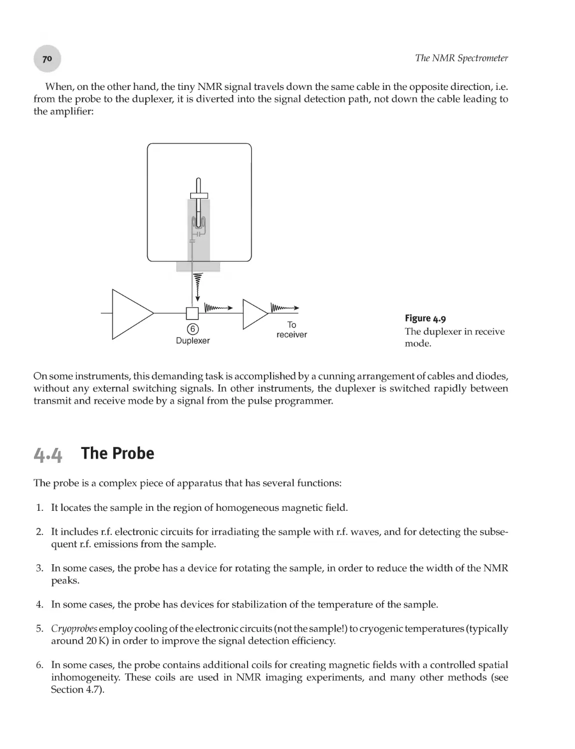
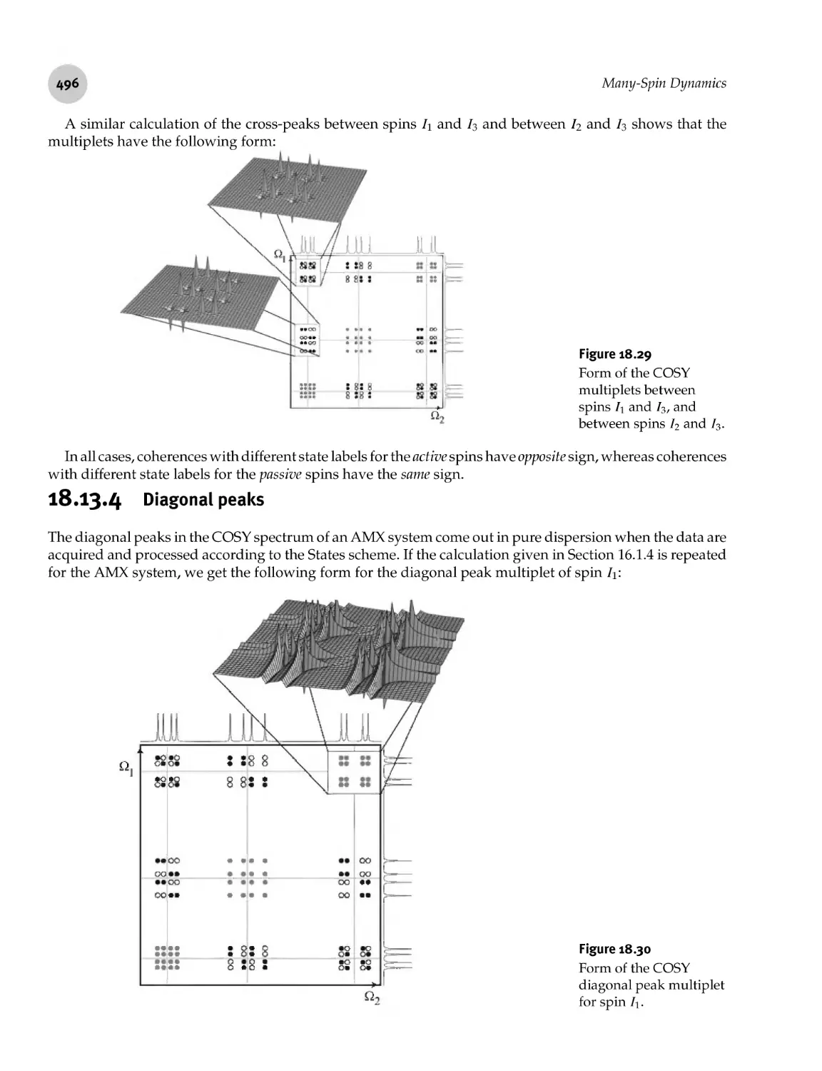
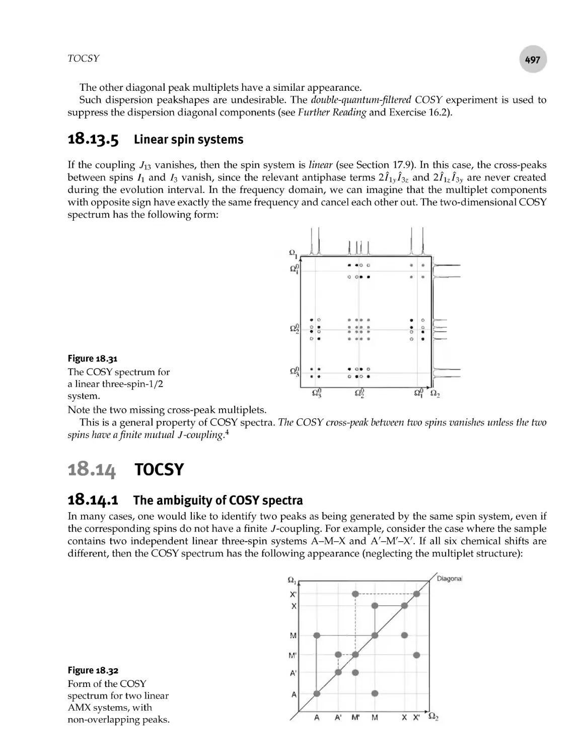
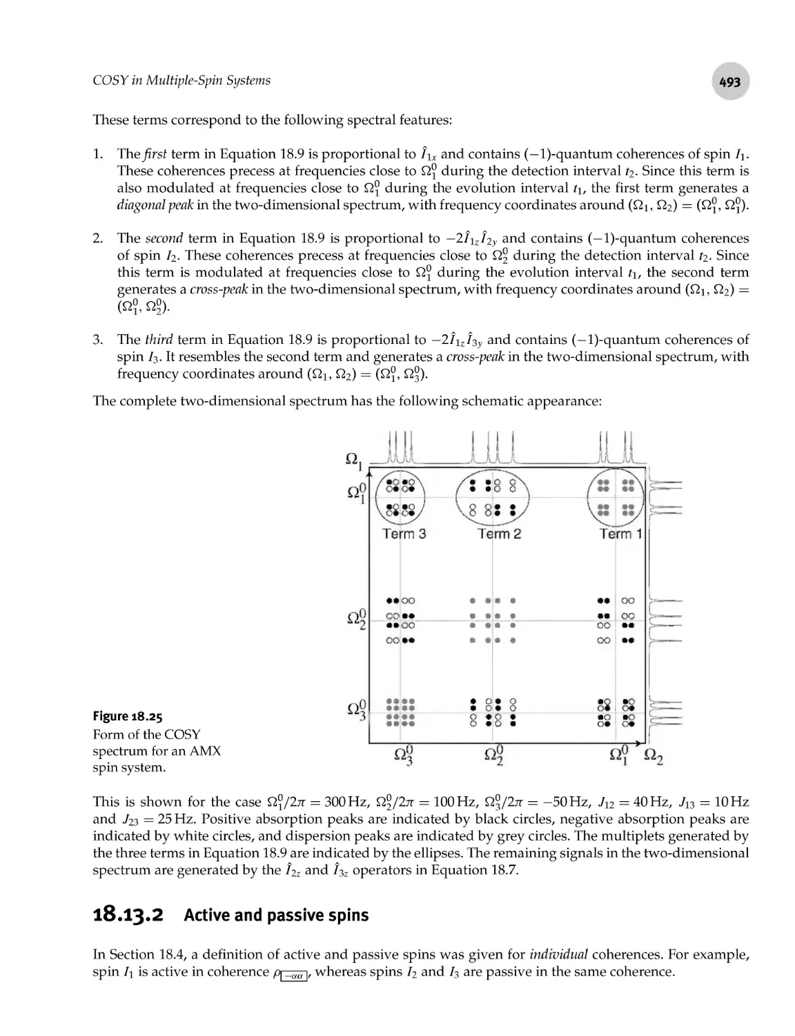
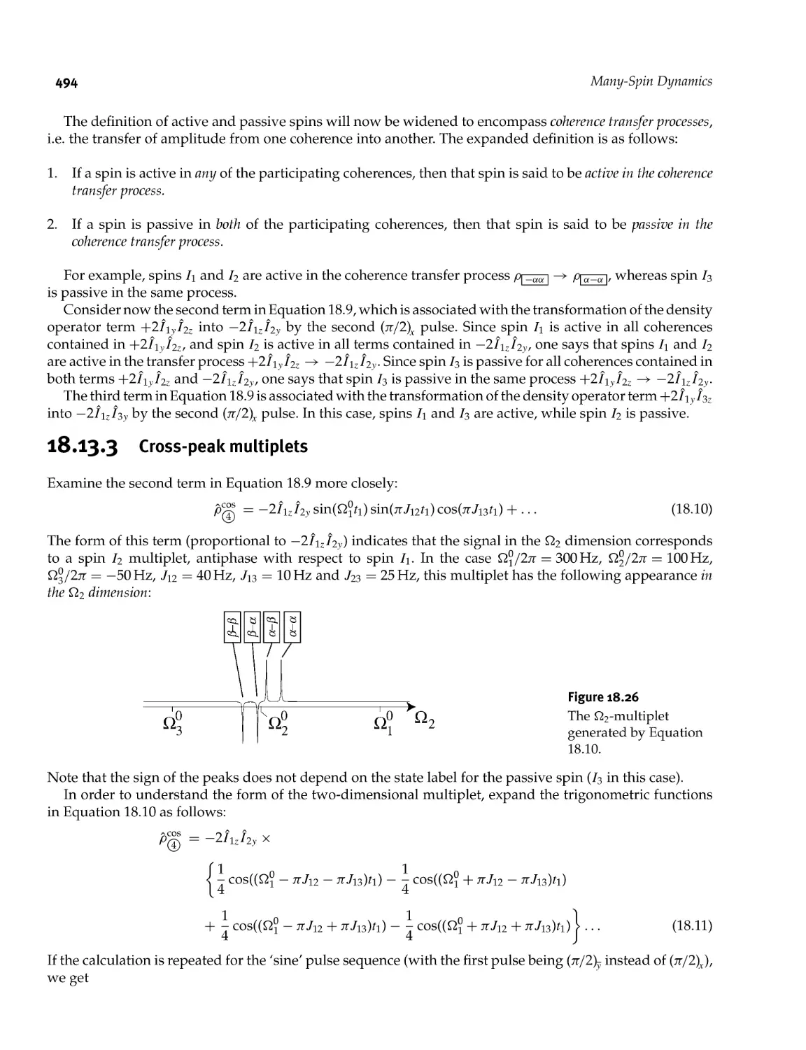
Text
                    Spin Dynamics
Basics of Nuclear Magnetic Resonance
Second edition
Malcolm H. Levitt
The University of Southampton, UK
John Wiley &. Sons, Ltd


Spin Dynamics
Second Edition


Spin Dynamics
Basics of Nuclear Magnetic Resonance
Second edition
Malcolm H. Levitt
The University of Southampton, UK
John Wiley &. Sons, Ltd

Copyright © 2008 John Wiley & Sons Ltd
The Atrium, Southern Gate
Chichester,
West Sussex P019 8SQ, England
Telephone (+44) 1243 779777
Email (for orders and customer service enquiries): cs- books@wileyco.uk
Visit our Home Page on www.wileyeurope.com or www.wiley.com
All Rights Reserved. No part of this publication may be reproduced, stored in a retrieval system or transmitted in any form or
by any means, electronic, mechanical, photocopying, recording, scanning or otherwise, except under the terms of the
Copyright, Designs and Patents Act 1988 or under the terms of a licence issued by the Copyright Licensing Agency Ltd, 90
Tottenham Court Road, London WIT 4LP, UK, without the permission in writing of the Publisher. Requests to the Publisher
should be addressed to the Permissions Department, John Wiley & Sons Ltd, The Atrium, Southern Gate, Chichester, West
Sussex P019 8SQ, England, or emailed to permreq@wiley.co.uk, or faxed to (+44) 1243 770620.
Designations used by companies to distinguish their products are often claimed as trademarks. All brand names and product
names used in this book are trade names, service marks, trademarks or registered trademarks of their respective owners. The
Publisher is not associated with any product or vendor mentioned in this book.
This publication is designed to provide accurate and authoritative information in regard to the subject matter covered. It is
sold on the understanding that the Publisher is not engaged in rendering professional services. If professional advice or other
expert assistance is required, the services of a competent professional should be sought.
Other Wiley Editorial Offices
John Wiley & Sons Inc., Ill River Street, Hoboken, NJ 07030, USA
Jossey- Bass, 989 Market Street, San Francisco, CA 94103- 1741, USA
Wiley- VCH Verlag GmbH, Boschstr. 12, D- 69469 Weinheim, Germany
John Wiley & Sons Australia Ltd, 42 McDougall Street Milton, Queensland 4064, Australia
John Wiley & Sons (Asia) Pte Ltd, 2 Clementi Loop #02- 01, Jin Xing Distripark, Singapore 129809
John Wiley & Sons Canada Ltd, 6045 Freemont Blvd, Mississauga, Ontario, L5R 4J3, Canada
Wiley also publishes its books in a variety of electronic formats. Some content that appears in print may not be available in
electronic books.
Library of Congress Cataloging- in- Publication Data
Levitt, Malcolm H.
Spin dynamics : basics of nuclear magnetic resonance / Malcolm H. Levitt.
- 2nd ed.
p. cm.
Includes bibliographical references.
ISBN 978- 0- 470- 51118- 3 (hb : acid- free paper) - ISBN 978- 0- 470- 51117- 6
(pbk: acid- free paper)
1. Nuclear spin. 2. Nuclear magnetic resonance. I. Title.
QC793.3.S6L47 2007
538'.362- dc22
2007022146
British Library Cataloguing in Publication Data
A catalogue record for this book is available from the British Library
ISBN 9780470511183 HB
9780470511176 PB
Typeset in 9.5/11.5 Palatino Roman by Thomson Digital, Noida, India
Printed and bound in Great Britain by Antony Rowe Ltd, Chippenham, Wiltshire
This book is printed on acid- free paper responsibly manufactured from sustainable forestry in which
at least two trees are planted for each one used for paper production.

To my mother and father


Preface xxi
Preface to the First Edition xxiii
Introduction 1
Parti Nuclear Magnetism 3
i Matter 5
5
5
6
6
7
9
9
10
11
12
12
14
14
15
15
15
15
15
16
17
17
17
19
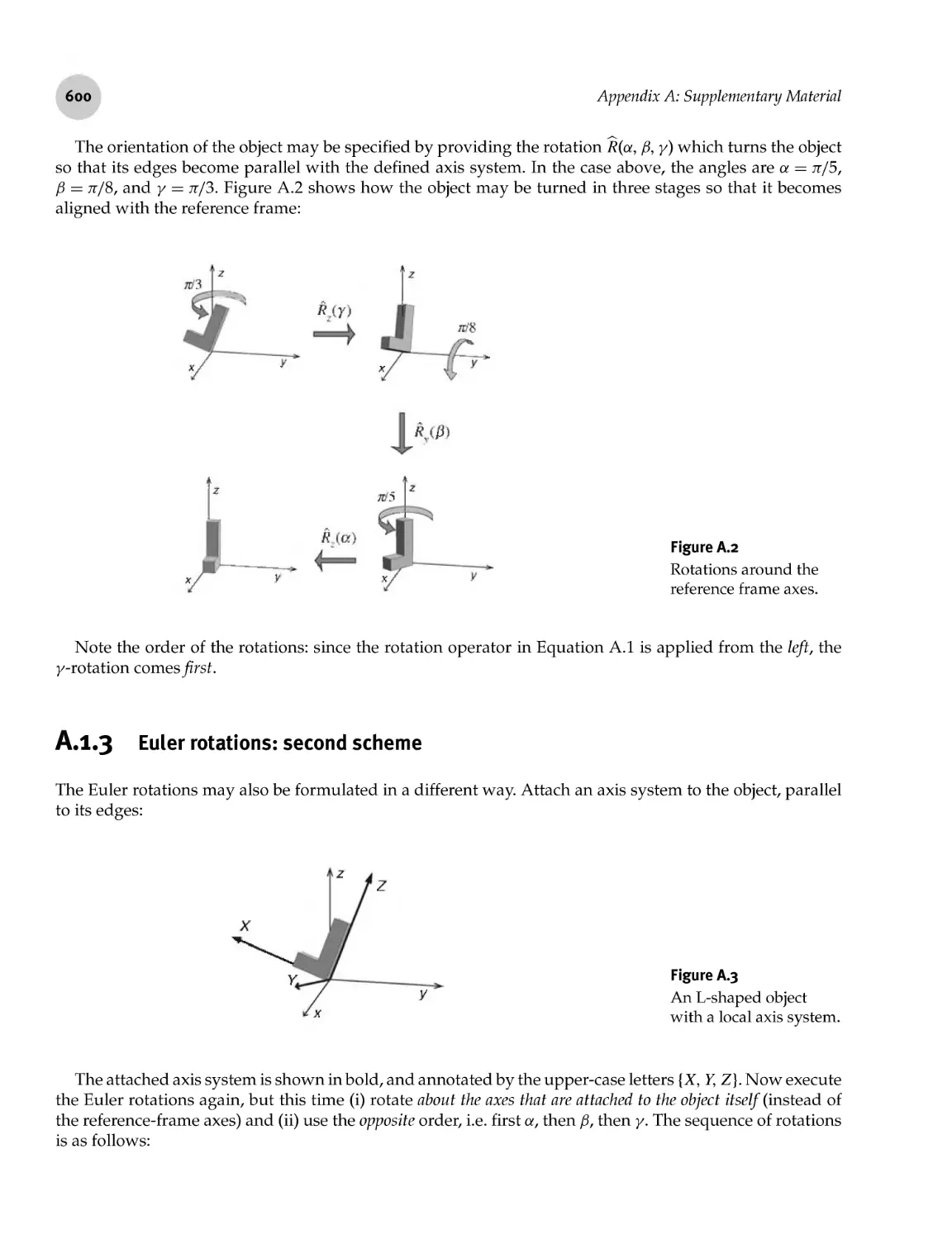
1.1
1.2
1.3
1.4
1.5
1.6
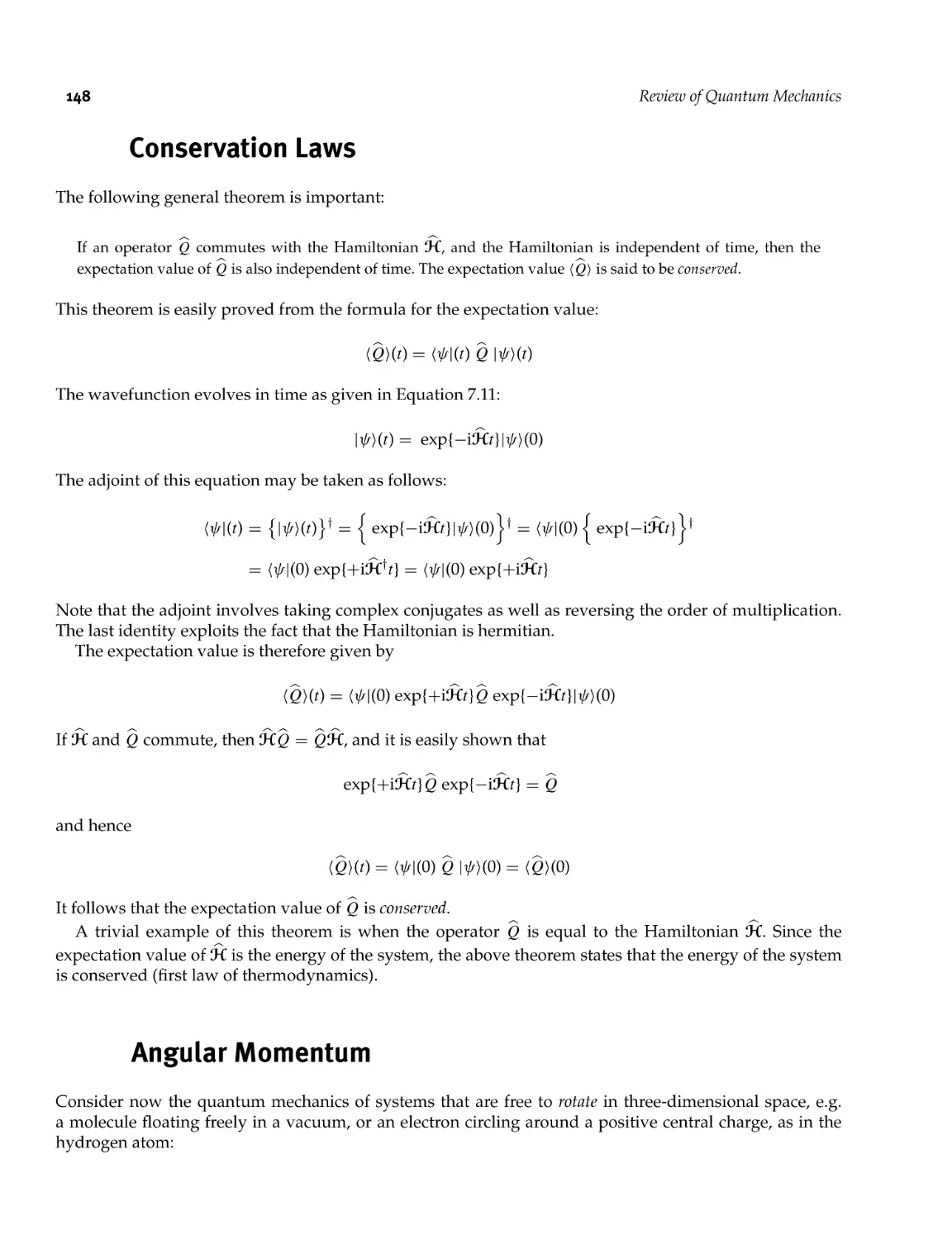
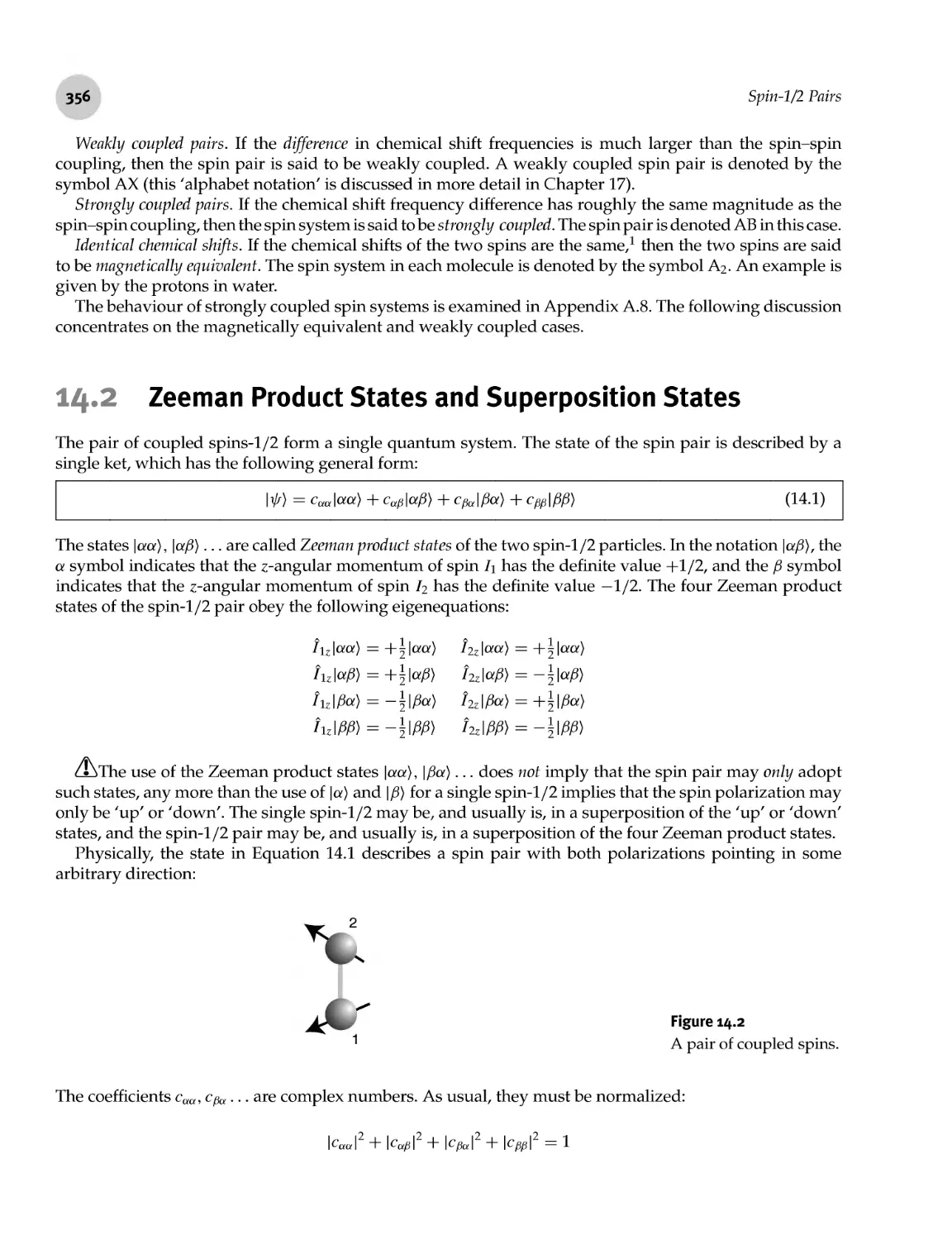
Atoms and Nuclei
Spin
1.2.1
1.2.2
1.2.3
1.2.4
1.2.5
Classical angular momentum
Quantum angular momentum
Spin angular momentum
Combining angular momenta
The Pauli Principle
Nuclei
1.3.1
1.3.2
1.3.3
The fundamental particles
Neutrons and protons
Isotopes
Nuclear Spin
1.4.1
1.4.2
1.4.3
1.4.4
1.4.5
1.4.6
Nuclear spin states
Nuclear Zeeman splitting
Zero- spin nuclei
Spin- 1/2 nuclei
Quadrupolar nuclei with integer spin
Quadrupolar nuclei with half- integer spin
Atomic and Molecular Structure
1.5.1
1.5.2
Atoms
Molecules
States of Matter
1.6.1
1.6.2
1.6.3
Gases
Liquids
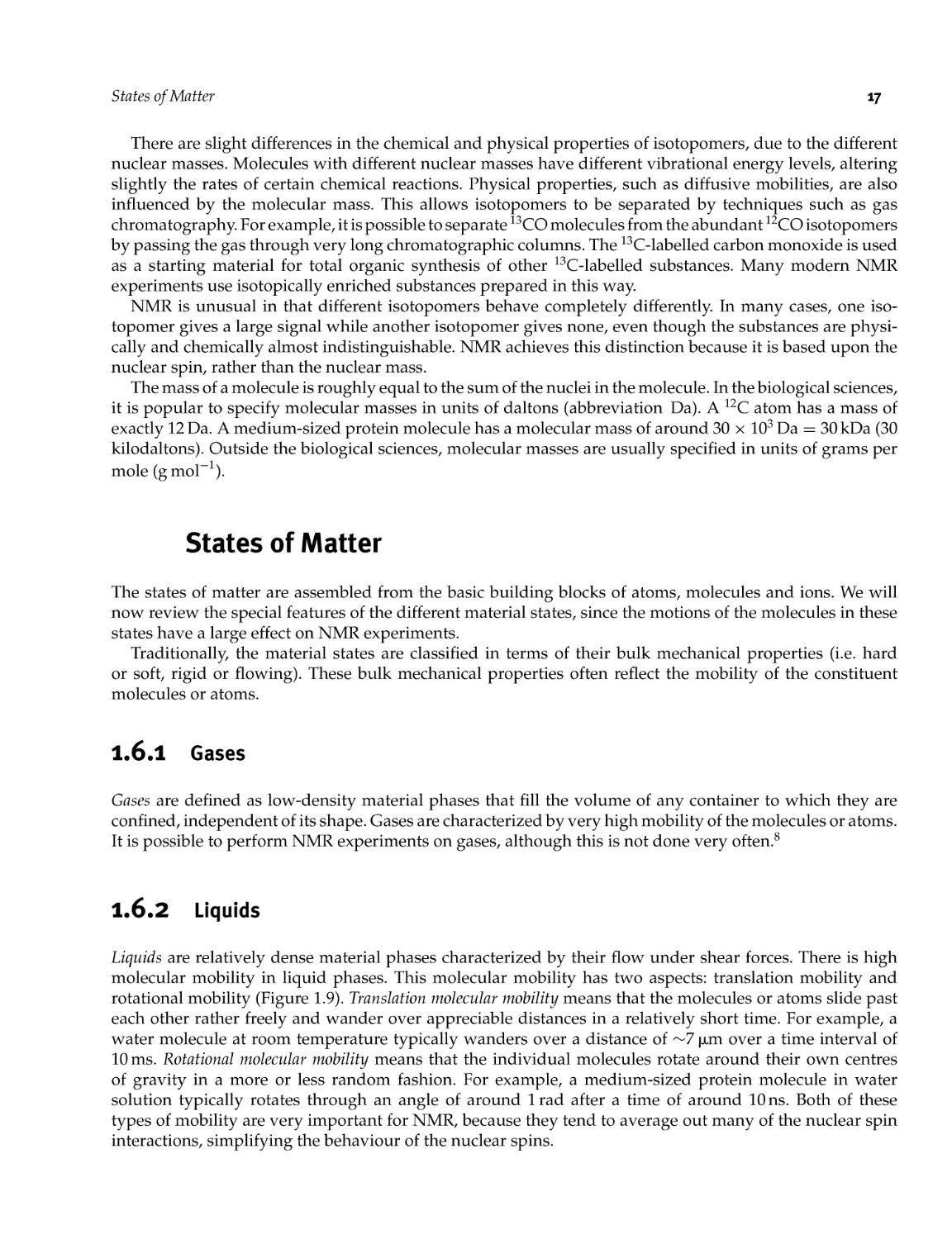
Solids

viii
Contents
Magnetism 23
2.1 The Electromagnetic Field 23
2.2 Macroscopic Magnetism 23
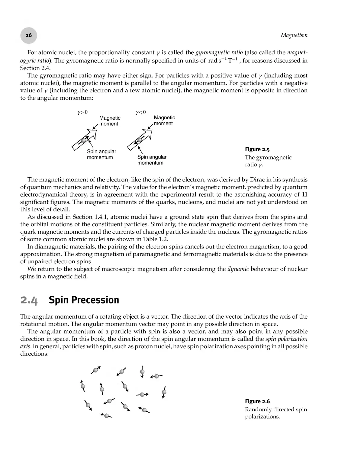
2.3 Microscopic Magnetism 25
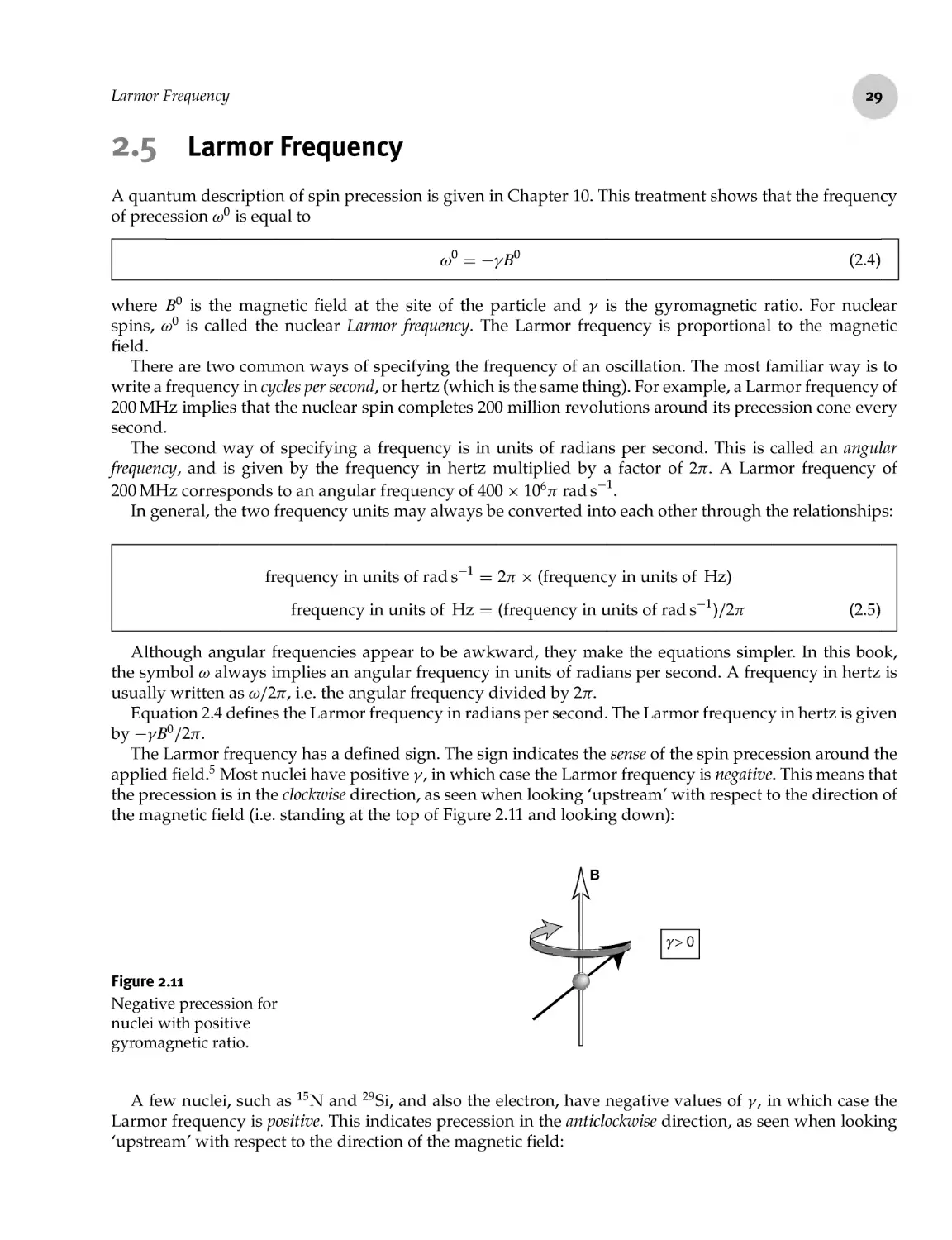
2.4 Spin Precession 26
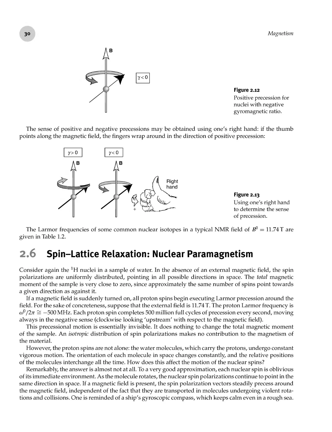
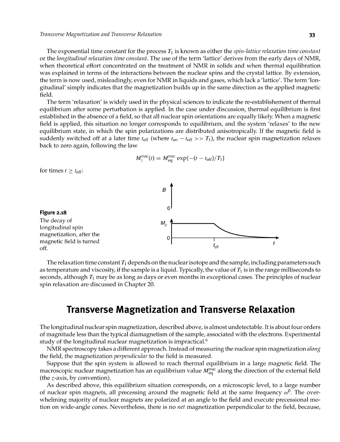
2.5 Larmor Frequency 29
2.6 Spin- Lattice Relaxation: Nuclear Paramagnetism 30
2.7 Transverse Magnetization and Transverse Relaxation 33
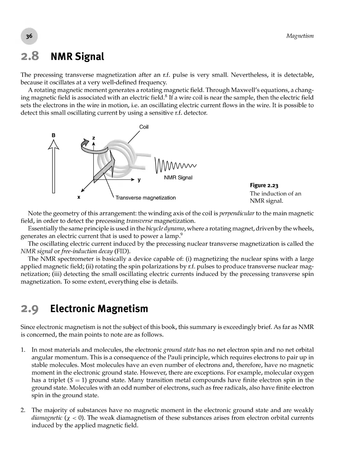
2.8 NMR Signal 36
2.9 Electronic Magnetism 36
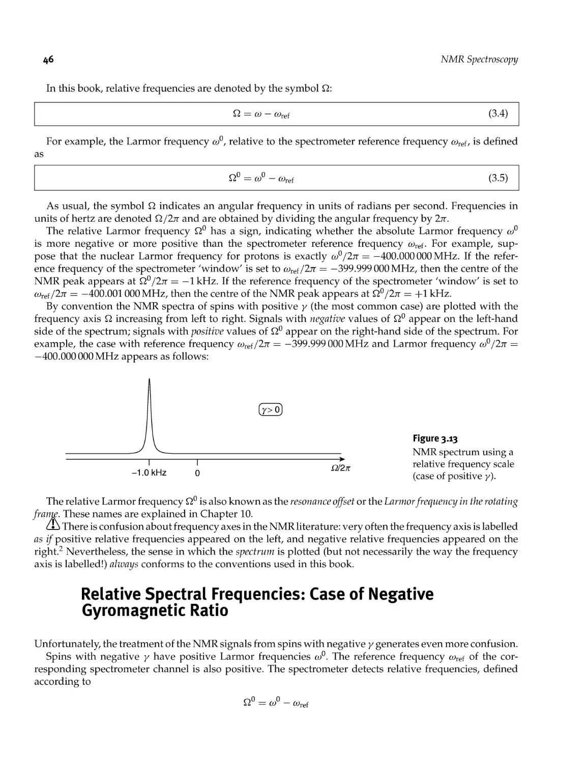
3 NMR Spectroscopy 39
3.1 A Simple Pulse Sequence 39
3.2 A Simple Spectrum 39
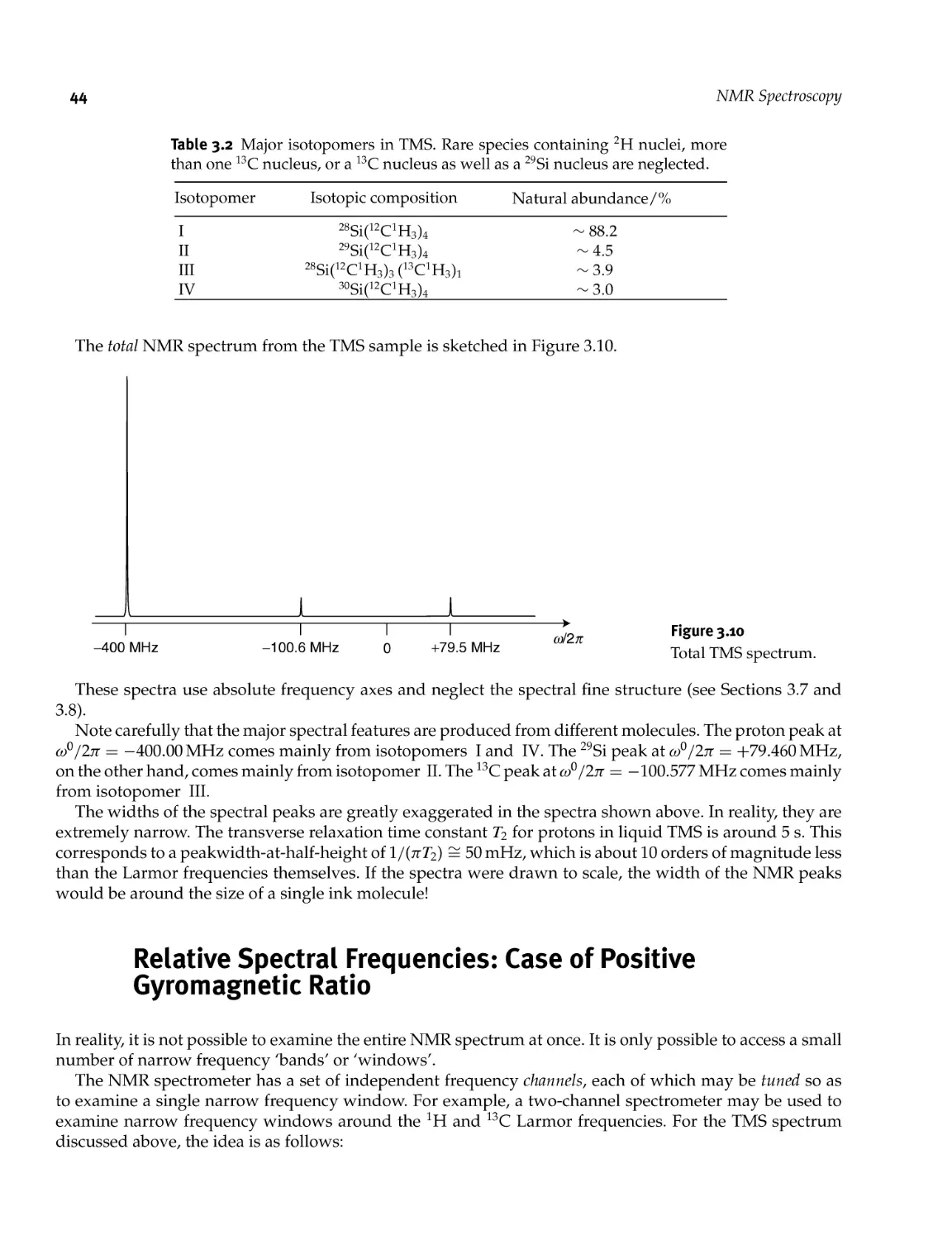
3.3 Isotopomeric Spectra 42
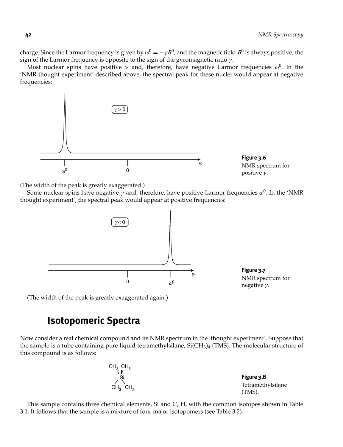
3.4 Relative Spectral Frequencies: Case of Positive Gyromagnetic Ratio 44
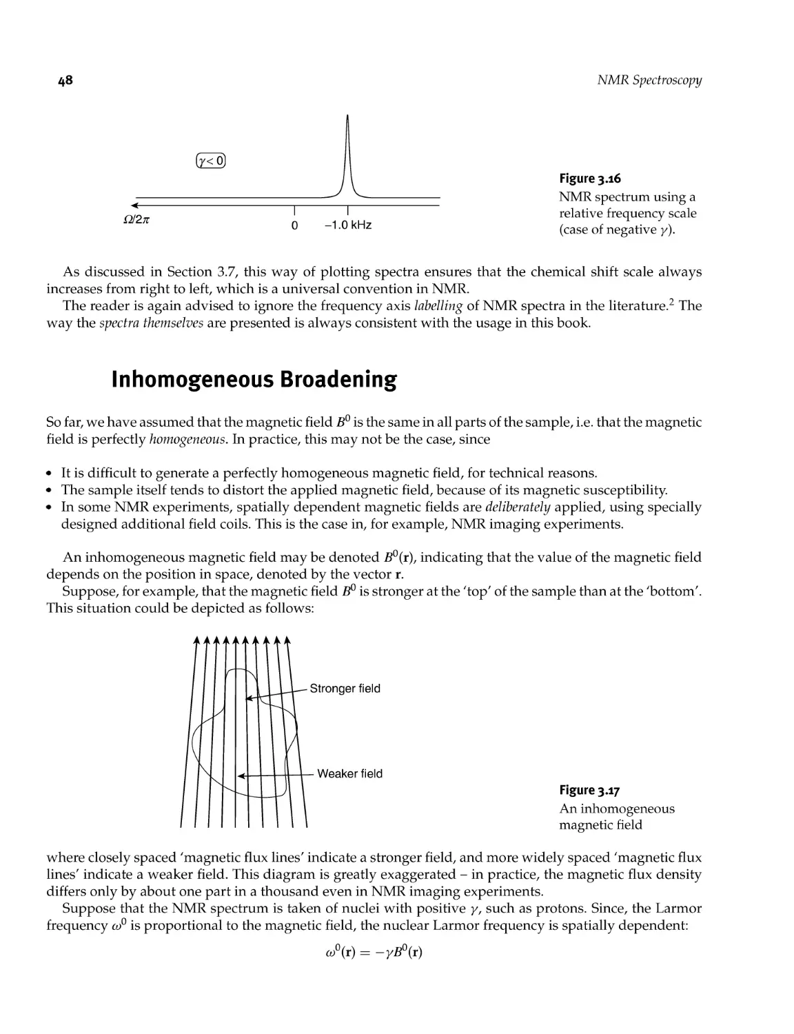
3.5 Relative Spectral Frequencies: Case of Negative Gyromagnetic Ratio 46
3.6 Inhomogeneous Broadening 48
3.7 Chemical Shifts 50
3.8 /- Coupling Multiplets 56
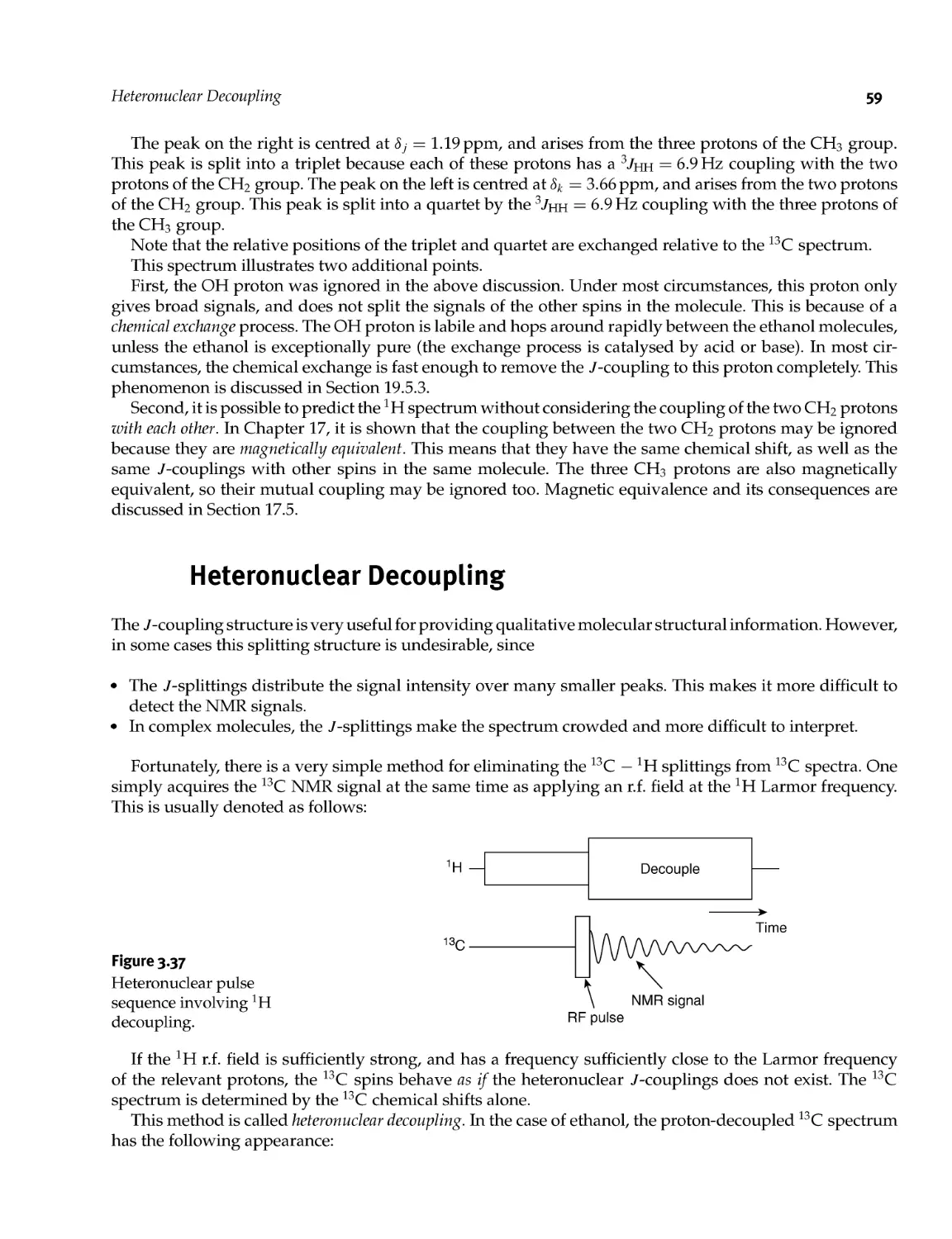
3.9 Heteronuclear Decoupling 59
Part 2 The NMR Experiment 63
4 The NMR Spectrometer 65
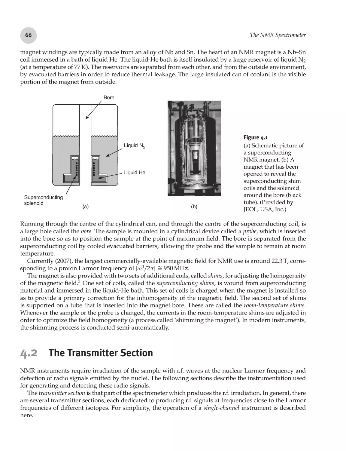
4.1 The Magnet 65
4.2 The Transmitter Section 66
4.2.1 The synthesizer: radio- frequency phase shifts 67
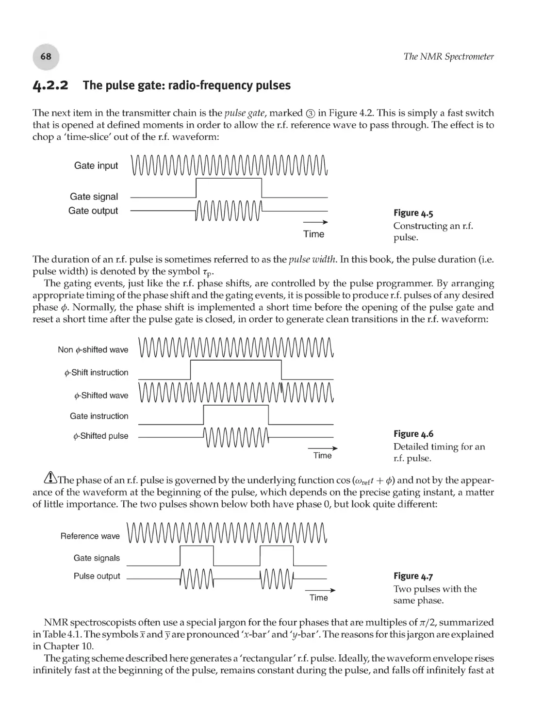
4.2.2 The pulse gate: radio- frequency pulses 68
4.2.3 Radio- frequency amplifier 69
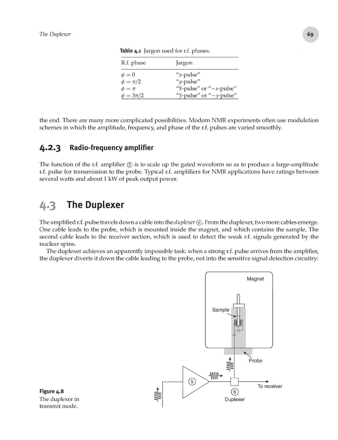
4.3 The Duplexer 69
4.4 The Probe 70
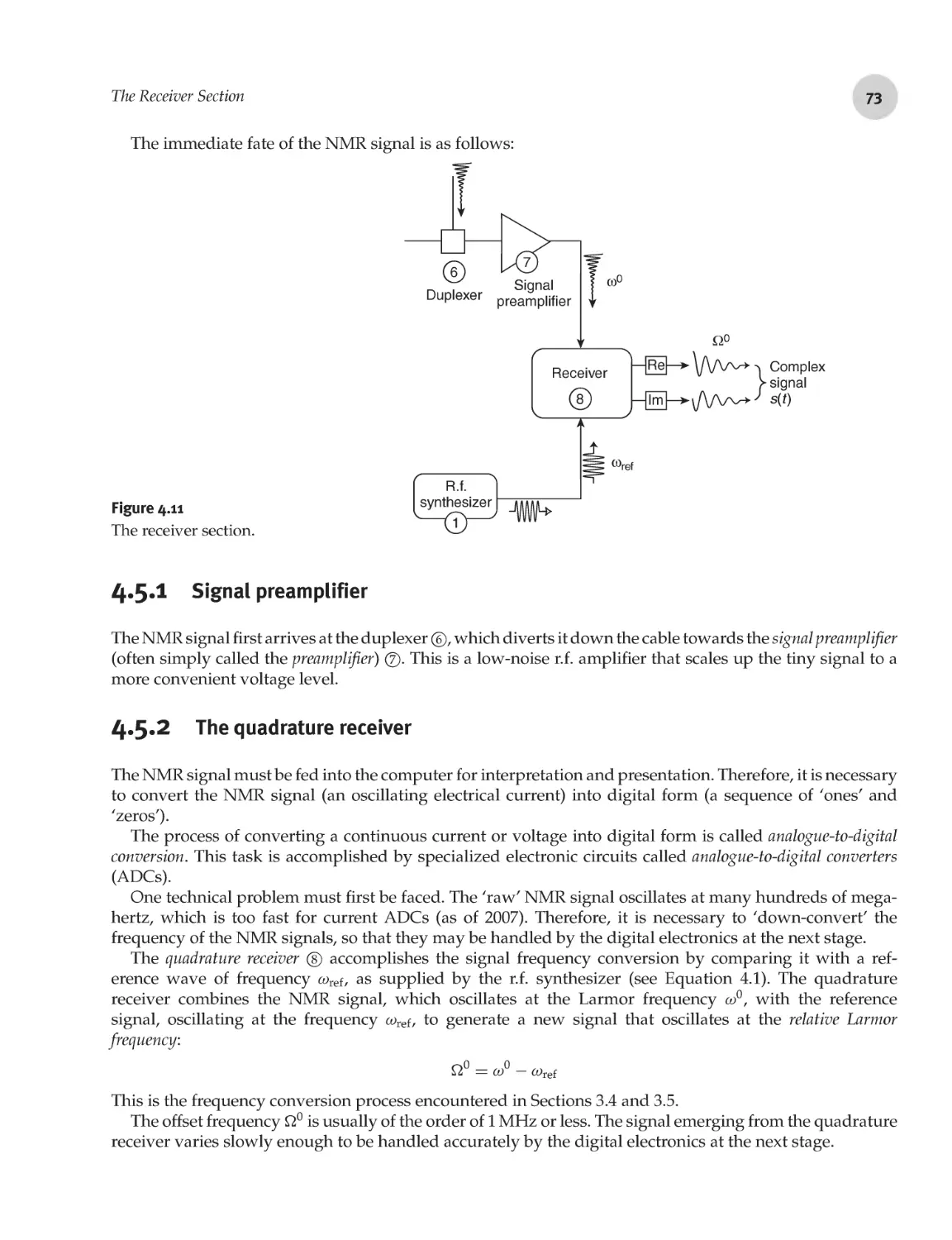
4.5 The Receiver Section 72
4.5.1 Signal preamplifier 73
4.5.2 The quadrature receiver 73
4.5.3 Analogue- digital conversion 74
4.5.4 Signal phase shifting 76
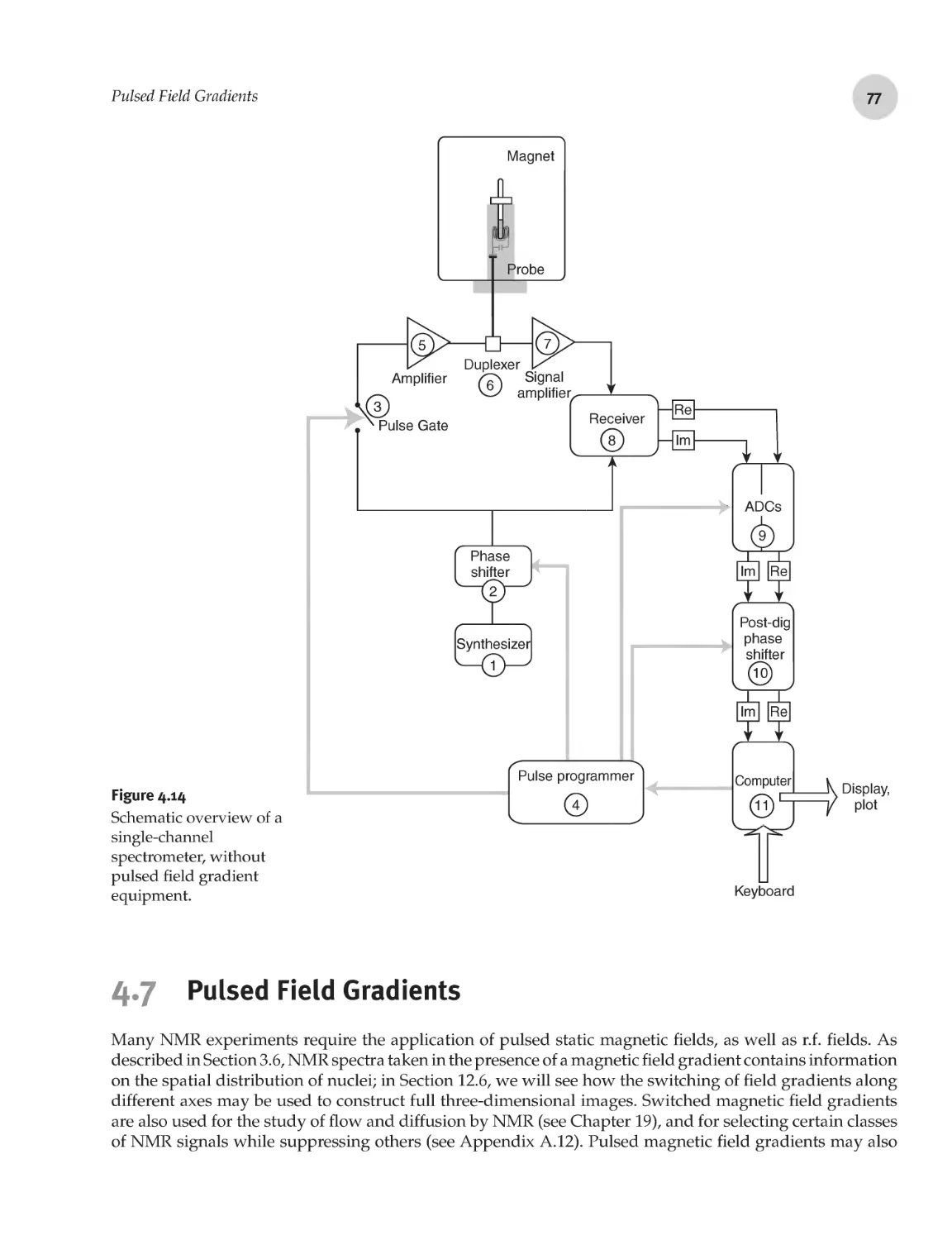
4.6 Overview of the Radio- Frequency Section 76
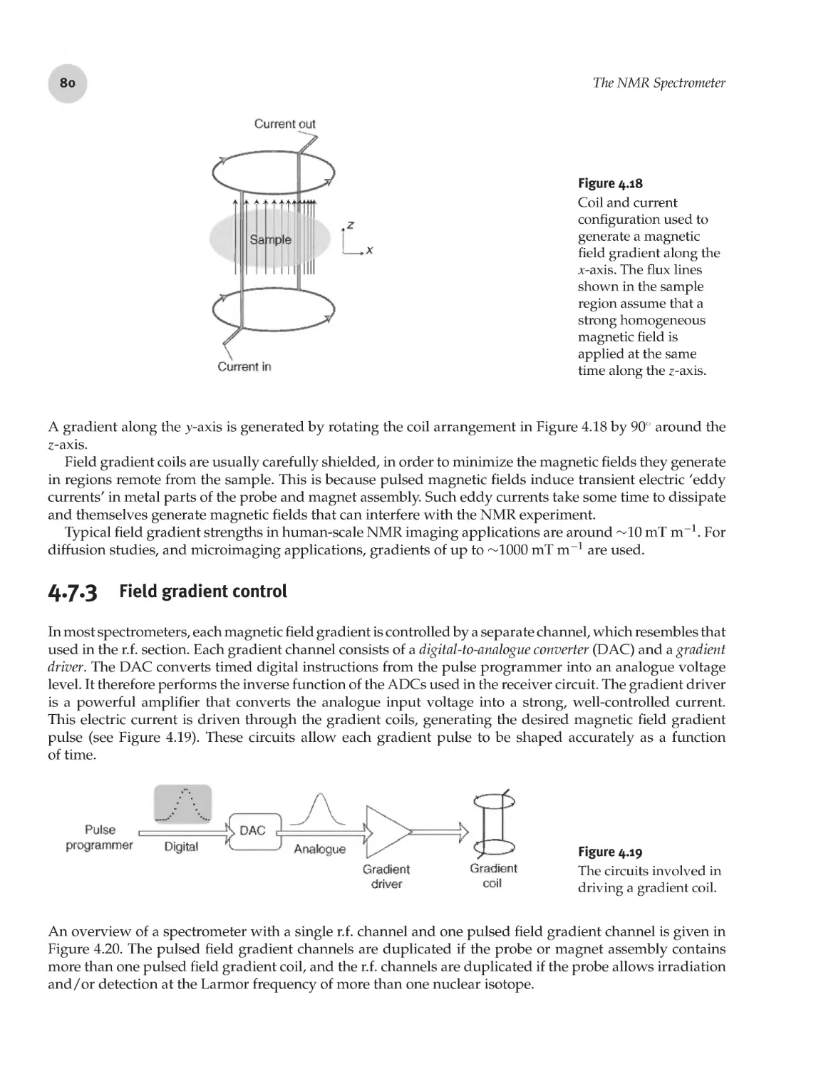
4.7 Pulsed Field Gradients 77
4.7.1 Magnetic field gradients 78
4.7.2 Field gradient coils 79
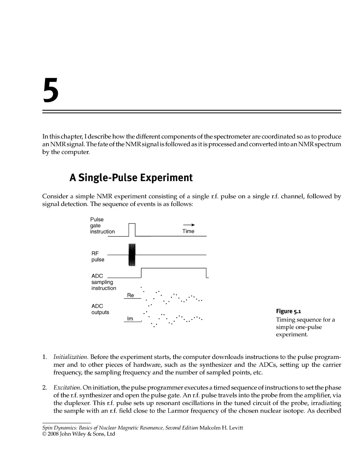
4.7.3 Field gradient control 80

Contents
ix
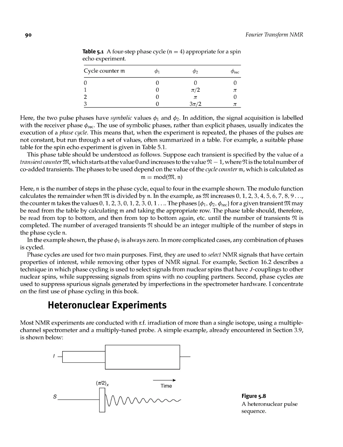
5 Fourier Transform NMR 85
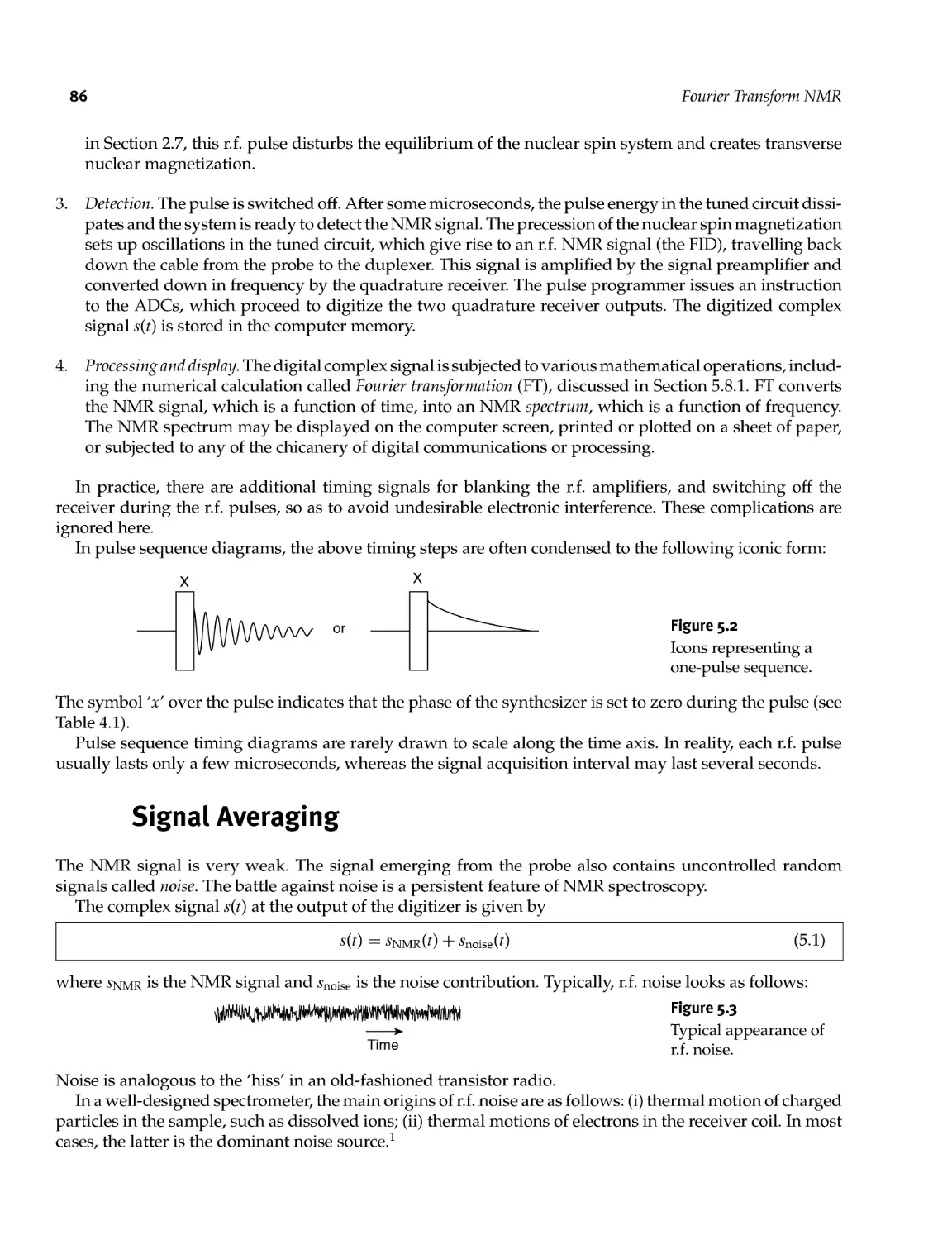
5.1 A Single- Pulse Experiment 85
5.2 Signal Averaging 86
5.3 Multiple- Pulse Experiments: Phase Cycling 89
5.4 Heteronuclear Experiments 90
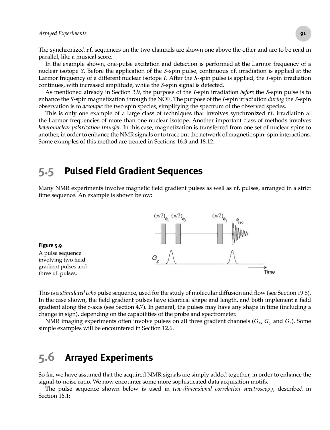
5.5 Pulsed Field Gradient Sequences 91
5.6 Arrayed Experiments 91
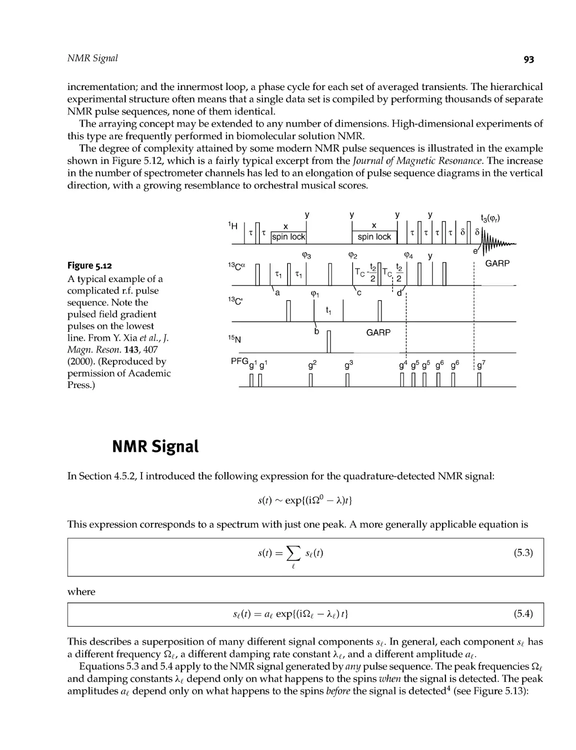
5.7 NMR Signal 93
5.8 NMR Spectrum 96
5.8.1 Fourier transformation 96
5.8.2 Lorentzians 96
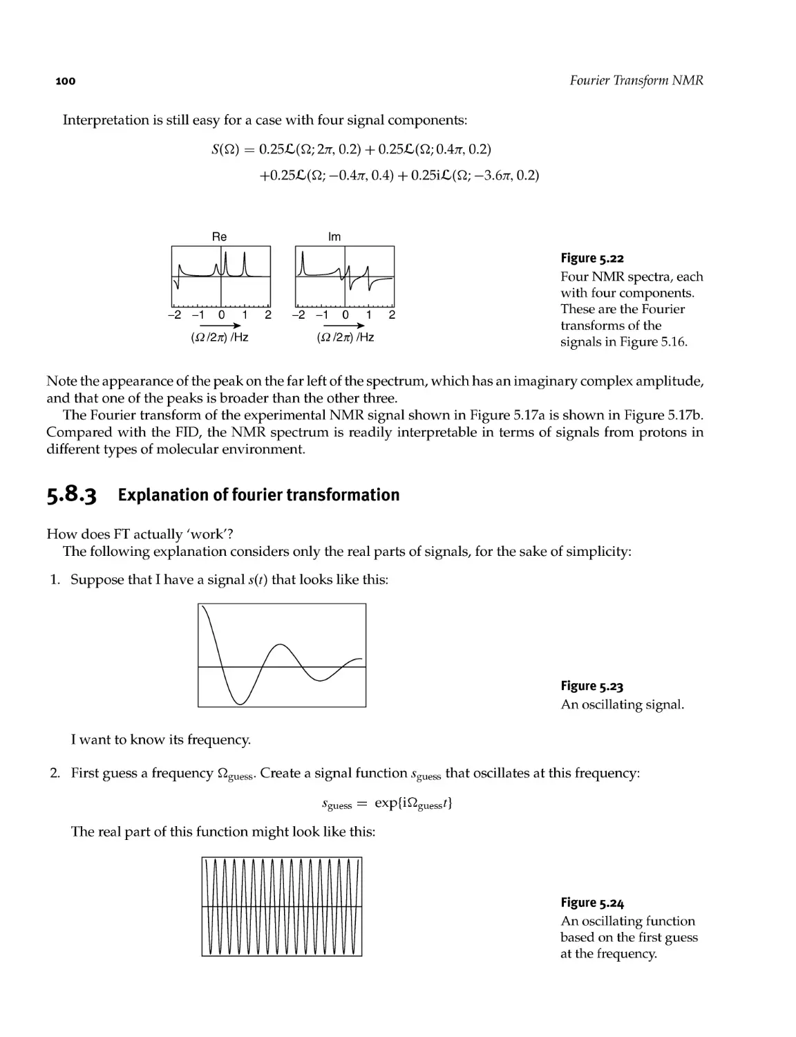
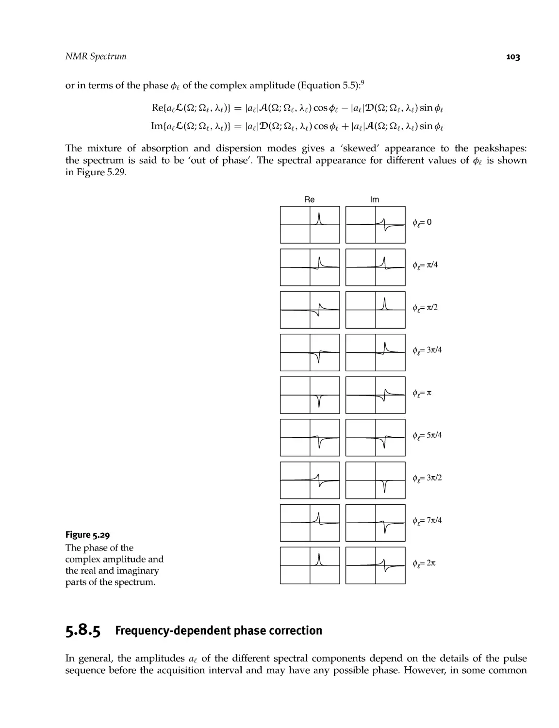
5.8.3 Explanation of Fourier transformation 100
5.8.4 Spectral phase shifts 102
5.8.5 Frequency- dependent phase correction 103
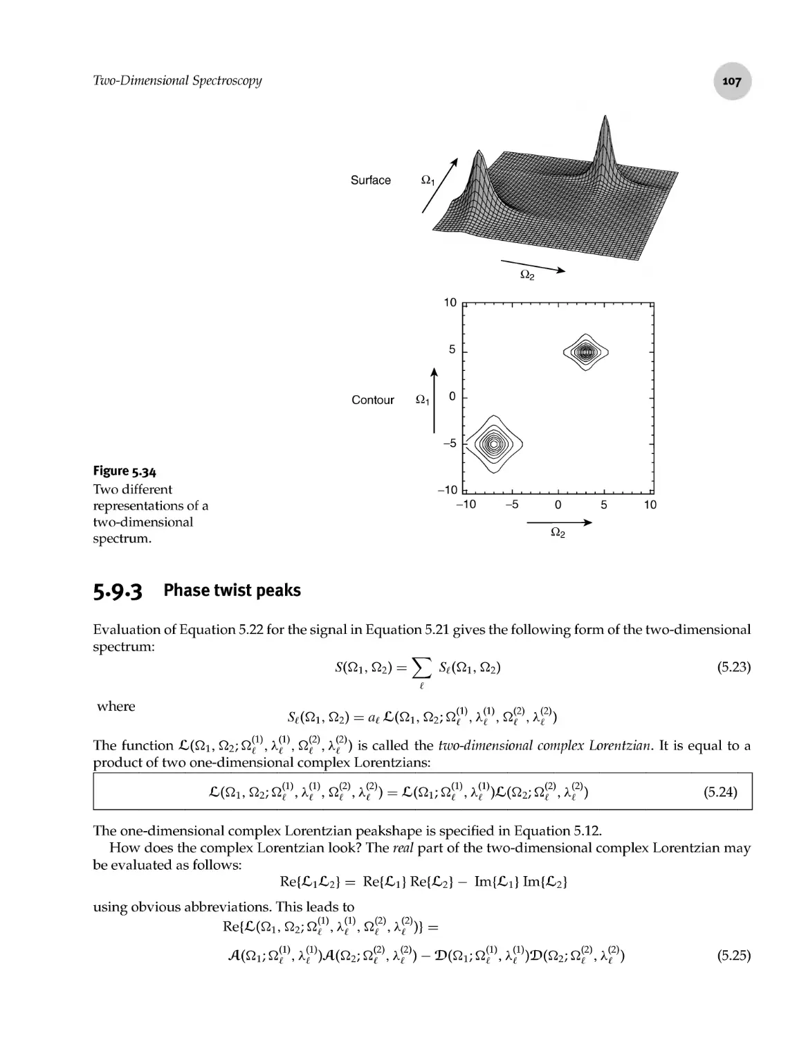
5.9 Two- Dimensional Spectroscopy 105
5.9.1 Two- dimensional signal surface 105
5.9.2 Two- dimensional Fourier transformation 105
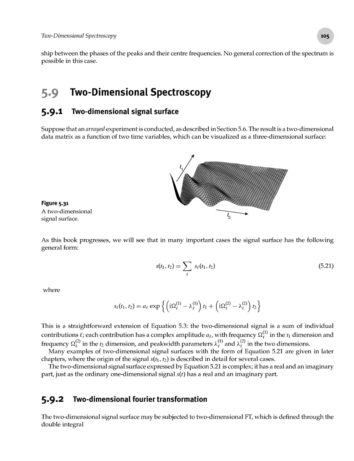
5.9.3 Phase twist peaks 107
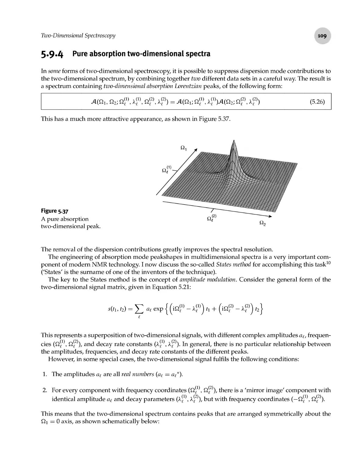
5.9.4 Pure absorption two- dimensional spectra 109
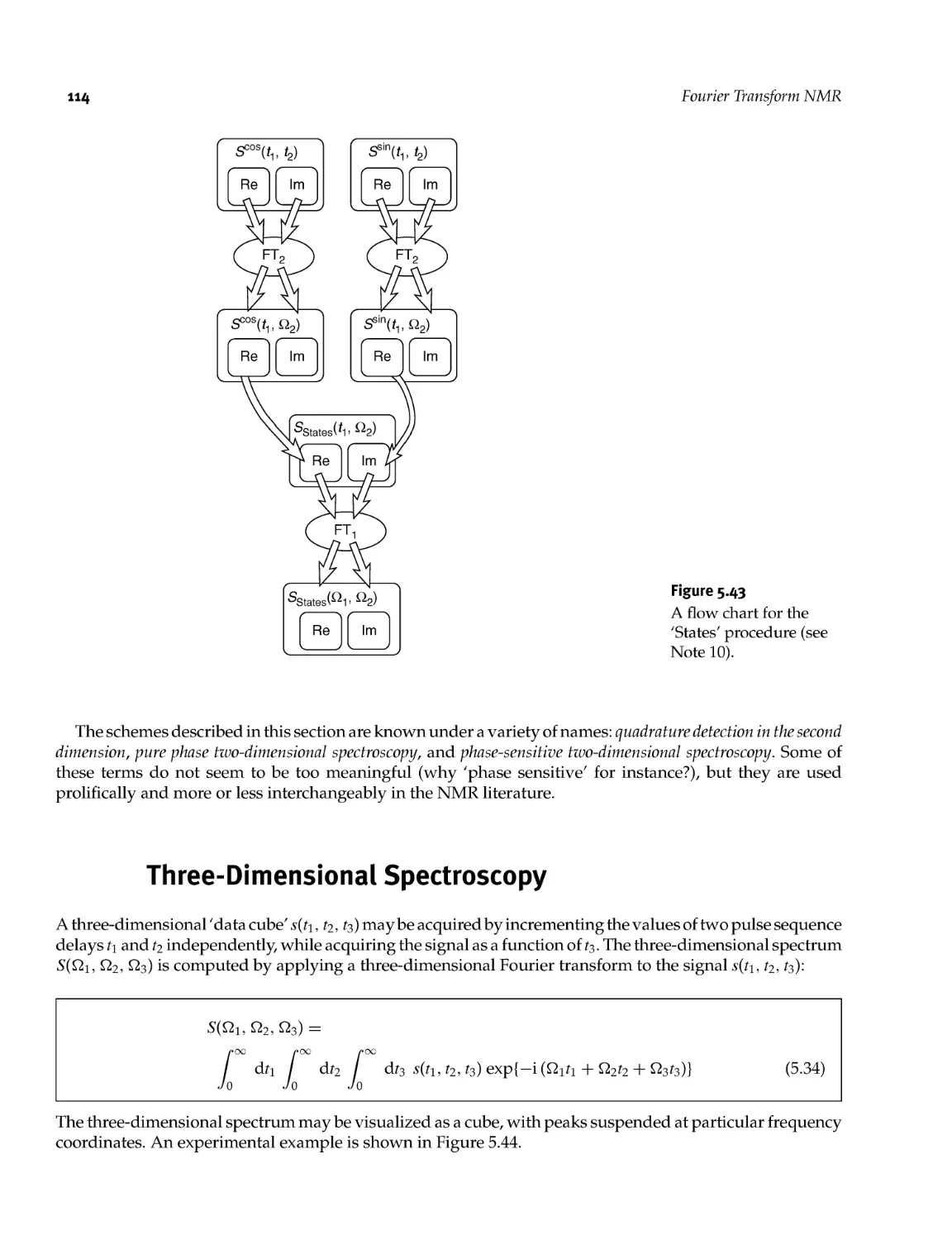
5.10 Three- Dimensional Spectroscopy 114
Part 3 Quantum Mechanics 119
Mathematical Techniques 121
6.1 Functions 121
6.1.1 Continuous functions 121
6.1.2 Normalization 122
6.1.3 Orthogonal and orthonormal functions 122
6.1.4 Dime notation 122
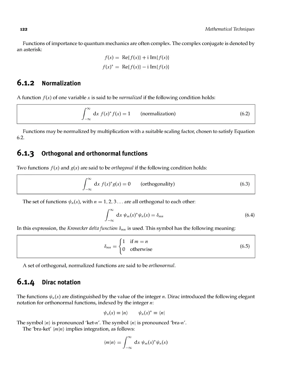
6.1.5 Vector representation of functions 123
6.2 Operators 125
6.2.1 Commutation 126
6.2.2 Matrix representations 126
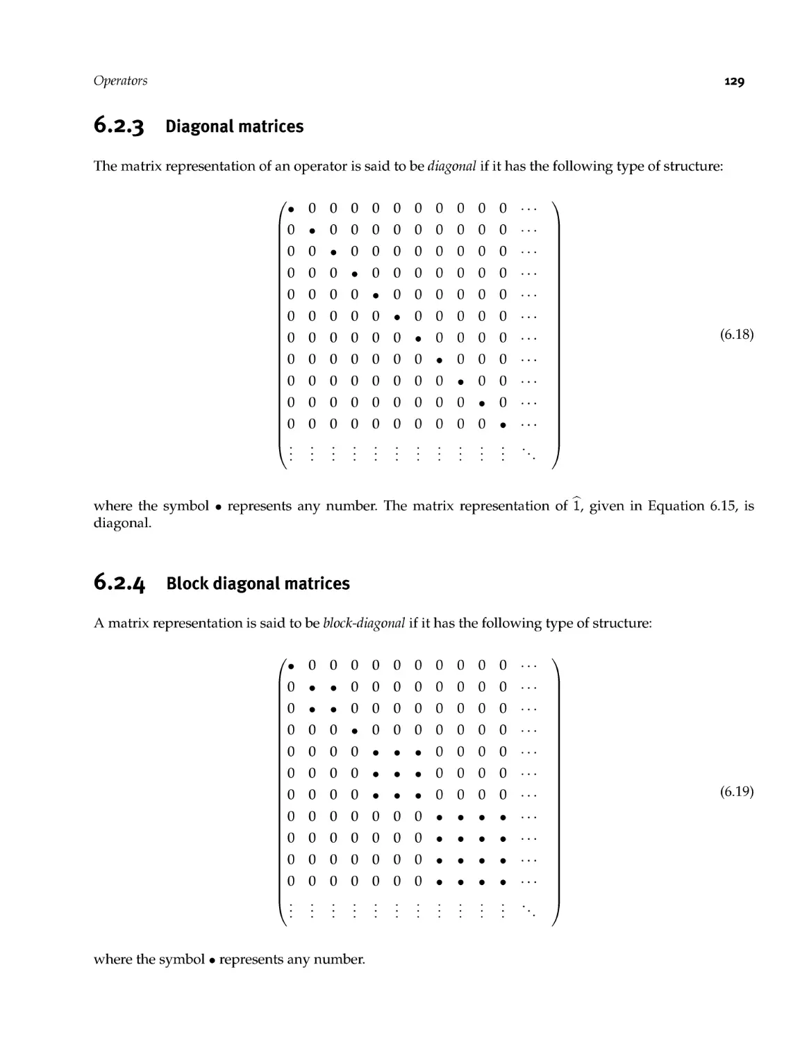
6.2.3 Diagonal matrices 129
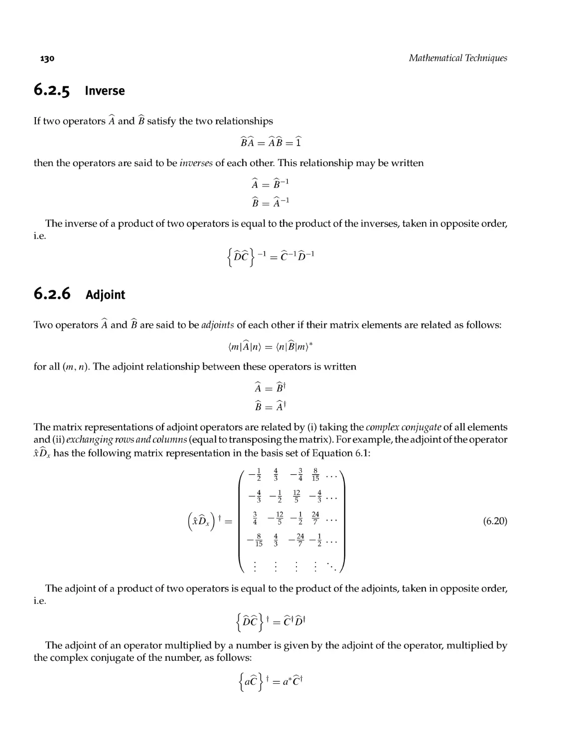
6.2.4 Block diagonal matrices 129
6.2.5 Inverse 130
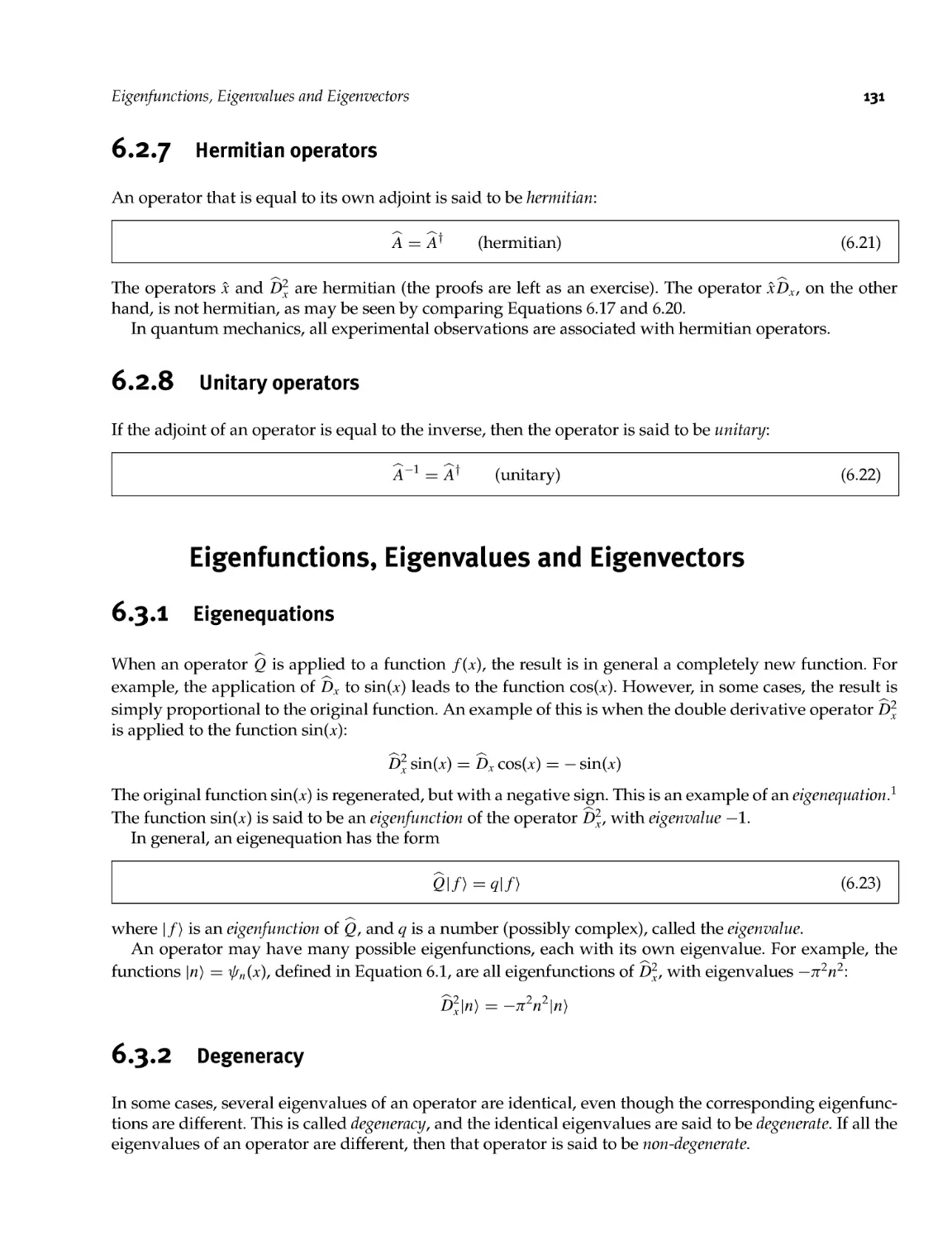
6.2.6 Adjoint 130
6.2.7 Hermitian operators 131
6.2.8 Unitary operators 131
6.3 Eigenfunctions, Eigenvalues and Eigenvectors 131
6.3.1 Eigenequations 131
6.3.2 Degeneracy 131
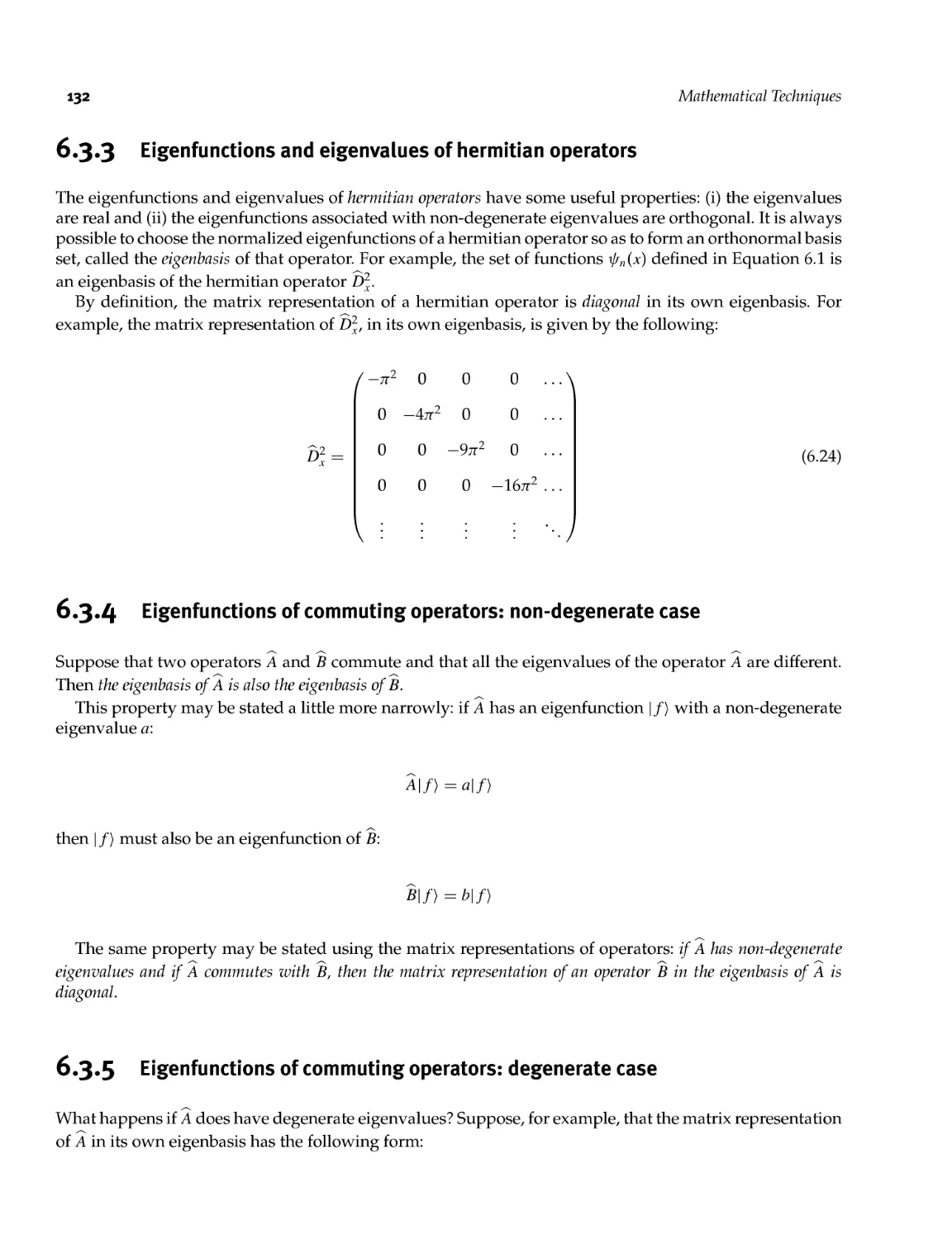
6.3.3 Eigenfunctions and eigenvalues of Hermitian operators 132
6.3.4 Eigenfunctions of commuting operators: non- degenerate case 132
6.3.5 Eigenfunctions of commuting operators: degenerate case 132
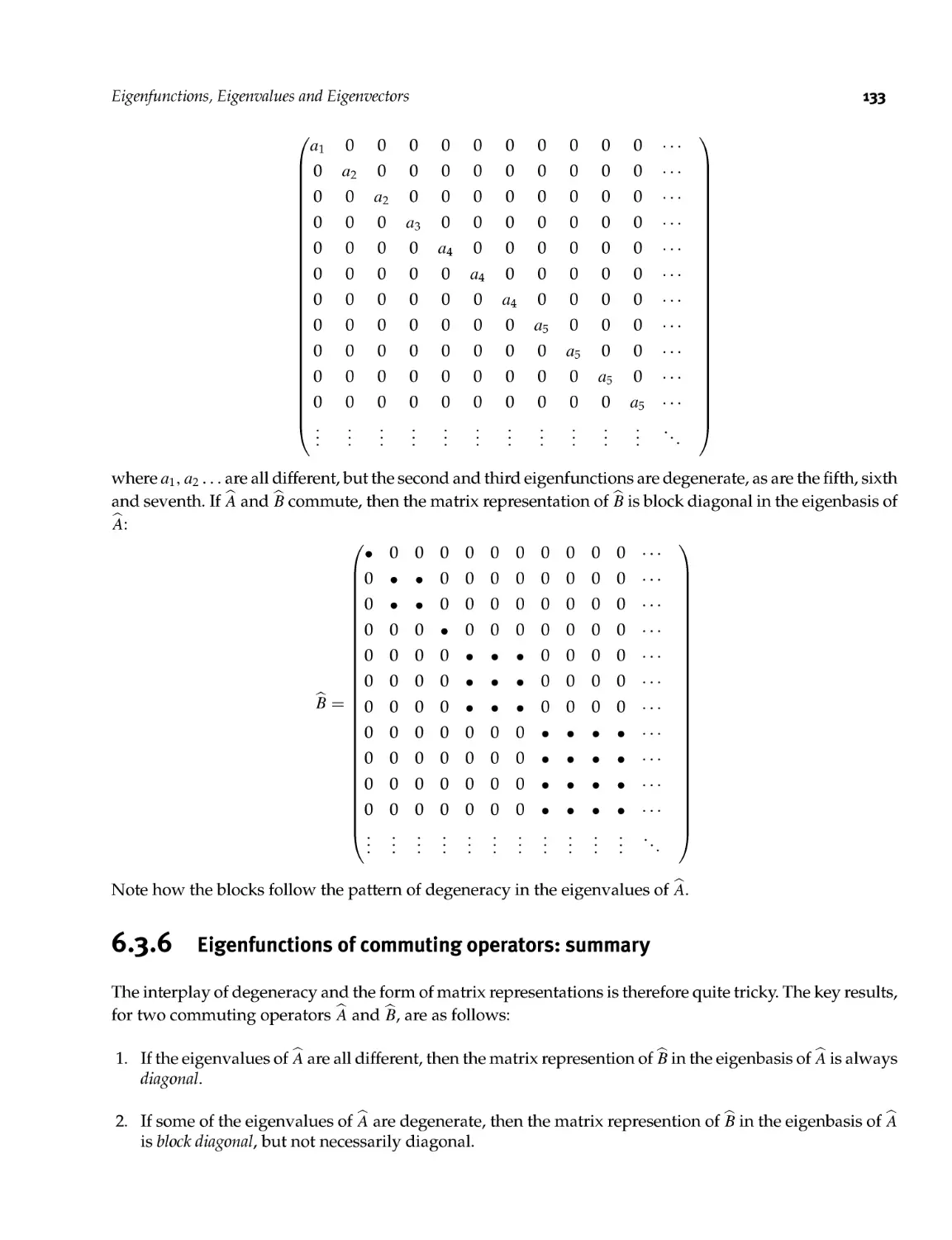
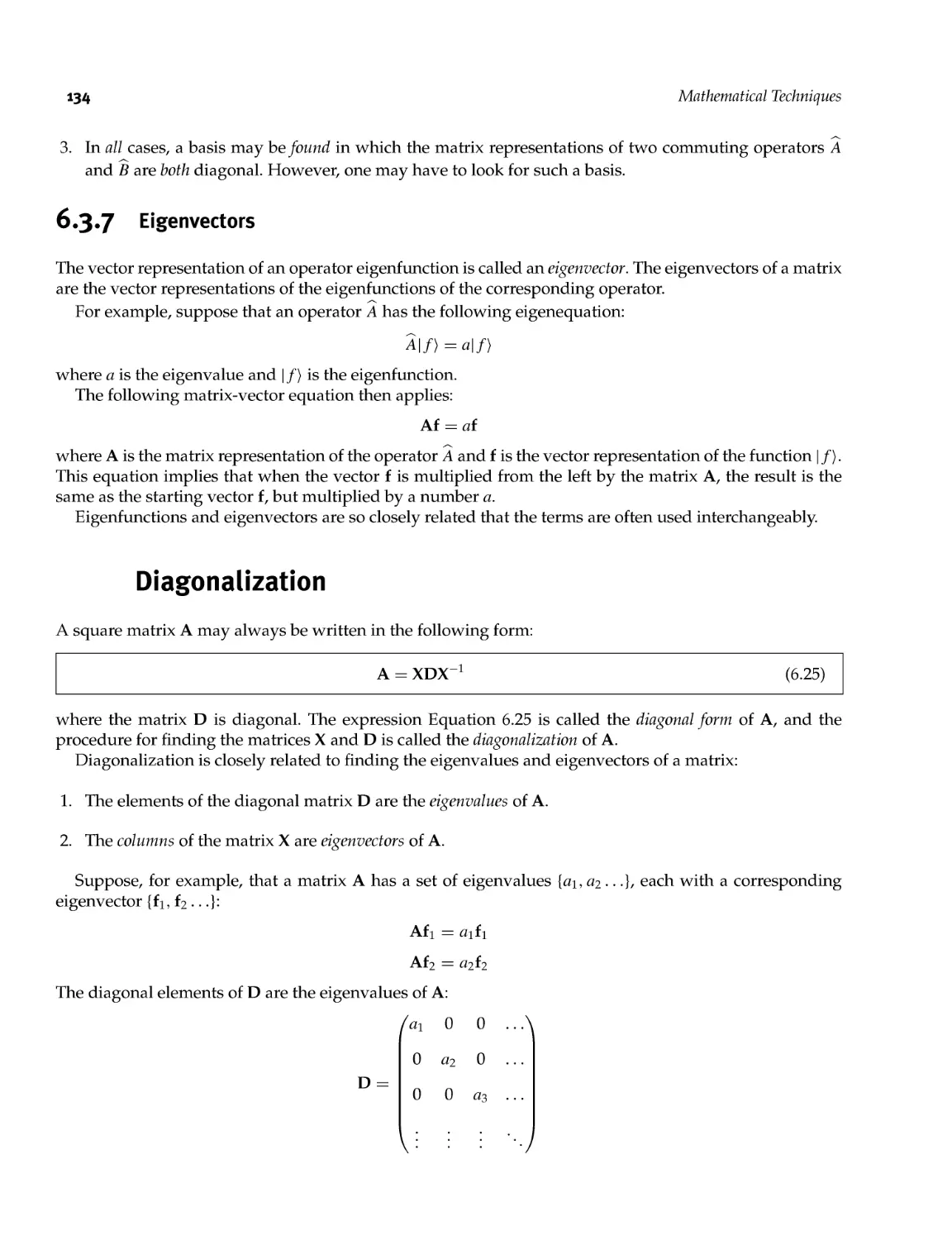
6.3.6 Eigenfunctions of commuting operators: summary 133
6.3.7 Eigenvectors 134

X
Contents
6.4 Diagonalization 134
6.4.1 Diagonalization of Hermitian or unitary matrices 135
6.5 Exponential Operators 135
6.5.1 Powers of operators 135
6.5.2 Exponentials of operators 136
6.5.3 Exponentials of unity and null operators 136
6.5.4 Products of exponential operators 137
6.5.5 Inverses of exponential operators 137
6.5.6 Complex exponentials of operators 137
6.5.7 Exponentials of small operators 137
6.5.8 Matrix representations of exponential operators 138
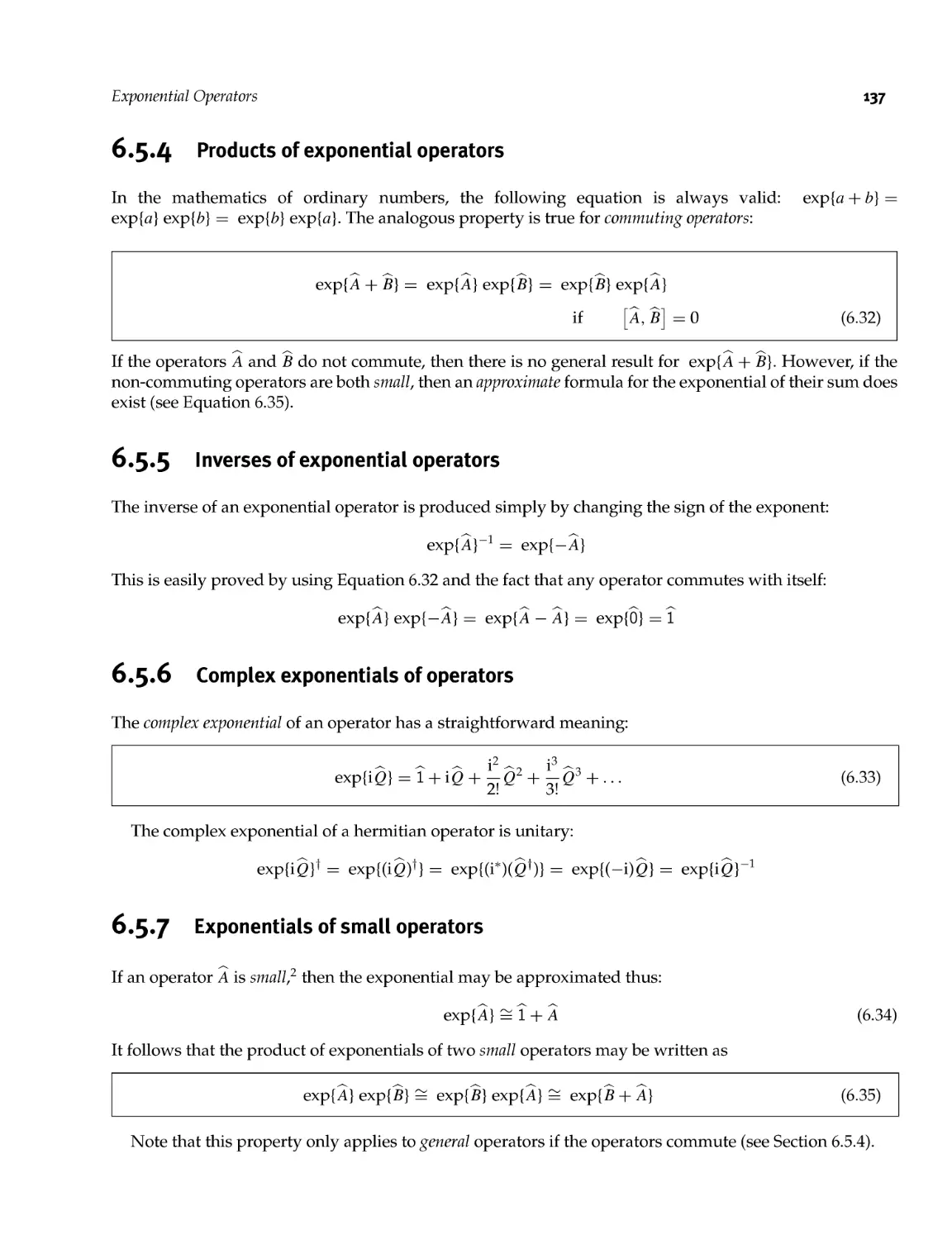
6.6 Cyclic Commutation 138
6.6.1 Definition of cyclic commutation 138
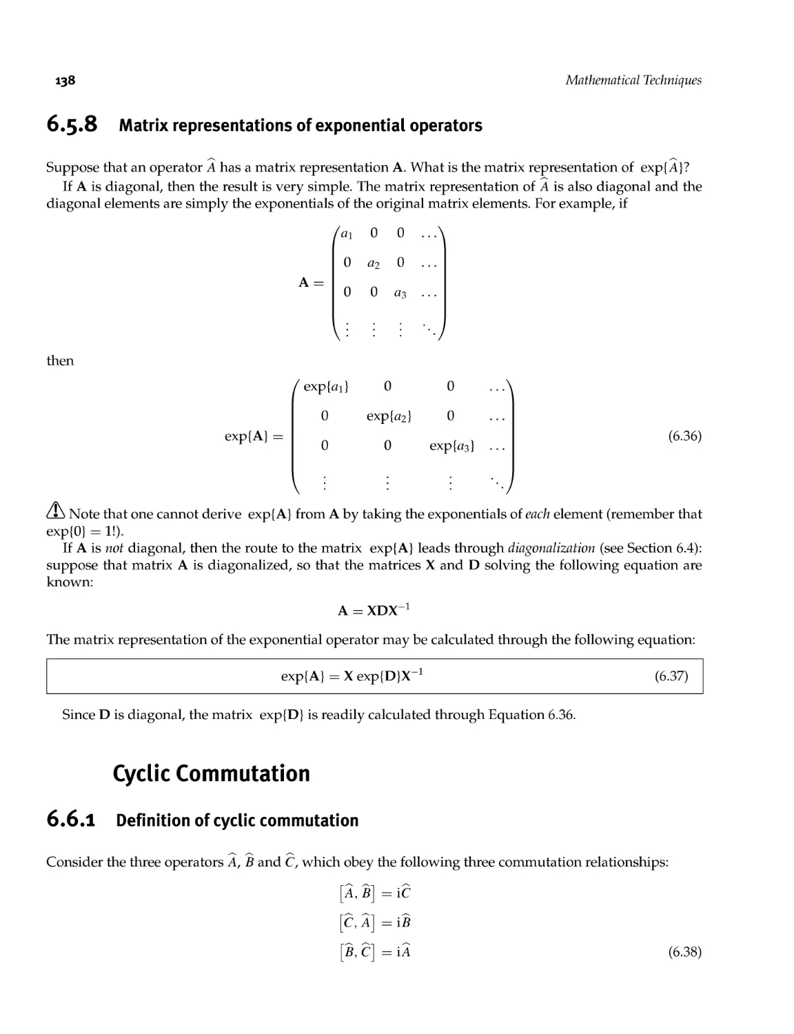
6.6.2 Sandwich formula 139
Review of Quantum Mechanics 143
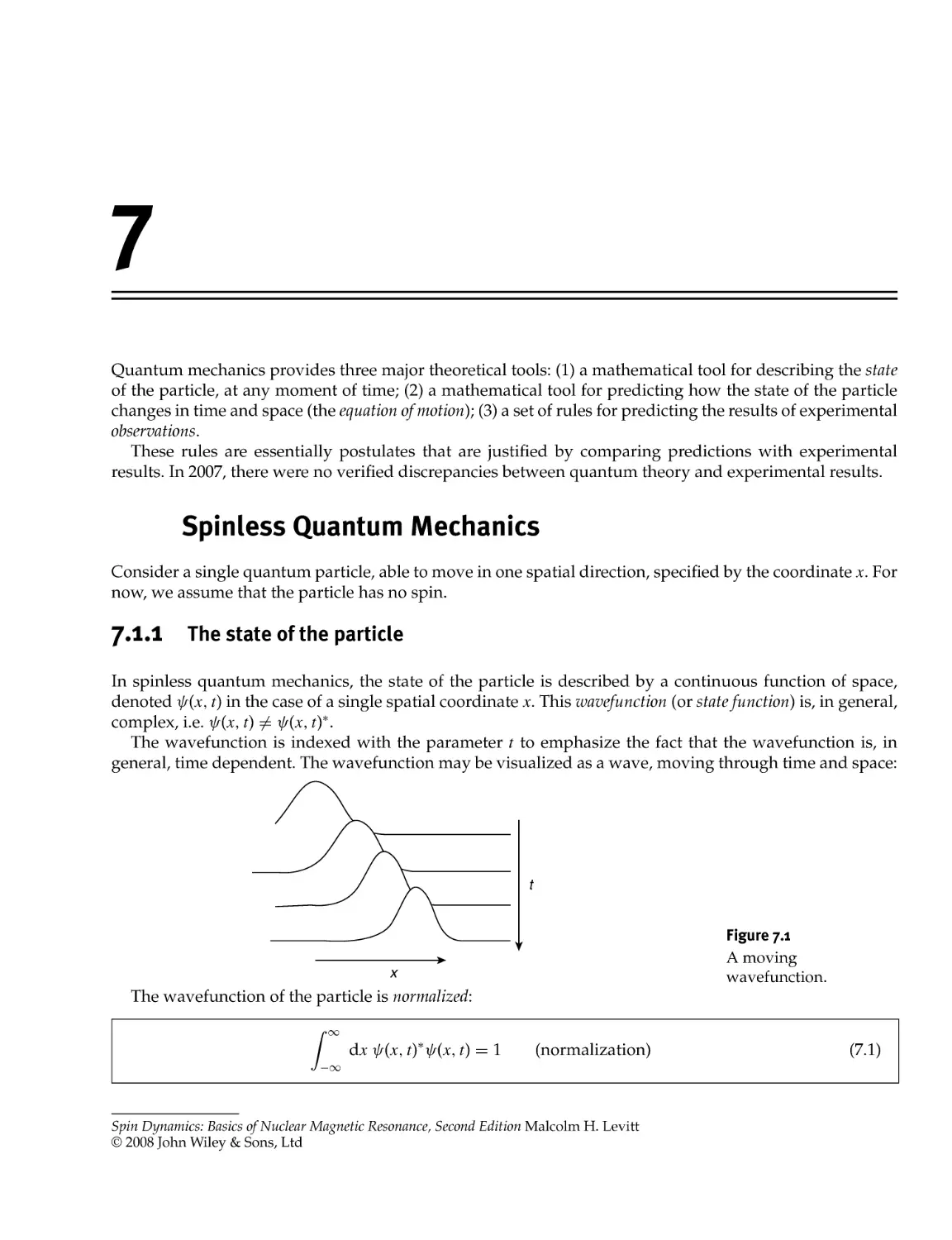
7.1 Spinless Quantum Mechanics 143
7.1.1 The state of the particle 143
7.1.2 The equation of motion 144
7.1.3 Experimental observations 144
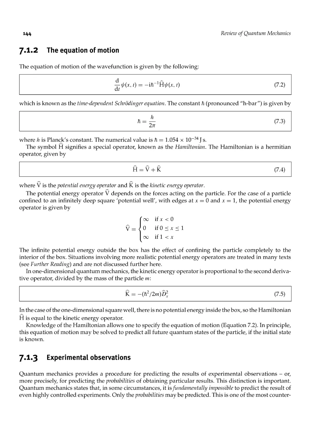
7.2 Energy Levels 145
7.3 Natural Units 146
7.4 Superposition States and Stationary States 147
7.5 Conservation Laws 148
7.6 Angular Momentum 148
7.6.1 Angular momentum operators 149
7.6.2 Rotation operators 149
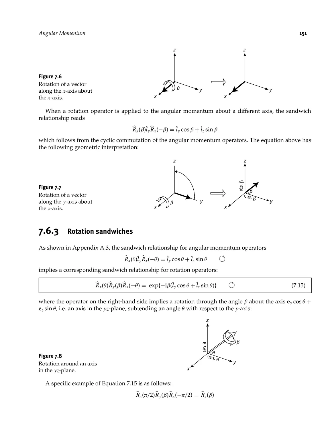
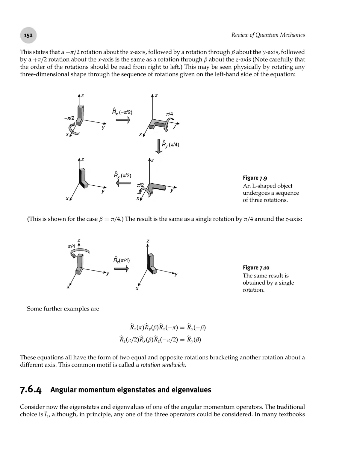
7.6.3 Rotation sandwiches 151
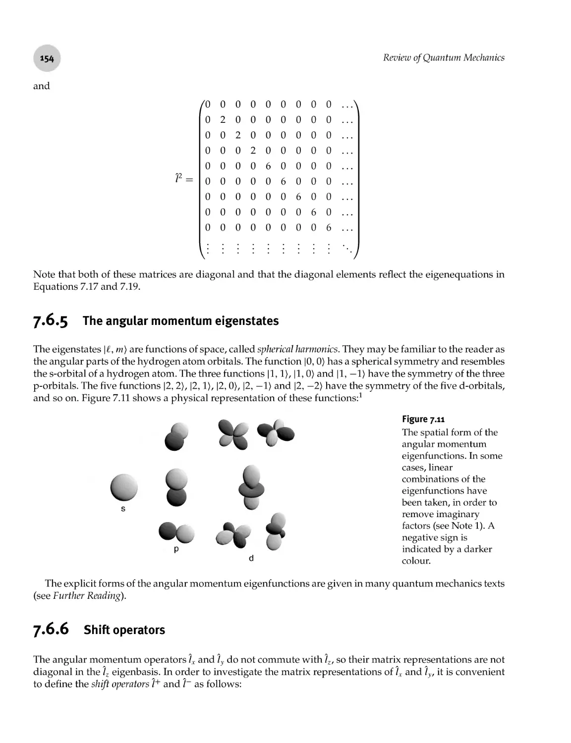
7.6.4 Angular momentum eigenstates and eigenvalues 152
7.6.5 The angular momentum eigenstates 154
7.6.6 Shift operators 154
7.6.7 Matrix representations of the angular momentum operators 156
7.7 Spin 157
7.7.1 Spin angular momentum operators 157
7.7.2 Spin rotation operators 158
7.7.3 Spin Zeeman basis 158
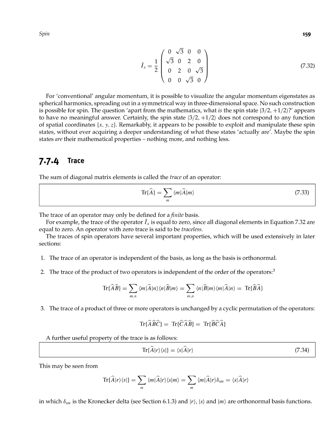
7.7.4 Trace 159
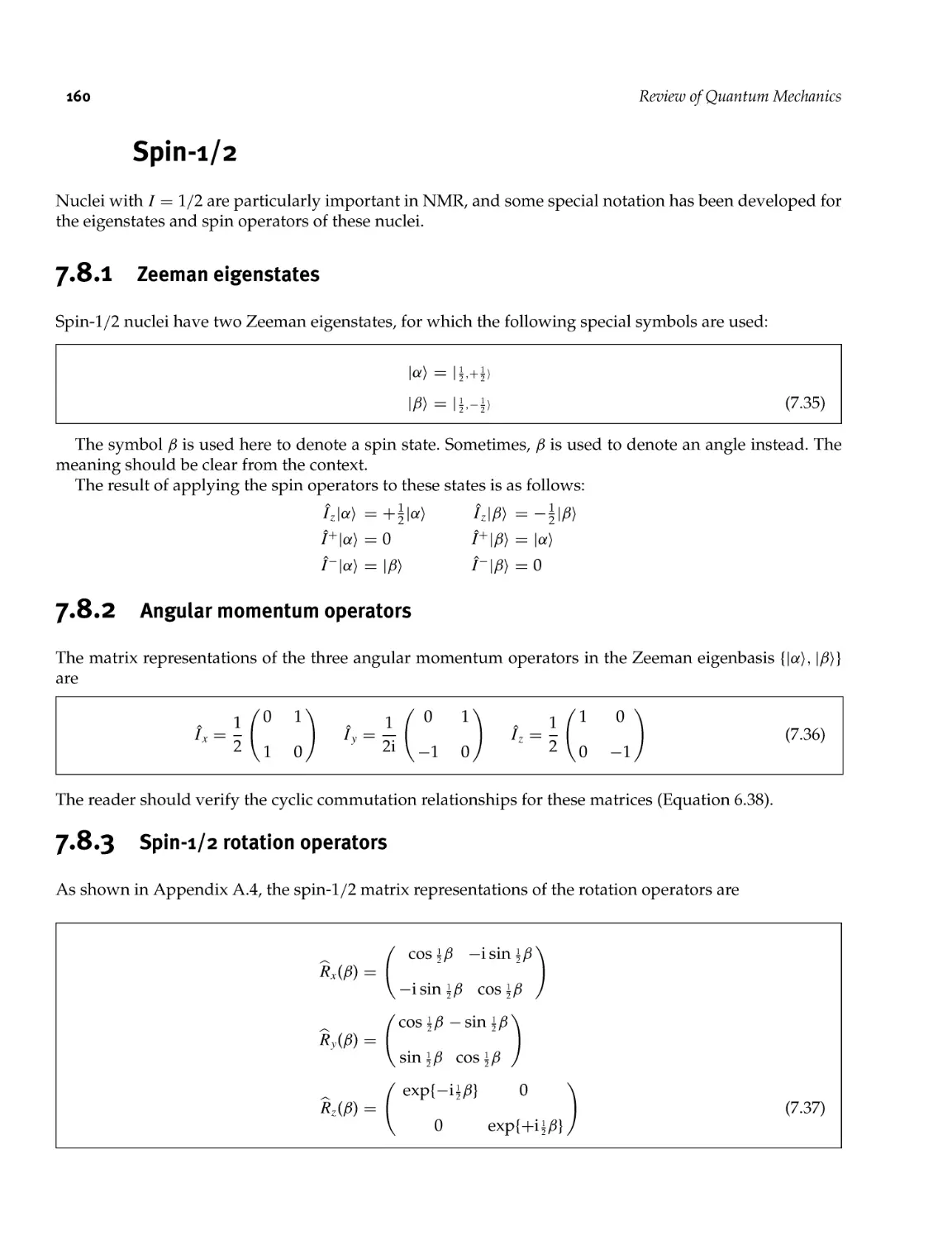
7.8 Spin- 1/2 160
7.8.1 Zeeman eigenstates 160
7.8.2 Angular momentum operators 160
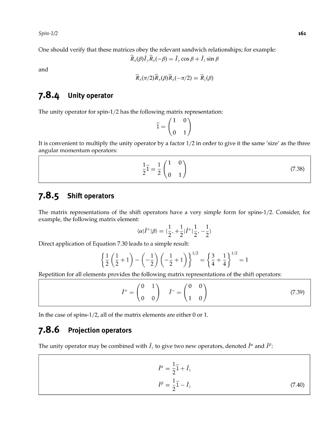
7.8.3 Spin- 1/2 rotation operators 160
7.8.4 Unity operator 161
7.8.5 Shift operators 161
7.8.6 Projection operators 161
7.8.7 Ket- bra notation 162
7.9 Higher Spin 162
7.9.1 Spin 1 = 1 163
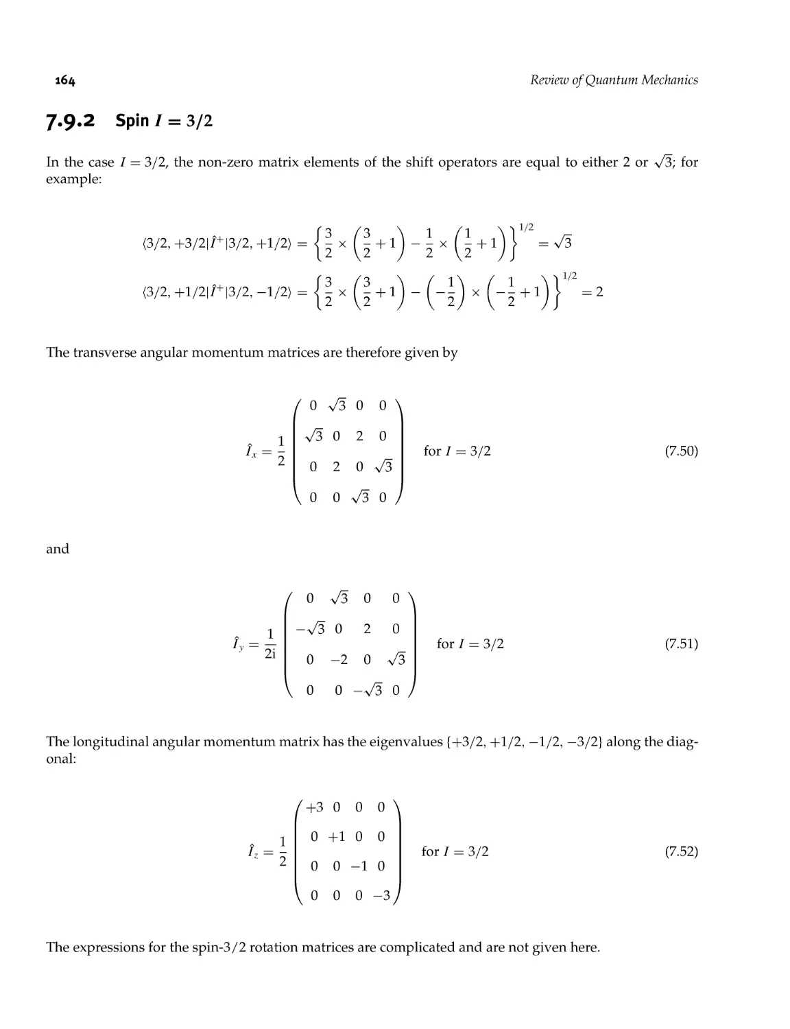
7.9.2 Spin / = 3/2 164
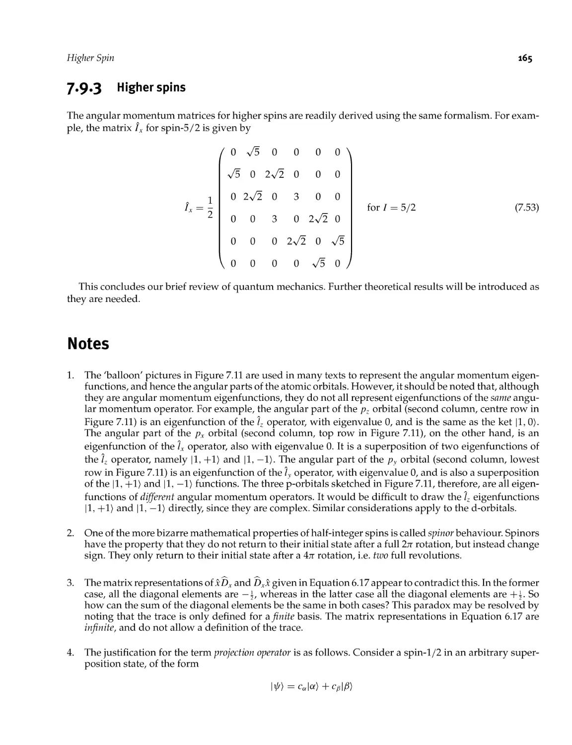
7.9.3 Higher spins 165

Contents
xi
Part 4 Nuclear Spin Interactions
169
8
Nuclear Spin Hamiltonian
171
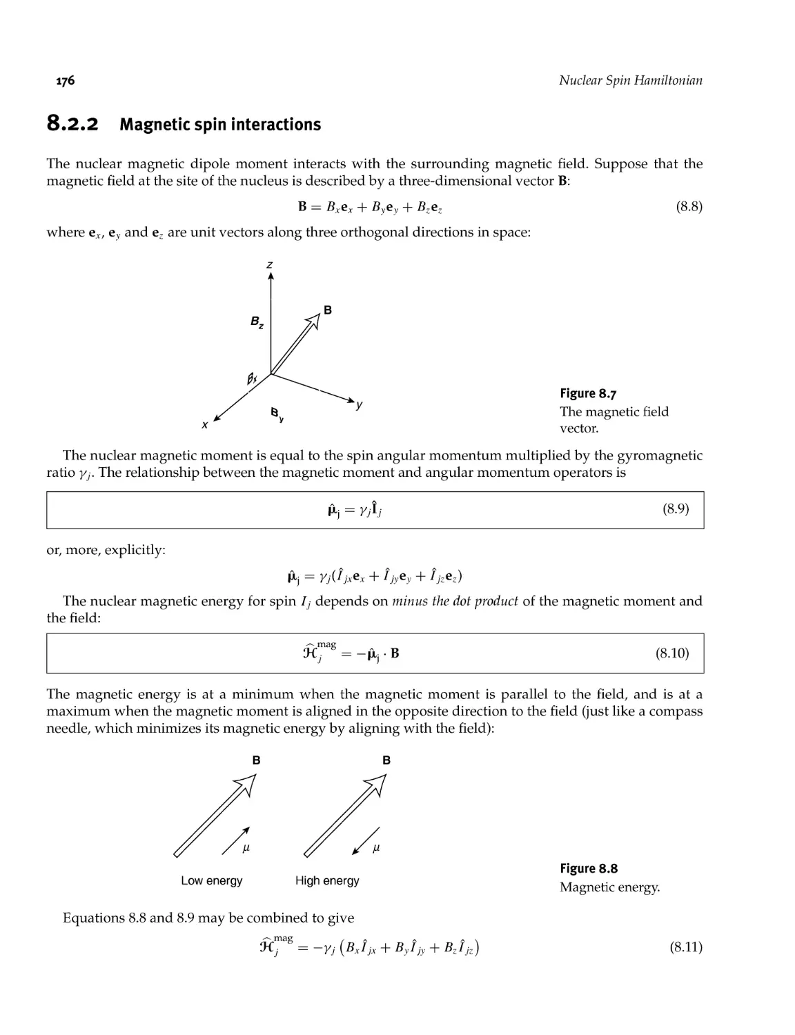
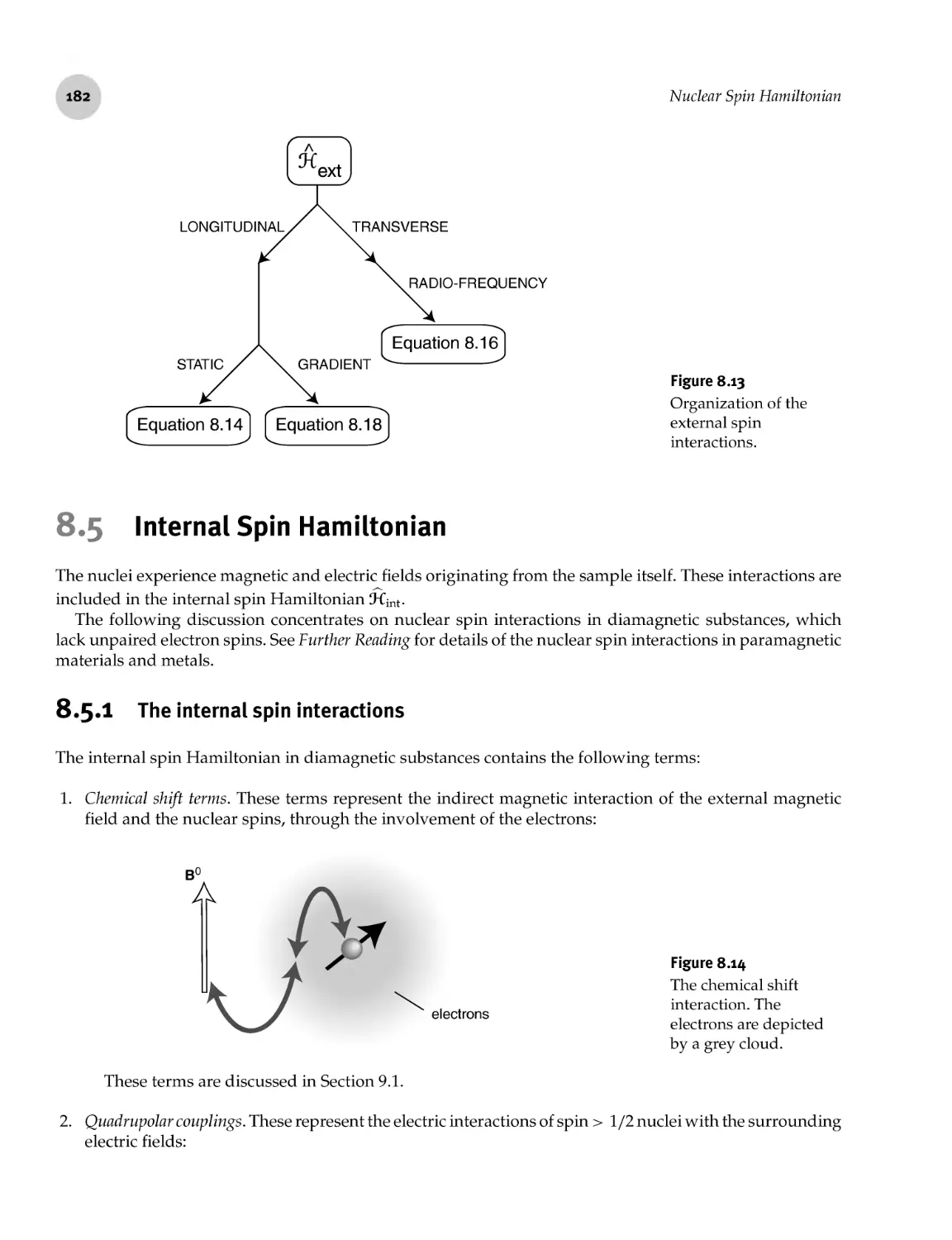
8.1
8.2
8.3
8.4
8.5
8.6
Spin Hamiltonian Hypothesis
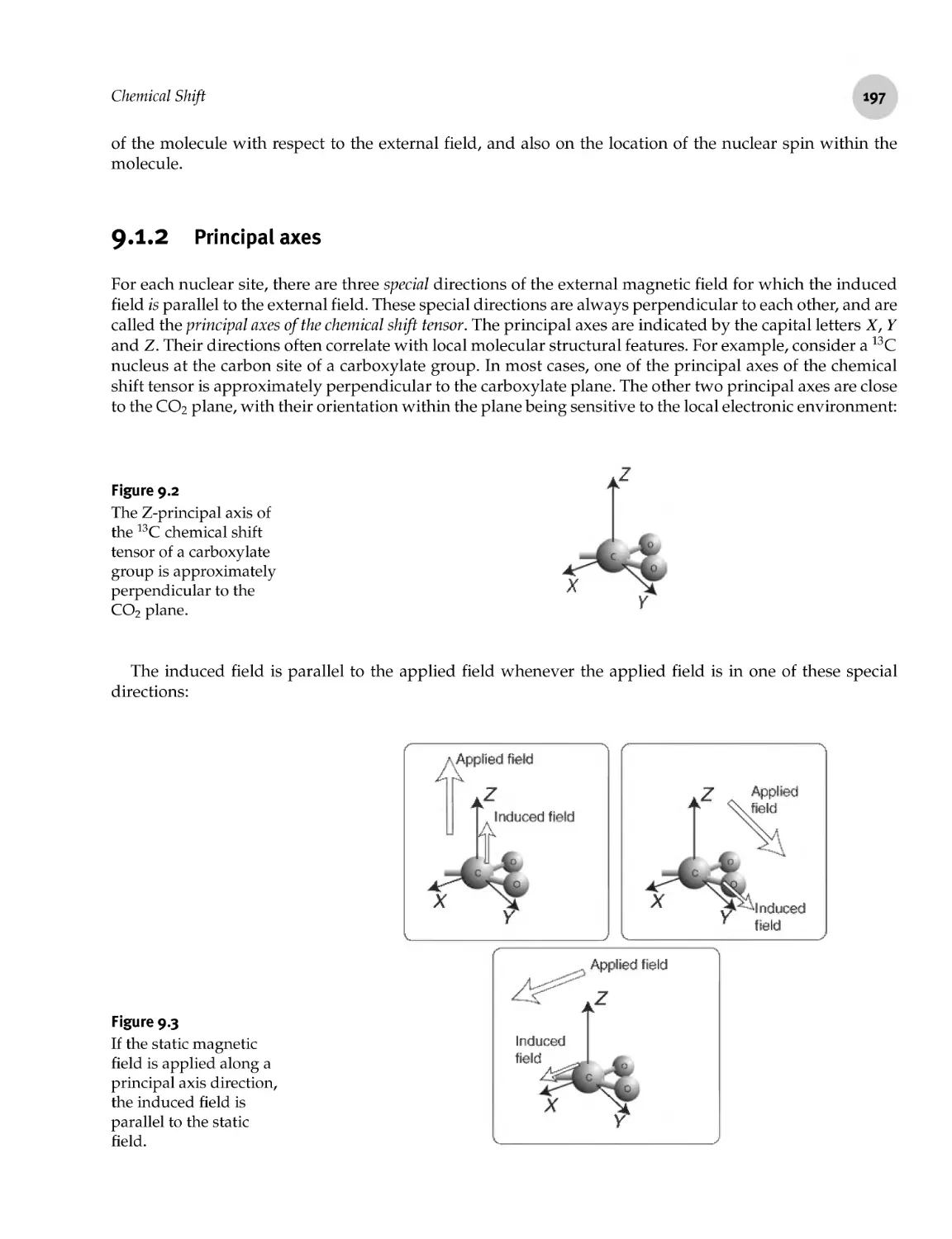
Electromagnetic Interactions
8.2.1 Electric spin Hamiltonian
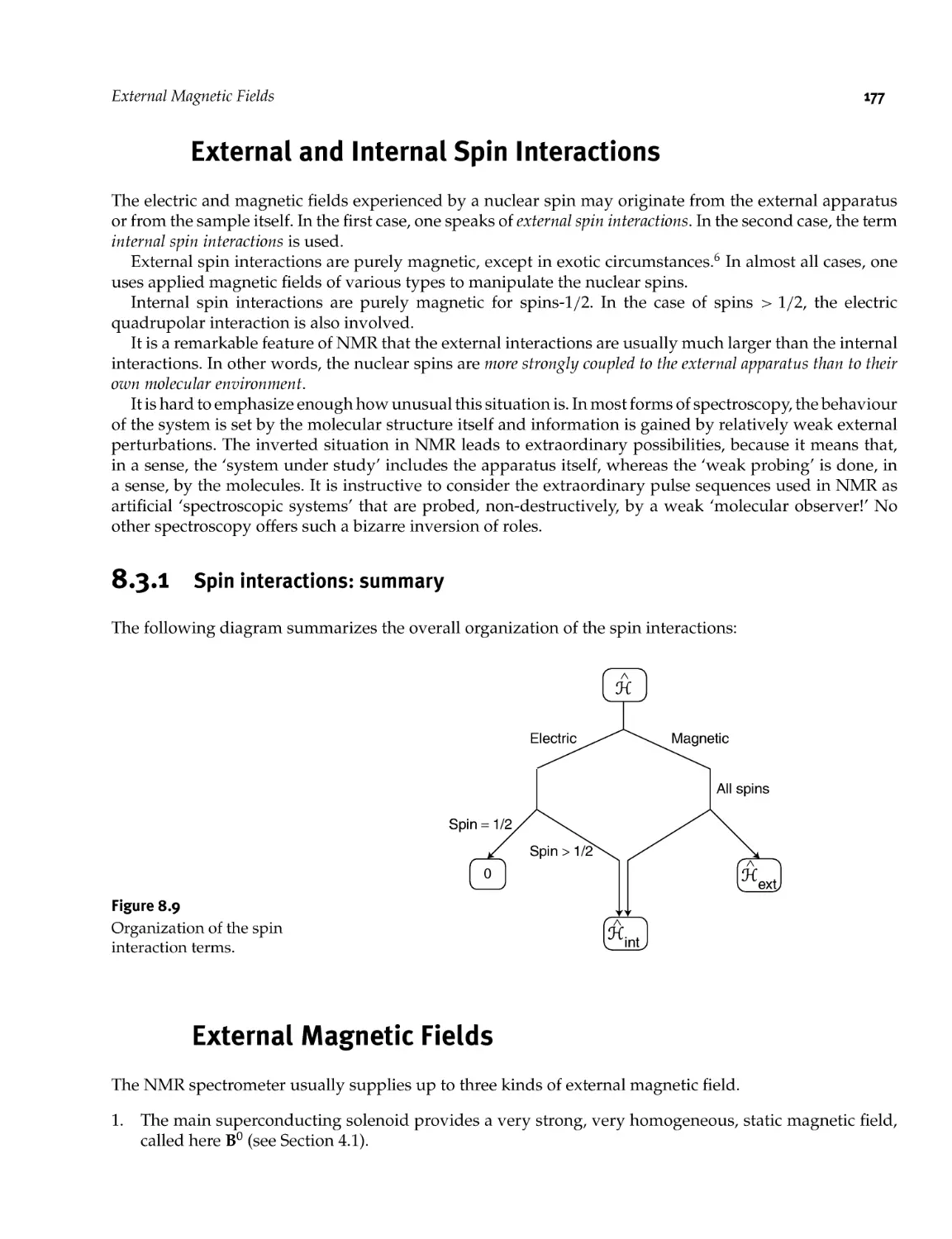
8.2.2 Magnetic spin interactions
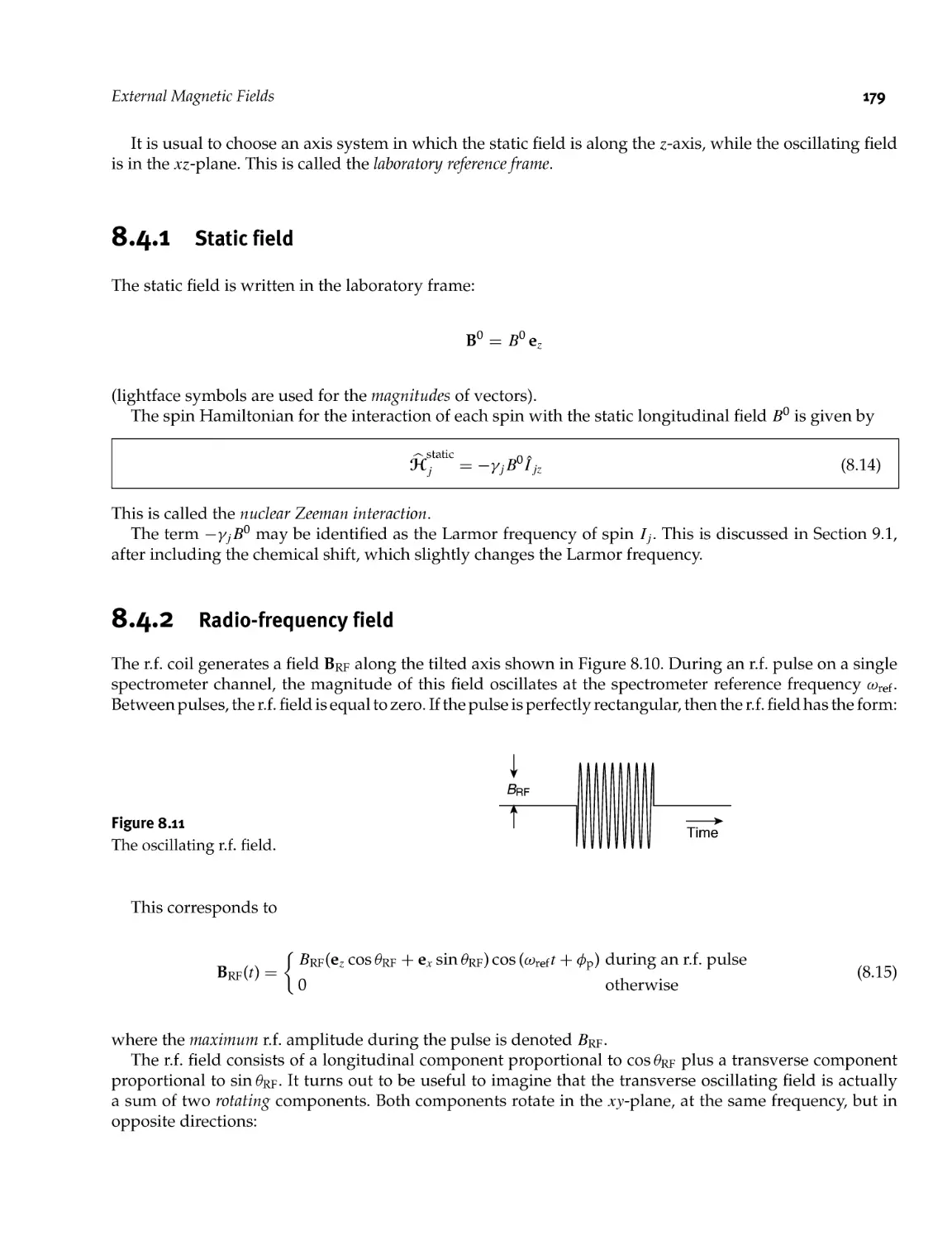
External and Internal Spin Interactions
8.3.1 Spin interactions: summary
External Magnetic Fields
8.4.1 Static field
8.4.2 Radio- frequency field
8.4.3 Gradient field
8.4.4 External spin interactions: summary
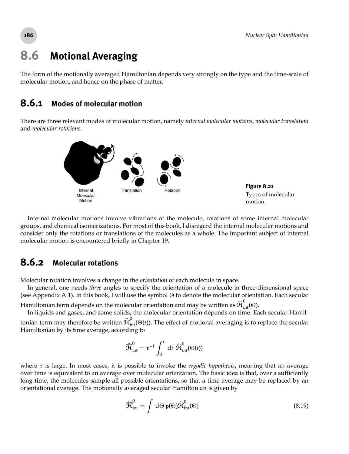
Internal Spin Hamiltonian
8.5.1 The internal spin interactions
8.5.2 Simplification of the internal Hamiltonian
Motional Averaging
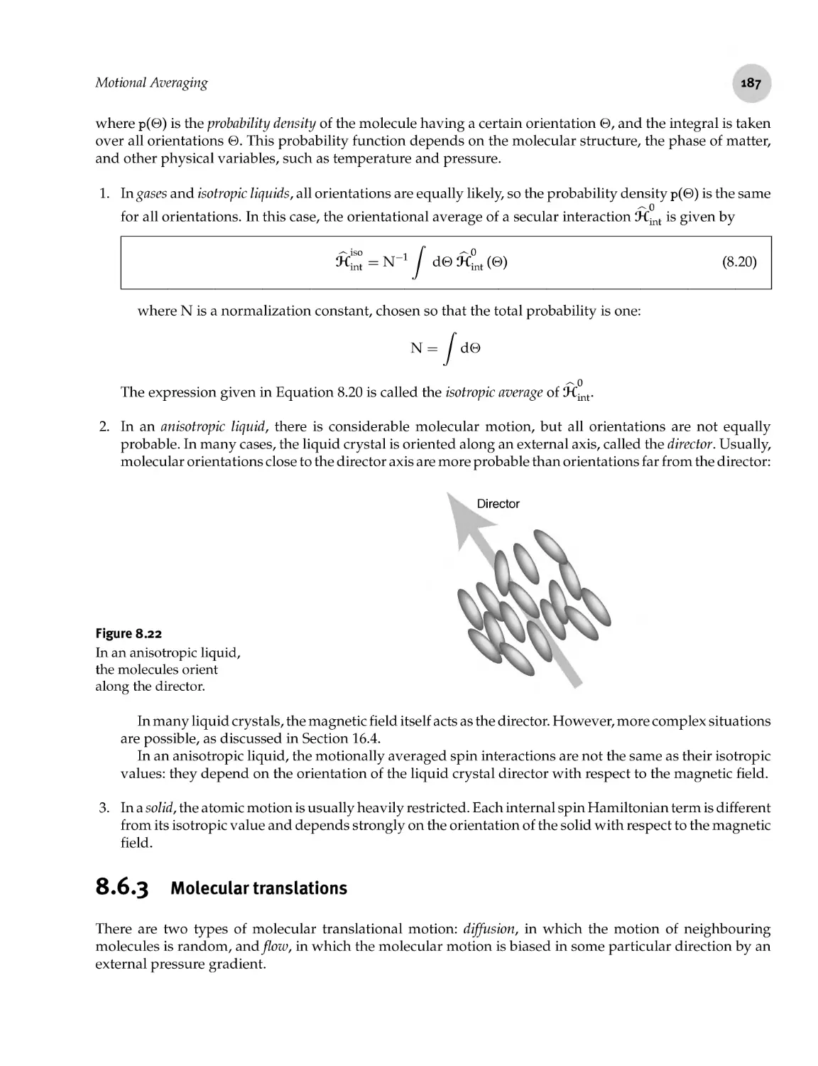
8.6.1 Modes of molecular motion
8.6.2 Molecular rotations
8.6.3 Molecular translations
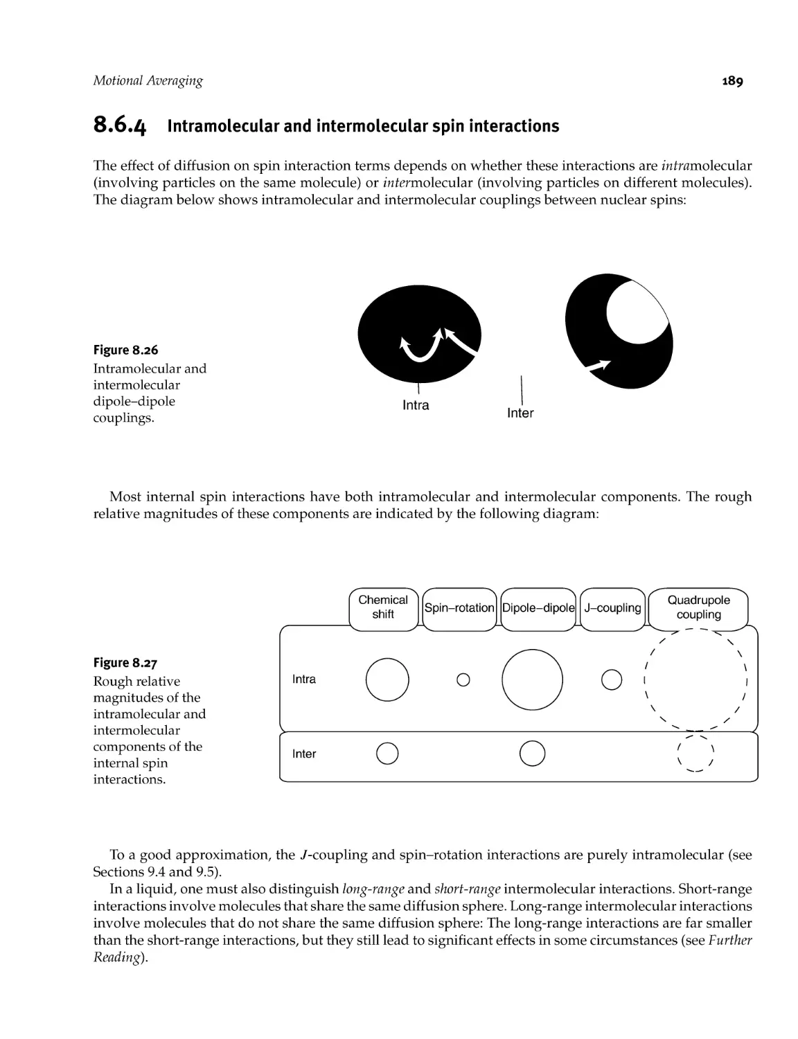
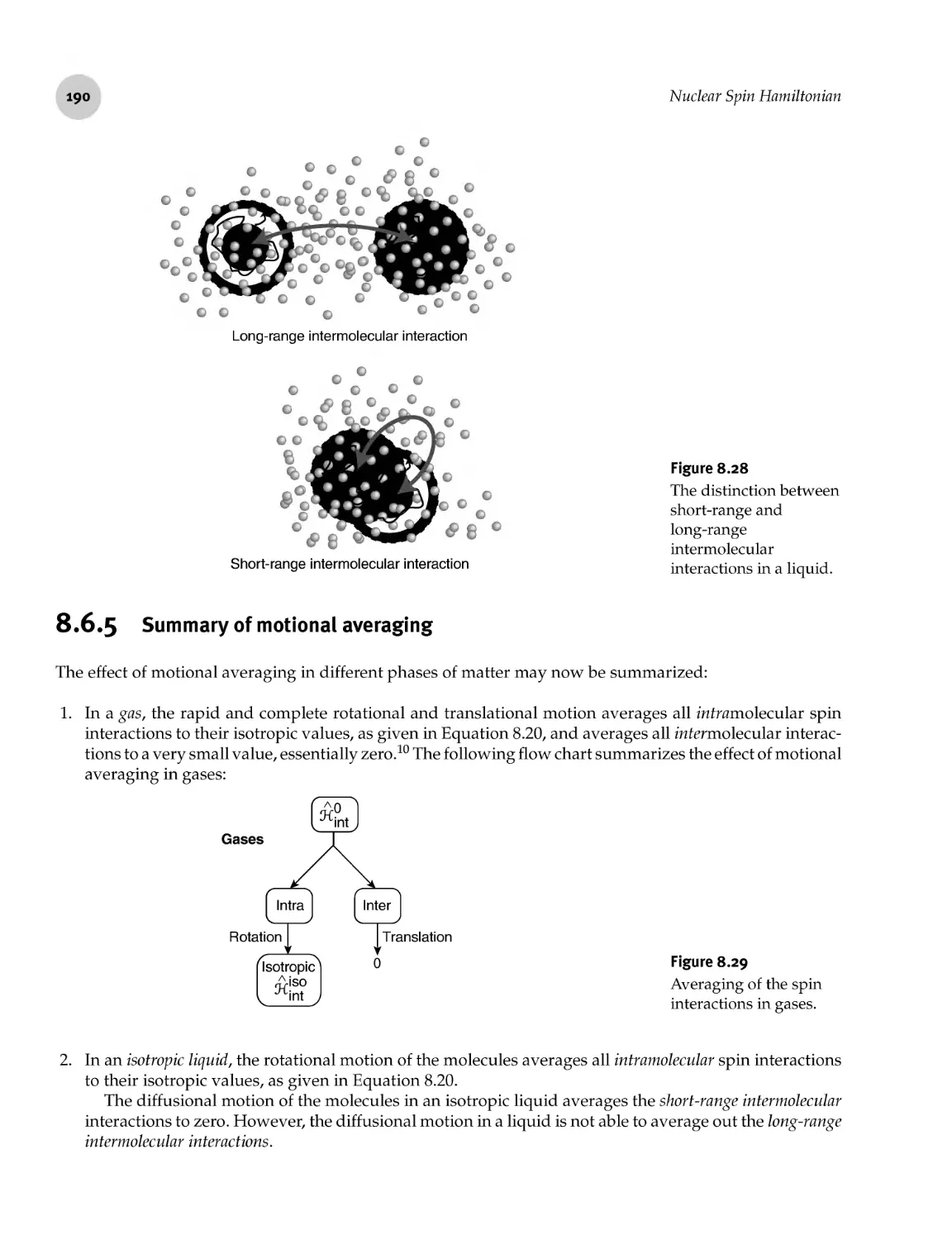
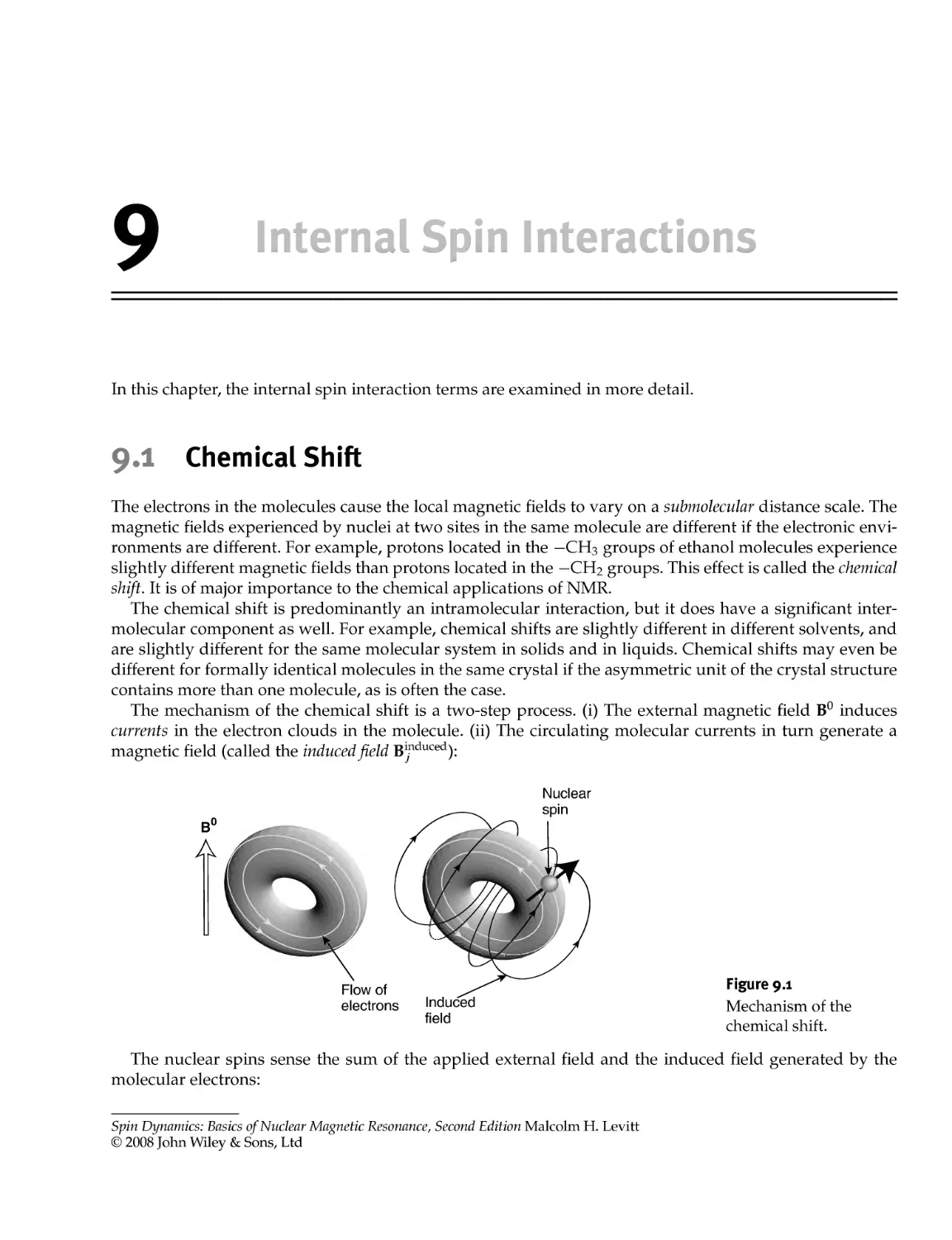
8.6.4 Intramolecular and intermolecular spin interactions
8.6.5 Summary of motional averaging
171
172
173
176
177
177
177
179
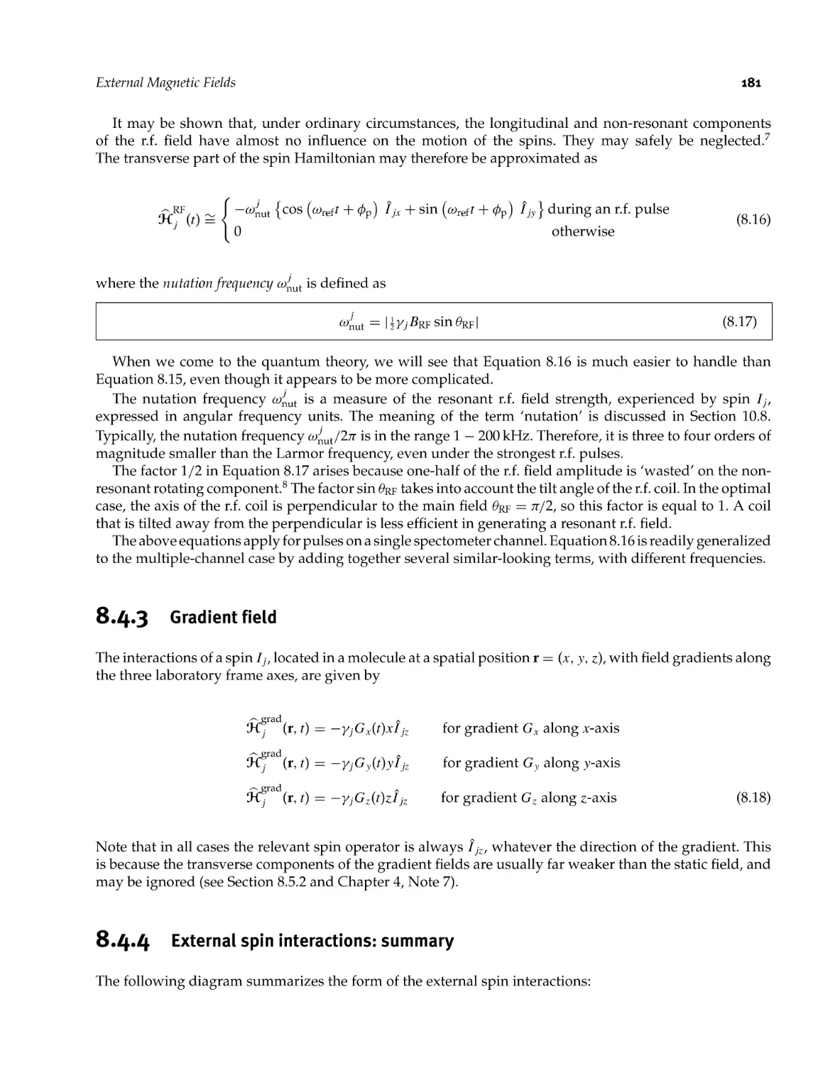
179
181
181
182
182
185
186
186
186
187
189
190
9
Internal Spin Interactions
195
9.2
9.1 Chemical Shift
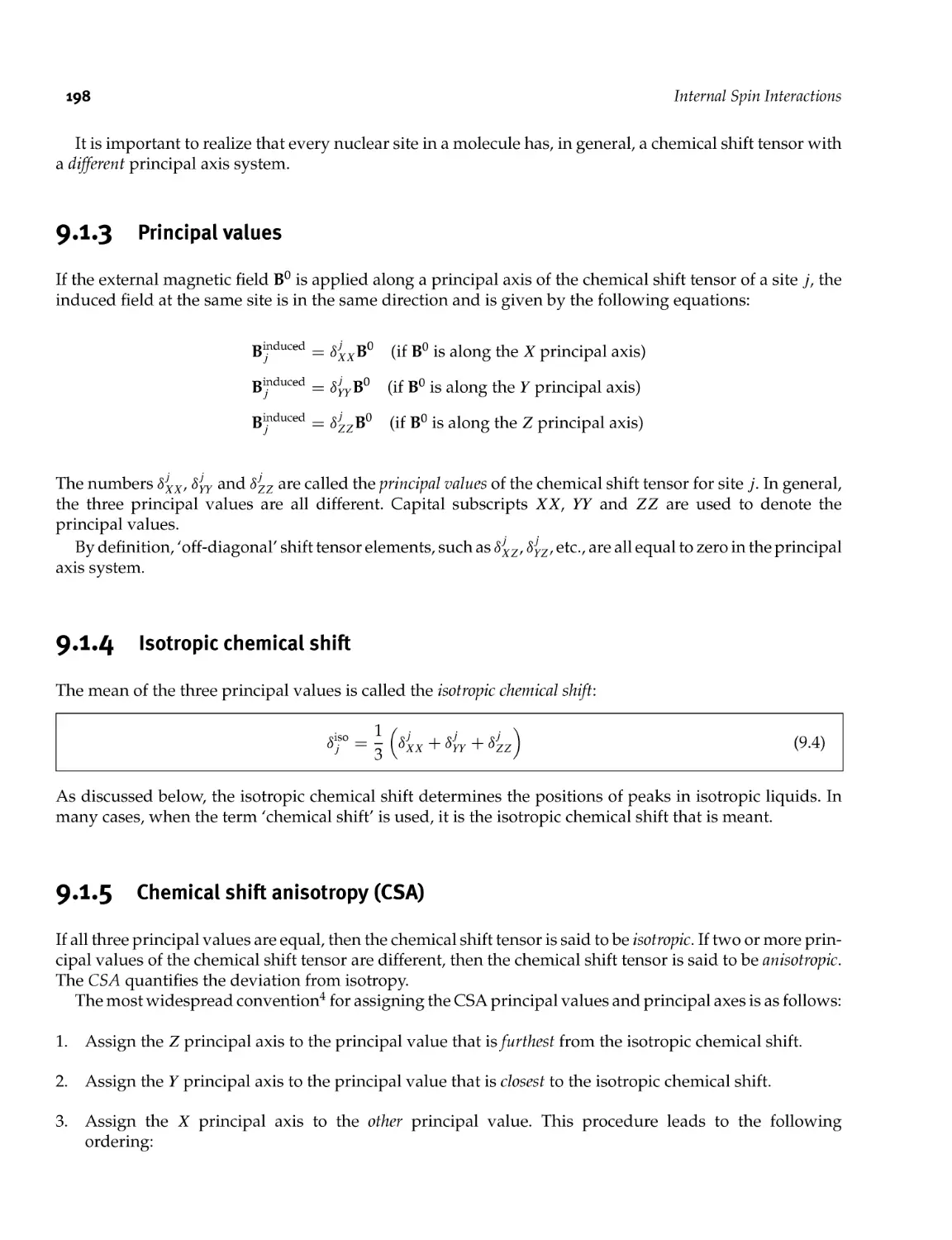
9.1.1 Chemical shift tensor
Principal axes
Principal values
Isotropic chemical shift
Chemical shift anisotropy (CSA)
Chemical shift for an arbitrary molecular orientation
Chemical shift frequency
Chemical shift interaction in isotropic liquids
Chemical shift interaction in anisotropic liquids
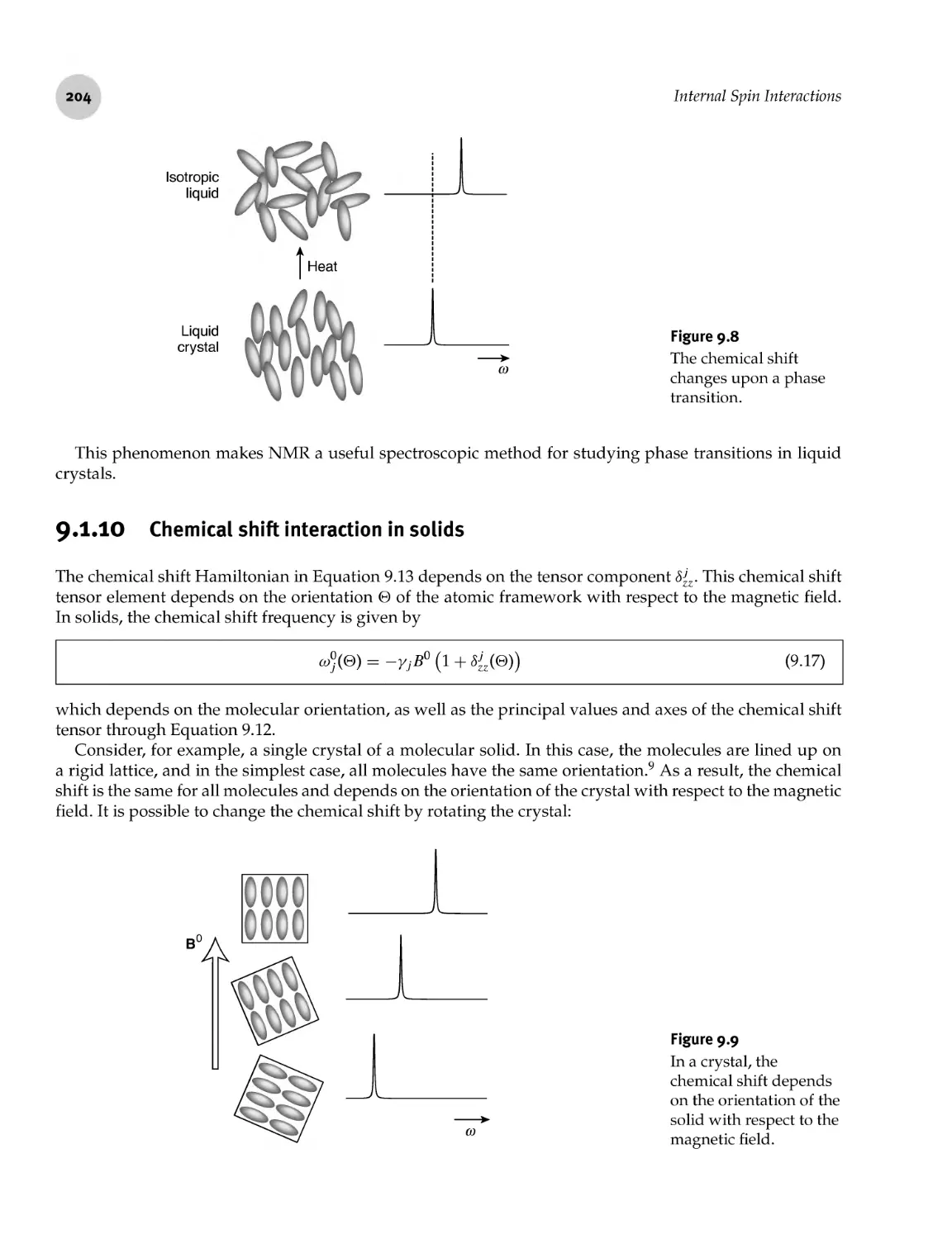
Chemical shift interaction in solids
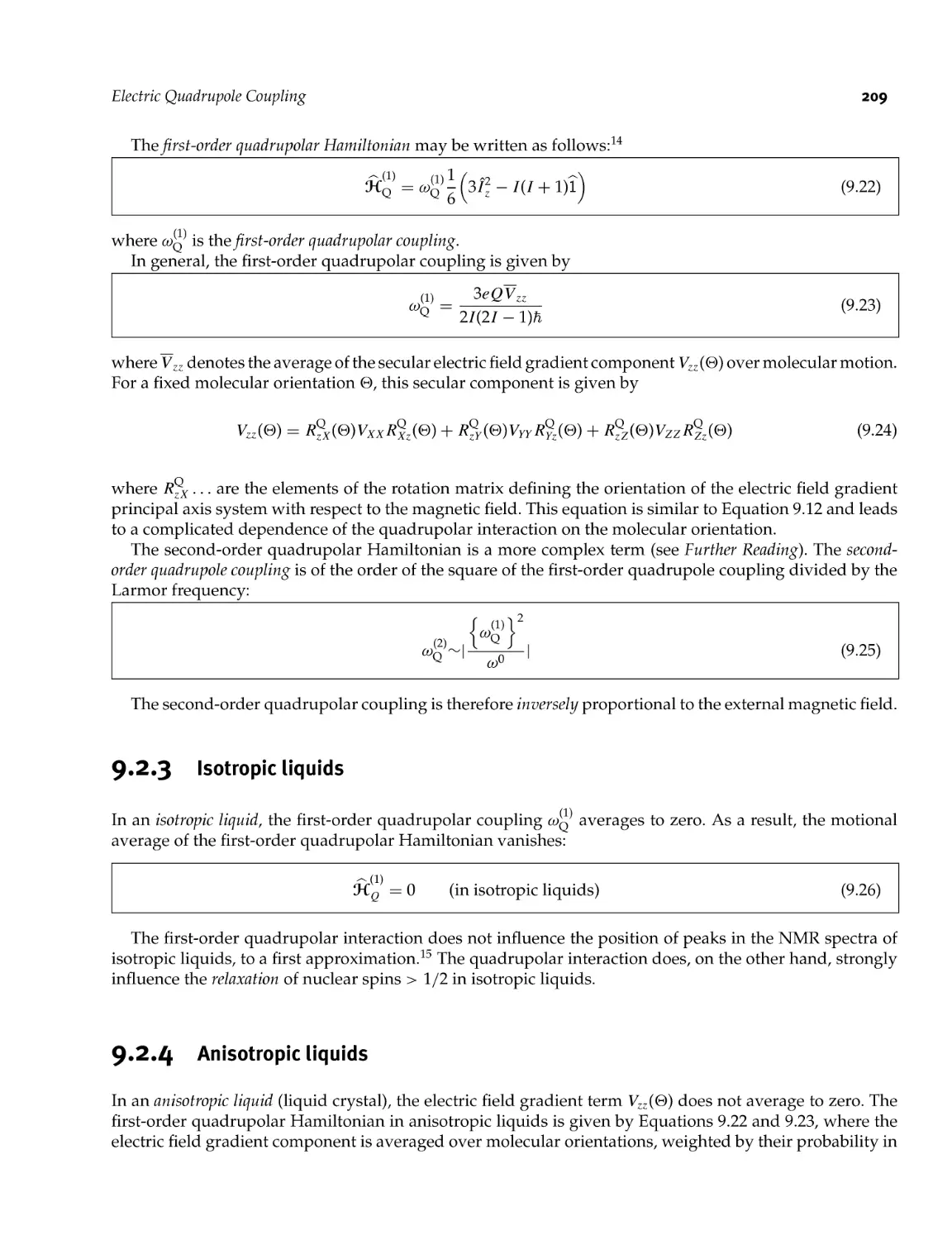
Chemical shift interaction: summary
Electric Quadrupole Coupling
9.2.1 Electric field gradient tensor
Nuclear quadrupole Hamiltonian
Isotropic liquids
Anisotropic liquids
Solids
Quadrupole interaction: summary
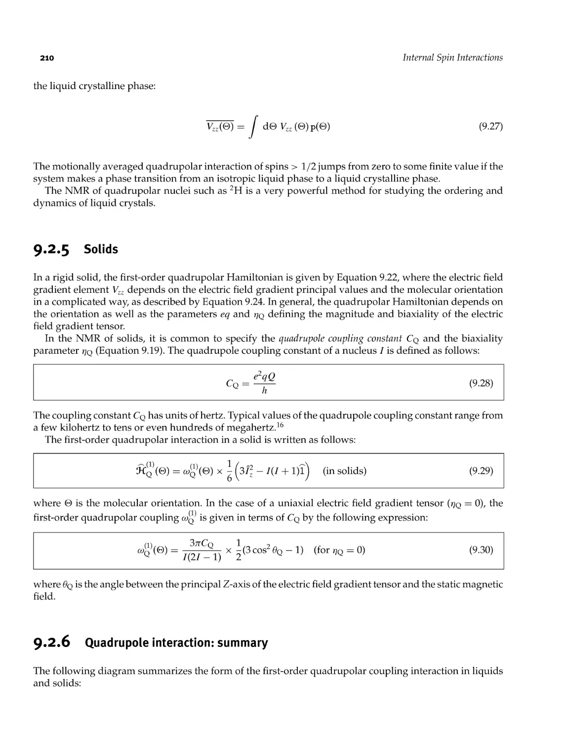
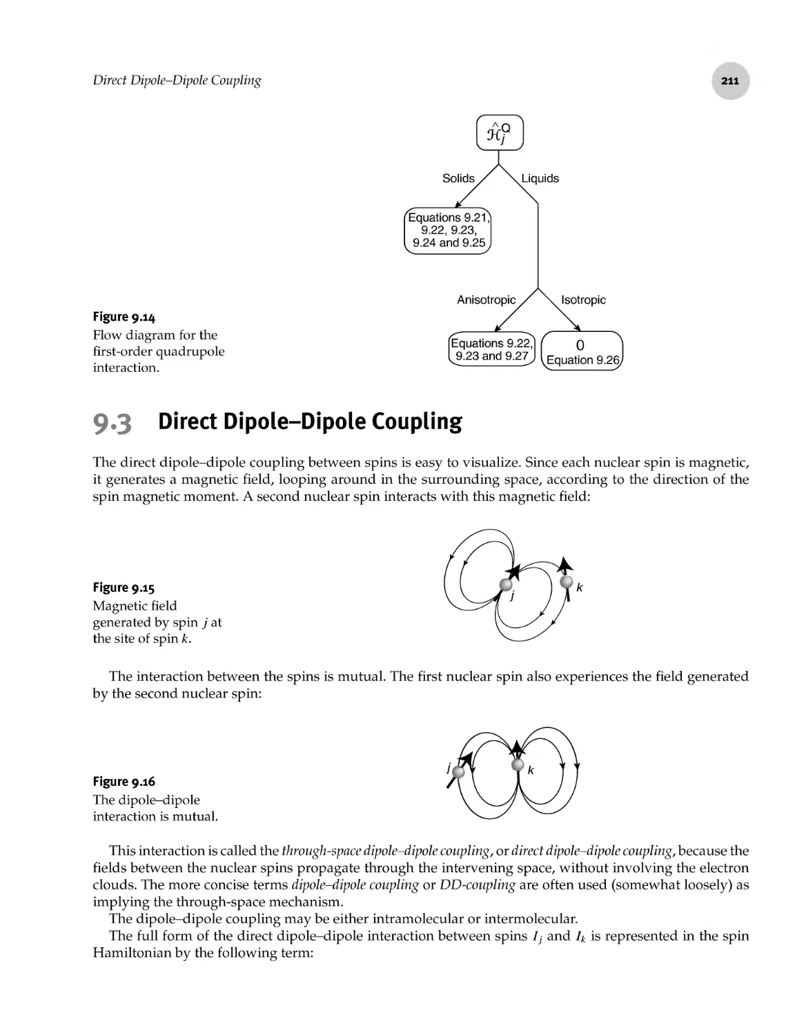
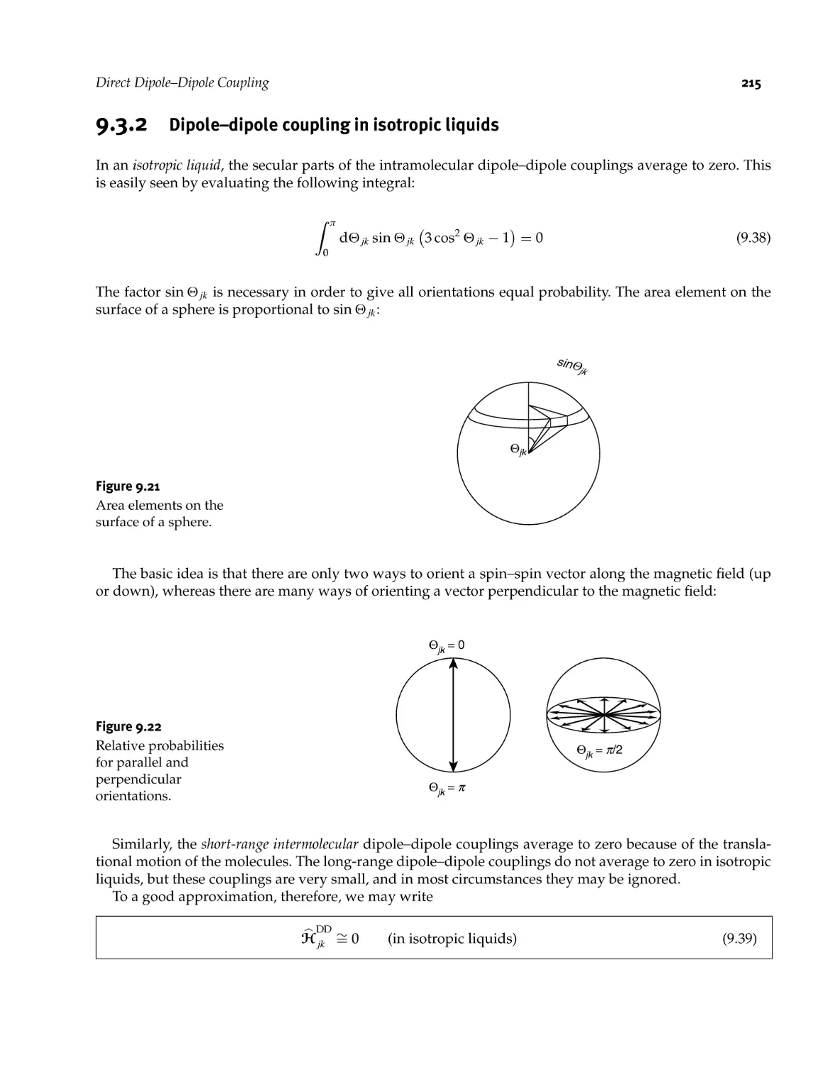
9.3 Direct Dipole- Dipole Coupling
9.3.1 Secular dipole- dipole coupling
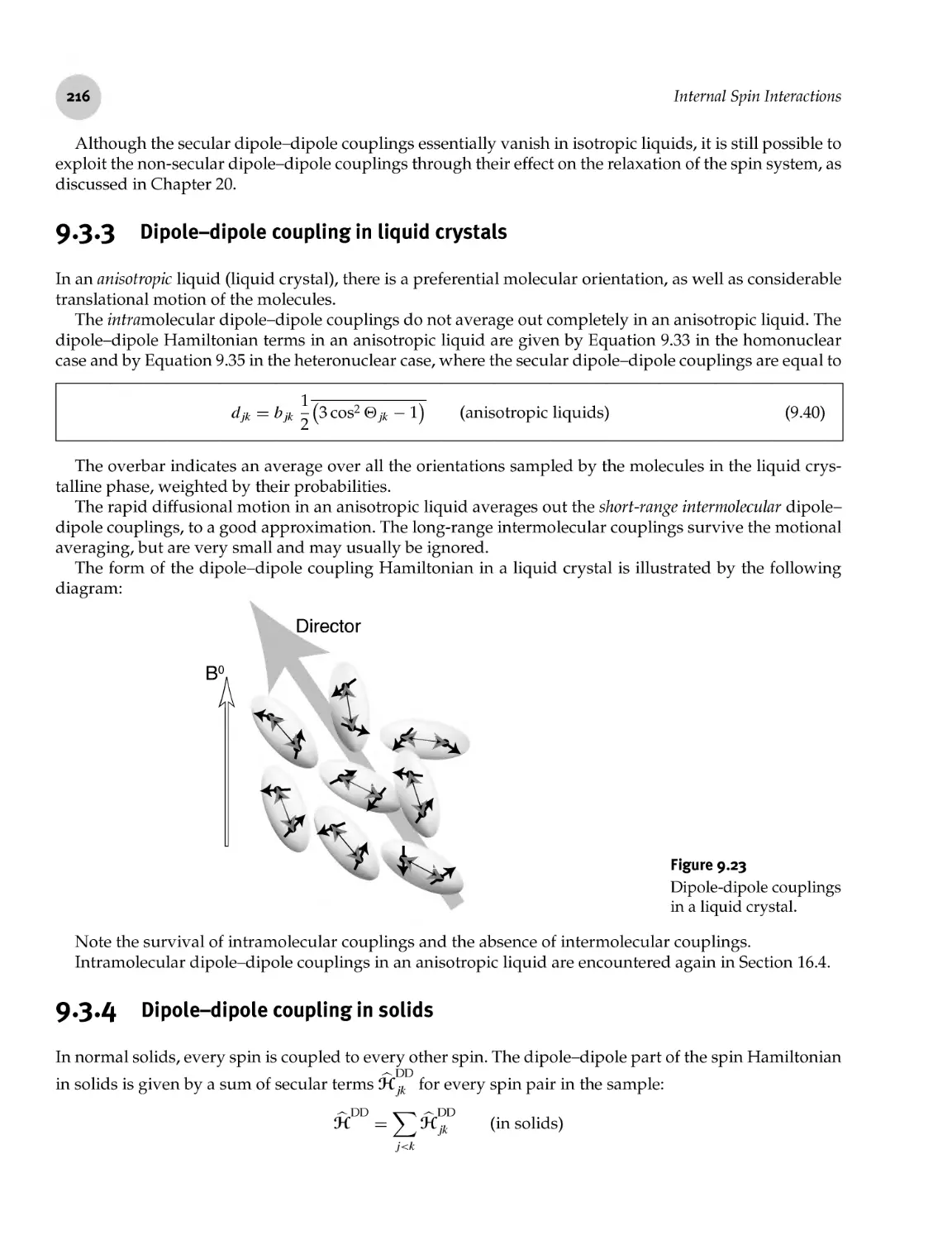
9.3.2 Dipole- dipole coupling in isotropic liquids
M.2
M.3
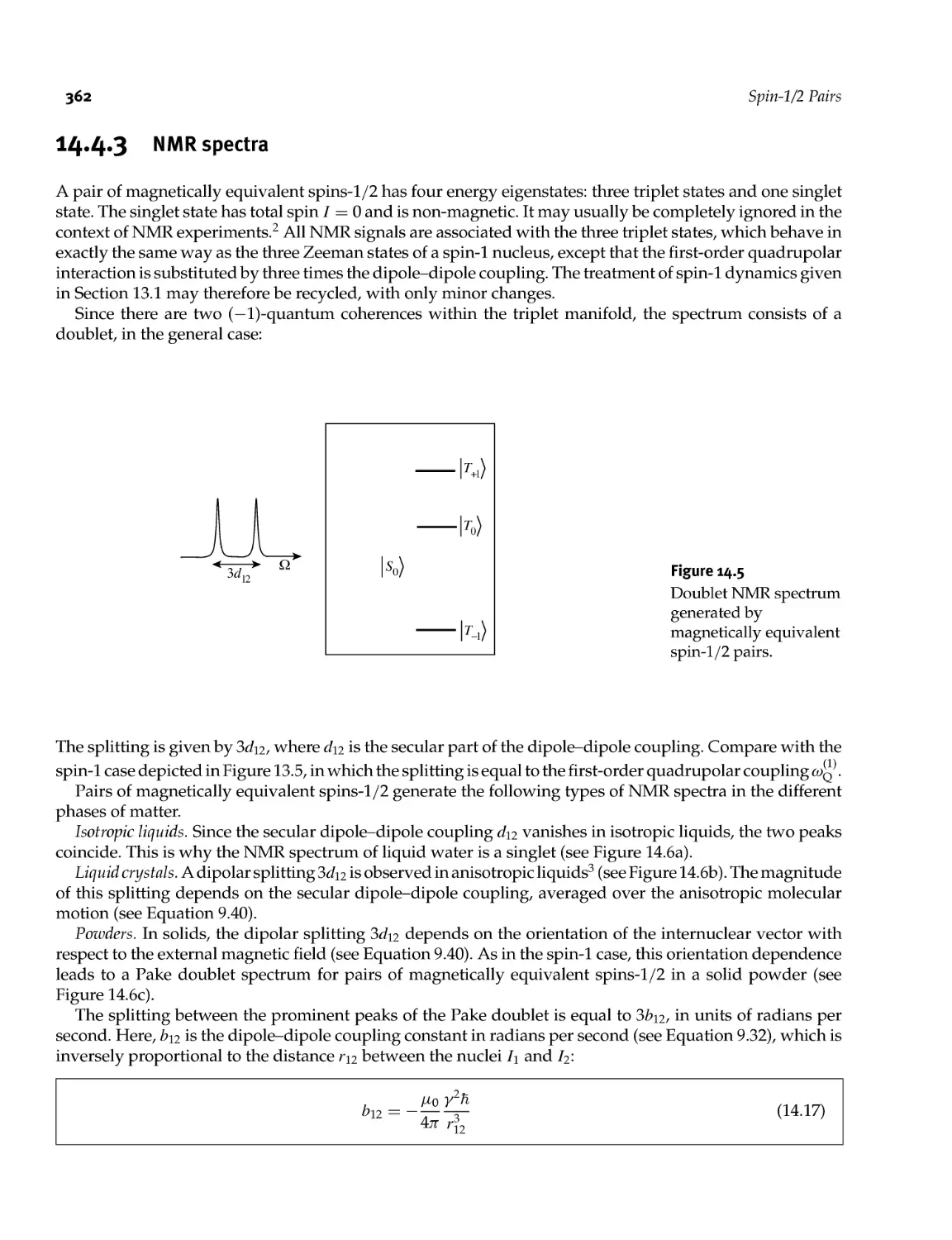
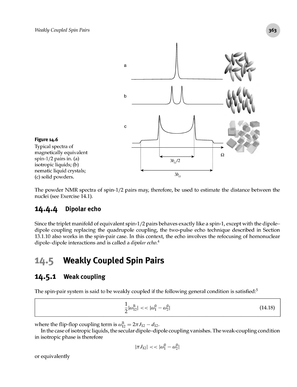
M.4
M.5
M.6
M.7
M.8
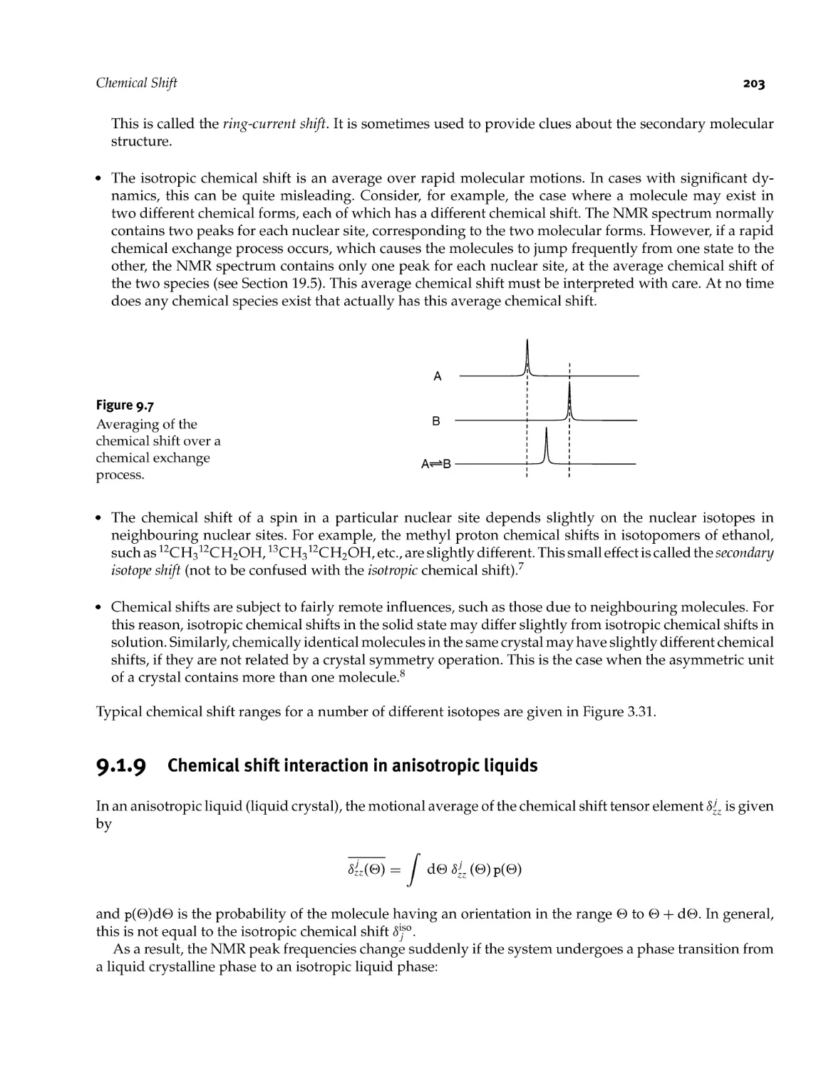
9.1.9
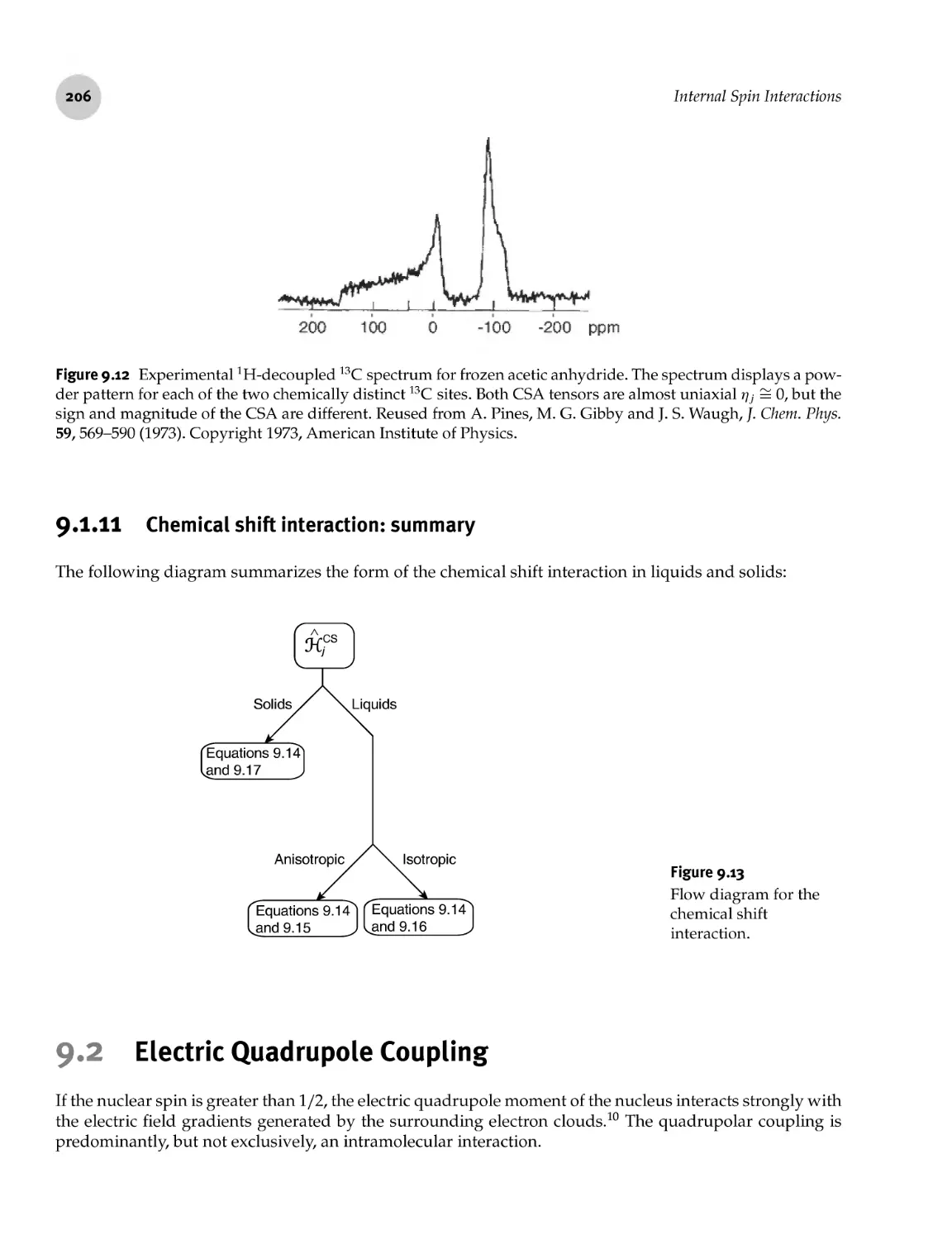
9.1.10
9.1.11
9.2.2
9.2.3
9.2.4
9.2.5
9.2.6
195
196
197
198
198
198
200
201
201
203
204
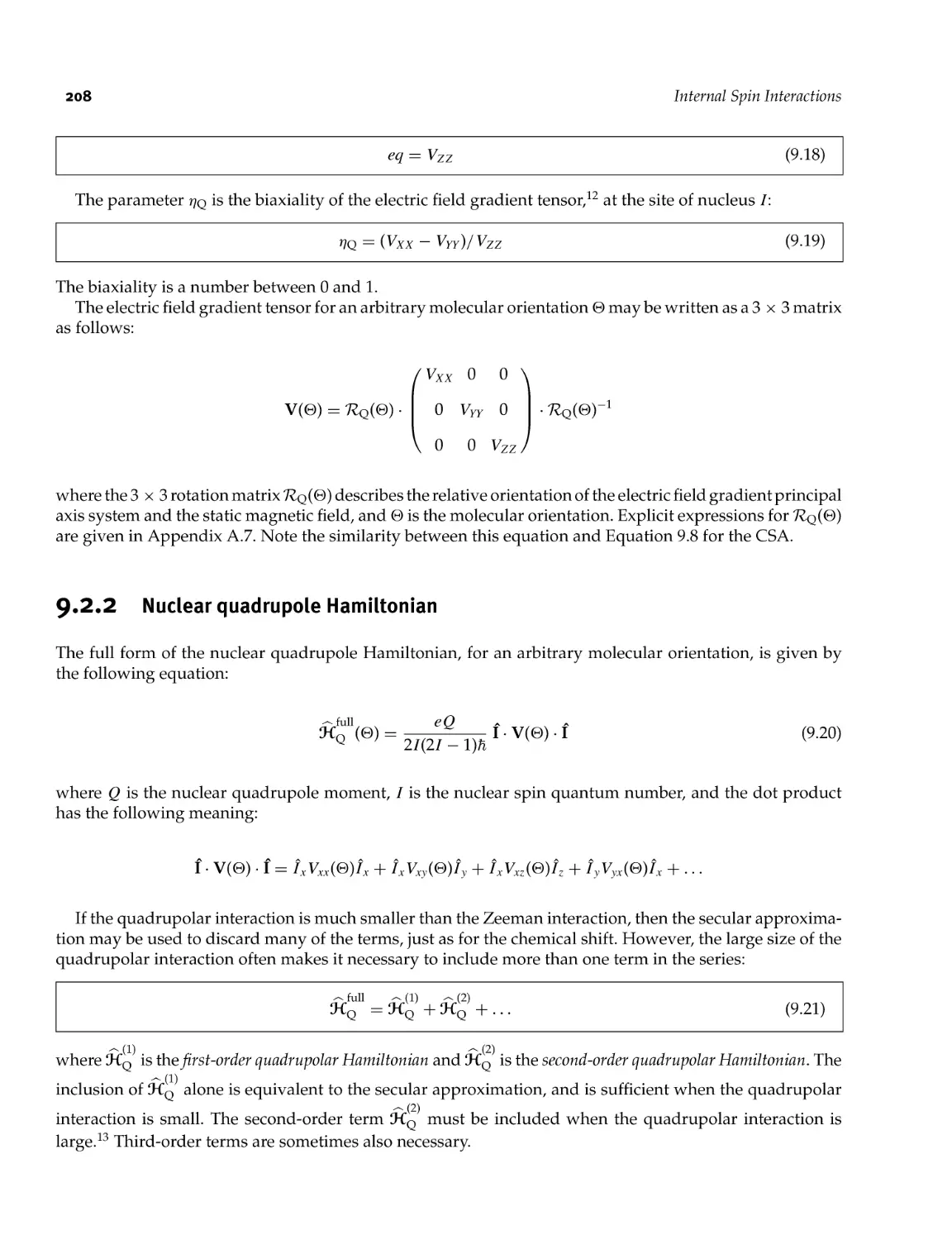
206
206
207
208
209
209
210
210
211
213
215

xii
Contents
9.3.3 Dipole- dipole coupling in liquid crystals 216
9.3.4 Dipole- dipole coupling in solids 216
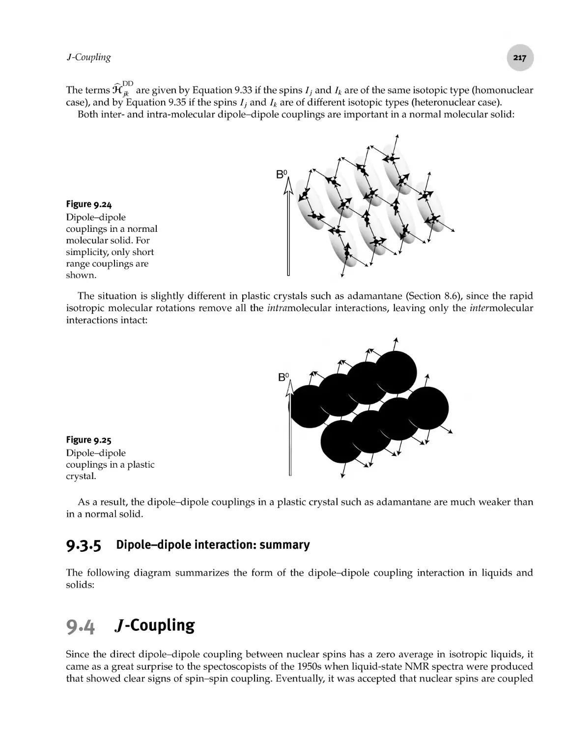
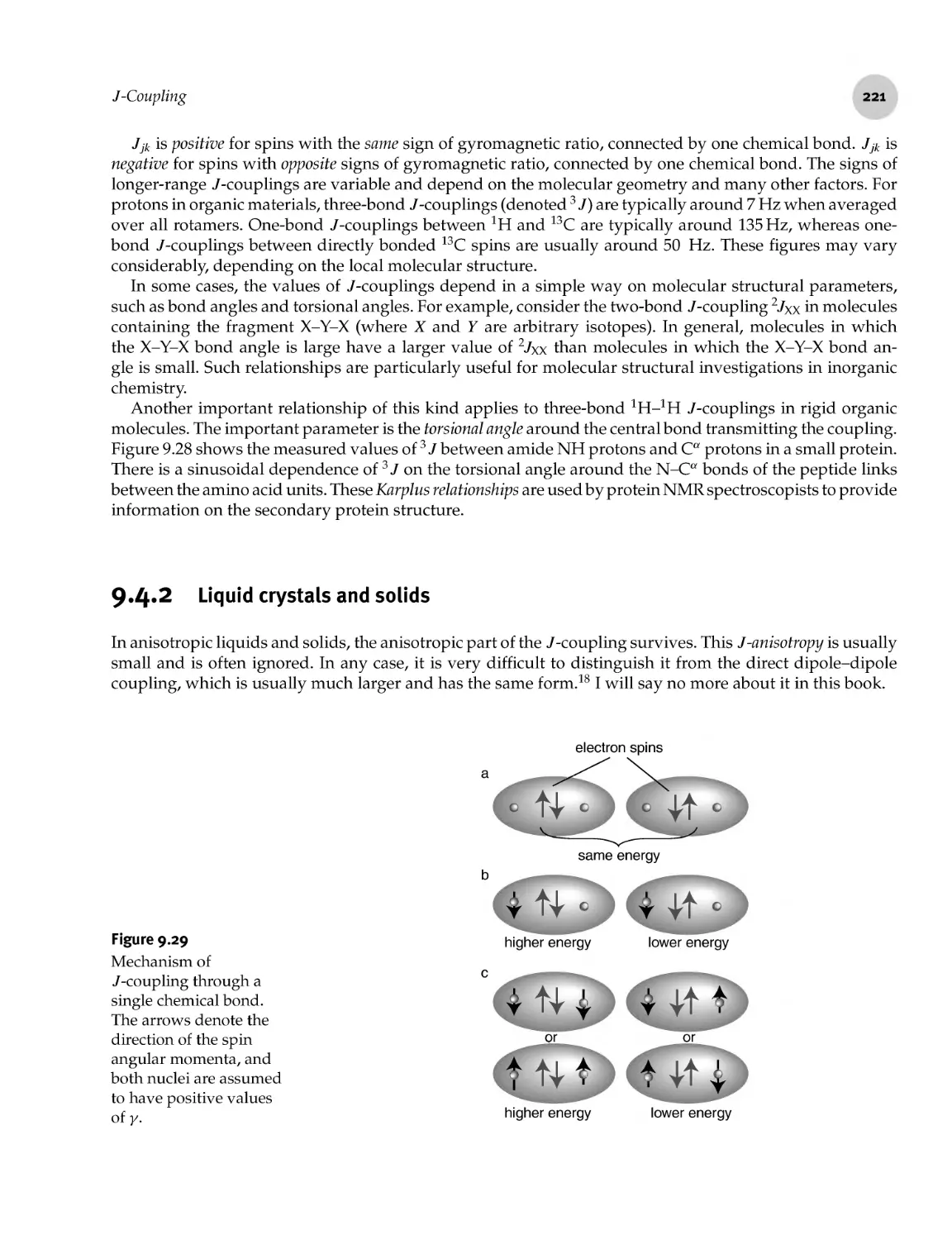
9.3.5 Dipole- dipole interaction: summary 217
9.4 /- Coupling 217
9.4.1 Isotropic /- coupling 219
9.4.2 Liquid crystals and solids 221
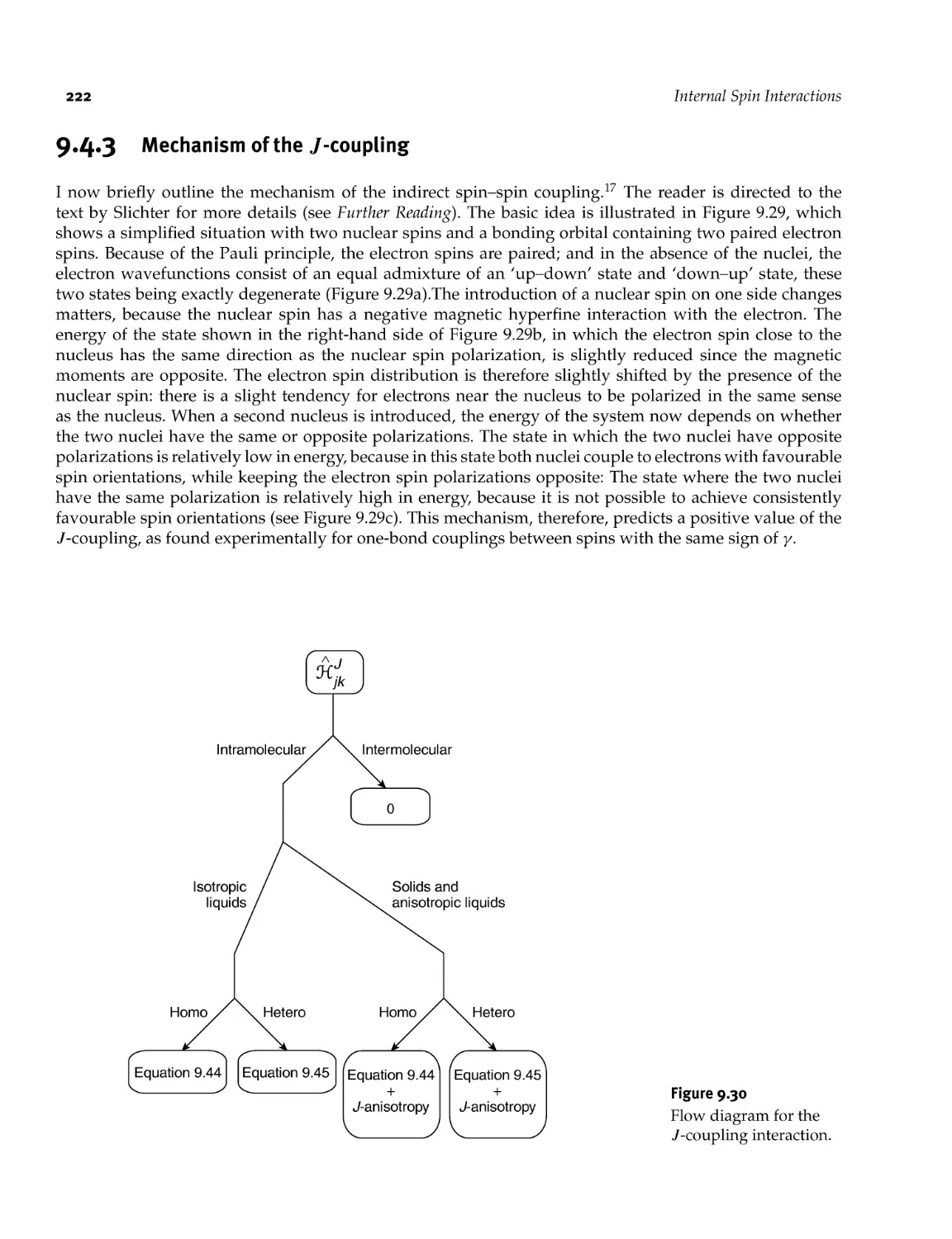
9.4.3 Mechanism of the /- coupling 222
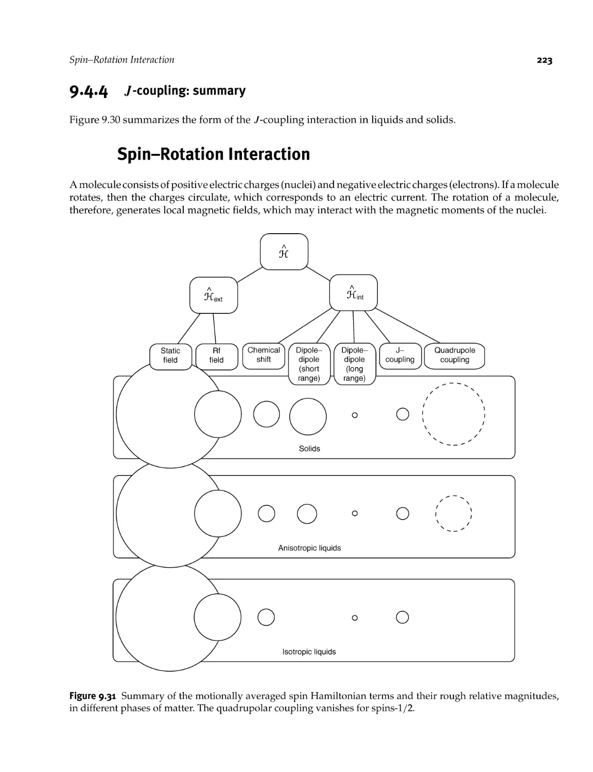
9.4.4 /- coupling: summary 223
9.5 Spin- Rotation Interaction 223
9.6 Summary of the Spin Hamiltonian Terms 224
Part 5 Uncoupled Spins 229
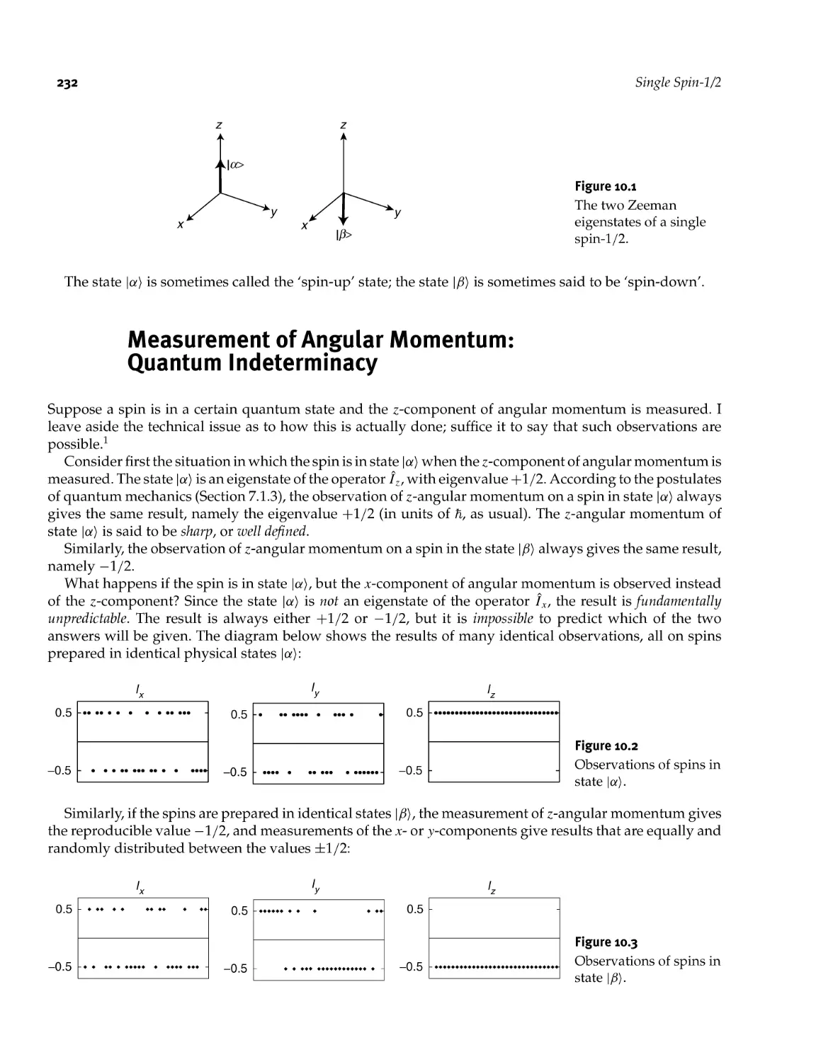
10 Single Spin- 1/2 231
10.1 Zeeman Eigenstates 231
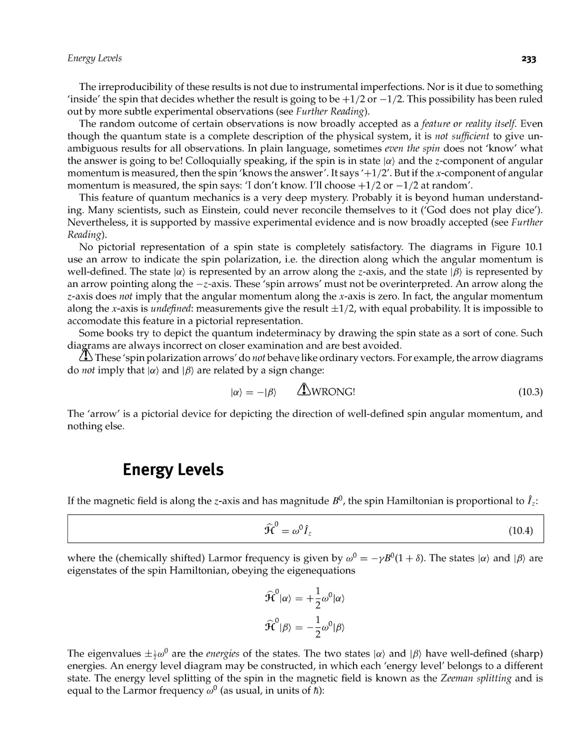
10.2 Measurement of Angular Momentum: Quantum Indeterminacy 232
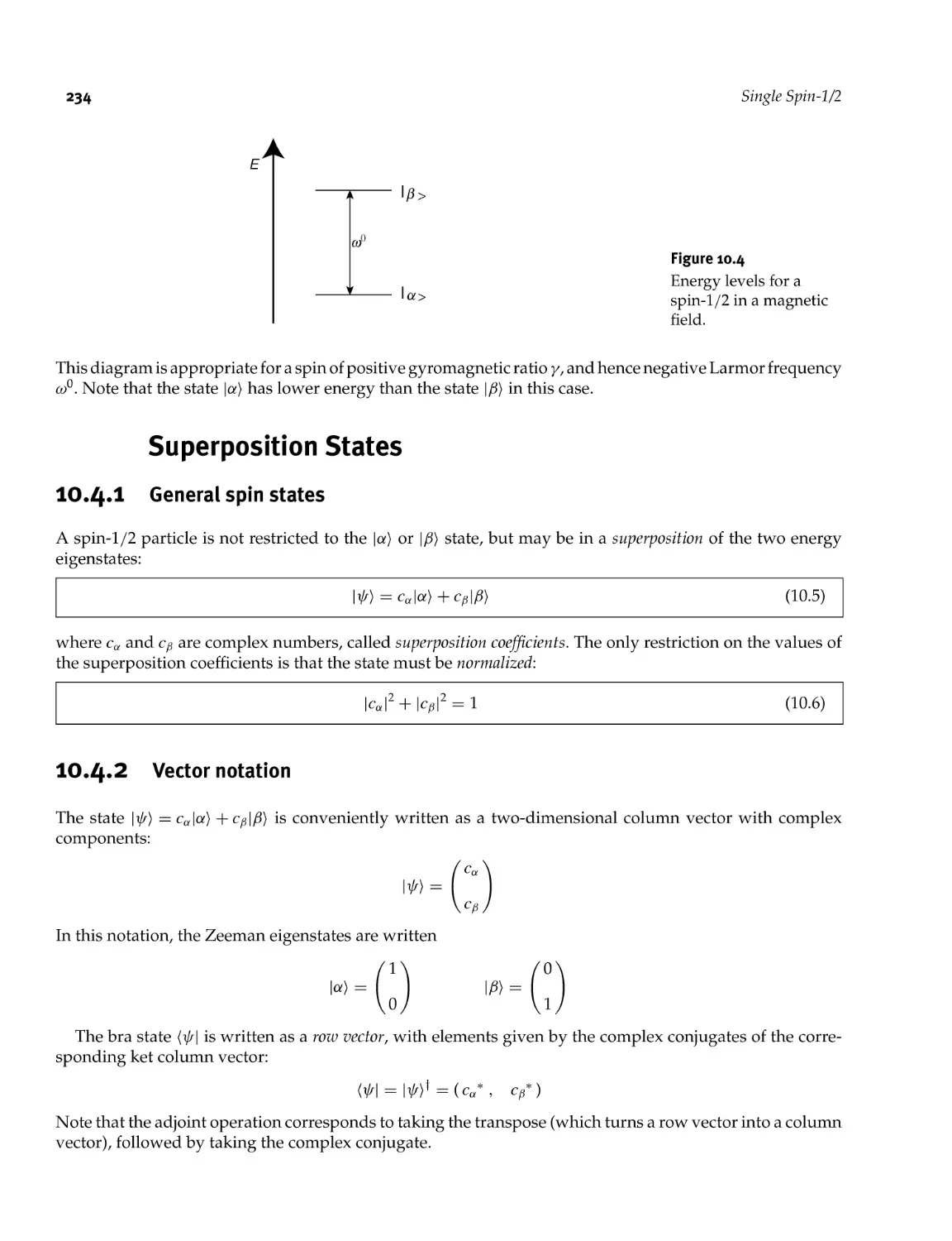
10.3 Energy Levels 233
10.4 Superposition States 234
10.4.1 General spin states 234
10.4.2 Vector notation 234
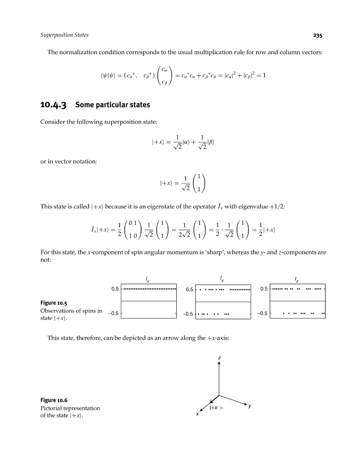
10.4.3 Some particular states 235
10.4.4 Phase factors 237
10.5 Spin Precession 238
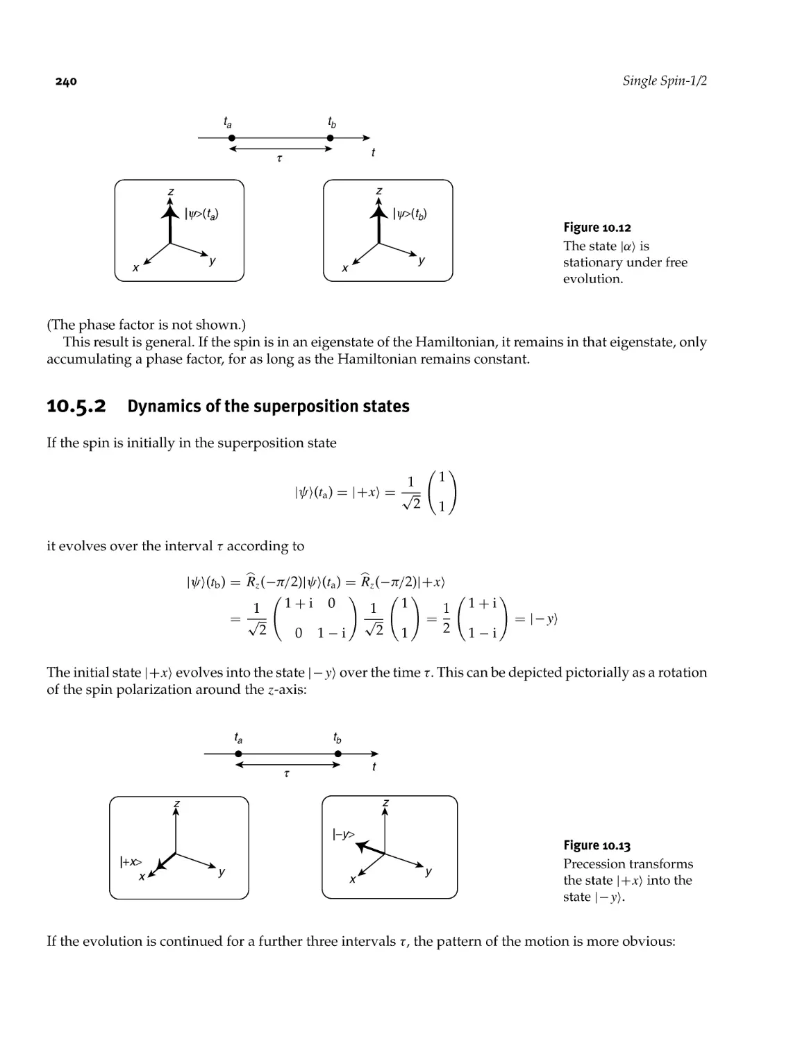
10.5.1 Dynamics of the eigenstates 239
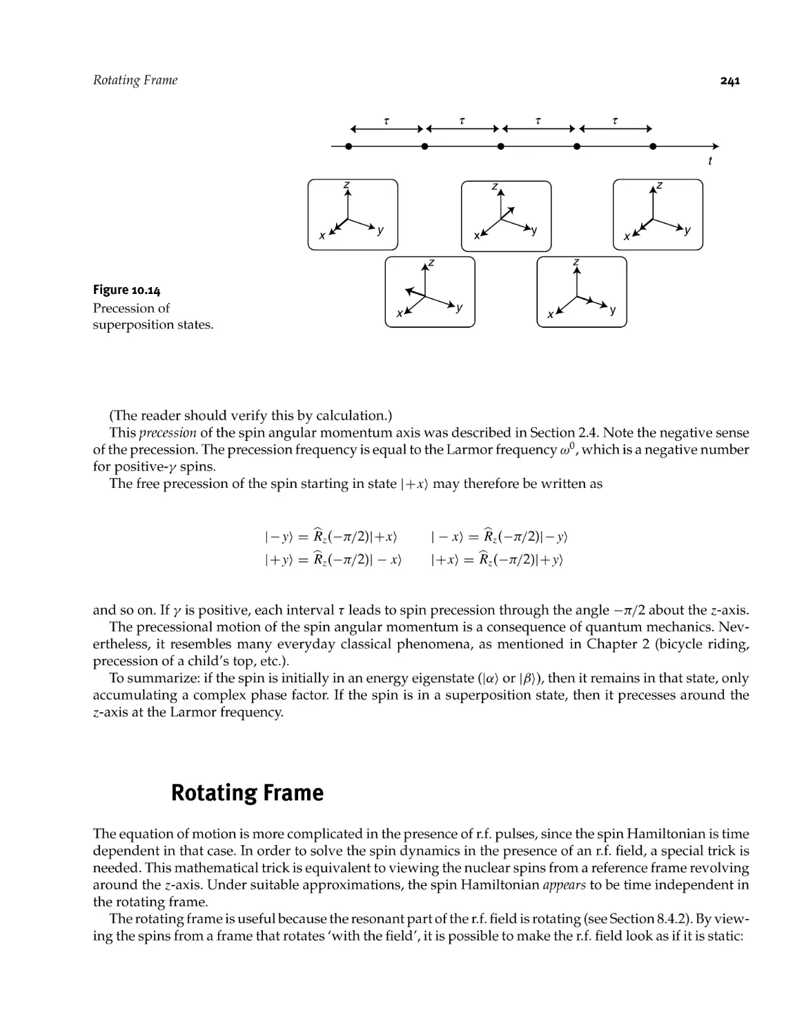
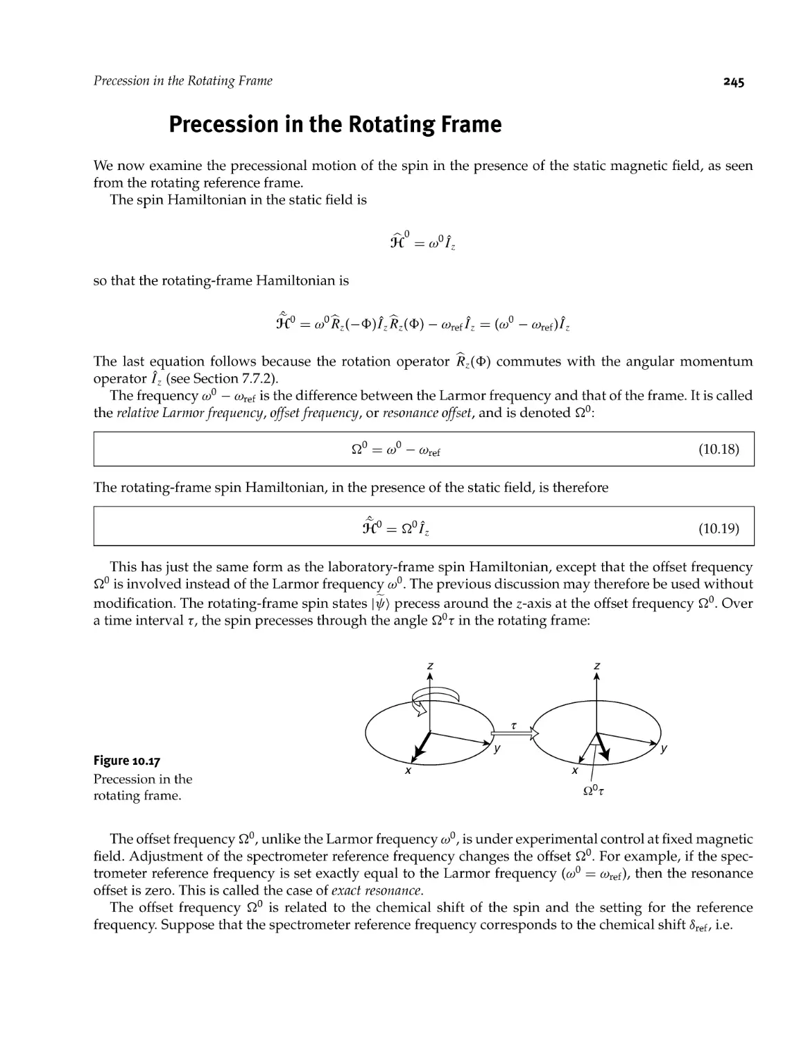
10.5.2 Dynamics of the superposition states 240
10.6 Rotating Frame 241
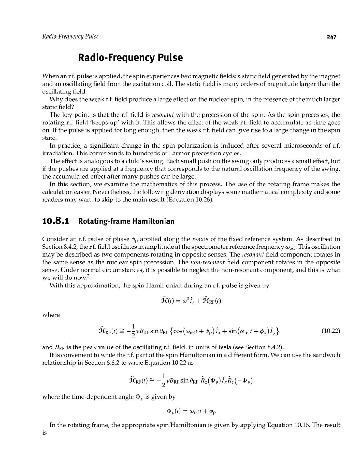
10.7 Precession in the Rotating Frame 245
10.8 Radio- frequency Pulse 247
10.8.1 Rotating- frame Hamiltonian 247
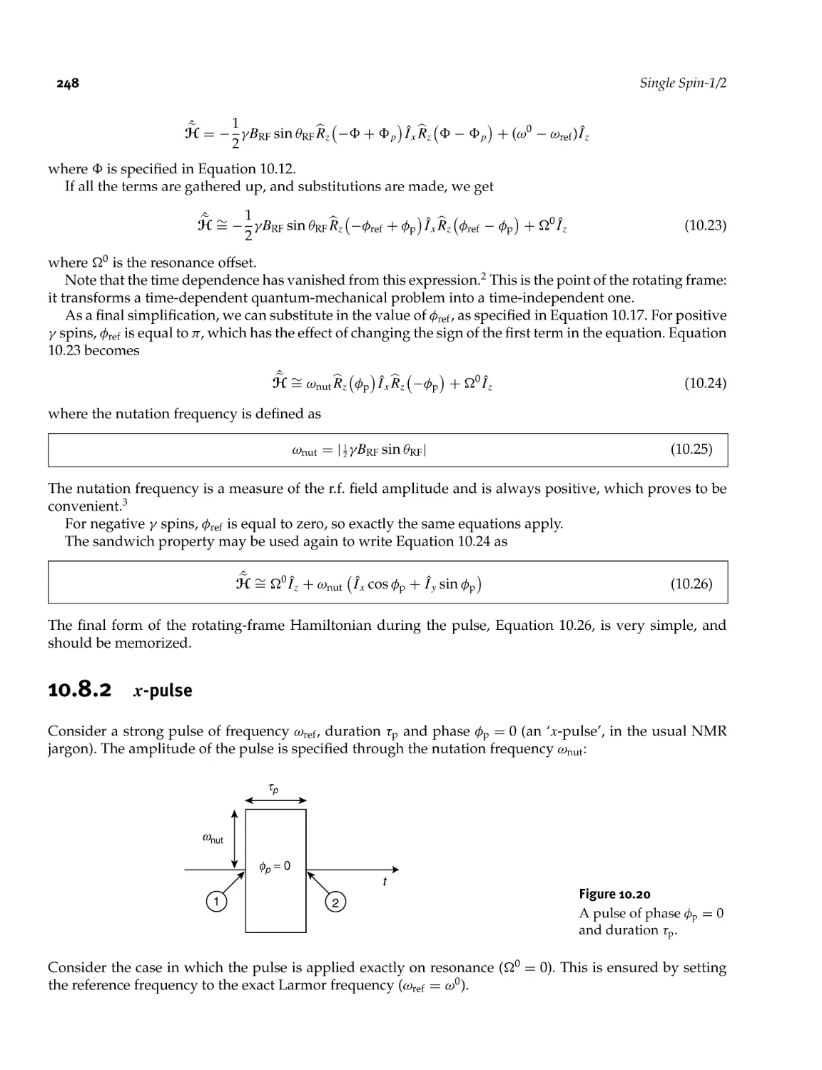
10.8.2 x- pulse 248
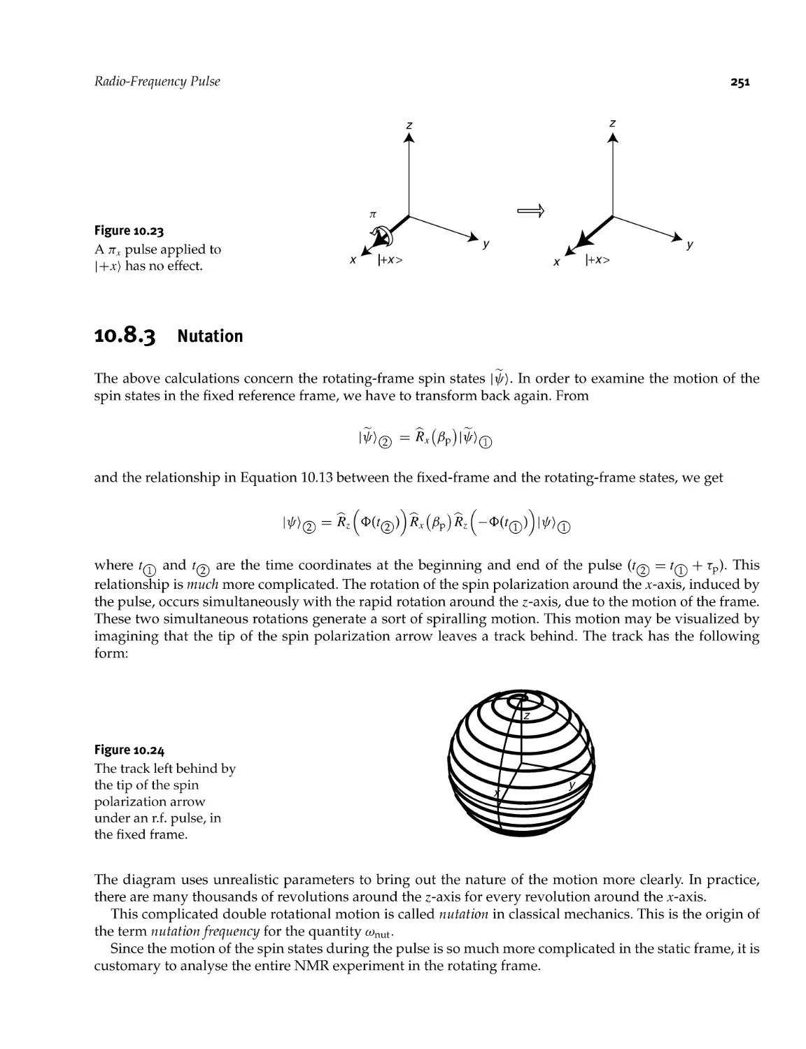
10.8.3 Nutation 251
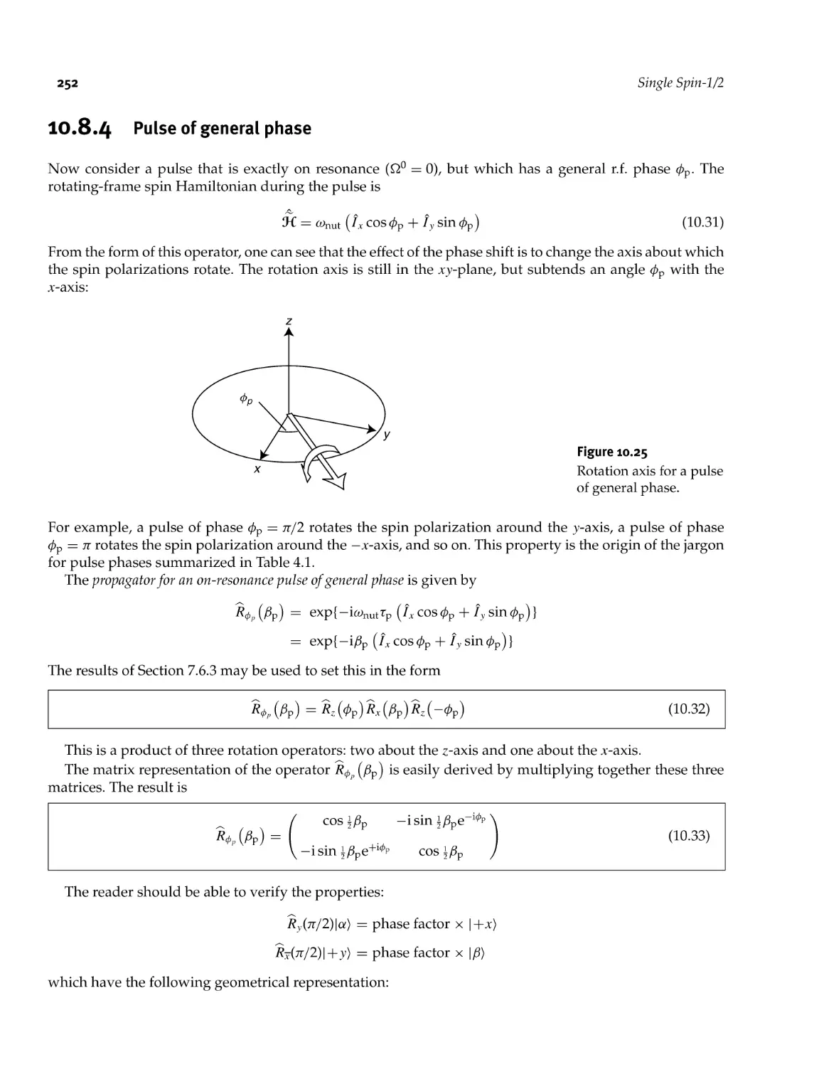
10.8.4 Pulse of general phase 252
10.8.5 Off- resonance effects 253
ii Ensemble of Spins- 1/2 259
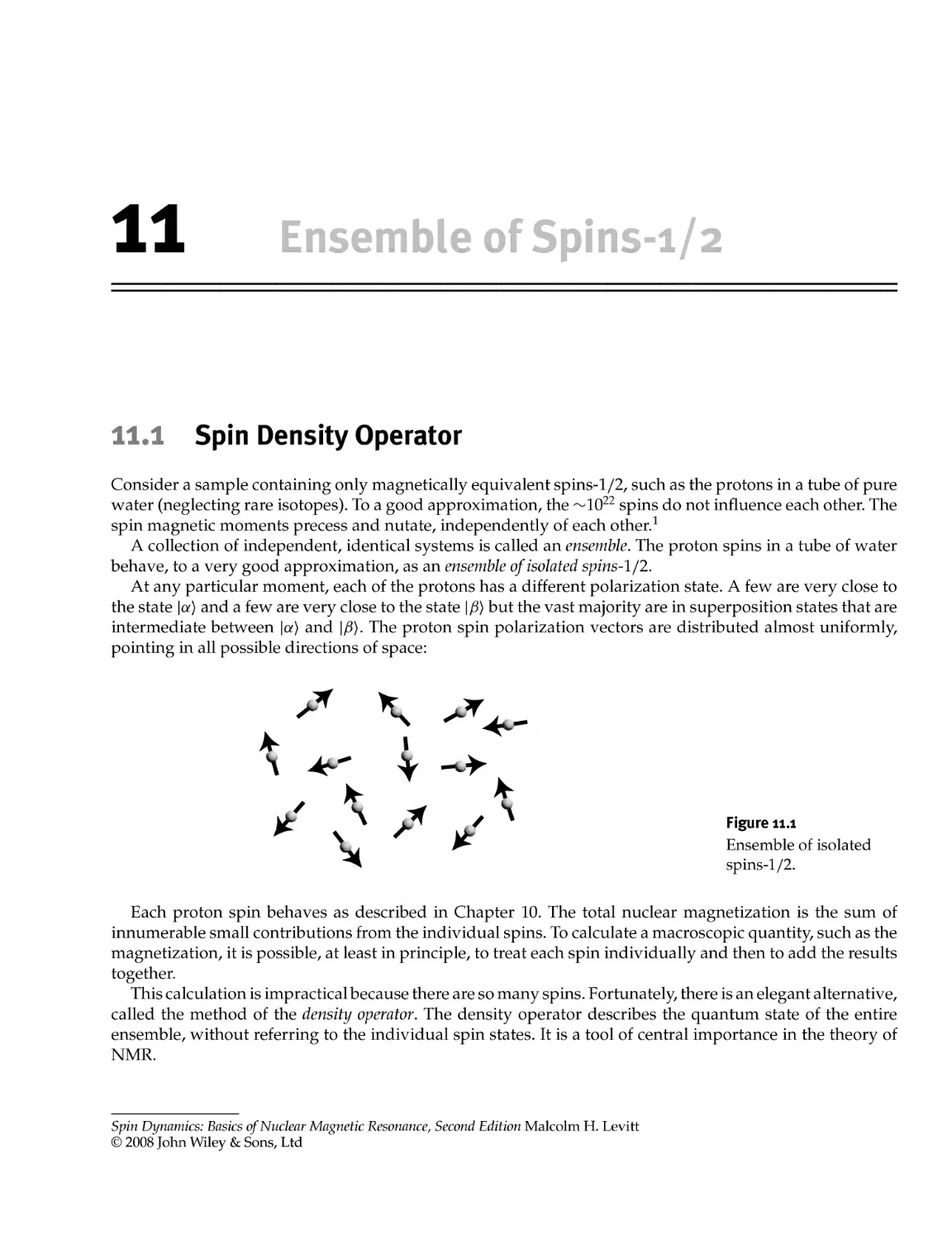
11.1 Spin Density Operator 259
11.2 Populations and Coherences 261
11.2.1 Density matrix 261
11.2.2 Box notation 261
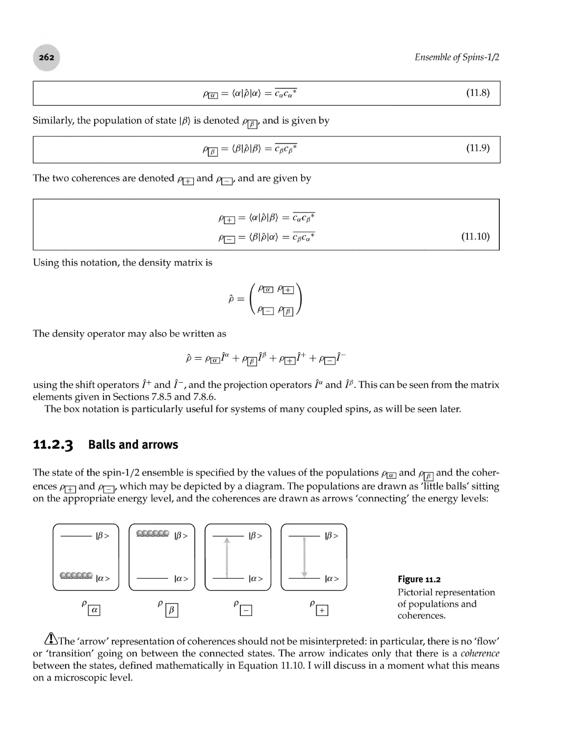
11.2.3 Balls and arrows 262
11.2.4 Orders of coherence 263
11.2.5 Relationships between populations and coherences 263
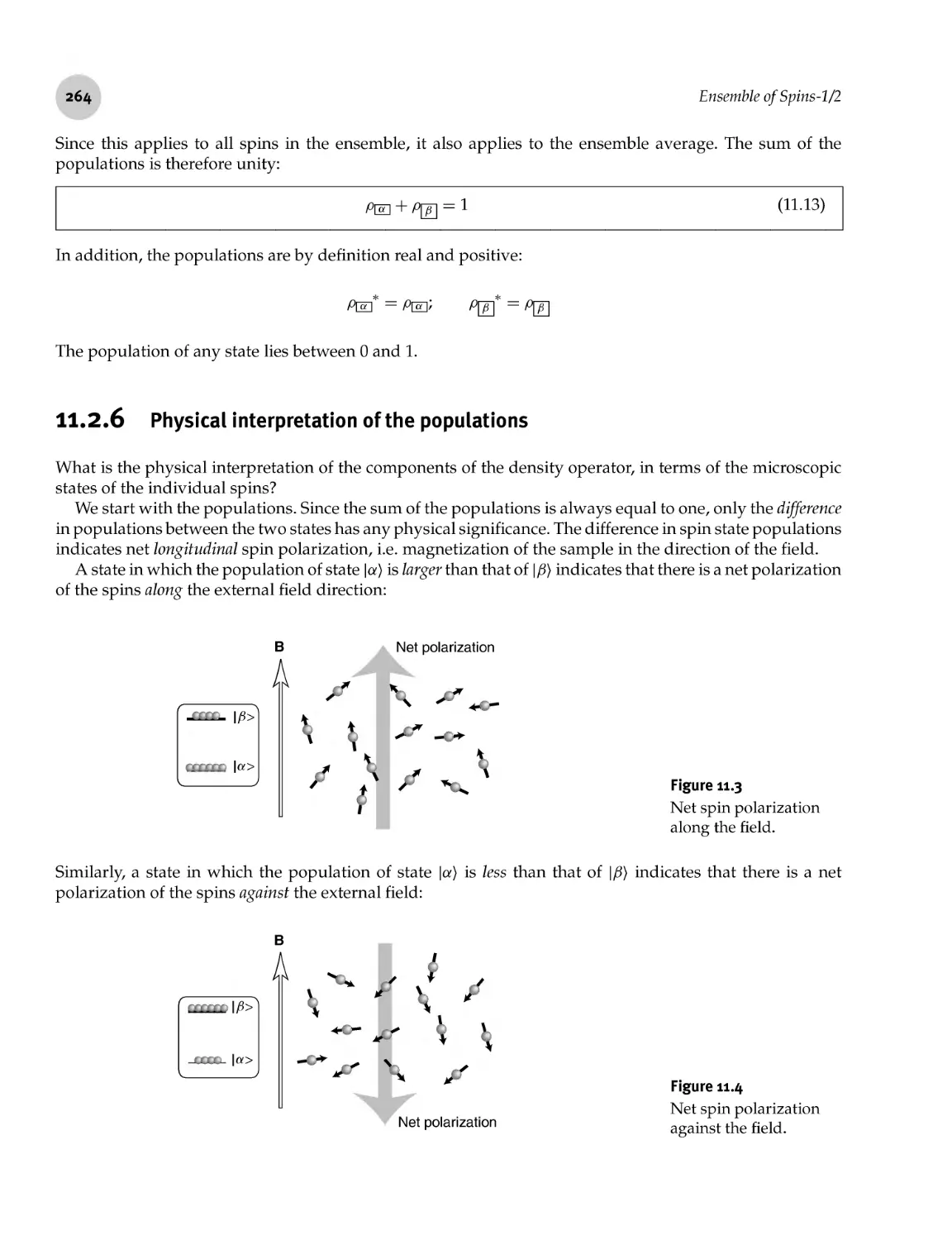
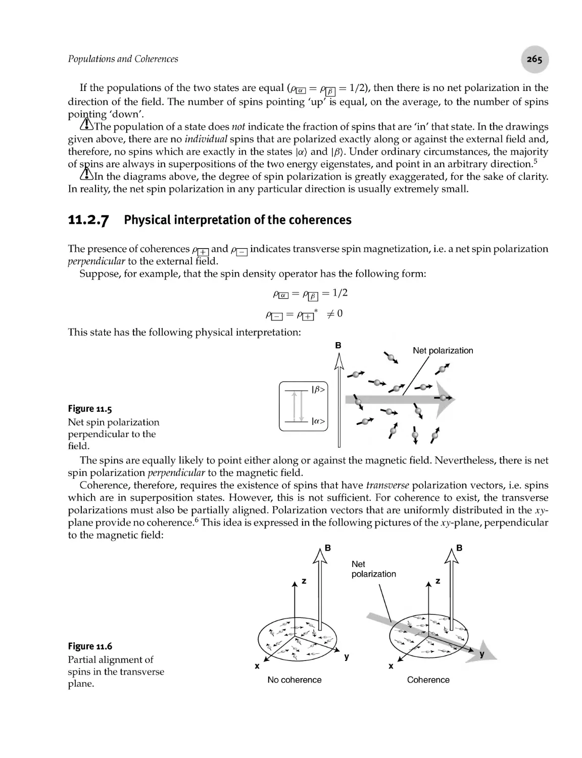
11.2.6 Physical interpretation of the populations 264
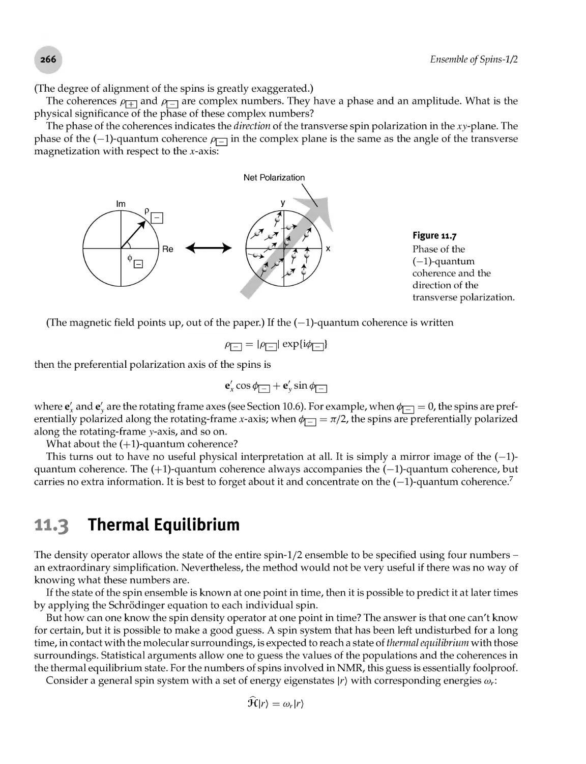
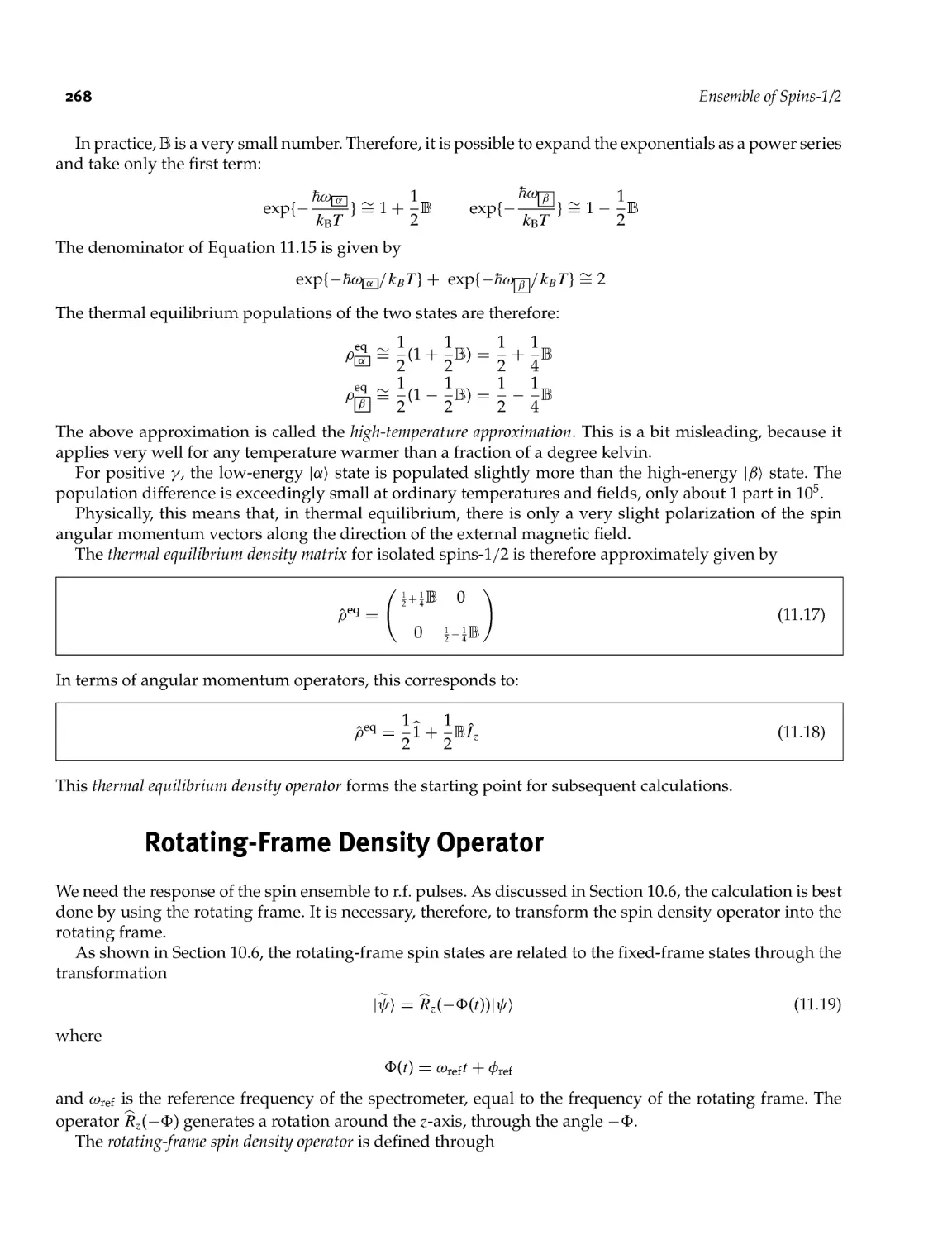
11.2.7 Physical interpretation of the coherences 265
11.3 Thermal Equilibrium 266
11.4 Rotating- Frame Density Operator 268

XIII
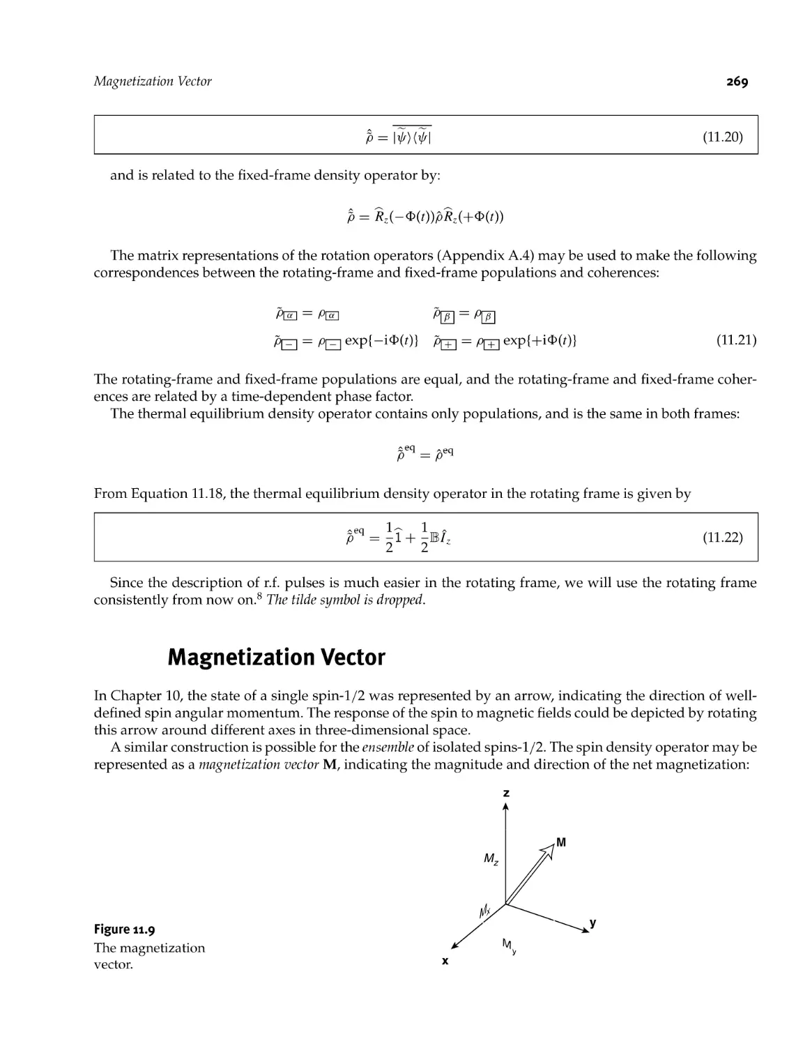
11.5 Magnetization Vector 269
11.6 Strong Radio- Frequency Pulse 270
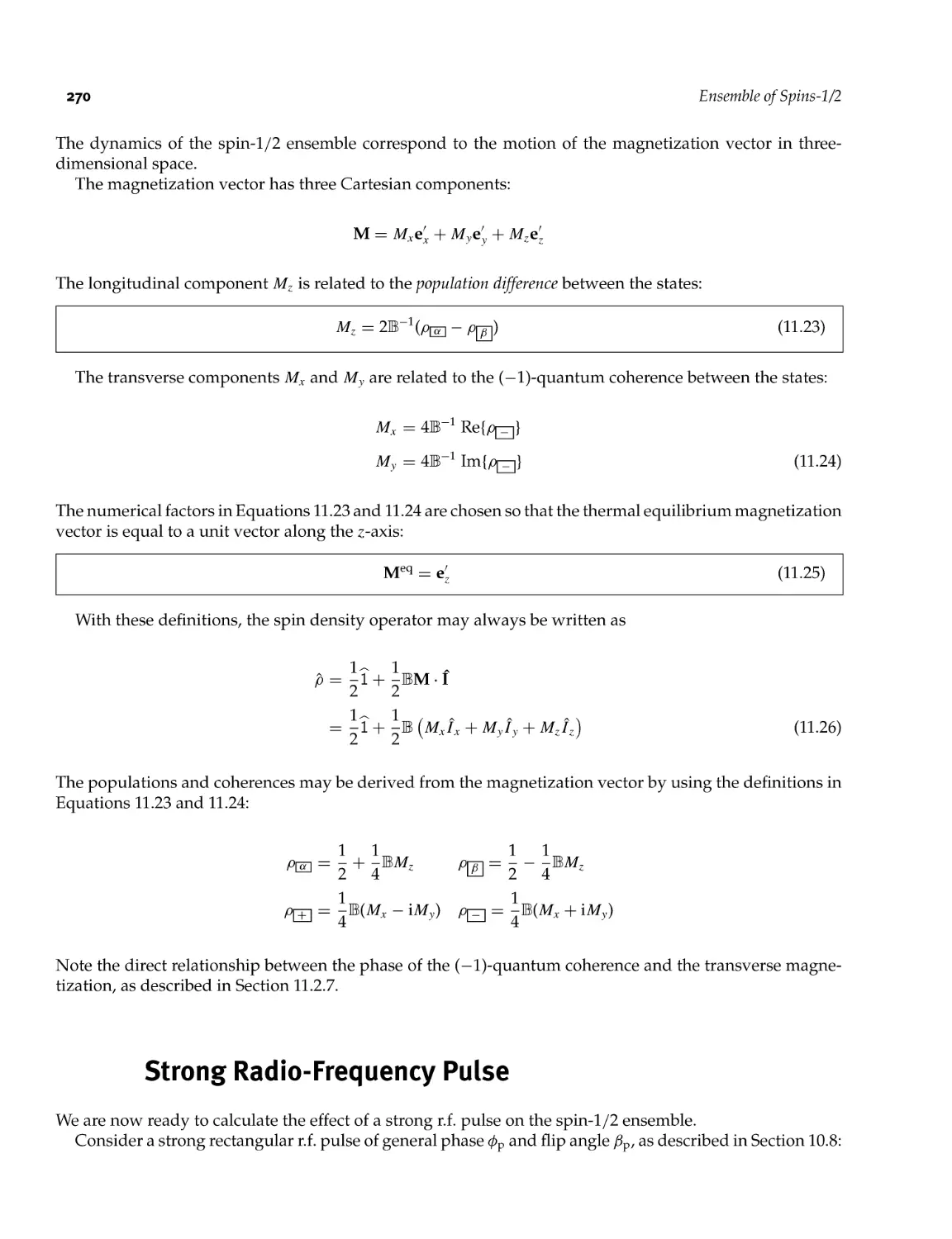
11.6.1 Excitation of coherence 271
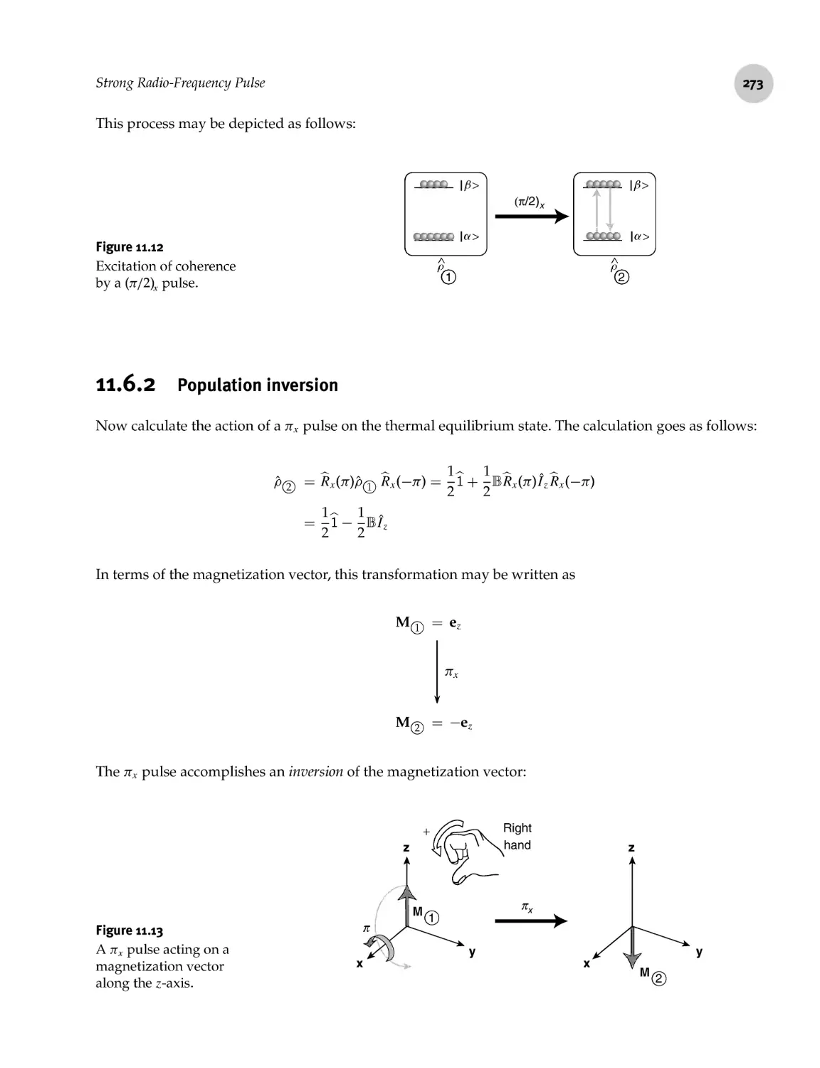
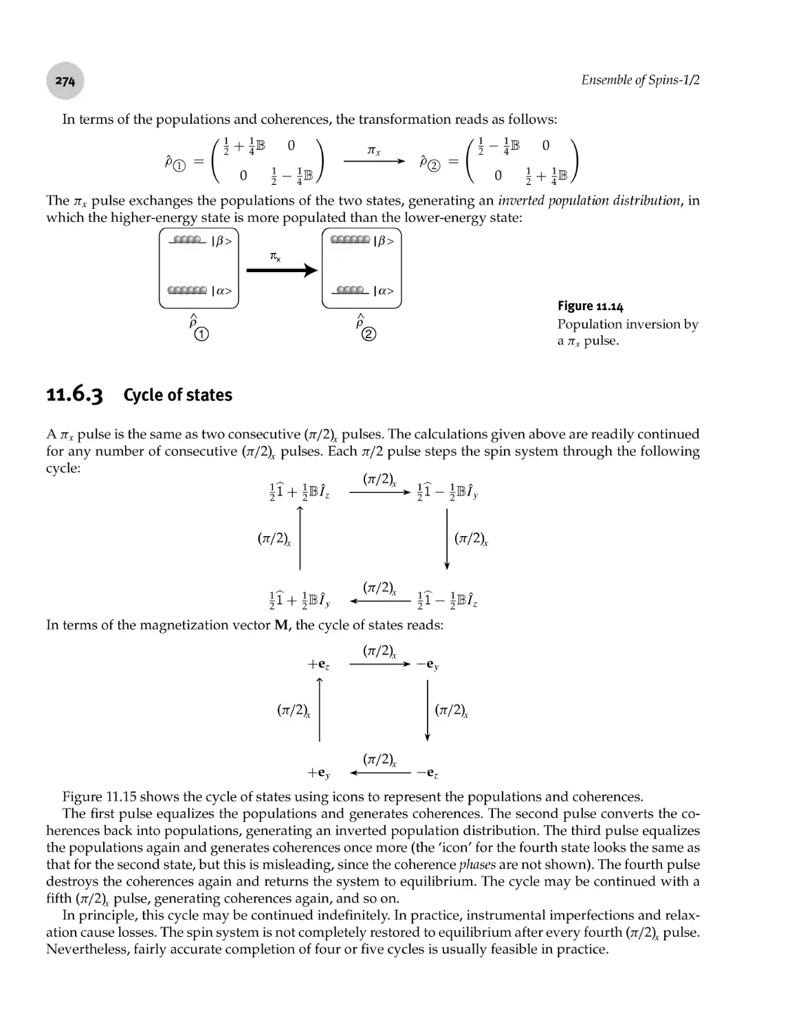
11.6.2 Population inversion 273
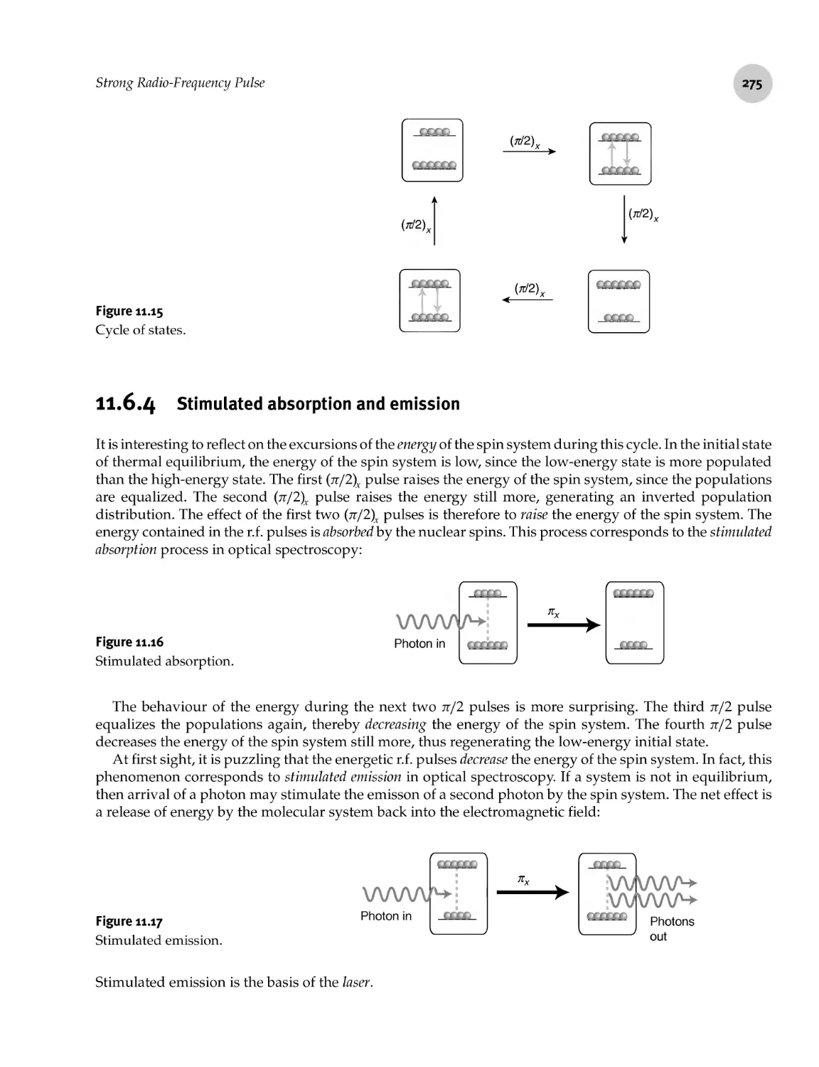
11.6.3 Cycle of states 274
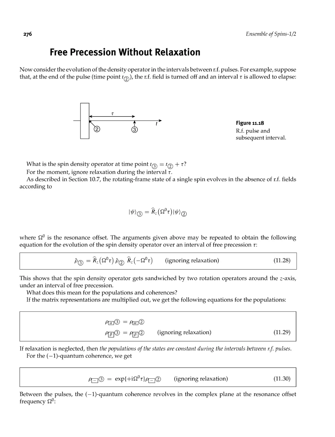
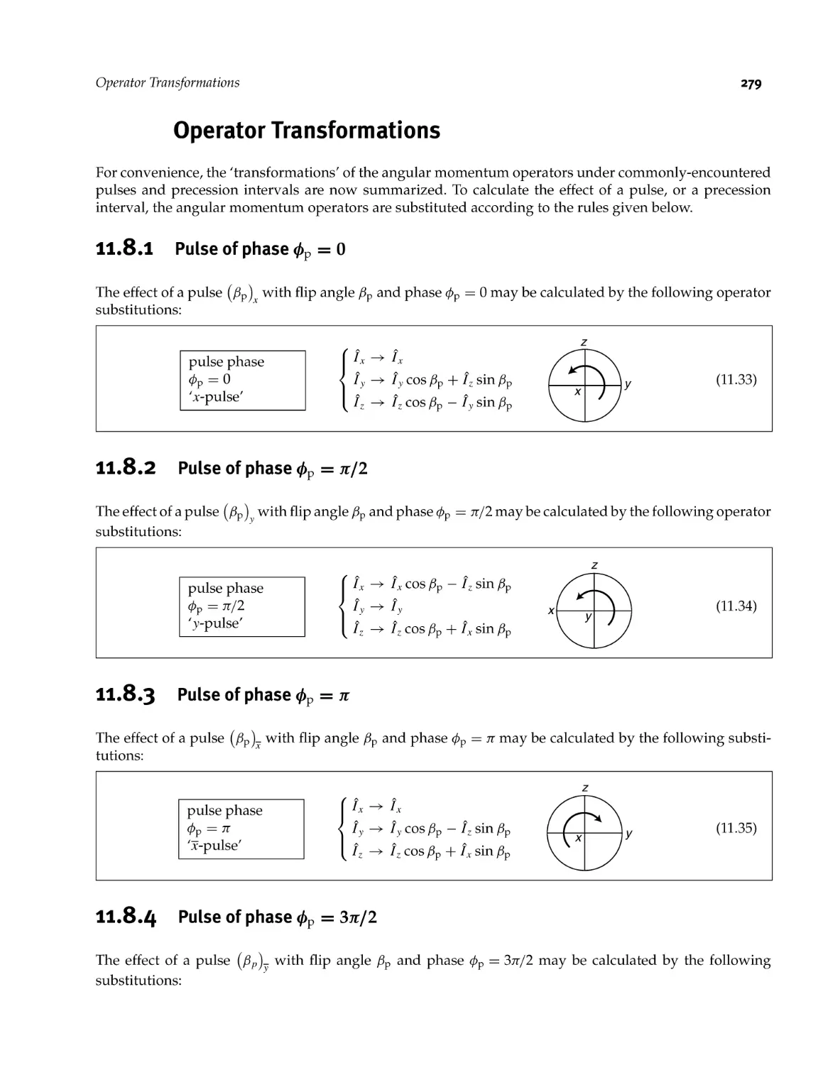
11.6.4 Stimulated absorption and emission 275
11.7 Free Precession Without Relaxation 276
11.8 Operator Transformations 279
11.8.1 Pulse of phase 0p = 0 279
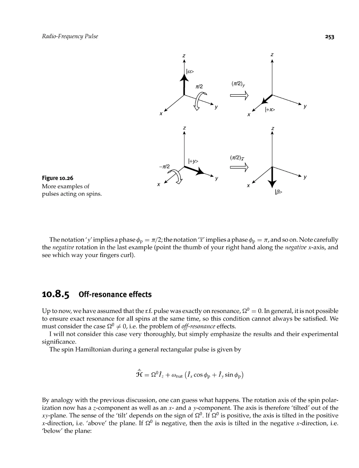
11.8.2 Pulse of phase 0p = tt/2 279
11.8.3 Pulse of phase 0p = tt 279
11.8.4 Pulse of phase 0p = 3tt/2 279
11.8.5 Pulse of general phase 0p 280
11.8.6 Free precession for an interval r 280
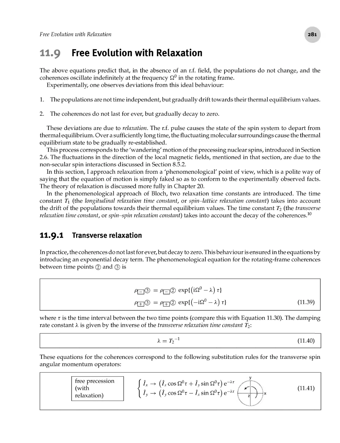
11.9 Free Evolution with Relaxation 281
11.9.1 Transverse relaxation 281
11.9.2 Longitudinal relaxation 283
11.10 Magnetization Vector Trajectories 285
11.11 NMR Signal and NMR Spectrum 287
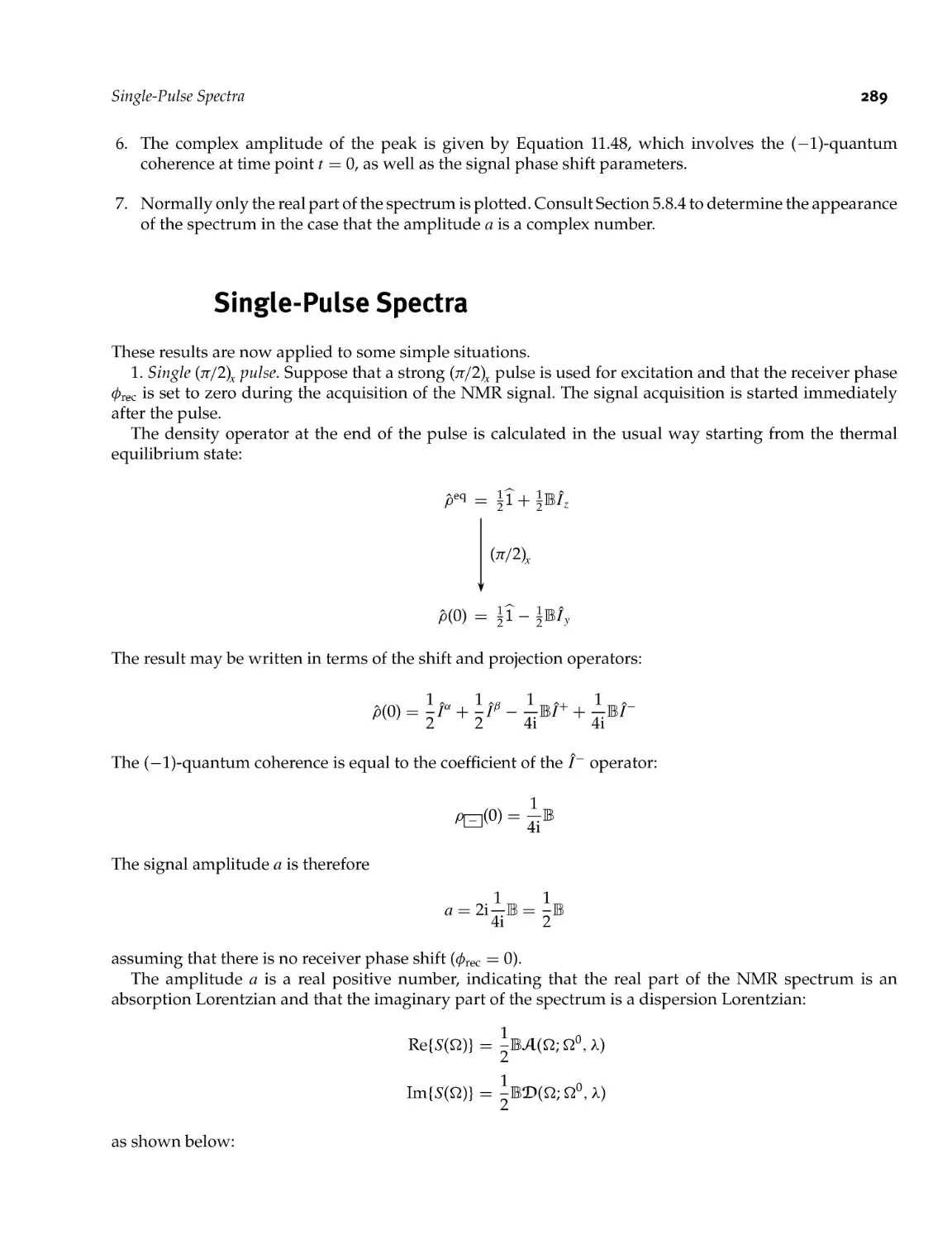
11.12 Single- Pulse Spectra 289
Experiments on Non- Interacting Spins- 1/2 295
12.1 Inversion Recovery: Measurement of T\ 295
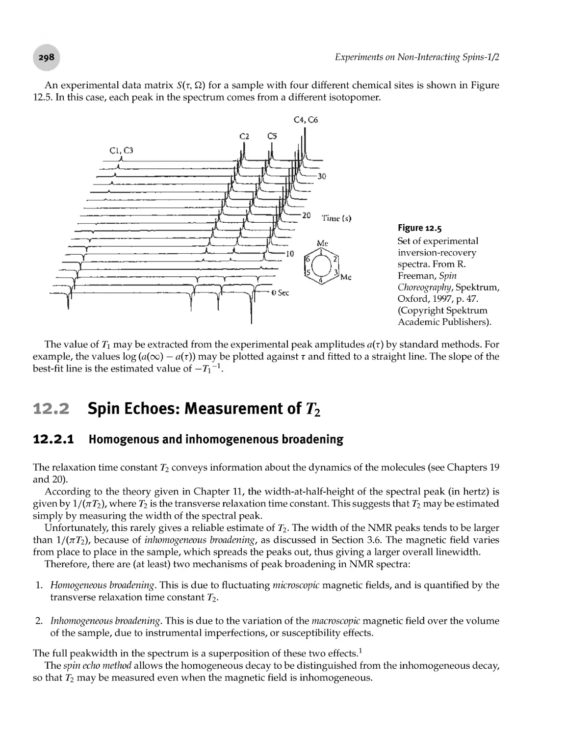
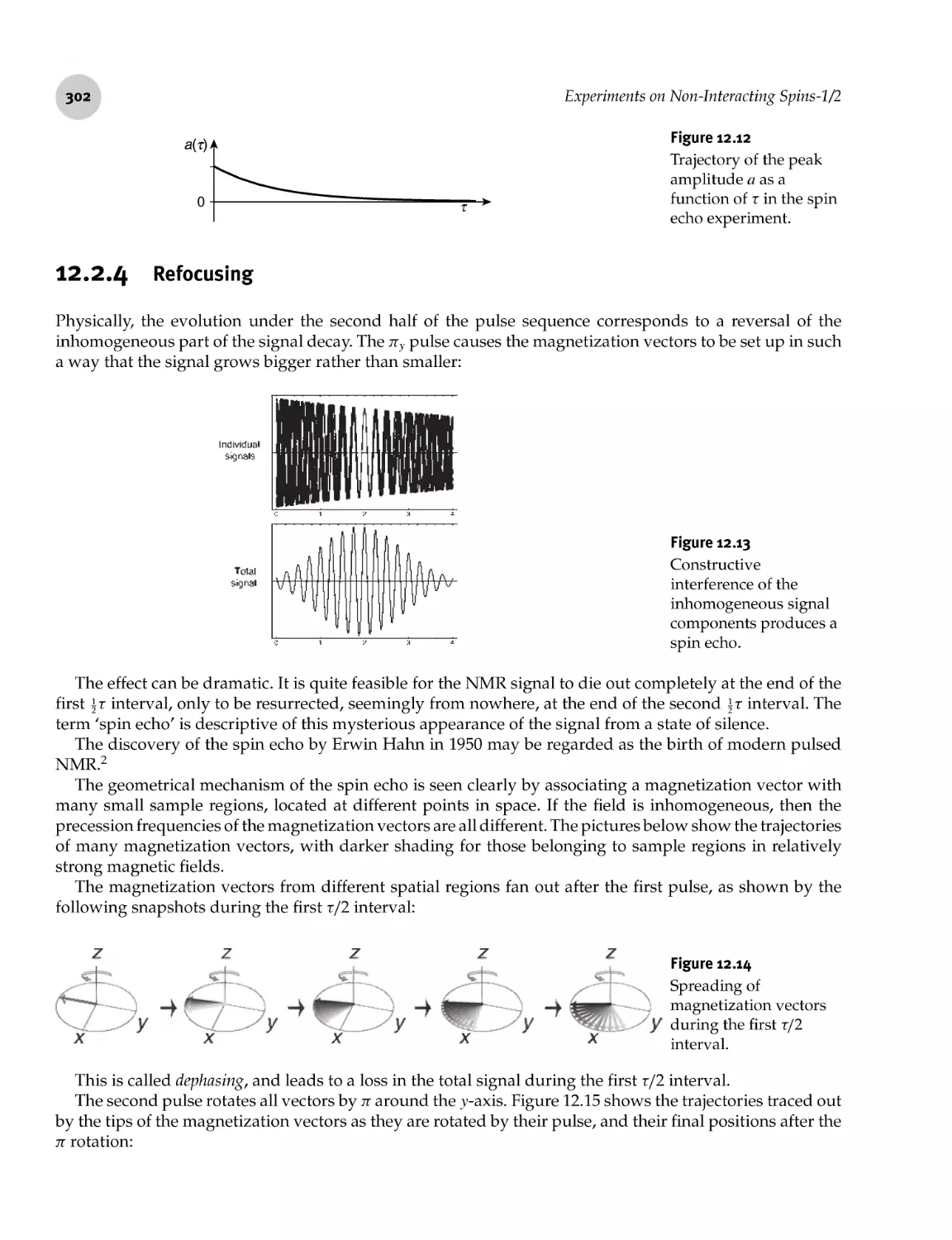
12.2 Spin Echoes: Measurement of T2 298
12.2.1 Homogenous and inhomogenenous broadening 298
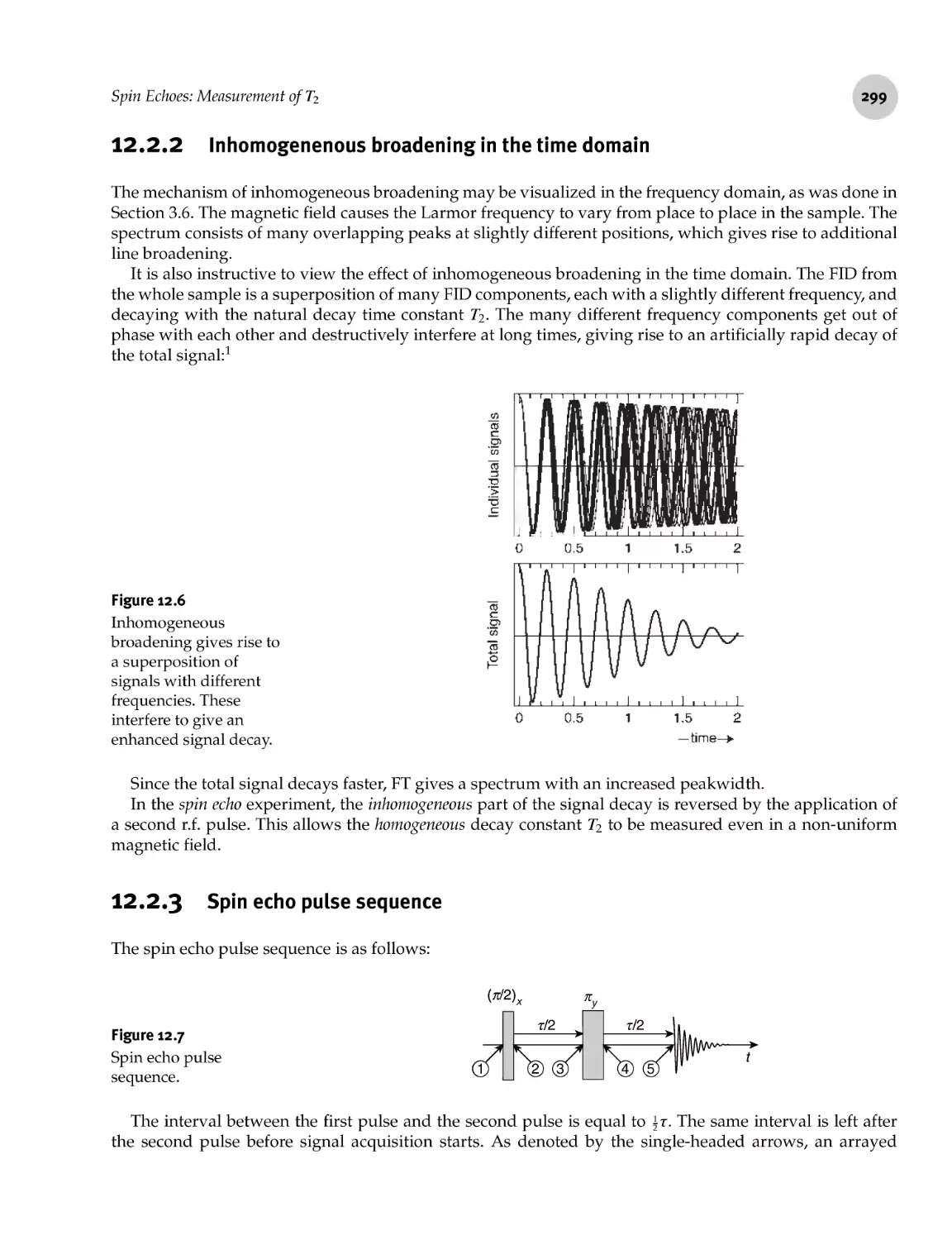
12.2.2 Inhomogenenous broadening in the time domain 299
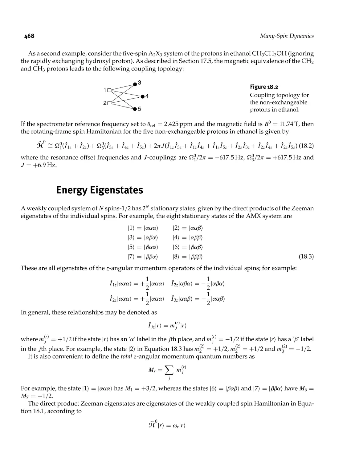
12.2.3 Spin echo pulse sequence 299
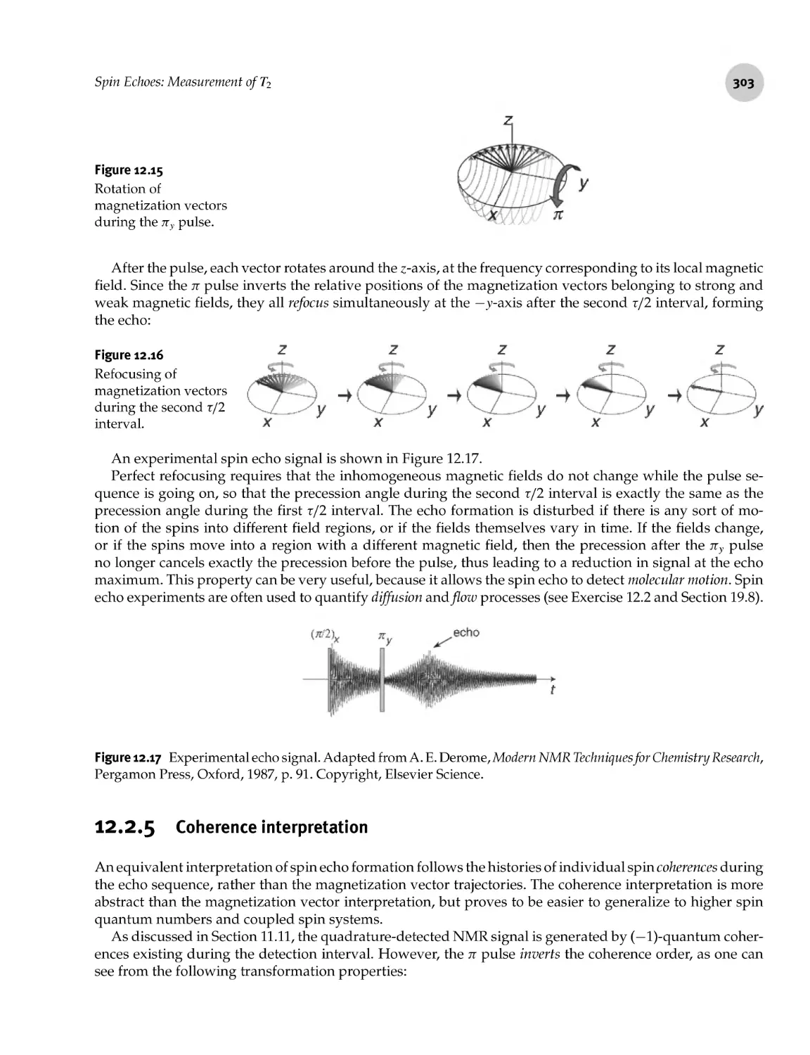
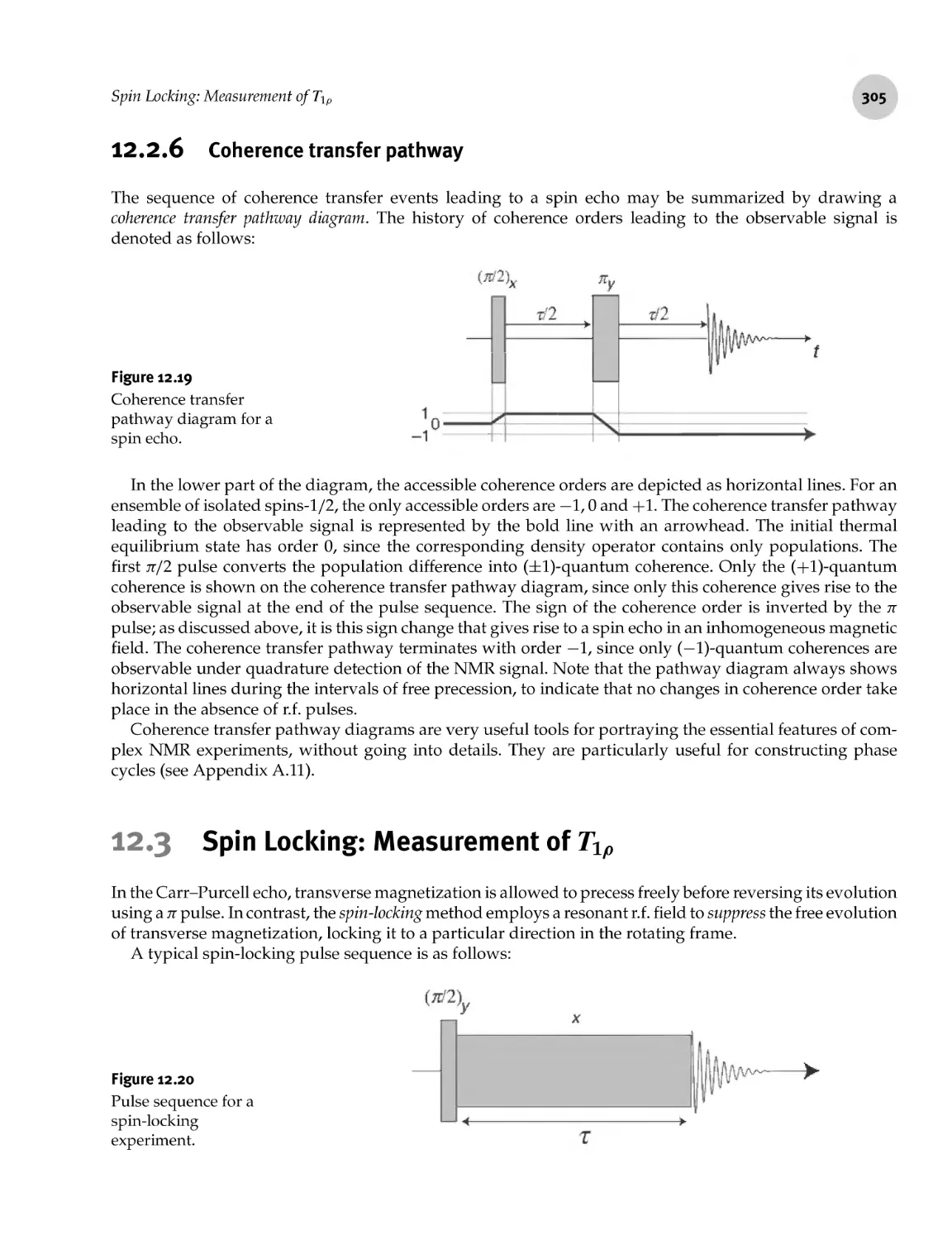
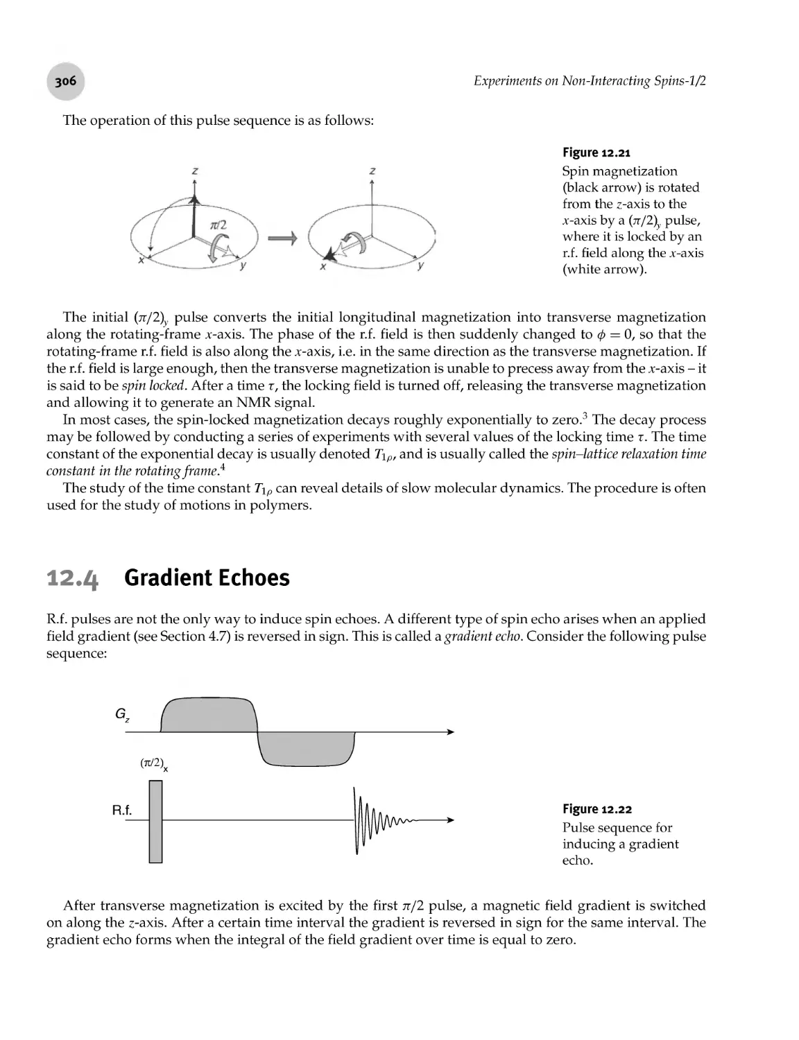
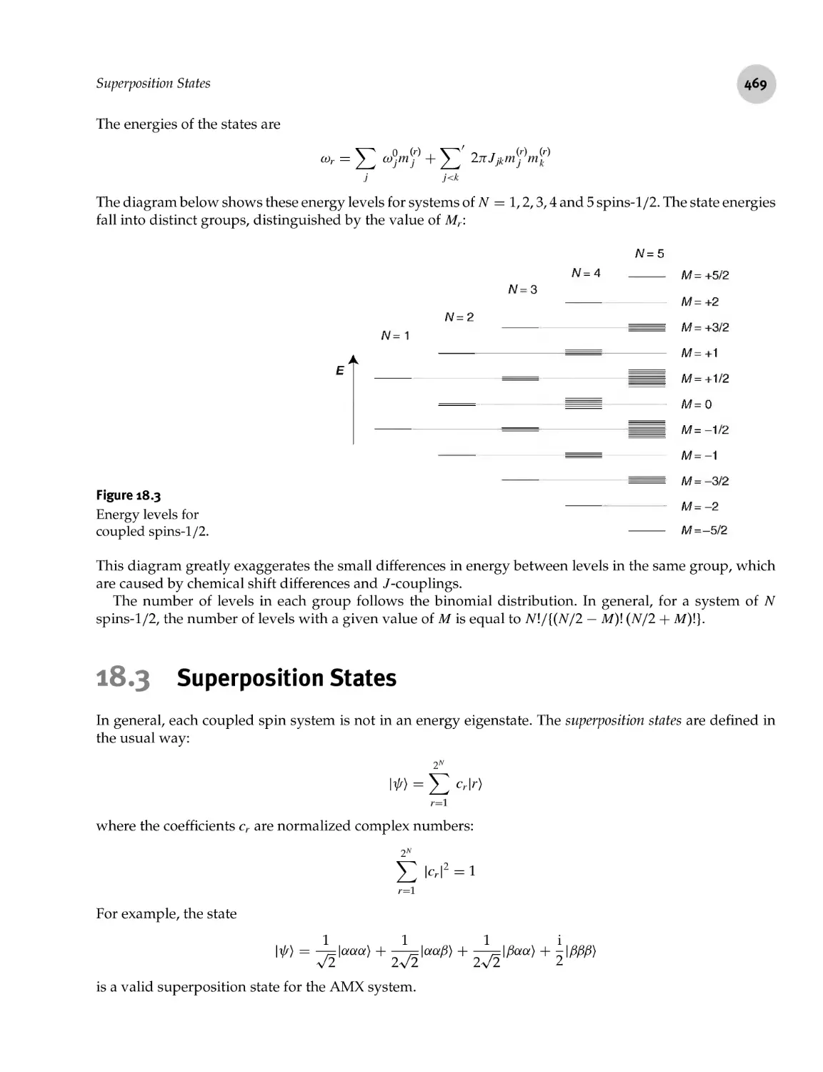
12.2.4 Refocusing 302
12.2.5 Coherence interpretation 303
12.2.6 Coherence transfer pathway 305
12.3 Spin Locking: Measurement of T\p 305
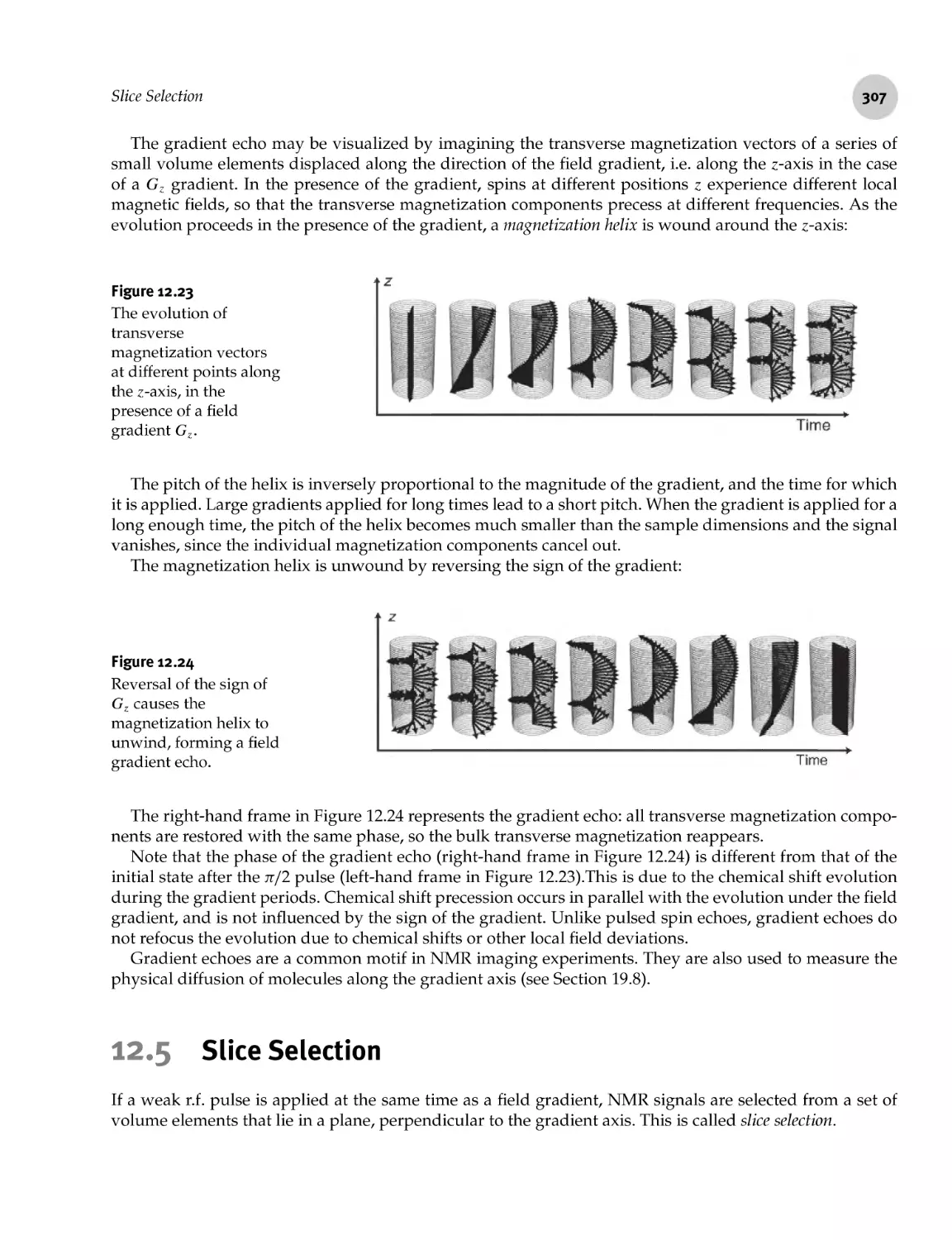
12.4 Gradient Echoes 306
12.5 Slice Selection 307
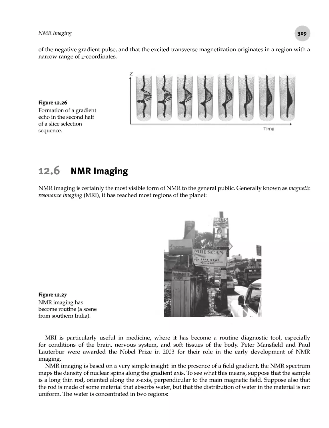
12.6 NMR Imaging 309
Quadrupolar Nuclei 319
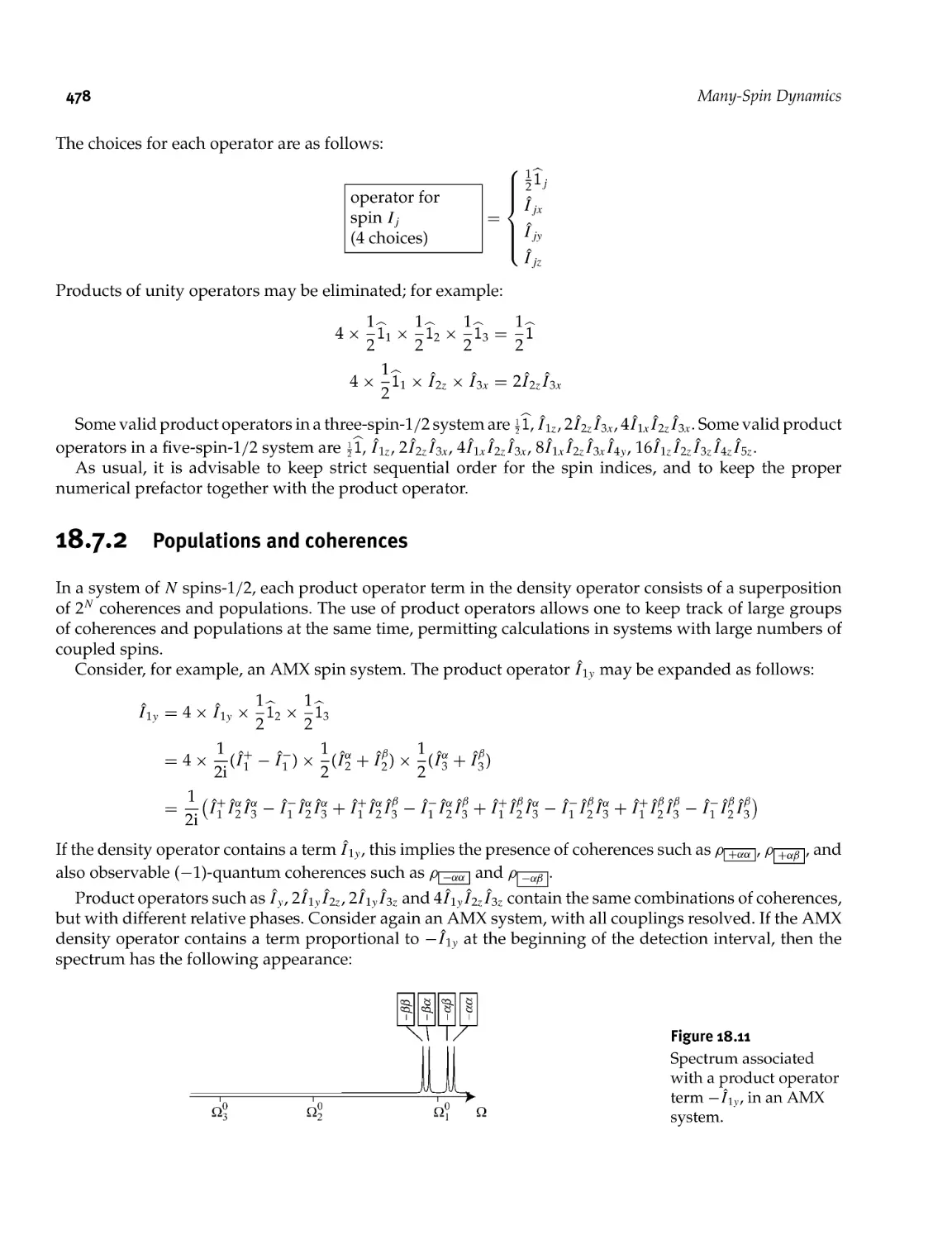
319
319
320
321
323
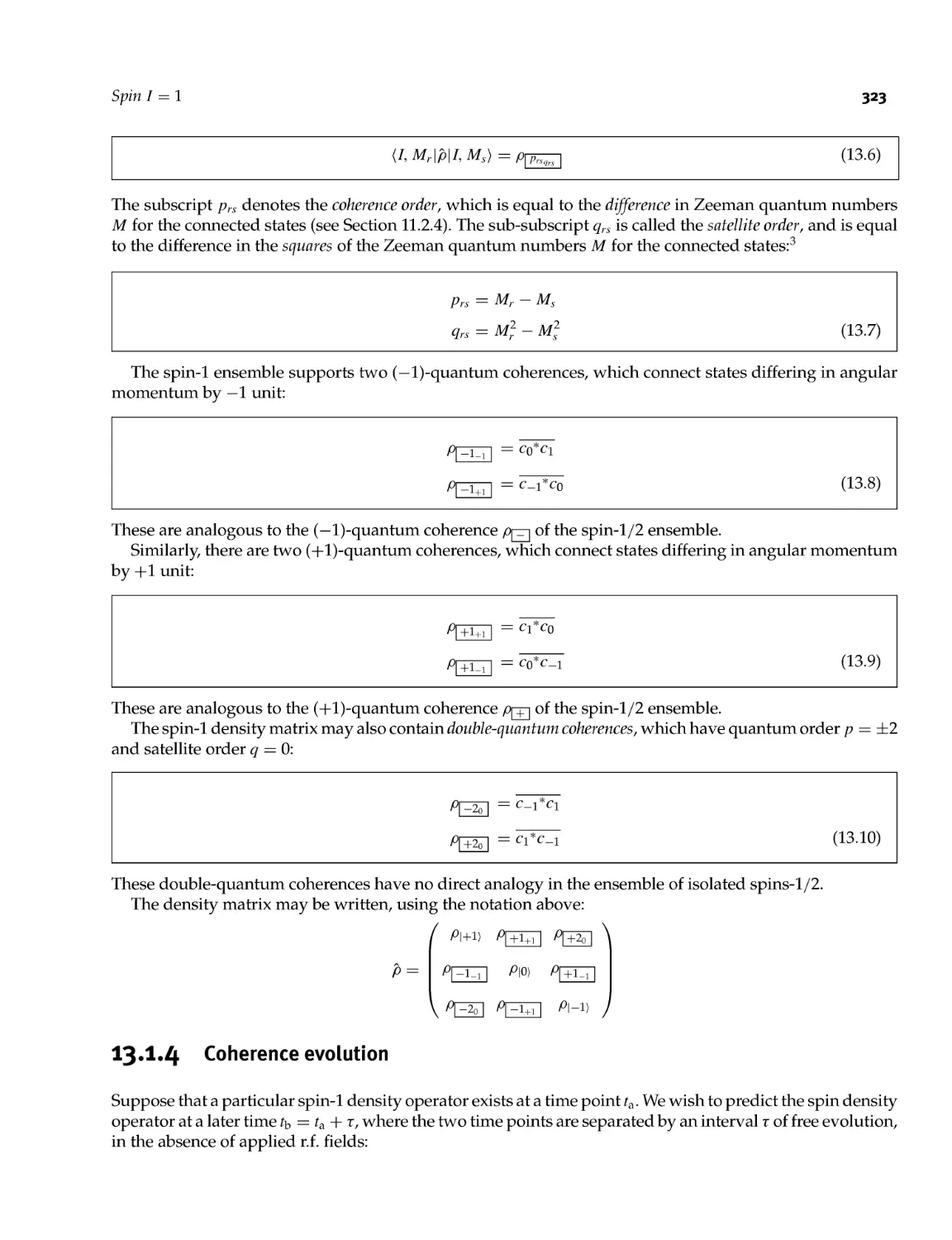
325
326
326
328
328
331
13.1 Spin/
13.1.1
13.1.2
13.1.3
13.1.4
13.1.5
13.1.6
13.1.7
13.1.8
13.1.9
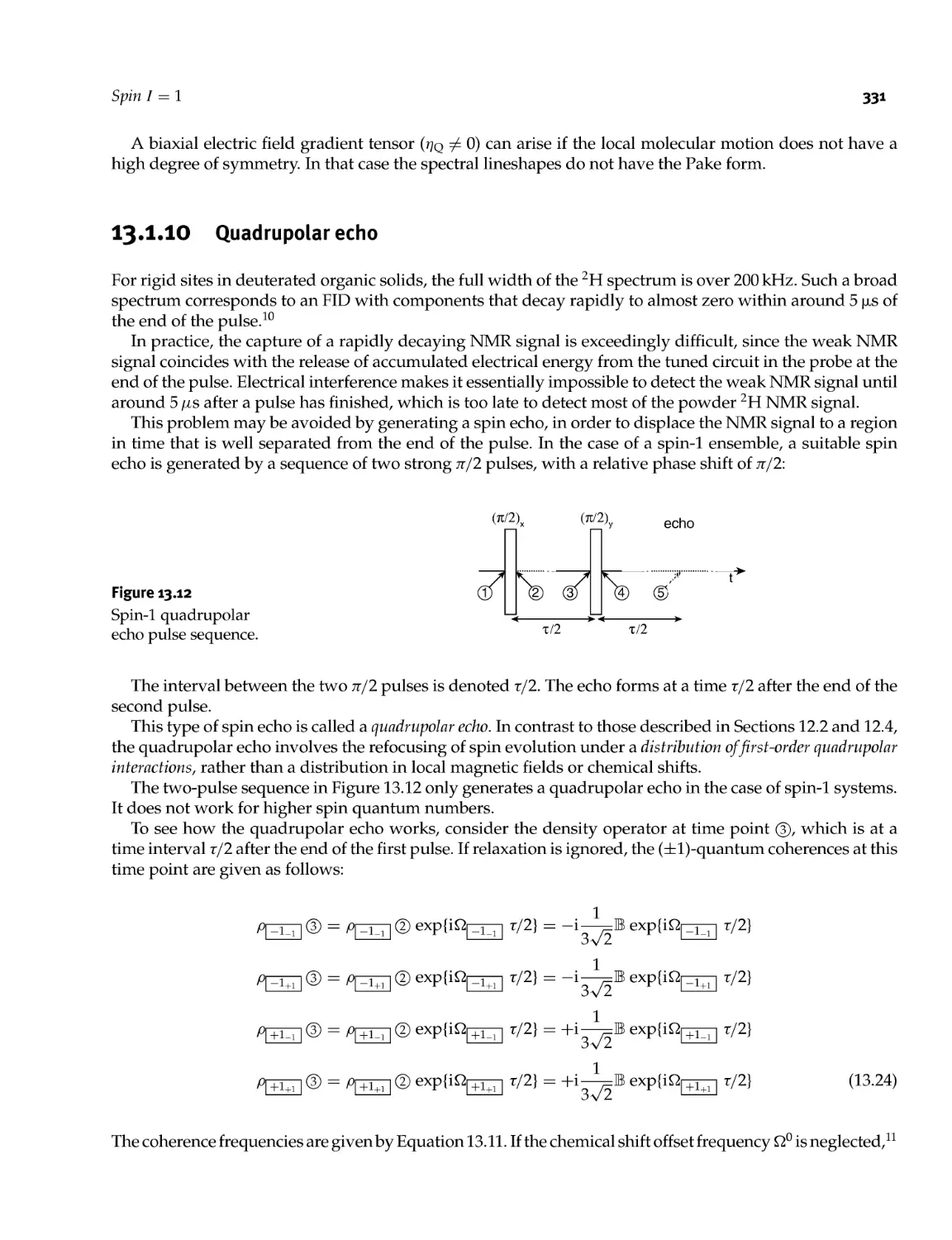
13.1.10
= 1
Spin- 1 states
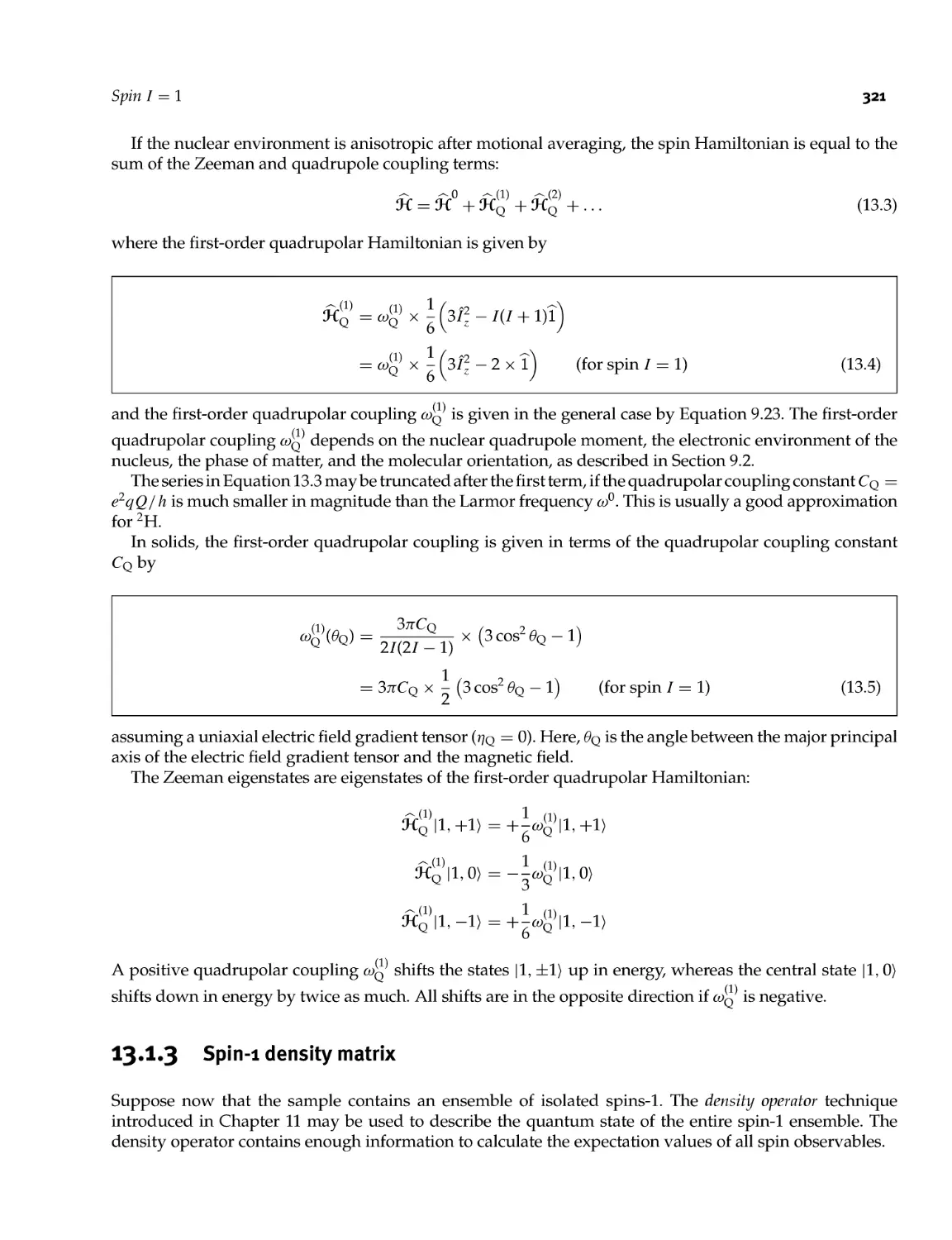
Spin- 1 energy levels
Spin- 1 density matrix
Coherence evolution
Observable coherences and NMR spectrum
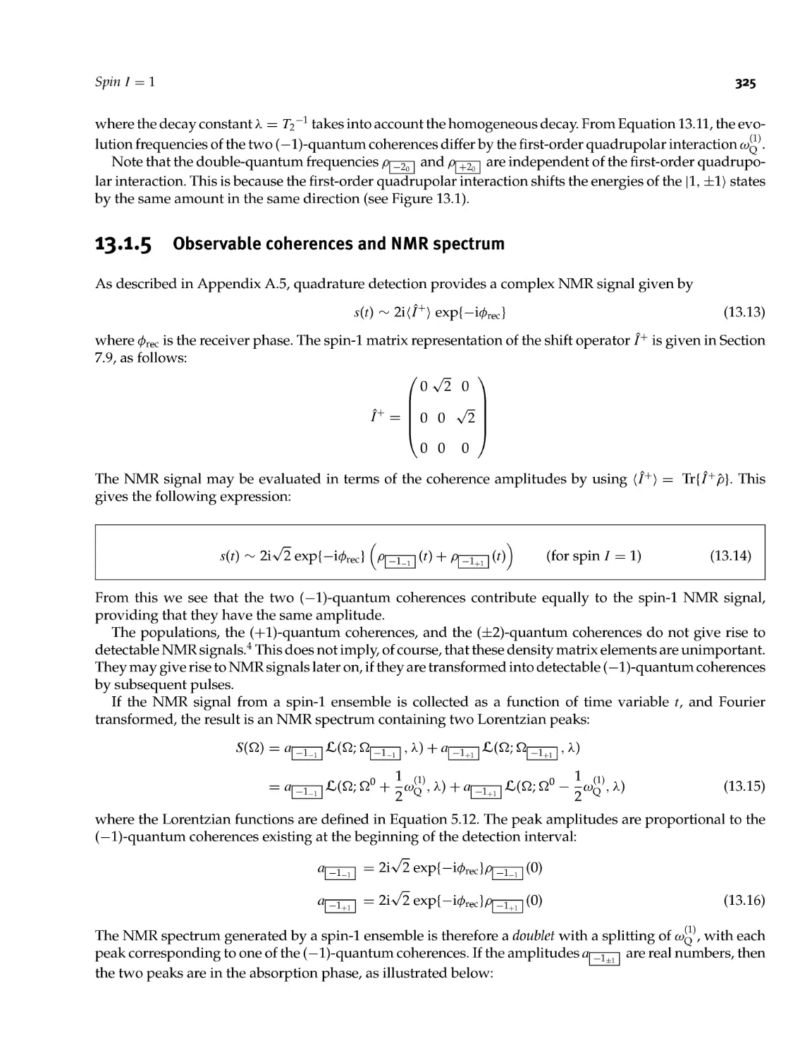
Thermal equilibrium
Strong radio- frequency pulse
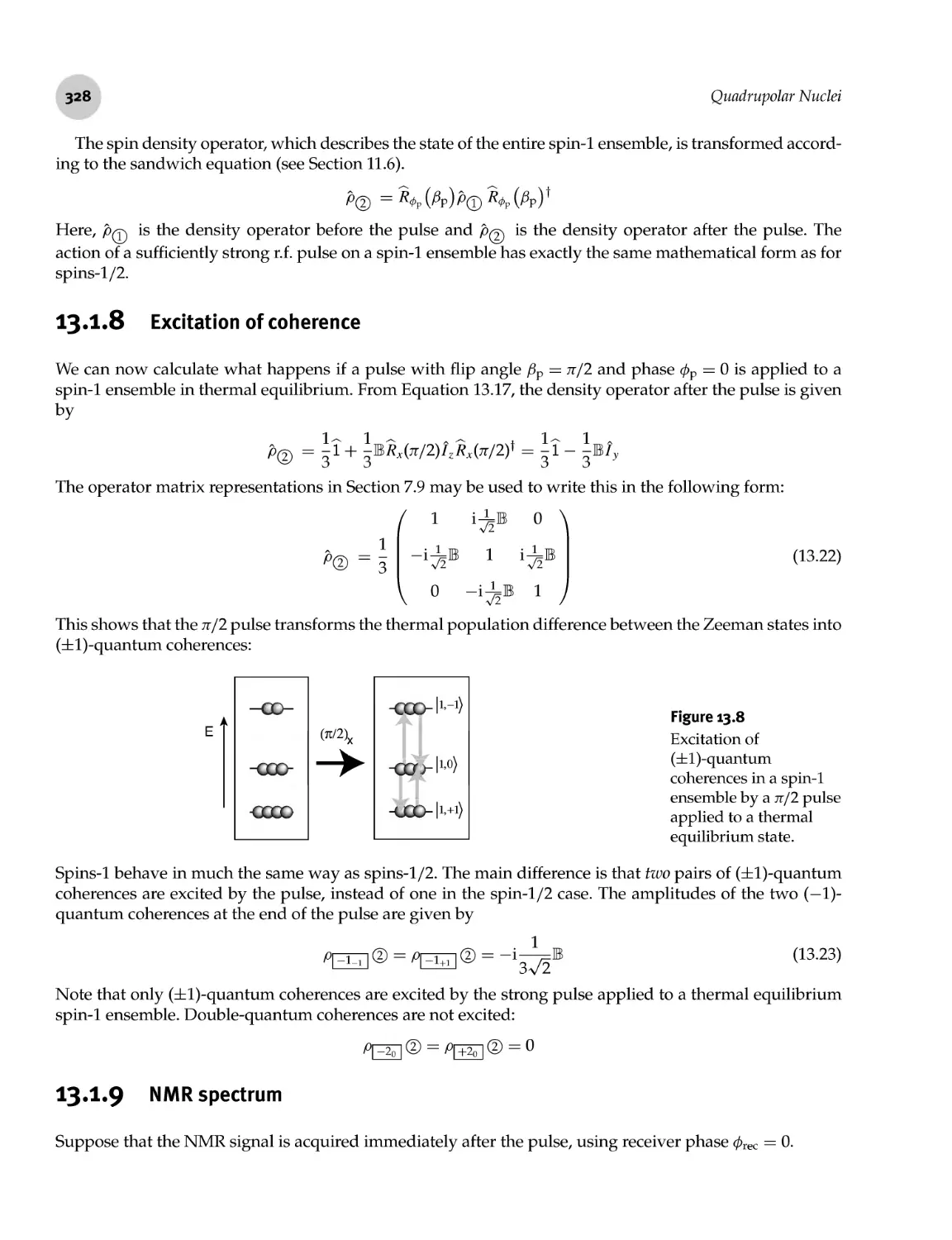
Excitation of coherence
NMR spectrum
Quadrupolar echo

xiv
Contents
13.2 Spin 7 = 3/2 334
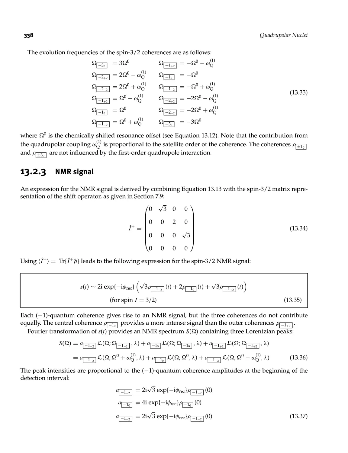
13.2.1 Spin- 3/2 energy levels 335
13.2.2 Populations and coherences 336
13.2.3 NMR signal 338
13.2.4 Single pulse spectrum 339
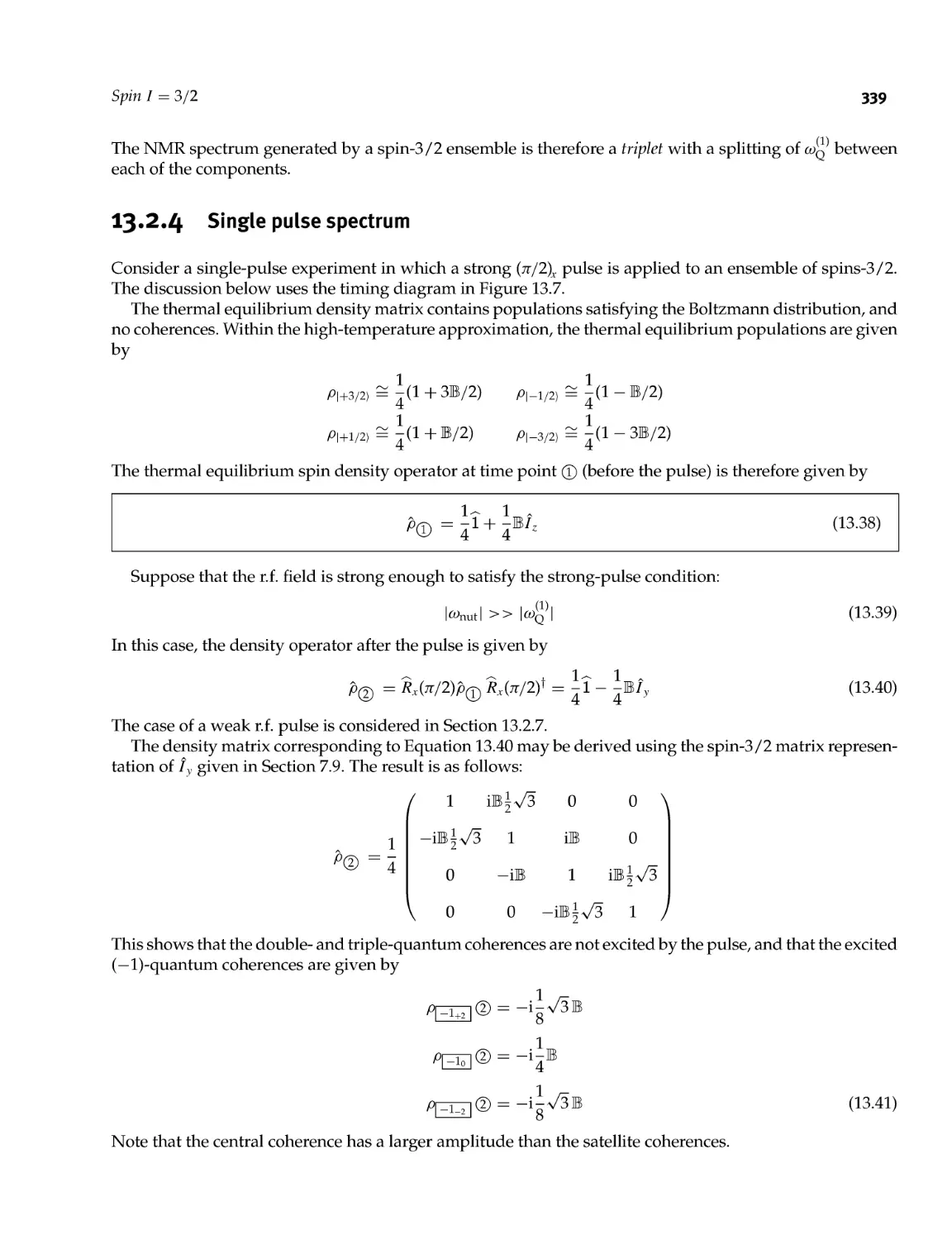
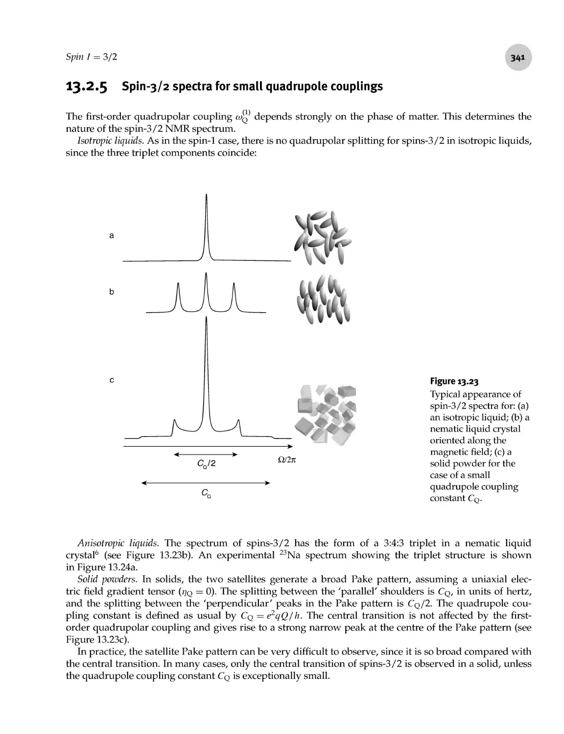
13.2.5 Spin- 3/2 spectra for small quadrupole couplings 341
13.2.6 Second- order quadrupole couplings 342
13.2.7 Central transition excitation 343
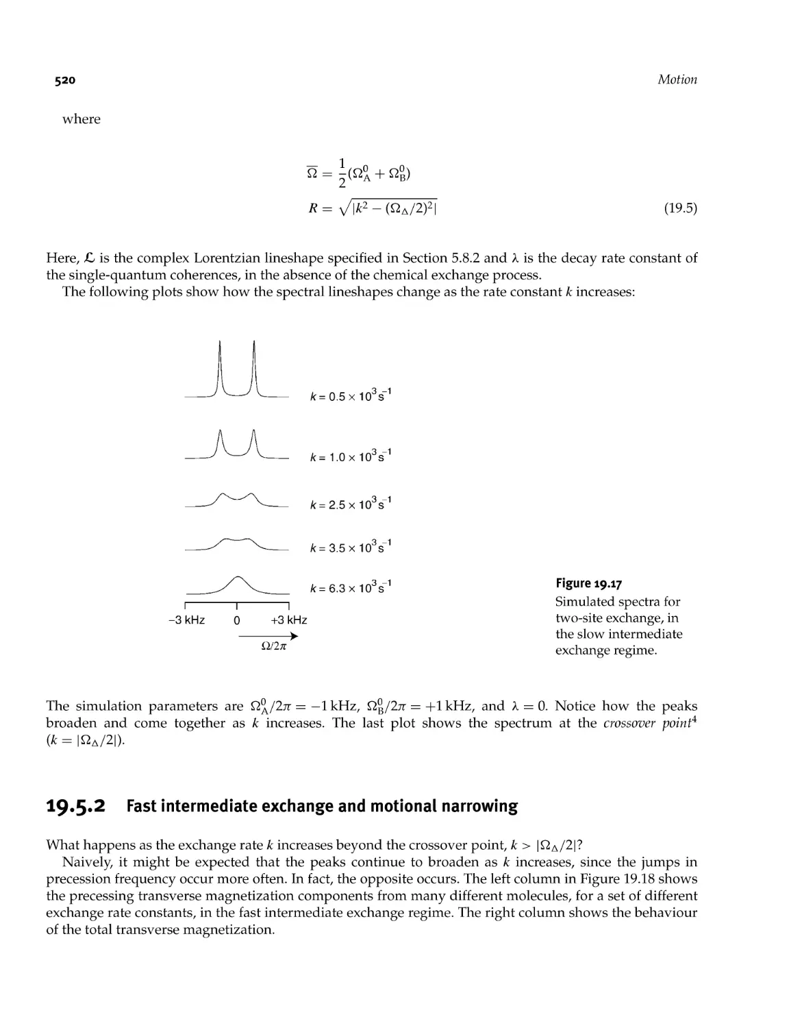
13.2.8 Central transition echo 345
13.3 Spin 7 = 5/2 345
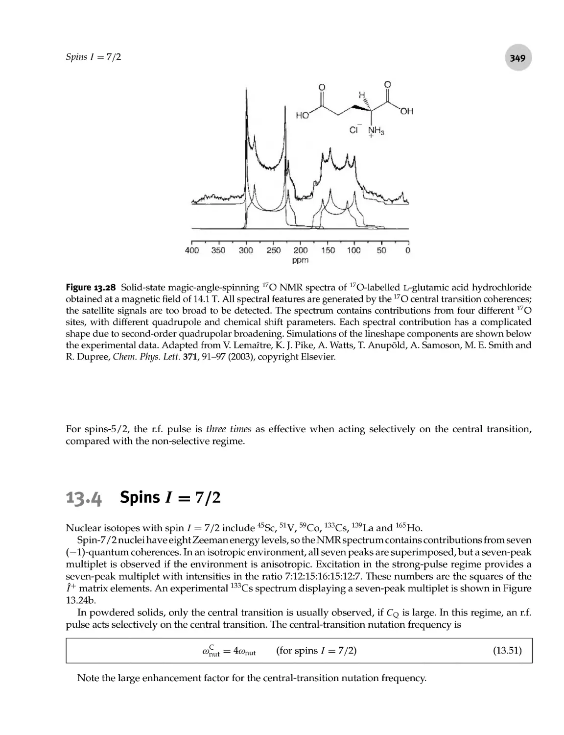
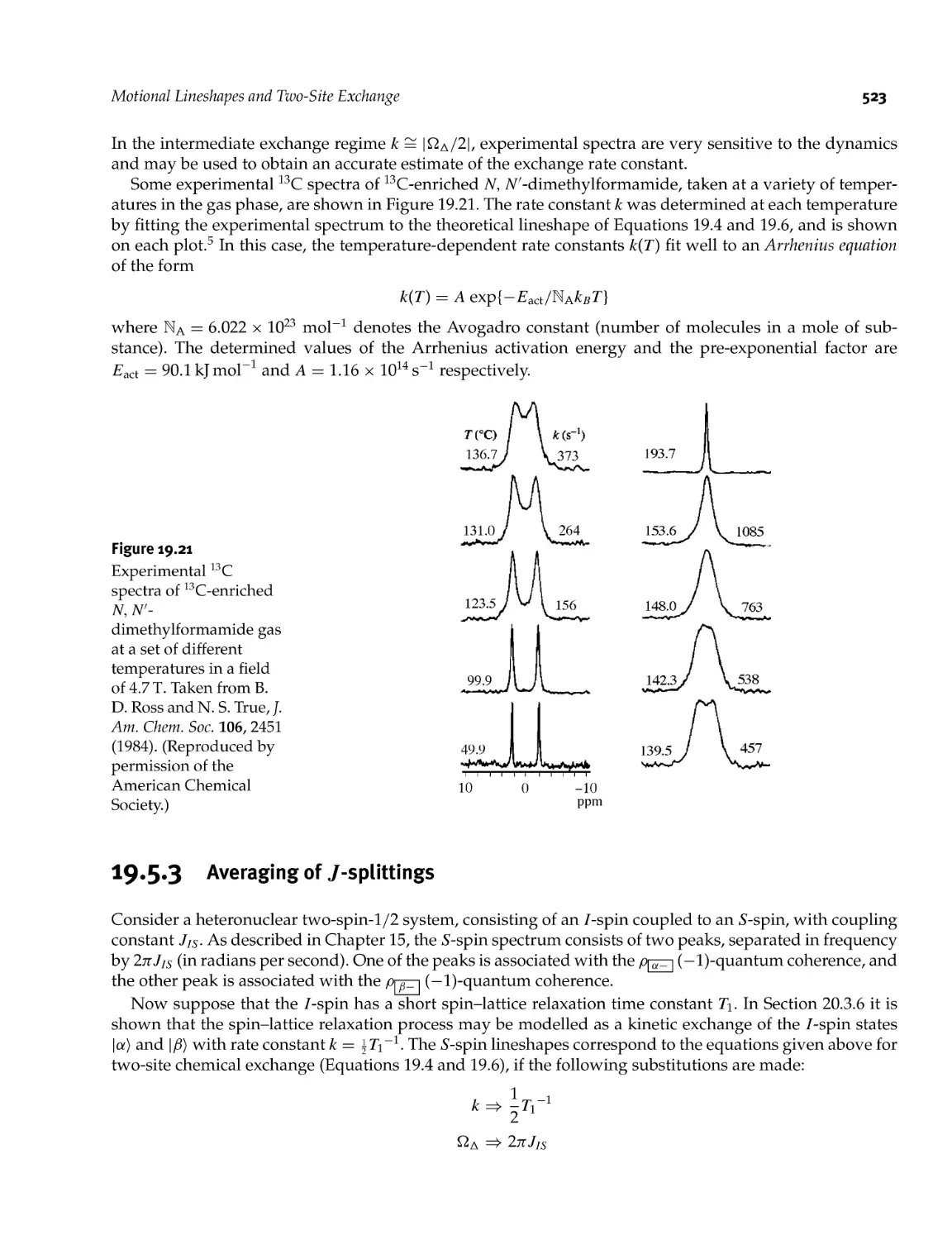
13.4 Spins 7 = 7/2 349
13.5 Spins 7 = 9/2 350
Part 6 Coupled Spins 353
14 Spin- 1/2 Pairs 355
14.1 Coupling Regimes 355
14.2 Zeeman Product States and Superposition States 356
14.3 Spin- Pair Hamiltonian 357
14.4 Pairs of Magnetically Equivalent Spins 359
14.4.1 Singlets and triplets 359
14.4.2 Energy levels 360
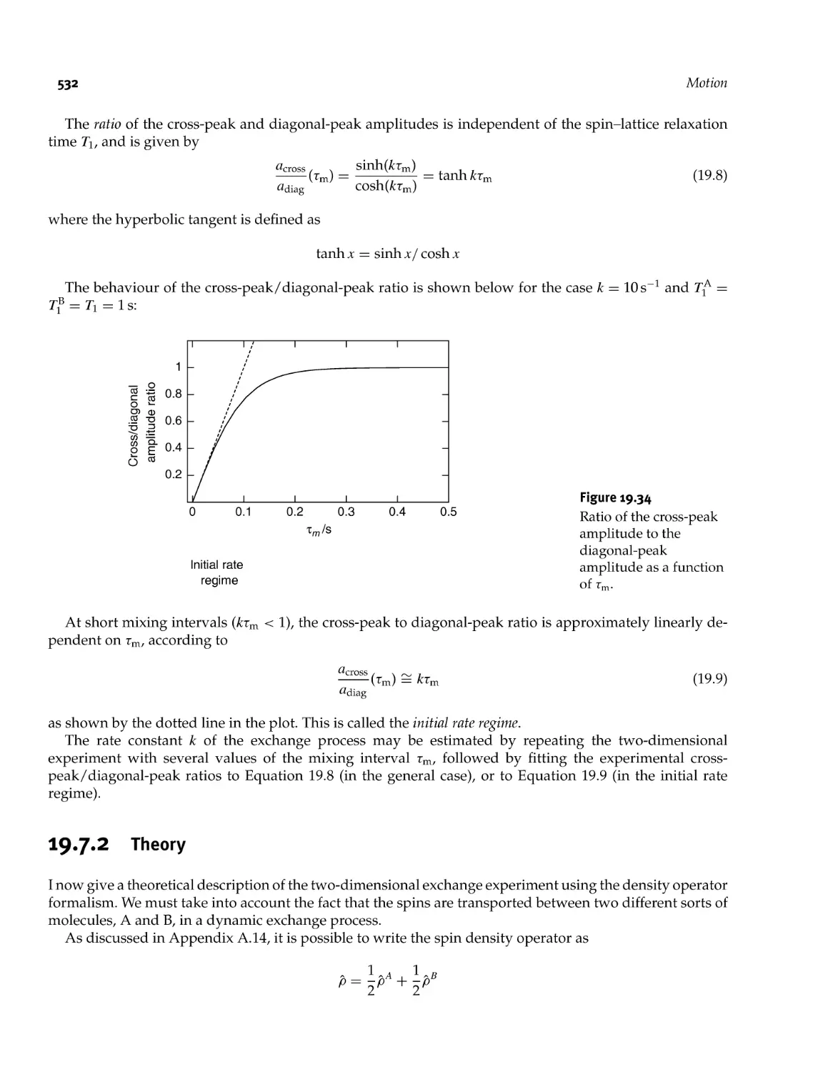
14.4.3 NMR spectra 362
14.4.4 Dipolar echo 363
14.5 Weakly Coupled Spin Pairs 363
14.5.1 Weak coupling 363
14.5.2 AX spin systems 364
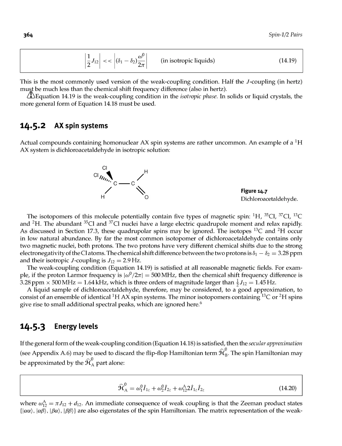
14.5.3 Energy levels 364
14.5.4 AX spectrum 365
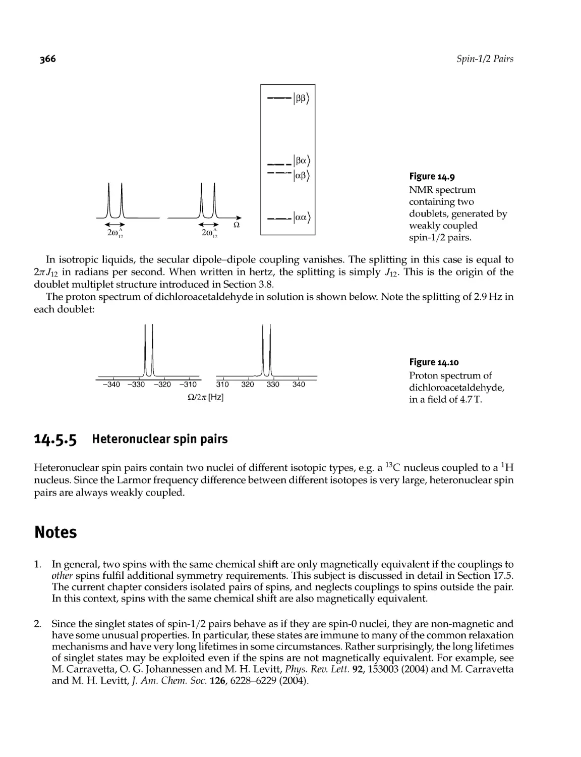
14.5.5 Heteronuclear spin pairs 366
15 Homonuclear AX System 369
15.1 Eigenstates and Energy Levels 369
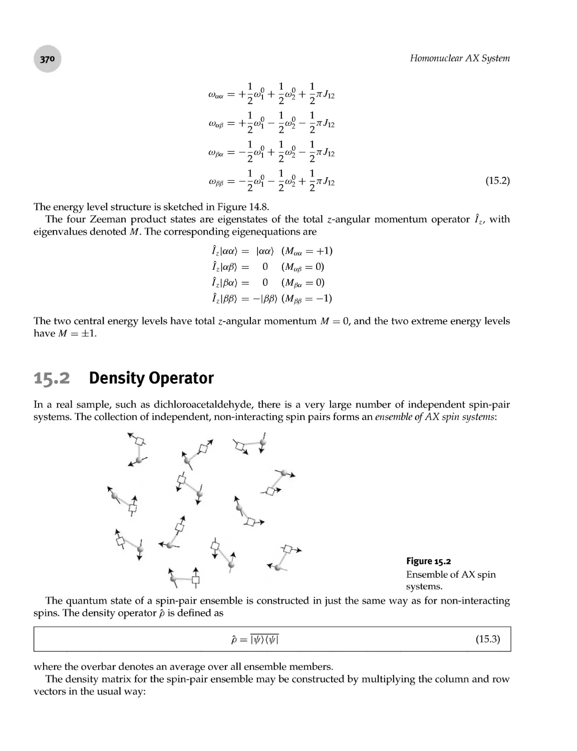
15.2 Density Operator 370
15.3 Rotating Frame 375
15.4 Free Evolution 376
15.4.1 Evolution of a spin pair 376
15.4.2 Evolution of the coherences 377
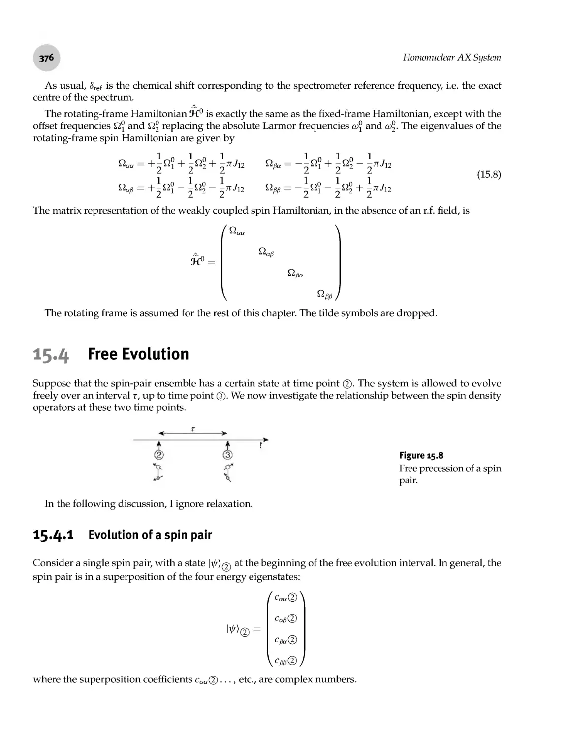
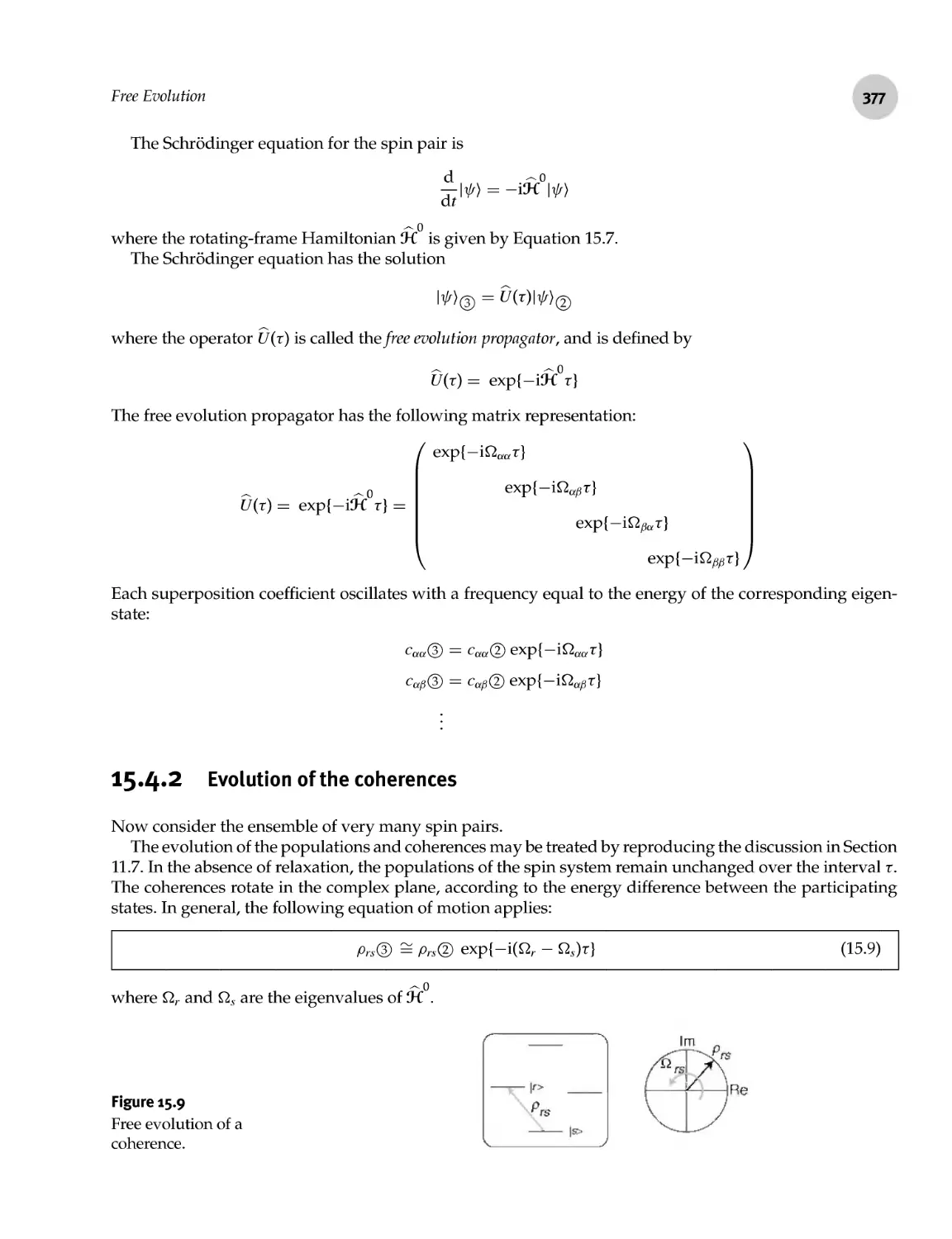
15.5 Spectrum of the AX System: Spin- Spin Splitting 378
15.6 Product Operators 381
15.6.1 Construction of product operators 382
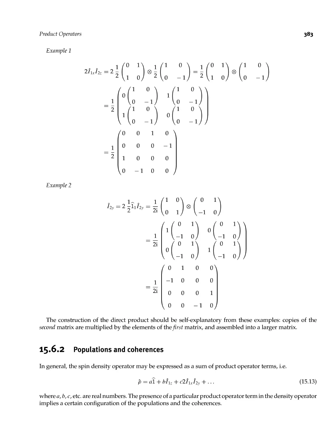
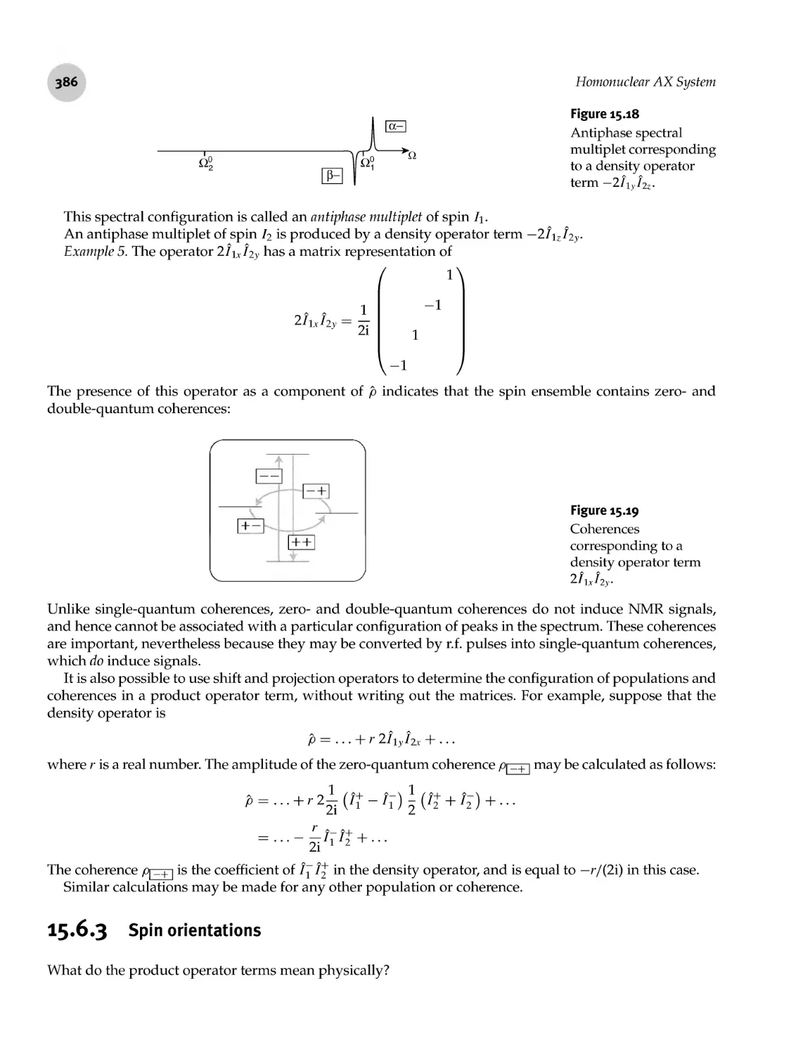
15.6.2 Populations and coherences 383
15.6.3 Spin orientations 386
15.7 Thermal Equilibrium 389
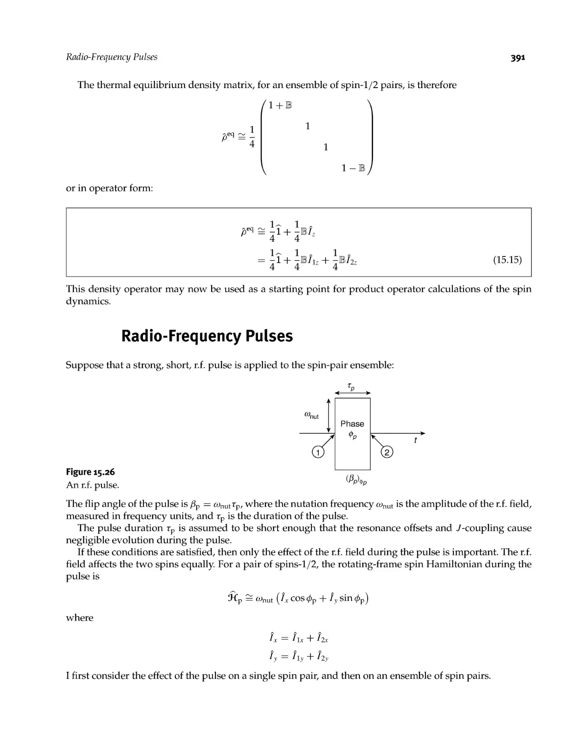
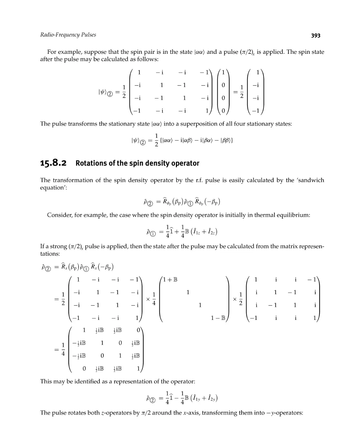
15.8 Radio- Frequency Pulses 391
15.8.1 Rotations of a single spin pair 392
15.8.2 Rotations of the spin density operator 393

XV
15.8.3 Operator transformations 395
15.9 Free Evolution of the Product Operators 397
15.9.1 Chemical shift evolution 399
15.9.2 /- coupling evolution 400
15.9.3 Relaxation 405
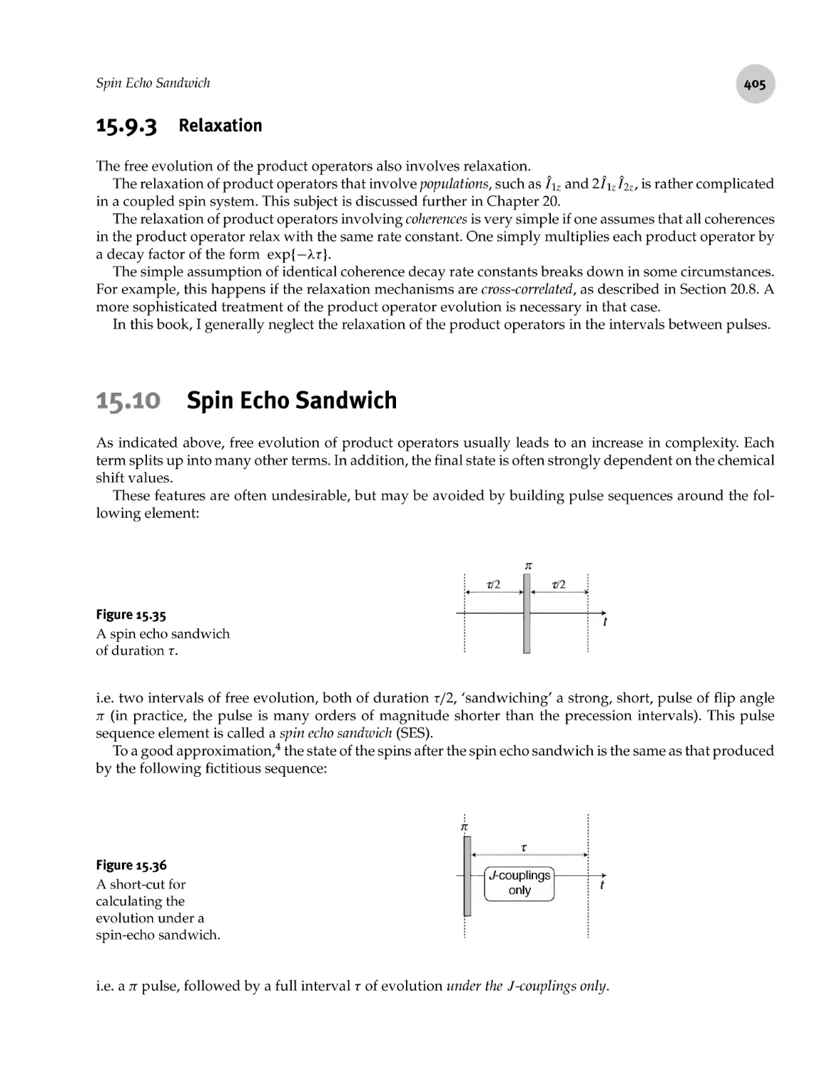
15.10 Spin Echo Sandwich 405
16 Experiments on AX Systems 409
16.1 COSY 409
409
411
411
415
418
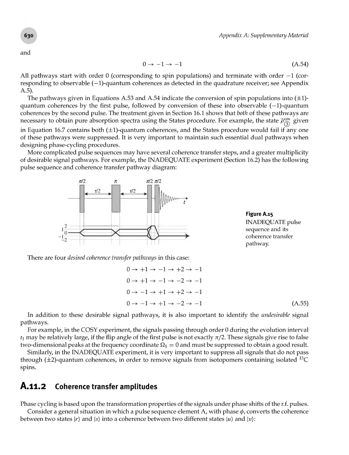
16.2 INADEQUATE 418
418
423
424
429
431
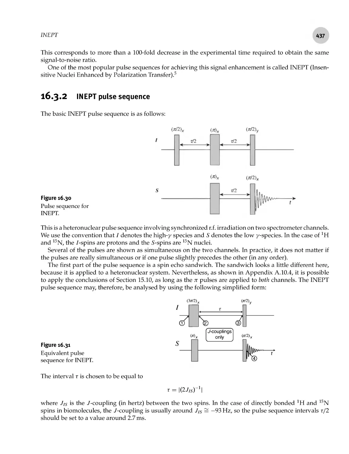
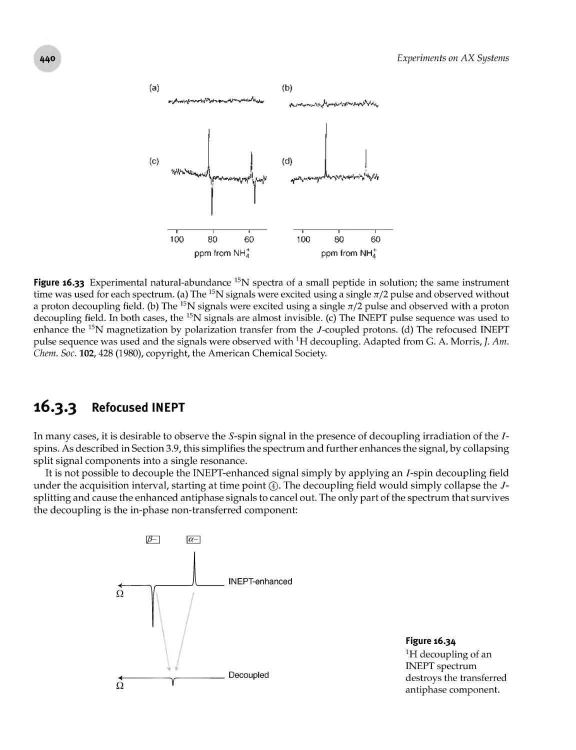
16.3 INEPT 436
436
437
440
16.4 Residual Dipolar Couplings 443
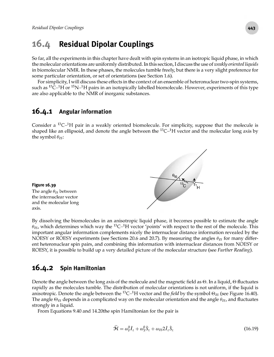
16.4.1 Angular information 443
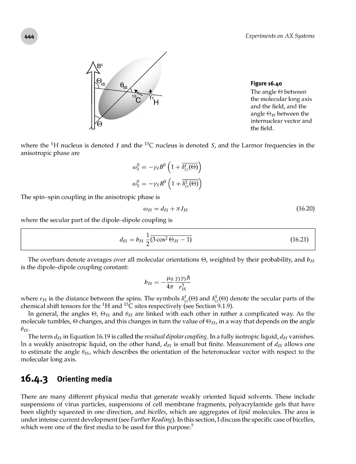
16.4.2 Spin Hamiltonian 443
16.4.3 Orienting media 444
16.4.4 Doublet splittings 446
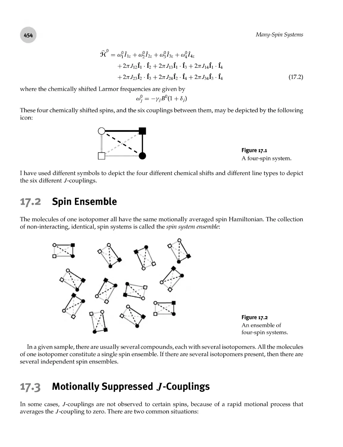
17 Many- Spin Systems 453
17.1 Molecular Spin System 453
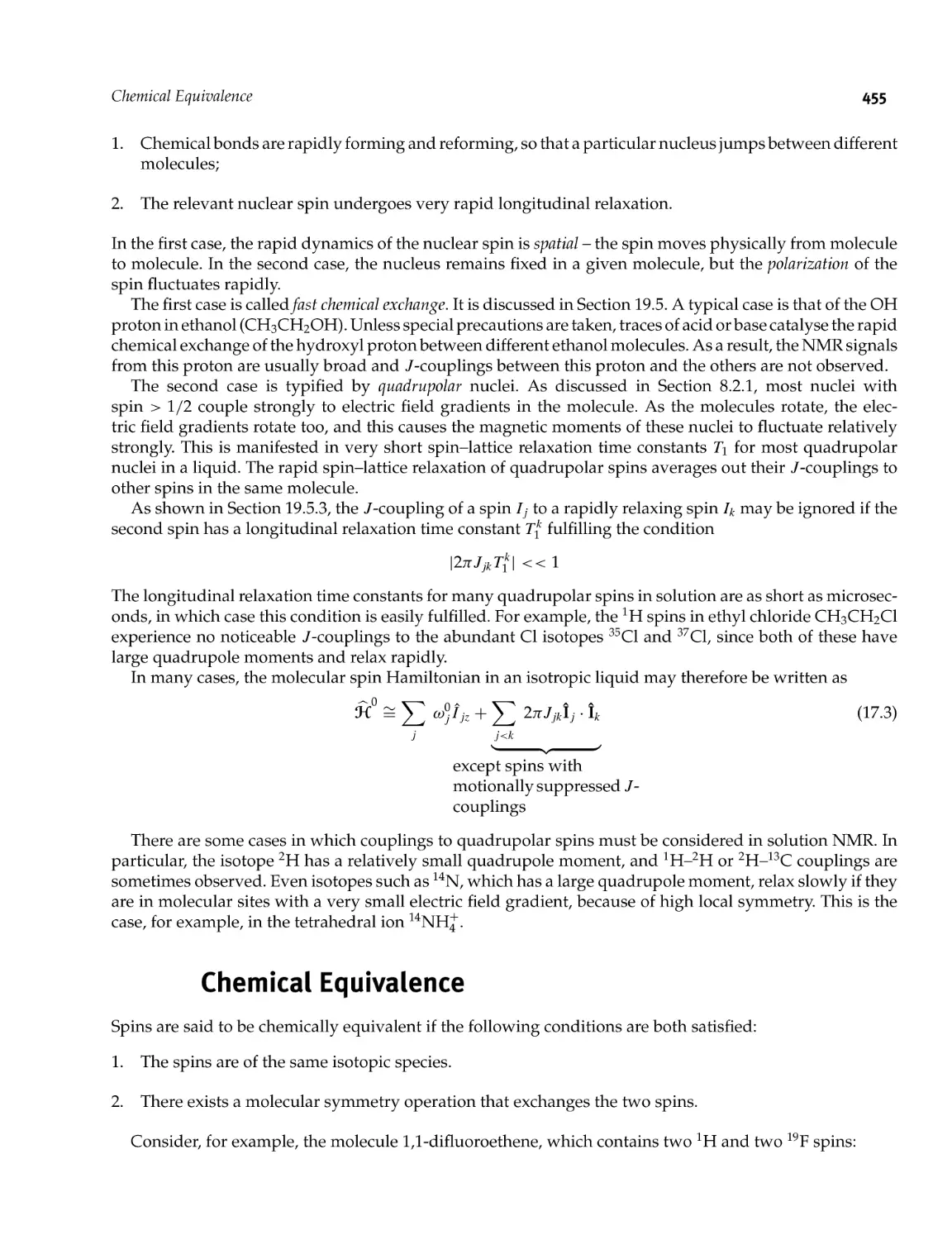
17.2 Spin Ensemble 454
17.3 Motionally Suppressed /- Couplings 454
17.4 Chemical Equivalence 455
17.5 Magnetic Equivalence 458
17.6 Weak Coupling 461
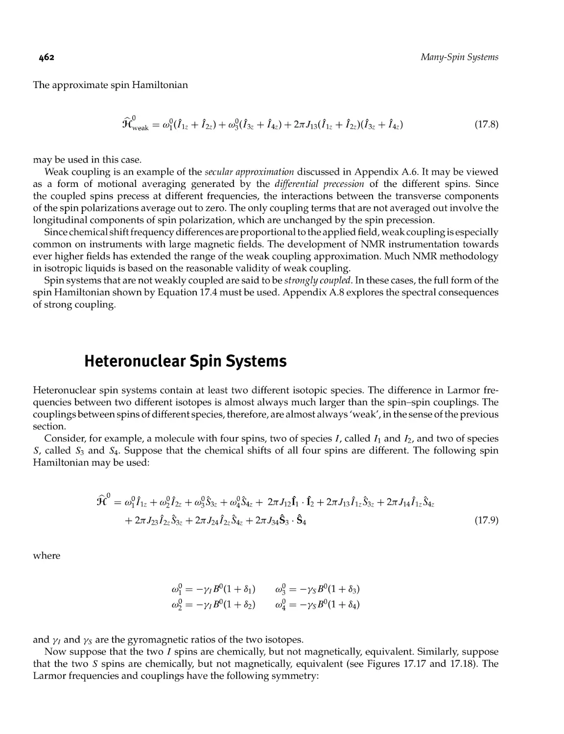
17.7 Heteronuclear Spin Systems 462
17.8 Alphabet Notation 463
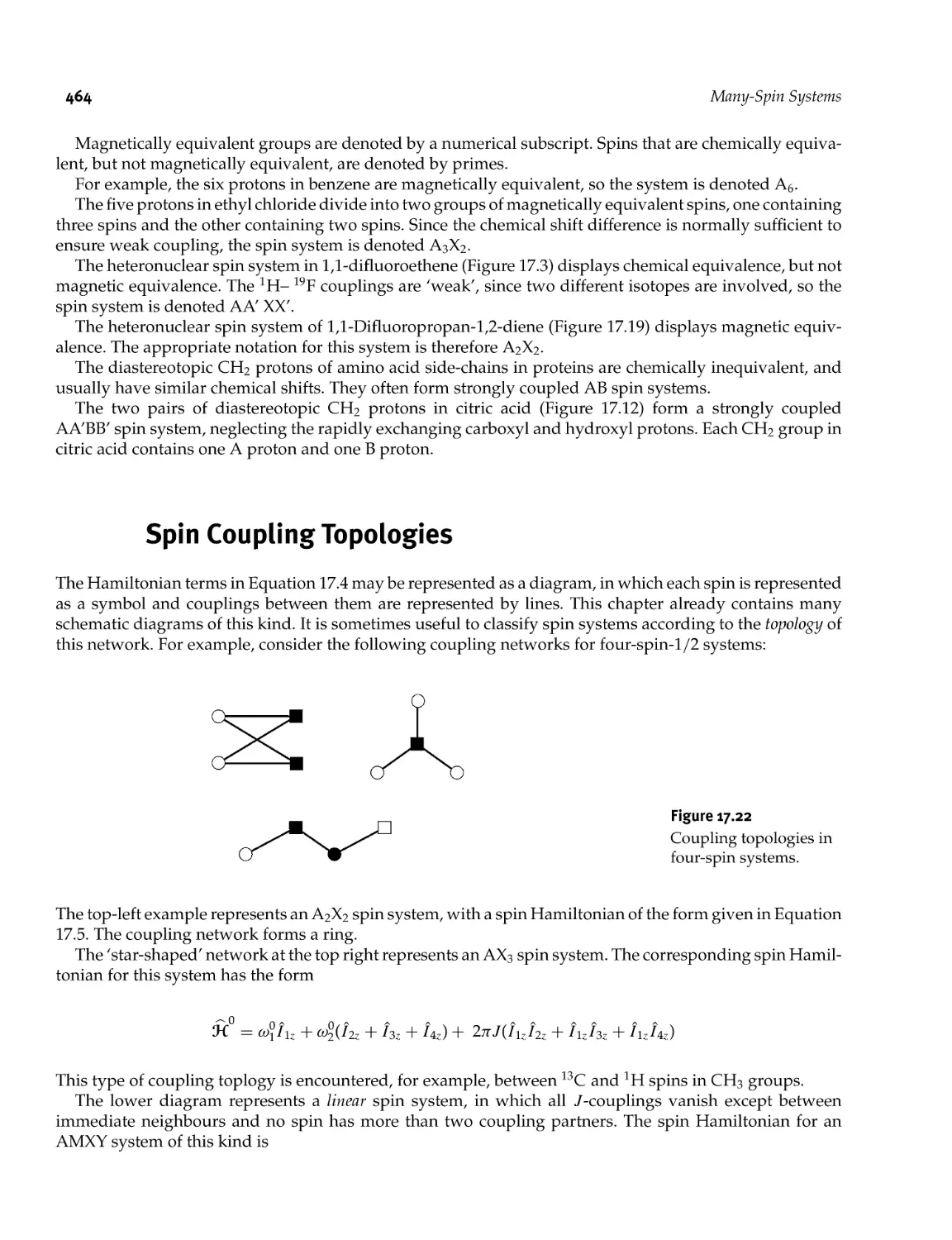
17.9 Spin Coupling Topologies 464
18 Many- Spin Dynamics 467
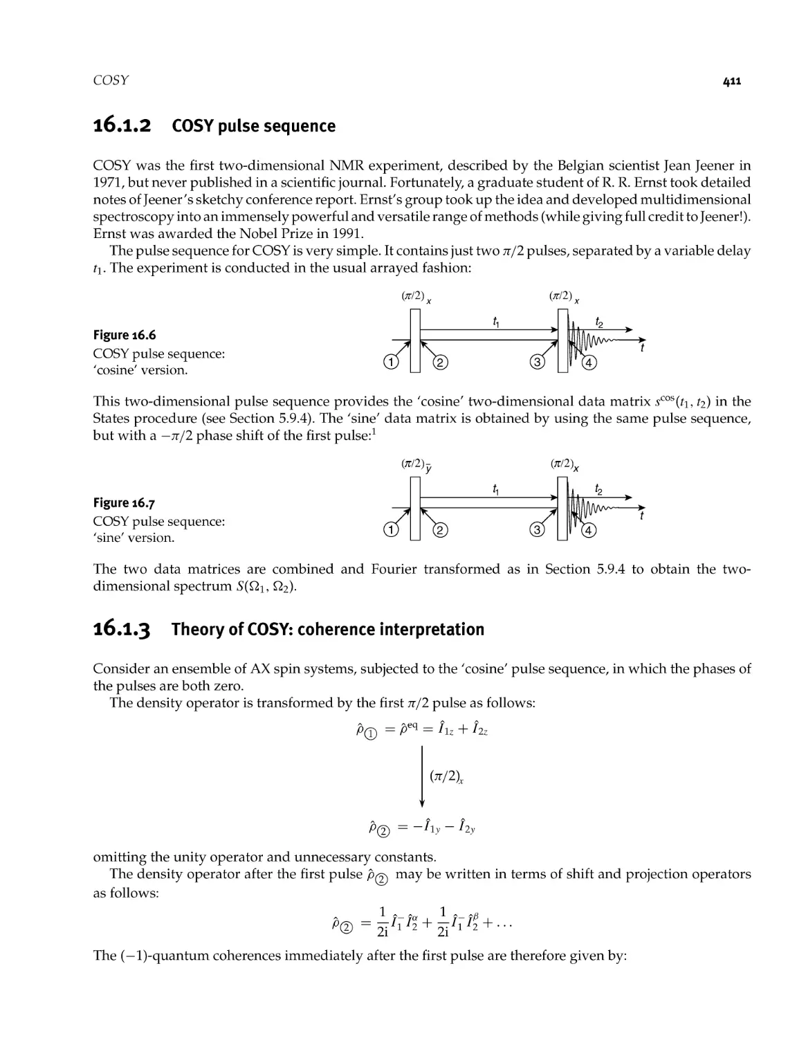
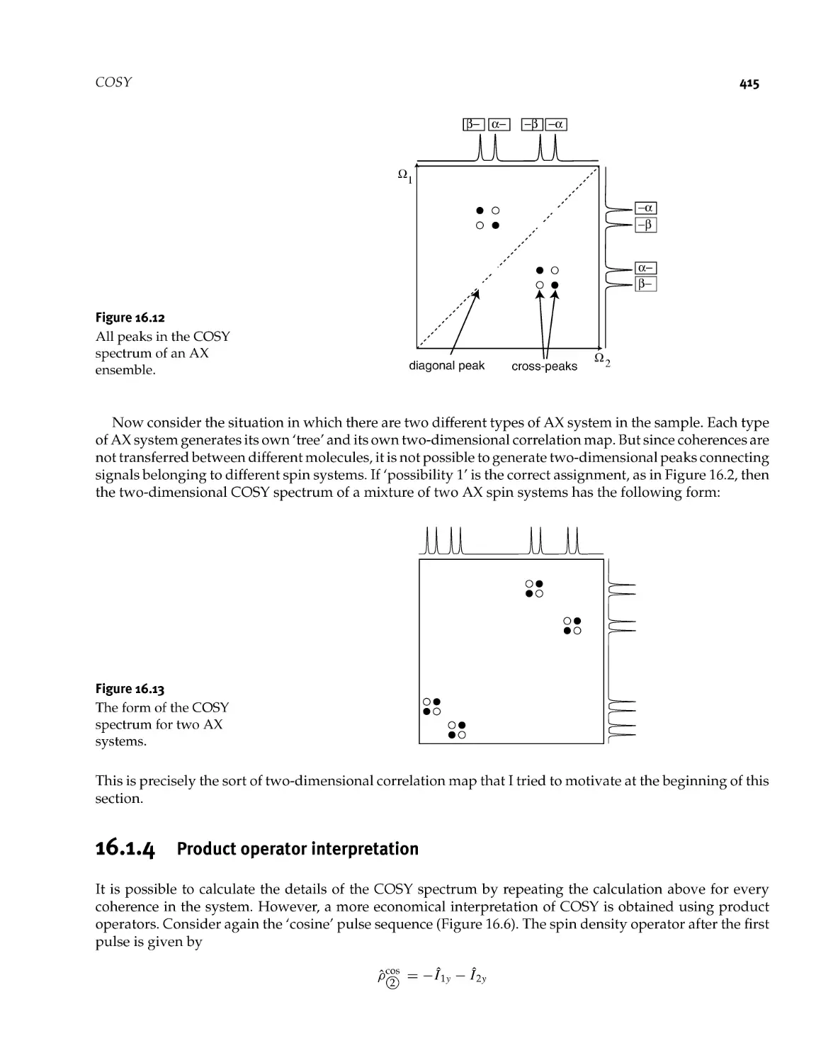
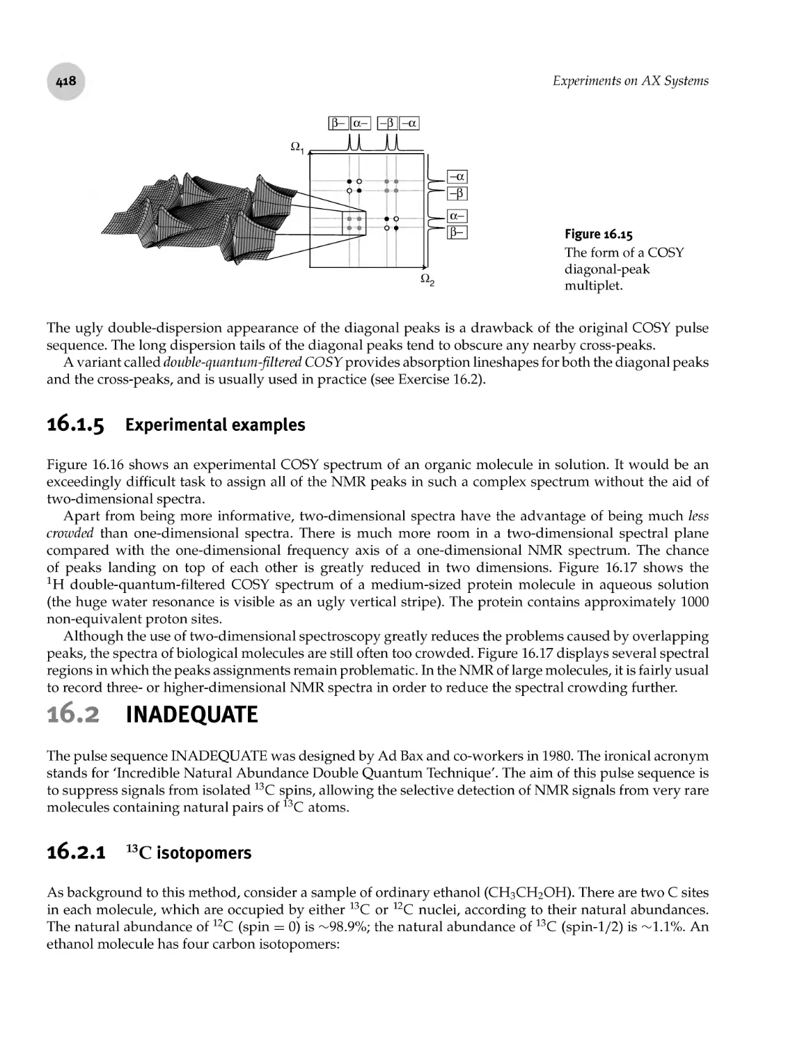
COSY
16.1.1
16.1.2
16.1.3
16.1.4
16.1.5
The assignment problem
COSY pulse sequence
Theory of COSY: coherence interpretation
Product operator interpretation
Experimental examples
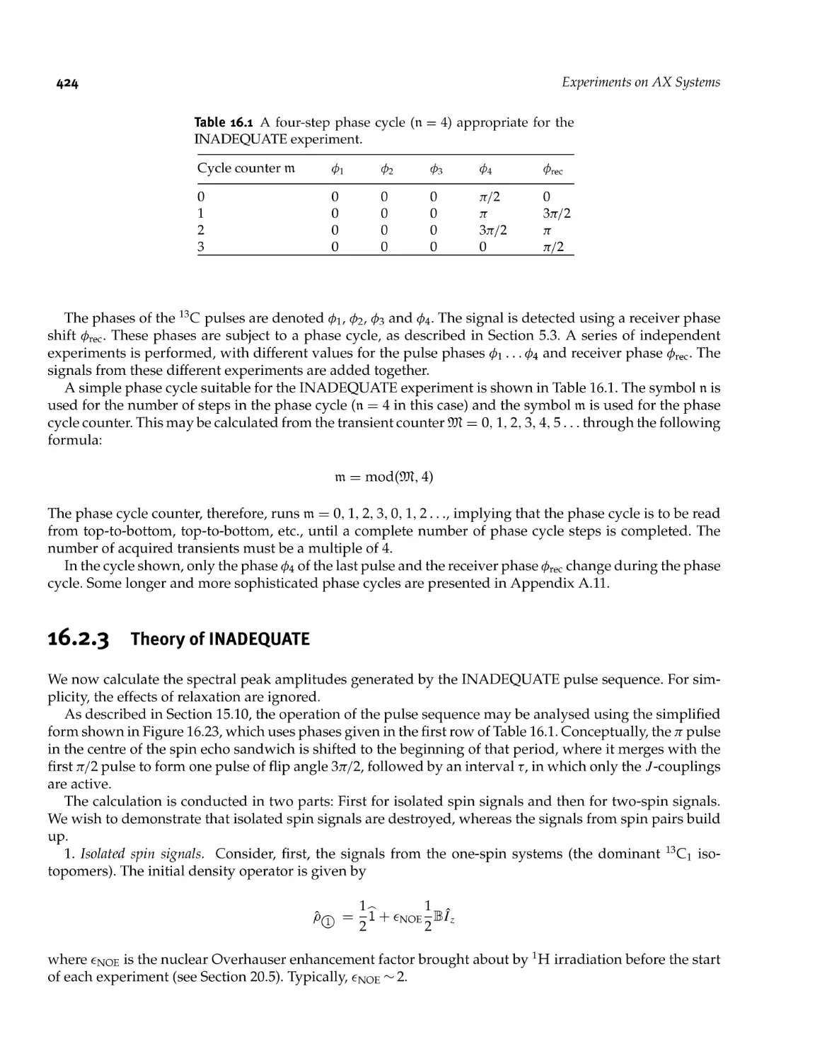
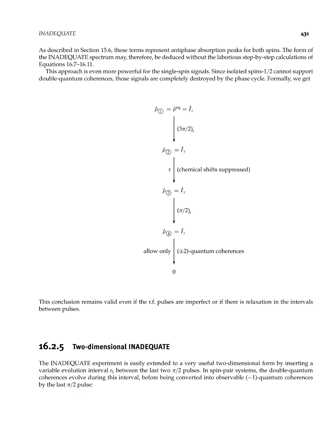
INADEQUATE
16.2.1
16.2.2
16.2.3
16.2.4
16.2.5
INEPT
16.3.1
16.3.2
16.3.3
13C isotopomers
Pulse sequence
Theory of INADEQUATE
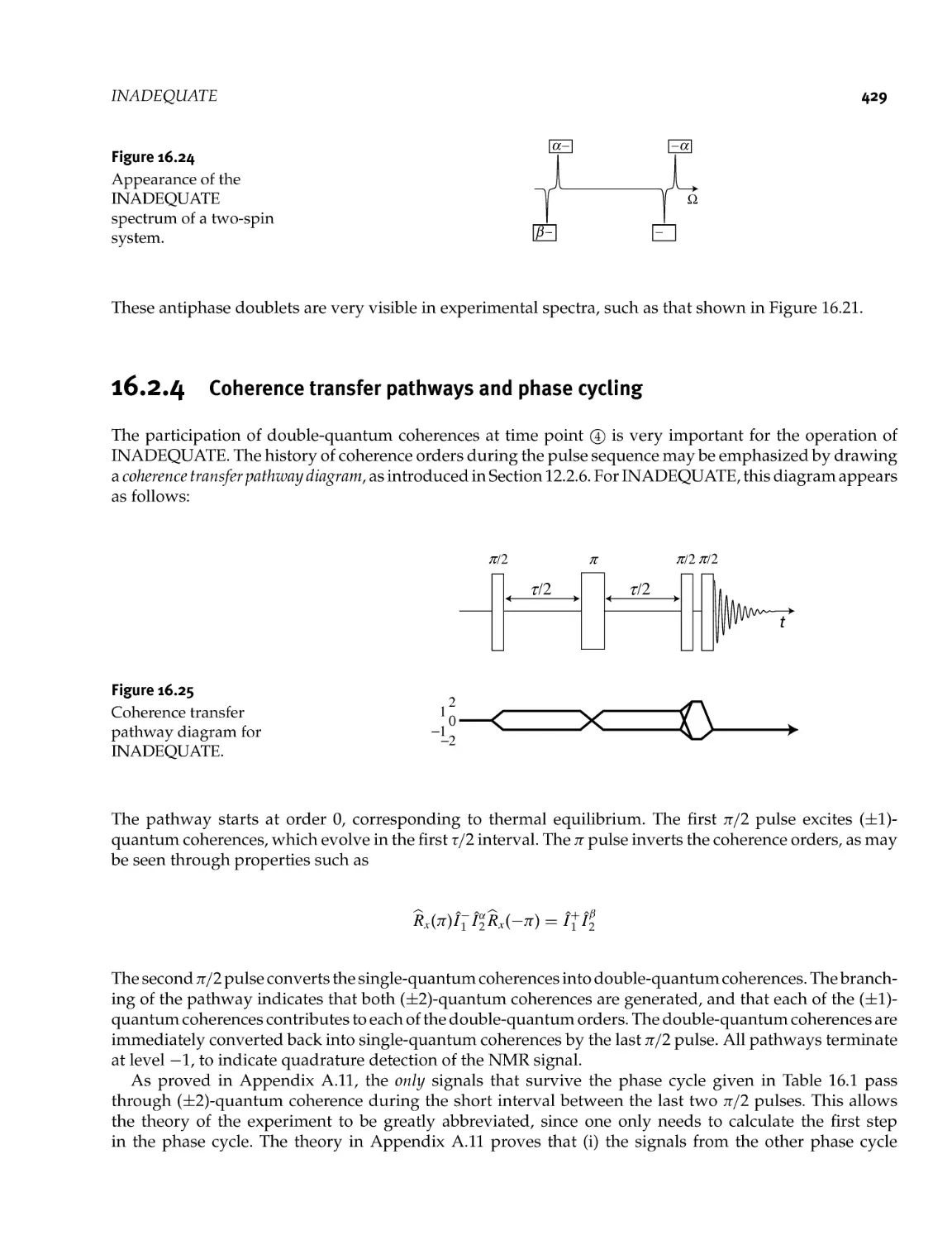
Coherence transfer pathways and phase cycling
Two- dimensional INADEQUATE
The sensitivity of nuclear isotopes
INEPT pulse sequence
Refocused INEPT
18.1 Spin Hamiltonian
18.2 Energy Eigenstates
467
468

xvi Contents
18.3 Superposition States 469
18.4 Spin Density Operator 470
18.5 Populations and Coherences 471
18.5.1 Coherence orders 471
18.5.2 Combination coherences and simple coherences 471
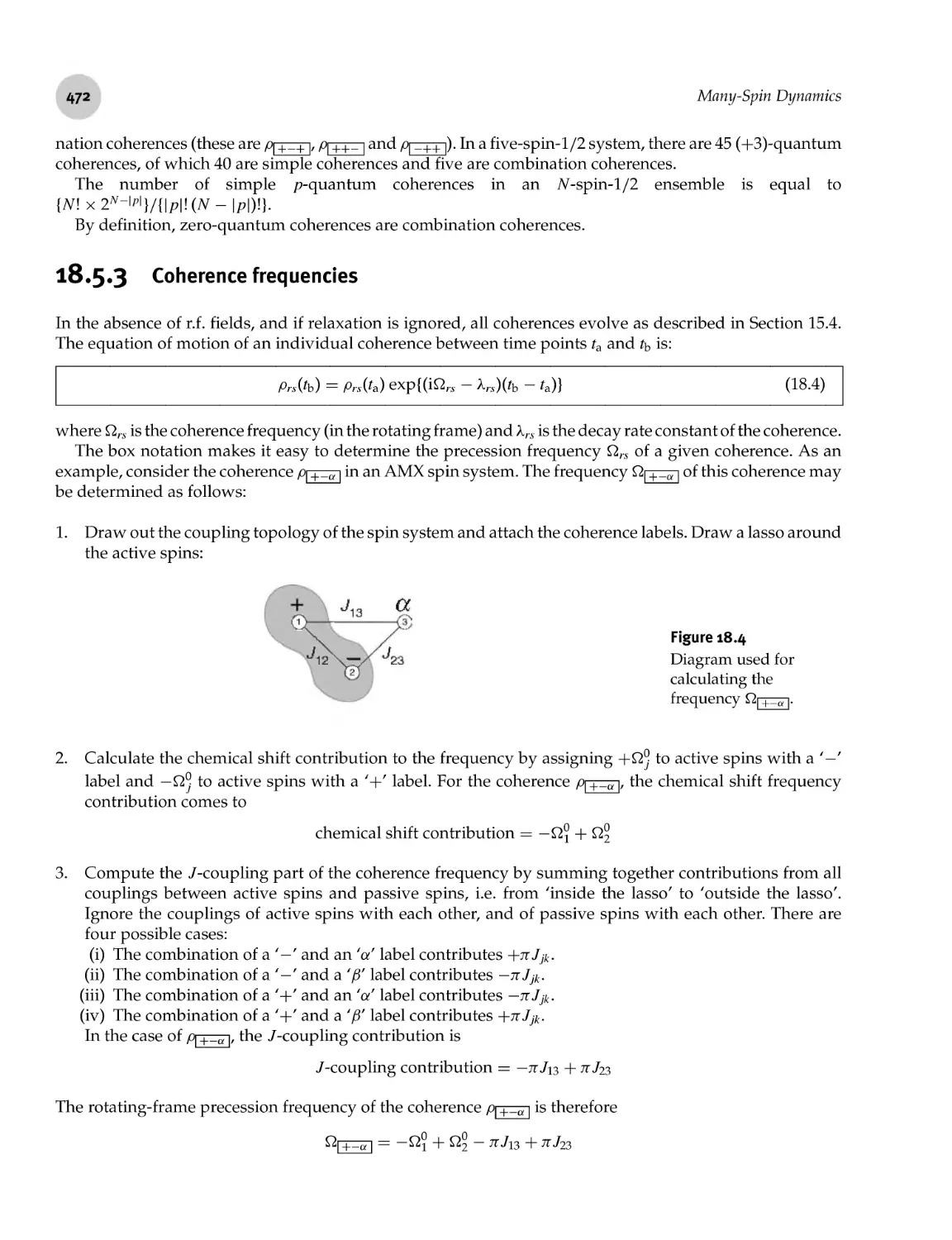
18.5.3 Coherence frequencies 472
18.5.4 Degenerate coherences 473
18.5.5 Observable coherences 473
18.6 NMR Spectra 475
18.7 Many- Spin Product Operators 477
18.7.1 Construction of product operators 477
18.7.2 Populations and coherences 478
18.7.3 Physical interpretation of product operators 480
18.8 Thermal Equilibrium 481
18.9 Radio- Frequency Pulses 481
18.10 Free Precession 482
18.10.1 Chemical shift evolution 482
18.10.2 /- coupling evolution 483
18.10.3 Relaxation 485
18.11 Spin Echo Sandwiches 485
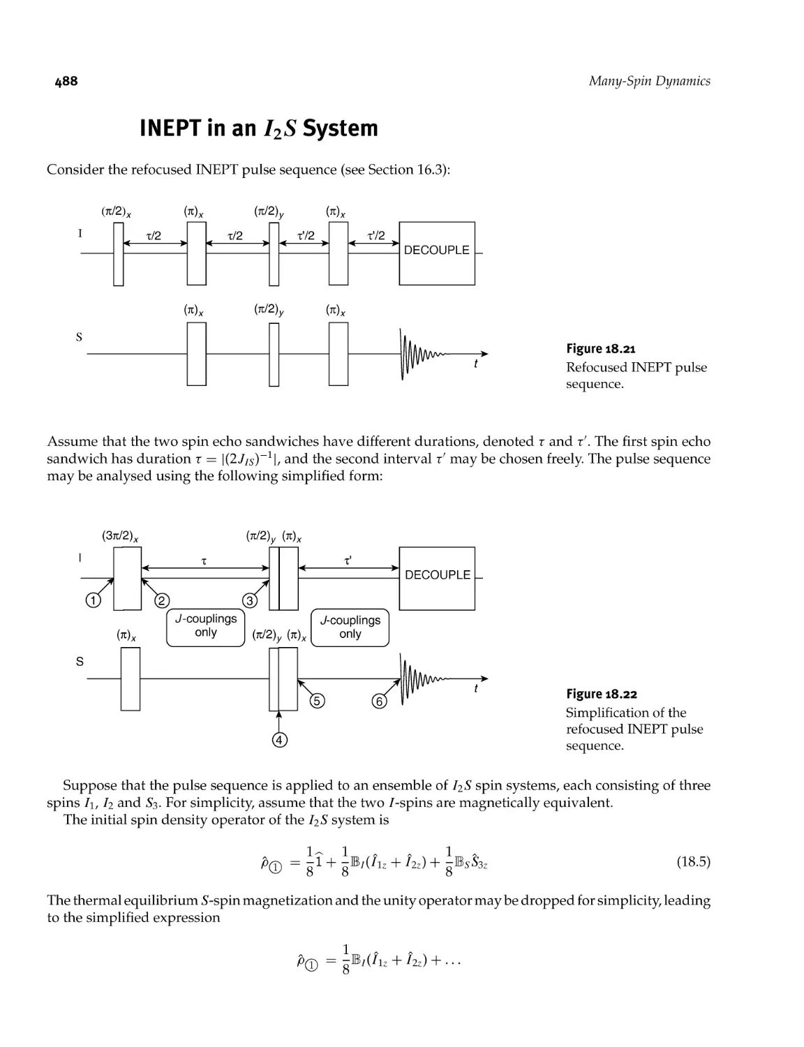
18.12 INEPT in an I2S System 488
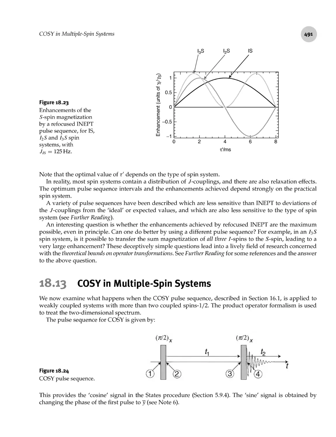
18.13 COSY in Multiple- Spin Systems 491
18.13.1 AMX spectrum 492
18.13.2 Active and passive spins 493
18.13.3 Cross- peak multiplets 494
18.13.4 Diagonal peaks 496
18.13.5 Linear spin systems 497
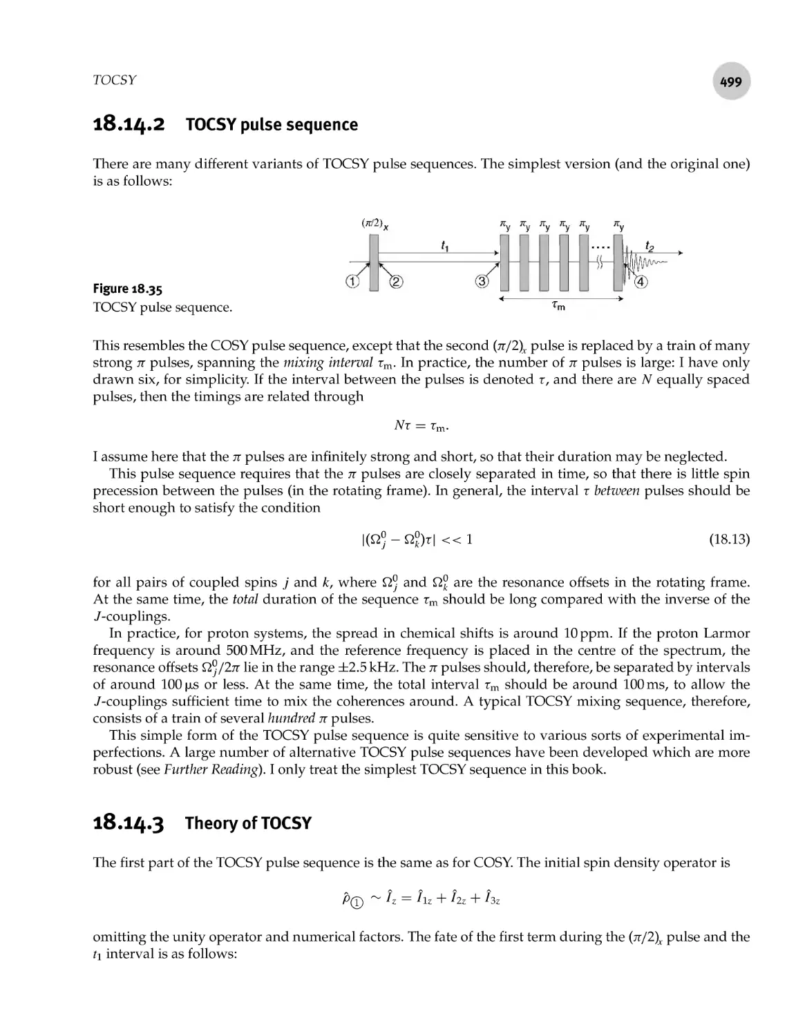
18.14 TOCSY 497
18.14.1 The ambiguity of COSY spectra 497
18.14.2 TOCSY pulse sequence 499
18.14.3 Theory of TOCSY 499
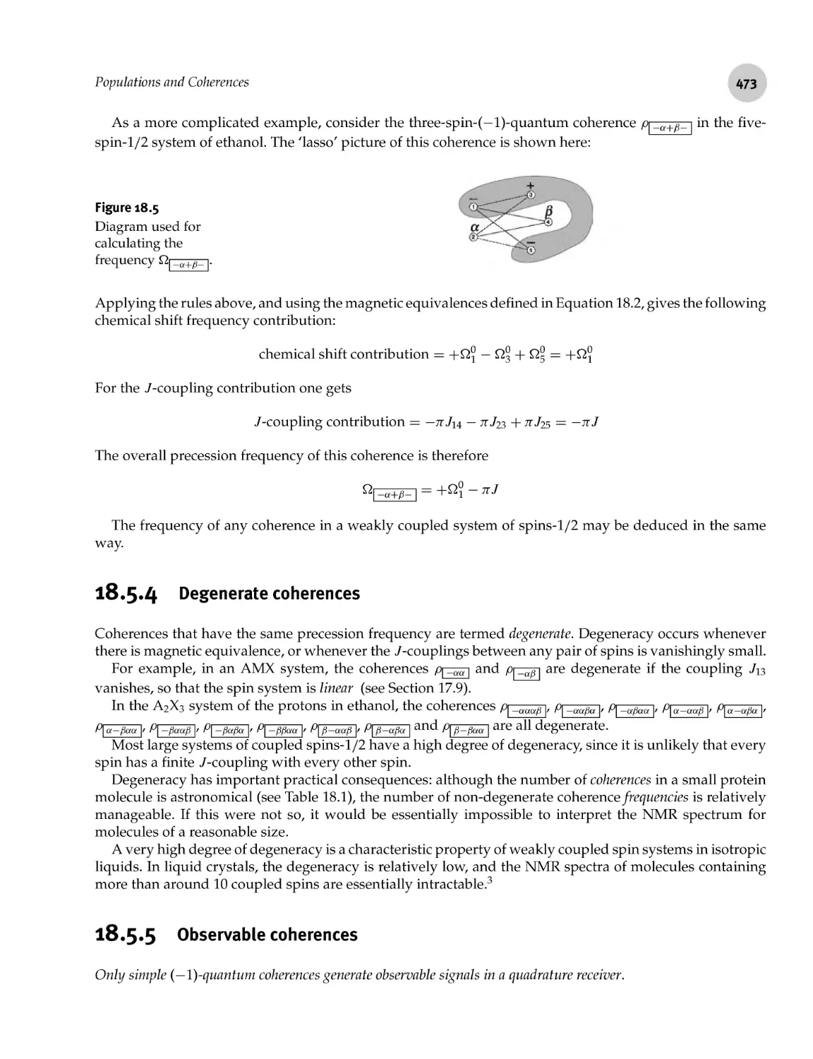
Part 7 Motion and Relaxation 507
19 Motion 509
19.1 Motional Processes 509
19.1.1 Molecular vibrations 509
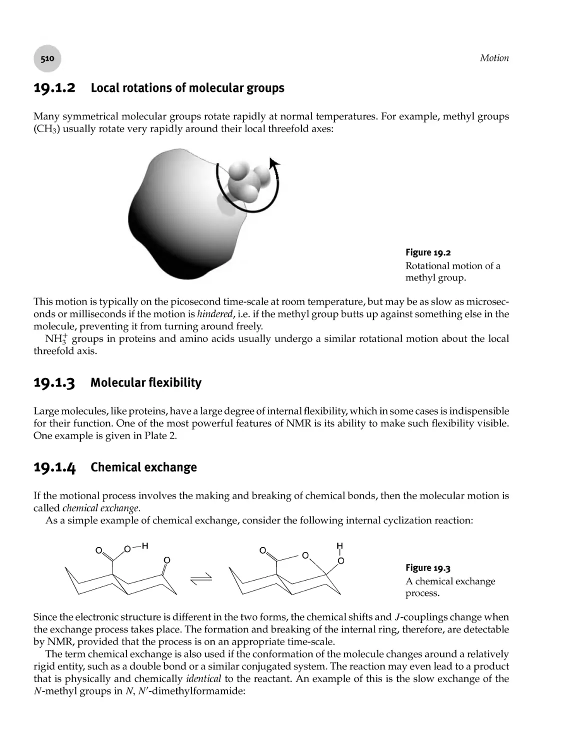
19.1.2 Local rotations of molecular groups 510
19.1.3 Molecular flexibility 510
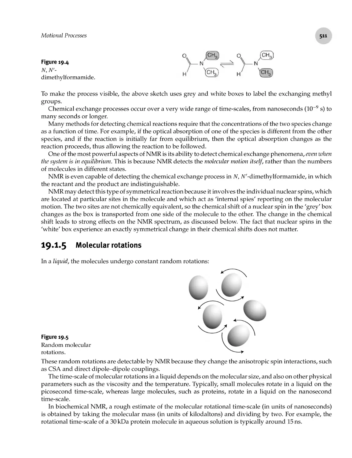
19.1.4 Chemical exchange 510
19.1.5 Molecular rotations 511
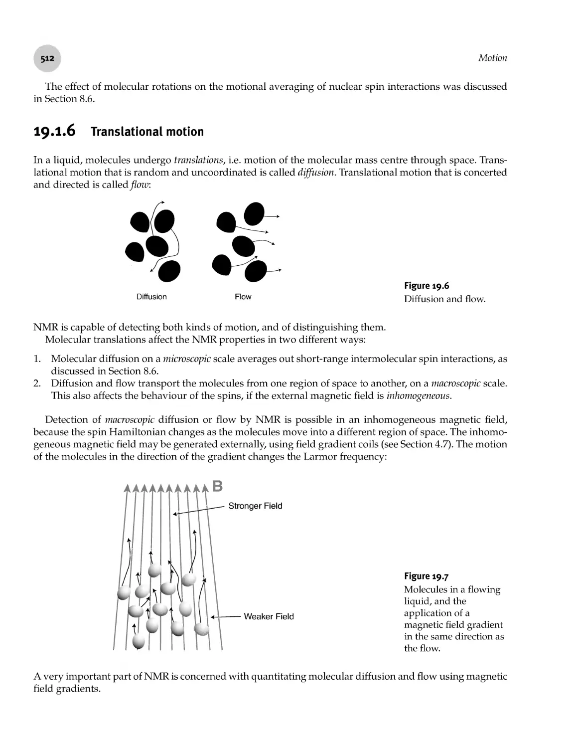
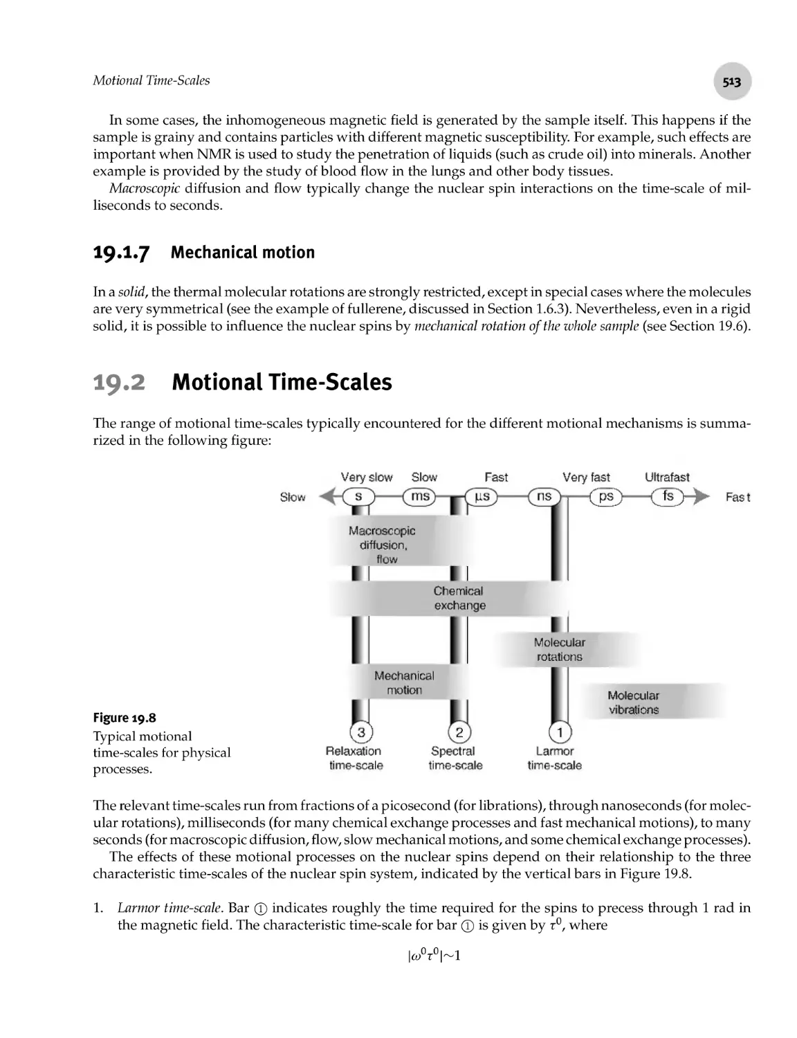
19.1.6 Translational motion 512
19.1.7 Mechanical motion 513
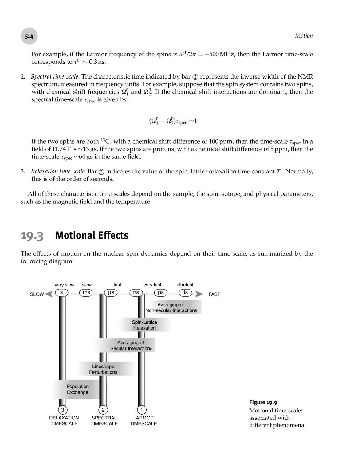
19.2 Motional Time- Scales 513
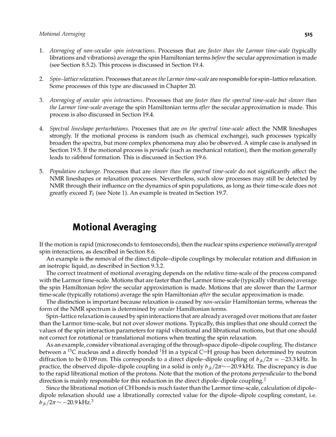
19.3 Motional Effects 514
19.4 Motional Averaging 515
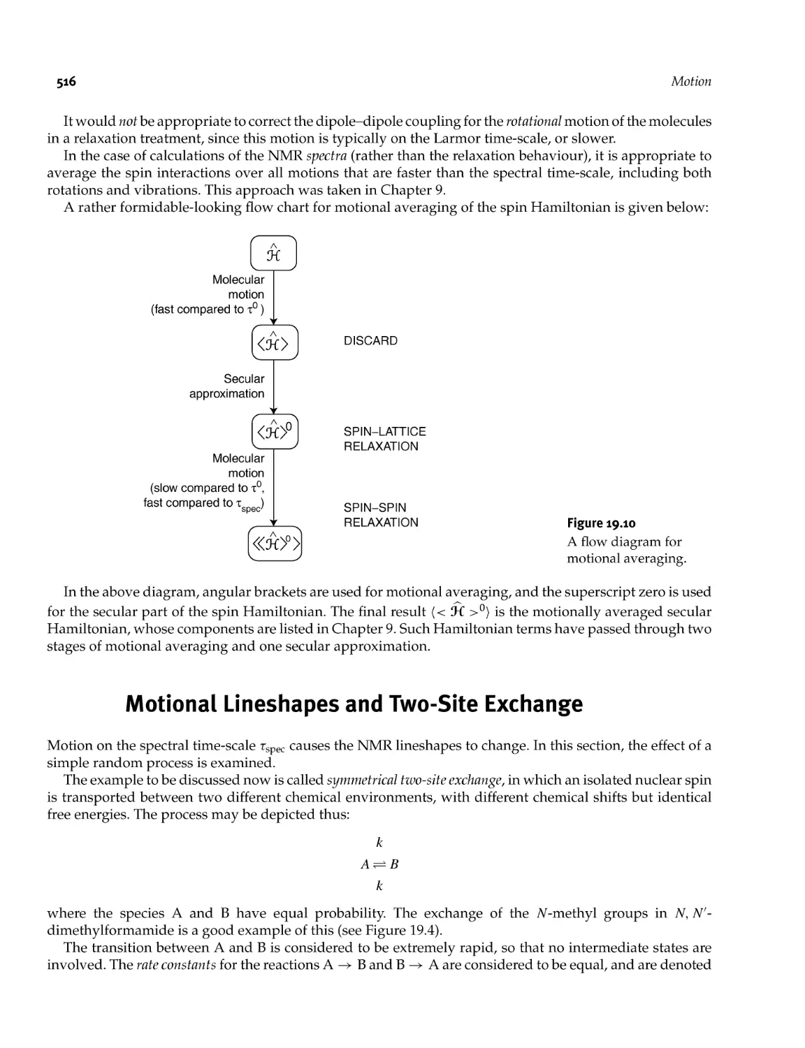
19.5 Motional Lineshapes and Two- Site Exchange 516

XVII
19.5.1 Slow intermediate exchange and motional broadening 518
19.5.2 Fast intermediate exchange and motional narrowing 520
19.5.3 Averaging of /- splittings 523
19.5.4 Asymmetric two- site exchange 524
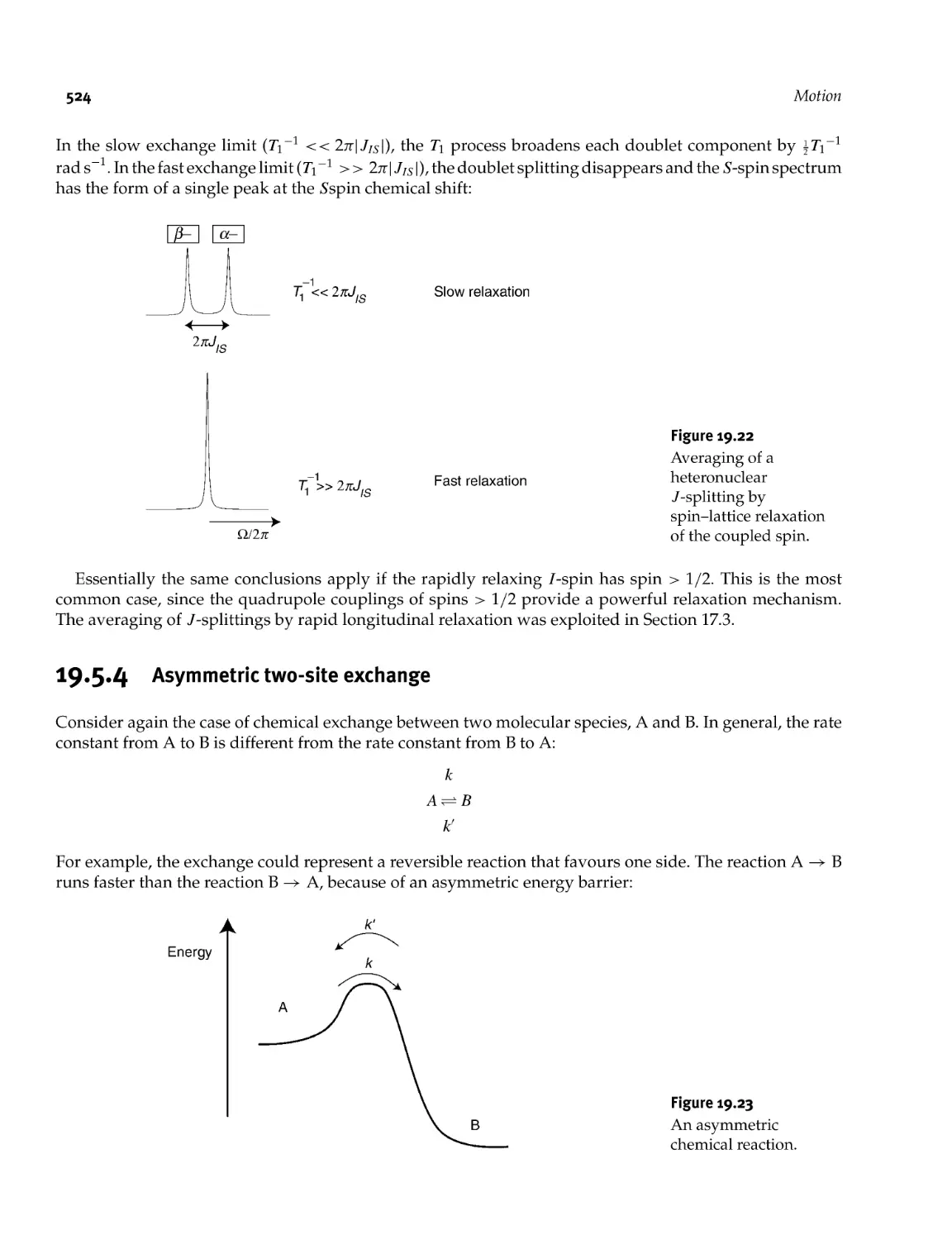
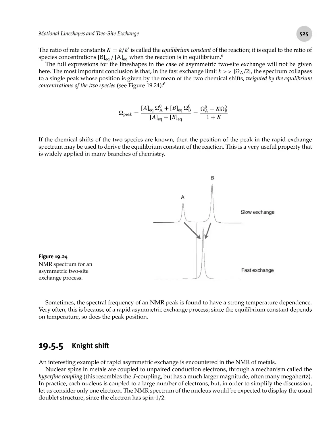
19.5.5 Knight shift 525
19.5.6 Paramagnetic shifts 527
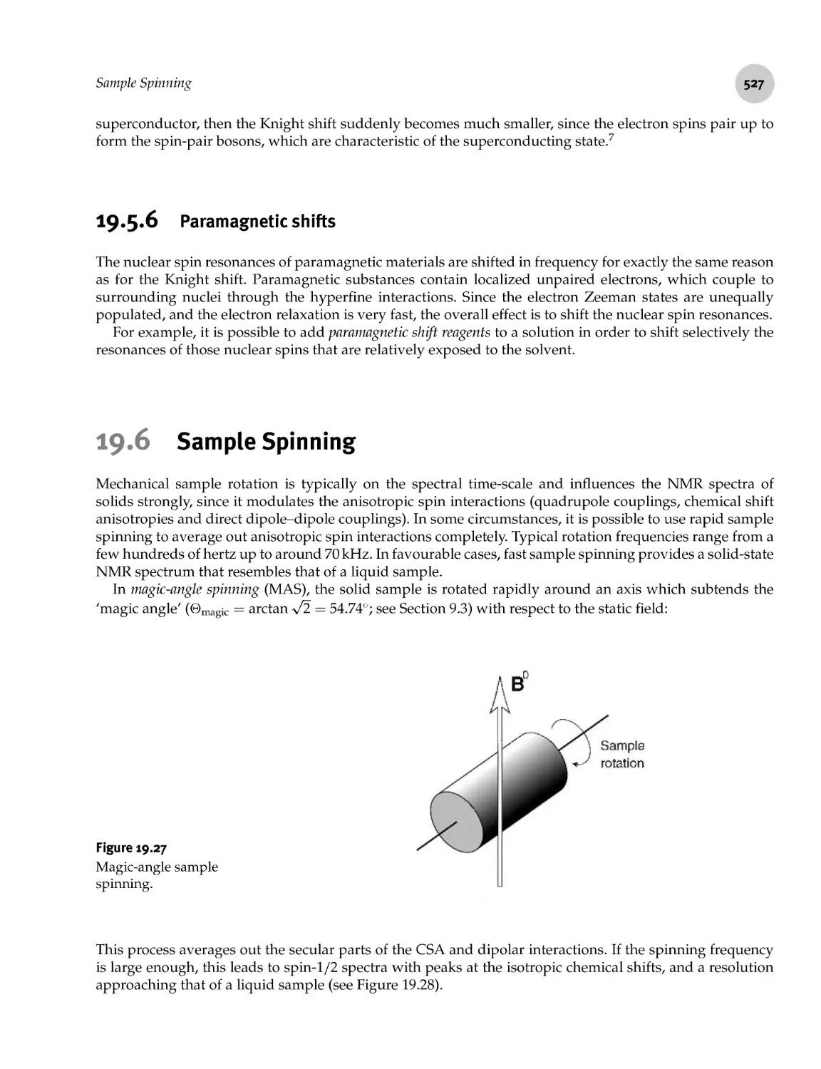
19.6 Sample Spinning 527
19.7 Longitudinal Magnetization Exchange 529
19.7.1 Two- dimensional exchange spectroscopy 529
19.7.2 Theory 532
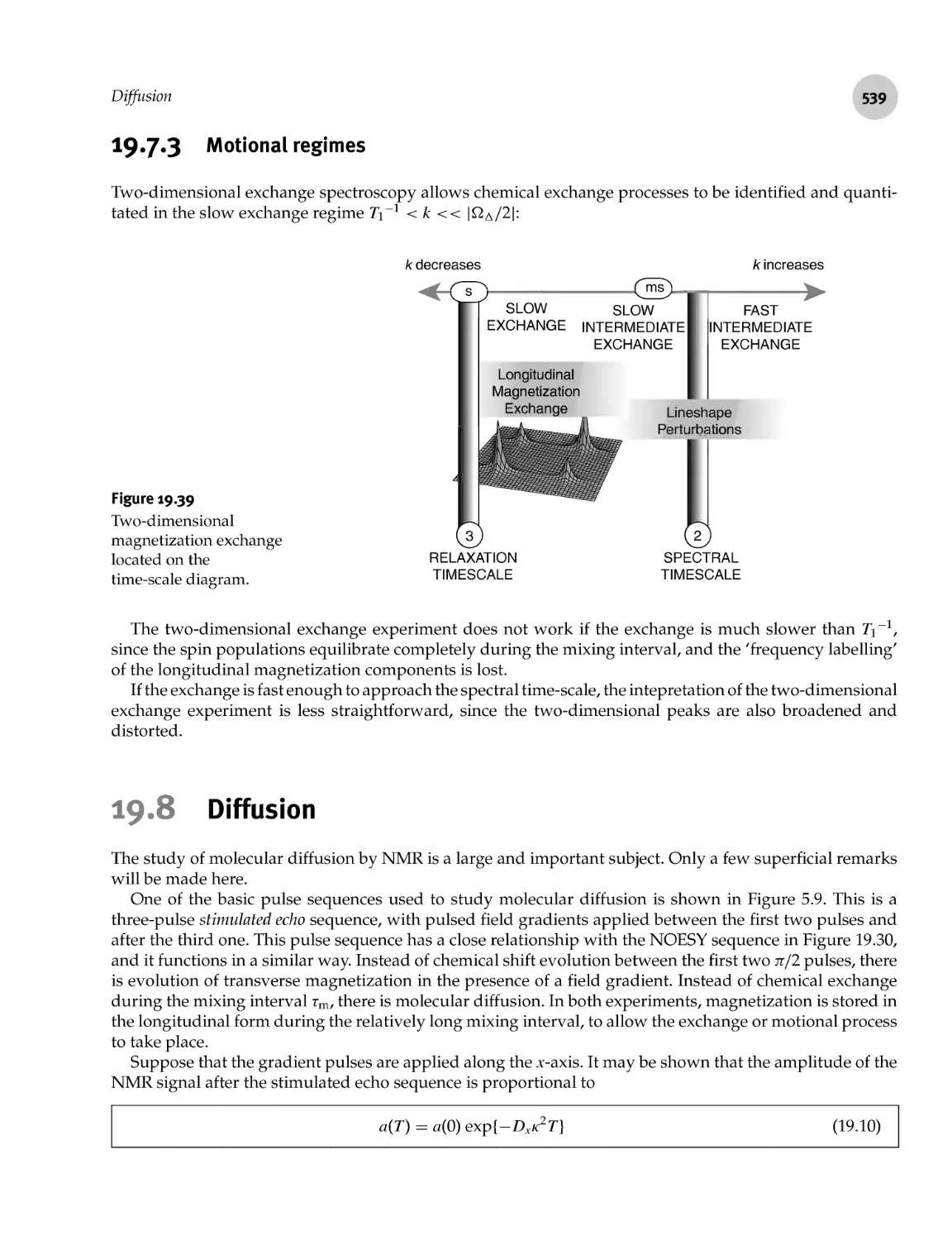
19.7.3 Motional regimes 539
19.8 Diffusion 539
543
543
543
545
545
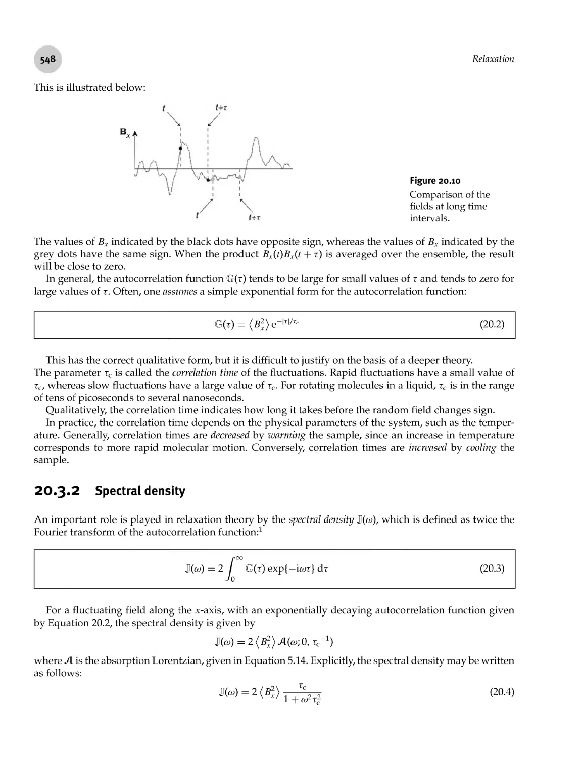
548
549
550
551
552
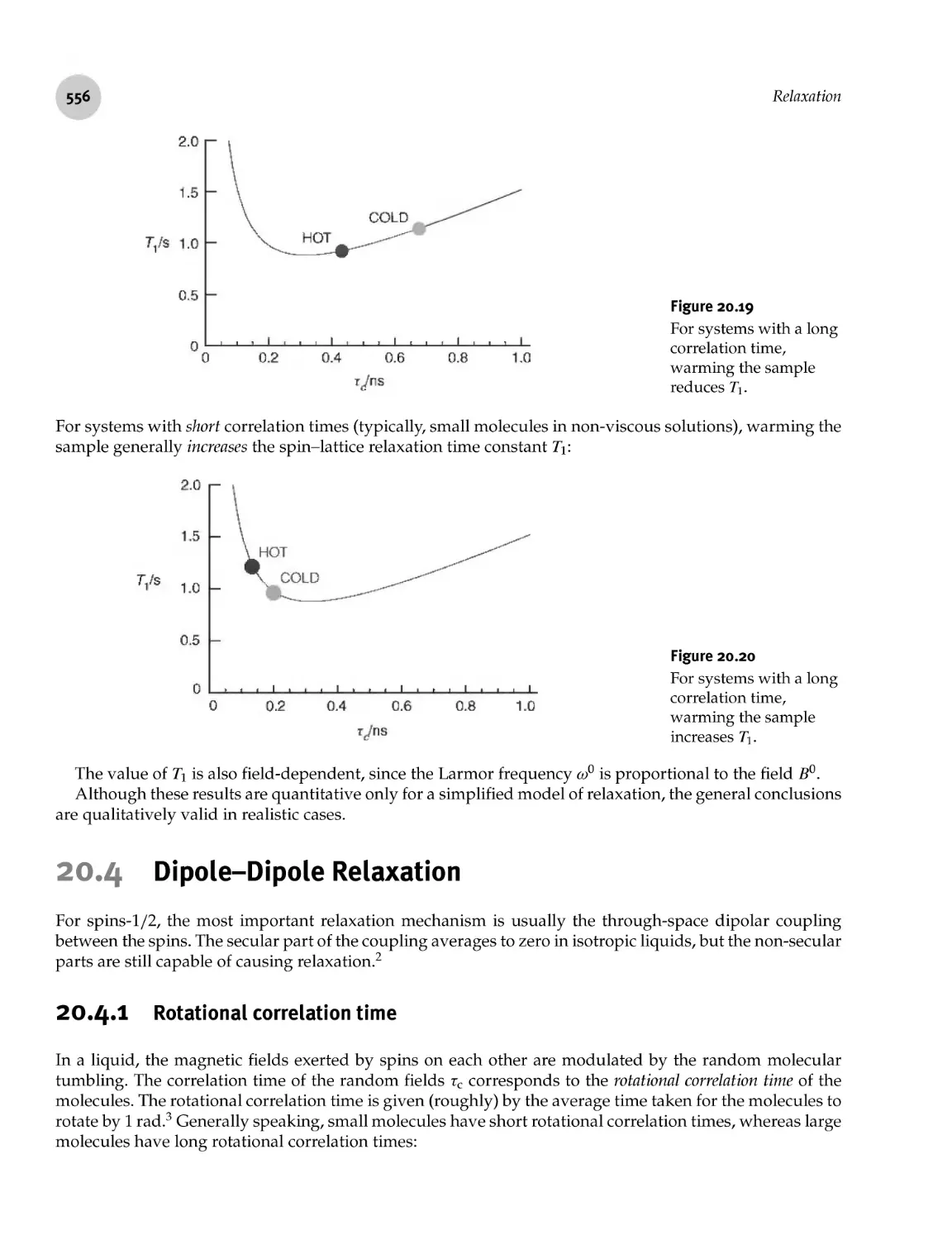
556
556
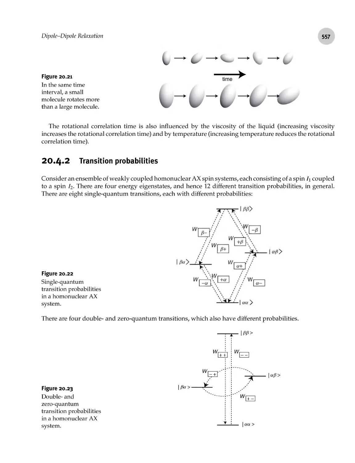
557
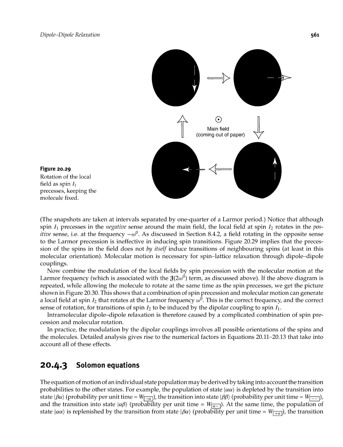
561
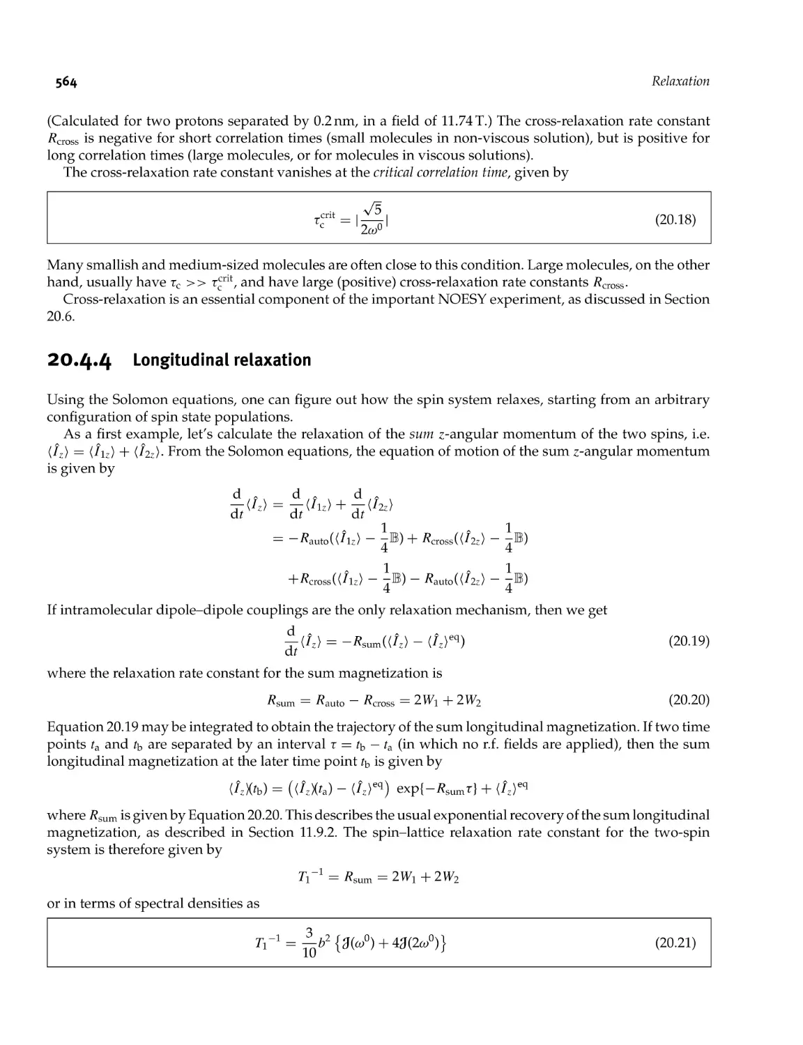
564
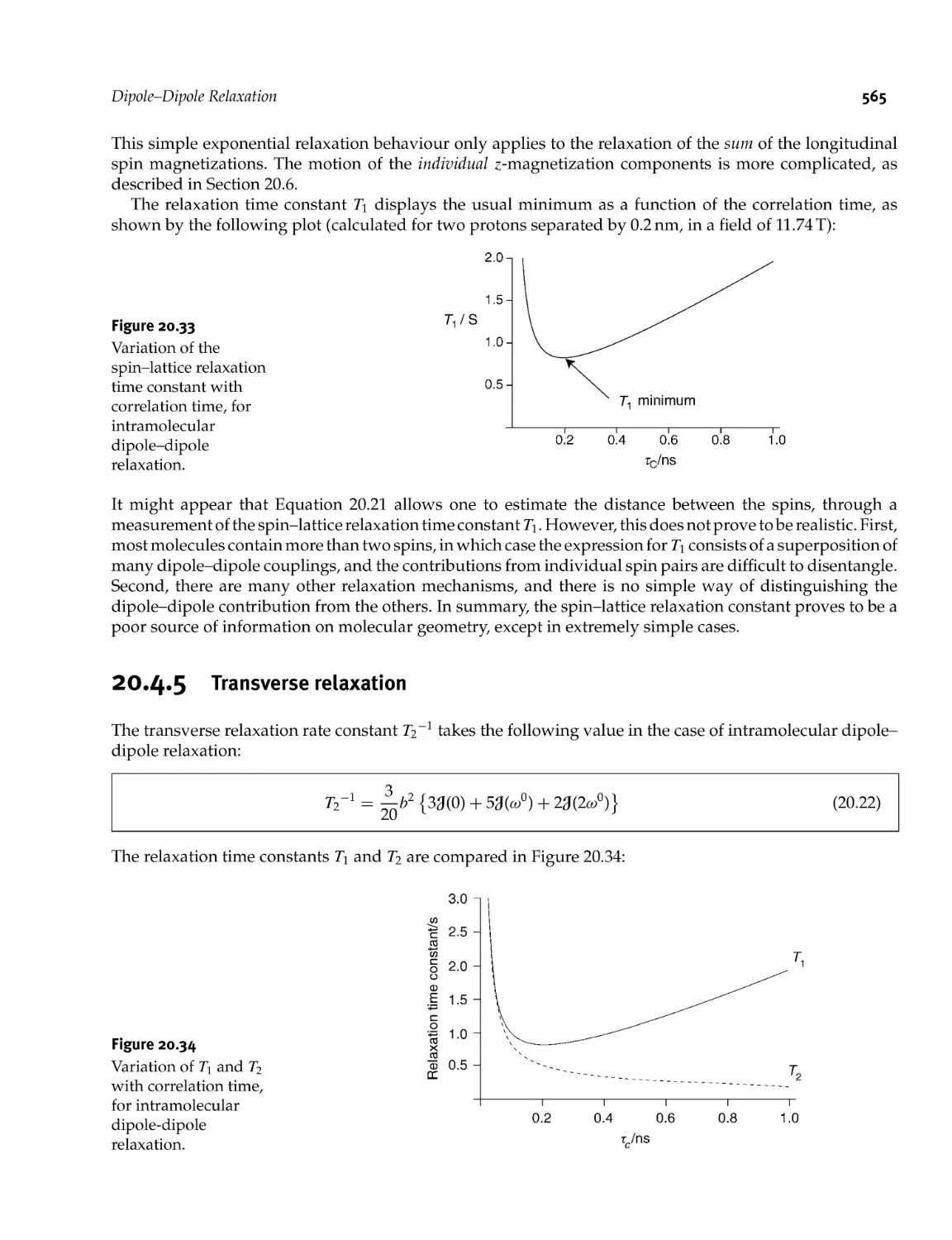
565
566
570
570
570
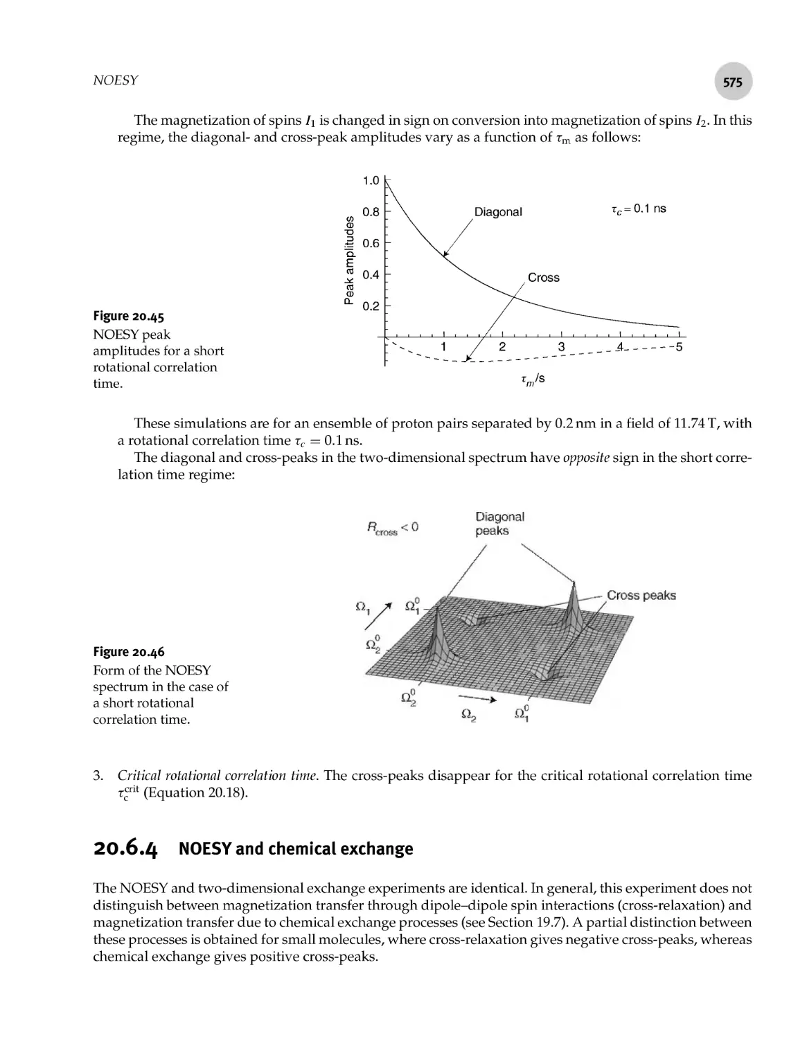
573
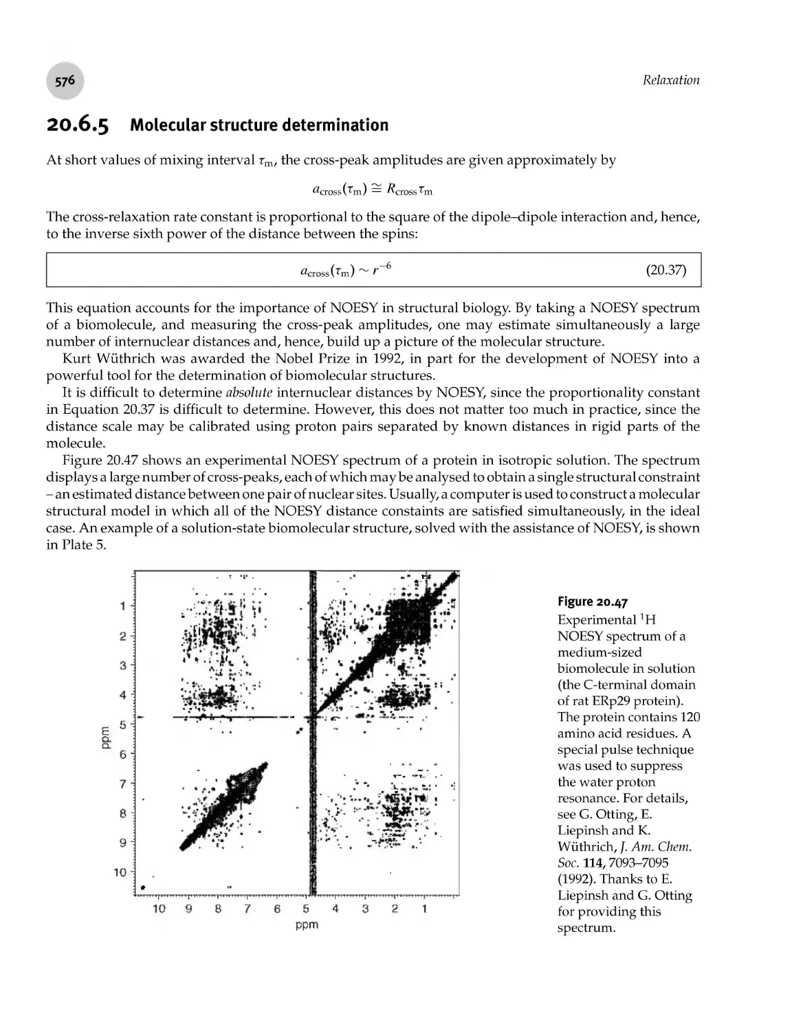
575
576
577
577
578
578
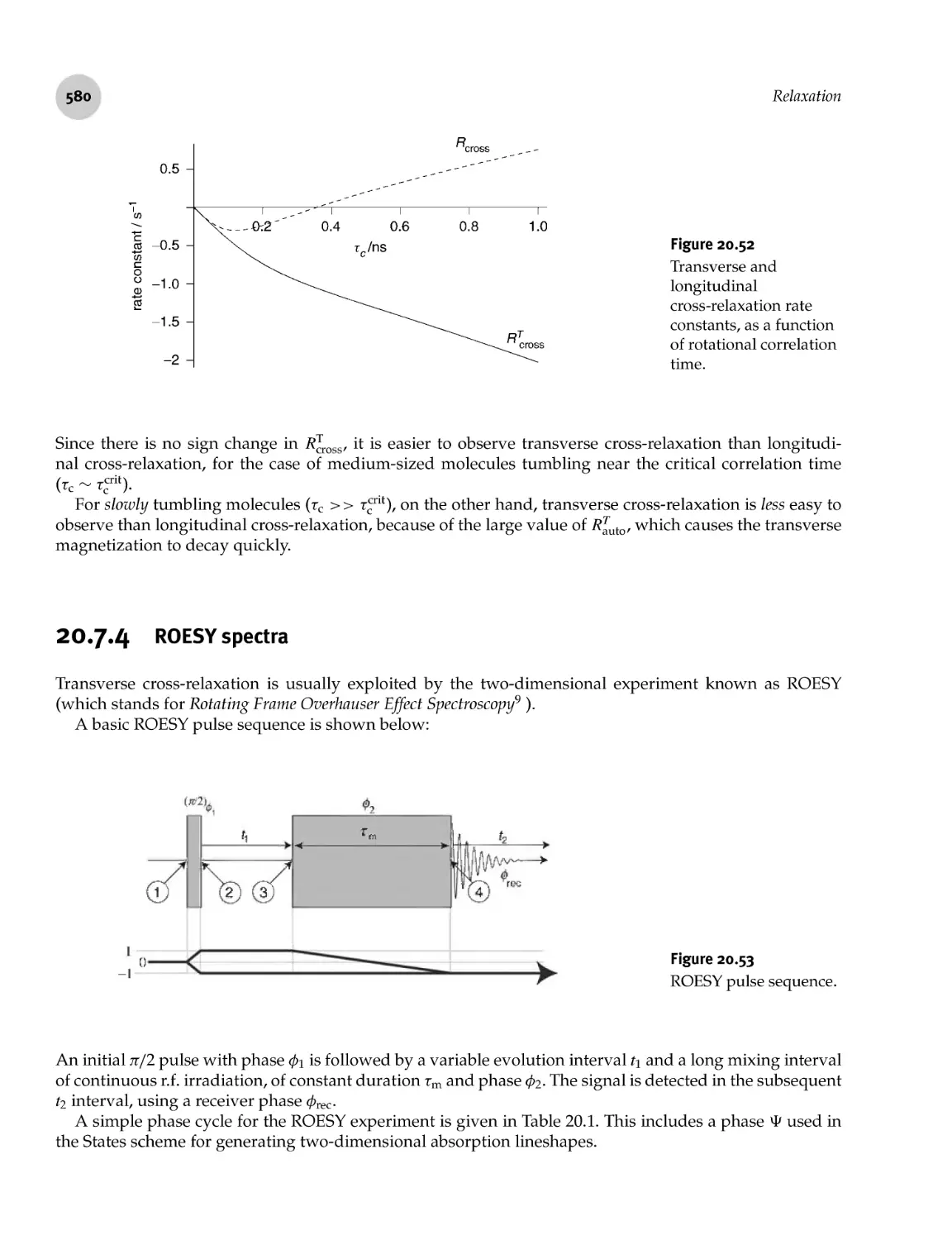
580
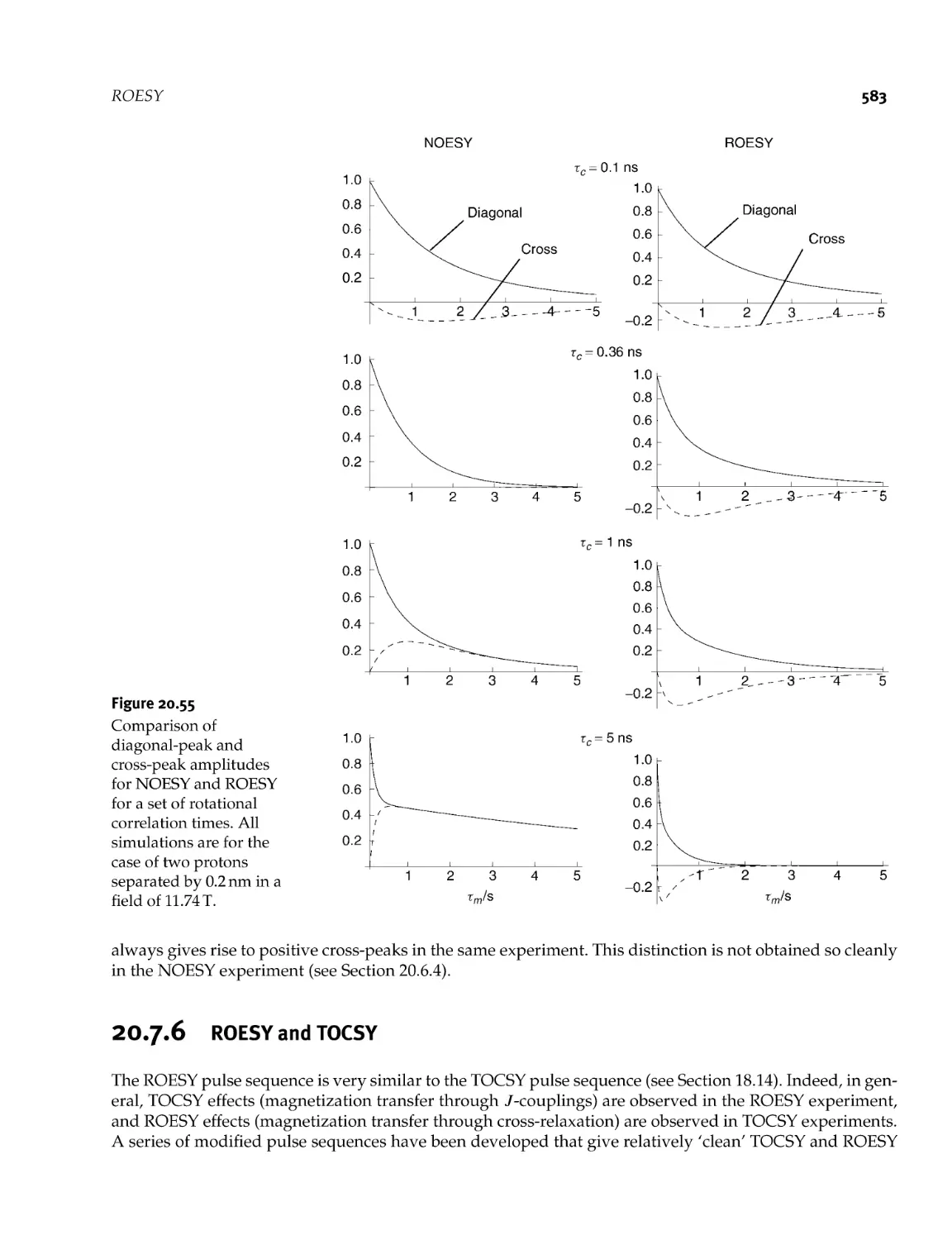
582
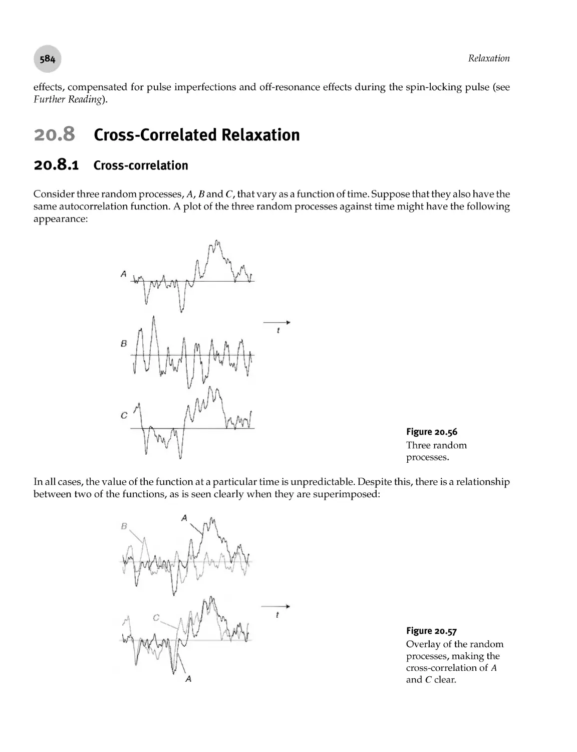
583
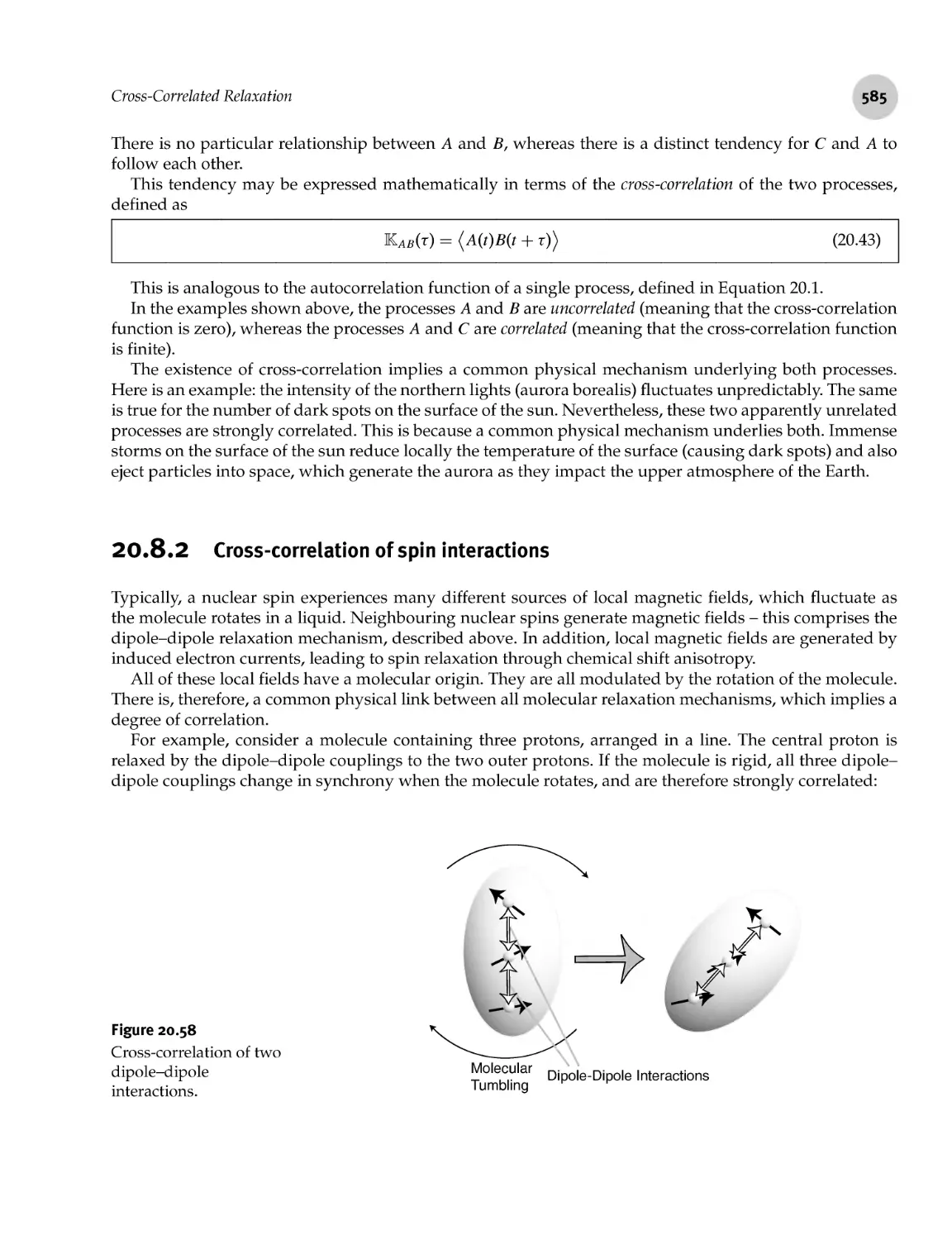
20.8 Cross- Correlated Relaxation 584
20.8.1 Cross- correlation 584
20.8.2 Cross- correlation of spin interactions 585
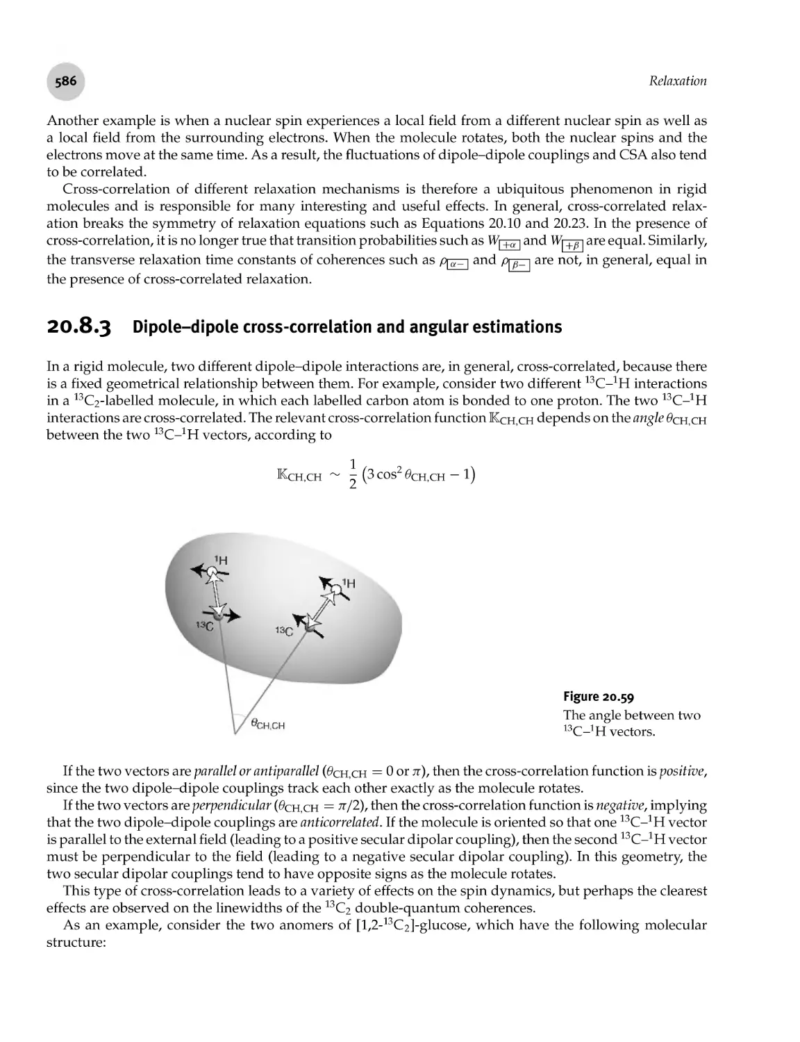
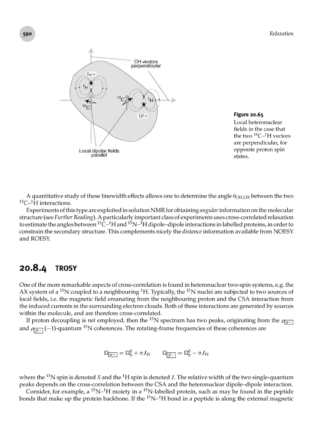
20.8.3 Dipole- dipole cross- correlation and angular estimations 586
20.8.4 TROSY 590
Relaxation
20.1
20.2
20.3
20.4
20.5
20.6
20.7
Types of Relaxation
Relaxation Mechanisms
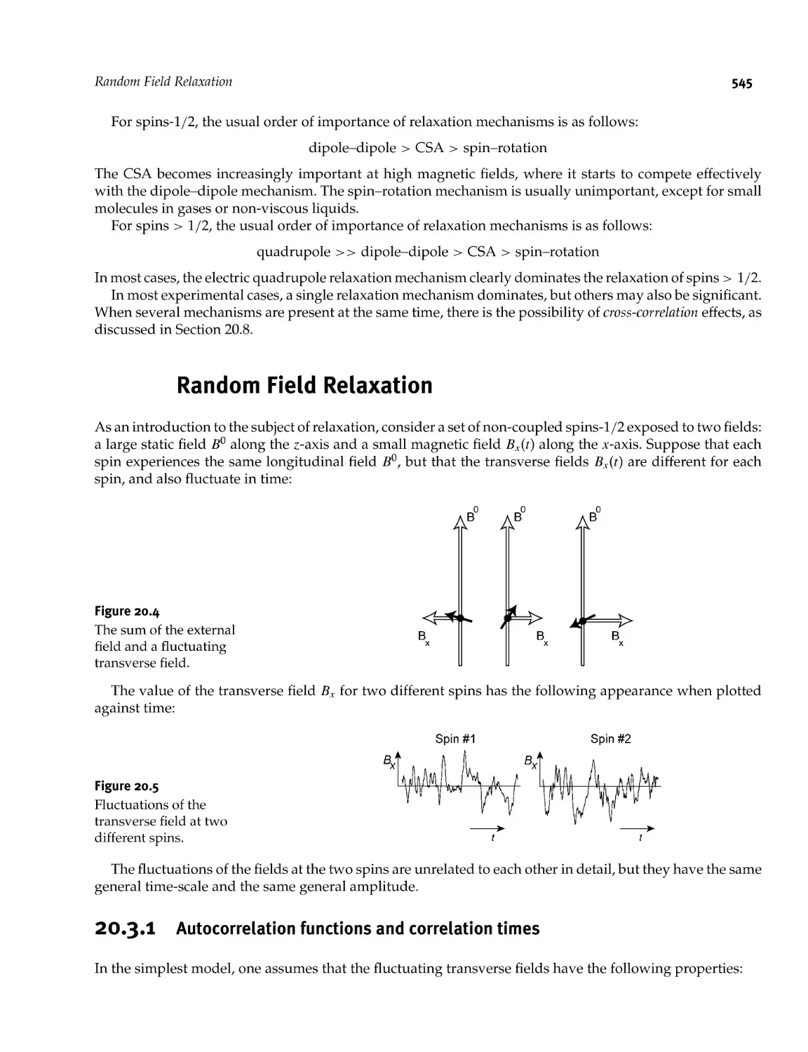
Random Field Relaxation
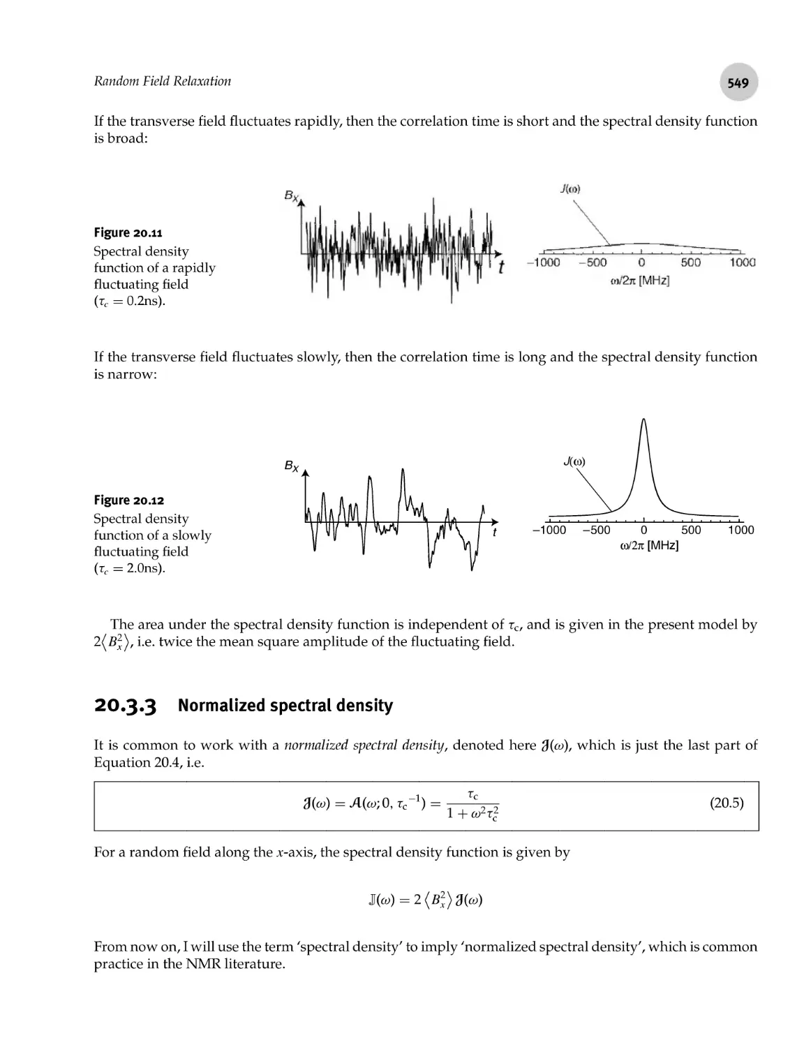
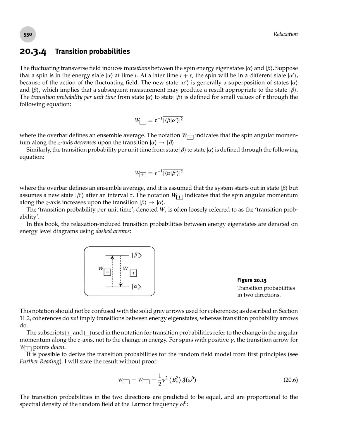
20.3.1 Autocorrelation functions and correlation times
20.3.2 Spectral density
20.3.3 Normalized spectral density
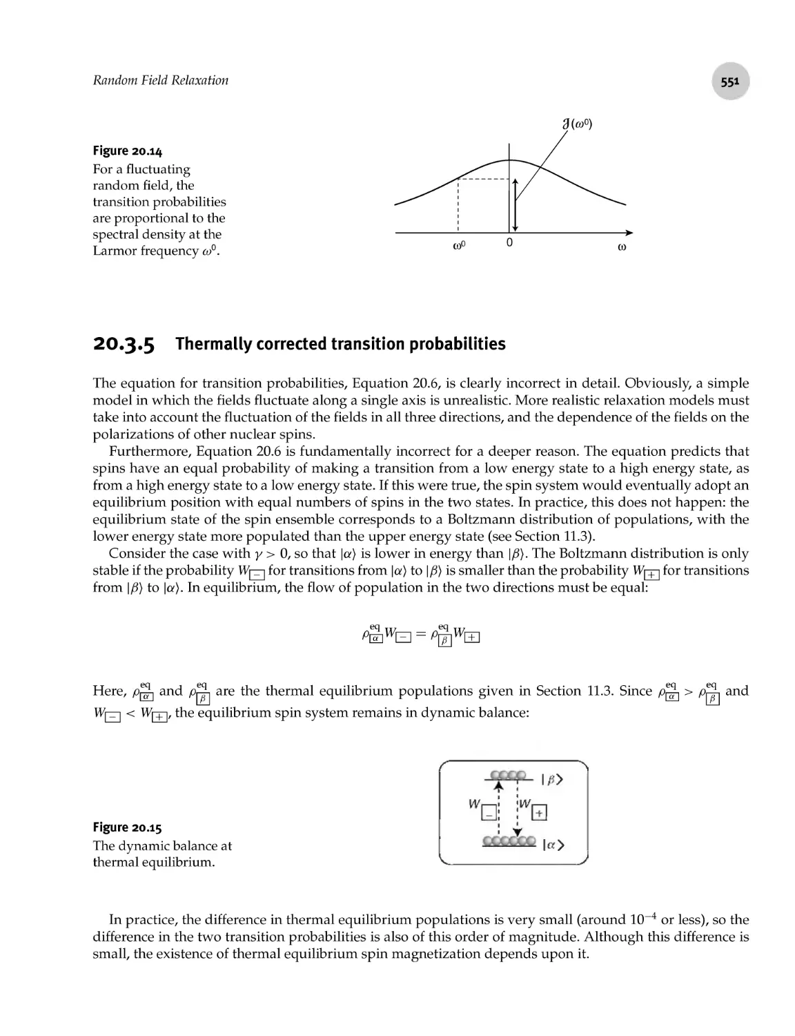
20.3.4 Transition probabilities
20.3.5 Thermally corrected transition probabilities
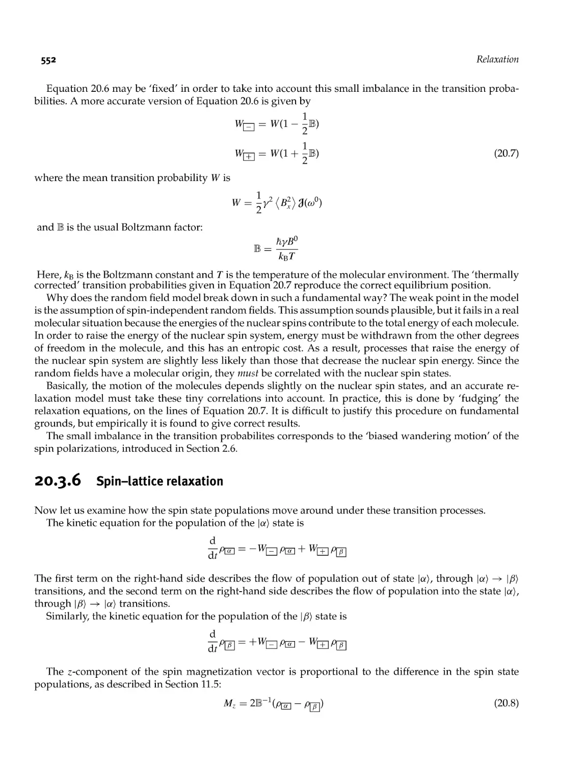
20.3.6 Spin- lattice relaxation
Dipole- Dipole Relaxation
20.4.1 Rotational correlation time
20.4.2 Transition probabilities
20.4.3 Solomon equations
20.4.4 Longitudinal relaxation
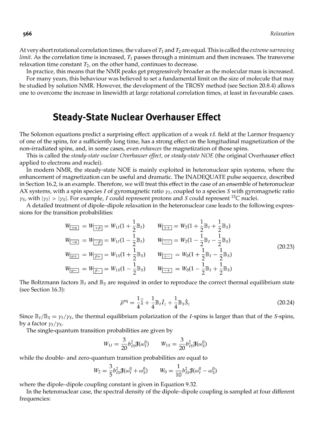
20.4.5 Transverse relaxation
Steady- State Nuclear Overhauser Effect
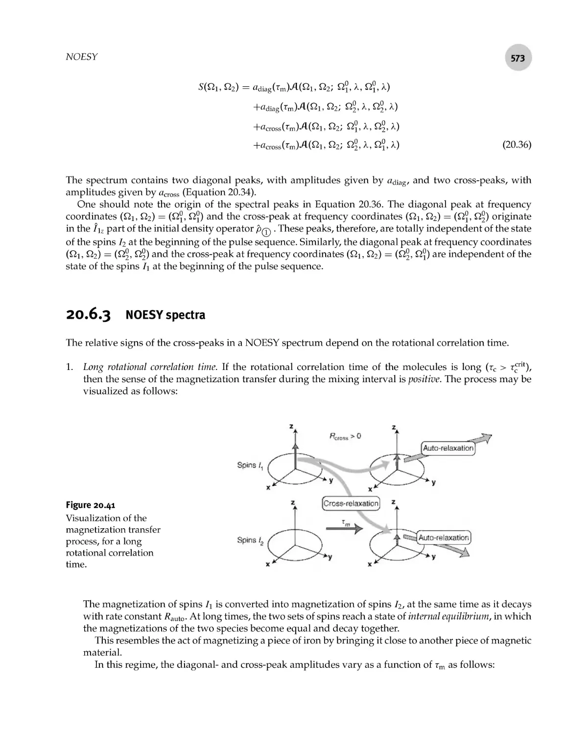
NOESY
20.6.1 NOESY pulse sequence
20.6.2 NOESY signal
20.6.3 NOESY spectra
20.6.4 NOESY and chemical exchange
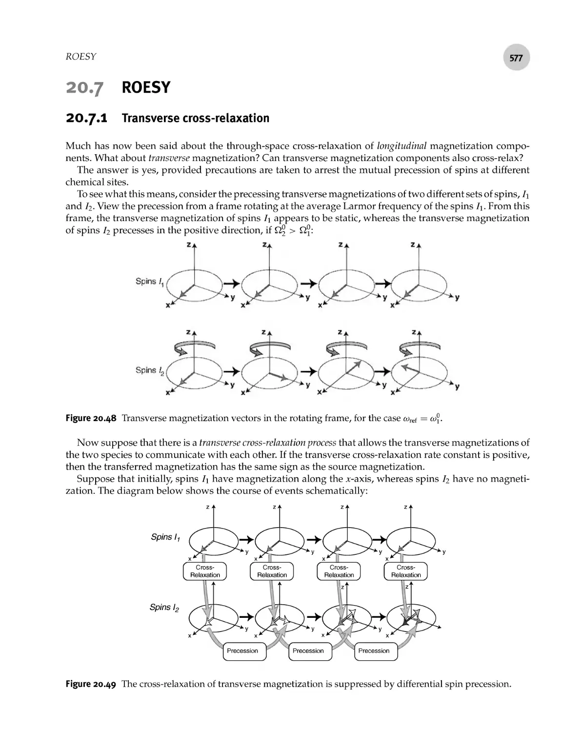
20.6.5 Molecular structure determination
ROESY
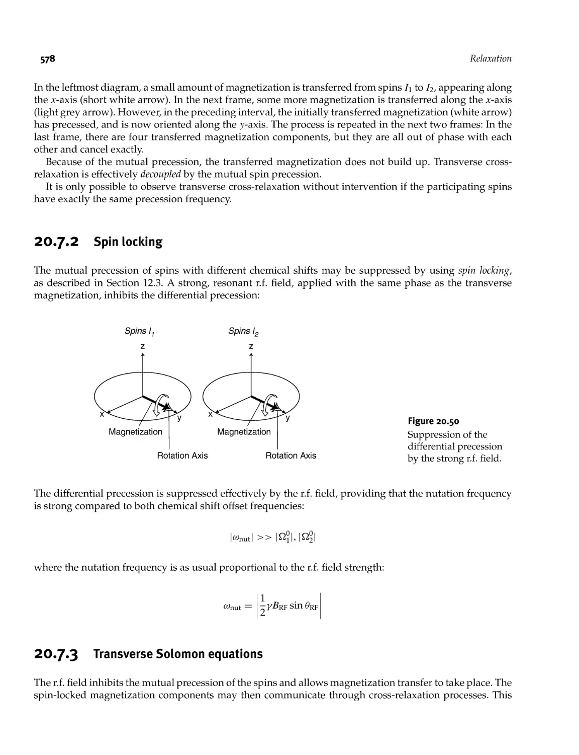
20.7.1 Transverse cross- relaxation
20.7.2 Spin locking
20.7.3 Transverse Solomon equations
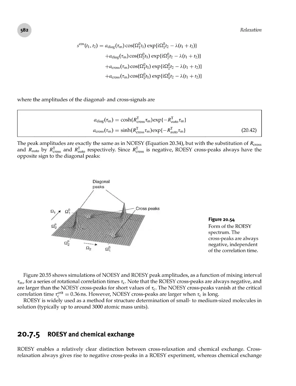
20.7.4 ROESY spectra
20.7.5 ROESY and chemical exchange
20.7.6 ROESY and TOCSY

xviii Contents
Part 8 Appendices 597
Appendix A: Supplementary Material 599
A.l Euler Angles and Frame Transformations 599
A.l.l Definition of the Euler angles 599
A.l.2 Euler rotations: first scheme 599
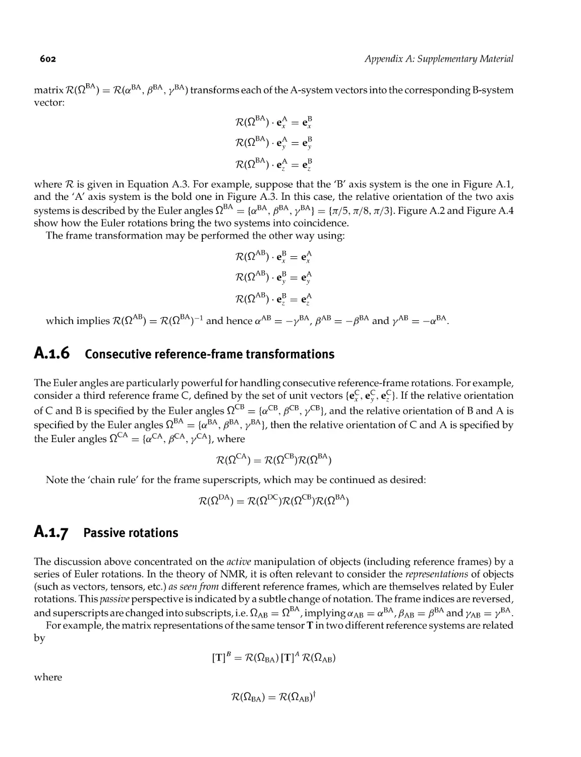
A.l.3 Euler rotations: second scheme 600
A.l.4 Euler rotation matrices 601
A.l.5 Reference- frame orientations 601
A.l.6 Consecutive reference- frame transformations 602
A.l.7 Passive rotations 602
A.l.8 Tensor transformations 603
A.l.9 Intermediate reference frames 604
A.2 Rotations and Cyclic Commutation 604
A.3 Rotation Sandwiches 605
A.4 Spin- 1/2 Rotation Operators 606
A.5 Quadrature Detection and Spin Coherences 608
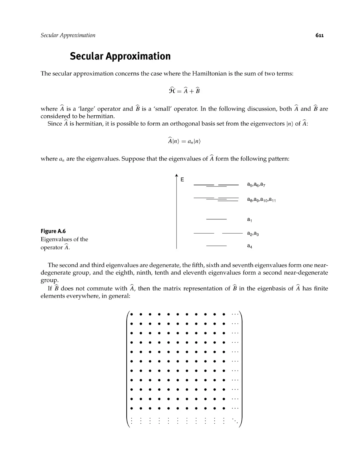
A.6 Secular Approximation 611
A.7 Quadrupolar Interaction 614
A.7.1 Full quadrupolar interaction 614
A.7.2 First- order quadrupolar interaction 614
A.7.3 Higher- order quadrupolar interactions 615
A.8 Strong Coupling 615
A.8.1 Strongly- coupled Spin- 1/2 pairs 615
A.8.2 General strongly coupled systems 620
A.9 /- Couplings and Magnetic Equivalence 621
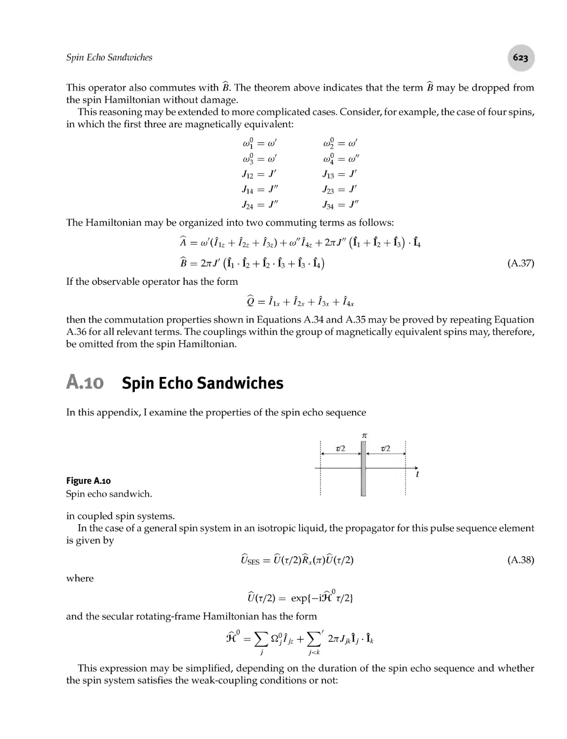
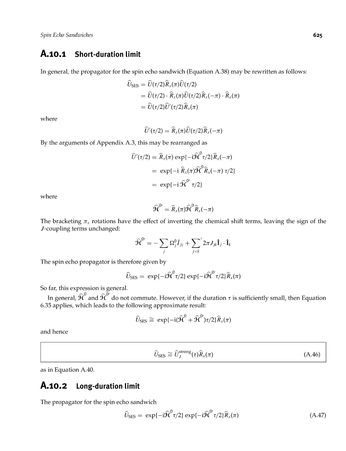
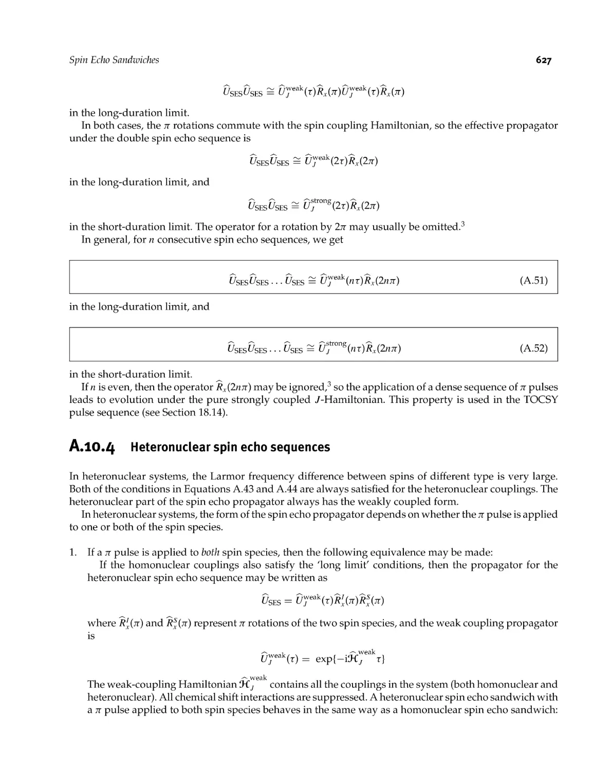
A. 10 Spin Echo Sandwiches 623
A.10.1 Short- duration limit 625
A. 10.2 Long- duration limit 625
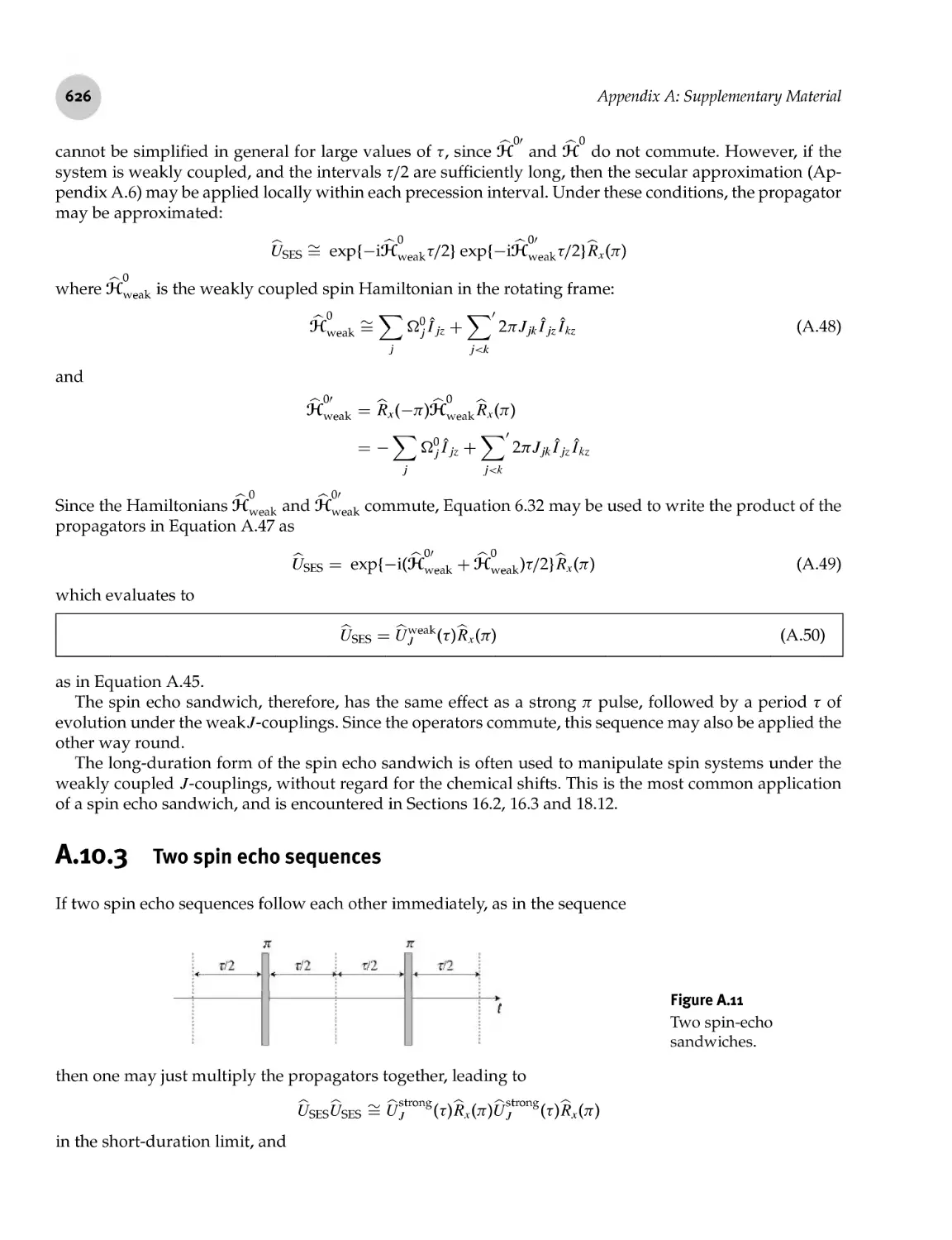
A. 10.3 Two spin echo sequences 626
A. 10.4 Heteronuclear spin echo sequences 627
A. 11 Phase Cycling 629
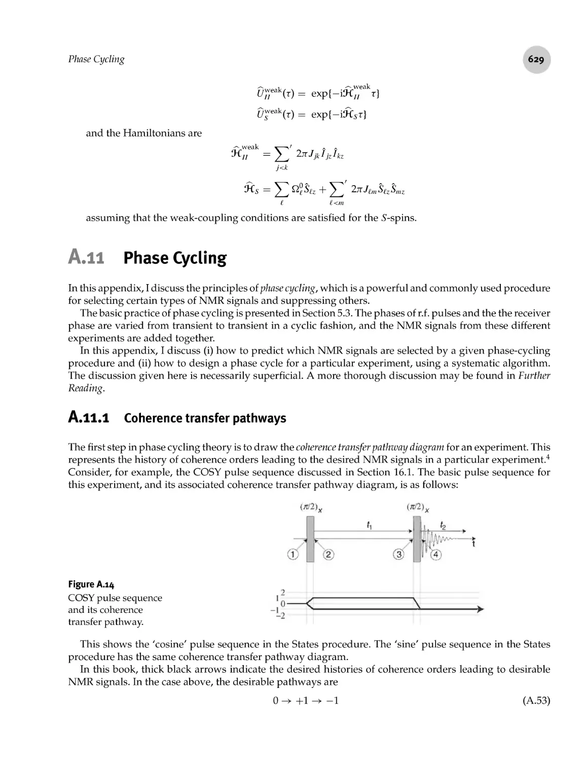
A. 11.1 Coherence transfer pathways 629
A. 11.2 Coherence transfer amplitudes 630
A. 11.3 Coherence orders and phase shifts 631
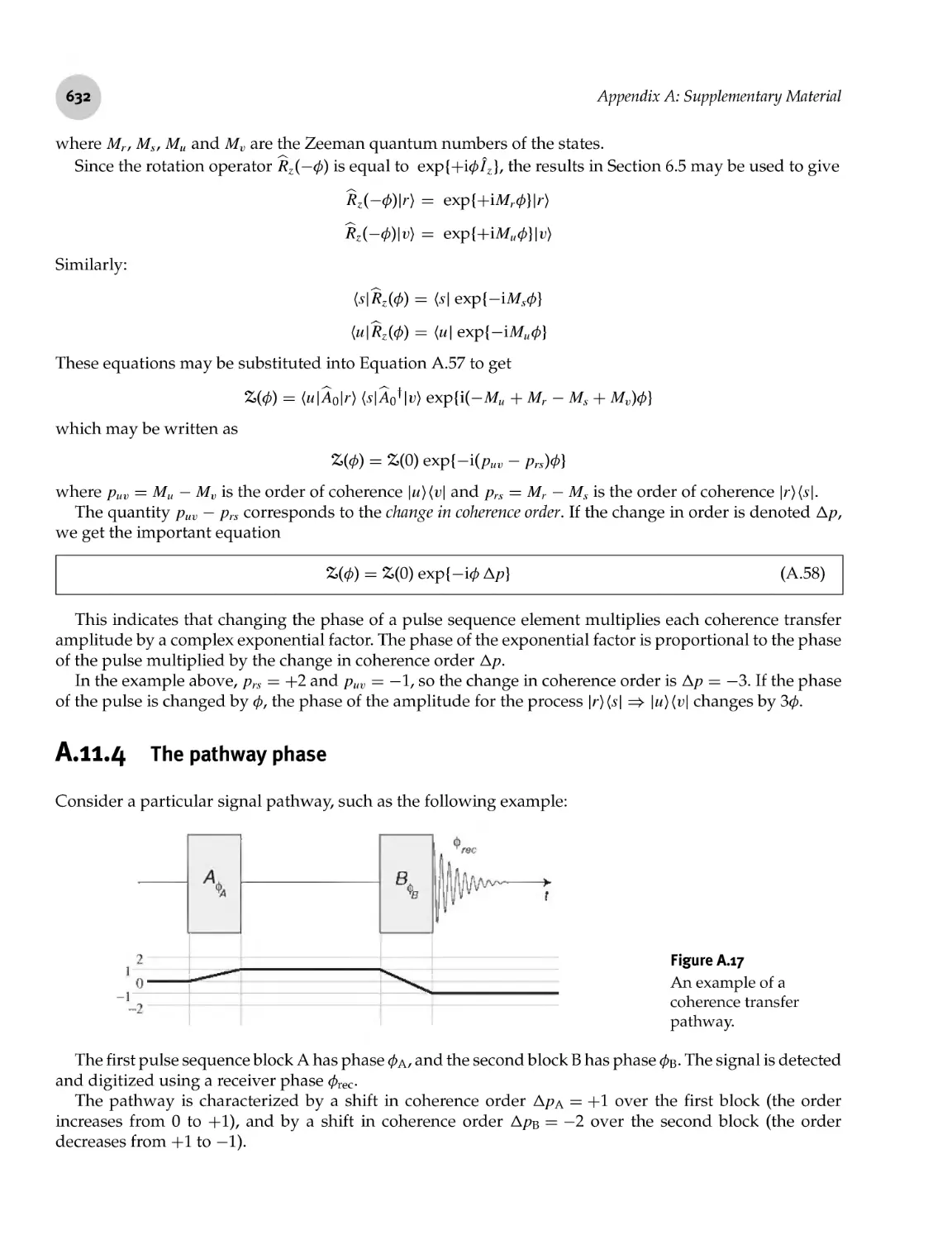
A.11.4 The pathway phase 632
A. 11.5 A sum theorem 633
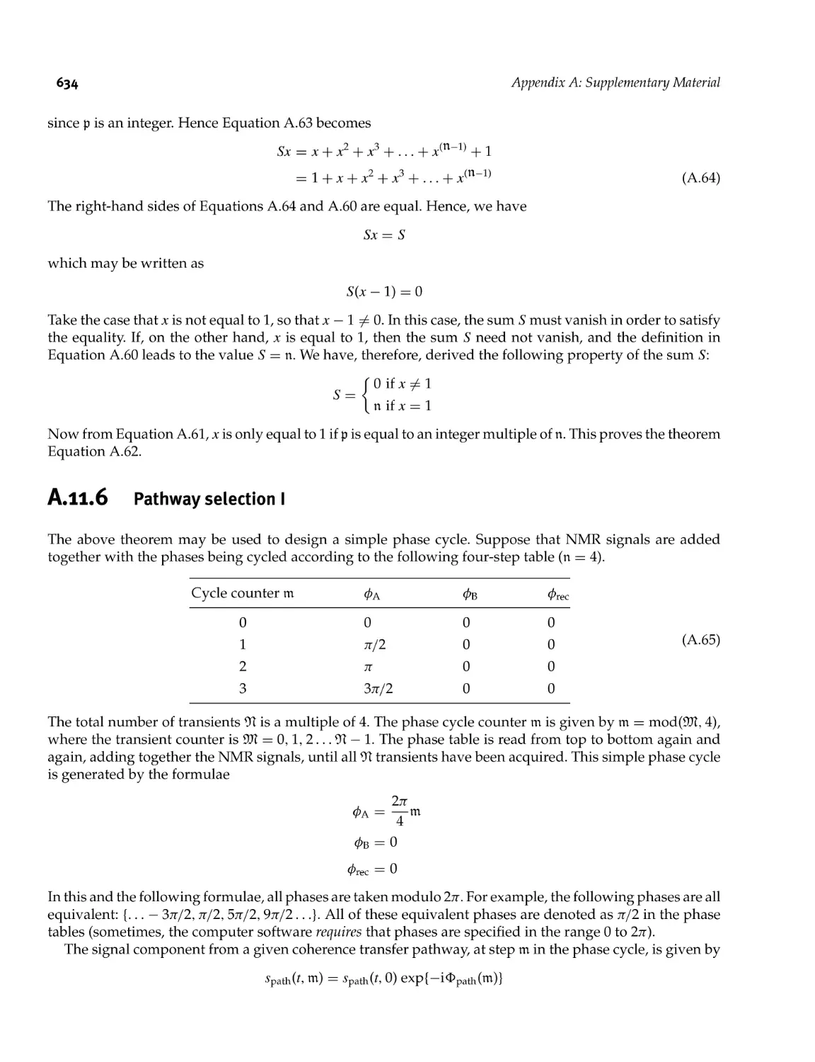
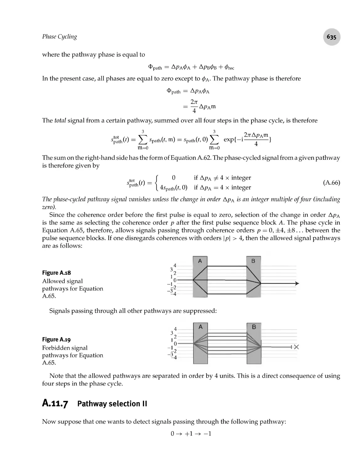
A. 11.6 Pathway selection I 634
A.11.7 Pathway selection II 635
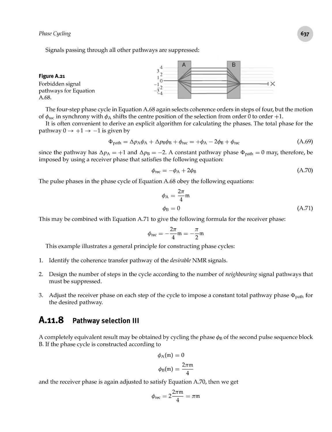
A.11.8 Pathway selection III 637
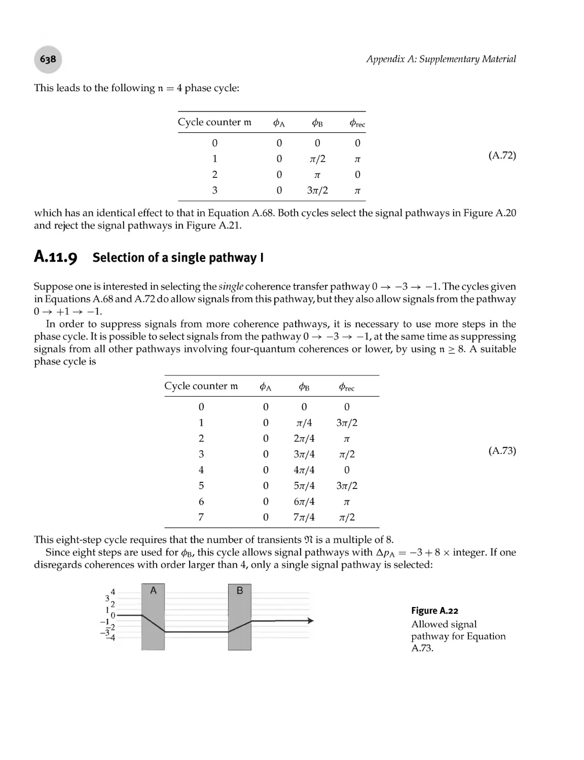
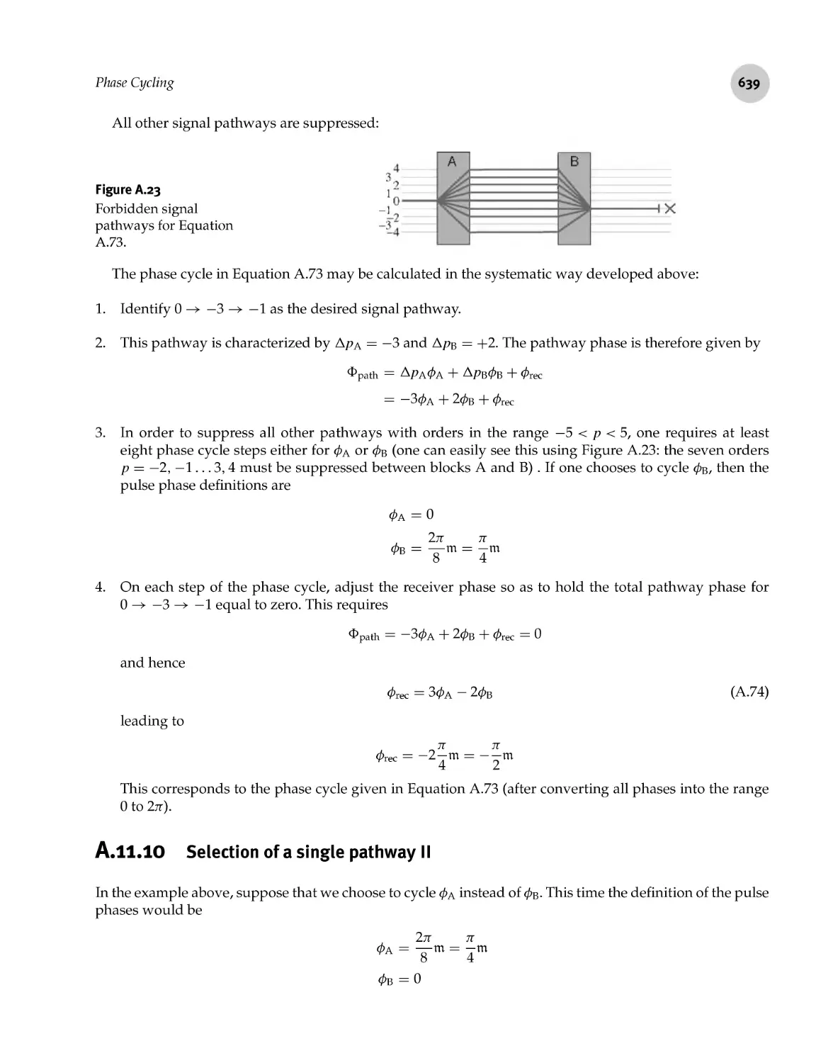
A. 11.9 Selection of a single pathway I 638
A.11.10 Selection of a single pathway II 639
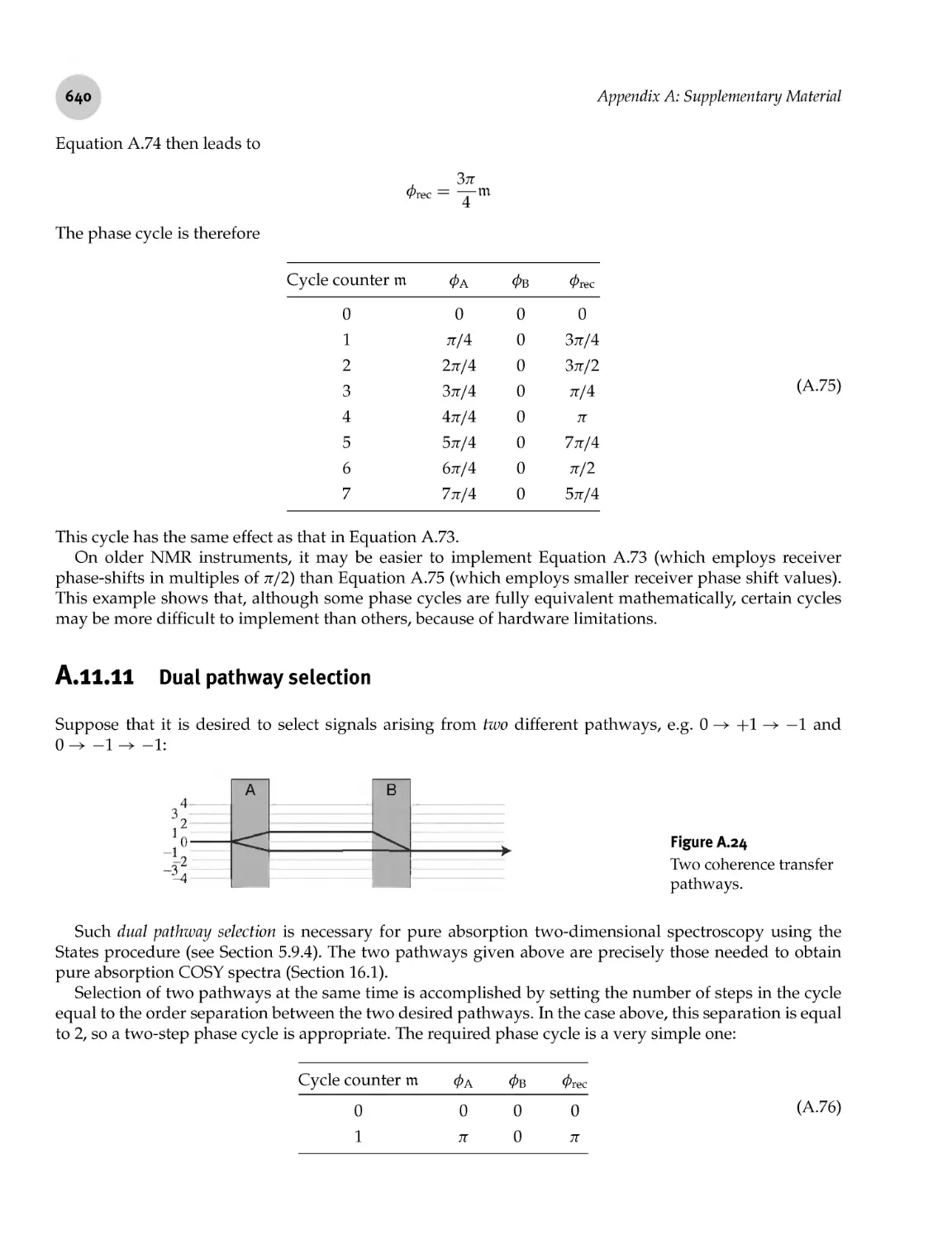
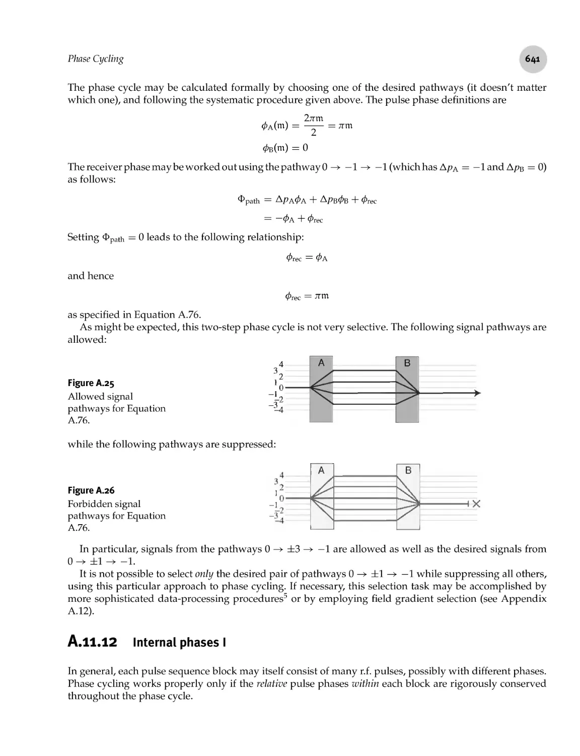
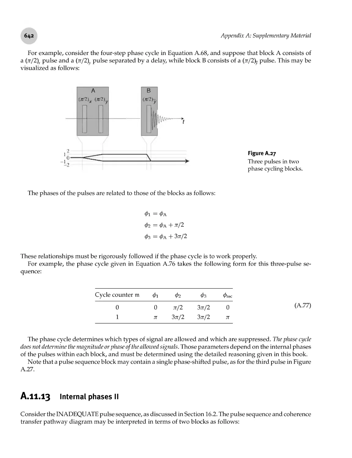
A.ll.ll Dual pathway selection 640
A.11.12 Internal phases I 641
A.11.13 Internal phases II 642
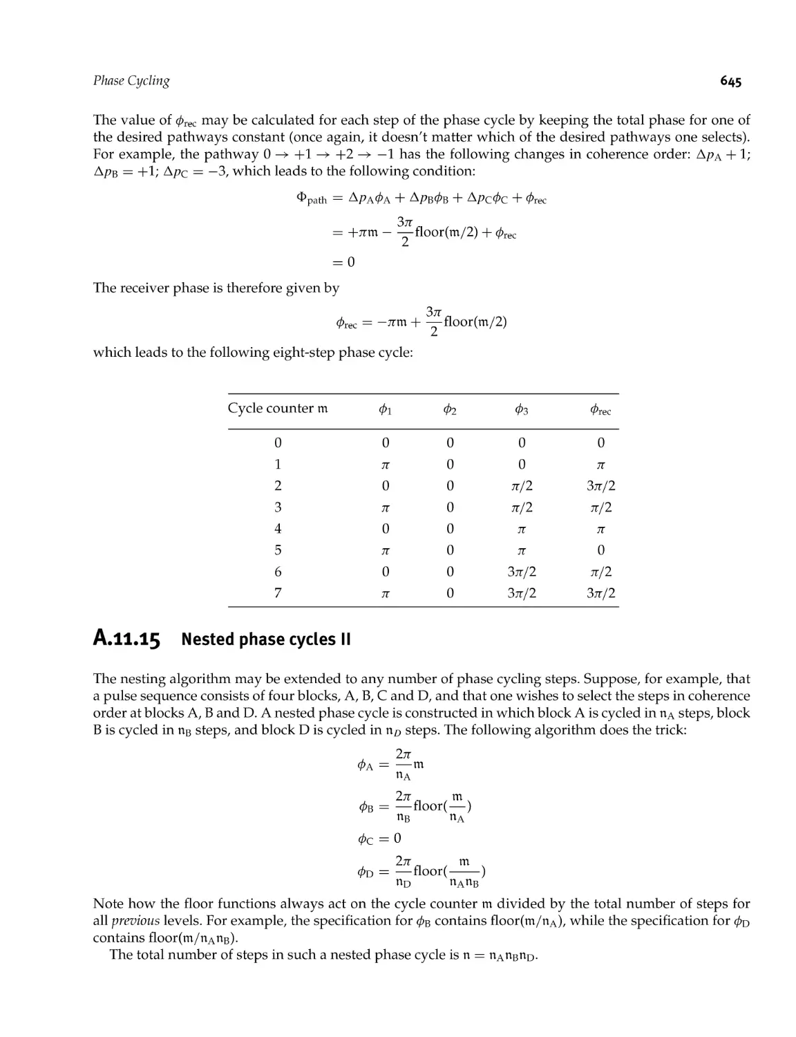
A.11.14 Nested phase cycles I 644
A.11.15 Nested phase cycles II 645
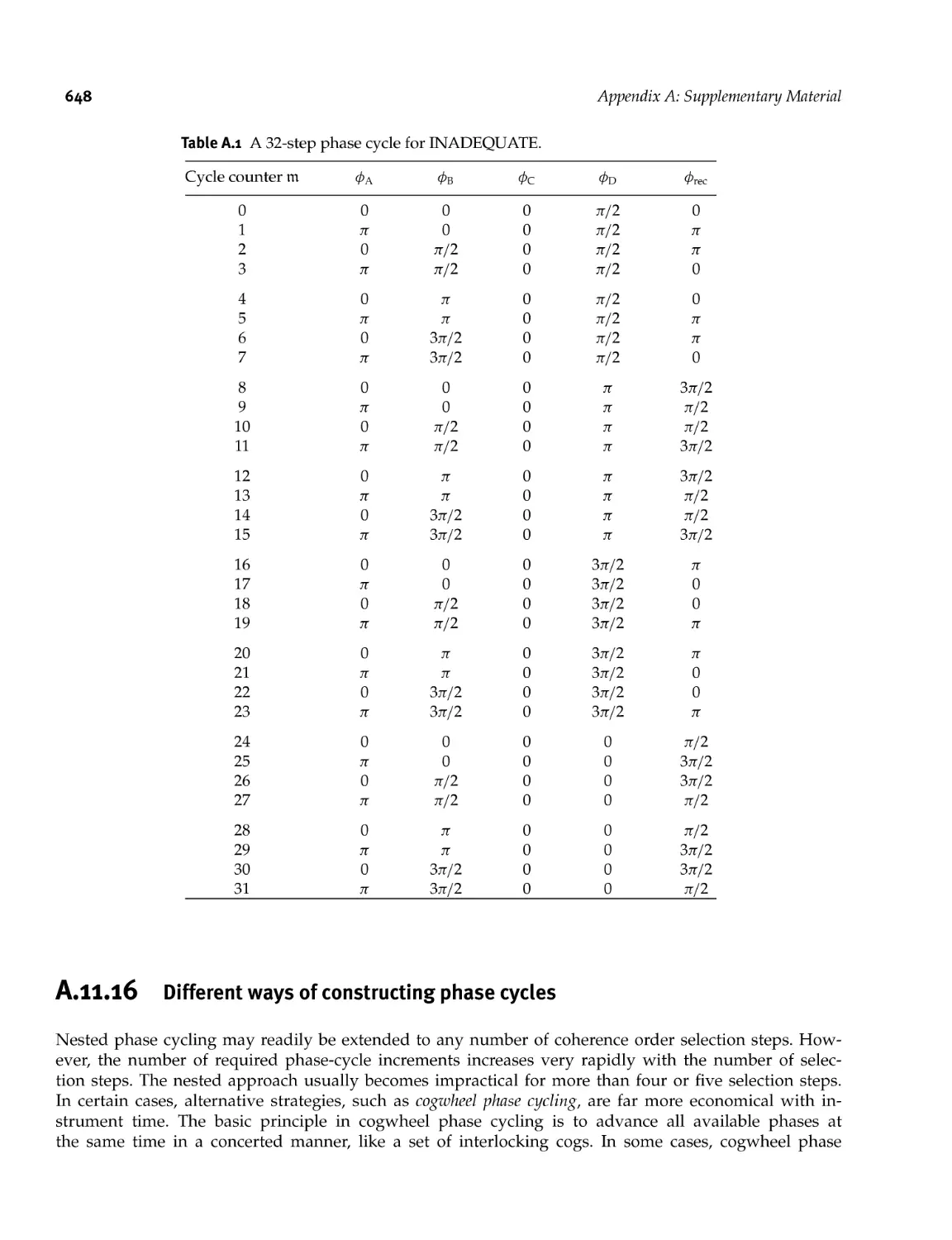
A. 11.16 Different ways of constructing phase cycles 648

Contents
xix
649
649
651
652
652
652
653
654
655
655
656
658
660
662
Appendix B: Symbols and Abbreviations 665
Answers to the Exercises 681
.12
.13
.14
.15
.16
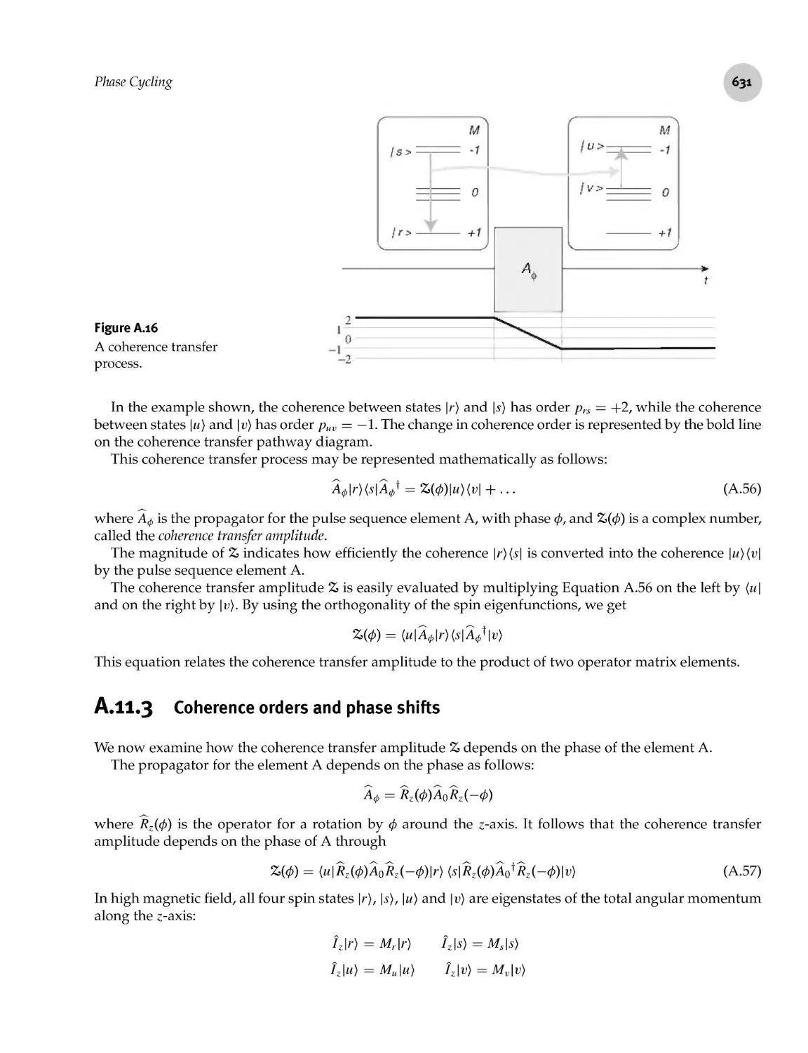
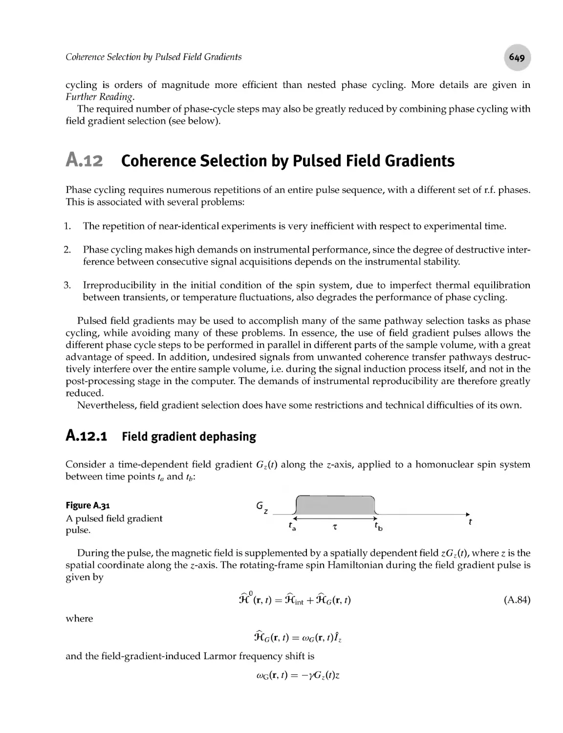
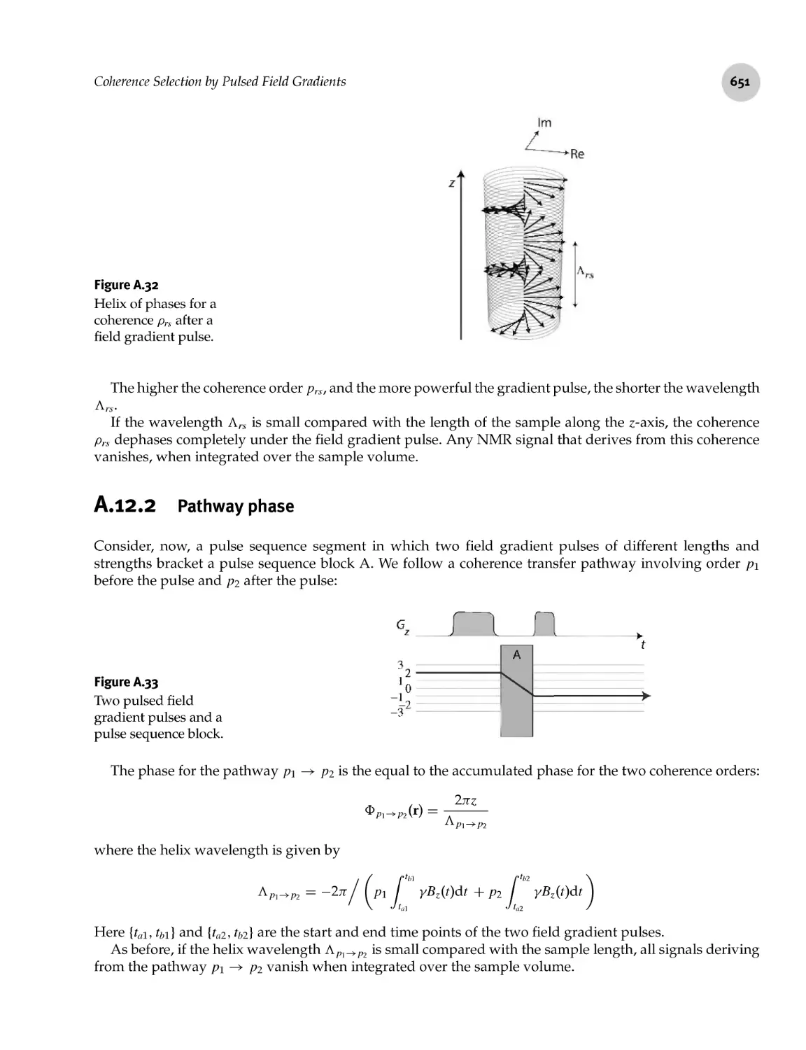
Coherence Selection by Pulsed Field Gradients
A.12.1 Field gradient dephasing
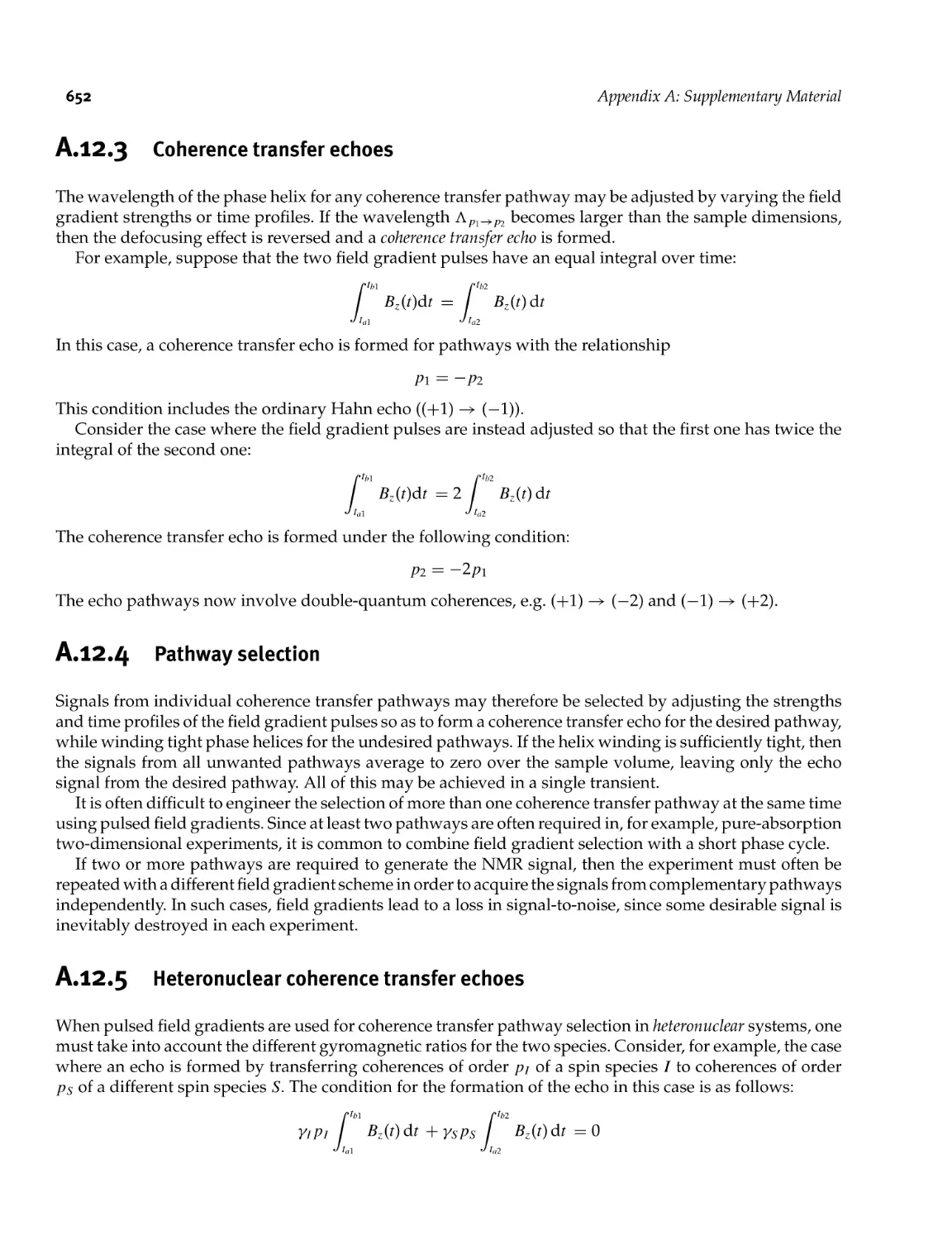
A.12.2 Pathway phase
A.12.3 Coherence transfer echoes
A.12.4 Pathway selection
A.12.5 Heteronuclear coherence transfer echoes
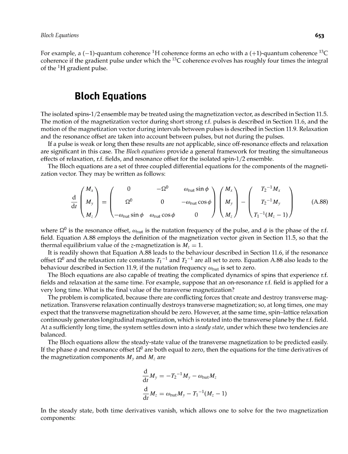
Bloch Equations
Chemical Exchange
A. 14.1 The incoherent dynamics
A.14.2 The coherent dynamics
A.14.3 The spectrum
A.14.4 Longitudinal magnetization exchange
Solomon Equations
Cross- Relaxation Dynamics
Index
693


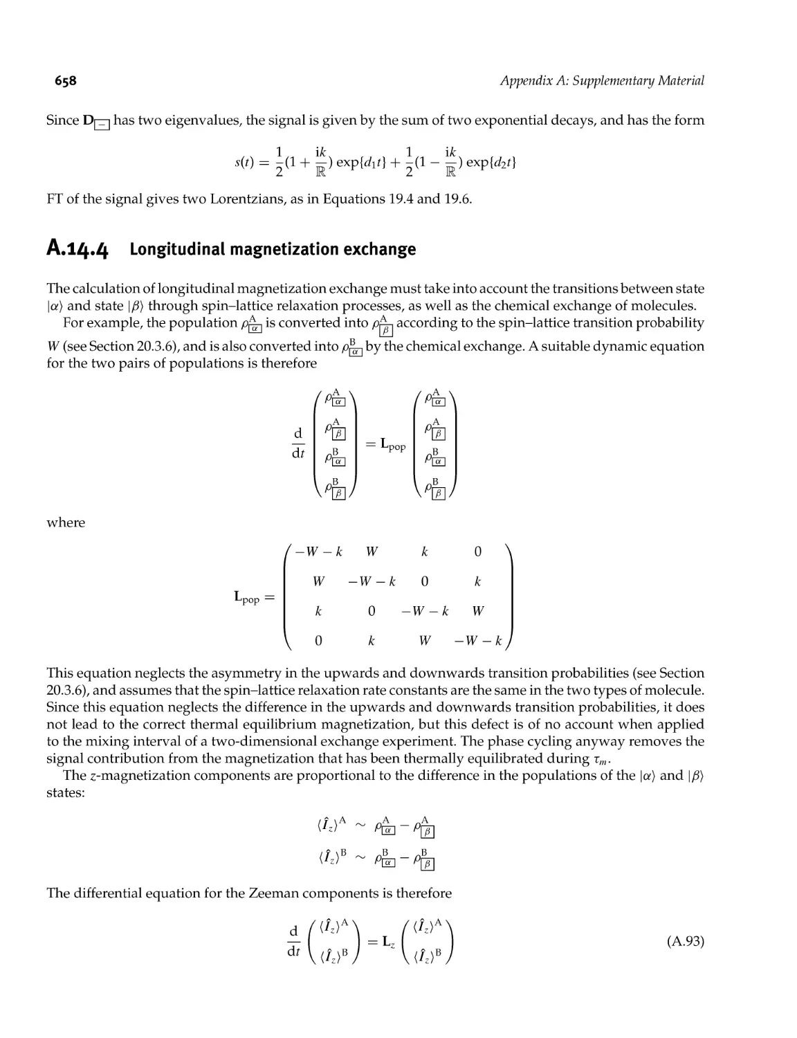
In this second edition I have tried to address some of the deficiencies of the first edition, but without
disturbing the structure of the text too much. I have now included an overview of the NMR of quadrupolar
nuclei, given the important subject of pulsed field gradients more prominence, and addressed the subject
of spin- 1/2 pairs in solids more thoroughly. It is a complex task to revise a large book, and I am not sure
whether I have been successful. Let's see what you think.
I am very grateful to all the people who pointed out errors in the first edition, which I hope to have
corrected in this new version. These include Juan Alberdi, Bernard Ancian, Stefan Berger, Tom Bloemberg,
Geoffrey Bodenhausen, Dave Bryce, Shidong Chu, Andre Dorsch, Nick Higham, Vladimir Hnizdo, Eric
Johnson, Alan Kenwright, Karel Klika, Olivier Lafon, Linda Lai, Young Lee, Phil Lucht, Slobodan Macura,
P. K. Madhu, Ian Malcolm, Arnold Maliniak, Emi Miyoshi, Gareth Morris, Norbert Muller, Juan Paniagua,
Tanja Pietrass, Tatyana Polynova, E. J. Pone, Jan Rainey, Michael Roehrl, David Siminovitch, Chunpen
Thomas, Bill Wallace, John Waugh, and Steven Wimperis. I also thank Zosia Beckles for help with the initial
computer spadework.
As always, my research group and our research visitors have been a constant source of inspiration
and enthusiasm. So I thank Giancarlo Antonioli, Jacco van Beek, Pauline Brouillaud, Darren Brouwer,
Marina Carravetta, Maria Concistre, Andre Dorsch, Axel Gansmuller, Natala Ivchenko, Ole Johannessen,
Per- Eugen Kristiansen, Linda Lai, P. K. Madhu, Salvatore Mamone, Ildefonso Marfn- Montesinos, Giulia
Mollica, and Giuseppe Pileio for your input. Many of the new sections in this book have derived from our
group discussions.
Special thanks to Geoffrey Bodenhausen and Angelika Sebald for giving detailed criticism on the text.
Thanks to P. K. Madhu for the photograph from India.
Fiona Woods and Andy Slade at Wiley have been patient, encouraging and helpful during the preparation
of this edition.
As usual, I take sole responsibility for any errors and omissions.
Finally, I thank my wife and daughter Latha and Leela again, for their renewed patience and support.
Technical Details
The book was written on Apple Macintosh® computers. The text was written in LaTeX®, using a large
number of self- programmed macros. Most of the diagrams were drawn by the author using a combination
of Mathematical and Adobe Illustrator®. Errata and supplementary notes are available through the website
www.mhl.soton.ac.uk


This book has a long prehistory. It began approximately 12 years ago, when I was persuaded by my friend
(and squash court enemy) Jim Sudmeier, to give a short series of lectures on the basics of NMR at Tufts
University in Boston, MA. The lectures were probably not a tremendous success, but I was inspired to
write up the material as some sort of short book. I was naive enough to feel that I could probably cover the
basics in perhaps 100 pages using a minimum of equations. I worked on this 'proto- book' for over a year in
Cambridge, England, before I realised that I was only scratching the surface of the subject and that I was
not yet prepared for the task.
The situation changed in Stockholm where I became involved in teaching an intensive course each year on
NMR to third- year undergraduates. Over a period of around seven years I built up a large set of handwritten
lecture notes. The experience of teaching made me realise how difficult it is to keep the subject accessible
while still imparting something useful to those students wishing to continue into NMR research. Over many
years I experimented with various permutations of the material until I ended up with a set of notes which
form the basis of this book.
The bulk of the final writing was done in India where I enjoyed the hospitality of Professor Anil Kumar
at the Indian Institute of Science in Bangalore for three months.
The book which emerged is still not precisely the one I wanted to write: I wanted to communicate the
beauty and usefulness of NMR in a rather simple and non- mathematical way. In the end, I did not succeed at
all in keeping down the number of equations. Teaching showed me that equations are simply the only way
to present the subject clearly. Nevertheless, although some of the mathematics may look a little frightening
to the uninitiated, I think none of it is truly difficult. Most workers in NMR, including myself, have somehow
learnt to muddle through the mathematics without any formal training, and the mathematics given here is
just a distillation of my own muddling.
The one thing more discouraging to students than anything else is bad terminology and notation,
especially when its defects are not pointed out plainly. Faced with a confusing but accepted term, many
students draw the conclusion that the problem lies in their own stupidity, rather in the true cause, which
is often simple carelessness by its originators, amplified by uncritical perpetuation. This problem falls into
a general pattern of teaching science as if everything is already understood and 'engraved in stone'. I care
too much about NMR to accept such a static view of the subject and I have tried to combat the most
offending eyesores in this book. Some of these suggestions may be controversial with established workers
in the field. Nevertheless, I stand by these suggestions and hope that they will catch on in time. I point
out the following items here: (i) I consistently distinguish between 'rate' (the change in something over
a small time interval, divided by the duration of that interval) and 'rate constant' (a factor appearing in
a rate equation); (ii) I consistently distinguish between 'time' (needs no explanation) and 'time constant'
(inverse of a rate constant); (iii) I consistently distinguish between a 'time point' and an 'interval' (which
is the separation between two time points); (iv) I use the notation t for a time point, and x for an interval
(with the single exception of the evolution interval in a two- dimensional experiment, for which I use the
widespread notation t\)) (v) I consistently use the correct physical sign for the nuclear Larmor frequency,

xxiv
Preface to the First Edition
the correct physical sign for the spectral frequency axes, and the correct sign for all spin interactions; (vi) I
change the sign of the cross- relaxation rate constant in the Solomon equations (Chapter 20), so as to bring
it into line with a kinetic description; (vii) I avoid terminology such as 'emission peak/, 'rotating- frame
experiment', 'phase- sensitive 2D experiment', and 'time- reversal experiment' which are widely used in the
field but which have no physical basis. I also avoid terminological fossils such as 'low field' and 'high field',
whose original physical basis has been undermined by the development of NMR methodology, leaving
them sadly marooned in a world in which they no longer make sense.
I have also not shied away from minor modifications of conventions for the sake of clarity. For example,
I consistently use a deshielding convention for all elements of the chemical shift tensor, instead of using the
deshielding convention for the isotropic chemical shift and the shielding convention for the chemical shift
anisotropy, which seems to be the standard practice.
I have also introduced some novel notation, for example the 'box notation' for coherences in a weakly
coupled system. I have personally used this notation for many years, and know that it is useful and that
it works. However, I have only rarely used it in a scientific paper. Here, I am taking the opportunity of
exposing it to a wider audience.
In one exceptional case I have allowed the convenience of the final equations, and consistency with
most of the existing literature, to overrule the transparency of the physics: I have imposed mathematically
positive rotations for r.f. pulses (the 'Ernst convention') by manipulating the definition of the rotating frame
in a messy way.
Although I have tried to take care, I am sure that this book contains many remaining inconsistencies, and
will be very grateful to be informed about them.
Another point of contention may be my presentation of quantum mechanics. In order to make NMR
comprehensible I attack vigorously the widespread view that spin- 1/2 particles only have two 'allowed
orientations' (up and down). Quantum mechanics says no such thing but it is surprising how emotionally
this view can be defended. Emotions may also be inflamed over my very 'physical' discussion of the
dynamics of single spins. I have been told in all seriousness that quantum mechanics 'forbids' any such
discussions. My view is that quantum mechanics is not understood in its completeness by anyone and that
the field is wide open to any physical interpretation, as long as that interpretation is demonstrably useful
in a particular situation. The interpretation presented in Chapter 9 and the following chapters is neither
radical nor original, but is nevertheless very useful for understanding NMR. I am fully aware that this
physical picture runs into trouble in certain situations (such as the observation of non- local entangled spin
states, as in the Einstein- Rosen- Podolosky paradox). Nevertheless, the 'arrow' picture of a single spin is
demonstrably useful over the limited domain of NMR, and I regularly use it myself in thinking about old
experiments and developing new ones.
Since NMR is an enormous subject, I have had to select only a very few experiments for detailed
discussion. Both my selection of topics and the very basic level at which many of these are treated will probably
annoy the specialists. For this I can only apologize. I could simply manage no more material at this stage.
One point on which I am personally dissatisfied is how little I manage to say about solid- state NMR, which
is my own main research interest. I had considered having a brief review of the field in a single chapter.
However, I decided against that, since it became rapidly clear that I could not maintain a comparable
depth of discussion without greatly increasing the size of the book. So I will have to defer the treatment of
solid- state NMR to another time, maybe another book.
One remark on my literature referencing: I have been very sparse, and have generally tried to restrict
myself to sources that I think will be useful to the reader. The references do not indicate the priority of some
group in a particular area.
There are many people other than myself who have contributed to this book. As I mentioned above, the
whole thing grew out of a series of lecture notes. Those notes would never have condensed into a useful form
without the participation and probing questions of the students I have taught in Stockholm, including Kai
Ulfstedt- Jakel, Tomas Hirsch, Baltzar Stevensson and Clas Landersjo. There are many others: unfortunately
I don't remember all of your names, but I do thank you if you read this. I did learn a lot from you all.

Preface to the First Edition
XXV
I do remember those students who went on to be my graduate students and co- workers, and I have relied
over the years on your enthusiasm, support, and amazing hard work. Many of you have also made very
specific and useful suggestions about this material. So thanks again to Zhiyan Song, Xiaolong Feng, Dick
Sandstrom, Oleg Antzutkin, Mattias Eden, Torgny Karlsson, Andreas Brinkmann, Marina Carravetta, Xin
Zhao, Lorens van Dam and Natala Ivchenko. I have also enjoyed the visits of many wonderful scientists,
all of whom have contributed to this book in one way or another, at least in spirit. These include Young K.
Lee, S. C. Shekar, K. D. Narayanan, Michael Helmle, Clemens Glaubitz, Angelika Sebald, Stefan Dusold,
Peter Verdegem, Sapna Ravindranathan, Pratima Ramasubrahmanyan, Colan Hughes, Henrik Luthman,
Jorn Schmedt auf der Giinne and P. K. Madhu. I am extremely grateful to the critical reading and detailed
suggestions of Gottfried Otting, Gareth Morris, Ole Johannessen, Arnold Maliniak, Dick Sandstrom, Maurice
Goldman, Colan Hughes and Ad Bax. Thanks also to Melinda Duer for ploughing through the first (aborted)
version of the book. I am also very grateful to Sapna Ravindranathan, Gottfried Otting, Warren Warren,
Jianyun Lu and Ad Bax for supplying some of the figures. Special thanks to Anil Kumar for your hospitality
in Bangalore and many delightful discussions. Very special thanks to Jozef Kowalewski for many years of
invaluable support in Stockholm and for your constructive comments on the text.
Special thanks to Angelika Sebald for a very large number of insightful and constructive suggestions.
Your knowledge and enthusiasm has been an inspiration.
In addition, I would like to thank Ray Freeman and Richard Ernst, from whom I learnt to think about
NMR in two very different ways.
Although many people have commented on the text of this book, I take sole responsibility for any errors
and omissions.
Finally, I thank my wonderful wife Latha and daughter Leela for your patience, understanding, advice,
encouragement and help, as I climbed this personal mountain.


Commonplace as such experiments have become in our laboratories, I have not yet lost that sense of wonder, and
delight, that this delicate motion should reside in all ordinary things around us, revealing itself only to him who
looks for it.
E. M. Purcell, Nobel Lecture, 1952
In December 1945, Purcell, Torrey and Pound detected weak radio- frequency signals generated by the
nuclei of atoms in ordinary matter (in fact, about 1 kg of paraffin wax). Almost simultaneously, Bloch, Hansen
and Packard independently performed a different experiment in which they observed radio signals from
the atomic nuclei in water. These two experiments were the birth of the field we now know as nuclear
magnetic resonance (NMR).
Before then, physicists knew a lot about atomic nuclei, but only through experiments on exotic states
of matter, such as found in particle beams or through energetic collisions in accelerators. How amazing to
detect atomic nuclei using nothing more sophisticated than a few army surplus electronic components, a
rather strong magnet, and a block of wax!
In his Nobel Prize address, Purcell was moved to a poetic description of his feeling of wonder, cited
above. He went on to describe how
in the winter of our first experiments... looking on snow with new eyes. There the snow lay around my doorstep -
great heaps of protons quietly precessing in the Earth's magnetic field. To see the world for a moment as something
rich and strange is the private reward of many a discovery.
In the years since then, NMR has become an incredible physical tool for investigating matter. Its range is
staggering, encompassing such diverse areas as brains, bones, cells, ceramics, inorganic chemistry,
chocolate, liquid crystals, laser- polarized gases, protein folding, surfaces, superconductors, zeolites, blood flow,
quantum geometric phases, drug development, polymers, natural products, electrophoresis, geology,
colloids, catalysis, food processing, metals, gyroscopic navigation, cement, paint, wood, quantum exchange,
phase transitions, ionic conductors, membranes, plants, micelles, grains, antiferromagnets, soil, quantum
dots, explosives detection, coal, quantum computing, cement, rubber, glasses, oil wells and Antarctic ice.
Two brief examples may suffice here to show the range and power of NMR.
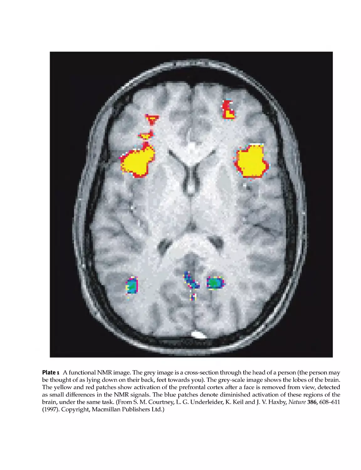
The first example is taken iromfunctional NMR imaging. As explained in Section 12.6, it is possible to use the
radio- frequency (r.f.) signals from the nuclei to build up a detailed picture of the three- dimensional structure
of an object. The grey image given in Plate 1 shows this method applied to a human head, revealing the
lobes of the brain inside the skull. The red and yellow flashes superimposed on the picture reveal differences
in the NMR signals when the subject is performing some mental task, in this case processing the memory
Spin Dynamics: Basics of Nuclear Magnetic Resonance, Second Edition Malcolm H. Levitt
© 2008 John Wiley & Sons, Ltd

2
Introduction
of a face that has just been removed from view. NMR can map out such mental processes because the brain
activity changes slightly the local oxygenation and flow of the blood, which affects the precession of the
protons in that region of the brain.
The second example illustrates the determination of biomolecular structures by NMR. Plate 2 shows
the structure of a protein molecule in solution, determined by a combination of multidimensional NMR
techniques, including the COSY and NOESY experiments described in Chapters 16 and 20. The structure
is colour coded to reveal the mobility of different parts of the molecule, as determined by NMR relaxation
experiments.
In this book, I want to provide the basic theoretical and conceptual equipment for understanding these
amazing experiments. At the same time, I want to reinforce Purcell's beautiful vision: the heaps of snow,
concealing innumerable nuclear magnets, in constant precessional motion. The years since 1945 have shown
us that Purcell was right. Matter really is like that. My aim in this book is to communicate the rigorous theory
of NMR, which is necessary for really understanding NMR experiments, but without losing sight of Purcell's
heaps of precessing protons.

Parti
i Matter
2 Magnetism
3 NMR Spectroscopy


1
Atoms and Nuclei
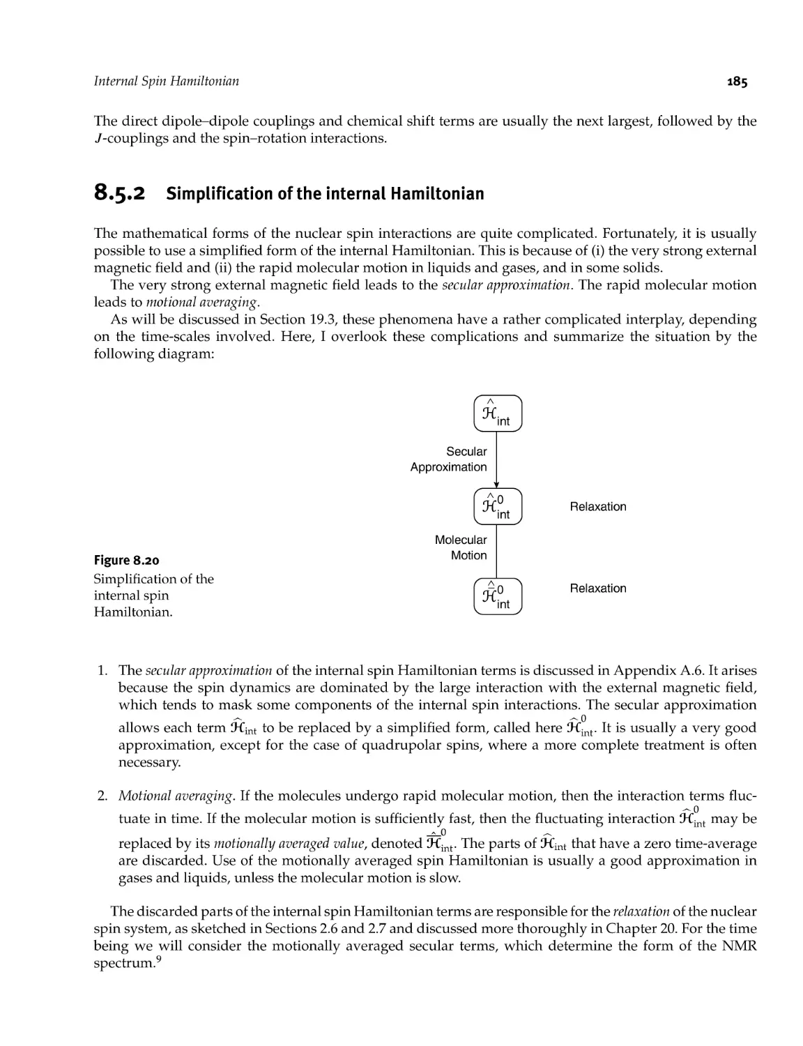
Matter is made of atoms. Atoms are made up of electrons and nuclei. Each atomic nucleus has four important
physical properties: mass, electric charge, magnetism and spin.
The mass of bulk matter is largely due to the mass of the nuclei. A large number of other physical
properties, such as heat capacity and viscosity, are strongly dependent on the nuclear mass.
The electric charge of atomic nuclei is supremely important. Atoms and molecules are bound together by
strong electrostatic interactions between the positively charged nuclei and the negatively charged electrons.
The chemical properties of each element are determined by the electric charge on the atomic nuclei.
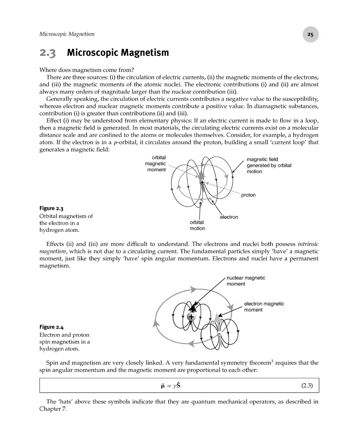
The other two properties, nuclear magnetism and nuclear spin, are much less evident. The magnetism of a
nucleus implies that it interacts with magnetic fields, like a small bar magnet. However, nuclear magnetism
is very weak and is of little consequence for atomic or molecular structure. The bulk magnetism of some
materials, such as iron, is due to the electrons, not to the nuclei.
The spin of the nucleus is even less tangible. The spin of a nucleus indicates that, very loosely speaking,
the atomic nucleus behaves as if it is spinning around, rotating in space like a tiny planet.
Nuclear magnetism and nuclear spin have almost no effect on the normal chemical and physical behaviour
of substances. Nevertheless, these two properties provide scientists with a wonderful tool for spying on the
microscopic and internal structure of objects without disturbing them.
Magnetic nuclei interact with magnetic fields. These magnetic fields may come from the molecular
environment, e.g. the surrounding electrons, or from other nuclear spins in the same molecule. Magnetic fields
may also originate from sources outside the sample, such as an external apparatus. This book tells a small
part of a long, complicated, and rather unlikely story: How the extremely weak magnetic interactions of
atomic nuclei with the molecular environment on one hand, and with the spectrometer apparatus on the
other hand, give access to detailed molecular information which is inaccessible by any other current method.
Spin
The concept of spin is difficult. It was forced upon scientists by the experimental evidence.1 Spin is a highly
abstract concept, which may never be entirely 'grasped' beyond knowing how to manipulate the quantum
mechanical equations.
Nevertheless, it is worth trying. NMR involves detailed manipulations of nuclear spins. The field has
developed to a high level of sophistication, in part because of the possibility of thinking 'physically' and
'geometrically' about spins without being entirely wrong. Geometrical arguments can never tell the whole
truth, because the human mind is probably incapable of grasping the entire content of quantum mechanics.
Spin Dynamics: Basics of Nuclear Magnetic Resonance, Second Edition Malcolm H. Levitt
© 2008 John Wiley & Sons, Ltd

6
Matter
Nevertheless, it is possible to acquire a feel for spin beyond a purely technical proficiency in the equations. In
this book, I will try to communicate how I think one should think about nuclear spins, as well as presenting
the technical mathematics.
1.2.1 Classical angular momentum
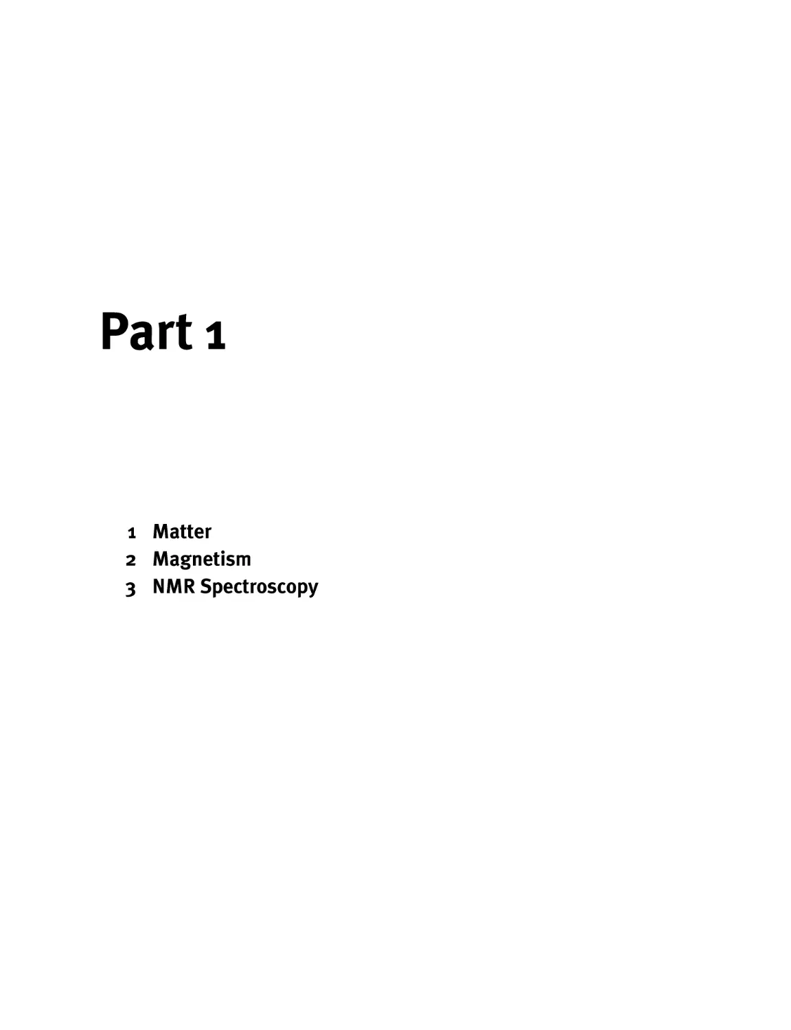
A rotating object possesses a quantity called angular momentum. This may be visualized as a vector pointing
along the axis about which the object rotates; your right hand may be used to figure out which way the
arrow points. If your thumb points along the rotation axis, then the right- hand fingers 'wrap around' in the
direction of the rotation:
Figure 1.1
Macroscopic angular
momentum.
1.2.2 Quantum angular momentum
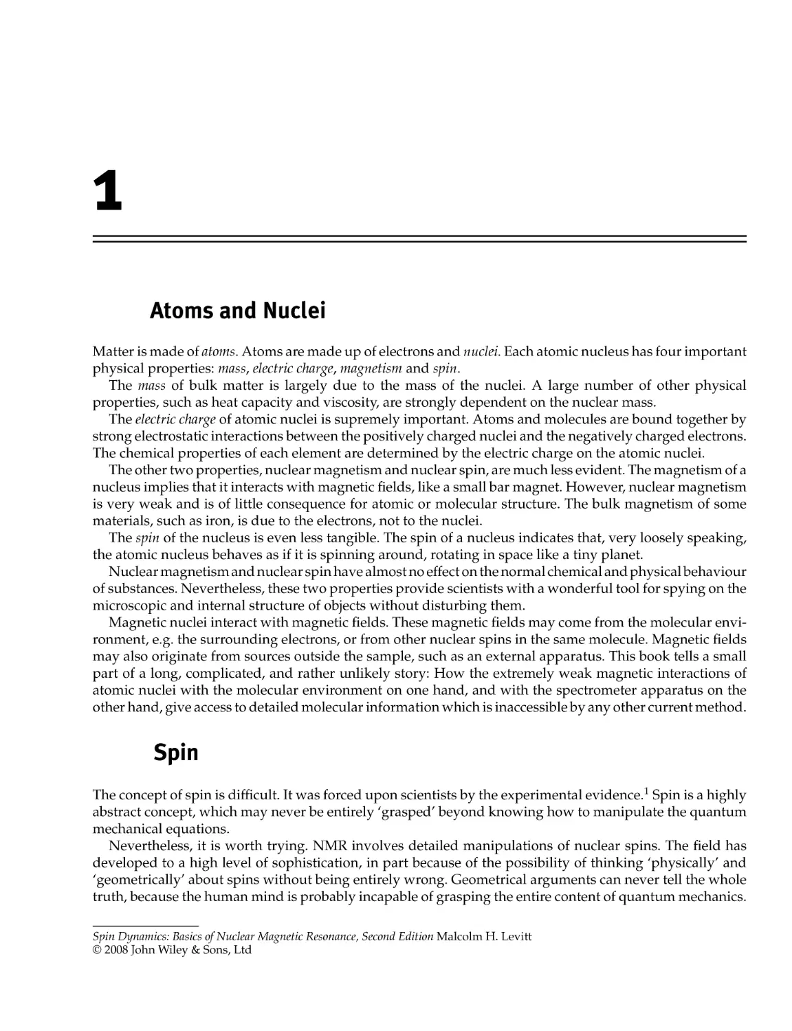
In quantum mechanics, angular momentum is quantized. Consider, for example, a diatomic molecule:
J = 3
J = 2
J=1
J=0
Magnetic
field
Figure 1.2
A rotating molecule, its
energy levels, and the
Zeeman effect.
As described in many texts (see Further Reading), and discussed further in Chapter 7, a rotating diatomic
molecule possesses a set of stable rotational states, in which the total angular momentum Ltot has one of
the values2
Ltot = [/(/ + l)]1%
(1.1)
where / takes integer values / = 0, 1, 2... and h = 1.054 x 10- 34 J s is Planck's constant divided by 2tt. This
equation implies the quantization of total angular momentum.
The rotational energy of a molecule is proportional to the square of the total angular momentum, so the
energy is also quantized. For a rigid molecule, the energies of the stable rotational states are
Ej = BJ(J + 1)
(1.2)

Spin
7
where B is called the rotational constant for the molecule. B is small for a heavy molecule and is large for a
light one.
The molecule may be in a stable state with zero total angular momentum, or with total angular momentum
\/2h, or with total angular momentum \f6h, etc. The actual rotational state of a molecule depends on its
history and its environment.
The total angular momentum of the molecule determines how fast it is rotating, but conveys no
information on the axis of the rotation.
More detail about the rotation of the molecule is given by specifying a second quantum number, Mj. This
quantum number Mj takes one of the 2 J + 1 integer values Mj = — /, — / + 1... + /, and says something
about the direction of the rotation. The quantum number Mj is sometimes referred to as the azimuthal
quantum number. The physical significance of Mj is examined more closely in Chapters 7 and 10.
In the absence of an external field, each of the 2 J + 1 states with the same value of / but different values
of Mj are degenerate, meaning that they have the same energy.
The application of a magnetic field breaks the degeneracy, causing each of the (2 J + 1) sublevels to have
a slightly different energy. This is called the Zeeman effect. The energy separation between the Mj sublevels
in a magnetic field is called the Zeeman splitting.
The basic features of this phenomenon are displayed by any physical system that is able to rotate.
Whatever the system is, there is always the same structure of (2 J + l)- fold degenerate energy levels. The stable
physical states of a rotating quantum system are always specified by a quantum number / for the total
angular momentum and an azimuthal quantum number Mj that carries information on the direction of
the rotation. The total angular momentum is always given by [/(/ + l)]1/2ft, and the azimuthal quantum
number Mj always takes one of the values Mj = — /, — / + 1... + /. The degeneracy of the Mj sublevels
may be broken by applying an electric or magnetic field.
1.2*3 Spin angular momentum
Spin is also a form of angular momentum. However, it is not produced by a rotation of the particle, but is
an intrinsic property of the particle itself.
The total angular momentum of particles with spin takes values of the form [S(S + l)]1/2h (the symbol
S is used instead of / to mark a distinction between spin angular momentum and rotational angular
momentum). Particles with spin S have (2S + 1) sublevels, which are degenerate in the absence of external
fields, but which may have a different energy if a magnetic or electric field is applied.
Each elementary particle has a particular value for the spin quantum number S. For some particles, S is
given by an integer, i.e. one of 0, 1, 2 For other particles, S is given by a half integer, i.e. one of 1/2, 3/2,
5/2....
Particles with integer spin are called bosons. Particles with half- integer spin are called fermions.
The spin of an elementary particle, such as an electron, is intrinsic and is independent of its history.
Elementary particles simply have spin; molecules acquire rotational angular momentum by energetic collisions.
At the absolute zero of the temperature scale, all rotational motion ceases (/ = 0). A particle such as an
electron, on the other hand, always has spin, even at absolute zero.
Half- integer spin posed severe problems for the physicists of the 1920s and 1930s. It may be shown
that half- integer spin cannot arise from 'something rotating', and, at that time, no other way of producing
angular momentum could be imagined. The concept of half- integer spin was resisted until the pressure
of experimental evidence became overwhelming. One of the greatest triumphs of theoretical physics was
Dime's derivation of electron spin- 1/2 from relativistic quantum mechanics. Nowadays, spin is a central
concept in our theoretical understanding of the world.
A particle like an electron may, therefore, have two kinds of angular momentum: (i) A 'conventional'
angular momentum arising from its motion. For example, an electron in an atom may have orbital angular
momentum due to its circulating motion around the nucleus. Such motion is associated with an integer

8
Matter
angular momentum quantum number and behaves just like the angular momentum of a rotating molecule,
(ii) 'Intrinsic' or spin angular momentum, which arises from nothing, being simply a feature of the electron's
'nature', and which is always the same, namely spin = 1/2.
There is no such concept as the rotation of the electron around its own axis; there is only spin.
The concept of intrinsic angular momentum is very difficult to grasp. Why should this be so? Why is
the intrinsic angular momentum of a particle more difficult to understand than intrinsic mass and intrinsic
electric charge?
The level of difficulty of a concept tends to be inversely proportional to its familiarity in the macroscopic
world. The concept of intrinsic mass is relatively easy to accept because mass has familiar everyday
manifestations. This is because the mass of two particles is the sum of the masses of the individual particles.
The mass of a book is therefore the sum of the masses of all the electrons, quarks, etc. of which the book is
composed (minus a relativistic correction - but let's forget about that!). So the concept of mass 'makes it' to
the macroscopic world. We can 'feel' mass and can imagine that fundamental particles 'have a mass'.
Electric charge is a little more difficult, because there are negative and positive charges, and in almost all
cases they cancel out for macroscopic objects. However, by performing simple experiments, like rubbing a
balloon on a woolly jumper, it is possible to separate some of the charges and achieve obvious macroscopic
effects, such as sticking a balloon to the ceiling. Through such experiences it is possible to get a feel for
charge, and become comfortable with the idea that fundamental particles 'have a charge'.
Similarly, magnetism acquires familiarity through the existence of ferromagnetic objects that possess
macroscopic magnetism.
Spin is more difficult, because there is no such thing as macroscopic spin. Matter is built up in such a
way that the spins of the different particles cancel out in any large object. Spin doesn't 'make it' to the
macroscopic world.2
This is not to say that spin is unimportant. In fact electron spin has a very profound effect on the everyday
world, because the stability of molecules and their chemical behaviour rely on it (as will be discussed shortly,
in the context of the Pauli principle). However, this effect is not obviously a consequence of electron spin,
and there are no large objects that have angular momentum 'by themselves', without rotating.3
Probably no- one really understands spin on a level above the technical mathematical rules. Fortunately it
doesn't matter so much. We know the rules for spin and that's enough to be able to exploit the phenomenon.
1.2*4 Combining angular momenta
Consider a system with two parts, each one being a source of angular momentum, with quantum numbers
J\ and /2- The angular momenta may be due to rotational motion or to spin. The total angular momentum
of the entire system is given by [/3(/3 + l)]1/2fr, where Jo, takes one of the following possible values:
\h~h\
, \h - /2I + I
h={. (1- 3)
Expressed in words, this means that the complete system has a total angular momentum quantum number
given either by the sum of the two individual angular momentum quantum numbers, or by the difference
in the two individual angular moment quantum numbers, or any of the values in between, in integer
steps.
In general, each of the possible total angular momentum states has a different energy. In many cases that
state itself behaves like a new object with angular momentum quantum number J3.
An important example of this combination rule involves two particles of spin- 1/2, i.e. S\ = S2 = 1/2. In
this case, we have |Si — S2I = 0 and \Si + S2I = 1. There are, therefore, only two possibilities for the total

Nuclei 9
angular momentum quantum number, namely S3 = 0 and S3 = 1. In the state S3 = 0, the spins of the two
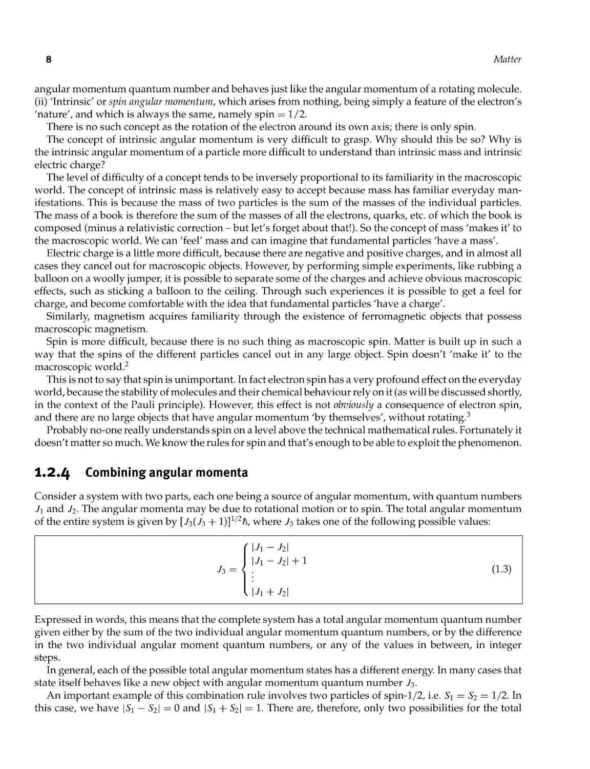
particles cancel each out. This idea is often expressed by saying that the spins are 'antiparallel' in the S3 = 0
state:
Figure 1.3
The combination of two
spins- 1/2 leads to a
singlet state with spin
S = 0 and a triplet state
with spin 5 = 1.
In the 'parallel' spin state 53 = 1, on the other hand, the spins of the two particles reinforce each other. In
general, the 53 = 0 and 53 = 1 states have different energy. Note that it is not possible to make a general
statement as to which state has the lowest energy; this depends on the details of the interactions in the system.
The 53 = 1 energy level has three substates, with azimuthal quantum number Ms = {— 1, 0, 1}. If the
environment is isotropic (the same in all directions of space), the three substates have the same energy.
States with total angular momentum 53 = 1 are often called triplet states, to stress this threefold degeneracy.
The degeneracy of the 53 = 1 level may be broken by applying an external field (magnetic or electric).
The 53 = 0 level, on the other hand, is not degenerate. The only state in this level has quantum number
Ms = 0. States with total angular momentum 53 = 0 are often called singlet states.
I.2.5 T^e Pauli Principle
The spin of particles has profound consequences. The Pauli principle4 states
two fermions may not have identical quantum states.
Since the electron is a fermion, this has major consequences for atomic and molecular structure. For example,
the periodic system, the stability of the chemical bond, and the conductivity of metals may all be explained
by allowing electrons to fill up available quantum states, at each stage pairing up electrons with opposite
spin before proceeding to the next level. This is called the Aufbau principle of matter, and is explained in
standard textbooks on atomic and molecular structure (see Further Reading).
The everyday fact that one's body does not collapse spontaneously into a black hole, therefore, depends
on the spin- 1/2 of the electron.
Nuclei
The next sections discuss briefly how the energy level structures of molecules, atoms, nuclei, and even the
elementary particles within the nuclei, fit into the angular momentum hierarchy of nature, according to the
rule given in Equation 1.3.
1.3*1 The fundamental particles
According to modern physics, everything in the universe is made up of three types of particle: leptons, quarks
and force particles.
Leptons are low- mass particles. Six varieties of lepton have currently been identified, but only one is
familiar to non- specialists. This is the electron, a lepton with electric charge — e and spin- 1/2. The unit of
electric charge e is defined as minus the electron charge and is equal to 1.602 x 10- 19 C.
S3=0
"Opposite spins"

10
Matter
Quarks are relatively heavy particles. At the time of writing (2007), it is believed that there are six 'flavours'
of quarks in nature, all of which have spin- 1/2. Three of the quarks have electric charge +2^/3. The other
three quarks have electric charge — e/3. Apart from their charge, the quarks are distinguished by additional
quantum numbers called 'strangeness', 'charm', 'top' and 'bottom', but there is no need to discuss these
topics here. It is speculated that quarks are themselves built up of extended objects, which have received
the dull name 'superstrings'.
Force particles are responsible for mediating the action of the different particles on each other. The most
important force particle is the photon, which is the particle manifestation of the electromagnetic field. Light,
which consists of electromagnetic waves, can be viewed as a stream of photons. The photon has no mass
and no electric charge, and has spin = 1. There are also force particles called gluons and vector bosons.
Gluons are manifestations of the so- called strong nuclear force, which holds the atomic nucleus and its
constituent particles together. Vector bosons are manifestations of the weak nuclear force, which is responsible
for radioactive /3- decay
I.3.2 Neutrons and protons
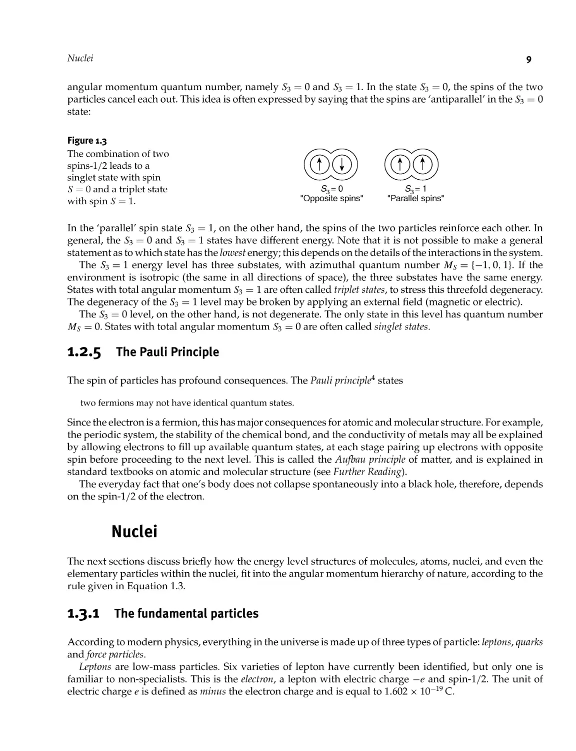
The neutron and the proton both consist of three quarks, stuck together by gluons.4
The neutron is composed of three quarks: two with charge — e/3 and one with charge +2^/3. Therefore,
the total electric charge of the neutron is zero; hence its name. The neutron has spin- 1/2. The neutron spin
is due to combinations of quark spins.5 For example, if two of the quark spins are antiparallel, we get an
S = 0 state. Addition of the third quark spin gives a total neutron spin S = 1/2:
Charge= 0
Spin=1/2
Figure 1.4
Charge ^ V__^ A neutron.
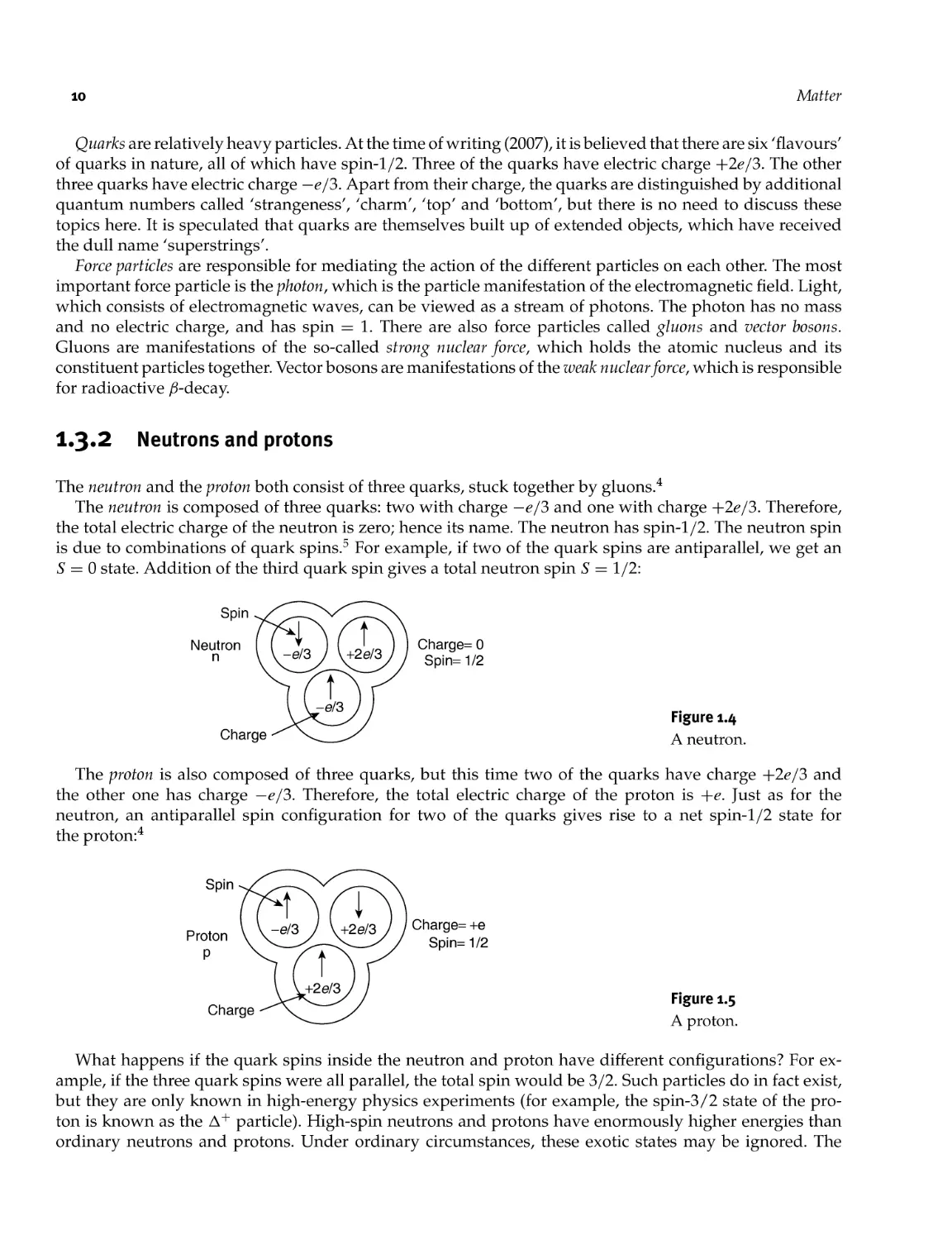
The proton is also composed of three quarks, but this time two of the quarks have charge +2<?/3 and
the other one has charge — e/3. Therefore, the total electric charge of the proton is +e. Just as for the
neutron, an antiparallel spin configuration for two of the quarks gives rise to a net spin- 1/2 state for
the proton:4
Charge= +e
Spin=1/2
^ , Figure 1.5
Charge ^X / A
^ ^ A proton.
What happens if the quark spins inside the neutron and proton have different configurations? For
example, if the three quark spins were all parallel, the total spin would be 3/2. Such particles do in fact exist,
but they are only known in high- energy physics experiments (for example, the spin- 3/2 state of the
proton is known as the A+ particle). High- spin neutrons and protons have enormously higher energies than
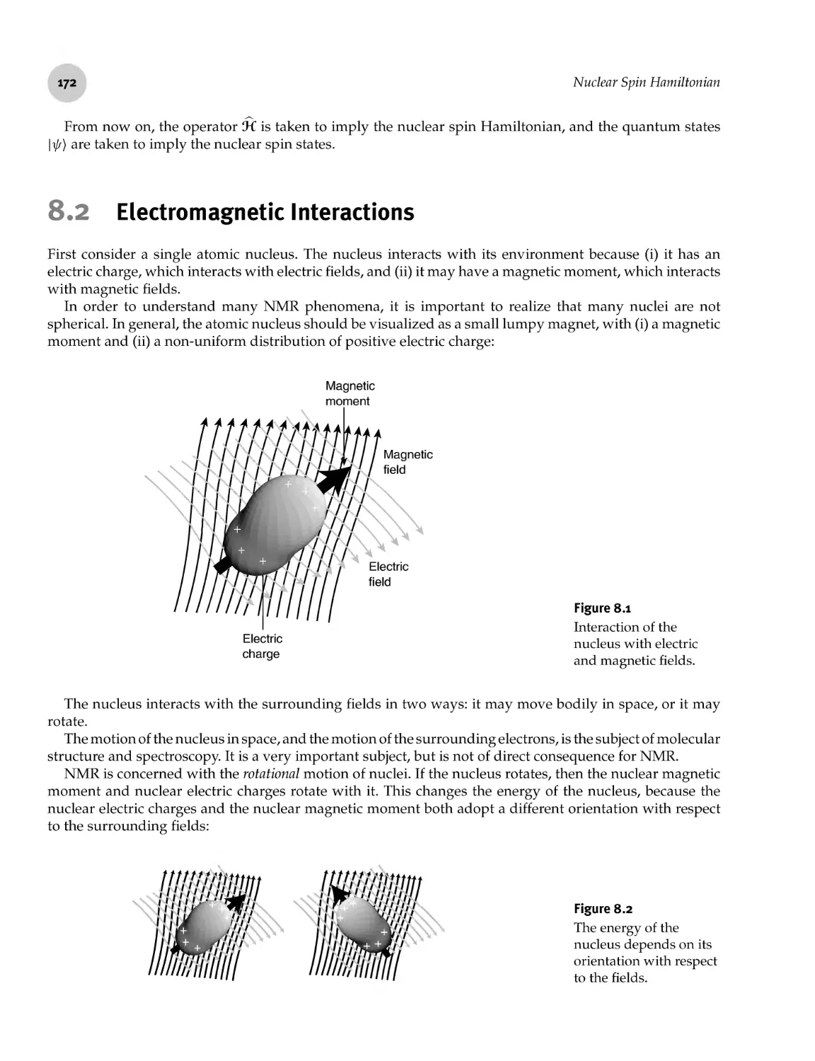
ordinary neutrons and protons. Under ordinary circumstances, these exotic states may be ignored. The

Table 1.1 Some properties of the most important elementary
particles.
Particle
e
n
P
photon
Rest mass/kg
9.109 x 10"31
1.675 x 10"26
1.673 x 10"26
0
Charge
— e
0
+e
0
Spin
1/2
1/2
1/2
1
neutron and proton may, therefore, be treated as distinct and independent particles, both with well- defined
spin- 1/2.
We also ignore the numerous other particles formed by combinations of different sets of quarks. From
now on, the only particles to be considered are the electron, the neutron, the proton and the photon, whose
relevant properties are summarized in Table 1.1.
1.3*3 Isotopes
The atomic nucleus consists of neutrons and protons.6 Neutrons and protons are known collectively as
nucleons.
An atomic nucleus is specified by three numbers: the atomic number, the mass number, and the spin quantum
number.
The atomic number Z specifies the number of protons inside the nucleus. The electric charge of the nucleus
is Ze. The electric charge of the nucleus determines the chemical properties of the atom of which the nucleus
is a part. The atomic number is traditionally denoted by a chemical symbol, for example H for Z = 1, He for
Z = 2, C for Z = 6, N for Z = 7, 0 for Z = 8, etc. The periodic table of the elements lists the atomic nuclei
in order of increasing atomic number.
The mass number specifies the number of nucleons in the nucleus, i.e. the total number of protons and
neutrons. Nuclei with the same atomic number but different mass numbers are called isotopes. Most
isotopes in existence are stable, meaning that the nucleus in question has no measurable tendency to explode
or disintegrate. Several isotopes are unstable, or radioactive, meaning that the nucleus tends to
disintegrate spontaneously, ejecting energetic particles, which are often dangerous. NMR is mainly concerned
with stable isotopes. Stable nuclei are usually formed from approximately equal numbers of protons and
neutrons.
Some common examples of stable isotopes are:
*H = p 12C = 6p + 6n
2H = p + n 13C = 6p + 7n
and so on.
Some examples of unstable (radioactive) isotopes are:
3H = p + 2n
14C = 6p + 8n
Lighter atomic nuclei were formed by the primal condensation of nucleons as the heat of the big bang
dissipated. Heavier nuclei (beyond and including iron) were synthesized later by nuclear fusion processes
inside stars. These complex nuclear processes led to a mix of isotopes with varying isotopic distributions.
These distributions are almost uniform over the surface of the Earth. For example, ~98.9% of carbon nuclei

12
Matter
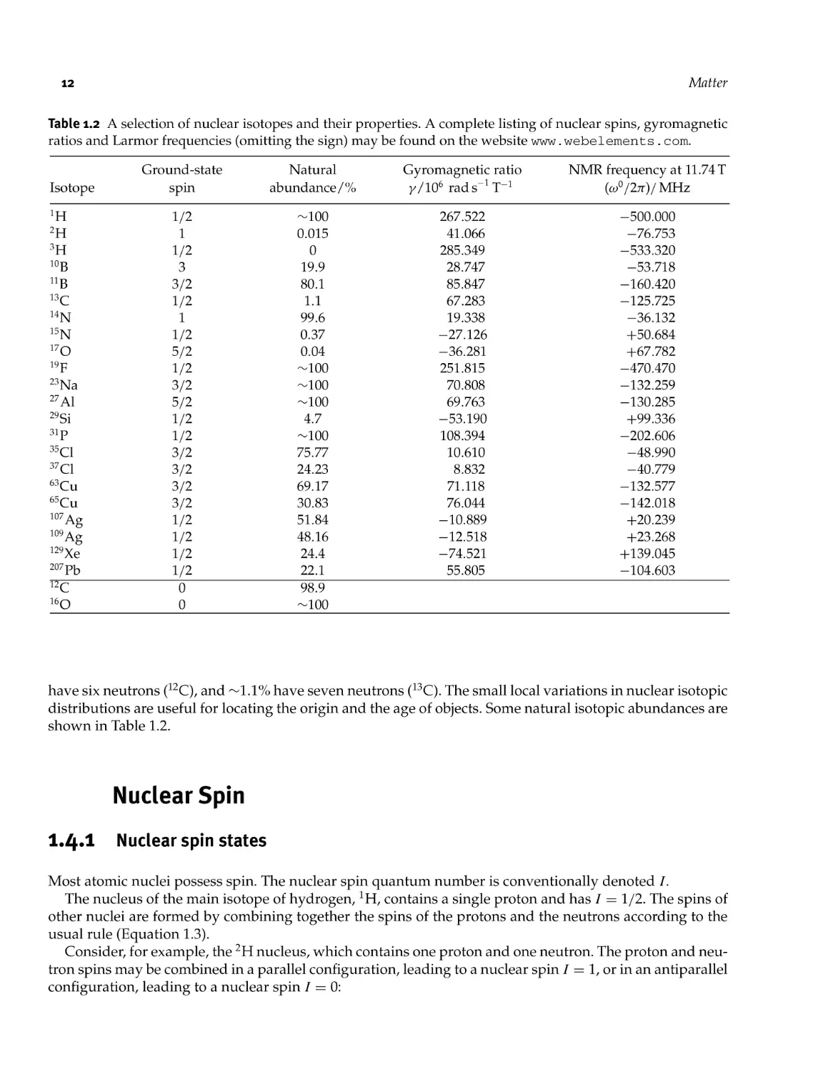
Table 1.2 A selection of nuclear isotopes and their properties. A complete listing of nuclear spins, gyromagnetic
ratios and Larmor frequencies (omitting the sign) may be found on the website www. webelements . com.
Isotope
iH
2H
3H
ioB
nB
13C
14N
15N
17o
19p
23Na
27 Al
29Si
31 p
35C1
37q
63Cu
65Cu
107 Ag
109Ag
129Xe
207pb
^c
16Q
Ground- state
spin
1/2
1
1/2
3
3/2
1/2
1
1/2
5/2
1/2
3/2
5/2
1/2
1/2
3/2
3/2
3/2
3/2
1/2
1/2
1/2
1/2
0
0
Natural
abundance /%
- 100
0.015
0
19.9
80.1
1.1
99.6
0.37
0.04
- 100
- 100
- 100
4.7
- 100
75.77
24.23
69.17
30.83
51.84
48.16
24.4
22.1
98^9
- 100
Gyromagnetic ratio
y/106 rads^T"1
267.522
41.066
285.349
28.747
85.847
67.283
19.338
- 27.126
- 36.281
251.815
70.808
69.763
- 53.190
108.394
10.610
8.832
71.118
76.044
- 10.889
- 12.518
- 74.521
55.805
NMR frequency at 11.74 T
(co°/2jt)/MHz
- 500.000
- 76.753
- 533.320
- 53.718
- 160.420
- 125.725
- 36.132
+50.684
+67.782
- 470.470
- 132.259
- 130.285
+99.336
- 202.606
- 48.990
- 40.779
- 132.577
- 142.018
+20.239
+23.268
+139.045
- 104.603
have six neutrons (12C), and — 1.1% have seven neutrons (13C). The small local variations in nuclear isotopic
distributions are useful for locating the origin and the age of objects. Some natural isotopic abundances are
shown in Table 1.2.
Nuclear Spin
I.4.I Nuclear spin states
Most atomic nuclei possess spin. The nuclear spin quantum number is conventionally denoted /.
The nucleus of the main isotope of hydrogen, aH, contains a single proton and has / = 1/2. The spins of
other nuclei are formed by combining together the spins of the protons and the neutrons according to the
usual rule (Equation 1.3).
Consider, for example, the 2H nucleus, which contains one proton and one neutron. The proton and
neutron spins may be combined in a parallel configuration, leading to a nuclear spin / = 1, or in an antiparallel
configuration, leading to a nuclear spin 1 = 0:

Nuclear Spin
13
Figure 1.6
Energy levels of a 2H
nucleus.
/=0
/=1
These two nuclear spin states have a large energy difference of ~10n kj mol- 1. This greatly exceeds
the energies available to ordinary chemical reactions or usual electromagnetic fields (for comparison, the
available thermal energy at room temperature is around ~2.5 kj mol- 1). The nuclear excited states may,
therefore, be ignored, except in exotic circumstances.7 The value of / in the lowest energy nuclear state is
called the ground state nuclear spin. For deuterium (symbol D or 2H), the ground state nuclear spin is / = 1.
For higher mass nuclei, the ground state is one of a large number of possible spin configurations of the
protons and neutrons:
Figure 1.7
Energy levels of a 6 Li
nucleus, showing the
ground state spin 1 = 1.
In general, there are no simple rules for which of the many possible states is the ground state. For our
purposes, the ground state nuclear spin is best regarded as an empirical property of each isotope.
Nevertheless, one property may be stated with certainty: from Equation 1.3, isotopes with even mass
numbers have integer spin and isotopes with odd mass numbers have half- integer spin.
Two further guidelines apply to isotopes with even mass numbers:
1. If the numbers of protons and neutrons are both even, the ground state nuclear spin is given by / = 0.
Some examples are: the nucleus 12C, which contains six protons and six neutrons; the nucleus 160, which
contains eight protons and eight neutrons; and the nucleus 56Fe, which has 26 protons and 30 neutrons.
All of these have a ground state spin 1 = 0.

14
Matter
2. If the numbers of protons and neutrons are both odd, the ground state nuclear spin is an integer larger
than zero. Some examples are the nuclei 2H (lp + In, ground state spin / = 1), 10B (5p + 5n, ground
state spin / = 3), 14N (7p + 7n, ground state spin 1 = 1) and 40K (19 p + 21n, ground state spin / = 4).
These rules may be understood using models of nuclear structure, a subject that will not be discussed further
here.
From now on, the ground state nuclear spin is simply called the 'nuclear spin', for the sake of simplicity.
Table 1.2 shows some of the nuclear isotopes of importance in NMR, together with their natural abundances.
An overview of all nuclear spins is given in the inside cover as Plates A, B and C.
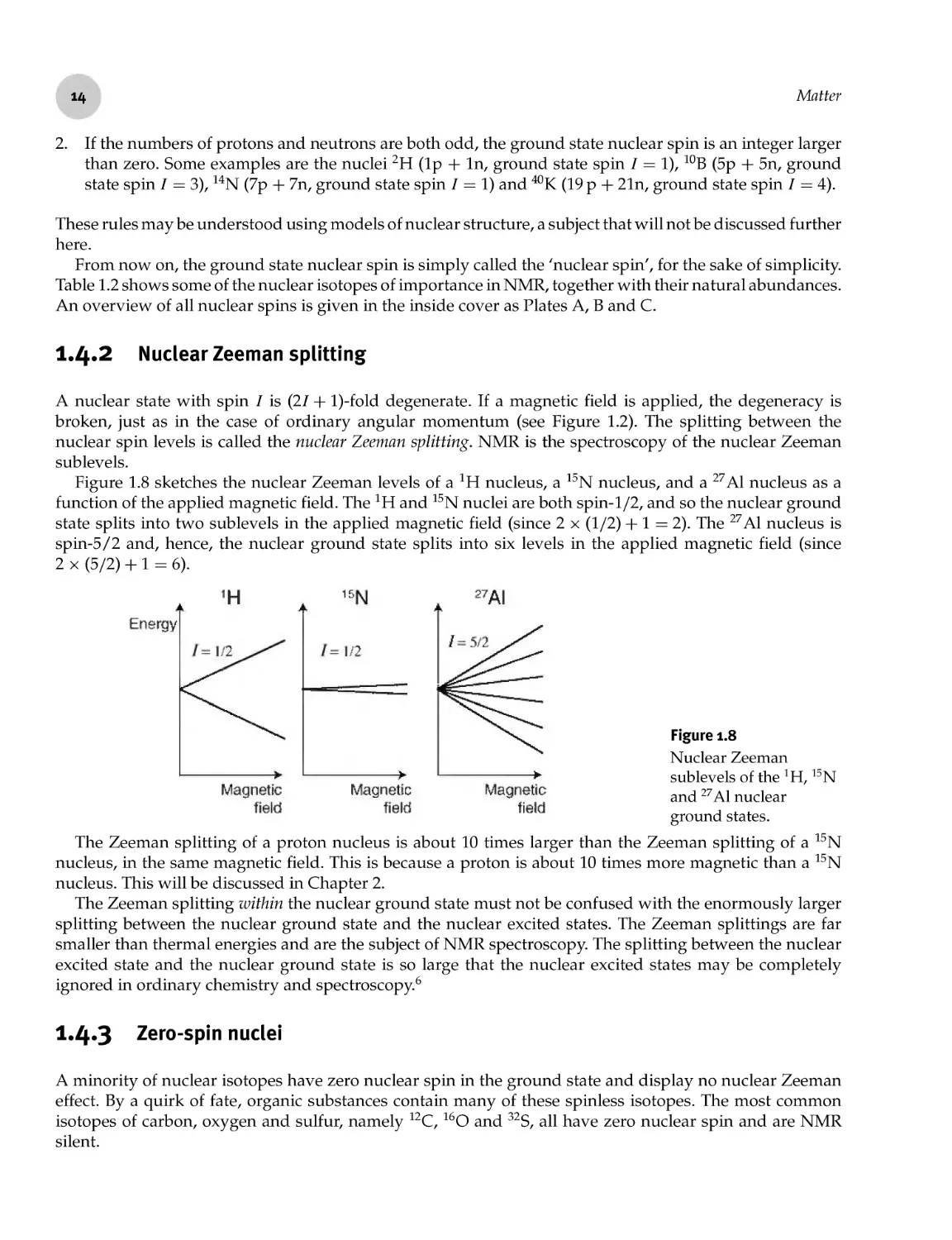
I.4.2 Nuclear Zeeman splitting
A nuclear state with spin / is (21 + l)- fold degenerate. If a magnetic field is applied, the degeneracy is
broken, just as in the case of ordinary angular momentum (see Figure 1.2). The splitting between the
nuclear spin levels is called the nuclear Zeeman splitting. NMR is the spectroscopy of the nuclear Zeeman
sublevels.
Figure 1.8 sketches the nuclear Zeeman levels of a 2H nucleus, a 15N nucleus, and a 27A1 nucleus as a
function of the applied magnetic field. The 2H and 15N nuclei are both spin- 1/2, and so the nuclear ground
state splits into two sublevels in the applied magnetic field (since 2 x (1/2) + 1=2). The 27A1 nucleus is
spin- 5/2 and, hence, the nuclear ground state splits into six levels in the applied magnetic field (since
2 x (5/2) + 1 = 6).
Energy
15
N
/- I.- 2
Magnetic
field
Magnetic
field
Magnetic
field
Figure 1.8
Nuclear Zeeman
sublevels of the1 H, 15N
and 27 Al nuclear
ground states.
The Zeeman splitting of a proton nucleus is about 10 times larger than the Zeeman splitting of a 15N
nucleus, in the same magnetic field. This is because a proton is about 10 times more magnetic than a 15N
nucleus. This will be discussed in Chapter 2.
The Zeeman splitting within the nuclear ground state must not be confused with the enormously larger
splitting between the nuclear ground state and the nuclear excited states. The Zeeman splittings are far
smaller than thermal energies and are the subject of NMR spectroscopy. The splitting between the nuclear
excited state and the nuclear ground state is so large that the nuclear excited states may be completely
ignored in ordinary chemistry and spectroscopy6
I.4.3 Zero- spin nuclei
A minority of nuclear isotopes have zero nuclear spin in the ground state and display no nuclear Zeeman
effect. By a quirk of fate, organic substances contain many of these spinless isotopes. The most common
isotopes of carbon, oxygen and sulfur, namely 12C, 160 and 32S, all have zero nuclear spin and are NMR
silent.

Atomic and Molecular Structure
15
1.4.4 Spin- 1/2 nuclei
Nuclei with spin 1 = 1/2 are of major importance in NMR. As discussed in Chapter 8, such nuclei are
spherical in shape and have convenient magnetic properties. Plate A shows the distribution of spin- 1/2
nuclei in the periodic table of the elements. They are mainly scattered around the right- hand side of the
periodic table.
Most chemical elements have no spin- 1/2 isotope. The alkali and alkaline earth metals possess no spin- 1/2
isotopes at all. In contrast, spin- 1/2 isotopes are well represented in organic materials. The most common
isotopes of hydrogen and phosphorus have spin- 1/2 (aH and 31P), and carbon and nitrogen possess the rare
spin- 1/2 isotopes 13C and 15N. The abundant fluorine isotope 19F is also of importance.
Spin- 1/2 isotopes are well represented in the precious and heavy metals, and the noble gases contain a
possess two spin- 1/2 isotopes, namely 3He and 129Xe.
1.4.5 Quadrupolar nuclei with integer spin
Nuclei with spin / > 1/2 are known as 'quadrupolar nuclei', for reasons discussed in Chapter 8. The NMR
of such nuclei is a rich but relatively difficult field, which is increasing in popularity, especially in the context
of solid- state NMR.
Quadrupolar nuclei with integer values of / are uncommon. Plate B shows their distribution in the
periodic table. By far the most abundant nucleus of this type is 14N, which occurs in almost 100% natural
abundance. Deuterium (2H) is of great importance despite its low natural abundance, since it is relatively
easy to separate from aH by physical methods and to prepare 2H- enriched substances.
The nuclear spins / = 3, 4, 5, 6 and 7 are represented by only one isotope each, some of which are obscure.
There are no nuclei at all with ground state spin 1 = 2. The 1 = 7 isotope 176Lu has the highest nuclear spin
in the entire periodic table.
1*4*6 Quadrupolar nuclei with half- integer spin
Quadrupolar nuclei with / = 3/2, 5/2, 7/2 or 9/2 are common (see Plate C). They are well represented
throughout the entire periodic table, but are particularly prominent for the alkali metals, the boron- to-
thallium group, and the halogens. There is a striking alternation across many parts of the periodic
table, with every other element possessing an abundant isotope with a half- integer quadrupolar nucleus.
I do not know the reason for this alternation, which must reflect some feature of nuclear structure and
energetics.
The importance of the isotopes is not necessarily reflected by their abundance. For example, the isotope
170 has a very low natural abundance but is, nevertheless, of great importance since it is the only stable
oxygen isotope with nuclear spin.
Atomic and Molecular Structure
1«5*1 Atoms
The atomic nucleus has a positive electric charge - \- Ze. An atom is composed of a nucleus surrounded by Z
electrons, each with charge — e. For example, an atom of 4He consists of a nucleus, containing two neutrons
and two protons, surrounded by a cloud of two electrons. The simplest atom is hydrogen, which contains
a nucleus of one proton and a single orbiting electron.

i6
Matter
An atom is electrically charged if the total charge on the nucleus does not balance out exactly the charge
on the electron cloud. Such species are called ions. For example, a nucleus containing 11 protons and 12
neutrons, surrounded by a cloud of 10 electrons, is called a 23Na ion. A nucleus containing 17 protons and
18 neutrons, surrounded by a cloud of 18 electrons, is called a 35C1 ion.
Atomic structure does not really concern us here, but it is worth seeing how the angular momentum
of the atom works out (see Further Reading for a more detailed discussion). There are three sources of
angular momentum in a hydrogen atom: the electron spin, the proton spin, and the electron orbital angular
momentum, which is associated with the motion of the electron around the nucleus. The orbital angular
momentum of the electron is characterized by a quantum number, usually called /. Since this type of
angular momentum is associated with motion, the quantum number / is an integer. Quantum states with
zero electron orbital angular momentum are called s- orbitals. Quantum states with electron orbital angular
momentum / = 1 are called p- orbitals, and so on. In addition, the energy levels of the H atom display fine
structure, which is due to the coupling of the electron orbital angular momentum to the electron spin. Even
closer observation of the energy levels reveals hyperfine structure, which is due to the participation of the
proton spin.
Atoms containing more than one electron have many more possibilities, because each electron is a
source of orbital angular momentum as well as spin angular momentum. In such systems, the Pauli
principle comes into play Electrons may only occupy identical orbital states if their spins are antiparallel. In
practice this means that the lowest energy states in an atom usually have small values of total electron
spin.
I.5.2 Molecules
An electron cloud containing more than one nucleus is called a molecule. For example, a molecule
of water (aH2160) consists of a cloud of 10 electrons surrounding three nuclei: one with eight
protons and eight neutrons (the oxygen nucleus), and two consisting of a single proton (the hydrogen
nuclei).
In a molecule, the quantum mechanical motion of the electrons constrains the nuclei to a particular
geometric configuration. In the case of the water molecule, the three nuclei are geometrically stable only
when the three nuclei form a triangular configuration with an H— O— H angle of around 105°.
A typical molecule contains many potential sources of angular momentum: the motion of the electrons
around the nuclei, the motion of the nuclear framework around the centre of mass of the molecule, in some
cases the rotation of internal molecular groups, the electron spins, and the nuclear spins. However, because
of the Pauli principle, and the quantum rules for chemical bonding, the electron orbital angular momenta
and the electron spin angular momenta almost always cancel out in the lowest energy state of a chemically
stable molecule (there are a few exceptions, such as O2, which has total electron spin 5 = 1 in the ground
state, and NO, which has finite orbital angular momentum in the ground state). In most cases, the only
sources of angular momentum in the molecular ground state are the molecular rotation and the nuclear
spins.
The motion of the nuclear framework can very often be treated 'classically': the molecule is treated as an
ordinary object rotating in space. Inside this rotating molecule are trapped the nuclear spins. This ignores
the quantum nature of the molecular motion. Nevertheless, it almost always gives reasonable answers, and
we will use it from now on.
Molecules differing only in the mass numbers of the nuclei are called isotopomers. Isotopomers usually
have almost identical chemical and physical properties, since these are determined almost completely by the
charges on the nuclei and the number of surrounding electrons. All substances are mixtures of isotopomers,
even when chemically pure. For example, pure water is composed mainly of the predominant isotopomer
aH2160, but there are also small amounts of the minor isotopomers aH2H170, aH2170, etc. The relative
abundance of the isotopomers is governed by the natural statistical distributions of the various isotopes.

States of Matter
17
There are slight differences in the chemical and physical properties of isotopomers, due to the different
nuclear masses. Molecules with different nuclear masses have different vibrational energy levels, altering
slightly the rates of certain chemical reactions. Physical properties, such as diffusive mobilities, are also
influenced by the molecular mass. This allows isotopomers to be separated by techniques such as gas
chromatography. For example, it is possible to separate 13CO molecules from the abundant 12CO isotopomers
by passing the gas through very long chromatographic columns. The 13C- labelled carbon monoxide is used
as a starting material for total organic synthesis of other 13C- labelled substances. Many modern NMR
experiments use isotopically enriched substances prepared in this way.
NMR is unusual in that different isotopomers behave completely differently. In many cases, one iso-
topomer gives a large signal while another isotopomer gives none, even though the substances are
physically and chemically almost indistinguishable. NMR achieves this distinction because it is based upon the
nuclear spin, rather than the nuclear mass.
The mass of a molecule is roughly equal to the sum of the nuclei in the molecule. In the biological sciences,
it is popular to specify molecular masses in units of daltons (abbreviation Da). A 12C atom has a mass of
exactly 12 Da. A medium- sized protein molecule has a molecular mass of around 30 x 103 Da = 30 kDa (30
kilodaltons). Outside the biological sciences, molecular masses are usually specified in units of grams per
mole (gmol- 1).
States of Matter
The states of matter are assembled from the basic building blocks of atoms, molecules and ions. We will
now review the special features of the different material states, since the motions of the molecules in these
states have a large effect on NMR experiments.
Traditionally, the material states are classified in terms of their bulk mechanical properties (i.e. hard
or soft, rigid or flowing). These bulk mechanical properties often reflect the mobility of the constituent
molecules or atoms.
1.6.1 Gases
Gases are defined as low- density material phases that fill the volume of any container to which they are
confined, independent of its shape. Gases are characterized by very high mobility of the molecules or atoms.
It is possible to perform NMR experiments on gases, although this is not done very often.8
1.6.2 Liquids
Liquids are relatively dense material phases characterized by their flow under shear forces. There is high
molecular mobility in liquid phases. This molecular mobility has two aspects: translation mobility and
rotational mobility (Figure 1.9). Translation molecular mobility means that the molecules or atoms slide past
each other rather freely and wander over appreciable distances in a relatively short time. For example, a
water molecule at room temperature typically wanders over a distance of ~7 \xm over a time interval of
10 ms. Rotational molecular mobility means that the individual molecules rotate around their own centres
of gravity in a more or less random fashion. For example, a medium- sized protein molecule in water
solution typically rotates through an angle of around lrad after a time of around 10 ns. Both of these
types of mobility are very important for NMR, because they tend to average out many of the nuclear spin
interactions, simplifying the behaviour of the nuclear spins.

18
Matter
u c
(a)
(b)
Figure 1.9
In a liquid, molecules
have both translation
mobility (a) and
rotational mobility (b).
If the liquid is isotropic,
the mobilities are the
same in all directions.
A further distinction must be made between isotropic and anisotropic liquid phases.
In isotropic liquids, the translation and rotational mobilities of the molecules are the same in all directions.
This is true, for example, in ordinary water or for molecules dissolved at low concentration in common
solvents. As discussed in Chapter 8, the molecular motion in an isotropic liquid effectively removes many
of the nuclear spin interactions, leading to rather simple NMR spectra.
There are also anisotropic liquids (also called liquid crystals), in which the molecules adopt a non- isotropic
spatial configuration. In some cases the molecules are arranged in layers, in other cases like coins stacked
up on top of each other, and in still other cases the molecules adopt a sort of loose helical structure. Despite
these loose spatial configurations, the molecules are still very mobile and the substance flows under shear
forces, which distinguishes a liquid crystal from a solid. An everyday example of a liquid crystal is a
soap film, in which the soap molecules are arranged in layers. As far as NMR is concerned, anisotropic
liquids behave very differently from isotropic liquids because the translation and rotational mobilities of
the molecules depend on the direction (Figure 1.10). Consider, for example, a case in which the molecules
are shaped like long rods and all the rods are, on average, aligned along a particular direction in space
(called the director in liquid- crystal science). It is easier for the molecules to spin around an axis that is
parallel with the director than around an axis that is perpendicular to the director. In the former case they
have a better chance of completing a full rotation without hitting a neighbouring molecule, as opposed
to the latter case, where collisions are almost inevitable. This motional anisotropy leads to incomplete
averaging of the nuclear spin interactions and, hence, more complicated NMR spectra. Nevertheless, the
NMR spectra of liquid crystals, and of molecules dissolved in liquid crystals, can be very informative.
One way in which anisotropic liquids are used to enhance the study of biological molecules is sketched in
Section 16.4.
Director
Figure 1.10
In an anisotropic liquid,
the molecular mobilities
depend on the direction
in space.

States of Matter
19
1.6*3 Solids
Solids are high- density material phases that resist shear forces without flowing. Solid materials have an
enormous variety of atomic structures. For example, there are molecular solids, which are composed of
distinct molecules held together by rather weak intermolecular forces, and non- molecular solids, in which
the atomic nuclei are gripped in an extended electron cloud network, which may extend to the boundaries
of the material. There are crystals, in which the nuclei are arranged on a repeating lattice, as well as glasses
and amorphous solids, in which long- range repeating patterns are difficult to identify.
The distinction between 'solid' and 'liquid' is not always unambiguous. The behaviour of matter under
shear forces depends strongly on the time- scale involved. For example, an ordinary liquid resists
deformations and appears as a hard solid on a time- scale of microseconds - as may be tested by diving stomach
first into a swimming pool. On the other hand, hard solids, such as rocks, may behave as liquids under long
time- scales.9
There is a great variety of electronic behaviour in solids. The majority of materials are electrical insulators,
with very restricted electron mobility. However, in some cases the electron mobility is high, even though
the atomic nuclei are more or less fixed in place. Such substances are metals. In special circumstances, the
electrons may pair up to form bosons that form macroscopic coherent quantum waves. This happens in
superconductors.
The motion of atoms and molecules is usually greatly restricted in solids. It is this feature that distinguishes
solids from liquids on the molecular level. Nevertheless, there can be substantial local motion. For example,
some molecular solids display considerable rotational motion of the molecules around their own lattice
positions. This often happens for solids composed of near- spherical molecules, e.g. the football- like fullerene
molecule C^q. At room temperature, the C60 'footballs' rotate randomly and isotropically around their own
centres in the solid:
0# >W" X Crtf $0 X ^? &>
'X " <y ~- $ / 'X .' <y '• V x a - ' <y *- v
oP - ' t{ " - *' * op •<> J - w op ■■> - - ^
Figure 1.11
Rotation of C6o
molecules in a solid.
•tv y^j
<& P>t
Even in molecules that do not jump or rotate as entire units, there are often local groups which have
considerable local mobility. For example, methyl groups — CH3 usually rotate rapidly at room temperature,
even in rigid solids. Often, solids display a variety of phases at different temperatures and pressures, with
different modes of atomic or molecular mobility.
Generally speaking, the NMR spectra of solids are generally broader and more complex than in liquids.
Nevertheless, there has been much recent technical progress in the NMR of solids. The development
of experimental techniques has made it possible to obtain solid- state NMR spectra with a resolution
approaching that obtained in isotropic liquids in many cases. This is very useful, because there are many
substances which cannot, or should not, be dissolved or melted.

20
Matter
Notes
1. Electron spin was first postulated by the Dutch graduate students Uhlenbeck and Goudsmidt in 1925.
Their supervisor stated that they could risk publication since they didn't yet have a reputation to
destroy The influential physicist Pauli initially poured scorn on the idea but later became one of its
chief proponents.
2. Throughout this book, a box drawn around an equation indicates that it is important in its own right.
3. Some large objects do in fact 'have angular momentum "by themselves, , / without rotating', although
the consequences are subtle and require fine experimental observations. For example, the Einstein-
de Haas effect shows that the act of magnetizing a substance imparts angular momentum to it (for
example, an object suspended by a fine thread starts rotating slowly as it is magnetized). A magnetized
substance, like a lump of iron, does have angular momentum, without rotating! There is even a converse
phenomenon called the Barnett effect: rotating an object magnetizes it! See E. T. Jaynes, Rev. Mod. Phys. 34,
143 (1962).
4. This is a simplified version of the Pauli principle. The full version is as follows:
The quantum mechanical state of a system containing two identical bosons is invariant under exchange of
the two bosons. The quantum mechanical state of a system containing two identical fermions changes sign
under exchange of the two fermions.
The theorem that two fermions may not occupy the same state follows as a consequence of the full
principle. As a matter of fact, the Tauli principle' was first given for fermions by Heisenberg, and
for bosons by Bose. It is a little mysterious why the principle has become attached to the name of
Pauli.
5. The discussion of neutron spin, proton spin, and nuclear spin given in this chapter is oversimplified.
In fact, it is known that the orbital motions of the quarks and gluons also contribute to the spin of
the proton and neutron (see, e.g., S. D. Bass, Science 315, 1672- 1673 (2007)). I deliberately give a naive
picture of neutron and proton spin here, because the details are not so important anyway for NMR and
because it does make a good story.
6. The neutrons and protons are bound together by an interchange of particles known as mesons. Each
meson is made up of two quarks.
7. In Mbssbauer spectroscopy, transitions between the nuclear energy levels are excited using energetic
y- rays.
8. There are some interesting applications of NMR in gases, although the low density of matter in a
gas leads to relatively weak NMR signals. For example, NMR of gaseous 129Xe is used to make
images of cavities inside hollow objects, including lungs. In this case, a special technique called
optical pumping is used to prepare 129Xe gas with a very high nuclear spin polarization, so as to
enhance the NMR signals. See, for example, B. M. Goodson, /. Magn. Reson. 155, 157- 216 (2002). Some
conventional gas- phase NMR spectra, obtained without the help of optical pumping, are shown in
Figure 19.21.
9. The first edition of this book propagated the urban myth that old glass windows are thicker at the
bottom because the glass creeps slowly under gravity. This is not true. The thickening at the bottom is
simply due to the manufacturing process. Thanks to the copy editor for pointing this out.

States of Matter
21
Further Reading
• For the fundamentals of quantum mechanics and atomic structure, see J. J. Sakurai, Modern Quantum
Mechanics, Addison- Wesley, 1994, and C. Cohen- Tannoudji, B. Diu, R Laloe, Quantum Mechanics Wiley,
London, 1977.
• For atomic structure and orbitals, see P. W. Atkins, Molecular Quantum Mechanics, Oxford University Press,
Oxford, 1983.
• For the consituents of matter, see F. Close, The quark structure of matter' in The New Physics, P. Davies,
(ed.), Cambridge University Press, Cambridge, 1989.
Exercises
1.1 Which of the following statements must be correct, which might possibly be correct, and which cannot
be correct?
(i) The nucleus 89Y (atomic number = 39) has a ground state spin 7 = 1/2.
(ii) The nucleus 90Zr (atomic number = 40) has a ground state spin 1 = 1.
(iii) The nucleus 91Zr (atomic number = 40) has a ground state spin 1 = 1/2.
(iv) The nucleus 92Mo (atomic number = 42) has a ground state spin 1 = 0.
(v) The nucleus 138La (atomic number = 57) has a ground state spin 1 = 0.
1.2 If a particle with spin S = 5/2 couples to a particle with spin S = 3/2, what are the possible values for
the spin of the resulting particle?


2
The Electromagnetic Field
It is possible to use either a classical or a quantum description of the electromagnetic field.
In the quantum description, the field appears as a collection of photons. This description is accurate, but
is difficult to use.
In the classical description, one associates two vectors, E and B, with every point of space. The field E is
called the electric field, and interacts with electric charges. The field B is called the magnetic field, and interacts
with magnetic moments1.
In NMR, the discrepancy between the classical and quantum field descriptions is negligible, and the
simpler classical formalism is preferable.
The magnitude of B is specified in units of tesla (symbol T). The older unit of gauss (symbol G) is also
sometimes used. The conversion is as follows: 1G = 10- 4 T. The natural magnetic field at the surface of the
Earth is — 50 jiT. NMR spectrometers currently operate with magnetic fields between around 4 T and 20 T.
The behaviour of the fields E and B in time and space is governed by the Maxwell equations. As shown
in standard texts (see Further Reading), these equations predict many effects, including the propagation of
fields E and B in empty space, y- rays, X- rays, light rays, infrared radiation, microwaves, and radio waves
are all electromagnetic waves, distinguished only by frequency. A table of typical frequencies and free- space
wavelengths for electromagnetic waves is given in Table 2.1.
Table 2.1 Typical frequencies and wavelengths of electromagnetic waves.
Type of Wave Typical frequency/Hz Typical wavelength
Radio - 108 - 3 m
Microwave — 1010 — 3 cm
Infrared - 3 x 1013 - 10 |xm
Ultraviolet - 3 x 1016 - 10 nm
X- ray - 3 x 1018 - 0.1 nm
yray - 3 x 1020 - lpm
Macroscopic Magnetism
All substances are magnetic, meaning that they have the capability of interacting with magnetic fields.
This interaction is usually expressed in terms of a magnetic moment |ul. The magnetic energy of a small
object depends on the interaction between its magnetic moment and the B field:
Spin Dynamics: Basics of Nuclear Magnetic Resonance, Second Edition Malcolm H. Levitt
© 2008 John Wiley & Sons, Ltd

24
Magnetism
^mag —
|UL B
(2.1)
The dot product indicates that the magnetic energy depends on the relative direction of the vectors B
and |ul. The negative sign indicates that the magnetic energy is lowest if the magnetic moment |ul is parallel
to the B field:
B B
A „ A
Figure 2.1
Low energy High energy Magnetic energy.
In general, Equation 2.1 should be integrated over the volume of the object.
In some substances, the magnetic moment is permanent, as for a bar magnet or a compass needle. In the
majority of substances, on the other hand, the magnetism is induced, meaning that the magnetic moment
appears only when an external magnetic field is present.
An object that is free to move tends to align along an external magnetic field so as to minimize the
magnetic energy. This is the principle of the compass needle, which has a permanent magnetic moment |ul.
The compass needle swings around to bring the magnetic moment |ul parallel to the Earth's field B.
Most objects display induced magnetism and only possess a magnetic moment in the presence of an
applied magnetic field. Such induced magnetic moments typically take some time to build up. The equilibrium
value of the induced magnetic moment is often proportional to the applied magnetic field B, and has the
same direction. In SI units, this relationship is written2 as follows:
/^induced — MO
_1VxB
(2.2)
where /xo = 4tt x 10- 7 H m_1 is an awkward constant, called the magnetic constant or vacuum permeability. V
is the volume of the object. The dimensionless number x is called the magnetic susceptibility of the material.
It expresses how readily the material develops a magnetic moment on exposure to an external magnetic
field, x may have either sign. Materials with a positive value of x are called paramagnetic. Most materials
have a negative value of x> and are called diamagnetic. For example, pure water has a magnetic susceptibility
X = - 9.05 x 10"6.
The susceptibility of an object determines how an applied magnetic field is distorted. Objects with a
positive susceptibility (x > 0) tend to pull the magnetic field into the material. Objects with negative
susceptibility (x < 0) tend to push the magnetic field out of the material.
Paramagnetic susceptibilities tend to be larger in magnitude than diamagnetic susceptibilites (as hinted
in Figure 2.2).
Magnetic field
Figure 2.2
An object distorts the
magnetic field
according to its
magnetic susceptibility.
The effect is greatly
exaggerated in the
diagrams shown here.
X>0
(Paramagnetism)
X<0
(Diamagnetism)

Microscopic Magnetism
25
2- ;l Microscopic Magnetism
Where does magnetism come from?
There are three sources: (i) the circulation of electric currents, (ii) the magnetic moments of the electrons,
and (iii) the magnetic moments of the atomic nuclei. The electronic contributions (i) and (ii) are almost
always many orders of magnitude larger than the nuclear contribution (iii).
Generally speaking, the circulation of electric currents contributes a negative value to the susceptibility,
whereas electron and nuclear magnetic moments contribute a positive value. In diamagnetic substances,
contribution (i) is greater than contributions (ii) and (iii).
Effect (i) may be understood from elementary physics: If an electric current is made to flow in a loop,
then a magnetic field is generated. In most materials, the circulating electric currents exist on a molecular
distance scale and are confined to the atoms or molecules themselves. Consider, for example, a hydrogen
atom. If the electron is in a /?- orbital, it circulates around the proton, building a small 'current loop' that
generates a magnetic field:
orbital r. r?<r^\ / magnetic field
magnetic ^- L\ \ V \ / generated by orbital
moment Y \\l/ \ V/ motion
proton
V Vv V~~
Figure 2.3
Orbital magnetism of | electron
the electron in a
hydrogen atom.
Effects (ii) and (iii) are more difficult to understand. The electrons and nuclei both possess intrinsic
magnetism, which is not due to a circulating current. The fundamental particles simply 'have' a magnetic
moment, just like they simply 'have' spin angular momentum. Electrons and nuclei have a permanent
magnetism.
nuclear magnetic
moment
electron magnetic
moment
t f S£ \ \ ^C- \
Figure 2.4
Electron and proton
spin magnetism in a
hydrogen atom.
Spin and magnetism are very closely linked. A very fundamental symmetry theorem3 requires that the
spin angular momentum and the magnetic moment are proportional to each other:
A = y§ (2.3)
The 'hats' above these symbols indicate that they are quantum mechanical operators, as described in
Chapter 7.

26
Magnetism
\ Figure 2.5
For atomic nuclei, the proportionality constant y is called the gyromagnetic ratio (also called the magnet-
ogyric ratio). The gyromagnetic ratio is normally specified in units of rad s_1 T_1, for reasons discussed in
Section 2.4.
The gyromagnetic ratio may have either sign. For particles with a positive value of y (including most
atomic nuclei), the magnetic moment is parallel to the angular momentum. For particles with a negative
value of y (including the electron and a few atomic nuclei), the magnetic moment is opposite in direction
to the angular momentum:
7> 0 7< 0
Magnetic Magnetic
• moment , moment
Spin angular
momentum Spin angular The gyromagnetic
momentum ratio y.
The magnetic moment of the electron, like the spin of the electron, was derived by Dirac in his synthesis
of quantum mechanics and relativity. The value for the electron's magnetic moment, predicted by quantum
electrodynamical theory, is in agreement with the experimental result to the astonishing accuracy of 11
significant figures. The magnetic moments of the quarks, nucleons, and nuclei are not yet understood on
this level of detail.
As discussed in Section 1.4.1, atomic nuclei have a ground state spin that derives from the spins and
the orbital motions of the constituent particles. Similarly, the nuclear magnetic moment derives from the
quark magnetic moments and the currents of charged particles inside the nucleus. The gyromagnetic ratios
of some common atomic nuclei are shown in Table 1.2.
In diamagnetic materials, the pairing of the electron spins cancels out the electron magnetism, to a good
approximation. The strong magnetism of paramagnetic and ferromagnetic materials is due to the presence
of unpaired electron spins.
We return to the subject of macroscopic magnetism after considering the dynamic behaviour of nuclear
spins in a magnetic field.
2.*, Spin Precession
The angular momentum of a rotating object is a vector. The direction of the vector indicates the axis of the
rotational motion. The angular momentum vector may point in any possible direction in space.
The angular momentum of a particle with spin is also a vector, and may also point in any possible
direction in space. In this book, the direction of the spin angular momentum is called the spin polarization
axis. In general, particles with spin, such as proton nuclei, have spin polarization axes pointing in all possible
directions:
\
Mjt
^- ^ polarizations.
1 „ - ^ *
V ^ N Figure 2.6
\ ^> "*C^ Randomly directed spin

Spin Precession
27
Elementary discussions of NMR often claim that, according to quantum mechanics, only certain directions
of spin angular momentum are 'allowed'. For example, it is often stated that spin- 1/2 particles may only
be polarized either 'up' or 'down'. This is incorrect. In Chapter 10, 1 discuss what quantum mechanics does
say about the behaviour of the spin angular momenta.
The magnetic moment of a nucleus points either in the same direction to the spin polarization (for nuclei
with y > 0), or in the opposite direction to the spin polarization (for nuclei with y < 0). For a sample in
equilibrium in the absence of a magnetic field, the distribution of magnetic moments is completely isotropic,
i.e. all possible directions are equally represented.
Now suppose that a magnetic field is suddenly applied to the sample. What happens to the spin magnetic
moments?
A compass needle rotates so as to bring the magnetic moment parallel to the field, minimizing the
magnetic energy:
Figure 2.7
Motion of a compass in
a magnetic field.
B
N
However, a nuclear spin is not a compass needle.4 The actual response of the spin polarization is to move
around the field. The magnetic moment of the spin moves on a cone, keeping a constant angle between the
spin magnetic moment and the field. This motion is called precession.
A°
^1
Figure 2.8
Spin precession.
\
The spin polarization axis goes around and around on the same precession cone, always keeping the
same angle between the spin axis and the field.
The angle of the cone depends only on the initial spin polarization. If the spin is initially polarized exactly
along or against the field, then it simply stays there, corresponding to precession on a cone of zero angle. If
the spin is initially polarized exactly perpendicular to the field, then the spin polarization moves on a flat
disk. For the majority of spins, the angle is intermediate between these extremes:

28
Magnetism
AB t
Figure 2.9
The angle of the
precession cone
depends on the initial
direction of the spin.
Spins behave in this way because they possess angular momentum as well as a magnetic
moment. The presence of angular momentum sharply changes the dynamical properties of the magnetic
moment.
Spin precession has many parallels in classical physics. Consider for example, a child's spinning
top:
Axis Vertical:
Stable Motion
Axis Tilted:
Precession
Figure 2.10
Precessional motion of a
spinning top.
If the top is set spinning with its axis exactly vertical, it has a stable motion. However, if its axis is slightly
skew, then the gravitational pull on the top plus the reaction of the ground on the top's tip combine to
produce a torque that 'tries' to pull the top to the ground. Nevertheless, if the top is spinning fast enough,
the top does not fall over immediately. Instead, the spinning axis executes a precessional motion, going
around in a circle. The term 'precession' is used in classical physics to describe such phenomena.
A similar effect may be observed while riding a bicycle. By leaning slightly to one side, one produces a
gravitational torque on the bicycle that might be expected to pull the bicycle immediately to the ground.
However, since the wheels have angular momentum, the effect produced is instead to rotate the axis of the
wheels so that the bicycle turns a corner. Motorcyclists exploit this effect by hanging off their vehicles on
one side when rounding a corner at speed.
A full treatment of such classical examples is very complicated, since they also involve friction, internal
degrees of freedom, and additional sources of angular momentum. It is possible to fall off a bicycle by
leaning too far, and a skewed top eventually does fall over. For nuclear spins, on the other hand, there are
essentially no complications. Precessing spins in a magnetic field offer extremely clean dynamics, free from
complicating factors.

Lartnor Frequency
29
2, f> Larmor Frequency
A quantum description of spin precession is given in Chapter 10. This treatment shows that the frequency
of precession co° is equal to
co° = - yB° (2.4)
where B° is the magnetic field at the site of the particle and y is the gyromagnetic ratio. For nuclear
spins, co° is called the nuclear Larmor frequency. The Larmor frequency is proportional to the magnetic
field.
There are two common ways of specifying the frequency of an oscillation. The most familiar way is to
write a frequency in cycles per second, or hertz (which is the same thing). For example, a Larmor frequency of
200 MHz implies that the nuclear spin completes 200 million revolutions around its precession cone every
second.
The second way of specifying a frequency is in units of radians per second. This is called an angular
frequency, and is given by the frequency in hertz multiplied by a factor of 2tt. A Larmor frequency of
200 MHz corresponds to an angular frequency of 400 x 106n rad s_1.
In general, the two frequency units may always be converted into each other through the relationships:
frequency in units of rad s = 2n x (frequency in units of Hz)
frequency in units of Hz = (frequency in units of rad s_1)/2tt (2.5)
Although angular frequencies appear to be awkward, they make the equations simpler. In this book,
the symbol co always implies an angular frequency in units of radians per second. A frequency in hertz is
usually written as co/Itt, i.e. the angular frequency divided by 2tt.
Equation 2.4 defines the Larmor frequency in radians per second. The Larmor frequency in hertz is given
by - yB°/2n.
The Larmor frequency has a defined sign. The sign indicates the sense of the spin precession around the
applied field.5 Most nuclei have positive y, in which case the Larmor frequency is negative. This means that
the precession is in the clockwise direction, as seen when looking 'upstream' with respect to the direction of
the magnetic field (i.e. standing at the top of Figure 2.11 and looking down):
Figure 2.11
Negative precession for
nuclei with positive
gyromagnetic ratio.
A few nuclei, such as 15N and 29Si, and also the electron, have negative values of y, in which case the
Larmor frequency is positive. This indicates precession in the anticlockwise direction, as seen when looking
'upstream' with respect to the direction of the magnetic field:
7>0

30
Magnetism
y<0
Figure 2.12
Positive precession for
nuclei with negative
gyromagnetic ratio.
The sense of positive and negative precessions may be obtained using one's right hand: if the thumb
points along the magnetic field, the fingers wrap around in the direction of positive precession:
7>0
7<0
f
Right
hand
Figure 2.13
Using one's right hand
to determine the sense
of precession.
The Larmor frequencies of some common nuclear isotopes in a typical NMR field of £° = 11.74 T are
given in Table 1.2.
_ r Spin- Lattice Relaxation: Nuclear Paramagnetism
Consider again the 2H nuclei in a sample of water. In the absence of an external magnetic field, the spin
polarizations are uniformly distributed, pointing in all possible directions in space. The total magnetic
moment of the sample is very close to zero, since approximately the same number of spins point towards
a given direction as against it.
If a magnetic field is suddenly turned on, all proton spins begin executing Larmor precession around the
field. For the sake of concreteness, suppose that the external field is 11.74 T. The proton Larmor frequency is
(xPI7ji = — 500 MHz. Each proton spin completes 500 million full cycles of precession every second, moving
always in the negative sense (clockwise looking 'upstream' with respect to the magnetic field).
This precessional motion is essentially invisible. It does nothing to change the total magnetic moment
of the sample. An isotropic distribution of spin polarizations makes no contribution to the magnetism of
the material.
However, the proton spins are not alone: the water molecules, which carry the protons, undergo constant
vigorous motion. The orientation of each molecule in space changes constantly, and the relative positions
of the molecules interchange all the time. How does this affect the motion of the nuclear spins?
Remarkably, the answer is almost not at all. To a very good approximation, each nuclear spin is oblivious
of its immediate environment. As the molecule rotates, the nuclear spin polarizations continue to point in the
same direction in space. If a magnetic field is present, the spin polarization vectors steadily precess around
the magnetic field, independent of the fact that they are transported in molecules undergoing violent
rotations and collisions. One is reminded of a ship's gyroscopic compass, which keeps calm even in a rough sea.

Spin- Lattice Relaxation: Nuclear Paramagnetism
31
However, on a closer look, one finds that the violent molecular surroundings do slightly influence the
nuclear magnets. Each molecule is full of magnetic particles: the electrons and nuclei are all sources of
magnetic fields. These fields are small, and they fluctuate rapidly because of the thermal motion of the
environment. At any given moment, the spin precesses about a field that is the sum of the external field,
which is static, and a very small microscopic field, which varies in time, and which may have any possible
direction in space. The total magnetic field seen by each spin, therefore, has a slightly fluctuating magnitude,
and also a slightly fluctuating direction. At any given time, the local magnetic field experienced by any one
nuclear spin is slightly different, both in magnitude and direction, to that of its neighbour:
Figure 2.14
Microscopic fields.
These variations are very small: for protons in a sample of water in a 11.74 T field, the local magnetic
field at the nuclei fluctuates in direction by only around 10- 4 degrees. Nevertheless, these tiny fluctuations
are very important, because in the long term they allow the isotropy of the nuclear spin polarization to be
broken and, hence, a macroscopic nuclear magnetic moment to develop. Without the fluctuating molecular
fields, nuclear magnetism would be unobservable.
What happens is quite complicated. The small fluctuating fields from the thermal environment cause a
gradual breakdown of the constant- angle 'cone precession' of the nuclear spins. For each spin, the angle
between the spin magnetic moment and the external field varies slightly. Over a long time, the magnetic
moment of each nuclear spin wanders around, moving between different 'precession cones', and eventually
sampling the entire range of possible orientations:
Figure 2.15
Precession in a
fluctuating field.
The 'precessional' and 'wandering' motions have very different time- scales. For nuclear spins, the time-
scale of the precessional motion is set by the inverse of the Larmor frequency, i.e. a few nanoseconds. The
time- scale for the 'wandering motion' under the random molecular fields, on the other hand, is often as long
as seconds. In typical cases, a nuclear spin executes many millions of precession circuits before deviating
appreciably from its cone of constant angle with respect to the external field.
The important thing is that this wandering motion is not completely isotropic. Since the environment has a
finite temperature, it is slightly more probable that the nuclear spin is driven towards an orientation with low
magnetic energy than towards an orientation with high magnetic energy. The thermal wandering motion is
therefore slightly biased towards spin orientations with magnetic moments parallel to the magnetic field.
The biased wandering motion leads eventually to a stable anisotropic distribution of nuclear spin
polarizations, called thermal equilibrium. Although this thermal equilibrium distribution is stable, it is not
static on a microscopic scale. The individual spin magnetic moments still execute continuously their pre-
cessing and wandering motion. However, the net distribution of spin orientations, with magnetic
moments along the field slightly more probable than orientations with magnetic moments opposed to the
field, is independent of time. The following figure greatly exaggerates the anisotropy, for the sake of
clarity:

32
Magnetism
A
Net magnetic
moment
A V.
4<^
- c>
^ ^ Thermal
C w W' equilibrium
Figure 2.16
Thermal equilibrium.
At realistic field strengths, the anisotropy of the polarization distribution at thermal equilibrium is directly
proportional to the ratio of the magnetic and thermal energies. The difference in magnetic energy between
a single proton polarized along the field and one polarized opposite to the field is hyB° = 3.3 x 10- 25 J in
a field of B° = 11.74 T. The available thermal energy at room temperature is kBT = 4.1 x 10- 21 J, which is
four orders of magnitude larger. For nuclear spins, there is only a very slight bias in the spin polarization
distribution at thermal equilibrium.
The anisotropy of the magnetization distribution in thermal equilibrium means that the entire sample
acquires a small net magnetic moment along the field, i.e. a longitudinal magnetic moment. This is the
microscopic mechanism of nuclear paramagnetism. For protons in water, the nuclear contribution to the
magnetic susceptibility may be calculated to be
_ fi0hzyzc
Xnuc ~ ~^r
where c is the number of protons per unit volume. This evaluates to
Xn
+4.04 x 10-
This is about three orders of magnitude smaller than the observed diamagnetism of water, which is due to
the electrons rather than to the nuclei (see Section 2.2).
If the external magnetic field is suddenly turned on (or if the sample is rapidly brought into the field) the
macroscopic nuclear magnetization is initially zero but gradually grows due to the biased wandering of the
spin polarizations, as discussed above. The build- up curve is usually approximately exponential. Suppose
that ton is defined as the moment when the external magnetic field is applied, and the direction of the field
is defined to be the z- axis. The build- up of longitudinal magnetization has the form
m
(t) = Menquc (1 - exp{- (; - 0/7!})
(2.6)
for times t > tQ
Figure 2.17
The build- up of
longitudinal spin
magnetization, after the
magnetic field is turned
on.

Transverse Magnetization and Transverse Relaxation
33
The exponential time constant for the process T\ is known as either the spin- lattice relaxation time constant
or the longitudinal relaxation time constant. The use of the term 'lattice' derives from the early days of NMR,
when theoretical effort concentrated on the treatment of NMR in solids and when thermal equilibration
was explained in terms of the interactions between the nuclear spins and the crystal lattice. By extension,
the term is now used, misleadingly, even for NMR in liquids and gases, which lack a 'lattice'. The term
'longitudinal' simply indicates that the magnetization builds up in the same direction as the applied magnetic
field.
The term 'relaxation' is widely used in the physical sciences to indicate the re- establishement of thermal
equilibrium after some perturbation is applied. In the case under discussion, thermal equilibrium is first
established in the absence of a field, so that all nuclear spin orientations are equally likely. When a magnetic
field is applied, this situation no longer corresponds to equilibrium, and the system 'relaxes' to the new
equilibrium state, in which the spin polarizations are distributed anisotropically If the magnetic field is
suddenly switched off at a later time fQff (where ton — £Qff >> T\), the nuclear spin magnetization relaxes
back to zero again, following the law
M™c« = M™c exp{- (; - ;off)/7i}
for times t > t0ff.
A
B
o'
Figure 2.18
The decay of
longitudinal spin
magnetization, after the
magnetic field is turned
off.
The relaxation time constant T\ depends on the nuclear isotope and the sample, including parameters such
as temperature and viscosity, if the sample is a liquid. Typically, the value of T\ is in the range milliseconds to
seconds, although T\ may be as long as days or even months in exceptional cases. The principles of nuclear
spin relaxation are discussed in Chapter 20.
Transverse Magnetization and Transverse Relaxation
The longitudinal nuclear spin magnetization, described above, is almost undetectable. It is about four orders
of magnitude less than the typical diamagnetism of the sample, associated with the electrons. Experimental
study of the longitudinal nuclear magnetization is impractical.6
NMR spectroscopy takes a different approach. Instead of measuring the nuclear spin magnetization along
the field, the magnetization perpendicular to the field is measured.
Suppose that the spin system is allowed to reach thermal equilibrium in a large magnetic field. The
macroscopic nuclear magnetization has an equilibrium value M™c along the direction of the external field
(the z- axis, by convention).
As described above, this equilibrium situation corresponds, on a microscopic level, to a large number
of nuclear spin magnets, all precessing around the magnetic field at the same frequency co°. The
overwhelming majority of nuclear magnets are polarized at an angle to the field and execute precessional
motion on wide- angle cones. Nevertheless, there is no net magnetization perpendicular to the field, because,

34
Magnetism
on average, the magnetization distribution in thermal equilibrium is cylindrically symmetrical around
the z- axis.
Now suppose that the polarization of every single spin is suddenly rotated by tt/2 radians around the
x- axis, by some external agency We will see in Chapter 10 that this is achieved by applying an r.f. pulse - an
oscillating magnetic field, of appropriate frequency and duration. For the time being, however, we ignore
the mechanism and discuss the consequences.
If a spin polarization is initially along the z- axis and is rotated by tt/2 about the x- axis, then the result is
a spin polarization along the — y- axis:
Right
hand
Figure 2.19
Rotation of a spin
around the x- axis.
Since the pulse rotates the polarization of every single spin in the sample by the same angle, the pulse
also rotates the entire nuclear magnetization distribution of the sample. The net spin polarization along the
z- axis is therefore transferred into a net spin polarization along the — y- axis, i.e. along an axis perpendicular
to the magnetic field. If we were to look 'down' the magnetic field, immediately after the pulse is switched
off, we would see slightly more spins polarized along the — y- axis than along the y- axis:7
A
Net moment
M'
4 *-
Figure 2.20
Polarization
distribution after a
pulse.
This net magnetic moment perpendicular to the magnetic field is called transverse magnetization.
Now suppose that the pulse is turned off and the spins resume their precessional motion. On a microscopic
level, this is 'business as usual'. The individual spins precess on their individual cones. On a macroscopic
scale, however, a new feature appears. The state immediately after the pulse corresponds to a net polarization
along the — y- axis, perpendicular to the main field. Since every single spin precesses, the bulk magnetic
moment also precesses. The macroscopic nuclear magnetization rotates in the xy- plane, perpendicular to
the main magnetic field:
B
A
Figure 2.21
Precession of the
transverse
magnetization.

Transverse Magnetization and Transverse Relaxation
35
The precession frequency of the transverse magnetic moment is equal to the precession frequency of the
individual spins, i.e. the nuclear Larmor frequency (Equation 2.4).
The macroscopic magnetization components at a time t after the pulse have the form
M™c = - M™c cos(aPt) exp{- t/T2}
M™c = M™csm(co°t)exp{- t/T2} (2.7)
The transverse magnetic moment precesses at the nuclear Larmor frequency co°, slowly decaying at the
same time:
"y |||1Maaaa>v- ,
Figure 2.22
Decay and oscillation of
the transverse
magnetization.
The transverse magnetization decays slowly because it is impossible to maintain exact synchrony between
the precessing nuclear magnets. Since the microscopic magnetic fields fluctuate slightly, the precessing
nuclear magnets gradually get out of phase with each other. Imagine a large number of clocks, started at the
same instant. For the first few hours or days, the clocks show exactly the same time. However, over a period
of weeks, small fluctuations in the timing of the different clocks cause them to lose synchrony, and after
a year or so the times shown will be completely random. The clocks will have lost coherence with each
other.
This decay process is irreversible. Once the transverse magnetization is gone, it cannot be recovered. The
clocks cannot be brought back into phase again without starting the whole experiment all over again. This
type of process is called homogeneous decay in the jargon of NMR.
The time constant T2 takes into account the homogeneous decay of the precessing macroscopic nuclear
magnetization. This time constant has various names, the most common being transverse relaxation time
constant, coherence dephasing time constant, coherence decay time constant, and spin- spin relaxation time constant.
The last of these is misleading, as it seems to imply that the destruction of transverse magnetization requires
interactions between the nuclear spins, which is not the case. All that is required is that different spins
experience slightly different magnetic fields, so that they precess at slightly different frequencies. This will
always be true in a real sample, independent of whether the spins interact with each other.
For the NMR of small molecules in liquids, T2 is typically of the same order of magnitude as T\, i.e. several
seconds. This implies that the nuclear spins execute several tens of millions of Larmor precession cycles
without losing synchrony, which is rather impressive. In other circumstances, such as for large molecules
in liquids, or for solids, the transverse relaxation time constant T2 may be as short as milliseconds.
This picture of transverse spin precession is greatly oversimplified because (i) it assumes that all spins in
the sample experience exactly the same magnetic field on the average and (ii) the interactions between the
nuclear spins are ignored. The true dynamics of nuclear spins are, in reality, considerably more complicated
than this. Nevertheless, the conceptual sketch given above is a reasonable first approximation. In certain
contexts, such as many NMR imaging experiments, this simple picture is quite adequate.

36
Magnetism
u»
NMR Signal
The precessing transverse magnetization after an r.f. pulse is very small. Nevertheless, it is detectable,
because it oscillates at a very well- defined frequency
A rotating magnetic moment generates a rotating magnetic field. Through Maxwell's equations, a
changing magnetic field is associated with an electric field.8 If a wire coil is near the sample, then the electric field
sets the electrons in the wire in motion, i.e. an oscillating electric current flows in the wire. It is possible to
detect this small oscillating current by using a sensitive r.f. detector.
Coil
B
A
> y
NMR Signal
Transverse magnetization
Figure 2.23
The induction of an
NMR signal.
Note the geometry of this arrangement: the winding axis of the coil is perpendicular to the main magnetic
field, in order to detect the precessing transverse magnetization.
Essentially the same principle is used in the bicycle dynamo, where a rotating magnet, driven by the wheels,
generates an electric current that is used to power a lamp.9
The oscillating electric current induced by the precessing nuclear transverse magnetization is called the
NMR signal or free- induction decay (FID).
The NMR spectrometer is basically a device capable of: (i) magnetizing the nuclear spins with a large
applied magnetic field; (ii) rotating the spin polarizations by r.f. pulses to produce transverse nuclear
magnetization; (iii) detecting the small oscillating electric currents induced by the precessing transverse spin
magnetization. To some extent, everything else is details.
?.* Electronic Magnetism
Since electronic magnetism is not the subject of this book, this summary is exceedingly brief. As far as NMR
is concerned, the main points to note are as follows.
1. In most materials and molecules, the electronic ground state has no net electron spin and no net orbital
angular momentum. This is a consequence of the Pauli principle, which requires electrons to pair up in
stable molecules. Most molecules have an even number of electrons and, therefore, have no magnetic
moment in the electronic ground state. However, there are exceptions. For example, molecular oxygen
has a triplet (S = 1) ground state. Many transition metal compounds have finite electron spin in the
ground state. Molecules with an odd number of electrons, such as free radicals, also have finite electron
spin in the ground state.
2. The majority of substances have no magnetic moment in the electronic ground state and are weakly
diamagnetic (x < 0). The weak diamagnetism of these substances arises from electron orbital currents
induced by the applied magnetic field.

Electronic Magnetism
37
3. Substances with magnetic ground states are usually paramagnetic (x > 0). If the electron magnetic
moments interact relatively weakly with each other, then it is possible to perform electron paramagnetic
resonance (EPR) experiments which are closely analogous to NMR experiments (EPR is also called electron
magnetic resonance (EMR) or electron spin resonance (ESR)). There are considerable technical differences
between nuclear and electron magnetic resonance, connected with the much larger linewidths, higher
frequencies, and shorter time- scales in the EPR case. We will not be concerned further with EPR here.
4. In many magnetic substances, the electron spins on neighbouring magnetic sites interact strongly. This
can give rise to strong cooperative effects, such as ferromagnetism and antiferromagnetism. The direction
of spin polarization on one molecular site strongly influences that of its neighbour, which in turn affects
its neighbour, and so on. In the end, millions of spins may be aligned mutually by a small external
perturbation, in a sort of molecular 'domino effect'. Cooperative electronic magnetism is often strong
enough to be directly tangible. How long would it have taken for humanity to discover the magnetic
field if naturally occuring pieces of ferromagnetic iron from meteorites did not exist?
For various reasons, NMR is relatively difficult in paramagnetic and ferromagnetic materials. This book
is concerned with nuclear magnetism in diamagnetic materials, in which case the existence of electronic
magnetism can be more or less ignored. This is not because it is small; on the contrary, electronic magnetism
is typically many orders of magnitude larger than the nuclear magnetism, even in diamagnetic substances.
Electronic diamagnetism is unimportant in NMR not because it is small, but because it is time independent.
It simply leads to a small change of the bulk magnetic field inside the sample, which is easily taken into
account by a rather trivial correction term.
The macroscopic aspects of electronic diamagnetism, therefore, are not very important in NMR.
However, there is also a microscopic aspect to electronic magnetism that has more important consequences. The
distribution of electrons in matter is very inhomogeneous when viewed on a molecular distance scale: most
of the electrons are very close to the nuclei or are located in the chemical bonds between the nuclei. Nuclear
spins at different sites within the same molecule, therefore, experience slightly different magnetic fields.
This important effect is called the chemical shift, which is introduced in Chapter 3.
Notes
1. B is also called the magnetic flux density field or the magnetic induction field. The field B is often confused
with a different field, conventionally notated H, which is introduced for mathematical convenience in
certain calculations. H may be regarded as the field B corrected for the bulk magnetism of the material,
and has no 'fundamental significance'. The H field is not used in this book.
2. The relationship shown by Equation 2.2 is not always valid. In anisotropic materials, such as solids and
liquid crystals, the induced magnetic moment is not necessarily in the same direction as the applied
field. The magnetic properties of anisotropic substances are described by a susceptibility tensor, which
may be written as a 3 x 3 matrix.
3. The proportionality of the magnetic moment and the spin angular momentum may be deduced from
the Wigner- Eckart theorem of quantum mechanics (see Further Reading).
4. Juan Paniagua has pointed out that the behaviour of a compass needle is not fundamentally different
from that of a nuclear spin. The magnetism of a compass needle is derived from electron spins and
is therefore also associated with an angular momentum. As a consequence, even a compass needle
precesses around the magnetic field, at least in principle. The main difference is that the electron spins
in a compass needle have very rapid spin- lattice relaxation. As a result, the magnetic energy is rapidly

38
Magnetism-
converted into thermal energy before a significant amount of precession takes place. For a nucleus, on
the other hand, the slow relaxation allows many millions of precession circuits to take place before
relaxation leads to reorientation.
5. In many NMR experiments, it is not necessary to consider the sign of the precession frequency in
order to perform the experiment. This is because one usually interacts with the nuclei with a linearly
polarized r.f. field, rather than a rotating r.f. field (see Section 8.4.2). Despite this, I carefully include the
sign of precession throughout this book, for the following reasons: (i) there are some NMR experiments,
especially in NMR imaging, where a rotating r.f. field is used - in these cases, it is essential to get the sense
of rotation correct in order to perform the experiment; (ii) careful consideration of signs is necessary in
many experiments in order to interpret the data correctly; (iii) I'm just irrationally obsessed by the issue.
6. It is possible to detect longitudinal nuclear magnetism by using the very sensitive detector known as a
superconducting quantum interference device (SQUID); see C. Connor, Adv. Magn. Opt. Reson. 15, 201
(1990).
7. The axes mentioned here refer to the rotating reference frame, as explained in Chapter 10.
8. The relevant Maxwell equation is
which links the time derivative of the magnetic field to a 'circulating' electric field. In NMR, the
circulating electric field drives the electrons around the windings of the coil (see Further Reading).
9. In practice, a bicycle dynamo is usually constructed the other way round, with the coil rotating and
the magnet fixed.
Further Reading
• For the relationship of the nuclear magnetic moment to the spin angular momentum, and the Wigner-
Eckart theorem, see A. Abragam, The Principles of Nuclear Magnetism, Clarendon Press, Oxford, 1961, and
E. Merzbacher, Quantum Mechanics, 3rd Edition, Wiley, New York, 1998.
• For texts on electromagnetism, see B. I. Bleaney and B. Bleaney, Electricity and Magnetism, Oxford
University Press, Oxford, 1976, and J. D. Jackson, Classical Electrodynamics, Wiley, New York, 1975.
Exercises
2.1 A sample containing magnetic nuclei is left to reach thermal equilibrium in zero magnetic field. A
magnetic field is switched on suddenly along the z- axis. After some time, the direction of the field is
instantaneously switched to the x- axis. Predict the motion of the three components of the nuclear spin
magnetization through this sequence of events, and describe the dynamics of the nuclear spins on a
microscopic level.

3
A Simple Pulse Sequence
The magnetic nuclear spins in a sample are detected through their FID. As discussed above, the FID is
induced by (i) allowing them to reach thermal equilibrium in a large magnetic field; (ii) rotating the nuclear
spin polarizations by an r. f. pulse; and (iii) detecting and amplifying the weak r. f. signal that is emitted as
the spins resume their precessional motion in the magnetic field.
This basic NMR technique is often depicted by the following icon:
\
NMR signal T\vu*3*
A simple pulse
R.f. pulse sequence.
showing the r. f. pulse and the induced NMR signal. We will see many such iconic pulse sequence
representations in the following pages.
In the chapters below, we investigate the theory behind this process, and the instrumentation that is used
to carry it out effectively. Before going into details, let us investigate, on a highly qualitative level, what the
FID tells us about the nuclear spins and the sample in which they are located.
A Simple Spectrum
As discussed before, the transverse magnetization components after the r.f. pulse have the following form:
M™c = - M™c cos(a)°t) exp{- t/T2}
Mnuc = Mnuc g^O^ exp{_t/Ti] (3 ^
Both components oscillate at the nuclear Larmor frequency co° and decay with the time constant T2.
Suppose that these two oscillating magnetization components M^uc(t) and M^uc(t) are measured as a
function of time, converted into digital form, and stored in a computer. In fact, the experiment cannot really
Spin Dynamics: Basics of Nuclear Magnetic Resonance, Second Edition Malcolm H. Levitt
© 2008 John Wiley & Sons, Ltd

40
NMR Spectroscopy
be done this way, for technical reasons.1 Nevertheless, let us persist with this 'thought experiment', for the
sake of argument. Later on, the true operation of an NMR spectrometer is discussed.
The signals described in Equation 3.1 contain enough information to determine both the magnitude of
the Larmor frequency co° and the decay time constant T^. The larger the Larmor frequency co°, the faster the
magnetization oscillates; and the larger the decay time constant Ti, the more slowly the signals decay. The
computer analyses the oscillations and presents the result as the following curve:
Figure 3.2
A simple spectrum.
The horizontal axis is an angular frequency axis, marked by the symbol co. The centre of the peak is placed
at the Larmor frequency of the spins, equal to co°.
In practice, this analysis is performed by a numerical operation called a Fourier transform, which is
described fully in Chapter 5.
The above plot is a simple example of an NMR spectrum. The Fourier transform generates a function with
the following mathematical form:
xz + (co - or)1
The value of S is at a maximum when the frequency coordinate co is equal to the Larmor frequency co°,
since co — co° vanishes in this case. The value of S is small when the frequency coordinate co is far from the
centre of the peak.
The parameter X is called the coherence decay rate constant, and is equal to the inverse of the transverse
relaxation time constant T2'.
X = 1 (3.3)
^2
The function in Equation 3.2 is called an absorption Lorentzian. It is encountered very often in the theory
of NMR.
The frequency axis in the NMR spectrum is labelled with the symbol co. As mentioned in Section 2.5, this
book uses the symbol co to indicate an angular frequency, measured in units of radians per second. Angular
frequency units are most convenient for NMR theory, since the equations have their simplest form in such
units.
The Lorentzian peakshape has a finite width. As marked on the diagram, the peakwidth at half- height,
measured in rads- 1, is equal to 2/T2 = 2X. This is defined in the following way: Determine the maximum
peak height, and then draw a horizontal line at half this vertical value:

A Simple Spectrum
41
Figure 3.3
Full width at
half- height.
2A
The horizontal line intersects the Lorentzian peak at two points, which are separated by 2X along the
horizontal axis.
Since X is equal to the inverse of the transverse relaxation time constant Ti, this implies that the peakwidth
at half- height is equal to 2/72, in units of radians per second.
The same NMR spectrum appears as follows when using a frequency scale of hertz:
1/(*T2)
Figure 3.4
Frequency scale in
hertz.
aPl2n
cdI2k
The peakwidth in units of hertz is given by 2X/2tt = X/tt = 1/(ttT2).
Note that a rapid decay of the transverse magnetization corresponds to a broad spectral peak. A slow decay
of the transverse magnetization corresponds to a narrow spectral peak.
The two transverse magnetization components in Equation 3.1 contain enough information to determine
the sign of the Larmor frequency op, as well as its magnitude. Note the different appearance of the two
oscillating components, for Larmor frequencies of the opposite sign:
Mv
Figure 3.5
Transverse
magnetization
components for
opposite signs of c
M„
In this book, we will always be faithful to the sign of the Larmor frequency. As described in Section 2.4,
the sign of the spin precession is a very real physical property of the nucleus, as real as the mass and the

42
NMR Spectroscopy
charge. Since the Larmor frequency is given by co° = — yB°, and the magnetic field B° is always positive, the
sign of the Larmor frequency is opposite to the sign of the gyromagnetic ratio y.
Most nuclear spins have positive y and, therefore, have negative Larmor frequencies co°. In the
'NMR thought experiment' described above, the spectral peak for these nuclei would appear at negative
frequencies:
[Y>0]
► Figure 3.6
' ' ro NMR spectrum for
Of)
03 positive y.
(The width of the peak is greatly exaggerated.)
Some nuclear spins have negative y and, therefore, have positive Larmor frequencies co°. In the 'NMR
thought experiment', the spectral peak would appear at positive frequencies:
(r<o)
(The width of the peak is greatly exaggerated again. ]
Figure 3.7
NMR spectrum for
negative y.
Isotopomeric Spectra
Now consider a real chemical compound and its NMR spectrum in the 'thought experiment'. Suppose that
the sample is a tube containing pure liquid tetramethylsilane, Si(CH3)4 (TMS). The molecular structure of
this compound is as follows:
CH3 CH3
%r
Si
/\
CHQ CHQ
Figure 3.8
Tetramethylsilane
(TMS).
This sample contains three chemical elements, Si and C, H, with the common isotopes shown in Table
3.1. It follows that the sample is a mixture of four major isotopomers (see Table 3.2).

Isotopomeric Spectra
Table 3.1 Common isotopes in TMS.
Isotope
Spin
Natural abundance/%
y/106 rads_1T
1 T_i
*H
12C
13C
28Si
29Si
30Si
1/2
0
1/2
0
1/2
0
- 100
- 98.9
- 1.1
- 92.2
- 4.7
- 3.1
267.5
67.3
- 53.2
The abundances of the different isotopomers are easily calculated using simple statistical arguments. For
example, the probability of a Si nucleus having mass number 28 is around 0.953, whereas the probability of
a C nucleus having mass numbers 12 or 13 is around 0.989 and 0.011 respectively. The probability of a TMS
molecule having one 28Si nucleus, three 12C nuclei, and one 13C nucleus is therefore — 4 x 0.922 x 0.9893 x
0.011 = 0.0392 = 3.92% (the factor of 4 is needed because it doesn't matter which of the four carbon nuclei
is 13C, so there are four equivalent ways of getting the same isotopomer).
Each isotopomer emits a different NMR signal. Suppose that the magnetic field is 9.3950 T, so that
the Larmor frequency of the proton spins is exactly co°/2n = — 400.000 MHz. In this magnetic field, the
Larmor frequency of the 13C spins is co°/2n = — 100.577 MHz, and the Larmor frequency of the 29Si spins
is co°/2n = +79.460 MHz. The 12C, 28Si and 30Si isotopes are 'silent', because these nuclei have no spin and
are not magnetic.
In the 'thought experiment', we imagine that the complete NMR spectrum, generated by all nuclei at the
same time, is detected. (To repeat, this is not actually possible, for technical reasons.) The individual NMR
spectra from isotopomers I, II, III and IV would have the following appearance (the peak heights are not
to scale):
28ov1
;Si(12C1l- L)
3'4
- 400 MHz
CO/27T
- 400 MHz
II 29Si(12C1Hq)
3'4
- i 1 +
0 +79.5 MHz co/2tt
III
28Si(12C1H3)3(13C1H3)
— i 1 1—
- 400 MHz - 100.6 MHz 0
CO/27T
Figure 3.9
Subspectra of TMS
isotopomers.
IV 30Si(12C1Hq)
3'4
- 400 MHz
CO/27T

44
NMR Spectroscopy
Table 3.2 Major isotopomers in TMS. Rare species containing 2H nuclei, more
than one 13C nucleus, or a 13C nucleus as well as a 29Si nucleus are neglected.
Isotopomer
Isotopic composition
Natural abundance/%
I
II
III
IV
28Si(12C1H3)4
29Si(12C1H3)4
28Si(12C1H3)3(13C1H3)1
30Si(12C1H3)4
- 88.2
- 4.5
- 3.9
- 3.0
The total NMR spectrum from the TMS sample is sketched in Figure 3.10.
1
- 400 MHz
1
- 100.6 MHz
1
+79.5 MHz
cqI2tz
Figure 3.10
Total TMS spectrum.
These spectra use absolute frequency axes and neglect the spectral fine structure (see Sections 3.7 and
3.8).
Note carefully that the major spectral features are produced from different molecules. The proton peak at
clP/Itt = - 400.00 MHz comes mainly from isotopomers I and IV. The 29Si peak at aP/ln = +79.460 MHz,
on the other hand, comes mainly from isotopomer II. The 13C peak at co°/2n = — 100.577 MHz comes mainly
from isotopomer III.
The widths of the spectral peaks are greatly exaggerated in the spectra shown above. In reality, they are
extremely narrow. The transverse relaxation time constant T2 for protons in liquid TMS is around 5 s. This
corresponds to a peakwidth- at- half- height of 1/(ttT2) = 50 mHz, which is about 10 orders of magnitude less
than the Larmor frequencies themselves. If the spectra were drawn to scale, the width of the NMR peaks
would be around the size of a single ink molecule!
Relative Spectral Frequencies: Case of Positive
Gyromagnetic Ratio
In reality, it is not possible to examine the entire NMR spectrum at once. It is only possible to access a small
number of narrow frequency 'bands' or 'windows'.
The NMR spectrometer has a set of independent frequency channels, each of which may be tuned so as
to examine a single narrow frequency window. For example, a two- channel spectrometer may be used to
examine narrow frequency windows around the aH and 13C Larmor frequencies. For the TMS spectrum
discussed above, the idea is as follows:

Relative Spectral Frequencies: Case of Positive Gyromagnetic Ratio
45
Figure 3.11
Regions of the TMS
spectrum.
- CO/271
JU
- > CO/271
- 400.5 MHz - 399.5 MHz
- 100.6 MHz
Only the aH and 13C signals are visible with the spectrometer in this configuration.
In practice, the bandwidth of each 'window' is around 1 MHz or less, which is almost always smaller
than the separation between nuclear Larmor frequencies of different isotopes. As a result, each spectrometer
channel only detects the NMR signals from a single isotopic species, except in very rare cases. One therefore
speaks of the 'aH channel', or the /13C channel', and so on, when referring to the different frequency windows
accessible to a given NMR instrument.
The centre frequency of each 'window' is under operator control. In this book, the centre frequency of a
given channel is called the reference frequency, and denoted coref (in units of radians per second). The sign of
the reference frequency is the same as the sign of the nuclear Larmor frequency for the isotope detected in
that channel. The reference frequency in units of hertz is written &>ref /2tt.
The NMR spectrometer always determines relative frequencies, produced by subtracting the reference
frequency coref from the frequency coordinate. This may be thought of as a shift of the spectral window, to
bring the reference frequency to the new zero position:
y^_
"ref
Figure 3.12
Constructing a
spectrum using a
relative frequency scale
(case of positive y).
Q

46
NMR Spectroscopy
In this book, relative frequencies are
For example,
as
the Larmor frequency
denoted by
Q = co -
the symbol Q:
- &>ref
co°, relative to the spectrometer
n° = co°
- &>ref
reference
frequency
&>ref/
(3.4)
is defined
(3.5)
As usual, the symbol Q indicates an angular frequency in units of radians per second. Frequencies in
units of hertz are denoted Q/Itt and are obtained by dividing the angular frequency by 2tt.
The relative Larmor frequency £2° has a sign, indicating whether the absolute Larmor frequency co°
is more negative or more positive than the spectrometer reference frequency coref. For example,
suppose that the nuclear Larmor frequency for protons is exactly co°/2tt = — 400.000000 MHz. If the
reference frequency of the spectrometer 'window' is set to coref/2n = - 399.999 000 MHz, then the centre of the
NMR peak appears at Q°/2n = - 1 kHz. If the reference frequency of the spectrometer 'window' is set to
coref/2jT = - 400.001000 MHz, then the centre of the NMR peak appears at OP/2tt = +1 kHz.
By convention the NMR spectra of spins with positive y (the most common case) are plotted with the
frequency axis Q increasing from left to right. Signals with negative values of £2° appear on the left- hand
side of the spectrum; signals with positive values of £2° appear on the right- hand side of the spectrum. For
example, the case with reference frequency coref/2n = — 399.999 000 MHz and Larmor frequency co°/2tt =
- 400.000000 MHz appears as follows:
— i r
- 1.0 kHz 0
Figure 3.13
NMR spectrum using a
QI2n relative frequency scale
(case of positive y).
The relative Larmor frequency £2° is also known as the resonance offset or the Larmor frequency in the rotating
frame. These names are explained in Chapter 10.
llS There is confusion about frequency axes in the NMR literature: very often the frequency axis is labelled
as if positive relative frequencies appeared on the left, and negative relative frequencies appeared on the
right.2 Nevertheless, the sense in which the spectrum is plotted (but not necessarily the way the frequency
axis is labelled!) always conforms to the conventions used in this book.
Relative Spectral Frequencies: Case of Negative
Gyromagnetic Ratio
Unfortunately, the treatment of the NMR signals from spins with negative y generates even more confusion.
Spins with negative y have positive Larmor frequencies co°. The reference frequency core{ of the
corresponding spectrometer channel is also positive. The spectrometer detects relative frequencies, defined
according to
\L = CO — COref

Relative Spectral Frequencies: Case of Negative Gyromagnetic Ratio 47
One may imagine the spectral window to be shifted by — &>ref, so that it is centred around zero frequency:
Figure 3.14
Constructing a
spectrum using a
relative frequency scale
(case of negative y).
^.
Q
For example, suppose that the nuclear Larmor frequency for 29Si is exactly aP/2n = +79.460 000 MHz. If
the reference frequency of the spectrometer 'window' is set to coref/2n = +79.461000 MHz, then the centre
of the NMR peak appears at Q°/2tt = — 1 kHz. If the reference frequency of the spectrometer 'window' is
set to cord/2n = +79.459 000 MHz, then the centre of the NMR peak appears at Q°/2n = +1 kHz.
cl^Now here's a difficult thing: For technical reasons, 3 the spectra from spins with negative y are always
plotted with the frequency coordinate running 'backwards', i.e. with negative relative frequencies on the
right and positive relative frequencies on the left! In other words, the spectrum is 'flipped over' before it is
plotted:
Q
fy^o]
Figure 3.15
The conventional
reversal of the &
frequency scale, in the
case of negative y.
For example, the case with reference frequency coref/2n ■
co°/2tt = +79.460 000 MHz is plotted as follows:
+79.461000 MHz and Larmor frequency

48
NMR Spectroscopy
(l<0)
QI2n
1
- 1.0 kHz
Figure 3.16
NMR spectrum using a
relative frequency scale
(case of negative y).
As discussed in Section 3.7, this way of plotting spectra ensures that the chemical shift scale always
increases from right to left, which is a universal convention in NMR.
The reader is again advised to ignore the frequency axis labelling of NMR spectra in the literature.2 The
way the spectra themselves are presented is always consistent with the usage in this book.
Inhomogeneous Broadening
So far, we have assumed that the magnetic field B° is the same in all parts of the sample, i.e. that the magnetic
field is perfectly homogeneous. In practice, this may not be the case, since
• It is difficult to generate a perfectly homogeneous magnetic field, for technical reasons.
• The sample itself tends to distort the applied magnetic field, because of its magnetic susceptibility.
• In some NMR experiments, spatially dependent magnetic fields are deliberately applied, using specially
designed additional field coils. This is the case in, for example, NMR imaging experiments.
An inhomogeneous magnetic field may be denoted B°(r), indicating that the value of the magnetic field
depends on the position in space, denoted by the vector r.
Suppose, for example, that the magnetic field B° is stronger at the 'top' of the sample than at the 'bottom'.
This situation could be depicted as follows:
Stronger field
Weaker field
Figure 3.17
An inhomogeneous
magnetic field
where closely spaced 'magnetic flux lines' indicate a stronger field, and more widely spaced 'magnetic flux
lines' indicate a weaker field. This diagram is greatly exaggerated - in practice, the magnetic flux density
differs only by about one part in a thousand even in NMR imaging experiments.
Suppose that the NMR spectrum is taken of nuclei with positive y, such as protons. Since, the Larmor
frequency co° is proportional to the magnetic field, the nuclear Larmor frequency is spatially dependent:
a)°(r) = - yB°(r)

Inhomogeneous Broadening
49
With the magnetic field configuration indicated above, nuclear spins at the top of the sample have a more
negative Larmor frequency, and appear on the left- hand side of the spectrum. Nuclear spins at the bottom of
the sample have a less negative Larmor frequency, and appear on the right- hand side of the spectrum. The total
proton NMR spectrum is a superposition of very many narrow peaks, each one coming from a different
place in the sample:
Sample
Figure 3.18
An inhomogeneously
broadened spectrum.
This effect is called inhomogeneous broadening. Since the magnetic field is inhomogeneous, the width of
the NMR peak may be much larger than would be predicted by the l/(7rr2) formula.
For a long time, inhomogeneous broadening was assumed to be a nuisance, and great efforts were made
in order to eliminate it. However, in 1972, Paul Lauterbur and Peter Mansfield realized independently that
controlled inhomogeneous broadening can be enormously useful because it causes the NMR spectrum to
depend on the shape of the sample and the distribution of magnetic spins within it. They received the Nobel
Prize for this insight in 2003. The inhomogeneously broadened NMR spectrum is a way of examining the
spatial structure of an object.
Consider, for example, the following bottle- shaped object, filled with a sample (such as water) containing
magnetic nuclear spins (protons, in this case):
r
Figure 3.19
A bottle.
1
Suppose this sample is placed in a magnetic field that depends on position in the way described before. The
top of the sample is in a stronger field than the bottom of the sample. If the magnetic field inhomogeneity is
carefully controlled, so that the field varies linearly with respect to vertical position, then the NMR spectrum
generated by the bottle- shaped sample has the following appearance:
Figure 3.20
Spectrum of a bottle in a
linear field gradient.
r
Q

50
NMR Spectroscopy
since the total amplitude of the NMR spectrum at a particular frequency depends on the number of spins
with just that Larmor frequency. There are fewer spins in the 'neck' than in the 'body', so the height of the
spectrum is less on the left than on the right. The 'bottle- shaped' profile of the sample is reproduced (lying
down) along the frequency axis of the NMR spectrum.
If the sample had a ring shape:
Figure 3.21
A ring.
and the magnetic field was unchanged, then the NMR spectrum would look as follows:
Q
Figure 3.22
Spectrum of a ring in a
linear field gradient.
The NMR spectra betray the spin density distribution in the sample, projected onto the vertical axis:
Q
Figure 3.23
Spatial projections and
NMR spectra in a field
gradient.
An NMR spectrum taken in the presence of a magnetic field gradient is therefore a strange sort of image
of the object, flattened onto one axis. Section 12.6 discusses how the method may be extended to remove
this flattening effect, allowing one to build up two- or three- dimensional pictures.
This is NMR imaging, a method of immense medical value. NMR imaging allows doctors and
surgeons to visualize the interior of the human body, without any invasive surgery or damaging high- energy
radiation.
In order to avoid the term 'nuclear', which tends to cause anxiety, NMR imaging is generally known in
the medical world as magnetic resonance imaging (MRI).
Chemical Shifts
Let us return to the situation in which the magnetic field is perfectly homogeneous, i.e. exactly the same
over the entire volume of the sample. In this case, there is no inhomogeneous broadening, so the width of
the NMR peaks is equal to the homogeneous peakwidth (1/(77T2) in units of hertz).

Chemical Shifts
51
Since the magnetic field is homogeneous, it might be expected that each nuclear isotope would give a
single narrow peak, reflecting its Larmor frequency in that magnetic field. For most substances, this turns
out to be incorrect. Although the magnetic field may be made very uniform on a macroscopic scale, it always
has small 'wrinkles' on a microscopic scale.
These microscopic magnetic wrinkles are caused by the fact that matter is made up of atoms. Although
a sample of water appears to be very homogeneous on a macroscopic distance scale, it is not at all
homogeneous when viewed on a molecular distance scale of a nanometre or less. The grainy microscopic
environment creates a slight lumpiness in the magnetic field. The size of these small magnetic wrinkles is
about the size of a single molecule:
Figure 3.24
Microscopic field
inhomogeneities.
Because of these microscopic wrinkles, the precise Larmor frequency of a given nucleus depends on the
atomic environment.
There are two important microscopic effects that influence the Larmor frequency of a given nuclear spin:
• Since electrons are magnetic, the nuclear Larmor frequency depends on the local electronic environment.
This effect is called the chemical shift in diamagnetic materials, the Knight shift in metals and
superconductors, and the paramagnetic shift in paramagnetic substances.
• The Larmor frequency depends on the presence of other magnetic nuclear spins in the same molecule, and
also the directions of their magnetic moments. This effect is called the nuclear spin- spin coupling.
These effects are very useful because they allow the atomic nuclei to behave as microscopic radio
transmitters, sending out highly local molecular information encoded as radio waves. The nuclear magnetic
signals reveal the electronic and nuclear environment of the observed spins.
Consider, for example, the chemical compound ethanol (CH3CH2OH), which is a liquid at room
temperature. The molecular structure is as follows:
Figure 3.25
Ethanol.
H
\
H
\
o-
The most common isotopomers are shown in Table 3.3.

52
NMR Spectroscopy
Table 3.3 Major isotopomers in ethanol.
Isotopomer
Natural abundance/%
I
II
III
12C1H312C1H21601H
13C1H312C1H21601H
12C1H313C1H216Q1H
^97.8
- 1.1
- 1.1
The 13C spectrum of ethanol is generated predominantly by isotopomers of type II and III. If the magnetic
field is B° = 4.70 T, then the subspectrum from isotopomer II has the following form:
Isotopomer 11
13C
~i 1 1 1 r
- 4000 - 2000 0 2000 4000
Q/2k
Figure 3.26
13 C spectrum of ethanol
isotopomer II in a field
of 4.7 T.
The subspectrum from isotopomer III has the form shown here:
Isotopomer in
13r
- 4000
- 2000
— I
0
Q/27T
2000
4000
Figure 3.27
13 C spectrum of ethanol
isotopomer III in a field
of 4.7 T.
The total 13C NMR spectrum is a superposition of these two subspectra, and appears as follows:
Total
~i
- 4000
- 2000
13C
— I
0
Q/2k
2000
4000
Figure 3.28
Total 13C spectrum of
ethanol in a field of
4.7T.

Chemical Shifts
53
The form of this spectrum is the result of two effects:
• Each 13C peak is split into a multiplet, meaning a group of equally spaced peaks with a symmetrical
intensity pattern.
• The multiplet from isotopomer II is shifted with respect to the multiplet from isotopomer III, by 1991 Hz
in the positive direction.
We will consider the multiplet structure later. For the moment, consider the 1991 Hz frequency shift
between the 13C peaks of the two isotopomers.
This shift arises because the electrons in the outer atomic shells, and in the chemical bonds holding the
ethanol molecule together, generate small magnetic fields that add to or subtract from the external magnetic
field B°. In some parts of the molecule the magnetic field is enhanced, in other places it is decreased,
compared with the applied external magnetic field. The precession frequency of a given atomic nucleus
is proportional to the local value of the magnetic field. As a result, the Larmor frequency depends on the
location of the nucleus in the molecule and on details of the electronic structure.
This effect is called the chemical shift because the induced field is generated by the valence and bonding
electrons, which are also heavily implicated in the chemical properties of the molecule.
The chemical shift (measured in frequency units) is field dependent. If the magnetic field is increased, then
the chemical shift also increases. To a very good approximation, the chemical shift, measured in frequency units,
is linearly proportional to the applied magnetic field.
If the external magnetic field is increased to B° = 9.40 T, then the 13C NMR spectrum has the following
appearance:
Figure 3.29
Total 13C spectrum of
ethanol in a field of
9.40 T.
13C
- 4000
- 2000
— i
0
Q/27T
2000
4000
The multiplet structure is the same, but the frequency difference between the isotopomer II and
isotopomer III signals is doubled, and is given by 3983 Hz.
Since the nuclear Larmor frequency and the chemical shift are both proportional to the applied magnetic
field, the ratio of these two quantities is fixed. In practical applications, it is convenient to specify chemical
shifts in terms of this ratio, since it only depends on the sample, not on the instrument. The field- independent
expression for the chemical shift is
where co° is the Larmor frequency of a particular nucleus, in the molecular site of interest, and o)jMS *s *ne
Larmor frequency of the same isotope in a reference compound (TMS) exposed to the same applied field. If
the applied field is increased, then both quantities co° and cojMS increase in the same proportion, so the ratio
8 remains constant.

54
NMR Spectroscopy
The equation assumes that TMS is chosen as the reference compound, which is often the case. By
definition, TMS spins have a chemical shift 8 = 0. TMS is particularly suitable as the chemical shift reference for
the aH, 13C, and 29Si chemical shift scales. TMS is chemically rather inert, and gives a sharp strong NMR
signal, which is usually at a frequency that is well displaced from other peaks. Often, a small amount of
TMS is added to the sample in order to set the reference for the chemical shift 8 scale.
Chemical shifts 8 are small numbers. It is common to specify them in terms of parts per million (ppm),
where the dimensionless symbol ppm has exactly the same meaning as 10- 6.
For ethanol, the CH2 site has a 13C chemical shift of 57.8 ppm, whereas the CH3 site has a 13C chemical
shift of 18.2 ppm. The ethanol spectrum may be labelled with a 8 scale as follows:
13C
80
60
— i—
40
20
5/ppm
Figure 3.30
Total 13C spectrum of
ethanol in a field of
4.7 T (8 chemical shift
scale).
chemical shift 8 scale always increases from right to left in plotted spectra. This is a universal
convention in NMR.
It is also convenient to associate the reference frequency of the spectrometer with a chemical shift value
<5ref, through the following equation:
8ref =
&>ref ^TMS
^TMS
(3.7)
The value of <5ref corresponds to the exact centre of the NMR spectrum, on the ppm scale. The spectrum
shown above assumes that the spectrometer reference frequency is placed at <5ref = 45.0 ppm.
Zl^The Larmor frequency of spins in the reference compound (denoted cjOjMS) should not be confused
with the spectrometer reference frequency (denoted &>ref). The frequency &>?MS sets the origin of the chemical
shift scale, whereas the frequency coref determines the position of the centre of the NMR spectrum, and may
be freely changed by the operator.
Equations 3.6 and 3.7 may be used to obtain the relative Larmor frequency of a spin with chemical shift
8, given the chemical shift at the centre of the spectrum <5ref:
Q = co - coref = (8 - <5ref) &>TMS
where &>?MS is the Larmor frequency of spins in the reference compound.
In practice, the following slightly looser equation may safely be used:
Q° = co° - coref ;
(8- 8ref)co°
(3.8)
which ignores the fine distinction between co0 and cojMS. The errors introduced are very small for chemical
shifts of normal size.

Chemical Shifts
55
For example, for ethanol, if the 13C Larmor frequency is — 50.288 MHz and the spectrometer reference
frequency is placed at <5ref = 45.0 ppm, then the relative 13C Larmor frequency of the CH2 site is
Q°/2jt = (57.8 x 10"6 - 45.0 x 10"6) x (- 50.288 x 106)Hz = - 643.6 Hz
and the relative 13C Larmor frequency of the CH3 site is
Q°/2tt = (18.2 x 10~6 - 45.0 x 10~6) x (- 50.288 x 106)Hz = +1347.7 Hz
The chemical shift is an empirical tool of immense use in chemistry Some typical chemical shifts for
different nuclei are given in Figure 3.31. The molecular mechanism of the chemical shift is explored in
Section 9.1.
1H SHIFTS
HSOg
COOH
I I I I
14 13 12 11
13C SHIFTS
CONH2
COOH
I I
200
15N SHIFTS
Nitroso
I I
800 700
170 SHIFTS
Ketones
I I
600 500
31P SHIFTS
I
CONH
CHO Aromatics
I I I I
10 9 8 7
Aromatics
Heteroaromatics
~i i i
150 100
HC
I
6
)N, ROH, - OCH3 N
- CH-
I I I
5 4 3
OCH3
- CH3 Cyclopropa
- CH2 - CH3 TMS
I I
2 1
CH2
- CH-
NCH2
I ~~i
50
CCH3
I
I
0
TMS
T
0
K1. . K1. . Nitriles Amides Alkylam
N_!^es Nltntenitro Purines Am¥c^cids
pyrimidines in peptides a- NH3
I I I
600 500 400
Inorganic acids
CO Amides C
I I
400 300
Phosphagens
Inorganic phosphates
Phospholipids
Sugar phosphates
Phosphodiesters
I I
N03
)rganic
I I
300 200
acids
I
200
I
100
co2
I
100
Pyrophosphate diesters
Nucleoside triphosphates
Nucleoside diphosphates
I
I
I
I
0
H20
I
0
I
ne
I I
5 (ppm from TMS)
I
5 (ppm from TMS)
ines
5 (ppm from NH4)
Alcohols
5 (ppm from H20)
I
- 10
10
15
20
25
Figure 3.31 Typical chemical shift ranges for :H, 13C, 15N, 170 and 31P in organic compounds. After O. Jardetzky
and G. C. K. Roberts, 'NMR in Molecular Biology, Academic Press, New York, 1981, copyright Academic Press.

56
NMR Spectroscopy
terms 'high- field' and 'low- field' are sometimes encountered. 'High- field' peaks correspond to
small 8 values, whereas 'low- field' peaks correspond to large 8 values. These terms are of historical origin
and are highly misleading.5 I will avoid the high- field/low- field terminology in this book.
./- Coupling Multiplets
Now consider the multiplet structure of the ethanol 13C spectrum.
The left- hand CH2 peak, from isotopomer III, is split into a group of three equally spaced peaks, with
relative intensities 1:2:1. A multiplet of this type is called a triplet. The right- hand CH3 peak, from isotopomer
II, is split into a group of four equally spaced peaks, with relative intensities 1:3:3:1. A multiplet of this type
is called a quartet. The 13C spectrum of liquid ethanol consists of a triplet on the left of the spectrum (which
comes from isotopomer III) and a quartet on the right of the spectrum (which comes from isotopomer II).
Other compounds display different types of multiplet. A group of two peaks, with equal intensities, is
called a doublet. A group of five equally spaced peaks, with relative intensities 1:4:6:4:1, is called a quintet.
An isolated peak, which does not belong to a multiplet, is called a singlet.
These multiplets arise because the precessing 13C spins are influenced by the magnetic aH nuclei in the
same molecule. One says that the 13C and aH spins are coupled.
As discussed in Chapter 8, there are two different mechanisms of spin- spin coupling. The strongest
mechanism is called the direct dipole- dipole coupling. This involves the direct influence of each spin on its
neighbour through the magnetic fields emanating through space. However, this mechanism is not
responsible for the multiplet structure in isotropic liquids. As discussed in Section 9.3, the direct dipole- dipole
coupling is effectively eliminated by the rapid molecular tumbling.
The mechanism responsible for the multiplet structure in isotropic liquids is called the J- coupling, or
the indirect dipole- dipole coupling. The term 'indirect' indicates that the nuclear spins are coupled together
with the help of the molecular electrons. Each proton weakly magnetizes the molecular electrons, which
generate a magnetic field at the site of the 13C spins. This transmitted field allows each 13C spin to sense
the presence of the neighbouring protons. The coupling also works the other way round: the 13C spin also
weakly magnetizes the electrons, which generate a field at the location of the aH spins. As discussed in
Section 9.4, a part of this indirect dipole- dipole coupling survives in isotropic liquids, and generates the
observed multiplet structure.
The /- coupling is always specified in hertz. For example, the /- coupling between the 13C and aH spins in
the CH3 group of ethanol is Jqh = 124.9 Hz. The /- coupling between the 13C and aH spins in the CH2 group
is /CH = 140.4 Hz. These numbers correspond to the frequency separation between the multiplet peaks.
Sometimes a superscript prefix is used to specify the number of chemical bonds separating the nuclei
involved in the /- coupling. The /- couplings specified above are written 1Jqh = 124.9 Hz and 1Jqh = 140.4 Hz
to indicate that the participating atoms are separated by one chemical bond. There are also long- range J-
couplings that involve atoms separated by two or more chemical bonds. For example, the /- coupling between
a 13C spin located on the CH2 group and the three CH3 protons of ethanol is 2/ch = — 4.6 Hz.
The meaning of the sign of the /- coupling is discussed in Section 9.4.
The /- splitting phenomenon is explained in Chapters 15 and 17. For the moment, I mention the phe-
nomenological rules for predicting the spectral structure, which work in many cases.
Consider first a simple case in which the molecules contain one 13C spin and one aH, with a /- coupling
equal to Jqh = 100 Hz. The spectral peak generated by the 13C spins is 'split' by the neighbouring proton,
appearing as a doublet with one peak shifted to positive frequency by 50 Hz and one peak shifted to negative
frequency by the same amount:

J- Coupling Multiplets
57
K 1H
Figure 3.32
A 13C doublet, caused
by coupling to one
proton.
A
100 Hz
If the 13C spin is coupled to two protons, then the splitting occurs twice, one for each 13C- aH /- coupling.
If both couplings are equal to Jqh = 100 Hz, then a triplet pattern is generated:
Figure 3.33
A 13C triplet, caused by
coupling to two
protons.
^
N
^1H
100 Hz
The amplitude ratio of 1:2:1 occurs because there are two ways of generating the inner peaks and only
one way of generating the outer ones.
If the 13C spin is coupled to three protons, then the splitting occurs three times. If all three couplings are
equal, then a quartet pattern is generated:
13C^
*1
\1H
AiH
Figure 3.34
A 13C quartet, caused
by coupling to three
protons.
u
_J_
100 Hz
The amplitude ratio of 1:3:3:1 occurs because there are three ways of generating the inner peaks and only
one way of generating the outer ones.
In general, if a nuclear spin is coupled to n equivalent spins- 1/2, its peak is split into an (n + l)- fold
multiplet, where the peak intensities within the multiplet are proportional to the binomial coefficients „ Cr,
where r = 0, 1... n. The binomial coefficients are given by
(n — r)\r\

58
NMR Spectroscopy
For example, the NMR peak of a 13C that is coupled to six equivalent protons is split into a 1:6:15:20:15:6:1
septet. The intensity ratios may be derived as follows:
sQ :
6!
1
6! xO!
6!
6Cl = 5!^T!=6
6^2 :
6!
15
4! x2!
and so on.
Now consider more closely the signals of ethanol isotopomer III, which are split into a triplet because
of the one- bond coupling between the 13C and aH spins in the CH2 group. An experimental 13C spectrum
of the CH2 region is shown below:
(5/ppm
59.0
58.0
57.0
56.0
Figure 3.35
Experimental 13C
spectrum of the CH2
region in ethanol.
This shows an additional quartet fine structure. This may be attributed to the two- bond coupling between
the 13C spin in the CH2 group and the three aH spins in the CH3 group.
In general, the spectral peaks are split again and again, according to the /- couplings of the corresponding
spin with all the other spins in the molecule.
What about the proton spectrum of ethanol? This spectrum is generated mainly from the abundant
isotopomer I, which does not contain a 13C spin. At a field of B° = 4.70 T, and with a spectrometer reference
frequency corresponding to 5ref = 2.4 ppm, the spectrum of this isotopomer appears as follows:
A
~l 1—
- 400 - 200
~n—
0
cqI2tz
200
400
Figure 3.36
*H spectrum of ethanol,
in a field of 4.7 T.

Heteronuclear Decoupling
59
The peak on the right is centred at Sj = 1.19 ppm, and arises from the three protons of the CH3 group.
This peak is split into a triplet because each of these protons has a 3/hh = 6.9 Hz coupling with the two
protons of the CH2 group. The peak on the left is centred at 5* = 3.66 ppm, and arises from the two protons
of the CH2 group. This peak is split into a quartet by the 3/hh = 6.9 Hz coupling with the three protons of
the CH3 group.
Note that the relative positions of the triplet and quartet are exchanged relative to the 13C spectrum.
This spectrum illustrates two additional points.
First, the OH proton was ignored in the above discussion. Under most circumstances, this proton only
gives broad signals, and does not split the signals of the other spins in the molecule. This is because of a
chemical exchange process. The OH proton is labile and hops around rapidly between the ethanol molecules,
unless the ethanol is exceptionally pure (the exchange process is catalysed by acid or base). In most
circumstances, the chemical exchange is fast enough to remove the /- coupling to this proton completely. This
phenomenon is discussed in Section 19.5.3.
Second, it is possible to predict the aH spectrum without considering the coupling of the two CH2 protons
with each other. In Chapter 17, it is shown that the coupling between the two CH2 protons may be ignored
because they are magnetically equivalent. This means that they have the same chemical shift, as well as the
same /- couplings with other spins in the same molecule. The three CH3 protons are also magnetically
equivalent, so their mutual coupling may be ignored too. Magnetic equivalence and its consequences are
discussed in Section 17.5.
Heteronuclear Decoupling
The /- coupling structure is very useful for providing qualitative molecular structural information. However,
in some cases this splitting structure is undesirable, since
• The /- splittings distribute the signal intensity over many smaller peaks. This makes it more difficult to
detect the NMR signals.
• In complex molecules, the /- splittings make the spectrum crowded and more difficult to interpret.
Fortunately, there is a very simple method for eliminating the 13C — aH splittings from 13C spectra. One
simply acquires the 13C NMR signal at the same time as applying an r.f. field at the aH Larmor frequency.
This is usually denoted as follows:
Decouple
13c
Figure 3.37
Heteronuclear pulse
sequence involving :H
decoupling.
If the aH r.f. field is sufficiently strong, and has a frequency sufficiently close to the Larmor frequency
of the relevant protons, the 13C spins behave as if the heteronuclear /- couplings does not exist. The 13C
spectrum is determined by the 13C chemical shifts alone.
This method is called heteronuclear decoupling. In the case of ethanol, the proton- decoupled 13C spectrum
has the following appearance:
Time
\
NMR signal
RF pulse

6o
NMR Spectroscopy
80
60
40
5/ppm
20
Figure 3.38
^- decoupled 13C
spectrum of ethanol.
The right- hand peak comes from isotopomer II; the left- hand peak comes from isotopomer III. Note the
disappearance of the multiplet structure.
In practice, the aH decoupling field is usually subjected to a specialized modulation scheme, in order to
make the decoupling more effective and to reduce the heating of the sample (see Further Reading).
The pulse sequence diagram given above also includes aH irradiation before the pulse is applied to the
13C spins. The purpose of this irradiation is to enhance the 13C magnetization through a phenomenon called
the nuclear Overhauser effect (NOE), which is discussed in Section 20.5. The proton irradiation before the
13 C pulse has nothing to do with decoupling, but simply causes the 13C signals to be stronger, in suitable
cases.
Notes
1. The devices used to convert a varying voltage into digital form (analogue- to- digital converters) can only
operate accurately enough at relatively low frequencies. In 2007, the maximum operation frequency of
these devices is less than most common nuclear Larmor frequencies. However, the continuing advances
in high- frequency electronics may soon change this situation.
2. The relative frequency axis used to label NMR spectra in much literature and on most commercial
spectrometers corresponds to the coordinate \co\ — \coref\. This is equal to — Q in the case of positive y,
and is equal to - \- Q in the case of negative y.
3. NMR spectrometers do not actually process the data from nuclei with negative y in a special way.
The 'flipping' effect described in Section 3.5 is an unintentional consequence of ignoring the sign of
precession during the excitation process and when the signal is detected. This issue is examined in
detail in M. H. Levitt. /. Magn. Reson., 126, 164- 182 (1997).
4. The symbols ppm and % do not represent units but numbers, i.e. 5 ppm = 5 x 10~6 and 5% = 0.05.
Therefore, they behave differently from, for example, a unit such as the kilogram (an equation such as
1 kg = 10~3 would be completely incorrect). This point is often misunderstood.
5. Before around 1966, most NMR spectra were acquired using a fixed r.f. frequency, while varying the
external magnetic field in order to bring different spin sites into resonance. Traditionally, the applied
magnetic field was plotted from left to right across the spectrum. Peaks appearing on the left- hand side
of the spectrum were called Tow- field' peaks, and peaks appearing on the right- hand side were called
'high- field' peaks. Nowadays (2007), almost all NMR spectra are acquired in a completely different way,

Heteronuclear Decoupling
61
using the pulse- Fourier transform approach at a fixed external magnetic field, which has rendered these
terms obsolete and confusing. For example, a 'low- field' spin site actually has a high local magnetic field
from the molecular environment, so that a relatively low external magnetic field is needed in order to
bring this site into resonance in a variable- field NMR experiment.
Further Reading
• For the applications of chemical shifts and /- couplings in chemistry, see the many articles in the
Encyclopedia of Nuclear Magnetic Resonance, D. M. Grant and R. K. Harris (eds), Wiley, 1996, as well as R. K.
Harris, Nuclear Magnetic Resonance Spectroscopy: A Physicochemical View, Longman, 1986, and J. K. Sanders
and B. K. Hunter, Modern NMR Spectroscopy. A Guide for Chemists, Oxford University Press, Oxford,
1993.
• For a review of modulation schemes for heteronuclear decoupling, and a summary of the theory, see A.
J. Shaka and J. Keeler, Prog. NMR Spectrosc. 19, 47(1987) and R. Freeman, Spin Choreography. Basic Steps in
High Resolution NMR, Spektrum, Oxford, 1997.
Exercises
3.1 Describe the aH and 13C spectra of the compound
H £'
\ , >CI
C C
V H
3.2 Assume isotopic abundances of 100% for aH and 1% for 13C. Assume that the one- bond 13C- aH /-
couplings are around 135 Hz and the three- bond aH- aH /- couplings are 7 Hz. Ignore the couplings to
the CI nuclei. How would the 13C spectrum change if strong r. f. irradiation were applied at the aH
Larmor frequency?
3.3 A sample of acetone (propan- 2- one, (CHs^CO) is enriched in 13C so that exactly 40% of the C atoms
are 13C and the other 60% are 12C (spin / = 0). The 13C atoms are randomly distributed. How many
isotopomers are there, and what are their relative proportions? (Ignore the isotopes of hydrogen and
oxygen.) Sketch the aH- decoupled 13C spectrum of each isotopomer, assuming that one- bond 13C- 13C
couplings are 50 Hz. Sketch the aH- decoupled 13C spectrum of the whole sample.
3.4 A compound has two different 13C sites with chemical shifts equal to 30 ppm and 100 ppm.
(i) At what magnetic field is the chemical frequency difference equal to 10 kHz?
(ii) The relative Larmor frequency of peaks from the two 13C sites are £1\/2tt = +6.0 kHz and
Q^/Itt = — 4.0 kHz. What is the ppm value 5ref of the spectrometer reference frequency?


Part 2
4 The NMR Spectrometer
5 Fourier Transform NMR


4
The NMR experiment is technically difficult. First, the NMR signal is very weak. Second, the Larmor
frequencies must be measured with extremely high accuracy (at least 1 part in 109). The twin challenges of
sensitivity and resolution are the keynotes of NMR instrumentation.
The NMR signal is weak for two reasons. First, the individual nuclear magnetic moments are very small
compared with those of electrons. Second, the distibution of nuclear magnetic moments is nearly isotropic.
As described in Chapter 2, macroscopic nuclear magnetism depends on the very slight thermal imbalance
of the distribution of magnetic moments. In ordinary circumstances, this imbalance represents only about
1 part in 105. Detection of the weak nuclear magnetism is a considerable instrumental challenge.
The problem of resolution has been mastered, and a great deal of progress has been made on the problem
of sensitivity. Nevertheless, sensitivity remains a great limitation of the NMR technique, at least in its
conventional form. Rather large amounts of sample are required, compared with other spectroscopies.
Around 1014 nuclear spins are typically required to obtain a usable NMR signal.1
In the following sections, I outline the operation of a typical solution- state NMR spectrometer. Solid-
state NMR spectrometers, and NMR imaging instruments, are based on similar principles, although with
technical differences that are largely restricted to the probe and magnet.
>- i The Magnet
Most NMR experiments require a magnetic field which is homogeneous (i.e. independent of position) within
at least 1 part in 109. This extremely high magnetic field homogeneity must be maintained over the entire
volume of the sample, i.e. around a cubic centimetre in solution NMR and many hundreds of cubic
centimetres in NMR imaging experiments. The magnetic field must also be extremely stable with respect to
time.
A perfectly uniform magnetic field avoids inhomogeneous broadening of the NMR signal (see Section
3.6) and allows the resolution of small differences in the nuclear Larmor frequency, due to chemical shifts,
spin- spin couplings, or other molecular interactions.
Almost all NMR spectrometers employ superconducting magnets. Superconductors are capable of
supporting large electric currents without any external source of power. Once charged with current, a
superconducting magnet runs almost indefinitely, providing an extremely stable magnetic field with no outside
interference.
At present (2007), superconducting materials must be cooled to around the boiling point of liquid
He (4.18 K) in order to support large magnetic fields without electrical resistance.2 The superconducting
Spin Dynamics: Basics of Nuclear Magnetic Resonance, Second Edition Malcolm H. Levitt
© 2008 John Wiley & Sons, Ltd

66
The NMR Spectrometer
magnet windings are typically made from an alloy of Nb and Sn. The heart of an NMR magnet is a Nb- Sn
coil immersed in a bath of liquid He. The liquid- He bath is itself insulated by a large reservoir of liquid N2
(at a temperature of 77 K). The reservoirs are separated from each other, and from the outside environment,
by evacuated barriers in order to reduce thermal leakage. The large insulated can of coolant is the visible
portion of the magnet from outside:
Bore
Liquid N2
Liquid He
Superconducting
solenoid
(a)
(b)
Figure 4.1
(a) Schematic picture of
a superconducting
NMR magnet, (b) A
magnet that has been
opened to reveal the
superconducting shim
coils and the solenoid
around the bore (black
tube). (Provided by
JEOL, USA, Inc.)
Running through the centre of the cylindrical can, and through the centre of the superconducting coil, is
a large hole called the bore. The sample is mounted in a cylindrical device called a probe, which is inserted
into the bore so as to position the sample at the point of maximum field. The bore is separated from the
superconducting coil by cooled evacuated barriers, allowing the probe and the sample to remain at room
temperature.
Currently (2007), the largest commercially- available magnetic field for NMR use is around 22.3 T,
corresponding to a proton Larmor frequency of \co°/2tt\ = 950 MHz.
The magnet is also provided with two sets of additional coils, called shims, for adjusting the homogeneity
of the magnetic field.3 One set of coils, called the superconducting shims, is wound from superconducting
material and immersed in the liquid- He bath. This set of coils is charged when the magnet is installed so
as to provide a primary correction for the inhomogeneity of the magnetic field. The second set of shims
is supported on a tube that is inserted into the magnet bore. These are called the room- temperature shims.
Whenever the sample or the probe is changed, the currents in the room- temperature shims are adjusted in
order to optimize the field homogeneity (a process called 'shimming the magnet'). In modern instruments,
the shimming process is conducted semi- automatically
The Transmitter Section
NMR instruments require irradiation of the sample with r.f. waves at the nuclear Larmor frequency and
detection of radio signals emitted by the nuclei. The following sections describe the instrumentation used
for generating and detecting these radio signals.
The transmitter section is that part of the spectrometer which produces the r.f. irradiation. In general, there
are several transmitter sections, each dedicated to producing r.f. signals at frequencies close to the Larmor
frequencies of different isotopes. For simplicity, the operation of a single- channel instrument is described
here.

The Transmitter Section
67
Pulse gate \
Pulse
programmer
Figure 4.2
The transmitter section.
4*2.1 The synthesizer: radio- frequency phase shifts
The r.f. synthesizer ® produces an oscillating electrical signal with a very well- defined frequency. This
electronic signal is usually subjected to a number of frequency conversion and electronic filtering steps,
which we will not go into here. The result is an r.f. wave that oscillates at the spectrometer reference frequency, 4
denoted &>ref.
As usual, the symbol 00 specifies the frequency in units of radians per second. The reference frequency in
hertz is therefore written coref /2tt. A reference frequency of 100 MHz corresponds to coref /2tt = 100 x 106 Hz.
In general, the synthesizer output wave is given by
Ssynth^ COS (cOreit + (j)(t)) (4.1)
where (p(t) is the r.f. phase and t is the time coordinate.
The phase of an oscillating wave indicates the position of the oscillation at the time origin t = 0:
Figure 4.3
Four different phases of
a wave.
t=0
In many NMR experiments, the r.f. phase (p{t) is jumped rapidly between different values. In the NMR
spectrometer, these discontinuous phase jump events are controlled by a timing device called the pulse
programmer (@ in Figure 4.2). The following figure shows the synthesizer output for a case in which the
phase shift (p jumps from an initial value 0 to a value of tt/2, and then back again to 0, after a certain interval:
0
tt/2
0
Figure 4.4
Changing the phase and
changing it back.
Time
Note the discontinuities in the synthesizer wave.

68
The NMR Spectrometer
4*2.2 The pulse gate: radio- frequency pulses
The next item in the transmitter chain is the pulse gate, marked (3) in Figure 4.2. This is simply a fast switch
that is opened at defined moments in order to allow the r.f. reference wave to pass through. The effect is to
chop a 'time- slice' out of the r.f. waveform:
Gate input
Gate signal
Gate output
Time
Figure 4.5
Constructing an r.f.
pulse.
The duration of an r.f. pulse is sometimes referred to as the pulse width. In this book, the pulse duration (i.e.
pulse width) is denoted by the symbol rp.
The gating events, just like the r.f. phase shifts, are controlled by the pulse programmer. By arranging
appropriate timing of the phase shift and the gating events, it is possible to produce r.f. pulses of any desired
phase (p. Normally, the phase shift is implemented a short time before the opening of the pulse gate and
reset a short time after the pulse gate is closed, in order to generate clean transitions in the r.f. waveform:
Non 0- shifted wave
0- Shift instruction
0- Shifted wave
Gate instruction
Time
^Shifted pulse '\/\/\/\/\/\/\/\/\/\ FiSure«- 6
Detailed timing for an
r.f. pulse.
phase of an r.f. pulse is governed by the underlying function cos (coreft + 0) and not by the
appearance of the waveform at the beginning of the pulse, which depends on the precise gating instant, a matter
of little importance. The two pulses shown below both have phase 0, but look quite different:
Reference wave
Gate signals
Pulse output
Time
Figure 4.7
Two pulses with the
same phase.
NMR spectroscopists often use a special jargon for the four phases that are multiples of tt/2, summarized
in Table 4.1. The symbols x and 3; are pronounced 'x- bar' and 'y- bar'. The reasons for this jargon are explained
in Chapter 10.
The gating scheme described here generates a 'rectangular' r.f. pulse. Ideally, the waveform envelope rises
infinitely fast at the beginning of the pulse, remains constant during the pulse, and falls off infinitely fast at

The Duplexer
69
Table 4.1 Jargon used for r.f. phases.
R.f. phase
Jargon
<p = 0
</> = 7T/2
<j> = Tt
(p = 3n/2
"x- pulse"
"y- pulse"
"x- pulse77 or'
"y- pulse" or'
'— x- pulse"
'— y- pulse"
the end. There are many more complicated possibilities. Modern NMR experiments often use modulation
schemes in which the amplitude, frequency, and phase of the r.f. pulses are varied smoothly.
4.2.3 Radio- frequency amplifier
The function of the r.f. amplifier (5) is to scale up the gated waveform so as to produce a large- amplitude
r.f. pulse for transmission to the probe. Typical r.f. amplifiers for NMR applications have ratings between
several watts and about 1 kW of peak output power.
I ' The Duplexer
The amplified r.f. pulse travels down a cable into the duplexer ©. From the duplexer, two more cables emerge.
One cable leads to the probe, which is mounted inside the magnet, and which contains the sample. The
second cable leads to the receiver section, which is used to detect the weak r.f. signals generated by the
nuclear spins.
The duplexer achieves an apparently impossible task: when a strong r.f. pulse arrives from the amplifier,
the duplexer diverts it down the cable leading to the probe, not into the sensitive signal detection circuitry:
Figure 4.8
The duplexer in
transmit mode.
Duplexer
To receiver

70
The NMR Spectrometer
When, on the other hand, the tiny NMR signal travels down the same cable in the opposite direction, i.e.
from the probe to the duplexer, it is diverted into the signal detection path, not down the cable leading to
the amplifier:
©
Duplexer
||||\/\/V\/v >►
To
receiver
Figure 4.9
The duplexer in receive
mode.
On some instruments, this demanding task is accomplished by a cunning arrangement of cables and diodes,
without any external switching signals. In other instruments, the duplexer is switched rapidly between
transmit and receive mode by a signal from the pulse programmer.
The Probe
The probe is a complex piece of apparatus that has several functions:
1. It locates the sample in the region of homogeneous magnetic field.
2. It includes r.f. electronic circuits for irradiating the sample with r.f. waves, and for detecting the
subsequent r.f. emissions from the sample.
3. In some cases, the probe has a device for rotating the sample, in order to reduce the width of the NMR
peaks.
4. In some cases, the probe has devices for stabilization of the temperature of the sample.
5. Cryoprobes employ cooling of the electronic circuits (not the sample!) to cryogenic temperatures (typically
around 20 K) in order to improve the signal detection efficiency.
6. In some cases, the probe contains additional coils for creating magnetic fields with a controlled spatial
inhomogeneity These coils are used in NMR imaging experiments, and many other methods (see
Section 4.7).

The Probe
71
The probe is the most specialized part of the NMR spectrometer, and is often the only part that needs to be
exchanged when switching between different NMR experiments, e.g. from liquid- state NMR experiments
to solid- state NMR experiments.
No attempt is made here to survey the different types of NMR probe. For the present purposes, consider
the following highly simplified representation of a liquid- state NMR probe:
Sample
Rotation
(optional)
A
Coil \ - *
Capacitor
Capacitor
Figure 4.10
A single- channel
solution NMR probe.
The sample is contained in a glass tube, which sits in a hole in the top of the probe so as to position the
sample inside the r.f. coil. When the probe is mounted in the magnet bore, the sample is located in the region
of homogeneous magnetic field.
For maximum resolution, NMR tubes are machined with high precision from very uniform glass, to
avoid undesirable distortions of the magnetic field. All probe components in the vicinity of the sample are
strictly non- magnetic. Even the electrical coil is usually made from a carefully chosen composite material
with near- zero net magnetic susceptibility.
In liquid- state NMR, the sample tube is often rotated around its long axis at a frequency of around
10 Hz. This is a form of motional averaging of the nuclear spin interactions. The spatial inhomogeneities
in the magnetic field are partially smoothed out by the sample motion, leading to enhanced
resolution.
I now discuss the probe electronics. Figure 4.10 shows a highly simplified r.f. circuit consisting of a coil
and two capacitors. The function of the coil is twofold. First, during the r.f. pulse, electrical currents in the
coil generate an oscillating magnetic field at the sample. As shown later, this oscillating field rotates the
nuclear spin polarizations and creates transverse magnetization. Second, when the r.f. pulse has terminated,
the precessing nuclear magnetization generates electrical currents in the coil that give rise to a detectable
signal travelling back down the cable again towards the duplexer. The duplexer diverts these weak NMR
signals towards the receiver electronics.
The coil geometry is such that it generates an oscillating magnetic field that is predominantly
perpendicular to the main magnetic field. This requires that the coil is not wound 'around' the sample tube,
but perpendicular to it. The importance of this geometry will become apparent when we go into the
theory.

72
The NMR Spectrometer
The two capacitors in the probe circuit have the following functions. The one marked Cm is called the
matching capacitor, this couples the external signals into the probe circuit with maximum efficiency. I will
not discuss it further. The capacitor marked Cj is called the tuning capacitor; this is more important for our
purposes. It is wired in parallel with the coil enclosing the sample.
The function of the tuning capacitor is to enhance the currents in the coil by electromagnetic resonance.
According to elementary circuit theory, a parallel circuit of a capacitor of value Cj (in units of farads)
and a coil of inductance L (in units of henrys) comprise an electromagnetic oscillator. The frequency of the
oscillator, in radians per second is given approximately by
coosc = (LCT)- 1/2 (4.2)
Energy in the circuit is stored alternately as an electric field between the plates of the tuning capacitor,
and as a magnetic field enclosed by the windings of the coil.
The tuned oscillator acts as an accumulator of energy for electromagnetic fields with a frequency matching
the oscillation frequency coosc. When the r.f. pulse arrives from the amplifier via the duplexer, it sets up
oscillations in the tuned circuit. If the frequency of the pulse &>Camer is close to the resonant frequency of the
circuit coosc, the oscillations build up. The phenomenon is similar to a child's swing: by giving the swing
small pushes at instants matching the natural resonant frequency, a large- amplitude motion is built up. The
swing accumulates mechanical energy. Similarly, the tuned circuit accumulates electrical energy, building
up a large oscillating magnetic field in the coil. This magnetic field is much larger than would be achieved
in the absence of the tuning capacitor Cj.
The reciprocal phenomenon takes place when the NMR signal is detected. In this case, the oscillating
magnetic field produced by Larmor precession of the spins drives resonant electrical oscillations in the
tuned circuit. The oscillating electrical signal induced by the spin precession is much larger than would be
achieved if the circuit were not tuned. The capacitor and coil act together to accumulate the energy of the
weak NMR signal.
The electrical properties of the tuned circuit are affected by the nature of the sample. It is necessary,
therefore, to adjust the values of the capacitors Cm and Cj every time the sample is changed. Normally, this
is done by manual adjustments of the capacitors - a process called 'tuning the probe'.
Once a circuit is tuned, it may only be used for the observation of a single nuclear isotope. R.f.
signals intended for different nuclear isotopes have too large a frequency difference to build up
appreciable amplitude in the same tuned circuit. However, it is technically feasible to share the same coil
between separate tuned circuits, each operating on a different frequency. This is called multiple
tuning, and requires careful electronic construction to isolate each circuit from the others. A multiple-
tuned coil is simultaneously involved in circuits resonating at a number of different frequencies.
Each circuit may be tuned independently to resonate at the Larmor frequency of a particular nuclear
isotope.
- The Receiver Section
We now trace the fate of the r.f. NMR signal generated by the nuclear spins, using instrumentation typical
for a relatively old- fashioned NMR instrument. Modern instruments employ a more sophisticated and
integrated processing of the NMR signal, but the principles are basically the same.

The Receiver Section
73
The immediate fate of the NMR signal is as follows:
(D
w Signal
Duplexer preamp|ifier
Q°
Figure 4.11
The receiver section.
■>l Complex
> signal
Hini]- ^\/VW*; s(t)
^ref
4.5.1 Signal preamplifier
The NMR signal first arrives at the duplexer ©, which diverts it down the cable towards the signal preamplifier
(often simply called the preamplifier) ®. This is a low- noise r.f. amplifier that scales up the tiny signal to a
more convenient voltage level.
4*5*2 The quadrature receiver
The NMR signal must be fed into the computer for interpretation and presentation. Therefore, it is necessary
to convert the NMR signal (an oscillating electrical current) into digital form (a sequence of 'ones' and
'zeros').
The process of converting a continuous current or voltage into digital form is called analogue- to- digital
conversion. This task is accomplished by specialized electronic circuits called analogue- to- digital converters
(ADCs).
One technical problem must first be faced. The 'raw' NMR signal oscillates at many hundreds of
megahertz, which is too fast for current ADCs (as of 2007). Therefore, it is necessary to 'down- convert' the
frequency of the NMR signals, so that they may be handled by the digital electronics at the next stage.
The quadrature receiver ® accomplishes the signal frequency conversion by comparing it with a
reference wave of frequency &>ref, as supplied by the r.f. synthesizer (see Equation 4.1). The quadrature
receiver combines the NMR signal, which oscillates at the Larmor frequency co°', with the reference
signal, oscillating at the frequency coref, to generate a new signal that oscillates at the relative Larmor
frequency:
nu = a>u
■&>ref
This is the frequency conversion process encountered in Sections 3.4 and 3.5.
The offset frequency £2° is usually of the order of 1 MHz or less. The signal emerging from the quadrature
receiver varies slowly enough to be handled accurately by the digital electronics at the next stage.

74
The NMR Spectrometer
A similar procedure takes place in an ordinary radio receiver. In that case, the modulated r.f. waves,
travelling through space, are detected and down- converted to the audible frequency range, where they are
transformed into mechanical oscillations to generate sound.
Usually, two output signals emerge from the receiver. The use of two outputs, rather than one, will now
be motivated.
Consider the r.f. signal from nuclear spins with Larmor frequency co° (for simplicity, suppose that there
is only one peak in the NMR spectrum). The NMR signal (FID) sfid has the form
SFK>(t)~ cos(<w°f)exp{ — Xt]
including a damping factor with the rate constant X = T2~l.
Now consider the output of the receiver. The simplest form of frequency down- conversion would
substitute co° by Q°, leading to
cos(Q°t)exp{- Xt} (4.3)
However, there is a problem. Equation 4.3 does not distinguish between signals generated by spins whose
precession frequencies co° are larger than coref from those whose precession frequencies co° are smaller than
&>ref. For example, suppose that protons are observed and that the proton Larmor frequency is close to
— 500 MHz. Suppose that the spectrometer reference frequency is set to exactly &>ref /2tt = — 500.000 000 MHz.
The precise precession frequency of the nuclei depends on the molecular environment. Nuclear spins in
environments with slightly stronger magnetic fields precess slightly faster, e.g. co°/2n = — 500.001000 MHz;
nuclear spins in environments with slightly smaller magnetic fields precess slightly slower, e.g. co°/2tt =
- 499.999 000 MHz. The difference frequency for spins of the first type is Q°/2tt = - 1.000 kHz, whereas the
difference frequency for spins of the second type is Q°/2tt = +1.000 kHz. Equation 4.3 does not distinguish
the signals from these physically distinct situations.
To resolve this ambiguity, the receiver supplies two output signals, of the form
sA(t) ~ cos(Q°t)exp{- Xt]
sB(t) ~ sm(pPt)exp{- Xt}
These two signals may be interpreted as the real and imaginary components of a single complex signal s(t),
i.e.
sA(t) = Re{s(t)} sB(t) = lm{s(t)}
where
s(t) = sA(t) + isB(t) ~ exp{(i^° - X)t} (4.4)
This complex NMR signal distinguishes between positive and negative values of £2° and retains full
information as to the magnitude of the Larmor frequency relative to that of the reference wave.
This two- output scheme is called quadrature detection. The electronic configuration and operation of a
typical quadrature detector is discussed in Appendix A.5.
The representation of an NMR signal as complex, with both a real and an imaginary part, is
mathematically very convenient. NMR signals with a decaying complex exponential form, as in Equation 4.4, will be
encountered a lot from now on.
4*5*3 Analogue- digital conversion
Each of the two outputs of the quadrature receiver ® are connected to their own ADC ®:

The Receiver Section
75
Figure 4.12
The digitizer and phase
shifter chain.
\/\/W* 0
Post- dig
phase shifter
Computer
Digitized
signals
An ADC is an electronic circuit that rapidly measures the voltage level of an input signal and presents the
information as a string of 'ones' and 'zeros'. The NMR signal is converted to digital form by repeating the
measurement at a set of consecutive time points and storing the information in the computer as an ordered
set of values. This is called digitization:
Time
Figure 4.13
Digitization.
Analogue
IN
Digital
OUT
The time separation between the sampling points of the ADCs is called the sampling interval, or the dwell
time in older literature (symbol Tsampie). The inverse of the sampling interval is the sampling bandwidth,
often referred to (somewhat misleadingly) as the spectral width. The sampling bandwidth sets the maximum
range of signal frequencies that is represented accurately by the sampling process (see Further Reading). NMR
signals with a wide range of frequencies (common in solid- state NMR) require more rapid sampling than
signals that span a narrow frequency range (common in liquid- state NMR). Typical samplingbandwidths are
around 4 MHz in solid- state NMR and around 250 kHz for liquid- state NMR. This corresponds to sampling
intervals rsampie of 250 ns and 4 jjls respectively.
For technical reasons, the number of sampled points nsamp\e is usually an integer power of 2. There is
a special jargon for the larger powers, as summarized in Table 4.2. For example, Sample = 210 = 1024 is
referred to as 'Ik', etc.
Table 4.2 Jargon used for the number of digital sampling points.
Number of
1024
2048
4096
8192
16384
32768
points
Power of 2
10
11
12
13
14
15
Jargon
Ik
2k
4k
8k
16k
32k

j6 The NMR Spectrometer
The total duration over which the signal is sampled is called the acquisition time and is given by
^acq — ^sample ^sample V*- ^7
For reasons of sensitivity and resolution, it is usually desirable to sample the NMR signal until it has died
out completely The digitization of 32k points, at 20 jjls per point, covers a time- span of about 0.65 s, which
is adequate in most circumstances (see Further Reading).
4*5*4 Signal phase shifting
In many experiments, the phases of the r.f. pulses, and that of the NMR signal, are changed in a
dynamic way as the experiment proceeds. As discussed later, this allows NMR signals to be distinguished
from experimental artefacts, and also allows different types of NMR signal to be distinguished from each
other.
The phases of r.f. pulses are changed as described in Section 4.2.2. The phase of the NMR signal may
also be changed as it passes through the receiver/digitizer chain. There are two ways to give the signal a
controllable phase shift. Both are in common use.
1. Receiver reference phase. As described above, the quadrature receiver compares the NMR signal with a
reference wave from the synthesizer. If the phase of the synthesizer reference wave is changed during
the entire period of signal detection, then this phase shift is transferred to the signal emerging from the
receiver.
2. Post- digitization phase. The second method for changing the signal phase operates on the digitized signal
emerging from the ADCs. The digitized complex signal is passed into a device called a post- digitization
phase shifter ©, which multiplies the signal by a complex phase factor before it is passed to the computer
©.
In modern instruments, both types of phase shifting are essentially equivalent and I will not distinguish
between them.5 The overall phase shift imparted to the NMR signal as it passes through the receiver- digitizer
chain is called the receiver phase and is denoted (prec.
Mathematically, the application of a receiver phase 0rec multiplies the complex NMR signal by the factor
exp{— i0rec}- This property will be used later on, when we analyse some actual NMR experiments.
r Overview of the Radio- Frequency Section
Figure 4.14 gives an overview of the r.f. generation and data processing pathway of a single- channel NMR
spectrometer.
The different electronic circuits are orchestrated by the pulse programmer, which receives its directions
from the computer. The computer is, in turn, controlled by the spectrometer operator.
The digitized NMR signal is returned to the computer, where it may be processed and displayed, as
described in Chapter 5.
A block diagram of a multiple- channel spectrometer, capable of excitation and detection at the Larmor
frequency of several isotopes simultaneously, may be derived from this one by duplicating the r.f. network
®- ©- ®- @- ©- ®_® shown in Figure 4.14. The probe is the only r.f. component that is not duplicated:
as described in Section 4.4, a multiple- channel probe accomodates many r.f. channels at the same time.
Sometimes, the receiver is not duplicated either, but assigned to one of the r.f. channels before the experiment
starts.

Pulsed Field Gradients
77
Duplexer
Amplifier /T\
^@
x Pulse Gate
Signal
amplifier
Figure 4.14
Schematic overview of a
single- channel
spectrometer, without
pulsed field gradient
equipment.
Pulse programmer
Jv Display,
y plot
Keyboard
Pulsed Field Gradients
Many NMR experiments require the application of pulsed static magnetic fields, as well as r.f. fields. As
described in Section 3.6, NMR spectra taken in the presence of a magnetic field gradient contains information
on the spatial distribution of nuclei; in Section 12.6, we will see how the switching of field gradients along
different axes may be used to construct full three- dimensional images. Switched magnetic field gradients
are also used for the study of flow and diffusion by NMR (see Chapter 19), and for selecting certain classes
of NMR signals while suppressing others (see Appendix A. 12). Pulsed magnetic field gradients may also

78
The NMR Spectrometer
be used to perform many different NMR experiments at the same time in different parts of the sample
tube.6
l\.J.l Magnetic field gradients
In the absence of a magnetic field gradient, the magnetic field is homogeneous. It has the same magnitude,
and same direction, at all points in space. If the strength of the magnetic field is 5°, and its direction is
defined as the z- axis, the magnetic field at point r is
B(r) = B°ez
where ez is a unit vector along the z- axis.
In the presence of a field gradient, on the other hand, the magnitude of the field varies in a controlled
fashion along the gradient direction. Consider, for example, a field gradient of magnitude Gx applied along
the x- axis, i.e. perpendicular to the main magnetic field. The magnetic field at point r in the presence of this
gradient is
B(r) = B°ez + Gxxez
(4.6)
where x is the coordinate along the x- axis, i.e.
Note carefully that Equation 4.6 describes a magnetic field that still points along the z- axis, but whose
magnitude varies as a function of x. The magnetic field in the presence of Gx may be visualized as follows:
Weak field
Mr +
Strong field
Figure 4.15
Magnetic flux lines in
the presence of a strong
magnetic field along the
z- axis and a field
gradient along the
The magnitude of the field is proportional to the density of field lines. Note the variation in the strength
of the field, but not its direction, along the x- axis.
For clarity, the sketch in Figure 4.15 greatly exaggerates the gradient. In practice, the variation of the
magnetic field across the sample is many orders of magnitude less than the size of the main magnetic
field.
Similarly, the magnetic field in the presence of a gradient Gz along the z- axis is described by
B(r) = B°ez + Gzzez
(4.7)
where z = r • ez. The magnetic field lines in the presence of Gz are visualized in Figure 4.16. This time, the
magnitude of the magnetic field varies along the z- axis, while its direction remains almost unchanged.7
Once again, the magnitude of the gradient is greatly exaggerated in this sketch.

Pulsed Field Gradients 79
Figure 4.16
Magnetic flux lines in
the presence of a strong
magnetic field along the
z- axis and a field
gradient along the
z- axis.
A field gradient Gy along the _y- axis is described by the equation
B(r) = B°ez + Gyyez (4.8)
where y = r • ey. It may be visualized by constructing a picture as in Figure 4.15, but where the field lines
get closer as one 'goes into the paper7.
4.7.2 Field gradient coils
Magnetic field gradients are imposed in NMR experiments by passing electrical currents through carefully
designed coils near the sample. In some cases, these gradient coils are incorporated into the NMR probe
itself; in other cases, they are part of the magnet and shim assembly.
For example, a gradient Gz may be generated by passing currents through opposed coils above and below
the sample:
Figure 4.17
Coil and current
configuration used to
generate a magnetic
field gradient along the
z- axis. The flux lines
shown in the sample
region assume that a
strong homogeneous
magnetic field is
applied at the same
time along the z- axis.
The field generated by the upper coil enhances the magnetic field in the sample, while the field generated
by the lower coil opposes it. Careful design of the geometry and current paths can lead to an accurate linear
field gradient Gz across the sample volume.
Similarly, a gradient Gx may be generated by the coil configuration sketched in Figure 4.18. The currents
running down each arm of the coils generate a field that enhances the magnetic field on the right- hand side
of the sample, but which opposes it on the left- hand side.
I ■ 1
[ I
A
Strong field
W
^
N
\
Weak field
Current out
;?:rt*TTTttM
Sample
lii , * 11 i
t.
Current in

8o
The NMR Spectrometer
Current out
Current in
Figure 4.18
Coil and current
configuration used to
generate a magnetic
field gradient along the
x- axis. The flux lines
shown in the sample
region assume that a
strong homogeneous
magnetic field is
applied at the same
time along the z- axis.
A gradient along the _y- axis is generated by rotating the coil arrangement in Figure 4.18 by 90° around the
z- axis.
Field gradient coils are usually carefully shielded, in order to minimize the magnetic fields they generate
in regions remote from the sample. This is because pulsed magnetic fields induce transient electric 'eddy
currents' in metal parts of the probe and magnet assembly. Such eddy currents take some time to dissipate
and themselves generate magnetic fields that can interfere with the NMR experiment.
Typical field gradient strengths in human- scale NMR imaging applications are around ~10 mT m_1. For
diffusion studies, and microimaging applications, gradients of up to ~1000 mT m_1 are used.
4*7*3 Held gradient control
In most spectrometers, each magnetic field gradient is controlled by a separate channel, which resembles that
used in the r.f. section. Each gradient channel consists of a digital- to- analogue converter (DAC) and a gradient
driver. The DAC converts timed digital instructions from the pulse programmer into an analogue voltage
level. It therefore performs the inverse function of the ADCs used in the receiver circuit. The gradient driver
is a powerful amplifier that converts the analogue input voltage into a strong, well- controlled current.
This electric current is driven through the gradient coils, generating the desired magnetic field gradient
pulse (see Figure 4.19). These circuits allow each gradient pulse to be shaped accurately as a function
of time.
Pulse c
programmer
Digital
£
DAC Hz
A
V
Analogue
- »
Gradient
driver
crf>
Gradient
coil
Figure 4.19
The circuits involved in
driving a gradient coil.
An overview of a spectrometer with a single r.f. channel and one pulsed field gradient channel is given in
Figure 4.20. The pulsed field gradient channels are duplicated if the probe or magnet assembly contains
more than one pulsed field gradient coil, and the r.f. channels are duplicated if the probe allows irradiation
and/or detection at the Larmor frequency of more than one nuclear isotope.

Pulsed Field Gradients
81
Magnet
\ Pulse gate
HE1-
Figure 4.20
Schematic overview of a
single- channel
spectrometer,
incorporating one
pulsed field gradient
channel.
DAC
Pulse programmer
li
ADCs
lm Re
Post- dig
phase
shifter
Iml Pel
$
Display,
plot
Keyboard
Notes
1. Various methods are available for transcending the sensitivity limitations of conventional NMR. These
schemes are aimed either at enhancing the net polarization of the nuclei or at improving the
detection strategy, or both. In dynamic nuclear polarization (DNP), the nuclear spin polarization of para-
magnetically doped materials is greatly enhanced by using microwave irradiation (e.g. see D. A.
Hall et al.f Science, 276, 930 (1997) and J. H. Ardenkjaer- Larsen et al.f Proc. Nat. Acad. Sci. USA, 100,
10158- 10163 (2003). Other polarization enhancement techniques include optical pumping of
noble gas nuclei (e.g. see B. M. Goodson, /. Magn. Reson. 155, 157- 216 (2002)), chemical reactions of
parahydrogen (e.g. see S. B. Duckett, C. J. Sleigh, Prog. NMR Spectrosc, 34, 71 (1999)), and photo-
induced radical- pair creation (M. G. Zysmilich, A. E. McDermott, Proc. Natl. Acad. Sci. USA, 93,
6857(1996)). Alternative detection methods have been proposed, such as superconducting quantum

82
The NMR Spectrometer
interference devices (SQUIDs) (see C. Connor, Adv. Magn. Opt. Reson., 15, 201 (1990)) and the
rotation of polarized light by the bulk nuclear magnetization (see I. M. Savukov et ah, Nature 442, 1021-
1024 (2006)). Mechanical oscillators are already sensitive enough to detect single electron spins (see
D. Rugar et ah, Nature, 430, 329- 332 (2004)), and have been used to detect small numbers of
nuclear spins (see D. Rugar et ah, Nature, 360, 563 (1992)). The magnetic properties of individual
nuclear spins have been probed by optical techniques (see J. Kohler et ah, Science, 268, 1457 (1995), J.
Wrachtrup et ah, Nature, 363, 244 (1993), and R Jelezko et ah, Phys. Rev. Lett, 93, 130501 (2004). None
of these methods has proven generally applicable, although many are very promising in specialized
circumstances.
2. At the moment (year 2007) the materials known as high- rc superconductors have not proven to be
suitable for the main coils of NMR magnets.
3. The English word shim means a small piece of metal. The field adjustment coils are called shim coils
because the original method for adjusting the field inhomogeneity involved moving small metal pieces
around. Apart from the shims, there is another coil that is used for compensating any small unde-
sired changes in the magnitude of the magnetic field, due to fluctuations in air pressure and
temperature, slight imperfections in the superconducting material, or other magnetic disturbances. A
feedback circuit continuously monitors the magnetic field in the sample and compensates any changes
by increasing or decreasing the current in the extra coil. In order for this to work, this
compensation circuit must obtain accurate, up- to- date, information as to the actual magnetic flux density in
the sample. Such information can only be provided with sufficient accuracy by one method, namely
NMR itself. Commercial spectrometers often run a separate NMR experiment on 2H spins,
deliberately introduced into the sample, in order to monitor the magnetic field. This feedback system is
called the field- frequency lock. It normally runs 'in the background', without intervention from the
operator.
4. There are some subtle issues concerning the signs of the frequencies and phase shifts used in the
spectrometer. For the sake of simplicity, I have ignored these complications. A complete treatment may
be found in M. H. Levitt, /. Magn. Reson., 126, 164 (1997) and M. H. Levitt, O. G. Johannessen, /. Magn.
Reson., 142, 190- 194 (2000).
5. Until recently, it was advisable to distinguish between the receiver reference phase and the post-
digitization phase, since they have slightly different characteristics: (i) the post- digitization phase
shift occurs after the quadrature detection of the NMR signal and is therefore immune to
instrumental imperfections such as misbalance of the two sections of the quadrature detector; (ii) in
older instruments, the choice of post- digitization phase shifts was frequently limited to multiples
of tt/2; (iii) in some NMR instruments, the hardware does not permit a receiver reference phase
shift, whereas any value of the receiver reference phase is permitted in others. In order to cater for
the variety of spectrometer configurations, the first edition of this book distinguished sharply
between these two types of signal phase shift. Fortunately, advances in receiver technology, such as
oversampling and digital signal post- processing, have largely erased these distinctions in modern
instruments.
6. For example, see L. Frydman, T Scherf, A. Lupulescu, Proc. Natl. Acad. Sci. USA, 99, 15 858- 15 862,
(2002).
7. Because of the geometrical properties of magnetic fields, it is strictly impossible to construct field
gradients that involve a pure variation of only one component of the magnetic field in only one direction,
while keeping the direction of the magnetic field constant. Figure 4.16 illustrates this difficulty: the
direction of the field is not strictly constant, as its magnitude is varied along the z- axis. Fortunately, the
errors caused by these inevitable field distortions are negligible in ordinary high- field NMR and NMR
imaging applications.

Pulsed Field Gradients
83
Further Reading
• For more on the practical aspects of the spectrometer, see E. Fukushima, S. B. W. Roeder, Experimental
Pulse NMR. A Nuts and Bolts Approach, Perseus Press, Cambridge, MA, USA, 1986.
• For discussion of the appropriate choice of sampling bandwidth and the total acquisition duration, see
A. E. Derome, Modern NMR Techniques in Chemistry Research, Pergamon Press, Oxford, 1990.


5
In this chapter, I describe how the different components of the spectrometer are coordinated so as to produce
an NMR signal. The fate of the NMR signal is followed as it is processed and converted into an NMR spectrum
by the computer.
A Single- Pulse Experiment
Consider a simple NMR experiment consisting of a single r.f. pulse on a single r.f. channel, followed by
signal detection. The sequence of events is as follows:
Pulse
gate
instruction
Time
- i
RF
pulse
ADC
sampling
instruction
Re
ADC
outputs .• .. m Figure 5.1
lm • \ .' "•..•'"'• Timing sequence for a
simple one- pulse
experiment.
1. Initialization. Before the experiment starts, the computer downloads instructions to the pulse
programmer and to other pieces of hardware, such as the synthesizer and the ADCs, setting up the carrier
frequency, the sampling frequency and the number of sampled points, etc.
2. Excitation. On initiation, the pulse programmer executes a timed sequence of instructions to set the phase
of the r.f. synthesizer and open the pulse gate. An r.f. pulse travels into the probe from the amplifier, via
the duplexer. This r.f. pulse sets up resonant oscillations in the tuned circuit of the probe, irradiating
the sample with an r.f. field close to the Larmor frequency of the chosen nuclear isotope. As decribed
Spin Dynamics: Basics of Nuclear Magnetic Resonance, Second Edition Malcolm H. Levitt
© 2008 John Wiley & Sons, Ltd

86
Fourier Transform NMR
in Section 2.7, this r.f. pulse disturbs the equilibrium of the nuclear spin system and creates transverse
nuclear magnetization.
3. Detection. The pulse is switched off. After some microseconds, the pulse energy in the tuned circuit
dissipates and the system is ready to detect the NMR signal. The precession of the nuclear spin magnetization
sets up oscillations in the tuned circuit, which give rise to an r.f. NMR signal (the FID), travelling back
down the cable from the probe to the duplexer. This signal is amplified by the signal preamplifier and
converted down in frequency by the quadrature receiver. The pulse programmer issues an instruction
to the ADCs, which proceed to digitize the two quadrature receiver outputs. The digitized complex
signal s(t) is stored in the computer memory.
4. Processing and display. The digital complex signal is subjected to various mathematical operations,
including the numerical calculation called Fourier transformation (FT), discussed in Section 5.8.1. FT converts
the NMR signal, which is a function of time, into an NMR spectrum, which is a function of frequency.
The NMR spectrum may be displayed on the computer screen, printed or plotted on a sheet of paper,
or subjected to any of the chicanery of digital communications or processing.
In practice, there are additional timing signals for blanking the r.f. amplifiers, and switching off the
receiver during the r.f. pulses, so as to avoid undesirable electronic interference. These complications are
ignored here.
In pulse sequence diagrams, the above timing steps are often condensed to the following iconic form:
Figure 5.2
Icons representing a
one- pulse sequence.
The symbol V over the pulse indicates that the phase of the synthesizer is set to zero during the pulse (see
Table 4.1).
Pulse sequence timing diagrams are rarely drawn to scale along the time axis. In reality, each r.f. pulse
usually lasts only a few microseconds, whereas the signal acquisition interval may last several seconds.
Signal Averaging
The NMR signal is very weak. The signal emerging from the probe also contains uncontrolled random
signals called noise. The battle against noise is a persistent feature of NMR spectroscopy.
The complex signal s(t) at the output of the digitizer is given by
S(t) = JNMRW + ^noiseW (5- 1)
where snmr is the NMR signal and sno{se is the noise contribution. Typically, r.f. noise looks as follows:
#*j1#^^^ Figure 5.3
► Typical appearance of
Time r.f. noise.
Noise is analogous to the 'hiss' in an old- fashioned transistor radio.
In a well- designed spectrometer, the main origins of r.f. noise are as follows: (i) thermal motion of charged
particles in the sample, such as dissolved ions; (ii) thermal motions of electrons in the receiver coil. In most
cases, the latter is the dominant noise source.1

Signal Averaging
87
The NMR spectrocopist has three ways of tackling the problem of noise. It is possible to exploit: (1) the
narrow frequency spectrum of the NMR signals, compared with the noise; (2) the different time- profiles of
the NMR signal and the noise - whereas the NMR signal tends to damp out as a function of time, the noise
remains time independent, on the average; and (3) the different statistical properties of the NMR signal and
the noise.
Property (1) may be exploited by good design of the r.f. hardware. It is not discussed further here. Property
(2) may be exploited by manipulating the data in the computer, after the NMR experiment is finished.2 See
Further Reading for some practical recommendations in this respect.
In this section, we will consider how to exploit property (3). The NMR signals are reproducible (to a
good approximation), whereas noise signals are random. If the same experiment is repeated, then the NMR
signal is identical (assuming that the sample is unchanged, the spins are in similar states at the beginning
of each experiment, and all the experimental parameters are well controlled). The noise, on the other hand,
varies in an irreproducible way if the experiment is repeated, since it comes from sources other than nuclear
spins. This property may be used to enhance the NMR signal at the expense of the noise. All that is needed
is to repeat the same experiment many times and to add the signals together. This procedure is called
signal averaging. (This term is not used very strictly. Often, the signal is 'summed' rather than 'averaged'.
Nevertheless, I will continue to use the more familiar term.)
To see how signal averaging works, consider two independent, identical, NMR experiments. The true
NMR signal ^nmr(I) from the first experiment is the same as the NMR signal snmr(2) from the second
experiment. The sum of the two NMR signals, denoted snmr(1 + 2), is simply twice the signal from any
individual experiment:
^nmr(1 + 2) = ^nmr(I) + ^nmr(2) = 2sNMR(l)
This simple relationship does not apply to the noise contributions, which are random. A suitable definition
of the noise amplitude in a single experiment is provided by the root- mean- square (RMS) noise, defined as
follows:
^noisev- U — \^noisev- '- j /
where the angled bracket indicates the average over all the sampling points. Note that the simpler expression
(snoise) would not do to quantify the noise, since the average of the noise points is approximately zero (the
noise is just as likely to be positive as to be negative).
This RMS noise statistic is the same for the two experiments, to a good approximation, assuming that the
noise is stationary (i.e. the amount of noise does not change from time to time):
^noisev^j = ^noisev^j
However, this does not imply that the sum of the noise signals from two experiments has twice the RMS
value. The RMS value of the summed noise is
0"noise(l + 2) = ((Snoise(l) + ^noise (2))2)
— \^noisel- U H~ ^noisel^ j£noise^Zj + ^noisei^j /
= {(Snoise(l)2) + (2^noise(lKoise(2)) + (*noise(2)2) j^
Now, since the noise is uncorrelated between the two experiments, the 'cross- term' (snoise (l)^noise (2)) vanishes.
The summed noise over two experiments, therefore, has the RMS value
Cnoise^ + 2) = V2 anoise(l)

88
Fourier Transform NMR
It is larger than the noise over a single experiment, but only by the approximate factor \/l. The signal- to- noise
ratio for the sum of the two experimental signals is \/l larger than that for one experiment:
^nmr(1 + 2) ^ 2snmr(1) _ /^^nmr(1)
0- 110186(1+2) ~ V2ornoise(l) OTnoise(l)
The arguments above are easily extended to show that the signal- to- noise ratio accumulated by adding
together 91 transients is a factor V5T larger than the signal- to- noise ratio for a single transient:
^nmr(1 + 2 + ... 91) ^ /— ^nmr(I)
tfnoise(l + 2 + ... 91) ^noiseCl)
The signal- to- noise ratio is approximately proportional to the square root of the number of summed
transients.
It follows that repetition of experiments, and summation of signals, gradually distinguishes the NMR
signals from the noise. The NMR signals and the noise both increase on signal averaging, but the NMR
signals increase faster:
Absolute Normalized
scale scale
1 transient
2 transients
10 transients
50 transients
100 transients
500 transients
The plots in the left column employ a uniform vertical scale, whereas the plots in the right column are
rescaled so that the highest peak fills the box.
In NMR jargon, the separate experiments that compose a signal averaging scheme are called transients.
The terms 'shots' and 'scans' are also used.
In principle, signal averaging always allows the NMR signals to be 'pulled out' of the noise. However,
signal averaging is very time consuming. In order to repeat an experiment precisely, it is necessary to wait
for the spin system to attain thermal equilibrium again. The different NMR experiments must be separated
by an interval that is longer than the spin- lattice relaxation time constant T\, several seconds in most cases.
The available instrumental time and the limitations on the long- term stability of the instrument or the
sample restrict the possibilities for distinguishing NMR signals from noise. For example, suppose that the
signal- to- noise ratio in the spectrum obtained from a single transient is 1/10 (meaning that the signal is
gvvwj
N^Av'^w^SMif'^^
m^m
Figure 5.4
Adding together
transients causes the
NMR signals to build
im faster than thp nnisp

Multiple- Pulse Experiments: Phase Cycling
89
completely buried in the noise). The signal- to- noise ratio may be transformed into 10:1 (which is usable), by
averaging the results of 10 000 transients. If each transient takes 1 s, then collecting the whole set requires
about 3 h of instrument time, which is acceptable. If, on the other hand, the signal- to- noise ratio in the
spectrum obtained from a single transient is only 1/100, then 300 h of instrument time would be required
to obtain an acceptable result. In many cases, this is not feasible.
Multiple- Pulse Experiments: Phase Cycling
Most NMR experiments employ more than one r.f. pulse. Consider, for example, the following pulse
sequence:
(*/2)0
M,
Figure 5.5
A two- pulse sequence.
This consists of two r.f. pulses, with the second pulse twice as long as the first. The time interval between
the pulses, marked by a double- headed arrow, is denoted r.
This pulse sequence is used to observe a phenomenon called a spin echo, discussed in Section 12.2. At the
moment, I am not going to explain this pulse sequence, but merely discuss the notation.
The two pulses are annotated in the form fy. For the first pulse, p has the value tt/2; for the second pulse,
fi = 7T. The value of p is called the flip angle of the r.f. pulse. The flip angle is a specialized notation for the
time duration of the pulse, as described in Section 10.8.2. The fact that ft for the second pulse is twice as large
as for the first pulse conveys the same information as the timing diagram, where the second pulse is drawn
twice as thick along the time axis as the first. As usual, the time axis is not realistic: the interval between the
pulses is usually several orders of magnitude larger than the pulse durations.
The value of (p in the notation fy describes the phase of the pulse, as described in Section 4.2.1.
In the scheme above, the first pulse has phase 0 = 0, and the second pulse has phase (p = tt/2. This explicit
notation implies that the pulse phases are fixed. If the experiment is repeated for the purposes of signal
averaging, then the same phases are used on each transient.
The following pulse sequence diagram means the same thing:
(n/2)
Figure 5.6
The same two- pulse
sequence.
The subscripts V and 'y' indicate r.f. phases according to Table 4.1.
Consider now the following pulse sequence diagram:
Figure 5.7
Two- pulse sequence
with symbolic phases.
%
K %
(K\

90
Fourier Transform NMR
Table 5.1 A four- step phase cycle (n = 4) appropriate for a spin
echo experiment.
Cycle counter m
0
1
2
3
01
0
0
0
0
02
0
7T/2
71
3tt/2
tyrec
0
Tt
0
71
Here, the two pulse phases have symbolic values 0i and 02. In addition, the signal acquisition is labelled
with the receiver phase 0rec- The use of symbolic phases, rather than explicit phases, usually indicates the
execution of a phase cycle. This means that, when the experiment is repeated, the phases of the pulses are
not constant, but run through a set of values, often summarized in a table. For example, a suitable phase
table for the spin echo experiment is given in Table 5.1.
This phase table should be understood as follows. Suppose each transient is specified by the value of a
transient counter 3Jt, which starts at the value 0 and increases to the value 91 — 1, where 91 is the total number of
co- added transients. The phases to be used depend on the value of the cycle counter m, which is calculated as
m = mod(97t, n)
Here, n is the number of steps in the phase cycle, equal to four in the example shown. The modulo function
calculates the remainder when 9Jt is divided by n. In the example, as 3Jt increases 0, 1, 2, 3, 4, 5, 6, 7, 8, 9...,
the counter m takes the values 0, 1, 2, 3, 0, 1, 2, 3, 0, 1.... The phases {0i, 02, 0rec} for a given transient 3Jt may
be read from the table by calculating m and taking the appropriate row. The phase table should, therefore,
be read from top to bottom, and then from top to bottom again, etc. until the number of transients 91 is
completed. The number of averaged transients 91 should be an integer multiple of the number of steps in
the phase cycle n.
In the example shown, the phase 0i is always zero. In more complicated cases, any combination of phases
is cycled.
Phase cycles are used for two main purposes. First, they are used to select NMR signals that have certain
properties of interest, while removing other types of NMR signal. For example, Section 16.2 describes a
technique in which phase cycling is used to select signals from nuclear spins that have /- couplings to other
nuclear spins, while suppressing signals from spins with no coupling partners. Second, phase cycles are
used to suppress spurious signals generated by imperfections in the spectrometer hardware. I concentrate
on the first use of phase cycling in this book.
Heteronuclear Experiments
Most NMR experiments are conducted with r.f. irradiation of more than a single isotope, using a multiple-
channel spectrometer and a multiply- tuned probe. A simple example, already encountered in Section 3.9,
is shown below:
/ —
S
PVWVVV^/
Figure 5.8
A heteronuclear pulse
sequence.

Arrayed Experiments
91
The synchronized r.f. sequences on the two channels are shown one above the other and are to be read in
parallel, like a musical score.
In the example shown, one- pulse excitation and detection is performed at the Larmor frequency of a
nuclear isotope S. Before the application of the S- spin pulse, continuous r.f. irradiation is applied at the
Larmor frequency of a different nuclear isotope /. After the S- spin pulse is applied, the /- spin irradiation
continues, with increased amplitude, while the S- spin signal is detected.
As mentioned already in Section 3.9, the purpose of the /- spin irradiation before the S- spin pulse is to
enhance the S- spin magnetization through the NOE. The purpose of the /- spin irradiation during the S- spin
observation is to decouple the two spin species, simplifying the spectrum of the observed species.
This is only one example of a large class of techniques that involves synchronized r.f. irradiation at
the Larmor frequencies of more than one nuclear isotope. Another important class of methods involves
heteronuclear polarization transfer. In this case, magnetization is transferred from one set of nuclear spins to
another, in order to enhance the NMR signals or to trace out the network of magnetic spin- spin interactions.
Some examples of this method are treated in Sections 16.3 and 18.12.
■; , . Pulsed Field Gradient Sequences
Many NMR experiments involve magnetic field gradient pulses as well as r.f. pulses, arranged in a strict
time sequence. An example is shown below:
Figure 5.9
A pulse sequence
involving two field
gradient pulses and
three r.f. pulses.
G_
A
(jl2)
<k , 0
Time
This is a stimulated echo pulse sequence, used for the study of molecular diffusion and flow (see Section 19.8).
In the case shown, the field gradient pulses have identical shape and length, and both implement a field
gradient along the z- axis (see Section 4.7). In general, the pulses may have any shape in time (including a
change in sign), depending on the capabilities of the probe and spectrometer.
NMR imaging experiments often involve pulses on all three gradient channels (Gx
simple examples will be encountered in Section 12.6.
Gy and Gz). Some
5 (> Arrayed Experiments
So far, we have assumed that the acquired NMR signals are simply added together, in order to enhance the
signal- to- noise ratio. We now encounter some more sophisticated data acquisition motifs.
The pulse sequence shown below is used in two- dimensional correlation spectroscopy, described in
Section 16.1:

92
Fourier Transform NMR
(71/2).
(7T/2X
Figure 5.10
A two- dimensional
1 z pulse sequence.
The sequence consists of two r.f. pulses with equal durations (both have flip angles P = tt/2), and with phases
0i and 02- Signal acquisition is conducted using a receiver phase (prec. As above, the use of these symbolic
phase values indicates the use of a phase cycle. A number of different transients are added together, varying
the pulse phases between consecutive pulse sequences, according to a phase table.
In Figure 5.10, the interval between the pulses is labelled with a single- headed arrow, marked t\. By
convention, the single- headed arrow indicates that a series of separate experiments is conducted, with the interval
t\ taking a set of different values. The digitized FIDs generated by pulse sequences with different values of
t\ are not added together, but stored in separate locations in the computer.
The data acquisition is marked with another single- headed arrow, labelled ti. The symbol t\ indicates the
variable interval between the two pulses, and the symbol t^ indicates the time coordinate of the digitized
signal.
The variation of both time variables, with separate data storage for each value of t\, leads to the
compilation of a data matrix. This may be regarded as the compilation of a two- dimensional signal surface s(t\, t^),
one row at a time:
Figure 5.11
Compilation of a
two- dimensional signal
surface by arrayed data
acquisition.
Each row of the data matrix is the result of a complete set of phase cycled experiments, all with the same
value of t\, but with cycling of the phases (j)\, fa and faec according to the phase table. When acquisition
of one row is completed, the variable delay t\ is changed, and the acquisition procedure is repeated. The
iconic pulse sequence diagrams imply a timing hierarchy, with time interval incrementation enclosing an
inner level of phase cycling.
Arrayed signal acquisition is the basis of most forms of two- dimensional spectroscopy?
Arraying may be extended to three dimensions by introduction of an additional variable parameter.
For example, a three- dimensional experiment may involve two variable delays, t\ and t^, in addition to
the ordinary time coordinate for the data acquisition (usually renamed £3 in this type of experiment). For
each value of t\ and ti, a complete phase cycle is performed, compiling a single line through a 'data cube'
s(h, h, h). This entire procedure is repeated, keeping t\ constant, but incrementing £2, building up a sampled
'plane' of data. Repetition for all values of t\ constructs the entire three- dimensional data set, plane by plane.
The experimental hierarchy reads as follows: an upper level of t^ incrementation; inside this a level of t\

NMR Signal
93
incrementation; and the innermost loop, a phase cycle for each set of averaged transients. The hierarchical
experimental structure often means that a single data set is compiled by performing thousands of separate
NMR pulse sequences, none of them identical.
The arraying concept may be extended to any number of dimensions. High- dimensional experiments of
this type are frequently performed in biomolecular solution NMR.
The degree of complexity attained by some modern NMR pulse sequences is illustrated in the example
shown in Figure 5.12, which is a fairly typical excerpt from the Journal of Magnetic Resonance. The increase
in the number of spectrometer channels has led to an elongation of pulse sequence diagrams in the vertical
direction, with a growing resemblance to orchestral musical scores.
Figure 5.12
A typical example of a
complicated r.f. pulse
sequence. Note the
pulsed field gradient
pulses on the lowest
line. From Y. Xia et al., J.
Magn. Reson. 143, 407
(2000). (Reproduced by
permission of Academic
Press.)
T Ispin lock
y y
x
spin lock
t3(<Pr)
93
92
94
13Ca r
11
^a
13C r
11
91
| t1
\
b r
15N
PFGg1
g1
g
2
2
Vc
:2
•J
I GARP
g3
Q4
g5
g5
g6
g6
GARP
g7
NMR Signal
In Section 4.5.2, 1 introduced the following expression for the quadrature- detected NMR signal:
s(t) ~ exp{(i^° - X)t}
This expression corresponds to a spectrum with just one peak. A more generally applicable equation is
where
s(t) = Y^ st(t)
1
st(t) = at exp{(i£^ - Xt) t}
(5.3)
(5.4)
This describes a superposition of many different signal components S£. In general, each component st has
a different frequency Qi, a different damping rate constant A^, and a different amplitude a^.
Equations 5.3 and 5.4 apply to the NMR signal generated by any pulse sequence. The peak frequencies Qi
and damping constants A^ depend only on what happens to the spins when the signal is detected. The peak
amplitudes ai depend only on what happens to the spins before the signal is detected4 (see Figure 5.13):

94
Fourier Transform NMR
\\ H ^/V\/Vwv\~~
V
V
al
Amplitudes
Q# \
Frequencies
and
Linewidths
Figure 5.13
The relationship
between the pulse
sequence, the
amplitudes, the
frequencies, and the
linewidths.
Most of the rest of this book is concerned with how to calculate at, Qi and Xt in specific cases.
The amplitudes ai are complex numbers in general. Each complex amplitude may be written as follows:
at = \at\ exp{i0€
(55)
The magnitude \ai\ is called the intensity of the signal component. The factor (pi is the phase of the signal
component.
The real and imaginary parts of the signal s are shown below for four different cases, all of which have
only one signal component. The corresponding values of the complex amplitude, the frequency, and the
damping rate constant are shown next to each plot:
at £IJ2tz Xt
Re
Im
02468 10 02468 10
1 Hz 0.2 s- 1
1 ■ ■ ■ ■ 1 ■ ■ ■ ■ 1 ■ ■ ■ ■ 1 ■ ■ ■ ■ 1 ■ ■ ■ ■ ii
02468 10 02468 10
0.2 Hz 0.2 s
02468 10 02468 10
- 0.2 Hz 0.4 s-
02468 10 02468 10
- ► ►
t/s
t/s
0.2 Hz 0.2 s"
Figure 5.14
Four time- domain NMR
signals, each with a
single component.
The second case has a much lower frequency than the first case. The second and third cases differ in the
sign of the frequency Qi, which is reflected in the sign of the imaginary component. In addition, the third
case has a larger value of A^, which gives rise to a steeper decay as a function of time. The fourth case has an

NMR Signal
95
imaginary complex amplitude ag. This interchanges the types of modulation seen in the real and imaginary
parts of the signal.
A signal with two components:
s(t) = 0.5 exp{(2jri - 0.2) t} + 0.5 exp{(0.4jri - 0.2) t}
has the following appearance:
(5.6)
Re
Im
Figure 5.15
A complex NMR signal
with two components.
02468 10 02468 10
t/s
t/s
which is much more difficult to interpret by eye.
In the last example, there are four signal components:
s(t) = 0.25 exp{(2jri - 0.2) t] + 0.25 exp{(0.4jri - 0.2) t}
+0.25 exp{(- 0.4jri - 0.4) t} + 0.25i exp{(- 3.6jri - 0.2) t}
leading to a very complicated appearance:
Re
Im
Figure 5.16
A complex NMR signal
with four components.
Y^WW^^
02468 10 02468 10
t/s
t/s
The experimental FID from the proton spins in a solution of a protein is shown in Figure 5.17a.
In this case, there are hundreds of signal components.
(a)
1 /*
<b)
"^
FT
Re{S(S2)}
20 40
Time/ms
10.0 ao 6.0 4.0 2.0 0.0
#ppm
Figure 5.17 Proton NMR signal s(t) for a solution of a protein (a) and its Fourier transform (b). Only the real parts
of the signal and the spectrum are shown - in fact, the imaginary part of the signal s(t) is also required for the
Fourier transform. Thanks to Jianyun Lu for supplying these data.

96
Fourier Transform NMR
NMR Spectrum
We now investigate the fate of the NMR signal after it has been stored in the computer.
5.8.I Fourier transformation
Fourier transformation (FT) is a mathematical technique that converts a function of time into a function
of frequency. The effect of FT is to make visible the individual components of the signal and plot their
frequencies in a visually accessible form. FT does not enhance the theoretical information content, but
makes the information in the signal more accessible to the human eye.
The mathematical definition of FT5 is
S(Q)
poo
/ s'
Jo
(t) exp{- ifir} At
(5.7)
The 'input' s is a function of time t; the 'output' S is a function of a frequency variable Q, and is called
the spectrum.
Both the time- domain signal s(t) and the spectrum S(Q) are complex functions. The functional relationship
between the real and imaginary parts of s(t) and S(Q) may be depicted as follows:
Re
Re
^
Im
FT
&
n
Im
■w
Time
Frequency
Figure 5.18
The relationship
between the real and
imaginary parts of s(t)
and S(Q).
Note that the real and imaginary parts of the spectrum are each derived from both the real part and the
imaginary part of the signal.
Figure 5.18 shows what happens when the signal has two components, as in Equation 5.6. Fourier
transformation renders the two components clearly visible as two spectral peaks.
5.8.2 Lorentzians
FT may be understood either on a purely mathematical level or by using physical arguments. I first give a
mathematical interpretation, and return later to the 'physical explanation'.
If Equation 5.7 is applied to Equation 5.3, we obtain
S(Q) = Y^ St(Q)
(5.8)

NMR Spectrum
97
where each spectral component St(Q) is the Fourier transform of the corresponding signal component:
POO
St(Q)= / st(t) exp{- iQt] dt
Jo
From Equation 5.4, this may be written as
POO
St(Q) = at / exp{- (i(Q- Qi) + Xi)t}dt
Jo
Direct integration gives
Sl(Q) :
Xi + i(Q — Qi
exp{- (i(Q- Qi) + Xi)t}
t^oo
(5.9)
t=0
Evaluation of the lower limit (t = 0) is easy, since e° = 1, but it is less obvious how to handle the upper limit
(t - > oo). The way forward is to use the following identity:
exp{(i&> — X)t} = (coscot + isinoot) exp{— Xt} (5.10)
Since the decay rate constant X is positive by definition, the factor exp{— Xt} goes to zero at t - > oo.
Furthermore, the cosine and sine functions are bounded by — 1 and +1. Hence, the complete expression in Equation
5.10 must vanish att^ oo. The upper limit of Equation 5.9, therefore, evaluates to zero, and we get
St(Q) = P x (0- 1) = at x ( ) (5.11)
A J Xt + i^- Vt) v J \kt + i(n- nt)J v J
The bracketed function is very important in the theory of NMR, and is called the complex Lorentzian. It is
defined as
L(Q; Slt, X)= * (5.12)
X + l(^ — Ql)
In the notation &(Q; Qi, X), the 'argument' of the function is the frequency coordinate Q, and Qi and X are
'parameters'. The parameter Qi indicates the centre frequency of the peak and X is a peakwidth parameter.
The spectral component in Equation 5.11 may be written in terms of the complex Lorentzian as
follows:
St(Q) = at £(Q; Qi9 Xt) (5.13)
Just as the time- domain signal is a superposition of oscillating components st, the spectrum is a superposition
of Lorentzian spectral components St.
The real part of the complex Lorentzian is called the absorption Lorentzian:
A(Q; Qt, X) = Re{£(Q; Qt, X)} = ^2 + (^_^)2 (5.14)
The imaginary part of the complex Lorentzian is called the dispersion Lorentzian'!
T>(Q; Qt, X) = Im{JC(Q; Qt, X)} =
Q- Qt
X2 + (Q- Qt)2
(5.15)

98
Fourier Transform NMR
The three peakshapes are related through the following equation:
£ = A + iD (5.16)
Whereas £ is a complex function, A and D are both real functions.
The absorption and dispersion Lorentzian peakshapes are sketched below:
Figure 5.19
Absorption and
dispersion Lorentzians.
The absorption Lorentzian has an integral of tt and a maximum height equal to A- 1. The full- width- at- half-
height (FWHH) of the absorption Lorentzian is given by 2X in units of radians per second. This is easily seen
from
\
A(£2;£2i, X)= - X'1
which has solutions at
Q = Qt ± X
The FWHH of the absorption Lorentzian in units of hertz is 2X/2tt = X/tt.
The dispersion Lorentzian has zero integral. The function passes through zero at the frequency coordinate
£V The frequency separation between the maximum and minimum points is 2X in units of radians per
second, which is the same as the FWHH of the absorption Lorentzian.
The absorption Lorentzian is proportional to (Q — Qi)~2 at large offsets Q — Qi from the centre frequency.
This inverse square dependence causes the absorption Lorentzian to die off rather quickly away from the
peak centre. The dispersion Lorentzian, on the other hand, has a (Q — Qi)'1 dependence at large offsets
and dies away much more slowly. As a result, dispersion Lorentzians have broader wings than
absorption Lorentzians. This fact is important in crowded spectra, since the wings from one peak may distort a
neighbouring, partially overlapping, peak.
Equation 5.8 indicates that the spectrum S(Q) is a superposition of complex Lorentzian peakshapes,
each deriving from a single oscillating time- domain component si(t). The effect of the Fourier transform is
therefore to make visible the frequency components contained in the complicated time- domain signal s{t).
Each frequency component is marked by a Lorentzian peak.
The plots shown in Figure 5.20 present the real and imaginary parts of the spectrum for four different
cases, each of which has only one spectral component.
Note how the parameters at, Qi and Xi affect the appearance of the real and imaginary parts of the
spectrum. In the first three cases, the amplitudes ai are real, so the real part of the spectrum contains an
absorption signal and the imaginary part of the spectrum contains a dispersion signal. In the last case, the
amplitude ai is imaginary, so the positions of the absorption and dispersion signals are interchanged. The
third case has a larger value of Xi, which gives rise to a broader peak.
Q

NMR Spectrum
99
Re
Im
1
■4-
at Q/2;r Xt
1 1 Hz 0.2 s~1
- 2- 1012- 2- 1012
A
■ft-
1 0.2 Hz 0.2 s
- 2- 1012- 2- 1012
A
- ^h
- 2- 1012- 2- 1012
- 1
1 - 0.2 Hz 0.4 s~1
Figure 5.20
Four NMR spectra, each
with a single
component. These are
the Fourier transforms
of the signals in Figure
5.14.
■h
*
i 0.2 Hz 0.2 s"
- 2- 1012- 2- 1012
>■ >
(Ql2n)lUz
(Ql2n)lY\z
This is an example of an important general principle:
Fast signal decay <<=>■ Broad peak
Slow signal decay <<=>■ Narrow peak
(5.17)
A spectrum with two components:
S(co) = 0.5£(^;2tt, 0.2) + 0.5£(^;0.4tt, 0.2)
has the following appearance:
Re
Im
Figure 5.21
Four NMR spectra, each
with two components.
These are the Fourier
transforms of the
signals in Figure 5.15.
H
Ur
- 2- 10 1
(X2/2^)/Hz
2 - 2- 10 1 2
(X2/2^)/Hz
(5.18)
which is easy to interpret. Note how the position of each peak in the spectrum corresponds to the value of
the parameter Qi in the Lorentzian function £j(Q; Qi, X).

100
Fourier Transform NMR
Interpretation is still easy for a case with four signal components:
S(Q) = 0.25£(Q;2tt, 0.2) + 0.25£(^;0.4tt, 0.2)
+0.25£(^; - 0.4tt, 0.4) + 0.25LC(^; - 3.6tt, 0.2)
f-
Re
ii
- 1 0 1
►
(QI2n) /Hz
Im
HH
- 1 0 1
►
(QI2n) /Hz
Figure 5.22
Four NMR spectra, each
with four components.
These are the Fourier
transforms of the
signals in Figure 5.16.
Note the appearance of the peak on the far left of the spectrum, which has an imaginary complex amplitude,
and that one of the peaks is broader than the other three.
The Fourier transform of the experimental NMR signal shown in Figure 5.17a is shown in Figure 5.17b.
Compared with the FID, the NMR spectrum is readily interpretable in terms of signals from protons in
different types of molecular environment.
5.8.3 Explanation of fourier transformation
How does FT actually 'work'?
The following explanation considers only the real parts of signals, for the sake of simplicity:
1. Suppose that I have a signal s(t) that looks like this:
Figure 5.23
An oscillating signal.
I want to know its frequency.
2. First guess a frequency £2guess- Create a signal function sguess that oscillates at this frequency:
^guess — GXp{lL<igUess?)
The real part of this function might look like this:
Figure 5.24
An oscillating function
based on the first guess
at the frequency.

NMR Spectrum
In this case the guess was wrong. The guessed frequency is too high.
3. Multiply s(t) by sguessW*- The real part of the result looks like this:
Figure 5.25
The product of the
signal and the first
oscillating function.
101
4. Integrate over time. In this case, the guess was not very good. The functions s(t) and SgUess(t) do not
match, so the product s(t)sgUess(t)* has as many positive as negative excursions, and the integral is close
to zero. The low value of this integral corresponds to the low value of the spectral function S(Q) when
Q is well away from the centre of the peak.
5. Try again with a frequency ^Less. The appropriate signal function is
0 guess
exptfft' *}
Suppose it looks like this:
Figure 5.26
An oscillating function
based on the second
guess at the frequency.
This time the guess is good. The guessed function sf ss matches the oscillations of the signal s(t) rather
well.
6. This is seen by multiplying s(t) by sguess W*:
Figure 5.27
The product of the
signal and the second
oscillating function.
This time the positions of the positive and negative excursions match in s(t) and sf ss(t). When s(t) is
positive, so is s' ss(t), and the product of the two is positive. When s(t) is negative, so is s' ss(t), and
the product of the two is again positive. As a result, the integral of s(t)sf ss(t)* is large. The high value
of this integral corresponds to the large value of the spectral function S(Q) when Q is close to the centre
of the peak.
7. One can visualize the Fourier transform as an automation of this procedure, stepping through all possible
values of ^guess- When £2guess bits the true frequency of a signal component, the integral goes up. When
^guess is far away from any of the frequency components in the signal, the integral goes down:

102
Fourier Transform NMR
'Good guess1
'Bad guesses'
Figure 5.28
How FT works.
In this way, the Fourier transform 'detects' the presence of oscillating components in the time- domain signal
and presents their frequencies in a visually accessible form.
Fourier transforms are not actually computed this way. In reality, a special numerical algorithm called
the fast Fourier transform (FFT) is used.8 This algorithm is very fast, but has the restriction that the number
of Fourier- transformed points must be an integer power of 2. This is the reason for the peculiar numbers
given in Table 4.2.
FT is not the only method for extracting the frequency components of a data set. There are other
schemes in common use, such as the maximum entropy method, linear prediction, etc. None of these
methods is as robust as the Fourier transform, although they may have advantages in certain cases, such
as when the signal- to- noise ratio is good but when there are only a few sampling points available. See
Further Reading.
5.8.4 Spectral phase shifts
If the amplitudes ai of the individual signal components are all real numbers, then the real part of the
spectrum Re{£(£2)} consists of absorption Lorentzians and the imaginary part of the spectrum Im{£(£2)}
consists of dispersion Lorentzians. Since absorption Lorentzians have better resolution than dispersion
Lorentzians, only the real part of the spectrum is usually displayed.
In general, the amplitudes ai of the spectral components St are complex. The real and imaginary
components of the spectrum are then mixtures of absorption and dispersion Lorentzians. This is seen by applying
the following identities:
Re{ab} = Re{a} Re{b} - lm{a} lm{b}
lm{ab} = Re{a} lm{b} + lm{a} Re{b}
The result for one spectral component is
Im{ai£j(Q; Qi, kt)}
Re{ai}A(Q; Qt, kt) - Im{<2€}D(^; Qt, kt)
Rete}D(^; Qt, kt) + \m{at}A(£l; Qt, kt)

NMR Spectrum
103
or in terms of the phase <fo of the complex amplitude (Equation 5.5)'?
Re{ai&(Q;Qi, \i)} = \ai\A(Q;Qi, ki)cos(/)i — \ai\D(Q;Qi, A^)sin<fo
\m{ai£j{£l;£li, 'ki)} = \a i\T) (Q- , Q1, \ 1) cos (p 1 + \a i\A(Q', Qi, \i) sin (pi
The mixture of absorption and dispersion modes gives a 'skewed' appearance to the peakshapes:
the spectrum is said to be 'out of phase'. The spectral appearance for different values of <fo is shown
in Figure 5.29.
Re
Im
Figure 5.29
The phase of the
complex amplitude and
the real and imaginary
parts of the spectrum.
A
J-
k-
T
Y
y
Yr-
4_
A
H-
4_
A
J-
k-
T
Y
T"
H^=
>, = 0
>, = 7C/4
>, = Till
k= 3k/4
K= 57T/4
k= 3k/2
k= ln/4
k=2k
5.8.5 Frequency- dependent phase correction
In general, the amplitudes ai of the different spectral components depend on the details of the pulse
sequence before the acquisition interval and may have any possible phase. However, in some common

104
Fourier Transform NMR
situations, the phases of the peaks depend in a simple, linear, fashion on the centre frequency of the spectral
component:
&^0(o)+0(1)n€
(5.19)
where the terms <p^ and <pW are the same for all peaks in the spectrum.
A simple, one- pulse, experiment often leads to peak phases of this form. The spectrometer electronics
give rise to unavoidable (p^ and <jp) terms. In addition, <jP^ is associated with experimental time delays,
such as the delay that must be left after the r.f. pulse before the NMR signal can be sampled, in order to allow
the pulse energy to dissipate. These phase shifts are often sample dependent and cannot be eliminated in a
universal way by spectrometer adjustments.
A four- peak spectrum showing a linear frequency- dependent phase shift is shown in Figure 5.30a.
(a)
J
1
iL
(c)
I
r
1
i
- 4]
(b)
u
M=^
(d)
y^
Figure 5.30 (a) A spectrum showing a mild frequency- dependent phase shift, (b) Phase- correction of the spectrum
shown in (a), (c) A spectrum showing a strong frequency- dependent phase shift, (d) Phase- correction of the
spectrum shown in (c), displaying a rolling baseline.
If 0(1) is not too large, then the phase of the spectrum may be corrected after the FT, to a good
approximation. Instead of displaying the real part of the spectrum S(Q), one displays the real part of the phase- corrected
spectrum Scorr(Q):
Scorr(V) = S(Q) exp{- i (0fo)rr + 4>^Q
(5.20)
In practice, the parameters 0corr and (pCorr are varied manually in an interactive fashion, until the spectrum
'comes into phase'. The spectrum achieves its best appearance when 0corr = </>^ and 0corr = </>^- The result
of phase- correcting Figure 5.30a is shown in Figure 5.30b.
Spectral phase correction is not a mathematically exact procedure for eliminating dispersion- mode
contributions from the spectrum. This is because Equation 5.19 indicates the centre frequency Qi of the
peaks, whereas Equation 5.20 employs the spectral frequency coordinate Q. As a result, frequency- dependent
spectral phase correction does not work precisely in the wings of the peaks or in regions where peaks
overlap. The distortions can be serious when the linear term <pW is large, as illustrated in Figure 5.30c and
d. Experimental NMR spectra often display such 'rolling baselines', which are frequently removed by a
further stage of data correction (not dealt with here).
To summarize, a linear frequency dependence of the phase of the spectral peaks is expected in many
simple experiments. If the frequency dependence is small, then the spectrum may be corrected, to a good
approximation. In the case of an arbitrary excitation sequence, on the other hand, there is no simple relation-

Two- Dimensional Spectroscopy
105
ship between the phases of the peaks and their centre frequencies. No general correction of the spectrum is
possible in this case.
*;.} Two- Dimensional Spectroscopy
5*<M Two- dimensional signal surface
Suppose that an arrayed experiment is conducted, as described in Section 5.6. The result is a two- dimensional
data matrix as a function of two time variables, which can be visualized as a three- dimensional surface:
Figure 5.31
A two- dimensional
signal surface.
As this book progresses, we will see that in many important cases the signal surface has the following
general form:
s(h, t2) = Y^ si(h, h) (5.21)
£
where
si(h, t2) = at exp { (idp - 41}) h + (ifif) - ^f) t2}
This is a straightforward extension of Equation 5.3: the two- dimensional signal is a sum of individual
contributions I; each contribution has a complex amplitude at, with frequency £l\' in the t\ dimension and
frequency Qt in the t2 dimension, and peakwidth parameters X\ and X\ in the two dimensions.
Many examples of two- dimensional signal surfaces with the form of Equation 5.21 are given in later
chapters, where the origin of the signal s(t\, t2) is described in detail for several cases.
The two- dimensional signal surface expressed by Equation 5.21 is complex; it has a real and an imaginary
part, just as the ordinary one- dimensional signal s(t) has a real and an imaginary part.
5*9*2 Two- dimensional fourier transformation
The two- dimensional signal surface may be subjected to two- dimensional FT, which is defined through the
double integral

io6
Fourier Transform NMR
S(Q1, Q2)
poo poo
/ dh dt2 s(h, t2) exp{- i (Q^ + ^2)}
Jo Jo
(5.22)
in direct analogy to Equation 5.7. The function S(Q\, Q2) is called the two- dimensional spectrum. It is a function
of two frequency variables and may also be visualized as a surface:
Figure 5.32
A two- dimensional
spectrum.
The two- dimensional spectrum has peaks at the coordinates {Q\ , Q\ ), corresponding to the frequencies
of the underlying oscillating signal contributions sg.
Just as in the one- dimensional case, the real and imaginary parts of the two- dimensional spectrum are
both derived from the real and imaginary parts of the time- domain signal:
Figure 5.33
The relationship
between the real and
imaginary parts of
s(h, t2) and 5(fii, ft2)-
Two- dimensional spectra may be depicted either as surface plots (as in the above figures) or as contour plots
(as in a topographic map). The same two- dimensional NMR spectrum is shown in both representations in
Figure 5.34.

Two- Dimensional Spectroscopy
107
Surface
Figure 5.34
Two different
representations of a
two- dimensional
spectrum.
Contour Q
Q2
5«9«3 Phase twist peaks
Evaluation of Equation 5.22 for the signal in Equation 5.21 gives the following form of the two- dimensional
spectrum:
5(fii, Q2) = Y^ s*(Qi> ^2) (5.23)
where
S£(Ql9 Q2) = at L(Ql9 Q2; &f\ xf\ Qf\ xf)
The function &(Qi, Q2', Q}\ X\\ Q\\ X\*) is called the two- dimensional complex Lorentzian. It is equal to a
product of two one- dimensional complex Lorentzians:
/C(^i, ^2/^£ » "Xg 1^1 1^1 ) = /C(£2i;£2£ , Xg )/C(^2/^£ » "Xg )
(5.24)
The one- dimensional complex Lorentzian peakshape is specified in Equation 5.12.
How does the complex Lorentzian look? The real part of the two- dimensional complex Lorentzian may
be evaluated as follows:
Re{£i£2}= Re{£i}Re{£2}- Im{£i} Im{£2}
using obvious abbreviations. This leads to
Re{£(ni, Q2; d$\ xf\ Qf\ xf)} =
A(Qv, Qf\ xf])A(Q2; nf\ 42)) - ^(^1; ®>Ti k^wnr, &f\ 42))
(5.25)

io8
Fourier Transform NMR
This two- dimensional function is shown below:
Figure 5.35
The real part of a
complex
two- dimensional
Lorentzian.
As can be seen, it is a peculiar mixture of absorption and dispersion- mode one- dimensional Lorentzians.
Near the centre of the peak, slices appear as absorption Lorentzians, but slices appear as dispersion
Lorentzians far from the centre.
The imaginary part of the two- dimensional complex Lorentzian may be evaluated through the following:
leading to
Im{£i£2} = Re{£i} Im{£2} + Im{£i} Re{£2
(1) , (1) 0(2) , (2)
Im{£(^!, ^2;^£ , X£
k&£ , A| )\
This function is plotted below:
Figure 5.36
The imaginary part of a
complex
two- dimensional
Lorentzian.
This is also a peculiar mixture of absorption and dispersion- mode one- dimensional Lorentzians, but this
time with dispersion in the middle and absorption at the edges.
The strange appearance of these functions has led to the name phase twist peaks. Just as the absorption and
dispersion Lorentzians are the 'fundamental' peakshapes in one- dimensional spectroscopy, so these weird
phase twists are the 'fundamental' peakshapes in two- dimensional spectroscopy.
These phase twist peakshapes are undesirable because of their long dispersion tails. In contrast to one-
dimensional FT NMR, the dispersion components in two- dimensional spectra may not be removed by phase
correction of the spectrum, at least not in any simple way. As shown in Equation 5.35, the real part of the
two- dimensional complex Lorentzian contains both absorption and dispersion mode shapes, inextricably
entangled.

Two- Dimensional Spectroscopy
109
5*9*4 Pure absorption two- dimensional spectra
In some forms of two- dimensional spectroscopy, it is possible to suppress dispersion mode contributions to
the two- dimensional spectrum, by combining together two different data sets in a careful way The result is
a spectrum containing two- dimensional absorption Lorentzian peaks, of the following form:
>l(^l, ^2/^£ •> ^£ ' ^£ ' ^l ) = *^v(£2l/ ^£ •> ^£ )Jv{Qi2/^'£ i^l )
(5.26)
This has a much more attractive appearance, as shown in Figure 5.37.
Figure 5.37
A pure absorption
two- dimensional peak.
The removal of the dispersion contributions greatly improves the spectral resolution.
The engineering of absorption mode peakshapes in multidimensional spectra is a very important
component of modern NMR technology. I now discuss the so- called States method for accomplishing this task10
('States' is the surname of one of the inventors of the technique).
The key to the States method is the concept of amplitude modulation. Consider the general form of the
two- dimensional signal matrix, given in Equation 5.21:
s(h, t2) = Y^ ai exP { (i^ - 41}) h + (iftf - 42)) '2}
This represents a superposition of two- dimensional signals, with different complex amplitudes ai,
frequencies (Qt , Qt ), and decay rate constants {X\ , X\ ). In general, there is no particular relationship between
the amplitudes, frequencies, and decay rate constants of the different peaks.
However, in some special cases, the two- dimensional signal fulfils the following conditions:
1. The amplitudes ai are all real numbers {at = ci£*).
2. For every component with frequency coordinates {Q} , Q} ), there is a 'mirror image' component with
identical amplitude ag and decay parameters {X\ , X\ ), but with frequency coordinates (— Qe , Qt ).
This means that the two- dimensional spectrum contains peaks that are arranged symmetrically about the
^i=0 axis, as shown schematically below:

110
Fourier Transform NMR
Q1 =0
Figure 5.38
A two- dimensional
spectrum with
symmetry about the
£2i = 0 axis.
In the time domain, this implies that the two- dimensional signal may be written as
scos(h, h) = ^ai cos(Qf]h) expi- X^h] exp{(i^2) - kfA t2}
(5.27)
This equation means that the NMR signal is amplitude modulated with respect to the evolution interval t\.
As t\ increases, the amplitude of the NMR signal oscillates up and down, but its phase never changes. The
form of the modulation is a cosine wave, hence the superscript 'cos' in Equation 5.27.
The effect of amplitude modulation is seen most clearly if a one- dimensional Fourier transform is
calculated with respect to the time variable t2, according to
S(h, Q2) = / dt2 s(t\, t2) exp{- iQ2t2]
Jo
Applied to the cosine- modulated signal, we get
Scos(h, Q2) = ^2^i cosiQ^h) exp{- 4\) £(^2; &f\ kf)
The real part of Scos{t\, ^2) for a typical cosine- modulated signal is shown below:
(5.28)
^2/2;r
10 kHz
Figure 5.39
The real part of the
cosine- modulated
signal Scos(tu Q2).

Two- Dimensional Spectroscopy
111
In this example, the two- dimensional signal contains two signal components, with parameters
- 3 kHz} (on the left) and {— 5 kHz, +7 kHz) (on the right), as well as their
{Q{p/2jt, Slf/ln} = {5 kHz,
mirror images at {Q^/2tt, Qf/2tt] = {- 5 kHz, - 3 kHz} and {+5 kHz, +7 kHz}. Notice how the peak
amplitudes are at a maximum for t\ = 0, and oscillate as t\ is increased, whereas the peak phases remain
constant.
Now suppose that a second two- dimensional experiment is performed that generates an amplitude
modulated two- dimensional signal, where the modulation function is a sine wave:
(h, h) = ^2 a£ sin(^\) exp{- xf]h} exp j (in® - xfA t2\
(5.29)
FT with respect to t2 provides a signal of the form.
Ssinfa, Q2) = ^2^i sin(^\) expi- k^h] C(Q2; nf\ xf)
(5.30)
The real part of Ssm(t\, Q2) is shown below:
Figure 5.40
The real part of the
sine- modulated signal
ssin(h, n2)-
Note that the signal amplitude is zero for t\ = 0. As t\ is increased, the signal amplitude increases in the
positive sense for the component with {Q[ /2tt, q[ /2tt} = {5 kHz, — 3 kHz} (since Q} is positive), and it
increases in the negative sense for the component with {Q£ /2n, Q£ /2tt} = {— 5 kHz, +7 kHz} (since Q£ is
negative in this case).
Typically, the pulse sequences for generating scos and ssm are related by changing the phase of one or
more r.f. pulses. Some concrete examples are given in Sections 16.1, 19.7 and 20.6.
If two- dimensional Fourier transforms of the signals scos and ssm are taken in the usual way, then one
obtains an unattractive mess of overlapping phase twist peaks. The plots below show the real parts of the
two- dimensional spectra Scos(Qi, Q2) and Ssin(Q\, Q2), generated by two- dimensional FT of scos(£i, t2) and
ssin(h, t2):

112
Fourier Transform NMR
Cosine modulated
a>/27i
Sine modulated
10 kHz
10 kHz
Figure 5.41
Two- dimensional
spectra of the cosine-
and sine- modulated
signals.
in a
a new
These spectra are full of dispersion modes and spectral overlap and would not be of much use.
In the States method, the results of the two different two- dimensional experiments are combined
special way. The real parts of the data matrices Scos(ti, Q2) and Ssm(ti, Q2) are put together to make ~
complex signal, 11 called here ^states(*i> ^2)-
Sstatefa, ^2) = Re{Scos(*i, ^2)} + i Re{Ssinfr, ^2)} (5.31)
This 'hybrid' signal has the following mathematical form:
Sstatesfa, ^2) = ^2 at exp{(i^1} - xf)h} A(Q2; nf\ ^f) (5.32)
FT of the States signal with respect to t\ gives a two- dimensional spectrum:
POO
Sstates(^l, ^2) = / d*i Sstates(*l, fi2> exp{- i£Vi}
Jo
= ^ aiUSlv Qf\ xf))A(Q2; tof\ xf) (5.33)
1
The real part of this spectrum is in pure absorption:
Re{SStates(^l, ^2)} = Yl alA(^'> ^\ 41})^(^2; «f\ *!?)
as shown below:

Two- Dimensional Spectroscopy
113
"States' spectrum
Figure 5.42
The real part of the
States two- dimensional
spectrum.
10 kHz
The 'image7 peaks are eliminated and the peaks are in pure absorption. Note that the signs of the Qi
(1) (2)
coordinates appear correctly for the two spectral components {Q\ /2tt, Q\ /2tt} = {5 kHz, — 3 kHz} and
{- 5 kHz, +7 kHz}.
To summarize, the States data acquisition/data processing scheme involves the following steps:
1. Design the two- dimensional NMR experiment so as to provide a cosine- modulated two- dimensional
signal, of the form given in Equation 5.27.
2. Perform this experiment so as to acquire a data matrix scos(ti, ^)-
3. Compute the Fourier transform with respect to t^ to obtain the data matrix Scos(ti, Q2) (Equation 5.28).
4. Construct a different two- dimensional NMR experiment so as to provide a sine- modulated two-
dimensional signal, of the form given in Equation 5.29.
5. Perform this second experiment so as to acquire a data matrix ssin(t\, ^)-
6. Compute the Fourier transform with respect to t^ to obtain the data matrix Ssm(ti, ^2) (Equation 5.30).
7. Combine the real parts of Scos(ti, ^2) and Ssm(ti, ^2) as a complex pair, in order to obtain the data matrix
Sstatesfa, ^2) (Equation 5.31).
8. Compute the Fourier transform with respect to t\ to obtain the two- dimensional spectrum Spates (^1» ^2)
(Equation 5.33).
9. The real part of this two- dimensional spectrum is in pure absorption mode.
A flow chart for the States procedure is shown in Figure 5.43.
Not all two- dimensional experiments are amenable to States data acquisition and processing. The
conditions for cosine and sine modulation are quite stringent and are not satsified in all two- dimensional
experiments. However, the practical advantages of pure absorption two- dimensional spectra are so great that
essentially all popular two- dimensional experiments employ the States method (or an equivalent procedure; see
Note 10).

114
Fourier Transform NMR
S?0S(tvQ2)
Re If Im 1
Re II Im 1
^States(^1 > ^2)
00
Figure 5.43
A flow chart for the
'States' procedure (see
Note 10).
The schemes described in this section are known under a variety of names: quadrature detection in the second
dimension, pure phase two- dimensional spectroscopy, and phase- sensitive two- dimensional spectroscopy. Some of
these terms do not seem to be too meaningful (why 'phase sensitive' for instance?), but they are used
prolifically and more or less interchangeably in the NMR literature.
Three- Dimensional Spectroscopy
A three- dimensional 'data cube' s(t\, t2, f3) may be acquired by incrementing the values of two pulse sequence
delays t\ and t2 independently, while acquiring the signal as a function of t$. The three- dimensional spectrum
S(Qi, Q2, ^3) is computed by applying a three- dimensional Fourier transform to the signal s(ti, t2, fy):
5(^i, Q2, ^3) :
poo poo poo
/ dh / dt2 / dt3 s(h, t2, h) exp{- i (£Vi + Q2t2 + £V3)} (5.34)
Jo Jo Jo
The three- dimensional spectrum may be visualized as a cube, with peaks suspended at particular frequency
coordinates. An experimental example is shown in Figure 5.44.

Three- Dimensional Spectroscopy
115
Q1
Figure 5.44
A three- dimensional
spectrum. Adapted
from C. Griesinger et ah,
J. Magn. Reson. 84, 14
(1989). (Copyright,
Academic Press.)
In practice, such fully three- dimensional displays are rather difficult to use. It is more common to
examine a set of sections of the three- dimensional spectrum, each of which is a two- dimensional
spectrum.
Three- and higher- dimensional spectroscopies are an important feature of modern biomolecular NMR.
However, I will not treat them further in this book.
Notes
1. Since the main source of r.f. noise is often the motion of electrons in the coil, the signal- to- noise ratio
of NMR spectrometers may be considerably increased by cooling the coil and associated electronics to
cryogenic temperatures (usually in the vicinity of 20 K). Probes equipped with such devices are called
cryoprobes.
2. The most common procedure is to multiply the NMR signal by a matched weighting function before
applying the Fourier transform. To obtain the optimal signal- to- noise ratio in the final spectrum, the
weighting function should match the envelope of the NMR signal exactly: where the NMR signal is
large, the weighting function should also be large, and where the NMR signal is small, the weighting
function should also be small. Matched weighting accentuates the NMR signal at those times when it
has the best chance of dominating the noise, and it reduces the noise at those times when the signal is
weak. However, the gain in signal- to- noise does not come for free: it is always accompanied by a loss
in spectral resolution. See Further Reading.
3. 'Ultraf ast' forms of two- dimensional spectroscopy have been invented that do not require arrayed signal
acquisition: instead of performing a set of consecutive experiments with different timings, the 'ultraf ast'
experiments use pulsed magnetic field gradients to perform many experiments in parallel in different
parts of the sample tube. See for example L. Frydman et ah, Proc. Natl. Acad. Sci. USA 99, 15 858- 15 862
(2002) and M. Gal et ah, J. Am. Chem. Soc. 128, 951- 956 (2006).
4. There are a number of subtle effects that cause the peak frequencies and damping constants to depend
on what happens before the signal is detected. All of these effects involve some form of feedback from
the macroscopic nuclear spin magnetization to the magnetic fields acting on the spins themselves. The
effects called radiation damping and the nuclear demagnetizing field fall into this category. For a review of
this subject, see M. H. Levitt, Concepts in Magn. Reson. 8, 77 (1996) and references therein. I ignore these
effects in this book.
Spectral
peaks

n6
Fourier Transform NMR
5. In practice, the FT is computed from the set of complex points sampled by the two ADCs. This numerical
computation differs from Equation 5.7 in a number of respects. First, the value of the signal is available
only up to a maximum time racq, not to infinity. Second, the signal is available as a set of discrete samples,
evenly spaced along the time axis, rather than as a continuous mathematical function. The discrepancy
between the 'discrete FT' performed by the computer and the 'continuous FT' indicated by Equation
5.7 leads to certain spectral effects, such as truncation distortions and the folding of peaks. Fortunately,
most of the dangerous effects of the discrete FT may be avoided by simple experimental precautions.
See Further Reading for a discussion of these technical issues.
6. A common definition of the dispersion Lorentzian has the opposite sign.
7. The terms 'absorption' and 'dispersion' are purely historical in origin and have no physical significance
in the ordinary NMR context. They are not related to the absorption of energy or the dispersion of
electromagnetic waves. The term 'emission', which is sometimes used to indicate a negative absorption
peak, is not recommended.
8. The FFT algorithm was invented by Cooley and Tukey in the 1950s, and has had a crucial influence
on the development of NMR. Tukey made a further memorable contribution: He invented the term
'software'!
9. The word 'phase' has a number of different uses in NMR:
• The term phase of matter indicates whether the substance is a solid, isotropic liquid, anisotropic liquid,
or a gas.
• The phase of an r.f signal indicates the time origin of the oscillation; this is the meaning of phase in,
for example, Section 4.2.1.
• The phase of a complex number indicates the value of (p in expressions of the form a = \a\ exp{i0}.
• The phase of a spectral peak indicates the proportions of absorption and dispersion peakshape
contributions, as discussed in Section 5.8.4.
The last three meanings are closely related, as explained in this book.
10. The States method was originally described in D. J. States, R. A. Haberkorn, D. J. Ruben/. Magn. Reson. 48,
286(1982). There is a slightly different data acquisition/processing scheme called time- proportional phase
incrementation (TPPI) that also suppresses image peaks and leads to pure absorption two- dimensional
spectra (D. Marion, K. Wuthrich, Biochem. Biophys. Res. Commun. 113, 967 (1983)). These methods are
not totally equivalent, and in some circumstances the TPPI method is slightly superior. As described
in the text, the States method combines two data sets that differ only in the phase of the excited
coherences. The evolution frequency of the excited coherences is unchanged. In the TPPI method, on
the other hand, the phase of the excited coherences is linked to incrementation of the evolution
interval, generating an effective frequency change of the coherences. This turns out to be useful. For
example, consider the case where longitudinal magnetization is present during the evolution interval
t\. This magnetization does not evolve (neglecting relaxation), and so generates 'axial peaks' on the
^i=0 axis. In the States method, these axial peaks sit in the middle of the single- quantum spectrum
and must usually be removed by a further stage of phase cycling (see Appendix A. 11). In the TPPI
method, on the other hand, the effective frequency shift of the coherences displaces the interesting two-
dimensional peaks from the vicinity of the Q\ = 0 axis to the edges of the two- dimensional spectrum,
so that, in many circumstances, a further level of phase cycling is unnecessary. In such cases, the TPPI
method is more economical of instrument time than the States method. Despite this subtle advantage
of TPPI, I have chosen to emphasize the States method in this book, since it is somewhat easier to
explain.
11. For historical reasons, most current practical implementations of the States method generate two data
sets, one of which is cosine modulated and the second of which is sine modulated, but with an inverted
sign. This requires that the sign of the imaginary part must also be inverted when combining the data

Three- Dimensional Spectroscopy
117
sets according to Equation 5.31. In this book, I have imposed a more natural phase convention for
the States procedure. All the phase cycles given in this book are compatible with Equation 5.31, as
written.
Further Reading
• For a discussion of post- processing of the NMR data to optimize sensitivity or resolution, see J. Keeler,
Understanding NMR Spectroscopy, Wiley, Chichester, 2005, and A. E. Derome, Modern NMR Techniques in
Chemistry Research, Pergamon Press, Oxford, 1990.
• For a discussion of the equivalence between the States method and TPPI, and a more thorough treatment
of two- dimensional data processing, see R. R. Ernst, G. Bodenhausen and A. Wokaun, Principles of Nuclear
Magnetic Resonance in One and Two Dimensions, Clarendon Press, Oxford, 1987.
• For more information on FT and some other data processing methods, see: A. G. Marshall and F. R.
Verdun, Fourier Transforms in NMR, Optical, and Mass Spectrometry, Elsevier, Amsterdam, 1990 ; R. N.
Bracewell, The Fourier Transform and its Applications, McGraw- Hill, New York, 1986; E. O. Brigham, The
Fast Fourier Transform and its Applications, Prentice Hall, Upper Saddle River, NJ, USA, 1988.
• For the mathematical principles underlying the FFT computer algorithm, see G. Strang, Linear Algebra
and its Applications, 3rd edition, Harcourt Brace Jovanovich, San Diego, CA, USA, 1988.
• For a review of fast data acquisition and processing schemes, see R. Freeman and E. Kupce, Concepts
Magn. Reson. 23, 63- 75 (2004).
Exercises
5.1 Sketch roughly the Fourier transforms of the following time- domain functions (the horizontal axes
show time in units of seconds):
(j) Re lm (iv) Re Im
A
\-
Y
^
- 2- 1012- 2- 1012
- 2- 1012- 2- 1012
(ii)
Re
A
- 2- 1012- 2- 1012
(v)
Re
Im
A
A
- A
\r
A
v-
- 2- 1012- 2- 1012
(iii)
Re
Im
^~
A
- 2- 1012- 2- 1012
(vi)
Re
Im
Y
A
K
^
- A
v-
- 2- 1012- 2- 1012

118
Fourier Transform NMR
5.2 The T\ of a certain sample decreases with increasing temperature. At 20 °C it is necessary to leave 10 s
between transients, whereas at 40 °C only 5 s is required. Suppose that 3 h of NMR spectrometer time
is available and that the instrument is already set up for operation at 20 °C. It takes 1 h to warm the
sample to 40 °C and to stabilize the temperature. Assume that the NMR signals are identical at the two
temperatures. What is the best strategy for acquiring the signals: running for 3 h at 20 °C, or warming
the sample and running for 2 h at 40 °C?

Part 3
6 Mathematical Techniques
7 Review of Quantum Mechanics


6
This chapter, and the following one, contain a brief review of mathematical techniques and the basic results
of quantum mechanics. Other texts should be consulted for a fuller discussion (see Further Reading). A more
'physical' presentation is given in the following chapters.
It is impossible to provide the necessary background without employing some rather technical
mathematics, which some readers may find difficult. It should be possible to skip these chapters on a first reading.
Functions
6.1.1 Continuous functions
Spinless quantum mechanics makes extensive use of continuous functions. An example of a continuous
function of the coordinate x is the sine function sin(x). The term 'continuous' indicates that the function
never makes a sudden jump when x changes by small amounts.
The discussion below uses the following set of continuous functions:
(0 iix<0
xlrn(x) = < 21/2 sin(Tmx) if 0 < x < 1 (6.1)
0 if 1 < x
v
If n is an integer, each function i/rn(x) is continuous, since there are no sudden jumps at the points x = 0 and
x = l:
AAA
Figure 6.1
0 - | Some continuous
x functions.
The function tyn(x) is localized to the interval 0 < x < 1.
Spin Dynamics: Basics of Nuclear Magnetic Resonance, Second Edition Malcolm H. Levitt
© 2008 John Wiley & Sons, Ltd

122 Mathematical Techniques
Functions of importance to quantum mechanics are often complex. The complex conjugate is denoted by
an asterisk:
f(x)= Re{/(x)} + ilm{/(x)}
/(*)*= Re{/(x)}- ilm{/(x)}
6.1.2 Normalization
A function f(x) of one variable x is said to be normalized if the following condition holds:
f
J - c
dx f(x)*f(x) = 1 (normalization) (6.2)
Functions may be normalized by multiplication with a suitable scaling factor, chosen to satisfy Equation
6.2.
6.I.3 Orthogonal and orthonormal functions
Two functions f(x) and g(x) are said to be orthogonal if the following condition holds:
/oo
dx f(x)*g(x) = 0 (orthogonality)
- 00
(6.3)
The set of functions isn(x), with n = l, 2, 3... are all orthogonal to each other:
dx irm(xfirn(x) = 8mn (6.4)
In this expression, the Kronecker delta function 8mn is used. This symbol has the following meaning:
A set of orthogonal, normalized functions are said to be orthonormal.
6.I.4 Dirac notation
The functions \jfn(x) are distinguished by the value of the integer n. Dirac introduced the following elegant
notation for orthonormal functions, indexed by the integer n\
\jfn(x) = \n) iM*)* = (n\
The symbol \n) is pronounced 'ket- rc'. The symbol (n\ is pronounced 'bra- rc'.
The 'bra- kef (m\n) implies integration, as follows:
1.)- /
m\n) = / dx^m(xf^n(x)

Functions
123
The orthonormalization condition (Equation 6.4) may therefore be written very concisely:
(m\n) = 8mn (orthonormality) (6.6)
In general, the Dirac 'bra' and the 'kef are related to each other by an operation known as the adjoint,
denoted by a dagger (t):
(/!|={|/!)}t \n) = {(n\f
For functions, the adjoint is equivalent to taking the complex conjugate. A more general definition of the
adjoint, which applies to operators as well as to functions, is given in Section 6.2.6.
6.I.5 Vector representation of functions
Suppose that a function f(x) is expressed as a sum of the orthonormal functions \n), multiplied by numbers,
called coefficients'.
fix) = hin{x) + M2{x) + fofoix) +...
In the above example, this is possible only if the function f(x) vanishes in the regions x < 0 and x > 1, since
all of the functions ^rn (x) also vanish there.
Using the Dirac notation, the above expression reads
l/) = /i|l) + /2|2) + /3|3) + ...
(The Dirac notation \f) for the function f(x) is a little loose, but is convenient.)
By multiplying both sides from the left by (n\, and using orthonormality, we get
(n\f) = fn
which shows that the coefficents in the expansion may be evaluated from the integral
*■/
/„ = / dxirn(x)*f(x)
For example, consider the following normalized function:
fix) = {
(0 ifx<0
16 ^„5
3^ sin* (jtx) ifO<x<l (6.7)
0 if 1 < x
which has the following appearance:
Figure 6.2
The function given in
Equation 6.7.

124
Mathematical Techniques
The expansion coefficients in terms of the basis functions in Equation 6.1 may be evaluated as follows:
5 fl
fi =
h =
3 V 7
5
3V14
1
3V14
/2 = 0
/4 = 0
(6.8)
All higher terms f&, fa ... are equal to zero in this case.
It is convenient to list the coefficients /i, /2...asa column vector, which is conveniently written as | /):
h
h
h
\f)
\:- J
This is called the vector representation of the function f(x) in the basis {ty\(x), ^W,
For example, the function in Equation 6.7 could be written as
5 2
3 V 7
I/)
5
3Vl4
1
3Vl4
V
/
The 'bra' representation of / is a row vector, generated by exchanging rows and columns, and taking the
complex conjugate:
(/l = {|/)}f = (/i*, h\ h\ h\ /5*- - - )

Operators
125
(Note that the adjoint turns a column vector into a row vector, as well as taking the complex conjugate.) For
example, the bra vector for the function given above is
</l = {|/>lt = (f#°'- 57Il'0'57il0'0- -
(The complex conjugate does not do anything in this case, since the coefficients are real.)
By definition, the vector representation of a basis ket contains only zeros, except in one place, where the
number one appears, for example:
12)
and
1
0
0
(2| = (0, 1, 0, 0, ...)
Using this representation, the orthonormality of the basis states appears as a straightforward application of
matrix multiplication; for example:
(1|2) = (1, 0, 0, 0, ...)
w
Operators
Quantum mechanics makes extensive use of operators, denoted in this book by a hat ("). Two examples are
the first and second derivative operators Dx and D2X, which have the following effect on operand functions
Dxftx)
dx
DzJ(x) = Dx{Dxf(x)}
d2f(x)
Another example is the operator x, which has the effect of multiplying the operand by the coordinate value:
xf(x) = xf(x)
For example, the operator Dx applied to the function \//n (x) yields
Dxtynix) = v2 nilcos(ri7Tx)
in the range 0 < x < 1.

126
Mathematical Techniques
A trivial example of an operator is the unity operator 1, which simply leaves any operand unchanged:
1/to = /to
Another trivial example is the null operator 0, which always generates the result zero, whatever the operand:
0/W = 0
6.2.1 Commutation
In everyday life, the effect of consecutive operations depends on their order. For example, the effect of
driving straight for 100 m, then turning left, and driving straight for 50 m, is different from the effect of
driving straight for 50 m, turning left, and driving straight for 100 m.
The effect of mathematical operators is also dependent on their order. The effect of applying an operator
A and then applying the operator B is notated BA, which implies
5A/(x) = 5{a/(x)}
Similarly, the effect of applying an operator B and then applying the operator A is notated A B. Note that
operators are written in order from right to left.
The commutator of two operators is defined thus:
[A, B] = AB - BA (6.9)
n^}_^{x/w}
For example, the commutator of the operators x and Dx is given by
[x, Dx] = - 1
which may be seen by applying the operators to a function f(x):
[x, Dx] f(x) = x {dx/(x)} - Dx {xf(x)}
fdftx
= x— <^ x— h f(x)— >
ax [ax ax J
= - fix) (6.10)
Two operators are said to commute if their commutator is zero. The result of applying two commuting
operators does not depend on the order in which they are applied. For example, the unity operator 1
commutes with all other operators.
Any operator commutes with any number. The symbols a A and Aa have the same meaning.
6.2.2 Matrix representations
The matrix element of an operator Q is defined as follows:

Operators
127
The matrix element depends on the basis states.
Here are some examples of matrix elements, using the operators discussed above and the basis set defined
in Equation 6.1:
32
(6.12)
<l|Ac|3>
<1|D2|1>
(2|D2|2>
<l|x|2> =
(l|x|3> =
= 0
= - 7t2
= - ±n2
16
~9^2
0
(11*14} = -
<1|*D, |3> =
(l|Ac*|3> =
(\\xDx\l) - -
(\\Dxx\\) =
225^2
3
" 4
3
~ 4
1
~~2
1
= 2
The matrix representation of an operator is an array of all possible matrix elements:
/(iiieii> aiei2)...\
Q
<2|G|1> (2\Q\2) ...
(6.13)
The matrix representation of an operator depends on the choice of basis.
For example, the operator x has the following matrix representation in the basis set of Equation 6.1:
/ \
16
"97T2
32
225;r2
16
~9jt2
~25tt2
0
0
48
25;r2
1
2
96
49;r2
32
225;r2 '
0 .
96
49;r2 '
1
2
•A
(6.14)
V : : : : •••/
The operators 0 and 1 have the following matrix representations:
/0 0 0 0 ...\
0 0 0 0
0 0 0 0
0 0 0 0
V; ; ; ;

128
Mathematical Techniques
(\ 0 0 0
0 10 0
0 0 10
0 0 0 1
V:
..A
•7
(6.15)
In this book, I use the same symbol for an operator and its matrix representation. There are occasional
pitfalls in this practice, which will be pointed out when they occur.
The matrix representation of the product of two operators is given by the usual law for matrix multiplication,
i.e.
(m\BA\n) = ^2 (m\B\p)(p\A\n)
(6.16)
where the sum runs over all basis states \p).
For example, the matrix representations of 5cDx and Dxx in the basis set of Equation 6.1 are given by
xDx
Dxx =
/ 2 2
_8_
15
15 ' ' ' \
3 12
"4 5
12
" 5
24
" 7
4 24
"3 7
4 3
"3 4
••/
■T5- \
4
3
3
4
8
15
1
2
12
5
4
3
12
5
1
2
24
7
4
3 ' '
24
7 ' '
1
2 ' '
•/
(6.17)
Note that the matrix representations of xDx and Dxx are different, since the operators x and Dx do not
commute. The matrix representations obey the equation [x, Dx~\ = 5cDx — Dxx = — 1, as they should according
to Equation 6.10.

Operators
129
6.2.3 Diagonal matrices
The matrix representation of an operator is said to be diagonal if it has the following type of structure:
\
/•
0
0
0
0
0
0
0
0
0
0
0
•
0
0
0
0
0
0
0
0
0
0
0
•
0
0
0
0
0
0
0
0
0
0
0
•
0
0
0
0
0
0
0
0
0
0
0
•
0
0
0
0
0
0
0
0
0
0
0
•
0
0
0
0
0
0
0
0
0
0
0
•
0
0
0
0
0
0
0
0
0
0
0
•
0
0
0
0
0
0
0
0
0
0
0
•
0
0
0
0
0
0
0
0
0
0
0
•
0
0
0
0
0
0
0
0
0
0
0
•
(6.18)
/
where the symbol • represents any number. The matrix representation of 1, given in Equation 6.15, is
diagonal.
6.2.4 Block diagonal matrices
A matrix representation is said to be block- diagonal if it has the following type of structure:
/•
0
0
0
0
0
0
0
0
0
0
0
•
•
0
0
0
0
0
0
0
0
0
•
•
0
0
0
0
0
0
0
0
0
0
0
•
0
0
0
0
0
0
0
0
0
0
0
•
•
•
0
0
0
0
0
0
0
0
•
•
•
0
0
0
0
0
0
0
0
•
•
•
0
0
0
0
0
0
0
0
0
0
0
•
•
•
•
0
0
0
0
0
0
0
•
•
•
•
0
0
0
0
0
0
0
•
•
•
•
0 ••
0 ••
0 ••
0 ••
0 ••
0 ••
0 ••
•
•
•
•
(6.19)
where the symbol • represents any number.

130
Mathematical Techniques
6.2.5 Inverse
If two operators A and B satisfy the two relationships
BA = AB = 1
then the operators are said to be inverses of each other. This relationship may be written
A = B'1
B = A'1
The inverse of a product of two operators is equal to the product of the inverses, taken in opposite order,
i.e.
{Scl- 1 = C~1D- 1
6.2.6 Adjoint
Two operators A and B are said to be adjoints of each other if their matrix elements are related as follows:
(w|A|n> = (n\B\m)*
for all (m, n). The adjoint relationship between these operators is written
A = B]
B = A1
The matrix representations of adjoint operators are related by (i) taking the complex conjugate of all elements
and (ii) exchanging rows and columns (equal to transposing the matrix). For example, the adjoint of the operator
xDx has the following matrix representation in the basis set of Equation 6.1:
/ _1 4 _3 _8_ \
/ 2 3 4 15 ' ' ' \
xD
)'-
4
3
3
4
8
15
1
2
12
5
4
3
12
5
1
2
24
7
4
3 ' ' '
24
7
1
2 . . .
(6.20)
V : : : : •••/
The adjoint of a product of two operators is equal to the product of the adjoints, taken in opposite order,
i.e.
|Sc]f = ctSt
The adjoint of an operator multiplied by a number is given by the adjoint of the operator, multiplied by
the complex conjugate of the number, as follows:
lady =a*Cf

Eigenfunctions, Eigenvalues and Eigenvectors 131
6.2.7 Hermitian operators
An operator that is equal to its own adjoint is said to be hermitian:
A = A] (hermitian) (6.21)
The operators x and D2 are hermitian (the proofs are left as an exercise). The operator 5cDx, on the other
hand, is not hermitian, as may be seen by comparing Equations 6.17 and 6.20.
In quantum mechanics, all experimental observations are associated with hermitian operators.
6.2.8 Unitary operators
If the adjoint of an operator is equal to the inverse, then the operator is said to be unitary:
A"1 = A1 (unitary) (6.22)
Eigenfunctions, Eigenvalues and Eigenvectors
6.3.1 Eigenequations
When an operator Q is applied to a function f(x), the result is in general a completely new function. For
example, the application of Dx to sin(x) leads to the function cos(x). However, in some cases, the result is
simply proportional to the original function. An example of this is when the double derivative operator D2
is applied to the function sin(x):
D2 sin(x) = Dx cos(x) = — sin(x)
The original function sin(x) is regenerated, but with a negative sign. This is an example of an eigenequation.1
The function sin(x) is said to be an eigenfunction of the operator D2, with eigenvalue — 1.
In general, an eigenequation has the form
Q\f)=q\f) (6- 23)
where | f) is an eigenfunction of Q, and q is a number (possibly complex), called the eigenvalue.
An operator may have many possible eigenfunctions, each with its own eigenvalue. For example, the
functions \n) = isn(x), defined in Equation 6.1, are all eigenfunctions of D2, with eigenvalues — 7i2n2:
D2x\n) = - 7T2n2\n)
6.3.2 Degeneracy
In some cases, several eigenvalues of an operator are identical, even though the corresponding
eigenfunctions are different. This is called degeneracy, and the identical eigenvalues are said to be degenerate. If all the
eigenvalues of an operator are different, then that operator is said to be non- degenerate.

132
Mathematical Techniques
6.3.3 Eigenfunctions and eigenvalues of hermitian operators
The eigenfunctions and eigenvalues of hermitian operators have some useful properties: (i) the eigenvalues
are real and (ii) the eigenfunctions associated with non- degenerate eigenvalues are orthogonal. It is always
possible to choose the normalized eigenfunctions of a hermitian operator so as to form an orthonormal basis
set, called the eigenbasis of that operator. For example, the set of functions \jfn(x) defined in Equation 6.1 is
an eigenbasis of the hermitian operator Z)2.
By definition, the matrix representation of a hermitian operator is diagonal in its own eigenbasis. For
example, the matrix representation of D\, in its own eigenbasis, is given by the following:
Di
(- JZ1 0 0 0 ...\
0 - 4tt2 0 0
0 0 - 9tt2 0
0 0 0 - 16tt2
V ; ; ; ; ■■.;
(6.24)
6.3.4 Eigenfunctions of commuting operators: non- degenerate case
Suppose that two operators A and B commute and that all the eigenvalues of the operator A are different.
Then the eigenbasis of A is also the eigenbasis of B.
This property may be stated a little more narrowly: if A has an eigenfunction | f) with a non- degenerate
eigenvalue a:
A\f)=a\f)
then I f) must also be an eigenfunction of B:
B\f)=b\f)
The same property may be stated using the matrix representations of operators: if A has non- degenerate
eigenvalues and if A commutes with B, then the matrix representation of an operator B in the eigenbasis of A is
diagonal.
6.3.5 Eigenfunctions of commuting operators: degenerate case
What happens if A does have degenerate eigenvalues? Suppose, for example, that the matrix representation
of A in its own eigenbasis has the following form:

Eigenfunctions, Eigenvalues and Eigenvectors
133
(a\
0
0
0
0
0
0
0
0
0
0
\ •
0
(22
0
0
0
0
0
0
0
0
0
0
0
(22
0
0
0
0
0
0
0
0
0
0
0
(23
0
0
0
0
0
0
0
0
0
0
0
(24
0
0
0
0
0
0
0
0
0
0
0
(24
0
0
0
0
0
0
0
0
0
0
0
(24
0
0
0
0
0
0
0
0
0
0
0
(25
0
0
0
0
0
0
0
0
0
0
0
(25
0
0
0
0
0
0
0
0
0
0
0
(25
0
0
0
0
0
0
0
0
0
0
0
(25
/
where a\, ai... are all different, but the second and third eigenfunctions are degenerate, as are the fifth, sixth
and seventh. If A and B commute, then the matrix representation of B is block diagonal in the eigenbasis of
A:
\
/•
0
0
0
0
0
0
0
0
0
0
\ •
0
•
•
0
0
0
0
0
0
0
0
0
•
•
0
0
0
0
0
0
0
0
0
0
0
•
0
0
0
0
0
0
0
0
0
0
0
•
•
•
0
0
0
0
0
0
0
0
•
•
•
0
0
0
0
0
0
0
0
•
•
•
0
0
0
0
0
0
0
0
0
0
0
•
•
•
•
0
0
0
0
0
0
0
•
•
•
•
0
0
0
0
0
0
0
•
•
•
•
0
0
0
0
0
0
0
•
•
•
•
/
Note how the blocks follow the pattern of degeneracy in the eigenvalues of A.
6.3.6 Eigenfunctions of commuting operators: summary
The interplay of degeneracy and the form of matrix representations is therefore quite tricky The key results,
for two commuting operators A and B, are as follows:
1. If the eigenvalues of A are all different, then the matrix represention of B in the eigenbasis of A is always
diagonal.
2. If some of the eigenvalues of A are degenerate, then the matrix represention of B in the eigenbasis of A
is block diagonal, but not necessarily diagonal.

134
Mathematical Techniques
3. In all cases, a basis may be found in which the matrix representations of two commuting operators A
and B are both diagonal. However, one may have to look for such a basis.
6.3»7 Eigenvectors
The vector representation of an operator eigenfunction is called an eigenvector. The eigenvectors of a matrix
are the vector representations of the eigenfunctions of the corresponding operator.
For example, suppose that an operator A has the following eigenequation:
A\f)=a\f)
where a is the eigenvalue and | f) is the eigenfunction.
The following matrix- vector equation then applies:
Af = ai
where A is the matrix representation of the operator A and f is the vector representation of the function | f).
This equation implies that when the vector f is multiplied from the left by the matrix A, the result is the
same as the starting vector f, but multiplied by a number a.
Eigenfunctions and eigenvectors are so closely related that the terms are often used interchangeably.
Diagonalization
A square matrix A may always be written in the following form:
A = XDX1 (6.25)
where the matrix D is diagonal. The expression Equation 6.25 is called the diagonal form of A, and the
procedure for finding the matrices X and D is called the diagonalization of A.
Diagonalization is closely related to finding the eigenvalues and eigenvectors of a matrix:
1. The elements of the diagonal matrix D are the eigenvalues of A.
2. The columns of the matrix X are eigenvectors of A.
Suppose, for example, that a matrix A has a set of eigenvalues {a\, a^ ...}, each with a corresponding
eigenvector {fi, f2 ...}:
Afi = a\i\
Af2 = <22^2
The diagonal elements of D are the eigenvalues of A:
lax 0 0 ...\
0 a2 0 ...
D =
0 0 a3 ...

Exponential Operators
135
The columns of the matrix X are the eigenvectors of A:
('■ '■
x =
fl, h,
{■■. ;
f3 ,
\
/
6.4.I Diagonalization of hermitian or unitary matrices
In general, the matrix X- 1 must be determined by a full matrix inversion of X. However, in the common
case that A is hermitian or unitary, a shortcut is available. Suppose that the eigenvectors are normalized, so
that
fif • fi = 1
f2t • f2 = 1
and so on, where the adjoint (t) implies transforming a column vector into a row vector, followed by taking
the complex conjugate. If the eigenvectors are normalized, then the matrix X- 1 is simply the adjoint of X:
X"1 = Xt
In this case, the diagonalization Equation 6.25 reads
A = XDXf (6.26)
The^adjoint is much easier to calculate than the inverse, so this form is very useful.
^Equation 6.26 may only be used if A is hermitian or unitary, and the eigenvectors are normalized.
Exponential Operators
6.5.I Powers of operators
The symbol AN, where N is an integer, should be understood in the following way:
A° = l
A1 =A
A2 = AA
A3 = AAA (6.27)
and so on.
All powers of an operator commute with each other, which implies that they have the same eigenfunctions;
i.e. if
Q\f)=q\f)
then

i36
Mathematical Techniques
QN\f)=qN\f)
(6.28)
The powers of the null and unity operators are given by
0^ = 0
T"=T
(6.29)
6.5.2 Exponentials of operators
The exponential of an ordinary number q is given by the following series:
1 1
exp{q} = 1 + q + - q2 + - q3 + ...
Similarly, the exponential of an operator has the following meaning:
exp{g} = T+ Q + - Q2 + - Q3 + ...
(6.30)
The exponential of an operator commutes with the original operator and, therefore, has the same eigen-
functions. The eigenvalues of exp{g} are given by the exponentials of the eigenvalues of Q, i.e.
eQ\f)=e"\f)
(6.31)
The matrix representation of an exponential operator exp{g} is diagonal in the eigenbase of Q. For
example, the matrix representation of the operator exp{Z)^}, in the eigenbasis \n), is given from Equation
6.24 by
(e- nl 0 0 0 ...\
0 e- 47r2 0 0 ..
exp{^} =
0 0 e'9*2 0
0 0 0 e
- 16;r2
V :
: '••/
6.5.3 Exponentials of unity and null operators
From Equations 6.29 and 6.30, the exponential of the unity operator is given by
exp{l} = e x 1
and the exponential of the null operator is equal to the unity operator:
exp{0} = T

Exponential Operators
137
6.5.4 Products of exponential operators
In the mathematics of ordinary numbers, the following equation is always valid: exp{a + b} =
exp{a} exp{Z?} = exp{Z?} exp{a}. The analogous property is true for commuting operators:
exp{A + B) = exp{A} exp{5} = exp{5} exp{A}
if [A, B]=0 (6.32)
If the operators A and B do not commute, then there is no general result for exp{A + B}. However, if the
non- commuting operators are both small, then an approximate formula for the exponential of their sum does
exist (see Equation 6.35).
6.5.5 Inverses of exponential operators
The inverse of an exponential operator is produced simply by changing the sign of the exponent:
exp{A}_1 = exp{— A}
This is easily proved by using Equation 6.32 and the fact that any operator commutes with itself:
exp{A} exp{- A} = exp{A - A} = exp{0} = 1
6.5.6 Complex exponentials of operators
The complex exponential of an operator has a straightforward meaning:
•2- 3
exp{ie}=T+iG + ^G2+^C3 + ... (6.33)
The complex exponential of a hermitian operator is unitary:
expligjt = exp{(ig)t} = exp{(i*)(et)} = exp{(- i)g} = explig}- 1
6.5.7 Exponentials of small operators
If an operator A is small, 2 then the exponential may be approximated thus:
exp{A}=T+A (6.34)
It follows that the product of exponentials of two small operators may be written as
exp{A} exp{B} = exp{B} exp{A} = exp{B + A} (6.35)
Note that this property only applies to general operators if the operators commute (see Section 6.5.4).

i38
Mathematical Techniques
6.5.8 Matrix representations of exponential operators
Suppose that an operator A has a matrix representation A. What is the matrix representation of exp{A}?
If A is diagonal, then the result is very simple. The matrix representation of A is also diagonal and the
diagonal elements are simply the exponentials of the original matrix elements. For example, if
(ax 0 0 ...\
0 a2 0 ..
0 0 a3 ..
V-
'••/
then
exp{A}
fexp{ai} 0 0
0 exp{<22} 0
0 0 exp{<23}
V : : :
...\
(6.36)
7
Note that one cannot derive exp{ A} from A by taking the exponentials of each element (remember that
exp{0} = 1!).
If A is not diagonal, then the route to the matrix exp{A} leads through diagonalization (see Section 6.4):
suppose that matrix A is diagonalized, so that the matrices X and D solving the following equation are
known:
A = XDX1
The matrix representation of the exponential operator may be calculated through the following equation:
exp{A} = X expfDJX- 1
(6.37)
Since D is diagonal, the matrix exp{D} is readily calculated through Equation 6.36.
Cyclic Commutation
6.6.1 Definition of cyclic commutation
Consider the three operators A, B and C, which obey the following three commutation relationships:
[A, B] = iC
[C, A] = IB
[B, C] = iA (6.38)

Cyclic Commutation
139
This is called a cyclic commutation relationship, since the three relationships may be generated from each
other by permuting the operators in a cyclic fashion, i.e.
Figure 6.3 f J
Cyclic permutation of \^_ A J
three operators. ^
Cyclic commutation is very important in the theory of NMR, and a special symbol Q is now introduced
for it. The following single expression implies all three relationships in Equation 6.38:
[A, B]=iC O
(6.39)
6.6.2 Sandwich formula
If the three operators A, B and C cyclically commute, then the following sandwich formula applies:
exp{- i6>A}5 exp{+i6>A} = Bcos6 + C sin6 Q
(6.40)
Geometrically, this result may be depicted as the 'rotation' of an operator B 'by' an operator A, through
an angle 6:
Figure 6.4
Geometrical
representation of the
sandwich formula
(Equation 6.40).
This relationship provides a fundamental link between cyclic commutation and the geometry of rotations.
It is of fundamental importance to the geometrical description of nuclear spin dynamics. A proof is given
in Appendix A.2.
The symbol Q in Equation 6.40 indicates that the operators may be cyclically permuted A - > B - > C - *
A By doing this one gets two more relationships:
exp{- i6>5}C exp{+i6>5} = C cos 0 + A sin 0
and
(6.41)
exp{- i6>C}A exp{+i6>C} = Acos6> + 5sin6>
which have the following geometrical interpretation:
(6.42)

140
Mathematical Techniques
Figure 6.5
Geometrical
representation of
Equations 6.41 and 6.42.
What happens if the operator A is rotated by B? One can figure this out by rearranging the cyclic
commutation relationship as follows:
[A, B]=iC O
- [B, A]=iC O
[(- 2), A] = iC O (6.43)
This implies that
exp{- i6>5}A exp{+i6>5} = exp{- i(- 6)(- B)}A exp{+i(- 0)(- B)}
= Acos(- 6>) + Csin(- 6>)
= A cos 6- C sin 0 Q (6.44)
which has the following geometric interpretation:
Figure 6.6
Geometrical
representation of
Equation 6.44.
Note that the rotation goes towards the negative axis this time.

Cyclic Commutation
141
By cyclically permuting Equation 6.44, one gets two more sandwich relationships:
exp{- i6C}B exp{+i6>C} = BcosO - AsinO
exp{- i6>A}Cexp{+i6>A} = Ccos6> - BsinO
Notes
1. The term 'eigen' is a German word meaning 'own' or 'characteristic'.
2. An operator is 'small' if the largest and the smallest eigenvalues differ by much less than 1.
Further Reading
• For a good introduction to the mathematics of complex numbers and matrices, see E. Steiner, The Chemistry
Maths Book, Oxford University Press, Oxford, 1996.
• For a good textbook on matrices and linear algebra, see G. Strang, Linear Algebra and its Applications, 3rd
edition, Harcourt Brace Jovanovich, San Diego, 1988.
Exercises
6.1 (i) Prove that the functions \jfn(x) in Equation 6.1 are normalized,
(ii) Prove that the function f(x) in Equation 6.7 is normalized,
(iii) What value of N normalizes the following function?
g(x)
(0 ifx<0
N sin3 (ttx) ifO<x<l
0 if 1 < x
6.2 Prove that the functions i/rn(x) in Equation 6.1 are orthogonal.
6.3 Evaluate the commutator [x, D^], by using the same technique as in Equation 6.10.
6.4 Derive the matrix elements listed in Equation 6.12.
6.5 Derive the first row of the matrix representation in Equation 6.14.
6.6 (i) Prove that the eigenvalues of Hermitian operators are real.
(ii) Prove that non- degenerate eigenvectors of Hermitian operators are orthogonal.


7
Quantum mechanics provides three major theoretical tools: (1) a mathematical tool for describing the state
of the particle, at any moment of time; (2) a mathematical tool for predicting how the state of the particle
changes in time and space (the equation of motion)', (3) a set of rules for predicting the results of experimental
observations.
These rules are essentially postulates that are justified by comparing predictions with experimental
results. In 2007, there were no verified discrepancies between quantum theory and experimental results.
Spinless Quantum Mechanics
Consider a single quantum particle, able to move in one spatial direction, specified by the coordinate x. For
now, we assume that the particle has no spin.
7*1*1 The state of the particle
In spinless quantum mechanics, the state of the particle is described by a continuous function of space,
denoted \//(x, t) in the case of a single spatial coordinate x. This wavefunction (or state function) is, in general,
complex, i.e. \/f(x, t) ^ \//(x, t)*.
The wavefunction is indexed with the parameter t to emphasize the fact that the wavefunction is, in
general, time dependent. The wavefunction may be visualized as a wave, moving through time and space:
Figure 7.1
A moving
wavefunction.
The wavefunction of the particle is normalized'.
f
J— c
dx \/f(x, t)*\jf(x, t) = 1 (normalization)
(7.1)
Spin Dynamics: Basics of Nuclear Magnetic Resonance, Second Edition Malcolm H. Levitt
© 2008 John Wiley & Sons, Ltd

144 Review of Quantum Mechanics
7*1*2 The equation of motion
The equation of motion of the wavefunction is given by the following:
which is
known as
the time
d ,
d^(x
t) = - ift"1Hi/f(x> t)
- dependent Schrodinger equation. The constant ft
n h
(pronounced
"h- bar;
(7.2)
') is given by
(7.3)
where h is Planck's constant. The numerical value is K = 1.054 x 10~34 Js.
The symbol H signifies a special operator, known as the Hamiltonian. The Hamiltonian is a hermitian
operator, given by
H = V + K (7.4)
where V is the potential energy operator and K is the kinetic energy operator.
The potential energy operator V depends on the forces acting on the particle. For the case of a particle
confined to an infinitely deep square 'potential weir, with edges at x = 0 and x = 1, the potential energy
operator is given by
( oo if x < 0
' 0 if 0 < x < 1
oo if 1 < x
The infinite potential energy outside the box has the effect of confining the particle completely to the
interior of the box. Situations involving more realistic potential energy operators are treated in many texts
(see Further Reading) and are not discussed further here.
In one- dimensional quantum mechanics, the kinetic energy operator is proportional to the second
derivative operator, divided by the mass of the particle m:
K = - (h2/2m)D2x (7.5)
In the case of the one- dimensional square well, there is no potential energy inside the box, so the Hamiltonian
H is equal to the kinetic energy operator.
Knowledge of the Hamiltonian allows one to specify the equation of motion (Equation 7.2). In principle,
this equation of motion may be solved to predict all future quantum states of the particle, if the initial state
is known.
7*1*3 Experimental observations
Quantum mechanics provides a procedure for predicting the results of experimental observations - or,
more precisely, for predicting the probabilities of obtaining particular results. This distinction is important.
Quantum mechanics states that, in some circumstances, it is fundamentally impossible to predict the result of
even highly controlled experiments. Only the probabilities may be predicted. This is one of the most counter-

Energy Levels
145
intuitive and controversial aspects of quantum mechanics, which is nevertheless in full agreement with all
known experimental results.
In quantum mechanics, each experimental observation is associated with a hermitian operator. For
example, the measurement of the position of a particle along the x- axis is associated with the operator x.
According to quantum mechanics, there are several possible results of any experimental observation,
which correspond to the eigenvalues of the observable operator. For example, an observation of the position of
a particle can only lead to a result that is an eigenvalue of the observable x. In general, there are many such
eigenvalues and, hence, many possible results of a given observation.
Can one specify the answer more precisely? Which of the many possible eigenvalues is actually chosen
when an observation is made? Remarkably, quantum mechanics does not make any definite commitment
about this. It only gives a formula for the probability of getting a particular eigenvalue. If the quantum state
is \\jj) and the observable operator is Q, then the probability of obtaining the result qn is given by
P(qn) = \(n\if)\2 (7.6)
where \ri) is the eigenstate of Q with eigenvalue qn, i.e.
Q\n) =qn\n)
The probability of getting a particular result qn is equal to 1 only if the system is in the corresponding
eigenstate, i.e. \\jr) = \n). In this case, the result is certain: the same experiment always gives the same result,
namely qn. In all other cases, the results of observations only follow statistical laws and the result of an
individual experiment is fundamentally unpredictable.
Although quantum mechanics is non- committal about the result of single observations, it does give a
definite formula for the average result of very many observations. This is called the expectation value, equal to
the matrix element
(Q) = WQW {7- 7)
where Q is the observable operator. The implications for nuclear spins are explored in Chapter 10.
Energy Levels
Since the Hamiltonian is hermitian, its eigenstates are orthogonal and its eigenvalues are real. The Hamilto-
nian eigenstates and eigenvalues play a very important role in the behaviour of quantum systems and have
special names. The Hamiltonian eigenvalues are called the energy levels of the quantum system, and the
Hamiltonian eigenstates are called the stationary states of the system or, equivalently, the energy eigenstates.
It is customary to draw an energy level diagram of the system, in which the Hamiltonian eigenvalues are
represented by horizontal lines. For example, a 'particle in a one- dimensional box' has a set of Hamiltonian
eigenstates that are equal to the functions \ri) = V^M defined in Equation 6.1:
H\n) = En\n) (7.8)
Here, En is the energy of the state \n), given by
_ 7T2n2h2
where L is the length of the box (L = 1 in the current case).

146
Review of Quantum Mechanics
Equation 7.8 is known as the time- independent Schrodinger equation. The diagram below shows the first
few energy levels En, and the corresponding stationary wavefunctions \n), for the particle in a box:
n = 4
n = 3
Figure 7.2
Energy levels for a
particle in a box and the
corresponding
wavef unctions.
Natural Units
The factor h 1 in Equation 7.2 is inconvenient. It may be removed by defining a 'Hamiltonian in natural
units' K as follows:
$C = h^H
(7.9)
The Schrodinger equation then reads
— i/(x, t) = - &£i/(x, t)
at
(7.10)
which proves to be more convenient to handle.
The Hamiltonians *K and H have the same eigenfunctions:
^n) = oon\n)
The eigenvalues of 3< are denoted con, and are given by
o)n = h En
The eigenvalues con, therefore, are the energies of the states \n), in units of h. For the particle in a one-
dimensional box, the energies oon are given by
0)n
7T2n2h
2m
From now on, natural units are used consistently. Energies in natural units are denoted by the symbol
co, to emphasize that they have the dimensions of frequency (s_1). The energies may be converted into SI
units (joules) by multiplication with the factor h.

Superposition States and Stationary States
147
Superposition States and Stationary States
It is sometimes stated that the only 'allowed' states of a quantum system are the energy eigenstates, and
that the system moves between these allowed states by discontinuous transitions ('quantum jumps'). These
statements are incorrect. In fact, any state of the form
l/) = /i|l) + /2|2) + /3|3) + ...
is a valid quantum state, providing that all of {|1), |2)...} are energy eigenstates and that the total state \f)
is normalized (Equation 6.2).
Superposition states are of fundamental importance in the theory of NMR, and they are discussed at length
in the following chapters.
What is the significance of the energy eigenstates \ri), given that they are not the only 'allowed' states?
The answer is that the energy eigenstates are the only states that are stationary. This means that if the
system is prepared in an energy eigenstate, then it remains in that eigenstate and does not change into some
other state, as long as the Hamiltonian does not change.
This may be seen as follows. Suppose that the state of the system is described at some time t by the state
vector \\jf)(t). The Schrodinger equation for the system is
^W(t) =- i$c\m)
If the Hamiltonian *K is time independent, then this is a first- order differential equation and is easily solved.
The solution is
W)(t) = exp{- ife}l^>(0) (7.11)
where the exponential operator should be interpreted as in Section 6.5 and where \i/r}(0) is the state of the
system at time t = 0. Now suppose that the system is in an energy eigenstate at time t = 0:
W(0) = In)
From Section 6.5, this state is an eigenstate of the exponential operator exp{— iJ- Ct}:
exp{— iUO}|«) = exp{— icont}\n)
It follows that the state of the system at time t is given by
\if)(t)= exp{- icont}\ir)(0)
The system, therefore, remains in the same state, multiplied by a complex time- dependent number, called
a phase factor. As discussed in Chapter 10, this phase factor may often be ignored, for most purposes. The
important thing is that the state \n) does not evolve into a mixture of states with different quantum numbers.
This simple relationship between the initial and final states only applies if the system is initially in an
energy eigenstate. For this reason, the energy eigenstates are said to be stationary. As time goes on, each
stationary state \ri) acquires a complex phase factor exp{— icont}, but does not mix with the other states.
The stationary states of a quantum system have a clear relationship with the 'normal modes' of a vibrating
molecule, or the 'standing wave patterns' in a guitar string or an organ pipe. They represent conserved
patterns of motion, which persist over a substantial length of time.

148
Review of Quantum Mechanics
Conservation Laws
The following general theorem is important:
If an operator Q commutes with the Hamiltonian 3"C, and the Hamiltonian is independent of time, then the
expectation value of Q is also independent of time. The expectation value (Q) is said to be conserved.
This theorem is easily proved from the formula for the expectation value:
(Q)(t) = W\(t)Q\m)
The wavefunction evolves in time as given in Equation 7.11:
W(t)= exp{- mt}\if)(0)
The adjoint of this equation may be taken as follows:
W(t) = {\m)Y = {expi- mwmy = w(0) {exp{- mt}y
= (is\(0) expf+tffo} = (is\(0) exp{+i$Ct}
Note that the adjoint involves taking complex conjugates as well as reversing the order of multiplication.
The last identity exploits the fact that the Hamiltonian is hermitian.
The expectation value is therefore given by
(Q)(t) = W\(0) exp{+mt}Q exp{- iftf} W(0)
If 3< and Q commute, then 3<Q = QK, and it is easily shown that
exp{+r£a}<2 exp{- mt} = Q
and hence
(Q)(t) = W\(0)QW)(0) = (G)(0)
It follows that the expectation value of Q is conserved.
A trivial example of this theorem is when the operator Q is equal to the Hamiltonian <K. Since the
expectation value of *K is the energy of the system, the above theorem states that the energy of the system
is conserved (first law of thermodynamics).
Angular Momentum
Consider now the quantum mechanics of systems that are free to rotate in three- dimensional space, e.g.
a molecule floating freely in a vacuum, or an electron circling around a positive central charge, as in the
hydrogen atom:

Angular Momentum
149
£
Figure 7.3
Two rotating objects.
The quantum state of a particle moving in three- dimensional space is a function of all three spatial
coordinates, as well as the time coordinate, i.e. i/r = ^(x, y, z, t).
7*6.1 Angular momentum operators
Quantum mechanical theory attaches great importance to the angular momentum operators of a rotating object.
There are three such operators, representing the angular momentum components along the three Cartesian
axes, as follows:
lx = - i(ybz - zby)
ly = - i(zDx - xbz)
lz = - i(xby - yDx) (7.12)
The operators x, y and z multiply the operand by the spatial coordinate, e.g.
x\[/(x, y, z, t) = x\[/(x, y, z, t)
The operators Dx/ Dy and Dz take the partial derivative with respect to one of the spatial coordinates, keeping
the other coordinates fixed; for example:
Dx\j/(x, y, z, t) = — \lr(x, y, z, t)
ox
The definitions in Equation 7.12 provide the angular momentum operators in 'natural units' of h: the right-
hand sides should be multiplied by h to obtain the expressions in SI units.
The angular momentum operators are hermitian.
It may be shown (see Further Reading) that the three angular momentum operators obey the cyclic
commutation relationships, defined in Equation 6.38:
[Ixi ly
ih
O
(7.13)
7*6.2 Rotation operators
The complex exponentials of angular momentum operators are called rotation operators. The rotation
operators around the three Cartesian axes are denoted as follows:

150
Review of Quantum Mechanics
RX(P) = expf- i&J
%{fi) = exp{- i/tfy}
Rz(0) = exp{- i/3/z}
(7.14)
Here, fi denotes the rotation angle. For example, the operator Rx(jt/2) performs a rotation through the angle
tt/2 about the x- axis:
k/2
The operator Ry(jr) performs a rotation through the angle tt about the _y- axis:
Figure 7.4
A rotation by tt/2 about
the x- axis.
Figure 7.5
A rotation by tt about
the y- axis.
Note that the formulae for the rotation operators in Equation 7.14 involve a negative sign. The operator
for a positive rotation about the x- axis through the angle p is equal to exp{— i{fix}.
The inverse of a rotation through the angle fi is a rotation through the angle — ft, about the same axis; for
example:
Rx(fi)Rx(- P) = Rx(- P)RX(P) = 1
Since the angular momentum operators are hermitian, the rotation operators are unitary:
RM* = RAP)- 1 = RA- P)
A rotation operator commutes with the angular momentum operator about the same axis; for example:
%(P% = IxRxtf)
This implies the following sandwich relationship:
RxiP%Rx(- P)=h
Geometrically, this corresponds to the fact that a rotation of a vector about its own axis does nothing:

Angular Momentum
151
Figure 7.6
Rotation of a vector
along the x- axis about
the x- axis.
When a rotation operator is applied to the angular momentum about a different axis, the sandwich
relationship reads
Rx(P)JyRX(- P) = Jy COS 0 + % Sin 0
which follows from the cyclic commutation of the angular momentum operators. The equation above has
the following geometric interpretation:
Figure 7.7
Rotation of a vector
along the y- axis about
the x- axis.
7.6.3 Rotation sandwiches
As shown in Appendix A.3, the sandwich relationship for angular momentum operators
Rx(6%Rx(- 6) = \y cos 6 + lz sin 6 O
implies a corresponding sandwich relationship for rotation operators:
Rx(0)Ry(P)Rx(- 0) = exp{- ipQycos0 + 1zsm0)} Q
(7.15)
where the operator on the right- hand side implies a rotation through the angle 0 about the axis e^ cos 6 +
ez sin 6, i.e. an axis in the yz- plane, subtending an angle 6 with respect to the y- axis:
Figure 7.8
Rotation around an axis
in the yz- plane.
A specific example of Equation 7.15 is as follows:
Rx(n/2)Ry(p)Rx(- n/2) = %(p)

152
Review of Quantum Mechanics
This states that a — tt/2 rotation about the x- axis, followed by a rotation through ft about the _y- axis, followed
by a +tt/2 rotation about the x- axis is the same as a rotation through p about the z- axis (Note carefully that
the order of the rotations should be read from right to left.) This may be seen physically by rotating any
three- dimensional shape through the sequence of rotations given on the left- hand side of the equation:
kz
- nil
RX(- *V)
Rx(7t/2)
nl4
Rv(nlA)
tt/2
Figure 7.9
An L- shaped object
undergoes a sequence
of three rotations.
(This is shown for the case p = tt/4.) The result is the same as a single rotation by tt/4 around the z- axis:
z
nIA I
Rz(nlA)
=4
Figure 7.10
The same result is
obtained by a single
rotation.
Some further examples are
Rx(7t)Ry{p)Rx(- 7t) = Ry(- P)
Rz(7T/2)Rx(P)Rz(- n/2) = Ry(fi)
These equations all have the form of two equal and opposite rotations bracketing another rotation about a
different axis. This common motif is called a rotation sandwich.
7.6.4 Angular momentum eigenstates and eigenvalues
Consider now the eigenstates and eigenvalues of one of the angular momentum operators. The traditional
choice is lz, although, in principle, any one of the three operators could be considered. In many textbooks

Angular Momentum
153
(see Further Reading) it is shown that the eigenstates of lz may be specified by two quantum numbers, called
here I and m, which take the following values:
£ = 0, 1, 2, ...
m = - I, - l + l, - 1 + 2 ... +1 (7.16)
The eigenstates of lz may, therefore, be written \l, m) and obey the following eigenequation:
lz\i, m) =m\i, m) (7.17)
The eigenvalue of angular momentum along the z- axis is therefore given by an integer m called the azimuihal
quantum number or projection quantum number.
The permitted values of m depend on the quantum number £. If I = 0, then only the value m = 0 is
allowed. If I = 1, then there are three possible values: m = — 1, 0 or 1. If I = 2, then there are five possible
values: m = — 2, — 1, 0, 1 or 2, and so on.
The quantum number I does not appear in Equation 7.17. The role of I is revealed if an operator /2 is
defined as follows:
/2 = /2+?2+22 (7>18)
This is called the total square angular momentum operator. It is shown in standard texts (see Further Reading)
that /2 commutes with lz, and that the eigenequation for /2 is
/2|£, m) = l(l + l)\l, m) (7.19)
The quantum number £ defines the total square angular momentum, and the quantum number m defines
the angular momentum along the z- axis.
Since the operators \z and /2 are hermitian, the set of eigenfunctions \£, m) is orthogonal. The set of
functions \l, m) may, therefore, be used as a basis for matrix representations, and is called here the Zeeman
eigenbasis.
If the eigenstates are arranged in the order \l, m) = |0, 0), |1, 1), |1, 0), |1, - 1), |2, 2), |2, 1), |2, 0), |2, - 1),
12, — 2)..., then the matrix representations of \z and /2 in the Zeeman eigenbasis are
(°
0
0
0
0
0
0
0
0
0
1
0
0
0
0
0
0
0
0
0
0
0
0
0
0
0
0
0
0
0
- 1
0
0
0
0
0
0
0
0
0
2
0
0
0
0
0
0
0
0
0
1
0
0
0
0
0
0
0
0
0
0
0
0
0
0
0
0
0
0
0
- 1
0
0
0
0
0
0
0
0
0
- 2
V
/

154
Review of Quantum Mechanics
and
¥ =
(0
0
0
0
0
0
0
0
0
0
2
0
0
0
0
0
0
0
0
0
2
0
0
0
0
0
0
0
0
0
2
0
0
0
0
0
0
0
0
0
6
0
0
0
0
0
0
0
0
0
6
0
0
0
0
0
0
0
0
0
6
0
0
0
0
0
0
0
0
0
6
0
0
0
0
0
0
0
0
0
6
Note that both of these matrices are diagonal and that the diagonal elements reflect the eigenequations in
Equations 7.17 and 7.19.
7.6.5 The angular momentum eigenstates
The eigenstates \l, m) are functions of space, called spherical harmonics. They may be familiar to the reader as
the angular parts of the hydrogen atom orbitals. The function |0, 0) has a spherical symmetry and resembles
the s- orbital of a hydrogen atom. The three functions |1, 1), |1, 0) and |1, — 1) have the symmetry of the three
p- orbitals. The five functions |2, 2), |2, 1), |2, 0), |2, — 1) and |2, — 2) have the symmetry of the five d- orbitals,
and so on. Figure 7.11 shows a physical representation of these functions:1
* \*
c W
Figure 7.11
The spatial form of the
angular momentum
eigenfunctions. In some
cases, linear
combinations of the
eigenfunctions have
been taken, in order to
remove imaginary
factors (see Note 1). A
negative sign is
indicated by a darker
colour.
The explicit forms of the angular momentum eigenfunctions are given in many quantum mechanics texts
(see Further Reading).
7.6.6 Shift operators
The angular momentum operators lx and ly do not commute with %, so their matrix representations are not
diagonal in the lz eigenbasis. In order to investigate the matrix representations of lx and ly/ it is convenient
to define the shift operators l+ and l~ as follows:

Angular Momentum
155
/+ = lx + i/v
7 = L — iL
(7.20)
The shift operators have the following effect on the eigenstates of I
l+\t, m) = {1(1 + 1) — m(m + l)}1/2\l, m + l)
l~\l9 m) = {l(l + 1) - m(m - 1)}1/2 \i, m - 1)
(7.21)
The shift operator /+ increases the quantum number m by one, while leaving I unchanged; the shift operator
?~ decreases the quantum number m by one, while leaving I unchanged. In both cases, the shift in quantum
number m is accompanied by scaling of the quantum state by one of the fearsome- looking factors given in
Equation 7.21. These factors are called shift operator matrix elements.
The matrix representations of the shift operators in the Zeeman eigenbasis are therefore
\
and
(°
0
0
0
0
0
0
0
0
0
0
0
0
0
0
0
0
0
0
V2
0
0
0
0
0
0
0
0
0
V2
0
0
0
0
0
0
0
0
0
0
0
0
0
0
0
0
0
0
0
2
0
0
0
0
0
0
0
0
0
V6
0
0
0
0
0
0
0
0
0
V6
0
0
0 ..
0 ..
0 ..
0 ..
0 ..
0 ..
0 ..
2 ..
0 ..
/o
0
0
0
0
0
0
0
0
0
0
V2
0
0
0
0
0
0
0
0
0
V2
0
0
0
0
0
0
0
0
0
0
0
0
0
0
0
0
0
0
0
2
0
0
0
0
0
0
0
0
0
V6
0
0
0
0
0
0
0
0
0
V6
0
0
0
0
0
0
0
0
0
2
0 ..
0 ..
0 ..
0 ..
0 ..
0 ..
0 ..
0 ..
0 ..
The shift operators are not hermitian. Note that the matrix elements are zero except on a line next to the
diagonal.

156 Review of Quantum Mechanics
7.6.7 Matrix representations of the angular momentum operators
The operators lx and ly are related to the shift operators as follows:
The matrix representations of the angular momentum operators along the x and _y- axes, in the Zeeman
eigenbasis, are as follows:
lx =
1
2
/o
0
0
0
0
0
0
0
0
0
0
V2
0
0
0
0
0
0
0
V2
0
V2
0
0
0
0
0
0
0
V2
0
0
0
0
0
0
0
0
0
0
0
2
0
0
0
0
0
0
0
2
0
V6
0
0
0
0
0
0
0
V6
0
V6
0
0
0
0
0
0
0
V6
0
2
0 .
0 .
0 .
0 .
0 .
0 .
0 .
2 .
0 .
v:
(7.23)
and
1
^ = 2i
/o
0
0
0
0
0
0
0
0
0
0
- V2
0
0
0
0
0
0
0
V2
0
- V2
0
0
0
0
0
0
0
V2
0
0
0
0
0
0
0
0
0
0
0
- 2
0
0
0
0
0
0
0
2
0
- a/6
0
0
0
0
0
0
0
a/6
0
- a/6
0
0
0
0
0
0
0
a/6
0
- 2
0
0
0
0
0
0
0
2
0
(7.24)
/
Since /2 has degenerate eigenvalues and commutes with both lx and 1y, the matrix representations given
in Equations 7.23 and 7.24 are block diagonal, as described in Section 6.3.6. The matrix representations of lx
and ly contain only zeros except for within the one- dimensional, three- dimensional, and five- dimensional

Spin
157
blocks corresponding to the quantum numbers \
/H 0
= 0, 1, 2...
0
0
...\
V '■
(7.25)
•7
Spin
Long before the experimental demonstration of particles with spin, mathematicians had noticed the abstract
possibility of £ taking half- integer values 1/2, 3/2..., as well as the integer values 0, 1, 2... that arise from
angular momentum physics, as discussed above.
For example, if t is equal to 3/2, then Equation 7.16 shows that m may take the values m =
+3/2, +1/2, - 1/2 and - 3/2. The four states \i, m) = |3/2, +3/2), |3/2, +1/2), |3/2, - 1/2) and |3/2, - 3/2)
define a four- dimensional 'block', in the sense of Equation 7.25. The same cyclic commutation
relationships apply as before, and the shift operators have matrix elements that conform to the standard equation,
Equation 7.21.
However, there is a catch. Although half- integer spin is a fully consistent 'mathematical' possibility, it
long appeared to have absolutely no relationship with the real world.2 The 'physical' angular momentum
operators defined in Equation 7.12 can never generate half- integer values of £.
Nevertheless, there is a wealth of experimental evidence for the existence, and even the prevalence, of
half- integer spin in the world of fundamental particles. The existence of half- integer spin has been forced
upon scientists by the weight of experimental evidence, although it is now understood on a deeper level
using relativistic quantum mechanics.
Spin is now interpreted as intrinsic angular momentum of the particle, completely distinct from the
rotational motion described by the angular momentum operators given in Equation 7.12. Remarkably, the
mathematics of spin has taken on a life of its own, released from any 'physical' framework. As long as the
mathematics is consistent, there is no need to ask 'where does the angular momentum come from'.
Most of this book concerns the spin of atomic nuclei. The symbol / is used for the nuclear spin angular
momentum.
7*7*1 Spin angular momentum operators
The operators for the three components of the spin angular momentum are denoted Ix, Iy and Iz, and have
the cyclic commutation relationships
\h, h
U,
o
(7.26)

158 Review of Quantum Mechanics
If the nuclear spin quantum number is I, then the operator Iz has 21 + 1 eigenstates \M):
IZ\I, M) = M\I, M) (7.27)
The azimuthal quantum number M takes one of the 21 + 1 values:
M = - /, - / + 1, - / + 2 ... + / (7.28)
The shift operators /+ and / are defined as
/+ = IX + ily
r = lx - ily (7.29)
and have the following effect on the spin states:
I+\I, M) = {/(/ + 1)- M(M + 1)}1/2|/, M + l)
r\I, M) = {/(/ + 1)- M(M- 1)}1/2|/, Af- 1) (7.30)
7*7*2 Spin rotation operators
The spin rotation operators are given by
RM = exp{- i^/x}
Ry(fi) = exp{- i/3/y}
Rz(0) = exp{- ifitz]
(7.31)
just as in Equation 7.14.
The same sandwich relationships apply as for 'ordinary' angular momentum; for example:
Rx(P)tyRx(- p) = Iy cos fi + Iz sin p
and
Rx(7T/2)Ry(P)Rx(- 7t/2) = Rz(p)
7*73 Spin Zeeman basis
Any spin state of a nucleus with quantum number / may be represented as a superposition of the 21 + 1
Zeeman eigenstates \M). One says that the Zeeman eigenstates \M) form & finite basis for the representation
of the spin operators, with dimension 21 + 1.
The spin operators of a nucleus with quantum number / may, therefore, be represented as matrices
with dimension (27 + 1) x (27 + 1). For example, the matrix representation of the operator Ix for a spin- 3/2
nucleus, in the Zeeman eigenbasis {|3/2, +3/2), |3/2, +1/2), |3/2, - 1/2), |3/2, - 3/2)} is given by

Spin
159
h
1
~ 2
/ 0 V3 0 0 \
V3 0 2 0
0 2 0 V3
\ 0 0 V3 0/
(7.32)
For 'conventional' angular momentum, it is possible to visualize the angular momentum eigenstates as
spherical harmonics, spreading out in a symmetrical way in three- dimensional space. No such construction
is possible for spin. The question 'apart from the mathematics, what is the spin state |3/2, +1/2)?' appears
to have no meaningful answer. Certainly, the spin state |3/2, +1/2) does not correspond to any function
of spatial coordinates {x, y, z}. Remarkably, it appears to be possible to exploit and manipulate these spin
states, without ever acquiring a deeper understanding of what these states 'actually are'. Maybe the spin
states are their mathematical properties - nothing more, and nothing less.
J.J.li Trace
The sum of diagonal matrix elements is called the trace of an operator:
Tr{A} = ^(m|A|m) (7.33)
The trace of an operator may only be defined for & finite basis.
For example, the trace of the operator Ix is equal to zero, since all diagonal elements in Equation 7.32 are
equal to zero. An operator with zero trace is said to be traceless.
The traces of spin operators have several important properties, which will be used extensively in later
sections:
1. The trace of an operator is independent of the basis, as long as the basis is orthonormal.
2. The trace of the product of two operators is independent of the order of the operators:3
Jr{AB} = Y^ (m\A\n)(n\B\m) = ^ (n\B\m)(m\A\n) = Tr{BA}
m, n m, n
3. The trace of a product of three or more operators is unchanged by a cyclic permutation of the operators:
Tr{ABC} = Tr{CAB} = Tr{BCA}
A further useful property of the trace is as follows:
Tr{A\r)(s\} = (s\A\r) (7.34)
This may be seen from
Tr{A\r)(s\} = ^ (m\A\r)(s\m) = ^ (m\A\r)8sm = (s\A\r)
m m
in which 8sm is the Kronecker delta (see Section 6.1.3) and \r), \s) and \m) are orthonormal basis functions.

160 Review of Quantum Mechanics
Spin- 1/2
Nuclei with 1 = 1/2 are particularly important in NMR, and some special notation has been developed for
the eigenstates and spin operators of these nuclei.
7*8.1 Zeeman eigenstates
Spin- l/2 nuclei have two Zeeman eigenstates, for which the following special symbols are used:
\P) = \l- \) (7- 35)
The symbol p is used here to denote a spin state. Sometimes, p is used to denote an angle instead. The
meaning should be clear from the context.
The result of applying the spin operators to these states is as follows:
tz\a) =+\\a) IZ\P) =~\\P)
7+|a)=0 l+\p>) = \a)
t~\a) = \P) t~\P)=0
7*8.2 Angular momentum operators
The matrix representations of the three angular momentum operators in the Zeeman eigenbasis {\a), \fi}}
are
1
7* = 0
2
(°
u
a\
0
1 /
h = ^[
2i \
' 0
v- 1
X\
0
1
h=~
2
(l
\o
°\
- 1/
(7.36)
The reader should verify the cyclic commutation relationships for these matrices (Equation 6.38).
7*8.3 Spin- i/2 rotation operators
As shown in Appendix A.4, the spin- 1/2 matrix representations of the rotation operators are
Rxifi) =
Rytf) =
X(p) =
/ cos i/3 - isinijS\
\— isinijS cosi/J /
/cosijS - sinijSX
\sinijS cosijS /
/ exp{- ii/3} 0 \
V 0 exp{+ii/?}/
(7.37)

Spin- 1/2
161
One should verify that these matrices obey the relevant sandwich relationships; for example:
Rx(P)tyRx(- p) = Iy cos fi + Iz sin p
and
Rx{n/2)Ry{p)Rx{- 7i/2) = Rz(p)
7.8.4 Unity operator
The unity operator for spin- 1/2 has the following matrix representation:
- c:)
It is convenient to multiply the unity operator by a factor 1/2 in order to give it the same 'size' as the three
angular momentum operators:
1-
21 =
1
- 2
(l
(0
°\
J
(7.38)
7.8.5 Shift operators
The matrix representations of the shift operators have a very simple form for spins- 1/2. Consider, for
example, the following matrix element:
11^, 11
<a|/+|£> = <- , +- |/+|- , - - >
Direct application of Equation 7.30 leads to a simple result:
{KM- Hx- Mr- f^r-
Repetition for all elements provides the following matrix representations of the shift operators:
/+ =
f°
\o
!\
0/
/" =
/°
=
\1
°\
0/
(7.39)
In the case of spins- 1/2, all of the matrix elements are either 0 or 1.
7*8.6 Projection operators
The unity operator may be combined with Iz to give two new operators, denoted I01 and P:

162
Review of Quantum Mechanics
These operators have the properties
Ia\a) = \a) P\a) = 0
/*!£)= 0 P\p) = \fi)
Their matrix representations are as follows:
I« =
f1
\o
°\
0/
/" =
f°
\o
°\
1/
(7.41)
The operators Ia and P are called projection operators in this book.4 The term polarization operator is also used.5
The polarization operator matrices (Equation 7.41) and shift operator matrices (Equation 7.39) complement
each other nicely.
7.8.7 Ket- bra notation
Sometimes it is convenient to notate the operators in terms of 'ket- bra' products. For spin- 1/2, the shift and
projection operators may be written as follows:
Ia =
p =
\a)(a\
mm
i+ - -
I- =
= \a)(P\
= 1/3) («l
(7.42)
One can see how this works by applying an operator to a particular state and using the orthonormality of
the states (Equation 6.6). For example, we have
I+\P) = \a}(P\P) = \a}xl = \a}
and similarly for the other states and other operators.
The 'ket- bra' product |a)(/J| must be distinguished from the 'bra- kef product (a|/3), which evaluates to
zero in this case.
Using this notation, the three angular momentum operators and the half- unity operator may be written
as follows:
/, = !(/+ + /- ) =\(\a)(P\ + \P)(a\)
!y = s(/+ " /_) = s(l«)^l " l/»X«D
Iz = i(/*- //>) =\(\a)(a\- \P)(P\)
*T =*(/* + /") = |(|ot><a| + |/5></5|)
(7.43)
Higher Spin
The matrix representations of the angular momentum and rotation operators for spin > 1/2 may be
calculated using the general equations in Sections 7.7.1 and 7.7.2. These matrices are now given explicitly for a
few important cases.

Higher Spin
163
7.9.I Spin 1 = 1
In the case of spin 1 = 1, the matrix elements of the shift operators are either 0 or \/2. For example, consider
the matrix element (1, +1|/+|1, 0), which may be evaluated by using Equation 7.30 as follows:
(1, +1|/+|1, 0) = {1 x (1 + 1) - 0 x (0 + 1)}V2 = 21/2
Repetition for all relevant elements leads to the following matrices for angular momentum along the x- and
_y- axes:
Ix =
f 0 V2 0 \
V2 0 V2
\ 0 V2 0 J
for / = 1
(7.44)
and
1
2i
/ 0 V2 0 \
- V2 0 V2
\ 0 - V2 0 y
for/
(7.45)
As usual, the matrix representation of the operator Iz is diagonal in the Zeeman basis, with the quantum
numbers M = {1, 0, — 1} on the diagonal:
/+1
0 0
\
0 0 0
V 0 0- 1/
for/:
(7.46)
The reader should verify the cyclic commutation relationships in Equation 6.38 by calculating the matrix
products.
The spin- 1 matrix representations for the rotation operators may be derived by using the techniques
described in Section 6.5.8. The results are
.2/
/ cos2(£/2) - i2- 1/2siny0 - sin2(£/2)\
Rx(fi) = exp{- iplx
- i2- 1/2siny0 cosfi
\- sm2(/3/2) - i2- a/2sir
i2- 1/2siny0
2
for/
(7.47)
cos"
/cos2(£/2) - 2- 1/2siny0 sin2(£/2) \
Ry(fi) = exp{- ipty
2- 1/2siny0 cosfi
Vsin2(^/2) 2- 1/2sin£
^- ^sin,
cos2(£/2) )
for/:
(7.48)
/ exp{— i</>} 0
Rz((p) = exp{- i(plz
\
0
1 0
0 exp{+i0}/
for/:
(7.49)

164
Review of Quantum Mechanics
7.9.2 Spin / = 3/2
In the case I = 3/2, the non- zero matrix elements of the shift operators are equal to either 2 or V3; for
example:
+ 1
<3/2, +3/2|/+|3/2, +l/2) = || x f|
<3/2, +1/2|7+13/2, - 1/2) = || x (| +1)
HHI
1/2
V3
+ 1
1/2
= 2
The transverse angular momentum matrices are therefore given by
/ 0 V3 0 0 \
V3 0 2 0
0 2 0 V3
V 0 0 V3 0 J
for / = 3/2
(7.50)
and
/v =
2i
/ 0 V3 0 0 \
- V3 0 2 0
0 - 2 0 V3
V 0 0 - V3 0 /
for / = 3/2
(7.51)
The longitudinal angular momentum matrix has the eigenvalues {+3/2, +1/2, — 1/2, — 3/2} along the
diagonal:
/+3 0 0 0 \
0+100
0 0- 10
\ 0 0 0 - 3/
for / = 3/2
(7.52)
The expressions for the spin- 3/2 rotation matrices are complicated and are not given here.

Higher Spin
165
7.9.3 Higher spins
The angular momentum matrices for higher spins are readily derived using the same formalism. For
example, the matrix Ix for spin- 5/2 is given by
/0 V5 0 0 00\
V5 0 2V2 000
0 2^2 0 3 0 0
0 0 3 0 2^2 0
000 2V2 0 V5
\00 0 0 V5 0/
This concludes our brief review of quantum mechanics. Further theoretical results will be introduced as
they are needed.
for / = 5/2
(7.53)
Notes
1. The 'balloon' pictures in Figure 7.11 are used in many texts to represent the angular momentum eigen-
functions, and hence the angular parts of the atomic orbitals. However, it should be noted that, although
they are angular momentum eigenfunctions, they do not all represent eigenfunctions of the same
angular momentum operator. For example, the angular part of the pz orbital (second column, centre row in
Figure 7.11) is an eigenfunction of the lz operator, with eigenvalue 0, and is the same as the ket |1, 0).
The angular part of the px orbital (second column, top row in Figure 7.11), on the other hand, is an
eigenf unction of the lx operator, also with eigenvalue 0. It is a superposition of two eigenfunctions of
the lz operator, namely |1, +1) and |1, — 1). The angular part of the py orbital (second column, lowest
row in Figure 7.11) is an eigenf unction of the ly operator, with eigenvalue 0, and is also a superposition
of the |1, +1) and |1, — 1) functions. The three p- orbitals sketched in Figure 7.11, therefore, are all
eigenfunctions of different angular momentum operators. It would be difficult to draw the \z eigenfunctions
|1, +1) and |1, — 1) directly, since they are complex. Similar considerations apply to the d- orbitals.
2. One of the more bizarre mathematical properties of half- integer spins is called spinor behaviour. Spinors
have the property that they do not return to their initial state after a full 2tt rotation, but instead change
sign. They only return to their initial state after a 4tt rotation, i.e. two full revolutions.
3. The matrix representations of xDx and Dxx given in Equation 6.17 appear to contradict this. In the former
case, all the diagonal elements are — \, whereas in the latter case all the diagonal elements are +±. So
how can the sum of the diagonal elements be the same in both cases? This paradox may be resolved by
noting that the trace is only defined for a finite basis. The matrix representations in Equation 6.17 are
infinite, and do not allow a definition of the trace.
The justification for the term projection operator is as follows. Consider a spin- 1/2 in an arbitrary
superposition state, of the form
W)=ca\a)+cp\P)

i66
Review of Quantum Mechanics
where ca and cp are complex numbers. This spin state may be written as a two- dimensional vector:
Application of the operator Ia to this state has the following effect:
""- G SO- *'1
The operator Ia removes the '|/J) part' of the state \\jr), and leaves only the '\a) part'. Mathematically,
this corresponds to a projection of the state \%lr) onto the state \a).
5. The operators Ia and ft are often referred to as polarization operators, but this is rather misleading. The
polarization of the spin along a particular axis is associated with the angular momentum operator along
that axis, not with the Ia or ft operators.
Further Reading
• Some recommended quantum mechanics textbooks include the following: J. J. Sakurai, Modern Quantum
Mechanics, Addison- Wesley, 1994; P. W. Atkins, Molecular Quantum Mechanics, Oxford University Press,
Oxford, 1983; C. Cohen- Tannoudji, B. Diu and F. Laloe, Quantum Mechanics, Wiley, London, 1977; E.
Merzbacher, Quantum Mechanics, 3rd edition, Wiley, New York, 1998.
• For the quantum theory of angular momentum, see the textbooks above and also W. J. Thompson, Angular
Momentum, Wiley, New York, 1994.
• For an accessible article describing the origin of spin- 1/2, see N. Zumbulyadis, Concepts Magn. Reson. 3,
89 (1991).
• The following book is recommended to the more advanced reader as a useful compilation of formulae
relating to the quantum mechanics of angular momentum: D. A. Varshalovich, A. N. Moskalev and V. K.
Kheronskii, Quantum Theory of Angular Momentum, World Scientific, Singapore, 1988.
Exercises
7.1 The following three operators have a cyclic commutation relationship (in the case of spins- 1/2):
[2IlxI2y, 2IlxI2z] = il2x O (7.54)
(i) Write down explicitly the three commutation relationships implied by Equation 7.54.
(ii) Evaluate the following expression:
exp{- i62Ilxl2y}2Ilxl2Zexp{+i62Ilxl2y}
(iii) Evaluate the following expression:
exp{- i02IlxI2y}l2x exp{- \- i02IlxI2y}
7.2 Suppose that a particle is confined to a one- dimensional box between x = 0 and x = 1 and has a
quantum wave function given by Equation 6.7. An observation is performed that is associated with
the operator Q = D*.

Higher Spin
167
(i) What is the probability of obtaining the result — tt2?
(ii) What is the probability of obtaining the result — 9tt2?
(iii) What is the probability of obtaining the result 2?
(iv) Suppose that a large number of measurements are made, on particles all in the same state given
by Equation 6.7. The results of all the measurements are averaged. To what value does the average
tend, as the number of measurements becomes very large?
7.3 Prove that the result of three consecutive rotations Rx(7T/2)Ry(iT)Rx(7T/2) is the same as that given by a
single rotation Ry(7t). Verify the identity by rotating your shoe.
7.4 Write down the matrix representations of /+, / , Iy and Iz for a spin- 5/2 particle.


Part 4
8 Nuclear Spin Hamiltonian
9 Internal Spin Interactions


8
It is a goal of this book to explain the dynamics of nuclear spins. To do this we need to solve the time- dependent
Schrodinger equation for the nuclei. The first step is to write down the Hamiltonian operator.
The next two chapters give the form of the nuclear spin Hamiltonian in diamagnetic materials and attempt
to explain physically why it looks as it does.
Spin Hamiltonian Hypothesis
The nuclear spins are not alone. Any real sample contains an astronomical number of electrons as well as
nuclei. In principle, the Schrodinger equation involves the motions of all the nuclei and all the electrons,
and the Hamiltonian operator involves the interactions between all of these particles.
In principle, the quantum state of the entire sample is fully described by a wave function l^fuii), which
contains information as to the positions, velocities, and spin states of all the electrons and nuclei. This
wavefunction obeys the time- dependent Schrodinger equation:
- H^fuiiW) = - i^Cfuul^fuuW)
at
where the Hamiltonian 3- Cfuii contains all interactions in the system.
This equation is complete, but useless. It cannot be solved in any realistic situation. For the purposes of
NMR, one works with a much simpler equation, in which only the nuclear spin states appear:
Here, l^spm) is the spin state of the nuclei and 3- CSpm is the nuclear spin Hamiltonian. The nuclear spin
Hamiltonian contains only terms that depend on the directions of the nuclear spin polarizations. This
assumes the magnetic and electrical influences of the rapidly moving electrons are blurred out, so that only
their average is seen. These 'blurred- out' electronic influences are contained in the spin Hamiltonian ^KSpm-
This massive simplification is called the spin Hamiltonian hypothesis. It rests on a separation of time- scales
for nuclear and electronic motions. The electronic motions are so rapid that the nuclear spins only sense a
time average of the fields they generate. Furthermore, the nuclear spin energies are assumed to be too small
to affect the motions of the electrons within the molecules, or the motions of the molecules themselves. In
practice, the nuclear spin Hamiltonian is a secure concept for almost all systems at ordinary temperatures.1
Spin Dynamics: Basics of Nuclear Magnetic Resonance, Second Edition Malcolm H. Levitt
© 2008 John Wiley & Sons, Ltd

172
Nuclear Spin Hamiltonian
From now on, the operator 'K is taken to imply the nuclear spin Hamiltonian, and the quantum states
\ty) are taken to imply the nuclear spin states.
, £ Electromagnetic Interactions
First consider a single atomic nucleus. The nucleus interacts with its environment because (i) it has an
electric charge, which interacts with electric fields, and (ii) it may have a magnetic moment, which interacts
with magnetic fields.
In order to understand many NMR phenomena, it is important to realize that many nuclei are not
spherical. In general, the atomic nucleus should be visualized as a small lumpy magnet, with (i) a magnetic
moment and (ii) a non- uniform distribution of positive electric charge:
Magnetic
moment
Magnetic
field
Electric
field
Electric
charge
Figure 8.1
Interaction of the
nucleus with electric
and magnetic fields.
The nucleus interacts with the surrounding fields in two ways: it may move bodily in space, or it may
rotate.
The motion of the nucleus in space, and the motion of the surrounding electrons, is the subject of molecular
structure and spectroscopy. It is a very important subject, but is not of direct consequence for NMR.
NMR is concerned with the rotational motion of nuclei. If the nucleus rotates, then the nuclear magnetic
moment and nuclear electric charges rotate with it. This changes the energy of the nucleus, because the
nuclear electric charges and the nuclear magnetic moment both adopt a different orientation with respect
to the surrounding fields:
Figure 8.2
The energy of the
nucleus depends on its
orientation with respect
to the fields.

Electromagnetic Interactions
173
The nuclear spin Hamiltonian contains terms that describe this orientation dependence of the nuclear
energy. In general, there are two terms: an electric spin Hamiltonian, which describes the way the nuclear
electric energy changes as the nucleus rotates, and a magnetic spin Hamiltonian, which describes the way the
nuclear magnetic energy changes as the nucleus rotates. The spin Hamiltonian operator for nucleus Ij may
therefore be written as
^ ^ elec ^ mag
<Kj = <Kj +Kj 8 (8.2)
8.2.1 Electric spin Hamiltonian
The distribution of electric charge in the nucleus is denoted by the symbol C(r).
It is very convenient to represent this Tumpy' charge distribution as a superposition of electric multipoles:
C(r) = C(0)(r) + C(1)(r) + C(2)(r) + ... (8.3)
Here, C(0) represents a spherical charge distribution, C(1) represents a dipolar electric charge distribution,
C(2) represents a quadrupolar electric charge distribution, and so on. Mathematically, these functions are
proportional to the spherical harmonics, and have exactly the same form as the s- , p- and d- orbitals in a
hydrogen atom:
Figure 8.3
Decomposition of the
electric charge
distribution into
multipole components.
^ ■ C X"^'-
The magnitude of the C^ term is the total electric charge of the nucleus, the magnitude of the C^ term is
called the electric dipole moment of the nucleus, the magnitude of the C(2) term is called the electric quadrupolar
moment of the nucleus, and so on.
Now suppose that the nucleus is immersed in an electric environment, which may be represented by an
electric potential field V(r), which depends on position:
Nucleus
Figure 8.4 _ ^_ ,
<rc^$^S\/^BWE557S~/ Electric
Interaction of the ^^^^§sR?^^^ potential
nucleus with an electric
potential field.
In a real molecule, the centre of the nucleus adopts a stable position at a minimum of the electric potential.
Note, however, that the electric potential may still vary from one side of the nucleus to the other, which
influences its rotational motion.
The electric potential field may be represented as a superposition of terms:
V(i) = V(0)(r) + V(1)(r) + V(2)(r) + ...
Here, V(0) is the electric potential at the centre of the nucleus, V(1) is the potential gradient at the centre of
the nucleus (proportional to the difference in the potential from one side of the nucleus to the other), V^

174
Nuclear Spin Hamiltonian
is the gradient of the gradient (i.e. how much the slope of the potential changes from one side of the nucleus
to the other), and so on. (For explicit expressions, see the text by Slichter in Further Reading.)
The electric interaction energy of the nucleus and the field may be written as follows:
Ey _£«>) , £0) , £<2) , £<3) ,
^elec — ^elec ^ ^elec ^ ^elec ^ ^elec ^ • • •
where each term comes from the interaction of a single multipole component of the charge distribution with
a different aspect of the potential:
^ec = /drC(°)y(°)(r)
EZ = fdr£WvW(r)
E^c= /drC(2)V(2)(r) (8.4)
and so on.
The first term E\^ec corresponds to the point charge approximation for the atomic nucleus. This term is
decisive for atomic and molecular structure, since it represents the electrostatic forces between the nuclei
and the electrons. However, it is of no direct importance in NMR. It is only responsible for holding the nuclei
in place at their appropriate molecular sites.
The term E^ represents the interaction of the nuclear electric dipole moment with the gradient of
the electric potential, i.e. the electric field. Since the electric fields inside a molecule are enormous, this
term might be expected to be huge. However, a very special circumstance intervenes. Nuclear physicists
have shown that, within experimental error, there is no nuclear electric dipole moment? The electric terms
Z7(!) /7(3) A5) all vanish
^elec' ^elec' ^elec • • • a11 VaniSU.
In addition, there is another symmetry property, which links the shape of the nucleus to the value of the
nuclear spin?
C(n) =0 for n > 21 (8.5)
This means that the series in Equation 8.3 does not go on for ever, but cuts off at 21.
This has consequences. Let us examine the situation for nuclei with / = 1/2, and then proceed to nuclei
of higher spin.
Spin- 1/2 nuclei. For spin- 1/2 nuclei, all electric multipole moments vanish except C^ (but see Note 4). The
only interaction between the nuclear spin and the electric potential is via the E^Jec term. This means that, for
spins- 1/2, there are no electric energy terms that depend on the orientation or internal structure of the nucleus. This is
quite extraordinary. It means, for example, that the 47 protons and 62 neutrons in a nucleus of109Ag behave
exactly like a single point charge at the nuclear centre, as far as electrical effects are concerned. The same
holds for any spin- 1/2 nucleus. Whatever the electrical environment, the nuclear electric energy is totally
independent of the orientation of the nucleus in space. A spin- 1/2 nucleus is not Tumpy', but behaves as a
perfectly smooth, magnetic, billiard ball:
Figure 8.5
Spin- 1/2 A spin- 1/2 nucleus is
spherical.
r
For spin- 1/2 nuclei, the electric interactions vanish:

Electromagnetic Interactions
175
2C, .
- elec
: 0 (for spin / = 1/2)
(8.6)
It is quite fantastic that this result may be derived purely on the grounds of symmetry and without any
detailed calculations.
For spins- 1/2, the magnetic effects are left with a completely free hand. These nuclei really behave like
perfect magnetic gyroscopes mounted on absolutely frictionless bearings.
Spins I > 1/2. For higher spin nuclei, the electric charge distribution is not spherically symmetrical. The
electric energy of the nucleus depends on its orientation with respect to the rest of the molecule. The most
important term is usually E^Jec, which represents the interaction of the quadrupole charge distribution of
the nucleus with the V® term, which we called above the gradient of the gradient of the electric potential.
Since the gradient of the potential is the same as the electric field, the gradient of the gradient of the potential
is the same as the gradient of the electric field. The main orientation- dependent electric term is therefore the
interaction of the electric quadrupole moment of the nucleus with the electric field gradient in the surrounding
space:5
Figure 8.6
Interaction of a
spin > 1/2 nucleus with
the electric field
gradient.
>1/2
The electric part of the spin Hamiltonian is therefore called the electric quadrupole interaction:
^.elec = ^Q ^ ^ ^ ^
(8.7)
The full form of the quadrupolar spin Hamiltonian is given in Appendix A.5. The quadrupole interaction
depends on a property of the nucleus (the nuclear quadrupole moment) as well as a property of the molecular
environment (the electric field gradient). For many nuclei of spin I > 1/2, the quadrupole coupling is often
as large as many megahertz, and in some cases hundreds of megahertz.
The term quadrupolar nucleus means 'nucleus of spin I > 1/2'. The NMR of quadrupolar nuclei is a more
complicated and richer field than that of spins- 1/2, because there are electric as well as magnetic influences
on the reorientation of the nuclei. Generally speaking, the NMR of quadrupolar nuclei is technically more
difficult than the NMR of spin- 1/2 nuclei. There are some exceptions: for example, 2H is a relatively 'friendly'
quadrupolar nucleus, since its electric quadrupolar moment is rather small. The NMR of quadrupolar nuclei
is an important and expanding field (see Further Reading).

i76
Nuclear Spin Hamiltonian
8.2.2 Magnetic spin interactions
The nuclear magnetic dipole moment interacts with the surrounding magnetic field. Suppose that the
magnetic field at the site of the nucleus is described by a three- dimensional vector B:
B = Bxex + Byey + Bzez
where ex, ey and ez are unit vectors along three orthogonal directions in space:
(8.8)
Figure 8.7
The magnetic field
vector.
The nuclear magnetic moment is equal to the spin angular momentum multiplied by the gyromagnetic
ratio Yj. The relationship between the magnetic moment and angular momentum operators is
ft = yAj
(8.9)
or, more, explicitly:
(L = Yj(IjxQx + h*y + hz*z)
The nuclear magnetic energy for spin Ij depends on minus the dot product of the magnetic moment and
the field:
^ mag
Kj S = - ^ B
(8.10)
The magnetic energy is at a minimum when the magnetic moment is parallel to the field, and is at a
maximum when the magnetic moment is aligned in the opposite direction to the field (just like a compass
needle, which minimizes its magnetic energy by aligning with the field):
Low energy
High energy
Figure 8.8
Magnetic energy.
Equations 8.8 and 8.9 may be combined to give
>mag
Kj = - Yj (BJjX + Byljy + Bjj:
(8.11)

External Magnetic Fields
177
External and Internal Spin Interactions
The electric and magnetic fields experienced by a nuclear spin may originate from the external apparatus
or from the sample itself. In the first case, one speaks of external spin interactions. In the second case, the term
internal spin interactions is used.
External spin interactions are purely magnetic, except in exotic circumstances.6 In almost all cases, one
uses applied magnetic fields of various types to manipulate the nuclear spins.
Internal spin interactions are purely magnetic for spins- 1/2. In the case of spins > 1/2, the electric
quadrupolar interaction is also involved.
It is a remarkable feature of NMR that the external interactions are usually much larger than the internal
interactions. In other words, the nuclear spins are more strongly coupled to the external apparatus than to their
own molecular environment.
It is hard to emphasize enough how unusual this situation is. In most forms of spectroscopy, the behaviour
of the system is set by the molecular structure itself and information is gained by relatively weak external
perturbations. The inverted situation in NMR leads to extraordinary possibilities, because it means that,
in a sense, the 'system under study' includes the apparatus itself, whereas the 'weak probing' is done, in
a sense, by the molecules. It is instructive to consider the extraordinary pulse sequences used in NMR as
artificial 'spectroscopic systems' that are probed, non- destructively, by a weak 'molecular observer!' No
other spectroscopy offers such a bizarre inversion of roles.
8.3.I Spin interactions: summary
The following diagram summarizes the overall organization of the spin interactions:
Electric
Magnetic
All spins
Figure 8.9
Organization of the spin
interaction terms.
Spin = 1/2
External Magnetic Fields
The NMR spectrometer usually supplies up to three kinds of external magnetic field.
1. The main superconducting solenoid provides a very strong, very homogeneous, static magnetic field,
called here B° (see Section 4.1).

i78
Nuclear Spin Hamiltonian
2. The r.f. coil in the probe generates an r.f. oscillating field, denoted here Brf(£) (see Section 4.4). In normal
circumstances, this field is as spatially homogeneous as possible.
3. Suitably equipped spectrometers may also provide a magnetic field gradient field, called here Bgrad(r, t).
This field is much weaker than B°, is dependent on the position coordinate r, and may have a controlled
time dependence. This field is provided by the gradient coils (see Section 4.7).
The physical configuration of the first two applied magnetic fields is shown below:
Figure 8.10
The laboratory frame,
the r.f. coil, and the
applied fields B° and
BRF. The gradient fields
are parallel to B° and
are not shown.
Ideally, the r.f. field Brf is perpendicular to the static field B°. However, in some cases, physical
constraints make it necessary to tilt the r.f. coil away from the perpendicular (this is true, for example,
in magic- angle- spinning NMR experiments; see Section 19.6). The tilt angle between the r.f. field and the
static field is denoted here #rf-
The external part of the spin Hamiltonian is therefore given to a good approximation by:
^ext(0 = ^static + ^gradfc 0 + ^Rf(0
(8.12)
where
^ ^- — v ^ static
^static = / J J~Cj
J
j
(8.13)
and the sums are taken over all spins in the sample. Here, *Kj is the interaction of each spin Ij with the
longitudinal static field B°, 3<j is the interaction of each spin Ij with the gradient field Bgrad, and 3<j is
the interaction of each spin with the r.f. field BRF generated by the r.f. coil.

External Magnetic Fields
179
It is usual to choose an axis system in which the static field is along the z- axis, while the oscillating field
is in the xz- plane. This is called the laboratory reference frame.
8.4.I Static field
The static field is written in the laboratory frame:
Bu = 5uez
(lightface symbols are used for the magnitudes of vectors).
The spin Hamiltonian for the interaction of each spin with the static longitudinal field B° is given by
- static
OCj = - YjB°Ijz (8.14)
This is called the nuclear Zeeman interaction.
The term — yjB° may be identified as the Larmor frequency of spin Ij. This is discussed in Section 9.1,
after including the chemical shift, which slightly changes the Larmor frequency.
8*4*2 Radio- frequency field
The r.f. coil generates a field Brf along the tilted axis shown in Figure 8.10. During an r.f. pulse on a single
spectrometer channel, the magnitude of this field oscillates at the spectrometer reference frequency &>ref.
Between pulses, the r.f. field is equal to zero. If the pulse is perfectly rectangular, then the r.f. field has the form:
Figure 8.11
The oscillating r.f. field.
This corresponds to
_, , , ( #RF(ez cos #rf + e* sin #RF) cos (core{t + 0p) during an r.f. pulse
Brf(0 = < (8.15)
[ 0 otherwise
where the maximum r.f. amplitude during the pulse is denoted 5rf.
The r.f. field consists of a longitudinal component proportional to cos #rf plus a transverse component
proportional to sin#Rp. It turns out to be useful to imagine that the transverse oscillating field is actually
a sum of two rotating components. Both components rotate in the xy- plane, at the same frequency, but in
opposite directions:

i8o
Nuclear Spin Hamiltonian
Rotating
Figure 8.12
The oscillating r.f. field
may be represented as
the sum of two rotating
fields.
(This shows the view from above.) The transverse component rotating in the same sense as the spin
precession (negative for spins with y > 0, positive sense for spins with y < 0) is called the resonant component of
the r.f. field. The transverse component rotating in the opposite sense to the Larmor frequency (positive for
spins with y > 0, and negative sense for spins with y < 0) is called the non- resonant r.f. field component.
Mathematically, the oscillating r.f. field is expressed as
Brf« = Bfl(t) + B™n_Ies(t) + Bf/ng(f)
where the two transverse components are as follows:
W<b (A
Dnon- resW
5RF sin#RF {cos(&>ref£ + </>p)e^ + sin(coreft + (pp)ey} during an r.f. pulse
otherwise
5RF sin#RF {cos(&>ref£ + </>p)e^ — sin(&>ref£ + 0P)eJ} during an r.f. pulse
otherwise
and the longitudinal r.f. field is given by
BS8« = \o
f 5rf cos #rf cos (&>reft + 0p) ez during an r.f. pulse
otherwise
For spins with positive y, the frequency &>ref is negative; for spins with negative y, the frequency &>ref is
positive.

External Magnetic Fields
181
It may be shown that, under ordinary circumstances, the longitudinal and non- resonant components
of the r.f. field have almost no influence on the motion of the spins. They may safely be neglected.7
The transverse part of the spin Hamiltonian may therefore be approximated as
$CRF(t) - { ~^ut ^C0S ^reit + ^ ^jx + Sin ^reit + ^ ^ during an r.f. pulse
1 I 0 otherwise
where the nutation frequency coJnut is defined as
|iy7- 5RFsin£RF| (8.17)
When we come to the quantum theory, we will see that Equation 8.16 is much easier to handle than
Equation 8.15, even though it appears to be more complicated.
The nutation frequency coJnut is a measure of the resonant r.f. field strength, experienced by spin Ij,
expressed in angular frequency units. The meaning of the term 'nutation' is discussed in Section 10.8.
Typically, the nutation frequency coJnut/27T is in the range 1 — 200 kHz. Therefore, it is three to four orders of
magnitude smaller than the Larmor frequency, even under the strongest r.f. pulses.
The factor 1/2 in Equation 8.17 arises because one- half of the r.f. field amplitude is 'wasted' on the non-
resonant rotating component.8 The factor sin 0rf takes into account the tilt angle of the r.f. coil. In the optimal
case, the axis of the r.f. coil is perpendicular to the main field #rf = tt/2, so this factor is equal to 1. A coil
that is tilted away from the perpendicular is less efficient in generating a resonant r.f. field.
The above equations apply for pulses on a single spectometer channel. Equation 8.16 is readily generalized
to the multiple- channel case by adding together several similar- looking terms, with different frequencies.
8.4.3 Gradient field
The interactions of a spin Ij, located in a molecule at a spatial position r = (x, 3;, z), with field gradients along
the three laboratory frame axes, are given by
$Cj (r, t) = — YjGx(t)xljZ for gradient Gx along x- axis
<K. (r, t) = — YjGy(t)yIjZ for gradient Gy along _y- axis
^ grad
<Kj (r, t) = — YjGz(t)zIjZ for gradient Gz along z- axis (8.18)
Note that in all cases the relevant spin operator is always Ijz, whatever the direction of the gradient. This
is because the transverse components of the gradient fields are usually far weaker than the static field, and
may be ignored (see Section 8.5.2 and Chapter 4, Note 7).
8*4*4 External spin interactions: summary
The following diagram summarizes the form of the external spin interactions:

182
Nuclear Spin Hamiltonian
LONGITUDINAL
RADIO- FREQUENCY
STATIC
GRADIENT
[Equation 8.161
[Equation 8.14J [Equation 8.18J
Figure 8.13
Organization of the
external spin
interactions.
W r-
InternalSpin Hamiltonian
The nuclei experience magnetic and electric fields originating from the sample itself. These interactions are
included in the internal spin Hamiltonian 3- Cmt-
The following discussion concentrates on nuclear spin interactions in diamagnetic substances, which
lack unpaired electron spins. See Further Reading for details of the nuclear spin interactions in paramagnetic
materials and metals.
8.5.I The internal spin interactions
The internal spin Hamiltonian in diamagnetic substances contains the following terms:
1. Chemical shift terms. These terms represent the indirect magnetic interaction of the external magnetic
field and the nuclear spins, through the involvement of the electrons:
A
\j
/>
electrons
Figure 8.14
The chemical shift
interaction. The
electrons are depicted
by a grey cloud.
These terms are discussed in Section 9.1.
2. Quadrupolar couplings. These represent the electric interactions of spin > 1/2 nuclei with the surrounding
electric fields:

Internal Spin Hamiltonian
183
Figure 8.15
The quadrupole
coupling interaction.
electron:
These terms are discussed in Section 9.2.
3. Direct dipole- dipole couplings. These represent the direct magnetic interactions of nuclear spins with each
other:
Figure 8.16
The direct
dipole- dipole coupling.
V
These terms are discussed in Section 9.3.
4. J- couplings. These represent the indirect magnetic interactions of nuclear spins with each other, through
the involvement of the electrons:
Figure 8.17
The indirect
dipole- dipole coupling
(/- coupling).
electrons
These terms are discussed in Section 9.4.
5. Spin- rotation interactions. These represent the interactions of the nuclear spins with magnetic fields
generated by rotational motion of the molecules:

184
Nuclear Spin Hamiltonian
Rotation
of
molecule
Figure 8.18
The spin- rotation
interaction.
These terms are discussed in Section 9.5.
The following diagram summarizes the organization and rough magnitude of the internal spin interactions
terms:
Electric
(spin >1/2 only)
o
O ;
Figure 8.19
Organization of the
internal spin interaction
terms, and their rough
relative magnitudes.
The quadrupolar
coupling vanishes for
spins- 1/2.
The circles display the typical relative size of these terms, in the absence of molecular motion. For
spins > 1/2, the quadrupole coupling is usually the largest term. However, this term vanishes for spins- 1/2.

Internal Spin Hamiltonian
185
The direct dipole- dipole couplings and chemical shift terms are usually the next largest, followed by the
/- couplings and the spin- rotation interactions.
8.5.2 Simplification of the internal Hamiltonian
The mathematical forms of the nuclear spin interactions are quite complicated. Fortunately, it is usually
possible to use a simplified form of the internal Hamiltonian. This is because of (i) the very strong external
magnetic field and (ii) the rapid molecular motion in liquids and gases, and in some solids.
The very strong external magnetic field leads to the secular approximation. The rapid molecular motion
leads to motional averaging.
As will be discussed in Section 19.3, these phenomena have a rather complicated interplay, depending
on the time- scales involved. Here, I overlook these complications and summarize the situation by the
following diagram:
Figure 8.20
Simplification of the
internal spin
Hamiltonian.
( A
^int
Secular
Approximation
Molecu
Moti
( Ao s
int
ar
on
rfrO
^int
Relaxation
Relaxation
1. The secular approximation of the internal spin Hamiltonian terms is discussed in Appendix A.6. It arises
because the spin dynamics are dominated by the large interaction with the external magnetic field,
which tends to mask some components of the internal spin interactions. The secular approximation
allows each term ^Kint to be replaced by a simplified form, called here ^Kint. It is usually a very good
approximation, except for the case of quadrupolar spins, where a more complete treatment is often
necessary.
2. Motional averaging. If the molecules undergo rapid molecular motion, then the interaction terms fluc-
tuate in time. If the molecular motion is sufficiently fast, then the fluctuating interaction 3- Cint may be
replaced by its motionally averaged value, denoted 3"Cint. The parts of ^Kint that have a zero time- average
are discarded. Use of the motionally averaged spin Hamiltonian is usually a good approximation in
gases and liquids, unless the molecular motion is slow.
The discarded parts of the internal spin Hamiltonian terms are responsible for the relaxation of the nuclear
spin system, as sketched in Sections 2.6 and 2.7 and discussed more thoroughly in Chapter 20. For the time
being we will consider the motionally averaged secular terms, which determine the form of the NMR
spectrum.9

186
Nuclear Spin Hamiltonian
t» Motional Averaging
The form of the motionally averaged Hamiltonian depends very strongly on the type and the time- scale of
molecular motion, and hence on the phase of matter.
8.6.1 Modes of molecular motion
There are three relevant modes of molecular motion, namely internal molecular motions, molecular translation
and molecular rotations.
9* $ *
Figure 8.21
Internal Translation Rotation
Molecular Types of molecular
Motion motion.
Internal molecular motions involve vibrations of the molecule, rotations of some internal molecular
groups, and chemical isomerizations. For most of this book, I disregard the internal molecular motions and
consider only the rotations or translations of the molecules as a whole. The important subject of internal
molecular motion is encountered briefly in Chapter 19.
8.6.2 Molecular rotations
Molecular rotation involves a change in the orientation of each molecule in space.
In general, one needs three angles to specify the orientation of a molecule in three- dimensional space
(see Appendix A.l). In this book, I will use the symbol 0 to denote the molecular orientation. Each secular
Hamiltonian term depends on the molecular orientation and may be written as CKint(B).
In liquids and gases, and some solids, the molecular orientation depends on time. Each secular Hamil-
tonian term may therefore be written J£int(@(t)). The effect of motional averaging is to replace the secular
Hamiltonian by its time average, according to
Kint = r"1 / dt K^m))
Jo
where r is large. In most cases, it is possible to invoke the ergodic hypothesis, meaning that an average
over time is equivalent to an average over molecular orientation. The basic idea is that, over a sufficiently
long time, the molecules sample all possible orientations, so that a time average may be replaced by an
orientational average. The motionally averaged secular Hamiltonian is given by
nllt=Jd&1?(&)^llt(&) (8.19)

Motional Averaging
187
where p(B) is the probability density of the molecule having a certain orientation ©, and the integral is taken
over all orientations 0. This probability function depends on the molecular structure, the phase of matter,
and other physical variables, such as temperature and pressure.
1. In gases and isotropic liquids, all orientations are equally likely, so the probability density p(B) is the same
for all orientations. In this case, the orientational average of a secular interaction CKint is given by
2£i«
:N"
/
de^:int(e)
(8.20)
where N is a normalization constant, chosen so that the total probability is one:
N= f d®
The expression given in Equation 8.20 is called the isotropic average of 3~Cint.
2. In an anisotropic liquid, there is considerable molecular motion, but all orientations are not equally
probable. In many cases, the liquid crystal is oriented along an external axis, called the director. Usually,
molecular orientations close to the director axis are more probable than orientations far from the director:
Director
Figure 8.22
In an anisotropic liquid,
the molecules orient
along the director.
In many liquid crystals, the magnetic field itself acts as the director. However, more complex situations
are possible, as discussed in Section 16.4.
In an anisotropic liquid, the motionally averaged spin interactions are not the same as their isotropic
values: they depend on the orientation of the liquid crystal director with respect to the magnetic field.
3. In a solid, the atomic motion is usually heavily restricted. Each internal spin Hamiltonian term is different
from its isotropic value and depends strongly on the orientation of the solid with respect to the magnetic
field.
8.6.3 Molecular translations
There are two types of molecular translational motion: diffusion, in which the motion of neighbouring
molecules is random, and flow, in which the molecular motion is biased in some particular direction by an
external pressure gradient.

188
Nuclear Spin Hamiltonian
Diffusion
Flow
Figure 8.23
Diffusion and flow.
In most cases, significant molecular diffusion only occurs in liquids and gases. Here, it proves to be
important to consider the distance range of molecular diffusion, on the time- scale of the NMR experiment
(typically, around 0.5 s).
1. In gases, diffusion is extremely fast and easily extends to the physical boundaries of the sample on the
time- scale of an NMR experiment. We may assume, therefore, that the positions of all molecules in a
gas are exchanged during an NMR pulse sequence:
Figure 8.24
Diffusion in a gas
proceeds over the entire
volume of the sample.
2. In liquids, diffusion is much slower, depending on the molecular size and on the viscosity. It is possible
to imagine a diffusion sphere in a liquid, within which the molecules are interchanged on the time- scale
of an NMR experiment. In most liquids, such a sphere has a radius of only around 10 [xm:
G
Oj
CJ
G
c
r c
J_r
> c
G
C
G
G
G
Diffusion sphere
Figure 8.25
Diffusion in a liquid is
restricted to a spherical
volume of a few tens of
micrometres in
diameter, on the
time- scale of an NMR
experiment.
The picture above is not realistic: In practice, the diffusion sphere contains ~1010 molecules, which are
all in close contact.
The precise boundary of a diffusion sphere is vague, but this proves not to be too important.
3. In solids, the diffusional motion of the molecules is usually insignificant on the NMR time- scale.

Motional Averaging
189
8.6.4 Intramolecular and intermolecular spin interactions
The effect of diffusion on spin interaction terms depends on whether these interactions are intramolecular
(involving particles on the same molecule) or mtermolecular (involving particles on different molecules).
The diagram below shows intramolecular and intermolecular couplings between nuclear spins:
Figure 8.26
Intramolecular and
intermolecular
dipole- dipole
couplings.
Intra
Inter
Most internal spin interactions have both intramolecular and intermolecular components. The rough
relative magnitudes of these components are indicated by the following diagram:
Chemical
shift
Spin- rotation
Dipole- dipole
Figure 8.27
Rough relative
magnitudes of the
intramolecular and
intermolecular
components of the
internal spin
interactions.
Intra
o
J- coupling
O
Quadrupole
coupling
Inter
o
o
/ \
To a good approximation, the /- coupling and spin- rotation interactions are purely intramolecular (see
Sections 9.4 and 9.5).
In a liquid, one must also distinguish long- range and short- range intermolecular interactions. Short- range
interactions involve molecules that share the same diffusion sphere. Long- range intermolecular interactions
involve molecules that do not share the same diffusion sphere: The long- range interactions are far smaller
than the short- range interactions, but they still lead to significant effects in some circumstances (see Further
Reading).

190
Nuclear Spin Hamiltonian
Long- range intermolecular interaction
Short- range intermolecular interaction
Figure 8.28
The distinction between
short- range and
long- range
intermolecular
interactions in a liquid.
8.6.5 Summary of motional averaging
The effect of motional averaging in different phases of matter may now be summarized:
1. In a gas, the rapid and complete rotational and translational motion averages all intramolecular spin
interactions to their isotropic values, as given in Equation 8.20, and averages all mtermolecular
interactions to a very small value, essentially zero.10 The following flow chart summarizes the effect of motional
averaging in gases:
Gases
Rotation
Translation
Figure 8.29
Averaging of the spin
interactions in gases.
2. In an isotropic liquid, the rotational motion of the molecules averages all intramolecular spin interactions
to their isotropic values, as given in Equation 8.20.
The diffusional motion of the molecules in an isotropic liquid averages the short- range intermolecular
interactions to zero. However, the diffusional motion in a liquid is not able to average out the long- range
intermolecular interactions.

Motional Averaging
191
The following flow chart summarizes the effect of motional averaging in isotropic liquids:
Figure 8.30
Averaging of the spin
interactions in isotropic
liquids.
Isotropic
liquids
Rotation
survives,
but very small
3. In an anisotropic liquid, the rotational motion of the molecules averages all intramolecular spin interactions
to values that are different from their isotropic values.
The diffusional motion of the molecules in an anisotropic liquid averages the short- range intermolecular
interactions to zero, whereas the long- range intermolecular interactions survive, just as for an isotropic
liquid.
The following flow chart summarizes the effect of motional averaging in anisotropic liquids:
Figure 8.31
Averaging of the spin
interactions in
anisotropic liquids.
Anisotropic
liquids
Rotation
survives,
but very small
4. In most solids, the atomic motion is highly restricted and there is little averaging of the internal spin
interactions, except by the restricted motions of some molecular groups. Both intramolecular and inter-

192
Nuclear Spin Hamiltonian
molecular spin interactions survive, and the internal spin Hamiltonian terms depend on the orientation
of the sample with respect to the magnetic field:
Normal
solids
Figure 8.32
The spin interactions of
a normal solid.
5. In certain molecular solids, called plastic crystals, an unusual situation arises. In these systems, the centres
of gravity of the molecules are fixed with respect to the crystal lattice, but the molecules themselves
rotate rapidly about their lattice sites, in many cases isotropically One example is the C60 solid depicted
in Section 1.6; another common example is provided by the hydrocarbon adamantane, which has the
following molecular structure:
Figure 8.33
Molecular structure of
adamantane.
In these special systems, the rapid molecular rotation averages out the intramolecular interactions to
their isotropic values, whereas the averaging of the mtermolecular interactions is incomplete, since the
molecular diffusion is slow. Figure 8.34 shows a flow chart for plastic crystals.
The plastic crystal adamantane is commonly encountered as a test substance in solid- state NMR.

Motional Averaging
193
Plastic
crystals
Figure 8.34
The spin interactions in
a plastic crystal
(assuming isotropic
molecular rotation).
Rotation
Rotation
ISO
Notes
1. The phenomenon of longitudinal spin relaxation presents difficulties for the spin Hamiltonian hypothesis.
As discussed in Section 2.6, the nuclear spin system relaxes towards an anisotropic equilibrium state, in
which there are more spins with magnetic moments along the field than in the opposite direction to the
field. This asymmetric equilibrium state would be impossible if the nuclear spin states did not have a
small influence on the motion of the molecules. It follows that Equation 8.1 cannot be exactly valid and,
furthermore, that NMR would be impossible if it were! See Section 20.3.6 for more on this tricky issue.
2. This property is connected with a symmetry property associated with the "standard model" of nuclear
physics called parity conservation. Although parity conservation holds to a very good approximation,
there is experimental evidence that parity- breaking leads to unconventional electric moments for heavy
nuclei (see, for example C. S. Wood et ah Science 275, 1759- 1763 (1997)).
3. This profound and non- intuitive result may be derived from the Wigner- Eckart theorem of quantum
mechanics. See the text by Slichter in Further Reading.
4. Nuclear physicists distinguish between the intrinsic quadrupolar moment of a nucleus, usually denoted
<2o, and the spectroscopic quadrupolar moment, usually denoted Q. Roughly speaking, go maybe regarded
as the 'true' quadrupolar moment and Q is the result of averaging the intrinsic quadrupole moment over
the angular momentum of the nucleus, go may be finite for nuclei with spin < 1, whereas g vanishes
for such nuclei. The relevant quantity in NMR is the spectroscopic quadrupole moment g. See e.g. P.
Pyykko, Mol. Phys. 99, 1617- 1629 (2001).
5. Some attempts have been made to detect the interaction of higher- order nuclear electric moments with
the surrounding electric fields, e.g. see M.- Y. Liao and G. S. Harbison, /. Chem. Phys. 100, 1895 (1994).
6. An exotic NMR experiment using applied electric fields to interact with the nuclear spins is described
in M. Lukac and E. L. Hahn, Adv. Magn. Reson. 14, 75 (1990).
7. The non- resonant and longitudinal components of the r.f. field can be important in NMR experiments
in very low field, and for NMR experiments in the presence of very large internal spin interactions, such
as quadrupolar couplings. For example, overtone NMR experiments sometimes exploit the longitudinal
r.f. field. See R. Tycko and S. J. Opella, /. Chem. Phys. 86, 1761 (1986).

194
Nuclear Spin Hamiltonian
8. It is technically possible to create an r.f. field that rotates, rather than oscillates (this is sometimes done
in NMR imaging instruments). This requires that the r.f. field rotates in the correct sense with respect
to the static field (see Section 2.5). In the case of a rotating r.f. field, the factor 1/2 may be omitted in
Equation 8.16.
9. The non- secular terms may cause shifts in the peak positions, called dynamic frequency shifts. These shifts
are usually very small, except for the case of quadrupolar interactions. Dynamic frequency shifts are
ignored in this book.
10. In rare cases, the chemical shift anisotropy (CSA) in gases does not average completely to zero. The
residual interaction is determined by the collisions of the noble gas atoms with the walls of the container,
which leads to NMR spectra that depend on the shape of the vessel. This phenomenon has been observed
for gas- phase 129Xe NMR; see B. M. Goodson, /. Magn. Reson. 155, 157- 216 (2002).
Further Reading
• For a treatment of the nuclear quadrupolar interaction, see C. P. Slichter, Principles of Magnetic Resonance,
3rd edition, Springer, Berlin, 1989.
• For a review of some effects involving long- range intermolecular dipolar interactions in liquids, see M.
H. Levitt, Concepts Magn. Reson., 8, 77 (1996).
• For applications of long- range dipole- dipole couplings, see S. Vathyam, S. Lee and W. S. Warren, Science,
272, 92 (1996) and references therein.
Exercises
8.1 An r.f. coil is tuned to oscillate at a frequency of coosc/2tt = 50.0 MHz. The peak value of the oscillating
magnetic field in the coil is 5rf = 1 mT.
(i) What value of the static field B° brings aH spins into resonance with the coil?
(ii) What is the nutation frequency conut of aH spins in the coil if the static field is set to the value
calculated in (i) and the coil is oriented perpendicular to the field (#rf = tt/2)?
(iii) What is the nutation frequency conut of aH spins in the coil if the static field is set to the value
calculated in (i) and the coil is at the magic angle to the field (#rf = arctan \/2)?
(iv) What value of the static field B° brings 15N spins into resonance with the coil?
(v) What is the nutation frequency conut of 15N spins in the coil if the static field is set to the value
calculated in (iv) and the coil is oriented perpendicular to the field (#rf = tt/2)?
(vi) What is the nutation frequency conut of 15N spins in the coil if the static field is set to the value
calculated in (iv) and the coil is at the magic angle to the field (#rf = arctan \/2)?

9
In this chapter, the internal spin interaction terms are examined in more detail.
^ Chemical Shift
The electrons in the molecules cause the local magnetic fields to vary on a submolecular distance scale. The
magnetic fields experienced by nuclei at two sites in the same molecule are different if the electronic
environments are different. For example, protons located in the — CH3 groups of ethanol molecules experience
slightly different magnetic fields than protons located in the — CH2 groups. This effect is called the chemical
shift. It is of major importance to the chemical applications of NMR.
The chemical shift is predominantly an intramolecular interaction, but it does have a significant inter-
molecular component as well. For example, chemical shifts are slightly different in different solvents, and
are slightly different for the same molecular system in solids and in liquids. Chemical shifts may even be
different for formally identical molecules in the same crystal if the asymmetric unit of the crystal structure
contains more than one molecule, as is often the case.
The mechanism of the chemical shift is a two- step process, (i) The external magnetic field B° induces
currents in the electron clouds in the molecule, (ii) The circulating molecular currents in turn generate a
magnetic field (called the induced field B^duced):
electrons Induced Mechanism of the
field chemical shift.
The nuclear spins sense the sum of the applied external field and the induced field generated by the
molecular electrons:
Spin Dynamics: Basics of Nuclear Magnetic Resonance, Second Edition Malcolm H. Levitt
© 2008 John Wiley & Sons, Ltd

196
Internal Spin Interactions
- ploc - pO _|_ - p induced
(9.1)
Typically, the induced field is only around 10~4 of the external field B°. This is small, but large enough
to give rise to measurable shifts in the spin precession frequencies.
The strength of the induced currents, and hence the induced field, is directly proportional to the applied
field B°.
The induced currents themselves may be explained by the quantum- mechanical behaviour of the
electrons. Two contributions to the induced currents have been identified: (1) field- induced circulation of
electrons in the ground electronic state (diamagnetic term)1 and (2) electron circulation through participation
of excited electronic states (paramagnetic term). These terms have similar magnitudes but opposite signs,
which makes the calculation of accurate chemical shifts a challenging task (see Further Reading).
9.1.1 Chemical shift tensor
The induced field is, to a very good approximation, linearly dependent on the applied field, and may be
written2
■pinduced <?j ^ - pO
(9.2)
The symbol 8j represents a 3 x 3 matrix of real numbers, called the chemical shift tensor of site Ij.
matrix- vector form, the equation reads
In
/ ninduced \
ninduced
j, y
\ ninduced /
fHxHyHz\ /o\
8J 8J 8J
uyx uyy uyz
\8j 8j 8j J
\ Z.X U7V U77 /
0
(9.3)
which evaluates to
/ ninduced \
B]
induced
j, y
induced
\ ninduced /
Hz*0
\8JBP)
assuming that the applied static field B° is along the z- axis of the laboratory frame. The use of the matrix
8j takes into account the fact that the induced field is usually in a different direction to the applied field.
For example, 8JXZB° signifies the component of the induced field in the x- direction when the external field is
applied in the z- direction. It may usually be assumed that 8j is symmetric, i.e. 8JX = 8Jyx, and so on.3
Why is the induced field not always parallel to the applied field? The basic idea is simple: since the
induced field lines form closed loops, they must change direction as they go around the molecule. In
addition, molecules have a definite three- dimensional shape, and the electrons may find it easier to circulate
around certain axes. For example, electrons run readily around the doughnut- shaped orbitals in a benzene
ring. If the ring is at some skewed orientation with respect to the field, one can easily imagine that the
induced field runs through the hole in the doughnut and out round the sides (illustrated in Figure 9.1). The
magnitude and direction of the induced field at a given nuclear site, therefore, depends on the orientation

Chemical Shift
197
of the molecule with respect to the external field, and also on the location of the nuclear spin within the
molecule.
9*1*2 Principal axes
For each nuclear site, there are three special directions of the external magnetic field for which the induced
field is parallel to the external field. These special directions are always perpendicular to each other, and are
called the principal axes of the chemical shift tensor. The principal axes are indicated by the capital letters X, Y
and Z. Their directions often correlate with local molecular structural features. For example, consider a 13C
nucleus at the carbon site of a carboxylate group. In most cases, one of the principal axes of the chemical
shift tensor is approximately perpendicular to the carboxylate plane. The other two principal axes are close
to the CO2 plane, with their orientation within the plane being sensitive to the local electronic environment:
Figure 9.2
The Z- principal axis of
the 13C chemical shift
tensor of a carboxylate
group is approximately
perpendicular to the
C02 plane.
x
fc
The induced field is parallel to the applied field whenever the applied field is in one of these special
directions:
a Applied field
/A
X
Figure 9.3
If the static magnetic
field is applied along a
principal axis direction,
the induced field is
parallel to the static
field.
Induced field
fe
*
Z Applied
A field
induced
field
/**
^
Induced
field
/£3
Applied field
k
T

198
Internal Spin Interactions
It is important to realize that every nuclear site in a molecule has, in general, a chemical shift tensor with
a different principal axis system.
9*1*3 Principal values
If the external magnetic field B° is applied along a principal axis of the chemical shift tensor of a site j, the
induced field at the same site is in the same direction and is given by the following equations:
<5^ZB° (if B° is along the X principal axis)
8JYYB° (if B° is along the Y principal axis)
8ZZB° (if B° is along the Z principal axis)
The numbers 8JXX, Syy and 8ZZ are called the principal values of the chemical shift tensor for site j. In general,
the three principal values are all different. Capital subscripts XX, YY and ZZ are used to denote the
principal values.
By definition, 'off- diagonal' shift tensor elements, such as 8JXZ, 8JYZ, etc., are all equal to zero in the principal
axis system.
9*1*4 Isotropic chemical shift
The mean of the three principal values is called the isotropic chemical shift:
5f = 5(4x + 4 + 4z) (9- 4)
As discussed below, the isotropic chemical shift determines the positions of peaks in isotropic liquids. In
many cases, when the term 'chemical shift' is used, it is the isotropic chemical shift that is meant.
9*1*5 Chemical shift anisotropy (CSA)
If all three principal values are equal, then the chemical shift tensor is said to be isotropic. If two or more
principal values of the chemical shift tensor are different, then the chemical shift tensor is said to be anisotropic.
The CSA quantifies the deviation from isotropy.
The most widespread convention4 for assigning the CSA principal values and principal axes is as follows:
1. Assign the Z principal axis to the principal value that is furthest from the isotropic chemical shift.
2. Assign the Y principal axis to the principal value that is closest to the isotropic chemical shift.
3. Assign the X principal axis to the other principal value. This procedure leads to the following
ordering:
■p induced
■p induced
B,
induced

Chemical Shift
199
l4z - *f I > l4z - «f I > l4r " *f I (9- 5)
The CSA is defined as the largest deviation in chemical shift from the isotropic value (including the sign):
8flso = 8JZZ - 8f (9.6)
The difference between the other two principal values is quantified by a parameter which is denoted rjj,
and which is known by a variety of names.5 In this book I use the term biaxiality. It is defined as follows:
8J - 8J
'J oamso v '
With this set of definitions, the biaxiality rjj takes values in the range 0 to 1.
If two principal values are equal, then the biaxiality rjj is equal to zero. The chemical shift tensor is then
saidtobe uniaxial.6
c^SThe conventional assignment of chemical shift principal values, given in Equation 9.5, does not
generally correspond to an ascending sequence 8JXX < 8JYY < Szz. This is commonly misunderstood.4
The chemical shift tensor of a particular molecular site is often represented by an ellipsoid. The
principal axes of the ellipsoid coincide with the chemical shift principal values. An isotropic CSA
tensor is represented by a sphere, whereas a uniaxial CSA tensor is represented by a cigar shape, and
a biaxial CSA tensor is represented by a flattened ellipsoid with different dimensions in all three
directions:
a , z
(jx - y
b /
t-
c z
(:*- '
\z
>C\i.y
\z
x yj Y
tz
H-
7
Z
A
z
^ t
W^ V
x'
Figure 9.4
Ellipsoids representing
CSA tensors, shown
from three different
viewpoints: (a) an
isotropic CSA tensor
^aniso = o); (b) a
uniaxial CSA tensor
(8f*° / 0, rjj = 0); (c) a
biaxial CSA tensor
(8fso / 0, r, j # 0).
In a complex molecular structure, the CSA tensors of the individual nuclear sites may be visualized by
drawing a molecular structure with ellipsoids centred at the relevant molecular position. The orientation,
size, and biaxiality of the ellipsoids allows one to visualize the principal values and principal axis
orientations of the individual chemical shift tensors. Figure 9.5 depicts peptide planes in a protein, with typical
CSA tensors attached to the 13C, aH and 15N sites.

200
Internal Spin Interactions
Figure 9.5 A peptide bond (- NH— CO- ) joins adjacent amino acids in a protein. In most cases, the four atoms of
the peptide bond lie close to the same plane, shown by the shaded region. The ellipsoids represent typical CSA
tensors for the chemical shielding of 13C, 15N and 1H nuclei at the C, N and H sites, and a typical electric field
gradient tensor for the quadrupolar interaction of a 170 nucleus at the carbonyl oxygen site. The arrows show an
orthogonal local axis system attached to the peptide plane. Adapted from M. Bak, R. Schultz, Y. Vosegaard and
N. C. Nielsen, /. Magn. Reson. 154, 28- 45 (2002), copyright Elsevier.
9*1*6 Chemical shift for an arbitrary molecular orientation
Suppose, now, that the direction of the magnetic field does not coincide with a principal axis direction. In
this case, the observed chemical shift is not equal to one of the three principal values.
The general case may be handled by writing the CSA tensor as follows:
M.
sj = nJ(&) ■
0 0 \
0 8Jyy 0
V 0 0 sjzzJ
■ nj(&y
(9.8)
where the orientation of the molecule is denoted © and 1Zj(®) is a 3 x 3 rotation matrix that describes the
relative orientation of the CSA principal axis and the external magnetic field:
KJ(@) =
and
nJ(&)-
(RJxX(@) RiY(&) RJxZ(&)\
RJyX(&) RyY(&) Riz(&)
\Rix(@) Riy(&) Riz(&)J
/RJXx(&) RjYx(&) RjZx(&)\
RjXy(&) RjYy(&) RjZy(&)
\RjXz(&) R{z(&) Riz(&)J
(9.9)
(9.10)
Expressions for the elements of W(&) and TV{&) l are given in Appendix A.l.

Chemical Shift
201
The nuclear spin interacts with the induced field according to the recipe in Section 8.2.2. The full form of
the chemical shift interaction of spin Ij is therefore
^CS'fu11 - - ^induced
= - Yj8iz(®)B°Ijx - YjVyz(®)B°Ijy - Yj8iz(®)B°Ijz (9.11)
where
8(z(&) = RjzX(&)8jxxRjXz(&) + RiY(&)SJYYR{z(&) + Riz(&)SjzzRjZz(&) (9.12)
and similarly for the elements SJXX(&) and SJy (&).
9*1*7 Chemical shift frequency
As shown in Appendix A.6, only the last term in Equation 9.11 is retained in the secular approximation.
The secular chemical shift Hamiltonian, after motional averaging, is therefore
^cs
K. ^- yj8Jzz(®)B0Ijz (9.13)
where the term 8JZZ depends on the molecular orientation © and the chemical shift principal values according
to Equation 9.12.
It is convenient to combine the external interaction in Equation 8.14 and the chemical shift interaction in
Equation 9.13:
^0 ^static ^CS nyv
<K} = "Kj + Hj = o)°jIjz (9.14)
where co® is called the chemically shifted Larmor frequency.
In general, the chemically shifted Larmor frequency co® depends on the motionally averaged chemical
shift according to
fj = - Y]BP 1 + 5^(0) (9.15)
This formula neglects susceptibility effects and the chemical shift of the reference compound used to set the
origin of the 8 = 0 scale (usually TMS).
As usual, the sign of the chemically shifted Larmor frequency to® depends on the sign of y7, i.e. negative
for spins with positive y7 and positive for spins with negative y7.
9*1*8 Chemical shift interaction in isotropic liquids
In an isotropic liquid, the molecules tumble rapidly through every conceivable molecular orientation, with
equal probability for each orientation. The observed chemical shift is therefore the isotropic average of the
term 8{Z(G):
8JZZ(®) = N_1 / dSSJzz(S) (in isotropic liquids)

202 Internal Spin Interactions
where N is a normalization constant, chosen so that the sum probability of all orientations is unity.
The isotropic average of 8{z(@) is simply the isotropic chemical shift, as defined in Equation 9.4:
8JZZ(®) = 8j° (in isotropic liquids)
The motionally averaged chemical shift Hamiltonian in isotropic liquids is therefore given by Equation 9.14,
where the isotropic chemical shift frequency is defined through:
co0. = - YjB0 (1 + Sf) (in isotropic liquids) (9.16)
In an isotropic liquid, the chemical shift is equal to the isotropic chemical shift and does not depend on the
orientation of the sample with respect to the magnetic field.
The isotropic chemical shift is of central importance in chemistry as a diagnostic tool for molecular
structure and dynamics. The literature on the subject is enormous (see Further Reading). Here, I simply note
the following qualitative observations:
• The major contribution to the chemical shift usually comes from the influence of low- lying electronic
excited states. Heavier atoms tend to have more low- lying excited states than lighter atoms, leading to a
larger chemical shift range for heavy isotopes. For example, the chemical shift range for aH is normally
only around lOppm, whereas for 13C it is around 200 ppm. Heavy nuclei, such as 209Pb, often have
chemical shifts of many thousands of parts per million.
• The chemical shift 8 correlates well with electronegativity: electronegative atoms, like O, CI, F, etc, tend
to withdraw electron density from neighbouring groups, increasing the local fields at the nuclei of
neighbouring atoms, which leads to increased 8 values.
• In rigid molecules with a well- defined three- dimensional structure, the chemical shift is influenced by
neighbouring molecular units with a strong magnetic susceptibility, even if there is no direct chemical
link. For example, a benzene ring readily supports induced electron currents and tends to decrease the
local fields of nuclei situated close to the local symmetry axis (decreasing 8) and increase the local fields
of nuclei close to the plane of the ring (increasing 8):
Shielding
Deshielding __ (low d)
(high d) X^Vl
Figure 9.6
The ring current shift.
Shielding
(low d)
Deshielding
(high d)

Chemical Shift
203
This is called the ring- current shift. It is sometimes used to provide clues about the secondary molecular
structure.
The isotropic chemical shift is an average over rapid molecular motions. In cases with significant
dynamics, this can be quite misleading. Consider, for example, the case where a molecule may exist in
two different chemical forms, each of which has a different chemical shift. The NMR spectrum normally
contains two peaks for each nuclear site, corresponding to the two molecular forms. However, if a rapid
chemical exchange process occurs, which causes the molecules to jump frequently from one state to the
other, the NMR spectrum contains only one peak for each nuclear site, at the average chemical shift of
the two species (see Section 19.5). This average chemical shift must be interpreted with care. At no time
does any chemical species exist that actually has this average chemical shift.
Figure 9.7
Averaging of the B
chemical shift over a
chemical exchange A^B
process.
• The chemical shift of a spin in a particular nuclear site depends slightly on the nuclear isotopes in
neighbouring nuclear sites. For example, the methyl proton chemical shifts in isotopomers of ethanol,
such as 12CH312CH2OH, 13CH312CH2OH, etc., are slightly different. This small effect is called the secondary
isotope shift (not to be confused with the isotropic chemical shift).7
• Chemical shifts are subject to fairly remote influences, such as those due to neighbouring molecules. For
this reason, isotropic chemical shifts in the solid state may differ slightly from isotropic chemical shifts in
solution. Similarly, chemically identical molecules in the same crystal may have slightly different chemical
shifts, if they are not related by a crystal symmetry operation. This is the case when the asymmetric unit
of a crystal contains more than one molecule.8
Typical chemical shift ranges for a number of different isotopes are given in Figure 3.31.
9*1*9 Chemical shift interaction in anisotropic liquids
In an anisotropic liquid (liquid crystal), the motional average of the chemical shift tensor element 8JZZ is given
by
&U®) = j
d©5i(©)p(©)
and p(B)dO is the probability of the molecule having an orientation in the range © to 0 + dO. In general,
this is not equal to the isotropic chemical shift 8J°.
As a result, the NMR peak frequencies change suddenly if the system undergoes a phase transition from
a liquid crystalline phase to an isotropic liquid phase:

204
Internal Spin Interactions
Isotropic
liquid
Liquid
crystal
Figure 9.8
The chemical shift
changes upon a phase
transition.
This phenomenon makes NMR a useful spectroscopic method for studying phase transitions in liquid
crystals.
9.1.10 Chemical shift interaction in solids
The chemical shift Hamiltonian in Equation 9.13 depends on the tensor component 8JZZ. This chemical shift
tensor element depends on the orientation © of the atomic framework with respect to the magnetic field.
In solids, the chemical shift frequency is given by
o>5(0) = - y7fi°(l + «i(0))
(9.17)
which depends on the molecular orientation, as well as the principal values and axes of the chemical shift
tensor through Equation 9.12.
Consider, for example, a single crystal of a molecular solid. In this case, the molecules are lined up on
a rigid lattice, and in the simplest case, all molecules have the same orientation.9 As a result, the chemical
shift is the same for all molecules and depends on the orientation of the crystal with respect to the magnetic
field. It is possible to change the chemical shift by rotating the crystal:
JL
JL
Figure 9.9
In a crystal, the
chemical shift depends
on the orientation of the
solid with respect to the
magnetic field.

Chemical Shift
205
A powder, on the other hand, the molecules have all possible orientations. The NMR spectrum of a powder
is often very broad, because the chemical shift of each crystallite is different. The solid- state NMR spectrum
of a powder has a typical broad shape with sharp corners, called a powder pattern:
Figure 9.10
Formation of a powder
pattern.
Powder
spectrum
Individual
peaks
The broad pattern comes from the superposition of many sharp peaks with different frequencies, each
one coming from a crystallite with a different orientation. The broadening of powder NMR spectra due to
CSA is an example of inhomogeneous broadening.
The sharp features of a chemical shift powder pattern coincide with the principal values of the chemical
shift tensor {8JXX, Syy, 8JZZ}. The shape of the static powder pattern generated by nuclei in a single molecular
site depends on the CSA (including the sign) and the biaxiality of the chemical shift tensor. Some typical
spectral shapes for single molecular sites in a powder sample are shown in Figure 9.11. An experimental
example is shown in Figure 9.12.
Figure 9.11
Powder pattern
lineshapes for a single
molecular site with
CSA. All patterns
belong to sites with the
same magnitude of CSA
|^niso|.TheCSAis
positive for the upper
two patterns, and
negative for the lower
two. The sign of the
CSA may be chosen
arbitrarily in the case of
maximum biaxiality
(rjj = 1). The dashed
line shows the position
of the isotropic chemical
shift ^so.
Saniso ^
j > (J
T|j = 0.5
Saniso n
j < U
The orientation dependence of the chemical shift in a solid may be reduced greatly if there is significant
molecular motion. In the extreme case of plastic crystals (see Section 8.6), the rapid isotropic motion of the
molecules almost completely removes the CSA.

206
Internal Spin Interactions
100 - 200 ppm
Figure 9.12 Experimental 1H- decoupled 13C spectrum for frozen acetic anhydride. The spectrum displays a
powder pattern for each of the two chemically distinct 13C sites. Both CSA tensors are almost uniaxial rjj = 0, but the
sign and magnitude of the CSA are different. Reused from A. Pines, M. G. Gibby and J. S. Waugh, /. Chem. Phys.
59, 569- 590 (1973). Copyright 1973, American Institute of Physics.
9.1.11 Chemical shift interaction: summary
The following diagram summarizes the form of the chemical shift interaction in liquids and solids:
Equations 9.14
and 9.17
Solids
Liquids
Anisotropic
Isotropic
Equations 9.14
and 9.15
Equations 9.14
and 9.16
Figure 9.13
Flow diagram for the
chemical shift
interaction.
- ..2 Electric Quadrupole Coupling
If the nuclear spin is greater than 1/2, the electric quadrupole moment of the nucleus interacts strongly with
the electric field gradients generated by the surrounding electron clouds.10 The quadrupolar coupling is
predominantly, but not exclusively, an intramolecular interaction.

Electric Quadrupole Coupling
Table 9.1 Quadrupole moments of selected nuclear isotopes with I > 1/2. A
complete listing of nuclear quadrupole moments may be found on the website
www. webelements . com.
Isotope
*H
6Li
7Li
nB
14N
17o
23Na
27 Al
45Sc
51y
55Mn
59Co
63Cu
65Cu
87Rb
93Nb
Ground- state spin
1
1
3/2
3/2
1
5/2
3/2
5/2
7/2
7/2
5/2
7/2
3/2
3/2
3/2
9/2
Natural abundance/%
0.012
7.59
92.41
80.1
99.6
0.038
100
100
100
99.8
100
100
69.2
30.8
27.8
100
Electric quadrupole
moment/ 10~28m2
0.2860
- 0.0808
- 4.01
4.059
2.044
- 2.558
10.4
14.66
- 22
- 5.2
0.33
0.42
- 0.22
- 0.204
0.132
- 0.32
Electric quadrupole moments for several nuclear isotopes are listed in Table 9.1.
The quadrupolar coupling involves both a nuclear property (the quadrupole moment of the nucleus) and
a molecular property (the electric field gradient created by the electrons at the site of the nucleus).11 As a
result, the nuclear quadrupole moments listed in Table 9.1 do not accurately reflect the typical magnitudes of
the electric quadrupole interaction. For example, nuclei with large quadrupole moments may still have small
quadrupole couplings, if the nuclear environment is so symmetric that the local electric field gradients are
small. This is often the case for metal nuclei such as 7Li (/ = 3/2), 23Na (/ = 3/2) and 27A1 (/ = 5/2), which
are often found in symmetrical ionic environments. The opposite phenomenon occurs for 14N (1 = 1), which
has a much smaller electric quadrupole moment than that of 23Na and 27A1, but which is usually found in
covalently bonded sites with large local field gradients. As a result, the electric quadrupole coupling of 14N
is usually large, except in exceptional cases of high symmetry, such as NHj and other quaternary ions.
In order to simplify the notation, the spin index j is dropped for the rest of this section.
9*2.1 Electric field gradient tensor
The electric field gradient at the nuclear site is a tensor, similar in properties to the CSA tensor. The electric
field gradient tensor at the site of a nucleus / has principal values, 12 denoted VXx, VYy and VZz, that sum
to zero:
Vxx + VYY + Vzz = 0
These three principal values are associated with three principal axes, which are often close to local
molecular symmetry axes. For example, Figure 9.5 shows an ellipsoid at the oxygen site, representing the
local electric field gradient tensor as experienced by a 170 nucleus.
The electric field gradient at the site of a nucleus / is usually specified by using two parameters, called
eq and tjq. The parameter eq is the largest principal value of the electric field gradient tensor:12

208
Internal Spin Interactions
The
parameter
*7Q
is the
biaxiality
eq =
Vzz
of the electric field gradient
VQ =
= (Vxx
- Vyy)/Vzz
tensor, 12
at the site of nucleus /:
(9.18)
(9.19)
The biaxiality is a number between 0 and 1.
The electric field gradient tensor for an arbitrary molecular orientation © may be written as a 3 x 3 matrix
as follows:
v(©) = nQ(®) •
(Vxx 0 0 \
0 VYY 0
V 0 0 VZZJ
• nQ(®)
m- 1
where the 3x3 rotation matrix 7£q(B) describes the relative orientation of the electric field gradient principal
axis system and the static magnetic field, and © is the molecular orientation. Explicit expressions for 1Zq(&)
are given in Appendix A.7. Note the similarity between this equation and Equation 9.8 for the CSA.
9*2.2 Nuclear quadrupole Hamiltonian
The full form of the nuclear quadrupole Hamiltonian, for an arbitrary molecular orientation, is given by
the following equation:
^n(B) = eQ I. V(©) • I (9.20)
Q v } 21(21- l)h
where Q is the nuclear quadrupole moment, / is the nuclear spin quantum number, and the dot product
has the following meaning:
I. V(0) • I = IXVXX(®)IX + IxVxy(®)Iy + IXVXZ(®)IZ + IyVyx(®)Ix + ...
If the quadrupolar interaction is much smaller than the Zeeman interaction, then the secular
approximation may be used to discard many of the terms, just as for the chemical shift. However, the large size of the
quadrupolar interaction often makes it necessary to include more than one term in the series:
- full - (1) - (2)
:kq =:Kq +:Kq +... (9.21)
where £cQ is the first- order quadrupolar Hamiltonian and £cQ is the second- order quadrupolar Hamiltonian. The
inclusion of CKq alone is equivalent to the secular approximation, and is sufficient when the quadrupolar
— (2)
interaction is small. The second- order term 3- Cq must be included when the quadrupolar interaction is
large.13 Third- order terms are sometimes also necessary.

Electric Quadrupole Coupling 209
The first- order quadrupolar Hamiltonian may be written as follows:14
&Q = WQ I (3/1 " 7<7 + !)l) (9- 22)
where &>q is the first- order cjuadrupolar coupling.
In general, the first- order quadrupolar coupling is given by
(1) 3eQVzz
°* = 21(21- l)h (9'23)
where Vzz denotes the average of the secular electric field gradient component Vzz(@) over molecular motion.
For a fixed molecular orientation ©, this secular component is given by
Vzz(&) = R%(&)VXXR%(&) + R%(©)VYYR%(G) + R%(&)VZZR%(&) (9.24)
where R~x ... are the elements of the rotation matrix defining the orientation of the electric field gradient
principal axis system with respect to the magnetic field. This equation is similar to Equation 9.12 and leads
to a complicated dependence of the quadrupolar interaction on the molecular orientation.
The second- order quadrupolar Hamiltonian is a more complex term (see Further Reading). The second-
order quadrupole coupling is of the order of the square of the first- order quadrupole coupling divided by the
Larmor frequency:
The second- order quadrupolar coupling is therefore inversely proportional to the external magnetic field.
9*2*3 Isotropic liquids
In an isotropic liquid, the first- ore
average of the first- order quadrupolar Hamiltonian vanishes:
In an isotropic liquid, the first- order quadrupolar coupling coq averages to zero. As a result, the motional
3<Q = 0 (in isotropic liquids) (9.26)
The first- order quadrupolar interaction does not influence the position of peaks in the NMR spectra of
isotropic liquids, to a first approximation.15 The quadrupolar interaction does, on the other hand, strongly
influence the relaxation of nuclear spins > 1/2 in isotropic liquids.
9*2*4 Anisotropic liquids
In an anisotropic liquid (liquid crystal), the electric field gradient term Vzz(@) does not average to zero. The
first- order quadrupolar Hamiltonian in anisotropic liquids is given by Equations 9.22 and 9.23, where the
electric field gradient component is averaged over molecular orientations, weighted by their probability in

210
Internal Spin Interactions
the liquid crystalline phase:
Vj&) = J de Vzz (©) p(0) (9.27)
The motionally averaged quadrupolar interaction of spins > 1/2 jumps from zero to some finite value if the
system makes a phase transition from an isotropic liquid phase to a liquid crystalline phase.
The NMR of quadrupolar nuclei such as 2H is a very powerful method for studying the ordering and
dynamics of liquid crystals.
9.2.5 Solids
In a rigid solid, the first- order quadrupolar Hamiltonian is given by Equation 9.22, where the electric field
gradient element Vzz depends on the electric field gradient principal values and the molecular orientation
in a complicated way, as described by Equation 9.24. In general, the quadrupolar Hamiltonian depends on
the orientation as well as the parameters eq and tjq defining the magnitude and biaxiality of the electric
field gradient tensor.
In the NMR of solids, it is common to specify the cjuadrupole coupling constant Cq and the biaxiality
parameter ^q (Equation 9.19). The quadrupole coupling constant of a nucleus / is defined as follows:
CQ = ^ (9.28)
The coupling constant Cq has units of hertz. Typical values of the quadrupole coupling constant range from
a few kilohertz to tens or even hundreds of megahertz.16
The first- order quadrupolar interaction in a solid is written as follows:
6<q(®) = cd{q\®) x X- (?>1\ - 1(1 + 1)T) (in solids) (9.29)
where 0 is the molecular orientation. In the case of a uniaxial electric field gradient tensor (^q = 0), the
first- order quadrupolar coupling o>q is given in terms of Cq by the following expression:
WQ)(@) = 7(27 - Ql) X ^(3cos2g(3 ~ V (f°rTO=0) (9- 3°)
where #q is the angle between the principal Z- axis of the electric field gradient tensor and the static magnetic
field.
9*2.6 Quadrupole interaction: summary
The following diagram summarizes the form of the first- order quadrupolar coupling interaction in liquids
and solids:

Direct Dipole- Dipole Coupling
211
Equations 9.21
9.22, 9.23,
9.24 and 9.25
Solids
Liquids
Anisotropic
Figure 9.14
Flow diagram for the
first- order quadrupole
interaction.
Isotropic
Equation 9.26,
9 *j Direct Dipole- Dipole Coupling
The direct dipole- dipole coupling between spins is easy to visualize. Since each nuclear spin is magnetic,
it generates a magnetic field, looping around in the surrounding space, according to the direction of the
spin magnetic moment. A second nuclear spin interacts with this magnetic field:
Figure 9.15
Magnetic field
generated by spin j at
the site of spin k.
The interaction between the spins is mutual. The first nuclear spin also experiences the field generated
by the second nuclear spin:
Figure 9.16
The dipole- dipole
interaction is mutual.
This interaction is called the through- space dipole- dipole coupling, or direct dipole- dipole coupling, because the
fields between the nuclear spins propagate through the intervening space, without involving the electron
clouds. The more concise terms dipole- dipole coupling or DD- coupling are often used (somewhat loosely) as
implying the through- space mechanism.
The dipole- dipole coupling may be either intramolecular or intermolecular.
The full form of the direct dipole- dipole interaction between spins Ij and 4 is represented in the spin
Hamiltonian by the following term:

212
Internal Spin Interactions
^7'm=b* (3ft • **)& ■e^) - h ■ **) (9- 31)
where e^ is a unit vector parallel to the line joining the centres of the two nuclei:
*1
f Figure 9.17
^ The unit vector ejk is
~£{ parallel to the line
* J passing through both
spins.
Note that the magnitude of the vector e# is defined to be e^ • e^ = 1.
The magnitude of the through- space interaction is given by the dipole- dipole coupling constant, usually
denoted bjk, and given by
where y7- and y^ are the gyromagnetic ratios of the two spins (units of radians per second) and r^ is the spin-
spin distance between the two spins (units of metres). The clumsy magnetic constant jjlq = 4tt x 10~7 H m_1
is required in SI units.
Equation 9.32 provides the through- space coupling in units of radians per second. For example, two aH
spins separated by a distance of 0.2 nm experience an interaction bjk/lir = — 15.012 kHz. The interaction goes
down according to the inverse cube of the internuclear distance, and scales linearly with the gyromagnetic
ratio of each interacting spin. Note that the dipole- dipole coupling bjk is a constant and does not depend on
molecular orientation. The dipole- dipole spin Hamiltonian in Equation 9.31, on the other hand, is orientation
dependent, since the vector e^ changes direction as the molecule rotates.
The negative sign in Equation 9.32 indicates that the coupling energy of the pair of interacting spins is
minimized when both are pointing in the same direction along the internuclear vector, like two bar magnets
arranged in a line, head to tail:
t
M
Figure 9.18
^t /$y Magnetic spins are like
Cj /• / bar magnets. Head to
/ /At / tail is the lowest energy
configuration.
The direct dipole- dipole coupling is very useful for molecular structural studies, since it depends only on
known physical constants and the inverse cube of the internuclear distance rjk3. Estimation of this coupling
provides a direct spectroscopic route to the distances between nuclei, and hence the geometrical form of
the molecule. Measuring the through- space couplings of many spin pairs in a molecule can tie down the
molecular structure and conformation unambiguously:
The NOESY and ROESY experiments (see Sections 20.6 and 20.7) make use of this principle.

Direct Dipole- Dipole Coupling 213
^ - - *., *
AZ*
J- ^ jk
"*;
Figure 9.19 \^ /\ ^
The magnitudes of ^L<- ►£..« J^'
many dipole- dipole r ^ ■' \
couplings may be used \ f/ ^^C^
to determine the )t
molecular structure.
93*1 Secular dipole- dipole coupling
Consider now a sample containing many spins. Each pair of spins has a direct dipole- dipole coupling,
described by Equation 9.31. The dipole- dipole coupling spin Hamiltonian of the whole sample is given by
— DD, full y^ V^ ^E
The double summation takes in all pairs of spins in the sample. This summation over pairs may also be
written:
— DD, full y^ ^DUfull
j<k
In high magnetic field, the non- secular part of the dipole- dipole coupling terms may be discarded. The
form of the secular dipole- dipole coupling depends on whether the spins Ij and 4 are of the same isotopic
species or not. As described in Appendix A.6, the secular approximation is based on the energy level
differences between energy eigenstates, and these energy level differences depend strongly on whether the
spin system is homonuclear or heteronuclear.
If the spins are of the same isotopic species (homonuclear case), then the secular part of the dipole- dipole
spin Hamiltonian is given by
3<jk (®jk) = djk (3IjZIkz — lj • Ik) (homonuclear case) (9.33)

214
Internal Spin Interactions
where djk is the secular dipole- dipole coupling, given by
1
djk = bjk - (3cos2®jk- l)
(9.34)
and Ojk is the angle between the vector joining the spins and the external magnetic field, i.e.
cos ®jk = ejk • ez
as shown below:
A
r,
Figure 9.20
The angle 0^ is used in
the calculation of the
secular dipole- dipole
coupling.
Note carefully the difference between the dipole- dipole coupling constant bjk and the secular dipole-
dipole coupling djk. The coupling constant bjk depends on the distance between the spins, but does not
depend on the orientation of the spin pair with respect to the magnetic field. The secular dipole- dipole
coupling djk depends on the orientation and the distance.
If the spins are of different isotopic species (heteronuclear case), then the secular part of the direct dipole-
dipole Hamiltonian is given by
DD
*Kjk (®jk) = djk2IjZhz (heteronuclear case)
(9.35)
where djk is given by Equation 9.34. In both cases, the direct dipole- dipole coupling depends on the
molecular orientation, through the angle 0#.
The secular dipole- dipole coupling has opposite sign for spin pairs aligned along the field (0^ = 0)
compared with spin pairs oriented perpendicular to the field (Ojk = tt/2). The secular dipole- dipole coupling djk
is equal to zero when the angle Ojk between the internuclear vector and the static field satisfies the equation
3 cos2 ©
jk
= 0
(9.36)
The solution of this equation is called the magic angle:
emagic = arctan V2 = 54.74°
(9.37)
There is also a solution of Equation 9.36 at Ojk = tt — OmagiC~125.26°.

Direct Dipole- Dipole Coupling
215
9*3*2 Dipole- dipole coupling in isotropic liquids
In an isotropic liquid, the secular parts of the intramolecular dipole- dipole couplings average to zero. This
is easily seen by evaluating the following integral:
Jo
d© ik sin © ik (3 cos2 © ik - l) = 0
yjk sin Wjk
jk-
(9.38)
The factor sin ©7^ is necessary in order to give all orientations equal probability. The area element on the
surface of a sphere is proportional to sin ©^:
Figure 9.21
Area elements on the
surface of a sphere.
The basic idea is that there are only two ways to orient a spin- spin vector along the magnetic field (up
or down), whereas there are many ways of orienting a vector perpendicular to the magnetic field:
Figure 9.22
Relative probabilities
for parallel and
perpendicular
orientations.
Similarly, the short- range intermolecular dipole- dipole couplings average to zero because of the transla-
tional motion of the molecules. The long- range dipole- dipole couplings do not average to zero in isotropic
liquids, but these couplings are very small, and in most circumstances they may be ignored.
To a good approximation, therefore, we may write
DD
(Kjk = 0 (in isotropic liquids)
(9.39)

216
Internal Spin Interactions
Although the secular dipole- dipole couplings essentially vanish in isotropic liquids, it is still possible to
exploit the non- secular dipole- dipole couplings through their effect on the relaxation of the spin system, as
discussed in Chapter 20.
9*3*3 Dipole- dipole coupling in liquid crystals
In an anisotropic liquid (liquid crystal), there is a preferential molecular orientation, as well as considerable
translational motion of the molecules.
The intramolecular dipole- dipole couplings do not average out completely in an anisotropic liquid. The
dipole- dipole Hamiltonian terms in an anisotropic liquid are given by Equation 9.33 in the homonuclear
case and by Equation 9.35 in the heteronuclear case, where the secular dipole- dipole couplings are equal to
1-
djk = bjk ^ (3 cos2 &jk — l) (anisotropic liquids)
(9.40)
The overbar indicates an average over all the orientations sampled by the molecules in the liquid
crystalline phase, weighted by their probabilities.
The rapid diffusional motion in an anisotropic liquid averages out the short- range intermolecular dipole-
dipole couplings, to a good approximation. The long- range intermolecular couplings survive the motional
averaging, but are very small and may usually be ignored.
The form of the dipole- dipole coupling Hamiltonian in a liquid crystal is illustrated by the following
diagram:
Director
B°
^ J**H**
Figure 9.23
Dipole- dipole couplings
in a liquid crystal.
Note the survival of intramolecular couplings and the absence of intermolecular couplings.
Intramolecular dipole- dipole couplings in an anisotropic liquid are encountered again in Section 16.4.
9*3*4 Dipole- dipole coupling in solids
In normal solids, every spin is coupled to every other spin. The dipole- dipole part of the spin Hamiltonian
in solids is given by a sum of secular terms <K- k for every spin pair in the sample:
<K
j<k
DD
jk
(in solids)

J- Coupling
217
— DD
The terms *K- k are given by Equation 9.33 if the spins Ij and 4 are of the same isotopic type (homonuclear
case), and by Equation 9.35 if the spins Ij and 4 are of different isotopic types (heteronuclear case).
Both inter- and intra- molecular dipole- dipole couplings are important in a normal molecular solid:
Figure 9.24
Dipole- dipole
couplings in a normal
molecular solid. For
simplicity, only short
range couplings are
shown.
The situation is slightly different in plastic crystals such as adamantane (Section 8.6), since the rapid
isotropic molecular rotations remove all the intramolecular interactions, leaving only the mfermolecular
interactions intact:
Figure 9.25
Dipole- dipole
couplings in a plastic
crystal.
As a result, the dipole- dipole couplings in a plastic crystal such as adamantane are much weaker than
in a normal solid.
9*3*5 Dipole- dipole interaction: summary
The following diagram summarizes the form of the dipole- dipole coupling interaction in liquids and
solids:
f- a± /- Coupling
Since the direct dipole- dipole coupling between nuclear spins has a zero average in isotropic liquids, it
came as a great surprise to the spectoscopists of the 1950s when liquid- state NMR spectra were produced
that showed clear signs of spin- spin coupling. Eventually, it was accepted that nuclear spins are coupled

218
Internal Spin Interactions
Liquids
Intramolecular
Intermolecular
Homo
Hetero
Equations
9.33 and 9.341
Equations
19.34 and 9.351
Long
range
very
small
Equation
9.39
Homo
Hetero
Figure 9.26
Flow diagram for the
dipole- dipole
interaction.
together even in completely isotropic liquids, because of the influence of the bonding electrons on the
magnetic fields running between the nuclear spins. This type of nucleus- nucleus coupling is called indirect,
to indicate the assistance of the bonding electrons in the coupling mechanism.
The participation of the electrons changes the orientation dependence of the interaction, thus generating
an isotropic part that survives motional averaging in an isotropic liquid. The indirect coupling is usually
represented by the symbol J. The terms indirect spin- spin coupling, J- coupling, and indirect dipole- dipole
coupling are all synonyms.17
The /- coupling represents the second great link between NMR and chemistry. The chemical shift indicates
the local electronic environment and the /- coupling provides a direct spectral manifestation of the chemical
bond. Two spins have a measurable /- coupling only if they are linked together through a small number of
chemical bonds, including hydrogen bonds. The /- coupling is exclusively intramolecular.
The full form of the intramolecular /- coupling interaction between spins Ij and 4 on the same molecule
is
, £j, full
: 2n ij • ]jk - ik
(9.41)
where J7* is the J- coupling tensor, a 3 x 3 real matrix. The factor of 2tt appears because the /- coupling is
invariably quoted in units of hertz, whereas all equations in this book use radians per second. In matrix-

J- Coupling
219
vector form, the equation reads as follows:
njk =
2tt (ijx, ijy, ijz;
jjk jjk jjk If
Jyx Jyy yz \ ^
W Jly Jiz) \hz)
or more explicitly
#
, full
27TJikjjkx+2jTJikJiyikx +.
yX1jy1kx "
9*4*1 Isotropic /- coupling
The /- coupling tensor J7* depends on molecular orientation. In an isotropic liquid, this tensor is averaged
out by the rapid molecular tumbling. The isotropic form of the /- coupling Hamiltonian is given by
^jk = In Jjk Ij • h
(9.42)
or explicitly:
^ ISO • yv yv yvyv yvyv
^jk = 2- TtJjk [Ijxhx + Ijyhy + IjzI 1
kz
The term J^ is called the isotropic J- coupling, or the scalar coupling. It is equal to the average of the diagonal
elements of the /- coupling tensor:
1
(J* + J* + J£)
(9.43)
The term 'scalar' indicates that 3ijk is independent of molecular orientation.
Equation 9.43 resembles the definition of the isotropic chemical shift (Equation 9.4). The physical
arguments used to justify the form of the isotropic chemical shift may also be used to justify the step from
Equation 9.41 to Equation 9.42.
The secular forms of the /- coupling Hamiltonian depend on whether the two spins are of the same
isotopic type (homonuclear case) or of different isotopic type (heteronuclear case).
In the homonuclear case, the secular /- coupling is the same as in Equation 9.42:
3±jk = IjrJjk lj • Ik (homonuclear case, isotropic liquids)
In the heteronuclear case, the secular form of the interaction is different:
3±jk = IjrJjk Ijzhz (heteronuclear case, isotropic liquids)
(9.44)
(9.45)

220
Internal Spin Interactions
Unlike the chemical shift, the /- coupling is independent of the applied magnetic field.
The /- coupling has a sign. A positive value of Jjk indicates that the spin- spin coupling makes a positive
contribution to the energy when the spin polarizations are parallel and a negative contribution when the
spin polarizations are opposite. In the case of negative Jjk, the energy changes are in the opposite direction:
Jjk>0
Jjk<0
Spins parallel
energy increased by
J- coupling
Spins parallel:
energy decreased by
J- coupling
Spins antiparallel:
energy decreased by
J- coupling
Spins antiparallel
energy increased by
J- coupling
Figure 9.27
The physical meaning
of the sign of J.
0
CD
i-
O
C\J
i-
O
CO
1
0
^1-
1
0
0
^1-
0
00
0
C\J
I-
0
CD
i-
q(°)
Figure 9.28 The three- bond /- couplings between HN protons and H" protons in a protein have a well- defined
dependence on the molecular torsional angle <p. Each filled circle represents a single amino acid residue in a
protein. The x- coordinate is the torsional angle as determined by X- ray crystallography; the y- coordinate is the
/- coupling as measured by solution NMR. The solid line is a semi- empirical curve called the Karplus equation,
which has the form 3/ = (6.4 cos2 6 — 1.4 cos 6 + 1.9) Hz, where 6 is the H- N- C- H torsional angle, given in terms
of the backbone torsional angle 0 by 6 = 4> — tt/3. Adapted from A. Pardi, M. Billeter and K. Wuthrich, /. Mol.
Biol, 180, 741- 751 (1984). (Copyright Academic Press).

J- Coupling
221
Jjk is positive for spins with the same sign of gyromagnetic ratio, connected by one chemical bond. J^ is
negative for spins with opposite signs of gyromagnetic ratio, connected by one chemical bond. The signs of
longer- range /- couplings are variable and depend on the molecular geometry and many other factors. For
protons in organic materials, three- bond /- couplings (denoted 3 J) are typically around 7 Hz when averaged
over all rotamers. One- bond /- couplings between aH and 13C are typically around 135 Hz, whereas one-
bond /- couplings between directly bonded 13C spins are usually around 50 Hz. These figures may vary
considerably, depending on the local molecular structure.
In some cases, the values of /- couplings depend in a simple way on molecular structural parameters,
such as bond angles and torsional angles. For example, consider the two- bond /- coupling 2/xx in molecules
containing the fragment X- Y- X (where X and Y are arbitrary isotopes). In general, molecules in which
the X- Y- X bond angle is large have a larger value of 2/xx than molecules in which the X- Y- X bond
angle is small. Such relationships are particularly useful for molecular structural investigations in inorganic
chemistry.
Another important relationship of this kind applies to three- bond aH- aH /- couplings in rigid organic
molecules. The important parameter is the torsional angle around the central bond transmitting the coupling.
Figure 9.28 shows the measured values of 3/ between amide NH protons and Ca protons in a small protein.
There is a sinusoidal dependence of 3 / on the torsional angle around the N- Ca bonds of the peptide links
between the amino acid units. These Karplus relationships are used by protein NMR spectroscopists to provide
information on the secondary protein structure.
9*4*2 Liquid crystals and solids
In anisotropic liquids and solids, the anisotropic part of the /- coupling survives. This J- anisotropy is usually
small and is often ignored. In any case, it is very difficult to distinguish it from the direct dipole- dipole
coupling, which is usually much larger and has the same form.18 I will say no more about it in this book.
Figure 9.29
Mechanism of
/- coupling through a
single chemical bond.
The arrows denote the
direction of the spin
angular momenta, and
both nuclei are assumed
to have positive values
of y.
I. O
O i
same energy
($■ t| °) (4 It °..
higher energy lower energy
c* ^ v 0 it t
or ""or"
if t| f) C> It 1
higher energy lower energy

222
Internal Spin Interactions
9*4*3 Mechanism of the /- coupling
I now briefly outline the mechanism of the indirect spin- spin coupling.17 The reader is directed to the
text by Slichter for more details (see Further Reading). The basic idea is illustrated in Figure 9.29, which
shows a simplified situation with two nuclear spins and a bonding orbital containing two paired electron
spins. Because of the Pauli principle, the electron spins are paired; and in the absence of the nuclei, the
electron wavefunctions consist of an equal admixture of an 'up- down' state and 'down- up' state, these
two states being exactly degenerate (Figure 9.29a).The introduction of a nuclear spin on one side changes
matters, because the nuclear spin has a negative magnetic hyperfine interaction with the electron. The
energy of the state shown in the right- hand side of Figure 9.29b, in which the electron spin close to the
nucleus has the same direction as the nuclear spin polarization, is slightly reduced since the magnetic
moments are opposite. The electron spin distribution is therefore slightly shifted by the presence of the
nuclear spin: there is a slight tendency for electrons near the nucleus to be polarized in the same sense
as the nucleus. When a second nucleus is introduced, the energy of the system now depends on whether
the two nuclei have the same or opposite polarizations. The state in which the two nuclei have opposite
polarizations is relatively low in energy, because in this state both nuclei couple to electrons with favourable
spin orientations, while keeping the electron spin polarizations opposite: The state where the two nuclei
have the same polarization is relatively high in energy, because it is not possible to achieve consistently
favourable spin orientations (see Figure 9.29c). This mechanism, therefore, predicts a positive value of the
/- coupling, as found experimentally for one- bond couplings between spins with the same sign of y.
Intramolecular
Intermolecular
Solids and
anisotropic liquids
Hetero
r V ^
Equation 9.44
+
J- ani sot ropy
v )
Equation 9.45
+
J- anisotropy
v )
Figure 9.30
Flow diagram for the
/- coupling interaction.

Spin- Rotation Interaction
223
9*4*4 /- coupling: summary
Figure 9.30 summarizes the form of the /- coupling interaction in liquids and solids.
Spin- Rotation Interaction
A molecule consists of positive electric charges (nuclei) and negative electric charges (electrons). If a molecule
rotates, then the charges circulate, which corresponds to an electric current. The rotation of a molecule,
therefore, generates local magnetic fields, which may interact with the magnetic moments of the nuclei.
o
Isotropic liquids
O
Figure 9.31 Summary of the motionally averaged spin Hamiltonian terms and their rough relative magnitudes,
in different phases of matter. The quadrupolar coupling vanishes for spins- 1/2.

224
Internal Spin Interactions
The spin- rotation interaction takes into account the direct interaction between the magnetic fields generated
by rapid molecular rotation and the nuclear spins.
The nuclear spin- rotation interaction is important in the microwave spectroscopy of gases, but is of only
marginal importance in NMR. The secular part of the spin- rotation interaction averages to zero in isotropic
liquids. However, the non- secular part of the spin- rotation interaction occasionally causes relaxation in
liquids and is often a dominant relaxation mechanism in gases (see Section 20.2).
The spin- rotation interaction is also unimportant in solid- state NMR, because the molecular rotation is
restricted.19
Summary of the Spin Hamiltonian Terms
Figure 9.31 gives the form and the rough relative magnitude of the motionally averaged spin Hamiltonian
terms, in different phases of matter. Note that the case of isotropic liquids is very special, since all the largest
internal terms average to zero. In addition, remember that the quadrupolar coupling vanishes for spins- 1/2.
Notes
1. The diamagnetic contribution to the chemical shift consists of field- induced electron currents in the
electronic ground states. At first sight, the existence of such currents is surprising, because in most
cases the electronic ground states have an orbital angular momentum quantum number equal to / = 0,
which sounds as if the electrons cannot circulate (circulation of the electrons implying finite orbital
angular momentum). This paradox is resolved by noting that most elementary discussions of quantum
mechanics are conducted in the absence of a magnetic field, and are misleading. In fact, if the Schrodinger
equation is solved in the presence of a magnetic field, one finds that electrons in / = 0 electronic states
do have electronic angular momentum in a magnetic field. Electron currents in / = 0 electronic states
are responsible for a number of effects, including the bulk diamagnetism of many materials.
2. Unfortunately, the field of chemical shifts is plagued by contradictory conventions. In this book, I always
use the deshielding convention for both isotropic and anisotropic chemical shifts, which are denoted by
the symbol 8. This conforms to standard practice for isotropic shifts in solution- state NMR (8 increases
from right to left in the spectrum). In solid- state NMR, on the other hand, it is quite common to use a
shielding convention, which is usually indicated by the symbol o. The shielding and deshielding chemical
shifts have the same magnitude but opposite signs. Unfortunately, many research articles do not state
which convention they use, and do not use the symbols consistently either.
3. In the most general case, the chemical shift tensor is not exactly symmetric about the diagonal (for
example, 8JX ^ 8Jyx). Normally, this lack of symmetry may be ignored, since it has no direct effects on
NMR lineshapes, and only a weak influence on relaxation. In this book, the antisymmetric part of the
chemical shift tensor is ignored, and all chemical shift tensors are assumed to have symmetric matrix
representations. Do not confuse the (very obscure) antisymmetric part of the chemical shift tensor with
the common and important case of a biaxial chemical shift tensor (rjj ^ 0). The potential for confusion is
not reduced by the common practice of calling the biaxiality rjj the 'asymmetry parameter' (see Note 5).
4. Numerical subscripts are used to indicate sequential ordering of the chemical shift principal
values: 8Jn > 8J22 > 8J33. When the shielding notation is used (see Note 2), the ordering is as follows:
an < a22 < a33- The correspondence between {8JXX, 8YY, 8]zz\ and {8Jn, 822, 8J33} depends on the sign of
^amso ^gee pjgUre 9#ii)# if ^amso ^ positive, then the correspondence is as follows: 8JXX = 833, 8JYY = 822,

Summary of the Spin Hamiltonian Terms
225
and 8ZZ = 8Jn. If <5^mso is negative, then the correspondence is instead: 8JXX = 8Jn, 8JYY = 8J22, and 8JZZ = 533.
The convention above is due to Ulrich Haeberlen.
5. The term rjj is commonly known as the asymmetry parameter or the rhombicity of the chemical shift tensor. I
find the term 'asymmetry' uninformative and confusing: the matrix representation of the relevant part of
the CSA tensor is always symmetric about the diagonal, irrespective of the value of r\j (although see Note
3). I favour the term biaxiality, which represents analogous phenomena in liquid crystal science and in
optics. The term rhombicity is used in similar circumstances in electron spin resonance and also has its merits.
6. The term symmetric tensor is sometimes used to indicate the case with rjj = 0. This is poor terminology,
since the matrix representation of the relevant part of the CSA tensors is always symmetric about the
diagonal, irrespective of the value of r\j (see Note 5). I favour the term uniaxial to indicate the situation
with rjj = 0.
7. A primary isotope shift concerns, for example, the difference in chemical shifts for aH nuclei in CHCI3
and for 2H nuclei in CDCI3.
8. The asymmetric unit of a crystal is the smallest unit from which the entire crystal may be constructed
by applying symmetry operations (rotations, reflections, etc.). In general, several asymmetric units
combine to form a unit cell, from which the entire structure may be derived by translations alone.
9. Many molecular crystal structures contain more than one molecule in the asymmetric unit. In a single
crystal at an arbitrary orientation, the number of peaks generated by one chemical site is given by the
number of molecules in the asymmetric unit.
10. The conventions used for the quadrupolar interaction follow those in A. Jerschow, Prog. NMR Spectrosc.
46, 63- 78 (2005).
11. It is now possible to calculate chemical shift tensors and electric field gradient tensors with high
accuracy and reliability in a wide variety of molecular systems, using quantum- mechanical calculations of
the electronic structure. See Further Reading.
12. The accepted convention for assigning the principal values of the electric field gradient tensor is as
follows:
\VZz\ >\Vyy\ >\VXx\
This is slightly different than that used for the chemical shift tensor (Equation 9.5).
13. The second- order quadrupolar term takes into account the second- order changes in the Hamiltonian
eigenvalues, but does not take into account the perturbation of the spin eigenstates by the quadrupole
coupling. There are some effects, such as overtone transitions, that require a more subtle treatment (see
Chapter 13, Note 4).
14. The unity operator 1 is often implied, rather than being written explicitly.
15. In liquids, the motionally averaged second- order quadrupole interaction gives rise to a shift in the
nuclear Larmor frequency, called the dynamic frequency shift.
16. The conventional definition of the quadrupole coupling constant Cq can be misleading, since the
Hamiltonian contains a factor of 2/(2/ — 1) in the denominator (see Equation 9.30). For high spin

226
Internal Spin Interactions
quantum numbers, this factor can reduce the effect of the quadrupole coupling by more than an order
of magnitude. For example, the factor 21(21 — 1) is equal to 72 for the spin- 9/2 case.
17. In certain circumstances, the /- coupling has a contribution from the nuclear exchange interaction as well as
the indirect spin- spin coupling. The nuclear exchange coupling involves a spatial overlap of the
quantum wavefunctions of the two nuclei. It is analogous to the very important electron exchange interaction
that is of central importance in a wide range of phenomena such as chemical bonding and macroscopic
magnetism. The nuclear exchange coupling is usually negligible, but it can be significant for light atoms,
such as hydrogen, in compounds with a low potential barrier for nuclear exchange. For example, the
nuclear exchange coupling give rises to large temperature- dependent /- couplings in certain metal
hydride complexes (e.g. see K. W. Zilm and J. M. Millar, Adv. Magn. Opt. Reson. 15, 163 (1990)). In special
cases, the exchange coupling can be extremely large. For example, in the dihydrogen molecule (H2), the
exchange coupling between the two protons is more than 10 orders of magnitude larger than the
"ordinary" /- coupling! The enormous nuclear exchange coupling between the protons in H2 forms the basis
oiparahydrogen- enhanced NMR; e.g. see J. Natterer and J. Bargon, Prog. NMR Spectrosc. 31, 293- 315 (1997).
18. /- couplings involving heavy nuclei are sometimes large. In these cases, the /- anisotropy may be
comparable to or even exceed the direct dipole- dipole coupling.
19. Solid samples are sometimes rapidly rotated at frequencies up to 70 kHz in order to improve the
spectral resolution (see Section 19.6). It is conceivable that the rapid bulk rotation of the sample could
lead to measurable spin- rotation effects at such frequencies.
Further Reading
• Other books that summarize the nuclear spin interactions are:
A. Abragam, The Principles of Nuclear Magnetism, Clarendon Press, Oxford, 1961; C. P. SlichterPrinciples
of Magnetic Resonance, 3rd edition, Springer, Berlin, 1989; M. Mehring, High Resolution NMR in Solids,
2nd edition, Springer, Berlin, 1982. Slichter is particularly recommended for nuclear spin interactions in
metallic and paramagnetic systems, and for the mechanism of the chemical shift and /- coupling.
• For a review of influences on isotropic chemical shifts, see H. Giinther, "NMR Spectroscopy", 2nd Edition,
(Wiley, Chichester, 1995).
• For the calculation of spin interaction parameters using quantum chemistry techniques, see M. Kaupp,
M. Buhl and V. G. Malkin, Calculation of NMR and EPR Parameters. Theory and Applications, Wiley- VCH,
2004.
• For a review of chemical shift anisotropies in biomolecules, including calculation techniques, see D. Sitkoff
and D. A. Case, Prog. NMR Spectrosc. 32, 165- 190 (1998).
• For a review of spin- spin coupling tensors, including quantum calculation methods, see J. Vaara, J.
Jokisaari, R. E. Wasylishen and D. L. Bryce, Prog. NMR Spectrosc. 41, 187- 232 (2002).
Exercises
9.1 (i) A molecule contains three protons I\, h and I3 arranged on the corners of an equilateral triangle
with sides of length r. The magnetic field B° is in the plane of the triangle, subtending an angle 6
with the line joining protons I\ and h'.

Summary of the Spin Hamiltonian Terms
227
(ii) Calculate the dipole- dipole coupling constant bu between spins I\ and h in the case that r = 0.2 nm
and 6 = tt/2.
(iii) Calculate the dipole- dipole coupling constant &13 between spins h and I3 in the case that r = 0.2 nm
and 6 = tt/2.
(iv) Calculate the secular dipole- dipole coupling d\2 between spins h and h in the case that r = 0.2 nm
and 0 = tt/2.
(v) Calculate the secular dipole- dipole coupling d^ between spins I\ and I3 in the case that r = 0.2 nm
and 6 = tt/2.
(vi) Calculate all three secular dipole- dipole couplings in the case that r = 0.2 nm and 6 = tt/4.
9.2 Suppose that the probability density of the angle ®^ between two spins Ij and 4 in an anisotropic
liquid is given by
v(®jk)=^(21 + cos2®jk)
9.3 This probability density function implies that molecular orientations with the vector e^ nearly parallel
to the field are slightly favoured in the anisotropic liquid,
(i) Verify that p(©7i) is normalized, i.e.
/"
Jo
d®jkp(®jk) sm&jk = 1
(ii) Calculate the secular dipole- dipole coupling d$ in the anisotropic liquid if the distance between
the spins is r = 0.3 nm.


Parts
10 Single Spin- 1/2
11 Ensemble of Spins- 1/2
12 Experiments on Non- Interacting Spins- 1/2
13 Quadrupolar Nuclei


10
The next four chapters concern the dynamics of one- spin systems, i.e. isolated nuclei that are assumed not to
interact with each other, to a good approximation. Many very important NMR experiments, such as NMR
imaging, may be treated well within this approximation.
We start by considering the simplest possible case: systems of isolated spins- 1/2.
Zeeman Eigenstates
According to the quantum theory of angular momentum (Chapter 7), a single spin- 1/2 has two eigenstates
of angular momentum along the z- axis, denoted \a) and |/J). These states are defined:
\a) =
\P) =
1
I- ,
2
1
lr
1
+ ~>
2
1
- 2>
(10.1)
using the notation \I, M), as given in Section 7.7. The states \a) and \/3) are called the Zeeman eigenstates of
the single spin- 1/2 and obey the following eigenequations:
1
h\<*) = +2la)
h\P) = ~\\P) (10.2)
Equation 10.2 indicates that the state \a) is an eigenstate of angular momentum along the z- axis, with
eigenvalue +1/2. A spin that is in the state \a) is said to be polarized along the z- axis. Similarly, the state |/J)
is an eigenstate of angular momentum along the z- axis, with eigenvalue - 1/2. A spin that is in the state |/J)
is said to be polarized along the - z- axis.
In diagrams, the spin states \a) and |/J) are represented by arrows pointing along the positive or negative
z- axis:
Spin Dynamics: Basics of Nuclear Magnetic Resonance, Second Edition Malcolm H. Levitt
© 2008 John Wiley & Sons, Ltd

232
Single Spin- 1/2
JL\co
Figure 10.1
The two Zeeman
eigenstates of a single
spin- 1/2.
The state \a) is sometimes called the 'spin- up' state; the state |/J) is sometimes said to be 'spin- down'.
Measurement of Angular Momentum:
Quantum Indeterminacy
Suppose a spin is in a certain quantum state and the z- component of angular momentum is measured. I
leave aside the technical issue as to how this is actually done; suffice it to say that such observations are
possible.1
Consider first the situation in which the spin is in state \a) when the z- component of angular momentum is
measured. The state \a) is an eigenstate of the operator Iz, with eigenvalue +1/2. According to the postulates
of quantum mechanics (Section 7.1.3), the observation of z- angular momentum on a spin in state \a) always
gives the same result, namely the eigenvalue +1/2 (in units of h, as usual). The z- angular momentum of
state \a) is said to be sharp, or well defined.
Similarly, the observation of z- angular momentum on a spin in the state |/J) always gives the same result,
namely — 1/2.
What happens if the spin is in state \a), but the x- component of angular momentum is observed instead
of the z- component? Since the state \a) is not an eigenstate of the operator Ix, the result is fundamentally
unpredictable. The result is always either +1/2 or — 1/2, but it is impossible to predict which of the two
answers will be given. The diagram below shows the results of many identical observations, all on spins
prepared in identical physical states \a):
0.5
- 0.5
•••••• • • • •• •••
• • •• ••• •• •
0.5
- 0.5
•• •••• • ••• (
• ••••••- !
0.5
- 0.5
Figure 10.2
Observations of spins in
state \a).
Similarly, if the spins are prepared in identical states |/J), the measurement of z- angular momentum gives
the reproducible value — 1/2, and measurements of the x- or ^- components give results that are equally and
randomly distributed between the values ±1/2:
0.5
- 0.5
0.5
- 0.5
0.5
- 0.5
Figure 10.3
Observations of spins in
state |/3).

Energy Levels
233
The irreproducibility of these results is not due to instrumental imperfections. Nor is it due to something
'inside' the spin that decides whether the result is going to be +1/2 or - 1/2. This possibility has been ruled
out by more subtle experimental observations (see Further Reading).
The random outcome of certain observations is now broadly accepted as a feature or reality itself. Even
though the quantum state is a complete description of the physical system, it is not sufficient to give
unambiguous results for all observations. In plain language, sometimes even the spin does not 'know' what
the answer is going to be! Colloquially speaking, if the spin is in state \a) and the z- component of angular
momentum is measured, then the spin 'knows the answer'. It says '+1/2'. But if the x- component of angular
momentum is measured, the spin says: T don't know. I'll choose +1/2 or — 1/2 at random'.
This feature of quantum mechanics is a very deep mystery. Probably it is beyond human
understanding. Many scientists, such as Einstein, could never reconcile themselves to it ('God does not play dice').
Nevertheless, it is supported by massive experimental evidence and is now broadly accepted (see Further
Reading).
No pictorial representation of a spin state is completely satisfactory. The diagrams in Figure 10.1
use an arrow to indicate the spin polarization, i.e. the direction along which the angular momentum is
well- defined. The state \a) is represented by an arrow along the z- axis, and the state |/3) is represented by
an arrow pointing along the — z- axis. These 'spin arrows' must not be overinterpreted. An arrow along the
z- axis does not imply that the angular momentum along the x- axis is zero. In fact, the angular momentum
along the x- axis is undefined: measurements give the result ±1/2, with equal probability. It is impossible to
accomodate this feature in a pictorial representation.
Some books try to depict the quantum indeterminacy by drawing the spin state as a sort of cone. Such
diagrams are always incorrect on closer examination and are best avoided.
US These 'spin polarization arrows' do not behave like ordinary vectors. For example, the arrow diagrams
do not imply that \a) and |/3) are related by a sign change:
\a) = - \P) ZL WRONG! (10.3)
The 'arrow' is a pictorial device for depicting the direction of well- defined spin angular momentum, and
nothing else.
Energy Levels
If the magnetic field is along the z- axis and has magnitude B°, the spin Hamiltonian is proportional to Iz:
$C = co°Iz (10.4)
where the (chemically shifted) Larmor frequency is given by co° = — yB°(l + 8). The states \a) and |/J) are
eigenstates of the spin Hamiltonian, obeying the eigenequations
$C°\a) = +- co°\a)
Sc°\P) = ~co°\P)
The eigenvalues ±i&>° are the energies of the states. The two states \a) and |/J) have well- defined (sharp)
energies. An energy level diagram may be constructed, in which each 'energy level' belongs to a different
state. The energy level splitting of the spin in the magnetic field is known as the Zeeman splitting and is
equal to the Larmor frequency co° (as usual, in units of h):

234
Single Spin- 1/2
1)8:
\a-
Figure 10.4
Energy levels for a
spin- 1/2 in a magnetic
field.
This diagram is appropriate for a spin of positive gyromagnetic ratio y, and hence negative Larmor frequency
oo°. Note that the state \a) has lower energy than the state |/J) in this case.
Superposition States
IO.4.I General spin states
A spin- 1/2 particle is not restricted to the \a) or |/J) state, but may be in a superposition of the two energy
eigenstates:
where ca and cp are complex
the superposition coefficients
W) = ca\a)+cp\P)
numbers, called superposition coefficients.
is that the state must be normalized'.
\ca\2 + \cp\2 = \
The
only
restriction
on
(10.5)
the values of
(10.6)
IO.4.2 Vector notation
The state \%lr) = ca\a) + c^l/J) is conveniently written as a two- dimensional column vector with complex
components:
In this notation, the Zeeman eigenstates are written
/1\
.CP,
\a) =
0
\P) =
1
The bra state (\//\ is written as a row vector, with elements given by the complex conjugates of the
corresponding ket column vector:
W = |^)t = (Ca*, cf)
Note that the adjoint operation corresponds to taking the transpose (which turns a row vector into a column
vector), followed by taking the complex conjugate.

Superposition States 235
The normalization condition corresponds to the usual multiplication rule for row and column vectors:
(W) = (ca*, c^)[ =ca*ca + c/c^ = |ca|2 + |c/ = l
10.43 Some particular states
Consider the following superposition state:
\+x) = JL\a) + JL\P)
V2 V2
or in vector notation:
!+*> =
V2
This state is called | +x) because it is an eigenstate of the operator Ix with eigenvalue +1/2:
i/01\ 1 /i\ 1 /i\ 1 1 /i\ 1
For this state, the x- component of spin angular momentum is 'sharp', whereas the y- and z- components are
not:
0.5
Figure 10.5
Observations of spins in _q j-
state I+jc).
0.5
- 0.5
0.5 V
- 0.5 V
This state, therefore, can be depicted as an arrow along the +x- axis:
Figure 10.6
Pictorial representation
of the state \+x).

236
Single Spin- 1/2
Similarly, consider the state \— y), defined as
1 1 1 f1 + V
This is an eigenstate of the operator Iy with eigenvalue — 1/2:
0 1\ 1 (l + V
iy\- y)
1 1
'l + V
2i\- 10/2\l- i/ 2 2 V 1 - i / 2
- y>
The ^- component of spin angular momentum is 'sharp', whereas the x- and z- components are not:
o.5 y
- 0.5
• • ••• • •••• •••••• •••H
I •• • • • • •••
0.5
H - 0.5
0.5
- 0.5
• •• • • • • •• ••
• •••••• ••• • •••••••
Figure 10.7
Observations of spins in
state \— y).
This state, therefore, can be depicted as a arrow along the — _y- axis:
\- y >
Figure 10.8
Pictorial representation
of the state \ — y).
If the magnetic field is along the z- axis, then superposition states such as \- \- x) and | — 3;) do not have
sharp energies. Therefore, it is not possible to attach these states to energy level diagrams. The spin is 'in
between' the energy levels. Nevertheless, the superposition states have just as much physical reality as the
Zeeman eigenstates, and they play a very important role in NMR.
A variety of spin- 1/2 quantum states, and ways of depicting these states, is shown below:

Superposition States
237
A z
">- GI-
«/
I/..- G).
4
| + X> =
J_/1
V2
(!)■
T
A z
'- ""* C)
Figure 10.9
A selection of spin
states.
'♦"- *&
i- ">- iP'
It is possible to construct quantum states with well- defined angular momentum in any spatial direction, not
just along the x- , y- or z- axes. For example, the state
cos We 2*
10, </>> =
obeys the following eigenequation:
(tzcosO + txsmOcos<l) + tySmOsmQ) \e, </>) = +- \0, </>)
and has the following geometric representation:
Figure 10.10
Pictorial representation
of the state |0, 0).
\e, <!»
10*4*4 Phase factors
Two states \\jj) and \ty)f differ by a phase factor if they can be expressed as follows:
For example, the state
\- y)' =
V2

238
Single Spin- 1/2
is related to the state
1- ^ = 0
by the phase factor exp{ijr/4}.
States related by a phase factor obey the same eigenequation and give the same results for most
observations (within the limits of quantum indeterminacy, as described above). Nevertheless, there are certain
situations in which the phase factors are relevant, so it is best to retain them.
It is not convenient to show the phase of the state on 'arrow diagrams'. The states | — y) and | - y)r, given
above, both have sharp y angular momentum of - 1/2, and must both be depicted as arrows pointing along
the negative _y- axis. The arrow diagrams are always incomplete in this sense.
cIS Changing the sign of a spin state is equivalent to multiplying it by the phase factor expfijr} = — 1. As
just mentioned, this does not change the direction of the spin polarization 'arrow'. The 'arrow' for — \a) is
the same as the arrow for \a); both point along the z- axis. Multiplying \a) by - 1 does not change it into the
state |/3) (see Equation 10.3).
Spin Precession
In general, the spin state | ty) depends on time - the spin precesses.
Suppose that one knows the spin state |^>(4) at an initial time point td, and wishes to predict the spin
state at a later time point t\>. The interval between the time points is given by r = % - ta:
lb
Figure 10.11
Two time points.
The law of motion of the spin is the time- dependent Schrodinger equation:
^\m) = - &\m) (io- 7)
If there is no r.f. field, the spin Hamiltonian is
3~C = 3~C = co Iz
The equation of motion of the spin, in the absence of an r.f. field, is therefore:
±W)(t) = - \a>°tz\m)
This is a simple first- order differential equation. The solution is
\if)(tb) = exp{- ico°rIz}\if)(ta) (10.8)
The exponential operator was already encountered in Section 7.8. It is equal to a rotation operator for the spin
around the z- axis:
RM = exp{- i0/z} (10.9)
The solution of the Schrodinger equation, in the absence of r.f. fields, is therefore:

Spin Precession
239
W(th) = Rz(o)°r)W(ta) (10.10)
In the absence of r.f. fields, the Schrodinger equation says that the spin rotates around the z- axis, through the
angle aPx. We will examine the physical meaning of this in a moment.
As described in Section 7.8, the matrix representation of the rotation operator is:
/exp{- ii0} 0 \
Rz(<t>) = exp{- i0/z} = (10.11)
V 0 exp{+ii0}/
This matrix is now used to do some explicit calculations.
IO.5.I Dynamics of the eigenstates
The motion of these states depends on the value of (xPx, where x is the elapsed interval between times ta
and t\y. For simplicity, consider a special case. Suppose that the elapsed interval x is given by
2co°
The absolute value is necessary because a time interval x is always positive, whatever the sign of the Larmor
frequency. If the gyromagnetic ratio y is positive, then the Larmor frequency co° = - yB° is negative, so the
(positive) interval x is given by
In this case, the relevant angle is
Q)°X = - Jt/2
The relationship between states at times ta and % is therefore
\if)(tb) = Rz(- 7T/2)\if)(ta)
where the rotation operator has a matrix representation:
/exp{+i7r/4} 0 \ 1 /1 + i 0 \
Rz(- x/2) = = - =[
\ 0 exp{- i7r/4}/ V2 ^ 0 1- iJ
Suppose that the spin is in an eigenstate \\jr){ta) = \a) at time ta. At time %, it is in the state
With) = Rz{- n/2)\m.) = A= ( ' . ) ( ) = 7f & + i)( ) = exp{+i7r/4}|a)
The new state | x/r) fa) is still an eigenstate of Iz, with eigenvalue +1/2. Apart from the phase factor exp{+ijr/4},
the spin 'didn't move'. The eigenstate \ct) is stationary:

240
Single Spin- 1/2
h
tb
t
Figure 10.12
The state \a) is
stationary under free
evolution.
(The phase factor is not shown.)
This result is general. If the spin is in an eigenstate of the Hamiltonian, it remains in that eigenstate, only
accumulating a phase factor, for as long as the Hamiltonian remains constant.
IO.5.2 Dynamics of the superposition states
If the spin is initially in the superposition state
hW(*a)=l+*>
V2ll
it evolves over the interval x according to
With) = Rz{- n/2)\m*) = Rz(- 7t/2)\+x)
1
1 + i 0
1
1
V2\ 0 1- i/ V2
'i + r
l- i>
I - y)
The initial state | - \- x) evolves into the state | — y) over the time r. This can be depicted pictorially as a rotation
of the spin polarization around the z- axis:
Figure 10.13
Precession transforms
the state \+x) into the
state \— y).
If the evolution is continued for a further three intervals r, the pattern of the motion is more obvious:

Rotating Frame
241
T T T T
< ► < ► < ► < ►
Figure 10.14
Precession of
superposition states.
(The reader should verify this by calculation.)
This precession of the spin angular momentum axis was described in Section 2.4. Note the negative sense
of the precession. The precession frequency is equal to the Larmor frequency co°', which is a negative number
for positive- y spins.
The free precession of the spin starting in state | +x) may therefore be written as
\- y) = Rz{- n/2)\+x)
\+y) = Rz(- n/2)\- x)
\- x) = Rz(- JT/2)\- y)
\+x) = Rz(- 7t/2)\+y)
and so on. If y is positive, each interval x leads to spin precession through the angle — tt/2 about the z- axis.
The precessional motion of the spin angular momentum is a consequence of quantum mechanics.
Nevertheless, it resembles many everyday classical phenomena, as mentioned in Chapter 2 (bicycle riding,
precession of a child's top, etc.).
To summarize: if the spin is initially in an energy eigenstate (\a) or |/J)), then it remains in that state, only
accumulating a complex phase factor. If the spin is in a superposition state, then it precesses around the
z- axis at the Larmor frequency.
Rotating Frame
The equation of motion is more complicated in the presence of r.f. pulses, since the spin Hamiltonian is time
dependent in that case. In order to solve the spin dynamics in the presence of an r.f. field, a special trick is
needed. This mathematical trick is equivalent to viewing the nuclear spins from a reference frame revolving
around the z- axis. Under suitable approximations, the spin Hamiltonian appears to be time independent in
the rotating frame.
The rotating frame is useful because the resonant part of the r.f. field is rotating (see Section 8.4.2). By
viewing the spins from a frame that rotates 'with the field', it is possible to make the r.f. field look as if it is static:

2^2
Single Spin- 1/2
Rotating
field
Apparent
static field
Rotating
observer
^7~
Figure 10.15
The rotating reference
frame.
In this way, a difficult time- dependent problem is reduced to a simpler form.
The use of the rotating frame is a necessary evil, and requires some notational complexity. The reader
may prefer to skip to the main results (Equations 10.15 and 10.16).
Consider two reference frames, i.e. a fixed reference frame, with axes ex/ ey/ ez/ and a rotating reference
frame, with axes denoted e', e', e':
Figure 10.16
The rotating frame axes
e', e' and e'.
The frame axes are related as
e^ = e* cos O(0 + e^ sin O(0
e' = e^ cos O(0 - ez sin O(0
where O(0 is a time- dependent angle. We consider the case where the frame rotates with a constant frequency
coref around the z- axis:
O(0 = coreft + 0ref
(10.12)
The appropriate choice of frame phase 0ref is discussed below.
For brevity, the symbol (0 indicating time dependence is now dropped.
Consider a spin with a Larmor frequency exactly equal to the reference frequency core{. If this spin were
prepared in a state | - \- x), then it would precess at the frequency &>ref, keeping its polarization arrow always
along the rotating axis e^. By the arguments of the previous section, this spin state must have the form
|+*') = £Z(<D)|+*)
in which the angle O increases in time, as given in Equation 10.12.

Rotating Frame
243
Now imagine that one were viewing the spin from the rotating frame. Clearly, the spin would appear to be
static, and identical to the state | +x). This statement can be formalized by writing
|+?) = |+x)
where the ~ symbol ('tilde') is taken to mean 'as viewed from the rotating frame'. It follows that the spin
state 'as viewed from the rotating frame' must be related to the spin state 'as viewed from the laboratory
frame' through
H^) = £z(- <D)l+y)
This relationship may be generalized: Any spin state 'viewed from the rotating frame' is related to the spin
state 'viewed from the fixed frame' through
W = *Z(- <D)W (10.13)
This equation may now be used to derive the equation of motion of the spin states 'as seen from the rotating
frame', 1*^).
I will now use the term rotating- frame spin states to mean 'spin states as seen from the rotating frame'.
Consider the time derivative of the rotating- frame state | \[r). By the usual chain rule for differentiation, it
is given by
|w = I {a, <- *)i*>} = {^<- *)} w) + *<- *) {£i*>} (io.i4)
From Equation 10.9, the time derivative of the rotation operator is
— J?Z(- <D) = — exp{+iO/z} = i/z J — <D 1 exp{+iO/z} = koref/Jz(- 0)
The first term on the right- hand- side of Equation 10.14 is therefore
J^(- °)| W = ia*ef/z*z(- <W> = i*wW>
The second term on the right- hand side may be calculated by the time- dependent Schrodinger equation:
£*(- <*>) j^w} = - i%(- <S>)K\i, ) = - iRz(- ®)KRz(<3>)\is}
where the last line uses the inverse of the relationship in Equation 10.13. All of these equations may be
combined to give the rotating- frame Schrodinger equation:
^- W) = - i<K\if) (10.15)

244
where the operator !K is given by
{k = X(- ®)$CRz(®)- a>le£lz (10.16)
Equation 10.15 is identical to the time- dependent Schrodinger equation (Equation 10.7), except for the
substitution of the rota ting- frame state | \[r) for the fixed- frame state | i/r), and the substitution of the operator !K
for the spin Hamiltonian <K. Therefore, it is natural to call the operator !K the rotating- frame spin Hamiltonian.
It plays the same role in the rotating frame as the ordinary Hamiltonian does in the fixed frame.
Equation 10.15 and Equation 10.16 are the main results of this section. They give a recipe for deriving
the dynamics of the spin states 'as viewed from the rotating frame'. One simply uses the ordinary time-
dependent Schrodinger equation, but substitutes the rotating- frame spin Hamiltonian 3< for the ordinary
spin Hamiltonian.
What is the physical significance of the two terms in Equation 10.16? The first term may be interpreted as
the usual Hamiltonian, rotated about the z- axis through the angle O. This rotation arises because the system
is viewed from a frame which is itself rotating. Any static spin operators appear to be rotating backwards
when viewed from this frame. The second term in Equation 10.16 is more subtle. It produces an additional
correction to the spin dynamics, over and above the transformations of the spin operators. This correction
arises because the frame is not executing a linear motion, but is rotating and, therefore, accelerating in the
technical sense.
An analogy with the everyday world may help. We all live on a rotating frame, because the Earth is rotating
about the north- south axis. In everyday life, we find it convenient to use our own planetary rotating frame,
rather than a frame that is fixed with respect to the stars. For example, when we say 'go west' or 'go east', we
are using implicitly the rotating reference frame (otherwise we would have to use different directions every
few minutes, as the Earth rotates). This procedure corresponds to using only the first term in Equation 10.16.
One simply forgets that the Earth is rotating, because we are rotating with it. However, just occasionally,
the second term makes its presence felt, often in a rather non- intuitive way. For example, the circulation
of the winds and the ocean currents are manifestations of planetary rotation. Sometimes fictitious forces,
called 'Coriolis forces', are invented to account for such effects, but the real cause is simply the rotation of
the planet. For nuclear spins, described in the rotating frame, the second term in Equation 10.16 takes into
account the ficititious 'Coriolis forces'.
So far, the equations were developed for the rotating frame in a rather general way. We must now be
more specific in our choice of frame. As discussed in Section 8.4.2, the frame frequency &>ref is equal to the
frequency of the resonant component of the r.f. pulse (i.e. the component that rotates in the same sense as the
spin precession). If y is positive, then the Larmor frequency co° = - yB° is negative, so coref is also negative.
On the other hand, if y is negative, then the Larmor frequency and &>ref are both positive. In addition, one
has to choose the phase of the rotating frame at time t = 0 (0ref in Equation 10.12). There are a number of
different conventions for this initial phase.
The convention followed in this book is as follows:
0ref = n (for y > 0)
0ref = 0 (for y < 0) (10.17)
The convention for 0ref has no practical consequences, but makes some calculations more convenient, as
will be seen.

Precession in the Rotating Frame
245
Precession in the Rotating Frame
We now examine the precessional motion of the spin in the presence of the static magnetic field, as seen
from the rotating reference frame.
The spin Hamiltonian in the static field is
<K =oj°Iz
so that the rotating- frame Hamiltonian is
K° = CO°Rz(- <S>)IzRz(<S>) ~ COrefh = (*>° " ^refA
The last equation follows because the rotation operator Rz($>) commutes with the angular momentum
operator Iz (see Section 7.7.2).
The frequency oo° — &>ref is the difference between the Larmor frequency and that of the frame. It is called
the relative Larmor frequency, off set frequency, or resonance offset, and is denoted £2°:
Q? = co° - coref (10.18)
The rotating- frame spin Hamiltonian, in the presence of the static field, is therefore
K° = Q°IZ (10.19)
This has just the same form as the laboratory- frame spin Hamiltonian, except that the offset frequency
£2° is involved instead of the Larmor frequency oo°. The previous discussion may therefore be used without
modification. The rotating- frame spin states \i[r) precess around the z- axis at the offset frequency Q°. Over
a time interval r, the spin precesses through the angle Q°r in the rotating frame:
z z
A A
Figure 10.17
Precession in the
rotating frame.
The offset frequency Q°, unlike the Larmor frequency co°, is under experimental control at fixed magnetic
field. Adjustment of the spectrometer reference frequency changes the offset Q°. For example, if the
spectrometer reference frequency is set exactly equal to the Larmor frequency (co° = &>ref), then the resonance
offset is zero. This is called the case of exact resonance.
The offset frequency £2° is related to the chemical shift of the spin and the setting for the reference
frequency. Suppose that the spectrometer reference frequency corresponds to the chemical shift <5ref, i.e.

246
Single Spin- 1/2
0)re{ =
In this case, the offset frequency is given by
^° =
- yB°(l + 8ref)
- yB°(8 - <5ref)
(10.20)
(10.21)
where — yB° is the Larmor frequency, including the sign.
Sections 3.4 and 3.5 examined the relationship between the offset frequency £2° and the chemical shift
scale. For spins of positive y, peaks on the left- hand side of the spectrum (high 8) correspond to spins
precessing in the negative sense in the rotating frame, whereas peaks on the right- hand side of the spectrum
(low 8) correspond to spins precessing in the positive sense in the rotating frame. Spins with chemical shifts
equal to 5ref have an offset frequency Q° = 0:
°ref
+ Q
Figure 10.18
Rotating frame
precession and the
frequency axis for y > 0.
For spins with negative y, the offset frequency axis runs in the opposite direction:
Figure 10.19
Rotating frame
precession and the
frequency axis for y < 0.

Radio- Frequency Pulse
247
Radio- Frequency Pulse
When an r.f. pulse is applied, the spin experiences two magnetic fields: a static field generated by the magnet
and an oscillating field from the excitation coil. The static field is many orders of magnitude larger than the
oscillating field.
Why does the weak r.f. field produce a large effect on the nuclear spin, in the presence of the much larger
static field?
The key point is that the r.f. field is resonant with the precession of the spin. As the spin precesses, the
rotating r.f. field 'keeps up' with it. This allows the effect of the weak r.f. field to accumulate as time goes
on. If the pulse is applied for long enough, then the weak r.f. field can give rise to a large change in the spin
state.
In practice, a significant change in the spin polarization is induced after several microseconds of r.f.
irradiation. This corresponds to hundreds of Larmor precession cycles.
The effect is analogous to a child's swing. Each small push on the swing only produces a small effect, but
if the pushes are applied at a frequency that corresponds to the natural oscillation frequency of the swing,
the accumulated effect after many pushes can be large.
In this section, we examine the mathematics of this process. The use of the rotating frame makes the
calculation easier. Nevertheless, the following derivation displays some mathematical complexity and some
readers may want to skip to the main result (Equation 10.26).
10.8.1 Rotating- frame Hamiltonian
Consider an r.f. pulse of phase 0p applied along the x- axis of the fixed reference system. As described in
Section 8.4.2, the r.f. field oscillates in amplitude at the spectrometer reference frequency coref. This oscillation
may be described as two components rotating in opposite senses. The resonant field component rotates in
the same sense as the nuclear spin precession. The non- resonant field component rotates in the opposite
sense. Under normal circumstances, it is possible to neglect the non- resonant component, and this is what
we will do now.2
With this approximation, the spin Hamiltonian during an r.f. pulse is given by
Si(t) = co°tz + 5CrfW
where
— 1
^rfW = - ^yBrfsin6>RF {cos(a)reit + <f>v)lx + sin(a)reit + <t>v)ly} (10.22)
and 5RF is the peak value of the oscillating r.f. field, in units of tesla (see Section 8.4.2).
It is convenient to write the r.f. part of the spin Hamiltonian in a different form. We can use the sandwich
relationship in Section 6.6.2 to write Equation 10.22 as
$CRF(t) = - - yBRFsm6R¥ Rz($>p)lxRz(- <S>P)
where the time- dependent angle O^ is given by
<$>p(t) = coreft + (pp
In the rotating frame, the appropriate spin Hamiltonian is given by applying Equation 10.16. The result
is

248
Single Spin- 1/2
<K = - - yBRFsin6R¥Rz(- $> + $>p)lxRz($> ~ ®P) + (co° - a)ref)Iz
where O is specified in Equation 10.12.
If all the terms are gathered up, and substitutions are made, we get
^ 1 — —
<K = - - yBw sin0rfRz(- 0ref + </>P)lxRz(</>ref ~ </>P) + ^°h
(10.23)
where Q° is the resonance offset.
Note that the time dependence has vanished from this expression.2 This is the point of the rotating frame:
it transforms a time- dependent quantum- mechanical problem into a time- independent one.
As a final simplification, we can substitute in the value of 0ref, as specified in Equation 10.17. For positive
y spins, 0ref is equal to tt, which has the effect of changing the sign of the first term in the equation. Equation
10.23 becomes
<K = a)nutRz((Pp)lxRz(- (pp) + n°/z
where the nutation frequency is defined as
(10.24)
(Onut = |iy£RFsin6>RF|
(10.25)
The nutation frequency is a measure of the r.f. field amplitude and is always positive, which proves to be
convenient.3
For negative y spins, 0ref is equal to zero, so exactly the same equations apply.
The sandwich property may be used again to write Equation 10.24 as
*K = Q°IZ + conut (/* cos 0p + Iy sin 0p)
(10.26)
The final form of the rota ting- frame Hamiltonian during the pulse, Equation 10.26, is very simple, and
should be memorized.
10.8.2 x- pulse
Consider a strong pulse of frequency &>ref, duration rp and phase 0p = 0 (an 'x- pulse', in the usual NMR
jargon). The amplitude of the pulse is specified through the nutation frequency conut:
Figure 10.20
A pulse of phase 0p = 0
and duration rp.
Consider the case in which the pulse is applied exactly on resonance (Q° = 0). This is ensured by setting
the reference frequency to the exact Larmor frequency (&>ref = co°).

Radio- Frequency Pulse
249
The time points ® and (2) indicate the start and end of the pulse, which is assumed to be perfectly
rectangular.
The rotating- frame spin Hamiltonian during the pulse is
J- Q — COnuflr
The motion of the spin states may be calculated through the rotating- frame Schrodinger equation (Equation
10.15). Suppose that the spin state before the pulse is given by \ir)(f\, and the spin state after the pulse is
given by \ir)@\ • By direct integration of the Schrodinger equation, these states are related by
W® =MPp)M®
where the pulse propagator Rx (/3p) is defined as
Rx(/3p) = exp{- i/3pIx}
and the angle y3p is given by
Pp = ^nut^p
(10.27)
(10.28)
(10.29)
The angle /Jp is called the flip angle of the pulse, and is by definition always positive. It is proportional to
the amplitude of the pulse, through the factor conut, and is also proportional to the duration of the pulse rp.
In order to discover what the pulse does, we can use the matrix representation of the rotation operator
Rx (/3p). This is derived in Appendix A.4, and is equal to
/ cos \fi - isini/3\
%{P) = (10.30)
V- isini^ cos 1/3 J
This matrix representation may be used to calculate what the pulse does to spins prepared in various
states.
1. A (n/2)x pulse applied to a spin in state \a). The notation (n/2)x implies that the flip angle is y3p = tt/2 and
the phase is 0p = 0. The transformation of the state may be calculated as follows:
^^ y; q^ M=e- ir; = .- , - *
Apart from the unimportant phase factor, the pulse transforms the state \a) into the state \— y), i.e. rotates
the polarization of the spin by tt/2 around the x- axis:

250
Single Spin- 1/2
Right
hand
Figure 10.21
The state \a) is
transformed into the
state \- y)bya(n/2)x
pulse.
Note the sense of the positive rotation: anticlockwise looking down the rotation axis towards the origin.
2. A ttx pulse applied to a spin in state \a). This time the flip angle is /Jp = tt and the phase is 0p = 0. The
transformation of the state is
Rx(n)\a)
0 - r
- i 0,
- m
Apart from the phase factor, the pulse transforms the state \a) into the state |/J):
Right
hand
Figure 10.22
The state \a) is
transformed into the
state |/3) by a izx pulse.
3. A (tt)x pulse applied to a spin in state \ - \- x). The transformation this time is:
Rx(n)\+x)
- i 0/ V2
L7!
- i\+x)
Apart from the phase factor, the pulse leaves the state | +x) unchanged:
Do you get the idea? Whatever the intial state of the spin in the rotating frame, the action of the pulse
can always be calculated geometrically, just by rotating the angular momentum around the x- axis through
an angle equal to the flip angle of the pulse. Only the phase factors are left out, and these are usually
unimportant.

Radio- Frequency Pulse
251
z
z
A
Figure 10.23
A 7TX pulse applied to
I +x) has no effect.
|+x>
10.8.3 Nutation
The above calculations concern the rotating- frame spin states \i[r). In order to examine the motion of the
spin states in the fixed reference frame, we have to transform back again. From
W)® =Rx(Pp)W®
and the relationship in Equation 10.13 between the fixed- frame and the rotating- frame states, we get
l^)© = ^(^(2)))^^p)^(- ^®))^)®
where t^\ and t^\ are the time coordinates at the beginning and end of the pulse (t^\ = frj) + tp). This
relationship is much more complicated. The rotation of the spin polarization around the x- axis, induced by
the pulse, occurs simultaneously with the rapid rotation around the z- axis, due to the motion of the frame.
These two simultaneous rotations generate a sort of spiralling motion. This motion may be visualized by
imagining that the tip of the spin polarization arrow leaves a track behind. The track has the following
form:
Figure 10.24
The track left behind by
the tip of the spin
polarization arrow
under an r.f. pulse, in
the fixed frame.
The diagram uses unrealistic parameters to bring out the nature of the motion more clearly. In practice,
there are many thousands of revolutions around the z- axis for every revolution around the x- axis.
This complicated double rotational motion is called nutation in classical mechanics. This is the origin of
the term nutation frequency for the quantity conut-
Since the motion of the spin states during the pulse is so much more complicated in the static frame, it is
customary to analyse the entire NMR experiment in the rotating frame.

252
Single Spin- 1/2
IO.8.4 Pulse of general phase
Now consider a pulse that is exactly on resonance (Q° = 0), but which has a general r.f. phase </>p. The
rotating- frame spin Hamiltonian during the pulse is
<K = o)nut (lx cos 0p + Iy sin </>p) (10.31)
From the form of this operator, one can see that the effect of the phase shift is to change the axis about which
the spin polarizations rotate. The rotation axis is still in the xy- plane, but subtends an angle 0p with the
x- axis:
z
^^- ^^ f^S^^ Figure 10.25
x \> , Xw Rotation axis for a pulse
^J of general phase.
For example, a pulse of phase 0p = tt/2 rotates the spin polarization around the _y- axis, a pulse of phase
<fip = jt rotates the spin polarization around the — x- axis, and so on. This property is the origin of the jargon
for pulse phases summarized in Table 4.1.
The propagator for an on- resonance pulse of general phase is given by
%p (Pp) = exp{- i«wnutrp (lx cos 0p + Iy sin </>p)}
= exp{- iySp (/* cos 0p + Iy sin 0p)}
The results of Section 7.6.3 may be used to set this in the form
This is a product of three rotation operators: two about the z- axis and one about the x- axis.
The matrix representation of the operator R(j)p (/Jp) is easily derived by multiplying together these three
matrices. The result is
R^
/ X /
M = [
\
f COS
^ — ism
\h
\Pve+1^
— isin
cos
, /Jpe"
\h
i^P\
/
(10.33)
The reader should be able to verify the properties:
Ry(n/2)\a) = phase factor x \- \- x)
%(7i/2)\+y) = phase factor x \0)
which have the following geometrical representation:

Radio- Frequency Pulse
253
7t/2
(Kl2)y
- 7tl2
Figure 10.26
More examples of
pulses acting on spins.
l+y>
ye*- ,
(nl2)7
\p>
The notation 'y' implies a phase 0p = tt/2; the notation '~x! implies a phase 0p = tt, and so on. Note carefully
the negative rotation in the last example (point the thumb of your right hand along the negative x- axis, and
see which way your fingers curl).
IO.8.5 Off- resonance effects
Up to now, we have assumed that the r.f. pulse was exactly on resonance, £2° = 0. In general, it is not possible
to ensure exact resonance for all spins at the same time, so this condition cannot always be satisfied. We
must consider the case £2° ^ 0, i.e. the problem of off- resonance effects.
I will not consider this case very thoroughly, but simply emphasize the results and their experimental
significance.
The spin Hamiltonian during a general rectangular pulse is given by
*K = Q°IZ + conut (/* cos 0p + Iy sin 0p)
By analogy with the previous discussion, one can guess what happens. The rotation axis of the spin
polarization now has a z- component as well as an x- and a ^- component. The axis is therefore 'tilted' out of the
xy- plane. The sense of the 'tilt' depends on the sign of Q°. If £2° is positive, the axis is tilted in the positive
x- direction, i.e. 'above' the plane. If £2° is negative, then the axis is tilted in the negative x- direction, i.e.
'below' the plane:

254
Single Spin- 1/2
7>0
°ref
Q
Cc5
c^,
Figure 10.27
Rotation axes for
off- resonance pulses.
(These diagrams apply to the case y > 0.)
I will not derive the propagator in this case explicitly. The following results are stated without proof,
although they may easily be verified from the matrix representations. The rotating- frame spin Hamiltonian
for an off- resonant pulse may be written
3~C = (weff • I
where weff is the effective rotation axis, given by
weff = coeft { e^ sin 0p cos (pp + e^ sin 0p sin 4>p + e[ cos 0p }
(10.34)
and {e^, e^, e^} are the axes of the rotating reference frame. The vector operator I is defined as
I = e'Jx + efyIy + efJz
The tilt of the rotation axis away from the z- axis is given by
0p = arctan(^)
The magnitude of the rotation frequency around the tilted axis is given by
^eff={Kut)2 + (^0)2}V2
(10.35)
(10.36)
The tilt 6p is defined such that 6p = n/2 in the exact on- resonance case (Or = 0).
Using these parameters, the rotating- frame spin Hamiltonian may be written as
^ = cDeffX((pp)Ry(ep)iz%(- ep)X(- (pp)

Radio- Frequency Pulse 255
The rotating- frame spin states before and after the pulse are related through
W® = RoxWq
where i?0ff is the off- resonance pulse propagator, given by
J?off = ^(0p)^(^p)^(a)effrp)^(- ^p)^(- (/)p) (10.37)
The off- resonance pulse propagator, therefore, may be written as a product of five rotations about
orthogonal axes. The frequency of the rotation is no longer equal to the nutation frequency conut/ but is given by
the square root of the sum of the squares of the nutation frequency and the offset Q°. Therefore, the rotation
frequency for a pulse applied off- resonance is always larger than the nutation frequency, so that the rotation
angle is always larger than the nominal flip angle /Jp = l^nut^pl- However, the rotation occurs about a tilted
axis, which makes it less effective.
Rather than delving into the mathematics of these transformations, I show below what happens to the
polarization of a spin in state \a) exposed to a tt/2 pulse with different resonance offsets Q°. For clarity, the
track of the tip of the polarization arrow is drawn during the pulse, but not the polarization arrow itself. The
diagrams depict the motion of the spin polarization around the rotation axis, which is shown as an 'open'
arrow. All pictures are shown in the rotating frame, and the value of Q°/conut is given above each diagram:
Figure 10.28
Off- resonance pulses
acting on spins initially
in the state \a). The
white arrow indicates
the rotation axis. The
black arrow indicates
the trace left by the tip
of the spin polarization
arrow. The labels show
the value of Q°/conut.
The pulse has an
on- resonance flip angle
&>nuttp = 7T/2.
When the pulse is far off resonance, nothing much happens. The tilt angle 0p is small, and the spin
polarization simply wobbles a number of times about an axis which is close to the z- axis. As the frequency
of the pulse approaches resonance, the excursions of the polarization arrow become larger until, at exact
resonance, the pulse transforms the state \a) exactly into the state \— y), as calculated before. When the
frequency of the pulse is changed further, the axis tilts in the opposite sense, and for large offsets there is
only a minor disturbance of the spin.
Another way to think about this is in terms of the transition probability for the spin states. The quantity
Pa^ = \(P\Roff(Q°)\a)\2
corresponds to the probability that a spin in state \a) before the pulse is found in the state |/J) after the pulse.
Figure 10.29 shows the transition probability Pa_^ as a function of resonance offset Q°, in the case of a n
pulse:

256
Single Spin- 1/2
Figure 10.29
Transition probability
for the process
I a) - > |/3) as a function
of resonance offset, in
the case of a tt pulse.
Exactly on resonance, the transition probability is unity because the pulse transforms the state \a) into
the state |/3). Off resonance, the transition probability declines, since the pulse becomes less effective.
Figure 10.30 explores the behaviour of the transition probability Pa_^ for larger resonance offsets or,
equivalently, for weaker r.f. fields:
1
0.8
0.6
0.4
0.2
0
- J
L
- 50
0
Q°/conut
50
Figure 10.30
Transition probability
for the process
I a) - > |/3) as a function
of resonance offset, in
the case of a tt pulse.
This shows clearly that a realistic r.f. pulse is frequency selective. Only spins that precess at a frequency
close to that of the r.f. irradiation are significantly affected by the pulse. In terms of the 'swing' analogy, this
corresponds to the everyday experience that small pushes must be timed very well to get a swing going.
The bandwidth of the pulse is proportional to the nutation frequency, and hence to the peak r.f. amplitude.4
If the pulse is strong (large peak r.f. amplitude), then the pulse is less frequency selective. If the pulse is weak
(small peak r.f. amplitude), then the pulse is more frequency selective.
These results have a large effect on the methodology of NMR. Generally speaking, it is desirable to use
r.f. fields that are as large as possible, so as to 'cover' all spins in the practical chemical shift range. Strong
pulses allow a reasonably uniform manipulation of all spins in the spectrum, irrespective of their chemical
shifts. In terms of the swing analogy, this corresponds to the use of brute force to correct for deficiencies in
one's timing.
The nutation frequency is limited by technical considerations. The largest achievable nutation frequency
is usually around 200 kHz, which is smaller than the difference in Larmor frequency between different
isotopes. An r.f. field applied near the Larmor frequency of one isotope generally has an insignificant
influence on the spins of a different isotope. This fact accounts for the design of multinuclear magnetic
resonance spectrometers, which employ multiple transmitter circuits and multiply tuned probes, in order
to irradiate the sample with a set of r.f. fields, each close to resonance for a different spin isotope.
In the rest of this book, I assume that r.f. pulses are strong, and use the form of the pulse propagator given
in Equation 10.33.

Radio- Frequency Pulse
257
Some NMR experiments employ a weak r.f. pulse (small value of &>nut)/ m order to influence only those
spins whose Larmor frequency falls in a narrow defined range. This is called & frequency- selective pulse.
The above calculations considered a rectangular r.f. pulse of constant phase, defined as one for which the r.f.
amplitude climbs infinitely fast at the start of the pulse, falls infinitely fast to zero at the end of the pulse,
and in which the phase and amplitude are constant during the pulse. It may be shown that a rectangular
r.f. pulse does not have optimal frequency selectivity. Much effort has gone into the development of shaped
r.f. pulses, whose waveforms are smoother and more complicated than a rectangular pulse, but which can
achieve a cleaner frequency selection. Such methods are widely used in NMR imaging.
Notes
1. Atoms may be sorted according to their spin angular momentum by allowing them to float through a
region of inhomogeneous magnetic field (Stern- Gerlach experiments). See the text by Cohen- Tannoudji
et at. in Further Reading.
2. The treatment given here neglects the effect of the non- resonant rotating component of the r.f. field.
This approximation is very good as long as the r.f. field is weak compared with the static field, which
is almost always the case.
3. The choice of rotating frame phase 0ref (Equation 10.17) leads to a consistently positive nutation
frequency conut (Equation 10.25). With this convention, all pulses execute positive right- handed rotations
around the rotating- frame axes. The NMR community is evenly split between those who use positive
right- handed rotations for pulses (as in this book), and those who prefer negative right- handed
rotations (so that, for example, a rotation by tt/2 around the x- axis transforms a vector along the z- axis into
a vector along the positive y- axis). All conventions lead, of course, to equivalent results, providing that
they are used consistently.
4. The relationship between the pulse bandwidth (the width of the frequency response) and the r.f. nutation
frequency conut is not straightforward. There are essentially two main regimes, determined by the value
of the flip angle y3p = &>nut V where rp is the pulse duration. If the flip angle is smaller than around tt/2
(the linear regime), then the pulse bandwidth is determined by the inverse of the pulse duration, rather
than the nutation frequency - i.e. the shorter the pulse, the wider its bandwidth. However, most r.f.
pulses operate in the non- linear regime, in which the flip angles are large (/3p > tt/2). In the non- linear
regime, it is the nutation frequency conut that determines the bandwidth of the frequency response, not
the pulse duration.
Further Reading
• For more on the quantum mechanics of a single spin- 1/2, see C. Cohen- Tannoudji, B. Diu and E Laloe,
Quantum Mechanics, Wiley, London, 1977.
• For a review of current thinking about the observation process in quantum mechanics, see A. Whitaker,
Einstein, Bohr and the Quantum Dilemma, Cambridge University Press, 1996.
• For more discussion of the rotating frame, and a treatment of selective pulses and shaped pulses, see R.
Freeman, Spin Choreography. Basic Steps in High Resolution NMR, Spektrum, Oxford, 1997.
• For a review of shaped pulses, see R. Freeman, Prog. NMR Spectrosc. 32, 59- 106 (1998).

258
Single Spin- 1/2
Exercises
10.1 In the following calculation, the spin- 1/2 state \6) is defined as
|0) = cosi(9|a)+isini6>|£)
(i) Show that the spin- 1/2 state \6) is an eigenstate of Iz cos 6 + Iy sin 6 and give the eigenvalue,
(ii) Give a pictorial representation of the state \6).
(iii) What pulse transforms the state \6) into the state |tt/2)? Derive the result geometrically and then
verify it mathematically
10.2 A sample containing protons is exposed to an r.f. magnetic field with peak amplitude 5rf = 469.8 jiT.
The frequency of the r.f. field is exactly resonant with the proton Larmor precession.
(i) What is the nutation frequency of the protons in units of hertz?
(ii) How long should the r.f. field be applied in order to generate a pulse with a flip angle of tt/2?
(iii) What is the flip angle of the protons if the pulse duration is kept as in (ii) but the peak r.f. field is
increased to 5RF = 939.6 jjlT?
10.3 A single spin- 1/2 in state \a) is exposed to a three- pulse sequence (n/2)xny(n/2)x.
(i) Calculate the spin state after the three- pulse sequence,
(ii) Show that the final spin state is an eigenstate of Iz. What is the eigenvalue?
(iii) Interpret the trajectory of the spin geometrically.
10.4 A single spin- 1/2 in state \a) is exposed to a tt/2 pulse of phase tt/2, followed by a tt pulse of phase
5tt/4.
(i) Calculate the spin state after the two- pulse sequence.
(ii) Show that the final spin state is an eigenstate of Iy. What is the eigenvalue?
(iii) Interpret the trajectory of the spin geometrically.
10.5 A pulse with nutation frequency conut/27T = 10 kHz is applied to a single spin- 1/2 in state \a). The
resonance offset of the pulse is exactly Q°/2tt = 10 kHz. If the spin has a 50% probability of making a
transition to the state \J3), what is the pulse duration?

11
llr?. Spin Density Operator
Consider a sample containing only magnetically equivalent spins- 1/2, such as the protons in a tube of pure
water (neglecting rare isotopes). To a good approximation, the ~1022 spins do not influence each other. The
spin magnetic moments precess and nutate, independently of each other.1
A collection of independent, identical systems is called an ensemble. The proton spins in a tube of water
behave, to a very good approximation, as an ensemble of isolated spins- 1/2.
At any particular moment, each of the protons has a different polarization state. A few are very close to
the state \a) and a few are very close to the state |/J) but the vast majority are in superposition states that are
intermediate between \a) and |/J). The proton spin polarization vectors are distributed almost uniformly,
pointing in all possible directions of space:
j X * \
)£ \ jfl / * Figure 11.1
t^ Ensemble of isolated
\
spins- 1/2.
Each proton spin behaves as described in Chapter 10. The total nuclear magnetization is the sum of
innumerable small contributions from the individual spins. To calculate a macroscopic quantity, such as the
magnetization, it is possible, at least in principle, to treat each spin individually and then to add the results
together.
This calculation is impractical because there are so many spins. Fortunately, there is an elegant alternative,
called the method of the density operator. The density operator describes the quantum state of the entire
ensemble, without referring to the individual spin states. It is a tool of central importance in the theory of
NMR.
Spin Dynamics: Basics of Nuclear Magnetic Resonance, Second Edition Malcolm H. Levitt
© 2008 John Wiley & Sons, Ltd

260
Ensemble ofSpins- 1/2
The density operator method is based on the properties of the expectation value of an observable (see
Section 7.1.3). Consider a single spin in a general superposition state:
w)= ( J (n.i)
The expectation value of an operator Q is given by
(Q) = WQW
( Qua Quf5 \ / Ca \
= (ca*, cf)\
\Q?a QtfJ \CpJ
= caca* Qaa + cacp* Qa/3 + cpca* Qpa + cpcp* Q^ (11.2)
The expression involves quadratic products of the superposition coefficients ca and cp. This suggests a way
of representing the state of the spin by these quadratic products, rather than the coefficients themselves. A
suitable construction is a matrix formed by multiplying the column vector \\j/} and the row vector (\j/\:
f ca \ J caca* cacp* \
W)W\= )(ca*, cp*)=[ (11- 3)
\CpJ \CpCa* CpCp* J
Note the order in which the bra and the ket are multiplied. If they were multiplied the other way round
(WW)/ the result would be unity.
The expectation value of the operator Q may be extracted from the object |^) (^1 as follows:
(Q)= Tr{\if)W\Q} (11.4)
where the trace operation is described in Section 7.7.4. It may easily be verified that the expressions shown
in Equations 11.2 and 11.4 are equivalent.
So far, this does not seem particularly helpful, since the state of the spin is represented in the matrix of
Equation 11.3 by four complex numbers, instead of the two complex numbers required in the column vector
of Equation 11.1.
However, now suppose there are two independent spins involved. Suppose the first spin has state |*^i)
and the second spin has state | ^2) • The result of measuring Q is still uncertain in general, because of quantum
indeterminacy. However, the most likely outcome is the sum of the two expectation values:
Gobs(most likely) = Wi\QWi) + (^IGI^J
which may be rewritten
Gobs(most likely) = Tr{(|^iX^il + I^X^I) Q)
If there are a large number of spins involved, then repetition of this derivation gives
Gobs(most likely) = Tr{(|^iX^il + Wi)Wi\ + • • •) G)
where the sum is taken over all spins in the ensemble.
Now suppose that an operator p is defined:
p = N- 1(|^i)(^il + hte)(W + ...)
where N is the number of members of the ensemble. For brevity, this expression may be written as
P=WW
(11.5)

Populations and Coherences
261
where the overbar indicates the average over all members of the ensemble. The macroscopic observation of
Q for the entire ensemble of spins yields the result
Gmacro = NTr{pe}
which suddenly looks rather simple.
For the large numbers of spins involved in NMR, it may be shown that this equation is exact to within
about N_1/2, which is smaller than 10~7 in the cases encountered in NMR.
If both sides are divided by N, the equation becomes
N- 1Gmaoo= Tr{pg}
Normally this equation is written (rather loosely) as
(Q) = Tr{pg} (11.6)
Strictly, the left- hand side is not really the expectation value for a single system, but the average
contribution of each ensemble member to the final macroscopic result, which is a slightly different thing.
Nevertheless, I will not be pedantic and continue with the usual notation (Equation 11.6).
For historical reasons, the operator p, defined in Equation 11.5, is known as the spin density operator?- '3
The term is unfortunate. The operator p has no relationship with the physical density of the sample.
One should be aware of the very remarkable nature of this result. Equation 11.6 says that the result of any
macroscopic observation may be deduced from two spin operators, with one representing the observable
that is being measured and the other representing the state of the entire spin ensemble, independent of the
number of spins it contains. This is an amazing simplification of the problem; instead of specifying the
individual microscopic states of ~1022 spins, one gets away with specifying the value of a single operator,
i.e. the spin density operator p.
Populations and Coherences
11.2.1 Density matrix
The matrix representation of the density operator, for an ensemble of non- interacting spins- 1/2, is given by
p =
( Paa Pap \
\ P/3a Pffl J
1 caca* cacp* \
\CpCa* CpCp* J
(11.7)
The overbars indicate an average over the ensemble. The right- hand- side in this equation is called the density
matrix.
The diagonal elements of the spin density operator paa and ppp are called the populations^ of states \a) and
I/J). The off- diagonal elements pap and ppa are called the coherences between states \a) and |/J).
11.2.2 Box notation
In this book, I use a special box notation for the populations and coherences. The population of state \a) is
denoted p^j, and is given by

262
Ensemble ofSpins- 1/2
P[a] = (<X\P\<X) = CoiCoL*
(11.8)
Similarly, the population of state |/J) is denoted pnn, and is given by
Pg] = (P\P\P) = CPCP*
(11.9)
The two coherences are denoted ppp] and ppq, and are given by
P[T] = («IPl^) = ^/j*
PQ = <^IPla) = C£C«*
(11.10)
Using this notation, the density matrix is
/ P{a} P[+] '
The density operator may also be written as
P = P[a]Ia + P^P + P[+]I+ + P[^~
using the shift operators I+ and /~, and the projection operators I01 and P. This can be seen from the matrix
elements given in Sections 7.8.5 and 7.8.6.
The box notation is particularly useful for systems of many coupled spins, as will be seen later.
11.23 Balls and arrows
The state of the spin- 1/2 ensemble is specified by the values of the populations p^ and pnn and the
coherences ppf] and ppq, which may be depicted by a diagram. The populations are drawn as Tittle balls' sitting
on the appropriate energy level, and the coherences are drawn as arrows 'connecting' the energy levels:
\P> UJ^LLL 0>
E
\a>
\P>
\a>
~n r
Ju
10 >
\a>
'E
Figure 11.2
Pictorial representation
of populations and
coherences.
'arrow' representation of coherences should not be misinterpreted: in particular, there is no 'flow'
or 'transition' going on between the connected states. The arrow indicates only that there is a coherence
between the states, defined mathematically in Equation 11.10.1 will discuss in a moment what this means
on a microscopic level.

Populations and Coherences
263
11.2*4 Orders of coherence
It proves useful to classify the spin coherences on the basis of a quantum number called the coherence order.
Consider a coherence prs between two energy eigenstates \r) and \s), defined as
Prs = (r\p\s) = (r\\l/}(\lf\s)
In high magnetic field, the two energy eigenstates have well- defined values of the angular momentum in
the magnetic field direction, by convention the z- axis:
Iz\r) = Mr\r)
Iz\s) = Ms\s)
The order prs of the coherence prs is defined as
prs = Mr- Ms (11.11)
i.e. the difference in the z- angular momentum of the connected states.
For an ensemble of non- interacting spins- 1/2, there are only two states, with z- angular momentum
quantum numbers ±1/2. The two coherences, therefore, have order +1 and — 1.
For the coherence ppq, the state \r) is equal to \a), and the state \s) is equal to |/3). The order of the coherence
pmis
/?m = (+^- (- ^ = +1
The coherence pr+n is known as a {- \- l)- quantum coherence.
For the coherence ppq, the state \r) is equal to |/3), and the state \s) is equal to \a). The order of the coherence
pQis
p{E} = (- d- (+d = - i
The coherence ppq is known as a (— l)- quantum coherence.
Since populations are diagonal elements, their coherence order is zero.
For non- interacting spins- 1/2, there are three possible values for the coherence order: — 1, 0 and +1.
Z!j>The relationship between coherence order and the 'arrow diagrams' requires care. The coherence order
corresponds to the z- angular momentum of the state at the arrow head, minus the z- angular momentum of
the state at the arrow tail. For spins of positive y, energy is proportional to negative z- angular momentum,
so the arrows for (+l)- quantum coherences point down, whereas the arrows for (- l)- quantum coherence
point up.
II.2.5 Relationships between populations and coherences
Coherences are complex numbers.
The (zbl)- quantum coherences are complex conjugates of each other:
pE = cacf = {cpca*} * = ps* (11.12)
It is impossible, therefore, to have a (+l)- quantum coherence without a (- l)- quantum coherence. Coherences
come in conjugate pairs.
The populations are also interdependent. The state of each spin is normalized:
CaCa* + CpCp* = 1

264
Ensemble ofSpins- 1/2
Since this applies to all spins in the ensemble, it also applies to the ensemble average. The sum of the
populations is therefore unity:
P[K\ + P[W\ — 1
(11.13)
In addition, the populations are by definition real and positive:
P[wf = P[w]', p^jrf = P[j]
The population of any state lies between 0 and 1.
11.2.6 Physical interpretation of the populations
What is the physical interpretation of the components of the density operator, in terms of the microscopic
states of the individual spins?
We start with the populations. Since the sum of the populations is always equal to one, only the difference
in populations between the two states has any physical significance. The difference in spin state populations
indicates net longitudinal spin polarization, i.e. magnetization of the sample in the direction of the field.
A state in which the population of state \a) is larger than that of |/3) indicates that there is a net polarization
of the spins along the external field direction:
A
Net polarization
s
I
Figure 11.3
Net spin polarization
along the field.
Similarly, a state in which the population of state \a) is less than that of |/3) indicates that there is a net
polarization of the spins against the external field:
A
S
I
)
\
Net polarization
Figure 11.4
Net spin polarization
against the field.

Populations and Coherences
265
If the populations of the two states are equal (p^ = pnn = 1/2), then there is no net polarization in the
direction of the field. The number of spins pointing 'up' is equal, on the average, to the number of spins
pointing 'down'.
<Ls_^The population of a state does not indicate the fraction of spins that are 'in' that state. In the drawings
given above, there are no individual spins that are polarized exactly along or against the external field and,
therefore, no spins which are exactly in the states \a) and |/J). Under ordinary circumstances, the majority
of spins are always in superpositions of the two energy eigenstates, and point in an arbitrary direction.5
clSln the diagrams above, the degree of spin polarization is greatly exaggerated, for the sake of clarity.
In reality, the net spin polarization in any particular direction is usually extremely small.
II.2.7 Physical interpretation of the coherences
The presence of coherences ppp- | and ppq indicates transverse spin magnetization, i.e. a net spin polarization
perpendicular to the external field.
Suppose, for example, that the spin density operator has the following form:
P[K\ = P[p] = V2
P[I] = P[±f ^°
This state has the following physical interpretation:
A
Net polarization
s,
Figure 11.5
Net spin polarization
perpendicular to the
field.
The spins are equally likely to point either along or against the magnetic field. Nevertheless, there is net
spin polarization perpendicular to the magnetic field.
Coherence, therefore, requires the existence of spins that have transverse polarization vectors, i.e. spins
which are in superposition states. However, this is not sufficient. For coherence to exist, the transverse
polarizations must also be partially aligned. Polarization vectors that are uniformly distributed in the xy-
plane provide no coherence.6 This idea is expressed in the following pictures of the xy- plane, perpendicular
to the magnetic field:
A" A"
*ir* Net ^
polarization
Figure 11.6
Partial alignment of
spins in the transverse
plane.
No coherence
Coherence

266
Ensemble ofSpins- 1/2
(The degree of alignment of the spins is greatly exaggerated.)
The coherences ppp- | and ppq are complex numbers. They have a phase and an amplitude. What is the
physical significance of the phase of these complex numbers?
The phase of the coherences indicates the direction of the transverse spin polarization in the xy- plane. The
phase of the (— l)- quantum coherence ppq in the complex plane is the same as the angle of the transverse
magnetization with respect to the x- axis:
Net Polarization
Re ^-
Figure 11.7
Phase of the
(— l)- quantum
coherence and the
direction of the
transverse polarization.
(The magnetic field points up, out of the paper.) If the (— l)- quantum coherence is written
P\E] = I^Q1 exp{i0[Z]}
then the preferential polarization axis of the spins is
e^cos^ + e^sin^
where e^ and e^ are the rotating frame axes (see Section 10.6). For example, when 0pq = 0, the spins are
preferentially polarized along the rotating- frame x- axis; when 0pq = tt/2, the spins are preferentially polarized
along the rotating- frame _y- axis, and so on.
What about the (+l)- quantum coherence?
This turns out to have no useful physical interpretation at all. It is simply a mirror image of the (— 1)-
quantum coherence. The (+l)- quantum coherence always accompanies the (— l)- quantum coherence, but
carries no extra information. It is best to forget about it and concentrate on the (— l)- quantum coherence.7
" * 3 Thermal Equilibrium
The density operator allows the state of the entire spin- 1/2 ensemble to be specified using four numbers -
an extraordinary simplification. Nevertheless, the method would not be very useful if there was no way of
knowing what these numbers are.
If the state of the spin ensemble is known at one point in time, then it is possible to predict it at later times
by applying the Schrodinger equation to each individual spin.
But how can one know the spin density operator at one point in time? The answer is that one can't know
for certain, but it is possible to make a good guess. A spin system that has been left undisturbed for a long
time, in contact with the molecular surroundings, is expected to reach a state of thermal equilibrium with those
surroundings. Statistical arguments allow one to guess the values of the populations and the coherences in
the thermal equilibrium state. For the numbers of spins involved in NMR, this guess is essentially foolproof.
Consider a general spin system with a set of energy eigenstates \r) with corresponding energies cor:
K\r)=a)r\r)

Thermal Equilibrium
267
Quantum statistical mechanics states that in thermal equilibrium at temperature T, the following properties
hold:
1. The coherences between the states are all zero:
p% = 0 (for r ± s)
(11.14)
2. The populations of the energy states obey the Boltzmann distribution:
oecl
exp{— hoOr/k^T}
J2S exp{- hcos/kBT]
(11.15)
where kB = 1.38066 x 10 23 JK is the Boltzmann constant, and the sum is over all eigenstates.
The Boltzmann distribution causes the lower energy eigenstates to be more populated than the higher
energy eigenstates:
Figure 11.8
Boltzmann distribution
of populations for spins
with positive y.
The difference in the population of two states at thermal equilibrium depends on their energy difference,
compared with the available thermal energy at the temperature of the sample. At room temperature, the
available thermal energy is kBT = 4.1 x 10~21 J .
For the case of the spin- 1/2 ensemble, the energies of the states are
0>[u] ■
com:
where co° = — yB°. The energy difference between the Zeeman states, for the case of protons in a field of
11.74T, is \hco°\ =3.3x KT25J.
Since the difference in energy between the Zeeman eigenstates is four orders of magnitude smaller than
the available thermal energy, the thermal equilibrium population difference between the states is very small.
It is possible to simplify Equation 11.15 by using some approximations.
Define the Boltzmann factor M through the following:
HyB°
~k^f
(11.16)
The exponential factors in Equation 11.15 may be written as follows:
exp{-
exp{;
exp{-
hoym
kBT
exp{-

268
Ensemble ofSpins- 1/2
In practice, IB is a very small number. Therefore, it is possible to expand the exponentials as a power series
and take only the first term:
The denominator of Equation 11.15 is given by
exp{- ha)^/kBT} + exp{- fta^y kBT} = 2
The thermal equilibrium populations of the two states are therefore:
11 11
The above approximation is called the high- temperature approximation. This is a bit misleading, because it
applies very well for any temperature warmer than a fraction of a degree kelvin.
For positive y, the low- energy \a) state is populated slightly more than the high- energy |/J) state. The
population difference is exceedingly small at ordinary temperatures and fields, only about 1 part in 105.
Physically, this means that, in thermal equilibrium, there is only a very slight polarization of the spin
angular momentum vectors along the direction of the external magnetic field.
The thermal equilibrium density matrix for isolated spins- 1/2 is therefore approximately given by
In terms of angular momentum operators, this corresponds to:
pei=h+h&Iz (11.18)
This thermal equilibrium density operator forms the starting point for subsequent calculations.
Rotating- Frame Density Operator
We need the response of the spin ensemble to r.f. pulses. As discussed in Section 10.6, the calculation is best
done by using the rotating frame. It is necessary, therefore, to transform the spin density operator into the
rotating frame.
As shown in Section 10.6, the rotating- frame spin states are related to the fixed- frame states through the
transformation
W = £z(- <D(f))W (11- 19)
where
O(0 = Q)reft + 0ref
and coref is the reference frequency of the spectrometer, equal to the frequency of the rotating frame. The
operator Rz(— ®) generates a rotation around the z- axis, through the angle - O.
The rotating- frame spin density operator is defined through

Magnetization Vector
269
P=WW
(11.20)
and is related to the fixed- frame density operator by:
P = Rz(- Q(t))PRz(+*(t))
The matrix representations of the rotation operators (Appendix A.4) may be used to make the following
correspondences between the rotating- frame and fixed- frame populations and coherences:
Pm = Pm P[p] = P\j]
PE1 = pH exp{- i<D(0} P[T] = P[±\ exp{+i<D(f)}
(11.21)
The rotating- frame and fixed- frame populations are equal, and the rotating- frame and fixed- frame
coherences are related by a time- dependent phase factor.
The thermal equilibrium density operator contains only populations, and is the same in both frames:
r=pe*
From Equation 11.18, the thermal equilibrium density operator in the rotating frame is given by
^eq
- 1 + - 1
2 2
(11.22)
Since the description of r.f. pulses is much easier in the rotating frame, we will use the rotating frame
consistently from now on.8 The tilde symbol is dropped.
Magnetization Vector
In Chapter 10, the state of a single spin- 1/2 was represented by an arrow, indicating the direction of well-
defined spin angular momentum. The response of the spin to magnetic fields could be depicted by rotating
this arrow around different axes in three- dimensional space.
A similar construction is possible for the ensemble of isolated spins- 1/2. The spin density operator may be
represented as a magnetization vector M, indicating the magnitude and direction of the net magnetization:
Figure 11.9
The magnetization
vector.

270 Ensemble of Spins- 1/2
The dynamics of the spin- 1/2 ensemble correspond to the motion of the magnetization vector in three-
dimensional space.
The magnetization vector has three Cartesian components:
M = Mxe'x + Mye'y + Mze'z
The longitudinal component Mz is related to the population difference between the states:
Mz =2B- a (pE- pH) (11.23)
The transverse components Mx and My are related to the (— l)- quantum coherence between the states:
Mx = 4B- 1 Re{pQ}
My = 4B- 1 Imfp^j} (11.24)
The numerical factors in Equations 11.23 and 11.24 are chosen so that the thermal equilibrium magnetization
vector is equal to a unit vector along the z- axis:
Mec* = e' (11.25)
With these definitions, the spin density operator may always be written as
1— 1
p = - 1 + - BM- I
2 2
= lt+ il (Mjx + MyIy + Mjz) (11.26)
The populations and coherences may be derived from the magnetization vector by using the definitions in
Equations 11.23 and 11.24:
pm = l- M(Mx - iMy) P[E]=l- M(Mx + iMy)
Note the direct relationship between the phase of the (— l)- quantum coherence and the transverse
magnetization, as described in Section 11.2.7.
Strong Radio- Frequency Pulse
We are now ready to calculate the effect of a strong r.f. pulse on the spin- 1/2 ensemble.
Consider a strong rectangular r.f. pulse of general phase 0p and flip angle /3p, as described in Section 10.8:

Strong Radio- Frequency Pulse
271
<— : >
Phase
Figure 11.10
An r.f. pulse.
(Pp\
The flip angle of the pulse y3p is given by /Jp = &>nut^p/ where the nutation frequency conut is a measure of
the amplitude of the r.f. field and rp is the pulse duration. The time points ® and © define the start and end
of the pulse. The pulse is assumed to be strong enough that the off- resonance effects described in Section
10.8.5 may be ignored.9
For each spin in the ensemble, the rotating- frame state after the pulse is related to the rotating- frame state
before the pulse through the following:
The corresponding equation for the 'bra' states is
m® = m®K(PpV
where the dagger symbol denotes the adjoint. Note that the adjoint reverses the order, as described in Section
6.2.6.
Since the rotation operators are unitary (see Section 7.6.2), this may be written as
The spin density operator after the pulse is therefore given by
P® = W®M® = R<h(Pp)W®W®R<h(- Pp)
The overbar in this equation means an average over all spins in the ensemble.
Now assume that all spins in the ensemble experience the same magnetic field. The ensemble average
may be restricted to the central part of this expression, giving
P® = ^(ft>) W®M®fyp(- A>)
which is equal to
P® =R*p(Pp)P®R<h(- Pp)
(11.27)
The pulse 'sandwiches' the density operator with two opposite rotation operators.
11.6.1 Excitation of coherence
We now use the sandwich equation to calculate the effect of a strong (tt/2)x pulse on an ensemble of non-
interacting spins- 1/2 in a state of thermal equilibrium.
Before the pulse, the spin density operator is
^®
oe<J
luh

272
Ensemble of Spins- 1/2
There are no coherences, and the populations are governed by the Boltzmann distribution, in the high-
temperature limit.
After the pulse, the spin density operator is
p@ = ^(tt/2)pq Rx(- n/2) = - Rx(7t/2)lRx(- 7t/2) + - BRx(n/2)tzRx(- n/2)
= ^l + ^ERx(n/2)tzRx(- n/2)
since the unity operator 1 commutes with all other operators.
The last term on the right- hand side may be calculated using the sandwich relationships given in Section
6.6.2:
The result is
Rx(jt/2)IzRx(- 7t/2) = - Iy
P©=21"21
If written in terms of the magnetization vector, this transformation is very simple:
M@ = ez
Y
M© = ~ey
The (7t/2)x pulse rotates the magnetization vector from the z- axis to the — y- axis:
■/^
Right
hand
A
n/2
M
©
(nl2)x
M
, ©
Figure n.n
A (tt/2)x pulse acting on
a magnetization vector
along the z- axis.
What happens to the populations and the coherences? In terms of the matrix representations, the action
of the pulse is as follows:
P®
0
0
WAt
2 411
- P©
2 4i
i« *
The pulse, therefore, accomplishes two tasks:
1. The pulse equalizes the populations of the two states.
2. The pulse converts the population difference into coherences.

Strong Radio- Frequency Pulse
This process may be depicted as follows:
Figure 11.12
Excitation of coherence
by a (tt/2)x pulse.
oxl_ \p>
CXC.CCC \a>
*©
(7t/2)x
r
CCOX
V
I0>
\a>
J
'©
11.6.2 Population inversion
Now calculate the action of a 77^ pulse on the thermal equilibrium state. The calculation goes as
p@ = Rx(x)P(T) %(- *) =^+ ^Rx(tt)IzRx(- tt)
1- 1 .
= - 1- - B/z
2 2 z
In terms of the magnetization vector, this transformation may be written as
M@ = ez
M© = ~ez
The nx pulse accomplishes an inversion of the magnetization vector:
■ *C
^==^\ Right
hand
%?
Figure 11.13
A ttx pulse acting on a
magnetization vector
along the z- axis.
w
M
©

274
Ensemble of Spins- 1/2
In terms of the populations and coherences, the transformation reads as follows:
p® = „ 1 i™ " p® =
o
The tt* pulse exchanges the populations of the two states, generating an inverted population distribution, in
which the higher- energy state is more populated than the lower- energy state:
OXLLL \p>
C.a.C. \a>
'©
Figure 11.14
Population inversion by
a 71 x pulse.
II.6.3 Cycle of states
A nx pulse is the same as two consecutive (n/2)x pulses. The calculations given above are readily continued
for any number of consecutive (n/2)x pulses. Each n/2 pulse steps the spin system through the following
cycle:
11+ij
il - ±Bly
W2\
(x/21
|l + ll
(^r/21
1-
In terms of the magnetization vector M, the cycle of states reads:
+ez
- ^ - ev
Wi\
WL\
+ev
Wi\
Figure 11.15 shows the cycle of states using icons to represent the populations and coherences.
The first pulse equalizes the populations and generates coherences. The second pulse converts the
coherences back into populations, generating an inverted population distribution. The third pulse equalizes
the populations again and generates coherences once more (the 'icon' for the fourth state looks the same as
that for the second state, but this is misleading, since the coherence phases are not shown). The fourth pulse
destroys the coherences again and returns the system to equilibrium. The cycle may be continued with a
fifth (tt/2)x pulse, generating coherences again, and so on.
In principle, this cycle may be continued indefinitely. In practice, instrumental imperfections and
relaxation cause losses. The spin system is not completely restored to equilibrium after every fourth (n/2)x pulse.
Nevertheless, fairly accurate completion of four or five cycles is usually feasible in practice.

Strong Radio- Frequency Pulse
275
(, u , ;, <., (,
(«*)x
(n/Z)x
(Kl2)x
Figure 11.15
Cycle of states.
. (**>*
II.6.4 Stimulated absorption and emission
It is interesting to reflect on the excursions of the energy of the spin system during this cycle. In the initial state
of thermal equilibrium, the energy of the spin system is low, since the low- energy state is more populated
than the high- energy state. The first (n/2)x pulse raises the energy of the spin system, since the populations
are equalized. The second (tt/2)x pulse raises the energy still more, generating an inverted population
distribution. The effect of the first two (tt/2)x pulses is therefore to raise the energy of the spin system. The
energy contained in the r.f. pulses is absorbed by the nuclear spins. This process corresponds to the stimulated
absorption process in optical spectroscopy:
Figure 11.16
Stimulated absorption.
Photon in
LILLLL,
The behaviour of the energy during the next two tt/2 pulses is more surprising. The third tt/2 pulse
equalizes the populations again, thereby decreasing the energy of the spin system. The fourth tt/2 pulse
decreases the energy of the spin system still more, thus regenerating the low- energy initial state.
At first sight, it is puzzling that the energetic r.f. pulses decrease the energy of the spin system. In fact, this
phenomenon corresponds to stimulated emission in optical spectroscopy. If a system is not in equilibrium,
then arrival of a photon may stimulate the emisson of a second photon by the spin system. The net effect is
a release of energy by the molecular system back into the electromagnetic field:
Figure 11.17
Stimulated emission.
Photon in
1 ((1
^ j
*x
w
r
v J
•// - »
Photons
Stimulated emission is the basis of the laser.

276
Ensemble ofSpins- 1/2
Free Precession Without Relaxation
Now consider the evolution of the density operator in the intervals between r.f. pulses. For example, suppose
that, at the end of the pulse (time point t^\), the r.f. field is turned off and an interval x is allowed to elapse:
K^ \ t Figure 11.18
® (3)
R.f. pulse and
subsequent interval.
What is the spin density operator at time point t^ = t^ + r?
For the moment, ignore relaxation during the interval r.
As described in Section 10.7, the rota ting- frame state of a single spin evolves in the absence of r.f. fields
according to
W@ = Rz(Q°r)\if)@
where £2° is the resonance offset. The arguments given above may be repeated to obtain the following
equation for the evolution of the spin density operator over an interval of free precession r:
p^ = tfz(^°t) pg) Rz(- Q°x) (ignoring relaxation) (11.28)
This shows that the spin density operator gets sandwiched by two rotation operators around the z- axis,
under an interval of free precession.
What does this mean for the populations and coherences?
If the matrix representations are multiplied out, we get the following equations for the populations:
P[K\® = P[m®
P[p]® = P[p]® (ignoring relaxation) (11.29)
If relaxation is neglected, then the populations of the states are constant during the intervals between r.f. pulses.
For the (— l)- quantum coherence, we get
ppq@ = exp{+i^°r}ppq(2) (ignoring relaxation) (11.30)
Between the pulses, the (— l)- quantum coherence revolves in the complex plane at the resonance offset
frequency £2°:

Free Precession Without Relaxation
*77
Figure 11.19
Precession of
(— l)- quantum
coherence.
3} Im £>0*
The corresponding equation for the (+l)- quantum coherence is
P[+\® = exp{- i^°r}p[qr](2) (ignoring relaxation)
which shows that the (+l)- quantum coherence rotates in the opposite sense at the same frequency.
The free precession equations may also be written in terms of the magnetization vector. The magnetization
vectors at the two time points are related by
Mx® = Mx® cos Q°t - My(2) sin Q°t
My® = Mx® sin Q°t + My® cos Q°t
Mz® = Mz®
(ignoring relaxation)
(11.31)
which represents a rotation of the magnetization vector around the z- axis at the frequency £2°
Figure 11.20
Precession of the
magnetization vector.
- *— ►
For example, consider a (n/2)x pulse applied to a spin ensemble in thermal equilibrium, followed by an
interval r of free precession:
(7d2)x
Figure 11.21
(tt/2)x pulse, followed
by a free precession
interval.
«1
rs j"

2/8
Ensemble of Spins- 1/2
The transformations of the spin density operator may be written as follows:
P® =Peq = 5?+iB/z
(w/2),
P® = £- Wy
P® = 5l + P
For the magnetization vector, this reads as
(11.32)
- IycosQ°r - \- IxsmQ°r)
M,
© = - e.
M/3) = (- eycosQ°r + e^sin^°r)
which may be depicted graphically as follows:
Figure 11.22
Motion of the
magnetization vector
during a pulse and the
following interval.
If the equations in Equation 11.32 are compared, one may say loosely that the operator Iz is 'transformed'
into — Iy by the (tt/2)x pulse, and that the operator — Iy is 'transformed' into
IyCOSQ
'r + ^sin^rbythe
interval of free precession. This is a convenient way of speaking, but should not be taken too literally. The
operators themselves are not changed, of course. It is the state of the spin ensemble that changes - and this
motion corresponds to the substitution of one angular momentum operator by another.

Operator Transformations
279
Operator Transformations
For convenience, the 'transformations' of the angular momentum operators under commonly- encountered
pulses and precession intervals are now summarized. To calculate the effect of a pulse, or a precession
interval, the angular momentum operators are substituted according to the rules given below.
11.8.1 Pulse of phase 0p = 0
The effect of a pulse (/Jp) with flip angle pp and phase (pp = 0 may be calculated by the following operator
substitutions:
pulse phase
'x- pulse'
<
ly - > ly cos Pp + Iz sin pp
Iz - > Iz cos Pp - Iy sin pp
2
f- K\
VI
\y
(11.33)
11.8.2 Pulse of phase 0p = jt/2
The effect of a pulse (y3p) with flip angle pp and phase (pp = tt/2 may be calculated by the following operator
substitutions:
pulse phase
</>P = jt/2
'y- pulse'
11.8.3 Pulse of phase 0p = n
The effect of a pulse (PP)- with flip angle pp and phase (pp = n may be calculated by the following
substitutions:
pulse phase
0p = 71
'x- pulse'
<
ly - > ly cos pp - Iz sin pp
Jz - > Iz cos Pp + lx sin pp
^~— 1
(r
vi
7
1— - >.
"\
V
(11.35)
II.8.4 Pulse of phase 0P = 3jt/2
The effect of a pulse (PP)- with flip angle pp and phase <fip = 3tt/2 may be calculated by the following
substitutions:
Ix cos Pp - Iz sin pp
Iz cos Pp + /* sin y0p
(11.34)

280
Ensemble of Spins- 1/2
pulse phase
4>p = 3tt/2
"y- pulse"
Ix - > Ix cos fiv + Iz sin ftp
Iy - /y
/z - > /z cos ftp - Ix sin Pp
#
(11.36)
II.8.5 Pulse of general phase 0p
From Equation 10.32, the effect of a pulse {ftp), with flip angle pp and general phase 0p may be deduced
by executing the following sequence of three transformations:
X{- cpP) X{PP)
AM
where the z- rotations transform the spin operators as follows:
z- rotation
through
the angle (pp
Ix cos (pp + Iy sin (pp
Iy cos (pp — Ix sin (pp
\ i 7 !
\ y
(11.37)
The effect of the central Rx {pp) rotation is given in Equation 11.33.
11.8.6 Free precession for an interval r
The effect of free precession for an interval x may be calculated as follows:
free precession
(no relaxation)
<
f Ix - > /jCOS^T + ZySin^r r. 1.
Iy - > Iy cos ^°r - Ix sin Q°r ^ *~\ \ (11.38)
r - }■ iX
This neglects relaxation during the interval r.
In all cases, the populations and coherences after a particular transformation may be calculated by writing
the spin density operator as a matrix and identifying the appropriate matrix elements. Another method is to
convert the angular momentum operators and the unity operator into shift and projection operators using
the following relationships:
1 ._, 1 .
2 2
1 , , 1 .
2i/+- 2i7"
The populations and coherences may be identified as the coefficients of the shift and projection operators
in the expression for the density operator:
P = P[a]ia + p^P + P[+]i+ + p^r

Free Evolution with Relaxation
281
™'j Free Evolution with Relaxation
The above equations predict that, in the absence of an r.f. field, the populations do not change, and the
coherences oscillate indefinitely at the frequency £2° in the rotating frame.
Experimentally, one observes deviations from this ideal behaviour:
1. The populations are not time independent, but gradually drift towards their thermal equilibrium values.
2. The coherences do not last for ever, but gradually decay to zero.
These deviations are due to relaxation. The r.f. pulse causes the state of the spin system to depart from
thermal equilibrium. Over a sufficiently long time, the fluctuating molecular surroundings cause the thermal
equilibrium state to be gradually re- established.
This process corresponds to the 'wandering' motion of the precessing nuclear spins, introduced in Section
2.6. The fluctuations in the direction of the local magnetic fields, mentioned in that section, are due to the
non- secular spin interactions discussed in Section 8.5.2.
In this section, I approach relaxation from a 'phenomenological' point of view, which is a polite way of
saying that the equation of motion is simply faked so as to conform to the experimentally observed facts.
The theory of relaxation is discussed more fully in Chapter 20.
In the phenomenological approach of Bloch, two relaxation time constants are introduced. The time
constant T\ (the longitudinal relaxation time constant, or spin- lattice relaxation constant) takes into account
the drift of the populations towards their thermal equilibrium values. The time constant T2 (the transverse
relaxation time constant, or spin- spin relaxation constant) takes into account the decay of the coherences.10
11.9*1 Transverse relaxation
In practice, the coherences do not last for ever, but decay to zero. This behaviour is ensured in the equations by
introducing an exponential decay term. The phenomenological equation for the rotating- frame coherences
between time points (2) and (3) is
pQ® = pQ© exp{(i^° - X) r}
pm® = pm© exp{(- i^° - X) x} (11.39)
where x is the time interval between the two time points (compare this with Equation 11.30). The damping
rate constant X is given by the inverse of the transverse relaxation time constant T2:
T2~x (11.40)
These equations for the coherences correspond to the following substitution rules for the transverse spin
angular momentum operators:
free precession
(with
relaxation)
y
[h^» ih cos Q°x + L sin Q°x) e~Xl / "~ \
< v } f ~\ (1141)
[Iy ^ (ly cos Q°x - Ix sin Q°x) e~Xl t - j ^
\ y

282
Ensemble of Spins- 1/2
This is an 'improved' version of Equation 11.38.
For the transverse components of the magnetization vector, the appropriate equations are
Mx® = (Mx® cos £2°t - My® sin Q°t) e"
My® = (Mx® sin Q°t + My® cos Q°t) e"
which improves on Equation 11.31. The basic idea is that the transverse components of the magnetization
vector decay at the same time as they precess:
Figure 11.23
Precession of the
magnetization vector,
accompanied by T2
decay.
(Note the shrinkage in the magnetization vector.)
Physically, it is easy to see why the coherences decay. Coherence requires a consistent polarization
direction of the spin ensemble. Each spin precesses around the z- axis according to the strength of the local
magnetic field. On the average, all spins experience the same field in a liquid, because of motional
averaging, which creates identical conditions for all the spins, on the average. However, at any particular instant in
time, the fields are slightly different on different spins, which causes a gradual loss of synchronization, like
clocks in a clock shop, all started at the same time.
roo)
COO),
O)
t- //-
CQQ)
COO)
1Q)
roo)
COO)
1 Q)J
roo)
COO)
l o) J
roo)
COO)
[CM
Figure 11.24
Microscopic mechanism
of coherence decay.
For nuclear spins, the loss of synchronization can be remarkably slow. In many cases, the spins execute
hundreds of millions of precession circuits before losing synchronization.

Free Evolution with Relaxation
283
The decay of coherence does not necessarily involve any exchange of energy with the surroundings.11
Coherence decay does, however, increase the entropy of the spin ensemble. The decay of coherence is therefore
an irreversible process.
11.9*2 Longitudinal relaxation
The equation of motion for the populations is more complicated than for the coherences, in the presence of
relaxation. The populations drift back to their thermal equilibrium values, while the coherences decay to zero.
The phenomological equation for the populations is
pie® = (m®- ^~T/Tl+p\h
(11.42)
where the thermal equilibrium populations are
eq J-
The time- constant T\ is the longitudinal or spin- lattice relaxation time, and is typically in the range 100 ms- 100 s
In exceptional cases, T\ may be as long as hours or even months.
When the interval x is equal to zero, Equation 11.42 gives the result p^w}® = p^w}®, as it should. If r is
large, on the other hand, the population becomes equal to its thermal equilibrium value, P[a~\®
similar property holds for the population of the |/3) state.
For example, consider the motion of the populations after a ttx pulse, applied to a spin ensemble in
thermal equilibrium. The populations immediately after the pulse are given by
11 11
neq A
P[a}® =
m® = 2 + il
as described in Section 11.6.2. The equation of motion of the populations after the pulse, as given by Equation
11.42, is therefore
P{a}® = ~ +
P[J]© =
, (l- 2e- ^)
, (l- 2e- ^)
The motion of the populations during and after the pulse is as follows:
Figure 11.25
Motion of the
populations during and
after a ttx pulse.

284
Ensemble of Spins- 1/2
The populations are inverted by the pulse and then slowly relax back to their equilibrium values. (The
duration of the pulse is exaggerated for clarity; in practice, the duration of the pulse is around five orders
of magnitude shorter than the time constant T\.)
As a second example, consider a (n/2)x pulse. In this case, the populations are equalized by the pulse
^ 1 ^ 1
P[a}® = ^ P\B® = 2
The equation of motion of the populations after the pulse is as follows:
P[B® = 2 " 41
which corresponds to the following motion:
(*/2)x
>(1
- c/Ti\
Figure 11.26
Motion of the
populations during and
after a (n/2)x pulse.
The populations are equalized by the pulse and then drift back to their different equilibrium values.
Longitudinal relaxation involves an exchange of energy between the spin system and the molecular
surroundings. The energy transport in a pulse experiment may be depicted as follows:
Apparatus
Spins
Molecules
Pulse
Spin- lattice
relaxation Figure 11.27
Energy transport in a
pulsed NMR
experiment.
The value of T\ sets a theoretical upper limit on the possible value of T2. This is because the
fluctuating molecular fields cannot rotate the individual spin polarizations towards the z- axis while maintaining
coherence of the transverse spin polarizations in the xy- plane. The following relationship holds absolutely:12
T2 < 27i (theoretical limit)
(11.43)

Magnetization Vector Trajectories 285
In most cases, however, it is usually found that T2 is less than, or equal to, T\:
T2 < 7i (usual practical limit) (11.44)
The case 2T\ > T2 > T\ is possible, but is rarely encountered.13
It is also possible to visualize longitudinal relaxation in terms of the z- component of the magnetization
vector. From Equations 11.23 and 11.42, the motion of the longitudinal component of the magnetization
vector is
Mz® = (Mz® - 1) e~T/Tl + 1 (11.45)
where thermal equilibrium is represented by a unit magnetization vector along the z- axis.
Consider again a ttx pulse. The trajectory of the z- component of the magnetization vector looks as follows:
T*
Figure 11.28
Motion of the
z- component of the
magnetization vector
during and after a ttx
pulse.
The magnetization vector is inverted and then relaxes back to its initial position.
In the case of a (n/2)x pulse, the z- component of the magnetization vector is destroyed by the pulse and
then recovers:
(nl2)x
II T+
Figure 11.29
Motion of the
z- component of the
magnetization vector
during and after a (tt/2)x
pulse.
Magnetization Vector Trajectories
In general, the populations and coherences change at the same time. The magnetization vector tracks out a
trajectory in three- dimensional space.

286
Ensemble ofSpins- 1/2
For example, consider a single (n/2)x pulse, applied to a thermal equilibrium system:
(7tl2)x
V\
r^ J"
Figure 11.30
A (tt/2)x pulse, followed
by a free precession
interval.
If the results in the previous sections are combined, we get the following evolution of the spin density
operator:
p® =peq = n + mh
W2l
P®
= n- miy
Pq = il + iM (1 - e~T/Tl) Iz + IM (- IycosQ°T + IxsinQ0r) e~T/T2
This corresponds to the following motion of the magnetization vector in the interval after the pulse:
Mx{x) = sin^°re"T/r2
My{x) = - cosQPxe- T/T2
Mz(r) = 1 - e~T/Tl
In order to visualize this motion, it is useful to follow the track left by the tip of the magnetization vector.
The following plots show the track traced out by the tip of the magnetization vector after a n/2 pulse, for
various parameters:
Q°/27r = 1 Hz
Figure 11.31
The trajectory taken by
the tip of the
magnetization vector,
after a (tt/2)x pulse
(case 1).

NMR Signal and NMR Spectrum
287
Figure 11.32
The trajectory taken by
the tip of the
magnetization vector,
after a (tt/2)x pulse
(case 2).
Q°/2;r=1 Hz
T, =2s
r2 = 4s
Figure 11.33
The trajectory taken by
the tip of the
magnetization vector,
after a (tt/2)x pulse
(case 3).
Q°/2;r=1 Hz
7", =2s
r2 = 1 s
Figure 11.32 corresponds to the rare case13 in which T2 is equal to 2T\.
Note how the transverse magnetization oscillates and dies out, at the same time as the longitudinal
magnetization relaxes back towards the z- axis.
NMR Signal and NMR Spectrum
The precessing transverse nuclear magnetization induces an electric current in the coil surrounding the
sample.11 As discussed in Chapter 4, the current is amplified and subjected to quadrature detection. The
two outputs of the quadrature detector are digitized and stored in the computer as a set of complex numbers.
The NMR signal is Fourier transformed to obtain the NMR spectrum.
In Appendix A.5, it is shown that the complex NMR signal has the following relationship with the
rotating- frame (— l)- quantum coherence:
s(t) ~ 2ips(r) exp{- i0rec}
(11.46)
where 0rec is the receiver phase shift, as discussed in Section 4.5.4.
Equation 11.46 states that only the rotating- frame (— l)- quantum coherence is detected in the quadrature
receiver.14 The populations and the (+l)- quantum coherence are both invisible. Only the (— l)- quantum
coherence gives rise to an NMR signal, and hence to the peak in the NMR spectrum:
Figure 11.34
The relationship
between the
(— l)- quantum
coherence and the
spectral peak.
NMR signal
NMR spectrum
Quadrature
detection
Fourier
transformation

288
Ensemble of Spins- 1/2
Let's get more quantitative. Suppose that the r.f. pulse sequence generates a (— l)- quantum coherence
with amplitude ppq(O) at the time point t = 0, which is defined as the start of signal acquisition.15 From
Equation 11.39, the amplitude of the coherence at a later time t > 0 is given by
p^(t) = pE](0)exp{(iQ0- k)t)}
where X = T^~x. These equations may be put together to obtain
s(t) = 2ipQ(0) exp{- i0rec + (in0 - X)t}
which may be written as
s(t) = a exp{ (in0 - X)t)} (11.47)
The signal amplitude a is given by
a = 2ipQ(0) exp{- i0rec} (11.48)
The amplitude of the NMR signal is therefore equal to the value of the (— l)- quantum coherence at the
beginning of signal detection multiplied by some phase factors.
The expression for the NMR signal in Equation 11.47 has the same form as that assumed in Section 5.7.
The discussion in Section 5.8.1 may now be followed to obtain the NMR spectrum after Fourier
transformation. The result is as follows:
S(Q) = aC(Q;Q°, k) (11.49)
where £ is the complex Lorentzian function defined in Equation 5.12. For an ensemble of isolated spins- 1/2,
the NMR spectrum consists of a single Lorentzian peak at the resonance offset Q°. The width at half- height
of the absorption peak is given in units of radians per second by 2k, where X is the coherence decay constant
X = T2_1. In units of hertz, the width at half- height is equal to 2k/2n = 1/(ttT2). The complex amplitude of
the peak is given by Equation 11.48, and is proportional to the (- l)- quantum coherence at the time point
t = 0, i.e. the start of the signal acquisition.
To summarize, for a system of isolated spins- 1/2, the NMR spectrum for a sequence of pulses may be
calculated through the following steps:
1. Determine the resonance offset Q°, based on the known chemical shift of the spins and the position of
the spectrometer reference frequency (Equation 10.21).
2. Set the spin density operator to the thermal equilibrium value (Equation 11.18).
3. Transform the spin density operator by the r.f. pulses according to Equations 11.33- 11.36. For free
precession, use Equations 11.29 and 11.38 if the intervals are short, so that relaxation may be neglected.
For long intervals, use Equations 11.41 and 11.42.
4. Stop the calculation at the beginning of signal acquisition, time point t = 0. Determine the (— 1 )- quantum
coherence ppq at this point.
5. The spectrum is given by Equation 11.49. This describes a Lorentzian peak centred at frequency Q°, and
with width at half- height 2X, where X is the inverse of Ti.

Single- Pulse Spectra
289
6. The complex amplitude of the peak is given by Equation 11.48, which involves the (— l)- quantum
coherence at time point t = 0, as well as the signal phase shift parameters.
7. Normally only the real part of the spectrum is plotted. Consult Section 5.8.4 to determine the appearance
of the spectrum in the case that the amplitude a is a complex number.
Single- Pulse Spectra
These results are now applied to some simple situations.
1. Single (tt/2)x pulse. Suppose that a strong (tt/2)x pulse is used for excitation and that the receiver phase
0rec is set to zero during the acquisition of the NMR signal. The signal acquisition is started immediately
after the pulse.
The density operator at the end of the pulse is calculated in the usual way starting from the thermal
equilibrium state:
, 6(0)= il- iB/y
The result may be written in terms of the shift and projection operators:
p(0) = \i« + \p - 1b/+ + 1b/-
v 2 2 4i 4i
The (— l)- quantum coherence is equal to the coefficient of the /~ operator:
The signal amplitude a is therefore
1 1
a = 2i— B = - B
4i 2
assuming that there is no receiver phase shift (0rec = 0).
The amplitude a is a real positive number, indicating that the real part of the NMR spectrum is an
absorption Lorentzian and that the imaginary part of the spectrum is a dispersion Lorentzian:
\
Re{S(£2)} = - MA(Q;Q°, X)
\
Im{S(^)} = - BD(^;^°, A)
as shown below:

290
Ensemble of Spins- 1/2
Re{S(Q)}
Q°
Q
lm{S(Q)}
Figure 11.35
Real and imaginary
parts of the spectrum
generated by a (tt/2)x
pulse with 0rec = 0.
2. Single (n/2) pulse. If a strong (n/2) pulse is used instead, the calculation of the spin density operator
runs as follows:
P^ = ±1 + -
(*/2\
p(0) = \l + \Mtx
\ia + \P + \m+ + \i
The amplitude of the (— l)- quantum coherence at the start of the detection is
The signal amplitude a is therefore
AS(0)=ZI
1 1
A = 2i- B = i- ]1
4 2
(11.50)
assuming no receiver phase shift (0rec = 0).
In this case, the amplitude a is imaginary. The real part of the NMR spectrum is a negative dispersion
Lorentzian and the imaginary part of the spectrum is in absorption:
1 1
Re{S(£2)} = — BD(^; Q°, X) lm{S(Q)} = - MA(Q; Q°, X)
as shown below:
Re{S(Q)}
lm{S(Q)}
Figure 11.36
Real and imaginary
parts of the spectrum
generated by a {ir/2)y
pulse with 0rec = 0.

Single- Pulse Spectra
291
Similar calculations may be performed for pulses of any desired phase. It is easy to verify that the real
part of the spectrum is in negative absorption for a {tt/2\ pulse, and that the real part of the spectrum is in
negative dispersion for a (tt/2)^ pulse.
Normally, these calculations are not performed in such detail. With experience, the form of the spectrum
is determined simply by inspection of the density operator at the beginning of the detection period. The
simple rules in the case 0rec = 0 are:
1. If the spin density operator p(0) contains a term proportional to — Iy (and no Ix terms), then the real part
of the spectrum is in positive absorption.
2. If the spin density operator p(0) contains a term proportional to Ix (and no Iy terms), then the real part
of the spectrum is in negative dispersion.
3. If the spin density operator p(0) contains a term proportional to +ty (and no tx terms), then the real part
of the spectrum is in negative absorption.
4. If the spin density operator p(0) contains a term proportional to - Ix (and no Iy terms), then the real part
of the spectrum is in positive dispersion.
Even more concisely:
P(0) - - ty
p(0) - + Ix
P(0) - + ty
p(0) - - Ix
0
positive absorption
- ► negative dispersion
- >■ negative absorption
- >■ positive dispersion
(11.51)
If the receiver phase is shifted, then the correspondences between the spin density operator and the
spectrum are different. For example, the rules for the case 0rec = tt/2 are as follows:
P(0) - - ty
p(0) ~ + Ix
P(0) - + ty
P(0) - - Ix
■7T/2
positive dispersion
positive absorption
negative dispersion
negative absorption
Notes
1. The protons in water behave independently of each other if one ignores (i) the intramolecular coupling
between the protons in each water molecule and also (ii) the mtermolecular couplings between protons
on different water molecules. As shown in Chapter 14, the intramolecular coupling may be neglected
(except for relaxation effects) if the two chemical shifts are the same and the sample is an isotropic liquid.
Both conditions are satisfied for the protons in water. The mtermolecular couplings in water are purely
long range (see Section 8.6.4) and may also be neglected, in most circumstances (see Further Reading to
Chapter 8).

292
Ensemble of Spins- 1/2
2. The much better term statistical operator is sometimes encountered.
3. The symbol a is sometimes used in the NMR literature instead of p.
4. The sum of the diagonal elements is equal to one, so they are best understood as the fractional populations
of the states. However, the term population has become standard.
5. The density operator does not specify a unique microscopic situation. The density operator only provides
sufficient information for predicting the results of macroscopic observations, which are ensemble
averages. For example, a hypothetical situation in which half the spins really are precisely in the state \a) and
half are precisely in the state |/J) would have a density operator with equal populations p^ = pnn = \.
This state would give the same value for all macroscopic observables as a more general state, in which
the spins are in superposition states and point in all possible directions. However, the situation in which
most of the spins are in superposition states is much more likely to be correct.
6. In systems of spins I > 1/2, and coupled spin systems, there may arise additional types of coherence
that cannot be represented as the alignment of spin polarizations with an external axis. This subject is
explored in Chapters 13 and 15.
7. The (+l)- quantum coherence may make its presence felt if the quadrature receiver is not correctly
adjusted, in which case it gives rise to quadrature image peaks at the frequency — Q° (see Appendix A.5).
Such image peaks have been rendered negligible by advances in receiver technology.
8. Although almost all NMR calculations are performed in the rotating frame, there is one important
exception. The estimation of the thermal equilibrium state through the Boltzmann distribution
(Equation 11.15) must be performed using the fixed- frame Hamiltonian. For example, it is incorrect to use
the eigenvalues of the rotating- frame Hamiltonian !K in the Boltzmann distribution.
9. The treatment of r.f. pulses in Section 11.8 ignores off- resonance effects and relaxation during the pulses.
A more complete treatment is given by the Block equations, which are discussed in Appendix A. 13.
10. In practice, the relaxation behaviour of spin systems is often quite complicated and cannot be described
by single exponential functions. One example is analysed more fully in Chapter 20.
11. The coupling of the spins to the receiver coil withdraws a small amount of energy from the spin system,
and acts in some respects like an additional relaxation mechanism. The generation of the NMR signal
itself tends to pull the magnetization vector towards its thermal equilibrium value. This effect is called
radiation damping or coil reaction. The real situation is complicated because of the 'feedback' between the
nuclear spin system and the tuned circuit in the probe: the nuclear spins induce an NMR signal in the
coil, which is amplified by electromagnetic resonance in the tuned circuit, which generates a magnetic
field in the sample, which acts back on the spins again, and so on. The evolution of the signal can get
quite complicated, with marked deviations from the simple form of Equation 11.47. It is even possible
for the signal to grow, rather than decay! See A. Vlassenbroek, J. Jeener and P. Broekaert, /. Chem. Phys.,
103, 5886 (1995). Such feedback effects are only dramatic in special circumstances, and I ignore them in
this book.
12. The relationship between T\ and T^ given in Equation 11.43 may be understood using relaxation theory,
as sketched in Chapter 20. In that chapter, it is shown that, for isolated spins- 1/2, the longitudinal
relaxation rate constant T\~l is equal to 2W, where W is the transition probability per unit time between
the states. In general, the transverse relaxation rate constant has two contributions, i.e. an adiabatic
contribution, which is due to the fluctuations of the energy levels, and a non- adiabatic contribution due

Single- Pulse Spectra
293
to the limited lifetime of the energy eigenstates, as a result of transitions. The transverse relaxation rate
constant T^~x cannot be smaller than the non- adiabatic contribution, which is equal to the transition
probability per unit time, W. Hence, we have r2_1 > W and T\~x = 2W, which leads to Equation 11.43.
In most common cases, there is also an adiabatic contribution to the transverse relaxation rate constant,
so that T2_1 is either approximately the same as or larger than the longitudinal relaxation rate constant
rr1.
13. The case where Ti > T\ is encountered when the spin relaxation is caused by fluctuating microscopic
fields that are predominantly transverse rather than longitudinal. One mechanism which gives rise to
fields of this form involves the antisymmetric component of the chemical shift tensor (not to be confused with
the CSA). In the notation of Section 9.1, this mechanism involves differences in non- secular chemical
shift tensor components of the form SJXZ - 8JZX and 8Jyz - 8Jzy. Molecular systems in which this mechanism
is dominant are exceedingly rare (see F. A. L. Anet, D. J. O'Leary, C. G. Wade and R. D. Johnson, Chem.
Phys. Lett, 171, 401 (1990)).
14. The fact that only the (— l)- quantum coherence is observable often causes confusion. As shown in
Appendix A.5, this is not a fundamental property of the detection process, but rather derives from
the particular representation of the quadrature receiver outputs as the two components of a complex
signal.
15. The choice of time origin t = 0 as the start of signal acquisition is consistent with the definition of Fourier
transformation, given in Section 5.8.1. Much NMR literature defines t = 0 to be the starting point of the
pulse sequence, but this is strictly incorrect. The distinction becomes important for experiments on
rotating samples, as is common in solid- state NMR.
Further Reading
• For further pedagogical discussion on the meaning of the spin density operator, see J. C. Paniagua,
Concepts Magn. Reson. A 28, 384- 409 (2006).
• For a more thorough introduction to the spin density operator, see M. Goldman, Quantum Description of
High- Resolution NMR in Liquids, Clarendon Press, Oxford, 1988 and R. R. Ernst, G. Bodenhausen and A.
Wokaun, Principles of Nuclear Magnetic Resonance in One and Two Dimensions, Clarendon Press, Oxford,
1987.
• For the connection between NMR and coherent optics, see E. Lippert and J. D. Macomber, Dynamics
During Spectroscopic Transitions, Springer, Berlin, 1995, and D. Suter, The Physics of Laser- Atom Interactions,
Cambridge University Press, Cambridge, 1997.
Exercises
11.1 An ensemble of isolated protons is in thermal equilibrium at a temperature of 300 K.
(i) At what magnetic field is the population difference between the \a) and |/J) spin states equal to
5 x 10- 5?
(ii) What is the proton Larmor frequency in this field?
(iii) What is the thermal equilibrium population difference between the \a) and |/J) states of 13C spins
at the same temperature and in the same field?

294
Ensemble of Spins- 1/2
11.2 In real experiments, the r.f. field created by the coil is not precisely uniform over the volume of the
sample. This imperfection is called r.f. inhomogeneity. This exercise examines one strategy for rendering
experiments less sensitive to r.f. inhomogeneity.
(i) An NMR experiment is performed on isolated proton spins. Suppose that the peak r.f. field in the
centre of the sample is 5rf = 4.697 mT, and that a pulse of duration rp = 5 juls and phase 0p = 0 is
applied. What is the flip angle of the pulse in the centre of the sample? If the magnetization vector
before the pulse is M = ez, what is the magnetization vector after the pulse? Ignore off- resonance
effects.
(ii) At the edge of the sample, the peak r.f. field is only 5rf = 4.228 mT. If the magnetization vector at
the edge of the sample before the pulse is M = ez/ what is the magnetization vector at the edge of
the sample after the pulse? What is the angle between the magnetization vectors at the edge of the
sample and at the centre of the sample, after the pulse?
(iii) Now suppose that the single r.f. pulse is replaced by a sequence of three pulses of durations 2.5 juls,
5.0 juls and 2.5 juls, with phases 0, tt/2 and 0, respectively. This three- pulse sequence is an example of
a composite pulse. If the magnetization vector before the pulse is M = ez/ what is the magnetization
vector at the centre of the sample after the pulse?
(iv) Calculate the magnetization vector at the edge of the sample after the composite pulse. What is the
angle between the magnetization vector at the edge of the sample and the magnetization vector at
the centre of the sample, after the pulse?
(v) Explain the operation of the composite pulse geometrically.

12
In this chapter I discuss some common NMR experiments that may be understood using the density operator
theory
"^ 1 Inversion Recovery: Measurement of Ji
The first experiment is a method for measuring the longitudinal relaxation time constant of the spins, T\.
The value of T\ provides valuable information as to the motion and dynamics of the molecules (see Chapter
20). Here, we are only concerned with the measurement procedure itself.
The usual technique for measuring T\ is called inversion recovery. The pulse sequence is given by:
rx im'2)x
n— i— Hk.
I'jiii'1, 1":/^- — * Figure 12.1
11 i Inversion- recovery
I 1 I— I pulse sequence.
and consists of two r.f. pulses separated by an interval r. The use of a single- headed arrow indicates that
the experiment is performed in an arrayed fashion, as described in Section 5.6. This means that the pulse
sequence is repeated, with different values of the interval r, and the results compiled in a two- dimensional
data matrix. If the time variable during the signal acquisition interval is denoted t, then the two- dimensional
data matrix may be denoted s(r, t).
The iconic pulse sequence given above conceals a number of details. First, for each value of r, the pulse
sequence and data acquisition are normally repeated many times, adding the signals together in order to
enhance the signal at the expense of the noise, as described in Section 5.2. Second, each repetition of the
pulse sequence is separated by a long interval rwait, during which the spins return to a reproducible thermal
equilibrium state. For this to be satisfied, the waiting interval rwait, plus the signal acquisition period racq,
must be several times the relaxation time constant T\ (which implies that one should already have a good
guess as to the value of T\ before determining it this way). Third, a phase cycle of the pulses is normally
Spin Dynamics: Basics of Nuclear Magnetic Resonance, Second Edition Malcolm H. Levitt
© 2008 John Wiley & Sons, Ltd

296
Experiments on Non- Interacting Spins- 1/2
performed to reduce the sensitivity of the experiment to imperfections. In the following discussion, I ignore
the phase cycle and assume that the r.f. pulses are perfect.
The first pulse in the sequence is a nx pulse and generates an inverted population distribution. The
populations relax back towards thermal equilibrium during the interval r: their progress is monitored
by the second pulse, which converts the population difference into coherences, including the observable
(— l)- quantum coherence, which induces an NMR signal:
(K/2)x
cxaxa
^ar
_L1.I1^- I I lXi±L
^- ar
^ar
NMR signal
The spin density operator goes through the following transformations:
p®=peq = £+1
2iwiz
Hx
IT It
P© = Rx(n)pQ Rx(- n) = 51 - 2
Figure 12.2
Populations and
coherences during the
inversion- recovery
pulse sequence.
P® = |l + |B(l- 2e- ^)/z
{*mx
p@ = Rx{7i/2)p@ Rx(- */2) = |1 - |B (1 - 2e~^) Iy
The observable spin coherence is therefore a function of the interval between the pulses r and the time t
after the last pulse. If the resonance offset of the spins is Q°, then the NMR signal is
s(r, t) = a(r) exp{(i^° - k) t]
where the amplitude a(r) reflects the history of the longitudinal magnetization:
a(r)= - M(l- 2e- T/T')
The spectral peak amplitude is negative for small values of r, but goes through zero and becomes positive
for large values of r:

Inversion Recovery: Measurement ofT\
297
Figure 12.3
Trajectory of the peak
amplitude a as a
function of r in the
inversion- recovery
experiment.
a(r).
Now suppose that there are several different spin ensembles in the sample. Each different spin ensemble
might belong to a different chemical compound, or to different isotopomers of the same compound. Different
regions of the sample may also constitute individual ensembles, if, for example, the magnetic field is different
at different points of space. In all cases, the total signal is simply a superposition of contributions from each
ensemble:
s(t, t) = ^2 aj(r) exp{(iQ°j - Xj) t)
Here, Q® is the resonance offset of spins in ensemble j and Xj is a peakwidth parameter for ensemble j. The
amplitude cij of each signal component reflects the spin- lattice relaxation history of spins in each ensemble:
ij(T)=±B(l- 2e- ^)
where T( is the spin- lattice relaxation time constant of spins belonging to ensemble j.
The data matrix s(r, t) is Fourier transformed with respect to t according to
S(r, Q)
f
Jo
s(r, t) exp{— iQt} dt
The result is
S(r, Q) = Y^ aj{x)L (Q; Q0., Xj)
We get a superposition of Lorentzian peaks, one for spins in each ensemble. Each peak amplitude depends
on r according to the spin- lattice relaxation time constant for the corresponding ensemble j:
Figure 12.4
Real part of a signal
data matrix s(t, t)
obtained from an
inversion- recovery
experiment.
In the surface above, note that the three peaks relax back to equilibrium at different rates. The value of
T[ for each ensemble may be deduced by tracking the individual amplitudes <z/(t).

298
Experiments on Non- Interacting Spins- 1/2
An experimental data matrix S(r, Q) for a sample with four different chemical sites is shown in Figure
12.5. In this case, each peak in the spectrum comes from a different isotopomer.
C4, C6
Figure 12.5
Set of experimental
inversion- recovery
spectra. From R.
Freeman, Spin
Choreography, Spektrum,
Oxford, 1997, p. 47.
(Copyright Spektrum
Academic Publishers).
The value of T\ may be extracted from the experimental peak amplitudes a(x) by standard methods. For
example, the values log (a(po) - a(x)) may be plotted against r and fitted to a straight line. The slope of the
best- fit line is the estimated value of — 7i- 1.
1'^ 11 Spin Echoes: Measurement of T2
12.2.1 Homogenous and inhomogenenous broadening
The relaxation time constant T2 conveys information about the dynamics of the molecules (see Chapters 19
and 20).
According to the theory given in Chapter 11, the width- at- half- height of the spectral peak (in hertz) is
given by 1/(ttT2), where T2 is the transverse relaxation time constant. This suggests that T2 may be estimated
simply by measuring the width of the spectral peak.
Unfortunately, this rarely gives a reliable estimate of T2. The width of the NMR peaks tends to be larger
than 1/(ttT2), because of inhomogeneous broadening, as discussed in Section 3.6. The magnetic field varies
from place to place in the sample, which spreads the peaks out, thus giving a larger overall linewidth.
Therefore, there are (at least) two mechanisms of peak broadening in NMR spectra:
1. Homogeneous broadening. This is due to fluctuating microscopic magnetic fields, and is quantified by the
transverse relaxation time constant T2.
2. Inhomogeneous broadening. This is due to the variation of the macroscopic magnetic field over the volume
of the sample, due to instrumental imperfections, or susceptibility effects.
The full peakwidth in the spectrum is a superposition of these two effects.1
The spin echo method allows the homogeneous decay to be distinguished from the inhomogeneous decay,
so that T2 may be measured even when the magnetic field is inhomogeneous.

Spin Echoes: Measurement ofT2
299
12.2.2 Inhomogenenous broadening in the time domain
The mechanism of inhomogeneous broadening may be visualized in the frequency domain, as was done in
Section 3.6. The magnetic field causes the Larmor frequency to vary from place to place in the sample. The
spectrum consists of many overlapping peaks at slightly different positions, which gives rise to additional
line broadening.
It is also instructive to view the effect of inhomogeneous broadening in the time domain. The FID from
the whole sample is a superposition of many FID components, each with a slightly different frequency, and
decaying with the natural decay time constant T2. The many different frequency components get out of
phase with each other and destructively interfere at long times, giving rise to an artificially rapid decay of
the total signal:1
Figure 12.6
Inhomogeneous
broadening gives rise to
a superposition of
signals with different
frequencies. These
interfere to give an
enhanced signal decay.
flj
c
en
c/>
m
£
0
J Vl
0.5
a' ' ' ' '
1" J 1 I
1
I I I . I
I I J 1 I
1.5
, , j . ,
, 1 ] 1 1
2
1 ' 1
1 , ]
0.5
1, 5 2
— time— ►
Since the total signal decays faster, FT gives a spectrum with an increased peakwidth.
In the spin echo experiment, the inhomogeneous part of the signal decay is reversed by the application of
a second r.f. pulse. This allows the homogeneous decay constant T2 to be measured even in a non- uniform
magnetic field.
12.2.3 Spin echo pulse sequence
The spin echo pulse sequence is as follows:
(nl2)x
Figure 12.7
Spin echo pulse
sequence.
r/2
©irb^i r^® 1
The interval between the first pulse and the second pulse is equal to \x. The same interval is left after
the second pulse before signal acquisition starts. As denoted by the single- headed arrows, an arrayed

300
Experiments on Non- Interacting Spins- 1/2
experiment is performed in which the experiment is repeated with different values of r (the two delays
marked \x are always kept the same as each other). The data matrix s(r, t) is Fourier transformed with
respect to t to give a spectrum S(r, Q), containing peaks whose amplitudes varies as a function of r:
Figure 12.8
Spectral data matrix
S(r, Q) from the spin
echo experiment.
The r- dependence of each peak amplitude may be analysed to obtain the value of T2 for each spin
ensemble, independent of the inhomogeneous broadening.
I first give a mathematical description of the experiment, returning afterwards to a more 'physical'
explanation.
For simplicity, consider first the case of just one spin ensemble. The transformation of the spin density
operator by the first pulse should be familiar by now:
p@ =p^ = \i +
2iwiz
p@
WA
= 51- 5B/3,
From now on, the 'population parts' of the density operator (terms proportional to 1 and Iz) will be dropped.
The subsequent evolution, including the second r.f. pulse, does not convert them into coherences, so they
do not contribute to the final NMR signal.
The evolution during the first \ x period runs as follows:
P®
■ + ...
Pq = \M (- IycosQ°lr + IxsmQ°lr) e- kiT + ...
This describes a rotation of the magnetization vector around the z- axis at the offset frequency £2°:
Figure 12.9
Precession of the
magnetization during
the first \ x interval.

Spin Echoes: Measurement of T2
301
The homogeneous decay of the transverse magnetization is taken into account by the exp{— X\x} term
(note the 'shrinkage' of the magnetization vector in the diagram above).
The second ny pulse has the effect of reversing the Ix component, leaving the Iy component unchanged:
Pq = IB (- tyCOsQ0\r + tx sin Q?\x) e'^ + ...
This is shown below:
P® = l^ (~IycosQ°lr - IxsmQ°lr) e~xl2T + .
Figure 12.10
Rotation of the
magnetization by the
(tt/2) pulse.
There now follows another \ r interval, before the signal is detected. During this period, the magnetization
vector rotates through an angle OP\x again. This rotation exactly compensates the precession between the
two pulses, leading to a magnetization vector exactly along the negative y- axis at time t = 0:
Figure 12.11
Precession of the
magnetization during
the second \ r interval.
Q°
cm,
t/2
It may be verified from the explicit transformation rules in Section 11.8, or from simple geometrical
arguments, that the result is
^®
ye~kT + ...
(12.1)
The peak amplitudes in the NMR spectra ^(r, Q) are therefore given by
1
a(x) =
- r/T2
The exponential decay may readily be analysed to obtain an estimate for the value of T2.
The key point here is that the final density operator p^, as given in Equation 12.1, is independent of
the value of the resonant offset Q°. This implies that the signal at this time point is independent of the
value of the magnetic field. By analysing the peak heights as a function of r, an estimate of T2 is obtained,
independent of the inhomogeneous broadening.

302
Experiments on Non- Interacting Spins- 1/2
a(r)A
Figure 12.12
Trajectory of the peak
amplitude a as a
function of r in the spin
echo experiment.
12.2*4 Refocusing
Physically, the evolution under the second half of the pulse sequence corresponds to a reversal of the
inhomogeneous part of the signal decay. The ny pulse causes the magnetization vectors to be set up in such
a way that the signal grows bigger rather than smaller:
Figure 12.13
*w* |\y^flllllmlllll[lllllfl^ interference of the
inhomogeneous signal
components produces a
spin echo.
The effect can be dramatic. It is quite feasible for the NMR signal to die out completely at the end of the
first \x interval, only to be resurrected, seemingly from nowhere, at the end of the second \x interval. The
term 'spin echo' is descriptive of this mysterious appearance of the signal from a state of silence.
The discovery of the spin echo by Erwin Hahn in 1950 may be regarded as the birth of modern pulsed
NMR.2
The geometrical mechanism of the spin echo is seen clearly by associating a magnetization vector with
many small sample regions, located at different points in space. If the field is inhomogeneous, then the
precession frequencies of the magnetization vectors are all different. The pictures below show the trajectories
of many magnetization vectors, with darker shading for those belonging to sample regions in relatively
strong magnetic fields.
The magnetization vectors from different spatial regions fan out after the first pulse, as shown by the
following snapshots during the first r/2 interval:
- ►
X
Figure 12.14
Spreading of
magnetization vectors
y during the first r/2
interval.
This is called dephasing, and leads to a loss in the total signal during the first r/2 interval.
The second pulse rotates all vectors by n around the y- axis. Figure 12.15 shows the trajectories traced out
by the tips of the magnetization vectors as they are rotated by their pulse, and their final positions after the
71 rotation:

Spin Echoes: Measurement ofT2
303
Figure 12.15
Rotation of
magnetization vectors
during the ny pulse.
After the pulse, each vector rotates around the z- axis, at the frequency corresponding to its local magnetic
field. Since the tt pulse inverts the relative positions of the magnetization vectors belonging to strong and
weak magnetic fields, they all refocus simultaneously at the — _y- axis after the second r/2 interval, forming
the echo:
Figure 12.16 Z Z Z Z Z
Refocusingof Jj«r ^j _^- ^— "- j
magnetization vectors , - ^ ^^H 1 f'^^>- _- i ^^*- , 4 _- k **"""- *
during the second r/2 V , '' y , y - ^\ y / y N y
interval. X X X X X
An experimental spin echo signal is shown in Figure 12.17.
Perfect refocusing requires that the inhomogeneous magnetic fields do not change while the pulse
sequence is going on, so that the precession angle during the second r/2 interval is exactly the same as the
precession angle during the first r/2 interval. The echo formation is disturbed if there is any sort of
motion of the spins into different field regions, or if the fields themselves vary in time. If the fields change,
or if the spins move into a region with a different magnetic field, then the precession after the ny pulse
no longer cancels exactly the precession before the pulse, thus leading to a reduction in signal at the echo
maximum. This property can be very useful, because it allows the spin echo to detect molecular motion. Spin
echo experiments are often used to quantify diffusion and flow processes (see Exercise 12.2 and Section 19.8).
\x..
echo
Figure 12.17 Experimental echo signal. Adapted from A. E. Derome, Modern NMR Techniques for Chemistry Research,
Pergamon Press, Oxford, 1987, p. 91. Copyright, Elsevier Science.
12.2.5 Coherence interpretation
An equivalent interpretation of spin echo formation follows the histories of individual spin coherences during
the echo sequence, rather than the magnetization vector trajectories. The coherence interpretation is more
abstract than the magnetization vector interpretation, but proves to be easier to generalize to higher spin
quantum numbers and coupled spin systems.
As discussed in Section 11.11, the quadrature- detected NMR signal is generated by (— l)- quantum
coherences existing during the detection interval. However, the n pulse inverts the coherence order, as one can
see from the following transformation properties:

304
Experiments on Non- Interacting Spins- 1/2
Ry(7T)I+Ry(7Ty = - r
Ry(jr)t- Ry(jr)i = - /+
(12.2)
It follows that the echo signal derives from (+l)- quantum coherences existing before the tt pulse (time point
(D), which are transformed by the pulse into observable (— l)- quantum coherences.
The following coherence transfer processes, therefore, give rise to the echo signal:
MMR signal
Figure 12.18
Coherence transfer
processes leading to the
spin echo signal.
The thermal equilibrium population difference is transformed by the tt/2 pulse into a (+l)- quantum
coherences, which evolves during the first r/2 interval (a (— l)- quantum coherence is also generated, but
this does not give rise to a final NMR signal, and may therefore be ignored). The (+l)- quantum coherence
is transformed by the ny pulse into a (— l)- quantum coherence, which, after evolving for a further interval
r/2, generates the quadrature NMR signal.
In the coherence interpretation, it is the sign inversion of coherence order induced by the tt pulse that gives
rise to the spin echo formation. As discussed in Section 11.7, the (+l)- quantum coherences evolve in the
complex plane at the negative resonance offset under free precession, and hence
P[T]® = P[T]© exp{(- i^ - A)r/2}
(12.3)
As shown in Equation 12.2, the ny pulse converts the (+l)- quantum coherence into a (— l)- quantum
coherence:
ph® = - pm©
(12.4)
The (— l)- quantum coherence evolves in the complex plane at the positive resonance offset under free
precession, and hence
PQ® = PQ® exp{(+i^ - A)r/2}
These equations may be combined to get
PQ® = - P[±]® exp{(- i^ - A)r/2} exp{(+i^ - A)r/2}
= - P[T}® expj- At}
(12.5)
(12.6)
The observable (— l)- quantum coherence at the peak of the echo is therefore independent of the resonance
offset, and hence of the local magnetic field strength.
This is an example of an important principle: whenever the sign of the coherence order is inverted by a
pulse and the magnetic field is inhomogeneous, a spin echo may be formed.

Spin Locking: Measurement of T\p
305
12.2.6 Coherence transfer pathway
The sequence of coherence transfer events leading to a spin echo may be summarized by drawing a
coherence transfer pathway diagram. The history of coherence orders leading to the observable signal is
denoted as follows:
(n>\
Figure 12.19
Coherence transfer
pathway diagram for a
spin echo.
t2 J t/2
H *
— |p/v^ >f
^s-
- 1
"X.
In the lower part of the diagram, the accessible coherence orders are depicted as horizontal lines. For an
ensemble of isolated spins- 1/2, the only accessible orders are — 1, 0 and +1. The coherence transfer pathway
leading to the observable signal is represented by the bold line with an arrowhead. The initial thermal
equilibrium state has order 0, since the corresponding density operator contains only populations. The
first tt/2 pulse converts the population difference into (zbl)- quantum coherence. Only the (+l)- quantum
coherence is shown on the coherence transfer pathway diagram, since only this coherence gives rise to the
observable signal at the end of the pulse sequence. The sign of the coherence order is inverted by the tt
pulse; as discussed above, it is this sign change that gives rise to a spin echo in an inhomogeneous magnetic
field. The coherence transfer pathway terminates with order — 1, since only (— l)- quantum coherences are
observable under quadrature detection of the NMR signal. Note that the pathway diagram always shows
horizontal lines during the intervals of free precession, to indicate that no changes in coherence order take
place in the absence of r.f. pulses.
Coherence transfer pathway diagrams are very useful tools for portraying the essential features of
complex NMR experiments, without going into details. They are particularly useful for constructing phase
cycles (see Appendix A. 11).
2 ? 1 Spin Locking: Measurement of 7
ip
In the Carr- Purcell echo, transverse magnetization is allowed to precess freely before reversing its evolution
using a tt pulse. In contrast, the spin- locking method employs a resonant r.f. field to suppress the free evolution
of transverse magnetization, locking it to a particular direction in the rotating frame.
A typical spin- locking pulse sequence is as follows:
Figure 12.20
Pulse sequence for a
spin- locking
experiment.
"F,
iii

306
Experiments on Non- Interacting Spins- 1/2
The operation of this pulse sequence is as follows:
Figure 12.21
Spin magnetization
(black arrow) is rotated
from the z- axis to the
\ x- axis by a {ir/2)y pulse,
where it is locked by an
r.f. field along the x- axis
(white arrow).
The initial (7i/2)y pulse converts the initial longitudinal magnetization into transverse magnetization
along the rotating- frame x- axis. The phase of the r.f. field is then suddenly changed to 4> = 0, so that the
rotating- frame r.f. field is also along the x- axis, i.e. in the same direction as the transverse magnetization. If
the r.f. field is large enough, then the transverse magnetization is unable to precess away from the x- axis - it
is said to be spin locked. After a time r, the locking field is turned off, releasing the transverse magnetization
and allowing it to generate an NMR signal.
In most cases, the spin- locked magnetization decays roughly exponentially to zero.3 The decay process
may be followed by conducting a series of experiments with several values of the locking time r. The time
constant of the exponential decay is usually denoted T\p, and is usually called the spin- lattice relaxation time
constant in the rotating framed
The study of the time constant T\p can reveal details of slow molecular dynamics. The procedure is often
used for the study of motions in polymers.
24 Gradient Echoes
R.f. pulses are not the only way to induce spin echoes. A different type of spin echo arises when an applied
field gradient (see Section 4.7) is reversed in sign. This is called a gradient echo. Consider the following pulse
sequence:
(*/2)x
Figure 12.22
Pulse sequence for
inducing a gradient
echo.
After transverse magnetization is excited by the first tt/2 pulse, a magnetic field gradient is switched
on along the z- axis. After a certain time interval the gradient is reversed in sign for the same interval. The
gradient echo forms when the integral of the field gradient over time is equal to zero.
ml
\4
<<v
R.f.

Slice Selection
307
The gradient echo may be visualized by imagining the transverse magnetization vectors of a series of
small volume elements displaced along the direction of the field gradient, i.e. along the z- axis in the case
of a Gz gradient. In the presence of the gradient, spins at different positions z experience different local
magnetic fields, so that the transverse magnetization components precess at different frequencies. As the
evolution proceeds in the presence of the gradient, a magnetization helix is wound around the z- axis:
Figure 12.23
The evolution of
transverse
magnetization vectors
at different points along
the z- axis, in the
presence of a field
gradient Gz.
The pitch of the helix is inversely proportional to the magnitude of the gradient, and the time for which
it is applied. Large gradients applied for long times lead to a short pitch. When the gradient is applied for a
long enough time, the pitch of the helix becomes much smaller than the sample dimensions and the signal
vanishes, since the individual magnetization components cancel out.
The magnetization helix is unwound by reversing the sign of the gradient:
Figure 12.24
Reversal of the sign of
Gz causes the
magnetization helix to
unwind, forming a field
gradient echo. Time
The right- hand frame in Figure 12.24 represents the gradient echo: all transverse magnetization
components are restored with the same phase, so the bulk transverse magnetization reappears.
Note that the phase of the gradient echo (right- hand frame in Figure 12.24) is different from that of the
initial state after the tt/2 pulse (left- hand frame in Figure 12.23).This is due to the chemical shift evolution
during the gradient periods. Chemical shift precession occurs in parallel with the evolution under the field
gradient, and is not influenced by the sign of the gradient. Unlike pulsed spin echoes, gradient echoes do
not refocus the evolution due to chemical shifts or other local field deviations.
Gradient echoes are a common motif in NMR imaging experiments. They are also used to measure the
physical diffusion of molecules along the gradient axis (see Section 19.8).
1- ~ Slice Selection
If a weak r.f. pulse is applied at the same time as a field gradient, NMR signals are selected from a set of
volume elements that lie in a plane, perpendicular to the gradient axis. This is called slice selection.

308
Experiments on Non- Interacting Spins- 1/2
Consider, for example, the following pulse sequence:
Figure 12.25
Pulse sequence for
selecting NMR signals
from a plane
perpendicular to the
z- axis.
The pulse sequence is similar to the gradient echo sequence in Figure 12.22, but there are three differences.
First, the field gradient Gz is turned on before the r.f. pulse is applied, so that the centre of the r.f. pulse
coincides with the centre of the positive gradient pulse (dashed line). Second, the r.f. pulse is not rectangular,
but has a smooth amplitude profile. Third, the negative gradient pulse is only half the duration of the positive
gradient pulse.
When the field gradient Gz is applied, the Larmor frequencies of the nuclei become dispersed along the
z- axis. As a result, the r.f. pulse is only exactly resonant with nuclei at one position along the z- axis. At this
position, the r.f. frequency is the same as the gradient- shifted Larmor frequency. For nuclei located at this
value of z, the on- resonance (n/2)x pulse excites transverse magnetization along the rotating- frame — _y- axis.
Now consider nuclei a short distance 8z above the position of exact resonance. Spins at this point
experience a resonance offset in the presence of the field gradient, given by
Q°(8Z) = - yGz8z
The effect of an off- resonance pulse is discussed in Section 10.8.5. Transverse magnetization will still be
excited by the pulse, providing that the resonance offset is not too large compared with the nutation
frequency &>nut/ which depends on the strength of the r.f. field. The width of the excited slice is therefore
approximately equal to 2\conut/yGz\. Strong r.f. fields and weak gradients excite a thick slice. Weak r.f. fields
and strong gradients excite a thin slice. The smooth shaping of the r.f. pulse profile in Figure 12.25
optimizes the selectivity, giving rise to insignificant excitation of transverse magnetization outside the selected
slice.
We must also consider the phase of the excited transverse magnetization. For nuclei that are exactly
on- resonance with the pulse, the transverse magnetization is generated along the rotating frame — 3;-
axis, as usual. But for nuclei that are slightly above or below the plane of exact resonance, the
transverse magnetization is generated with a phase shift, as discussed in Section 10.8.5. This phase shift
depends on the resonance offset, and hence on position along the z- axis. It may be shown that the
phase shift is the same as that which would have arisen if the transverse magnetization had been
generated instantaneously at the exact centre of the pulse (dashed line in Figure 12.25), and then
allowed to precess in the presence of the field gradient. In order to obtain a significant NMR
signal, the phase shift across the selected slice must be refocused by reversing the sign of the
gradient. The gradient echo forms when the integral of the positive gradient, measured from the centre of
the pulse onwards, is equal to the integral of the negative gradient. This is the configuration shown in
Figure 12.25.
Figure 12.26 shows the evolution of the magnetization helix during the interval when a negative field
gradient is applied. Note that the final transverse magnetization components come into phase at the end

NMR Imaging
309
of the negative gradient pulse, and that the excited transverse magnetization originates in a region with a
narrow range of z- coordinates.
Figure 12.26
Formation of a gradient
echo in the second half
of a slice selection
sequence.
Time
i^., £ NMR Imaging
NMR imaging is certainly the most visible form of NMR to the general public. Generally known as magnetic
resonance imaging (MRI), it has reached most regions of the planet:
Figure 12.27
NMR imaging has
become routine (a scene
from southern India).
MRI is particularly useful in medicine, where it has become a routine diagnostic tool, especially
for conditions of the brain, nervous system, and soft tissues of the body. Peter Mansfield and Paul
Lauterbur were awarded the Nobel Prize in 2003 for their role in the early development of NMR
imaging.
NMR imaging is based on a very simple insight: in the presence of a field gradient, the NMR spectrum
maps the density of nuclear spins along the gradient axis. To see what this means, suppose that the sample
is a long thin rod, oriented along the x- axis, perpendicular to the main magnetic field. Suppose also that
the rod is made of some material that absorbs water, but that the distribution of water in the material is not
uniform. The water is concentrated in two regions:

3io
Experiments on Non- Interacting Spins- 1/2
Water
x=0
Figure 12.28
A thin rod containing
two regions of high
water density.
The density of the water may be described by a function d(x), which in the case above has the following
form:
d[x)A
n
_^Z
lA J
x=0
Figure 12.29
The water density in the
rod.
The centre of the rod is assumed to be the point x = 0.
Suppose now that a field gradient Gx is applied along the x- axis, using the coils and drivers described in
Section 4.7. In the presence of the gradient, nuclear spins in the rod experience a total field that is given by
the sum of the main magnetic field and the gradient field:
B = (B° + Gxx) ez
(ignoring chemical shifts). Note that the gradient field and the main field are both along the z- axis. As
described in Section 4.7, a gradient Gx does not describe a field along the x- axis, but instead a field along
the z- axis that depends on the x- coordinate.5
In the presence of the gradient, the Larmor frequency of a spin is dependent on its position in space x,
and is given by
a)°(x) = - y(B° + Gxx) = co°(0) - yGxx
where a)°(0) is the Larmor frequency in the exact centre of the rod.
Suppose now that an NMR experiment is performed using a spectrometer reference frequency &>ref equal
to the Larmor frequency at the centre of the rod co°(0). The offset frequency of the spins is spatially dependent:
Q°(x) = aP(x) — coref = — yGxx
The important point is that the Larmor frequency depends in a very simple way on spatial position. Each
part of the sample gives an NMR peak at a frequency that is directly proportional to the spatial coordinate
of the precessing spins:
1 I ' I >
_.>WV.
J
L.
n
Figure 12.30
Mapping of spatial
position on to spectral
coordinate, for a field
gradient along the
x- axis.

NMR Imaging
311
(This is drawn for a negative gradient.)
This simple relationship between the frequency of a peak and the position in space works the other way
round as well. If one obtains a peak at a frequency Q, then this signal must originate from a point in space
xQ, given by
Q = - yGxxn
and hence
xn
yGx
(12.7)
If the field gradient Gx is known, then one can work out from which part of the sample a given NMR signal
comes from.
Now consider the NMR spectrum from the entire sample. All the peaks add up, and the more spins there
are in a particular place, the more peaks add up at a particular point in the spectrum. As a result, the total
spectral amplitude at a particular spectral coordinate Q is directly proportional to the total spin density at
the corresponding spatial coordinate x:
S(Q)~d(xQ)
Here d(x) is the spin density function, and xq is the spatial coordinate corresponding to the offset frequency
Q, in the presence of the field gradient Gx.
The NMR spectrum is therefore a map of the spin density function d(x):
Figure 12.31
Mapping of spin
density onto the NMR
spectrum, for a field
gradient along the
S(n)
Water
/
— r
x=0
^
A
a
The NMR spectrum in the presence of the gradient reveals directly the distribution of water in the rod.
In practice, most samples are not long thin rods. The above technique does not work very well for a
sample of general shape, because there are many positions in the sample that have the same x- coordinate,
and which give NMR peaks at the same place in the spectrum. The one- dimensional spectrum of the form
gives the projection of the spin density along the x- axis, as illustrated below:
Figure 12.32
Projection of spin
density on to the x- axis,
for a ring- shaped
sample.
S(Q)>
Q

312
Experiments on Non- Interacting Spins- 1/2
The projection gives some clues about the spatial distribution of nuclear spins, but not the whole answer.
Two objects may have very different spatial spin distributions, but still give the same projection along the
x- axis:
S(Q)
y y
yjt
Q
Figure 12.33
A different sample
geometry that gives the
same projection onto
the x- axis.
To get more spatial information, the method has to be extended further, using the concept of two-
dimensional spectroscopy (Section 5.9). Suppose that the sample is a flat pancake, oriented in the xy- plane:
Figure 12.34
A pancake- shaped
object in the xy- plane.
We wish to make an image of this flat object by NMR.
Consider the following pulse sequence:
G„
a
Figure 12.35
A two- dimensional
NMR imaging pulse
sequence.

NMR Imaging
313
After the initial tt/2 pulse for exciting the spin coherences, there follows a variable evolution interval t\
during which the gradient Gx is applied, and the magnetic field has the following form:
B = (B° + Gxx) ez (during h)
At time point (3), the magnetic field gradient Gx is turned off, and the gradient Gy is turned on. The magnetic
field has the following form during the signal acquisition interval t2\
B = (B° + Gyy) ez
(during t2)
The experiment is conducted in an arrayed fashion, with the interval t\ taking a large set of values, so that
a data matrix s(t\, t2) is built up, in the fashion described in Section 5.6.
Consider first the NMR signal from just one point in the sample, with spatial coordinate (x, y):
f °
L- - d
<^ f
■ >
Figure 12.36
One point in the
pancake- shaped object,
with coordinates x and y. x
The Larmor frequency of the spins is different in the two parts of the pulse sequence, because the external
magnetic field is different. During the t\ interval, the magnetic field gradient is along the x- axis, so the offset
frequency during t\ is given by
Q°(l) = - yGxx (12.8)
During the ti interval, the magnetic field gradient is along the z- axis, so the offset frequency during ti is
given instead by
n°(2) = - yGyy (12.9)
After the first tt/2 pulse, the spin density operator at the point (x, 3;) is given as usual by
The observable (— l)- quantum coherence at this point is therefore
During the subsequent t\ period, this coherence precesses at the frequency Q°(l), so that at time point (3)
the coherence amplitude is
^Q® = ^B exp{(i^°(l) - X)h}
where X is the inverse of T2. The precession continues during the ti period, so that at time point 0 the
coherence amplitude is
1
^Q® = ^B exp{(i^°(l) - k)h + (in°(2) - X) t2}

314
Experiments on Non- Interacting Spins- 1/2
The NMR signal is proportional to the amplitude of the (— l)- quantum coherence. The component of the
two- dimensional NMR signal originating from a volume element at point (x, y) is therefore
s(h, t2;x, y) ~ exp{(i^°(l) - k) h + (i^°(2) - k) h} (12.10)
Now suppose that a two- dimensional FT is performed, as described in Section 5.9. The two- dimensional
spectrum contains a peak at the frequency coordinates (£2°(1), £2°(2)):
S(Ql9 Q2;x, y) ~ £ (^i, ^2; ^°(1), A, Q°(2), k)
using the two- dimensional complex Lorentzian function defined in Equation 5.20.
Now from Equations 12.8 and 12.9, the frequency coordinates Q°(l) and Q°(2) are directly proportional
to the spatial coordinates x and 3;. The position of the peak in the two- dimensional spectrum, therefore,
maps directly onto the position of the spins in the spatial (x, y) plane:
^21
■ >
Q°(2)
Figure 12.37
A point in the object
gives a peak at the
corresponding position
in the two- dimensional
spectrum.
A different point in the object generates a peak at a different position in the two- dimensional spectrum:
£W
Q°(2)
Figure 12.38
A different point in the
object gives a peak at a
different position in the
two- dimensional
spectrum.
(These sketches are for negative gradients Gx and Gy.)
In practice, all regions in the sample contribute simultaneously. The two- dimensional spectrum is a
superposition of many two- dimensional peaks. The total amplitude at a certain point in the two- dimensional
spectrum depends on how many spins are found at the corresponding point in real space, according to
5(fii, to2)~d(xQ19yQ2)
where d(x, y) is the density of spins at point (x, y), and the coordinates x^ and y^2 are given by
Xq- l = —
Q1
yGx
yn2 = -
Q2
yGy
by analogy to Equation 12.7.
The two- dimensional spectrum is therefore an image of the two- dimensional spin density:

NMR Imaging
315
Real object
2D- spectrum
Figure 12.39
Mapping of a
two- dimensional object
onto a two- dimensional
NMR spectrum (shown
as a contour plot).
An image of a three- dimensional object may be constructed by performing a three- dimensional NMR
experiment, using gradients along all three axes, followed by three- dimensional FT of the data matrix,
as described in Section 5.10. Alternatively, a two- dimensional image of a slice through the object may be
generated by the following pulse sequence:
Gx
Gy
G> j
R.f.
t
< ~\
(*/2)x
tl
r
>
t2
f
ht*~
u
Figure 12.40
Pulse sequence for
NMR imaging of a slice
through a
three- dimensional
object, perpendicular to
the z- axis.
This combines the two- dimensional pulse sequence of Figure 12.35 with the slice selection technique
of Figure 12.25. The position and thickness of the slice along the z- axis is set by adjusting the r.f. pulse
frequency and the amplitude of the Gz gradient.
Whereas an ordinary photograph (or an X- ray image) counts photons, an NMR image counts protons.
This discussion only scratches the surface of a very rich subject. The simple pulse sequences described
above give relatively poor resolution and are susceptible to various instrumental imperfections. In practice,
a whole array of more sophisticated procedures is available that gives better, faster, and more reliable
performance (see Further Reading). Contrast is often enhanced by using pulse sequences that are sensitive
to 7\ or T2, as well as the spin density. It is also possible to produce images that contain signals only from
spins in a flowing liquid, such as blood. One may also combine imaging with the other techniques described
in this book to produce NMR spectra at certain points in the body, and hence follow the concentration of
metabolites.
Three- dimensional NMR images are shown in Plate 3 and Plate 4.
An even more remarkable development is functional NMR imaging (fMRI), in which small differences
in the brain NMR image are detected when mental processes are underway (see Further Reading). An
example of fMRI is given in Plate 1. The mechanism of functional contrast in NMR imaging is believed to
involve changes in blood flow, and the different magnetic susceptibilities of oxygenated and deoxygenated
blood.

316 Experiments on Non- Interacting Spins- 1/2
Notes
1. The effects of T2 decay and inhomogeneous broadening are sometimes combined by using an 'effective
T2 parameter, usually denoted T2*, where T2 < T2 (the asterisk does not indicate the complex conjugate
in this case). The inhomogeneously broadened linewidth is given by 1/(ttT2*) in units of hertz. Unlike
T2, the effective time constant T2* has no fundamental significance and depends on the magnetic field
homogeneity. Only the inhomogeneous contribution to T2* is refocused by using a spin echo.
2. The spin echoes originally described by Hahn involved two tt/2 pulses (see E. L. Hahn, Phys. Rev., 80,
580(1950)). However, this type of spin echo is relatively weak and difficult to use. The 'modern' type of
spin echo, induced by a tt pulse, was developed by Carr and Purcell (see H. Y. Carr, E. M. Purcell, Phys.
Rev. 94, 630(1954)). Despite this, jr- pulse echoes are commonly called 'Hahn echoes'.
3. One occasionally finds a statement that the spin- locked magnetization does not decay to zero, but
to a position of thermal equilibrium state along the spin- locking field, i.e. a value proportional to
yBRF/ksT, where BRF is the locking field and T is the temperature. This is not correct. The final state
of the spin system is unrelated to thermal equilibrium, since the spin Hamiltonian is time dependent.
The correct final value of the transverse magnetization is zero, assuming that the nutation frequency is
large compared with the relaxation time constants.
4. The notation T\p, and the term 'spin- lattice relaxation in the rotating frame' are unfortunate for the
following reasons. First, exchange of energy with the lattice is not required for the T\p process. Second,
the decay of spin- locked transverse magnetization is more closely related to T2 than to T\. Third, the
use of a rotating reference frame is obviously irrelevant to a physical phenomenon such as the decay
of magnetization. A more accurate term would be 'decay time constant for transverse magnetization in
the presence of an r.f. field', with the suggested notation T2RF.
5. The fields created by the gradient coils also have components in the x- and ^- directions. These transverse
field components are unimportant in practice, because of the dominating effect of the main magnetic
field (compare Section 9.1.7).
Further Reading
• For more on spin echoes, see R. Freeman, Spin Choreography. Basic Steps in High Resolution NMR, Spektrum,
Oxford, 1997, and J. Keeler, Understanding NMR Spectroscopy, Wiley, Chichester, 2005.
• For the theory of Tlp, see T E. Bull, Prog. NMR Spectrosc. 24, 377- 410 (1992).
• NMR imaging is an enormous field. For an early review, see P. Mansfield and P. G. Morris, 'NMR imaging
in biomedicine', Adv. Magn. Reson. Suppl. 2, (1982).
For later material, see the many entries in D. M. Grant and R. K. Harris (eds), Encyclopedia of Nuclear
Magnetic Resonance, Wiley, 1996.
• For the applications of imaging to small objects, see P. T Callaghan, Principles of Nuclear Magnetic Resonance
Microscopy, Clarendon Press, Oxford, 1991.
• For a theoretical treatment of selected imaging methodologies, see the appropriate chapter of R. R.
Ernst, G. Bodenhausen, A. Wokaun, Principles of Nuclear Magnetic Resonance in One and Two Dimensions,
Clarendon Press, Oxford, 1987.
• For the mechanism and examples of functional NMR imaging, see S. A. Huettel, A. W. Song and G.
McCarthy, Functional Magnetic Resonance Imaging, Sinauer, Sunderland, USA, 2004.

NMR Imaging
317
Exercises
12.1 The amplitudes of two peaks in an inversion- recovery experiment depend on the interval r as
shown in the following table:
r/s Amplitude of peak 1 Amplitude of peak 2
0
1
2
3
4
5
6
7
8
9
10
- 0.96
- 0.18
0.30
0.60
0.69
0.84
0.88
0.92
1.00
1.00
0.98
- 0.96
- 0.67
- 0.37
- 0.11
0.10
0.27
0.41
0.55
0.61
0.72
0.78
Estimate the value of 7\ for each peak.
12.2 This exercise illustrates the measurement of flow by NMR. An NMR probe is equipped with special
field coils, which slightly enhance the magnetic field along the z- axis for spatial positions x < 0, and
which slightly decrease the magnetic field along the z- axis for spatial positions x > 0. A pipe containing
a flowing liquid is mounted in the probe, with the liquid flowing along the x- axis:
The flow velocity is urns- 1. We follow the proton NMR signals from a plug of liquid, positioned
initially at xo. One may imagine that only the plug of liquid contains protons, the rest of the fluid being
non- protonated. Suppose that the difference in magnetic field for positive and negative values of x is
equal to A B.
A spin echo sequence (tt/2)x — r/2 — ny — x/2 — (acquire signal) is applied to the flowing sample.
The plug of liquid has position x0 at the beginning of the pulse sequence (the diagram shows a negative
value of xo).
Calculate the phase of the NMR signals at the end of the pulse sequence in the following cases:
(i) xo is positive, so that the plug of liquid does not cross the line x = 0 during the pulse sequence,
(ii) xo satisfies — vx/2 < xo < 0, so that the plug crosses the line x = 0 before the tt pulse arrives,
(iii) xo satisfies — vx < xo < — vx/2, so that the plug crosses the line x = 0 after the tt pulse arrives,
(iv) xo satisfies xo < — vx, so that the plug of liquid does not cross the line x = 0 before signal acquisition.


13
Nuclei with spin I > 1/2 have an electric quadrupole moment. Quadrupolar nuclear isotopes are widely
distributed throughout the periodic table, and include many important elements that lack spin- 1/2 isotopes,
such as the alkali metals. The NMR of quadrupolar nuclei offers many theoretical and practical challenges,
due to the strong interactions between the nuclear electric quadrupole moments and the local electric field
gradients that are present in many substances. This chapter only scratches the surface of a very rich subject.
Spin 1 = 1
The only natural spin 1 = 1 nuclei are 2H, 14N and 6Li (see Plate B).
Although nitrogen is a very important element, and 14N is 99.6% abundant, NMR experiments on 14N
nuclei are seldom performed. This is because 14N often experiences considerable electric field gradients,
giving rise to coupling constants Cq of many megahertz. The large quadrupolar interactions and relatively
low gyromagnetic ratio makes 14N a difficult NMR nucleus in most circumstances.1
Deuterium (2H), in contrast, has a very low natural abundance (0.012%), but a low electric quadrupolar
moment. Since it is often relatively easy and inexpensive to enrich materials in 2H, and the low value of Q
leads to rather small nuclear quadrupolar interactions, deuterium NMR is very popular, especially in the
NMR of solids and liquid crystals.
The quadrupolar coupling constant Cq for 2H depends strongly on the local electronic environment
and on internal molecular motion. For 2H nuclei in CD groups, attached to rigid parts of the molecule,
the quadrupolar coupling constant is typically around Cq = 130 kHz. The quadrupole coupling can be
considerably reduced in the presence of internal molecular motions. For example, 2H nuclei in rapidly
rotating NDj groups have a typical quadrupolar coupling constant of around 50 kHz. The quadrupole
coupling tensor may become strongly biaxial (rjQ ^ 0) if the local molecular motion lacks symmetry. The
sensitivity of 2H spectra to the symmetry and time- scale of molecular motion is one of the informative and
useful features of solid- state 2H NMR.
NMR experiments on 6Li are uncommon, since the spin- 3/2 isotope 7Li is more abundant and has a
larger gyromagnetic ratio.
13.1.1 Spin- i states
A spin- 1 nucleus / has three eigenstates of angular momentum along the z- axis, denoted by the kets |1, M)
where the quantum number M is equal to +1, 0, or — 1. These Zeeman eigenstates have the properties given
in Section 7.9:
IZ\1, M) = M\1, M)
/2|1, M) = 1(1 + 1)|1, M) = 2|1, M) (13.1)
Spin Dynamics: Basics of Nuclear Magnetic Resonance, Second Edition Malcolm H. Levitt
© 2008 John Wiley & Sons, Ltd

320
Quadrupolar Nuclei
where I2 = 1\ + I2 + I2.
In general, the quantum state of a spin- 1 nucleus is a superposition of all three Zeeman eigenstates, as
follows:
|^)=Ci|l, +l)+C0|l, 0)+C_i|l, - l)
where the coefficients {ci, Co, c_i} are complex numbers.2 The same state may be written in column vector
form:
/C1\
W)
\c- J
The 'bra' state is the adjoint of the 'kef state:
<^l = (ci*, c0*, c_i*)
The normalization condition is as follows:
(W) = |ci|2 + |c0|2 + |c_i|2 = l
13.1.2 Spin- i energy levels
In the presence of a strong external magnetic field B° along the z- axis, a spin- 1 nucleus experiences a Zeeman
Hamiltonian of the usual form:
<K =aPl7
(13.2)
where the nuclear Larmor frequency is given by
co° = - yB°(l + 8)
and 8 is the chemical shift. The states |1, M) are energy eigenstates in the presence of the field B°:
$C°\1, M) =Mcq°\1, M)
The energy- level diagram for a spin- 1 nucleus /, therefore, has three energy levels, spaced evenly by co° in
natural units, if the quadrupole interaction is ignored:
M
(o^X'
(o°- X
1, 0)
c
Ul)
ZEEMAN +
ZEEMAN 1ST_0RDER
QUADRUPOLE
Figure 13.1
Energy levels of a spin- 1
nucleus.

Spin 1 = 1
321
If the nuclear environment is anisotropic after motional averaging, the spin Hamiltonian is equal to the
sum of the Zeeman and quadrupole coupling terms:
- - 0 - (1) - (2)
j~C = j~C + j~Cq H~ 9~Cq H~ • • • (13.3)
where the first- order quadrupolar Hamiltonian is given by
Kq=J£xU3I2z- 1(1+ 1)1
JD v \(in.
<^q x 7 ( 3/f - 2 x 1) (for spin 7 = 1) (13.4)
and the first- order quadrupolar coupling coL is given in the general case by Equation 9.23. The first- order
quadrupolar coupling cdq depends on the nuclear quadrupole moment, the electronic environment of the
nucleus, the phase of matter, and the molecular orientation, as described in Section 9.2.
The series in Equation 13.3 maybe truncated after the first term, if the quadrupolar coupling constant Cq =
e2qQ/ h is much smaller in magnitude than the Larmor frequency co°. This is usually a good approximation
for 2H.
In solids, the first- order quadrupolar coupling is given in terms of the quadrupolar coupling constant
CQby
a^^=2mhx{3ax?eQ~1)
\
3ttCq x - (3 cos2 0Q - 1) (for spin 1 = 1) (13.5)
assuming a uniaxial electric field gradient tensor (tjq = 0). Here, 6q is the angle between the major principal
axis of the electric field gradient tensor and the magnetic field.
The Zeeman eigenstates are eigenstates of the first- order quadrupolar Hamiltonian:
Kq|1, +1>=+^q|1, +1)
Kq|1, 0> = - ^)|1, 0)
Kq|1, - 1>=+^q|1, - 1)
A positive quadrupolar coupling ccL shifts the states |1, =bl) up in energy, whereas the central state |1, 0)
shifts down in energy by twice as much. All shifts are in the opposite direction if cjOq is negative.
13«1«3 Spin- i density matrix
Suppose now that the sample contains an ensemble of isolated spins- 1. The density operator technique
introduced in Chapter 11 may be used to describe the quantum state of the entire spin- 1 ensemble. The
density operator contains enough information to calculate the expectation values of all spin observables.

322
Quadrupolar Nuclei
The density operator of the spin- 1 ensemble may be written as follows:
P = WW
where the overbar denotes an ensemble average. For a spin- 1 ensemble, the matrix representation of the
density operator (the density matrix) is a 3 x 3 complex matrix of the following form:
/ C\*C\ Ci*C0 Ci*C_i \
CO Cl CqTCq CqTC- 1
\C_i*Ci C_i*C0 C_i*C_i/
Each element of the density matrix is given by a product of superposition coefficients for a pair of spin
states, averaged over the ensemble.
Populations appear on the diagonal of the density operator, and are denoted in this book by the following
symbols:
P|+l> = Ci*Ci
P|0) = Of Q)
P|_l) = C_i*C_i
The populations are often represented by Tittle balls' sitting on the energy levels:
Figure 13.2
State populations for an
ensemble of spins- 1.
The three populations p\+\), P\o) and p|_i) of the spin- 1 ensemble are analogous to the two populations
Pr^i and pnn of the spin- 1/2 ensemble. The three spin- 1 populations sum to unity:
P|+l) + P|0) + P|- l) = 1
The off- diagonal density matrix elements are called coherences. The spin- 1 ensemble supports six
coherences, instead of two for the spin- 1/2 ensemble. The coherences are represented by arrows linking a pair of
energy levels:
- 1QCs
+1QCs
±2QCs
Figure 13.3
Coherences for an
ensemble of spins- 1.
In this book, the coherences of quadrupolar nuclei are denoted as follows:

Spin 1 = 1
323
(I, Mr\p\I, Ms) = p^
(13.6)
The subscript prs denotes the coherence order, which is equal to the difference in Zeeman quantum numbers
M for the connected states (see Section 11.2.4). The sub- subscript qrs is called the satellite order, and is equal
to the difference in the squares of the Zeeman quantum numbers M for the connected states:3
prs = Mr- Ms
qrs = Mr2 - M]
(13.7)
The spin- 1 ensemble supports two (— l)- quantum coherences, which connect states differing in angular
momentum by — 1 unit:
^B3
= c0*ci
= c_i*c0
(13.8)
These are analogous to the (— l)- quantum coherence ppq of the spin- 1/2 ensemble.
Similarly, there are two (H- l)- quantum coherences, which connect states differing in angular momentum
by +1 unit:
= ci*cQ
= Q)*c_i
(13.9)
These are analogous to the (+l)- quantum coherence ppq of the spin- 1/2 ensemble.
The spin- 1 density matrix may also contain double- quantum coherences, which have quantum order p = ±2
and satellite order q = 0:
*Tfrl = c~lVl
Pf+2^1 = C1*C- 1
(13.10)
These double- quantum coherences have no direct analogy in the ensemble of isolated spins- 1/2.
The density matrix may be written, using the notation above:
I3.I.4 Coherence evolution
Suppose that a particular spin- 1 density operator exists at a time point ta. We wish to predict the spin density
operator at a later time % = ta + r, where the two time points are separated by an interval r of free evolution,
in the absence of applied r.f. fields:

324
Quadrupolar Nuclei
t
a fb
T T f
L T J
~* *~
s
^
>,
t'
Figure 13.4
Free evolution of a
spin- 1 ensemble over an
interval r.
If spin- lattice relaxation is ignored, and no r.f. field is applied, then the populations do not change:
Pi+i)(rb) = P|+i)(ra)
P|0)(*b) = P|0)fe)
P\- i){tb) = Pi- i)(4)
The coherences, on the other hand, oscillate at the energy level differences of the connected states, as
described in Section 11.7. The rotating- frame frequencies of all six coherences in the spin- 1 ensemble are as
follows:
where the chemical shift offset frequency is given by
Q° = - YB°(8 - 8rei)
(13.12)
as in the spin- 1/2 case. Here, 8 is the chemical shift and <5ref is the chemical shift corresponding to the
spectrometer reference frequency.
For example, the (— l)- quantum coherences evolve as follows:

Spin 1 = 1
325
where the decay constant X = T2 l takes into account the homogeneous decay. From Equation 13.11, the
evolution frequencies of the two (— l)- quantum coherences differ by the first- order quadrupolar interaction cdq .
Note that the double- quantum frequencies Pr^] aRd P[+27| are independent of the first- order
quadrupolar interaction. This is because the first- order quadrupolar interaction shifts the energies of the 11, =bl) states
by the same amount in the same direction (see Figure 13.1).
13*1*5 Observable coherences and NMR spectrum
As described in Appendix A.5, quadrature detection provides a complex NMR signal given by
s(t) ~ 2i(/+) exp{- i(/>rec} (13.13)
where 0rec is the receiver phase. The spin- 1 matrix representation of the shift operator /+ is given in Section
7.9, as follows:
/+
/0V2 0 \
0 0 V2
\oo 0/
The NMR signal may be evaluated in terms of the coherence amplitudes by using (I+) = Tr{/+p}. This
gives the following expression:
s(t) ~ 2iV2 exp{- i0rec} (/Pprri (t) + Ppi^] «) (for spin / = 1) (13.14)
From this we see that the two (— l)- quantum coherences contribute equally to the spin- 1 NMR signal,
providing that they have the same amplitude.
The populations, the (+l)- quantum coherences, and the (±2)- quantum coherences do not give rise to
detectable NMR signals.4 This does not imply, of course, that these density matrix elements are unimportant.
They may give rise to NMR signals later on, if they are transformed into detectable (— l)- quantum coherences
by subsequent pulses.
If the NMR signal from a spin- 1 ensemble is collected as a function of time variable t, and Fourier
transformed, the result is an NMR spectrum containing two Lorentzian peaks:
S(Q) = a[=TT\ &(&; Qpi^i, A) + flpi^ L(Q; Qpr^ , X)
1 1
= qp^ L(Q; Q° + - co(q\ X) + a^^\ L(Q; Q° - - co(q\ X) (13.15)
where the Lorentzian functions are defined in Equation 5.12. The peak amplitudes are proportional to the
(— l)- quantum coherences existing at the beginning of the detection interval:
api^l = 2iV2 exp{- i0rec}ppi^i (0)
api^l = 2iV2 exp{- i0rec}ppi^ (0) (13.16)
The NMR spectrum generated by a spin- 1 ensemble is therefore a doublet with a splitting of coL , with each
peak corresponding to one of the (— l)- quantum coherences. If the amplitudes a _1±l 1 are real numbers, then
the two peaks are in the absorption phase, as illustrated below:

326
Quadrupolar Nuclei
Figure 13.5
Each (— 1 )- quantum
coherence in a spin- 1
ensemble gives rise to a
spectral peak.
I3.I.6 Thermal equilibrium
In thermal equilibrium, the density matrix contains populations given by the Boltzmann distribution, and
no coherences. If the temperature is high compared with the Zeeman splitting and the Zeeman splitting is
much larger than the quadrupolar interaction, then the thermal equilibrium populations may be calculated
according to the technique in Section 11.3. This leads to the following equilibrium spin- 1 populations:
Pl+i> = - (!+]
P|0) =
Pl- D = 3d
where the Boltzmann factor B is given in Equation 11.16. Since B is very small, this represents a tiny excess
of population in the lower |1, +1) state and a tiny deficit of population in the upper |1, — 1) state:
A
- cc^l1- - 1)
- coo- 11, 0)
■CGGOM
Figure 13.6
Thermal equilibrium
state for an ensemble of
spins- 1 (the population
differences are greatly
exaggerated).
The thermal equilibrium spin density operator is therefore given by
1- 1 .
peq = - 1 + - B7,
H 3 3
(13.17)
I3.I.7 Strong radio- frequency pulse
Suppose that a strong r.f. pulse of phase 0p and duration rp is applied to an ensemble of spins- 1. We wish
to calculate the spin density operator at time point (2) after the pulse, if it is known at time point ® before
the pulse:

Spin 1 = 1
327
Figure 13.7
R.f. pulse applied to a
spin- 1 ensemble.
Phase
(Pp\
The rotating- frame spin Hamiltonian during the pulse is given by
^p = 2Cint + <Wnut(£c COS 0p + Iy sin 0p)
(13.18)
where the nutation frequency a)nut is proportional to the strength of the resonant r.f. field component, as in
Equation 10.25:
*>mit = \iYB sin#RF|
(13.19)
3- Cint is the internal spin Hamiltonian in the rotating reference frame:
IKjnt = £2 Iz + 3"Cq
It can be difficult to treat the evolution of the spin system under the Hamiltonian in Equation 13.18, since
the internal and external parts of the Hamiltonian may have similar magnitudes and do not commute with
each other. However, the problem becomes much simpler to handle in the strong pulse limit. This requires that
the interaction with the r.f. field is much stronger than the chemical shifts and the first- order quadrupolar
interaction:
Wl
kwnutl» in°Ua>Q
(13.20)
The 'strong pulse' condition in Equation 13.20 requires either a small quadrupolar interaction, or a very
strong r.f. field.
The strong pulse condition is usually difficult to satisfy for 14N, due to the very large quadrupole
interaction. The rest of this section, therefore, mainly concerns 2H NMR, where the strong pulse condition is often
satisfied to a good approximation.
In the strong pulse limit, the internal spin Hamiltonian may be ignored during the r.f. pulse, so the
rotating- frame spin Hamiltonian during the pulse is given by
^p = (Oraitilx COS 0p + Iy sin 0p)
The nuclear spin states, therefore, are transformed by the pulse as follows:
where | f) ^ is the spin state before the pulse, | f) g, is the spin state after the pulse, and the flip angle is given
by
Pp — <^nut^p
(13.21)
where rp is the pulse duration, and R^ (/3p) is a rotation operator, as described in Section 10.8.

328
Quadrupolar Nuclei
The spin density operator, which describes the state of the entire spin- 1 ensemble, is transformed
according to the sandwich equation (see Section 11.6).
P® =^p(^p)P®^p(^p)f
Here, p^\ is the density operator before the pulse and pg\ is the density operator after the pulse. The
action of a sufficiently strong r.f. pulse on a spin- 1 ensemble has exactly the same mathematical form as for
spins- 1/2.
I3.I.8 Excitation of coherence
We can now calculate what happens if a pulse with flip angle f3p = tt/2 and phase 0p = 0 is applied to a
spin- 1 ensemble in thermal equilibrium. From Equation 13.17, the density operator after the pulse is given
by
P@=ll+ ^nRx(7z/2)IzRx(x/tf = ^t- l®ty
The operator matrix representations in Section 7.9 may be used to write this in the following form:
/ 1
P®
lvr
1
o \
V
0 - ^
i
(13.22)
/
This shows that the tt/2 pulse transforms the thermal population difference between the Zeeman states into
(dzl)- quantum coherences:
- coo-
- QQy
- uoo-
i.- i)
1, 0)
i, +i)
Figure 13.8
Excitation of
(±l)- quantum
coherences in a spin- 1
ensemble by a tt/2 pulse
applied to a thermal
equilibrium state.
Spins- 1 behave in much the same way as spins- 1/2. The main difference is that two pairs of (dzl)- quantum
coherences are excited by the pulse, instead of one in the spin- 1/2 case. The amplitudes of the two (— 1)-
quantum coherences at the end of the pulse are given by
pB3© = pes© = - ^7=1
(13.23)
Note that only (zbl)- quantum coherences are excited by the strong pulse applied to a thermal equilibrium
spin- 1 ensemble. Double- quantum coherences are not excited:
13.1.9 NMR spectrum
Suppose that the NMR signal is acquired immediately after the pulse, using receiver phase 0rec = 0.

Spin 1 = 1
329
FT of the NMR signal provides the NMR spectrum, which consists of two Lorentzian peaks, at frequencies
£2° =b \ol>q , as described in Equation 13.15. The amplitudes of the peaks may be calculated by combining
Equations 13.16 and 13.23, in the case 0rec = 0:
, ES=2iV2x{- i^B} = ?B
- l- i
Since the amplitudes are real, the real part of the NMR spectrum consists of two absorption- mode Lorentzian
peaks, with equal amplitudes (see Section 11.11):
2 / 1 1 \
S(Q) = - B ( A(Q; Q° + - coQ, A) + A(Q; Q° - - coQ, A) j
The form of the NMR spectrum depends strongly on the phase of matter, since this determines the size
of the motionally averaged first- order quadrupolar coupling coq :
*&
Figure 13.9
Typical appearance of
spin- 1 spectra for: (a) an
isotropic liquid; (b) a
nematic liquid crystal
oriented along the
magnetic field; (c) a
solid powder.
Q/27C
3CQ/4
3Cn/2
Isotropic liquids. The first- order quadrupole coupling coq vanishes in isotropic liquids, so the two peaks
coincide. There is no quadrupolar splitting for spins- 1 in isotropic liquids (see Figure 13.9a).5
Liquid crystals. A quadrupolar splitting cdq is observed in anisotropic liquids (see Figure 13.9b). The
quadrupolar splitting is proportional to the nuclear quadrupole moment, and the motional average of the
electric field gradient at the site of the nucleus (see Equation 9.23). The appearance of a 2H quadrupolar
splitting is a clear signature of a liquid crystal phase.6
Solid powders. In solids, the quadrupolar splitting cjOq depends on the orientation of the electric field
gradient tensor with respect to the external magnetic field (see Equation 13.5). In a powder, the molecules
take a variety of orientations with respect to the magnetic field. This leads to a distribution of first- order
splittings cdq, and hence a broad spectrum with a characteristic shape. In the common case of a uniaxial
electric field gradient tensor (^q = 0), the spectrum has a characteristic symmetric shape, called a Pake
doublet7 (see Figure 13.9c).

330
Quadrupolar Nuclei
For a uniaxial electric field gradient tensor, the splitting between the two outermost shoulders of the
spin- 1 Pake doublet is equal to 3Cq/2, in units of hertz, where the quadrupole coupling constant is Cq =
e2qQ/h. The splitting between the strong inner peaks is 3Cq/4, in units of hertz.
The strong inner peaks of the Pake doublet are generated by molecules for which the unique principal
axis of the electric field gradient tensor is perpendicular to the magnetic field. The weaker outer shoulders of
the Pake doublet correspond to molecules for which the unique principal axis of the electric field gradient
tensor is parallel to the magnetic field:
«*^N
3072
Q/2tc
Figure 13.10
The main features of the
spin- 1 Pake pattern, and
the corresponding
orientations of the
electric field gradient
tensor.
The shoulders are weaker than the main peaks because it is much more likely that the unique electric
field gradient principal axis is almost perpendicular to the field, rather than almost parallel to it.8
The symmetrical Pake doublet9 is actually a superposition of two asymmetric spectral components, each
generated by a different (— l)- quantum coherence. The underlying spectral components are made clearer in
the following diagram:
I
|i, - i>
_|1, 0>
|U1)
Q
Figure 13.11
A Pake doublet has two
components, one from
each of the
(— l)- quantum
coherences.
The lineshape generated by each coherence has the same form as the powder pattern for a uniaxial CSA
tensor (see Section 9.1).

Spin 1 = 1
331
A biaxial electric field gradient tensor (tjq ^ 0) can arise if the local molecular motion does not have a
high degree of symmetry. In that case the spectral lineshapes do not have the Pake form.
I3.I.IO Quadrupolar echo
For rigid sites in deuterated organic solids, the full width of the 2H spectrum is over 200 kHz. Such a broad
spectrum corresponds to an FID with components that decay rapidly to almost zero within around 5 [is of
the end of the pulse.10
In practice, the capture of a rapidly decaying NMR signal is exceedingly difficult, since the weak NMR
signal coincides with the release of accumulated electrical energy from the tuned circuit in the probe at the
end of the pulse. Electrical interference makes it essentially impossible to detect the weak NMR signal until
around 5 /xs after a pulse has finished, which is too late to detect most of the powder 2H NMR signal.
This problem may be avoided by generating a spin echo, in order to displace the NMR signal to a region
in time that is well separated from the end of the pulse. In the case of a spin- 1 ensemble, a suitable spin
echo is generated by a sequence of two strong tt/2 pulses, with a relative phase shift of tt/2:
(7U/2)
Figure 13.12
Spin- 1 quadrupolar
echo pulse sequence.
(*/2)v
®\ \®®\
echo
T/2
T/2
The interval between the two tt/2 pulses is denoted t/2. The echo forms at a time t/2 after the end of the
second pulse.
This type of spin echo is called a quadrupolar echo. In contrast to those described in Sections 12.2 and 12.4,
the quadrupolar echo involves the refocusing of spin evolution under a distribution of first- order quadrupolar
interactions, rather than a distribution in local magnetic fields or chemical shifts.
The two- pulse sequence in Figure 13.12 only generates a quadrupolar echo in the case of spin- 1 systems.
It does not work for higher spin quantum numbers.
To see how the quadrupolar echo works, consider the density operator at time point ©, which is at a
time interval t/2 after the end of the first pulse. If relaxation is ignored, the (dzl)- quantum coherences at this
time point are given as follows:
1
■/2}
PpiTl ® = PRTTI ® expji^p^ t/2} = - i^=® expfiflrznri r,
PRT^I ® = PRi^l © expji^p^ t/2} = - i^=® expji^p^ t/2}
■/2}
PFTT1 ® = PFTT1 ® expfiflr+i^ t/2} = +i^=® expji^p^ t,
PFT^l ® = P[+hn ® exP^FT^l r/2} = +i^/fB exP{ife t/2}
(13.24)
The coherence frequencies are given by Equation 13.11. If the chemical shift offset frequency £2° is neglected,

332
Quadrupolar Nuclei
Equation 13.24 may be simplified as follows:
(!),
Ppi^l ® = _i^yfB exp{i- ^T} p££
(!),
PFTT1 ® = +i^/fB exP{i|^Q r) P^T
— i— — B exp{— i- a)n x)
3V2 4 g
+i^Bexp{- i^41)r}
(13.25)
^Q
J1)
Since the first- order quadrupolar coupling coq depends on molecular orientation, all coherences dephase
in the complex plane during the first interval r/2. Note that the complex phase factors in Equation 13.25
depend on the satellite order of the coherences (lower subscript). The (— l)- quantum coherence pi _1_11 has
the same complex phase factor as the (+l)- quantum coherence pi +1_: 1, and similarly for a _1+i 1 and Pv±T+
For this reason, it is convenient to group coherences according to the satellite order. The (zbl)- quantum
part of the density matrix at time point (3) may be written in the following way:
/
000
\
(!),
P® =- i^|BexP(ii^Qr
10- 1
Vo 0 0 J
t
0
°\
1 1 (I)
i— — B exp{— i- coWr
3V2 4 Q
0 0 0
Vo 1 0/
(13.26)
The first term in the right- hand side of Equation 13.26 includes coherences with satellite order q = — 1 and
the second term includes coherences with satellite order q = +1.
Now consider the second (tt/2) pulse, which is also assumed to be strong. This pulse transforms the
density operator as follows:
P@ =%(ji/2)P®%(ji/2)]
where the spin- 1 matrix representation of the rotation operator is given in Section 7.9.1:
/ 1 - V2 1 \
Ry(7T/2) =- L/2 0 - V2
\1 y/2 1 J
Straightforward matrix multiplication leads to the following properties:
Ry(7t/2)
Ry(7T/2)
/o 0 0 \
10- 1
^(7T/2)t =
/o - 1 o\
0 0 0
\0 0 0 / \0 1 0/
/o - 1 o\ /o 0 0 \
0 0 0
\o 1 0/
^(;r/2)t =
10- 1
\0 0 0 /
(13.27)
These are the central results leading to the spin- 1 quadrupolar echo: the set of coherences with satellite
order q = +1 is exchanged with the set of coherences with satellite order q = — 1. These coherence transfer
processes are depicted in Figure 13.13.

Spin 1 = 1
333
Figure 13.13
Coherence exchange
processes induced by
the second pulse in a
quadrupolar spin echo.
— 11.- 1}
11, 0)
M
|i.- i>
11, 0)
M
gC]
— ►
>
— ►
_|1, 0>
- K+0
_|1, 0)
- M
Equations 13.26 and 13.27 may be combined to obtain the spin density operator after the second pulse:
/'
0 0 0
p© =
.(!),
3V2
;exp{- i- ^r
\
10- 1
Vo 0 0 J
r
0 - 1 0
a).
■ i— — B exp{i- arnV
3V2 4 Q
\
0 0 0
Vo 1 0/
(13.28)
The (— l)- quantum coherences after the second pulse are therefore given by
(!),
PES® = - i^Tf16^"1^ r
(!),
^F^® = "i^7fBexp{i4a;Q r
Further evolution for the interval r/2 refocuses the dispersion of phases, leading to:
1 1
PFITl ® = PFTT1 ® exp{+i- 41}r} = - i^=I
.(!),
*TCl ® = *TCl ® exp{- i j^t} = - i^=:
The two (— l)- quantum coherences come into phase at the time point (5), leading to a spin density operator
that is independent of the first- order quadrupole coupling coL . This is the quadrupolar echo. Acquisition
of the decaying NMR signal after the quadrupolar echo, followed by FT, generates a spin- 1 NMR spectrum,
undisturbed by interference from the r.f. pulses. An experimental example of a spectrum obtained this way
is shown in Figure 13.14.

334
Quadrupolar Nuclei
100 kHz
Figure 13.14 Experimental 2H spectrum of deuterated poly(methylmethacrylate), showing two superimposed
Pake patterns with different values of the quadrupole coupling constant Cq. Adapted from M. H. Levitt, D. Suter
and R. R. Ernst, /. Chem. Phys. 80, 3064 (1984). Copyright 1984, American Institute of Physics.
A coherence transfer pathway diagram for the quadrupolar echo pulse sequence is shown
below.
(n/2)x
(*/2)v
ql°=A
Figure 13.15
Coherence transfer
pathway diagram for a
quadrupolar spin echo.
The two staves depict the histories of coherence orders p and satellite orders q leading to the final NMR
signal. The upper stave spans all orders p between — 2 and +2, since the spin- 1 density matrix may contain
double- quantum coherences as well as populations and single- quantum coherences.
The upper stave shows that the pathway leading to the NMR signal starts with order 0, corresponding to
thermal equilibrium populations, and terminates with order — 1, corresponding to the quadrature- detected
NMR signal. Double- quantum coherences are not involved. Note that the coherence transfer pathway for
the quadrupolar echo involves both orders p = ±1 between the two pulses, unlike the Hahn echo (see
Section 12.2.6), for which only the (H- l)- quantum pathway forms an echo.
The lower stave shows the sign change of satellite order induced by the second tt/2 pulse. It is this
change in satellite order q that leads to the quadrupolar echo. The final NMR signal is induced by both
(— l)- quantum coherences, with satellite orders q = ±1.
'j U Spin / = 3/2
There is a large number of spins- 3/2 isotopes in the periodic table (see Plate C). The alkali metals are
especially well represented: 7Li, 23Na, 39K and 87Rb. There are also several halogen isotopes with spin- 3/2: 35C1,
37C1, 79Br and 81Br. The semi- metal nuclides 69Ga, 71Ga and 75 As are particularly useful for the study of
semiconductors. Other important spin- 3/2 nuclides include the two copper isotopes 63Cu and 65Cu, the boron
isotope nB, the gold isotope197 Au, the iridium isotopes 191Ir and 193Ir, and the noble gas nuclides 21Ne and 131Xe.

Spin I = 3/2
335
13.2.1 Spin- 3/2 energy levels
The quantum mechanics of a spin- 3/2 nucleus may be developed on the same lines as for spin- 1. In the case
of spin- 3/2, there are four eigenstates of angular momentum along the z- axis, denoted ||, M) where the
quantum number M is equal to +3/2, +1/2, — 1/2 or — 3/2, and the Zeeman eigenstates have the following
properties:
/Z||, M)=M||, M)
/2|| M) = 1(1 + 1)|| M) = ^|| M) (13.29)
For a spin- 3/2, the first- order quadrupolar Hamiltonian is given by
= cojg x X- Ul2z - ^T j (for spin / = 3/2) (13.30)
where the first- order quadrupolar coupling cdq is given by Equation 9.23.
In the case of a solid, the first- order quadrupolar coupling is given by
.<i>, ^_ 3*CQ ^Weo- D
1
= ttCq x I (3 cos2 6>Q - 1) (for spin / = 3/2) (13.31)
assuming a uniaxial electric field gradient tensor (tjq = 0). Here, 6q is the angle between the major principal
axis of the electric field gradient tensor and the magnetic field. Note that the first- order quadrupolar coupling
for spin- 3 /2 is three times smaller that for spin- 1, given the same quadrupole coupling constant Cq (compare
Equation 13.5 and 13.31).
The four Zeeman eigenstates 11, M) are eigenstates of the first- order quadrupolar Hamiltonian:
lQ!2'M/ __r2V ~4/ Q 2'
leading to the following eigenequations:
- (i) 3 3 1 m 3 3 - (i) 3 1 1 m 3 1
u ' 2 2 2^2 2 u ' 2 2 2^2 2
If the quadrupolar coupling coW is positive, then the energies of the outer states 11, ± |) are shifted upwards
in energy by (Oq/2, while the energies of the inner states 11, ±\) are shifted down in energy by the same
amount (see Figure 13.16).

336
Quadrupolar Nuclei
.^— "'
r«°
\\ 1
v >. ^- ^^
\ ■
of
^ — - "*
.- i>
Zeeman
Zeeman +
1st- order
quadrupole
Figure 13.16
Energy levels of a
spin- 3/2 nucleus, in the
case of positive
gyromagnetic ratio.
13*2.2 Populations and coherences
The quantum state of a spin- 3/2 ensemble may be written as a 4 x 4 density matrix, as follows:
( P1+3/2) PfTI^I PfT^TI PfT^I \
PFTT1 /°I+V2> /°[+i7| ^FT71
PF2TI /°ra pl- V2> PfTTTI
\ PE§] PR^I Ppi^l >°l- 3/2> /
The populations of the four Zeeman states are denoted p 1+3/2), P1+1/2)/ P1- 1/2) and p 1- 3/2)/ and may be
represented diagramatically as Tittle balls' sitting on the corresponding energy level:
\1r)W\
(13.32)
A
cco
cco
ceo
ceo
I- .— )
I 2 ' 2/
I1."1)
I 2 ' 2/
I 2 ' 2/
P|+3/2) P| + L/2)
P|- 1/2)
P|- 3/2)
Figure 13.17
State populations for an
ensemble of spins- 3/2.
The 12 coherences of the spin- 3/2 ensemble are labelled using the coherence order and satellite order,
as defined in Equation 13.7. For example, the coherence pi +1+21 is given by the following density matrix
element:
PfTuT] = <3A +3/2| p |3/2, +1/2}
The two subscript labels of this coherence are derived as follows:
P =
* ™_+1 , _r?v- av- «
The other labels in Equation 13.32 are derived in a similar way.
The spin- 1 ensemble supports three (— l)- quantum coherences, denoted ppr:
'^°Ek
and
PEH

Spin I = 3/2
337
Figure 13.18
The (— l)- quantum
coherences for an
ensemble of spins- 3/2.
eT
I 2' 2/
lf+i>
lf- +f>
PB
PH
PQ
The coherence Pprn involves the two innermost eigenstates |3/2, ±1/2), and is particularly important,
as discussed below. It is associated with the central transition of the spin- 3/2 system.
The (+l)- quantum coherences a +1_21, Prprn and pi +1+21 may be represented by arrows running in the
opposite direction to the (— l)- quantum coherences:
Figure 13.19
The (+l)- quantum
coherences for an
ensemble of spins- 3/2.
A
I1.- 1)
|2' 2/
lf.4)
PH
PH
PH
The spin- 3/2 ensemble may also support double- quantum coherences (with order p = ±2) and a pair of
triple- quantum coherences (with order p = ±3). These may be depicted as follows:
Figure 13.20
The (±2)- quantum
coherences and
(±3)- quantum
coherences for an
ensemble of spins- 3/2.
A
- 2QC
fa\
?3 fa
fa\
I1- 1)
I 2 ' 2/
lw>
I 2 ' 2/
+2QC
±3QC
These double- and triple- quantum coherences have no counterpart for spins- 1/2.

338
Quadrupolar Nuclei
The evolution frequencies of the spin- 3/2 coherences are as follows:
"es
"F^l
o
"l - 2- 2 |
QEIB
fiB3
o
"| - 1- 2 |
= 3^°
= 2Q°- a>V
= 2fi° + »£)
= Q° - co{£
= fi°
= n0 + co{£
o
"|+l+2 |
1 +1o 1
o
"I+1- 2I
"eud
"F2TI
^[+371
= _^o _ ^a)
= - n°
= - Q° + J£
= - 2Q°- JV
= - 2£2° + ft>g)
= - 3fi°
(13.33)
where £2° is the chemically shifted resonance offset (see Equation 13.12). Note that the contribution from
the quadrupolar coupling cdq is proportional to the satellite order of the coherence. The coherences Pr±T7|
and Pr±37| are not influenced by the first- order quadrupole interaction.
13.2.3 NMR signal
An expression for the NMR signal is derived by combining Equation 13.13 with the spin- 3/2 matrix
representation of the shift operator, as given in Section 7.9:
/0 V3 0 0 \
0 0 2 0
(13.34)
0 0 0 V3
\0 0 0 0 /
Using (/+) = Tr{/+p} leads to the following expression for the spin- 3/2 NMR signal:
m*
- 2i exp{- ic/>rec} (Sp[zrp[ (?) + 2pr^] (t) + V%3^1«)
(for spin / = 3/2)
(13.35)
Each (— l)- quantum coherence gives rise to an NMR signal, but the three coherences do not contribute
equally. The central coherence Pppi provides a more intense signal than the outer coherences pi _1±21.
Fourier transformation of s(t) provides an NMR spectrum S(Q) containing three Lorentzian peaks:
S(Q) = apip] £(ft; ^pip], X) + ap^] £(ft; ^p^], A) + ^pip] L(Q; ^pip], A)
= apTp1i:(^; ^° + a^\ X) + ap^^fl; fi°, A) + flpi^ £(fi; ^° - a^\ A) (13.36)
The peak intensities are proportional to the (— l)- quantum coherence amplitudes at the beginning of the
detection interval:
apiP] = 2iV3 exp{- i0rec}ppipi (0)
^PT^I = 4i exp{- i0rec}ppi^ (0)
flpip] = 2iV3 expl- i^edppip] (0) (13.37)

Spin I = 3/2
339
J1) 1
The NMR spectrum generated by a spin- 3/2 ensemble is therefore a triplet with a splitting of cjOq between
each of the components.
13*2.4 Single pulse spectrum
Consider a single- pulse experiment in which a strong (tt/2)x pulse is applied to an ensemble of spins- 3/2.
The discussion below uses the timing diagram in Figure 13.7.
The thermal equilibrium density matrix contains populations satisfying the Boltzmann distribution, and
no coherences. Within the high- temperature approximation, the thermal equilibrium populations are given
by
Pl+3/2) = - (l + 3B/2) P|_1/2) = - (l-
1
Pl+l/2) = 4(1 +
P|- 3/2> = 4(l- 3B/2)
The thermal equilibrium spin density operator at time point ® (before the pulse) is therefore given by
1^ 1
(13.38)
Suppose that the r.f. field is strong enough to satisfy the strong- pulse condition:
|6*iutl >> 1^1
In this case, the density operator after the pulse is given by
p@ = Rx(n/2)PQ Rx(n/2? = h- h
(13.39)
(13.40)
The case of a weak r.f. pulse is considered in Section 13.2.7.
The density matrix corresponding to Equation 13.40 may be derived using the spin- 3/2 matrix
representation of Iy given in Section 7.9. The result is as follows:
/
P® =
*|V3
0
0
V 0
V3 1
0 \
0
0 - iB^V3 1
/
This shows that the double- and triple- quantum coherences are not excited by the pulse, and that the excited
(— l)- quantum coherences are given by
PFU^]®
- i- V31
- ili
4
PEh]®
PB3© = - i- v/3B
Note that the central coherence has a larger amplitude than the satellite coherences.
(13.41)

340
Quadrupolar Nuclei
The effect of the strong pulse on the populations and coherences is as follows:
(71/2).
Figure 13.21
A strong n/2 pulse
eliminates population
differences and creates
(±l)- quantum
coherences.
All populations are equalized, and (zbl)- quantum coherences are created. The stronger amplitudes of the
central coherences are represented by the heavier arrows.
Equation 13.41 may be combined with Equations 13.36 and 13.37 to derive the NMR spectrum obtained
by Fourier transforming the quadrature- detected NMR signal. If the receiver phase is zero (</>rec = 0), the
result is
fl)
S(Q) = - ML(Q; Q° + cog, X) + BL(Q; Q°, X) + - BL(Q; Q° - co^\ X)
The NMR spectrum of a single spin- 3/2 ensemble, excited by a strong tt/2 pulse, is a 3:4:3 triplet, with a
S1)
splitting of coq between adjacent peaks:
Figure 13.22
The spectrum of a
spin- 3/2 ensemble and
the corresponding
(— l)- quantum
coherences.
The unequal peak intensities arise because (i) the satellite (— l)- quantum coherences have a smaller
amplitude than the central (— l)- quantum coherence and (ii) the satellite (— l)- quantum coherences are less
efficient in inducing an NMR signal than the central (— l)- quantum coherence. The peak intensity ratio
3:4:3 corresponds to the squares of the I+ matrix elements, which are given by {V3, 2, V3} (see Equation
13.34).
The central peak of the spin- 3/2 triplet is of particular importance and is called the central transition. The
outer peaks are called satellite transitions.12

Spin I = 3/2
341
13*2.5 Spin- 3/2 spectra for small quadrupole couplings
J1)
The first- order quadrupolar coupling coq depends strongly on the phase of matter. This determines the
nature of the spin- 3/2 NMR spectrum.
Isotropic liquids. As in the spin- 1 case, there is no quadrupolar splitting for spins- 3/2 in isotropic liquids,
since the three triplet components coincide:
S&
h
CQ/2
Q/2%
Figure 13.23
Typical appearance of
spin- 3/2 spectra for: (a)
an isotropic liquid; (b) a
nematic liquid crystal
oriented along the
magnetic field; (c) a
solid powder for the
case of a small
quadrupole coupling
constant Cq.
Anisotropic liquids. The spectrum of spins- 3/2 has the form of a 3:4:3 triplet in a nematic liquid
crystal6 (see Figure 13.23b). An experimental 23Na spectrum showing the triplet structure is shown
in Figure 13.24a.
Solid powders. In solids, the two satellites generate a broad Pake pattern, assuming a uniaxial
electric field gradient tensor (tjq = 0). The splitting between the 'parallel' shoulders is Cq, in units of hertz,
and the splitting between the 'perpendicular' peaks in the Pake pattern is Cq/2. The quadrupole
coupling constant is defined as usual by Cq = e2qQ/h. The central transition is not affected by the first-
order quadrupolar coupling and gives rise to a strong narrow peak at the centre of the Pake pattern (see
Figure 13.23c).
In practice, the satellite Pake pattern can be very difficult to observe, since it is so broad compared with
the central transition. In many cases, only the central transition of spins- 3/2 is observed in a solid, unless
the quadrupole coupling constant Cq is exceptionally small.

342
Quadrupolar Nuclei
222.0 Hz
< >
11.99 Hz
< >
A stre
t
Figure 13.24 NMR spectra of alkali metal ions in a stretched gelatine gel. The mechanical stretching of the gel
creates a slight anisotropy in the ionic environments, leading to a small quadrupole coupling Cq. (a) 23Na (spin
/ = 3/2) and (b) 133Cs (spin / = 7/2). Adapted from P. W. Kuchel, B. E. Chapman, N. Miffler, W. A. Bubb, D. J.
Philp and A. M. Torres, /. Magn. Reson. 180, 256- 265 (2006), copyright Elsevier.
13*2.6 Second- order quadrupole couplings
If Cq is large, the satellite transitions are too broad to be observed, and are also excited very inefficiently.
In this case, only the central transition peak is observed. This peak is relatively narrow, since the central
transition frequency ^pi^n is independent of the first- order quadrupolar interaction coq.
In the case of large Cq, second- order quadrupolar interactions become important. The second- order
quadrupolar coupling is proportional to the square of the first- order quadrupole coupling divided by the
Larmor frequency (see Equation 9.25). Since the second- order quadrupolar coupling depends on
molecular orientation, the central transitions of spins- 3/2 display complicated broad lineshapes in powdered
solids.
These second- order effects can be very considerable. It is not uncommon for second- order central-
transition lineshapes to be hundreds of kilohertz wide.
The second- order quadrupolar broadening is usually undesirable, since it makes the spectra very
complicated and obscures chemical shifts. Since the second- order coupling is inversely proportional to the static
magnetic field (see Equation 9.25), it may be reduced in magnitude by increasing the static field. In general,
the solid- state NMR spectroscopy of spins- 3/2 (and half- integer spins in general) benefits greatly from
using the highest possible magnetic field strengths.
Although the second- order quadrupolar broadening may be reduced by increasing the static magnetic
field, it may not be eliminated completely in this way. A range of experimental methods are available
for completely eliminating the second- order quadrupolar broadening, 13 greatly improving the chemical
site resolution of half- integer quadrupolar NMR. One set of methods involves rotating the sample rapidly
about two different axes, either simultaneously (double rotation, or DOR) or sequentially (dynamic angle
spinning, or DAS). Another set of methods involves combining rapid sample rotation with pulse- induced
coherence transfers. One variant is called multiple- quantum NMR (multiple- quantum magic- angle- spinning
or MQ- MAS). Another method involves satellite coherences instead of multiple- quantum coherences, and

Spin I = 3/2
343
is called satellite transition magic- angle- spinning or ST- MAS. See Further Reading for a description of these
techniques.
13*2.7 Central transition excitation
If the quadrupole coupling constant Cq is very large, then practical r.f. field strengths are too weak to impose
the strong- pulse condition of Equation 13.39, at least for the vast majority of molecular orientations. The
analysis in Section 13.2.4 is therefore invalid in the case of strong quadrupolar coupling.
Consider the spin Hamiltonian during an r.f. pulse of phase 0p = 0. If the second- order quadrupolar
coupling and chemical shifts are ignored, the total rotating- frame spin Hamiltonian is given by
>(!)
.(!)
<KV = !Kq + COrmth = G>q
Iz~ - 1) - \- COnuJx
The spin- 3/2 matrix representation of this Hamiltonian is as follows:
!Kn
W1) I
2o>q 2
v3«nut
^V3&>nut — j0)o
\
^nut
0
&>nut
l.J1) 1
~ V 3conu
2 V 3&>nut
2^Q
(13.42)
/
Now suppose that the nutation frequency under the r.f. field is weak compared with the first- order
quadrupolar coupling:
(i)
l^nutl << |<Wq I
This is the opposite limit to that discussed in Section 13.2.4.
In the weak- pulse limit, the secular approximation maybe applied to Equation 13.42. Off- diagonal matrix
elements that connect large differences in diagonal elements are ignored (see Appendix A. 6). This leads to
the following approximate expression for the Hamiltonian during the pulse:
/ 2^Q
!Kp =
0
0
U — ^con conut
0
\ 0 0 0
Suppose now that the pulse is applied to a thermal equilibrium spin density operator of the form
"2^Q
&>nut
0
0 \
0
- 2<wQ U
(13.43)
1rP I
2^Q /
P®
4 4

344
Quadrupolar Nuclei
where the matrix representation of Iz is given by
/§ 0 0 0 \
0 \ 0
0 0
(13.44)
\0 0 0 - \j
Since Equations 13.43 and 13.44 are block diagonal, it is easy to show that the density operator after the
pulse is given by
1- 1 -
p= - 1 + - B exp{- i!KpTp}/z exp{+i^Kprp}
It 1.
4 4
/| 0 0 0 \
0 ^cos(^) +i±sin(^) 0
0 - i\sm(J§) - Icos(^) 0
\0 0 0- 1
(13.45)
VV- LL^i^^p lO Ul^^fH.IM.1- MWIW»W(^TU, t6^/&lVWl^
^p = ^nutTP
and <w£ut *s *ne nutation frequency on the central transition, given by
o£ut = 2<wnut (for spins / = 3/2)
(13.46)
(13.47)
The excitation of the central- transition coherence is maximized for the central- transition flip angle /£ =
tt/2. This corresponds to a selective tt/2 rotation on the central transition of the spin- 3/2 system. Under these
conditions, the population difference across the central transition is completely converted into central-
transition (zbl)- quantum coherences:
Figure 13.25
A selective tt/2 pulse on
the central transition
converts the central
transition population
difference into central
transition coherences.
{Kllf

Spin I = 5/2
345
Note that the populations of the outer levels are not perturbed by the selective pulse on the central
transition.14
One curious feature should be noted carefully. Equation 13.47 shows that the central- transition nutation
frequency in the selective pulse regime is twice that which would be expected for a strong pulse using the
same r.f. field. This counter- intuitive effect may be rationalized by imagining that a strong, non- selective,
pulse 'wastes' some of the r.f. power on exciting the satellite transitions. The pulse becomes twice as efficient
when the r.f. field is concentrated on the central transition alone.
This effect often catches out inexperienced spectroscopists. For example, suppose that the 23Na nutation
frequency is calibrated by observing the pulse response in a solution of NaCl. In this case, the quadrupole
coupling is zero, so the pulse operates in the 'strong- pulse' regime, and the nuclei respond according to
the non- selective nutation frequency conut. The NMR signal is maximized by choosing a pulse duration rp
such that pp = a)nutTp = tt/2. However, if the same pulse is used on a solid sample containing 23Na ions
in a high- CQ environment, the 23Na NMR signal vanishes! This is because the r.f. field is now selective
on the central transition, with a central transition nutation frequency co^ut = 2conut. The central transition
flip angle for the same pulse duration rp is /£ = co^utrp = n> which leads to a failure of central transition
coherence excitation. The correct procedure is to halve the pulse duration on changing from the 1ow- Cq to the
high- CQ sample.
13*2.8 Central transition echo
The shifts caused by the second- order quadrupolar interaction lead to an inhomogeneous broadening of
the central transition peak. This corresponds to a rapid decay of the NMR signal after the central- transition
excitation pulse. The inhomogeneous decay may be ref ocused by applying a tt pulse to the central transition,
in order to generate a spin echo. In this respect, the second- order quadrupolar broadening for the central
transition of spins / = 3/2 behaves in the same way as CSA broadening of spins / = 1/2 in powdered solids.
In both cases, a tt pulse leads to a spin echo.
cl^The pulse duration must take into account the fact that the nutation frequency on the 1 = 3/2 central
transition is twice the non- selective nutation frequency for the same r.f. field strength, as described above. A
central- transition echo is induced by a pulse with a duration rp satisfying the condition co^ut rp = 2conut rp = tt.
Zl^Do not confuse the central- transition spin echo for / = 3/2 with the non- selective spin echo for 1 = 1.
Although the quadrupolar interaction is involved in both cases, the pulse sequences are completely different.
The 1 = 1 echo involves two tt/2 pulses, with a phase shift of tt/2 (a '90- 90 echo'), whereas the second pulse
in the / = 3/2 sequence has a central- transition flip angle of tt (a '90- 180 echo').
Spin / = 5/2
The most important nuclides with spin / = 5/2 are 170, 25Mg, 27A1, 55Mn, 121Sb, 127I and the two rhenium
isotopes 185Re and 187Re.
170 is the only stable oxygen isotope that is NMR active. It is, therefore, of great importance, despite
its very low natural abundance and large quadrupole moment. It is feasible, although expensive, to enrich
materials with 170 so that NMR may be used to probe the local environments of the oxygen atoms in a
molecule or mineral.
27 Al NMR is of great importance in inorganic chemistry. It is a relatively 'easy' spin- 5/2 isotope, since it
has a high natural abundance and a reasonably large gyromagnetic ratio.

346
Quadrupolar Nuclei
The quantum mechanics of spins- 5/2 may be developed in the same way as for spins- 3/2. There are six
Zeeman eigenstates, with the following properties:
/z||m)=M||m)
5 5 35 5
I2\- , M) = /(/ + 1)|- , M) = — \- , M)
where M = {5/2, 3/2... — 5/2}. The first- order quadrupolar Hamiltonian is given by
<=^xlf37?
7(7 + l)T)
fi) ~ 1 ( n 7'
= <x- /;- - l) (for spin I = 5/2) (13.48)
The first- order quadrupolar coupling is given by
*>qW = § x \ (3 cos2 °Q ~x) (for sPin 7 = W (13- 49)
assuming a uniaxial electric field gradient tensor (tjq = 0). Note the factor of 10 in the denominator of the
right- hand side of Equation 13.49. The effect of the quadrupole coupling constant Cq is scaled down strongly
for spin- 5/2.
The Zeeman eigenstates are also eigenstates of the first- order quadrupolar Hamiltonian, as follows:
^(i) 5
^(i) 5
^(i) 5
4-
4=
4=
- ■AA5
4„wi5
4
4
4
For spins- 5/2, a positive first- order coupling cdq increases the energy of the outer pair of states, while
decreasing the energy of the inner four states (see Figure 13.26). This figure is appropriate for the 27 Al case,
which has a positive gyromagnetic ratio. The arrangement of energy levels is inverted in the case of 170,
which has a negative gyromagnetic ratio.

Spin I = 5/2
347
Figure 13.26
Energy levels of a
spin- 5/2 nucleus, for a
positive gyromagnetic
ratio.
L°
0
CO
L°
0
CO
0
CO
Zeeman
Zeeman+
1 st- order
quadrupole
I- — - \
U' 2/
I- — - \
U' 2/
U' 2/
1 + l\
2'^2/
2'^2/
1 + l\
2'^2/
The quantum state of a spin- 5/2 ensemble may be represented by a 6 x 6 density matrix, comprising
six populations on the diagonal, five (— l)- quantum coherences, five (+l)- quantum coherences, four (— 2)-
quantum coherences, four (+2)- quantum coherences, three (— 3)- quantum coherences, three (+3)- quantum
coherences, two (— 4)- quantum coherences, two (+2)- quantum coherences, and a pair of coherences with
order ±5. The complete density matrix, including the satellite order indices, is as follows:
( Pl+5/2) PfTT^I P\+2^\ P[+^\ P\+^\ P[+5^ \
PFT^] ^1+3/2) P[TT^] P[T2^] P[T%] P[T4T
^F^n PElI] P|+1/2) PE3 pF2T1 ^F3T
^R^l Ppz^] PEh] p\- 1^ P[+i^\ P[+2T
^R^l ^F371 ^F2^1 ^FT^I >°i- 3/2> P[TTT
V PB3 PB3 pF3TT1 ^F^TI ^B3 P|- 5/2) 7
As usual, the observable (— l)- quantum coherences are the most important. Excitation with a tt/2 pulse in the
strong- pulse regime (\conut\ >> \coq\) provides a five- peak spectrum, with intensities in the ratio 5:8:9:8:5,
as shown below:

348
Quadrupolar Nuclei
Figure 13.27
The spectrum of a
spin- 5/2 ensemble and
the corresponding
(— l)- quantum
coherences.
The splitting between adjacent peaks is cdq, as for spins- 1 and spins- 3/2. The peak intensities correspond
to the squares of the matrix elements of /+:
/0 V5 0 0 0 0 \
0 0 2V2 000
/+ =
0 0 0 3 0 0
0000 2V2 0
0 0 0 0 0 V5
\0 0
0 0 0
0/
In isotropic liquids, the first- order quadrupolar coupling vanishes, so all five spectral peaks are coincident.
For example, the NMR spectrum of 170- labelled water is a single line (the /- couplings to the protons are
unresolved).
In anisotropic liquids, the five- peak multiplet of Figure 13.27 becomes visible.
In powdered solids, the satellite peaks from the p\ _1±21 and pi _1±41 coherences are generally too broad to
observe. The spectra are dominated by the central- transition peak from the coherence Pprn, for which the
frequency is independent of the first- order quadrupole coupling cdq. Nevertheless, the central- transition
(2)
peaks are broadened by the second- order quadrupole coupling cdq, which may be as large as hundreds of
kilohertz, in the case of 170. An experimental example is shown in Figure 13.28.
As in the spin- 3/2 case, the second- order quadrupole broadening may be reduced by using a strong static
magnetic field, and may be eliminated entirely using methods such as DAS, DOR, MQ- MAS, or ST- MAS
(see Further Reading).
When Cq is large, r.f. pulses act selectively on the central transition, as described in Section 13.2.7. The
central- transition nutation frequency is given by
: 30)n
(for spins / = 5/2)
(13.50)

Spins I = 7/2
349
¥M^
i— ■— i— ■— i— ■— r— ■— i— ■— t— ■— i— ■— i— ■— i
400 350 300 250 200 150 100 50 0
ppm
Figure 13.28 Solid- state magic- angle- spinning 170 NMR spectra of 170- labelled L- glutamic acid hydrochloride
obtained at a magnetic field of 14.1 T. All spectral features are generated by the 170 central transition coherences;
the satellite signals are too broad to be detected. The spectrum contains contributions from four different 170
sites, with different quadrupole and chemical shift parameters. Each spectral contribution has a complicated
shape due to second- order quadrupolar broadening. Simulations of the lineshape components are shown below
the experimental data. Adapted from V. Lemaztre, K. J. Pike, A. Watts, T. Anupold, A. Samoson, M. E. Smith and
R. Dupree, Chem. Phys. Lett. 371, 91- 97 (2003), copyright Elsevier.
For spins- 5/2, the r.f. pulse is three times as effective when acting selectively on the central transition,
compared with the non- selective regime.
i Spins / = 7/2
Nuclear isotopes with spin / = 7/2 include 45Sc, 51V, 59Co, 133Cs, 139La and 165Ho.
Spin- 7/2 nuclei have eight Zeeman energy levels, so the NMR spectrum contains contributions from seven
(— l)- quantum coherences. In an isotropic environment, all seven peaks are superimposed, but a seven- peak
multiplet is observed if the environment is anisotropic. Excitation in the strong- pulse regime provides a
seven- peak multiplet with intensities in the ratio 7:12:15:16:15:12:7. These numbers are the squares of the
I+ matrix elements. An experimental 133Cs spectrum displaying a seven- peak multiplet is shown in Figure
13.24b.
In powdered solids, only the central transition is usually observed, if Cq is large. In this regime, an r.f.
pulse acts selectively on the central transition. The central- transition nutation frequency is
= 4&>nut (for spins / = 7/2)
(13.51)
Note the large enhancement factor for the central- transition nutation frequency.

350
Quadrupolar Nuclei
Spins / = 9/2
Spin / = 9/2 isotopes include 83Kr, 93Nb, 115In, and 209Bi.
The / = 9/2 isotope 93Nb is the most magnetic nuclide in the periodic table. The magnitude of the nuclear
magnetic moment is given by
bi) = (iL2)1/2 = yh{i(i + l)}1'2
Although the gyromagnetic ratio of 93Nb is only 24% that of aH, the high nuclear spin of 93Nb leads to a
nuclear magnetic moment (/x) that is about 50% greater than that of aH.
Notes
1. 14N NMR is relatively straightforward if the nitrogen is in a sufficiently symmetrical environment (e.g.
in the case of NHj ions), or if the molecular site has a high degree of mobility so that the electric field
gradient is averaged to a small value.
2. A general quantum state of a spin- 1/2 nucleus may be depicted by drawing a polarization arrow pointing
in the direction of defined - \- \ angular momentum. By extension, the general quantum state of a spin- 1
nucleus may be depicted using two arrows, and the general quantum state of a spin- 3/2 nucleus may
be depicted using three arrows, and so on. This technique is sketched in R. Penrose, 'The Emperor's New
Mind', Oxford University Press, 1989, p. 353.
3. The use of the satellite order index was developed by S. Antonijevic and G. Bodenhausen, /. Magn.
Reson. 180, 297- 304 (2006), following the early analysis of I. Solomon, Phys. Rev. 110, 61 (1958).
4. The (=L2)- quantum coherences of spins 1 = 1 give rise to weak NMR signals at twice the Larmor
frequency, in the case of large quadrupolar couplings. These peaks are called overtones and result from the
breakdown of the secular approximation. The (±2)- quantum overtone frequencies are insensitive to the
first- order quadrupole coupling (see Equation 13.11). Overtone 14N spectroscopy may be used to study
peptide conformations (e.g. see R. Tycko and S. J. Opella, /. Am. Chem. Soc. 108, 3531 (1986)).
5. The absence of a quadrupolar splitting for 2H nuclei in isotropic liquids allows the 2H resonance to be
used for stabilizing the magnetic field in solution NMR experiments. See Chapter 4 Note 3.
6. There is a rich variety of liquid crystal phases, and not all of them give rise to the simple multi-
plets depicted in Figures 13.9 and 13.23. In general, more complex spectra are observed, which
depend on the orientational distribution of the liquid crystal director axes with respect to the magnetic
field.
7. The lineshape is named after its discoverer, George E. Pake (J. Chem. Phys. 16, 327 (1948)).
8. The greater probability of perpendicular orientations compared with parallel orientations is discussed
in Section 9.3.2.
9. This discussion of quadrupolar lineshapes neglects the influence of CSA. In the presence of CSA
interactions, the contributions from the two (— l)- quantum coherences are different, giving rise to asymmetrical
powder lineshapes.

Spins I = 9/2
351
10. The effective time origin of the 2H NMR signal is actually at the centre of the r.f. pulse, so a reduction in
the 'dead time' to zero would still not be good enough to detect an accurate powder NMR signal.
11. The description of the spin- 1 quadrupolar echo is significantly more complicated if chemical shifts
cannot be neglected. In that case, coherences must be followed individually, instead of grouping them
together as in Equation 13.26. A full analysis distinguishes between coherence transfers that change
both the coherence order and the satellite order (such as pi +1+11 =>- a _1_11) and coherence transfers that
only change the satellite order (such as pi _1+11 =>- a _Xi 1). In the former case, a Zeeman echo is formed
at the same time as the quadrupolar echo. This means that the chemical shift evolution refocuses at
the same time as the first- order quadrupole evolution. In the second case, only a quadrupolar echo is
formed. This means that the first- order quadrupole evolution refocuses, but the chemical shift evolution
does not. The echo signal is a superposition of these different components.
12. Strictly speaking, the spectral peaks do not arise from transitions, but from coherences. Nevertheless, I
retain the common terms central transition and satellite transition, for the sake of consistency with the
literature.
13. Although techniques such as DOR and MQ- MAS remove second- order quadrupolar broadening, they do
not remove all effects of the second- order quadrupolar interaction. There is also a second- order quadrupolar
shift, which is analogous to a chemical shift, and which is not removed by DOR, MQ- MAS, and similar
methods. This second- order shift is also observed in isotropic liquids where it is given the name 'dynamic
frequency shift'.
14. Figure 13.25 suggests that the population difference across the central transition is enhanced if the
populations are first equalized across each of the two satellite transitions. Saturation of the two satellite
transitions by using a suitably modulated r.f. field may, therefore, be used to enhance the central-
transition signal generated by a subsequent selective (tt/2)^ pulse. A number of experimental methods
exploit this trick. One example is described in H. T Kwak, S. Prasad, T Clark and P. J. Grandinetti, Solid
State Nucl. Magn. Reson. 24, 71- 77 (2003). See Exercise 13.1.
Further Reading
• A good introduction to the solid- state NMR of quadrupolar nuclei is given in M. J. Duer, Introduction to
Solid- State NMR Spectroscopy, Blackwell Science, 2004.
• The following article is recommended as a good introduction to solid- state NMR in general, including a
concise overview of quadrupolar NMR techniques: D. D. Laws, H.- M. L. Bitter and A. Jerschow, Angew.
Chem. Int. Ed. 41, 3096- 3129 (2002).
• It needs a steady head to navigate the formal theory of quadrupolar NMR in solids. A reliable guide is
provided by A. Jerschow, Prog. NMR Spectrosc. 46, 63- 78 (2005).
• A review of 23Na NMR in anisotropic environments is given in R. Kemp- Harper, S. P. Brown, C. E. Hughes,
S. Peter and S. Wimperis, Prog. NMR Spectrosc. 30, 157- 181 (1997).
• Techniques for the NMR of quadrupolar nuclei in solids are reviewed by M. E. Smith and E. R. H. van
Eck, Prog. NMR Spectrosc. 34, 159- 201 (1999), and S. E. Ashbrook and M. J. Duer, Concepts Magn. Reson. A
28, 183- 248 (2006).
• An excellent review of satellite- transition magic- angle- spinning experiments is given in S. E. Ashbrook
and S. Wimperis, Prog. NMR Spectrosc. 45, 53- 108 (2004).
• The following classic paper on quadrupolar echoes in solids is still instructive: I. Solomon, Phys. Rev. 110,
61 (1958).

352
Quadrupolar Nuclei
Exercises
13.1 Consider an ensemble of spin- / nuclei, where / is a half- integer greater than 1 (i.e. / = 3/2, or 5/2,
or 7/2, etc.) The spin system is left to reach thermal equilibrium, and then all the satellite transitions
are completely saturated by a suitably modulated r.f. field. What is the enhancement factor for the
population difference across the central transition?
13.2 In Section 13.2.7, it is shown that the nutation frequency of the spin / = 3/2 central transition is
enhanced by a factor 2 when the transition is excited selectively, compared with the non- selective case.
What is the enhancement factor for general / (assuming that / is a half- integer greater than 1)?
13.3 The quadrupolar echo pulse sequence in Figure 13.12 uses two tt/2 pulses with a relative phase shift
of tt/2. Show that the same sequence generates double- quantum coherence if the two pulses have the
same phase.
13.4 How many peaks are observed for an ensemble of spin- 9 /2 nuclei in a slightly anisotropic environment?
What are the relative intensities of the multiplet components for ideal strong- pulse excitation?

Part 6
14 Spin- 1/2 Pairs
15 Homonuclear AX System
16 Experiments on AX Systems
17 Many- Spin Systems
18 Many- Spin Dynamics


14
In all real samples, the nuclear spins interact with each other. In the previous chapters, these spin- spin
interactions were either completely ignored or absorbed into phenomenological relaxation parameters, which
describe the damping of the coherences or the drift of the populations towards their thermal equilibrium
values.
Most samples consist of more complex molecules which contain more than one spin. In general, the spin-
spin couplings cannot be ignored. In this chapter, I discuss the simplest possible situation: a large number
of identical molecules, each containing only two spins- 1/2. In this case, the set of nuclear spins comprises
an ensemble ofspin- 1/2 pairs:
C ** Figure 14.1
£ ^ Ensemble of spin- 1/2
\ T pairs.
If the members of the pair are of the same isotopic type, then the spin system consists of a homonuclear spin
pair. If the members of the pair are of different isotopic types, then the term heteronuclear spin pair is used.
I now examine the behaviour of spin- 1/2 pairs in the presence of dipole- dipole couplings as well as
/- couplings, allowing the treatment of spin- 1/2 pairs in isotropic liquids, liquid crystals, and solids. The
pairs are assumed to be homonuclear for most of this chapter.
<- • kr *
Coupling Regimes
The behaviour of homonuclear spin- 1/2 pairs depends strongly on the difference in chemical shifts between
the spins, as compared to the spin- spin coupling.
Spin Dynamics: Basics of Nuclear Magnetic Resonance, Second Edition Malcolm H. Levitt
© 2008 John Wiley & Sons, Ltd

356
Spin- 1/2 Pairs
Weakly coupled pairs. If the difference in chemical shift frequencies is much larger than the spin- spin
coupling, then the spin pair is said to be weakly coupled. A weakly coupled spin pair is denoted by the
symbol AX (this 'alphabet notation' is discussed in more detail in Chapter 17).
Strongly coupled pairs. If the chemical shift frequency difference has roughly the same magnitude as the
spin- spin coupling, then the spin system is said to be strongly coupled. The spin pair is denoted AB in this case.
Identical chemical shifts. If the chemical shifts of the two spins are the same, 1 then the two spins are said
to be magnetically equivalent. The spin system in each molecule is denoted by the symbol A2. An example is
given by the protons in water.
The behaviour of strongly coupled spin systems is examined in Appendix A.8. The following discussion
concentrates on the magnetically equivalent and weakly coupled cases.
: >, Zeeman Product States and Superposition States
The pair of coupled spins- 1/2 form a single quantum system. The state of the spin pair is described by a
single ket, which has the following general form:
W) = caa\aa) + CaP\aP) + c^fia) + cpp\ffl (14.1)
The states |aa), \afi)... are called Zeeman product states of the two spin- 1/2 particles. In the notation \aj3), the
a symbol indicates that the z- angular momentum of spin I\ has the definite value +1/2, and the p symbol
indicates that the z- angular momentum of spin h has the definite value — 1/2. The four Zeeman product
states of the spin- 1/2 pair obey the following eigenequations:
I\z\aa) = +^|aa> l2z\oi(x) = +^|aa>
hzW) = +|N?> hzW) = - \W)
hz\M = - \\pa) I2z\M = +\\M
hz \ffl = ~\ \ffl l2z \ffl = ~\ \ffl
use of the Zeeman product states |aa), |/ta)... does not imply that the spin pair may only adopt
such states, any more than the use of \a) and |/3) for a single spin- 1/2 implies that the spin polarization may
only be 'up' or 'down'. The single spin- 1/2 may be, and usually is, in a superposition of the 'up' or 'down'
states, and the spin- 1/2 pair may be, and usually is, in a superposition of the four Zeeman product states.
Physically, the state in Equation 14.1 describes a spin pair with both polarizations pointing in some
arbitrary direction:
Figure 14.2
A pair of coupled spins.
The coefficients caa, cpa ... are complex numbers. As usual, they must be normalized:
\Caa\2 + M2 + M2 + M2 = 1

Spin- Pair Hamiltonian
357
w
The superposition state in Equation 14.1 is conveniently written as a column vector:
The normalization condition may then be written as
/ Caa \
(r/r\r/r) = (caa*, c^*, c^*, c^* ) -
C/3a
1
Once again, note the use of the complex conjugate when transforming the 'kef column vector to the 'bra'
row vector.
Spin- Pair Hamiltonian
The behaviour of an individual spin pair is treated by constructing the Hamiltonian and solving the
Schrodinger equation.
Start with the most general case. Each of the spins I\ and h has a different chemical shift 8\ and 82, leading
to chemically shifted Larmor frequencies given by
a% = - yBP(l + 81)
oP2 = - r^i1 + fc)
(14.2)
The spins have a mutual /- coupling Ju, and also a secular dipole- dipole coupling du, as described in
Sections 9.3 and 9.4.
The secular spin Hamiltonian is equal to
<K = cJihz + co°2I2z + 2jtJ12li • I2 + du(3IlzI2z - h • I2)
(14.3)
Our first task is to form the matrix representation of this Hamiltonian in the basis of Zeeman product states
{\aa), \ctfi), I/fa), 1/3/3)}. To do this, first expand the scalar product Ii • I2 into the explicit angular momentum
operators:
h h = hxhx + hyhy + hzhz
The products of the x- and ^- operators may be expanded into shift operators (see Section 7.8.5), as follows:
1
hxhx + hyhy :
(7+/2- + /r/+

358
Spin- 1/2 Pairs
The spin Hamiltonian in Equation 14.3 may be split into two terms:
- 0 - 0 - 0
(14.4)
where the two parts are
HA = to?/u + a>°2I2z + a&2 V&
JCR
1
, JUr
(7+/2+ + /1- /2-
(14.5)
The spin- spin coupling terms are defined as follows:
(Dyi = 7TJi2 + d\2
0)^2 = 2.7tJi2 — d\i
(14.6)
The term 3iA is called the diagonal part of the spin Hamiltonian. The term !KB is called the off- diagonal part
of the spin Hamiltonian, or sometimes the flip- flop term. Equation 14.6 shows that the /- coupling and the
dipole- dipole coupling contribute to both terms, but with different pre- factors and different signs.
The matrix representations of the two parts of the Hamiltonian in the Zeeman product basis
{|aa), \aP), \Pa), \PP)} are given by
/o% + o% + a>£2 0 0 0 \
!KA
0)\ — C&2 — OX
0
0
uu
- <J{ + CO2- 0)^2
(14.7)
- 0)° - 0)2+0)^2/
and
!KR =
/0 0 0 0\
0 0 a>\2 0
0 co\2 0 0
\0 0 0 0/
(14.8)
For example, the element in the second row and third column of the matrix representation of !KB may be
calculated as follows:
(ap\$cl\pa) = \co\2 (afi\ (t+t2 + 1^1+) \fia)
^2 ((aftf+qWa) + (ap\tit+\pa))
- (42((aP\aP)+0)
u12
I now consider the cases of magnetic equivalence and weak coupling separately.

Pairs of Magnetically Equivalent Spins
359
Pairs of Magnetically Equivalent Spins
I4.4.I Singlets and triplets
If the two chemical shifts are the same co® = co\ = co°, the spins are magnetically equivalent. The matrix
representation of the spin Hamiltonian is given by
/2co° + co£2 0 0
<K
\
0
0
0
uu uj12
0
0
*12 ~(DY1 °
0 0 - 2co° + cof2 J
(in the Zeeman product basis)
(14.9)
This matrix is not diagonal, which indicates that the Zeeman product states {|aa), |a/J), |/fa), 1/3/3)} are not
all eigenstates of the Hamiltonian.
The Hamiltonian matrix may be diagonalized by choosing a different set of four basis states, called the
singlet- triplet basis. Choose three triplet states, defined as follows:
\T+1) = |aa)
\T0) = - =(\aP) + \Pa))
V2
\T- i) = \ffl
(14.10)
and one singlet state, defined as follows:
The triplet states \T+\) and \T- \) are the same as the Zeeman product states |aa) and \pp) respectively. The
states \Tq) and \So) are normalized superpositions of the states \ctfi) and |/fa), but with opposite signs.
The matrix elements of the Hamiltonian in the singlet- triplet basis may be derived according to the
following example:
(So\$C°\T0) = I ((afi\ - (Pa\)$C° (\a0) + \M)
((aP\$C°\aP) - (Pa\6<\aP) + (aP\$C°\p<x) - (Pa\6<°\Pa))
■ d)^2 - co\2 + co\2 - (- CQu)) = 0
Repetition for all elements generates the following matrix representation in the singlet- triplet basis:
/aP + lnJu + ldu
^0 1
*=2
0
- di2 + j7TJ\2
0 \
0
0 - co0 + \izJyi + \dn 0
0 0 - \nJvi)
(in the singlet- triplet basis)
(14.12)

360
Spin- 1/2 Pairs
Since this matrix is diagonal, the singlet- triplet basis states {| T+\), \Tq), \ T- \), | Sb)} are the energy eigenstates
of the magnetically equivalent spin pair.
The three triplet states of the spin- 1/2 pair behave in a similar way to the three states of a single nuclear
spin with 1 = 1. The analogy may be emphasized by constructing total angular momentum operators by
adding together the angular momentum operators of the two spins:
h = hx + hx
Iy = I\y + I2y
h = hz + hz
(14.13)
The total square angular momentum operator may be constructed as follows:
p = 1\ + fy + 1\ (14.14)
The three triplet states obey the following eigenequations:
IZ\TM) = M\TM)
I2\TM)=2\TM) (14.15)
where M is equal to +1, 0, or — 1. Equation 14.15 is exactly the same as the eigenequations for the three
states |1, M) of a spin- 1 nucleus (see Equation 13.1).
Similarly the singlet state \Sq) behaves in the same way as the state of a spin 1 = 0 nucleus:
/z|Sb)=0
/2|So>=0 (14.16)
The magnetically equivalent pairs of spins- 1/2 behave like a set of independent spin- 0 and spin- 1 nuclei.2
14.4.2 Energy levels
The energy levels are equal to the diagonal elements of Equation 14.12. The corresponding eigenequations
are as follows:
6<\T+1) = (a>° + - ttJu + - d12) \T+1)
$C°\To) = (- nJi2- d12)\To)
ftV- i> = {- oP + - ttJ12 + - d12) |r_i)
Sc°\So) = (~7tJ12)\So)
The energy contributions of the different terms are sketched in Figure 14.3. The Zeeman interaction of one
spin with the magnetic field creates a splitting co°. Each level is split again by the Zeeman interaction of
the second spin with the field. This leads to a three- level structure, with the central level being doubly
degenerate. The /- coupling breaks the degeneracy by shifting three levels in one direction, with one of
the central levels being shifted by three times as much in the opposite direction. Finally, the dipole- dipole

Pairs of Magnetically Equivalent Spins
36i
coupling shifts two of the levels up and one level down. Note that the energy of the singlet state (shown in
grey) is not affected by the dipole- dipole coupling.
Figure 14.3
Energy levels for a pair
of magnetically
equivalent spins- 1/2.
The singlet state is
shown in grey. The
energy level shifts due
to the spin- spin
couplings are greatly
exaggerated. The
/- coupling and
dipole- dipole (DD)
coupling are assumed
to have opposite signs.
A
afi
T
A
coo
T ^~^~
A
>
C0Q
Zeeman
Zeeman Zeeman
+ J +J+DD
T„)
If the energy levels of the singlet and triplet states are separated, then we get the picture shown in Figure
14.4. The energy level differences between adjacent triplet states are co° =b |du- The /- coupling shifts the
energy of the singlet state relative to the triplet states, but does not influence the triplet splittings.
I*.>
Figure 14.4
Singlet and triplet
energy levels for a pair
of magnetically
equivalent spins- 1/2.
K)
<D°- ld12
\To)
co° +\du
l^>
Singlet
Triplet
The energy levels of the triplet states, therefore, are the same as for a spin- 1 nucleus (see Figure 13.1), but
fi)
with the first- order quadrupolar coupling arJ replaced by three times the dipole- dipole coupling d\2-

362
Spin- 1/2 Pairs
14.4.3 NMR spectra
A pair of magnetically equivalent spins- 1/2 has four energy eigenstates: three triplet states and one singlet
state. The singlet state has total spin 1 = 0 and is non- magnetic. It may usually be completely ignored in the
context of NMR experiments.2 All NMR signals are associated with the three triplet states, which behave in
exactly the same way as the three Zeeman states of a spin- 1 nucleus, except that the first- order quadrupolar
interaction is substituted by three times the dipole- dipole coupling. The treatment of spin- 1 dynamics given
in Section 13.1 may therefore be recycled, with only minor changes.
Since there are two (— l)- quantum coherences within the triplet manifold, the spectrum consists of a
doublet, in the general case:
Figure 14.5
Doublet NMR spectrum
generated by
magnetically equivalent
spin- 1/2 pairs.
The splitting is given by 3du, where du is the secular part of the dipole- dipole coupling. Compare with the
spin- 1 case depicted in Figure 13.5, in which the splitting is equal to the first- order quadrupolar coupling coL .
Pairs of magnetically equivalent spins- 1/2 generate the following types of NMR spectra in the different
phases of matter.
Isotropic liquids. Since the secular dipole- dipole coupling du vanishes in isotropic liquids, the two peaks
coincide. This is why the NMR spectrum of liquid water is a singlet (see Figure 14.6a).
Liquid crystals. A dipolar splitting 3du is observed in anisotropic liquids3 (see Figure 14.6b). The magnitude
of this splitting depends on the secular dipole- dipole coupling, averaged over the anisotropic molecular
motion (see Equation 9.40).
Powders. In solids, the dipolar splitting 3du depends on the orientation of the internuclear vector with
respect to the external magnetic field (see Equation 9.40). As in the spin- 1 case, this orientation dependence
leads to a Pake doublet spectrum for pairs of magnetically equivalent spins- 1/2 in a solid powder (see
Figure 14.6c).
The splitting between the prominent peaks of the Pake doublet is equal to 3bu, in units of radians per
second. Here, bu is the dipole- dipole coupling constant in radians per second (see Equation 9.32), which is
inversely proportional to the distance ru between the nuclei h and h'.
bu = 5-
4tt
(14.17)
12

Weakly Coupled Spin Pairs
363
Figure 14.6
Typical spectra of
magnetically equivalent
spin- 1/2 pairs in. (a)
isotropic liquids; (b)
nematic liquid crystals;
(c) solid powders.
A
Q
3^/2
3fc„
The powder NMR spectra of spin- 1/2 pairs may, therefore, be used to estimate the distance between the
nuclei (see Exercise 14.1).
14*4*4 Dipolar echo
Since the triplet manifold of equivalent spin- 1/2 pairs behaves exactly like a spin- 1, except with the dipole-
dipole coupling replacing the quadrupole coupling, the two- pulse echo technique described in Section
13.1.10 also works in the spin- pair case. In this context, the echo involves the refocusing of homonuclear
dipole- dipole interactions and is called a dipolar echo.41
" " 5 Weakly Coupled Spin Pairs
14*5*! Weak coupling
The spin- pair system is said to be weakly coupled if the following general condition is satisfied:5
y12l
(14.18)
where the flip- flop coupling term is co\2 = 2ttJu — ^12-
In the case of isotropic liquids, the secular dipole- dipole coupling vanishes. The weak- coupling condition
in isotropic phase is therefore
\nJn\ «\a)°1- co°2\
or equivalently

364
Spin- 1/2 Pairs
1
2712
(*i " 52)=-
Z7T
(in isotropic liquids) (14.19)
This is the most commonly used version of the weak- coupling condition. Half the /- coupling (in hertz)
must be much less than the chemical shift frequency difference (also in hertz).
^Equation 14.19 is the weak- coupling condition in the isotropic phase. In solids or liquid crystals, the
more general form of Equation 14.18 must be used.
14.5.2 AX spin systems
Actual compounds containing homonuclear AX spin systems are rather uncommon. An example of a aH
AX system is dichloroacetaldehyde in isotropic solution:
™ * H
' C C
/ ^ Figure 14.7
O Dichloroacetaldehyde.
The isotopomers of this molecule potentially contain five types of magnetic spin: aH, 35C1, 37C1, 13C
and 2H. The abundant 35C1 and 37C1 nuclei have a large electric quadrupole moment and relax rapidly.
As discussed in Section 17.3, these quadrupolar spins may be ignored. The isotopes 13C and 2H occur
in low natural abundance. By far the most common isotopomer of dichloroacetaldehyde contains only
two magnetic nuclei, both protons. The two protons have very different chemical shifts due to the strong
electronegativity of the CI atoms. The chemical shift difference between the two protons is <5i — 82 = 3.28 ppm
and their isotropic /- coupling is Jn =2.9 Hz.
The weak- coupling condition (Equation 14.19) is satisfied at all reasonable magnetic fields. For
example, if the proton Larmor frequency is \co0/2jt\ = 500MHz, then the chemical shift frequency difference is
3.28 ppm x 500 MHz = 1.64 kHz, which is three orders of magnitude larger than ^Ju = 1.45 Hz.
A liquid sample of dichloroacetaldehyde, therefore, may be considered, to a good approximation, to
consist of an ensemble of identical aH AX spin systems. The minor isotopomers containing 13C or 2H spins
give rise to small additional spectral peaks, which are ignored here.6
14*5*3 Energy levels
If the general form of the weak- coupling condition (Equation 14.18) is satisfied, then the secular approximation
(see Appendix A. 6) may be used to discard the flip- flop Hamiltonian term !KB. The spin Hamiltonian may
be approximated by the !KA part alone:
$C°A = aPJiz + (4hz + o)f22IlzI2z (14.20)
where co^2 = ttJu + dn- An immediate consequence of weak coupling is that the Zeeman product states
{\aa), \ctfi), I/fa), 1/3/3)} are also eigenstates of the spin Hamiltonian. The matrix representation of the weak-

Weakly Coupled Spin Pairs
365
coupling Hamiltonian is given in Equation 14.7. The corresponding eigenequations are
^KA\aa) = o)aa\otot) J£A\a/3)
2tA\Pa) = compel)
K°A\ffl
o)ap\aP)
■o>pp\m
where the energies of the states are given by
+ 2^ + 2^ + 2^2
1
1
G)pa
toffl
+ 2^1 ~ 2^2 ~ 2^12
0 0 A
~2C°1 + 2^2 ~ I™12
(14.21)
The contributions to the energy levels of the weakly coupled spin pair are sketched in Figure 14.8. The
Zeeman interactions of the two spins with the magnetic field create a three- level structure, with the central
level being doubly degenerate. The different chemical shifts of the two spins, followed by the /- coupling
and the dipole- dipole coupling, break the degeneracy. In contrast to the magnetically equivalent case, the
/- coupling and the dipole- dipole coupling work in exactly the same way, and either reinforce each other
or partially cancel, depending on the relative signs.
|PP)
Figure 14.8
Energy levels for a
weakly coupled
spin- 1/2 pair.
>
(0°
y.
(0°
|pa)
jap)
aa]
ZEEMAN
ZEEMAN ZEEMAN ZEEMAN+
+ CS + CS+J CS+J+DD
The figure above is not to scale; in reality, the splitting between the two central levels is far smaller than
the Zeeman splitting.
14*5*4 AX spectrum
The NMR spectrum of an AX system contains four peaks, corresponding to the four different (— l)- quantum
coherences in the AX spin ensemble, as shown in Figure 14.9. In general, the splitting between the
components of each doublet is 2co^2 = IttJu + 2dn. The splitting, therefore, contains a contribution from both the
/- coupling and the secular dipole- dipole coupling.

366
Spin- 1/2 Pairs
Figure 14.9
NMR spectrum
containing two
doublets, generated by
weakly coupled
spin- 1/2 pairs.
In isotropic liquids, the secular dipole- dipole coupling vanishes. The splitting in this case is equal to
TjiJn in radians per second. When written in hertz, the splitting is simply Jn. This is the origin of the
doublet multiplet structure introduced in Section 3.8.
The proton spectrum of dichloroacetaldehyde in solution is shown below. Note the splitting of 2.9 Hz in
each doublet:
- 340 - 330
- 320
- 310 310
Q/2n [Hz]
320 330
340
Figure 14.10
Proton spectrum of
dichloroacetaldehyde,
in a field of 4.7 T.
14*5*5 Heteronuclear spin pairs
Heteronuclear spin pairs contain two nuclei of different isotopic types, e.g. a 13C nucleus coupled to a aH
nucleus. Since the Larmor frequency difference between different isotopes is very large, heteronuclear spin
pairs are always weakly coupled.
Notes
1. In general, two spins with the same chemical shift are only magnetically equivalent if the couplings to
other spins fulfil additional symmetry requirements. This subject is discussed in detail in Section 17.5.
The current chapter considers isolated pairs of spins, and neglects couplings to spins outside the pair.
In this context, spins with the same chemical shift are also magnetically equivalent.
2. Since the singlet states of spin- 1/2 pairs behave as if they are spin- 0 nuclei, they are non- magnetic and
have some unusual properties. In particular, these states are immune to many of the common relaxation
mechanisms and have very long lifetimes in some circumstances. Rather surprisingly, the long lifetimes
of singlet states may be exploited even if the spins are not magnetically equivalent. For example, see
M. Carravetta, O. G. Johannessen and M. H. Levitt, Phys. Rev. Lett 92, 153003 (2004) and M. Carravetta
and M. H. Levitt, /. Am. Chem. Soc. 126, 6228- 6229 (2004).

Weakly Coupled Spin Pairs
367
3. See Chapter 13 Note 6.
4. The dipolar echo induced by a two- pulse sequence is sometimes called a solid echo. The terms dipolar
echo and solid echo are both rather misleading, since the echo formation is specific to well- separated pairs
of magnetically equivalent spins- 1/2.
5. Equation 14.19 does not ensure the validity of neglecting !KB under all experimental situations (see
Section 18.14).
6. Small additional peaks due to minor isotopomers are sometimes termed satellites. The same term has a
completely different meaning in the context of quadrupolar nuclei (see Chapter 13).
Exercises
14.1 In the original paper by G. E. Pake (/. Chem. Phys. 16, 327 (1948)), the distance between the protons in
water was estimated by measuring the aH powder spectrum of gypsum (calcium sulfate dihydrate).
The splitting between the strong peaks in the Pake doublet was found to be 10.8 G (1.08 mT), in an
old- fashioned swept- field experiment.
(i) Show that the Pake splitting corresponds to 45.98 kHz in a modern NMR protocol,
(ii) Use this number to estimate the distance between the two protons in a water molecule.


15
I now examine the dynamics of a homonuclear AX system in more detail.
Each molecule contains two spins- 1/2, I\ and I2/ which are of the same isotopic type but with different
chemical shifts. The sketches below use different symbols to denote the inequivalence of the sites:
<CX Figure 15.1
A pair of coupled spins
^#^* with different chemical
1 shifts.
In the following discussion, the spins are assumed to have a positive gyromagnetic ratio y. The chemical
shifts of the two sites are arranged in the order 8\ < 82. This implies that the resonances of spin I\ appear
to the right of those of spins I2, in a conventionally presented spectrum. The chemically shifted Larmor
frequencies co® and co\ are defined in Equation 14.2, and are both negative, with &>J > co^.
For simplicity, an isotropic liquid phase is assumed. The diagonal part of the coupling term is therefore
given by co^2 = ttJ\2 (see Equation 14.6).
The spin system is assumed to satisfy Equation 14.19 and is therefore weakly coupled. The off- diagonal
coupling term !KB is neglected, as described in Section 14.5.
Eigenstates and Energy Levels
The weakly coupled spin Hamiltonian for a spin- 1/2 pair in isotropic liquids is given by
5l = (D%z + co°2I2z + 2jtJ12I1zI2z (15.1)
The Zeeman product states {|aa), |a/3), |/ta), |$S)} are eigenstates of the weakly coupled spin Hamiltonian,
as follows:
- 0 - 0
!K |aa) = a)aa\aa) !K \afi} = Q)ap\aP)
$C°\Pa) = copalPa) $?\ffi = copp\tf)
where the energies of the states are given in isotropic phase by
Spin Dynamics: Basics of Nuclear Magnetic Resonance, Second Edition Malcolm H. Levitt
© 2008 John Wiley & Sons, Ltd

370
Homonuclear AX System
1 0 1 0 1
ti>afi =
G>Pa =
copp =
+\<4-
- \<$ +
4*-
\«%-
\4-
\<% +
i
1
1
- jt7i2
(15.2)
The energy level structure is sketched in Figure 14.8.
The four Zeeman product states are eigenstates of the total z- angular momentum operator Iz/ with
eigenvalues denoted M. The corresponding eigenequations are
Iz\aa) = |aa) (Maa =+1)
1Z\<*P)= 0 (M^ = 0)
tz\/kt)= 0 (M/to = 0)
7z|/3/3> = - |^> (M^ = - 1)
The two central energy levels have total z- angular momentum M = 0, and the two extreme energy levels
have M = ±1.
J.V Density Operator
In a real sample, such as dichloroacetaldehyde, there is a very large number of independent spin- pair
systems. The collection of independent, non- interacting spin pairs forms an ensemble of AX spin systems:
•? - o*
V
*
\ $
. - . Figure 15.2
Ensemble of AX spin
systems.
The quantum state of a spin- pair ensemble is constructed in just the same way as for non- interacting
spins. The density operator p is defined as
P=WW (15.3)
where the overbar denotes an average over all ensemble members.
The density matrix for the spin- pair ensemble may be constructed by multiplying the column and row
vectors in the usual way:

Density Operator
371
/ c<m \
Cfia
Can , cap , cpa , c^ ;
' caacaa
Cafi Cua.
CfiuCua.
Caa^aP
CafiCafi*
Cj3aCaj3*
Caa^Pa
CapCpa*
Cj3aC/3a*
CaaCffl* \
CafiCpp*
CpaCpp*
\cpp ) \CppCaa* CppCafi* CppCpa* CppCpp* J
As for non- interacting spins, I now introduce the 'box notation', and write the density matrix as follows:
p =
1 AW1 P[a+]
\PEE} PEE
PfuT\
P[±E]
P\E1
P[±±]\
^±a
p\m
pm)
(15.4)
The four elements on the diagonal represent the populations of the four energy eigenstates. The 12 off-
diagonal elements represent coherences between pairs of states.
Although there are 16 elements in the density operator, they are not all independent of each other. The
four populations sum to unity, since the state of each spin pair is normalized:
P[m + P[P^\ + P[aP\ + P[PP] = 1
The coherences appear in complex conjugate pairs:
PB = f\S±\ pE3 = pF+1*
and so on. There are nine independent quantities in the density operator of the ensemble of spin- 1/2 pairs.
The coherences are classified according to the difference in the quantum number M for the connected
states.
Coherences connecting states whose total z- angular momentum quantum numbers differ by one are
called (zbl)- quantum coherences, or single- quantum coherences. Such coherences also arise for isolated spins-
1/2, as discussed in Chapter 11.
Coherences connecting states whose total z- angular momentum quantum numbers differ by two are
called (=b2)- quantum coherences, or double- quantum coherences. Such coherences cannot arise for isolated
spins- 1/2, but may exist for nuclei with I >1 (see Chapter 13).
Coherences connecting states whose total z- angular momentum quantum numbers are the same are
called zero- quantum coherences. These coherences are a feature of coupled spin systems, and cannot arise for
isolated nuclei.
The term multiple- quantum coherence is used for coherences with orders not equal to =bl. Zero- quantum
coherences are also classed as multiple- quantum coherences.
The 'box notation' allows the coherence order to be determined by inspection. The order is the sum of
contributions from each symbol in the box, a'— ' contributing — 1, a'+' contributing +1, and 'a' and'$' both
contribute zero. For example, populations such as p\aa\ have order zero, whereas P[++] is a (+2)- quantum
coherence.
It is sometimes convenient to use a pictorial representation of the populations and coherences. For
example, the term p^a} is defined as
P\~acr\ '■
QyaQy
and represents the (fractional) population of state |aa). It may be depicted by 'little balls' sitting on the |aa)
energy level:

372
Homonuclear AX System
CCCPOQ
\aa>
_V
Figure 15.3
The population of state
The (— l)- quantum coherence pp^| is defined as
PFa~l — cPaCa
(15.5)
It represents the coherent superposition of states \aa) and |/to). It may be represented on a diagram as an
arrow leading from state |aa) to state |/fa):
f
V
— \p<*>
— \au>
^
J
Figure 15.4
The coherence pp^|.
The arrow for a (— l)- quantum coherence points up for spins of positive y.
l±STo understand the correspondence between the two sides of Equation 15.5, read the product cpacaa*
from right to left. The quantum number for the first spin changes in the negative direction on going from
right to left (from +1/2 to — 1/2), hence the '— ' label. The quantum number for the second spin remains
unchanged at +1/2, hence the 'a' label. This is the significance of the box notation pp^- |. Similar arguments
apply to the box notation for the other populations and coherences.
Loosely speaking, the coherence pp^rj may be referred to as a '(— l)- quantum coherence of spin I\, with
spin I2 in the state \ct)'. This language is misleading, since almost all spins in the ensemble are in superposition
states under ordinary circumstances. Nevertheless, the above terminology is a useful shorthand.
""\
|/Ja>
\ap>
_y
Figure 15.5
The coherence pppq.

Density Operator
373
P\ cm |
P\j$\
population of
state |aa)
population of
H stated)
population of
state \afi)
population of
state \pp)
IP«>
"^
\ua>
- J
CCCCCC
|(xp>
_v
Figure 15.6 Representations of populations in an AX spin ensemble.
To continue: the zero- quantum coherence pppq is defined as
PFPq = o^c>*
It represents a coherent superposition of states |/fa) and |a/J). Its diagrammatic representation is shown in
Figure 15.5. Diagrammatic representations of all populations and coherences are shown in Figures 15.6 and
15.7.

374
Homonuclear AX System
p\E]
p\±E\
PE3
(— l)- quantum
coherences
of spin I\
(— l)- quantum
coherences
of spin I2
(H- l)- quantum
coherences
of spin h
(H- l)- quantum
coherences
of spin h
zero- quantum
coherences
f
v_
r~
v_
r~
v_
r~
v_
r~
EEI
E
S
XE\
[±3
Ef
E
EH
E
EE
\
_j
^\
_j
^\
_y
^\
_J
^\
- J
Figure 15.7 Representations of coherences in an AX spin ensemble.

Rotating Frame
375
tE] I double- quantum
P[++] j coherences
"^
tl
b±]
y
Figure 15.7 {Continued).
* *» ■? Rotating Frame
The behaviour of the spin- pair system is analysed most conveniently in a rotating reference frame, in which
the action of the r.f. fields appears as simple as possible. The theory of the rotating frame may be developed
by extending the arguments given in Section 10.6 for non- interacting spins.
A rotating- frame spin density operator is defined as follows:
P = Rz(- Q(t))PRz(+Wt))
where the rotating- frame transformation operator is
RZ(Q) = exp{- iO/J = exp{- iO(/u + I2z)}
The rotation angle of the frame is given, as before, by
O(0 = CQreft + 0ref
where the appropriate choices for &>ref and 0ref are discussed in Section 10.6.
The spin density operator evolves under the rotating- frame Hamiltonian *K, given by
k = Rz(- 0)KRz(0) - corefIz (15.6)
In the absence of an r.f. pulse, the rotating- frame spin Hamiltonian for the weakly coupled spin pair is
K° = Rz(- 0)K°Rz(0) - coreiIz
This evaluates to
^ = nj/lz + Q°2I2z + 2jtJ12I1zI2z (15.7)
where the offset frequencies Q® and Q2 represent differences between the chemically shifted Larmor
frequencies and the spectrometer reference frequency:
Q° = cjo^- ^ef = - yB°(81 - <5ref)
Qf^ = (£>2 — &>ref = — yB°(82 — 5ref)

376
Homonuclear AX System
As usual, 5ref is the chemical shift corresponding to the spectrometer reference frequency, i.e. the exact
centre of the spectrum.
The rotating- frame Hamiltonian 3€° is exactly the same as the fixed- frame Hamiltonian, except with the
offset frequencies Q® and Q® replacing the absolute Larmor frequencies co® and (xP2. The eigenvalues of the
rotating- frame spin Hamiltonian are given by
1 0 1 0 1
1 0 1 0 1
(15.8)
The matrix representation of the weakly coupled spin Hamiltonian, in the absence of an r.f. field, is
/Qa
^
\
ft
'00
a
{5a
\
QwJ
The rotating frame is assumed for the rest of this chapter. The tilde symbols are dropped.
* ~./i Free Evolution
Suppose that the spin- pair ensemble has a certain state at time point ©. The system is allowed to evolve
freely over an interval r, up to time point ©. We now investigate the relationship between the spin density
operators at these two time points.
X
Figure 15.8
Free precession of a spin
pair.
In the following discussion, I ignore relaxation.
I5.4.I Evolution of a spin pair
Consider a single spin pair, with a state IVO® at the beginning of the free evolution interval. In general, the
spin pair is in a superposition of the four energy eigenstates:
fcaa®\
W@
C/ta®
where the superposition coefficients caa® ..., etc., are complex numbers.

Free Evolution
377
The Schrodinger equation for the spin pair is
d ^o
— W) = - m\rl, )
where the rota ting- frame Hamiltonian J£ is given by Equation 15.7.
The Schrodinger equation has the solution
where the operator U(r) is called the free evolution propagator, and is defined by
U{x) = exp{- i£c°r}
The free evolution propagator has the following matrix representation:
/ expj- i^t}
U{x) = exp{- i^<: r}
\
V
exp{- i^r}
expl- iQpat}
exp{- i%jt}/
Each superposition coefficient oscillates with a frequency equal to the energy of the corresponding eigen-
state:
Caa® = Caa® exp{- iQaat}
cap® = c^® exp(- i^r)
15.4.2 Evolution of the coherences
Now consider the ensemble of very many spin pairs.
The evolution of the populations and coherences may be treated by reproducing the discussion in Section
11.7. In the absence of relaxation, the populations of the spin system remain unchanged over the interval r.
The coherences rotate in the complex plane, according to the energy difference between the participating
states. In general, the following equation of motion applies:
prs® exp{- i(Qr - Qs)r}
(15.9)
where Qr and Qs are the eigenvalues of 3<
Figure 15.9
Free evolution of a
coherence.

378
Homonuclear AX System
For example, the coherence prqn involves the states \r) = \fifi) and |,
evolves according to
Pp^@ = P[3© exp{i^p^r}
where the characteristic frequency ^rz^i is
£2|— g- i = — (^^ — £2^) = fia — 7T/i2
= |a/3). The coherence, therefore,
Similar equations apply for the other coherences. For completeness, the characteristic frequencies of all
coherences are listed here:
Relaxation ma1"
^E3 =
QEB =
^F^l =
Q[E] =
^[^n =
%3 =
^f+ll =
^E3 =
Q[P+] =
Q[^+] =
Q[++] =
— (&PP — ^cm) = ^1 + ^2
— (&PP — &ap) = Q1 — 7lJ\2
— (&Pa — ^aa) = ^i + ^12
— (&PP ~ &Pa) = ^2 ~~ TtJll
— (&ap — ^aa) = ^2 + ^J\2
— (Qpa — &ap) = ^2 — ^2
— (&ap — &Pa) = — ^2 + ^2
- (Qap - Qpp) = - fi? + nJ12
~(^aa — ^)8a) = — ^l — ^12
~(^a - &pp) = ~^2 + 7tJ^
~(^aa — ^ajS) = — ^2 — 7r^12
~(^aa — ^j8j8) = — ^! — ^2
Y be included in the evolution equations in a phenomenologic
(15.10)
al way by adding a damping
term. The evolution of a (— l)- quantum coherence is written as
Pp^1@ = P[3© exp{(i^p^ - A)r}
where A is the damping rate constant (inverse of T2 for that particular coherence). In general, each of the six
independent coherences in the spin- pair ensemble has a different damping rate constant. For simplicity, I
assume here that all the damping rate constants are the same.1
The relaxation of the populations in a spin- pair ensemble is an important but complicated subject, which
is tackled in Chapter 20.
Spectrum of the AX System: Spin- Spin Splitting
Assume that an r.f. pulse sequence is applied to the spin- pair ensemble, and the NMR signal detected
afterwards. As always, the time point t = 0 is defined as the start of signal detection, i.e. just after the end of
the pulse sequence. The pulse sequence leads to a spin density operator p(0), which then evolves freely over
the subsequent time interval. The complex NMR signal emerging from the quadrature receiver is collected
and digitized. In this section, I consider the form of the NMR signal generated by the spin- pair ensemble,
and its relationship with the coherences existing at time t = 0.

Spectrum of the AX System: Spin- Spin Splitting
379
By repeating the arguments given in Appendix A. 5, one gets the following relationship between the
quadrature NMR signal and the (— l)- quantum coherences of the spin system:
s(t) = 2i(pp^(Q + p^rjt) + ptf=ft) + p&=rjt)) exp{- i(/)rec} (15.11)
Here, 0rec is the overall signal phase shift in the receiver and digitizer, as discussed in Section 4.5.4.
For an ensemble of spin- 1/2 pairs, there are four (— l)- quantum coherences, and hence four independent
contributions to the NMR signal.
The four (— l)- quantum coherences evolve in the rotating frame according to the following equations:
Pppft) = /Of=g(0) exp{(i^p^ - X)t}
PTZJt) = /or=^(0) exp{(i^p^ - k)t]
Ptf=ft) = Pg£](0) exp{(i^^q - A)f}
PW^jt) = P[^r](0) exp{(ifl^ - X)t}
where ^p^i... are the characteristic frequencies, given in Equation 15.10.
After FT, the NMR spectrum from the spin- pair ensemble contains four peaks:
where the complex amplitude of each peak depends on the amplitude of the corresponding coherence at
the beginning of the detection period:
= 2iP[3](0) exp{- i0rec} or^T] = 2ip^p) exp{- i0rec}
ap^l = 2ipp^(0) exp{- i(/)rec} a^ = 2ip^q(0) exp{- i0rec}
Just as for the spin- 1/2 case, the appearance of the spectral peaks depends on the phase of the complex
amplitudes. For example, if Ap^- i is real and positive, then the real part of S(Q) contains a positive absorption
Lorentzian centred at Q = ^pji, and so on.
The peak frequencies correspond to the precession frequencies of the (— l)- quantum coherences in the
rotating frame, given by Equation 15.10. These frequencies may be deduced by inspection from the 'box
notation'. The spin with a '— ' symbol contributes the chemical shift offset frequency, and the spin with an
'a' or '$' symbol contributes plus or minus one- half of the /- coupling. For example, the coherence prqn
generates a peak at the frequency ^p^i = Q® — ttJu, whereas the coherence pp^q generates a peak at the
frequency £2^1 = Q, ® + ^hi-

380
Homonuclear AX System
The spectrum, therefore, contains four peaks, two of which are near the chemical shift frequency Q® and
two of which are near the chemical shift frequency £l\, with a 'splitting' given by the /- coupling IttJu.
The assignment of the peaks to particular coherences depends on the sign of the gyromagnetic ratio and
the sign of the /- coupling. In Figures 15.10 and 15.11, it is assumed that the gyromagnetic ratio y is positive,
so that the frequency axis increases from left to right.
In the case Jn > 0, the peak assignments are as follows:
f y>0 ]
v..
H
J_U^
Hi iH
0°,
^
Q
Figure 15.10
Relationship between
the coherences and the
spectrum for y > 0 and
J12 > 0.
The a- components are displaced towards positive frequency if the /- coupling is positive.
For J12 < 0, the peaks are assigned as follows:
E H
Hi iE
H
i.F ^l.F
Q? Q
Figure 15.11
Relationship between
the coherences and the
spectrum for y > 0 and
J12 < 0.
The a- components are displaced towards negative frequency if the /- coupling is negative.
If the gyromagnetic ratio y is negative, then the frequency axis increases from right to left (see Section
3.5). The peak assignments are as follows:

Product Operators
381
(jy<o)
(Jl2>0)
H
H
Figure 15.12
Relationship between
the coherences and the
spectrum for y > 0 and
J12 < 0.
s
Q Q?
H
QV
Figure 15.13
Relationship between
the coherences and the
spectrum for y < 0 and
J12 < 0.
( v<o)
(Jl2<0 )
H
Q Q°
H E
H
Q°
As before, the a- components are displaced towards positive frequency if the /- coupling is positive, but are
displaced towards negative frequency if the /- coupling is negative.
This is the origin of the spectral splittings by /- couplings, described in Section 3.8.2
Product Operators
We now calculate the evolution of the spin- pair density operator through some r.f. pulse sequences.
Recall the treatment of non- interacting spins- 1/2. In that case, spin dynamical calculations are performed
most conveniently by rotating the angular momentum operators Ix/ Iy and Iz in three- dimensional space,
as summarized in Section 11.8. During strong r.f. pulses, the spin angular momentum is rotated about axes
in the xy- plane of the rotating frame, according to the flip angles and phases of the pulses. During intervals
of free precession, the spin angular momentum is rotated about the z- axis, at the chemical shift frequency
in the rotating frame.

382
Homonuclear AX System
For coupled spin systems, this technique is extended. Instead of rotating single angular momentum
operators, one must rotate products of angular momentum operators. The effect of spin- spin couplings
must be considered alongside the action of strong r.f. pulses and chemical shifts.
The product operator formalism is a calculation method for weakly coupled spin systems. It is most useful
for pulse sequences consisting of only two sorts of elements, i.e. very short r.f. pulses and free precession
intervals in which the r.f. field is turned completely off. In such cases, the product operator method
often allows the dynamics of coupled spin systems to be calculated by simple geometrical arguments and
employing minimal mathematics.
In this section, the product operator method is applied to the homonuclear AX system.
I5.6.I Construction of product operators
The subject of product operators may be introduced through their matrix representations.
For an isolated spin- 1/2, the four operators \ 1, Ix, Iy and Iz have the following matrix representations in
the basis {\a), \fi}}:
kl
For the two- spin system, 16 product operators may be constructed through the following recipe:
product operator
2x
operator for
spin I\
(4 choices)
operator for
spin I2
(4 choices)
Examples of valid product operators for the two- spin system are 2IizI2x and 2IixI2x.
When \ 1 operators are involved, the product operator may be abbreviated; for example:
22ll2l2=21
2 - hzh = hz
The operators li, I2 and 1 are entirely equivalent:
ti=T2=T
The subscripts 1 and 2 are useful for bookkeeping, but have no other significance in this context. Note
carefully that the implied summation
I1 + I2
(incorrect!)
does not hold for the unity operators.
It is advisable to retain the factors of two in product operators such as 2I\zi2z, 2I\xI2y. Do not group the
factors of two with any other numerical factors. Always use a consistent order for indices 1 and 2.
The matrix representations of the product operators may be constructed by taking the direct product of
the matrix representations of the individual operators:

Product Operators
Example 1
'0 V
2hJ2z = 2
383
Example 2
K0
'1
\
/o
0
1
0
0
0
\)
1
0
0
0
^0
'1
0
0 \
- 1
0
° )
■1//
hy = 2 - hhy = —
1
2i
:)
0
r
1
0 r
- 1 o.
10
0
!\\
- 1 0,
' 0 V
( 0
- 1 o,
- 1 oy
' 0 1\
.- 1 oiy
1
2i
1
- 1 0
0 0
\ 0 0
0
0
0
- 1 0/
0
1
The construction of the direct product should be self- explanatory from these examples: copies of the
second matrix are multiplied by the elements of the first matrix, and assembled into a larger matrix.
15*6.2 Populations and coherences
In general, the spin density operator may be expressed as a sum of product operator terms, i.e.
P = al + bllz + c2IlxI2y + ... (15.13)
where a, b, c, etc. are real numbers. The presence of a particular product operator term in the density operator
implies a certain configuration of the populations and the coherences.

384
Homonuclear AX System
Example 1. The operator l\z has a matrix representation of
/I
1
1
V
- v
(omitting zero elements). If p contains a (positive) term 7iz, then the populations of states |/to) and |$8)
are depleted with respect to the populations of states |a/J) and |aa). The product operator I\z indicates a
population differential across the single- quantum transitions of spin Iy.
Qjrxrv.
^
crxcx'
fififyyifb
GCOCCO
^
Figure 15.14
Population distribution
corresponding to a
density operator term
In this diagram, 'hollow balls' represent 'negative populations', and 'filled balls' represent 'positive
populations'. The concept of a negative population is possible because we are only considering the contribution
of a single term to the density operator; when all terms are taken into account, the total population of each
state is always positive.
Example 2. The operator 2IizI2z has a matrix representation of
/1
2/iA = 2
\
V
V
If p contains a (positive) term 2I\zI2zi then the two central states \afi) and |/fa) are depleted in population
with respect to the outer states |aa) and |$8):
QQQQQQ
"^
ccccco
- J
Figure 15.15
Population distribution
corresponding to a
density operator term
2/W
This population pattern is called two- spin Zeeman order.

Product Operators
385
Example 3. The operator — Iiy has a matrix representation of
/o 0 - 1 0 \
'lj
1
2i
0 0
1 0
\0 1
- 1
0
0/
If p contains a term — /iy, then the spin ensemble contains single- quantum coherences belonging to spin h:
EE
^HK\
.J
Figure 15.16
Coherences
corresponding to a
density operator term
Single- quantum coherences are capable of inducing an NMR signal, so the presence of a term — l\y in the
density operator p(0) is associated with observable spectral peaks. For example, suppose that the receiver
phase shift 0rec is zero. If the density operator at the start of signal detection p(0) contains a component
proportional to — I\y, then the (— l)- quantum coherences pp^- i(O) and pp^|(0) are proportional to (l/2i).
From Equation 15.12, FT of the signal generates a spectrum with two absorption peaks near the chemical
shift of spin Iy.
Figure 15.17
In- phase spectral
multiplet corresponding
to a density operator
term — I\y.
[oH
Q°
Q°
Q
(This sketch is shown for the case of positive y and positive /12.) This spectral configuration is called an
in- phase multiplet of spin I\.
Example 4. The operator — 21\yI^z has a matrix representation of
- 2- hyhz =
2i
(0
0
1
1°
0
0
0
- 1
- 1
0
0
0
o\
1
0
0/
If p contains a term — 2IiyI2z, then the (— l)- quantum coherences pp^i and pr=«] have opposite sign. The
spectrum obtained by Fourier transforming the signal displays two absorption peaks near the chemical
shift of spin I\, with the Pr^n peak inverted in sign with respect to the pp^g peak:

386
Homonuclear AX System
foR
~Q°~
Figure 15.18
Antiphase spectral
multiplet corresponding
to a density operator
term — 2IlyI2z.
This spectral configuration is called an antiphase multiplet of spin I\.
An antiphase multiplet of spin I2 is produced by a density operator term — 2I\zl2T
Example 5. The operator 2I\xl2y has a matrix representation of
2/lx/2y = ^7
- 1
V- 1 /
The presence of this operator as a component of p indicates that the spin ensemble contains zero- and
double- quantum coherences:
Figure 15.19
Coherences
corresponding to a
density operator term
2/VV
Unlike single- quantum coherences, zero- and double- quantum coherences do not induce NMR signals,
and hence cannot be associated with a particular configuration of peaks in the spectrum. These coherences
are important, nevertheless because they may be converted by r.f. pulses into single- quantum coherences,
which do induce signals.
It is also possible to use shift and projection operators to determine the configuration of populations and
coherences in a product operator term, without writing out the matrices. For example, suppose that the
density operator is
p = ... + r 2IlyI2x + ...
where r is a real number. The amplitude of the zero- quantum coherence Pp+- | may be calculated as follows:
P = ... + r2i(/+- /1- )l(/+ + /2- )+...
2i
/r it + ...
The coherence /Qp+~| is the coefficient of I1 /J in the density operator, and is equal to — r/(2i) in this case.
Similar calculations may be made for any other population or coherence.
15*6.3 Spin orientations
What do the product operator terms mean physically?

Product Operators
387
In this section, I draw schematic pictures of microscopic spin orientations for a few different members
of the ensemble. I distinguish between the two sets of spins by using a 'ball' for spins 1 and a 'square' for
spins 2. To bring out the features of each product operator, I have greatly exaggerated the preference of the
spins for particular configurations, which is sometimes misleading. In practice, the statistical tendencies are
exceedingly small (around 10- 5), and would be invisible if drawn realistically.
Example 1. The operator l\z. If the spin density operator contains a term I\ZI there is a net polarization of
spins h along the magnetic field direction (z- axis). The polarizations of spins h are isotropically distributed:
Z
Figure 15.20
Microscopic spin
polarizations
corresponding to a
density operator term
l\z. Spins l\ are shown
as spheres; spins I2 are
shown as squares.
Example 2. The operator I2z. The presence of a term I2z in the density operator implies that there is a
net polarization of spins h along the magnetic field, and the polarizations of spins h are isotropically
distributed:
Z
Figure 15.21
Microscopic spin
polarizations
corresponding to a
density operator term
Example 3. The operator /ljr. The presence of a term I\x in the density operator implies that the polarization
vectors of spins h tend to be aligned along the x- axis. The polarization vectors of spins h have no preferential
orientation (see Figure 15.22).
The following examples introduce the new concept of correlations between the polarizations of the two
spins.
Example 4. The operator 2I\zI2z. The presence of the two- spin Zeeman order term 2I\zI2z in the density
operator implies that there is no net tendency for either of the spin species to be polarized along the z- axis.
Nevertheless, there is a correlation between the spin polarizations. Although the polarization direction for a
given spin l\ is unpredictable, its neighbour I2 is likely to have the same direction of polarization along the
magnetic field, as shown in Figure 15.23. Note that the correlation only applies to the z- components of the
spin polarization vectors.
\
$
«- Dr
0 ^
\
t
£
y
\
*
$
k
\
- o>
«- Q-
- O*
Y
f
\
$
h
S

388
Homonuclear AX System
^x
'$
0 V
«- Ch
- o*
J*
- o*
*>
*
Figure 15.22
Microscopic spin
polarizations
corresponding to a
density operator term
Figure 15.23
Microscopic spin
polarizations
corresponding to a
density operator term
The concept of correlation is subtle but important. The following analogy might help. Choose at random
a large number of married couples. Now pick blindly one married pair from this 'ensemble'. There is no
way of predicting in advance whether the man is shorter or taller than the average. The same goes for the
woman. However, one may state with some confidence that if the man is shorter than the average, then so
is the woman. Similarly, if the chosen man is taller than the average, then the woman also tends to be taller.
This is because height is strongly correlated within married couples.
Something analogous is going on for a spin- pair ensemble in a density operator state containing the term
2/iz hz • The z- components of the polarizations are randomly distributed, but correlated within each spin pair.
Example 5. The operator 2IixI2x. The presence of the product operator term 2IixI2x implies a correlation
in the x- components of the spin polarizations:
- or
x^ \^
JO*
<0-
«- a-
Figure 15.24
Microscopic spin
polarizations
corresponding to a
density operator term
There is no individual tendency for either set of spins to be polarized in a particular direction. However, if
a given spin is polarized along +x, then its neighbour tends also to be polarized along +x. Similarly, if a
given spin is polarized along — x, then its neighbour tends also to be polarized along — x.

Thermal Equilibrium
389
There are also more complicated possibilites. For example, the presence of a term 2I\zl2x implies a
correlation of the z- components of the polarizations of spins h with the x- components of the polarizations
of spins h, i.e. if a spin I\ is polarized along the z- axis, then its neighbour tends to be polarized along the
x- axis, and so on. It is difficult to convey these properties accurately in a simple diagram, and I will not
attempt it.
The presence of a negative term — 21\zI2z in the spin density operator implies antico?relation. The two
members of a spin pair tend to have opposite spin polarizations along the z- axis.
The above diagrams shed light on the physical significance of zero- and double- quantum coherences. It is
sometimes stated that multiple- quantum coherences are intrinsically quantum mechanical. This conclusion
is false. Zero- and double- quantum coherences are contained in product operator terms like 21\xI2x, which
merely indicate certain modes of correlation of the transverse spin polarizations. Correlation is by no means
a quantum- mechanical concept, as illustrated by the married couple analogy given above.
In general, the spin density operator contains a sum of product operator terms, as in Equation 15.13. The
statistical distribution of the microscopic spin polarizations is therefore a superposition of the elemental
distributions described above. This is quite difficult to visualize, and an analogy may help again. A random
selection of people from a crowd includes single people as well as married couples. The married couples
display a correlation of characteristics, such as height (the two- spin terms, such as 2IixI2y); the single
people are, for the moment, uncorrelated with anyone else (the one- spin terms, such as l\z). A statistical
measurement of the entire population, without knowledge of marital status, displays a superposition of the
statistical properties of these two independent segments of the population. As time goes by, the interactions
between single people lead to the development of new correlated states, and also their destruction. These
phenomena also have their analogy in the world of the spins (see below).
Thermal Equilibrium
When the spin ensemble is left undisturbed for a sufficient amount of time, it adopts a state of thermal
equilibrium with respect to the molecular environment. The thermal equilibrium spin density operator
may be estimated by making use of the same assumptions as in Section 11.3, namely: (1) no coherences; (2)
populations determined by the Boltzmann distribution at the temperature of the molecular environment.
For example, the population of state |aa) in thermal equilibrium at temperature T is given by
eq _ exp{- ha)aa/kBT}
Pm} ~ Es exp{- hcos/kBT}
where kB is the Boltzmann constant and the sum is over all four eigenstates. Employing the high- temperature
appoximation (kBT much greater than 1Q spin energy differences), the exponentials in this expression may
be written as
exp{- hcoaa/kBT} = 1 - — ^
Kb!
Since the sum of the fixed- frame energies is zero (see Equation 15.2):
toaa + U>Pa + 0)ap + G>pp = 0
the sum in the denominator reduces to
^ exp{- ha)s/kBT}=4

390
Homonuclear AX System
within the same level of approximation. The population of state \aa) is therefore given by
^
P[QfcT\ :
1-
fl(J)aa
Now, from Equation 15.2, the energy of state |aa) is
1 0 1 0 1
- yB° + i- 1- yB\81 + 82) + \ttJ12\
Under ordinary circumstances, the second term is around five orders of magnitude smaller than the first,
and may be ignored for the purposes of estimating the thermal equilibrium populations. This is called the
high- field approximation. Within the twin approximations of high field and high temperature, the thermal
equilibrium population of state \aa) may be expressed as
^
1 1
naa~\ — a ^
4 4
where the Boltzmann factor is defined as
hyB°
(15.14)
as before.
Repetition of these arguments gives the following values for the thermal equilibrium populations:
eq ,
eq ^
1 1,
4 + 41
1
eq ^ x
P[M~4
which has the following form:
_CCCD_|/p>
lfl*>
ccccc
■^
ccccc
\(Xtf>
\<*P>
- J
Figure 15.25
Thermal equilibrium
populations in the AX
spin ensemble.
The lowest energy state \olol) is the most populated; the highest energy state \/3/3) is the least populated. The
two central energy states \afi) and \{kx) are approximately degenerate and have the same populations in
thermal equilibrium.

Radio- Frequency Pulses
391
The thermal equilibrium density matrix, for an ensemble of spin- 1/2 pairs, is therefore
/1 + B \
1
1
1
*eq
V
7
or in operator form:
This density operator may now be used as a starting point for product operator calculations of the spin
dynamics.
Radio- Frequency Pulses
Suppose that a strong, short, r.f. pulse is applied to the spin- pair ensemble:
Figure 15.26
An r.f. pulse.
Phase
(Pp\
The flip angle of the pulse is /3p = &>nutTp, where the nutation frequency conut is the amplitude of the r.f. field,
measured in frequency units, and rp is the duration of the pulse.
The pulse duration rp is assumed to be short enough that the resonance offsets and /- coupling cause
negligible evolution during the pulse.
If these conditions are satisfied, then only the effect of the r.f. field during the pulse is important. The r.f.
field affects the two spins equally. For a pair of spins- 1/2, the rotating- frame spin Hamiltonian during the
pulse is
where
^P = conut (h cos 0p + Iy sin 0p)
h = hx + hx
hy + hy
I first consider the effect of the pulse on a single spin pair, and then on an ensemble of spin pairs.

392
Homonuclear AX System
I5.8.I Rotations of a single spin pair
Consider a single spin pair in a rotating- frame state |^>(T) before the pulse. During the pulse, the spin state
evolves according to the time- dependent Schrodinger equation:
d:\m) =- &p\m)
&f
with the solution
where the rotation operator is
w® = K(pp)w®
R(
■p w;
exp{- i:KpTp}
Since all operators of spin I\ commute with the operators of spin h, the spin- pair rotation operator may
be factorized:
where the rotation operators for the individual spins are
^i, 0p(^p) = exp{- i£p (llx cos0p + Ily sin0p)}
#2, 0p(ySp) = exp{- i£p (l2x cos0p + I2y sin0p)}
Repeating the discussion in Section 10.8, these rotation operators may be written as
Ri^iPp) =Riz(c/)p)Rix(Pp)Riz(- (I)p)
where
Riz((pP) = exp{- i0p/u}
Rix(Pp) = exp{- i/3pIlx}
and similarly for the operators of spin I2.
It is possible to examine the effect of the pulse on an individual spin pair by using the matrix
representations of the rotation operators. The matrix representation of R^ (/Jp) is given by the direct product of the
individual rotation operators:
Kih>) = *i, *Ah)K*Ah)
( <*
- isce+
\- s-
isce+
2„2
\ — ise+
— isce- — isce-
2 2
2 2
— isce+ — isce+
\se
c
— s^e
- \se+
2„2 \
\sce_
isce-
using the abbreviations
c = cos \fip
s = sin \fip
e± = exp{±i(/>p}

Radio- Frequency Pulses
393
For example, suppose that the spin pair is in the state \aa) and a pulse (tt/2)x is applied. The spin state
after the pulse may be calculated as follows:
/ i
w® =
— i — i
i - i
- i i
V- 1
l
l
- 1\
— i
— i
V
H
0
0
W
i
~ 2
/ 1\
— i
— i
l- v
The pulse transforms the stationary state \aa) into a superposition of all four stationary states:
W@ = ^ {\<xct) ~ i\<*P) ~ i\M - \ffl]
15*8.2 Rotations of the spin density operator
The transformation of the spin density operator by the r.f. pulse is easily calculated by the 'sandwich
equation':
P® =fyp(ft>)0®fyp(- £p)
Consider, for example, the case where the spin density operator is initially in thermal equilibrium:
If a strong (tt/2)x pulse is applied, then the state after the pulse may be calculated from the matrix
representations:
p® =Mh)t>®M- (h)
( i - i - i - i\
- i i - i -
- i - i i
V- i - i - i i)
( 1 liB liB 0\
/l+I
/ 1
V"1
1
- 1
i
- A
i
i
1 0 10
o i an
V o ii
V
This may be identified as a representation of the operator:
P®=\l- \®{hy + hy)
The pulse rotates both z- operators by tt/2 around the x- axis, transforming them into — ^- operators:

394
Homonuclear AX System
n/2
7U/2
iy
(#2),
2y
A L.
iy
2y
Figure 15.27
A (tt/2)^ pulse
transforms the thermal
equilibrium AX density
operator.
In a second example, consider an initial density operator of the form
P® = • • • + r2IlxI2y + ...
where r is a real number. The matrix representation of 2I\xI2y may be found in the usual way:
/ 0 0 0 1\
Hlxhy :
2I
2
1
2i
0
- 1
M
oj
1
~ 2i
0
0
V- 1
0
1
0
- 1
0
0
0
0
v)
The density operator contains zero- and double- quantum coherences.
The action of the pulse on the multiple- quantum coherences may be calculated as follows:
Rx{7i/2)2ilxi2yRx{- 7i/2)
( 1
1
8i
- 1
i 1
i - 1
V- l - i
/o 0 1
0 0 0- 1
10 0 0
\o - 1 0 oy
- i - i\
1 - i
1 - i
- i I/
0\
/ 0 0 0 1\ / 1 i
0 0- 10 i 1
x
0 1 0 0 i - 1
\- l 0 0 0/ \- l i
'or
10,
'1 0 N
0 - 1
: 2/1, /2z
- A
V
The multiple- quantum coherences are transformed by the pulse into antiphase single- quantum coherences.
A 'rotation picture' again clarifies this transformation:

Radio- Frequency Pulses
395
Figure 15.28
A (tt/2)x pulse
transforms the density
operator term 2/ljc/2r
A /x
iM^t,
I L
7l/2
'■Pf^^l
15*8.3 Operator transformations
The matrix multiplication scheme described above is straightforward, but clumsy. Much work is saved by
using the commutation relationships of the operators, rather than their matrix representations.
Consider, for example, the transformation of multiple- quantum coherences, as analysed above. The same
relationship may also be deduced in the following way:
Rx(jt/2)2IlxI2yRx(- 7T/2) = R1x(jt/2)R2x(jt/2) • 2IlxI2y • R1x(- jt/2)R2x(- jt/2)
= 2 R1x(tt/2)I1xR1x(- 7t/2) • R2x(7T/2)I2yR2x(- 7T/2)
The last step follows because all operators that act on spins I\ commute with all operators acting on spins
The first term in the product is given by
R1x(jt/2)I1xR1x(- 7t/2) = Ilx
since the operator for a rotation around the x- axis commutes with l\x.
The second term R2x(7T/2)I2yR2x(— 7r/2) may be analysed using the cyclic commutation relationships of the
angular momentum operators for spin I2:
[4o hy] = i/fc O
As shown in Section 6.6.2, cyclic commutation leads to the following property:
Rix (Pp) hyRix (- Pp)= hy cos £p + l2z sin pp
The transformation
W2\
2- hxhy
- ^ 2hxhz
follows easily.
The transformation rules for a pulse with phase 0p = 0 ('x- pulse') may be depicted as

396
Homonuclear AX System
\
Looking down x i
the x- axis
\
1/
iy
Figure 15.29
Transformation rules for
a pulse with phase
</>n=0.
and summarized as follows:
!? _^ !?
hx - > hx
hy - > hy cos pp + Ilz sin pp
hz - > hz cos yftp - hy sin fip
(15.16)
and similarly for spin I2.
The transformation rules for a pulse with phase 0p = tt/2 ('y- pulse') may be depicted as:
Looking down
the y- axis
Figure 15.30
Transformation rules for
a pulse with phase
</>p = 71 jl.
and summarized as follows:

Free Evolution of the Product Operators
397
!? _^ !?
hx - + hx cos y£p - /u sin pp
/u - > /lzcos0p + /jcsin£p
(15.17)
and similarly for spin h.
These transformations have a straightforward physical interpretation in terms of the microscopic
polarization states of the spins. For example, a density operator term proportional to l\z indicates a preferential
polarization of spins h along the z- axis, uncorrected with the states of spins h- A (tt/2) pulse rotates all spin
polarizations around the _y- axis through an angle of tt/2, so that spins I\ become preferentially polarized
along the x- axis after the pulse, but are still uncorrelated with spins h-
The transformation properties of the individual spin operators, for pulses of any phase, are summarized
in Section 11.8.
Free Evolution of the Product Operators
Now consider the free evolution of the spin density operator between the pulses. It is possible to perform
this calculation using the individual populations and coherences, as discussed in Section 15.4. However, in
many cases, the calculations are made more comfortable by using the cyclic commutation properties of the
product operators.
Assume that the spin density operator p^\ is known at a time point ©, and that we want to calculate
it at a later time ©. The two time points are separated by an interval x of free evolution in the absence of
applied r.f. fields.
If relaxation is ignored, the evolution may be calculated by the 'sandwich equation':
where
U = exp{- i^C r}
and *K is the weakly coupled spin Hamiltonian in the rotating frame (Equation 15.7).
The spin Hamiltonian is the sum of three terms, all of which commute with each other:
- 0 - 0 - 0 - 0
J~C = J~C^ + JV2 ~~h 9~ti2
where
JV2 = £^2^2z
- 0 „ „
<KU = ttJ\2 2Iizl2z
and
J~C^, JV2 = J\>i, J~ti2 = - J^2' *^M2 = ^
From Equation 6.32, the evolution operator may be factorized into three commuting terms:

398
Homonuclear AX System
U(r) = U1(r)U2(r)U12(r) (15.18)
where
[ul9u2] = [u1, u12] = [u2, u12] =0
The mutual commutation of these terms implies that the product in Equation 15.18 may be written in any
order.
The term U\ is the chemical shift propagator for spins Iy.
U1 = exp{- i^?r Ilz} = *iz(n?r)
The term U2 is the chemical shift propagator for spins I2:
U2 = exp{- i^°t I2z\ = R2z(Q°2r)
The term Un is the J- coupling propagator.
U\2= eyjp{— 'mJi2T2IizI2z}
(15.19)
(15.20)
(15.21)
The spin density operator at time point (3) may be calculated using any order for the three operations:
P© = U12{t) U2(r) U1(r)p@ U1(r)- 1 ^(r)"1 U12(r)- 1
V v /
chemical shift
of spin I\
chemical shift of spin I2
or
spin- spin coupling
P© = U12(r) U1(r) U2(r)p@ U^x)- 1 U1(r)- 1 U12(r)- 1
V v /
chemical shift of
spin I2
chemical shift of spin I\
or
spin- spin coupling
p@=U2(r) U1(r)U12(r)p@U12(ry1U1(r)- 1 ^(r)"1
V v /
spin- spin coupling
chemical shift of spin I\
chemical shift of spin I2
and so on. The order of the operations may be chosen according to the circumstances of the calculation.

Free Evolution of the Product Operators
399
Using an obvious notation, these calculation methods may be denoted as follows:
a\r Q°2r nJnx
P® ** ** ^ P®
or alternatively:
P®
Q°2r
*&\Z TZJyiZ
- * p®
and so on.
15.9^ Chemical shift evolution
The transformation of the density operator under the terms U\ and U2 is very similar to their transformations
under r.f. pulses. The only differences are: (1) the rotations occur around the z- axis, rather than around axes
in the xy- plane; (2) the rotation angles are different for the two spins.
The transformation rules may be summarized as
hy
Q^r
- ► hx cos Q®r + hy sin Q®r
- ► I\y cos £l\x — I\x sin £l\r
(15.22)
and depicted as follows:
Figure 15.31
Transformation rules for
the chemical shift
evolution of spins I\.
iy
\
Az
+'i*
.<&.
\ St\v
iy
"V V
'u
Looking down v^
the z- axis
1x
Similar relationships apply for spin I2.

400
Homonuclear AX System
For example, the chemical shift evolution of a density operator term I\x may be calculated as follows:
Q°2r
T
hX
T
l\x cos Q\r + hy sin £^t
or written more formally:
U1{x)U2{r)ilxU2{r)- 1U1{x)- 1 = tucosQ^r + tlysmQ^r
The result is the same if the operations are taken the other way round.
Similarly, the chemical shift evolution of the product operator term 2I\xl2y may be calculated as follows:
2l\xI2y
2 (lix cos Q®r + hy sin fijr) ^
21 ix (/2j cos ^r ~~ ^2* sin ^r) cos ^?r
+21 ly (l2y COS ^2r ~~ ?2x sm ^2T) Sm ^1T
or more formally:
U1(r)U2(r)2Ilxl2yU2(r)~1U1(r)- 1 = 2IlxI2y cos Q^x cos ^r - 2IlxI2x cos ^?r sin Q°2x
+2IiyI2y sin ^Jr cos Q\x — 2l\yl2x sin ^Jr sin Q\x
Remember that the action of the /- coupling is not yet included.
These transformations correspond to the independent precession of the spins around the z- axis at their
individual chemical shift offset frequencies.
15.9.2 /- coupling evolution
The action of the /- coupling introduces some new features. Density operator terms proportional to single-
spin operators such as l\x are converted into two- spin terms such as 2I\yI2z, and vice versa. This indicates

Free Evolution of the Product Operators
401
the creation, and destruction, of correlations between the spin polarizations, under the influence of the spin- spin
couplings.
The transformations of the product operator terms may be calculated from the following cyclic
commutation relationships, which apply to the spin- 1/2 matrix representations:
[2/u/\, Ilx]
[2/iA, hx]
[2IlxI2z, Ily]
[Zhzhx, hy]
ilhyhz O
i2/\/2j O
12/1A O
i2ilzi2z O
(15.23)
The cyclic commutation relationships may be depicted geometrically:
Figure 15.32
Cyclic commutation
relationships of product
operators.
2A L
^x2z
2A L
^z2x
Note the common pattern. In the right- handed axis system, with a z- operator along the vertical axis, an
x- operator is always placed on the left and a ^- operator on the right. If the x- operator occurs in a product
with a z- operator on the left, then the z- operator is missing on the right. If the z- operator is missing on the
left, then the ^- operator occurs in a product with a z- operator on the right. Note also that the operators
are always written with the indices 1 and 2 in the same order. This is not essential, but it simplifies the
bookkeeping.
Each of the diagrams above implies a geometrical representation of the product operator transformations.
For example, Figures 15.32a indicates the following transformations:
Uii^hxUniry1 = Iix cos ttJut + 2IlyI2z sin jiJyix
lJ\2(x)71\yI2zUYi(xYx = 2IiyI2zcos7TJi2'c — I ixsm7t Jut

402
Homonuclear AX System
which are conveniently notated as
tzJyiT
- ► I\x cos 71J12 x + 21\y l2Z sin nJu x
■>- 2Iiyl2z cos nJ\ix — I\x sin ttJ^x
7lJ12T
Looking down the
z- axis towards the origin
Figure 15.33
Transformation rules for
the /- coupling (part 1).
Similarly, Figure 15.32c indicates the following transformations:
2hJ
JlJ\2X
lx*2z
[iy
- ► 2Iixl2Z cos iiJ\2X + i\y sin 71/12 r
- ► Iiy cos ttJuX — 2f\xf'2Z sin 71/12 *
These diagrams are shown for the case of positive /12; if /12 is negative, the rotation is in the opposite
sense.

Free Evolution of the Product Operators
403
7lJ12T
Figure 15.34
Transformation rules for
the /- coupling (part 2).
Looking down the
z- axis towards the origin
These relationships indicate the creation and destruction of spin correlations by evolution in the presence
of the couplings. This works as follows on the microscopic level. In the presence of couplings, the magnetic
fields at the sites of spins I\ depend on the instantaneous polarizations of the spins h- The angle through
which spins h precess over a certain interval depends, therefore, on the states of spins h- Over a period of
time, the transverse polarizations of spins h develop a correlation with the longitudinal polarizations of spins
h- The correlated spin state that develops corresponds to the presence of a density operator term 21\yI^z.
The same correlation may also be destroyed by a continuation of the same mechanism.
To complete the picture of evolution under the /- coupling, one also needs the following commutation
relationships:3
[2IlzI2z, Ilz] = [2l\J2z, I2z] = 0
[2IlzI2z, 2hzI2z] = [2Iizhz, l\ =0
[2IlzI2z, 2IlxI2x] = [2IlzI2z, 2IlxI2y] =0
[2IlzI2z, 2hyl2x] = [2hyI2z, 2hj2y] =0
(15.24)
This implies that the /- coupling does not cause any evolution of density operator terms such as 2Iiyl2X:
Zllyhx
^■hxhx
tzJyit
Zhyhx
^■hxhx
Double- and zero- quantum coherences do not evolve under the coupling between the two involved spins.

404
Homonuclear AX System
We are now ready to complete the calculation of the free evolution of the density operator term /lx:
Q°2r
T
fix
T
l\x cos Q\r + /i- y sin S^t
tzJyiT
T
/i* cos ^Jr cos 7r/i2t + /i- y sin fijr cos tt/12T
- \- 2I\yl2z cos ^Jr sin tt/^t — 7I\XI^Z sin £^t sin 71/121
If the initial term is instead 2t\xIiy, the free evolution transformations are instead:
Zhxhy
jiJyiX
T
^■hxhy
Zhxhy cos ^Jr + 2IiyI2y sin fijr
2- Iixhy cos ^Jr cos ^t + Zhyhy sin ^Jr cos ^t
— 2I\xl2x cos ^Jr sin ^t — ^- hyhx sin £^t sin ^t
Note that the term 21\xliy is unchanged by the spin- spin coupling. This follows from the commutation
properties in Equation 15.24.

Spin Echo Sandwich
405
15.93 Relaxation
The free evolution of the product operators also involves relaxation.
The relaxation of product operators that involve populations, such as I\z and 2I\zl2z, is rather complicated
in a coupled spin system. This subject is discussed further in Chapter 20.
The relaxation of product operators involving coherences is very simple if one assumes that all coherences
in the product operator relax with the same rate constant. One simply multiplies each product operator by
a decay factor of the form exp{— Xr}.
The simple assumption of identical coherence decay rate constants breaks down in some circumstances.
For example, this happens if the relaxation mechanisms are cross- correlated, as described in Section 20.8. A
more sophisticated treatment of the product operator evolution is necessary in that case.
In this book, I generally neglect the relaxation of the product operators in the intervals between pulses.
ijv1- Spin Echo Sandwich
As indicated above, free evolution of product operators usually leads to an increase in complexity. Each
term splits up into many other terms. In addition, the final state is often strongly dependent on the chemical
shift values.
These features are often undesirable, but may be avoided by building pulse sequences around the
following element:
K
Figure 15.35
A spin echo sandwich
of duration r.
i.e. two intervals of free evolution, both of duration r/2, 'sandwiching' a strong, short, pulse of flip angle
71 (in practice, the pulse is many orders of magnitude shorter than the precession intervals). This pulse
sequence element is called a spin echo sandwich (SES).
To a good approximation, 4 the state of the spins after the spin echo sandwich is the same as that produced
by the following fictitious sequence:
k
Figure 15.36
A short- cut for
calculating the
evolution under a
spin- echo sandwich.
i.e. a 71 pulse, followed by a full interval r of evolution under the J- couplings only.
Til
t
J- couplings
only

406 Homonuclear AX System
Mathematically, this implies that the spin echo sandwich propagator, given by
Uses = U(t/2)Rx(jt)U(t/2)
may be written as
Uses = Ul2{x)Rx{n)
(15.25)
This property is proved in Appendix A. 10.
By basing a pulse sequence upon spin echo sandwich elements, it is possible to make use of the J-
couplings without worrying about the precise values of the chemical shifts. The calculation of the spin
dynamics is easier, and the pulse sequences are more effective.
A further simplification may often be made. In many cases, the values of the /- couplings are rather well
known beforehand. For example, three- bond 1H- 1H /- couplings are often around ~7.5Hz in
conformational^ mobile systems, and one- bond aH- 13C /- couplings are around ~135Hz. Suppose that the total
duration of the spin echo sandwich x is set equal to the value
K2/12)
(The magnitude symbol is necessary, because /12 may be negative, while x is always positive.) This implies
that x should be set close to the value 67 ms in the case of three- bond 1H- 1H /- couplings, and close to the
value 3.7 ms in the case of one- bond aH- 13C /- couplings.
If x is set to the value |(2/i2)_1| and /12 is positive, then iiJyix is equal to +tt/2, and the transformations
of product operators by the /- coupling part of the propagator become simple:
hx
2- hyhz
hx
2- hzhy
2/iA
hy
2I\zl2x
7TJ12T
7TJ12T
7TJ12T
jzJyiX
jzJyiX
71Jy2.X
tzJyiZ
tzJyiZ
2- hyhz
^ llljly
** - hx
** hy
^ - 2IlxI2z
** hy
* - 2- hzhx
> for /12 > 0
All other product operators are unchanged. To calculate the full effect of the spin echo sandwich, the tt pulse
should be taken into account as well. If the tt pulse has phase 0p = 0, we get

Spin Echo Sandwich
407
hx
2Ilyhz
l- u
2hzI2y
2hJ2z
hy
2/V2*
hy
™x
™x
7TX
7TX
7TX
7TX
7TX
'k
2hyhz
l- u
2hzI2y
- 2/u/2z
- fly
- 2/V2*
fn
7TJ12T
tzJyiT
tzJyiT
tzJyiT
tzJyiT
tzJyiT
^ 2IlyI2z
+- - hx
*- Ihzhy
*- - hx
*> ~hy
^ liiJiz
- hy
jzJyiT
^ 2IlzI2x
> for J\i > 0
A spin echo sandwich with an appropriately chosen duration may, therefore, be used for the complete
conversion of uncorrected spin states into correlated spin states, and vice versa. Spin echo sandwiches are
ubiquitous in liquid- state NMR. Some examples are given in Chapter 16.
If r = \(2J\2)~l I and J\2 is negative, then izJyix is equal to — tt/2, and the transformations by the spin echo
sandwich have the opposite sign; for example:
hx -
hyhz
7TX
— *- hx
— ► 2/13, /^
7lJ\2X
7lJ\2X
^ ~2hJ
\yL1z
+ hx
for J12 < 0
Notes
1. Cross- correlation effects (see Section 20.8) may cause coherences such as pp^j and pp^i to relax with
different rate constants.
2. It is tempting to make the following 'physical interpretation' of the splitting associated with the J-
coupling: the peak at frequency £2p^| = £l\ + ttJu is associated with the precession of spins h, with
spins h in the \a) state, whereas the peak at frequency ^p^i = £l\ — ttJu is associated with the precession
of spins h, with spins h being in the |/3) state. Spins in the \a) state shift the magnetic field experienced
by their neighbours in one direction, and spins in the |/3) state shift the magnetic field of their neighbours
in the opposite direction.
Although this argument is tempting, it must be wrong, since most of the spin pairs in the ensemble
are actually in superposition states, with spin polarization vectors pointing in arbitrary directions. The
discussion given in this chapter explains the appearance of the spectral splittings from the Schrodinger
equation while avoiding the unrealistic assumption that the spins are only in states \a) or |/3).
3. The last two cyclic commutation relationships in Equation 15.24 only apply to spins- 1/2 and may be
derived by multiplying out the matrix representations.
4. See Appendix A. 10 for a general treatment of spin echo sandwiches.

408
Homonuclear AX System
Further Reading
For more product operator theory, see: R. R. Ernst, G. Bodenhausen and A. Wokaun, Principles of Nuclear
Magnetic Resonance in One and Two Dimensions, Clarendon Press, Oxford, 1987; M. Goldman, Quantum
Description of High- Resolution NMR in Liquids, Clarendon Press, Oxford, 1988; J. Cavanagh, W. J. Fairbrother,
A. G. Palmer and N. J. Skelton, Protein NMR Spectroscopy. Principles and Practice, Academic, New York,
1996; and J. Keeler, Understanding NMR Spectroscopy, Wiley, Chichester, 2005.
Exercises
15.1 This exercise concerns the transformation of a single population p^ in an AX spin system. Suppose
that the spin ensemble is only populated in the single state \aa), i.e.
0
0
0
0
\0 0 0 0/
(i) What is the density operator after a strong (tt/2) pulse?
(ii) What is the density operator after a pulse with phase tt/2 and an arbitrary flip angle p.
(iii) Suppose that the flip angle fi is very small, and ignore all terms that have a power of 3 or higher in
f3 after the pulse. Which coherences are excited by the pulse to first order in p. Which coherences are
excited by the pulse to second order in p. Suggest a pattern for these observations.

16
This chapter discusses some practical NMR experiments on coupled spins in isotropic liquids. For simplicity,
I assume that the experiments are conducted on weakly coupled AX systems.
l5s± COSY
l6.1.1 The assignment problem
Suppose that the sample contains a mixture of two different compounds, each with a different AX spin
system, but with identical /- couplings. The NMR spectrum would have the following appearance:
Figure 16.1
(III II || An ambiguous
jUI jl_k JlA_ jul_ ^ one- dimensional
spectrum.
Clearly, this spectrum has a number of different interpretations. The peaks might belong to the different
spin systems as follows:
I Possibility 11
Substance 1
Substance 2
II p
or
ll
- *
^ Figure 16.2
" One interpretation.
Spin Dynamics: Basics of Nuclear Magnetic Resonance, Second Edition Malcolm H. Levitt
© 2008 John Wiley & Sons, Ltd

4io
Experiments on AX Systems
Substance 1
(Possibility?)
Substance 2
Q
- A v.
il
Figure 16.3
A second interpretation.
or perhaps:
^Possibility 3y
Substance 1
Substance 2
II
£1
Q
Figure 16.4
A third interpretation.
It is not possible to distinguish between these interpretations by examining the one- dimensional NMR
spectrum alone.
If the compounds are known, then chemical shift values may provide some clues. However, in many
cases, chemical shifts do not provide an unambiguous answer.
The above example illustrates the assignment problem. The one- dimensional NMR spectrum provides no
indication as to which NMR peaks originate in the same spin system, and which originate in different spin
systems.
Ideally, one would like a 'correlation map', indicating pictorially which peaks 'belong together'. The
'correlation maps' for the three possible peak assignments all look different:
(a) JUUUL^OL (b) JUUL^UjL (o iilLJLJL
Figure 16.5 Correlation maps for (a) the first interpretation, (b) the second interpretation and (c) the third
interpretation.
In this section, we investigate a simple two- dimensional NMR technique, called correlation spectroscopy
(COSY), that provides such experimental correlation maps, indicating the correct assignment of peaks.
COSY is now an essential tool in the NMR of complex molecules.

cosy
411
l6.1.2 COSY pulse sequence
COSY was the first two- dimensional NMR experiment, described by the Belgian scientist Jean Jeener in
1971, but never published in a scientific journal. Fortunately, a graduate student of R. R. Ernst took detailed
notes of Jeener's sketchy conference report. Ernst's group took up the idea and developed multidimensional
spectroscopy into an immensely powerful and versatile range of methods (while giving full credit to Jeener!).
Ernst was awarded the Nobel Prize in 1991.
The pulse sequence for COSY is very simple. It contains just two tt/2 pulses, separated by a variable delay
t\. The experiment is conducted in the usual arrayed fashion:
(tf/2)s
(*/2) v
Figure 16.6
COSY pulse sequence:
cosine version.
®\\® ®\
This two- dimensional pulse sequence provides the 'cosine' two- dimensional data matrix scos(ti, t^) in the
States procedure (see Section 5.9.4). The 'sine' data matrix is obtained by using the same pulse sequence,
but with a — tt/2 phase shift of the first pulse:1
(nll)-
Figure 16.7
COSY pulse sequence:
sine version.
(nll)y
GuPS ®\
The two data matrices are combined and Fourier transformed as in Section 5.9.4 to obtain the two-
dimensional spectrum S{Q\, Q2).
16.I.3 Theory of COSY: coherence interpretation
Consider an ensemble of AX spin systems, subjected to the 'cosine' pulse sequence, in which the phases of
the pulses are both zero.
The density operator is transformed by the first tt/2 pulse as follows:
P®
necl
hz + hz
(*/2)x
omitting the unity operator and unnecessary constants.
The density operator after the first pulse p@\ may be written in terms of shift and projection operators
as follows:
The (— l)- quantum coherences immediately after the first pulse are therefore given by:

412
Experiments on AX Systems
^ 1 ^ 1
PE3® = 2i p^3® = 2i
PE3® = 2i PB® = 2i
The first pulse may be thought of as generating a branching 'tree' of (zbl)- quantum coherences:
Figure 16.8
Generation of
coherences by the first
pulse in COSY.
During the interval t\, the coherences evolve at their characteristic frequencies. At time point (3), just
before the second tt/2 pulse, the (— l)- quantum coherences have the following amplitudes:
1 1
PF^I® = 2[ exP((i^E«] ~ x) '1} P[^1@ = ^r exp{(i%^ - X) h}
1 1
Pp^1@ = — exp{(i^p^ - A)^} /ogr]® = — exp{(i^rgq - ^1}
where the characteristic frequencies of the coherences are given in Equation 15.10.1 have assumed that all
the decay constants X are the same, for the sake of simplicity.
The spin density operator at time point (3) is therefore given by
1 1
P® = 2i exP{(^E«] " A) 'itfr*2 + ^ exp{(inr=g " ^iKr'2 + • • •
i.e. one term for each of the excited coherences. In the 'tree' picture, the t\ evolution causes each branch to
'grow', without branching any further:
G>
- ►BE]
- ►RTI
.B*E]
* [+a] Figure 16.9
y ^ Evolution of coherences
© during fi.
Let us take just one of these branches and examine how it gives rise to an NMR signal in the period after
the second tt/2 pulse.
The fate of the coherence pp^]@ may be examined by evaluating the following transformation:
Rx(n/2)ti%Rx(- n/2)

cosy
413
This is conveniently evaluated by using the matrix representations. The matrix representation of the rotation
operator Rx(tt/2) is
/ 1
Rx(n/2) :
V2
1
71
- A
V- 1
The transformation of the coherence pp^| by the second tt/2 pulse is therefore
/ 1
Rx(7T/2)qta2Rx(- 7T/2) =
1
V- 1
/ 1
1
— 1
1
- 1
— i
i i
1 - 1
- 1 1
— 1
- 1
1
— i
- 1\ /0
0
— 1
— i
V
1
- A
1
1
V
/- i 1 1
- 1 - i - i
1 i i
\- i 1 1
V
0
0
0
0
1
- 1
o\
0
0
°7
V
This indicates that the pulse transforms the single coherence pp^| into raery o£/zer population and coherence
in the spin system:
(n/2)* 1111
Each 'branch' of the 'tree' forks again into many different 'twigs':
Figure 16.10
Branching of coherences
induced by the second
pulse in COSY.
The process by which a single coherence is converted by an r.f. pulse into one or more different coherences
is called coherence transfer.

414
Experiments on AX Systems
Let us concentrate for the moment on a single 'twig' of the 'tree', corresponding to the following coherence
transfer history:
*eq
WQy
PE3
(*/2)x
Pr^n
The NMR signal component from this single 'twig' will be denoted
The signal generated by this single coherence transfer pathway is proportional to (1) the efficiency with
which the coherence pp^| is excited by the first r.f. pulse, (2) the amplitude factor accumulated by the
coherence pp^- | during its evolution in the t\ period, (3) the amplitude for conversion of the coherence pp^- |
into p[^r\ by the second tt/2 pulse, (4) the amplitude factor accumulated by the coherence p[^r\ during its
evolution in the t2 period, and (5) a factor 2i coming from the quadrature detection process.2 By combining
all these factors we get the following result:
S[=^W=jh, t2) = ( — J x exp{(i^p^ - k) h] x ( - - J x exp{(i%^q - k) t2} x (2i)
giving
S[=ay+\a=](t1, t2) = - - exp{(i^E^] - k)h + (i%^q - k) t2}
We have seen this type of two- dimensional signal in Section 5.9. After two- dimensional FT, we get
a two- dimensional spectrum with a peak at the frequency coordinates (£2i, ^2) = (Qpa> ffio^n)- Since the
frequency of coherence pj- ^- j is ^[^] = fij + irJn, and the frequency of coherence p^iq is ^ = £2° + 7r^i2,
this contribution to the two- dimensional spectrum has the following appearance:
a]
Peak
Figure 16.11
A single peak in a
COSY spectrum.
This is only one 'twig' of the 'tree'. In fact, every coherence in the spin system is converted into every other
coherence by the second tt/2 pulse. When the signal is summed over all 'twigs', we get a two- dimensional
spectrum with a peak in every possible place, as shown in Figure 16.12.
Peaks with the same frequency in the two dimensions are called diagonal peaks (they lie on the dashed
line in the plot above). Peaks with different frequency in the two dimensions are called cross- peaks.
In general, diagonal peaks are not particularly informative, whereas cross- peaks carry useful
information.
The phases of the COSY peaks (indicated by the shading) are discussed below.

cosy
415
QE][oP] FBIRH
Figure 16.12
All peaks in the COSY
spectrum of an AX
ensemble. diagonal peak cross- peaks
Now consider the situation in which there are two different types of AX system in the sample. Each type
of AX system generates its own 'tree' and its own two- dimensional correlation map. But since coherences are
not transferred between different molecules, it is not possible to generate two- dimensional peaks connecting
signals belonging to different spin systems. If 'possibility V is the correct assignment, as in Figure 16.2, then
the two- dimensional COSY spectrum of a mixture of two AX spin systems has the following form:
juuu iiil
Figure 16.13
The form of the COSY
spectrum for two AX
systems.
This is precisely the sort of two- dimensional correlation map that I tried to motivate at the beginning of this
section.
16.I.4 Product operator interpretation
It is possible to calculate the details of the COSY spectrum by repeating the calculation above for every
coherence in the system. However, a more economical interpretation of COSY is obtained using product
operators. Consider again the 'cosine' pulse sequence (Figure 16.6). The spin density operator after the first
pulse is given by
P(2) — ~lly ~ l2y

4i6
Experiments on AX Systems
omitting the unity operator and the numerical factors. The product operator evolution rules in Section 15.9
may be used to write down the density operator at the end of the t\ interval, time point ©:
^® = ~^ly cos(^i^ cos(^/i2^i) + 2/1*722 cos(^^i) sin(7r/i2^i)
- \- I\x sm(Q\ti) cos(7TJuh) + 2I\yI2z sin(^^i) smfaJnh)
— I2y cos(^^i) cos(7r/i2^i) + 2I\zI2x cos(^^i) sin(7TJi2ti)
+I2x sin(^i) cos(7r/i2^i) + 2IlzI2y sin(^i) sin(7r/i2^i) (16.1)
This is a superposition of in- phase single- quantum terms (I\x, I\y, I2x and l2y) and antiphase single- quantum
terms (2IlyI2z, 2IlxI2z, 2IlzI2y and 2IiJ2x).
This density operator is transformed by the (tt/2)x pulse according to the rules given in Section 15.8:
P0 = - hz COS(fi^i) COS(7T/i2?l) - 2IlxI2y COS(fi^i) sin(7T/i2?l)
+I\X sin(^^i) cos(7r/i2^i) — 2I\zl2y sin(^^i) sin(7r/i2^i)
— I2z cos(Q\t\) cos(7r/i2^i) — 2I\yI2x cos(^^i) sin(7TJi2ti)
- \- I2x sin^^i) cos(7r/i2^i) — 2I\yl2z sin^^i) sin{7i J\2ti)
In order to analyse the NMR signal, we need only consider the single- quantum terms:
^@ = +^ sin(^i^ cos(nJ12ti) - 2IlzI2y sin(^^a) sm(nJ12h)
+I2x sin(^i) cos(7r/i2^i) - 2IlyI2z sin(^i) sminJuh) + ... (16.2)
If we repeat the calculation for the 'sine' pulse sequence (Figure 16.7), we get
^® = ~^lx cos(^i^ cos(^/i2^i) + 2IlzI2y cos(fi?fi) sm(nJ12h)
- I2x cos(^i) cos(7r/i2^i) + 2IlyI2z cos(^i) sm(7t J12h) + ... (16.3)
Examine in detail the second terms in Equations 16.2 and 16.3:
p™ = - 2IlzI2y sin(n?*i) sm(jtJ12h) + ...
pg = +2hzhy cos{Q\h) sminJnh) + ...
Standard trigonometric identities may be used to write these terms as follows:
p^S = - 2/U/2j X - {COS ((ft? - 7TJ12)h) - COS ((fl° + 7TJ12)h) } + . . .
pg = - 2IlzI2y x - {sin ((£>? - nJu)h) - sin ((£>? + nJu)ti)} + ... (16.4)
These terms display the appropriate cosine and sine amplitude modulations for the two pulse sequences,
as required in the States procedure (Section 5.9.4). The frequency of these modulations is Q® =b tt J\2, with
the two components having opposite sign. In addition, the density operator term — 2I\zl2y implies an
antiphase absorption peak, centred around frequency £2° m me ^2 dimension. Equation 16.4, therefore,
signifies a doubly antiphase cross- peak, in which each component has pure absorption phase, after States data
processing. An expansion of the cross- peak is shown on the following page:

cosy
417
BSEBS
q1 H JUL
I A
Figure 16.14
The form of a COSY
cross- peak multiplet.
- ED
- E
If one examines the fourth terms in Equations 16.2 and 16.3, one finds another doubly antiphase pure
absorption cross- peak, but this time centred at frequency coordinates (Q\, ^2) = (^ ^?)-
The first and third terms in Equations 16.2 and 16.3 do not work out so comfortably. These terms describe
diagonal and near- diagonal peaks, and are given by
P0 = hx sm(Q\h) cosipJnh) + ...
°®
- l\x cos(f25/i)cos(^7i2fi) +.
Trigonometric identities give
j&@ = lu x 2 {sin((«; + nJl2)h) + sin((n? - nJl2)h)} + ...
0@ = lix x - {- cos((n? + nJvdh) ~ cos((n? - Jth2)h)} + ...
(16.5)
Everything is wrong here. We have sine modulations with respect to t\ in the 'cosine' data set, and we
have cosine modulations with respect to t\ in the 'sine' data set. Furthermore, the I\x terms in the density
operator indicate dispersion peaks in the ^2 dimension, instead of absorption peaks. As a result, the States
procedure does not work at all for these peaks. States data processing, as described in Section 5.9.4, gives
the following shape for the diagonal peak:
Re{SStates(^l, ^2)} = - 2>(fti; ft? - ^12, A)D(^2; ft? - nJn, A)
\
+ - T>(Q1; £l\ + nJ12, A)D(^2; ft? - nVi2, A)
\
+ - D(^i; £l\ - 7T/i2, A)D(^2; ft? + nVi2, A)
+ - D(^i; fi? + tt/i2, A)D(^2; fi? + ^12, A)
which appears as follows:

4i8
Experiments on AX Systems
a
EBE0S
U_JJ_
• o » -
1 «■ i 1 - • o
| ■ : | O •
i
Fee
Lb
Figure 16.15
The form of a COSY
diagonal- peak
multiplet.
The ugly double- dispersion appearance of the diagonal peaks is a drawback of the original COSY pulse
sequence. The long dispersion tails of the diagonal peaks tend to obscure any nearby cross- peaks.
A variant called double- quantum- filtered COSY provides absorption lineshapes for both the diagonal peaks
and the cross- peaks, and is usually used in practice (see Exercise 16.2).
16.I.5 Experimental examples
Figure 16.16 shows an experimental COSY spectrum of an organic molecule in solution. It would be an
exceedingly difficult task to assign all of the NMR peaks in such a complex spectrum without the aid of
two- dimensional spectra.
Apart from being more informative, two- dimensional spectra have the advantage of being much less
crowded than one- dimensional spectra. There is much more room in a two- dimensional spectral plane
compared with the one- dimensional frequency axis of a one- dimensional NMR spectrum. The chance
of peaks landing on top of each other is greatly reduced in two dimensions. Figure 16.17 shows the
aH double- quantum- filtered COSY spectrum of a medium- sized protein molecule in aqueous solution
(the huge water resonance is visible as an ugly vertical stripe). The protein contains approximately 1000
non- equivalent proton sites.
Although the use of two- dimensional spectroscopy greatly reduces the problems caused by overlapping
peaks, the spectra of biological molecules are still often too crowded. Figure 16.17 displays several spectral
regions in which the peaks assignments remain problematic. In the NMR of large molecules, it is fairly usual
to record three- or higher- dimensional NMR spectra in order to reduce the spectral crowding further.
■A.j
INADEQUATE
The pulse sequence INADEQUATE was designed by Ad Bax and co- workers in 1980. The ironical acronym
stands for 'Incredible Natural Abundance Double Quantum Technique'. The aim of this pulse sequence is
to suppress signals from isolated 13C spins, allowing the selective detection of NMR signals from very rare
molecules containing natural pairs of 13C atoms.
l6.2.1 13C isotopomers
As background to this method, consider a sample of ordinary ethanol (CH3CH2OH). There are two C sites
in each molecule, which are occupied by either 13C or 12C nuclei, according to their natural abundances.
The natural abundance of 12C (spin = 0) is ~98.9%; the natural abundance of 13C (spin- 1/2) is ~1.1%. An
ethanol molecule has four carbon isotopomers:

INADEQUATE
419
it
if
G
2
m m
|H1S
■u
»H,
11
s
K
i»
Q
OT
- 7™'— i— T— !— ■— r— T— t— ■— 1— p~i— ■— \~>— t— 1— [— r— ]— *— |— ■— (— ■— (— , — , — ■— 1— (— j-
4.2 4.0 3.8 3.6 3.4 3.2 3.0 2.8 2.6 2.4 2.2 2.0 1.8 1.6 1.4 1.2
ppm
Figure 16.16 Experimental aH COSY spectrum of an organic molecule in solution. Adapted from A. E. Derome,
Modern NMR Techniques in Chemistry Research, Pergamon Press, Oxford, 1990, p. 192. Copyright 1990, Elsevier
Science.

420
Experiments on AX Systems
1 - A
2J
3H
4^
I 5"
6^
7 J
8J
9H
10 J
IT 1 T T T TT r 11 T^r'IT'T IT T'Tl 1 T TV I I I I I I I I I I I I I I I I I I I TT IT'T'T I T T T rT J rfff ( TTP T T TTTTT TT T TT T'< T Ttrnn HI! Ill T TT T T T T IT'T T1 T FT
10 98765432 1
ppm
Figure 16.17 Experimental aH COSY spectrum of a medium- sized biomolecule in solution (the C- terminal domain
of rat ERp29 protein). The protein contains 120 amino acid residues. A long interval of weak r.f. irradiation at the
water proton Larmor frequency ('presaturation') was applied before the start of the pulse sequence to suppress
the water proton signals. The residual water signal is visible as a strong vertical band in the centre of the spectrum.
Thanks to E. Liepinsh and G. Otting for supplying this spectrum.

INADEQUATE
421
• Species I.12CH312CH2OH; both C sites are occupied by 12C nuclei.
• Species II. 13CH312CH2OH; the CH3 site is occupied by 13C and the CH2 site is occupied by 12C.
• Species III. 12CH313CH2OH; the CH3 site is occupied by 12C and the CH2 site is occupied by 13C.
• Species IV. 13CH313CH2OH; both C sites are occupied by 13C nuclei.
The relative abundances of these isotopomers may be calculated as follows. Suppose that the fractional
abundance of 13C is x, and that of 12C is 1 — x. The fractional abundance of species I is equal to the probability
that the CH3 site is occupied by 12C, multiplied by the probability that the CH2 site is also occupied by 12C.
This probability is
Pi = (1 - jc)(1 - jc) = 97.81%
using the value x = 1.1%.
Similarly, the fractional abundance of species II is equal to the probability that the CH3 site is occupied
by 13C, multiplied by the probability that the CH2 site is occupied by 12C:
Pn = (1 - x)x = 1.09%
and likewise for the fractional abundance of species III:
Pin = jc(1 - jc) = 1.09%
The fractional abundance of the 13C2 species IV is equal to:
Piv
; 0.012%
This means that only around 1 out of every 10 000 ethanol molecules contains two 13C spins.
Since the dominant isotopomer I contains no 13C spins, the 13C spectrum of ethanol is dominated by
signals from the isotopomers II and III. If the aH spins are decoupled by an r.f. field at the proton Larmor
frequency, each of these isotopomers contributes a single spectral peak, at the chemical shift of the 13C site.
Isotopomer II gives a peak at the chemical shift of spins in the ethanol CH3 site, and isotopomer III gives a
peak at the chemical shift of spins in the ethanol CH2 site:
H OH
Figure 16.18
Ethanol isotopomers II
and III and their
^- decoupled 13C
spectra.
Ill
H
H OH
a
_JL
a
The rare isotopomer IV contains two 13C spins, which form a homonuclear AX system in the presence of
proton decoupling. The 7- coupling between the 13C spins is around 50 Hz. This isotopomer contributes a
four- line spectral pattern:

422
Experiments on AX Systems
IV
H
HH^"^tHH il ^1L
OH Q
Figure 16.19
Ethanol isotopomer IV
and its 1H- decoupled
13C spectrum.
(The spectrum is shown at 100 times magnification). The total spectrum therefore consists of two large peaks
from the relatively common isotopomers II and III, and four very small satellite peaks generated by the rare
isotopomer IV:
III
_JL
Q
Figure 16.20
Total ^- decoupled 13C
spectrum of ethanol.
In practice, the satellite peaks are extremely difficult to observe, since the main peaks are ~200 times larger.
(A factor of 100 comes from the relative abundances of the isotopomers, and a further factor of 2 comes
from the fact that the 13C2 peaks are split by the /- coupling.)
INADEQUATE is a method that supresses the main peaks, which come from non- interacting spins- 1/2.
Only 'satellite' signals from the rare spin- 1/2 pairs appear in the final spectrum.
(b)
(a)
c
c- 11
- 5
C- 7
I
1 1
180 160
C- 1
C- 5
HO
7
co-
6
l
140
C- 7
- 0
3a
"6 a"
e
- CH2-
3
O
^1
0
I
120
C- 4
9
CH3
C- 4
|
I
100
Ij
i
8(
C- 3
C- 3
I
u
)
c- e
C- 8
^- ^
C- 3a
^.
I
60
C- 3a £
C- 6a
XJ
I
4
>i
C- 6
D
5a C- 6
C- 9
i
I
20 <5
C- 9
(c)
u
^Y" Jv^ipYY yJ<^Jy^y ^MUrY* ■^vUr ^^w
Figure 16.21 13C spectra of the compound shown in (a) (a small amount of a paramagnetic relaxation agent was
added to the solution in order to decrease the waiting interval between transients), (b) Proton- decoupled 13C
spectrum, (c) Expanded sections of the 13C INADEQUATE spectrum, showing the antiphase 13C2 satellites. The
data were taken over 16 h on 1.2 g of material in a field of 9.4 T. Adapted from J. Buddrus and H. Bauer, Angew.
Chem. Int. Ed. Engl. 26, 625 (1987). (Reproduced by permission of Wiley- VCH.)

INADEQUATE
423
An experimental example is given in Figure 16.21, which shows the INADEQUATE spectrum of a sample
in which each molecule has 10 inequivalent carbon sites. In this case, there are 45 possible 13C2 isotopomers
(10C2 = 10!/(2! 8!) = 45), each giving four satellite signals. The experimental INADEQUATE spectrum at
the top of the figure displays many such 13C2 signals. The satellite signals are invisible in the conventional
13C spectrum in Figure 16.21b.
The satellite peaks produced by INADEQUATE have a characteristic antiphase configuration. We will
see why soon.
Why is the observation of satellite signals useful? First, the observation of 13C2 satellites allows the
measurement of 13C- 13C /- couplings. These couplings, especially longer- range couplings, often provide
useful information as to the geometry of the molecules. Second, the examination of 13C2 satellite spectra
assists greatly in the assignment of the 13C spectrum: molecules with many carbon sites provide a spectrum
with many 13C peaks, and it is not always possible to decide which peak belongs to which site. By observing
the 13C- 13C couplings, one may figure out which carbon site is a neighbour to which other site.
l6.2.2 Pulse sequence
The INADEQUATE pulse sequence is as follows:
(**)*
<*V2 w\w\
Figure 16.22
INADEQUATE pulse
sequence.
Til
Til
< >
The aH r.f. fields are denoted /, and the 13C r.f. fields are denoted S.
The pulse sequence on the 13C spins consists of three pulses of flip angle tt/2 and one pulse of flip angle tt.
The last two tt/2 pulses follow each other almost immediately; it is only necessary to wait a few microseconds
for the r.f. phase shift to be implemented.
The first part of the pulse sequence involves a spin echo sandwich with duration r. The interval x is chosen
to match the 13C- 13C coupling constant, according to
r=|(2/i2)- 1|
One- bond 13C- 13C couplings are often around +50 Hz, so the value of x is approximately 10 ms. The pulse
sequence intervals, therefore, are r/2 = 5 ms. However, one should be aware that the values of one- bond
13C- 13C coupling constants vary considerably from compound to compound, so that the figure of 5 ms is
only a rough estimate.
Irradiation is applied at the aH Larmor frequency throughout the sequence and the observation interval, in
order to decouple the 13C spins from the protons. In addition, one normally applies low- level aH irradiation
for several seconds before the start of the 13C pulse sequence. This enhances the 13C magnetization through
the NOE, as discussed in Section 20.5.
As usual, the pulse sequence is not drawn to scale along the time axis. In practice, the durations of the
pulses are much smaller than the intervals between the pulses, and the aH irradiation before the sequence
lasts much longer than anything else.

Experiments on AX Systems
Table 16.1 A four- step phase cycle (n = 4) appropriate for the
INADEQUATE experiment.
Cycle counter m
0
1
2
3
01
0
0
0
0
02
0
0
0
0
03
0
0
0
0
04
7T/2
TT
37T/2
0
0rec
0
3tt/2
TT
TT/2
The phases of the 13C pulses are denoted 0i, 02, 03 and 04. The signal is detected using a receiver phase
shift 0rec. These phases are subject to a phase cycle, as described in Section 5.3. A series of independent
experiments is performed, with different values for the pulse phases 0i... 04 and receiver phase 0rec- The
signals from these different experiments are added together.
A simple phase cycle suitable for the INADEQUATE experiment is shown in Table 16.1. The symbol n is
used for the number of steps in the phase cycle (n = 4 in this case) and the symbol m is used for the phase
cycle counter. This maybe calculated from the transient counter 9JI = 0, 1, 2, 3, 4, 5 ... through the following
formula:
m = mod(OT, 4)
The phase cycle counter, therefore, runs m = 0, 1, 2, 3, 0, 1, 2..., implying that the phase cycle is to be read
from top- to- bottom, top- to- bottom, etc., until a complete number of phase cycle steps is completed. The
number of acquired transients must be a multiple of 4.
In the cycle shown, only the phase 04 of the last pulse and the receiver phase 0rec change during the phase
cycle. Some longer and more sophisticated phase cycles are presented in Appendix A. 11.
16.2.3 Theory of INADEQUATE
We now calculate the spectral peak amplitudes generated by the INADEQUATE pulse sequence. For
simplicity, the effects of relaxation are ignored.
As described in Section 15.10, the operation of the pulse sequence may be analysed using the simplified
form shown in Figure 16.23, which uses phases given in the first row of Table 16.1. Conceptually, the tt pulse
in the centre of the spin echo sandwich is shifted to the beginning of that period, where it merges with the
first tt/2 pulse to form one pulse of flip angle 3tt/2, followed by an interval r, in which only the /- couplings
are active.
The calculation is conducted in two parts: First for isolated spin signals and then for two- spin signals.
We wish to demonstrate that isolated spin signals are destroyed, whereas the signals from spin pairs build
up.
1. Isolated spin signals. Consider, first, the signals from the one- spin systems (the dominant 13Ci iso-
topomers). The initial density operator is given by
1^ 1 .
where 6noe is the nuclear Overhauser enhancement factor brought about by aH irradiation before the start
of each experiment (see Section 20.5). Typically, 6noe ~ 2.

INADEQUATE
425
Figure 16.23
Conceptual
simplification of the
INADEQUATE pulse
sequence.
(71/2)
(7C)x (7l/2)x (71/2)
T/2
< >
T/2
< >
(3tc/2)v
J
(K/2) (7T/2).
T
►
fj- couplingsl _,
W only i@
I ec
©
The density operator may be written in a simplified form, leaving out the unity operator and numerical
factors:
This notation is loose but convenient.
The evolution of the density operator up to time point ® runs as follows:
PQ = p^ = Iz
(37T/2),
p® = +/J
(chemical shifts suppressed)
P® = +?y
P® =h
The x interval has no effect for isolated spins- 1/2, since there are no /- couplings.

426
Experiments on AX Systems
The phase of the next pulse depends on the step in the phase cycle. Let p2^ denote the density operator
at time point ®, for phase cycle step m.
For m = 0, the phase of the last pulse is 04 = tt/2, leading to
f ^ - [0] f
P® = h *> P® = h
For the other phase cycle steps, we get different final states:
fr/2k .[i] t
P® P® = Iy
(7T/2V
^ - [2] f
P® P® = - h
W2l .[3] f
P® P® = ~Iy
Time point ® is the start of signal detection, defined as usual t = 0. The amplitudes of the (— l)- quantum
coherence at this time are deduced from the density operator in the usual way:
^©.4 , ga, _4
The amplitude of the spectral peak is given by the equation:
a = 2ips(5) exp{- i0rec}
The receiver phase 0rec depends on the step in the phase cycle, according to Table 16.1. The peak amplitude
for each step in the phase cycle must be worked out individually. For example, for the phase cycle step
m = 1, the signal amplitude works out as
a[1] = 2ip^@ exp{- i37r/2} = - i
The results for all the phase cycle steps are
fl[0] = i ai2] = J
a[l] = _i a[3] = _i
The average phase- cycled peak amplitude is therefore identically zero:
3
^m] _ q
4
m=o
This is the expected result. The signals from isolated spins cancel out.
2. Two- spin signals. Turning now to the calculation of the two- spin signals, the initial density operator
may be written strictly as

INADEQUATE
427
1— 1
P® = 7I + ^noetB (/u + /2z
where 6noe is the nuclear Overhauser enhancement factor. For simplicity, use the loose form:
P® ~hz + ^2z
The propagation of the spin- pair density operator up to time point @ runs as follows:
P® = Peq = hz + hz
(3jt/2)x
P® = hy + hy
tzJyiT
P® = — 2hxl2z - Zhzhx
P@ = 2hxhy + 2Ilyl2x
This assumes that the interval r is exactly matched to the /- coupling, r = |(2/i2)_1|, and Ju > 0.
For the spin- pair system, the density operator at time point ® corresponds to a state of correlated spin
polarizations. If the last two terms are expanded in terms of shift operators, we get
2IlxI2y + 2IlyI2x = - if+I+ + if- f-
(16.6)
This indicates the presence of double- quantum coherences at time point ®:
P[++l© = - i
Pr=i© =i
The presence of double- quantum coherences at the junction of the last two pulses is crucial for the operation
of the pulse sequence.

428
Experiments on AX Systems
For the moment, we proceed by calculating the individual result of each step in the phase cycle.
The state of the spin- pair ensemble after the last pulse, for each of the phase cycle steps, is
(*/2),
-
p®
p®
p®
p®
v ' 'y
>-
>►
>►
*[0]
P®
p®
b[2]
p®
p®
= — 3- hzhy — 1I\yl- 2z
= — Zhxhz — 2/iz/2*
= "2- hzhy + 2/ly/2z
= ^hxhz +2I\zl2x
(16.7)
All of these density operators correspond to states of antiphase transverse magnetization, as discussed
in Section 15.6.
Each spin- pair ensemble has four (— l)- quantum coherences and generates four spectral peaks. Consider
for the moment the peak associated with the coherence Pp^i- The amplitude of this coherence at the end
of the pulse sequence, for each of the four steps of the phase cycle, is given by
The amplitude of this peak, in the successive experiments, is given by
JO] _ [1] [2] [3] __1 (169)
taking into account the changing values of 0rec on the different steps of the cycle.
This peak has the same amplitude for the four different experiments, despite the fact that the phases of
the pulses and the receiver are different. The average phase- cycled amplitude is therefore:
am = \ E "So = - 1 (16- 10)
m=o
The arguments may be repeated for the other three coherences, which have phase- cycled amplitudes:
av
«g3 = +1 (16.11)
The INADEQUATE spectrum from the two- spin systems, therefore, has a characteristic antiphase
appearance:

INADEQUATE
429
Figure 16.24
Appearance of the
INADEQUATE
spectrum of a two- spin
system.
These antiphase doublets are very visible in experimental spectra, such as that shown in Figure 16.21.
l6.2«4 Coherence transfer pathways and phase cycling
The participation of double- quantum coherences at time point 0 is very important for the operation of
INADEQUATE. The history of coherence orders during the pulse sequence may be emphasized by drawing
a coherence transfer pathway diagram, as introduced in Section 12.2.6. For INADEQUATE, this diagram appears
as follows:
nil nil
Figure 16.25
Coherence transfer
pathway diagram for
INADEQUATE.
I T/2 ,
X
< T/2 ,
1
c
The pathway starts at order 0, corresponding to thermal equilibrium. The first tt/2 pulse excites (±1)-
quantum coherences, which evolve in the first r/2 interval. The n pulse inverts the coherence orders, as may
be seen through properties such as
Rx{7i)qia2Rx{- 7i) = /+/£
The second tt/2 pulse converts the single- quantum coherences into double- quantum coherences. The
branching of the pathway indicates that both (±2)- quantum coherences are generated, and that each of the (±1)-
quantum coherences contributes to each of the double- quantum orders. The double- quantum coherences are
immediately converted back into single- quantum coherences by the last tt/2 pulse. All pathways terminate
at level — 1, to indicate quadrature detection of the NMR signal.
As proved in Appendix A.ll, the only signals that survive the phase cycle given in Table 16.1 pass
through (±2)- quantum coherence during the short interval between the last two tt/2 pulses. This allows
the theory of the experiment to be greatly abbreviated, since one only needs to calculate the first step
in the phase cycle. The theory in Appendix A.ll proves that (i) the signals from the other phase cycle

430
Experiments on AX Systems
steps are the same, providing that the density operator elements correspond to (=L2)- quantum coherences
at time point 0, and (ii) signals passing through all other density operator components at time point 0
vanish.
Using this point of view, the calculation up to time point 0 may be repeated for the spin- pair signals:
P® = Peq = hz + hz
(37T/2),
P© = hy + Iiy
tzJyiT
P@ = - Zlixhz - 1- hzhx
(*/2X
P0 = 2- hxhy + 2- hyhx
allow only
(±2)- quantum coherences
(16.12)
P0 = 2- hxhy + 2- hyhx
The density operator term llixliy + lliylix passes through the final step unscathed, since it contains only
(=L2)- quantum coherences (Equation 16.6).
The first step of the phase cycle may be used to continue the calculation:
P® = 2- hxhy + 2- hyhx
(*/2\
P@ = - Zhzhy - 2- hyhz

INADEQUATE
431
As described in Section 15.6, these terms represent antiphase absorption peaks for both spins. The form of
the INADEQUATE spectrum may, therefore, be deduced without the laborious step- by- step calculations of
Equations 16.7- 16.11.
This approach is even more powerful for the single- spin signals. Since isolated spins- 1/2 cannot support
double- quantum coherences, those signals are completely destroyed by the phase cycle. Formally, we get
P® = ^ = fz
(37T/2),
P© = h
(chemical shifts suppressed)
P© =h
P®
allow only
(*/2),
= /z
(=L2)- quantum coherences
This conclusion remains valid even if the r.f. pulses are imperfect or if there is relaxation in the intervals
between pulses.
16.2.5 Two- dimensional INADEQUATE
The INADEQUATE experiment is easily extended to a very useful two- dimensional form by inserting a
variable evolution interval t\ between the last two tt/2 pulses. In spin- pair systems, the double- quantum
coherences evolve during this interval, before being converted into observable (— l)- quantum coherences
by the last tt/2 pulse:

432
Experiments on AX Systems
(7l/2)(
*1
« T/2 >
H
T/2
(it/2)^ (rc/2)^
LJ (4(5)L- 1
Figure 16.26
Two- dimensional
INADEQUATE pulse
sequence and the
transformations of
populations and
coherences.
A phase cycle suitable for the two- dimensional INADEQUATE experiment is given in Table 16.2. It is the
same as in the one- dimensional experiment, except for an additional phase shift of the first three pulses,
which is used in the States procedure for obtaining pure absorption two- dimensional lineshapes (see Section
5.9.4).
The operation of the first part of the 'cosine' pulse sequence is as follows:
P® = Peq = hz + hz
(37T/2),
tzJyiT
(*/2\
p™ =2IlxI2y + 2IlyI2x
where the superscript 'cos' refers to the 'cosine' pulse sequence (*I> = 0 in Table 16.2).
The phase cycling selects only (±2)- quantum coherences at this point, which leaves this particular density
operator unscathed. All signals from isolated spins- 1/2 are suppressed.

INADEQUATE
433
Table 16.2 A four- step phase cycle (n = 4) appropriate for the two- dimensional
INADEQUATE experiment. The phase ^ is equal to zero for the 'cosine' data
set in the States procedure, whereas ^ = — tt/4 for the 'sine' data set in the States
procedure.1
Cycle counter m
0
1
2
3
01
^
^
V
^
02
^
*l>
V
ty
03
^
^
^
^
04
7T/2
7T
3tt/2
0
0rec
0
3tt/2
Tt
7T/2
The evolution during the t\ interval may be calculated according to the principles in Section 15.9:
^(i) = 2- hxhy + 2- hyhx
j&g = (2IlxI2y + 2Ilyhx) cos ((fl? + Q°2)h)
- (2IlxI2x - Ihyhy) sin ((n° + n°)*i)
Note that the double- quantum evolution proceeds as the sum of the two chemical shift frequencies and is
independent of the /- coupling.
The final tt/2 pulse transforms the spin- pair density operator as follows:
;ag = {ihJiy + 2/V2, ) cos ((n? + ofyh)
- (2IlxI2x - Ihyhy) sin ((ft? + n§)ri)
(^/2)v
p^8 = - (2/u/2j + 2hyhz) cos ((n° + Q°2)h)
- (2ilzhz - ihyhy) sin ((n? + n§)ri)
Only the first term in p^- f contains observable single- quantum coherences. For the purpose of the final NMR
signal, the density operator may therefore be simplified as follows:
(ihzhy + 2hyl2z) COS ((^? + Q°2)h) + . . .
(16.13)
The observable operators generate antiphase multiplets, as in the one- dimensional experiment. Note the
cosine modulation of the signal with respect to the evolution interval t\.

434
Experiments on AX Systems
If the calculation is repeated for the 'sine' pulse sequence in the States procedure1 (*I> =
Table 16.2), we get
- tt/4 in
U®
(2Ilzi2y + 2IlyI2z) sin ((n° + Q%) + ...
(16.14)
In this case, the signal has a sine modulation with respect to the evolution interval t\.
For a single AX system, States data processing (Section 5.9.4) of the cosine and sine two- dimensional data
sets gives a two- dimensional spectrum of the following form:
Q1 Jt
||||§§|F q^+q2
-
Q°
I
O 9
d2
I I
O •
>
EB
\eW\
^o
ji^L
Figure 16.27
Two- dimensional
INADEQUATE
spectrum of a single AX
spin ensemble.
The peaks are in positive and negative pure absorption, and appear at the double- quantum frequency
Q^ + ^2 m *ne ^1- dimension.
Note that the double- quantum coherences are not directly observable, but are observed indirectly in the
two- dimensional experiment by transforming them into observable (— l)- quantum coherences using a tt/2
pulse. The modulations of the observable signals reveal the existence of the 'hidden' (±2)- quantum
coherences during the t\ interval.
If the two- dimensional INADEQUATE experiment is performed on a sample containing many AX
systems (e.g. the natural 13C- 13C isotopomers of an organic compound containing more than two carbon sites),
then the two- dimensional spectrum has the following appearance:
The two- dimensional peaks are symmetrically disposed about the 'double- quantum diagonal' (the dashed
line ^1 = 2^2 in Figure 16.28). A practical example of a two- dimensional 13C INADEQUATE spectrum of
an organic compound is given in Figure 16.29. Such two- dimensional INADEQUATE spectra are extremely
useful for assigning 13C spectra and deducing the molecular structure.

INADEQUATE
435
Figure 16.28
Form of the
two- dimensional
INADEQUATE
spectrum for many 13C2
pairs.
n.*
o *
o • / o •
o •
o •
o • / o •
o •
LI*.
KHzi
0, 5,
a
- 0.5
- 1.0 A
* ** **%
.62,
ALL-
y.4 FGHG6
- 1.0
- 0.5
i V2ti [kHz]
0.5
II
*
i
- i— — * r
M
**- -
4l*
____ !f;;K__
•*- !•
h
- ^ r-
— * 1
f£
10
OH
4 l?
^OH
F
OH
Izh.
3"— ' ^- <*
OH
Figure 16.29 Two- dimensional INADEQUATE 13C spectrum of a sucrose solution. The conventional 13C spectrum
at the top of the plot was assigned by noting which resonances are linked in the double- quantum 13C spectrum.
Adapted from A. Bax, R. Freeman, T. A. Frenkiel and M. H. Levitt, /. Magn. Reson. 43, 478 (1981). Copyright,
Academic Press.

436
Experiments on AX Systems
The main drawback of the INADEQUATE experiment, as applied to 13C in natural abundance, is its very
low sensitivity, due to the extreme rarity of the natural 13C2 isotopomers. In most cases, the experiment
requires large quantities of material in order to obtain sufficient signal.
INEPT
16.3.I The sensitivity of nuclear isotopes
In general, nuclear isotopes with high gyromagnetic ratio y are easier to observe than those with small y
values. There are several reasons for this:
1. The nuclear magnetic moment is proportional to y. A large value of y implies strongly magnetic spins,
a large macroscopic magnetic moment, and a strong NMR signal.
2. The magnitude of the nuclear Larmor frequency is proportional to y. The induced current in the coil
is proportional to the rate of change of the magnetic moment, so the strength of the NMR signal is
proportional to the Larmor frequency (see Appendix A.5).
3. At thermal equilibrium, the Boltzmann polarization of the spins in the magnetic field is proportional to
the Zeeman energy level splitting, which is also proportional to y.
4. Strongly magnetic spins couple strongly to the molecular environment, and tend to have shorter values
of T\. This allows experiments to be repeated more quickly, in order to enhance the signal- to- noise ratio
(see Section 5.2)?
One factor that works in the opposite sense is:
5. Empirically, the noise generated by electrons in the coil is approximately proportional to the square root
of the frequency.
Overall, these factors lead to the following rough dependence of signal- to- noise ratio on y and field B° (see
Note 4):
signal/noise oc \y\5/2(B°)3/2 (16.15)
For example, a certain number of aH nuclei provide a signal- to- noise ratio that is about 300 times larger
than an equal number of 15N nuclei, at the same magnetic field. This implies that one needs about 100 000
times longer to acquire a 15N spectrum with the same signal- to- noise ratio as a aH spectrum, even if the
number of spins is the same in the two cases.
In this section, I discuss a method for transferring polarization from the strongly magnetic proton spins
to the weakly magnetic 15N nuclei, using the /- couplings between the spins. This gets around factors 3
and 4 in the list above. After polarization transfer, the magnetization of the 15N nuclei depends not on the
15N y- value but on that of the bonded protons. For 15N, polarization transfer from neighbouring aH nuclei
enhances the NMR signal by a factor of up to | y(1H)/y(15N) | = 10. In addition, experiments may be repeated
at a rate set by the T\ values of the protons, rather than those of the 15N spins, which are usually longer.

INEPT
437
This corresponds to more than a 100- fold decrease in the experimental time required to obtain the same
signal- to- noise ratio.
One of the most popular pulse sequences for achieving this signal enhancement is called INEPT
(Insensitive Nuclei Enhanced by Polarization Transfer).5
16.3.2 INEPT pulse sequence
The basic INEPT pulse sequence is as follows:
{rJ2)x
in\
(flfcV
t/2
< H
Tf2
{x>x
{x/2)x
Figure 16.30
Pulse sequence for
INEPT.
1/2
i>~
This is a heteronuclear pulse sequence involving synchronized r.f. irradiation on two spectrometer channels.
We use the convention that / denotes the high- y species and S denotes the low y- species. In the case of aH
and 15N, the /- spins are protons and the S- spins are 15N nuclei.
Several of the pulses are shown as simultaneous on the two channels. In practice, it does not matter if
the pulses are really simultaneous or if one pulse slightly precedes the other (in any order).
The first part of the pulse sequence is a spin echo sandwich. The sandwich looks a little different here,
because it is applied to a heteronuclear system. Nevertheless, as shown in Appendix A. 10.4, it is possible
to apply the conclusions of Section 15.10, as long as the tt pulses are applied to both channels. The INEPT
pulse sequence may, therefore, be analysed by using the following simplified form:
(3tf2)„
W2)v
Figure 16.31
Equivalent pulse
sequence for INEPT.
The interval r is chosen to be equal to
A
Wx
■4 W
® ®l
fj- couplingsl
[ only J &
H)x
|P/Vw f*
r = |(2//s)-
where J^ is the /- coupling (in hertz) between the two spins. In the case of directly bonded aH and 15N
spins in biomolecules, the /- coupling is usually around JIS = — 93 Hz, so the pulse sequence intervals r/2
should be set to a value around 2.7 ms.

438
Experiments on AX Systems
The spin density operator at time point ® corresponds to thermal equilibrium. For a heteronuclear
two- spin system, this is given by
p® =\l + \®ih + \®sSz
(16.16)
where B7 and B^ are the Boltzmann factors of the two spin species:
YiB°
YsB°
kBT
(16.17)
and yi and ys are the gyromagnetic ratios. In the case of / =aH and S =15N, the Boltzmann factors are
related by B7 = - 10B5.
The density operator may be propagated through the pulse sequence, using the fact that pulses on the
/- channel only rotate the polarizations of the /- spins, and similarly for the pulses on the ^- channel. For
example, the effect of the first two pulses is as follows:
(37T/2)/
P® = \l+\®ily+\®s$z
n't.
p® = iT+iB>7>iB^
The effect of the spin echo sandwich may be calculated using the results of Section 15.10. If J^ is negative
(the usual situation for aH and 15N spins) and the delay x is set to the value \2Jjs\~1, then the angle ttJjs is
equal to — tt/2. The calculation continues as follows:
P® = ^+\®lty- \®S$z
ttJist (/- couplings only)
^® = j^+j®/2/A- jB^Sz
The last two tt/2 pulses rotate the spin species about different axes. The result is

INEPT
439
^©
= - T+- B72/^
4 4
I^x^z — T^S^z
W
1^1 . . 1 .
- 1 - - B/2/.& - - B5SZ
4 4 7 z z 4 3 z
(W
P@
- 1+ - B72/zSy +
^S^y
(16.18)
transferred non- transferred
The 'transferred' term corresponds to antiphase S- spin magnetization, and is proportional to the Boltzmann
factor of spin /. The 'non- transferred' term corresponds to negative in- phase S- spin magnetization, and is
proportional to the Boltzmann factor of spin S. The resulting 15N spectrum is a superposition of both of
these components, and appears as follows for the directly bonded aH- 15N case (see Note 6):
B EE]
Q
Transferred
Non- transferred
Total
Figure 16.32
Components of the
INEPT spectrum for the
case of a 1H- 15N system.
Note that the transferred signal is much larger than the non- transferred signal, and is in antiphase. Figure
16.33 shows some experimental INEPT spectra, which display the expected enhancement.

440
Experiments on AX Systems
(a)
^ArtW^**^
(b)
^rf^^t/^i^tfVMVVAv
(c)
wssb
f*fi+***\r^Hp
M)
iy1A^v^^/^Vsv'1<sVr*vV V'»
100 80 60
ppm from NH^
100 80 60
ppm from NH|
Figure 16.33 Experimental natural- abundance 15N spectra of a small peptide in solution; the same instrument
time was used for each spectrum, (a) The 15N signals were excited using a single tt/2 pulse and observed without
a proton decoupling field, (b) The 15N signals were excited using a single tt/2 pulse and observed with a proton
decoupling field. In both cases, the 15N signals are almost invisible, (c) The INEPT pulse sequence was used to
enhance the 15N magnetization by polarization transfer from the /- coupled protons, (d) The refocused INEPT
pulse sequence was used and the signals were observed with aH decoupling. Adapted from G. A. Morris, /. Am.
Chem. Soc. 102, 428 (1980), copyright, the American Chemical Society.
16.3.3 Refocused INEPT
In many cases, it is desirable to observe the S- spin signal in the presence of decoupling irradiation of the I-
spins. As described in Section 3.9, this simplifies the spectrum and further enhances the signal, by collapsing
split signal components into a single resonance.
It is not possible to decouple the INEPT- enhanced signal simply by applying an /- spin decoupling field
under the acquisition interval, starting at time point 0. The decoupling field would simply collapse the J-
splitting and cause the enhanced antiphase signals to cancel out. The only part of the spectrum that survives
the decoupling is the in- phase non- transferred component:
B
\cR
INEPT- enhanced
Q
Q
Decoupled
Figure 16.34
rH decoupling of an
INEPT spectrum
destroys the transferred
antiphase component.

INEPT
441
In order to allow decoupling, it is necessary to refocus the enhanced antiphase components, so that they
are brought back into phase again. This may be done by adding another spin echo sandwich to the pulse
sequence. The refocused INEPT pulse sequence is as follows:
(nil)
_ T/2
*
w,
T/2
(7tl
»»
T/2
*
T/2
Decouple
Figure 16.35
Refocused INEPT pulse
sequence.
W*
(*/2)o
(*)*
Apart from the additional spin echo sandwich, the phase of one of the S- spin pulses has been changed. This
modification allows one to produce enhanced spectra in absorption phase.
The pulse sequence may be analysed by using the standard simplifications for the spin echo sandwiches:
Figure 16.36
Equivalent refocused
INEPT pulse sequence.
(37T/2) y
{7tl2)y{7f)x
(*)*
J- couplings
only
W?)yWx
J- couplings
only
Decouple
7UJ
I® ®l
©
The propagation of the density operator through the last part of the pulse sequence is as follows:
(n/2)' (n/2£
P@ = ^l + ^MjllX + l^sS,
7t'x, 7TSx
p© = \l- jB/2/zS, + jBsS,

442
Experiments on AX Systems
izJist (/- couplings only)
P® =Z1 +
>lSy
s2IzSv
transferred non- transferred
The 'transferred' term corresponds to in- phase S- spin magnetization and is proportional to the Boltzmann
factor of spin /. It gives rise to a positive in- phase signal (see Note 6). The 'non- transfer red' term corresponds
to antiphase S- spin magnetization. Upon decoupling, the non- transferred term cancels out, leaving only a
greatly enhanced signal from the in- phase transferred term (see Figure 16.37). An experimental spectrum
obtained with refocused- INEPT is shown in Figure 16.38.
The behaviour of INEPT in systems with more than two spins is discussed in Section 18.12.
Q
Trar
i
isferre
H
i
d
il
Non- transferred
A
V
A
Q
■4
a
Figure 16.37
Subspectral
components for
refocused INEPT.
110
100 95
ppm
Enhanced with reiocuseti
INEPT
Not enhanced
Figure 16.38 Experimental 15N spectra of gramicidin in aqueous solution, using a single tt/2 pulse to excite the 15N
spectrum (bottom) and using refocused INEPT (top). Adapted from Encyclopedia of Nuclear Magnetic Resonance,
Vol. 4, D. M. Grant and R. K. Harris (eds), Wiley, Chichester, p. 2533 (Reproduced by permission of Wiley & Sons,
Inc.)

Residual Dipolar Couplings
443
i™ >j Residual Dipolar Couplings
So far, all the experiments in this chapter have dealt with spin systems in an isotropic liquid phase, in which
the molecular orientations are uniformly distributed. In this section, I discuss the use of weakly oriented liquids
in biomolecular NMR. In these phases, the molecules tumble freely, but there is a very slight preference for
some particular orientation, or set of orientations (see Section 1.6).
For simplicity, I will discuss these effects in the context of an ensemble of heteronuclear two- spin systems,
such as 13C- aH or 15N- aH pairs in an isotopically labelled biomolecule. However, experiments of this type
are also applicable to the NMR of inorganic substances.
l6«4*l Angular information
Consider a 13C- aH pair in a weakly oriented biomolecule. For simplicity, suppose that the molecule is
shaped like an ellipsoid, and denote the angle between the 13C- 1H vector and the molecular long axis by
the symbol 6IS:
Figure 16.39
The angle 0IS between
the internuclear vector
and the molecular long
axis.
By dissolving the biomolecules in an anisotropic liquid phase, it becomes possible to estimate the angle
6is, which determines which way the 13C- aH vector 'points' with respect to the rest of the molecule. This
important angular information complements nicely the internuclear distance information revealed by the
NOESY or ROESY experiments (see Sections 20.6 and 20.7). By measuring the angles 6 is for many
different heteronuclear spin pairs, and combining this information with internuclear distances from NOESY or
ROESY, it is possible to build up a very detailed picture of the molecular structure (see Further Reading).
16.4*2 Spin Hamiltonian
Denote the angle between the long axis of the molecule and the magnetic field as B. In a liquid, © fluctuates
rapidly as the molecules tumble. The distribution of molecular orientations is not uniform, if the liquid is
anisotropic. Denote the angle between the 13C- aH vector and the field by the symbol ©/$ (see Figure 16.40).
The angle &is depends in a complicated way on the molecular orientation and the angle 6IS, and fluctuates
strongly in a liquid.
From Equations 9.40 and 14.20the spin Hamiltonian for the pair is
ft = a)°IIz + cosSz + coIS2IzSz (16.19)

444
Experiments on AX Systems
Figure 16.40
The angle 0 between
the molecular long axis
and the field, and the
angle <dIS between the
internuclear vector and
the field.
where the aH nucleus is denoted / and the 13C nucleus is denoted S, and the Larmor frequencies in the
anisotropic phase are
a0, = - Y, BP(l+ *%&))
4 = - YsB°(l+8fJ©))
The spin- spin coupling in the anisotropic phase is
vis = dis + nJis (16.20)
where the secular part of the dipole- dipole coupling is
dis =bIS - (3cos2®IS - 1)
(16.21)
The overbars denote averages over all molecular orientations ®, weighted by their probability, and bis
is the dipole- dipole coupling constant:
Mo YiYsh
?is =
4tt r?c
where ris is the distance between the spins. The symbols <^z(0) and 8%z(@) denote the secular parts of the
chemical shift tensors for the aH and 13C sites respectively (see Section 9.1.9).
In general, the angles B, &is and 6is are linked with each other in rather a complicated way. As the
molecule tumbles, © changes, and this changes in turn the value of ©/$, in a way that depends on the angle
0/s.
The term dJS in Equation 16.19 is called the residual dipolar coupling. In a fully isotropic liquid, dJS vanishes.
In a weakly anisotropic liquid, on the other hand, dis is small but finite. Measurement of dis allows one
to estimate the angle 6is, which describes the orientation of the heteronuclear vector with respect to the
molecular long axis.
16.4.3 Orienting media
There are many different physical media that generate weakly oriented liquid solvents. These include
suspensions of virus particles, suspensions of cell membrane fragments, polyacrylamide gels that have
been slightly squeezed in one direction, and bicelles, which are aggregates of lipid molecules. The area is
under intense current development (see Further Reading). In this section, I discuss the specific case of bicelles,
which were one of the first media to be used for this purpose.7

Residual Dipolar Couplings
445
Lipids are amphiphilic organic molecules, with a polar headgroup attached to hydrophobic aliphatic
chains. In water, the lipid molecules tend to aggregate spontaneously into bilayers, in which the hydrophobic
tails are in contact and shielded from the water by the hydrophilic headgroups. For certain mixtures of
lipids, the bilayers form disk- shaped aggregates called bicelles, which swim around freely in the aqueous
solution.7 Often, the bicelles are circular in profile, and, under suitable conditions, the bicelle disks orient
spontaneously in a strong external magnetic field, because they have an anisotropic magnetic susceptibility
(see Section 2.2). In many cases, the disks tend to orient so that the external magnetic field is approximately
in the plane of each disk:
Figure 16.41
A bicelle is composed of
a lipid bilayer.
Headgroup
In addition, steric interference between the bicelle disks causes them to stack up like coins. The bicelle disks,
therefore, are oriented with respect to each other as well as with respect to the magnetic field. Locally, the
director for the bicelle phase is perpendicular to the magnetic field:
A
Figure 16.42
The bicelle director is
perpendicular to the
field. The normals to the
bicelle planes (indicated
by arrows) are aligned
with the director.
Director
If biomolecules are dissolved in the liquid between the bicelles, then the orientation of the bicelles is
transferred weakly to the orientation of the biomolecules. One simple mechanism for this orientation transfer
process is sketched here. In practice, the process may be complex and involves a superposition of several
different mechanisms.
Biomolecules in solution acquire a partial orientation by collisions with the bicelle disks. The usual
tendency is for the long axes of the molecules to become slightly oriented parallel to the bicelle planes - one
can imagine the molecules being squeezed between the bicelles, and there is more room for the molecules
if they are oriented this way:

446
Experiments on AX Systems
In reality, the tendency for orientation is very small (only around 10~3), but this is enough to lead to useful
effects on the NMR spectrum.
Note carefully that the long axes of the molecules are not oriented along the magnetic field. The long axes
of the molecules are uniformly distributed around the director, which is itself perpendicular to the magnetic
field. Any orientation of the molecular long axis that is perpendicular to the director is equally likely.
U nfavo u ra ble 0 rientat i on
Director
Favourable Orientations
Figure 16.43
Molecules in solution
tend to be oriented so
that their long axes are
in the plane of the
bicelles, i.e.
perpendicular to the
director.
16.4.4 Doublet splittings
The spin Hamiltonian for the weakly oriented heteronuclear spin pair, Equation 16.19, is identical to that in
an isotropic phase, except that (i) the chemical shift terms are different and (ii) that the /- coupling term ttJis is
replaced by a term cojs including both the /- coupling and the residual dipolar coupling (see Equation 16.19).
The 13C spectrum, therefore, consists of a doublet with splitting Icois = ^Jis + 2d/s in units of radians
per second, or JIS + dIS/7t in units of hertz. The doublet splitting is either slightly larger than the /- coupling
or slightly smaller, depending on the orientation of the 13C- aH vector with respect to the molecule.
If the 13C- aH vector is parallel to the long axis of the molecule, then the doublet splitting is slightly smaller.
This may be seen as follows. Suppose, for simplicity, that the orientation of the molecules by the bicelles is
extreme, so that all molecular long axes are forced to be parallel to the bicelle planes. View the system along
the bicelle director, so that the bicelle planes appear to be in the plane of the paper:
Bicelles fin plane of paper)
\ Bio molecules
ab \
A *^
#
'A
vf.
c 1
H
Figure 16.44
Case where the 13C- JH
vectors are along the
long axis of the
molecules, and the
molecular long axes are
parallel to the bicelle
planes.

Residual Dipolar Couplings
447
In this case, the angle O/s between the 13C- aH vector and the field takes all possible angles with equal
probability, even though the molecules are partially ordered. The relevant orientational average is therefore
^(3cos2e7, - l) = {In)- 1 J &®IS 1 (3 cos2 ®IS - l) = J
(Note the subtle difference between this planar average and the spherical average calculated in Equation
9.38.) It follows that, in this extreme situation of perfect orientation by the bicelles, with the 13C- aH vectors
along the long axes of the molecules, the doublet splitting is given in units of radians per second by
2(j)j:
ZxJis + - zbIS
(16.22)
In practice, the degree of orientation by the bicelles is very small, so the relevant factor is much less than
1/2. Nevertheless, the residual dipolar coupling retains the same sign as in the idealized calculation. Since
the dipolar coupling constant bis is negative for 13C- aH interactions, whereas the one- bond /- coupling is
positive, the effect of the orientation by the bicelles is to reduce the doublet splitting slightly, compared with
its value in isotropic liquids:
Figure 16.45
If the 13C- 1H vectors are
parallel to the molecular
long axes, then the
^C^H splitting is
slightly smaller in the
oriented bicelle phase.
S-
>>
< /
E
* Jl
Isotropic Phase q
- f _J 1 .
T Bicelle Phase ^
(Splitting Smaller)
The calculation for 13C- aH vectors which are perpendicular to the molecular long axis is more
complicated, since there are two degrees of freedom in this case. The molecules may tumble around their own
long axes, and the long axes may themselves rotate in the plane of the bicelles. A detailed calculation (not
reproduced here) gives the following result:
1
(3cos2e/5- l) =
The doublet splitting, in the case that the 13C- aH vectors are perpendicular to the molecular long axes, is
given in this extreme case by
2a>IS = 2ttJis - - bIS
(16.23)
Since bIS is negative, the doublet splitting in the oriented phase is slightly larger than its value in isotropic
phase:

448
Experiments on AX Systems
JUL
Isotropic Phase q
[cP]
Bicelle Phase ^
(Splitting Larger)
Figure 16.46
If the 13C- 1H vectors are
perpendicular to the
molecular long axes, the
13C- aH splitting is
slightly larger in the
oriented bicelle phase.
By studying the small changes in the doublet splittings, when a biomolecule is dissolved in a bicelle
solution, it is possible to deduce the orientations of the 13C- aH vectors with respect to the molecular long
axes. An experimental example is shown in Figure 16.47.
9
111
6Q
113
6
4.0
(a)
Q
140
6
3fi
: \
f
155
0
136
6
•;)
130
6
40
F
(b)
142
6
3b
2<1H">
0
151
0
v. (C>
148
6 QR53
150
R420
U f\E49
149
0
4.U
ST
144
6
58
F, (13C^
5t*
:60
t
ppm
Figure 16.47 Experimental measurements of residual dipolar couplings in a weakly oriented liquid. The plots
show extracts from the C^- H" regions of two- dimensional 1H- 13C correlation spectra, for solutions of the small
protein called bovine pancreatic trypsin inhibitor (BPTI). The 13C resonances are split into doublets through the
coupling to the directly bonded proton. Plots (a) and (b) are taken in two different weakly oriented phases,
containing different concentrations of the bicelle- forming agents DMPC (dimyristoyl- phosphatidylcholine) and
DHPC (dihexanoyl- phosphatidylcholine). Plot (c) is taken in isotropic solution. The splittings in (c) are equal to
the ]H- 13C /- couplings, and the splittings in (a) and (b) contain contributions from the dipole- dipole couplings.
Most splittings increase when going from (a) to (c), but one decreases. This is because of the different relative
angles of the 1H- 13C internuclear vectors relative to the order axis. Adapted from M. Ottiger and A. Bax, /. Biomol.
NMR 12, 361- 372 (1998), copyright, Springer Science and Business Media.
Similar studies are possible for other heteronuclear pairs of nuclei, such as 15N and aH, and also homonu-
clear spin pairs, such as protons. The splittings for directly bonded 15N- aH pairs behave in the same way
as for directly bonded 13C- aH pairs. The splitting becomes smaller in the oriented bicelle solution if the
15N- aH vector is parallel to the molecular long axis, and it becomes slightly larger in the oriented phase
if the 15N- aH vector is perpendicular to the molecular long axis. This may be seen from Equations 16.22
and 16.23, using the fact that bis is positive for the 15N- aH interaction and that Jjs is negative for directly
bonded - ^JSMH pairs.
There are also many other media that may be used to induce a weak molecular orientation, giving rise to
a similar dependence of the spectral splittings on the directions of the internuclear vectors. In some cases,

Residual Dipolar Couplings
449
the magnetic susceptibility of the biomolecules itself causes weak orientational effects, without assistance
from agents such as bicelles (see Further Reading).
It might be expected that increasing the degree of orientation of the molecules would make these effects
larger and, hence, improve the quality of the geometrical information. However, in most cases, increasing
the molecular alignment sharply degrades the resolution, sensitivity, and simplicity of the spectra. This
is because almost all realistic molecules contain many coupled spins. If the molecules are oriented too
strongly, then all of the dipolar couplings in the system become finite. The spin system becomes strongly
coupled, and the spectrum becomes intractable. The beauty of the bicelle work is that the molecules are
oriented so slightly that the system remains weakly coupled. The largest dipolar couplings only act as weak
perturbations of the /- couplings, and the huge number of additional dipolar couplings only give rise to a
slight broadening.
Notes
1. The pulse sequence phases are consistent with the 'sign- corrected' version of the States procedure
discussed in Section 5.9.4. The use of O = — tt/4 for the 'sine' signal derives from the fact that double-
quantum coherences are twice as sensitive to r.f. phase shifts as single- quantum coherences (see
Appendix A.11.3).
2. In strongly coupled systems, the signal induced by a coherence transfer pathway incurs an additional
factor representing the coupling strength of the coherence to the receiver coil (see Appendix A.8). In the
case of the weakly coupled systems discussed in the current chapter, the signal coupling strengths are
the same for all observable (— l)- quantum coherences.
3. There are cases in which nuclei with large values of y relax more slowly than nuclei with small values
of y. For example, consider an ensemble of isolated 13C- aH systems, and assume that the relaxation is
caused predominantly by the intramolecular dipole- dipole interaction of the two spins, as discussed
in Chapter 20. The mutual dipole- dipole interactions of the two spins are exactly equal: the 13C spin
experiences a strong local field generated by the strongly magnetic aH neighbour, but interacts weakly
with that field since the y- value of 13C is relatively low. Similarly, the aH spin experiences a weak local
field generated by the weakly magnetic 13C neighbour, but interacts strongly with that field since the
y- value of aH is relatively high. Since the mutual dipole- dipole interactions are equal, one might expect
that the spin- lattice relaxation time constants of the aH and 13C spins should also be the same. However,
there is another effect involved. As described in Chapter 20, the values of T\ depend on the spectral
density of the dipole- dipole fluctuations at the nuclear Larmor frequency. Since the 13C spins have
a lower Larmor frequency than aH spins in the same field, and since the spectral density function is
peaked at zero frequency, the 13C spins have shorter values of T\ than aH spins in this particular case.
This is actually observed experimentally in heavily deuterated biomolecules. More commonly, aH spins
have more rapid longitudinal relaxation than 13C spins, because each aH couples strongly to local fields
generated by other protons.
4. The formula in Equation 16.15, which relates the signal- to- noise ratio to y and B°, is very rough and
assumes comparable linewidths and probe performance.
5. The INEPT pulse sequence was invented by Gareth Morris (see G. A. Morris and R. Freeman, /. Am.
Chem. Soc. 101, 760 (1979)). Non- native English speakers may not be aware that INEPT is another ironical
NMR acronym. The word means 'clumsy' or 'incompetent'.

450
Experiments on AX Systems
6. Estimating the spectral appearance in Figures 16.32 and 16.37 requires great care. Equation 16.18
indicates the presence of a non- transferred term proportional to + ^B^ and a transferred term proportional
to - \- ^Ei2IzSy. Taking the non- transferred term first, one should remember that the thermal equilibrium
density operator contains a term proportional to - \- ^EsSz/ which may be converted into a term
proportional to — \MsSy by a (tt/2)x pulse. For the case S = 15N, the Boltzmann factor B^ is negative (see
Equation 16.17), and hence we should interpret a positive term proportional to Sy as representing a
positive absorption signal. The non- transferred term in Equation 16.18, therefore, represents a negative
in- phase signal, as shown in Figure 16.32. The transferred term, on the other hand, is proportional to
- \- ^Ei2IzSy/ which should be interpreted as a positive antiphase signal, since B7 is positive for the case
/ = aH. Finally, the assignment of the spectral peaks to the coherences p^rj and Pnrr\ requires taking into
account the negative values of ys and the one- bond aH- 15N /- coupling (see Section 15.5). Experimental
realizations of this experiment may not reproduce the expected peak pattern because of inconsistencies
in the signs of r.f. phase shifts on many NMR spectrometers (see M. H. Levitt, /. Magn. Reson. 126, 164
(1997) and M. H. Levitt and O. G. Johannessen, /. Magn. Reson. 142, 190- 194 (2000).
7. It is possible that lipids do not actually form disk- like bicelles under the conditions typically used for
biochemical NMR. There is evidence that the lipid bilayers are organized in highly perforated
sheetlike structures (the 'Swiss cheese model'), rather than disks. Nevertheless, the precise nature of the
lipid phase does not have appreciable consequences for the NMR properties of the partially oriented
molecules outside the bilayers.
Further Reading
• For a pedagogical explanation of the experiments in this chapter, use J. Keeler, Understanding NMR
Spectroscopy, Wiley, Chichester, 2005.
• For a more detailed description of NMR experiments on coupled spin systems, including double-
quantum- filtered COSY, see J. Cavanagh, W. J. Fairbrother, A. G. Palmer and N. J. Skelton, Protein NMR
Spectroscopy. Principles and Practice, Academic Press, New York, 1996.
• For further discussion of INADEQUATE and INEPT, see R. Freeman, Spin Choreography. Basic Steps in
High Resolution NMR, Spektrum, Oxford, 1997.
• For more on biomolecular NMR experiments in weakly oriented media, see E. de Alba and N. Tjandra,
Prog. NMR Spectrosc. 40, 175- 197 (2002) and M. Blackledge, Prog. NMR Spectrosc. 46, 23- 61 (2005).
Exercises
16.1 This exercise investigates the important heteronuclear multiple- quantum coherence (HMQC) experiment,
which generates two- dimensional spectra in which the chemical shifts of different spin species appear
along the two axes. In this exercise, the HMQC experiment is examined for the simple case of two
coupled spins- 1/2 of different species / and S.
The pulse sequence for the 'cosine' experiment in the States procedure is shown below:

Residual Dipolar Couplings
451
<**>«
, '2 ,
U^
f„2 i, 2
— ! ** >
( = 2),
P
n
Decouple L - +■
The delays x are given by x = (2//s)_1, where //s is the /- coupling between the two spins. The interval
t\ is incremented in an arrayed fashion (the /- spin n pulse is always kept in the middle of the t\
interval). The /- spin signal is observed at the end of each pulse sequence,
(i) If the spin density operator before the first pulse is given by p(0) = Iz, and relaxation is neglected,
what is the spin density operator at the start of the detection period for an arbitrary value of hi
(ii) Sketch the form of the two- dimensional spectrum for a single IS spin system,
(iii) How should the pulse sequence be modified in order to provide the 'sine' component in the States
procedure?
16.2 This exercise investigates the double- quantum- filtered COSY (2QF- COSY) experiment. The 'cosine' pulse
sequence is as follows:
{7tl2\
%
<tf\(jtf\
tfl
^
The phase table is as follows:
Cycle counter m
0
1
2
3
01
3tt/2
3tt/2
3tt/2
3tt/2
02
0
0
0
0
03
tt/2
7T
3tt/2
0
0rec
0
3tt/2
71
7T/2
Assume a homonuclear AX spin system. The short delay between the last two tt/2 pulses may be
ignored.
(i) Take the first step in the phase cycle procedure (m = 0). For simplicity, start with an initial spin
density operator p/^ ~/iz. What is the spin density operator at time point 0?
(ii) Convert the x- and z- operators at time point 0 into shift operators. Which coherence orders are
excited at this point?
(iii) The phase cycle has the effect of suppressing all signal components that do not pass through
(=L2)- quantum coherences at time point 0. Select the operators that have order ±2 and apply
the final tt/2 pulse. What is the spin density operator at time point (5)? To bring out the meaning

452
Experiments on AX Systems
of the final expression, replace all products of trigonometric functions by single trigonometric
functions.
(iv) Repeat the calculation for the 'sine' component of the States procedure, in which the first pulse
has phase tt instead of phase 3tt/2. Use the same initial density operator.
(v) Repeat the calculations using the full form of the initial spin density operator, p^\ ~/lz + I2z.
Sketch the form of the two- dimensional spectrum and remark on the shapes of the diagonal
peaks and cross- peaks. What are the favourable properties of the double- quantum- filtered COSY
spectrum? Are there any disadvantages of double- quantum- filtered COSY compared with
ordinary COSY?

*7
Most molecules contain many more than two coupled nuclear spins. In this chapter, I discuss how to write
down the spin Hamiltonian for many- spin systems.
ZI^Much of the discussion in this chapter is specific to the NMR of isotropic liquids, and is not generally
applicable to solids and liquid crystals.
Molecular Spin System
In isotropic liquids, the only terms that survive the motional averaging are (i) the isotropic parts of the
intramolecular interactions and (ii) the long- range dipole- dipole interactions. If the long- range dipole-
dipole interactions are ignored (see Section 8.6.4), the spin Hamiltonian in an isotropic liquid is purely
intramolecular.
All molecules of the same isotopomeric species, therefore, have the same motionally averaged spin
Hamiltonian, given by
where !Krf represents the interaction with the r.f. field, and !K contains the interaction with the static field,
plus the secular parts of the intramolecular chemical shift and /- coupling terms:
^° = Y, tfi* + Y, 2jtJA - tk t17- 1)
i j<k
V v '
all spins in one molecule
The isotropic chemically shifted Larmor frequency afj is defined in Equation 9.16.
The term molecular spin system refers to the coupled nuclear spins in a single molecule. Often, the term
spin system is used to imply the molecular spin system.
If all the spins in the molecular spin system are of the same isotopic type, then the spin system is said to
be homonuclear. If more than one isotope is present, then the spin system is said to be heteronuclear.
Suppose, for example, that each molecule contains four spins, of the same isotopic type. The molecular
spin system has the following spin Hamiltonian:
Spin Dynamics: Basics of Nuclear Magnetic Resonance, Second Edition Malcolm H. Levitt
© 2008 John Wiley & Sons, Ltd

454
Many- Spin Systems
+ 27r/i2Ii • I2 + 27r/i3Ii • I3 + lirJuh • I4
+ 27T/23l2 ' I3 + 27T/24l2 * I4 + 27r/34l3 • I4 (17.2)
where the chemically shifted Larmor frequencies are given by
co0j = - YjB0(1 + Sj)
These four chemically shifted spins, and the six couplings between them, may be depicted by the following
icon:
O:
D
Figure 17.1
A four- spin system.
I have used different symbols to depict the four different chemical shifts and different line types to depict
the six different /- couplings.
V Spin Ensemble
The molecules of one isotopomer all have the same motionally averaged spin Hamiltonian. The collection
of non- interacting, identical, spin systems is called the spin system ensemble:
Figure 17.2
An ensemble of
four- spin systems.
In a given sample, there are usually several compounds, each with several isotopomers. All the molecules
of one isotopomer constitute a single spin ensemble. If there are several isotopomers present, then there are
several independent spin ensembles.
1f.^ Motionally Suppressed /- Couplings
In some cases, /- couplings are not observed to certain spins, because of a rapid motional process that
averages the /- coupling to zero. There are two common situations:

Chemical Equivalence
455
1. Chemical bonds are rapidly forming and reforming, so that a particular nucleus jumps between different
molecules;
2. The relevant nuclear spin undergoes very rapid longitudinal relaxation.
In the first case, the rapid dynamics of the nuclear spin is spatial - the spin moves physically from molecule
to molecule. In the second case, the nucleus remains fixed in a given molecule, but the polarization of the
spin fluctuates rapidly.
The first case is called fast chemical exchange. It is discussed in Section 19.5. A typical case is that of the OH
proton in ethanol (CH3CH2OH). Unless special precautions are taken, traces of acid or base catalyse the rapid
chemical exchange of the hydroxyl proton between different ethanol molecules. As a result, the NMR signals
from this proton are usually broad and /- couplings between this proton and the others are not observed.
The second case is typified by quadrupolar nuclei. As discussed in Section 8.2.1, most nuclei with
spin > 1/2 couple strongly to electric field gradients in the molecule. As the molecules rotate, the
electric field gradients rotate too, and this causes the magnetic moments of these nuclei to fluctuate relatively
strongly. This is manifested in very short spin- lattice relaxation time constants T\ for most quadrupolar
nuclei in a liquid. The rapid spin- lattice relaxation of quadrupolar spins averages out their /- couplings to
other spins in the same molecule.
As shown in Section 19.5.3, the /- coupling of a spin Ij to a rapidly relaxing spin 4 may be ignored if the
second spin has a longitudinal relaxation time constant T* fulfilling the condition
\ljzJjkT\\ «1
The longitudinal relaxation time constants for many quadrupolar spins in solution are as short as
microseconds, in which case this condition is easily fulfilled. For example, the aH spins in ethyl chloride CH3CH2CI
experience no noticeable /- couplings to the abundant CI isotopes 35C1 and 37C1, since both of these have
large quadrupole moments and relax rapidly.
In many cases, the molecular spin Hamiltonian in an isotropic liquid may therefore be written as
K = Y, <o°jljz + Y, l7TjJklJ'tk <17- 3>
j i<k
V v '
except spins with
motionally suppressed /-
couplings
There are some cases in which couplings to quadrupolar spins must be considered in solution NMR. In
particular, the isotope 2H has a relatively small quadrupole moment, and aH- 2H or 2H- 13C couplings are
sometimes observed. Even isotopes such as 14N, which has a large quadrupole moment, relax slowly if they
are in molecular sites with a very small electric field gradient, because of high local symmetry. This is the
case, for example, in the tetrahedral ion 14NHj.
Chemical Equivalence
Spins are said to be chemically equivalent if the following conditions are both satisfied:
1. The spins are of the same isotopic species.
2. There exists a molecular symmetry operation that exchanges the two spins.
Consider, for example, the molecule 1, 1- difluoroethene, which contains two aH and two 19F spins:

456
Many- Spin Systems
H F
xc=c/
/
H
\
Figure 17.3
1, 1- Difluoroethene.
There is clearly a reflection symmetry plane down the centre of the molecule (top to bottom in the diagram
above). Reflection in the plane exchanges the two protons, indicating that they are chemically equivalent.
The same reflection exchanges the two fluorine atoms, indicating that they are also chemically equivalent.
The four- spin system of 1, 1- difluoroethene may, therefore, be represented by the following icon:
- n
Figure 17.4
The four- spin system of
1, 1- difluoroethene.
Chemically equivalent spins have been given the same symbol. Those /- couplings that are interchanged
by reflection have been given the same style.
Other familiar examples of chemical equivalence are the six protons in benzene and the two protons in
water:
H H
Figure 17.5
Benzene and water.
The corresponding spin systems may be depicted by the following icons:
J L
Figure 17.6
Proton spin systems in
benzene and water.
Spins with identical chemical shifts are depicted by identical symbols; identical /- couplings are represented
by lines of the same style.
Chemically equivalent spins have the same chemical shift. However, the inverse does not always hold.
Two spins with the same chemical shift are not necessarily chemically equivalent. The coincidence of the
shifts may be purely accidental, having nothing to do with molecular symmetry.
In molecules that have rapid internal mobility, the spin Hamiltonian is averaged over the accessible
molecular conformations, weighted by their populations. This often creates additional opportunites for
chemical equivalence. Consider, for example, the methyl protons in ethyl chloride (CH3CH2CI). Looking
down the C— C bond, we would see the following picture in one of the low- energy staggered conformations:
Figure 17.7
Newman projection of
CH3CH2CL

Chemical Equivalence
457
The two CH2 protons are clearly chemically equivalent, because of the plane of symmetry defined by
CI— C— C— H3. The two CH3 protons marked Hi and H2 are also chemically equivalent for the same reason.
However, the proton H3 cannot be exchanged with Hi or H2 by a symmetry operation, so it is not chemically
equivalent to the other two, in this conformation.
However, the methyl group rapidly rotates around the C— C bond, allowing the molecule to explore the
other two staggered conformations:
Figure 17.8
Two more staggered
conformations of
CH3CH2CL
The three staggered conformations have the same energy, so the molecule spends equal time in each of
them. When averaged over all three conformations, each of the three CH3 protons experiences the same
environment, so all three CH3 protons in ethyl chloride are chemically equivalent. The coupling diagram
for the protons in ethyl chloride is as follows:
Figure 17.9 \
Coupling diagram for }
CH3CH2CL •
There are some subtle traps in this type of system. Consider, for example, the two CH2 protons in a
molecule of the following type:
Figure 17.10
A molecule containing
diastereotopic CH2
protons.
J CI
where the groups Ri, R2 and R3 are all different. Assume, again, that the molecule has full rotational mobility
about the C— C bond.
It is tempting to assume that high rotational mobility tends to average out the environments of the
two CH2 protons, leading to chemical equivalence. This is incorrect, as may be seen from the following
representations of the three staggered conformations, looking down the C— C bond:
Figure 17.11
Three staggered
conformations, all
inequivalent.

458
Many- Spin Systems
None of these conformations has a plane of symmetry, so no pair of protons is chemically equivalent in any of
the three conformations. Furthermore, no two conformations have the same energy The three conformations
have different populations in thermal equilibrium. The CH2 protons in this type of system, therefore, are
not chemically equivalent in general, whatever the degree of internal mobility. The two CH2 protons have
different chemical shifts.
The chemical equivalence of CH2 protons is even broken by remote influences. Suppose that the groups
R2 and R3 are identical, but the group Ri is chiral (meaning that it cannot be superimposed on its own mirror
image). In this case, the two CH2 protons are still inequivalent. This situation is common in biological NMR,
since most biologically active molecules are chiral.
Although chirality often leads to chemical inequivalence, inequivalent CH2 protons may also occur in
molecules that are not chiral. The case of citric acid is instructive:
COOH COOH
Yv ^^ ^H Figure 17.12
/ \ Molecular structure of
HO COOH citric acid
The molecule as a whole has a plane of symmetry (perpendicular to the paper, through the central carbon
atom) and is therefore not chiral. Nevertheless, there is no molecular symmetry operation that exchanges
the two protons in the same CH2 group with each other (the mirror reflection exchanges protons in different
CH2 groups). The two protons within each CH2 group are chemically inequivalent. This remains true even
if there is full rotational mobility around the carbon- carbon bonds.
Chemically inequivalent protons in CH2 groups are called diastereotopic protons.
7 i Magnetic Equivalence
Magnetic equivalence is a strong form of chemical equivalence. A set of spins is magnetically equivalent IF
• Condition 1: the spins have the same chemical shifts
AND
• (Condition 2a: the spins have identical couplings to all other spins in the molecule
OR
• Condition 2b: there are no other spins in the molecule.)
Consider, for example, the protons in the commonest isotopomer of benzene. The protons are chemically
equivalent (Condition 1). Since there are no other spins in the molecule, they are also magnetically equivalent
(Condition 2b). The same is true for the usual isotopomer of water. The two protons are chemically equivalent
(Condition 1), and there are no other spins in the molecule (Condition 2b). The two protons of water are
magnetically equivalent.
As a second example, reconsider the case of ethyl chloride, CH3CH2C1. As discussed before, the two CH2
protons are chemically equivalent (Condition 1). In addition, each of the two CH2 protons has the same
coupling with each of the three CH3 protons (Condition 2a). Similarly, the three CH3 protons are chemically
equivalent (Condition 1) and have identical couplings with each of the two CH2 protons (Condition 2a).
The spin system in CH3CH2C1 contains one group of three magnetically equivalent protons and one group
of two magnetically equivalent protons.

Magnetic Equivalence
459
Magnetic equivalence is important because it allows the spin Hamiltonian to be simplified. One example
of this was already encountered in Section 14.4, for the case of a spin- 1/2 pair. It was shown that the
/- coupling between the two spins has no effect on the NMR properties, providing that (i) there are only
two spins and (ii) they have the same chemical shift. In this case, the /- coupling term may be omitted from
the spin Hamiltonian, without changing any physical predictions.
In the special case of the two- spin system discussed in Section 14.4, chemical equivalence necessarily
implies to magnetic equivalence, through Condition 2b above. In the general case of more than two coupled
spins, chemical equivalence does not imply magnetic equivalence.
In Appendix A.9, it is shown that the NMR signal is independent of spin- spin coupling terms within
magnetically equivalent groups. It is therefore convenient to omit these couplings from the spin Hamiltonian,
which then reads
^° = Y. *>°;* + Yl l7zJjklj - tk <17- 4>
j i<k
V v '
except spins with motionally
suppressed /- couplings
The 'prime' on the summation indicates the exclusion of couplings between magnetically equivalent spins.
For example, consider the spin system specified in Equation 17.2. If spin I\ is magnetically equivalent to
h, and I3 is magnetically equivalent to h, then we have
/l3 = /l4 = J23 = ^24
as depicted in the following coupling diagram:
Figure 17.13
A four- spin system with q
two pairs of N * N ^ '
magnetically equivalent
spins.
o-
Since there are two groups of magnetically equivalent pairs of spins, the following simplified spin
Hamiltonian may be used:
K = c4(tu + I2z) + c4(t3z + hz) + 2tt/13(Ii + I2) • (I3 + I4) (17.5)
which may be represented by the following diagram:
Figure 17.14
The couplings between ^ v „'
magnetically equivalent ^ ' v ^
spins may be omitted. O ■
Another example is the spin system of CH3CH2CI, which may be represented as follows:

460
Many- Spin Systems
Figure 17.15
Coupling diagram for
CH3CH2CI, omitting
couplings between
magnetically equivalent
spins.
Similarly, the spin systems of benzene and water may be depicted thus:
□
□
Figure 17.16
Proton spin systems in
benzene and water,
omitting couplings
between magnetically
equivalent spins.
indicating that, effectively, there are no active /- couplings between any of the spins in these last two
molecules.
Reconsider now the 1, 1- difluoroethene molecule. As discussed before, the two protons are chemically
equivalent, as are the two fluorine spins. Are the two protons magnetically equivalent?
Rather surprisingly, the answer is negative. Each of the two protons has a different coupling with each
of the two fluorine nuclei, since one coupling is between spins in trans geometry and the other coupling
involves cis geometry:
H
H
H
.H
F- c^
- ir
Figure 17.17
Spin- spin couplings in
1, 1- Difluoroethene.
It follows that the two protons in this molecule are chemically equivalent, but not magnetically
equivalent. The same holds for the two fluorine nuclei. The coupling diagram for 1, 1- difluoroethene cannot be
simplified, and is still as shown below:
y
Figure 17.18
The four- spin system of
1, 1- Difluoroethene.
It is instructive to contrast this case with the similar molecule l, l- Difluoropropan- l, 2- diene, which has
the following molecular geometry:
...in H
Figure 17.19
l, l- Difluoropropan- l, 2-
diene.
The two protons nuclei are clearly chemically equivalent, as are the two 19F nuclei. In addition, the geometry
of the molecule is such that all four 19F- aH couplings are equal:

Weak Coupling 461
Figure 17.20
Spin- spin couplings in
l, l- difluoropropan- l, 2
diene.
The two protons are therefore magnetically equivalent, as are the two 19F nuclei. The spin system for this
molecule, therefore, may be simplified:
Figure 17.21
The four- spin system of
l, l- difluoropropan- l, 2-
diene.
The apparent disappearance of /- couplings between magnetically equivalent spins is quite surprising. A
physical explanation runs as follows. For magnetically equivalent spins, the local magnetic fields, whatever
their source, are exactly the same on the two spins. It follows that the motion of the two spin polarizations is
identical. Whatever happens, the polarizations of the two spins are locked in the same relative orientation.
There is, therefore, no need to incorporate a term in the spin Hamiltonian that takes into account the
dependence of the energy on this relative spin orientation.
Weak Coupling
The weak- coupling approximation has already been encountered for the case of spin- 1/2 pairs in Section
14.5.
The situation is a bit more complicated when more than two spins are involved. A system of many
coupled spins is said to be weakly coupled if the following condition is satisfied for all pairs of magnetically
inequivalent spins:
\aPj- aPk\»\nJjk\ (17.6)
In other words, the frequency differences created by chemical shifts must be much larger than the J-
couplings between magnetically inequivalent spins. If the weak- coupling approximation is valid, then the
following simplified spin Hamiltonian may be used:1
Y. *>°;* + Y, 27TjJk!Jzhz (17.7)
except spins with mo-
tionally suppressed J-
couplings
For example, suppose that the spin system in Equation 17.5 obeys the condition:
\a%- (4\ » \nJ13\
c=c:=c
..iuH
□
□
K,
weak

462
The approximate spin Hamiltonian
^weak = 0%(tlz + I2z) + c4(t3z + hz) + 27TJ13(Ilz + I2z)(I3z + I4z) (17.8)
may be used in this case.
Weak coupling is an example of the secular approximation discussed in Appendix A.6. It may be viewed
as a form of motional averaging generated by the differential precession of the different spins. Since
the coupled spins precess at different frequencies, the interactions between the transverse components
of the spin polarizations average out to zero. The only coupling terms that are not averaged out involve the
longitudinal components of spin polarization, which are unchanged by the spin precession.
Since chemical shift frequency differences are proportional to the applied field, weak coupling is especially
common on instruments with large magnetic fields. The development of NMR instrumentation towards
ever higher fields has extended the range of the weak coupling approximation. Much NMR methodology
in isotropic liquids is based on the reasonable validity of weak coupling.
Spin systems that are not weakly coupled are said to be strongly coupled. In these cases, the full form of the
spin Hamiltonian shown by Equation 17.4 must be used. Appendix A.8 explores the spectral consequences
of strong coupling.
HeteronuclearSpin Systems
Heteronuclear spin systems contain at least two different isotopic species. The difference in Larmor
frequencies between two different isotopes is almost always much larger than the spin- spin couplings. The
couplings between spins of different species, therefore, are almost always 'weak', in the sense of the previous
section.
Consider, for example, a molecule with four spins, two of species /, called h and h, and two of species
S, called S3 and S4. Suppose that the chemical shifts of all four spins are different. The following spin
Hamiltonian may be used:
3- C = 0)^1 \z + 0)2l2z + ^3^3z + <^4^4z + IttJ^I • I2 + ^J\?>hz^?>z + ^Juhz^4z
+ 7jzJ23I2zS3z + Inh/Jifi/k + 27r/34S3 • S4 (17.9)
where
cd\ = - YlB°(l + 81) col = - YsB°(l + 83)
col = - YiB°(l + 62) col = - YsB°(l + 64)
and Yi and ys are the gyromagnetic ratios of the two isotopes.
Now suppose that the two / spins are chemically, but not magnetically, equivalent. Similarly, suppose
that the two S spins are chemically, but not magnetically, equivalent (see Figures 17.17 and 17.18). The
Larmor frequencies and couplings have the following symmetry:

Alphabet Notation 463
u2
J13 = J24
In this case, the spin Hamiltonian may be written as follows:
*K = co^hz + hz) + o)3(S3Z + ^4z) + 2tt/i2Ii • I2 + InJi^hzSzz + hzS±z)
+ 27TJ14(I1zS4z + /2z%) + 27T/34S3 • §4 (17.10)
Suppose, now, that the two / spins are magnetically equivalent and the two S spins are also magnetically
equivalent (see Figures 17.19 and 17.20). The /- couplings now have the symmetry
Jl3 = Ju = Jl3 = Jl4
and the spin Hamiltonian may be simplified further:
*K = CO^hz + hz) + ^(^z + ^4z) + 2tt/i3(/izS'3z + hzS^z + ^U^4z + hz^3z)
Now go back to the case in which the spins are chemically equivalent but not magnetically equivalent
(Equation 17.10). Suppose that a strong r.f. decoupling field is applied continuously at the Larmor frequency
of species /, in order to effectively remove the couplings to species S (see Section 3.9). In the presence
of a heteronuclear decoupling field, all Hamiltonian terms involving the irradiated spins may usually
be dropped from the effective spin Hamiltonian, providing caution is used.2 In the presence of /- spin
decoupling, the spin Hamiltonian may therefore be written as follows:
!K (with /- spin decoupling) = co^(S3Z + ^4z) + 271/3483 • §4
The decoupling field effectively renders the S- spins magnetically equivalent, so the spin Hamiltonian may
be simplified further:
!K (with /- spin decoupling) = co^(S3Z + S4z)
For this system, the S- spins behave as isolated spins in the presence of /- spin decoupling.
Alphabet Notation
Molecular spin systems are often denoted using the letters of the alphabet. The idea is that spins with very
different chemical shifts are denoted by letters that are remote in the alphabet. This usually implies weak
coupling. Spins with similar chemical shifts are denoted by letters which are close in the alphabet. The
notation AB implies strong coupling.

464
Many- Spin Systems
Magnetically equivalent groups are denoted by a numerical subscript. Spins that are chemically
equivalent, but not magnetically equivalent, are denoted by primes.
For example, the six protons in benzene are magnetically equivalent, so the system is denoted A&.
The five protons in ethyl chloride divide into two groups of magnetically equivalent spins, one containing
three spins and the other containing two spins. Since the chemical shift difference is normally sufficient to
ensure weak coupling, the spin system is denoted A3X2.
The heteronuclear spin system in 1, 1- difluoroethene (Figure 17.3) displays chemical equivalence, but not
magnetic equivalence. The aH- 19F couplings are 'weak', since two different isotopes are involved, so the
spin system is denoted A A' XX'.
The heteronuclear spin system of l, l- Difluoropropan- l, 2- diene (Figure 17.19) displays magnetic
equivalence. The appropriate notation for this system is therefore A2X2.
The diastereotopic CH2 protons of amino acid side- chains in proteins are chemically inequivalent, and
usually have similar chemical shifts. They often form strongly coupled AB spin systems.
The two pairs of diastereotopic CH2 protons in citric acid (Figure 17.12) form a strongly coupled
AA'BB' spin system, neglecting the rapidly exchanging carboxyl and hydroxyl protons. Each CH2 group in
citric acid contains one A proton and one B proton.
Spin Coupling Topologies
The Hamiltonian terms in Equation 17.4 may be represented as a diagram, in which each spin is represented
as a symbol and couplings between them are represented by lines. This chapter already contains many
schematic diagrams of this kind. It is sometimes useful to classify spin systems according to the topology of
this network. For example, consider the following coupling networks for four- spin- 1/2 systems:
2<I yk
Figure 17.22
Coupling topologies in
four- spin systems.
The top- left example represents an A2X2 spin system, with a spin Hamiltonian of the form given in Equation
17.5. The coupling network forms a ring.
The 'star- shaped' network at the top right represents an AX3 spin system. The corresponding spin
Hamiltonian for this system has the form
K = <w?/lz + co°2(I2z + I3z + hz) + 2ttJ(I1zI2z + IlzI3z + Ilzhz)
This type of coupling toplogy is encountered, for example, between 13C and aH spins in CH3 groups.
The lower diagram represents a linear spin system, in which all /- couplings vanish except between
immediate neighbours and no spin has more than two coupling partners. The spin Hamiltonian for an
AMXY system of this kind is

Spin Coupling Topologies 465
^£ = (DXI\Z + &>2^2z + <^3^3z + 0)^1^ + ^hlhzhz + ^hzhzhz + ^h^hzUz
Linear spin systems are commonly encountered when the molecular structure has the form of a chain, e.g.
in the side chains of some amino acids.
Notes
1. The validity of the weak coupling approximation depends on the r.f. pulse sequence. In particular, the
weak coupling Hamiltonian is only valid if Equation 17.6 is satisfied and if the spin system is allowed
to evolve in the absence of r.f. fields for an interval x that is long enough to satisfy the condition
\<d]- 4\t»\
Sometimes, densely spaced pulse sequences are applied that deliberately violate this condition, causing
a weakly coupled spin system to behave temporarily as if it were strongly coupled (see Section 18.14
and Appendix A. 6).
2. It is not always safe to take decoupling into account by cleansing the spin Hamiltonian of those operators
which involve the irradiated spins. Although this approach gives correct results for the evolution of
the observed spins, it does not give correct results for the evolution of the irradiated spins. One can get
away with this if the decoupling field is maintained for the rest of the pulse sequence, but misleading
results are obtained if the decoupling field is switched on and off. For a description of the pitfalls, see
M. H. Levitt, G. Bodenhausen, and R. R. Ernst, /. Magn. Reson., 53, 443 (1983).
Further Reading
• For a thorough text on the classification of spin systems, see P. L. Corio, Structure of High- Resolution NMR
Spectra, Academic Press, New York, 1966. Unfortunately, this book is hard to obtain, and I am unaware
of a good alternative.
• For an accessible discussion of heteronuclear spin decoupling, see R. Freeman, Spin Choreography. Basic
Steps in High Resolution NMR., Spektrum, Oxford, 1997.
Exercises
17.1 For each of the compounds given below, indicate whether the protons Ha and Hb are chemically
equivalent, magnetically equivalent, or both.
i ii iii
CI^/°n^CI CI^/°n^H, H^/°n^H
Hb Ha CI Ha H^ Ha

466 Many- Spin Systems
17.2 Give the alphabet notation for the proton spin systems in the following compounds:
CI C! CI Br CI H
CI A CI CK X Cl CI X .CI
A A X A A' A
H H CI CI H H CI CI H H CI CI
i ii iii
H _H CI H CI _H
C\ X CI C1 X H CK \ ^CJ
A X f. h A t
H H CI CI H H CI CI H H H H
iv v vi
In each case, assume free rotation around the C— C single bonds.

18
The dynamics of many- spin systems can be quite complicated. Nevertheless, matters may still be kept well
under control, at least in favourable circumstances.1
For simplicity, this chapter deals only with weakly coupled spin- 1/2 systems in isotropic liquids.
Spin Hamiltonian
In the absence of an r.f. field, the spin Hamiltonian for a set of weakly coupled spins in an isotropic liquid
is given by Equation 17.7:
K=Y, tfljz + Yl l7TjJkhzhz (18.1)
j i<k
The sum is taken over all magnetically inequivalent spins, ignoring spins undergoing rapid dynamics.
As a first example, consider the three- proton AMX system of 2, 3- dibromopropanoic acid:
Br H2 OH
H3 Br
The OH proton is in fast intermolecular exchange and may be ignored. The quadrupolar Br nuclei may also
be ignored. The two - CH2Br protons are diastereotopic and have different chemical shifts (see Section 17.4).
The chemical shifts of the three spins are 8\ = 3.70 ppm, 82 = 3.92 ppm and 83 = 4.50 ppm, and the three
/- couplings are Jn = — 10.1 Hz, /13 = +4.3 Hz and J23 = +11.3 Hz. In a reasonably high magnetic field, the
weak coupling condition (Equation 17.6) is well satisfied for all spin pairs.
If the spectrometer reference frequency is set to <5ref = 4.10ppm and the magnetic field is B° = 11.7AT,
then the rotating- frame spin Hamiltonian for the three non- exchangeable protons in 2, 3- dibromopropanoic
acid is given by
6< = n°/lz + QP2I2z + n°3I3z + IjTJnhJiz + 2ttJ13I1zI3z + 27TJ23l2zhz
where the resonance offset frequencies of the three spins are £1\/2tt = +200 Hz, Q^/Itt = +90 Hz and
Q°3/2tt = - 200 Hz.
Figure 18.1
2, 3- Dibromopropanoic
acid
Spin Dynamics: Basics of Nuclear Magnetic Resonance, Second Edition Malcolm H. Levitt
© 2008 John Wiley & Sons, Ltd

468
Many- Spin Dynamics
As a second example, consider the five- spin A2X3 system of the protons in ethanol CH3CH2OH (ignoring
the rapidly exchanging hydroxyl proton). As described in Section 17.5, the magnetic equivalence of the CH2
and CH3 protons leads to the following coupling topology:
Figure 18.2
Coupling topology for
the non- exchangeable
protons in ethanol.
If the spectrometer reference frequency set to <5ref = 2.425 ppm and the magnetic field is B° = 11.74 T, then
the rotating- frame spin Hamiltonian for the five non- exchangeable protons in ethanol is given by
5< = n°(/lz + i2z) + n°(/3z + hz + i5z) + 2jtj(i1zi3z + tlzhz + /lz/5z + t2zt3z + t2zhz + t2zt5z) (18.2)
where the resonance offset frequencies and /- couplings are Q\/2tt = — 617.5 Hz, Q^/Itt = +617.5 Hz and
/ = +6.9Hz.
Energy Eigenstates
A weakly coupled system of N spins- 1/2 has 2N stationary states, given by the direct products of the Zeeman
eigenstates of the individual spins. For example, the eight stationary states of the AMX system are
|1) = |aaa) |2) = |aa£)
|3) = \afia) |4) = \afifi)
|5) = \fiaa) |6) = \pafi)
|7) = Wa) |8) = \Ptf) (18.3)
These are all eigenstates of the z- angular momentum operators of the individual spins; for example:
1 . 1
7iz|aaa) = - \- - \aaa) I2z\afia) = — - \afia)
1 . 1
I2z\aaa) = +- |aaa) hz\ota^) = - - \aa/3)
In general, these relationships may be denoted as
tjz\r)=mf\r)
(r) (r)
where my = +1/2 if the state \r) has an 'a' label in the jth place, and my = — 1/2 if the state \r) has a'$' label
(2) (2) (2)
in the jth place. For example, the state |2) in Equation 18.3 has m\ = +1/2, m\ = +1/2 and m\ = — 1/2.
It is also convenient to define the total z- angular momentum quantum numbers as
^ = E
(r)
my
For example, the state |1) = \aaa) has M1 = +3/2, whereas the states |6) = \/3a/3) and \7) = \/3/3a) have M6 =
M7 = - 1/2.
The direct product Zeeman eigenstates are eigenstates of the weakly coupled spin Hamiltonian in
Equation 18.1, according to
6<\r)=cor\r)

Superposition States
469
The energies of the states are
(r), Ar)
m)
The diagram below shows these energy levels for systems of N = 1, 2, 3, 4 and 5 spins- 1/2. The state energies
fall into distinct groups, distinguished by the value of Mr:
N=5
A/=4
W=3
W=2
N=Jl
Figure 18.3
Energy levels for
coupled spins- 1/2.
M=+5/2
M=+2
M=+3/2
M=+1
M=+1/2
M=Q
M=- M2
M=- 1
M=- 3/2
M=- 2
M=- 5/2
This diagram greatly exaggerates the small differences in energy between levels in the same group, which
are caused by chemical shift differences and /- couplings.
The number of levels in each group follows the binomial distribution. In general, for a system of N
spins- 1/2, the number of levels with a given value of M is equal to N\/{(N/2 — M)\ {N/2 + M)!}.
n \>c J Superposition States
In general, each coupled spin system is not in an energy eigenstate. The superposition states are defined in
the usual way:
2^
w) = J2c^
where the coefficients cr are normalized complex numbers:
£ i^i2 = 1
For example, the state
\if) = A=\<*<*a) + ^j=\<*<*P) + ^^aa> + ^W®
is a valid superposition state for the AMX system.

470
Many- Spin Dynamics
Spin Density Operator
The quantum state of an ensemble of multiple- spin systems is described by the spin density operator,
defined by
P = WW
where \\jj) is the state of an individual spin system and the overbar indicates an ensemble average.
The spin density operator of an ensemble of A/- spin- l/2 systems may be written as a 2N x 2N density
matrix. The 'box notation', described in Section 15.2, is very useful for specifying the density matrix elements.
For example, the 8x8 density matrix of an ensemble of AMX spin systems may be written as follows:
/ P[aaa} P\ gg+ \ P\ g+g \ P\ g++ \ P\ +gg \ P\ +g+ \ P\ ++g \ P\ +++ | \
P&z=\ P^aJ] PE±E\ pW+f\ IF^I P[+^\ PEEE P\±±B
P[a=a] P\ g- + | P[g~pg~\ P\gJ+\ P\ +- a \ P\ +- + I P[TJ3a] P\aJ+\
PW=] P[g~p\ P[gJ=] p^W\ P[+=] P[+3] P[+FH P[+m
PF^l PF^+1 PF+^1 PF++1 P[jtoZ\ PHto+1 P\J+g- \ P]J++\
PE^E PE^B pE±3 PEIB PB P\EB p[Z±3 P\EB
PEE*] PEEE] PEM PEH P\EE\ P\E±] P\M\ P\M±]
\PEEE PEEE PEE] PEEB p{EB P\EB p{MB p\m\ J
The density matrix of an ensemble of AMX systems contains eight populations P[ggg~\, Pr^gj] • • • PVppp] (on the
top- left to bottom- right diagonal) and 56 coherences pp^qq, P[g~W] • • • PW17] (°^tne diagonal).
The procedure for obtaining the 'box notation' for a given element may be illustrated by the following
example. Consider the density matrix element p& = (6\p\7) = (/ta/J|jo|/J/ta). This is a coherence between
states |/3/ta) and (/ta/J|, and since the spin states should be read from right to left, the 'coherence arrow' points
in this case from to \Pfia) - > \Pafi}.
The state labels for the three spins may now be compared between the two states \Pfia) and |/fa/J). Spin
h is in state |/J) for both states, which is indicated by a '$' label inside the box. Spin h is transformed from
state |/3) to state \a) in making the transformation |/J/ta) — > \$oi$), which is indicated by a '+' label inside the
box. Spin I3 is transformed from state \a) to state \fi), which is indicated by a '— ' label inside the box. The
box notation for the element (6|p|7) is therefore pi ^+_ i.
Similarly, the box notation for the element P35 = (3|p|5) = (aPa\p\Paa) is p\ +_a \.
The box notation is easily extended to larger numbers of spins- 1/2. For example, in the five- spin- 1/2
system of ethanol, the density matrix element (/3aaa/3|p|aa/3a/3) may be denoted pi _a+ap 1.
Spins with labels '+' or '— ' inside the box are termed active. Spins with labels 'a' or '$' inside the box are
termed passive. For example, in the coherence p\ _a+aj3 1, spins h and I3 are active, while spins h, h and I5
are passive.

Populations and Coherences 471
Table 18.1 Numbers of coherences for A^- spin- 1/2 systems. There are equal numbers of coherences with order — p
and +p.
Number of spins N
0- quantum
(+l)- quantum
(+2)- quantum
(+3)- quantum
(+4)- quantum
(+5)- quantum
(+6)- quantum
l- spin- (+l)- quantum
2- spin- (+2)- quantum
3- spin- (+3)- quantum
4- spin- (+4)- quantum
5- spin- (+5)- quantum
6- spin- (+6)- quantum
1
0
1
0
0
0
0
0
1
0
0
0
0
0
2
2
4
1
0
0
0
0
4
1
0
0
0
0
3
12
15
6
1
0
0
0
12
6
1
0
0
0
4
54
56
28
8
1
0
0
32
24
8
1
0
0
5
220
210
120
45
10
1
0
80
80
40
10
1
0
6
860
792
495
220
66
12
1
192
240
160
60
12
1
10
183 732
167960
125970
77520
38760
15504
4845
5120
11520
15360
13440
8064
3360
100
9.0 x 1058
8.9 x 1058
8.7 x 1058
8.3 x 1058
7.7 x 1058
7.1 x 1058
6.3 x 1058
6.3 x 1031
1.5 x 1033
2.6 x 1034
3.1 x 1035
3.0 x 1036
2.4 x 1037
500
2.7 x 10299
2.7 x 10299
2.7 x 10299
2.7 x 10299
2.6 x 10299
2.6 x 10299
2.5 x 10299
8.2 x 10152
1.0 x 10155
8.5 x 10156
5.3 x 10158
2.6 x 10160
1.1 x 10162
Populations and Coherences
18.5.1 Coherence orders
The box notation makes it very easy to deduce the order of a coherence. Each '+' symbol inside the box
contributes +1 to the order, each '— ' symbol inside the box contributes — 1, and a or f3 symbols contribute
zero. For example, p\ a++ \ is a (+2)- quantum coherence, and p\ _+_ | is a (— l)- quantum coherence.
The number of coherences of a given order increases very rapidly with the number of coupled spins. The
top half of Table 18.1 shows the number of coherences of different order for systems of 1, 2, 3, 4, 5, 6, 10, 100
and 500 coupled spins- 1/2.
For a single spin- 1/2, there are no zero- quantum coherences, and only one coherence of order +1. For two
spins- 1/2, there are two zero- quantum coherences, four (+l)- quantum coherence, and one (+2)- quantum
coherence. For three spins- 1/2, there are 12 zero- quantum coherences, 15 (+l)- quantum coherences, six
(+2)- quantum coherences, and one (+3)- quantum coherence.
For 10 coupled spins- 1/2, there are 167960 (+l)- quantum coherences. In a small protein, there are
approximately 500 protons, and the number of (+l)- quantum coherences is given by the mind- boggling figure
of~2.7xl0299.
18.5.2 Combination coherences and simple coherences
Consider the coherences p\ +_+ | and pr^zri of an AMX spin ensemble. The order of coherence is — 1 in both
cases. However, the number of active spins is three in the first case and one in the second case. These
different types of coherence are distinguished by denoting p\ +_+ | as a three- spin- (— l)- quantum coherence,
while pp^H is a one- spin- (- l)- quantum coherence.
Coherences in which the number of active spins is greater than the coherence order are called combination
coherences. Coherences that are not combination coherences are referred to in this book as simple coherences.2
In the example above, p\ +_+1 is a combination coherence, whereas pp^iq is a simple coherence.
The lower half of Table 18.1 shows the number of simple coherences in different spin systems. For these
coherences, the number of active spins is equal to the coherence order. For example, in a three- spin- 1/2
system, there are 15 (+l)- quantum coherences. Twelve of these are simple coherences, and three are combi-

472 Many- Spin Dynamics
nation coherences (these are p\+- + \, p\ ++_ | and p\ _++ |). In a five- spin- 1/2 system, there are 45 (+3)- quantum
coherences, of which 40 are simple coherences and five are combination coherences.
The number of simple /^- quantum coherences in an A/- spin- l/2 ensemble is equal to
{N\x2N- M}/{\p\\(N- \p\)\}.
By definition, zero- quantum coherences are combination coherences.
18.5.3 Coherence frequencies
In the absence of r.f. fields, and if relaxation is ignored, all coherences evolve as described in Section 15.4.
The equation of motion of an individual coherence between time points ta and % is:
Prsifh) = Prs(ta) exp{(lQrs - Xrs)(tb - ta)} (18.4)
where Qrs is the coherence frequency (in the rotating frame) and Xrs is the decay rate constant of the coherence.
The box notation makes it easy to determine the precession frequency Qrs of a given coherence. As an
example, consider the coherence p\ +_a \ in an AMX spin system. The frequency Q\ +_a \ of this coherence may
be determined as follows:
1. Draw out the coupling topology of the spin system and attach the coherence labels. Draw a lasso around
the active spins:
Figure 18.4
Diagram used for
calculating the
frequency Q\ +_a \.
2. Calculate the chemical shift contribution to the frequency by assigning - \- Q°j to active spins with a '— '
label and — Q°j to active spins with a '+' label. For the coherence p\ +_a \, the chemical shift frequency
contribution comes to
chemical shift contribution = — £l\ + Q^
3. Compute the /- coupling part of the coherence frequency by summing together contributions from all
couplings between active spins and passive spins, i.e. from 'inside the lasso' to 'outside the lasso'.
Ignore the couplings of active spins with each other, and of passive spins with each other. There are
four possible cases:
(i) The combination of a '— ' and an V label contributes +7r//£.
(ii) The combination of a '— ' and a '/T label contributes — ttJ^.
(iii) The combination of a '+' and an 'a' label contributes — TiJjk.
(iv) The combination of a '+' and a '$' label contributes - \- 7tJjk.
In the case of p\ +_a \, the /- coupling contribution is
/- coupling contribution = — 71/13 + ^23
The rotating- frame precession frequency of the coherence p\ +_a \ is therefore
^r+^i = ~^i + ^2 ~ nh?> + ^23

Populations and Coherences i\j^
As a more complicated example, consider the three- spin- (— l)- quantum coherence pi _a+jg_ i in the five-
spin- 1/2 system of ethanol. The 'lasso' picture of this coherence is shown here:
Figure 18.5
Diagram used for
calculating the
frequency to\- a+P- \
Applying the rules above, and using the magnetic equivalences defined in Equation 18.2, gives the following
chemical shift frequency contribution:
chemical shift contribution = +^J - £2° + oP5 = +^J
For the /- coupling contribution one gets
/- coupling contribution = — 71/14 — ^23 + nJis = — nJ
The overall precession frequency of this coherence is therefore
The frequency of any coherence in a weakly coupled system of spins- 1/2 may be deduced in the same
way
18.5.4 Degenerate coherences
Coherences that have the same precession frequency are termed degenerate. Degeneracy occurs whenever
there is magnetic equivalence, or whenever the /- couplings between any pair of spins is vanishingly small.
For example, in an AMX system, the coherences pp^| and Pp^n are degenerate if the coupling /13
vanishes, so that the spin system is linear (see Section 17.9).
In the A2X3 system of the protons in ethanol, the coherences Pp^, Pp^], Pp^> Ppz^g> Pp^fa>
P\a- Paa\r /°Rfo^> Pp^fa> P\^^} P[£^$\ P[E<*&*\ ^ P{EM\ *** *U deSenemte-
Most large systems of coupled spins- 1/2 have a high degree of degeneracy, since it is unlikely that every
spin has a finite /- coupling with every other spin.
Degeneracy has important practical consequences: although the number of coherences in a small protein
molecule is astronomical (see Table 18.1), the number of non- degenerate coherence frequencies is relatively
manageable. If this were not so, it would be essentially impossible to interpret the NMR spectrum for
molecules of a reasonable size.
A very high degree of degeneracy is a characteristic property of weakly coupled spin systems in isotropic
liquids. In liquid crystals, the degeneracy is relatively low, and the NMR spectra of molecules containing
more than around 10 coupled spins are essentially intractable.3
l8.5«5 Observable coherences
Only simple (— l)- quantum coherences generate observable signals in a quadrature receiver.

474
Many- Spin Dynamics
This may readily be seen by using the formula for the total spin magnetization along the x- axis:
Mx ~ (Ix) = Trip/, } = Tr{pllx} + Tr{pl2x} + ...
In the case of a three- spin- 1/2 system we get
Mx ~ Tr{pllx} + Tr{pl2x} + Tr{pl3x}
Each individual term may be expanded as follows:
Tr{p/lx} = Jr{pi(I+ + q)(Ia2 + f2)(Ia3 + /f)}
= i Tr{p/+/^} + \ Tr{pl+Ia2f3} + ...
Operators such as I^I^I^ mav be written in the following 'ket- bra' form:
The properties of the trace (see Section 7.7.4) may be exploited as follows:
Tr{p/+/«/t} = Tr{P\aaP)(PaP\} = (PaP\P\aafi) = pp^
These arguments may be put together to obtain:
MX~{IX) = - P[=aa] + 2PES + ' ' ' + 2P^+^1 + ' ' '
Only simple (zbl)- quantum coherences appear in the sum.
Although the transverse magnetization Mx contains contributions from the simple (+l)- quantum
coherences as well as the simple (— l)- quantum coherences, the quadrature- detected NMR signal is purely
generated by the simple (— l)- quantum coherences, defined as usual in the rotating frame. The
arguments given in Appendix A.5 may be used to derive the following formula for the quadrature
NMR signal:
s(t)~2i(p^p) + p^tfp) + ...) exp{- i(/>rec}
Here, 0rec is the receiver phase, as specified in Section 4.5.4.
Although only simple (— l)- quantum coherences generate observable signals directly, the other
coherences may be observed indirectly by using two- dimensional spectroscopy.

NMR Spectra
475
NMR Spectra
Each of the simple (— l)- quantum coherences is associated with a single spectral peak.
For example, the NMR spectrum of an AMX system has the following mathematical form:
S(Q) = ap^C^; flp^, X) + ap^£(fl; flp^, A) + .
There is one term for each of the 12 observable coherences, and the complex amplitudes have the form
ap^l = 2iPF^l(°) exp{- i0rec}
^p^l = 2iPp^l(Q) exp{- i0rec}
and so on. The time point £ = 0 corresponds to the beginning of signal detection.
As described in Section 15.5, each peak contributes an absorption Lorentzian if the complex
amplitude is a real number, but contributes a dispersion Lorentzian if the complex amplitude is an imaginary
number.
If the amplitudes of the simple (— l)- quantum coherences are real and equal at time t = 0, then the
spectrum of an AMX system has the following appearance:
Figure 18.6
Assignment of AMX
spectral peaks if all
/- couplings and the
gyromagnetic ratio are
positive.
P Q
This spectrum corresponds to the case Q\/2n = 300 Hz, QP2/2tt = 100 Hz, Q^/ln = - 50 Hz, Jl2 = 40 Hz,
J13 = 10 Hz and J23 = 25 Hz.
The signs of the /- couplings do not affect the appearance of the spectrum, but do influence the correct
labelling of the peaks. For example, if J23 = — 25 Hz, while all other parameters are unchanged, the spectrum
should be labelled as follows:
Figure 18.7
Assignment of AMX
spectral peaks if /23 is
negative.
lAJul
Q"
^\Trr
Ul
Q"
ATTA
W
Q'
, 0 Q
1

476
Many- Spin Dynamics
Suppose, now, that the coupling /13 vanishes, so that the spin system is linear (see Section 17.9). Several
pairs of coherences become degenerate, and the spectrum has the following form:
«L I s,
u
ai
ATrr
OK
u
Q(
P a
Figure 18.8
Assignment of AMX
spectral peaks for a
linear three- spin
system, showing
degeneracy.
This spectrum corresponds to the /- coupling parameters Jn = 40 Hz, /13 = 10 Hz and J23 = 0.
If spins h and I3 are magnetically equivalent, then further degeneracy arises, since the chemical shift
frequencies Q® and £2° are the same, and the /- couplings Jn and J23 are also identical. The spectrum has
the following form in this case:
i
TTT
JLUL
OK
^F^
Q(
, 0 rQ
Oi
Figure 18.9
Assignment of spectral
peaks for an AX2 spin
system.
This corresponds to an AX2 spectrum with parameters Q\/2tt = Q^/Itt = 300 Hz, Q^/Itt = 100 Hz and Jn =
/23 = 40Hz.
This AX2 spectrum reveals the /- coupled multiplet structure discussed in Section 3.8. The 'A' spin (^2)
is coupled to two magnetically equivalent 'X' spins (h and I3), providing a triplet multiplet structure, with
amplitudes in the ratio 1:2:1. The 'X' spins (h and I3) are coupled to a single 'A' spin (72), so the 'X' spin
peak is a doublet.
Note how the amplitude ratios of the multiplet components may be interpreted in terms of the
degeneracies of the coherences. The central peak of the 'A' spin triplet is twice as intense as the two outer peaks,
because it is generated by twice as many coherences.
The spectrum of the A2X3 ethanol spin system appears as follows (the /- coupling is exaggerated for
clarity):

Many- Spin Product Operators
477
Figure 18.10
Assignment of spectral
peaks for an A2X3
system.
k
1
ha.
i
ca.
«
ua
1
<3
a
0
<3
1
K
*
co
aa.
«
CO
aa.
«
CO
CO.
The magnetic equivalence leads to a high degeneracy of the coherences. Even the smallest peaks in the
spectrum contain contributions from four degenerate coherences, and the largest peak in the spectrum is
24- fold degenerate. The A- spin peak is a quartet, since each A spin is coupled to three X spins. The X- spin
peak is a triplet, since each X spin is coupled to two A spins.
Many- Spin Product Operators
Spin dynamical calculations in weakly coupled spin- 1/2 systems are greatly facilitated by the product
operator formalism, introduced in Section 15.6. The formalism needs to be extended in order to handle
systems of more than two coupled spins- 1/2.
18.7.I Construction of product operators
Product operators for an ensemble of A/- spin- l/2 systems may be constructed through the following
procedure:
product
operator
2^- !)
operator for
spin I\
(4 choices)
operator for
spin I2
(4 choices)
operator for
spin IN
(4 choices)

478
Many- Spin Dynamics
The choices for each operator are as follows:
operator for
spin Ij
(4 choices)
( i
Products of unity operators may be eliminated; for example:
1- 1- 1- 1-
4 x - li x - 12 x - 13 = - 1
2 2 2 2
1-
4 x - la x 72z x 73jc = 2I2zhx
Some valid product operators in a three- spin- 1/2 system are \ 1, I\z, 2I2zl3x, ^hxhzhx- Some valid product
operators in a five- spin- 1/2 system are ±T, 7U, 2/^7^, ^hxhzhx, %hxhzhxhy/ I61izl2zhzhzhz-
As usual, it is advisable to keep strict sequential order for the spin indices, and to keep the proper
numerical prefactor together with the product operator.
18.7.2 Populations and coherences
In a system of N spins- 1/2, each product operator term in the density operator consists of a superposition
of 2N coherences and populations. The use of product operators allows one to keep track of large groups
of coherences and populations at the same time, permitting calculations in systems with large numbers of
coupled spins.
Consider, for example, an AMX spin system. The product operator I\y may be expanded as follows:
1- 1-
hy =4X Ily X - 12 X - 13
4 x - (7+
2iv l
/r)xi(/5 + /£)xi(/g + /g)
2i
(/1 ^iH h hh + h hh h hh + h hh h ^2^3 + h hh
ITW
If the density operator contains a term I\y, this implies the presence of coherences such as p\ +aa \, pr^f\, and
also observable (— l)- quantum coherences such as pp^| and pp^n.
Product operators such as Iy, 2Iiyl2Z, 21^1^ and 4:Iiyl2zhz contain the same combinations of coherences,
but with different relative phases. Consider again an AMX system, with all couplings resolved. If the AMX
density operator contains a term proportional to — I\y at the beginning of the detection interval, then the
spectrum has the following appearance:
tii
nS
Mill
W
n
Figure 18.11
Spectrum associated
with a product operator
term — l\yr in an AMX
system.

Many- Spin Product Operators
479
If the AMX density operator contains a term proportional to — 2IiyI2z at the beginning of the detection
interval, then the spectrum has the following antiphase appearance:
Figure 18.12
Spectrum associated
with a product operator
term — 2IiyI2z, in an
AMX system.
$
Q,
Note that peaks from coherences with different labels for spin I2 have opposite sign.
A term proportional to — 2I\yI^ at the beginning of the detection interval generates a different sort of
antiphase spectrum:
Figure 18.13
Spectrum associated
with a product operator
term — 2IiyI3z, in an
AMX system.
n°3
n°
This time, the peaks from coherences with different labels for spin I3 have opposite sign.
A term proportional to — AIiy 1^ I^z at the beginning of the detection interval generates a 'doubly antiphase'
spectrum:
Figure 18.14
Spectrum associated
with a product operator
term — AIiyI2zl3Z/ in an
AMX system.
"3"
Q!
The peak signs are inverted according to the labels of both spins h and I3.
In magnetically equivalent systems, the degenerate peaks may either reinforce or cancel each other. For
example, consider an AX2 system, in which I\ and I3 are magnetically equivalent. A product operator term
— i\y generates a spectrum with the following in- phase appearance:

48o
Many- Spin Dynamics
fiK
\- Pa\ \- PP\ \- ap\\- aa\
fi CI
Figure 18.15
Spectrum associated
with a product operator
term — I\y, in an AX2
system.
A product operator term — 2I\yl2z generates an antiphase spectrum:
Figure 18.16
Spectrum associated
with a product operator
term — 2IiyI2z, in an AX2
system.
A product operator term — 2IlyI3z/ on the other hand, generates no signal at all, since the antiphase peaks
from degenerate coherences such as pp^| and Pp^n have opposite sign and cancel exactly.4
Similarly, the central peak in the A- spin triplet of the AX2 system vanishes for the antiphase spectrum
generated by the term — 2IizI2y:
[ED 1~^1
Figure 18.17
Spectrum associated
with a product operator
term — 2l\zl2yi in an AX2
system.
18.7.3 Physical interpretation of product operators
Product operators in systems of many coupled spins- 1/2 have an analogous physical intepretation to that
given in Section 15.6 for coupled spin pairs. Density operator terms such as l\x indicate a partial alignment
of spins h with the x- axis. Density operator terms such as 2Iixl2X indicate that the x- components of the spin
angular momenta for spins I\ and I2 are correlated.
Density operator terms such as 4:1 lx I2x i^x indicate three- way correlations. The presence of a term 41 ix I2x hx
in the density operator indicates that all three spins I\, h and I3 tend to have the same polarization along
the x- axis. This is depicted (in greatly exaggerated form) in the following diagram:

Radio Frequency Pulses
481
*V ^ v^
, _>♦ *^-
Figure 18.18
Physical interpretation
of a density operator
term4/lx/2x/3x.
>-
^ ^
;C3 Thermal Equilibrium
Thermal equilibrium in an ensemble of A/- spin- l/2 systems corresponds to the usual Boltzmann distribution
of populations (see Sections 11.3 and 15.7). In high magnetic field and at normal temperatures, the thermal
equilibrium spin density operator of a homonuclear spin system may be approximated as follows:
pe*=2- Nl+2- NMIz
= 2""T + 2""B (llz + I2z + ... + INz)
where B is the Boltzmann factor, B = hyB°/kBT.
In many calculations, it is permissible to omit the unity operator and the numerical factors, and simply
write
pec* ~ Iz = Ilz + I2z + ... + Inz
In the case of heteronuclear spin systems, the Boltzmann factors are different for different spins. For
example, the thermal equilibrium spin density operator for a heteronuclear I2S system is written as
p^ = - 1 + - (B7/u + Mjl2z + MsS3z)
where B7 = hyIB°/kBT and Ms = hysB°/kBT.
1 "* G Radio Frequency Pulses
The transformation of a multiple- spin product operator by a strong r.f. pulse is easily calculated by rotating
each of the individual operator terms. The technique is exactly the same as for two- spin product operators,
as described in Section 15.8. The appropriate transformations for strong pulses with phases 0p = 0 and
0p = jt/2 are summarized in Equations 15.6 and 15.7.
For example, a product operator term 4:IizI2xI3y is rotated by a non- selective (tt/2)x pulse as follows:
, , , (*/2l , , , , , ,
^hzhxhy ^ 4(- /lj)(/2, )(/3z) = - Ihyhxhz
In heteronuclear spin systems, only the operators that belong to the resonant spin species are rotated; for
example:
, , , (*/2)H , , , , , ,
4hzI2xS3y ^ 4(- /1, )(/2, )(53j) = - 4IlyI2xS3y

482
Many- Spin Dynamics
^hzhxS3y ^ ^hzhxS3z
Free Precession
If relaxation is ignored, the evolution of a multiple- spin product operator under an interval of free evolution
may be deduced by extending the treatment in Section 15.9.
For weakly coupled systems, the calculation of product operator evolution may be split up into separate
sub- calculations for the evolution under each chemical shift frequency, and under each /- coupling. These
sub- calculations may be taken in any order, since the corresponding spin propagators commute.
For example, in an AMX system, the evolution of a particular product operator term over an interval r
may be calculated by the following sequence of transformations:
^1^ ^2r ^3T TZJyiX 7lJ\3X 7TJ23T
^ ^ ^ ^ ^ ^
18.10.1 Chemical shift evolution
The evolution under a chemical shift term is readily calculated by rotating the appropriate spin operator Ij
through the angle OPjt about the z- axis. The appropriate transformations are given in Equation 15.22.
The calculation is repeated for each spin operator in the product.
For example, the chemical shift evolution of the product operator term 4lizl2Xl3y in an AMX system is
as follows:
^hzhxhy
T
^Izhxhy
Q°2r
T
^hzihx cos Q^x + I2y sin Q^hy
Q°3r
^hzihx cos Q^r + l^y sin ^2r)(^3j cos Q®r — I^x sin Q®r)
or, to summarize:

Free Precession
483
ihzhxhy
Q%t
Q°3t
^hzhxhy cos Q^r cos Q^r + AlizI2yhy sin Q^r cos ^t
— ^Iizhxhx cos ^2r sin ^3r ~~ ^hzhyhx sin ^t sin ^t
18.10.2 /- coupling evolution
The calculation of /- coupling evolution in multiple- spin product operators exploits the commutation
relationships summarized in Equations 15.23 and 15.24.
Suppose that we wish to calculate the transformation under the /- coupling between spins Ij and 4 over
the interval r. The product operator does not evolve under the coupling Jjk in the following cases:
1. If both spins Ij and 4 are missing in the product operator.
2. If only one spin Ij or 4 is present, and that spin carries a z label.
3. If both spins Ij or Ik are present, but both spins carry a z label.
4. If both spins Ij or 4 are present, but neither spin carries a z label.
Some examples of these cases are as follows:
7TJ12T
hy
hz
2- hzhy
2- hzhz
2l2xhx
lllyhx
^lyhxhz
► hy
TZJyiT
► hz
tzJyiT ^ ^
► 2hzhy
tzJyiT ^ ^
► 2- hzhz
7TJ23T ^ ^
^ Ihxhx
7TJ13T ^ ^
> Ihyhx
tzJyiZ ^ ^ ^
► ^hyllxhz
(case 1)
(case 2)
(case 2)
(case 3)
(case 4)
(case 4)
(case 4)

484
Many- Spin Dynamics
In all other cases, the product operator does evolve under the relevant /- coupling, and the appropriate
transformation may be deduced using Equation 15.23.
For example, consider the transformation of ^liylixhz under the coupling /23- The product operator may
be written as
^hyhxhz = ihyVllxhz)
The following diagram may be used to deduce the /- coupling evolution of the bracketed term:
'2y
Figure 18.19
Cyclic commutation
diagram used for
calculating the
evolution of 2I2xl3Z
under /23-
This leads to
2Ily(2I2J3z)
7TJ23T
or to summarize:
21 iy (2l2xl3z cos 7TJ23T + hy sinnJ^r)
^hyhxhz
77- /23 T
AIlyI2xl3z cos 7TJ23T + 2IlyI2y sin 7TJ23T
The evolution of the term 4:Iiyl2Xl3Z under all three /- couplings may be deduced by putting all of these
arguments together:
^lyhxhz
77- /121

Spin Echo Sandwiches
485
tflyllxhz
TlJ^X
AIlyI2xl3z cos tzJ^x + 2IlyI2y sin nJ^x
7TJ13X
^hyhxhz COS7TJ23X cosnJisx — 2I\xl2X cos 77- /23^ sin71/13r
- \- 2I\yl2y sin 7TJ23X costtJisX — 4Iixl2yl3Z sin ttJ23X sintt/13T
18.IO.3 Relaxation
In practice, the precession of the coherences is accompanied by decay. In simple cases, the coherence decay
may be taken into account by multiplying each product operator term with an exponential decay factor.
However, this procedure is invalid if the different coherences that make up a given product operator term
have different decay time constants (see Section 20.8).
Spin Echo Sandwiches
Spin echo sandwiches may be used to simplify the evolution of product operator terms, as described in
Section 15.10. Under suitable conditions (see Appendix A. 10), chemical shift terms are suppressed, and
the propagation may be calculated using a n rotation of all spin operators, followed by an interval of free
evolution under the /- couplings alone.
For example, the evolution of the term 4:Iiyl2xhz under a spin echo sandwich (SES) containing a central
nx pulse is as follows:
4lly?2xhz
Hx
±(- hy)hX(- hz) = 4/VV3z
7lJ\2X
^lyhxhz

486
Many- Spin Dynamics
ttJi^x
^hyhxhz cos nJ13 - 2IlxI2x sin nJ13
TZJ^X
^hyhxhz C0S nJl3r COS 71^23^ + 2- hyhy COS TlJ^X sin TlJ^X
— 2I\xl2x sin 77- /131 cos77- /23 ^ — ^hxhyhz sin7r/i3t sin71/23^
4/lJ2^/3z
SES
^hyhxhz COS 7T/i3T COS 71^23^ + 2I\yl2y COS 77\/i3T sin TT/23^
— 2Iixl2x sin 77- /131 cos 77- /23 ^ — 4:Iixl2yhz sin7r/i3t sin7r/23^
In the case that all /- couplings between magnetically inequivalent spins have the same magnitude,
a particularly simple effect is obtained when the spin echo sandwich has a duration r = |(2/)_1|. Each
product operator is transformed into only one term. Consider, for example, the product operator AlizI2xl3y
in the A2X3 system of the protons in ethanol. As shown in Figure 18.20, this term propagates as follows:
or in summary:
^Izhxhy
SES
8(- /2, )(- /3, )(+/4z)(+/5z) = Shxhxhzhz
Note that the final result of this propagation depends strongly on the topology of the coupling
network.5

Spin Echo Sandwiches
487
^H>
Figure 18.20
Propagation of a
product operator in a
A2X3/ system, assuming
positive /- couplings.

488
Many- Spin Dynamics
INEPT in an I2S System
Consider the refocused INEPT pulse sequence (see Section 16.3):
(7C/2)X
Wx (n/2)y Mx
< T/2 >
< T/2 >
« T'/2 >
< T'/2>
DECOUPLE
Wx
fa/2)y (n)x
Figure 18.21
Refocused INEPT pulse
sequence.
Assume that the two spin echo sandwiches have different durations, denoted x and t'. The first spin echo
sandwich has duration r = I^Z/s)- 1!, and the second interval x' may be chosen freely. The pulse sequence
may be analysed using the following simplified form:
@K/2)x (*>2)y Wx
1
</
< T >
\) (§^|
T1
DECOUPLE
Wx
J- couplings
only
(7T/2)y (7T)X
J- couplings
only
\% ®1
©
Figure 18.22
Simplification of the
refocused INEPT pulse
sequence.
Suppose that the pulse sequence is applied to an ensemble of hS spin systems, each consisting of three
spins I\, h and S3. For simplicity, assume that the two /- spins are magnetically equivalent.
The initial spin density operator of the hS system is
p@ = - T+ - B7(/iz + I2z) + - MsS3z
(18.5)
The thermal equilibrium S- spin magnetization and the unity operator may be dropped for simplicity, leading
to the simplified expression
p@ = - B7(/u + I2z) + ...

INEPT in an I2S System
489
If relaxation is ignored, then the propagation of the spin density operator during the first half of the pulse
sequence is as follows:
p@ = lB7(/iz + I2z) + • • •
{?>7T/2i;m
>x>Jlx
P® = iMhy + hy) + • • •
(/- couplings only)
P® = - g®/(2/u$3z + 2/2A) + • •
(7T/2V, (7T/2\S
p@ = |B7(2/US3, + 2I2zS3x) + ...
This shows that the thermal equilibrium /- spin magnetization is converted into antiphase transverse S- spin
magnetization.
Each of the product operator terms in p^ continues to propagate as follows:
2hzS3x
"x^x
— 2I\zS3x
7lJ\3x'
- 2IlzS3x cos 7iJX3x' - S3y sin7iJX3x'
7lJl3x'
- 2I\zS3xQO§7ZJ\3x' COS7TJ23Tf — 4iIizl2zS3yCOS7TJi3Tf sinTT/23^
— S3y sin77- /13Tr cosTiJ^x' + 2l2ZS3x sm7r/i3t/ sin ttJzst'

490 Many- Spin Dynamics
The propagation of the spin density operator through the entire sequence, therefore, may be written as
p@ = lMj(Ilz + I2z) + ...
p@ = - gB/S^p sin nJ13xf costt/23^) + • •
= - 5B/S33, sin(2^/i3T') + ...
The other terms have been dropped from the density operator because they generate antiphase S- spin
signals that cancel out when a decoupling field is applied to the /- spins.
The transferred signal is maximized by adjusting the duration of the second spin echo sandwich to the
value x' = K4//S)- 1! . The final density operator is then
p® =
lS?, y + ■
(18.6)
This may be contrasted with the thermal equilibrium S- spin term in Equation 18.5, which has a factor ^Ms.
When x' is given by x' = K4//S)- 11, the S- spin magnetization is enhanced by a factor yi/ys, compared with
its thermal equilibrium value.
This shows that, in this idealized case, refocused INEPT leads to the same maximum enhancement of the
S- spin signal for I2S and IS spin systems, but that the optimal duration of the second spin echo is different
in the two cases. The optimal duration x' for an hS system is one- half of the optimal duration for an IS spin
system (assuming equal coupling constants).
If the arguments are repeated for an idealized I3S spin system, consisting of three chemically equivalent
spins I\, h, h and a fourth spin £4, we obtain a final spin density operator given by
p(y\ = — - B/54- y x 3 sin(7TJi3Xf) cos2(71/13tr) + • • •
The enhancement reaches a maximum value of lyj/VSys = 1.155yi/ys for the pulse sequence interval
x' = {cos_1V2/3} KjzJis). Therefore, it is possible to enhance the S- spin magnetization by slightly more
than the ratio yi/ys, in the case of an ideal I3S spin system.
The refocused INEPT enhancement factors for IS, hS and I3S spin systems are sketched below as a
function of the interval x'\

COSY in Multiple- Spin Systems
491
Figure 18.23
Enhancements of the
S- spin magnetization
by a refocused INEPT
pulse sequence, for IS,
I2S and I3S spin
systems, with
//5 = 125Hz.
Note that the optimal value of x' depends on the type of spin system.
In reality, most spin systems contain a distribution of /- couplings, and there are also relaxation effects.
The optimum pulse sequence intervals and the enhancements achieved depend strongly on the practical
spin system.
A variety of pulse sequences have been described which are less sensitive than INEPT to deviations of
the /- couplings from the 'ideal' or expected values, and which are also less sensitive to the type of spin
system (see further Reading).
An interesting question is whether the enhancements achieved by refocused INEPT are the maximum
possible, even in principle. Can one do better by using a different pulse sequence? For example, in an I3S
spin system, is it possible to transfer the sum magnetization of all three /- spins to the S- spin, leading to a
very large enhancement? These deceptively simple questions lead into a lively field of research concerned
with the theoretical bounds on operator transformations. See Further Reading for some references and the answer
to the above question.
1— :% COSY in Multiple- Spin Systems
We now examine what happens when the COSY pulse sequence, described in Section 16.1, is applied to
weakly coupled systems with more than two coupled spins- 1/2. The product operator formalism is used
to treat the two- dimensional spectrum.
The pulse sequence for COSY is given by:
&dx
Figure 18.24
COSY pulse sequence.
h
(T/2),
— h m*— j
This provides the 'cosine' signal in the States procedure (Section 5.9.4). The 'sine' signal is obtained by
changing the phase of the first pulse to 3; (see Note 6).

492
Many- Spin Dynamics
18.I3.I AMX spectrum
Consider first an AMX spin system. The initial spin density operator is
p@ - Iz = Ilz + I2z + I3z (18.7)
omitting the unity operator and numerical factors. Consider the fate of the first term, under the 'cosine'
pulse sequence (phase x for the first pulse):
P® = hz + • • •
(*/2l
U®
~hy + •
pS|> = — fly cos(£2^i) cos(7TJuh) cos(jrJi3ti) + I\x sin(^^i) cos(7TJuh) cos(tt/i3?i)
- \- 2I\x I2z cos(Q, ®ti) sin(7r/i2^i) cos(tt/i3?i) + lliyliz sm(Q\ti) sin(7r/i2^i) cos(tt Ji^ti)
- \- 2IixI3z cos(Q^ti) cos(nJi2h) sin(7r/i3?i) + 2IiyI3z sin(^^i) cosinJnh) sin(7r/i3?i)
+4:Ilyl2Zl3z cos(£^i) sin(7r/i2^i) sin(7r/i3?i) - ^lixlizhz sin(^^i) sin(7r/i2^) sin(7r/i3^) + .
The second (tt/2)x pulse transforms the product operators as follows:
- cos
p®
pc™ = — Ilz cos(£2^i) cos(nJuh) cos(nJi3h) + l\x sin(^^i) cos(nJuh) cos(nJi3h)
— 2IixI2y cos(£2^i) sin(7r/i2^i) cos(tt/i3?i) — 2I\zl2y sin(^^i) sin(7r/i2^i) cos(tt/i3?i)
— 2IixI3y cos(£2^i) cos(tt/i2^i) sin(7r/i3?i) — 2IizI3y sin(^^i) cos(tt/i2^i) sin(7r/i3?i)
+4:Ilzl2yl3y cos(£2^i) sin(7r/i2^i) sin(7r/i3^) - 4:IlxI2yl3y sin(^^i) sin(7r/i2^) sin(7r/i3^) + ...
For simplicity, suppress all terms that do not contain observable (simple) (— l)- quantum coherences:
P® = +/iJcSin(^i)cos(jT/i2fi)cos(jr/i3fi)
— 2IizI2y sin(^^i) sin(7r/i2^i) cos(7r/i3?i)
— 2Iizl3y sin(^^i) cos(tt/i2^i) sminJitfi) + ...
(18.8)
(18.9)

COSY in Multiple- Spin Systems
493
These terms correspond to the following spectral features:
1. The first term in Equation 18.9 is proportional to I\x and contains (— l)- quantum coherences of spin I\.
These coherences precess at frequencies close to Q® during the detection interval ti. Since this term is
also modulated at frequencies close to Q® during the evolution interval t\, the first term generates a
diagonal peak in the two- dimensional spectrum, with frequency coordinates around (Q\, ^2) = (^?, ^?)-
2. The second term in Equation 18.9 is proportional to — 2t\zIiy and contains (— l)- quantum coherences
of spin I2. These coherences precess at frequencies close to ^° during the detection interval ti. Since
this term is modulated at frequencies close to Q® during the evolution interval t\, the second term
generates a cross- peak in the two- dimensional spectrum, with frequency coordinates around (Q\, ^2) =
3. The third term in Equation 18.9 is proportional to — 2IizI3y and contains (— l)- quantum coherences of
spin I3. It resembles the second term and generates a cross- peak in the two- dimensional spectrum, with
frequency coordinates around (Q\, ^2) = (^?, ^3)-
The complete two- dimensional spectrum has the following schematic appearance:
Figure 18.25
Form of the COSY
spectrum for an AMX
spin system.
Q°
lO
• •GO
> O „, 6 O
I J«*«
Q3
• G# O
• 09 5
Q»
•■ oc
00 ••
■Q »0
•o »o
o* o#
7$f*n2
This is shown for the case Q^/ln = 300 Hz, Q°2/2n = 100 Hz, Q°3/2n = - 50 Hz, J12 = 40 Hz, J13 = 10 Hz
and J23 = 25 Hz. Positive absorption peaks are indicated by black circles, negative absorption peaks are
indicated by white circles, and dispersion peaks are indicated by grey circles. The multiplets generated by
the three terms in Equation 18.9 are indicated by the ellipses. The remaining signals in the two- dimensional
spectrum are generated by the I2z and I3z operators in Equation 18.7.
18.13.2 Active and passive spins
In Section 18.4, a definition of active and passive spins was given for individual coherences. For example,
spin I\ is active in coherence p\ _aa \, whereas spins h and I3 are passive in the same coherence.

494
Many- Spin Dynamics
The definition of active and passive spins will now be widened to encompass coherence transfer processes,
i.e. the transfer of amplitude from one coherence into another. The expanded definition is as follows:
1. If a spin is active in any of the participating coherences, then that spin is said to be active in the coherence
transfer process.
2. If a spin is passive in both of the participating coherences, then that spin is said to be passive in the
coherence transfer process.
T\ - > Pr^^y whereas spin I3
For example, spins h and I2 are active in the coherence transfer process p^z
is passive in the same process.
Consider now the second term in Equation 18.9, which is associated with the transformation of the density
operator term +2/1^/2^ into — 2I\zl2y by the second (n/2)x pulse. Since spin I\ is active in all coherences
contained in - \- 2IiyI2z, and spin I2 is active in all terms contained in — 2I\zl2y, one says that spins I\ and I2
are active in the transfer process - \- 2I\yI2z - > — 2I\zI2y. Since spin I3 is passive for all coherences contained in
both terms - \- 2I\yI2z and — 2IizI2y, one says that spin I3 is passive in the same process - \- 2I\yI2z - > — 2I\zi2y.
The third term in Equation 18.9 is associated with the transformation of the density operator term +2/1^/3^
into — 2Iizl3y by the second (n/2)x pulse. In this case, spins h and I3 are active, while spin I2 is passive.
18.13.3 Cross- peak multiplets
Examine the second term in Equation 18.9 more closely:
°®
- 2I\zI2y sin(^^i) sin(7r/i2?i) cos(nJi3ti) + .
(18.10)
The form of this term (proportional to — 2I\zI2y) indicates that the signal in the Q2 dimension corresponds
to a spin I2 multiplet, antiphase with respect to spin I\. In the case Q\/2tt = 300Hz, Q^/2tt = 100Hz,
Q®/2tt = — 50 Hz, /12 = 40 Hz, /13 = 10 Hz and J23 = 25 Hz, this multiplet has the following appearance in
the ^2 dimension:
Figure 18.26
The ^2- multiplet
generated by Equation
18.10.
Note that the sign of the peaks does not depend on the state label for the passive spin (I3 in this case).
In order to understand the form of the two- dimensional multiplet, expand the trigonometric functions
in Equation 18.10 as follows:
p^s = - 2/V2, x
(1 1
<^ - COS((^? - 7TJ12 - 7TJi3)h) - - COS((^? + 7ZJ12 - TtJ^h)
1 1 1
+ - cos((^? - nJ12 + 7rJ13)h) - - cos((^? + nJ12 + nJ^h) >... (18.11)
If the calculation is repeated for the 'sine' pulse sequence (with the first pulse being (tt/2)^ instead of (tt/2)x),
we get

COSY in Multiple- Spin Systems
495
°®
- 2/i7/:
lz*2y
[ 1 1
<^ - sin ((^5 - 7iJn - JrJ13)h) - - sin ((^ + tt/i2 - JrJ13)h)
+ - sm((Q°1-
■ ttJ12 + 7r/13)ri) - - sin ((^? + ^/12 + 7r/13)ri) I... (18.12)
The 'cosine' pulse sequence only gives rise to cosine modulation terms in t\, whereas the 'sine' experiment
only gives rise to sine modulation terms. As a result, the States procedure gives pure absorption lineshapes
for all spectral components generated by Equation 18.10.
Equations 18.11 and 18.12 show that the modulation components have different signs. The components
with frequency Q® — nJu ± nh?> are positive and the components with frequency Q® + nJu ± nJi3 are
negative. This implies the following appearance for the multiplet in the £l\ dimension'.
Figure 18.27
The ^1- multiplet
generated by Equation
18.10.
f*=>
iA
a?
^1
nr
The form of the multiplet in the Qi dimension may be traced to its origin in the term proportional to - \- 2Iiyl2Z
in Equation 18.8.
The two- dimensional cross- peak between spins I\ and h, therefore, has the following appearance:
Hi
n.
Figure 18.28
Form of the COSY
multiplet between spins
l\ and I2.
k 8888\
8888 \
••OO
OO**
••00
09 ••
: :8 8
8 8::
: 8:8
8:8:
••
••
00
00
•0
o*
•0
o*
OO
OO
••
••
\ 8888
nP

496
Many- Spin Dynamics
A similar calculation of the cross- peaks between spins I\ and I3 and between I2 and I3 shows that the
multiplets have the following form:
Figure 18.29
Form of the COSY
multiplets between
spins I\ and /3/ and
between spins I2 and I3.
In all cases, coherences with different state labels for the active spins have opposite sign, whereas coherences
with different state labels for the passive spins have the same sign.
18.13*4 Diagonal peaks
The diagonal peaks in the COSY spectrum of an AMX system come out in pure dispersion when the data are
acquired and processed according to the States scheme. If the calculation given in Section 16.1.4 is repeated
for the AMX system, we get the following form for the diagonal peak multiplet of spin h:
Q.
\
BO BO
OB OB
88 S8
••OO
OOSB
• •OO
OOBB
« ■.
0 ^C
C 4*
*
*
18 8 \
8 8:
«
e
•
a
8
■ ,
0 ,
» »
• a
8:
:8
•
s
j
«
a
8
a
a
| " V. \
1
BB OO
• B OO
OO **
OO aa
BO BO
OB O*
so aO
Ob Ob
*- l
Q,
Figure 18.30
Form of the COSY
diagonal peak multiplet
for spin h.

TOCSY
497
The other diagonal peak multiplets have a similar appearance.
Such dispersion peakshapes are undesirable. The double- quantum- filtered COSY experiment is used to
suppress the dispersion diagonal components (see Further Reading and Exercise 16.2).
18.13.5 Linear spin systems
If the coupling Ji3 vanishes, then the spin system is linear (see Section 17.9). In this case, the cross- peaks
between spins l\ and I3 vanish, since the relevant antiphase terms 2IiyI3z and 2IizI3y are never created
during the evolution interval. In the frequency domain, we can imagine that the multiplet components
with opposite sign have exactly the same frequency and cancel each other out. The two- dimensional COSY
spectrum has the following form:
Figure 18.31
The COSY spectrum for
a linear three- spin- 1/2
system.
Note the two missing cross- peak multiplets.
This is a general property of COSY spectra. The COSY cross- peak between two spins vanishes unless the two
spins have a finite mutual J- coupling.4"
1 ^ - 4 TOCSY
18.I4.I The ambiguity of COSY spectra
In many cases, one would like to identify two peaks as being generated by the same spin system, even if
the corresponding spins do not have a finite /- coupling. For example, consider the case where the sample
contains two independent linear three- spin systems A- M- X and A'- M'- X'. If all six chemical shifts are
different, then the COSY spectrum has the following appearance (neglecting the multiplet structure):
Figure 18.32
Form of the COSY
spectrum for two linear
AMX systems, with
non- overlapping peaks.
Diatjona
A' M' M X X' &i

498
Many- Spin Dynamics
If the spin systems are linear, then there are no cross- peaks between A and X spins, or between Af and X
spins. Nevertheless, it is possible to establish that the A and X spins belong to the spin system by following
the connectivity through the M spin peak, as illustrated by the solid line. Similarly, the A'- M'- X' connectivity
may be established by following the dashed line through the M7 peak.
Now suppose that the chemical shifts of M and M' are the same. The COSY spectrum has the following
appearance:
M, Mr
Diagoria
A A MM X X1 Li:
Figure 18.33
Form of the COSY
spectrum for two linear
AMX systems, in the
case that the two M
spins have the same
chemical shifts.
The coincidence of the M and M7 resonances makes it impossible to disentangle the peaks from the two spin
systems. The assignments become ambiguous, even though the A, Ar, X and X peaks are all well resolved.
This simple example shows that the information content of COSY spectra is rapidly compromised when
some peaks overlap, particularly in linear spin systems.
For this reason, NMR methods have been developed to allow the identification of resonances generated
by the same spin system, even if they belong to spins that are not directly coupled with each other. One
popular set of methods is called TOCSY (which stands for Total Correlation Spectroscopy).7
The basic aim of TOCSY is to produce cross- peaks between all spins that belong to the same spin system.
An idealized TOCSY spectrum for a mixture of linear AMX and A'M'X' spin systems, in which M and M7
have the same chemical shifts, appears as follows:
a,
X"
X
MrM'
A1
A
i
1
>
V
• - - - -
•
/
- #- -
- m—
•
•
■ 'A
~~~J*
m •
•
•
Tt^Diagons
A A1 MM
x x1 n,
Figure 18.34
Form of the TOCSY
spectrum for two linear
AMX systems, in the
case that the two M
spins have the same
chemical shifts.
This clearly establishes that the A and X peaks belong to one spin system, and that the Af and X peaks
belong to another.

TOCSY
499
18.14.2 TOCSY pulse sequence
There are many different variants of TOCSY pulse sequences. The simplest version (and the original one)
is as follows:
0*2)v
7Zy 7Ty Ky 7Ty Ky Ky
®\l® ®\
M
Figure 18.35
TOCSY pulse sequence.
This resembles the COSY pulse sequence, except that the second (tt/2)x pulse is replaced by a train of many
strong n pulses, spanning the mixing interval rm. In practice, the number of n pulses is large: I have only
drawn six, for simplicity. If the interval between the pulses is denoted r, and there are N equally spaced
pulses, then the timings are related through
Aft = rm.
I assume here that the n pulses are infinitely strong and short, so that their duration may be neglected.
This pulse sequence requires that the n pulses are closely separated in time, so that there is little spin
precession between the pulses (in the rotating frame). In general, the interval x between pulses should be
short enough to satisfy the condition
|(^- ^)r| «1
(18.13)
for all pairs of coupled spins j and k, where OPj and Q® are the resonance offsets in the rotating frame.
At the same time, the total duration of the sequence rm should be long compared with the inverse of the
/- couplings.
In practice, for proton systems, the spread in chemical shifts is around lOppm. If the proton Larmor
frequency is around 500 MHz, and the reference frequency is placed in the centre of the spectrum, the
resonance offsets QPj/Itt lie in the range ±2.5 kHz. The n pulses should, therefore, be separated by intervals
of around 100 jjls or less. At the same time, the total interval rm should be around 100 ms, to allow the
/- couplings sufficient time to mix the coherences around. A typical TOCSY mixing sequence, therefore,
consists of a train of several hundred n pulses.
This simple form of the TOCSY pulse sequence is quite sensitive to various sorts of experimental
imperfections. A large number of alternative TOCSY pulse sequences have been developed which are more
robust (see Further Reading). I only treat the simplest TOCSY sequence in this book.
18.14.3 Theory of TOCSY
The first part of the TOCSY pulse sequence is the same as for COSY. The initial spin density operator is
P® ~ h = hz + hz + hz
omitting the unity operator and numerical factors. The fate of the first term during the (n/2)x pulse and the
t\ interval is as follows:

500
Many- Spin Dynamics
P(T) = hz + • • •
pg) = — I\y cos(^i) cos(nJuh) cos(nJi3h) + ... (18.14)
There now follows the TOCSY mixing sequence of many closely spaced n pulses. Since the delay between
the pulses satisfies Equation 18.13, the treatment given in Appendix A.10.1 is appropriate. The propagator
for the mixing sequence is therefore
U^ = Uf °n§(rm) = exp{- i^tr°n§rm} (18.15)
^ strong
where *Kj is given by:
^strong \~^r
j<k
For a three- spin system, the TOCSY mixing Hamiltonian is:
^ Strong yv yv yv yvyv
*Kj = 27TJi2(hxhx + hyhy + hzhz)
+ 27TJ13(I1XI3X + hyl3y + hZhz)
- \- 27TJ23(hxhx + hyhy + hzhz)
It is not easy to calculate the evolution of the spin density operator p^ in Equation 18.14 under this
Hamiltonian. The product operator evolution rules given in Section 18.10 do not apply because the system
is strongly coupled in the presence of the dense sequence of tt pulses.
Nevertheless, some general conclusions about the evolution are readily drawn. The strongly coupled
^ strong
/- coupling Hamiltonian !K7 commutes with the total angular momentum operators along all three axes:
[^ru]=o
[^r"jy]=o
[Kjmn^ h] = 0 (18.16)
where
h = hx + hx + hx
and so on. As discussed in Section 7.5, these commutation properties imply that the total angular momentum
along any axis is always preserved under the strongly coupled TOCSY evolution.
Consider, for example, the first term in Equation 18.14, representing angular momentum of spins I\
along the — _y- axis. During the mixing sequence, the angular momentum of spins I\ along the — _y- axis
must decrease, since this term is converted into other terms. However, the commutation rules shown in

TOCSY
501
Equation 18.16 imply that this decrease must be accompanied by an increase in the polarization of spins h
and I3 along the same axis. In other words, the total polarization along the — _y- axis (or any other axis) may
only be transferred between spins, never destroyed, as long as relaxation is neglected.
The idea of TOCSY mixing may be expressed in terms of magnetization vectors as follows:
Spins/-
Spins/;
Figure 18.36
A qualitative picture of
magnetization transfer
between three spins
under TOCSY.
SpinsA
The magnetization along a particular axis is transferred between the three spins through the network of
/- couplings, keeping the total magnetization in any direction constant.
Note in particular that magnetization may be transferred from spins I\ to spins h, even if the coupling
constant /13 is vanishingly small. Given sufficient time, magnetization will get there, as long as the spins
participate in the same coupling network.
Figure 18.37 shows accurate simulations of TOCSY dynamics in a linear four- spin system, with coupling
constants J\2 = 10 Hz, J23 = 5 Hz and J34 = — 7 Hz: Magnetization starts on spin I\ and oscillates rapidly
between the two directly bonded spins h and h- After a short delay, magnetization starts to develop on
the next spin 1$, reaching a maximum on that spin after around 160 ms. Magnetization appears a little more
slowly on the most distant spin I4. Although the system never reaches a true equilibrium, the state at long
times corresponds very roughly to an even distribution of magnetization throughout the whole spin system.
The calculation of a TOCSY spectrum for the AMX system may now be continued, based on the very
rough assumption that the magnetization reaches an even distribution amongst the spins after a long TOCSY
pulse sequence. With this assumption, we get8 the following equation:

502
Many- Spin Dynamics
10 5 - 7
0 0.1 0.2 0.3 0.4 0.5
0 0.1 0.2 0.3 0.4 0.5
0 0.1 0.2 0.3 0.4 0.5
CK>^)
o<y<yo
(H>^)
Figure 18.37
Accurate simulations of
TOCSY spin dynamics,
for a linear four- spin
system, with the
indicated /- couplings.
pg) = — Iiy cos(Q^h) cos(jrJi2h) cos(jrJi3ti) + .
TOCSY mixing
P0 = - |/iJcos(^^i)cos(7r/i2^)cos(7r/i3?i)
— ^hy cos(Q^h) cos(nJuh) cos(nJi3h)
- \l?, y COS(^^i) COS(7T/i2^i) COS(7T/i3?i) + . . .
This corresponds to one diagonal peak and two cross- peaks, and it is readily shown that all multiplet
components are in positive absorption after the States procedure.8
The idealized form of a TOCSY spectrum in an AMX system is therefore as follows:

TOCSY
503
Figure 18.38
Ideal form of the
TOCSY spectrum of an
AMX spin system.
Notes
1. In favourable cases, many successive manipulations of coupled multiple- spin systems may be
performed with great accuracy. It has been proposed to exploit such predictable spin manipulations as
a way of performing certain algorithmic computations. In principle, the quantum- mechanical nature
of the spin system allows certain computational tasks to be performed more rapidly than by using
conventional sequential algorithms. Some primitive demonstrations of NMR quantum computing have
actually been performed (see J. A. Jones, Prog. NMR Spectrosc. 38, 325- 360 (2001)). However, as of 2007,
practical quantum computing by NMR appears to be a very long way off. For a critical view, see W. S.
Warren Science, 277, 1688- 1689 (1997).
2. The term simple coherence is new. There does seem to be a need for a term that is complementary to
combination coherence.
An exception is when the liquid crystal phase is very weakly ordered, so that the secular dipole- dipole
couplings are essentially finite only for neighbouring pairs of spins. This maintains a large degree of
degeneracy, keeping such spectra interpretable (see Section 16.4).
The cancellation of opposite degenerate peaks is imperfect if the peaks have different widths. Typically,
this occurs in the presence of cross- correlated relaxation mechanisms (see Section 20.8). For an example
of unexpected coherence transfer caused by cross- correlated relaxation, see N. Muller, G. Bodenhausen,
K. Wuthrich, R. R. Ernst, /. Magn. Reson., 65, 531 (1985).

504
Many- Spin Dynamics
5. This property has been used to design pulse sequences that select out signals generated by spin systems
with a given coupling topology (see M. H. Levitt and R. R. Ernst, /. Chem. Phys., 83, 3297 (1985)).
6. The pulse sequence phases are consistent with the 'sign- corrected' version of the States procedure
discussed in Section 5.9.4.
7. TOCSY is also known as HOHAHA, which stands for Homonuclear Hartmann- Hahn. This name comes
from the close relationship between the TOCSY method and an older polarization transfer scheme
originally invented for heteronuclear spin systems by Hartmann and Hahn. The Hartmann- Hahn method
is best known in solid- state NMR, but the original paper does describe liquid- state applications as well
(see S. R. Hartmann and E. L. Hahn, Phys. Rev. 128, 2042 (1962)).
8. I have omitted the x- components of spin angular momentum in Equation 18.14, which are also preserved
through the TOCSY mixing process and give rise to dispersion- mode peak components. In practice, these
x- components tend to be destroyed by the accumulating effect of pulse imperfections (the phases of
the 7i pulses are selected so as to rotate the magnetization components around the _y- axis, so that all
^- components are preserved, even if the pulses are imperfect). There are also many more sophisticated
TOCSY pulse sequences in which the x- components are destroyed in a more exact way (see Further
Reading).
Further Reading
• For a different angle on the material in this chapter, see J. Keeler, 'Understanding NMR Spectroscopy/ Wiley,
Chichester, 2005.
• For a detailed treatment of experiments on multiple- spin systems, including many applications, see J.
Cavanagh, W. J. Fairbrother, A. G. Palmer and N. J. Skelton, Protein NMR Spectroscopy. Principles and
Practice, Academic Press, New York, 1996.
• For deeper analysis of multiple spin- 1/2 systems, see R. R. Ernst, G. Bodenhausen and A. Wokaun,
Principles of Nuclear Magnetic Resonance in One and Two Dimensions, Clarendon Press, Oxford, 1987, and
M. Goldman, Quantum Description of High- Resolution NMR in Liquids, Clarendon Press, Oxford, 1988.
• For reviews of polarization transfer pulse sequences, see O. W. Sorensen, Prog. NMR Spectrosc. 21, 503- 569
(1989) and D. M. Doddrell, in the Encyclopedia of Nuclear Magnetic Resonance, vol. 6, D. M. Grant and R.
K. Harris (eds), Wiley, 1996, pp. 3645- 3654.
• For the subject of polarization transfer bounds, e.g. see S. J. Glaser, T. Schulte- Herbruggen, M. Sieveking,
O. Schedletzky, N. C. Nielsen, O. W. Sorensen and C. Griesinger, Science 280, 421^24 (1998) and references
therein.
• For a review of more advanced TOCSY pulse sequences, see J. Sleucher, J. Quant, S. J. Glaser and C.
Griesinger, in the Encyclopedia of Nuclear Magnetic Resonance, vol. 6, D. M. Grant and R. K. Harris (eds),
Wiley, 1996, p. 4789.
Exercises
18.1 This exercise investigates the DEPT pulse sequence for polarization transfer between different spin
species (see D. M. Doddrell, D. T Pegg, and M. R. Bendall /. Magn. Reson., 48, 323 (1982)). One version
of the DEPT pulse sequence is as follows:

TOCSY
505
I
)x
T
Wy
X
(
T
DECOUPLE
(7T/2)
The flip angle 0 of the last pulse on the /- spin channel is variable. Consider two spin species, / and S,
with gyromagnetic ratios yi and ys. Assume that the delays are set to the value x = (27/s)- 1, where Jis
is the /- coupling.
(i) Consider the case of an IS spin system. If the initial spin density operator is pfi\ ~ lz, what is the
spin density operator at the start of the signal detection period, for an arbitrary value of 61 What
flip angle 6 should be used to obtain the largest signal? By how much may the signal be enhanced
compared with an experiment in which the signal is induced by a single tt/2 pulse on the S- spin?
(ii) Repeat the calculation for an I2S spin system. At the end of the calculation, only retain terms that
give rise to observable signals. What flip angle 6 should be used to obtain the largest signal? What
is the maximum signal enhancement factor?
(iii) Repeat the calculation in (ii) for an I3S spin system.


Part 7
19 Motion
20 Relaxation


19
One of the most important and useful features of NMR is its ability to probe molecular motion, over a wide
range of time- scales, ranging from picoseconds (10~12 s) to tens of seconds, or even longer in favourable
cases.
I: .1 Motional Processes
Motional processes may be detected by NMR if they change the nuclear spin Hamiltonian. The nature of
these motional effects depends on the type of motion and their time- scale.
19.I.I Molecular vibrations
Molecules are not rigid objects. They are full of internal dynamics. In general, all nuclei oscillate rapidly
around their mean positions. Such motions are called vibrations, and typically are on the time- scale of
picoseconds (10~12 s) or shorter. In general, a vibrational motion is slow if there are many atoms involved,
and if those atoms are relatively massive.
Light atoms, such as hydrogen, undergo particularly rapid local oscillations, with a relatively large
amplitude. These highly local motions are called Vibrations. For example, the typical motion of a C— H group
may be depicted as follows:
^^ ^ 4 Figure 19.1
/ Librational motion of a
>S hydrogen atom attached
*^ to a heavy atom.
Note that the main direction of the libration is perpendicular to the C— H bond direction. Typical libration
amplitudes are about ±15°.
Spin Dynamics: Basics of Nuclear Magnetic Resonance, Second Edition Malcolm H. Levitt
© 2008 John Wiley & Sons, Ltd

5io
Motion
I9.I.2 Local rotations of molecular groups
Many symmetrical molecular groups rotate rapidly at normal temperatures. For example, methyl groups
(CH3) usually rotate very rapidly around their local threefold axes:
Figure 19.2
Rotational motion of a
methyl group.
This motion is typically on the picosecond time- scale at room temperature, but may be as slow as
microseconds or milliseconds if the motion is hindered, i.e. if the methyl group butts up against something else in the
molecule, preventing it from turning around freely.
NHj groups in proteins and amino acids usually undergo a similar rotational motion about the local
threefold axis.
19.1.3 Molecular flexibility
Large molecules, like proteins, have a large degree of internal flexibility, which in some cases is indispensible
for their function. One of the most powerful features of NMR is its ability to make such flexibility visible.
One example is given in Plate 2.
19.1.4 Chemical exchange
If the motional process involves the making and breaking of chemical bonds, then the molecular motion is
called chemical exchange.
As a simple example of chemical exchange, consider the following internal cyclization reaction:
Figure 19.3
A chemical exchange
process.
Since the electronic structure is different in the two forms, the chemical shifts and /- couplings change when
the exchange process takes place. The formation and breaking of the internal ring, therefore, are detectable
by NMR, provided that the process is on an appropriate time- scale.
The term chemical exchange is also used if the conformation of the molecule changes around a relatively
rigid entity, such as a double bond or a similar conjugated system. The reaction may even lead to a product
that is physically and chemically identical to the reactant. An example of this is the slow exchange of the
A/- methyl groups in N, A^- dimethylformamide:

Motional Processes
511
CHJ n fCH
Figure 19.4 V_ N ^— ^ \
dime thy If ormamide.
CH3) H' W
To make the process visible, the above sketch uses grey and white boxes to label the exchanging methyl
groups.
Chemical exchange processes occur over a very wide range of time- scales, from nanoseconds (10~9 s) to
many seconds or longer.
Many methods for detecting chemical reactions require that the concentrations of the two species change
as a function of time. For example, if the optical absorption of one of the species is different from the other
species, and if the reaction is initially far from equilibrium, then the optical absorption changes as the
reaction proceeds, thus allowing the reaction to be followed.
One of the most powerful aspects of NMR is its ability to detect chemical exchange phenomena, even when
the system is in equilibrium. This is because NMR detects the molecular motion itself, rather than the numbers
of molecules in different states.
NMR is even capable of detecting the chemical exchange process in N, AT- dimethylformamide, in which
the reactant and the product are indistinguishable.
NMR may detect this type of symmetrical reaction because it involves the individual nuclear spins, which
are located at particular sites in the molecule and which act as 'internal spies' reporting on the molecular
motion. The two sites are not chemically equivalent, so the chemical shift of a nuclear spin in the 'grey' box
changes as the box is transported from one side of the molecule to the other. The change in the chemical
shift leads to strong effects on the NMR spectrum, as discussed below. The fact that nuclear spins in the
'white' box experience an exactly symmetrical change in their chemical shifts does not matter.
I9.I.5 Molecular rotations
In a liquid, the molecules undergo constant random rotations:
Figure 19.5
Random molecular
rotations.
These random rotations are detectable by NMR because they change the anisotropic spin interactions, such
as CSA and direct dipole- dipole couplings.
The time- scale of molecular rotations in a liquid depends on the molecular size, and also on other physical
parameters such as the viscosity and the temperature. Typically, small molecules rotate in a liquid on the
picosecond time- scale, whereas large molecules, such as proteins, rotate in a liquid on the nanosecond
time- scale.
In biochemical NMR, a rough estimate of the molecular rotational time- scale (in units of nanoseconds)
is obtained by taking the molecular mass (in units of kilodaltons) and dividing by two. For example, the
rotational time- scale of a 30 kDa protein molecule in aqueous solution is typically around 15 ns.

512
Motion
The effect of molecular rotations on the motional averaging of nuclear spin interactions was discussed
in Section 8.6.
I9.I.6 Translational motion
In a liquid, molecules undergo translations, i.e. motion of the molecular mass centre through space.
Translational motion that is random and uncoordinated is called diffusion. Translational motion that is concerted
and directed is called flow:
Diffusion
Flow
Figure 19.6
Diffusion and flow.
NMR is capable of detecting both kinds of motion, and of distinguishing them.
Molecular translations affect the NMR properties in two different ways:
1. Molecular diffusion on a microscopic scale averages out short- range intermolecular spin interactions, as
discussed in Section 8.6.
2. Diffusion and flow transport the molecules from one region of space to another, on a macroscopic scale.
This also affects the behaviour of the spins, if the external magnetic field is inhomogeneous.
Detection of macroscopic diffusion or flow by NMR is possible in an inhomogeneous magnetic field,
because the spin Hamiltonian changes as the molecules move into a different region of space. The
inhomogeneous magnetic field may be generated externally, using field gradient coils (see Section 4.7). The motion
of the molecules in the direction of the gradient changes the Larmor frequency:
t
111! ! i Ll
Stronger Field
Weaker Field
Figure 19.7
Molecules in a flowing
liquid, and the
application of a
magnetic field gradient
in the same direction as
the flow.
A very important part of NMR is concerned with quantitating molecular diffusion and flow using magnetic
field gradients.

Motional Time- Scales
513
In some cases, the inhomogeneous magnetic field is generated by the sample itself. This happens if the
sample is grainy and contains particles with different magnetic susceptibility For example, such effects are
important when NMR is used to study the penetration of liquids (such as crude oil) into minerals. Another
example is provided by the study of blood flow in the lungs and other body tissues.
Macroscopic diffusion and flow typically change the nuclear spin interactions on the time- scale of
milliseconds to seconds.
I9.I.7 Mechanical motion
In a solid, the thermal molecular rotations are strongly restricted, except in special cases where the molecules
are very symmetrical (see the example of fullerene, discussed in Section 1.6.3). Nevertheless, even in a rigid
solid, it is possible to influence the nuclear spins by mechanical rotation of the whole sample (see Section 19.6).
iw J Motional Time- Scales
The range of motional time- scales typically encountered for the different motional mechanisms is
summarized in the following figure:
Very slow Slow
Fast
Very fast Ultrafast
slow ^~QO— C^I)nrC^— c^>r" ^Cp^> t KJEy \
Figure 19.8
Typical motional
time- scales for physical
processes.
Macroscopic
diffusion,
flow
I I
I I
Chemical
exchange
Mechanical
motion
u a
Relaxation
time- scale
Spectral
time- scale
Fast
II
Molecular
rotations
Larmor
time- scale
Molecular
vibrations
The relevant time- scales run from fractions of a picosecond (for librations), through nanoseconds (for
molecular rotations), milliseconds (for many chemical exchange processes and fast mechanical motions), to many
seconds (for macroscopic diffusion, flow, slow mechanical motions, and some chemical exchange processes).
The effects of these motional processes on the nuclear spins depend on their relationship to the three
characteristic time- scales of the nuclear spin system, indicated by the vertical bars in Figure 19.8.
Larmor time- scale. Bar ® indicates roughly the time required for the spins to precess through 1 rad in
the magnetic field. The characteristic time- scale for bar ® is given by r°, where
IcAVi

514
Motion
For example, if the Larmor frequency of the spins is co°/2n = — 500 MHz, then the Larmor time- scale
corresponds to r° ~ 0.3 ns.
2. Spectral time- scale. The characteristic time indicated by bar ® represents the inverse width of the NMR
spectrum, measured in frequency units. For example, suppose that the spin system contains two spins,
with chemical shift frequencies Q® and OQ- ^ the chemical shift interactions are dominant, then the
spectral time- scale rspec is given by:
l(Vi — S22>)TSpec|~l
If the two spins are both 13C, with a chemical shift difference of 100 ppm, then the time- scale rspec in a
field of 11.74 T is ~13 |jls. If the two spins are protons, with a chemical shift difference of 5 ppm, then the
time- scale rspec ~64 jjls in the same field.
3. Relaxation time- scale. Bar (3) indicates the value of the spin- lattice relaxation time constant 7i. Normally,
this is of the order of seconds.
All of these characteristic time- scales depend on the sample, the spin isotope, and physical parameters,
such as the magnetic field and the temperature.
J *
Motional Effects
The effects of motion on the nuclear spin dynamics depend on their time- scale, as summarized by the
following diagram:
SLOW^
very slow slow fast
■ ■CO. - .(§)... - ^s)-
«
very fast ultrafast
- (Pl>- - <!>> FAST
Averaging of
Non- secular Interactions
Spin- Lattice
Relaxation
II
Averaging of
Secular Interactions
Lineshape
Perturbations
Population
Exchange
U
©
RELAXATION
TIMESCALE
SPECTRAL
TIMESCALE
LARMOR
TIMESCALE
Figure 19.9
Motional time- scales
associated with
different phenomena.

Motional Averaging
515
1. Averaging of non- secular spin interactions. Processes that are faster than the Larmor time- scale (typically
librations and vibrations) average the spin Hamiltonian terms before the secular approximation is made
(see Section 8.5.2). This process is discussed in Section 19.4.
2. Spin- lattice relaxation. Processes that are on the Larmor time- scale are responsible for spin- lattice relaxation.
Some processes of this type are discussed in Chapter 20.
3. Averaging of secular spin interactions. Processes that are faster than the spectral time- scale but slower than
the Larmor time- scale average the spin Hamiltonian terms after the secular approximation is made. This
process is also discussed in Section 19.4.
4. Spectral lineshape perturbations. Processes that are on the spectral time- scale affect the NMR lineshapes
strongly. If the motional process is random (such as chemical exchange), such processes typically
broaden the spectra, but more complex phenomena may also be observed. A simple case is analysed in
Section 19.5. If the motional process is periodic (such as mechanical rotation), then the motion generally
leads to sideband formation. This is discussed in Section 19.6.
5. Population exchange. Processes that are slower than the spectral time- scale do not significantly affect the
NMR lineshapes or relaxation processes. Nevertheless, such slow processes may still be detected by
NMR through their influence on the dynamics of spin populations, as long as their time- scale does not
greatly exceed 7\ (see Note 1). An example is treated in Section 19.7.
Motional Averaging
If the motion is rapid (microseconds to femtoseconds), then the nuclear spins experience motionally averaged
spin interactions, as described in Section 8.6.
An example is the removal of the direct dipole- dipole couplings by molecular rotation and diffusion in
an isotropic liquid, as described in Section 9.3.2.
The correct treatment of motional averaging depends on the relative time- scale of the process compared
with the Larmor time- scale. Motions that are faster than the Larmor time- scale (typically vibrations) average
the spin Hamiltonian before the secular approximation is made. Motions that are slower than the Larmor
time- scale (typically rotations) average the spin Hamiltonian after the secular approximation is made.
The distinction is important because relaxation is caused by non- secular Hamiltonian terms, whereas the
form of the NMR spectrum is determined by secular Hamiltonian terms.
Spin- lattice relaxation is caused by spin interactions that are already averaged over motions that are faster
than the Larmor time- scale, but not over slower motions. Typically, this implies that one should correct the
values of the spin interaction parameters for rapid vibrational and librational motions, but that one should
not correct for rotational or translational motions when treating the spin relaxation.
As an example, consider vibrational averaging of the through- space dipole- dipole coupling. The distance
between a 13C nucleus and a directly bonded aH in a typical C— H group has been determined by neutron
diffraction to be 0.109 nm. This corresponds to a direct dipole- dipole coupling of bjk/ln = — 23.3 kHz. In
practice, the observed dipole- dipole coupling in a solid is only bjk/2n~— 20.9 kHz. The discrepancy is due
to the rapid librational motion of the protons. Note that the motion of the protons perpendicular to the bond
direction is mainly responsible for this reduction in the direct dipole- dipole coupling.2
Since the librational motion of CH bonds is much faster than the Larmor time- scale, calculation of dipole-
dipole relaxation should use a librationally corrected value for the dipole- dipole coupling constant, i.e.
bjk/27T~ - 20.9 kHz.3

5i6
Motion
It would not be appropriate to correct the dipole- dipole coupling for the rotational motion of the molecules
in a relaxation treatment, since this motion is typically on the Larmor time- scale, or slower.
In the case of calculations of the NMR spectra (rather than the relaxation behaviour), it is appropriate to
average the spin interactions over all motions that are faster than the spectral time- scale, including both
rotations and vibrations. This approach was taken in Chapter 9.
A rather formidable- looking flow chart for motional averaging of the spin Hamiltonian is given below:
W
Molecular
motion
(fast compared to t° )
\0i>
Secular
approximation
ob0
Molecular
motion
(slow compared to t°,
fast compared to tspec)
DISCARD
SPIN- LATTICE
RELAXATION
SPIN- SPIN
RELAXATION
«^>°>
Figure 19.10
A flow diagram for
motional averaging.
In the above diagram, angular brackets are used for motional averaging, and the superscript zero is used
for the secular part of the spin Hamiltonian. The final result (< !K >°) is the motionally averaged secular
Hamiltonian, whose components are listed in Chapter 9. Such Hamiltonian terms have passed through two
stages of motional averaging and one secular approximation.
Motional Lineshapes and Two- Site Exchange
Motion on the spectral time- scale rspec causes the NMR lineshapes to change. In this section, the effect of a
simple random process is examined.
The example to be discussed now is called symmetrical two- site exchange, in which an isolated nuclear spin
is transported between two different chemical environments, with different chemical shifts but identical
free energies. The process may be depicted thus:
k
k
where the species A and B have equal probability. The exchange of the A/- methyl groups in N, Nf-
dimethylformamide is a good example of this (see Figure 19.4).
The transition between A and B is considered to be extremely rapid, so that no intermediate states are
involved. The rate constants for the reactions A - > B and B - > A are considered to be equal, and are denoted

Motional Lineshapes and Two- Site Exchange 517
k. This means that each molecule has a probability kr of making a transition to the other state within a short
interval r. The rate constant k is also known as the transition probability per unit time.
The trajectories of five different molecules, all starting in the state A, have the following form:
~n b 1 s
"a— L^J a 1 B r- £
~a""LLJ a— L£J a—
aTJLI a
Figure 19.11
A set of trajectories for
molecules undergoing
two- site exchange.
These examples are consistent with the case k = 3 x 103 s_1.
The effect of the exchange process on the NMR spectrum depends on the difference in the chemical shift
frequencies of the two sites, compared with the exchange rate. Denote the chemical shift frequencies in the
two states by Q°A and Q^. Define the chemical shift difference frequency through:
QA = Q°A- Q°B (19.1)
If the exchange rate constant has roughly the same magnitude as Qa, then the system is said to be in the
intermediate exchange regime. This is the regime in which the NMR lineshapes are particularly sensitive to
the chemical exchange process.
In the following discussion, we distinguish between two different 'sub- regimes' of intermediate exchange:
1. If the exchange rate constant is smaller than half the magnitude of QA (but still comparable in size to
QA), then the process is said to be in the slow intermediate exchange regime:
k < |^a/2| (slow intermediate exchange) (19.2)
2. If the exchange rate constant is larger than half the magnitude of £2 a (but still comparable in size to Qa),
then the process is said to be in the fast intermediate exchange regime:
k > |^a/2| (fast intermediate exchange) (19.3)
The case k = |£2a/2| is known as the crossover point.41
These motional regimes may be located on the time- scale diagram as follows:
1 ms

518
Motion
k = Qx 2
fc decreases | ' A increases
Slow 1
Intermediate 1
exchange 1
Fast
Intermediate
exchange
Lireshape
perturbations
V!
, 2
Figure 19.12
The two regimes of
intermediate two- site
exchange, located on
the time- scale diagram.
For two- site exchange, the quantity |2/£2A| corresponds to the 'spectral time- scale' rspec, mentioned above.
The effect of the chemical exchange on the spectrum is now explored in these two regimes.
I9.5.I Slow intermediate exchange and motional broadening
The term 'slow intermediate exchange' is rather misleading. In fact, the transitions between the two
molecular states do not happen very often, but when a transition does occur, it is extremely fast. The term 'infrequent
exchange' would be more accurate. For simplicity, I continue to use the common term 'slow intermediate
exchange', despite its defects.
When the molecule makes a transition between the two states, the precession frequency of the nucleus
changes suddenly. This is depicted for a single molecule in the following diagram:
Figure 19.13
Change in the
precession frequency on
v a molecular exchange
t process.
In the case shown, the precession frequency (relative to the spectrometer reference frequency) is higher for
spins in molecules of type B than for molecules of type A (the simulation parameters are Q°a/2tt = 10 kHz,
Ql/2n = 30 kHz and k = 3 x 103 s"1).
The unpredictable jumps in precession frequency cause enhanced dephasing of the transverse
magnetization, as shown in the figure below. This shows a superposition of 20 different simulations of the precessing
transverse magnetization of spins starting off in molecules of type A but which jump at random intervals
between the states A and B:
Figure 19.14
Superposition of
transverse
magnetization
oscillations for 20
chemically exchanging
molecules, all starting in
the same state.

Motional Lineshapes and Two- Site Exchange
519
(In this case, the simulation parameters are Qa/2tt = 10 kHz, Q^/2tt = 11 kHz and k = 500 s_1). The pre-
cessing magnetization starts off in phase, but gradually loses coordination as the molecules jump back
and forth. This loss of coordination leads to enhanced decay of the total transverse magnetization. The
simulation below shows the sum of many such simulations:
Figure 19.15
Total transverse
magnetization for many
chemically exchanging
molecules, all starting in
the same state.
The decay of the transverse magnetization is plain.
Figure 19.16 shows a superposition of precessing transverse magnetization components from many
different molecules on the left and the behaviour of the total transverse magnetization on the right for a set
of different k values:
Figure 19.16
Simulations of the
precessing transverse
magnetization, for three
different exchange rate
constants in the slow
intermediate exchange
regime.
l ^
/f = 0.2x10;?s1
- fr=1.0x1(rs~
fc = 6, 3x1QV
(The simulation parameters are QA/2n = 2 kHz and Q^/2tt = 4 kHz; each plot spans 1 ms.) If the exchange
is faster, then the decay is faster, leading to broader NMR peaks. This is called motional broadening.
A formal treatment of the symmetrical two- site exchange spectrum is given in Appendix A. 14. In the
slow intermediate exchange regime (k < \QA/2\), the spectral lineshape is given by
S(Q)= - (l- — )£(tt;Q + R, X + k)
(19.4)

520
Motion-
where
R = v/|*2 - (fiA/2)2|
(19.5)
Here, £ is the complex Lorentzian lineshape specified in Section 5.8.2 and X is the decay rate constant of
the single- quantum coherences, in the absence of the chemical exchange process.
The following plots show how the spectral lineshapes change as the rate constant k increases:
/c=0.5x 103s1
k= 1.0x103s1
/c=2.5x103s1
/c=3.5x103s1
/c=6.3x103s1
1
- 3 kHz
~l
0 +3 kHz
►
QJilK
Figure 19.17
Simulated spectra for
two- site exchange, in
the slow intermediate
exchange regime.
The simulation parameters are Q°A/2n = — 1 kHz, Q^/2n = +1 kHz, and X = 0. Notice how the peaks
broaden and come together as k increases. The last plot shows the spectrum at the crossover point41
(*=|nA/2|).
19.5.2 Fast intermediate exchange and motional narrowing
What happens as the exchange rate k increases beyond the crossover point, k > \QA/2\?
Naively, it might be expected that the peaks continue to broaden as k increases, since the jumps in
precession frequency occur more often. In fact, the opposite occurs. The left column in Figure 19.18 shows
the precessing transverse magnetization components from many different molecules, for a set of different
exchange rate constants, in the fast intermediate exchange regime. The right column shows the behaviour
of the total transverse magnetization.

Motional Lineshapes and Two- Site Exchange
521
Figure 19.18
Simulations of the
precessing transverse
magnetization, for three
different exchange rate
constants in the fast
intermediate exchange
regime.
/c=6.3x 103S1
/t=20x103S1
/c=50x103S1
(The simulation parameters are QA/2n = 2 kHz and Q^/2tt = 4 kHz; each plot spans 1 ms.) Remarkably,
the decay of the total transverse magnetization gets slower as the exchange rate constant k increases. In the
fast exchange regime, the NMR peakwidth is reduced by the rapid molecular jumps. This is called motional
narrowing.
Motional narrowing occurs when the jumps are so frequent that spins in different chemical sites have
no time to accumulate a significant phase difference between jumps. Significant precession takes place
only after a time interval that corresponds to a large number of site jumps. Since roughly equal amounts
of time are spent in the two sites, the average precession frequency is rather well defined, even when the
precise timing of the individual frequency jumps is unpredictable. In the limit of very fast jumps, the spins
experience the average precession frequency of the two sites.
In the fast intermediate exchange regime (k > \Q&/2\), the theoretical spectral lineshape is given by the
following expression:
S(Q) = - (l + - )C(Q;Q, X + k- R)
(19.6)
where Q and R are defined as in Equation 19.5. Some calculated spectra are shown in Figure 19.19 for
the case QA/2n = — 1 kHz, Q^/2n = +1 kHz, and X = 0. Notice how the peak gets narrower as k increases
beyond the crossover point.

522
Motion
/c=6.3x103s1
/c=10x103s1
/c=20x103s1
/t=30x103s1
J
/c=50x103s1
i r-
+3 kHz 0
+3 kHz
ailn
Figure 19.19
Simulated spectra for
two- site exchange, in
the fast intermediate
exchange regime.
The spectral effects of motion may, therefore, be specified exactly for the case of symmetrical two- site
exchange. In the slow intermediate exchange regime, the motion causes broadening. As the exchange rate is
increased towards the crossover point, the peaks from the distinct chemical sites move together and finally
merge. Further increase in the exchange rate causes narrowing of the coalesced peak. In the limit of very
fast exchange, the spins only experience the average chemical shift, taken over the motion.
We may now place the case of two- site exchange firmly on the time- scale diagram:
k =
k decreases .
Slow
fntermedfate
exchange
SJ
.A/2
Fast
intermediate
exchange
11
Lineshape
1 1 perturbations
! 1 ■'
1
Cro
L
SB
1
aver
k increa
<^ :■
Averaging of
secul ar 1 nt eract f 0 ns
1
11
A A
Figure 19.20
Intermediate two- site
exchange located on the
time- scale diagram.

Motional Lineshapes and Two- Site Exchange
523
In the intermediate exchange regime k = \Q^/2\, experimental spectra are very sensitive to the dynamics
and may be used to obtain an accurate estimate of the exchange rate constant.
Some experimental 13C spectra of 13C- enriched N, A^- dimethylformamide, taken at a variety of
temperatures in the gas phase, are shown in Figure 19.21. The rate constant k was determined at each temperature
by fitting the experimental spectrum to the theoretical lineshape of Equations 19.4 and 19.6, and is shown
on each plot.5 In this case, the temperature- dependent rate constants k(T) fit well to an Arrhenius equation
of the form
k(T) = A exp{- Eact/NAkBT}
where Na = 6.022 x 1023 mol- 1 denotes the Avogadro constant (number of molecules in a mole of
substance). The determined values of the Arrhenius activation energy and the pre- exponential factor are
Eact = 90.1 kjmol- 1 and A = 1.16 x 1014 s_1 respectively.
Figure 19.21
Experimental 13C
spectra of 13C- enriched
N, N'-
dimethylformamide gas
at a set of different
temperatures in a field
of 4.7 T. Taken from B.
D. Ross and N. S. True, /.
Am. Chem. Soc. 106, 2451
(1984). (Reproduced by
permission of the
American Chemical
Society.)
10 0
19«5«3 Averaging of /- splittings
Consider a heteronuclear two- spin- 1/2 system, consisting of an /- spin coupled to an S- spin, with coupling
constant JIS. As described in Chapter 15, the S- spin spectrum consists of two peaks, separated in frequency
by 2nJIS (in radians per second). One of the peaks is associated with the p[^=] (— l)- quantum coherence, and
the other peak is associated with the Pnr~| (— l)- quantum coherence.
Now suppose that the /- spin has a short spin- lattice relaxation time constant 7\. In Section 20.3.6 it is
shown that the spin- lattice relaxation process may be modelled as a kinetic exchange of the /- spin states
\a) and |/J) with rate constant k = \T\~X • The S- spin lineshapes correspond to the equations given above for
two- site chemical exchange (Equations 19.4 and 19.6), if the following substitutions are made:
k=> ^r1
Qa
1,
2'
2ttJis

524
Motion-
In the slow exchange limit (T\~l « 27r|//s|), the T\ process broadens each doublet component by \T\~X
rad s_1. In the fast exchange limit (T\_1 > > 2n | J is \), the doublet splitting disappears and the S- spin spectrum
has the form of a single peak at the Sspin chemical shift:
2nJl
IS
Q./2K
ri «2kJis
Slow relaxation
71 >>2kJis
Fast relaxation
Figure 19.22
Averaging of a
heteronuclear
/- splitting by
spin- lattice relaxation
of the coupled spin.
Essentially the same conclusions apply if the rapidly relaxing /- spin has spin > 1/2. This is the most
common case, since the quadrupole couplings of spins > 1/2 provide a powerful relaxation mechanism.
The averaging of /- splittings by rapid longitudinal relaxation was exploited in Section 17.3.
19*5*4 Asymmetric two- site exchange
Consider again the case of chemical exchange between two molecular species, A and B. In general, the rate
constant from A to B is different from the rate constant from B to A:
k
kf
For example, the exchange could represent a reversible reaction that favours one side. The reaction A — >► B
runs faster than the reaction B — >► A, because of an asymmetric energy barrier:
Energy
Figure 19.23
An asymmetric
chemical reaction.

Motional Lineshapes and Two- Site Exchange
525
The ratio of rate constants K = k/kf is called the equilibrium constant of the reaction; it is equal to the ratio of
species concentrations [B]eq / [A]eq when the reaction is in equilibrium.6
The full expressions for the lineshapes in the case of asymmetric two- site exchange will not be given
here. The most important conclusion is that, in the fast exchange limit k» | £2 a/2 I, the spectrum collapses
to a single peak whose position is given by the mean of the two chemical shifts, weighted by the equilibrium
concentrations of the two species (see Figure 19.24):6
peak [Ale, + [B]eq 1 + k
If the chemical shifts of the two species are known, then the position of the peak in the rapid- exchange
spectrum may be used to derive the equilibrium constant of the reaction. This is a very useful property that
is widely applied in many branches of chemistry.
Slow exchange
\;/
Figure 19.24
NMR spectrum for an
asymmetric two- site Fast exchange
exchange process. - F
Sometimes, the spectral frequency of an NMR peak is found to have a strong temperature dependence.
Very often, this is because of a rapid asymmetric exchange process; since the equilibrium constant depends
on temperature, so does the peak position.
19.5.5 Knight shift
An interesting example of rapid asymmetric exchange is encountered in the NMR of metals.
Nuclear spins in metals are coupled to unpaired conduction electrons, through a mechanism called the
hyper fine coupling (this resembles the /- coupling, but has a much larger magnitude, often many megahertz).
In practice, each nucleus is coupled to a large number of electrons, but, in order to simplify the discussion,
let us consider only one electron. The NMR spectrum of the nucleus would be expected to display the usual
doublet structure, since the electron has spin- 1/2:

526
Motion
*
K
Nucleus ) V 7| Electron Figure 19.25
Hyperfine doublet of a
Hyperfine nucleus coupled to an
coupling electron.
In this diagram, the P\jzr\ peak is shown as being more intense than the pr^g peak, since the Boltzmann
distribution leads to a higher population in the electronic |/J) states than in the electronic \a) states, because
of the Zeeman splitting of the electron in the magnetic field, and the fact that the electron has negative
gyromagnetic ratio.
In the case of nuclear spins, this population difference is negligible, because the Zeeman energy is at least
five orders of magnitude smaller than the available thermal energy, at room temperature. For electrons, on
the other hand, the Zeeman splitting is three orders of magnitude larger, and the Boltzmann population
differential may no longer be ignored.
As a result, the case of a nucleus coupled to an electron corresponds to the asymmetric two- site exchange
problem. The asymmetry is caused by the different energies of the electronic \a) and |/J) states.
If the electrons have a very short T\ (which is almost always the case), then the NMR spectrum collapses
to a single peak, as described in Section 19.5.4. The position of the peak depends on the relative populations
of the electronic states and is therefore shifted, since these states are not equally populated:
OB
L«=j
, ; 1
Figure 19.26
Origin of the Knight
Knight shift shi|_ g
This is called the Knight shift (after its discoverer), and is widely used to probe the electronic structures of
metals, semiconductors, and superconductors.7
The Knight shift depends linearly on the magnetic field and is inversely proportional to the absolute
temperature, as may easily be deduced from the rough mechanistic sketch given above.
If a metal is cooled, the Knight shift increases, since the difference in Boltzmann populations between
the electronic states increases. However, if the metal is cooled so much that it makes a transition into a

Sample Spinning
527
superconductor, then the Knight shift suddenly becomes much smaller, since the electron spins pair up to
form the spin- pair bosons, which are characteristic of the superconducting state.7
19*5*6 Paramagnetic shifts
The nuclear spin resonances of paramagnetic materials are shifted in frequency for exactly the same reason
as for the Knight shift. Paramagnetic substances contain localized unpaired electrons, which couple to
surrounding nuclei through the hyperfine interactions. Since the electron Zeeman states are unequally
populated, and the electron relaxation is very fast, the overall effect is to shift the nuclear spin resonances.
For example, it is possible to add paramagnetic shift reagents to a solution in order to shift selectively the
resonances of those nuclear spins that are relatively exposed to the solvent.
• * r
\
Sample Spinning
Mechanical sample rotation is typically on the spectral time- scale and influences the NMR spectra of
solids strongly, since it modulates the anisotropic spin interactions (quadrupole couplings, chemical shift
anisotropics and direct dipole- dipole couplings). In some circumstances, it is possible to use rapid sample
spinning to average out anisotropic spin interactions completely. Typical rotation frequencies range from a
few hundreds of hertz up to around 70 kHz. In favourable cases, fast sample spinning provides a solid- state
NMR spectrum that resembles that of a liquid sample.
In magic- angle spinning (MAS), the solid sample is rotated rapidly around an axis which subtends the
'magic angle' (Bmagk = arctan \fl = 54.74°; see Section 9.3) with respect to the static field:
Figure 19.27
Magic- angle sample
spinning.
SampfG
rotation
This process averages out the secular parts of the CSA and dipolar interactions. If the spinning frequency
is large enough, this leads to spin- 1/2 spectra with peaks at the isotropic chemical shifts, and a resolution
approaching that of a liquid sample (see Figure 19.28).

528
Motion
Wp^rii.
170
JULAjUliWWi
60
&C/DDITI
15
Figure 19.28
1H- decoupled
solid- state 13C spectra of
cyclosporin A (see
inset), in a magnetic
field of 11.74 T, at a
magic- angle spinning
frequency of
Q)r/2n = 33.3 kHz.
Adapted from D. D.
Laws, H.- M. L. Bitter
and A. Jerschow, Angew.
Chem. Int. Ed. 41,
3096- 3129 (2002).
If the magic- angle- spinning frequency is not sufficiently large compared with shift anisotropics, the
spectrum contains extra peaks called spinning sidebands. These appear at frequencies given by coJ° + kcor,
where cor is the spinning frequency and k is an integer. A set of experimental spectra displaying spinning
sidebands is shown in Figure 19.29. A variety of methods exist for separating or suppressing spinning
sidebands, even at low spinning frequencies (see Further Reading).
(a) 10 kHz
CO Dx
_J „JL
(b) 5 kHz
JL
JL.
(c) 2 kHz
^L- U, J „H , MlJl
MK
(d) 1 kHz
(e)
250 200 150 100 50 0
^ 6 /ppm
Figure 19.29
1H- decoupled
solid- state 13C spectra of
13C2- glycine powder, in
a magnetic field of
11.74 T, at a variety of
magic- angle spinning
frequencies. Spectrum
(e) is a simulated static
spectrum. Adapted
from D. D. Laws, H.- M.
L. Bitter and A.
Jerschow, Angew. Chem.
Int. Ed. 41, 3096- 3129
(2002).

Longitudinal Magnetization Exchange
529
In most commercial magic- angle- spinning NMR probes, the r.f. coil is wound about the sample rotation
axis (0rf = ©magic/ see Figure 8.10). This leads to the simplest mechanical construction, but reduces the
nutation frequency generated by a given r.f. field. The nutation frequency scaling factor for a coil at the
magic angle is sin0Rp = sin(arctan \/l) = V2/3 = 0.816.
The central transition peaks of half- integer quadrupolar nuclei are broadened by second- order quadrupo-
lar interactions, which cannot be eliminated by magic- angle spinning alone. A variety of methods are
available for eliminating second- order quadrupolar broadening, including rotation of the sample about two
axes at the same time, and combinations of magic- angle spinning and r.f. pulses (see the Further Reading to
Chapter 13).
"* f Longitudinal Magnetization Exchange
Let us now return to the symmetrical two- site exchange process between species A and B:
k
k
Suppose now that the exchange process occurs infrequently, so that k < < | £2a/2| . In this regime of very slow
exchange, the effect on the NMR spectrum is minor. The exchange process merely broadens the NMR peaks
slightly. According to Equation 19.4, the widths of the two peaks are given by 2{X + k) rads- 1, rather than
2X rads- 1, which would be the peak widths if there were no exchange. If the natural decay constant X is
larger than k, then the lineshapes are insensitive to the exchange process.
In this regime, it is very difficult to study the slow exchange process using the peak broadening, which
is neither strong nor particularly specific. A different approach is therefore necessary for studying dynamic
processes in the slow exchange regime.
19- 7*1 Two- dimensional exchange spectroscopy
Slow exchange may be studied by using the exchange of longitudinal magnetization between the two chemical
sites. This may be done by performing two- dimensional spectroscopy with a sequence of three tt/2 pulses:
Figure 19.30
Pulse sequence for
two- dimensional
exchange spectroscopy.
WK
U2L
7\
i®®\
{#21
rb ®\
<.
>

530
Motion
Table 19.1 An eight- step phase cycle (n = 8) appropriate for the 2D- exchange
experiment8. The phase ^ is used in the States scheme for generating pure
absorption 2D lineshapes, with discrimination of positive and negative &i-
frequencies (see Section 5.9.4). For the "cosine" data set, ^ = 0. For the "sine"
data set, *I> = - tt/2 (see Note 9).
Cycle counter m
0
1
2
3
4
5
6
7
<h
^
*I> + 7T
V
*I> + 7T
^
*I> + 7T
^
*I> + 7T
02
7T
7T
7T
71
71
71
71
71
03
0
0
7T/2
7T/2
71
71
3tt/2
3tt/2
</>rec
0
71
Till
3tt/2
71
0
3tt/2
tt/2
As usual, the single- headed arrow labelled t\ implies arrayed signal acquisition with variation of this time
delay. The double- headed arrow marked rm implies that this interval is kept fixed during the acquisition of
the two- dimensional data matrix sfa, t- i).
The fixed interval rm plays a central role in this experiment and is called the mixing interval.
The diagram shows the coherence transfer pathways for this pulse sequence: the desired signals pass
through (zbl)- quantum coherence during the interval between the first tt/2 pulses, have coherence
order zero during the mixing interval rm, and are converted into observable (— l)- quantum coherences by
the last tt/2 pulse. An eight- step phase cycle for selecting this signal pathway is given in Table 19.1.
This phase table also includes the implementation of the States scheme for generating pure absorption
two- dimensional lineshapes (see Section 5.9.4). The phase cycle may be treated using the principles in
Appendix A. 11.
Consider the simplest possible case, in which each molecule contains a single, isolated, nuclear spin- 1/2.
The chemical exchange process changes the chemical shift of the spin. In the case of slow symmetrical
two- site exchange, the two- dimensional spectrum has the following form:
rK Diagonal
peaks
Figure 19.31
Schematic form of a
two- dimensional
exchange spectrum.
There are two diagonal peaks, at frequency coordinates (Qi, ^2) = (&% ^a) an(^ (^i> ^2) = (^b> ^b)/ an(^
two cross- peaks, at frequency coordinates (Qi, ^2) = (^A' ^b) and(£2i, ^2) = (^B' ^a) • ^ne existence of the

Longitudinal Magnetization Exchange
531
cross- peaks is a signature of the dynamic exchange process between the two sites. The cross- peak amplitudes
provide a quantitative estimate of the exchange rate constant.
At short mixing intervals rm < k~l, the cross- peaks are absent and the spectrum contains only diagonal
peaks. As the mixing interval increases, the cross- peaks become more intense and the diagonal peaks weaker.
If the mixing interval is longer than around 2&_1, the cross- peaks and diagonal peaks have approximately
equal intensity. Further increase in rm causes both cross- peaks and diagonal peaks to decrease:
kx<< 1
n9
*T ~2
n9
*k>2
increase L
•
•
•
•
increase
a,
Figure 19.32 Change in the two- dimensional exchange spectrum as the mixing interval rm increases, for the case
of symmetrical two- site exchange.
A derivation of the theoretical peak amplitudes is given in Appendix A. 14.4. If the spin- lattice relaxation
times of the two sites are the same (7\A = T® = 7i), then the amplitudes of the diagonal and cross- peaks are
given by
^diag(tm) = cosh(/nrm) exp{- (k + 71 a)rm}
^cross(tm) = sinh(/;Tm) exp{- (k+ 7i_1)Tm}
(19.7)
where the hyperbolic cosine and sine functions are defined as:
coshx = - (e* + e x)
sinhx = - (ex - e x)
The peak amplitudes are shown below for the case k = 10s_1 and 7\A = Tf = 7\ = 1 s:
Figure 19.33
Diagonal and
cross- peak amplitudes
as a function of rm.
Diagonal peak
amplitudes
Cross peak
amplitudes
0 0.1 0.2 0.3 0.4 0.5
Tm/S
0 0.1 0.2 0.3 0.4 0.5
Tm/S

532
Motion
The ratio of the cross- peak and diagonal- peak amplitudes is independent of the spin- lattice relaxation
time T\, and is given by
Across, v sinh(/n:m)
(r™) = TTi— T = tanh/^m (19.8)
<2diag cosh{krm)
where the hyperbolic tangent is defined as
tanh x = sinh x/ cosh x
The behaviour of the cross- peak/diagonal- peak ratio is shown below for the case k = 10s_1 and 7\A =
Tf = 7i = 1 s:
- = o
o >-
O) (D
CC "o
^ .2
"~- > —
ir> —
Cros:
amp
1
0.8
0.6
0.4
0.2
1 H 1
/ /
i /
I /
_ //
- /
_L \ 1
1 \
-
_
-
1 \
0.1
Initial rate
regime
0.2 0.3
Tm/S
0.4
0.5
Figure 19.34
Ratio of the cross- peak
amplitude to the
diagonal- peak
amplitude as a function
of Tm.
At short mixing intervals (krm < 1), the cross- peak to diagonal- peak ratio is approximately linearly
dependent on tm/ according to
^diag
' ( \ ^^ J
(19.9)
as shown by the dotted line in the plot. This is called the initial rate regime.
The rate constant k of the exchange process may be estimated by repeating the two- dimensional
experiment with several values of the mixing interval rm/ followed by fitting the experimental cross-
peak/diagonal- peak ratios to Equation 19.8 (in the general case), or to Equation 19.9 (in the initial rate
regime).
19.7.2 Theory
I now give a theoretical description of the two- dimensional exchange experiment using the density operator
formalism. We must take into account the fact that the spins are transported between two different sorts of
molecules, A and B, in a dynamic exchange process.
As discussed in Appendix A. 14, it is possible to write the spin density operator as

Longitudinal Magnetization Exchange
533
for the case of two- site exchange. The density operator of spins in molecules of type A is given by
PA = WWA
where the overbar indicates averaging over all type- A molecules. Similarly, the density operator of spins in
molecules B is given by
P* = W)W\
where the overbar indicates averaging over all type- B molecules.
The spin density operator components at the beginning of the pulse sequence are given by
v®-
%'
ignoring the unity operator and the usual numerical factors. This describes a state in which the spins of
both types of molecule are weakly polarized along the z- axis by the external magnetic field.
In the case of very slow exchange (k < < \Q&/2\), the evolution of the spin density operator components up
to time point 0 may be calculated independently, using the geometrical arguments developed in Chapters
11 and 12. For spins in molecules of type A, the first two tt/2 pulses and the variable interval t\ lead to the
following transformation:
y®
W2i
U®
P® = (- ^c^A^ + hsmi^h)) exp{- k'h}
(x/2l
P® = (+/zcos(n^i) + /, 3in(n^i)) exp{- X'h}
(The phases of the pulses correspond to the first row of Table 19.1, with * :
depicted in the following diagrams:
0.) These transformations are

534
Motion
Figure 19.35
Transformations of the
density operator of
spins in type- A
molecules, during the
first part of a
two- dimensional
exchange pulse
sequence.
Equation 19.10 includes a damping factor exp{— Xft{\ for the decay of transverse relaxation during the
evolution interval t\. According to Equation 19.4, the decay rate constant is given by
Xf = X + k
where the contribution k takes into account the peak broadening from the slow exchange process and X takes
into account any other coherence decay mechanisms. The overall transverse relaxation time is T2 = 1/A/.
Similarly, the density operator for spins in molecules of type B at time point 0 is given by
P@ = (+/zcos(n^i) + /, sin(n^i)) exp{- A'*i}
As shown in Appendix A. 11, the phase cycle specified in Table 19.1 has the effect of suppressing all signal
contributions that do not pass through longitudinal magnetization under the mixing interval. As a result,
only the longitudinal spin density operator components at time point 0 need be taken into account. These
are
p^ = Iz cos(Q°Ah) exp{- A/*i} + ...
Pfe = h cos(ngfi) exp{- Xfh} + .
In the two- dimensional experiment, data are collected with a large number of values of the evolution
interval t\. As t\ increases, the longitudinal magnetization of spins in molecules A oscillates at the frequency
Q^. Similarly, the longitudinal magnetization of spins in molecules B oscillates at the frequency Q^. These
characterisitic t\ modulations provide frequency labels that reveal the origin of the longitudinal magnetization
components at time point 0.

Longitudinal Magnetization Exchange
535
Consider now the evolution of the density operator in the mixing interval rm. The exchange process leads
to a transport of longitudinal magnetization between the two components of the spin density operator, pA
and pB, at the same time as the magnetization components decay, due to spin- lattice relaxation. The fate of
the A- type spin magnetization during the mixing interval is sketched below:
Figure 19.36
Physical processes
during the mixing
interval of a
two- dimensional
exchange experiment.
Spins in
molecules A
Spins in
molecules B
Spin- Lattice
Relaxation
Spin- Lattice
Relaxation
An accurate treatment of the magnetization dynamics is given in Appendix A. 14.4. The spin density
operator at time (5) is given by
p^ = Iz {aA^A(rm) cos(QAh) + aB- >A(Tm) cos(fi^i)} exp{- A/^} + ...
p^ = Iz {flB^B(Tm)C0S(^i) + flA- ^Tm) COS(fi^l)} exp{- A/*i} + . . .
where the diagonal- and cross- magnetization transfer amplitudes are given in Equation 19.7.
The final tt/2 pulse performs the usual conversion of longitudinal magnetization into transverse
magnetization:
P@ =- Iy{aA^A(Tm)cos(QAh) + aB^A(Tm)cos(Qlh)} exp{- A/fi} + ...
The (— l)- quantum coherences at the beginning of the detection interval, therefore, are
PQ© = — {flA^A(Tm)C0S(^l) + flB^A(Tm)C0S(^i)} exp{- A/*i}
P[£]© = — {flB^B(Tm)C0S(^i) + flA^B(Tm)C0S(^l)} exp{- A/*i}
The transverse magnetization precesses during the subsequent detection interval at the appropriate chemical

536
Motion
shift frequency and induces a quadrature NMR signal in the usual way. For spins in molecules A during
the detection interval, the signal is given by
sT(h, t2) = 2ip^© exp{(in° - k')t2]
(The superscript 'cos' indicates the 'cosine' data set in the States procedure, generated with phase *I> = 0.)
For spins in molecules B during the detection interval, the signal is given by
s%*(tl912) = 2ip^© exp{(iQ°B - k')t2]
These results may be combined to obtain the full two- dimensional signal for the 'cosine' data set (*I> = 0):
SC°S(h, t2) = S^A(h, h) + ^B(t!, t2) + ^A(n, t2) + ^B(f!, t2)
with
flA^A(tm)cos(fi^i) exp{- kfti] exp{(iQ°A - ^)h}
flA^fi(Tm)cos(^i) exp{- A/*i} exp{(ift£ - k')t2}
flB^A(Tm)cos(^i) exp{- A/^} exp{(i£^ - X)h}
^B^B(tm)cos(^^i) exp{- kfh] exp{(i^ - k')t2]
The terms sc£Xa and sB°XB generate the two diagonal peaks in the two- dimensional spectrum. The terms
scaXb aRd sb°Xa generate the two cross- peaks.
Note that all four signals display cosine modulations with respect to t\, as required for the 'cosine' data
set in the States data acquisition scheme.
If the derivation is repeated for the 'sine' data set (*I> = — tt/2), 9 we get
^Ci, t2) = 4\A(tl, h) + 4%B(tl, h) + ^Afa, t2) + sf^B(h, t2)
with
flA- ^A(Tm)sin(^i) exp{- k'h} exp{(i^ - *%}
flA- ^B(Tm)sin(^i) exp{- A/^} exp{(i^ - k')t2}
flB^A(Tm)sin(^i) expl- k'h} exp{(i^ - X)h}
flB- ^B(tm)sin(^i) exp{- k'ti} exp{(ifig - k')t2]
All terms have sine modulations with respect to t\, as required by the States scheme.
sEUCi.fe)
scB°XA(h, t2)
S^A(h, t2)
sfXB(h, t2)

Longitudinal Magnetization Exchange
537
The data sets scos(ti, t2) and ssm(ti, t2) are combined and processed as described in Section 5.9.4 to obtain
the two- dimensional spectrum:
5(fii, Q2) = SA^A(Ql9 Q2) + SA^B(Ql9 Q2) + Sb- aC^i, ^2) + SB- B(fti, ^2)
where
Re{5A^A(fii, ^2)} = ^diag(rm) A(Ql9 Q2, ^°A, A', ^A, k')
Re{5A^B(fii, ^2)} = ^cross(rm) ^1, ^2; £2A, X', fig, A')
Re{5B^A(ni, ^2)} = ^cross(rm) ^1, ^2; fig, X', ^A, A')
Re{5B^B(fii, ^2)} = ^diag(rm) yi(ni, ^2; n£, a', n£, a')
and
^diag = ^A^A = ^B^B
Across = &A^B = &B^A
The two- dimensional absorption lineshape ^l is defined in Equation 5.26.
The result is a two- dimensional spectrum containing two absorption diagonal peaks with amplitudes
^diag and two absorption cross- peaks with amplitudes Across:
Diagonal
peaks
Figure 19.37
Form of the
two- dimensional
exchange spectrum. Cross- peaks
An experimental application of two- dimensional exchange spectroscopy is shown in Figure 19.38.

538
Motion
C SA G t> B
iii .Kii.R. ?. in \ i
0
A.
HrVco, 3Ni\ >N r\- n\
ha MeD HK Br(C0)3 MeN
75% 25% J
a P
« ::
8 a
• •
6? *
o *
• #
O o
0 o
"T"
8.0
7.5
7.0
6.5 ppm
Figure 19.38 Proton two- dimensional exchange spectrum of the organometallic fluxional compound
[ReBr(CO)3(Me2- bppy)], where bppy denotes 2, 6- bis(pyrazol- l- yl)pyridine (see inset). The mixing interval was
rm = 0.1 s. The off- diagonal peaks may be interpreted in terms of an exchange of the metal atom between two
pairs of nitrogen binding sites, as shown in the inset. Adapted from E. W. Abel, et ah, J. Chem. Soc. Dalton Trans.,
1079 (1994). (Copyright, the Royal Society of Chemistry.)

Diffusion
539
19*7*3 Motional regimes
Two- dimensional exchange spectroscopy allows chemical exchange processes to be identified and quanti-
tated in the slow exchange regime 7i_1 < k << \QA/2\:
k decreases
Figure 19.39
Two- dimensional
magnetization exchange
located on the
time- scale diagram.
SLOW
EXCHANGE
SLOW
INTERMEDIATE
EXCHANGE
Longitudinal
Magnetization
Exchange
k increases
FAST
INTERMEDIATE
EXCHANGE
RELAXATION
TIMESCALE
Lineshape
Perturbations
SPECTRAL
TIMESCALE
The two- dimensional exchange experiment does not work if the exchange is much slower than T\~x,
since the spin populations equilibrate completely during the mixing interval, and the 'frequency labelling'
of the longitudinal magnetization components is lost.
If the exchange is fast enough to approach the spectral time- scale, the intepretation of the two- dimensional
exchange experiment is less straightforward, since the two- dimensional peaks are also broadened and
distorted.
1 m - $ Diffusion
The study of molecular diffusion by NMR is a large and important subject. Only a few superficial remarks
will be made here.
One of the basic pulse sequences used to study molecular diffusion is shown in Figure 5.9. This is a
three- pulse stimulated echo sequence, with pulsed field gradients applied between the first two pulses and
after the third one. This pulse sequence has a close relationship with the NOESY sequence in Figure 19.30,
and it functions in a similar way. Instead of chemical shift evolution between the first two tt/2 pulses, there
is evolution of transverse magnetization in the presence of a field gradient. Instead of chemical exchange
during the mixing interval rm, there is molecular diffusion. In both experiments, magnetization is stored in
the longitudinal form during the relatively long mixing interval, to allow the exchange or motional process
to take place.
Suppose that the gradient pulses are applied along the x- axis. It may be shown that the amplitude of the
NMR signal after the stimulated echo sequence is proportional to
a(T) = a(0) exp{- DxK2T}
(19.10)

540
Motion-
where T is the effective time interval between the two gradient pulses (in general, this takes into account
their finite duration), Dx is the diffusion coefficient of the molecules in the x- direction, and k is a measure
of the strength of the gradient pulses, given by
K = l^GGmaxTG
where Gmax is the maximum gradient strength, rG is the gradient pulse duration, and the factor aG takes
into account the rounded shape of the gradient pulse:
^G = G- aax lQ' G{t)dt
Jo
The signal, therefore, decays as a function of the interval between the gradient pulses, and the rate constant
of this decay may be used to estimate the diffusion constant.
If the experiment is repeated with gradient pulses in the three different directions, it is possible to estimate
the three diffusion constants {Dx, Dy, Dz} individually In an isotropic medium, all three diffusion constants
are the same, but in an anisotropic medium, such as many body tissues, they are not. For example, the
diffusion of water is easier along the length of a narrow channel rather than perpendicular to it:
Y
Figure 19.40
The diffusion of water
in a fibrous or
channel- like system is
anisotropic: diffusion is
faster along the channel
(white) than diffusion
perpendicular to the
channel (black).
By studying the directions of fastest diffusion for neighbouring volume elements in an NMR image, it
is possible to trace out the pathways of nerves and similar channel- like structures in the human body. This
technique is called diffusion tensor imaging. An experimental result is shown in Plate 4.
Notes
1. In some cases, motional processes that are significantly slower than T\ may be studied by exploiting
long- lived spin states. For example, see S. Cavadini, J. Dittmer, S. Antonijevic and G. Bodenhausen, /. Am.
Chem. Soc. 127, 15 744- 15 748 (2005).

Diffusion
541
2. The spin- spin distance also varies during vibrational or librational motion. However, the oscillation of
the distance tends to increase the value of the dipole- dipole coupling constant. The observed decrease in
the dipole- dipole coupling constants is due to the angular libration, which more than compensates the
opposite effect of the bond length oscillations. To calculate the motionally averaged dipolar coupling,
one must average the full form of the dipolar interaction (Equation 9.3).A motional average of the r- 3
term alone gives incorrect results. The commonly encountered expression b ~ (r~3 ), where the angular
brackets denote motional averaging, is incorrect in general.
3. Relaxation calculations in liquids that do not employ librationally corrected dipole- dipole coupling
constants may lead to an overestimate of the internal molecular mobility and flexibility.
4. The crossover point between the two exchange regimes is close, but not identical, to the coalesence point, at
which the two peaks merge into one. Coalescence is defined by the point at which the second derivative
of Re{£(£2)} with respect to Q vanishes, at the mean frequency of the two peaks Q = Q. If X is ignored,
coalescence occurs at the rate constant k = £2A/(2\/2).
5. When performing such fits, one should be aware that the chemical shifts may be temperature dependent,
as well as the exchange rate constant.
6. I neglect here the distinction between the concentration and the kinetic activity of a substance.
7. At first sight, it is surprising that NMR may be performed at all on superconductors, which are known
to exclude the magnetic field (this is called the Meissner effect). NMR studies are possible because of the
finite penetration depth of the magnetic field into the interior of a superconductor. If a superconducting
sample is sufficiently finely divided, then NMR signals may be picked up from most of the sample
volume.
8. The r.f. phases specified in Table 19.1 employ a n phase shift for the second pulse. This choice of phases
leads to consistently positive diagonal peaks and cross- peaks in two- dimensional exchange spectra.
9. The pulse sequence phases are consistent with the 'sign- corrected' version of the States procedure
discussed in Section 5.9.4.
Further Reading
• For a review of chemical exchange effects in NMR, see A. D. Bain, Prog. NMR Spectrosc. 43, 63- 103 (2003).
• For reviews of solid- state NMR, including magic- angle- spinning, see M. J. Duer, Introduction to Solid- State
NMR Spectroscopy, Blackwell Science, 2004; K. Schmidt- Rohr, H. W. Spiess, Multidimensional Solid- State
NMR and Polymers, Academic Press, London, 1994; M. Mehring, High Resolution NMR in Solids, 2nd
edition, Springer, Berlin, 1982.
• For a review of sideband suppression and separation methods in magic- angle- spinning NMR, see O. N.
Antzutkin, Prog. NMR Spectrosc. 35, 203- 266 (1999).
• For diffusion and flow measurements by NMR, see C. S. Johnson Jr, Prog. NMR Spectrosc. 34, 203- 256
(1999), and the articles in the Encyclopedia of Nuclear Magnetic Resonance, D. M. Grant and R. K. Harris
(eds), Wiley, 1996, by K. J. Packer (vol. 3, pp. 1615- 1626) and C. S. Johnson Jr, (vol. 3, pp. 1626- 1644).
• See Concepts in Magnetic Resonance, Part A, 28 (2), (2006) for a series of explanatory articles on diffusion
tensor imaging.

542
Motion
Exercises
19.1 Consider an idealized symmetrical two- site exchange process, with kinetics described by the Arrhenius
equation over a wide range in temperature. The pre- exponential constant is A = 1014 s_1 and the
activation energy is Eact = 57 kj mol- 1. The exchange process causes a change in the 13C chemical shift
at a certain molecular site to change by 50ppm, while the aH chemical shift at a different molecular
site changes by 5 ppm. All the parameters are assumed to be temperature independent,
(i) At what magnetic field is the crossover in the 13C lineshapes observed if the sample temperature is
T = 300K?
(ii) At what magnetic field is the crossover in the aH lineshapes observed if the sample temperature is
T = 300K?
(iii) At what temperature is the crossover in the aH lineshapes observed if the proton Larmor frequency
is co°/2n = - 200 MHz?
(iv) Over which range in temperatures does one expect two- dimensional exchange spectroscopy to be
useful for studying the exchange process? Assume that 7\ is of the order of several seconds,
(v) Around which temperature does one expect the exchange process to become a mechanism for proton
spin- lattice relaxation if the magnetic field is B° = 11T?

20
Types of Relaxation
If the sample is allowed to be undisturbed for a long time in the magnetic field, it reaches a state of thermal
equilibrium. As discussed in Section 11.3, this implies (i) that all coherences are absent and (ii) that the
populations are given by the Boltzmann distribution, at the temperature of the molecular environment.
R.f. pulses disturb the equilibrium of the spin system. The populations after a pulse usually deviate from
their thermal equilibrium values and, in many cases, coherences are created. For example, a n pulse inverts
the population distribution, whereas a tt/2 pulse equalizes spin state population and generates coherences.
Relaxation is the process by which equilibrium is regained, through interaction of the spin system with
the thermal molecular environment.
Relaxation processes may be divided into two types. Spin- lattice relaxation is concerned with the
movement of spin populations back to their Boltzmann distribution values. Spin- spin relaxation is concerned with
the decay of coherences. Spin- lattice relaxation is also known as longitudinal relaxation; spin- spin relaxation
is also known as transverse relaxation.
In an ensemble of isolated spins- 1/2, there are only two time constants for the relaxation processes: these
are the spin- lattice relaxation time constant T\ for the equilibration of populations and the transverse relaxation
time constant T^ for the decay of single- quantum coherences.
In systems with coupled spins, relaxation is a more subtle and varied phenomenon, and one needs many
more time constants to characterize it, as discussed below.
The study of nuclear spin relaxation is important for several reasons, including the following:
1. Many motional processes in molecules may be studied by nuclear spin relaxation.
2. Nuclear spin relaxation is sensitive to non- secular spin interactions (see Section 8.5.2). The study of
relaxation can reveal these 'hidden' spin interactions, which have little effect on the ordinary NMR spectrum.
A very important example is the through- space dipole- dipole coupling in isotropic liquids. As discussed
in Section 9.3, the secular dipole- dipole couplings average to zero in isotropic liquids, and have almost
no effect on the ordinary NMR spectrum. The study of spin relaxation reveals the non- secular parts of
the dipole- dipole coupling, thus allowing these couplings to be used for the determination of molecular
structure in biomolecules, through the so- called NOESY and ROESY experiments, as discussed below.
Relaxation Mechanisms
For spins- 1/2, relaxation is caused by fluctuating magnetic fields at the sites of the nuclear spins, caused by
thermal motion of the molecules.
Spin Dynamics: Basics of Nuclear Magnetic Resonance, Second Edition Malcolm H. Levitt
© 2008 John Wiley & Sons, Ltd

544
Relaxation
For example, consider the direct dipole- dipole coupling between two nuclear spins in the same molecule.
As the molecule tumbles, the magnitude and direction of the magnetic field exerted by one spin on the other
changes:
Figure 20.1
Modulation of the local
dipolar field by
molecular rotation.
Another source of local fields is the CSA. As discussed in Section 9.1, these fields are caused by molecular
electron currents induced by the external magnetic field. As the molecules tumble in a liquid, the direction
and magnitude of these local fields also change:
Figure 20.2
Modulation of the
chemical shift
interaction by
molecular rotation.
If one adds these small local fields to the large static field from the magnet, one gets a total field that
fluctuates slightly in direction and magnitude as the molecules rotate:
Figure 20.3
Wobbling of the total
local field.
As discussed qualitatively in Section 2.6, this 'wobbling' of the local magnetic field is very slight, but is
sufficient to cause spin- lattice relaxation.

Random Field Relaxation
545
For spins- 1/2, the usual order of importance of relaxation mechanisms is as follows:
dipole- dipole > CSA > spin- rotation
The CSA becomes increasingly important at high magnetic fields, where it starts to compete effectively
with the dipole- dipole mechanism. The spin- rotation mechanism is usually unimportant, except for small
molecules in gases or non- viscous liquids.
For spins > 1/2, the usual order of importance of relaxation mechanisms is as follows:
quadrupole >> dipole- dipole > CSA > spin- rotation
In most cases, the electric quadrupole relaxation mechanism clearly dominates the relaxation of spins > 1/2.
In most experimental cases, a single relaxation mechanism dominates, but others may also be significant.
When several mechanisms are present at the same time, there is the possibility of cross- correlation effects, as
discussed in Section 20.8.
Random Field Relaxation
As an introduction to the subject of relaxation, consider a set of non- coupled spins- 1/2 exposed to two fields:
a large static field B° along the z- axis and a small magnetic field Bx{t) along the x- axis. Suppose that each
spin experiences the same longitudinal field B°, but that the transverse fields Bx(t) are different for each
spin, and also fluctuate in time:
AB A1
Figure 20.4
The sum of the external
field and a fluctuating
transverse field.
The value of the transverse field Bx for two different spins has the following appearance when plotted
against time:
AB
^*L s^> 4^=^
Spin#1
Spin #2
Figure 20.5
Fluctuations of the
transverse field at two
different spins.
The fluctuations of the fields at the two spins are unrelated to each other in detail, but they have the same
general time- scale and the same general amplitude.
20«3*1 Autocorrelation functions and correlation times
In the simplest model, one assumes that the fluctuating transverse fields have the following properties:

546
Relaxation
1. The fluctuating fields have zero average:
(Bx(t)) = 0
For each spin, the field switches between the negative and positive x- axis, so that the average field along
the x- axis is zero. In this equation, the angular brackets imply either an average over a long time for a
single spin, or an average over many spins at any particular moment; one assumes that these two types
of average are the same (this is called the ergodic hypothesis).
2. One needs a way of defining the magnitude of the fluctuating fields. The average value of the field will
not do, because it is zero for all spins, as indicated above. Instead, one uses the mean square fluctuating
field defined by
<s, 2«)^o
The square field B\ is plotted below as a function of time for two spins:
Spin #1
B2A
B2A
Spin #2
AfwAM/uwi
Figure 20.6
Fluctuations of the
square transverse field
at two different spins.
Since the square of the field is always positive, the mean square field is not zero, and is the same for all
spins. The value of {B2x(t)) is indicated by a dashed line in the plots.
3. One also needs a way of defining how rapidly the field fluctuates. This is done by using the autocorrelation
function of the field, which is defined as follows:
(r) = (Bx(t)Bx(t + r))^0
(20.1)
Here, r is a time interval, whose meaning is examined below. A rapidly fluctuating field has an
autocorrelation function that decays quickly with respect to r:
fast fluctuations
B, A
G(t)
A
(Bl)
Figure 20.7
Autocorrelation
function of a rapidly
fluctuating field.
A slowly fluctuating field, on the other hand, has an autocorrelation function that decays slowly with
respect to r:

Random Field Relaxation
547
slow fluctuations
G(r)
Figure 20.8
Autocorrelation
function of a slowly
fluctuating field.
By definition, the autocorrelation function at r = 0 is equal to the mean square field:
G(0) = (B2x(t))
As discussed below, the decay rate and form of the autocorrelation function G(r) turns out to be very
important for the spin relaxation.
4. The definition of the autocorrelation function, Equation 20.1, is independent of the time point t. This is
called the stationary assumption.
5. The fluctuating fields are assumed to be spin independent. This means that the field experienced by a
particular spin depends neither on the orientation of that spin, nor on the orientations of other spins
in the vicinity. The fields are assumed to emanate from some source external to the spin system, which
is itself ignorant of the states of the spins on which it acts. This is clearly an incorrect assumption for
relaxation mechanisms such as the dipole- dipole coupling, in which the fields depend explicitly on the
states of neighbouring spins. We must expect the treatment to be only qualitative in this case. In fact, the
assumption of spin- independent random fields is not strictly valid for any true relaxation mechanism,
as discussed in Section 20.3.6.
The physical meaning of the autocorrelation function is now examined in more detail. The general idea
is to compare the field at any one time point t with its value at a later time point t + r.
If the interval x is small compared with the time- scale of the fluctuations, then the values of the field at
the two time points tend to be similar: if Bx{t) is positive, then Bx{t + r) also tends to be positive; while if
Bx(t) is negative, then Bx(t + r) is usually also negative. In both cases, the product of Bx{t) and Bx(t + r)
is positive, and is close to the value (B2x(t)). This is illustrated below for two choices of the initial time
point t:
Figure 20.9
Comparison of the
fields at close time
intervals.
The values of Bx indicated by the black dots have the same sign. The same is true for the values of Bx
indicated by the grey dots.
If the interval x is long compared with the time- scale of the fluctuations, then the system loses its 'memory'.
There is no longer any consistent relationship between the value of the function at times separated by x.

548
Relaxation
This is illustrated below:
t t+z
X /
t
- " v\ 7 ~\*
J \A
^- v^
\
t+T
Figure 20.10
Comparison of the
fields at long time
intervals.
The values of Bx indicated by the black dots have opposite sign, whereas the values of Bx indicated by the
grey dots have the same sign. When the product Bx(t)Bx(t + r) is averaged over the ensemble, the result
will be close to zero.
In general, the autocorrelation function G(r) tends to be large for small values of x and tends to zero for
large values of r. Often, one assumes a simple exponential form for the autocorrelation function:
G(r) = <2£)e- '*'/*
(20.2)
This has the correct qualitative form, but it is difficult to justify on the basis of a deeper theory.
The parameter rc is called the correlation time of the fluctuations. Rapid fluctuations have a small value of
rc, whereas slow fluctuations have a large value of rc. For rotating molecules in a liquid, rc is in the range
of tens of picoseconds to several nanoseconds.
Qualitatively, the correlation time indicates how long it takes before the random field changes sign.
In practice, the correlation time depends on the physical parameters of the system, such as the
temperature. Generally, correlation times are decreased by warming the sample, since an increase in temperature
corresponds to more rapid molecular motion. Conversely, correlation times are increased by cooling the
sample.
20.3.2 Spectral density
An important role is played in relaxation theory by the spectral density J(<w), which is defined as twice the
Fourier transform of the autocorrelation function:1
JM
Jo
G(t) exp{— icox} dr
(20.3)
For a fluctuating field along the x- axis, with an exponentially decaying autocorrelation function given
by Equation 20.2, the spectral density is given by
S(co) = 2(B2x)A(co;0, tc- 1)
tio
where A is the absorption Lorentzian, given in Equation 5.14. Explicitly, the spectral density may be written
as follows:
+ cozT:
, 2r2
(20.4)

Random Field Relaxation
549
If the transverse field fluctuates rapidly, then the correlation time is short and the spectral density function
is broad:
Figure 20.11
Spectral density
function of a rapidly
fluctuating field
(tc = 0.2ns).
M)
V
- 1000 - 500 0 500
oi/2ji [MHz]
1000
If the transverse field fluctuates slowly, then the correlation time is long and the spectral density function
is narrow:
Figure 20.12
Spectral density
function of a slowly
fluctuating field
(tc = 2.0ns).
- 1000 - 500 0 500
co/2tt [MHz]
1000
The area under the spectral density function is independent of rc, and is given in the present model by
2(Bl), i.e. twice the mean square amplitude of the fluctuating field.
2O.3.3 Normalized spectral density
It is common to work with a normalized spectral density, denoted here d(co), which is just the last part of
Equation 20.4, i.e.
3(ct)) = A(o);0, Tc- 1)-
1 + o)2xi
, 2T2
(20.5)
For a random field along the x- axis, the spectral density function is given by
l(a>) = 2(B2x)3(co)
From now on, I will use the term 'spectral density' to imply 'normalized spectral density', which is common
practice in the NMR literature.

550
Relaxation
20.3.4 Transition probabilities
The fluctuating transverse field induces transitions between the spin energy eigenstates \a) and |/J). Suppose
that a spin is in the energy state \a) at time t. At a later time t + r, the spin will be in a different state \af),
because of the action of the fluctuating field. The new state \a!) is generally a superposition of states \a)
and \P), which implies that a subsequent measurement may produce a result appropriate to the state |/J).
The transition probability per unit time from state \a) to state |/J) is defined for small values of x through the
following equation:
Wx
E:
- 'l^k
'\|2
where the overbar defines an ensemble average. The notation Wpq indicates that the spin angular
momentum along the z- axis decreases upon the transition \a) - > \/3).
Similarly, the transition probability per unit time from state |/3) to state \a) is defined through the following
equation:
'\|2
W{B = r- 1\(a\p
where the overbar defines an ensemble average, and it is assumed that the system starts out in state |/J) but
assumes a new state \ft) after an interval r. The notation Wpq indicates that the spin angular momentum
along the z- axis increases upon the transition |/J) - > |a).
The 'transition probability per unit time', denoted W, is often loosely referred to as the 'transition
probability'.
In this book, the relaxation- induced transition probabilities between energy eigenstates are denoted on
energy level diagrams using dashed arrows:
W,
B
W
\P>
Q
~>
j
Figure 20.13
Transition probabilities
in two directions.
This notation should not be confused with the solid grey arrows used for coherences; as described in Section
11.2, coherences do not imply transitions between energy eigenstates, whereas transition probability arrows
do.
The subscripts [+] and EH used in the notation for transition probabilities refer to the change in the angular
momentum along the z- axis, not to the change in energy. For spins with positive y, the transition arrow for
Wpp- | points down.
It is possible to derive the transition probabilities for the random field model from first principles (see
Further Reading). I will state the result without proof:
W[E] = W[I]=- y2(B2x)3(co0)
(20.6)
The transition probabilities in the two directions are predicted to be equal, and are proportional to the
spectral density of the random field at the Larmor frequency co°:

Random Field Relaxation
3(fl>°)
Figure 20.14
For a fluctuating
random field, the
transition probabilities
are proportional to the
spectral density at the
Larmor frequency co°.
20.3.5 Thermally corrected transition probabilities
The equation for transition probabilities, Equation 20.6, is clearly incorrect in detail. Obviously, a simple
model in which the fields fluctuate along a single axis is unrealistic. More realistic relaxation models must
take into account the fluctuation of the fields in all three directions, and the dependence of the fields on the
polarizations of other nuclear spins.
Furthermore, Equation 20.6 is fundamentally incorrect for a deeper reason. The equation predicts that
spins have an equal probability of making a transition from a low energy state to a high energy state, as
from a high energy state to a low energy state. If this were true, the spin system would eventually adopt an
equilibrium position with equal numbers of spins in the two states. In practice, this does not happen: the
equilibrium state of the spin ensemble corresponds to a Boltzmann distribution of populations, with the
lower energy state more populated than the upper energy state (see Section 11.3).
Consider the case with y > 0, so that \a) is lower in energy than |/J). The Boltzmann distribution is only
stable if the probability Wpq for transitions from \a) to |/J) is smaller than the probability Wrgq for transitions
from I/J) to \a). In equilibrium, the flow of population in the two directions must be equal:
PEWE:
P^Wr
°\ifm
Here, p^ and p2n are the thermal equilibrium populations given in Section 11.3. Since p^ > pSi and
Wpq < Wpp], the equilibrium spin system remains in dynamic balance:
Figure 20.15
The dynamic balance at
thermal equilibrium.
W\
a
IV,
\p>
Y
^
J
In practice, the difference in thermal equilibrium populations is very small (around 10~4 or less), so the
difference in the two transition probabilities is also of this order of magnitude. Although this difference is
small, the existence of thermal equilibrium spin magnetization depends upon it.

552
Relaxation
Equation 20.6 may be 'fixed' in order to take into account this small imbalance in the transition
probabilities. A more accurate version of Equation 20.6 is given by
WQ = W(l - ±B)
Wffi = W(l + ^B) (20.7)
where the mean transition probability W is
and IB is the usual Boltzmann factor:
W=1- y2(B2x)3(a)°)
hyB°
Here, &b is the Boltzmann constant and T is the temperature of the molecular environment. The 'thermally
corrected' transition probabilities given in Equation 20.7 reproduce the correct equilibrium position.
Why does the random field model break down in such a fundamental way? The weak point in the model
is the assumption of spin- independent random fields. This assumption sounds plausible, but it fails in a real
molecular situation because the energies of the nuclear spins contribute to the total energy of each molecule.
In order to raise the energy of the nuclear spin system, energy must be withdrawn from the other degrees
of freedom in the molecule, and this has an entropic cost. As a result, processes that raise the energy of
the nuclear spin system are slightly less likely than those that decrease the nuclear spin energy. Since the
random fields have a molecular origin, they must be correlated with the nuclear spin states.
Basically, the motion of the molecules depends slightly on the nuclear spin states, and an accurate
relaxation model must take these tiny correlations into account. In practice, this is done by 'fudging' the
relaxation equations, on the lines of Equation 20.7. It is difficult to justify this procedure on fundamental
grounds, but empirically it is found to give correct results.
The small imbalance in the transition probabilites corresponds to the 'biased wandering motion' of the
spin polarizations, introduced in Section 2.6.
20*3*6 Spin- lattice relaxation
Now let us examine how the spin state populations move around under these transition processes.
The kinetic equation for the population of the \a) state is
d
— pE = - WQ pE + Wm p^
The first term on the right- hand side describes the flow of population out of state \a), through \a) - > |/J)
transitions, and the second term on the right- hand side describes the flow of population into the state \a),
through |/J) - > \a) transitions.
Similarly, the kinetic equation for the population of the |/J) state is
d
- pffl = ^W^p^ - WffiP0
The z- component of the spin magnetization vector is proportional to the difference in the spin state
populations, as described in Section 11.5:
Mz =2B- a (p^- pH) (20.8)

Random Field Relaxation
553
It follows that the z- component of the normalized magnetization vector has the following equation of
motion:
= 4B- a(- WQPE + WmpH)
= - 2W(MZ - 1)
The last line follows by using p^ + pnn = 1, and Equations 20.7 and 20.8.
The equation of motion may be integrated to get
Mz(r) = (Mz(0)- l)e- 2WT + l
which is exactly the same as that given in Equation 11.45, provided the spin- lattice relaxation rate constant
is set equal to
:2W
(20.9)
The spin- lattice relaxation rate constant is equal to twice the mean transition probability per unit time between the
states.
For the model of a fluctuating random field along the x- axis, this implies the following expression for the
spin- lattice relaxation rate constant:
If we plot the spin- lattice relaxation time constant against the correlation time xc, we get the following curve:
Gases
Figure 20.16
The spin- lattice
relaxation time constant
as a function of
correlation time for
random field
fluctuations. Typical
ranges of correlation
time are shown.
y%
2.0
1.5
1.0
0, 5
0
c
,
)
Small molecules
in non- viscous
\ liquids
\
. , 1 , . , 1
0.2 0.4
Medium- sized
molecules
in non- viscous
Eiquids
71 minimum
. L . t . ,
0.6
rc/ns
Large
molecules
and
viscous
liquids
. t . , . i
0.8 1.0

554
Relaxation
(This curve is calculated for protons in a static field of 11.74 T, with a fluctuating random field of mean
square amplitude (#*) = 10~8 T2.) There is a certain correlation time rc for which relaxation is most efficient.
In the example above, the T\ minimum occurs at rc = 0.32 ns.
Figure 20.16 shows typical ranges of correlation times around room temperature. Molecules in
gases have the lowest correlation times, followed by small molecules in non- viscous liquids. Large
molecules, or molecules in viscous liquids, have correlation times of several nanoseconds at room
temperature.
It is a fortuitous circumstance that the most common experimental situation in solution NMR, namely
medium- size molecules in non- viscous solutions near room temperature, falls close to the T\ minimum. The
small values of 7\ permit more rapid averaging of NMR signals, and hence a relatively high signal- to- noise
ratio within a given experimental time (see Section 5.2).
The physical reason for the T\ minimum may be seen from the spectral density plots. If we plot the
spectral density against frequency for a set of correlation times xCf one sees that the spectral density at a
certain frequency co° first rises when rc is increased from a very small value. The following plots show the
spectral density at the proton Larmor frequency cjo°/2tt = - 500 MHz:
3(- °)
Tr=0.05 ns
- 800 - 600 - 400 - 200 0
co/2jt [MHz]
xr = 0.15 ns
- 800 - 600 - 400 - 200 0
co/2jt[MHz]
d(a>°)
xr = 0.3 ns
- 800 - 600 - 400 - 200 0
o)/2jt [MHz]
Figure 20.17
Spectral density as a
function of correlation
time, for fluctuations
faster than the T\
minimum.

Random Field Relaxation
555
The spectral density falls again as rc is increased beyond the optimum value, as shown
below:
- 800 - 600 - 400 - 200 0
co/2* [MHz]
«
- 800 - 600 - 400 - 200 0
co/2* [MHz]
Figure 20.18
Spectral density as a
function of correlation
time, for fluctuations
slower than the 7\
minimum.
- 800 - 600 - 400 - 200 0
co/2* [MHz]
At short correlation times rC/ the spectrum of the fluctuations is very broad, so that the value of 3
at any particular frequency is small. At long correlation times, the spectral density function is sharply
peaked around co = 0, so the value of 3 at any high frequency is again small. Relaxation is most
efficient at an intermediate value of rC/ where the spectral density function is neither too broad nor too
narrow.
In practice, the spin- lattice relaxation time constant 7\ depends on temperature. This is because the
random field fluctuations originate in the molecular environment, and the correlation time rc is
temperature dependent. Warming the sample makes the fluctuations faster, reducing the correlation time, whereas
cooling the sample slows down the fluctuations, lengthening the correlation time. The effect of
temperature on 7i depends on the location of rc with respect to the T\ minimum. For systems with long correlation
times (typically, viscous solutions or large molecules), warming the sample generally reduces the spin- lattice
relaxation time constant T\\

556
Relaxation
2.0 r-
1.5 h
T/S 1.0
05 h
COLD
_L
_L
_i i i i i_
_L
0.2 0.4 0.6 0.8
1, C
Figure 20.19
For systems with a long
correlation time,
warming the sample
reduces 7\.
For systems with short correlation times (typically, small molecules in non- viscous solutions), warming the
sample generally increases the spin- lattice relaxation time constant T\\
2.0 1-
Figure 20.20
For systems with a long
correlation time,
warming the sample
increases T\.
The value of T\ is also field- dependent, since the Larmor frequency co° is proportional to the field B°.
Although these results are quantitative only for a simplified model of relaxation, the general conclusions
are qualitatively valid in realistic cases.
}.:, Dipole- Dipole Relaxation
For spins- 1/2, the most important relaxation mechanism is usually the through- space dipolar coupling
between the spins. The secular part of the coupling averages to zero in isotropic liquids, but the non- secular
parts are still capable of causing relaxation.2
20.4*1 Rotational correlation time
In a liquid, the magnetic fields exerted by spins on each other are modulated by the random molecular
tumbling. The correlation time of the random fields rc corresponds to the rotational correlation time of the
molecules. The rotational correlation time is given (roughly) by the average time taken for the molecules to
rotate by 1 rad.3 Generally speaking, small molecules have short rotational correlation times, whereas large
molecules have long rotational correlation times:

Dipole- Dipole Relaxation
557
Figure 20.21
In the same time
interval, a small
molecule rotates more
than a large molecule.
c
^
time
V^c
The rotational correlation time is also influenced by the viscosity of the liquid (increasing viscosity
increases the rotational correlation time) and by temperature (increasing temperature reduces the rotational
correlation time).
20*4*2 Transition probabilities
Consider an ensemble of weakly coupled homonuclear AX spin systems, each consisting of a spin l\ coupled
to a spin 1^. There are four energy eigenstates, and hence 12 different transition probabilities, in general.
There are eight single- quantum transitions, each with different probabilities:
l^>
W\
E
l<w*>
IA*>_
W\
*\
Figure 20.22
Single- quantum
transition probabilities
in a homonuclear AX
system.
E'/
Ww- ^V^\ //W|— 1
There are four double- and zero- quantum transitions, which also have different probabilities.
*- \W>
w.
\m
w,
E3"
Figure 20.23
Double- and
zero- quantum
transition probabilities
in a homonuclear AX
system.
\0a>-
W,
E3
\<*P>
w
E3

558
Relaxation
The notation resembles that used for coherences, but recall that coherences do not involve transitions between
states, whereas spin- lattice relaxation processes do.
Suppose that each molecule only contains two spins of the same type and that the only relaxation
mechanism is the intramolecular dipole- dipole interaction of these spins with each other. In this case, the following
relationships exist between the transition probabilities (see Further Reading):
Wr
1
fei = wm = w^h = wm = Wi(1 + 21
Wr
E3
Wr
Wr
= %3
Wppq = W2(l + B)
Wp^] = W2(l - B)
WE3 = WEH = wo
Wi(l-
(20.10)
Here, W\ is the single- quantum transition probability. Detailed calculation (see Further Reading) provides the
following result:
W1 = - b2d(a)°)
(20.11)
where the quantity 3(oP) is the spectral density of the dipole- dipole couplings at the Larmor frequency co°:
- 1000 - 500 0
(co/2tt) / MHz
500
1000
Figure 20.24
Dipole- dipole spectral
density at the Larmor
frequency co = co°.
(This and the following plots are shown for protons in a field B° = 11.74 T and a rotational correlation time
tc = 0.2 ns.) If vibrational motions are ignored, then the dipole- dipole coupling constant is given by
_ Mo hy2
~ 4tt r3
where the distance between the spins is denoted r. In practice, the value of the dipole- dipole coupling
constant is somewhat smaller than this estimate, because of rapid vibrational and librational motions (see
Section 19.4).
The double- quantum transition probability W2 is given by
W2 = - b23(2co°)
5
(20.12)
where #(2&>°) is the spectral density at twice the Larmor frequency:

Dipole- Dipole Relaxation
559
3(2co°)
Figure 20.25
Dipole- dipole spectral
density at twice the
Larmor frequency
co = 2co°.
- 1000 - 500 0 500
(co/2tt) /MHz
1000
The zero- quantum transition probability Wo is given by
wo = ^2a(o)
(20.13)
where 3(0) is the spectral density at zero frequency:
Figure 20.26
Dipole- dipole spectral
density at zero
frequency co = 0.
- 1000 - 500 0 500
(CO/27T) /MHZ
1000
The factors IB in Equation 20.10 provide thermal corrections of the transition probabilities, as in Section
20.3.5. These factors ensure the correct thermal equilibrium state of the AX ensemble, as described in Section
15.7.
All of the transition probabilities depend on the square of the dipole- dipole coupling, and hence on the
inverse sixth power of the internuclear distance:
War
(20.14)
This very important relationship summarizes the principle behind the determination of molecular
structure by NMR in isotropic liquids.
These equations predict that, for short rotational correlation times (typically, small molecules in non-
viscous solutions), the transition probabilities have the following relationship:
W2 > Wi > W0
(short rc
For short rc, the spectral density function 3(co) is almost independent of co, and the numerical factors in
Equations 20.11- 20.13 govern the relative magnitude of the transition probabilities.
For long rotational correlation times, on the other hand (typically, for large molecules or for viscous
solutions), the transition probabilities have the following relationship:
W0 > Wi > W2
(long rc
In this case, the peaked form of 3(co) around co = 0 governs the magnitude of the transition probabilities.
The importance of the spectral density at twice the Larmor frequency is striking and demands a physical
explanation. What's going on?

560
Relaxation
The basic reason for the 2a)° terms is the geometry of the dipolar local field. To see this, consider a molecule
containing two spins, I\ and Ii. Suppose that the molecule is oriented so that the vector joining the two
spins is in the plane of the paper, and suppose that the angular momentum of spin I\ is also in the same
plane. The angular momentum of spin I2 is assumed to be perpendicular to the plane of the paper. We view
the dipolar magnetic field emanating from spin I\, and the local field experienced by spin I2'.
FieJd emanating from sptn/T
Spin/j (pointing qui
of the paper)
Local dipolar field
exerted by spin it on spin A.
Molecule
Figure 20.27
Local fields in a
molecule.
Suppose, now, that the molecule rotates in the plane of the paper. Keep the polarization of spin I\ fixed and
follow carefully the motion of the local field at spin I2 (indicated by the white arrow):
Figure 20.28
Rotation of the local
field as the molecule
rotates, keeping the
spin polarization fixed.
Although the molecule rotates by tt/4 between snapshots, the local dipolar field rotates by roughly tt/2
each time. This implies that, to a good approximation, molecular rotation at the frequency co modulates the
dipolar field at the frequency 2a>. The fluctuation frequency of the dipole- dipole couplings is effectively
doubled by this effect. The #(2&>°) term in the dipole- dipole spectral density is mainly produced by molecular
rotations at the Larmor frequency co°.
Now let's take into account the precession of the spins in the magnetic field. Assume that the static
magnetic field is coming out of the plane of the paper, and allow spin I\ to precess around the magnetic
field (in the negative sense, assuming y > 0). Initially, we keep the molecule fixed and then see what effect
the precession of spin I\ has on the local field at spin I2:

Dipole- Dipole Relaxation
561
A
0
Main field
(coming out of paper)
Figure 20.29
Rotation of the local
field as spin h
precesses, keeping the
molecule fixed.
(The snapshots are taken at intervals separated by one- quarter of a Larmor period.) Notice that although
spin I\ precesses in the negative sense around the main field, the local field at spin I2 rotates in the
positive sense, i.e. at the frequency - co0. As discussed in Section 8.4.2, a field rotating in the opposite sense
to the Larmor precession is ineffective in inducing spin transitions. Figure 20.29 implies that the
precession of the spins in the field does not by itself induce transitions of neighbouring spins (at least in this
molecular orientation). Molecular motion is necessary for spin- lattice relaxation through dipole- dipole
couplings.
Now combine the modulation of the local fields by spin precession with the molecular motion at the
Larmor frequency (which is associated with the J(2&>°) term, as discussed above). If the above diagram is
repeated, while allowing the molecule to rotate at the same time as the spin precesses, we get the picture
shown in Figure 20.30. This shows that a combination of spin precession and molecular motion can generate
a local field at spin h that rotates at the Larmor frequency co°. This is the correct frequency, and the correct
sense of rotation, for transitions of spin I2 to be induced by the dipolar coupling to spin I\.
Intramolecular dipole- dipole relaxation is therefore caused by a complicated combination of spin
precession and molecular rotation.
In practice, the modulation by the dipolar couplings involves all possible orientations of the spins and
the molecules. Detailed analysis gives rise to the numerical factors in Equations 20.11- 20.13 that take into
account all of these effects.
2O.4.3 Solomon equations
The equation of motion of an individual state population may be derived by taking into account the transition
probabilities to the other states. For example, the population of state \olol) is depleted by the transition into
state I/fa) (probability per unit time = Wp^i), the transition into state |/3/3) (probability per unit time = Wp^- j),
and the transition into state |a/J) (probability per unit time = Wp^q). At the same time, the population of
state \olol) is replenished by the transition from state |/fa) (probability per unit time = Wj- +^- |), the transition

562
Relaxation
Figure 20.30
The combined effects of
molecular rotation and
spin precession.
from state |/3/3) (probability per unit time = Wrqqr]), and the transition from state |a/3) (probability per unit
time = W^qq). The kinetic equation for the population of state \aa) is therefore
+^r+^iPgg + W[++]P[W] + ^fe+iPg]
The individual transition probabilities are given by Equation 20.10. Similar equations may be written down
for the kinetic equations of the other three populations.
It is convenient to convert the kinetic equations for the populations into kinetic equations for the
longitudinal magnetizations of the two types of spin. The longitudinal magnetizations of the two spins I\ and h
are given by
1 1
(hz) = - jP\m] - -
\a\ + o^H
2' \pp\
1111
(hz) = ^P[aa} + ^P[^to] - 2P[W\ ~ 2PS\
As shown in Appendix A. 15, these equations may be rewritten in terms of the Solomon equations for the
relaxation of the two- spin system:4
- ^auto Across \ / (hz) ~ (hz)^^
Across - Rauto) \ (hz) ~ (hz)^ ,
(20.15)

Dipole- Dipole Relaxation
563
The terms (/iz)eq and (l2Z)eq m Equation 20.15 are the thermal equilibrium expectation values of the
angular momentum operators, and are given by
</u)eq = </2z>eq = |»
as given in Section 15.7.
^auto is called the leakage rate constant or auto- relaxation rate constant, and is given by
*auto = Wb+2Wi + W2
(20.16)
or in terms of the spectral densities as
tfauto = ^b2 {3(0) + 33(^°) + 63(20)°)}
The auto- relaxation rate constant has the following dependence on the rotational correlation time rc:
Figure 20.31
Variation of the
auto- relaxation rate
constant with
correlation time.
1.2
1
0.8
0
1 0.6
as
0.4
0.2
1
0.2
1
0.4
1
0.6
1
0.8
1
1
rr/ns
(Calculated for two protons separated by 0.2 nm, in a field of 11.74 T.)
The term Across is called the cross- relaxation rate constant, and is given by4
W0- W2
(20.17)
or in terms of the spectral densities as
R<
cross = ^b2 {3(0) - 63(2a)0)}
The cross- relaxation rate constant Across has a strong dependence on the rotational correlation time and
changes sign as rc is increased:
Figure 20.32
Variation of the
cross- relaxation rate
constant with
correlation time.

564
Relaxation
(Calculated for two protons separated by 0.2 nm, in a field of 11.74 T.) The cross- relaxation rate constant
7?cross is negative for short correlation times (small molecules in non- viscous solution), but is positive for
long correlation times (large molecules, or for molecules in viscous solutions).
The cross- relaxation rate constant vanishes at the critical correlation time, given by
1^1 (20.18)
Many smallish and medium- sized molecules are often close to this condition. Large molecules, on the other
hand, usually have rc >> t£nt, and have large (positive) cross- relaxation rate constants Rcmss.
Cross- relaxation is an essential component of the important NOESY experiment, as discussed in Section
20.6.
20*4*4 Longitudinal relaxation
Using the Solomon equations, one can figure out how the spin system relaxes, starting from an arbitrary
configuration of spin state populations.
As a first example, let's calculate the relaxation of the sum z- angular momentum of the two spins, i.e.
(Iz) = (Ilz) - \- (I2z). From the Solomon equations, the equation of motion of the sum z- angular momentum
is given by
d . d . d .
1 . 1
= — Rautoiihz) — T®) + Rcrossiihz) ~ T®)
1 . 1
+ ^cross((^lz) — 7®) — Rauto((hz) ~ 7®)
If intramolecular dipole- dipole couplings are the only relaxation mechanism, then we get
^(tz) = - Rsum((tz) ~ (h)eq) (20.19)
where the relaxation rate constant for the sum magnetization is
#sum = #auto " Across = 2 W1 + 2 W2 (20.20)
Equation 20.19 may be integrated to obtain the trajectory of the sum longitudinal magnetization. If two time
points ta and % are separated by an interval x = % — ta (in which no r.f. fields are applied), then the sum
longitudinal magnetization at the later time point % is given by
(hitb) = (</zX'a) " </z>eq) exp{- Rsumr} + </zr
where Rsum is given by Equation 20.20. This describes the usual exponential recovery of the sum longitudinal
magnetization, as described in Section 11.9.2. The spin- lattice relaxation rate constant for the two- spin
system is therefore given by
rr1 = ^um = 2w1 + 2w2
or in terms of spectral densities as
7T1 = ^b2 {3(co°) + 43(20)°)} (20.21)

Dipole- Dipole Relaxation
565
This simple exponential relaxation behaviour only applies to the relaxation of the sum of the longitudinal
spin magnetizations. The motion of the individual z- magnetization components is more complicated, as
described in Section 20.6.
The relaxation time constant T\ displays the usual minimum as a function of the correlation time, as
shown by the following plot (calculated for two protons separated by 0.2 nm, in a field of 11.74 T):
2.0
Figure 20.33
Variation of the
spin- lattice relaxation
time constant with
correlation time, for
intramolecular
dipole- dipole
relaxation.
7- , /S
1.5-
1.0-
0.5-
7"- , minimum
0.2
0.4 0.6
rc/ns
0.8
1.0
It might appear that Equation 20.21 allows one to estimate the distance between the spins, through a
measurement of the spin- lattice relaxation time constant T\. However, this does not prove to be realistic. First,
most molecules contain more than two spins, in which case the expression for 7\ consists of a superposition of
many dipole- dipole couplings, and the contributions from individual spin pairs are difficult to disentangle.
Second, there are many other relaxation mechanisms, and there is no simple way of distinguishing the
dipole- dipole contribution from the others. In summary, the spin- lattice relaxation constant proves to be a
poor source of information on molecular geometry, except in extremely simple cases.
20.4.5 Transverse relaxation
The transverse relaxation rate constant T^~x takes the following value in the case of intramolecular dipole-
dipole relaxation:
r2- a = - b2 {33(0) + 53{oP) + 23(20)°)}
20
(20.22)
The relaxation time constants T\ and T2 are compared in Figure 20.34:
3.0 - 1
2.5
Figure 20.34
Variation of 7\ and T2
with correlation time,
for intramolecular
dipole- dipole
relaxation.
fe 2.0
o
CD
.1 1.5
I i.o-
CO
X
CO
"5 0.5
DC
0.2
0.4 0.6
T„/ns
— i r
0.8 1.0

566
Relaxation
At very short rotational correlation times, the values of T\ and T2 are equal. This is called the extreme narrowing
limit. As the correlation time is increased, 7\ passes through a minimum and then increases. The transverse
relaxation time constant T2l on the other hand, continues to decrease.
In practice, this means that the NMR peaks get progressively broader as the molecular mass is increased.
For many years, this behaviour was believed to set a fundamental limit on the size of molecule that may
be studied by solution NMR. However, the development of the TROSY method (see Section 20.8.4) allows
one to overcome the increase in linewidth at large rotational correlation times, at least in favourable cases.
Steady- State Nuclear Overhauser Effect
The Solomon equations predict a surprising effect: application of a weak r.f. field at the Larmor frequency
of one of the spins, for a sufficiently long time, has a strong effect on the longitudinal magnetization of the
non- irradiated spins, and, in some cases, even enhances the magnetization of those spins.
This is called the steady- state nuclear Overhauser effect, or steady- state NOE (the original Overhauser effect
applied to electrons and nuclei).
In modern NMR, the steady- state NOE is mainly exploited in heteronuclear spin systems, where the
enhancement of magnetization can be useful and dramatic. The INADEQUATE pulse sequence, described
in Section 16.2, is an example. Therefore, we will treat this effect in the case of an ensemble of heteronuclear
AX systems, with a spin species / of gyromagnetic ratio //, coupled to a species S with gyromagnetic ratio
ys, with IyiI > \y$\. For example, / could represent protons and S could represent 13C nuclei.
A detailed treatment of dipole- dipole relaxation in the heteronuclear case leads to the following
expressions for the transition probabilities:
(20.23)
The Boltzmann factors B/ and B^ are required in order to reproduce the correct thermal equilibrium state
(see Section 16.3):
Pe*=\l + \MItz + ±Ms$z (20.24)
Since B//B5 = Yi/Ys, the thermal equilibrium polarization of the /- spins is larger than that of the S- spins,
by a factor Yi/Ys-
The single- quantum transition probabilities are given by
W11 = ^isM) Wis = ^b$s3(<4)
while the double- and zero- quantum transition probabilities are equal to
W2 = IbtsdiaPj + co°s) Wo = ^btsdico0! - co°s)
where the dipole- dipole coupling constant is given in Equation 9.32.
In the heteronuclear case, the spectral density of the dipole- dipole coupling is sampled at four different
frequencies:
W[+^
^E3
%a
fe
= W^j = Wu(l + \m, )
= W^ = WU(1 - \^>i)
= Wm = Wls(l + \®s)
= W[E] = W1S(1 - h&s)
^EH =
wEB-
%3
web
= W2(l + - M, + - Ms)
= W2(l - - M, - - Ms)
= WQ(1 + - M, - - Ms)
= W0(l - - M, + - Ms)

Steady- State Nuclear Overhauser Effect
567
0(fl>?- fl#
0(*>?)
»
0 «»?- «#
Figure 20.35
Spectral densities in a
heteronuclear spin pair.
- 1000
1000
(co/2tt) / MHz
(This plot is shown for / = aH and S = 13C, in a field of B° = 11.74 T.)
Now assume that a continuous r.f. field is applied at the /- spin Larmor frequency, inducing transitions
across two pairs of energy levels:
\M>
Figure 20.36
Irradiation of two pairs
of transitions in a
steady- state NOE
experiment.
. uf« y
Assume that, after sufficient time, the r.f. field equalizes the populations across the irradiated transitions,
so that one may write
ran
B
(20.25)
where A and B are as yet unknown. The superscript 'ss' stands for 'steady state', implying that, after
sufficiently long r.f. irradiation, the populations settle into steady- state values, which do not change any
more, as long as the r.f. field is left on.
The fact that the populations equalize after a sufficiently long interval of resonant irradiation is called
saturation. It is presented here as an assumption, but it may be justified theoretically, for sufficiently strong
r.f. fields, by using a more sophisticated analysis of the combined effects of r.f. irradiation and relaxation.
Equation 20.25 allows us to deduce the steady- state populations A and B by simple kinetic arguments.
In the steady state, the flux into the pair of populations p^ and pn^i is equal to the flux out. Similarly, the
flux into the pair of populations pn^- i and pr^n is equal to the flux out.
The flux into the {p[adr\, PH^]} Parr is given by
flux in = (W^ + Wgg + W^ + W^) B
as may be seen from the following diagram:

568
Relaxation
*&>
— 1
W\B
^i^>
\ I + + 1
, > K V-
\ \ "**
7\ \ \
^- wi— i
r J«±]
|aor>
- M>
Figure 20.37
Population flux into one
pair of states in a
steady- state NOE
experiment.
Similarly, the flux out of the {p[aa], Pn^il pair is given by
flux out = (Wrjgq + Wp^ + Wppq + W^)A
as shown below:
At the steady state:
flux in = flux out
In addition, the sum of all populations is equal to one:
2A + IB = 1
Figure 20.38
Population flux out of a
pair of states in a
steady- state NOE
experiment.
(20.26)
(20.27)
Equations 20.26 and 20.27 may be solved and the transition probabilities in Equation 20.23 substituted in.
By using the fact that B/ and B^ are very small, we get after some manipulations:

Steady- State Nuclear Overhauser Effect
569
^ = ^|g = 4 (1 + 6noe- B^
1 / 1
- I 1 — 6NOE- B.S
where the NOE enhancement factor 6noe is given by5
^NOE = 1 +
// W2 — Wo
(20.28)
The steady- state spin density operator is
1~ 1 .
Pss = t1 + ^noetBs5z
By comparing with Equation 20.24, one sees that the S- spin magnetization is enhanced by a factor 6noe,
compared with its thermal equilibrium value.
The NOE enhancement factor depends on the correlation time, and hence the motion of the molecules.
In the limit of very rapid molecular motion (small values of rc), the enhancement factor is given by
6NOE(fast motion) = 1 +
Yi
2- Ys
This factor is equal to 2.99 for the case / = aH and S = 13C, and - 3.93 for the case / = aH and S = 15N,
implying that the 15N magnetization changes sign when the aH spins are saturated.
The enhancement factor is reduced if the molecular motion is slow. In the limit of slow molecular motion
(very large values of rc), the enhancement factor is given by
^NOE(very slow motion)
(y?- yg)(3y?+ 5/7/5- 10^)
3n4 + y}y\ - ^yiy\ +10^
This factor is equal to 1.153 for the case / = aH and S = 13C, and 0.783 for the case / = aH and S = 15N. For
very slow molecular motion, the 13C magnetization is only slightly enhanced by aH irradiation, and for the
case of 15N the magnetization is reduced by aH irradiation. The following plot shows the variation of 6noe
with rc, for / = aH and S = 13C or 15N in a field of B° = 11.74T:
Figure 20.39
Variation of steady- state
NOE as a function of
correlation time, for
pairs.
"NOE
0.5 1^- ~ 1.5 2.0 2.5 3.0
Note that the sign of the steady- state 15N magnetization changes sign as the molecular motion is slowed
down.

570
Relaxation
In practice, the spin relaxation is not purely due to the heteronuclear dipole- dipole interaction. The
presence of additional relaxation mechanisms further reduces the steady- state magnetization.
The steady- state NOE gives smaller theoretical enhancements than the INEPT method (see Section
16.3), and is sensitive to the details of the relaxation mechanisms and the molecular motion.
Nevertheless, the technique is useful for positive- y nuclei, such as 13C, where it is more simple and reliable than the
INEPT method, and has the advantage of not requiring a resolved /- coupling. For negative- y nuclei, such
as 15N, on the other hand, saturation of the protons often destroys the 15N magnetization rather than
enhancing it.
4*
NOESY
The cross- relaxation phenomenon is used in the NOESY experiment, which is one of the most widely used
NMR methods for determining the structures of molecules in solution.
NOESY stands for Nuclear Overhauser Effect Spectroscopy.6
20.6.1 NOESY pulse sequence
The basic NOESY pulse sequence is precisely the same as that used in two- dimensional exchange
spectroscopy, described in Section 19.7. The pulse sequence diagram is repeated here:
%
(/' % ®\
(JT/2)
r® ®\
>
"X.
Figure 20.40
NOESY pulse sequence.
The phase cycle7 is specified in Table 19.1.
20.6.2 NOESY signal
Consider an ensemble of homonuclear two- spin systems, in which the spins have chemical shift frequencies
£l\ and QP2. The spins within each pair are assumed to be close in space, but have no /- coupling with each
other.

NOESY
571
The density operator may be calculated from time point ® to time point 0 as follows:
P® = hz + hz
P@ = ~hy ~ hy
P® = (- /lyCOS^O + Zusin^i)) expl- A^}
+ (- hy cos(Q°2h) + hx sin(fi^i)) exp{- A^}
(*/2fc
(20.29)
P@ = (/ucos(^^i) + /i^sin(^^i)) exp{- Aia}
+ (72z cos(fi^i) + hx sm{^2h)) exp{- A^}
(The phases of the pulses correspond to the first row of Table 19.1, with *I> = 0.) The decay rate constant of
the transverse magnetization is given by A = T2~l-
The phase cycle has the effect of suppressing signals that do not originate in longitudinal magnetization
between time points @ and ®. The transverse terms in Equation 20.29 may therefore be ignored:
P© = (hz cos(fi^i) + hz cos(Q°2h)) exp{- Xh} + ...
The magnetization components evolve in the mixing interval rm according to the following simplified form
of the Solomon equations, in which the thermal equilibrium terms are dropped:
(20.30)
This step is justifiable, since the magnetization exchange takes place in the middle of a pulse sequence that
involves phase cycling. The thermal equilibrium terms give rise to constant signals that are removed by the
phase cycling procedure.8
The equation of motion of the magnetization components is solved in Appendix A. 16. The density
operator components are transformed as follows during the mixing interval rm of the NOESY pulse
sequence:
hz ► ai^i(rm)hz + ai^2(rm)hz
(20.31)
hz ► a2- +i(Tm)hz + a2^2(?m)hz
where the transfer amplitudes are given by Equation A. 100:
fll^l(tm) = ^2^2(tm) = COSh(#crossTm) exp{- #autoTm}
0i- >2(tm) = 02- >i(tm) = sinh(#crossTm) exp{- #autoTm}
(20.32)

572
Relaxation
The longitudinal part of the density operator at time point (5) is therefore given by
P@ = Iizai- +i(Tm)cos(Qiti)exp{- Xti}
+hz a2^i{Tm)cos(£llh) exp{- Xh}
+hz a2^2(rm) cos(QP2h) exp{- Aia}
+hz ai^2(Tm) cos(^^i) exp{- Xh} + ...
The last (tt/2)x pulse gives
P@ = - hy a^^Tm) cosiQ^h) exp{- Xh}
- hy a2^i(rm) cos(Q2h) exp{- Xh}
- hy a2^2(rm) cos(Q2h) exp{- Xh}
~hy fll^2(Tm) COS(£^i) exp{- A^} + . . .
The two- dimensional signal is therefore
scos(h, h) = fli^i(rm)cos(fi^i) exp{iQ^t2 - X(h + f2)}
+^2^l(tm)C0S(^^l) exp{ifi^2 ~ M'l + ^2)}
+tfi^2(Trm)cos(^i) exp{ifi^2 - M'l + ^2)}
+a2- +2(rm) cos(Q°2h) exp{iQ^t2 - X(h + t2)} (20.33)
where the amplitudes of the diagonal- and cross- signals are
tfdiag = ai_»i = <22^2 = cosh(7?crossrm)exp{- 7?autorm}
Across = ^1^2 = a2^i = sinh(^crossrm)exp{- 7?autorm} (20.34)
The superscript 'cos' in Equation 20.33 indicates the 'cosine' two- dimensional experiment in the States
procedure (*I> = 0 in Table 19.1).
Repetition of the calculation for the 'sine' component of the States two- dimensional signal (*I> = — tt/2 in
Table 19.1) gives
*sin(*i, h) = a1^1(rm)sin(^??1) exp{i^2 - X(h + t2)}
- \- a2^1(rm)sm(Q°2t1) exp{iQ°2t2 - Hh + ^2)}
+a1^2(Tm)sm(Q°h) exp{iQP2t2 - X(h + t2)}
+a2^2(rm) sm(Q°2h) exp{i£$t2 - X(h + t2)} (20.35)
All signal components have the correct cosine and sine modulations in the two States experiments, so the
procedure in Section 5.9.4 may be followed to obtain a two- dimensional spectrum with pure absorption
lineshapes for all components:

NOESY
573
(20.36)
The spectrum contains two diagonal peaks, with amplitudes given by ^diag/ and two cross- peaks, with
amplitudes given by acmss (Equation 20.34).
One should note the origin of the spectral peaks in Equation 20.36. The diagonal peak at frequency
coordinates (Qi, Q2) = (^?, ^?) and the cross- peak at frequency coordinates (Qi, Q2) = (^?, ^2) originate
in the I\z part of the initial density operator p^\. These peaks, therefore, are totally independent of the state
of the spins h at the beginning of the pulse sequence. Similarly, the diagonal peak at frequency coordinates
(Qi, Q2) = (^2' ^2) and the cross- peak at frequency coordinates (Qi, Q2) = (^» ^1) are independent of the
state of the spins I\ at the beginning of the pulse sequence.
20.6.3 NOESY spectra
The relative signs of the cross- peaks in a NOESY spectrum depend on the rotational correlation time.
1. Long rotational correlation time. If the rotational correlation time of the molecules is long (rc > t£nt),
then the sense of the magnetization transfer during the mixing interval is positive. The process may be
visualized as follows:
Spins \A
Figure 20.41
Visualization of the
magnetization transfer
process, for a long
rotational correlation
time.
Spins \*>
The magnetization of spins I\ is converted into magnetization of spins h, at the same time as it decays
with rate constant #auto- At long times, the two sets of spins reach a state of internal equilibrium, in which
the magnetizations of the two species become equal and decay together.
This resembles the act of magnetizing a piece of iron by bringing it close to another piece of magnetic
material.
In this regime, the diagonal- and cross- peak amplitudes vary as a function of rm as follows:

574
Relaxation
Diagonal
Figure 20.42
NOESYpeak
amplitudes for a long
rotational correlation
time.
These simulations are for an ensemble of proton pairs separated by 0.2 nm in a field of 11.74 T, with
a rotational correlation time xc = 1 ns.
The diagonal and cross- peaks in the two- dimensional spectrum have the same sign in the long
correlation time regime:
Diagonal
peaks
— Cross peaks
Figure 20.43
Form of the NOESY
spectrum in the case of
a long rotational
correlation time.
2. Short rotational correlation time. If the rotational correlation time of the molecules is short (rc < r£rit), then
the sense of the magnetization transfer during the mixing interval is negative, which may be visualized
as follows:
Spins ^
Spins L
Figure 20.44
Visualization of the
magnetization transfer
process, for a short
rotational correlation
time.

NOESY
575
The magnetization of spins l\ is changed in sign on conversion into magnetization of spins h- In this
regime, the diagonal- and cross- peak amplitudes vary as a function of rm as follows:
Figure 20.45
NOESY peak
amplitudes for a short
rotational correlation
time.
Diagonal
0.1 ns
rjs
These simulations are for an ensemble of proton pairs separated by 0.2 nm in a field of 11.74 T, with
a rotational correlation time xc =0.1 ns.
The diagonal and cross- peaks in the two- dimensional spectrum have opposite sign in the short
correlation time regime:
Figure 20.46
Form of the NOESY
spectrum in the case of
a short rotational
correlation time.
Diagonal
peaks
Cross peaks
Q2 ^
3. Critical rotational correlation time. The cross- peaks disappear for the critical rotational correlation time
- crit
(Equation 20.18).
20.6*4 NOESY and chemical exchange
The NOESY and two- dimensional exchange experiments are identical. In general, this experiment does not
distinguish between magnetization transfer through dipole- dipole spin interactions (cross- relaxation) and
magnetization transfer due to chemical exchange processes (see Section 19.7). A partial distinction between
these processes is obtained for small molecules, where cross- relaxation gives negative cross- peaks, whereas
chemical exchange gives positive cross- peaks.

576
Relaxation
20.6.5 Molecular structure determination
At short values of mixing interval rm/ the cross- peak amplitudes are given approximately by
^crossV^m/ — ^cross ^m
The cross- relaxation rate constant is proportional to the square of the dipole- dipole interaction and, hence,
to the inverse sixth power of the distance between the spins:
Across\^m) ^ r
(20.37)
This equation accounts for the importance of NOESY in structural biology By taking a NOESY spectrum
of a biomolecule, and measuring the cross- peak amplitudes, one may estimate simultaneously a large
number of internuclear distances and, hence, build up a picture of the molecular structure.
Kurt Wuthrich was awarded the Nobel Prize in 1992, in part for the development of NOESY into a
powerful tool for the determination of biomolecular structures.
It is difficult to determine absolute internuclear distances by NOESY, since the proportionality constant
in Equation 20.37 is difficult to determine. However, this does not matter too much in practice, since the
distance scale may be calibrated using proton pairs separated by known distances in rigid parts of the
molecule.
Figure 20.47 shows an experimental NOESY spectrum of a protein in isotropic solution. The spectrum
displays a large number of cross- peaks, each of which maybe analysed to obtain a single structural constraint
- an estimated distance between one pair of nuclear sites. Usually, a computer is used to construct a molecular
structural model in which all of the NOESY distance constaints are satisfied simultaneously, in the ideal
case. An example of a solution- state biomolecular structure, solved with the assistance of NOESY, is shown
in Plate 5.
1 -
2-
3-
4-
E S-
61
7-
B
9-
10 -
#
^ r
10
T t T r
ifti&:;!
— »— j^ ^ *i— ■— I**—
*' ■
^
■ - vjflr
■^£r
^■•'
«
l ■ r
9 8 7
B - - ' ~zr
1 '" ^^Km^**'
W " * j/fJ m 'it- ■ ~
.- j
r 1
1
r— : r.~- ■ — - fc- i '
" " ■
...
I , " "' Tt_... V l ■:
1 ■* \ ■" - ■ *»" - -
. 1. , . . .
""■ n r f ■ ' ir_
6 5 4 3 2 1
ppn
n
Figure 20.47
Experimental XH
NOESY spectrum of a
medium- sized
biomolecule in solution
(the C- terminal domain
of rat ERp29 protein).
The protein contains 120
amino acid residues. A
special pulse technique
was used to suppress
the water proton
resonance. For details,
see G. Otting, E.
Liepinsh and K.
Wuthrich, /. Am. Chem.
Soc. 114, 7093- 7095
(1992). Thanks to E.
Liepinsh and G. Otting
for providing this
spectrum.

ROESY
577
'2C y ROESY
20.7.I Transverse cross- relaxation
Much has now been said about the through- space cross- relaxation of longitudinal magnetization
components. What about transverse magnetization? Can transverse magnetization components also cross- relax?
The answer is yes, provided precautions are taken to arrest the mutual precession of spins at different
chemical sites.
To see what this means, consider the precessing transverse magnetizations of two different sets of spins, I\
and I2. View the precession from a frame rotating at the average Larmor frequency of the spins I\. From this
frame, the transverse magnetization of spins h appears to be static, whereas the transverse magnetization
of spins h precesses in the positive direction, if £l\ > £l\:
Zi Z+ ZA Zi
Spins /j i
Spins
za
*V>#2Si-
Figure 20.48 Transverse magnetization vectors in the rotating frame, for the case &>ref
Now suppose that there is a transverse cross- relaxation process that allows the transverse magnetizations of
the two species to communicate with each other. If the transverse cross- relaxation rate constant is positive,
then the transferred magnetization has the same sign as the source magnetization.
Suppose that initially, spins h have magnetization along the x- axis, whereas spins h have no
magnetization. The diagram below shows the course of events schematically:
- "• <Z&<£z
Spins I2
Precession
Precession p S Precession 1
Figure 20.49 The cross- relaxation of transverse magnetization is suppressed by differential spin precession.

578
Relaxation
In the leftmost diagram, a small amount of magnetization is transferred from spins I\ to h, appearing along
the x- axis (short white arrow). In the next frame, some more magnetization is transferred along the x- axis
(light grey arrow). However, in the preceding interval, the initially transferred magnetization (white arrow)
has precessed, and is now oriented along the _y- axis. The process is repeated in the next two frames: In the
last frame, there are four transferred magnetization components, but they are all out of phase with each
other and cancel exactly.
Because of the mutual precession, the transferred magnetization does not build up. Transverse cross-
relaxation is effectively decoupled by the mutual spin precession.
It is only possible to observe transverse cross- relaxation without intervention if the participating spins
have exactly the same precession frequency.
20.7.2 Spin locking
The mutual precession of spins with different chemical shifts may be suppressed by using spin locking,
as described in Section 12.3. A strong, resonant r.f. field, applied with the same phase as the transverse
magnetization, inhibits the differential precession:
Magnetization
Rotation Axis
Rotation Axis
Figure 20.50
Suppression of the
differential precession
by the strong r.f. field.
The differential precession is suppressed effectively by the r.f. field, providing that the nutation frequency
is strong compared to both chemical shift offset frequencies:
Kut| »|n?un°|
where the nutation frequency is as usual proportional to the r.f. field strength:
&>nut
1
- y£RFsin#RF
20.7*3 Transverse Solomon equations
The r.f. field inhibits the mutual precession of the spins and allows magnetization transfer to take place. The
spin- locked magnetization components may then communicate through cross- relaxation processes. This

ROESY
579
process is described by the transverse Solomon equations, which are analogous to the simplified longitudinal
Solomon equations given in Equation 20.30:
&t
'(hyY
Ahy).
^auto ^cross \ / \*ly)
dT _dT
cross auto ,
Ahy).
(20.38)
The superscript T indicates 'transverse'.
The transverse relaxation rate constants are somewhat different from the longitudinal ones. For
intramolecular dipole- dipole relaxation between two spins, the transverse auto- relaxation rate constant is
given by
*Lo = ^2 (53(0) + 93(co°) + 63(20)°)}
(20.39)
and the transverse cross- relaxation rate constant is given by4
R'
- - b2 {23(0) + 33(0)°)}
(20.40)
The longitudinal and transverse auto- relaxation rate constants are the same for fast molecular motion,
but the transverse relaxation is faster if the molecular tumbling is slow (see Figure 20.51, which is calculated
for two protons separated by 0.2 nm, in a field of 11.74 T.)
Figure 20.51
Transverse and
longitudinal
auto- relaxation rate
constants, as a function
of rotational correlation
time.
„/ns
The longitudinal and transverse cross- relaxation rate constants are also the same for rapid molecular
tumbling, but behave quite differently as the rotational correlation time is increased. As discussed in Section
20.6, the longitudinal cross- relaxation rate constant changes sign as a function of rc. The transverse cross-
relaxation rate constant, on the other hand, is always negative:4

580
Relaxation
B
"5
0.5 -
0.5 -
- 1.0 -
1.5 -
- 2 -
V I ^-
^^
' l l
0.4 0.6
rc/ns
cross _ _ -
- - ■"""
I I
0.8 1.0
^~~~~~~~^^ cross
Figure 20.52
Transverse and
longitudinal
cross- relaxation rate
constants, as a function
of rotational correlation
time.
Since there is no sign change in R^mss, it is easier to observe transverse cross- relaxation than
longitudinal cross- relaxation, for the case of medium- sized molecules tumbling near the critical correlation time
(To
- crit
)•
For slowly tumbling molecules (rc > > t£rit), on the other hand, transverse cross- relaxation is less easy to
observe than longitudinal cross- relaxation, because of the large value of R^nio, which causes the transverse
magnetization to decay quickly
20.7.4 ROESY spectra
Transverse cross- relaxation is usually exploited by the two- dimensional experiment known as ROESY
(which stands for Rotating Frame Overhauser Effect Spectroscopy9 ).
A basic ROESY pulse sequence is shown below:
ti
\)df
I"- ;
Figure 20.53
ROESY pulse sequence.
An initial tt/2 pulse with phase (pi is followed by a variable evolution interval t\ and a long mixing interval
of continuous r.f. irradiation, of constant duration rm and phase 02- The signal is detected in the subsequent
t2 interval, using a receiver phase (prec.
A simple phase cycle for the ROESY experiment is given in Table 20.1. This includes a phase ^ used in
the States scheme for generating two- dimensional absorption lineshapes.

ROESY
581
Table 20.1 A two- step phase cycle (n = 2) appropriate for the ROESY
experiment. The phase ^ is used in the States scheme for generating
pure absorption two- dimensional lineshapes, with discrimination
of positive and negative ^1- frequencies (see Section 5.9.4). For the
'cosine' data set, ^ = 0. For the 'sine' data set, ^ = — tt/2.
Cycle counter m
\>\
^ + 7T
TT/2
7T/2
0
Calculation of the spin- density operator for an ensemble of homonuclear spin pairs runs as follows up
to time point (3), for the case *I> = 0:
P® = hz + hz
P© = - fly ~ Iiy
P© = (- hyCOsiQ^h) + IusmiQ^h)) exp{- ^}
+ (- hy cos(Q°2h) + I2x sm(Q°2h)) exp{- kh}
(20.41)
The strong r.f. field is applied with phase 02 = tt/2, which spin- locks the ^- components of the spin angular
momenta. The x- components nutate rapidly around the spin- locking field, and are usually effectively
destroyed by the inhomogeneity in the r.f. field. There are variants of the ROESY pulse sequence that destroy
these components in a more sophisticated and exact way (see Further Reading).
The Iiy and f2y components evolve according to the transverse Solomon equations, Equation 20.38. These
equations may be solved using the technique described in Appendix A. 16. The result is
P®
- /iJcos(^^i)cosh(^rossrm) exp{- Aii - #JutoTm}
- flycos(Qlh) sinh(^rosstm) exp{- A^ - Rlutorm}
- 72jcos(^^i)cosh(^rossrm) exp{- kh - ^r,
- 72jcos(^^i)sinh(^rossrm) exp{- kh - R^r,
autorm/
LautormJ + ■
The resulting two- dimensional signal, for the case of *I> = 0, is given by

582
Relaxation
SC°S(h, h) = fldiag(Tm)C0S(fi^i) exp{i^2 - X{h + t2)}
- \- acmss(rm)cos(Q°1t1) exp{iQ°2t2 - M*i + ^2)}
+^cross(tm)cOS(^^l) expfifijfc ~ M*l + f2)}
where the amplitudes of the diagonal- and cross- signals are
tfdiag(rm) = cosh(^rossrm)exp{- ^utorm}
^cross(tm) = sinh(^rossrm)exp{- ^utorm}
(20.42)
The peak amplitudes are exactly the same as in NOESY (Equation 20.34), but with the substitution of Across
and Rauto by Rjmss and 7?Juto respectively. Since Rjmss is negative, ROESY cross- peaks always have the
opposite sign to the diagonal peaks:
Diagonal
peaks
Cress peaks
Figure 20.54
Form of the ROESY
spectrum. The
cross- peaks are always
negative, independent
of the correlation time.
Figure 20.55 shows simulations of NOESY and ROESY peak amplitudes, as a function of mixing interval
rm, for a series of rotational correlation times rc. Note that the ROESY cross- peaks are always negative, and
are larger than the NOESY cross- peaks for short values of rc. The NOESY cross- peaks vanish at the critical
correlation time t£nt = 0.36 ns. However, NOESY cross- peaks are larger when rc is long.
ROESY is widely used as a method for structure determination of small- to medium- sized molecules in
solution (typically up to around 3000 atomic mass units).
20.7.5 ROESY and chemical exchange
ROESY enables a relatively clear distinction between cross- relaxation and chemical exchange. Cross-
relaxation always gives rise to negative cross- peaks in a ROESY experiment, whereas chemical exchange

ROESY
583
NOESY
ROESY
tr=0.1 ns
Figure 20.55
Comparison of
diagonal- peak and
cross- peak amplitudes
for NOESY and ROESY
for a set of rotational
correlation times. All
simulations are for the
case of two protons
separated by 0.2 nm in a
field of 11.74 T.
Diagonal
1.0
0.8
0.6
0.4
0.2
- 0.2
- \ Diagonal
\yS Cross
\^^ /
^^v~- _____^
always gives rise to positive cross- peaks in the same experiment. This distinction is not obtained so cleanly
in the NOESY experiment (see Section 20.6.4).
20.7.6 ROESY and TOCSY
The ROESY pulse sequence is very similar to the TOCSY pulse sequence (see Section 18.14). Indeed, in
general, TOCSY effects (magnetization transfer through /- couplings) are observed in the ROESY experiment,
and ROESY effects (magnetization transfer through cross- relaxation) are observed in TOCSY experiments.
A series of modified pulse sequences have been developed that give relatively 'clean' TOCSY and ROESY

584
Relaxation
effects, compensated for pulse imperfections and off- resonance effects during the spin- locking pulse (see
Further Reading).
~ r} Cross- Correlated Relaxation
20.8.1 Cross- correlation
Consider three random processes, A, B and C, that vary as a function of time. Suppose that they also have the
same autocorrelation function. A plot of the three random processes against time might have the following
appearance:
Figure 20.56
Three random
processes.
In all cases, the value of the function at a particular time is unpredictable. Despite this, there is a relationship
between two of the functions, as is seen clearly when they are superimposed:
' y\
Figure 20.57
Overlay of the random
processes, making the
cross- correlation of A
and C clear.

Cross- Correlated Relaxation 585
There is no particular relationship between A and B, whereas there is a distinct tendency for C and A to
follow each other.
This tendency may be expressed mathematically in terms of the cross- correlation of the two processes,
defined as
KAB(r) = (A(t)B(t + t)) (20.43)
This is analogous to the autocorrelation function of a single process, defined in Equation 20.1.
In the examples shown above, the processes A and B are uncorrelated (meaning that the cross- correlation
function is zero), whereas the processes A and C are correlated (meaning that the cross- correlation function
is finite).
The existence of cross- correlation implies a common physical mechanism underlying both processes.
Here is an example: the intensity of the northern lights (aurora borealis) fluctuates unpredictably. The same
is true for the number of dark spots on the surface of the sun. Nevertheless, these two apparently unrelated
processes are strongly correlated. This is because a common physical mechanism underlies both. Immense
storms on the surface of the sun reduce locally the temperature of the surface (causing dark spots) and also
eject particles into space, which generate the aurora as they impact the upper atmosphere of the Earth.
20.8.2 Cross- correlation of spin interactions
Typically, a nuclear spin experiences many different sources of local magnetic fields, which fluctuate as
the molecule rotates in a liquid. Neighbouring nuclear spins generate magnetic fields - this comprises the
dipole- dipole relaxation mechanism, described above. In addition, local magnetic fields are generated by
induced electron currents, leading to spin relaxation through chemical shift anisotropy
All of these local fields have a molecular origin. They are all modulated by the rotation of the molecule.
There is, therefore, a common physical link between all molecular relaxation mechanisms, which implies a
degree of correlation.
For example, consider a molecule containing three protons, arranged in a line. The central proton is
relaxed by the dipole- dipole couplings to the two outer protons. If the molecule is rigid, all three dipole-
dipole couplings change in synchrony when the molecule rotates, and are therefore strongly correlated:
Figure 20.58
Cross- correlation of two
dipole- dipole Molecular Dipo|e_Djpo|e interactions
interactions. Tumbling

586
Relaxation
Another example is when a nuclear spin experiences a local field from a different nuclear spin as well as
a local field from the surrounding electrons. When the molecule rotates, both the nuclear spins and the
electrons move at the same time. As a result, the fluctuations of dipole- dipole couplings and CSA also tend
to be correlated.
Cross- correlation of different relaxation mechanisms is therefore a ubiquitous phenomenon in rigid
molecules and is responsible for many interesting and useful effects. In general, cross- correlated
relaxation breaks the symmetry of relaxation equations such as Equations 20.10 and 20.23. In the presence of
cross- correlation, it is no longer true that transition probabilities such as Wq^- j and Wh^n are equal. Similarly,
the transverse relaxation time constants of coherences such as P[^r\ and Pnr~| are n°t/ m general, equal in
the presence of cross- correlated relaxation.
20.8.3 Dipole- dipole cross- correlation and angular estimations
In a rigid molecule, two different dipole- dipole interactions are, in general, cross- correlated, because there
is a fixed geometrical relationship between them. For example, consider two different 13C- aH interactions
in a 13C2- labelled molecule, in which each labelled carbon atom is bonded to one proton. The two 13C- aH
interactions are cross- correlated. The relevant cross- correlation function Kch, ch depends on the angle #ch, ch
between the two 13C- aH vectors, according to
\
IKCH, CH ~ - (3 COS2 6>CH, CH ~ l)
\\ J
K1
Figure 20.59
■■' The angle between two
yCH.CH 13^ itt
1JC- H vectors.
If the two vectors are parallel or antiparallel (#ch, ch = 0 or tt), then the cross- correlation function is positive,
since the two dipole- dipole couplings track each other exactly as the molecule rotates.
If the two vectors are perpendicular (#ch, ch = tt/2), then the cross- correlation function is negative, implying
that the two dipole- dipole couplings are anticorr'elated. If the molecule is oriented so that one 13C- aH vector
is parallel to the external field (leading to a positive secular dipolar coupling), then the second 13C- aH vector
must be perpendicular to the field (leading to a negative secular dipolar coupling). In this geometry, the
two secular dipolar couplings tend to have opposite signs as the molecule rotates.
This type of cross- correlation leads to a variety of effects on the spin dynamics, but perhaps the clearest
effects are observed on the linewidths of the 13C2 double- quantum coherences.
As an example, consider the two anomers of [l, 2- 13C2]- glucose, which have the following molecular
structure:

Cross- Correlated Relaxation
587
[1, 2 - C2] - a - glunose
HCT
Figure 20.60
The two anomers of
[l, 2- 13C2]- glucose,
showing the HCCH
four- spin moieties.
13,
[1, 2- cy- /<- glucose
The two CH vectors are roughly perpendicular in the a- anomer, whereas they are approximately antiparallel
in the /3- anomer.
As discussed in Chapter 17, there are four (- 2)- quantum 13C2 coherences in this four- spin system,
denoted p\a a\, p\a p\, ftp a\ and pip ^1 (the state labels are arranged as follows: 1H- 13C- 13C- 1H). These
coherences may be excited, for example, by using the INADEQUATE pulse sequence (see Section 16.2) and
allowed to evolve in the absence of proton decoupling. Two- dimensional spectroscopy maybe used to obtain
a double- quantum 13C spectrum, which contains four peaks, one for each (— 2)- quantum 13C2 coherence.
The frequencies of these coherences may be deduced using the arguments given in Section 18.5.3. They
are as follows:
Q\
Q\
\a— a\ = ^2 + ^3 + 7I^12 + ^B + ^24 + 7T^34
fi = £22 + £23 + 7lJ\2 + 7T/i3 — 7T/24 — ^34
Q\
;E
Q\
J^F]
Q>2 H" ^3 — 7T/l2 — JIJ13 + 71^24 H~ 7T^34
Q>2 H~ ^3 — 7lJl2 ~ 7T*/l3 — 7r/24 — 7T^34
If proton decoupling is not used during the evolution interval, the 13C2 double- quantum spectrum has the
form of a four- peak multiplet, centred around the sum of the offset frequencies £2° + Q%.
An experimental example for the /3- anomer is shown in Figure 20.61. The different widths of the four
peaks are clearly visible. The two central peaks, which are associated with the p\a ^i and ftp a\ coherences,
are narrow, whereas the two outer peaks, which are associated with the coherences p\a a\ and pip p\, are
broad.

588
Relaxation
Mm
m n pn
- 19.8
- 19.0 kHz
SV2*
Figure 20.61 Experimental 2Q spectrum of [l, 2- 13C2]- /3- glucose in viscous solution. The plot shows a one-
dimensional slice through a two- dimensional 2Q spectrum. Adapted from S. Ravindranathan, X. Feng, T. Karlsson
and M. H. Levitt, /. Am. Chem. Soc, 122, 1102- 1115 (2000). (Copyright the American Chemical Society).
These peak width variations are due to the cross- correlation of the two 13C- aH dipolar interactions. The
relaxation of the double- quantum 13C2 coherences depends primarily on the sum of the local fields at the
two 13C sites. The sum of the local fields depends on the molecular geometry and also on the proton spin
states.
Consider, for example, the coherence p\a ^ 1, which generates one of the central peaks in the 2Q multiplet.
The local fields in the /3- anomer, with the protons in states \a) and |/3), may be visualized as follows:
CH vectors
an ti parallel
■^ la>
\
\
Local dipolar fields
opposite
Figure 20.62
Local heteronuclear
fields in the case that
the two ^C^H vectors
are antiparallel, for
opposite proton spin
states.
Although each 13C experiences a strong local field from its proton neighbour, the sum of the local fields,
which is important for 2Q evolution, cancels out in this geometry. This remains true even when the molecule
rotates.
The outer peaks, which belong to the p\a a\ and pip ^i coherences, are broad because the heteronuclear
local fields at the two carbon sites add up constructively, for these proton states, in this molecular geometry:

Cross- Correlated Relaxation
589
CH vectors
antiparailel
i ^ A J
\'3c;
\
Figure 20.63
Local heteronuclear
fields in the case that
the two 13C- XH vectors
are antiparailel, for
equal proton spin states.
\
\
if- ^
■'"A1!- !
Local dipolar fields
equal
An experimental 2Q 13C spectrum for the a- anomer is shown below. The outer peaks are narrower than
the inner peaks, which are poorly resolved in this case:
1
1
CO.
1
1
1
1
_8_
1
1
- 20.2
- 20.0
- 19.8
a/271
- 19.0 kHz
Figure 20.64 Experimental 2Q spectrum of [l, 2- 13C2]- a- grucose in viscous solution. The plot shows a one-
dimensional slice through a two- dimensional 2Q spectrum. Adapted from S. Ravindranathan, X. Feng, T Karlsson
and M. H. Levitt, /. Am. Chem. Soc, 122, 1102- 1115 (2000). (Copyright the American Chemical Society).
This peak width pattern is again easily rationalized by considering the molecular geometry. For the
a- anomer, the two 13C- aH vectors are almost perpendicular. The local fields in the a- anomer, with the
protons in states \a) and |/3), are depicted in Figure 20.65. In this case, the local fields at the two carbon sites
build up constructively, leading to broad peaks for the coherences p\a ^ 1 and pip a\.

590
Relaxation
\ 13C,
CH vectors
perpendicular
Vx
>
V > <H\ • ^
Local dipolar fields
parallel
*
/
Figure 20.65
Local heteronuclear
fields in the case that
the two ^C^H vectors
are perpendicular, for
opposite proton spin
states.
A quantitative study of these linewidth effects allows one to determine the angle #ch, ch between the two
13C- aH interactions.
Experiments of this type are exploited in solution NMR for obtaining angular information on the molecular
structure (see Further Reading). A particularly important class of experiments uses cross- correlated relaxation
to estimate the angles between 13C- aH and 15N- aH dipole- dipole interactions in labelled proteins, in order to
constrain the secondary structure. This complements nicely the distance information available from NOESY
and ROESY.
20.8.4 TROSY
One of the more remarkable aspects of cross- correlation is found in heteronuclear two- spin systems, e.g. the
AX system of a 15N coupled to a neighbouring aH. Typically, the 15N nuclei are subjected to two sources of
local fields, i.e. the magnetic field emanating from the neighbouring proton and the CSA interaction from
the induced currents in the surrounding electron clouds. Both of these interactions are generated by sources
within the molecule, and are therefore cross- correlated.
If proton decoupling is not employed, then the 15N spectrum has two peaks, originating from the p^q
and Pnrr\ (— l)- quantum 15N coherences. The rota ting- frame frequencies of these coherences are
Q\
!rj*=r] = Q°s + 7Tl
is
Q\
Ql
■ 7lJ1
IS
where the 15N spin is denoted S and the aH spin is denoted /. The relative width of the two single- quantum
peaks depends on the cross- correlation between the CSA and the heteronuclear dipole- dipole interaction.
Consider, for example, a 15N- aH moiety in a 15N- labelled protein, such as may be found in the peptide
bonds that make up the protein backbone. If the 15N- aH bond in a peptide is along the external magnetic

Cross- Correlated Relaxation
591
field, then the induced currents in the electron clouds set up a local magnetic field at the 15N nucleus that
is parallel to the external field:10
/
Applied Field
y y
^'
y
induced
FieJd
(CSA)
i H j
^ Y *
:15n l
0
Figure 20.66
Induced field around
the 15N site in a
15N- labelled peptide
bond, when the NH
vector is parallel to the
external field.
If the 15N- aH bond is perpendicular to the external magnetic field, then the induced magnetic field at the
15N nucleus tends to oppose the external field:
/) * Applied Field
\
Figure 20.67
Induced field around
the 15N site in a
15N- labelled peptide
bond, when the NH
vector is perpendicular
to the external field.
<** yy
'»)
\
Inducea
Field
(CSA)
\
As the molecule rotates, the induced fields at the 15N nucleus are modulated, which leads to relaxation.
This is the mechanism of relaxation through CSA.
The induced fields are proportional to the external magnetic field B°, and the relaxation rate constants
are proportional to the square of the local magnetic fields (Equation 20.6). As a result, the CSA relaxation
mechanism is proportional to the square of the external magnetic field and becomes competitive with the
dipole- dipole relaxation mechanism at the highest commercially- available magnetic field, which is currently
around 22.3 T (in 2007).
Now consider what happens if we also take the local field from the aH into account. If the aH is in the |/3)
state and the NH vector is parallel to the field, then the local field from the aH at the site of the 15N nucleus

592
Relaxation
tends to oppose the external field:
/
Applied Field
^
Field /'\
from
Proton / isN ^
A A
^C
Figure 20.68
Local field generated by
the proton in the \fi)
state, when the NH
vector is parallel to the
external field.
Similarly, if the aH is in the |/J) state and the NH vector is perpendicular to the field, then the local field
from the aH at the site of the 15N nucleus tends to be parallel to the external field:
x Applied Field
>" f\
\p>
v_y fcv*y > *
o
Field
from
Proton
Figure 20.69
Local field generated by
the proton in the |/3)
state, when the NH
vector is perpendicular
to the external field.
To summarize, the local field at the 15N nucleus contains a contribution from the CSA and from the
aH magnetic moment. When the aH is in the |/J) state, these two contributions always have opposite sign,
whatever the orientation of the molecule. The 15N local field is reduced by the interference of the CSA and
dipolar interactions, in the case of the |/J) proton spin state.
Similarly, when the 2H is in the \a) state, these two contributions always have the same sign, whatever
the orientation of the molecule. The 15N local field is increased by the interference of the CSA and dipolar
interactions, in the case of the \a) proton spin state.
As a result, the peak due to the 15N coherence Pnr~| is narrowed by the CSA/dipole- dipole cross-
correlation, whereas the peak due to the 15N coherence pj^zr] is broadened by the CSA/dipole- dipole cross-
correlation.
The CSA interaction is proportional to the external field. It is possible, therefore, to adjust the CSA
interaction by changing the external field. At a certain value of the field, the CSA and dipole- dipole interactions
exactly cancel each other out for the |/3) proton spin state. The precise value of the optimum field depends on
the magnitude and orientation of the chemical shift tensor and may differ from site to site in a biomolecule.
For many 15N- 2H spin pairs in proteins, the optimal narrowing effects are anticipated to occur in the range
20- 25 T, and may now be exploited on the highest currently available magnetic fields.

Cross- Correlated Relaxation 593
Significant broadening/narrowing effects are observed even at moderate magnetic fields. The
experimental example shown in Figure 20.70 was obtained for a 15N- labelled protein- DNA complex in a field of
17.6 T. Note the assignment of the peaks: the absolute frequency axis for 15N runs from right to left (see
Section 3.5), and the one- bond 15N- aH /- coupling is negative, so the peak for pp^q is to the right of the peak
for Prgzri (see Section 15.5).
Figure 20.70
15N doublet obtained
from one protonated
15Nsiteinal7kDa
protein- DNA complex
without :H decoupling.
Adapted from K.
Pervushin, R. Riek, G.
Wider and K. Wuthrich,
Proc. Natl Acad. Sci.
USA, 94, 12 366- 12 371
(1997). Copyright
National Academy of
Sciences, U.S.A.
The narrowing of one multiplet component by CSA/dipole- dipole cross- correlation is only observed
if the spectrum is acquired without proton decoupling. If the proton decoupler is turned on, then a single
relatively broad peak is observed.
The term TROSY refers to a set of techniques that exploit these differential linewidth effects for enhancing
the NMR of large biomolecules (the acronym stands for Transverse Relaxation Optimized Spectroscopy).11
TROSY techniques exploit the following elements: (i) acquisition of the NMR signal without heteronuclear
decoupling, in order to resolve the /- coupled multiplets; (ii) careful choice of the external magnetic field so
as to achieve optimal line narrowing of some multiplet components through cross- correlation; (iii) careful
pulse sequence design so as to make predominant use of the slowly decaying coherences, and to avoid
passing the signal through coherences with short lifetimes; (iv) extensive deuteration of the biological
molecules so as to reduce all sources of relaxation that are not amenable to cancellation by cross- correlation.
In suitable cases, TROSY allows narrow peaks to be obtained from large macromolecules in solution,
under circumstances that would normally give hopelessly broad spectra.11
Notes
1. The factor of two in this equation is a consequence of the definition of the Fourier transform in this book,
which employs an integral over time from 0 to +00. In the original relaxation theory, a 'two- sided' Fourier
transform was used, in which the integral runs from — 00 to +00.
2. All the transition probabilities derived in this section are roughly equal to T\~x (give or take some
numerical factors). Therefore, it is remarkable that, in the right circumstances, some types of spin order
persist for orders of magnitude longer than T\. See Chapter 14, Note 2.
3. The strict definition of the rotational correlation time rc is quite involved. Consider some vector fixed
with respect to the molecule. The direction of this vector may be defined using two angles 6 and (p.
As the molecule rotates, the vector rotates with it, so the angles 0 and cp change. It is possible to
calculate some special functions, called second- rank spherical harmonics, which depend on 6 and 0. There
are five such functions, which resemble the d- orbitals used in atomic theory, and which are denoted
132 131
<$/ppm

594
Relaxation
Y2m(@, </>)/ where the index m takes values m = — 2, — 1, 0, 1, 2. Since 6 and 0 depend on time, the
functions Y2m also depend on time, and it is possible to define autocorrelation functions of the following
form:
Cm(r) = (F2m(0)F2m(rr)
If the molecules tumble isotropically, then all five autocorrelation functions Gm are the same. In addition,
it is usually assumed that the autocorrelation function decays exponentially with respect to r. The
rotational correlation time rc is defined as the time constant for this exponential decay
4. For historical reasons, it is common to employ a Solomon cross- relaxation rate constant denoted o that
is equal to — RCmss- 1 have changed the sign of the cross- relaxation rate constant to bring the definition
into line with that used in ordinary kinetics. I suspect that the historical definition of o, and its curious
choice of sign, was flavoured by early NMR experiments on small molecules, for which Across is negative.
Readers who are used to the historical definition may substitute Across by — a in all expressions.
5. The NOE enhancement factor is often written as r\ = 6Noe — 1, where r\ is the last term in Equation 20.28.
With this definition, rj = 0 indicates no enhancement of the signal, and rj = 1 indicates a doubling of the
signal when the dipolar- coupled spin species is saturated.
6. Strictly speaking, the NOE refers to the steady- state enhancement of one spin species when the
populations of a second spin species are saturated by a resonant r.f. field (Section 20.5). This is not obviously
related to the NOESY experiment, which does not employ saturation. The name arose historically
through the so- called transient NOE experiment, which was a precursor of NOESY. In this experiment,
the populations of the spin states are perturbed by r.f. pulse sequences, and the cross- relaxation followed
as a function of time.
7. The NOESY phase cycle specified in Table 19.1 includes a tt phase shift for the second pulse and leads
to consistently positive diagonal peaks. The cross- peaks are positive for NOESY experiments on slowly
tumbling molecules (RCmss > 0), and negative for NOESY experiments on rapidly tumbling molecules
(Across < 0). One should be aware that many standard NOESY pulse sequences do not include the tt
phase shift on the second pulse, and give rise to spectra in which both diagonal- and cross- peaks have
an inverted sign.
8. For a justification of this, see R. R. Ernst, G. Bodenhausen and A. Wokaun, "Principles of Nuclear Magnetic
Resonance in One and Two Dimensions", Clarendon Press, Oxford, 1987, p. 287- 288.
9. It has become customary to name any experiment that employs an extended period of r.f. irradiation
a 'rotating- frame experiment'. This is a curious and misleading practice, since essentially all NMR
experiments are easiest to analyse in the rotating reference frame. The original name for the ROESY
experiment is CAMELSPIN (which stands for Cross- Relaxation Appropriate for Minimolecules Emulated
by Locked Spins), but this title is rarely used now.
10. The discussion of dipole- dipole CSA cross- correlation in a 15N- aH spin pair assumes a uniaxial 15N
CSA tensor with 8JZZ < 8J°, i.e. a negative CSA in deshielding units, and zero biaxiality Experimentally
determined 15N CSA tensors in peptide bonds have approximately uniaxial CSA tensors with the sign
and orientation assumed here.
11. K. Pervushin, R. Riek, G. Wider, and K. Wiithrich Proc. Natl Acad. Sci USA, 94, 12 366- 12 371 (1997);
K. Wiithrich Nature Struct. Biol, 5, 492 (1998).

Cross- Correlated Relaxation
595
Further Reading
• The classic paper on relaxation in liquids is N. Bloembergen, E. M. Purcell and R. V. Pound, Phys. Rev. 73,
679- 712 (1948). It is still a fresh source of physical insights.
• For a thorough review of relaxation in liquids, including key results for many different mechanisms, see
J. Kowalewski and L. Maler, 'Nuclear Spin Relaxation in Liquids: Theory, Experiments and Applications/ CRC
Press, Boca Raton, Florida, 2006.
• For the formal relaxation theory, see A. Abragam, 'The Principles of Nuclear Magnetism",
Clarendon Press, Oxford, 1961; C. P. Slichter, "Principles of Magnetic Resonance", 3rd Edition Springer,
Berlin, 1989 and R. R. Ernst, G. Bodenhausen, and A. Wokaun, "Principles of Nuclear Magnetic Resonance
in One and Two Dimensions", Clarendon Press, Oxford, 1987.
• For a summary of theoretical relaxation time constants in liquids, treating a variety of motional models, see
J. McConnell, "The Theory of NMR Spin Relaxation in Liquids", Cambridge University Press, Cambridge,
1987.
• For the application of NOESY to biomolecular structure determination, see K. Wuthrich, "NMR of Proteins
and Nucleic Acids", Wiley, New York, 1986, and J. Cavanagh, W. J. Fairbrother, A. G. Palmer and N. J.
Skelton, "Protein NMR Spectroscopy. Principles and Practice", Academic Press New York, 1996.
• For more detail on ROESY, see the articles in the "Encyclopedia of Nuclear Magnetic Resonance", Wiley,
1996, by A. Bax and S. Grzesiek, (vol. 7, p. 4157) and J. Sleucher, J. Quant, S. J. Glaser and C. Griesinger
(vol. 6, p. 4789).
• For the applications of cross- correlated relaxation to biomolecules, see B. Reif, M. Hennig and C.
Griesinger, Science, 276, 1230 (1997), and B. Brutscher Concepts Magn. Reson., 12, 207- 228 (2000).
• For parallels between cross- correlated double- quantum experiments in solids and liquids, see S. Ravin-
dranathan, X. Feng, G. Widmalm, and M. H. Levitt, /. Am. Chem. Soc, 122, 1102- 1115 (2000).
• For a comprehensive review of cross- correlation effects, see Anil Kumar, R. Christy Rani Grace and P. K.
Madhu, Prog. NMR Spectrosc, 37, 191- 319 (2000).
Exercises
20.1 Consider a molecule with rotational correlation time rc = 0.3 ns, containing a pair of protons separated
by 2 nm. Assume that the relaxation is caused exclusively by intramolecular dipole- dipole couplings,
(i) Plot the relaxation time constants T\ and T2 against field B°, in the range B° = 0 to B° = 20 T.
Comment on the form of the plots,
(ii) Plot the NOESY cross- relaxation rate constant Across and the ROESY cross- relaxation rate constant
^ross against the static field B°, in the range B° = 0 to B° = 20 T. Is NOESY or ROESY expected to
be better at high magnetic field?


Part 8
i Appendix A: Supplementary Material
2 Appendix B: List of Symbols
3 Answers to the Exercises


- Euler Angles and Frame Transformations
The orientation of a rigid object in three- dimensional space may be specified using three angles. There are
different systems for defining the three orientational angles, which have advantages in different
circumstances. The Euler angles are particularly useful in many NMR contexts.
A.l.l Definition of the Euler angles
In this book I use the zyz- convention for the Euler angles. In this system, a general rotation in three-
dimensional space is expressed as the product of three rotations: a rotation by an angle y about the z- axis,
a rotation by an angle p about the y- axis, and a rotation by an angle a about the z- axis again:
R(a, p, y) = Rz(a)Ry(P)Rz(y) (A.l)
Note the right- to- left chronological order of the rotations on the right- hand side.
In this appendix, the symbol Q denotes a set of three Euler angles: Q = {a, fi, y}. A modified font
distinguishes Q from the frequency symbol Q.
A.l.2 Euler rotations: first scheme
To see how the Euler angles are used, consider the L- shaped object shown below, which has an arbitrary
orientation with respect to a Cartesian reference frame:
j
Figure A.i
An L- shaped object.
Spin Dynamics: Basics of Nuclear Magnetic Resonance, Second Edition Malcolm H. Levitt
© 2008 John Wiley & Sons, Ltd

6oo
Appendix A: Supplementary Material
The orientation of the object may be specified by providing the rotation R(a, fa y) which turns the object
so that its edges become parallel with the defined axis system. In the case above, the angles are a = tt/5,
ft = tt/8, and y = tt/3. Figure A.2 shows how the object may be turned in three stages so that it becomes
aligned with the reference frame:
/r- 3
*
•/
I
- A
R<7)
fl.fco
ik- ""
/TO
<s= «
I
x/
Figure A.2
Rotations around the
reference frame axes.
Note the order of the rotations: since the rotation operator in Equation A.l is applied from the left, the
y- rotation comes first.
A.l.3 Euler rotations: second scheme
The Euler rotations may also be formulated in a different way. Attach an axis system to the object, parallel
to its edges:
Figure A.3
An L- shaped object
with a local axis system.
The attached axis system is shown in bold, and annotated by the upper- case letters {X, Y, Z}. Now execute
the Euler rotations again, but this time (i) rotate about the axes that are attached to the object itself (instead of
the reference- frame axes) and (ii) use the opposite order, i.e. first a, then ft, then y. The sequence of rotations
is as follows:

Euler Angles and Frame Transformations
601
RA<x)
f
r
/?8
b
ifi)
xft,
Figure A.4
Rotations around the
local axes.
I
R(y)
v
\-
The final orientations in Figures A.2 and A.4 are identical, even though the intermediate positions are
different! This equivalence may be expressed by the following equation:
Rz(a)Ry(P)Rz(Y) = Rz"(.Y)Rr(fi)Rz(a)
(A.2)
Here, Rz(a) is a rotation around the Z- axis of the attached system, and Ry{p) is a rotation around the F- axis
of the attached system, etc. The 'primed' notation Ry(P) indicates that the central rotation occurs about a
'new' F- axis that has already been transformed by the first Rz(a) rotation. Similarly, the final Rz"(y) rotation
occurs about a 'new' Z- axis that has already been transformed by the first Rz(ot) rotation, and then by the
second Ry\P) rotation. As shown in Figure A.4, the rotation axes follow the object as it is rotated. The Euler
angle fi represents the angle between the initial and final z- axes.
Equation A.2 is a general result, independent of the values of the angles {a, ft, y}.
The two different methods of performing the Euler rotations are equally valid, but the second way is
often easier to visualize.
A.1.4 Euler rotation matrices
The Cartesian rotation matrix, written in terms of Euler angles, is as follows:
/ cos a cos P cos y — sin a sin y — sin a cos y — cos a cos P sin y cos a sin ft \
sin a cos P cos y + cos a sin y cos a cos y — sin a cos P sin y sin a sin ft
— sin fi cosy sin/3 sin y cos/3 /
The inverse of 1Z(a, ft, y) is 7Z(— y, — fa — a).
(A3)
\
A.1.5 Reference- frame orientations
The Euler angles are particularly useful for defining the relative orientations of two different orthogonal
axis systems. For example, consider two different orthogonal reference frames, A and B, defined by the
sets of unit vectors {e^, e^, e^} and {e^, e^, e^}. The set of Euler angles QBA = {aBA, /3BA, yBA} may be used
to specify the relative orientation of these two axis systems. The angles are defined in such a way that the

602
Appendix A: Supplementary Material
matrix 7Z(Q ) = 7Z(aBA, /3BA, yBA) transforms each of the A- system vectors into the corresponding B- system
vector:
7e(fiBA)- exA = exB
TZ(QBA) • ef = eB
where 1Z is given in Equation A.3. For example, suppose that the 'B' axis system is the one in Figure A.l,
and the 'A' axis system is the bold one in Figure A.3. In this case, the relative orientation of the two axis
systems is described by the Euler angles QBA = {aBA, £BA, yBA} = {tt/5, tt/8, tt/3}. Figure A.2 and Figure A.4
show how the Euler rotations bring the two systems into coincidence.
The frame transformation may be performed the other way using:
7^ftAB).eB = eA
7^ftAB).eB = eA
1Z(QAB) • eB = eA
which implies ft(ftAB) = ^(QBA)- a and hence aAB = - yBA, /3AB = - /3BA and yAB = - aBA.
A.l.6 Consecutive reference- frame transformations
The Euler angles are particularly powerful for handling consecutive reference- frame rotations. For example,
consider a third reference frame C, defined by the set of unit vectors {ej, e^, e^}. If the relative orientation
of C and B is specified by the Euler angles Q = {aCB, /3CB, yCB}, and the relative orientation of B and A is
specified by the Euler angles Q = {aBA, /3BA, yBA}, then the relative orientation of C and A is specified by
the Euler angles QCA = {aCA, /3CA, yCA}, where
ft(ftCA) = ft(ftCB)ft(ftBA)
Note the 'chain rule' for the frame superscripts, which may be continued as desired:
n(Q°A) = ^(QDC)^(QCB)^(QBA)
A.1.7 Passive rotations
The discussion above concentrated on the active manipulation of objects (including reference frames) by a
series of Euler rotations. In the theory of NMR, it is often relevant to consider the representations of objects
(such as vectors, tensors, etc.) as seen from different reference frames, which are themselves related by Euler
rotations. This passive perspective is indicated by a subtle change of notation. The frame indices are reversed,
and superscripts are changed into subscripts, i.e. Qab = & / implying o?ab = aBA, Pab = PBA and /ab = yBA-
For example, the matrix representations of the same tensor T in two different reference systems are related
by
[T]B = 7e(QBA)[T]A7e(QAB)
where
ft(ftBA) = ^(Qab)1

Euler Angles and Frame Transformations
603
The arrangement of the 'passive subscripts' allows use of the chain rule for consecutive transformations;
for example:
[T]c = ^(Qcb)^(Qba) [T]a ^(Qab)^(Qbc) (A.4)
The chains of frame labels may readily be followed inwards, allowing the transformations to be written
down by inspection. The convenience of this chain property is lost if active notation is used in this context.
Note that an 'active' angle such as aBA has exactly the same meaning as the 'passive' angle a^B - the
different notations are used purely for orthographic convenience, depending on whether the calculation
involves the rotation of an object with respect to a fixed reference frame, or the appearance of a fixed object
as seen from a rotated reference frame.
A.1.8 Tensor transformations
As one example of this technique, consider a chemical shift tensor 8j with principal components
{SJXX, 8Jyy, 8JZZ}. When written in its principal axis frame, this tensor has a diagonal representation:
/4x 0 0 \
0 8Jyy 0
V 0 0 sjzJ
Suppose, now, that a laboratory reference frame L is defined with the z- axis along the static magnetic
field direction. The relative orientation of the principal axis frame of the chemical shift tensor at site Ij
with respect to the laboratory frame L is specified using the Euler angle set QLP = {a^F, /^p, y- LP} in active
notation, or equivalently Q]PL = {a]FL, /3]FL, y]FL} in passive notation. The matrix representation of the tensor
in the laboratory frame may be derived as follows:
[v]L = nnlP)- [&i]p- iwiFL) (a.5)
Note, again, the chaining of the frame labels in the passive convention.
Consider, now, the common situation in which the chemical shift tensor has a fixed orientation with
respect to a molecule reference frame M, while the orientation of the molecule changes, relative to the
external magnetic field. If the orientation of the chemical shift tensor principal axis system at site Ij with
respect to the molecular reference frame is specified using the Euler angles ft]PM, and the orientation of the
molecule with respect to the laboratory frame L is specified using the Euler angles Qml/ then the matrix
7£(QPL) in Equation A.5 is given by
ft(ft]PL) = ft(ftPMMftML) (A.6)
The matrix W(®) used in Section 9.1 should be identified with 7Z(Q]Fl) in Equation A.6. The generic symbol
0 for the molecular orientation with respect to the static magnetic field, which is used throughout the book,
should be identified with the Euler angle set Qml-
For example, the term RJzX(®) m Equation 9.12 should be interpreted as follows:
RjzX(@) = RZX(&FL)
= Rzx(Q- pm)Rxx(Q- Ml) + Rzy(^FM)Ryx(^- ML) + Rzz(Q.fm)Rzx(Q.Ml)
where the rotation matrix elements are specified in terms of the Euler angles in Equation A.3.
[#Y

6o4
Appendix A: Supplementary Material
A.1.9 Intermediate reference frames
The chain rule (Equation A.4) makes it straightforward to incorporate any number of intermediate reference
frames between the principal axis system of a tensor and the laboratory frame. Multiple reference frames
are often used in solid- state NMR. For example, in a rotating sample, it is often useful to define a reference
frame R that is fixed to the sample holder and which rotates with respect to the laboratory frame. In this
case, the transformation in Equation A.6 reads as follows:
where ft]PM defines the orientation of the CSA principal axis system with respect to the molecular reference
frame, Qmr defines the orientation of the molecular reference frame with respect to the sample holder, and
Qrl(0 defines the orientation of the sample holder with respect to the magnetic field. In a rotating sample,
the Euler angle «rl is time dependent.
Any number of intermediate reference frames may be introduced this way, always chaining the frame
labels to keep track of the successive rotations.
Further discussion is beyond the scope of this book, but the literature contains many examples of this
technique. See, for example, A. Brinkmann and M. H. Levitt, /. Chem. Phys. 115, 357- 384 (2001).
Rotations and Cyclic Commutation
In this appendix, I prove that the cyclic commutation:
[A, 2] = iC O (A.7)
implies the property
exp{- iOA}B exp{+i6>A} = BcosO + Csin6> (A.8)
which may be interpreted as a rotation of operator B towards the operator C, around the A axis, as discussed
in Section 6.6.2.
For clarity, the following proof is conducted in terms of the specific case A = Iz, B = Ix, C = Iy, which
corresponds to the identity
Rz{6)IxRz{- 6) = Ixcos6 + Iy sine (A.9)
However, since only cyclic commutation is used, the result applies to any three operators satisfying Equation
A.7.
A number of proofs of Equation A.9 exist.1 My personal favourite runs as follows. Consider the operator
/~, defined as usual:
/- = Ix - ily
From the cyclic commutation relationships, the commutator of Iz and /~ is given by
[tZ9 /"J = [tZ9 IX] - i[/z, Iy] = ily ~ i(~ilx) = - r
Hence, we have
izr- riz = - r
or equivalently
IJ- = rlz - r = r(lz - T) (A.io)

Rotation Sandwiches
Now multiply both sides of this equation on the left by Iz. We get
I2zr = izr(iz- i)
If the identity shown in Equation A. 10 is substituted in on the right- hand side, we get
Pj- = i- (iz - t)(/z - T) = /- (/, - T)2
This may be repeated any number of times to generate the relationship
inzr = r(iz- iy
where n is a positive integer. The following result may, therefore, be established:
exp{- i0/z}/- = £i- ^/-
n=0
*- ^ n\
n=0
= /- exp{- i0(/z- l)}
Since the unity operator commutes with all other operators, this may be written as
exp{- i6>/z}/~ = /" exp{- i6>/z} exp{i#T}
Now, since ln = 1 for all n, we have
exp{i(9t} = eiol
Therefore:
exp{- i(9/z}/- = eier exp{- i6>/z}
This equation may be multiplied from the right by exp{+i#/z} to get
exp{- i6>/z}/" exp{+i6>/z} = eieI~
Similar arguments may be used to derive an analogous relationship for /+:
exp{- i(9/z}/+ exp{+i(9/z} = e~ieI+
These two equations may be added together to generate the desired result:
1 1
exp{- i6>/z}/^ exp{+i6>/z} = - el9r + - e~ieI+ = 7^cos6> + Iysm0
Rotation Sandwiches
In this appendix, I prove the rotation sandwich property:
Rx(0)Ry(P)Rx(- 0) = exp{- ip(tycosO + tzsmO)} O (A.11)
For clarity, the equations are written using spin angular momentum operators, but the properties are
general for any set of three cyclically commuting operators.

6o6
Appendix A: Supplementary Material
The sandwich relationship for angular momentum operators (Equation A.8) may be used to write the
right- hand side of Equation A. 11 as
exp{- i£ (Iycos6 + /zsin6>)} = exp{- ipRx(0)IyRx(- 0)}
The exponential may be expanded as an infinite series:
exp{- i0x(e)lyRx(- e)} = 1 + (- i0x(e)tyRx(- e))
(— \R)2 ^ ^ (— \B)3 ^ ^
+ y- ^[Rx(o)iyRx(- o)]2 + K— ^- [Rx(e)tyRx(- e)]3 +...
Consider the third term. We find
[Rx(0)IyRx(- 0)]2 = Rx(0)IyRx(- 0)Rx(0)IyRx(- 0) = Rx(6)tytyRx(- 6)
since the opposite rotation operators in the middle of the expression annihilate. The same happens for all
the other terms. Even the unity operator at the beginning of the series may be written as
l = Rx(0)lRx(- 0)
The whole expression is therefore
exp{- ipRx(0)tyRx(- 0)} = Rx(0) |t+ (- ipty) + {- Z^- IyIy + ... j Rx(- 0)
= Rx(0) exp{- ipfy}Rx(- 6)
= Rx(6)Ry(P)Rx(- 6)
which corresponds to the left- hand side of Equation A. 11.
Numerous other rotation sandwich relationships may be generated by cyclically permuting the operators.
Spin- l/2 Rotation Operators
The operator for a rotation about the x- axis through the angle ft is given by
RX(P) = exp{- iptx]
The matrix representation of this operator is not easy to calculate, since Ix is not diagonal. One way is to
use the techniques in Section 6.5.8. An alternative method is given here.
The operator exp{— ifilx} may be understood as the infinite series
(- iB)2 . . (- iB)3 . . .
exp{- ipix] = 1 + (- ipix) + - ^hh + y- ^IJxIx + ... (A.12)
The sum in Equation A.12 may be sorted into two 'sub- sums', one involving even powers and one involving
odd powers of 21 x (we will see why we need the factor of two in a moment):
expt- ift.) = 1 - iQ/) &, f + iQ/s) 0, )* + ...

Spin- 1/2 Rotation Operators
607
Now note the following property of the spin- 1/2 matrix representation of 21 x:
»- HQ}'- QC:)- P- '
This means that any even power of 21 x has the same spin- 1/2 matrix representation as unity, and any odd
power of 21 x has the same spin- 1/2 matrix representation as 21 x itself. The series, therefore, may be written
1/1V 1 (\ x4
exp{- i^} = l 1- - l- fi +4^) + -
1 \ 1 (\ \3 1 (\ x 5
The individual series expansions may be identified as equal to the sine and cosine of half the angle; so, we
can write
RX(P) = exp{- iptx] = Tcos - fi - i2Ix sin - p (for / = 1/2) (A.13)
Zl^This relationship applies only to the spin- 1/2 matrix representations of RX(P) and Ix/ and not to the
operators themselves.
The spin- 1/2 matrix representation of the operator RX(P) is therefore
cos \p — isin^/
RM = . . (A.14)
\— isin \p cos \p )
Similar arguments may be used to obtain the spin- 1/2 matrix representation of the operator Ry(P):
The matrix representation of the operator RZ(P) is obtained more easily, since Iz is diagonal in the Zeeman
basis:
/exp{- ii£} 0 \
RZ(P) = (A.16)
V 0 expl+ii^}/

6o8
Appendix A: Supplementary Material
Quadrature Detection and Spin Coherences
The NMR signal is generated by electromagnetic induction of a current in the coil, produced by the pre-
cessing nuclear spin magnetization.
In this appendix, I use a notational distinction between the laboratory frame and the rotating- frame
coherences. Rotating- frame coherences are denoted by a tilde.
Suppose that the coil is aligned along the x- axis of the laboratory frame. The nuclear spin magnetization
along this axis is given by
Mx ~ (Ix) = Trip/, } - p^ + p^ (A.17)
where ppq and ppq are laboratory- frame (zbl)- quantum coherences. Both the (+1)- and (— l)- quantum
coherences in the laboratory frame contribute to the transverse nuclear spin magnetization.
The voltage generated in the coil is proportional to the time derivative of the nuclear spin magnetization
in the coil direction. Assuming that the FID is simply proportional to this voltage, and ignoring constant
instrumental phase shifts, we obtain the following:
snv(t) ~ ^E]W + d^pEW
The coherences are time dependent through the Schrodinger equation. Their equation of motion in the
laboratory frame is
pQ« = pQ(0) exp{(io)° - X)t}
P[±](t) = P[T](0) expK- W3 - k)t}
and hence the FID is given by
sfidW ~ ioPp^p) - ioPp^p)
since co° is much larger than X. The constant factor co° is now omitted, after noting that the amplitude of
the signal is proportional to the Larmor frequency (this is one of the reasons that high fields and large
gyromagnetic ratios are favourable for NMR experiments; see Section 16.3.1).
We now assume that this signal is amplified and passed into the quadrature receiver without any
substantial change.
A block diagram of a traditional quadrature receiver is shown below:

Quadrature Detection and Spin Coherences
Figure A.5
Schematic of a
quadrature receiver.
From
signal
preamplifier
From
Rf synthesizer
KL
RECEIVER
MIXER
X
FILTER —
MIXER
X
FILTER —
71/2
Modern equipment often uses a more sophisticated handling of the signal, but the basic principles are
the same.
The NMR signal enters from the top left, whereas the receiver reference signal, given by
Srec(t) ~ COS(cDreft + (p\{c)
enters from the bottom left. The round symbol indicates the possibility of giving this reference signal an r.f.
phase shift (pfec.
The receiver reference signal is split into two paths. In the top path, the reference signal is unchanged:
4cW ~ C0S(0W + </>rec)
In the lower path, the reference signal is given an additional phase shift of tt/2:
4C« ~ C0S(0W + 0reC + n/2)
The NMR signal is also split into two paths. Consider the upper path first.
The NMR signal sfid and the reference signal s^c both enter an electronic device called a mixer. This
simply multiplies the two signals together. The signal exiting the upper mixer is therefore
Jfid(04cW ~ 1 0°E]W " P[±]W) cos(o)reft + (/4)
which evaluates to
*fid«4cM ~ ^PQ(O)exp{i[(a)° + a)ref)^ + 0rt]}e- A?
\
+ - ipQ(0) exp{i[(co° - o>ref)t - 0rl]} e~kt
\
- 2iP[±](0) exp{i[- (o)° - coref)t + 4>rr{c}} e~kt
- ^ipm(0) exp{i[- (o)° + corei)t - (Plfec]} e~kt
This signal now passes into a low- pass r.f. filter, which removes the high- frequency components. In the
present case, the filter removes the components oscillating at co° + &>ref, and it retains those components

6io
Appendix A: Supplementary Material
oscillating at the low frequency Q° = co° — coref. The signal sa emerging from the filter is therefore
*aM ~ ^ipQ(0)exp{i(^°^- ^c)}e- A?
2
■iipm(0)exp{i(- ^°^ + ^c)}e-
From the relationship between laboratory frame and rotating- frame coherences (Equation 11.21), this
equation may be written as
*aW ~ - ipH(0)exp{i(f20f- </.rr^ + </.ref))e- ^
- ^i^(O) exp{i(- fi°r + #<c - <fcef)} e- xt (A.18)
The term 0ref represents the angle of the rotating frame with respect to the laboratory frame at the time
origin t = 0 (see Section 10.6).
The equation for the precession of the rotating- frame coherences (Equation 11.39) allows the above
equation to be simplified:
1 1
*aW ~ 2iy5H^ exp{- i(0^c - 0ref)} - - ip[+](t) exp{i(0rr^c - 0ref)}
The same arguments may be repeated to obtain the filtered signal emerging from the second signal path
in the receiver:
1 1
SB(t) ~ ^teW exP{- i(0rec - &ef)} + ^EjW exPW</>rec ~ <^ef)}
These signals are treated as two components of one complex signal:
s(t) = sA(t) + isB(f)
This evaluates to
s(t) ~ ip^t) exp{- i(0^c - 0ref)}
which only contains contributions from the rotating- frame (— l)- quantum coherence. The (+l)- quantum
coherence contribution has disappeared.
In addition, a phase shift 0dig is sometimes imposed after digitization of the signal. If this is included, we
get
S(t) ~ ipQ(0 exp{- i(0^c + 0dig - 0ref)}
It is possible to ignore the constant phase 0ref, since there are many other instrumental sources of a constant
phase shift, and the spectral phase is adjusted anyway after FT using the phase correction parameter 0corr
(see Section 5.8.5). If the frame phase shift 0ref is removed, and numerical factors adjusted for convenience,
then we get
s(t) ~ 2ipQ(0 exp{- i((/4 + 0dig)}
The r.f. receiver reference phase and post- digitization phase shift maybe combined to give an overall receiver
phase:
0rec = </>rec + 0dig
This gives the following expression for the quadrature signal:
s(t) ~ 2ips(0 exp{- i0rec}
which is used in the main text.

Secular Approximation
611
Secular Approximation
The secular approximation concerns the case where the Hamiltonian is the sum of two terms:
$C= A + B
where A is a Targe' operator and B is a 'small' operator. In the following discussion, both A and B are
considered to be hermitian.
Since A is hermitian, it is possible to form an orthogonal basis set from the eigenvectors \ri) of A:
A\n) = an\n)
where an are the eigenvalues. Suppose that the eigenvalues of A form the following pattern:
Figure A.6
Eigenvalues of the
operator A.
ac, afi, a7
a8>a9>a10>a11
a2'a3
a4
The second and third eigenvalues are degenerate, the fifth, sixth and seventh eigenvalues form one near-
degenerate group, and the eighth, ninth, tenth and eleventh eigenvalues form a second near- degenerate
gr0UP-
If B does not commute with A, then the matrix representation of B in the eigenbasis of A has finite
elements everywhere, in general:
/•
•\

612
Appendix A: Supplementary Material
The secular approximation for B takes only the block diagonal form of this matrix:
\
z?u =
/•
0
0
0
0
0
0
0
0
0
0
0
•
•
0
0
0
0
0
0
0
0
0
•
•
0
0
0
0
0
0
0
0
0
0
0
•
0
0
0
0
0
0
0
0
0
0
0
•
•
•
0
0
0
0
0
0
0
0
•
•
•
0
0
0
0
0
0
0
0
•
•
•
0
0
0
0
0
0
0
0
0
0
0
•
•
•
•
0
0
0
0
0
0
0
•
•
•
•
0
0
0
0
0
0
0
•
•
•
•
0
0
0
0
0
0
0
•
•
•
•
(A.19)
where the blocks are formed by the pattern of degenerate or near- degenerate eigenvalues of A.
Another way of writing the secular approximation for B is
Bu
E*«
i\m)(n\
(A.20)
where \ri) are the eigenfunctions of A and bmn = (m\B\n) is a matrix element of B in the eigenbase of A. The
'primed' summation only includes terms that 'connect' degenerate or near- degenerate eigenstates of A.
How 'near' does 'near- degenerate' have to be? Strictly, the summation in Equation A.20 omits terms for
which the following inequality holds:
\bmn\ « \am - an
(A.21)
A matrix element of B may be dropped if its magnitude is small compared with the corresponding difference
in the eigenvalues of A.
The secular Hamiltonian B° has the block- diagonal matrix representation given in Equation A.19. In
general, B° does not commute with A, since the matrix representation in Equation A.19 may have off-
diagonal elements connecting eigenstates of A that are not exactly degenerate (contrast the discussion in
Section 6.3.6).
The consequences of the secular approximation are best illustrated by specific examples.
Example 1. Chemical shift interaction of spin- 1/2
Consider a single spin- 1/2, with the following Hamiltonian terms:
aTL
B = Q)XIX + COzIz
The term A represents the interaction of the spin with a field along the z- axis, and B represents the interaction
of the spin with a small additional field, with a longitudinal component proportional to coz and a transverse
component proportional to cox. The terms cox and coz are assumed to be much smaller than co°. This situation
resembles the full form of the chemical shift interaction, given in Equation 9.11.

Secular Approximation
613
The eigenbasis of A is defined by the two kets |1) = | + 1/2) and |2) = | - 1/2):
A|l)=fli|l) A\2)=a2\2)
with eigenvalues
1 0 1 0
a\ = - \- - co a? = — co
2 2
The matrix representation of B in this basis is
The secular approximation for B, therefore, has a matrix representation given by
1 fcoz 0 \
B°
2
0 - coZ/
since the 'off- diagonal' elements cox connect eigenstates of A with non- degenerate eigenvalues ±±co°. The
secular approximation for B is therefore
B° = coJz
which represents the interaction of the spin with only the longitudinal part of the additional field, as in
Equation 9.13.
Example 2. Two spins- 1/2
In a second example, consider the case of two spins- 1/2 I\ and I2, with Larmor frequencies co\ and co\, a
/- coupling J\i, and a secular dipole- dipole coupling d\2, as discussed in Chapter 14. The spin Hamiltonian
may be written as *K = CKA + CKB, where the matrix representations of the two parts of the Hamiltonian are
given by Equations 14.7 and 14.8, in the Zeeman product basis.
The Hamiltonian 3- CB is off- diagonal in the Zeeman product basis. The secular approximation allows CKB
to be omitted, providing that the off- diagonal elements of CKB are much smaller than the differences in the
connected diagonal elements of CKA.
Since the difference between the diagonal eigenvalues in rows 2 and 3 is equal to co\ — co\, and the off-
diagonal elements are both equal to \co\ = ttJyi — \dn, the off- diagonal part of B may be ignored if the
condition
\co\- co\\ » \7TJ12- ^d12\ (A.22)
is satisfied. In an isotropic phase, this reduces to the condition in Equation 14.19.
Equation A.22 is always valid for the coupling between nuclei of different isotopic types, since the
difference in Larmor frequency is very large in that case.
ZI^The secular approximation shown in Equation A.20 is a result of time- independent perturbation theory.
It must, therefore, be applied with caution to time- dependent situations, which are common in NMR. In
general, the off- diagonal element bmn may be ignored only if Equation A.21 is satisfied and if bmn has a time
dependence that is slow compared with the difference in eigenvalues \am — an\. For example, the homonu-
clear weak- coupling approximation breaks down if sufficiently rapid r.f. pulse sequences are applied (see
Section 18.14 and Appendix A.10).

614
Appendix A: Supplementary Material
Quadrupolar Interaction
A.7.1 Full quadrupolar interaction
The spin Hamiltonian for the full electric quadrupolar interaction of spin / is given by (see Further Reading)
*Kr
^full
eQ
I.V.I
Q 2/(2/ - lyr
where the tensor V represents the electric field gradient at the site of the nucleus:
/ *xx * xy *xz \
(A.23)
V =
Vyx Vyy Vyz
(A.24)
\v^ vzy vzzJ
and Q is the nuclear electric quadrupole moment. The elements of V are given by the second derivatives of
the electric potential V:
d2v I
dxdy I at nucleus
and similarly for the terms Vzz/ Vzx/ and so on. By definition, V is symmetric, i.e. Vxy = Vyx, etc. In addition,
electromagnetic theory constrains V to be traceless, i.e. Vxx + Vyy + Vzz = 0.
The principal values of the electric field gradient tensor are
1
Vxx = - - eq(l- riQ)
1
Vyy = - - eq(l + 7iQ)
Vxx = eq
where r] is the biaxiality The representation of the electric field gradient tensor in the laboratory frame is
given by
(Vxx 0 0 \
V = ^(Q?P)
0 Vyy 0
V 0 0 Vzz)
■ft(fi&)
(A.25)
Here, 7£(ftpL) defines the relative orientation of the electric field gradient principal axis system and the
laboratory frame:
ML)
The Euler angle set QpM defines the orientation of the electric field gradient tensor in the molecular frame
(compare with Equation A. 6).
A.7.2 First- order quadrupolar interaction
The secular part of the quadrupolar Hamiltonian in Equation A.23 is given in the general case by
xl(3/2- /(/ + l)T) (A.26)

Strong Coupling
615
where the first- order quadrupolar coupling is given by
3eQ
S1)
2/(2/ - \)h
- V7!
(A.27)
Here, Vzz is a component of the electric field gradient tensor in the laboratory frame (Equation A.25).
In the case of a uniaxial electric field gradient tensor (rjQ = 0), this component is given by
Vzz = Vzz \{3 cos2 6Q- 1)
where 0q is the angle between the unique principal axis of the electric field gradient tensor and the magnetic
field (#q corresponds to the Euler angle /3pL). In the uniaxial case, Equation A.27 reduces to
3e2Qq 1 2
x - (3 cos 6Q - 1)
2/(2/ - \)h 2
3ttCq 1 2
x - (3 cos 6Q - 1)
1(21- 1) 2V
(A.28)
as in Equation 9.30.
A.7.3 Higher- order quadrupolar interactions
The second- order quadrupolar interaction is best described using the technique of irreducible spherical tensor
operators and is given explicitly elsewhere (e.g. see A. Jerschow, Prog. NMR Spectrosc. 46, 63- 78 (2005)).
For nuclei with spin / > 2, there are additional electric and magnetic interactions. For example, the Ej^,
term represents the interaction of the C(4) part of the electric charge distribution (the 'electric hexadecapole
moment') with the fourth derivative of the electric potential. There are also high- order magnetic interactions.
In practice, all higher- order electromagnetic interactions are weak and unimportant.
Strong Coupling
A.8.1 Strongly- coupled Spin- 1/2 pairs
Chapter 14 considers the dynamics of spin- 1/2 pairs in two extreme cases: magnetic equivalence (no
difference in chemical shifts) and weak coupling (a large difference in chemical shifts). This appendix considers
the general case.
The rotating- frame spin Hamiltonian is given by
K = Q°tlz + Q°2I2z + 2tt/12Ii • I2 + d12(3hzhz ~ h • t2)
which has the following matrix representation in the Zeeman product basis:
<K
0
0
0
'12
0
0
^A
uu
, JY1
"12
0
"^A
0 \
0
(A.29)

6i6
Appendix A: Supplementary Material
where the A and B coupling terms are given by
0)12 = 7lJ\2 + d\2
0)^2 = 2ttJi2 ~ d\2
and the sum and difference of the chemical shift frequencies are
Q^ = Q° + Q°2
It is possible to solve for the eigenvalues and eigenvectors of the matrix in Equation A.29 using standard
methods.2 The eigenvectors are given by
II)
13) =
and the eigenvalues are given by
/1\
0
0
W
/ o \
- sin if
cos if
0
|2>
/ 0 \
COS \%
sini§
V 0 )
0
0
W
^2 = - - <2 +
14) =
K2)2 + ^i
^
i
ul2 ■
{cd\2)2 + Q2a Q4 = - (- nE + o4)
where the angle § is defined by
tan§:
y12
fi/s
(A.30)
(A.31)
If the angle § is small, then the system is weakly coupled. If the angle § approaches tt/2, then the system is
strongly coupled.
We can use these results to see what happens when an NMR signal is induced by a strong tt/2 pulse.
Take the usual expression for the thermal equilibrium spin density operator:
P®
?>«!,
hz + hz
omitting the unity operator and the Boltzmann factor. The thermal equilibrium density operator is
independent of whether the spin system is weakly or strongly coupled, within the usual approximations of high
temperature and high field.
The (tt/2)x pulse rotates the spin density operator in the usual way, yielding
P® ~ — hy — hy
This transformation is also independent of the coupling state of the spin system.

Strong Coupling
617
Now suppose that the system evolves freely, in the absence of r.f. fields. The treatment in Section 15.9
does not apply if the system is strongly coupled. How does one proceed?
The first step is to express the spin density operator in terms of the coherences between the eigenstates
of 3- C, defined in Equation A.30. This may be done using
4 4
r=\ 5=1
where prs is the coherence between eigenstate \r) and eigenstate \s).lf the time point t = 0 corresponds to
the end of the pulse, then the coherence prs at t = 0 is given by
prs(0) = (r\p@ \s) = - {r\(Ily + t2y)\s)
The coherences may be evaluated by using the vector representations of (r\ and \s), and the matrix
representation of I\y + hy For example, the (— l)- quantum coherence between states |2) and 11) is given by
0 1 1 0\ /1\
- 1 0 0 10
- 1 0 0 10
^0- 1- 1 0/ \0j
= i(cos^ + sinl^
If the calculation is repeated for the other three (— l)- quantum coherences, we get:
11 1
P3i(0) = — (cos- I- sin- |)
11 1
P42(0) = — (cos- I + sin- |)
11 1
P4s(0) = — (cos- I- sin- |)
If the angle § is equal to zero, all four (— l)- quantum coherences have equal amplitude. This is the weak
coupling case. If the angle § is equal to tt/2, on the other hand, the coherences p^\ and P43 are not excited
by the pulse at all. This is the case of magnetic equivalence. In the general strong coupling case, all four
(— l)- quantum coherences are excited, but with unequal amplitudes.
Now suppose that the system evolves for an interval t. The coherences oscillate as usual according to the
difference in energies between the states involved (see Section 15.4). A given coherence, therefore, has the
following value at time t\
prs{t) = prs(0) exp{[- i(^r - Qs) - X]t}
where a damping decay constant X has been included to take into account transverse relaxation (assumed
to be the same for all coherences, for the sake of simplicity). The rota ting- frame eigenvalues £2r and Qs are
specified in Equation A.30.
Each oscillating (— l)- quantum coherence induces an NMR signal, which therefore has the form
4 4
s(t) = ^^2 ars exp{[i^r5 - X]t}
r=\ 5=1
P2l(0)
1 / 1 1
0 , cos - £ , sin - £ , 0
2 2
2i

6i8
Appendix A: Supplementary Material
The terms ars are the complex amplitudes of the spectral peaks. The peak frequencies are given by differences
in the Hamiltonian eigenvalues:
In order to complete the calculation of the NMR signal, we require the signal amplitudes ars. Here,
we must be careful, since in strongly coupled systems the different (— l)- quantum coherences couple to
the observable magnetization with different efficiencies. This may be seen by repeating the arguments in
Appendix A.5 for the strongly coupled system. For example, Equation A. 17 becomes
4 4 4 4
Mx ~ Ch) = Trip/, } = Y, Yl (r\P\s)(s\tx\r) = Yl $>- <*!/>)
r=l 5=1 r=l 5=1
which shows that a coherence prs couples to the observable magnetization with a factor (s\Ix\r). The signal
coupling efficiencies for the four (— l)- quantum coherences in the AB system are readily calculated to be
(1I/J2) = ^(cos ^ + sin 1§) (1I/J3) = ^(cos ^ - sin ^)
(2|7, |4) = l(cos \h + sin 1§) (3|7, |4) = ^(cos ^ - sin 1§)
In general, two of the four coherences provide stronger NMR signals than the other two. In the case of
magnetic equivalence (§ = tt/2), two of the coherences do not induce NMR signals at all.
Taking this into account, we get the following general expression for the quadrature- detected signal
amplitude generated by the coherence prs:
ars = 2iprs(0)(r\tx\s) exp{- i0rec} (A.32)
where 0rec is the receiver phase. This equation applies to any (— l)- quantum coherence in an arbitrary
coupled system.
The above expressions may be combined to obtain the NMR signal obtained by applying a single tt/2
pulse to an ensemble of AB systems:
s(t) = (22i exp{[i^2i - ^]t} + (23i exp{[i^3i - X]t}
+(242 exp{[i^42 - X]t} + (243 exp{[i^43 - X]t}
The signal frequencies are given by
«3i = - ^s + <2 + - ^/k2)2 + ^|
^42 = - «E " C0f2 + - ^/K2)2 + ^|
^43 = 2^S " <4 " 2V(^)2 + ^i
and the signal amplitudes after a single tt/2 pulse are

Strong Coupling
619
1/1 1
a2i = - ( cos - § + sin - §
1/1 1
a42 = - cos - § + sin - §
- (l + sin§)
- (l + sin£)
1/1 1
<231 = - ( cos - § — sin - §
1/1 1
a43 = - cos - § — sin - §
:(l- sin§)
- (l- sin£)
assuming 0rec = 0.
After FT, we get the following expression for the NMR spectrum:
S(Q) = a2iJC(Q; Q2i, A) + a3i&(Q; ^31, A) + a42^(^; ^42, A) + <343£(^; ^43, A)
displaying four peaks with different frequencies and amplitudes.
The simulations shown below illustrate the case with Q^ = 0, no dipole- dipole coupling (djk = 0), a
/- coupling of Jjk = 10 Hz, and different values for the chemical shift frequency difference Qa-
AX
JL
JL
JL
AB
Figure A.7
Spectra of spin- 1/2
pairs, in the case of
Jjk = 10 Hz and zero
dipole- dipole coupling.
I
- 200 Hz
jk hL
JK_
JL
0
Q./2K
Qa/2k
200 Hz
150 Hz
100 Hz
50 Hz
20 Hz
10 Hz
5 Hz
1
+200 Hz
In the limit of a large frequency difference Q&, the system is weakly coupled, and the spectrum displays the
typical four- peak pattern of an AX spin system (although with small residual distortions in the relative peak
amplitudes). As Qa is reduced, the outer peaks lose amplitude (these peaks correspond to the coherences p^\
and P43, which are weakly excited by the tt/2 pulse and which also couple poorly to the observable signal).
At the same time, the inner peaks gain amplitude. In the case of a very small chemical shift difference, the
outer peaks disappear and the inner peaks coalesce. In the limit of a identical chemical shift frequencies,
the system displays only a single spectral peak. This is the case of magnetic equivalence in the absence of
/- coupling (see Figure 14.6a).
The simulation shown in Figure A.8 illustrates what happens if there is no /- coupling Jjk = 0, but there
is a finite secular dipole- dipole coupling of djk/ljt = 10 Hz. The behaviour of the spin system is similar to
the /- coupled case in the limit of large chemical shift difference: a four- peak AX pattern is observed, with a
frequency splitting of 2djk/27T = 20 Hz between the doublet components. However, when £2A is reduced, it
is the central peaks that lose amplitude in the dipolar- coupled case. At very small values of Q&, the central
peaks vanish altogether, leaving a doublet with splitting 3djk/27t = 30 Hz.

620
Appendix A: Supplementary Material
kj u
Aa aA
XL
JUL
XL
^- 2*
200 Hz
150 Hz
100 Hz
50 Hz
20 Hz
10 Hz
5 Hz
2 Hz
Figure A.8
Spectra of spin- 1/2
- 200 Hz 0 +200 Hz pairs, in the case
- > djk = 10 Hz and zero
U/2/r
./- coupling.
Note carefully that the magnetic equivalence of the two spins in the case £2a = 0 does not remove the
spin- spin splitting, in the case of a dipolar- coupled system (see Figure 14.6b).
The above expressions also apply when both /- couplings and secular dipolar couplings exist at the same
time. The following simulation is for the case Q^ = 0 and Jjk = djk/liT = 10 Hz:
nA/27i
AX LA JUl 200 Hz
A A A A
_AJ LA.
_^AL_
MM
AA
JUL
150 Hz
100 Hz
50 Hz
20 Hz
10 Hz
5 Hz
2 Hz
Figure A.9
- 200Hz^ 0 ^200 Hz SPectra of sPin- l/2
^ pairs, in the case of
H/271 Jjk = djk = lQUz.
Remarkably, all four peak amplitudes remain the same, independent of the shift frequency difference
QA. Formally, this system is weakly coupled for all values of £2A (§ = 0 in Equation A.31).
Strongly- coupled spectra are sometimes called "second- order spectra" in the literature, while weakly-
coupled spectra are sometimes called "first- order". The meaning of these terms is unclear, and they should
be avoided.
A.8.2 General strongly coupled systems
The situation is more complicated when there are more than two coupled spins, but the general principles
are the same. The spectrum induced by a single strong tt/2 pulse, applied to a thermal equilibrium spin

J- Couplings and Magnetic Equivalence
621
ensemble in high magnetic field, may be calculated as follows:
1. Construct the rotating- frame Hamiltonian operator 3- C for the spin system.
2. Calculate the matrix representation H of the Hamiltonian 3- C in a suitable basis (for example the Zeeman
product basis). If each spin system contains N coupled spins- 1/2, the dimension of the matrix H is
2n x 2^
3. Determine the matrix representation of the operator /+ in the same basis. Denote this I+.
4. Determine the eigenvalues and normalized eigenvectors of H (see Section 6.4). Each normalized
eigenvector xr corresponds to a rotating- frame Hamiltonian eigenvalue Qr, with the eigenvalue index r taking
the values {1, 2... 2*}:
In simple cases, the eigenvalues and eigenvectors may be determined analytically, as in Section A.8. In
more complicated cases, numerical methods are available for diagonalizing the matrix.
5. In general, the NMR spectrum consists of 22N spectral peaks, each corresponding to a coherence between
the eigenvectors. The coherence frequencies correspond to differences in Hamiltonian eigenvalues:
The peak amplitudes correspond to the squares of the matrix elements of /+:
ars = |xrf - I+- x5|2
6. The NMR spectrum is a sum of Lorentzians, one for each coherence:
S(Q) = Y^ arS&(tt; nrs, A) (A.33)
r, s=l
where X = r2_1.
In practice, the sum in Equation A.33 may be restricted to (— l)- quantum coherences, since the amplitudes
ars vanish in all other cases.
/- Couplings and Magnetic Equivalence
In this appendix, I prove that /- couplings between magnetically equivalent spins may be omitted from the
spin Hamiltonian without changing the results of any calculations.
Consider first the following theorem. Suppose that the spin Hamiltonian contains two hermitian terms
A and B, which mutually commute:
[A, B] =
Suppose also that B commutes with an operator Q:
A + B
0 (A.34)
= 0 (A.35)
[*G]

622
Appendix A: Supplementary Material
The theorem states that the expectation value of Q may be calculated as a function of time without including
the term B in the Hamiltonian.
This may be shown as follows. The Schrodinger equation leads to the following equation of motion for
a spin state | i/r):
W(t)= exp{- i6<t}\if)(0)
If the Hamiltonian contains two commuting terms, then the exponential operator may be written as
exp{— YKt} = exp{— iBt} exp{— iAt}
The equation of motion for the ket and bra states is therefore
\\jf){t)= exp{- i2fc}exp{- iAf}|^)(0)
W\{t) = (^r|(0) exp{+iA^} exp{+i/fr}
The expectation value of the operator Q evolves as follows:
(Q)(t) = W(t) Q W(t)
= (^|(0) exp{+iAt} exp{+iBt}Q exp{- iBt} exp{- iA?}|^)(0)
Now if the operators Q and B commute, then
exp{+iBt}Q exp{- iBt} = Q
Hence
(Q)(t) = (if\(0) exp{+iAt}Q exp{- iAt}\if)(0)
which is independent of B.
This theorem may be applied to the problem of magnetic equivalence as follows. Consider a molecular
spin system containing three spins I\, h and 1$, with the following relationships between the chemical shift
frequencies and the /- couplings:
co® = oof co\ = oof
0)1 = 0)" J12 = f
Jl3 = J" Jl3 = J"
Spins h and h are magnetically equivalent according to the standard definition.
The spin Hamiltonian may be divided up as in Equation A.34, with
A = oj\I1z + I2z) + co"hz + 2nJ" (Ii + I2) • I3
B = In J' Ii • I2
The commutation of A and B may be demonstrated by repeating the following reasoning for all the relevant
terms:
[ (/u + hx) hx , hzhz] = [hx + /2„ hzhz] hx = 0 (A.36)
Furthermore, all relevant observable operators also commute with B. This is because the observation
process always involves a sum of contributions from all spins of the same isotopic type. For example, a
typical observable operator corresponds to the sum of spin angular momentum along the x- axis:
Q = tu + hx + hx

Spin Echo Sandwiches
623
This operator also commutes with B. The theorem above indicates that the term B may be dropped from
the spin Hamiltonian without damage.
This reasoning may be extended to more complicated cases. Consider, for example, the case of four spins,
in which the first three are magnetically equivalent:
00
hi — Jr J13 = Jf
Ju = J" J23 = J'
1/24 = J ^34 = J
The Hamiltonian may be organized into two commuting terms as follows:
A = oo\llz + I2z + I3z) + co"hz + 2nJ" (Ii + I2 + I3) • I4
B = 2jtf (h • I2 + I2 • I3 + I3 • I4) (A.37)
If the observable operator has the form
Q = tix + hx + hx + hx
then the commutation properties shown in Equations A.34 and A.35 may be proved by repeating Equation
A.36 for all relevant terms. The couplings within the group of magnetically equivalent spins may, therefore,
be omitted from the spin Hamiltonian.
Spin Echo Sandwiches
In this appendix, I examine the properties of the spin echo sequence
T/2
T/2
Figure A.10
Spin echo sandwich.
in coupled spin systems.
In the case of a general spin system in an isotropic liquid, the propagator for this pulse sequence element
is given by
&ses = U(r/2)Rx(it)U(r/2) (A.38)
where
U(r/2) = exp{- i^C°r/2}
and the secular rotating- frame Hamiltonian has the form
This expression may be simplified, depending on the duration of the spin echo sequence and whether
the spin system satisfies the weak- coupling conditions or not:

624
Appendix A: Supplementary Material
1. The short- duration limit. If the duration x of the spin echo sequence satisfies
m°j - £2°)r| « 1 (A.39)
for all pairs of coupled spins j and k, then the propagator for the spin echo sandwich may be written as
"^strong
Uses = Uj 6(x)Rx(jt) (short- duration limit) (A.40)
where ifjrong is given by
Uf ong(r) = exp{- i^s;r°n^} (A.41)
and
^ strong x— ^ ~ ,
Kj =Y1 27TjJklJ'lk (A- 42)
j<k
In the short- duration limit, the system is rotated by the tt pulse, followed by evolution under the strongly
coupled form of the /- couplings. Note that Equation A.40 always applies at short durations, even for
systems that satisfy the usual weak- coupling condition.
2. The long- duration limit. If the spin system satisfies the weak- coupling condition
\(Q0j- Q°k)\»\7TJjk\ (A.43)
and the duration r of the spin echo sequence is sufficiently long, i.e.
\(Q°j - Q°k)r\ » 1 (A.44)
for all pairs of magnetically equivalent coupled spins j and k, then the propagator for the spin echo
sandwich is given by
Uses = Ujedk(r)Rx(7r) (long- duration limit) (A.45)
where UJe is given by
^ i ^ weak
Ujeak(r) = expi- XKj x}
and
*Kj = 2_^ 27TJjkIjzIkz
j<k
The expression for the propagator (Equation A.45) corresponds to Equation 15.25 in the case of an AX
system. In the long- duration limit, the system is rotated by the tt pulse, followed by evolution under
the weakly coupled form of the /- couplings.
These properties are now proved.

Spin Echo Sandwiches
625
A.10.1 Short- duration limit
In general, the propagator for the spin echo sandwich (Equation A.38) may be rewritten as follows:
Uses = U (r/ 2) Rx(jt)U (r/2)
= U(r/2) • Rx(it)U(r/2)Rx(- 7t) • Rx(x)
= U(r/2)Uf (r/2) Rx(tt)
where
U\r/2) = Rx(7i)U(T/2)Rx(- 7i)
By the arguments of Appendix A.3, this may be rearranged as
Uf(r/2) = Rx(tt) exp{- i$C r/2}Rx(- tt)
= exp{- i Rx(tt)6<Rx(- 7t) t/2}
= expf- i^c'r^}
where
$C°' = Rx(x)WRx(- x)
The bracketing ttx rotations have the effect of inverting the chemical shift terms, leaving the sign of the
/- coupling terms unchanged:
ft* = - E u°J!j;+E' 2nJ*li •!*
i j<k
The spin echo propagator is therefore given by
Uses = exp{- i6< r/2} exp{- i6<fr/2}Rx(tt)
So far, this expression is general.
In general, *K and *K do not commute. However, if the duration r is sufficiently small, then Equation
6.35 applies, which leads to the following approximate result:
USes= exp{- i($C° + $C%/2}Rx(7t)
and hence
UsES = uT°nHr)Rx(7T) (A.46)
as in Equation A.40.
A.10.2 Long- duration limit
The propagator for the spin echo sandwich
Uses = exp{- i^C°r/2} exp{- i^r/2}Rx(tt) (A.47)

626
Appendix A: Supplementary Material
^0/ ^0
cannot be simplified in general for large values of r, since J£ and J£ do not commute. However, if the
system is weakly coupled, and the intervals r/2 are sufficiently long, then the secular approximation
(Appendix A.6) may be applied locally within each precession interval. Under these conditions, the propagator
may be approximated:
Uses = exp{- i^eakr/2} exp{- i^eakr/2}^(7r)
^o
where ^Kweak is the weakly coupled spin Hamiltonian in the rotating frame:
ftweak = E aViz + E' 2^*7Vfe (A.48)
and
i j<k
Since the Hamiltonians 3~Cweak and 3~Cweak commute, Equation 6.32 may be used to write the product of the
propagators in Equation A.47 as
Uses = exp{- i(^eak + ^eak)r/2}^(7r)
(A.49)
which evaluates to
Uses = Uj""(T)Rx(7r)
(A.50)
as in Equation A.45.
The spin echo sandwich, therefore, has the same effect as a strong tt pulse, followed by a period r of
evolution under the weakJ- couplings. Since the operators commute, this sequence may also be applied the
other way round.
The long- duration form of the spin echo sandwich is often used to manipulate spin systems under the
weakly coupled /- couplings, without regard for the chemical shifts. This is the most common application
of a spin echo sandwich, and is encountered in Sections 16.2, 16.3 and 18.12.
A.10.3 Two spin echo sequences
If two spin echo sequences follow each other immediately, as in the sequence
r/2
1 tf2 j. v2 .
71
rZ
t
Figure A.11
Two spin- echo
sandwiches.
then one may just multiply the propagators together, leading to
USESUSES = ufonHr)Rx(7t)ufonHr)Rx^)
in the short- duration limit, and

Spin Echo Sandwiches
627
f/SESf/SES = Ujeak(T)RA7T)Uyeak(T)Rx(7T)
in the long- duration limit.
In both cases, the tt rotations commute with the spin coupling Hamiltonian, so the effective propagator
under the double spin echo sequence is
UsesUses = &7eak(2r)^(27r)
in the long- duration limit, and
USesUSes ^ Uf °^(2t)Rx(2tt)
in the short- duration limit. The operator for a rotation by 2tt may usually be omitted.3
In general, for n consecutive spin echo sequences, we get
t/sES^SES • • • t/sES = Ujeak(nr)Rx(2n7T) (A.51)
in the long- duration limit, and
&ses&ses • • • Uses = uf°ns(nr)Rx(2nTr) (A.52)
in the short- duration limit.
If n is even, then the operator Rx{2utt) may be ignored, 3 so the application of a dense sequence of tt pulses
leads to evolution under the pure strongly coupled /- Hamiltonian. This property is used in the TOCSY
pulse sequence (see Section 18.14).
A.IO.4 Heteronuclear spin echo sequences
In heteronuclear systems, the Larmor frequency difference between spins of different type is very large.
Both of the conditions in Equations A.43 and A.44 are always satisfied for the heteronuclear couplings. The
heteronuclear part of the spin echo propagator always has the weakly coupled form.
In heteronuclear systems, the form of the spin echo propagator depends on whether the tt pulse is applied
to one or both of the spin species.
1. If a tt pulse is applied to both spin species, then the following equivalence may be made:
If the homonuclear couplings also satisfy the Tong limit' conditions, then the propagator for the
heteronuclear spin echo sequence may be written as
Uses = UT^^R^R^tt)
where Rx(tt) and R^(tt) represent tt rotations of the two spin species, and the weak coupling propagator
is
Ujeak(r) = exp{- i^7eakr}
^ weak
The weak- coupling Hamiltonian *Kj contains all the couplings in the system (both homonuclear and
heteronuclear). All chemical shift interactions are suppressed. A heteronuclear spin echo sandwich with
a tt pulse applied to both spin species behaves in the same way as a homonuclear spin echo sandwich:

Appendix A: Supplementary Material
V
All
^- couplings,
|no chemical
shifts
Figure A.12
Heteronuclear spin echo
sequence, with n pulses
on both channels.
2. If a 7T pulse is applied to only one spin species, on the other hand, the following equivalence applies:
/ :
I J- couplings I
I only I
Chemical shifts!
and I
J- couplings I
Figure A.13
Heteronuclear spin echo
sequence, with a n pulse
on the /- spin channel.
The spin echo sandwich suppresses chemical shifts for the irradiated species, but not for the non-
irradiated species. Furthermore, the spin echo sandwich suppresses heteronuclear 7- couplings, but
retains homonuclear /- couplings. Formally, the propagator for this single- channel spin echo sandwich
is
Uses = U^WU^Wifr)
where the propagators are

Phase Cycling
629
and the Hamiltonians are
^ 1 - — weak
uyrHr) = expi- m, , t}
^eak(r) = exp{- mst}
^ weak ^— */ ^ ^
"Kjj = 2_^ InJjkljzhz
j<k
27TJimSizSmz
i i<m
assuming that the weak- coupling conditions are satisfied for the S- spins.
aJ i Phase Cycling
In this appendix, I discuss the principles of phase cycling, which is a powerful and commonly used procedure
for selecting certain types of NMR signals and suppressing others.
The basic practice of phase cycling is presented in Section 5.3. The phases of r.f. pulses and the the receiver
phase are varied from transient to transient in a cyclic fashion, and the NMR signals from these different
experiments are added together.
In this appendix, I discuss (i) how to predict which NMR signals are selected by a given phase- cycling
procedure and (ii) how to design a phase cycle for a particular experiment, using a systematic algorithm.
The discussion given here is necessarily superficial. A more thorough discussion may be found in Further
Reading.
A.ll.l Coherence transfer pathways
The first step in phase cycling theory is to draw the coherence transfer pathway diagram for an experiment. This
represents the history of coherence orders leading to the desired NMR signals in a particular experiment.4
Consider, for example, the COSY pulse sequence discussed in Section 16.1. The basic pulse sequence for
this experiment, and its associated coherence transfer pathway diagram, is as follows:
1*21, \nl\x
'2
« it
* U ■>■
t
X
Figure A.14
COSY pulse sequence
and its coherence
transfer pathway.
This shows the 'cosine' pulse sequence in the States procedure. The 'sine' pulse sequence in the States
procedure has the same coherence transfer pathway diagram.
In this book, thick black arrows indicate the desired histories of coherence orders leading to desirable
NMR signals. In the case above, the desirable pathways are
0 - ► +1 - ► - 1 (A.53)

630
Appendix A: Supplementary Material
and
0
(A.54)
All pathways start with order 0 (corresponding to spin populations) and terminate with order — 1
(corresponding to observable (— l)- quantum coherences as detected in the quadrature receiver; see Appendix
A.5).
The pathways given in Equations A.53 and A.54 indicate the conversion of spin populations into (±1)-
quantum coherences by the first pulse, followed by conversion of these into observable (— l)- quantum
coherences by the second pulse. The treatment given in Section 16.1 shows that both of these pathways are
necessary to obtain pure absorption spectra using the States procedure. For example, the state p5~f given
in Equation 16.7 contains both (zbl)- quantum coherences, and the States procedure would fail if any one
of these pathways were suppressed. It is very important to maintain such essential dual pathways when
designing phase- cycling procedures.
More complicated pulse sequences may have several coherence transfer steps, and a greater multiplicity
of desirable signal pathways. For example, the INADEQUATE experiment (Section 16.2) has the following
pulse sequence and coherence transfer pathway diagram:
nil
nil jr/2
I "2 »
< r/2 »
yc
Ll'
<\
Figure A.15
INADEQUATE pulse
sequence and its
coherence transfer
pathway.
There are four desired coherence transfer pathways in this case:
0^+1^- 1^+2^
0^+1
0
- 1 - ► - 2 ■
+1^+2-
+1 - ► - 2 ■
(A.55)
In addition to these desirable signal pathways, it is also important to identify the undesirable signal
pathways.
For example, in the COSY experiment, the signals passing through order 0 during the evolution interval
t\ may be relatively large, if the flip angle of the first pulse is not exactly tt/2. These signals give rise to false
two- dimensional peaks at the frequency coordinate Qi = 0 and must be suppressed to obtain a good result.
Similarly, in the INADEQUATE experiment, it is very important to suppress all signals that do not pass
through (±2)- quantum coherences, in order to remove signals from isotopomers containing isolated 13C
spins.
A.11.2 Coherence transfer amplitudes
Phase cycling is based upon the transformation properties of the signals under phase shifts of the r.f. pulses.
Consider a general situation in which a pulse sequence element A, with phase 0, converts the coherence
between two states \r) and \s) into a coherence between two different states \u) and \v):

Phase Cycling
631
ls>
M
- 1
I u>z
M
- 1
jv;
Figure A.16
A coherence transfer
process.
}r>.
+ 7
+ 7
t
In the example shown, the coherence between states \r) and \s) has order prs = +2, while the coherence
between states \u) and \v) has order puv = — 1. The change in coherence order is represented by the bold line
on the coherence transfer pathway diagram.
This coherence transfer process may be represented mathematically as follows:
A^islA^ = Z((P)\u)(v\ + .
(A.56)
where A$ is the propagator for the pulse sequence element A, with phase 0, and %(<p) is a complex number,
called the coherence transfer amplitude.
The magnitude of Z indicates how efficiently the coherence \r){s\ is converted into the coherence \u)(v\
by the pulse sequence element A.
The coherence transfer amplitude Z is easily evaluated by multiplying Equation A.56 on the left by (u |
and on the right by \v). By using the orthogonality of the spin eigenfunctions, we get
Z(4>) = (u\At\r)(s\Aj\v)
This equation relates the coherence transfer amplitude to the product of two operator matrix elements.
A.ll.3 Coherence orders and phase shifts
We now examine how the coherence transfer amplitude Z depends on the phase of the element A.
The propagator for the element A depends on the phase as follows:
A0 = Rz(4>)AoRz(- 4>)
where Rz((p) is the operator for a rotation by cp around the z- axis. It follows that the coherence transfer
amplitude depends on the phase of A through
Z(<P) = (u\Rz(<P)AoRz(- <p)\r) (s\Rz(4>)VRz(- 4>)\v)
(A.57)
In high magnetic field, all four spin states \r), \s), \u) and \v) are eigenstates of the total angular momentum
along the z- axis:
Iz\r)=Mr\r) Iz\s)=Ms\s)
Iz\u) = Mu\u) Iz\v) = Mv\v)

632
Appendix A: Supplementary Material
where Mr, Ms, Mu and Mv are the Zeeman quantum numbers of the states.
Since the rotation operator Rz(— cp) is equal to exp{+i0/z}, the results in Section 6.5 may be used to give
%(- <P)\r) = exp{+iMr0}|r>
Rz(- 4>)\v) = exp{+iMw0}|i;>
Similarly:
(s\Rz(<P) = (s\ exp{- iM50}
(u\\((p) = (u\ exp{- iMM0}
These equations may be substituted into Equation A.57 to get
2, (0) = (u\A0\r) (s\Aq^\v) exp{i(- MM + Mr - Ms + Mv)4>]
which may be written as
2, (0) = 2, (0) exp{- i(Puv - Prs)(P}
where puv = Mu — Mv is the order of coherence \u)(v\ and prs = Mr — Ms is the order of coherence \r){s\.
The quantity puv — prs corresponds to the change in coherence order. If the change in order is denoted A/?,
we get the important equation
2, (0) = 2, (O)exp{- i0A/?}
(A.58)
This indicates that changing the phase of a pulse sequence element multiplies each coherence transfer
amplitude by a complex exponential factor. The phase of the exponential factor is proportional to the phase
of the pulse multiplied by the change in coherence order Ap.
In the example above, prs = +2 and puv = — 1, so the change in coherence order is Ap = — 3. If the phase
of the pulse is changed by 0, the phase of the amplitude for the process \r){s\ => \u){v\ changes by 30.
A.II.4 The pathway phase
Consider a particular signal pathway, such as the following example:
- 1
Figure A.17
An example of a
coherence transfer
pathway.
The first pulse sequence block A has phase 0A/ and the second block B has phase 0b- The signal is detected
and digitized using a receiver phase (prec.
The pathway is characterized by a shift in coherence order A/?a = +1 over the first block (the order
increases from 0 to +1), and by a shift in coherence order A/?b = — 2 over the second block (the order
decreases from +1 to — 1).

Phase Cycling
633
Suppose that an experiment is conducted with some value for the phases 0A/ </>b and 0rec. The NMR signal
is the sum of contributions from many pathways, including the one shown. We may write this as
S(t', 0A, 0B, 0rec) = /2 SPath^'f ^A' ^B' ^rec^
path
where the sum is taken over all possible signal pathways.
Now suppose that a 'reference' experiment is conducted, in which all phases 0a, 0b and 0rec are equal to
zero. The signal in the reference experiment is given by
s(t; 0, 0, 0)= Y^ V*fo°'0'°)
path
From Equation A.58, the signal contributions from each pathway have a simple relationship in the two
experiments: They are related through
Spath(^0A, 0B, 0rec) = Sp^ti(t) °> °> °) exp{- iOpath}
where Opath is the total pathway phase, given by
Opath = A/?A0A + A/?B0B + 0rec (A.59)
In the example above, the changes in coherence order are A/? a = +1 and A/?b = — 2, so the total pathway
phase is
^path = +0A - 20B + 0rec
A.ll.5 A sum theorem
Before proceeding, we require the following result.
Consider the following sum of n terms:
S = l+x + x2 + x3 + ...+ x(n~2) + x(n- 1} (A.60)
where
2;rp
x= exp{i— } (A.61)
n
and p and n are integers.
This sum has the following property:
, ' 0 if p 7^ n x integer
S= { & (A.62)
n if p = n x integer
The theorem Equation A.62 may be proved in the following way. Multiply Equation A.60 by x on both
sides:
Sx = x + x2 + x3 + ... + x(n- 1} + xn (A.63)
Now from the definition of x (Equation A.61), we have
xn = exp{i2;rp} = 1

634
Appendix A: Supplementary Material
since p is an integer. Hence Equation A.63 becomes
Sx = x + x2 + x3 + ... + x(n_1) + 1
= l+x + x2 + x3 + ...+ x(n- 1} (A.64)
The right- hand sides of Equations A.64 and A.60 are equal. Hence, we have
Sx = S
which may be written as
S(x - 1) = 0
Take the case that x is not equal to 1, so that x — 1 ^ 0. In this case, the sum S must vanish in order to satisfy
the equality. If, on the other hand, x is equal to 1, then the sum S need not vanish, and the definition in
Equation A.60 leads to the value S = n. We have, therefore, derived the following property of the sum S:
s= (Oiix^l
\ n if x = 1
Now from Equation A.61, x is only equal to 1 if p is equal to an integer multiple of n. This proves the theorem
Equation A. 62.
A.11.6 Pathway selection I
The above theorem may be used to design a simple phase cycle. Suppose that NMR signals are added
together with the phases being cycled according to the following four- step table (n = 4).
(A.65)
The total number of transients 91 is a multiple of 4. The phase cycle counter m is given by m = mod(97t, 4),
where the transient counter is97t = 0, l, 2...9T — 1. The phase table is read from top to bottom again and
again, adding together the NMR signals, until all 91 transients have been acquired. This simple phase cycle
is generated by the formulae
2tt
</>a = - ^- m
0B = O
0rec = 0
In this and the following formulae, all phases are taken modulo 2tt. For example, the following phases are all
equivalent: {... — 3tt/2, tt/2, 5tt/2, 9tt/2 ...}. All of these equivalent phases are denoted as tt/2 in the phase
tables (sometimes, the computer software requires that phases are specified in the range 0 to 2tt).
The signal component from a given coherence transfer pathway, at step m in the phase cycle, is given by
sPath(t, m) = Spath(^, 0) exp{- iOpath(m)}
Cycle counter m
0
1
2
3
0A
0
tt/2
71
37T/2
0B
0
0
0
0
0rec
0
0
0
0

Phase Cycling
635
where the pathway phase is equal to
Opath = A/?A0A + A/?B0B + </>rec
In the present case, all phases are equal to zero except to 0a- The pathway phase is therefore
^path = A/?A0A
27T
= — ApAm
The total signal from a certain pathway, summed over all four steps in the phase cycle, is therefore
3 3
4°athW = Yl Vfrfr m) = Vth('> °) Yl exp{- i
2tt A/?Atn
m=o
m=o
The sum on the right- hand side has the form of Equation A.62. The phase- cycled signal from a given pathway
is therefore given by
^path
(t)
0 if A/?a /4x integer
4spath(*, 0) if A/?A = 4 x integer
(A.66)
The phase- cycled pathway signal vanishes unless the change in order A/?a is an integer multiple of four (including
zero).
Since the coherence order before the first pulse is equal to zero, selection of the change in order A/? a
is the same as selecting the coherence order p after the first pulse sequence block A. The phase cycle in
Equation A.65, therefore, allows signals passing through coherence orders p = 0, d=4, ±8... between the
pulse sequence blocks. If one disregards coherences with orders \p\ > 4, then the allowed signal pathways
are as follows:
Figure A.18
Allowed signal
pathways for Equation
A.65.
Signals passing through all other pathways are suppressed:
Figure A.19
Forbidden signal
pathways for Equation
A.65.
4
m
HX
Note that the allowed pathways are separated in order by 4 units. This is a direct consequence of using
four steps in the phase cycle.
A.ll.7 Pathway selection 11
Now suppose that one wants to detect signals passing through the following pathway:
0^+1^- 1

636
Appendix A: Supplementary Material
while suppressing signals from neighbouring pathways.
Consider first the four- step phase cycle of Equation A.65. The table below shows the total phase Opath
for the pathway 0 - > +1 - > — 1 at each step in the phase cycle, as specified from Equation A.59:
Cycle counter
0
1
2
3
m
0A
0
7T/2
71
37T/2
0B
0
0
0
0
0rec
0
0
0
0
Opath(0 - > +1 - > - 1)
0
7T/2
71
37T/2
(A.67)
Since the total pathway phase varies from one step in the phase cycle to the next, the signals from the desired
pathway 0 - > +1 - > — 1 cancel out exactly, under the phase cycle of Equation A.65, as predicted in Equation
A.66.
Now suppose that the receiver phase 0rec is changed in synchrony with the phase 0A/ in order to keep
^path constant for the desired pathway 0 — > +1 — > — 1. This may be done by setting the receiver phase equal
to minus the last column in Equation A.67, providing
Cycle counter m
0A
0B
0n
Opath(0 "> +1 "> - 1)
0
1
2
3
0
tt/2
71
37T/2
0
0
0
0
0
- tt/2
— 71
- 37T/2
0
0
0
0
The total pathway phase Opath is now equal to zero for all steps m, for the desired pathway 0 - ► +1 - ► — 1.
Phases may be converted into the interval 0 to 2tt by the procedure (p =>> mod(0, 2tt). We get the following
table:
(A.68)
The phase cycle in Equation A.68 has Opath = 0 for the pathway 0 - ► +1 - ► — 1, ensuring that signals passing
through this pathway interfere constructively as the signals are accumulated.
Since 0a is cycled in four steps, the phase cycle in Equation A.68 selects not only signals with A/?A/ but
all signals obeying A/?a = +1 + 4 x integer, i.e. A/?a = ... — 7, — 3, +1, +5 If one disregards coherences
with orders \p\ > 4, then the allowed signal pathways are as follows:
Cycle counter
0
1
2
3
m
0A
0
tt/2
71
37T/2
0B
0
0
0
0
0rec
0
3tt/2
71
TT/2
B
\>
Figure A.20
Allowed signal
pathways for Equation
A.68.

Phase Cycling
637
Signals passing through all other pathways are suppressed:
Figure A.21
Forbidden signal
pathways for Equation
A.68.
HX
The four- step phase cycle in Equation A.68 again selects coherence orders in steps of four, but the motion
of 0rec in synchrony with 0a shifts the centre position of the selection from order 0 to order +1.
It is often convenient to derive an explicit algorithm for calculating the phases. The total phase for the
pathway 0^+1^— 1 is given by
^path = A/?A0A + A/?B0B + </>rec = +</>A ~ 20B + </>rec
(A.69)
since the pathway has A/?a = +1 and A/?b = — 2. A constant pathway phase Opath = 0 may, therefore, be
imposed by using a receiver phase that satisfies the following equation:
0rec = - 0A+20B (A.70)
The pulse phases in the phase cycle of Equation A.68 obey the following equations:
2tt
</>a = - ^- m
0b = 0 (A.71)
This may be combined with Equation A.71 to give the following formula for the receiver phase:
2tt 7i
0rec = — 2~m = - - m
This example illustrates a general principle for constructing phase cycles:
1. Identify the coherence transfer pathway of the desirable NMR signals.
2. Design the number of steps in the cycle according to the number of neighbouring signal pathways that
must be suppressed.
3. Adjust the receiver phase on each step of the cycle to impose a constant total pathway phase Opath for
the desired pathway.
A.11.8 Pathway selection 111
A completely equivalent result may be obtained by cycling the phase 0b of the second pulse sequence block
B. If the phase cycle is constructed according to
0A(m) = 0
. . 27rm
0b(hi) = — —
and the receiver phase is again adjusted to satisfy Equation A.70, then we get
27rm
0rec = 2— - — = Ttxn

638
Appendix A: Supplementary Material
This leads to the following n = 4 phase cycle:
Cycle counter m
0
1
2
3
0A
0
0
0
0
0B
0
tt/2
71
37T/2
0rec
0
71
0
71
(A.72)
which has an identical effect to that in Equation A.68. Both cycles select the signal pathways in Figure A.20
and reject the signal pathways in Figure A.21.
A.II.9 Selection of a single pathway I
Suppose one is interested in selecting the single coherence transfer pathway 0 — > — 3 — >► — 1. The cycles given
in Equations A.68 and A.72 do allow signals from this pathway, but they also allow signals from the pathway
0^+1^ - 1.
In order to suppress signals from more coherence pathways, it is necessary to use more steps in the
phase cycle. It is possible to select signals from the pathway 0 — > — 3 — > — 1, at the same time as suppressing
signals from all other pathways involving four- quantum coherences or lower, by using n > 8. A suitable
phase cycle is
Cycle counter m
0
1
2
3
4
5
6
7
0A
0
0
0
0
0
0
0
0
0B
0
7T/4
2tt/4
3tt/4
4tt/4
5tt/4
6tt/4
7tt/4
0rec
0
3tt/2
71
Till
0
3tt/2
71
Till
(A.73)
This eight- step cycle requires that the number of transients 91 is a multiple of 8.
Since eight steps are used for cpB, this cycle allows signal pathways with A/?a = — 3 + 8 x integer. If one
disregards coherences with order larger than 4, only a single signal pathway is selected:
- 4
"N
B
Figure A.22
Allowed signal
pathway for Equation
A.73.

Phase Cycling
639
All other signal pathways are suppressed:
Figure A.23
Forbidden signal
pathways for Equation
A.73.
4
V
"34
hX
The phase cycle in Equation A.73 may be calculated in the systematic way developed above:
1. Identify 0 — > — 3 — > — 1 as the desired signal pathway
2. This pathway is characterized by A/? a = — 3 and A/?b = +2. The pathway phase is therefore given by
Opath = A/?A0A + A/?B0B + </>rec
= - 30A + 20B + 0rec
3. In order to suppress all other pathways with orders in the range — 5<p<5, one requires at least
eight phase cycle steps either for 0a or 0B (one can easily see this using Figure A.23: the seven orders
p = — 2, — 1... 3, 4 must be suppressed between blocks A and B) . If one chooses to cycle 0b / then the
pulse phase definitions are
0A = O
2tt
7T
m = — m
4
4. On each step of the phase cycle, adjust the receiver phase so as to hold the total pathway phase for
0 - > — 3 - > — 1 equal to zero. This requires
and hence
leading to
^path = - 30A + 20B + 0rec = 0
0rec = 30A ~ 20B
(A.74)
0K
- 2- m.
11
This corresponds to the phase cycle given in Equation A.73 (after converting all phases into the range
0 to 2tt).
A.11.10 Selection of a single pathway 11
In the example above, suppose that we choose to cycle 0a instead of 0b- This time the definition of the pulse
phases would be
7.71 It
4>A = — ra= - m

640
Appendix A: Supplementary Material
Equation A. 74 then leads to
The phase cycle is therefore
3tt
fcec = - ^m
Cycle counter m
0
1
2
3
4
5
6
7
0A
0
tt/4
2tt/4
3tt/4
4tt/4
5tt/4
6tt/4
7tt/4
0B
0
0
0
0
0
0
0
0
0rec
0
3tt/4
3tt/2
tt/4
71
77T/4
tt/2
5tt/A
(A.75)
This cycle has the same effect as that in Equation A.73.
On older NMR instruments, it may be easier to implement Equation A.73 (which employs receiver
phase- shifts in multiples of tt/2) than Equation A.75 (which employs smaller receiver phase shift values).
This example shows that, although some phase cycles are fully equivalent mathematically, certain cycles
may be more difficult to implement than others, because of hardware limitations.
A.ll.ll Dual pathway selection
Suppose that it is desired to select signals arising from two different pathways, e.g. 0^+1^— 1 and
()- ► - !- ► - 1:
I
Figure A.24
Two coherence transfer
pathways.
Such dual pathway selection is necessary for pure absorption two- dimensional spectroscopy using the
States procedure (see Section 5.9.4). The two pathways given above are precisely those needed to obtain
pure absorption COSY spectra (Section 16.1).
Selection of two pathways at the same time is accomplished by setting the number of steps in the cycle
equal to the order separation between the two desired pathways. In the case above, this separation is equal
to 2, so a two- step phase cycle is appropriate. The required phase cycle is a very simple one:
Cycle counter m 0a 0b </>n
0
71
0
71
(A.76)

Phase Cycling
641
The phase cycle may be calculated formally by choosing one of the desired pathways (it doesn't matter
which one), and following the systematic procedure given above. The pulse phase definitions are
0a(hi)
iTtm
- 1 (which has A/?a = — 1 and A/?B = 0)
0B(m) = 0
The receiver phase may be worked out using the pathway 0 - > — 1
as follows:
^path = A/?A0A + A/?B0B + </>rec
= ~<pA + 0rec
Setting Opath = 0 leads to the following relationship:
0rec = 0A
and hence
0rec = jTxn
as specified in Equation A.76.
As might be expected, this two- step phase cycle is not very selective. The following signal pathways are
allowed:
Figure A.25
Allowed signal
pathways for Equation
A.76.
4
while the following pathways are suppressed:
4
3 J
u
] - ,
3- 4
• A
1 J
\
B '
1
■4X
Figure A.26
Forbidden signal
pathways for Equation
A.76.
In particular, signals from the pathways 0 — > =L3 — > — 1 are allowed as well as the desired signals from
0^ ±1 - ► - 1.
It is not possible to select only the desired pair of pathways 0 - > ±1 - > — 1 while suppressing all others,
using this particular approach to phase cycling. If necessary, this selection task may be accomplished by
more sophisticated data- processing procedures5 or by employing field gradient selection (see Appendix
A.12).
A.11.12 Internal phases I
In general, each pulse sequence block may itself consist of many r.f. pulses, possibly with different phases.
Phase cycling works properly only if the relative pulse phases within each block are rigorously conserved
throughout the phase cycle.

642
Appendix A: Supplementary Material
For example, consider the four- step phase cycle in Equation A.68, and suppose that block A consists of
a (tt/2)^ pulse and a (tt/2)^ pulse separated by a delay, while block B consists of a (tt/2)^ pulse. This may be
visualized as follows:
A
W
X
Figure A.27
Three pulses in two
phase cycling blocks.
The phases of the pulses are related to those of the blocks as follows:
01 = 0A
02 = 0A + 7T/2
03 = 0A + 37T/2
These relationships must be rigorously followed if the phase cycle is to work properly.
For example, the phase cycle given in Equation A.76 takes the following form for this three- pulse
sequence:
Cycle counter m
01
02
03
0
7T
7T/2
3tt/2
3tt/2
3tt/2
0
7T
(A.77)
The phase cycle determines which types of signal are allowed and which are suppressed. The phase cycle
does not determine the magnitude or phase of the allowed signals. Those parameters depend on the internal phases
of the pulses within each block, and must be determined using the detailed reasoning given in this book.
Note that a pulse sequence block may contain a single phase- shifted pulse, as for the third pulse in Figure
A.27.
A.ll.13 Internal phases II
Consider the INADEQUATE pulse sequence, as discussed in Section 16.2. The pulse sequence and coherence
transfer pathway diagram may be interpreted in terms of two blocks as follows:

Phase Cycling
643
(rt2)v
«ji
Figure A.28
INADEQUATE pulse
sequence formulated as
two blocks.
Kx {702)^
r/2
B
\KI2)
y/
Yr li
The first three pulses convert populations into (=L2)- quantum coherences, and the last pulse converts the
(±2)- quantum coherences into observable (— l)- quantum coherences.
The relationship between the four pulse phases and the two block phases is as follows:
using the arguments above:
01 =
03 =
dua
= 0A
= 0A
lpath
02 =
04 =
waysO
= 0A
= 0B + 7T/2
^+2^ -
- landO^
- 2- >
- 1 maybe
(A.78)
calculated
Cycle counter
0
1
2
3
m
0A
0
0
0
0
0B
0
tt/2
7T
3tt/2
0rec
0
3tt/2
71
TT/2
(A.79)
An explicit phase cycle for this experiment is therefore
Cycle counter m
0
1
2
3
01
0
0
0
0
02
0
0
0
0
03
0
0
0
0
04
tt/2
7T
3tt/2
0
0rec
0
3tt/2
71
tt/2
(A.80)
This phase cycle was used in Section 16.2.
Note that the phase of the last pulse starts at tt/2. This has no bearing on the operation of the phase cycle,
which only concerns changes in the relative phases of the pulse sequence blocks. The initial value of 04 is
decided by external arguments. In the case of Equation A.80, the initial value 04 = tt/2 causes the spin- pair
peaks to be in absorption mode, as discussed in Section 16.2.

644
Appendix A: Supplementary Material
A.ll.14 Nested phase cycles I
Sometimes more than one stage of coherence transfer pathway selection is required in a pulse sequence.
Consider, for example, the pulse sequence for double- quantum- filtered COSY, shown below:
A
B
\
ft
h i ■■■- ►
1. ■ t
11 r ■'■
<\
Figure A.29
Double- quantum-
filtered COSY pulse
sequence formulated as
three blocks.
The indicated coherence transfer pathways may be selected by suppressing all signal paths that do not
involve coherence order steps A/? a = ±1 over the first block A, as well as those that do not involve coherence
order steps Ape = +1 or — 3 over the third block C.
The selection of coherence order steps A/? a = ±1 implies that the block phase 0a must be cycled in two
steps. The selection of coherence order steps Ape = +1 or — 3 implies that the block phase 0c must be cycled
in four steps. In order to select signal pathways with the desired values for both A/?a and A/?c, the phase
cycles for blocks A and C are nested. This means that, for every step in the cycle of block A, a complete cycle
of block C is performed. This leads to a full cycle consisting of 2 x 4 = 8 steps.
The mathematical function floor(x) proves to be useful for specifying nested phase cycles. The function
floor(x) returns the largest integer that is not greater than x. It 'rounds down' the argument x to the next
integer. Some examples are: floor(0.9) = 0; floor(1) = 1; floor(1.9) = 1; floor(— 1.9) = — 2.
A two- step phase cycle for 0a, nested inside a four- step cycle for 0c, may be specified as follows:
0A
Ittxti
= 0
0c = - ^floor(m/2) = ^ floor (m/2)
The following table shows how the floor function generates the nested cycles:
Cycle counter m
0
1
2
3
4
5
6
7
floor(m
0
0
1
1
2
2
3
3
i/2)
0A
0
71
0
71
0
71
0
71
0B
0
0
0
0
0
0
0
0
0C
0
0
tt/2
tt/2
71
71
37T/2
37T/2

Phase Cycling
645
The value of 0rec may be calculated for each step of the phase cycle by keeping the total phase for one of
the desired pathways constant (once again, it doesn't matter which of the desired pathways one selects).
For example, the pathway 0^+1^+2^— 1 has the following changes in coherence order: A/? a + 1;
A/?b = +1; A/?c = — 3, which leads to the following condition:
^path = A/?A0A + A/?B0B + A/?C0C + 0rec
3tt
= +7rm — — floor (m/2) + 0rec
= 0
The receiver phase is therefore given by
3tt
— TTxn - \ floor (m/2)
which leads to the following eight- step phase cycle:
Cycle counter m
0
1
2
3
4
5
6
7
01
0
7T
0
TT
0
7T
0
TT
02
0
0
0
0
0
0
0
0
03
0
0
tt/2
tt/2
TT
TT
3tt/2
3tt/2
0rec
0
TT
3tt/2
tt/2
71
0
tt/2
3tt/2
A.ll.15 Nested phase cycles II
The nesting algorithm may be extended to any number of phase cycling steps. Suppose, for example, that
a pulse sequence consists of four blocks, A, B, C and D, and that one wishes to select the steps in coherence
order at blocks A, B and D. A nested phase cycle is constructed in which block A is cycled in ha steps, block
B is cycled in ub steps, and block D is cycled in xyd steps. The following algorithm does the trick:
2tt
0A = — m
nA
2tt m.
0B = — floor (— )
Hb ha
0c = 0
2tt _ / m .
0D = — floor ( )
nD nAnB
Note how the floor functions always act on the cycle counter m divided by the total number of steps for
all previous levels. For example, the specification for 0B contains floor (hi/ha), while the specification for 0D
contains floor(m/nAns).
The total number of steps in such a nested phase cycle is n = rtAHBrtD.

646 Appendix A: Supplementary Material
The following table shows how the nesting works for the case ha = 2, ub = 2 and no = 4:
Cycle counter m
0
1
2
3
4
5
6
7
8
9
10
11
12
13
14
15
floor(m/2)
0
0
1
1
0
0
1
1
0
0
1
1
0
0
1
1
floor(m/4)
0
0
0
0
1
1
1
1
2
2
2
2
3
3
3
3
</>A
0
IT
0
IT
0
IT
0
IT
0
IT
0
IT
0
IT
0
IT
</>B
0
0
IT
IT
0
0
IT
IT
0
0
IT
IT
0
0
IT
IT
(pc
0
0
0
0
0
0
0
0
0
0
0
0
0
0
0
0
</>D
0
0
0
0
7T/2
tt/2
tt/2
tt/2
TT
TT
TT
IT
37T/2
3it/2
3it/2
3it/2
At each step, the receiver phase 0rec may be calculated so as to give a total phase of zero for any one of the
desired signal pathways.
As an example, consider a more sophisticated version of the INADEQUATE phase cycle, in which the
first two pulses are cycled independently, as well as the last pulse:
A
8
>C
(rc'2)
D
W2)
}y/
ty
Figure A.30
INADEQUATE pulse
sequence formulated as
four blocks.

Phase Cycling
647
The pulse phases are related to the phases of the blocks through
01 = 0A
02 = 0B
03 = 0C
04 = 0D + 7T/2 (A.81)
The phase of the first block 0a is cycled in ha = 2 steps (in order to select A/? a = ±1); the phase of the second
block 0b is cycled in ub = 4 steps (in order to select A/?b = ±2); the phase of the fourth block 0d is cycled in
nD = 4 steps (in order to select A/?d = +1 and — 3). The algorithm for the pulse phases is therefore
0a (m) = — m = Ttrn
nA
.. 2tt m. tt„ .m.
0B(m) = — floor (— ) = - floor(- )
nB nA 2 2
0c(m) = 0
2tt tn tt tn
0D(m) = _floor( ) = - floor(- ) (A.82)
nD nAnB 2 8
The total number of steps in this phase cycle is n = nA^no = 32.
For each step in the phase cycle, the receiver phase may be calculated using the total phase equation for
any one of desired pathways, e.g. 0^+1^— 1^— 2^ — 1, which has A/?a = +1, A/?b = — 2, Ape = — 1,
A/?D = +1:
Opath = A/?A0A + A/?B0B + A/?C0C + A/?D0D + 0rec
.m. tt„ .m.
= +7rm - 7rfloor(— ) + - floor (— ) + 0rec
Z Z o
= 0
The algorithm for the receiver phase is therefore
m tt m
0rec = — Tim + 7rfloor(— ) — — floor(— ) (A.83)
2 2 8
The explicit 32- step phase cycle is shown in Table A.l.
Whenever possible, it is best to allow the computer software to calculate the phases using an algorithm
of the form given above, rather than by using laborious and error- prone phase tables. Unfortunately, pulse-
programming software on commercial NMR instruments does not yet facilitate a rational approach.

648
Appendix A: Supplementary Material
Table A.i A 32- step phase cycle for INADEQUATE.
counter m
0
1
2
3
4
5
6
7
8
9
10
11
12
13
14
15
16
17
18
19
20
21
22
23
24
25
26
27
28
29
30
31
0A
0
7T
0
71
0
7T
0
71
0
7T
0
7T
0
71
0
7T
0
71
0
7T
0
7T
0
71
0
7T
0
71
0
7T
0
7T
0B
0
0
7T/2
7T/2
71
71
3tt/2
3tt/2
0
0
7T/2
7T/2
7T
7T
3tt/2
3tt/2
0
0
7T/2
7T/2
7T
7T
3tt/2
3tt/2
0
0
7T/2
7T/2
7T
71
3tt/2
3tt/2
0C
0
0
0
0
0
0
0
0
0
0
0
0
0
0
0
0
0
0
0
0
0
0
0
0
0
0
0
0
0
0
0
0
0D
7T/2
7T/2
7T/2
7T/2
7T/2
7T/2
7T/2
7T/2
71
71
71
71
71
71
71
71
3tt/2
3tt/2
3tt/2
3tt/2
3tt/2
3tt/2
3tt/2
3tt/2
0
0
0
0
0
0
0
0
0rec
0
71
71
0
0
71
71
0
3tt/2
tt/2
tt/2
3tt/2
3tt/2
tt/2
tt/2
3tt/2
71
0
0
71
71
0
0
71
tt/2
3tt/2
3tt/2
tt/2
tt/2
3tt/2
3tt/2
tt/2
A.ll.l6 Different ways of constructing phase cycles
Nested phase cycling may readily be extended to any number of coherence order selection steps.
However, the number of required phase- cycle increments increases very rapidly with the number of
selection steps. The nested approach usually becomes impractical for more than four or five selection steps.
In certain cases, alternative strategies, such as cogwheel phase cycling, are far more economical with
instrument time. The basic principle in cogwheel phase cycling is to advance all available phases at
the same time in a concerted manner, like a set of interlocking cogs. In some cases, cogwheel phase

Coherence Selection by Pulsed Field Gradients
649
cycling is orders of magnitude more efficient than nested phase cycling. More details are given in
Further Reading.
The required number of phase- cycle steps may also be greatly reduced by combining phase cycling with
field gradient selection (see below).
.V ? Coherence Selection by Pulsed Field Gradients
Phase cycling requires numerous repetitions of an entire pulse sequence, with a different set of r.f. phases.
This is associated with several problems:
1. The repetition of near- identical experiments is very inefficient with respect to experimental time.
2. Phase cycling makes high demands on instrumental performance, since the degree of destructive
interference between consecutive signal acquisitions depends on the instrumental stability.
3. ^reproducibility in the initial condition of the spin system, due to imperfect thermal equilibration
between transients, or temperature fluctuations, also degrades the performance of phase cycling.
Pulsed field gradients may be used to accomplish many of the same pathway selection tasks as phase
cycling, while avoiding many of these problems. In essence, the use of field gradient pulses allows the
different phase cycle steps to be performed in parallel in different parts of the sample volume, with a great
advantage of speed. In addition, undesired signals from unwanted coherence transfer pathways
destructively interfere over the entire sample volume, i.e. during the signal induction process itself, and not in the
post- processing stage in the computer. The demands of instrumental reproducibility are therefore greatly
reduced.
Nevertheless, field gradient selection does have some restrictions and technical difficulties of its own.
A.12.1 Field gradient dephasing
Consider a time- dependent field gradient Gz(t) along the z- axis, applied to a homonuclear spin system
between time points ta and ^:
z
Figure A.31 G
A pulsed field gradient «-
pulse. a x 'b
During the pulse, the magnetic field is supplemented by a spatially dependent field zGz{t), where z is the
spatial coordinate along the z- axis. The rotating- frame spin Hamiltonian during the field gradient pulse is
given by
£c°(r, t) = ^Cint + £cG(r, t) (A.84)
where
£cG(r, t) = coG(r, t)Iz
and the field- gradient- induced Larmor frequency shift is
a)G(r, t) = - yGz(t)z

650
Appendix A: Supplementary Material
Crucially, the two terms in Equation A.84 commute, assuming the secular approximation for the internal
spin Hamiltonian. This allows the spin system propagator to be factored into two commuting terms:
U(tb, ta) = Uint(tb, ta)UG(tb, ta) (A.85)
where the propagator under the field gradient pulse is
UG(tb, ta) = £z(<DG(r)) (A.86)
and the spatially dependent rotation angle is
- I"
Jta
<Mr)= / coG(r, t)dt (A.87)
Jta
Since the two terms in Equation A.85 commute, they may be considered independently The propagator
f/int under the internal Hamiltonian may, therefore, be ignored for the moment, since it acts in just the same
way as it does in the absence of the field gradient. One should simply remember that the internal spin
interactions continue to act during the entire interval r.
As shown in Equation A.86, the field gradient pulse induces a spatially dependent rotation around the
z- axis, through the angle Oq. The effect on a Hamiltonian eigenstate is as follows:
Rz{QG(r))\r) = exp{iMrOG(r)}|r)
where Mr is the total Zeeman quantum number of the state
Iz\r) = Mr\r)
The effect of the field gradient pulse on a spin coherence prs is therefore
Prs(tb) = Prs{ta) exp{i/?r50G(r)}
where prs is the coherence order. This shows that the phase of a coherence prs is rotated by the field- gradient
pulse, through the angle /?r5Oc(r). The phase rotation angle of the coherence is therefore proportional to
1. the coherence order prs;
2. the amplitude of the gradient Gz, integrated over time (see Equation A.87);
3. the spatial coordinate z;
4. the gyromagnetic ratio y.
After the field gradient pulse the phase of the coherence is given by
2ttz
(prs(r)
where Ars is given by
Ars = - In prs / yBz(t)dt
tb
The phase of the coherence after the pulse, therefore, forms a helix with respect to the spatial coordinate z-
The wavelength of the helix is given by Ars:

Coherence Selection by Pulsed Field Gradients
651
Im
/
Figure A.32
Helix of phases for a
coherence prs after a
field gradient pulse.
*Re
The higher the coherence order prs, and the more powerful the gradient pulse, the shorter the wavelength
Ar5.
If the wavelength Ar5 is small compared with the length of the sample along the z- axis, the coherence
prs dephases completely under the field gradient pulse. Any NMR signal that derives from this coherence
vanishes, when integrated over the sample volume.
A.12.2 Pathway phase
Consider, now, a pulse sequence segment in which two field gradient pulses of different lengths and
strengths bracket a pulse sequence block A. We follow a coherence transfer pathway involving order p\
before the pulse and pi after the pulse:
Figure A.33
Two pulsed field
gradient pulses and a
pulse sequence block.
- 1
Z j
0
- 2
l L_
A
L
n
>
f
v
w
The phase for the pathway p\ - > pi is the equal to the accumulated phase for the two coherence orders:
2ttz
Oc
2(r) =
A,
where the helix wavelength is given by
ap^P2 = - 2*/ I Pi / yBz(t)dt +p2
yBz(t)dt +p2 yBz{t)dt
Here {ta\, fa} and {ta2, ^2} are the start and end time points of the two field gradient pulses.
As before, if the helix wavelength APl^P2 is small compared with the sample length, all signals deriving
from the pathway p\ — » pi vanish when integrated over the sample volume.

652
Appendix A: Supplementary Material
A.12.3 Coherence transfer echoes
The wavelength of the phase helix for any coherence transfer pathway may be adjusted by varying the field
gradient strengths or time profiles. If the wavelength APl^P2 becomes larger than the sample dimensions,
then the defocusing effect is reversed and a coherence transfer echo is formed.
For example, suppose that the two field gradient pulses have an equal integral over time:
ptbi phi
/ Bz(t)dt = / Bz(t)dt
In this case, a coherence transfer echo is formed for pathways with the relationship
Pi = - P2
This condition includes the ordinary Hahn echo ((+1) - > (— 1)).
Consider the case where the field gradient pulses are instead adjusted so that the first one has twice the
integral of the second one:
/ Bz{t)dt=2 Bz(t)dt
The coherence transfer echo is formed under the following condition:
p2 = - 2pi
The echo pathways now involve double- quantum coherences, e.g. (+1) - > (— 2) and (— 1) - > (+2).
A.12.4 Pathway selection
Signals from individual coherence transfer pathways may therefore be selected by adjusting the strengths
and time profiles of the field gradient pulses so as to form a coherence transfer echo for the desired pathway,
while winding tight phase helices for the undesired pathways. If the helix winding is sufficiently tight, then
the signals from all unwanted pathways average to zero over the sample volume, leaving only the echo
signal from the desired pathway. All of this may be achieved in a single transient.
It is often difficult to engineer the selection of more than one coherence transfer pathway at the same time
using pulsed field gradients. Since at least two pathways are often required in, for example, pure- absorption
two- dimensional experiments, it is common to combine field gradient selection with a short phase cycle.
If two or more pathways are required to generate the NMR signal, then the experiment must often be
repeated with a different field gradient scheme in order to acquire the signals from complementary pathways
independently. In such cases, field gradients lead to a loss in signal- to- noise, since some desirable signal is
inevitably destroyed in each experiment.
A.12.5 Heteronuclear coherence transfer echoes
When pulsed field gradients are used for coherence transfer pathway selection in heteronuclear systems, one
must take into account the different gyromagnetic ratios for the two species. Consider, for example, the case
where an echo is formed by transferring coherences of order /?/ of a spin species / to coherences of order
Ps of a different spin species S. The condition for the formation of the echo in this case is as follows:
rtbi rhi
ylPl / Bz(t)dt + ysps / Bz(t)dt = 0

Block Equations
653
For example, a (— l)- quantum coherence aH coherence forms an echo with a (+l)- quantum coherence 13C
coherence if the gradient pulse under which the 13C coherence evolves has roughly four times the integral
of the aH gradient pulse.
Bloch Equations
The isolated spins- 1/2 ensemble may be treated using the magnetization vector, as described in Section 11.5.
The motion of the magnetization vector during short strong r.f. pulses is described in Section 11.6, and the
motion of the magnetization vector during intervals between pulses is described in Section 11.9. Relaxation
and the resonance offset are taken into account between pulses, but not during the pulses.
If a pulse is weak or long then these results are not applicable, since off- resonance effects and relaxation
are significant in this case. The Bloch equations provide a general framework for treating the simultaneous
effects of relaxation, r.f. fields, and resonance offset for the isolated spin- 1/2 ensemble.
The Bloch equations are a set of three coupled differential equations for the components of the
magnetization vector. They may be written as follows:
d
a~t
(Mx\
Mv
(
WnUtsin0 \ (MX\
\mJ
0 - Q°
Q° 0 — COnut COS (p
\— <^nutsin(/> (jonutcos(p 0
Mv
\mJ
/ Ti~XMx \
T2- 1My
\Tr\Mz- \))
(A.88)
where £2° is the resonance offset, co^t is the nutation frequency of the pulse, and <fi is the phase of the r.f.
field. Equation A.88 employs the definition of the magnetization vector given in Section 11.5, so that the
thermal equilibrium value of the z- magnetization is Mz = 1.
It is readily shown that Equation A.88 leads to the behaviour described in Section 11.6, if the resonance
offset £2° and the relaxation rate constants T\~x and r2_1 are all set to zero. Equation A.88 also leads to the
behaviour described in Section 11.9, if the nutation frequency conut is set to zero.
The Bloch equations are also capable of treating the complicated dynamics of spins that experience r.f.
fields and relaxation at the same time. For example, suppose that an on- resonance r.f. field is applied for a
very long time. What is the final value of the transverse magnetization?
The problem is complicated, because there are conflicting forces that create and destroy transverse
magnetization. Transverse relaxation continually destroys transverse magnetization; so, at long times, one may
expect that the transverse magnetization should be zero. However, at the same time, spin- lattice relaxation
continously generates longitudinal magnetization, which is rotated into the transverse plane by the r.f. field.
At a sufficiently long time, the system settles down into a steady state, under which these two tendencies are
balanced.
The Bloch equations allow the steady- state value of the transverse magnetization to be predicted easily.
If the phase (p and resonance offset £2° are both equal to zero, then the equations for the time derivatives of
the magnetization components My and Mz are
d ,
My = - T2- 1My- o)nutMz
at
- Mz = conniMy- T1- \Mz- l)
In the steady state, both time derivatives vanish, which allows one to solve for the two magnetization
components:

654
Appendix A: Supplementary Material
M^steady state) = - 2 ™*
i + 7ir2<ut
1
Mz (steady state) = =— (A.89)
1 + TiT2CD^ni
This shows that steady- state magnetization can exist, as long as T2 is not too short and the nutation frequency
conut is not too large. However, if the nutation frequency conut is strong compared with the relaxation rate
constants, then the spin magnetization is destroyed in the steady state. This is called saturation.
Before 1966, most chemical applications of NMR were performed using continuous- wave spectrometers,
which relied on the detection of the steady- state transverse magnetization, as a function of the static magnetic
field. The Bloch equations lost their central place in NMR theory when the continuous- wave method was
displaced by the Fourier transform technique, which is much more versatile and sensitive.
Chemical Exchange
In this appendix, I discuss the theory of spin dynamics in the presence of symmetrical two- site exchange,
as used for the calculation of lineshapes in Section 19.5 and for the calculation of the two- dimensional
exchange spectrum in Section 19.7.
Consider a symmetrical two- site exchange of the form:
k
k
where the species A and B have equal probability. The rate constants k are equal to the transition probability
per unit time between the two species, and are the same for the forward and backward reaction.
The definition of the spin density operator, as given in Section 11.1, is
W)W\
where the overbar indicates the average over all spin systems in the sample. If the sample contains Na
molecules of type A and Nb molecules of type B, then the density operator may be written as
where the total number of molecules is N = Na + Nb- The density operator of spins in molecules A is given
by
>>A
■A
where the overbar indicates averaging over all molecules of type A. Similarly, the density operator of spins
in molecules B is given by
PB = WW\B
where the overbar indicates averaging over all molecules of type B.
In the case of isolated spins- 1/2, each density operator term may be written in terms of two populations
and two coherences, which are defined in the usual way:
p^= (a\if)(if\a)A
p^]=(a\if)(if\P)

Chemical Exchange
655
and so on.
We need to develop a dynamic equation for the four populations and four coherences, under the influence
of the spin Hamiltonian, as well as the chemical exchange process. The behaviour of the spins under the
spin Hamiltonian is called coherent dynamics, since the spin Hamiltonian is the same for all molecules of a
certain type. The exchange behaviour is termed incoherent dynamics, since the precise instant at which each
molecule changes state is unpredictable.
A.14.1 The incoherent dynamics
Consider first only the exchange process, omitting the magnetic fields and other interactions. Consider the
term p^, which represents the population of state \a), averaging over the Na molecules that are in state A.
Imagine the fate of this population during a small interval of time &t.
On average, &NAd£ molecules change state from A to B in an interval &t, carrying their spins with them.
The contribution to p^- j from these spins will therefore be lost. However, at the same time, the population
p^- | receives an influx from the &NBd£ spins that change their state in the opposite direction, from B to A.
These spins carry their population p^, with them.
If one assumes that the spin states do not change under the exchange process (which is a good
approximation if the jumps are very fast), then the equation of motion for the population p^, , taking into account
only the exchange process, is
^P^o = ~kP\k} + *Ptb (exchange only)
Similarly, the equation of motion for /&- , , taking into account only the exchange process, is
^;P[L = - £P[L + kP\w] (exchange only)
These equations may be combined to obtain
- k+k\ ((fa\
l = l (exchange only)
f^j \+k- kj\f^j
An equivalent equation is obtained for each component of the density operator. For example, for the (— 1)-
quantum coherences we get
'p^n\ f- k+k\ (P^\
(exchange only) (A.90)
These equations assume that the chemical exchange is a Markow process, implying that the probability of a
jump during a small interval dt is independent of the previous history of the molecule. In practice, this is
a good approximation for chemical reactions.
A.14*2 The coherent dynamics
The spins also evolve under their spin interactions. For example, if exchange were absent, then the rotating-
frame (— l)- quantum coherences of spins in molecules of type A evolve according to
P^rpb) = P^rpa) exp{(i£^ - A- M (no exchange)

656
Appendix A: Supplementary Material
where x is the interval between time points ta and tb, and X is the natural decay rate constant. This equation
may be differentiated to obtain
— p^ = (iQ°A - X)p^ (no exchange)
The analogous equation for the (— l)- quantum coherences of spins in molecules of type B is
— p^ = (iQ°B - X)p^ (no exchange)
These equations may be combined to give
'iQ°A - X
0 iQB- X
(no exchange)
(A.91)
A.14.3 The spectrum
In practice, exchange and coherent evolution takes place at the same time. This may be taken into account
by simply adding Equations A.90 and A.91 together. We get
(A.92)
(XL \ nD I 1 nD I
\PE]/ \PQ/
where the matrix L^j is equal to
/iQ°A- X- k +k \
V +k iVPB- X- k)
In order to calculate the NMR spectrum, we need to figure out how the (— l)- quantum coherences evolve
in time. This is easily done by integrating Equation A.92:
B , , < :VSW
where the propagator Vpq is given by
VQ(f) = exp{LQf}
As shown in Section 6.5.82 the exponential may be written as follows:
exp{LQf} = XQ exp{DQf JX^f1
where Xpq is a matrix whose columns are given by the eigenvectors of Iq, Xpq- 1 is the inverse of Xpq,
and Dpr] is a diagonal matrix with diagonal elements equal to the eigenvalues of Lpq. Evaluation of the
eigenvalues and eigenvectors gives the following formulae:
M o\
vo d2J

Chemical Exchange 657
/— i(2IR + QA) i(2M - QA)\
V 2k 2k
1
2i£ 7R - Qa
<Q =
SRk
where
and the two eigenvalues are
Here, Q is defined in Equation 19.5 as
X^"1
- 2i£ 2M + ^a>
0 oO
£2 a = £2 a — £2
R=V/(QA/2)2- P
d1 = tt- iR- k- X
d2 = ti + iR- k- X
The complex quantity R is related to the real quantity R defined in Equation 19.5 as follows:
R = R if£<^A/2
R = iR if£>^A/2
Since D^j is diagonal, the exponential is given by (see Section 6.5)
/ exptfi*} 0 \
exp{DQf} =
V 0 exp{d2t}J
If the (— l)- quantum coherences are excited by a (tt/2)x pulse, then the initial coherences are
/^)) 4iW
The (— l)- quantum part of the spin density operator at time t is therefore
The quadrature NMR signal is proportional to the amplitude of the (— l)- quantum coherences, multiplied
by 2i (ignoring the receiver and digitizer phase). The time- domain signal may therefore be written as
s(t) = (2i, 2i). ^

658
Appendix A: Supplementary Material
Since D^j has two eigenvalues, the signal is given by the sum of two exponential decays, and has the form
*(t) = 2(1 + jj) expWi*} + - (1 - l- ) exp{d2t}
FT of the signal gives two Lorentzians, as in Equations 19.4 and 19.6.
A.14.4 Longitudinal magnetization exchange
The calculation of longitudinal magnetization exchange must take into account the transitions between state
\a) and state |/J) through spin- lattice relaxation processes, as well as the chemical exchange of molecules.
For example, the population p^, is converted into p^- , according to the spin- lattice transition probability
W (see Section 20.3.6), and is also converted into pt, by the chemical exchange. A suitable dynamic equation
for the two pairs of populations is therefore
d
dt
nB
VhJ
up°p
.A
nB
Vml
where
L- pOp
(- W- k W k 0 \
W - W- k 0 k
k 0 - W- k W
V 0
w
- W- k)
This equation neglects the asymmetry in the upwards and downwards transition probabilities (see Section
20.3.6), and assumes that the spin- lattice relaxation rate constants are the same in the two types of molecule.
Since this equation neglects the difference in the upwards and downwards transition probabilities, it does
not lead to the correct thermal equilibrium magnetization, but this defect is of no account when applied
to the mixing interval of a two- dimensional exchange experiment. The phase cycling anyway removes the
signal contribution from the magnetization that has been thermally equilibrated during rm.
The z- magnetization components are proportional to the difference in the populations of the \a) and |/J)
states:
B ^ nB - nB
The differential equation for the Zeeman components is therefore
</z)A\_ /(/z>A\
(A.93)

Chemical Exchange 659
where
V k - 2W- kJ
The relevant eigenvalue and eigenvector matrices in this case are
\0 d2J
- V, 3
- <: 3
where the two eigenvalues are
dx = - 2k - 2W = - 2k - Tx~x
d2 = - 2W = - Ti'1
The amplitude for Zeeman magnetization transfer from molecules A to molecules B is therefore given by
aA^B(rm) = (0 , 1) • Xz exp{Dzrm}Xz_1 •
which evaluates to
aA^B(rm) = sinh(krm) exp{- (k + T\~x)xm]
Similarly, the amplitude for Zeeman magnetization to remain on the molecules A is
aA^A(rm) = (1 , 0) • Xz explD.T^X, - 1 • f J
which evaluates to
aA^A(?m) = cosh(krm) exp{- (k + Tx~x)xm\
The amplitudes of the diagonal peaks in a two- site two- dimensional exchange spectrum are therefore
tfdiag = tfA^A = ^B^B = cosh(krm) exp{- (k + Tx~x)xm\ (A.94)
The amplitudes of the cross- peaks are
Across = ^A^B = ^B^A = sinh(/;Tm) exp{- (k + T\~x)xm\ (A.95)
as in Equation 19.7.

66o
Appendix A: Supplementary Material
Solomon Equations
The relaxation equations for the populations in an ensemble of homonuclear two- spin systems may be cast
in the following form:
where the population vector is
and the kinetic matrix for the populations is
i'
J P[acT\ \
f>[E
\f\mJ
((- ffB - wQ - wEE]) w^ w^
W^ (- Hfe] - WEB ~ WEE> WE3
WQ WEB (- W^j - W[IB - WE)
V
Wr
E3
Wr
Wr
fe (- ^E3- ^Ea- w^v
z =
The diagonal elements ensure that the sum of all populations remains constant. The transition probabilities
WnjTri, WpjT]... are given in Equation 20.10.
In order to define the state of the ensemble in terms of product operators, introduce the Zeeman order
vector:
( <1> \
(hz)
Chz)
\{2hzI2z)J
The vector of populations may be transformed into the Zeeman order vector as follows:
Z = TZpP
where the transformation matrix is
TZp =
f1
1
1
K1
i
i
- i
- i
i
- i
i
- i
i\
- i
- i
V

Solomon Equations
661
The kinetic matrix may be transformed between the two bases using
Wz = TzpWpTpz
where
The result is
Ti
pz :
:¥■
ZP
:¥■
ZP
/
0
0
M(W1 + W2) - (W0 + 2W1 + W2)
B(Wi + W2) W0 - W2 - (W0 + 2Wi + W2)
0 BWi BWi
0 0\
W0 - W2 MW2
The equation of motion of the Zeeman order vector Z is therefore
d
MW2
- 4Wi/
dt
Z = '
zZ
(A.96)
(A.97)
The thermal equilibrium value of the Zeeman order vector is defined by
d,
c^Zeq
and is given by
Z,
'eq
/ZZeq :
V 0 /
0
(A.98)
to first order in the Boltzmann factor B, which is very small. Hence, Equation A.97 may be written as:
/z(Z - Zeq) (A.99)
^(Z- Zeq):
Since the difference vector Z — Zeq has elements that are only of the order of the Boltzmann factor B, it is
possible to drop elements of the order B in the kinetic matrix Wz, in order to obtain results that are accurate
to first order in the Boltzmann factor. The expression Equation A.96, therefore, may be replaced by
/0 0 0 0 \
0 - (W0 + 2Wi + W2) Wo - W2 0
0 Wo- W2 - (Wo + 2Wi + W2) 0
\0 0 0 - 4Wi/
yz =

662
Appendix A: Supplementary Material
providing the matrix Wz is used in the context of Equation A.99. The block- diagonal form of this matrix
allows the central two rows and columns to be extracted, giving
'(/\>- (/u)eq\
.(/2z)- (/2z)eV
which are the Solomon equations, with
Across =W0- W2
as used in the text.
The treatment given here is readily generalized by allowing pairs of transition probabilities such as fci
and WHg] to be different, in order to take into account cross- correlation effects (see Section 20.8). This leads to
the generalized Solomon equations, in which the two- spin order (21^1^) participates in the dynamic equations
together with the one- spin orders (Iiz) and (I^) (see Further Reading).
Cross- Relaxation Dynamics
The equation of motion for the magnetization exchange between spins I\ and h under the mixing interval of
a NOESY experiment is given by the simplified Solomon equations (Equation 20.30), in which the thermal
equilibrium terms are dropped:
— ^Solomon I I
\(hz)J
where
^Solomon =
and the auto- and cross- relaxation rate constants are given in Equations 20.16 and 20.17. The situation is
precisely analogous to that holding under two- site chemical exchange (Equation A.93), if one makes the
following substitutions:
(?z)A => (hz) (hf => (?2Z)
2W = T\ =$> Rzuto — Across k =>■ Across
The amplitudes for the magnetization transfer processes may therefore be obtained by making the
appropriate substitutions in Equations A.94 and A.95:
fll^l(tm) = ^2^2(tm) = COSh(#crossTm) exp{- #autoTm}
0i- *2(Tm) = fl2^i(Tm) = sinh(^cr0sstm) exp{- Rautorm} (A.100)
This result is used in Equations 20.34 and 20.42.

Cross- Relaxation Dynamics
663
Notes
1. For a different proof of Equation A.9, see C. P. Slichter Principles of Magnetic Resonance, 3rd edition,
Springer, Berlin, 1989.
2. See, for example, G. Strang, Linear Algebra and its Applications, 3rd edition, Harcourt Brace Jovanovich,
San Diego, 1988.
3. For a system of N spins- 1/2, the operator for a rotation through the angle 2tt is given by
Rx(2tt) = (- l)^t
The factor of (— 1)^ is usually irrelevant, since propagators always act on the spin density operator in
pairs (e.g. see Equation 11.27). The product of two Rx(2tt) propagators is always equal to unity.
4. The coherence transfer pathway technique was described almost simultaneously by A. D. Bain, /. Magn.
Reson. 56, 418^27 (1984) and G. Bodenhausen, H. Kogler and R. R. Ernst, /. Magn. Reson. 58, 370- 388
(1984).
5. See N. Ivchenko, C. E. Hughes and M. H. Levitt, /. Magn. Reson. 160, 52- 58 (2003).
Further Reading
• For a full discussion of the quadrupolar Hamiltonian, see A. Jerschow, Prog. NMR Spectrosc. 46, 63- 78
(2005).
• For more on the selection of coherence transfer pathways by phase cycling and pulsed field gradients,
see J. Keeler, Understanding NMR Spectroscopy, Wiley, Chichester, 2005.
• For cogwheel phase cycling, see: M. H. Levitt, P. K. Madhu and C. E. Hughes, /. Magn. Reson. 155, 300- 306
(2002); A. Jerschow and R. Kumar, /. Magn. Reson. 160, 59- 64 (2003) and N. Ivchenko, C. E. Hughes and
M. H. Levitt, /. Magn. Reson. 164, 286- 293 (2003); G. Zuckerstatter and N. Miiller, Concepts in Magn. Reson.,
30A, 81- 99 (2007).
• For the selection of coherence transfer pathways by pulsed field gradients, see R. E. Hurd, in Encyclopedia
of Nuclear Magnetic Resonance, D. M. Grant and R. K. Harris (eds) Wiley, 1996, vol. 3, p. 1990, and A.
Jerschow and N. Miiller, /. Magn. Reson., 134, 17- 29 (1998).
• For the generalized Solomon equations, including cross- correlated relaxation, see C. Dalvit and
G. Bodenhausen, Adv. Magn. Reson., 14, 1 (1990).
• For more theory of NMR in chemically exchanging systems, see A. D. Bain, Prog. NMR Spectrosc. 43,
63- 103 (2003).


0 null operator
1 unity operator
lj, Ik unity operators for spins Ij and 4
li, I2 ... unity operators for spins h, h ...
®, ©, (3)... time points in a pulse sequence
|1), 12)... energy eigenstates in a coupled spin system
a complex amplitude
at complex amplitude of signal component si
cij peak amplitudes for spins j
(2cross amplitude of a cross- peak
<2diag amplitude of a diagonal peak
0i_»i, ai^2 • • • amplitudes for auto- relaxation and cross- relaxation processes in NOESY
cia^a, ^a^b • • • amplitudes for magnetization transfer processes in two- site exchange
d\ _a I, d\ _Q I . . . amplitudes of (— l)- quantum coherence signals, in an ensemble of spin- 1/2
pairs
oi[=aa], «p^i • • • amplitudes of signals from coherences pp^j, Pp^/TI... in an ensemble of
three- spin- 1/2 systems
flrp^l amplitudes of signal from a coherence of quantum order p and satellite
order q in an ensemble of quadrupolar nuclei
ars amplitudes of signal from coherence prs
<2[m] signal amplitude for the pulse sequence corresponding to phase cycle index
m
al— L signal amplitude from coherence Ppji, for phase cycle index m
drzj] phase- cycled signal amplitude from coherence t
an eigenvalues of the operator A
a an Euler angle
aBA last Euler angle used when transforming the reference axes of frame A into
those of frame B
«ab passive notation for aBA
I a) state of spin- 1/2 with angular momentum of +1/2 along the z- axis
|aa), \afi)... states of a spin- 1/2 pair
\aaa), |aa/3)... spin states in an ensemble of three- spin- 1/2 systems
Spin Dynamics: Basics of Nuclear Magnetic Resonance, Second Edition Malcolm H. Levitt
© 2008 John Wiley & Sons, Ltd

Appendix B: Symbols and Abbreviations
pre- exponential factor in Arrhenius equation
strongly coupled two- spin- 1/2 system
weakly coupled two- spin- 1/2 system
arbitrary operator
adjoint of operator A
inverse of operator A
Nth power of operator A
propagator for a pulse sequence element A with phase <fi
an arbitrary matrix
absorption Lorentzian function
dipole- dipole coupling constant between spins Ij and 4
dipole- dipole coupling constant between spins / and S
rotational constant
magnitude of static (main) magnetic field
Cartesian components of the magnetic field
magnitude of r.f. magnetic field
peak value of the r.f. magnetic field
Cartesian components of the induced magnetic field at the site of spin Ij
magnetic field
static field vector
total magnetic field
induced magnetic field at the site of spin Ij
local magnetic field at the site of spin Ij
r.f. field vector
non- resonant component of the r.f. field vector
resonant component of the r.f. field vector
gradient field, corresponding to a variation of field along the z- axis with
respect to the x- coordinate
gradient field, corresponding to a variation of field along the z- axis with
respect to the ^- coordinate
gradient field, corresponding to a variation of field along the z- axis with
respect to the z- coordinate
arbitrary operator
secular part of the operator B
Boltzmann factor
Boltzmann factors for spin species / and S
an Euler angle
second Euler angle used when transforming the reference axes of frame A
into those of frame B
passive notation for f3BA
flip angle of r.f. pulse
central transition flip angle
r.f. pulse with flip angle /Jp and phase 0p
r.f. pulse with flip angle /3p and phase 0p = 0
r.f. pulse with flip angle f3p and phase <fip = tt
r.f. pulse with flip angle /Jp and phase 0p = tt/2
r.f. pulse with flip angle /Jp and phase 0p = 3tt/2

Appendix B: Symbols and Abbreviations
667
\P)
cosh
COSY
Cr
^a.a.1 Ccifi • • •
Cm
Cj
Cq
c
c
d°\ c^...
Da
dis
djk
Dx
Dx
Dx
D
D
D,
Vmn
8
81, 82...
sf
oaniso
<$ref
8j , 8j ...
uxx' uxy ' ' '
°XX> °YY> °ZZ
8J
e
eq
e
exp{A}
Ej
^act
^elec
E(0) E(D
elec' elec ' ' '
E
state of spin- 1/2 with angular momentum of — 1/2 along the z- axis
hyperbolic cosine coshx = i(e* + e_Jf)
Correlation Spectroscopy, a simple form of two- dimensional spectroscopy
useful for mapping coherence transfer processes and assigning peaks
superposition coefficient of state \r)
superposition coefficients for one spin- 1/2
superposition coefficients for a spin- 1/2 pair
value of matching capacitor
value of tuning capacitor
quadrupolar coupling
arbitrary operator
electric charge density
multipole components of the nuclear electric charge density
Dalton, a unit of molecular mass; the mass of one 12C atom is 12 Da
secular dipole- dipole coupling between spins / and S
secular dipole- dipole coupling between spins Ij and 4
diffusion coefficient in the x- direction
operator for the first derivative with respect to x
operator for the second derivative with respect to x
dispersion Lorentzian function
a diagonal matrix
diagonal matrix with elements given by the eigenvalues of Lpq
diagonal matrix with elements given by the eigenvalues of Lz
Kronecker delta: 8mn = 0 for m ^ n; 8mn = lform=n
chemical shift (dimensionless)
isotropic chemical shifts of spins l\, li...
isotropic chemical shift of spin Ij
chemical shift anisotropy of spin Ij
equivalent chemical shift of the spectrometer reference frequency
components of the chemical shift tensor of spin Ij
principal values of the chemical shift tensor of spin Ij
chemical shift tensor of spin Ij
electric charge of the proton; e = 1.602 x 10~19 C
largest principal value of the electric field gradient tensor
Euler's number, e = 2.71828...
exponential of operator A
energy of a rotational state with quantum number /
energy level (=Hamiltonian eigenvalue)
activation energy in Arrhenius equation
electric interaction energy
multipole components of the electric interaction energy
unit vectors along three orthogonal axes
rotating frame axes
orthogonal axis system of reference frame A
orthogonal axis system of reference frame B
unit vector parallel to the vector between spins Ij and 4
electric field

668
Appendix B: Symbols and Abbreviations
6noe nuclear Overhauser enhancement factor, defined as the ratio between the
enhanced and the non- enhanced magnetization
FID free induction decay = NMR signal
floor floor function; floor(x) returns the largest integer that is not greater than x
f vector representation of function f(x)
/i, fi... coefficients of the expansion of f(x) in the basis of functions i/rn(x)
| f) Dirac notation for the function f(x)
<fi r.f. phase
<fip phase of an r.f. pulse
0i, 02 ... phases of r.f. pulses
0a, </>b • • • phases of pulse sequence blocks A, B...
<firec combined phase shift of NMR signal, including receiver phase shift and
post- digitization phase shift
0dig phase shift of digitized NMR signal
(pt phase of signal component si
0ref angle of the rotating frame at time t = 0
0pq phase of the coherence ppq
<p^ first- order part of the frequency dependence of the peak phase
0(o) zero- order part of the frequency dependence of the peak phase
</4>rr first- order phase correction parameter
</4>rr zero- order phase correction parameter
O rotation angle of rotating frame
Og rotation angle induced by gradient pulse
Opath total pathway phase
G gauss, an old unit of magnetic field (non- SI); 1G = 10~4 T
Gx magnitude of the gradient in the z- component of the field with respect to
the x- axis
Gy magnitude of the gradient in the z- component of the field with respect to
the _y- axis
Gz magnitude of the gradient in the z- component of the field with respect to
the z- axis
Gmax maximum gradient strength
G(t) autocorrelation function of a random process
Gm (r) autocorrelation function of a second- rank spherical harmonic
y gyromagnetic ratio; also, an Euler angle
Yj, Yk... gyromagnetic ratios of nuclei Ij, 4 • • •
Yi, Ys gyromagnetic ratios of two different isotopes
yBA first Euler angle used when transforming the reference axes of frame A into
those of frame B
Yab passive notation for yBA
h Planck's constant; h = 6.626 x 10~34 Js
h Planck's constant divided by 2tt; h = 1.055 x 10~34 J s
Hz hertz, cycles per second (unit of frequency)
H Hamiltonian operator, in SI units
H matrix representation of a Hamiltonian
3- C Hamiltonian operator (in natural units)
!K secular spin Hamiltonian
!K secular dipole- dipole interaction (for all spin pairs)

Appendix B: Symbols and Abbreviations
669
— DD.full
3- C full form of the dipole- dipole interaction (for all spin pairs)
!Kext external spin Hamiltonian
!Kfuii complete Hamiltonian operator of the sample
!Kgrad Hamiltonian for the interaction with the gradient field
!Kint internal spin Hamiltonian
^ iso ^ 0
!Kint isotropic part of a secular spin interaction !Kint
^0 ^
!Kint secular part of internal spin Hamiltonian !Kmt
^.0
!Kint motionally averaged secular Hamiltonian
!K chemical shift interaction of spin 4
^ CS, iso
*Kj isotropic chemical shift interaction of spin 4
^ elec
!K electric part of the Hamiltonian for spin 4
9£jk secular dipole- dipole interaction between spins Ij and 4
— DD, full
9£jk full form of the dipole- dipole interaction between spins Ij and 4
- ^ iso
<Kjk isotropic /- coupling interaction between spins Ij and 4
(Kjk secular /- coupling interaction between spins Ij and 4
3\jk full form of the /- coupling interaction between spins Ij and 4
^ mag
3- Cy magnetic part of the Hamiltonian for spin Ij
!>C electric quadrupole interaction of nucleus Ij
*Kj r.f. spin Hamiltonian for nucleus Ij
■^ strong
*Kj /- coupling Hamiltonian in the strongly coupled limit
^ weak
*Kj /- coupling Hamiltonian in the weakly coupled limit
!Krf r.f. part of external spin Hamiltonian
!Kq first- order quadrupolar Hamiltonian
- (2)
!Kq second- order quadrupolar Hamiltonian
!Kstatic static part of external spin Hamiltonian
!K12 secular Hamiltonian for the coupling between spins I\ and 4
!K secular spin Hamiltonian with the opposite sign of the chemical shift terms
!K° secular spin Hamiltonian, in the rotating frame
!Kweak weakly coupled form of the secular spin Hamiltonian
!Kweak weakly coupled form of the secular spin Hamiltonian, with the opposite
sign of the chemical shift terms
<K1, !K2 ... secular Hamiltonians for spins I\, 4 • • •
r] old definition of the NOE enhancement factor, r] = 1 indicates a doubling
of the signal (see 6noe)
rjj biaxiality (asymmetry parameter) of chemical shift tensor of spin 4
t]q biaxiality (asymmetry parameter) of electric field gradient tensor
i square root of — 1
Im imaginary part of a complex number

670
Appendix B: Symbols and Abbreviations
INADEQUATE
INEPT
Ix, Iy, h
fa
P
hx, hy, hz
hx, hy, hz
fa fa
11, 12 • • •
f f
h
\I, M)
1+
J
J
f, J"
h, h, h
JCH
Jjk
hi, J13 • •
hs
2J
3J
Jjk
TJk jjk
Jxx> Jxy ' '
JM
d(co)
k
k'
kB
K
K
Kab
^CH, CH
K
I2
Incredible Natural Abundance DoublE QUAnTum Experiment, a pulse
sequence that selects peaks passing through double- quantum coherences,
suppressing isolated spin signals
Insensitive Nuclei Enhanced by Polarization Transfer, a pulse sequence that
implements magnetization transfer from one spin species to another, using
the /- couplings
nuclear spin quantum number; in addition, a nuclear spin species
operators for the three components of nuclear spin angular momentum
nuclear spin shift operators
projection operator onto state \a) for a single spin- 1/2
projection operator onto state |/J) for a single spin- 1/2
angular momentum operators for spin I\
angular momentum operators for spin h
spin angular momentum operators of nucleus Ij
projection operators onto state \a) for spins h, h ...
projection operators onto state |/J) for spins h, h- ..
vector operator for the spin angular momentum of nucleus Ij,
I; = ijx
QX - \~ 1 jyQy - \~ 1 77 67
scalar product of angular momentum operators, equal to
* jx*kx T" * jy*ky
+ Ijzhz
state of spin- / nucleus with azimuthal quantum number M
matrix representation of the operator /+
a spin index
/- coupling (in hertz); in addition, angular momentum quantum number
/- couplings
total angular momentum quantum numbers
/- coupling between 13C and aH (units of hertz)
isotropic /- coupling between spins Ij and 4
/- couplings between spins I\ and h, etc.
heteronuclear /- coupling constant (in hertz)
one- bond /- coupling
two- bond /- coupling
three- bond /- coupling
/- coupling tensor between spins Ij and 4
components of the /- coupling tensor between spins Ij and 4
spectral density
normalized spectral density
a spin index; in addition, a kinetic rate constant
a kinetic rate constant
Boltzmann constant = 1.381 x KT23JK- 1
equilibrium constant of an exchange process
kinetic energy operator
cross- correlation function of two random processes
cross- correlation of the dipole- dipole interactions within two 13C- aH pairs
strength of a gradient pulse
an index for signal components and for spectral peaks;in addition, orbital
angular momentum quantum number
angular momentum operators (in natural units)
operator for the total square angular momentum (in natural units)

Appendix B: Symbols and Abbreviations
671
/+,
L
Ltot
£
Lpop
^Solomon
x
X'
h
xt
xt
Ks
Ks
mod
ms
m
m
(r)
Mj
Mr
Ms
Ms
Mx, My, Mz
Mnuc^ Mnuc^ Mm
Mnuc
M
Meci
m
m
Mo
/^induced
NOE
NOESY
angular momentum shift operators
angular momentum eigenstate with total square angular momentum
1(1 - \- l)h and z- angular momentum mh
inductance of coil
total angular momentum
complex Lorentzian function
dynamic matrix for the evolution of (— l)- quantum coherences in a two- site
exchange problem
dynamic matrix for the evolution of populations in a two- site exchange
problem
Solomon matrix for relaxation in a two- spin- 1/2 system
dynamic matrix for the evolution of Zeeman magnetizations in a two- site
exchange problem
decay rate constant of a coherence (or transverse magnetization); X = T2~l;
peakwidth at half- height = 2X in units of radians per second
coherence decay rate constant in slow two- site exchange; sum of the natural
decay rate constant X and the exchange rate constant k
linewidth parameter for spins j
decay rate constant of signal component si
width parameter of a two- dimensional peak in the ^1 dimension
width parameter of a two- dimensional peak in the ^2 dimension
decay rate constant of coherence prs
spatial wavelength of phase helix induced by gradient pulse, for coherence
Prs
modulo function; mod(<2, b) takes the remainder when a is divided by b
millisecond, 10~3 s
an integer; in addition, mass of a particle
azimuthal quantum number of spin Ij in the state \r)
azimuthal quantum number for a rotating object; Mj = — J, — / + 1... + /
angular momentum of state \r) along z- axis
angular momentum of state \s) along z- axis
azimuthal quantum number for a spin; Ms = — S, — S + 1... - \- S
components of the magnetization vector
components of nuclear magnetization
equilibrium value of nuclear magnetization along z- axis
magnetization vector
equilibrium nuclear magnetization vector
phase cycle counter, m = 0, 1... n — 1
transient counter, 9JI = 0, 1... 91 — 1
magnetic constant; /xo = 4tt x 10_7Hm_1. Often required for
electromagnetic equations in SI units
magnetic moment
induced magnetic moment
operator for the magnetic moment vector
nuclear Overhauser effect, the change in the magnetization of one nuclear
spin species when a second spin species is saturated. The original
Overhauser effect involved nuclei and electrons in metals
Nuclear Overhauser Spectroscopy, a form of two- dimensional spectroscopy
in which the cross- peaks are generated by dipole- dipole cross- relaxation.

672
Appendix B: Symbols and Abbreviations
nm nanometre, 10~9 m
ns nanosecond, 10~9 s
n an integer
ftsampie number of signal sampling points
N number of spins in a spin system; in addition, number of pulses; in addition,
an integer
N normalization constant
n total number of steps in a phase cycle
ha, ub • • • number of steps in the phase cycles for individual pulse sequence blocks
A, B...
91 number of acquired transients
N number of members of the spin ensemble
Na, Nb number of molecules of types A and B
Na Avogadro's number, i.e. number of molecules in a mole of substance =
6.022 x 1023
ppm parts per million, 10~6
p coherence order
prs order of the coherence prs
Ap change in coherence order
A/?a, A/?B ... changes in coherence order over pulse sequence blocks A, B...
P probability
Pi, Pn ... probabilities of isotopomers
P(qn) probability of observing the result qn
Pa^p probability of a spin- 1/2 making a transition \a) - > |/J)
p probability density function
p(0) d® probability of a molecule having an orientation in the range 0 to 0 + d®
p an integer
P vector of populations in a two- spin- 1/2 system
tt mathematical constant, tt = 3.1415...
(tt/2)x pulse of flip angle tt/2 and phase 0p = 0
{ir/2)y pulse of flip angle tt/2 and phase 0p = tt/2
(tt/2\ pulse of flip angle tt/2 and phase 0p = tt
(tt/2V pulse of flip angle tt/2 and phase 0p = 3tt/2
ttx pulse of flip angle tt and phase 0p = 0
TTy pulse of flip angle tt and phase 0p = tt/2
ttj pulse of flip angle tt and phase <fip = tt
TTj pulse of flip angle tt and phase 0p = 3tt/2
(tt/2)/ tt/2 pulse applied to spin species /
(tt/2)x tt/2 pulse applied to spin species S
q largest principal value of the electric field gradient tensor, divided by e; also
satellite order
qn an eigenvalue of the operator Q
qrs satellite order of the coherence prs
Q electric quadrupole moment
<2macro result of a macroscopic observation of the operator Q
Qaa, Qap ... matrix elements of a spin- 1/2 operator Q
Q arbitrary operator
(Q) expectation value of the operator Q
(Q)eq expectation value of the operator Q in thermal equilibrium

Appendix B: Symbols and Abbreviations
673
01, 92
#CH, CH
&IS
0
^ magic
r.f.
Re
ROESY
R, R
W
nQ
, R{
Rix
^auto
dT
^auto
xY •
cross
T
cross
R,
K
^sum
RAP)
Ry(P)
Rz(P)
Ruifi)
Riz(P)
A.
>p\Hp
l.^(ft,
Pn
Pn
eq
rr
P[K\i P\T\
P[T>P[Z]
tilt angles of rotation axes for spins I\ and h
angle between two 13C- aH internuclear vectors
angle subtended by the molecular long axis and the vector between spins
/and S
angle between the unique axis of an uniaxial electric field gradient tensor
and the static magnetic field
angle between the r.f. and static magnetic fields
molecular orientation
the magic angle, ©magic = arctan \/l = 54.7356°
angle subtended by the external field and the vector between spins / and S
angle between the vector e^ and the magnetic field
radio- frequency
real part of a complex number
Rotating- frame nuclear Overhauser Spectroscopy, a form of two-
dimensional spectroscopy in which the cross- peaks are generated by
transverse cross- relaxation in the presence of an r.f. field
spatial position, written as a three- dimensional vector
distance between spins Ij and 4
expressions appearing in the theory of two- site exchange
three- dimensional rotation matrix, written using Euler angles
rotation matrix describing the orientation of the principal axis system of the
chemical shift tensor for spin Ij with respect to the static field
rotation matrix describing the orientation of the principal axis system of the
electric field gradient tensor with respect to the static field
elements of the matrix TV
auto- relaxation rate constant in Solomon equations
transverse auto- relaxation rate constant
cross- relaxation rate constant in Solomon equations (with sign corrected)
transverse cross- relaxation rate constant (with sign corrected)
relaxation rate constant for the sum magnetization
operator for the rotation through the angle p about the rotating- frame
x- axis
operator for the rotation through the angle p about the rotating- frame
_y- axis
operator for the rotation through the angle ft about the z- axis
operator for a rotation of one or more spins through the angle y3p about the
axis e^ cos 0p + e^ sin 0p
operator for the rotation of spin I\ through the angle p about the rotating-
frame x- axis
operator for the rotation of spin h through the angle f3 about the z- axis
operators for rotations of individual spins I\, h ... through the angle y3p
about the axis e^ cos 0p + e^ sin 0p
population of state \r)
coherence between states \r) and \s)
thermal equilibrium value of the population prr
thermal equilibrium value of the coherence prs
populations of states \a) and |/3), in a spin- 1/2 ensemble
coherences in a spin- 1/2 ensemble

674
Appendix B: Symbols and Abbreviations
eq eq
P[^|'P[J]
Pl+D
P|0)
Pl- D
Pl+3/2)
Pl+1/2)
Pl- 1/2)
Pl- 3/2)
PS
P[ocr], Pf^T] • • ■
eq eq
%«]' P[jp\ ' ' '
P\aaa b P\uu+] •
P\a a h P\u^_
P\ - g+cqg | • • •
%]> P[T] ' ' '
rtB rtB
%]' P[T] ' ' '
P
peCl
pa, pb
- cos - cos
p®'p© • • •
y®'^@
J™]
p
PH, P[T]
s
sinh
s(t, t)
s(h, t2)
s(h, t2, t3)
scos{h, t2)
sskl(h, t2)
st(t)
si(h, t2)
thermal equilibrium populations of states \a) and \fi), in a spin- 1/2 ensemble
population of state |1, +1) in a spin- 1 ensemble
population of state |1, 0) in a spin- 1 ensemble
population of state |1, — 1) in a spin- 1 ensemble
population of state | /, +3/2) in an ensemble of half- integer spins / > 3/2
population of state |/, +1/2) in an ensemble of half- integer spins / > 3/2
population of state |/, — 1/2) in an ensemble of half- integer spins / > 3/2
population of state |/, — 3/2) in an ensemble of half- integer spins / > 3/2
coherence in an ensemble of quadrupolar nuclei, with coherence order p
and satellite order q
central transition (— l)- quantum coherence in an ensemble of half- integer
spins / > 3/2
populations and coherences for an ensemble of spin- 1/2 pairs
thermal equilibrium populations in an ensemble of spin- 1/2 pairs
populations and coherences in an ensemble of three- spin- 1/2 systems
(— 2)- quantum coherences in an ensemble of four- spin systems
coherences in an ensemble of five- spin- 1/2 systems
populations and coherences for molecules of type A
populations and coherences for molecules of type B
coherence Pp^i at time point (5), for the pulse sequence corresponding to
phase cycle index m
spin density operator
thermal equilibrium spin density operator
components of the spin density operator in a two- site exchange problem
spin density operator at time points ®, © ...
spin density operator at time points ®, © ..
quence of a States data- acquisition scheme
spin density operator at time points ®, ©.
quence of a States data- acquisition scheme
density operator at time point ©, for the pulse sequence corresponding to
phase cycle index m
rotating- frame spin density operator
spin- 1/2 populations in the rotating frame
spin- 1/2 coherences in the rotating frame
second (unit of time)
hyperbolic sine, sinhx = l(ex — e~x)
complex NMR signal emerging from the digitizer
signal matrix of an arrayed experiment with variation of the interval r
two- dimensional signal surface
three- dimensional signal surface
cosine signal surface in the two- dimensional States procedure
sine signal surface in the two- dimensional States procedure
signal component corresponding to one spectral peak in a one- dimensional
spectrum
signal component corresponding to one spectral peak in a two- dimensional
spectrum
during the 'cosine' pulse se-
.. during the 'sine' pulse se-

Appendix B: Symbols and Abbreviations
675
^nmr
^noise
^guess
^synth
^path
ctot
^path
eA B
rec
, cos „cos
rec
^A^A' ^A^B ' ' '
^| — a |- »| a— |
^States (^1, ^2)
St(Q)
^A- >- A, Sa- ^B • •
0X, Oy . . .
Six, Sly . . .
s
I So)
a
^noise
tanh
t
h
h
*on> *off
T
Tr
TOCSY
TMS
T
r.f. NMR signal emerging from the probe
output signals of quadrature receiver
component of the digitized signal s{t) due to the nuclear spins
component of the digitized signal s(t) due to noise
guessed form of NMR signal
r.f. output signal of the synthesizer
signal component with a certain history of coherence orders
signal component with a certain history of coherence orders, summed over
all steps in a phase cycle
r.f. reference signals for the quadrature receiver
components of the cosine signal surface in a two- dimensional exchange
experiment
components of the sine signal surface in a two- dimensional exchange
experiment
two- dimensional signal component for one coherence transfer process in a
COSY experiment
a nuclear spin species
one- dimensional NMR spectrum
NMR spectrum as a function of the variable interval x
two- dimensional NMR spectrum
States two- dimensional spectrum
three- dimensional NMR spectrum
one peak in a one- dimensional NMR spectrum
one peak in a two- dimensional NMR spectrum
components of a two- dimensional exchange spectrum
operators for the spin angular momentum components of spin S
operators for the spin angular momentum components of spin Si
vector operator for the spin angular momentum,
singlet state
old definition of the cross- relaxation rate constant in the Solomon equations
(see Across); in addition, chemical shielding factor (opposite in sign to the
chemical shift 8). Both meanings of o are avoided in this book
alternative notation for spin density operator p (not used in this book)
shape factor for gradient pulse
mean- square noise
sum over spin pairs, excluding those that are magnetically equivalent
hyperbolic tangent, where tanh x = sinh x/ cosh x
a time point, and a time coordinate
two time points
incremented time interval in a two- dimensional experiment
signal acquisition interval in a two- dimensional experiment
time points at which a field is turned on and off
tesla, unit of magnetic field
trace of a matrix representation (sum of diagonal elements)
TOtal Correlation Spectroscopy, a form of two- dimensional spectroscopy
generating cross- peaks for all spins belonging to the same spin system
tetramethylsilane, Si(CHs)4
absolute temperature in units of Kelvin

Appendix B: Symbols and Abbreviations
longitudinal relaxation time constant = spin- lattice relaxation time constant
spin- lattice relaxation time of spins Ij
spin- lattice relaxation time constant of spins 4
spin- lattice relaxation time constants of spins in chemical species A and B
spin- lattice relaxation time constant in the rotating frame = transverse
relaxation time constant in the presence of a spin- locking field
transverse relaxation time constant = spin- spin relaxation time constant
fictitious transverse relaxation time constant corresponding to the inhomo-
geneously broadened linewidth
triplet states
matrix for the transformation of Zeeman orders into populations
matrix for the transformation of populations into Zeeman orders
a spin interaction tensor
matrix representation of a spin interaction tensor, in reference frame A
an interval between two time points
mixing interval in TOCSY, NOESY and ROESY pulse sequences
r.f. pulse duration
gradient pulse duration
Larmor time- scale
correlation time of a random process
critical rotational correlation time (at which cross- relaxation disappears)
signal detection interval
spectral time- scale
interval between signal sampling points
free precession propagator over an interval x
free precession propagators under the Hamiltonians <K1, !K2 ...
free precession propagator under the Hamiltonian !K12
propagator under a field gradient pulse
^ strong
propagator under the strongly coupled /- coupling Hamiltonian !K7
^ weak
propagator under the weakly coupled /- coupling Hamiltonian *Kj
propagator for the mixing interval of a pulse sequence
propagator for a spin echo sandwich
volume; in addition, electric potential
potential energy operator
electric field gradient tensor
multipole components of the electric potential
Cartesian components of the electric field gradient at spin Ij
principal values of the electric field gradient tensor at spin Ij
propagator for (— l)- quantum coherences in a two- site exchange problem
mean transition probability per unit time in a spin- 1/2 ensemble
mean zero- quantum transition probability per unit time in a homonuclear
spin pair ensemble
mean double- quantum transition probability per unit time in a
homonuclear spin pair ensemble
mean single- quantum transition probability per unit time in a homonuclear
spin pair ensemble

Appendix B: Symbols and Abbreviations
677
W\i, Wis mean single- quantum transition probabilities per unit time for species /
and S
Wpp- |, Wpq transition probabilities per unit time in a spin- 1/2 ensemble
Wp^- |, Wp/TI • • • transition probabilities per unit time in a 2- spin- l/2 ensemble
Wp kinetic matrix for the evolution of populations in a 2- spin- l/2 system
00 frequency in units of radians per second
co/2tt frequency in units of hertz
co° signed) precession frequency (=Larmor frequency) in units of radians per
second
oo°/2tt signed) precession frequency (=Larmor frequency) in units of hertz
cJj, oc%... chemically shifted Larmor frequencies of spins //, 4 • • •
&>J, co\ ... chemically shifted Larmor frequencies of spins I\, h...
co^2, oo\2 components of the spin- spin coupling between spins I\ and h
coIS heteronuclear spin- spin coupling in anisotropic phase
cog field- gradient- induced Larmor frequency shift
coq first- order quadrupole coupling
J2)
J
second- order quadrupole coupling
con eigenvalue of the Hamiltonian *K = energy level (in units of h)
nutation frequency of spin Ij
co^ut central transition nutation frequency
coosc oscillation frequency of tuned circuit in probe
ojref signed) spectrometer reference frequency in units of radians per second
(J} resonance offset frequency of spins /
co°s resonance offset frequency of spins S
cojMS Larmor frequency of spins in Si(CH3)4 in units of radians per second
co\ co" chemical shift frequencies
Wuu, u>ap ... energy eigenvalues for a weakly coupled spin- 1/2 pair
cox, coy, coz Cartesian components of the magnetic field, expressed as frequencies (e.g.
cox = - yBx)
Q signed) frequency relative to spectrometer reference (^resonance offset
frequency) in units of radians per second
Q /2tt signed) frequency relative to spectrometer reference (=frequency coordinate
in spectrum) in units of hertz
£2° Larmor frequency relative to spectrometer reference (^resonance offset
frequency) in units of radians per second
Q°/2tt Larmor frequency relative to spectrometer reference (^resonance offset
frequency = frequency coordinate of spectral peak) in units of hertz
£2i frequency coordinate of a two- dimensional spectrum (in the indirectly
detected dimension)
^2 frequency coordinate of a two- dimensional spectrum (in the directly
detected dimension)
£2A difference in chemical shift frequencies
Q^ sum of chemical shift frequencies
Qi rotating- frame frequency of a spectral peak
Q[' frequency coordinate of a two- dimensional peak in the ^1 dimension
(2)
Q\ frequency coordinate of a two- dimensional peak in the ^2 dimension
^guess guessed frequency of NMR signal
resonance offset frequencies of spins I\, h ...

Appendix B: Symbols and Abbreviations
resonance offset frequencies of spins /, - , 4 • • •
resonance offset frequency in the t\ interval
resonance offset frequency in the ti interval
resonance offset frequency of a spin in two different chemical species, A
andB
mean resonance offset frequency of a spin in a chemically exchanging
molecule
eigenvalues of the rotating- frame Hamiltonian, for a weakly coupled spin-
1/2 pair
rotating- frame frequency of coherence prs
rotating- frame precession frequencies of coherences in an ensemble of spin-
1/2 pairs
frequency of a coherence p\ +_a \ in an ensemble of three- spin- 1/2 systems
frequency of a coherence pi _a+jg_ i in an ensemble of five- spin- 1/2 systems
frequencies of (— 2)- quantum coherences in an ensemble of four- spin
systems
set of Euler angles {aBA, f3BA, yBA} that may be used to transform the
reference axes of frame A into those of frame B
passive notation for the Euler angle set QBA
spatial coordinate; in addition, used to indicate an r.f. phase 0 = 0
indicates an r.f. phase <fi = tt
position in space corresponding to a resonance offset Q, in the presence of
a field gradient Gx
position in space corresponding to a resonance offset Qi, in the presence of
a field gradient Gx
operator for multiplication by the coordinate x
spin- 1/2 state with angular momentum +1/2 along the x- axis
spin- 1/2 state with angular momentum — 1/2 along the x- axis
matrix with columns given by the eigenvectors of A
matrix with columns given by the eigenvectors of Lz
matrix with columns given by the eigenvectors of Lpq
magnetic susceptibility
nuclear contribution to the magnetic susceptibility
angle appearing in the theory of the AB system
spatial coordinate; in addition, used to indicate an r.f. phase (p = tt/2
indicates an r.f. phase <fi = 3tt/2
spin- 1/2 state with angular momentum +1/2 along the _y- axis
spin- 1/2 state with angular momentum — 1/2 along the _y- axis
second- rank spherical harmonic
one- dimensional particle wavefunction
one of a set of continuous orthonormal functions of x
Dirac notation ('ket- psi') for an arbitrary spin state, or the spatial
wavefunction ty(x, t)
Dirac notation ('bra- psi') for the adjoint of \%lr)
spin states at time points ®, © ...
complete wavefunction of the sample
quantum state of the nuclear spins
additional r.f. phase shift in States procedure
spatial coordinate, usually in the direction of the main magnetic field

Appendix B: Symbols and Abbreviations
679
zq2 position in space corresponding to a resonance offset Q2, in the presence of
a field gradient Gz
Z atomic number = nuclear charge/^
% coherence transfer amplitude
Z vector of Zeeman orders in a two- spin- 1/2 system
Zeq vector of thermal equilibrium Zeeman orders in a two- spin- 1/2 system
0 direct product
(m\n) Dirac bracket of (m\ and \ri)
[A, B\ commutator AB — BA
uJyiX
Q^r
Qu2r
SES
propagation under a (tt/2)x pulse
propagation under the /- coupling between spins h and h over an interval r
propagation under a ttx pulse
propagation under the chemical shift of spin I\ over an interval r
propagation under the chemical shift of spin h over an interval r
propagation under a spin echo sandwich
[A]eq equilibrium concentration of chemical species A
(Q) expectation value of the operator Q
O cyclic commutation


Chapter 1
1.1 (i) Might possibly be correct. The total number of nucleons is odd, so the ground- state spin is a
half- integer. More cannot be said using the simple rules for spin. In fact, the ground- state spin is
/ = 1/2, so the statement is correct.
(ii) Cannot be correct. The numbers of protons and neutrons are both even, so the ground- state spin
must be I = 0.
(iii) Might possibly be correct. The total number of nucleons is odd, so the ground- state spin must be
a half- integer. In fact, the ground- state spin is 7 = 5/2.
(iv) Must be correct. The numbers of protons and neutrons are both even, so the ground- state spin is
7 = 0.
(v) Cannot be correct. The numbers of protons and neutrons are both odd, so the ground- state spin
must be an integer larger than zero. In fact, 1 = 5.
1.2 1, 2, 3 or 4.
Chapter 2
2.1 The field and magnetization trajectories are as follows:
Spin Dynamics: Basics of Nuclear Magnetic Resonance, Second Edition Malcolm H. Levitt
© 2008 John Wiley & Sons, Ltd

682
Answers to the Exercises
M„
Mt,
i
IjuyyVWWwvA/^
time
Chapter 3
3.1 (i) The aH spectrum contains a doublet with a splitting of around 7 Hz on the right- hand side of the
spectrum (low 8) and a quartet with a splitting of around 7 Hz on the left- hand side of the spectrum
(high 8). The integrated intensity of the doublet is three times more than that of the quartet.
(ii) The 13C spectrum contains a doublet with a splitting of around 135 Hz on the left- hand side of
the spectrum (high 8) and a quartet with a splitting of around 135 Hz on the right- hand side
of the spectrum (low 8). The quartet and the doublet have approximately the same integrated
intensity When viewed with high resolution, each component of the doublet displays a quartet
fine structure, and each peak of the quartet displays a doublet fine structure.
(iii) In the presence of proton decoupling, the 13C spectrum takes the form of two narrow peaks. A
close inspection should reveal two very small 'satellites' on each side of both peaks, due to the
rare isotopomers with two 13C nuclei in each molecule.
3.2 The isotopomers, their relative proportions, and their aH- decoupled 13C spectra are as follows:
(i) Isotopomer I: (12CH3)212CO. Abundance = 21.6%. No 13C spectrum.
(ii) Isotopomer II: 13CH312CH312CO. Abundance = 28.8%. A single peak at low 8 (right- hand side of
the spectrum).
(iii) Isotopomer III: (12CH3)213CO. Abundance = 14.4%. A single peak at high 8 (left- hand side of the
spectrum).
(iv) Isotopomer IV: 13CH312CH313CO. Abundance = 19.2%. A doublet at high 8, and another doublet
at low 8.
(v) Isotopomer V: (13CH3)212CO. Abundance = 9.6%. A single peak at low 8.
(vi) Isotopomer VI: (13CH3)213CO. Abundance = 6.4%. A triplet at high 8, and a doublet with twice
the integrated intensity at low 8.

Answers to the Exercises
683
The 1H- decoupled 13C spectrum, and the assignments of the peaks to the isotopomers, are as follows:
CHa subspect rum
CO subspectrum
MI AT
IV
VI
AxLjl
* +
II.V
ILIV.VL
.JUUL
< *■
50 Hz
3.3 (i) 5° = 13.341 T.
(ii) 5ref = 72.0 ppm.
Chapter 5
5.1 The horizontal axes show frequency Q/2tt in units of hertz:
0)
Re
Im
A
^-
- 2- 1012- 2- 1012
(iv)
Re
Im
Y
^
- 2- 1012- 2- 1012
(ii)
Re
Im
A
- 2- 1012- 2- 1012
(v)
Re
Im
A
A
- A
\r
y\
v-
- 2- 1012- 2- 1012
(iii)
Re
(^
N
Im
A
- 2- 1012- 2- 1012
(vi)
Re
Im
Y
A
N-
N
- A
v-
- 2- 1012- 2- 1012
5.2 Running for 2 h at 40 °C with a delay of 5 s between transients gives a signal- to- noise ratio that is a
factor of V4/3 better than running for 3 h at 20 °C with a delay of 10 s between transients.

684
Answers to the Exercises
Chapter 6
6.1 (iii) iV = 4x 5~1/2.
6.3 [jc, E>1] = - 2DX
6.6 (i) Suppose that the operator A is hermitian, and that \a) is an eigenvector of A with eigenvalue a, i.e.
A\a) = a\a) (1)
The adjoint of both sides gives
(a\A] = a*(a\
Since A is hermitian, we can write A "I" = A, and multiplying with \a) from the right gives
(<z|A|<z) = a*(a\a)
Similarly, multiplying Equation (1) from the left with (a\ gives
(<z|A|<z) = a(a\a)
The two last equations may be subtracted from each other to give
(a — a*)(a\a) = 0
It follows that the eigenvalue a is real, except in the pathological (and trivial) case where \a) is a
vector of zeros, so that (a\a) = 0.
(ii) Suppose that |1) and |2) are eigenvectors of the hermitian operator A with eigenvalues a\ and a^
respectively, i.e.
A|l)=fli|l)
A|2) = fl2|2) (2)
The adjoint of the second equation in Equation (2) gives
(2|At=02*(2|
and hence
(2\A = a2{2\
using the hermiticity of A and the fact that a2 is real. Multiplying with |1) from the right gives
(2|A|1) =a2(2|l)
Similarly, multiplying the first equation in Equation (2) with (2| from the left gives
(2|A|l)=fli(2|l)
Subtracting the last two equations from each other gives
(fl2- ai)(2|l)=0 (3)
If the eigenvalues a\ and a2 are different (non- degenerate case), then the bracketed term is
nonzero. In this case, Equation (3) may only be satisfied if (2|1) = 0, which proves the orthogonality
of |1) and 12). If, on the other hand, the eigenvalues a\ and a2 are the same (degenerate case), then
(Equation (3)) is satisfied even if (211) is non- zero. The eigenvectors may be non- orthogonal in this
case.

Answers to the Exercises
685
Chapter 7
7.1 (i)
(ii)
(iii)
[2IlxI2y, 2IlxI2z] =1/2*
[Itx, 2IlxI2y] = i2IlxI2z
[2IlxI2z, I2x] = illuhy
exY>{- \62IixI2y}2IixI2z exp{+i^2/^/2j} = ^hxhz cos6- \- I2xsin^
exp{- i62IlxI2y}I2x exp{+i^2/^/2j} = hx cosO - 2IlxI2z sin#
7.2 (i) The state ^\ (x) in Equation 6.1 is an eigenstate of D2 with eigenvalue — tt2 (see Equation 6.24). The
probability of obtaining the value — tt2, therefore, is given by
This evaluates to
P(- 7T2)=|<1|/>|2
, (5 [T\ 50
l(1|/>l = UV7 =^=0- 794
using the expansion coefficient given in Equation 6.8.
(ii) The state V^M in Equation 6.1 is an eigenstate of D2 with eigenvalue — 9tt2 (see Equation 6.24).
The probability of obtaining the value — 9tt2, therefore, is given by
P(- 9tt2)=|(3|/)|2= ^|=0.198
Izo
(iii) The probability of obtaining the value 2 is exactly zero, since 2.0 is not an eigenvalue of D2.
(iv) The average of many observations tends to the expectation value of D2 for particles in state \f),
which is given by
(/1
~ I"1 ~ 25
Dl\f) = j dxf(xTD2J(x) = - - it1
7.3 One way to prove this is as follows (the dots are only intended to clarify the working, and have no
meaning):
Rx{7i/2)Ry(n)Rx{7i/2) = Rx(n/2)Ry(7i)Rx{n/2) ■ 1
= Rx(7t/2)Ry(7z)Rx(7t/2) ■ Ry(- 7z)Ry(7z)
= Rx(n/2) ■ Ry{n)Rx(Ti/2)Ry{- Ti) ■ Ry{n)
= Rx(7t/2) ■ Rx(- 7t/2) ■ Ry(7t)
= l- Ry(7T)

686
Answers to the Exercises
The crucial step in the proof uses the sandwich relationship in Equation 7.15.
7.4 The matrix representations for spin- 5/2 operators, in the basis \I, M) = {|5/2, +5/2), |5/2, +3/2),
|5/2, +1/2), |5/2, - 1/2), |5/2, - 3/2), |5/2, - 5/2)} are as follows:
/0 V5 0 0 0 0\
o o 2V2 000
0 0 0 3 0 0
/+ =
00 00 2V2 0
0 0 0 0 0 V5
\0 0 0 0 0 0/
/ 0 0 0 0 0 0\
V5 0 0 0 0 0
0 2V2 0000
/" =
0 0 3 0 0 0
000 2V2 0 0
\ 0 0 0 0 V50/
/ 0 V5 0 0 0 0\
- V5 0 2V2 0 00
x 0 - 2V2 0 3 0 0
Zl 0 0- 3 0 2^2 0
000 - 2V2 0 V5
V 0 0 0 0 - V5 0 /
/|ooooo\
0 I 0 0 0 0
0 0 \ 0 0 0
tz=\
0 0 0- ^00
0 0 0 0 - | 0
\ 0 0 0 0 0 - \J

Answers to the Exercises
687
Chapter 8
8.1 (i) B° = 1.174 T; (ii) oW2tt = 21.29 kHz; (iii) co^/lTt = 17.38 kHz; (iv) B° = 11.593 T; (v) conut/27t =
2.15 kHz; (vi) conut/27t = 1.76 kHz.
Chapter 9
9.1 (i) b12/27T = - 15.012 kHz; (ii) b13/2jr = - 15.012 kHz; (iii) J12/2tt =+7.506 kHz; (iv) d12/27i =
- 9.382 kHz; (v) d12/27t = - 3.753 kHz; d13/27t = - 13.504 kHz; d23/27T = +5.997 kHz.
\
9.2 (ii)djk = f*d®jkp(®jk)bjk- (3cos2®jk - 1) sin©# = 2bjk/\55.lir = 0.3nm, thendjk/2n = - 57.4Hz.
Chapter 10
10.1 (i) The eigenvalue is + \. (ii) The state may be represented as an arrow in the zy plane subtending an
angle 6 with the z- axis. (iii) The required pulse has flip angle (tt/2 — 6) and phase tt.
10.2 (i) <wnut/27r = 10 kHz. (ii) 25 jxs; (iii) tt.
10.3 (i) \0).
(ii) - 1/2.
(ii) +1/2.
10.5 Tp = 35.35 [is.
Chapter 11
11.1 (i) 14.68T; (ii) - 625.1 MHz; (iii) 12.6 x IO"6.
11.2 (i) it; - ez.
(ii) - 0.3096^ - 0.951ez; 18°.
(iii) - ez.
(iv) 0.048c* - O.OOSe^ - 0.999ez; 2.8°.
(v) See R. Freeman, Spin Choreography. Basic Steps in High Resolution NMR, Spektrum, Oxford, 1997.
Chapter 12
12.1 Peak 1: 7\ = 2 s; peak 2: 7\ = 5 s.

688
Answers to the Exercises
12.2 The signal phases are as follows:
(i) zero (the spin echo sequence refocuses the phase).
(ii) - yABxo/v
(iii) yABr + yABx0/v
(iv) zero (the spin echo sequence refocuses the phase).
Chapter 13
13.1 A spin / has 21 + 1 energy levels, with M running from — / to +/ in integer steps. There are, therefore,
I - \- \ levels with positive M running from +1/2 to +/ in integer steps. The mean value of M for
all positive- M levels, therefore, is \{I + \). This should be compared with the value of 1/2 when no
saturation is applied. The central- transition enhancement factor on satellite saturation, therefore, is
7+i.
13.2 From Equation 7.30 the matrix element of /+ across the central transition is y 1(1 + 1) — i\){— \) -
I + \. The central transition nutation enhancement on selective excitation, therefore, is / + \ (again!
13.3 The matrix representation of a (tt/2)x pulse is given in Section 7.9.1, and is equal to
( 1 - iV2 - 1 \
- iV2 0 - i>/2
V - 1 - iV2 1 J
Matrix multiplications as in Equation 13.27 give
/0 0 0 \ /l 0 - 1\
Rx(*/2) = -
Rx(n/2)
1 0 - 1
\o o o /
/0 - 1 0\
Rxfr/2)
0
Vo
0
0/
Rx(n/2)i = iV2
Rx(n/2)i = iV2
0 0 0
\l 0 - \j
/ 1 0 1 \
0 0
- 1 0
0
(4)
1/
It follows that double- quantum coherences are excited, with amplitudes proportional to
2i( exp{i^}T} - expl- ii^r}) = sin \co^r.
13.4 A nine- peak multiplet with intensities in the ratio 9:16:21:24:25:24:21:16:9.
Chapter 14
14.1 (i) 10.8 G corresponds to 1.08 x 10 3 T. This may be multiplied by the proton gyromagnetic ratio of
267.5 x lO^ads"1^1 to obtain 288 x 103rads_1 = 45.98 kHz.

Answers to the Exercises
689
(ii) The splitting between the strong 'perpendicular' peaks in the Pake doublet
is \3b/2\, where b is the dipole- dipole coupling constant. Hence |Z?/2tt| = | x
45.98kHz = 30.66 kHz. Solution of \b\ = {^/^7i)y2hr- 3 = 2tt x 30.66 x 103 rads"1 gives
r = 158 pm.
Chapter 15
15.1 (i)
P=4
(ii)
(\ 1 1 1\
1111
1111
\\ 1 1 1/
/ c4 c3s c3s c2s2\
C3S C2S2 C2S2 C3S
C3S C2S2 C2S2 C3S
\C2S2 CS3 CS3 S4 J
where C = cos(/3/2) and S = sin(£/2).
(iii)
/1- I/S2
IP
IP
V W
\p \p
\P2 \P2
\P2 \P2
0 0
\P2\
0
0
0 /
p =
Single- quantum coherences that share a state with the original population are excited to first order
in p. Multiple- quantum coherences are excited to second order in p.
Chapter 16
16.1 (i) p = - Iy cos Q°sh - (2IXSX cos Q°sr + 2h% sin Q°sr) sin Q^h;
(iii) change the phase of the first pulse to — y.
16.2 (i)
pg\ = — I\x cos Q^ti cos nJt\ + 2IizI2y cos Q\t\ sin nJt\
— l\z sin Q®ti cos nJt\ — 2I\xIiy sin Q^t\ sin nJt\

690
Answers to the Exercises
(ii) For a general value of t\, all coherence orders — 2, — 1, 0, 1 and 2 are excited at time
point 0.
(iii)
\
p^ = - Ihyhz T (C0S(^? + 7lJ)h ~ COS{QPx - 7TJ)h)
\
- Ihzhy T (C0S(^? + 7lJ)h - COS(^? - 7lJ)h)
(iv)
\
ps£ = - 2IlyI2z - (sin(^° + 7iJ)h - sin(^? - 7TJ)h)
\
- 2IlzI2y t (sin(^? + 7zJ)h - sin(^? - 7rJ)h)
(v) Both the diagonal- peak multiplets and the cross- peak multiplets are in antiphase absorption.
Another advantage of 2QF- COSY is that signals from non- coupled spins- 1/2 are suppressed, as
in the INADEQUATE experiment. One drawback of 2QF- COSY is that one half of the signal
amplitude is lost, compared with ordinary COSY.
Chapter 17
17.1 (i) Chemically and magnetically equivalent; (ii) chemically and magnetically inequivalent; (iii)
chemically equivalent but magnetically inequivalent.
17.2 (i) A2; (ii) AB; (iii) ABX; (iv) AArBBr; (v) ABMX; (vi) AArBBrX.
Chapter 18
18.1 (i) The final spin density operator is p^ ~ — Sy sin 6 + The optimal flip angle is 0 = tt/2. The
maximum signal enhancement is yi/ys-
(ii) The final spin density operator is p^ ~ — Sy sin 20 + The optimal flip angle is 6 = tt/4. The
maximum signal enhancement is yi/ys-
(iii) The final spin density operator is p^ ~ — 3Sycos26sin6 + .... The optimal flip angle is 6 =
arccos V2/3. The maximum signal enhancement is 1.15yi/ys- Note that these results resemble
those obtained for INEPT, but with the dependence on the pulse sequence delay r replaced by a
dependence on the flip angle 6.
Chapter 19
19.1 (i) B° = 7.08 T.
(ii) 5° = 17.8T.

Answers to the Exercises
691
(iii) T = 283.5 K.
(iv) Between around T = 210 K and 280 K.
(v) Around T = 660 K.
Chapter 20
20.1 (i) The plots of 7\ and T2 against field are as follows:
2, 0 1
1.51 y
Relaxation
time
constant /s
B°/J
T\ increases with field, since spin- lattice relaxation requires spectral density at the Larmor
frequency co° (and also twice the Larmor frequency). Spin- lattice relaxation is less effective at
high field since the spectral density function decays with respect to frequency, and the Larmor
frequency is higher at high field. Transverse relaxation, on the other hand, involves spectral
densities at a selection of frequencies, including zero. The zero- frequency contribution to the transverse
relaxation is field independent. As a result, the transverse relaxation time constant is relatively
insensitive to field. (This applies to the case of homonuclear dipole- dipole relaxation, but not
necessarily to other relaxation mechanisms, such as those involving the CSA).
(ii) The plots of Rc
Relaxation
time
constant /s
0-
^0, 2
- 0.4
- 0.6
- 08
1
- 1.2
, and ^ross against field are as follows:
B°(T
10
15
20
/
A
Ft
/
/
The ROESY experiment is expected to be superior at high field, since the transverse cross-
relaxation rate constant remains large (and negative). The longitudinal cross- relaxation rate
constant, involved in the NOESY experiment, becomes small (and positive) at high field.


2D exchange spectroscopy 529ff
2D exchange spectroscopy, experimental example
538
pulse sequence for 529
theory of 532
2D FT, definition of 105
2D INADEQUATE 431ff
2D INADEQUATE, experimental example 435
phase cycle 433
pulse sequence for 432
spectral appearance 434
States procedure 432
2D spectroscopy 92, 105ff
2D spectroscopy, phase- sensitive 114
pure absorption 109
pure phase 114
ultrafast 115
3D FT, definition of 114
3D spectroscopy 92, 114
AArBBr spin system, example of 464
AArXXr spin system, example of 464
AB spin system, example of 464
form of spectrum 619
absorption 40, 116
absorption, stimulated 275
abundance, natural 12
acquisition time 76
activation energy 523
active spin 470, 493
activity, kinetic 541
adamantane 192, 217
ADC 74ff
adjoint of function 123
adjoint of operator 130
107Ag, nuclear properties of 12
109 Ag, nuclear properties of 12
shape of nucleus 174
27 Al 345
27A1, nuclear properties of 12
quadrupole moment 207
alphabet notation for spin systems 356, 463ff
aluminium see 27A1
ammonium ion 207, 350, 455
amplifier, for NMR signal 73
power 69
amplitude, complex 94
amplitude modulation 109
AMX spin system, example of 467
analogue- to- digital converter see ADC
angular frequency 29, 40
angular momentum 148ff
angular momentum, classical 6
combination rule 8
intrinsic 7, 157
measurement of 232
orbital 7, 16, 224
quantization of 6
total 6, 500
angular momentum operator 149ff
angular momentum operator, cyclic commutation
143, 395, 484, 604ff
definition of 149
eigenstates and eigenvalues 152
matrix representation 156
rotation of 151
spin see spin angular momentum operator

694
Index
angular momentum operator, (Continued)
total 500
total square 153, 360
anisotropic liquid 18, 443
anisotropic liquid, AX systems in 443ff
chemical shift in 203
DD coupling in 216
J- coupling in 221
magnetically- equivalent spin pairs in 362
molecular motion in 187
motional averaging in 191
orientational average in 187
quadrupolar coupling in 209
spin- 1 spectrum 329
spin- 3/2 spectrum 341
spin- 5/2 spectrum 348
anomer 587
anticorrelation of spin polarizations 389
antiferromagnetism 37
antimony see 121Sb
antiphase peaks 386, 428
antiphase peaks, in 2D INADEQUATE 434
in COSY 416ff, 491ff
in INADEQUATE 423
in INEPT 439
antisymmetric component of a tensor 224
arrayed experiments 91
Arrhenius equation 523
arrow, double- headed, in pulse sequence
diagrams 89
single- headed, in pulse sequence diagrams
92
arrow, notation for coherence 262
notation for transition probability 550
arsenic see 75As
75 As 334
assignment 409
assignment, by 2D INADEQUATE 434
by COSY 409ff
by INADEQUATE 423
byTOCSY 497ff
asymmetric unit, of crystal 225
asymmetry parameter see biaxiality
atom, structure of 15ff
atomic number 11
atomic orbitals 16, 154, 165
197 Au 334
Aufbau principle 9
aurora borealis 585
autocorrelation function 545ff
auto- relaxation rate constant, longitudinal 563
transverse 579
average, planar 447
spherical 215, 447
Avogadro constant 523
AX spectrum 378ff
AX spectrum, form of 366, 619
peak assignment 380
AX spin system, energy levels of 364
example of 364
experiments on 409ff
heteronuclear 438ff, 443ff
homonuclear 369ff
meaning of 356
spectrum of 365, 378ff
A3X2 spin system, example of 464
azimuthal quantum number see quantum number,
azimuthal
10B, nuclear properties of 12
spin of 14
nB 334
11B, nuclear properties of 12, 12
quadrupole moment 207
ball, notation for population 262
bandwidth, pulse 256
sampling 75
Barnett effect 20
baseline distortions 104
basis, singlet- triplet 359
Zeeman 153
Bax, Ad 418
benzene, chemical equivalence in 456
magnetic equivalence in 458, 460
beta- decay 10
B field 37
209Bi 350
biaxiality 224, 225, 319, 614
biaxiality, of CSA tensor 199, 225
of electric field gradient tensor 208
bicelles 444, 450
bicycle 28, 36, 38, 241
bilayers 445
binomial coefficients 57
bismuth see 209Bi
Bloch equations 292, 653ff
Bloch, Felix 1, 281, 653
block diagonal matrix 129, 612
blood 315, 513
Boltzmann constant 267

Index
695
Boltzmann distribution 551, 267, 292, 326, 389, 526
Boltzmann factor 267, 326, 390, 438, 481, 552
Boltzmann, Ludwig 267
bore of magnet 66
boron see10B and nB
Bose, S. N. 20
boson 7
boson, spin- pair 527
vector 10
bounds on operator transformations 491
box notation, for 5- spin- l /2 system 473
for AMX system 470
for AX systems 371
for quadrupolar nuclei 323
for single spins- 1/2 261
frequency calculation using 472
79Br 334
81Br 334
bra state 122
brain 315, Plates 1, 3 and 4
bra- ket 123, 162
broadening, homogeneous 298
induced by cross- correlation 588ff
inhomogeneous 48ff, 204, 298
motional 518ff
bromine see 79Br and 81Br
12C, abundance of 418
composition of nucleus 11
mass of 17
nuclear properties of 12
13 C, abundance of 418
composition of nucleus 11
nuclear properties of 12
spin of 13
13C, spin of 15
typical chemical shifts of 55
14C, composition of nucleus 11
C60 see fullerene
caesium see 133Cs
calcium sulfate dihydrate see gypsum
CAMELSPIN 594
capacitors, matching and tuning 72
carbon see 12C, 13C and 14C
Carr- Purcell echo 316
central transition, echo of 345
excitation of 343ff
flip angle of 344
for spin- 3/2 337, 340
for spin- 5/2 348
for spin- 7/2 349
signal enhancement techniques 351
cesium see caesium
CH2 protons, chemically inequivalent 457, 458,
467
magnetically equivalent 458
CH3 group see methyl group
CH3 protons, magnetically equivalent 458
channels, spectrometer 44
chemical bond 218
chemical equivalence 455ff
chemical equivalence, and chirality 458
definition of 455
chemical exchange 510, 516ff
chemical exchange, and chemical shift 203
andNOESY 575
andROESY 582
coalescence point 541
crossover point 517
effect on J- couplings 59
experimental example 523
fast intermediate 520ff
lineshape formulae 519, 520
slow intermediate 518ff
theory 654ff
timescale of 511
chemical shift 50ff, 182, 195ff
chemical shift, and electronegativity 202
and phase transition 204
and secular approximation 612
anisotropy of see CSA
antisymmetric component 293
chemical exchange and 203
definition of 53
direction of scale 54
evolution induced by 280, 399ff, 482ff
field dependence 53
for general molecular orientation 200
full form of interaction 201
in anisotropic liquid 203
in isotropic liquid 201
in solid 204
202
203
influences on
isotope effects
isotropic 198
mechanism of
195
of reference frequency 54
ring current mechanism 203
temperature dependence of 525, 541
typical ranges 55

696
Index
chemical shift anisotropy see CSA
chemical shift frequency 201
chemical shift tensor 196
chemical shift tensor,
ellipsoidal representation 199
principal axes 197, 198
principal values 198, 224
uniaxial 199
chirality 458
citric acid 458
35C1 334
35C1, J- coupling to 364, 455
nuclear properties of 12
37C1 334
37C1, J- coupling to 364, 455
nuclear properties of 12
59Co, quadrupole moment 207
59Co 349
coalescence point 541
cobalt see 59Co
cogwheel phase cycle 648
coherence, arrow notation for 263
assignments in AX system 380
calculation of frequency 472
combination 471
decay rate constant 40
decay time constant see T2
definition of 261
dephasing time constant see T2
double- quantum see double- quantum
coherence
evolution of 377
excitation of 271, 328
helical phase pattern induced by field gradient
651
in multiple spin- 1/2 systems 471
in rotating frame 269
in spin- 1/2 ensemble 261
multiple- quantum see multiple- quantum
coherence
observable 473
phase of 266
physical interpretation 265
relationship to NMR signal 287, 293, 608ff
simple 471, 503
single- quantum see single- quantum coherence
triple- quantum 337
zero- quantum see zero- quantum coherence
coherence decay time constant 35
coherence dephasing time constant 35
coherence order 323, 336, 371, 632
coherence order, change in 632
definition of 263
from box notation 471
inversion by tt pulse 303
coherence transfer 332, 413
coherence transfer amplitude, definition 630
dependence on phase 631
coherence transfer echo 652
coherence transfer pathway 305ff, 629ff
coherence transfer pathway, phase of 633, 651
selection by magnetic field gradients 640,
649ff
selection by phase cycling 634ff
coherence transfer pathway diagram,
for 2D exchange 529
for COSY 629
for double- quantum- filtered COSY 644
for INADEQUATE 429, 630, 643, 646
for quadrupolar echo 334
for spin echo 305
coherences, degenerate 473, 503
number of 471
coil, field gradient 79ff
oriented at magic angle 529
receiver/transmitter 71
coil reaction 292
combination coherence 471
commutation, definition of 126
commutation, cyclic see cyclic commutation
commutator, definition of 126
compass 27, 30, 37, 176
complex amplitude see amplitude, complex
complex conjugate 122
complex Lorentzian see Lorentzian, complex
composite pulse see pulse, composite
conservation laws 148, 500
continuous wave method 653
contour plot 107
Cooley, James 116
copper see 63Cu and 65Cu
Coriolis force 244
correlation of spin polarizations see spin correlation
correlation spectroscopy see COSY
correlation time 545ff
correlation time, critical 564, 575
definition of 548
rotational 556
temperature dependence 548
cosh function 531

Index
697
COSY, ambiguity of spectra 497
coherence theory 411
coherence transfer pathway diagram 629
cross peaks 414, 494
diagonal peaks 414, 496
double- quantum filtered see double- quantum-
filtered COSY
experimental examples 418, 419, 420
in AMX systems 492
in AX systems 409ff
in multiple- spin systems 491ff
peakshapes in 416ff
product operator theory 415ff, 491ff
pulse sequence 411, 491
States procedure for 411, 417
unexpected cross peaks in 503
vanishing cross peaks in 497
counter, cycle 90
transient 90
coupling, direct dipole- dipole see DD coupling
hyperfine see hyperfine coupling
indirect dipole- dipole coupling see J- coupling
scalar see J- coupling, isotropic
strong see strong coupling
through- space dipole- dipole see DD coupling
weak see weak coupling
critical correlation time 564, 575
cross peak, definition of 414
in 2D exchange 530, 537
in COSY 414, 493
inNOESY 573
inROESY 582
inTOCSY 502
cross- correlated relaxation 584ff
cross- correlated relaxation,
and product operators 405, 407
and unexpected COSY peaks 503
experimental examples 588, 589
linewidth effects 588ff
cross- correlation, and Solomon equations 662
and transition probability 586
between DD couplings 585
DD- CSA 590ff
cross- correlation function,
and interbond angle 586
definition 585
crossover point 517, 520
cross- relaxation 662
cross- relaxation, in NOESY 573
longitudinal 564
transverse 577
cross- relaxation rate constant, longitudinal 563
sign convention 594
transverse 579
cryoprobe 70, 115
crystal 19
crystal, asymmetric unit of 203, 225
chemical shift in 203
unit cell 225
133Cs 342, 349
CSA 198ff, 590
CSA, antisymmetric component 224
as relaxation mechanism 544
biaxiality of 199
definition of 199
for quadrupolar nuclei 350
in gas 194
CSA- DD cross correlation, in TOCSY 497ff
CTP diagram see coherence
transfer pathway diagram
63Cu 334
63Cu, nuclear properties of 12
quadrupole moment 207
65Cu 334
65Cu, nuclear properties of 12
quadrupole moment 207
cycle counter 90
cyclic commutation, and 3D rotations 138ff, 604ff
of angular momentum operators 143, 395, 484,
604ff
of product operators 401, 484
cyclosporin 528
DAC 79
Dalton (Da) 17
DAS 342, 348, 351
data matrix 92
DD coupling 183, 211ff, 556ff
DD coupling, and AB spectra 620
and motional averaging 541
and relaxation 216
angle between pair of 586
between 13C and aH 515
cross- correlated 585
full form of interaction 212
heteronuclear secular form 214, 443
homonuclear secular form 213, 357
in anisotropic liquid 216
in isotropic liquid 215
in solid 216

698
Index
DD coupling (Continued)
and AB spectra 620
long- range 215, 453
residual 443ff
short- range 215
splitting caused by 620
vibrationally averaged 515
DD coupling constant 212, 362, 444, 558
DD coupling constant, sign of 212
DD relaxation 544, 556ff
DD- CSA cross correlation 586
linewidth effects 592
DD- DD cross correlation 585
decay, homogeneous 35
decoupling, heteronuclear 59ff, 91
degeneracy 7, 131
degeneracy, of coherences 473, 503
demagnetizing field, nuclear 115
density matrix see density operator
density operator 259ff
density operator, and density matrix 261
definition of 261
for AMX ensemble 470ff
for AX ensemble 370ff
for quadrupolar nuclei 321ff, 336, 347
in rotating frame 268
microscopic ambiguity of 292
thermal equilibrium 268, 326, 389, 481,
543, 551
DEPT 504
deshielding convention, for chemical shifts 224
deuteration 593
deuterium see 2H
diagonal, double- quantum 434
diagonal matrix 129
diagonal peak, definition of 414
in 2D exchange 530, 537
in COSY 414, 493, 496
inNOESY 573
inROESY 582
inTOCSY 502
diagonalization, of matrix 134ff
diamagnetism 24, 36
diastereotopic protons 457, 458, 467
diffusion 77, 187ff, 512, 539ff
diffusion, and gradient echoes 307
coefficient of 540
estimation by spin echo 303
diffusion tensor 540
diffusion tensor imaging see DTI
digital- to- analogue converter see DAC
digitization 75
digitizer phase 76
dihydrogen 226
dipolar echo 363, 367
dipole- dipole coupling 56
Dirac notation 122
Dirac, Paul 7, 26, 122
direct dipole- dipole coupling see DD coupling
direct product of matrices 382
director 18, 187, 445, 446
dispersion Lorentzian see Lorentzian, dispersion
DNP 81
DOR 342, 348, 351, 529
double rotation see DOR
double- quantum coherence 587
double- quantum coherence, and phase shifts 449
evolution of 403, 433
for quadrupolar nuclei 323, 337
in AX system 371, 386
in INADEQUATE 427ff
physical interpretation 389
double- quantum diagonal 434
double- quantum- filtered COSY 418, 451, 497
double- quantum- filtered COSY, coherence transfer
pathway diagram 644
phase cycle 451, 645
pulse sequence 451
doublet (J- multiplet) 56, 476
DTI 540, Plate 4
duplexer 69
dwell time 75
dynamic frequency shift 194, 225, 351
dynamic nuclear polarization see DNP
dynamic- angle spinning 342
echo, spin see spin echo
effective rotation axis, for off- resonance pulse 254
eigenbasis, Zeeman 153
eigenequation 131ff
eigenfunction 131ff
eigenfunctions, of commuting operators 132
of hermitian operator 132
eigenvalue 131ff
eigenvalues, of hermitian operator 132
eigenvector 134
Einstein, Albert 20, 233
Einstein- de Haas effect 20
electric charge, nuclear 5, 172
electric dipole moment, vanishes for nucleus 174

Index
electric field 23
electric field gradient 175
electric field gradient tensor, biaxiality of 208
principal axes 207, 614
principal values 207, 225, 614
electric multipole moments, nuclear 173, 615
electric potential 173
electric quadrupole coupling
see quadrupole interaction
electric quadrupole moment, nuclear 173, 175
table of values 207
vanishes for spin- 1 /2 174
electromagnetic interaction, high- order 615
electron, charge of 9
mass of 11
spin of 9, 11, 16
electron magnetic resonance see EPR
electron paramagnetic resonance see EPR
electron spin resonance see EPR
electronic structure calculations 225
emission, stimulated 275
emission peak, discouraged nomenclature 116
EMR see EPR
energy, activation 523
conservation of 148
in natural units 146
magnetic 24, 176
rotational 7
thermal 267
transport in an NMR experiment 284
energy levels, as eigenvalues of
Hamiltonian 145
for particle in a box 145
for quadrupolar nuclei 321, 335, 347
for spin- 1 /2 233
of AMX system 468
of AX system 364
of magnetically- equivalent spin pair 360
of multiple spin- 1 /2 systems 469
ensemble, definition 259
of isolated spins- 1 /2 259ff
of multiple spin- 1 /2 systems 470
of quadrupolar nuclei 321
of spin pairs 355
entropy 283
EPR 37
equilibrium constant 525
equilibrium, thermal see thermal equilibrium
equivalence, chemical see chemical equivalence
magnetic see magnetic equivalence
ergodic hypothesis 186, 546
Ernst, Richard R. 411
ESR 37
ethanol 476, 486
ethanol, aH spectrum of 58
13C spectrum of 52, 53, 54, 58, 60, 422
chemical exchange in 455
isotopomers of 52, 418ff
proton spin system 468
ethyl chloride, chemical equivalence in 456
J- couplings in 455
magnetic equivalence in 458
Euler angles 599ff
Euler rotation matrix 601
evolution, free see free evolution
evolution operator see propagator
exchange, chemical see chemical exchange
excitation of coherence 328
expectation value 145, 260
exponential operator 135ff
exponential operator, inverse of 137
matrix representation of 138
products of 137
extreme narrowing 566
19F, nuclear properties of 12
spin of 15
fast Fourier transform see FFT
56Fe, spin of 13
fermion 7, 9
ferromagnetism 8, 26, 37
FFT 102, 116
fid 36
field, electric 23
electromagnetic 23
gradient see pulsed field gradient
induced see magnetic field, induced
magnetic see magnetic field
magnetic flux density see magnetic field
magnetic induction see magnetic field
radiofrequency see r.f. field
field gradient coil 79ff
field- frequency lock see lock
fine structure 16
first- order quadrupolar Hamiltonian
see quadrupolar coupling, first order
first- order spectra 620
flip angle 89, 249, 270, 327, 339, 343, 391
flip- flop term 358, 364
floor function 644
flow 77, 187, 303, 315, 317, 512
fluorine see 19F

700
flux density see magnetic field
fluxional compound 538
fMRI 315, Plate 1
folding 116
force particle 9
Fourier transformation see FT see FT
Fourier transformation, two- dimensional see 2D FT
frame, rotating see rotating frame
free evolution 376, 397ff, 472, 482
free induction decay 36
free precession, of single spin- 1/2 240
of spin- 1/2 ensemble (with relaxation) 281ff
of spin- 1/2 ensemble (without relaxation)
276ff, 280
propagator see propagator
free radical 36
frequency, angular see angular frequency
chemical shift see chemical shift frequency
Larmor 29ff
nutation see nutation frequency
of rotating frame 242
offset see resonance offset
precession 29ff
quadrupolar see quadrupolar coupling
constant
reference 45
relative (for y < 0) 47
relative (for y > 0) 45
relative Larmor see resonance offset
frequency axis, labelling of 46, 47, 60
frequency labelling, of magnetization
components 534
frequency shift, dynamic 194, 351
FT 86ff, 593
FT, computer algorithm see FFT
definition of 96
discrete 116
explanation of 100
fast see FFT
fullerene 19, 192, 513
full- width- at- half- height see FWHH
function, basis 124
continuous 121
state 143
vector representation of 123
functional magnetic resonance imaging see fMRI
functional NMR imaging see fMRI
functions, orthogonal 122
orthonormal 122
FWHH 98
Index
69Ga 334
71Ga 334
gallium see 69Ga and 71Ga
gas 545
gas, definition of 17
diffusion in 188
experimental spectra of 523
motional averaging in 190
noble, optical pumping in 81, 334
orientational average in 187
relaxation in 224
spin- rotation interaction in 224
Gauss 23
gel 342, 444
geology 19
glass 19, 20
glucose, anomers of 587
cross- correlated relaxation in 587
gluon 10, 20
God 233
gold see 197Au
Goudsmidt, Samuel 20
gradient driver 79
gradient echoes 306ff, 652ff
gramicidin 442
gypsum 367
gyromagnetic ratio, definition of 26
sign of 26
table of values 12
aH see also proton
aH, typical chemical shifts of 55
2H 319, 350, 351
2H, and molecular motion 319
as quadrupolar nucleus 175
composition of nucleus 13
experimental spectrum 334
J- coupling to 455
nuclear properties of 12
quadrupole moment 207
spin of 13, 13, 15
used for lock 82
3H, composition of nucleus 11, 11
nuclear properties of 12
H20 see water
Hahn echo 316, 334
Hahn, Erwin 302, 504
halogen 334
Hamiltonian 144

Index
701
Hamiltonian, eigenvalues of see energy levels
Hamiltonian, for particle in box 144
spin see spin Hamiltonian
Hartmann- Hahn transfer 504
3 He, spin of 15
helium, liquid 66
hermitian operator 131
hermitian operator, complex exponential of 137
eigenvalues of 132
hertz (Hz), conversion to rads- 1 29
definition of 29
heteronuclear AX system 438ff, 443ff
heteronuclear decoupling 59ff, 463, 463, 465
heteronuclear experiments 90
heteronuclear multiple- quantum coherence
see HMQC
heteronuclear spin system 462
H field 37
high- field approximation 390
high- temperature approximation 268, 389
HMQC 450
HMQC, pulse sequence 451
165Ho 349
HOHAHA see TOCSY, see TOCSY
holmium see 165Ho
homogeneous broadening
see broadening, homogeneous
homogeneous decay see decay, homogeneous
homonuclear AX system 369ff
homonuclear spin system see spin system,
homonuclear
hydride, metal 226
hydrogen, isotopes of see proton, deuterium
and tritium
molecular see dihydrogen
hydrogen bond 218
hydrogen molecule 226
hyperfine coupling 16, 222, 525
hyperfine structure 16
127I 345
imaging, NMR see MRI
115In 350
INADEQUATE 418ff
INADEQUATE, 2D see 2D INADEQUATE
acronym 418
coherence transfer pathway 429ff
coherence transfer pathway diagram 630, 643,
646
experimental example 422
in cross- correlated relaxation experiment 587
low sensitivity of 436
phase cycle 424, 643, 648
product operator theory 424ff
pulse sequence 423
spectral appearance 429
indeterminacy, quantum 145, 232
indirect dipole- dipole coupling see J- coupling
indium see 115In
INEPT 436ff, 488ff, 570
INEPT, acronym 437
experimental example 440
in I2S systems 488ff
in I3S systems 490
meaning of word 449
product operator theory for 438ff
pulse sequence 437
refocussed see refocussed INEPT
spectral appearance 439
inhomogeneous broadening 48ff, 204, 345
initial rate regime 532
in- phase multiplet 385
insulator, electric 19
interaction, cross- correlated 585
electromagnetic 172
intermolecular 189
intramolecular 189
long- range intermolecular 189, 291
non- secular see spin Hamiltonian, non- secular
nuclear exchange 226
quadrupolar see quadrupolar coupling
short- range intermolecular 189
spin- rotation 183
Zeeman 179
interbond angle, and cross- correlated relaxation
590
and J- coupling 221
intermolecular interaction
see interaction, intermolecular
internal molecular motion
see molecular motion, internal
interval, mixing see mixing interval
sampling see sampling interval
waiting see waiting interval
intramolecular interaction
see interaction, intramolecular
intrinsic quadrupole moment 193
inverse of operator 130
inversion- recovery 295ff
iodine see 127I

702
Index
ion 16
191Ir 334
193Ir 334
iridium see 191Ir and 193Ir
iron 37
iron see 56Fe
isotope shift, primary 225
secondary 203
isotopes, 11 ff
abundance of 11
radioactive 11
stable 11
table of properties 12
isotopic enrichment 17
isotopomers 16, 42ff, 418ff, 454
isotopomers, abundance calculation 43, 421
number of 423
separation of 17
isotropic average 187, 201
isotropic chemical shift see chemical shift, isotropic
isotropic J- coupling see J- coupling, isotropic
isotropic liquid 18
isotropic liquid, chemical shift in 201
DD coupling in 215
J- coupling in 219
motional averaging in 190
orientational average in 187
quadrupolar relaxation in 209
quadrupole coupling in 209
spectrum of magnetically- equivalent spin pairs
362
spin- 1 spectrum 329
spin- 3/2 spectrum 341
spin- 5/2 spectrum 348
spin- rotation interaction in 223
J- anisotropy 221, 226
J- coupling 51, 183, 217ff, 523
J- coupling, and hydrogen bond 218
and interbond angle 221
and magnetic equivalence 621ff
and multiple- quantum evolution 403
and peak assignment 380
and quadrupolar nuclei 364
and secular approximation 613
and torsional angle 220
13C - 13C 221, 421, 423
13C- aH 221, 406
evolution caused by 483
evolution induced by 400ff
exchange contribution 226
full form of interaction 218
aH - aH 221, 406
heteronuclear secular form 219
homonuclear secular form 219
in anisotropic liquid 221
in isotropic liquid 219
in solid 221
isotropic 219
Karplus relationship 221
long- range 55
mechanism of 222ff
motionally suppressed 364, 454ff
multiplets caused by 56ff
15C- aH 437
notation 55
sign of 220
tensor 218
Jeener, Jean 411
39K 334
40K 14
Karplus relationship 221
ket state 122
ket- bra 162
kilodalton (kDa) 17
kinetic energy operator 144
k- j argon 75
Knight shift 51, 525
83Kr 350
Kronecker delta 122
krypton see 83Kr
139La 349
laboratory frame 179, 603
lanthanum see 139La
Larmor frequency 29ff, 201, 453
Larmor timescale 513
laser 275
Lauterbur, Paul 49, 309
lead see 207Pb
leakage rate constant
see auto- relaxation rate constant
lepton 9
6Li 319
6Li, quadrupole moment 207
spin of 13
7Li 319, 334
7Li, quadrupole moment 207

Index
703
libration 509, 541
linear prediction 102
linear regime 257
linear spin system 464, 476, 497, 498
lineshape, motional see motional lineshape
linewidth 98
linewidth, cross- correlation effects 497ff, 590ff
definition 40
relationship to T2 40, 288
lipids 445, 450
liquid, anisotropic see anisotropic liquid
definition of 17
isotropic see isotropic liquid
weakly oriented 443ff
liquid crystal, see anisotropic liquid
lithium see 6Li and 7Li
lock, field- frequency 82, 350
longitudinal, meaning of 32
longitudinal cross- relaxation see cross- relaxation,
longitudinal
longitudinal magnetization see magnetization,
longitudinal
longitudinal magnetization, exchange of 529ff
longitudinal relaxation 30ff, 283, 543, 552, 564ff
long- lived spin states 540, 593
Lorentzian, absorption (ID) 40, 97
absorption (2D) 109
complex (ID) 97
complex (2D) 107
dispersion (ID) 97, 116
low- field/high- field notation, recommendation
against 56, 60
176Lu, spin of 15
lungs 513
magic angle 214, 527
magic- angle spinning see MAS
magnesium see 25Mg
magnet 65ff
magnet, bore of 66
physical construction 65
superconducting 65
magnetic constant 24
magnetic equivalence 366, 458ff, 619, 621ff
magnetic equivalence, and degeneracy 476
and J- coupling 459
and multiplet structure 59
consequences of 459
definition 458
magnetic field 23
magnetic field, external 177
gradient see pulsed field gradient
induced 195
radiofrequency 178
static 177
magnetic field gradient see pulsed field gradient
magnetic field homogeneity 65
magnetic flux density field 37
magnetic induction field 37
magnetic moment 23
magnetic resonance imaging see MRI
magnetic susceptibility see susceptibility, magnetic
magnetism, electronic 36ff
induced 24
intrinsic 25
macroscopic 23
microscopic 25
permanent 24
magnetization, longitudinal 32, 270
steady state 653
transverse 33ff, 270
magnetization exchange, longitudinal 529ff, 658
magnetization helix 307
magnetization vector 269ff
magnetization vector, relaxation of 285
trajectory of 285
magnetoencephalography Plate 3
magnetogyric ratio see gyromagnetic ratio
manganese see 55Mn and 57Mn
Mansfield, Peter 49, 309
Markow process 655
married couples 388, 389
MAS 178, 226, 527ff
MAS, experimental example 528
multiple- quantum see MQ- MAS
satellite transition see ST- MAS
mass, molecular 17
mass number 11
mass of nucleus 5
matched weighting 115
matrix, block diagonal 129, 612
diagonal 129
trace of 159
traceless 159
matrix element 127
matrix representation 127
matter, states of 17ff
maximum entropy 102
Maxwell equations 23, 36, 38
mechanical detection of NMR 82

704
Index
megahertz (MHz) 29
Meissner effect 541
meson 20
metabolites 315
metal 19, 526
metal, alkali 334
metal hydride 226
meteorite 37
methyl group, rotation of 19, 510
25Mg 345
microwave 81
mineral 513
mixer, r.f. 609
mixing interval, in 2D exchange 530
inNOESY 571
inROESY 580
inTOCSY 499
mixing time see mixing interval
55Mn 345
55Mn, quadrupole moment 207
molecular motion 186, 509ff
molecular motion, in anisotropic liquid 18, 187
in gas 187
in isotropic liquid 18, 187
in polymers 306
in proteins 510, Plate 2
in solid 19, 187
internal 19, 186, 331, 331
translational 512
molecular rotation 18, 186, 511
molecular rotation, and DD relaxation 556ff
effect of temperature 511
effect of viscosity 511
rough estimate of timescale 511
molecular spin system see spin system
molecular structure determination, by
cross- correlated relaxation 590
by NOESY 576, Plates 2 and 5
by residual DD couplings 443
byROESY 582
molecular translation 186, 187, 512
molecule, structure of 16ff
Mossbauer spectroscopy 20
motion 509ff
motional averaging 71, 185, 186ff, 515ff
motional broadening 518ff
motional lineshapes 516ff, 516ff
motional narrowing 520ff
motional processes 509ff
motional regime 517, 522, 539
MQ- MAS 342, 348
MRI, basic explanation 50ff
functional see fMRI
image generated by Plates 1, 3 and 4
more detailed explanation 309ff
pulse sequence for 312, 313
multiple- quantum coherence, heteronuclear
see HMQC
in AX system 371
multiple- quantum MAS see MQ- MAS
multiplet, antiphase 386
cross- peak see cross- peak multiplet
in- phase 385
spectral 53ff
multipole, electric see electric multipole
14N 319, 350
14N, difficulty of NMR 319
J- coupling to 455
nuclear properties of 12
quadrupole moment 207
spin of 14, 15
15N, nuclear properties of 12
sense of precession 29
sensitivity enhancement of 436ff
spin of 15
typical chemical shifts of 55
typical CSA of 594
23Na 334
23Na, nuclear properties of 12
quadrupole moment 207
spectrum of 342
natural abundance, table of values 12
natural units 146
93Nb, magnetic moment 350
quadrupole moment 207
spin of 350
21Ne 334
neon see 21Ne
nerves, tracing by DTI 540
nested phase cycle 644
neutron, mass of 11
spin of 10, 11
structure of 10
Newman projection 456
NH3+, rotation of 510
NH4+ see ammonium ion
niobium see 93Nb
nitrogen, isotopes of see 14N and 15N
liquid 66

Index
70S
NMR, discovery of 1
Fourier transform 85ff
range of 1
NMR imaging see MRI
NMR imaging, functional see fMRI
NMR quantum computing 503
NMR signal 36ff
NMR signal, and quadrature detection 287, 6
complex 74
factors influencing strength of 436
general form of 93
reasons for its weakness 65
relationship to coherence 287, 293, 608ff
NMR spectrometer 65ff
NMR spectrum 96ff
NMR spectrum, first- order 620
second- order 620
NMR tube 71
NO (nitric oxide) 16
Nobel prize 1, 49, 309, 411, 576
noble gas 81, 194, 334
NOE 60, 91, 423, 424
NOE, enhancement factor 424, 427, 569, 594
for13C 569
for 15N 569
theory of 566ff
NOESY 443, 570ff
NOESY, and chemical exchange 575
and molecular structure determination
Plate 5
diagonal and cross peak amplitudes 572
distance dependence of cross peaks 576
experimental example 576, Plate 5
pulse sequence 570
sign of cross peaks 573, 594
noise, frequency dependence of 436
origins of 86
root- mean- square (rms) 87
stationary 87
suppression of 87
uncorrelated 87
non- linear regime 257
normalization 122, 143
northern lights 585
nuclear demagnetizing field 115
nuclear electric moment, high- order 193
nuclear exchange interaction 226
nuclear force, strong 10
weak 10
nuclear magnetic resonance see NMR
nuclear Overhauser effect see NOE
nuclear spin 12ff
nuclear spin, ground state 13
of all isotopesPlates A, B, C
table of values 12
nucleon 11
nucleus, properties of 5
quadrupolar see quadrupolar nucleus
structure of 11 ff
null operator 126
exponential of 136
number of sampling points, jargon for 75
nutation, meaning of 251
nutation frequency 181, 248, 251, 256, 270, 327, 339,
343, 391, 578
nutation frequency, central- transition 344, 348,
349
160, nuclear properties of 12
spin of 13
170 345
170, experimental example 349
nuclear properties of 12
quadrupole moment 207
spin of 15
typical chemical shifts of 55
observation in quantum mechanics 144ff, 232
ocean currents 244
off- resonance effects 253
offset, resonance see resonance offset
oil 513
operator 124ff
adjoint of 130
operator, angular momentum see angular
momentum operator
operator complex exponential of 137
operator, density see density operator
exponential 135ff
exponential of small 137
hermitian 131
inverse of 130
kinetic energy 144
magnetic moment 176
matrix representation of 127
null 126
polarization see projection operator
potential energy 144
power of 135
product see product operator

jo6
Index
operator, (Continued)
density see density operator
projection 165
rotation see rotation operator
shift see shift operator
statistical 292
trace of 159, 159
traceless 159
unitary 131
unity 126
operator transformations, bounds on 491
for isolated spins- 1 /2 279ff
optical detection 82
optical pumping 20, 81
orbital angular momentum see angular momentum,
orbital
orbitals, atomic see atomic orbitals
order of coherence see coherence order
orientation transfer 445
orienting media 444
orthogonal 122
orthonormal 122
oscillator, electromagnetic 72
mechanical 82
Overhauser, Albert 566
Overhauser effect, steady state 566ff
oversampling 82
overtone 193, 225, 350
oxygen see 160 and 170
oxygen, molecular 16
31P, nuclear properties of 12
typical chemical shifts of 55
Pake, George 329
Pake pattern 329, 330, 341, 362, 367
parahydrogen 81, 226
paramagnetic shift 51, 527
paramagnetism 32, 24, 37
parity conservation 193
parts per million see ppm
passive rotations 602
passive spin 470, 493
pathway phase, for coherence transfer 632
Pauli principle 9, 16, 20, 36, 222
Pauli, Wolfgang 20
207 Pb, nuclear properties of 12
typical chemical shift range of 202
peak amplitude, general formula 618, 620
peakwidth see linewidth
Penrose, Roger 350
perturbation theory, time- independent 613
phase, digitizer 76, see digitizer phase
jargon for 69
of coherence transfer pathway 633, 651
of quantum state 147
of signal component 94
post- digitization 76
radiofrequency 68
receiver 76
phase correction, frequency- dependent 103
phase cycle, cogwheel 648
counter for 90
for 2D exchange 530
for 2D INADEQUATE 433
for double- quantum- filtered COSY, 645
for INADEQUATE 424, 643, 648
forROESY 581
for spin echo 90
general construction procedure 637
nested 644
phase cycling 629ff
phase cycling, and States procedure 640
and thermal equilibrium terms 571
introduction 89
phase factor 236
phase of matter 17ff
phase shift, radio- frequency 67
sign of 82, 450
signal 76, 82
spectral 102
phase transition, and chemical shift 204
and quadrupolar coupling 210
phase twist 107
phosphorus see 31P
photon 10
spin of 11
Planck constant 6, 144
plastic crystal 192, 204, 217
plot, contour 107
surface 107
polarization operator 162, 166
polarization transfer 437
polarized light, rotation of 82
poly(methylmethacrylate) 334
polymers 306
population, definition of 261
for spin- 1 322
for spin- 3/2 336
fractional 292
in rotating frame 269

Index
707
population, (Continued)
in thermal equilibrium 267
of multiple spin- 1 /2 systems 471
of spin- 1/2 ensemble 261
physical interpretation 264
population inversion 273
population vector 660
post- digitization phase 76
potassium see 39K and 40K
potential energy operator 144
powder 204
powder, spectrum of magnetically- equivalent spin
pairs 362
spin- 1 spectrum 329
spin- 3/2 spectrum 341
spin- 5/2 spectrum 348
powder pattern 204
powder pattern, experimental example 206
for spin- 1 329, 330
ppm, meaning of 54, 60
preamplifier, signal 73
precession, qualitative picture 26ff
quantum derivation 240
sense of 29, 38, 41
precession frequency 29ff
precession in rotating frame 245
sense of 246
pre- exponential factor, in Arrhenius equation 523
principal axes 197, 614
principal values 198, 614
probability density 187
probe 70ff
probe, tuning the 72
product, direct see direct product
product operator 381ff, 477
product operator, and cyclic commutation 401
and populations/coherences 383
and spectral appearance 479
and spin correlations 389
chemical shift evolution 399ff, 482
commutation 403
construction of 382, 477
free evolution of 397ff
J- coupling evolution 400ff, 483
physical interpretation 386ff, 480
relaxation of 405
rotation of 391ff, 481
product state, Zeeman 356, 370
projection operator, ket- bra notation 162
meaning of 165
spin- 1 /2 162
propagator, chemical shift 398
for off- resonance pulse 255
for on- resonance pulse 252
free evolution 377
J- coupling 398
pulse 249
spin echo sandwich 406
protein, COSY spectrum of 420
degeneracy of coherences 473
molecular motion in 510, Plate 2
NOESY spectrum of 576
residual dipolar couplings in 448
rotational diffusion of 17
spectrum of 448
structure of 2, Plates 2 and 5
typical ID spectrum 95
proton see also aH
proton, charge of 10, 11
mass of 11
nuclear properties of 12, 12
spin of 10, 11
structure of 10
protons, diastereotopic 457, 458, 467
pulse, bandwidth of 256, 257
composite 294
duration of 89
flip angle 89
frequency- selective 257, 308
generation of 68
icon 39
notation for 89
of general phase 252
on AX ensemble 391£f
on quadrupolar nuclei 326ff, 339ff, 343ff, 348,
349
on single spin- 1 /2 247ff
on spin- 1 /2 ensemble 270, 279
phase of 68
propagator of 249
qualitative picture 34
rectangular 68, 257
shaped 257, 308
strong 256
weak 256, 257
pulse flip angle see flip angle
pulse gate 68
pulse programmer 67
pulse sequence, 2D 92
2D exchange 529
2D INADEQUATE 432
2QF- COSY 451

708
pulse sequence (Continued)
3D 92
arrayed 91
COSY 91
DEPT 505
for COSY 411
for MRI 312, 315
for refocussed INEPT 488
gradient echo 306
heteronuclear 90
HMQC 451
INADEQUATE 423
INEPT 437
inversion- recovery 295
NOESY 570
pulsed field gradient 91
quadrupolar echo 331
refocussed INEPT 441
ROESY 580
slice selection 308
spin echo 89, 299
spin- locking 305
stimulated echo 91
TOCSY 499
two- dimensional 92
pulse width 68
pulsed field gradient, and coherence transfer
pathway selection 649ff
hardware 77ff
in diffusion experiments 540
in MRI 309ff
Purcell, Edward 1, 316
pure absorption 2D spectroscopy 109
quadrature detection 74, 287ff, 608ff
quadrature detection, in the second dimension
114
quadrature image 292
quadrature receiver see receiver, quadrature
quadrupolar coupling 182, 206ff, 319, 614ff
quadrupolar coupling, biaxiality of tensor
319, 331
first- order see quadrupolar interaction, first
order
for spin- 1 321
for spin- 3/2 335
for spin- 5/2 346
in anisotropic liquid 209
in isotropic liquid 209
in solid 210
Index
second- order see quadrupolar interaction,
second order
quadrupolar coupling constant 210, 225, 321, 346
quadrupolar echo 331ff, 351
quadrupolar interaction, first- order 321, 335, 346,
361, 615
full form 208, 614
second- order 208, 225, 348, 615
third- order 208
quadrupolar nuclei 175, 319ff
quadrupolar nuclei, half- integer spin 15, Plate C
integer spin 15, Plate B
J- couplings involving 364, 455
relaxation 455
quadrupolar relaxation 364, 545
quadrupolar shift, second- order 351
quadrupole moment, nuclear 193, 614
quantum chemistry 225
quantum computing, by NMR 503
quantum electrodynamics 26
quantum indeterminacy 145, 232
quantum mechanics, relativistic 7
spinless 143ff
statistical 267
quantum number, azimuthal 7, 153, 158
nuclear spin 11
projection 153
quark 10, 20
quartet (J- multiplet) 56, 477
quintet (J- multiplet) 56
r.f. field 179
r.f. field, inhomogeneity of 294
longitudinal component 180, 193
non- resonant component 180, 193, 257
resonant component 180
rotating 180, 194
r.f. phase 68
r.f. pulse see pulse
r.f. synthesizer see synthesizer
radiation damping 115, 292
radical, free 36
radical pairs, photoinduced 81
radio receiver 74
radio- frequency see r.f.
rad s_1, conversion to Hz 29
random field, spin- dependent 552
spin- independent 547
stationary 547
random field relaxation see relaxation, random field

Index
709
rate constant, auto- relaxation see
auto- relaxation rate constant
coherence decay see
coherence decay rate constant
cross- relaxation see
cross- relaxation rate constant
for chemical exchange 516
leakage see auto- relaxation rate constant
87Rb 334
87Rb, quadrupole moment 207
185Re 345
187Re 345
receiver, quadrature 73
receiver artefact see quadrature image
receiver phase see phase, receiver
receiver phase, hardware limitations 640
receiver section 72
reference frame, laboratory see laboratory frame
orientation of 601
rotating see rotating frame
transformations of 599ff
reference frequency 45
reference frequency, chemical shift of 54
refocused INEPT 440
refocused INEPT, experimental example 440, 442
pulse sequence 441
refocusing 302ff
relative frequency see frequency, relative
relative Larmor frequency 245
relative Larmor frequency, definition of 46
generation in receiver 73
relaxation 185, 543ff
relaxation, and spin Hamiltonian hypothesis 193
byCSA 544
by DD coupling 544, 556ff
by quadrupole coupling see
quadrupolar relaxation
by spin- rotation interaction see
spin- rotation relaxation
cross- correlated see cross- correlated relaxation
longitudinal see longitudinal relaxation
mechanisms of 543
of heteronuclear systems 449
of many- spin systems 485
quadrupolar see quadrupolar relaxation
random field 545ff
spin- lattice see longitudinal relaxation
spin- rotation 545
spin- spin see transverse relaxation
transverse see transverse relaxation
relaxation agent, paramagnetic 422
relaxation time constant, for coherence decay 35
longitudinal see Ti
spin- lattice see Ti
spin- spin see T2
transverse see T2
relaxation timescale 514
residual DD coupling 443ff
residual DD coupling, experimental example 448
resonance offset 46, 245
rest mass 11
rhenium see 185Re and 187Re
rhombicity see biaxiality
ring- current shift 203
ROESY 443, 577ff
ROESY, and chemical exchange 582
and molecular structure determination 582
andTOCSY 583
diagonal and cross peak amplitudes 582
pulse sequence 580
sign of cross peaks 582
rotating frame 241, 375ff
rotating frame, experiment in 594
phase convention 244
phase of 244
precession in 245
spin Hamiltonian in 244
spin state in 243
rotation, hindered 510
mechanical 70, see also MAS, DOR
molecular see molecular rotation
of the earth 244
passive 602
rotation axis, effective 254
rotation operator, definition 150
spin see spin rotation operator
rotation sandwich 151, 605ff
rotational constant, molecular 7
rotational correlation time 556, 593
rotational energy 7
rubidium see 87Rb
32S, spin of 14
sampling bandwidth
75
sampling interval 75
sampling points, jargon for 75
sandwich formula see cyclic commutation
satellite order 323, 332, 334, 336, 347, 350, 351
satellite peak 367, 422
satellite transition 340, 351

7io
Index
satellite- transition MAS see ST- MAS
saturation 567, 594, 653
121Sb 345
45Sc, quadrupole moment 207
45Sc 349
scalar coupling see J- coupling, isotropic
scandium see 45Sc
Schrodinger equation in rotating frame 243
Schrodinger equation, time- dependent 144, 238
time- independent 146
second- order quadrupolar coupling see quadrupolar
interaction, second order
second- order spectra 620
secular approximation 185, 462, 611 ff
semiconductor 334, 526
semi- metal 334
sense of precession 30, 38
sensitivity, field dependence of 436
isotope dependence of 436
methods for enhancing 81
of INADEQUATE 436
SES see spin echo sandwich
shielding, chemical see chemical shift
shielding convention 224
shift, chemical see chemical shift
Knight see Knight shift
paramagnetic see paramagnetic shift
ring current see ring current shift
shift operator, definition 154
ket- bra notation 162
matrix representation 154
spin- 1/2 161
shift reagent, paramagnetic 527
shim, meaning of word 82
room- temperature 66
superconducting 66
shoe 167
28Si, natural abundance of 43
29 Si, natural abundance of 43
nuclear properties of 12
sense of precession 29
30Si, natural abundance of 43
signal amplitude, and (- l)- quantum coherence 288
signal averaging 86
signal pathway see coherence transfer pathway
signal surface, two- dimensional 105
signal- to- noise ratio 88
silicon see 28Si, 29Si and 30Si
silver see 107Ag and 109Ag
simple coherence 471, 503
singlet (non- split peak) 56
singlet state 366, 9, 359
singlet- triplet basis 359
sinh function 531
slice selection 307ff
soap film 18
sodium see 23Na
solid, amorphous 19
chemical shift in 204
DD coupling 216
definition of 19
diffusion in 188
J- coupling 221
mechanical rotation of 513
molecular 19
motional averaging in 191
non- molecular 19
quadrupole coupling in 210
spin- rotation interaction in 224
solid echo 367
Solomon equations 660ff
Solomon equations, and cross- correlation 662
generalized 662
longitudinal 561ff
transverse 578
spectral density 548ff
spectral density, at the Larmor frequency 558
at twice the Larmor frequency 558, 560ff
at zero frequency 559
normalized 549
spectral timescale 514
spectral width see bandwidth, sampling
spectrometer, NMR 65ff
spectrometer channels 44
spectroscopy, three- dimensional see 3D
spectroscopy
two- dimensional see 2D spectroscopy
spectrum, definition of 97
of AX system 365
phase- corrected 104
simple example 40
two- dimensional 106, see 2D spectroscopy
spherical harmonic 154, 593
spherical tensor operator, irreducible 615
spin 157ff
spin, active see active spin
concept of 5ff
nuclear 11, Plates A, B, C
passive see passive spin
spin angular momentum operator 157

Index
711
spin angular momentum operator,
cyclic commutation of 157
eigenequation of 158
matrix representation of 160
spin correlation, and product operators 387, 480
creation and destruction 389, 401, 407
spin coupling topology 464
spin density distribution 50, 311
spin density matrix see density matrix
spin density operator see density operator
spin echo 298ff
spin echo, Carr- Purcell type 316
coherence interpretation 303
coherence transfer 652
coherence transfer pathway 305
dipolar 363, 367
Hahn type 316, 334, 345
induced by gradient reversal 306
of central transition 345
phase cycle 90
pulse sequence 89, 299
quadrupolar 331ff, 351
solid 367
stimulated 91, 539
Zeeman 351
spin echo sandwich 405ff, 485, 623ff
spin echo sandwich, heteronuclear 437, 627
in INADEQUATE 424
in INEPT 437
in refocussed INEPT 441
long duration limit 625
short duration limit 625
spin ensemble 454, see ensemble
spin Hamiltonian 171ff
spin Hamiltonian, diagonal part 358
during pulse 248
electric 173
flip- flop term 358
for gradient field 181
hypothesis 171, 193
in rotating frame 244, 247
internal 182ff
magnetic 173
motional averaging of 516
of AB system 615
of AX system 369
off- diagonal part 358
secular 185
transverse part 181
with heteronuclear decoupling 463, 465
spin interaction, external 177
internal 177
spin locking 305ff, 316, 578, 581
spin pair, Hamiltonian of 357, 615
heteronuclear 355, 366
homonuclear 355, 615
magnetically equivalent 359ff, 619
rotations of 392
strongly- coupled 356, 615ff
superposition state of 356
weakly- coupled 356, 363ff, 619ff
spin polarization, arrow symbol 231, 238
axis of 26
spin precession see preceession
spin quantum number 11
spin rotation operator 158, 606ff
spin rotation operator, sandwich formula 158
spin state, in rotating frame 243
long- lived 366, 540, 593
spin state, arrow symbol 231, 238
spin system, heteronuclear 453, 462
homonuclear 453
linear 464, 476, 497, 498
molecular 453
spin- 1 319ff
spin- 1, angular momentum operator 163
coherence 322
density matrix of 321
eigenstates of 319
energy levels 320
method of depicting state 350
population 322
rotation operator 163
superposition state of 320
spin- 1/2 15, 231ff, Plate A
spin- 1/2, angular momentum operator 160
ensemble 259ff
general state of 234
pairs of 355ff
polarization operator 162
projection operator 162
rotation operator 160, 606ff
shift operator 161
superposition state of 234
unity operator 161
Zeeman eigenstate of 160
spin- 3/2 334ff
spin- 3/2, angular momentum operator 163
arrow notation for state 350
coherence 336

712
spin- 3/2, (Continued)
density matrix of 336
eigenstates of 335
energy levels 335
population 336
spectrum of 340
spin- 5/2 345ff
spin- 5/2, angular momentum operator 165
density matrix of 347
eigenstates of 346
energy levels 346
spectrum of 348
spin- 7/2, energy levels 349
spectrum of 349
spin- 7/2 349ff
spin- 9/2 350
spin- down 232
spin- lattice relaxation 543, 552ff
spin- lattice relaxation, in rotating frame 306, 316
spin- lattice relaxation time constant see Ti
spinning sideband 528
spinor 165
spin- rotation interaction 183, 223, 226, 545
spin- rotation relaxation 545
spin- spin coupling 51
spin- spin relaxation see transverse relaxation
spin- spin relaxation time constant see T2
spin- up 232
SQUID 38, 82
standard model 193
state function, quantum 143
state of matter 17ff
States procedure 109ff, 450
States procedure, comparison with TPPI 116
for 2D exchange 530, 536
for 2D INADEQUATE 432
for COSY 411, 491, 495, 496
forNOESY 572
forROESY 581
forTOCSY 502
sign convention 116, 503
stationary random field 547
stationary state 145, 147ff, 240
statistical operator 292
statistical quantum mechanics 267
steady state NOE see NOE
steady- state magnetization 653
Stern- Gerlach experiment 257
stimulated absorption 275
stimulated echo 91, 539
Index
stimulated emission 275
ST- MAS 343, 348
strong coupling 449, 462, 613, 615ff
strong nuclear force 10
strong pulse limit, for quadrupolar nuclei 327, 339,
347
sucrose 435
sulfur see 32S
sum theorem for phase cycling 633
sunspots 585
superconducting quantum interference device see
SQUID
superconductor 19, 66
superconductor, high- rc 82
Knight shift in 527
Meissner effect in 541
NMRin 541
superposition state 147ff
superposition state, dynamics of 240
for spin- 1 321
of AMX system 469
of AX system 370
of spin- 1/2 234
super string 10
surface plot 107
susceptibility, magnetic 24, 32, 315, 445, 449
tensor of 37
swing, child's 72, 247, 256
synthesizer, radio- frequency 67
Ta 33, 283, 543, 564
Ti, and transition probability 553
field- dependence 556
in heteronuclear systems 449
in spin- pair systems 564
measurement of 295
mechanism of see longitudinal relaxation
minimum of 554, 565
of electrons 526
of quadrupolar nuclei 455
relationship with T2 284, 292
temperature- dependence 555, 556
Tlp 305, 316
T2 35, 281, 543, 565
T2, adiabatic contribution to 292
in homonuclear AX system 565
measurement of 298
mechanism of 282
non- adiabatic contribution to 292
relationship with Ta 284, 292

Index
713
T* 316
tanh function 532
tensor, antisymmetric part 224
chemical shift 603, see CSA
diffusion 540
electric field gradient 207, 614
J- coupling 218
susceptibility 37
symmetric see tensor, uniaxial
transformations of 603
uniaxial 225
tesla 23
thermal energy 267
thermal equilibrium 31, 32, 266ff, 292, 326, 389, 4*
543, 551
thermodynamics, first law of 148
three- dimensional see 3D
through- space dipole- dipole coupling see
DD coupling
time- dependent Schrodinger equation
see Schrodinger equation
time- proportional phase incrementation see TPPI
timescale, Larmor 513
of chemical exchange 511
of diffusion 513
of flow 513
of vibration 509
relaxation 514
spectral 514
TMS, isotopomers of 44
TOCSY 497ff, 627
TOCSY, and ROESY 583
pulse sequence 499
simulation of 502
theory of 499ff
top (child's toy) 28
torsional angle 221
TPPI 116
trace, of a matrix 159
of an operator 159
properties of 159
traceless matrix 159
transformation, Fourier see FT
transient 88
transient counter 90
transient NOE experiment 594
transition probability 550ff
transition probability, and cross correlation 586
arrow notation 550
distance dependence 559
double- quantum 558
for DD relaxation 557ff
for pulse 255
for random field relaxation 552
heteronuclear 566, 567
homonuclear 558
of relaxation process 292
per unit time 517, 550
single- quantum 558
thermally corrected 551
zero- quantum 559
translation, molecular see molecular translation
transmitter section 66ff
transverse, definition of 34
transverse cross- relaxation 577
transverse magnetization 33ff, 270
transverse magnetization, steady state 654
transverse relaxation 33ff, 281, 543
transverse relaxation, adiabatic contribution 292
non- adiabatic contribution 292
transverse Solomon equations 578
triple- quantum coherence, for spin- 3/2 337
in multiple spin- 1/2 systems 471
triplet (J- multiplet) 56, 476, 476
triplet state 9, 359
tritium see 3H
TROSY 566, 590ff
TROSY, experimental example 593
meaning of acronym 593
truncation of signal 116
Tukey, John 116
tuning 72
two- dimensional see 2D
two- site exchange, asymmetric 524
symmetric 516ff, 529
two- spin order 384
Uhlenbeck, George 20
unit cell 225
unitary operator 131
units, natural 146
unity operator 126, 136
51V, quadrupole moment 207
5iv 349
vacuum permeability 24
vanadium see 51V
vector, column 124
row 124

714
Index
vector representation 123
vibration, molecular 509, 515, 541
virus 444
Wiithrich, Kurt 576
waiting interval 295
water, chemical equivalence in 456
DD coupling in 367
diffusion in 17
isotopomers of 16
magnetic equivalence in 458, 460
molecular structure of 16
17 O spectrum of 348
spin system of 259, 291
susceptibility of 24
wavefunction 143
wavelength, electromagnetic 23
weak coupling 363ff, 461ff, 613, 619ff
weak coupling, breakdown of 465, 500
condition in isotropic liquids 364, 461
general condition 363
weak nuclear force 10
weak pulse limit, for quadrupolar nuclei 2
349
Wigner- Eckart theorem 37, 193
wind, and Coriolis force 244
129Xe, chemical shift 194
129Xe, nuclear properties of 12
129Xe, optical pumping of 20, 81
129Xe, spin of 15
131Xe 334
xenon see 129Xe and 131Xe
Zeeman echo 351
Zeeman effect 7
Zeeman eigenbasis 153
Zeeman eigenstate 160, 231
Zeeman order vector 660
Zeeman product state 356, 370
Zeeman splitting 7, 14ff, 233
zero- quantum coherence 471
zero- quantum coherence, evolution of 403
in AX system 371, 386
physical interpretation 389
zero- spin nuclei 14
\, 348,

Plate l A functional NMR image. The grey image is a cross- section through the head of a person (the person may
be thought of as lying down on their back, feet towards you). The grey- scale image shows the lobes of the brain.
The yellow and red patches show activation of the prefrontal cortex after a face is removed from view, detected
as small differences in the NMR signals. The blue patches denote diminished activation of these regions of the
brain, under the same task. (From S. M. Courtney, L. G. Underleider, K. Keil and J. V. Haxby, Nature 386, 608- 611
(1997). Copyright, Macmillan Publishers Ltd.)

Plate 2 Backbone structure of a protein molecule in solution (residues 55- 206 of the HIV- 1 Nef protein), as
determined by NMR. The structure is colour encoded to display the mobilities of different parts of the molecule,
as revealed by 1H- 15N NOE values (see Chapter 20). Blue: least mobile; red: most mobile. The N- terminal tail that
anchors the protein to the membrane is disordered and not shown. (For details, see S. Grzesiek, A. Bax, J. Hu,
J. Kaufman, I. Palmer, S. J. Stahl, N. Tjandra, and P. T. Wingfield, Protein Science, 6, 1248- 1263 (1997)). Thanks to
Ad Bax for supplying this figure.

Plate 3 Three- dimensional NMR image of a human head, with layers of tissue computationally peeled off so that
the brain is partially visible. The yellow spot shows the approximate location of neuronal activity in response
to a sound. This spot was not obtained by functional NMR imaging, but by magnetoencephalography (analysis
of the weak magnetic fields generated by electrical currents in the brain). The illustration was prepared by
Mr Eero Salli. Thanks to Professor Hannu Aronen, Department of Radiology, and Dr Risto Ilmoniemi, BioMag
Laboratory, Helsinki University Central Hospital, Finland, for permission to use this image.

Plate 4 A three- dimensional rendering of the neural pathways connecting the two hemispheres of the human
brain. These pathways were delineated using diffusion tensor MRI. The different colours indicate tracks
connecting distinct brain regions. This figure was supplied by Roland Henry and SungWon Chung, Department of
Radiology, University of California, San Francisco, USA.

Plate 5 Experimental solution- state structure of a protein, solved by using NOESY distance constraints. The
molecule is a 15 kDa protein called cellular retinol binding protein II. The structure was solved using a combination
of double- quantum- filtered COSY, NOESY and TOCSY experiments, including three- dimensional combinations
of these techniques. The final structure was derived employing 3980 NOESY distance constraints and displays a
10- stranded /3- barrel motif, (a) The protein backbone, depicted as a sausage, enclosing the retinol ligand
(spacefilling model), (b) The retinol binding site and the retinol ligand (red). The NOESY distance constraints involving
the protein protons (yellow) and the ligand protons are shown by lines. For full details, see J. Lu, C.- L. Lin,
C. Tang, J. W. Ponder, J. L. F. Kao, D. P. Cistola; and E. Li, /. Mol Biol, 286, 1179- 1195 (1999) and the same authors
in /. Mol Biol, 300, 619- 632 (2000). Thanks to J. Lu for preparing this figure.


0 ©
SPIN- 1/2 ISOTOPES
3^
0 ( 29SiJ31^^>j {™) 0
89Y
0 0
(ATT77Se)0 0
[Nb) (mo) {tc} („| i03Rh ^Hno?lVT>^^117Jhsjl^>1- 2g^eS0h29X^
© © ©) © © fl83Vv) 0^87O^j(^T 195PtT^Yl99Hg Y*_*/\207Pi>j[ ^^ogpo^At) ^
% ^205TI
[Rf| {Db} {Sg} |Bh} {Hs} {Mt} |Dsl {uu} C"^V A^)
u) (ce) M>M (Nd) (Pm\ (sm) (eu) (ccM rrbj (d^ HHoj
J4^**). J******"t J**^**"t J**^**"t J*****^ ^^fc^^^^J1^*— - jf^^u J**^**"t J**^**"t J**^**"t J**^**"t J******"t
£** fn.) {pa} fu) \rMaBPum*"} fCm} CBk} Ccf) fFv) iFm*
o
radioactive
abundance < 1%
Plate A Distribution of spins- 1/2 in the periodic table. In this and the following plates, the colours indicate the magnitude of the gyromagnetic
ratio y, relative to that of XH (see inset). The sizes of the symbols are related to the natural abundance of the isotopes, with a dotted border
indicating a natural abundance of less than 1%.

©
0
Na J ( Mg
INTEGER SPIN ISOTOPES
© &~(v(D © ©
S'i © © ©<?>© ©©©©©©©©©©©©
000006000000000000
© ©\© ©©©©©©©©©©©©€)©©
©
»*138LaV© © © © © © © © © © © © ©
p O A {7% O
&S frs (?%
** I**?
^ ^
abundance <1%
Plate B Distribution of integer spins in the periodic table. The symbol shape indicates the spin quantum number (see inset).

SPIN- 3/2, 5/2, 7/2 and 9/2 ISOTOPES
f- 0
T— «
A>
\23f4
\ 39K
/sSRbt
— z
/9Be /
/25Mg\
J% 45Sc
/
, 471U sw- ^
{4§Ti"
^91Zr\93Nb,
55Mn
; Q*J / 170 V (F Tv"2lNe"V
/ 7\~' ~ - - <35Cl/- '
690
59COvJjBihv^^j^67Zn^ jiGJTJjSGe) 75AS
r 99Ru
^87F
— .
185Re
193lr,
Mi3lTrW ... \l23Sb/, .
115ln >- /i21Sb
L1 /bLU^ 7gHfy ° ry 187 >^v
VX 197AuN?°1l>
[ 209Bi *- * v
! Lr 1 * Rf | f Db ^
139La
t/ 141 Pr Vaii 'px
P?*7^ V 231 Pa /\ .^ ^T
167EJ (r^)^U3Yb
Plate C Distribution of half- integer spins with I > 1. The symbol shape indicates the spin quantum number (see inset).