R.W. Sharpe
Differential Geometry
Cartan's Generalization
of Klein's Erlangen Program
Foreword by S.S. Chern
With 104 Illustrations
Springer

R.W. Sharpe
Department of Mathematics
University of Toronto
Toronto, M5S 1A1
Canada
Editorial Board
S. Axler
Department of
Mathematics
Michigan State University
East Lansing, MI 48824
USA
F.W. Gehring
Department of
Mathematics
University of Michigan
Ann Arbor, MI 48109
USA
P.R. Halmos
Department of
Mathematics
Santa Clara University
Santa Clara, CA 95053
USA
Mathematics Subject Classification (1991): 53-01, 53A40, 53A20, 53B21
Library of Congress Cataloging-in-Publication Data
Sharpe, R.W. (Richard W.)
Differential geometry : Cartan's generalization of Klein's
Erlangen program / by R.W. Sharpe.
p. cm. - (Graduate texts in mathematics ; 166)
Includes bibliographic references and index.
ISBN 0-387-94732-9 (hard : alk. paper
1. Geometry, Differential. I. Title. II. Series.
QA641.S437 1996
516.3'6-dc20 96-13757
Printed on acid-free paper.
© 1997 R.W. Sharpe
All rights reserved. This work may not be translated or copied in whole or in part without
the written permission of the publisher (Springer-Verlag New York, Inc., 175 Fifth
Avenue, New York, NY 10010, USA), except for brief excerpts in connection with reviews or
scholarly analysis. Use in connection with any form of information storage and retrieval,
electronic adaptation, computer software, or by similar or dissimilar methodology now
known or hereafter developed is forbidden.
The use of general descriptive names, trade names, trademarks, etc., in this publication,
even if the former are not especially identified, is not to be taken as a sign that such
names, as understood by the Trade Marks and Merchandise Marks Act, may accordingly
be used freely by anyone.
Production managed by Robert Wexler; manufacturing supervised by Jacqui Ashri.
Photocomposed pages prepared by Sirovich, Warren, R.I. in T^X using Springer's svsing
macro.
Printed and bound by R.R Donnelley and Sons, Harrisonburg, VA.
Printed in the United States of America.
987654321
ISBN 0-387-94732-9 Springer-Verlag New York Berlin Heidelberg SPIN 10534001

Foreword
I am honored by Professor Sharpe's request to write a forward to his
beautiful book.
In his preface he asks the innocent question, "Why is differential
geometry the study of a connection on a principal bundle?" The answer is
of course very simple; because Euclidean geometry studies a connection
on a principal bundle, and all geometries are in a sense generalizations of
Euclidean geometry.
In fact, let En be the Euclidean space of η dimensions. We call an or-
thonormal frame x, e\,..., en (n-hl vectors), where χ is the position vector
and ei have the scalar products
(ei,ej) = Sij, 1 < г J < n.
Then the space of all orthonormal frames is a principal fiber bundle with
group 0(n) and base space En, the projection being defined by mapping
x, ei,..., en to x. The equations
l<7<n
define the Maurer-Cartan forms ω^, with
uJij + Uji = 0, 1 < г, j < n.
They satisfy the Maurer-Cartan equations
1<к<п

vi Foreword
This is Euclidean geometry by moving frames. The ω^ define the
parallelism or connection. The Maurer-Cartan equations say that the connection
is flat. This formulation has a great generalization.
As in all disciplines, the development of differential geometry is tortuous.
The basic notion is that of a manifold. This is a space whose coordinates
are defined up to some transformation and have no intrinsic meaning. The
notion is original, bold, and powerful. Naturally, it took some time for the
concept to be absorbed and the technology to be developed. For example,
the great mathematician Jacques Hadamard "felt insuperable difficulty ...
in mastering more than a rather elementary and superficial knowledge of
the theory of Lie groups," a notion based on that of a manifold [1]. Also,
it took Einstein seven years to pass from his special relativity in 1908 to
his general relativity in 1915. He explained the long delay in the following
words: "Why were another seven years required for the construction of the
general theory of relativity? The main reason lies in the fact that it is not so
easy to free oneself from the idea that coordinates must have an immediate
metrical meaning." [2]
On the technology side the breakthrough was achieved by the tensor
analysis of Ricci calculus. The central theme was Riemannian geometry,
which Riemann formulated in 1854. Its fundamental problem is the "form
problem": To decide when two Riemannian metrics differ by a change in
coordinates. This problem was solved by E. Christoffel and R. Lipschitz
in 1870. Christoffel's solution introduces a covariant differentiation, which
could be given an elegant geometrical setting through the parallelism of
Levi-Civita. Tensor analysis is extremely effective and has dominated
differential geometry for a century.
Another technical tool, which has not quite received the recognition it
deserves, is the exterior differential calculus of Elie Cartan. This was
introduced by Cartan in 1922, following the work of Frobenius and Darboux. All
the exterior differential forms on a manifold form a ring. It depends only
on the differentiable structure of the manifold and not on any additional
structure such as a Riemannian metric or an affine connection. Topolog-
ically it leads to the de Rham theory. Less known is its effectiveness in
treating local problems.
A fundamental question is the equivalence problem for G-structures:
Given, on an η-dimensional manifold with coordinates иг, a set of linear
differential forms u/, a similar set a;*·7 with coordinates u*i, and a subgroup
G С G/(n,R), determine the conditions under which there exist functions
u*j =u*j(u1,...,un), 1 <i,j <n,
such that after substitution the a;*·7 differ from the a;·7 by a transformation
of G. The form problem in Riemannian geometry is the case G = 0(n).
The solution of the form problem by Cartan's method of equivalence
leads automatically to the tensor analysis. Thus, the method of
equivalence is more general. In the case G = 0(n), this leads to the Levi-Civita

Foreword vii
parallelism and the Riemannian geometry. In this way Euclidean
geometry generalizes to Riemannian geometry. For a general G, the solution of
the equivalence problem is not always easy (cf. the Preface), although it is
proved that it can always be achieved in a finite number of steps.
Philosophically nice problems have nice answers.
Klein geometry can be developed through the Maurer-Cartan equations.
The generalization of the above discussion, from 0(n) to G, gives Cartan's
generalized spaces, essentially a connection in a principal bundle.
A fundamental problem is the relation of the local geometry with the
global properties of the spaces in question. Such a result is the so-called
Chern-Weil theorem that the characteristic classes can be represented by
differential forms constructed explicitly from the curvature. The simplest
result is the Gauss-Bonnet formula.
I wish to take this occasion to mention some recent developments on
Finsler geometry [3]. This is the geometry of a very simple integral and
was discussed in problem 23 of Hilbert's Paris address in 1900. By a proper
interpretation of the analytical results, Finsler geometry now assumes a
very simple form showing it to be a family of geometries quite analogous
to the Riemannian case.
Differential geometry offers an open vista of manifolds with structures,
finite or infinite dimensional. There are also simple and difficult
low-dimensional problems, of the garden variety. If one switches between the two, life
is indeed very enjoyable.
It is a great mystery that the infinitesimal calculus is a source of such
depth and beauty.
References
[1] J. Hadamard, Psychology of Invention in the Mathematical Field,
Princeton University Press, Princeton, 1945, p. 115.
[2] A. Einstein, Autobiographical Notes, in Albert Einstein: Philosopher
Scientists, p. 67, 2nd ed., 1949, in vol. 7 of the series The Library of
Living Philosophers, Evanston, IL, edited by P.A. Schilpp.
[3] D. Bao and S.S. Chern, On a notable connection in Finsler geometry,
Houston J. Math. 19 (1993), 135-180.
S.S. Chern
Mathematical Sciences Research Institute
Berkeley, CA 94720, USA

Preface
This book is a study of an aspect of Elie Cartan's contribution to the
question "What is geometry?"
In the last century two great generalizations of Euclidean geometry
appeared. The first was the discovery of the non-Euclidean geometries. These
were organized into a coherent whole by Felix Klein, who recognized them
as various examples of coset spaces G/H of Lie groups. In this book we refer
to these latter as Klein geometries. The second generalization was Georg
Riemann's discovery of what we now call Riemannian geometry. These two
theories seemed largely incompatible with one other.1
In the early 1920s Elie Cartan, one of the pioneers of the theory of
Lie groups, found that it was possible to obtain a common generalization
of these theories, which he called espaces generalizes and we call Cartan
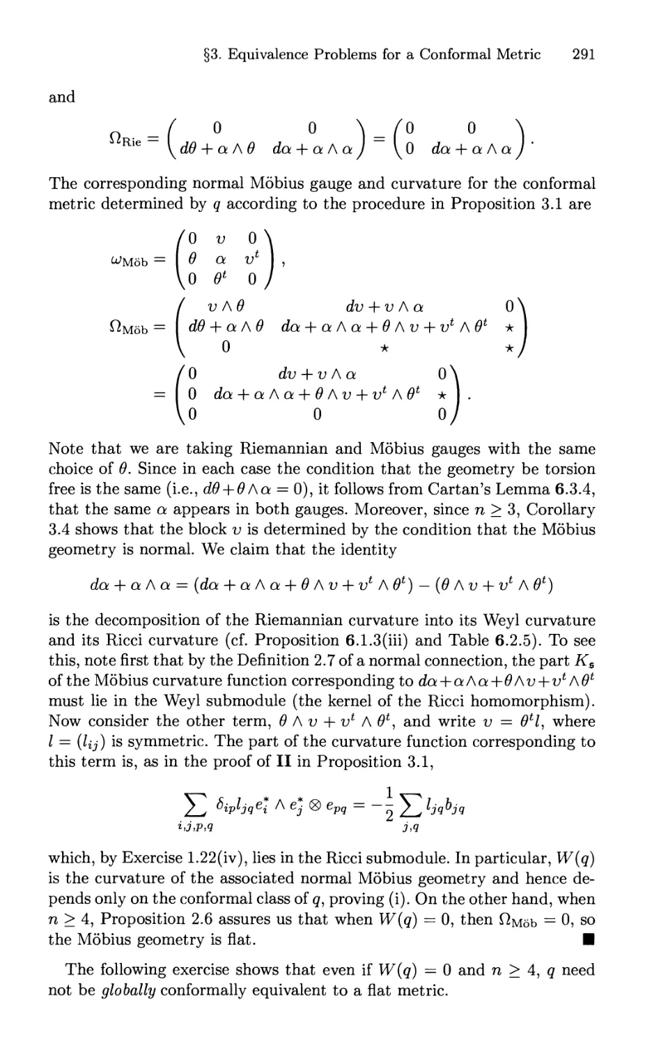
geometries (see diagram).
Euclidean generalization Klein
Geometry Geometries
generali-
generalization zation
Riemannian generalization Cartan
Geometry * Geometries
1The only relationship was the "accident" that some of the non-Euclidean
geometries could be regarded as special cases of Riemannian geometries.

x Preface
Looking at this diagram vertically, we can say that just as a Riemannian
geometry may be regarded, locally, as modeled on Euclidean space but
made "lumpy" by the introduction of a curvature, so a Cartan geometry
may be regarded, locally, as modeled on one of the Klein geometries but
made "lumpy" by the introduction of curvature appropriate to the model
in question. Looking at the same diagram horizontally, a Cartan geometry
may be regarded as a non-Euclidean analog of Riemannian geometry.
Cartan actually gave the first example of a Cartan geometry more than
a decade earlier, in the remarkable tour de force [E. Cartan, 1910]. In that
paper he considered the case of a two-dimensional distribution on a five-
dimensional manifold. He showed that such a distribution determined, and
was determined by, a Cartan geometry modeled on the homogeneous space
G2/H, where Я is a certain nine-dimensional subgroup of the fourteen-
dimensional exceptional Lie group G2· This process of associating a
Cartan geometry to a raw geometric entity (the distribution) is an example
of "solving the equivalence problem" for the entity in question. Although
the solution of an equivalence problem is not always a Cartan geometry,
in many important cases it is. When it is, the invariants of the geometry
(curvature, etc.) are a priori invariants of the raw geometric entity. We
recommend [R.B. Gardner, 1989] for an account of the method of equivalence.
To be a little more precise, a Cartan geometry on Μ consists of a pair
(Ρ,ω), where Ρ is a principal bundle Η —> Ρ —> Μ and ω, the Cartan
connection, is a differential form on P. The bundle generalizes the bundle
Η —> G —> G/H associated to the Klein setting, and the form ω generalizes
the Maurer-Cartan form uq on the Lie group G. In fact, the curvature of
the Cartan geometry, defined as dw + \{ω,ω\, is the complete local
obstruction to Ρ being a Lie group.
One reason for the power of Cartan's method comes from the fact that
these new geometries maintain the same intimate relation with Lie groups
that one sees in the case of homogeneous spaces. This means, for example,
that constructions in the theory of homogeneous spaces often generalize
in a simple manner to the general "curved" case of Cartan geometries.
It also means that the differential forms that appear are always related
to components of the Maurer-Cartan form of the Lie group, a context in
which their significance remains clear.
In the particular case of a Riemannian manifold M, Cartan's point of
view offered a new and profound vantage point that is largely responsible
for the modern insistence on "doing differential geometry on the bundle Ρ
of orthonormal frames over M."
The history of the study of Cartan geometries is somewhat troubled. First
is the difficulty Cartan faced in trying to express notions for which there was
no truly suitable language.2 Next is the widely noted difficulty in reading
2This difficulty was resolved with the introduction of the notion of a principal
bundle and of vector-valued forms on such a bundle.

Preface xi
Cartan.3 In his paper [C. Ehresmann, 1950] Charles Ehresmann gave for
the first time a rigorous global definition of a Cartan connection as a special
case of a more general notion now called an Ehresmann connection (or more
simply, a connection). For various reasons4 the Ehresmann definition was
taken as the definitive one, and Cartan's original notion went into a more
or less total eclipse for a long time. The beautiful geometrical origin and
insight connected with Cartan's view were, for many, simply lost. In short,
although the Ehresmann definition gives us a good notion, it hides the real
story about why it is so good. In this connection, the following quotation
is interesting [S.S. Chern, 1979]:
The physicist C.N. Yang wrote [C.N. Yang, 1977]: "That non-
abelian gauge fields are conceptually identical to ideas in the
beautiful theory of fibre bundles, developed by mathematicians
without reference to the physical world, was a great marvel to
me." In 1975 he mentioned to me: "This is both thrilling and
puzzling, since you mathematicians dreamed up these concepts
out of nowhere."
Far from arising "out of nowhere," the simple and compelling geometric
origin of a connection on a principal bundle is that it is a generalization
of the Maurer-Cartan form. Moreover, a study of the Cartan connection
itself can illuminate and unify many aspects of differential geometry.
Novelties
Aside from the fact that one cannot find a fully developed, modern
exposition of Cartan connections elsewhere, what is new or different in this
book?
New Treatment
This book is written at a level that can be understood by a first- or second-
year graduate student. In particular, we include the relevant theory of
manifolds, distributions and Lie groups. For us, a manifold is, by definition, a
3To paraphrase Robert Bryant, 'You read the introduction to a paper of
Cartan and you understand nothing. Then you read the rest of the paper and
still you understand nothing. Then you go back and read the introduction again
and there begins to be the faint glimmer of something very interesting."
4At that stage it was easier to read Ehresmann than Cartan. There was also
the attraction of a more general and global notion.

xii Preface
locally Euclidean, paracompact Hausdorff space. This is the same as a
locally Euclidean Hausdorff space each of whose components has a countable
basis.5 In particular, Lie groups are defined to be manifolds in this sense.
The result of Yamabe and Kuranishi ([H. Yamabe, 1950]) that a connected
subgroup of a Lie group is a Lie subgroup implies that any subgroup of a
Lie group is a Lie group in the present sense. The discussion of subman-
ifolds given in Chapter 1 is broad enough to include these subgroups as
submanifolds.
In our coverage of bundle theory, we emphasize the abstract principal
bundles rather than bundles of frames.6 Of course, these two views are
really equivalent. In the case of the "first-order" geometries, the equivalence is
quite simple. However, in the case of "higher-order" geometries, the choice
of the higher-order frames usually seems to be decided on a rather ad
hoc basis and can be complicated. Here the bundle approach gives a real
advantage, and the right choice of frames becomes clear (if needed) once
the bundle is understood. Another important advantage of working with
the bundles themselves is that they give a common language, facilitating
comparison between geometries and emphasizing the relation to the model
space. In this sense, comparing Cartan geometries is like comparing Klein
geometries.
Chapter 3 contains a complete and economical development of the Lie
group—Lie algebra correspondence based on the fundamental theorem of
non-abelian calculus. One of the novelties here is the characterization of
a Lie group as a manifold equipped with a Lie algebra-valued form on it
satisfying certain properties. This characterization prepares the reader for
the generalization to Cartan geometries in Chapter 5.
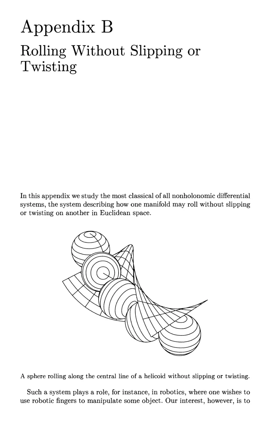
Finally, in Appendix В we explain how one manifold may roll
without slipping or twisting on another in Euclidean space. We also show how
this notion yields a differential system that contains both the Levi-Civita
connection and the Ehresmann connection on the normal bundle for a sub-
manifold of Euclidean space.
New Results
Let us move on to some results we believe are new. In Chapter 4 we
introduce the fundamental property of Klein geometries characterizing the
kernel of such a geometry. This result is used in Chapter 5 in an essential
way to show the equivalence of the base and bundle definitions of Cartan
geometries in the effective case. In Chapter 5 we introduce and classify
Cartan space forms. These geometries generalize the classical Riemannian
5The usual definition requires a manifold to have a countable basis (cf., e.g.,
[Boothby, W. 1986, p. 6]).
6 In much the same way, one might emphasize an abstract Lie group rather
than a matrix group realizing it.

Preface xiii
space forms.7 One important ingredient of this classification is the property
(apparently new) of a Cartan geometry called "geometric orient ability."
Another is the notion of "model mutation." Finally, in Chapter 7 we give
a classification of the submanifolds of a Mobius geometry. This
classification is more general than that of [A. Fialkow, 1944] in that ours allows the
presence of umbilic points.
Prerequisites and Conventions
This book assumes very few prerequisites. The reader needs to be familiar
with some basic ideas of group theory, including the notion of a group
acting on a set. Results from the calculus of several variables, point set
topology, and the theory of covering spaces are used in various places, and
the long, exact sequence of homotopy theory is used once (at the end of
Chapter 5). Aside from this, most of the material is developed ab initio.
However, the reader is invited to shoulder some of the burden of the work
in that essential use is made of a few of the exercises. These exercises are
denoted by an asterisk to the right of the exercise number.
The numbering follows a single sequence throughout the book, with all
items (definitions, theorems, figures, etc.) in a single stream. Thus 4.3.2
refers to Chapter 4, Section 3, item 2. For references to items occurring in
the same chapter, we omit the chapter number, so that in Chapter 4, 4.3.2
becomes 3.2.
We use the following dictionary of symbols to denote the ends of various
items:
symbol end of
Φ definition
□ exercise
■ proof
♦ example
Although it will often be convenient for us to write column vectors as
row vectors, the reader should remember that all vectors are in fact column
vectors.
7In fact, this notion is general enough to immediately allow a description of
general symmetric spaces.

xiv Preface
Limitations
The reader will find no mention here of some basic topics in differential
geometry, such as Stokes' theorem, characteristic classes, and complex
geometries. Also, our approach to Lie theory is "elementary" in that we do
not discuss or use the classification theory of Lie groups, with its attendant
study of roots, weights, and representations.
Originally, we had wished to include more than the three examples of
Cart an geometries studied here; but in the end, the pressures of time, space,
and energy limited this impulse. The three geometries we do study are not
developed in complete analogy to each other. For example, the discussion
of immersed curves in a Mobius geometry in terms of the normal forms
given in Chapter 7 does of course have a Riemannian analog, but that is
not studied in this book. And one may study subgeometries of projective
geometries just as one studies subgeometries of Riemannian and Mobius
geometries, but we do not do so here. We have also resisted the impulse
to make a "dictionary" translating among the various versions of Cartan's
view, Ehresmann's view,8 and the view expressed in [L.P. Eisenhart, 1964].
In the end, however, for those who are interested in it, it should be
abundantly clear how Cartan's view does illuminate the others.
Some Personal Remarks
An author often writes a book in order to sort out his or her own
understanding of the subject. This is the circumstance in the present case. When
I was an undergraduate, differential geometry appeared to me to be a study
of curvatures of curves and surfaces in R3. As a graduate student I learned
that it is the study of a connection on a principal bundle. I wondered what
had become of the curves and surfaces, and I studied topology instead.
The reawakening of my interest in this subject began in 1987 when Tom
Willmore very kindly wrote me a note thanking me for a preprint and
mentioning his great interest in what is known as the Willmore conjecture (cf.
7.6). This led me once again to look at principal bundles and connections.
In particular, I wondered whether there was an intrinsically defined Ehres-
mann connection on a surface in 53 that was invariant under the group
of Mobius transformations of 53. It turns out there is no such connection.
However, after calculating normal forms for surfaces in the Mobius sphere
53 (cf. [G. Cairns, R. Sharpe, and L. Webb, 1994]), it became clear to me
that there must be some other kind of invariantly defined structure
inherited on the surface from its embedding in 53. (In Chapter 7 it is shown
See, however, the discussion in Appendix A dealing with the relationship
between Cart an and Ehresmann connections.

Preface x ν
that a Cartan connection is defined in this situation, and, in fact, Cartan
also knew this [E. Cartan, 1923].)
During this time it began to seem strange to me that Ehresmann
connections play such a prominent role in modern differential geometry. In some
cases, such as the Levi-Civita connection, the connection is determined
by the geometry. In many cases, however, one makes use of an arbitrary
connection that one proves to exist by a general technique. This is the
appropriate point of view for the construction of the characteristic classes of
Chern and Pontryagin. There one may use any connection, since the aim
is to obtain topological invariants for which the particular choice of
connection does not matter. But these considerations seem to be at their base
topological rather than differential geometric. My innocent question, left
over from my undergraduate days, was "Why is differential geometry the
study of a connection on a principal bundle?" And I began, rather
impertinently, to ask this question at every opportunity, usually picking on some
unsuspecting differential geometer who did not know me very well.
During one of these sessions, Min Oo remarked that Elie Cartan had
considered connections with values in a Lie algebra larger than that of the
fiber.9 Later I read, and translated,10 Cartan's book [E. Cartan, 1935]. I
browsed through Cartan's collected works and through those of his
successors and interpreters. It became clear to me that Cartan had a subtle
and really wonderful idea, which gives a fully satisfying explanation for the
modern, and approximately true, notion that differential geometry is the
study of an Ehresmann connection on a principal bundle. There seems to be
no treatment of these things in the standard texts on differential geometry.
In the few books where the Cartan connections are mentioned at all (e.g.,
[J. Dieudonne 1974], [W.A. Poor, 1981], and [M. Spivak, 1979]), they make
only a brief appearance, perhaps in the exercises or toward the end of the
book, and one is left with the impression that the notion is only a quaint
curiosity left over from bygone days. Six years ago I began to scribble some
notes about these things and to talk about them; after a number of months
had passed, I realized I was writing a book on the subject.
* * *
I would like to thank everyone who has had an influence on this book.
In addition to those mentioned above, I am grateful to Bernard Kamte,
Joe Repka, Qunfeng Yang, and my wife, Mary, for their comments on
portions of the manuscript. I would also like to acknowledge my gratitude to
9See [E. Ruh, 1993] for a brief recent overview of Cartan connections and some
of their applications.
10A copy of my translation, which is only a rough draft, can be found in the
Mathematics Library at the University of Toronto.

xvi Preface
the National Science and Engineering Research Council of Canada for its
support of this project through grant #OGP0004621.
Finally, I would like to thank Velamir Jurdjevic for his encouragement
over the years. It was Vel who suggested that, although it is perhaps
impossible to catch all the errors before a book reaches print, the principal
demand is that a book be interesting. As for the first part of his remark,
the responsibility for any remaining errors lies with me. I will leave it to
the reader to judge whether or not this principal demand has been met.
Richard Sharpe
Toronto, Canada
October 16, 1995

Contents
Foreword ν
Preface ix
1 In the Ashes of the Ether: Differential Topology 1
§1. Smooth Manifolds 3
§2. Submanifolds 17
§3. Fiber Bundles 28
§4. Tangent Vectors, Bundles, and Fields 39
§5. Differential Forms 52
2 Looking for the Forest in the Leaves: Foliations 65
§1. Integral Curves 66
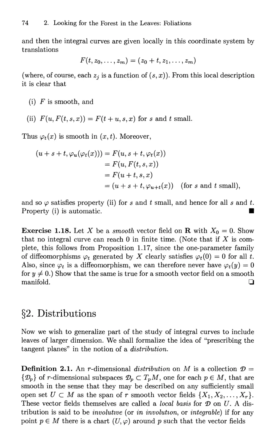
§2. Distributions 74
§3. Integrability Conditions 75
§4. The Frobenius Theorem 76
§5. The Frobenius Theorem in Terms of Differential Forms . . 79
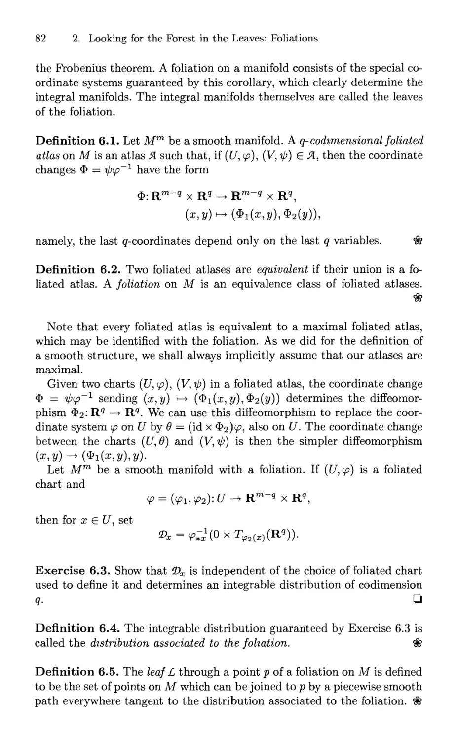
§6. Foliations 81
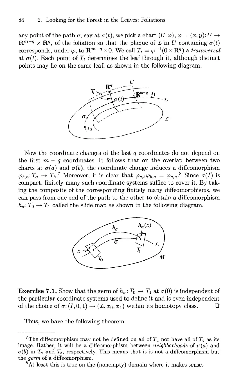
§7. Leaf Holonomy 83
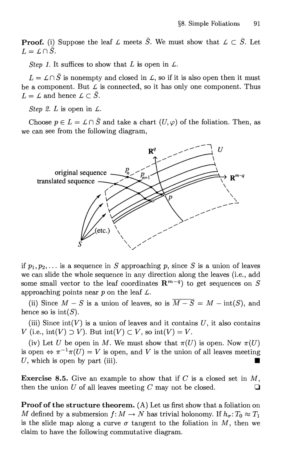
§8. Simple Foliations 90
3 The Fundamental Theorem of Calculus 95
§1. The Maurer-Cartan Form 96
§2. Lie Algebras 101

xviii Contents
§3. Structural Equation 108
§4. Adjoint Action 110
§5. The Darboux Derivative 115
§6. The Fundamental Theorem: Local Version 116
§7. The Fundamental Theorem: Global Version 118
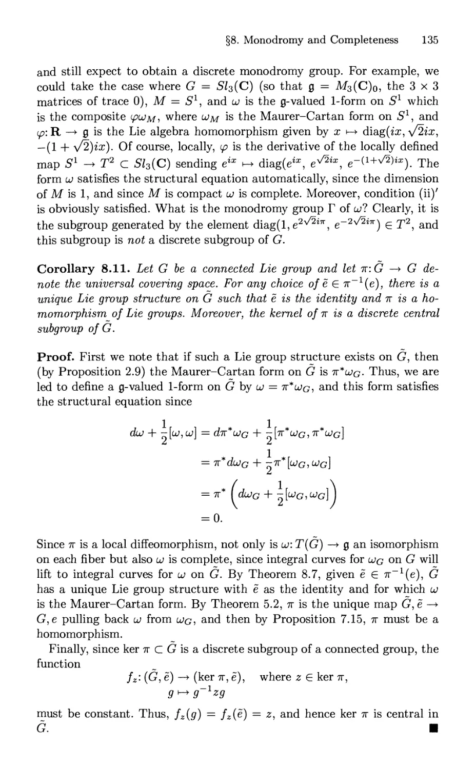
§8. Monodromy and Completeness 128
4 Shapes Fantastic: Klein Geometries 137
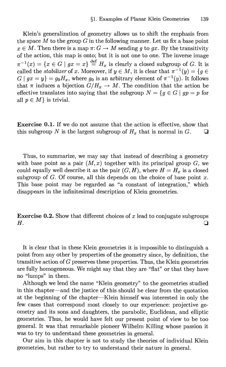
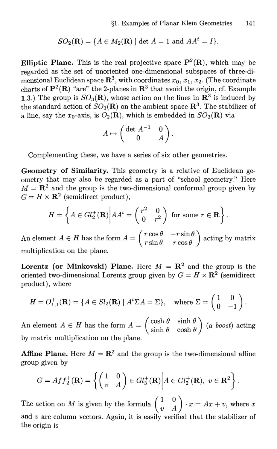
§1. Examples of Planar Klein Geometries 140
§2. Principal Bundles: Characterization and Reduction .... 144
§3. Klein Geometries 150
§4. A Fundamental Property 160
§5. The Tangent Bundle of a Klein Geometry 162
§6. The Meteor Tracking Problem 164
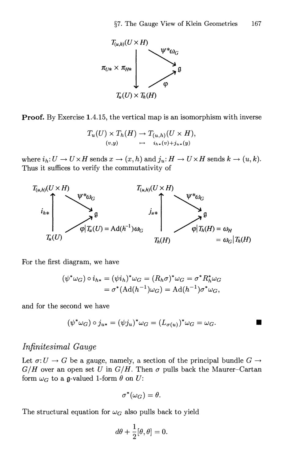
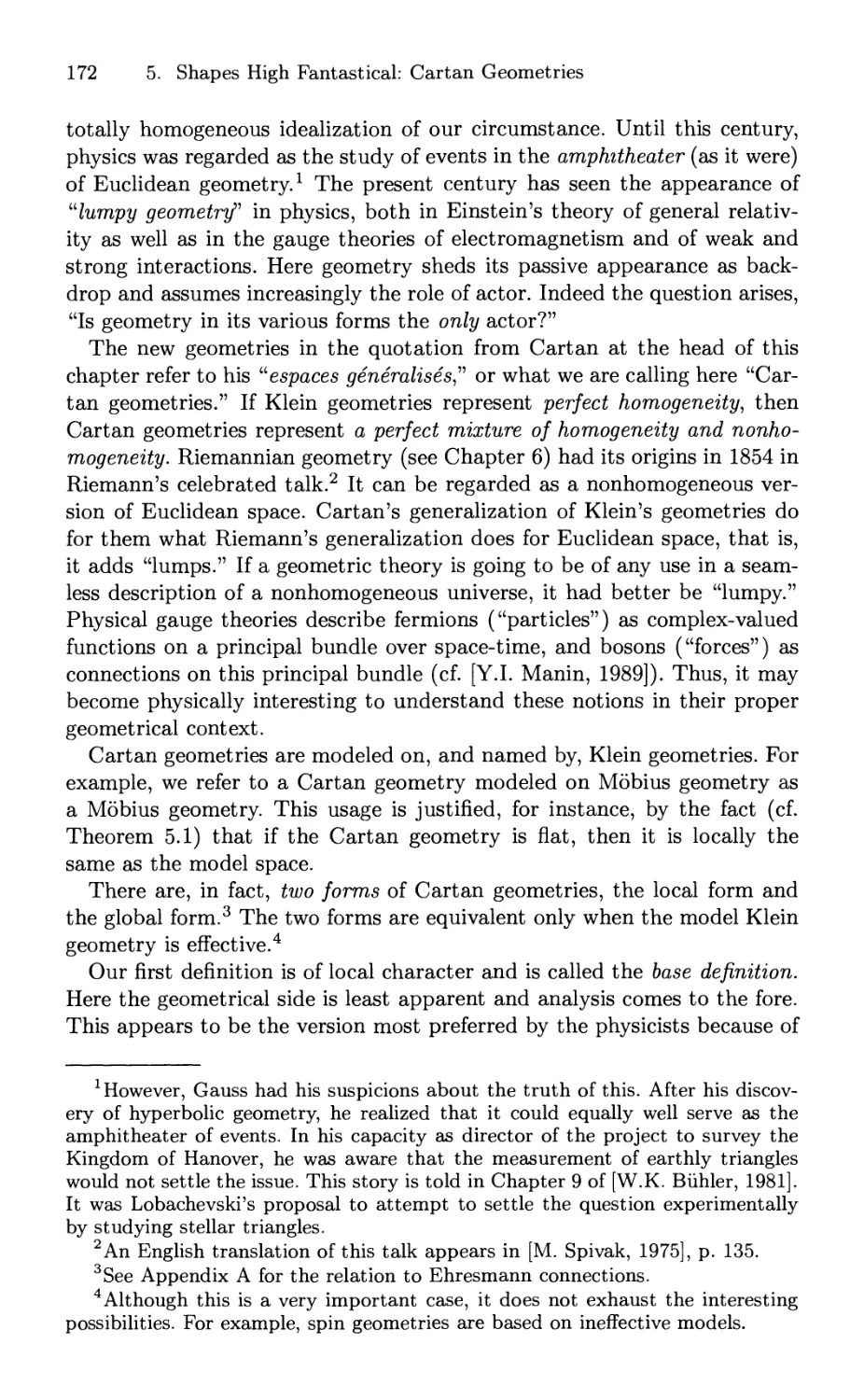
§7. The Gauge View of Klein Geometries 166
5 Shapes High Fantastical: Cartan Geometries 171
§1. The Base Definition of Cartan Geometries 173
§2. The Principal Bundle Hidden in a Cartan Geometry . . . 178
§3. The Bundle Definition of a Cartan Geometry 184
§4. Development, Geometric Orientation, and Holonomy . . . 202
§5. Flat Cartan Geometries and Uniformization 211
§6. Cartan Space Forms 217
§7. Symmetric Spaces 225
6 Riemannian Geometry 227
§1. The Model Euclidean Space 228
§2. Euclidean and Riemannian Geometry 234
§3. The Equivalence Problem for Riemannian Metrics .... 237
§4. Riemannian Space Forms 241
§5. Subgeometry of a Riemannian Geometry 244
§6. Isoparametric Submanifolds 259
7 Mobius Geometry 265
§1. The Mobius and Weyl Models 267
§2. Mobius and Weyl Geometries 277
§3. Equivalence Problems for a Conformal Metric 284
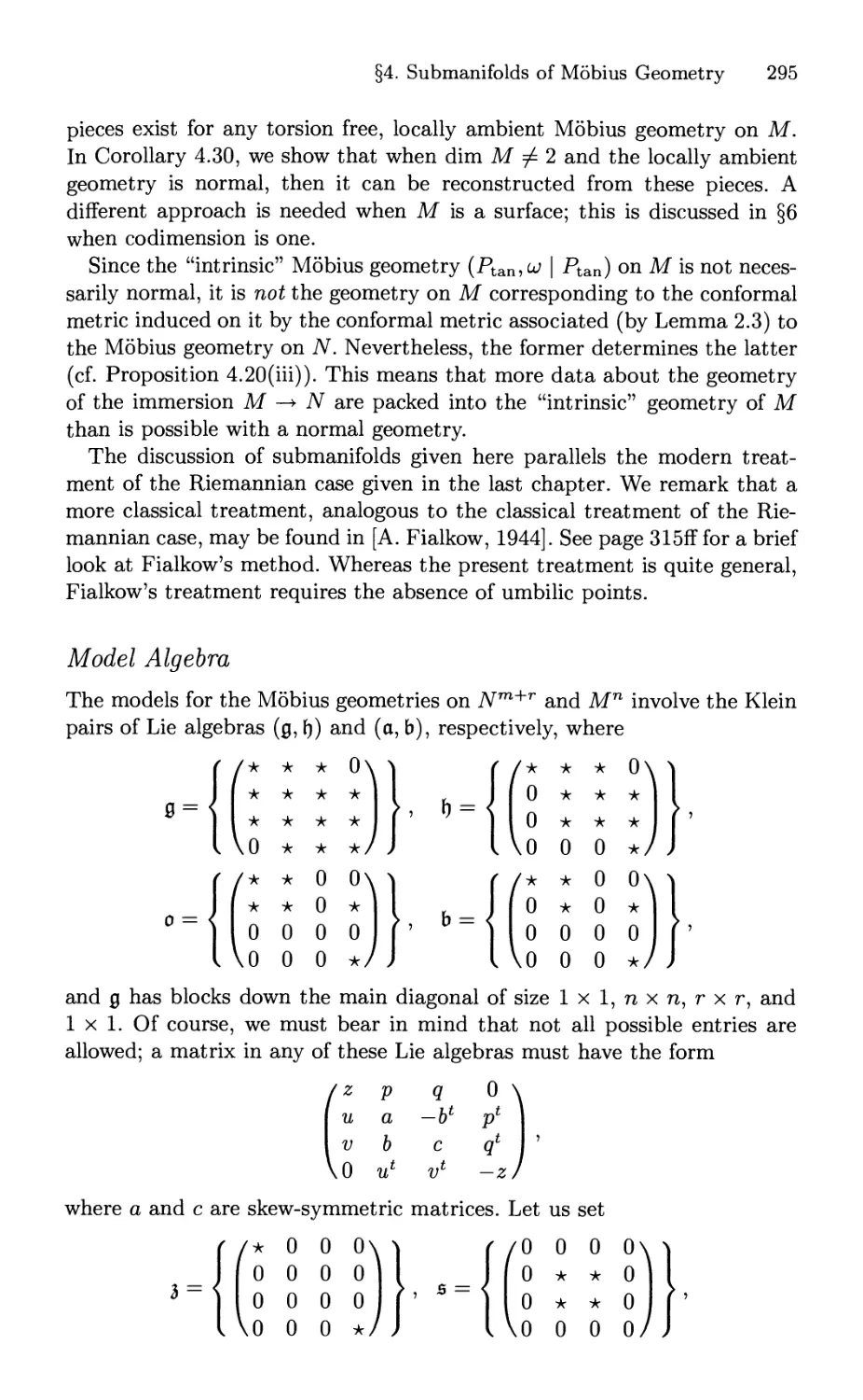
§4. Submanifolds of Mobius Geometry 294
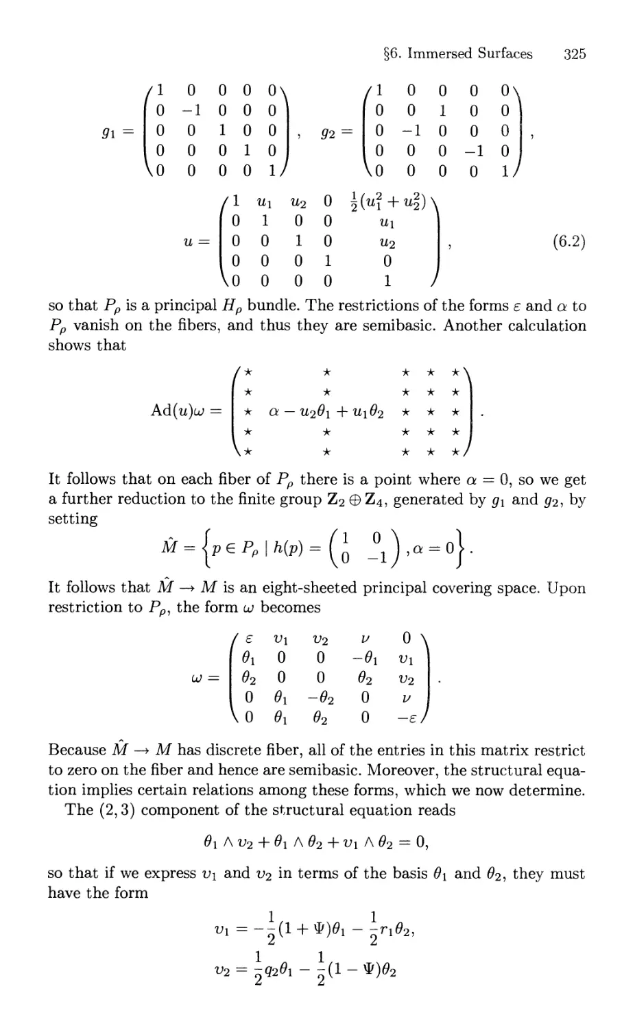
§5. Immersed Curves 318
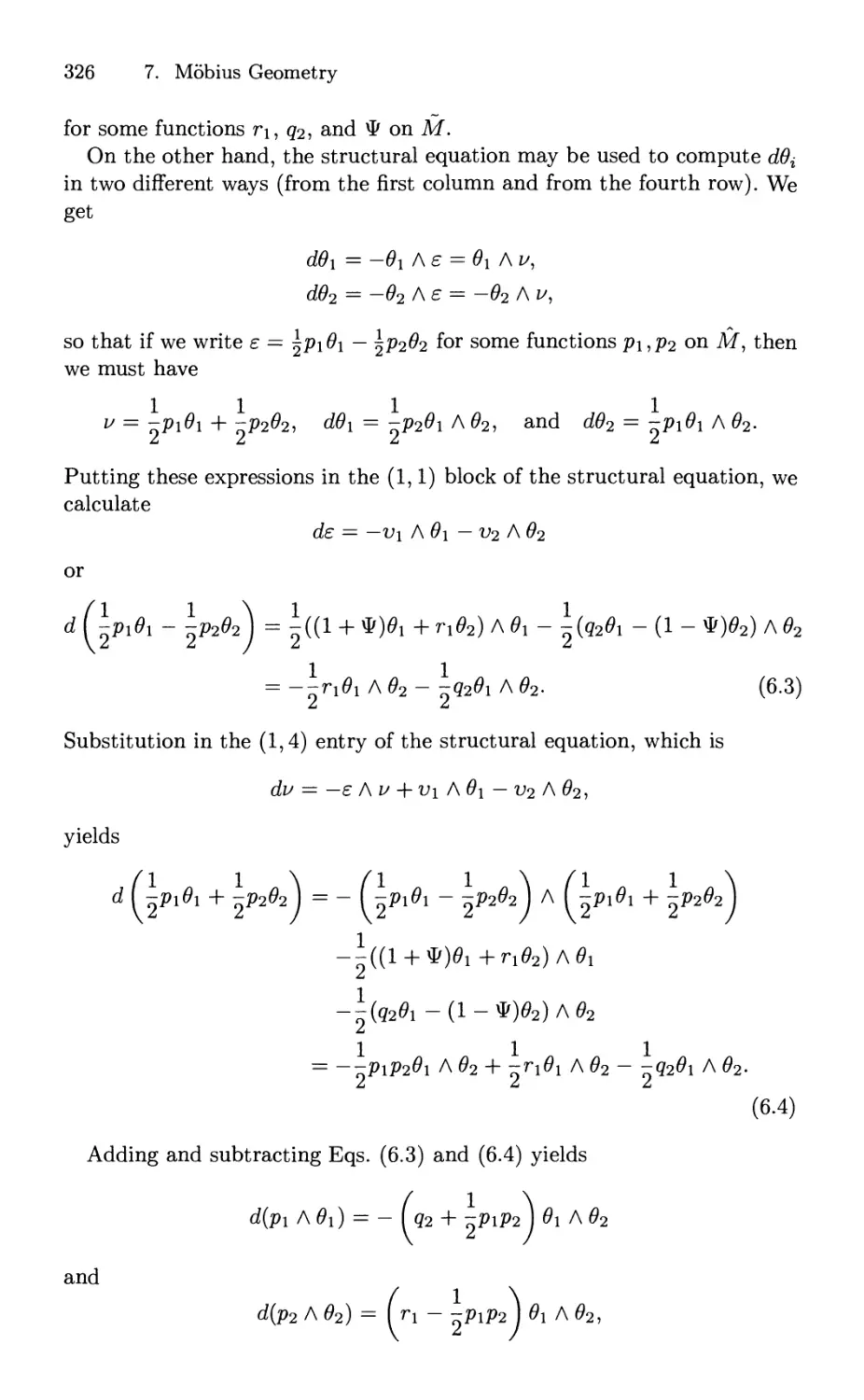
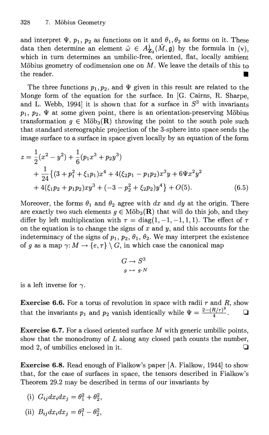
§6. Immersed Surfaces 323
8 Projective Geometry 331
§1. The Projective Model 332
§2. Projective Cartan Geometries 338
§3. The Geometry of Geodesies 343

Contents xix
§4. The Projective Connection in a Riemannian Geometry . . 349
§5. A Brief Tour of Projective Geometry 353
A Ehresmann Connections 357
§1. The Geometric Origin of Ehresmann Connections 358
§2. The Reductive Case 362
§3. Ehresmann Connections Generalize Cartan Connections . 365
§4. Covariant Derivative 371
В Rolling Without Slipping or Twisting 375
§1. Rolling Maps 376
§2. The Existence and Uniqueness of Rolling Maps 378
§3. Relation to Levi-Civita and Normal Connections 382
§4. Transitivity of Rolling Without Slipping or Twisting . . . 388
С Classification of One-Dimensional Effective Klein Pairs 391
§1. Classification of One-Dimensional Effective Klein Pairs . . 391
D Differential Operators Obtained from Symmetry 397
§1. Real Representations of S02(R) 397
§2. Operators on Riemannian Surfaces 400
Ε Characterization of Principal Bundles 407
Bibliography 411
Index
417

1
In the Ashes of the Ether:
Differential Topology
It must be agreed that "hypergeometry" seems to have been
devised in order to strike the imagination of people who have not
enough mathematical knowledge to be aware of the true
character of an algebraic construction expressed in geometric terms,
for that is what "hypergeometry" really is. -R. Guenon, 1945
Is Euclidean geometry true? It has no meaning. ... One
geometry cannot be more true than another; it can only be more
convenient. -H. Poincare, 1902
I attach special importance to the view of geometry which I have
just set forth, because without it I should have been unable to
formulate the theory of relativity. -A. Einstein, 1922
Although several mathematicians, especially C.F. Gauss, studied the
notion of a smooth manifold in special cases, the idea of an abstract manifold
of arbitrary finite dimension seems to be due to Riemann. Mathematicians
were led to these notions only slowly. As the idea of a vector space of
dimension higher than three became acceptable in the last century, algebraic
geometers began to study the solutions of polynomial equations in many
variables. For example, they studied the algebraic curves in the complex
projective plane, which in the real sense is roughly the study of ordinary
surfaces in four-dimensional space. At the same time, mathematical
physicists interested themselves in six-dimensional space, the state space of a
single particle with three position and three momentum variables; if TV

2 1. In the Ashes of the Ether: Differential Topology
particles are considered, the dimension of the state space jumps to 67V.
The seamless algebraic passage between the ordinary notions of space and
their higher-dimensional analogs must have prepared the way for the
acceptance of Riemann's abstract manifolds. But the willingness and even
the necessity of regarding these developments as truly geometrical was slow
to take hold and was fiercely resisted in some quarters.1
Riemann's work was followed with papers by Christoffel, Ricci, and Levi-
Civita. Klein and Lie were interested in the study of Lie groups and their
homogeneous spaces, which are again examples of manifolds, albeit very
special ones. A real boost to the subject came with Einstein's discovery of
general relativity in 1915. At this stage it became much clearer that the
fourth dimension might be scientifically regarded as more than some
geometrical fantasy. Einstein himself regarded the abstract four-manifold2 as
what remains of the "ether" in general relativity (cf. [A. Einstein, 1922]).
In the early years these spaces were thought about only locally, as pieces
of four-dimensional Euclidean space. Later the notion of "cosmology"
appeared (cf. [D. Howard and J. Stachel, eds., 1989]) and began to show
the influence of the global topology. Perhaps we may say that in studying
smooth manifolds we are studying the possible shapes of the ether.
In the hierarchy of geometry (whose "spine" rises from homotopy theory
through cell complexes, through topological and smooth manifolds to
analytic varieties), the category of smooth manifolds and maps lies "halfway"
between the global rigidity of the analytic category and the almost total
flabbiness of the topological category. We might say that a smooth
manifold possesses full infinitesimal rigidity governed by Taylor's theorem while
at the same time having absolutely no rigidity relating points that are not
"infinitesimally near" each other, as is seen by the existence of partitions
of unity (cf. [W. Boothby, 1986], pp. 193-195). Smooth manifolds are
sufficiently rigid to act as a support for the structures of differential geomtery
while at the same time being sufficiently flexible to act as a model for
many physical and mathematical circumstances that allow independent
local perturbations. Perhaps the smooth "substance" may be regarded as a
mathematical model for Aristotle's materia prima or the Hindu prakriti.
In this chapter we show how the differential calculus lives on after the
death of a preferred coordinate system. In particular, we discuss some of the
beautiful and elementary constructions surrounding the notion of a smooth
^f. [M. Monastyrski, 1987], pp. 22 and 64.
2Einstein admits [A. Einstein, 1922] his difficulty in conceiving space-time
without a metric. In fact, he spent the rest of his life searching for a geometric
structure on a four-manifold supplementing the metric to include electromag-
netism within a unified field theory generalizing his general theory of
relativity. The general question of "what geometry on a manifold supports physics?"
remains vital to the present day. On the other hand, the context for all such
structures seems to continue to include a smooth manifold.

§1. Smooth Manifolds 3
manifold. Care is taken to show the relation between the forms of these
constructions for the concrete situation of manifolds embedded in an ambient
Euclidean space and those for an abstract, coordinate-independent,
manifold.
§1. Smooth Manifolds
The definitive modern definition of a smooth manifold seems to have been
given by Hassler Whitney ([H. Whitney, 1936]), in which a smooth manifold
is presented as floppy pieces of Euclidean space glued together with a sort
of differentiable glue. But in order to gain perspective, we start our more
detailed discussion with topological manifolds.
Topological Manifolds
Definition 1.1. Let Μ be a paracompact3 Hausdorff space. We call Μ an
n-dimensional topological manifold (and write it Mn if we wish to denote
the dimension) if for each point ρ G Μ there is an open set U in Μ
containing ρ such that U is homeomorphic to an open subset of Rn by some
homeomorphism φ.4 Such a pair ([/, φ) is called a local coordinate system
or (in the maritime terminology) a chart on M. On the other hand, φ~ι
is called a local parameterization of M. Often, however, speaking loosely,
both φ and φ~ι are referred to as coordinate systems. *
We note that if Μ is an η-manifold, then so is every open subset of it;
in particular, the components of Μ are also manifolds. On the other hand,
manifolds are quite badly behaved with respect to quotients. Taking the
quotient of a manifold by almost any equivalence relation on it leads out
of the category of manifolds. Some notable exceptions to this are studied
later under the name of fiber bundles.
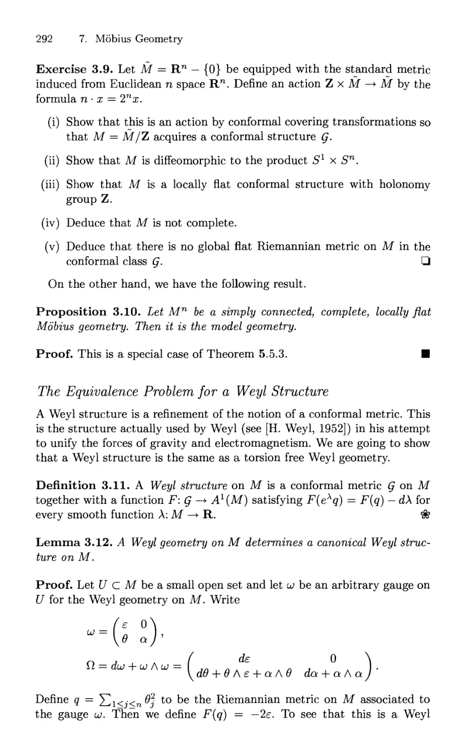
Example 1.2 (the η-sphere). Let Mn = Sn = {x G Rn+1 | χ · χ = 1}·
Set U — {χ G Sn | xn+i > — 1}· Then U is an open subset of 5n, as is its
homeomorphic image p(U), where p: Rn+1 —» Rn+1 is the reflection in the
hyperplane xn+i = 0. The open sets U and p(U) together form a covering
for Sn. We can see that U (and hence p(U)) is homeomorphic to Rn by
considering the stereographic projection φ from the point — en+i given by
3This is equivalent to each component of Μ having a countable basis for its
topology (cf. [J. Dugundiji, 1966], p. 241).
4 We note that only the topological structure of Rn is brought into play here.
In particular, neither the Euclidean structure nor the affine space structure has
any role. Nevertheless, we shall continue to refer to Rn as Euclidean space.

4 1. In the Ashes of the Ether: Differential Topology
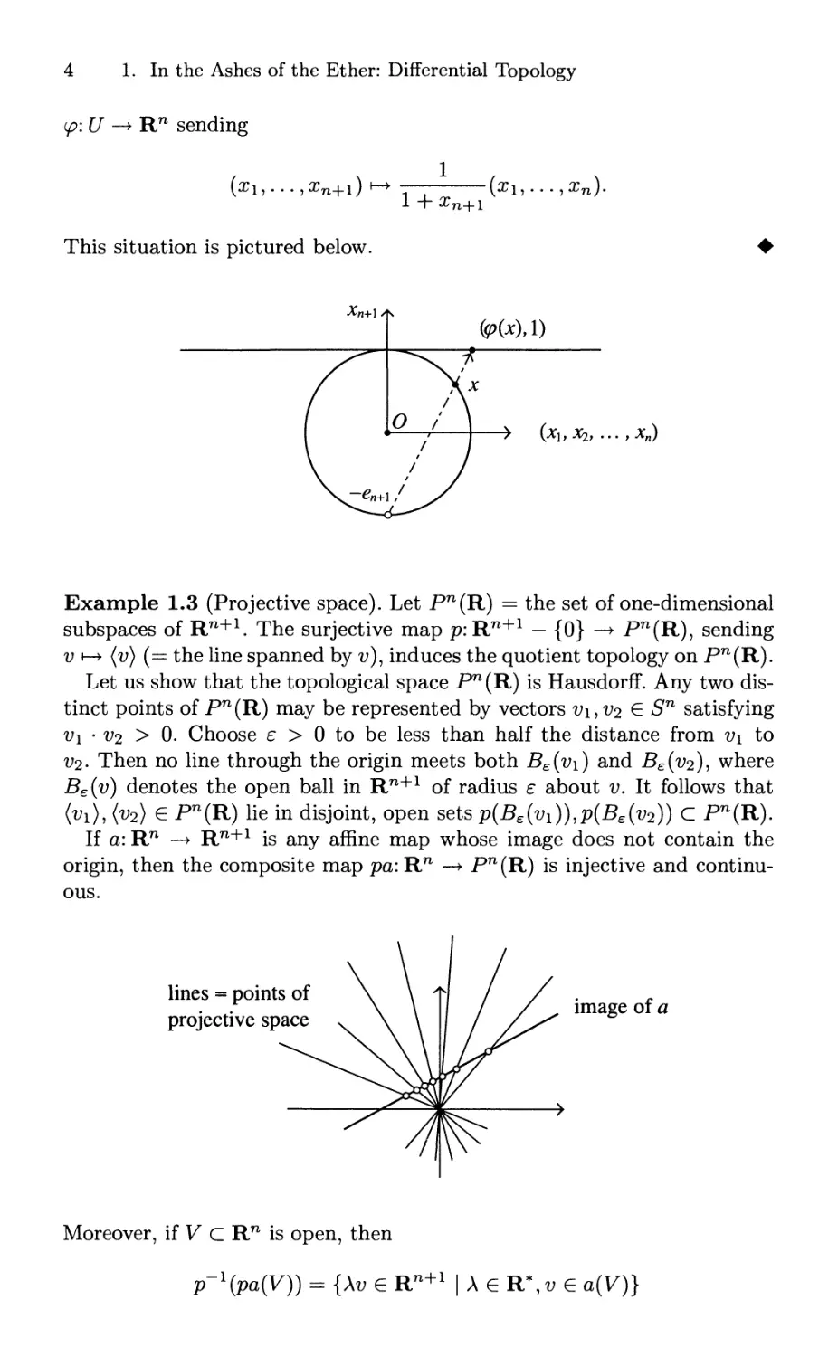
φ: U —► Rn sending
(χι,...,χη+ι) ·->
This situation is pictured below.
1
1 +^n+l
yX\, . . . , Xn)·
Xn+\
ШЛ)
> (хиХ2,...,Хп)
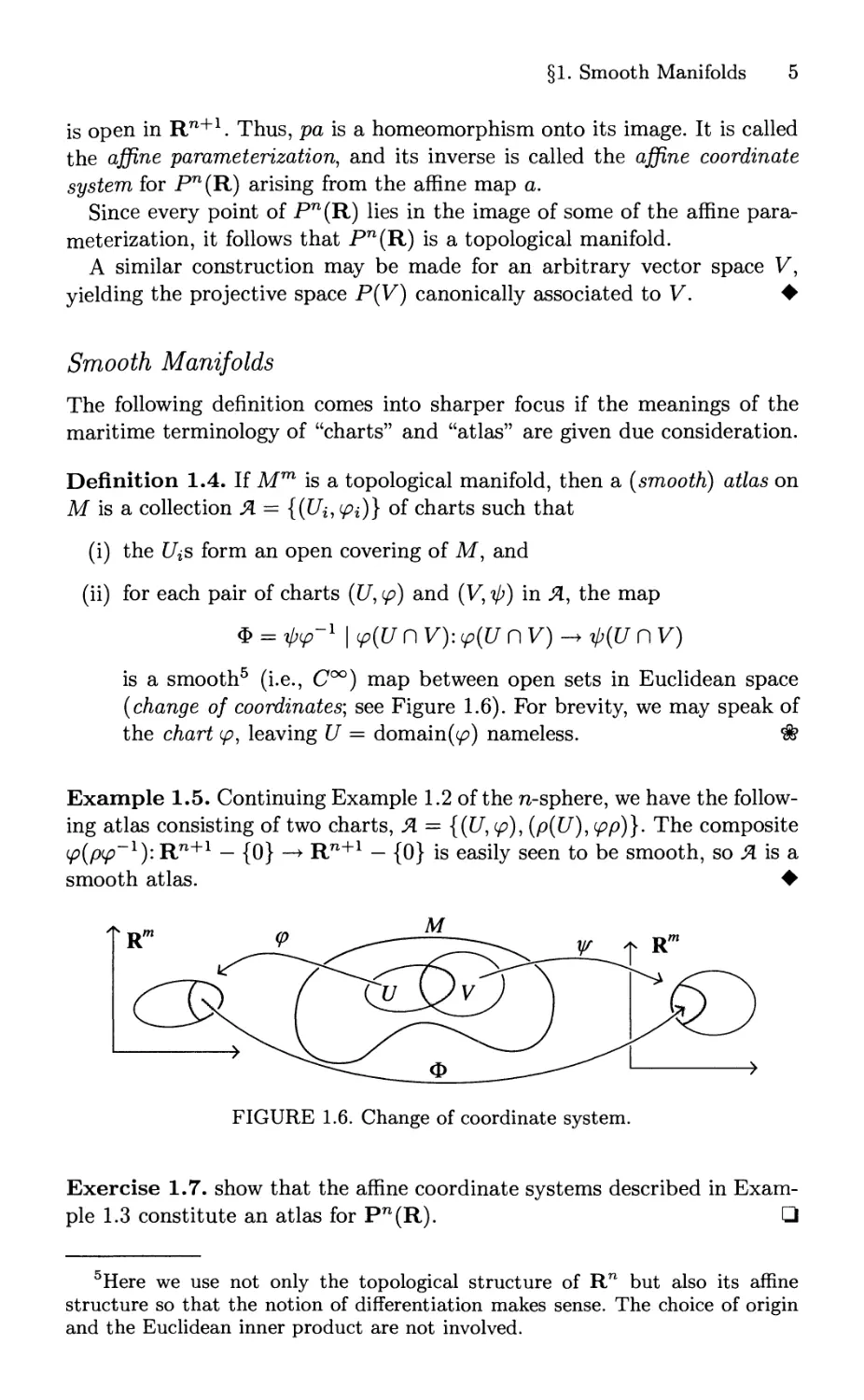
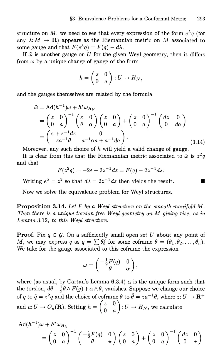
Example 1.3 (Projective space). Let Pn(R) = the set of one-dimensional
subspaces of Rn+1. The surjective map p:Rn+1 — {0} —► Pn(R), sending
ν ь-> (υ) (= the line spanned by υ), induces the quotient topology on Pn(R).
Let us show that the topological space Pn(R) is Hausdorff. Any two
distinct points of Pn(R) may be represented by vectors v\,V2 £ Sn satisfying
V\ · V2 > 0. Choose ε > 0 to be less than half the distance from i?i to
V2- Then no line through the origin meets both Bs{v\) and Βε{ν2), where
Βε(υ) denotes the open ball in Rn+1 of radius ε about v. It follows that
(vi), (v2) e Pn(R) lie in disjoint, open sets ρ(Βε(νι)),ρ(Βε(ν2)) С Pn(R).
If a: Rn —> Rn+1 is any affine map whose image does not contain the
origin, then the composite map pa: Rn —» Pn(R) is injective and
continuous.
lines = points of
projective space
image of a
Moreover, if V С Rn is open, then
p-\pa(V)) = {\v e Rn+1 | λ e K\v e a(V)}

§1. Smooth Manifolds 5
is open in Rn+1. Thus, pa is a homeomorphism onto its image. It is called
the affine parameterization, and its inverse is called the affine coordinate
system for Pn(R) arising from the affine map a.
Since every point of Pn(R) lies in the image of some of the affine
parameterization, it follows that Pn(R) is a topological manifold.
A similar construction may be made for an arbitrary vector space V,
yielding the projective space P(V) canonically associated to V. ♦
Smooth Manifolds
The following definition comes into sharper focus if the meanings of the
maritime terminology of "charts" and "atlas" are given due consideration.
Definition 1.4. If Mm is a topological manifold, then a (smooth) atlas on
Μ is a collection Я — {(Ε/*, φι)} of charts such that
(i) the UiS form an open covering of Μ, and
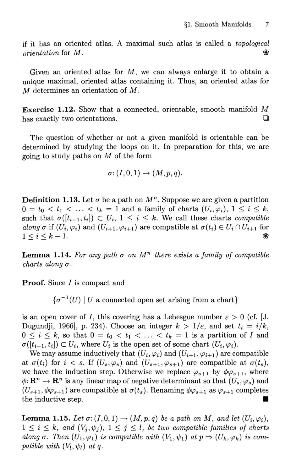
(ii) for each pair of charts ([/, φ) and (V, ψ) in Я, the map
φ = ψφ-ι Ι φ(υ η V): φ(ϋ ПУ)-> φ(ϋ Π V)
is a smooth5 (i.e., C°°) map between open sets in Euclidean space
(change of coordinates; see Figure 1.6). For brevity, we may speak of
the chart φ, leaving U = domain((^) nameless. *
Example 1.5. Continuing Example 1.2 of the η-sphere, we have the
following atlas consisting of two charts, Я = {(ί/, φ), (p(U), φ ρ)}· The composite
φ(ρφ~ι): Rn+1 — {0} —► Rn+1 — {0} is easily seen to be smooth, so Л is a
smooth atlas. ♦
FIGURE 1.6. Change of coordinate system.
Exercise 1.7. show that the affine coordinate systems described in
Example 1.3 constitute an atlas for Pn(R). □
5Here we use not only the topological structure of Rn but also its affine
structure so that the notion of differentiation makes sense. The choice of origin
and the Euclidean inner product are not involved.

6 1. In the Ashes of the Ether: Differential Topology
The main point of introducing smooth atlases is to be able to
unambiguously differentiate the composite appearing in Definition 1.4(ii) as often as
we please. For this simple purpose the particular choice of atlas is not
important, so we are led to make the definition that two atlases are equivalent
if their union is also an atlas. This in turn leads to the following definition.
Definition 1.8. A smooth structure on a topological manifold is an
equivalence class of atlases, and a smooth manifold is a topological manifold with
a specified smooth structure. *
For example, the atlas for the η-sphere above endows it with a smooth
structure called the canonical smooth structure.
Starting with a given atlas, we can enlarge it to the union of all the
atlases equivalent to it. This will give a unique maximal atlas equivalent
to the given one, and the smooth structure may be identified with the
corresponding maximal atlas. In particular, if φ is a chart in the maximal
atlas of a smooth manifold, and / is a local diffeomorphism of Rn with
image(^) С domain(/), then /φ is also a chart in the maximal atlas. This
kind of procedure allows a great deal of flexibility in the choice of chart.
For example, we can "tidy up" the chart φ with respect to a point ρ G U
by following φ with a translation in Rn so that the new chart sends ρ to
0 G Rn. We may further follow φ by some linear transformation of Rn
to move the various directions into convenient positions. We shall always
implicitly assume we are dealing with a maximal atlas, even if it is described
by a particular choice of a nonmaximal one.
Orientability
Definition 1.9. Let ([/, φ) and (V, ψ) be two charts for the smooth
manifold Mn. We say these charts are compatible on W С U Π V if the change
of coordinate mapping Φ = ψφ~ι \ φ{ϋ Π V) has positive Jacobian
determinant at each point of tp(W). We say they are compatible if they are
compatible on U Π V. *
Remark 1.10. Since the sign of the determinant of the Jacobian matrix
(ψ ο φ~ιγ(χ) is constant on each component of φ{ϋ Π V), it follows that if
({/, φ) and (V, ψ) are compatible at χ G U Π V, then they are compatible
on the component of U Π V containing x. On the other hand, if they are
not compatible at a point χ e U Π V, then the charts (υ,φ) and (ν,φψ)
are compatible, where φ is any linear transformation of Rn of negative
determinant.
Definition 1.11. Let Μ be a smooth manifold. An atlas for Μ is oriented
if any two charts in it are compatible. Μ is called topologically orientable

§1. Smooth Manifolds 7
if it has an oriented atlas. A maximal such atlas is called a topological
onentation for Μ. Φ
Given an oriented atlas for Μ, we can always enlarge it to obtain a
unique maximal, oriented atlas containing it. Thus, an oriented atlas for
Μ determines an orientation of M.
Exercise 1.12. Show that a connected, orientable, smooth manifold Μ
has exactly two orientations. □
The question of whether or not a given manifold is orientable can be
determined by studying the loops on it. In preparation for this, we are
going to study paths on Μ of the form
σ: (7,0,1)-* (M,p,q).
Definition 1.13. Let σ be a path on Mn. Suppose we are given a partition
0 = to < ti < ... < tk = 1 and a family of charts (Ui,tpi), 1 < г < к,
such that σ([ίΐ-ι,^]) С Щ, 1 < г < к. We call these charts compatible
along σ if {ϋ%,ψϊ) and ([/г+ь^г+ι) are compatible at σ(^) Е^П t/i+i for
1 < i < к- 1. *
Lemma 1.14. For any path σ on Mn there exists a family of compatible
charts along σ.
Proof. Since I is compact and
{a~l(U) | U a connected open set arising from a chart}
is an open cover of 7, this covering has a Lebesgue number ε > 0 (cf. [J.
Dugundji, 1966], p. 234). Choose an integer к > Ι/ε, and set ti — г/к,
0 < г < к, so that 0 = ίο < ^ι < ... < £fc = 1 is a partition of 7 and
σ([^-ι,^]) С Ui, where Щ is the open set of some chart {υ%,ψι)·
We may assume inductively that (Щ, φι) and (£/г+ь ^г+ι) are compatible
at a(ti) for г < s. If (Us,tps) and (£/s+1,(^s+i) are compatible at a(ts),
we have the induction step. Otherwise we replace φ8+ι by φφ8+\, where
ф: Rn —» Rn is any linear map of negative determinant so that (Us, φ8) and
({7s+i,0(^s+i) are compatible at a(ts). Renaming φφδ+ι as φ8+ι completes
the inductive step. ■
Lemma 1.15. Let σ: (7,0,1) —> (M,p,q) be a path on M, and let (C/»,^),
1 < г < к, and (Vj,^j), 1 < j < I, be two compatible families of charts
along σ. Then {ϋ\,φι) is compatible with (Vi,^i) at ρ =$> (Uk,<Pk) ls
compatible with (νι,ψι) at q.

8 1. In the Ashes of the Ether: Differential Topology
Proof. Let 0 = so < si < ... < Sk = 1 and 0 = to < t\ < ... < ti = 1
be the partitions of I corresponding to the compatible families of charts
(Ui,ipi), 1 < г < к, and (Vj,i/jj), 1 < j <l, respectively. Let Si — [si_i,Si]
and Tj = [tj-\,tj]. The proof is by induction, where the inductive step is
Suppose that Si PiTj ^ 0 and (Ui,ipi) is compatible with (Vj,^j) on
a(SinTj). Then, either
(i) Si+iHTj φ 0 and (υί+ι,ψί+ι) is compatible with (Vj,^) on σ(5ΐ+ι(Ί
Tj),
or
(ii) Si HTj+i φ 0 and (Ui,ipi) is compatible with (Vj+i^j+i) on σ(5» Π
Since (I7i,(^i) is compatible with (V\,^i) at p, it will follow inductively
that (C/fc,(^fc) is compatible with (V/,^/) at g.
Let us verify the inductive step. If Si < tj, then Si £ SiP\ S^+i Π Tj, so
Si+i C\Tj φ$. Now (Ui,tpi) and ([/i+i,<£>i+i) are compatible at σ(βί), so it
follows from the inductive hypothesis that (£/i+i,^i+i) is compatible with
(Vj,^j) at a(si). Hence, by Remark 1.9, ([/г+ь^г+ι) is compatible with
(Vj,ipj) on σ(5ί+ι HTj). This verifies condition (i). Similarly, in the case
tj < Si, we get condition (ii). ■
Now we are ready for the notion of an orientation-preserving loop, which
is the key to the question of the orientability of a manifold.
Definition 1.16. Let λ: (1,0,1) —» (Μ,ρ,ρ) be a loop on M. We say that
λ is orientation preserving if there is a compatible family of charts (Ui, ψί),
1 < i < k, along λ such that (ΙΙι,ψι) is compatible with (Uk^k) at p. *
Note that, by Lemma 1.15, if a loop λ is orientation preserving, then any
family of charts compatible along λ will have the property described in
Definition 1.16. Now we are ready for our characterization of the orientability
of manifolds in terms of loops.
Proposition 1.17. Let Μ be a smooth manifold. Then
Μ is orientable <=> every loop on Μ is orientation preserving.
Proof. =>: Given a loop λ: (7,0,1) —» (Μ,ρ,ρ) on M, we may select a
family of charts, (ΙΙΐ,φΐ), 1 < г < к, from an oriented atlas for Μ as in the
proof of Lemma 1.14. These charts will automatically be compatible since
the atlas is oriented. In particular, (U\,tpi) is compatible with (Uk^k) at
p, so the loop λ is orientation preserving.

§1. Smooth Manifolds 9
4=: It suffices to consider the case when Μ is connected. Fix a point
ρ G M, and choose a connected chart ([/, <p) with ρ Ε U. For every point
# G M, choose a path σ: (/,0,1) —» (Μ,ρ, χ) joining ρ to χ, and choose a
family of connected charts ({/», v?i), 1 < ^ < &, compatible along σ, starting
with (ί/ь^О = (U,ip). Set (Ux,<px) = (Uk,<pk). Then {(Ε/*,^) |xGM}
is an atlas for M. We claim that it is oriented. It suffices to show that any
two charts (υχ,φχ) and (ϋν,φν) are compatible at every point ζ G UxC\Uy.
Suppose that (Ε/*, <£>*), 1 < г < к, is the compatible family of charts used
to obtain (υχ,φχ) and that (V^,^), 1 < г < I, is the compatible family of
charts used to obtain (Uy,ipy).
Since Ux and C/y are connected, we can join χ to ζ in С/я and у to ζ in Uy.
These paths, together with the paths from ρ to χ and y, give a loop based at
z. Since this loop is orientation preserving and the family of charts along it
corresponding to the open sets Ux = Uk, · · ·, E/2, U\ = U — V\, V2, · · ·, Ц —
Uy is compatible, it follows that (Ux,ipx) and (Uy,ipy) are compatible at
ζ eUxnuy. ш
Corollary 1.18. Let Μ be a connected, smooth manifold and let ρ G M.
Then
Μ is orientable <=> every loop on Μ based at ρ is orientation preserving.
Proof. In the proof of the proposition, the only loops we needed were ones
that passed through the fixed point p. Thus it suffices to show that if, for a
given orientation-preserving loop, we change the point on it that we regard
as the base point, then the new loop is still orientation preserving. But this
is clear. ■

10 1. In the Ashes of the Ether: Differential Topology
Examples of Smooth Manifolds
The fundamental example of a smooth η-manifold is of course Rn itself
with its atlas consisting of the identity map alone. More generally, any
finite dimensional real vector space V carries a canonical smooth structure
in the following manner. If dim(Vr) = n, we take the atlas consisting of
all linear isomorphisms φ: V —► Rn. The collection of such maps is an
atlas since for any two, φ and ψ, the change of coordinates is a linear map
ψφ~ι\~Κη —► Rn and hence smooth. Although we do not prove it here, it
turns out that the canonical structure on V is, up to diffeomorphism (see
Definition 1.20 ahead), the unique smooth structure except in the case with
dim(V) = 4. In the latter case it turns out that there are infinitely many
smooth structures on V. (Cf. [D. Freed and K. Uhlenbeck, 1984], pp. 17-19,
and [R. Kirby, 1989].)
We shall deal only with the canonical smooth structures on vector spaces.
In particular, if V and W are finite-dimensional real vector spaces, then
Hom(V, W) is a vector space whose dimension is dim(V) · dim(VF) and
hence has a canonical smooth structure. The special case when V — W =
Rn is of particular interest to us. It is the space of real η χ η matrices,
which we denote by Mn(R).
Example 1.19. Let Μ be an open subset of Rn (or more generally an
open set in any finite-dimensional vector space). Then the inclusion map
Μ С Rn is an atlas with one chart that provides a smooth structure on
M. In particular,
G/„(R) = {Ae Mn(R) | det(A) ф 0},
is an open set in the vector space Mn(R) since det: Mn(R) —» R is a
continuous map. (In fact, it is a polynomial map.) Thus Gln(R) is, canonically,
a smooth manifold. We can say even more. Both of the maps
/i:GZn(R) x Gln(H) —» GZn(R) (matrix multiplication),
l: Gln(R) —► Gln(H) (inversion)
are continuous (and even rational) maps. Thus GZn(R) is an example of a
topological group. ♦
Now consider two smooth manifolds Mm and Nn. We can form their
Cartesian product Μ χ TV. If (p, q) G Μ χ TV, we may choose charts ([/, φ)
and (V, ψ) around ρ and g, respectively. Then U χ V is open in Μ χ TV,
and (U χ ν,φ χ ψ) is a chart around (p,q). It is easy to verify that the
collection of all such charts is an atlas for Μ χ TV and so determines a
smooth structure on it. For example, the canonical smooth structure on
Rm+n is the product of the canonical structures on the factors Rm x Rn.

§1. Smooth Manifolds 11
Two great questions in the study of smooth manifolds, which were largely
answered in the 1960s, were "Does a given topological manifold necessarily
have a smooth structure?" and "If a topological manifold has a smooth
structure, is it unique?" The answers to both of these questions is generally
no. For example, it is known that the spheres of dimension <6 have unique
smooth structures, but there are 28 distinct smooth structures on the 7-
sphere. For η > 7, there is generally more than one smooth structure on
the η-sphere (cf. [A. Kosinski, 1993]).
Smooth Maps
Not only does a smooth structure allow us unambiguously to differentiate
the composites Φ appearing in the definition of atlases, it also allows us
to differentiate certain maps between manifolds. It will take us a while to
see how this may be done, and the full story will only appear in §4. Here
we prepare the way by describing the functions that we will eventually
differentiate.
Definition 1.20. A map f:M —► N between smooth manifolds is called
smooth (or C°°) if it is continuous and for each point ρ Ε Μ there is a chart
(17, φ) on Μ with peU and a chart (V, ψ) on Μ with f(p) e V such that
the composite Φ = ψ/φ~ι is smooth. Φ is called the coordinate expression
for /. The map / is called a diffeomorphism if it is smooth and bijective
with a smooth inverse. ft
It is clear that the smoothness of a map is independent of the choice of
charts on Μ and TV. What is more, we even have the notion of the rank of
a smooth map at a point.

12 1. In the Ashes of the Ether: Differential Topology
Definition 1.21. The rank of a smooth map /: Μ —» TV at a point ρ G Μ,
denoted by rankp(/), is the rank of the Jacobian matrix
Φ'(ψ(ρ)) = Шг'ЧШ),
where φ and ^ are charts containing ρ and /(p), respectively. *
Varying the choice of the charts merely left and right composes Φ with
local diffeomorphisms of Euclidean space which, by the chain rule, left and
right multiplies Φ'(φ(ρ)) by invertible matrices, and this will not change
the rank.
Differentiable topology is the study of the properties of smooth manifolds
that are preserved by diffeomorphism.
Here is a criterion for a smooth homeomorphism to be a diffeomorphism.
Theorem 1.22. Let f: Μ —+ N be a smooth bisection between smooth
manifolds on the same dimension m. Then f is a diffeomorphism if and
only if its rank at each point of Μ is т.
Proof. Both the condition on the rank and the smoothness are local
conditions, so it suffices to consider the case when Μ and TV are open
subsets of Euclidean space. Let g: N —» Μ be the inverse function for
/. Now if g is smooth, then applying the chain rule to g(f(x)) = χ
yields g'(f(x))f'(x) = I and hence det(g'(f (x))) det(f'(x)) = 1, so that
det(//(x)) ф 0 and thus rankp/ = m. Conversely, if rankp/ = m, then
det(//(p)) ф 0 and the inverse function theorem says that there is a unique
local inverse h for / satisfying h(f(p)) = ρ and that h is smooth. The
uniqueness tells us that g = h on their common domain, so that g = f~l
is smooth. ■
Lie Groups
We now introduce some of the main players in the study of differential
geometry; these are the Lie groups studied by Sophus Lie, Felix Klein, and
Wilhelm Killing and developed by Elie Cartan. They constitute the basic
symmetry groups of differential geometry, and of nature too.
Definition 1.23. A Lie group is a group G that is also a smooth manifold
in a way that is compatible with the group structure in the sense that the
maps
(i) (multiplication) μ: G χ G —► G,
(ii) (inversion) l: G —» G
are both smooth.
cS

§1. Smooth Manifolds 13
Example 1.24. Any finite-dimensional real vector space V is a smooth
manifold in a canonical fashion and is an abelian group under vector
addition. Since addition and subtraction of vectors are smooth, V is a Lie
group. ♦
Example 1.25. We have already seen that Gln(R) — {x e Mn(R) |
det(x) φ 0} is a topological group and that multiplication and inversion
are the restriction of rational functions Mn(R) x Mn(R) —» Mn(R) and
Mn(R) —* -^n(R)· Hence they are smooth and GZn(R) is a Lie group. ♦
More examples of Lie groups may be found at the end of this chapter,
on page 63.
Definition 1.26. A homomorphism between Lie groups G and Я is a
smooth map (p:G —» H, which is also a homomorphism in the sense of
group theory. *
Example 1.27. The exponential mapping exp: (R, -f) —» (R+, x) is an
isomorphism of Lie groups (i.e., it and its inverse are both homomorphisms).
Although he did not have the larger concept of Lie groups, it was the
existence of this isomorphism that made possible Napier's (1614) construction
of his table of logarithms turning multiplication into addition. ♦
Smooth Maps of Constant Rank
Now we study the most important species of smooth maps, those of
constant rank. For clarity, we begin with three local results that will soon be
rephrased in terms of smooth manifolds.
Lemma 1.28. Let /:(Rr+rn,0) —» (Rr,0) be a smooth map defined on a
neighborhood of 0 which satisfies /'(О) = (7,0).6 Then there is a diffeomor-
phism J: (Rr+rn,0) —» (Rr+rn,0) defined on a neighborhood of 0 such that
f о J is a restriction of the canonical first factor projection mapping
π: Rr χ Rm -» Rr.
(x,y) ■-► χ
Proof. Define
G: Rr χ Rm -» Rr χ Rm.
(χ,υ) ·-»· (f(x,y),y)
Now G is smooth and G;(0,0) = I n T ]. Thus G is a local diffeomorphism
of (Rr χ Rm, 0) with inverse J, say. Since π ο G(x, у) = /(χ, г/), we have
foJ = noGoJ = n. Ш
So, in particular, / has rank r at the origin.

14 1. In the Ashes of the Ether: Differential Topology
Now we apply this lemma to study maps of constant rank.
Proposition 1.29. Let /: (Rr+m,0) -> (Rr+n,0) be a smooth map of
constant rank r defined on a neighborhood of 0 that satisfies /'(O) r
0 0y
Then there are diffeomorphisms, also defined on a neighborhood of 0, of the
form #:(Rr+n,0) -» (Rr+n,0) and J:(Rr+m,0) -» (Rr+m,0) such that,
on some neighborhood of 0, Η о / о J is a restriction of the canonical map
π: Rr χ Rm -> Rr x Rn.
(x,y) ·-» (x,0)
Proof. Write / as / = (Д, /2): Rr+m -» Rr χ Rn, that is, fx is the first r
components of / and /2 is the last η components. Then /{(0) = (/,0), so
by Lemma 1.28 there is a local diffeomorphism of the form J: (Rr+rn, 0) —»
(Rr+rn, 0) defined on a neighborhood of 0 such that
(RrxRm,0)^(Rr,0)
is a restriction of the canonical projection. Therefore, replacing / by / о J,
we may assume that f(x,y) = (x, f2(x,y)). It follows that
Now the condition that / has constant rank r, which is still true for our
new /, means that the Jacobian matrix (9/2/Эг/) vanishes so that f2(x,y)
is independent of the variable y. Thus, we may write f2(x,y) = h(x), say.
Define Я: (Rr+n,0) -» (Rr+n,0) by H(x,y) = {x,y - h\x)). Then Я is a
local diffeomorphism and
Hf(x,y) = H(xyh(x)) = (x,0). M
Exercise 1.30. Show that in general, Proposition 1.28 becomes false if we
insist that either Η or J must be the identity. □
Now we put Proposition 1.29 in terms of an arbitrary smooth map of
constant rank.
Theorem 1.31. Let f: Мш —» Nn be a smooth map with constant rank
r. For each point ρ G M, there are charts ([/, φ) and (V, ψ) around ρ and
f{p), respectively, such that φ(ρ) = 0, φ{ί{ρ)) = 0, f(U) С V, U and V
are connected, and ψίφ~ι is a restriction of the canonical map
Rr χ Rm-r _, Rr χ Rn-r
(x,y) ι-»· (ж,0)

§1. Smooth Manifolds 15
Proof. Choose arbitrary charts {ϋ,φ) and (V, ?/>) around ρ and /(p).
After translation we may assume that φ(ρ) — 0 and ψ/(ρ)) = 0. Then
ψ/φ~1'· (Rm, 0) —► (Rn, 0) is defined on a neighborhood of 0, and since the
nxm matrix (ψ/φ~ι)'(0) has rank r, we may choose matrices A G GZn(R)
and jB G GZm(R) such that
(Αφ/(Βφ)-% = Α(φ/φ-1)'0Β-1 = (£ °) .
Replacing ^ and φ by Л^ and jEfy?, respectively, we may assume that ψ
and φ satisfy the hypotheses of Proposition 1.29. Thus there are diffeomor-
phisms
tf:(Rn,0)->(Rn,0) and J: (Rm,0) -> (Rm,0)
defined on a neighborhood of 0, such that Η ο ψ ο f ο φ~ι ο J: (Rm, 0) —»
(Rn,0) is a restriction of
Rr χ Krn-r _^ Rr χ Rn-r
(я,у) ·->► (ζ,Ο)
Replacing ^ by Ηψ and <p by J~ ιφ finishes the proof, except for the
conditions on U and V, which we leave to the reader. ■
Now let us mention the following two extreme cases of maps of constant
rank.
Definition 1.32. Let /: Mm —» Nn be a smooth map with constant rank.
Then / is called an immersion if the rank is m, and a submersion if the
rank is п. Ф
We apply Theorem 1.31 to these special cases to obtain the following
result.
Corollary 1.33. Let /: Mm -» Nn be a smooth map. Then,
(i) / is an immersion
(for each point ρ G Μ there are coordinate systems (t/, <p), (V, VO
about ρ and /(p), respectively, such that the composite ψ/φ~ι
is a restriction of the coordinate inclusion 6:Rm —» Rm χ Rn_rn,
(ii) / zs an submersion
(for each point ρ Ε Μ there are coordinate systems (C/, φ), (V, ^)
about ρ and /(p), respectively, such that the composite ψ/φ~ι
is a restriction of the coordinate projection π: Rn χ Rm-n —» Rn

16 1. In the Ashes of the Ether: Differential Topology
Proof. In each case, <= is obvious, and => comes from Theorem 1.31. ■
Exercise 1.34. Let Mm be a smooth manifold, and let ι\ Μ —» Rn be a
smooth injective map. Show that ι is an immersion if and only if, for each
point ρ G M, there is an m-dimensional coordinate subspace V С Rn such
that the composite with the orthogonal projection onto V, πι: Μ —» V, has
rank m at p. □
Exercise 1.35. Show that in Corollary 1.33 the equivalences are still true
if in (i) we prescribe the coordinate system (υ,φ) and in (ii) we prescribe
the coordinate system (V, <p). Q
Proper Maps, Ernbeddings, and Weak Ernbeddings
We conclude this section with a discussion of some variations on the theme
of well-behaved mappings. We begin with a discussion of the important
notion of proper mappings.
Definition 1.36. Let /: X —» Υ be a continuous map with X, У Hausdorff.
Then / is called proper if f~l(K) is compact for every compact К С У.
(Note that if X is compact, then / is automatically proper.) ft
Proposition 1.37. Let X and Υ be topological spaces that are Hausdorff
and first countable. Let f:X—*Y be a continuous proper injection. Then
f:X —» f(X) is a homeomorphism (where the topology on f(X) is the
subspace topology), and f(X) is a closed subset ofY.
Proof. Since f:X —> f(X) is a continuous bijection, we need only see
that it maps open sets to open sets, or equivalently, that it maps closed
sets to closed sets. Let С be closed in X. Suppose that у lies in the
closure of /(C) in Y. Since Υ is first countable, there is a sequence of points
χι, Χ2, · · · £ С such that f(xj) — yj —» y- Now the set К = {у,у\,У2,·· ·}
is compact. Because / is proper, f~l(K) is also compact. Since X is first
countable, the sequence xi,X2» · · · lying m f~l(K) Π С has a convergent
subsequence, converging to χ G C, say. Since Υ is Hausdorff, the
corresponding subsequence of the 2/1,2/2»··· must then converge to f(x), and
hence у = f(x) G /(C). Thus /(C) is closed in Υ and / maps closed sets
to closed sets. In particular, taking С = X shows f(X) is a closed subset
ofY. ■
Definition 1.38. An embedding is a one-to-one immersion /: Μ —» TV such
that the mapping /: Μ —» /(Μ) is a homeomorphism (where the topology
on f(M) is the subspace topology inherited from TV). ft
Proposition 1.39. Л proper one-to-one immersion is an embedding.

§2. Submanifolds 17
Proof. This is a simple consequence of Proposition 1.37. ■
Definition 1.40. A weak embedding is a one-to-one immersion f:M —> N
such that, for every smooth map g: S —> N with g(S) С /(М), the induced
map g: S —» Μ, defined by # = / ο #, is smooth. ft
Lemma 1.41. ///: Μ -+ N is a weak embedding, there is a unique smooth
structure on Μ for which this is true.
Proof. Let M\ be Μ with a possibly distinct smooth structure such that
the map /ι: Μχ —» TV (which is the same as /) is also a weak embedding.
Then the induced map id: M\ —» Μ is smooth. Similarly, the induced map
zd: Μ —» Mi is smooth, so the two smooth structures are identical. ■
Exercise 1.42. Let A G G/n+1(R), and consider the mapping
фл: Pn(R) -» Pn(R) defined by фА(1) = Al.
(a) Let an affine coordinate system on Pn(R) arise from the affine map
/:Rn —► Rn+1 given by f(x\,... ,xn) = (1»#ь ... ,xn)· Show that in
this coordinate system
Φα(χ) = ;, where A = I , ) , with dalxl block
Ύ v J cx + d \b a J
and α an η χ η block.
(b) Show that φ a is a diffeomorphism. □
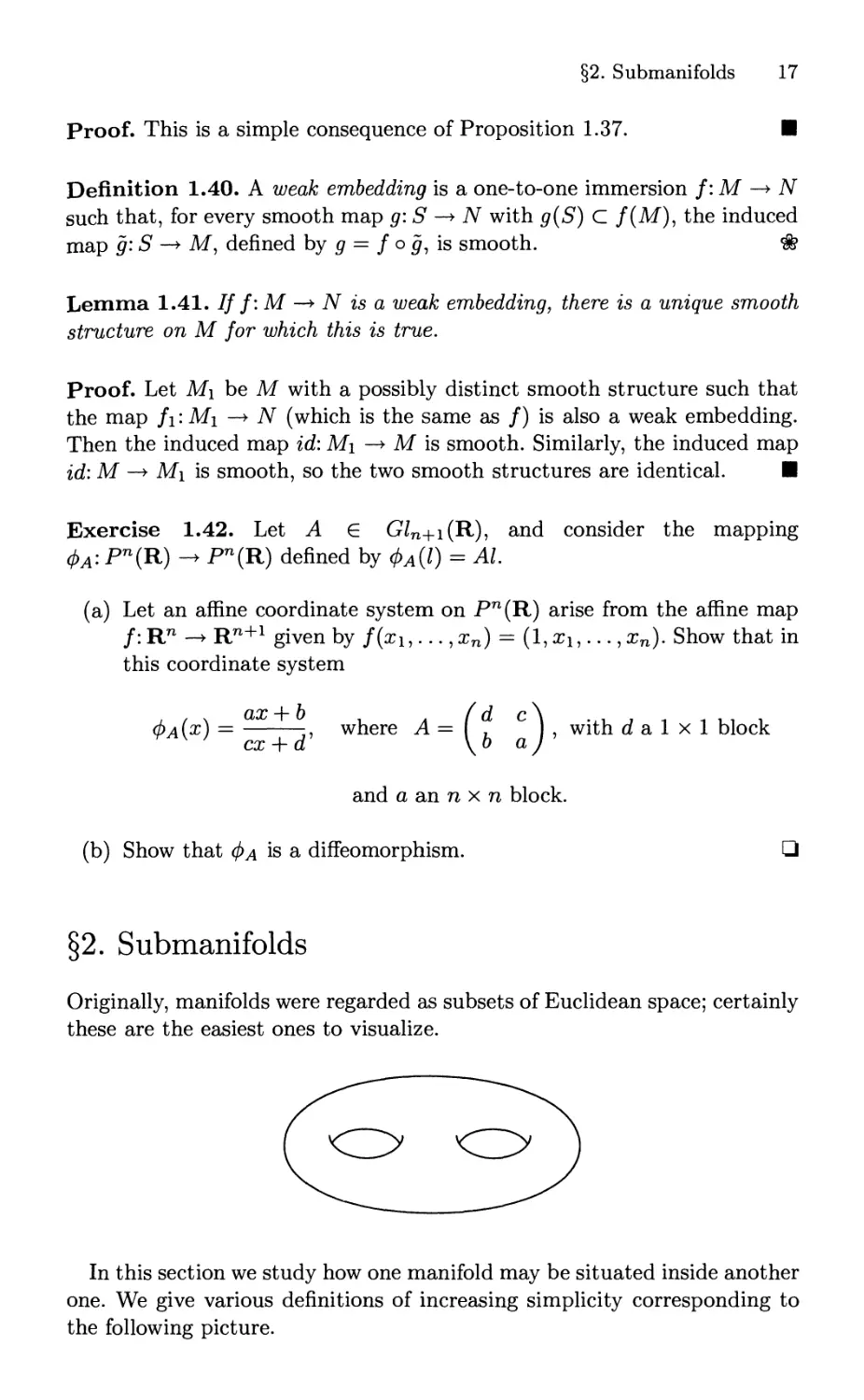
§2. Submanifolds
Originally, manifolds were regarded as subsets of Euclidean space; certainly
these are the easiest ones to visualize.
О <Z>
In this section we study how one manifold may be situated inside another
one. We give various definitions of increasing simplicity corresponding to
the following picture.

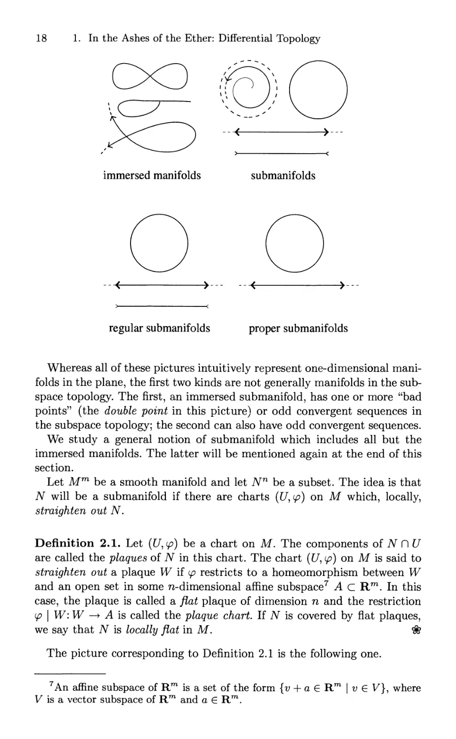
18 1. In the Ashes of the Ether: Differential Topology
immersed manifolds submanifolds
regular submanifolds proper submanifolds
Whereas all of these pictures intuitively represent one-dimensional
manifolds in the plane, the first two kinds are not generally manifolds in the sub-
space topology. The first, an immersed submanifold, has one or more "bad
points" (the double point in this picture) or odd convergent sequences in
the subspace topology; the second can also have odd convergent sequences.
We study a general notion of submanifold which includes all but the
immersed manifolds. The latter will be mentioned again at the end of this
section.
Let Mm be a smooth manifold and let TV71 be a subset. The idea is that
TV will be a submanifold if there are charts ([/, φ) on Μ which, locally,
straighten out TV.
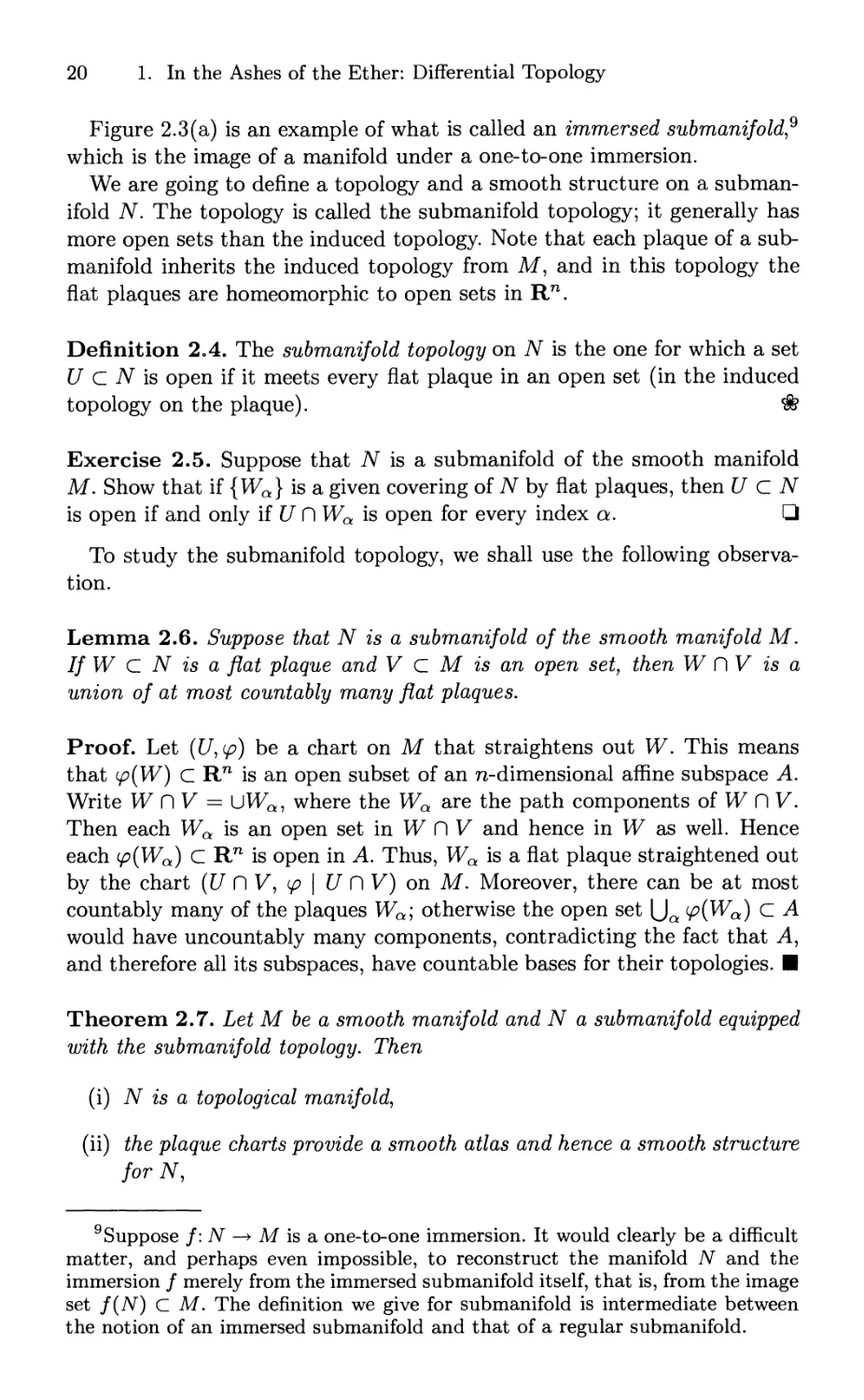
Definition 2.1. Let (υ,φ) be a chart on M. The components of TV Π U
are called the plaques of TV in this chart. The chart ([/, φ) on Μ is said to
straighten out a plaque W if φ restricts to a homeomorphism between W
and an open set in some η-dimensional affine subspace7 А С Rm. In this
case, the plaque is called a flat plaque of dimension η and the restriction
φ | W: W —» A is called the plaque chart. If TV is covered by flat plaques,
we say that TV is locally flat in Μ. Φ
The picture corresponding to Definition 2.1 is the following one.
7An affine subspace of Rm is a set of the form {v + a € R771 | ν € V}, where
V is a vector subspace of Rm and a 6 Rm.

§2. Submanifolds 19
U\
Note that in this picture TV meets U in two plaques, but here only one gets
straightened out by this coordinate system. There is no limitation on the
number of plaques in a chart; it may even be infinite.
Definition 2.2. Let Mm be a smooth manifold. A subset TV of Μ is called
a smooth (n-dimensional) submanifold if there is a covering {Ua} of TV by
open sets of Μ such that the components of Ua Π TV are all flat plaques of
dimension n.s *
Of course we may always "tidy up" φ so that the affine subspace Л is a
coordinate subspace, say the coordinate subspace corresponding to the first
η coordinates, and so that φ(ρ) = 0; but this is not always appropriate.
The coordinate charts guaranteed by the definition tell us that "locally"
the pair (M, TV) looks like the pair (Rm, Rn). This eliminates some of the
phenomena of strange convergent sequences and the phenomena of limit
points of nontrivial topology such as appear in Figure 2.3.
(a) (b)
FIGURE 2.3. Odd limit points.
8This definition and the lemma and theorem that follow were inspired by a
discussion in [P. Molino, 1988], pp. 11-12. We note, however, that the property
that every plaque in U Π TV is flat is not easily verified unless TV has some other
special property allowing us to assume that C/OTV has just one plaque. The aim is
to have a definition broad enough to include nonclosed subgroups of a Lie group
and, more generally, the leaves of a foliation (cf. Chapter 2) for which this "one
plaque" property may fail.

20 1. In the Ashes of the Ether: Differential Topology
Figure 2.3(a) is an example of what is called an immersed submanifold9
which is the image of a manifold under a one-to-one immersion.
We are going to define a topology and a smooth structure on a
submanifold TV. The topology is called the submanifold topology; it generally has
more open sets than the induced topology. Note that each plaque of a
submanifold inherits the induced topology from Μ, and in this topology the
flat plaques are homeomorphic to open sets in Rn.
Definition 2.4. The submanifold topology on TV is the one for which a set
U С N is open if it meets every flat plaque in an open set (in the induced
topology on the plaque). *
Exercise 2.5. Suppose that TV is a submanifold of the smooth manifold
M. Show that if {Wa} is a given covering of TV by flat plaques, then U С TV
is open if and only if U Π Wa is open for every index a. □
To study the submanifold topology, we shall use the following
observation.
Lemma 2.6. Suppose that TV is a submanifold of the smooth manifold M.
If W С TV is a flat plaque and V С Μ is an open set, then W Π V is a
union of at most countably many flat plaques.
Proof. Let (U,ip) be a chart on Μ that straightens out W. This means
that ip(W) С Rn is an open subset of an η-dimensional affine subspace A.
Write W Π V = UWa, where the Wa are the path components of W Π V.
Then each Wa is an open set in W Π V and hence in W as well. Hence
each ip(Wa) С Rn is open in A. Thus, Wa is a flat plaque straightened out
by the chart (U Π V, φ \ U Π V) on M. Moreover, there can be at most
countably many of the plaques Wa; otherwise the open set (JQ V>(Wa) С А
would have uncountably many components, contradicting the fact that A,
and therefore all its subspaces, have countable bases for their topologies. ■
Theorem 2.7. Let Μ be a smooth manifold and TV a submanifold equipped
with the submanifold topology. Then
(i) N is a topological manifold,
(ii) the plaque charts provide a smooth atlas and hence a smooth structure
for TV,
9 Suppose /: TV —» Μ is a one-to-one immersion. It would clearly be a difficult
matter, and perhaps even impossible, to reconstruct the manifold TV and the
immersion / merely from the immersed submanifold itself, that is, from the image
set /(TV) С М. The definition we give for submanifold is intermediate between
the notion of an immersed submanifold and that of a regular submanifold.

§2. Submanifolds 21
(iii) the inclusion map N С М is a weak embedding.
Proof, (i) To see that the inclusion TV С М is continuous, it suffices to
show that any open set V С М meets any plaque of TV in an open subset
of that plaque. But since the topology on a plaque is just the induced
topology as a subset of Μ, this is clear. Since TV С М is continuous and
Μ is Hausdorff, it follows that TV is Hausdorff. The flat plaque charts show
that TV is locally Euclidean.
It remains to see that TV is paracompact in the submanifold topology. For
this it suffices to show that each component of TV is a countable union of flat
plaques. Without loss of generality, we may assume TV is path connected.
Since Μ is a paracompact Hausdorff space, so is TV, and we may choose
a locally finite refinement of the open cover {Ua}aei of TV (see Definition
2.2). Calling this locally finite refinement {Ua}aei again, we note that by
Lemma 2.6 it still has the property that each component of Ua П TV is a
flat plaque.
Fix a base point χ G TV. Now if J = {αϊ,...,α*:} is a sequence of
elements of 7, we let Aj denote the subset of TV which may be joined to χ
by a piecewise smooth path on Μ that lies on TV and passes successively
through Uai,Ua2,.-.,Uak'
Of course, there may be no overlap between successive C/s, in which case
Aj = ®.
First note that, because TV is assumed path connected and the unit
interval is compact, each point у Ε Μ may be joined to χ by a path in Aj
for some J; thus \Jj Aj — TV. Next note that Aj С Uak Π TV is a union
of components of Uak Π TV, each one of which is a flat plaque. If we can
show that the number of components of Aj is at most countable, we will
be finished since the local finiteness of the covering {Ua}aei implies that
{J | φ J < к and A j φ 0} is finite and hence TV is covered by at most
countably many flat plaques.
We show by induction on #J that the number of components of Aj is
at most countable. If # J = 1, then clearly Aj has at most one component.
Suppose that
J = {αϊ,... ,Qfc}, J' = {ai,...,Qfc_i},

22 1. In the Ashes of the Ether: Differential Topology
and we already know that Aj> has at most countably many components.
By Lemma 2.6, each plaque of Aj> meets at most countably many plaques
in Uik Π TV. Thus, Aj has at most countably many components.
(ii) The smooth compatibility of the plaque charts is an immediate
consequence of the smooth compatibility of the charts on M.
(iii) First note that the inclusion TV С М is obviously a one-to-one
immersion. Now let g: S —» Μ be a smooth map, with g(S) С TV. To check
that the induced map /: S —► TV is smooth, let (W, φ \ W) be a plaque
chart. Then by definition,
/ I f~l(W) is smooth & (φ | W)(f | /_1(^)) is smooth.
But (φ | W) о (/ | f~l(W)) = (φ | W) о (g \ g~\W)) = (<pg \ g-\W)) is
smooth. ■
Regular Subrnanifolds
Now we pass to the definition of regular subrnanifolds, which are simpler
and more important than the general subrnanifolds studied above. They
intersect more neatly with coordinate charts of the ambient manifold; in
particular, the various components of this intersection do not pile up.
However, we pay for the simplicity of regular subrnanifolds by the exclusion of
important examples, including the nonclosed subgroups of Lie groups and
the leaves of some foliations.
Definition 2.8. An η-dimensional submanifold TV С М is regular if there
is a covering {Ua} of TV by open sets of Μ such that, for each a, Ua Π TV
is a single flat plaque of dimension п. Ф
Proposition 2.9. For a regular submanifold, the subspace topology is the
same as the submanifold topology.
Proof. Let TV С М be a regular submanifold. Since this inclusion map
is continuous when TV is given the submanifold topology, to show that
the two topologies are the same, it suffices to show that given any subset
V С TV open in the submanifold topology, there is an open set V С М
with TV Π V — V so that V is also open in the subspace topology.
Since V is a union of flat plaques, it is sufficient to find V in the case that
V itself is a flat plaque. Choose a chart ([/, φ) that straightens this plaque
and contains no other plaques. We may assume φ: (С/, V) —► (Rn x Rm_n,
Rn χ 0). Then V = φ~ι(φ{ν) χ Βε(0)) will do the job, where Βε(0) is the
open ε ball about the origin in Rm_n. ■
Proper Subrnanifolds
Even more restrictive than regular subrnanifolds are the proper
subrnanifolds.

§2. Submanifolds 23
Definition 2.10. A submanifold TV С М is called proper if it meets every
compact subset of Μ in a compact subset of TV (in the submanifold
topology). Note that this is equivalent to saying that the inclusion map TV С М
is proper. *
Theorem 2.11. Let N С Μ be a proper submanifold. Then Μ is regular.
Proof. Fix ρ Ε N. Take a chart (ΖΙ,φ) for M, with U compact, that
straightens out the plaque W — U Π TV containing p. Now, as in the last
paragraph of the proof of Proposition 2.9, we may assume that φ{ϋ) —
(p(W) x Βε(0). We may choose a sequence of open sets Uj — φ~ι{φ{νΫ) χ
Be/j(0)), j — 1, 2,..., so that (Uj, φ \ Uj) is also a chart straightening out
the plaque W and Π?>ι Uj — W. We want to show that some Щ meets TV
in just the single plaque W, which will prove regularity. Suppose otherwise.
Then we could find an infinite sequence of points χ χ, #2»... on TV — W, with
Xi eUj С U each in a distinct plaque of U. Since U is compact, there is a
convergent subsequence whose points, together with their limit, constitute
a closed and therefore compact set К С Ό Π TV. Repeating this argument
with a slightly smaller plaque W С Wf С W, we obtain К С U Π TV. But
this is impossible since each point of К lies in a distinct plaque of U and
these plaques constitute an open cover of К in the submanifold topology
having no finite subcover, which contradicts the compactness of К. Ш
Exercise 2.12. Show that neither the union nor the intersection of two
proper submanifolds need be a submanifold. □
Submanifolds Described Implicitly
Here is a simple criterion for the smoothness of a submanifold described
implicitly.
Theorem 2.13. Let Мш and Nn be smooth manifolds with m > n, and
let f:M—*Nbea smooth map. For у G TV, we set My — f~l(y). Assume
that f has constant rank, r say, on a neighborhood of My. Then My is a
smooth proper submanifold of Μ of dimension m — r.
Proof. Let ρ G My. Since the rank is constant on a neighborhood of p,
by Theorem 1.31 there are coordinate charts (U,tp) and (ν,ψ) around ρ
and f(p), respectively, such that φ(ρ) — 0, ψ(/(ρ)) — 0, and ι\)ίφ~χ is a
restriction of the canonical map
π: Rr χ Rmr -> Rr χ Rnr.
(X,y) ни- (X,0)
Thus φ(υί)Μυ) С 0 x Rm_r in Rr χ Rm_r. Hence My has just one plaque
in U and φ straightens out this plaque. This shows that My is a regular

24 1. In the Ashes of the Ether: Differential Topology
Mv
Μλ
λ =1/2 \ Ι A=l
FIGURE 2.15. Various elliptic curves.
submanifold. Since My is closed and Μ is Hausdorff, it follows that Myf)K
is compact for every compact К С Μ. Thus My is proper. ■
Example 2.14. Let M\ = {(x,y) G R2 | y2 = x(x - l)(x - λ)}, which
is the Weierstrass normal form of the general cubic (elliptic) curve, λ is a
parameter that we will take to be real. Thus M\ is given implicitly as the
zero set of the function /: R2 —* R, where
/(я,2/) = y2 -x(x- l)(x-X) = y2 -x3 + (X + l)x2 -Xx.
Calculating, we have ff(x,y) — (—3x2 + 2(λ -h l)x — A, 2y). The maximal
possible rank for the derivative is 1, and we can find all points on M\ where
this fails by solving the system
x(x-l)(x-X) =y2,
3x2 - 2(A + l)x -l· 1 = 0,
J/ = 0.
The only solutions are (x,y,X) = (0,0,0) and (1,0,1), which shows that
M\ is a smooth submanifold unless λ = 0 or 1 and that, in these exceptional
cases, M0 — {(0,0)} and Μχ — {(1,0)} are also smooth submanifolds of R2.
Figure 2.15 shows these singular points on Mq and M\, as well as one of
the more typical cases of a nonsingular M\. ♦
Example 2.16. Let us reconsider the n-sphere
Sn = {x G Rn+1 \x-x = l}.
Thus, Sn = F-X({1}), where F:Rn+1 -» R given by F(x) = x-x.
Calculating from first principles, Ff(x)v = 2χ·υ. Thus, F has rank 1 everywhere
on Sn. It follows from Theorem 2.13 that Sn is a smooth submanifold of
Rn+1. ♦

§2. Submanifolds 25
Example 2.17. Let On(R) = {A e Afn(R) | A A1 = 1} = the orthogonal
group. Define F: Mn(K) -> Mn(R) by F(4) = AA*, so that On(R) =
F~l(I)· Now F is smooth and we may calculate
F'{A)V = lim | {F(A + ftV) - F(j4)}
/i->0 ft
= lim 1{(A + ftV)(i4 -l· hVf - AA1}
h—>0 h
= lim jfftVA* + hAVb + ftW}
Л—0 ft
In the particular case that A — I, we have ker F'(I) = on(R), the vector
space of all η χ η skew-symmetric matrices. Note that dim on(R) = ^n(n —
1). More generally we have an isomorphism on(R) ~ ker Ff(A), which sends
S ·—► SA for any A Ε On(R). In particular, the rank of F is constant along
On(R), so On(R) is a smooth submanifold of Mn(R). ♦
Exercise 2.18. Note that the smooth map det: On(R) —* R has values ±1
(since 1 = аеЬ(ААг) = det(4) det(A) = det(^)2), so it follows that On(R)
is the disjoint union of two open sets. Show that these are the components
of On (R). □
Exercise 2.19. Assume the situation of Theorem 2.12; let W С N be a
submanifold; and assume for each χ e f~l(W) that f*(TxM) + Tf^W =
Tf{x)N. Show that f~l{W) is a submanifold of M. □
Submanifolds Described Parametrically
Now we pass to the dual situation of a manifold described parametrically.
Theorem 2.20. Let Mm and Nn be smooth manifolds, and let f:M -> N
be a proper one-to-one immersion. Then f(M) is a regular submanifold of
N and the map f:M —* f(M) is a diffeomorphism.
Proof. We first show that f(M) is a regular manifold. Choose ρ G M,
and set q — f(p)· Since / is an immersion, its rank is m everywhere. Then
by Corollary 1.33 there are connected coordinate charts (U,tp) and (V, VO
around ρ and q, respectively, such that φ(ρ) = 0, ψ(ς) — 0, f(U) С /(V),
and ψίφ~ι is the restriction to φ{ϋ) of the canonical inclusion
l: Rm -> Rm χ Rn"m.
χ ■-► (z,0)
Thus ψ{ί(ϋ)) lies in an open subset of Rm χ 0 С Rm χ Rn_m. Using the
fact that / is proper, an argument similar to the proof of Theorem 2.11

26 1. In the Ashes of the Ether: Differential Topology
allows us to shrink U and V so that f(U) Π V = f(M) Π V is connected.
Since (V, ψ) straightens out the unique plaque f(M) Π V in V, it follows
that f(M) is a regular submanifold.
By Theorem 2.7(iii), f(M) С TV is a weak embedding. Since f:M -> N
is smooth, it follows (cf. Definition 1.40) that the map /: Μ —» f(M) is also
smooth. Since both f(M) С TV and f: Μ —+ N are one-to-one immersions,
it follows that /: Μ —» /(Μ) is a bijective immersion. Then by Theorem
1.22, / is a diffeomorphism. ■
This theorem shows that the image of a proper embedding is a smooth
submanifold. We remark that the embedding theorem of Whitney tells us
that every smooth η-manifold admits a proper embedding as a smooth
submanifold of Euclidean space of dimension 2n -h 1 (cf. [J. Milnor, 1965]).
Immersed Manifolds and Immersed Submanifolds
Definition 2.21. An immersed manifold in Μ is the image of an immersion
/:7V —► M. (Note that the image is not in general a submanifold!) An
immersed submanifold is the image of a one-to-one immersion /: TV —» M.
For example, the elliptic curve Μχ appearing in Example 2.14 may be
regarded as an immersed manifold in R2. In such a case, it is still true
that each point ρ Ε Ν has a neighborhood U С N such that f(U) is a
submanifold of Μ diffeomorphic to U.
Exercise 2.22. Show that the curve Mx = {(x,y) G R2 | y2 = x{x - l)2}
is an immersed submanifold of R2 by parametrizing it by the slope of the
line through (x,y) G M\ and (1,0). □
Exercise 2.23. Show that all of the following inclusions are proper
inclusions:
, , ч ( weakly 1
< , .. .. > D < embedded > D {submanifolds}
submanifolds I . .. .. [ J
4 J у submanifolds)
J regular 1 J proper
\ submanifolds J [ submanifolds
(Hint: To show that the first and second inclusions are proper, consider
Figure 2.3.) □
The following exercise provides a preview of the "second fundamental
form" of a submanifold of Rn.

§2. Submanifolds 27
Exercise 2.24.* Suppose that Μ С R is given implicitly in a
neighborhood of ρ G Μ by the zero set of a function of maximal rank F: ΈΙΝ —» ΈΙν.
The tangent space to Μ at χ is defined to be the kernel of the linear
surjection ^(χ):ΚΝ —► Kv and is denoted TX{M). Define the second
fundamental form of Μ at χ by the formula
BX:TX(M) χ ГЖ(М) -> ΚΝ/Τ(Μ),
F'(x){Bx{u,v)) = F"(x)(u,v).
It follows that the symmetric bilinear form Bx(u, v) G RiV/T(M) is defined.
(i) Let a(t) be path on Μ С ΈΙΝ through χ and v(t) a vector field tangent
to Μ along σ. Show that at x,v — —Βχ(σ,ν) mod TX(M).
(ii) Use (i) to show that BX:TX(M) χ ΤΧ(Μ) -» R^/T^M) is
independent of the choice of F.
(iii) Show that by using the Euclidean metric on ΈΙΝ we can reinterpret
Bx as a map Б^: TX(M) χ TX(M) —► ХЦМ)1- (orthogonal complement) and
then define the "transpose"
BX:TX{M) x T^M)1· - TX(M),
{u,Bx(v,w)) = {Bx(u,v),w) for all u,υ eTx(M), weTx(M)L.
Show that if a(t) is a path on Μ С ΈΙΝ through χ and w(t) a vector field
normal to Μ along σ, then at x, it/ = £?£(σ,ΐ/;) mod ХЦМ)-1.
(iv) Find an analog of (iii) that does not rely on using a Euclidean metric.
□
In this formulation of the second fundamental form, it is clear that it has
fairly strong invariance properties. The following exercises make this more
precise.
Exercise 2.25. Suppose that Μ С HN is given implicitly in a
neighborhood of ρ G Μ as the zero set of a function of maximal rank F: ΈΙΝ —» Rv,
and let φ: HN —► HN be a diffeomorphism. Set F = F о 0, and let Б
and В be the second fundamental forms associated to Μ — F~l(0) and
Μ = F_1(0), respectively. Show φχ(Β(ύ,ϋ)) = B(u,v) + φχ(ϋ,,ϋ) mod
Τφ(χ)(Μ) for all u,v e TX(M), where w = фх(й) and ν = φχ(ν). □
Exercise 2.26. Let Μ С RN and let φ: ΚΝ -> RN be any invertible affine
map. Let Bx (respectively, Βψ^) denote the second fundamental form of
Μ at χ (respectively, of φ(Μ) at ф(х)). Show that
φχ(Βχ(η,υ)) = Βφ(χ)(φ'χη,φ'χυ) mod TX{M) for all ti,ti6 TX(M). □
Exercise 2.27. Assume the hypotheses of Exercise 2.26, and let ρ: ΈΙΝ —»
R be a smooth function. Define φ — -ф: HN —► RN, and show that
φ'^η,υ) = --{р'х(у)Ф'х(и) + р'х(и)фх(у)и - φ'^η,υ)} mod φ(χ)

28 1. In the Ashes of the Ether: Differential Topology
for allu^eR .
(Of course, we must avoid points where ρ vanishes.) Using the results of
§4, deduce the analog of Exercise 2.26 for a submanifold Μ С PN(R) and
an invertible projective transformation φ:Ρη(ΈΙ) —» Pn(R). □
Exercise 2.28. Assume the hypotheses and notation of Exercises 2.25 and
2.27. Let p(x) = χ/(χ·χ) (inversion). Show that, in this case, ф'х(Вх(й, ν)) —
Вф(х){и,у) - 2(u · ν/ρ{χ))φ{χ). □
Note that Exercise 2.28 shows that the "raw" second fundamental form
fails to be invariant under inversion. Nevertheless, we can obtain an
invariant second fundamental form by taking the "traceless" version of £?, as
indicated in the following exercise.
Exercise 2.29.* Let V be a Euclidean space (with inner product "·") and
W a vector space. Let B: V x V —» W be a symmetric form. Define Trace
* = Σ,<4 <dim ν ^(еь ег) £ W, where {e^} is an orthonormal basis for V.
Define Bo(u, v) — B(u, v) — (Trace £?/dim V)u · v.
(a) Show that Trace В is independent of the choice of the basis.
(b) Assuming the hypotheses of Exercise 2.28, show that ф'х(Во(й,у)) —
В0(щу). □
We shall revisit some of the ideas of these exercises in Chapters 6 and 7.
§3. Fiber Bundles
Everyone knows the usefulness in advanced calculus of studying vector-
valued functions. Consider, for example, the velocity field of a particle
moving along a fixed curve 7 in R2. This field is described by a function
v:j —► R2 defined along the curve. From another point of view, this same
field may be regarded as a function whose value at χ e 7 lies in the one-
dimensional subspace Vx of R2 that is parallel to the tangent line Tx to the
curve at x.

§3. Fiber Bundles 29
We emphasize that {Vx \ χ e 7} is a family of subspaces parametrized by
7·
Fiber bundles formalize the notion of a "parametrized family of so-and-
so's." The "so-and-so" is called the fiber and may be a vector space as
in the example above (corresponding to a vector bundle) or a Lie group
(corresponding to a principal G bundle). These two are the most important
cases, although other fibers may also serve as necessary. Sections (or in
the case of vector bundles, one often says vector fields or tensors), which
generalize functions, are functions on the parameter space whose value at
x lies in "the so-and-so at x." If the parametrized family is constant, then
fields (sections) reduce to ordinary functions.
The justification for the degree of generality employed here will appear
first in the next section, where it is shown that a smooth manifold has a
tangent bundle intrinsically associated with it, and again in Chapter 5, where
it is shown that a Cartan geometry has a principal G bundle intrinsically
associated with \t.
As with manifolds, it is possible to discuss both topological and smooth
bundles. Of course, our principal interest is in the smooth case.
Topological Bundles and Smooth Bundles
Definition 3.1. Let F be a topological space and π: Ε —> В a continuous
map. We call the quadruple ξ — (E,B,n,F) a {locally trivial) fiber
bundle with (abstract) fiber F if, for each point b G B, there is an open set
U С В containing ρ such that π~ι(ϋ) is homeomorphic to U χ F by a
homeomorphism φ such that the following diagram commutes.
K~\U) —^—^UxF
A /proJ!
U
The pair (U,tp) is called a chart (or local bundle coordinate system). Φ
Note that π-1 (6), the fiber over B, denoted i% is homeomorphic to F
for all b G В. В is called the base space and Ε the total space of the
bundle. Given a bundle £, we sometimes denote by Β (£), Ε (ξ), etc., the
corresponding parts of the bundle. If the base, fiber, and total spaces are
smooth manifolds, π is a smooth map, and the charts may always be chosen
to be smooth maps, then we have a smooth bundle. Two bundles ξι and
£2 over the same base В are said to be isomorphic if there is a
homeomorphism (diffeomorphism) φ between the total spaces such that the following

30 1. In the Ashes of the Ether: Differential Topology
diagram commutes, φ is called a bundle isomorphism or, in the case when
£x = ξ2 a bundle automorphism.
Example 3.2. The simplest example of a bundle is the product bundle
Ε — Β χ F with π = πχ (projection on the first factor). This bundle is
also called the trivial bundle. If Ε is a locally compact Hausdorff space,
then a necessary and sufficient condition that a bundle ξ — (Ε, £?, π, F) be
(isomorphic to) the trivial bundle is the existence of a trivializatwn, which
is a continuous (smooth) map t: Ε —► F that induces a homeomorphism
(diffeomorphism) upon restriction to each fiber π-1 (6). In this case the map
(p, t):E —» Б χ F is a homeomorphism (diffeomorphism) commuting with
the canonical projection to B. ♦
Example 3.3. Perhaps the simplest example of a nontrivial bundle is the
Mobius band Ε pictured in Figure 3.4. It is clear that if we remove any
point from the base B, we get an open set U homeomorphic to the interval
(0,1) and n~l(U) is homeomorphic to (0,1) χ [0,1]. Thus it is a bundle
over В — Sl with fiber I = [0,1]. But it is not a trivial bundle; if it were,
the boundary would consist of two components, whereas in fact it has only
one (Figure 3.4). ♦
'В
UxF
/ ί projection on 1
πχ [the first factor]
FIGURE 3.4. Mobius band.

§3. Fiber Bundles 31
Example 3.5. The canonical line bundle over projective space
generalizes the Mobius band. This is the bundle π: Ε —► Pn(R), where Ε —
{(I, v) e Pn(R) x Rn+1 | ν β 1} and π(1,ν) = I. To see this is a
bundle, let a:Rn —► Rn+1 be an affine map whose image does not contain
the origin (cf. Example 1.3). Then Ua = pa(Rn) is open in Pn(R) and
pa:Hn —» Ua is a diffeomorphism. We define <p~x: t/a x R —* π~ι(υα) by
(Ζ, λ) ι—► (/, Xa(pa)~l(l)). It is easily checked that φ~ι is a diffeomorphism
that is linear on fibers, and that the pairs {(Ua,ipa)} constitute an atlas
for the line bundle E.
In a similar fashion we may describe the canonical line bundle Ε over
the projective space P(V) associated to any vector space V. ♦
Example 3.6. By definition, every covering space π: Ε —» В is a fiber
bundle with discrete fiber. ♦
G Bundles
Now we consider the following, more refined notion of a bundle in which a
Lie group of symmetries appears.
Definition 3.7. Let ξ — (Ε, Β, π, F) be a smooth fiber bundle, and suppose
that G is a Lie group that acts smoothly on F as a group of diffeomor-
phisms. A G atlas for ξ is a collection Я = {(υ^ψί)} of charts for ξ such
that
(i) the Ui cover B,
(ii) for each pair of charts ([/, φ) and (V, V7) m ·# the map
Φ - ν*?"1: (t/ П У) x F -+ (t/ П 10 x F,
called a coordinate change, has the form Ф(и, f) = (u,h(u)f), where
h: U Π V —» G is a smooth map called a transition function. Φ
Note that in the case when the homomorphism G —» Diff(F) has a kernel
Я", then Я is a closed10 normal subgroup and the action factors through
G/H, so the bundle may also be regarded as a G/H bundle.11 Thus there is
nothing lost if we make the restriction that G acts effectively on F, namely,
that Η — 1. In this case we may speak of an effective G bundle. Just as in
the case of manifolds, we call two G atlases equivalent if their union is also
a G atlas.
10Let Δ = {(χ, χ) G F χ F \ χ € F}. Since the action is a smooth map
Gx F —* F, the graph of this map, given by Γ = {(#, χ, г/) € G χ F χ F | gx = y},
is closed and hence so is the intersection TC\GxA = HxA.
11 In Chapter 4 it will be shown that Η and G/H are again Lie groups.

32 1. In the Ashes of the Ether: Differential Topology
Definition 3.8. A G structure on the smooth bundle ξ is an equivalence
class of G atlases on ξ, and a G bundle is a smooth bundle ξ with a specified
G structure. *
Exercise 3.9 (Product bundles). Let ξj — (Ej,Bj,nj,Fj,Gj), j — 1, 2, be
two "G" bundles. Show that ξιχξ2 = (Εχ χ Ε2, Β ι χ Β2, πι χ π2, Fx x F2,
Gi χ G2) is a Gi χ G2 bundle in a canonical fashion. □
Exercise 3.10 (Induced, or pullback bundles). Let ξ — (E,B,n,F,G)
be a smooth G bundle and let f:X —► В be a smooth map. Let /*(£) =
(ΕΊ,Χ,πι,^, G), where Εχ = {(ж,е) G XxE* | /(χ) = 7r(e)} and 7Ti(:c,e) =
x. Show that it is a smooth G bundle. □
Definition 3.11. A G bundle is flat if all the transition functions
h:U P\V —+ G are constant. (This happens, in particular, if G is a
discrete group.)12 *
Exercise 3.12. Let В be a manifold with universal cover B. Show that a
flat G-bundle over В with fiber F induces a trivial bundle over В with a
canonical trivialization and that the action of the group of covering
transformations on the fiber is a representation n\(B,b) —» G. Conversely, show
that every representation πι (£?,&) —» G arises in this way. □
Given a G atlas, we can consider the union of all G atlases equivalent
to it to obtain the unique maximal atlas equivalent to the given one. The
12The reader may wonder about the origin and importance of flat bundles
in geometry. It often happens that one makes some locally defined geometrical
construction on a manifold which depends on a choice in some discrete universe
of possible choices. By the discreteness any choice can be extended smoothly
over small neighborhoods, but globally one may not be able to do this. The
appearance of this situation is a sure sign of the presence of a helpful flat bundle
that resolves the global ambiguity. For example, at a nonumbilic point ρ on an
oriented surface in 3-space, there are two principal tangent lines corresponding to
the two principal curvatures. Although we may choose two unit vectors e\ and ei
in these two directions at p, there is no unique choice. Of course, we may assume
that the basis (ei,e2) gives the correct orientation for the surface, but that still
leaves the choice between ±(ei,e2). If we work only locally, we may just choose
one of the two, say (ei, ег), and be done with it. It is a fact, however, that as we
push our choice (ei,e2) along a loop enclosing a single (generic) umbilic point, it
will come back to ρ as the other choice, —(ei,e2). This indicates the presence of
a flat bundle, in this case the flat line bundle L with discrete group ±1, with the
property that the fiber turns over every time we pass around a generic umbilic.
Rather than regarding ei and €2 as sections of the tangent bundle Τ of the surface,
which would run into sign trouble as we pass around an umbilic, we regard them
as sections of the tensor product Τ ® L. The rectification of the sign is built
into L. And, moreover, rather than saying that we have now accommodated the
frame by a clever construction, it is more true to say that the frame was always
geometrically comprised of sections of Τ 0 L but we just didn't know it before.

§3. Fiber Bundles 33
G structure may be identified with this maximal atlas, and the remarks
about tidying up the coordinate charts in the corresponding situation for
smooth manifolds apply here as well. Two G bundles are isomorphic if they
are isomorphic as bundles by an isomorphism identifying the G structures.
Example 3.13. A finite covering space π: Μ —» Μ is a G bundle with
discrete fiber whose group is the permutation group of the fiber. (If the
fiber is not finite, the permutation group is not countable.) ♦
Example 3.14. We sketch a more complicated example of a G bundle,
the Hopf fibration 51 -> 53 -> 52. The Lie group 51 = {AgC||A|-1}
acts smoothly on S3 = {w = (wo,wi) e C2 | \w0\2 + \wi\2 = 1} by the
formula λ · (wo,w\) = (\wo, \w\). We shall regard 52 as the union of two
copies of С with identifications, 52 = Co υφ Ci, where φ: C$ —» CJ is
given by φ(ζο) — Zq1. The map φ may be regarded as arising from two
stereographic projections from the sphere of radius 1/2 in R3 as in the
following figure. (The complex planes are arranged so that their positive
real axes are parallel.)
Cj (= copy of C0
"turned over")
Co(=C)
Now the map π: 53 —► 52 is given by
zx =z0l =Φ(ζ0)
n(w) — <
wi/wo G Ci if wo ф О,
wq/wi e Co if w\ ф 0.
Note that if wo,w\ Φ 0, the two definitions agree. It is easy to verify that
π(ύ) = π (υ) <=ϊ и = λν for some λ Ε S1. The trivializations are
тг-ЧСо) » Co x S\ 7r_1(Ci) » Cx χ S\
(w0,wi) ^ (wi/w0,wo/\w0\), (w0,wi) ^ (w0/wi,wi/\wi\),
and the coordinate change between these is seen to be
t^Q X *b > L^j^ X »b ,
(z,\)»{l/z,\z/\z\).
Since this is of the form (ζ,Χ) ι—► (ip(z),h(z)\), we have an 51 bundle
over 52. The inverse image of a circle on 52 in 53 is a torus. Picturing

34 1. In the Ashes of the Ether: Differential Topology
north pole fiber
FIGURE 3.15. The Hopf fibration.
53 minus the north pole as R3 via stereographic projection, Figure 3.15
shows an accurate cutaway perspective view in R3 of the fibers on the three
tori lying over the equator, and the ±45 degree parallels of 52. The fibers
themselves correspond to the places where the ratio Wi/wq is constant and
appear as circles in Figure 3.15. The fibers over the north and south poles,
namely, the z-axis and the "central circle," are also shown. In fact, the
subset of R3 consisting of R3 — z-axis - central circle is "foliated" by the
tori lying over the lines of latitude on the 2-sphere.
All but two of the fibers of the Hopf bundle lie on these tori in R3. On
each torus the fibers run around "once in each direction." The base 52
may be regarded as "the space of fibers" in the sense that π establishes a
bijection between the set of fibers and the base. Moreover, the topology on
the base indicates the mutual disposition of the fibers in the sense that two
fibers are "near" each other when the corresponding points in В are "near"
each other. Figure 3.16 shows how the "space of fibers" of the Hopf bundle
fit together topologically to form the 2-sphere. One of the tori of Figure

§3. Fiber Bundles 35
cross
sectional
disc
FIGURE 3.16. Topology of the space of fibers.
3.16 has been singled out. A cross-sectional disc for the corresponding solid
torus meets every fiber inside the torus just once. The "complementary
disc" meets each fiber outside the torus once. The fibers on the torus meet
each disc once in its bounding circle and provide a diffeomorphism between
these two circles. Thus the "space of fibers" is made up of two 2-discs glued
together by a diffeomorphism of their boundaries, which is just the 2-sphere.
♦
Exercise 3.17. Show that the Mobius band is a G bundle with G = Z/2.
□
Construction of Bundles
Now that we have seen an interesting example of a G bundle, let us return
to the definition to see what ingredients are required for the construction of
a G bundle. It is clear from the definition that if we are given an effective
G bundle, then we are given
(i) a Lie group G acting smoothly on a smooth manifold F,
(ii) an open covering {Ua} of a manifold £?,
(iii) smooth maps hpa: UanUp —> G related by the property that if Ua Π
UpP\U7 φ 0, then on this intersection we have h7phpa = hlot.
The latter property is a consequence of the existence of the effective G
bundle and may be seen as follows. We may assume that the open sets Ua
are indexed by the trivializations
one of the fibers
on the torus
<*:K~l(Ua)->Ua xF.

36 1. In the Ashes of the Ether: Differential Topology
The coordinate changes are βα l: (Ua Π Up) xF-> (Ua Π Up) χ F, where
-1
IS
Pa~l(u,f) = (u,hpaf). Thus, the obvious identity ^β~ιβα~χ = ηα
equivalent to h1php(X = h1QL.
It is quite clear that this procedure may be reversed in that if we are
given the data of (i), (ii), and (Hi), we can construct a G bundle by forming
the disjoint union of the products Up χ F and dividing by the equivalence
relation generated by making the identifications
UaxF
U
{Ua nUp)xF
(ti,/)
UpxF
U
(UanUp)xF
(U,ft/3Q/)·
Exercise 3.18. Verify that this procedure does yield a smooth G bundle
over В with fiber F and that if the data (i), (ii), and (iii) arose from a G
bundle, this procedure reconstructs that G bundle (up to isomorphism). □
Principal Bundles
A special type of G bundle is the one for which the group G "is the same
as" the fiber F in the sense that for some (and hence any) point /o G F, the
map G —> F sending g —» gf0 is a diffeomorphism. (For example, the Hopf
bundle fits this description.) It then follows that the G bundle is effective,
so the transition maps h:U C\V —> G are determined by the bundle. Note
that the diffeomorphism G —> F does not yield a canonical identification of
G with the abstract fiber F, because the bijection will vary with the choice
of /o G F. Nevertheless, once we have chosen such an identification, we can
reconstruct the bundle using G itself as the (abstract) fiber together with
the left action of G on itself, as may be seen from the following diagram.
(*,gf0) I
UxF 3 Τ (UnV)xF
UxG 3 | (UnV)xG
(μ, g) h
-> (u,h(u)gf0)
-> (UnV)xF
VxF
-> (UnV)xG | с VxG
> (u,h(u)g)
Moreover, it further follows from this diagram that a principal G bundle
has a smooth right G action, as may be seen by comparing the coordinate
changes before and after we identify the fiber with G. The right G action
commutes with the coordinate changes, which themselves involve only the
left G action. This leads us to the following definition.

§3. Fiber Bundles 37
Definition 3.19. A principal13 G bundle is a smooth fiber bundle ξ =
(Ρ, Ρ, π, F) together with a right action Ρ xG —> Ρ that is fiber preserving
and acts simply transitively on each fiber. ft
Example 3.20. A regular covering space π: Μ —» Μ is a G bundle with
discrete fiber whose group is πι(Μ, fe)/iV, where AT = Image π*: πι (Μ, Ь) —»
πι(Μ,6). ♦
Exercise 3.21. Verify that a principal G bundle does in fact possess a
canonical effective G bundle structure. [Hint: the coordinate changes must
commute with the G action.] □
Exercise 3.22.* Let ξ = (Ρ, Ρ,π, Ρ) be a principal G bundle. Show that
the action Ρ χ G —» Ρ is proper in the sense that if Л and Ρ are compact
subsets of Ρ then {# e G | (#Л) Π Β φ 0} is compact. □
Exercise 3.23.* Let Η —» Ρ —» Μ be a principal bundle, and suppose
that Μ is connected. Fix a component Pi of Ρ and an element pi Ε Pi,
and set #x = {h G Я | pxh e Pi}.
(i) Show that Η ι is a codimension-zero subgroup of H.
(ii) Show that ΡχΗχ С Рх.
(iii) Show that H\ —» Pi —» Μ is a principal #i bundle. □
The case of a principal G bundle is fundamental because of the inverse
constructions that allow us to pass back and forth between effective G
bundles with fiber F and principal G bundles. These passages may be
described as follows. An effective G bundle with fiber F determines the
transition functions h: U Π V —» G, and hence, as above, we can construct
a principal G bundle called the associated G bundle. Conversely, given a
principal G bundle ξ and a smooth effective action of G on a manifold P, we
can use the action to construct a G bundle with fiber F denoted by ξ Xq F.
These two constructions are inverse to each other. Therefore, we may say
that the fiber of an effective G bundle may be regarded as a variable for
which we may substitute any manifold on which G acts effectively.
Vector Bundles
A special case of a G bundle is a real vector bundle. In this case the fiber is
a real finite-dimensional vector space V and the group is the general linear
group G = Gl(V). An isomorphism of vector bundles is an isomorphism of
This term apparently arises because a principal bundle generalizes the so-
called principal group of a Klein geometry (cf. Chapter 4).

38 1. In the Ashes of the Ether: Differential Topology
bundles that is linear on the fibers. Since the action of G on V is transitive
and effective, it follows that we may pass back and forth between the vector
bundle and the principal G bundle ξ. What is more, given any smooth linear
representation p:G —> G(W), we can pass from the original vector bundle
to the associated principal bundle ξ and then to the G bundle with fiber W
denoted by ξ xp W. In fact, the fibers of the canonical map ξχ\Υ —> ξχρ\¥
are just the orbits of the left G action G χ ξ xW —> ξ xW given by
g-(x,w) = (xg~\ p(g)w).
Example 3.24 (Exterior power). If ξ is a vector bundle with fiber V, with
group Gl(V) acting on V by the standard representation, then Gl(V) also
act on AP(V), the pth exterior power. Thus, we have an associated bundle
Λρ(£), called the pth exterior power of ξ. ♦
Exercise 3.25 (Whitney sum). Let ξι and £2 be two vector bundles over
the same base £?, and let Δ: Β —> Β χ В be the diagonal map. Then the
Whitney sum of the bundles is ξι θ£2 = Δ* (ξι х£г)· Show that the Whitney
sum is associative and commutative (up to bundle isomorphism). □
Exercise 3.26 (Quotient Bundle). Let ξι and ξ2 be two vector bundles over
the same base £?, and let φ: ξι —» £2 be a smooth injection covering the
identity on В and linear on fibers. Show that there is a canonical quotient
bundle £2/^1 over В whose fibers are the quotients of the corresponding
fibers of ξι and £2· ^
Sections
Now let us consider sections (also called fields or tensors, in the case of
vector bundles), the generalization of functions mentioned in the introduction
to this section.
Definition 3.27. Let ξ = (Ε, #,π, F) be a bundle. A section over U С В
is a continuous (or smooth, in the case of a smooth bundle) map a:U —> Ε
such that πσ = idjg. The space of all (smooth) sections of η is denoted by
Γ(η). *
In general, a field in an n-dimensional real vector bundle may be regarded
as a generalization of a vector-valued function on the base, which is locally,
of course, exactly what a field is in this case. In fact, the same may be said
about sections on a general bundle. The advantage of the generalization is
that, in many geometric circumstances, fields correspond more closely to
the nature of things than do functions. The close relationship between fields
and functions accounts for the fact that in the presence of a trivial bundle

§4. Tangent Vectors, Bundles, and Fields 39
with a canonical trivialization t:E —> F, there is a tendency to identify the
field σ:Β—>Ε with the corresponding function ta: В —> F.
Let ξ = (£*,£?, π, G) be a principal G bundle over £?, and consider the
bundle η = ξ XgF with fiber F, associated to ξ by a smooth effective action
ρ of G on a manifold F. There is an important bijective correspondence
ψ:Α°(Ε,ρ)^Γ(η)
where
A°(E,p) = {f:E -> F | / is smooth, and f(pg) = p(g-l)f(p)}
and the section ψ(/): Β —» τ/ is induced by the map Ρ —> Ρ χ F sending
p^ (pJ(p))·
Exercise 3.28.* Verify that the above correspondence is well defined and
bijective. □
§4. Tangent Vectors, Bundles, and Fields
Tangent vectors have a schizophrenic nature. On the one hand, they have
a geometric aspect in which they appear as directions in space: if I stand in
a manifold, I can move in a variety of directions, which may be described
as the tangent vectors at my position. On the other hand, they have an
analytical aspect in which they appear as "directional derivatives," which
is to say as first-order partial differential operators that, when applied to a
smooth function, give its rate of increase in the given direction. Although
these are "the same" notion in some sense, they nevertheless have a different
development. While "directions" strike the mind as a primarily geometric
notion, differential operators lie in the domain of analysis and can, for
example, be composed to yield partial differential operators of arbitrary
order whose geometric significance is often unclear.14
Geometric Vectors
We start with the geometric view of vectors. In courses on advanced
calculus, we learn how, at least in certain cases, to find the tangent plane at
a point ρ of a submanifold Mm С Rn. There are two methods, depending
on whether the submanifold is described parametrically or implicitly. Of
14In fact, we are simplifying matters somewhat. The schizophrenic nature of
tangent vectors also includes a third personality, an algebraic one. If mx is the
ideal of smooth functions on Μ which vanish at the point x, then the space
of tangent vectors at χ can also be identified with the dual space (mx/m£)*.
However, we do not pursue this aspect of tangent vectors here.

40 1. In the Ashes of the Ether: Differential Topology
course, in cases where both methods apply, they lead to the same tangent
plane which we shall denote by Tp(M)geometric· Later we shall drop the
term geometric.
The Parametric Method. Let ρ G Mm, where Mm is a submanifold of
Rn. Assume that ρ lies in a neighborhood of Mm which is defined para-
metrically by a parameterization /: (t/,0) —» (Mm,p), where U is an open
set in Rm and rank0(/) = n. Then the tangent plane TP(M)geometric is also
described parametrically as the image of the affine map A: Rm —» Rn given
hyAv = f(0) + f'(0)v.
Exercise 4.1. Let on(R) = {X e M„(R) | X1 = -X} be the \n(n - 1)-
dimensional vector space of skew-symmetric matrices. Show that the Cayley
parameterization
/:o„(R)->Mn(R), where f(X) = (I + X)(I - X)~l
is a smooth embedding whose image is an open subset of 50n(R). □
Example 4.2. Let us find the tangent plane at the identity I = /(0) of
the submanifold described parametrically by / in Exercise 4.1. Calculating
the derivative /;(0) from first principles, we have
lim \{f(hY) - /(0)} = Km 1{(/ + hY)(I - hY)~l
1
1}
= bm-{{I + hY)-{I-hY)}{I-hY)-1
= 2Y.
Thus, the tangent plane at the identity is (a translated copy of) on(R)
itself, parametrized by the affine map A: on(R) —» Mn(R) given by A(Y) =
I + 2Y. ♦
The Implicit Method. Let ρ e Mm, where Μ is a submanifold of Rn.
Assume that ρ G U С Rn, where U Π Μ is defined implicitly as the zero
set of a smooth map F: U —» Rn_m such that rankp(F) = n — m. Then the

§4. Tangent Vectors, Bundles, and Fields 41
the two geometrical placements difficulty separating
of tangent spaces tangent vectors
FIGURE 4.4.
tangent plane Tp(M)ge0metric is also described implicitly as the zero set of
the affine map B: Rm -» Rn given by Bv = F'{p){v - p).
Example 4.3. Let us calculate the tangent plane of the η-sphere Sn =
{x G Rn+1 | χ · χ = 1} by this method. Here F:Rn+1 -» R is given by
F{x) = χ · χ — 1. Calculating the derivative of F from first principles yields
F'{x)v = 2x - v. Thus, rankx(F) = 1 for each χ G Sn, and the tangent
plane is given by Tx(Sn)geometr[c = {x + v e Rn+1 \x -v = 0}. ♦
These constructions of the tangent planes suffer from several disadvantages.
The first one, which is not very serious, is that although the tangent plane
can be regarded as a vector space, it is generally not a vector subspace
of the ambient Rn (Figure 4.4). This can be fixed by translating each
tangent plane TP(M) geometric by — ρ so that it becomes a subspace with
ρ corresponding to the origin (cf. Figure 4.4). We continue to denote this
by TP(M)geometric· The more substantial second objection is that vectors
in distinct tangent planes may correspond to the same point in Rn. This
can be remedied by means of the following construction, which defines the
geometric tangent bundle T(M)geometT-lc of a smooth submanifold Μ of Rn:
T(M)geometric = {(p,v) G Г X Rn | P G M, V G Tp(M)}.
It is easy to see that T(M)geometric is always a smooth submanifold of
Rn χ Rn. For example, if Μ is given implicitly as
Μ = {ρ € R" | F(p) = 0},
where F: R™ -» Rn_m is smooth with rankp^) = η - m for all ρ G M,
then T(M) is given implicitly as
T(M)geometric = {(p,v) € R" x Rn | F(p) = 0,F'(p)v = 0},

42 1. In the Ashes of the Ether: Differential Topology
namely, as the zero set of the smooth function
(F, B): Rn χ Rn -> Rn"m χ Rn"m,
where B(p, v) = F'(p)v. Let (x, y) denote the coordinates of the two factors
Rn χ Rn. Calculating the derivative, we have
(^'MHffl Д ι.
\дхэ) \dy3)J
which has rank 2(rc — m) everywhere, since both main diagonal entries are
copies of F'(p), which has rank η — га.
Exercise 4.5. Show that if Μ is given implicitly by F = 0 as above, then
the first factor projecton π:Τ(Μ) —> Μ has a canonical vector bundle
structure. □
Analytic Vectors
As interesting and geometrically explicit as the preceding results are, there
still remains the major disadvantage that the definition of the tangent
plane and that of tangent bundle seem to depend on the way in which Μ is
embedded in Rn. It is much more satisfying and useful to ask and answer
the following question: "Is there an intrinsic way of associating a tangent
plane and tangent bundle to a smooth manifold so that it is not only
independent of a particular embedding, but also so that if we do have an
embedding Mm —» Rn, we can see that we get the same answer as above?"
Using Whitney's embedding theorem it is possible, although awkward, to
show directly that the above construction is what we seek. However, it is
better now to abandon, temporarily, the geometric aspects of vectors and
pass to the analytic description of tangent vectors as directional derivatives.
To a vector ν = (vi,...,vn) £ Rn we may associate the differential
operator
D* = Σ *^>
1<г<п г
called the directional derivative in the direction v. In the case that ν is a unit
vector in Rn and /: Rn —» R is a smooth function, then the geometrical
meaning of Dv(f)(x) is that it gives the rate of change of / in the direction
v. We codify the notion of a differential operator in the following definition.
Definition 4.6. A derivation at ρ G Mm is a real-valued operator D
defined on smooth functions whose domain contains a neighborhood of ρ
such that, for every pair f,gof such functions, D satisfies the following
two properties:

§4. Tangent Vectors, Bundles, and Fields 43
(i) (Linearity) D(af + pg) = aD(f) + pD(g) for all α, β e R,
(ii) (Leibnitz formula) D(fg) = D{f)g(p) + f(p)D(g). *
The space of all derivations at a point ρ clearly constitutes a real vector
space, which we call the analytic tangent space of Μ at ρ and denote by
Tp(M)anaiytic. Moreover, the two properties imply that D(c) = 0 for any
constant function c. It is not clear at this stage that Tp(M)anaiytic is finite
dimensional, although we shall soon see it is of dimension m. Later, when
we have seen that this definition of the tangent space is in full agreement
with the geometric definition, we shall drop the term analytic.
We need several simple results before we can compare analytic and
geometric vectors. The first shows that smooth maps induce linear
transformations between the analytic tangent spaces at corresponding points. In a
word, it says that we can differentiate smooth maps.
Theorem 4.7.
(a) (Derivative) If g: (Мш,х) —» (Nn,y) is a smooth map, then g induces
a linear map g*x: Tx(M)anaiytic -» Ty(iV) analytic defined by (g*xD)h =
D(hg).
(b) (Chain Rule) If д:(Мш,х) -» (Nn,y) and f:(Nn,y) -» (Ρ^,ζ) are
smooth maps, then (fg)*x = f*yg*x.
Proof. Both statements are simple exercises. ■
Corollary 4.8. If f:M—*Nisa diffeomorphism in some neighborhood of
χ e M, then /*x:Tx(M)anaiytic -»l/(x)(iV)anaiytic is an isomorphism.
Proof. Let χ e U С Μ with U open and f:U —> f(U) a diffeomorphism.
Let g be the inverse diffeomorphism. Applying the chain rule to gf = idu
and fg = id/(t/), we get id = #*y/*x and id = /*x^*y. Thus /*x is an
isomorphism. ■
The next result is a special case of Taylor's theorem and the result that
follows it applies it to determine the derivations at a point in Euclidean
space.
Lemma 4.9. Iff is a smooth function defined in a neighborhood of ρ G Rn,
then
/(x) = /(p)+ ς (ж*-л)(|^(р)+^)|,
1<г<п ^ °Xi >
where the functions a»(x) are smooth and vanish at p.

44 1. In the Ashes of the Ether: Differential Topology
Proof. Write
m-m=fdf{p+l{rP))dt= Σ (**-*) f f(P+t(X-P))dt.
Jo dt ^n Λ dxi
Now, integrating by parts, we get
df Il Гl d2 f
= t-^-{p + t{x-p))\ - t Σ —1-(р + Цх-р))&-р№
oxi \0 j0 1<J-<n υχίθχ3
where the ai(x) are obviously smooth and vanish at p. Ш
Proposition 4.10. If Ό is an open subset o/Rn and D is a derivation at
ρ e U, then
d= ς D^hd
dxi
l<i<n
f(x) = f(p)+ Σ fc-PO^iP)+«*(*)),
1<г<п г
Proof. Write
a/
dxi
as in the lemma. Applying D to both sides yields
Df = 0+ Σ D{xi-pi)(^{p) + ai{x)\+0= £ D{Xi)^{p). ■
1<г<п \ г / 1<г<п г
Corollary 4.11. dim Tp(Rn)anaiytic = n.
Proof. The formula shows that Tp(Rn)anaiytiC is spanned by the derivations
* ~ 9xi \p
These derivations are linearly independent since we obtain Xj = 0(1 < j <
n) when a putative relation Σ XiDi — 0 is applied to the function Xj. ■
Corollary 4.12. Let f:M —> N be a smooth map. Then the rank of f at
ρ e Μ is the rank of /*p:Tp(M)anaiytic -» T/(p)
\1* Janalytic·

§4. Tangent Vectors, Bundles, and Fields 45
Proof. This is a local question, so we may assume that Μ is an open set
in Rm (with coordinates xi,... , xm) and TV is an open set in Rn (with
coordinates xi,... ,xn). We show that in this case the rank of /*p is the
same as the rank of the Jacobian matrix of / at p. Set Di — d/dxi and
write
(f*P)Di= ^2 aijDj, 1 < i < m.
l<j<n
Then oij = ((/*„)A)sj = Di(xj о /) = Di(fj) = (dfj/dx^p). Thus, the
Jacobian matrix is, in fact, the matrix of the linear transformation /*p in
the basis Д. ■
Corollary 4.13. If g: Μ —» N is a smooth map whose derivative
g*x : Tp(M)anaiytic -» T^(p)(iV)anaiytic w « /mear isomorphism for a given
point ρ, then g is a local diffeomorphism (i.e., ρ has an open neighborhood
U such that g(U) is open and g \ U is a diffeomorphism onto its image).
Proof. The isomorphism implies that Μ and TV have the same dimension
m and that / has rank m at p, so the inverse function theorem applies. ■
Identity of Geometric and Analytic Vectors
At this stage it is possible to compare the analytic vectors to the geometric
ones. Thus, suppose we have a smooth submanifold of Euclidean space
l: Mm С Rn given as the zero set of a smooth function F = (F\,..., Fn_m):
Rn _> Цп-rn of rank n _ m Then
Tp(M)ge0metric = ker F'(p)l Rn -> Rn~m.
Now the smooth inclusion l: Мш С Rn induces a linear map
L*p'. lpylVl Janalytic * J-p\^ /analytic·
If D e Tp(Mm)analytic, then upD e Tp(Rn)analytic, and by Proposition 4.10
we can write
t*pD = ^2 νί~Έ~·> wnere уг = (i*pD)xi e R.
л^ ^ OX%
1<г<п
We claim that [v\,... ,vn) e Tp(M)geometriC. To see this, note that
Fj(L(x)) = 0 for all χ e Μ and for all j. Thus, for D e Tp(M)an^ytic,
we have
0 = D(Fji) = (i»*PP) = η,ι(ρ)(ι.ρ(Ό))
= fj^p) Σ υ^ I = Σ Vi^{p)
\l<i<n °Xl) l<i<n °Xl
=> F'(P)V = 0^υ& Tp(M)geometric·

46 1. In the Ashes of the Ether: Differential Topology
This yields a linear map
1 ρyNl Janalytic y ■*■ ρ\Μ· )geometric
D i-»· ((l*pD)xi, ..., (upD)xn).
To show that the map is injective (and hence an isomorphism since the
dimensions are the same), it suffices to show that if (l*pD)xj = 0, 1 < j < η
then Df — 0 for every smooth function / defined on a neighborhood of
ρ in M. Now the value of Df is not altered if we restrict / to a smaller
domain about p. But if the domain is small enough, then / extends to a
neighborhood of ρ in Rm, that is, / = gi for g smooth on a neighborhood
of ρ inRm. Thus,
Df = D{gi) = g*L{p)Up(D) = (uP(D))g = Σ v< |f-(p) = 0
since Vi — (upD)xi = 0. These remarks yield a canonical identification
between Tp(Mmanalytic and Тр(М)ёеоmetric in the case Μ С Rm.
The Tangent Bundle
Now let us return to the tangent bundle. We want to give a definition of
T{M) as a smooth manifold intrinsically associated to the smooth manifold
Μ and also to show that it is a G/m(R) bundle with fiber Rm under the
standard action.
For each manifold Μ we define T(M)anaiytic as a set to be the disjoint
union of the vector spaces TP(M), ρ G M. Denote by π the canonical
projection map π: T(M)anaiytic —» Μ sending the vector ν e TP(M) to
the point ρ G M. If /: Μ —» TV is a smooth map, then we define a map
analytic
—» T(7V)anaiytic by sending the vector ν G Tp(M) to /*pv G
Tf(p)(N) such that the diagram commutes.
/*
^M)a55Jtfc > ^analytic
^ /
Μ > N
Now we put a topology on the sets T(M)anaiytiC by modeling pieces of it
on a special case of the geometric tangent bundle. We do this first for the
case Μ — Ό — open set in Rm. As sets we have the identification
πΝ

§4. Tangent Vectors, Bundles, and Fields 47
J- (^)analytic — ·*■ \U /geometric — сУ X rv ,
Now the right-hand side comes equipped with a topology, a smooth
structure, and even the structure of a (trivial) smooth Gin(R) bundle. The idea
is to pass this to T(M)anaiytic.
Let Я = {(t/, φ)} be a smooth atlas for M. Then φ: U -» φ(ϋ) С Rm is
a homeomorphism onto its image and φ*\ T({7)anaiytic —* ^(^(^OJanaiytic —
<p(U) x Rm.
The Topology. A set W С T(M)analytic is open ^^(1УП T(£/)anaiytic)
is open in φ(ϋ) χ Rm for all (17, φ) G Λ.
The Atlas for the Smooth Structure. Take Τ = {(T(£/)anaiytic,^*) I
(и,<р)ел}.
The Bundle. Again take <B = {(T(£/)anaiytic,^*) I (t/,<p) G Л}.
Exercise 4.14.* Show that T(M)anaiytic is a smooth manifold of dimension
2ra and that (T(M)anaiytic» M, π, Rm) is a smooth GZm(R) bundle that can
be canonically identified with the geometric tangent bundle T(M)geometric
whenever Μ is a submanifold of Rm. □
From now on we drop the decorations analytic and geometric in reference
to tangent vectors and bundles.
Since the action of Gin(R) on Rn is faithful, we have available the bundle
<-» G bundle correspondence, described on page 36, and so we may speak
of the bundle associated to any representation of Gin(R).
Exercise 4.15.* Let Μ and TV be smooth manifolds and let πΜ\ Μ χ TV —>
Μ and π ν' Μ χ TV —» TV be the canonical projections. They induce maps
πΜ*:Τ(Μ χ TV) -» T(M) and πΝ*:Τ(Μ χ TV) -» T(TV), which we can
combine into a map 7Гм* х πΝ*:Τ(Μ χ TV) -> T(M) χ T(TV). Show that
this map is a diffeomorphism. [Hint: Use the atlas for Μ χ TV to reduce the
question to the case where Μ and TV are open sets in Euclidean spaces.] □
Exercise 4.16.* Continuing the notation of the last exercise, we fix ρ G Μ
and q e TV and define
iM: M->MxTV, iN: TV-> Μ χ TV,
UM: TP(M) χ Tq(N) -> TP(M), ΠΝ: ΤΡ(Μ) χ T,'(W) -> T9(JV),
(ω, υ) ι—> ω, (ω, υ) ι—> υ.

48 1. In the Ashes of the Ether: Differential Topology
Show that the following maps are inverse to each other:
πΜ*(ρ,ς) χ πΝ*(ρ,ς)
T{p,q)(MxN) 7=± Tp(M)xTq(N).
Exercise 4.17. Show that a smooth manifold Μ of dimension η is ori-
entable if and only if the nth exterior power \n(T(M)) is a trivial line
bundle over M. [Hint: Choose a never-zero section e G Γ(λη(Τ(Κη))). If
Xn(T(M)) is trivial, we may choose a never-zero section σ G Γ(λη(Τ(Μ))).
Consider the charts (U,tp) such that, for each χ G Ε/, σ(χ) and β(φ(χ))
correspond up to a positive scalar factor under the isomorphism
φ*χ:λη(Τχ(Μ)) ^ \η(Τφ(χ)(ΈΙη)).
Show these charts yield an orientation for Μ.] □
It sometimes happens that the tangent bundle T(M) of a smooth
manifold Μ may be described by a G atlas, where G is some closed subgroup
of Gln(H). In this case T(M) acquires a G structure, so that it becomes a
G bundle. In this case we say that the manifold Μ has a G structure. For
example, every manifold has an On(R) structure (cf. [W. Boothby, 1986],
p. 195). In general, if Η is a closed Lie subgroup of G and a G bundle has
an atlas involving only Я, we say that the Η structure defined by such an
atlas is a reduction of the structure group from G to Η.
Here is a useful result generalizing part of the mean-value theorem.
Proposition 4.18. Let f: Μ —> N be a smooth map of smooth manifolds.
Assume f*:T(M) —» T(N) is the zero map on each tangent space. Then f
is constant on each component of M.
Proof. It suffices to show that for any chart (ν,ψ) on TV, / is constant
in each component of the open set f~l(V)· Let p, q lie in one component
of f-\V). We show that f(p) = f(q). Let σ: (7,0,1) -> (f-l(V),p,q)
be a smooth path joining ρ and q. Now consider F = tyfo\ I —» Rm. By
the chain rule we have Ff(t) = 0 for all i, so by the ordinary mean-value
theorem, each of the m components of F is constant. Thus, F is constant,
and so f{p) = ii~lF{0) = ^~lF(l) = f(q). Ш
Next we generalize part of the fundamental theorem of calculus.
Proposition 4.19. Let Μ and N be smooth manifolds with Μ connected
and N having trivial tangent bundle, with trivialization t:T(N) —» V. Let
f,g:M—>N be smooth maps satisfying

§4. Tangent Vectors, Bundles, and Fields 49
(i) f(p) = q(p) for some point ρ e M,
(ii) i/* = tg* as maps T(M) -» V.
Then f = g.
Proof. It suffices to show that f(q) = g(q) for all q G M. But Μ is
connected, so we may choose a smooth path σ:(7,0,1) —» (Μ,ρ, g), and we
are reduced to demonstrating the result for the case Μ = R. Moreover, by
covering σ(7) with coordinate charts and using the compactness of 7, we
can write σ as a composite of finitely many paths, each one lying in a single
coordinate chart. Thus we are reduced to considering the case Μ = R and
N = Rm. Now, if £/* = tg* for one trivialization, then the same is true for
any other trivialization, so writing fa and gi for the coordinates of / and
#, we see that condition (ii) becomes
dfi dgi .
~m = ~m for a11 '·
Thus, fi(t) = gi(t) + Ci for some constant C*. But by (i), all the d must
vanish, and so / = g. ■
Vector Fields
A vector field on a smooth manifold Μ is a smooth section of the tangent
bundle T(M). In particular, it is a map X associating to each point ρ Ε Μ
a vector Xp G TP(M). Let us see what smoothness means in terms of local
coordinates. Let (T(U),(p*) be a bundle coordinate chart corresponding
to the chart (U,ip) on M. Setting V — ip(U), we have the commutative
diagram of smooth maps:
T(U) -^ T(V) = VxKm
I I
и -^ ν
The horizontal arrows are diffeomorphisms that identify the left and right
sides. Thus, we may write a vector field X on U in these coordinates as a
map
Y:V ->V x Rm,
Y{x) = (χ,αι(χ),... ,am(x)). Clearly, Υ (and hence X) is smooth if and
only if each am: V —» R is smooth. We may say this is an invariant way by
noting that
Υ smooth => Y{f) = У^аг(х)^—(x) 1S smooth for all smooth /: V —» R.
Conversely,

50 1. In the Ashes of the Ether: Differential Topology
Y(f) — /_\ai^x)~^—(x) smooth for all smooth /: V —» R
• OXi
Σ9χ'
<α{χ)ητ^-{χ) = dj{x) is smooth for all j
OXi
=> Υ smooth.
Proposition 4.20. A section X ofT(M) is smooth <=$> X(f) is smooth for
allfeC°°(M).
Proof. => To check if X(f) is smooth, we need only check that its
restriction to each chart U is smooth. But by the remarks above, X smooth
implies that X(g) is smooth for all g G C°°{U). Now if / G C°°{M), then
/ | U G C°°(U), and so X(f) | U = X(f \ U) is smooth. Thus X(f) is
smooth.
<= Now assume that X(f) is smooth for all / G C°°(M). If we can
show that X(g) is smooth for all g G C°°(U), then we will be done. But
for each point ρ G U there is a function h G C°°(M) that is identically
1 on a neighborhood V of ρ and identically zero on a neighborhood of
M-U (cf. [W. Boothby, 1986], pp. 193-195, on partitions of unity). Thus,
hg G C°°(M) so X{hg) is smooth on M. But X(g) = X(hg) on V, and so
X(g) is smooth on V. Since ρ was arbitrary, X(g) is smooth on all of U. Ш
The mapping properties of vector fields are not very good. If φ: Μ —» TV
is a smooth map and X is a vector field on Μ, then φ*(Χ) is not in general
a vector field on TV. It can generally be regarded only as a section of the
pullback bundle φ*(Τ(Ν)). If φ is injective, then φ*{Χ) may be regarded
as a vector field on φ{Μ). The following definition is the best we can do
by way of a naturality property.
Definition 4.21. Let φ: Μ —» TV be a smooth injection and let X and F
be vector fields on Μ and TV, respectively. We say that X and Υ are <p
related if X(/<p) = (Г (/))<? for all / G C°°(TV). *
We may now assemble the properties of smooth vector fields X on Μ which
say that
(1) X:C°°{M) -» C°°{M) is an R-linear map,
(2) X(fg) = X(f)g + fX(g).
Property 2 merely restates the definition of a derivation at ρ for each ρ G M.
The only thing new here is that, for X smooth, X(f) is also smooth. In fact,

§4. Tangent Vectors, Bundles, and Fields 51
these properties say that the smooth vector fields on Μ are the derivations
Der(M) on C°°(M).
The derivations Der(M) constitute a vector space over R (of infinite
dimension). But there is an additional structure, a multiplication called
bracket and denoted [X, Y], which turns Der(M) into a Lie algebra.15 This
operation is defined by [X, Y] — XY - YX and satisfies
(1) (Bilinearity) [, ]: Der(M) χ Der(M) -» Der(M) is R-bilinear,
(2) (Skew symmetry) [X,Y] = -[Г,Х],
(3) (Jacobi identity) [[X,Г], Z] + [[У, Z], X] + [[Z,X], Г] = 0.
These properties are all easy to show. In addition, there is the following
naturality property.
Lemma 4.22. Let φ: Μ —> N be a smooth injection. Let X\ and X2 be
vector fields on M, and let Y\ and Y2 be vector fields on N. If Xj is φ
related to Yj for j = 1,2, respectively, then [Xi,X2] and [Yi,Y2] are φ
related.
Proof. Since {Υ^})φ — Xj(/^), we have
([Yi,Y2]f)<p = {ΥιΥ2Ϊ)φ - (Υ2Υιί)φ
= Χι{{Υ2ί)φ)-Χ2{{Υιί)φ)
= Χι(Χ2(/φ))-Χ2(Χι(/φ))
= [XuX2](ftp). m
We end the section by showing the local coordinate expression for the
bracket of two vector fields. We have
*= Σ «(*)£. y= Σ ых)±
1<г<п 1<7<тг J
л Jrf. \ l dXi l dXi j dXj '
Exercise 4.23. (i) Let D e Der(M). Assume that / G C°°(M) vanishes
on a neighborhood V οϊ ρ e M. Show that Df also vanishes on V.
(ii) Show that every derivation D G Der(M) arises from a smooth vector
field. □
See Chapter 3.2.6 for the formal definition.

52 1. In the Ashes of the Ether: Differential Topology
§5. Differential Forms
Let us begin with a rough and ready description of p-forms for ρ < 2. The
0-forms (with values in a finite-dimensional vector space V) on a manifold
Μ are just the V-valued functions on M. The 1-forms generalize the
derivatives of functions on M. The 2-forms are used as a way of formalizing the
necessary conditions on a 1-form for it to be the derivative of a function.
Now let us give the formal definition of a 1-form.
Definition 5.1. Let Μ be a smooth manifold and V be a finite-dimensional
vector space. A smooth V-valued 1-form on Μ is simply a smooth map
ω:Τ(Μ) -» V that is linear on each fiber TX(M). When V = R (or
dim(Vr) = 1), we speak of a smooth 1-form on M. More generally, if Ε
is a flat vector bundle over M, a smooth E-valued 1-form on Μ is simply
a smooth map ω:Τ(Μ) —» 2£ restricting to a linear map ωχ:Τχ(Μ) —» 2£x
on each fiber of T(M).
Exterior Derivative of a Smooth Function
If /: Μ —» R is a smooth function defined on a smooth manifold, then
a 1-form arises from differentiation as follows. The derivative of / is
f*:T(M) —» T(R), and since T(R) has a canonical trivialization
T(R) и R x R,
(t,a&|t)~(i,a)
we may write Д in the form /*χν = (f(x),f'(x)v). Then define the 1-
form df:T(M) -» R by the formula d/(v) = /'(x)v for ν G TX(M). In
exactly the same way, if /: Μ —» TV and Τ (TV) has a canonical trivialization
T(7V) « TV χ V (for example, when TV = V is a vector space), we can define
a 1-form d/ with values in the vector space V, which is well defined (relative
to the given trivialization). In every case, the form df is a smooth 1-form
on M, which we call the exterior derivative of /.
Exercise 5.2. If we are given a trivialization Θ:Τ(Ν) —» V, then any
smooth map τ: Ν —* Gl(V) determines a new trivialization by twisting the
original according to ΘΤ:Τ(Ν) —» V, where θτ{ρ,ν) = (ρ,τ(ρ)θ(υ)). Show
that the exterior derivative computed relative to the trivialization θ is the
same as that computed relative to the trivialization θτ if and only if r is
constant.16 □
This exercise shows that, in general, it is impossible to have a canonically
defined exterior derivative for forms with values in a vector bundle Ε over M,
since the differentiation is not independent of the coordinate changes. There is,
however, an important exception to this. In the case of a flat bundle E, the
coordinate changes are constant; in this case, we do have exterior derivatives.

§5. Differential Forms 53
Proposition 5.3. If ν Ε Tp(M) and f: Μ —» R is smooth, then df(v) —
v(f)-
Proof. Write f*pv = α JU Applying both sides to the identity function
h.K -> R, Λ(ί) = t yields v(/) = v(hf) = (f*pv)(h) = a. Thus, f*pv =
v(f)lk\ f( ν ^°' ^У *^е definition of d, we get the result. ■
Definition 5.4. If / is a smooth F-valued function on Μ and X is a
smooth vector field on M, we define X(f)\p — /*(XP). *
Exercise 5.5. If e^ is any basis of V, and we write / = Σ Λ^, show that
*(/)Ip = Σ/<*(**>)*· Q
Interpretation of dx
The notion of the exterior derivative of a mapping allows us to throw some
light on Leibnitz's differential notation for the calculus. For example,
everyone is familiar with the expression for the derivative of у — f(x) in the form
^ = f\x) or, written more symbolically as "differentials" by dy = f'{x)dx.
The latter expression can be given the following interpretation. The smooth
map /: R —» R given by у — f(x) has derivative Д: T(R) —» T(R), which,
if written in the canonical trivialization for T(R) with coordinates (χ,ν),
has the form f*xv = (/(x), f'(x)v). Thus, the exterior derivative d/ is given
by dfx(v) = f'{x)v. In particular, if we regard x: R -> R as the identity
function, then dx(v) — v. Hence dfx(v) — ff{x)dx{v), that is, dy = f\x)dx.
This identifies the Leibnitz dy with the exterior derivative of the mapping
у = f(x). The form dx has the interpretation as "the general infinitesimal
change of x" in the sense that if we apply it to any "specific infinitesimal
change of x" in the amount Ax 6 TX(R), we get dx(Ax) — Ax. Similarly,
dy is "the general allowable infinitesimal change in у — /(χ)" in the sense
that if we apply it to any "specific infinitesimal change of x" in the amount
Ax G TX(R), we get dy(Ax) = ff(x)Ax for the resulting specific change in
V-
Interpretation of Total Derivatives
Now let us look at the connection between the exterior derivative and
the Leibnitz differential notation for smooth maps /:Rn —» R. Let (x,v)
denote the coordinates for points in
T(Rn) и Rn χ Rn.
We have the ith coordinate function a^: Rn —» R, Xi(x) — X{. As in the
one-variable case, there is the convenient confusion between the function

54 1. In the Ashes of the Ether: Differential Topology
and the coordinate. The exterior derivative dxi'. Rn χ Rn —» R is given by
dxi(v) — V{. Now write f*xv — (f(x), f'(x)v) so we see that the exterior
derivative of / is given by
dfx(v) = f'(x)v= Σ д^щ = Σ dx~dXi^'
1<г<п 1<г<п
Suppressing the vector υ yields dfx = Σι<ΐ<η№f/dxi)dxi, which is the
Leibnitz total derivative. For another discussion of the relationship between
the old and new notation, see [M. Spivak, 1970], pp. 153-154.
Exterior Differential Forms
Now we come to the question of higher derivatives. As usual in modern
differential geometry, we shall be concerned only with the skew-symmetric
part of the higher derivatives. In essence, what we shall be doing is taking
the partial derivatives with respect to the base (i.e., manifold) variables
and skew-symmetrizing the result, thus forgetting about the part of the
higher derivatives that vanish under this procedure. However, this will not
be made explicit in our treatment. The part of the higher derivative that
disappears has not been studied much in differential geometry since Elie
Cartan showed how useful it is to consider only the skew-symmetric part,
that is, the exterior derivative. The old masters did use the symmetric part,
and more recently it seems to have found an application in probability
theory (cf. [P.A. Meyer, 1989], [J.E. White, 1982], and [B.L. Foster, 1986]).
What are we going to differentiate? We are going to differentiate V-
valued p-forms on Μ to obtain V-valued (pH-l)-forms on M. These p-forms
consist of the following generalizations of 1-forms.
Definition 5.6. Let Μ be a smooth manifold and V be a finite-dimensional
vector space. A smooth V-valuedp-form17 on Μ is a smooth map ω: Τ(Μ)Θ
... Θ T(M) —► V whose restriction to any fiber TX(M) Θ ... Θ ΤΧ(Μ) -» V
is multilinear and totally skew-symmetric in its vector arguments for all
χ G M. When V = R (or dim(V) = 1), we speak of a smooth p-form on
M. #
Although the definition is for general p, for the most part we shall need to
work only with ρ < 2 or 3. Note that, by definition, Α°(Μ, V) is declared
to be the V-valued functions on M. Also note that AP(M, V) = 0 for
ρ > dim M.
17Just as in the case of 1-forms, we could consider forms with values in a flat
vector bundle over M. Once again exterior differentiation is canonically defined
(cf. Footnotes 10 and 11).

§5. Differential Forms 55
The p-forms make up an infinite-dimensional vector space denoted by
AP(M,V). We set
A(M,V)= 0 Ap(M,V).
0<p<m
Note that a smooth map f:M —► TV induces a backward map /*:
Ap(N, V) -+ Ap(M, V) defined by
(f*u)x{Xi,..., Xp) = w/(l)(/Ji,.. ·, f*Xp), where Xb ..., Xp e ГЯ(М).
The exterior (or wedge) product of a Vi-valued p-form ω\ with a V2-
valued g-form ω2 is a Vi ® Wvalued (p -f g)-form cji Л CJ2. It is defined
by18
ωι Λ £j2(vi,...,vp+g)
Σ (-^VfMi)' · · · >Mp)) ® ^2K(p+i), · · · ,Mg))·
σ runs over all
(p,g) shuffles
Exercise 5.7. Show that ωχ Λ α;2 is a (p -f g)-form. □
Exercise 5.8. Show that if /: TV —» Μ is a smooth map, then /*(ωιΑω2) =
Г(и1)АГ(и2). □
Now we are going to describe the totally skew maps at a point. Let U and
V be finite-dimensional vector spaces of dimension и and v, respectively.
Let ei,...,en be a basis of [/, ej,...,e* be the dual basis of {/*, and
/i,...,/u be a basis of V. Let the symbol /, J,... denote the sequence
{гьг2,...,гр}, {ii,i2, · · · JP}, · · ·, where 1 < h < i2 < ... < ip < u, etc.
We use the abbreviations
e/ = {ei1,..., ег-р), e7 = (e^,..., efp), etc.
Exercise 5.9. Show that
(i) / Π J φ 0 =* ej Л е} = 0,
(ii) JnJ = 0=>ejAe} = (-1)σε^, where If is the list of indices J, J
written in increasing order, and σ is the shuffle permutation mapping
{/, J} to K. □
σ is a shuffle permutation Ίϊ r < s => a(r) < a(s) whenever both r and s lie
in {1,2,... ,p}, or both lie in {p + 1,... ,p + g}.

56 1. In the Ashes of the Ether: Differential Topology
Lemma 5.10. The vector space of all totally skew-symmetric maps
U xU χ ... χ t/ -» V
ρ copies
/ms dimension I j ν and has a basis given by ejfj, where I runs through
all the possibilities described above and 1 < j < v.
Proof. First note that e*j(ej) = Sjj (= 1 if / = J and vanishes otherwise).
Now given an arbitrary totally skew map F:U χ U... x U —> V, we can
express it in terms of the basis for V as F = Σ Fifi, where Fi'.U xUx ... χ
U —> R are the various components of i*1 in the basis of V. Clearly, the Fi are
themselves totally skew maps. Thus it suffices to consider the case V = R.
The independence of the e) is easily seen, for if ^ a/ej = 0, then evaluating
on ej shows aj = 0 for all J. Conversely, evaluating F — ^ F(e/)ej on any
ej always gives 0, so it follows from the multilinearity of the expression
that the ej span the space of totally skew maps. ■
Next we consider p-forms in the case Μ = Rm. Since T(M) = Rm χ Rm,
we have the canonical identification
T(M) ©...© T(M) «Rwx(Rm ©...© Rm).
(p copies) (p copies)
Let us consider the coordinate function X{: Rn —>· R, with
dxi:T(Rn)-*R,
(x,v)-+Vi.
Now the dxi\ form a basis for Tx(Rn)*, and thus
dx/ = dx{x A dxi2 Λ ... Λ dx{p
(where / is the sequence 1 < i\ < %2 < ... < ip < m), restricts to dxj\ to
give a basis for the totally skew-symmetric R-valued functions Tx(Rn)®p —»
R. It follows that an R-valued p-form on Rm has the form ω = ^ ai{x)dxi,
where the summation takes place over the sequences / described above and
the coefficient functions ai(x) are smooth.
Exercise 5.11. Show that the p-form ω = Y^ai{x)dxi on Rm is smooth
<&> the coefficient functions ai(x) are all smooth. □
Exterior Differentiation of Forms
Now we define the exterior derivative d:Ap{M,V) —» ЛР+1(М, V) as
follows. Choose a coordinate chart ([/, (/?) on Μ and a basis Д,..., fv of F.
In terms of this coordinate system, we define

§5. Differential Forms 57
d [У2aijdxifj) = ^{dajj) A dxjfj.
To see that this is well defined, (i.e., independent of the choice of coordinate
chart (£/, φ) and of the basis of V), we could, by brute force, try to compute
the effect of changing these choices. However, it makes better sense to
follow the more subtle route of showing that d, defined with respect to
a coordinate system as above, satisfies several properties and that these
properties characterize it.
Lemma 5.12.
(i) d{u\ + ω2) = du\ + du2.
(ii) ά(ωι Α ω2) = άω\ Λω2 + (-l)fcu;i Λ άω2, where к = deg(cji).
(iii) d(dw) = 0, or, more briefly, d2 = 0.
Proof, (i) is obvious.
(ii) By virtue of (i), we may assume that ωχ = f dxjep and ω2 = 9 dxjhq,
where {ep} is a basis of V\ and {hq} is a basis of V2. Then
cji Λ ω2 = fgdxj A dxjev 0 /i9, so
d(u\ Α ω2) = d{fg)dxj A dxjep 0 hq
— (9df H- / dg)dxj A dxjep 0 hq
= gdf A dxj A dxjep 0 hq + / dg A dxj A dxjep 0 hq
— gdf A dxi A dxjep 0 hq + ( —l)fc/ dxj A dg A dxjep 0 hq
— dwi Αω2 + ( — l)fco;i Λ dw2.
(iii) Again by virtue of (i) we may assume that ω = f dxjep. Then
(It ■ A rlnr tp„ ят
OXi
άω = d(f dxiep) — df A dxjep — £_. ъ—dxi A dxjepi and so
(df \ d2 f
2^ -r—dxi A dxjep 1 = 2_\ я—я—^хэ Л ^Xi Л dxjep = 0,
C/Xi J OX^OX j
since the terms Θχ £χ, dxj A dxi are skew symmetric in the indices г and
j. ' ■
Lemma 5.13. // two vector-valued operators on forms satisfy the three
properties of the previous lemma and agree on functions, then they are
identical.
Proof. Let d! be another operator on forms defined in an open set of Rn
which satisfies the three properties of the previous lemma. To verify that
d = df, it suffices to show that dw = d'u for ω = f dxjep. We have

58 1. In the Ashes of the Ether: Differential Topology
d'(/ dxrep) = (d''f)dxjep + / d'{dxjep) (by ii)
= {df)dxjep -f / d'{dxjep) since d' = d on functions
= du + fd'(dxjep) (by i).
Thus it suffices to show that d'{dxj) = 0, where
G^C/ = dx^ Л б?Хг2 Л ... Л dXip = d'x^ Л d'Xi2 Л ... Л G^Xip
by equality on functions. Thus, d'{dxj) — df(dfX[) = 0 inductively by (ii)
and (iii). ■
Corollary 5.14. There is a unique operator d: AP(M,V) -» Av+l(M, V),
defined for all ρ and for all V, that satisfies (i), (ii), and (iii) and reduces
to df = Σ -Q^dxi on functions.
Proof. By the lemma, the ds defined in terms of the various coordinate
charts must all agree on the intersections of these coordinate charts. ■
By a procedure like that above, we could also show that our d is the
unique operator d:Av(M) -> Av+l(M) satisfying (i), (ii), and (iii) and
reducing to df = Σ §£-dxi on functions.
By Proposition 5.3, df(X) — X(f) for F-valued functions on M. There
are similar expressions for the derivative du> of a p-form ω evaluated on
ρ Η-1 vector fields Xq> · · ·, Xp- The most important case for us is the case
ρ = 1. We demonstrate this case and leave the rest as an exercise.
Lemma 5.15. Let ω be a V-valued 1-form on the smooth manifold M,
and let X and Υ be two vector fields on M. Then άω(Χ, Υ) = Χ(ω(Υ)) —
Υ(ω(Χ))-ω([Χ,Υ\).
Proof. It suffices to verify this formula for 1-forms of the form ω = f dg
since every 1-form is locally expressible as a sum of such terms.
{LHS}: άω = df A dg so du(X, Y) = df{X)dg{Y) - df(Y)dg(X)
= X(f)Y(g)-Y(f)X(g);
{RHS}: Χ(ω(Υ))-Υ(ω(Χ))-ω([Χ,Υ})
= X(f dg(Y)) - Y(f dg(X)) - f dg([X, Y])
= X(fY(g)) - Y(fX(g)) - f[X, Y](g)
= X(f)Y(g) + fXY(g) - Y(f)X(g) - fYX(g) - f[X, Y](g)
= X(f)Y(g) + f[X, Y](g) - Y(f)X(g) - f[X, Y](g)
= X(f)Y(g) - Y(f)X(g).
Hence, {LHS} = {RHS}.
■

§5. Differential Forms 59
Exercise 5.16.* Show that if u; is a p-form, then
dw(*o,...,*p) = Σ (-1)%И^о,..-Дг,...,^р)
0<г<р
0<i<j<p
where a "hat" means "omit this entry." □
Proposition 5.17 (Naturality of d). If f: Μ —> TV is a smooth map, then
the following diagram commutes for all p.
AP(N,V) — >AP+\N,V)
f
AP(M,V)
f
->AP+\M,V)
Proof. It suffices to check the result for maps between Euclidean spaces.
The proof is by induction on p. By linearity we may assume the p-form is
ω = g dxj. For ρ = 0 we have
f*(dg)(X) = dg{UX) = (f,X)g = X(f*(g)) = X(gf) = d(gf)(X),
and so f*(dg) = d(f*(g)).19 Now assume the result holds in dimension <p.
Writing dxi = dxj Α άχκ, with |7| = ρ and \J\, \K\ < p, we have
d(f*w) = d(r(gdxjAdxK))
= d(f*(gdxj)Af*(dxK))
= d(f*(gdxj)) Л Г(ахк) ± f*(gdxj) Λ d(f*(dxK))
= (f*d{gdxj)) Λ f*{dxK) ± r(gdxj) Λ f*(d(dxK)) (by induction)
= f*(d(gdxj)AdxK)±0
= f*(d(gdxj AdxK))
= Γ{άω). ■
We remark that the naturality of the exterior derivative is perhaps its
most important property. It says that d is a version of differentiation that
is independent of the coordinate system used. Thus, it constitutes a
basic ingredient in the search for "a theory of differential equations that is
independent of the coordinate system used to describe them" (cf. the
Introduction to Chapter 8). In fact, every differential equation may be expressed
in terms of the operator d (cf., e.g., [S.S. Chern and C. Chevalley, 1952]).
9Note that f*{g) = gf (composition).

60 1. In the Ashes of the Ether: Differential Topology
Change of Coefficients
If φ: V\ —> V2 is a linear map of vector spaces,20 then it induces a linear
map
(P*:Ap(M,Vl)-+Ap(M,V2)
defined by φ*(ω)(Χι,... ,XP) = φ*(ω(Χ\,... ,XP))· It is clear that such a
coefficient homomorphism always commutes with d.
Coefficient Multiplication
In the case that the coefficient vector space V has a multiplication given
by m:V <S>V —» V (i.e., a bilinear but not necessarily commutative or
associative map), then we obtain a corresponding map
m*: A(M,V ®V) -> A(M,V)
ω ь-> га* (ω),
where (ra*(u;))(Xi,... ,XP) = πι,(ω(Χι,... ,XP)).
This map turns A(M, V) into an algebra with multiplication given by
AP(M, V) χ Aq(M, V) -^ Ap+q(M, V®V)^ Ap+q(M, V).
Exercise 5.18. d(m*(ui А ω2)) = τη*(άωι Λ ω2) Η- (—l)pra*(u;i Λ du;2). ^
Let us now consider the case where the coefficients consist of a graded
associative algebra <B — 0r>o #r· As above we denote the multiplication
in *B by ra: *B <g) *B —» #. Then the multiplication on forms is
AP(M, <Br) χ Л9(М, %>) -^ Ap+q{M, % <g> <BS)) ^ Ap+q(M, 2r+s)
and yields a bigraded associative differential algebra, as the following
exercise will show.
Exercise 5.19. Let Ъ be as above.
(i) Show that (dm*(ui A u;2)) = m^{du\ Α ω2) -f ( —l)pra*(u;i Λ du^).
(ii) Show that ra*(ra*(u;i Λ ω2) Λ α;3) = ra*(u;i Λ ra*(u;2 Λ о;з))·
(iii) If <B is graded commutative (e.g., $ is an exterior algebra or a Clifford
algebra), show that m*(u)p,rAuq,s) — {—l)pr+qsm^{uq^Aup^r), where
ир,г е Ap(M,%), etc. □
This may also be a morphism of flat vector bundles.

§5. Differential Forms 61
A particularly interesting case of coefficient multiplication occurs when
V = £J, a Lie algebra.21 We denote the product here by (ω\,ω2) ~* [ωι,α^]·
In this case we obtain a differential graded Lie algebra defined by the
properties given in the following exercise.
Exercise 5.20.* Let ир,ид,иг G A(M,q) be forms of dimension p, q, and
r, respectively. Show that the multiplication [ , ] on A(M, g) satisfies the
formulas
(i) d[up,uq} = [duup,uq] + (-1)ρ[ωρ,άω4],
(ii) [ω4,ωρ] = (-1)">+1[ωρ,ω4],
(iii) {-ΐηωρ,ω4],ωτ] + (-1)™[^ □
Note that if ω G Al(M,g), then the mapping T(M) Θ Γ(Μ) -> g sending
(X,У) —» [а;(Х),а;(У)] is skew symmetric and is therefore an element of
A2(M,g). The relation between [ω(Χ),ω(Υ)] and [ω,ω](Χ,Υ) is given by
the following lemma.
Lemma 5.21.
[ωλ,ω2\{Χ,Υ) = [ω1(Χ),ω2(Υ)} + [ω2(Χ),ωι(Υ)].
In particular,
[ω(Χ)ΜΥ)] = \[»Μ(Χ,Υ)·
Proof.
[ωλ,ω2](Χ,Υ) = (τη,(ωιΛω2))(Χ,Υ)
= πι((ωιΛω2)(Χ,Υ))
= τη(ωι(Χ) ® ω2(Υ) - ωλ(Υ) ® ω2(Χ))
= [ωι(Χ),ω2(Υ)]-[ωι(Υ),ω2(Χ)\
= [ωι(Χ),ω2(Υ)] + ЫХ),иг(У)] ■
The proof of the following result has already been shown, but we state
it explicitly for future reference.
Proposition 5.22. Let f:M —> N be a smooth map and let φ: ί) —> g be a
Lie algebra homomorphism. Then the map φ*/*: Л*(TV, ί)) —» Л*(М, д) zs
α homomorphism of Lie algebras.
It is the study of the deep meaning associated with the g-valued 1-forms
and 2-forms on Μ—which may be regarded as elements of the graded Lie
algebra A*(M,g)—which is the subject of this book.
21 See Chapter 3 for the formal definition.

62 1. In the Ashes of the Ether: Differential Topology
Basic and Sernibasic Forms
The terms basic and sernibasic have to do with forms on the total space of
a bundle. They refer to how these forms are related to the fiber and base
directions. Let F —» Ε Д Μ be a fiber bundle over the manifold Μ. Then
ж*:АР(М)сАР(Е).
Definition 5.23. Let ω G А*>(Е).
(i) a; is basic if it lies in the image of π*.
(ii) ω is sernibasic if ω(υι,... ,vn) = 0 whenever v\ is tangent to a fiber.
Lemma 5.24.
(i) Basic forms are sernibasic.
(ii) ω is sernibasic <Φ each ρ Ε Ε has a neighborhood U on which there are
basic forms ωι such that ω = Σ αιωι for some functions ai'.U —> R.
Proof, (i) If ω is basic, then ω = π* τ/ for some form η on Μ. If v\ is
tangent to a fiber, then π*νι = 0, so ω(υι,... ,vn) — π*η(υι,... ,vn) =
η(π*υι,...,π*υη) = 0.
(ii) <=: Since the forms a;» are basic, they are also sernibasic and their
combination ω = Y^aiUi is also sernibasic.
=>: Fix ρ G E. Choose a local trivialization φ of Ε over a coordinate
neighborhood (V,x) around π(ρ) G Μ so that ^:π-1(ν) ^FxF. Write
Ρ = (Pm,Pf) in this local trivialization. Then choose a coordinate
neighborhood (W,y) around pf G F. Then (χ ο ψ, у о ψ) is a local coordinate system
on a neighborhood ψ~ι(ν χ W) of p. Abbreviate (χ ο ψ, у о ψ) by (x,у).
Write the sernibasic p-form ω as cj = ^ ajjdxj Λ cfa/j. Let 6/ and ej be the
bases dual to cfo/ and dyj. Since cj is sernibasic, акь — и(рк Л еь) = 0 if
L ^ 0. Thus, α; = Y^a^dxi. Ш
Lemma 5.25. Lei Η -^ Ρ —> Μ be a principal Η bundle with right action
Rh'. Ρ —* Ρ, /г G Я. Lei η be a p-form on P. Then
ω is basic <=ϊ ω is sernibasic and right Η invariant.
Proof. =>: By Lemma 5.24(i), we need only show that ω is basic =ϊ ω right
Η invariant. But ω is basic =ϊ ω = π*η for some form η on Μ => R*hu =
Д*тг*77 = (тгД/0*/? = 7г*77 = ω (cf. Definition 3.19).
-Ф=: By Lemma 5.24(ii), we may write, locally, ω = Σαΐωί f°r some
basic forms Ui and functions ai: C/ —» R. We may assume that the Ui are
independent at each point. Now the Η invariance implies that

§5. Differential Forms 63
Y^diUi = R*h {^aiUiJ = ^,RhaiRhui = ^2(Rhai)^i => Rhai = di.
Thus, di(p) = di(ph), so the coefficients ai are constant along the fibers
and so are basic functions. Thus, ω itself is basic. ■
Some Lie Groups
Here is a description of some of the most common Lie groups. These
examples are linear groups, which means that each occurs as a subgroup
of Gln(R) which we studied in Exercise 1.19. We also list their tangent
spaces at the identity expressed as subspaces of the vector space Mn(R).
This means that these tangent spaces have been translated so as to pass
through the origin. They are named by the corresponding Gothic letters.
The Positive General Linear Group (the identity component of Gin(R)
G/+(R) = {A e G/„(R) | det A > 0},
flI+(R) = Mn(R).
The Projective General Linear Group
PGln(R) = Gln(R)/{\I € Gln(R) \ λ e R},
pg[„(R) = {A e M„(R) | Trace A = 0}.
The Special Linear Group
Sln(R) = {Ag Gln(R) | det A = 1},
sl„(R) = {A G Af„(R) | Trace A = 0}.
The Projective Special Linear Group
PSln(R) = Sln(R)/{XI e Sln(R) | λ e R},
ps(„(R) = {A 6 Mn(R) | Traced = 0}.
The Orthogonal Group
On(R) = {Ae Gln(R) | AAl = 1},
o„(R) = {Ae Mn(R) \А + А* = 0}.
The Orthogonal Group of signature p, q
0P;9(R) = {A 6 Glp+q(R) | ΑΣΡ,4Α* = Σρ>9} ,
oPl,(R) = {A 6 Mp+g(R) | ΑΣΡί4 + Σ,ΡΛΑι = 0} ,

64 1. In the Ashes of the Ether: Differential Topology
where Σρ,,= (£ Д
The Special Orthogonal Group
SOn(R) = {A 6 Gln(R) | AA* = l,detA= 1},
so„(R) = {A G M„(R) | A + A* = 0} = o„(R).
T/ie Special Orthogonal Group of signature p, q
50Pj,(R) = {A e G/P+9(R) | ΑΣρ,,Α* = Ep,„deti4 = 1},
soP;9(R) = {A 6 MP+9(R) | ΛΣΡ;9 + ЕР;9Л' = 0},
where ΣΜ=(£ Д
T/ie Lorentz Group
Lnil(R) = {Л G Gin+i(R) | Л'ЕА = Σ},
l„,i(R) = {Л G M„+i(R) | Α'Σ + ΣΛ = 0},
/0 0-1
where Σ = 0 J„_i 0
\-l 0 0
The Unitary Group
Un(C) = {Ae Gln(C) | AA* = /„}, _ ,t
ип(с) = {ЛбМп(с)и + А* = о}, whe*eA -Α·
The Special Unitary Group
SUn(C) = {A<E Gln(C) | AA* = In, det A = 1},
su„(C) = {Л G Af„(C) | Л + А* =0, ТгасеЛ = 0}.
ГЛе Euclidean Group
Eucn(R) = |Q °) € G/„+i(R) | υ G R",Ag 50n(R)|,
euc„(R) = |Y* д\ 6M„+1(R)|t;GRn,^eson(R)|.
The Positive Affine Group
Afft(R) = { (* ° ) G G/++1(R) 11; 6 R", Л G G/+(R)J ,
off+(R) = |Q ° ) G M„+1(R) | υ G R", Л G fl[„(R)J .
Exercise 5.26. (i) Verify that each of these Lie groups is in fact a group
and that each has the corresponding tangent space at the identity.
(ii) Show that Ln,i(R) и On>i(R). □

2
Looking for the Forest in the
Leaves: Foliations
... leaves, leaves overhead and underfoot and in your face and
in your eyes, endless leaves on endless trees.
-Ursula K. Le Guin, 1977
A foliation is, roughly speaking, a decomposition of a manifold Μ into
p-dimensional submanifolds (the leaves of the foliation) that lie neatly side
by side.1 The simplest case (p = 1) consists of the integral curves of a
nonzero vector field, or a line field. This case is studied in §1. The higher-
dimensional analog of a line field is a p-dimensional distribution, that is,
a p-dimensional subspace in each tangent space fitting together smoothly
with each other. These are studied in §2. Here, however, in contrast to
the vector field case, when ρ > 1 we cannot always find leaves tangent
to the distribution at every point. There are integrability conditions that
must be satisfied in order for this to be possible. These are studied in §3,
and in §4 we show that they are sufficient for the existence of the leaves.
In §5 we reformulate both the notion of distribution and the integrability
conditions in terms of vector-valued differential forms. In §6 we give the
modern definition of foliations, and in §7 we show that the leaves near a
point on a given leaf are distributed in the same fashion no matter which
point on the leaf one chooses. This leads us to introduce leaf holonomy
in §8, which we use to study the space of leaves of a foliation, showing in
particular that if all the leaves are compact and have trivial holonomy, then
г¥от the formal definition, see §6.

66 2. Looking for the Forest in the Leaves: Foliations
they are all diffeomorphic and form the fibers of a smooth fiber bundle. We
remark that we do not make use of §7 and §8 in the rest of the book.
Although the theory of foliations may appear at first sight to be a rather
abstract subject, as we shall see it is a natural and useful generalization
of the ideas of elementary calculus. In this chapter we present only a brief
introduction to this subject which has undergone a vigorous development
in the last two decades. For more information, we recommend the excellent
book by Pierre Molino ([P. Molino, 1988]).
§1. Integral Curves
In this section we study a special case of how a submanifold may be
obtained by specifying its tangent planes. The original example of this sort
of thing is the fundamental theorem of calculus, which says that given the
slope of a graph in R2 over each point of an interval I = (a, b) on the x-axis,
there is a unique graph, or integral curve, passing through each point over
7. Here is a picture of some of these graphs for a given slope function.
On a general smooth manifold Μ, we may again obtain integral curves by
arbitrarily prescribing smoothly varying tangent lines. But, in fact, in this
section we will deal rather with vector fields on Μ (which do determine
line fields at points of Μ where they do not vanish) and these yield
parameterized integral curves. Parameterization of a leaf really only makes sense
when the leaf has dimension one, so the generalization (in §2) of the work
in this section to foliations consisting of higher-dimensional leaves will of
necessity be only partial (but still very interesting). Given a smooth vector
field X on a smooth manifold Μ, an integral curve for X through ρ is a
parametrized curve σ: ((—ε, ε), 0) —» (Μ,ρ) whose tangent at the point a(t)
is the vector Xa(t), that is,
X,
σ(ί)
. ,ч def
σ{τ) = a*t
In the following figure we picture some of the integral curves of a vector
field in R2. In this picture there is one point Ρ (a critical point) where the
vector field vanishes.

§1. Integral Curves 67
In this particular case, this point is the end of two integral curves and the
beginning of two others. The parametrized integral curves "slow down" as
they approach such a point and "speed up" as they leave it. Of course,
a particle moving under the influence of such a velocity field will never
pass through a critical point even if it were to reach such a point in finite
time (which cannot happen for a smooth vector field; cf. Exercise 1.18. Its
velocity would be zero there, and so it would sit there forever.
Our first aim in this section is to show that, locally, a smooth vector
field always has an integral curve through any point ρ where it doesn't
vanish. In fact, Theorem 1.2 on the linearization of vector fields given below
shows even more: it shows that around any point ρ £ M, where Xp φ Ο,
there is a local coordinate system ([/, ψ) such that the integral curves near
ρ are given by (ψ2,...,φη) = constant. This means that locally, up to
diffeomorphism, the integral curves are arranged exactly as the family of
lines parallel to the χ ι axis in Rn. To show this we need the following
local existence theorem from the ordinary differential equations (cf., e.g.,
[L. Loomis and S. Sternberg, 1968], pp. 266-275).
Theorem 1.1. Let f(t,x) = (fi(t, x),..., fn(t,x)) be a smooth, Rn-valued
function defined on some open set J xU o/Rx Rn? where 0 £ J. Consider
the system of equations for an unknown function g = (#i,..., gn): R —» U
given by
9[(t) = fi(t,gi(t),...,gn(t)),
92(t) = f2(t,gi(t),...,gn(t)),
9n(t) = fn{t,gi(t),...,gn(t)),
with initial conditions g\(0) = c\, #2(0) = C2, · · ·, <7n(0) = cn.
(i) (Existence and uniqueness). For any с = (ci,...,cn) £ U, there
is an ε > 0 such that this system has a unique smooth solution
g:(-e,e) -* U.

68 2. Looking for the Forest in the Leaves: Foliations
(ii) (Smoothness in initial conditions). For any ρ £ U, there is an open set
V with ρ £ V С U, an ε > 0, and a smooth map g: (—ε, ε) χ V —» U
such that g(-,c): (—ε, ε) —> U is the unique smooth solution of the
system with initial condition с for any с £ V.
Theorem 1.2 (Linearization of Vector Fields). If X is a vector field defined
on a smooth η-manifold M, then for each ρ £ Μ where Xp φ 0 it is possible
to find a local coordinate system ([/, ψ) around ρ such that U is an open set
of the form [—ε, ε] χ [—ε, ε] χ ... χ [—ε, ε] (α "cube") in these coordinates,
ρ is at the center of the cube, and φ*{Χ) = д/дх\.2
Proof. Since this is a local result, we may assume that Μ is an open set
U С Rn, ρ = 0, X is never zero on [/, and, after a change of basis in
Rn, Xq — e\. Write Χ = Σ fj(x)eji where fy. U —» R for each j. Now let
g: R χ Rn —» Rn (defined on some neighborhood of (0, c)) be the solution
of the system (dg/dt)(t,c) = f(g(t,c)), with initial condition #(0,c) = с
whose existence is guaranteed by Theorem 1.1. φ is going to be the (suitably
restricted) inverse of
h(xu. ..,xn) = #(#i,0, x2, · · ·, in)-
In terms of /г, the conditions on g become
dh/dxi = f(h) and h(0, x2, · · ·, xn) = (0, ^2, · · ·, xn),
namely, /i*(ei) = X at every point and h*(ej) — ej (2 < j < n) at the
origin. Thus, the Jacobian matrix for h is the identity at the origin, and
so h is a local diffeomorphism on some cube centered at the origin. The
inverse φ of h has the required properties. ■
Exercise 1.3 (Application to PDE's). Consider the partial differential
equation
, J/ , ч df , J/ _, ч
ai(xW+a2(xfe +' ·'+a-(xfe =6(ж)'
where χ £ С/, an open set in Rn, a(x) = (αι(χ),... ,an(x)) and b(x) are
smooth functions, and a{x) is never zero on U. Show that about each
point of U there is a coordinate system у — (г/χ,... ,?/n) such that in the
^-coordinates the partial differential equation assumes the form
It =c^·
дуг
Deduce the general solution of this equation. □
2These coordinates are sometimes called "flow box" coordinates.

§1. Integral Curves 69
Complete Vector Fields
If crj:((aj,bj),Cj) —► (M,p) (j = 1,2) are two integral curves through p,
then after a translation of the parameter for σ-z (say), we may assume
that C\ = C2. Then by the uniqueness part of the theorem on differential
equations, we see that σ\ = σ2 on (αι,&ι) Π (α2,62). Thus, we can define
σ on (ab &i) U (a2, b2) to be σ^· on (a^, fy). Applying Zorn's lemma, we see
that a maximal integral curve through a point ρ always exists.
There are four possible cases for a maximal integral curve σ. Up to a
translation of parameters, it can only have domain of one of four types:
(Ο,α), (0, oo), (—oo,0), or (—00,00).
Definition 1.4. An integral curve is complete if its domain is of the last
type. A vector field is complete if all of its integral curves are complete, ft
Exercise 1.5. Find four never-zero vector fields on the interval (0,1) whose
integral curves exhibit the four possible types of domains. □
Proposition 1.6. A vector field with compact support? is complete.
Proof. Suppose that X is a vector field on Μ with compact support. Let
a(t) be a maximal integral curve of X, with domain (a, b). Let us assume
that b < 00 and deduce a contradiction. (Showing that a = —00 is handled
in a similar manner.)
If X vanishes at a point σ(ίο), then clearly a(t) = σ(ίο) for all t > to,
and so b = 00. Thus, we may assume that Xa(t) IS never zero for t G (a, b).
It follows that σ is a curve on the compact support of X, and hence there
is a sequence tk —► b such that a(tk) converges to a cluster point, у say, of
the set {σ(ί) | t G (a, 6)}. Now we pass to the product manifold Μ χ R,
and consider the vector field Υ = (X,d/dt) on it. We easily check that
r(t) = (σ(ί), t), t e (a, 6), is an integral curve for Υ and that the projection
on Μ of any integral curve for Υ is an integral curve for X. Now Υ is a
never-zero field, so the linearization of vector fields (Theorem 1.1) applies
to it, yielding
• a neighborhood V of the point у = (?/, 6),
• flowbox coordinates (x,u) G Rn x R for V in which
- V is a cube of side 2ε,
- ?/ corresponds to the point (0,b) (in flowbox coordinates),
3The support of a vector field on Μ is the closure of the subset of points of
Μ where X does not vanish.

70 2. Looking for the Forest in the Leaves: Foliations
Υ = д/дщ
the integral curves of Υ have the form χ χ (—ε, ε) (in flowbox
coordinates).
2ε
(Ι
11
τ
rweR
ι/
τ
У
xeRn
Since Нт^-*сю T(tk) — У the integral curve r must meet V, and in fact
it must meet the integral curve 0 χ (—ε, ε) (given in flowbox coordinates).
It follows that the integral curve r (and hence also the integral curve σ)
is defined in the interval (a, b -f ε) which shows that b is not maximal, a
contradiction to the finiteness of b. Ш
Proposition 1.7. Let Μ be a proper submanifold of N. Let X be a complete
vector field on TV such that for every χ G M, Xx G TX(M). Then X\
also complete.
\m
Proof. Let σ: ((—ε, ε),0) —► (Μ,ρ) be an integral curve on Μ for X\M
through p. Then it is also an integral curve on TV for X through ρ Ε N. But
since X is complete on TV, σ extends to an integral curve σ: (R, 0) —► (N,p)
on TV for X through ρ e N. If a(t) still lies on Μ for all t e R, then we're
done. Therefore we may suppose that this fails for some t > 0 (reversing the
sign of X if necessary). Set t0 = sup{t e R | σ([0, t]) С Μ}. If σ(ί0) Ξ Μ,
then we have a contradiction, since then, by Theorem l.l(i), for some δ > 0
we must have σ((ίο — ε, to + ε)) С Μ which conflicts with the maximality
of to. If a(to) $. M, then the sequence Xk — cr(£o(l — (Vn))) *s a sequence
of points on Μ which converges on TV but not on M. But Μ is proper so
this is also a contradiction. ■
Exercise 1.8. Show by example that the condition that the submanifold
be proper is necessary for the conclusion to hold. □
Exercise 1.9. Show that the vector fields on R2 given by X = у2{д/дх),
Υ = х2(д/ду) are complete, but that X + Υ is not complete. □
Exercise 1.10. Show that any smooth vector field on a smooth manifold
Μ is the sum of two complete vector fields. [Hint: you may assume that the
constant function 1 on Μ may be written as the sum of two nonnegative
smooth functions 1 = ρχ + p2 with the property that the support of each
Pi (г = 1,2) is a disjoint union of compact sets.] □

§1. Integral Curves 71
One-Parameter Groups of Diffeornorphisrns
Let us consider a smooth map φ: R χ Μ —► Μ. For convenience we shall
often abbreviate φ(ί,χ) as ^(x).
Definition 1.11. φ is a one-parameter group of diffeornorphisrns (or &flow)
if
(1) <po(ff) = я f°r aU x € M,
(2) <^s(^i(x)) = (^s+i(x) for all s, ί e R, and all χ e M. *
We remark that
(i) <£>s(<£_s(x)) = <£>o(#) = x so that each <ps is in fact a diffeomorphism.
(ii) The map R —> Diff(M) which sends ί —► φί is a group homomor-
phism.
Lemma 1.12. Suppose that {Ua} is an open cover of Μ and εα > 0.
(i) A one-parameter group is determined by its restriction to the sets
(ii) Suppose that we are given smooth maps φα: (—εα, εα) xUa —> Μ such
that 1.11(1) holds and 1.11(2) holds where it makes sense, and that
these maps agree along the overlaps of the domains. Then if either
the cover {Ua} is finite or inf εα > 0 these maps are obtained as the
restrictions of a unique one-parameter group of diffeornorphisrns.
Proof, (i) Suppose that φ and θ are two one-parameter families with the
same restrictions to each (—εα,εα) χ Ua- We claim that for each χ G Μ
we have tpt(x) = 0t(x) for all t. Clearly this is true for t G (—εα,εα), where
χ G Ua- Moreover the set 14 = {t G R | <ρ*(χ) = 0t(x)} is closed. But if
t G Vx, then we have tpt(x) = 0t{x) G £//3 for some β. We then have, for all
s G (-εβ,εβ),
φ3+ι(χ) = φ3(ψι(χ)) = θ3(θι(χ)) = 03+t{x).
Thus Vx is open. Since 0 G 14, Vx is not empty and hence 14 = R.
(ii) Since a finite cover implies ε = ίηίεα > 0 we assume the latter.
This implies that we have a well-defined smooth map φ:{—ε, ε) χ Μ —> Μ
defined by φ\(—ε,ε)χυα = ψα\(—ε, e)xUa- Then we define ^:RxM —» Μ
by φ3{χ) = Ψ™/η(χ) (the Ti-fold composition) for any η > \s/e\.
Claim 1. φ is well defined. If η > \s/e\ and A; is a positive integer then
Р^кЛх) = (^/kn)n(x) = (v>8/n)n(x)- In particular, if m and η are both
> \s/e\, then φ"Β/η{χ) = φ^η(χ) = ^/m(4

72 2. Looking for the Forest in the Leaves: Foliations
Claim 2. φ is smooth. Since φ3{χ) = φ™/η(χ) it suffices to note that
φ3/η(χ) is smooth.
Claim 3. φ is a one-parameter group of diffeomorphisms,
φ3+ι{χ) = {φ{3+ι)/η)η{χ) = {φ3/ηΨι/η)η{^)
— (iPs/n)n(iPt/n)n(x) (Since we can reorder for small parameters)
= φ3{ψι{χ))·
Claim 4- φ restricts to φα on (—εα,εα) χ Ua. By definition φ restricts to
φα on (—ε,ε) χ Ua. But then the argument of (i) above shows φ restricts
to φα on (—εα,εα) χ Ua. ■
The Generator of a One-Parameter Group of Diffeomorphisms
Let us fix χ e Μ and put a(t) = ipt(x) so that σ: (R, 0) —» (M,x) is a
curve on M. Now the tangent vector to this curve at χ is σ*(Α)), where
D3 = §-t\t=s. We set Xx = σ*φ0).
Then X is a smooth vector field on Μ, called the infinitesimal generator
of φ. It tells how each point begins to move under the action of the motion
ipt for "infinitesimal" t.
Exercise 1.13. Verify that the infinitesimal generator is a smooth vector
field. [Hint: Show that Xx(f) = (d/dt)f(tp(t,x))\t=0.] □
By Lemma 1.12 we see that for any ε > 0, knowledge of φι for \t\ < ε
suffices to determine φί for all t G R. This may make it plausible that
a knowledge of (pt for t infinitesimal (i.e., knowledge of the infinitesimal
generator) is enough to determine the flow ipt. We develop this theme in
the following proposition and its corollary.
Proposition 1.14. Let <pt be a flow with the vector field X as its
infinitesimal generator. The curves σ(ί) = (ft(x) are integral curves for the vector
field X.
Proof. We must show that Χσ(3) = a*(D3) for all s. Fix t and set a(s) =
<*p{s,x) and σι (s) = ip(s,tp(t,x)), which is φ(β + t,x) by property (2) of
Definition 1.11. Hence ai(s) = a(s + t). Thus,

§1. Integral Curves 73
γ д<71
s=0
ds
σ*(Α)·
s=t
Corollary 1.15. Two one-parameter families of diffeomorphism with the
same infinitesimal generator are equal.
Proof. The vector field determines the integral curves, which determine
the one-parameter families of diffeomorphisms. ■
Proposition 1.14 and its corollary imply that the following definition
makes sense.
Definition 1.16. Let φ be a flow with infinitesimal generator X. Then we
say that φ is the flow generated by Χ. Φ
There is a partial converse to Proposition 1.14:
Proposition 1.17. Let X be a vector field on the manifold M. Assume
any one of the following:
(a) M is compact; or
(b) X has compact support; or
(c) X is complete.
Then there is a unique one-parameter group of diffeomorphisms with X as
generator.
Proof. If such a one-parameter group exists then it is unique by the last
corollary. Since (a) => (b) => (c), it is enough to prove existence assuming
(c).
Since X is complete, we have an integral curve σ: R, 0 —» Μ, χ through
any point χ G M. We define ipt(x) = a(t). This defines ψί(χ) for all χ and £,
and it remains to show that φι is a one-parameter group of diffeomorphisms.
Once again, we use the trick of passing to the vector field Υ — (д/ds, X)
on R χ M, and note that r{t) = F(t,s,x) = (s + t,ipt{x)) is an integral
curve for Υ through the point (5, x). Since У is a never-zero field, we can
linearize it on a neighborhood U x V of any point of R χ Μ as in the
following figure
— > zo

74 2. Looking for the Forest in the Leaves: Foliations
and then the integral curves are given locally in this coordinate system by
translations
F(t, z0, · · ·, Zm) = (z0 + £, zi,..., zm)
(where, of course, each Zj is a function of (s, x)). Prom this local description
it is clear that
(i) F is smooth, and
(ii) F(u, F(t, s, x)) = F(t -f u, s, x) for s and £ small.
Thus <£>t(x) is smooth in (χ, £). Moreover,
(u + s + £, <Pu(<pt(ff))) = F(u, s + t, 4>t(x))
= F(u,F(t,s,x))
= F(u + t,s,x)
= (u + s + t, φη+ι{χ)) (for s and t small),
and so φ satisfies property (ii) for s and t small, and hence for all s and t.
Property (i) is automatic. ■
Exercise 1.18. Let X be a smooth vector field on R with Xq = 0. Show
that no integral curve can reach 0 in finite time. (Note that if X is
complete, this follows from Proposition 1.17, since the one-parameter family
of diffeomorphisms φι generated by X clearly satisfies ^(0) = 0 for all t.
Also, since φί is a diffeomorphism, we can therefore never have ipt{y) — 0
for у ф 0.) Show that the same is true for a smooth vector field on a smooth
manifold. □
§2. Distributions
Now we wish to generalize part of the study of integral curves to include
leaves of larger dimension. We shall formalize the idea of "prescribing the
tangent planes" in the notion of a distribution.
Definition 2.1. An r-dimensional distribution on Μ is a collection iZ) =
{(Dp} of r-dimensional subspaces (Dp С TpM, one for each ρ G Μ, that are
smooth in the sense that they may be described on any sufficiently small
open set U С Μ as the span of r smooth vector fields {Χι, Χ2» --·,ΧΓ}·
These vector fields themselves are called a local basis for (D on U. A
distribution is said to be involutive (or in involution, or integrable) if for any
point ρ Ε Μ there is a chart ([/, φ) around ρ such that the vector fields

§3. Integrability Conditions 75
form a basis of <D on U. *
Definition 2.2. A connected r-dimensional submanifold TV of Μ is called
an integral submanifold for the r-dimensional distribution iZ) if (Dp = TP(N)
for each ρ e TV.4 *
In the case of an involutive distribution, it is clear that the equations
φτ+ι{ν) = Cr+i, · · ·, φη(ρ) = Cn
describe an (n—r)-parameter family of r-dimensional integral submanifolds
for iZ) (one for each choice of с = (cr+i,..., cn)) and that any point in U
has such an integral submanifold passing through it.
§3. Integrability Conditions
In contrast to the case of a single vector field, not every distribution has
an integral submanifold through every point.
Example 3.1. Consider the two-dimensional distribution on R3 consisting
of planes normal to the vector field n(x,y,z) — (г/, —χ, 1) as in the figure
below.
We can see directly from this figure that there are no integral surfaces
through 0 for this distribution. For if there were such a surface through the
4More generally, if s < r, an s-dimensional connected submanifold AT of Μ is
called an integral submanifold for *D if TpN С ίΖ)ρ for each ρ 6 N. However, we
won't use this generalization in this book.

76 2. Looking for the Forest in the Leaves: Foliations
origin, it would be tangent to the (x, г/)-р1апе there, but a small loop on the
surface about the z-axis could never actually close up since its z-coordinate
would always be increasing as we pass counterclockwise around it. ♦
Suppose N is an integral submanifold for a distribution on M. Suppose
that a local basis for the distribution is given on a neighborhood of ρ Ε Ν
is by Xi,..., Xn. Let i: N —> Μ be the inclusion map. Since Xj\n is г
related to Xj for each j = Ι,.,.,η, we have %^[Χι\ν,Χ^\ν] = [Xi,Xj]\n-
It follows that [X2-,Xj] is also tangent to N at p, that is, it lies in
span{XbX2,--.,Xn} at p.
Definition 3.2. The system of vector fields {Χχ, X2, ...Дп}опС/сМ
is called (algebraically)5 involutive (or mtegrable) if the bracket [Xi,Xj] lies
in span{Xi, X2, · · ·, Xn} for each г and j. $b
As we have just seen, algebraic involutivity is a necessary condition that
a system of η < m vector fields {Xi,X2,... ,Xn} on an m-manifold Μ
have an integral submanifold through each point p. The existence of an
integral manifold through each point is in turn a necessary condition for
the distribution to be involutive. In the case of Example 3.1, a local basis
for the distribution is given by
X - — - — X -— x —
dx dz' dy dz'
so that
[XbX2] = 2— £span{XbX2}.
It follows that the distribution has no integral manifolds.
Exercise 3.3. Show that if {Xb X2,..., Xr} and {Y\, Y2,..., Yr} are two
local bases on an open set U С М for the distribution CD, then one is
algebraically involutive if and only if the other is. □
The exercise implies that the algebraic involutivity is a property of the
distribution itself. Hence we see that a necessary condition that a
distribution (D be involutive is that it be algebraically involutive.
§4. The Probenius Theorem
The content of the following theorem is that the condition of algebraic
involutivity, which is necessary for the involutivity of the distribution, is
5This word is bracketed because we shall omit it as unnecessary once the
Frobenius theorem (Theorem 4.1), is proved.

§3. Integrability Conditions 77
also a sufficient condition. This fact allows us to dispense henceforth with
the adjective algebraic in the phrase algebraically mvolutive.
Theorem 4.1 (Frobenius). Let Μ be an m-dimensional manifold and let
CD be an r-dimensional distribution on M. Then
CD algebraically involutive <5 CD involutive.
Proof. (We follow [S.S. Chern and J. Wolfson, 1981]. For another
interesting proof, cf. [W. Boothby, 1986], p. 161.)
<= This direction was shown above.
=> For r = 1 the theorem is implied by the linearization of vector fields.
We proceed by induction on r > 2. The method is to use the induction
hypothesis and the linearization of vector fields to successively improve a
local basis of CD. The theorem is local, so we may assume Μ = U = an
open subset of Rm, ρ = 0 G U, and CD is given on U by a local basis
{Xi,X2,.-.,Xr}· At each step the vector fields and the open set U will
change, but we will keep the same notation for them. Our goal is to produce
a coordinate system χ = (χχ,..., xm) and a local basis for CD on U of the
form {Χι = д/dXi, X2 = д/дх2, ·.., Xr = d/dxr}.
Step 1. There is a local coordinate system χ = (χχ,..., хш) and a local
basis for CD on U of the form {Χχ, X2, · · ·, Xr-i, Xr — d/dxr}.
This is just the linearization of the vector field Xr.
Step 2. There is a local coordinate system χ = (χι,... ,xm) and a local
basis for CD on U of the form {Χχ,Χ2, ·. ·, Xr-i, Xr — d/dxr} such that
{Xi,X2, · · · ,Xr-i} is in algebraic involution and Xj(xr) = 0 for 1 < j <
r- 1.
Set
Χ'ά = Xj - Xj(xr)Xr for 1 < j < r - 1,
Xr — Xr.
Note that
X'j(xr) = 0 for 1 < j <r- 1,
X'Axt) = 1-
Writing6
[X'i,Xj] = ai:J{x)Xr mod{Xi,X2,... ,X'r_x} for 1 < i, j < r - 1,
6An equation of the form A = В mod{Ci, · · ·, Cs} means that A — В lies in
the span of C\,..., Cs.

78 2. Looking for the Forest in the Leaves: Foliations
we see that α^·(χ) = 0 for 1 < г, j < r — 1 by evaluating both sides on xr.
Thus {X[, Xf2, · · ·, Xr-i) is m algebraic involution.
Step 3. There is a local coordinate system χ = (χχ,..., хш) and a local
basis for CD on C/ of the form {Χχ = д/дх\, X2 = д/дх2,. · · ,Xr-i —
д/дхг-ι, Xr = Х^кл<тСл9/9хл}, where the final coefficients £a, r <
A < m are functions of xr, xr+x,..., xm alone.
By the induction hypothesis applied to the results of step 2, we can find
a coordinate system у = (г/χ,..., ym) such that
span{Xx,X2,---,Xr-i} = span{d/dyi,d/dy2,... id/dyr-i}.
It follows that {д/ду\,д/ду2, · · ·, д/дуг-\,д/дхг} is a local basis for the
distribution and, moreover, that dxr/dyj = 0 for 1 < j < r — 1.
Writing
[d/dyj,d/dxr] = bj(x)d/dxr mod{d/dy\,..., d/dyr-i} for 1 < j < r — 1,
we see that bj(x) = 0 for 1 < j < r — 1 by evaluating both sides on xr.
Thus we may write
[_ dyj' dxr
= Σ c^ forl<j<r-l.
Now, expressing the d/dxr in terms of the г/s, we may write
— = Τ α—
Putting this in the previous formula yields
1<A< W,Wa = г£ *к1& forl^^-L
\<А<т J \<k<i—1
Comparing the two sides, we see that OCa/Oxj — 0 for r < A < m and
1 < j < r — 1· It follows that £r,..., £m are functions of xr,..., xm alone.
5£ep ^. There is a local coordinate system χ = (χχ,.. ·, xm) and a local
basis for <D on C/ of the form {Χχ = д/дх\, X2 — д/дх2, · · · , Xr-i =
д/дхг-ι, Xr = ^г<л<тСл(^г,---,^т)(9/9хл)}, where the coefficients
Сл, г < Л < m, are functions of xr, xr+x,..., хш alone.
Set
Xj=Xj for 1 <j<r-l,
Xfr = Xr- 22 Сл^л·
KA<r-l

§5. The Frobenius Theorem in Terms of Differential Forms 79
Then {X[,..., Xfr} is still a local basis for Ί) and X'r has the form
Xr — / J Сл(хг? · · · » xm)"o ·
r<A<m
Step 5. There is a local coordinate system χ — (χι,... ,xm) and a local
basis for £> on U of the form {Xi = д/дх\, Х2 = д/дх2, ...,ХГ = д/дхг}.
The vector field Xr is a vector field on Rm_r, and by the linearization
of vector fields we can find a change of the variables that makes
X'r a coordinate field without affecting the other variables. This completes
the proof. ■
The proof of the Frobenius theorem not only tells us that the leaves
through any point exist, but also tells us something about their mutual
disposition. It says that, locally, an integrable r-dimensional distribution on
an m-dimensional manifold looks like the affine r-planes in Rr χ Rm_r with
"second coordinate" constant. More formally, we have the next corollary.
Corollary 4.2. Let Μ he an m-dimensional manifold and let <D be an in-
volutive r-dimensional distribution on M. Then for each point ρ G Μ there
is a local coordinate system (£/, x) about ρ such that the integral manifold
through q meets U in a set containing
У (я) = W Ξ U I Xj(q') = Xj(q) form-r<j< m}.
Moreover, if (U,x) and (V,y) are two such coordinate systems, then the
coordinate changes Φ = xy~l have the form
V^l \%1 > · · · > %m)·) · · · > ^m—r\%l > · · · > %τη)·)
™m—r-f-1 \^m—r-f-1 >···>*^τη/?···> ^m\^m—r-f-1 > · · · > ^m) )·
Proof. This is a simple consequence of step 5 in the proof of the theorem.
§5. The Frobenius Theorem in Terms of
Differential Forms
For us, the most useful formulation of the Frobenius theorem is in terms of
differential forms. This is the context in which a distribution is given, not
in local terms as the span of smooth vector fields, but in global terms as
the kernel of a V-valued 1-form.

80 2. Looking for the Forest in the Leaves: Foliations
Proposition 5.1. Let ω be a smooth 1-form on Mm with values in the
vector space V. Assume that η — dim ker ωχ is constant for χ G M. Then
ker ωχ is a distribution.
Proof. We must show that, locally, ker ωχ is spanned by η linearly
independent, smooth vector fields. Choose a basis {ei,..., eq} for V, and write
ω = Y^Uiei, where the Ui are smooth 1-forms. Fix a point ρ Ε Μ around
which we want to find a local basis of ker ωχ. Write ωι = Σ Q>ij(x)dxj in a
local coordinate system on U about ρ so that ω = Y^aij{x)dxjei, and set
A(x) = (aij(x)), a q χ ra matrix. Now
ω(υ) = 0 <=> 2_]aij(x)vj = 0 for all г
(where Vj = dxj(v)), so
dim ker ωχ = η «Φ rank(a^(x)) —m —п.
Thus we may assume, possibly after changing the basis of V and reordering
the Xj that the first (ra —η) χ (m — n) block of A(p) — (α^-(ρ)) is invertible.
Thus, the same is true on some neighborhood of p, which we again call
C/, and because of the rank condition the last (q — (m — n)) rows are
linearly dependent on the first (m — n) rows. Thus, on U we clearly have
ker ω = Пкег uj, with the intersection taken over the range 1 < j < m — n.
Now set
_ J Ui, 1 < г < m — n,
\ dxi, m — η < i <m.
The 77i, 1 < г < m, form a basis for the 1-forms on U. We write т^ =
Y^bij(x)dxj, 1 < г < т. The vector fields Xj = Y^Cjk{x){d/dxk) dual to
the щ are smooth since the coefficients are given by (bij(x)) (cjk(x)) = /,
and (bij(x)) is invertible. Moreover, the smooth vector fields Xj, for ra, η <
j < m, form a local basis for the distribution ker ωχ. Ш
Exercise 5.2. Let Μ be a smooth manifold and ω: Τ(Μ) —► V a (smooth)
trivialization of the tangent bundle. Show that for all ν G V, ω~ι{ν) is
a smooth vector field on M. If ρ G M, let c(t,p,v) (defined for all t
on some neighborhood of zero) denote the integral curve of ω~ι{ν) with
c(0,p, v) — p. Show that c(at,p, v) = c(t,p,av). Show that the map
ехрш:Т(М) —► Μ χ Μ, which sends (x,г*/) —► (х,с(1,х,о;(г*/))), is defined
on some neighborhood of the zero section and is a diffeomorphism of some
neighborhood U of the zero section onto a neighborhood of the diagonal in
Μ χ Μ. □
Now we are in a position to ask what form the integrability conditions
for a distribution assume when the distribution is given as the kernel of a
V-valued 1-form ω. We have the next result which is the differential form
version of Frobenius' theorem.

§6. Foliations 81
Proposition 5.3. Let ω be a smooth 1-form on Μ with values in the
vector space V. Assume that η = dim ker ωχ is constant for χ G Μ, and
let *D — {ker ωχ \ χ G M} be the distribution determined by ω. Then
CD is integrable & du(X, Y) = 0 whenever ω(Χ) = ω(Υ) — 0.
Proof. Let us choose a local basis X\,..., Xr for CD in a neighborhood U
of a point of M.
Then CD integrable on U <3> [Xj,Xk] G span{Xb ..., Xr} for 1 < j, к < г
^ ш([Х,,Хк]) = 0 for 1 < j, к < г.
But since u(Xj) = 0, 1 < j < r, we have (cf. Lemma 1.5.15) for 1 < j,k < r
MXj'Xk) = *>(**)) - Хк(и(ха))-ш([х,,хк\) = -L>([Xj,xk]),
and so
<D integrable on U & du(Xj,Xk) = 0 for 1 < j, к < г,
which implies the result. ■
Corollary 5.4. Let ω be a smooth 1-form on Μ with values in the vector
space V. Let W С V be a subspace, and assume that η = dim uj~1(W) is
constant for χ G M. Then CD — {^^{W) \ χ G M} is a distribution and
CD integrable <&> du(X, Y) G W whenever ω(Χ) and ω(Υ) lie in W.
Proof. The distribution CD is the kernel of the smooth 1-form ω mod W
taking values in V/W. The equivalence of the integrability for condition
for ω mod W and the one given above for CD is clear. ■
Exercise 5.5. Let ω = (cji, ... ,ων) be a smooth 1-form on Μ with values
in ΈΙν. Assume that η = dim ker ωχ is constant for χ G M, and let CD =
{ker ωχ | χ G M} be the distribution determined by ω. Show that
CD integrable <=$> duii G Ι (ωχ, ...,ων),
where Ι (ωχ,. ..,ωυ) is the ideal in A(M) generated by cji, ..., ωυ. □
§6. Foliations
The modern study of integrable distributions is called the theory of
foliations. The idea is to abstract the property contained in the corollary to

82 2. Looking for the Forest in the Leaves: Foliations
the Frobenius theorem. A foliation on a manifold consists of the special
coordinate systems guaranteed by this corollary, which clearly determine the
integral manifolds. The integral manifolds themselves are called the leaves
of the foliation.
Definition 6.1. Let Mm be a smooth manifold. A q-codimensional foliated
atlas on Μ is an atlas Я such that, if (t/, φ), (V, ψ) G Я, then the coordinate
changes Φ = ψφ~ι have the form
Φ: Rm-q χ R9 -+ Rm"9 x R9,
(χ,?/)^(Φ1(χ,2/),Φ2(2/)),
namely, the last ^-coordinates depend only on the last q variables. ft
Definition 6.2. Two foliated atlases are equivalent if their union is a
foliated atlas. A foliation on Μ is an equivalence class of foliated atlases.
Note that every foliated atlas is equivalent to a maximal foliated atlas,
which may be identified with the foliation. As we did for the definition of
a smooth structure, we shall always implicitly assume that our atlases are
maximal.
Given two charts ([/, φ), (V, ψ) in a foliated atlas, the coordinate change
Φ = ψφ~λ sending (χ, у) ь-> (Ф1(х,у),Ф2(у)) determines the diffeomor-
phism Ф2·^9 —► R9· We can use this diffeomorphism to replace the
coordinate system φ on U by θ = (id χ Фг)^, also on U. The coordinate change
between the charts ([/, Θ) and (V, ψ) is then the simpler diffeomorphism
(x,y) -+ (Φι(ζ,2/),2/).
Let Mm be a smooth manifold with a foliation. If (υ,φ) is a foliated
chart and
^fe,V2):i/-Rm-«xR',
then for xei/, set
©^^(OxT^fR')).
Exercise 6.3. Show that Ί)χ is independent of the choice of foliated chart
used to define it and determines an integrable distribution of codimension
q. □
Definition 6.4. The integrable distribution guaranteed by Exercise 6.3 is
called the distribution associated to the foliation. ft
Definition 6.5. The leaf L through a point ρ of a foliation on Μ is defined
to be the set of points on Μ which can be joined to ρ by a piecewise smooth
path everywhere tangent to the distribution associated to the foliation, ft

§7. Leaf Holonomy 83
Proposition 6.6. Every leaf L of a foliation of codimenswn q on Mm is
a smooth submanifold of dimension πι — q and is an integral submanifold
for the associated distribution 2).
Proof. Let χ G L and ([/, φ) be a chart of a foliated atlas with χ G U.
Now χ e (p~1(Rm~q x y) for some у е Kq. Let W be the path component
of ip~1(Rrn~q x y) containing x. Since W is connected and is an integral
manifold of the distribution 2), we have χ G W С L. On the other hand, W
is a flat plaque of L in the chart (ϋ,φ). Thus, L is covered by flat plaques
of dimension m — q, and so L satisfies the condition of Definition 1.2.1 for
a submanifold. Moreover, since L is a union of open plaques, each of which
is an integral submanifold for the distribution 2), it follows that L is also
an integral submanifold for 2). ■
Corollary 6.7. Every leaf of a foliation is a maximal connected integral
submanifold of the associated distribution CD.
Proof. It suffices to show that every connected integral manifold of Ί)
containing χ lies in the leaf containing x. Suppose that TV С Μ is such a
submanifold. Let L be the leaf through x. Since TV is connected, any point
у £ N may be joined to χ by a smooth path on TV. Since TV is an integral
submanifold for 2), this smooth path is everywhere tangent to 2), and hence
y£L. Thus, TV С L. Ш
Definition 6.8. A product (or trivial) foliation is one on a manifold
Μ = Nq χ L for which the atlas is just the product of the atlases of
the factors. *
Example 6.9. If F —► Ε —► В is a smooth bundle, then the local product
structure determines a foliation on E, called the vertical foliation, for which
the leaves are the fibers. ♦
§7. Leaf Holonomy
Now we show that for a fixed leaf X, the way that the various nearby leaves
arrange themselves about L near a given point ρ G L is in fact independent
of the choice of ρ G L. Of course, this arrangement does depend very much
on the choice of L itself. This will lead to the notion of holonomy, which
describes how the leaves near L "wind around" L.
Sliding Along Leaves
The basic construction is the following. Fix a leaf L and two points on it
xo,ffi £ £· Next choose a continuous path σ: (7,0,1) —► (Χ,χ0»^ι)· Now at

84 2. Looking for the Forest in the Leaves: Foliations
any point of the path σ, say at σ(£), we pick a chart ([/, φ), φ = (χ, у): U —►
цгп-q χ R9? of the foliation so that the plaque of L in U containing σ(ί)
corresponds, under <p, to Rm_9 χ 0. We call Tt = φ~λ(0 χ R9) a transversal
at σ(ί). Each point of Tt determines the leaf through it, although distinct
points may lie on the same leaf, as shown in the following diagram.
Now the coordinate changes of the last q coordinates do not depend on
the first m — q coordinates. It follows that on the overlap between two
charts at σ(α) and σ(6), the coordinate change induces a diffeomorphism
φ^α'·Τα —► Tb.7 Moreover, it is clear that <рс,ъЧ>ъ,а = ψο,α? Since σ(Ι) is
compact, finitely many such coordinate systems suffice to cover it. By
taking the composite of the corresponding finitely many diffeomorphisms, we
can pass from one end of the path to the other to obtain a diffeomorphism
ha:To —> T\ called the slide map as shown in the following diagram.
Exercise 7.1. Show that the germ of ha:To —► T\ at σ(0) is independent of
the particular coordinate systems used to define it and is even independent
of the choice of σ: (/, 0,1) —► (X, xq, x\) within its homotopy class. □
Thus, we have the following theorem.
7The diffeomorphism may not be defined on all of Ta nor have all of Тъ as its
image. Rather, it will be a diffeomorphism between neighborhoods of σ(α) and
a(b) in Ta and Тъ, respectively. This means that it is not a diffeomorphism but
the germ of a diffeomorphism.
8At least this is true on the (nonempty) domain where it makes sense.

§7. Leaf Holonomy 85
Theorem 7.2. Let σ: (1,0,1) —► (Χ,χο,χι) be a continuous path on a leaf
of a foliation of Μ. Let To and T\ be two transversals of the foliation at
х0 andx\, respectively. Then there exist open subsets T$ andT[ of To and
T\, which are still transversals of the foliation at xq and x\, respectively,
and a diffeomorphism φ: Tq —► T[ such that
(i) £χ = Ap(x) for all x ^ Tq, where £χ denotes the leaf through x,
(ii) φ depends only on the homotopy class of σ: (/,0,1) —► (£,xo»#i)»
(iii) if σj corresponds to φ^ for j = 1,2 and σι(1) = аг(0), then the
composite path σ\* σ2 (i.e., first follow σι, then follow аг) corresponds
to the composite mapping ψ2°ψ\-
Corollary 7.3. Let L be a closed leaf, and let Τ be a transversal. Then
ΤΊΊ L is a discrete subset ofT.
Proof. It suffices to show that Κ Π L is discrete for every compact set
К in T. Since L is closed in Μ, it follows that A — Κ Π L is closed. If
A is not discrete, then there is a point ρ Ε Κ which is an accumulation
point of A. Since A is closed, ρ G A. Now by the theorem, if q G A,
there is a diffeomorphism between some neighborhood of ρ in Τ and some
neighborhood of q in Τ mapping points of A to points of A. Thus, q e A
is also an accumulation point of A. This means that every point of A is
an accumulation point. Thus, Л is a perfect set. But every perfect set
is uncountable, so we see that L contains the uncountable set A, which
is obviously discrete in the leaf topology. But L is paracompact, so any
discrete set is at most countable,9 which is a contradiction. ■
Corollary 7.4. Every closed leaf is a regular submanifold of M.
Proof. Let L be a closed leaf, pGX, and let Τ be a transversal at ρ arising
from the chart ([/, φ). Since Τ Π L is a discrete subset of Γ, we can shrink
the size of the chart ([/, φ) so that the new reduced transversal meets the
leaf in the single point p. This chart shows that L is a regular submanifold
near p. Since ρ is arbitrary, L is a regular submanifold. ■
Exercise 7.5. Let А С Rn be a closed set with every point an accumulation
point. Show that A is uncountable. [Hint: Since each point ρ G A is an
accumulation point, for every η > 0 there is a point q Φ ρ with \q—p\ < 1/n.
Fix ρ G A and take two distinct such qs for η = 1. Then repeat the argument
for each of the qs in place of ρ for η — 2. Repeat this process to construct
A discrete implies each point ρ G A has an open neighborhood U with A — ρ
mUc.

86 2. Looking for the Forest in the Leaves: Foliations
inductively an uncountable number of convergent sequences with distinct
limits.] □
Definition 7.6. Let us fix a leaf £, a point ρ G L and a transversal Τ to the
foliation at p. Let G(T,p) be the group of germs diffeomorphisms of (T,p)
at p. Then our construction associates to each loop λ: (I,dl) —► (L,p) a
germ of a diffeomorphism <ρ(λ) G G(T,p). In fact, because of properties (ii)
and (iii) of Theorem 7.3, φ induces a group homomorphism φ*: щ(£,р) —►
G(T,p) called "the leaf (or transverse) holonomy." ft
Exercise 7.7. Show that if Το,ΧΊ are two transversals through the end
points x$,x\ G £ of a path σ: (7,0,1) —► (Χ, χο,χι), then the canonical
(germ of a) diffeomorphism /:(To,xo) ~► C^b^i) induces a commutative
diagram:
Or
□
Of course, the reason for using germs of diffeomorphisms is to have well-
defined maps, since there is no guarantee how the "Poincare first return
map" φ(Χ) will behave with respect to the transversal Τ on two counts.
First, a loop may either increase or decrease the size of Τ (or even do
something more complicated). Second, different loops may do different things.
However, in the special case that the leaf has finitely generated
fundamental group (in particular, if it is compact),10 there is a kind of bound on
the behavior of the holonomy in the sense that we may choose transversals
T\ С T2 at ρ such that for some set of generators {pi,..., Qk} of m(L,p) we
have ip*(gi)T\ С T2 for 1 < г < к. If, in this special case, the holonomy is
trivial, it follows easily that ip*{gi) is defined on T\ for all % and, moreover,
is the identity there. It then follows that φ* (g) is defined and is the identity
on T\ for all g G πι(Χ,ρ). This suggests the following.
Theorem 7.8. Let Μ be a foliated manifold and let L be a compact leaf
with trivial holonomy. Then there is a neighborhood U of L in Μ such that
there exists a leaf-preserving diffeomorphism L χ Τ —> С/, where Τ is a
transversal at ρ Ε L.
Here we use the fact that the fundamental group of a compact manifold is
finitely generated. Cf. [J. Dugundji, 1966].

§7. Leaf Holonomy 87
Proof. Since L is a compact leaf in M, each point of L lies in a coordinate
neighborhood of the foliated atlas meeting L in just one plaque. Using the
compactness of L again, we may refine this cover to a finite one consisting
of foliated coordinate neighborhoods (ϋι,ψι), 1 < г < η, meeting L in
the plaques {/», 1 < г < п. Since the holonomy is trivial, we may assume
once and for all that, for each у G Κς, the leaf containing the plaque
(^r^R771-9 χ y) depends only on y, not on i. This means we have matched
up all the plaques, as in the following figure.
coordinate system
φ{ on Ui
coordinate system
PjOnUj
The remaining problem is to match up all the transversals. Let us now
choose smaller open sets W% С Ui that still form a cover of L and satisfy
Wi С Ui. To prove the theorem it is enough to construct inductively a
sequence of open sets Vk of L and smooth maps Д: Vfc x R9 —► Μ, 1 < к <
η, such that
(i) Ui<i<fcWicVfccUi<i<fc^,
(ii) Д is a leaf-preserving diffeomorphism onto its image which gives the
canonical inclusion Vk С L upon restriction to 14 x 0, and such that
the leaf containing fk{Vk x y) is independent of к.
Set V\ — R\V\ L, and let /i be the composite
Vi χ W φ^Χά ^(Vi) xR^ftcM.
Next we describe the inductive step. Thus, we suppose we are given
the open set Vi in L and the smooth map fi'.Vi χ Kq —► Μ satisfying
the hypotheses (i) and (ii) above for г — к and we wish to obtain them for
i = A;-hi. We will do this by altering the definition of Д on (VkC\Uk+i) xΚ-ς
to make it match up with ipk+i- As we shall see, in order to do this we will
also have to shrink the size of the Hq factor in Vk x Κς to an open disc,
but we shall continue to denote the reduced factor by R/7 since they are
diffeomorphic.
Set t/fc+i = C/, Wk+i = W, fk — /, and Vk — V. Choose К compact
with W С К С ί/, and restrict the size of Kq so that f((Vf)K) χ Rq) С U
as in the following picture.

88 2. Looking for the Forest in the Leaves: Foliations
transverse
directions
U·
m
fflE
XV xR*)
To alter /, we require a simple technical lemma.
Sublemma 7.9. Let А с В be smooth manifolds and let f:A χ Kq —►
BxHq be a diffeomorphism onto its image of the form f{x,y) = (Ф(х1у)1у)
which satisfies Φ (ж, 0) = χ for all χ e A. Let ρ: Α χ Hq —► R be any smooth
function. Set fp(x,y) = (Ф(х,ур(х,у)),у). Then for any compact set К С
A there is a neighborhood TofO in Hq such that fp: 'mt(K) χ Τ —► В xRq
is a diffeomorphism onto its image. In particular, if p(x, у) = О at some
point, then fp{x,y) — (x,y) at that point.
Proof. Since / and fp agree along the coordinate plane у = 0 and / is an
immersion there, fp is also an immersion. It follows by continuity of the
Jacobian matrix that fp is also an immersion on some neighborhood of the
coordinate plane у = 0 in A x Hq. But any such neighborhood contains
some product neighborhood Κ χΤχ with К compact and T\ a transversal.
Finally, we claim that since f p is an embedding along Κ χ 0, it must also be
an embedding along some neighborhood of the form KxT\ otherwise there
would be sequences of distinct points {pj}, {qj} with second coordinates
tending to 0 satisfying fp(pj) = fp(qj) for all j. Passing to a subsequence,
we may assume the first coordinates converge; then they must converge to
the same point in K. But since fp is a local diffeomorphism, this means
that we must have Pj = qj for j sufficiently large, which is a contradiction.
Now we return to the proof of the theorem. Let L be any other compact
set satisfying W С L С int K.

§7. Leaf Holonomy 89
We may choose p:VxRq -+R with values in [0,1] to be 1 on (V - Κ) χ R9
and 0 on L χ R9. Then we replace / by fp as in the lemma and restrict
the size of R9 again, and we have the following picture.
U-
Щ
ffi
MVxR4)
That is, for (x, y) G L χ R9, we have tpk+ifp(x,y) — (x,y)- Thus, we can
extend fp over (W U V) x R9 with the required properties. ■
For the case of a compact leaf with trivial holonomy, we see the local
triviality of the foliation near this leaf. If the leaf is noncompact, such
an argument is unavailable. Nevertheless, if U is any relatively compact
submanifold of a closed leaf L such that the holonomy of L vanishes on the
image of πι({7) in πι(Χ), the foliation is once again trivial near this part
of the leaf.
Here is an application of this result which amplifies an aspect of the
fundamental theorem of calculus discussed in Proposition 1.4.19.
Theorem 7.10. Let Μ and N be smooth manifolds with Μ connected, and
lett:T(N) —> V be a trivialization of the tangent bundle of N. Suppose that
fn, f:M —> N are smooth maps satisfying
(i) f*t = f*tforalln = l,2,...,
(ii) lim„—с» fn(p) = f(p) for some ре М.
Then linin^oo fn{x) — f(x) for all χ 6 Μ.
Proof. Let χ G Μ be an arbitrary point. Since Μ is connected we can
always find a smooth immersion σ: (7,0,1) —► (Μ,ρ, χ). Now by replacing
fn and / by fna and fa, respectively, and ρ and χ by 0 and 1, respectively,
we may assume that Μ has dimension one. Set η = f*t and note that
the graphs Ln and L of fn and / are leaves in the one-dimensional (and
hence integrable) foliation on 7 χ TV given by π\*η — π2*£ = 0. Clearly, each
leaf passes from 0 to 1 in the first coordinate and all are homeomorphic
to the interval [0,1] by projection. By the previous result, we can find a
neighborhood U of L in [0,1] χ TV and a leaf-preserving diffeomorphism
LxT —► [/, where Τ is a transversal at ρ G L. By (ii), for sufficiently large
n, Ln С {/; so under the diffeomorphism U —> L χ T, Ln corresponds to a
leaf of the form L χ и for some и еТ. Then the result is clear. ■

90 2. Looking for the Forest in the Leaves: Foliations
§8. Simple Foliations
In this final section we study the simple foliations, which are indeed one of
the simplest kinds of foliations.
Definition 8.1. A foliation on Μ is called simple if its leaves are the level
sets of a submersion /: Μ —> TV. In particular, this means the level sets of
/ are required to be connected. Φ
Our aim is to characterize a simple foliation in terms of its holonomy
and its leaf space. The leaf space is obtained as follows. If Μ is a foliated
manifold, then there is an equivalence relation given on it by declaring
x ~ у <^ χ and у lie in the same leaf of M.
Definition 8.2. The quotient space M/~ equipped with the quotient
topology is called the space of leaves. We denote by π: Μ —» M/~ the
canonical projection. *
The characterization of simple foliations is given in the following theorem.
Structure Theorem 8.3.
(A) If a foliation is simple, then each leaf has trivial holonomy, and the
leaf space is Hausdorff.
(B) Suppose a foliation has these properties:
(i) each leaf has trivial holonomy;
(ii) the leaf space is Hausdorff;
(iii) each leaf has a finitely generated fundamental group.
Then the foliation is simple.
We begin the proof of this result with a technical lemma.
Lemma 8.4. Let Μ be a foliated manifold and S С М.
(i) If S is a union of leaves, then so is S.
(ii) 7/5 is a union of leaves, then so is int(5).
(iii) Let U be an open set of M. Then the union V of all leaves meeting
U is open.
(iv) The canonical projection π: Μ —> M/~ is an open mapping.

§8. Simple Foliations 91
Proof, (i) Suppose the leaf L meets S. We must show that L С S. Let
L = LC\S.
Step 1. It suffices to show that L is open in L.
L = LP\S is nonempty and closed in £, so if it is also open then it must
be a component. But L is connected, so it has only one component. Thus
L = L and hence L С S.
Step 2. L is open in L.
Choose ρ G L = Χ Π S and take a chart ([/, φ) of the foliation. Then, as
we can see from the following diagram,
original sequence
translated sequence
if Pi,P2» · · · is a sequence in S approaching p, since S is a union of leaves
we can slide the whole sequence in any direction along the leaves (i.e., add
some small vector to the leaf coordinates Rm_9) to get sequences on S
approaching points near ρ on the leaf L.
(ii) Since Μ — S is a union of leaves, so is Μ — S = Μ — int(5), and
hence so is int(5).
(iii) Since int^) is a union of leaves and it contains C/, it also contains
V (i.e., mt(Y) D V). But int(F) С V, so int(F) = V.
(iv) Let U be open in M. We must show that tt(U) is open. Now n(U)
is open & n~ln(U) = V is open, and V is the union of all leaves meeting
{/, which is open by part (iii). ■
Exercise 8.5. Give an example to show that if С is a closed set in M,
then the union U of all leaves meeting С may not be closed. □
Proof of the structure theorem. (A) Let us first show that a foliation on
Μ defined by a submersion f:M —► N has trivial holonomy. If ha:Tq и I\
is the slide map along a curve σ tangent to the foliation in M, then we
claim to have the following commutative diagram.

92 2. Looking for the Forest in the Leaves: Foliations
к
X?
N
This is obviously true for transversals in a single chart; so it is also true
in general, by the multiplicativity of the slide maps with respect to path
multiplication. But / is injective on small transversals; thus it follows that
for a closed curve, ha — id, and so the holonomy is trivial. Now let us see
that the leaf space is Hausdorff. The submersion /: Μ —► TV factors through
the leaf space M/~, giving a continuous bijection M/~ —► TV. Since TV is
Hausdorff, it follows that M/~ is also Hausdorff.
Note that, for a foliation defined by a submersion, the continuous
bijection M/~ —> TV is actually a homeomorphism since submersions are open.
This fact indicates how to proceed in the proof of (B): it suggests that we
look for a smooth structure on the leaf space M/~ with respect to which
the canonical projection is smooth and a submersion.
(B) Let us assume that Μ has a foliation with trivial holonomy and
Hausdorff leaf space M/~. The latter condition implies in particular that
each leaf is closed. Pick a leaf L and let ρ G L. Take a chart (£/, φ) of
the foliation around p. Let Τ be the transversal at ρ arising from this
chart. Since π\(£) is finitely generated and the holonomy is trivial, we
may assume that Τ is so small that it meets each leaf at most once. Thus
π | Τ: Τ —► M/~ is injective. Now let V be a neighborhood of ρ in L. Then,
for Τ and V sufficiently small, the set Τ χ V (in the product structure
of the chart) is an open set in U. Since π is an open map, it follows that
7г(Т) = π (Τ χ V) is open in the leaf space. In fact, more generally it is clear
that π | Τ: Τ —► M/~ is an open map and hence is a homeomorphism onto
its image. This shows that M/~ is locally Euclidean of dimension equal to
the codimension of the foliation. Moreover, two charts of the type we have
constructed differ by the sliding maps, which are diffeomorphisms (where
defined). Thus the atlas is smooth, and the projection map π: Μ —» M/~
is clearly a submersion: locally, it is just the projection map Τ xV —> T. ■
Corollary 8.6. A foliation whose leaves are all compact and all have tnvial
holonomy is simple. Moreover, if the ambient manifold Μ is connected, then
the projection to the leaf space π: Μ —» M/~ provides Μ with the structure
of a smooth fiber bundle.
Proof. Since each leaf is compact, it follows that each leaf has a finitely
generated fundamental group. Thus, by the structure theorem, to see that
the foliation is simple, we need only show that the leaf space is Hausdorff.
Let Xj, j = 1, 2, be distinct leaves. Now, according to Theorem 7.8, we can

§8. Simple Foliations 93
find trivially foliated product neighborhoods Uj of Lj, j = 1,2, together
with foliation-preserving diffeomorphisms fji Lj xR9->[/j,j = l,2. Now
the compact sets Lj, j = 1,2, can be separated by open sets and, again
by the compactness of the Lj, we may choose these open sets to be of the
form fj{Lj χ Tj) С Uj. Clearly, these project to disjoint open sets in the
leaf space separating the leaves L\ and Lz. The proof that the projection to
the leaf space equips Μ with the structure of a smooth fiber bundle follows
easily from the existence of the trivially foliated product neighborhoods. ■
Exercise 8.7. Consider the components of n~l(y) for all у G R, where
π: R2 — (0,0) —» R is given by projection on the second factor. Show that
these components are the leaves of a foliation on R2 — (0,0) such that every
leaf is closed and has trivial holonomy. Show also that the leaf space is not
Hausdorff. □
The phenomenon behind this example depends on the lack of "transverse
completeness." The following result shows what can be done with a strong
transversal completeness condition.
Proposition 8.8 ([C. Ehresmann, 1961]). Let π: Μ —► TV be a submersion
of connected manifolds such that, for each point ρ G N, there are complete
vector fields on Μ which project to complete vector fields on N whose values
at ρ span Tp(N). Then π: Μ —> N is a smooth bundle.
Proof. Fix ρ G N and choose complete vector fields X\,..., Xn on Μ
that project to complete vector fields Yi,...,Vn on TV and such that
Y\\p, · ·. ,Yn\p form a basis of TP(N). Let φ\ and ψΐ denote the one-
parameter groups generated by Xj and Yj, respectively. Since π maps the
vector field Xj to the vector field Yj, clearly it maps the integral curves of
Xj to those of Yj and we have π ο φ^ = ip3t ο π. Now the map
(Rn,0)->(W,p) given by (ίι,...,ί„)~<°</£°···°<(ρ)
is a diffeomorphism on some neighborhood U of the origin in Rn to some
neighborhood of ρ in TV, and
π~ι(ρ) xU -+ Μ defined by (q, tu ..., tn) ^ φ\χ ο φ\ ο · - · о φ^ (q)
is also a diffeomorphism onto its image and covers the previous map. Thus,
it is a bundle chart. ■

3
The Fundamental Theorem of
Calculus
Every time we integrate a function J f{x)dx we are concerned
with a 1-form f(x)dx on an interval [a, b] with values in the Lie
algebra of real numbers, and the integral is an element of the
Lie group of real numbers. -common room conversation
The main theme of this chapter is the discussion of a nonabelian analog
of the elementary fundamental theorem of calculus. We now sketch the
main ideas followed in studying this theme.
The problem is to characterize the smooth maps f:M —» G, where Μ
is a smooth manifold and G is a Lie group with Lie algebra g (defined
in §2). It turns out that the tangent bundle of G has a canonical trivi-
alization ug-T(G) —» g. This trivialization may be regarded as a 1-form
on G with values in g and is called the Maurer-Cartan form. Using this
form, we can reinterpret the derivative f*:T(M) —» T(G) as the composite
cl>g/*:Τ(Μ) —» g, which "forgets" the images f(x) G G and remembers
only the linear part of the map. This composite cjg/* = /*^g is a g-valued
1-form on Μ called the Darboux derivative (cf. §5). It turns out that the
Darboux derivative determines the map / up to translation by a constant
element of G, the analog of the constant of integration of elementary
calculus. The latter part of the chapter analyzes what conditions a g-valued
1-form a; on Μ must possess for it to be the Darboux derivative of some
map Μ —> G. Such a map is an indefinite integral or primitive of ω. From

96 3. The Fundamental Theorem of Calculus
another point of view, it is a period mapping determined by ω.1 There are
two conditions for the existence of a primitive, one local and one global.
The local condition is an integrability condition (the structural equation),
which is a special case of the integrability condition for distributions. The
global condition is a monodromy condition, which is automatically
satisfied for simply connected M. Taken together, this material constitutes the
nonabelian fundamental theorem of calculus (Theorem 7.14) and is indeed
fundamental for our later understanding of Cartan's geometries.
The second theme of this chapter is the study of the elementary theory
of Lie groups. In particular, we obtain a full picture of the correspondence
between Lie groups and Lie algebras.2
The third theme of this chapter is the characterization of a Lie group
in terms of its Maurer-Cartan form (Theorem 8.7). It is this description
that forms the basis for Cartan's generalization of Klein geometries. In
particular, it will allow us to classify the Cart an space forms in Chapter 5.
§1. The Maurer-Cartan Form
In Euclidean space, parallel translation of vectors allows us to find a
canonical trivialization of the tangent bundle. This notion is so fundamental that
some authors define two vectors based at different points of Rn to be the
same if there is a translation carrying one of them to the other. The
possibility of doing this depends on the existence of a group—in this case, the
group of translations—acting smoothly and simply transitively on Rn.
Left and Right Translation
The circumstances mentioned above apply to any Lie group G, because the
left translation Lg:G —> G given by Lg(a) = да is a diffeomorphism (with
inverse Lg-\) so that the induced maps on the tangent spaces
Lg-u:Tg{G)-+Te{G)
are all isomorphisms of vector spaces. This yields a canonical trivialization
of the tangent bundle T{G). In fact, we could equally well use right
translation Rh'.G —> G given by Rh(a) = ah. It follows that there are two ways
(which are generally distinct if the group is not abelian) of identifying the
space of tangent vectors at any point g G G with the space of tangent
vectors at the identity e. Here is an example showing how these identifications
work for the general linear group.
*See Remark 8.12 at the end of the chapter.
2See the end of §2 for an outline of this.

§1. The Maurer-Cartan Form 97
Example 1.1. Regarding Gin(R) as an open submanifold of the vector
space Mn(R), the "geometric" interpretation of T(G/n(R)) discussed in §4
of Chapter 1 yields the identification T(G/„(R)) = GZ„(R) χ Mn(R). Thus
the tangent bundle is manifestly trivial in this way, but the trivialization
uses the parallel translation in the vector space Mn(R). We are going to
use this trivialization to calculate the one we are really interested in, which
arises from the group structure on G/n(R). For g G G/n(R), we calculate
the derivative Lg*:Gln(R) x M„(R) —► G/„(R) χ M„(R) as follows. Let
(α,ν) e Gin(R) x Mn(R). Then
-{Lg(a + tv) - Lg(a)} = -Lg(tv) = gv.
Thus Lg*(a,v) = (ga,gv). Similarly, Rg*(a,v) = (ag,vg). ♦
The Map /i*: T(G χ G) -> T(G)
According to Exercise 1.4.16 we can identify the tangent bundle of G χ G
with T{G) χ T(G) by means of the diffeomorphism πι* χ n2*:T(G χ G) —►
T(G) x T(G). In the following proposition we use this identification to
calculate the derivative of the multiplication μ-.G χ G -+ G (cf. Definition
1.1.23).
Proposition 1.2. Define θ by the commutativity of the following diagram.
Щ* X 7Г2*
T(G x G) -^-> 7(G) x 7(G)
μ*
7(G)
Tften # satisfies 0((g, u) χ (ft, v)) = (gh, Rh*u + Lg*v).
Proof. First note that the formula for θ makes sense in that since и G
Tg(G), it follows that Rh*u G Tgh(G), and since ν G ХЦС), it follows that
b<>*^ G T^(G). The spaces T(G χ G), T(G) χ T(G), and T(G) are all vector
bundles, and the three maps are bundle maps that cover the maps in the
following diagram.
id
GxG > GxG
\ /
/

98 3. The Fundamental Theorem of Calculus
Thus, it suffices to verify the formula for 0|, the restriction of θ to an
arbitrary fiber, say the fiber over (#, h) G G χ G. Since θ\ is a linear map,
it must be of the form
e\:Tg{G)xTh(G)-+Tgh(G),
(u,v)
A(u)+B(v)
where the maps A and В are linear (and may vary with g and h). To
calculate A and B, we shall make use of the two maps
Xh'.G
9 *
GxG,
pg:G
h t
GxG.
(9>h)
Now Ah and pg are connected by multiplication to left and right translations
by the formulas μο\Η = Rh and μορ9 = Lg. The chain rule applied to the
first equation yields the following commutative diagram (where Ch'-G —> G
is the constant map with value h).
no
1СЦ-Х Cftf:
(g,u)
id* χ c/ji|c
T(G) < £— T(G) x T(G) (gh, R^u) <r^ . fc, u) x (A, 0)
It follows that A(u) = Rh*u. Similarly, B(y) = L9*v.
Maurer-Cartan Form
Let us continue our study of the trivialization of the tangent bundle of a
Lie group determined by left translation. Let % — Te(G).
Definition 1.3. Let G be a Lie group. Then the left-invariant Maurer-
Cartan form ωg'· Τ(G) —» g is defined by ujg(v) = Lg-i*(v) for ν e Tg(G).3
3The left-invariant Maurer-Cartan form is the grandfather of all the left-
invariant forms on G. Taking the pth exterior power yields a left-invariant Ap(g)-
valued p-form on G, Xp(ug)' Ap(T(G)) —► Ap(g). Any left-invariant R-valued
p-form may be obtained from this one by composition with some linear map
λρ{&) —* R· In particular, if ρ = η = dim G, then An(g) has dimension 1 and
Xu(ug) is the Haar measure on G.

§1. The Maurer-Cartan Form 99
The term left-invariant refers to the fact that uG is invariant under left
translation, which may be seen as follows. Since ν G Tg(G) implies that
Lh*(v) e Thg{G), we have
(Lh*uG)v = uG(Lh*(v)) = L(hgyi*(Lh*(v)) = Lg-i*(v) = uG{v).
To see that uG is a smooth form, we note that it may be written as a
composite of smooth maps
T{G) ^dGx T(G) l-3(?x T(G) ^ T(G) χ T{G) -^ T(G).
(g,u) ^ 9*(9,u) ι-»· g~lx(g,u) ^ {g~l ,0)x (g,u) ^ {e,Lg-i„u)
Example 1.4. G = R. The Maurer-Cartan form is exactly the form dx
defined in Proposition 1.5.3. ♦
Example 1.5. G = (R+,·). Here e = 1 &ηάω(χ,ν) — Lx-\^[v) = (l/x)v —
(l/x)dx(v). Thus ω = (l/x)dx, where dx is as above (but restricted to R+).
♦
Example 1.6. G = Sl = {z e С \ \z\ = 1}, so T(Sl) = {(eie,ireie) |r,0e
R}. In particular, g = Te(Sl) = {(l,n) | r e R}. The left action of 51 on
T(Sl) is given by
S1 xT(Sl)-+T{Sl).
Let us calculate the Maurer-Cartan form. We have
uG{ew ,ireie) = Le-ie^eie,ireie) = (l,ir).
Te(G) = Q
This description of the Maurer-Cartan form is extrinsic since the group
has been regarded as sitting in С = R2. For an intrinsic view, see Example
1.10. ♦
Example 1.7. G — Gln(R). The Maurer-Cartan form at a point ν G Tg(G)
is (cf. Example 1.1) ω(ν) — Lg-i*(g,v) — {e,g~lv). Or, identifying the

100 3. The Fundamental Theorem of Calculus
Te(G) with Mn(R), we have ω(υ) = g~lv for ν G Tg(G). The classical
way of writing the Maurer-Cartan form on Gln(R) is g~ldg. This has the
following meaning. The factor g~l is an abbreviation for Lg-i*. Regard
g G Gln(R) as "the general point," that is, g is the identity map on G/n(R).
Then dg is the identity map on the tangent bundle. If ν G Tg(Gln(R)), then
g~ldg(g,v) — g~l(g,v) = (e,g~lv); namely, g~ldg is the Maurer-Cartan
form. Let us write this out explicitly in the case η — 2. (The case η — 1
appears above.) Let g — (хц) so that the x^ are the coordinate functions
on Gl2(R). Then dg — (dxij) and g~ldg — (xij)~l(dxij). Writing out the
matrices, we have
(x\\ χ\ί\ fdxn dxi2\
\^21 X22J \dx2l dx22 J
= / Χ22/Δ -χι2/Δ\ fdxn dxi2\
\-x2i/A хц/А J \dx2i dx22)'
where Δ = detg = хцх22 — ^12^21· In its full glory, this is
_ ( [x22dx\\ - x\2dx2i)/A (x22dxi2 - xi2dx22)/A
V (—^21^11 + xndx2i)/A {-x2\dxi2 - xndx22)/A
Thus we have represented ω explicitly as a 2 χ 2 matrix of 1-forms defined
on Gl2(R) which is constructed from the coordinate functions x^ (and
their exterior derivatives) on M2(H) restricted to Gl2(R). Clearly, we can
do the same for any Gln(R).
Behavior of Maurer-Cartan Forms Under Hornornorphisrn
Proposition 1.8. Let φ: G\ —> G2 be a homomorphism of Lie groups.
Then φ*ω2 — φ^ωχ, where the left-hand side is the pullback of the Maurer-
Cartan form on G2 to G\ via φ, and the right-hand side is the Maurer-
Cartan form on G\ with values interpreted in g2 — Te(G2) via the derivative
of φ ate,(p*e:Te(Gi)->T2(G2).
Proof. Let ν G Tg(Gi). Then
{φ*ω2)ν = ω2(φ*9(ν)) = Ιφ{9)-ι*(φ*9(υ)) = tp*e(Lg-i*(v)) = φ*9(ωι(υ)).
All the equalities are obvious except perhaps for the third one. This
equality, which depends on the fact that φ is a homomorphism, follows from the
commutativity of the following diagram.
Ψ
Gx >G2
L8~l 1 φ 1 L(p(s)-]
Gx >G2

§2. Lie Algebras 101
Corollary 1.9. Let Η be a Lie subgroup of G. Then u;# = ug\H.
Example 1.10. Consider the homomorphism exp: R —» Sl given by
exp(#) = егв(в e R). According to Proposition 1.8, we have exp* CJ51 =
exp^o ^R1 · But we know that ωηι — άθ and that exp^g is an isomorphism.
Therefore, identifying the tangent spaces at the identity of R and 51 via
exp*o> we таУ write the equation simply as exp* CJ51 = άθ. This may be
further reinterpreted as follows. Instead of regarding θ as the identity map
on R, let us regard it as the "function" Θ: S1 —> R sending егв ι—► θ. Of
course, this is a "multivalued function" with many smooth branches
differing from each other by constants, integral multiples of 2π. But, even
though θ itself is not a function on S1, nevertheless d9:T(Sl) —» R is
a well-defined 1-form. With this interpretation of άθ, the equation reads
exp* CJ51 = exp* d<9, i.e., ω3ι = άθ. ♦
Example 1.11. 50n(R). Now 50n(R) is a Lie subgroup of G/n(R). By
Corollary 1.9, the Maurer-Cartan form on SOn(R) is just the restriction of
the Maurer-Cartan form on Gln(R). Thus, as above, it may be written as
g~ldg, and the explicit coordinate expression is the same as above. Similar
statements hold for all Lie subgroups of Gln(R). ♦
§2. Lie Algebras
Although the axioms for a Lie group G are quite simple, they are very
strong. In this section we show how, by combining these axioms and using
the various maps which they guarantee, we obtain a multiplication on the
tangent space Te(G) which turns it into a (nonassociative) algebra, the Lie
algebra of G. Our practice will be to designate the Lie algebra of G by g,
of Я by I), and so forth. The multiplication is constructed by identifying
g with the vector space of left-invariant vector fields on G which can be
"multiplied" by the bracket operation. The Lie algebra g should be regarded
as an infinitesimal version of the group,4 as it turns out to encode and
control almost every aspect of the group G (cf. the "primer" at the end of
this section).
Left-Invariant Vector Fields
Definition 2.1. A left-invariant vector field on the Lie group G is a vector
field satisfying either of the properties in the following lemma. *
Lemma 2.2. Let G be a Lie group and let X be a vector field on G. The
following two properties of X are equivalent:
4Indeed, Lie called it an "infinitesimal group."

102 3. The Fundamental Theorem of Calculus
(i) ug(X) is a constant (as a ^-valued function on G);
(ii) Lg*Xa = Xga for all a,g G G.
Proof.
uG{X) is constant & La-\ + (Xa) = L^ga)-i^(Xga) \/a,g eG
(applying Lga* to both sides) & Lg*(Xa) = Xga\/a,g G G. Ш
Proposition 2.3.
(i) The left-invariant vector fields form a vector subspace of the real
vector space of all vector fields on G.
(ii) The mapping
( vector space of ]
I left-invariant > > g
I vector fields on G)
Χ ι > Xe
is a linear isomorphism.
(iii) If X and Υ are left-invariant vector fields, then so is [X,Y].
Proof. Part (i) is an obvious consequence of Lemma 2.2(i). For part (ii),
note that the mapping is clearly linear. Also, if Xe — 0, then 0 = Lg*Xe —
Xg by Lemma 2.2(H). Moreover, if ν G g, we may define Xg = Lg*v, so
that
Thus, X is left invariant with Xe — v, and so the map is surjective. Finally,
for part (iii) we note that the left invariance of X may be rephrased by
saying that X is Lg related to itself for all g G G, and the same may be
said of Y. By Lemma 1.4.22, the bracket [X, У] is also Lg related to itself
for all g e G; that is, [X, Y] is left invariant. ■
Definition 2.4. If ν G g, the Lie algebra of G, then v^ denotes the
corresponding left-invariant vector field on G. ft

§2. Lie Algebras 103
Lie Algebras
The vector space g can be given a multiplication. Two vectors u, ν G g
determine two left-invariant vector fields υ) and v^ on G from which we
may form the commutator [г^,г^], which, by Proposition 2.3 (iii), is also
left invariant. Then [щ ν] G g is defined to be the value of the commutator
at the origin. The vector space g, equipped with this multiplication, is
called the Lie algebra of G.
Proposition 2.5. The multiplication [ , ]:gx^->0 satisfies the following
properties.
(i) (Skew symmetry) [u,v] — — [v,u], Vu,v G g.
(ii) (Bilinearity) [au + bv, w] — a[u, w] + b[v, w], Vtx, v, w G g, and Va, b G
R.
(iii) (Jacobi identity) [[u, v],w] + [[v, w],u] + [[w,u],v] = 0.
Proof. These are all immediate consequences of the properties of brackets
of vector fields. ■
We now give the abstract notion of a Lie algebra which does not a priori
arise as the Lie algebra of a Lie group (although cf. Theorem 7.20).
Definition 2.6. A Lie algebra consists of a finite-dimensional real5 vector
space g together with a multiplication [ , ]:gxg->g satisfying the three
properties of Proposition 2.5. A homomorphism of Lie algebras is a linear
map φ: g\ —» £2 that preserves the multiplication, namely
[ψ(ν),φ(υ)]Β2 =<p([u,v]gi). #
Definition 2.7. A subalgebra of a Lie algebra g is a vector subspace ()Cg
satisfying [fj,fj] С I). An idea/ of a Lie algebra g is a subalgebra i) с д
satisfying [f),g] С I). #
Example 2.8. The Lie algebra of Gln(R) is denoted by gln(R). As a
vector space it is just Te(G/n(R)), which we have identified with Mn(R),
the vector space of η χ η matrices. To find the multiplication, we note that
if A = (aij) G Mn(R), then the left-invariant vector field corresponding to
5The restriction to vector spaces over the real field is of course unnecessary.
Lie algebras over the complex numbers or even arbitrary fields are commonly
considered. The case of infinite-dimensional Lie algebras has also attracted much
interest.

104 3. The Fundamental Theorem of Calculus
it is given by Ag = (#, gA). As a derivation of functions (writing g — (xij)),
we have
, _v- д
A9 ~ 2^Xiiaik dxik
Now let us calculate the commutator of two such vector fields corresponding
to A = (aij) and В = (bij) e M„(R). We have
Ed v^ д
xij^jk о » / j XpqDqr о
. . . OXik OXpr
i,J,k P,Q,r ^
EdxPQh д ^~-у dxjj д
г,j,к ^ i,J,к ^
p,q,r P,q,r
Now terms in the first sum on the right vanish unless ρ — i and q — k.
Similarly, terms in the second sum vanish unless ρ — i and r = j. Thus,
in the first sum we may replace ρ by г and q by k. After this is done, we
exchange the indices к <-» r. In the second sum we replace ρ by г and r by
j. After this is done, we exchange the indices q <-» j and then replace the
new q by r. Then the right-hand side becomes
Σ 1 Σ x^' zJ(a^rfc ~~ bjrark)
.... , dxifc
г,к ^ j
Clearly, this is the left-invariant vector field corresponding to the matrix
А В — ΒΑ. Thus, the multiplication in the Lie algebra of matrices Mn(R)
is given by the formula [A, B] = А В - ΒΑ. Φ
Proposition 2.9.
(i) The derivative at the identity of a homomorphism of Lie groups
φ: G\ —» G<i is a homomorphism of the corresponding Lie algebras
(ii) If φ: G\ —» G2 and ψ: G<i —» G3 are homomorphisms of Lie groups,
then
(iii) 7/ 26?: G —> G is the identity map, then so is id*e: g —> g.
(iv) 7/ <£> 25 an isomorphism of Lie groups, then φ* is an isomorphism of
Lie algebras.
(v) If G\ is connected and φ* is an isomorphism of Lie algebras, then
ker φ is a discrete central subgroup of G.

§2. Lie Algebras 105
Proof, (i) Let u, ν G (ц. By Proposition 2.3(ii) we may uniquely extend
these vectors to left-invariant vector fields Χ, Υ on G\ (i.e., such that Xe —
u^ ye — v). Set υ! — φ*{η) and ν' — φ*{ν) in g2 and extend these to left-
invariant vector fields X' and У on G<i. Since φ is a homomorphism, it
follows that (poLg = Σφ(9)οφ. Differentiating this equation yields φ*οΣ9* —
L<p(g)* °Ψ*ι so tnat
φ*{Χ9) = V>*(L9*u) = Ap(0)*(<P*M) - L^g^iu1) = X^}.
Thus, X and X' are <p related. Similarly, У and Y' are <p related. It
follows from Lemma 1.4.22 that [X, У] and [Х',У] are also (^-related. In
particular, φ*([υ,,υ]) = [φ*υ,,φ*υ].
(ii) This is just the chain rule (Theorem 1.4.7b).
(iii) This is obvious from the definition of the derivative.
(iv) From (ii) and (iii) we see that if the inverse of φ is ψ, then the inverse
of (£*e is ф*е.
(v) From (i) we have φ+9 = L^g^e οφ+Β °L~}e for all g so that φ*9 is an
isomorphism for all g. It follows that φ is a local diffeomorphism at each
point and hence that φ~1(β) is discrete. ■
Corollary 2.10. The Lie algebra of a subgroup Η of a Lie group G is a
subalgebra of the Lie algebra of G.
Corollary 2.10 makes it possible to describe the structure of the Lie
algebras of any subgroup of G/n(R); for example, any of the subgroups
given at the end of Chapter 1. In each case the bracket operation on the
corresponding Lie algebra of matrices is just the commutator [A, B] —
AB - В A.
One-Dimensional Lie Subgroups
One-dimensional Lie groups have quite special properties and are
important, as they appear in large quantities as subgroups of general Lie groups.
Proposition 2.11. Let G be a Lie group with Lie algebra g, and let ν G g.
Then there is a unique homomorphism of Lie groups φ: R —» G such that
<p*e(d/dt) = v.
Proof. By Proposition 2.3(H), there is a left-invariant vector field X
corresponding to ν (i.e., so that Xe — v). Let φ: ((α, Ъ), 0) —» (G, e) be a maximal
integral curve for X through zero. For с G (a, 6), we consider the function
/c: (a + c, 6 + c) —> G defined by fc(t) = φ(ό)φ(ί - с). Now we have

106 3. The Fundamental Theorem of Calculus
/c* dt
^V(c)* ° Ψ*
t0j
dt
L<p(c)*(X<p(c)<p(t0-c)) - Xf(t0)-
From this equation we can draw the following two conclusions.
First, the equation says that fc is an integral curve for X through /(c) =
(^(c), so by uniqueness f(t) = φ{ί) for all t in the common domain. But
then we may patch these integral curves together to get an integral curve
with a larger domain of definition than that of φ. In particular, by taking
с > 0 we see that b can be made bigger, and by taking с < 0 we see that
a can be made smaller. These yield contradictions unless a — — oo and
b = oo. Thus φ: (R, 0) -» (G, e).
Second, the equation says that ip(s)ip{i) — Lp^ip^s+fj — s) = f3(s+t) —
φ(β + £), so that φ is a homomorphism. Since it is also smooth, it is a
homomorphism of Lie groups. ■
Corollary 2.12. Every left-invariant vector field on a Lie group is
complete. (Of course, the same is also true for right-invariant vector fields.)
Proof. The integral curve through e is a homomorphism φ:ΈΙ —» G; in
particular, it is defined for all parameter values. Now consider the curve
Lg(p: R, 0 -> G, g. We have
(ί9φ)*
dt
= Lg* ο φ*
dt
- Lg^(X^to)) - XLgip(t0)
tQj
so that Lgtp is an integral curve through g defined for all parameter values.
Thus, the left-invariant vector field X is complete. ■
Example 2.13. Consider G = R2/Z2, where Z2 is the lattice of integer
points in R2. This is a compact Lie group that is not simply connected. The
universal cover is G — R2. The covering projection is π: G —» G, sending
(x, 2/) ι-* (е27Ггх,е2?гг2/). It is clear that in G a one-dimensional subgroup Η
is just a one-dimensional subspace of R2; in particular, they are all closed
subgroups of R2. However, the image π(Η) = Η of such a subgroup (which
can be any one-dimensional subgroup of G) is not necessarily closed. In fact,
a necessary and sufficient condition for a subgroup π(Η) — Η to be closed
is that the line Η have rational slope in the standard coordinates of R2. ♦
Example 2.14. The group G in the preceding example sits as a closed
(diagonal) subgroup in the simply connected group Sls(C) via the
homomorphism (егх,егу) —» diag(e2X,e22/,e~^x+2/)), so this latter group also
contains one-dimensional subgroups that are not closed. ♦
Exercise 2.15.* Let Ρ be a smooth manifold, Η a Lie group, and μ: Ρ χ
Я->?а smooth right action. If X G f) (the Lie algebra of Я"), we define a

§2. Lie Algebras 107
vector field X1" on Ρ by (X^)p — μ*(Ρ)β)(0,Χ). (This is the vector field that
describes how each point ρ G Ρ moves under the action of "the infinitesimal
element X e #.")
(a) Show that in the case where Ρ — G is a Lie group with Η С G a
subgroup, and μ: G χ Η —> G is the group multiplication, that X1"
here agrees with that of Definition 2.4.
(b) Let Q be another smooth manifold and v\ Q χ Η —» Q be another
smooth right action. Suppose that φ: Ρ —> Q is Η equivariant, that
is, the following diagram commutes.
PxH^P
φ x id i Ι φ
QxH^Q
Show that the vector fields on Ρ and Q corresponding to X G f) and arising
from the actions of Η are φ related. ♦
A Primer on the Lie Group-Lie Algebra Correspondence
In this subsection we give a preview of certain facts concerning Lie groups
and algebras whose proofs are consequences of the fundamental theorem of
calculus, which we will supply later in the chapter, and Ado's theorem.
Given a Lie group G, the universal cover G exists. By Corollary 8.11
G has a unique6 Lie group structure such that the projection map is a
homomorphism. Moreover, the kernel of this homomorphism is a discrete
central subgroup of the universal cover by Proposition 2.9(v). By
Proposition 2.9 this homomorphism induces an isomorphism of the corresponding
Lie algebras. The simplest example of this situation is the homomorphism
R-> 51 sending θ ^ βίθ.
The correspondence that associates to each Lie group its Lie algebra
(Proposition 2.5) and to each homomorphism of Lie groups the
corresponding homomorphism of Lie algebras (Proposition 2.9) is a functor from the
category of Lie groups and homomorphisms to the category of Lie algebras
and homomorphisms. It turns out that this functor is onto in the sense
that every abstract Lie algebra is realized as the Lie algebra of some Lie
group (Proposition 7.20), and every homomorphism of Lie algebras is the
derivative of some homomorphism between some realization of the algebras
(Proposition 7.15).
It is not quite unique. There is no uniquely determined identity element. Any
point lying over the identity element of G may serve as the identity. Once this
choice is made, the rest of the Lie group structure is determined.

108 3. The Fundamental Theorem of Calculus
However, the functor is not injective, as we saw earlier, since a Lie group
always has the same Lie algebra as its universal cover. Nevertheless, for
connected Lie groups this is the only thing that can go wrong. Two
connected Lie groups with the same Lie algebra have the same universal cover
(Proposition 7.20). If we restrict the functor to the Lie groups G that are
connected and simply connected, it becomes an equivalence of categories.
For subgroups, it may be shown [H. Yamabe, 1950] that if G is a Lie
group and Η is any subgroup, then there is a unique smooth structure on
Η such that the inclusion map is a weak embedding, and Η is a Lie group
with this smooth structure.
§3. Structural Equation
Let G be a Lie group with Lie algebra g. The structural equation for the
Maurer-Cartan form leads to the first of two necessary conditions that a
g-valued 1-form on a manifold Μ be the Darboux derivative (cf. §5) of a
map Μ —► G.
Let us calculate the exterior derivative of the Maurer-Cartan form uq
of a Lie group G. The calculation is merely an application of the general
formula
άω0{Χ,Υ)=Χ{ω0{Υ)) + Υ{ω0{Χ))-ω0({Χ,Υ}),
derived in Chapter 1 (Lemma 1.5.15), which holds for any 1-form and any
pair of vector fields. In our case we take X and Υ to be left-invariant fields
so that lug(X) and ug(Y) are constant. Then the first two terms on the
right vanish. As for the last term, since X and Υ are left invariant, the
bracket [Х,У] is also left invariant, and so we have ug([X,Y]) = [X-, Y]e-
But [X, Y]e = [Xe, Fe], where, by definition, the bracket on the right is the
Lie bracket in g. Thus the last term is —\ug{X)^g{X)]· This yields the
following equation, known as the structural equation:
\c!wg(X,Y) + [ujg(X),u;g(Y)}=0\
We have derived this equation for left-invariant fields X and Y. But it is
a linear equation relating 2-forms, and hence it must hold for any pair of
vectors u, ν G Tg(G) that are the restrictions of left-invariant vector fields
on G. But this is true for arbitrary vectors и and v, since by Proposition
2.3(ii) any vector may be extended by left translation to a left-invariant
vector field of G. Thus, the structural equation holds for arbitrary vector
fields X and Y.
The structural equation may also be written (Lemma 1.5.21) as
d^G + -[ω0,ω0] =0.

§3. Structural Equation 109
The structural equation may be thought of as merely a formula for the
exterior derivative of the Maurer-Cartan form. But it is much more than
just that. In Theorem 8.7 we show that it provides a local characterization
of a Lie group. Thus, it determines the structure of the group locally and
can be regarded as a fundamental defining property of the Lie group.
If G is abelian, the second term in the structural equation vanishes and
the equation reads άωο — 0.
Example 3.1. G — Gln(H). Let us check the structural equation using
the explicit formula for the Maurer-Cartan form ug = (xij)~l(dxij). We
work in the differential algebra of η χ η matrices over the ring of R-valued
differential forms on Mn(R). We may write
(Xij)uJG = (dXij).
Taking the exterior derivative of this equation of matrices of 1-forms kills
the right-hand side and leaves
(dxij) AuG + (xij)dwG = 0.
Now replace (dxij) by (xij)^G to get
(Xij)uJG Λ UG + (Xij)duG = 0.
Since (xij) is invertible, we finally get
due H- ujg Л ug — 0.
To compare this with the original structural equation, we write ug — (^ij)
so that
ug Л uG = {uij) Л (uij) = (EfcCJifc Л ukj).
Now
EkuikALukj(X,Y) = Ek{uik{X)wkj(Y)-Ljik(Y)u>kj{X)}.
So7
(Е»Л^)(1,Г) = (uik(X))(ukj(Y)) - (uik(Y))(ukj(X))
or
uG Л u;G(X, Y) = uG{X)uG(Y) - uG{Y)uG{X)
= [ug(X),ujg(Y)}.
7Here (uij(X)) denotes the matrix with components Uij(X).

ПО 3. The Fundamental Theorem of Calculus
§4. Adjoint Action
The adjoint action is a bookkeeping device that allows us to compare the
left and right translations. More precisely, it is the derivative of the
conjugation action of G on itself. It will allow us (cf. Proposition 4.10) to pull
back the Maurer-Cartan form via the multiplication and inversion maps μ
and ι. Let us see how it arises.
A Lie group G acts on itself on the left by conjugation
GxG->G.
(g,h) ни. Ad(g)h=ghg-1
This smooth map induces, for each g G G, the homomorphism of Lie groups
Ad(g):G->G,
h ι-»· ghg~l
called the inner automorphism induced by g. The map
Ad: G -» Aut(G)
g ^ Ad(fif)
is called the (left) adjoint action ofG on itself. It is not necessary to concern
ourselves with the question of whether Aut(G) is a manifold (it is!), so we
shall put the map Ad in the background and concentrate on the maps
Ad(g). For each g G G this map is a isomorphism of Lie groups, and so
by Proposition 2.9 its derivative at the identity is an isomorphism of Lie
algebras. It is this "infinitesimal" version of the adjoint action that interests
us.
Definition 4.1. Let G be a Lie group with Lie algebra g. Define Ad(g) =
Ad(g)*e G Gl(g). The (left) adjoint representation8 is the map Ad:G —»
Gl(g) sending g \~* Ad(g). Equivalently, we may speak of the (left) adjoint
action of G on g as the map G x g —» g sending (g, ν) ι—► Ad(g)v. *
Proposition 4.2.
(a) Ad(#):g —» g is an isomorphism of Lie algebras, and the map
Ad: G —» Gl(g) is a homomorphism of Lie groups.
(b) If X is a left-invariant vector field on G, then so is Ad(g)*X for all
gcG.
8If G is a Lie group and У is a (finite-dimensional) real or complex vector
space, then a (finite dimensional) representation of G on V is a homomorphism
of Lie groups p:G —► Gl(V).

§4. Adjoint Action 111
(c) R*gUG — Ad(# ι)ωο· (Note that Ad(g l) acts on the values of uq
and these values lie in g.)
Proof, (a) This is just a special case of Proposition 2.9(i).
(b) We calculate
Lh*(Ad(g)*X) = Lh* о Lg* о Ед-1„(Х)
— Rg-l* О Lh* ° Lg*(X)
= Rg-l*(X)
= Rg-i*oLg*(X) = Ad(g)*X.
(c) Let ν e Th(G) so that Rg*(v) e Tgh(G). Then
R^G(v) = uuG(Rg*v) = L(hg)-i*Rg*v = (Lg-i*Rg*)(Lh-i*v)
= Ad(g-luG(v). Ш
Example 4.3. G — G/n(R). Let us compute the adjoint action in this
case. We have Ad(g) = Lg о Rg-i. Thus Ad(g)*X = Lg* о Rg-i*X.
By Example 1.1, calculating the derivatives Lg* and Rg-i* shows us that
Ad(#)*: M„(R) -» Mn(R) sends υ »-► gvg~l. ♦
Definition 4.4. For g a Lie algebra,
(i) AutLie(g) = {Te Gl(g) I T[u,v] = [Tu,Tv], Vu,v e fl},
(ii) fl[Lie(fl) = {T e fl[(fl) I 2>,ν] - [Tu,t;] + [u,Tt;], Vu,t; G fl}. *
Exercise 4.5. Show that
(a) AutLie(^) is a Lie group.
(b) the Lie algebra of AutUe(g) is 0iLie(0)·
(c) Let g be the Lie algebra of G. Show the derivative of Ad:G —»
AutLie(^) at e is the map ad:g —» д1ыеЫ defined by ad(tz)v = [tx,v].
(Hence G abelian <ίΦ Ad trivial => Ad trivial => ad trivial => [ , ]
trivial.) □
Corollary 4.6.
(i) The map Ad: G —» G/(g) iafces z£s values in Autue(g)·
(ii) Ad(Ad(#))(ad) = adoAd(#).

112 3. The Fundamental Theorem of Calculus
Proof, (i) This is just Proposition 4.2(a).
(ii)By (i) wehdLveAd(g)[u,v] = [Ad(g)u, Ad(g)v], or Ad(g)[u, Ad^"1)^]
= [Ad(g)u,v], so that Ad(Ad(g))(ad(u)) = ad(Ad(g)u). ■
Exercise 4.7.* Let G be a Lie group with Lie algebra g and let Η С G be
a closed subgroup with Lie algebra f). Show that
(a) if Η is normal in G, then f) is an ideal of g,
(b) if f) is an ideal of g and if Η and G are connected, then Η is normal
inG,
(c) if Η is normal in G, then (Ad(tf) -/)gCi). □
Exercise 4.8.*
(a) Show that Hom(A2(g/f)),g) is an Η module under the action
№){v,w) = M{h№Ad{h-1)v,Aa{h-l)w), heH.
(b) Show that if Η is connected, then
Hom„(A2(0/f,,0)
= {φ e Hom(A2(g/f)),g | &ά(μ)φ(ν,νϋ) = <^(ad(tx)v,iy) + <p(v,ad(tz)ii;)}
is the submodule of if invariant elements in Hom(A2(g/f),g) under
the action given in (a).
(c) For the case of the Euclidean algebra g = eucn(R), t) — son(R), take
the basis e» = J5», e^· = £^· — E^. Write <p G Hom(A2(g/f)), t)) as φ =
Σ aijkie* A e*· (g) e^, where a^ is skew symmetric in each of the first
and last pairs of indices. Show that φ e Homf,(A2(g/f)), fj) <ίΦ a^j = с
for some с and ацы vanishes when {г,^} Φ {кJ}. [Hint: Treat the
cases η = 2, η = 3, and η > 3 separately.] (This result will be basic
for our study of constant-curvature Riemannian spaces in Chapter
6.) Show also that Hom0n(R)(A2(g/f)), f>) = Ноть(А2(д/*)), f,). □
Exercise 4.9.* Show that the adjoint representation Ad: G —» G/(g) pulls
back the Maurer-Cartan form mgi(q) according to Αά*ωοΐ(Β) = ad^c)·
[Note: ad(a;G) is the g tie (β)-valued form on G given by ad (u;g) ν =
οά(ωο(ν)) for υ G T(G). In more detail, this reads (a,d(uG)v)w = [ug(v),w]
for ν e T{G) and w e g] □

§4. Adjoint Action 113
Product and Quotient Rules
Using the adjoint action of G on g, we obtain the following fundamental
formulas showing how the Maurer-Cartan form behaves with respect to
multiplication and inversion.
Proposition 4.10. Let μ-.G χ G —> G be multiplication and l:G —> G be
the inverse. Then9
(i) μ*ωα = (π^Αά'^πΙωο) + n$uG, i.e.,
μ*ω0{ιυ) = Аа~1(Н)(ис(тгиъи)) +ис(к2*и]) forw е Τ^λ)(ΰ χ G),
(ii) l*ug = -Adcjc, i.e.,
l*ljg{v) = -Ad(g)uG(v) for ν e Tg{G).
Proof. Recall from Proposition 1.2 the commutative diagram
щ* χ 7Γ2*
T(G x G) -^-> 7(G) x 7(G)
7(G)
where #((#, w) χ (ft, v)) — (gh, Rh*u + Lg*v). Let г/; G T(G x G) correspond
under πι* χ π2* to the element (g, u) χ (ft, г;) G T(G) χ T(G). We calculate
(μ*ω0)νο = ω0(μ*νο)
= uG0((g,u) x (ft, v))
= uG(gh, Rh*u + Ly*v)
= L^gh)-i^{Rh^u + L^v)
= Lh-\^Lg-i^Rh^u + Lh-i*Lg-i*Lg*v
— Lh-i^R^Lg-\^u + Lh-\^v
= Lh-i*Rh*LjG(u) +ujg(v)
= Ad(ft_1)o;G(w) + cjg(v)
= Ad(ft_1)o;G(^*ii;) + u;g(7t2*w)
- <(Ad(ft_1)o;G)ii; + π$(α;σ)ΐί7,
9Of course, m:G χ G —* G denotes projection to the ith factor, Ad 1: G —►
Aut(g) is the map sending # —► Ad(flf)-1, and π^Αά-1 acts on the values of n*UG-

114 3. The Fundamental Theorem of Calculus
which verifies (i). To see how (ii) is a consequence of (i), consider the
composite map
G-^+GxG^GxG-^G.
9 ·-»· (9,9) ·-»· (Sf,Sf_1) ·-»· 1
Now, this composite is the constant map, so the pullback of the Maurer-
Cartan form vanishes. Thus ((id χ ι)Α)*μ*ωο = 0, and so by (i),
0 = ((id χ 0Δ)*Κ(Ad(g)uG) + π*2ωα)
= (πι(id x L)A)*(Ad(g)ujG) + (π2(ίά χ ήΑ)*ωα)
= Ad(g)(jjG + L*ujG. Ш
Corollary 4.11. Let /ι,/2: Μ -» G, and set h(x) = f1(x)f2(x)~1. Then
h?uiG = Ad(f2(x)){Ku>G ~ />g}·
Proof. Write h(x) as the composite
M^MxMfl-H2 GxG ^ GxG -^ G.
χ ~ (x,x) ~ (fl(x),f2(x)) ~ (fi(x)j2(x)-1) - fi(x)f2(x)-1
Then
h*u;G = ((id x 0(/i x /2)A)*/i*u;G
= ((id χ 0(/i x /2)A)*K(Ad(/2)u;G) + 7r^G)
- (πχ(id χ 0(/i x /2)A)*Ad(/2)o;G + (π2(ϊά χ ι)(/ι x /2)A)*o;G
= /fAd(/2)u;G + /2n*a;G
= /*Ad(/2)o;G - /2*Ad(/2)o;G
= Αά(/2){/Γ(ωσ)-/2*(ϋ;σ)}. ■
Exercise 4.12.* Let /1, /2: Μ —► G, and set Л(ж) = fi(x)f2(x). Show that
/**u;G - Ad^*)"1)/*^ + />G. □
Exercise 4.13. Let Η be a Lie group, V a vector space, and ρ: Η —» Gi(V)
a representation. Let C/ be a manifold, X a vector field on [/, and h:U —> H,
f:U —>V smooth functions. Show that
Xi/Kh-1)/) = P(h-l)X(f) - (Aa(h)(h*wH(X)))f. □
Exercise 4.14.* Let G be a Lie group with Lie algebra g and let Η be
a Lie subgroup of G. Let θ be a g-valued 1-form on the manifold U and
k: U -> H. Show that

§5. The Darboux Derivative 115
ά{Αά(^λ)θ} = Aa{k~l)de - [Аа{к~1)в, к*ин]
(cf. Lemma 1.5.21 for the bracket of two g-valued 1-forms). □
The last two exercises are a good test of your ability to differentiate. Can
you find a common generalization of them? We note that Exercise 4.14 is
fundamental for the elementary properties of Cartan gauges in Chapter 5.
§5. The Darboux Derivative
Although we could have defined the Darboux derivative in §1, it is not until
now that we can show anything of its usefulness.
Let
( G be a Lie group,
g be the Lie algebra of G,
< uq be the Maurer-Cartan form on G,
Μ be a smooth manifold,
I /: Μ —» G be a smooth map.
Definition 5.1. The (left) Darboux derivative of / is the g-valued 1-form
cjf = f*(uc) on M. *
The map / itself is called an integral or primitive of cj. It may also be
called a period map associated to ω. It is obvious from the naturality of d
that cjf satisfies the analog of the structural equation, that is,
άωί(Χ,Υ) + [ωί(Χ),ωΙ(Υ)]=0.
Why is this 1-form Uf called a derivative? In general, if /: Μ —» AT,
then we have called the induced map f*:T(M) —» T(N) "the derivative of
/." However, this map is not exactly analogous to the usual derivative for
functions on R since it has the original map / built into it. In the special
case when N — G, a Lie group, we may follow /* with the Maurer-Cartan
form uq to obtain the map cjg/* = /*^g = ω!'·Τ(Μ) —» Τ (Ν) —» д. The
precise effect of this composition is to "forget" the underlying map / and
keep only the tangential information. Thus, ω/ is the precise analog of the
usual derivative of functions on R.
The main property of the (left) Darboux derivative ω/ is that it
determines / up to left translation by a constant element of G.
Theorem 5.2 (Uniqueness of the primitive). Let Μ be a connected
manifold and /i, /2: Μ —» G be smooth maps such that Uf1 — Uf2. Then there is
an element С G G (the constant of integration) such that /2(я) = С · fi(x)
for all χ e M.

116 3. The Fundamental Theorem of Calculus
Proof. Consider the map h: Μ —> G given by h(x) = f2(x)fi(x)~1.
According to Corollary 4.11, h*(uc) — Ad(/i)(/2 u;g — /i^g)· Since this
latter expression vanishes by assumption and h*(uc) — ^g^*, we see that
h*:T(M) —» T(G) induces the zero map on each tangent space. It
follows from Proposition 1.4.18 that h is the constant function. Thus, we get
h(x) — С for all χ Ε Μ, where С is some fixed element of G. In particular,
f2(x) = С · /i(x) for all χ e Μ. Μ
Corollary 5.3. (a) Let G be a Lie group with Lie algebra g. Then Ad: G —»
Gl(g) is the unique map f: G —» Gl(g) satisfying the two properties
0) f(e) = e
(ii) /*o;G/(0) = ad(o;G)
(b) Let g:I,0 —> G, e be a path on G. Then Ad(g): I, e —» G/(g), e г*5 i/ie
development, starting at the identity, of ad(#*(u;G)) on G/(g).
Proof, (a) First we note that Ad does indeed satisfy the two properties: the
first is obvious and the second is Exercise 4.9. On the other hand, Theorem
5.2 guarantees the uniqueness of /.
(b) We have (Ad(#))*u;G/(g) = #*Ad*u;G/(g) = g*(&d(u;G)) = 8id(g*ujG).
■
Exercise 5.4. Show that if G is a connected Lie group and φ: G —» G is
a homomorphism of Lie groups that induces the identity map on the Lie
algebras, then φ itself is the identity. □
Exercise 5.5. Show that the map /: G —» Gl(g) defined by f(g) — Ad(#_1)
is the unique map satisfying (i) /(e) = e and (ii) /*ujgi(q) — —ad(a;G)· Q
§6. The Fundamental Theorem: Local Version
How can we characterize those g-valued 1-forms ω on Μ that are Darboux
derivatives? In the last section we showed that a Darboux derivative
satisfies the structural equation. Now we show that this necessary condition
is also sufficient, at least locally. The beautiful proof of this is due to Elie
Cartan.
Theorem 6.1. Let G be a Lie group with Lie algebra g. Let ω be a g-
valued 1-form on the smooth manifold Μ satisfying the structural equation
άω + §[ω,ω] = 0. Then, for each point ρ G Μ, there is a neighborhood U
of ρ and a smooth map f:U—>G such that ω \ U = Uf.
Proof. The meaning of the Darboux derivative of a map / is that if we are
sitting at a point ρ Ε Μ and we want to move in the direction w G TP(M),

§6. The Fundamental Theorem: Local Version 117
then, even though we don't know the image point /(p), nevertheless the
vector ljp(w) G g, interpreted as a left-invariant vector field on G, tells us
how the image point f(x) should move no matter where it is situated.
The idea of Cartan's proof is to construct, locally, the graph of / in
Μ χ G. If there is such an /, then a point (p, f(p)) on the graph can move
only in certain directions if it is to remain on the graph. In fact, a tangent
vector to the graph (v,w) must satisfy the condition f*(v) — w.
G
fip)
Ρ
This is equivalent to the condition ωο(/*(ν)) — ujg(w), which in turn is just
the condition Uf(w) — ujg(v). That was for the case when / exists. If we
are merely given the form cj, then the condition ω(w) — ujg(v) determines
a distribution on Μ χ G. We shall show that this distribution is involutive
and that any leaf is, locally, the graph of a possible /.
Now we pass to the formal proof. Let πο· G χ Μ —» G and пм'· Gx Μ —>
Μ denote the canonical projections. Let Ω = π*Μ(ω) — ttq{ug) and let
<D — ker Ω be the distribution defined by the kernel of Ω. Actually, we
don't yet know that it is a distribution. By Proposition 2.5.1, it suffices to
show that it has constant rank.
Fix a point (p, g) £ Μ χ G. We are going to show
7ГМ*(9,р) I ®(9,P): ®(9,P) -* Tp(M)
is an isomorphism. In particular, this will verify that ker Ω has constant
rank = dim M. If 7Гм*К^) — 0 f°r some (v,w) e £>(g,p) — {(v,w) G
TP(M) χ Tg(G) | ω(υ) = ujg(w)}, we have the implications nM*(v,w) —
0 => ν — 0 =>10 ug(w) = 0 => w — 0 => (v,w) — 0, and so we see that
7rM*(£f,p) I 2) is injective. Conversely, if υ G Tp(M), then {v,Uq1{u{v))p) G
0(3,p), and so пм*(д,Р) | 0 is surjective.
Now we are going to show that CD is integrable. Calculating the exterior
derivative of Ω, we get
(ΚΙ = άπ*Μ(ω) - άπ^(ωα)
= π*Μ(άω)-πο(άω0)
(ν, w)
'This follows since ω(ν) = ug(w) for (v,w) in the distribution.

118 3. The Fundamental Theorem of Calculus
= π*Μ \-^[ω,ω]) ~ πο I-^g^g])
Now make the replacement π*Μ{ω) = Kq(ujg) + Ω so that11
άΩ = ~[π*0ω0,Ω] - \{ΩΧ0ω0] - ±[Ω,Ω].
Thus, с?0(Х,У) - 0 whenever Ω(Χ) = Ω(Υ) = 0. Therefore, by
Proposition 2.5.3, the distribution ker Ω is integrable.
Finally, we are going to construct, for each ρ G Μ, a neighborhood U
of ρ in Μ and a smooth map f:U—>G such that ω | U = Uf. Let X be
a leaf through the point (p, g) Ε Μ χ G. The derivative of the restriction
of 7Гм to X induces the isomorphism 7гм*: ®(д,р) ~* TP(M) studied above,
and so π μ | X is a local diffeomorphism of a neighborhood of (p,g) to
some neighborhood U of ρ G Μ. Let F: U —» X be the inverse map. Since
kmF — id(/, F must have the form F(p) = (p, /(p)), where /:{/—* G. Now
^*(Ω) = Ω^* = 0, since the image of F is tangent to the distribution on
which Ω vanishes. Thus, we have
0 = ^*(Ω)
= (ttmF)*u) - (ttgF)*ug
= ω- ί*(ωο)-
That is, ω \ U = uf. Ш
Exercise 6.2. Let g be a Lie algebra and [)Cga Lie subalgebra. Let ω be
a g-valued 1-form on Μ such that ω~ι(\)) is a distribution 2) on Μ (i.e.,
dima;~1(i}) is a constant, independent of x). Show that if άω-\-^[ω,ω] takes
values in f), then 2) is integrable. □
Exercise 6.3.* Let G be a Lie group with Lie algebra g and let f) С g be
a Lie subalgebra of g. Show that there is a unique connected Lie subgroup
Η С G with Lie algebra I). □
§7. The Fundamental Theorem: Global Version
Passing from the local existence to the global existence of the nonabelian
integral requires the entry of a new idea. We assume that the reader is
11 The reader should resist the urge to put the sum of the first two terms in the
following expression equal to zero. In fact, the expression [cji,cj2] is symmetric in
the two 1-forms cji,cj2 (cf. Exercise 1.5.20).

§7. The Fundamental Theorem: Global Version 119
familiar with the notion of the fundamental group of a space, in the sense
of algebraic topology. We shall also use the following facts.
(1) For Μ a smooth manifold, every continuous map λ: (7,0,1) —»
(Μ, ρ, q) is homotopic to a smooth map.
(2) If λ0, λχ: (7,0,1) —» (Μ,ρ, q) are smooth maps that are continuously
homotopic, then they are smoothly homotopic.
Thus, for a smooth manifold Μ, the fundamental group π\ (Μ, b) can be
regarded as the group of smooth homotopy classes of smooth loops on M.
We are going to show that a g-valued 1-form a; on Μ that satisfies the
structural equation άω + ^[ω,α;] =0 determines a homomorphism
Φω:πι(Μ,6)-*σ
called the monodromy representation. It will turn out that this
representation is trivial if and only if ω is the Darboux derivative of some map
Μ —> G. Thus, the monodromy will be the last obstruction to the global
existence of a primitive for ω.
Development
Let ω be a g-valued 1-form on M. The dim Μ — 1 case is quite exceptional
in that, for it, the structural equation is always satisfied, there being no
nonzero 2-forms on a one-dimensional manifold. Thus, the local existence
theorem always applies to this case. Let us assume for definiteness that
Μ — I — [a, 6]. With this special assumption, we have the following global
existence theorem.
Theorem 7.1. Let ω be a smooth g-valued 1-form on I = [a, b]. Then there
is a unique map
/:(J,a)->(G,ff)
with Darboux derivative ω.
Proof. By Proposition 5.2, if / exists, it is unique. By the local fundamental
theorem, Theorem 6.1, each point lies in an open interval on which ω is
the Darboux derivative of a map into G. Since I is compact and these
intervals form an open cover, it follows that I is covered by finitely many
open intervals Ui, 1 < i < n, on each of which ω is the Darboux derivative
of a map into G. In fact, we may assume that UiPiUj = 0 unless \i—j\ < 1
and that tG = a e Ui. Choose U Е^П C/i+i for 1 < i < n.

120 3. The Fundamental Theorem of Calculus
1 .
Pf
u2
Us
__rV^
Un-i
—I
i\
Un
LJ
tn=a ϊΛ
Ы-\
t„=b
We inductively choose primitives fi\ Щ —* G such that /ι(α) = #, fi+i(ti) =
fi(U) for 1 < г < η — 1. By the uniqueness of the primitives, we have
/г+ι = /г on Ui Π {/г+i. Thus we may patch these maps together, setting
/(0 — /г(0 for t Ε Ui to obtain a map /: 7 —» G. Clearly, /(a) = # and
/><?)= ω. ■
Definition 7.2. The unique smooth map f:I —> G satisfying /(a) = g and
/*(^g) = ω is called the development of ω on G along I starting at g. (It
is, of course, merely a suggestive name for a primitive of ω.) ft
Remark 7.3. It suffices that ω be merely piecewise smooth on 7 for there
to be a unique development. It will be continuous everywhere and smooth
where ω is smooth. Indeed, if a = to < t\ < · · · < tn — b is a partition
of 7 and ω \ [ti-i,U] is smooth for all г — Ι,.,.,η, then we can choose
developments /*:[^-ιΛ] -* G so that /x(a) = g, Λ+ι(^) = fi(U) for
1 < г < η — 1. Patching together, we set f(t) = fi(t) for t G [^г-ъ^г] to
obtain a continuous map /:7 —» G that satisfies /*(cjg) = cj except when
t = ti, 1 < г < rc — 1.
Next we pass to a more general situation.
Definition 7.4. Let 7 = [a, 6], let Μ be a manifold of arbitrary dimension,
and let ω be a smooth g-valued 1-form on M. Given a piecewise smooth
path σ: (7, α, b) —» (Μ,ρ, g), let σ: (7, α) —» (G, #) be the development of
the g-valued 1-form σ*(ω), which means σ*(α;^) = σ*(ω). We call σ the
development of ω along σ starting at g. ft
Exercise 7.5.* Let 7, Μ, and ω be as in Definition 7.4. Show the following:
(a) Let σ: (7, α, 6) —» (M,p,q) have development σ: (7, α, 6) —» (G, #,ft).
Then
(i) &σ: (7, α, 6) —» (G, &#, kh) is also a development of σ.
(ii) σ_1:(7, α, 6) —» (G, ft, #) is a development of σ_1:(7,α,6) —»
(M,p,q). (Here inverse refers to the reverse path rather than
inverse in the group G.)
(b) Set J = [6, c], and let σ: (7, α, 6) —> (Μ,ρ, q) and ρ: (7,6, с) -» (Μ, д, г)
have developments σ: (7, α, b) —> (G, #, ft) and ρ: (7, α, 6) —» (G, ft, fc).

§7. The Fundamental Theorem: Global Version 121
Then σ * p: (7, a,c) —» (M,p,r) has development <7*p:(7,a,c) —>
(G,M). ^
Exercise 7.6. Show that the endpoint σ(1) of the development of a smooth
path is invariant under smooth reparameterization of the path. □
In general, however, the endpoint σ(1) of the development depends not
just on <7, but on the whole path σ joining ρ to q. Nevertheless, we now show
that when the 1-forma; on Μ satisfies the structural equation άω-\-^[ω, ω] —
0, then σ(1) depends only on the homotopy class of σ (and the starting
point g).
Theorem 7.7. Let Μ be a smooth manifold and let σο, o\: (7, a, b) —»
(M,p,g) be smooth homotopic paths. If ω is a smooth g-valued 1-form on
Μ that satisfies the structural equation, then its developments, starting at
g, along σο and σ\ have the same endpoints.
Proof. Let h: (7 χ 7, a x 7, b χ 7) —>· (Μ, ρ, q) be the homotopy joining σο
and σχ.
Οχ
—*►-
σ0 7x7
Now h*u is a g-valued 1-form on 7 χ 7 that satisfies the structural equation.
By Theorem 6.1, each point of 7 χ 7 lies in a square neighborhood on which
h*u is the Darboux derivative of a map into G. Given a point t G 7, the
compact set 7 χ t is covered by finitely many of these open sets, and, by
an argument like the one above for the interval, we obtain an open set of
the form 7 χ С/, with U an open interval, on which h*u is the Darboux
derivative of some map into G. A similar analysis allows us to fit these
maps together to get, finally, a map H:I χ I —> G such that H(a,a) — g
and H*(ug) — h*u. Since h(b,u) = q is constant for и G 7, it follows that
h*u — H*(ug) vanishes along the right edge of 7 χ 7, and hence Η is also
constant along this right edge. In particular, H{b,a) = H(b,b), and so the
developments of ω along σο and σ\ both end at the same point in G. ■
Exercise 7.8. Show that Theorem 7.7 remains true for homotopic piece-
wise smooth paths. [Hint: Show that a piecewise smooth path has a
reparameterization that is a smooth path.] □

122 3. The Fundamental Theorem of Calculus
Monodrorny
As before, Μ is a smooth manifold and a; is a g-valued 1-form on Μ that
satisfies the structural equation. Let I = [0,1], fix a base point b G M,
and let λ: (7, dl) —» (M, 6) be a smooth closed loop.12 According to the
last result, we may develop ω along λ starting at e, and the endpoint
φ (Λ) = λ(1) of this development will be a point of G that, by Theorem
7.7, is independent of the specific loop λ chosen within a homotopy class.
In this way the development yields a well-defined map, Φ^: πι (Μ, Ь) —» G.
Definition 7.9. The map Φω:πχ(Μ,b) —» G described above is called the
monodrorny representation of cj. The image of Φ^ denoted by Г С G is
called the group of periods {period group), or the monodrorny group. Φ
Proposition 7.10. The monodrorny representation is a group homomor-
phism.
Proof. The reader can easily construct a proof by referring to the following
picture.
Oft.!* Аз) = (V АзХ!) = Φ(λ!)Α2(1) = Φ(λί Φ(*2)
In this diagram the left translation Φ(λι)λ2 is, of course, the development
of λ2 starting at Φ(λι). ■
Period Group Only Defined Up to Conjugacy
The fact that the fundamental group depends on the choice of base point is
reflected in the fact that the period group is only defined up to conjugacy.
First we recall the effect of change of base point from bo to b\ on the
fundamental group of a path-connected space. If σ: (/,0,1) —» (Μ, bo,b\)
is a path joining the two points, then there is an isomorphism
!a/ = {o,i}.

§7. The Fundamental Theorem: Global Version 123
οσ:πι(Μ,6ι)-»πι(Μ,6ο)
induced by the map on loops sending
λ ι—► σ*λ*σ_1.
Let σ: (7,0) —» (G, e) be the development of a g-valued 1-form a; on Μ
along σ starting at e. Then we have the conjugation map ca^y.G —» G
sending # ι—► σ(1)^σ(1)_1.
Theorem 7.11. Lei Φ^·:πι(Μ,6j) —> G, j = 0,1, denote the monodromy
representations with respect to two base points. Let σ: (7,0,1) —» (Μ, fro? &i)
6e α ραί/ι joining &o to b\. T/ien £fte following diagram commutes.
^(M,b0) —->G
Φο
λγ,(Μ,*,) —^G
Proof. Let λ: (7,97) —» (Μ, bi) be a loop on Μ representing the element
[λ] e 7Ti(M,fei) and let σ:(7,0) -» (G,e) and λ: (7,0) -» (G, e) be the
developments of σ and λ, respectively, starting at e.
σ(1)λ(1) = σ(1)Φ1([λ])
The diagram shows that the development of σ * λ * σ~ι is σ * (σ(1)λ) *
(σ(1)Φ1([λ])(σΓί)), which ends at
а(1)Фх([А])(^)(1) = ^^([ADSil)-1 = ^^([λ]).
The equation (σ_1)(1) = σ(1)_1 used here comes from Exercise 7.5(a). ■

124 3. The Fundamental Theorem of Calculus
Proposition 7.12. Let Μ be a smooth connected manifold, letb G M. and
let /: (M, b) —» (G, g) be a smooth map. Set ω = /*α;^. ТЛега for any curve
σ: (7,0,1) —» (Μ, Ь,х), ί/ie development, starting at g, ends at f(x).
Proof. Since (/σ)*ωο = cr*f*ujG — σ*ω, the development of ω along
σ: (7,0,1) -» (Μ, b, χ) is just /σ, and /σ(1) = f(x). Ш
Corollary 7.13. The monodromy representation of a Darboux derivative
is trivial.
Proof. Write ω = /*cjg, where /: (M,b) —» (G,g). Replacing / by Lg-\f
if necessary (which doesn't alter the Darboux derivative), we may assume
that /: (M, b) -> (G, e). For any loop λ: (7,0,1) —► (Μ, 6,6), the proposition
says that the development, starting at e, of u; along λ ends at /λ(1) =
/(b) = e. Thus Φω([λ]) = β. ■
The Fundamental Theorem
Now we can assemble our results into the following statement, the
fundamental theorem of nonabelian calculus.
Theorem 7.14 (Fundamental theorem of calculus). Let G be a Lie group
with Lie algebra g. Let Μ be a smooth connected manifold and let ω be a
g-valued 1-form on M. Then
{ω is the Darboux derivative} J \.L J7 2L ? J ·> I
г Д/Г ^ } ^ \ (n) the monodromy representation >
of some map Μ -> G / | ^ ^^ ft) ^ ^ ^ ^.^ J
Moreover, if these conditions are satisfied, the integral of ω is unique up to
left translation by a constant element of G.
Proof. The last statement is just the uniqueness of the primitive,
Theorem 5.2. For the implication =>, (i) is shown in the discussion following
Definition 5.1 and (ii) is Corollary 7.13.
Let us verify the implication <=. Define /: (M,b) —» (G, e) by declaring
f(x) to be the endpoint of the development of ω along any path from b to
x. This definition makes / well defined under homotopies of the path by
Theorem 7.7 and under general changes in the path by the very definition
of monodromy, Definition 7.9. We need to check that ω = Uf.
Note that the value of f(x) may be obtained in two steps as follows. If
xo G Μ, we may choose a path from b to xq and then another from χ ο
to χ. Then if the development of the first path starts at e and ends at go,
while the development of the second starts at e and ends at g, then the
development of the composite path will start at e and end at g$g.

§7. The Fundamental Theorem: Global Version 125
Now the local existence theorem guarantees that, for each point χ ο G Μ,
there is a connected open set U about xo and also a smooth map fu-U -+ G
satisfying f^uc — ω. After a left translation of fu by some element of G,
we may assume that fu(xo) — f(xo)· Now the development of ω, starting
at f(xo), along any curve σ: (7,0,1) —► (U,xo,x) ends at fu(x)· By the
remarks in the last paragraph, it also ends at f(x), so fu(x) — f(x) for all
x eU. Thus, /*cjg = fu^G = ω on U. Ш
Some Remarks About the Fundamental Theorem
The fundamental theorem certainly generalizes the usual fundamental
theorem of elementary calculus concerning maps /: (a, b) —► R. In that case,
conditions (i) and (ii) are automatic, so the theorem reads that every
smooth R-valued 1-form on [a, b] is the derivative of some smooth map
/ that is unique up to an additive constant.
It also generalizes the theorem that says that a vector field v: U —► Rn
on a simply connected, open set U of Rn that satisfies the equation
dvj dvj =
dxj dxi
for all г < i,j < n, has a potential function. To see this, write ν —
(v\,... ,vn), and set ω — Y^Vidxi. Then ω is an R-valued 1-form on [/,
and we have
l<i,j<n г l<i<j<n Ч г 3/
Moreover, since R is abelian, [ω, ω] = 0 and hence the structural equation
holds. Thus, by the fundamental theorem, a function V: U —► R exists such
that V*{dx) = ω. Now (V*(dx))ei = dx(V*{ei)) = dx(dV/dxi) = dV/dxi.
Thus ω = У*б?х = Y^{dV/dxi)dxi, that is, ^ = dV/dxi, for all 1 < г < η.
It is worthwhile to see (at least once) the coordinate expression of the
structural equation for a nonabelian group. We shall do this for the group
G/n(R). Of course, the same expression then works for any subgroup. Let
us assume that ω is an Mn(R)-valued 1-form on some open set U of Rm.
Thus, for ν G T(U), we have ω(υ) = (Aij(v)), where the entries Aij are
R-valued 1-forms on U. We use the basis др = д/дхр, 1 < ρ < га, and set
Ap = (Aij(др)) so that Ap: U -+ Mn(R). Then
dw(dp, dq) = dpu(dq) - dqu(dp) - ш[др, dq]
= dpu(dq) - dqu(dp)
= UpAq — UqAp
and

126 3. The Fundamental Theorem of Calculus
1
2
Thus, the structural equation becomes
-[u,u](dp,dq) = [ш(др),и(дч)] = [Ар,Ая\-
^-^ + [Ap,Aq} = 0 iorl<p,q<m.
In terms of the entries Ацр (where Ap = ^]κ· ·<η Л^ре^·), the structural
equation is
~Q^ ~Q^ Ь Z_^ {AikpAkjq - AikqAkjp) = 0
l<fc<n
for 1 < p, q < m and 1 < г, j < n.
The fundamental theorem tells us that whenever we see equations like
these we may interpret the Aps or AijPs as the coordinate expression of an
Mn(R)-valued 1-form ω that on U is locally (and globally if U is simply
connected) the Darboux derivative of a Gln(H)-valued function В on U.
That is, B~ldB = ω. Moreover, if U is connected, then such a B is unique
up to left translation.
This is an existence and uniqueness theorem for solutions of a certain
partial differential equation. In coordinates it says that for U connected and
simply connected, and provided the structural equations hold, the system
dB
-— = BAV for 1 < ρ < m
oxp
or, the same as above but in more detail, the system
дВц
У^ BikAkjP for 1 < ρ < m and 1 <i,j <n
dxP i<k<n
has a solution,13 which is unique up to left multiplication of the matrix В
by a constant matrix.
The Lie Group-Lie Algebra Correspondence
We end this section with some applications of the fundamental theorem of
calculus to the Lie group-Lie algebra correspondence outlined at the end
of §2.
Proposition 7.15. Let G and Η be Lie groups with Lie algebras g and I).
// G is connected and simply connected, then every homomorphism of Lie
algebras φ-Q -^ Ь is induced by a unique homomorphism Ф: G —> H.
The solution is a "nonabelian potential function."

§7. The Fundamental Theorem: Global Version 127
Proof. The composition ω = φωο is an \)-valued, left-invariant 1-form
on G that satisfies the structural equation (since άω + \{ω,ω] — άφωο +
\{φωο,φωο] — φάωο + ^[<^g^g] — 0). Thus there is a unique smooth
map Φ: (G, e) —► (H,e) satisfying Φ*(ω#) = ω. We claim that Φ is a
homomorphism. To see this, consider /: (G, e) —► (H,e) defined by f(g) =
Ф(#о)_1Ф(#о#) for some fixed g0. Now / = L<p(go)-i ο Φ ο Lgo, and so
f*uH = 1;Ф\о).1Уй = Ь*доФ*шн = Vgu = ω.
Since / and Φ agree at the identity and have the same Darboux
derivative, it follows that / = Φ and hence Ф{д) = Ф(до)~1Ф(дод), that is,
Ф(#о)Ф(#) = Ф(#о#) for all g and for all g0. Ш
In particular, connected and simply connected Lie groups with
isomorphic Lie algebras are themselves isomorphic. More precisely, we have the
following result.
Corollary 7.16. Let G and Η be connected and simply connected Lie
groups with Lie algebra, g and \) and let φ.%-+\) be an isomorphism of Lie
algebras. Then φ is induced by a unique isomorphism of groups Φ: G —> H.
Proof. The existence and uniqueness of a homomorphism Φ: G —► Η is
guaranteed by Proposition 7.15. Since φ is an isomorphism, it follows that
the kernel of Φ is a discrete central subgroup and so Φ is a covering map.
Since Η is simply connected, the covering must be trivial and hence Φ is
an isomorphism. ■
We may also apply these ideas to obtain the correspondence between the
representations of a Lie group and the representations of its Lie algebra.
Definition 7.17. A representation of a Lie algebra g on a finite vector
space V is a Lie algebra homomorphism p: g —► Ql(V). *
Corollary 7.18. Let G be a connected and simply connected Lie group with
Lie algebra g. Let V be a finite-dimensional vector space and let p: g —>
gl(V) be a representation. Then there is a unique representation R:G —>
Gl{V) satisfying R*e = p.
Proof. Apply Corollary 7.16. ■
Finally, we want to show that every (real) Lie algebra is the Lie algebra
of a Lie group. For this we use (the real version of) Ado's theorem, which
we state without proof.
Theorem 7.19 (Ado's theorem). Every real Lie algebra g is isomorphic
to a subalgebra of the Lie algebra gl(V) for some finite-dimensional real,
vector space V.

128 3. The Fundamental Theorem of Calculus
Proof. Cf. [M. Postnikov, 1986] or [W. Fulton and J. Harris, 1991]. ■
Theorem 7.20. Let g be an arbitrary, finite-dimensional, real Lie algebra.
Then there is, up to isomorphism, a unique connected and simply connected
Lie group G whose Lie algebra is isomorphic to g.
Proof. By Theorem 7.19, we may regard the Lie algebra g as a subalgebra
g С gl(V), where gl(V) is the Lie algebra of the Lie group Gl(V). By
Exercise 6.3, there is a unique connected Lie group Go С Gl(V) with Lie algebra
g. Let G be the universal cover of Go- Then by Corollary 8.II,14 G is also a
Lie group with Lie algebra g and it is connected and simply connected. By
Corollary 7.16, if G' is another connected and simply connected Lie group
with Lie algebra g, then G and G' are isomorphic. ■
§8. Monodromy and Completeness
In this, the final section of this chapter, we study the monodromy group
from the viewpoint of covering spaces. In certain cases we relate the
completeness of a Lie algebra-valued 1-form to the discreteness of the period
ёгоирГ = Фы(тг1(М,Ь))сС.
Monodromy from the Viewpoint of Covering Transformations
Let π: Μ —> Μ be the universal cover of M, and let b G Μ be a choice
of base point lying over b. Because π is a local diffeomorphism, the form
π* (ω) satisfies the structural equation when ω does. In this case, since Μ
is simply connected, its monodromy is trivial. Thus, by the fundamental
theorem, there is a unique primitive /: (M,b) —► (G,e) for π*(ω).
Proposition 8.1. There is a unique homomorphism Φ: Qaf(M/M) —» G
satisfying fT = Φ(Τ)/ for every Τ G Qat(M/M)}b
Proof. Every covering transformation Τ G QaC(M/M) preserves the form
π*(ω) (since Τ*(π*(ω)) = (πΤ)*ω = π*(ω)), and so we have
(fT)*uG = T*(f*(uG)) = Т*7г» = π» = f*uG.
Thus, by the fundamental theorem, fT and / differ by left multiplication
by a constant element Ф(Т) G G, that is, fT — Ф(Т)/. In particular,
1 We do not appeal to the statement of Theorem 7.20 in any other proof of
this chapter.
15By QaC{M/M) = {T e Diff(M) | ποΤ = π}, we denote the group of covering
transformations.

§8. Monodromy and Completeness 129
fT(b) = Ф(Т)/(Ь) = Ф(Т). To see that Φ is a group homomorphism, note
that
Φ(5Γ) = f(ST(l·)) = Ф(5)/(Г(Ь)) = Ф(5)Ф(Г)/(Ь) = Ф(5)Ф(Т). ■
Now we show that the isomorphism σ: QaC{M/M) —► πι(Μ, b) sending
Τ ι—> [π(λ)] (where λ is any path on Μ joining b to T(b)) relates the two
versions of monodromy. We have the following result.
Proposition 8.2. The following diagram commutes.
QaC(M, b)
•|\
1 φ ^
щ(М,Ь) ► G
Proof. The equation fT(b) = Φ(Τ) identifies Φ(Τ) as the endpoint in G
of the development of π*ω along a path in Μ joining b to T(b). Clearly,
development of ω along the image loop in Μ starting at b yields the same
endpoint (in G). This fact is the commutativity of the diagram. ■
Completeness
Next we introduce the important notion of a complete 1-form.
Definition 8.3. Let a; be a F-valued 1-form on the manifold M. A vector
field X on Μ is said to be ω-constant Ίϊω(Χ) is constant on M. The form ω
is said to be complete if every cj-constant vector field X on Μ is complete.
Example 8.4. Every F-valued 1-form on a compact manifold Μ is
complete. This is a consequence of Proposition 2.1.6, which says that every
vector field on a compact manifold is complete. ♦
Example 8.5. Let a; be a complete V-valued 1-form on the manifold M.
Let TV be a closed submanifold of M. Then ω \ Ν is complete. Note that
this example may be of small content since there may not be any cj-constant
vector fields on TV. ♦
Example 8.6. The Maurer-Cartan form on a Lie group G is complete.
This follows since the ω constant vector fields are just the left-invariant
fields, which we have shown to be complete (cf. Corollary 2.12). ♦

130 3. The Fundamental Theorem of Calculus
Characterization of Lie Groups
The final result, (Theorem 8.7), shows that in a certain sense the Maurer-
Cartan form determines the group up to some covering. (It is this
description of a Lie group that will generalize to the notion of a Cartan connection
on a principal bundle. However, in this we are getting somewhat ahead of
ourselves.)
Theorem 8.7. Let Μ be a connected smooth manifold and let g be a Lie
algebra. Let ω be a g-valued 1-form on Μ that satisfies the conditions
(i) άω + ±[ω,ω] = 0,
(η) ω: Τ (Μ) —» g is an isomorphism on each fiber,
(iii) ω is complete.
Then
(a) The universal cover of M, π-.G —> M, has, for an arbitrary choice
e G G, the structure of a Lie group with identity element e and Lie
algebra g whose Maurer-Cartan form is π*ω.
(b) The period group Γ = Φω(πι(Μ, b) С G acts by left multiplication on
G as the group of covering transformations for the cover π: G —> Μ.
Proof. The case πχ(Μ) — 1.
Here we have G = M. This case involves five steps. The first shows
how to construct a map /: Μ —» Gl(g) that will eventually be given by
f(g) = Ad(g). The second step constructs, for an arbitrary choice of e G
G — Μ, a "multiplication" map μ: Μ χ Μ —► Μ satisfying the conditions
/i(e,e) = e and μ*ω = (тг^/)-1?Γία; -\-^2ω· The third step shows that / is a
homomorphism with respect to the multiplication μ. The fourth shows that
μ is associative. The fifth step constructs the inversion map l: Μ —» Μ, and
shows that ι is inversion with with respect to μ.
Step 1. Corollary 5.3 shows that /: Μ —> AutLie(s) should have Darboux
derivative 77/ = ad(cj) (G glue(&)) and satisfy /(e) = e. Thus, the form ω
will determine /, provided η — ad(cj) is integrable. But
dr7+ ybliV] = ad(du;) + -[ad(u;),ad(u;)] = ad ( du + -[ω,ω] J = 0,
and since Μ is simply connected, it follows from the fundamental theorem,
Theorem 7.14, that η is the Darboux derivative of a unique map /: Μ —>
Gl(g) satisfying /(e) = e. In particular, df = /oad(o;) (where the product
on the right is composition of elements of Ql(g)).

§8. Monodromy and Completeness 131
Step 2. We construct the multiplication map. Proposition 4.10 shows that
μ: Μ χ Μ —> Μ should have Darboux derivative at(x,i/)EMxM given
by
η = πί(Λ%_1)ω) + π*2ω = it\{f{y)-lbj) + -π\ω = {ττ*2Γι)ττ\ω + τ*2ω,
where ж^.М χ Μ —* Μ denotes projection on the ith factor. Thus, the
form ω will determine μ, provided η is integrable. Now
άη + \[η,η] = ^(Г^ЖИ) + тг2*(Г ^(eb)) + тг2*(<М
+ ^[τ2(Γ1)(πί(ω)),π2*(/-1)(πί(ω))]
+ [^(/_1)(πί(α;)),π5α;] + |[π*ω,π>]
= π2*Κ/-1))«(α;)) + π2*(/-1)«(ίίω + ^μ,ω]))
+ тг^еЬ + jjkw]) + Η(/_1)Κ(ω)),π2*ω].
Since d(/_1) = -adw о /-1 and16
π^-αάωΓ^πΚω)) = -7г2*^)тг2*(Г ^«(ω))
= -[7Γ2*ω,π2*(/-1)(7Γί(ω))]
= -[т5(Г1ЖН),7г2*и;],
it follows that c/77 -f |[т7,77] = 0. Since Μ is simply connected, the
fundamental theorem shows that 77 is the Darboux derivative of a unique map
μ: Μ χ Μ -> Μ satisfying /i(e, e) = е.
5iep 3. We show that /: Μ —» Μ is a homomorphism with respect to μ
in the sense that /(μ(χ,ν)) = f(x)f(y) for all x,y e M. We shall verify
the commutativity of the following diagram.
MxM
/x/
Gl(g)xGl(g)
-» Μ
Mc/
/
* G/Ce>
It is clear that this diagram commutes at (e,e). Since Μ is connected, by
Proposition 1.4.19 it suffices to show that the Maurer-Cartan form wqi on
Note that by Exercise 1.5.20, the bracket is symmetric on 1-forms.

132 3. The Fundamental Theorem of Calculus
G/(g), with values in qI(q), pulls back to the same form on Μ χ Μ along
the two possible routes. That is, we must show that
(/ ο μ)*ω0ι = (μοι ο (/ χ f))*uGi-
Calculating the left-hand side at (x,y) G Μ χ Μ, we have
(ί°μ)*ω& = μ*ί*ωοι = μ*(&ά(ω)) (where ad(cj)?; = [ω,υ])
= &ά(μ*(ω))
= ad(^*(/-V^) + 7r2*u;)
= ad((/-1(j/)«w)+^u;)
= Ad(/_1(2/))«ad ω) + ^ad ω (since f~l(y) G AutLie(g)),
while the right-hand side is
(μαι ° (/ x f))*UGi = (/ x /)>^ ^g/
= (/ x /H^Ad"1)^*^) + tt*u;g/}
= Ы о (/ х /)Τ(Αά-ι)(πΙωοι) + (тг2 ο (/ χ /))*uG/
= (/ ο ^)*(Ad-x)((/ ο πχγωοι) + (/ ο tt2)*u;g/
= (Adi/^)-1)^/*^) + τγ*/*^ζ
= (Ad(/(j/)_1)«ad ω) + ^ad ω.
This verifies that / is a homomorphism with respect to μ.
Step 4- Now we show that μ is associative. We shall verify the commu-
tativity of the following diagram.
uxid
Mx Mx Μ >MxM
id χμ
>
MxM-
-> Μ
It is clear that this diagram commutes at (e,e,e). Since Μ is connected,
it suffices to show that the form ω on Μ pulls back to the same form on
Μ χ Μ χ Μ along the two possible routes. That is, we must show that
(μο(μχίά))*ω = (μο(ίάχμ))*ω. Calculating the left-hand side at (x,y,z) G
Μ χ Μ χ Μ, and using pi'. Μ χ Μ χ ΑΙ —> Μ, Pij- Μ χ Μ χ ΑΙ —>· Μ χ ΑΙ
to denote projection to the ith or zjth factors, we have
(μ ο (μ χ id))*£j = (μ x id)*/i*u;
= (μ x Ίά)*(/(ζ)-ιπΙω+πΖω)
= f(z)-l(m ο {μ χ id))*£j + (π2 ο (μ χ id))*u;

§8. Monodromy and Completeness 133
= /(2)_1(μ° Ρΐ2)*ω + ρ%ω
= /(«)_1Ρί2(/(ί/)_1τίω + π» + ρ%ω
= f(z)-lf(y)-l(*i ο Ρΐ2)*ω + }{г)-\ж2 о ρ12)*ω + ρ*3ω
= }{ζ)-ιί{υ)-ιρ\ω + ί{ζ)-ιρ*2ω + ρ*3ω.
On the other hand,
(μ ο (id χ μ))*ω = (id χ μ)*μ*ω
= (id χ μ)*(/(νζ)-ιπΙω + π$ω)
= f(yz)~l(ni ο (id χ μ))*ω + (π2 ο (id χ μ))*ω
= f(yz)~lplu + (μ ο ρ23)*ω
= f(yz)~lp*u + p22V*u
= f{yz)~lp*u + Р2з(/(^)~17ГГ^ + *2fc>)
= f(yz)~lp*U + /(^)~1(7Г1 ° P23)*^ + (ТГ2 О p23)*^
= f(yz)~lp*u + f{z)~lp2U + Рз^
= f(z)-lf(vTlPlu + /CO"1/*" + р5"·
This verifies the associativity.
5iep 5. Finally, we construct the inversion map. Proposition 4.10 shows
that i\M -* Μ must have Darboux derivative given by
77 = —Ad(x)o; = — /ω.
Thus the form ω will determine 6, provided we can show that —fu is
integrable. But since
άη + 2fo> r/] = -d/a; - / da; + -/[ω,ω]
= -f a,d(u)u - f 1--[ω,ω]1 +-f[u,c
= -/[ω,ω] + /[ω,ω} = 0
and Μ is simply connected, it follows from the fundamental theorem that
77 is the Darboux derivative of a unique map l:M —> Μ satisfying u(e) = e.
However, we must still verify that ι is the inverse map, that it satisfies
μ(ί(χ),χ) = e. For this we shall verify the commutativity of the following
diagram.
MxM iXld>MxM
4 ϊμ
Μ >e eM

134 3. The Fundamental Theorem of Calculus
It is clear that this diagram commutes at e. Since Μ is connected, for the
general commutativity it suffices to show that the form ω on Μ pulls back
to the same form on Μ along the two possible routes. Since it obviously
pulls back to 0 via the lower route, we must show the same for the upper
route, namely, that (μ(ι χ id)A)*u; = 0. Calculating at χ G Μ, we have
μ ο (l χ id) ο Δ)*ω = Δ*(^ χ id)*/i*u;
= Α* (ι χ id)*(f(x)-lnlu> + π»
= A*(f(x)-l(t χ id)*7r*u; + (tx id)*^a;)
= A*(f(x)-1{n1 o(lx id))*cj + (π2 ο (l χ id))*cj)
= A*(f(x)~l(L ο 7Γι)*ω + π^α;)
= Δ*(/(χ)_1π^*α; + π»
= Δ*(/(χ)"1πί(-/(χ)ϋ;)+π5ϋ;)
= Δ*(-7Για; +π^ω)
= -(πιΔ)*α; + (π2Δ)*α; = -α; + α; = 0.
Thus, ι is an inverse for μ.
The case πχ(Μ) φ 1.
Here the form a; on Μ pulls up to the form π*α; on the universal cover G
of M. Clearly, π*α; satisfies the same three conditions on G that ω satisfies
on M. Thus case 1 applies to the pair (G,cj), and we see that for any fixed
choice of e G G there is a Lie group structure on G for which e is the identity
and 7T*u; is the Maurer-Cartan form. By Proposition 8.1, there is a unique
injective homomorphism Φ: QaC{G/M) —► G satisfying Ф(Т)д = T(g) for all
Τ G QaC(G/M). Thus, the group of covering transformations is identified
with the period group, a discrete subgroup Г С G. ■
Remark 8.8. Dropping condition (iii) in Theorem 8.7 still leaves us with
the manifold M, which is locally a Lie group.
Remark 8.9. If we drop condition (i), we are left with what may be
regarded as a "deformation" of a Lie group. For example, we might consider
altering the form ω, which does satisfy (i), (ii), and (iii), by the addition
of a small form η such that ut = ω -\- ίη still satisfies (ii) for t G [0,1] so
that ω χ is a deformation of ω. The new form may also satisfy (iii), but it
will not, in general, continue to satisfy (i), and so we will not even get a
Lie group locally.
Remark 8.10. Except in special cases, we cannot weaken condition (ii) to
the following
(ii)7 ω:Τχ(Μ) —► g is an injection for all χ

§8. Monodromy and Completeness 135
and still expect to obtain a discrete monodromy group. For example, we
could take the case where G = Sl3(C) (so that g = M3(C)0, the 3x3
matrices of trace 0), Μ = S1, and ω is the g-valued 1-form on 51 which
is the composite φωΜ, where им is the Maurer-Cartan form on S1, and
φ: R —► g is the Lie algebra homomorphism given by χ ι-* diag(zx, л/2гх,
—(1 Η- л/2)гх). Of course, locally, φ is the derivative of the locally defined
map S1 -> T2 С 5/3(C) sending eix .-> diag(eix, e^ix, е-(1+^)^). The
form ω satisfies the structural equation automatically, since the dimension
of Μ is 1, and since Μ is compact ω is complete. Moreover, condition (ii)'
is obviously satisfied. What is the monodromy group Γ of ω? Clearly, it is
the subgroup generated by the element diag(l, e2v/2i7r, e~2^iir) G T2, and
this subgroup is not a discrete subgroup of G.
Corollary 8.11. Let G be a connected Lie group and let π:0 —> G
denote the universal covering space. For any choice of ё G n~l(e), there is a
unique Lie group structure on G such that ё is the identity and π is a
homomorphism of Lie groups. Moreover, the kernel of π is a discrete central
subgroup ofG.
Proof. First we note that if such a Lie group structure exists on G, then
(by Proposition 2.9) the Maurer-Cartan form on G is π*ωο· Thus, we are
led to define a g-valued 1-form on G by ω — 7t*o;g, and this form satisfies
the structural equation since
άω + -[ω, ω] =άπ*ωα + -[тт*и;с,7г*и;с]
= π*άωα + ^[ω0,ω0]
= π* (a\jG + -[uG,uG]
= 0.
Since π is a local diffeomorphism, not only is ω: T(G) —» g an isomorphism
on each fiber but also ω is complete, since integral curves for uG on G will
lift to integral curves for ω on G. By Theorem 8.7, given ё G 7r_1(e), G
has a unique Lie group structure with ё as the identity and for which ω
is the Maurer-Cartan form. By Theorem 5.2, π is the unique map G, ё —>
G,e pulling back ω from uG, and then by Proposition 7.15, π must be a
homomorphism.
Finally, since ker π С G is a discrete subgroup of a connected group, the
function
fz: (G, e) —» (ker π, e), where ζ G ker π,
must be constant. Thus, fz(g) — fz(e) — z-> and hence ker π is central in
G. Ш

136 3. The Fundamental Theorem of Calculus
The Classical Period Mapping
Remark 8.12. This final remark constitutes a brief discussion of the
classical period mapping and is addressed to those who know something about
complex analysis. Let Μ — Mg be a Riemann surface of genus g. Then
Hl(Mg, C) = Ί?9 is spanned by g closed (i.e., dw = 0) holomorphic 1-forms
cji, ... ,ω9 and their conjugates. Let ω = (ω\,... ,ω9). This is a closed 1-
form on Mg with values in C9 = R2fif which is the (abelian) Lie algebra
of C9 (so that [ω, ω] = 0). Thus, ω satisfies the structural equation.
Moreover, it is complete since Μ is compact. It is known from complex analysis
that ω:Τρ(Μ) —» С9 is complex linear and injective for every ρ G Μ and
that the period group is discrete. However, the period group must contain
a basis for C9, for if it were merely to span a proper (complex) subspace
V, then the composite
period
mapping projection
Μ PP *>C8/L—· > C8/ V
would give a nonconstant holomorphic function on Μ, which, by the
maximum modulus principle, is impossible for Μ compact. Thus, L is a lattice
in C9, and we get the map Mg —► C9/L, which is classically called the
period mapping. The receiving group C9/L is called the Jacobian variety.

4
Shapes Fantastic: Klein Geometries
Let us now do away with the concrete conception of space ...
and regard it only as a manifoldness of η dimensions .... By
analogy with the transformations of space we speak of
transformations of the manifoldness; they also form groups. But there is
no longer, as there is in space, one group distinguished above the
rest by its signification; each group is of equal importance with
every other. The following comprehensive problem then arises
as a generalization of geometry:
"Given a manifoldness and a group of transformations of the
same; to investigate the configurations belonging to the
manifoldness with regard to such properties as are not altered by the
transformation of the group." -Felix Klein, 1872
During the 19th century, non-Euclidean geometry made its appearance
with the independent discovery by Gauss, Bolyai, and Lobachevski of
hyperbolic geometry in the plane. This geometry is very close to Euclidean
geometry, satisfying as it does all the axioms except for the existence of
a unique line through a point parallel to a given line. Elliptic geometry,
the geometry of antipodal pairs of points on the sphere, appeared and
again was non-Euclidean in this strong sense. In fact, another geometry,
spherical geometry, had been studied by navigators for centuries, without
being considered as "non-Euclidean" since it has models in Euclidean 3-
space and perhaps also because, considered in its two-dimensional aspect,
it more violently violates the axioms of Euclidean geometry. In the course

138 4. Shapes Fantastic: Klein Geometries
of a few decades, the number of these new geometries proliferated to
include affine geometry, projective geometry, Mobius geometry, Lie sphere
geometry, Laguerre geometry and so on. Each geometry has its own set
of theorems, that is, its own theory. In addition to this there are relations
among the geometries. For example a theorem that seems to belong to
Euclidean geometry might still be true in projective geometry. Moreover, a
purely projective proof, which could employ the larger group of projective
symmetries, might well be simpler.1
It was Felix Klein's idea to bring order to these new geometries by means
of the unifying notion of the principal group2 of a geometry. He noticed
that each geometry, Μ say, is a connected manifold and has a Lie group
G of "motions" acting transitively3 on it and, moreover, all the properties
of figures studied in the geometry remain invariant under these motions.
If, in addition, the action is effective,4 we may speak of an effective Klein
geometry. It is this group G of motions that Klein called the principal group
of the geometry, or more briefly, the group of the geometry. In the case of
Euclidean geometry, the properties studied are angle and length, and the
group is the group of rigid motions; for projective geometry, the properties
are concurrence of lines and collinearity of points and the group is the
group of projective transformations, and so forth. Thus, Klein extended
the notion of geometry by defining a geometry to consist of a Lie group G,
a smooth manifold Μ, and a smooth, transitive, and effective action of G
on M.5 The study of such a geometry is the study of those properties of
figures in Μ that remain invariant under the action of G.
1 Associated to each of these geometries is not only a simple theory (a goniom-
etry) in which one studies figures like triangles but also a differential geometry in
which one studies the "figures" consisting of smooth curves and surfaces in the
geometry. A great deal of effort was spent in studying these generalizations of
differential geometry in the last decades of the 19th century and in the first four
decades of this century.
2Klein called this group the haugtgruppe of the geometry. In his translation of
Klein's Erlangen program [F. Klein, 1872], Haskell renders this as principal group.
This has the two-fold advantage that the modern notion of a principal bundle
generalizes this group and that the competing English term fundamental group,
which many authors have used, is easily confused with Poincare's completely
accepted use of the latter term for πι(Μ).
3Let G χ Μ —» Μ sending (ρ, χ) —> gx be a group action. Recall that the
action is said to be transitive if, for any pair of points x,y G M, there is an
element g G G such that gx = y.
4An action is said to be effective if gx = χ for all χ G Μ implies that g is the
identity element of G.
5The formal definition of a Klein geometry is given in §3. We shall not insist
on an effective action.

§1. Examples of Planar Klein Geometries 139
Klein's generalization of geometry allows us to shift the emphasis from
the space Μ to the group G in the following manner. Let us fix a base point
x G M. Then there is a map π: G —» Μ sending g to gx. By the transitivity
of the action, this map is onto; but it is not one to one. The inverse image
π~λ(x) = {x £ G \ gx = x} = Hx is clearly a closed subgroup of G. It is
called the stabilizer of χ. Moreover, if у G M, it is clear that тг~1(у) — {g G
G | gx = y} — 9οΗχ, where go is an arbitrary element of тг~1(у). It follows
that π induces a bijection G/Hx —» M. The condition that the action be
effective translates into saying that the subgroup TV = {g G G \ gp = ρ for
all ρ G M} is trivial.
Exercise 0.1. If we do not assume that the action is effective, show that
this subgroup N is the largest subgroup of Hx that is normal in G. □
Thus, to summarize, we may say that instead of describing a geometry
with base point as a pair (M,x) together with its principal group G, we
could equally well describe it as the pair (G, ϋΓ), where Η — Hx is a closed
subgroup of G. Of course, all this depends on the choice of base point x.
This base point may be regarded as "a constant of integration," which
disappears in the infinitesimal description of Klein geometries.
Exercise 0.2. Show that different choices of χ lead to conjugate subgroups
tf. □
It is clear that in these Klein geometries it is impossible to distinguish a
point from any other by properties of the geometry since, by definition, the
transitive action of G preserves these properties. Thus, the Klein geometries
are fully homogeneous. We might say that they are "flat" or that they have
no "lumps" in them.
Although we lend the name "Klein geometry" to the geometries studied
in this chapter—and the justice of this should be clear from the quotation
at the beginning of the chapter—Klein himself was interested in only the
few cases that correspond most closely to our experience: projective
geometry and its sons and daughters, the parabolic, Euclidean, and elliptic
geometries. Thus, he would have felt our present point of view to be too
general. It was that remarkable pioneer Wilhelm Killing whose passion it
was to try to understand these geometries in general.
Our aim in this chapter is not to study the theories of individual Klein
geometries, but rather to try to understand their nature in general.

140 4. Shapes Fantastic: Klein Geometries
§1. Examples of Planar Klein Geometries
Let us see how Klein's ideas, described in this chapter's Introduction, work
in some cases of more or less familiar two-dimensional geometries.6 Each of
these planar geometries is merely a single example drawn from an infinite
series of higher-dimensional analogs.
"School Geometry" (the Euclidean plane). In this case Μ — R2. The
Lie group of symmetries or congruences or rigid motions7 is
G = £7uc2(R) = |^
0
(cos* -άηθ\ Λ/ι
v ' l sin θ cos θ J \v2
which acts on Μ by the formula
г»/л\ ) -x = R(0)x + v, where χ — [ l
V Щв) J K ' \X2
An easy calculation shows that the stabilizer of the origin of R2 is the
subgroup of rotations
Η = 502(R) = {(J д^рен}.
Then we have the basic identification Euc2(R)/S02(R>) ~ R2· In fact,
Euc2(R) и 50г(К) х R2 (the semidirect product with respect to the
standard representation of 50г(К) on R2).
Next follow the two non-Euclidean8 geometries.
Hyperbolic Plane. In this case Μ = {ζ — χ + iy G С | у > 0}. The
group is the group of Mobius transformations G — ^^(R) = {A E M2(R) |
det A = 1}, which acts on Μ by the formula
a b \ az + b
ζ —
с d J cz + d'
It is easy to check that this is indeed an action on Μ and also that the
stabilizer of the point г G Μ is the circle group
6 A complete list of all 23 families of two-dimensional Klein geometries (13 of
which are singleton families) may be found in [B. Komrakov, A. Churyumov, and
B. Doubrov, 1993].
7Of course, in picking this group we have rather arbitrarily chosen to ignore
the orientation-reversing congruences. In fact, there are actually two distinct
interpretations of "school geometry."
8That is, non-Euclidean in the strong sense. See the introduction to this
chapter.

§1. Examples of Planar Klein Geometries 141
S<32(R) = {A e M2(R) | det A = 1 and AAl = /}.
Elliptic Plane. This is the real projective space P2(R), which may be
regarded as the set of unoriented one-dimensional subspaces of
three-dimensional Euclidean space R3, with coordinates xo1x\1X2- (The coordinate
charts of P2(R) "are" the 2-planes in R3 that avoid the origin, cf. Example
1.3.) The group is SOs(R), whose action on the lines in R3 is induced by
the standard action of SOs(R) on the ambient space R3. The stabilizer of
a line, say the xo-axis, is 02(R)? which is embedded in SOs(R) via
det A~l 0
0 A
Complementing these, we have a series of six other geometries.
Geometry of Similarity. This geometry is a relative of Euclidean
geometry that may also be regarded as a part of "school geometry." Here
Μ = R2 and the group is the two-dimensional conformal group given by
Q — Η χ R2 (semidirect product),
*-{
A e Glt(R)
r2 0
0
AAl = ( л 2 ) for some r G R '
An element A G Η has the form A — ( . a ) acting by matrix
multiplication on the plane.
r sin θ r cos θ
Lorentz (or Minkovski) Plane. Here Μ — R2 and the group is the
oriented two-dimensional Lorentz group given by G = Η χ R2 (semidirect
product), where
Я = 0^1(К) = {Ле5/2(К)|Л*ЕЛ = Е}, where Σ = ( J Д V
An element A G Η has the form ^4=1 . , й ,fl (a boost) acting
by matrix multiplication on the plane.
Affine Plane. Here Μ — R2 and the group is the two-dimensional affine
group given by
G = Aff+(R) = |Q °) e GI+(R)\a e Gi2+(R), ν G R2J .
The action on Μ is given by the formula ( \ · χ = Ax + v, where χ
and ν are column vectors. Again, it is easily verified that the stabilizer of
the origin is

142 4. Shapes Fantastic: Klein Geometries
A G G/+(R) \ и GZ+(R)
and G ~ Я χ R2 (semidirect product).
Real Projective Plane. The space is the real projective space P2(R) just
as in the elliptic case, but the group is now the full general linear group
Gls(R). The group Gls(R) acts on R3 in the standard way and so it also
acts on the "lines" in R3. The stabilizer of the xo-axis is #, where
A gGZ2(R), veB2, AeR*|
and TV = {XI G Gls(R) | λ G R*} is the largest normal subgroup of G in
#.
Mobius Plane. Next we consider the Mobius plane. Here the space Μ is
the standard 2-sphere, 52 = {x G R3 | x\ + x\ + x\ — 1}. The principal
group is the oriented Lorentz group L3ji(R) = {A e SU(R) \ ΑιΣΑ = Σ},
where
/ 0 0 0 -1\
0 10 0 1
Ιο οι or
\-l 0 0 0/
This time, however, it is more difficult to describe the action. The Lorentz
group G = Z/35i(R) acts on R4 so that the level sets of the quadratic form
—2x0^3 -f x\ H- x\ are preserved. In particular, the light cone L, given by
—2x0^3 -f x\ H- x\ = 0, is preserved. Now the light cone is homogeneous
in the sense that if χ G L, then Xx G L for all λ G R. Thus, L is a union
of lines through the origin, and the linear action of G on R4 restricts to
give an action on this set of lines. Each such line meets the hyperplane
^о + ^з — λ/2 in exactly one point, so the set of lines in the light cone may
be identified with the intersection
Ln{xGR4|xo+^3 = \/2}
= {x G R4 | x0 + хз = л/2, -2x0^3 + x\ + x\ = 0}.
The change of variables
xo = (1 +2/o)A/2,ffi = 2/1,^2 = 2/2,
x3 = (l-!/o)/>/2,
identifies the set of lines in the light cone with the 2-sphere
{</GR3|</? + ^+^ = l}.
H = {(1 a)^gi^
H = {(o l)^WR)
This yields the action of G on S2.

§1. Examples of Planar Klein Geometries 143
Lie Sphere Plane (cf. [Т.Е. Cecil and S.-S. Chern, 1987] or [Т.Е. Cecil,
1980]). Prom one point of view, the space here is the quadric Q in P3(R),
given by —XQ-\-xf-\-x% — x% = 0. Prom another point of view, it is the space
Λ of lines on the quadric Q. Λ appears to be more important for Lie sphere
geometry then Q (cf. the references cited above). However, dim Λ = 3,
so this space is not a two-dimensional geometry, and we will restrict our
remarks to Q, which does have dimension 2. Q is the projective completion9
of a hyperboloid of 1-sheet in R3 given by x\ -f x\ — x\ — 1 and so is diffeo-
morphic to a torus. These facts can be pieced together from the following
diagram.
θ + π
θ + π
The finite points of Q have the interpretation as oriented 0-spheres on Sl
as follows. For a finite point η G Q, we have the oriented orthogonal plane
n1- meeting the circle on the light cone given by x3 = 1 in two (distinct)
oriented points (one plus, one minus), that is, in an oriented zero spehre σ.
As η tends to infinity, the two points of the corresponding sphere σ move
together to yield an unoriented point sphere in the limit.
the circle in the plane jc3= 1
_2_
9Briefly, given any set of polynomials Pj(x) = 0, j = l,...,r, where χ =
(χι,... ,xn) G Rn, we have, on the one hand, the locus X С Rn given by
I = {xG Rn | Pj{x) = 0, j = 1,...,r}. On the other hand, we may homogenize
the polynomials Pj to get polynomials Qj in the variables у = (xo, · · · ,a?n) by
setting Qj(y) = Xq Qj(x/xo), where the powers dj are chosen just larger enough
to make the Qs polynomials. Then the equations Q = 0 have a locus Υ С Рп,
and Υ Π Rn = X. Then Υ is called the projective completion of X.

144 4. Shapes Fantastic: Klein Geometries
(A point sphere can be perturbed in a pencil of spheres containing two
copies of each unoriented sphere, one for each orientation; a point sphere
may be thought of as the moment of change of orientation in a pencil
of infinitesimal oriented spheres.) The group is G = 0^2(R) = {A e
5/4(R) Ι ΑιΣΑ = Σ}, where Σ = diag(-l,l, 1,-1). G acts transitively
on the quadric, and we take Η to be the stabilizer of the line spanned by
(1,1,0,0) corresponding to the equatorial 0-sphere S° consisting of the two
points (±1,0,0) in the figure above.
We mention one other plane geometry, which, although identical to one
already considered, in its higher-dimensional incarnations becomes an
independent geometry.
Complex Projective Line. Here Μ — S2, the Riemann sphere (or the
complex projective line), and the group G is the group of Mobius
transformations of M, G = Sh(C), with
H = <AeSl2(C)
::)}·
Exercise 1.1. Show that S72 (C) is isomorphic to the Lorentz group and
that the complex projective line is the same as the Mobius plane. □
§2. Principal Bundles: Characterization and
Reduction
The examples of the last section make it clear that the study of "non-
Euclidean geometry" really is the study of the left coset spaces G/H, where
Я is a closed subgroup of the Lie group G. There are, however, some
technical questions that begin to arise. For example, it is not so obvious
that a geometry in Klein's sense is always a smooth manifold. The purpose
of this section is to deal with this difficulty and also to show that the map
G —» G/H is a principal Η bundle.10 In fact, in anticipation of later need,
we shall prove something still more general. We are going to characterize the
principal Η bundles Ρ —» Μ in terms of properties of the action PxH —> P.
At the end of the section we give a brief study of the notion of a reduction
of a principal bundle.
Definition 2.1. Let Ρ be a smooth manifold, Η a Lie group, and PxH —>
Ρ a smooth action.
10Such bundles constitute the first and motivating examples of principal
bundles; the Hopf bundle S1 —► S3 —► S2 studied in the first chapter is, of course,
among these.

§2. Principal Bundles: Characterization and Reduction 145
(i) The action is called free if ph — ρ for some ρ G Ρ => h = e.
(ii) The action is called proper if A and В compact => {ft G Я | Ah Π Β φ
0} is compact. ft
Proposition 2.2. Lei G be a Lie group and Η С G a closed subgroup.
Then the action G χ Η —> G given by multiplication is free and proper.
Proof. Free action: If gh = g, then multiplying by g~l yields ft = e.
Proper action: Let A and В be compact subsets of G, and let К = {ft G
Я | Aft ПВ/Й}. We show that К is compact. Suppose that fti, ft2,... is
an infinite sequence in K. Then there are infinite sequences αι,α2,.·· in
Л and bi,&2,··· m В such that a^-ftj = bj for all j. Since A is compact,
we may pass to a subsequence J С {1, 2,...} such that {aj}j^j converges
to a. Passing to a further subsequence L С J, we may also assume that
{bj}jeL converges to b. Thus {ftj = (aj)-1bj}jeL converges to ba~l and
every sequence in К has a convergent subsequence. Thus К is compact. ■
Next we verify that right principal Η bundles have these properties.
Proposition 2.3. Let ξ = (Ρ, π, Μ, Η) be a right principal Η bundle. Then
the action Ρ χ Η —> Ρ is free and proper.
Proof. The fact that the bundle is locally a product U χ Η, with the
canonical right Η action, shows that the action is free. The argument in
Proposition 2.2 shows that, for any sequence {ft^·} in К — {ft G Η \ Ah Π
Я/0}, there are sequences {o>j}jeL in A and {bj}jeL in В converging to
a and b, respectively, and such that ajhj = bj and for all j. Now n(a,j) =
7r(ajhj) = n(bj) for all j, so π (α) = π(6). Thus a = hb for some ft G H.
We claim that \im{hj}jeL = h. To see this, note that for large j all of
the terms in the sequences lie in a single coordinate chart. This allows us
to assume we have the trivial bundle Ρ = Μ χ Η. Projecting on the Η
factor by ρ leads to the equation p(aj)hj = p(bj) in the group H. Thus
{hj = p(aj)~lp(bj)}jeL converges to p(a)~lp(b). Thus, every sequence in
К has a convergent subsequence. ■
Now we complete this cycle of ideas by showing that these properties
characterize principal bundles over a smooth manifold. We have the
following result whose proof, being rather technical, is given in Appendix E.
Theorem 2.4. Let Ρ be a smooth manifold, Η a Lie group, and μ: ΡχΗ —>
Ρ a smooth, free, proper right action. Then
(i) P/H with the quotient topology is a topological manifold (dim P/H =
dim Ρ - dim Я),

146 4. Shapes Fantastic: Klein Geometries
(ii) P/H has a unique smooth structure for which the canonical projection
π: Ρ —» Ρ/Η is a submersion,
(iii) ξ = (Ρ, π, Ρ/Η, Η) is a smooth principal right H bundle.
Example 2.5. It is important that the action be proper. For example,
in the case of the right action G χ Я —» G by a subgroup Я С G, if
the subgroup is not closed, then the action is not proper and the quotient
G/H need not be a manifold. The standard example of this is the case
of the torus G = T2 = R2/Z2 and an irrational subgroup Я of G. To
describe the meaning of this, we pass to the universal cover G\ = R2
with the corresponding lattice Ζ2 = {(α, b) Ε R2 | a, 6 G Z} as kernel of
the projection map R2 -» R2/Z2. Let HY = {(i, д/2 i) | * G R}. In Gx the
subgroup H\ is a straight line, so it is closed. However, since y/2 is irrational,
its image Я in G is a dense subgroup; in particular, Я is not closed. To
see how bad the quotient topology on G/H is, note that if /: G/H —» R
is any continuous function, then its lift to G is also continuous. Since /
is constant on a dense subset of G, it is constant everywhere. Thus there
are no nonconstant continuous functions on G/H. In particular, it is not a
manifold. ♦
Example 2.6. From the preceding example we might be led to wonder if
the problem arises only from the fact that the torus T2 fails to be simply
connected. Might it be true that for simply connected groups G, subalge-
bras of g may always be realized as closed subgroups of G? The answer is
again no in general, for many simply connected groups contain the torus
as a subgroup; and so the phenomenon of the previous example persists.
For example, Sl^(C) is simply connected, and yet it contains the torus T2
as the subgroup diag(e^, βίφ', е"^+(^), θ,φβΈΙ. ♦
Exercise 2.7. Show that if G is a Lie group and Я is a closed normal
subgroup of G, then G/H has a unique Lie group structure such that the
projection map π: G —» G/H is a homomorphism of Lie groups. □
Exercise 2.8. Let
ρ: Χ χ Я -» X
(x,h) ι—► χ h
be a right action of a topological group Я on a Hausdorff space X. Show
that ρ is proper as an action if and only if the map
X xH ->X xX
(x,h) ι—► (χ,χ h)
is proper.
□

§2. Principal Bundles: Characterization and Reduction 147
Exercise 2.9. Let
p: X x Я -» X
(x,h) ι—► χ h
be a proper right action of a topological group Я on a Hausdorff space X.
Show that
XxHxH -> X xH
(x,h,k) ι—► (χ fc,fc_1/i)
is also a proper action. □
Exercise 2.10. Let W be a real n-dimensional vector space. Let Gvs(W)
denote the set of all s-dimensional subspaces of W. Show that Grs(W)
can be given a unique smooth structure such that, if V G Grs(W) and
W = U Θ V, then the canonical map Hom(V, {/) —» Grs(VF) sending / ι-*
graph(/) is a smooth map onto an open subset. [Hint: Fix a basis and an
inner product in W. Show that the map On(R) —» Grs(VF) sending Л to
the subspace of VF spanned by the first s columns of A induces a bijection
of sets On(R)/(Oe(R) x On_s(R)) -> Grs(W).] □
Definition 2.11. The manifold Grs(W) described in Exercise 2.10 is called
the Grassmannian of s-dimensional subspaces ofW. Φ
Reduction of Principal Bundles
An important procedure in working with principal bundles is the notion of
a reduction of a principal bundle.
Definition 2.12. Let Я be a Lie group and Hq С Я a subgroup. Let
Я -> Ρ -> Μ be a principal Я bundle over M. An Я0 reduction of this
bundle is a submanifold Pq C. Ρ such that Po —* Μ is an Hq bundle and
the action of Щ on Po is the restriction of the action of Я on P. *
The following lemma is a preparation for studying one way in which
reductions arise.
Lemma 2.13. Let
μ-.GxM -» Af
(g,x) ^ g x
be a smooth left action of a Lie group G on a connected smooth manifold
M. Then every orbit X С М of this action is a submanifold. Moreover, if
the action is proper, then X is a proper submanifold.
Proof. Fix an orbit X С Μ and choose x0 G X. Set Я = {g G G \ gxo =
xo}. It will suffice to show that Я is a closed subgroup of G, that the
induced map

148 4. Shapes Fantastic: Klein Geometries
G/H -* Μ
gH y-> g x0
is an injective immersion with image X, and that, if the original action is
proper, then G/H —» Μ is a proper embedding.
S'iep i. Я is a closed subgroup of G, and the induced map
G/H -^ Μ
gH >-+ g x0
is injective with image X.
Since μ~ι(χ0) is closed and Я χ χ0 — μ~ι(χο) ΓΊ (G χ Χο), it follows that
Η χ x0 is closed in G χ Μ and hence Я is closed in G. The fact that the
map is injective with image X is clear.
Step 2.
G/H-^ Μ
gH »—► g Xq
is an immersion.
Define
φ-.g-* μ
ρ »—»· ρ·ζο
and note that Ф_1(яо) = Я. Set V = ker Ф*е С Te(G) = g, the Lie algebra
of G, and let i) denote the Lie algebra of Я. Since Φ is constant on Я, it
follows that Ф*е(Те(Я)) = 0, and hence f)CF. We are going to show that
V С f). Since the left translations
h ι—► p/i a: i—► pa;
are diffeomorphisms, and since ΦοΙ5 = ί3 ο f, it follows that
Ψ*ρ Ο Lg*e = Ьд*х0 ° Ф*е>
and hence ker Φ*ρ = Ьр5)секег(Ф5)се) = 1^*е V for all g Ε G. Thus on G, Φ has
constant rank r = dim g—dim V, and so by Theorem 1.1.31 the components
of the level surfaces of Φ foliate G with codimension r. The component of
the identity in Φ_1(χο) = Η is the identity component subgroup Я0 with
Lie algera I). Thus V С ί) and so К = I). Now consider the following
commutative diagram.
\ψ.β
ГН(С/Д) —> Τ^Λί)

§2. Principal Bundles: Characterization and Reduction 149
Since the two downward arrows in the diagram both have the kernel
Lg*eV·> it follows that the bottom map is injective, so
G/#-> Μ
gH !-► g.Xo
is an immersion.
Step 3. If the original action is proper, then G/H —» Μ is a proper
embedding.
Suppose that μ: G χ Μ —» Μ is proper. Let С С М be any compact set.
Then
*-1(C) = {geG\gx0eC},
and the latter is compact since С and {xo} are compact. Hence the image
of Ф_1(С) in G/# is also compact. But this image is just the inverse image
of С under the map G/H -» M. Ш
We now apply this lemma to obtain a simple but useful sufficient
condition for the existence of a reduction.
Proposition 2.14. Suppose that Η —> Ρ —> Μ is a smooth principal
Η bundle. Let Q be a manifold equipped with a smooth, proper, right Η
action. Let f:P —> Q be a smooth equivariant map (i.e., f(ph) = f(p)h
for all h G H). Fix a point qo G Q, and set Щ = {ho G Η \ qoho = qo}·
Suppose that qo G Q lies in the image under f of each fiber of P. Then
(i) Pq = f~l(qo) is aw #o reduction of P.
Fix another point q\ G Q, and set Hi = {h\ G Η \ q\h\ — q\}. Suppose
that q\ G Q also lies in the image under f of each fiber of P, so that by (i)
Pi — f~l(q\) is also an Hq reduction of P. Then
(ii) there exists an element h G Η such that Η ι = h~lHoh and, for any
such element h, we have P\ = P^h.
Proof, (i) First we show that P0 is a submanifold of P. For this it suffices
to show that / has constant rank. Since qo lies in the image under / of
each fiber of P, it follows that the image of / is the orbit X = qoH С Q.
By Lemma 2.13, since the action Q χ Η —> Q is proper, all the orbits, and
in particular X, are proper submanifolds of Q. Since / takes values in X,
it follows that rankp/ < dim X. We show equality by verifying that, for
each fiber, rank(/ | fiber) = dim X. But the map that / restricts to on any
fiber is, up to change of coordinates, the map Η —» X sending h —» qoh,
which has rank = dim X by the lemma. Thus / has constant rank and Po
is a submanifold of P.
Next we note that

150 4. Shapes Fantastic: Klein Geometries
heH0<=>q0h = q0<=>f l(q0h) = f l(q0) & f \qo)h = f l(q0)
<=> P0h = P0,
so we see that Pq is stable under the induced action of Щ.
Let p,pf lie in the same fiber of P0. Then there is an h e Η such that
p' — ph e Pq. Thus q0 = f(ph) — f(p)h — q0h, and so h e H0. It follows
that the induced action of #o on Pq is transitive on each fiber of Pq. Since
Pq = f~l(qo) is closed in Ρ and Hq is closed in H, the induced action of
Ho on Pq is proper and free. By Theorem 2.4, P$ is a principal Hq bundle
over Μ and is therefore an Щ reduction of P.
(ii) This part is easy, and so we leave it to the reader. ■
Exercise 2.15. Suppose that Η —> Ρ —» Μ is a smooth principal Η
bundle. Let ρ: Η —» Gf(V) be a representation. Give sufficient conditions
for the following subsets S С Р to be reductions.
(i) Let f:P —> V transform according to f(ph) = p(h~l)f(p). Let v0 e
V, and take 5 = f~l(vo)·
(ii) Let Grn(VQ = the Grassmannian of η-dimensional subspaces of V
and ρ denote the standard action of Η on Gr^F) induced by p.
Let f:P —» Grn(F) transform according to /(pft) = p(h~l)f(p). Let
Vb G Grn(F), and take 5 = /"Ч^о).
§3. Klein Geometries
Now we are in a position to give the formal definition for Klein
geometries, which we have roughly described in the introduction to this chapter.
However, to flesh out the context in which they appear, we first prove the
following result.
Proposition 3.1. Let G be a Lie group and Η С G a closed subgroup. Then
there is a unique maximal normal subgroup К of G lying in H. Moreover,
К is a closed Lie subgroup of H, the left action of G on G/H induces a left
action of G/K on G/H, and there is a diffeomorphism (G/K)/(H/K) —»
G/H commuting with the canonical left G/K actions.
Proof. Let К be the group generated by all the normal subgroups of G
that lie in H. Then К is clearly a normal subgroup of G that lies in Η
and is, moreover, the unique maximal normal subgroup of G that lies in
H. Since the closure of К is also a normal subgroup of G that lies in Я, it
follows that К itself is closed. Now apply the general result of Kuranishi
and Yamabe (cf. [H. Yamabe, 1950]) that a subgroup of a Lie group is a

§3. Klein Geometries 151
Lie group11 to see that К is a Lie group. Finally, by Theorem 2.4, the
canonical map π: G/K —» G/H is a principal fiber bundle with fiber H/K.
Thus π induces a diffeomorphism (G/K)/(H/K) —» G/Я commuting with
the canonical left G/K" actions. ■
Definition 3.2. A Klein geometry is a pair (G, Я), where G is a Lie group
and Я С G a closed subgroup such that С/Я" is connected. G is called
the principal group of the geometry. The kernel of a Klein geometry (G/H)
is the largest subgroup Κ οϊ Η that is normal in G. A Klein geometry
(G, Я) is effective if /Γ = 1 and locally effective if K" is discrete. A Klein
geometry is geometrically oriented if G is connected. The connected coset
space Μ — G/H is called the space of the Klein geometry or sometimes, by
abuse of notation, merely the Klein geometry.12 A Klein geometry is called
primitive if the identity component He С Н is maximal among the proper
closed connected subgroups of G. A Klein geometry is called reductive if
there is an Ad H-module decomposition g = \) 0 p, where g and \) are the
Lie algebras of G and Я, respectively. *
We use the remainder of this subsection to discuss some aspects of this
definition.
If (G, H) is a Klein geometry with kernel K, then, for any closed subgroup
N С К that is normal in G, by Proposition 3.1 the pair (G/7V, H/N)
is also a Klein geometry with space (G/N)/(H/N) и G/Я. Of course,
these geometries are all ineffective except when N = K. This leads to the
following.
Definition 3.3. Let (G, H) be a Klein geometry with kernel K. Then
the Klein geometry (G/K, H/K) is called the associated effective Klein
geometry. Φ
Exercise 3.4. Let Ke be the identity component of K. Show that (G/Ke,
H/Ke) is a locally effective Klein geometry with kernel K/Ke. □
The reader may be wondering why all this fuss about ineffective Klein
geometries. Proposition 3.1 seems to indicate that if we are interested in
the geometry of the coset space G/H we need only consider the effective
case. Why not define Klein geometries to be effective? The first point is
that doing this would eliminate the subtle phenomenon of spin. While we
do not deal with this notion in this book, we can keep it within the scope of
11 What they show is that a path-connected subgroup of a Lie group is a Lie
subgroup. Since we allow uncountably many components for our manifolds, this
is enough to ensure that any subgroup of a Lie group is a Lie subgroup.
12Note that the Euclidean plane and the affine plane have the same space (i.e.,
R2) even though the geometries are distinct.

152 4. Shapes Fantastic: Klein Geometries
our definition by allowing our Klein geometries to be merely locally effective
rather than demanding effectiveness. We may say that the geometrically
important cases of Klein geometries are the locally effective ones. The
second point to be made is that ineffective geometries, even ones that are
not locally effective, do turn up, so we might as well have a language that
allows us to speak of them. For example, of the planar geometries given in
§1, only four were given with an effective description (Euclidean geometry,
hyperbolic geometry, geometry of similarity, and Lorentz geometry). We
could have done this for the others, too, but then we would have had to
describe the kernels.
The space G/H of a geometrically oriented Klein geometry need not be
topologically orientable in the sense of Definition 1.1.9. For example, the
effective version of the real projective plane has connected principal group
G — PS73(R) and so is geometrically oriented, but the projective plane is
not topologically orientable. On the other hand, consider the subgeometry
(G, H) of the geometry of similarity, where Η is generated by SO2(R) and
the dilation
R2->R2
ν *-+ 2v
and G — Η χ R2 (semidirect product). The space here is R2, which is
topologically orientable, but since G has infinitely many components the
Klein geometry (G/H) is not geometrically orientable. Note that G acts
on the space R2 by transformations preserving the topological orientation.
The real meaning of the notion of a geometrically oriented geometry will
become clear only in §4 of Chapter 5 when we extend the definition to
include Cartan geometries.
The following result shows that every Klein geometry (G, H) determines
a geometrically oriented geometry with the same space but with a possibly
smaller principal group.
Proposition 3.5. Let (G, H) be a pair of Lie groups, where Η is a closed
subgroup of G, and suppose that G/H is connected. Let Ge be the identity
component of G, and set Щ — Η DGe. Then
(i) G = Ge-H,
(ii) G/H = Ge/H0.
Proof, (i) It suffices to show that G С Ge · H. Let g G G. Since G/H is
connected, there is a path in G/H joining gH G G/H to eH G G/H. Since
the map G —» G/H is a bundle, we can lift this path to a path joining
g G G to some element h G H. Thus, gh~l G Ge and g = (gh~l)h G GeH.
(ii) By (i) the map j: Ge —» G/H is surjective. Suppose g\, g2 G Ge. Then
92l9\ e Ge and
j(9i) = ЗШ <=>9ι£ 92Η & g2~lgl G H.

§3. Klein Geometries 153
Thus, j induces a diffeomorphism Ge/H0 —» G/H. Ш
Exercise 3.6. Let (G, H) be a pair of Lie groups, where Я is a closed
subgroup of G. Let Ge be the identity component of G, and set Hq = HilGe.
(i) Show that the set of products Ge · Η = {gh e G \ g e Ge, h e H} is
a subgroup of G.
(ii) Show that the inclusion Ge С G induces a smooth inclusion Ge/Ho С
G/H whose image is a component of G/H. □
We remark that the bundle Ho —> Ge —> Ge/#o is an example of a
reduction of the bundle Η —> G —> G/H.
Lie-Theoretic Properties of'Klein Geometries
As motivation for the bundle definition of Cartan geometries given in
Definition 5.3.1, we draw the reader's attention to the following data associated
to a Klein geometry (G, H):
(a) the smooth manifold Μ = G/H;
(b) the principal Η bundle Η С G -» G/H;
(c) the Maurer-Cartan form ug'-T(G) —► g satisfying
(i) cjg is a linear isomorphism on each fiber,
(ii) Щис = Ad(h~l)uG for all h e Η (Proposition 3.4.2, part c)13,
(Hi) cjg(X+) = X for all X e \) (cf. Exercise 3.2.15).
The general usage in modern literature is to use the term homogeneous
space for the coset space G/H, where nothing is assumed about the Lie
groups Η С G, except that Η is closed in G (cf. e.g., [M. Golubitski,
1972]). Older literature uses the term Klein space.
Geometrical Isomorphism and Mutation
Definition 3.7. Klein geometries (G\,Hi) and (G2,H2) are called
geometrically isomorphic if there is a Lie group isomorphism φ: G\ —» G2 such
that φ(Ηχ) = H2. *
In particular, the pairs (G, H) and (G, gHg~l) are geometrically
isomorphic. A useful generalization of isomorphism is the notion of mutation.
Actually, this is true for all h € G, but Rh arises from right Η action on the
principal bundle

154 4. Shapes Fantastic: Klein Geometries
Definition 3.8. Klein geometries (Gi,#i) and (G2,H2) are mutants (of
each other) if there is an isomorphism of Lie groups φ: H\ —» H2 such
that the induced algebra isomorphism </?*e:f)i —» f)2 extends to a linear
isomorphism λ: gi —» £2, which is an ii module map (i.e., a map satisfying
X(Ad(h)v) = Ad(ip(h))(\(v))). The pair (</?, λ) is called a mutation from
(Gb^)to(G2^2). *
Exercise 3.9. Show that (EuCn(R),SOn(R)), (SOn+1(R),SO„(R)), and
(Ln>i(R), 50n(R)) are all mutants of each other. (They are Euclidean
space Rn, elliptic space 5n, and hyperbolic space Hn, respectively.) □
Locally Klein Geometries
Here is a generalization of the notion of a Klein geometry.
Definition 3.10. Let (G, #) be a homogeneous space, and let Г С G
be a discrete subgroup such that Г acts effectively by left multiplication
as a group of covering transformations on the space G/H with Г \ G/H
connected. Then the triple (Г, G, H) is called a locally Klein geometry. It
is called geometrically oriented if G is connected. The double coset space
Г \ G/H is called the space of the locally Klein geometry or, by abuse of
notation, merely a locally Klein geometry. ft
In the case that Г is the identity, this reduces to the Klein geometry
(G,H).
Note that in the definition of a locally Klein geometry (Г, G, H) it is not
assumed that (G,H) is a Klein geomtery, that is, it is not assumed that
G/H is connected. A consequence of the following exercise is that we can
always replace (Г, G, H) by a locally Klein geometry (Го,Со,#) with the
same space, and for which (Gq,H) is a Klein geometry.
Exercise 3.11. Suppose that (Г, G, #) is a locally Klein geometry. Set
Go = Ge · Я, where Ge is the identity component of G, and Г0 = G0 Π Γ.
Show that Go is a Lie group, Go/Η is connected, and the inclusion Go С G
induces a diffeomorphism ф: Г0 \ Go —> Г \ G. □
Just as in the case of Klein geometries, locally Klein geometries also have
an associated principal bundle. This fact depends on the following lemma.
Lemma 3.12. Let Г and Η be Lie groups with free commuting left and
right proper actions (respectively) on the smooth manifold X. Then
(Γ \ Χ) χ Η -> Γ \ X is proper ^ Γ χ (Χ/Η) -> Χ/Η is proper
Proof. By symmetry it suffices to prove only the implication =Φ.

§3. Klein Geometries 155
Step 1. The action
(ГхЯ)х1-> X
((g,h),x) »-+ gxh~l
is proper.
Let A,B С ХЪе compact, and let С = {(#,ft) G Γ χ Η \ gAhПВ/0}.
We must show that С is compact. It suffices to show it is sequentially
compact.
Let {gi,hi) G Г х Я, г = 1, 2,... be a sequence in C. Let Л' and B' denote
the images (which are compact) of A and Я, respectively, in Γ \ X. Since
(Г\1)хЯ-> T\X is a proper action, the set C" = {ft G Я | A'ftnB' ^ 0}
is compact. Moreover it is clear that hi G С", г = 1,2, Hence {ft^}
has a convergent subsequence. Replacing (gi,hi) Ε С, г = 1,2,... by the
corresponding subsequence, we may assume that
(i) limftt = ftoo e С
Since (gi,hi) G С we may choose points a^ G A and bi Ε Β such that
gidihi = 6^, г = 1,2, Since Л and В are compact {a^} and {bi} have
convergent subsequences. Replacing (дг,Ы) G С, г = 1,2,... by a
corresponding subsequence, we obtain, in addition to (i),
(ii) lima^ = a^ G A
(Hi) Нт&г = Ьоо е В.
Now let /i С X be a compact neighborhood of a^hoo so that a^fti G K",
i> N. Since Γ χ Χ —> X is a proper action, the set
C" = {g 6 Г | <^П {бос} φ 0} = {<? 6 Γ Ι ,Γ1^ € К)
is compact. Now lim^ lboo = lim^ lbi = \im aihi = aooftoo G X. Thus
g^lbOQ Ε К, г > Μ and hence gi e C", i > M. Thus {^} has a convergent
subsequence, and we may pass to this subsequence to obtain, in addition
to (i), (ii), and (Hi):
(iv) lim^i = g^ G Γ
It follows that the original sequence (gi, hi) G Γ χ Я, г = 1,2,... has a
convergent subsequence, and hence С is sequentially compact.
Step 2. The action Γ χ (Χ/Η) -> Χ/Η is proper.
Let А, В С X/Η be compact. We must show that {g G Γ | gA Π Β φ 0}
is compact. If we write A — Ui<2<a^b ^ ~ Ui<7<6 Bj-> w^n ^i and Bj
compact, then it suffices to show that {g G Γ | gAi Π Bj φ 0} is compact
for all г, j. Thus it suffices to assume that A and В are small sets (i.e.,
subordinate to some open covering of X/H). Now, by Theorem 2.4, the
map X —* Х/Я is a principal Я bundle, so there is an open covering of

156 4. Shapes Fantastic: Klein Geometries
X/H such that over each open set of this cover the bundle X —> X/H is
trivial. We assume that A and В are subordinate to this cover.
Applying a local section to A and B, we can obtain compact sets Af
and B' in X with images A and В in Х/Я. Thus, {(g, К) е Г х Я |
gA'h-1 Π 5' / 0} is compact. Therefore, the image of this set under the
canonical projection Γ χ Η —» Γ is also compact; but this image is clearly
{деГ\дАпВ^Щ. Ш
Corollary 3.13. Let (I\G, Η) be a locally Klein geometry. Then the map
Γ \ G —» Γ \ G/H is a principal Η bundle.
Proof. Apply Lemma 3.12, taking X = G, and use the left and right
multiplication actions of Γ and H, respectively, on G. Since Γ and Η are
closed subgroups, these actions are proper. Since (Γ, G, H) is locally Klein,
it follows that the action Γ χ (G/H) —► G/H is free and proper. So by the
lemma, (Γ \ G) χ Η —» Γ \ G is also free and proper. The result then follows
from Theorem 2.4. ■
We remark that, according to Exercise 3.11, the principal bundle Y\G —»
Γ \ G/H is the same as the principal bundle Γ0 \ Go —► Г0 \ Gq/H.
Example 3.14. Consider the case of the hyperbolic plane Μ — 5/2(R)/
S02(R). It is known that any closed, orientable surface Mg of genus g > 1
can appear as the quotient Γ \ Μ for some choice of Г С S^R)· Let Yg
be such a subgroup. Then the quotient Mg = Yg \ Μ is a locally Klein
geometry in the sense of the definition above. ♦
We note that if (Γ, G, H) is a locally Klein geometry, then the Maurer-
Cartan form ug'-T(G) —> g, because of its left invariance, induces a form
urXG:T(F\G)-+Q.
Exercise 3.15. Show that the form ur\G has properties analogous to those
of the Maurer-Cartan form given on page 153. □
Lie Algebras of a Klein Geometry
For each Klein geometry (G, #), we have the corresponding pair of Lie
algebras (g, i)). If {G,H) is effective, then \) contains no nontrivial ideal of
g (cf. Exercise 3.4.7).
Definition 3.16. An infinitesimal Klein geometry, or more briefly, a Klein
pair, is a pair of Lie algebras (g, f)) where f) is a subalgebra of g. The kernel
I of (g, f)) is the largest ideal of g contained in f). If £ = 0, we say the pair
(g, \)) is effective. If there is an i)-module decomposition g = i) 0 p, we say
(g,i)) is reductive. *

§3. Klein Geometries 157
Let us consider the correspondence
{Klein geometries} —» {Klein pairs}.
(G,H) ~ (fl,b)
This correspondence is not surjective, since Remark 3.8.10 gives an
example of an effective Klein pair (g, f)) for which f) cannot be realized as a
closed subgroup in any realization of g. We could define the closure of \) of
f) to be the Lie algebra of the closure of the realization of f) in the connected
and simply connected realization of g. Then it is clear that the image of
the correspondence consists of the Klein pairs (g, f)) where f) is closed (i.e.,
Ϊ) — f)). It is easy to see that the Lie algebra I of the kernel К of a Klein
geometry (G, H) is the kernel of the associated Klein pair (g, f)).
Exercise 3.17. Let (g, i)) be an effective Klein pair with \) closed.
(a) Show that every realization is locally effective.
(b) Show that there is an effective realization.
(c) Study the relationship among the collection of all realizations of (g, \)).
□
One-Dimensional Effective Geometries
It is a remarkable fact that the real line supports exactly three effective
Klein geometries. These are as follows.
Definition 3.18. (i) The Euclidean line is (R, 0) with Klein pair (g,f)) =
(R,0).
(ii) The affine line is (Afft(R), Glf(JEL)), with Klein pair (g,f)) =
(afh(R), flli(R)), where
Afft(R)={(l 2)|ceR,dGR+J,G^(R)= j(j 2)|deR+}'
aff+(R) = {(° ^|cGR,rfGR+},0[+(R)={(° y|d6R+}.
(iii) The universal cover of the projective line is (G, H) with Klein pair
(g,i)), where
G — Sl2(R) = the universal cover of G = S72(R),
Η = the identity component of the inverse image in G of Η С G,
and where
*={(V !;)hR*'&eR}·

158 4. Shapes Fantastic: Klein Geometries
The Lie algebras of G and Η (and of G and H) are
*={{~cd !0Ьйек}'Н("о" S)lMeR}· *
The proof of this depends on the following classification of Klein pairs.
Proposition 3.19. Let (g, f)) be an effective Klein pair with dim g/f) =
1. Then (g, f)) is isomorphic to one of the three Klein pairs described in
Definition 3.18.
Proof. See Appendix C. ■
We use this proposition to prove the following slightly more general result
than that stated at the start of this subsection.
Proposition 3.20.
(i) There are exactly three isomorphism classes of effective Klein
geometries on the real line: the Euclidean line, the affine line, and the
universal cover of the real projective line.
(ii) There are two families of isomorphism classes of effective Klein
geometries on the circle.
(a) One is the family of Euclidean circles (R/(/Z),0) with the same
Klein pair as the Euclidean line. The parameter I G R+ is the
length of the circle.
(b) The other is the family of finite covers of the projective line
(PS/2(R)(n), #(n)) with the same Klein pair as the projective
line. The parameter η G Z"1" {the degree) indexes the subgroup
пЪ 9* nm(PSl2(B.)) С π1(Ρ5ϊ2(Κ)) = Ζ
determining the covering PS^CR-)^ —» PSfaiR), and H^
is the component of the identity of the preimage of Η in
P5/2(R)(n).
Proof. Suppose (G, H) is a one-dimensional effective Klein geometry with
Klein pair (g, f)). Then by Proposition 3.19, (g, f)) must be the Euclidean,
affine, or projective Klein pair.
First assume that (g, f)) = (R, 0). Then the universal cover of G is R; in
particular, G is abelian, and so Я is a normal subgroup. Since the geometry
is effective, Η — 0. The preimage of Η in the universal cover is a discrete
subgroup that must then take the form VL С R. Thus G = R/(iZ). This
is the real line if / = 0 and is the circle otherwise.

§3. Klein Geometries 159
Next assume that (g, f)) is the affine Klein pair. Then g is realized by
the connected and simply connected group Afff(R). As a simple
calculation shows, Aff^(H) has no center and hence Aff^(R) is the unique
realization of g. Now f) С g has G/^~(R) as its unique connected realization
in Afff(R). Another simple calculation shows that G/+(R) is a maximal
subgroup in Afft(R) and hence Я = G/+(R). Thus (G, Я) = (ДГ/+(К),
G/^"(R)). In particular, G/H = R. Thus, there are no affine Klein
geometries on the circle and just one on the line.
Finally, assume that (g, f)) is the projective Klein pair. Then g is realized
by the connected and simply connected universal cover of S72(R) denoted
by 5/2(R). In fact, the projection S/2(R)_-> S/2(R)/{±/} = PS/2(R)
is a 2-fold covering so that the composite S72 (R) —» 572(R) —* PS72(R)
displays S72(R) as the universal cover of PS/2(R). Now the kernel of the
covering homomorphism S72(R) —» PSi2(R)) is 7Ti(PS72(R)) = Ζ and is a
central subgroup. On the other hand, PSi2(R) has no center, and so Ζ is
the whole center of S72(R). Now if G is an arbitrary connected realization
of g, there is a covering homomorphism p:G —» PSi2(R) determined by
the subgroup p*K\{G) = nZ С ^(P5i2(R)) = Z, that is, by the integer
n. Thus, we may write G = PS72(R)^· Since the pair (G,H) is effective,
Η Π center(G) = {e}. Thus, Η is isomorphic to its image H0 in P5i2(R),
and hence Щ contains the connected subgroup of PS72(R) with Lie algebra
f). This latter subgroup is isomorphic to the image of
6GR, deR+j cSi2(R).
under the projection map S72(R) —» PSi2(R).
However, a third simple calculation shows that this subgroup is a
maximal subgroup of S72(R). Thus, it is isomorphic under the projection map
to Hq С PS72(R). In fact, since Щ is connected and simply connected,
there is a canonical homomorphism Щ С PS72(R)(n) lifting the inclusion
for each η and hence we have the following diagram.
H0czPSi2(R)^R
55 Φ Φ >l·
Hq^PSI^RJ^S1
«J, J, J, «-foldcover
Я0е PSlflL) -> Sl
From this it follows that there is just one isomorphism class of projective
geometries on the real line, while for the circle there is one for each positive
integer. ■
Exercise 3.21. Verify the three "simple calculations" referred to in the
previous proof. □
ν ί

160 4. Shapes Fantastic: Klein Geometries
Exercise 3.22. (a) Show that the Euclidean circles (Definition 3.18(ii),
part a) are isomorphic as Klein geometries if and only if they have the
same length.
(b) Show that two projective circles (Definition 3.18(ii), part b) are
isomorphic as Klein geometries if and only if they have the same degree n.
□
Exercise 3.23. Show that the geometries in Definition 3.18(i) and (ii) are
reductive but that in 3.18(iii) is not reductive. □
§4. A Fundamental Property
In this section we prove a basic technical result about the connection
between a Klein geometry and its associated infinitesimal geometry.
Theorem 4.1. Let (G,H) be a Klein geometry with kernel К and
associated Klein pair (g, f)) with kernel t. Then К = {h e Η \ Ad(h)v — vet for
all ν e g}.
Corollary 4.2 (Fundamental property of effective Klein geometries). If
(G, H) is an effective Klein geometry, N is a subgroup of H, and η is the
Lie algebra of N, then
N = {he Η I Ad(h)v - ν e η for all υ e g} => N = {e}.
Our proof of this result and its corollary depend on the following two
lemmas.
Lemma 4.3. Let η С f) С g be Lie algebras and N С Н Lie groups realizing
the inclusion nc(). Assume N is normal in Η, and let
N' = {he Η I Ad(h)v -v en for all ν e g}.
Then Nf is also a normal subgroup of H.
Proof, (i) Clearly e e TV'.
(ii) Next, a e N' => Ad(a)v - υ e η for all υ e g => υ - Αά(α~ι)ν e
Ad(a-1)n, for all υ e g; but TV is normal in H. Thus Ad(a-1)n С п. Hence
α"1 e Nf.
(Hi)
α,βεΝ' => Αά(αβ)ν -ν = Αά(α)(Αά(β)ν - ν) + (Ad(a)v - υ)
e Ad(a)n -f η = η for all ν e g.
Hence αβ e N'. Thus TV' is a group. Finally, we verify it is normal in H.

§4. A Fundamental Property 161
(iv)
aeN',heH=> Ad(h~lah)v -v = Ad(h-l){Ad(a)(Ad(h)v) - (Ad(h)v)}
e Ad(h~l)n = η for all υ e д. Ш
Lemma 4.4. Let f) С g be an embedding of Lie algebras and Η realize f).
Define a sequence of subgroups of Η inductively by
Νχ = {he Η I Ad(h)v - ν e n0 for all ν e g},
where no = Lie algebra of Nq = f),
N2 = {he Η \ Ad(h)v - ν e tii for all υ e g},
where xi\ = Lie algebra of N\,
Nk = {he Η I Ad(h)v -v e nk-i for all ν e g},
where π^_! = Lie algebra of Nk-\.
Then Nq D Ni D N2 D ... D Nk D ... are all Lie groups that are closed
and normal in Η and, after finitely many steps, the sequence stabilizes at
a group N^ whose Lie algebra Поо is an ideal in g and satisfies
N^ = {h e Η I Ad(h)v - ν e n^ for all υ e g}.
Proof. Applying Lemma 4.3 inductively, we see that each of the groups
Nk is normal in H. Also, if we assume Nj D Nj+ι (which holds for j = 0),
then xij D tty+i, so that
η e Nj+2 => Ad(n)v - ν e nJ+i for all υ e g
=> Ad(n)v — ν exij for all υ e g
=> η e Nj+ι, and hence A^+i D Nj+2-
Now set TVqo = HTVj. Since each is Nj normal in Я, so is N^. We note
that the sequence of Lie algebras xij and hence also the identity components
of the NjS form a decreasing sequence which must become constant after
finitely many steps. It follows from their definition that the JV^s themselves
must also stabilize in the same finite number of steps, and so Noo is again
a Lie group. Clearly
N00 = {he Η \ Ad(h)v - υ e Поо for all υ e g}. ■
Corollary 4.5. Let Η be a closed subgroup of G realizing the inclusion
f) С g. Assume that G is connected. Then in addition to the result of Lemma
4.4, TVqo ^ normal in G.

162 4. Shapes Fantastic: Klein Geometries
Proof. We continue from the end of the proof of Lemma 4.4. Writing the
condition
NQO = {he Η \ Ad(h)v -v eN^ for all ν e $}
infinitesimally, we see the Lie algebra Поо of N^ satisfies {η^,β} С 0, so
that Поо is an ideal of g. By Exercise 3.4.7 the identity component of TVqo
is a normal subgroup of G. For η G iVoo, we have
Ad(n)(Ad(g)v) - Ad(g)v G n^,
so that
Ad(g-lng)v-v = Ad(g-l){Ad(n)(Ad(g)v)-Ad(g)v} G AdQT1)^ = η*,.
(The latter equality comes from the fact that the identity component of
Noo is already known to be normal in G.) Thus, g~lng G N^. It follows
that TVqo itself is normal in G. ■
Proof of Theorem 4.1. It suffices to show that К — N^. The inclusion
К D TVqo follows from the maximality of К (cf. Definition 3.2). We need
to show that К С N^. The fact that К С N0 = Η is automatic. Let us
assume inductively that К С Nj. Thus t С xij. Now the fact that К is
normal in G implies, by Exercise 3.4.7, that &d(k)v — ν G Ϊ for all к G К
and for all ν G 0. Thus,
К С {h G Η | ad(ft)v - υ G t for all υ G g}
С {h G Η | ad(/i)i; -vGtij for all ν e &} = A^+i-
It follows by induction that К С TVqo? and hence K" = iVoo. ■
Proof of Corollary 4.2. The second half of the preceding argument shows
that any subgroup TV satisfying the condition TV С {h G Η \ &d(h)v — v en
for all υ e g} lies in N^. But TVoo = 1, since it is a normal subgroup of G
lying in H. Ш
§5. The Tangent Bundle of a Klein Geometry-
Let us consider a bundle chart (U, ψ) for the principal Η bundle π: G —»
G/Я. Thus we have the diffeomorphism ψ:17 χ Η —> n~l(U) С G. Clearly,
this yields a commutative diagram.
% tft/* x тгя*
Т{п\и))<г^г T(UxH)-^T(U)xT(H)

§5. The Tangent Bundle of a Klein Geometry 163
The top right-hand diffeomorphism is the one described in Exercise 1.4.15.
From this diagram it follows that, if χ = 7г(#), the diagram
ι " π
W :г—> 0
I 1
TX{GIH) I8 > fl/f,
is commutative,14 with exact columns. Since f) is only a subalgebra of g
(not an ideal), the quotient space g/f) is merely a vector space (not a Lie
algebra). The linear isomorphism φ9 is the unique map making the diagram
commute.
We can identify the tangent space of G/H at χ with g/f), but the
identification φ9 depends on the choice of g G G over x. In fact, since TiRfi — 7г,
the relation Щ^н — Ad(/i)_1u;# implies that φ9\ι — Αά(Η)~ιφ9. It follows
that the identification oiTx(G/H) with g/ί) is determined only up to the
adjoint action of Η on g/ί). This fact accounts for the frequent occurrence
of the adjoint action in the sequel.
Proposition 5.1. T(G/H) и G χ я g/ί) (as vector bundles over G/H).
Proof. Define a map φ: G χ g —» T(G/H) by <p(<7 χ ν) = (π(^),π*Ι/^*τ;),
where π: G —» С/Я" is the canonical projection. Clearly, φ is smooth, sur-
jective, and linear for fixed g. Moreover, for ν G Te(H), Lg*v G Tg(gH) G
ker π*. Thus, (^(# xd) = (<7,0). There is also another fact about φ. We
have
ip(gh,ka(h~l)v) = (Tr(gh),K*Lgh*ka(h~l)v) = (n(g),K*(Lgh*Lh-i*Rh*v))
= (n(g),Lg*n*(Rh*v)) = (n(g),Lg*(nRh)*v)
= (n(g),Lg*(n*(v)) =φ(9,ν).
Thus, φ induces a smooth quotient mapping φ-.G χ я β/ϊ) —* T(G/H).
Moreover, this map is injective since φ($ xv) — (p(gf χ ν') implies g' = gh for
some h G Η and n*Lgh*vf — n*Lg*v. The latter means that n*Lh*vf = π*ν
and hence that v' — Ad(h~l^v G \). Thus,
Of course, the top map is not really uh except in the case when g G H.
However, for any choice of gh G gH, the composite Tg(gH) 9—> Th(hH) =
Th(H) —^> f) is the same, so we may sensibly denote this map by uh-

164 4. Shapes Fantastic: Klein Geometries
gf χ v' = gh x Ad(h l)v (mod \)) = g xv in G xH g/f)·
Thus, φ is a vector bundle map covering the identity on the base G/H,
which is linear on fibers. ■
This proposition gives an identification of each tangent space Tg(G/H)
with g/f). This identification is canonical up to the adjoint action of Η
on g/f). Since tangential information involves only derivatives of the first
order, we can make the following rough division of Klein geometries into
two types according to whether or not Η is faithfully represented by the
adjoint action on the tangent space.
Definition 5.2. A Klein geometry G/H is οϊ first order if the
representation Аад/ъ'.Н —» G/(g/f)) is faithful (i.e., injective). Otherwise, the
geometry is said to have higher order. Φ
As one may see in Appendix C, the classification of primitive effective
pairs (g, f)) breaks into two cases of quite different nature depending on
whether or not adQ^: f) —» G7(g/i)) is injective.
§6. The Meteor Tracking Problem
In order to motivate the need for the notion of a gauge, we begin by
describing the meteor tracking problem in a Klein geometry Μ — G/H.
Suppose we live in a small open set U С М and a meteor flashes through
U. We wish to describe the motion of the meteor. We assume the meteor is
rigid and sufficiently complicated. By the term rigid in the given geometry,
we mean that for any two of its positions, where it has the configurations15
Xo and X\ say, there is an element of G carrying X0 to X\. By sufficiently
complicated we mean that the subgroup of G that fixes the body pointwise
(its stabilizer) is the identity. It follows that if X(t) is the configuration
of its points at time £, then there is a unique path g(t) in G, the group of
"rigid motions" for X, such that X(t) — g(t)X(0). One way to describe the
motion would be to specify the path g(t) itself. However, it is more useful
for us, and closer to what is actually observed, to describe the motion
differently. We first describe the motion of one of its points q G X(0),
which we take to be e#, by a path q(t) — g(t)H on [/, and then describe
the motion of the rest of the body as turning about this one point as it
moves along. To describe this turning, we need the notion of a gauge.
15If the "abstract" meteor is the point set X, then a configuration Xo of these
points in Μ is a map Xo: X —> M. This is what Cartan originally had in mind
when using the term "moving frame."

§6. The Meteor Tracking Problem 165
What Is a Gauge?
The following figure depicts the anatomy of a generic gauge.16
Something fixed,
but arbitrary ν^Τ^ζ
(the choice of gauge) /^ ~ 3 д
Something moving "V млллллл
(what we wish to measure)
We see that this structure consists of two parts:
(1) a part that is fixed but arbitrary, the numbered marks (the "choice
of gauge")
(2) a part that is moving and that we wish to measure by comparison to
the fixed part. In our example of the meteor tracking problem, the moving
part is the meteor itself. What is the fixed part?
Let us assume that the open set U is small enough so that there is a
smooth section a:U —> G. Of course, once there is one σ there will be
many others also, and if σ\ and σ<ι are two such sections, then they will
differ by a map h:U —> H, namely,
σ2{η) = ai(u)h(u).
The "choice of gauge" is merely a choice of one of these sections. The section
is the gauge and the relation between σι and σ2 above is called a gauge
transformation. A choice of gauge can be regarded as a choice of motions,
varying smoothly with u, which maps the base point to u. The value of a
gauge at a point may be called a frame at that point and the gauge itself
may be called a moving frame. From this point of view the principal bundle
G —» G/H is a bundle of frames.
Now let us see how we may use the gauge a:U —> G to track the meteor.
Since both a(q(t)) and g(t) lie over g(£), they must differ by an element
k(t) G H. Thus, in the presence of a gauge, the motion may be described
by giving q(t) and k(t). The latter describes the way the meteor turns
16Hermann Weyl's original use of the term gauge was in the restricted sense
of the gauge of a railway track and refers to a scale factor. This appears as the
special case Η = R+. It is a happy accident of language that the term gauge also
has the more generic interpretation given here.

166 4. Shapes Fantastic: Klein Geometries
about the point q(t). We emphasize that there is no intrinsic geometric
meaning attached to the choice of gauge, or indeed to the function k(t)
alone. Together, however, they complete the description of the motion of
the meteor.
§7. The Gauge View of Klein Geometries
In this section we are going to formulate various aspects of the Klein
geometry Μ = G/H from the gauge point of view. These remarks will serve as
the motivation for the base definition of Cartan geometries given in §1 of
the next chapter, which studies Cartan's generalization of Klein geometries.
Gauge Picture of Bundle Charts
Fix a bundle coordinate chart (t/,V0 f°r the principal Η bundle n:G —»
G/H. Thus we have the diffeomorphism ψ-.υ χ Η —> n~l(U). Note that,
since such a chart is by definition right Η equivariant, specifying ψ is
equivalent to specifying a section σ over U. More precisely, setting a(u) —
ψ(ν,, e), we have ф(и, h) = a(u)h.
Let us study the coordinate change resulting from a change of sections
over U. Suppose that σι and σ<ι are two sections of G —> G/H over U. Thus,
there is a unique smooth map k:U —► Η such that a2(u) — o\(u)k(u) for
и G U. If φι and φ>2 are the corresponding trivializations of 7г_1(£/), we
have the diagram
UxH-^ n~l(U) ^-UxH.
(u,h) »—у ai(u)h=a2(u)h «—< (u,h)
It follows that ^Vi(^?^) — (^,σ2(ϊχ)_1σι(ΐχ)/ι) = (u,k(u)~lh). Thus, it
is possible to reconstruct the bundle G —► G/H if we are given only the
transition functions (or gauge transformations) k:U —► H.
Gauge Picture of Maurer-Cartan Form
Let us consider now the shape taken by the Maurer-Cartan form on a
coordinate chart given by a section σ of G —* G/H over an open set U.
The coordinate chart corresponding to σ is
ψ:ΙΙχΗ-^π-ι(υ).
(u,h) и-* Rhcr(u)
We calculate ψ*(ωο).
Proposition 7.1. The following diagram commutes, where
φ(ν, у) = Ad(h)~luG(v) + uH(y).

§7. The Gauge View of Klein Geometries 167
тш(ихщ
Яда Х Яда
Ψ*ωα
φ
UU) χ щн)
Proof. By Exercise 1.4.15, the vertical map is an isomorphism with inverse
Tu(U)xTh(H)^T^h)(UxH),
(v,y) *-+ ih*(v)+ju*(y)
where г^: U —» UxЯ sends χ —» (χ, ft) 8inaju:H —> UxH sends A; —» (гг, fc).
Thus it suffices to verify the commutativity of
TiUth)(UxH)
*h*
V*c%
Тш(ихН)
J и*
UU)
(p\UU) = Aa{h-x)<»G
ЩН)
J*(DG
rq>\Th(H)=(uH
= o>G\Th(H)
For the first diagram, we have
(fwG)oi^ = (фгн)*ис = (Rha)*LuG = σ* R*huG
= a*(Aa{h-l)uG) = Ad(ft_1)ff*u;G,
and for the second we have
(ψ*ω0) ο ju* = (ψ3η)*ωα = {La{u)YuG = uG. ■
Infinitesimal Gauge
Let σ: U —» G be a gauge, namely, a section of the principal bundle G —»
G//Z" over an open set C/ in С/Я". Then σ pulls back the Maurer-Cartan
form uG to a g-valued 1-form θ on [/:
σ*{ωα) = θ.
The structural equation for uG also pulls back to yield
άθ+-[θ,θ]=0.

168 4. Shapes Fantastic: Klein Geometries
We note that not only does σ determine θ but the reverse is almost true as
well, since the fundamental theorem of calculus says that θ determines σ up
to left multiplication by a fixed element of G. Indeed, for an effective Klein
geometry, if σ is a section, then да is a section <=> g = e.17 For this reason
we may refer to both σ and θ as gauges on M. If we wish to distinguish
them, we shall refer to θ as an infinitesimal gauge. In fact, it will be the
infinitesimal form of the gauge that will be of the most use to us exactly
because it is "independent of the base point." We may further note that
since σ is a section, by the diagrams in §5 identifying (noncanonically) the
tangent space of G/H with g/ί), the composite mapping
canonical
is an isomorphism for every и Εί/.
The infinitesimal gauge θ can be roughly interpreted as assigning to each
tangent vector ν G TU(M) the infinitesimal motion I -f εθ(ν) G G (where
ε is infinitesimal and we are thinking of G as a matrix group so that the
addition makes sense) of Μ whose effect on и itself is to move it to и -f εν.
By varying the trivialization ψ, or equivalently by varying the section σ,
we change the infinitesimal gauge Θ. We may see the variation explicitly in
the following way. Let σ\ and σ2 be two sections over U. Then, as we saw
above, there is a smooth map h:U —> Η such that a2(u) — o\{u)h(u) for
и G U. According to the product rule (Proposition 3.4.10), differentiating
this formula yields
that is,
02-Ad^-1)^-^^
More explicitly, if ν e TU(U), then θ2(ν) = Ad(/i~1)i91(i;) +uH(h*(v)).
We call such a variation of the infinitesimal gauge θ an {infinitesimal)
change of gauge, and the two infinitesimal gauges are said to be (infinites-
imally) gauge equivalent. We denote this symbolically by
θι =>h θ2.
It is quite clear from the "integral" version of the gauge that this is an
equivalence relation, at least among gauges with a common domain of
definition.
17If да is also a section, then χ = n(ga(x)) and hence gx = χ for all χ G U.
Thus f^gf G Я for all / G tt'^U) С G. This shows that {/ G G \ f~lgf G #}
contains an open subset of G. But it is also an analytic subset of G, so it must
be equal to G, at least for G connected. Thus g G Π/eG/^/-1, and this latter
is a normal subgroup of G in Η and is therefore trivial.

§7. The Gauge View of Klein Geometries 169
Exercise 7.2. Let uq be the right-invariant Maurer-Cartan form on G,
and set θ = σ*ώο· Show that this (right) infinitesimal gauge transforms
according to θ2 = #i + Ad(ai)/i*o;#, where σ2 = o\h. □
To prepare for later work with Cartan geometries, we make the following
definition.
Definition 7.3. A gauge symmetry of a Klein geometry (G, H) is a smooth
map b:G —> G such that
(i) b(gh) = b(g)h for all h e Я, and
(ϋ) %) Ξ ^Я^"1 for all g e G. Φ
Exercise 7.4. Show that a gauge symmetry is just a bundle automorphism
of the principal bundle Η —» G —» G/Я. □
Exercise 7.5. Show that a gauge symmetry b:G —► G determines and is
determined by a smooth map /: G/H —» G such that /(#) e gHg~l for all
££G. □

Shapes High Fantastical: Cartan
Geometries
In the wake of the movement of ideas which followed the
general theory of relativity, I was led to introduce the notion of new
geometries, more general than Riemannian geometry, and
playing with respect to the different Klein geometries the same role
as the Riemannian geometries play with respect to Euclidean
space. The vast synthesis that I realized in this way depends
of course on the ideas of Klein formulated in his celebrated
Erlangen programme while at the same time going far beyond
it since it includes Riemannian geometry, which had formed a
completely isolated branch of geometry, within the compass of a
very general scheme in which the notion of group still plays a
fundamental role. -E. Cartan, 1939
The universe appears to be a nice mixture of homogeneity and nonho-
mogeneity. At almost any location and scale, one is likely to see nothing
(i.e., homogeneity) except for some concentrations ("lumps") of something
at some great distance. If we move to the center of one of these
concentrations, the nonhomogeneity may become more apparent; but if we then
change our scale, the nonhomogeneity disappears and we are left with
virtual homogeneity again. In a broad sense this is the fractal nature of the
universe. Human life on earth is quite exceptional in this regard. We appear
to be located at a position and scale where the nonhomogeneity is quite
manifest. Nevertheless, we have not been so completely drowned in
nonhomogeneity that we were prevented from discovering Euclidean geometry, a

172 5. Shapes High Fantastical: Cartan Geometries
totally homogeneous idealization of our circumstance. Until this century,
physics was regarded as the study of events in the amphitheater (as it were)
of Euclidean geometry.1 The present century has seen the appearance of
"lumpy geometry" in physics, both in Einstein's theory of general
relativity as well as in the gauge theories of electromagnetism and of weak and
strong interactions. Here geometry sheds its passive appearance as
backdrop and assumes increasingly the role of actor. Indeed the question arises,
"Is geometry in its various forms the only actor?"
The new geometries in the quotation from Cartan at the head of this
chapter refer to his "espaces generalises" or what we are calling here
"Cartan geometries." If Klein geometries represent perfect homogeneity, then
Cartan geometries represent a perfect mixture of homogeneity and nonho-
mogeneity. Riemannian geometry (see Chapter 6) had its origins in 1854 in
Riemann's celebrated talk.2 It can be regarded as a nonhomogeneous
version of Euclidean space. Cartan's generalization of Klein's geometries do
for them what Riemann's generalization does for Euclidean space, that is,
it adds "lumps." If a geometric theory is going to be of any use in a
seamless description of a nonhomogeneous universe, it had better be "lumpy."
Physical gauge theories describe fermions ("particles") as complex-valued
functions on a principal bundle over space-time, and bosons ("forces") as
connections on this principal bundle (cf. [Y.I. Manin, 1989]). Thus, it may
become physically interesting to understand these notions in their proper
geometrical context.
Cartan geometries are modeled on, and named by, Klein geometries. For
example, we refer to a Cartan geometry modeled on Mobius geometry as
a Mobius geometry. This usage is justified, for instance, by the fact (cf.
Theorem 5.1) that if the Cartan geometry is flat, then it is locally the
same as the model space.
There are, in fact, two forms of Cartan geometries, the local form and
the global form.3 The two forms are equivalent only when the model Klein
geometry is effective.4
Our first definition is of local character and is called the base definition.
Here the geometrical side is least apparent and analysis comes to the fore.
This appears to be the version most preferred by the physicists because of
however, Gauss had his suspicions about the truth of this. After his
discovery of hyperbolic geometry, he realized that it could equally well serve as the
amphitheater of events. In his capacity as director of the project to survey the
Kingdom of Hanover, he was aware that the measurement of earthly triangles
would not settle the issue. This story is told in Chapter 9 of [W.K. Buhler, 1981].
It was Lobachevski's proposal to attempt to settle the question experimentally
by studying stellar triangles.
2An English translation of this talk appears in [M. Spivak, 1975], p. 135.
3See Appendix A for the relation to Ehresmann connections.
4 Although this is a very important case, it does not exhaust the interesting
possibilities. For example, spin geometries are based on ineffective models.

§1. The Base Definition of Cartan Geometries 173
the local and analytical character of measurement. The second definition
is global and is called the principal bundle definition. Roughly speaking, it
presents a Cartan geometry as "a deformation of a Lie group which fixes
the cosets of a closed subgroup."
In §1 we use the gauge idea to generalize the notion of a Klein geometry
(G, #) to that of the local version of "a Cartan geometry modeled on
(G, H)" We also introduce the curvature 2-form, which is a measure of the
failure of the structural equation. In §2 we see how, for effective geometries,
a Cartan geometry determines a principal bundle and a Cartan connection
on it. In §3 we give the global definition of a Cartan geometry in terms
of the data obtained in §2. At the same time this definition generalizes
the Lie-theoretic properties of the Klein geometries given on page 153.
Section 3 continues with the study of a number of concepts related to
Cartan geometry, including the tangent bundle, the curvature function,
Bianchi identity, tensors, differentiation, and special geometries. Section 4
introduces the notion of developing a curve in a Cartan geometry as a curve
in the model space. In the case of closed curves, this leads to the notion of
the holonomy group. This group is a subgroup of the group G of the model.
In the case of a complete flat geometry, it is just the monodromy group. It is
one measure of the failure of the geometry to be Klein. Also in this section,
the notion of geometric orientation is generalized to Cartan geometries to
prepare the way for the classification in §5 of geometrically oriented locally
Klein geometries among Cartan geometries. In §6 we study the Cartan space
forms, a class of geometries generalizing the Riemannian space forms. These
again turn out to be locally Klein, but the model may change. The ideas
in this section revolve around the notion of model mutation, which refers
to the possibility of altering the model Klein geometry on which a given
Cartan geometry is modeled. It is a change that may alter the curvature
but in which there is no loss of information about the original geometry.
Finally, in the short §7, we apply the classification of Cartan space forms to
the case of symmetric spaces. These latter can be defined for any reductive
model.
§1. The Base Definition of Cartan Geometries
In Chapter 4 we showed how a Klein geometry Μ gives rise to a gauge, or
rather an equivalence class of gauges, on each sufficiently small open set.
We are now going to generalize this notion to that of a geometry modeled
on a Klein geometry. But first there is the question of what data to take as
the model geometry. The apparently simplest way would be to use a Klein
geometry (G, H) itself as the model. This approach, however, would result
in later difficulties related to the fact that the influence of the model is
essentially local. For this reason we take the following definition.

174 5. Shapes High Fantastical: Cartan Geometries
Definition 1.1. A model geometry for a Cartan geometry consists of
(i) an effective5 infinitesimal Klein geometry (g, I)),
(ii) a Lie group Η realizing i),
(Hi) a representation, denoted Ad: Я —» С7ые((0> extending Ad^.H —>
G/Lie(W-
The kernel К of the representation Ad: Η —» С7ые(в) ^s called the kernel of
the model geometry. If K is trivial, the model geometry is called effective.
A model geometry is called primitive is the subalgebra f) is a maximal
subalgebra of g. It is called reductive if there is an Η module decomposition
fl = i) Θ p. *
We note that the hypothesis of effectiveness in Definition 1.1 (i) implies
that the kernel К is a discrete subgroup of H. It is clear that an effective
Klein geometry (G, #), or more generally a Klein geometry with discrete
kernel, canonically determines a model geometry. From now on we assume
that we have chosen once and for all a fixed model geometry.
Cartan Gauge
Definition 1.2. Consider a model geometry (g, i)) with group H. A Cartan
gauge with this model on a smooth manifold Μ is a pair ([/, #f/), where U
is an open set of Μ and #f/ (which we may abbreviate by Θ) is a g-valued
1-form on U satisfying the regularity condition that
canonical
is a linear isomorphism for each и G U. (One usually assumes that U is a
coordinate neighborhood in Μ, although this is not strictly necessary.) ft
Definition 1.3. If Μ is a smooth manifold, then a Cartan atlas on Μ is
a collection Л = {(t/a,0a)} of Cartan gauges with model (g, fj) and group
Η such that
(i) (Covering) the Ua's form an open cover of Μ,
(ii) (Compatibility) if (U,9u), (V,6v) £ -Я, then there exists a smooth
map fc: 17 Π V -» Я such that6 6>v = Ad(A;"1)i9{/ + /с*и;я onUnV.
5It is possible to omit the effectiveness condition here, but there seems to be
no gain in doing so.
6This equation is an abbreviation. It means that for each χ 6 U Π V we have
{θν)χ = AdMa;)-1)^)* + {k*)xoJH.

§1. The Base Definition of Cartan Geometries 175
(This compatibility relation is also called gauge equivalence.) Φ
Let us take a moment to study the compatibility relation between θυ and
θγ. As in the last chapter, we denote this relation by writing θυ =>k θγ.
The following lemma is not unexpected since it is obvious for the original
("integral") version of gauges given in the last chapter.
Lemma 1.4. Suppose that (0^, U) are Cartan gauges for i = 1, 2,3. Then
(i) #i =>id #i,
(ii) #i =>k #2 implies 02 =H-i #ъ
(iii) 0i =>h 02 and 02 =H #3 imply θ ι =>hk 03.
Proof, (i) is obvious.
(ii) 02 = Ad^-1)^ + k*(u)h) implies
0i=Ad(fc)(02-fc>tf))
= Ad(fc) 02-Ad(k)(k*(LjH))·
Now by the quotient rule, Corollary 3.4.11, Ad(k)(k*(uH)) = -(к~1)*ин,
so
0X = Ad(k)02 + (k-l)*uH, i.e., 02 =»fc-i 0i.
(iii) 02 = Ad(/i-x)0i + h*(u)H) and 03 = Ad(/c-1)02 + /с*(^я) imply
03 = Ad^XAdt/T1)^ + Л*(а;я)) + к*{шн)
= Ad((/i/c)-1)01 + Ad(/T ^(ад) + **(уя).
Now by the product rule, Proposition 3.4.10, applied to the composite
U-^+UxU^HxH-^H,
we have
(hk)*uH = ((Λ χ к)А)У*ин
= ((h χ к)АУ(п1Аа(к-г)шн + тг*и;я)
= (πι (ft x /c)A)*Ad(fc_1)u;tf + (π2(Λ x к)А)*ин
= Ad(fc_1)ft*u;tf + &*ω#
and so
03 = Ad(ft/c)"1)01 + Ad^"1)/**^)) + k*(uH)
= Ad{{hk)-1)el + {hk)*uH. Ш

176 5. Shapes High Fantastical: Cartan Geometries
Exercise 1.5. Suppose that Ad: Я —► Gl(g/l)) is surjective. Let (£/, Θ) be
a Cartan gauge and let x: U —» g/f) be any local coordinate system. Show
that each point ρ EU lies in a neighborhood V С U such that the Cartan
gauge (V,0 | V) is gauge equivalent to a gauge (ν,ψ) with φ = dx mod i).
□
Just as in the case of manifolds, bundles, and foliations, we call two
atlases equivalent if their union is also an atlas, and we note that there is
a unique maximal atlas equivalent to a given one.
Definition 1.6. A Cartan structure on a smooth manifold Μ consists of an
equivalence class of Cartan atlases on M. A Cartan geometry7 is a smooth
manifold Μ together with a specified Cartan structure. A Cartan geometry
is effective if the model is effective. Φ
Definition 1.7. Let Μχ and M2 be two Cartan geometries with the same
model geometry. A diffeomorphism φ: Μ\ —» M2 is called an isomorphism
of geometries (or a geometric isomorphism) if for any Cartan gauge (С/, вц)
on M2, the gauge (φ~ι(ΙΙ),φ*θυ) induced on Μχ is compatible with the
Cartan atlas on Mx. &
Curvature
We note that in defining the notion of a Cartan geometry, we have not
mentioned the structural equation. This is not an oversight. Rather, it
constitutes Elie Cartan's basic insight as the means for generalizing the
Klein geometries. In particular, for any Cartan gauge (U,0u), the g-valued
2-form θ{/ = άθυ Η- |[0£Λ θ и] on U need not vanish. As we shall presently
see, θ{/ is a measure of the nonhomogeneity—the lumpiness—of a Cartan
geometry.
Definition 1.8. The form θυ — άθυ Η- \[θυ,θυ] on U associated to a
Cartan gauge (0, U) is called the curvature with respect to this gauge. *
Of course, like the gauge вц, the curvature is not intrinsically defined.
Let us see how it transforms as we alter the gauge.
Lemma 1.9. Suppose that (Oi,U) are Cartan gauges on U for i = 1,2.
Then
0\ =>h 02 implies θ2 = Ad{h~l)Q\.
Proof. Calculating the exterior derivative of the equation
7Later in this chapter we shall give another definition (3.1, page 184) of a
Cartan geometry equivalent to this one only in the effective case. The later definition
is the definitive one.

§1. The Base Definition of Cart an Geometries 177
02 = Ad(h-1)e1+h*LjH,
we get, using the formula for d{Ad(h~1)9i} in Exercise 3.4.14 and the
symmetry of the bracket on 1-forms (Exercise 1.5.20(H)),
d02 = Ad(h-1)de1-hAd(h-1)euh*uH]-l[h*uH,A
It follows that
θ2=<»2 + ^[02,02]
= Ad{h-l)dex - ^[Adih^OiXuH] - \[h*u>H, АЩ/Г1^] + h*duH
+ ^[Ad{h-X)ei + /i*u;tf,Ad(/r1)01 +h*uH]
= Adih-1) 1мг + \[θι,θΛ + ft* ldwH + ^я,"я]}
= Ad(ft_1)6i since d<;# + -[u;#,u;#] = О
by the structural equation given in §3 of Chapter 3. ■
A simple consequence of this is that the vanishing of the curvature is an
intrinsic condition, independent of the choice of gauge.
Definition 1.10. A Cartan geometry whose curvature vanishes at every
point is called flat. Φ
The analog for a Cartan geometry of the structural equation for a Lie
group is flatness. While the strucural equation always holds for a Lie group,
not all Cartan geometries are flat.
Example 1.11. The simplest examples of Cartan geometries are, of course,
the Klein geometries G/H themselves equipped with the Cartan gauges
described in Chapter 4. We showed there that these charts were all regular
and compatible. This is called the canonical Cartan geometry on G/H. ♦
Example 1.12. The next simplest examples are the open subsets of a
Klein geometry. These clearly inherit the structure of a Cartan geometry by
restriction. In general, these will not be Klein geometries. Nevertheless, they
still satisfy the Maurer-Cartan equation, so they are flat Cartan geometries.
Moreover, if such a flat Klein geometry is not simply connected, each of its
covering spaces will have the structure of a Cartan geometry induced on it
by the covering map. These geometries are again flat. ♦
Example 1.13. The final example we give now is the case of a locally Klein
geometry T\G/H, where Γ is a subgroup of G that acts on G/H by left

178 5. Shapes High Fantastical: Cartan Geometries
multiplication as a group of covering transformations. The transformations
in Γ act as geometric isomorphisms on G/H. Since the projection G/H —»
Y\G/H is a covering map, it is a local diffeomorphism, and we can transport
the Cartan atlas from G/H to Γ \ G/H. The result is a Cartan atlas on
Γ \ G/H, and the covering projection is locally a geometric isomorphism.
In particular, the curvature on Γ \ G/H that vanishes so it is a flat Cartan
geometry. ♦
Since all of these examples are flat, the reader may well be wondering
if there are any nonflat examples. Of course, there are such examples. In
particular, in §6 we will study cases where the curvature is nonzero but, in a
certain sense, constant. More generally, it often happens that a submanifold
of a Klein geometry can be canonically equipped with the structure of a
Cartan geometry, and these are seldom flat. Examples of this are given in
Chapters 6 and 7.
Finally, we define the notion of a gauge symmetry of a Cartan atlas.
Definition 1.14. Suppose that Я = {(E/Q,0Q) | a G A} is a maximal atlas
for a Cartan geometry on the manifold M. A gauge symmetry of the Cartan
geometry is a permutation b: A —> A such that
(i) Ub(a) = Ua, and
(ii) b satisfies the compatibility condition: if Ua = Up and θα =ϊ^ θβ,
then 0b(a) =>h 0b(/3). *
The full meaning of this rather subtle notion of symmetry will become
evident only after we study, in §2, the principal bundle associated to a
Cartan geometry. In any case it is clear from its definition that a gauge
symmetry does not alter the geometry in any way.
§2. The Principal Bundle Hidden in a Cartan
Geometry
In the case of a Klein geometry Μ = G/H, there is a canonical principal
bundle η over Μ given by Η —> G —> Μ with the property that the Cartan
gauges are all obtained by pulling back the Maurer-Cartan form on G via
sections of η. It is natural to ask whether a similar bundle exists canonically
for any Cartan geometry. The answer is that it does, provided the model
geometry is effective, and in this section we describe it. The construction
depends on the fundamental property of Klein geometries given in §4 of
Chapter 4.
Proposition 2.1. Let U support a Cartan geometry modeled on (g, \)) with
group H. Let К be the kernel and let Qj (j = 1,2) be two compatible Cartan

§2. The Principal Bundle Hidden in a Cart an Geometry 179
gauges on U. Then θχ =>k #2 for a smooth function k:U —» Η that is unique
up to multiplication with a smooth function l:U —+ K. In particular, if the
Cartan geometry is effective, then к is unique.8
Proof. If k\ and k2 are two such fcs, then by Lemma 1.4,
Thus it suffices to show that θ =Η θ implies к takes values in K. That is,
we must show that every solution к to the equation
θ = Ad(/Tx)<9 + k*uH, where k:U -» #, (2.2)
takes values in K. Although this may look like a nasty problem in
differential equations, it turns out that it can be solved by means of linear
algebra by using the fundamental property of Klein geometries. Recall that
we showed in Lemma 4.4.4 that the series of groups
7V0 = H, with Lie algebra no = F),
TVi = {ft e Я I Ad(h)v — ν G no for all ν G g}, with Lie algebra tii,
N2 = {ft G Η | Ad(h)v — ν G Πι for all υ G g}, with Lie algebra n2,
Nk = {ft G Η | Ad(h)v — ν Ε η^_ι for all υ G g}, with Lie algebra n^,
are all Lie groups that are closed and normal in H. They satisfy Л^ Э
TVi D A^2 D ... D Ν^ D ..., and this chain stabilizes after finitely many
steps at a group Л^ whose Lie algebra Поо is an ideal in g; moreover,
Noo = {he Η \ Ad(h)v -v епоо^у е g}.
In the present case, since η^ С I), it follows (cf. Definition 1.1 (i)) that
Поо = 0. Thus, A^oo is discrete and
Noo = {ft g Η | Ad(h)v -v = 0 for all ν G g}
= ker(Ad:#->GI(fl)) = JT.
We now show by induction that к takes its values in Ns, for 5 = 0,1,
Since No = H, we see that к: U —» iVs for 5 = 0. Assume inductively that
fc: E/ -» Ns. Fix w G t/. Then Eq. (2.2), rewritten as Ad(fc"ι)θ-θ = -ωΗΚ,
says that for any ν G θ{Τη(ϋ)) we have
Ad(k(u)~l)v — ve im8Lge(uuHk*u) С ns.
8We remark that this result is true even in cases where К is not discrete.
Thus, it applies to the more general notion of a Cartan geometry with model as
described in footnote 5.

180 5. Shapes High Fantastical: Cartan Geometries
But since Ns is normal in #, by Exercise 3.4.7(c), the same conclusion also
holds if ν G i).
By the regularity condition on 0,g = f) + 0(Tu(U)), which implies
Ad(k(u)~l)v -v ens
for every ν G 0. Thus, fc(tx) G iVs+i. But w was arbitrary here, so in fact
k:U-+ N3+x. It follows that к: U -+ TVoo = К. Ш
The Principal Bundle of an Effective Cartan Geometry
Now we are ready to pass to a description of the principal Η bundle
associated to an effective Cartan geometry. Let Zl = {U} be a cover of Μ by
sufficiently small, connected open sets (i.e., so that each is contained in the
domain of a Cartan gauge and the intersection of any two of them is
connected). The principal bundle we seek is obtained by glueing together the
products U χ Η for all U G 11. For each U G £i, we choose a representative
connection 1-form вц- Now if U\,U2 G U have corresponding forms #i,#2,
then along U\C\U2 there is a gauge equivalence θ\ =>k θ2 given, according to
Proposition 2.1, by a uniquely determined smooth map к: U\ Г1С/2 —► H. We
can glue ί/ι χ Я to ί/2 χ Я along the common (U\ П[/2)хЯЬу making the
identification (tx, /г) <-> (tx, k{u)~lh) as in Figure 2.2. It is easily checked that
these identifications are compatible along the intersections of three open
sets, so they fit together to give a right principal Η bundle P. Of course,
the right action of Я in a coordinate patch is just right multiplication on
the second factor, which clearly commutes with the identification maps.
UiXH
U2xH
FIGURE 2.2.

§2. The Principal Bundle Hidden in a Cartan Geometry 181
By this construction, an effective Cartan geometry uniquely determines a
right principal Η bundle π: Ρ —> M.
Right Multiplication and Ad
As we know, each vector ν G \) uniquely determines a left-invariant vector
field V on the Lie group Η whose value at e is v. Such a vector field extends
over U x Η as v^ = (0,V). Because the field V is left invariant and the
bundle Ρ is made up of identification maps that alter the second factor
only by left multiplication, the vector fields v^ on the coordinate patches
U x Η fit together to yield a well-defined vector field v^ on Ρ itself.
Lemma 2.3. Let R^: Ρ —> Ρ denote right multiplication by к G H. Then
(Rk)*(vl) = (Ad(k-l)v)i for all ν e Ϊ).
Proof. Since both sides are invariantly defined, we need only check the
formula on a coordinate patch of the form U χ Η. In this coordinate patch,
right multiplication takes the form Rk = id χ r^, where r^: Η —» Η is just
right multiplication on H. Let lk'H—*H denote left multiplication on H.
Thus, in our coordinate patch we have
(Я*)*И = (id x rfc)*((0,V0) = (0,rfc*V0
= (0,rfc#/fc-i*^) = (Ad(fc-1)v)t,
where we use the fact that V is a left-invariant vector field to write V =
lk-**V. Ш
The Cartan Connection
In addition to the bundle Ρ just constructed, we also get a g-valued 1-form
ω on P, called the Cartan connection, arising as follows. Given a gauge
(17,0), we have the canonical linear isomorphism
u;:T(Uth)(U x Я) can-^lcal TU(U) χ Th{H) -+ TU{U) χ ί) - g.
(w,y) ■- («,wtf(y)) -+ Ac1(/i-1)0(i;)+u;h(2/)
Let us verify that as we vary the gauge, these isomorphisms fit together
smoothly to give a 1-form ω on P. We do this by comparing them by a
transition function of the form
f = (fi,f2):UxH^ UxH.
(u,h) ь- (u,fc(u)-1/i)
The derivative of this map is the vertical left-hand map in the following
diagram.

182 5. Shapes High Fantastical: Cartan Geometries
T(u,h)(U x H) > β (ν, у,) , > Adih^Mv) + ωΗ(Λ)
i
I! where
T(uMuT%(U x H) > 9 (v,y2). > Κά(Κ\)θ2(ν) + ωΗ(γ2)
Since f2(u,h) — k(u)~lh and f2*(v,yi) — 2/2, it follows from Proposition
3.4.10 ii) and Exercise 3.4.12 that
^(2/2) =ω//(/2*(ν,ί/ι)) = fe{uH){v,y{) = -Adt/r^X^H^ + ^H^i).
This fact, together with the formula #2 = Ad(fc-1)^ + к*ин, verifies the
arrow conjectured in the diagram above.
Properties of the Cartan Connection
Proposition 2.4. The Cartan connection ω on Ρ with values in g has the
properties
(i) for each point ρ G P, the linear map ωρ:Τρ(Ρ) —> g is an
isomorphism,
(ii) {Rh)*Lj = Ad(h-l)u>,
(iii) ω(ν^) — ν for all ν el).
Proof, (i) Since dim Ρ — dim Μ + dim Η — dim g/ϊ) + dim \) — dim g,
it suffices to show that ωρ:Τρ(Ρ) —► g is a monomorphism for each p.
Thus, it suffices to show that for ν G TU(U) and ?/ G Th{H), the equation
Ad(/Tx )#(?;) +ия(2/) = ° implies (v,y) = 0. Now Ad(ft"ι)θ(ν) = -uH(y)
lies in i), and since i) is Ad(#) stable, this means that θ(ν) e \). Thus ν = 0
by the regularity property for Cartan gauges. But then ин(у) — 0, and
hence у — 0 since u;# is injective.
(ii) We must verify the commutativity of the following diagram.
T(u>h)(UxH) —— > g (y,y) . > Aa(h-x)e(v)^H(y)
#** Ad(k~x)\ where
? Adtr1)
T(uM{U x H) — > g (v, Rk* y). > AdWtyv) +Щ (#**y)
But Ad(^)"1^) +а;я(Дк#2/) = Ad^XAd^"1)^) +uH(y))·
(iii) The vector field v^ in a chart is given by (0,F), where V is
the left-invariant vector field on Η corresponding to v. Thus, cj(0, V) =
Ad(h-1)6(0)+iJH(Vr) = v. ■

§2. The Principal Bundle Hidden in a Cartan Geometry 183
Note that the Cartan connection ω on Ρ gives a canonical parallelization
of the space Ρ and is the analog of the Maurer-Cartan form that appears
on Ρ — G in the case of a Klein geometry Μ — G/H.
Proposition 2.5. Let a:U —> Ρ be any section over U.
(i) θ — σ*ω is a Cartan gauge on U compatible with the Cartan geometry
on M.
(ii) Let Ω be the ^-valued 2-form on Ρ given by Ω — άω + |[α;,α;]. Then
(τ*Ω = θ, the curvature computed from the gauge σ*ω.
Proof, (i) To see this we note that it is automatically true for any of the
sections used to define Ρ and that the others differ from these by gauge
transformations.
(ii) Θ = άθ + \[θ,θ] = σ*(άω + %[ω,ώ\) = σ*(Ω)· ■
Proposition 2.6. There is a canonical one-to-one correspondence between
gauge symmetries of an effective Cartan geometry and bundle
automorphisms of the bundle P.
Proof. Let b: Ρ —> Ρ be a bundle automorphism and ω the Cartan
connection on P. Then b determines a gauge symmetry on the maximal
atlas Я in the following fashion. Given a connected open set U С М over
which Ρ is trivial, and a section σ: U —» P, we may compose σ with b to
obtain another section ba: U —> P. Thus, we obtain two Cartan gauges,
({/, <τ*(ω)) and (U,a*(b*u)). We define the gauge symmetry by sending
(υ,σ*(ω)) —► (U,a*(b*u;)). Compatibility condition (i) for gauge
symmetries is automatic, and condition (ii) follows also, for if θα =>h θβ, then
writing θα = σ*(ω) and θ β — <Τβ(ω), we have σβ = aah and hence
οσβ = b(aah) = b(aa)h since b is a bundle map; thus, (6σα)*α; =>h (bσβ)*ω,
which is condition (ii).
Conversely, suppose that we are given a gauge symmetry b permuting the
charts in a maximal atlas for a Cartan geometry. Then we may construct a
bundle automorphism of the bundle Ρ as follows. Given a chart (ΙΙα,θα) G
-Я = {{Ua,ea) | a G Я}, we have the associated chart (£4(а),#ь(а)) G Ά
given by the gauge symmetry. Now Ua = Ub(a) = U, say. These two charts
determine two trivializations (which are bundle maps), φα:ΙΙ χ Η —> Ρ
and фъ(а)'-и x Η —> P. We define the bundle map over U by ψ^^Ψα1·
Moreover, compatibility condition (ii) for gauge symmetries ensures that
if (ΙΙβ,θβ) G Я is another chart with Ό β — C/a, then the same gauge
transformation h giving θα =>h θβ also identifies their images under the
gauge symmetry 9ца) =>h #ь(/3)· This means that ψβ(χ,ΐζ) — фа(х,Ь,(х)к)
and Vb(/3)(s»fc) = Фъ(а)(х,Ь(х)к), and hence фц^Фа1 = Фъ^Фр1- Tnus>
the bundle maps we have defined over our open sets U fit together to give
a uniquely determined bundle map on P.

184 5. Shapes High Fantastical: Cart an Geometries
Finally, we leave it as an easy task for the reader to verify that the two
correspondences we have described are actually inverse to each other. ■
§3. The Bundle Definition of a Cartan Geometry
Motivated either by the discussion above or by the Lie-theoretic
properties of Klein geometries mentioned on p. 153, we are led to the following
alternate definition of a Cartan geometry.
Definition 3.1. A Cartan geometry ξ = {Ρ, ω) on Μ modeled on (g, \))
with group Η consists of the following data:
(a) a smooth manifold Μ;
(b) a principal right Η bundle Ρ over Μ;
(c) a g-valued 1-form a; on Ρ satisfies the following conditions:
(i) for each point ρ G P, the linear map ωρ:Τρ(Ρ) —» g is an
isomorphism;
(ii) (Rh)*u> = Ad(h~l)u for all h e #;
(iii) cjpft) = χ for all X e\).
By abuse of notation, we also speak of a Cartan geometry M. The g-
valued 2-form on Ρ given by Ω = άω -f |[ω,ω] is called the curvature. If
9'· Q -* &/Ь is the canonical projection, then ρ(Ω) is called the torsion. If
Ω takes values in the subalgebra f), we say the geometry is torsion free, or
without torsion. The geometry is called complete if the form ω is complete,
that is, if all the cj-constant vector fields are complete.9 We say a
Cartan geometry is effective, primitive or reductive, respectively, if the model
geometry is effective, primitive or reductive. ft
A geometry in the global sense of Definition 3.1 determines one in the
local sense of Definition 1.6, but the definitions are equivalent only when
the model is effective. The discussion in §2 culminating in Proposition
2.5 of the previous section shows that every effective Cartan geometry in
the original sense corresponds to an effective Cartan geometry in the new
sense. Proposition 2.6 shows that the converse is true and that the two
correspondences are inverse to each other. We shall henceforth take the
present definition as the definitive one.
It would be very interesting to have a definition of completeness in terms
of Μ somewhat along the lines of Riemannian geometry, namely, something like
completeness of geodesies. Cf. [B. Kamte, 1995].

§3. The Bundle Definition of a Cartan Geometry 185
Definition 3.2. Let (Ρχ,ωι) and (Ρ2,ω2) be Cartan geometries on Mi and
Mi respectively, modeled on the pair (g, f)) with group H. Let /: Mi —» M2
be an immersion covered by an Η bundle map /: P\ —» P2 with the property
that /*α;2 = ωχ. Then / is called a /oca/ isomorphism of geometries, or а
/oca/ geometric isomorphism. If in addition / is a diffeomorphism then it is
called an isomorphism of geometries, or a geometric1® isomorphism. Φ
Exercise 3.3. If (Ρ,ω) is a Cartan geometry and b: Ρ —» Ρ is any bundle
automorphism, show that (P, &*(u;)) is also a Cartan geometry. □
Note, in particular, that if ξ — (Ρ,ω) is a Cartan geometry on M, then it
is geometrically equivalent to the geometry &*£ = (P, b*u)), where b: Ρ —> Ρ
is an?/ bundle map. It turns out that the two Cartan connections will be
equal if and only if the b is the identity (see Theorem 3.5 ahead), but
it is clear that the geometries must be regarded as "the same" from the
base definition of the geometry. The two Cartan connections ω and 0*ω are
called gauge equivalent connections.
Exercise 3.4. Verify that two effective Cartan geometries are isomorphic
in the original sense of Definition 1.7 if and only if their corresponding
geometries are isomorphic in the sense of Definition 3.2. □
We have the following uniqueness theorem for the bundle map covering
an isomorphism of geometries.
Theorem 3.5. Suppose that φ: Μ\ —» M2 is an isomorphism of effective
Cartan geometries, and let fj'.Pi —► Pi (j = 1,2) be two Η bundle maps
covering φ and satisfying //^2 = uji (j = 1,2). Then f\ = /2.
Proof. Setting / = /х_1/2 (where /1_1:P2 —» P\ is the inverse of /1), we
obtain an Η bundle map /: P\ —► P\ satisfying /*cji = ωχ and covering the
identity map. Thus, it suffices to show that such a map is the identity. We
set ω — ω\ and Ρ = Ρχ. Define ψ: Ρ —> Η by f(p) — ρψ(ρ). Let us factor
/ as
f:pA+pxp^PxHJUp,
where μ is the right multiplication map. Thus
ω — (μ ο (id χ ψ) ο Δ)*ω
= A*(idx ?/>)*μ*ω
= A*(id χ φ)*{πΙΑά(φ~ι)ω + π^ωΗ]
= Αά(ψ~ι)ω + ψ*ωΗ.
Cartan uses the term holoedrique instead of geometric.

186 5. Shapes High Fantastical: Cartan Geometries
It follows that Αά(φ~ι)ω — ω = —ф*ин- But then, proceeding as in the
last paragraph of Proposition 2.1, we may show by induction that φ takes
its values in 7VS, for s = 0,1,2, Since No = Я, we see that φ: Ρ -> Ns
for s = 0. Assume inductively that φ: Ρ -> Ns. Fix ρ G P. Then the
equation says that for ν G ωρ(Τρ(Ρ)) = g we have Αά(φ(ρ)~ι)ν — ν G
image^tfV^x) С ns. Thus, ^(p) G iVj+i by definition. But ρ was arbitrary
here, so in fact φ: Ρ —» TVj+i· It follows by induction that φ:Ρ —> N^. Since
TVoo is a normal subgroup of G that lies in #, it follows that TVoo С if.
Since we have assumed that the geometry is effective, ф(р) = 1 for all
peP. Ш
The following two exercises express obvious facts about the hierarchy of
Cartan geometries on bundles intermediate between Ρ and M.
Exercise 3.6. Let (Ρ, ω) be a Cartan geometry modeled on (g, f)) with
group Η and let Б С Н be a closed subgroup with Lie algebra b. Show
that (Ρ, ω) may also be regarded as a Cartan geometry on P/B modeled
on (g, b) with group B. □
Exercise 3.7. Let Ρ be an Η bundle over Μ and let В С Н be a closed
subgroup. Assume that (P, cj) is a Cartan geometry on P/P modeled on
(g, b) with group B. Show that necessary and sufficient conditions on the
form ω so that (Ρ, ω) is a Cartan geometry on Μ modeled on (g, f)) with
group ϋΓ are that condition (c), parts (ii) and (iii) hold for all elements of
Η and f), respectively, and not just those of В and b. □
Exercise 3.8. Resolve the following paradox. We have described above a
procedure that yields a one-to-one correspondence:
J Equivalence classes of 1 -> J Cartan geometries 1
\ Cartan atlases on Μ J ^7 [ (Ρ,ω)οηΜ J
Let (Ρ, ω) be a Cartan geometry. If b: Ρ —> Ρ is any nontrivial bundle
automorphism, set η = b*(u). Then, by Theorem 3.5, η φ ω, and by
Exercise 3.4, (P, 77) is also a Cartan geometry. Now, given an open set
U С Μ and a section σ: U —> Ρ, the forms cj and 77 pull back by σ to
yield forms σ*ω and σ*(?7) = σ*(6*(ω)) = (6σ)*α;, which are compatible
in the sense of Definition 1.3 since σ and ba are both sections over U (cf.
Proposition 2.5). Thus β(Ρ,η) = β(Ρ,ω) and hence (Ρ,η) = αβ(Ρ,η) =
αβ(Ρ,ω) — (Ρ, ω). This is in apparent contradiction to the fact that τ)φω.
□
As one might expect from the strong form of the invariance of the
curvature in the base definition, there is an analogously strong invariance in
the bundle definition. We have the following result.

§3. The Bundle Definition of a Cartan Geometry 187
Lemma 3.9. Let (Ρ, ω) be a Cartan geometry on Μ modeled on (g, f))
with group H. Assume φ: Ρ —> Η is a smooth map. Define f:P —> Ρ by
f(p) = R*(p)P· Then /*Ω = Αά(ψ(ρ))Ω.
Proof. By the calculation in Theorem 3.5, we have f*u = Αά(ψ~ι)ω -f
ф*и>н· Thus, by a calculation entirely analogous to the one in Lemma 1.9,
we obtain /*Ω = Αά(ψ(ρ))Γί. Μ
Corollary 3.10. The curvature form Q(u,v) vanishes whenever и or ν is
tangent to the fiber.
Proof. We may suppose that u,v G TP(P) are independent and that ν is
tangent to the fiber. We may choose arbitrarily any map φ: (Ρ, ρ) —► (#, е)
such that ψ*ρ(ν) = —ωρ(ν). (Since v is tangent to the fiber, ψ*ρ(ν) Ε f) =
Te(#).) Define /: Ρ -» Ρ by f(q) = q-^{q). By the calculation in Theorem
3.5, and by the lemma, at ρ we have
/*cj = Ad(^_1)o; + ψ*ωΗ =ω + ψ*ωΗ and /*Ω = Ω,
so that up(f*v) — ωρ(υ) +инф*р{ъ) = ωρ(ν) —ωρ(ν) = 0, that is, f*v = 0.
Thus, П(щ ν) = (/*Ω)(ΐ/, ν) = Ω(/*ϊχ, Дν) = Ω(Дu, 0) = 0. ■
Corollary 3.11. The curvature form Ω may be regarded as a 2-form on
the pullback of the tangent bundle of Μ to P.
Proof. By Corollary 3.10, the curvature may be regarded as a 2-form on the
quotient bundle T(P)/ker π* that is canonically isomorphic to π*(Τ(Μ)).
■
We also obtain various foliations on the principal bundle P, as seen in
the following exercise.
Exercise 3.12.* Let Μ be a manifold and ξ = (Ρ, ω) a Cartan geometry
on Μ modeled on (g, i)) with group H.
(a) Let V be any vector subspace of the Lie algebra f). Show that u~l{V)
is an integrable distribution on Ρ if and only if V is a subalgebra of
(b) If ξ is torsion free and V is a vector subspace of g containing f), show
that ω~ι(ν) is an integrable distribution on Ρ if and only if V is a
subalgebra of g. □
The manifold Ρ may be regarded as some sort of "lumpy Lie group"11
that is homogeneous in the Η direction. Moreover, ω may be regarded
11 Of course, it is not a group.

188 5. Shapes High Fantastical: Cartan Geometries
as a "lumpy" version of the Maurer-Cartan form. As we shall see in the
following result, ω restricts to the Maurer-Cartan form on the fibers and
hence satisfies the structural equation in the fiber directions; but when
Ω φ 0, we lose the "rigidity" that would otherwise have been provided
by the structural equation in the base directions and that would have as a
consequence that, locally, Ρ would be a Lie group with ω its Maurer-Cartan
form. (This subject is studied in detail again in §5.) Thus, the curvature
measures this loss of rigidity.
Lemma 3.13. Each fiber F of the principal bundle Ρ is canonically
identified with Η up to left multiplication by some element of H. The Maurer-
Cartan form ω η on Η induces a canonical form ωρ on F that agrees with
the restriction of the Cartan connection ω on Ρ to F.
Proof. By the very definition of a principal bundle, any fiber F of Ρ may
be canonically identified with Η up to left multiplication by some element
of H. This means that the left-invariant Maurer-Cartan form u;# on Η
canonically determines a "Maurer-Cartan" form ω ρ on the fiber F. Again
by definition, the vector field v^ on P, for ν £ f), restricts to a vector field on
each fiber, which, under the canonical identification of F with Η (always
modulo left multiplication), corresponds to a left-invariant vector field on
H. Then the condition ω(ν^) —ν for all ν £ f) implies ωρ = ω \ F. Ш
Exercise 3.14. Use this result to get a second proof that the curvature
form vanishes when restricted to any fiber. □
Tangent Bundle of a Cartan Geometry
In §4.5, we saw that the tangent bundle of a Klein geometry G/H can be
expressed as a vector bundle associated to the principal bundle Η —> G —>
G/H via the representation
AdflA:tf-+End(fl/f>),
so that T(G/H) и G x# &/Ь- We also saw the related fact that for each
element g £ G there is a canonical linear isomorphism (pg:TgH(G/H) —»
g/f) such that φ9\ι = Αά{Η~ι)φ9. These relationships continue to hold for
Cartan geometries. This is expressed in the next result.
Theorem 3.15. Let {Ρ,ω) be a Cartan geometry on Μ modeled on (g, f))
with group H. Then there is a canonical bundle isomorphism T(M) и Рхн
g/f). Moreover, for each point ρ £ Ρ with π(ρ) = χ, there is a canonical
linear isomorphism φρ:Τχ{Μ) —» g/f) such that φρ^ = Ad{h~l)ipp.
Proof. Consider the following diagram. The columns are short, exact
sequences and the two upper rows are isomorphisms, so there is a canonical
isomorphism across the bottom making the diagram commute.

§3. The Bundle Definition of a Cartan Geometry 189
TP(pH) J ) f,
I
^ ω
W) —-—> 9
Ψ φ Φ
Moreover, if г; G TX(M), we may write ν = π*ρ(ιι) = n*ph(Rh*u) for some
и в TP(P). Thus,
<PPh(v) = 4>ph{K*ph{Rh*u))
= p{uph(Rh*u))
= p(Ad(h-l)up(u))
= Ad(h-l)p(up(u))
= Aa(h~l)(pp(n*p(u))
= Αά(Η-ι)φρ(ν).
It follows that we may define a smooth bundle map
q:Pxg-+ T(M).
(p,w) ·-+ (π{Ρ),φ-ι{ρ(ιυ))
Note that
q(ph, Ad(h~l)w) = (n(ph)^^(p(Ad(h-l)w)))
= (π(ρ),(Αά(Η)φρΗ)-ι(ρ(η>))
= (π(ρ),φΡι(ρΜ)
= q(p,w).
Thus, we get a canonical smooth bundle map q: Ρ x# 8/Ъ —> Τ (Μ). This is
a vector bundle equivalence since it is an isomorphism on fibers and induces
the identity map on the base M. Ш
Corollary 3.16. Let (Ρ,ω) be a Cartan geometry on Μ modeled on (g, ())
with group H. The vector fields X on Μ are in bijective correspondence with
functions f:P —» g/f) transforming according to the adjoint representation
(i.e., f(ph) — AdQ/t)(h~l)f(p)). The correspondence is given by
X^fx = {peP^ φΡ{Χ*(ρ)) e ф}.

190 5. Shapes High Fantastical: Cartan Geometries
Proof, fx transforms correctly since
fxiph) = ψΜ^(ρΗ)) = АЩ/Г1 νρ(Χπ(ρ)) = Adih-^fxip).
Conversely, a function /: Ρ —> g/f) transforming according to the adjoint
representation arises from the vector field X given by Xx — ψρ1{ί(ρ)),
where ρ G Ρ is any point lying over χ G M. The choice of ρ does not
matter since ^(/(pft)) = (Aa(h-^p)-l(Ad(h-l)f(p)) = φ-ι(№)· ■
Definition 3.17. Let (Ρ,ω) be a Cartan geometry on Μ modeled on (g, ())
with group H. A vector bundle Ε —» Ρ is called a geometnc vector bundle if
it is given in the form Ε = Ρ x# У for some representation p: Η —> Gl(V).
Example 3.18. Theorem 3.15 shows that T(M) is always a geometric
bundle. ♦
Proposition 3.19. Let Μ be a connected manifold. Let (Ρ,ω) be a Cartan
geometry on Μ modeled on (g, ()) with groups H. Fix χ Ε Μ and fix ρ Ε Ρ
lying over x. Then
( Adg/b(h) G Gl+(a/b) for every
Μ is orientable <=$ I h G Η such that ph G Ρ lies in the
У same path components as ρ G P.
Proof. Recall that Μ is orientiable if and only if every loop on Μ is
orientation preserving (Proposition 1.1.17). Let λ: (/, 0,1) —» (Μ, χ, χ) be a
loop on M. By Proposition 1.1.14, we may choose a partition of 7, 0 = to <
t\ < · · · < tk — 1, and a compatible family of charts (Ui,i/>i), 1 < i < &»
such that λ([ίΐ_ι,ίΐ]) С С/», 1 < г < к. Let σ: (7,0,1) —» (P,p,hp) be any
lift of λ. We consider the linear isomorphisms
R" ^ TaW(M) ^ 0/f), t e [ii-i.ti], l < i < k,
and a basis for g/ί) so that this composite has positive determinant for t — 0.
The compatibility of the family of charts together with the continuity of
these maps implies that these maps have positive determinant for all t G I.
Then the commutativity of the diagram
R»«_!u. TAM)-^g/\j

§3. The Bundle Definition of a Cartan Geometry 191
shows that the loop λ is orientation preserving (i.e., ^fc+χ^ΓΛ nas positive
determinant) if and only if Ad(h~l) has positive determinant.
Thus, if Μ is orientable, then a path on Ρ joining ρ to ph projects to an
orient able loop on M, and hence Ad(h) has positive determinant.
Conversely, suppose Ad(h) has positive determinant whenever ρ can be
joined to ph by a path. Then if λ is any loop on Μ based at x, we can
lift λ to a path joining ρ and ph for some h e H. Since Ad(h) has positive
determinant, it follows that λ is orientation preserving. ■
Definition 3.20. A Cartan geometry ξ — {Ρ, ω) on Μ, modeled on (g, f))
with group Я, is a first-order geometry if Ad: Я —» Gl(g/\j) is injective.
Otherwise it is a higher- order geometry. &
Exercise 3.21.* Let ξ = (Ρ, ω) be a first-order Cartan geometry on M,
modeled on (g, fj) with group Я. Fix a basis (ei,..., en) for g/ί). Call the
bases of TX(M) of the form (φ~ 1(ё\),..., φ~ 1(ёп)), where ρ Ε Ρ lies over
χ, admissible frames. Let Q be the set of admissible frames over Μ with
right Я action given by
(<Ppl(ei), · · · > <Pp Чёп)) · Л = (^(ei), · ■ ·, ^(ёп))·
Show that Q is a principal right Я bundle over Μ and that the map Ρ —> Q
sending
P^ (^(ei)»···»^1^))
is a bundle isomorphism. □
Curvature Function
The curvature form Ω on the principal bundle Ρ determines a certain
function К on Ρ called the curvature function.
Definition 3.22. The curvature function K:P —> Hom(A2(g/i)),g) is
defined by the formula
К{р){ХъХ2) = ςΐρ{ω-ιΧι,ω-1Χ2).
Lemma 3.23. The curvature function is well defined and satisfies the in-
variance property
K(ph)(XuX2) = Ad(h-l)(K(p)(Ad(h)XuAd(h)X2)).
Proof. First consider ρ fixed and suppose that Yj — Xj + Vj, for j —
1,2, for some V0 e I). Then ίϊ^ω^Υχ,ω-^) = ftp(u-lXuu-lX2) by
Corollary 3.10, since uj~1Vj is tangent to the fiber. Thus, К takes values in

192 5. Shapes High Fantastical: Cart an Geometries
Hom(A2(g/i)),g). The invariance property follows from those of ω and Ω.
Exercise 3.24. Let Μ be a manifold; let (Ρ*, ω*), г — 1, 2, be two
geometrically equivalent Cartan geometries on Μ with curvature functions UQ, and
let b: Pi —» P2 be a geometrical equivalence. Show that K2(b{p)) = Ki(p).
□
As in Exercise 3.28 of Chapter 1, we may interpret the curvature
function as a section, the curvature section, of the vector bundle, for ρ = 2,
over Μ given by CP(M) = Ρ xH Hom(Ap(g/i)),g). The action of Η on
Hom(A*(fl/fO,fl) is given by h · φ = Ad(/i)^(Ap(Ad(/i-1))).
Exercise 3.25. Show that the two bundles CP(M) associated to two
geometrically equivalent Cartan geometries on Μ are canonically isomorphic
and that, for ρ = 2, this isomorphism identifies the two curvature sections.
□
Exercise 3.26. Show that a Cartan geometry is torsion free if and only if
the curvature function takes values in the subrepresentation Hom(A2(g/i)),
0)cHom(A2(g/0),g). □
Exercise 3.27. Show that K(p){X,Y) = [Χ,Υ] - ωρ([ω-ι(Χ),ω-ι(Υ)}).
This identity interprets the curvature function as measuring the difference
between the Lie algebra bracket and the bracket of the corresponding vector
fields on P. □
Bianchi Identity
Within the graded Lie algebra A(P, g) of g-valued exterior differential forms
on any manifold P, various identities arise automatically. Here are some of
them.
Lemma 3.28. Let α, β G A(P,q) be homogeneous12 elements. Then
' deg β is odd,
' deg β is even.
[αΛβ,β}\ = {ΐ[[α'β]'β] ;;de^isodd'
Proof. The graded Jacobi identity (Exercise 1.5.20(iii)) yields
(-ίγα[[β,β},α} + (-1)*[\β,α],β\ + {-1)α\[α,β],β\ = О,
where α = deg a and b — deg β. By graded commutativity (Exercise
1.5.20(ii)), this is
That is, each lies entirely within some grade of A(P,g).

§3. The Bundle Definition of a Cartan Geometry 193
(_l)ba(-l)2ba+1[a,[A/3]] + (-lf(-l)ba+1[[«^b/3] + (-l)ab[^/3]^]=0,
which yields the result. ■
Corollary 3.29. [α, [α, α]] = 0 for every homogeneous element a G
A(P,s).
Proof. We may clearly assume that deg a is even, so that
[α,[α,α]] = 2[[α,α],α] (by (3.28))
= — 2[α, [α, α]] (by graded commutativity). щ
The following Bianchi identity is a formal consequence of the above
identities and hence is true of the "curvature" associated to any element of
degree 1 in Л(Р,д).13
Lemma 3.30 (The Bianchi identity). dVt = [Ω,ω].
Proof. Taking the exterior derivative of Ω = άω -f |[α;,α;], we get (cf.
Exercise 1.5.20(i)
dft = 0 -f -{[du;,u;] — [ω, do;]}
= 2^Ω ~ 2^'^'^ ~ ^'Ω ~ 2^,α;^
= -{[Ω,ω] - [ω,Ω]} (by the corollary 3.29)
= [Ω, ω] (by graded commutativity). щ
Exercise 3.31. Show that [Ω,Ω] -f [[Ω,ω],α;] = |[Ω, [α;,α;]] by taking the
exterior derivative of the Bianchi identity. (In fact, there is a whole sequence
of derived identities obtained by successive differentiation of the Bianchi
identity.) □
The original Bianchi identity of Riemannian geometry is usually
expressed as two identities, called the first and second Bianchi identities.
In that case the Lie algebra g is the Lie algebra of rigid motions of
Euclidean space which decomposes canonically as a direct sum of a translation
part and a rotation part. The two classical identities correspond to the two
projections. See Chapter 6, section 2, for more details.
More generally, it is true of the curvature associated to any element of degree
1 in any differential graded Lie algebra.

194 5. Shapes High Fantastical: Cart an Geometries
Tensors
Definition 3.32. Let ξ = {Ρ,ω) be a Cartan geometry on Μ modeled
on (g, ()) with group H. Let V be a vector space and ρ: Η —> Gl(V) a
representation. A tensor of type (V, p) is a function f:P—>V transforming
according to the formula R*hf — p(h~l)f. Φ
We have already seen several examples of tensors. For example, the
curvature function of a Cartan geometry is a tensor of type (Hom(A2(g/i)), g),
Hom(A2(Ad6/l)), Ad6)). Tensors of type (V, p) may of course be interpreted
as sections of the vector bundle E(p) = Ρ χ # (V, ρ) (cf. Corollary 3.16 and
Exercise 1.3.28, for example).
How does a tensor of type (V, p) appear in a gauge? The following
definition replies to this question.
Definition 3.33. Let (t/,0) be a gauge of a Cartan geometry (Ρ,ω)
corresponding to the section a: U —» Ρ (i.e., σ*ω = 0). If /: Ρ —» V is a tensor
of type (V, p), then φ — fa: U —» V is called (ifte expression of) the tensor
in the gauge (t/, 0). *
Lemma 3.34. Lei φ:ϋ —>V be the expression of a tensor of type (V, p) m
the gauge (C/,0). Lei 0 =>h 0', ft: C/ —» H, denote a change of gauge. Then
р(ЬГ1)ф\ U —> V is the expression of the same tensor in the gauge (C/,0').
Proof. The change of gauge determined by h:U —> Η replaces the section
a: U —» Ρ by aft: С/ —» Ρ, so that φ = fa gets replaced by (// = /(aft) =
p(h-l)f(a) = p(h-^. Ш
Universal Covariant Derivative
Suppose V is a vector space and / G j4°(P, V) (i.e., / is a function on Ρ
with values in V). Then the universal covariant derivative D is, roughly
speaking, just the derivative of / with respect to the ω-constant vector
fields.14 More precisely, if X G g, then
Dxf = uj-l(X)f, so DX:A°(P,V)->A°(P,V). (3.35)
Since this expression is linear in X, we may regard D itself as the adjoint
operator
D: A°(P, V) -> A°(P, V ® g*) defined by ix.{Df) = Dxf.
(Note that ΐχ* is the coefficient homomorphism induced by
14E. Cartan studied this notion in the context of projective and conformal
geometry in his papers [E. Cartan, 1934, 1935, and 1937].

§3. The Bundle Definition of a Cartan Geometry 195
tx:V ® β*-* V.
For the details of this, see the subsection concerning change of coefficients
in §1.5.) The universal covariant derivative is the grandfather of all
"geometric" differential operators (i.e., operators with geometric meaning) in a
Cartan geometry.15 For example, as we shall see below, the universal co-
variant derivative, which exists in any Cartan geometry, gives rise to the
usual covariant derivative if the geometry is reductive (cf. Definition 3.42).
In Appendix D we show how the classical operators in the plane (i.e., div,
curl, and the Cauchy-Riemann operator) arise from it via representation
theory.
Suppose that f:P —» V is a tensor of type (V,p). It is interesting to
inquire after the transformation properties of Dp to see if it also may be
interpreted as a tensor of some type.
Definition 3.36. For any representation ρ: Η —» Gl(V), we denote by
A*(P,(V,p))(=A*(P,p))
= {η: Xq(T(P)) ->ν\ϋ*Ηη = ρ{Η~ι)η, for all h G tf}
the associated space of functions (if q — 0) or forms (if q > 0). Aq{P, V, p))
is called the space of q-forms on Ρ transforming according to the
representation p. *
(We shall deal mostly with the case of functions in our use of this definition.)
Exercise 3.37. Show that there is a canonical isomorphism φ: Aq(P,p) w
A°(P, p® A9(Ad*)). (Note that an example of this correspondence is given
in the case q = 2 by Κ = φ(Ω); cf. Definition 3.22.) □
Lemma 3.38. D: A°(P, p) -» ΑΌ(Ρ, ρ <g> Ad*).
Proof. Let / G A°(P, p); then for any ρ e Ρ, ν G g, we have
ix4R*h(Df))(p) = LX*((Df)(ph))
= (Dxf)(ph)
= «>;№)/■
Now the equation R^u = Aa{h~l)u may be read as uphRh* — Ad(/i_1)u;p
for each p, and hence ω~£ — Κ^ω~λAd(h). Thus,
15Cartan's book [E. Cartan, 1938] (English translation, [E. Cartan, 1966]) is
devoted to the study of differential operators in Riemannian and Lorentzian
geometries from this point of view. For example, he is able to derive the Dirac
operator.

196 5. Shapes High Fantastical: Cartan Geometries
Lx.(RUDf))b>) = (Дь.КЧАсКВД))/.
Since for any vector field У on Ρ we have
(Rh.Y)f = Wh.Y) = (fRh)*Y = p{h'l)UY = pih-^Yf,
taking Υ = ω"1(Α(1(/ι)Χ), we get
LX4R*h(Df))(p) = pih-^-'iAd^X))/ = p(h-l)bKdWX}. Ш
Note that even if the representation (V, p) is irreducible, the same need
not be true of (V ® β*, ρ0 Ad*). For example, it may be that the latter
decomposes as a sum of several representations V ® £* = W^. Θ... Θ Wfc. In
that case D may be broken up correspondingly as a sum D = D\-\ \-Dk
of several first-order differential operators where the Dj are the projections
of D on the various summands. This is the way in which the Cauchy-
Riemann operator, div, and curl are obtained in Appendix D.
The following result calculates Df in the fiber direction.
Lemma 3.39. For X e f) and f e A°(P,p), we have LX*(Df) = -p*(X)f,
where p*: i) —» End(F) is the derivative at the identity of the representation
p:H->Gl(V).
Proof.
(Lx.(Df))(p) = u~\X)f = Μω~ι(Χ))
-aL/e-*'*»-!
= -p*(X)f(p).
p(exp(-tX))f(p)
Exercise 3.40. Exercise 3.37 allows us to extend the definition of the
universal covariant derivative to forms on Ρ with values in (V, p) to yield
a map D:Aq(P,p) —» Л9(Р, ρ 0 g*). Suppose 77 is any 9 form on P. Show
Όη — 0 if and only if 77 may be expressed as a linear combination, with
constant coefficients, of exterior products of the components of the Cartan
connection ω with respect to some basis of g. □
Because of the canonical identification A°(P, p) — A°(M,E), where Ε is
the vector bundle Ρ χ я (V, ρ), the universal covariant derivative associated
to (V,p) may equivalently be regarded as a linear first-order differential
operator D:A°(M,E) -» A°(M,F), where F = Ρ xH (V (g) g*, ρ 0 Ad*).
We note that this operator gives the derivatives of a section of Ε not in
a direction given by a tangent vector of Μ but in a direction given by a
tangent vector of P. Another way to say this is that to describe how a

§3. The Bundle Definition of a Cartan Geometry 197
section changes from point to point it is not enough to give the two nearby
points of M; we must give two nearby frames of Μ (infinitesimal meteors
in the parlance of §4.6).
Exercise 3.41. Show that, if Ρ is connected, then
ker(L>: A°(M, E) -» A°(M, F)) = VH
where
VH = {veV\ p(h)v = ν for all h Ε Η}. □
This exercise shows that, apart from the constant functions, there are no
tensors on Μ that are "generalized covariant constant" functions.
Finally, we remark that if the representation V0g* decomposes as
a sum of representations V ® β* = W\ Θ ··· Θ Wk, then the bundle
F decomposes correspondingly as a sum F — F\ Θ ··· Θ i^, where
Fi — Ρ Хн Wi. Moreover, the constituent operators in the
decomposition D = D\ + --· + Dk may be regarded as first-order linear differential
operators Dk: A?(M, E) -» Ap(M, Fi).
Covariant Derivative in a Reductive Geometry
The covariant derivative D (see Definition 3.47) generalizes the vector
gradient in Euclidean space (see Exercise 3.50). However, the existence of a
covariant derivative requires that the geometry be reductive.16
Definition 3.42. A Cartan geometry modeled on (g, fj) with group Η is
reductive if there is an Η module decomposition g — \) Θ ρ (cf. Definition
4.3.2).17 *
Let us assume now that the geometry we are considering is reductive in
this sense. Any form with values in g will decompose into an i) component
and a p component. This is true in particular for a Cartan connection
(ω = ω^ Η- ωρ) and any gauge (0 = вц Η- θρ). In addition, the universal
covariant derivative also decomposes as Ό χ = Ό^χ Η- Όρχ.
By Lemma 3.39, for X e j) and / e A°(P,p), iXJ(Df) = -p(X)f,
namely, D^ = —p. That is, D^ merely tells us how / transforms under
6The reductive geometries have, therefore, a much richer structure than the
nonreductive ones.
17This use of the term reductive conflicts with another use of it in the theory of
Lie algebras, which calls a Lie algebra reductive if it is the sum of a semisimple
ideal and an abelian ideal. The two notions are loosely related in the following
sense. Given a Klein pair (g, Ϊ)) for which the representation ad: \) —> βί(β/ϊ)) is
injective and \) is reductive in the Lie algebra sense, then (g, Ϊ)) is reductive in
the sense of Definition 3.42 (cf., e.g., [J. Humphreys, 1972], pp. 31 and 102, and
[W. Fulton and J. Harris, 1991], p. 131).

198 5. Shapes High Fantastical: Cart an Geometries
Я, which we already know, so this projection is not very interesting. The
component Dp, on the other hand, is very interesting.
Definition 3.43. In a reductive geometry the operator Dp is called (the
bundle version of) the covariant derivative. A function /: Ρ —► V is called
covariant constant or parallel if Dpf = 0. ft
Since sections of geometric vector bundles over Μ can be interpreted as
functions on P, it follows that this notion of parallel applies also to these
sections. We wish now to go into more detail on this point in order to
reinterpret the covariant derivative (as well as the notion of parallel) at the
level of sections. The key idea is to use the reductive hypothesis again to
get a canonical way of lifting a vector field on Μ to a vector field on P.
Definition 3.44. The distribution on Ρ given by ω^ =0 is called the
horizontal distribution and vectors in it are called horizontal vectors. ft
Note that a function /: Ρ —» V is parallel if and only if it is constant in
the horizontal directions. We now relate these horizontal directions to the
directions in the base M.
Lemma 3.45. The projection π: Ρ —> Μ induces an isomorphism between
the vector space of horizontal vectors at ρ Ε Ρ and Τπ(ρ)(Μ).
Proof. From the exactness of the columns in the following diagram and
from its commutativity
Tp{pH) J ) f,
1
TP(P) % > β = ί)®Ρ
ψ φ ψ
(see the proof of Theorem 3.15), the lemma is immediate. ■
Definition 3.46. Let (Ρ, ω) be a reductive Cartan geometry on M. If X
is a vector field on M, then the horizontal lift of X, denoted by X, is the
(unique) vector field on Μ such that π*ρ(Χ) = Χπ(ρ) for all ρ G Ρ and
ub(X) = 0. ft
Definition 3.47. Let (Ρ, ω) be a reductive Cartan geometry on Μ, Ε —
Ρ χ н (V, ρ), and Χ e Γ(Τ(Μ)). Let φ: Γ (Ε) и А° (Ρ, ρ) be the usual

§3. The Bundle Definition of a Cart an Geometry 199
identification of sections of vector bundles associated to Ρ with functions
on Ρ (cf. Exercise 1.3.28). The (base version of the) covariant derivative
Όχ:Γ(Ε) -» Γ {Ε) is defined by the equation i/>(Dxf) = Χ(ψ(/)), where
/ e Γ(Ε). *
Proposition 3.48. Let k: Μ -» R, Χ, Υ e Γ(Τ(Μ)), and f,g e T(E);
then the covariant derivative has the following properties:
(i) Dx(f+g) = Dxf + Dxg;
(ii) Dx+Yf = Dx! + Dxf;
(iii) DkXf = kDxf;
(iv) Dx(kf) = X(k)f + kDxf.
Proof, (i) and (ii) are straightforward from the R-linearity of ψ and of
the R-bilinearity of the derivation X. For (iii) we note that ж*(к)Х is the
horizontal lift of kX, where π: Ρ —> Μ is the canonical projection. Thus,
tl>(DkXf) = А,.(к)*Ш)) = *4*)£>χ(ψϋ)) = n*(k)ip(Dxf) = tKkDxf)
whence (iii). Finally,
t(Dx(kf)) = XMkf))
= Х(п*(к)ф(/))
= Χ(π*(Α)Μ/)+π*(*)ΧΜ/))
= (n*X{k))t{f)+T'{k)t(Dxf)
= t{X(k)f) + u(kDxf),
which, by the linearity and injectivity of ψ, yields (iv). ■
Although we see some of the properties of D from Proposition 3.48, it is
still not clear how to calculate it in terms of a gauge. The following result
remedies this.
Proposition 3.49. Let
({/, Θ) be a gauge for a reductive Cartan geometry,
X be a vector field on U,
φ be the expression in the gauge (t/, 0) of a tensor of type (V, p).
Then Όχφ = Χ(φ) — р*(вц(Х))ф is the expression in the gauge ([/,Θ) of
the covariant derivative of the tensor expressed by φ in the gauge ([/, Θ).
Proof. Let a:U —> Pjj = n~l(U) be the section corresponding to the
gauge ([/, Θ) and let Φ: Ρ —► V be the tensor of type (V, p) of which φ is

200 5. Shapes High Fantastical: Cartan Geometries
the expression. If σ*(Χ) were horizontal, then our job would be easy since
then it would be the horizontal lift of X and we would have
(Όχφ)(χ) = (ΌχΦ)σ(χ) = Χσ(χ)(Φ) = Φ.(Χσ(χ)) = Φ*(σ*(Χ,))
= (Φ ο σ)*(Χχ) = φ*{Χχ) = Χχ(Φ)-
This does indeed yield the formula claimed when σ*(Χ) is horizontal since
in that case the expression fy (X) vanishes. The general case will come from
making a change of gauge so that σ*(Χ) is horizontal in the new gauge σ'.
We have Θ' = Ad(h~l)9 + Л*(о;я)· Applying this to X and taking the \)
components yields
ffb{X) = ka{h-l)eb(X)+uH(KX).
We may choose h: U —► Η so that at a fixed but arbitrarily chosen point χ
we have h(x) — e and h*X = —Θ^{Χ). Then, at x, we have
Όχφ' = Χ(φ') = Χ{ρ{Η-ι)φ) = Χ{ρ{Η-ι))φ + ρ(Η-1)Χ(φ)
= -(ρ(Η)*(Χ))φ + Χ(φ).
The left- (and therefore right-) hand side of this equation is ΌχΦ expressed
in the gauge ([/, Θ'). By Lemma 3.34, and because h(x) — e, this is the same,
at x, as the expression for ΌχΦ in the gauge (U,0). Ш
Exercise 3.50. Show that in Euclidean space the covariant derivative of
a vector field is just the usual vector gradient. [Hint: Apply Proposition
3.49 using the gauge given by θ(βι) = ί n J G eucn(R), where e» is the
standard column vector.] □
For simplicity, we have expressed the covariant derivative as a map Όχ\
Τ (Ε) —» Γ (Ε), where Χ is a vector field on X. However, we note that this
operator is local in the sense that the value of Dxf at χ depends only on
the value of X at χ and the behavior of / on a neighborhood of χ in M.
(In fact, only the zero- and first-order terms of the Taylor series of / at χ
play a role in the contribution of / to this formula. Cartan would say that
the formula depends only on the values of / in a first-order neighborhood
of χ in M.) These and similar facts may be invoked to justify the following
definition and exercise.
Definition 3.51. A section η G T(E(p)) is called parallel along a curve
σ:Ι -» Μ if Όσ^η = 0 for every t el. *
Exercise 3.52. Show that a function f:P —► (V,p) is parallel in the sense
of Definition 3.43 if and only if the corresponding section η G Y{E(p)) is
parallel along every curve in M. □

§3. The Bundle Definition of a Cartan Geometry 201
Special Geometries
In general, the values of the curvature form will span, as a vector space,
the whole of the Lie algebra g. In special cases, however, this span may not
be the whole of g. For example, in the case of a torsion free geometry, the
span will lie in f). However, as the following lemma shows, the span cannot
be an arbitrary vector subspace of g.
Lemma 3.53. Let V С g be the vector subspace spanned by the values of
the curvature form Ω. Then V is an Η submodule of g.
Proof. It suffices to show that the set of values of Ω is stable under the
adjoint action of Я. Let ν = Ωρ(Χρ,Υρ). Then Аа(к~1)у = Ad(h-l)(np(Xp,
Yp)) = {R*hilp)(Xp, Yp) = Qph(Rh*Xp, Rh*Yp) = a value of Ω. ■
In particular, if V С f), so that the geometry is torsion free, then V is an
ideal in \).
Definition 3.54. Let V С д be an Я submodule. A Cartan geometry of
g-curvature type V is a geometry whose curvature form takes values in V.
Assume now that our geometry is torsion free and the adjoint action of
Η on f) is irreducible. In this case, there are no special geometries arising
from g curvature-type conditions. Nevertheless, the representation of Η
on Hom(A2(g/i)), i)) may have nontrivial submodules V so that one may
distinguish various cases according to how К relates to these submodules.
The following definition carries the same idea as Definition 3.54 but the
context is different.
Definition 3.55. Let V С Hom(A2(g/i)), i)) be an Η submodule. A Cartan
geometry of curvature type V is a geometry whose curvature function К
takes values in V. *
By Exercise 3.4.8(b), Ноть(А2(д/{)), ij) С Hom(A2(g/i)), ij) is a
submodule and, for Η connected, it is the submodule of Η invariant elements. If
the submodule is nontrivial, this leads to a class of special geometries, the
constant-curvature geometries, studied in §4.
When Η is a compact group, it is known from the representation theory
of Lie groups that Hom(A2(g/i)), i)) decomposes as a direct sum of
irreducible submodules. In this case C2{M) and its section К will split up
correspondingly, and we may speak of the various "component curvatures"
associated to K. For example, in the general Riemannian case C2(M) splits
into three pieces corresponding to the scalar, the Ricci, and the Weyl
curvatures (cf. Table 2.5 on page 236). In the special case when Μ has dimension
4, the Weyl curvature splits up further into a self-dual and an anti-self-dual
part.

202 5. Shapes High Fantastical: Cartan Geometries
When Η is noncompact, even though Hom(A2(g/f)), i}) may not in general
decompose into irreducibles, it may still have nontrivial submodules. For
example, the composite mapping
Hom(A2(0/f,), {,) « A2(0/f))* ® t, Ы-^ \2{фГ <g> End(fl/{,)
и λ2(0/())* ® Φ ® (fl/W* - (fl/W* ® (fl/W*
i*Au*(g)v(g)ii;* ι-»· (t*(v)u*-u*(v)t*)®w*
is an if module homomorphism, and so its kernel is a submodule.
Definition 3.56. The kernel of the composite mapping above is called the
normal submodule o/Hom(A2(g/f)), i)). ft
Exercise 3.57. Show that if End(g/i}) is given the Η module structure
h-φ = Ad(/i)0Ad(/i_1), then the map ad: i) —» End(g/i}) and the canonical
map End(g/i)) —» g/f) 0 (β/f))* are Я module maps. Use these facts to
verify that the composite mapping above is an Η module map. ft
The normal submodule will be useful in defining normal geometries. In
some cases—for example, in conformal geometries—"normal" means that
К takes values in the normal submodule. In other cases, such as projective
geometry, it means that К takes values in a submodule analogous to the
normal submodule. In general, however, a normal geometry is defined in
a somewhat ad hoc manner so that the Cartan geometry will be uniquely
determined by a given set of geometric data that may seem at the outset to
have no necessary connection with a Cartan geometry at all but determines
one via Cartan's method of equivalence. Several examples of this are given
in Chapters 6, 7, and 8 on specific geometries.
§4. Development, Geometric Orientation, and
Holonomy
In this section we study properties related to paths in a Cartan
geometry. In particular, we introduce the notion of geometric orientation18 in
this context. Its importance for us is in connection with the classification
of locally Klein geometries given in Theorem 5.4. Then we discuss issues
connected with the development of paths in a Cartan geometry as paths
on the model space. In the last part of this section, we apply the notion
of development to introduce and to discuss some issues surrounding the
holonomy group of a Cartan geometry.
Our notion of a geometric orientation differs from the notion of the same
name discussed in [E. Cartan, 1941].

§4. Development, Geometric Orientation, and Holonomy 203
Recall the notion of development given in Definition 3.7.4 in
connection with the global version of the fundamental theorem. In that case we
assumed we had
a Lie group G with Lie algebra g,
a manifold Ρ equipped with a g-valued 1-form ω,
a piecewise smooth path σ: (/, α, b) —» (Ρ, ρ, g), where I — [a, b].
We showed that, given g e G, there is always a unique path σ: (7, α) —>
(G, #) such that σ*ωο = cr*cj. This path on G was called the development
of ω starting at g.
Recall that ad ω takes values in the Lie algebra End(g) of Gl(g) (cf.
Exercise 3.4.9).
Lemma 4.1. Let λ be a path on Ρ and let
(i) λ: (I, a) —> (G, e) be the development of λ via ω,
(ii) λ: (I, a) —> (G/(g),e) бе £Ле development of λ via ad ω.
Then X(t) = Ad(\(t)) for t e I.
Proof. Since, by Proposition 3.1.8, the homomorphism Ad: G —> Gl(g) has
the property that Αά*ωοΐ($) = Ad*ea;G, it follows that
Αά(\)*ωοι(9) = A*Ad*o;G/(6) - A*Ad*eu;G = Ad*e(A*u;G)
= Ad*e(A*u;) = A*Ad*e(u;) = A*ad ω = A*cjg/(6)·
Since A(0) =e = Ad(A(0)), it follows that Ad(A) = A. ■
Geometric Orientation
Let ξ = (Ρ, ω) be a Cartan geometry on a manifold Μ with model (g, ())
and (not necessarily connected) group #. We approach the notion of a
geometric orientation for ξ indirectly through the notion of the geometric
orientation-preserving subgroup of H.
Definition 4.2. Fix a point ρ e Ρ lying over x. An element h G Η is
called geometrically orientation preserving with respect to the base point
ρ if there is a path A from ρ Ε Ρ to ph Ε Ρ whose development, via ad
ω, yields a path A on Gl(g) joining the identity e to Ad(/i). The set of

204 5. Shapes High Fantastical: Cartan Geometries
geometrically orientation-preserving elements of Η is denoted by Hor (cf.
Propositions 4.4 and 4.5). *
We will need the following result.
Lemma 4.3. Let p,q G P, let σ be a path joining ρ to q, and let σ: (/, α) —»
(G/(g),e) be its development, via ad ω, on Gl(g). We claim that, for any
h G H, the development of Rh,o~ on Gl(g), via ad ω, and starting at the
identity, is the composite
Ad(Ad(/i)_1)
(/,0)-^(GZ(fl),e) — (<ЭД,е).
P^Ad(/i)-15rAd(/i)
Proof. We calculate
(Αά(Αά(ΗΓι)οσ)*ωοιω = σ(Αά(Αά(Η)-ι))*ωοι(9)
= σ*(Αά(Αά(ΗΓι))ωοι(9) (by 3.1.8)
= Αά(Αά(Η-ι))σ*ωοι{9) = Ad(Ad(/rx))a*(ad ω)
(by definition of σ)
= a*(Ad(Ad(/i"1))ado;) = a*(ad(Ad(/i-1)a;)) (by 3.3.5(H))
= (ϋΗσ)**ά(ω).
By the uniqueness part of the fundamental theorem of calculus (3.5.2),
Ad(Ad(h)~l) ο σ is the development of Rh,o~. Ш
Proposition 4.4. For Ρ connected, the subset Hor С Η of elements
preserving the geometric orientation does not depend on the choice of p.
Proof. Fix p,q G P. Let h G Hor preserve the geometric orientation with
respect to p. We wish to show that it also preserves the geometric
orientation with respect to q.
Let λ be a path joining ρ to ph and σ be a path joining ρ to q. Let
the developments of λ and σ on Gl(g), via ad ω, and starting at the
identity, be denoted by λ: (7, α, b) —► (Gl(g),e,Ad(h)) and σ:(/,α, b) —►
(G/(g),e,Ad(r1)), respectively.
By Lemma 4.3, the development of Rh,o~, via ad cj, and starting at the
identity, ends at Ad(Ad(/i)_1)Ad(0 = Ad(h~llh).
Using this fact, the following diagram, and Exercise 3.7.5, we see the
path σ_1 • λ • (Rh<?) develops, via ad ug, to a path on Gl(g) joining e to
Ad{Tl)Ad{h) · Ad{h~llh) = Ad{h).

§4. Development, Geometric Orientation, and Holonomy 205
Ad(/
Ad(/
Gi(a)
This shows that h preserves the geometric orientation with respect to q. Ш
Proposition 4.5. For Ρ connected, we have He С Hor < Η.
Proof. If h lies in the identity component He of Я", then there is a path
h(t) on Η with h(0) = e and h(l) = h. This path then yields a path ph(t)
on Ρ joining ρ and ph. Since this path lies on the fiber pH, where ω restricts
to the Maurer-Cartan form of H, it follows that ph(t) develops to h(t) on
Η and hence to Ad(h(t)) on Gl(g). Thus it joins e to Ad(ft), showing that
h G Hor.
Next we show that Hor is a subgroup of Η by showing that it is closed
under multiplication and inverse.
If hi,h,2 £ Hor, then there are paths λι and λ2 joining ρ to phi and
ph2, respectively, whose developments λι and λ2 on Gl(g), via ad cj, join
the identity to Ad(fti) and Ad(/i2), respectively. Moreover, by Lemma 4.3,
Rh2^i develops to Ad(Ad(/i2)_1Ai.
Then the path λ2 • (i?^2Ai) joins ρ to ph\h2 and develops, via ad cj, to the
path λ2 • Ad(/i2)Ad(Ad(/i2)_1)Ai on Gl(g) joining e to Ad(ftife2). Thus,
hih,2 G iior·
If /г G Яог, then there is a path λ joining ρ to p/i whose development λ
on GI(q) via ad ω, joins the identity to Ad(h). Then λ-1 is a path joining

206 5. Shapes High Fantastical: Cartan Geometries
q (= ph) to qh~l (= p), and the development of λ-1, via ad ω, starting
at the identity on Gl(g) is (cf. Exercise 3.7.5) Ad(/i)_1A_1, which ends at
Ad(h)~l. Thus,/ι"1 eHor.
To show that Hor С Η is normal, let h G Hor and к G H. Choose a path
λ, joining ρ to ph, so that it develops, via ad ω, to a path λ on Gl(g) joining
e to Ad(h). By Lemma 4.3, Rk\, which joins pk to phk = pk(k~lhk),
develops, via ad ω, to the composite
which ends at Ad(Ad(k)-l)Ad(h) = Ad(k~lhk). Thus, k~lhk G Hor. Ш
While in general it seems difficult to describe the geometric orientation-
preserving subgroup Hor of a Cartan geometry with more precision than
that given in Proposition 4.5, there is an important case in which Hor = He.
Proposition 4.6. Let (Ρ,ω) be a Cartan geometry on Μ modeled on (g, i})
with group Η. Let G be a Lie group realizing g and containing Η as a
subgroup. Assume that
(i) GeC\H = He, and
(ii) AdgiG —> Gl(g) is infective.
Then Иor = He.
Proof. Since Hor D He by Proposition 4.5, it suffices to show the reverse
inclusion. Let h G Hor and fix ρ G P. Then there is a path λ joining ρ
to ph whose development, via ad cj, yields a path λ on Gl(g) joining the
identity e to AdQ(h). We can also develop λ via ω, to yield a path λ on
G joining the identity e to an element g G G. By Lemma 4.1, Ad6(A) = λ
so, in particular, Ad6(#) = AdQ(h). Thus, g = h, since Ad6 is injective. It
follows that h G GeC\H — He and hence Hor С Не. Ш
Corollary 4.7. Suppose that Η is a Lie group and p:H —* Gl(V) is an
injective homomorphism. Regarding V as an abelian Lie algebra, we set
g = f) xp V (i.e., [h,v] = p*(h)v for h el), ν G V). Let (Ρ,ω) be a Cartan
geometry on Μ modeled on (β, f)) with group Η. Then Hor — He whenever
Ρ is connected.
Proof. First note that g is the Lie algebra of the Lie group G = Η xpV.
Clearly, Η С G. By the proposition, it suffices to verify conditions (i) and
(i) Let (h,v) e Η xpV and (k,w) G i) xp V. We have
Ad(ft, v)(k, w) = (ad(ft)fc, p{h)(w - p*{k)v)).

§4. Development, Geometric Orientation, and Holonomy 207
Then
( Ad{h)k = k, (Ad(h) = idb,
Ad(h,v) = id0 =» < p(h)w = w, for all (k,w) G g =» < ρ(/ι) = idy,
Ιρ(λ)ρ*(Φ = ο, U = o,
and so Ad0: G —» G/(g) is injective because ρ is injective.
(ii) As a topological space, G is just the topological product of Я and V.
Since V is contractible, it follows that Ge — HexV and hence GeilH = He.
Definition 4.8. Let ξ = (Ρ, ω) be a Cartan geometry on a manifold Μ
with model (g, i}) and (not necessarily connected) group Η. ξ is called
geometrically oriented if ϋΓΟΓ = H. The principal covering MOT = P/Hor —»
Μ (with group H/Hor) is called the geometric orientation cover of Μ.
ζ is called geometrically orientable if there is a reduction of the bundle
Ρ —» Μ to the subgroup ϋΓΟΓ. A geometric orientation is the choice of such
a reduction. ft
Exercise 4.9. Show that a Cartan geometry ξ — (Ρ, ω) on Μ is
geometrically orientiable if and only if the principal covering space Mor —> Μ is
trivial. Show that the geometric orientation cover of Μ is geometrically
oriented. □
Proposition 4.10. Locally Klein geometries are geometrically oriented.
Proof. Consider a locally Klein geometry Μ = Γ \ G/H. As a Cartan
geometry, this has principal bundle Ρ = Γ \ G and Cartan connection ω =
ur\G- Fix the point ρ = Ге e Ρ = T\G. Let h G Η be arbitrary. Since G is
connected, we may choose a path A: (7,0,1) —» (С,е,/г). Let its projection
to Ρ be λ: (7,0,1) —» (P,p,ph). Since π*α;ρ\σ — ^G, it follows that the
development of λ on G via λ*ωΓ\ο is the same as the development of λ on
G via ωό, which is just λ itself, which ends at h. Thus, the development of
λ on GI(q) via ad ωΓ\ο is the development of λ on Gl(g) via ad uq-, which
is λ = Ad(A) ending at Ad(/i). Thus, h G Hor for any h G H. It follows
that locally Klein geometries are geometrically oriented. ■
Lemma 4.11. The Cartan geometry ξ = {Ρ, ω) on Mor with model (g,f))
and group Hor is orientable with a canonical orientation.
Proof. By the very definition of Hor, the geometry is geometrically
orientable and is itself a geometric orientation.

208 5. Shapes High Fantastical: Cart an Geometries
Development of Paths on Μ
Let ξ = (Ρ, ω) be a Cartan geometry on Μ modelled on the Klein geometry
(G, H). Here we are ultimately interested in the development of a path
on Μ as a path on G/H. However, we begin by considering again the
development of paths on P. If ξ is flat, so that the structural equation
holds for ω then the discussion of monodromy given in §7 of Chapter 3
applies directly. In the case of a general Cartan geometry the structural
equation fails so the development of a path on Ρ depends on more than
just the homotopy class of this path. However, there is a remnant of the
structural equation still in force. According to Lemma 3.13, on each fiber
pH of Ρ the Cartan connection can be identified with the Maurer-Cartan
form of H. This means that the structural equation continues to hold in
the fiber directions even in the most general Cartan geometries. The effect
of this will be to maintain some homotopy invariance in the fiber direction
in the development construction. Our study of this phenomenon will be
based on the following observation.
Lemma 4.12. Let ξ = (Ρ, ω) be a Cartan geometry modeled on the Klein
geometry (G,H). Let
σ:(7,α,6) -» (P,p,q)
h:I->H
be piecewise smooth maps, where I = [a,b]. Then (ah)~ = ah, where the
development (ah)~ starts at h{a) and the development a starts at e G G.
Proof. First note that (ah)~(a) = h(a) = a(a)h(a), so the two curves on
G start at the same place. Let us show that the Darboux derivatives of ah
and (ah)~ are the same.
For ah we can use Exercise 3.4.12 to calculate the Darboux derivative
as
{ph)*UG = Ad(/i_1)a*u;G + №ω0.
Now consider (ah)~. By the definition of development, we have
{ah)~*UG — (ah)*uj. We cannot use Exercise 3.4.12 to calculate (ah)*ω,
since ah takes values in P, which is not a Lie group. However, a similar
calculation is possible. Factoring ah as
we find
(ah)*u = (μο(α x h)o Α)*ω
= ((a x h) οΔ)*μ*ω
= ((σ x h) о A)*(Ad(/Tх)7Гр^ + π*ΗωΗ)

§4. Development, Geometric Orientation, and Holonomy 209
^ = Ad(h~~l)(np ο (σ x ft) ο Α)*ω + π# ο (σ χ ft) ο Α)*ωΗ
= Ad(h-l)a*u + h*uH
= Aa(h~l)a*uG + h*uG.
Thus, (σΙι)*ωο = (σϊι)~*ωο and hence ah = (ah)~. Ш
The first consequence of Lemma 4.12 is that we can extend the notion of
development of paths on Ρ to that of development of paths on M. Whereas
a path on Ρ develops a path on G, a path on Μ develops a path on a model
space G/H. This is studied in Proposition 4.13 and Definition 4.15.
Proposition 4.13. Let ξ = (Ρ, ω) be a Cartan geometry on the manifold Μ
modeled on the Klein geometry (G, 77). Let σ:(7,α,6) —» (Μ,χ,у), where
I = [α, b]. Let σ: (7,α, b) —» (Ρ,ρ, q) be any lift, and let σ: (I, a) —» (G, e) 6e
zis development on G. T/ien г£§ image σ — πσ: (/,α) —» {G/H,e) in G/H
is a curve that is independent of the choice of the lift σ.
Proof. If σ: (7,α,6) —» (P,p,q) is a lift of σ developing to σ: {I, a) —» (G,e),
then any other lift has the form σ/i for some map h:I —> Η and by Lemma
4.12, σ/ι develops to ah. Since πσ/ι = πσ, the two developments on G/H
are the same. ■
Exercise 4.14.* In the context of Proposition 4.13, consider a
reductive model of the form (G,#) = (Я xp V,H), where p:H -» G/(F)
is a representation and we regard V as a commutative Lie group. Then
G/H = V and fl = f) xp V (i.e., [ft,v] = p{h)v for ft G Ρ), ν e V).
Now the curve σ: (7, α, 6) —» (Μ,χ, у) may be lifted to a horizontal curve
σ: (7, α, 6) —» (Ρ,ρ, g), namely, a curve such that σ*α; takes values in V.19
Show that the development of σ on V is the curve σ: (7, α) —» (V, 0)
satisfying σ*ω = da. □
Since any curve on Μ has a lift to P, the following definition makes
sense.
Definition 4.15. Let ξ = (Ρ, α;) be a Cartan geometry on the manifold Μ
modeled on the Klein geometry (G,H). Let σ: (7, α, b) —» {Μ, χ, у), where
7 = [α, 6]. Then the development of σ on G/H is the projection to G/H of
the development on G of any lift to Ρ of σ. *
For a concrete interpretation of this notion of development, see §3 in
Appendix B.
Of course, V is its own Lie algebra.

210 5. Shapes High Fantastical: Cartan Geometries
This definition has a certain conceptual power. For example, if we have
a notion of straight line20 on G/77, we can define the corresponding notion
of a geodesic on Μ by calling a path on Μ a geodesic if it develops to
a straight line on G/H. See Definitions 6.2.6 and 8.3.4 for examples in
Riemannian and projective geometries. In general, however, there is no
notion of a straight line in G/H. There is, however, the following more
general notion.
Definition 4.16. Let ξ = {Ρ,ω) be a Cartan geometry on Μ modeled
on (g, rj) with group H. A generalized circle is a curve on Μ that is the
projection of an integral curve of an ω constant vector field on P. Φ
Exercise 4.17. (i) Show that the generalized circles in a Klein geometry
Μ = G/H are the projections to Μ of the left G translates of the one-
parameter subgroups of G.
(ii) Show that the generalized circles in the Euclidean plane are the
circles and the straight lines. Determine the generalized circles in Euclidean
3-space. □
Holonorny
A second consequence of Lemma 4.12 is that we obtain an analog of the
notion of the monodromy of a loop on Ρ called the holonorny of a loop on
M. In general, only the loops on Μ whose classes lie in Im π*: πι(Ρ,ρ) —>
πι (Μ, χ) have well-defined holonomies attached to them. (But see §3 of
Appendix A.)
Definition 4.18. Let ξ = (Ρ, ω) be a Cartan geometry on Μ modeled
on the Klein geometry (G, #). Fix a point ρ e Ρ lying over χ e M.
Let λ: (7, dl) —► (M,x) (where 7 = [a, b]) represent an element of Im
7Γ*:7Γι(Ρ,ρ) —► πι (Μ, χ). Let λ:(7,<97) —► (Ρ, ρ) be any lift, and let
λ: (7, a) —> (G, e) be its development on G. Then λ(α) £ G is called the
holonorny of the loop λ with respect to p. The holonorny group of ξ with
respect to ρ is the set Ф(р) С G of all such holonomies. φ
This definition is justified in the following exercise.
Exercise 4.19.
(i) Show that the holonorny of a loop with respect to ρ is independent
of the choice of lift.
20In a reductive model G/H where Q = \) Θ p, a straight line is (up to left
translation) the image of a one-parameter subgroup whose generator lies in p.
In the absence of this property, there is no general notion of a straight line in a
homogeneous space. The best one can do in general is speak about generalized
circles, that is, the images of arbitrary one-parameter subgroups.

§5. Flat Cartan Geometries and Uniformization 211
(ii) Show that if the holonomy of the loop λ with respect to ρ is g, then
its holonomy with respect to ph is h~lgh. In particular, Ф(рИ) —
Η~ιΦ{ρ)Ιι.
(iii) Show that Ф(р) С G is a subgroup.
(iv) Show that if p, q £ Ρ lie over x, у £ Μ, respectively, and σ: (/, 0,1) —»
(Ρ,ρ, g), then Ф(?/) = #_1Ф(:с)<7, where # is the endpoint of a
development (starting at e £ G) of σ.
(ν) Let ρ С Im π*: πι (Ρ, ρ) —» πι (Μ, χ) be a subgroup. Show that the
holonomies corresponding to the loops in Μ with classes in ρ form a
subgroup Φρ(ρ) С Φ (ρ).
(vi) Show that for a flat geometry Φ(ρ) is the monodromy group of (Ρ, α;)
of Definition 3.7.9. □
Definition 4.20. The subgroup Фо(р) С Φ (ρ) corresponding to the null-
homotopic loops on Μ is called the restricted holonomy group. Φ
Exercise 4.21. Show that
(i) Φο(ρ) is a connected subgroup of G,
(ii) Φο(ρ) is a normal subgroup of Φ(ρ),
(iii) Φο(ρ) is trivial for a flat geometry,
(iv) there is a canonical epimorphism πχ(Μ,χ) —» Φ(ρ)/Φο(ρ). (This
could justly be called the monodromy representation of the Cartan
geometry.) □
Example 4.22. One interpretation of the meaning of a torsion free
geometry is that infinitesimal loops have no translation part to their holonomy.
However, this doesn't necessarily hold true for actual loops. The example
of a sphere rolling without slipping or twisting on a plane given in
Appendix В models the development, and clearly rolling a sphere once along
an equator gives a pure translation as its development. ♦
§5. Flat Cartan Geometries and Uniformization
In this section we study in detail the question, when is a connected Cartan
geometry a locally Klein geometry? Locally, the only obstruction is the
obvious one: the curvature. This is our first result. For the corresponding global
statement, there are two reasons why mere flatness is not enough. First, any
open subset of a Klein geometry is flat but is not geometrically equivalent

212 5. Shapes High Fantastical: Cart an Geometries
to a Klein geometry. The missing ingredient here is completeness. Second,
by Proposition 4.10, locally Klein geometries are geometrically orientable.
For these reasons the argument in the global case is more involved than the
local one and uses the "characterization of Lie groups" given in Chapter 3.
Theorem 5.1. Let Μ be a flat, effective Cartan geometry modeled on
(g, f)) with group Η. Then each point of Μ has a neighborhood U which
is canonically isomorphic as a Cartan geometry to an open subset of the
model Klein geometry G/H, where G is any Lie group realizing g.
Proof. Fix a point χ £ M. Let (£/, Θ) be a Cartan gauge on Μ, with U
connected, simply connected, and containing x. Flatness means the structural
equation holds, so by the fundamental theorem of calculus, there is a map
/: U —» G, unique up to left translation, satisfying /*(cjg) = Θ. Fix и £ U,
and set g = f(u), χ — тг(д). Then we have the following commutative
diagram.
T8(gH) ΊΤ-* f,
η
ι
Tg(G) „ > 9
J*u/
π,
*g
proj
TU(U) Tx(G/H)^->g/b
By the regularity condition on Θ, it follows that the composite
proj ви = proj cjG/*n = φ9{πί)*η'·Τη(υ) -» g/i)
is an isomorphism. Thus, the map ρ — π/: U —» G/H is an immersion, and
hence a local diffeomorphism.
Shrinking U if necessary, we get an injective immersion l:U —> V С G/H
onto an open set V. Clearly, this is a geometrical isomorphism onto its
image since σ: V —» G defined by σ(ι(υ)) = f(v) is a section, over V, of
n:G —» G/#, and the gauge σ*(ωο) on G/# pulls back under ι to yield
6»G)) = (σι)*(ω0) = f*{u>G) = 0. Ш
We also have the following companion result giving uniqueness.
Theorem 5.2. Let U С G/H be a connected and simply connected open
subset and let (Ρ,ω) be the Cartan geometry induced on U by this
inclusion. Let f: U —» G/H be a local geometric isomorphism. Then there is an
element g £ G such that f(x) — gx for all χ £ U.
Proof. Let (Pf,ujf) be the Cartan geometry on U induced by /. We have
the following commutative diagrams.

§5. Flat Cartan Geometries and Uniformization 213
/
Ρ с G Pf cz G
ι
С
1 π
ι
f
π
U с GIH U с GIH
Since / is a local geometric isomorphism, there is a bundle map k:P —> P/
covering the identity map on U and such that &*ω/ = ω. Then
Tu;G = ω = k*ujf = k*f*uG = {fk)*uG
so that by Theorem 3.5.2, I and /fc differ by left translation by an element
g £ G. Since к covers the identity, it follows that f(x) = gx for all χ £ U.
Geometrically Oriented, Complete, Flat Cartan Geometries
Now we pass to a study of geometrically oriented, complete, flat Cartan
geometries. Every locally Klein geometry Γ \ G/H is not only flat in its
canonical Cartan structure but is complete since the cj-constant vector
fields on G are just the left-invariant vector fields which are complete. It
is also geometrically oriented by Proposition 4.10. Our aim is to show the
converse, namely that every geometrically oriented, complete, flat Cartan
geometry arises in this way.
The following theorem generalizes results found, for example, in [J.H.C.
Whitehead, 1932] and [C. Ehresmann, 1936].
Theorem 5.3. Let ξ = (Ρ, ω) be a complete, flat, connected, geometrically
oriented Cartan geometry, with model (g, f)) and group H, on a manifold
M. Then there is a connected Lie group G with Lie algebra 9 containing
Η as a closed subgroup and a subgroup Г С G such that (Г \ G, ujt\g)
is a locally Klein geometry on Г \ G/H and such that ξ is geometrically
isomorphic to it. In particular, Μ = Γ \ G/H.
Proof. Let π: Go —» Ρ denote the universal cover of P, and fix e £ Go- Let
ρ = 7r(e) £ P. Theorem 3.8.7 applies to give us the following two pieces of
data:
(a) there is a unique Lie group structure on Go with Lie algebra g such
that e is the identity and π*(ω) = cjg0;
(b) the group of covering transformations of π: Go —> Ρ is a subgroup
Г0 С Go acting on Go by left translations. Thus, Ρ = Γ0 \ Go-
Using this data, we define К = {JheH^ e K~l(ph) | Ad(fc) = Ad(h)}. We
are going to show that

214 5. Shapes High Fantastical: Cartan Geometries
(i) К is a closed subgroup of Go (see steps 2 and 3 below),
(ii) the map ф: К —> Η defined by n(k) = рф(к) is a covering epimor-
phism of Lie groups (step 4),
(iii) the kernel of φ is a normal subgroup Ζ of Go and Γο Π Κ = Ζ (step
β).
In the presence of these three facts, we can set G = Go/Z, Γ = Γο/Ζ.
Then Η = K/Z С G is a closed subgroup, Ρ = Γ0 \ G0 = Г \ G, and
ω — ur\G- Thus, ξ is geometrically isomorphic to (Γ \ G,ur\G) and, by
Lemma 4.3.12, Γ acts as a group of covering transformations on the space
G/H with quotient M. Now we proceed to verify (i), (ii), and (iii).
Step 1. φ is surjective.
Proof of step 1: We show that for every h £ Η there is an element к £
n~l(ph) С Go such that Ad(fc) = Ad(ft). It will follow that к £ К and,
since π (к) = ph, ф(к) = h.
Since the geometry is geometrically oriented, we may choose a path
λ:7,0,1 —» P,p,ph such that it develops on G/(g), via ad(cj), to a path
λ: 7,0,1 —» G/(g), 7, Ad(h). The lift of λ to Go joins the identity to some
element к on Go by a path whose development on G/(g), via ad(cjG), is,
since 7T*(u;) = uq-, once again λ. But by Corollary 3.5.3, this development
is just the restriction to the path of the adjoint representation of Go- Thus
Ad(ife) = Ad(h).
Step 2. К is a union of path components of π~ι(ρΗ) and hence is a
closed submanifold of Go-
Proof of Step 2: Suppose that к and / lie in the same path component of
π~ι(ρΗ). It is sufficient to show that к £ К => I £ К.
Write 7r(fc) = ph and π (I) = phs, where h,s £ H. Then there is a path σ
on π~ι(ρΗ) joining к to / and covering a path σ on Ρ joining ph and phs.
Since к £ K, there is a path λ on Go from e to & covering a path λ from ρ
to p/i on Ρ such that Ad(fc) = Ad(ft). Then the path λ • σ joins e to f and
projects to a path λ^σοηΡ joining ρ to pfts. This path develops (see the
figure below) via ad(cj) to a path joining e to Ad(hs) on Gf(g). Then, as
in step 1, Ad(Z) = Ad(fts), and so / G K.

§5. Flat Cartan Geometries and Uniformization 215
Finally, we note that since pH С Ρ is a regular submanifold and π: Go —»
Ρ is a covering space, it follows that π~ι(ρΗ) is a regular submanifold of
Go· Thus K, being a union of some of the components of π~ι(ρΗ), is also
a regular submanifold and hence is closed.
Step 3. К is a group and К = {g G G | Rg — Rh for some h G #}, where
Rg\ Ρ —► Ρ is induced by Rg: Go —► Go-
Proo/ o/ 5iep 3: First we show the inclusion c.
Let к G K. Since Ρ = Го \ Go, and the left and right actions commute, it
follows that Rk'.G —> G induces a map on P, which we denote by Rk'. Ρ —>
P. Now
π*№) = Я!ь7г*о; = P^Go = Ad(k-l)uGo = Ad(h-l)uGo
= Ad(h-l)n*u = 7r*(Ad(/r x)u;) = π*(Ρ^α;).
Since π* is injective, it follows that Щи = R*hu, so that Rk and P^ are
equal if they agree at a single point. But we also know that RkP = π(Ρ^ε) =
тг(&) = ph = RhP, so that P^ = P^ on P.
Now we show the inclusion D.
Let # satisfy Rg — Rh for some h e H. On the one hand,
Ad(^"1)a;Go = Щж*и) = π" Щи = π*ϋΤΗω = π*Αά(Η~ι)ω = Αά(Η~ι)ω0ο
and hence Ad(g) = Ad(ft). On the other hand,
Rg = Rh=> R9P = RhP => к(ед) = ph => g G n~l(ph).
Thus, g e K.
Now we show that К is a group. Clearly, e Ε K. If k £ K, then Rk — Rh
for some h G #, so P^-i = P^"1 = P^1 = Р/г-ι and hence k~l G /f.
Finally, if fcb fc2 £ #\ then Pfci = Rhl, Ы e Η for г = 1, 2. Thus, Pfclfc2 =
Rk2Rk! = Pfc2P/u = P/n/i2 and hence кгк2 G if.
5iep 4- For all elements к е К and # G Go, π(<7&) = п(д)ф(к). Also,
φ: К —> Η is & covering epimorphism. In particular, the Lie algebra of К
is the subalgebra ()C0.
Proof of Step 4: We have n(gk) — π(Ρ^) — Rk^(g) = Rh^(g) = K(g)h.
Taking g = e, we see by definition that ф(к) = h and we have verified the
formula. Now we apply this formula to show that φ is a homomorphism.
Let ki,k2 e K. Then
7r(e)0(fcifc2) = тг(^1^2) = 7r(fci)0(fc2) = *"(e)0(fci)0(fc2).
Thus, 0(fci*2) = Ф(к1)ф(к2).
Since π: Go —> Ρ is a covering map and 0 is the restriction of π to a union
of path components over pH (^ #), it follows that 0 is also a covering map.

216 5. Shapes High Fantastical: Cartan Geometries
Step 5. Γο Π Κ = {7 G Го | Ad(7) = e}.
Proof of Step 5: 7 G Γ0 => n(*ye) = 7r(e) = p. Thus, Г0 С π-1 (ρ) С
π~ι(ρΗ). Hence 7^Г0ПЯ'^7^Го and Ad(7) = е.
5iep tf. Let Ζ be the kernel of φ. Then Ζ = Γο Π Κ and is a normal
subgroup of Go-
Proof of Step 6: Consider the right action of ζ G Ζ on Γ0 \ Go- This action
is of course trivial, but it means that for each g G Go there is an element
7 G Го such that 7*7 = gz. This shows that gzg~l G Г0 for all g G Go- Let N
be the subgroup of Go generated by the set {gzg~l \ ζ G Z, g G Go} С Tq.
Since this generating set is stable under conjugation by elements of G, it
follows that TV is a normal subgroup of G that lies in Tq.
We have Ζ С N С Г0. Also, for 2 G Ζ,
Ad(^-1) = Ad(i/)Ad(^)Ad((/-1)
= Ad(g)Ad(g-1)
= e.
So by step 5, N С Г0 П К". Hence Ζ С TV С Г0 П К.
On the other hand, let g G Γ0 Π Κ. Then ^еГ0=} 7г(е) = ж{д) =
7г(е)ф(д). Thus, 0(#) = е and hence # G ker φ = Z.lt follows that ToDK С
Ζ and Ζ С Ν с Γο Π К С Ζ. Thus, Ζ = Ν = Γ0 Π Κ is normal in G0. ■
If we have two locally Klein geometries (Tj\G/H), j = 1,2, for which the
subgroups Tj, j = 1,2, are conjugate in G, say cTic~l — Γ2, then there is
a geometric isomorphism relating these geometries induced by Lc: G —» G.
The following result shows that this is the only geometric isomorphism
between two such locally Klein geometries.
Proposition 5.4 (Geometric rgidity). If (Tj \ G,H), j = 1,2, are two
locally Klein geometries that are geometrically isomorphic in their canonical
structures as Cartan geometries modeled on the Klein geometry (G,H),
then the subgroups Γι and Γ2 are conjugate in G by some element с G G
and the geometric isomorphism is induced by the left translation Lc: G —> G.
Proof. Let π: G —► G be the universal covering group, and consider the
following commutative diagram
1"
G=>r,
I7*
»r2\G
«"OD-ficG
/
l*
r.cG
|π'
E\G
/

§6. Cartan Space Forms 217
where / is the Η bundle map satisfying /*^r2\G — ωΓι\σ and / is any lift
of / to the universal covers. Since ^r2\G and ^Ti\g both lift to Uq on G,
and / is just / locally, it follows that /*ω£ = ω& and hence by Theorem
3.5.2, / is just left multiplication by some element с G G.
For all 7i G Γι, we have
7Γ2 ° 7Γ о /(7i) = / о m ο π(7ι) = f ο πι о 7г(е) = π2 ο π о /(e),
and so it follows that for all 71 G Γι, there is a 72 G f2 such that /(71) =
72/(e). Recalling that / is left multiplication yields cr/i — 72c or οη\θ~ι G
f2. Thus, cTic~l С Г2. The same argument applied to f~l yields the
reverse inclusion so that cY\c~l = Г2. Since the kernel of n:G —» G is a
central subgroup Ζ and Tj/Z = Tj, it follows that cTic~l = Γ2, where
С = 7г(с). ■
Moduli Space of Complete, Flat Geometries
Suppose that Г С G is a subgroup. It acts as a group of covering
transformations on G/H if and only if the following two conditions hold.
(i) (Free action) For every g G Г, д~1Гд Π Η = e.
(ii) (Proper action) For every compact set К С G, {7 G Г | 7/f Π /Γ# ^
0} is finite.
In light of Theorems 5.3 and Proposition 5.4, we see that the "moduli
space" of geometric isomorphism classes of complete, flat Cartan geometries
modeled on a given Klein geometry (G, H) may be identified with the set
of G conjugacy classes of subgroups Г С G satisfying (i) and (ii).
§6. Cartan Space Forms
In this section we introduce and study Cartan geometries of constant
curvature. The possibility for the existence of nontrivial (i.e., nonflat) examples
of these is governed by the Η module Hom#(A2(g/f)), fy)? which depends
only on the model. If this module vanishes, there are no nontrivial examples
(cf. Exercise 6.7). A Cartan form is a complete, torsion free, geometrically
oriented, constant-curvature geometry, and our main result is that these
geometries are all locally Klein geometries of the form Γ \ Gf /H, where the
Lie algebra of G' may not be the model algebra.
Mutation
The appearance of G' in the preceding description is the result of model
mutation. Mutation replaces a geometry modeled on (g, f)) with group Η

218 5. Shapes High Fantastical: Cart an Geometries
by one modeled on (g', f)) with group H. We formulate the precise relation
we require for mutation between models in the following definition which
is essentially the same as Definition 4.3.8.
Definition 6.1. Let (g, f)) and (g',l)) be two models with group H. A
mutation map is an Ad(#) module isomorphism λ: g —» g' satisfying
(i) λ | \) = idb,
(ii) for all u, ν e g, [X{u),X{v)\ = X([u,v]) mod i).
We say the model (g', f)) with group Я is a mutant of the model (g, f)) with
group Η. <&
We mention that in [K. De Paepe, 1996] it is shown that, for primitive
models of higher order, mutations are always trivial in the sense that the
map λ is always a Lie algebra isomorphism. Thus, in the primitive case,
mutation is entirely a phenomenon of first-order geometries.
Example 6.2. Take Η = 50„(R), \) = so„(R). Now define g", g°, g+ as
follows:
0 =
tigR",46fi
These are all mutants of each other, since we may define
a — 0+ sending (^ A)»[v A
and
go^g- sending (0 °)^(° *Q.
It is easily verified that these are mutation maps. ♦
Mutation of models gives rise to mutation of geometries. This is described
in the following result.
Proposition 6.3. Let Μ be a manifold and let ξ — (Ρ, ω) be a Cartan
geometry on Μ modeled on (g, f)) with group Η. Let X: g —* g' be a mutation
of models, and set u/ = Χω. Then £' = (Ρ, ω') is a Cartan geometry on Μ
modeled on (g',f)) with group H. Moreover,
(i) the curvatures of these geometries are related by Ω' = λΩΗ-|([α/,α/] —
λ[ω,ω]),

§6. Cartan Space Forms 219
(ii) the geometry ξ' is complete if and only if the geometry ξ is complete.
Under the additional hypothesis that ξ is torsion free, we have
(iii) ξ' is torsion free,
(iv) λ induces a bisection
leg
i) I is a subalgebra
И) Ь С I
ϊ Γ. , I i) [ is a subalgebra 1
/~VC0|ii)i,c[ /·
Proof. Let us first verify that u/ is a Cartan connection. (We refer to
Definition 3.1, page 184.)
Properties (a) and (b) are clear.
(c) (i) Since λ: g —» g' is a linear isomorphism, it follows that u/ —
Χω: ΤΡ(Ρ) —» 02 is a linear isomorphism for each ρ Ε P.
(с) (ii) Using the fact that λ: g —► g' is an Η module isomorphism, we
see that
(Rh)*u)' = (Rhy\u = X(Rh)*uj = XAd(h-l)uj = Ad(h-l)u'.
(c) (iii) If X e i), let X^ be the corresponding vector field on Ρ so
that ω(ΧΪ) = X. Since λ | f) = idb, it follows that X* = A(X)t. Thus,
cj'(A(X)t) = ω'{Χ*) = Aij(Xt) = A(X).
(i) We calculate the curvature of the mutated geometry:
Ω' = βω' + )-{ω',ω']
= ά{Χω) + \[ω',ω'\
= Χ{άω)+1-[ω',ω'\
A (du + ^[ω,ω]\ + \{{ω',ω'} - \[ω,ω\)
= ΑΩ+±([ϋ/ν]-λΚϋ>]).
(ii) The equivalence of the completeness of the geometries ξι and ξ2 is a
consequence of the fact that the ω ι -constant vector fields are the same as
the u;2-constant fields.
(iii) By the definition of mutation, we have |([u/,u/] — λ [ω, ω]) G ϊ). Thus,
Ω e \) & ΧΩ e Ь & Ω' e ί>.
(iv) Suppose that i) С l С g for some Lie subalgebra I different from \)
and g. Then, by Exercise 3.12(a), ω-1 (I) is an integrable distribution on
P. But then
{ω')-\Χ{\)) = {Χω)-\Χ(\)) = ω-\\),

220 5. Shapes High Fantastical: Cartan Geometries
so that the same integrable distribution may be described as (ω )_1(^(0)·
Then () С А([) С g', and by Exercise 3.12(b) we see that λ (I) is a subalgebra.
Since λ: g —> g' is an isomorphism, it follows that it induces an injective
mapping
ilCfl
i) I is a subalgebra Ί J ,
ii)f>ci JC\0
i) I is a subalgebra
ii) (, С I
Finally, since λ l: g' —» g is also a model mutation, this inclusion must be
a bijection. ■
Note that in mutating the model geometry, no information is lost. We
may read the mutation data "backwards" and so recover the original
geometry. One may say that mutant geometries are the same geometry with
different presentations. The interest in mutation lies in the possibility of
changing, and perhaps simplifying, the curvature.
Mutation for Reductive Models
In the case of a reductive model, the notion of mutation takes on a special
significance, which can already be seen in Example 6.2 involving reductive
models. Recall that a Cartan geometry with model pair (g, f)) is reductive
if there is an Η module decomposition g = f) 0 p.
Lemma 6.4. Let (g, f)) be a reductive model pair, with group H. Write the
Η module decomposition as g = f) Θ p. Then there is, up to isomorphism,
a unique mutant (g', f)) with g' = f) Θ ρ' and [ρ', ρ'] = 0.
Proof. Existence. Set ρ' = ρ as an \) (and H) module but with
multiplication on p' given by [ρ',ρ'] = 0. It is then easy to verify that g' = \) 0 p' is
a Lie algebra and that the canonical map g —» g' is a mutation.
Uniqueness. This part is easy. ■
Since, in the reductive case, we can always find a mutation such that
[p»p] = 0? and since we lose no information by passing to a mutation,
it follows that for reductive Cartan geometries we exclude nothing if we
assume that [p,p] = 0. This allows us to completely forget about the larger
Lie algebra g and retain only the subalgebra f) and the Η module p.
If, in addition to being reductive, the geometry is of first order (i.e.,
Ad: Я —» G/(g/i)) is injective, cf. Definition 3.20), we may use the
isomorphism φρ:Τ(Μ) —» g/ί) и ρ to reinterpret the bundle Ρ as a bundle
of frames (cf. Exercise 3.21) with group Η С G/n(R), and we can forget
about ρ too. This leads to the notion of an Ehresmann connection (see also
Appendix A).

§6. Cartan Space Forms 221
Uniformization of Constant-Curvature Geometries
Constant-curvature Cartan geometries are generalizations of the classical
Riemannian space forms, namely, geometries of constant sectional
curvature that are, locally, Euclidean space, the round spheres, and hyperbolic
space. The generalization we consider includes, for example, products of
the classical space forms. The main point is that every constant-curvature
Cartan geometry is locally a mutation of a flat Cartan geometry. In
particular, each of the three classical types of Riemannian space forms is locally
a mutation of each of the other two.
Definition 6.5. Let Μ be a connected manifold and let ξ — (Ρ, ω) be
a Cartan geometry on Μ modeled on (g, ()) with group H. Let Ω be the
curvature 2-form. We say that ξ has constant curvature if Ωρ(Χρ,Υρ) is
independent of ρ Ε Ρ whenever the vector fields X and Υ are cj-constant
vector fields. A Cartan space form is a complete, torsion free, geometrically
oriented Cartan geometry of constant curvature. *
The constant-curvature condition may also be expressed by saying that
the curvature function Κ: Ρ —» Hom(A2(g/f)), f)) is constant, since
ΓΩρ(ω-1(«),ω-1(«)),|
Κ (ρ) = constant <=> < is independent of ρ >
[ for all ΐ/, υ G g J
S (Ρ,ω) has constant curvature.
This may be restated a bit more computationally as follows.
Lemma 6.6. Let Μ be a connected manifold and let ξ = (Ρ, ω) be a torsion
free Cartan geometry on Μ modeled on (g, fj) with group Η and curvature
2-form Ω. Let {e/} be a basis of\) and let {e;} complete this to a basis of
0. Let θι denote the erfh component of ω with respect to this basis. Then
we may write Ω = Σ^/α^/^ί Λ OjCi, where α^ι = —а^ц: Ρ —» R and
(Ρ,ω) has constant curvatures the functions a^i are all constant.
Proof. It is clear (cf. Corollary 3.10) that (Ρ,ω) has constant curvature <=>
Qp(uj~les,u~let) is independent of ρ for all 1 < 5, t < n. But
Qp(u~les,u~let) = Σ^Ια^Ιθί A9j(u~les,uj~let)eI
— %ijiaiji(6iS6jt - 6it6js)ei
= Σ/(αβί/ - atsi)ei = 2EastieIl
which finishes the proof.
■

222 5. Shapes High Fantastical: Cartan Geometries
The following exercise shows that the existence of nontrivial examples
of Cartan space forms modeled on the Klein pair (g, ()) depends on the
nontriviality of Hom#(A2(g/i)), pj).
Exercise 6.7. Suppose that Hom#(A2(g/i)), pj) is trivial and that К is
constant along each fiber of P. Deduce that the geometry is flat (cf. Exercise
3.4.8). □
The fundamental fact about the constant-curvature Cartan geometries is
that, at least locally, they are all mutations of flat geometries. The first step
toward proving this is to find the appropriate mutation of the Lie algebra
0·
Proposition 6.8. Let К G Hom(A2(g), ()) be the {value of the)
curvature function of a torsion free, constant-curvature Cartan geometry, so
that K(q, i)) = 0. Let g' be g equipped with the multiplication given by
[tx, v]f = [u, v] — K(u, v). Then g' is a Lie algebra, and for all u, ν G g and
heH, [Ad(h)u,Ad(h)v]' = Ad(h)[u,v]'.
Proof. The bilinearity and skew symmetry of the bracket [ , ]' are
obvious, but we need to check the Jacobi identity, [[tz, τ^',κ;]' -f [[г/;,?/]',^]' -f
[[ν,ΐϋ]',^]' = 0. Since [и,ν]' = [и, ν] — К (и, υ), this reads, in terms of [ , ],
as
[[u, v] — K(u, v), w] — K([u, v] — K(u, v), w)
+ (cyclic permutations of u, v, and w) = 0. (6.9)
Now the bracket [ , ] already satisfies the Jacobi identity. The terms
K(K(u,v),w) are of the form jRT(f),g) and so vanish by Corollary 3.10.
Thus, the Jacobi identity for [, ]; is equivalent to the identity
— [K(u, v), w] — K{[u, v],w) + (cyclic permutations of u, v, and w) = 0.
(6.10)
We show this is a consequence of the Bianchi identity άΩ, = [Ω, ω] as
follows. Let Xq, X1? X2 be three u;-constant vector fields on P. Then we
may explicitly calculate the two sides of the Bianchi identity
(ΚΙ(Χο,Χι,Χ2) = [Ω,ω](Χ0,Χι,Χ2).
By Exercise 1.5.16, the left-hand side is
2
^(-1уХ^П(Х0,...,Хи...,Х2))
2 = 0
0<i<j<2

§6. Cartan Space Forms 223
The first sum vanishes by the constancy of Ω on cj-constant vector fields,
and the second sum is simply
-Ω([Χο,Χι],Χ2) + η([Χο,Χ2],Χι)-Ω{[Χι,Χ2],Χο).
The right-hand side is
£ (-ΐΠΩ(Χσ(0),Χσ(1)),ω(Χσ(2))]
(2,1) shufffles σ
= [Ω(Χ0,Χι),ω(Χ2)} - [Ω(Χ0,Χ2)ΜΧι)] + №Д2)^№)]·
Thus the Bianchi identity reduces to
Ω([Χ0,Χι],Χ2) + [Ω(Χο,Χι),ω(Χ2)]
+ (cyclic permutations of 0, 1, and 2) = 0. (6-H)
Set ω(Χο) = и, ω (Χ ι) = ν, ω(Χ2) = w. Calculating again, we have
ΜΧο,Χι) = Χο(ω(Χι)) - Χι МВД - ω([Χ0,Χι]
= 0-0-ω{[Χο,Χι]),
and so
Κ{η,υ) = Ω{Χ0,Χι) = ΜΧο,Χι) + [ω{Χο)ΜΧι)]
= -ω([Χο,Χι]) + {η,ν}.
Thus, Ω([Χ0, Χι], Χ2) = Κ(ω([Χο, Χι]), ω{Χ2)) = К([щ ν] -К(щ v),w) =
K([u,v],w). This identity allows us to rewrite Eq. (6.11) in terms of K,
yielding
K([u, v],w) + [K(u, v),w] + (cyclic permutations of u, v, and w) = 0,
which is exactly the identity in Eq. (6.10) required of [ , ]' for it to satisfy
the Jacobi identity.
Finally, we show [Ad(h)u, Ad(h)v]' = Ad(ft)[t/,v]'. Recall Lemma 3.23,
which says that
K(Ad(h)u,Ad(h)v) = Ad(h)K(u,v)
Thus
[Ad(h)u,Ad(h)v]' = [Ad{h)u,Ad{h)v] - К(Ad(h)u, Ad(h)v)
= Ad(h)[u,v] - Ad(h)K(u,v)
= Ad(h)[u,v]'. Ш
The following result describes all the Cartan space forms with a
connected model group H.

224 5. Shapes High Fantastical: Cartan Geometries
Theorem 6.12. Let Μ be a connected manifold and let ξ = (Ρ, α;) be a
Cartan space form on Μ modeled on (g, ()) with group H. Suppose one of
the following conditions holds.21
(i) Η is connected.
(ii) Μ is simply connected.
Then ξ is a mutation of a locally Klein geometry Γ \ Gf/H, where G' has
Lie algebra g' as described in Proposition 6.8.
Proof. The "identity" map l: g —» g' is a linear isomorphism. Since
Κ§·> δ) — 0? the restriction of ι to \) is an isomorphism of Lie algebras.
This same identity also ensures that [u,v]' — [u,v] whenever и G f). It
follows that the identity map l: g —» g' commutes with the adjoint action of
the identity component He С Η. By model mutation we may regard Μ
as equipped with the geometry of vanishing curvature modeled on (g',f))
with group H. Either of conditions (i) or (ii) implies that the geometry
is geometrically oriented. Then the classification of complete, flat
geometries, Theorem 5.3, applies to tell us that ξ is locally Klein and of the form
Γ \ G'/H. Ш
Exercise 6.13. (a) Suppose that (P,u>) is a constant-curvature Cartan
geometry, and let ([/, Θ) be a compatible gauge with curvature Θ. Let e;, 1 <
г < η, be a fixed basis for g/f) and let ei{x) G TX(U) be the corresponding
smooth vector fields on U defined by e* = 9(ei(x)), 1 < i < n. Show that
(i) for each 1 < г, j < n, Qx{ei(x),ej{x)) is independent of χ G {/;
(ii) for any h e Η and any χ e U,
Αά(Η)θχ(θ-ι(ιι),θ-ι(ν)) = 0x(^-1(Ad(/i),^),^-1(Ad(^)).
[Hint for (ii): Relate Ωρ(ω~ι(η),ω~ι(ν)) and ^ph(^~h(u),u~^(v))].
(b) Show that when the adjoint representation Ad: Η —» End(g/i)) is
faithful, then the converse of (a) holds. That is, in this case, show that if
a Cartan geometry (Ρ,ω) is covered by gauges satisfying (i) and (ii), then
it must have constant curvature. [Hint: Show first that if (i) and (ii) hold
for one gauge and one basis {e;}, they hold for all equivalent gauges and
all bases.] □
I do not know whether or not the property of being geometrically orientable
is unchanged under mutation. If it is, then Theorem 6.12 is true without the
necessity of these conditions.

§7. Symmetric Spaces 225
§7. Symmetric Spaces
One of the classical definitions of a Riemannian locally symmetric space
is a Riemannian geometry in which the curvature is covariant constant.
This definition continues to make sense for any reductive Cartan geometry
using the covariant derivative of Definition 3.43. As usual, for reductive
geometries we assume that g = \) Θ ρ is a fixed Η module decomposition.
Definition 7.1. Let Μ be a reductive Cartan geometry modeled on (g, f))
with group Η. Μ is called a locally symmetric Cartan geometry if the
curvature function К satisfies DPK = 0. *
The following result shows that the locally symmetric spaces are
"geometries extended from flat geometries."
Proposition 7.2. Let Μ be a locally symmetric Cartan geometry (Ρ, ω)
modeled on (g, f)) with group Η. Then there is a reduction of the bundle
Ρ to a connected principal bundle P\ with group H\ С Η such that (Pi,
ω\ = ω \ P\) is a constant-curvature Cartan geometry modeled on the Klein
pair (f)i 0p,f)i) with group H\. Moreover, if (Ρ,ω) is complete, then so is
(Ρι,ωι).
Proof. Fix po e P, let P0 = {p e Ρ \ K(p) = K(p0)}, and let H0 =
{h G Η | h · K(po) = K(po)}. Then Щ is a closed subgroup of H. Let f)o
be its Lie algebra. Since К is constant along horizontal paths in Ρ (i.e.,
paths tangent to the distribution u;_1(p)) and horizontal paths can join
any point to any fiber, the function К takes on the value K(po) on each
fiber. Since K(ph) = h~l · K(p), К is equivariant. Thus, by Proposition
4.2.14, Hq —► Po —► Μ is a principal bundle. The fact that К is constant
along paths in Ρ tangent to the distribution ω~ι(ρ) implies that, for each
ρ e P, we have ωρ(Τρ(Ρο)) D p. Since the fiber of Po is Я0, it follows
that ωρ(Τρ(Ρο)) D f)o· The equality dim Po = dim Μ + dim Щ implies
ωρ(Τρ(Ρ0)) = ί)ο θ p. Thus, ω0 = ω \ P0 is an (ί)ο θ p)-valued 1-form
on Po. Since the form ω:Τρ(Ρ) —► g satisfies conditions (i), (ii), and (iii)
of Definition 3.1, it follows that ωο does as well, and so it is a Cartan
connection on Po. Let us calculate the curvature of this geometry. It is
Ω0 = άω0 + - [ω0, ωο] = ί άω + - [ω, ω] ) \ Ρ0 = Ω | Ρ0.
Since the curvature function Ко = К \ Po = constant, the geometry
(Po,u;o) has constant curvature.
Finally, fix a component Pi of P0 and an element pi G Pi, and set
Hi — {h e Η I pih e Pi}. By Exercise 1.3.23, Ηχ has codimension zero
in Η and Hi —► Px —» Μ is a principal Hi bundle. Setting ωχ = ωο \ Pi,
we see that (Pi,u;i) is a connected, constant-curvature Cartan geometry
on Μ modeled on (ί)ιθρ,ί)ι) with group H\.

226 5. Shapes High Fantastical: Cartan Geometries
The completeness of Ρ implies the completeness of Pq since the ωο~
constant vector fields on Pq are restrictions of cj-constant vector fields on
P. Ш
Corollary 7.3. Let ξ = (Ρ, ω) be a complete, reductive, locally symmetric
Cartan geometry on Μ modeled on (g, f)) with group H. If Μ is connected
and simply connected, then it has the form Gi/Ηχ, where H\ С Но is a
closed subgroup with Lie algebra f)i and G\ is a Lie group with Lie algebra
f)o Θ Ρ, with bracket given by [u, v\ = [u, v] — Kq(u, v).
Proof. The long, exact homotopy sequence
. . . -> 7Ti(M) - 7Γο(#ΐ) - ΤΓο(Ρΐ) - ■ · ■
О О
shows that Η χ is connected. The corollary follows by applying Theorem
6.12 to the conclusion of Proposition 7.2. ■

6
Riemannian Geometry
A Riemannian geometry consists of a smooth manifold Μ together with
a Riemannian metric, that is, a smooth function qM'-T(M) —► R, which
restricts to a positive, definite, quadratic form on each tangent space.1
Euclidean geometry of dimension n, denoted by En, consists of the pair
(Rn, (—,—)), where (—,—) is the usual inner product on Rn. It may be
regarded as the simplest example of a Riemannian geometry by defining
q:T(M) = RnxRn-^R by q(x,v) = (υ,υ).
This example makes it clear how Riemannian geometry is a generalization
of Euclidean geometry.
A deeper study of Riemannian geometry shows that more structure can
be canonically associated to a manifold with a Riemannian metric,
including the bundle of orthonormal frames along with its tautological 1-forms
and the Levi-Civita connection. This construction is reviewed in §3. The
extra canonical structure just mentioned determines a torsion free Cartan
geometry on Μ modeled on Euclidean space. Conversely, any Cartan
geometry on Μ modeled on Euclidean space determines, up to a constant
scalar factor, a Riemannian metric on M. These facts provide a more
profound justification for regarding a Riemannian manifold as a generalization
of Euclidean space and show the equivalence between Riemann's original
idea and Cartan's version of the same thing.
1Riemann actually had something more general in mind. Cf. [S.-S. Chern,
1996].

228 6. Riemannian Geometry
In §1 we study, in an ad hoc manner, the representation theory associated
to the model Euclidean space. In §2 we define the Cartan geometries
modeled on Euclidean space, giving a brief picture of the corresponding special
geometries and ending with a discussion of the geodesies. In §3 we show
how these geometries "geometrize" Riemannian metrics as described in the
preceding paragraph. In §4 we study some of the special geometries, the
Riemannian space forms. In §5 we pass to a study of subgeometries,
second fundamental form, Ehresmann connection on the normal bundle, and a
complete set of invariants for a submanifold. In §6 we apply these notions to
introduce isoparametric submanifolds of Riemannian space form. We end
that section by proving Cartan's formula relating the principal curvatures
of an isoparametric hypersurface in a space form.
§1. The Model Euclidean Space
There are really two versions of Euclidean geometry, the oriented and the
unoriented models. We describe the unoriented version here; the oriented
one is obtained from it by replacing On(R) by 50n(R). Let G = Eucn(R)
be the group of rigid motions of Euclidean η space. Let Η = On(R) С G
denote the subgroup fixing the origin. In more detail,
G={(1 ")eMn+1(R|i€On(R)J,
Я={(о Ji)eMn+1(R)M€On(R)J,
with Lie algebras 0 = eucn(R) and f) = o„(R) given by
0,veRn\,
Definition 1.1. The group Eucn(R.) = G is called the Euclidean group in
dimension n. The pair (G, Д"), with Η « On(R), described above is called
the Euclidean model dimension n. ft
The model geometry is reductive since the subalgebra i) С 0 has an
Ad(#) invariant complement
P = {(°v o)eMn+1(R)|W€R"},
and so 0 = \) 0 ρ is an Η module decomposition, and the adjoint action of
Η on ρ « g/ί) is given by ad(^)i; = Av. Let e» e ρ denote the standard
9 = {{°v °А)€Мп+1(В.)\А + А* =

§1. The Model Euclidean Space 229
basis and let e^j G i) denote the unique elements satisfying ad(e^)efc =
SjkCi — fiik^j such that ad(eP7) corresponds to ep 0 e* — eq 0 e* under the
canonical isomorphism End(g/fj) w (fl/f)) 0 (fl/f))*· Note that {e^ | г < j}
is the standard basis for F).
The structure of the Η modules rj and Hom(A2(g/i)), fj) determine the
possible types of the (torsion free) special Cartan geometries modeled on
Euclidean space. The remainder of this section is devoted to the study of
these models.
Exercise 1.2. Show that i) is a simple Lie algebra for η φ 4, and that for
η = 4, \) w 5θ(3) Θ 5θ(3). [ffmi: For η = 4, consider the matrices
/ 0 1 0 0\
-10 0 0 |
0 0 0 1
\ 0 0-10/
/0010
" 0 0 0-1
-10 0 0
\ 0 1 0 0
0
0
\-l
0 0 Γ
0 1 0
-10 0
о о о,
and
/0 1
-1 0
0 0
0
0
0
0
0
-1
V ο ο ι ο
0
0 V
-1 0
о о
\-l 0 0 0,
It follows from this exercise that for η φ 4 there are no special types
of torsion free Cartan geometry on Μ modeled on Euclidean space
arising from the ideals of h. However, there is still the possibility of
special types of geometries arising from the decomposition of the Η module
Hom(A2(g/h), h). Note that this module vanishes for η = 1.
Definition 1.3. The Ricci homomorphism is the composite mapping
Ricci:Hom(A2(g/h),f))
A2(0/h)* ® 0
id<g)ad χ2
\2(&/Ы ® End(0/h) -^ (β/ίο* ® Ы/Ы,
where φ{ν\ A v% 0 ψ) = v\ 0 (v^ ο φ) — v% 0 (v\ ο φ). i
Proposition 1.4. Let η > 2.
(i) Ricci is an Η module homomorphism satisfying
Ricci(e* Λ e* 0 epq) = bjVe\ 0 e* - bjqe\ 0 e* - <5ipe* 0 e* + ^7e* 0 e;
50 that, in particular,
(a) w/ien гфкф j, Ricci(e* Л e£ 0 e^) = e* 0 e* + <5^е£ 0 e£.

230 6. Riemannian Geometry
Moreover
(b) for η — 2, Ricci is injective.
(c) for η > 2, Ricci is surjective.
(ii) Let Hom(A2(g/i)), \))в С Hom(A2(g/i)), ()) denote the subspace of
elements satisfying the "first Bianchi identity" given by:
φ G Hom(A2(g/i)), \))B if and only if
Σσ6Λ3[^(^(σ(ι)Λ^σ(2)),^σ(3)] =0, for alluuu2,u3 e g/i)
(where As is the alternating group of order 3). Then Hom(A2(g/F)), \))B
is an Η submodule o/Hom(A2(g/i)), \)).
Moreover
(a) let φ = Σα^ρςβ* Л е* 0 epq e Hom(A2(g/i)), f)) where
ijpq ^
skew symmetric in the first two and last two indices. Then
φ e Hom(A2(g/f)),f))B & aijkq+ajkiq+akijq = 0 for alli,j,k,q
(b) for η = 2, Hom(A2(g/i)), Ь)в = Hom(A2(g/i)), f,)
(c) for η > 2, Жссг(Нот(А2(д/()), \))в) = S2($/\)Y (the symmetric
elements in (g/i))* 0 (fl/f))*)·
(Hi) Let η > 2 and set bij = ^к^<п(ег* л e£ ® efcj + ej л e£ ® e^),
1 < г, j < гг. Then
Ricci(bij) = (n- 2)(e* 0 e* + e* 0 e*) + 26ijEke*k 0 e£
T/ie elements b^ are linearly independent, and the vector space they
span is an Η submodule Rn С Hom(A2(g/i)), \))в- The Ricci homo-
morphism induces an isomorphism Rn —► 5'2(g/())* and a canonical
Η module decomposition into irreducible pieces
Яот(Х2(д/Ъ), t))B ъ Rn®Wn
where Wn = ker Ricci \ Rn.
(iv) The submodule Horri{)(A2(g/()), ()) С Hom(A2(g/i)), F))b /ias dimension
1 and generator E^e* Λ e£ 0 e^ = ^Σ^η and its image in S2(%/\))*
is ^(3n-4)Efce*0e£.
(v) There is an Η module decomposition Rn « Rqu 0 Horri{)(A2(g/()), ())
corresponding under the Ricci homomorphism to the decomposition
S2(g/i))* » (Ех<*<пе£ 0 ej> Θ {г/; e 52(g/())* | TYace τι; = 0}.

§1. The Model Euclidean Space 231
Proof, (i) We leave it to the reader to check that each of the maps
composing Ricci is an Η module homomorphism. Next, note that under Ricci,
the element e\ A e*j 0 epq is mapped according to
e* Ле·^) epq не*Ле·® ad(ep<7)
■-» e\ Ле·® Et(bqtep - bpieq)e\
н-> Е^е*(^ер - bvteq)c[ 0 c\ - T,te\[bqtev - bvteq)e] 0 e\
= bjve\ 0 e* - bjqe\ 0 e* - ^peJ 0 e* + biqe] 0 e*
and in particular,
(a) for i φ j = ρ φ q, Ricci{el A e1j 0 ejq) = e* 0 e* + biqc) 0 e*.
(b) For η = 2, dim A2(g/i)) = dim i) = 1 so that e\ A e2 0 e2i is clearly a
basis for Hom(A2(g/i)), ()) and, by the formula (a), Ricci(el A e2 0 e2i) =
el 0 e\ + e* 0 e* φ 0.
(c) On the other hand, for η > 2, it is clear that Ricci is surjective from
the formula for Ricci(e^ A e£ 0 e^·) given in (a).
(ii) The condition that φ G Hom(A2(g/l)), ί))β implies that for all
^1,^2,^3 eg/f),
Σσ€Α3Α(1(Λ)^(Α(1(Λ-1)ι/σ(1) Λ Ad(h-l)vff(2)),Ad(h-l)vff(3)] = 0
which is
Σσ€Λ3[Αά(Λ)(^(Α(1(Λ-1)ι/σ(2))),ι/σ(3)] = 0
and so
ΣσβΑ3[(Αά(Η)φ)(νσ{ι) Ai/ff(2)),^(3)] = 0.
Thus Ad(ft)<p G Hom(A2(g/i)), fj)# and so the latter is an Η submodule of
Hom(A2(g/i)),i)).
(a) The condition that φ G Hom(A2(g/l), F))b may clearly be written as
ΖσβΑ3[φ&σ(1) Aei<7(2)),ei<7(3)] =0, for 3l\iui2,i3
which, since φ(βίσ{ι) A et-ff(2)) = 2EP7(ai<7(1)i<7(2)P7)epg, becomes
U = ^^a6A3,P7a«cT(i)i<T(2)P7Lepq'e*c7(3)J = ~^^^еА3,рО'г(7(1)га(2)гсг(3)р^р·
Since the ep are independent, this is equivalent to (ii)(a).
(b) Let us fix г ф к Φ j and note that by (ii)(a)
1 ι
-е^Ле^0е^+Ое^Ле^0е^—-е^Ле*0е^ = ejAe^e^ G Hom(A2(g/f)), f>)B.
Thus, for η = 2, the basis e^ Λ e£ 0 e2i for Hom(A2(g/i)), ()) lies in
Hom(A2(g/f)),i)) which verifies (ii)(b).
(c) On the other hand, for η > 2 the formula in (i) verifies (H)(b).
(iii) Again we leave it to the reader to verify that Rn is an Η submodule.
Using the formula in (i)(a) we calculate

232 6. Riemannian Geometry
Ricci(bij) = Efc7£ijjfficd(e* Λ e% 0 ещ + e* Л е\ 0 еы)
= EMiJ(e* 0 e* + ej 0 e* + 26це% 0 e£)
= Г Σ*^,,(β? 0 ej + e* 0 e*) if i φ j
\2Е^(е^егЧе^е^) if г = j
= f (n - 2)(e* 0 e* + e* 0 e*) if г ^ j
\ 2(n - l)e* 0 e* + 2Efc^eJ 0 e* if i = j
f (n - 2)(e* 0 e* + e* 0 e*) if % φ j
{ 2(n - 2)e* 0 e* + 2Efce£ 0 e£ if i = j
= (n- 2)(e* 0 e) + e* 0 e*) + 26ijEke*k 0 e£.
It is clear from this formula that the elements Ricci(bij), г <i,j <n are
linearly independent and span the symmetric submodule 52(g/l))* С (g/F))*0
(g/ί))*. It follows immediately that the Ricci homomorphism induces an
isomorphism Rn —» 52(g/())* and that Hom(A2(g/i)), ί))β « Rn 0 Wn is an
isomorphism of if modules.
(iv) We refer to Exercise 3.4.8(c) for the proof that Homl)(A2(g/()), fj) has
dimension one with the given generator. It is clear that Σ^ε* Λ e\ 0 e^ =
^Σ^ and, using the formula in (Hi), it is easy to determine its image in
52(g/i))* is as stated.
(v) The decomposition
52(g/())*^(E1<fc<ne^0e^)
Θ {w G S2(g/f))* | w = Tnjdije* 0 e* with Σ^α = 0}
is just the decomposition of η χ η symmetric matrices as a sum of
multiples of the identity matrix and trace zero matrices. This decomposition
is clearly stable under conjugation by any orthogonal matrix. The first
summand is irreducible because its dimension is one. For the irreducibil-
ity of the second summation, see Exercise 1.6. Since the Ricci
homomorphism restricts to an isomorphism Rn и S2(fl/f))* that, by (iv), identifies
Homl)(A2(g/()), ()) with (Ei<^<ne^ 0 e£), we may define Ron to be the sub-
module of Rn corresponding to the "trace zero" submodule of S2(g/i))*.
Then the decomposition Rn « Homl)(A2(g/()), ()) 0 Ron is clear. ■
Definition 1.5. The submodules of Hom(A2(g/i)), ()) described in
Proposition 1.4 have the following names:
(i) Нот(А2(д/()),())в is the Bianchi submodule.
(ii) Rn is the Ricci submodule.
(iii) Wn is the Weyl submodule.
(iv) Ron is the traceless Ricci submodule.
(v) Homl)(A2(g/()),()) is the scalar submodule.
cS

§1. The Model Euclidean Space 233
Exercise 1.6. Let 50n(R) act on the space of trace-free symmetric
η x η matrices Symn(R)o by conjugation. Show that this
representation is irreducible. [Hint: Suppose there is a nonzero subrepresentation
V С Symn(R)o. Each nonzero element of V is conjugate to a diagonal
matrix of the form diag(a, /?,...), where α φ β and neither is zero. Then this
diagonal matrix is in turn conjugate to the same matrix with a and β
interchanged. The difference, which also lies in V, is a multiple of a matrix of
the form diag(l, —1,0,... ,0). It then easily follows that V = Symn(R)0.]
□
It is known that as an On(R) module, Wn is irreducible (cf. [I.M. Singer
and J.A. Thorpe, 1969]).
Exercise 1.7. Show that, as an 50n(R) module, Wn can decompose into
at most two submodules and, if it does so, these submodules are isomorphic
and will be interchanged by the action of any orientation-reversing element
ofOn(R). □
Note that when η = 4, W4 = W+ ® W~ as an 504(R) module (cf. [I.M.
Singer and J.A. Thorpe, 1969]). Wn is irreducible as an 50n(R) module for
η φ A. The existence of the decomposition W4 = W+ 0 W~ in dimension 4
is at the root of Donaldson's important work relating differential geometry
to the structure of smooth four-dimensional manifolds (cf. [S. Donaldson
and P.B. Kronheimer, 1990]).
In summary, the decomposition into three irreducible On(R) modules
Hom(A2(g/i)), f,)B = Hom^g/i)), t>) Θ Rn Θ Wn
provides a corresponding decomposition of L G Hom(A2(g/()),())в as L =
s(L) + ro(L) + W(L), where the notation is chosen so that s, ro, and W will
correspond to the scalar, traceless Ricci, and Weyl curvatures respectively.
We end this section with the following criterion for the equality of
elements of Hom(A2(g/i)), ί))β.
Proposition 1.8.
(i) φ G #ora(A2(p), ())в satisfies
{αά(φ(Χ Λ Y))Z, W) = {αά(φ(Ζ Λ W))X, Υ) for all X, Y,Z,W e p.
(ii) Let φ\,φ<ι G Яот(А2(р), ί))β. Then
^ ί (ftd(^i(vi Λν2))νι,ν2> = (ad(<p2(vi Λν2))νι,ν2)
ψ1 {for allvi,v2 G p.
Proof, (i) This is a consequence of the Bianchi identity. Adding the
equations

234 6. Riemannian Geometry
(*ά(φ{Χ A Y))Z, W) + (ad(^(r Λ Z))X, W) + (ad(p(Z Λ Χ))Υ, W)=0
-((ad(<p{W A X))Y, Z) + (ad(^(X Λ y))W, Z) + (ad(^(F Λ W))X, Z)) = 0
-((ad(p(Z Λ W))X, Y) + (ad(p(W Λ X))Z, Г) + (ad(^(X Λ Z))W, Y)) = 0
(ad(<p(Y Λ Z))W, X) + (ad(<p(Z Λ W)) У, X) + (ad(<p( W Λ y))Z, X) = 0
and using the skew symmetry of {οά(φ(Χ Α Υ))Ζ, W) in Χ, Υ and Z, W
yields
2(ad(<p(X Λ Κ))Ζ, W) - 2(*ά(φ(Ζ A W))X, Y) = 0 for all X, Y,Z,W e p.
(ii) It suffices to prove this result for the case φ\ (= <p say) and <p2 = 0.
Since => is automatic, we prove <=. Suppose
{ad(ip(vi Av2))vi,v2) = 0 for all νι,ν2 Ε p. (*)
Then (ad((^(vi Λ (v2 + ι;4)))^ι, ^2 + ν a) = 0 for all vb v2, г;4 е p. So by (*),
(ad((^(vi Λν2))νι,ν4) + (ad(<p(vi Л^,^) = 0 for all vi,v2,V4 £ Ρ
or, by (i),
(ad(<p(vi Λ ν2))νι, V4) = 0 f°r all vi, v2, ^4 e p. (**)
Thus, (ad(^((vi+V3)Av2))(vi+V3),V4> = 0 for all vi,v2,v3,v4 Ε p. So by
(**),
(&ά(φ(νι Av2))v3,v4) + (ad(<p(v3 Λ^))^,^) = 0 for all vi,v2,v3,v4 Ε ρ
and so, by the Bianchi identity, {a,d(ip(vi A v2))v3,v4) = 0 for all vi,v2,V3,
υ4 Ε p. Thus, 99 = 0. ■
§2. Euclidean and Riemannian Geometry
Definition 2.1. Let Μ be a smooth manifold. A Euclidean geometry on
Μ is a Cartan geometry on Μ modeled on Euclidean space. A Riemannian
geometry2 on Μ is a torsion free Euclidean geometry. *
We continue the notation at the beginning of §1. Let us assume that
(Ρ, ω) is a Euclidean geometry on Μ with model (g, fj) and group H. Since
the Lie algebra g decomposes as an Η module as g = ί) Θ p, the Cartan
connection ω: Τ (Ρ) —>> g and the curvature Ω: A2(P) —► g decompose
correspondingly as ω — ω^ 0 ωρ and Ω = Ω^ 0 Ωρ. These may also be expressed
as
2Of course, this is not the usual definition of a Riemannian geometry, which
is a manifold together with a Riemnanian metric on it. The equivalence (up to
scale) of these definitions will be shown in §3.

§2. Euclidean and Riemannian Geometry 235
(° °\ ν" ^γ^ ί ° o^
Ω = (ωρ Ц) = Σ *« + Σ ЪЧ, or Ω = ( ° ° ) .
4 ' 1<г<п 1<г<.7<п ч '
Definition 2.2. In the case of a Riemannian geometry, the form ω^ is
called the Levi-Civita connection. The form ωρ has been called the solder
form. *
Exercise 2.3. Verify that the Levi-Civita connection on the principal
bundle Ρ satisfies the following properties:
(i) R*hub = Aa(h-l)ub;
(ii) шь(Х*) = X for every lei). □
The properties of ω^ given in this exercise were adopted by Ehresmann
as the definition of what is today called an Ehresmann connection on the
principal bundle Ρ with any group as fiber.
Definition 2.4. Let Η —» Ρ —» Μ be an arbitrary principal bundle over
Μ and let i) be the Lie algebra of H. An Ehresmann connection of Ρ is an
(^-valued 1-form 7 satisfying the conditions
(i) R*hl = Ad(/i-x)7, and
(ii) 7(Xt) = χ for every x6(,,
The curvature of the Ehresmann connection 7 is the two form d^-\-\ [7,7].
Ehresmann connections are studied in [S. Kobayashi and K. Nomizu,
1963] and enjoy wide usage since in important cases—Riemannian
geometry, for example—all of the geometry may be simply expressed in terms of
an Ehresmann connection. See Appendix A for a discussion of Ehresmann
connections and their relationship with Cartan connections.
Special Geometries
We are going to study the most important case, the Riemannian
geometries3 on M. Thus, we assume that Ωρ = 0 or, equivalently, Ω; = 0,
1 < i < n.
3The more general Euclidean geometries are apparently not very important.
The Lorentzian analog of the extreme case of a Euclidean geometry on a manifold
Μ with Ω^ = 0 was investigated by Einstein from 1929-1932 in the hope that a

236 6. Riemannian Geometry
The Bianchi identity is dVt = [Ω,ω] or
0 0
0 <mb
0 0
О Пь
0
ω»
0
0
ΩΗ Λί
0
This identity decomposes into
(first Bianchi identity) 0 = Ω^ Λ ωρ or 0 = V · Ω^· Λ cjj,
(second Bianchi identity) аЩ = [Ω^,α;^], or
dttij = J2k№ik A ukj - Uik Λ Qkj).
The curvature function K:P -+ Hom(A2(p), ()) is defined by
Κ(ρ)(υι,υ2) = ^ίρ(ω~ι(νι),ω~ι(ν2)) for vi,v2 Ε p.
Writing Ω^ = ΣΜα^^ω^; Λ ω ι (which we may do since Ω is semibasic),
the first Bianchi identity becomes 0 = ^jkiaijki^k Α ωι A Uj, or aijki +
Q>ikij +aujk — 0 f°r aH h 3·* ^» '· Thus К takes values in Hom(A2(p), ί))β. It
follows from the results of § 1 that in a Riemannian geometry the curvature
function decomposes as
K = s(K)+r0(K) + W(K).
Table 2.5 lists the usual terminology.
TABLE 2.5
s(K)
scalar curvature
МЮ
traceless Ricci
curvature
s(K) + r0(K)
Ricci curvature
W(K)
Weyl curvature
W(K) = r0(K) = 0
constant curvature
if η > 2 (cf. §4)
W(K) = 0
conformally flat
(cf. Theorem 7.3.9)
r0(K) = 0
Einstein
manifold
Geodesies
The notion of a straight line in Euclidean space immediately extends to
the notion of a geodesic in a Riemannian manifold as follows.
Definition 2.6. A geodesic in a Riemannian manifold Μ is a curve on Μ
whose development in Euclidean space is a straight line. &
unified field theory might be based on it [E. Cartan and A. Einstein, 1979]. Since
the holonomy of such a geometry is purely translational, and the translations form
a normal subgroup of all the group of all motions, there is an absolute parallelism
on Μ in the sense that there is a canonical trivialization of the tangent bundle
of Μ inducing isometries between the tangent spaces at any two points of M.

§3. The Equivalence Problem for Riemannian Metrics 237
Note that we speak here of an unparametrized geodesic. One may of
course choose the arclength parameterization for a geodesic, which is also
the parameterization by the arclength of the development.
Proposition 2.7. Let ([/, 9) be a Riemannian gauge on M. Let I denote
the interval (a, b). Then the geodesies c: I —> Μ are the solutions of the
ODE.
в^ду + Р^с) Θη(ό)· + Ρη(ό) \-ηίληίλ
—тттл— = ■ ■ · = —w-пл—> where pi(v) = 2^ θ*Λυ)θΛυ)·
0i (с) МО ^
Proof. We must show that the given differential equation is a necessary
and sufficient condition for the regular curve c(t) to develop to a straight
line in the model space Rn. Consider the associated function 9(c): I —► g,
which develops to give a curve on G
c:I,a —► G, e
satisfying uc(c(t)) = 9(c(t)). Now the projection of this curve to the model
space Rn is c(£)eo, where eo G Rn+1. Then c(t)eo lies in a straight-line
segment in Rn if and only if c(t)e0 and c(t)e0 are linearly dependent. Since
c(t) is regular, it is a geodesic if and only if there is a function \{t) such
that ceo = ^ceo or, equivalently, c~lceo = Ac-1 ceo-
But we have c~lc = ug(c) — 9(c). Since (c_1) = —c~lcc~l, we also
have
9(c)' = -c-l'cc-l'c+c-le= -9(c)2 + c~lc.
With these identities, the equation for geodesies becomes 9(c) eo H-
9(c)2eo — X9(c)eo. If the gauge is written as
\ 9i θα
the geodesic equation may be expressed as
9i(c)
— λ for г — 1,... ,n.
Exercise 2.8. Show that the equations for a geodesic parametrized by
arclength are 9i(c)' -f Pi(c) = 0, 1 < г < п. □
§3. The Equivalence Problem for Riemannian
Metrics
We begin with the classical definition of a Riemannian metric.

238 6. Riemannian Geometry
Definition 3.1. A Riemannian metric on a manifold Μ is a smooth
function qM'-T(M) —► R whose restrictions qx:Tx(M) —► R are all nondegen-
erate quadratic forms. φ
What is the relation between this notion and that of a Riemannian
geometry as given in Definition 2.1? It turns out that these two notions are, up
to a constant scale factor, the same. The following proposition shows that a
Euclidean geometry on a manifold always determines a Riemannian metric
up to scale. The converse will be treated in Theorem 3.4. Taken together,
these results "geometrize" or "solve the equivalence problem" for
Riemannian metrics in the sense that they show that two manifolds equipped with
Riemannian metrics are isometric up to scale if and only if the associated
Riemannian geometries are geometrically isomorphic.
Proposition 3.2. A Riemannian geometry on Μ determines a
Riemannian metric on Μ up to constant scale factor.
Proof. As we noted in §1, the adjoint action of Η = SOn(R) on g induces
the standard action on g/() « Rn given by ad^)^ = Av. This action
preserves the standard quadratic form q on g/ί), and in fact q is, up to
scale, the only quadratic form on g/ί) preserved by H. We may use the
isomorphisms φρ:Τχ(Μ) —► g/ί) (where ρ G π~ι(χ)) to transport q to a
quadratic form qp on TX(M) defined by qp(v) = q^p(y))· Since φν^ —
Αά(Η~ι)φρ, it follows that
QPh(v) = q(<pPh(v)) = q(Ad(h-l)(pp(v)) = ς(φΡ(υ)) = qp{v).
Thus, the quadratic form qp on TX(M) is independent of the choice of
ρ G π_1(χ), and we have found a canonical (up-to-scale) Riemannian metric
<7m on M. To see that qM is smooth, consider the following diagrams.
ωΌ ω
π*ρ\ π*
Ψ φ Ψ Ψ Ψ
£\ J* £\ i*
R R
FIGURES 3.3(a) and (b)
The diagram on the left commutes by the definition of qx and of φρ, and it
implies the commutativity of the diagram on the right. However, the upper
composite T(P) —► R in the diagram on the right is clearly smooth, and
since π* is a submersion, it follows that qM is smooth. ■

§3. The Equivalence Problem for Riemannian Metrics 239
The proof of the converse of Proposition 3.2 depends on the following
lemma, which will also be useful in other contexts.
Cartan's Lemma 3.4. (a) Let V be an n-dimensional vector space, and let
Oi G V*, г\ — 1,..., n, be a basis. Let μι G \2{V*), г = 1,..., η, be arbitrary.
Then there exists a unique collection of elements θ^ G V*, i,j — 1,... ,rc,
satisfying
(i) θίά + θόί = 0,
(ii) μϊ + Σάθίά Λ 0, = 0.
(b) Suppose that 0^ G Al(U), where U is some open set in Rn? and that
μί G A2(U). Then the forms θ^ guaranteed by the lemma are smooth, that
is,9ijeAl{U).
Proof, (a) Existence. Write μι = J] · kAijk@j A 0^, where we may assume
Aijk H- Aikj = 0, so the As are uniquely determined. Set
% = - 2^№iik + Aikj ~ Akji)0k-
к
Then
(i) 6ij + Oji = —Y>k(Ajik + Aikj — Akji + A^k + Ajki - Akij)0k — 0,
(ii) TtjOij A 9j = —EjkAikj9k A 9j — Ejk(Ajik — Akji)0k A 9j
— ~μ% - ^j<k(Ajik - Akji - Akij + Ajki)0k A 0j
= -μι-
Uniqueness. If there were two sets of 1-forms satisfying (i) and (ii),
their differences 7^ would satisfy (i) and (ii) with μί = 0. Writing
7ij = ЕкВцк0к, (i) implies Bijk + Bjik = 0 and (ii) implies 0 = Yt^ijAOj =
YtjkBijkOk Λ 0j = Ej<fc(i^jfc - Bikj)9k A 9j, so Bijk = Bikj. But skew
symmetry in the first two indices together with symmetry in the last two indices
imply that all the Bs vanish.
(b) This is automatic from the formula for 0^· appearing in the proof of
(a). ■
We apply this lemma to obtain the next result.
Theorem 3.5. Let (M,g) be a smooth manifold equipped with a
Riemannian metric g. There is exactly one torsion free Cartan geometry on Μ
whose associated metric is, up to scale, g.
Proof. Let e(x) = (ei(x),e2(x),... ,en(x)) be any choice of orthonormal
frame field on an open set U С Μ, and let 0i,..., 0n G Al(U) be the dual
1-forms. Lemma 3.4 assures us that there are unique forms (θ^) on U such
that d(0i) + (9ij) A (0;) = 0. We set

240 6. Riemannian Geometry
0 Лелчад.
Thus, θ is a g-valued 1-form on [/, and since e(x) is a frame, 0 has the
property that the composite
tx(U) -^ 9 ^ 9/0
is an isomorphism. Thus, θ is a Cartan gauge. It is clear that the
Riemannian metric induced on U from the standard Euclidean metric on g/fj is the
original metric g \ U. The whole of Μ is covered by such Cartan gauges, and
it remains only to show that a different choice of orthonormal frame fields
yields an equivalent gauge. Suppose that f(x) — (/i(x), /20*0, · · · »/n(^))
is another orthonormal frame field with dual 1-forms ψχ,... ,ψη G Al(U).
Now the two frame fields must be related by an orthogonal transformation
h:U —► O(rc), so that fi(x) = Ejhijej, and ^i(x) = EjhijOj. But under the
change of gauge h:U —> 0(n), we have
fl^Adih-^fl + h'W
1 0V° "V1 'Λ + ί1 °
0 h~l J \0i *у vo лу \o •
0 0\_/0 0
h-l(9i) *) ~ \фг •
and since this new gauge must also be torsion free, by the Cartan lemma
it must be the unique torsion free gauge corresponding to the coframe
^ь · · ·»Ψη· Thus, θ and ψ are gauge equivalent. In this way we have
constructed a Riemannian geometry on Μ whose associated Riemannian
metric is, up to scale, g. Moreover, the construction shows that any Riemannian
gauge whose associated metric is g will be gauge equivalent to the ones
constructed above. ■
Exercise 3.6. Show that the bundle Ρ associated to the Cartan geometry
described in the proof of Theorem 3.5 may be identified, with the aid of
the isomorphisms φρ:Τχ(Μ) —► ρ, with the On(R) bundle of orthonormal
frames on M. If Ρ is regarded as the bundle of orthonormal frames on M,
show that the solder form ωρ is determined by Ρ alone. (For this reason,
the analog of ωρ on the bundle of orthonormal frames is sometimes referred
to as the tautological form.) Cf. also Exercise 5.3.21 and §2 of Appendix A.
□
Exercise 3.7. Let (U,x) be a coordinate neighborhood in a Riemannian
geometry, and suppose that in this coordinate system
g— 2_. gijdxi ®dxj.
l<i,j<n

§4. Riemannian Space Forms 241
Choosing an orthonormal frame field (ei, e2,..., en) on U determines the
dual coframe field (0χ, #2, · · ·, θη). Let
e = 0p + 0beAl(U,t),
where
θ' = {1 ο) and *» = (ο *°)'
be the corresponding unique torsion free gauge on U guaranteed by
Theorem 3.5. Recall that the covariant derivative DyX is determined by
ΘΡ(ΌΧΥ) = ΧΧ(ΘΡ(Υ)) + [вь(Х),вр(У)]
(cf. Proposition 5.3.49).
(a) Show that Dxei = Y,l<k<nOki{X)ek.
(b) Show that X{g{Y, Z)) = g(DxY, Z)+g(Y, DXZ). [Hint: Use the fact
that the linear map 6P:TU(U) —^ ρ is an isometry to write
g(DxY,Z) = Χ(ΘΡ(Υ)) ■ ΘΡ(Ζ) + [вь(Х),вр(¥)) ■ θν(Ζ),
and then use the skew symmetry of вц(Х).]
(c) Writing Ddidj = Ei<fc<n7^fc, where ds = d/dxs, 1 < s < n,
calculate дкд(дг, dj) in terms of the 7s using the formula in (b). Show
that
l<k<n
where g^^ = digjk, and so forth. □
§4. Riemannian Space Forms
In this section we study the special geometries for which W(K) = ro(K) =
0. Our first aim is to justify the terminology in Table 2.5, referring to these
geometries as having constant sectional curvature. In these geometries the
curvature function takes values in Hom^A^g/i)), fj). By Exercise 3.4.6(c),
this is a one-dimensional vector space, so the curvature must have the form
Thus, the curvature function is K(p) = ^ c(p)e* Л e* 0 e^, where с = c(p)
is some function on P. The case of η = dim g/F) = 2 is somewhat special
since Hom(A2(g/i)),i)) = Homl)(A2(0/()), fj), so it is no condition at all to

242 6. Riemannian Geometry
say the curvature takes values in this submodule. However, if we avoid this
case, we can prove that the curvature function is constant as follows.
Lemma 4.1. Suppose the curvature function for a Riemannian geometry
takes values in Hom0(A2(g/f)), ()). Ifn>3, then the curvature function is
constant.
Proof. This is an application of the Bianchi identity dft — [Ω,ω], which in
this case reads
Hi'0 °
\0 ο(θ{Αθό)
0 0 \ / 0 0
О с&Лва))'\М (%)
0 0
0 c^k(OiAOkA0kj-0ikA0kA0j)
Since the geometry is torsion free, d9i — — Y^9k A 9ki, so the Bianchi
identity reads, for each z,j,
d[cQi A 0j) = c(-0i Α άθό + dOi Α θά) = βά(θι Α θά).
Hence (dc) Α θι A Oj = 0 for all г, j and so, if η > 3, then dc = 0 and с is
constant. ■
A Riemannian space form is a complete Riemannian geometry with
constant sectional curvature. (We take here the definition of completeness
described in Definition 5.3.1. This implies the completeness of geodesies,
which is the classical notion of completeness.) By Proposition 4.5, a
Riemannian space form is a Cartan space form whose model is Euclidean space
(cf. §4 of Chapter 5). Of course this case is simpler than the general one
in that the coefficients of the curvature function are not only constant (cf.
Lemma 5.6.7), they are all equal. For η > 2 this follows from Lemma 4.1,
while for η = 2 there is only one coefficient. We are going to describe the
universal cover of a Riemannian space form.
Proposition 4.2. Let Mn, η > 2, be a Riemannian space form of curvature
c. Let Μ be the universal cover of M.
(i) lfc = 0, M = Eucn(R)/On(R) (Euclidean n-space)
(ii) Ifc>0,M = On+i(R)/On(R) (the n-sphere)
(iii) lfc<0, M = Oi>n(R)/On(R) (hyperbolic n-space).
Proof. Since the property of having a constant curvature function is local,
the universal cover Μ also has constant curvature. Moreover the property
of completeness for Μ passes to completeness for the universal cover. Thus
Μ is also a Riemannian space form. If с — 0 then Μ is flat and hence it

§4. Riemannian Space Forms 243
is the model space Eucn(R)/On(R). Suppose that с ф 0. Then we have
model mutations
eucn(R) -+ on+i(R) if с > 0 and eucn(R) -+ Oi>n(R) if с < 0
/0 0\ /0 -cvl\ /0 0\ /0 ctA
\v A J ^ \cv A J \v A J ^ \cv A J
By Proposition 5.6.4(i) and (ii) both of these mutated geometries are flat
and complete. Since they are also simply connected they are geometrically
orientable (Exercise 5.4.9) and so, by Theorem 5.5.4, they are as described
in (ii) and (iii) above. ■
Sectional Curvature
In this subsection we relate the previous results of this section to the
classical notion of a manifold with constant sectional curvature.
Exercise 4.3. Let Μ be a Riemannian manifold and let V С ТХ(М) be a
2-plane. Choose
(i) an orthonormal basis e, / Ε V,
(ii) a point ρ Ε Ρ lying over x,
(iii) lifts e, / G TP(P) lying over e and /.
Show that the number R(e,f) — (а,а(К(р)(ир(ё),ир(/)))ир(ё),ир(/))
depends only on the (unoriented) 2-plane V. In particular, it is independent
of the choices in (i), (ii), and (iii). □
Let Gr2(T(M)) denote the Grassman bundle of oriented 2-planes in the
tangent bundle of M. Exercise 4.3 justifies the following definition.
Definition 4.4. Sectional curvature is the function R: Gr2(T(M)) —» R
defined in Exercise 4.3. A Riemannian geometry is said to have constant
sectional curvature с at χ G Μ if R(V) — с for every 2-plane V С ТХ{М). А
Riemannian geometry has constant sectional curvature с if R is the constant
function with value с on Gr2(T(M)). Φ
Proposition 4.5. The following are equivalent.
(i) A Riemannian geometry has constant sectional curvature с at χ G M.
(ii) K(p) — cY^i<Cj e* Λ e* 0 e^· (c G R) on the fiber over x.
Proof. Let V = cY/i<je*Ae*®eij = ^с^е*Ле*®е^· G Hom^A2^/!)),
\))b- Then for orthonormal vectors υ\ — Σ^α^, ν^ — Σι biei, we have

244 6. Riemannian Geometry
(ad(<p(vi Av2))v2,vi)
= *}Г akbiasbt(ad((p(ek Л е{))еи es)
klst
= 2° Σ akbiasbt{8Ld(e* A e*(ek A e{) ® еы)еи es)
i jklst
= 9C Σ a^iash(SikSji - 6u6jk)(ad(eki)et,e3)
г j klst
= 2C Σ akbiasht(6ikuji - Sii6jk){6itek - 6ktei,es)
г j klst
= oc Σ a^iasbtSik6ji6it6ks - -c 22 akbiasbt6ikbji6ktks
ijklst ikjlst
~2C z2 akbiasbtbubjkbitbks + -c ^J ^kbiasbt8ii8jk8kt8is
ijklst ijklst
= -c2_^a>ibjaihj — -cj^aibjdjbi — -cj^ajbidjbi + -c^^djbiOibj
ij ij ij ij
~ C /_^ °"i bj "~ c / J O'ibiCLjbj
ij ij
= c Σ a2i Σ tf -c Σαί bi Σ аэ ьэ
i j i j
— C.
Thus (i) is equivalent to the statement:
(аа(К{р)(шр(ё),шр(/)))шр(ё),шр(/)) = с
for any orthonormal vectors e, / G u;"1^). This, in turn, is equivalent to
the statement: (a,d(K(p)(vi Λ ^2)^1,^2) = с for every pair of orthonormal
vectors v\,V2 G p. But by Proposition 1.8(ii), ad(ii(p)) is determined by
this formula, so we must have ad(ii(p)) = αφ. ■
§5. Subgeometry of a Riemannian Geometry-
Suppose we are given a Riemannian manifold ATn+r and an immersion
/: Mn —» 7Vn+r with normal bundle ν (cf. Exercise 5.7). Our main aim
in this section is to describe (Ρ/,α;/), the "locally ambient geometry of
TV along /" (Definition 5.5). This is a geometric entity that contains all
the geometry of the map / and in which the role of the ambient manifold
TV is greatly reduced. It is an example of "a locally ambient Riemannian
geometry (Ρ, ω) of codimension r on M" described in Definition 5.2. In

§5. Subgeometry of a Riemannian Geometry 245
Proposition 5.8 we show that when N is the Euclidean space Rn+r the
map / is determined up to an isometry of Rn+r by the locally ambient
geometry of TV along /. In Proposition 5.9, 5.12, and 5.14 we show how
to fracture a locally ambient Riemannian geometry on Μ into three pieces
consisting of
(i) the induced Riemannian geometry on Μ (the tangential part of
(ВД),
(ii) an Ehresmann connection 7 on the normal bundle ν (the normed part
of(i»),
(iii) a ^-valued form В (the second fundamental form) on T(M) (the
glueing data).
The remainder of the section studies the principal curvatures associated
to the second fundamental form when the normal bundle is relatively flat
(Definition 5.23).
Model Algebra
We begin with some notation describing the algebra for the model
consisting of Euclidean (n + r)-dimensional space and the standard n-dimensional
subspace. The corresponding Lie algebras are
b =
where the diagonal blocks are 1 χ 1, η χ η, and r x r. Of course, we must
bear in mind that not all possible entries are allowed. Any matrix in g must
have the form
'0 0 0
A -Bl
В D
where A and D are skew-symmetric matrices. As in §1 we have the On+r(R)
module decomposition g = \) Θ p. We also note the On(R) χ Or(R)
decompositions α = b Θ t and ρ = 10 u, where
u =
(In particular, we may identify t with α/b and u with g/(fj + a).)

246 6. Riemannian Geometry
Geometry of N Localized Along f
Recall that we are studying an immersion f:M—>N into a Riemannian
manifold. The description of the geometry of TV localized along / is based
on the tangent reduction PT along /. This is a reduction of the pullback
bundle f*(P) given by
Pr = {(*,!>) 6 /* (P) | M/*(T*(M)) = t}.
PT sits in the following commutative diagram
Ρτ с fiP)
f
->P
id ' /
Μ = Μ > Ν
It is a principal bundle over Μ with group HT = 0(ή) χ 0(r) whose Lie
algebra is
f /0 0 0'
Ьт = {[о * о
(До о *.
If we set ωΤ = /*(ω) | PT, then since
t = φρ(ΜΤ(Μ))) = ^(Л(тг,(Тр(Рг))))
= wp(£(T(PT)))mod f) = /*(u;)(rp(PT))mod f),
it follows that ωτ mod t) takes values in t and hence has the form
'0 0 0
ωτ
θ a -pt
0 β 7
Moreover, the restriction of the curvature form to Pr has the shape
Ω,τ=άωτ -f ωτ Α ωτ
/0 0 0
= \ άθ + αΛθ άα + αΛα-βιΛβ •
\ 0 άβ + βΛα + ^Λβ άΊ + ΊΛΊ-βΛβ*/ (5.1)
This leads us to make the following definition, which we will relate to
(Ρτ,ωτ) in Lemma 5.4.
Definition 5.2. Let Μ be a smooth manifold of dimension n. A locally
ambient Riemannian geometry on Μ of codimension r is a pair (Ρ, ω) where

§5. Subgeometry of a Riemannian Geometry 247
(i) Ρ is a principal 0(n) χ 0(r) bundle over M, and
(ii) ω is an (ί) Θ t)-valued form on Ρ satisfying the following conditions:
(a) ω:Τ(Ρτ) —» ί) 0 t is injective at each point, and its composite
with the canonical projection i) 01 —» i)r 01 is surjective at each
point;
(b) R*hu = Aa(h~l)u for all h e #r;
(c) ωτ(Χ*) = X for each X e i)r.
(Ρ, ω) is called torsion free if, in the notation of Eq. (5.1), άθ -f α Α θ — 0.
Two locally ambient geometries (Ρχ,ωχ) and (Рг,^) on Μ are said to be
equivalent if there is an Or(R) χ Or(R) bundle map 6: Pi —> P2 such that
6*(ω2)=ωι. *
Definition 5.3. The normal bundle associated to the locally ambient
Riemannian geometry (Ρ, ω) is the r-dimensional vector bundle
ν = Ρ Xon(R)xor(R) Rr
where the action of On(R) χ Or(R) on Rr is the standard second factor
action. It has a canonical (up to constant scale) metric qv\ ν —» R on it. *
The point of Definition 5.2 is that it describes the data associated to the
immersion /: Μ —» TV we have been discussing.
Lemma 5.4. (Ρτ,ωτ) is a locally ambient geometry on Μ of codimension
r.
Proof. We verify the conditions of Definition 5.2. (i) is obvious, as is the
fact that ωτ is an (i) 0 t)-valued form on Pr. Condition (ii) (b) is an
automatic consequence of the formula on Ρ that Щи — Ad(h~l)cj for all
h G H. Condition (ii) (c) comes from the fact that the inclusion Pr С /*(Р)
is equivariant with respect to the two actions of HT; hence, for lGf)r, the
vector field X^ on /*(P) restricts to the vector field X^ on Pr. The injec-
tivity of condition (ii) (a) comes from the facts that ωτ = /*(ω) | Pr, / is
an immersion, and ω is injective. The rest of (ii) (a) comes from combining
(ii) (c) with the fact, shown just before Definition 5.2, that ωτ(Τρ(Ρτ)) — t
mod i) for all ρ G Pr. ■
We signal the importance of this example of a locally ambient geometry
by giving the following definition.
Definition 5.5. Let TV be a Riemannian manifold and let /: Μ —» TV be
an immersion. The locally ambient geometry of N along f (or along Μ if
/ is an inclusion) is the pair (Pr,u;r). ft

248 6. Riemannian Geometry
Exercise 5.6. Let φ: Ν —> N is an isometry of the Riemannian manifold
TV. If /: Μ —» TV is an immersion, show that the locally ambient geometry
of TV along / is equivalent to the locally ambient geometry of TV along φ/.
□
Exercise 5.7. Show that the normal bundle of an immersion /: Μ —» TV
given by ν = {(x,v) e MxT(N) \ ν e Μ, ν e /^(T^M))-1}, is canonically
isomorphic to the normal bundle, in the sense of Definition 5.3, of the locally
ambient geometry (Ρτ,ωτ) associated to / as in Lemma 5.4. □
Now we can justify the terminology "ambient geometry localized along
/" by showing that, at least in the case of an ambient Euclidean space, it
does indeed encapsulate all the geometry of /.
Proposition 5.8. (i) Let /: Mn —» Rn+r (Euclidean space) be an
immersion. If (Ρτ,ωτ) is the ambient geometry localized along f, then
cLjt + ωτ Λ ωτ = 0 and the monodromy representation Φωτ is trivial.
(ii) Conversely, let Mn be a connected η-dimensional manifold and let
(Ρ, ω) be a locally ambient geometry on Μ of codimension r satisfying du-\-
ωΛω = 0 with trivial monodromy. Then there is an immersion /: Mn —»
Rn+r? determined up to left multiplication by an isometry o/Rn+r? such
that the Euclidean geometry of Rn+r localized along f is equivalent to the
geometry (Ρ, ω).
Proof. This is just an application of the fundamental theorem of calculus
(cf. Theorem 3.7.14). ■
Fracturing the Local Geometry
Now let (Ρ, ω) be a locally ambient geometry on Μ of codimension r. The
next step in our investigation is to decompose (Ρ, ω) into the three pieces
mentioned in the introduction to this section. First we show that the bundle
Ρ itself decomposes as the fiber product of principal bundles determined
by the tangent bundle of Μ and the associated normal vector bundle v.
Proposition 5.9. Let Ptan = P/Or(R) and Pnor = P/On(R). Then
(0 Ptan is a principal On(R) bundle and Pnor is a principal Or(R)
bundle,
(ii) Ρ = Ptan хм Pnor {fiber product),
(iii) Ptan and Pnor are principal bundles associated to the tangent of Μ
and the normal bundle ν over Μ arising from (Ρ,ω). Moreover, if
(Ρ, ω) is the locally ambient geometry of an immersion f, then ν is
the normal bundle of f.

§5. Subgeometry of a Riemannian Geometry 249
Proof, (i) Since the actions of On(R) and of Or(R) on Ρ commute, we
see that On(H) acts smoothly on Ptan. Since the action of On(H) χ Or(R)
is proper on Ρ and transitive on the fibers of Ρ —» Μ, it follows that the
action of Οη(ΈΙ) is proper on Ptan and transitive on the fibers of Ptan —» M.
Hence Ptan is a right principal On(H) bundle over M. The case of Pnor —» Μ
is similar.
(ii) The two smooth bundle maps (defined by projection) Or(R) —» Ρ —»
Ptan and On(R) —» Ρ —» Pnor induce a smooth map into the fiber product
Ρ —» Ptan xm ^Рпог· This map covers the identity on Μ and is obviously an
On(R) χ Or(R) bundle map.
(iii) Since the standard action of On(R) on Rn is faithful, the principal
bundle Ptan —> Μ is determined by its associated vector bundle. The case
of
-Pnor ~~* Μ is similar.
As for the identification of the associated vector bundles, we deal with
the case of the normal bundle only and leave the similar case of the tangent
bundle to the reader. Define Ρ χ u —» ν by sending (p,v) —» ψρ1(ν). Note
that since φρ is an isometry and for ρ G Ρ, φρ(Τη^(Μ)) = t, it follows
that ^р(^тг(р)) = u, and hence φρι(ν) — &V(p)· Since every /г G On(R)
acts trivially on u we have φ~^(ν) = φ~ι(Αά(Η)ν) = ψρ1(ν)- Thus, the
map induces a smooth bundle map Pnor x u = P/On(R) χ u —» г^. But
we also have, for every fc G Or(R), φ~£(ν) = (p~l(Ad(k)v). It follows that
(p, v) and (pk, Ad(fc_1)i;) have the same image in v. Thus, we get a further
induced map Pnor xo(r) u —» г^. This map is vector bundle map covering
the identity on M, and the fibers have the same dimensions. Thus, it is a
bundle equivalence. ■
Exercise 5.10. Let (Ρ,ω) be a locally ambient geometry on M. Show that
Ρ XAd t may be canonically identified with the tangent bundle of M. □
Writing
/0 0 0 \
ω=[θ а -/?Ч, (5.11)
\0 β 7 /
the next step is to see that the parts α and 7 of the form ω determine,
and are determined by, certain induced forms (to which we give the same
names) on Ptan and Pnor.
Proposition 5.12. Let (Ρ, ω) be α locally ambient geometry on Μ of codi-
mension r.
(i) The forms a and θ (respectively, 7) appearing in the block
decomposition of ω are the pullback under the canonical projection Ρ —> Ptan
(respectively, Pnor) of unique forms, which we denoted again by a and
θ (respectively, 7) on Ptan (respectively, Pnor)-

250 6. Riemannian Geometry
(ii) Let 7 be the form on Pnor guaranteed by (i). Then 7 is an Ehresmann
connection on Pnor.
(iii Let
ωΜ=(0θ α)
be the form on Ptan guaranteed by (i). Then {Ptan,им) is a Euclidean
geometry on M. Moreover, if(P,u) arises from an immersion, then
the Riemannian metric on Μ associated to (Ptan, им) is the metric
induced on Μ from N. Finally, (Ptan, им) is torsion free if and only
if (Ρ, u) is torsion free.
Proof, (i) We deal with 7 only, the cases of a and θ being similar. The
transformation law in Definition 5.2(b) implies that for h G On(R), Щ^у =
7; moreover, 5.2(c) says that u(X^) = X for X G i)r, so in particular
a(X^) = 0 for X G a. Thus, 7 is basic for the principal bundle Ρ —>
P/On(R) = Pnor, and since π*: Al(P/On(R)) -» Al(P) is injective, there
is a unique form on Pnor pulling back to 7.
(ii) The transformation law in 5.2(b) implies that for h G Or(R),
jR^7 = Ad(/i-1)7; moreover, 5.2(c) says that ω(Χ^) = X for X e i)r,
so in particular j(X^) — X for Χ Ε u. Since the projection Ρ —» P/On(R)
is Or(R) equivariant and π*: Al(P/On(R),u) —» ^(Ρ,ιι) is injective, it
follows that the formulas #£7 = Κά(Η~ι)η for /г G Or(R) and 7(Xf) = X
for X G o(r) also hold for the version of 7 on Pnor. Thus, 7 satisfies the
conditions for an Ehresmann connection (cf. Definition 2.4) on ΡηθΓ·
(iii) To see that им is a trivialization of the tangent bundle of Ptan, since
dim Ptan = dim a, it suffices to show that ujM'T(Ptan) —» α is surjective,
or, equivalently, that the form п*(им)-Т(Р) —» α is surjective. But since
tt*(^m) is just the canonical projection of ω on a, by condition 5.2(a) it is
surjective. The proof that им satisfies the conditions
(a) R*hUM = Ad(h~l)uM for h G On(R) and
(b) и;м{Х*) = ХЬтХеЬ
is similar to the proof of (ii). Thus, им is a Euclidean geometry on M.
Suppose that (Ρ, ω) arises from an immersion /: Μ —» TV. Let (Рдг,о;дг)
denote the Riemannian geometry on TV and let φ^Ν:Τυ(Ν) —» g/ί) be the
usual isomorphism, where рдг G Рлг lies over у Е N. Since it is clear that
φρ{ν) = φΦ о /*p(v), for any ν G TX(M) and for any ρ G Ptan covering x,
the induced Riemannian metric qM'-T(M) —» i? arising from the immersion
is given by

§5. Subgeometry of a Riemannian Geometry 251
9m(v) = 9n(/*(v))
where φρ refers to the geometry (Рг&п^м)·
The last statement of (iii) is obvious. ■
Exercise 5.13. Suppose that G —> Ρ —» Μ is any principal bundle and
# С G is a closed normal subgroup. Then G acts on Ρ and P/# so that
the principal bundle map π: Ρ —» Ρ/Я is G equivariant. Let X G 0. Show
that the two versions of X\ one on Ρ and one on P/H, correspond under
π*. (This is a point we glossed over in the proof of Proposition 5.12(i) and
(u).) □
At this stage we have two of the three pieces of the localized geometry
(Ρ, ω), namely the Riemannian geometry on Μ (corresponding to a) and
the Ehresmann connection on the normal bundle (corresponding to 7). The
remaining piece, which corresponds to /?, is the second fundamental form.
The Second Fundamental Form
Proposition 5.14. Let (Ρ, ω) be a locally ambient geometry on Μ of codi-
mension r and let ν be the normal bundle associated to it. The form β on
Ρ given in Eq. (5.11) determines, and is determined by, the bilinear
symmetric form В G Hom(T(M) θΤ(Μ),ν), which is given, independently of
the choice of ρ lying over χ, by
<pp(Bx(u,v)) = β(ω~ι(φρ(η)))φρ(ν), where u, ν G TX(M).
Moreover, there are symmetric matrix-valued functions h(i): PT —»
Mn(R) (= End{i)) defined by the equation βι = θιΗ{ι), where βι is the
ith row of β. These functions are related to В by the formula
φρ(ηΥϊι(1)φρ(ν)\
φΡ{μΥΗ{τ)φρ{ν))
Proof. First we show that the expression β(ω~ι(ιυι))νυ2 is symmetric in
w\,W2 G t. The structural equation for ωτ in the (3,1) block is β Α θ = 0.
This implies that the zth row of β may be expressed as βι — #έ/ι(ζ), where
h(i) is an r χ r matrix-valued function on Pr. (We may also regard h(i)
as taking values in End(t); cf. Lemma 5.21 ahead.) In fact, the condition
βι Λ θ = 0 for all i implies that h(i) is a symmetric matrix. Thus, the
expression
φρ{Β{η,ν)) =

252 6. Riemannian Geometry
/в^ш-^ымщ
p(upl(wl))w2 =
W2
y&iw^iwxmr)/
/w\h(l)w2\
\w\h(r)w2)
(5.15)
is symmetric in w\ and w2.
Now consider the function b e C{Pr, (52(t*) ® u, p)) = 52(Ad*) ® Ad,
where p, given by
b(p)(wi,w2) = P(u~l(wi))w2, where Wi G t for г = 1,2.
Let us show that the function b has the transformation properties indicated.
For h = diag(^,D) e On(R) χ Or(R), we have
b(ph)(wuw2) = p(u~f^(wl))w2
= p(Rh*u-l(Ad(h)wl))w2
= (RlP)(u-l(Ad(h)wl))w2
= D-lp(u-l(Ad(h)wl))Aw2
= Ad(h-l)b(p)(Ad(h)wuAd(h)w2) = (p(h-l)b(p))(wuw2).
Clearly, β determines and is determined by b.
Note that b(p)((pp(vi),(pp(v2)) e u. Since φρ~ι(\ή — vx — the normal
space at χ G M, it follows that the formula defining Bx(vi,v2) makes
sense; we must also show that it is independent of the choice of ρ lying over
x. But this follows immediately from the transformation laws for b and for
φ. Finally, we note that since φρ is an isomorphism for each ρ, Β and b
determine each other.
As for the last formula, we have
<pp(B(u,v)) = b((pp(u)^p(v)) = β(ω-ι(φρ(ιι)))φρ(ν)
'φΡ(υ,γΗ(1)φρ(υΥ
^P{u)bh(r)ipp{v) t
With Proposition 5.14 we have completed the decomposition of a locally
ambient geometry into its three parts as mentioned in the introduction to
this section. Moreover it should be clear that the original locally ambient
geometry can be unambiguously reconstructed from these parts.
The following exercise describes the mean curvature associated to a
locally ambient geometry.
Exercise 5.16. Let eb e2,..., en be an orthonormal basis for TX(M). Show
that the normal vector Tr Β = Σ{ B(ei, ei) is independent of the choice of
this basis. (The normal vector ^Tr В is called the mean curvature vector
at χ G M. Its length is called the mean curvature at x.) □

§5. Subgeometry of a Riemannian Geometry 253
Now we pass to a study of the Weingarten maps associated to a locally
ambient geometry.
Definition 5.17. Let (Ρ,ω) be a locally ambient geometry on Μ of
codimension r. The second fundamental form associated to (Ρ, ω) is the
bilinear symmetric form В G Hom(T(M) φ T(M),v) given in
Proposition 5.14. Given a normal vector X G vx, χ G M, the
corresponding Weingarten map or shape operator Lx G End(Tx(M)) is defined by
(Χ,Β(η,υ))„ = (u,Lx(v))M. *
Lemma 5.18. Lx is a self-adjoint map depending linearly on X.
Proof. The calculation
(u,Lx(v)) = (X,B(u,v)) = (X,B(v,u))
= (v,Lx(u)) = (Lx(u),v)
shows that Lx is self-adjoint. For the linearity in X, we have
(u, LaX+bY (v)) = {aX + bY, B{u, v)) = a(X, В(щ ν)) + b(Y, В(щ ν))
= a{u, Lx{y)) + b(u, LY(v)) = (u, aLx(v) -f- bLY{v)),
and so Lax+bY — aLx + bLy. Ш
Since the endomorphisms Lx are self-adjoint, all their eigenvalues are
real. This leads to the following definition.
Definition 5.19. The eigenvalues of Lx G End(TX(M)) are called the
principal curvatures associated to the normal vector X G vx{M). *
Definition 5.20. The principal curvatures of Μ С TV are constant if, for
any curve σ: I —» Μ and any parallel normal field X on Μ defined along
σ, the set of eigenvalues of Lx is independent of the point on σ where they
are calculated. ft
Next we compare the Weingarten maps to the matrices h(i).
Lemma 5.21.
(i) Lx(v) = Σ^^ΨρίΧ^φ-^Η^φ^ν)).
(ii) h(i) = φρο L^i{et) ο φ~ι e End(i).
Proof. We have

254 6. Riemannian Geometry
{u,Lx(v))M = {X,B{u,v))v = {φρ(Χ),φρ{Β(μ,ν)))η
ι f φρ{ν)1Κΐ)φρ(ν)\,
= UP(X)A : } ·
\ \<pP(u)*h(r)tpp(v)J'u
Thus,
(Vp(u),(pp(Lx(v)))t = ]Γ Ψρ(^ΨΡ(η)ιΗ{1ζ)φρ{ν)
\<k<r
= {ψρ{η), Σ 4>p{X)kh(k)4>p{y))i.
\<k<r
This yields (i). Taking X — φρι{βί) (where e*, 1 < г < η, is the standard
basis of t) in (i), we get Lx(v) = φρ1(1ι(ι)φρ(υ)), which is (ii). ■
Corollary 5.22. The Weingarten maps all commute with each other if and
only if all the h(i) commute with each other.
Principal Curvatures for Relatively Flat Normal Bundles
Definition 5.23. Let TV be a Riemannian manifold. An immersion /: Μ —»
TV has a relatively flat normal bundle if β Α β1 = 0 or, equivalently, d^ +
7 Λ 7 = Ω, where Ω is the curvature entry on Pr of the (3,3) block of the
locally ambient geometry. *
Example 5.24. A codimension-1 submanifold of Euclidean space is
automatically relatively flat since Ω = 0 in a flat geometry, and 7 = 0 since
7 is a 1 χ 1 skew matrix. More generally, a codimension-r submanifold of
Euclidean space is relatively flat if and only if the Ehresmann connection
on the normal bundle (cf. Definition 2.4) is flat (i.e., has curvature zero).
♦
Proposition 5.25. The following statements are equivalent:
(i) Μ С N has a relatively flat normal bundle.
(ii) h(i)h(j) = h(j)h(i) for all 1 < ij < r.
(iii) The Weingarten maps Lx all commute with each other.
Proof, (i) <3> (ii). By definition, (i) is equivalent to β Α β1 = 0. Thus, this
equivalence is the same as
(/? Λ /?%· = 0 & h(i) and h(j) commute.

§5. Subgeometry of a Riemannian Geometry 255
We have
(/? Λ β% =βιΛ β] = 0έ/ι(ζ) Λ (θιΗ^)Υ (cf. Proposition 5.14)
= ΘιΗ{ϊ) Λ h(j)0 = Σ °kh(i)kr Λ h{J)riei
krl
= Σ ( ^(h(i)krhU)rl ~ h(i)krh(j)H) \θίςΑθ1
k<l \ r J
к<1
Since h(i) and h(j) are symmetric matrices, it follows that [h(i),h(j)] is
skew symmetric. Hence,
(/? Λ β% = 0& [ft(i), ft(j)]w =0 for all к < I & [ft(i), h(j)] = 0.
The equivalence (ii) <=> (iii) is just Corollary 5.22. ■
Corollary 5.26. Suppose Μ С N has a relatively flat normal bundle.
Define
Лх = {λ e и* | Lxv = X(X)v for some ν e TX(M) - {0} and all X e vx),
and set
TX(M)X = {ve TX{M) | Lxv = X(X)v for all X e vx).
Then TX(M) — φλΕΛ Τχ(Μ)χ is an orthogonal decomposition of the
tangent space.
Proof. Since the collection of all Weingarten maps is a commutative subset
of End(Tx(M)), we know from linear algebra that they are simultaneously
diagonalizable (cf., e.g., [N. Jacobson, 1953], pp. 132-133). This gives a
decomposition TX(M) = ®Ei such that each Ei is an eigenspace for every
Weingarten map. Let \i{X) denote the eigenvalue of Lx on Ei. Then the
linearity of Lx in X implies that λ^ G v*. Thus, λ^ G Ax and Ei С Тх(М)\г.
Since TX(M)X Π Τχ(Μ)μ = 0 for λ φ μ and TX(M) = ΘΕ{ С 0Τχ(Μ)λί,
the direct-sum decomposition follows. To see that it is orthogonal, choose
и е τχ(Μ)μ, ν e TX{M)X, λ φ μ.
Then there is a vector Χ Ε vx with λ(Χ) φ μ(Χ) so that
(A(X) - μ(Χ))(η, ν) = (X(X)u, ν) - (щ μ(Χ)ν)
= (Lxu, ν) - {и, Lxv) = 0.
Thus, (щ ν) = 0. ■
Definition 5.27. Suppose that f: Μ —> N has a relatively flat normal
bundle. Referring to Corollary 5.26 we have the following:

256 6. Riemannian Geometry
(i) The elements of Ax are called the dual principal curvatures4 at x.
(ii) The eigenspaces TX{M)\ С TX(M), λ G Ax given in the proof of
Corollary 5.26 are called the principal subspaces (or directions if they
are one-dimensional) of TX(M) at x.
(iii) The decomposition TX(M) = ®TX(M)\ is called the principal
curvature decomposition.
(iv) The normal vector Xx G T^M)1- given by (Χχ,υ) = λ(ν) for all
ν G T^M)1- is called the mean curvature vector associated to λ Ε A
(or to the principal subspace TX(M)X С TX(M)). Φ
Exercise 5.28.* Let Μ С N have a relatively flat normal bundle.
(i) Show that B(u,v) = {u,v)Xx for all u,v G TX(M)\.
(ii) Assume that Ax contains a constant number of elements for χ G £/,
a simply connected open set in M. Show that there is a canonical
identification among the Λχ, χ G Ε/, and that under this identification the X\ are
smooth normal vector fields along U.
(iii) Deduce from (ii) that, for each λ G Λχ, the TX{M)\ yield a
distribution along U.
(iv) Show that the mean curvature vector is
- ]T nxXx, where nx = dim T{M)\,
λΕΛ
and the mean curvature μ is given by μ2 = (1/n2) ]Γ^ λΕΛ ηκη\{Χκ, Χχ).
□
This exercise allows us to identify the elements in different Ax for χ
varying in a small, open set when #AX is constant. In fact, more is true in
this case.
Proposition 5.29. Suppose the immersion f:M—>N has a relatively flat
normal bundle and the function #AX: Μ —> Ζ is constant. Then
(i) rt\ = dim Τχ(Μ)χ is independent of x.
Choose any orthogonal decomposition i = φλΕΛ ix, where dim ίχ = ηχ.
(ii) There is a canonical reduction o/On(R) χ Or(R) —> Pr —> Μ to a
principal bundle
(хлелОпл(Я)) x Or(R) -> PA -> Μ
4In the case of a hypersurface, the numerical values of the elements of Λχ on
the unique (up to sign) unit normal vector are what are usually known as the
principal curvatures.

§5. Subgeometry of a Riemannian Geometry 257
given by
Pa = {p G Pr | φρ(Τχ(Μ)χ) = ix for all λ G A, where χ = π(ρ)}.
(iii) Regarding h(k) as taking values in End(i), we may also describe Рд
as
PA = {pe PT\ h(k) | ik = Χ(φ~ι(ek))idix for all X G Λ andl < к < г}.
Set aSi — Xi((p~l(es)), 1 < г < η, η+1 < s <n + r, where Xi G Λ is
determined by the condition e^ G i\t.
(iv) The X\eAOnx(R) bundle Рд/(1 x Or(R)) —> Μ is a reduction of the
bundle
On(R) -> Ptan - M.
(v) The (2,2) 6/ос/ь о/ the curvature function for Ptan (i-e., for the sub-
manifold M) is given by
#2,2+ Σ №Д;К*Ле*®е^
l<i,j<n
where Xi is the normal vector given by {Xi, —) = X, where i is
determined by the condition e^ G t\. #2,2 is the (2,2) block of the locally
ambient curvature function restricted to Рд. It is Or(R) invariant
and so is basic for the bundle Рд —» Рл/(1 х Or(R)) = Ptan- (In VaT~
ticular, the multiplicities of the Xs correspond to the multiplicities of
the Xs.)
Proof, (i) This follows immediately from Exercise 5.28(iii).
(ii) We shall only verify that the fiber is as stated. Let ρ G Рд and
h G On(R) x Or(R). Then
phePA& ψρη(Τχ(Μ)χ) = ix for all λ G Λ
<^> Αά(ϊι-ι)φρ(Τχ(Μ)χ) = ix for all λ G Λ
<^> Ad(ft_1)tA = U for all λ G Λ
^ h e (xxeAOnx(R)) χ Or(R).
(iii) Assume that ρ G Рд. If ν G U, then
h(k)v = φρο L^-i(efc) ο φ-ι(ν) = φΡ(Χ(φ~1 ^))φ~ι(ν)) = Х((р~1(ек))у,
and so
Рд С {р G Pr I h(fc)|tA = A(^"1(eA:))idtA for all λ G A and 1 < к < г}.

258 6. Riemannian Geometry
The reverse inclusion is similar.
(iv) The inclusion Рд С Pr induces an inclusion Рд/Ог(К) С
Pr/Or(R) = Ptan.
(ν) We have
(an 0 0 \ /αηθι ■■■ αι„#η
О '·· 0 I so/J= I :
О О Clin/ \0"п1&1 '*" Q"nn@n >
and
/?'л/? = ( Ι Σ α«α^Ι θ*Λθΐ
\ \n+l<s<n+r J
Now asi — \i((p~l(es)) = (Xi,ip~l(es)) is the 5th component of Xi in the
orthonormal basis (^^(еД η + 1 < s < η + r, for ^(M)-1. Thus,
7 ^ aSidsj — (Xi,Xj).
n-\-l<s<n-\-r
From Eq. (5.1), the (2,2) block of the curvature on Рд is Ω22 = da + α Λ
α — /?* Λ /?, from which the result easily follows. ■
Definition 5.30. The reduction of On(R) —» Ptan —* Μ described in
Proposition 5.29(iv) is called the principal curvature reduction. ft
Definition 5.31. Let Ρ —» Μ be a principal bundle and Q С Ρ be a
reduction of it. Let X be a distribution on P. We say that the reduction
is compatible with the distribution if, for each point g G Q, we have Lq С
Tq(Q). *
In general, there is no reason why the principal curvature reduction
should be compatible with the Levi-Civita connection.
Example 5.32. Consider the case of an umbilic-free surface Μ in 3-space
with no flat points. The curvature reduction Q С Ptan is a principal bundle
with group Oi(R) x Oi(R) = Z2 x Z2 and so is a covering space of the
surface. Compatibility with the Levi-Civita connection would mean that
the Levi-Civita connection form a would vanish on Q. Choosing a local
section of Q would yield a gauge in which a vanishes, and hence so would
the curvature. This would imply that Μ is flat. ♦
For a submanifold Μ С N with a relatively flat normal bundle, the
condition of constant principal curvatures has a special significance in that
the vector fields X\ are parallel.
Lemma 5.33. Let Μ С N be a submanifold of a Riemannian manifold.
Then the following conditions are equivalent:

§6. Isoparametric Submanifolds 259
(i) The principal curvature sections λ Ε A of the normal bundle are
parallel along any curve.
(ii) The principal curvatures of Μ are constant.
(iii) The normal vector fields X\, λ G Λ, are parallel along any curve.
Proof. Let σ be a curve on Μ and let Ζ be its tangent field. Let X be any
parallel normal field along σ (i.e., normal to M) and let λ Ε Λ.
(i) & {U)
λ is parallel along σ ^ DzX — 0 along σ
Γ λ(Χ) constant along
1 for all X parallel along
■Λ
(ii) 45 (iii)
( \(X) constant along σ Λ ( {Χχ, X) constant along σ Λ
\ for all Χ parallel along σ J (^ for all X parallel along σ J
& X\ parallel along σ. ■
§6. Isoparametric Submanifolds
Elie Cartan [E. Cartan, 1938] uses the term isoparametric ("same
parameters") to refer to hypersurfaces Mn С ζ?£+1 having constant principal
curvatures (these are the "parameters" of the submanifold) in a space Q™+1
of constant curvature c.
Definition 6.1. A submanifold Μ С N of a Riemannian manifold is
isoparametric* if it has constant principal curvatures and its normal bundle
is relatively flat. *
Isoparametric submanifolds of Riemannian space forms have been
studied extensively in the past decade or so (see [C.-L. Terng, 1993] and the
references given there). Cartan showed that isoparametric hypersurfaces of
Euclidean space are spheres, hyperplanes, or a product of the two. He also
5 In the more usual definition, one assumes that N is a Riemannian space form
and that the normal bundle of Μ С iV is flat. However, our definition generalizes
this one since the flatness follows from the commuting of the Weingarten maps
in this case; cf. [C.-L. Terng, 1993].

260 6. Riemannian Geometry
showed that in hyperbolic space isoparametric hypersurfaces are totally
umbilic, while in spheres there are many examples. Thorbergson [G. Thor-
bergson, 1991] has shown that any isoparametric submanifold (Rn+r,Mn)
of codimension r > 3 in Euclidean space is isometric to a pair (Te(G/H),
Ad(H)v), where ν e Te(G/H), for some symmetric space G/H. For
hypersurfaces in spheres ([H. Ozeki and M. Takeuchi, 1975 and 1976]) and
for codimension 2 in Euclidean space [D. Ferus, H. Karcher, and H. Mun-
zner, 1981], there are examples of isoparametric submanifolds that are not
locally symmetric.
We shall study only the case of hypersurfaces. Let Mn С Qc+1 be a
hypersurface in a Riemannian space form of curvature c. Let us choose a
section of the principal curvature reduction (Proposition 5.29(iv)) so that
the 1-forms that make up the Cartan connection on Ρ pull back to Μ to
yield a gauge of the form
0
θ
0
0
ω
efh
0
-he
0
where h = h(l) = diag(Ai,..., λ„), the diagonal matrix of principal
curvatures. The structural equation is then
0 0 0
άθ + ωΑθ άω + ω Λ ω - h0 Λ 6lh -d(h0) - ω Λ (ΗΘ)
0 * 0
Ό 0 0Ν
0 ев Α θ* 0 | , (6.2)
,0 0 0,
whence, in particular,
0 = -d(h0) -ωΛϊιθ
= -(dh) Λθ-Ηάθ-ωΛϊιθ (6.3)
= -(dh) Λθ + ΗωΛθ-ω Λϊιθ.
Umbilic Hypersurfaces
Our first application of Eq. (6.3) is to the case when all the eigenvalues of
h are equal.
Definition 6.4. Let Mn С Qc +1 be a hypersurface in a Riemannian space
form of curvature с. М is called an umbilic hypersurface if the principal
curvatures of Μ are all equal at each point. ft
Proposition 6.5. If η > 1, the principal curvature of a connected umbilic
hypersurface Mn С Q™+1 is constant on M. Moreover, Μ is a Riemannian
space form of curvature c + A2.

§6. Isoparametric Submanifolds 261
Proof. In this case h is a multiple of the identity, so hu Λ θ = ω Λ Ηθ. Thus,
Eq. (6.3) becomes (dXI) Α θ = 0, or dX Λ 0< = 0 for 1 < i < n. Thus, there
exist functions a^ such that d\ = a^ for each i. Since η > 2, it follows that
a2^2 — ai#i — 0· Hence, a,2 = a\ = 0 and dA = 0. Thus, λ is constant. The
induced geometry has Cartan connection I й J with curvature form
0 0 \ = /0 0
άθ + ωΛθ άω + ωΛω)~\0 (λ2 + с)в Л Θ1
where the last equality comes from the structural equation (6.2).
Cartan's Formula for Isoparametric Hypersurfaces
We return to the case where Μ is an isoparametric hypersurface in a space.
Then the diagonal matrix h is constant over M. Equation (6.3) now reads
hu Λ θ = ω Λ Ηθ or, in coordinate form,
V"\Ai - λ3)ω^ Λ 6j = 0 for г = 1,... ,n. (6.6)
Let us write Uij = Y^k9ijk0k (since the #s constitute a basis). Since ω^ —
—ujji it follows that gijk = —gjik· Putting this in Eq. (6.6) yields
У^(Аг - Xj)gijk0k Л 9j = 0 for г = 1,..., n,
3 к
or
(λ< - \j)gijk = (λ. - Afc)0tAy for all z,j, fc = 1,..., n. (6.7)
Lemma 6.8. Let a^k — (K — ^j)9ijk- Then aijk is fully symmetric in all
its indices and it vanishes if two indices are equal.
Proof. Equation (6.7) shows that a^k is symmetric in the last two indices.
Moreover, both g^ and (A^ — A^) are skew symmetric in the indices г and
j, so aijk is also symmetric in the first two indices. It follows that а^к is
symmetric in all the indices. Since а^к obviously vanishes if the first two
indices are equal, by symmetry it must vanish if any two indices are equal.
Corollary 6.9. If either (i) λ^ φ X3 — Xk or (ii) A^ = λ7 φ Xk, then
9ijk = 0.
Proof, (i) Xj = Xk => ajki = 0 => aijk = 0 => gijk = 0 (using λ; φ X3).
The other case is similar. ■

262 6. Riemannian Geometry
Next, consider the exterior derivative of the equation ω^ = Y^kgijkQk-
It is
к к
= Σ dViJb Л Ок - 5Z 9ijkWkl Λ θι
к kl
= /_^ dgijk Л Ok — 2_^gijkgkirQr Α 0z,
к klr
where we use the (2,1) block of the structural equation (6.2) for the second
equality. From the (2, 2) block of the same equation, we get, for all 1 <
hj <n,
cOiAOj — 2^dgijkAek — 2_^gijkgkirurA0i+2_^9irkgrjiukA0i — XiXj0iA6j.
к klr klr
The only terms in Σ к dg^k A 0& that can contain 0* Л 0j are dg^ Л 0^ +
dgijj AOj. If Xi Φ Xj, these terms vanish by Corollary 6.9, and equating the
coefficients of 0* Λ 6j will yield
с= / ^gjjkygkjj gkij) ~г у j^gjrxgrjj girjgrji) a%aj
к г
XiXj + c = ^{-gijkgkji + gijkgkij - gikjgkji) (since giri = 0). (6.10)
Lemma 6.11. If Xi φ Xj, the only terms giving a nonzero contribution to
the sum in Eq. (6.10) are those for which the index к satisfies Xk φ Χχ and
Xk φ Aj.
Proof. Consider a term -gijkgkji + gijkgkij + gikigkjj - gikjgkji for which
*k = λ< Φ Xj. By Corollary 6.9, we have gijk = gkjj = g%kj = 0, so the
term vanishes. The case οϊ Xk φ Xi = Xj is similar. ■
Thus, the only nonzero terms in the sum in Eq. (6.10) arise from indices
fc for which all three of λ^, λ^, and λ^ are distinct. In particular, each of
the gs appearing in these terms of the sum may be expressed in terms of
the as (Lemma 6.8), and we get
all к such that \ г j κ j
1
+
or
Xi ~ Xj Xk Xi Xi ~ Xk Xk ~ Xj

§6. Isoparametric Submanifolds 263
This formula quickly simplifies to yield Cartan's formula,
a?
A4Ai+c = -2 £ ijk
all к such that
(K - Afc)(Ajf - Afc)
Proposition 6.12. 7/ an isoparametric hypersurface in a space form of
curvature с has only two distinct principal curvatures, \\ and \2 say, then
λιλ2 = -с.
Proof. The right-hand side of Cartan's formula vanishes. ■
In [E. Cartan, 1938] other conclusions are drawn from this formula.
In particular, it is shown that a connected isoparametric hypersurface in
Mm С Q^+1 has at most two eigenvalues if с < 0.

7
Mobius Geometry
Hermann Weyl defined a conformal structure on a manifold Μ as an
equivalence class of Riemannian metrics, where two metrics are equivalent if they
differ by a factor that is a smooth positive function on M. Suppose Μ is
equipped with a conformal structure and u,v G TXM. Then the angle
between и and ν makes sense, as does the ratio of the lengths of и and v, but
the lengths themselves have no meaning.
In Elie Cartan's view, a "conformal structure" on Μ is a Cartan
geometry on Μ modeled on the Klein geometry whose space is the η-sphere and
whose principal group is the full group of conformal (i.e., angle preserving)
transformations. This group turns out to be the projective Lorentz group
in dimension η+ 2. This is the geometry that we call the Mobius geometry.
Weyl also considered a structure on Μ intermediate between the two
described above which amounts to a Cartan geometry on Μ modeled on
Rn with its full group of conformal transformations as the principal group,
which is the group of Euclidean similarities. This is the geometry we call
the Weyl geometry. If we regard Sn as being Rn U {00} (via stereographic
projection), then the subgroup of the projective Lorentz group which fixes
00 is the principal group of the Weyl model.
A recent survey and overview of many results about conformal geometry
and its generalizations from a somewhat different point of view than ours
may be found in [M.A. Akivis and V.V. Goldberg, 1996].
In §1 we study the Mobius and Weyl model geometries. In §2 we pass
to the consideration of Cartan geometries with these models. In particular,
we show that every Mobius (or Weyl) geometry on a manifold Μ deter-

266 7. Mobius Geometry
mines a conformal structure on M. We also study some basic properties of
Mobius and Weyl geometries, including special curvatures and normal
geometries. In §3 we solve the equivalence problem for conformal structures.
That is, for manifolds of dimension >2, we show that to a given
conformal structure there corresponds a unique normal Mobius geometry giving
rise to the original conformal structure as in §2 (Proposition 3.1). Since a
Riemannian structure determines a conformal structure, which in turn
determines a normal Mobius geometry, the curvature of this latter geometry
is a conformal invariant of the original Riemannian geometry. This turns
out to be the Weyl curvature (Table 6.2.5) of the Riemannian geometry,
and so we have a conceptual proof for the conformal invariance of this part
of the Riemannian curvature (Theorem 3.8). The section ends by solving
the equivalence problem for Weyl structures (Definition 3.11) in terms of
Weyl geometries (Proposition 3.14). The following figure summarizes the
relationships among these geometries in dimensions >2.
<
conformal structure
or
normal
Mobius geometry
generalization
> >
ι Weyl structure '
or
ι Weyl geometry
^ or
special curvature
^Mobius geometry)
generalization
>
general ]
Mobius V
I geometry
Conversely (again for dimension >2), an arbitrary Mobius geometry canon-
ically determines a normal Mobius geometry, but of course this
correspondence is not one to one.
In §4 we study immersions of submanifolds in normal Mobius geometries,
showing how the ambient geometry localizes along the immersion to give
data (a "locally ambient geometry"; cf. Definition 4.8 and Lemma 4.14)
determining it. We then study how the localized geometry decomposes
into tangential, normal, and gluing data1 (see Propositions 4.18, 4.20, and
4.21), and we characterize such data in simple cases. If the submanifold is
not a surface, then these three data determine the locally ambient geometry
from which they arise.
For a surface immersed in Rn, we apply this to study the relation between
Riemannian and Mobius geometries. Although the conformal structure
inherited by this surface is necessarily flat, the (nonnormal) Mobius geometry
it inherits is not flat. When η — 3, its curvature may be identified with the
Willmore form (H2 — K)dA. In Riemannian geometry, the Gauss
curvature К is regarded as intrinsic (since it can be calculated from the metric
induced on the surface) while the mean curvature is regarded as extrinsic.
Thus, the Willmore form, while appearing to be extrinsic data from the
I.e., second fundamental form data.

§1. The Mobius and Weyl Models 267
Riemannian perspective, is seen to be intrinsic data from the perspective
of the Mobius geometry2 induced on M. Section 4 ends with a brief
comparison with Aaron Fialkow's work on the classification of submanifolds.
In §5 we classify the immersions of vertex free curves in normal
geometries of two and three dimensions. The method here is alternative to, and
less general than, the one given in §4, but the form of the answer is simpler.
In §6 we use the method of §5 to study the class of umbilic free surfaces
in the conformal three sphere. This gives an approach that is an alternate
to the one given in §4 and avoids the difficulty with the exceptional case of
surfaces referred to above.
Throughout this chapter, (G,H) = (Mobn(R),Mobn(R)0) denotes the
Klein geometry of the Mobius group and its subgroup (see Definition 1.7);
(g,i)) denotes the corresponding pair of Lie algebras (see Exercise 1.13);
Mq will denote (a space canonically identified with) the homogeneous space
G/H (see Definition 1.2); and Μ itself will denote the space of an arbitrary
Cartan geometry modeled on (g, ()) with group H.
§1. The Mobius and Weyl Models
In this section we study the standard model of Mobius η space which, as
we will see, may be identified with the η-sphere Sn together with its group
G consisting of the group of all conformal transformations. To describe the
group G and its action, we will regard Sn as the space of one-dimensional
lightlike subspaces of (n -f 2)-dimensional Lorentz space (cf. Lemma 1.3).
Thus, G will be related to the Lorentz group.
Lorentz Space and Mobius Space
Lorentz space is L = Rn+2 (with basis eo, eb ..., en+1) equipped with the
indefinite quadratic form q^: L —» R given by
4l{x) = -2xoXn+i + Σ x^'
\<k<n
In the given basis, the matrix for this form is
/ 0 0-1
Ση+Μ = 0 In 0
\-l 0 0
2It was this fact that originally kindled the author's interest in Cartan's es-
paces generalises.

268 7. Mobius Geometry
Lemma 1.1. The affine map ^:Rn+1 —» L sending
(Уо,У1,---,Уп) »-► ί--?=(1 + 2/ο)»2/ι»···»2/η,--^(1-2/ο))
zs an affine isometric embedding of Euclidean space into Lorentz space.
Proof. The derivative of ψ at χ G Rn+1 is
ψ*χ:Τχ(Κη+ι)-+Τφ{χ)(τ,),
In particular,
дь(Ф*х(у)) = qL l-j=v0,vi,...,vn,—y=u0
= 2Й"°)(71''°)+1<?</'=?°М·
where qo is the standard metric on Rn+2. ■
Definition 1.2. A vector ν G L is called lightlike if qij(v) = 0. A subspace
of L is called lightlike if it consists of lightlike vectors. The set of lightlike
points in P(L) (the projective space of L; cf. Example 1.1.3) is denoted by
M0 and is called the projective model of Mobius η space. Φ
Lemma 1.3. The map ^:Rn+1 —» L induces a canonical diffeomorphism
&Sn -» Af0.
Proof. According to Example 1.1.3, the affine map ^:Rn+1 —» L given
in Lemma 1.1 defines an affine coordinate system ^:Rn+1 —» P(L) for
P(L). This coordinate system includes all points of P(L) except for those
corresponding to the one-dimensional subspaces lying on the hyperplane
^o Η- ^η+1 — 0, and these latter are never lightlike. Thus, the space of
lightlike lines in L lies in the image of ψ. In the coordinate system ψ, the
condition of being lightlike is
1/S-1+ Σ Ук = ° or Σ vl = 1· ■
1<Α:<η 0<Α;<π
The Canonical Line Bundle
The canonical (real) line bundle over P(L) (cf. Example 1.3.5) may be
restricted to yield a line bundle Ε over the subspace of lightlike lines,
M0 С P(L), which we again call the canonical line bundle. More precisely,
we have the following definition.
Definition 1.4. The canonical line bundle over M0 is Ε = {(ν, I) G LxM0 |
vel}. *

§1. The Mobius and Weyl Models 269
Mobius Group
Consider the Lorentz group
£n+i,i(R) = {g £ G/n+2(R) | g Ση+ι5ι# = Ση+ι?ι}.
It is clear that Ln+i?i (R) is a Lie group that acts smoothly on the projective
space P(L) of lines in L and that this in turn induces a smooth action on
the subspace of lightlike lines M0 С P(L). However, the induced action on
M0 is not effective since ±1 acts trivially.
Exercise 1.5. Show that the action of Ln+i>i(R) on P(L) is transitive on
the Mobius space of lightlike lines M0 С P(L). □
Lemma 1.6. The action o/Ln+i>i(R) on Μβ has kernel ±1.
Proof. As we mentioned above, the kernel К obviously contains ±1 so we
need only show the reverse inclusion. Now Ln+i>i(R) acts on the canonical
line bundle Ε (cf. Definition 1.4) according to the formula g(v, I) = (gv,gl).
Ifg fixes I e M0, then for each ν 6 I we have gv = Xtv for some Χι e Spec(#),
the set of eigenvalues of g. Thus, g £ К implies that gv = λιν (where I is
the span of v) for every lightlike vector v. Since M0 (= Sn) is connected
and Χι depends continuously on I 6 Sn and Spec(#) is discrete, it follows
that Χι is independent of I, say λ/ = λ. Thus, gv = Xv for every lightlike
vector weL. Since lightlike vectors given by
e0,en+i,eJ- + -7=(e0 + en+i) for 1 < j < η
1
span L, it follows that g = XL Finally, we note that
λ Ση+ι?ι = g Ση+ι5ι# = Ση+ι?ι => Χ — 1 => λ = ±1. ■
Definition 1.7. The group Mobn(R) = Ln+M(R)/{±/} is called the
Mobius group in η dimensions. The pair (G, Я"), where Η — Mobn(R)0 =
{h G Mobn(R) | h[eo] = [eo]}, is called the Mobius model in dimension n.
Here [eo] denotes the class of eo in P(L). Φ
It is the group Η = Mobn(R)o that will be crucial for an understanding
of Mobius geometries, so we need to have a way of representing its elements.
These may be expressed as matrices, as the following result shows.
Lemma 1.8. Let Η be
ζ
0
0
0
a
0
0 \
0
z-4
Λ
°
Vo
я
1
0
r
?4
1
ζ e R+, a G On(R), q* € R", r = -qq*

270 7. Mobius Geometry
(i) Η is a subgroup o/Ln+i?i(R).
(ii) Every element of Η has a unique decomposition as a block diagonal
times a block upper triangular matrix as above.
(iii) Η acts effectively on Mq.
(iv) The canonical projection Ln+i?i(R) —» Mo6n(R) induces an
isomorphism Η —» Mobn(R)o «so ί/ιαί Я = Mo6n(R)o ma?/ 6e regarded as
the matrix group H.
Proof. Parts (i) and (ii) are easy. Part (iii) is a consequence of the fact that
Η Π {i/} = {/}. Let us deal with part (iv). It is clear that Ln+i?i(R) —►
Ln+i?i(R)/{±/} induces a homomorphism Η —► Mobn(R)o and that by
(iii) this has trivial kernel. We must see that it is surjective. Any element of
Mobn(R)0 may be covered by some element g G Ln+i>i(R), and we must
have g[eo] = [eo]. Thus, g must have the form
(• • *\
о • • J,
0 0*/
where the zero in the (3, 2) block arises as a consequence of the fact that
<7*Еп+1д<7 = Ση+ι?ι. Multiplying g by —/ if necessary (which doesn't alter
its image in Mobn(R)0), we may assume g has the form
(z * * \
0 5 • J ,
0 0 z~lJ
where ζ G R+. It is then an easy matter to use again the fact that g satisfies
9l Ση+ι,ι 9 = Ση+ι,ι t0 deduce that g G H. Ш
Exercise 1.9. Prove the assertion of the last sentence in Lemma 1.8. □
Corollary 1.10. Each of G and Η has two components. Η is generated by
its identity component He and the element diag(l, — 1,1,..., 1) G H.
Proof. The proof of Lemma 1.8 provides a difFeomorphism Η —> R+ x
On(R) x Rn, sending (in the notation of Lemma 1.8) h ι—► (z,a,qb). Now
On(R) has two components while R+ and Rn are connected. Thus, Η has

§1. The Mobius and Weyl Models 271
two components. Since diag(l, —1,1,... ,1) lies in the nonidentity
component of #, it, together with #e, generates H. On the other hand, for
η > 1, G/H — Sn is connected and simply connected. Thus, the long
exact sequence of homotopy groups 1 = n\(G/H) —» тг0(Н) —» kq(G) —►
7To(G/H) = 1 shows that Я and G have the same number of components
(cf. [D. Husemoller, 1966], p. 92). We leave the case η = 1 for the reader.
■
By Lemma 1.12 and Corollary 3.7 ahead, we see that the group G may
also be described as the group of all conformal transformations of the
standard η-sphere (cf. also [M. Berger, 1987], Theorem 18.10.4). The precise
definition of conformal transformations is as follows.
Definition 1.11. A diffeomorphism 0:5n —» Sn is called a conformal
transformation of the standard η-sphere if, for each χ G 5n, φ*χ: Tx(Sn) —>
Тф(х)(Зп) preserves the canonical Riemannian metric qo up to scale. *
Lemma 1.12. Mobn(R) acts on Sn as a group of conformal
transformations.
Proof. The action of Ln+i?i(R) on Sn as defined above may also be
described by the formula дф{х) = μ(χ)ψ^χ), where xGS" and μ(χ) G R*
is chosen so that μ{χ)ψ^χ) G Im ψ. Differentiating, we see that for any
ν G Tx(Sn), we have
9Ψ*χ(ν) = μ*χ(ν)Ψ(9χ) +/i(x)iffx(^W)·
Since g*x(v) G Tgx(Sn), it follows that gx and g*x(y) are perpendicular
in Rn+1. Hence by Lemma 1.1, it follows that tp(gx) and ip*gx(g*x(v)) are
perpendicular in L. Since we also know that ip(gx) is light like, it follows
that
qo(v) = Яь(Ф*х(у)) (by Lemma 1.1)
= Ql(9iI>*x(v)) (by the definition of Ln+M(R))
= qL^*x{v)i>{gx) + μ(χ)Ψ*9χ(9*χ(ν))) (by the formula above)
= (ϋ,(μ*χ(ν)Ψ(9χ)) + 2{μ^χ{ν)^χ))ιΈη+ιΛ{μ{χ)φ^9Χ^^χ{ν))^
+ ςϊ,(μ(χ)Ψ*9χ(9*χ(ν)))
= qL^{x)il>*9x(9*x(v))) (by the remarks above)
= /i(x)2iL(^5x(5*xW))
= μ(x)2qo(g*χ(v)) (by Lemma 1.1).
Thus, the action of Ln+i5i(R), and hence of Mobn(R), preserves go UP to
scale. ■

272 7. Mobius Geometry
Lie Algebras for the Mobius Model
Exercise 1.13.* (i) The pair (G,H) has Lie algebras (g, f)), where
i/z Q 0\] (fzqO \]
3= { Ρ s <?' > , f) = < 0 s 9* > , where sl = -s,
l\° ρ1 -*)) IVo о -z)\
and g has blocks down the main diagonal of size Ιχΐ,ηχη, and lxl.
(ii) g decomposes (as a vector space) as g = ρ θ 5 θ 3 θ q, so that
()=5030q, where
P= < Ρ 0 0 >, s =
fo 0
ρ 0
\0 pl
ζ 0
0 0
0 0
0
0
0
0
0
—ζ
0
0
0
0
0
0
0
s
0
q
0
0
0N
0
0,
0
g4
0
(iii) Show that q,3 Θ q and $ 0 q are ideals of I).
(iv) Show that for η -φ 4 the ideals in (iii) are the only ideals of \).
(v) Show that for η = 4 we have s = 00(4) = so(3) Θ so(3) = WP+ Θ W_
as Lie algebras. Show also that the complete list of ideals of \) in this case
is
q,3®4»5 0q,W+0q,iy_eq,3elV+eq, and 3 Θ W_ Θ q. □
Exercise 1.14. Setting g_i = p, go — 5 0 3, and gi = q, show that
[9a, 9b] С да+ь for all a and 6 (where ga = 0 if α φ -1, 0, 1). □
Adjoint Action
It is a simple computation to show that the adjoint action of h G Η on g/f)
is given by Ad(ft)v = sz-1?;, where
/z 0 0 \ /1 q r\ г
h= 0 5 0 0 1 ςΜ and r = -ад*.
VOOz-WVOOl/ 2
Quadratic Form Invariant up to Scale on g/i)
Lemma 1.15. There is a quadratic form qg/^'-g/t) —» R гу/ггсЛ zs Ad(H)
invariant up to scale. Such a quadratic form is unique up to scale.

§1. The Mobius and Weyl Models 273
L-{0}-
A
Ψ
a
Ψ
with maps
5Г-*->А4>< G/H
diffeo. diffeo.
Proof. Define
χ h-
(w, [w]), (ge0,[gej)<
(v,0
I
[v]
+ gH
FIGURE 1.16.
%/b Ι Ρ *
0 ρ*
<fo(p) = Σ Pi
KKn
The formula above for the adjoint action implies that qQ/i)(Ad(h)v) =
z~2%/\){v)· As f°r tne uniqueness, it is well known (and, in any case, easily
shown) that qo is unique up to scale among the quadratic forms invariant
under the subgroup On(R) С Η. Hence it is also unique up to scale under
the larger group. ■
Identifying Mobius Space with G/H
The Mobius model may be described in three ways: as the homogeneous
space G/H; as the space Mq of lightlike lines in P(L); and as the n-sphere
Sn. These descriptions are related in Figure 1.16, where Ε is the canonical
line bundle over M0. Moreover, there is a left action of G on every space
in this diagram. (The action on Sn is of course defined via the map ψ.) It
is clear that all the maps are G-equivariant except for φ. As usual, we let
N = e0 G Rn+1 be the "north pole" of Sn. Since ψ(Ν) = [e0], it follows
that the composite map G/H —» Sn sends gH —» gN.
Lie-Theoretic Interpretation of the Quadratic Form qQ
Lemma 1.17. Let w G Te{G/H), and write it as w = ne*(v), where
ν =
0 pl
e 9 = TeG.
Then under the identification G/H —» Sn given by Figure 1.16, ν
corresponds to the tangent vector и — (Ο,ρι,... ,pn) G IV (5n) С T/v(Rn+1).

274 7. Mobius Geometry
Proof. The map a: G —» L sending g ι—> ge$ has derivative a*e: % = TeG —>
L sending ν ι-* г>е0. The derivative of the commutative diagram in Figure
1.16 yields the following commutative diagram.
T\m(L) >7<>ь,ы)(£)<-
Ψ*Ν
TN(Sn)·
Ψ*Ν
•Te(G) в ν
Я*£
->7^(Μ0)< T[e](G/H) э vv
For the proof of the lemma, it suffices to show that the elements ν G
Te(G) = g and iP*n{u) £ Teo(L) = L correspond under a*e. But by the
definition of ψ (Lemma 1.1) and the definition of a,
Ψ*Ν(ν>) = (0,pi,...,pn,0) = | p
/0 0 0
a*e(v) = ρ 0 0
\0 p* 0
The diffeomorphism С/Я" —» Sn sending gH ι—► #iV determines a
quadratic form up to scale on TxSn for each χ G 5n as follows. Fix # G G such
that χ = gN, and define the quadratic form as the composite
Tx(Sn) £■ T[g](G/H) ^ g/t) 4-^X R.
Of course the choice of g is not unique. It may be varied by right
multiplication by any element
(z * *
0 * * I G #,
0 0 z~\
which will replace qg/btpg by qg/^9h = q9/b(Ad(h-l)tpg) = z2qQ/b(tpg).
Moreover, the following diagram is commutative, where the vertical
arrows are induced by the left action of 7 G G.
1 i >
Trx(S") < — T[n](G/H) ^

§1. The Mobius and Weyl Models 275
From this it follows that the quadratic form we have constructed on T(Sn)
is invariant up to scale under the action of G.
Lemma 1.18. Up to scale, the quadratic form onT(Sn) constructed above
is the standard one.
Proof. By Lemma 1.12 and the remarks above, both qo and the form
constructed above are invariant up to scale under the action of G on Sn.
Since this action is transitive, it suffices to prove the two forms agree at N.
But from Lemma 1.17, we see that
/• • 0N
u = (0,p) = (0,pu...,pn)eTN(Sn)cTN(Rn+l)^[p * *
\0 pl *
'■■ a/b *-* Яв/ъ(р) = Σ P2i=^o(v)·
Ki<n
Ricci Hornornorphisrn
For the next definitions, and for later purposes, we once again need the
Ricci homomorphism, denoted by Ricci, which in the Mobius context is
given as the composite of the following maps.
Ricci:Hom(X2(Q/b),s) « \2{φ)* 0 5 id-^d A2(g/i))* 0End(g/i))
- A2(g/0)* 0 а/Ь ® (fl/W* contra-^°^ad (g/0)* 0 (в/Ы
t* Aw* 0^01/;* »-► (u*(v)t* - i*(v)w*)0'u;*
(1.19)
Exercise 1.20. Show that q and q Θ s are Η submodules of i) under the
adjoint action. It follows that we may regard 5 as an Я module via the
canonical isomorphism s w (q0s)/q. Show that Ricci is an H module
map. □
Definition 1.21. In Mobius geometry the normal Η submodule of
Hom(A2(g/i)), fj) is the kernel of homomorphism
Ricci : Hom(A2(g/i)),5) -> (φ)* 0 (fl/f,)V
The following exercise is a partial analog of Proposition 6.1.4. Such an
analog is possible since the adjoint action of Η on g/fj is the same as in the
Riemannian case except for an additional scaling factor (see the subsection
preceding Lemma 1.16).

276 7. Mobius Geometry
Exercise 1.22.* Let η > 2, and fix an orthogonal equinormal basis e; e
£j/f), 1 < г < η (i.e., orthogonal and of equal length with respect to the
quadratic form of Lemma 1.15). Let epq С s, 1 < ρ < q < η be the unique
(and standard) basis such that ad(epq) corresponds to ep 0 e* — eq 0 e*
under the canonical isomorphism End(g/i)) ^ (β/ί)) 0 (β/β)*·
(i) Show that Ricci is an Я module homomorphism satisfying
Ricci(e* Л e* 0 epq) = 6jpe* 0 e* - ^-pe* 0 e* - <5ipe* 0 e* + 6iqe* 0 e*
so that, in particular when гфкф j,
Ricd(e* Л e*, 0 ekj) = e* 0 e* + <%e£ 0 e*k.
(ii) Show that
(a) for η = 2, Ягссг is injective so that the normal submodule is
trivial,
and
(b) for η > 2, Ricci is surjective.
(iii) Let η > 2 and set φ = J2ijpq ^ijVqe\ л ej ® eP9 G Hom(A2(g/i)), ())
where α^·Ρ9 is skew symmetric in the first two indices and the last two
indices. Assume in addition that akijk = a>hjik for all indices. This latter
condition would be a consequence of the Bianchi identities were they to
hold (cf. the proof of I in Proposition 3.1 ahead). Show
Ricci(ip) = 22akiJkei ® e**
ijk
(iv) Let η > 2 and set bij = Y^i<k<n(ei л et ® ekj + е!· Л e*k 0 efc<),
1 < hj <n. Show that
Ricci(bij) = (n - 2)(e* 0 e* + e* 0 e*) + 26ia ^ e£ 0 e£.
Show the elements b^ are linearly independent, and span a submodule
i?n С Hom(A2(g/i)),()) (the analogue in Mobius geometry of the Ricci
submodule, cf. Definition 6.1.5(ii)). Show that Rn has trivial intersection
with Wn — ker Ricci (the analogue of the Weyl submodule). □
The Weyl Model
Definition 1.23. The Weyl model is the Euclidean geometry of similarity.
Its groups (Сдг,Ядг) are given by
zGR+,pGRn,seOn(R) ,
H^HIn Ϊ ) UeR+,seOn(R)l A

§2. Mobius and Weyl Geometries 277
Exercise 1.24. Show that the Lie algebras of the Weyl model are
BN = \(l °0)\zeR,peRn,3eon{R)\,
m
ζ g R, 5 e on(R)
The Euclidean group of similarities Gjy acts on Rn according to the
formula
(z o^ -i/ , a
• χ = ζ (sx H-p).
ζ 0
ρ s
0 ρ*
0
0
—ζ
If we identify Rn with Sn — N via stereographic projection (where N
is the north pole of 5n), then Gn and Η ν are identified with the
subgroups fixing TV of the corresponding Mobius groups G and H. Thus, the
Weyl model may be regarded as a subgeometry of the Mobius model. In
particular, the inclusion ддг С д is given by
ζ Ο
ρ s
§2. Mobius and Weyl Geometries
In this section we study some elementary aspects of Mobius geometry. We
show that a Mobius geometry on Μ determines a conformal metric on M.
We also investigate the various possibilities of special curvatures including
normal geometries and Weyl geometries.
Definition 2.1. Let Μ be a smooth manifold. A Mobius geometry on Μ
is a Cartan geometry on Μ modeled on the Mobius model. ft
Let us begin by studying the conformal metric canonically associated to
a Mobius geometry.
The Conformal Metric Determined by a Mobius Geometry
Definition 2.2. Let Μ be a smooth η-manifold. Two metrics qi,q2-
T(M) —» R are called conformally equivalent if there is a positive smooth
function λ: Μ —» R such that q2 — \q\. A conformal equivalence class of
metrics Q on Μ is called a conformal metric. If χ G M, then Qx denotes
the restrictions of the elements of Q to TX(M). ft
Lemma 2.3. Let Μ be a smooth manifold. A Mobius geometry (Ρ, ω) on
Μ determines a conformal metric on M.

278 7. Mobius Geometry
Proof. As usual, we have the isomorphism φρ:Τχ(Μ) —» g/ί) for each
ρ Ε Ρ situated above χ G M. Using a fixed choice, say qQ/^, of one of the
quadratic forms given in Lemma 1.15, we can construct, on each open set
U С Μ over which there is a section σ: U —» P, a metric defined by
0*(v) = 3Wf)(<Ar(*)(^)) for each v e T*(M)·
Now two such sections differ by a change of gauge of the form
(z * * \
0 • • I : £7 -» Я,
0 0 z"1/
and as in the remarks following Lemma 1.17, the corresponding metrics
differ by a factor of z2, where ζ = z(h) is as in the expression for h above.
From this it is also clear that, by an appropriate change of gauge in this
way, we can obtain any metric on U conformally equivalent to qx. Thus,
we have a well-defined conformal metric on U.
The only remaining point is to show that there is a globally defined metric
on Μ restricting to the local conformal metrics we have described above.
For this we use the notion of a partition of unity (cf. [W.M. Boothby, 1986],
pp. 193-198). Choose sections aa:Ua —» P, where the Ua cover M, and
let qa:T(Ua) —» R be the corresponding metrics. Since Μ is paracompact,
we may find a locally finite refinement of the cover {Ua} and restrict the
aas to it. Thus, without loss of generality, we may assume that {Ua} itself
is locally finite. Then we may choose a partition of unity pa subordinate
to {Ua} and set q — J2apaQa- Then q is a smooth metric on M, and on
each Ua it is a finite sum of conformally equivalent local metrics of the
type described above and is therefore conformally equivalent to any one of
them. ■
Example 2.4. Consider the model geometry G/H, which by Lemma 1.3
we have identified with the unit sphere Sn С Rn+1. According to Lemma
1.18, the conformal metric constructed by the procedure of Lemma 2.3 is
the class of the standard metric on Sn. ♦
Special Curvatures
In Mobius geometry, the Cartan connection and its curvature take values
in g, and so they may in general be written in block form as
f1
ω=\θ
Vo
η
ν
a
θ1
1
О

§2. Mobius and Weyl Geometries 279
(with blocks of size 1 χ Ι,ηχη and lxl down the main diagonal) and
Έ Υ Ο
Ω = Ι Θ Α Υ1
0 θ* -Ε/
de + υ Α θ άυ + ε/\ν + υ/\α 0 \
άθ + θΛε + αΛθ аа + вЛу + аЛа + уьЛвь * . (2.5)
О • •/
We may say that the torsion free Mobius geometries that are "farthest"
from the Riemannian geometries are those for which the curvature has
no Riemannian part, that is, no rotational part. These are the geometries
with θ = 0 and A — 0. However, the following result shows that nontrivial
examples of such geometries can exist only in dimensions <3.
Proposition 2.6. Suppose the curvature takes values in the ideal3 0q (c/.
Exercise 1.13) so that it has the form
(Ε Υ 0
Ω = Ι 0 0 Υ1
\0 0 -Εt
Then
(i) dim M > 3 => Ε = 0,
(ii) dim M > 4 =ϊ Υ = 0.
Proof. Since E is semibasic, we may write it as
Ε = 2_^ fijOi Λ 0j.
i<j
Recall the Bianchi identity dft = [ft,ω] (Lemma 5.3.30). The (2,1) block
of this identity is
0 = ΘΑΕ
or
O = 0kAE for к = 1,... ,n = dim M.
Thus, for all fc,
i<j
For к fixed and к φ г < j φ к, the forms θ к Л θ ι Λ 0j are independent.
Thus, fij = 0 whenever there is a & φ i,j. But for η > 3, such a & exists
for every pair (г,^). Thus Ε = 0.

280 7. Mobius Geometry
Now consider the (2, 2) block of the Bianchi identity. It reads
0 = Yl Αθι -ΘΑΥ
or
0 = Y{ л 0j - θι A Yj for г J = 1,..., n.
Thus, for all г, j, we have Yi A 0j Α θι — 0* A Yj Α 0* — 0. This means that the
3-form Yi Авг has a factor 6j for all j. For η > 4, this means that У*Λ0; = О
for all i. Thus, we may write Yi — φ{ Α θ ι for some 1-forms φι. Putting this
in 0 = Yi A 0j -θιΑ Yj yields
фгАвгА 0j -OiA φά A 0j = 0
or
{фг+Фэ)Г\в{Г\ва=й.
From this we see that for any three distinct indices г, j, &, we have
φι + φ^ is a linear combination of θι and 0j,
0j -f 0^ is a linear combination of 0j and ^^,
0i -f фк is a linear combination of 0* and 0fc.
We may solve these equations for ф{. The solution shows that, for any three
distinct indices г, j, k, the form φι is a linear combination of 0;, 0j, and
0^. For η > 4 and / any index different from г, this process will yield a
linear expression for φι that is free of θι. This shows that φι can only be a
multiple of 0;. But then У^ = φι Α θι = 0. ■
Normal Mobius Geometries
Somewhat more subtle in their definition than the subclasses of geometries
considered above are the normal geometries.
Definition 2.7. A Mobius geometry is called normal if
(i) it is of type s Θ q (i.e., Θ = 0 and Ε — 0), and
(ii) the 5 component Ks: Ρ —» Hom(A2(g/i)),s) of curvature function
takes values in the normal submodule described in Definition 1.21. *
One of the consequences of the proof of Proposition 3.1 ahead is that, in
the presence of condition (i), condition (ii) may be regarded as saying that
the block ν of the form ω (see Eq. (2.5)) is determined in a certain way by
the other blocks of ω.
We shall need the explicit formula for Ks in terms of the block A in the
curvature form Ω of Eq. (2.5). Let e* G g/f) and epq G в be as in Exercise
1.22. Since A is semibasic, we may express it as
A. = у A-ijpqUi A Uj Qs) epq.
i<j

§2. Mobius and Weyl Geometries 281
Lemma 2.8. Ks = £r<e>p<g Arsvqe% Λ e* 0 epq.
Proof. Since K{u,v) — Ω(ω_1(ΐ/),α;_1(ΐ;)), for r < s we have
Ks(er,es) = A(u~l(er),u~l(es))
= ^2 AiJPQ^i Λ 9j)(uj~1 (er),u~l(es)) ® epq
i<j
v<q
= У ^ s\.ijpq\0ir0js 0jr0is)6pq = У^ s*-rSpq€pq.
i<j p<q
p<q
Thus,
Ks = ^К5(ег,е3)е1 Л e* = ^ Агзрде* Л е* ® evq.
r<s r<s
p<q
Three-Dimensional Normal Mobius Geometry
Proposition 2.9. Let (Ρ, ω) be a Mobius geometry on the three-
dimensional manifold M. Then (Ρ,ω) is normals the curvature of (Ρ,ω)
takes its values in q.
Proof. =$> By Definition 2.7(i), the connection and curvature take the form
and Ω
To show that the curvature takes its values in q is to show that A = 0,
which we do now.
Since the space of the geometry has dimension 3, it follows that ^Л^з,
^Λ^ι, and θ\ Λ#2 constitute a basis for the semibasic 2-forms on P. Since
curvature is semibasic, we may express A in the form A = (αχ * *)02 Л 0з +
(*а2*)#з Λ θι -f (* * аз)#1 Λ 02, where a\ is the first column of (αϊ * *), and
so forth. The Bianchi identity in the (2,1) block has the form Α /\θ — 0.
Mutiplying this out yields
(Μι Λ 02 Л 03,0,0) + (0, Μι Λ 02 Λ 03,Ο) + (0,0, Μι Λ 02 Λ 03) = 0,
and hence αχ = α2 — α3 = 0. After a brief reflection, it follows that A must
have the form
0 Μι Λ 02 Μι Λ 03 '
-Μι Λ 02 0 М2Л03
-Mi Л 03 -М2 Л 03 0

282 7. Mobius Geometry
Thus, Ks = Мз Л е* ® e23 + 6263 Л е* 0 e3i + 63ei Ле^ ei2. Applying the
Ricci homomorphism (cf. Exercise 1.22(i)), we get
-Ricci(Ks) = 6i(e2 ® e\ + e3 0 e3) + 62(β2 0 e^ + e\ 0 e3)
+ 63(et 0ei-he2 0e;)
= (b2 + &зК 0 ei + (63 + 6i)e2 0 e\ + (6X + 62)e3 0 e£.
Since the geometry is normal, Ricci(Ks) = 0 and hence b\ = b2 = 63 = 0.
Thus A = 0.
ΦΦ· Since the curvature of (Ρ,ω) takes its values in q, condition 2.7(i)
holds and A = 0. Thus, we need verify only 2.7(ii). But by Lemma 2.8,
A = 0=^Ks=0=> Ricci(Ks) = 0. ■
Weyl Geometry
In 1918, H. Weyl introduced a generalization of Riemannian geometry in
an attempt to formulate a unified field theory (cf. [H. Weyl, 1952]). The
fundamental idea was that, since there is no standard of length in the
universe, the final length of a ruler moved along a path might well depend on
the path. From this ingredient he constructed a theory unifying
gravitation and electromagnetism. Although Einstein rejected Weyl's unreliable
ruler as physically wrong, and the theory fell into disrepute, its
mathematical structure has nevertheless resurfaced as a fundamental part of the
"standard theory" of particle physics, where the unreliable length has been
reinterpreted as an unreliable phase [S.-S. Chern, 1977].
We shall introduce Weyl's geometry, not as Weyl originally did,3 but as
a particular case of a Cartan geometry.
Definition 2.10. Let Μ be a smooth manifold. A Weyl geometry on Μ is
a Cartan geometry modeled on the Weyl model. ft
In a Weyl geometry, the Cartan connection and its curvature take values
in gw? and so they may in general be written in block form as
n ] and Ω = ( ~ .
θα) \θ Α
Theorem 2.11. A torsion free Mobius geometry (Ρ, ω) on the surface Μ
with connection and curvature given by
ε v\ v2 0
#i 0 —a v\
θ2 a 0 v2
0 0i θ2 -ε j
ω=\θ: ° "α Ul | and Ω =
θ2 a 0 v2
Ε
0
0
0
Υι
0
Λ21
0
Yi
-A2i
0
0
0
Vi
Yi
Ε
3Cf. Definition 3.11 for a definition equivalent to Weyl's.

§2. Mobius and Weyl Geometries 283
for which Ε and A never vanish simultaneously, canonically determines a
Weyl geometry (Pweyb ^Weyi) on Μ of curvature
(de 0 0 "
^Weyi = I 0 0 —da
0 da 0
Proof. Every entry in the curvature form is a semibase 2-form. Since θχ Αθ2
is a basis for the semibasic 2-forms, it follows that each entry is a multiple
of it, so we may write
Ω =
Ί
о
Vo
0
a
0
"2
—a
0
0
Ui
"2
-el
θχΑθ2
Now the element
k =
1 Qi 42 r\
0 1 0 qx
0 0 1
,0 0 0
ΐ/
еЯ, where г =-(ς?+^),
transforms the curvature according to the formula
(2.12)
r \
-Qi
-42
1 /
/e
0
0
Vo
«1
0
α
0
Ui
—a
0
0
°\
щ 1
^2
-e/
<9ιΛ6>2
'e Ui—q2d + qie u2 + qia + q2e
0 0 -a
0 a 0
6>ιΛ6>2.
,0
0
0
The equations
^l - q2a + q\e
u2 + q\a -\-q2e
0,
0
may be solved uniquely for qi and q2 provided that
det
-a e
e a
-(a2 + e2)^0,

284 7. Mobius Geometry
that is, provided that Ε and A never vanish simultaneously. Since we are
assuming this, it follows not only that in any fiber there are points for which
У ι = Уч = 0, but also that changing such a point by right multiplication
by any element к ф I of the form given in Eq. (2.12) will never preserve
this property. On the other hand, elements of the form
k =
0 0 0 \
cos b — sin b 0
sin b cos b 0
0 0 z~lJ
always preserve this property. Set
Pweyi = {p e Ρ | Yx = y2 = 0}.
Then by Proposition 4.2.14, Pweyi is a reduction of Ρ to the Weyl group
HN. The form
(ε vi υ2 Ο \
0i 0 -a vi \
θ2 ol 0 v2 I
0 6>x <92 -ε/
restricts to give a form on Pweyb but of course it need not happen that
vi = v2 — 0. Nevertheless, the part of this form given by
/ ε 0 0
^Weyi = I 0i 0 -a
\θ2 a 0
on Pweyi determines a Weyl geometry on Μ with curvature
Ω Weyl — G^Weyl + ^Weyl Λ CJ\Veyl =
<te 0 0 \ (άε 0 0
d0i -h 0i Λ ε - α Α θ2 0 -da I = I 0 0 -da
Kd02 + 02 Λ ε + α Λ 0Χ da 0 / \0 da 0
§3. Equivalence Problems for a Conformal Metric
In this section we study two equivalence problems associated with
conformal metrics. The first is the equivalence problem for a conformal metric
itself. The solution here is a certain normal Mobius geometry. The second is
the equivalence problem for a "Weyl structure," which is a conformal
metric together with a certain compatible family of 1-forms. Here the solution
is a Weyl geometry.

§3. Equivalence Problems for a Conformal Metric 285
The Equivalence Problem for a Conformal Metric
As we saw in Lemma 2.3, a Mobius geometry on Mn uniquely determines
a conformal metric on M. Here we study the converse and show that to
a conformal metric Q on Mn, η > 3, there corresponds a unique normal
Mobius geometry on Μ giving rise to Q by the process described in Lemma
2.3. (The case η = 2 is exceptional in this regard; cf. the discussion given
in the course of the proof below of Proposition 3.1.)
This result is an immediate consequence of the following proposition.
Proposition 3.1. To each conformal metric Q on the open set U С Rn,
η > 2, there corresponds a unique normal Mobius geometry on U whose
associated conformal metric is the original one.
Proof. We first find a Cartan gauge on U. Let q be a representative metric
in the given conformal class of metrics on U. We may choose, with
respect to g, an orthonormal basis of tangent vector fields еДх) along U. Let
Qi. T(U) —» R, i = 1,..., n, be the dual 1-forms on U. Then
<?(«) = 5>(V)2.
Conversely, every decomposition of q as a sum of squares arises in this way.
A gauge on U modeled on Mobius geometry may be written in block
form as
(ε ν Ο
ω = Ι θ α ν1
\0 θ1 -ε
We claim it is no restriction to consider only gauges satisfying ε = 0,
which we shall assume in the sequel. To justify this, consider a change of
gauge of the form h:U —> Я, where
1 r \rr1^
0 1 r*
^0 0 1
This will effect the replacement ω —> Ad(h~l)u + Ь?ин, or
ε
θ
0
υ
a
θ'
0
υ1
—ε
Since the 0$, г — 1,... ,n, is a basis for the 1-forms on [/, the form гв =
Σϊ Ггвг is an arbitrary 1-form on U. Thus, we may take it to be equal to ε
so that the (1,1) entry of the new gauge vanishes.

286 7. Mobius Geometry
The curvature of our gauge (with ε = 0) has the form
υ Αθ dv + v Λα 0'
άω + ωΑω=\άθ + αΑθ da +α Αα + Θ Αν+ νι Αθ1 *
0 • *
(3.2)
where the components denoted by stars are determined by symmetry
from other components already displayed. We aim to choose ω so that Τ
and Ε vanish and so that "A has no Ricci curvature."
According to Cartan's lemma 6.3.3, given forms 0*: T(U) —» R, г =
1,... ,n, there is a unique skew symmetric matrix-valued form a = (α^·):
T(U) -» on(R) = Skewn(R) such that the torsion Τ = άθ-\-αΑθ = 0.
Thus, the condition that Τ — 0 forces the choice of a.
We may write ν = 0*/, where / = (Ζ^·) is some η χ η matrix-valued
function on U. We claim that the symmetry of / is necessary and sufficient
for the vanishing of E. In fact,
Ε = νΑθ = θΗΑθ= Σ hjOiAOj
l<i,j<n
= у (lij — lji)0i Л 0j.
l<i<j<n
Thus, Ε = 0^1* = I.
Finally, we ask if we can choose ν (i.e., /) so that Ks lies in the kernel of
the Ricci homomorphism Ricci: Hom(A2(g/i)),s) —» (β/f))* ® (β/f))*. There
are two parts to this.
I. We show that no matter what υ is, Ricci(Ks) lies in the symmetric
submodule 52(д/())* С (β/ί))*®(β/ί))*· (Since the 5 here corresponds to i) in
Proposition 6.1.4, the symmetry of the values of the Ricci homomorphism
follows from that discussion. However, for the convenience of the reader,
we reprove this result in the present context.)
II. For η > 3, there is a unique choice of / such that Ks G ker Ricci.
Proof of I. Ricci(KB) lies in the symmetric submodule of (g/i))* 0 (&/Ъ)*·
Since Τ = 0, the Bianchi identity corresponding to this block reads
Α Α θ = 0, or J2S Aks Α θ3 = 0 for 1 < k,s < n. Evaluating this on
ei A ej A e^ yields
0 = Σ Λι™ л °Лег Л ej А ек)

§3. Equivalence Problems for a Conformal Metric 287
= 2 22{Aks(ei,ej)6sk + Aks(ej,ek)8si + Aks(ek, ei)6sj}
s
= 2{0 + Аы(е0,ек) + ^fcj(efc, e»)}.
Thus, i4fci(ej, ek) = Akj(ei, ek), which shows that
Ks=^2 Apq(ei, ej)e\ Λ e* 0 epq
i<j
p<q
satisfies the conditions of Exercise 1.22(iii), and so
Ricci(Ks) = Σ Akj(ei,en)el 0 e*
г J, к
is symmetric. ■
Proof of II. Let us see first how the curvature block A depends on /. The
structural Eq. (3.2) implies (where Epq is the matrix with 1 in position
(p, q) and zeroes elsewhere)
A - (da + a A a) = θ Α υ + υ1 Α θ1
= θα (β*/) + (ϊ*0) л α1
— / J Op A Ojljg 0 Epq -f- ^ ^ /jp02 Λ 0ς 0 -Epg
= / ^ bipljqQi Α θj 0 i£p9 -f- ^ ^ bjqhpOi A 9j 0 -Ep9.
ij,p,q i,j,p,q
In the second sum we switch г <-> j, ρ <-> g and reorder the wedge product
to get
A — (da -\- aAa) = Y^ 6ipljq6i A 9j 0 2£pg
i,j,p,q
— У ^ 6ipljq9i A 6j 0 Eqp
ij,p,q
= /2 ^ipljqQi Л 9j 0 epq,
i,j,p,q
where epq = Epq — Eqp. Thus, we see that the terms in Ks involving / are
/] bipljqe[ A e*j 0 epq = - ^ hqej л ei ® e«9
t,J,P,q i,j,q
- Σ hq(e*j л e* ® ei9 -f e* Л е\ 0 e^·)
2
3,q

288 7. Mobius Geometry
where we have used the symmetry of / and the definition of bij given in
Exercise 1.22(iv). Both of these ingredients are used again to show that the
terms in Ricci(Ks) involving / are
"2 ^hqIHcci(bjq) = -- ^1оя{{п - 2)(e* 0 e* + e* 0 e*)
j,q j,q
+ 26j^kel 0 e*k)
= --{n - 2)Ej)9/J9(e* 0 e* + e* 0 e*)
= -(n - 2) ^ /i9e* 0 e* - Trace(/)Efce^ 0 e*k
It is easily seen that for η > 2 this is an arbitrary element of the symmetric
submodule of (g/f))* 0 (β/f))* and that / is determined by this expression.
Thus, in that case there is a unique value of / for which Ricci(Ks) = 0. On
the other hand, when η — 2, the expression reduces to
-TYace(/)^e*0e*,
г
in which case we do not get an arbitrary element of the symmetric sub-
module of (g/t))* 0 (β/f))*, nor is / determined by this element.
Let us review what we have done so far. We have described a procedure
that may be represented schematically as in the following diagram.
choice of
representative
Q ι ► q £$
(a conformal
metric on U) choice of
decomposition η
ι > q{v) = Σ 0f(v)2
ι = 1
normal conformal
gauge satisfying
, , /£ = 0
1 > \θ = (θ, ft)'
normal conformal
ι > Cartan geometry
on U
It is clear from the construction that the conformal class of metric obtained
from the resulting geometry is Q again. Moreover, the procedure we have

§3. Equivalence Problems for a Conformal Metric 289
described is completely determined except for the choices in the first two
stages. Let us investigate the effect of varying these two choices. If θ{ is
another coframe decomposing another choice q' G Q, then we may write
θί — Y^hijej, where at each point (bij) = za~l, a positive scalar multiple
of ζ of a rotation a~l. Let us set
/z 0 0 \
h= 0 a 0 .
\0 0 z~l I
Then h: U —► Η is a gauge transformation and
ώ = Ad(h~l)u + /г*о;я
is also a normal gauge (since normality is a gauge-invariant notion).
Moreover, θ = Αά(Ιι~ι)θ mod I), so ώ is the unique normal gauge associated
to the decomposition of q' by θ as in the construction above. In
particular, varying the two choices merely replaces the gauge ω by the equivalent
gauge ώ and has no effect on the corresponding normal Mobius geometry.
Exercise 3.3. In the derivation of step I of Proposition 3.1 it is assumed
that e{ A ej Λ e^ φ 0, which requires η > 2. Verify that Aki(ej,ek) =
Akj{ei, ek) even when η = 2. □
Corollary 3.4. Let (Ρ,ω) be a Mobius geometry on Mn, η > 2, of type
5 0q. Then there is a unique replacement for the block ν of ω (с/. Eq. (2.5))
so that the resulting geometry on Μ is normal.
Proof. Let Q be the conformal structure on Μ determined by the given
Mobius geometry. By Proposition 3.1 there is a unique geometry on Μ of
type 5 0q with Ricci Ks in the normal submodule. Moreover, the
construction of this geometry given in Proposition 3.1 shows that, except for the
block υ, all the blocks of its Cartan connection are determined by Q and
the condition that the geometry have type 5 0 q. It follows that, except for
the block υ, the geometry (Ρ,ω) is the one constructed in Proposition 3.1
and that there is a unique choice of the block ν yielding a normal geometry.
Corollary 3.5. Let U С Sn (n > 2) be any connected and simply connected
open subset and let f:U —> Sn be any smooth immersion pulling back the
canonical metric q^ on Sn to a metric f*qo conformally equivalent to the
induced metric qo \U. Then there is an element g G G such that f(x) = gx
for all χ G U. In particular, f is infective and extends to a conformal
automorphism of the whole sphere.

290 7. Mobius Geometry
Proof. Since η > 2, there are canonical normal Mobius geometries
associated to the conformal metrics on U and Sn. By the theorem, / must be a
local geometric isomorphism of these geometries. So, by Theorem 5.5.2, /
is the restriction of the action by left translation of an element g G G. Ш
Exercise 3.6. Show that this corollary is false if η = 2. [Hint: the Riemann
mapping theorem says that any connected and simply connected proper
open subset U С С is diffeomorphic to the open unit disc by a holomorphic
and therefore conformal mapping.]
Corollary 3.7. The group of conformal diffeomorphisms of Sn (n > 2) is
the Mobius group G.
Proof. By Lemma 1.12 we know that G is a subgroup of the conformal
diffeomorphisms of Sn. By Corollary 3.5 we know that, for η > 2, any
conformal diffeomorphism is an element of G. Ш
This corollary also holds for η = 2, although the proof given is no longer
valid.
The Mobius Geometry Associated to a Riernannian Geometry
In this subsection we shall identify the Weyl curvature, introduced in Table
6.2.5 for a Riernannian manifold Mn with metric q, with part of the
curvature for the normal Mobius geometry associated to the conformal class of
metric determined by q. This will show not only that the Weyl curvature
of a Riernannian manifold is an invariant of the conformal class of the
metric but that for η > 4 its vanishing is a necessary and sufficient condition
for the metric to be locally conformally flat. More precisely, we have the
following result.
Theorem 3.8. Let Mn be a smooth manifold. If q is a Riernannian metric
on M, let W(q) denote the Weyl curvature of the Riernannian manifold
(M,q).
(i) Ifqi and q2 are two Riernannian metrics on Μ differing by a smooth
positive factor, then W(q\) = Wfa).
(ii) If W(q) — 0 and η > 4, then on each sufficiently small open set U
about any point in Μ, there is a flat Riernannian metric on U that
differs from q by a smooth positive factor.
Proof. This theorem is local, so we work with a gauge on an open set
U С М. We may write the Riernannian gauge and (torsion free) curvature

§3. Equivalence Problems for a Conformal Metric 291
and
0 0 \ fO 0
^Rie —
dO + α Αθ da + a A a J \0 da + α Λα
The corresponding normal Mobius gauge and curvature for the conformal
metric determined by q according to the procedure in Proposition 3.1 are
^Mob
υ Αθ dv + v A a 0'
J^Mob = ( άθ + αΑθ άα + αΑα + θΑυ + υιΑθ* *
О • •
0 dv + υ Α a 0'
О άα + αΑα + θΑυ + ^Αθ1 *
о о оу
Note that we are taking Riemannian and Mobius gauges with the same
choice of Θ. Since in each case the condition that the geometry be torsion
free is the same (i.e., άθ + θΑα = 0), it follows from Cartan's Lemma 6.3.4,
that the same a appears in both gauges. Moreover, since η > 3, Corollary
3.4 shows that the block ν is determined by the condition that the Mobius
geometry is normal. We claim that the identity
da + a A a = (da + a A a + θ Α ν + ν1 Α Θ1) - (θ Α υ + ν1 Α Θ1)
is the decomposition of the Riemannian curvature into its Weyl curvature
and its Ricci curvature (cf. Proposition 6.1.3(iii) and Table 6.2.5). To see
this, note first that by the Definition 2.7 of a normal connection, the part Ks
of the Mobius curvature function corresponding to da -\-aAa+θ Αν -\-νι Α Θ1
must lie in the Weyl submodule (the kernel of the Ricci homomorphism).
Now consider the other term, θ Α υ + υ1 Α θ1, and write ν = θ11, where
I — (kj) is symmetric. The part of the curvature function corresponding to
this term is, as in the proof of II in Proposition 3.1,
/ j ^ipijq^i Λ ej 0 epq = — - 2_^ IjqVjq
i,j,P,q j,q
which, by Exercise 1.22(iv), lies in the Ricci submodule. In particular, W(q)
is the curvature of the associated normal Mobius geometry and hence
depends only on the conformal class of q, proving (i). On the other hand, when
η > 4, Proposition 2.6 assures us that when W(q) = 0, then Ωμ(Λ = 0, so
the Mobius geometry is flat. ■
The following exercise shows that even if W(q) — 0 and η > 4, q need
not be globally conformally equivalent to a flat metric.

292 7. Mobius Geometry
Exercise 3.9. Let Μ = Rn — {0} be equipped with the standard metric
induced from Euclidean η space Rn. Define an action Ζ χ Μ —► Μ by the
formula η · χ — 2nx.
(i) Show that this is an action by conformal covering transformations so
that Μ = Μ/Ζ acquires a conformal structure Q.
(ii) Show that Μ is diffeomorphic to the product Sl χ Sn.
(iii) Show that Μ is a locally flat conformal structure with holonomy
group Z.
(iv) Deduce that Μ is not complete.
(v) Deduce that there is no global flat Riemannian metric on Μ in the
conformal class Q. □
On the other hand, we have the following result.
Proposition 3.10. Let Mn be a simply connected, complete, locally flat
Mobius geometry. Then it is the model geometry.
Proof. This is a special case of Theorem 5.5.3. ■
The Equivalence Problem for a Weyl Structure
A Weyl structure is a refinement of the notion of a conformal metric. This
is the structure actually used by Weyl (see [H. Weyl, 1952]) in his attempt
to unify the forces of gravity and electromagnetism. We are going to show
that a Weyl structure is the same as a torsion free Weyl geometry.
Definition 3.11. A Weyl structure on Μ is a conformal metric Q on Μ
together with a function F: Q —► Al(M) satisfying F(exq) = F(q) - d\ for
every smooth function λ: Μ —► R. ft
Lemma 3.12. A Weyl geometry on Μ determines a canonical Weyl
structure on M.
Proof. Let U С Μ be a small open set and let ω be an arbitrary gauge on
U for the Weyl geometry on M. Write
(ε 0
ω={θ α,
П = ^ + уЛу=(й + Ш + аЛв da + ала
Define q — J2i<j<n@] t0 ^e tne Riemannian metric on Μ associated to
the gauge ω. Then we define F(q) = —2ε. To see that this is a Weyl

§3. Equivalence Problems for a Conformal Metric 293
structure on Μ, we need to see that every expression of the form exq (for
any λ: Μ —► R) appears as the Riemannian metric on Μ associated to
some gauge and that F(exq) — F(q) — d\.
If ώ is another gauge on U for the given Weyl geometry, then it differs
from a; by a unique change of gauge of the form
i)
h=iZ0 "):U^HN,
and the gauges themselves are related by the formula
ώ = Ad(h~l)u + h*UHN
ζ 0\_1/ε 0\fz 0\ (z OV1 fdz 0
0 α) \θ α)\0 a) + \0 a) \0 da
ε + ζ~ιάζ Ο \
ζα~ιθ a~laa + a~lda J ' (3.14)
Moreover, any such choice of h will yield a valid change of gauge.
It is clear from this that the Riemannian metric associated to ώ is z2q
and that
F(z2q) = -2ε - 2z~xdz = F(q) - 2z~ldz.
Writing ex = z2 so that d\ = 2z~ldz then yields the result. ■
Now we solve the equivalence problem for Weyl structures.
Proposition 3.14. Let F by a Weyl structure on the smooth manifold M.
Then there is a unique torsion free Weyl geometry on Μ giving rise, as in
Lemma 3.12, to this Weyl structure.
Proof. Fix q G Q. On a sufficiently small open set U about any point of
Μ, we may express q as q = ΣΘ2 for some coframe θ = {θ\, θ2, · ·., θη).
We take for the gauge associated to this coframe the expression
— i'-if»> °
в а
where (as usual, by Cartan's Lemma 6.3.4) a is the unique form such that
the torsion, άθ — \θΛF(g) + αΛθ, vanishes. Suppose we change our choice
of q to q = z2q and the choice of coframe θ to θ = ζα~ιθ, where z:U —> R+
and a: U -+ On(R). Setting Λ = ( q °a]:U-+HN, we calculate
Ad(h-1)w + h*wHN
ζ oyV-2F(9) 0\fz 0\ (z Oy1 fdz 0
0 α V θ * \0 a \0 a

294 7. Mobius Geometry
= (-\F{q)+z~ldz 0\
^ ζα~ιθ •J
^ za"^ •у V 0 */"
Since a gauge transformation will not alter the torsion, the vanishing of the
torsion in the new gauge is automatic. Thus, the (2, 2) entry of this gauge
is the correct one.
In summary, we see that altering the choice of metric and coframe has
no effect on the Weyl geometry. It merely replaces the given gauge by one
equivalent to it. Thus, the torsion free Weyl geometry is uniquely
determined by the Weyl structure. Moreover, it is clear from the discussion that
the Weyl structure determined by this geometry according to Lemma 3.12
is just the original one. ■
§4. Submanifolds of Mobius Geometry-
Suppose we are given a torsion free Mobius geometry ATn+r and an
immersion /: Mn —► ATm+r. After establishing some algebraic notation, we
explain how to obtain the "locally ambient geometry of N along /" (this
notion is formalized in Definition 4.8). The main technical point is to find a
certain reduction of the restriction to Μ of the ambient principal bundle to
a principal bundle Η χ —► Ρχ —► Μ with group Η χ « Mobm(R)0 x Or(R).
This is achieved by taking a subbundle of the tangent reduction along which
a certain collection of traces vanishes. The locally ambient geometry of N
along / is the bundle Ρχ together with the restriction to it of the Cartan
connection for N. This is analogous to the Riemannian case in that this
geometric entity contains, in principle, all of the geometry of the map /. In
Proposition 4.17 we show that, when N is the Mobius sphere, this datum
does indeed determine the immersion /: Μ —► N up to a Mobius
transformation of N. Thus, in this case, the locally ambient geometry of N along
Μ is a complete invariant for the map /.
The next step in studying the locally ambient Mobius geometry on Μ
is to see how it fractures into the tangential part (the "intrinsic" Mobius
geometry on M, which is not necessarily normal), the normal4 part (the
Ehresmann connection on the normal bundle u), and the "gluing" data
(the second fundamental form). This decomposition depends on factoring
the bundle Ρχ as a fiber product Ρχ « Ptan Хм Рпот- The tangential and
normal parts of the locally ambient geometry on Μ are essentially given
by the restrictions ω \ Ptan and ω \ Pn0r of the Cartan connection ω. These
4Note the two different uses of the word normal here. The meaning should
always be clear from the context.

§4. Submanifolds of Mobius Geometry 295
pieces exist for any torsion free, locally ambient Mobius geometry on M.
In Corollary 4.30, we show that when dim Μ φ 2 and the locally ambient
geometry is normal, then it can be reconstructed from these pieces. A
different approach is needed when Μ is a surface; this is discussed in §6
when codimension is one.
Since the "intrinsic" Mobius geometry (Pt&n,u \ Ptan) on Μ is not
necessarily normal, it is not the geometry on Μ corresponding to the conformal
metric induced on it by the conformal metric associated (by Lemma 2.3) to
the Mobius geometry on N. Nevertheless, the former determines the latter
(cf. Proposition 4.20(iii)). This means that more data about the geometry
of the immersion Μ —► N are packed into the "intrinsic" geometry of Μ
than is possible with a normal geometry.
The discussion of submanifolds given here parallels the modern
treatment of the Riemannian case given in the last chapter. We remark that a
more classical treatment, analogous to the classical treatment of the
Riemannian case, may be found in [A. Fialkow, 1944]. See page 315ff for a brief
look at Fialkow's method. Whereas the present treatment is quite general,
Fialkow's treatment requires the absence of umbilic points.
Model Algebra
The models for the Mobius geometries on ATm+r and Mn involve the Klein
pairs of Lie algebras (g, ()) and (a, b), respectively, where
Q= \
*
•
*
0
•
•
0
0
•
•
•
•
•
•
0
0
•
•
•
•
0
0
0
0
°\
* 1
*
*/
°\
• 1
0 ι
*/
b={
(*
о
0
Vo
f*
0
. 0
Vo
*
*
*
0
*
*
0
0
*
*
•
0
0
0
0
0
°\
•
*
*/
°\
• 1
0 ι
*/
and g has blocks down the main diagonal of size lxl, η χ η, r χ r, and
1 χ 1. Of course, we must bear in mind that not all possible entries are
allowed; a matrix in any of these Lie algebras must have the form
(z
и
V
Vo
ρ
a
b
Я
-bl
0
Pl
where a and с are skew-symmetric matrices. Let us set

296 7. Mobius Geometry
0(n)
q = = <
• о о о
0*00
0 0 0 0
0 0 0 0
/0 0 0 0\
* о о о 1
о о о о I
\o * о o/
( /0 * * 0\
0 0 0*1
о о о *
l\o о о о/
o(r) =
/0 0 0 0\ ^
f о о о о I
0 0*0
Vo о о o/
/0 0 0 0\
0 0 0 0 1
* о о о I
\0 0 * 0/
Then we have the canonical з®о(гг)фо(г) module decomposition g/f) = t®u.
The First Reduction
Recall that we are studying an immersion /: Mn —> Nn+r, where N is
equipped with a Mobius geometry (Ρ, ω). The description of the geometry
of N localized along / is more complicated than in the case of Riemannian
geometry, although it begins in the same way with the tangent reduction
PT along /. This is the reduction of the pullback bundle f*(P) given by
Pt = {(x,p) G /*(P) | ψρ{ί,{Τχ{Μ))) = φ С φ).
The reduction PT sits in the commutative diagram
Pr
Μ
ПР)
id
Μ
/
/
■* Ρ
-> Ν
The tangent reduction PT has group HT = {h e Η \ Ad(h~l)a/b = a/b}.
An easy calculation (starting from the description of Η given in Lemma
1.8) shows that HT consists of all elements of Η having the form
1 ρ q s
0 1 0 pl
0 0 1 q]
,0001
ζ 0 0 0 \
0 α 0 0
0 0 с 0
0 0 0 z~lJ
where рь G Rn, <f <E Rn, 5 = \{ppl + qql) G R, ζ e R+, a e On(R),
с G Or(R). The Lie algebra \)r of HT consists of elements of the form

§4. Submanifolds of Mobius Geometry 297
If we set ωτ = f*(u) | Pr, then we have the following.
Lemma 4.1. f*(u)(T(PT)) = a mod i).
Proof. а/Ъ = φρ{/*(Τπ(ρ)Μ)) = φρ(/*π+(ΤρΡτ)) = ωρ(/*(ΤρΡτ)) mod
t) = f*(uj)(T(PT))moat). ■
Corollary 4.2. ωτ mod I) takes values in a/b С g/f) and Zience a;r /ms £fte
/orra
/ε ν ν 0
_ [ θ α -β1 υ1
Ur~ \0 β δ ν1
\0 6>έ 0 -ε,
Т/ге Second Fundamental Form on the First Reduction
To continue we need to find a reduction of Pr involving some of the
"normal" information encoded in the second fundamental form. We note that
this procedure has no analog in Riemannian geometry, where the tangential
information alone is sufficient to describe all of the reduction needed.
The appearance of an aspect of the second fundamental form for the
very definition of the second bundle reduction requires that we introduce
it right away, not in the final form in which it will eventually appear, but
in its raw form as a collection of matrices.
The form ωτ transforms under к G Hr according to
R\uT
Ad(k-l)uT = k'
0
Vo
a
β
θ1
ν
-β1
7
О
°\
к,
where
Ί ρ q
О 1 О
О 0 1
,0 0 0
with
\{ppb + qqb). (4.3)
For any I G l)r, we have ωτ(Χ^) = X and hence β(Χ^) — 0. Since the
value of X^ at some point ρ G Pr runs through all the fiber directions as
X varies in i)r, it follows that the form β vanishes on each fiber and is
therefore semibasic. This implies that the zth row of β may be expressed

298 7. Mobius Geometry
as β{ = θ*Ίτ(ϊ), where h(i), 1 < г < r, is an η χ η matrix-valued function on
Pr. These h(i) constitute the raw version of the second fundamental form5
on M.
Lemma 4.4. The vanishing of the (3,1) curvature block is equivalent to
the symmetry of h(i) for all i.
Proof. The vanishing of the (3,1) curvature block is equivalent to βΑθ = 0,
or, for all г,
0 = β Λ θ = θιΗ{%) Αθ = Σ eph(i)pq Λ 0q
p<q
which is equivalent to the symmetry of h(i) for all г. Ш
Since we are dealing here only with the case when the ambient geometry
is torsion free, then in particular the (3,1) block of the curvature does
vanish. Thus, the following expression, Eq. (4.5), is symmetric in v\ and
V2'·
b(p)(vi,v2) = β(ωρ1(ν1))ν2 = ··· \v2
fv\h(l)v2\
= \ ··· I, where v\,v2 G t. (4.5)
\v\h(r)v2J
To proceed further, we need to know how the h(i) transform under the
action of к G HT.
Lemma 4.6. For к as in Eq. (4.3), and for each j,
Rlh(j) = z-'z-'a-1 | ^Су(Л(0 + qiI) U.
Proof. Since /?г· = 0th(i), we first need to calculate how Θ and β on PT
change under the action of к G Hr. Using the formula RkUJ = Ad(k~l)u
with к as in Eq. (4.3), we easily calculate that
Π*,β = ο-1(β + (ΐθί)α and Щ.0 = ζα'χθ.
5Of course, it is only in the Riemannian case that there is, properly speaking,
a first fundamental form. It is the Riemannian metrics itself.

§4. Submanifolds of Mobius Geometry 299
On the one hand,
RlP = c-1№ + qtet)a = c-1
On the other hand,
R-Ιβ = R*k
Ά+ίι*'
'вг(Ц1)+Я11)а'
a = с
Pr + qrOt j \ei(h{r)A-qrl)a)
θ%(1)\ (Rl^RlhilY
fh{r)J \ICketRrkh{r)i
'{za-4YRlh{\)\ fPzaRlh{iy
(za-^YRthir)) \etzaRkh(r)i
Combining these yields, for each j,
e^aRlhiJ) = jth row of c"1
\θί(Η{τ) + ςΓ1)α/
= Y^cijet(h(i) + qiI)a,
г
which, since θ has linearly independent entries, yields the result. ■
The Second Reduction P\
From Lemma 4.6 we see that, for any point pGPT, there is а к G Hr of
the form
/1 0 q s\
k =
0 10 0
0 0 1 ql
Vo ο ο ι/
where s = -qql,
such that, at pk G PT, all of the symmetric matrices h(j) have trace zero.
(Just take qj = —trace h(j) for all j.) Moreover, given any point ρ G PT
at which trace h(j)(p) = 0 for all j, then in the notation of Eq. (4.3), for
к e #r,
trace h(j)(pk) = 0 for all j & qj = 0 for all j.
This, together with the smoothness of the function trace h(j), is sufficient
(cf. Proposition 4.2.14) for the equations trace h(j) = 0, 1 < j < r, to give
a further reduction of the principal bundle HT —» PT —» Μ to a principal
bundle H\ —» P\ —» Μ, where
#л = <
/■
^
/z 0 0
0 α 0
0 0c
\0 0 0
° \
0
0
z-4
/1 ρ 0 s \
0 1 0 p1'
0 0 1 0 ,
\0 0 0 1/
where 5 = -ppl
> .

300 7. Mobius Geometry
Note that Ηχ is isomorphic to a product of the two subgroups
#л ^ Mobm(R)0 xOr(R)
corresponding to the decomposition of group elements given by
9 =
(z 0 0 0
0 α 0 0
0 0 с 0
V0 0 0 z~l
ζ 0 0 0
0 α 0 0
0 0 10
\\θ 0 0 ζ-
1 0 0 0\
0 10 0
0 0 с 0
о о о ι/
(where s = -рр1)-
(4.7)
It follows that the Lie algebra of Ηχ is given by
f)\ = b0o(r) =
/*
0
0
Vo
• 0 0\
• 0 •
0*0
0 0*
We set ωχ = /*(u;) | Ρ\. The pair (Ρχ,ωχ) is our candidate for the invariant
describing the immersion / (cf. Lemma 4.14).
Geometry of N Localized Along f
The preceding discussion leads us to the following definition, which is
justified in Lemma 4.14.
Definition 4.8. Let Μ be a smooth manifold of dimension n. A locally
ambient Mobius geometry on Μ of codimension r is a pair (Ρ,α;), where
(i) Ρ is a principal Η χ = Mobn(R)0 x Or(R) bundle over Μ,
(ii) ω is an (I) + a)-valued form on Ρ satisfying the conditions
(a) ω:Τ(Ρ) —* ί) + α is injective at each point; ω-1(ί)) is tangent to
the fiber at each point; and the composite of u; and the canonical
Ηχ module projection ί) + α —» α Θ о (г) are surjective at each
point.
(b) R%u = Aa(k~l)u for all к е Hx.
(c) cj(Xt) = χ for each X e ί)λ (= Ь Θ o(r)).

§4. Submanifolds of Mobius Geometry 301
Just as for the case of a submanifold, we may write
ω =
ν
0
?' ν1
7 vb
0 -ε)
(d) The zth row β(ϊ) of β has the form β{%) = θιΗ(ϊ), where h{i) is an
nxn symmetric matrix of trace zero. (This is the condition that the
ambient geometry be torsion free along Μ in the direction normal to
M.)
The curvature of (Ρ, ω) is άω -f ω Α ω =
(de + ν Α θ dv + εΛν + νΛα+νΛβ dv + ε /\ ν — ν Λ β* + ν Λ j 0
άθ + θ/\ε + α/\θ άα-\-θ/\ν + α/\α-βί/\β + νί/\θί * *
0 άβ + βΛα+ΊΛβ + ^Λθ* d-y - β Λ β1 + 7 Λ 7* *
0 * 0 *
(Ρ, ω) is called torsion free if άθ + ε Λ θ + α Λ θ = 0.
(Ρ, ω) is called normal if it is torsion free, of type s Θ q, and Ks lies
in the kernel of the Ricci homomorphism restricted to Hom(A2(a/b),s) С
Hom(A2(g/i)),s). (Ks is the part of the curvature function corresponding
to the (2,2), (2,3), (3,2), and (3,3) curvature blocks.)
A gauge on U С Μ for a locally ambient geometry (P, cj) is a form σ*(ω)
where σ: U —» Ρ is any section.
Two local ambient geometries (Pi,cji) and (Рг,^) on Μ are said to be
equivalent if there is an Mobn(R) χ Or(R) bundle map b: P\ —» P2 such
that 6*(o;2) = cl>i. *
We note that since cj(X^) = X for each X G ()a, it follows that ^(-X"*) = 0
for X G ()λ· Thus ν vanishes on all vectors tangent to the fiber of P, namely,
ν is semibasic. We also note without proof that an effective locally ambient
geometry may be described by its gauges just as for Cartan geometries (cf.
Chapter 5, §2).
Proposition 4.9. Let Mn be a manifold of dimension η > 0 and let
ω —
be a gauge for a locally ambient Mobius geometry of codimension r on M.
Regard α, β, 7, and ε as fixed. Let us write the forms ν and ν in terms of
the basis θ arising from the gauge as {v v) = θ11 where I is an η χ (n + r)
matrix.
(a) (i) If ηφ2 there is a unique choice of и such that Ricci(Ks) takes
values in the span of e* 0 e^ for 1 < г, j < n.
ε
θ
0
0
ν
a
β
θ1
ν
-β1
Ί
0
0
υ1
ν1
—ε

302 7. Mobius Geometry
(ii) Ifn = 2 then ν has no influence on Ricci(Ks).
(b) (i) Ifn>2 there is a unique choice of υ such that Ricci(Ks) takes
values in the span of e* 0 e!· for l<i<n,n+l<j<n + r.
(ii) If η = 2 only the trace of ν {= l\\ + I22) has an influence on
Ricci(Ks). It contributes the terms — (l\\ +l22)(e\ ®z\ -fe^e^).
(iii) If η — 1 then υ has no influence on Ricci(Ks).
Proof. We begin by calculating the contributions made by ν and ν to
Ricci(Ks). From Definition 4.8(d) we see that the terms in the s block of
the curvature matrix arising from υ and ν are
θΑυ + υ'Αθ1 θΛν\ ίθ\Α , ., .t л (θ\
$)a« + «a(JP'
1<ς<η+Γ 1<ς<η+Γ
= 2L, ^9^Ρ Λ @k{Epq — Eqp)
l<p,k<n
l<g<n+r
= 2L/ 'fcg^pл QkCpq-
l<p,k<n
l<g<n+r
It follows that the terms in Ks arising from υ and ν are
- 51 'fcg4Ae£®epg-
l<g<n+r
Hence, by Exercise 1.22(i), in terms of Ricci(Ks) arising from υ and ν are
- ^ lkqRicci(el Λ e* 0 eP9)
l<p,fc<n
l<g<n+r
Σ Me* ® ej + ife,e; ® φ
l<p,fc<n,l<i/<n+r
l<p,fc<n>l<9<™+^ l<p,fc<n,l<i/<n+r
^фрфч.кфщ k^p^q,k=q
Σ tkqSkqep ® e*
l<p,k<n,l<q<n+r
k^p^q
)еЯ

§4. Submanifolds of Mobius Geometry 303
\<k<n,l<q<n+r l<k<n,l<q<n+r
k^q k=q
- Σ 1кквр0 ер
l<p,k<n
k-φν
= -(n-2) ς Wfc®e;- Σ ^4®4
e9
l<fc<n l<fc<n
l<g<n+r
- Σ 'fcfcep <8) e* Η- Σ 1кке*к®е1
\<p,k<n l<k<n
= -(n-2) ς Мь®е;- Σ /fcfc Σ ep0ep (*)
l<fc<n l<fc<n l<p<n
\<q<n+r
The terms in the formula (*) involving e\ 0 e* for 1 < A; < η, η + 1 <
g < η -h r, which is the same as the terms depending on v, are
-fa-2) 5Z Mfc®^ (**)
l<fc<n
n+l<g<n+r
Since this vanishes for η — 2, we verify (a)(ii). When η φ 2 it is clear from
the expression (**) that any variation of ν will be reflected in a variation
of the coefficients of e£®e* for 1 < к < η, η-hi < q < n + r and, moreover,
any variation in these coefficients may be achieved by a suitable choice of
v. This proves (a)(i).
The terms in the formula (*) involving e\ 0 e* for 1 < k, q < n, which is
the same as the terms depending on v, are
~(n -2) Σ hqel®e*q- ^T lkk ]T e^ej. (* * *)
l<fc<n l<fc<n l<p<n
\<q<n
Note that the sum of the coefficients of the terms e£ 0 e£, 1 < A; < η in
this expression is
-2(n-l) ^ lkk.
l<k<n
Thus for η φ 1, the expression (* * *) determines the expression
~{n -2) Σ 'fc^fc®^
l<fc<n
1<9<η
and for η φ 2 the converse holds. These remarks show that, for η > 2, any
variation of υ will be reflected in a variation of the coefficients of e£ ® e*
for 1 < A; < n, 1<<7<п and, moreover, any variation in these coefficients

304 7. Mobius Geometry
may be achieved by a suitable choice of v. This proves (b)(i). If η = 2, the
expression (* * *) reduces to
-(hi + k2)(el <8> e* + e£ 0 ej)
which verifies (b)(ii). Finally, if η = 1, the expression (* * *) vanishes and
(b)(iii) is verified. ■
Exercise 4.10.* Prove the following analog of Proposition 2.6. Let (Ρ,ω)
be a locally ambient Mobius geometry on Mn of type 3 Θ q.
(i) If dim Μ > 3, then the 3 block of the curvature vanishes.
(ii) If dim Μ > 4, then the curvature vanishes. □
The following result is an analog of Theorem 5.3.15.
Proposition 4.11. Let (Ρ,ω) be a locally ambient Mobius geometry on
Μ of codimension r and let χ G M. Then for each ρ Ε Ρ over χ, there
is a unique linear isomorphism φρ:Τπ^Μ —» α/Ь such that the following
diagram commutes.
W) ^ И+»
I , I
TX(P) - ~ ν" ■> Φ c (Ь + α)/ϊ)
Moreover, if h G Mo6m(R) χ Or(R), Йеп (/^ = Ad(/i_1)(£p.
Proof. The existence, linearity, uniqueness, and injectivity of φρ follow
from the fact that
ωρ(ν) = 0 mod ϊ) <=ϊ υ is tangent to the fiber of Ρ —» Μ.
Since dim Μ = dim α/Ь, it follows that </?p is an isomorphism. The final
fact comes from applying Ad(/i)_1 to the equation φρ ο π*ρ = ωρ mod f) to
get
Αά(Η)~1φρ ο π*ρ = Ad(/i)_1u;p mod f)
= Upfc о Дл# mod fj
= ^ρΛ ° 7Γ*ρ/ι ° -R/i*
= φΡΗ°π*ρ (since πο Rh = π).
Since π*ρ is surjective, it follows that ψφ = Αά(Ιι~1)φρ. Ш

§4. Submanifolds of Mobius Geometry 305
Corollary 4.12. In the case of a locally ambient geometry arising from
an immersion f:M —> N into a torsion free Mobius geometry, the map
φρ:Τχ(Μ) —» a/b given by the theorem is the pullback, via /*, of the
corresponding map φ?(ρ):^(^χ)(Ν) —» g/f) for the Mobius geometry on TV.
Proof. This is simply the fact that, in terms of the form cj, in both cases
the map φ is given by the block Θ. Ш
Definition 4.13. Let (Ρ, ω) be a locally ambient Mobius geometry on Μ of
codimension r. The normal bundle associated to (Ρ,ω) is the r-dimensional
vector bundle unOT = Ρ χ#λ Rr, where the action of H\ = Mobm(R)o x
Or(R) on Rr is the standard second factor action. qnOT:vnoT —» R is the
canonical (up to constant scale) metric on ипот. Ф
The point of Definitions 4.8 and 4.13 is that they describe the data
associated to the immersion /: Μ —» TV we have been discussing.
Lemma 4.14. The pair (Ρχ,ωχ) described on page 300 is a normal, locally
ambient Mobius geometry on Μ of codimension r.
Proof. Condition (i) of Definition 4.8 is obvious, as is the fact that ωχ is an
(f) -f a)-valued form on Ρχ. Condition (ii)(b) is an automatic consequence
of the formula on Ρ that R*hu = Ad(h~l)u for all h G H. Condition
(ii)(c) comes from the definition of a Cartan geometry and the fact that
the inclusion Ρχ С /* (Ρ) is equivariant with respect to the right actions of
#λ; hence for X e (ц, the vector field X^ on /*(P) restricts to the vector
field X^ on Ρχ. The injectivity of (ii)(a) comes from the fact that ωχ =
/*(cj) | Ρχ, f is an immersion, and ω is injective. The rest of (ii)(a) comes
from combining (ii)(c) with the fact (Lemma 4.1) that ωτ(Τρ(Ρτ)) = a mod
i) for all ρ Ε Ρχ. Condition (ii)(d) follows from the nature of the first and
second reductions. ■
We emphasize this example of a locally ambient geometry by giving the
following definition.
Definition 4.15. Let TV be a Mobius manifold and let /: Μ —» TV be an
immersion. The locally ambient Mobius geometry of η along f (or along Μ
if / is an inclusion) is the pair (Ρχ,ωχ). *
Exercise 4.16. Let φ: Ν —» TV be a geometrical automorphism of a Mobius
geometry on TV. If /: Μ —» TV is an immersion, show that the locally
ambient Mobius geometry of TV along / is equivalent to the locally ambient
conformal geometry of TV along 0/. □
Now we can justify the terminology "ambient Mobius geometry localized
along /" by showing that, at least in the case when the ambient geometry

306 7. Mobius Geometry
is the model Mobius sphere, it does indeed encapsulate all the geometry of
/·
Proposition 4.17. (i) Let f:Mn -> 5n+r (standard Mobius sphere) be
an immersion. If (Ρχ,ωχ) is the ambient geometry localized along f, then
dwT -f- ωτ Λ ωτ = 0 and the monodromy representation Φωτ is trivial.
(ii) Conversely, let Mn be a connected η-dimensional manifold and let
(Ρ,ω) be a locally ambient Mobius geometry on Μ of codimension r
satisfying άω -f ω Α ω — 0 with trivial monodromy. Then there is an immersion
f:Mn —» 5n+r? determined up to left multiplication with a Mobius
motion o/Rn+r? such that the Mobius geometry of gn+r localized along f is
equivalent to the geometry (Ρ,ω).
Proof. This is just an application of the fundamental theorem of calculus,
Theorem 3.7.14. ■
Decomposing a Locally Ambient Geometry
Let (Ρ,ω) be a torsion free locally ambient Mobius geometry on Μ of
codimension r. As in the Riemannian case studied in the last chapter, we
wish to decompose (Ρ, ω) into three pieces. The first two of these pieces are
the induced Mobius geometry on Μ and the Ehresmann connection on the
normal bundle. These are described ahead in Propositions 4.18 and 4.20.
The final piece is the second fundamental form described in Proposition
4.21 and Definition 4.22. As we mentioned before, although these three
pieces exist in general, the locally ambient geometry may not in general be
reconstructed from these pieces alone without the presence of some extra
hypothesis such as that of normality (cf. Theorem 4.29).
First we show that the bundle Ρ itself decomposes as the fiber
product of principal bundles determined by the tangent bundle of Μ and the
associated normal vector bundle vnOT.
Proposition 4.18. Let (Ρ,ω) be a locally ambient Mobius geometry on Μ
of codimension r and let Ptan = P/0(r) and Pnor = Р/МоЬь(R)o·
(i) Ptan is a principal Mobn(H)o bundle and Pnor is a principal Or(R)
bundle.
(ii) Ρ = Ptan хм Pnor {fiber product).
(iii) There is a canonical bundle equivalent Ptan xMobn(R)0 &/Ь, where the
action of Mobn(R)o on a/b is induced from the adjoint action.
(iv) Let vnor be the normal bundle over Μ associated to (Ρ, ω). Then Pnor
is the principal bundle associated to vnor. Moreover, if (Ρ, ω) is the
locally ambient geometry of an immersion f, then vnor is the normal
bundle of f'.

§4. Submanifolds of Mobius Geometry 307
Proof, (i) Since the right actions of Mobn(R)o and of Or(R) on Ρ
commute, we see that Mobn(R)o acts smoothly on Ptan· Since the action of
Mobn(R)o x Or{H) is proper on Ρ and transitive and effective on the
fibers of Ρ —» Μ, it follows that the action of Mobn(R)0 is proper ОП Ptan
(cf. the proof of Lemma 4.3.12) and transitive and effective on the fibers of
-Ptan —* M. Hence Ptan is a right principal Mobn(R)o bundle over M. The
case of Pnor —* Μ is similar.
(ii) The two smooth bundle maps Or(R) —» Ρ —» Ptan and Mobn(R)0 —»
Ρ —* Ρηοτ (defined by projection) induce a smooth map into the fiber
product Ρ —» Ptan Хм -Pnor· This map covers the identity on Μ and is
obviously an Mobn(R)0 x Or(R) bundle isomorphism.
(iii) Define Ρ χ α/b -» T(M) by (ρ, ν) -» (ρ"1 (ν) (cf. Proposition
4.11). Since every h G Or(R) acts trivially on α/b, we have φ~^{ν) =
φ~ι{Αά{Η)ν) = φ~ι{ν). Thus, the map Ρ χ α/b -> T(M) induces a smooth
bundle map Ptan x α/b — (P/On(R)) χ ci/b —> T'(Af). But we also have,
for every к G Mobn(R)0, ψρ^(ν) — Ψρ1(^(^)ν)· ^ follows that the points
(p,v), (pk,Ad(k~l)v) e Ptan x α/b have the same image in T(M). Thus,
we get a further induced map Ptan Хмоьп(Я)0 α/β ~* T(M). This map is
a vector bundle map covering the identity on M, and the fibers have the
same dimensions. Thus, it is a bundle equivalence.
(iv) This is similar to the proof in the Riemannian case (cf. 6.5.9(iii))
and we leave it to the reader. ■
Now we are in a position to study how the form a; of a locally ambient
Mobius geometry (Ρ,ω) decomposes. Let us write
ω —
(ε
1 θ
. 0
Vo
υ
a
β
et
ν
-β1
Ί
0
0
υ*
ι/
-ε
^tan —
(ε
'θ
0
\0
υ
α
0
0*
υ
0
0
0
υ
υ1
0
—ε
(4.19)
The next step is to see that the parts u;tan and 7 of the form ω determine,
and are determined by, certain induced forms (to which we give the same
names) on Ptan and Pnor·
Proposition 4.20. Let (Ρ, ω) be a locally ambient Mobius geometry on Μ
of codimension r.
(i) The form ωίαη {respectively, 7) is basic for the canonical projection
Ρ —» Ptan {respectively, Pn0r)· We use the same name utan
{respectively, unor) to denote the corresponding form on Ptan {respectively,
±nor)·
(ii) Let 7 be the form on Pnor guaranteed by (i). Then 7 is an Ehresmann
connection on the principal bundle Or(R) —» Pnor —» M.
(iii) Let Utan be the form on Ptan guaranteed by (i). Then {Ptan^tan) is a
Mobius geometry on Μ. Moreover, г/(Р, ω) arises from an immersion

308 7. Mobius Geometry
f:M—>N, then the conformal metric on Μ associated to (Ptan^tan)
is the conformal metric induced on Μ from N.
(iv) (Ρ,ω) is torsion free <=> (Ptan^tan) is torsion free.
Proof, (i) We deal with 7 only, the cases of utan being similar. The
transformation law in Definition 4.8(ii) (b) implies that, for h G Mobn(R)0,
ЩП — 7' and moreover, 4.8(H) (c) says that ω(Χ^) = X for X G f)A, so in
particular j(X^) = 0 for X G a. Thus, by Lemma 1.5.25, 7 is basic for the
principal bundle Ρ —» P/Mobn(R)0 = Pnor·
(ii) The transformation law 4.8(ii) (b) implies that, for h G Or(R),
#£7 = Ad(/i_1)7, and moreover 4.8(ii) (c) says that ω(Χ^) = X for
X G i)A, so in particular, ί(Χ^) = X for X G o(r). Since the projection
Ρ -» P/Mobn(R)0 is Or(R) equivalent and π*: ^1(P/Mobn(R)0, o(r)) -»
Л*(Р, o(r)) is injective, it follows that the formulas #£7 = Ad(/i_1)7 for
/i G Or(R) and 7(X^) = X for X G o(r) also hold for the version of 7
on Pnor· Thus, 7 satisfies the conditions for an Ehresmann connection (cf.
Definition 6.2.4 of Appendix A) on Pnor·
(iii) To see that utan is a trivialization of the tangent bundle of Ptan, since
dim Ptan = dim 0, it suffices to show that uJtan-T(Ptan) —* 0 is surjective,
or, equivalently, that the corresponding form utan:T(P) —» 0 is surjective.
But since utan is just the canonical projection of u; on 0, by condition
(ii)(a) of Definition 4.8, it is surjective. The proof that utan satisfies the
conditions
(a) R*hLutan = Ad(/i~1)o;tan for h G On(R),
(b) utan(Xi)=XfovXeb
is similar to the proof of (ii). Thus, utan is a Mobius geometry on M.
If (Ρ,ω) arises from an immersion /, then the induced conformal metric
qM-T(M) —» R on Μ arising from the Mobius geometry (Ptam^tan) is,
using Corollary 4.12, given as follows:
Qm(v) = \\φρ(ν)\\, where φρ arises from the geometry of Μ
= ||ρ/(ρ)(/*(ν))||, where φ^ρ) arises from the
locally ambient geometry of /
= Qn(Mv))-
Part (iv) is obvious. ■
The Second Fundamental Form
The second fundamental form is the last of the three pieces of a locally
ambient geometry. From one point of view, the second fundamental form

§4. Submanifolds of Mobius Geometry 309
on Μ is just the restriction to P\ of the trace zero matrices h(j) defined
on PT. This may be rephrased by saying that the second fundamental form
is a differential form on Μ with values in a certain vector bundle P\ xp
(52(t) ® u). Equivalently, we may also say that it is a bilinear symmetric
form В on T(M) of trace zero and with values in the normal bundle unor.
All of this is described in the following result.
Proposition 4.21. Let (Ρ,ω) be a locally ambient geometry on M, and let
v-nor be the associated normal bundle. The block β of the form ω on Ρ given
in Definition 4.8 determines, and is determined by, either of the following:
(i) the function b G A°(P, p), where
ρ = S2(Ad*) <g> Ad: #λ -» Gl(S2(C) <g> u)),
given by
b(p)(v\,v2) = β(ω~ι(νι))υ2, where v< G i for i = 1,2;
(ii) The symmetric bilinear form В G Hom(S2(T(M)),vnor) given by
φΡ(Βχ(υι,υ2)) = b{p){ipp(yx),ipp{v2)),
where v< G TX(M) for г = 1,2.
Proof, (i) β is a 1-form on Ρ taking values in Hom(t,u) (= t* 0 u). From
the discussion on page 298, b(p)(v\,v2) — β(ω~ι(ν\))ν2 is symmetric in
v\ and v2, so that b may be regarded as a function on Ρ with values in
52(t*) ®u. Now let us see how b transforms. Write g e Mobn(R)0 x Or(R)
as in Eq. (4.7) so that, in particular, Ad(g)v\ — av\. Now β transforms
according to Д*/? = c~lβα, and so 6 transforms according to
b(pg)(vuv2) = β{ω~91(υι))υ2
= P(Rg*u>-1(Ad(g)vi))v2
= (Ιΐ;β)(ω-1(αν1))ν2
= ^~ιβα)(ω~λ(ανχ))ν2
= ο~ιβ(ω~1(αυι))αυ2
= c~xb(p)(avi,av2)
= ((p(9-1)b)(p))(vuV2)·
Thus, b G A°(P,p). Clearly, β determines and is determined by b.
(ii) Note that b(p)((pp(v\),φρ(υ2)) G u. Since φ~χ()Χ) — vx = the normal
space at χ G M, it follows that the formula defining Bx(v\,v2) makes
sense (i.e., it takes values in vnor); neverthless, we must show that it is

310 7. Mobius Geometry
independent of the choice of ρ lying over x. But this follows immediately
from the transformation laws for b and for φ. Finally, we note that since
φ ρ is an isomorphism for each p, it follows that В and b determine each
other. ■
Definition 4.22. Let (Ρ,ω) be a locally ambient geometry on Μ of codi-
mension r. The second fundamental form associated to (Ρ,ω) is the bilinear
symmetric form В G Hom(S2 (T(M)), vnOT) given in Proposition 4.21(ii).
Given a normal vector X G vx (x G M), the corresponding Weingarten
map Lx G End(Tx(M)) is defined by (X,B(u,v))v = {u,Lx(y))M· *
Definition 4.23. A bilnear symmetric form В G Hom(52(T(ra)), νηοτ) has
trace zero if, for any orthogonal equinormal basis ei,e2,...,en of T(M),
Σί B(e<, e<) = 0. An element b G A°(P, p), where ρ = 52(Ad*) 0 Ad: Hx ->
G/(52(t*) 0u)), has irace zero if, for any othogonal equinormal basis ei, e2,
..., e„ of t, X)i b(p)(et, e<) = 0 (cf. Exercise 1.2.29). *
Exercise 4.24. (a) Show that the two notions of "trace zero" given in
Definition 4.23 agree if В and b are related as in Proposition 4.21(H).
(b) Show that an element В е Hom(S2(T(M)),zynor) has trace zero if
and only if the corresponding Weingarten maps Lx have trace zero for all
X e vx.
(c) Show that the second fundamental form given in Definition 4.22 has
trace zero. □
Lemma 4.25. Lx is a self-adjoint map depending linearly on X.
Proof. (u,Lx(v)) = (X,B(u,v)) = (X,B(v,u)) = (v,Lx(u)) =
(Lx(u),v). Also,
(u, Lax+bY (v)) = {aX + bY, B(u, v)) = a{X, В(щ ν)) + Ь(У, В(щ ν))
= a{u,Lx(v)) +b{u,LY(v)) = (u,aLx(v)+ bLY(v)),
and so Lax+bY — aLx H- bLy. Ш
Definition 4.26. Let TV be a torsion free Mobius geometry and let /: Μ —»
TV be an immersion. A point χ e Μ is called umbilic for this immersion if
the second fundamental form vanishes at χ. Φ
Note that when Μ is a curve, every point is umbilic, so this notion is
not important for curves. (See Definition 5.1 for the appropriate notion for
curves.)
Exercise 4.27. Let Μ С TV be a Riemannian inclusion. Then, by
Proposition 3.1, we may regard TV as a Mobius geometry. If Вще and £?моь are
the second fundamental forms in the corresponding geometries, show that
#Mob — #Rie — ^Mob #Rie· Deduce that χ G Μ is umbilic in the
Riemannian sense if and only if it is umbilic in the Mobius sense. □

§4. Submanifolds of Mobius Geometry 311
Reconstructing a Locally Ambient Geometry from Its Parts
Consider the following collection of data:
(a) a Mobius geometry on Μ of type s Θ q
(the "intrinsic geometry" (Ptan,^tan));
(4.28) <
(b) a vector bundle on Μ equipped with an Ehresmann
connection (vnor and 7);
(c) a trace zero element of Hom(52(T(M)), unOT)
(the second fundamental form B).
We have seen (Propositions 4.20 and 4.21(H)) how a locally ambient
geometry (Ρ,ω) decomposes to determine data of this form. Now we study the
converse.
Theorem 4.29. Let Μ be a manifold of dimension η φ 2. If we are given
the data of the form in (4.28), then there is a unique locally ambient
geometry (P,u>) on Μ giving rise to it such that Ricci(Ks) takes values in the
span o/e*®e*, l<i,j<n.
Proof. Note first that by Proposition 4.18(ii) we must have Ρ = Ptan Хм
Pnor, and since Pnor is the principal bundle associated to unor (Proposition
4.18(iv)), the data (a) and (b) determine P. We must now see that every
block in the form
0
ω =
is also determined. Pulling up the form
Wta
/ε ν 0 0 \
θ α 0 υ1
0 0 0 0
\θ θ1 0 -ε)
of (a) to Ρ determines every block of ω except for 7, /?, and v. But 7 and β
are determined by (b) and (c), respectively. Proposition 4.9(a) shows that
ν is determined by the condition on Ricci(Ks). Ш
Corollary 4.30. Let Μ be α manifold of dimension η φ 2. Then a normal
locally ambient geometry (Р,ш) on Μ is determined by the data of the form
(4.28) it gives use to.
Proof. The final condition of Theorem 4.29 is automatic in the presence
of normality. ■

312 7. Mobius Geometry
Subrnanifolds of Mobius Spheres
Submanifolds Mm of the flat space gn+r constitute an important special
example of the general theory discussed above. We have already noted in
Proposition 4.17 that the ambient geometry localized along / is a complete
invariant for an immersion /: Mn —» gn+r up to a Mobius transformation of
the ambient space 5n+r. Moreover, by Proposition 4.17, an arbitrary local
ambient geometry arises from an immersion into the sphere if and only if
its curvature and monodromy vanish. It is interesting to try to restate this
result in terms of data of the form of (4.28). The immediate difficulty is
that the monodromy condition doesn't seem to break up in this way. We
avoid this difficulty by assuming that Μ is simply connected, so that the
monodromy condition is automatic.
Theorem 4.31. Let Μ be a simply connected manifold of dimension n>4,
and assume that
(a) (Ptan,utan) is an arbitrary Mobius geometry on Μ of type s 0 q (c/.
Exercise 1.13(H)),
(b) vn0r is an arbitrary r-dimensional vector bundle on Μ equipped with
an Ehresmann connection 7,
(c) В G Hom(S2(T(M)),vnor) is an arbitrary element of trace zero.
Let β denote the Ηom(t,u)-valued form on Ρ corresponding to В via the
formula of Proposition 4.21. Let ν be the form guaranteed by Proposition
4.9(a). Then (a), (b), and (c) arise from an immersion Μ —» gn+r if and
only if the following equations hold:
da + а A a + θ Λ υ + ν1 Λ θ1 = β1 Λ /?,
d/? + /?Aa + 7A/? + i/A0*=O, (4.32)
б?7 + 7 Λ 7* = β Λ β1
Proof. By Theorem 4.29, parts (a), (b), and (c) will always fit together to
give a unique locally ambient geometry of codimension r of type s Θ q such
that Ricci(Ks) takes values in the span of e* 0 e^, 1 < i,j < n. Referring
to the curvature given in Definition 4.8(d), we see that the vanishing of
the curvature implies Eq. (4.32). Conversely, in the presence of Eq. (4.32),
the locally ambient geometry is normal and indeed of type q. Since η > 4,
the curvature vanishes by Exercise 4.10(H). The monodromy also vanishes
since Μ is simply connected. Thus (a), (b) and (c) arise from an immersion
Μ -» 5n+r. ■

§4. Submanifolds of Mobius Geometry 313
Comparison of Riernannian and Conformal Surfaces in Space
Suppose we are given a two-dimensional submanifold M2 С Rn+2 in
Euclidean space. We may equip Rn+2 with the canonical normal Mobius
geometry associated with its Riernannian structure and then take the induced
Mobius geometry on M. We may also take the induced Riernannian
structure on M. This yields two geometries on Μ with different models and
different curvatures. Here we study the question of the relation between
them. It is convenient to work with the gauge version of the geometries.
Because of the existence of the tangent reduction in the Riernannian case,
we may choose a gauge on Rn+2 such that the restriction to Μ of it and
its curvature have the form
^Ri(
^Rie =
0
θ
0
0
a
β
0
άθ + α
0
0
-β1
Ί
Αθ
0
άα + αΛα-βιΛβ
άβ + βΛα+^Λβ
0
*
άΊ + Ί л 7 - β Λ /?*
The Riernannian geometry induced on the surface has gauge and curvature
given by
^Ric
0 0
θ a
^Rie \άθ + αΛθ da + αΛα) \0 β1 Α β
/0 0 0
= 0 0 ΚθλΛθ2 \ ,
V 0 -Κθχ Αθ2 0
respectively, where K is the Gauss curvature.
Now we pass to the Mobius case. Once again the existence of the tangent
reduction (which is, of course, the same as in the Riernannian case) allows
us to choose a gauge on Rn+2 such that the restriction to Μ of the gauge
and its curvature are
/°
''Mob
'Mob =
-/3'
°\
0 β 7 v
\0 Θ1 0 0 /
0 dv+νΛα+νΛβ άν-ν/Κβ*+ν/\η 0>
άθ+α/\θ άα+θΛν+αΛα-β* Λβ+ν* Λθ* *
0 άβ+βΛα+^Λβ <*7-/ЗЛ/3*+7Л7
0 * 0 0,
= ο,

314 7. Mobius Geometry
where the 0, a, /3, 7 are the same as in the Riemannian case. But this is
not yet the final reduction for a submanifold in conformal geometry (see
the second reduction on page 302). The final reduction has the effect of
making β trace free, replacing it with β0 = β — \ Trace /3, and hence
replacing h(i) by ho(i) = h(i) — \ Trace h(i)I, while leaving the entries 0,
a, and 7 unaltered. The entries υ and ν do change, to ν and ν say. Thus,
the Mobius geometry induced on the surface itself has gauge and curvature
given by
/0 ν 0
^7Mob = \ θ a vl
\0 Θ1 0
0 άν -f ν A a
SMob = \ άθ + α/\θ άα + θΑϋ + αΛα + ^Λθ1
0 •
/0 Li0iA02 £20ιΛ02 0\
0 0 —JRTo^i Л 02 •
0 #ο0ι Л 02 0 •
\0 0 0 О/
-ϋΑβ0
о
Definition 4.33. i^o is called the Willmore curvature6 of the conformal
surface Μ. *
Exercise 4.34. (a) Show that Kq: Μ —» R is independent of the choice of
conformal gauge.
(b) Show that at points where K0 doesn't vanish, there is no information
contained in the functions L\,L<i. [Hint: show that there is a choice of
conformal gauge for which L\ = L2 = 0.]
(c) Show that at a point χ G Μ where Kq does vanish, the functions
1/1,1/2 determine a canonical covector ηχ e TX{M)*. □
Writing ft(z) = ί , 1, it follows that
ft(i)0 Л 0* ft(i) =
a b\ f 0 0i Λ 02 λ (a b
b ο)[-θ1Αθ2 0 J \b с
0 1
-1 0
det(ft(i))0i Λ 02.
We also have
*»<»)- l ь J "I 0 Ha + c) -{ b -Ш-с) '
6The analogy with the Gauss curvature suggests the opposite sign for Ко-
However, the present convention ensures that Ко > О.

§4. Submanifolds of Mobius Geometry 315
so that
det(MO) = -τ(α " c)2 " ^ (< 0)
= --(a + c)2 + ac-b2
4
= - ( -Trace h(i) J + det h(i).
Since
/б*Л(1)\
β* Λβ = (Η(1)θ-··Η(η)θ)Λ
it follows that
]Γ ft(t)0A0fft(t),
1<г<п
\(?'Л(п)/
^л^=(_°1 о) '9ι Λ ^2 Σ dethO),
^ / 1<Г*'<Гп
1<г<п
and similarly,
βί0Αβο=(^1 J)^iA^2 Σ det Μ*)·
^ ' 1<г<п
Thus, the Gauss and Willmore curvatures of the surface may be expressed
as
κ=ς det(M*)),
1<г'<п
Κο = - Σ ^(^W) (>0)
1<г<п
= Σ J Qtrace Μ*')) " det(ft(i)) > = Я2
1<г<п I ^ ' J
К
This is conceptually interesting as it shows that the conformal curvature,
which is "intrinsic" to the conformal structure, when looked at from the
Riemannian point of view involves the mean curvature, which is "extrinsic"
in that view.
Willmore [T.J. Willmore, 1966] conjectures that for a torus T2 embedded
in R3, the inequality fT2(H2 — K)dA > 2π2 holds. This conjecture is still
open. (See [T.J. Willmore, 1993] for a report of recent work.)
Fialkow's Relative Conformal Invariant Λ
Aaron Fialkow gave a classification of submanifolds of a conformal
manifold provided the submanifold is free of umbilic points ([A. Fialkow, 1944]).

316 7. Mobius Geometry
Since a conformal manifold supports a unique normal Mobius geometry
(Proposition 3.1), the present classification is certainly more general than
his. The assumption that the submanifold is free of umbilics allows Fi-
alkow to associate to each representative metric q on Μ a canonical
positive smooth function Λ on Μ that scales the same way the representative
metric scales. Then q/A is a confermally invariant Riemannian metric on
M. The same remarks apply to the metric on the normal bundle, and one
may consider a conformally invariant second fundamental form b/A2. In
this way Fialkow converts conformal notions to Riemannian ones, making
available the whole machinery of Riemannian geometry for the study of
the conformal geometry of submanifolds. He gives a local classification in
terms of symmetric tensors consisting of
(i) the metric q/A,
(ii) r additional tensors (some of which may vanish) of orders
4,6,..., 2r + 2,
(iii) the "deviation tensor" of order 2 (necessary only for surfaces).
The case of a surface in space is somewhat special in that (ii) consists of
a single tensor, which is in fact the square of a tensor of order 2 so that
three symmetric tensors of order 2 suffice for the local description of a
hypersurface. For a comparison of Fialkow's classification and the present
one in this case, see Exercises 6.6 and 6.7. Here we limit our discussion to
Fialkow's function Λ.
Let ei, e2, · · ·, er be an equinormal7 basis for the normal space ux and
let Li, L2, · · ·, Lr be the corresponding Weingarten maps.
Lemma 4.35. Let Xik, г = 1,... ,n, be the eigenvalues of Lk, 1 < к < r.
Then A = Y^ijk(^ik — Xjk)2 is invariant under an orthonormal change of
the basis e\, e2, · · ·, er of the normal space.
Proof. Set V = TX(M) so that Lk: V -» V for each k. Then L\: V -» V
and Lk 0 Lk'· V 0 V —» V 0 V. Since each of the Lk is diagonalizable, it is
easily verified that
Л = 2n Σ Trace(LJb) - 2 ]T Trace(Lfc 0 Lfc).
l<fc<n l<fc<n
Replacing the basis {e^} by the basis {ei = 5^7au'ej'}» wnere (aij) 1S an
orthogonal matrix, will replace the corresponding Weingarten maps {Lk}
ЬУ {^ = Y^j^jLj}. Then
I.e., a basis whose elements are orthogonal and of equal lengths.

§4. Submanifolds of Mobius Geometry 317
Y^ Trace(Z^) = Y^ aijaijTr&ce(LjLk)
l<k<n l<i,j,k<n
= Σ SjkTmceiLjLk) = ^ Trace(L^),
l<i,j,k<n l<k<n
and similarly,
У^ Trace(Zfc ®Zfc) = ^ akpakqTr8Lce(Lp ® Lq)
1<к<п 1<&>Р>9<™
= 5Z ^P9TraCe(^P ® Lq)
l<p,q<n
= Σ Trace(Lfc0Lfc).
l<fc<n ■
Corollary 4.36. χ Ε Μ is umbilic <^> A(x) = 0.
Proof. First note that if Lx is a multiple of the identity for each X in a
basis of the normal space vx, then by Lemma 4.25, Lx is a multiple of the
identity for every X G vx. Thus, we have
A(x) = 0&Xik = Xjk for 1 < г J, k<r
<=> Lk is a multiple of the identity for 1 < к < г
<& χ is umbilic. щ
Now let us reinterpret Л as a function on P\. For this we fix, once and
for all, an equinormal basis {es} for u. Then for each ρ G P\, {^^(es)} is
an equinormal basis for vx, and we may write A(p) for Λ with respect to
this basis. The effect of replacing ρ by ph, where
/μ 00 0 \ /1 ρ 0 s\
0 α 0 0
0 0 d 0
\0 0 0 μ-1/
0 1 0 pl
0 0 10
,0 0 0 1 /
G#x, where s = ψ ' p\
is to replace φρ l(es) by
<р^(ёа) = (Ad(h-l)<pp)-l(Ba) = φ;1(Αά(Η)β3)
The orthonormal change d of the basis {<£p(es)} has no effect on Λ, while
the scaling μ-1 multiplies Λ by μ-1. Thus, up to a universal choice (the
choice of the equinormal basis {es} for u), Λ determines a well-defined
function on Ρ transforming according to A(ph) = μ~χΑ(ρ).

318 7. Mobius Geometry
In the case where Μ has no umbilics, so that Λ is never zero, we obtain
a further reduction of the bundle P\ by setting
Ρμ = {ρ e Ρλ Ι Λ(ρ) = 1}.
Exercise 4.37. Suppose that Μ С N С Q are three conformal manifolds
with Μ and TV receiving their geometries from Q. Assume that Μ is totally
umbilic in TV and TV is totally umbilic in Q. Show that Μ is totally umbilic
inQ. □
§5. Immersed Curves
Let us assume we are given an abstract locally ambient geometry on a
curve. We study this geometry in the case of a curve of codimension one
or two that is without vertices. These hypotheses allow a reduction of the
locally ambient geometry to a principal bundle with discrete fiber. In this
case the locally ambient geometry on Μ may be fully described by certain
canonical functions and forms on Μ itself.8
Definition 5.1. Let Μ be a connected manifold of dimension one, and let
(Ρ, ω) be a locally ambient Mobius geometry of codimension r on M. A
point χ G Μ is a vertex for this geometry if the block ν of ω vanishes (see
Definition 4.8). *
Recall that by Lemma 4.14 an immersion of a submanifold Μ into a
Mobius geometry determines a locally ambient geometry on M. It follows
that Definition 5.1 defines the notion of a vertex for any immersion of a
one-dimensional manifold into a Mobius geometry.
Exercise 5.2. Show that for curves in the plane (regarded as a Mobius
geometry) a vertex is just an inflection point. □
Proposition 5.3. Let Μ be a connected manifold of dimension one, and
let (P,u) be a vertex-free locally ambient Mobius geometry of codimension
one on M. Then (Ρ,ω) is determined (up to equivalence) by a canonical
function κ\: Μ —» R and a canonical (up to sign) 1-form ±θ G Al(M).
Proof. We refer to Definition 4.8, where the locally ambient geometry has
the connection form
Actually, it would be more proper to say that these forms and functions
take their values in certain flat line bundles over Μ according to the principles
described in footnote 12 of Chapter 1. However, the situation is so elementary
here that we confine ourselves to the brief Remark 5.4.

§5. Immersed Curves 319
ω —
'ε υ ν Ο
θ Ο Ο υ
Ο Ο Ο ν
,0 θ Ο -ε,
in which the blocks a and 7 vanish because they are lxl skew-symmetric
matrices and the block β vanishes because its ith row β(ϊ) is 6h(i) and h(i)
is a 1 x 1 matrix of trace zero (cf. 4.8(d)). Since ν is semibasic, we have
у — f$ for some function / on P. The vertex-free condition means that ν
never vanishes and so neither does /.
We are going to find two successive reductions of the bundle P. These
reductions will be defined by ν = θ and {ν = θ, ε = 0}, respectively. The
initial group (i.e., of P) is
Ял=МоЬ!(К)0х{±1}.
The First Reduction, ω transforms according to R*lj = Ad(g )ω. Let us
write g G H\ as
9 =
Then ν transforms according to Щи — α2μ lv and θ transforms according
to R*0 = αλμθ. Thus,
ν = /Θ =» RTgu = R*gfR*ge
=ϊ α2μ~1ν = (Ι1*9/)αιμθ
=>α2μ-1/θ=(Ρ*9/)αιμθ
=» R*gf = αια2μ~2ί.
Hence / assumes the value 1 on every fiber. It follows that we may reduce
the bundle to a subbundle P\ C. Ρ defined by / = 1 (or ν = θ) which has
group
1
0
0
0
0
a
0
0
0
0
a
0
°\
0
0
1/
/!
0
0
Vo
Ρ
1
0
0
0
0
1
0
8\
Ρ
0 ,
1/
:Ρ2,α
±1
On this reduction the form ε is semibasic, so we may write ε — /θ for some
(new) function on the reduced bundle.
The Second Reduction. The final reduction depends how ε transforms under
the element

320 7. Mobius Geometry
0 1 0 pM
0 0 1 0 1
0 0 0 1/
1 2
A simple calculation shows that Ще = ε — ρθ. By choosing ρ = /, we
see that there is a point on each fiber where ε = 0. Thus, there is a final
reduction P2 С Pi С Ρ via the equation ε = 0 to the discrete group Z2
generated by w = diag(l, —1,-1,1). On this reduction, the form restricts
to
0
θ
0
0
υ
0
0
θ
θ
0
0
0
0
υ
θ
0
ω
and this time ν is semibasic. Thus, we may write ν = κ\θ for some function
K\ on P2. Now an easy calculation shows that ν and θ change sign under
the action of w. Thus, κ\ is constant on the fibers of P2 and hence is basic.
On the other hand, θ is defined up to sign on Μ, so we may express the
induced form on Μ as ±θ. Clearly, this function κ\ and form ±θ constitute
a complete set of invariants for the immersion. ■
Remark 5.4. Note that prescribing an orientation for Μ would allow a
canonical choice among the forms ±θ (if e\ G TX(M) is positively oriented,
choose the sign so that θ{β\) > 0). We remark that θ G AX(P2, R) may also
be regarded as an element θ Ε Α1 (Μ, С), where ζ is the (trivial) line bundle
associated to P2 by the canonical representation of Z2 —» Οχ (R) sending
w ι-* — 1, where it; = diag(l, —1,-1,1,1) as above. Similar remarks apply
to the θ and κ2 appearing in Theorem 5.6.
Definition 5.5. ±θ is called the conformal arclength of Μ, and κ\ is called
the conformal curvature of Μ. Й
It may be shown (cf., e.g., [G. Cairns and R. Sharpe, 1990]) that for a
curve in the (x, г/)-р1апе with Taylor expansion at the origin of the form
У ~ \χ2 + ^Ακ^χΑ + 0(x5), then, at the origin, θ = dx and K4 is the
conformal curvature.
Now we turn to the case of a vertex-free curve in an ambient geometry
of codimension two.
Theorem 5.6. Let Μ be a connected manifold of dimension one, and let
(Ρ,α;) be a vertex-free, locally ambient Mobius geometry of codimension
two on M. Then (Ρ,ω) is determined (up to equivalence) by a canonical
function κ\\ Μ —» H, a canonical (up to sign) function ±κ,2'· Μ —» R? and
a canonical (up to sign) 1-form ±θ G Al(M).
Proof. Referring to Definition 4.8, the locally ambient geometry has the
form

§5. Immersed Curves 321
ε
θ
0
0
ν
0
0
θ
ν
0
7
0
0
ν
ν
—ί
where the block a vanishes because it is a 1 χ 1 skew-symmetric matrix,
and the block β vanishes because its zth row β(ι) is 0h(i) and h(i) is a 1 x 1
matrix of trace zero. Since ν is semibasic, we may write ν — /θ for some
function f:P —> R2. Since ν never vanishes (cf. Definition 5.1), neither
does the function /.
We are going to find two successive reductions of the bundle Ρ defined
by [v — θβχ] and {v = #ei, ε = 0}, respectively. The initial group of Ρ is
#A = M5bi(R)0xO2(R).
The First Reduction, ω transforms according to Щи — Ad(^_1)a;. Let us
write
9 =
where ζ > 0, a\ G {=Ь1}, с G 02(R), s — \p2. Then ν and θ transform
according to R*v = z~xvc and R*9 = α\ζθ. Thus,
v = fe=*irgV = Щ!Щв
^z-lvc = ax{R*gf)z6
^z-1fce = al(R*gf)ze
^R*gf = aiz-2fc.
Since / never vanishes, it follows that it assumes the value e* G R2 on every
fiber. Thus, we may reduce the bundle to a subbundle P\ С Р defined by
f = t\ (or ν = θβι), which has group
ζ
0
0
0
0
αϊ
0
0
0
0
с
0
° >
0
0
z-Ч
/!
°
0
Vo
Ρ
1
0
0
0
0
1
0
8\
ρ ι
0 ,
1/
ί1
о
о
о
Vo
о
αϊ
0
0
0
0
0
ах
0
0
0
0
0
αϊ
0
°\
0
о
о
1/
Ζ1
о
о
о
Vo
о
о
1
о
о
Ρ
о
о
1/
On this reduction, the form ω restricts to
ω
(ε υ θ
(9 0 0
0 0 0
0 0 7
Vo θ о
0
0
-7
0
0
оьа2 6 {±1}, s= -ρ2
г;
θ
0
-ε J
in which, except for v, all the forms are semibasic. In particular, we may
write ε — /θ for some (new) function / on the reduced bundle.

322 7. Mobius Geometry
The Second Reduction. The final reduction depends on how ε transforms
under the element
/!
0
0
Vo
Ρ
1
0
0
0
0
h
0
s
Ρ
0
1
Β=ψ
A simple calculation shows that R*e — ε — ρθ. By choosing ρ — /, we
see that there is a point on each fiber where ε = 0. Thus, there is a final
reduction P2 С P\ С Ρ via the equation ε — 0 to the group
{±1} χ {±1} = ^
0 =
/1 0 0 0 0\
0 αϊ 0 0 0
0 0 αϊ 0 0
0 0 0 α2 0
\0 0 0 0 l/
аьа2 G {±1}
(5.7)
On this reduction, the form restricts to
/0 г; θ 0
<9 0 0 0
0 0 0 -7 θ
0 0 7 0 0
\0 0 0 0 0
ν
I
and this time every entry is semibasic. Thus, we may write ν = κ\θ and
7 = /ς2# for some functions tti, к,2: Рч —» R. An easy calculation shows that
for g as in Eq. (5.7) we have
#*<9 = αι<9, R*gv = aiv, Я*7 = aia27,
so that #*tti = «i, Я*/^2 = α2κ;2. Thus, we may regard κ\ as a function
on Μ, κ:2 as a function on Μ defined up to sign, and θ as a 1-form on Μ
defined up to sign. The functions κ\, κ2 and the form θ obviously constitute
a complete set of invariants for (Ρ,ω). Ш
It may be shown (cf., e.g., [G. Cairns, R. Sharpe, and L. Webb, 1994])
that, up to confermal transformation, every vertex-free curve in 3 space
has a Taylor expansion at the origin of the form
1 3 1 ,rt
Ζ=^Κ2Χ4+0(Χ5)
κ1)χ5+0(χ6),
and that, in this coordinate system, θ = dx at the origin and κ;ι, κ2 are the
values at the origin of the corresponding functions described in Theorem
5.6.
Exercise 5.8. Generalize Theorems 5.3 and 5.6 to the case of arbitrary
codimension. □

§6. Immersed Surfaces 323
§6. Immersed Surfaces
For a surface Μ, the classification of immersions given in §4 fails in that a
normal locally ambient geometry on Μ cannot be reconstructed from the
intrinsic geometry on Μ, the Ehresmann connection on the normal bundle,
and the second fundamental form (cf. Theorem 4.29).
In this section we provide, for surfaces in R3, a partial alternative of
the theory of immersions given in §4, which is analogous to our study for
curves in §5. We study in some detail the case of a flat locally ambient
geometry on a surface under the restriction that the geometry is without
umbilic points and both the ambient and induced geometries are oriented.
The absence of umbilic points allows us to reduce the principal bundle of
the local ambient geometry to a bundle with discrete fiber. This principal
bundle may be described as the bundle of "double orientations" of Μ,
where a double orientation is an orientation for each of the two principal
subspaces which are compatible with the orientation of the surface at that
point.9 The local ambient geometry on Μ may then be fully described by
certain canonical functions and forms on Μ itself. All but one of these
forms and functions have values in a certain real flat line bundle L over the
surface. L is the line bundle described in footnote 12 of Chapter 1.
Proposition 6.1. Let Μ be a connected, topologically oriented manifold
of dimension two, and let (Ρ,ω) be an umbilic-free, topologically oriented,
flat, locally ambient Mobius geometry of codimension one on Μ (e.g., one
arising from an immersion Μ —» 53). Let us write the form as
Iе
01
#2
0
Vo
Vi
0
a
βχ
θχ
V2
—a
0
fo
02
V
βχ
βΐ
0
0
°\
Vi
V2
V .
-ε)
Then, canonically associated to (Ρ,ω) are
(i) a two-fold cover Μ —> Μ with associated flat line bundle L over Μ,
(ii) a function Φ: Μ —» R,
(iii) sectionspi,p2 G A°(M,L) (= A£2(M,(R,-)), where (R, -) denotes
the nontrivial representation of z2,
(iv) L-valued 1-forms θχ,θ2 e Al(M,L)(= Л^2(М, (R,-)).
Let ξ\,^2 be the vector fields dual to θ\,θ<ι. Then these data satisfy the
relation
9Since the principal directions have distinct eigenvalues, they may be
canonically ordered, so "compatible" makes sense here.

324 7. Mobius Geometry
ω
(ν) άώ + ώ Λ ώ = 0, w/zere
[\ρ\Θ\-\ρίΘί • •
Ι 0ι 0 0
—
θ2 0 0
0 б! -02
V ο • •
•
•
*
0
0
0 \
-^((1 + Φ)0ι + (ξιΡ2+ΡιΡ2)02) *
5(«2Ρΐ-ΡΐΡ2)βΐ-(1-Φ)02)
-^(Ρ101+Ρ202)
ги/геге Ζ2 ac£s 6г/ ί/ге covering transformation on Μ, and by Ad(r), τ =
diag(l, —1,-1,1,1) on q. (As usual, the entries denoted by stars are
determined by symmetry.)
Moreover, given data as in (i), (ii), (iii) and (iv) satisfying relation (v),
there is, up to equivalence, a unique locally ambient geometry giving rise to
it
Proof. As usual, we let Η χ be the group of the locally ambient Mobius
geometry. We claim the absence of umbilic points means that it is possible
to obtain a reduction of the principle bundle P. This reduction is given by
■{
P e Px I h[p) =
0
-1
Q = ui, where β = 0*h.
Let us see that this reduction exists. According to Definition 4.8(b), we
have jR£cu = ka(k~x)u for all к G Яд, so calculating as in Lemma 4.6, we
get R*kh = (z~1cl)a~lha, where
k =
where r = \uul, ζ > 0, a G О2(Г0> с= ±1. The absence of umbilic points
means that h is a nonsingular matrix. Of course, h is also symmetric of
trace zero. Thus, we may choose a rotation a and a scaling z~lc such that
l Д), proving the existence of the reduction.
Upon restriction to Pp, the form ω becomes
1
0
0
0
и
h
0
0
0
0
1
0
r\
ul
0
1/
(z
fo
0
Vo
0
a
0
0
0
0
с
0
0
0
0
ζ'1
(z lcl)a lha
(ε
θι
θι
0
Vo
V\
0
a
θχ
θι
V2
—a
0
-02
^2
ι/
-01
02
0
0
v2
V
-ε)
A simple calculation shows that the stabilizer of
subgroup of Η ρ generated by elements of the form
1 0
in Яд is the

§6. Immersed Surfaces 325
9\
(\ 0 0 0 0\
0-1000
0 0 10 0
0 0 0 10
Vo ο ο ο ι/
и —
0
0
0
Vo
ux
1
0
0
0
u2
0
1
0
0
92
(l
0
0
0
Vo
0 0 0 0
0 10 0
-10 0 0
0 0-10
0 0 0 l/
3(«1+«2)\
u2
0
1
(6.2)
/
so that Pp is a principal Hp bundle. The restrictions of the forms ε and a to
Pp vanish on the fibers, and thus they are semibasic. Another calculation
shows that
λά{υ)ω
/• • • • *\
* • • • • '
* a — 112Θ1 + ιΐιθ2 * * •
* • • • •
It follows that on each fiber of Pp there is a point where a = 0, so we get
a further reduction to the finite group Z2 Θ Z4, generated by g\ and g2l by
setting
1 0
Μ
= {pePP\h(p)=(l _°1),α = θ}.
It follows that Μ —> Μ is an eight-sheeted principal covering space. Upon
V\
0
0
01
01
f2
0
0
-02
02
1/
-01
02
0
0
0 \
V\ '
f2
^ 1
-ε/
restriction to Pp, the form ω becomes
Iе
01
ω — 02
Is
Because Μ —> Μ has discrete fiber, all of the entries in this matrix restrict
to zero on the fiber and hence are semibasic. Moreover, the structural
equation implies certain relations among these forms, which we now determine.
The (2,3) component of the structural equation reads
0i Λ υ2 + 0ι Λ 02 + υι Λ 02 = 0,
so that if we express v\ and v2 in terms of the basis θ\ and 02, they must
have the form
Ы =--(1 + Ф)0! --П02,
1
v2
-<Ζ201--(1-Φ)02

326 7. Mobius Geometry
for some functions n, q2, and Φ on M.
On the other hand, the structural equation may be used to compute dOi
in two different ways (from the first column and from the fourth row). We
get
dOx = -0i Λ ε = θχ Α ι/,
dQ2 = -θ2Αε = -02 Λ ν,
so that if we write ε = \ρ\θ\ — \p2Q2 for some functions p\ ,p2 on M, then
we must have
111 1
ν = 2Ριθι + 2P2°21 d°l = 2Ρ2θΐ Λ 6>2' and d°2 = 2Ρχθχ Α °2'
Putting these expressions in the (1,1) block of the structural equation, we
calculate
de — —v\ Α θ\ — υ2 Α θ2
or
d ί^ρχθχ - ^Ρ2θλ = 1((1 + Φ)0ι + Πθ2) Λ 01 - ^2ΘΧ - (1 - Φ)62) Λ 02
= -^Γι0ιΛ02-^2^ιΛ02. (6.3)
Substitution in the (1,4) entry of the structural equation, which is
dv — — ε Α ν + v\ Α θχ — υ2 Λ 02,
yields
d ί 2^ι6>1 + 2^2<92) =~\2Ριθι~ 2Ρ2θ2) Λ ( 2Pl6>1 + Ψ2®2
-^((1 + Ψ)0ι+η02)Λ0ι
-^(926ι-(1-Φ)62)Λ02
1 11
= -ψ\Ρ2θ\ Α 02 + -7Ί01 Λ 02 - -9201 Λ 02.
(6.4)
Adding and subtracting Eqs. (6.3) and (6.4) yields
d{p\ A 0i) = - ί q2 + -P1P2 1 01 Λ 02
and
d(P2 Λ 02) = Ι η - -ριρ2 J 0i Λ 02,

§6. Immersed Surfaces 327
which in turn imply that
dpi Λ 0i +ρχάθι = -(q2 + -ρχρ2 J θχ Α θ2
and
dp2 Λ θ2 +ρ2άθ2 = ί η - -Ρ\ρ2 J θχ Λ 02,
or
dpi Λ <7ι<9ι + (q2 -\-ρ\ρ2)θ2 and dp2 Λ θ2 — [τχ - Ρχρ2)θχ Λ θ2.
Thus, we may write
dpx =ςχθχ+ (q2 -\-ρχρ2)θ2 and dp2 = (n - ρχρ2)θχ + r2<92
for some functions qx and r2. Note that from this equation it follows that,
if ξχ and ξ2 are the vector fields dual to θχ and #2, then
ξιΡι = Qu bPi = 42 +P1P2, ξιΡ2 = rx- ρχρ2 and ξ2ρ2 = r2.
From the equation R*u = Аа(д~1)и, we obtain the following table
showing how the various items transform.
V
R9lV
R92V
θχ
-θχ
-θ2
θ2
θ2
θχ
Ρι
-Ρι
Ρ2
Ρ2
Ρ2
-Ρι
φ
φ
-φ
It follows that the 2-form θχ Αθ2 is invariant under g2 but changes sign under
gx. If there were a path on Μ joining ρ Ε Μ to pgx, this path would cover
an orientation-reversing loop on M. By hypothesis, no such loop exists.
Thus, Μ = Mf U Μ1 gx for some submanifold (a union of components) of
M' С Μ, and Μ' —» Μ is a four-fold cover (a principal Z4 bundle with
group generated by g2). If there were a path on M' joining ρ e M' to pg2,
this path would cover a loop on Μ that would be orientation reversing for
the locally ambient geometry. Again by hypothesis, no such loop exists, so
M' = MUMg2 for some submanifold (a union of components) Μ С М' and
Μ —» Μ is a two-fold cover (a principal Z2 bundle with group generated
by τ — (#2)2). From the table above we have the following:
V
Rrv
θχ
-θχ
θ2
-θ2
Ρι
-Ρι
Ρ2
-Vi
Φ
Φ
Let L be the real line bundle over Μ associated to Μ via the representation
Z2 - {±1} С Gii(R). It follows that puP2 e A°(M,L), θχ,θ2Ε A\M,L),
Φ G A°(M, R) and that these items fit together to yield the form ώ as
described in (v). Conversely, given the data (i), (ii), (iii), and (iv) satisfying
(v), we can construct the principal bundle Z2 —» Μ —» Μ associated to L

328 7. Mobius Geometry
and interpret Φ, pi, p2 as functions on it and θχ,θ2 as forms on it. These
data then determine an element ώ G ^22(M,g) by the formula in (v),
which in turn determines an umbilic-free, oriented, flat, locally ambient
Mobius geometry of codimension one on M. We leave the details of this to
the reader. ■
The three functions p\,p2, and Φ given in this result are related to the
Monge form of the equation for the surface. In [G. Cairns, R. Sharpe,
and L. Webb, 1994] it is shown that for a surface in 53 with invariants
Pi, p2, Φ at some given point, there is an orientation-preserving Mobius
transformation g G МоЬз(К) throwing the point to the south pole such
that standard stereographic projection of the 3-sphere into space sends the
image surface to a surface in space given locally by an equation of the form
z=-(x2-y2) + -(plX3+p2y3)
+ 24 {(3 + Pi + f iPi )χΑ + 4(&Pi - PiP2)x3y + 6Φχ V
+ 4(ξιΡ2 +PiP2)xy3 + (-3 -pl+ ЬР2)У4} + 0(5). (6.5)
Moreover, the forms θ\ and θ2 agree with dx and cfa/ at the origin. There
are exactly two such elements g G МоЬз(К) that will do this job, and they
differ by left multiplication with r = diag(l, —1, —1,1,1). The effect of r
on the equation is to change the signs of χ and y, and this accounts for the
indeterminacy of the signs of pi, p2, #ι, θ2. We may interpret the existence
of g as a map 7: Μ —» {e, r} \ G, in which case the canonical map
G-+S3
is a left inverse for 7.
Exercise 6.6. For a torus of revolution in space with radii r and R, show
that the invariants p\ and p2 vanish identically while Φ = 4 . □
Exercise 6.7. For a closed oriented surface Μ with generic umbilic points,
show that the monodromy of L along any closed path counts the number,
mod 2, of umbilics enclosed in it. □
Exercise 6.8. Read enough of Fialkow's paper [A. Fialkow, 1944] to show
that, for the case of surfaces in space, the tensors described in Fialkow's
Theorem 29.2 may be described in terms of our invariants by
(i) Gijdxidxj =θ\+θ\,
(ii) Bijdxidxj — Θ2 — 0f,

§6. Immersed Surfaces 329
(iii) Eijdxtdxj = (2 + ±(3p? -vl) ~ Шт) - *))*? + ((ζιρ2) - (&Ρι) +
VxVl)Wl + (2 - |(Ρ? - 3ρ1) - |(Φ - (ξ2Ρ2)))θΙ
In particular, show that in the case of a torus of revolution, the deviation
form is
Eijdxidxj = h + ^Φ J 0? + f 2 - ^Φ J 0|. □
Exercise 6.9. Verify that Fialkow's invariants do indeed determine our
invariants in the case of a surface in space. □

8
Projective Geometry
In the elementary sense, to solve a differential equation means to find a
change of coordinates in which one recognizes the equation as one of known
type. To truly be able to carry this out means that one is somehow able
to deal with the differential equation in all possible coordinate systems.
One of Elie Cartan's ideas was to develop a theory of differential equations
that was independent of the coordinate system used to express it. This
idea of Cartan is very ambitious and includes both ordinary and partial
differential equations within its scope. It can be especially useful in the
study of "overdetermined" partial differential equations, which often arise
in differential geometric settings.
In this context, the following kind of question arises. Given a system of
differential equations on a manifold, can one "geometrize" the system in
the sense of associating to it, independently of any coordinate system, a
canonical Cartan geometry (i.e., a connection) from which alone one can
recover the original system of differential equations? Generally speaking, the
answer is no. There do exist, however, some remarkable cases of both
ordinary and partial differential equations in which the answer is yes. The first
example of this is Cartan's five-variables paper referred to in the preface.
There he introduced the method of equivalence for solving this question.
Many authors have continued to study Cartan's method of equivalence.
For example, Tanaka (see [N. Tanaka, 1978] and the references therein)
took up this line of work and addressed the general problem of attaching
a Cartan geometry to a certain kind of A;-dimensional distribution on an
η-dimensional manifold. In favorable cases, this yields a Cartan geometry.

332 8. Projective Geometry
We will not study Cartan's general program here. For that we refer the
reader to [R. Bryant, S.-S. Chern, R. Gardner, and H. Goldschmidt, 1991].
In this chapter, the theme we have been discussing is taken up in the
particular context of the "geometrization" of a certain class of systems of
second-order ordinary differential equations on a manifold. These systems
include the equations for geodesies in a Riemannian manifold as examples.
The Cartan geometry that solves the equivalence problem here is modeled
on projective space, and the solutions of the equations are recovered as the
geodesies of the projective geometry.
In §1 we establish the basic notation for the η-dimensional real
projective model space Pn with fundamental group G, the group of (almost) all
projective transformations (Definition 1.3). In §2 we introduce the basic
terminology of projective Cartan geometries and define the special geometries,
including the normal geometries. We also show the existence of a
canonical projective gauge associated to a fixed coordinate system (Proposition
2.2). In §3 we define geodesies in a projective Cartan geometry (Definition
3.4). We show that the set С of all curves on a manifold Μ that satisfy an
ordinary second-order differential equation of a certain type determines a
unique normal projective connection on Μ with С as its set of geodesies
(Theorem 3.8(iii)). This is Cartan's version of the geometry of paths of O.
Veblen and T.Y. Thomas. In Exercise 3.3 we point out that this theory
applies to the second-order ODE
y" = A(x, y) + B(x, y)y' + C(x, y){y')2 + D[x, y)(y'f,
an example of which Cartan was particularly proud. In §4 we show that the
set of geodesies of a Riemannian geometry on Μ is also of this type, and
we determine the corresponding normal projective geometry (Theorem 4.1).
We then apply this to prove a result of Beltrami stating that a Riemannian
manifold Μ whose geodesies are all straight lines in some coordinate system
must be of constant curvature (Theorem 4.2). The material in the first four
sections is loosely modeled on [E. Cartan, 1924]. Finally, in §5 we take a
brief tour of some of the literature associated with projective connections.
We mention here the recent publication of [M.A. Akivis and V.V. Goldberg,
1993] in which the reader will find further details about projective Cartan
geometries.
§1. The Projective Model
Projective space Pn = Pn(R) was defined in Definition 1.1.3. Three points
of Pn are said to be collinear if they lie on a single line (cf. Definition
1.11). One version of the fundamental theorem of projective geometry (cf.
[P. Samuel, 1988], p. 18) says that, for η > 2, the group of diffeomorphisms
of Pn that preserve collinearity is PG/n+i(R) with its standard action on

§1. The Projective Model 333
Pn (induced from the standard action of G/n+i(R) on Rn+1). Prom that
point, of view it would make sense to take PG/n+i(R) as the fundamental
group of the geometry. However, it is more convenient to work with the
subgroup G = PS7n+i(R), which is not much different from PGln+i(R),
as the following exercise shows.
Exercise 1.1.*
(i) Show that there is a canonical inclusion PS7n+i(R) С PG/n+i(R).
(ii) Show that PS7n+i(R) is the identity component of PG/n+i(R).
(iii) Show that PGZn+i(R) is
J connected if η -h 1 is odd
[ has two components if η -f 1 is even. □
Lemma 1.2. Let Ζ = {A7n+i G S7n+i(R) | A G R*} so that PS7n+i(R) =
S7n+i(R)/Z. Then Ζ is the center o/S7n+i(R) and
-{i
if η -f1 is odd,
±1 if η Η-1 is even.
Proof. To calculate Z, we have
A7„+1 6 Sln+l (R)^A^ = 1^A = {1 * n + ) is odd'
-rv/ ^ _j_^ if η-h 1 is even.
It is clear that Ζ lies in the center. Let us show that if g is central, it must
lie in Z. If g G S7n+i(R) is central, it must commute with diag(±l, ±1,...,
±1) e S7n+i(R) for all possible choices of the sign; when η > 2, this forces
g to be diagonal. When η = 1, the fact that g must commute with (
and ( J forces it to be diagonal. Since the diagonal matrix g must also
commute with all matrices of the form
//.
' 0
0
Vo
0
0
-1
0
0
1
0
0
0
0
0
J-n—s— 1
it follows that g = XIn-\-i for some A G R. ■
In working with elements of G = PS7n+i(R), it will often be convenient
in this chapter to represent these elements as matrices. Such an expression
is only defined mod Z, but we shall not always include this proviso even
though it must be understood to be present.

334
8. Projective Geometry
Let eo, ei,..., en be the standard basis of Rn+1. It is easily seen that the
stabilizer in G = PS/n+i(R) of the point [e0] G Pn is given by
H=ihePSln+l(R) \h= (Z0 |Λ mod zj,
where the diagonal blocks of the matrix have sizes lxl and η χ η, so it
follows that the map G —» Pn sending # ι—► ^[e0] induces a diffeomorphism
G/Я и Pn. As usual, we will generally work with G/H instead of Pn.
Definition 1.3. The group PSin+i(R) = G is called the projective group
in η dimensions. The pair (G, Я), where Я is described above, is called the
projective model in η dimensions. φ
Exercise 1.4. Show that the Lie algebras of G and Я are given by
/1 η
g = {<?GMn+1(R) | TYace(<?) = 0} , f|=^Gfl|/i=« ρ
V0 α
Exercise 1.5.* Show that the following three subgroups of Η are
connected, are normal in Я, and have the following Lie algebras:
b =
Ъг =
H2 =
f>2 =
hePSln+xCR) \he (z0 J4modz,*>o|,
heg\h =
ζ ρ
0 α
hePSln+i{B) \he (J Η mod zj,
/iGMn+1(R)|/i=[[ J J,Tracea = o|;
hePSln+l(K)\he fj ^modzj,
/i G Mn+i(R) I /i =
0 ρ
0 0
□
To describe all the normal subgroups of Я, we shall use the homomor-
phism
, я f R-* for η + 1 odd,
[ R+ for η -f1 even,
0:
sending
:)~tt
for η Η-1 odd,
z\ for η Η-1 even.

§1. The Projective Model 335
Lemma 1.6.
(i) He, Hi, #2, ο,ηά {e} are the only connected normal subgroups of Η.
(ii) The other normal subgroups of Η are given by φ~ι(Α), where A is a
nontrivial subgroup of
Г R* for η + 1 odd,
I R+ for η + 1 even.
Proof. Let N С Η be a normal subgroup, Α/" φ {e}. The commutator
relation
ζ ρ
0 α
1 Q
О 1
1 zga
О 1
shows that N contains an element of the form
ρ φ 0. The commutator relation
ζ ρ
0 α
(mod Z) with
ζ ρ
0 α
2/ 0
0 /
1 (I-y)pa l
0 1
shows that N contains an element of the form
ρ φ 0. The commutator relation
1 ρ
0 1
(mod Z) with
1 ρ
0 1
1 0
0 b
1 p(I-b-1)
0 1
contains an element
#2 we are done, so let us assume that TV
(mod Z) with ζ φ 1 or α φ 1. Since AT С
shows that N D H2. If N
' ζ ρ
0 a j
Sln+i(R)/Z, it follows that if a = I then 2=1. Thus, we may assume
that α φ I. Since AT D #2, it follows that (z J (mod Z) G TV. The
commutator relation
ζ 0
0 a
1 0
0 6
0
[a A
shows that
(mod Z)e N for all b G Sln(R). Since P5i„(R) is
1 0
,0 [o,b].
simple, it follows that N D H\. Since #i is the kernel of 0, it follows that
Ν = φ~ι(Α), where
vv y I R+ for η + 1 even.
Now apply Exercise 1.5.

336 8. Projective Geometry
Now we work toward the introduction of the normal submodule of
Hom(A2(fl/l)), i>).
Lemma 1.7. There is a canonical isomorphism ad\\)/\)2 ~ End(%/\)).
Proof. Consider the homomorphism ad: f) —» End(g/f)). This is given
explicitly by
, , ζ ρ \ ( * * \ _ ( z Ρ \ ( * * \ ( * * \ ( z Ρ
0 a I \v • / \ 0 a ) \v • 7 \v * 7 V 0 α
(α — zl)v * ) '
so it induces a map ad: f)/f)2 —* End(g/f)), which is easily seen to be an
isomorphism. ■
For the next definitions and for later purposes, we will need the following
composite Η module map, which is the projective analog of the Ricci
homomorphism (cf. Definitions 6.1.3 and 7.1.19) and which we again denote
by Ricci.
0 projection 0
Нот(Х2(в/ЬШ ► Hom(X2(g/i)),tytk)
о * id®ad 9 л
- X2(0/F)f<8>[)/F)2 » X2(fl/f)f ®End(0/f))
о ^ ^ contraction ^ ^
= λ2(0/ί))*<8>0/^<8)(0/())* > (g/i)f <8)(fl/f)f
ί*Λ M* ® V ® W* . > (ll*(v) ί*-ί*(ν) И*) <g> W*
(1.8)
Definition 1.9. In projective geometry, the normal submodule of
Hom(A2(g/fj), i)) is the kernel of the Я module map Ricci: Hom(A2(g, fj), fj)
—» (β/l))* ® (β/1))* given by (1.8). Similarly, the symmetric submodule of
Hom(A2(g/fj), fj) is the kernel of the composite Я module map
Hom(A2(£,/l>), f,) ^? (fl/ί,)* <g> (fl/f,)* - A2(fl/^)*. ■
Exercise 1.10.* For 0 < p, q < n, define
f £p9
if Ρ Φ q,
Eo<Kn^r if Ρ = q,
where the Epq G Mn+1 (R) are the standard elementary matrices. Let ег· G
β/ϊ), 1 < г < n, be the standard basis (i.e., a is the class of Ei0).

§1. The Projective Model 337
(i) Verify that the epq (for 1 < p, q < n, and 0 = ρ < q < n) constitute
a basis for \).
(ii) Show that the element evq G f), 1 < p, q < n, corresponds to ep <g)
e* under the composite homomorphism t) —► f)/f)2 —* End(g/f)) «
Ы/Ь) ® (fl/f))*·
(iii) Show that
Accitf л e; β eP9) = {J*** " W ® «5 jff J > J; Q
Lines
Definition 1.11. A line in Pn is the set of all one-dimensional subspaces
of a two-dimensional subspace of Rn+1. Three points of Pn are said to be
collinear if they lie on a single line. Φ
Note that the projective group acts transitively on the set of lines of
Pn. A line on Pn meets any affine coordinate chart of Pn in a line with
respect to the affine coordinate system. In such a coordinate system a line
may be parametrized in the usual way; such a parameter is called an affine
parameter. These lines, unparametrized, will be the models for geodesies
in the next section.
Let us study the generalized circles (cf. Definition 5.4.16) on Pn with a
view toward determining which generalized circles are straight lines.
Lemma 1.12. Let X G g have block decomposition of the form X =
'. The generalized circle corresponding to the vector X is a straight
q a
line if and only if q ^ 0 and is an eigenvector for a.
Proof. Recall that a generalized circle is the projection to Pn of the
integral curve of an uq constant vector field V on G. We shall exclude the
generalized circles that degenerate to points. Let X = lug(V) Ε g. Then the
integral curves of V are the left translates of the one-parameter subgroup
generated by X. This subgroup φ: R —» G is given by
71 = 0
Since left translation by g on Pn moves generalized circles to generalized
circles and straight lines to straight lines, the character of any generalized
circle corresponding to X will be determined by that of the projection of
φ{ί) to Pn, which is the curve <£>(£) [eo]. If this curve on Pn lies on a line, then
φ(ί)βο lies on a plane, which implies that the derivatives <^m)(0)eo = Xmeo,
m = 0,1,..., span a space of dimension at most two. Consider

338 8. Projective Geometry
*-(ί). Μ;)· **-(<£:?>.)·
If the span of the first two of these vectors is one-dimensional, it follows
that q — 0 and hence that Xkeo — zkeo, so that <^(£)[ео] = [^(0eo] =
[ei2e0] = [eo]. This is the degenerate case that we are excluding. On the
other hand, if the span of the first three of these vectors is two-dimensional,
then g/0 and the vectors (zl + a)q and q are linearly dependent. This
means that q is an eigenvector for a and it implies, by an easy calculation,
that the span of all the Xmeo, m = 0,1,..., is also two-dimensional and
hence that ^(i)[eo] lies on a Hne· "
§2. Projective Cart an Geometries
In this section we study some elementary aspects of projective geometry.
We briefly study the canonical gauge associated to a coordinate system and
the special geometries including the normal geometries.
Definition 2.1. Let Μ be a smooth manifold. A projective geometry on
Μ is a Cartan geometry on Μ modeled on the projective model. φ
Let us write the connection and curvature forms as
'=0 a)'
_ /Ε Y\ _ , _ / άε + νΛθ άυ + εΛυ + υΛαλ
\θ Α)~+πΑπ~\άθ + θΛε + αΛθ da + θΛυ + αΛα)
As usual, we will also denote by π and Π the corresponding connection
and curvature forms in their various gauge incarnations.
Proposition 2.2. Suppose that (U,x) is a coordinate system on a manifold
Μ equipped with a projective Cartan geometry. Then this geometry has a
unique gauge (C/, π = ( . J) such that ε = 0 and θ{ = dxi for i =
Ι,.,.,η.1
Proof. It is enough to show that this is true on a sufficiently small
neighborhood V of each point χ G U since, by the uniqueness, all these gauges
will fit together to give a gauge on U.
Since, by Lemma 1.7, the adjoint representation ad: f) —» End(g/f)) is a
surjection in projective geometry, then by Exercise 5.1.5, there is a
neighborhood V of each point χ 6 U and a gauge (V, π) such that 0* = dxi for
1This result explains the frequent occurrence of the condition ε = 0 for
projective gauges in the literature, e.g. [E. Cartan, 1937] and [S.-S. Chern, 1937].

§2. Projective Cartan Geometries 339
г — 1,..., η. Now we make a change of gauge via h: V —► Η of the form
h — I 1 J so that
^(θ ~1&)(β α)(θ J)+/l*W/r=(e~eW *
Since the components of θ span the space of 1-forms on V, we may choose
the function b: V —► Rn in a unique manner so as to kill the first component
of the new gauge. This yields the existence of the required gauge on V.
Now we study the uniqueness. Note than an arbitrary change of gauge
h:V —> Η will alter a gauge with first column I ) as follows. Writing
h = ' 0 A '' We haVe
Ad(h-l)n + h*u>H
. a wH •
+ l 0 •
dx
a~l -a~lbA-l\ ( О Л fa b
О Л /Ιώ •До Л
-α Х6Л ldx + а*ин *
aA~ldx •
For the new gauge to have the same form as the old one, we must have
A — al and — a~lbA~ldx + α*ω# = 0. The first equation implies that
1 = det h — adet A — an+1. Thus a = ±1, and so the second equation
implies that 6 = 0. Hence h — ±1, and so h is the identity in PSZn+i(R).
Torsion and Torsion Free Geometries
Recall that a torsion free geometry is one for which the curvature takes
values in the Η submodule f) С д. Here is a criterion for a projective
torsion free geometry.
Lemma 2.3. Let Μ be equipped with a projective geometry. Fix a
coordinate system on U С Μ, and let (С/, π — ί ~ 1) be the gauge provided
by Proposition 2.2. If we write ctik = Σκ/<η Гш#ь then the geometry is
torsion free if and only if Г^ is symmetric in the last two indices.
Proof. Torsion free θθ = 0θάθ + θΛε + αΛθ = 0. But in the gauge
of Proposition 2.2, θ — dx so άθ = 0. Also ε — 0, so
torsion free <=ϊ α Λθ = 0

340 8. Projective Geometry
^ Σ, aik Λ 0k = 0 for 1 < i < η
1<к<п
^ Σ Vikl°l A°k=Q for 1 < i < η
l<fc<n
&ГШ =Тцк for 1 < i,k,l < η. ■
Exercise 2.4.* Show that in a torsion free projective Cartan geometry the
curvature satisfies the equation Α Αθ — θ Α ε = 0. [Hint: use the Bianchi
identity.] □
The Curvature Function
For later work it is useful to calculate the curvature function with respect
to the gauge given in Proposition 2.2.
Proposition 2.5. Let π = ( ~ J be a gauge of the form guaranteed by
Proposition 2.2 and let di = -£^-. Assume the geometry is torsion free so
that we may write the corresponding curvature as Π = ( . 1. Then the
curvature function satisfies
W K = 2 Σ Apq(d" dj)ei л ej* ® epq mod Hom(A2(g/f)), fj2),
(ii) Ricci(K)= Σ Ι Σ Aqj{dhdq)\e*®e*.
l<i,j<n \l<g<n /
Proof, (i) Since we can write the curvature as
Π = (Hpq) = 2_^ RpqEpg = - ^^ Hpq(di, Oj)0i A 0jEpq
0<P,9<7i 0<p,q<n
l<i,j<n
(where as usual Epq G Mn+i(R) is the standard elementary matrix), it
follows that we can write the curvature function (using the notation of
Exercise 1.10) as
Κ = \ ]T Ilpq(di,dj)e*Ae*®E1
0<p,q<n
l<ij<n
= o Σ Прд(9ь^)е*Ле^®е
0<ρ,ς<η
1<2,J<71

§2. Projective Cartan Geometries 341
+ 2ί^ΤΤ> Σ ПРрй-^КЛе*® Σ Етг
0<ρ<η 0<r<n
l<2,J<n
2 Σ иря(д" дз)е* л ej* ® еРя
0<p,q<n
I since 2_] npp(9i,9j) = 0 for all г, j'J
^ 0<p<n '
- Σ Apq(di,dj)e* Λ e* 0 eP9 mod Hom(A2(g/f)), f)2).
(ii) Prom (i) and Exercise l.lO(iii), we have
Ricci(K) — - V^ Apq(di,dj) Ricci(e1 Λ e* 0 epq)
2
l<i,j,p,q<n
= 2 Σ A^(&, fy) (e*<5ip - e*5<p) 0 e*
l<i,j,q<n l<M>i/<n
= Σ ( Σ ^(ад))е:®е;.
1<г,д<п \l<j<n /
Special Geometries
As we saw in Lemma 1.6, t) contains two ideals, t) D t)i D t)2- We study
the two subclasses of torsion free geometries for which the curvature takes
values in f^> г = 1,2, respectively.
Curvature type t)\. This means that the curvature has the form
Exercise 2.6. Show that for a geometry of curvature type fji, the Bianchi
identity implies, in addition to the relations of Exercise 2.4, the relation
ΥΑθ = 0. □
Curvature type f)2· This means that the curvature has the form
loo

342 8. Projective Geometry
Proposition 2.7. A projective Cartan geometry of dimension η > 2 with
curvature in f)2 is flat-
Proof. The Bianchi identity is
Ε Υ
θ Α
Ε Υ\ (ε ν
θ ΑίΛθ α
In the present case, where Ε = θ = A — 0, the (2, 2) component of this
identity is 0 = θ A Y. It follows that Υι — θιΑ фг for some 1-forms фг. Thus,
for η > 2, Yi has all three of #ι, θ2, #з as factors, which is impossible for a
nonzero 2-form. Hence Yi = 0 for ι > 1, and so Υ — 0. ■
Normal and Symmetric Projective Cartan Geometries
Somewhat more subtle in their definition than the subclasses of geometries
considered above are the normal geometries and the symmetric geometries.
Definition 2.8. A projective Cartan geometry is called normal
(respectively, symmetric) if its curvature function Κ: Ρ —> Hom(A2(g/f)), f)) takes
values in the normal (respectively, symmetric) submodule described in
Definition 1.9. #
Note that a normal geometry is symmetric and that both geometries are
of type f)i.
Proposition 2.9. A type f)i projective geometry is symmetric.
Proof. It suffices to show that this is true for a single gauge, so we shall
use the gauge of Proposition 2.2.
Let us consider first the case η — 2. In this case we have
Ricci(K)= Σ Ι Σ Agj(dudg)\e;®e;,
1<M<2 \1<9<2 J
so the symmetry follows from the calculation
Σ V(diA)- Σ АяЛд2,дд) = А22(д1,д2)-Ап(д2,д1)
l<q<2 1<9<2
= А22(д1,д2) + А11(дид2)
together with the fact that Ε — 0 and Ε + Trace A — 0.
For the case η > 3, we use the part of the Bianchi identity iffl = [Π,π]
coming from the (2,1) block, which reads (from Exercise 2.4 and the fact
that ε = 0) Α Α θ = 0. Evaluating this equation on the triple dq A di A <9j,
we get

§3. The Geometry of Geodesies 343
° = Σ Aqk^Ok(dqAdiAdj)
l<k<n
= Σ {Agk(9qAdi)6kj + Aqk(diAdj)6kq + Aqk(dj Adq)8ki)
l<k<n
= Aqj(dq A di) + Aqq(di A dj) + Aqi{da A dq).
Now Trace A — Trace Π — Ε — 0, so summing on q we get
0 = Σ ^«(0дЛй)+ Σ Aq№jAdq),
l<q<n 1<9<^
or
J] Л„-(йлЗ,)= 53 A9i(djAd9).
l<q<n 1<9<™
It follows that Ricci К takes its values in the symmetric part of (g/i))*
§3. The Geometry of Geodesies
In this section we are going to study collections of regular curves c: I —>
U С Rn satisfying a system of ODEs of the form
E(P): '^ + P^ = ^ + p2(c) = _ = cn + Pn(c)^
where Ρ = (РЬ...,Р„) with Р*(г;) = Σ having coefficients α^·:
£7->R.
Lemma 3.2. (i) For each point χ G U and for each vector ν G TX(U), a
system of the form E(P) has a unique solution c(t), defined on a neighborhood
ofO, satisfying c(0) = χ and c(0) = v.
(ii) Let E(P) and E(Q) be two systems of ODEs of the above type. They
have the same solutions if and only if there is a 1-form φ G Al(U) such
that Pi{v) — Qi(v) + У{ф{у) for all v.
Proof, (i) This is a consequence of the usual existence result for solutions of
ODEs. Of course, it does not depend on the Ps being quadratic functions,
(ii) 4= Since
с\+Рг(с) Ci+Qi(c) + Ci<f)(c) Ci + Qi(c)
r = : = : + 0(c),
Cj Cj C{
it follows that E(P) is satisfied 44> E(Q) is satisfied.
=> Suppose that a curve с satisfies E(P) 44> с satisfies E(Q). Taking the
difference of the equations E(P) and E(Q) yields

344 8. Projective Geometry
P1(c)-Q1(c)= =Pn(c)-Qn(c)=m (gay)_
Cl Cn
By (i) there are solutions с of E(P) satisfying c(0) = χ and c(0) = ν for χ
and г> arbitrary so that φ is defined for every χ G £/ and for every г> G TX(U).
Since Ρ and Q are quadratic, it follows that ф{у) is linear in v. Thus φ is
a 1-form and Pi(v) = Qi(v) -f νιφ{ν) for all v. ■
Exercise 3.3. Show that for η = 2, the system of ordinary differential
equations E(P) reduces to a single equation that may be put in the form
y" = A + By' + C(y')2 + D(y'f
(where A, B, C, D are functions of (x,y) G R2 and ' denotes derivative
with respect to x). □
Geodesies
Definition 3.4. Let Μ be a manifold equipped with a projective geometry.
A geodesic on Μ is a curve that develops to a straight line in the model
geometry. ft
Note that by Proposition 5.4.13, development is the same no matter
what gauge is used. Thus, the notion of geodesic is well defined. Note also
that we are concerned with unparametrized geodesies.2 We are going to
show that these geodesies of Μ satisfy a second-order ordinary
differential equation of type E(P) for some P. Then we shall show a converse,
that a second-order differential equation of this type determines a unique
normal projective geometry on Μ whose geodesies are the solutions of the
differential equations.
(ε ν \
* I) be a projective Cartan gauge and
let c: (a,/?) —> U be a smooth curve. Then с is a geodesic if and only if for
all i = 1,2,..., n, the following expressions are equal:
gj(c)4-Pi(c)
Oi(c) '
where "·" — d/dt and Pi (1 < г < η) are the homogeneous quadratic
polynomials
2 We could of course also discuss parametrized geodesies, that is, those geodesies
for which the parameter of the development on Pn is a projective parameter,
that is, a parameter that, in any affine coordinate system, is a linear fractional
transformation of an affine parameter.

§3. The Geometry of Geodesies 345
Pi{v)= Σ <*ijWj(v)·
1<3<п
In particular, the geodesies are completely independent of the choice of v.
Proof. We must show that the given differential equation is a necessary
and sufficient condition for the curve c(t) to develop (cf. Definition 5.4.15)
to a straight line in the model space Pn. We can develop the associated
function 7r(c): (α,/?) —► g, to obtain a curve c: ((a,/?),0) —► (G,e) satisfying
(jg(c(t)) = n(c(t)). The projection of this curve to the model space Pn is
c(£)[eo], where [eo] G Pn, and this curve in Pn is covered by the curve
c(t)eo in Rn+1. Now c(£)[eo] lies in a straight-line segment in Pn if and
only if c(t)eo lies in a plane of Rn+1; the latter condition is equivalent to
the condition that c(t)eo, c(t)eo, and c(t)e$ are linearly dependent. Thus,
c(t) is a geodesic if and only if there are functions μ(ί) and X(t) such that
ceo = /лсео Η- Aceo or, equivalently, c_1ceo = /ieo H- Ac-1 ceo- But we have
c_1c = cjg(c) = 7r(c). Also, since (c_1) = —c~lcc~l, we have
7r(c) = -C_1CC_1C H- C~lC = -7r(c)2 -f C_1C.
Using these identities, the equation that с be a geodesic becomes
7r(c)"e0 + тг(с)2е0 = /ie0 -l· λπ(έ)β0.
The eo component of this equation is the only component involving μ, and
it may be satisfied by taking it as a definition of μ. The other components
of this equation may be expressed in terms of the constituent forms of π
to yield
0*(c) +Eo<j<naij(c)0j(c) λ г · 1
fp- =λ, for г = 1,...,η. ■
Corollary 3.6. If (C/,π = ( й I) is a gauge for which dxi = θι, then
the equation for the geodesies is the system E(P), where Ρ = (Pi,..., Pn)
and Pi(v) = T,o<j<nai3(v)°3(v)·
Proof. In this case we simply have щ{с) = di, so ^тгг(с) = J^c* = c\. Ш
Exercise 3.7. Verify that the condition of the equality for all i = 1, 2,..., η
of the expressions
Oi(c)
is a condition that is independent of the way in which the curve с is
parametrized. □

346 8. Projective Geometry
Theorem 3.8. Suppose we are given, on an open set U С Rn, a collection
of curves С constituting the solutions of a system of ordinary differential
equations of the form E(P) (cf. Eq. (3.1)).
(i) There are many projective geometries on U having the curves С as
their geodesies. We can represent the geometrical equivalence class of
(ε ν \
й J with 6i = dxi,
1 < i < η, and ε — 0. Among these geometries,
(a) the block a — (ctij) is determined by С up to addition by a matrix
S = (Sij) = (/ ^Ajjfcflfc)
where Л^ is skew symmetric in the last two indices but is otherwise
arbitrary,
(b) the block υ may be chosen arbitrarily, and
(c) the variation by the matrix S together with the form ν
parametrizes in a one-to-one fashion the geometric equivalence classes
of geometries whose geodesies are C.
(ii) Among the geometries described in (i), there is exactly one choice of
the a yielding a torsion free geometry. This choice is independent of
the block v, so this block parametrizes the torsion free geometries in
a one-to-one fashion.
(Hi) Among the geometries described in (i), there is a unique normal
projective Cartan geometry.
Proof, (i) Let us find all the projective Cartan geometries with С as
geodesies.
First we note that although the curves С satisfy the system E(P), this
doesn't mean that Ρ is determined by C. In fact, by Lemma 3.2(ii) we know
that С determines Ρ only up to the addition by a term of the form νφ(υ),
where φ is an arbitrary 1-form on U.
By Proposition 2.2 we know that any projective geometry on U С Rn,
with standard coordinates χ = (χχ,... ,xn), has a unique gauge π =
(ε ν\
a J on Rn satisfying ε — 0 and θ = dx. Thus, we merely need to
determine all the ways of choosing the remaining blocks a and ν so that
the curves С are geodesies. The only a priori condition on the block a is
that Trace a) — 0 (recall that ε = 0).
Now by Proposition 3.5 the geodesies of a geometry are the smooth curves
ο:(α,β) —► U that are solutions of the equations stating the equality, for
alii = 1,2,..., n, of the expressions

§3. The Geometry of Geodesies 347
Сг + 2^1<г<п агз\Ч^З
It follows that the geometries in which the curves С are geodesies are those
for which
У^ aij(v)v3 = Pt(v) +ντφ(υ), г = 1,...,п, (3.9)
1<3<п
where φ G ^(^O 1S arbitrary. Thus, the collection of geometric
isomorphism classes of geometries with the required geodesies is in one-to-
one correspondence with the collection of solutions a of (3.9) satisfying
Trace(a) = 0.
Let us solve Eq. (3.9) for the forms агз. Write the homogeneous quadratic
polynomials Рг as
P%(vi,...,vn) = ΣΚ*3\ν)ν3ΐ
where ϋτ3(υ) is some linear combination of the vts. The R{3 are determined
by this equation up to addition with Sl3 = Y^AijkVk, where Λ is skew
symmetric in the last two indices but is otherwise arbitrary.
Now set агз = Rl3 for г φ j, 1 < г, j < η, and агг = Rti - £ ^x<fc<n Rkk
for 1 < г < п. Then Trace(a) = 0, so the π = ( J constitutes a
projective gauge. Moreover, for 1 < i < n, we have3
Σ aijdxj=Pt(dxi,...,dxn)-dxtl- ^ Rkk J .
1<3<п \П l<k<n J
Thus, Eq. (3.9) is satisfied by this choice of π no matter how the block ν
is chosen and no matter how the a is varied by the matrix S. Moreover,
by Proposition 2.2 each of these variations leads to a distinct geometric
isomorphism class of projective Cartan geometry. This finishes the proof of
(0·
(ii) By Lemma 2.3, a geometry is torsion free if and only if, for a gauge
of the type given in Proposition 2.2 (as is the case in the proof of (i)), when
we write агк — ^Γ^ί/, then Гг^ is symmetric in the last two indices. For
a geometry with geodesies C, the choice of the агк is determined up to the
replacement
where Агзк is skew symmetric in the last two variables. Clearly, we may
take Агзк — —\(Yi3k — ^гкз) to be minus the skew-symmetric (in the last
two indices) part of Tiki and so replace π by a torsion free connection. It is
3The product of 1-forms is the symmetric product here.

348 8. Projective Geometry
clear from this that there is a unique block a such that π = ( , J has
geodesies С for which this is true. The only remaining freedom in choosing
the connection comes from the choice of the block u, which may be chosen
arbitrarily and which therefore parametrizes the geometric isomorphism
classes of torsion free geometries with geodesies C.
(iii) Now we show that among the geometries constructed in (i) is a
unique normal geometry. Since a normal geometry is torsion free, by (ii)
only the freedom to choose the block ν remains. Since a normal geometry is
of type I)i, the (1,1) block of the curvature vanishes. Let us write υ = θ1 a
for some function a:U —> Mn(R), so that the curvature has the form
T7 f° Y\ A _l. л ίυΑθ * ^
11 = л Λι— απ-\-πΑπ=[ Λ . Λα
\0 AJ \ 0 άα + θΛυ + αΛα]
θιαΛθ *
0 άα + θΛθ*α + α Λ α
In particular, the vanishing of the (1,1) block is equivalent to the matrix
a's being symmetric since
0 = θιαΛθ = ^2 Qiaij л fy = Σ, (av ~ a3^i л @з ■
l<i,j<n l<i<j<n
Finally, we study the effect on the curvature function of varying the block
v. We see that the change υ *-* v + 0lb (where b is a symmetric nxn matrix)
has the following effect on A:
Α = άα + θΛυ + αΛα^άα + θΛ(ν + вьЬ) +аЛа = А + 0Лв*Ь
so that
Apq(di,d3) .-> Apq(di,d3) + (0 Л вьЪ)ря(дг,д3)
= Ард(д{,д3)+ Σ 0РА0кЬкд(д{,д3)
1<к<п
= Аря(дг,д3) + 22 №Pihj - SPJ6kl)bkq
l<k<n
— ^pq 0piOjq 0pjbiq.
Since by Proposition 2.5(ii) we have
mcci(K)= Σ Σ л«(0„з,))е;®е;,
l<i,j<n \l<i/<n
it follows that

§4. The Projective Connection in a Riemannian Geometry 349
Ricci(K) h-> Ricci(K) + ^ Σ (^Aj - 5ggb»j) e* 0 e*
l<2,j<n \ 1<ς<η /
= Ricci(K) - (n - 1) ^ 6l:7e* 0 e*.
l<i,j<n
By Proposition 2.9, Ricci(K) takes values in the symmetric part of
(β/ϊ))* 0 (β/l))*, so ^ follows that for η > 1 there is a unique choice of
the symmetric matrix (bik) such that Ricci(K) = 0. Thus, among the
projective geometries whose geodesies are C, there is a unique normal geometry.
Corollary 3.10. Suppose we are given a manifold Mn on which there is
a system Ε of second-order ODEs such that Μ is covered by coordinate
systems in each of which the system Ε assumes the form of equation E(P)
for some Ρ (с/. Eq. (3.1)). Then there is a unique normal projective Cartan
geometry on Μ whose geodesies are the solutions of E.
Proof. If we choose a coordinate system in which the system Ε has the
form of equation E(P), then on each coordinate patch this corollary is
just 3.8(iii). The uniqueness allows us to fit together the geometries on the
various coordinate patches. ■
§4. The Projective Connection in a Riemannian
Geometry
In this study we study the geodesies in a torsion free Riemannian geometry
on Μ and construct from them a normal projective Cartan geometry on
M. Thus we have two model pairs, the Riemannian pair (дше, ()ше) with
group i?Rie and the projective pair (g, \)) with group H. We shall regard
gpue as a subalgebra of g and Нще as a subgroup of Η according to
с
А
С fl = < ( а . J | α + trace A = О L
Яше = Ш a) lceR",^eO„(R)|
с я = PSin+i(R) = Uac ЬЛ е sin+1(R)\/ζ.
The proof of the following theorem is really an application of the ideas
in the proof of Theorem 3.8. However, for the sake of clarity we include all
the details.

350 8. Projective Geometry
Theorem 4.1. The equation for the geodesies in a Euclidean geometry
is of the type E(P), so there is a canonical normal projective connection
with these geodesies. If the geometry is Reimannian (i.e., a torsion free
Euclidean geometry) with gauge and curvature given by
ω={θ a)> П=[о А
then the associated normal projective geometry has gauge and curvature
given by
0 г/
where
θ a
and
υ=^ΓΪ Σ { Σ А1Л^еЛек
\<к<п ^l<i<n J
_'0 dv + υΛθ"
10 Α + θΛυ Ι'
Proof. By Proposition 6.2.7 the equation for the geodesies of a Euclidean
geometry with gauge π is
в^сУ+Р^с) = = θη(ό)'+Ρη(ό)
θι(ό) '" θη(έ)
where
Since this has the form of equation E(P) (see Eq. (3.1)), it follows that
there is a unique normal projective Cart an geometry on Μ whose geodesies
are the Euclidean geodesies.
Let us determine this projective geometry explicitly in the case when
π is torsion free. We begin by studying a projective gauge of the form
Ό ι/
π = ( й ) ^*е'' ^ anc^ a come fr°m the Riemannian gauge, ε = 0, and
ν is to be determined) so that the corresponding curvature is
ν Αθ dv + υ /\α
'ЧаЛ^ άα + θΛν + αΛα
Since ω is torsion free, it follows immediately that π is also torsion free. The
equation for the projective geodesies is (by Proposition 3.5) the equality,
for 1 < г < η, of the expressions

§4. The Projective Connection in a Riemannian Geometry 351
^(έ)· + Σκ3·<η%(%(^)
Note that this is identical to the equation for the Riemannian geodesies
and is independent of the choices for the block v.
It remains to show how to choose the block υ to obtain a normal
geometry. The projective curvature mod f)2 is
ϊ1=(υΑθ * ^ί=Ω+ί^Λ* * ^
\ 0 άα + θΛυ + αΛα] \ 0 θΑυ]'
Since a normal geometry is of type I)i, it follows that we must choose the
block υ so that the (1,1) block of the curvature vanishes. If we write υ = 9lb
for some function b: U —► Mn(R), the (1,1) block of the curvature is
уле = еььле= γ^ е{ь{3-лθά = Σ (bv-Ы^лЬ·
l<i,j<n l<i<j<n
In particular, the vanishing of the (1,1) block is equivalent to the matrix
6's being symmetric. Let us assume this from now on. We have
Π = (ΠΡ9)= Σ Пряеря = \ Σ Πρ,φ,^ΜΛ!^
l<i,j<n
= - Σ (Apq(di,dj) + θρ ЛУд(дг,д^)в{ AOjEpq
0<ρ,ς<η
1<2,J<71
(where as usual Epq G Mn+i(R) is the standard elementary matrix). It
follows that we can write the curvature function (using the notation of
Exercise 1.10 and the calculation of Theorem 3.8) as
l<i,j,p,q<n
mod#ora(A2(g/f)),f)2).
Applying the Ricci homomorphism Ricci : Hom(A2(g/f)), fj) —► (g/f))* 0
(β/Ι})* (Definition 1.9), the curvature function is mapped (Exercise
l.lO(iii)) to
Ricci{K)=l- Σ Σ (\-№,9д)+^Л^№,ад е*®е*
= 5 Σ f Σ Aqj{dudq)\el®e)
l<i,j<n \ l<q<n J

352 8. Projective Geometry
e* ® e*
+ \ Σ Σ ь^л м&л) < ®е.
^ Σ ( Σ л«(йл))
l<z,j<n \ 1<ς<η /
+ Ο Σ/ Σ/ brj(6qi6rq - <Sgg<Sri) I
^ Σ ( Σ ^·φα)κ®*;
e* ® e*
1<z,j <n
Since Ricci(K) takes values in the symmetric submodule of (β/f))* 0
(g/ί})* (Proposition 2.9), it follows that Ricci(K) — 0 if and only if we take
bn
— ^ Aqj(di,dq).
l<q<n
The Configuration of Geodesies
The following figures serve to remind the reader that central projections
provide, locally, a geodesic-preserving diffeomorphism between the n-sphere
and Euclidean space and also between η-dimensional hyperbolic space and
Euclidean space.
geodesic
image of
geodesic under
imtral projection
plane
tangent
to south pole
Now we wish to show the converse of this, due to Beltrami, that a Rie-
mannian manifold whose geodesic configuration is locally the same as
Euclidean space must have constant curvature.
Theorem 4.2. Let Μ be a Riemannian manifold such that each point has
a coordinate system in which every geodesic is a straight line. Then Μ has
constant curvature.

§5. A Brief Tour of Projective Geometry 353
Proof. By Proposition 6.4.5, it suffices to show that А — c0 /\θι for some
constant c. The hypotheses imply that the normal projective geometry on
Μ with the same geodesies as the Riemannian structure on Μ must be
flat.
Projective flatness means Π = 0, so in particular, by Theorem 4.1, A -f
Q/\v = 0. Since A is skew symmetric, it follows that the diagonal terms of
0 Λ ν must vanish. Thus, Vi = λ^ for some functions λ^, 1 < г < п. Thus,
Aij — —XjOi Л #j, and then the skew symmetry of A implies that λ^ is
independent of г, 1 < г < η, say λ^ = —с. Thus, υ = —ев1 and A = c0 Л 0£,
but we need to show that с is constant.
For η > 2, the constancy of с is contained in Lemma 6.4.1 (it is a
consequence of the Riemannian Bianchi identity). For η — 2, the projective
gauge and curvature are
/0 -cQx -οθ2\
π = 0i 0 012
\#2 -012 0 J
( 0
0 = Π = άθι+θ12Λθ2
\άθ2-θ12Αθι
respectively. Thus,
0 = d(c0i) - c02 Л 0i2 = dc Л 0i + cd0i - с02 Л 0i2
= dc Λ 0i - C0i2 Λ 02 - c02 Λ 0i2 = dc Л 0i,
0 = d(c02) + c0! Л 0i2 = dc Л 02 + cd02 + c0i Л 0i2
= dc Л 02 + c0i2 Л 0i + c0i Л 012 = dc Л 02.
Hence, dc = 0 and с is constant. ■
§5. A Brief Tour of Projective Geometry
In this section we describe very briefly a small sampling of the literature
related to projective Cartan geometries.
Cartan's Notion of a Subgeornetry
Cartan studied a general (and perhaps peculiar by the usual standard)
notion for the induced geometry on a submanifold. In Cartan's version we
have a submanifold Мш С Pn. We select for each point χ G Μ a
"normal" space for Μ consisting of a projective subspace Рп~ш(х) transverse
to TX(M) and use it to obtain a reduction of the principal bundle. (A more
usual way is to try to define a projective normal vector to a sufficiently non-
degenerate surface. Both methods are discussed in [M.A. Akivis and V.V.
-{d(c0i)-c02A0i2}
0
-d0i2 + c0iA02)
-{d(c02)+C0lΛ0l2},
d0i2 - C0i Λ 02
0

354 8. Projective Geometry
Goldberg, 1993], pp. 173ff). The result of this is that we obtain an induced
projective Cart an geometry on Μ, but it will depend on the choice of
"normal" spaces. Chern proved [S.-S. Chern, 1937] that in the analytic category
every projective Cartan geometry on Μ arises in this way, provided
{h(m2 + 2ra — 1) if m is odd,
\(m2 + 2ra -hi) if m is even.
Families of Subrnanifolds
In [S.-S. Chern, 1943], Chern generalized both Cartan's result on geodesies
in §3 and the analogous results of Hatchtroudi on hypersurfaces by showing
that to certain (k -f l)(n — k) parameter families of A:-dimensional
subrnanifolds of Mn, there may be uniquely attached a normal projective
connection. Yen [C.T. Yen, 1953] gave a geometric version of this. Chern and
Griffiths [S.-S. Chern and P. Griffiths, 1978] showed that flat projective
connections are characterized by having a two-parameter family of totally
geodesic subrnanifolds, suitably distributed (cf. Chern's remark on page
xxiv of [S.-S. Chern, 1978]).
Differential Equations
If P2 = G/H, then the bundle of contact elements (i.e., pairs (x,L) where
L С TX(P2) is a one-dimensional subspace) is В — G/K (where К С
Η is the subgroup of ϋΓ, of codimension one, fixing a given line in P2).
Cartan showed that a general ordinary second-order differential equation on
a two dimensional manifold M2 determines a canonical Cartan geometry,
modeled on В — G/K, on the bundle B(M) of contact elements of M.
There is a differential invariant arising from the curvature of this geometry
which vanishes if and only if the equation is of the type considered in §3.
In this case the geometry is the "pull up" of the projective geometry on
M.
Chern [S.-S. Chern, 1940] generalized this to a third-order ODE on a
surface M2. He also found a different invariant I that can be calculated
from the equation. When I = 0, he associates to the equation a Cartan
geometry on the 3-manifold of solution of the ODE modeled on Gio/Hj,
where Сю is the group of contact transformations in the plane (i.e., the
Lie sphere group). On the other hand, if Ι φ 0, then he associates to the
equation a Cartan geometry with fundamental group the five-dimensional
conformal group.
For some purposes (e.g., in control theory) the equivalence under change
of variables of second-order ordinary differential equations needs to be
studied with respect to a smaller group than the group of all diffeomor-
phisms of the space of variables. Taking the case of an equation of the form

§5. A Brief Tour of Projective Geometry 355
y" — F(x, у, у'), (х, у) е R2, we may wish to consider changes of variables
of the form χ ι—> ф(х), у ι—> ф(х,у). The advantage of this kind of change
of variables is that it preserves the role of the independent variable. It is
studied in [N. Kamran, K.G. Lamb, and W.F. Shadwick, 1985].
CR Geometry
CR Geometry is the study of the invariants of real hypersurfaces M2n~l С
Cn that are unchanged under complex analytic change of variables of Cn.
For a recent treatment of CR geometry, see [H. Jacobowitz, 1990]. Chern
[S.-S. Chern, 1975] showed that when Μ is real analytic, there is a canonical
projective Cartan geometry induced on Μ which is such an invariant.

Appendix A
Ehresmann Connections
Charles Ehresmann introduced his definition of an infinitesimal connection
on a principal bundle in his paper [C. Ehresmann, 1950]. It put the notion
of a Cartan connection on a rigorous footing and generalized it at the
same time (cf. Proposition 3.1). Ehresmann's definition was accepted as the
definitive definition of a connection. The reader can find a full exposition
of this point of view in [S. Kobayashi and K. Nomizu, 1963].
And yet there has been some dissatisfaction with this state of affairs,
leading one well-known mathematician to say that the theory of connections
was founded on the wrong definition. This is a consequence, it seems, of two
factors. First, Ehresmann connections are extremely general and so include
perhaps much more than is actually interesting.1 Secondly, Ehresmann's
formulation hides the similarity that connections can have to the Maurer-
Cartan form on a Lie group and so provides an unnecessary obstacle to
one's understanding.
On the other hand Ehresmann connections appear as important
components of the Cartan connections (cf. 6.5.12 ii) and 7.4.21) as well as being
the foundation for the notion of covariant differentiation, so they do have
a job to do.
Perhaps the relation between Cartan connections and Ehresmann
connections is something like the relation between rings of algebraic integers
*Ιη a different context, Chern [S.-S. Chern, 1966, p. 167] comments on what
is perhaps the inevitability of this situation.

358 Appendix A. Ehresmann Connections
and arbitrary commutative rings in that each degree of generality
illuminates the other.
We pass now to the definition given in Chapter 6 of an Ehresmann
connection on a principal bundle. We repeat it here for convenience.
Definition 6.2.4. Let Η —» Ρ —» Μ be an arbitrary principal bundle over
Μ and let Ϊ) be the Lie algebra of H. An Ehresmann connection on Ρ is
an (^-valued form 7 satisfying the conditions
(i) Д^7 = Ас1(Л-1)7,
(ii) 7(Xt) = χ for every Xef)m
The curvature of the Ehresmann connection 7 is the (^-valued 2-form on Ρ
given by άη + \ [7,7]. *
In view of the apparent formal similarity between this definition and
the definition of a Cartan connection, it is appropriate to remark on an
important difference between them. The form 7 takes values in the Lie
algebra of the fiber of the principal bundle, so its restriction to any tangent
space of P, 7P: TP(P) —» I), must have a kernel whose dimension is at least
the dimension of M. In fact, condition (ii) implies that 7 is onto, so it
follows that dim ker 7P = dim Μ for all ρ Ε P. This circumstance is at
variance with that of a Cartan connection, which has no kernel at all.
What is the relation between Ehresmann connections and Cartan
connections? There are two ways of considering this issue.
For a first-order reductive Cartan geometry, we show in §2 that the
notion of a Cartan geometry is equivalent to the notion of a bundle of frames
together with an Ehresmann connection on it. An example of this
correspondence is given in Exercise 6.3.6 in the case of Riemannian geometry.
On the other hand, we shall see in §3 how an arbitrary Cartan geometry
(P,cj) modeled on the Klein pair (G,H) determines, and is determined by,
a special kind of Ehresmann connection on the principal G bundle PxhG.
This correspondence is different from—and perhaps less geometric than—
the one described in §2.
§1. The Geometric Origin of Ehresmann
Connections
Perhaps the motivating reason for Levi-Civita's search for what is now
called the Levi-Civita connection was the need to find an analog of the
vector gradient of Euclidean geometry (cf. Exercise 5.3.50) in the context of
Riemannian geometry. In fact, Levi-Civita called his discovery the absolute
derivative. The idea was generalized in 1917 by Η. Weyl to arbitrary vector
bundles and was later developed by a number of people, including Schouten,

§1. The Geometric Origin of Ehresmann Connections 359
T.Y. Thomas, E. Cartan, and finally С Ehresmann. While this discovery
had primarily analytical roots, it could also have resulted from certain
simple geometric considerations, which I will sketch now.
Given a vector field Υ on a manifold Μ and a vector Xx e TX(M), what
should XX(Y) G TX(M) mean? We may of course formally write
XJY) = \imYx+tXx~Yx.
There is a small difficulty with giving meaning to the expression Yx+txx,
but this may be solved using a Taylor expansion in t. More serious is
the fact that the difference involves two vectors at different points of the
manifold (i.e., in two different vector spaces), and so it has no meaning.
In Euclidean space we can canonically identify any two tangent spaces by
parallel translation, so the difference makes sense there, and in that case
XX(Y) is just the usual vector gradient given by
^(Λ^τ+-+/-έ)=χ*(/ι)^+-+χ-(/-)έ·
In a general Riemannian manifold, however, we would need to have an
"infinitesimal connection," that is, an aifine isometry2 between the tangent
spaces of the two "infinitesimally close" points χ and "x -f tXx" This will
lead to aifine isometries TX(M) и Ty(M) whenever χ and у can be joined by
a path, with the isometry being obtained by integration along the curve,
that is, by composing the infinitesimal isomorphisms step by step along
the curve. Of course, the isometry may well depend on the curve so chosen.
This leads us to ask, "is the notion of an infinitesimal connection a natural
one in differential geometry?" We are going to give some examples to show
that the answer is yes.
Involutes of Curves
The first examples of this refer to the case of a curve Μ in the Euclidean
plane. This is a trivial case, but it serves to help us orient ourselves. Up to
translation, there is a unique orientation-preserving isometry between the
tangent spaces of M. The geometry suggests two ways of identifying the
tangent spaces corresponding to the Ehresmann and Cartan connections,
respectively. The first is to slide the tangent line Ε a at A along the curve
to В so that the point of contact on the moving line is fixed on that line.
2We do not wish to assume at the outset that the isometry preserves the origin.
Of course, the Levi-Civita connection does preserve it. Even more generally, we
can consider an infinitesimal connection on a manifold without any Riemannian
structure, which would be a diffeomorphism between the tangent spaces of two
"infinitesimally close" points.

360 Appendix A. Ehresmann Connections
We might imagine the tangent line to be fastened rigidly to a small bead
fitted around the curve but free to slide along it as in the figure. In this
scheme, parallel translation preserves the origin.
The second way is to allow the tangent line to roll without slipping along
the curve. If a thread is wound along the curve and the part not in contact
with the curve is pulled tight, then this part is tangent to the curve, and its
successive positions as the thread is unwound identify the various tangent
lines. In this scenario the points of the rolling tangent line trace out the
involutes of the curve in the plane as in Figure A.l. The origin is not
preserved under this version of parallel translation.
FIGURE A.l
In each of these cases the identification between tangent spaces at nearby
points on the curve may be regarded as a one-dimensional distribution on
the tangent bundle T(M) of the curve. This is perhaps clearest in the case
of involutes, which, although they lie in the plane, may also be regarded as
lying on the image of the canonical map
T(M) -» R2.
(χ,ι>) ι—► x+v
As curves in T(M), the involutes are integral curves of the distribution on
T(M). Although the involutes have cusps, as seen in Figure A.l, this is

§1. The Geometric Origin of Ehresmann Connections 361
merely an artifact of the mapping from the tangent bundle into the plane.
There are no singularities in the corresponding distribution in the tangent
bundle itself (as in the following picture).
fibers
^
Μ
к г ч 'I—^к—τ*—τ*—η
ЦМ)
This distribution gives an identification between the fibers of T(M) and
indicates how, for an arbitrary manifold Μ of dimension n, a distribution ϊ(
of dimension η on T(M) that is transverse to the fibers of T(M) describes
an infinitesimal connection.
In none of these examples have we been dealing with an Ehresmann
connection on a principal bundle, so the reader has the right to ask, "what,
if any, is the relationship between these notions and the definition of an
Ehresmann connection?" We provide the answer to this question in the
following two exercises.
Exercise 1.2. (i) Let 7 be an Ehresmann connection on the principal
bundle Η —> Ρ —> Μ. Show that the distribution <D on Ρ given by <DP —
ker 7P satisfies the conditions
(a) TP(P) = Tp(pH) <g> Ц, for all peP,
(b) Rh*2)p = <Dph for all ρ G P, ft G H.
(ii) Let Η —» Ρ —» Μ be a principal bundle and let CD be a distribution on Ρ
satisfying conditions (a) and (b). Show that there is a unique Ehresmann
connection 7 on Ρ giving rise to Ю as in (i) (cf. [S. Kobayashi and K.
Nomizu, 1963], pp. 63-64). □
Exercise 1.3. Let Η —» Ρ —» Μ be a principal Η bundle and let Ю be a
distribution on Ρ satisfying conditions (a) and (b) of Exercise 1.2(i). Let
V —» Ε —» Μ be the vector bundle associated to the principal bundle Ρ
by the representation (V,p) (i.e., Ε1 = Ρ χ я V^; cf. p. 39). Show that there
is a unique distribution (De on Ε such that the derivatives of the canonical
maps fv:P—*E = Ρ Χχ V sending ρ ι—> (ρ,ν) yield isomorphisms in the
following diagram.

362 Appendix A. Ehresmann Connections
4 1-
Show also that the distribution T>e is transverse to the fiber (i.e., no nonzero
vector in T>e is tangent to the fiber). □
Rolling Without Slipping or Twisting Along a Surface in
3-Space
A procedure generalizing the notion of an involute can be carried out
for a surface Μ in 3-space. Given two points А, В G Μ and a curve
σ: ([α, b], α, b) —» (Μ, Л, Б), we may allow the tangent plane to "roll without
slipping or twisting" along the curve in order to identify the tangent planes
at A and B. If we then translate the final position of the tangent plane
so that its origin coincides with the point B, this procedure describes the
Levi-Civita parallelism (in the induced metric) on the surface.3 The new
ingredient here is that the distributions on the tangent bundle that arise
in this way are generally no longer integrable, so the parallel translation
definitely depends on the choice of the path.
In Appendix В the notion of one manifold rolling without slipping or
twisting on another in Euclidean space and its relationship to Levi-Civita
connection and the Ehresmann connection on the normal bundle are
studied in detail.
§2. The Reductive Case
In this section our aim is to show that in the case of a first-order reductive
Cartan geometry, we have the following equivalence:
first-order Cartan geometries on Μ with
reductive model (f) Θ p, f)), group Я,
and Cartan connection ω = ωρ -j- ω^
(principal Η frame bundles Ρ over Μ
with fundamental form ωρ on Ρ and
Ehresmann connection ω^ on Ρ
Lemma 2.1. Let (Ρ,ω) be a reductive Cartan geometry on Μ modeled on
(g, f)) with group Η so that $ = ϊ) Θ ρ is an Η module decomposition. Let ω^
3If we take the raw, untranslated identification, we get the Cartan connection
on the surface. See also the remarks at the end of §3.

§2. The Reductive Case 363
be the Ϊ) projection of ω. Then ω^ is an Ehresmann connection on Ρ and
Ρ has a canonical {up to a choice of basis for p) interpretation as a frame
bundle with group Η.
Proof. Let us decompose the Cartan connection as ω — ω^ -f ωρ.
Proof of Property 6.2.4(i) of an Ehresmann connection: By Definition
5.3.1(c)(ii), for a Cartan connection we have R^u = Ad(h~l)u. Hence
R*hub + Д^р = Ad(h~l)ub +Ad(/T1)u;p, or
R*hub - Ad(h~l)ub = -R*hup + Ad(h~l)up.
Since the left side takes values in I) and the right side takes values in p,
both sides vanish, and so
R*hub = Ad{h-l)u>b.
Proof of Property (U) of an Ehresmann connection. By Definition 5.3.1(c)
(iii), for a Cartan connection we have ω(Χ^) = X for every X e f). Hence
Χ=ω(Χ*)=ω)(Χ*)+ωρ(Χ*), or
X-wb(Xt)=(Jp(xt).
Since the left side takes values in \) and the right side takes values in p,
both sides vanish so
To interpret Ρ as a frame bundle, we refer to the procedure outlined in
Exercise 5.3.21. ■
There is a kind of converse to this result that depends on the
following notion of the fundamental forms on the principal frame bundle of a
manifold.
Definition 2.2. Let G/„(R) -» Ρ -» Mn be the principal G/„(R) bundle
of frames on M. The fundamental forms #i,#2, · · · ,θη are the forms on
Ρ defined as follows. A point ρ Ε Ρ consists of a pair (x,e), where e =
(ei,e2,·.. ,en) is a frame at χ (i.e., a basis of TX(M)). Thus, for ν G TP(P),
we may write π*ρ(ι/) = Oi(is)ei + Q<i(y)e<2. Λ Η- On(v)en, and this defines
4Such forms have also been called "canonical" or "solder" forms. The
terminology depends on the context. When we are given the frame bundle of a manifold,
the correct terminology is "fundamental" or "canonical" forms since, as described
in the definition, they are canonically determined on the frame bundle. On the
other hand, if we are given a principal bundle, then the "solder forms" are not
canonical, but once they are given they allow us to uniquely identify this
principal bundle with a bundle of frames so that the solder forms correspond to the
restriction of the canonical forms. Thus, the solder forms allow us to "solder" (in
the sense of "identify") the two bundles.

364 Appendix A. Ehresmann Connections
the fundamental forms. Moreover, given any reduction Η —» Q —» Μ, the
restrictions of the fundamental forms to Q are called the fundamental forms
of the frame bundle Q. Φ
Proposition 2.3. Let Η —* Ρ —* Mn be any reduction of the principal
GZn(R) frame bundle associated to the tangent bundle of M. Let Ϊ) be the
Lie algebra of Η and let 7 be an Ehresmann connection on P. Let ρ = Rn
be the standard reprsentation of G/n(R) restricted to H, and let g = ί) Θ ρ
be the Lie algebra for which i) is a subalgebra, the action of Ί) on ρ is the
standard adjoint action, and [p,p] = 0. Let θ — (#i,02» · · · »^n)* denote the
p-valued 1-form on Ρ determined by the fundamental forms. Then
is a Cartan connection on Ρ modeled on the pair (g,f)) with group H.
Proof. It suffices to verify condition 5.3.1(c).
First we verify the condition 5.3.1(c)(iii). By Definition 6.2.4(ii), we have
ί(Χ^) = X for every X el). Since X^ is tangent to the fiber, by Definition
2.2, ΘΡ(Χ1) = 0. Thus, ωρ(Χ*) = X for all X ef)-
Next we verify the condition 5.3.1(c)(i), which says that ωρ:Τρ(Ρ) —» g
is an isomorphism for each ρ G P. Since the dimensions are the same, it
suffices to show surjectivity. By the verification of condition 5.3.1(c)(iii)
above, the algebra i) lies in the image of ωρ. On the other hand, ker 7p has
dimension η — dim Μ and is complementary to the tangent space of the
fiber at p. Thus, by Definition 2.2, θρ | ker 7P: ker 7P —» p is an isomorphism
and hence ωρ:Τρ(Ρ) —» g is surjective.
Finally we verify the condition 5.3.1(c)(ii), which says that (Rh)*u —
Ad(/i_1)u; for all h G H. The right action of Я on Ρ is given by the
formula
(ei,e2,.·. ,en) · h = I ^ Λαέ», ^Z ^«ei,..., J^ Λ<ηβ<)
\ 1<г<п 1<г<п 1<г<п
where h Ε Η С Gln(R). Now, writing ρ = (еь ег, · · ·, еп) Ε P, the defining
equation π*ρ(ζ/) = #i(^)ei Η Η- вп{и)еп for the fundamental form yields
0i(i/)ei+--- + 0n(i/)en
= 7T*pZ/
= (πο Дл)#р1/ (since π ο Rh = π)
= K*ph(Rh*v)
= 0i(Rh*v)(ei ■ ft) + ■ ■ ■ + 0n(Rh*is)(en · ft)
= J^ ej(Rh*i>)hijei
l<i,j<n

§3. Ehresmann Connections Generalize Cartan Connections 365
\<j<n 1<.7<™
from which it follows that θι(ν) = Σκκη^^*17)^ anc^ hence that
R*h0 = h~le. Thus,
= Ad(/i_1)7 + /i_10 (the first term comes from Definition 6.2.4(i))
= Aa(h~l)u. Ш
Exercise 2.4. Verify that the correspondences given in Propositions 2.1
and 2.3 are inverse to each other and so complete the verification of the
equivalence given at the beginning of §2. □
§3. Ehresmann Connections Generalize Cartan
Connections
Suppose we are given a Cartan geometry (Ρ,ω) on Μ modeled on the
Klein geometry (G,H) with Lie algebras (g,i)). From the right principal
Η bundle Η -м> Ρ —> Μ and the action of Η on G by left multiplication,
we obtain the associated right principal G bundle G —> Q —> Μ and we
have the canonical inclusion Ρ С Q — Ρ Хя G sending ρ ι—► (ρ, e). We are
going to show that certain Ehresmann connections on Q restrict to give all
Cartan connections on P.
Proposition 3.1. Let (G,H) be a Klein geometry and let Ρ and Q be
principal Η and G bundles, respectively, over a manifold M. Assume that
dim G = dim Ρ and that φ: Ρ —> Q is an Η bundle map. Then the
correspondence
(Ehresmann connections λ m ( Cartan
on Q whose kernels do > -^-> < connections
not meet φ*(Τ(Ρ)) J | onP
is a bisection of sets.
Proof. The correspondence w ι—> ω — φ*ζυ. We must show that ω is a
Cartan connection.
Since φ*(Τ(Ρ)) Πker w — 0, it follows that ω — φ*νσ is a g-valued 1-form
on Ρ with no kernel.
First we verify condition 5.3.1(c)(i). Since dim Ρ = dim g and
ωρ: Tp(P) —» g is injective, it follows that it is an isomorphism.
Next we verify condition 5.3.1(c)(iii). Since φ: Ρ —» Q is an Η bundle
map, it follows from Exercise 3.2.15(b) that for all ν G I), the vector fields

366 Appendix A. Ehresmann Connections
X = z/t on Ρ (calculated via the right Η action on P) and Υ — ι/t on Q
(calculated via the right G action on Q) are φ related (i.e., φ*ρ(Χρ) — Υψ(ρ)
for all ρ e P). Thus ω(Χρ) — φ*π(Χρ) = τσ(φ*(Χρ)) = τσ(Υφ^) — ν for
all ν G 0.
Finally, we verify condition 5.3.1(c)(ii). We have
Κ\ω = R*htp*w = (tpRh)*w = (Rhip)*w = φ* R*hw
= tp*Ad(h-l)w = Αά(Η~ι)φ*ω.
Thus, ω — φ*τυ is indeed a Cartan connection.
Tfte correspondence ω *-> π = j(u). Given a Cartan connection ω on P,
we may extend it to a form w — j(u) on Ρ χ G by means of the formula
G7(PiP) = Ad(#_1)7r*u; + 7г£и;с,
where πρ: Ρ χ G —> Ρ and πο'· Ρ x G —> G are the canonical projections.
We are going to show first that w is the pull-up of an Ehresmann
connection on Ρ χ# G whose kernel does not meet ф*(Т(Р)). This will show
that j is a map
(Cartan λ ( Ehresmann connections Ϊ
connections > -?-> < on Q whose kernels do > ,
on Ρ J [ not meet φ*(Τ(Ρ)) J
which means that it is a possible inverse for the map φ*.
Note that the form w satisfies the condition νσ(0 χ z/t) — ν for all i/Gg.
This verifies condition 6.2.4(H) for (the pull-up to Ρ χ G of) an Ehresmann
connection on Ρ χ я G. We also see that w restricts to ω on Ρ χ e. In
particular, zu does not vanish on T(P χ e).
Now we study the effect on w of right multiplication by 7 Ε G on the
second factor of Ρ χ G, which we denote by id χ Αγ. Under this map, zu
pulls back by
(id χ ^7)*^(р,р7) = ^7(р,<гу) ° (id x Ay)*
= (Adtei)-1^ + π£ωσ) ο (id χ Д7)*
= Ad(#7)_1u;^p* о (id χ Αγ)*) -h^ciTTG* ° (id x Ay)*)
= Ad(#7)-1)u;^p*) + ^с(Ау* ottg*)
= Ad(^7)_1^a; + Ad^-1)^^*)
= Ad(7)-1(AdЫ-1π;u; + π^G)
= Ad(7)-1n7.
This verifies condition 6.2.4(i) for (the pull-up to Ρ χ G of) an Ehresmann
connection on Ρ χ я G.
Finally, let us verify that w is basic for the Η bundle map Ρ χ G —>
Ρ xя G (i.e., that it is the pull-up of a form on Ρ Хн G). By Lemma
1.5.21, it suffices to show that w is invariant under the maps

§3. Ehresmann Connections Generalize Cartan Connections 367
/ ah: PxG-> PxG
(P,9) ·-»· (ph,h-lg)
and vanishes in the fiber directions of PxG —> Ρ Хн G. For the former
condition, we calculate
(ahw){p,g) = w{ph,h-*g) ° <*h*
= Ad(h~lg)~ln*Puj о ah* + π*0ωο ο ah*
= Ad(/i_1#)_1u; ο πρ* ο αΛ# + cjg ο πο* ο αΛ#
= Aa(h~lg)~luo Rh* ο πΡ* + uq ° Lh-i* ofG,
= Ad(/i~1^)~1Ad(/i~1V ο πΡ* +wGo πα*
= Аа(д)~1прш + тг^с = ^(P,<?)·
Now consider the latter condition. Fix ν G \) С g. Let ι/t be the vector on
PxG corresponding to ν with respect to the right Η action on Ρ χ G
given by
(^W) = ((a*p x /^G)o(id χ id x 6 x id) о (id χ Δ χ id) о p)^^(0,0, ι/)
= (μρ χ μ^)* ο (id χ id χ t x id)* о (id χ Δ χ id)* о р*(р,д,е)(0,0, ν)
= (μρ х μσ)* ο (id χ id χ 6 χ id)*^^^^)(0,г^,ζ^,0)
= (μρ χ μσ)*(Ρ,β,β,ρ)(0,ι/,-^,0)
= (μρ*(Ρ,β)(0,ι/),μσ*(β,ρ)(-^0))
= (u;-1Mp,-w-1(Ad(^)i/)!l),
so that
G7(p,p)(I/t)=a7(p,p)(w"1(I/)»-wG1(Ad(^-1)i/))
= Αά{3-ι)π*Ρω{ω~ι{ν), -^(Adfo"»)
= Ad(<T>-(Ad(<T»
= 0.
Since the vector fields z/t span the space of fiber directions, this finishes the
proof of the second condition. Thus, w does pass down to yield a g-valued
form on Ρ Хн G. The resulting form obviously satisfies conditions (i) and
(ii) for an Ehresmann connection as well as the condition that ker w meets
φ*{Τ{Ρ)) only in zero.
The correspondences φ* and j are inverse to each other. To see this, we
first calculate

368 Appendix A. Ehresmann Connections
= Αά(β~ι)φ*π*Ρωρ + φ*π^ω0β
= (πρ οφ)*ωρ + 0
showing that the composite φ* j is the identity.
On the other hand, φ* is injective, for if φ*(πι) — φ*(τυ2), then w\
and ΖΣ72 agree on the image φ*(Τ(Ρ)) and hence on all the right translates
Rg*4>*{T{P)). But they also agree on the vector fields ι/t for all i/Gg, and
these two kinds of vectors span the whole of T(Q).
Thus, φ* and j are inverse to each other. ■
Two Notions of Development
Suppose the manifold Μ is equipped with a Cartan geometry modeled on
the Klein pair (G,H). Let σ: 7 —» Μ be a path on M. In §4 of Chapter 5,
we showed how to develop the path σ to a path σ: 7 —» С/Я" on the model
space G//Z". The same methods showed how to associate to a loop σ on Μ
the (Cartan) holonomy of σ which is an element of H. For an Ehresmann
connection on a principal bundle over Μ, there is, in general, no analog of
the development of a path on M. However, there is always an analog of the
holonomy of a loop. It is this concept that we study here.
Our study depends on the following generalization of the notion of
horizontal vectors given in Definition 5.3.44.
Definition 3.2. Let Η —» Ρ —> Μ be a principal Η bundle over Μ, let i)
be the Lie algebra of 77, and let 7 be an Ehresmann connection on P. A
vector ν G TP(P) is horizontal if 7(1/) = 0. A path σ: 7 —» Ρ is horizontal if
cr*7 = 0 (i.e., the tangent vectors of σ are all horizontal). *
Exercise 3.3.* Let Μ be equipped with a principal bundle Q and an
Ehresmann connection on it.
(i) Show that the map π*ρ:Τρ(Ρ) —» X^M) induced by the projection
π: Ρ —> Μ restricts to give an isomorphism between the horizontal
vectors at ρ e Ρ and TX(M) (cf. Lemma 5.3.45).
(ii) Fix xq £ Μ and fix a point qo G Q lying over it. Show that every
path on Μ starting at xq is covered by a unique horizontal path on
Q starting at qo (cf. the proof of Proposition B.2.3). □
Definition 3.4. Let Q —» Μ be a principal G bundle equipped with an
Ehresmann connection and let c: (7,97) —» (M, xo) be a closed path on Μ.
Fix qo € Q lying over xq? and let c: (7,0,1) —» (Q,#o»(7i) be the unique
horizontal lift of с starting at qo. Since qo and #ι lie in the same fiber of

§3. Ehresmann Connections Generalize Cartan Connections 369
Q, we may write qo — q\g for some g G G. The (Ehresmann) holonomy of
с with respect to qo is д. Ф
The behavior of this notion of holonomy is somewhat different than that
of the notion of Cartan geometries given in Definition 5.4.18. Here is a
table comparing these behaviors of holonomies of loops on M.
Comparison of Holonomy of Loops
Cartan Holonomy Ehresmann Holonomy
• Has values in G · Has values in Η
• Varies by conjugacy according · Varies by conjugacy according
to the starting point of the lift. to the starting point of the lift.
• Only applies to loops on Μ · Applies to all loops on M.
that lift to loops on P.
Proposition 3.5. Assume the context of Definition 3.4. If the Ehresmann
holonomy of с with respect to qo is g, then the Ehresmann holonomy of с
with respect to qoh is h~lgh.
Proof. Let c: (7, 0,1) —> (Q, go? Qi) be the unique horizontal lift of с starting
at go· We claim that the unique horizontal lift of с starting at qoh is Rh о
с: (7, 0,1) —» (Q, qoh, q\h). Clearly, this is a lift of c, but it is also horizontal
since
(Ял о c)*7 = с*Я£7 = c*Ad(/Tx)7 = Ad(/rx)c*7 = 0
(since с is horizontal). But qoh — qigh — q\h(h~lgh), so h~lgh is the
holonomy of с starting at qoh. Ш
Since the Ehresmann connection may be regarded as a generalization of
the Cartan connection in two distinct ways, we may compare the notions
of holonomy in each of these two ways.
We study first the relation between the holonomy of a Cartan
connection and the Ehresmann connection derived from it via the procedure of
Proposition 3.1.
Proposition 3.6. Let (Ρ,ω) be a Cartan geometry on Μ modeled on
(G,H) and let (Q,w) be the corresponding Ehresmann connection as given
in Proposition 3.1. Fix a point xo G Μ and a loop c:(l,dl) —» (M,x0)
that lifts to a loop based at qo G Po· Then the Cartan and Ehresmann
holonomies of с are the same.
Proof. Let c: (7,0,1) —» (P Хя G, (po,e), (po,g)) be any horizontal lift of с
and let с = (ci,c2): (7,0,1) —► (PxG,(p0,e),(po^)) be a lift of с to Ρ χ G.
By Definition 3.4, the Ehresmann holonomy of с is g~l.
On the other hand, according to the proof of Proposition 3.1,

370 Appendix A. Ehresmann Connections
0 = c*W(p^g) =Ф- 0 = Ad(# )с π*Ρω -f с Kq — Ad(c^~ )c\u + c^cjg,
so that by Proposition 3.4.10(ii)
c[u = -Ad(c2)c^o;G = (c^1)*^·
Since ci is a lift to Ρ of c, it follows (cf. Definition 3.7.2) that c^1 is the
development of с in the Cartan sense, so that the Cartan holonomy of с is
c2_1(l) — 9~1· Thus, the two holonomies are the same. ■
Finally, we study a simple case of the relation between the holonomy of a
Cartan connection and an Ehresmann connection when the two connections
are related as in §2.
Proposition 3.7. Let (Ρ,ω) be such a Cartan geometry on Μ modeled
on (G = Η xp L,H), where Η xp L is a semidirect product (with L the
normal subgroup). Fix a point xq G Μ and a loop c: (7, dl) —» (Μ,χο) that
lifts to a loop based at qo G Лэ (tyin9 over x$). Let g, \), and ρ be the Lie
algebras of G, Η', and L, respectively. Decompose the Cartan connections
as ω = ω^+ωρ, so that (by Lemma 2.1) ω^ is an Ehresmann connection on
P. Then the Ehresmann holonomy of с is the Η component of the Cartan
holonomy of c.
Proof. On the one hand, we may fix a lift c: (7,0,1) —» (P, qo,qo) of с to
a closed loop on P. On the other hand, by Exercise 3.3(ii), the loop с also
has a unique horizontal lift C2: (7,0,1) —» (Q,qo,qi) starting at q^.
Because c\ and c2 are both lifts of the same loop c, there is a unique map
h: (7,0) -» (#,e) such that c2(t) = cx(t)h(t). Let h(t) = h(l - t). We have
Qi — c2(l) = Ci(l)ft(l) = qoh(l). Thus, h(l)~l is the Ehresmann holonomy
of с based at qo- On the other hand, the Cartan holonomy of с is obtained
as the endpoint of the development, starting at the identity, of any loop
on Ρ based at qo and covering the loop c; for instance, the loop (q^h) *C2.
The development of this loop is obtained (cf. Exercise 3.7.5(b)) by path
multiplication of the development of c2 with the development of q^h.
Now c^u — (%ωρ (here we use the fact that с^иц — О, which holds since
c2 is a horizontal curve). Thus, c^ui is a form with values in ρ С 0, so its

§4. Covariant Derivative 371
development on G, starting &texeeHxpL, lies entirely on the subgroup
L and hence ends at an element of the form e χ I G Η xp L. On the other
hand, the curve q^h on Ρ develops (cf. Lemma 5.4.12) to the curve, starting
8LtexeeHxpL, given by h(l)~lh and hence it also develops to the curve,
starting at e χ I G Η xpL, given by (e χ l)h(l)~lh. Thus, the development
of (qoh) * C2, starting at e x e G Я xp L, ends at
(e χ l)h(l)-lh(l) = h(l)~l χ p(h(l)){l).
This is the С art an holonomy and its Η component is the Ehresmann holon-
omy. ■
It is interesting to compare this result to the case of rolling without
slipping or twisting described in Appendix B. For a 2-sphere rolling on
a plane along a closed loop on the sphere, the initial and final points of
contact are the same on the sphere but differ by a translation on the plane.
The total effect on the sphere is to undergo a two-dimensional rotation and
translation. The rotation part is the Ehresmann holonomy of the loop on
the sphere, whereas the rotation and translation are the Cartan holonomy
of the loop on the sphere.
§4. Covariant Derivative
In Chapter 5 we discussed the covariant derivative associated to a reductive
Cartan geometry (cf. Definition 5.3.46 through Exercise 5.3.52). In this
section we show this notion generalizes to arbitrary Ehresmann
connections (Proposition 4.4). As in Definition 5.3.46, the definition of covariant
derivative depends on the notion of a horizontal vector given, in the present
context, in Definition 3.2.
Definition 4.1. Let
(i) G —» Q —» Μ be a principal bundle over Μ,
(ii) 7 be an Ehresmann connection on Q,
(iii) Ε be the vector bundle associated to a representation (V, p) of G (i.e.,
E = Q xGl/), and
(iv) У be a tangent vector field on Μ and Υ its horizontal lift to Q.
The covariant derivative Όγ:Γ(Ε) —> Γ (Ε) associated to these data is
defined by the following diagram.

372 Appendix A. Ehresmann Connections
A\Q,p)-Ϊ-+A\Q,p)
ψ
ψ
DYX
Γ(Ε) > Γ(Ε)
(Cf. Exercise 1.3.28 for a description of the isomorphism φ.) φ
In preparation for the calculation given in Proposition B.3.7, it is useful
to reformulate the definition of covariant derivative for the case where Q
can be interpreted as a frame bundle of E.
Proposition 4.2. When the representation (V, p) in Definition 4.1 is
faithful, then
(i) given a fixed basis ё\,..., e~v for V, there is a canonical interpretation
of Q as the bundle of frames of Ε given by
qeQ^ (ei (<?),..., e„(<7)), where ei(q) = (q,ei) eQ xGV = E,
(ii) the covariant derivative ΏγΧ, where X G T(E), may be calculated as
follows. Express the vector field X in terms of the basis ei(q) as X —
ai(q)ei(q) Η + a„(q)ej;(q). Let Yq — Tq(Q) denote the horizontal
lift ofYx. Then (DYX)X = Yq(ai)ei(q) + · · · + Yq{av)ev{q).
Proof, (i) For this we refer the reader to the discussion on page 37.
(ii) Define /: Q —► V by f(q) = Ei<j<i/ai(i)^'· We claim that / G
A°(Q,p). To see this, first note that
ej(qh) = (qh, ej) e Q xG V
= (q,p(h)ej)
= Y^p(h)jk(q,ek).
Thus,
Σ аз(я)ео(я) = x = Σ aj(Qh)ej(qh) = ^ aj(qh)p(h)jkek{q)
\<j<v l<j<v l<J,fc<^
and hence
ak{q) = Σ aMh)p(h)jk,
l<j<v
or
аз{Ф) = Σ ak(Q)p(h~l)kj.
\<k<v

§4. Covariant Derivative 373
It follows that
f(Qh) = Σ aMh)ej = Σ ak(q)p(h~l)kjej
l<j<v l<3,k<v>
= p(h~1) Σ MQ)ek = p(h-1)f(q).
\<j,k<V
Next we claim that ψ(/) — X, which follows from the fact that ψ(/) £
T(E) — T(Q xgV) is induced by the map Q —» Q χ V sending
q^(qJ(q))= U, Σ аЛя)ёз\ = Σ азШ^ёз)
\ 1<3<" J 1<3<"
l<j<v
Now, according to Definition 4.1 we have (ΌγΧ)χ — ψ(Ϋς(/)), and the
latter is induced by the map Q —> Q χ V sending
Q ·-> (Q,Yq(f)) =\Q>Yq[ Σ aJeJ )) = \q> Σ ^я(аз)ёз
We note that in the case described in Proposition 4.2, it is clear that the
covariant derivative (ΌγΧ)χ depends only on the value of У at x. This is
also true in general.
Exercise 4.3. (i) Verify that the properties of Proposition 5.3.48 remain
true for the covariant derivative of Definition 4.1.
(ii) Verify that, for each χ G Μ, the vector (ΌγΧ)χ G Ex (= the fiber of
Ε over x) depends only on the value of У at χ and the values of X along
any curve in Μ tangent to Υ at X.
(iii) Strengthen the result of (ii) by showing that the dependence on the
curve is actually only a dependence on the first two terms of the Taylor
series5 for the curve at x. □
Proposition 4.4. The covariant derivative associated to a reductive Car-
tan geometry is the same as the covariant derivative associated to the Ehres-
mann geometry obtained from it by the procedure of §2.
Proof. Let us decompose the Cartan connection as ω — ω^ -f ωρ as in
Lemma 2.1. Then ω^ is an Ehresmann connection, and the procedure for
associating a covariant derivative to it described in Definitions 5.3.46 and
5.3.47 is identical to that of Definitions 3.2 and 4.1. ■
5 In any coordinate system.

Appendix В
Rolling Without Slipping or
Twisting
In this appendix we study the most classical of all nonholonomic differential
systems, the system describing how one manifold may roll without slipping
or twisting on another in Euclidean space.
A sphere rolling along the central line of a helicoid without slipping or twisting.
Such a system plays a role, for instance, in robotics, where one wishes to
use robotic fingers to manipulate some object. Our interest, however, is to

376 Appendix B. Rolling Without Slipping or Twisting
show the relationship of this concrete physical notion to the idea of Levi-
Civita connection of a Riemannian manifold and the canonical Ehresmann
connection on its normal bundle in Euclidean space.1
In §1 we give a definition of the notion of rolling without slipping or
twisting in an "elementary" form which appeals directly to the intuition
in Euclidean space. In §2 we reformulate this definition in terms of a
differential sysem (i.e., a distribution) on a state space. In this formulation
we easily obtain the existence and uniqueness of rolling without slipping or
twisting. In particular, this yields isometries between the ambient tangent
spaces at each point of the rolling. In §3 we show how this notion gives
rise to both the Levi-Civita connection and the normal connection for a
submanifold of Euclidean space. The section ends by relating the notion
of rolling a manifold Mn on Rn to the notion of development described in
Chapter 5. In particular, we show that a curve on Μ rolls without slipping
on a straight line in Rn if and only if the curve is a geodesic. We also
show that a vector field along a curve in Μ is parallel if and only if its
image in Rn is parallel. This result (Proposition 3.5) makes the notion of
the Levi-Civita connection and the normal connection for a submanifold
of Euclidean space quite concrete. Finally, in §4, we study what happens
when we roll one manifold on a second while the second is itself rolling on
a third.
§1. Rolling Maps
In order to study rolling maps we need to have a way to represent elements
of Еисдг(К), the group of isometries of Euclidean TV space. If g G Eucat(R),
then we may write
g:Kn -> Rn,
ν ι—► Av+p
where A G On(R) and ρ G R^. It is easy to verify that the map
Euciv(R) -> | (I JJg GlN+i{R) | A G On(R),p G Rn|
is an isomorphism.
A rolling map will be a certain kind of one-parameter family
g: I —> Eucat(R). We write g(t)v = A(t)v +p{i). For fixed t G /, we have
g(t): KN -» RN with derivative g(t)* = A(t): KN -» RN, here "*" refers to
the partial derivative with respect to the space coordinates. We write the
^oth of these connections are described in Chapter 6. See also [C. Dodson
and T. Poston, 1991], pp. 207ff., for a treatment of the tangential part of this
result. We also refer the reader to [R.L. Bryant and L. Hsu, 1993], p. 456, for a
more advanced study of aspects of this kind of differential system.

§1. Rolling Maps 377
partial derivative of g(t) with respect to the parameter t as g(t): Rn —» Rn.
In particular, the composite mapping g(t)g(t)~l:HlN —» RN makes sense.
The following definition formalizes the intuitive notion of one manifold
rolling on another in Euclidean space without slipping or twisting. The
subsequent interpretation is meant to explain the sense in which it does so.
Definition 1.1. Let M£, M? С RN (where TV = η + r) be submanifolds.
Then a map g: I —> Еисдг(К) satisfying the following properties for each
t G / is called a rolling of Μχ on Mq without slipping or twisting. More
briefly, we shall call g a rolling map.
The "rolling" condition:
(1) There is a piecewise smooth "rolling curve on Μι" σχ:Ι —* Mi such
that
(a) g(t)ai(t) Ε Μ0, and
(b) TgdwMtWi) = Tg(t)triW(M0) for all t.
The curve gq'.I —» M0 defined by σο(£) = g(t)o~i(t) is called the
development1 of σ\ on Mq .
The "no-slip" condition:
(2) g{t)g{t)-lvo{t) = о for ail t.
The tangential part of the "no-twist" condition:
(3) {g{t)9{t)-l)*TMt){M0) С Τσο(ί)(Μ0)χ for all t.
The normal part of the "no-twist" condition:
(4) {g(t)g{t)-%TMt){M^ С Τσο(£)(Μ0) for all t. *
Interpretation
Condition (1) says that M\ moves under the action of g(t) so as to be
tangent to Mo at the point ao(t) — g(t)a\(t) at time t. Condition (2)
says that the infinitesimal isometry g(t)g(t)~l fixes σο(£)> namely, that it
is an infinitesimal rotation about the point ao(t). This is the "no-slip"
condition. Next we consider conditions (3) and (4). Each tangent vector
w G Tq(Mi) (respectively, normal vector w G Tq(M\)L), as it is carried
along by the motion g(t), determines a one-parameter family of vectors
wt = g(t)*w e Tg(t)q(g(t)Mi) (respectively, Tg^t)q(g(t)Mi)L) with velocity
wt. Now suppose ν e Τρ(ίο)σι(ίο)(^(ί0)Μι) (= Τσο(£ο)(Μ0)). Setting w =
g(to)^lv, we have υ = wto — g(to)*w and
2See §5 for the relationship of this to the definition of development given in
§4 of Chapter 5.

378 Appendix B. Rolling Without Slipping or Twisting
™t\t=to = g(t0)*w = g(t0)*g(t0)*lv = (g(t0)g(to)~l)*v.
Thus, condition (3) says that the motion of a vector ν e Tg^(Tl^to)(g(to)Mi)
(= Τσο(ίο)(Μο)) that is "stuck to g(t)Mi" has no component of velocity in
the tangential direction. This is the tangential part of the "no-twist"
condition. Condition (4) says that a vector ν e Τσ^^(ί)Μι)Σ, as it is carried
along by g(t), has no component of velocity in the normal direction. This
is the normal part of the "no twist" condition.
§2. The Existence and Uniqueness of Rolling Maps
The interpretation given in §1 makes it clear that the conditions of
Definition 1.1 should be required of a rolling map. What is not clear is the
existence and uniqueness, for each curve σ(ί), of a rolling map with a(t) as
its rolling curve.
The most convenient3 way to deal with the existence and uniqueness
question is to reformulate the equations of Definition 1.1 as a differential
system, that is, as an η-dimensional distribution on a certain configuration
space Σ. Roughly speaking, the configuration space Σ is the space of all
positions of Mi in which it is tangent to Mq. More precisely, we define the
configuration space to be
Σ = {(p,A,q) G M0 x Олг(К) х Мг \ ATq(Mx) = Tp(M0)}
(where we are identifying TP(M0) and Tq{M\) with subspaces of KN in the
usual way).
Why should Σ be regarded as the configuration space? First note that
there is a canonical smooth map
φ: Σ ->Eucn(R),
(p,A,q) н-> д
where g = φ(ρ, A, q) is defined by
g:Rn-> Rn.
χ »—► A(x — q)+p
Since gq = ρ and g* — A, it follows that g*Tq(Mi) — Tp(Mq). Thus we see
that a point in Σ determines a point ρ G Mq and an isometry g G Еисдг(К)
such that gM\ is tangent to Mq at ρ = gq. This explains the sense in which
Σ may be called the configuration space of all positions of M\ in which it
is tangent to M0.
3This is instructive as well as convenient, as it introduces the reader to a
beautiful application of differential systems.

§2. The Existence and Uniqueness of Rolling Maps 379
The first order of business is to determine the tangent bundle of Σ. It
is not difficult to verify that the canonical projection Σ —» Mq χ Μχ is a
fiber bundle with fibers On(H) χ Or(R). It follows that Σ is a manifold of
dimension 2n + \n{n — 1) + ^r(r — 1). We shall also need to use the second
fundamental form as it is described in Exercise 1.2.24. In particular, we
shall interpret the second fundamental form as having values in the normal
bundle of the manifold on which it is defined.
Proposition 2.1. Let Bo and Βχ denote the second fundamental forms for
M0 and Mi, respectively. Let V С TP(M0) x Ta(On(R)) χ Tp(M0) be given
by
V={(p, A, q) | AA~lu = ΑΒχ(</, Au) - B0(p, u) mod Tp(M0),
Vu e TP(M0)}.
ThenT(PtAt4)(E) = V.
Proof. We know that (p, Л, q) G T(p5α,9)(Σ) if and only if it is the derivative
at (p,A,q) of a curve (p(t), A(t),q(t)) on Σ. Let u\{t) be a vector field
tangent to Mi defined along q(t). Then, by the definition of Σ, the vector
field uo(t) = A(t)ui(t) is tangent to Mq alongp(t). Differentiating produces
u0(t) = A(t)u1(t) + A(t)ui(t).
By Exercise 1.2.24, we have
uo(t) = -В0(р,и0)тоаТр(М0) and ui(t) = -Bi(q,ui)modTq(Mi).
Thus, at (p, Л, q) we have
-B0(p,u0) = Aui - ABi(q,ui)modTp(M0), or
-B0(p, u) = AA~lu - ABx(q, A~lu) mod TP(M0) for all и G TP(M).
(2.2)
Thus, Т(рЛд)(Е)сУ.
On the other hand, we claim that dim V < 2n + ^n(n — 1) -l· |r(r — 1),
from which the proposition follows.
To see this, we note that AA~1 is skew symmetric (since AAl = I =>
ААг+АА* = 0 =ϊ АА~1 + (АА~1У = 0). If we express the skew-symmetric
matrix AA~l with respect to an orthonormal basis of ΈΙΝ that is adapted
to Tq(Mi) (i.e., the first η basis elements span Tg(Mi), which implies that
the last r basis elements span Tq(Mi)L), then Eq. (2.2) determines the
(2,1) block of AA~1 in terms of ρ and <j, so we have (in the given basis)
Aa~1 = I
unknown η χ η \ ( known \
skew-symmetric matrix J у by symmetry J
/i \ ( unknown r χ r
' I skew-symmetric matrix

380 Appendix B. Rolling Without Slipping or Twisting
Thus, we see that specifying the variables ρ G Tp(Mo) and q G Tq(Mi),
each with at most η degrees of freedom, forces AA~l to lie in a subspace
of dimension \n{n — 1) -f \τ{τ — 1). It follows that we have the inequality
dim V < 2n + -n(n - 1) + -r(r - 1). ■
A smooth curve c: I —» Σ determines a smooth curve фос: I —» Еисдг(К).
The next order of business is to determine the conditions on с that will
ensure that φ о с is a rolling map.
Lemma 2.3. фос is a rolling map if and only if с is tangent to the n-
dimensional distribution Q on Σ given by
(i) ρ = Aq,
(ii) AA~lu = ABi(A~lp, A~lu) - B0(p,u) for allue TP(M0),
(iii) AA~lu = -AB[{A-lp,A-lu) + B$(p,i/) for all ν e TP{M0)L. {See
Exercise 1.2.24(iii) for the definition of Вг.)
Moreover, the derivative of the canonical map Σ —» Μ induces the
isomorphism shown in the following diagram.
\/
TPiM)
Proof. Let c(t) be any curve on Σ. We write с = (ρ, A, q) and с = (ρ, A, q)
and we try to express conditions (2), (3), and (4) of Definition 1.1 in terms
of c. (Condition (1) is, of course, built into the very definiton of Σ.) We
have
gv = A(v — q) +p so gv — A(v — q)+p — Aq
and
g~lv = A~l(v -p) + q,
so that
gg~lv = А(А~1(у -p))-\-p-Aq
and
(gg~l)*v = AA~lv.
Since gg~la — gg~lp — ρ — Aq, it follows that condition 1.1(2), namely,
gg~la = 0, is equivalent to ρ = Aq.
Now (gg~1)* — AA~l implies that condition 1.1(3), namely,

§2. The Existence and Uniqueness of Rolling Maps 381
(^-1).T(7o(t)(Mo)cT(ro(t)(Mo)x
(and, respectively, condition 1.1(4), i.e., (дд~1)*Тр(М0)1- С TP(M0)), is
equivalent to AA~1Tp(M0) С Tp(M0)L (respectively, AA~1Tp(Mq)l с
Tp(Mo)), which by Proposition 2.1, is equivalent to the equation А А"1 и =
ΑΒι(Α~ιρ, A~lu) — B0(p,u) for all и G TP(M0) (respectively, to the
equation AA~lv = -AB\(A~lp,A~lv) + Blfav) for all υ e TP(M0)L). Of
course, by Exercise 1.2.24, this latter equation is always true mod Tp(M0)
(respectively, mod Tp(M$)L), and the right-hand side always takes values
in the normal bundle (respectively, the tangent bundle) of M$. But here
the left side also lies in Tp(Mo)1- (respectively, mod TP(M0)), so we get
equality.
Thus, φ о с is a rolling map if and only if с is tangent to the distribution
To calculate the dimension of ^, we again fix, as in the proof of
Proposition 2.1, an orthonormal basis of Rn+r that is adapted to Tq(M\) and
consider the matrix AA~l which is skew symmetric in this basis. By
Definition 1.1(3) and 1.1(4), AA~l must, in this basis, have the form
(s ?)■
Thus AA~l is completely determined by its value on Tp(Mo), which is
known by equation 2.3(H) at the point (p, A, q) once either ρ or q is known.
By equation 2.3(i), q determines p, so it follows that dim ^ < n. On
the other hand, for any choice of q G Tq(Mi) equations (i), (ii), and (iii)
can be solved for ρ and A so that dim ^ = n. Finally, this same
argument shows that the canonical projection π: Σ —» Μ inducing the map
π*(ρ,Α,9):Τ(ρ,Α9)(Σ) -* Τρ(μ) nas tne property that 7Γ#(ρ>Λ>ς) | ^ is an
isomorphism. ■
Now we are in a position to obtain the existence and uniqueness of rolling
maps.
Proposition 2.4. Let Μβ,Μ™ С Rn+r be submanifolds and let (po, A), <7o)
G Σ. Assume we are given a piecewise smooth curve σι: (7,0) —» (Mi,go)
(respectively, σο'(1,0) —» (Μο,Ρο))· Then there is a unique rolling map
g:(I,0) —» (EuCn(R.), id) with rolling curve σι (respectively, development
Proof. We may as well assume that the curve is smooth since we can patch
the smooth pieces together to obtain the general case. We will deal only
with the case of σχ: (1,0) —» (Mi,go)? as the other case is similar in the
configuration space setting we are using. Pulling back the bundle
M0 x On(R) χ Or(R) -» Σ -» Μι

382 Appendix B. Rolling Without Slipping or Twisting
over I along σι yields a bundle
M0 x 50n(R) χ SOr(K) -> Σσι -> 7
on which the restriction !^7l of the distribution ^ has dimension 1. Since
a one-dimensional distribution is always integrable, there exists a unique
curve in Σσι through (po> Abtfo) £ Σσι which is tangent to ^, The image
of this curve in Σ is tangent to ^ and covers σ\. By Lemma 2.3, this proves
the existence and uniqueness of the rolling map given in Definition 1.1.
§3. Relation to Levi-Civita and Normal
Connections
In this section we relate our discussion of "rolling without slipping or
twisting" to the Levi-Civita connection and to the Ehresmann connection on
the normal bundle. Some of this material necessarily covers ground similar
to that of §6.5.
We consider the case of the standard η-plane Rn (= Μχ in the notation
above) С HN rolling on a manifold Mn (= M0 in the notation above) С
ΈΙΝ. Then
Σ = {(p,A,q) eMx Одг(К) χ Rn | ARn = TP{M)}
is the configuration space for this pair of manifolds, and we again have the
distribution ^ on it described in Lemma 2.3. We are going to study the
following diagram of fiber bundles.
The three spaces -Ftan? ^nor and PT are the bundles over Μ that we have
already considered in §6.5. We are going to describe the images of ^ under
these maps and show in particular that its images in T(Pt3in) and T(Pnor)
are (the kernels of) the Levi-Civita and the normal connections. Since,
by Exercise A. 1.3, these kernels determine the connections, we see that
for a manifold in Euclidean space the notion of rolling without slipping or
twisting includes the notions of the Levi-Civita connection on the tangent
bundle and the Ehresmann connection on the normal bundle.
We define
ΐ8θ(Κ*,ΚΝ) = {φ e Нот(К*,К") Ι (φ[μ),φ[υ)) = {u,v)\/u,v e Rk}
and set

§3. Relation to Levi-Civita and Normal Connections 383
PT = {(p,A) eMx On(K) I A(Kn) = rp(Af)},
^tan = {(ρ,φ) eMx Ъю(Кп,К") I φ(ΈΙη) = Tp(M)},
Pnor = {(ρ,φ) eMx Ъю(Кг,К") I ^(Rr) = Tp(M)L].
Lemma 3.1. The map PT —> Μ (respectively, Ptan —> M, Pnor —» M)
induced by canonical projection is a principal On(R) x Or(R) (respectively,
On(R), Or(R)) bundle map.
Proof. We deal with the map PT —> Μ only, the others being similar.
Consider the right action
Ρτ χ On(R) x Or(R) -> PT.
This action is free and proper (note that On(R) x Or(R) is compact) and
acts transitively on the fibers of the projection PT —» Μ. It follows from
Theorem 4.2.4 that PT —»> Μ is a principal bundle with group On(H) x
Or(R). ■
Exercise 3.2. Verify that Ptan and Pnor are the tangent and normal or-
thonormal frame bundles associated to the inclusion Μ С ΈΙΝ as in §6.5.
Show also that PT corresponds to the bundle of the same name in §6.5. О
Lemma 3.3. For ρ e Μ let V С TP(RN) χ Τα(Ον(Κ)) be defined by
(p, A) G V <=ϊ ρ and A satisfy the following conditions
(i) AA~lu = -B(p,u) mod TP(M) for all и е TP(M).
(ii) AA~lv = Bl(p,v) mod TP(M)L for alive TP(M)L.
ThenT{vA)(PT)GV.
Proof. Let (p,A) G PT, and consider the vector space V. In an orthonor-
mal basis of TP(HN) adapted to TP(M) (cf. the proof of Proposition 2.1),
conditions (i) and (ii) imply that the matrix AA~l has the block form
a a-i _ ( arbitrary determined by ρ
у determined by ρ arbitrary
In particular, the dimension of V is
dim Μ + dim On(R) + dim Or(R) = dim PT.
Thus, it suffices to verify the inclusion T^p^(PT) С V. Suppose that
(p,A) e T(P)i4)(PT). Let (p(t),A(t)) be a curve on PT with tangent (p,A) at

384 Appendix B. Rolling Without Slipping or Twisting
(p, A). Let u{t) be a tangent field (respectively, normal field) to Μ along the
curvep(t). Then A~l(t)u(t) e RnxO (respectively, OxRr). Differentiating,
we get
-A-l(t)A(t)A-l(t)u(t) + A~l(t)u(t) e Rn x 0 respectively, 0 χ Rr)
or
-A(t)A-l(t)u(t) + ώ(ί) e TP(M) (respectively, TP{M)L)).
But we know from Exercise 1.2.24(i) (respectively, (Hi)) that
u{t) = -B(p(t), u{i)) mod TP(M)
respectively,
u(t) = JBi(p(i),tx(i))modTp(M)-L),
so
A(t)A-\t)u(t) + B(p(t)Mt))tTp(M)
respectively,
A(t)A-l(t)u(t) - в*(р(0,и(0) е Tp(M)L).
This verifies the inclusion C. ■
Exercise 3.4. Show that
T{p^(Ptan) = {(ρ,Φ) e TP(M) χ Hom(Rn,R^) | φ = -Β(ρ,φ(—))
moaTp(M)},
T(p^)(Pnor) = {faΦ) Ε ΤΡ(Μ) χ Hom(Rn,R") Ι ф = -Β*{ρΜ—))
modTp(M)±}. ■
It is convenient now to regard the group of Euclidean isometries Eucat(R)
as the matrix group (with lxl and Ν χ Ν blocks down the diagonal in
the block form)
EuCiV(R) = i(l Jje GlN+l(R) | ρ e RN, A e On(R)\
with Lie algebra
cncN(K) = U°p γ\ EMN+1(R)|pERN, ieo;v(R)}.
In this picture, the isometry given by gv = Αυ+ ρ corresponds to the matrix
ί .1, and the (left invariant) Maurer-Cartan form on Eucat(R) may
be expressed as

§3. Relation to Levi-Civita and Normal Connections 385
ι o\_1/o o\ / ι о \ /о о
^EucN(R)-lp Aj yp AJ-\-A~lp A~lJ\p A
0 0 \
A~lp A~lAJ'
Let us express the Maurer-Cartan form on Еисдг(К) (with Ιχΐ,ηχη,
and r χ r blocks down the diagonal in the block form) as
^Eucn+r(R)
Then we have
Proposition 3.5. The inclusion Μ С Rn+r is covered by the right
On(R) χ Or(R) equivariant map
l:Pt С Eucn+r(R).
Let us define Η = ker(a | Ρτ) Π ker(6 \ PT). Then, for each (p,A,q) e Σ,
the derivative of the canonical map Σ —» PT induces the isomorphism in
the following diagram.
Т(рЛя)(Е) z> %jpA4)
Proof. Since
('■"ь'Еисл, (R)) (ρ,Α) (Ρ,Α)
= (wBuca,(R))/1 0\(».(РД))=(Д А-1 а)'
x: :r
using the block form of the Maurer-Cartan form, we have
1λ_(α(ρ,Α) -β* (ρ, A)
Λ-\β(ρ,Α) Ί(ρ,Α)
The proof of Lemma 3.1 shows that Рт С Eucn+r(R) is a right On(R) x
Or(R) equivariant map. Now the derivative of the map Σ —» PT is given
by (p, Л, q) ι-* (p, A), and so, according to the description of ^ in Lemma
2.3, (and in the present case, B0 = В and Βλ = 0) the image of ^p,A,q)
under this map is W(p,a) С ТР(М) х Тд(Оп(К)) where
(ρ, A) e W(PiA) & the following two conditions hold:

386 Appendix B. Rolling Without Slipping or Twisting
(i) А А'1 и = -B(p,u), for all и G TP(M)
(ii) AA~lv = -B»(p,i/), for all ν G TP{M)^.
Thus,
/ · k\ c w _ / ^4-%(M) С Гр(М)-1-, and
Г A-lA(Rn χ 0) с 0 χ Rr, and
t^-^ioxR7·) cR"xO
a(p,A) = 0, and
.6faA) = 0
=>(p,A)€!H(PtA).
{:
Thus W(p^a) С ^(ρ,Α)· On the other hand, by Lemma 2.3, the composite
%(p,A,q) —* Τ(ρ,Α)(Ρτ) —» TP(M) is an isomorphism, so that ^р>л,д) —*
T(p ^4)(PT) is injective. Since PT is a principal On(R) x Or(R) bundle over
Μ and α Θ 7 restricts to the fiber of PT to yield the Maurer-Cartan form
on On(R) x Or(R), it follows that dim Η = η = dim ^, and so the image
of %,A,g) is%,A)· ■
Corollary 3.6. For each (p,A) G PT, the canonical projections PT —» Ргап
and PT —» Pnor induces the isomorphisms in the following diagram.
Uplift 3 ^ T^tf) 3 ^
^(ρ,ΑΐΗ^ί^ιι) => ker (a)(p,A|H^ ^1^(0 ^ ^Г (y)(p^|Rr)
Proof. The proofs are similar, so we consider only the projection PT —»
Ptan· Now the form α on PT is basic for this projection (Proposition 6.5.12)
so the distribution ker a makes sense as a distribution on Ptan· Since Η =
кег(а I Рт)Г)кег(<5 | PT), the canonical projection maps 0{ to ker a. Finally,
since the derivative of the composite map PT —» Ptan —* Μ is injective on
#", it follows that #" —» ker α is injective, and since the dimensions are the
same, it is an isomorphism. ■
Proposition 3.5 establishes the link between "rolling without slipping or
twisting" and the usual connection forms on a submanifold of ΈΙΝ since
we know from Proposition 6.5.12 that ker(a | Ρτ) Π ker(<5 | PT) projects to
the Levi-Civita connection on Ptan and to the canonical normal connection
Proposition 3.7. Let t \~* (ao(t),A(t),a\(t)) G Σ be an integral curve for
the distribution H^.

§3. Relation to Levi-Civita and Normal Connections 387
(i) t ι-* σ\{ί) G Rn is the development (in the sense of Definition 5.4.15)
oft ι-» a0(t) G M.
(ii) If v(t) is a vector field along t ι-» ao(t) G Μ which is tangent
(respectively, normal) to Μ, then
DMt)v{t) = A(t)(A(t)-lv(t)),
where Όσο^ν(ί) is the Levi-Civita (respectively, the canonical
normal) covariant derivative.
(Hi) A vector field v(t) along 11-* ao(t) G Μ which is tangent (respectively,
normal) to Μ is parallel if and only if A(t)~lv(t) is constant.
Proof, (i) Exercise 5.4.14 tells us how to develop a curve t ι—► ao(t) G Μ
to a curve on the model space of a reductive geometry. It says we must first
take the horizontal lift σ: (/, a) —» (Ptan,p), which in the present case is the
projection of 11-* (ao(t),A(t),a\(t)) G Σ, to Ptan- Then we must solve the
equation σ*α;ι&η = da (i.e., ut3in(a) = σ) for the development σ: (/,α) —»
(Rn,0). But this equation is, in the present circumstance, the equation
A(t)~la0(t) = a(t). But since, by the definition of ^, A(t)~l&0(t) = &i(t),
the uniqueness of development implies a(t) = a\(t) for all t.
(ii) Case (1): v(t) is a tangent vector field. According to Definition A.4.1,
the covariant derivative ΌχΥ', for X G ТЖ(М) and У a tangent vector field
on M, is calculated as follows: express У as a function /y: Ρ —» g/(); lift X
to a horizontal vector Xp = TP(P)\ compute Xp(fY) G g/ί); and then set
DxY = v-l(xp(fY))eTx(M).
First consider the tangent vector field v(t) on M. It determines the
function t ^ φ{σ{ί),Α{ι))(ν(ΐ)) e g/i).
Next, since the curve t \~* ao(t) has the lift t \~* (ao(t),A(t),a\(t)) G Σ,
which is an integral curve for the distribution ^, it follows by Corollary 3.6
that the curve t ι-* (ao(t),A(t) \ Rn χ 0) is a horizontal lift to Ptan, that
is, (&o(t),A(t) | Rn χ 0)) is a horizontal vector covering &o(t).
Putting this all together, we have
Ψ(σ(ί)1Α(ί))(Οσο(ί)υ(ί)) = (^(σ(ί),Α(ί))(ν(ί)))
= (A(t)~\v(t)))
= ^{(T(t),A(t)M(t)(A(t)-l(v(t)))).
Since 4>(a{t),A(t)) is injective, this verifies case (1).
Case (2): v(t) is a normal vector field. This time the covariant derivative
is taken with respect to the Ehresmann connection on the principal Or(R)
bundle Or(R) —» Q —» Μ of normal frames on M.
According to Definition A.4.1, the covariant derivative ΌχΥ, for X G
TX(M) and У a normal vector field on M, may be calculated as follows:
express У as a function fy.Q —» Rr (i.e., write У in terms of the basis

388 Appendix B. Rolling Without Slipping or Twisting
given by the frame q £ Q); lift X to a horizontal vector Xq £ Tq(Q);
compute I9(/y) G Rr. Then DXY is the normal vector to Μ which, when
expressed in the basis q £ ζ), is Xq(fy).
First consider the normal vector field v(t) on M. It determines the
function t ь-> A{t)-lv(t) £ Rr with derivative 11-» (A(t)-lv(t)) £ Rr.
Since the curve t ι—> σο(0 has the lift t ι-* (ao(t),A(t),a\(t)) £ Σ, which
is an integral curve for the distribution $t, it follows by Corollary 3.6 that
the curve t ι—> (ao(t),A(t) | 0 χ Rr) is a horizontal lift to Pnor> that is, for
each £, (&o(t),A(t) | 0 χ Rr) is a horizontal vector covering &o(t).
Putting all this together, we have
DMt)v(t) = A(t)(A(t)-1(v(t))).
(iii) This is an immediate consequence of (ii). ■
§4. Transitivity of Rolling Without Slipping or
Twisting
in this section we will study the "composite" of two "rollings without
slipping or twisting."
Theorem 4.1. Let three submanifolds Mo,M1?M2 С ΈΙΝ be given which
are tangent to each other at some point ρ £ M0 Π Μγ Π Μ2, and let a path
σ0: (/,0) —► (M0,p) be given. Suppose that
(a) M\ rolls on M0 along σ\: (1,0) —» (M\,p) without slipping or twisting
via Q\: (1,0) —+ (Eucn(H.),I), with development σο: (1,0) —► (Mo,ρ),
(b) M2 rolls on Mi along σ2 without slipping or twisting via g2. (1,0) —»
(Eucn(R),I), with development σ^ (/,0) —» (Мьр).
Then it follows that
(c) M2 rolls on Mq along σ2 without slipping or twisting via #i#2: (/, 0) —»
(Eucn(R),I), with development σο: (/,0) —» (Mo, ρ).
Proof. It suffices to show that <7i#2 verifies properties (1), (2), (3), and (4)
of Definition 1.1.
(1) By (a), a0(t) = si(f)*i(0 and Τ^φ,^Μ,) = Τσο(ί)(Μ0).
By (b), σι(ί) - 02(0*2(0 and Τσι(ί)(02(θΜ2) = Τσι{ί){Μχ).
Thus, σ^0 = g\(t)g2(t)a3(t) and
Та1(0ЫО£2(0^з) = 0ι(Ο*Τσ2(ί)(02(θΜ3)
= ^(0*τσ2(ί)(Μ2)
= Tai{t)(gi(t)M2)
= Τσι{ί)(Μι).

§4. Transitivity of Rolling Without Slipping or Twisting 389
In the proof of the remaining parts, we shall need the (easily proved)
formula
(SiWfciOJ'iffiiOfcit))"1 =Λ(ί)5ι(ί)_1 +ft(<)fls(Oft(t)"1Si(<)"1·
(2)
{9i{t)92{t))-{9x{t)g2{t))-lax(t)
= 9ι(ί)9ι(ί)-ισι(ή + 9i{t)92{t)92{t)-l9i{t)-^x{t)
= 0 + 9l(t)g2(t)g2(t)-la2(t) = 0.
(3)
((Λ(ί)52(ί))·(5ι(ί)№(ί))-1),Τσι(ί)(Μ1)
= (^(«Ы*)"1).^)^) + ЫОЫгЫ*)-1^)-1)*^)^)
С Τσι(ί)(Μ1)χ +9i(tU92(t)92(t)-l),9i(t):1T<Tl(t)(Ml)
с т^м^ + Ы0*(Ы%2(*Г1)*т(Г2(4)(м2)
с T<ri(t)(M1)-L + fll(i).Toa(t)(M2)-L сг^^смо-1-.
(4) is similar to (3). Η
Corollary 4.2. Suppose that two manifolds Мь M2 С RN are given which
are tangent to each other at some point ρ £ Μχ Π M2, and let a path
σ\: (/,0) —► (Μι,ρ) be given. Suppose that
(a) M2 rolls on M\ along σ\ without slipping or twisting via g\\ (/,0) —>
(Eucn(R),I), with development σ2: (/,0) —► (M2lp).
Then it follows that
(b) M\ rolls on M2 along σ2 without slipping or twisting via g2 = pj"1:
(7,0) —» (Etxcn(R, 7), w/ii/i development σ\\ (7',0) —► (Mbp).
Proof. Apply the theorem to the case Ms = M\ to see that M\ rolls on Mi
along σι without slipping or twisting via g\g2. (7,0) —► (Eucn(R), 7), with
development σ3: (7,0) —► (M2,p). But obviously pxp2 = -f and σ3 = σχ. Β
Corollary 4.3. The "rolling data" consisting of a fixed manifold Μ and a
curve σ on it depend only on the curve in space and the tangent spaces to
Μ along the curve.
Proof. Construct a manifold M\ out of σ and the tangent spaces along
the curve by letting Vt be the subspace of Τσ^(Μ) orthogonal to af(t)
and setting Μγ — UVJ. It is easy to see that M\ is a manifold in some
neighborhood of σ which is a smooth curve on M\. Moreover, the rolling

390 Appendix B. Rolling Without Slipping or Twisting
map of Μγ on Μ is the identity. Thus, by multiplication, if we wish to find
the rolling map of Μ along (Μ,σ), it is enough to roll it along (Μχ,σ) or
indeed any other manifold tangent to Μ along σ. ■
Exercise 4.4. Verify that the picture given at the beginning of this
appendix is correct. That is, show that a sphere rolling on the central line of
a helicoid rolls along a line of longitude. [Hint: use the fact that the central
line of a helicoid is a geodesic] □

Appendix С
Classification of One-Dimensional
Effective Klein Pairs
The classification of the one-dimensional effective Klein pairs was first given
by Lie in the nineteenth century. In §1 we give a modern proof. In fact, the
method we follow forms the basis for the "rough" classification of the
primitive effective Klein pairs of any dimension over any field of characteristic
zero (cf., e.g., [K. DePaepe, 1996]). More information on the classification
of Klein pairs over the real and complex fields may be found in [K. Yam-
aguchi, 1993].
§1. Classification of One-Dimensional Effective
Klein Pairs
Proposition 4.3.19. Let (g, fj) be an effective Klein pair with dim g/f) =
1. Then (g, fj) is isomorphic to one of the three Klein pairs described in
Definition 4.3.18.
Proof. Assume first that the adjoint action ad: f) —» End(g/f)) is injective.
Since dim g/f) = 1, we get End (g/f)) = R. This means that either
(i) t) = 0, in which case (g, f)) = (R,0), or
(ii) f) = R and the adjoint map is an isomorphism.
In this latter case we may choose a unique /iGf) such that ad(ft) = idfl/j>.
Thus, if gi e g represents a basis element of g/f), then we have [h,g\] =
Q\ +h\ for some h\ G i). But then the element g = g\+h\ also represents the

392 Appendix C. Classification of One-Dimensional Effective Klein Pairs
same basis element of g/f), and moreover [h,g] = [h,gi H-fti] = [h,g\] -fO =
gY -}- h\ = g. The map sending
ι о J and ^(o ι
establishes the isomorphism with the Klein pair of the affine line.
This leaves us with the most complicated case where the adjoint action
ad: f) —» End (g/f)) has a non zero kernel, which we assume for the rest of
the proof. Define a sequence of subalgebras U-\ D Uq D U\ D Ό<ι D ... by
setting U-i = g, U0 = f), and then, inductively, £/s+1 = {x e Us \ [g,x] с
Us} for s = 0,1, In particular, we note that
Ui = ker(ad: f> -» End(fl/f>) ^ 0.
Sublemma 1.1.
(i) [UuU^CUt+j.
(ii) For some μ > 0, we have dim(£/s/£/s+1) = 1 for — 1 < 5 < μ and
Us = 0 /ОГ 5 > /i.
(iii) [£7-b£7e] ££/β/οτ·0<*<μ.
Proof, (i) The result is obviously true if г < 0 and j < 0. Fix s > 1,
and assume by induction that the result is true for —1 < г, —1 < j, and
i+ j < s. Suppose г Η- j = s. Then
ad(fl) [£/*,£/,·] С [adWbUj] + [C^ad^]
С [i/t_i, ί/j] -l· [17», i/j_i] С t/t+j-i (by induction).
Thus, [£/*,£/,] С £/*+,.
(ii) Since dim g < oo and Uo D U\ D Ό<ι..., it follows that, for some
minimal μ, ϋμ+\ = £/μ+2· But then [g, Ε/μ+ι] С Ε/μ+ι. Thus, ϋμ+ι is an ideal
in g contained in I) and hence vanishes by the hypothesis of effectiveness.
Since U\ φ 0, μ > 0. Next consider the maps ad: Us —► Hom(g, U3-\). These
induce maps
£7β/£7β+1-> Hom(fl, £/β-ι/^Λ
which are injective because, by definition of the C/Ss, if χ G U3 and [x, g] С
t/s, then χ G f/s+i. Since [t/s,f)] С U3, these maps induce injective maps
£7β/£7β+1-> Hom(fl/f>, £7β_ι/£7β).
Since dim g/f) = 1, it follows that dim([/s/17s+i) < dim(t/s_i/17s). But dim
U-i/Uo = dim g/f) = 1. Assuming inductively that dim(U3-i/U3) = 1, it
follows that dim(C/s/{7s+i) < 1. Either dim(Us/Us+i) = 1, in which case

§1. Classification of One-Dimensional Effective Klein Pairs 393
s < μ and the induction continues, or dim(U3/U3+\) = 0, in which case
U3 = U3+i so that s = μ -f1.
(iii) [U-i,U3] С U3 => Us С Us+i => Us = Us+i => s > μ. Μ
Sublemma 1.2. The associated graded Lie algebra U-\/Uo®Uq/U\Q>· · -0
υμ/υμ+\ has a basis es G Us/Us+\,s = — 1,0...,μ, such that
(i) [eo, e3] = —2se3 for s = —1,0,1,... and
(ii) [e_bes+1] = e3 for s = 0,1,....
Proof. Part (ii) of the Sublemma 1.1 tells us that the associated graded
Lie algebra U-\/Uq Θ Uq/U\ Θ · · · Θ υμ/υμ+\ has every grade of dimension
one, and part (iii) says that [C/_i/C/o, U3/U3+\] Φ 0 for 0 < s < μ. Fix
basis elements e_i G U-\/Uo and (temporarily) eM G £/μ/£/μ+ι, ancj define
es = [e_i, es+i] for s = μ — 1,..., 0 inductively. By Sublemma 1.1 (iii) none
of the e3s vanish. Now define Xj by [eo, e3] = X3e3 for s = — 1,0,1,..., μ,
and note that
Xses = [e0,e3]
= [e0, [e_bee+i]]
= [[eo»e_i],ee+1] -h [e_b [e0, es+1]]
= [A-ie_i,ee+i] -h [e_b As+1es+1]
— ^_ies -f- \3+\е3.
This yields As+i = As —λ_ι. Thus, As = —sA_i. Since [C/_i/{7o, Uq/U\] has
—A_ie_i = [e_i,eo] as a basis, it follows that λ_ι φ 0. If we replace our
choice of eM by 2eM/A_i, this replaces es by 2es/A_i for s = μ — 1,..., 0
and also replaces A_i by 2 so that A_s = —2^. However, the equations
e3 — [e_i, es+i] for s = μ — 1,..., 0 continue to hold. Ш
Sublemma 1.3. The Lie algebra g has a basis x3, — 1 < s < μ, with x3 G U3
a lift of e3 G U3/U3+\, such that
(i) [xq,x3] = —2sxz for s = —1,0,1,... ,μ and
(ii) [χ_ι,χ3+ι] = xz for s = 0,1,... ,μ - 1 and
(iii) [xt,x3] G {xt+3) {the span of xt+3)
Proof, (i) Let Xq G f) be any lift of eo- We know from linear algebra
that the characteristic polynomials of ad(xo) and ad(eo) are the same.
Since, by Sublemma 1.2, ad(eo) is diagonalizable, with all eigenspaces of
dimension one and eigenvalues 2,0, —2,..., — 2μ, the equality of the
characteristic polynomials shows the same is true of ad(xo)· For s φ 0, let
x3 denote an eigenvector of ad(xo) with eigenvalue — 2s. Replacing each
xs, — 1 <s</i,5^0, by some multiple, we may assume that x3 G U3 is a

394 Appendix C. Classification of One-Dimensional Effective Klein Pairs
lift of es G Us/Us+i for — 1 < s < μ. It is clear that xs — 1 < s < μ forms
a basis for g. This proves (i).
Now note that
8Ld(x0)[xt,Xs] = [did(xo)xt,Xs] + [xt,&d(x0)xs]
= -2t[xt,xs] - 2s[xuxs]
= -2(t + s)[xt,xs].
(ii) Now [x_bxs+1] G Us covers [e_i,es+i] = es G Us/Us+\ for all s. Since,
by the preceding formula,
8Ld(x0)[x-i,xs+i] = -2s[x-i,xs+i],
we see that [x_bxs+1] is the unique eigenvector of ad(xo) lifting es. Thus
[ж_ьж5+1] = xs for s = 0,1,...,μ - 1.
(iii) Since ad(xo)[#i,#s] = —2(t + s)[xt,x3] we see that [жг,ж5] lies in the
—2(t -f s)-eigenspace of ad(xo) which, by (i), is (xt+3). Ш
Next we use the Killing form В on g defined by
B(x,y) = Trace(ad(x)ad(?/)).
Note that
В(ж0, ж0) = Trace(ad(x0)2) = (~2)2 -f 02 + 22 + 42 + · · · + 4/i2 > 0.
Sublemma 1.4. B([x, y], z) = B(x, [τ/, ζ]) for all x,y,z G g. Moreover, the
radical of В is an ideal of g.
Proof. We have аа([ж,г/]) = [ad(x),ad(?/)] G End(g), so, setting X =
ad(x), Υ = ad(?/), Ζ = ad(z), we have
B([x, y], z) — B(x, [г/, ζ]) — Trace(ad[x, y\&d{z)) — Trace (ad (ж) ad [г/, ζ])
= Trace([X, Y]Z) - Тгасе(Х[Г, Ζ])
= Trace(XrZ - YXZ - (XYZ - XZY))
= Trdice(-YXZ + XZY)
= Trace([XZ,r]) = 0.
By definition Rad(£?) = {x G g \ B(x,g) = 0} is the radical of B. If
χ G Rad(£?) and у G g, then В([ж,г/],д) = £?(ж, [г/, д]) = 0 by the first part
of the lemma. Thus, Rad(£?) is an ideal. Ш
Now we are in a position to complete the proof of the proposition using
the basis ж_ь Жо,... for g constructed in Sublemma 1.3. Sublemma 1.3(iii)
shows us that ad(xs)ad(xi)xw G (xs+t+u)- It follows that for s -f t Φ 0,

§1. Classification of One-Dimensional Effective Klein Pairs 395
&ά(χ3)&ά(χι) is nilpotent. In particular, B(x3,xt) = 0 unless s -f t = 0.
Thus, Rad В D U2.
Suppose U2 φ 0. We derive a contradiction as follows.
Since 0 φ U2 С Rad(£?) and Rad(£?) <£_ f) (since (g, fj) is effective) it
follows that there is an element of the form
αχ-γ + βχ0 + 7#ι G Rad(£?) with α φ 0.
Since i?(:ro> #o) 7^ 0? we have
0 = B(ax-i + βχ0 +7Χι, x0)
= βΒ(χο,χο)=ϊβ = 0.
Since Rad(£?) is an ideal we also have
[χ-ι,αχ-ι +7X1] = 7x0 £ Rad(£?)
so 7 = 0. Finally we have
[χι,αχ-i] = axo G Rad(£?)
so a = 0, which is a contradiction.
Thus, U2 = 0 and so μ < 1. But by Sublemma l.l(ii), μ > 1. Thus, /i = 1
and the map sending
χ-^(! ο)
χο -(ν ;)
Xl "(2 J)
establishes an isomorphism between (g, fj) and the Klein pair of the
projective line. ■

Appendix D
Differential Operators Obtained
from Symmetry
In this appendix we apply the ideas about geometric differential operators
described toward the end of §5 of Chapter 3 to show how curl, divergence,
and the Cauchy-Riemann operator arise from symmetry considerations on
a two-dimensional Riemannian manifold. This appendix may be regarded
as an introduction to [E. Cartan, 1966]. The main aim of that book is to
obtain the Dirac operator on a four-dimensional Lorentzian manifold. We
present the simplest case of Cartan's method, with the aim of clarifying
the principles involved in obtaining geometric differential operators from
symmetry considerations in a Cartan geometry.1
Throughout this appendix we are considering an oriented Riemannian
surface with model (β, f)) = (euc2(R), so2(R)) and group Η = S02(R).
In §1 we give a very pedestrian introduction to the "plethysm" of
representations of the circle group. In §2 we apply this to decompose the
covariant derivative on Riemannian surfaces.
§1. Real Representations of 50г(К)
Let Vk = (R2,pfc), к G Z, denote the real two-dimensional representation
of S02(R) given by
1On p. 55 of [E. Cartan, 1966] one can find a very brief description of the
analogous material in the case of Euclidean 3-space.

398 Appendix D. Differential Operators Obtained from Symmetry
(cos# — sin#\ (cosкв — sinA;#\ сгл ,— .
sinfl cosi? ) = [sinke созкв J e 5°2(R)-
The isomorphism
SOy(K) - Uy(C)
(cos θ — sin#\ .a
) k+ егв
sin θ cos θ J
allows us to make the reinterpretation Vk = (С,р^), with рк(егв) = егкв.
Let ек, Д denote the standard real basis for Vk and let e£, /£ G V£ be the
dual basis.2 Under the identification R2 и С we have the correspondence
Хквк + 2/fc/fc ^ ^fc = %k + ij/fc-
Exercise 1.1. Show that the representations V±k are isomorphic (over R).
Note that Vo = U Θ Ε/, where С/ is the trivial one-dimensional
representation. In fact, the representations Vk, к > 0, together with [/, constitute a
complete set of isomorphism classes of all the irreducible representations.
Every finite-dimensional representation is isomorphic to a direct sum of
copies of these representations. However, we don't really need these facts.
What is important for our study is the Clebsch-Gordan (or plethysm)
problem of describing the decomposition of the tensor products of the
representations Vfc. This is given in Lemma 1.2. Further information on plethysm
may be found in [W. Fulton and J. Harris, 1991].
Lemma 1.2. (i) For k,l ^ 0, there is an isomorphism of representations
φ: Vk 0 Vi = Vk-ι Θ Vib+j defined by
( ф(ек 0 ei) = \ek-i + \ek+u
I Ф(1к 0 fl) = \zk-l - \tk+U
I Ф(ек 0 fi) = -\fk-i + \fk+i,
{ Φ{ίк ® et) = \fk-i + \fk+i
or, equivalently,
( <jrl{ek+i) = ek 0 ei - fk 0 Д
I </>-l(ek-i) = ek 0 ei + fk 0 //,
| 0_1(/fc+z) = ek 0 fi + Д 0 ez,
(ii) T/iere is an isomorphism of representations r: V£ —» Vfc defined by
2Note that the left 50n(R) module structure on Homj^(Rn,R) is always
taken to be (h · y?)(v) = ip(h~1v). While it would be possible to drop the inverse
in the present abelian (n = 2) case, there would eventually be conflict with the
other cases.

§1. Real Representations of 50г(К) 399
jr(el) = ek,
\r(/fe*) = /fc.
Proof, (i) It is clear that φ is a linear isomorphism. Let Zk £ T4, ^ G Vj,
regarding these as complex numbers. Then the formulas above imply that
ф(гк <g) ζι) = {\zkZi, \zkz{) e Vk-i Θ T4+j, which makes obvious the fact
that φ is an 502(R) module isomorphism.
(ii) Clearly, r is a linear isomorphism. We must see that it satisfies
r(eie · φ) = eie · τ(φ) for all φ e V£ = HomR(Ffc,R).
We may write
^ = ^(efc)4+^(/fc)/fc
so that we have
eie-V = (eie-V)(ek)el + (eie^)(fk)rk
Thus,
r{eie ■ ψ) = тЫе-мек)е*к + V{e~ike' Д)Я)
= ip(e-ikt)ek)ek + ψ{ε~ίΜ fk)fk
= v?(cos(fc#)efc - sm(k9)fk)ek + ip(sm(k6)ek + cos(k6)fk)fk
= (p(ek)(cos(ke)ek + sin(ke)fk) + <р(Д)(- sin(fc<9)efe + cos(fc<9)/fc)
= <p(ek)(eu,-ek)+<p(fk)(ei°-fk)
= eie ■ Ыек)ек + р(А)Л)
= ei0 ■ τ(φ). Ш
Let
/о о о \ /о о о\ /о о о\
So = 0 0 -1,^=1 0 0 , Е2 = 0 0 0 е в,
\0 1 О / \0 О О/ \1 О О/
and let Eg*, £?, Щ G β* be the dual basis.
Corollary 1.3. Vk <8>β* и 14-ι θ^θ Vfe+1, where the isomorphism sends
ek®E£^ek, fk®E^^fk,
ek®E\ y-> iefc_! +^efe+i, /fc®£i ·->· i/fc_! + ±/fc+1,
ek ® E^ ι-»· -^/fc-i + l/fc+i, fk®E^^ \ek-i - \ek+l.
Proof. Since f) ~ U and ρ и V^, it follows from Lemma 1.2(ii) that

400 Appendix D. Differential Operators Obtained from Symmetry
g* = i)* ep* «t/e Vi.
e* k+ и (a generator of U)
El ι—► ei
The rest is a direct application of Lemma 1.2(i). ■
Exercise 1.4. Find analogs of Exercise 1.1, Lemma 1.2, and Corollary 1.3
for the group 02(R). □
§2. Operators on Riemannian Surfaces
Let Μ be an oriented Riemannian surface and let Ρ be the oriented or-
thonormal frame bundle over Μ with canonical projection π: Ρ —» Μ.
Namely,
Ρ = {(х,еье2) I x e M,ebe2 G TX(M)}
where the pairs (ei,e2) are oriented orthonormal bases of TX(M) and
7г(ж, ei, e2) = x. The right action of S02(R) on Ρ is given by
(x,ei,e2) · #(s) = (x,ei cos 5 -fsinse2, —ei sins -f cosse2),
where
„, ν /cos5 —sins
Я(5) =
v ' \sms cos 5
We are going to link up the representation theory of §1 with the derivative
on P. We begin by expressing the Cartan connection form on Ρ as
/0 0 0 \
ω= \θι 0 -a) eAl(P,zuc2(R)).
\θ2 α 0 /
The forms α, θ\, θ2 are defined (cf. Chapter 6) by the equations
π*Μ = 0i(y)el + 02(v)e2 for all ν е Т(ж>М1>М2)(Р),
άθι-αΑθ2 = Ο,
d6>2 + α Λ 6>! = 0.
Let Xq, Χχ, X2 denote the vector fields on Ρ dual to α, θ\, θ2.
Lemma 2.1.
(i) 7Γ*(-ΧΊ) = еь π*(Χ2) = e2.
(ii) If X is an arbitrary vector field on M, its horizontal lift {i.e., the
unique lifl on which a vanishes) at (x,ei,e2) G Ρ is given by X —
(X ■ e1)X1 + (X ■ e2)X2.

§2. Operators on Riemannian Surfaces 401
Proof, (i) This follows from the equation π*{ν) = #i(^)ei + #2(^)e2 and
the fact that Χχ,Χ2 are dual to #i,#2.
(ii) Since α(Χγ) = a(X2) = 0, it follows that (X · ex)Xi + (X · e2)X2 is
horizontal, and by (i) it is a lift of X. ■
Lemma 2.2.
(i) Fix ρ G P, and define c:I —► Ρ by c(s) = ρ · R(s). Then c'(0) = Xqp.
(ii) Lei F: Ρ —* Vk transform according to F(ph) = Pk(h~l)F(p) for
h e SOa(R). Then (X0F)(p) = * ( Д j) F(p).
(iii) Lei X be a vector field on Μ', and consider the functions X · ef. Ρ —»
R, г = 1,2. T/ien
Jf0<-y,e1> = (Jf,e2>,
Xo<-y,e2> = -<Jf,ei>.
Proof, (i) Factor the curve с as the composite. Then
c*cj = (μ ο (id x R) ο υ2)*ω
= 6* о (id* хй>^
= б* о (id* x Д*)^^)-1)^ + тг*^я)
= Ad(R(s)~l)(np ο (id x R) ο *,2)*u; + (тгя о (id x R) ο υ2ΥωΗ
= Ad(R(s)-l)(np о 62)*cj + #*и;я = Д*ЗД,
since 7Гр о б2 is constant. Thus,
"Mo))=4-(s)LH4s
= Д*и;я
s=0
б?5
■■(JH\R*
' ds
s=0
-л'г
s=0
1 -1
1 о
s=0
Thus, c'(0) = Jf0.
(ii) Fix ρ G P, and take с as in (i). Then by (i) we have (XqF)(p) =
F(c(5))'|s=0. Now
F(c(s)) = F(p ■ R(s)) = pk(R{a))-lF(p) = R(-ks)F(p),
so (X0F)(p) = R(-ks)'\s=0F(p). But
*(-M'L=o
cos ks sin ks
— sin ks cos A;s
0 к
-к 0
s=0
-fcsinfcs к cos ks
-k cos ks —к sinks
s=0

402 Appendix D. Differential Operators Obtained from Symmetry
(iii) Define F:P -* R2 by F(p) = (j*'^j J, where ρ = (x,eue2).
Then
F(p.R(s))=(/^C0SSe'+Sinse2\)
v v " \\X, -smsei +cosse2))
= fC0SS SinS)({/Xyei\)=R(s)F(P).
\-sms cossj \(X,e2) у
Thus, F transforms as a function F: Ρ —> V\. Hence,
(X0F)(p)=^1 l^)F(p),
or
X0(X,el)\_f (X,e2)
^Xo(X,e2)J \-{X,ei)
Proposition 2.3. LetT(k) denote the space of smooth functions F: Ρ —> Vk
transforming according to F(ph) = pk(h~l)F(p) for h e Η = S02(R).3
Write F e T(k) as
F=(^)=Fiek + F2fk.
(i) The universal covariant derivative DF: Ρ —» Vk 0 £J* is given by
OF = XY[F) 0 E\ + X2(F) 0 £* + Х0(Л 0 £0*·
(ii) Decomposing DF in terms of the components of Vk 0 g* = 14_ι Θ
Vfc Θ Vfc+i г/ге/ds (when к φ 0) ί/ie ί/iree operators
D: г(к) {д^д) Г(Л -1)0 Γ(Λ) Θ Γ(Λ + 1),
where
I f Χι Χ2\ Ύ , ( 0 l\ δ Ι (Χλ -Χ2
9=2\-Χ2 Χι)' Jk = k{-1 Ol· 9=2V^2 *
Proof. For v e g, we have (DF)v = ω l(v)F:P —► Vfc. In particular,
(DF)Ei = Xi(F), 0 < г < 2, which verifies (i). Now calculate
3Of course, Г(&) may also be interpreted as the space of smooth sections of
the associated 2-plane bundle Ρ x# Vk-

§2. Operators on Riemannian Surfaces 403
DF = X0{FYek + F2fk) ® К + Xi(Fiek + F2fk) ® F*
+ X2(Fyek + F2fk) ® EZ
= XoiF,)^ ® F0* + X0(F2)fk ® F0*
+ X^e* ® F* + Xy(F2)fk <g> F* + X2{Fx)ek ® F*
+ x2(F2)/fc®F2*.
Breaking up this expression according to the decomposition of Vk ® β*
indicated in Corollary 1.3 yields
£г = Хо(^1)ек + .ВДг)/к
+ X1(F1) Qefc_! + lefc+i) + лда) Q/fc_! + i/fc+1
+ X2(F0 (-^/fc-i + |/fc+i) + *2(F2) Qefe_! - ^efc+1
+ ^(№(F0 + X2(F2))efc_1 + (A-!(F2) - Χ2(^))Λ-ι)
+ i((X1(F1)-X2(F2))efc+1 + (X1(F2) + X2(F1))/fc+1).
This, together with Lemma 2.2, yields the result. Η
Corollary 2.4. T/ie covariant derivative DF: Ρ —> Vk <8> p* is given 6?/
DF = Xj (F) <g> F* + X2(F) ® F2*
and decomposes as
T(k){^T(k-l)®T{k+l).
Proof. This follows directly from the proposition. Η
Definition 2.5. The operator В is called the Cauchy-Riemann operator.
σο
The following lemma prepares the way for the calculation of д and д in
a gauge.
Lemma 2.6. Fix a local section σ(χ) = (x,ei,e2) of Ρ (so e\,e<i is an
orthonormal frame on M).
(i) At points of Ρ in the image ofa, we have Xi = a*(ei) — a(a*(ei))Xo,
г = 1,2. Now let
0 0 0
θχ 0 -a
<92 a 0
denote the infinitesimal gauge corresponding to σ.

404 Appendix D. Differential Operators Obtained from Symmetry
(й)
а{Х · ei) - a(ei)X · e2 if j = 1,
-№ * ei) - Ί e.(X . e2) _ a(e.)X . ei if j = 2.
Proof, (i) By Lemma 2.1(i), π*(Χ.) = e», i = 1, 2, so 7Γ*(Χ; - а*(е»)) = 0.
Thus, Xi = a*(ei) + λΧο for some function λ. Applying a to this equation
yields 0 = а(а*(е.)) + λ.
(ϋ)
X,(X · e,·) = (a - а(а)Х0)(Х · ea) by (i)
= et(X · ej) - a(ei)X0(X · e,·)
= f е»рГ · ei) - a(ei)X · e2 if j = 1,
\ ei(X · e2) - a(et)X · ei if j = 2,
where the final equalities come from Corollary 2.2(Hi). ■
Theorem 2.7. (i) If we interpret the operator <Э:Г(1) —» Г(0) as a map
from vector fields on Μ to pairs of functions on M, it assumes the form,
with respect to the gauge above,
dF = 1 f ex(X - ex) + e2(X · e2) - a(e2)X - ex - а(ех)Х · e2\
2 Vei(^ * Ы - e2(X · eY) + a(e2)X · e2 - a(ei)X · eY )'
In particular, in the case when Μ is the Euclidean plane with the
standard coordinates X\, x2, we may take e\ = д/дх\, e2 — д/дх2 (in which
case, a = 0), and the last expression reduces to
ι /EL· + UL·
f)F — _ ( dxi dx2
x дх\ дх2
whose components are half of the usual expressions for divergence and curl
(ii) If we reinterpret д: Г(0) —» Г(1) as a map from R2-valued functions
on Μ to vector fields on M, this operator takes the form
df = |(M/i) - e2(/2))ei + (e2(/x) +ei(/2))e2).
The right side is the same no matter what orthonormal basis (ei, e2) is used.
In particular, when Μ is the Euclidean (x\,x2) plane and e\ = д/дх\,
e2 = д/дх2, the equation df = 0 becomes the Cauchy-Riemann equations
dj\=dh df1 = _df1
дх\ дх2 дх2 дх\'
Proof, (i) The vector field X on Μ corresponds (cf. Corollary 5.3.16) to
the function F:P —► V\ given by F(x,ebe2) = (X · eb X · e2). Thus,

§2. Operators on Riemannian Surfaces 405
1 ( Χι X2\ {FA _ 1 / Xi(Fl)+X2(F2)
dF 2\-X2 Xi)\F2) 2\-X2(Fl)+Xl(F2)
1{ Χλ(Χ - ei) + X2(X - e2)
2 \-X2(X-el)+Xl(X.e2)
By Lemma 2.6 we get
aF = 1 { ei(X · ei) - a(ex)X · e2 + e2(X · e2) - a(e2)X · б!
2 V ~e2(^ · ex) + a(e2)X · e2 + eY(X · e2) - a{eY)X · б!
which yields the formula. Thus the final remark is clear.
(ii) Reinterpreting / = ( у j : Μ -» R2 as the element F = π* / =
( ^ J) ) Ξ Γ(0), we calculate
α 2 V ^2 JfJ Wb) 2 ν^2(π*/ι)+^ι(π*/2)7
~2 \(**(X2))fi+(**(Xi))f2j 2 W/O+^W
= 2^,e1>e2)((ei(/i) - e2(/2))ei + (e2(/i) + ex(f2))e2).
Interpreting this as a vector field on Μ gives the result. Η
We remark that the Cauchy-Riemann operator on a Riemannian surface
is a special case of the Dirac operator on an even-dimensional manifold.

Appendix E
Characterization of Principal
Bundles
We give a proof of the following result stated in Chapter 4.
Theorem 4.2.4. Let Ρ be a smooth manifold, Η a Lie group, and μ: Ρ χ
Η —* Ρ a smooth, free, proper right action. Then
(i) P/H with the quotient topology is a topological manifold (dim P/H —
dim Ρ - dim #),
(ii) P/H has a unique smooth structure for which the canonical projection
Ρ —» P/H is a submersion,
(iii) ξ — (Ρ, π, Μ, Η) is a smooth principal right Η bundle.
Proof, (i) Step 1. The orbits of Η yield a foliation on P.
Since the composite μο \h:P —* Ρ χ Η —+ Ρ sending ρ ι—► (ρ, Κ) ι-* ph
is a diffeomorphism for all /i £ H, it follows that the action μ: Ρ χ Η —► Ρ
is a submersion and hence induces a foliation on Ρ χ Η with leaves of the
form
Lp = {(q,h)ePxH\qh = p}.
The leaves of this foliation are permuted under right action of Η on the
second factor of Ρ χ H. This foliation projects, via the first factor projection
Ρ χ Η —» Ρ, to a foliation on Ρ whose leaves are the orbits of H.
Step 2. The leaves of the foliation on Ρ are properly embedded subman-
ifolds.

408 Appendix E. Characterization of Principal Bundles
Define φρ: Η —» Ρ by ft —» ph. Every leaf is the image of one of these
maps. Since the map φρ factors as φρ = μορρ, where pp:H —> PxH sends
h —» (p, ft), it is smooth; since the action is free, φν is injective.
If К С Ρ is a compact set, then φ~ι{Κ) = {ft G Я | {p}ft ПК/Й},
which is compact since {p} and if are compact and the action is proper.
Finally, we show that φρ: Η —» Ρ is an immersion. If it is not an
immersion, then for some ft G Я the map (pp*h:Th(H) —► Tph{P) is not
injective. But then the commutativity of the diagrams (where ra\P-+P
sends g ι-* да for α G Я)
гл(Я) —> ^(P)
shows that (pp*e:Te(H) —» Tp(P) is not injective (take а = ft-1) and that
if ^ G ker (^p*e, then Pa*^ G Ker φρ*α for all a e H. Choose such a ^ 7^ 0,
and let ^:R -> Я be the one-parameter subgroup satisfying ^*e(l) = v.
Let 5 G R, and set ft = ^(5). Now the derivative of the composite φρ ο ψ
at 5 G R is ipp*ip*h-Ts(R) —► Th(H) —» Tph(P), which vanishes. Thus the
composite ^p ο ^ is constant, and in particular <pp is not injective, which is
a contradiction.
5iep 5. For each point ρ Ε Ρ there is a foliated chart (ΙΙ,φ), with
<?: Wp) ~» (Rn x Rm_n,0) and a set Τ = φ~ι(0 χ P™"n), with ε > 0,
such that the map a:T χ Η —> Ρ sending (£,ft) ь-» ift is a diffeomorphism
onto its image.
Fix ρ Ε Ρ, and let X be the leaf through p. Since X is proper, we may
choose a foliated chart ([/, <p), with φ: (Ε/, Е/П£,р) -» (Rn χ Rm_n, Rn x 0,
0 χ 0). Now we set Τ = Τε = φ~ι(0 χ Ρ™"71), where B™~n is a ball of
radius ε about the origin in Rm_n, so that Τ has compact closure.
We claim that there is a neighborhood of the identity V С Η such that
TV С U. For if this fails, we can find a sequence of neighborhoods of the
identity Vn С Я, п = 1,2,..., which all have compact closures and satisfy
Я -
я -
%
%
-> Ρ

Appendix E. Characterization of Principal Bundles 409
oo
Vi D V2 D V2 D V3 D · · · D f] Vn = e
n=l
such that each set TVn meets the complement of U. Now choose sequences
tn G Τ and vn e Vn with int;n in the complement of U. Since Τ and V^
have compact closures, we may, by passing to subsequences, assume that
tn and vn converge to t G Τ and e G H, respectively. Thus, tnvn —* t, which
again lies in the complement of U. But this is impossible since t G Τ С U.
This proves the existence of V С Η such that TV С U.
Replacing 1^сЯЬу its identity component, we may assume that it is
an open path-connected neighborhood of the identity satisfying TV С U.
Set Κε = К = {h e Η \fhnf φ 0}. Now since f is compact and the
action is proper, it follows that К is compact. We claim that e G К is an
isolated point of К so that К — {e} is again compact. It suffices to show
that Vf\K = {e}. Let h e VC\K, and choose a path σ: (7,0,1) -> (V,e,ft).
Since the path
ρσ:(/,0,1)->(Ε/,ρ,ρΛ)
lies in a single plaque and both p,ph G f, it follows that ph = ρ so that
/i = e.
Next we claim that for some ε > 0, the map α = αε:ΤεχΗ —► Ρ sending
(ί, /ι) —* ί/ι is injective. Suppose not. Then we may choose, for each n, two
unequal pairs of points (in, /in), (un, kn) €Τι/η χ Η with tnhn — unkn for
all n. Thus, tn = unXn (where λη = knh~l) and hence λη G Κχ/η С ΚΊ·
Now if we were to have tn — un, it would follow that λη = e, since the
action is free, and then the pairs {tn,hn), (un,hn) would be equal. Since
we assume this fails, it follows that we must have λη G K\ — {e} for all n.
Since Κ ι is compact, a subsequence of the Ans converges to some λοο φ е.
But tn = un\n and un both converge to p; therefore, taking the limit, we
get ρ = ρλοο, which implies that λ^ — e, since the action is free. This is
a contradiction. Since for the choice of ε in the last paragraph the map a
is a smooth injection, and the dimensions of its domain and range are the
same, we need only show that it is an immersion to finish step 3. Because
of the commutative diagram
TxH a ) Ρ
idx/Ц |g
TxH a ) Ρ
it suffices to show that a*: T(i>e)(Tf χ Η) —► Tt(P) is injective for all t eT.
But Γ(ί|β)(Τ χ Η) = Tt(T) ®Te(H), and the restriction of a* to the first
factor is the inclusion-induced map Tt(T) —» Tt(P), while the restriction
to the second factor is a map (pt:Te(H) —» Tt(P). These maps are both

410 Appendix E. Characterization of Principal Bundles
inclusions, and the images lie in subspaces having only 0 in common, so a*
is injective.
Step 4- The quotient space P/H is Hausdorff.
Let p, q G Ρ lie in distinct Я orbits. Choose a transversal Τ containing ρ
as in step 3. We may assume that the oribit of q does not meet the closure
of T, for it meets the coordinate system about ρ in at most one plaque,
which we may avoid by shrinking the transversal T. Similarly, let U be a
transversal containing q whose closure does not meet the orbit of p. Now
the orbits UH form a closed set that meets Τ in a closed set T0. Since
ρ e Τ — T0 and the latter is open in T, we may further shrink Τ so that
Τ Η Π UH = 0. In particular, Τ Η and UH are disjoint, so their images
separate the images of ρ and q in P/H.
Step 5. The quotient space P/H is locally Euclidean of dimension equal to
dim P — dim H. If Τ is one of the transversals through ρ guaranteed by step
3 and π: Ρ —» P/H is the canonical projection map, then (π(Τ), (π | T)~l)
is a coordinate chart for P/H.
It suffices to show that the induced map π | Τ: Τ —» π(Τ) is a homeo-
morphism. It is certainly continuous, and by step 3 it is bijective. But it is
also open, for if U С Τ is open, then UH is open and hence n(U) is open
in тг(Т). Finally, dim P/H = dim Τ = dim Ρ - dim Я.
(ii) The charts (π(Τ), (π | Τ)-1) arising from the transversals of step 3
yield a smooth structure of G/H.
It suffices to show that two such charts, (π(Τ), (π | T)_1) and (π(17),
(π Ι [Ζ)"1) sav> are smoothly compatible. But (π | Τ)-χ(π(Τ) Π тг(Т)) =
Τ HUH and (π | U)~l(n(T) Π тг(Т)) =THnU. Moreover, the change of
coordinate mapping is just the "sliding" map Τ Π UH —► ТЯ П С/, which
is known to be smooth from Chapter 2.
(iii) ξ = (Ρ, π, Μ, Я) is a smooth principal right Η bundle.
Let Τ be a transversal as in step 3. Then π(Τ) is an open set in P/H.
Define
ф: тг(Т) х Я -> π-χ(π(Τ)) by V>M0> Λ) = ^·
This was shown to be a diffeomorphism in step 3. Given two transversals T\
and T2, we get two maps φι and V>2 and the associated transition function
φ- Vi: π(Γι) Π тг(Т2) х Я -> π(Τχ) Π π(Τ2) χ Я.
Define /:Τι -> Я by setting ?/>2"Vi(7r(0>e) = (*"(*),/(*))· Then / is
smooth and
^νι(π(ί),Λ) = (π(ί),/(ίΓ1Λ).
Thus, the maps φ constitute an Η atlas for the bundle Ρ —► P/H. Ш

Bibliography
Μ.A. Akivis and V.V. Goldberg, Conformal Differential Geometry and Its
Generalizations, Wiley Interscience, 1996.
M.A. Akivis and V.V. Goldberg, Projective Differential Geometry of Sub-
manifolds, North-Holland, Amsterdam, 1993.
J. Beem and P. Ehrlich, Global Lorentzian Geometry, Dekker, New York,
1991.
M. Berger, Geometry II, Springer-Verlag, New York, 1987.
W. Boothby, An Introduction to Differentiable Manifolds and Riemannian
Geometry, 2nd ed., Academic Press, San Diego, 1986.
R.L. Bryant and L. Hsu, Rigidity of integral curves of rank 2 distributions,
Invent. Math. 114, 435-461, 1993.
R. Bryant, S.-S. Chern, R. Gardner, H. Goldschmidt, and PA. Griffiths,
Exterior Differential Systems, Springer-Verlag, New York, 1991.
W.K. Buhler, Gauss, A Biographical Study, Springer-Verlag, New York,
1981.
G. Cairns and R. Sharpe, The inversive differential geometry of plane
curves, VEnseignement Math. 36, 175-196, 1990.
G. Cairns, R. Sharpe, and L. Webb, Conformal invariants for curves and
surfaces in three dimensional space, Rocky Mountain Journal of
Mathematics, 24, no. 3, 933-959, 1994.
E. Cartan, Les systemes de Pfaff a cinq variables et les equations aux
derivees partielles du second ordre, Ann. Ec. Norm. 27, 109-192, 1910.
E. Cartan, Les espaces a connexion conforme, Ann. Soc. Pol. Math. 2,
171-221, 1923.

412 Bibliography
Ε. Cartan, Sur les varietes a connexion projective, Bull. Soc. Math. France,
52, 205-241. See also the collected works, vol. Ilia, 825-861, 1924.
E. Cartan, Le calcul tensoriel en geometrie projective, C.R. Acad. Sci. 198,
2033-2037, 1934.
E. Cartan, La Methode du Repere Mobile, la Theorie des Groupes Continus
et les Espaces Generalises, Exposes de Geometrie, V, Paris, Hermann,
1935.
E. Cartan, Le calcul tensoriel projectif, Recueil Soc. Math. Moscow, 42,
131-148, 1935.
E. Cartan, L'extension du calcul tensoriel aux geometries non affines, Ann.
Math. 38, 1-13, 1937.
E. Cartan, Legons sur la Theorie des Espaces a Connexion Projective,
Paris, Gautier, 1937.
E. Cartan, Families de surfaces isoparametriques dans les espaces a cour-
bure constant, Annali di Mat. 17, 177-191, 1938. Also in the collected
works.
E. Cartan, Lecons sur la Theorie des Spineurs I, II, Exposes de Geometrie,
XI, Hermann, Paris, 1938.
E. Cartan, Selecta Jubile Scientifique, Paris, Gauthier, 1939.
E. Cartan, La notion dOrientation dans les differentes geometries, Bull.
Soc. Math. France, 69, 47-70, 1941.
E. Cartan, The Theory of Spinors, Hermann, Paris, 1966, translation of
Lecons sur la Theorie des Spineurs I, II, Exposes de Geometrie, XI,
Hermann, Paris, 1938.
E. Cartan and A. Einstein, Letters on Absolute Parallelism 1929-1932,
Princeton University Press, Princeton, 1979.
T. Cecil, Lie Sphere Geometry, Springer-Verlag, New York, 1992.
T. Cecil and S.-S. Chern, Tautness and Lie sphere geometry, Math. Ann.
278, 381-399, 1987.
S.-S. Chern, Sur la possibilite de plonger un espace a connexion projective
donne dans un espace projectif, Bull. Sci. Mat. 61, 234-243, 1937.
S.-S. Chern, The geometry of the differential equation y'" = F(x, y, yf', y"),
Science Reports Tsing Hua Univ. 4, 97-111, 1940.
S.-S. Chern, A generalization of the projective geometry of linear spaces,
Proc. Nat. Acad, of Sci. USA, 29, 33-43, 1943.
S.-S. Chern, The geometry of G-structures, Bull. Amer. Math. Soc. 72,
167-219, 1966.
S.-S. Chern, On the projective structure of real hypersurfaces in Cn+1,
Math. Scandinavia, 36, 74-82, 1975.
S.-S. Chern, Circle bundles, in Geometry and Topology, III Latin Amer.
School of Math., Lecture Notes in Math., Springer-Verlag, 597, 114—
131, 1977.
S.-S. Chern, Selected Papers, Springer-Verlag, New York, 1978.
S.-S. Chern, From triangles to manifolds, Amer. Math. Monthly, 86, 339-
349, 1979.

Bibliography 413
S.-S. Chern, Finsler geometry is just Riemannian geometry without the
quadratic condition, Notices of the AMS, 43, no. 9, 959-963, 1996.
S.-S. Chern and C. Chevalley, Elie Cartan and his mathematical work, Bull.
AMS, 58, 217-250, 1952.
S.-S. Chern and P.A. Griffiths, An inequality for the rank of a web and
webs of maximal rank, Annali Sc. Norm. Sup.-Pisa, Serie IV, 5, 539-
557, 1978.
S.-S. Chern and J. Wolfson, A simple proof of Frobenius theorem, Manifolds
and Lie Groups, Papers in Honor of Y. Matsushima, Birkhauser, 347-
349, 1981.
K. DePaepe, Primitive Effective Pairs of Lie Algebras over a Field of
Characteristic Zero, Ph.D. Thesis, University of Toronto, 1996.
J. Dieudonne, Treatise on Analysis, 4, translated by LG. Macdonald, Pure
and Applied Mathematics, Vol. 10-IV, Academic Press, New York-
London, 1974.
C. Dodson and T. Poston, Tensor Geometry, 2nd ed., Springer-Verlag, New
York, 1991.
S. Donaldson and P.B. Kronheimer, The Geometry of Four-Manifolds,
Oxford Science Publications, 1990.
J. Dugundji, Topology, Allyn & Bacon Inc., Boston, 1966.
C. Ehresmann, Sur les espaces localement homogenes, L'Enseignement
Math. 35, 317-333, 1936.
C. Ehresmann, Les connexions infinitesimales dans un espace fibre differ-
entiable, Collogue de Topologie, Bruxelles, 29-55, Thone, Liege, 1951.
С Ehresmann, Structures feuilletees, Proc. Vth Can. Congress, Montreal,
109-172, 1961.
A. Einstein, Ether and Relativity, in Sidelights on Relativity, translated by
G.B. Jeffrey and W. Perrett, Methuin, 1922.
L.P. Eisenhart, Non-Riemannian Geometry, AMS Colloquium Publications
VIII, fifth printing, 1964.
D. Ferus, H. Karcher, and H. Munzner, Cliffordalgebren und neue isopara-
metrische Hyperflaschen, Math. Z. 177, 479-502, 1981.
A. Fialkow, Conformal differential geometry of a subspace, T.A.M.S. 56,
309-433, 1944.
B.L. Foster, Would Liebniz Lie to You? Math. Intelligencer, 8, no. 3, 34-40,
1986.
D. Freed and K. Uhlenbeck, Instantons and Four-Manifolds, Springer-
Verlag, Berlin, New York, 1984.
W. Fulton and J. Harris, Representation Theory, A First Course, Springer-
Verlag Graduate Texts in Mathematics, New York, 1991.
R.B. Gardner, The Method of Equivalence and Its Applications, CBMS-
NSF Regional Conference Series in Applied Mathematics, 58, Society
for Industrial and Applied Mathematics, Philadelphia, 1989.
M. Golubitski, Primitive actions and maximal subgroups of Lie groups, J.
Diff. Geometry, 7, 175-191, 1972.

414 Bibliography
R. Guenon, The Reign of Quantity and the Signs of the Times, Penguin
Metaphyscial Library. This is a reprint of the 1952 translation by Lord
Northbourne of the French original published by Edition Gallimard,
Paris, 1945.
D. Howard and J. Stachel, ed., Einstein and the History of General
Relativity, Birkhauser, Boston, 1989.
J. Humphreys, Introduction to Lie Algebras and Representation Theory,
Springer-Verlag, New York, 1972.
D. Husemoller, Fiber Bundles, McGraw-Hill, New York, 1966.
H. Jacobowitz, An Introduction to CR Structures, Math. Surveys and
Monographs, 32, Amer. Math. Soc, Providence, RI, 1990.
N. Jacobson, Lectures in Abstract Algebra, 2, Van Nostrand, London, 1953.
N. Kamran, K. Lamb, and W. Shadwick, The local equivalence problem for
y" = F(x, y, yf) and the Panleve transcendants, J. of Diff. Geometry,
22, 139-150, 1985.
B. Kamte, Cercles generalises et completude dans la geometric de Cartan,
Master's thesis, University of Quebec at Montreal, 1995.
R. Kirby, The Topology of Four Manifolds, Springer-Verlag, New York,
1989.
F. Klein, from Klein's Erlangen Program of 1872, English translation "A
Comparative Review of Recent Researches in Geometry" translated by
M.W. Haskell, Bull. A MS (formally Bull, of the New York Math. Soc),
July 1893.
S. Kobayashi and K. Nomizu, Foundations of Differential Geometry, Vol
1, Interscience, New York, 1963.
B. Komrakov, A. Churyumov, and B. Doubrov, Two Dimensional
Homogeneous Spaces, Preprint Series, Inst, of Math., Univ. of Oslo, 1993.
A. Kosinski, Differential Manifolds, Academic Press, Boston, 1993.
Ursula K. Le Guin, Excerpt from The World is a Forest, ©1972 by Ursula
K. Le Guin; first appeared in Again, Dangerous Visions; reprinted by
permission of the author and the author's agent, Virginia Kidd.
L. Loomis and S. Sternberg, Advanced Calculus, Addison-Wesley, 1968.
Y. Manin, Strings, Math. Intelligencer, 11, no. 2, 59-65, 1989.
P. Meyer, Qu'est ce qu'une differentielle d'ordre n? Expo. Math. 7, 249-264,
1989.
J. Milnor, Topology from the Differentiable Viewpoint, Univ. of Virginia
Press, Charlottesville, Virginia, 1965.
P. Molino, Riemannian Foliations, Birkhauser, Boston, 1988.
M. Monastyrski, Riemann, Topology and Physics, Birkhauser, Boston,
1987.
H. Ozeki and M. Takeuchi, On some types of isoparametric hypersurfaces
in spheres I, Tokohu Math. J. 127, no. 2, 515-559, 1975.
H. Ozeki and M. Takeuchi, On some types of isoparametric hypersurfaces
in spheres II, Tokohu Math. J. 128, no. 2, 7-55, 1976.

Bibliography 415
Η. Poincare, Science and Hypothesis, Dover, 1952, page 50. This is a
translation of the French original published in 1902.
W.A. Poor, Differential Geometric Structures, McGraw-Hill, New York,
1981.
M. Postnikov, Lectures in Geometry, Semester V, Lie Groups and Lie
Algebras, Mir, Moscow, 1986.
E. Ruh, Cartan connections, Proc. Sympos. Pure Math. 54, part 3, A.M.S.,
Providence, RI, 1993.
P. Samuel, Projective Geometry, Undergradute Texts in Mathematics,
Springer-Verlag, New York, 1988.
I. Singer and J. Thorpe, The curvature of 4-dimensional Einstein spaces,
355-366, in Global Analysis, Papers in Honor of Kunihiko Kodaira,
edited by D. Spencer and S. lyanaga, Princeton Math. Series No. 29,
1969.
M. Spivak, A Comprehensive Introduction to Differential Geometry, Vol. 1
& 2, second edition, Publish or Perish Press, Houston, Texas, 1970 and
1979.
N. Tanaka, On the equivalence problem associated with simple graded Lie
algebras, Hokkaido Math. J. 8, 23-84, 1978.
C.-L. Terng, Recent progess in submanifold geometry, Proc. of Symp. in
Pure Math. 54, Part 1, 1993.
G. Thorbergson, Isoparametric foliations and their buildings, Ann. Math.
133, 429-446, 1991.
H. Weyl, Space, Time, Matter, Dover Publications, New York, 1952 (a
reprint of Weyl's book, the first edition of which was originally published
in German in 1918).
J.E. White, The Method of Iterated Tangents with Applications in Local
Riemannian Geometry, Pitmann, Boston, 1982.
J.H.C. Whitehead, Locally homogeneous spaces in differential geometry,
Ann. of Math. 33, no. 2, 681-687, 1932.
H. Whitney, Differentiable Manifolds, Annals of Math. 37, no. 3, 645-680,
1936.
T. Willmore, Note on embedded surfaces, An Stiint. Univ. ((Al I. Cusa"
Iasi s. I. a. Mat. 11, 493-496, 1965.
T. Willmore, Riemannian Geometry, Clarendon, Oxford, 1993.
C.N. Yang, Magnetic monopoles, fibre bundles and gauge fields, An. New
York Acad. Sci. 294, 86-97, 1977.
H. Yamabe, On an arcwise connected subgroup of a Lie group, Osaka Math.
J. 2, no. 1, 13-14, 1950.
K. Yamaguchi, Differential systems associated with simple graded Lie
algebras, in Progress in Differential Geometry, 413-494, in the series
Advanced Studies in Mathematics, 22, ed. by K. Shiohama, Math. Soc. of
Japan, 1993.
C.T. Yen, Sur la connexion projective normale associee a un feuilletage du
deuxieme ordre, Ann. Mat. Рига Appl. 34, no. 4, 55-94, 1953.

Index
Action
effective, 138
free, 145
proper, 145
transitive, 138
Ado's theorem, 127
affine coordinate system, 5
affine plane, 141
atlas, 5
Cartan, 174
g-codimensional foliated, 82
Bianchi identities
first and second, 193, 236
Bianchi submodule, 232
bundle, 29
G atlas, 31
G bundle, 31, 32
G structure, 32, 33
automorphism, 30
base space, 29
construction of G bundles, 35
effective G bundle, 31
exterior power, 38
flat, 32
induced or pullback bundles, 32
isomorphic G bundles, 33
isomorphism, 30
principal, 36, 37
product bundle, 32
quotient bundle, 38
reduction, 147
section, 38
smooth, 29
tangent, 46
total space, 29
transition function, 31
trivial or product, 30
trivialization, 30
vector bundles, 37
Whitney sum, 38
Calculus, fundamental theorem, 66
canonical line bundle, 31, 268
Cartan atlas, 174
Cartan connection, 181
Cartan gauge, 174
Cartan geometry, 176, 184
admissible frames, 191
Bianchi identity, 192, 193
connection, 181
constant curvature, 221
covariant derivative, 198
curvature function, 191

418 Index
Cartan geometry (continued)
curvature, 184
curvature section, 192
effective, 176, 184
first-order, 191
flat, 177
generalized circle, 210
geometric orientation, 203, 207
geometrically oriented, 207
higher-order, 191
holonomy, 210
isomorphism, 176, 185
local isomorphism, 185
locally symmetric, 225
moduli space of, 217
normal, 202
of g-curvature type V, 201
of curvature type V, 201
primitive, 184
reductive, 184, 197
space form, 221
special curvature, 201
tangent bundle of, 188
tensors of type (V, p), 194
torsion free, 184
torsion, 184
Cartan structure, 176
Cartan's formula, 263
Cauchy-Riemann operator, 403
charts, 5
compatible, 6
compatible along a path, 7
Clebsch-Gordan problem, 398
collinear points in Pn, 332, 337
complete
1-form, 129
vector field, 69
complex projective line, 144
conformal
arclength, 320
curvature, 320
metric, 277
transformation, 271
conformally flat, 236
constant curvature, 236
constant of integration, 115
contact elements, 354
covariant constant, 198
covariant derivative, 371
base version, 199
universal, 194
CR geometry, 355
curl, 404
curvature, 176
Darboux derivative, 115
derivation, 50
at p, 42
development, 368, 377
of a g-valued 1-form, 119, 120
diffeomorphism, 11
differential equation, 331, 354
differential form
1-form, 52
p-forms, 54
basic and semibasic, 62
transforming according to a
representation, 195
differential operators, 195
Dirac operator, 405
directional derivative in Rn, 42
distribution, 74
associated to a foliation, 82
integral submanifold, 75
involutive or integrable, 74
local basis, 74
divergence, 404
dual principal curvature, 256
Ehresmann connection, 235, 358
curvature of, 358
Einstein manifold, 236
elliptic curve, 24
elliptic plane, 141
embedding, 16
weak, 17
equivalence problem
for conformal metrics, 285
for Weyl structure, 292
Euclidean n-space, 242
Euclidean geometry, 227, 234
Euclidean group, 228
Euclidean model, 228
Euclidean plane, 140
exterior derivative
of a p-form, 56
of a function, 52
exterior product of p-forms, 55

Index 419
Families of submanifolds, 354
fiber, 29
flow generated by a vector field, 73
foliation, 82
characterization of simple, 90
leaf, 82
production or trivial, 83
simple, 90
vertical foliation of a bundle, 83
frame bundle
fundamental forms, 363
Frobenius theorem, 76
theorem, differential form
version, 81
fundamental theorem of calculus,
124
Gauge, 165
gauge symmetry, 169, 178
generalized circle, 337
geodesies, 236, 344
configuration of, 352
geometric rigidity, 216
geometry of similarity, 141
Grassmannian, 147
group of periods, 122
Holonomy group, 210
restricted, 211
holonomy
Cartan 210
Ehresmann, 369
of a leaf, 86
homogeneous space, 153
homomorphism, 13
Hopf fibration, 33
horizontal
curve, 368
distribution, 198
vector, 269, 368
hyperbolic n-space, 242
hyperbolic plane, 140
Infinitesimal gauge, 167
integral of a 0 valued 1-form, 115
involutes of curves, 359
isoparametric, 259
Jacobian variety, 136
Klein geometry, 151
associated effective, 151
effective, 151
first order, 164
fundamental property, 160
geometric isomorphism, 153
geometrically oriented, 151
higher order, 164
infinitesimal, 156
kernel, 151
Lie theoretic properties, 153
locally effective, 151
one-dimensional effective
geometries, 157
primitive, 151
principal group, 151
space, 151
tangent bundle, 163
Klein pair, 156
effective, 156
reductive, 156
Klein space, 153
Leaves, space of, 90
Levi-Civita
connection, 235, 358
parallelism, 362
Lie algebra, 103
representation, 127
subalgebra and ideal, 103
Lie group, 12
adjoint action and representation,
110
characterization, 130
completeness of left-invariant
fields of, 106
left and right translation, 96
left invariant field v\ 102
left invariant vector fields, 101
Lie group-Lie algebra
correspondence, 107, 126
one-dimensional subgroups, 105
product and quotient rules, 113
standard examples, 63
structural equation, 108
vector field X* induced by action
of, 107
Lie sphere plane, 143
light cone, 142

420 Index
lightlike
subspace, 268
vector, 268
line in Pn, 337
locally ambient geometry, 247
locally Klein geometry, 154
locally, flat, 18
Lorentz plane, 141
Mobius band, 30
Mobius geometry, 277
locally ambient, 305
normal, 280
normal submodule, 275
Ricci homomorphism, 275
special curvature, 278
three-dimensional normal, 281
Mobius model, 269
Lie algebra for, 272
Mobius plane, 142
Mobius group, 269
manifold
G structure, 48
immersed, 26
orientable, 6
reduction of structure group, 48
smooth, 6
topological, 3
topological orientation, 7
Maurer-Cartan form, 98
mean curvature vector, 256
method of equivalence, 331
model algebra
Mobius geometry, 271
Mobius subgeometry, 295
projective geometry, 332, 338
Riemannian geometry, 228
Riemannian subgeometry, 245
model geometry, 174
effective, 174
kernel, 174
primitive, 174
reductive, 174
moduli space of Cartan geometries,
217
monodromy and covering
transformations, 128
monodromy, 122
monodromy group, 122
monodromy representation, 122
mutation, 154, 217, 243
n-sphere, 3, 5, 24, 242, 273
no-slip condition, 377
no-twist condition, 377
normal bundle, 247, 248, 305
relatively flat, 254
normal submodule, 202, 275, 336
One-parameter groups, 71, 72
pth exterior power, 38
parallel, 198
period group, 122
defined up to conjugacy, 122
period map, 115
classical, 136
plaque, 18
chart, 18
plethysm, 397
Poincare, first return map, 86
primitive models, 218
principal bundle, 36, 37
reduction, 147
principal curvature decomposition,
256
principal curvatures, 253
constant, 259
principal subspaces, 256
projective completion, 143
projective geometry, 338
curvature function, 340
normal, 342
normal space, 353
special geometries, 341
subgeometry, 353
symmetric, 342
torsion free, 339
projective group, 334
projective model, 334
projective model of Mobius η space,
268
projective, space, 4
proper, 16
Quotient bundle, 38
Rank, 12

Index 421
real projective plane, 142
reduction
compatible with a distribution,
258
of principal bundle, 147
reductive, 220
Ricci curvature, 236
Ricci homomorphism, 229
Ricci submodule, 232
Riemannian geometry, 234
locally ambient, 246
Riemannian metric, 227, 238
Riemannian space form, 242
rolling map, 377
Scalar curvature, 236
scalar submodule, 232
second fundamental form, 27, 253,
310
section, parallel, 200
sectional curvature, 243
shape operator, 253
slide map, 84
smooth
map, 11
structure, 6
solder form, 235, 363
sphere, 3, 24
submanifold
described implicitly, 23
described parametrically, 25
immersed, 18, 26
proper, 23
regular, 22
smooth, 19
topology, 20
subspace, affine, 18
symmetric submodule, 336
Tangent bundle, 41, 46
tangent space, 27
tensor
gauge expression of, 194
of type (V», 194
trace zero, 310
traceless Ricci, 236
Umbilic hypersurface, 260
umbilic point, 310
Vector bundle
geometric, 190
isomorphism, 37
vector field, 49
u>constant, 129
algebraically involutive or
integrable system of, 76
bracket, 51
complete, 69
horizontal lift, 198
linearization, 68
related by a map, 50
vectors
analytic, 42
geometric, 39
Wedge product of p-forms, 55
Weingarten map, 253, 310
Weyl curvature, 236
Weyl geometry, 282
Weyl structure, 292
Weyl submodule, 232
Whitney sum, 38
Whitney's embedding theorem, 26
Willmore curvature, 314