/


Author: Guillemin V. Sternberg Sh.
ISBN: 0-521-24866-3


Text
Symplectic
techniques in physics
VICTOR GUILLEMIN
Professor of Mathematics
Massachusetts Institute of Technology
SHLOMO STERNBERG
George Putnam Professor of Pure and Applied Mathematics
Harvard University
and Permanent Sackler Fellow
University of Tel Aviv
UP COLLEGE OF SCIENCE
DILlMAN CENTRAL LI BRARY
II 111111I111111111
II
.J
111111111111
UDSCB0035134
Published by the Press Syndicate of the University of Cambridge
The Pitt Building, Trumpington Street, Cambridge CB2 1RP
40 West 20th Street, New York, NY 10011-4211, USA
10 Stamford Road, Oakleigh, Melbourne 3166, Australia
@ Cambridge University Press 1984
First published 1984
Reprinted 1986
First paperback edition 1990
Reprinted 1991, 1993
Printed in the United States of America
Library of Congress Cataloging in Publication Data
Guillemin, Victor, 1937-
Symplectic techniques in physics.
Bibliography: p.
Includes index.
1. Geometry, Differential. 2. Mathematical
physics. 3. Transformations (Mathematics).
I. Sternberg, Shlomo. II. Title.
QC20.7.D52G84 1984 530.1'5636 83-7762
ISBN 0-521-24866-3 hardback
ISBN 0-521-38990-9 paperback
Contents
Preface page IX
I Introduction 1
1 Gaussian optics 7
2 Hamilton's method in Gaussian optics 17
3 Fermat's principle 20
4 From Gaussian optics to linear optics 23
5 Geometrical optics, Hamilton's method, and the theory of
geometrical aberrations 34
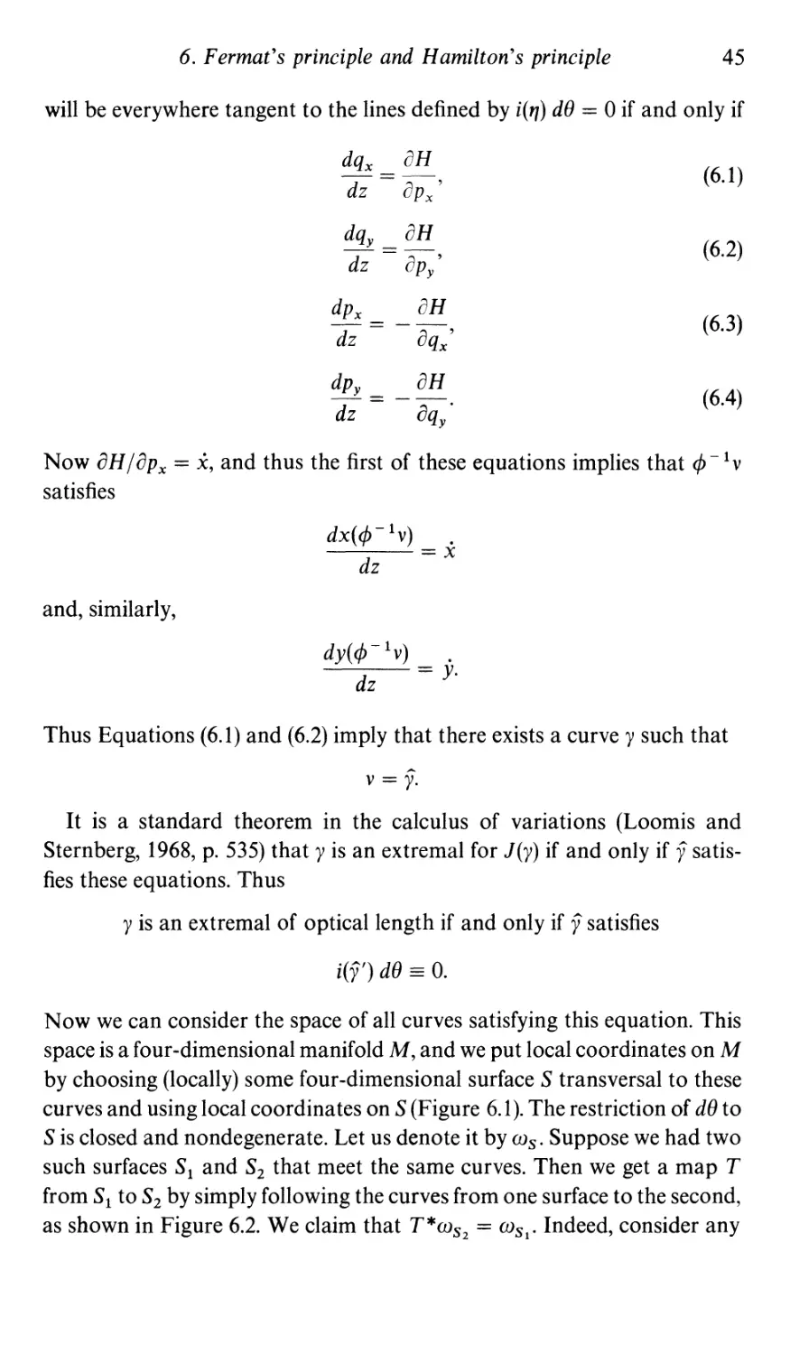
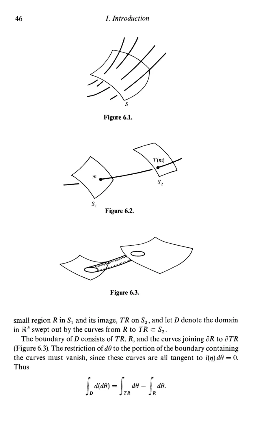
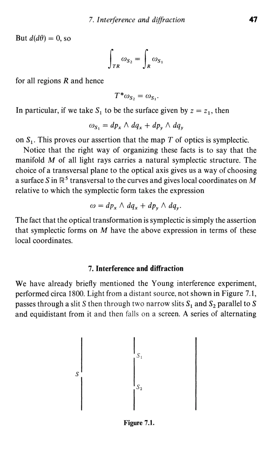
6 Fermat's principle and Hamilton's principle 42
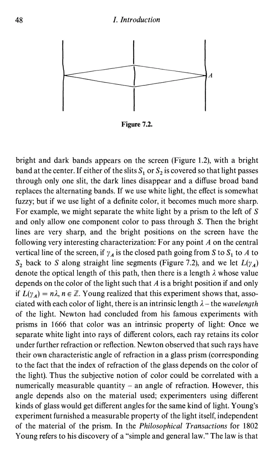
7 Interference and diffraction 47
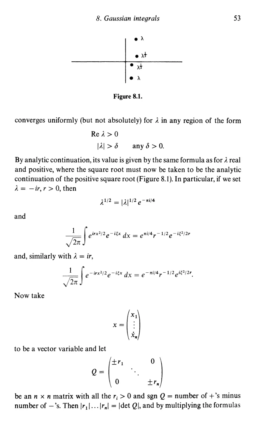
8 Gaussian integrals 51
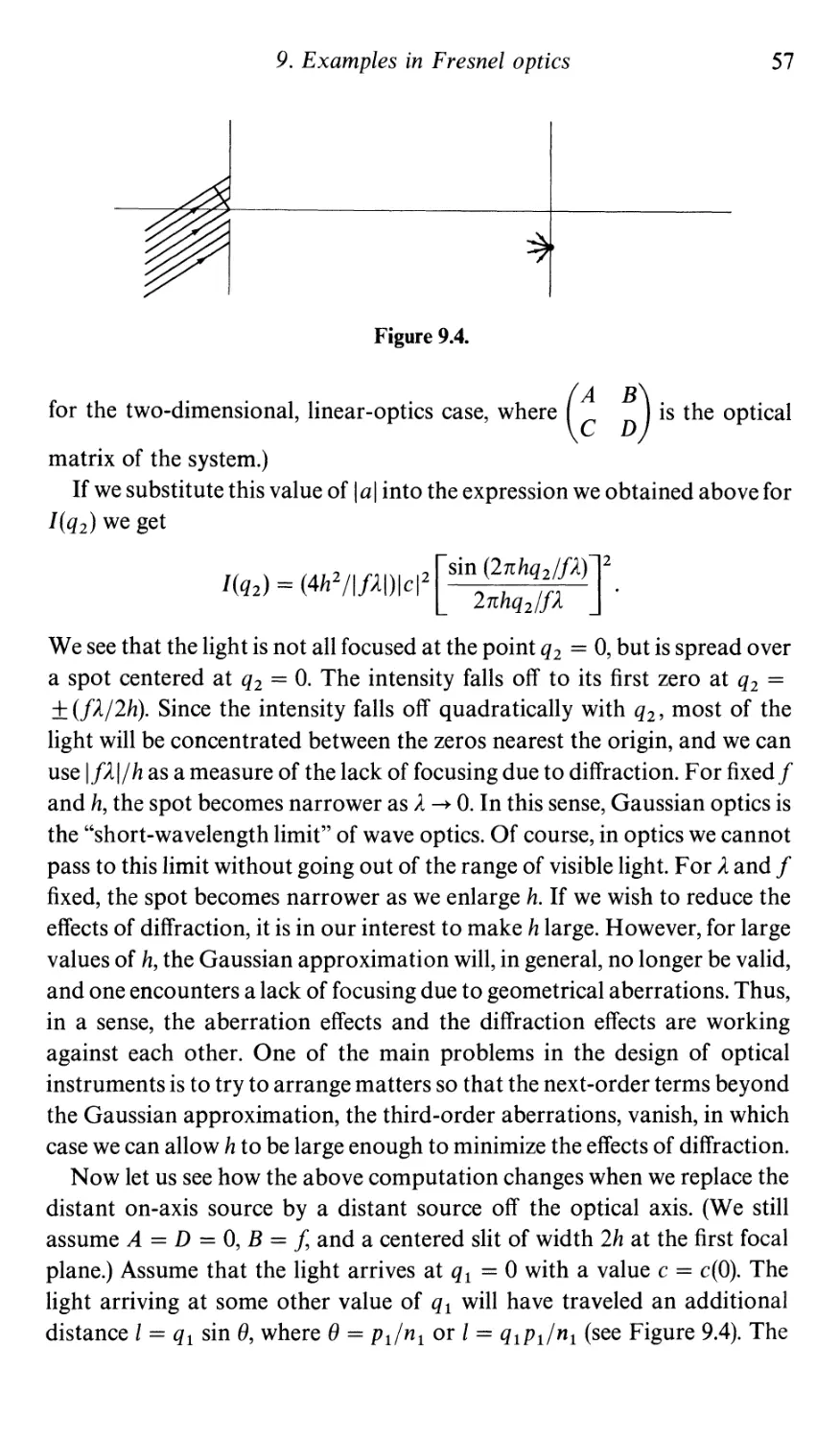
9 Exarnples in Fresnel optics 54
10 The phase factor 60
11 Fresnel's formula 71
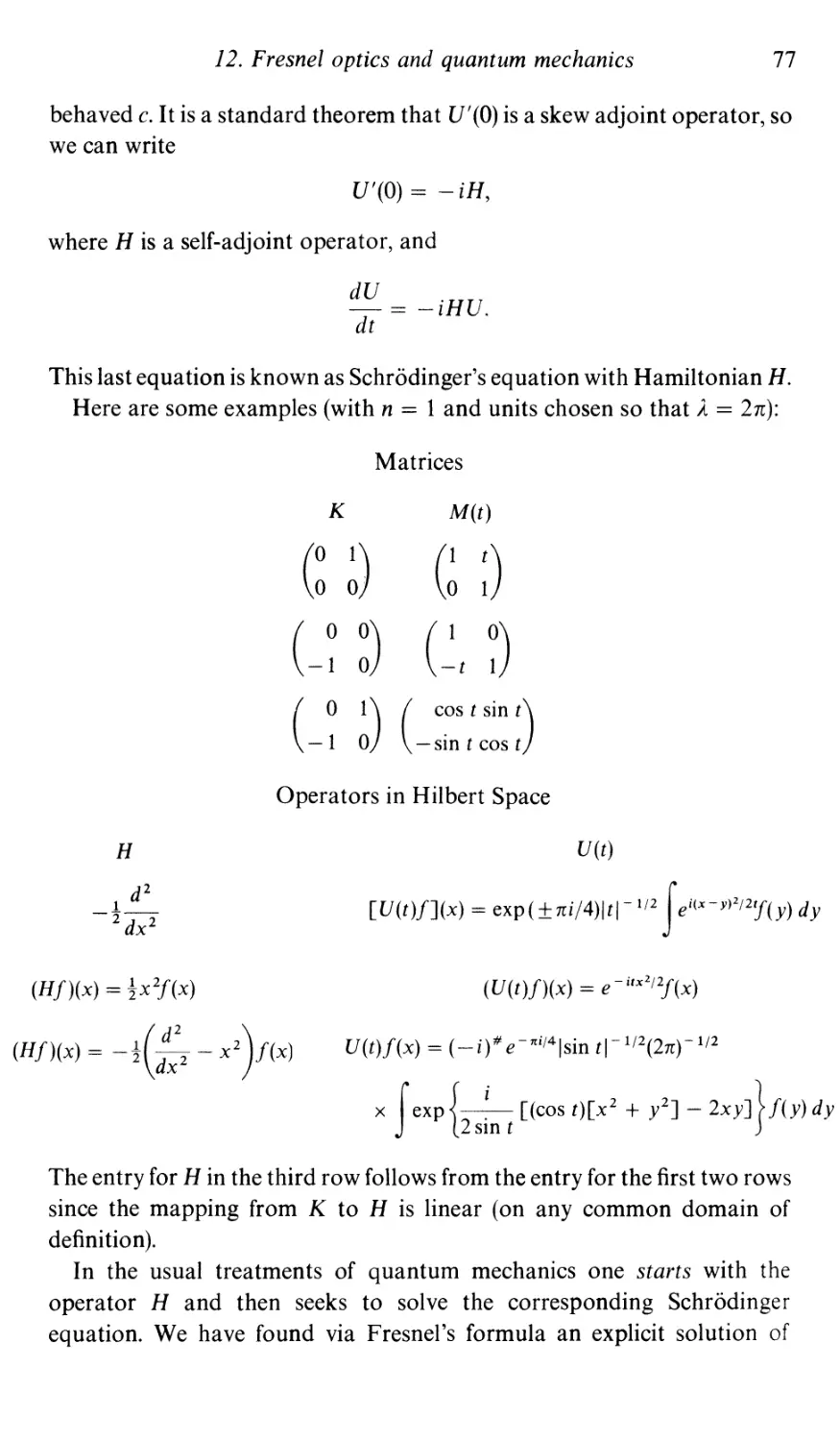
12 Fresnel optics and quantum mechanics 75
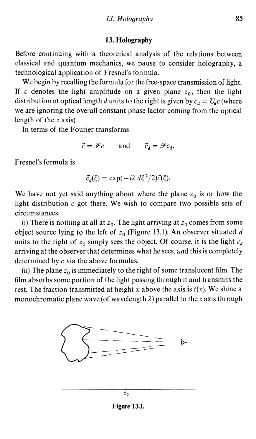
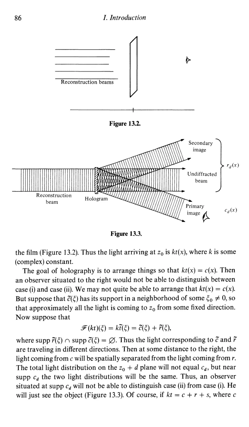
13 Holography 85
14 Poisson brackets 88
15 The Heisenberg group and representation 92
16 The Groenwald-van Hove theorem 101
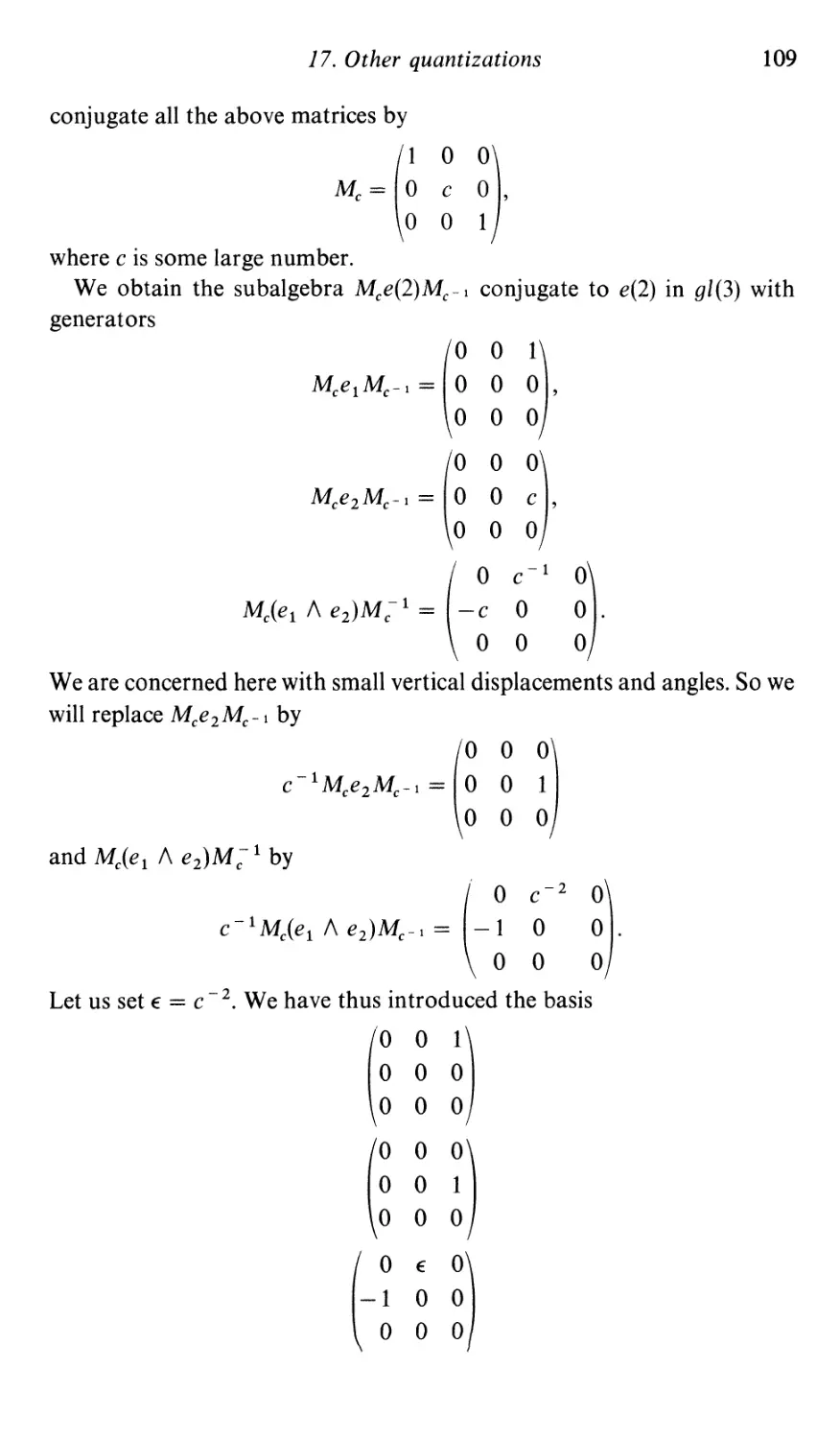
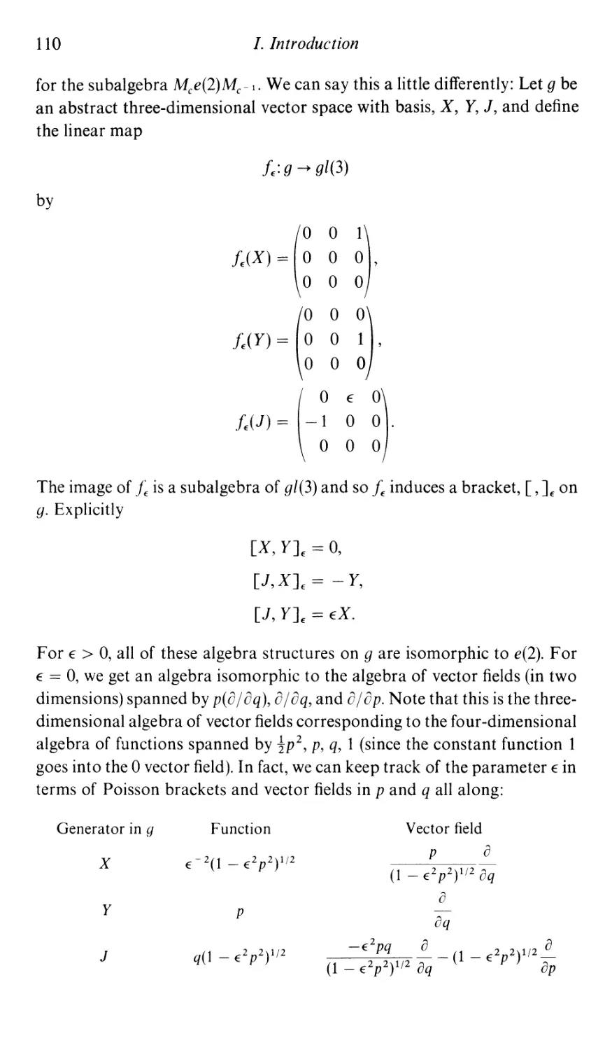
17 Other quantizations 104
18 Polarization of light 116
19 The coadjoint orbit of a semidirect product 124
20 Electromagnetism and the determination of symplectic
structures 130
Epilogue: Why symplectic geometry? 145
v
VI
Contents
II The geometry of the moment map 151
21 Normal forms 151
22 The Darboux-Weinstein theorem 155
23 Kaehler manifolds 160
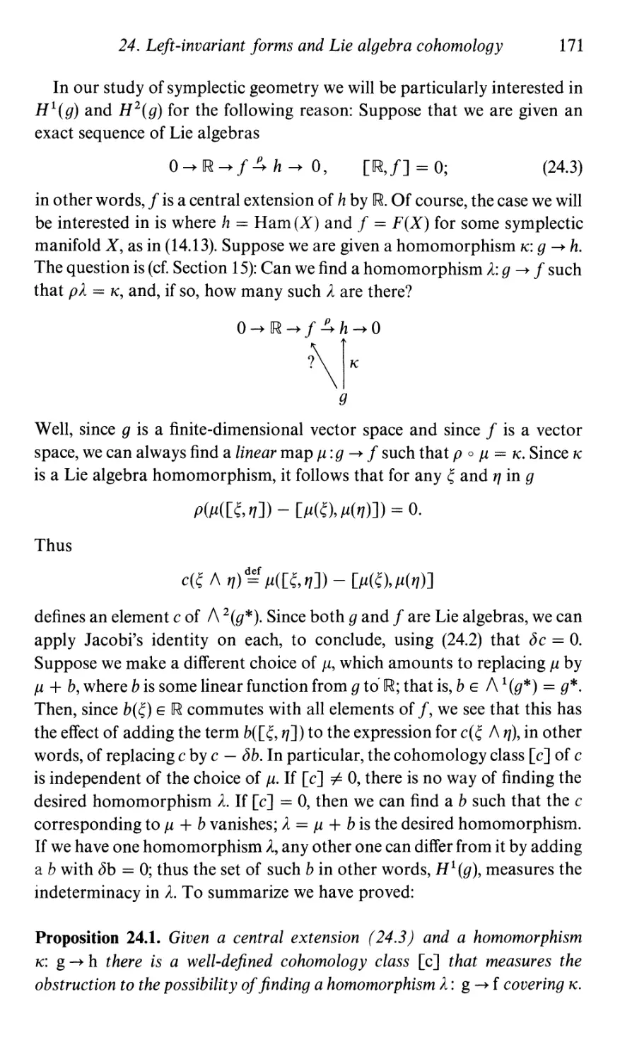
24 Left-invariant forms and Lie algebra cohomology 169
25 Symplectic group actions 172
26 The moment map and some of its properties 183
27 Group actions and foliations 196
28 Collective motion 210
29 Cotangent bundles and the moment map for semi direct
products 220
30 More Euler-Poisson equations 233
31 The choice of a collective Hamiltonian 242
32 Convexity properties of toral group actions 249
33 The lemma of stationary phase 260
34 Geometric quantization 265
III Motion in a Yang-Mills field and the principle of
general covariance 272
35 The equations of motion of a classical particle in a
Y ang- Mills field 272
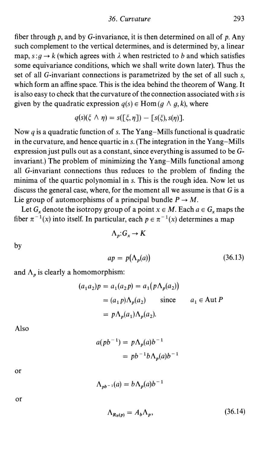
36 Curvature 283
37 The energy-momentum tensor and the current 296
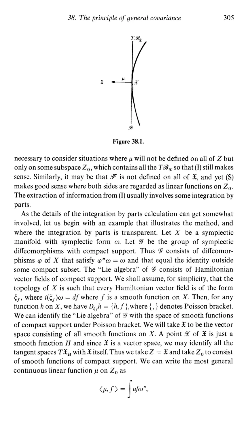
38 The principle of general covariance 304
39 Isotropic and coisotropic embeddings 313
40 Symplectic induction 319
41 Symplectic slices and moment reconstruction 324
42 An alternative approach to the equations of motion 331
43 The moment map and kinetic theory 344
IV Complete integrability 349
44 Fibrations by tori 349
45 Collective complete integrability 359
46 Collective action variables 367
47 The Kostant-Symes lemma and some of its variants 371
48 Systems of Calogero type 381
49 Solitons and coadjoint structures 391
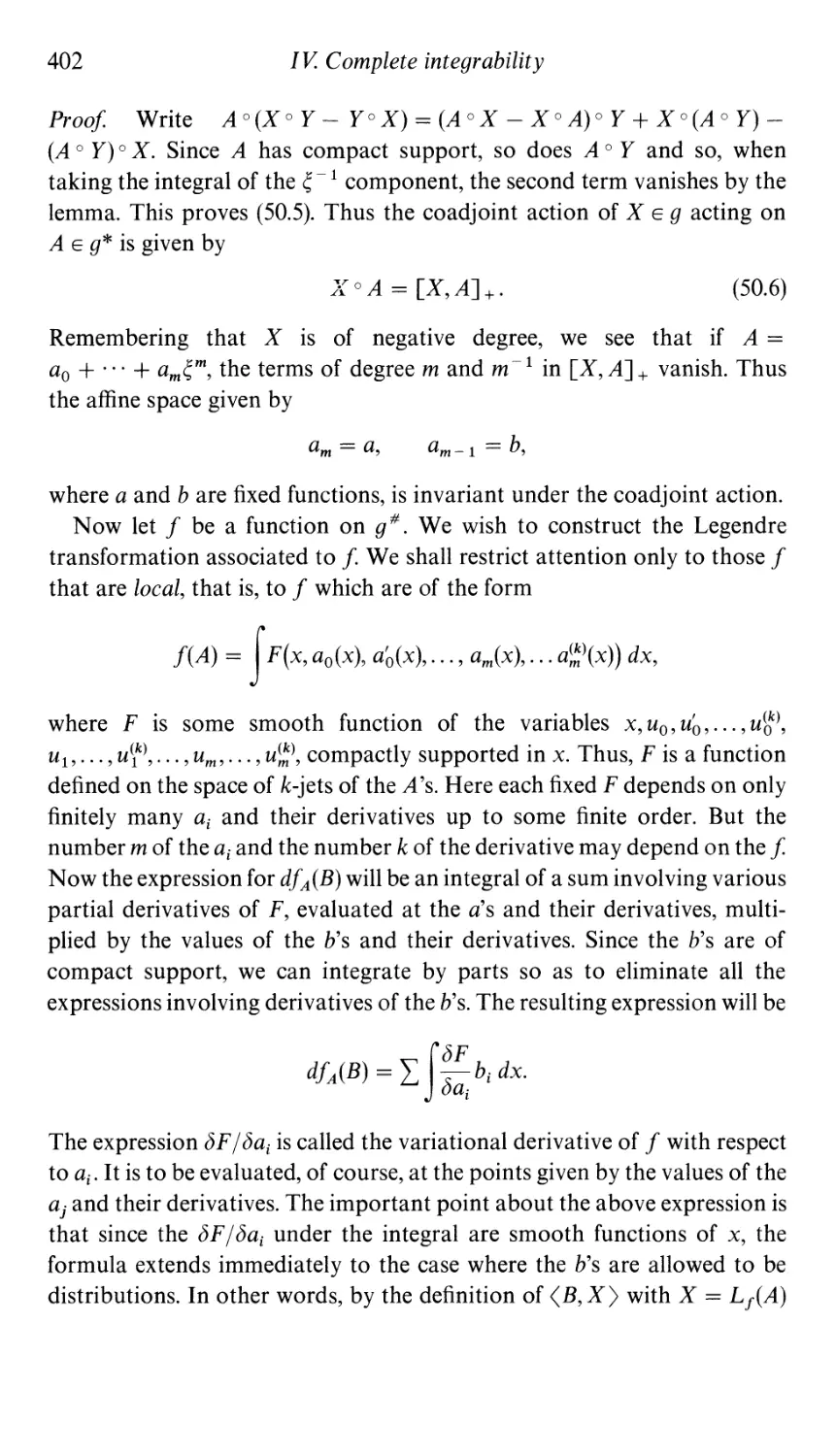
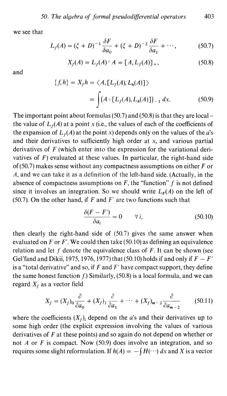
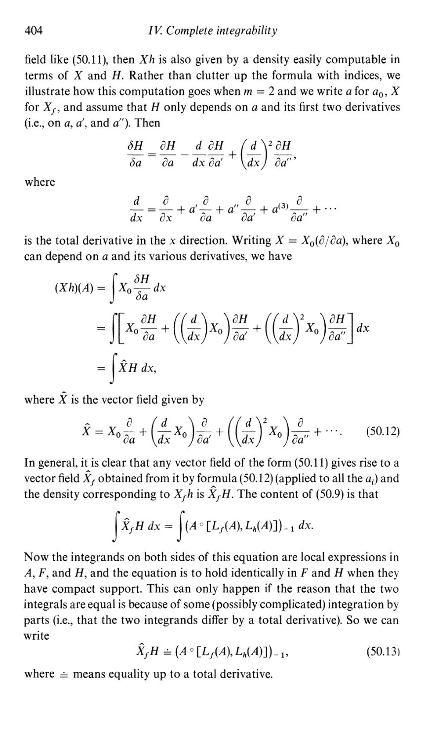
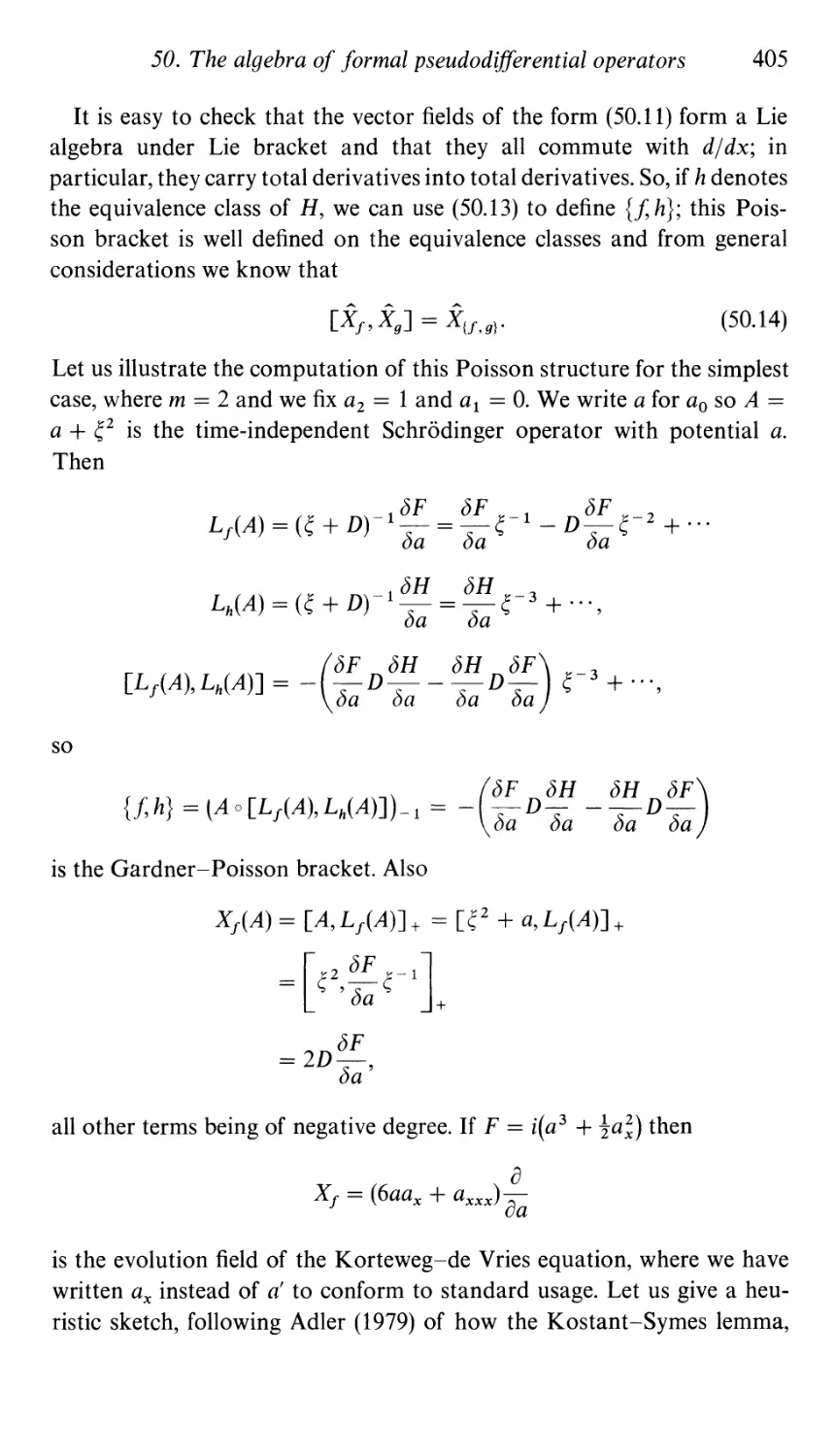
50 The algebra of formal pseudodifferential operators 397
51 The higher-order calculus of variations in one variable 407
Contents
Vll
V Contractions of symplectic homogeneous spaces
52 The Whitehead lemmas
53 The Hochschild-Serre spectral sequence
54 Galilean and Poincare elementary particles
55 Coppersmith's theory
References
Index
416
417
430
437
446
458
467
Preface
This book is based on lectures on symplectic geometry that we have given
over the past few years at MIT, Harvard University, and the University of
Tel Aviv. Symplectic geometry - especially under its old name, "the theory
of canonical transformations" - is a venerable topic in mathematical
physics. It has recently experienced a great rejuvenation and is currently an
active area of research. Our purpose in this book is twofold: to provide an
introduction to the subject and to present the central results of the subject
from a modern point of view. There is, accordingly, a difference in style and
tone between Chapter I and the rest of the book.
Chapter I is directed at the general reader interested in mathematics or
physics. The mathematical prerequisites are quite modest. A knowledge of
calculus and the rudiments of linear algebra suffice for most of the chapter.
Although some mention of more sophisticated topics is made from time to
time, the passages containing such material are inessential and can be
glossed over without loss of continuity. The mix of mathematics and
physics is homogeneous. We have tried the genetic approach. Using the
various theories of light as our paradigm, we have attempted to explain the
development of the mathematical and physical ideas involved in symplectic
geometry. Despite its elementary character, most of the key ideas of the
book are to be found, albeit in embryonic form, in Chapter I.
,
Chapter II presents the key mathematical results of the book and
describes several of the important physical applications. The style is more
formal and the mathematical demands are greater than those of Chapter 1.
The reader is expected to have some familiarity with the basics of dif-
ferential geometry and a degree of mathematical sophistication. The mix
between the mathematics and the physics is less homogeneous here.
We have indicated those sections that can be skipped by a reader more
interested in the physical applications than in the mathematical proofs.
IX
x
Preface
Chapters III, IV, and V are practically independent of one another.
Chapter III is mainly concerned with the use of symplectic geometry as a
tool for formulating (possible) laws of physics. The main theme is the
principle of general covariance due to Einstein, Infeld, and Hoffman in a
form recently explained and recast by Souriau. Section 41 contains one of
the main mathematical results of the book.
Chapter IV is devoted to the use of the interaction between group theory
and symplectic geometry for the solution of various mechanical systems.
We have tried to explain how a broad variety of integrable mechanical
systems can be explained using overt or hidden symmetries. We have, in the
main, restricted attention to finite-dimensional systems, although we do
discuss some evolution equations of the Korteweg-de Vries type. We have
not included the very interesting work involving the Kac- Moody algebras.
Chapter V serves two purposes. The first part presents some of the key
results in the theory of Lie algebras that are needed and used throughout
the book. Although these results, and our treatment of them, are completely
standard, we provide them here for the convenience of the reader. We also
illustrate these results in computations of physical interest. The second part
is a discussion of the deformation theory of symplectic group actions. The
results are all due to Don Coppersmith, and much of the last few sections is
taken directly from his unpublished Harvard thesis. We thank him for his
kind permission to reproduce these results here. Much work remains to be
done on this highly interesting and important topic.
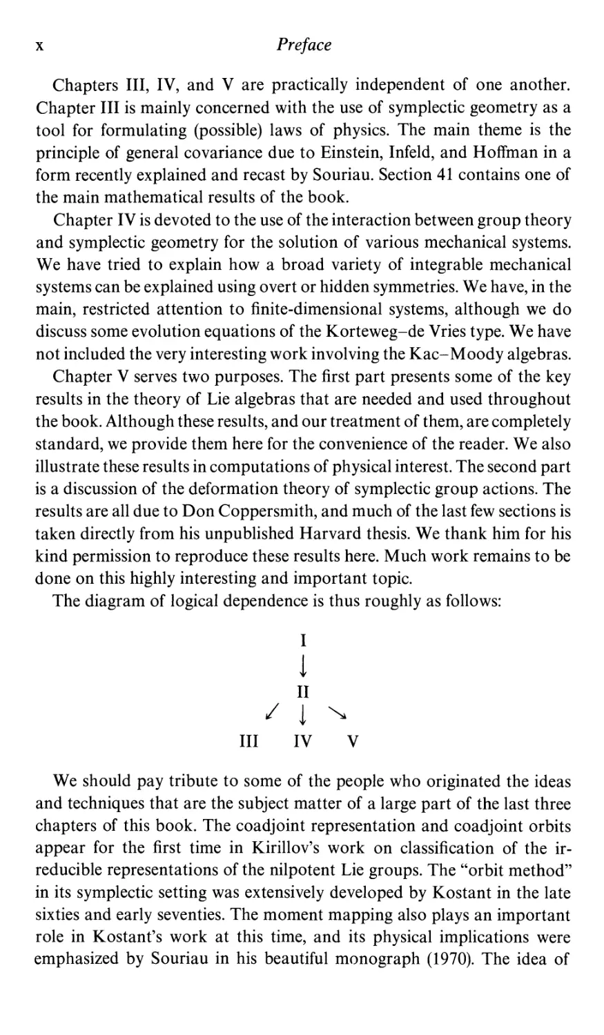
The diagram of logical dependence is thus roughly as follows:
I
!
II
/ 1
III IV V
We should pay tribute to some of the people who originated the ideas
and techniques that are the subject matter of a large part of the last three
chapters of this book. The coadjoint representation and coadjoint orbits
appear for the first time in Kirillov's work on classification of the ir-
reducible representations of the nilpotent Lie groups. The "orbit method"
in its symplectic setting was extensively developed by Kostant in the late
sixties and early seventies. The moment mapping also plays an important
role in Kostant's work at this time, and its physical implications were
emphasized by Souriau in his beautiful monograph (1970). The idea of
Preface
Xl
reduction occurs for the first time in the short paper of Marsden and
Weinstein (1974) and was subsequently used by them and their students and
collaborators for a wide range of applications in mathematics and physics.
The recent work, described in Chapter IV, on complete integrability owes
much to the work of Arnold and Moser in the late sixties and early
seventies. In particular, it was from their work that the idea emerged that
the complete integrability of most of the classical examples of completely
integrable systems could be accounted for by "hidden symmetries." The
material in the first part of Chapter IV, on Lagrangian fib rations and the
geometric structure of completely integrable systems, is largely adapted
from Duistermaat's beautiful paper (1980); and the material in Section 33,
on stationary phase, is based partly on work of Duistermaat and Heckman
and partly on work (some of it unpublished) of Bott and Berline and
Vergne.
We wish to thank Professor G. Emch for a careful reading and many
constructive comments on Chapter 1. We also wish to thank Bert Kostant
for long and fruitful collaboration on many of the topics covered in this
book and for his permission to reproduce many joint results, and Jerry
Marsden and Alan Weinstein for intense but friendly competition. We
would also like to express our appreciation to many of our friends who
provided illuminating conversations, unexpected insights, and moral
support during the three or four years that this book was in gestation (as
course notes for graduate courses at Harvard and MIT). Among them are
Michael Atiyah, Bob Blattner, Raoul Bott, David Kahzdan, Richard
Melrose, John Rawnsley, J. M. Souriau, Joe Wolf, and Alejandro Uribe.
V. G.
S. S.
December 1982
I
Introduction
Not enough has been written about the philosophical problems involved in
the application of mathematics, and particularly of group theory, to
physics. On the one hand, mathematics is created to solve specific problems
arising in physics, and, on the other hand, it provides the very language in
which the laws of physics are formulated. One need only think of calculus
or of Fourier analysis as examples of this dual relationship.
We are all familiar with the exploitation of symmetry in the solution of a
mathematical problem. On the other hand, the very assertion of symmetry
is often the most profound formulation of a physical law or the key step in
the development of a new theory.
Another example is provided by Hamiltonian mechanics. The math-
ematical theory underlying Hamiltonian mechanics is currently called
symplectic geometry. We briefly recall the basic definitions and early
history. A symplectic vector space is a real vector space equipped with an
anti symmetric, nondegenerate bilinear form. For example, on 1R2 we can
define the form (,) by (ut>uz) = qlPZ - qzPt> where U 1 = (:J and U z =
(::). It is not hard to prove that such a vector space must be even-
dimensional (if .finite-dimensional) (see Section 21 below). A linear isomor-
phism of a symplectic vector space V (or more generally of V onto W) is
called symplectic if it preserves the bilinear form. (In two dimensions, a
linear transformation is symplectic if and only if its determinant is 1. In
higher dimensions, the condition is more restrictive.) A differentiable map
of an open subset of a symplectic vector space V into W is called symplectic
if its (Jacobian) matrix of partial derivatives is symplectic at every point. A
symplectic manifold M is an even-dimensional manifold that locally has the
1
2
I. Introduction
structure of a symplectic vector space. This means that one has local charts
l/Ji mapping open sets Vi of M onto open subsets of some fixed symplectic
vector space V and such that the change of coordinates maps l/J i 0 l/J j- 1
defined on l/Jj(V i n V) are symplectic. (Alternatively, thanks to a theorem
of Darboux (see Chapter II, Section 22), a symplectic manifold is a manifold
together with a closed 2-form of maximal rank.) One has the obvious
definition of symplectic diffeomorphism (i.e., one-to-one smooth trans-
formations with smooth inverses, which are locally symplectic in the above
sense). In the older literature, symplectic diffeomorphisms were called
canonical transformations. Symplectic geometry is the study of symplectic
manifolds and diffeomorphisms. The relation with mechanics is usually
expressed by saying that the phase space of a mechanical system is a
symplectic manifold and that the time evolution of a (conservative)
dynamical system is a one-parameter family of symplectic diffeomor-
phisms. The role of the symplectic structure had first appeared, at least
implicitly, in Lagrange's work on the variation of the orbital parameters of
the planets in celestial mechanics. Its central importance, emerged,
however, from the work of Hamilton.
At the age of eighteen, Hamilton submitted a paper entitled "Caustics" to
Dr. John Brinkley, then the first royal astronomer for Ireland, who, as a
result, is said to have remarked "This young man, I do not say will be but is
the first mathematician of his age." Brinkley presented the paper to the
Royal Irish Academy. It was referred, as usual, to a committee, whose
report, while acknowledging the novelty and value of its contents
recommended that it should be further developed and simplified before
publication. Five years later, in greatly expanded form, the paper finally
appeared, entitled "Theory of systems of rays," published in 1828 in the
Transactions of the Royal Irish Academy.
The gist of Hamiltonian optics, in modern language is as follows: One is
interested in studying the geometry of rays of light as they pass through
some optical system. Suppose our system is aligned along some axis, and we
study rays that enter the system at the left and emerge from the right. The
portion of the rays to the left of the system are straight line segments. One
needs four variables, locally, to specify such a line - two variables to specify
the point of intersection of the line with a plane perpendicular to the optical
axis and two additional angular variables giving the inclination of the line
to this plane. The problem is to relate the incoming line segments, to the left
of the system, to the outgoing line segments to the right. The first basic
assertion is that if we use the proper coordinates (which involve the index of
refraction of the ambient space), the transformation from the incoming to
the outgoing coordinates is a symplectic diffeomorphism. Thus geometrical
I. Introduction
3
optics is reduced to symplectic geometry. Hamilton showed that if the
graph of a symplectic transformation satisfies an appropriate "transver-
sality" condition, then the transformation determines and is determined by
a function of one-half the number of incoming and outgoing variables -
the so-called generating function of the symplectic transformation. As this
function is determined solely by the physical properties of the optical
system, Hamilton called it a characteristic function. Depending on the
transversality assumptions made, it can be a function of the points of in-
tersection of the incoming and outgoing rays with the transversal planes-
the point characteristic, the incoming points of the intersection and the
outgoing angles - the mixed characteristic, or the incoming and outgoing
angles - the angle characteristic. These functions are of use in combining
optical systems, that is, in composing the corresponding symplectic trans-
formations. They are also extremely useful in describing the deviation of
the symplectic transformations from linearity - the geometric aberrations
of the optical system. Finally, they are closely related to the optical length
of the light rays themselves, and these light rays can be characterized as
being extremals for optical length (Fermat's principle).
Some years later, Hamilton realized that this same method applies
unchanged to mechanics: Replace the optical axis by the time axis, the light
rays by the trajectories of the system, and the four incoming and four
outgoing variables by the 2n incoming and outgoing variables of the phase
space of the mechanical system. Hamilton's methods, as developed by
Jacobi and other great nineteenth-century mathematicians, became a pow-
erful tool in the solution or analysis of mechanical problems. Hamilton's
analogy between optics and mechanics served as a guiding beacon to the
development of quantum mechanics some one hundred years later.
The main purpose of this chapter is to discuss the relation between linear
optics, geometric optics, and wave optics, stressing Hamilton's point of
view and the corresponding relations between classical and quantum
mechanics.
We first make a few comments on the relation between various theories
of optics. In the histqry of physics it is often the case that when an older
theory is superseded by a newer one, the older theory still retains its valid-
ity - either as an approximation to the newer theory, an approximation that
is valid for an interesting range of circumstances, or as a special case of the
newer theory. Thus Newtonian mechanics can be regarded as approxi-
mation to relativistic mechanics, valid when the velocities that arise are
very small in comparison to the velocity of light. Similarly, Newtonian
mechanics can be regarded as an approximation to quantum mechanics,
4
I. Introduction
valid when the bodies in question are sufficiently large. Kepler's laws of
planetary motion are a special case of Newton's laws, valid for the inverse-
square law of force between two bodies. Kepler's laws can also be regarded
as an approximation to the laws of motion derived from Newtonian
mechanics when we ignore the effects of the planets on one another's
motion.
The currently held theory of light is known as quantum electrodynamics.
It describes very successfully and very accurately the interaction of light
with charged particles, explaining both the discrete character of light, as
evinced in the photoelectric effect, and the wavelike character of electro-
magnetic radiation. The triumph of nineteenth-century physics was Max-
well's electromagnetic theory, which was a self-contained theory explaining
electricity, magnetism, and electromagnetic radiation. Maxwell's theory
can be regarded as an approximation to quantum electrodynamics, valid in
that range where it is safe to ignore quantum effects. Maxwell's theory fails
to explain a whole range of phenomena that occur at the atomic or
su ba tomic level.
One of Maxwell's remarkable discoveries was that visible light is a form
of electromagnetic radiation, as is "radiant heat." In fact, since Maxwell,
optics is a special chapter of the theory of electricity and magnetism that
treats electromagnetic vibrations of all wavelengths: from the shortest
y rays of radioactive substances (having a wavelength of one hundred
millionth of a millimeter) up through x rays, ultraviolet, visible light, and
infrared to the longest radio waves (having a wavelength of many
kilometers).
Maxwell's theory dealt with the source of electromagnetic radiation as
well as its propagation. Before Maxwell, there was a fairly well developed
wave theory of light, due mainly to Fresnel, which dealt rather successfully
with the propagation of light in various media, but had nothing to say
about the production of light. Fresnel's theory did account for three phys-
ical effects that could not be explained by earlier theories - diffraction,
interference, and polarization. Diffraction has to do with the behavior of
light in the immediate vicinity of surfaces through which it is transmitted or
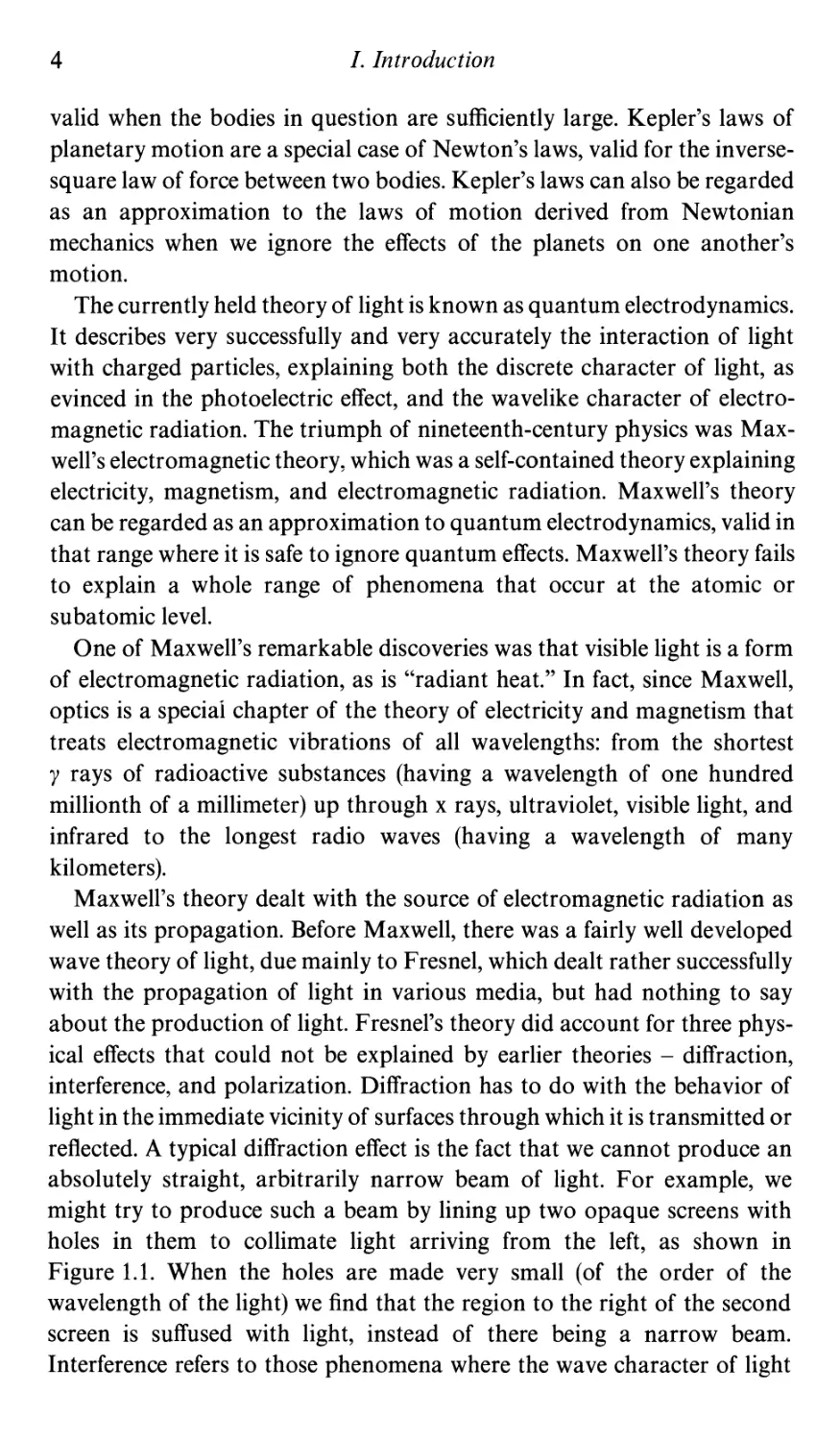
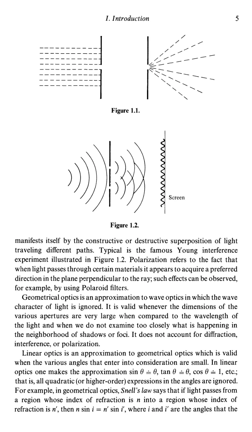
reflected. A typical diffraction effect is the fact that we cannot produce an
absolutely straight, arbitrarily narrow beam of light. For example, we
might try to produce such a beam by lining up two opaque screens with
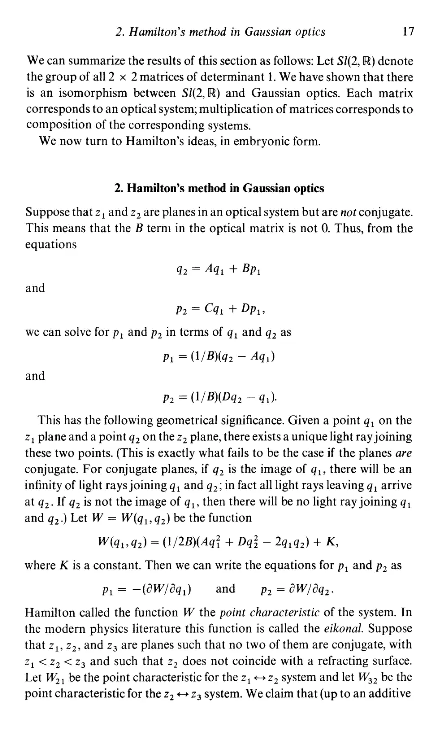
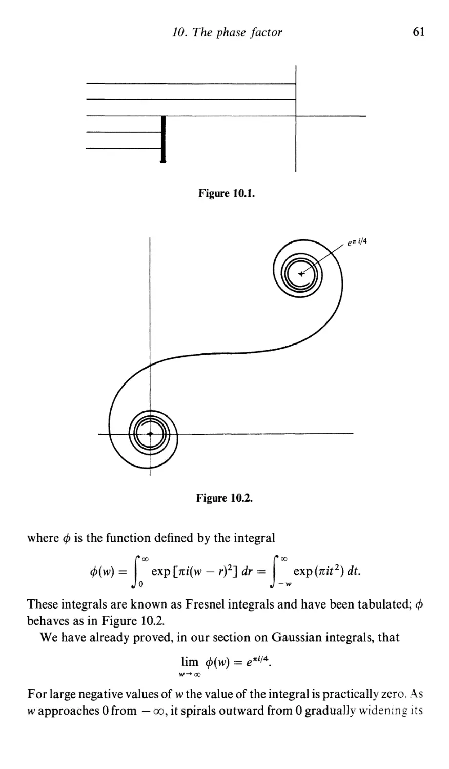
holes in them to collimate light arriving from the left, as shown in
Figure 1.1. When the holes are made very small (of the order of the
wavelength of the light) we find that the region to the right of the second
screen is suffused with light, instead of there being a narrow beam.
Interference refers to those phenomena where the wave character of light
I. Introduction
----------- l
-----------
-----------
-----------
Figure 1.1.
Figure 1.2.
5
/
/
/
/ //
/ /
/ /'" ---
/'" --
-
-
"......... --
""'......... --
""'-........., ---
"- ,
"-
""'-
"-
/'"
........
,
,
Screen
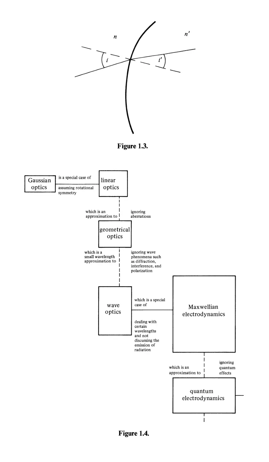
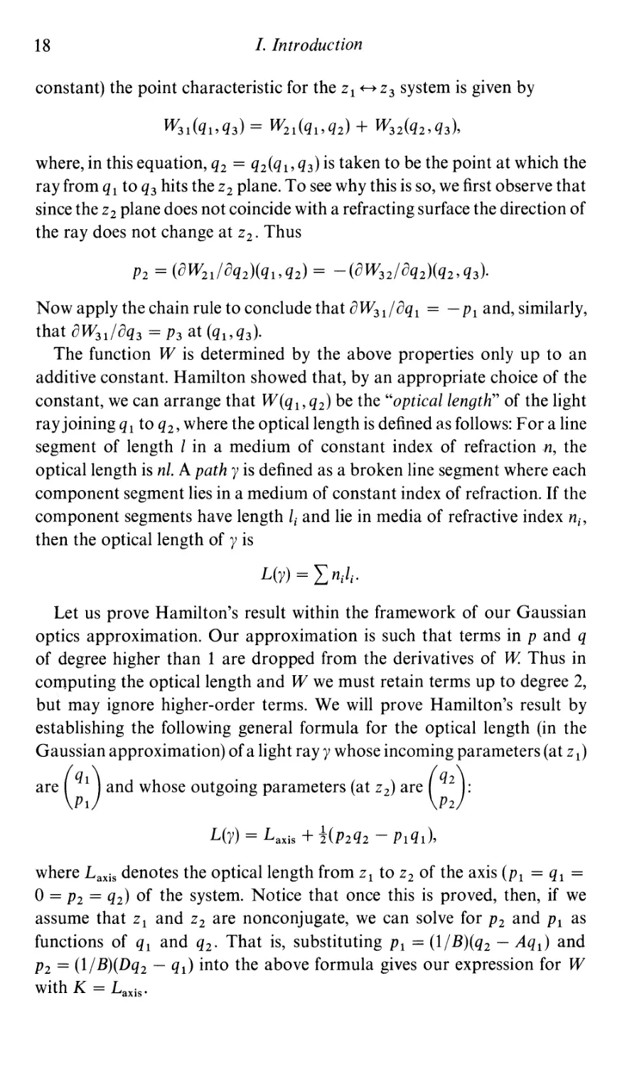
manifests itself by the constructive or destructive superposition of light
traveling different paths. Typical is the famous Young interference
experiment illustrated in Figure 1.2. Polarization refers to the fact that
when light passes through certain materials it appears to acquire a preferred
direction in the plane perpendicular to the ray; such effects can be observed,
for example, by using Polaroid filters.
Geometrical optics is an approximation to wave optics in which the wave
character of light is ignored. It is valid whenever the dimensions of the
various apertures are very large when compared to the wavelength of
the light and when we do not examine too closely what is happening in
the neighborhood of shadows or foci. It does not account for diffraction,
interference, or polarization.
Linear optics is an approximation to geometrical optics which is valid
when the various angles that enter into consideration are small. In linear
optics one makes the approximation sin 0 . 0, tan 0 . 0, cos 0 . 1, etc.;
that is, all quadratic (or higher-order) expressions in the angles are ignored.
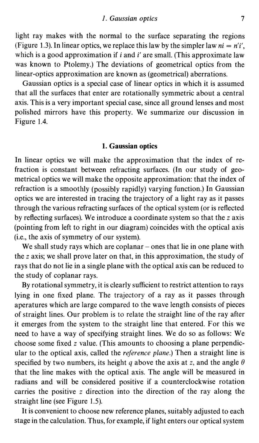
For example, in geometrical optics, Snell's law says that if light passes from
a region whose index of refraction is n into a region whose index of
refraction is n', then n sin i = n' sin i', where i and i' are the angles that the
Figure 1.3.
Gaussian is a special case of linear
optics assuming rotational optics
symmetry
I
I
I
which is an I
approximation to I
I
ignoring
aberrations
geometrical
optics
which is a
small wavelength
approximation to
ignoring wave
phenomena such
as diffraction,
interference, and
polarization
I
I
which is a special
wave case of Maxwellian
optics electrodynamics
dealing with
certain
wavelengths
and not
discussing the
emission of
radiation
I
which is an
approximation to
ignoring
quantum
effects
quantum
electrodynamics
Figure 1.4.
1. Gaussian optics
7
light ray makes with the normal to the surface separating the regions
(Figure 1.3). In linear optics, we replace this law by the simpler law ni = n'i',
which is a good approximation if i and i' are small. (This approximate law
was known to Ptolemy.) The deviations of geometrical optics from the
linear-optics approximation are known as (geometrical) aberrations.
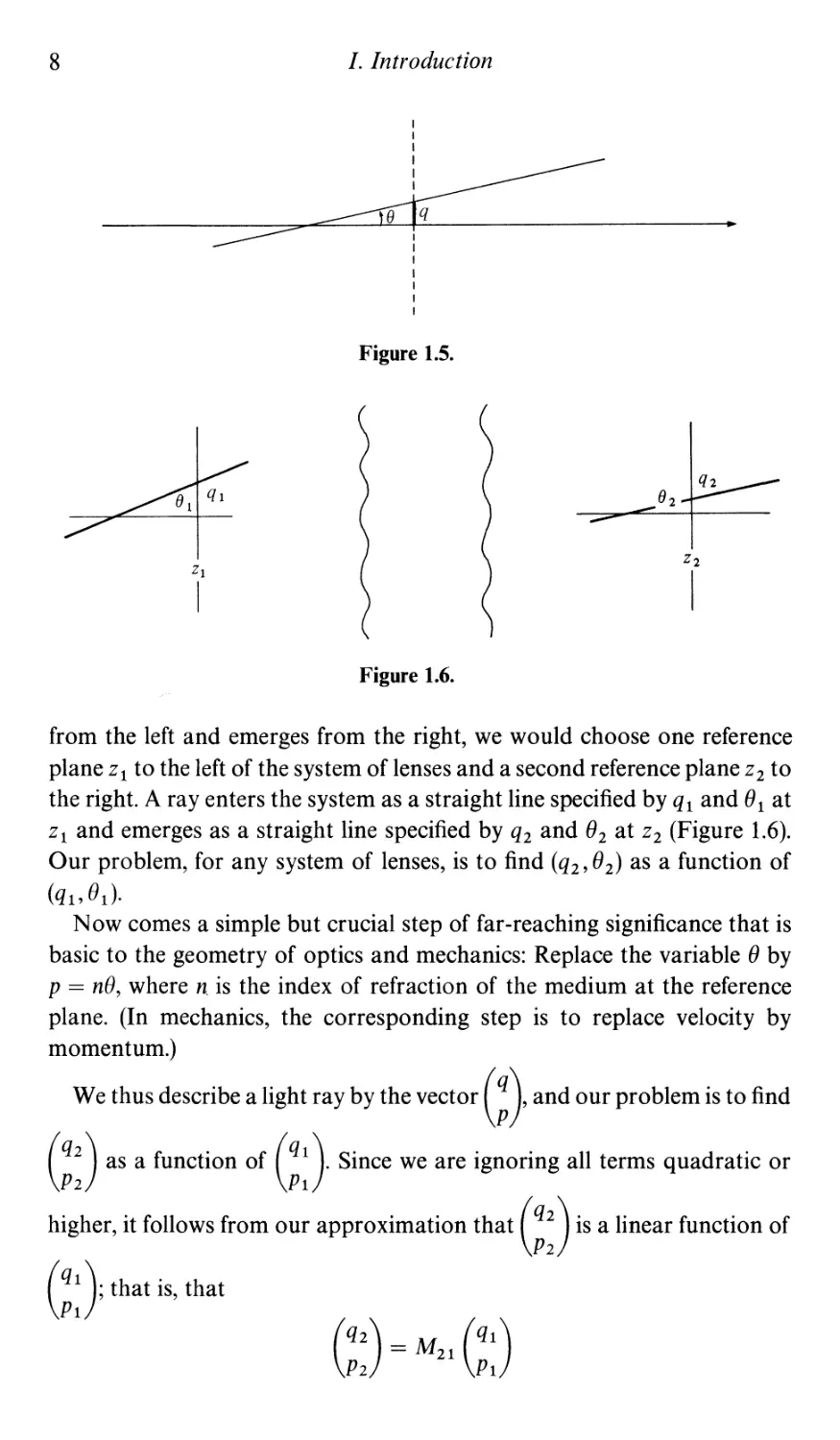
Gaussian optics is a special case of linear optics in which it is assumed
that all the surfaces that enter are rotationally symmetric about a central
axis. This is a very important special case, since all ground lenses and most
polished mirrors have this property. We summarize our discussion in
Figure 1.4.
1. Gaussian optics
In linear optics we will make the approximation that the index of re-
fraction is constant between refracting surfaces. (In our study of geo-
metrical optics we will make the opposite approximation: that the index of
refraction is a smoothly (possibly rapidly) varying function.) In Gaussian
optics we are interested in tracing the trajectory of a light ray as it passes
through the various refracting surfaces of the optical system (or is reflected
by reflecting surfaces). We introduce a coordinate system so that the z axis
(pointing from left to right in our diagram) coincides with the optical axis
(i.e., the axis of symmetry of our system).
We shall study rays which are coplanar - ones that lie in one plane with
the z axis; we shall prove later on that, in this approximation, the study of
rays that do not lie in a single plane with the optical axis can be reduced to
the study of coplanar rays.
By rotational symmetry, it is clearly sufficient to restrict attention to rays
lying in one fixed plane. The trajectory of a ray as it passes through
aperatures which are large compared to the wave length consists of pieces
of straight lines. Our problem is to relate the straight line of the ray after
it emerges from the system to the straight line that entered. For this we
need to have a way of specifying straight lines. We do so as follows: We
choose some fixed z value. (This amounts to choosing a plane perpendic-
ular to the optical axis, called the reference plane.) Then a straight line is
specified by two numbers, its height q above the axis at z, and the angle ()
that the line makes with the optical axis. The angle will be measured in
radians and will be considered positive if a counterclockwise rotation
carries the positive z direction into the direction of the ray along the
s traigh t line (see Figure 1.5).
It is convenient to choose new reference planes, suitably adjusted to each
stage in the calculation. Thus, for example, if light enters our optical system
8
I. Introduction
I
I
I
__________ I
I
I
I
I
I
I
.
Figure 1.5.
Zl
I
Z2
I
Figure 1.6.
from the left and emerges from the right, we would choose one reference
plane z 1 to the left of the system of lenses and a second reference plane z 2 to
the right. A ray enters the system as a straight line specified by q 1 and 0 1 at
z 1 and emerges as a straight line specified by q2 and O 2 at Z2 (Figure 1.6).
Our problem, for any system of lenses, is to find (q2' ( 2 ) as a function of
(q 1, ( 1 ),
Now comes a simple but crucial step of far-reaching significance that is
basic to the geometry of optics and mechanics: Replace the variable 0 by
p = nO, where n. is the index of refraction of the medium at the reference
plane. (In mechanics, the corresponding step is to replace velocity by
momentum.)
We thus describe a light ray by the vector (:} and our problem is to find
(::) as a function of (::} Since we are ignoring all terms quadratic or
higher, it follows from our approximation that (::) is a linear function of
(::} that is, that
(::) = M 21 (::)
1. Gaussian optics
9
q2 }
(tan e d =. e 1 t = ( ) PI
ql
t
ZI
Z2
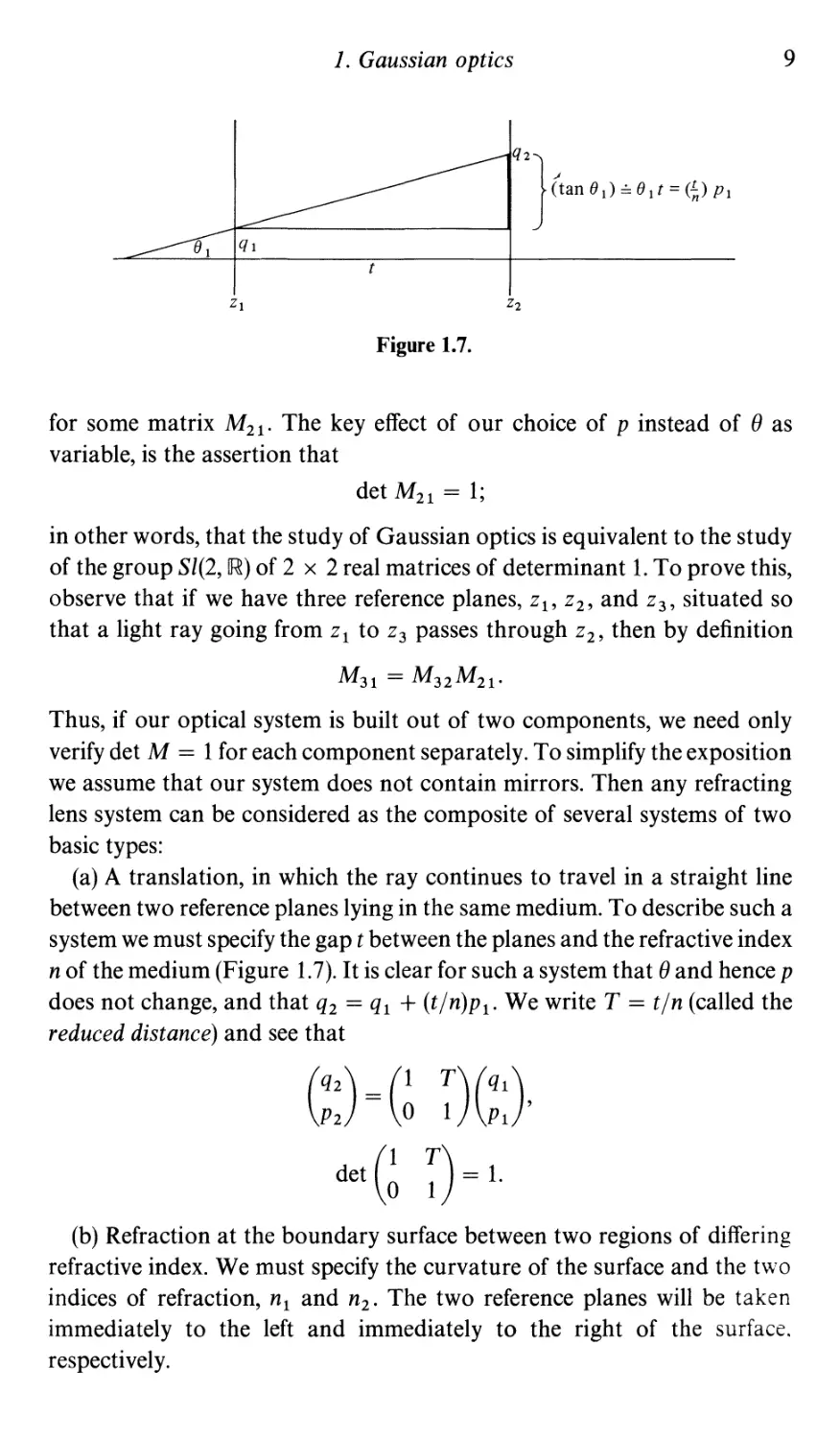
Figure 1.7.
for some matrix M 21 . The key effect of our choice of p instead of () as
variable, is the assertion that
det M 21 = 1;
in other words, that the study of Gaussian optics is equivalent to the study
of the group 81(2, lR) of 2 x 2 real matrices of determinant 1. To prove this,
observe that if we have three reference planes, z l' Z 2, and z 3' situated so
that a light ray going from z 1 to Z3 passes through Z2, then by definition
M 31 = M 32 M 21 .
Thus, if our optical system is built out of two components, we need only
verify det M = 1 for each component separately. To simplify the exposition
we assume that our system does not contain mirrors. Then any refracting
lens system can be considered as the composite of several systems of two
basic types:
(a) A translation, in which the ray continues to travel in a straight line
between two reference planes lying in the same medium. To describe such a
system we must specify the gap t between the planes and the refractive index
n of the medium (Figure 1.7). It is clear for such a system that () and hence p
does not change, and that q2 = ql + (t/n)pl' We write T = t/n (called the
reduced distance) and see that
(: ) = G )(::}
det ( ) = 1.
(b) Refraction at the boundary surface between two regions of differing
refractive index. We must specify the curvature of the surface and the t\VO
indices of refraction, n 1 and n 2 . The two reference planes will be taken
immediately to the left and immediately to the right of the surface.
respectively.
10
I. Introduction
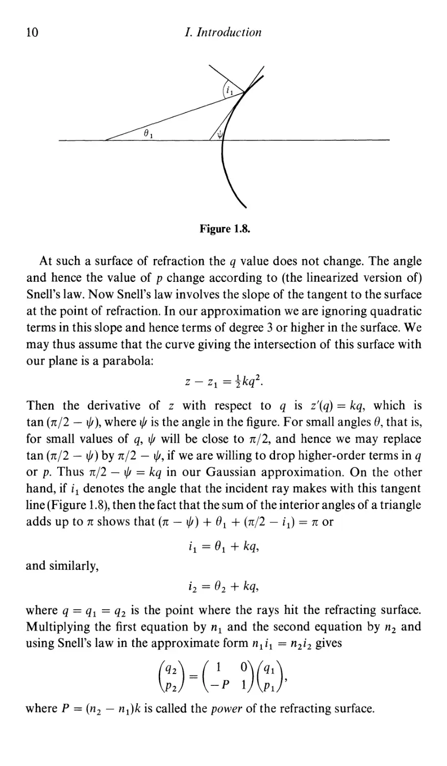
Figure 1.8.
At such a surface of refraction the q value does not change. The angle
and hence the value of p change according to (the linearized version of)
Snell's law. Now Snell's law involves the slope of the tangent to the surface
at the point of refraction. In our approximation we are ignoring quadratic
terms in this slope and hence terms of degree 3 or higher in the surface. We
may thus assume that the curve giving the intersection of this surface with
our plane is a parabola:
1 k 2
Z - Z1 = 2" q .
Then the derivative of z with respect to q is z'(q) = kq, which is
tan (n12 - t/J), where t/J is the angle in the figure. For small angles (), that is,
for small values of q, t/J will be close to n12, and hence we may replace
tan (n12 - t/J) by nl2 - t/J, if we are willing to drop higher-order terms in q
or p. Thus nl2 - t/J = kq in our Gaussian approximation. On the other
hand, if i 1 denotes the angle that the incident ray makes with this tangent
line (Figure 1.8), then the fact that the sum of the interior angles of a triangle
adds up to n shows that (n - t/J) + ()1 + (n12 - i 1 ) = n or
i 1 = () 1 + kq,
and similarly,
i 2 = () 2 + kq,
where q = q1 = q2 is the point where the rays hit the refracting surface.
Multiplying the first equation by n 1 and the second equation by n2 and
using Snell's law in the approximate form n 1 i 1 = n 2 i 2 gives
(: ) = ( p )(::}
where P = (n 2 - n1)k is called the power of the refracting surface.
1. Gaussian optics
11
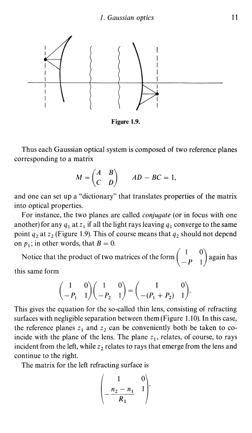
Figure 1.9.
Thus each Gaussian optical system is composed of two reference planes
corresponding to a matrix
M = ( )
and one can set up a "dictionary" that translates properties of the matrix
into optical properties.
F or instance, the two planes are called conjugate (or in focus with one
another) for any q 1 at 2 1 if all the light rays leaving q 1 converge to the same
point q2 at 2 2 (Figure 1.9). This of course means that q2 should not depend
on PI; in other words, that B == O.
Notice that the product of two matrices of the form ( p ) again has
this same form
AD - BC == 1,
( _lp! ) (_lp2 ) = ( _(P!l+ P2) ).
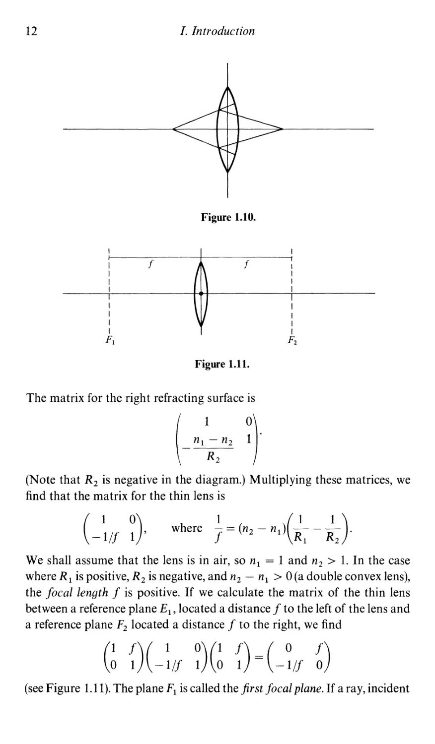
This gives the equation for the so-called thin lens, consisting of refracting
surfaces with negligible separation between them (Figure 1.10). In this case,
the reference planes 2 1 and 2 2 can be conveniently both be taken to co-
incide with the plane of the lens. The plane 2 1 , relates, of course, to rays
incident from the left, while z 2 relates to rays that emerge from the lens and
con tin ue to the right.
The matrix for the left refracting surface is
1 0
n 2 - n 1 1
Rl
12
I. Introduction
Figure 1.10.
f
f
I
I
I
I
F I
I
I
I
I
F 2
Figure 1.11.
The matrix for the right refracting surface is
1 0
n 1 - n 2 l'
R 2
(Note that R 2 is negative in the diagram.) Multiplying these matrices, we
find that the matrix for the thin lens is
(- /f ).
1 ( 1 1 )
where -=(n 2 -n 1 ) --- .
f Rl R 2
We shall assume that the lens is in air, so n 1 = 1 and n 2 > 1. In the case
where Rl is positive, R 2 is negative, and n2 - n 1 > 0 (a double convex lens),
the focal length f is positive. If we calculate the matrix of the thin lens
between a reference plane £1' located a distance f to the left of the lens and
a reference plane F 2 located a distance f to the right, we find
( {) ( - /f ) ( {) = ( - /f )
(see Figure 1.11). The plane F 1 is called the first focal plane. If a ray, incident
1. Gaussian optics
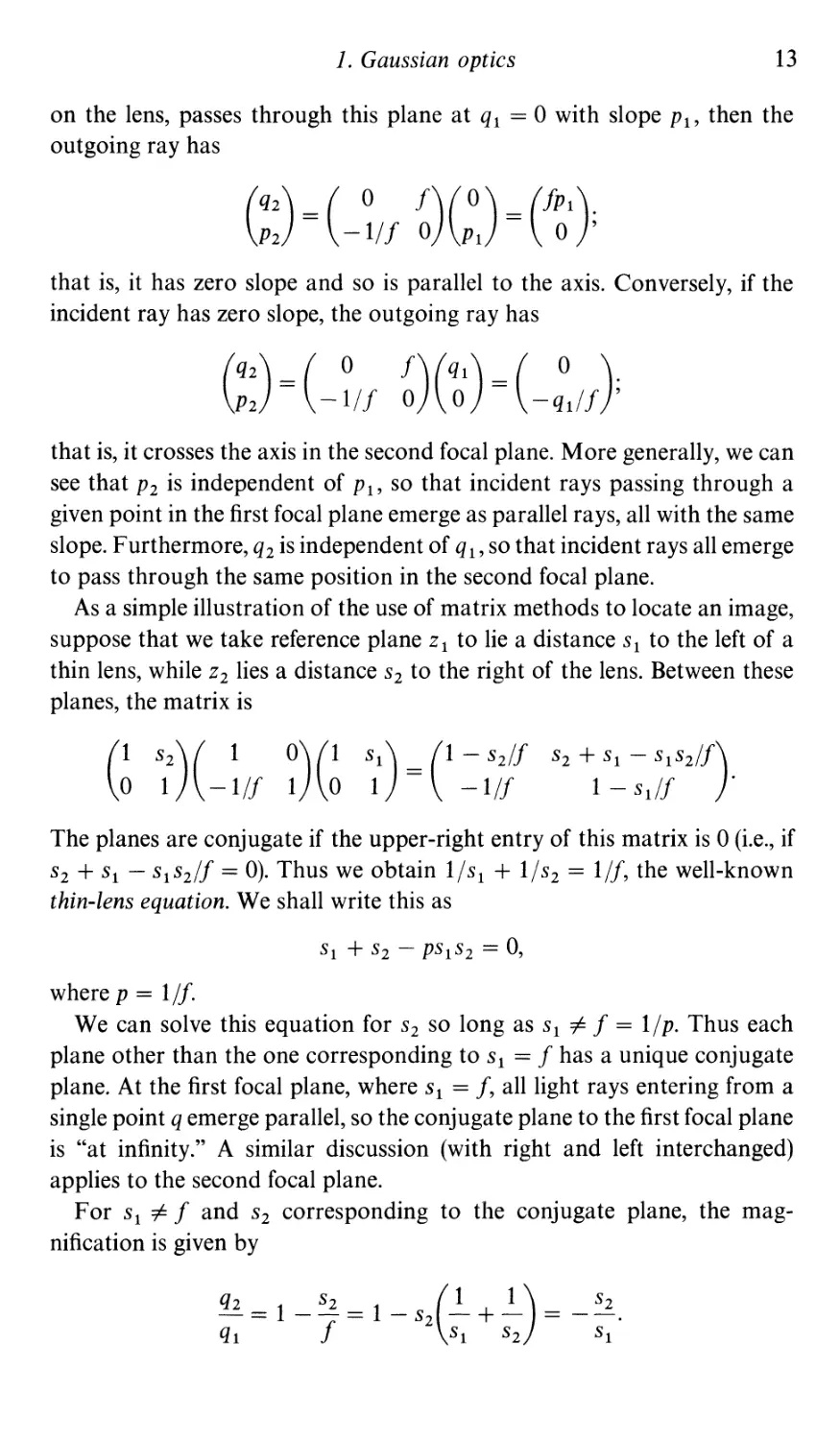
13
on the lens, passes through this plane at q I == 0 with slope PI' then the
outgoing ray has
(;:) = ( _ /f ) ( ) = (I l);
that is, it has zero slope and so is parallel to the axis. Conversely, if the
incident ray has zero slope, the outgoing ray has
(;:) = (_ /f )( 1) = (-qOdI);
that is, it crosses the axis in the second focal plane. More generally, we can
see that P2 is independent of PI' so that incident rays passing through a
given point in the first focal plane emerge as parallel rays, all with the same
slope. Furthermore, q2 is independent of q I' so that incident rays all emerge
to pass through the same position in the second focal plane.
As a simple illustration of the use of matrix methods to locate an image,
suppose that we take reference plane Z I to lie a distance s I to the left of a
thin lens, while Z2 lies a distance S2 to the right of the lens. Between these
planes, the matrix is
( 1 S2 ) ( 1 0 ) ( 1 SI ) == ( 1 - s21f S2 + SI - SIS2If ) .
o 1 -1 If 1 0 1 -1 If l-s l lf
The planes are conjugate if the upper-right entry of this matrix is 0 (i.e., if
S2 + SI - s I s21f == 0). Thus we obtain 1/ s I + 1/ s 2 == 11f, the well-known
thin-lens equation. We shall write this as
SI + S2 - PS I S2 == 0,
where P = 1 If.
We can solve this equation for S2 so long as SI # f == lip. Thus each
plane other than the one corresponding to SI == f has a unique conjugate
plane. At the first focal plane, where SI == f, all light rays entering from a
single point q emerge parallel, so the conjugate plane to the first focal plane
is "at infinity." A similar discussion (with right and left interchanged)
applies to the second focal plane.
For SI # f and S2 corresponding to the conjugate plane, the mag-
nification is given by
q2 == 1 _ S2 == 1 _ S2 ( + ) == _ S2 .
ql f Sl S2 Sl
14
I. Introduction
I
Zl
Z2
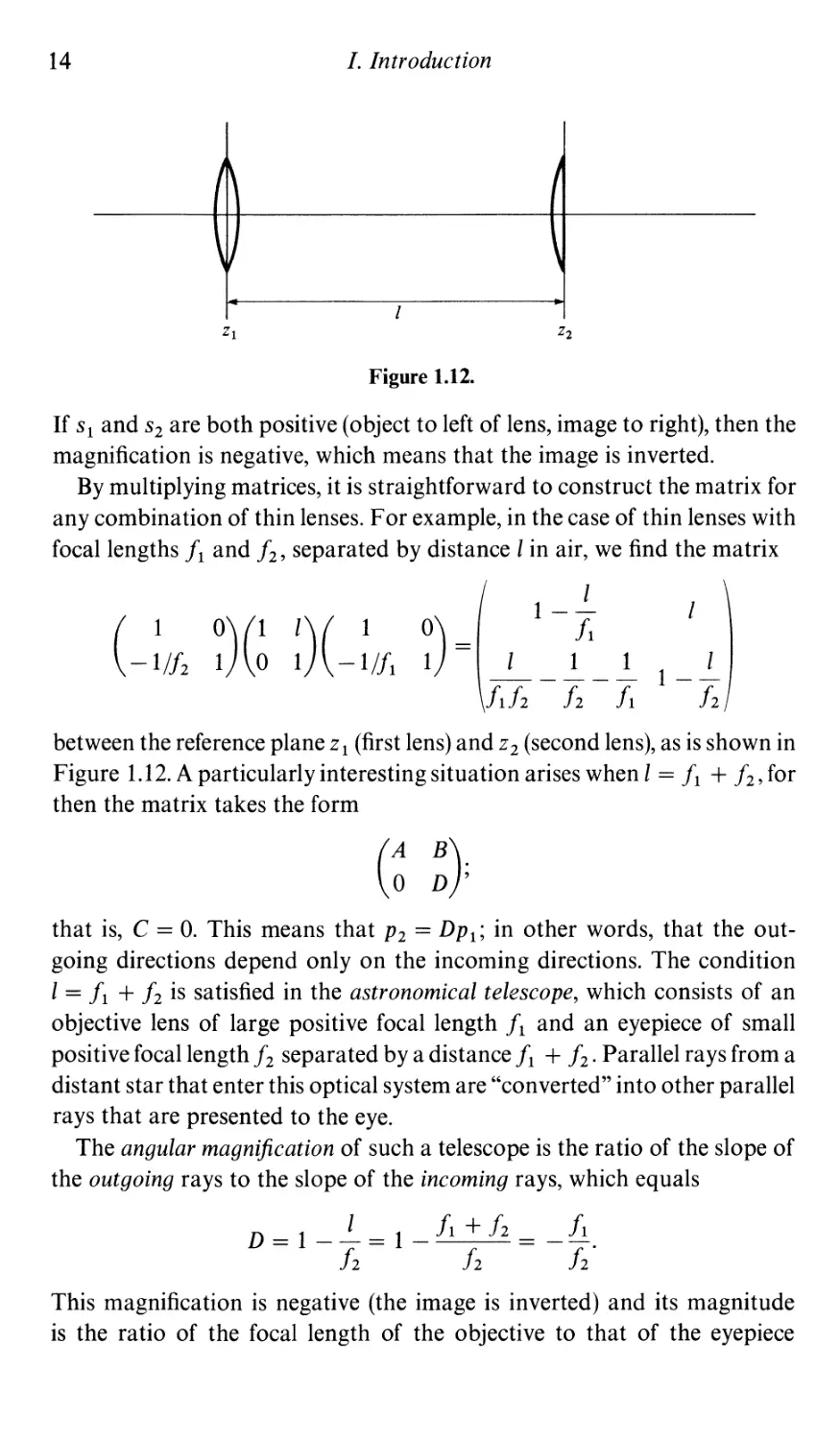
Figure 1.12.
If s 1 and S2 are both positive (object to left of lens, image to right), then the
magnification is negative, which means that the image is inverted.
By multiplying matrices, it is straightforward to construct the matrix for
any combination of thin lenses. For example, in the case of thin lenses with
focal lengths fl and f2, separated by distance I in air, we find the matrix
(-://2 )(
:)(-://1 )=
I
1-- I
fl
I 1 1 I
----- 1--
flf2 f2 fl f2
between the reference plane z 1 (first lens) and Z2 (second lens), as is shown in
Figure 1.12. A particularly interesting situation arises when I = fl + f2, for
then the matrix takes the form
( }
that is, C = O. This means that P2 = Dpl; in other words, that the out-
going directions depend only on the incoming directions. The condition
I = fl + f2 is satisfied in the astronomical telescope, which consists of an
objective lens of large positive focal length fl and an eyepiece of small
positive focal length f2 separated by a distance fl + f2' Parallel rays from a
distant star that enter this optical system are "converted" into other parallel
ra ys that are presented to the eye.
The angular magnification of such a telescope is the ratio of the slope of
the outgoing rays to the slope of the incoming rays, which equals
D = 1 _ = 1 _ fl + f2 = _ fl .
f2 f2 f2
This magnification is negative (the image is inverted) and its magnitude
is the ratio of the focal length of the objective to that of the eyepiece
1. Gaussian optics
15
I
21 2 2
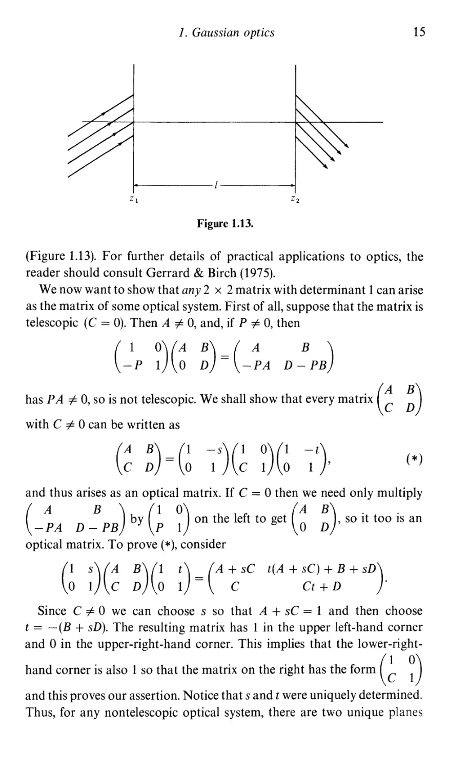
Figure 1.13.
(Figure 1.13). For further details of practical applications to optics, the
reader should consult Gerrard & Birch (1975).
We now want to show that any 2 x 2 matrix with determinant 1 can arise
as the matrix of some optical system. First of all, suppose that the matrix is
telescopic (C == 0). Then A # 0, and, if P # 0, then
( p )( )=(- A D PB)
has P A =I 0, so is not telescopic. We shall show that every matrix ( )
with C # 0 can be written as
( ) = G s)( )G
-t )
1 '
(*)
and thus arises as an optical matrix. If C == 0 then we need only multiply
( A B ) ( 1 0 ) ( A B ) . .
by on the left to get , so It too IS an
-PA D - PB P 1 0 D
optical matrix. To prove (*), consider
( 1 S )( A B )( l t ) == ( A + sC t(A + sC) + B + SD ) .
o 1 C DOl C Ct + D
Since C # 0 we can choose s so that A + sC == 1 and then choose
t == - (B + sD). The resulting matrix has 1 in the upper left-hand corner
and 0 in the upper-right-hand corner. This implies that the lower-right-
hand corner is also 1 so that the matrix on the right has the form ( )
and this proves our assertion. Notice that sand t were uniquely determined.
Thus, for any nontelescopic optical system, there are two unique planes
16
I. Introduction
F 2
Second
focal
plane
Figure 1.14.
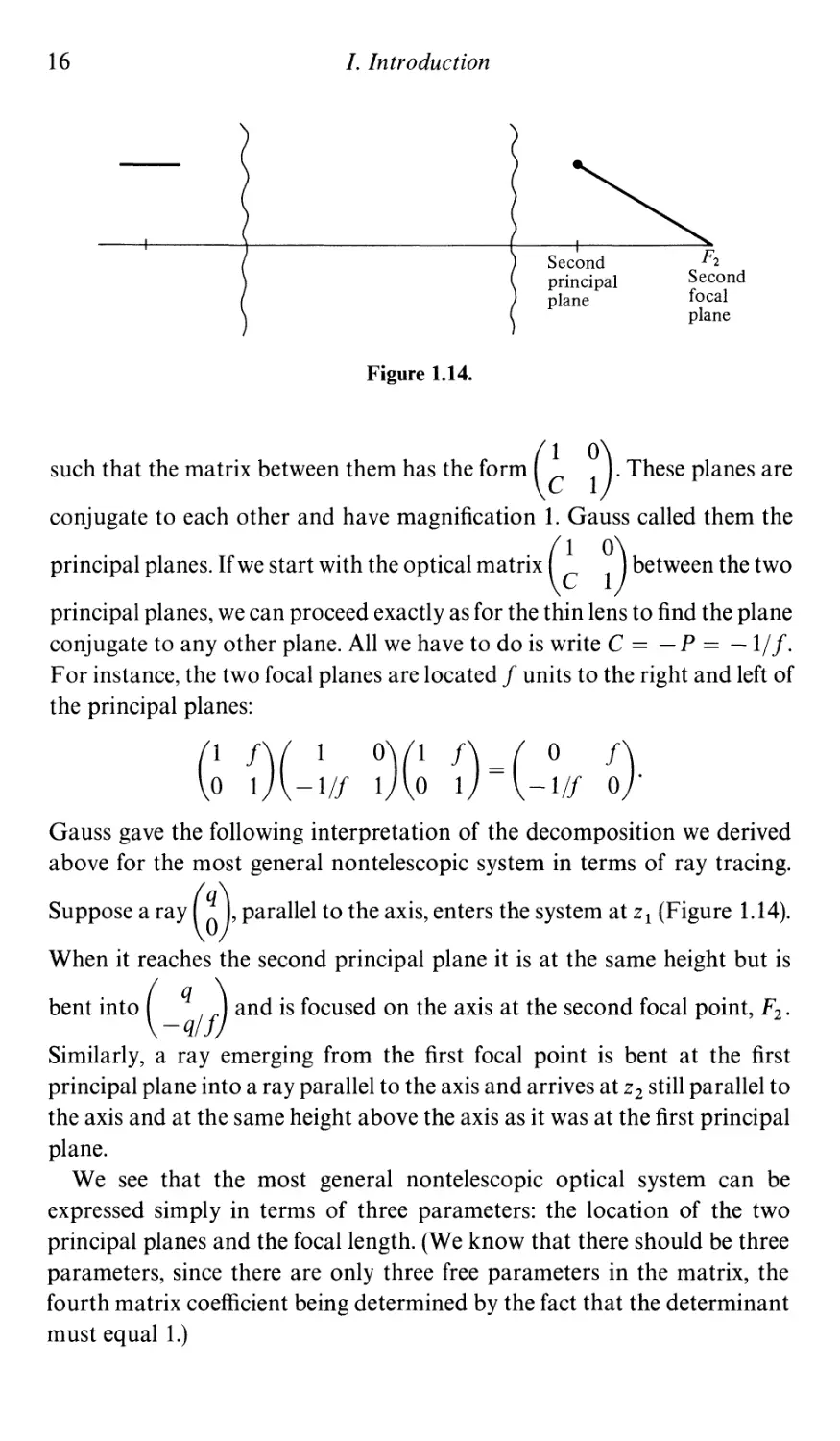
such that the matrix between them has the form ( ). These planes are
conjugate to each other and have magnification 1. Gauss called them the
principal planes. Ifwe start with the optical matrix ( ) between the two
principal planes, we can proceed exactly as for the thin lens to find the plane
conjugate to any other plane. All we have to do is write C = - P = -1/ f.
F or instance, the two focal planes are located f units to the right and left of
the principal planes:
G {)( - /f )( {) = (- /f ).
Gauss gave the following interpretation of the decomposition we derived
above for the most general nontelescopic system in terms of ray tracing.
Suppose a ray ( ), parallel to the axis, enters the system at z 1 (Figure 1.14).
When it reaches the second principal plane it is at the same height but is
bent into ( _ / f) and is focused on the axis at the second focal point, F 2 .
Similarly, a ray emerging from the first focal point is bent at the first
principal plane into a ray parallel to the axis and arrives at z 2 still parallel to
the axis and at the same height above the axis as it was at the first principal
plane.
We see that the most general nontelescopic optical system can be
expressed simply in terms of three parameters: the location of the two
principal planes and the focal length. (We know that there should be three
parameters, since there are only three free parameters in the matrix, the
fourth matrix coefficient being determined by the fact that the determinant
must equal 1.)
2. H ami/ton's method in Gaussian optics
17
We can summarize the results of this section as follows: Let 81(2, !R) denote
the group of all 2 x 2 matrices of determinant 1. We have shown that there
is an isomorphism between 81(2,!R) and Gaussian optics. Each matrix
corresponds to an optical system; multiplication of matrices corresponds to
composition of the corresponding systems.
We now turn to Hamilton's ideas, in embryonic form.
2. Hamilton's method in Gaussian optics
Suppose that 2 I and 22 are planes in an optical system but are not conjugate.
This means that the B ternl in the optical matrix is not O. Thus, from the
equations
q2 = Aqi + BpI
and
P2 = Cql + DpI,
we can solve for PI and P2 in terms of qi and q2 as
PI = (II B)(q2 - Aql)
and
P2 = (II B)(Dq2 - ql)'
This has the following geometrical significance. Given a point q I on the
2 I plane and a point q2 on the 22 plane, there exists a unique light ray joining
these two points. (This is exactly what fails to be the case if the planes are
conjugate. For conjugate planes, if q2 is the image of q I' there will be an
infinity of light rays joining qi and q2; in fact all light rays leaving qi arrive
at q2' If q2 is not the image of ql, then there will be no light ray joining qi
and q2') Let W = W(ql, q2) be the function
W(ql,q2) = (1/2B)(Aqi + Dq - 2qIq2) + K,
where K is a constant. Then we can write the equations for PI and P2 as
PI = -(oWloql)
and
P2 = oWloq2'
Hamilton called the function W the point characteristic of the system. In
the modern physics literature this function is called the eikonal. Suppose
that 2 I' 22, and 23 are planes such that no two of them are conjugate, with
Z I < 22 < 23 and such that 2 2 does not coincide with a refracting surface.
Let W 2I be the point characteristic for the 2 I 22 system and let W 32 be the
point characteristic for the Z2 +-+ 23 system. We claim that (up to an additive
18
I. Introduction
constant) the point characteristic for the 2 1 23 system is given by
W 3 1 (q 1 , q 3) = W 2 1 ( q 1 , q 2) + W 3 2 ( q 2 , q 3 ),
where, in this equation, q2 = q2(qI, q3) is taken to be the point at which the
ray from q 1 to q3 hits the 22 plane. To see why this is so, we first observe that
since the 22 plane does not coincide with a refracting surface the direction of
the ray does not change at 22' Thus
P2 = (JW 21 jJq2)(ql,q2) = -(JW 32 jJq2)(q2,q3)'
Now apply the chain rule to conclude that JW 31 jJql = - PI and, similarly,
that JW 3I jJq3 = P3 at (qI,q3)'
The function W is determined by the above properties only up to an
additive constant. Hamilton showed that, by an appropriate choice of the
constant, we can arrange that W(q 1, q2) be the "optical length" of the light
ray joining ql to q2, where the optical length is defined as follows: For a line
segment of length I in a medium of constant index of refraction n, the
optical length is nl. A path y is defined as a broken line segment where each
component segment lies in a medium of constant index of refraction. If the
component segments have length Ii and lie in media of refractive index n i ,
then the optical length of y is
L(y) = I nJi.
Let us prove Hamilton's result within the framework of our Gaussian
optics approximation. Our approximation is such that terms in P and q
of degree higher than 1 are dropped from the derivatives of W Thus in
computing the optical length and W we must retain terms up to degree 2,
but may ignore higher-order terms. We will prove Hamilton's result by
establishing the following general formula for the optical length (in the
Gaussian approximation) of a light ray y whose incoming parameters (at z 1)
are (:J and whose outgoing parameters (at Z2) are (::)
L(y) = L axis + !(P2q2 - PIQl),
where L axis denotes the optical length from z 1 to 2 2 of the axis (p 1 = Q 1 =
o = P2 = Q2) of the system. Notice that once this is proved, then, if we
assume that 2 1 and 22 are nonconjugate, we can solve for P2 and PI as
functions of Ql and Q2' That is, substituting PI = (ljB)(Q2 - AQI) and
P2 = (ljB)(DQ2 - QI) into the above formula gives our expression for W
with K = L axis '
2. H ami/ton's method in Gaussian optics
19
'Y
l ::
ql
d
Figure 2.1.
z
"
z
Figure 2.2.
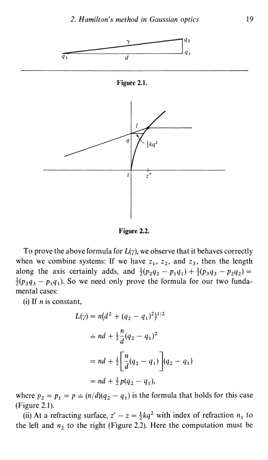
To prove the above formula for L(y), we observe that it behaves correctly
w hen we combine systems: If we have Z I' Z 2, and Z 3' then the length
along the axis certainly adds, and !(P2q2 - PI ql) + !(P3q3 - P2q2) =
!(P3q3 - PIQI)' So we need only prove the formula for our two funda-
men tal cases:
(i) If n is cons tan t,
L(y) = n(d 2 + (Q2 - qI)2)1/2
1 n 2
. nd + 2d(Q2 - QI)
= nd +![ S(q2 - qd}q2 - ql)
= nd + !P(Q2 - QI),
where P2 = PI = P . (njd)(Q2 - QI) is the formula that holds for this case
(Figure 2.1).
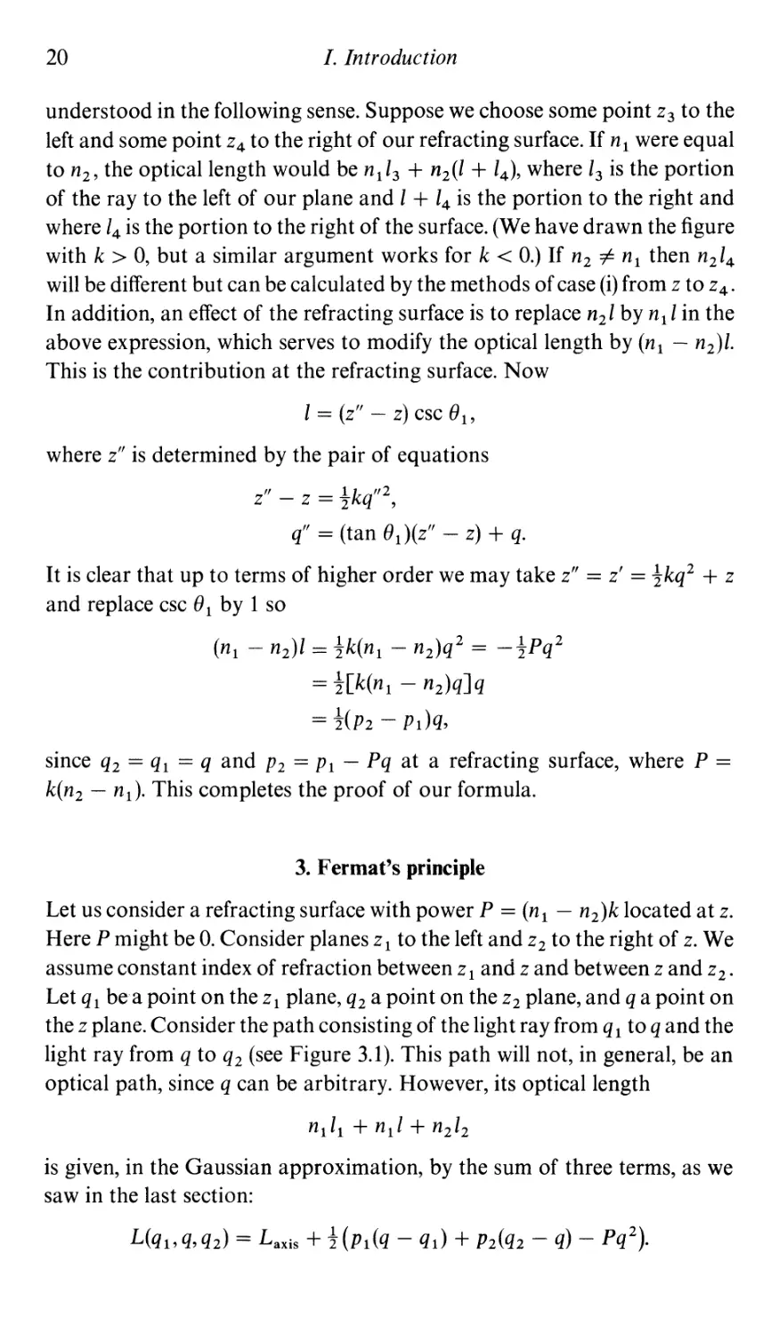
(ii) At a refracting surface, z' - z = !kQ2 with index of refraction n 1 to
the left and n 2 to the right (Figure 2.2). Here the computation must be
20
I. Introduction
understood in the following sense. Suppose we choose some point Z3 to the
left and some point Z4 to the right of our refracting surface. If n 1 were equal
to n 2 , the optical length would be n 113 + n 2 (1 + 1 4 ), where 13 is the portion
of the ray to the left of our plane and 1 + 14 is the portion to the right and
where 14 is the portion to the right of the surface. (We have drawn the figure
with k > 0, but a similar argument works for k < 0.) If n2 # n 1 then n 2 1 4
will be different but can be calculated by the methods of case (i) from z to Z4'
In addition, an effect of the refracting surface is to replace n21 by nIl in the
above expression, which serves to modify the optical length by (n 1 - n 2 )1.
This is the contribution at the refracting surface. Now
1 = (z" - z) CSC (}I,
where z" is determined by the pair of equations
z" - z = !kq,,2,
q" = (tan (}I)(Z" - z) + q.
It is clear that up to terms of higher order we may take z" = z' = tkq2 + z
and replace csc () I by 1 so
(n i - n 2 )1 = tk(n i - n 2 )q2 = -tPq2
= ![k(n i - n 2 )q]q
= t(P2 - PI)q,
since q2 = qi = q and P2 = PI - Pq at a refracting surface, where P =
k(n2 - n l ). This completes the proof of our formula.
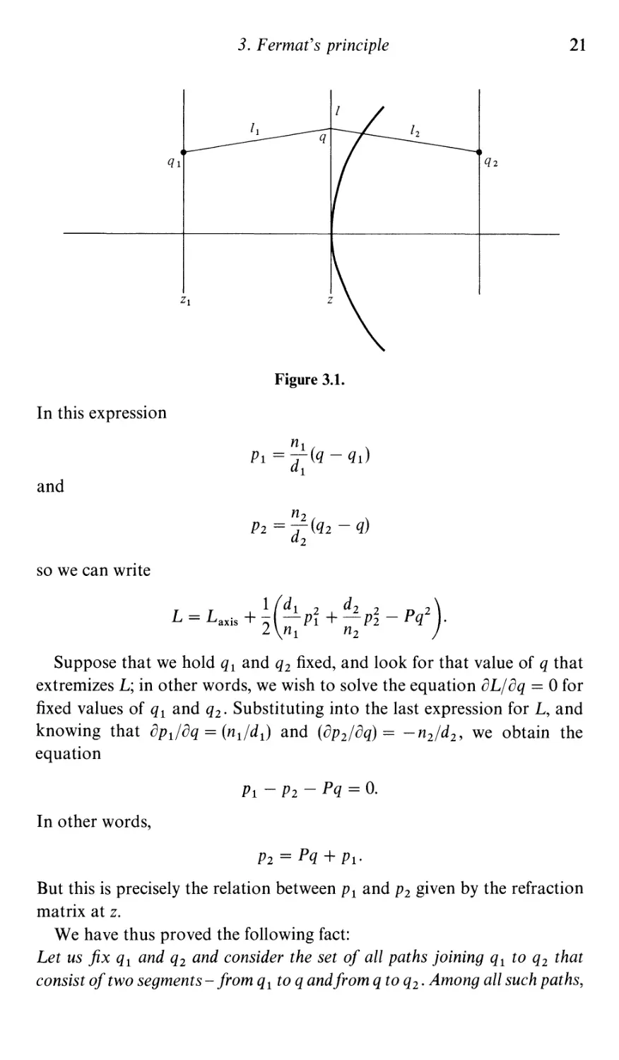
3. Fermat's principle
Let us consider a refracting surface with power P = (n 1 - n 2 )k located at z.
Here P might be O. Consider planes z I to the left and Z2 to the right of z. We
assume constant index of refraction between z I and z and between z and z 2'
Let q I be a poin t on the z I plane, q 2 a poin t on the z 2 plane, and q a poin t on
the z plane. Consider the path consisting of the light ray from q 1 to q and the
light ray from q to q2 (see Figure 3.1). This path will not, in general, be an
optical path, since q can be arbitrary. However, its optical length
n 1 1 1 + nIl + n 2 1 2
is given, in the Gaussian approximation, by the sum of three terms, as we
saw in the last section:
L(ql' q, q2) = L axis + t (PI (q - ql) + P2(q2 - q) - Pq2).
3. Fermat's principle
21
q
q2
ql
Zl
Figure 3.1.
In this expression
n i
Pl = d 1 (q - qd
and
n 2
pz = d z (qz - q)
so we can write
1 ( d i 2 d 2 2 2 )
L = L axis + _ 2 -PI + -P2 - Pq .
n i n 2
Suppose that we hold qi and q2 fixed, and look for that value of q that
extremizes L; in other words, we wish to solve the equation aLl aq = 0 for
fixed values of qi and q2' Substituting into the last expression for L, and
knowing that apilaq = (nlld l ) and (ap2Iaq) = -n 2 Id 2 , we obtain the
equation
PI - P2 - Pq = O.
In other words,
P2 = Pq + Pl'
But this is precisely the relation between P I and P2 given by the refraction
matrix at z.
We have thus proved the following fact:
Let us fix q I and q 2 and consider the set of all paths joining q I to q 2 that
consist of two segments - from q I to q andfrom q to q2' Among all such paths,
22
I. Introduction
the actual light ray can be characterized as that path for which the optical
length L takes on an extreme value, that is, for which
8L = 0
oq .
This is (our Gaussian approximation to) the famous Fermat principle of
"least time." Let us now check whether this extremum is a maximum or
minimum. Let us substitute PI = (nIldl)(q - ql) and P2 = (n2Id 2 )(q2 - q)
into our formula for L to obtain a third expression for L:
L = nIdI + n2 d 2 + !{(nIldl)(q - ql)2 + (n 2 Id 2 )(q2 - q)2 _ Pq2}.
The coefficient of q2 is !(niid l + n 2 /d 2 - P). Thus the extremum is a
minimum if
(nIl d l ) + (n 2 1 d 2 ) - P > 0
and a maximum if
(nIl d l ) + (n21 d 2 ) - P < O.
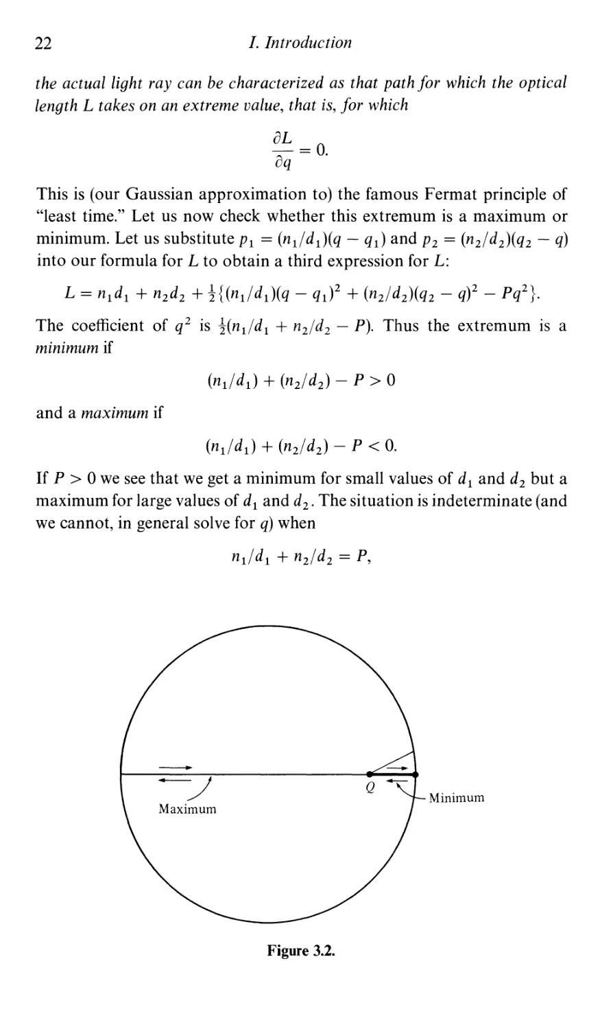
If P > 0 we see that we get a minimum for small values of d l and d 2 but a
maximum for large values of d l and d 2 . The situation is indeterminate (and
we cannot, in general solve for q) when
niid l + n 2 1d 2 = P,
Minimum
Figure 3.2.
4. From Gaussian optics to linear optics
23
which is precisely the condition that the planes are conjugate. Thus, we get a
minimum if the conjugate plane to z 1 does not lie between z 1 and Z2 and a
maximum otherwise. The fact that L is minimized only up to the first
conjugate point is true in a more general setting and is known as the Morse
index theorem. (For more on Morse theory, see Milnor 1963.)
To see an intuitively obvious example of this phenomenon, let us
consider light being reflected from a concave spherical mirror. We take a
point Q inside the sphere and let the light shine along a diameter so that it
bounces back to Q. Then it is clear that the distance to the mirror is a local
minimum if Q is closer than the center, and a maximum otherwise (see
Figure 3.2).
4. From Gaussian optics to linear optics
What happens if we drop the assumption of rotational symmetry but retain
the approximation that all terms higher than the first order in the angles
and distances to one can be ignored? First of all, in specifying a ray, we now
need four variables: qx and qy, which specify where the ray intersects a plane
transverse to the z axis, and two angles, Ox and 0Y' which specify the
direction of the ray. A direction in three-dimensional space is specified by a
unit vector, v = (v x , v y , v z ). If v is close to pointing in the positive z direction,
it will have the form v = (Ox, 0Y' v z ), where V z . 1 - !(O + 0;) . 1, pro-
vided Ox and Oy are small. Again, we replace the 0 variables by p variables,
where Px = nO x and Py = nO y . (If the medium is anisotropic, as is the case
in certain kinds of crystals, the relation between the 0 variables and the p
variables can be more complicated, but we will not concern ourselves with
that here.) All of this, of course, is taking place at some fixed plane. If we
consider two planes z 1 and z 2' the ray will correspond to vectors
qxl qx2
U 1 = qyl and U 2 = qy2
Pxl Px2
Pyl P y 2
a t the respective planes.
Our problem is to find the form of the relationship between U 1 and U2'
Since we are ignoring all higher-order terms, we know that
U2 = Mu 1 ,
where M is some 4 x 4 matrix. Our problem is to ascertain what kind of
4 x 4 matrices can actually arise in linear optics. The most obvious guess is
24
I. Introduction
Figure 4.1.
that M must satisfy the requirement det M == 1. This is not the right answer,
however. It is true that all optical matrices must have unit determinant, but
it is not true that all 4 x 4 matrices of determinant 1 can actually arise as
transformation matrices in linear optics. There is a stronger condition that
must be imposed. In order to explain what this stronger condition is, we first
go back and reformulate the condition that a 2 x 2 matrix has determinant
1. We then formulate this condition in four variables. Let
w = (;)
and
Wi = (;:)
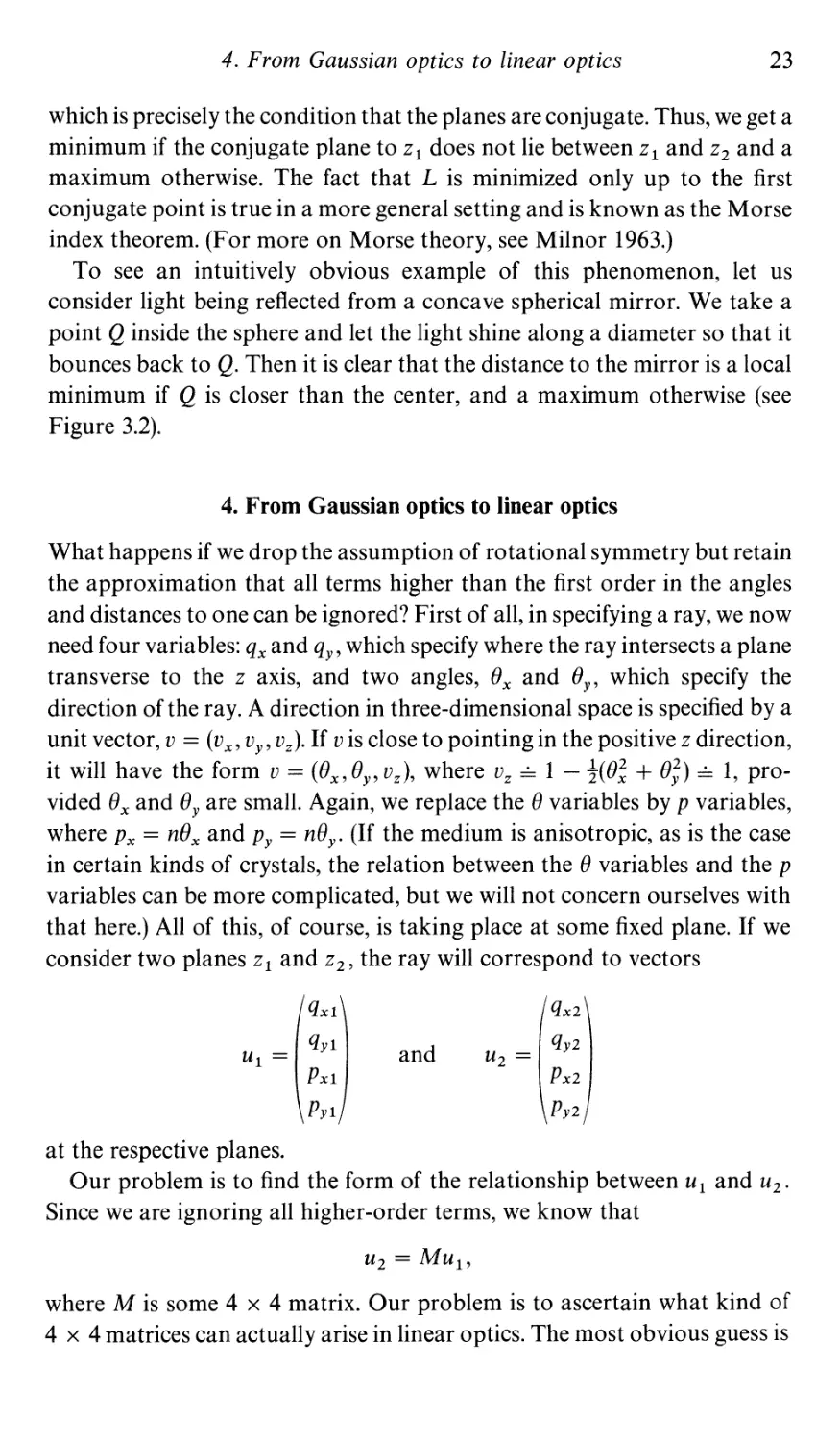
be two vectors in the plane. We define an antisymmetric "product," w(w, w')
between these two vectors by the formula
w(w, w') == qp' - q'p.
The geometric meaning of w(w, w') is that it represents the oriented area of
the parallelogram spanned by the vectors wand w' (see Figure 4.1). It is
clear from both the definition and the geometry that w is antisymmetric:
w(w, w') == - w(w', w).
A 2 x 2 matrix preserves area and orientation if and only if its determinant
equals 1. Thus a 2 x 2 matrix M has determinant 1 if and only if
w(Mw, Mw') == w(w, w')
for all wand w'. Now suppose that
qx q
u== qy and u' == q
Px p
Py p
4. From Gaussian optics to linear optics
25
are two vectors in four-dimensional space. We define
( ' ) , , + ' ,
w u, u = qxPx - qxPx qyPy - qyPy.
The product w is still antisymmetric.
w(u', u) = - w(u, u');
but the geometric significance of w is not so transparent.
It turns out that a 4 x 4 matrix M can arise as the transformation matrix
of a linear optical system if and only if
w(Mu, Mu') = w(u, u'),
for all vectors u and u'. These kinds of matrices are called (linear) canonical
transformations in the physics literature, and are called (linear) symplectic
transformations in the mathematics literature. They (and their higher-
dimensional generalizations) playa crucial role in theoretical mechanics
and geometry.
After developing some of the basic facts about the group of linear
symplectic transformations in four variables, we shall see that our argu-
ments showing that Gaussian optics is equivalent to SI(2, lR) can be used
to show that linear optics is equivalent to Sp(4, lR), the group of linear
symplectic transformations in 4 variables.
In general, let V be any (finite-dimensional, real) vector space. A bilinear
form Q on V is any function Q: V x V lR that is linear in each variable
when the other variable is held fixed; that is, Q(u, v) is a linear function of v
for each fixed u and a linear function of u for each fixed v. We say that Q is
anti symmetric if Q(u, v) = -Q(v, u) for all u and v in V. We say that Q is
non degenerate if the linear function Q(u,') is not identically zero unless u
itself is zero. An anti symmetric, nondegenerate bilinear form on V is called a
symplectic form. A vector space possessing a given symplectic form is called
a symplectic vector space, or is said to have a symplectic structure. If V is a
symplectic vector space with symplectic form Q, and if A is a linear trans-
formation of V into itself, we say that A is a symplectic transformation if
Q(Au, Av) = Q(u, v) for all u and v in V. Later on we shall see that every
symplectic vector space must be even-dimensional and that every symplec-
tic linear transformation must have determinant 1 and, hence, be invertible.
It is clear that the inverse of any symplectic transformation must be
symplectic and that the product of any two symplectic transformations
must be symplectic. Hence, the collection of all symplectic linear trans-
formations form a group, which is known as the symplectic group (of V),
and is denoted by Sp(V).
26
I. Introduction
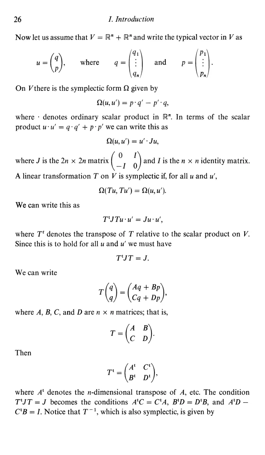
Now let us assume that V = IRn + IRn and write the typical vector in V as
u = (:),
where
q = (}:) and
p=(}:)-
On Vthere is the symplectic form Q given by
Q( u, u') = p' q' - p' . q,
where. denotes ordinary scalar product in IRn. In terms of the scalar
product u. u' = q' q' + p' p' we can write this as
Q(u, u') = u' . Ju,
where J is the 2n x 2n matrix ( I ) and I is the n x n identity matrix.
A linear transformation T on V is symplectic if, for all u and u',
Q(Tu, Tu') = Q(u, u').
We can write this as
TtJTu'u' = Ju.u'
,
where T t denotes the transpose of T relative to the scalar product on V.
Since this is to hold for all u and u' we must have
TtJT = J.
We can write
T ( q ) = ( Aq + BP ) ,
q Cq + Dp
where A, B, C, and Dare n x n matrices; that is,
T = ( ).
Then
( At ct )
T t -
- B t D t '
where At denotes the n-dimensional transpose of A, etc. The condition
TtJT = J becomes the conditions AtC = CtA, BtD = DtB, and AtD -
CtB = I. Notice that T -1, which is also symplectic, is given by
4. From Gaussian optics to linear optics
27
( Dt -B t )
T- 1 -
- - C t At '
and so we also have
DC t = CD t
and
BAt = AB t .
We now turn to the problem of justifying the assertion that the group
of linear symplectic transformations (in four dimensions) is precisely the
collection of all transformations of linear optics. As in the case of Gaussian
optics, the argument can be split into two parts: The first is a physical part
showing that (in the linear approximation) the matrix ( I 0 ) , where
-p I
P = pt is a symmetric matrix, corresponds to refraction at a surface be-
tween two regions of constant index of refraction (and that every P can
arise) and that ( I) corresponds to motion in a medium of constant
index of refraction, where d is the optical distance along the axis. The
second is a mathematical argument showing that every symplectic matrix
can be written as a product of matrices of the above types. Let us begin with
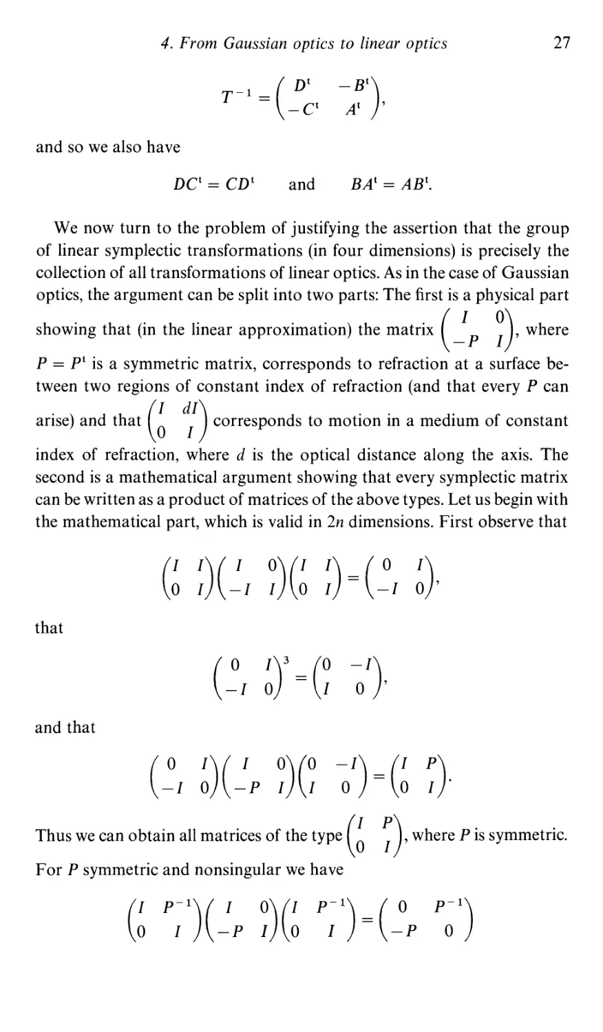
the mathematical part, which is valid in 2n dimensions. First observe that
G )( I )G )=( I }
that
( 0 1 ) 3 = ( 0 - I )
-I 0 I 0 '
and that
( 0 I ) ( I 0 ) ( 0 - I ) ( I P )
-I 0 -p I I 0 - 0 I .
( I P ) . .
Thus we can obtain all matrices of the type 0 I ' where P IS symmetrIc.
For P symmetric and nonsingular we have
( I P-l )( I 0 )( 1 P-l ) = ( 0 P-l )
o I -P I 0 I -P 0
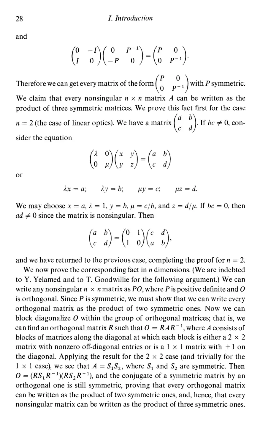
28
I. Introduction
and
( 0 -1 )( 0 P-l ) = ( p 0 ) .
I 0 - P 0 0 p- 1
Therefore we can get every matrix of the form ( p 1 ) with P symmetric.
We claim that every nonsingular n x n matrix A can be written as the
product of three symmetric matrices. We prove this fact first for the case
n = 2 (the case of linear optics). We have a matrix (: :). If be #- 0, con-
sider the equation
( )(; ) = (: :)
or
AX = a'
,
AY = b;
IlY = c;
IlZ = d.
We may choose X = a, A = 1, Y = b, Il = cjb, and z = djll. If bc = 0, then
ad =1= 0 since the matrix is nonsingular. Then
(: :) = ( )( )
and we have returned to the previous case, completing the proof for n = 2.
We now prove the corresponding fact in n dimensions. (We are indebted
to Y. Yelamed and to T. Goodwillie for the following argument.) We can
write any nonsingular n x n matrix as PO, where P is positive definite and 0
is orthogonal. Since P is symmetric, we must show that we can write every
orthogonal matrix as the product of two symmetric ones. Now we can
block diagonalize 0 within the group of orthogonal matrices; that is, we
can find an orthogonal matrix R such that 0 = RAR - 1, where A consists of
blocks of matrices along the diagonal at which each block is either a 2 x 2
matrix with nonzero off-diagonal entries or is a 1 x 1 matrix with + 1 on
the diagonal. Applying the result for the 2 x 2 case (and trivially for the
1 x 1 case), we see that A = SlS2, where Sl and S2 are symmetric. Then
o = (RS 1 R - 1 )(RS 2 R - 1), and the conjugate of a symmetric matrix by an
orthogonal one is still symmetric, proving that every orthogonal matrix
can be written as the product of two symmetric ones, and, hence, that every
nonsingular matrix can be written as the product of three symmetric ones.
4. From Gaussian optics to linear optics
29
Now P- 1 Q -1 ... R -1 = [(PQ... RYJ -1 if P, Q,..., R are symmetric. We
thus can get every symplectic transformation of the form
( (A -1).
Now consider a symplectic matrix ( ) with A nonsingular. Then
(!E )( ) = (c _A EA D EB).
Choose E = CA -1, which is possible since CA -1 is symmetric. We then get
( D EB)
with D - EB = (At) -1. Multiplying by ( A 1
( A 1B).
0 ) .
At gIves
We can thus obtain any symplectic matrix with A nonsingular. Now
suppose that A is singular. Then we can find invertible n x n matrices Land
M such that
LAM = ( }
where Ir is the r x r identity matrix, r = rank A. We may thus pre- and
postmultiply by
( (V -1)
and
( J
respectively, and assume that our matrix ( ) is such that
A=( ).
We can write
C = ( C 1 C2 )
C 3 C 4 '
30
I. Introduction
\\'here C 1 is the r x r component of C, etc. Then
AtC = ( 1
C 2 )
o '
and the condition that AtC be symmetric implies that C 2 = 0 and that C 1 is
symmetric. Now
G )( ) = (A +c EC B +D ED ).
We choose
E = ( 0 0 )
o In -r .
Then E is symmetric and
A + E C = ( Ir )
C 3 4 .
We claim that this matrix is nonsingular. For otherwise C 4 would be
singular. But this would mean that there is some vector v i= 0 whose first
r components vanish and which is sent into zero by C, since C 2 = O. Thus
Av = 0 and Cv = 0, implying that (DtA - BtC)v = 0, contradicting the
condition that DtA - BtC = I. Thus A + EC is nonsingular, and we have
returned to the preceding case.
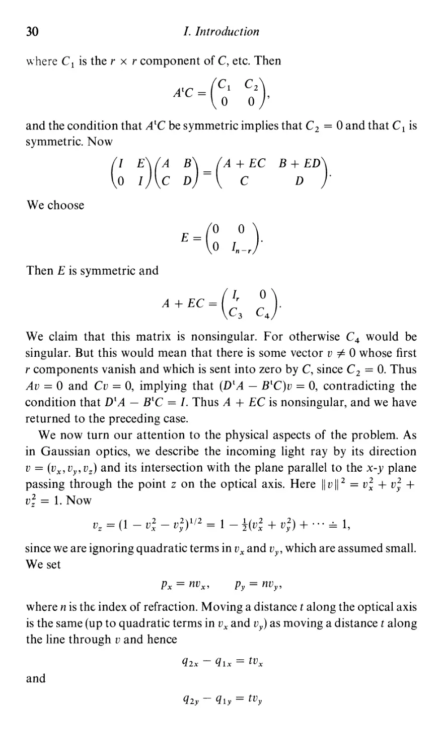
We now turn our attention to the physical aspects of the problem. As
in Gaussian optics, we describe the incoming light ray by its direction
v = (v x , v y , v z ) and its intersection with the plane parallel to the x-y plane
passing through the point z on the optical axis. Here II v 11 2 = v; + v; +
v; = 1. Now
v = ( 1 - v 2 - V 2 ) 1/2 = 1 - l ( v 2 + V2 ) + . .. 1
z x y 2 x y -,
since we are ignoring quadratic terms in V x and v y , which are assumed small.
We set
Px = nv x ,
Py = nv y ,
where n is tht: index of refraction. Moving a distance t along the optical axis
is the same (up to quadratic terms in V x and v y ) as moving a distance t along
the line through v and hence
q2x - Qlx = tv x
and
Q2y - Qly = tv y
4. From Gaussian optics to linear optics
31
q =( : )
Figure 4.2.
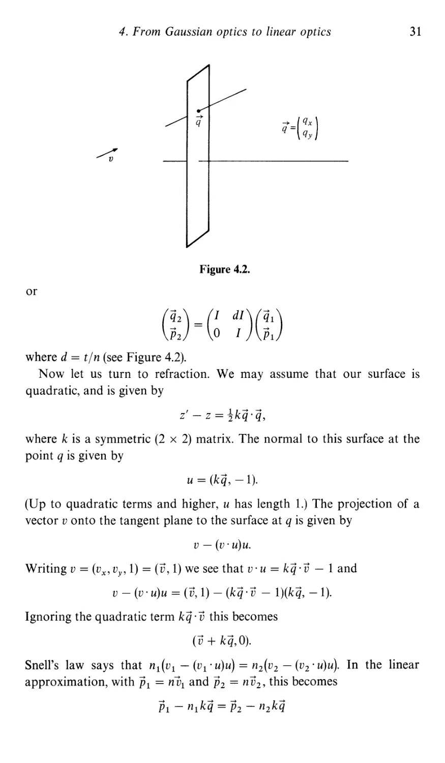
or
( ) = G a:) ( :)
where d = tin (see Figure 4.2).
Now let us turn to refraction. We may assume that our surface is
quadratic, and is given by
, l k -+ -+
Z-Z=2"q'q,
where k is a symmetric (2 x 2) matrix. The normal to this surface at the
point q is given by
u = (kq, -1).
(Up to quadratic terms and higher, u has length 1.) The projection of a
vector v onto the tangent plane to the surface at q is given by
v - (v' u)u.
Writing v = (v x , v y , 1) = (v, 1) we see that v' u = k(j' v-I and
v - (v'u)u = (v, 1) - (k(j'v - l)(k(j, -1).
Ignoring the quadratic term k(j' v this becomes
(v + k(j,O).
Snell's law says that n 1 (V1 - (V1 . u)u) = n 2 (v 2 - (V2 . u)u). In the linear
approximation, with P1 = n V1 and P2 = n V2' this becomes
-+ k -+ -+ k -+
P1 - n1 q = P2 - n2 q
32
I. Introduction
or
-+ -+ P -+
P2 = P1 - q,
where
p = -(n1 - n2)k.
We thus get the refraction matrix ( I 0 ) . This concludes our proof that
-P I
linear optics is isomorphic to the study of the group Sp(4, IR).
There is one more point relating to Gaussian optics that deserves
mention. Suppose that our optical system is rotationally invariant; then at
each refracting surface, the power matrix P is of the form P = cI, where c is
a scalar and I is the 2 x 2 identity matrix. It is clear that the collection of
matrices that one can get by multiplying such matrices with ( a:) will be
of the form (: D. These form a subgroup of Sp(4, IR) that is isomorphic
to SI(2, IR) = Sp(2, IR). Note that a matrix of the above form, when acting on
qx
qy
Px
Py
is the same as (: ) acting separately on (::) and (;:). Thus, in our
study of Gaussian optics the restriction to paraxial rays was unnecessary.
We could have treated skew rays by simply treating the x and y compo-
nents separately in the same fashion. This is a consequence of the linear
approximation.
The basic formula for the optical length
L = L axis + !( P 2 . q 2 - P 1 . q 1)
(where the P and q components are now vectors) is proved exactly as it was
in the Gaussian case, by looking at what happens at each of our basic
components. There is no point in repeating the proof.
Two planes are called nonconjugate if, in the optical matrix relating
them, the matrix B is nonsingular. Then we can solve the equations
q2 = Aq1 + Bp1
4. From Gaussian optics to linear optics
33
and
P2 = Cq1 + Dp1
for P1 and P2 as
B - 1 A B -1
P1 = - q1 + q2
and
P2 = (C - DB- 1 A)q1 + DB- 1 q2'
We can then write
L = L axis + W(q l' q2),
where
W(q1, q2) = t[DB- 1 q2 . q2 + B- 1 Aq1 . ql - 2(B t )-1 q1 . q2J.
(In proving this formula we make use of the identity
- B t - 1 == C - DB - 1 A
,
which follows for nonsingular B from AtD - BtC == I.) A direct com-
putation (using the above identity) shows that (in the obvious sense)
8L
- == P2
8q2
and
8L
8q 1 == - P l'
Thus a knowledge of L allows us to determine P1 and P2 in terms of q 1
and q2'
In the next section we will move from linear optics to geometrical optics. In
geometrical optics we will have to be a little more careful about our choice
of P variables. In linear optics we have identified e, sin e, and tan e, where e
is a small angle. It turns out that sin e is the right variable to use. More
precisely, let us assume that the index of refraction is now a smoothly
varying function in space (perhaps rapidly changing across an interface)
so that the optical rays will now be smooth curves instead of broken line
segments. We will still use the z axis to parametrize these rays (we are
staying away from large deviations from the optical axis), and so a ray \\'ill
be given by a pair of functions x(z) and y(z) and we will write x for dx d:.
34
I. Introduction
We set
xn(x, y, z)
Px = ) 1 + x2 + y2'
qx == x,
yn(x, y, z)
Py = )1 + x2 + y2 ;
qy == y
as the parameters describing a light ray at the z plane. The basic assertion of
geometrical optics is that the transformation from one z plane to another is
a symplectic diffeomorphism. Hamilton derived this from Fermat's prin-
ciple. We shall present the argument in Section 6.
5. Geometrical optics, Hamilton's method, and the theory of
geometrical aberrations
Let (VI' WI) and (V 2 , ( 2 ) be two copies of [R4 (or more generally of [R2n or,
even more generally, they can be any two symplectic manifolds of the same
dimension).
On VI x V 2 we can put the symplectic form
o == n!w 2 - niw 1 ,
where TC I and TC 2 denote the projections onto the first and second com-
ponents. By abuse of notation we shall usually drop the n*'s and simply
write this as
0==W2- W 1'
A smooth map T: VI V 2 is called a symplectic diffeomorphism (or
symplectomorphism or canonical transformation) if T*W2 == WI and if Tis
a diffeomorphism. (Notice that the condition T*w 2 == WI' together with the
fact that the ware nondegenerate, implies that dTx is injective for each x in
VI; that is, that T is a local diffeomorphism since V 1 and V 2 have the same
dimension. Since all the considerations in this section will be purely local,
we shall simply work with the condition T*W2 == WI')
The submanifold graph T == (v, Tv) is a dim V 1 submanifold of V 1 x V 2
and we shall let I: graph T VI X V 2 denote its standard injection as a
submanifold. Then it is clear that T is symplectic if and only if
1*0 == O.
(A submanifold A of VI x V 2 with the property that dim A == idim(V 1 x
V 2 ) == dim V 1 and that satisfies 1*0 == 0 is called a Lagrangian (or some-
times a canonical) relation. If n 1 maps A diffeomorphically onto VI' then we
can write A == graph T, where T is a symplectic diffeomorphism.)
5. Geometrical optics, Hamilton's method, aberrations 35
In the case that VI = V 2 = [R" + [R" we can consider the form
a = P2 . dq2 - PI . dq I
on VI x V 2 and observe that da = Q. Thus, for any symplectic diffeomorph-
ism T we have dz*a = O.
Let us suppose that the projection (;:) (;:) -+ (:J is a diffeomor-
phism (locally) when restricted to graph T. Then we can introduce the q I'S
and q2'S as coordinates on graph T and write (at least locally)
z*a = dL
for some function L. (Hamil ton called this function the point characteristic
of the optical system, as it depends on the incoming and outgoing "points"
q I and q2') From L we can reconstruct the submanifold graph T and, hence,
the mapping T by the formulas
dL = P2 . dq2 - PI . dq I
oL
so P2 = -
Oq2
and
oL
PI = - oq I .
In the case that T is a linear transformation, the condition that the
projection onto the space of (q I' q2) be a local diffeomorphism is equi-
valent, as we have seen, to the condition that B be nonsingular. The planes
are not conjugate to one another. In that case we have seen that we may
take L to be the optical length of the unique ray joining q1 to q2 and that the
formula for L is given by
L = L axis + W,
where
W(q1, q2) = ![DB- 1 q2' q2 + B- 1 Aq1 . q1 - 2(B t )-1 q1 . Q2J.
In the general case it can be proved that L still coincides with the optical
length. But for the moment it is enough to know that we can always find
some function L that generates the symplectic transformation T.
Note that the important geometrical information lies in T, or what is the
same, in graph T; and the important geometrical condition is that
z*Q = O.
The fact that we could choose ql and q2 as coordinates and choose a as
above was only auxiliary information. For example, suppose we could solve
for Q 1, q2 in terms of P1, P2, that is, that the projection onto the P1, P2
subspace were a diffeomorphism on graph T. (Geometrically this means
36
I. Introduction
that we can use the incoming and outgoing angles to uniquely determine
the ray.) Then we could consider the form
f3 = ql 'dpl - q2 'dp2'
Notice that
df3 = da = dp2 /\ dq2 - dpl /\ dql = Q
everywhere and hence df3 = 0 on graph T. Also notice that
f3 = a - d ( q 2 . P 2 - q 1 . P 1 ).
Hence, we may set
A = L - (q2 . P2 - ql . Pi)
and conclude that
dA = f3 = ql 'dpl - q2 'dp2
on graph T. Hamilton called A the angle characteristic and the preceding
equation can be written as
aA
ql = apl '
aA
q2 = - ap2 .
As above, we can consider A as "generating" the transformation T.
Finally, suppose we let
y = -(q2 .dp2 + Pl 'dql) = a - d(p2 'q2)'
Then again dy = da everywhere. We can write y = dM, where M = L -
P2q2 on graph T. Suppose that we can solve for Pl and q2 in terms of ql and
P2 on graph T. Then we get
aM
q2 = --
ap2
and
aM
Pi = --
aql
as equations generating the transformation T. Hamilton called the function
M the mixed characteristic of the system. The "asymmetric" assumption
involved in the mixed characteristic may seem a bit strange at first, but let us
point out that this is exactly the situation that arises when we want to study
what happens near a pair of conjugate planes. Indeed, let us assume that the
planes are in perfect focus with each other in the linear approximation; that
is, that the matrix B = O. Then the optical matrix between these two focal
planes is given by
( A l)
5. Geometrical optics, Hamilton's method, aberrations 37
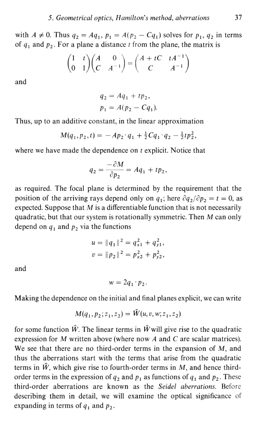
with A i= O. Thus q2 == Aql' PI == A(P2 - Cql) solves for PI' q2 in terms
of q I and P2' For a plane a distance t from the plane, the matrix is
( 1 t )( A 0 ) == ( A + tC tA- 1 )
o 1 C A-I C A- 1
and
q2 == Aqi + tp2,
PI == A(P2 - Cql)'
Thus, up to an additive constant, in the linear approximation
M(ql,P2,t) == -Ap2 'ql + !Cq1 'q2 - !tp ,
where we have made the dependence on t explicit. Notice that
-8M
q2 == 8 == Aqi + tp2,
P2
as required. The focal plane is determined by the requirement that the
position of the arriving rays depend only on q 1; here 8q2/8P2 == t == 0, as
expected. Suppose that M is a differentiable function that is not necessarily
quadratic, but that our system is rotationally symmetric. Then M can only
depend on q 1 and P2 via the functions
u == IIq111 2 == q;1 + q;1,
v == II P211 2 == P;2 + P;2,
and
W == 2q I . P2.
Making the dependence on the initial and final planes explicit, we can write
M(q1,P2;ZI,Z2) == W(u, v, W;ZI,Z2)
for some function W. The linear terms in Wwill give rise to the quadratic
expression for M written above (where now A and C are scalar matrices).
We see that there are no third-order terms in the expansion of M, and
thus the aberrations start with the terms that arise from the quadratic
terms in W, which give rise to fourth-order terms in M, and hence third-
order terms in the expression of q 2 and P 1 as functions of q 1 and P2' These
third-order aberrations are kno\vn as the Seidel aberrations. Before
describing thelll in detail, we will examine the optical significance of
expanding in terms of q 1 and P2 .
38
I. Introduction
o
Zl
Z2
Zo
Figure 5.1.
I
Zl
I
f
-
Z2
Figure 5.2.
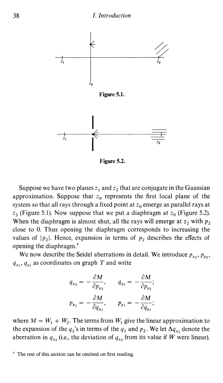
Suppose we have two planes z 1 and Z2 that are conjugate in the Gaussian
approximation. Suppose that Zo represents the first local plane of the
system so that all rays through a fixed point at Zo emerge as parallel rays at
Z2 (Figure 5.1). Now suppose that we put a diaphragm at Zo (Figure 5.2).
When the diaphragm is almost shut, all the rays will emerge at Z2 with P2
close to O. Thus opening the diaphragm corresponds to increasing the
values of I P21. Hence, expansion in terms of P2 describes the effects of
opening the diaphragm. t
We now describe the Seidel aberrations in detail. We introduce PX2' P y2 ,
qXl' qYl as coordinates on graph T and write
aM
qX2 = -a--'
PX2
aM
QY2 = -a--;
P Y2
aM
PXl = -a--'
Q X l
aM
P Y1 = -a--;
QYl
where M = W 1 + W 2 . The terms from W 1 give the linear approximation to
the expansion of the Q2'S in terms of the Q1 and P2' We let I1Q x 2 denote the
aberration in QX2 (i.e., the deviation of QX2 from its value if W were linear).
t The rest of this section can be omitted on first reading.
5. Geometrical optics, Hamilton's method, aberrations 39
Thus
oW 2
I1Q x 2 = -8'
PX2
so
( OW 2 OW 2 )
I1Qx2 = - 2 ow q X l + ----a;;- PX2 ,
( OW 2 OW 2 )
I1Pxl = - 2 -au QXl + ow PX2 ,
( OW 2 OW 2 )
I1qY2 = - 2 ow qYl + ----a;;- P Y2 ;
( OW 2 OW 2 )
I1P Y1 = - 2 --a;;- QYl + ow P Y2 .
The most general quadratic form in three variables depends on SIX
parameters. With a view to later interpretation let us set
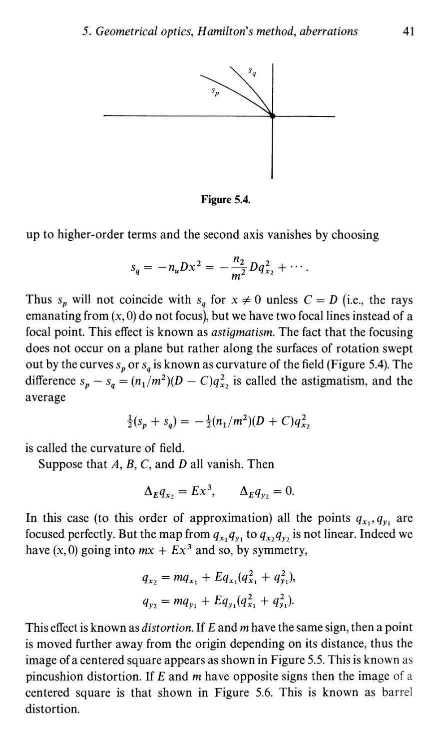
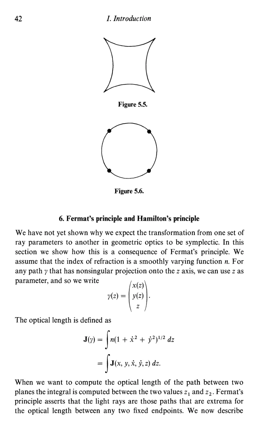
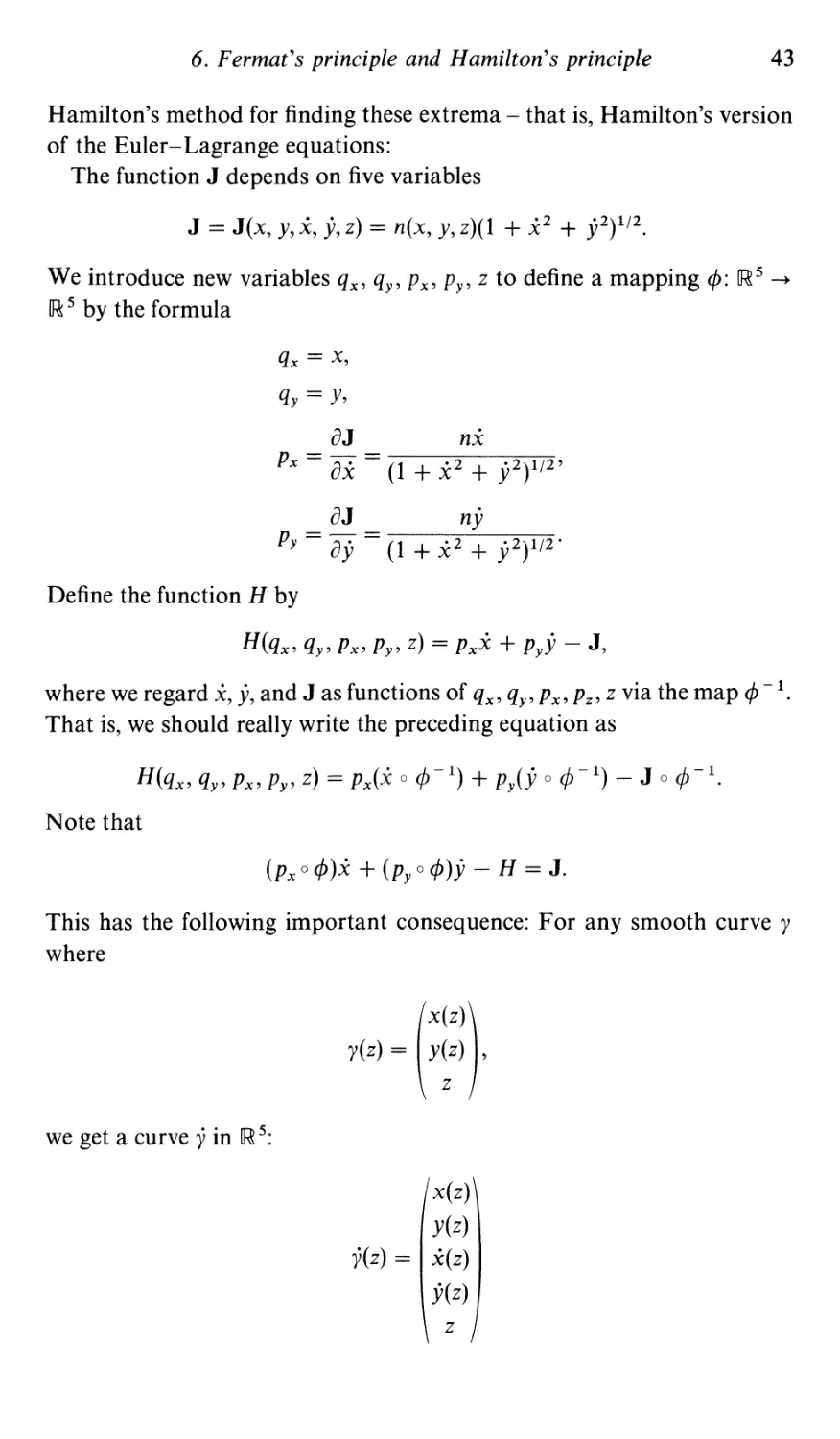
W 2 = - [iFu2 + iAv 2 + i(C - D)w 2 + !Duv + !Euw + iBvw].
Then our equations become
I1Qx2 = [Eu + tBv + !(C - D)W]Q x l + [A v + Du + tBW]P X 2;
I1QY2 = [Eu + tBv + !(C - D)W]QYl + [Av + Du + t B w]P y2 o
To investigate the meaning of these equations we consider incoming rays
with
QYl = 0,
and introduce polar coordinates
P X 2 = P cos qJ,
Q X l = X
P Y2 = p SIn qJ,
so that u = X2, V = p2, and w = 2x p cos qJ and we get
Qx2 = A p 3 COS qJ + t B p 2 (3 cos 2 qJ + sin 2 qJ)x + C(p cos qJ)x 2 + EX3.
I1QY2 = A p 3 sin qJ + Bp2 (sin qJ cos qJ)x + D(p sin qJ)X2
so that A, B, C, D, and E are the coefficients of terms involving increasing
powers of x. For x = 0 only the first term appears. This represents the fact
that the point is not perfectly focused, but is imaged on a disk of radius A p 3,
where p2 = P;2 + P;2 is determined, as we remarked above, by the opening
of the diaphragm. This is spherical aberration.
Suppose we have corrected for spherical aberration (or are willing to
ignore it), and let us consider the contribution of the second term. For fixed
p and x, the curve
I1 B Qx2 = tB p 2 X (3 cos 2 qJ + sin 2 qJ) = tB p 2 X (2 + cos 2qJ),
I1 B Q q2 = Bp2X sin qJ cos qJ = t Bp2X sin 2qJ
40
I. Introduction
Figure 5.3.
describes the circle of center == i Bp2X and radius == t Bp2X twice as qJ goes
from 0 to 2n. If we now put a ring diaphragm (i.e., one that stops all rays
except those passing through a circular ring) at the focal plane, then
rotational symmetry guarantees that the corresponding rays all have
P 2 + P;2 constant, and thus they image on one of the above circles. These
circles are illustrated in Figure 5.3: The effect is that rays emanating from x
form a plane like image reminiscent of a comet; hence, this aberration is
known as coma.
Suppose the system is corrected for spherical aberration and coma so
that A == B == 0, and let us consider the effects of C and D:
I1 c ,nq x 2 == Cx 2 P cos qJ;
I1 c ,nQY3 == DX2 p sin qJ.
We see that rays passing through the ring diaphragm form an ellipse on the
image plane. In order to understand this effect, note what happens if we try
to improve the focus by moving the plane z == Z 1 by an amount s. Thus we
wish to consider M Z1 ,Z2 +S' We assume that n 2 is constant. Then the ray given
by (x, 0; PX2' P y2 ) will intersect the plane z == Z2 + s at x 2 (s), Y2(S), where
x 2 (s) == X 2 + S P X 2 == mx + ( C + ) p cos qJ,
n 2 n2
Y2(S) == Y2 + S P Y2 == ( DX 2 + ) p sin qJ,
n 2 n 2
thus describing an ellipse about mx with axes
S
Cx 2 + -
n2
and
S
DX2 + -.
n 2
We can make the first axis vanish by choosing
2 n 2 2
Sp == -n 2 Cx == - CQx2
m
5. Geometrical optics, H ami/ton's method, aberrations 41
Figure 5.4.
up to higher-order terms and the second axis vanishes by choosing
S - n DX 2 - n2 D q 2 + ...
q - - u - - X2 .
m
Thus sp will not coincide with Sq for x =I=- 0 unless C = D (i.e., the rays
emanating from (x, 0) do not focus), but we have two focal lines instead of a
focal point. This effect is known as astigmatism. The fact that the focusing
does not occur on a plane but rather along the surfaces of rotation swept
out by the curves sp or Sq is known as curvature of the field (Figure 5.4). The
difference sp - Sq = (n 1 /m 2 )(D - C)q 2 is called the astigmatism, and the
average
!(Sp + Sq) = - !(nl/m2)(D + C)q 2
is called the curvature of field.
Suppose that A, B, C, and D all vanish. Then
d E q x 2 = Ex3,
d E qY2 = o.
In this case (to this order of approximation) all the points q X l' qYl are
focused perfectly. But the map from q X l qYl to Q X 2qY2 is not linear. Indeed we
have (x, 0) going into mx + Ex 3 and so, by symmetry,
QX2 = mQxl + EQxl(Q l + Q;J,
QY2 = mQYl + EqYl (Q l + Q;J.
This effect is known as distortion. If E and m have the same sign, then a point
is moved further away from the origin depending on its distance, thus the
image of a centered square appears as shown in Figure 5.5. This is known as
pincushion distortion. If E and m have opposite signs then the image of a
centered square is that shown in Figure 5.6. This is known as barrel
distortion.
42
I. Introduction
Figure 5.5.
Figure 5.6.
6. Fermat's principle and Hamilton's principle
We have not yet shown why we expect the transformation from one set of
ray parameters to another in geometric optics to be symplectic. In this
section we show how this is a consequence of Fermat's principle. We
assume that the index of refraction is a smoothly varying function n. For
any path y that has nonsingular projection onto the z axis, we can use z as
parameter, and so we write
x(z)
y(z) = y(z) .
z
The optical length is defined as
J(y) = f n(l + x 2 + y2)1/2 dz
= f J(x, y, X, y, z) dz.
When we want to compute the optical length of the path between two
planes the integral is computed between the two values Zl and Z2' Fermat's
principle asserts that the light rays are those paths that are extrema for
the optical length between any two fixed endpoints. We now describe
6. Fermat's principle and Hamilton's principle
43
Hamilton's method for finding these extrema - that is, Hamilton's version
of the Euler-Lagrange equations:
The function J depends on five variables
J = J(x, y, X, y, z) = n{x, y, z){l + x 2 + y2)1/2.
We introduce new variables qx, qy, Px, Py, z to define a mapping <jJ: IR5 -+
IR 5 by the formula
qx = x,
qy = y,
8J nx
Px = 8x = {I + x 2 + y2)1/2'
8J ny
Py = 8y = (1 + x 2 + y2)1/2'
Define the function H by
H(qx, qy, Px, Py, z) = Pxx + Pyy - J,
where we regard X, y, and J as functions of qx, qy, Px, pz, z via the map <jJ -1.
That is, we should really write the preceding equation as
H(qx, qy, Px, Py, z) = Px{x 0 cjJ-l) + Py{y 0 cjJ-l) - J 0 cjJ-l.
Note that
(Px o <jJ)x + (pyo <jJ)y - H = J.
This has the following important consequence: For any smooth curve y
where
x{z)
y(z) = y(z) ,
z
we get a curve y in IR 5:
x(z)
y(z)
y(z) = x(z)
y(z)
z
44
I. Introduction
and, hence, a smooth curve
y = cp 0 y
in IR 5 .
Now y*dqx = x dz and y*dqy = Y dz, so
Y*(Pxdqx + pydqy - H dz) = J(y(z») dz.
In other words, if we define the form 0 on IR 5 by
o = Pxdqx + pydqy - H dz,
we see that
J(y) = fye,
Consider the form
dO = dpx /\ dqx + dpy /\ dqy - dH /\ dz
on IR 5. This form is closed and clearly has rank 4. It therefore defines at each
point of IR 5 a one-dimensional subspace spanned by those vectors 11 that
sa tisfy
i(I1) dO = O.
If we choose Yf of the form Yf = ojoz + A(ojoqx) + B(ojoqy) + C(ojopx) +
D(ojopy), then
;(17) de = ( c + ; )dqx + (D + :: )d q y
- ( A - 8H ) d P z - ( B _ 8H ) d P Y
8px 8py
( 8H 8H oH 8H )
- +A-+B-+C-+D- dz.
8qx 8qy 8px 8py
In other words, a curve v in IR 5 given by
qx(z)
qy(z)
v(z) = Px(z)
py(z)
z
6. Fermat's principle and Hamilton's principle
45
will be everywhere tangent to the lines defined by i(,.,) dO = 0 if and only if
dqx 8H
-
dz 8px ,
dqy 8H
-
dz 8py ,
dpx 8H
- --
dz 8qx ,
dpy 8H
--
dz oqy
(6.1 )
(6.2)
(6.3)
(6.4)
Now oHjopx = X, and thus the first of these equations implies that cp-Iv
satisfies
dx(cp -IV) .
=x
dz
and, similarly,
d y( cp - 1 v) .
dz = y.
Thus Equations (6.1) and (6.2) imply that there exists a curve y such that
.....
V = y.
It is a standard theorem in the calculus of variations (Loomis and
Sternberg, 1968, p. 535) that y is an extremal for J(y) if and only if y satis-
fies these equations. Thus
y is an extremal of optical length if and only if y satisfies
i(y') dO = O.
Now we can consider the space of all curves satisfying this equation. This
space is a four-dimensional manifold M, and we put local coordinates on M
by choosing (locally) some four-dimensional surface S transversal to these
curves and using local coordinates on S (Figure 6.1). The restriction of dO to
S is closed and nondegenerate. Let us denote it by W s . Suppose we had two
such surfaces SI and S2 that meet the same curves. Then we get a map T
from Sl to S2 by simply following the curves from one surface to the second,
as shown in Figure 6.2. We claim that T*w S2 = WSt' Indeed, consider any
46
I. Introduction
//
.--/ /'
s
Figure 6.1.
Sl
Figure 6.2.
Figure 6.3.
small region R in Sl and its image, TR on S2, and let D denote the domain
in IR 5 swept out by the curves from R to TR C S2.
The boundary of D consists of TR, R, and the curves joining aR to aTR
(Figure 6.3). The restriction of dO to the portion of the boundary containing
the curves must vanish, since these curves are all tangent to i(,.,) dO = O.
Thus
f d(dO) = f dO - f dO.
J D TR R
7. Interference and diffraction
47
But d(dO) = 0, so
f OJS2 = f OJSl
TR R
for all regions R and hence
T*OJ sz = OJ S1 '
In particular, if we take 8 1 to be the surface given by z = Z 1, then
OJ s 1 = dpx /\ dqx + dpy /\ dqy
on S l' This proves our assertion that the map T of optics is symplectic.
Notice that the right way of organizing these facts is to say that the
manifold M of all light rays carries a natural symplectic structure. The
choice of a transversal plane to the optical axis gives us a way of choosing
a surface 8 in !R 5 transversal to the curves and gives local coordinates on M
relative to which the symplectic form takes the expression
OJ = dpx /\ dqx + dpy /\ dqy.
The fact that the optical transformation is symplectic is simply the assertion
that symplectic forms on M have the above expression in terms of these
local coordinates.
7. Interference and diffraction
We have already briefly mentioned the Young interference experiment,
performed circa 1800. Light from a distant source, not shown in Figure 7.1,
passes through a slit S then through two narrow slits Sl and S2 parallel to S
and equidistant from it and then falls on a screen. A series of alternating
51
s
52
Figure 7.1.
48
I. Introduction
A
Figure 7.2.
bright and dark bands appears on the screen (Figure 1.2), with a bright
band at the center. If either of the slits 8 1 or 8 2 is covered so that light passes
through only one slit, the dark lines disappear and a diffuse broad band
replaces the alternating bands. If we use white light, the effect is somewhat
fuzzy; but if we use light of a definite color, it becomes much more sharp.
For example, we might separate the white light by a prism to the left of 8
and only allow one component color to pass through S. Then the bright
lines are very sharp, and the bright positions on the screen have the
following very interesting characterization: For any point A on the central
vertical line of the screen, if Y A is the closed path going from S to S1 to A to
S2 back to 8 along straight line segments (Figure 7.2), and we let L(y A)
denote the optical length of this path, then there is a length A whose value
depends on the color of the light such that A is a bright position if and only
if L(y A) = nA, n E 7L. Young realized that this experiment shows that, asso-
ciated with each color of light, there is an intrinsic length A - the wavelength
of the light. Newton had concluded from his famous experiments with
prisms in 1666 that color was an intrinsic property of light: Once we
separate white light into rays of different colors, each ray retains its color
under further refraction or reflection. Newton observed that such rays have
their own characteristic angle of refraction in a glass prism (corresponding
to the fact that the index of refraction of the glass depends on the color of
the light). Thus the subjective notion of color could be correlated with a
numerically measurable quantity - an angle of refraction. However, this
angle depends also on the material used; experimenters using different
kinds of glass would get different angles for the same kind of light. Young's
experiment furnished a measurable property of the light itself, independent
of the material of the prism. In the Philosophical Transactions for 1802
Young refers to his discovery of a "simple and general law." The law is that
7. Interference and diffraction
49
wherever two portions of the same light arrive at the eye by different routes, either
exactly or very nearly in the same direction, the light becomes most intense where
the difference of the routes is a multiple of a certain length and least intense in the
intermediate state of the interfering portions; and this length is different for light of
different colours.
Fresnel suggested that the integrality condition be written in the form
exp [2ni(lj A)L(y A)] = 1
and be explained as follows t: Associated with each point on the light rays of
geometrical optics is a complex number c. As the light propagates along the
ray, not only does the amplitude Icl decrease due to the attenuation of the
light, but the phase changes. As we move along the ray a distance of optical
length 1, the change in phase is given by multiplication by the factor
exp(2nilj A), where A is the wavelength of the light. If light arrives at some
point Q from various rays we add the c's for each ray to obtain a total value
C, and the intensity I of the light is proportional to I C1 2 . This is Fresnel's
explanation of the Young interference experiment: For any point A on the
screen, let Ci be the contribution coming from the SSiA path, i = 1, 2. The
two complex numbers C 1 and C2 will have the same phase precisely when the
integrality condition is satisfied, and so the two contributions will reinforce
each other. In fact, as long as the two optical lengths do not differ by very
much, there will not be much difference in the attenuation of the light along
the different paths, and the intensity at any point A will be given roughly by
I = Icl 2 1 {exp [2ni(L(y A)j A)] + I} 1 2 ,
which accounts for interference bands.
Let us formulate Fresnel's ideas in more mathematical terms. Suppose
that z 1 and Z2 are two nonconjugate planes. Thus, for every pair of points
(q l' q2) there is a unique light ray that joins them and whose optical length
is given by a well-determined function L(Ql,q2)' Suppose that we know
the light distribution C 1 (Ql) at every point in the Zl plane. Our problem is
to determine the light distribution c 2 ( . ) on the z 2 plane. Our optical data
are now functions (instead of ray parameters), and the optical system is
determined by a transformation on functions instead of a symplectic trans-
formation as is the case in geometrical optics. Now let Q 2 be a point in the
t We are, for the moment, oversimplifying Fresnel's explanation in that we are ignoring the
phenomenon of polarization. We shall come back to this later on. The polarization effect
also has to do with Young's requirement that the light arriving via different routes comes in
at "nearly the same direction."
50
I. Introduction
Z2 plane. As the light propagates from ql to q2 it will undergo both a phase
change and attenuation, so that when it arrives at q 2 it will contribute the
term
a(ql, q2, A) exp [2niL(ql' q2)/ A]C 1 (ql)
to the total expression for the light at q2, where L is the optical length of the
path and a(L) is the attenuation factor along the optical path. To find the
light at q2 we must integrate this expression over ql to get the total of all
the contributions. Of course, to do this we must know the function a.
We now propose to employ Fresnel's ideas, but in the linear approxi-
mation. In terms of the diagram of theories of Figure 1.4, we are adding
an "intermediate" theory, one which takes account of interference and
diffraction, but not geometric aberration (and, temporarily, ignores
polarization). For lack of a better name, let us call this approximate theory
"Fresnel optics." In Fresnel optics we will be able to determine the value of
a (up to a sign) from the knowledge of L. This is true for the following
reasons:
(i) We are in a situation where linear optics is valid. This is so because we
know, for one reason or another (for instance by the presence of stops or
diaphragms in the apparatus), that C 1 (ql) essentially vanishes for large
values of ql and Q2' We assume that a is a relatively slowly varying function.
Hence, we may assume that a is a constant and move it to the left of the
integration sign.
Thus our formula for C2 is
C 2 (q2) = a f c 1 (ql) exp [2niL(ql' q2)/ A] dql>
where a is a constant, as yet undetermined but L is a known (quadratic)
function of ql and q2. The intensity at the point q2 is given by
1 2 (q2) = I C 2(q2)1 2
and the intensity at q 1 is given by
1 1 (ql) = Ic 1 (ql)1 2 .
(ii) We assume that the total intensity of the light on the Z2 plane is the
same as the total intensity of the light on the z 1 plane; that is:
f1C2(q2W dq2 = f IC1 (QlW dQl'
8. Gaussian integrals
51
If this is possible at all (and we shall see that it is), it will determine lal, so
that a will be determined up to a phase factor.
(iii) The "constant" a will depend on the wavelength A. Assume (in partial
contradiction to condition (i)) that our diaphragm openings are large in
comparison to A and that we are located at a (vertical) distance of many
wavelengths from the boundaries of any of the stops or diaphragms. Then
we would expect that the phase of the arriving light should be the same as if
the stops were not present. For example, suppose we have no lenses or other
apparatus but simply place a half-plane opaque screen to block out the
incoming light. We would expect that high above the screen the light should
behave as if the screen were not present. This will allow us to determine the
phase of a.
In order to work out the details we will need some facts about integrals of
quadratic exponentials, so we digress slightly in the next section to develop
these basic results.
8. Gaussian integrals
Everything in this section stems from the basic fact that
1 f oo
e -x 2 /2 dx = 1.
)be - 00
Now
This is proved by taking the square of the left-hand side:
( 1 f oo e-x2/2 dX ) 2 = f oo f ro e-(x2+y2)/2 dx dy
)be -00 2n -00 -00
= f 21t f 00 e -r 2 /2 r dr de
2n 0 - 00
= tro e- r2 / 2 r dr = 1.
1 f 00 e -x 2 /2 -71 X dx
)be - 00
converges for all complex values of 1] and uniformly in any compact region.
Hence, it defines an analytic function that may be evaluated by taking 1] to
be real and then using analytic continuation. For real 1], we simply complete
52
1. Introduction
the square and make a change of variables:
f exp( -x 2 /2 - xl1) dx = f exp [ -(x + I1f/2 + 11 2 /2] dx
= exp (11 2 /2) f exp [ - (x + 11)2/ 2 ] dx
= etf2/2.
This is true for all complex values of Yf. In particular, taking Yf = i(, we get
f exp( x2/2 - i(x) dx = exp( - e/2).
In other words, the Fourier transform of exp( -x2/2) is exp( -(2/2). Now
set x = J2u, where J2 > 0 is some positive real number. Then dx = J2 du
and setting == ( we get
1 f - Au 2 /2 - i u d _ - 2/2A
Fe e e u- fJe .
v 2n vA
Now this last integral converges for any)" with Re)" > 0 and A -# O. Indeed,
for S > R > 0
I s e-).x2/2e-i x dx = - I s ;- (e-Ax2/2)e-i X dx
R R )"X dx
- A R 2/2 - i R - AS 2/2 - i s I s d ( i X )
e e e e _ Ax 2 /2 e
R - S + e - d -;- dx.
)" )" R X /LX
In this last integral we can write
e- AX2 / 2 = _ e-).x2/2
Ax dx
and integrate by parts once again. We thus see that
I s e-Ax2/2e-i Xdx = O ( ) .
R lAIR
We thus see that
f e-h2/2e-i x dx
8. Gaussian integrals
53
. A
. At
· xt
. A
Figure 8.1.
converges uniformly (but not absolutely) for A in any region of the form
Re A > 0
IAI > b
any b > O.
By analytic continuation, its value is given by the same formula as for A real
and positive, where the square root must now be taken to be the analytic
continuation of the positive square root (Figure 8.1). In particular, if we set
A = - ir, r > 0, then
A 1/2 = IAI1/2 e- 1ti/4
and
fi f eirx2/2e-i x dx = e1[i/4r-1/2e-i 2/2r
and, similarly with A = ir,
fi f e - irx 2 /2 e - i x dx = e - 1[ i /4r -1/2 ei 2/2r.
Now take
x=
to be a vector variable and let
Q=
+ rl 0
o + rn
be an n x n matrix with all the r i > 0 and sgn Q = number of + 's minus
number of - 's. Then Ir 1 1.. .Irnl = Idet QI, and by multiplying the formulas
54
I. Introduction
for the one-dimensional integrals, we get
(2:t/ Z f exp GQX . x) exp ( - i ' x) dx = Iclet QI- 1 / Z exp ( i sgn Q )
x ex p ( _ Q-l . ),
where now is also a vector and Q-l is the inverse matrix. We have proved
this for diagonal Q. But given any nonsingular symmetric matrix Q, we can
find an orthogonal matrix 0 such that OQO - 1 is diagonal. This proves that
the above formula is true for all such Q. This is the formula we need for
Fresnel optics.
9. Examples in Fresnel optics
In this section we work out some examples of Fresnel's formula, and
propose how to determine the constant a that occurs in it. We will then
justify this choice in the succeeding sections. From a mathematical point of
view it is a bit easier to work out the integrals first in one dimension; that is,
to first do Fresnel optics with linear optics replaced by Gaussian optics. The
mathematics is a bit simpler but some care is needed in the physical
interpretation. For instance, we will want to talk of a one-dimensional
diaphragm that blocks out all light except that arriving at - h < q < h, as
in Figure 9.1a. Physically, this corresponds to a slit like that shown in
Figure 9.1b. In Gauss-Fresnel optics the intensity of light at q2 on the Z2
"plane" is given by
I(q2) == Ic 2 (q2)1 2 ,
where
cz(qz) = a f c1(qd exp [2niL (ql, qz)/ A] dql
with
L = W + L axis
and
W(Ql,q2) = (lj2B)(Aqi + Dq - 2Q1Q2),
where a is an overall constant describing the attenuation of the system, and
where ( ) is the optical matrix.
9. Examples in Fresnel optics
55
h
t
"-
"
"
h
-h
(a) (b)
Figure 9.1.
=j
F}=z} H 2 F 2 =Z2
Figure 9.2.
Let us now work out the integral in a number of simple cases. Suppose
that z 1 and z 2 are the focal planes of the lens system, so that A = D = 0 and
B = j' is the focal length. (This special case is known as Fraunhofer
diffraction.) Let us assume, first of all, that light arrives from a distant
source located on the optical axis, so that the light rays are all parallel to the
axis, and that the arriving light all has the same c value near the axis. We
place an opaque screen at z 1 with a slit of width 2h centered on the axis
(Figure 9.2), allowing some of the light to pass through. Thus, C 1 (q 1) = c
for - h < q1 < h, where c is a constant, and C 1 (q1) = 0 for Iq11 > h. Geo-
metrical optics predicts that all the light will be focused at q2 = O. Let
us see what Fresnel's formula gives. The integral becomes
C 2 (q2) = ac fh exp( -2niqlQ2/f).,) dql
= 2ach [ sin (2nq2h/fA) ]
2nq2 h /fA
56
I. Introduction
[ Si 0 J
e
Figure 9.3.
so that
I(q2) = Ic 2 (Q2)1 2
_ 2 h 2 2 [ sin(2nh Q 2 If A) ] 2
- 4a lei 2nhqz/fA
Now lim o _ o [sin 010] = 1 and limo_oo [sin 010] = 0, and, in fact, the graph
of the function [sin 0/ OJ 2 looks something like Figure 9.3. The total
intensity of the light arriving at the Z2 plane is given by J I(Q2) dQ2'
Substituting the above formula for I(Q2) gives, by the change-of-variables
formula for an integral.
f I(qz) dqz = (4a Z h Z lel z lfAI/2nh)J,
where
J = f:ro [ Si; O J dO = n;
so the total light intensity arriving at the Z2 plane is 2a 2 hlcl 2 lfAI. The total
light intensity passing through the screen at Z 1 is 2h I c 1 2 . We expect that the
total light leaving the Zi plane will arrive somewhere on the Z2 plane, which
then tells us that the factor a must have its absolute value given by
lal = IfAI- i / 2 .
(More generally, a similar computation, which will be presented later will
show that
lal = IBAI- i / 2
for the one-dimensional case and
'a' = Idet ABI- i / 2 = A -ildet BI- i / 2
9. Examples in Fresnel optics
57
Figure 9.4.
for the two-dimensional, linear-optics case, where ( ) is the optical
matrix of the system.)
If we substitute this value of lal into the expression we obtained above for
I(q2) we get
I(qz) = (4h Z /lfAl)lcl z [ sin2 : j[A) J ·
We see that the light is not all focused at the point q2 = 0, but is spread over
a spot centered at q2 = O. The intensity falls off to its first zero at q2 =
+ (fA/2h). Since the intensity falls off quadratically with q2, most of the
light will be concentrated between the zeros nearest the origin, and we can
use If AI/ h as a measure of the lack of focusing due to diffraction. For fixed f
and h, the spot becomes narrower as A O. In this sense, Gaussian optics is
the "short-wavelength limit" of wave optics. Of course, in optics we cannot
pass to this limit without going out of the range of visible light. For A and f
fixed, the spot becomes narrower as we enlarge h. If we wish to reduce the
effects of diffraction, it is in our interest to make h large. However, for large
values of h, the Gaussian approximation will, in general, no longer be valid,
and one encounters a lack of focusing due to geometrical aberrations. Thus,
in a sense, the aberration effects and the diffraction effects are working
against each other. One of the main problems in the design of optical
instruments is to try to arrange matters so that the next-order terms beyond
the Gaussian approximation, the third-order aberrations, vanish, in which
case we can allow h to be large enough to minimize the effects of diffraction.
Now let us see how the above computation changes when we replace the
distant on-axis source by a distant source off the optical axis. (We still
assume A = D = 0, B = f, and a centered slit of width 2h at the first focal
plane.) Assume that the light arrives at q 1 = 0 with a value c = c(O). The
light arriving at some other value of ql will have traveled an additional
distance 1 = ql sin (), where () = Pl/nl or 1 = qlPl/nl (see Figure 9.4). The
58
I. Introduction
optical length of the additional path is nIl = qIPI, and, hence, the light will
arrive at the point qi on the ZI plane with the value
c(qt) = exp(2niqIpI/ A ) c(O)
= exp(2niqIpI/A) C
That means that
Cp,(qz) = C f exp (2niqlpd A) exp ( - 2niql qz/jA) dq 1
= C fex P [ -2niql(qz - jPl)/jA] dql'
If C O (Q2) denotes the value computed above for PI = 0, we can write this last
equation as
CPl (q2) = CO(q2 - fpI)'
The spot of light is now centered at the point fpI in the Z2 plane, which is
precisely the point where all the incoming lines would be focused according
to geometrical optics. Thus the shift in phase of the arriving light at Z 1 is
translated into a shift of the image point at z 2' Let us now turn to a famous
example of a two-dimensional diffraction integral, where we take lal =
A -Ildet BI-1/2. We consider the case where there are no lenses at all in the
optical system, so that the optical matrix is given by ( d:), where d is the
distance traversed. Thus
Cz(qxz, qyz) = a f C 1 (qxl, qYl) exp {2ni[(qxz - qXl)Z
+ (qY2 - qYI)2]/2dA} dqxI dqyI
where
'a' = IAdl- l .
Let us evaluate this integral for the following situation: Light parallel to the
optical axis arrives at a plane at which there is a circular opaque disk
perpendicular to the axis, with its center on the axis (Figure 9.5). Thus
C I = 0 inside the circle and C I = C is constant outside the circle. We shall
take qx2 = qy2 = 0 so that we are positioned on the axis. We write x for
9. Examples in Fresnel optics
59
q 1 plane
q 2 plane
Figure 9.5.
Qx1 and y for Qy1 and R for the radius of the disk. The above integral
becomes c times
(Ad)-l [00 exp [2ni(x 2 + y2)/2dA.] dx dy
J x 2 + y2 > R 2
f 00 f 21t
= lim (Ad) -1 exp [2n(i - c:)r 2 j2dA] r dr de
£-1-0 R 0
2n f oo
= lim ' d exp [2n(i - c:)r 2 j2dA] r dr
£-1-0/L R
= lim [00 exp [(i - /;)s2/2] s ds,
£-1-0 Jb
_ ( 2n ) 1/2
b - dA R
= _e ib2 / 2 .
Thus
1 2 (0,0) = lel 2 .
The intensity of the light along the axis is the same as if the disk were not
present! There is a white spot in the shadow of a circular disk. (Of course
this is valid where the linear approximation is valid. So the disk can't be too
large in comparison to the distance d.)
Fresnel presented his memoir on diffraction for the prize of the French
Academy in 1818. Poisson, Biot, and Laplace were on the committee to
judge the paper, and all three were supporters of the corpuscular theory of
light. Fresnel had calculated various cases of his formula and compared
them with experiment. But Poisson noticed that one could calculate the
integral for a circular disk, and come to the conclusion that there is a white
spot in the center of the shadow of a circular disk. He raised this as an
objection to the whole theory, since it was patently ridiculous. However.
60
I. Introduction
Arago and Fresnel went and performed the experiment, and, sure enough
the spot was there, whereupon Fresnel was awarded the prize. This
phenomenon is now known as the "Poisson spot."
10. The phase factor
We now turn to the problem of determining the correct phase factor in the
constant a, whose absolute value we have already determined. We thus
wri te
a = ulal,
where u is some number of absolute value 1 that must be determined, and
lal = A -lldet BI- 1 / 2
in two-dimensional linear optics, and
a = (AB)-1/2
in the one-dimensional Gaussian situation. The principle that we shall use
to determine u is that if we are at a distance of many wavelengths (i.e.,
multiples of A) vertically distant from any stops or diaphragms in our
apparatus, the light should behave approximately as if these stops are not
present. For simplicity we argue in the Gaussian case. Suppose that we are
in an optical situation with no lenses at all; simply put an opaque screen at
Z I that blocks out all the light arriving with q 1 < 0, and examine the light
which arrives at z 2' which is a distance d from Z I (Figure 10.1). Let us
assume that the arriving light comes from a distant on-axis point and so
arrives with PI = 0 and with constant phase. Thus
C(ql) = c
=0
for
for
ql 0
ql < 0
and the optical matrix is ( ), so that
W(ql' q2) = (1/2d)(qi + q - 2qlq2)
= (1/2d)(q I - q2)2.
We get
C(q2) = uc(d2) -1/2 LX> exp [ni(q2 - qlf/ Ad] dq 1
= uccjJ(q2/(Ad)1/2),
10. The phase factor
61
Figure 10.1.
en 1/4
Figure 10.2.
where cp is the function defined by the integral
cp(w) = f oo exp [ni(w - r)2] dr = f oo exp(nit2) dt.
o -w
These integrals are known as Fresnel integrals and have been tabulated; cp
behaves as in Figure 10.2.
We have already proved, in our section on Gaussian integrals, that
lim cp( w) = e1ti/4.
w oo
For large negative values of w the value of the integral is practically zero. A.s
w approaches 0 from - 00, it spirals outward from 0 gradually widening its
62
I. Introduction
1.7
1
0.78
(a)
(b)
Figure 10.3. Illumination near the geometric shadow of the edge of a screen and the
observed diffraction figure.
swing until at w = 0 it moves over to swing about the point e Tti / 4 in a
gradually diminishing spiral as w goes to + 00. (These spirals are known
as the Cornu spirals.) We see (Figure 10.3) that there will be some illumi-
nation in the geometrical shadow, and for sufficiently large values of q2
the light arriving at the 22 plane will have the same intensity as the light
passing the 2 1 planes; in other words, the effect of the opaque screen can be
ignored.
We would expect for large enough q2 that the phase of the arriving light
should also be unaffected by the lower half screen at z l' If the screen were
not present, the light arriving at 22 would have the value exp (2nidj ;t)c for
all values of q2' The evaluation of the Fresnel integral as e Tti / 4 for large w
gives the value ueTti/4C for the light arriving at large values of q2' How do we
alter the integral formula for the diffracted light to make these two values
agree? The first obvious step is to use the correct arbitrary constant in the
eikonal. The optical length between q 1 at 2 1 and q 2 at z 2 is
[d 2 + (q2 - ql)2]1/2 d + (lj2d)(q2 - ql)2.
10. The phase factor
63
q2
ql
d
Zl
Z2
Figure 10.4.
(See Figure 10.4). We should use the formula
L( q l' q 2) = d + (1/ 2d)( q 2 - q 1 )2
instead of our previous expression, which did not have the d in it. Including
the d will modify the earlier computation by multiplying it by an overall
factor of e2Ttid/A. With this corrected value of L our integral formula now
gives ueTti/4e2Ttid/Ac for the light which arrives at large values of q2' We are
still off by the factor e Tti / 4 , which is independent of A, d, or anything else in
the problem. There isn't much we can do about it at this stage other than to
compensate for it in our integral formula: Choose u = e -Tti/4. Thus the
general formula now reads
e -1ti/4IBAI- 1 / 2 f c(q 1) exp [2niL(q1' q2)/ A] dq l'
where L(ql' q2) is the optical length of the light ray joining ql to q2' The
phase factor e -Tti/4 occurring in front of the integral certainly looks ad hoc
and mysterious. It caused a great deal of resistance, at first, to the
acceptance of Fresnel's ideas. [Some 30 years after Fresnel proposed his
formula Helmholtz showed that this factor is a consequence of the wave
equation and an integral formula in vector calculus known today as Stokes'
theorem (see Guillemin-Sternberg (1977), Chapter I for a modern presen-
tation of Helmholtz's argument).] The formula as written is still not quite
right; it is only valid for positive values of B. When B is negative the correct
phase factor is e + Tti/4. (We could have expected this had we interchanged the
role of z 1 and Z2 in the preceding discussion.) The correct formula for the
diffracted light is thus given by
exp( + ni/4)IBAI- 1 / 2 f c (qd ex P[2niL(q1,q2)/A] dqb
where L(Ql' Q2) is the optical length of the light ray joining Ql to Q2 and
where + refers to the sign of B.
64
I. Introduction
Before giving further illustrations and applications of Fresnel's formula,
we should discuss here the nature of this formula and the relation between
Fresnel's wave optics and Gaussian optics. In Gaussian optics each optical
system is described by a matrix that gives the relation between the incoming
and outgoing light rays. In Fresnel optics the same optical system is
described by an integral transform relating the entire incoming light
distribution to the outgoing light distribution:
matrix
Wave optics
(in the Gaussian approximation)
integral transform
Gaussian optics
M = ( )
( ql ) M ( ql ) = ( Aql + BP1 )
Pl Pl Cql + Dpl
F
C l C2 = FC l
(Fe 1)(qZ) = exp( + ni/4) IBAI- I/Z f c 1 (q 1)
x exp [2niL(ql' q2)/ l]dql'
where
1 2 2
L(ql, q2) = -(Aql + Dq2 - 2qlq2) + d
2B
The explicit formula for F given in the last line is only valid when B #- O.
Although we expect that the operator F from functions to functions be
defined for all optical systems, it need not be given by a smooth integral
kernel. For example, if the planes z 1 and Z2 coincide so that we are dealing
with a "trivial" optical system, then M = ( ) is the identity matrix and
F is the identity operator. The identity operator is a perfectly nice operator,
but it cannot be represented by a smooth integral kernel. (Its integral kernel
is £5(x - y), that is, f(x) = Sf(y)£5(x - y) dy.) To see that we are on the right
track, let us examine what happens to the transformation formula for free-
space transmission (no lenses) as the optical distance approaches O. Thus for
d>O
(FdC){X) = exp ( - nij4) Idll- 1/2 f c{y) exp [{2nij2dl){x - y)2] dy.
We claim that
lim Fdc = C.
d O+
10. The phase factor
65
To prove this we shall make use of several facts from the theory of Fourier
transforms.
(i) Let f be a smooth function that vanishes rapidly at infinity together
with its derivatives; that is,
C
If(ft)(x)! 1 + Ixl k '
for each k and n, where C depends on k, n, and f. Its Fourier transform f is
defined by
( 1 ) 1/2 f oo
(fff)( () = 2n _ 00 e - i Xf(x) dx.
The Fourier inversion formula says that
( 1 ) 1/2 f oo
f(x) == - e+i X(fff)( ) d
2n - 00
so that
ff(!#'J)(x) == f( - x)
and
ff4f == f.
(ii) The Fourier transform carries convolution into multiplication. Let
cp * f be defined by
( 1 ) 1/2 f oo
<J> * f(x) = 2n 00 <J>(x - y)f(y) dy
for functions cp and f. Then
(cp* f) == ( <p)( f).
We can write this equation as follows: Let Cc/J denote the operator of
convolution by cp so that cc/J(f) == cp * f. Let M", denote the operator of
multiplication by t/J so that
M",g = t/Jg.
Then setting f = -1g and t/J = cp we see that
Cc/J -1 = M:i'c/J'
(iii) The Fourier transform of
1 _ x 2 /2t
-e
Jt
66
I. Introduction
IS
- t 2/2
e
for any t with Re t > O. The square root in this formula is chosen to be
positive for real positive t and analytically continued for Re t O. In
particular, letting t approach the point iP on the positive imaginary axis we
see that the Fourier transform of (1/ltI 1 / 2 )exp(-x 2 /2t) approaches
exp( +ni/4) exp( -iP 2/2). Thus
ff (ld21- 1/2 exp [(2ni/d2)x 2 /2]) = exp (ni/4) exp ( - i 2 /2 ).
Now Fd is convolution with
exp ( - ni/4) IdAI- 1 / 2 exp [(2ni/dA)x 2 /2]
and, hence, the Fourier transform of Fdc is given by
ff(FdC)( ) = ex p ( -i 2/2 }ffC)( ).
It is clear that as d 0, G;(Fdc) g;c, and hence, by the Fourier inversion
formula,
Fdc c.
Note that the correct phase factor, in particular the e:t1ti/4, plays a crucial
role in this computation.
Having emphasized the importance of the role of the phase factors e:t1ti/4,
we now point out that these very factors show that the preceding
description can't be 100 percent correct. Indeed, if F 21 is the Fresnel
transform between the planes Z1 and Z2 and F 32 the transform between the
planes Z2 and Z3, then we want F 31 = F 32 0 F 21 to be the transform between
the planes z 1 and Z 3' Now the expression for L in the formula for F has a
quadratic term and a constant term. The constant terms come out of the
integral and behave nicely under composition:
d 31 = d 21 + d 32
d 31
I
-I
d 21
d 32
so
exp (2nid 31 / A) = exp (2nid 21 / A) exp (2nid 32 / A).
We can ignore the constant term in L if we want to check whether or not
F 32 0 F 21 = F 31 .
10. The phase factor
67
Thus we may replace L by
1 22
W(Ql, Q2) = 2B (Aq 1 + Dq2 - 2ql q2)
and write U for the corresponding opera tor.
Now let us consider five points Z l' Z 2' Z 3' Z4, Z s.
.
Zl
.
Z2
.
.
Z4
.
Zs
-
-3
Let's assume the same optical matrix ( 1 ) applies between each
successive pair of points. Then
U 21 = U 32 = U 43 = U S4 = V,
where
U c(x) = e -"i/41 AI- i / 2 f e - 2"ix Y /A C (Y) dy
or, scaling the lengths so that A = 2n
Uc(r) = e-"i/4 1 f e-iXYc(y) dy
Jb;
so that the operator U is just the Fourier transform, multiplied by e -n:i/4
U = e-n:i/4ff"
,
where ff denotes the Fourier transform. Now recall that the Fourier
inversion formula implies that ff" 4 c = c, and, indeed,
( 0 1 ) 4 = ( 1 0 )
-1 0 0 1 .
On the other hand, because of the phase factor e-n:i/4, U 4 = -I, instead of
getting U 4 = I. Thus the preceding prescription cannot be completely
correct and we cannot hope to assign a Fresnel transform to each optical
matrix so that the identity F 31 = F 32 0 F 21 holds.
What we can do is the following: Let us go back to the original
components of our optical systems, with straight line propagation and
refraction at a surface. Every optical system can be built up out of a
succession of such components. We can write down the Fresnel transform
for each such component and then define the transform to be the
composition of the transform associated with each component. Then, of
68
I. Introduction
course, F 31 = F 32 0 F 21 holds automatically. We shall show that for any
G . . I h . ( A B ) .
aUSSIan optIca system w ose matrIx C D satIsfies B i= 0, the
preceding formula is correct up to sign.
The situation is very much like extracting a square root. Suppose that we
decide to assign the operation of multiplication by Zl/2 to the complex
number z with Izl = 1. If we want 1 to be assigned to the identity operator
and the operators to depend continuously on z near z = 1, we must define
the square root to be (eiO)1/2 = e iO / 2 . On the other hand, taking f) = 2n we
find that e iO / 2 = -1. To rectify the situation, we must pass to the "double
cover" of the circle. In much the same way, the operators of Fresnel optics
(in the Gaussian approximation) form a double cover of the group of 2 x 2
ma trices of determinant 1.
We have already worked out Fresnel's formula for straight-line propa-
gation. If the optical distance is d, then the operator is given by
[FdcJ(r) = exp (- ni(4) IAdI- i / 2 f c(y) exp {2n{ d + 2 (x - yf JI A} dy
and, dropping the axial contribution,
[ U(l> f) c }X) = exp ( - ni(4) IAdI- i / 2 f c(y) exp [2ni 2 A (x - yf J dy.
Suppose we have a refracting surface of power P, so that its matrix is
( 1 0 ) . We have computed the change in optical length as we pass
-p 1
through this surface and found it to be -! Pq2 for any ray at height q. Thus
Fresnel's prescription gives
[ U(!p?) J = multiplication by exp ( - ipx 2 j2A);
tha tis,
[ U(!p ?)c }X) = exp( -iPx 2 j2A)c(x).
Now
U(l>f)
is convolution by exp ( + ni/4) IP AI- 1/2 exp (2nix 2 P /2)w), where - is used
for P > 0 and + for P < O. Assertions (ii) and (iii) about the Fourier
transform listed on page 65 imply that
10. The phase factor
69
ff'U ( l P ) ff' -1 = U ( 1 0 ) .
01 -P1
Having defined the operators U for our two basic components, we then
define the operator for any system as the composite of the various
components. Let us work through some examples. Suppose that we have a
single refracting surface of power P with displacements to the right and left
of the surface
t
s
with t, s optical lengths. We thus want to compute
U ( 1 S ) 0 U ( 1 0 ) 0 U ( 1 t ) .
01 -P1 01
In Gaussian optics the matrix of this system is obtained by multiplying the
matrices to obtain
( 1 S )( 1 0 )( 1 t ) = ( l-SP t+S-PSt ) = ( A B ) .
o 1 - P 1 0 1 - P 1 - tP C D
We shall assume that B i= O. Let us choose units so that A = 2n. Then,
applied to any function c, the composite of the three operators, evaluated at
x IS
exp( -ni/4) 12nsr 1/2 f exp [i(x - z)2/2s]
X [ exp ( - iPZ2 /2) exp ( - ni/4) 12ntl- 1/2 f exp [i(z - yf /2t]c(y) dy ] dz.
So we must evaluate the integral
f exp [i(x - z)2/2s] exp( -ipz2/2)exp [i(z - yf/2t] dz.
We can write the exponent as
[ 2 2 1 ( 1 1 ) 2 ( X Y ) ]
i x /2s + y /2t + 2 + t - P z - -; + t Z .
The first two terms do not depend on Z so their exponential can be pulled
out as a factor. The integral to evaluate thus becomes
fexp[{ +}_p)Z2/2-i C + )zJdZ,
70
I. Introduction
which is (2n)1/2 times the Fourier transform of exp [i(l/s + lit - P)z2/2]
evaluated at the point xis + ylt. Now the Fourier transform of
exp (iQZ2 12) is exp ( + nil4) I QI- 1 / 2 exp ( - i 2 12Q). The + is given by the
sign of Q. Substituting = xis + y It gives
1 1 - 1/ 2 { ( X Y ) 2 / [ ( 1 1 ) J}
(2n)1/2exp( + ni/4) +t-P exp -i +t 2 +t-P .
Resubstituting all the factors gives
1 1 - 1/2
(2n)-1/2e-1ti/4e-1ti/4e:!:1ti/4Isl-1/2Itl-1/2 _ + _ _ P
s t
x exp i g: + : - (: + y / [ 2 G + - P ) J}.
Now
B = s + t - Pst = st G + - P )
and
D 1 - tP
2B 2(s + t - Pst)
is the coefficient of x 2 in the brackets of the exponential and similarly, AI2B
is the coefficient of y2. Thus the above expression simplifies to
e-"i/4e-"i/4ehi/412nBI-1/2exp C [Dx 2 + A y 2 - 2X Y ])-
Up to the phase factors in front, this is our original formula for the
transform associated with ( )- Now let us examine these phase factors.
If B > 0 then the third factor is e + 1ti/4 and the product simplifies to e -1ti/4
and we recover our original formula. If B < 0, then the third factor is e -1ti/4
and we get e - 31ti/4 = - e + 1ti/4 so the answer differs from the preceding one
by an overall minus sign. Recall that 1 Is + 1 It - P > 0 if the conjugate
point to z does not lie between z 1 and Z2, whereas lis + lit - P < 0 if Z2 is
beyond the conjugate point.
The preceding discussion shows that we must modify Fresnel's original
description: Not only does the phase of light get multiplied by e id / A as we
move along a ray . We get an extra factor of - i = e -1ti/4 . e -1ti/4 as the light
passes through a conjugate point. As strange as this prescription seems, this
fact was experimentally observed by Gouy in 1890. We have described and
explained his experiment in Guillemin and Sternberg, 1977, Chapter I.
11. Fresnel's formula
71
11. Fresnel's formula
Let us work with the n-dimensional case, Sp(2n, lR), since it requires no
additional effort. For convenience, we take A = 2n. (This can be thought of
as a choice of units of length, which can be undone at the end of the
argument.) We recall that matrices of the form
C dI) d > 0,
o I '
and
(!p } p = pt
,
generate Sp(2n, lR). We now define the operators V d and V p by
(UdC)(X) = exp ( - nin/4) r n / 2 (2n) -n/2 f exp [i(x - yf /2d]c(y) dy
and
( c)(x) = exp ( - iPx' xj2)c(x).
We define
p(U d ) = G )
and
p(Vp) = (!p }
and for any product of V's and V's, the product of the corresponding
elements in Sp(2n, lR). So, for instance:
( I dlI )( I 0 )( 1 d2I )( I
P(U d1 V Pt U d2 V P2 ) = 0 I -P 1 1 0 I -P 2
}
etc. We have thus constructed a homomorphism of the group G generated
by the V's and V's onto Sp(2n, lR).t We claim that if X EGis such that
t Strictly speaking, we must show that map p is well defined, that is, that it depends on the
element X E G and not on the way that X is written as a product of V's and V's. This fo11o\\ s
from the proof of the next assertion.
72
I. Introduction
p(X) = ( ) with B nonsingular, then the operator X is given by
(Xc)(x) = i#e- Itin / 4 Idet BI- 1 / 2 (2n)-n/2 f eiW(X,y)c(y) dy,
where
W(x, y) = t[DB-IX'X + B- I Ay' y - 2Bt-ly'X]
and
# is even if det B > 0,
# is odd if det B < O.
In particular, for such X, the matrix p(X) determines X up to sign.
We will prove this fact by induction on the number of factors of X. It is
true by definition for X = U d (with # = 0). If
X = U d V p
then
(Xc)(x) = exp( -ninj4)d- n / 2 (2n)-n/2
x feXP[i(X - y)2/2d - iPy' y/2]c(y)dy
and
p(X) = C =:p I).
Since B- 1 A = d- l I - P, we see that the exponential is precisely
iW(x, y), as required. So again, the formula is correct with # = O.
We thus need only multiply on the left - we assume the formula for X -
and check that it remains true for VpX and UdX. Now
X _ ( I 0 ) ( A B ) _ ( A B )
p( V p ) - _ PIC D - C - PAD - P B
so that B is unchanged and the term DB- l in W is replaced by DB- l - P.
But this is just the same as multiplying by exp ( - iPx' xj2). Thus we must
check what happens when we multiply on the left by (J,.
p(lJ,X) = ( t:)( ) = (A tC B tD)
11. Fresnel's formula
73
and we are assuming that t is such that B + tD is nonsingular. We must
compute [ X. It is clearly given by the integral kernel (UtXc)(z) =
J F(z, y)c(y)dy, where F(z, y) is given by
e - mti/4 e - mri/4i# t - n/21 det BI- 1/2(2n) - n/2
X (2n)-n/2 f exp H [(z - qf/t + DB- 1 q. q + B- 1 Ay- Y - 2B t y. q]} dq.
We can write the (2n)-n/2 J exp {...} dq as
exp H [t- 1 z 2 + B- 1 Ay- y] } (2n)-n/2
x fexpG(t-1 + DB-l)q.q - i(t-1z + Bt-1y).qJ dq
and the integral in this expression is just the Fourier transform of
exp [i(t- 1 + DB- 1 )q' q/2] evaluated at the point (t- 1 z + Bt-1y). This is a
Gaussian integral that we know how to compute. By our general formula,
it is given by
ex p [ sgn(t- 1 / + DB- 1 )}det(t- 1 / + DB- 1 )1- 1 / 2
x ex p [ _ (t-l + DB- 1 )-1(t-1 Z + Bt-l y ).(t-1Z + B t - 1 y)].
We substitute this into the original expression and make the following
observations:
t- 1 I + DB- 1 = t- 1 (B + tD)B- 1
and hence
Idet(t- 1 I + DB- 1 )1- 1 / 2 . t- n / 2 'Idet BI- 1 / 2 = Idet(B + tD)I- 1 / 2 .
Also, t- 1 I + DB- 1 is a symmetric matrix. For small positive values of t it is
positive definite. Also for these values of t, the term exp [(nij4)sgn(t- 1 I +
DB-I)] exactly cancels the term e- 1tin / 4 , and also det(B + tD) has the same
sign as det B. For larger values of t, the matrix t - 1 I + DB - 1 may have some
negative eigenvalues and
ex p [ :i sgn(t-1/ + DB-l)Jex P ( -nin/4) = i b ,
where b is the number of negative eigenvalues. But
(_l)b = sgn(det (t- 1 I + DB-I)) = sgn det (B + tD)/sgn det B,
74
I. Introduction
so the phase factor in front is i# +b, where ( -1)# +b = sgn det (B + tD).
Thus all the constant factors in the formula for UtX check. We must now
examine the exponential terms. For this we simply collect coefficients in z
and y in the quadratic expression. The pure z term is i/2 times
t- 1 z.z - (t- 1 I + DB-1)-lt- 1 Z.t- 1 z
and, writing (t- 1 I + DB-I) = t- 1 (B + tD)B- 1 , this becomes
t- 1 z.z - B(B + tD)-lt- 1 Z'Z = (t- 1 (B + tD) - t- 1 B)(B + tD)-lZ.Z
=D{B+tD)-1Z'Z,
which is exactly the term in the expression of W(z, y) required for the matrix
( ( A + tC B + tD )
P UtX) = CD'
The coefficient involving y and z is - i/2 times
B(B + tD)-1tt- 1 z'Bt-1y + B(B + tD)-ltBt-1y.t- 1 z,
which, since (I + tDB- 1 )-1 = [(B + tD)B- 1 J- 1 = B(B + tD)-l IS sym-
metric, is just
2B(B + tD)-lt. t- 1 z. B t - 1 y = 2(B + tD)-lZ' y,
which is the correct expression. Finally, the expression quadratic in y is 1
times
B- 1 Ay. Y - B(B + tD)-l t B t - 1 y' B t - 1 y
= [B - 1 A y - (B + tD) - 1 tB t - 1 Y ] . y.
Now - B t - 1 = C - DB- 1 A, since our matrix is symmetric, and so
B- 1 A - (B + tD)-l t B t -1 = B- 1 A + (B + tD)-1 t (C - DB- 1 A)
= (B + tD)-l[(B + tD)B- 1 A + tC - tDB- 1 A]
= (B + tD)-l(A + tC),
as required.
We have defined a group of operators G on Hilbert space and a
homomorphism p from G to Sp(2n, !R) and have seen that the map p is 2 to 1
over those symplectic matrices with B nonsingular. From this it is not hard
to prove (we shall give the details in the next section) that p is 2 to 1
everywhere; that is, that G is a double covering of the symplectic group. It is
called the metaplectic group and is usually denoted by M p(2n, !R). We shall
12. Fresnel optics and quantum mechanics
75
follow this nomenclature from now on. The action of Mp(2n, !R) on Hilbert
space given above is called the metaplectic representation. Thus Fresnel
optics is equivalent to the study of the metaplectic representation of
Mp(4, !R). We should point out that the metaplectic representation is
unitary: Every operator U in our collection satisfies
" U c II = II c ",
where
licll 2 = (2n)-n/2 f'C(qW dq.
For a proof we observe that since the product of any number of unitary
operators is unitary, we need only verify that each of our basic operators, U d
and V p is unitary. Now V p is clearly unitary, since it consists of
multiplication by a function of absolution value 1. On the other hand, a
basic theorem in the theory of Fourier transforms, Plancherel's theorem,
asserts that the Fourier transform F is unitary. Since U d is conjugate to I
via the Fourier transform, we conclude that U d is unitary, and hence every
U E Mp(2n, !R) is unitary.
12. Fresnel optics and quantum mechanics
In this section we shall present some applications of Fresnel's formula to
quantum mechanics. In particular, we shall see that Fresnel's formula
provides an explicit solution to Schrodinger's equation for an interesting
class of systems. For this purpose we must describe the relation between
Fresnel's optics and quantum mechanics. It is well known that the founders
of "wave mechanics," which then developed into "quantum mechanics"
were guided by an analogy: They felt that just as there was a wave optics
that was a more accurate physical theory than Hamilton's geometrical
optics, there should be a wave mechanics standing in the same relation to
classical mechanics. The purpose of this section is to show that for linear
mechanical systems, this analogy can be given a precise mathematical form,
and is nothing but the relation between the metaplectic representation and
the symplectic group Sp(n, !R), as described in Section 11.
We begin with some elementary observations. Notice that the operators
of the form V p all commute with one another and, in fact,
VP10 V P2 = V P1 +P2
76
I. Introduction
and, of course, the image of these operators under p, satisfy the corre-
sponding identity
(_Ipl )( _Ipz ) = (_(P1I+ Pz) }
In particular, for a given P, the set of operators Ji;p forms a one-parameter
group of operators: V(S + t)P = P 0 Ji;p. Similarly the operators
Up = ffV p ff- 1
form a commutative family with
UPlO U P2 = U(Pl + P2)'
since conjugation by ff is a group isomorphism. Recall that the operator Up
is given by the formula
(Upc)(x) = exp ( -nin/4) exp (ni sgnP /4) Idet PI- 1/2
x f exp [iP - l(X - y). (x - y)/2] c(y) dy.
In particular, for fixed P, the operators U tP form a one-parameter group of
operators: s+t)P = Uspu,p.
More generally, any family of operators U(t) E Mp(2n, lR) that depend
continuously on t and satisfy U(t 1 + t 2 ) = U(t 1 )U(t 2 ) is called a one-
parameter group of operators. To such a one-parameter group of
operators there will be a corresponding one-parameter group of matrices
M(t). Of course, M(t) will be close to the identity matrix for small values of
Itl. For such small It I we can uniquely recover U(t) from M(t), since only one
of the two possible choices of the Fresnel operator corresponding to M(t)
will be close to the identity. Of course, once we know U(t) for smallltl, we
know it for all t since U(t) = U(t/n)n.
Since M(t) is a one-parameter group of symplectic matrices, it is easy to
prove that M depends differentiably on t and we can write
M'(O) = K
and
M(t) = e'K.
Thus M(t) and hence U(t) are determined by K.
We can also consider the operator U'(O) defined by
U'(O)c = lim U(t)c - c .
t-O t
Here this limit need not exist for all c, but we do expect it to exist for well-
12. Fresnel optics and quantum mechanics
77
behaved c. It is a standard theorem that U'(O) is a skew adjoint operator, so
we can write
U'(O) == - iH,
where H is a self-adjoint operator, and
dU
- == -iHU.
dt
This last equation is known as Schrodinger's equation with Hamiltonian H.
Here are some examples (with n == 1 and units chosen so that A == 2n):
M a trices
J( (t)
( ) ( :)
(- ) ( t )
( 0 1 ) ( cas t sin t )
- 1 0 - sin t cas t
Operators in Hilbert Space
H
U(t)
[U(t )f](x) = exp ( + ni/4)ltl- 1/2 f ei(x- M2'f(y) dy
d 2
1
-2-
dx 2
(Hf)(x) == ! x 2 f(x)
(Hf)(x) = t( ::2 x 2 )f(X)
(U(t)f)(x) == e- itx2 /2j(x)
U(t)f(x) = (-i)#e- ni / 4 Isin tl- 1 / 2 (2n)-1/2
x f ex p { [(cas t)[X2 + y2J - 2X YJ } f(Y) dy
2 SIn t
The entry for H in the third row follows from the entry for the first two rows
since the mapping from K to H is linear (on any common domain of
definition).
In the usual treatments of quantum mechanics one starts with the
operator H and then seeks to solve the corresponding Schrodinger
equation. We have found via Fresnel's formula an explicit solution of
78
I. Introduction
Schrodinger's equation for those H's arising in the left-hand column (for
arbitrary values of n). The corresponding one-parameter group M(t) of
(q, p) space is called the "classical motion" corresponding to H. For
example, looking at the H in the first line of our table, the one-parameter
group M(t) is
(;) ( q : t p ).
If we interpret q as the position and p as the momentum of a classical
particle, then these equations represent the motion of a particle (of mass
m = 1) moving in the absence of any external force - the so-called free
particle, and -!(d 2 Idx 2 ) is known as the Hamiltonian of a free (nonrela-
tivistic) particle. In our formulas above, and in most of what follows, we
choose units so that m = 1 and h = 1. If we do not use these units, then the
Hamiltonian H for a free particle becomes
h d 2
H = - 2m dx 2 '
and we merely have to replace t by thlm in U(t) to get the solution to this
Hamiltonian. Let t/J be some function of x that is square integrable over lR,
and let us set
(x,t) = (U( t) }x).
Then t/J(', t) is called a wavefunction at time t and its interpretation is that
p(x, t) = It/J(x, t)12
represents the probability density at time t of finding the particle in some
region of space. (Thus instead of light intensity we talk of probability
density.) It is usual to take t/J such that II t/J 112 = 1, and then by the unitarity
of U(t) we know that" t/J(', t)" 2 = 1 for all t, so that at any time the total
probability of finding the particle somewhere in space equals 1. For
example, suppose that we take our initial t/J = t/J(.,O) to be a Gaussian:
(x, 0) = A exp [ - ;a22 + ikox J
The normalization to II t/J 112 = 1 requires that we choose A so that
2 1
IAI = C'
a y 1C
12. Fresnel optics and quantum mechanics
79
We can now substitute into the integral expression for U to obtain a
formula for t/J(x, t) for any time t. The integral reduces to a Gaussian integral
of the type studied in Section 8, and a straightforward computation shows
that
I/J( ) _ A { x 2 - 2ia 2 kox + i(ht/2m)k a2 }
x, t - [1 + i(ht/ma2)J1/2 exp 2a 2 [1 + i(ht/ma 2 )J .
The probability density at time t is thus given by
2 IAI2 { [x - ( hk o/m)tJ2 }
p(x, t) = II/J(x, t)1 = [1 + (htjma2)2J2 exp - a 2 [1 + (htjma 2 )2J .
Notice that this is again a Gaussian density, but now the maximum has
moved from x = 0 to x = (hko/m)t. The maximum of the "wave" is moving
with velocity hko/m. At the same time the "wave packet" has broadened
from a width measured by a (the denominator in the exponent of the
Gaussian at t = 0) to the value given by
, [ ( ht ) 2 J 1/2
a =a 1 + -
ma 2
at time t. This is the typical behavior of a relatively sharply peaked initial
wave packet t/J. It moves with a certain velocity while simultaneously
spreading out. All of the detailed information is contained, of course, in the
explicit expression for the integral kernel for U(t).
The Hamiltonian H = !( - d 2 j dx 2 + x 2 ) is known as the Hamiltonian of
the harmonic oscillator. (We are back in units where h = m = 1 and we are
assuming that the frequency of our oscillator is 1). In this case, the classical
trajectories are circles: The matrix M(t) is just rotation through angle t.
Again, our formula for U(t), a special case of Fresnel's formula, gives the
explicit solution. In the physics literature the formula for the solution to the
harmonic oscillator Hamiltonian is known as Mehler's formula.
For the case of the harmonic oscillator the one-parameter group U(t) is a
representation of a compact group, the circle, and, hence, on general
principles (the Peter- Weyl theorem), the space L 2(lR) decomposes into a
direct sum of irreducibles that must be one-dimensional, since the circle is
abelian. Thus !( - d 2 jdx 2 + x 2 ) has a discrete spectrum. We can actually
compute its spectrum as follows:
d n -x 2 /2 ( n-l n+ 1 ) -x2/2
- X e = nx - x e
dx
80
I. Introduction
so
d 2
- x n e- x2 / 2 = ( n(n - 1)x n - 2 - (2n + l)x n + xn+2)e- x2 / 2
dx 2
and hence,
( _ + X2 ) x n e- X2 / 2 = ( n + ) xne-X2/2 - .1 n (n _ 1)xn-2e-x2/2.
2 dx 2 2 2
Thus, if we let :F,. denote the space of all functions of the form
p(x) exp ( - x 2 /2) with p(x) a polynomial of degree at most n, we see that
H c
n n
and H takes the triangular form
1
"2
o (1 + !)
o (2 + !)
o (n + !)
with respect to the monomial basis exp ( - x 2 /2), x exp ( - x 2 /2), . . . ,
x n exp (- x 2 /2). From this follows that the numbers (n +!) are all
eigenvalues of H and that the corresponding eigenvectors are of the form
Hn(x) exp ( - x 2 /2), where Hn(x) is a polynomial of degree n (called the nth
Hermite polynomial). To show that these are all the eigenvalues it is enough
to prove that if f c L 2(lR) is such that (I, x n exp ( - x 2/2)) = 0 for all n then
f = O. But if (I, xne< - x 2 /2») = 0 for all n then
(f, e - (x -a)2/2) = lim e -a 2 /2 f ( f, (a )k e - X 2/ 2 ) = 0
n- 00 0 n.
so
cp(a) = J2;rU* e- X2/2 )(a) = f f(x)e-(x-a)2 /2 dx = 0
for all a. But, taking the Fourier transform we see that
o = C qJ)( ) = (fff)( )e- 2/2 V ,
and since exp(- 2/2) is positive everywhere we conclude that fff and
hence f = O. Thus the spectrum of!( - (d 2 /dx 2 ) + x 2 ) consists precisely of
the numbers (n + !), and the Hermite functions Hn(x)exp( -x 2 /2) form an
orthonormal basis of L 2(lR).
12. Fresnel optics and quantum mechanics
81
We now wish to determine which Hamiltonians actually arise from the
metaplectic representation. For this purpose we must first describe which
matrices are in the Lie algebra of the symplectic group, that is, which
matrices K are such that e sK is symplectic for all s. Differentiating the
equation
(eSK)J (esKr == J
with respect to s and setting s == 0 shows that K must satisfy
KJ + J K t == 0,
and, conversely, if K satisfies this identity, then since the derivative of e sK
with respect to s is Ke sK we see that the derivative of (eSK)J(eSK)t with
respect to s vanishes identically. At s = 0 its value is J, so we see that
KJ + J K t == 0 is a necessary and sufficient condition for e sK to be sym-
plectic for all s. The set of such K's is called the symplectic algebra
and will be denoted by sp(2n). If we write K out as
K = ( )
the condition becomes
M + L t == 0,
Q == Q\
P == pt
so the most general symplectic matrix looks like
( -Qv)
where L is an arbitrary n x n matrix and P and Q are symmetric. The space
sp(2n) is a Lie algebra: It is closed under the Lie bracket (commutator)
operation
[k l , k 2 J == k i k 2 - k 2 k l .
This can be checked directly, or can be seen to follow from standard facts
about groups of matrices. Notice that the set of all matrices of the form
( ).
p == pt
,
is a commutative subalgebra:
[( 0 0 ) ( 0 O )J == 0
PI 0' P 2 0 .
82
I. Introduction
We claim that these matrices together with ( ) generate sp(2n) as an
alge bra. Indeed,
[( ).( )J=( _OP).
and if P 1 and P 2 are symmetric, then
[( l _OpJ, ( z _OpJJ = (P1PZ ° PZPl P1PZ ° pzpJ
and P 1 P 2 - P 2 P 1 is antisymmetric. Thus we can get all matrices of the form
( _OV)
as combinations of successive brackets of ( )'s and ( ). Finally
[( _Ov). ( ) ] = ( L V)
so we get all of sp(2n). For any symmetric matrix P, the one-parameter
group of matrices
c )
corresponds to the one parameter group V- tp of operators, so
dV_ tp
dt
- multiplication by iPx . x/2
t = 0
and similarly ( ) corresponds to the operator
( o i + ... + O ; ).
Now, as operators,
i 0 2 ( i ) 1 0 ( 0 )
2: ax} 2: LPklXkXl = - 4: OXj IXl + njXk + L Pk1XkXl oX j
1 ( 0 0 2 )
= - 4: 2bjkbjl j + 4 IXl OXj + L Pk/Xk X / ax}
12. Fresnel optics and quantum mechanics
83
since P is symmetric, so
[ i ( 02 0 2 ) i ] ( 0 1 )
2 oxt +...+ ox; '2LnlXkX/ = - L kXk OXj +2 trP
and the commutator of two such operators L p and L p ' is easily computed to
be
a
- L Aijx j -;-,
uX.
l
where A = P P' - P' P is antisymmetric, and so, for a general ( _Ov).
we expect the corresponding operator to be
-[ LLijxj%x i +!trL]
(where the second term means multiplication by -!tr L).
Finally,
( 0 ) 02 0 2 0 0 0
X k ox! ox] - ox] X k ox! = - 2D kj ox! ox j '
so
[ ( 0 1 ) i 0 2 ] i ( ) 0 0
- LLijX i OXj +2 trL '2 L ox; =2 L Ljk+Lkj oxjox k '
showing that the operator corresponding to ( ) should be
i 0 0
- 2 LQjk -;--;-'
uX j uX k
Now for any two matrices or operators A and B, we have
d
_ esBetAe -sB = e sB Ae -sB
dt t = 0
and
:s e sB Ae- sB = BA - AB.
Since we know that the operators U t and V p generate G = Mp(2n) and
we know that the map p from Mp(2n) into Sp(2n) is a homomorphism, we
84
I. Introduction
know (and can also check directly) that the assignments
( 0 0 ) i
P ° -+"2 L PkIXkX/,
( _OV) -+ -( I LjkX k O j + tr L),
and
( 0 Q ) i a a
° ° -+"2LQjk OXjOXk
is an isomorphism of Lie algebras. These operators (or rather - i times
them) are the Hamiltonians that arise from Fresnel optics.
The operators so obtained are all skew adjoint and have a common dense
domain of definition, the Schwartz space of rapidly decreasing smooth
functions. By a standard theorem in the theory of Lie groups this implies
that there is a corresponding unitary representation U of the universal
covering group Sp(2n, rR) on the Hilbert space of functions inducing the
given representation of Lie algebras. Now it is easy to see that the funda-
mental group of Sp(2n, rR) is Z; indeed, a standard theorem says that the
fundamental group of a Lie group is the same as the fundamental group
of its maximal compact subgroup. It is easy to check that any maximal
compact subgroup is (conjugate to) U(n) and that SU(n) is simply con-
nected, so that the fundamental group of U(n) is Z. So Sp(2n, rR) has a
unique double cover; call it Mp(2n, lR). We have a tower of coverings
"'-' u
Sp(2n, lR) ---+ unitary operators on H
I - ........-"
n ",'
....
Mp(2n, rR),.............
n t
Sp(2n, rR)
and have checked that if nT = ( ) with B nonsingular, then U(T) can
be only one of two operators and so can depend only on fiT E M p(2n, rR).
Since the set of ( ) with B nonsingular is dense on Sp(2n, IR), we con-
clude that U(T) depends only on fiT in general. Thus we really have a
unitary representation, U, of Mp(2n, lR) whose infinitesimal representa-
tion on the Lie algebra is the given one. Thus, in terms of the notation of
the preceding section, we see that G is really the double cover of Sp(2n, lR),
as was promised.
13. Holography
85
13. Holography
Before continuing with a theoretical analysis of the relations between
classical and quantum mechanics, we pause to consider holography, a
technological application of Fresnel's formula.
We begin by recalling the formula for the free-space transmission of light.
If C denotes the light amplitude on a given plane Zo, then the light
distribution at optical length d units to the right is given by Cd = c (where
we are ignoring the overall constant phase factor coming from the optical
length of the z axis).
In terms of the Fourier transforms
c= C
and
,..., c;;;;
Cd = :#'c d ,
Fresnel's formula is
Cd( ) = exp( - iA d 2 /2)c( ).
We have not yet said anything about where the plane Zo is or how the
light distribution C got there. We wish to compare two possible sets of
circumstances.
(i) There is nothing at all at zoo The light arriving at Zo comes from some
object source lying to the left of Zo (Figure 13.1). An observer situated d
units to the right of Zo simply sees the object. Of course, it is the light Cd
arriving at the observer that determines what he sees, al1d this is completely
determined by C via the above formulas.
(ii) The plane Zo is immediately to the right of some translucent film. The
film absorbs some portion of the light passing through it and transmits the
rest. The fraction transmitted at height x above the axis is t(x). We shine a
monochromatic plane wave (of wavelength A) parallel to the z axis through
--
--
-
-
--
---
-
--
- -:::::---
--
--
I
Zo
Figure 13.1.
86
I. Introduction
Reconstruction beams
Figure 13.2.
Reconstruction
beam
Secondary
Image
r d (x)
Undiffracted
beam
Primary
image (>..
Cd (x)
Figure 13.3.
the film (Figure 13.2). Thus the light arriving at Zo is kt(x), where k is some
(complex) constant.
The goal of holography is to arrange things so that kt(x) = c(x). Then
an observer situated to the right would not be able to distinguish between
case (i) and case (ii). We may not quite be able to arrange that kt(x) = c(x).
But suppose that c( ) has its support in a neighborhood of some o :f. 0, so
that approximately all the light is coming to Zo from some fixed direction.
Now suppose that
g;(kt)( ) = kt( ) = c( ) + r( ),
where supp r( ) n supp c( ) = 0. Thus the light corresponding to c and r
are traveling in different directions. Then at some distance to the right, the
light coming from C will be spatially separated from the light coming from r.
The total light distribution on the Zo + d plane will not equal Cd' but near
supp Cd the two light distributions will be the same. Thus, an observer
situated at supp Cd will not be able to distinguish case (ii) from case (i). He
will just see the object (Figure 13.3). Of course, if kt = C + r + s, where C
13. Holography
87
and r are as above and s is very small in comparison with c, then an observer
situated at supp Cd will see the object with a certain amount of blurring or
other distortion.
The task is to prepare the film. This can be done photographically.
Within a certain range (avoiding under or over exposure) a photographic
emulsion responds (darkens) proportionally to the intensity of the total
arriving radiation. The (negative) film so obtained thus has a transmission
function
t(x) = 1 - yI(x),
where y is a proportionality factor depending on the film, and I(x) is the
intensity of the radiation arriving at x. Suppose we shine a plane wave
parallel to the axis onto the plane and superimposed it upon the light
arriving from the object. We assume that the light illuminating the object is
coherent with the plane wave source. Then the amplitude of the light
arriving at x is
a + c(x) = a + fi; f c( Oei x d ,
where a is a complex constant. The intensity at x is
l(x) = la + c(xW = Jal 2 + fi; f ac( )ei X dx
+ fi; f ac( )e-i X d + Ic(xW.
Now suppose that we use a very intense plane wave so that lal is much
larger than Ic(x)1 while y, the sensitivity of the film, is small. Then Ylc(x)1 2
can be ignored relative to the remaining three terms in yI(x) and
1 f - .
t(x) = 1 - yI(x) = -yac(x) + 1 - ylal 2 + ac( )e-I x d .
The first term is proportional to c(x). The second term is just a plane wave
passing through. We can write the third term as (1/J21[) S ac( - )ei X d .
If c is supported near o i= 0 then the integrand in this last integral is
supported near - o. In fact, it is not hard to see that the third term is
proportional to the light that would arrive from an (imaginary) object
situated at the mirror image of the real object in the plane.
88
I. Introduction
14. Poisson brackets
In Section 12 we had occasion to study the "infinitesimal generators" of
various one-parameter groups of linear symplectic transformations. In this
section we wish to study these "infinitesimal symplectic transformations" in
more detail, and also consider the nonlinear case.
Let X = 1R 2 n = IRn + IRn and OJ its symplectic form
OJ = - L dpi /\ dqi'
(14.1 )
(More generally, for the purpose of the next chapter, we may let X be an
arbitrary symplectic manifold and OJ its symplectic form. We will attempt to
formulate most of the proofs so that they apply in the more general setting.
A general theorem asserts that locally we can always introduce coordinates
so that ()) has the form (14.1).)
Let 4>t: X X be a one-parameter group of symplectic diffeomorphisms;
in other words
cpiOJ = OJ
(14.2)
for all t. Let be the vector field on X which is the infinitesimal generator of
4>t. By a standard formula in differential geometry (Loomis and Sternberg,
1968, p. 456, or for a more general formula, see Section 22), we know that,
whether or not (14.2) holds,
d
dt cpi OJ = i( ) dOJ + di( )OJ
where i( ) denotes interior product by . In the case at hand dOJ = 0 so (14.2)
implies
di( )OJ = O.
(14.3)
A vector field satisfying (14.3) is called an infinitesimal symplectic
transformation (an infinitesimal canonical transformation in the physics
literature). Locally on X (and globally if X = 1R 2 n or, more generally if
R 1 (X) = 0), (14.3) is equivalent to the existence of a smooth function H
determined up to a (local) constant such that
i( )OJ = dR.
(14.4)
To emphasize the relation between and H we shall write H for when
(14.4) holds. Thus, for OJ given by (14.1), the vector field H is given by
;; _ oR 0 oR 0
SH- -----'
OPi Oqi Oqi OPi
(14.5)
14. Poisson brackets
89
The trajectories of (14.5) are thus the solution curves of the system of
differential equations:
dqi
dt
oH
°Pi'
dpi
dt
oH
Oqi'
(14.6)
which are known as Hamilton's equations in the physics literature. The
function H is called the (classical) Hamiltonian. If H 1 and H 2 are two
functions, we define their Poisson bracket by
{H 1 ,H 2 } = - HIH2'
(14.7)
By (14.4)
{H 1 , H 2 } = - i( Hl )dH 2 = - i( Hl )i( H2)OJ
so
{H 1 ,H 2 } = -{H 2 ,H 1 }.
It follows from (14.5) and (14.7) that
{H 1 ,H 2 } = L oH1 oH 2 _ oH 2 OHl
Oqi OPi Oqi OPi
is the local expression for the Poisson bracket and from (14.9) it follows that
( 14.8)
(14.9)
{Hi {H 2 ,H 3 }} = {{H 1 ,H 2 },H 3 } + {H 2 , {H 1 ,H 3 }}.
(14.10)
More generally, we can let A be any commutative ring with elementsf1' f2,
etc. A Poisson bracket on A is a binary relation { , }: A x A --. A sending
(11, 12) --. {I1, I2} and satisfying the relations
anti symmetry:
derivation property:
Jacobi's identity:
{ 11 , I2} = - {I2 , fl }
{I1 , 12 f3} = {fl, f2 } f3 + f2 {f1 , f3 }
{fl {f2, f3}} = { {f1 , f2 } , f3} + {f2, {f1, f3} }.
In other words, the Poisson bracket makes A into a Lie algebra with the
additional requirement that the bracket acts as a derivation of the
commutative multiplication. We shall encounter a number of examples of
such Poisson algebras in what follows.
For the moment, however, we restrict our attention to the example at
hand. Let H 1 and H 2 be smooth functions on X. Then,
D Hl(i( H2)0J) = i(D Hl H2)0J + i( H2)D HIOJ
= i(D Hl H2)OJ
90
I. Introduction
sIn ce
D Hl W == O.
But
i( H2)W == dH 2
and
D Hl(dH2) == -d{HI,H2}
so
{Hl,H2} == -D Hl H2.
(14.11)
Now the group, Diff X, of all diffeomorphisms of X, acts on the space of all
functions on X where cP E Diff X sends the function f into
p (cp)f== cp*-If== fo cp-l.
If CPt is a one-parameter group of diffeomorphisms with infinitesimal
generator and f a smooth function, then
d
dt P (cpt)f
== -D f
t = 0
and so we get an action of the Lie algebra D(X) of all vector fields, on the
space of all functions defined by
py;( )f == - D f == - i( ) df == - f.
(14.12)
Let :F (X) denote the space of smooth functions on X and let
Ham(X) c D(X) denote the space of all vector fields of the form H' We
have a linear map from :F(X) to Ham(X) sending each function H into
the corresponding vector field H' If X is connected, the kernel of this map
consists of the constants. We can express them by saying that the sequence
o [R ff(X) Ham (X) 0
(14.13)
is an exact sequence of maps, in the sense that the image of each map is the
kernel of the next. (Here the map [R ff (X) is the injection of [R as the
constant functions.)
Equations (14.7) and (14.12) say that the action of HI on (X) given by
(left) Poisson bracket is consistent with the action, p y;( H 1)' of H 1 on (X).
The group Diff(X) acts on vector fields by the representation Pn given by
Pn(CP)YJ == cp* -IYJ,
for any YJ E D(X).
The corresponding infinitesimal action is given by
p n( )YJ == - D YJ.
14. Poisson brackets
91
Equation (14.11) says that (left) Poisson bracket by HI is consistent with the
action PD('HJ on Ham (X). Finally, the map of D(X) x D(X) D(X)
sending (" 11) PD(')11 makes D(X) into a Lie algebra with
[',11J = P D( )t].
Equation (14.11) can also be regarded as asserting that the maps in (14.13)
are homomorphisms of Lie algebras. Here [R is thought of as the trivial Lie
algebra. From (14.9) it is clear that the constants (and only the constants)
have Poisson bracket 0 with all functions. Thus the image of [R is the center
of (X). We say that (14.13) describes (X) as a central extension of
Ham (X).
Let us work out some examples. Take X = [R2. Taking H(q,p) = tp2 in
(14.5), we see that
a
C; p 2f2 = P oq
and (14.6) becomes
:t (:) = ( )(:}
Thus the function tp2 corresponds to the linear vector field p(o / oq) which
can also be thought of as the matrix ( ) belonging to the Lie algebra
sp(2) of the symplectic group. A similar computation yields the table
pq
Vector field Matrix
0 ( )
p-
oq
0 ( 1 )
-q-
op
0 0 G 1)
q- - p-
oq op
Quadratic polynomial
!p2
!q2
and we have an isomorphism between the algebra of quadratic homo-
geneous polynomials (in two variables) and the symplectic algebra. Thus.
for example, the harmonic-oscillator Hamiltonian !(p2 + q2) corresponds
to the infinitesimal rotation ( 0 1 ) . The same result clearly holds in
-1 0
2n dimensions: A matrix ( ;) belongs to the Lie algebra sp(2n, IR) if
92
I. Introduction
and only if
( )( I )+( I )( )'=O
or
x t = - W
,
y= yt
Z = zt.
It follows from (14.5) that the quadratic form
QT(q, p) = !(yp' p - Zq' q + 2Xq' p)
(14.14 )
corresponds to the matrix
T= ( _:}
We can also write this as
QT(U) = t(Tu, u).
(14.15)
We can replace the discussion of Section 12 as follows, using the
isomorphism between the algebra of quadratic homogeneous polynomials
under Poisson bracket and the Lie algebra of the symplectic group: We
have associated to each homogeneous quadratic polynomial Hel a self-
adjoint operator Hqu on the Hilbert space L 2 in such a way that the map
from Hel to - iHqu carries Poisson brackets into commutators; that is, we
have a representation of the Lie algebra of homogeneous quadratic poly-
nomials. We have also "integrated" this Lie algebra representation so as to
obtain a representation of the metaplectic group.
15. The Heisenberg group and representation
The space of homogeneous quadratic polynomials forms a subalgebra of
the algebra, (X) of all functions on X = 1R 2 n under Poisson bracket. But
so does the algebra of inhomogeneous quadratic polynomials. The purpose
of this section is to extend the results of the preceding sections from the
algebra of homogeneous polynomials to the algebra of inhomogeneous
polynomials. There are a number of subtle points here that require some
care.
First of all, we observe that whereas the space of homogeneous quadratic
polynomials forms a subalgebra, the space of homogeneous linear
15. The Heisenberg group and representation
93
polynomials does not:
{q,p} == 1
for n == 1, or, more generally, for arbitrary n
1
{qk,PI} == 6kl == 0
if k == 1,
if k i= t.
(15.1)
The vector field corresponding to Pi is alaqi, which represents in-
finitesimal translation in the qi direction and similarly, the vector field
corresponding to qi is - alapi' Thus the image of the space of homogeneous
linear polynomials is the space of all constant vector fields. These do form a
Lie algebra, the commutative Lie algebra of all infinitesimal translations,
which we may denote by 1R 2 n. Thus 1R 2 n is a commutative subalgebra of
Ham (X). The homomorphism from ff(X) to Ham (X) has the constants as
kernel, and a constant Poisson commutes with every function. So replacing
the qi by qi + Ci and the Pj by Pj + d j , where the c's and d's are constants,
will not affect relation (15.1). Thus there is no subalgebra of ff(X) that
projects isomorphically onto 1R 2 n. Thus, if we take g == 1R 2 n we have a
homomorphism (actually an isomorphism) i of g --+ Ham (X), but there is
no way of lifting this to a homomorphism A: g --+ ff(X) so as to make the
diagram
o --+ IR --+ ff (X) --+ Ham (X) --+ 0
, .
-_ l
-
A --g
commute. This is in contrast to the situation in the preceding section, where
for g == sp(2n) we were able to find ) (which identified sp(2n) with the space
of homogeneous quadratic polynomials). In the next chapter we will
discuss conditions on a general Lie algebra g and homomorphism i that
determine when such a A exists and to what extent it is unique.
In any event the algebra of (inhomogeneous) linear functions does form
a Lie subalgebra of ff(1R 2 n) that projects homomorphically onto the
commutative algebra of infinitesimal translations 1R 2 n. Now we can also
consider the group of all translations of 1R 2 n and look for a group £'(1R 2 n),
that projects homomorphically such that this projection is the group-
theoretical version of the above homomorphism.
Let V be a symplectic vector space with symplectic form w, and let S
denote the unit circle in the complex plane. The Heisenberg group £'(V) is
the set
£'(V) == V x S
94
I. Introduction
endowed with the multiplication
(Vl> Zl)(V Z , zz) = (V 1 + Vz, Zl Zz exp G w(Vl> V Z )) ). (15.2)
Readers should check the axioms for a group are satisfied by this law of
multiplication. In particular, check that the inverse is given by
(V,Z)-l == (-V,Z-l)
(15.3)
and that the set (tv, e itO ) is a (and in fact the most general) one-parameter
group. Both of these facts follow from the anti symmetry of w, in particular,
from the fact that w(v, v) == O. Thus we may identify the Lie algebra of Yf(V)
as a vector space with
h(V) == V x irR.
Conjugation in the group is given by
(Vl,Zl)'(VZ,ZZ)'(Vl,Zl)-l == (vz,z z exp[iw(Vl'V Z )])' (15.4)
again by the antisymmetry of w. In particular, the adjoint representation of
Yf(V) on h(V) is given by
Ad(Vl,zd(U, i8) def d d (v 1 , Z d(tu, e it6 )(vl> Z d- 1
t t=O
(tu, e it (6 + W(VI,U)))
dt t = 0
== (u, i(8 + w(v, u))).
The Lie bracket, by definition, is given by
d
[(u 1 ,i81),(u z ,i8z)] == - d Ad(tut,exP(itOd)(uz,i8z)
t t=O
== (0, iW(Ul' u z ))
or, since the i is completely superfluous in this formula, we may identify h(V)
with V x rR and write the Lie bracket as
[(u 1 ,81),(uz,8z)] == (O,W(Ul'U Z ))'
(15.5)
The Lie algebra h(V) is known as the Heisenberg algebra. We may identify
the (homogeneous) linear functions on V with V using the form w. (This is
precisely the identification of linear functions with constant vector fields -
they are thought of as vectors in V.) Then V x rR can be identified with the
15. The Heisenberg group and representation
95
inhomogeneous linear functions on V and it is easy to check that this is an
isomorphism of Lie algebras.
Let us illustrate this identification when V == [R2 where OJ is given by
w( (;). (;:) ) = qp' - q'p.
The vector ( ) is identified with the linear function that sends (;) into
the number
w( C).(;)) = p.
Thus, the element ( ( ), 0 ) of the Heisenberg algebra is identified with the
function p. Similarly, the element ( G)' 0) of the Heisenberg algebra is
identified with the function - q. Finally, the element (( ), 1) of the
Heisenberg algebra is identified with the constant function, 1. In the
Heisenberg algebra we have
[(( ),o),(( ),o)J =(( ),1),
while
{p, - q} == 1
This exhibits the isomorphism between the Heisenberg algebra and the
algebra of the linear inhomogeneous functions under Poisson bracket.
For the case of V = [R2n = [Rn + [Rn, the elements (( ).1) and
( ( ).1). where q, p E [Rn, generate the group £'(V) and we have the
multiplication rules
( ( 1 ). 1 ) ( ( 2). 1) = ( (q 1 ; q 2 ). 1 ).
( (%J, 1 ) ( (%J, I) = ( (p 1 p)' 1 ).
(( ).1) (( ).1) = ((;). e- iH / 2 ).
96
I. Introduction
We shall now construct a unitary representation of the group Jf(1R 2 n) on
the space L 2(lRn). In fact, we can give an "optical" interpretation of the
action of the generators: The vector ( ) corresponds to translation in the
vertical direction, that is, to moving the optical axis to ( ) from ( ). We
therefore define
,( (( ).l))C = c q ,
where
Cq(x) = c(x - (j).
The vector ( ) corresponds to tilting the axis through "angle" p, which has
the effect of changing the phase (see our discussion of interference in Sec-
tion 9). We define
,( (( ).1))c = eiP-xc.
Notice that
,( ( ).1 ),( ( ).1)c = eiP-xc q
and multiplication in the Heisenberg group gives
(( ).1)(( ).1 )=(( ).e-iP.q/2}
,( ( ( ). e- i p.q/2))c = ,( ( ( ). e- iP . q / 2 ) ),( ( ( ).1))c = eiP-x cq .
To determine the representation, we must choose the value of ,( ( ). Z). If
we expect the representation to be irreducible (and it turns out that
this will be the case) then, since ( ( ). z) is in the center of Heisenberg
group, ,( ( ). z) must be multiplication by a scalar, and for, to be a
representation, this scalar must be zn for some integer n. The standard
physics convention, and the one that matches with the formulas of the
15. The Heisenberg group and representation
97
preceding sections, is to take n = - 1. Thus we define
['r( ( ( ).z))c }X) = z-le-ip.-t1/2eiP'xc(x - q). (15.6)
It now follows that
( .( ( } z).( ( ). z)c }X)
_ ,-1 -1 -ip"q'/2 -ip'q/2 ip"x ip(x-q') ( -+ -+' )
-z z e e e e cx-q-q
= (z'ze i (Q'op-P"Q)/2)-l e -[i(P+P')/2'(Q+q')e i (P+P')oX c (x _ (ij + q'))
proving that
!( v', z')!( v, z) = !( V + v', zz' eiw(v' ,v)/2),
and we see that! is a representation of (V).
The group Sp(V) preserves the linear and symplectic structure of V and
hence acts as a group of automorphisms of (V). Explicitly, for T E Sp(V),
we define
T(v, z) = (Tv, z).
The group Mp(V) is the double cover of Sp(V) and therefore also acts as
automorphisms of (V): If X E Mp(V) and X denotes its image in Sp(V),
we define
X(v, z) = (Xv, z).
We have the metaplectic representation U of Mp(V) and the Heisenberg
representation! of (V). We claim that they are related by the basic
formula
U(X)!(a)U(X- 1 ) = !(Xa).
( 15. 7)
To prove this, it is enough to prove it for generators; so we may assume that
X = ( I)
U(X) = U d ,
or
U(X) = V p ,
x= ( I 0 )
-p I
in the notation of Section 4, and that
a = ( ( ). 1 )
98
I. Introduction
or
a=(( ).1).
so there are four cases to check. Actually, two of them are trivial: If a =
( ( ).1) and X = ( p } then both ,(a) and U(X) are multiplication
operators and hence commute, while
( p )( )=( ).
The case is similar for a = ( ( ). 1) and X = ( d:).
If U(X) = V p and a = ( ( ). 1 ). then
xa=((_ q).l)
so
(-r(Xa)c}(x) = eiP-q.-q/2e-iP-qoxc(x - q)
and
(V_ pc) = eiPxox/2 c(x)
[Cr(a)V_p}c](x) = exp [iP(x - q)' (x - q)/2]c(x - q)
= exp{iPx'x/2 + iPq'q/2 - iPq'x)c(x - q)
so
(VpT(a) V_pc}(x) = eiPqoq/2e-iPq-xc(x - q),
as required. The remaining case we leave to the reader as an exercise in
Gaussian integrals (or they can be reduced to the preceding case by the
Fourier transform).
We can reformulate the conclusion of our basic formula (15.7) using the
notion of the semidirect product of two groups whose definition we now
recall: Let Hand N be groups and let H act as automorphisms of N. We
shall denote the action of X E H on a E N by X a, and the group
multiplication in H and in N by'. We can then make the set H x N into a
group by the law
(X, a). (Y, b) = (X' Y, a' (Xb)).
15. The Heisenberg group and representation
99
It is easy to check that this satisfies all the conditions for a group
multiplication. The resulting group is called the semi direct product of H
and N. Suppose that p and T are representations of Hand N on the same
space V. Suppose furthermore that
p(X)T(a)p(X - 1) == T(X a).
Then we can define a representation (J of the semidirect product of Hand N
by
a(X, a) == T(a)p(X).
Then
O"(X, a)O"(Y, b) == T(a)p(X)T(b)p(Y)
== T(a)p(X)T(b)p(X- 1 )p(X)p(Y)
== T(a' Xb)p(X . Y)
= 0"( (X, a)(Y, b))
so that 0" is indeed a representation.
In our case, we take H = Mp(V) (where V = [Rn + [Rn) and N == (V). It
is easy to check that the Lie algebra of the semidirect product in this case is
precisely the space of inhomogeneous quadratic polynomials. We have
constructed a representation of the semidirect product Mp(V)@ (V)
and thus a "quantization procedure" for all inhomogeneous quadratic
polynomials, which was one of our goals.
The question naturally now arises as to how far the quantization
procedure extends beyond the quadratic polynomials. After all, in our
original justification of the (linear) Fresnel formula in Section 8, we made
the approximating and simplifying assumption that the attenuation factor
a was a constant. There is no reason to believe this to be true in a nonlinear
theory. The answer to our question is, at least as far as polynomials are
concerned, not at all! Before going to the demonstration of this assertion in
the next section, we pause to summarize some relevant facts about the
Heisenberg and metaplectic representation that will make the results of the
next section even more striking.
It is not difficult to check that the representation T of the Heisen berg
group is irreducible. A theorem of Stone and von Neumann (see Macke).
1968, pp. 49-53 for a proof) says that it is the unique irreducible repre-
sentation of (V) with the property that
T(O,Z) = z-lI,
100
I. Introduction
where I is the identity operator. That is, any other irreducible represen-
tation of (V) with this property must be unitarily equivalent to !, and (by
the irreducibility of !) the unitary operator effecting the equivalence is
determined up to a scalar. In particular, for M E Sp(V) the representation
! M defined by
!M(a) = !(Ma)
must be unitarily equivalent to !, so there exists a unitary operator U M such
that
!M = UM!U M .
As U M is determined up to a constant multiple, it follows that
U Mt U M2 = c(M 1 , M2)UMtM2'
where c(M 1 , M 2 ) is some complex number of absolute value 1. In other
words, the mapping M U M is a projective representation of the symplectic
group. From general principles we know that this corresponds to an
ordinary (unitary) representation of the universal covering group of the
symplectic group. We know from the preceding discussion that it is, in fact,
a representation of the double cover,
U g = p(X).
We are thus in the following situation: If we believe in the primacy of the
Heisenberg commutation relations (i.e., in the Heisenberg group and its
unique irreducible representation), then almost all of the preceding
discussion is superfluous as far as quantum mechanics is concerned. The
Heisenberg representation is unique; it determines a unique projective
representation of the symplectic group from general principles of represen-
tation theory. This determines a unique representation of the universal
cover of Sp(V) and hence, in particular, a unique method of quantizing
quadratic polynomials. All of this without any computation at all! It
requires some work (but only a modest amount) to verify that it is a
representation of the double cover and, perhaps, the explicit formulas are
of some use. But starting with the Heisenberg group we could dispense with
all the preceding discussion and proceed completely abstractly. The rub
comes from the results of the next section. Having committed ourselves to
the Heisenberg (canonical) commutation relations, it turns out that we
cannot get beyond quadratic polynomials.
16. The Groenwald-van Hove theorem
101
16. The Groenwald-van Hove theorem
The representation of the space of quadratic polynomials that we have
been studying is given (for n = 1) by the table
Polynomial Corresponding operator
1 -l
q -ix
8
p ax
q2 -ix 2
pq -[x :x + tJ
p2 8 2
l-
8x 2
(where on the right, ix means the operator of multiplication by ix, etc.). As
a warm-up to reading this section, the reader should check directly that
the table does indeed give a representation of Lie algebras, that is, that
the Poisson bracket of any two functions on the left corresponds to the
commutator of the corresponding operators on the right.
We shall prove the following facts (we follow the presentation of
Chernoff (1981)):
(i) The algebra of quadratic polynomials is a maximal subalgebra (under
Poisson bracket) of the algebra of all polynomials.
Let 0- denote our representation so that o-(q) = ix, etc. Let
A{f) = i {f)
so that
1
[A(f), A(g)] = -:- A( {f, g})
l
(16.1 )
for all quadratic polynomials. Write
Q = A(q)
and
P = A(p)
and observe from the table that
A(q2) = Q2
and
A(p2) = p2.
( 16.2)
102
I. Introduction
Then (we shall prove):
(ii) If A is any linear map from polynomials to an associative algebra
satisfying (16.1) and (16.2), then we must have
A(q3) = Q3,
A(p3) = p3
(16.3)
and
A{q2p) = t{Q2 P + PQ2),
A{qp2) = t{p2Q + QP2).
(16.4)
A direct computation shows that
!{q3,p3} = q2p2 = t{pq2,p2q},
but a more tedious computation shows that
(16.5)
1 2
9i [Q3, p3J = Q2p2 - 2iQP - 3"
(16.6)
and, further,
;i G(PQ2 + Q2P), (P2Q + QP2)J = Q2p2 - 2iQP -l. (16.7)
Putting these facts together, we arrive at the theorem of Groenwald and
van Hove - there is no way of extending the metaplectic representation to
include any nonquadratic polynomial. Indeed, by (i), the sub algebra
generated by this polynomial together with the quadratic ones must be the
algebra of all polynomials. But then (16.3), (16.5), and (16.6), on the one
hand, and (16.4), (16.5), and (16.7), on the other, assign two distinct values
to A(q2p2), yielding a contradiction.
For the proof of (i) we first observe that the space 8 1 of homogeneous
polynomials of degree 1 is irreducible under Sp([R2). Indeed,
{pq, pjqk} == (j _ k)pjqk
and the values j - k are all distinct as j and k range over all nonnegative
integers with j + k = 1. It follows that any invariant subspace must contain
a monomial. But
{t q 2, p j q k} = jpj-lqk+ 1,
so repeated bracketing by !q2 shows that any invariant subspace must
contain q1 and that repeated bracketing with t p 2 gives all monomials.
(A similar argument works in n dimensions, showing the space S[ of
homogeneous polynomials of degree 1 in the p/s and q/s is irreducible under
Sp(2n).)
16. The Groenwald-van Hove theorem
103
If f is any nonquadratic polynomial in the p's and q's, repeated
bracketing by q or p would yield a cubic polynomial with nonvanishing
homogeneous cubic component. Since quadratic polynomials already
belong to our set, we can subtract off the quadratic terms and get a nonzero
element of S3' Thus the subalgebra generated by f and the quadratic
polynomials must contain all of 53' But
{q3,p3} == 9q2p2
is a nonzero element of 54 and hence, by the irreducibility of S4, our
subalgebra must contain all of 54' Then
{q3,p4} == 12q2p3,
and so we get all of S 5' etc. This proves (i).
We now prove (16.3). First observe that
{q2,p2} == 4pq
and so
1 1
4A(pq) == i [Q2, p2J == 2 [QP + PQJ.
Write A(q3) == X. Now
{q3,q} == 0
and
{q3,p} == 3q2,
and so we must have
[X,QJ == 0
and
[X, PJ == 3iQ2.
But
[Q3,QJ == 0
and
[Q3,p] == 3iQ2,
so if we set
x - Q3 == Y,
then
[Y, Q] == [Y, P] == O.
But
{q3, pq} == 3 q 3,
which implies that
3iX == [X, t(PQ + QP)].
104
I. Inlroduc lion
But
[Y,PQJ = [Y,PJQ + P[Y,QJ = 0
so
[X,t(PQ + QP)J = [Q3,t(PQ + QP)J
so
3iX = [Q3,t(PQ + QP)J = 3iQ3
so
x = Q3,
proving (16.3) for q (with a similar argument for p). Now
{q3,p2} = 6q2p,
hence
1
A(q2, p) = 6i [Q3, p2]
= i (p[Q3, P] + [Q3, P]P)
= ;i (3PQ2 + 3Q2 P),
proving (16.4) for q2p (and a similar argument gives the result for p2 q ). The
proof of (16.5), (16.6), and (16.7) are left to the reader.
17. Other quantizations
It is not clear how to evaluate the Groenwald-van Hove theorem. It is true
that the algebra of inhomogeneous quadratic polynomials is a maximal
sub algebra of the space of all polynomials under Poisson bracket, and
hence we do not expect to be able to "quantize" anything beyond qua-
dratic polynomials in a way consistent with our metaplectic quantiza-
tion. Yet there will exist interesting groups that are not contained in the
inhomogeneous metaplectic group, which act as symplectic transforma-
tions and have a concomitant unitary representation, and so will have their
own "quantization rules."
To illustrate what we have in mind, let us return to rotationally
symmetric optics, and consider the "trivial" case where the index of
refraction is constant. In the geometric-optics approximation, the light rays
17. Other quantizations
105
are just straight lines. In the wave-optics approximation (still ignoring
polarization effects) we would be considering solutions of the reduced wave
equation
( 02 U 02U )
dx 2 + dy2 + ),2 U = 0,
where A is the wavelength of the light. In both approximations the group of
Euclidean motions of the plane E(2) acts as a group of symmetries. Let us
carry out the details of this and related examples.
Let V be a real vector space equipped with a nondegenerate symmetric
scalar product (, ). We let O( V) denote the corresponding orthogonal
group; that is, the group of linear transformations A that satisfy
(Au, Av) == (u, v)
v u, V E V.
We let E(V) denote the group of Euclidean motions, so an a E E(V) is a
transformation of the form
x Ax + b
A E O(V), b E V
for any x E V. We can describe this transformation in matrix form by
wri ting
a = ( )
and x as G) so
( ) G) = ( Ax 1+ b).
The product of two Euclidean motions can be computed by "matrix
multiplication"
( At
a t a 2 == 0
b11)( 2 bt)=(A A2 A1b\+b 1 ).
The Lie algebra of O( V), denoted by o( V), consists of those linear
transformations t1 that satisfy
(t1U, v) + (u, t1v) == O.
The dimension of o(V) is clearly given by !d(d - 1), where d == dim V, and
this is the same as dim /\ 2(V). Given e 1\ f E /\ 2(V), we can define a linear
106
I. Introduction
transformation Ie 1\ f E Hom(V, V) by
Ie 1\ fU == - (f, u)e + (e, u)f;
and then
(lel\fU,V) == -(f,u)(e,v) + (e,u)(f,v)
is clearly antisymmetric in u and v. Thus Ie 1\ f E o( V). Now Ie 1\ f is clearly
linear in e and f. Thus we have defined a linear map from !\ 2 V o(V) and
it is easy to check that this map is an isomorphism. Henceforth we shall
drop the symboll and simply write
(e /\ f)u == - (f, u)e + (e, u)f.
This identification of /\ 2( V) with o( V) depends only on the fact that ( , )
is nondegenerate, it need not be positive definite.
The Lie algebra of E(V), denoted by e(V), can be described as the set of
all matrices of the form
( )
YJ E o( V), E V.
The Lie bracket is just the matrix commutator so
[( ).( )J=( 1 2 0 2 1 1(2 0 2(1).
Since the zeros in the bottom row are irrelevant to this computation, we
shall frequently drop them and write a typical element of e(V) as (YJ, ) and
the above bracket relations are written as
[( YJ 1 , 1 ), (YJ 1 , 2) ] = (YJ 1 YJ 2 - YJ 2 YJ 1 , YJ 1 2 - YJ 2 1)'
The three examples that we shall be primarily interested in are V = [R 2 or
[R3, with the standard Euclidean metric, and V = [R4, with the Minkowski
metric. For the case V == [Rn, with the standard Euclidean metric, we shall
write E(n) instead of E(lRn), etc.
Thus, the Lie algebra e(2) is three-dimensional. If e 1 , e2 is an ortho-
normal basis of [R2, then a basis of e(2) is given by
(0, e 1 ) which we shall write as e 1 ,
(0, e 2) which we shall write as e2,
and
(el /\ e2'0) which we shall write as e 1 /\ e 2 .
17. Other quantizations
107
q
q - t tan ()
Figure 17.1.
The bracket relations are
[ e 1 , e 2] == 0,
[e l A e 2 ,e 1 ] == e2,
[e l A e2,e 2 ] = -e l .
Now the group of Euclidean motions acts on the space of straight lines in
the plane. Recall that q denotes the y intercept (see Figure 17.1). Hence the
one-parameter group of translations in the e2 direction is
(:) (q; t).
The corresponding infinitesimal transformation is clearly given by Poisson
bracket with the function p.
Translation in the e 1 direction is
(;) (q P t tan e).
sin () == p
or
P
q-t
(:) p J l - p2 ,
and the infinitesimal generator is Poisson bracket by the function
(1 - p2)1/2. Finally, it is easy to check that
{-q J 1 - p2, p} == - J 1 _ p2
and
{-q J 1-p2, J 1-p2} =p
108
I. Introduction
so - q(l - p2)1/2 corresponds to the infinitesimal rotation e 1 1\ e. We thus
have an isomorphism of e(2) with an algebra of functions (under Poisson
bracket) given by
e2 p,
el J 1- p2,
e 1 1\ e 2 -q J 1 - p2.
Note that the image algebra is not contained in the algebra of inhomo-
geneous quadratic polynomials. We shall soon describe a family of unitary
irreducible representations of £(2) that will give us a quantization
procedure for this image algebra; that is, a consistent quantization scheme
for the three Hamiltonians p, (1 - p2)1/2, q(l - p2)1/2. It is just that this
scheme cannot be made consistent with the metaplectic representation.
Note also, that in the Gaussian limit, where we ignore expressions cubic or
higher, our Euclidean algebra "tends to" the four-dimensional algebra
spanned by the functions 1, q, p, and t p 2.
Let us spend some time now analyzing this limit process, which is known
as a "contraction," that goes from the three-dimensional Euclidean algebra
e(2) to the algebra of the "free system" in Gaussian optics. We shall present
the formal theory of this procedure in Chapter V.
Writing out the complete 3 x 3 matrix form of the generators of e(2) we
have
0 0 1
e 1 = 0 0 0
0 0 0
0 0 0
e 2 = 0 0 1
0 0 0
0 1 0
e 1 1\ e 2 = -1 0 o .
0 0 0
In the Gaussian approximation, we are assuming that the off-axis distances
are all very small. This suggests that we should introduce units of length in
the vertical (perpendicular to axis) direction that are much smaller than the
units we will use to measure along the axis. In other words, we should
17. Other quantizations
109
conjugate all the above matrices by
100
Me = 0 c 0
001
where c is some large number.
We obtain the subalgebra M e e(2) Me - 1 conjugate to e(2) in gl (3) with
generators
0 0 1
Me IM-l = 0 0 0
e c
0 0 0
0 0 0
Me2M-l= 0 0 c
e e
0 0 0
0 - 1 0
C
Me(e1 1\ e2)M e- 1 = 0 o .
0 0 0
We are concerned here with small vertical displacements and angles. So we
will replace Mee2Me- 1 by
000
c -1M e 2 M - 1 = 0 0 1
e e
000
and MAe 1 1\ e2)M e- 1 by
( 0 c- 2 0
c- 1 M c (el!\e 2 )M c -l= - .
Let us set E = C - 2 . We have thus in trod uced the basis
( 0 1
0 0
0 0
0 0 0
0 0 1
0 0 0
o E 0
-1 0 0
0 0 0
110
I. Introduction
for the subalgebra Mce(2)Mc- 1. We can say this a little differently: Let g be
an abstract three-dimensional vector space with basis, X, Y, J, and define
the linear map
f€: g -+ gl(3)
by
0 0 1
f€(X) == 0 0 0
0 0 0
0 0
f€(Y) == 0 0
0 0
0 E 0
f€( J) == -1 0 o .
0 0 0
The image of j is a subalgebra of gl(3) and so f€ induces a bracket, [, J€ on
g. Explicitly
[X, YJ€ == 0,
[J, XJ€ == - Y,
[J, YJ€ == EX.
For E > 0, all of these algebra structures on g are isomorphic to e(2). For
E == 0, we get an algebra isomorphic to the algebra of vector fields (in two
dimensions) spanned by p( 0 / oq), 0/ oq, and 0/0 p. Note that this is the three-
dimensional alge bra of vector fields corresponding to the four-dimensional
algebra of functions spanned by !p2, p, q, 1 (since the constant function 1
goes into the 0 vector field). In fact, we can keep track of the parameter E in
terms of Poisson brackets and vector fields in p and q all along:
y
p
Vector field
p 0
(1 - E2p2)1/2 oq
o
oq
_E 2 pq _ (1 _ E2p2)1/2
(1 - E2p2)1/2 oq op
Generator in g
Function
x
E- 2 (1 _ E2p2)1/2
J
q(l - E2p2)1/2
17. Other quantizations
111
Notice that there is some trouble with the first row in the middle column at
E = 0 - the image of X blows up. We can express this in a mathematically
more precise way. Let cP€ be the linear map from g to vector fields in p, q
given on generators by the rule that assigns the element in the third column
to the element of the first. Thus
r/", ( X ) - p 8
\f/€ - (1 _ E 2 p2)1/2 8q'
etc. Then cP€ is an isomorphism of g, with bracket [, J€ into the Hamiltonian
vector fields in the plane. For E > 0, there is a unique subalgebra of
functions that projects isomorphically onto the image of cP €' Thus there is
an isomorphism t/1€ from e(2) into ff([R2) so that the diagram
o -+ [R -+ ff([R2) -+ Ham ([R2) -+ 0
! .
g
commutes. On generators, the map t/1 € assigns to elements of the first
column the corresponding element of the second column in the above table.
For E = 0, there is no isomorphic lifting of cP€(g) into ff([R2), and so we
must pass to the four-dimensional algebra {I, q, p, t p 2}, which projects
onto the three-dimensional algebra cPo(g). It is in this sense that the family
of three-dimensional algebras {E- 2 (1 - E2p2)1/2,p,q(1 - E2p2)1!2} tends
to the four-dimensional alge bra { 1, t p2, p, q} . We shall return to the general
theory of this contraction process in Chapter V.
We can also follow the contraction at the level of unitary represen-
tations; that is, in quantum mechanics. We have already observed that in
the wave theory, we should be considering the space of solutions of the
reduced wave equation
dU+).2 U =0,
with the Euclidean group acting in the standard fashion:
[p(a)uJ(x) = u(a-1x)
for any a E £(2) and x E [R2. We can represent the most general solution of
the reduced wave equation as
u(x, y) = f exp {i[xA. cas 8 + yA. sin 8]}j(8)d8.
(In other words, the Fourier transform of u is supported on the circle of
112
I. Introduction
radius A.) We have:
u(x - Xo, y) = f exp {i[xA. cas 0 + yhin OJ} exp( - ixoA. cas e)j(O) de,
so we define
1 0 Xo
A. 0 1 0 f (e) = exp ( - iXoA cos e)f(e),
p
0 0 1
and similarly
1 0 0
A.
A. 0 1 f (e) = exp ( - iYoA sin e)f(e)
p
0 0
and
cos eo sin eo 0
A.
A. - sin eo cos eo 0 f (e) = f(e - eo).
p
0 0 1
If we let f range over L 2[0, 2n], this gives the unitary representation of £(2)
corresponding to the reduced wave equation with parameter A. The
corresponding infinitesimal representation of the Lie algebra e(2) = gl is
given by
.
P ;.(X) = iA cos e,
P ;.(Y) = iA sin e,
and
· 0
P ;.(J) = oe '
This, of course, corresponds to the value of E = 1. For E > 0, we get a
representation of ge, obtained by setting
P ..:.. ( X ) = iA cos E 1/2 e P ..:.. ( Y ) = E 1/2 iA sin E 1/2 e
;',e , ;',e ,
and
. 0
P ;',e( J) = oe '
If we simply let E 0 in these representations, keeping A fixed, the limiting
representation that we get is not very interesting. However, something
interesting happens when we take A = E -1. (More generally, we could let
A 00 in such a way that EA h, where h is some constant.) Then
Pe- 1 ,e(X) = iE -1 cos E 1/2 e,
Pe- l,e(Y) = iE -1/2 sin E1/2f),
and
· 0
Pe- 1 ,e(J) = oe '
17. Other quantizations
113
As before, there is some trouble with the first term, which is tending to
infinity. If we were allowed to "renormalize" by subtracting off the scalar
operator iE- 1 and then let E 0, we would obtain the limiting operators
8(X) = - i!e 2 ,
.
8(Y) = ie,
and
· a
8(J) = ae .
The three operators involving e generate a four-dimensional Lie algebra
isomorphic to the algebra spanned by 1, q, p, !p2, and it is easy to see that
the representation we obtain is precisely the metaplectic representation
(where we have applied the Fourier transform to pass from x to e). Thus we
must justify and/or explain the process of subtracting off the scalar
operator. For this we need to recall the definition of a projective
representation, a notion that we have already briefly alluded to: If H is a
vector space, we let Gl(H) denote the group of all invertible linear
transformations on H, and Pl(H) denotes the quotient group, Pl(H) =
Gl(H)/ cI, where cI denotes the subgroup consisting of all nonzero scalar
operators. A projective representation of a group G on H is a homomor-
phism of G into Pl(H). Similarly, we can let gl(H) denote the Lie algebra of
all linear transformations of H. The set of scalar operators, c is the center of
gl(H) and hence we can form the quotient algebra pl(H) = gl(H)/c. A
projective representation of a Lie algebra g on a vector space H is a
homomorphism of g into pl(H). Any ordinary representation of g on H (i.e.,
a homomorphism of g into gl(H)), determines a projective representation
by simply passing to the quotient. But not every projective representation
of g need come from an ordinary representation. We can think of a
projective representation as assigning to every element of g an "operator up
to a scalar operator." We can now formulate our limiting process for the
Pe- l,e by saying that the projective representations associated to the Pe-1,e
tend to a limiting projective representation as E 0, and that this limiting
projective representation does not come from an ordinary representation
of go but does come from the restriction of the metaplectic representation
to the four-dimensional extended algebra. Note the similarity between the
classical and quantum mechanical situations. In the classical case, we had a
family of homomorphisms of g into Ham (X) that could be lifted to ff (X)
for E > 0, but not for E = 0, where we had to pass to a central extension of
go. Similarly, in the quantum mechanical case, we have a family of
homomorphisms of g into pl(H) that can be lifted to gl(H) for E > 0, but not
for E = 0, where we must pass to the same central extension. The reason for
this analogy can best be understood in the framework of geometric
quantization, cf. Kostant (1970), Simms and Woodhouse (1976), Guillemin
and Sternberg (1977), Snyaticki (1980), and Woodhouse (1980).
114
I. Introduction
We should also point out that the limit process that we have described,
the passage by contraction from the Euclidean algebra e(2) to the algebra
of "free Gaussian optics," is the counterpart of a very familiar limiting
process - the passage from the Poincare group to the Galilean group: We
need only replace the optical axis by the time axis and the off-axial direction
by 3-space. Here are the details: Special relativity assumes that space-time
consists of a four-dimensional space [Rl,3 equipped with a scalar product of
signature + - - -. The corresponding Euclidean group, called the
Poincare group, is the group of symmetries of special relativity and its Lie
algebra consists of all 5 x 5 matrices of the form
( )
B E 0(1,3), b E [RI,3.
Our own individual psychological space and time gives a space-time
splitting, so that we can write a point in [RI,3 as a column vector
(t,X 1 ,X 2 ,X 3 ), which we may write as ( ). Thus we can write the most
general element of the Poincare algebra as a 5 x 5 matrix of the form
0 VI V 2 V 3 t
Vi 0 a l2 a l3 Xl
V2 -a12 0 a23 X2 ,
V3 -a 13 -a23 0 X 3
0 0 0 0 0
which we will write more simply as
o v t t
o
X E [R3, V E [R3, t E [R, A E 0(3).
This is the form of the typical element of the Poincare algebra relative to a
coordinate system in which the speed of light is set equal to 1. Our
psychological perception tends to exaggerate spatial distances relative to
time units in such a coordinate system, so that the speed of light takes on a
value c. To find the form of the Poincare algebra in a coordinate system
where the speed of light is c, we must expand the spatial coordinates by a
factor of c. This is the same as conjugating the above matrices by the matrix
1 0 0 0 0
0 c 0 0 0
M= 0 0 c 0 0
c
0 0 0 c 0
0 0 0 0 1
17. Other quantizations
115
so as to obtain matrices of the form
o e-Iv t t
A
000
For each positive value of e, we obtain a different subalgebra of 5 x 5
matrices. They are all isomorphic (and indeed conjugate) to the Poincare
algebra. Within the framework of our distended coordinates, the vector ev
gives a "velocity" (or "boost") transformation and the vector ex gives a
spatial translation. If we are accustomed to dealing with velocities and
displacements which are small relative to the velocity of light, it makes
sense to introduce v = ev and x = ex and so parametrize the elements of
one such algebra (corresponding to a fixed e) as
0 - 2-t
e v
- A
v
0
t
o
Let us now set, as before, E = e - 2 and drop the bars over the v's and x's. We
thus obtain, for each E > 0, a map of the ten-dimensional space spanned by
the A's, v's, x's, and t's into the space of 5 x 5 matrices. Explicitly, this map
IS
o EV t t
(A,v,x,t) v A
000
For each E, we get an induced Lie bracket structure [']E on g. Explicitly, if
l = (A 1 ,V I ,X 1 ,t l )
and
2 = (A 2 ,V2,X 2 ,t 2 )
then
[ l' 2]E = ([AI' A 2 ] + E(V 1 -@ v - v 2 @ v ), A I V 2 - A 2 v l ,
AIX2 + t 2 v 1 - A 2 x I - t l v 2 , E(V I . x 2 - v 2 ' Xl)).
For E = 0, the image algebra is the Galilean algebra (corresponding to an
infinite speed of light). We can also find an analog for the algebras of
functions under Poisson brackets that we introduced in the optical
situation, where we now look at a six-dimensional space with coordinates
L . 2 2 2 2 " 0 . d
qx, qy, qz, Px, PY' pz. ettIng p = Px + Py + pz, we can, lor E > consl er
the ten-dimensional algebra spanned by
Px, PY' pz, E- 2 (1 + E2p2)1/2, qx(l + E2p2)1/2,
qy(l + €2p2)1/2, qz(l + E2p2)1/2, qxPy - qypx,
qxPz - qzpx, and qypz - qzPy.
116
I. Introduction
It is easy to check that this algebra is isomorphic to ge for E > 0, and is thus
the corresponding algebra of Hamiltonian vector fields. For E = 0, the
limiting algebra of Hamiltonian vector fields exists and is isomorphic to the
Galilean algebra. Similar results hold on the quantum mechanical level. Of
course, this particular homomorphism of the algebra ge into functions is
not the only one we might want to examine and deform. The general theory
of such homomorphism will be presented in Chapter V.
18. Polarization of light
In the preceding section we constructed a one-parameter family of
representations of the Euclidean group E(2) that depend on the parameter
A, which corresponds to the wavelength of light. Indeed, throughout most
of the previous discussion, the parameter A was present, although on
occasion, we found it convenient to choose our unit of length so that A = 2 n
"in order to make the A disappear from the final formulas." But both in the
Euclidean and Fresnel situations, the parameter A, describing differ-
ent unitary representations, corresponds to a physically observable para-
meter - the wavelength. We could also introduce the parameter A into the
geometrical-optics approximation by observing that the symplectic form
Adp /\ dq is preserved by our symplectic diffeomorphisms. This looks very
artificial at the moment, although we will see that it lies behind the
deformation procedure of the preceding section.
For a true theory of light we should pass from two dimensions to three,
and thus look at the representations of the three-dimensional Euclidean
group. Similarly, we should look at various possible homomorphisms of
the group £(3) into the group of symplectic diffeomorphisms of various
spaces. We might then hope to give some physical interpretation to some of
these representations or actions. In order to give the physical interpretation
we first must recall and describe a physical phenomenon that we have been
avoiding until now, namely, the polarization of light.
Light of a fixed wavelength can be obtained by passing white light
through a prism and selecting the light emerging at a definite angle. We can
think of the original white light as being a superposition of light of various
wavelengths: The physical operation performed by the prism can be
thought of as "projecting" onto a simple component of the original white
light. There are infinitely many components, corresponding to the possible
values of the wavelength. If we start with light of a fixed wavelength and
pass it through a Polaroid filter, it turns out that the emerging light is also,
in some sense that we will explain below, simpler than the light we started
18. Polarization of light
117
with. Arago and Fresnel conducted a whole series of clever experiments
that investigated the interference and diffraction properties of polarized
light. They found, for example, that two beams of light parallel to one
another will not interfere if one beam has passed through a Polaroid filter
and the other through a second Polaroid filter oriented at a right angle to
the first. (Of course they did not have Polaroid filters at their disposal, but
used other polarizing devices.) If the beams are at right angles to each other
(and come from some coherent source), then, again, they will or will not
interfere according to how they are polarized. By a careful analysis of the
underlying Euclidean geometry of the experiments, they came to the
conclusion that all the effects could be explained if the following
modifications are made in the description of the nature of light that we gave
in Section 7:
Light at any point is described by a complex vector c rather than a complex number.
Thus c = (c x , c y , c z ), where each of the components is a complex number. The
intensity of the light is given by
I = "c 11 2 = IC x l 2 + ICyl2 + Ic z l 2 .
The light vector at any point is obtained by adding the light vector contributions
associated with each of the light rays arriving at that point. The light vector
associated with any light ray is always perpendicular to the ray. Thus, for example, if
the ray is parallel to the z axis, we have C z = 0 for any light vector associated with the
ray. As light of a fixed wavelength A propagates along a ray, it is multiplied by the
phase factor e 21til /\ where l is the optical length of the path. It is also multiplied by a
factor accounting for the attenuation of the light and for the fact that the plane
perpendicular to the ray is changing. In the Gaussian approximation, where we take
cos (pin) . 1, we may ignore the change in direction of this plane and use the same
value for a as given in the preceding section. In fact the same diffraction formula can
be used for the Gaussian approximation with the understanding that c is now a
vector.
Let us now fix attention on the light vector associated with a position on
the fixed ray. We examine what is happening at some distance from
refracting surfaces. We may thus assume that the ray is a straight line, say
the z axis. Then C z = 0 and the light vector is specified by the two-
dimensional vector ( :). The light is said to be linearly polarized if the two
complex numbers C x and c y have the same phase; thus c is linearly polar-
ized if
G:) = e2ni G:)
118
I. Introduction
(:: )
Figure 18.1.
Figure 18.2.
for real numbers r x and ry. Notice that if c is linearly polarized, then so is wc
for any complex number w. In particular, e21tiljAc is again linearly polarized,
so that the light remains linearly polarized as it propagates along the ray.
The reason for this name is the following: Suppose that we consider the real
part of the vector e21tiljAc for varying values of I. Thus
Re[e21tilIAc] == ( r x cos t ) , t == 2n[ljA + cp],
r y COS t
moves back and forth on the line through the vector G:) as I varies (Fig-
ures 18.1 and 18.2). Light is said to be circularly polarized if c has the form
c = e 21ti <!> ( J Then
2 ° lj ' ( cos t )
Re [e 1tl "cJ == r .
+ sIn t
18. Polarization of light
119
describes a circle in the counterclockwise direction for + (in which case we
talk of right-handed circularly polarized light) and in the clockwise
direction for - (left-handed circular polarization). In the general case,
Re [e21tiIJAc] describes an ellipse, and we say that the light is elliptically
polarized.
A linear polarizer is an apparatus (such as a sheet of Polaroid filter) that
converts the light passing through it into linearly polarized light. Let G:)
be the vector describing the direction of polarization of the emerging
polarized light. We say that the apparatus is an ideal linear polarizer if all
light that enters the apparatus in a state of linear polarization parallel to
G:) is 100 percent transmitted. In other words, if we place two ideal linear
polarizers one behind the other and they are both oriented parallel to each
other, then the effect is the same as if the second polarizer were absent. On
the other hand, if the two linear polarizers are oriented at right angles to
each other, no light is transmitted. In fact, by considering various possible
relative orientations of two linear polarizers placed in sequence, we
conclude the following:
Let L be an ideal linear polarizer whose emerging light vector is in the
direction of the real unit vector u = (::). so u; + u; = 1. Then L acts on
any light vector c = ( :) by converting it into the light vector Luc, where L.
is the 2 x 2 matrix giving the projection onto the line through u; thus
= ( UxU x UXUy )
Lu .
uyu x UyU y
For example, if the light emerging from the linear polarizer is all parallel to
the x axis, it will act by multiplying the light vector by ( ). If the light
emerges linearly polarized in the y direction the matrix is the projection
ma trix ( ) . An other device that is of freq uent use in polarization optics
is known as a linear retarder. Relative to the appropriate axes, it has the
effect of multiplying each of the two coordinates of the light vector by
(different) phase factors. Thus, if the axes are the x and y axes, the effect of
such a device is the same as multiplication by a diagonal matrix
(e l
o ) = ei 1 ( 1 0 . )
ei 2 0 e - fA '
where d = £5 1 - £5 2 ,
120
I. Introduction
Since we are not usually interested in the overall phase factor ei l, it is the
angle of retardation d that is the important parameter in the device. If
d = n/2, for example, the device is called a quarter wave plate (with fast axis
along the x axis). More generally, let R(e) denote the rotation matrix
R(e) = ( c s f) - sin e ) .
SIn f} cos e
Then the most general linear retarder, with fast axis at angle e to the x axis,
can obviously be obtained by conjugating the preceding matrix by the
rotation matrix R(e); that is
ei01R(e)G e iA)R(-e) = R(e)(e l e 2)R(-e)
represents the most general linear retarder. For example, suppose we want
to describe a quarter wave plate with fast axis at 45° relative to the x axis.
Then e = n/4, and d = n/2. If we choose the overall phases with £5 1 = n/4,
then matrix multiplication gives
(l/fi) G :)
as the matrix representing this device. (N ote that this device has the effect of
changing light that is linearly polarized along the x axis into right-handed
circularly polarized light.) In general, any succession of linear polarizers
and retarders can now be analyzed in terms of the multiplication of their
corresponding 2 x 2 complex matrices. In this way, the study of the most
general polarizer is reduced to the study of the collection of complex 2 x 2
matrices under multiplication. This is not surprising since the set of all
possible light vectors on a given ray is just a two-dimensional complex
vector space.
From an intuitive physical point of view, linearly polarized light with its
preferred direction of oscillation in space is perhaps the easiest form of light
to comprehend. But from the group-theoretical viewpoint, especially that
of the Euclidean group, circularly polarized light is the simplest for the
following reason: Suppose we are in a situation where Euclidean geometry
applies - in empty space with a constant index of refraction so that the light
rays are all straight lines. The group E(3) acts transitively on the (four-
dimensional) space of straight lines; that is, we can find a Euclidean motion
carrying any given straight line into any other. Let us focus our attention on
one particular straight line, say the z axis. The subgroup E(3)z, which fixes
18. Polarization of light
121
this straight line, consists of all possible rotations about the z axis and
translations along the z axis (we are assuming that we are dealing with the
proper Euclidean group, excluding reflections). In other words E(3)z is the
direct product E(3) = T x [R, where T consists of all rotations about the z
axis and [R consists of all translations along the z axis. We can use (8,1) to
denote the element of E(3)z consisting of rotation through angle 8 about the
z axis and translation through a distance 1 along the z axis. Rotation
through angle 8 is given by the matrix
( cos 8
sin 8
- sin 8 )
cos 8
relative to the basis spanned by the unit vectors in the x and y directions.
These form a basis for the vector space perpendicular to the z axis. But
remember that we are considering our light vector to lie in the com-
plexification of this vector space. In this complexified vector space, the
vectors ( ) and ( i) are eigenvectors for the above rotation matrix with
eigenvalues e - wand e W . If we ignore the attenuation factor, then translation
a distance 1 has the effect of multiplying the light vector by the factor e 21til / A .
If we define the functions Xs,p by
X ( 8 1 ) = ei(sO + pi)
s,p , ,
then (for integral values of s and arbitrary real values of p) the functions Xs,p
are the characters of the group E(3)z . We see that circularly polarized light
corresponds to the characters with values
s = +1
- ,
p = 2n/A,
where A is the wavelength of the light and + 1 corresponds to left-handed
circularly polarized light and -1 to right-handed circularly polarized light.
The geometrical significance of the identification of circularly polarized
light with characters of E(3)z depends on the following facts, whose proof
we defer to the next chapter: Let G be a Lie group and g its Lie algebra, so
that G acts on g via the adjoint representation. (For example, if G is given
as a group of matrices, then g consists of those matrices, X such that
exp tX E G for all t, and a E G acts on X E g by sending it into aX a-i.) Let
g* denote the dual space of g; that is, the space of linear functions on g and
let < a, > be the value of the linear function a E g * on E g. Then G has a
linear representation on g * given by
< all.., > = <a, Ada - 1 >.
122
I. Introduction
In the case where we have identified G as a group of matrices, so that
becomes identified with some matrix X, this last equation becomes
(arx, X) = (rx, a -1 X a).
For each rx E g*, let G. rx denote the G orbit through rx so that
G . rx = {arx, a E G}.
Then G. rx carries a natural G-invariant symplectic form OJ, which can be
described as follows: Since G acts on G . rx, every E g determines a vector
field on G. rx and, in particular, a tangent vector p at each {3 E G. rx. Since G
acts transitively on G. rx, the vectors of the form p fill out the whole tangent
space to G. rx at {3 as ranges over all of g. If p and 11 p are two such tangent
vectors, then the value of the symplectic form OJ on them is given by
OJp( p,11p) = -({3,[ ,11]).
Of course, we must prove that this formula is well defined (that the right-
hand side is independent of the or 11 we choose to represent the p and 11p)
and that the form OJ so defined is nondegenerate and closed. We will prove
these facts in Chapter 11. We have thus produced a large family of
symplectic manifolds on which the group G acts transitively. We shall also
prove that if the group G satisfies a certain mild condi tion (and all the
Euclidean groups in three or more dimensions do), then these are essentially
all the transitive symplectic G spaces. More precisely, any symplectic
manifold on which G acts transitively as a group of symplectic diffeomor-
phisms is a covering space of some such orbit by a covering map that is
locally a symplectic diffeomorphism.
So we must compute the orbits of E(3) acting on the dual of its Lie
algebra. We shall do this in the next section. We state the results of the
computation here: There is a two parameter family of four-dimensional
orbits, a one-parameter family of two-dimensional orbits, and a single zero-
dimensional orbit (the origin). Each of the four-dimensional orbits is
equivalent, as a G space, to the space of straight lines in three-dimensional
space; they differ in their symplectic structures. In other words, there is a
two-parameter family of E(3)-invariant symplectic structures on the space
of straight lines. Let us describe the parameterization of these symplectic
structures. Let us fix a straight line, say the z axis. The subgroup fixing the z
axis is just our subgroup E(3)z. We may thus identify the space of straight
lines as the homogenous space E(3)/ E(3)z. The claim is that there is a two-
parameter family of elements rx E e(3)* with the property that the subgroup
18. Polarization of light
123
fixing a is exactly E(3)z. Now rotations about the z axis have a nontrivial
action on infinitesimal translations along the x or y axis and on
infinitesimal rotations about the x or y axes. So if a is to be left-invariant by
E(3)z, it must vanish when evaluated on infinitesimal translations along
or rotations about the x or y axes. Thus a is completely determined by
its values on infinitesimal translations along and rotations about the z
axis. Let r denote infinitesimal rotation about the z axis chosen so that
exp 2 nr = id and let t denote some nonzero infinitesimal translation along
the z axis. (Thus a choice of t is essentially the same as a choice of a unit of
length.) We can then write
( a, r) = s
and
(a,t) = p,
and we see that a is completely determined by the two real parameters sand
p. We also see that p has the units of inverse length. We shall see in the next
section that p = 0 corresponds to a two-dimensional orbit, so that the four-
dimensional orbits are precisely those with s arbitrary but p > 0 so we may
write
p = 2n/A,
where A is some length. The most general element of the Lie algebra e(3)z
can be written as
8r + It,
and, using the exponential map from the Lie algebra e(3)z to the Lie group
E(3)z, we can write the general element of E(3)z as
(8, I) = exp(8r + It).
We can then try to define the function Xa on E(3)z by
Xa( exp (X)) = e i < a,X >,
or, more explicitly,
Xa( (8, I)) = ei(sO + pi).
The problem with this "definition" is that for 8 = 2n, exp (2nr) = id,
whereas e is ' 2n = 1 if and only if s is an integer. Thus we can only define Xa
when s is an integer, in which case it coincides with the character Xs,p that we
introduced earlier. Thus we can think of the general a as an "infinitesimal
character" that can be exponentiated to an honest character if and only if
the integrality (or "quantum") condition - that s be an integer, is satisfied.
124
I. Introduction
We shall see later that this is a typical situation for the general Lie group
case. We shall also see that if we use the universal covering group of the
Euclidean group (which essentially involves replacing the group SO(3)
by SU(2)) then the correct quantum condition becomes that s be half-
integral. In sum, we see that purely group-theoretical notions - the
problem of classifying transitive symplectic £(3) spaces - give rise to
physical parameters that we can identify with wavelength and polarization.
19. The coadjoint orbit structure of a semidirect product
In this section we shall compute the action of £(3) on the dual of its Lie
algebra and determine the orbits for this action. The principles involved in
this computation are valid in a more general setting, that of the semidirect
product of any Lie group with a vector space. Let H be a Lie group and
suppose that we are given a representation of H on some real vector space.
We can then form the semidirect product of Hand V. Let us denote the
semidirect product by G. Thus, for example, if H = SO(3) and V = [R3, the
semi direct product is just the group of Euclidean motions. As in the case of
£(3) we can write the elements of G as (dim V + 1) x (dim V + 1) matrices
of the form ( ). where a E H c Gl(V) and v E V and we can write
elements of the Lie algebra 9 as ( ). where A E h c gl(v) and x E V.
Thus h is identified with the set of ( ) and V with the set of ( )-
Now
Ad(g1)( ) = ( )( ;)( rl
=( )( )(a l -a t - 1 v)
= ( aAa- 1 ax-aAa-lv )
o 0 .
Let us write the most general element of g* as (a, p), where a E h* and p E V*
so that
((a,p),( ))= <a, A) + <p,x).
19. The coadjoint orbit of a semidirect product 125
Then
\ [Ad{g d a , p)], ( )) = \(a, p), Ad(a 1 -a; 1vl ))
=\(a, p), (a- Aa a-Ix a-lAD))
= <a, a-I Aa) + <p, a- 1 Av) + <p, a- 1 x).
For p E V* and u E V, define p 0 U E h* by
«p 0 u), A) = <p, Au).
(19.1)
Let Ad # h denote the coadjoint action of H on h*. Then we have proved that
Ad # ( ) - (Ad # h + * - I 0 * - I ) ( 19 2)
(g ) a, p - a a a p' v, a p . .
The G orbits in g* are thus fibered over the H orbits in V*. Suppose we pick
an H orbit N in V* and want to describe the various G orbits in g* "sitting
over" N. Pick some point pEN, let Hp c H be the isotropy group of p, and
let hp c h be the Lie algebra of Hp. Since hp is a subalgebra of h, we get a
projection, Te p : h* h; , where Tepa is simply the restriction of a, which is a
linear function on all of h to the subspace hp. We claim that
a - aO = p 0 u for some v E V
if and only if
°
1C p lJ. = 1C p lJ. .
Indeed, < p 0 u, 11) = <I1P, v) for any 11 E h. If 11 E hp so that 11 p = 0, this
implies < p 0 v, 11 > = 0, so Tep(a - a ' ) = O. Conversely, the set of all
elements of gl(V) = V @ V* that are orthogonal to p @ v c V* @ V, is
(n 2 - n) = dimensional and contains the (n 2 - n)-dimensional space of all
B satisfying B*p = 0 (by the preceding result applied to h = gl(V)). Thus
these two spaces coincide. The image of p @ V in h* under the map
V* @ V h* dual to the map h gl(V) = V* is p 0 V. From this it
follows that the orthogonal space of p 0 V in h is just the inverse image in h
of gl(V)p; that is hp.
Thus, once we have picked an orbit N of H on V*, and a point pEN, the
classification of the orbits above N reduce to the classification of the Hp
orbits in h;. Let us see what these results say when V is a vector space
equipped with a nondegenerate scalar product and H = SO(V) is the
connected component of the orthogonal group for this scalar product.
Thus, if V = [R3 with the positive definite scalar product, H = SO(3) and
126
I. Introduction
G = £(3) is the Euclidean group in three dimension. If V = [Rl,3 is Minkow-
ski space, then H = L is the Lorentz group and G is the Poincare group. We
may identify V with V* using the scalar product, and also identify h with h*.
We ;may also identify h with 1\ 2V, where the decomposable 2-vector u /\ w
is identified with the operator Au 1\ W:
AUl\wv = (w,v)u - (v,u)w,
where (,) denotes the scalar product on V. Let us examine the meaning of
the operator 0 given by (19.1) in this case. We have
(p, Au 1\ w v > = (p, (w, v)u - (v, u)w)
= (p, u)(w, v) - (p, w)(v, u)
= det ( (P, u) (p, W) ) .
(v,u) (v,w)
But this determinant is precisely the scalar product of the elements p /\ v
and u /\ w in /\ 2(V) with respect to the scalar product induced from the
scalar product on v: If we denote this by (,) as well, then (19.1) becomes
(p 0 v, Au 1\ W > = (p /\ v, u /\ w>
or, in other words,
p 0 v = p /\ v.
There is also some slight simplification in (19.2). Under the identification of
1\ 2 V with o{V)*, the coadjoint action of SO(V) on o(V)* becomes identified
with the usual action of SO(V) on /\ 2 V. Also, under the identification of V
with V*, a*-l becomes simply a. Writing ( )(fJ, p) instead of
Ad[g 1)(P, p),
(19.2) can be written as
( ) (P, p) = (ap + ap /\ v,ap).
In other words, the rotation a acts on ({3, p) by simply rotating {3 and p. The
translation through v does not change p but does replace {3 by {3 + p /\ v. In
three dimensions this transformation law for ({3, p) is familiar from
elementary mechanics - we can think of p as linear momentum and {3 as
angular momentum. Both p and {3 are rotated arbitrarily; the linear
momentum is independent of the origin of coordinates, but a translation
(19.3)
19. The coadjoint orbit of a semidirect product 127
does change the origin and modifies {3 as above. We will return to this point
shortly.
The orbits of SO(V) acting on V are the connected components of the
(dim V-I) dimensional "spheres" lip 11 2 == const., p #- 0, together with
the zero-dimensional orbit, consisting of the origin {O}.
For the case of £(3) these orbits are just two-dimensional spheres. So, for
example, we may apply a suitable rotation to the element ({3, p) to bring it to
the form (y, ke 3 ), where e 3 denotes the unit vector in the z direction and
k == II p II. There are now two alternatives, k == 0 or k #- O. If k == 0, so that
p == 0, then the action of the translations in (19.3) is trivial and the rotation a
sends ({3, 0) into (a{3,O). Again this subdivides into two cases: If {3 == 0 then
we get the zero-dimensional coadjoint orbit {(O,O)}. If {3 #- 0 then the
coadjoint orbit through {3 is the two-dimensional sphere {( a{3, O)}. These are
the zero- and two-dimensional coadjoint orbits of £(3). (The physical
significance of the two-dimensional orbits will be discussed later.) Now let
us turn to the case where p #- O. If v == ae 1 + be2 + ce3, then, with p == ke 3 ,
p /\ v == kae 3 /\ el + kbe 3 /\ e2'
Writing
y == xel /\ e3 + y e 2 /\ e3 + sel /\ e2,
we can set
y + p /\ v == se 1 /\ e 2 .
In other words, on every orbit with p =1= 0, there is a unique point of the form
a == (se 1 /\ e 2 , ke3)'
k == II p II.
It is clear that the subgroup of E(3) that leaves a fixed is precisely the group
E(3)z of those Euclidean motions that fix the z axis. Thus, as £(3) spaces,
these orbits look like the space of straight lines in [R3 and the different
symplectic structures are parameterized by the real number s and the
positive number k, as predicted in the preceding section. Notice that if
a == (se 1 /\ e 2 , ke 3), then
( se l /\ e2) /\ ke 3 == (sk)el /\ e2 /\ e 3 .
For general ({3, p) we have
{3 /\ p == (a{3 + ap /\ v) /\ ap,
since ap /\ v /\ ap == 0 and a{3 /\ ap == (det a) {3 /\ p and det a == 1. So the
functions k(a) == II p II, defined for all a == ({3, p), and s(a), defined for 'Y. with
128
I. Introduction
p#-O by {3 /\ P = s(a)k(a)e l /\ e 2 /\ e 3 , are invariant under the action of
£(3) and the four-dimensional orbits are described by the different possible
val ues of the functions k and s.
Now let us return to the analogy between (19.3) and the transformation
law for linear and angular momentum and formulate this analogy in a more
mathematically precise manner. Suppose that we had a system of N
classical particles. The phase space of this system consists of all points of the
form
(ql,...,qN;Pl"",PN) = ZE [R6N,
where qi E [R3 represents the position of the ith particle and Pi E [R3
represents its momentum. The group £(3) acts on this phase space: A
Euclidean motion applies to all the position vectors simultaneously,
translation has no effect on momentum but rotations act on all the
momentum vectors simultaneously so that the action is given by
( }ql,...,qN; Pi"'" PN) = (aql + v,...,aqN + v;apb...,apN)'
(19.4)
The total linear momentum is the function P defined on phase space by
p(Z) = PI + ... + PN
( 19.5)
and the total angular momentum is the function given by
{3(Z) = PI /\ qi + ... + PN /\ qN'
( 19.6)
We can now define the map <I> from the phase space to e(3)* given by
<I>(Z) = ({3(z), p(z)).
Combining equations (19.4)-(19.6) and comparing them with (19.3), we see
that for any b = ( ) E £(3) we have
<I>(bz) = b<l>(z).
( 19. 7)
As we shall see in the next chapter, the map <I> and Equation (19.7) have
generalizations to arbitrary groups G and certain of their symplectic
actions. The study of this "generalized moment map," its geometry, and its
physical applications will be one of our major concerns.
For now we concentrate our attention on £(3) and examine what
happens for a single particle (N = 1). The phase space is now six-
dimensional. The group £(3) does not act transitively on all of phase space
19. The coadjoint orbit of a semidirect product 129
since II p II is preserved. The orbit of £(3) through a point (q, p) with p#-O is
clearly five-dimensional, consisting of all (q', p') with II p' II = II p II. The map
<I> must carry this five-dimensional orbit onto a single orbit of £(3) acting on
e(3)* because of (19.7). Since <I>(q, p) = (p /\ q, p), we see that the image of <I>
is precisely the orbit with s = 0 and k = II p II. Two points (q, p) and (q', p')
have the same image under <I> if and only if p' = p and p /\ q' = p 1\ q. For
p#-O this last condition can hold if and only if q - q' is some multiple
of p. Thus
<I>-l(<I>(q, p)) = {(q + tp, p)}
is a straight line, which we may think of as the trajectory of the particle with
momentum p. In this sense we see that the four-dimensional symplectic
orbits of £(3) with s = 0 correspond to the space of trajectories of classical
particles; the straight lines of the coadjoint orbit are the trajectories of the
particle. We know s = 0 because a standard classical particle has no
"intrinsic angular momentum." The existence of other coadjoint orbits with
s =I- 0 suggests that there should exist particles with an intrinsic angular
momentum or "spin." In fact, in an experiment done in the 1930s by Beck at
the suggestion of Einstein, the photon was shown to have just such an
intrinsic angular momentum measured mechanically.
We now come to another important point. In the preceding section we
treated k as an object having units of inverse length. Indeed, this is the
natural choice of units from the group-theoretical point of view, since in
e(3)* p is something dual to translations. In the present section we have been
discussing k or p in terms of momentum. What is the relation between the
two? Let us try to give an answer from a purely Euclidean point of view:
Suppose that mechanics had developed before the invention of clocks. So
we could observe the trajectories of particles, their collisions and de-
flections, but not their velocities. For instance we might be able to observe
tracks in a bubble chamber or on a photographic plate. (In the case of light,
all of the work described above was done before there was any accurate
measurement of the velocity of light.) The configuration space of a single
particle is just the three-dimensional Euclidean space [R3, the correspond-
ing phase space is six-dimensional with coordinates (q, p), where q and pare
3-vectors. As we have seen, each free classical particle; that is, each of the
five-dimensional orbits of £(3) acting on the six-dimensional phase space is
parametrized by its value of k = II p II. In the absence of clocks we cannot
measure velocity so we cannot distinguish between a "light particle moving
fast" or a "heavy particle moving slowly." (Of course, from the scattering
experiments themselves, we would be led to discover new conserved
130
I. Introduction
quantities such as energy, and thus be led to enlarge the group. But we do
not want to go into this point.) Without some way of relating momentum to
length, we would introduce "independent units" of momentum, perhaps by
combining particles in various ways and performing collision experiments.
But we know that the "natural units" should be inverse length. A single
experiment, the photoelectric effect, involving an interaction between light
and one of our "particles" would then give us the conversion factor, and
allow us to write II p II = hi A. Thus, from this group-theoretical point of
view, Planck's constant h is a conversion factor from the "independent"
units of momentum to the "natural" units of inverse length. Of course, the
story did not develop that way. The "conversion factor" was first found
between "energy" and "inverse time"; but to explain this would involve us in
large groups such as the Galilean or Poincare groups. We shall study the
symplectic homogeneous manifolds for these groups in Chapter V.
20. Electromagnetism and the determination of symplectic structures
In this section we give a rapid review of the basic facts in electromagnetic
theory, with an emphasis on the intimate relations between the objects of
the theory and the geometry of space and of space-time. We shall present
the theory in two versions: The nonrelativistic, pre- Maxwellian version and
then in the full setting of Maxwell's equations. In the pre- Maxwellian
version, we shall see that the geometry of space is intimately related to the
dielectric properties of the vacuum, while the electric field and charge
determine the "Hamiltonian" and the magnetic field and electric charge
determine the symplectic structure on the six-dimensional phase space of a
particle. In Maxwell's version, we shall see that the dielectric properties of
the vacuum determine the conformal structure of space-time, and the
electromagnetic field (and charge) determines the symplectic structure of
the eight-dimensional phase space. More precisely, we wish to establish the
following points:
(A) In electrostatics, the dielectric properties of the vacuum determine
Euclidean geometry.
(B) In magnetostatics the magnetic field determines the symplectic
structure on phase space.
(C) In Maxwell's electrodynamics the constitutive properties of the
vacuum determine the conformal geometry of space-time.
(D) The electromagnetic field determines the symplectic structure of the
relativistic particle.
Our treatment is (essentially) an extract from Sternberg (1978).
20. Electromagnetism
131
A. Electrostatics: The dielectric properties of the vacuum
determine Euclidean geometry
We begin by formulating in geometrical terms the fundamental objects of
electrostatics. The electric field strength E is a linear differential form,
which, when integrated along any path, gives the voltage drop across that
path; thus the units of E will be voltage/length. Since voltage has units
energy/charge and force has units energy/length, we can also write the units
of E as force/charge. We emphasize that E, as a geometrical object, is a
linear differential form on three-dimensional space, because, by its physical
definition, it is something that assigns voltage differences to paths by
integration. The second fundamental object in electrostatics is the dielectric
displacement. It is a 2-form, D, which, when integrated over the boundary
surface of any region, gives the total charge contained in that region. Thus D
is a 2-form that satisfies the equation
dD = 4np dx /\ dy /\ dz,
where the 3-form p dx /\ dy /\ dz represents the density of charge in any
three-dimensional region. By its definition, D assigns charge to surfaces by a
process of integration. Therefore, by its defining properties, it is given as a
2-form on three-dimensional space (and not as a vector field as prescribed
in the standard treatments). There are two fundamental equations in
electrostatics. The first of these postulates a relationship between E and D
determined by the medium. The second asserts that dE = O. Now E is a 1-
form and D is a 2-form. We cannot have functional relationships between a
I-form and a 2-form on a three-dimensional space without imposing severe
geometrical restrictions on the space. More specifically, the relationship
between E and D in what is known as a homogeneous isotropic medium is
as follows: One postulates that there is a preferred rectangular (i.e.,
Euclidean) coordinate system x, y, and z and, therefore, a well-defined *
operator given by
*dx = dy /\ dz,
*dy = -dx /\ dz,
*dz = dx /\ dy,
which relates I-forms to 2-forms and that
D = E*E
,
where E is a function of the medium, known as its dielectric constant. In
vacuo the function E is a constant, Eo, known as the dielectric constant of the
132
I. Introduction
vacuum. Now in three dimensions the * operator associated to a Riemann
metric completely determines the metric. Giving the * operator is the same
as giving the metric. Therefore, the law of electrostatics D = Eo * E
completely determines the Riemannian geometry of space, which is asserted
by the experimental laws of electrostatics to be Euclidean. We refer the
reader to Loomis and Sternberg (1968) or Sternberg (1983, p. 23) or any
modern book on advanced calculus for the basic properties of the *
opera tor.
The statement that it is the dielectric properties of the vacuum that
determine Euclidean geometry is not merely a mathematical sophistry. In
fact, the forces between charged bodies in any medium are determined by
the dielectric properties of that medium. Since the forces that bind together
macroscopic bodies as we know them are principally electrostatic in nature,
it is the dielectric property of the vacuum that fixes our rigid bodies. We use
rigid bodies as measuring rods to determine the geometry of space. It is in
this very real sense that the dielectric properties of the vacuum determine
Euclidean geometry.
We should emphasize once again, in view of what is going to follow, that
it is not the field itself, the E or the D, that determines the Euclidean
geometry, but rather the response of the vacuum to the presence of the field
in potentio; the fixing of the relationship between the E and the D that
determines Euclidean geometry. Euclidean geometry in turn, determines
the equations of motion of a free, uncharged particle in space. Giving a
Riemannian geometry determines a scalar product on the tangent space at
any point and, therefore, on the cotangent space as well. The equations of
motion of a free particle of mass m are determined by the Hamiltonian
function Yf m on T*IR3, where
1 2
Yfm(q, p) = 2m II p II ,
where q = (x, y, z) is the position and p = (Px, Py, pz) is the momentum of
the free particle.
The effect of an actual electrostatic field is to modify the equations of
motion of a charged particle. We consider a particle whose charge e is
sufficiently small so that its effect on the electromagnetic field can be
ignored. So we are dealing with the passive equations of a test particle of
small charge in the presence of a given electrostatic field. The field equation
dE = 0 is locally equivalent to the existence of a function cjJ such that E =
- dcP. Let us assume that we are dealing with a region of space that is simply
connected, so that we will take cP to be globally defined in our region. Then
20. Electromagnetism
133
the equations of motion of a charged particle are given by a modified
Hamiltonian Yf m,e,CP, where
1
Yf m,e,cp(q, p) = 2m II p 11 2 + ecjJ(q).
In all of the above discussion we have been regarding charge as an
independent unit. Therefore, strictly speaking, we should consider the
electric field strength E not as a numerical-valued linear differential form,
but rather as vector-valued linear differential form with values in a one-
dimensional space dual to the charges. Then the choice of units of charge
would amount to the choice of a basis in this one-dimensional vector space.
Actually, as we shall see later on, the correct formulation will be to consider
the field strength as a vector-bundle-valued differential form and the precise
geometrical character of this vector bundle will be elucidated.
B. M agnetostatics: The magnetic field determines the symplectic
structure on phase space
In the preceding section we wrote down the Hamiltonian for a charged test
particle in the presence of an electric field. In writing such a Hamiltonian,
we implicitly took for granted that one would derive Hamilton's equations
from this Hamiltonian by the standard procedure. That is, we took for
granted that there existed a symplectic form OJ on the phase space T*1R 3 and
that the vector field describing the differential equations of motion of the
particle was derived from the Hamiltonian by the standard procedure:
i( Jf)OJ = dYf.
We also took for granted that the symplectic form OJ was the canonical
symplectic form carried by T*!R 3 in virtue of its being a cotangent bundle.
That is, we took
OJ = dqx /\ dpx + dqy /\ dpy + dqz /\ dpz.
In magneto statics, there are also two fundamental quantities, the
magnetic flux, B, and the magnetic loop tension. Faraday's law of induction
says that associated with any system of magnets there is a certain flux. If y is
a closed circuit and S is a surface whose boundary is y, then the change of
flux through S (by, for example, moving the magnets) induces an
electromotive force around y. Put more mathematically, let
B = Bx dy /\ dz - By dx /\ dz + Bz dx /\ dYe
Let S be a surface with boundary y, then Faraday's law of induction
134
I. Introduction
says that
f B == - f E.
dt s y
From its definition as a flux we see that we must regard B as a 2-form on
three-dimensional space.
Now, the presence of a magnetic flux changes the motion of a small test
particle in its presence. The change in the equations of motion can be
described as follows. We are given B as a 2-form on 1R3. By the standard
projection 7r of T* [R 3 onto [R 3, assigning to each point in phase space the
corresponding point in configuration space, we can regard B equally well as
being defined on T*[R3. With this new identification we would write
B == Bx dqy /\ dqz - By dqx /\ dqz + Bz dqx /\ dqy.
Here we write qx for x 0 7r, etc.
It is a fundamental law of electromagnetism that the integral of B around
any closed surface in space vanishes ("There is no true magnetism," to quote
Hertz), thus
dB == O.
This means that the form
OJe,B == OJ + eB
is a closed 2-form defined on T*[R3. We claim that OJe,B is also nondegen-
erate. Indeed, let us examine the equations
i( Jf)OJe,B == dYe.
Let us write
a a
ff = a oq + b op
a a a
== ax a + a y a + a z a + b
qx qy qz
a a a
x a + by a + b z a .
Px Py pz
Then
i( Jf )OJe,B == ax(dpx - eB y dqz + eBz dqy) - b x dqx + two similar terms.
On the other hand,
aYe aYe
dYe ==-dq +-dp
aq ap
aYe aYe
== - dqx + - dpx + two similar terms.
oqx oPx
20. Electromagnetism
135
Comparing the coefficient of dpx shows that
aYf
ax == a
Px
and comparing the coefficient of dqx shows that
aYf ( c Yf aYf )
b x == - a + e a Bz - a By
qx Py pz
plus similar equations for a y , a z , by, and b z . In particular, we see that the a's
and b's are completely determined and, hence, that the form OJe,B is
nondegenerate. If we take the Hamiltonian Yf to be Yf m,e,qJ as described in
the preceding section, then
a:lf 1
-==-p
apx m x
so
dqx 1
- d == - Px, etc.,
t m
aYf acjJ
- == e- == -eE
aqx ox x
so
dpx == ( E + Py B _ pz B )
dt e x m z mY'
and the differential equations that we obtain are precisely the classical
differential equations for a charged particle in the presence of a given
external electric and magnetic field. Thus, the presence of the magnetic field
B modifies the equations of motion of a charged particle by modifying the
symplectic structure on the cotangent bundle.
The magnetic flux also makes its presence felt by affecting the equations
of motion of a magnet considered as a spinning electrical particle. To
describe these equations of motion, we must replace the six-dimensional
phase space T*[R3 by the eight-dimensional space given as the direct
product T*!R 3 x S2, where S2 is the standard two-dimensional sphere. Let
o denote the standard volume form on the unit sphere S2. On the product
space T*!R 3 x S2 we can put the symplectic structure given by
OJe,B + sO,
where the parameter s is called the spin of the particle. Now, we can think of
a vector U E S 2 as determining a vector su E [R 3 of length s. In turn, we can
regard, in view of a fixed orientation on space, the vector su as determining
a bivector in [R 3:
S == * (Su) E ;\ 2 [R 3,
and we can then, at each point of [R 3, take the scalar product of S with the
136
I. Introduction
b
Space
Figure 20.1.
magnetic flux at that point, also regarded as an exterior 2-vector at the
point in question. Thus S' B is a well-defined function on T*!R 3 x S2. Let
us now introduce the modified Hamiltonian :If m,e,cp,J}"B given by
1 2
Yf m,e,cp,J}"B(q, p, u) = 2m II p II + cjJ(q) + flS' B.
Here the parameter fl is called the magnetic moment of the particle and we
will leave it as an exercise to the reader to verify that the equations of
motion associated with this Hamiltonian relative to the symplectic
structure described above gives precisely what is required for the equations
of a charged spinning particle with magnetic moment fl in the presence of
an external electric and magnetic field.
C. Maxwell's equations: The constitutive properties of the
vacuum determine the conformal geometry of space-time
Electrostatics and magnetostatics are only approximately correct. They
must be replaced by Maxwell's theory, which we now quickly review.
We begin by rewriting Faraday's law of induction
f B = - f E
dt s y
in a form that is more accessible to the space-time approach. Consider an
interval [a, bJ in time and the three-dimensional cylinder S x [a, bJ whose
boundary is the two-dimensional cylinder y x [a, bJ together with the top
and the bottom of this two-dimensional cylinder. (See Figure 20.1.)
Integrating Faraday's law of induction with respect to t from a to b gives the
20. Electromagnetism
137
equation
f B - f B + J E /\ dt = O.
s x {b} ,'S x {a} )' x [a, b]
Let us set
F = B + E /\ dt
so that F is a 2-form defined on four-dimensional space. Let C denote the
three-dimensional cylinder, C = S x [a, bJ so that
oC = S x {b} - S x {a} + y x [a,bJ.
Now, B is a 2-form involving just the spatial differentials and, therefore,
must vanish when restricted to the side y x [a, bJ of the cylinder, while dt
and, hence, E /\ dt must vanish on the top and the bottom. Thus, we can
write Faraday's law of induction as
f F = O.
ae
We can also consider a three-dimensional region C lying entirely in space
at one fixed constant time. In this case, oC will be a surface on which dt = 0
so that
f F- f B
ae ae
and by the absence of true magnetism, this surface integral must vanish.
Thus, Jae F = 0 for all three-dimensional cubes whose sides are parallel to
any three of the four coordinate axes. This is enough to imply that dF = 0,
where now, of course, d stands for the exterior derivative in 4-space. Since
F = Bx dy /\ dz - By dx /\ dz + Bz dz /\ dy + Ex dy /\ dt
+ Ey d y /\ Ez dz /\ dt,
the equation dF = 0 is equivalent to the four equations
oBx oB y oBz _ 0
ox + oy + ox - ,
oBx _ oE y + oEz = 0
ot oz oy
oB y _ oEz + oEx = 0
ot ox OZ '
oBz _ oEx + oE y = O.
ot oy ox
We will use Faraday's law to define B so that the units of Bare
vol tage . time energy' time
area - charge' (length)2 .
138
I. Introduction
Ampere's law relates current to magnetism. It says that the electric current
flux through a surface S whose boundary is y equals the magnetic loop
tension around y. According to Maxwell's great discovery, we must write
the electric current flux as the sum of two terms aD/at + 4nj, where D is the
dielectric displacement andj is the current density of moving charges. (For
slowly varying fields, the first term is negligible in comparison to the second
and did not appear in Ampere's original formulation.) The magnetic loop
tension is obtained by integrating a linear differential form H, called the
"magnetic field strength" around y. Thus Ampere's law says
Is ( + 4n j ) = 1 H.
Consider the three-dimensional cylinder C == S x [a, bJ as before and set
G == D - H 1\ dt.
We integrate Ampere's law from a to b with respect to t and get
f G == - 4n f j /\ dt
Be e
If we consider a three-dimensional region R at constant time, then dt
vanishes on aR and the integral of Gover aR is the same as the integral of D.
This equals 4n x (the total charge in R) which is 4n S p dx 1\ dy 1\ dz. Thus,
for regions which lie in constant time, we have
f.,R G = 4n I pdx /\ dy /\ dz.
Let us set
J == p dx /\ d y /\ dz - j /\ dt
and we see that
f G == 4n f J
Be e
for any three-dimensional cube whose sides are parallel to the coordinate
axes. Thus
dG == 4nJ,
from which it follows that dJ == O.
20. Electromagnetism
139
We summarize:
Set
F = B + E /\ dt
G = D - H /\ dt
then Maxwell's equations say
dF = 0
dG = 4nJ.
Note that Maxwell's equations are invariant under smooth, orientation-
preserving changes of coordinates.
We will use Ampere's law to define H. D has units charge/area so
aD/ at has units charge/(area' time) and j has units current/area =
charge/(area' time). Thus H has units charge/(time . length). Tn vacuo we
have the constitutive relations
D = Eo * E
and
B = flo * H.
EO has units:
charge length (charge)2
x = .
area voltage energy' length
fl 0 has uni ts
energy' time time. length
x
charge.Oength)2 charge
energy' (time )2
(charge)2 . length .
Thus l/Eoflo has units Oength)2/(time)2 = (velocity)2. Thus the theory of
electromagnetism has a fundamental velocity built into it. It was Maxwell's
great discovery that this velocity is exactly c - the velocity of light! So
introduce c dt instead of dt and the four-dimensional * operator becomes
* (dx /\ dy) = -c dz /\ dt,
* (dy /\ dz) = c dy /\ dt,
* (dy /\ dz) = -c dx /\ dt,
* (dx /\ c dt) = dy /\ dz,
* (dy /\ c dt) = -dx /\ dz,
* (dz /\ c d t) = dx /\ d y.
Then
* F = -c(Bz dz /\ dt + By dy /\ dt + Bz dx /\ dt)
+ (l/c)(Ex dy /\ dz - Ey dx /\ dz + Ez dx /\ dy).
140
I. Introduction
The constitutive equations can be written as
G = J EO//lo X * F.
Now in four dimensions, the * operator from /\ 2 -1> /\ 2 does not determine
the metric. It does determine it up to scalar multiple at each point. Thus the
constitutive properties of the vacuum determine the conformal Lorentzian
structure of space-time.
From now on we shall use coordinates in which c = 1. Thus Xo, Xl' X2, X 3
will be coordinates on space-time with
ds 2 = dX6 - dXI - dx - dx ,
the Lorentz metric, and * dx 1 /\ dx 2 = dxo /\ dX3, etc.
D. The Lorentz force: The electromagnetic field determines the
symplectic structure on the phase space of space-time
We denote our four-dimensional space-time by M so that T* M denotes its
cotangent bundle, and OJ the canonical 2-form on T* M. Suppose we are
given an electromagnetic field F, which is a 2-form on M. Via the projection
n: T* M -1> M we can pull F back to T* M to obtain a 2-form on T* M,
which we shall continue to denote by F. We define
OJe,F = OJ + eF,
where e is an electric charge. One half of Maxwell's equations assert that
dF = 0, so that dOJ e F = O. Since F involves only dq's (i.e., differentials
,
coming from M), it is easy to check, using the same argument as in the
preceding subsection, that OJe,F is nondegenerate. Thus e and F determine a
symplectic structure on T* M. Let Yf be a function on T* M and suppose
that the Hamiltonian equations corresponding to Yf and to the canonical
symplectic form OJ describe the equations of motion of a free uncharged
particle. Then the Hamiltonian equations corresponding to H relative to
the symplectic form OJe,F describe the equations of motion of a charged
particle of charge e in the presence of the external electromagnetic field F.
As before, we are assuming that the charge e is sufficiently small that we
can neglect the influence of the particle on the electromagnetic field. If we
take M = IR 1,3 to be Minkowski space with the standard Lorentz metric,
and we take
Yf(p, q) = t II P 11 2 = t(P6 - PI - p - p ),
then it is easy to check, using the same methods as in subsection C, that this
gives the standard Lorentz equations. We shall redo this calculation in a
20. Electromagnetism
141
more general setting later on. We have introduced the effect of the
electromagnetic field by keeping the same Hamiltonian Yf but modifying
the symplectic structure. In the standard physics literature, there is another
procedure, called "minimal coupling," for obtaining the Lorentz equation
that keeps the original symplectic structure but modifies the Hamiltonian.
Let us pause to show that the two procedures are formally equivalent. The
minimal coupling prescription is as follows: We can, at least locally, find a
I-form A on M called a 4-potential, satisfying dA = F. We can think of A as
a section of T* M and introduce a modified Hamiltonian Yfe,A, where
Yfe,A(q, p) = Yf(q, p - eA(n(q))).
The second-order differential equations determined by the Hamiltonian
equations of Yfe,A relative to the canonical form OJ are again the Lorentz
equations. To see why the two procedures are the same, let us introduce the
map CfJe,A of T* M into itself defined by
CfJe,A(q, p) = (q, p + eA(q)).
Let e = p'dq be the canonical (action) form on T*M so that OJ = -de.
Then
CfJe,A* e = e + en* A.
HereAisa 1-formonMson*Aisa I-form on T*Manddn*A = n* dA =
n* F. We have been writing F for n* F so, applying d to the preceding
equation, we get
CfJ:,A OJ = OJ + eF = OJe,F'
On the other hand, CfJ;l(q, p) = (q, p - eA(q)) so
(CfJ;l)*Yf = Yfe,AO
It is now clear that the solution curves of Yf = CfJe,A * Yfe,A relative to
OJe,A = CfJe,A *OJ are the images, under CfJe,A of the solution curves of Yfe,A
relative to OJ. Since no CfJe,A = n, we obtain the same trajectories on M
from one system as from the other.
There are some important differences between the space-time treatment
described in this section, and the discussion in Subsections A and B. First of
all, in contrast to the electrostatic case, the Riemannian (Lorentzian) metric
of space-time is not completely determined by the electromagnetic
constitutive properties of the vacuum, and hence the Hamiltonian Yf must
be specified. The special theory of relativity assumes that M = 1,3 with its
flat metric, and Yf = ! II P 11 2 , as above. (The constitutive properties of the
vacuum would allow any metric conformally equivalent to the flat metric
142
I. Introduction
and hence any Hamiltonian of the form Yf(q, p) = tA(q)llp//2, where A is
any function on [Ri,3.) The general theory of relativity supposes the
existence of a Lorentzian metric g determined from Einstein's equation that
provides a theory of the gravitational force in addition to electromagnet-
ism. Then Maxwell's equations are replaced by the equations dF = 0 and
d * F = J, where now the * operator is that determined by g. (To the extent
that g is not conformally equivalent to a flat metric, this implies a
modification in Maxwell's equations.) Then Yf is taken to be Yf(q, p) =
t II P 11 2 , where now lip 11 2 means the square length of the covector p relative
to g. The trajectories of the Hamiltonian vector field corresponding to Yf
relative to the canonical form W - of the "free" Hamiltonian equa-
tions - project onto the geodesics of g. The presence of an electromagnetic
field F modifies these equations for a charged particle as indicated above.
A second difference between the relativistic formulation of this sub-
section and the nonrelativistic formulation in Subsections A and B lies in
the concept of mass. In Subsection A we introduced the mass as a
parameter in the Hamiltonian on a six-dimensional phase space. Here
T* M is eight-dimensional and the mass is introduced by considering the
seven-dimensional manifold Yf = trn 2 . The vector field ,1l' is tangent to
this submanifold, where ,1l' denotes the Hamiltonian vector field associated
to Yf by the form We,F' Let we,F,m denote the restriction of We,F to the
submanifold Yf = trn 2 . Then we,F,m is a closed 2-form of rank 6 on a seven-
dimensional manifold and so has a one-dimensional null foliation spanned
by ,1l" The projection onto M of the integral curves of this null foliation are
the world lines of the particles of mass rn. t
Let us now examine the relativistic equations for a spinning particle. In
three dimensions, we identified the spin of a particle at a point in space as an
anti symmetric tensor; that is, as an element of 1\ 2[R3. Under the
identification of 1\ 2[R3 with [R3 we could regard the set of all spin vectors of
constant length as a sphere, and hence were able to use the symplectic
structure of the sphere. In four dimensions, we should regard the spin as an
element of 1\ 2([Ri,3) at each point. We must describe the analog of the
sphere and the corresponding symplectic structure. To this end, we recall
that for any vector space V carrying a nondegenerate scalar product we
may identify o(V)* with 1\ 2(V). Here O(V) denotes the orthogonal group of
V and o(V) the Lie algebra of O(V) and o(V)* the dual space of o(V). The
identification of o(V) with 1\ 2(V) is just the usual identification of
infinitesimal orthogonal transformations with anti symmetric tensors of
t The rest of this should be omitted on a first reading.
20. Electromagnetism
143
degree 2. The identification of o(V) with o(V)* comes from the scalar
product on V (or if you like, from the Killing form of o( V)). Now if G is any
Lie group and g its Lie algebra, then G acts on g via the adjoint
representation and on g*, the dual space of g by the contragredient to the
adjoint representation, known as the coadjoint representation.
We shall prove in the next chapter that all of the orbits of G acting on g*
are symplectic manifolds; that is, if I E g* and (!) = G. 1, then (!) carries a
canonical symplectic structure that is invariant under the action of G. Let
us denote the symplectic form on (!) by Q(D. If M is a (pseudo-) Riemannian
manifold, let BM denote the bundle of orthonormal frames of M. If O(V) is
the orthogonal group of the corresponding metric, then we can form the
associated bundle BM x !\ 2VjO(V), which may be identified with the
bundle of antisymmetric 2-tensors !\ 2T M. With each orbit (!), we may form
the associated bundle BM x (!) jO(V) that will be a submanifold of !\ 2T M,
which we shall denote by 1\ 2TM(D' In the case of special relativity, where we
may choose a global flat frame, we may use this frame to identify !\ 2 T M (D
with M x (!). A different choice of frame modifies this identification by the
action of an element of O(V) on (!). Since Q(D is invariant under the action of
O( V), we see that Q(D is well defined as a 2-form on 1\ 2 T M (D'
We can use the projection n: T * M M to pull the bundle !\ 2 T M (D back
to T* M; in other words, we can consider it as a bundle over T* M. Again, in
the case of special relativity, where we can choose a globally defined flat
frame on M, we may, using this frame, identify the pulled-back bundle with
T* M x (!) and observe that the form Q(D is well defined on it. Finally, we
may define the form
OJe,F,(D = OJe,F + Q(D
on T* M x (!). Since OJe,F and Q(D are each closed and nondegenerate, and
since they involve different variables, it is clear that OJe,F,(D is a well-defined
symplectic structure on the pulled-back bundle n# 1\ 2TM(De (Our con-
struction made use of the global trivialization available in special relativity.
Later on we shall see how to define the symplectic structure in general and
shall see that the Riemannian curvature will enter.) In case M = [R3, the
orbits (!) are the spheres of radius s (and the origin corresponding to s = 0)
and the construction reduces to the construction in Subsection B. For
M = [R1,3 we must examine the orbits of the Lorentz group acting on
1\ 2([R 1,3). If 8 E 1\ 2([R 1,3) then 8 /\ 8 E !\ 4([R 1,3), which, up to choice of
orientation, we may identify with [R. Thus 18 /\ 81 is a function on 1\ 2([R1,3)
invariant under the action of the Lorentz group. Also, the scalar product on
[R 1,3 induces a scalar product on !\ 2([R 1,3) and so 11811 2 is a second invariant
144
I. Introduction
function. It is easy to see that these invariant functions are independent and
that, in fact, all the orbits are four-dimensional (except for {O}, which is zero-
dimensional). Thus, for nonzero orbits, the symplectic manifold n # 1\ 2 T M (9
is twelve-dimensional. Since, in the nonrelativistic limit, the symplectic
manifold corresponding to a spinning particle was eight-dimensional, we
must describe a procedure for cutting down four dimensions. Actually, as in
the case of a particle without spin, we shall describe a presymplectic
manifold whose dimension is one more than the dimension of the
nonrelativistic limiting manifold, and whose null foliations project onto the
world lines of the spinning particle. We thus want to get to a nine-
dimensional manifold; that is, cut down three dimensions. This is done as
follows: For any p E [R 1,3 consider the constraint
* 8 /\ p == O.
For example, if p == reo this implies that 8 is a linear combination of
e 1 /\ e2,e 1 /\ e 3 ,ande 2 /\ e3.(Heree o ,e 1 ,e 2 ,e 3 isanorthonormalbasisof
[R 1,3.) In other words, "8 is spinning in space in the rest frame of p." By
readjusting the basis e 1 , e 2 , e 3 of space we can arrange that
8 == se 2 /\ e 3
so that 8 /\ 8 == 0 and 11811 2 == S2. Thus, for II p 11 2 > 0, the condition
* 8 /\ p == 0 requires us to restrict attention to orbits satisfying 8 /\ 8 == O.
We assume that 118" 2 == S2 > O.
Now 8 is an anti symmetric 2-tensor, as is F. We can therefore form their
scalar product 8, F, which is a scalar-valued function. Let f > 0 be any
differentiable function of a real variable and consider the submanifold Y g
defined by the equations
*8 /\ p == 0
and
Yf(q, p) == f(e8 * F).
We claim that Y g is nine-dimensional. Indeed, since for fixed q, these
equations are invariant under the action of the Lorentz group acting on p
and 8, it is enough to show that the fiber of Y g over q is five-dimensional,
and for this it suffices to show that the isotropy group of some point (q, p, 8)
of Y g is a one-dimensional subgroup of the Lorentz group. Since f > 0 we
can choose p == reo and hence 8 == se2 /\ e 3 . It is clear that the isotropy
group consists of those orthogonal transformations of space which fix the
e 1 axis, and so is one-dimensional. For generic f the restriction of We F (9 to
I , ,
Y g has rank 8, and so its null foliation is one-dimensional. The correspond-
ing integral curves describe the motion of a spinning particle.
Epilogue: Why symplectic geometry?
145
Notice that the notion of a Lagrangian has been entirely eliminated and
the notion of "force" has also been almost completely removed from the
theory. It only makes its appearance in the form of inertial forces in writing
down Yf. As we shall see in Chapter III, this last vestige can also be
removed, and the entire classical theory of particle motion can be reduced
to the construction of presymplectic manifolds.
Epilogue: Why symplectic geometry?
We hope that in the course of this long chapter we have convinced the
reader that symplectic geometry plays a crucial role in the formulation of
many branches of classical and quantum physics. The next chapter will be
highly mathematical - we will spend a lot of effort in developing the
mathematical interactions of group theory and symplectic geometry. So it
might not be a bad idea to pause here with a more speculative and
philosophical section in which we try to present several (probably not all) of
the more "fundamental" physical principles that give rise to symplectic
geometry. Of course, in any such discussion, one must have some prejudice
about what is regarded as a fundamental principle in physics.
Three principles, each quite different from the others, all giving rise to
the same systems of Hamilton's equations, are (i) the variational principle
(ii) the method of high-frequency approximation, and (iii) the principle
of general covariance. Let us illustrate what we mean by each of these
principles for the case of the motion of a particle in a Riemannian (or
pseudo-Riemannian) manifold. The equations of motion in this case are
the Hamiltonian equations corresponding to the function Yf(q, p) = ill P 11 2
on T* X , which X is a (pseudo- )Riemannian manifold. The solution curves
are geodesics of M (traversed so as to maintain constant (kinetic) energy).
The question is: Why these equations - Why geodesics?
Our first "fundamental" principle, (i), says that what is at issue is a
variational problem; the Hamilton equations are the Euler-Lagrange
equations for the integral J L(q, q) ds along curves, where q denotes the
tangent vector to the curve and L(q, q) = 1-11 q 11 2 . As the Euler-Lagrange
equations are exactly the same as Hamilton's equations, it is difficult to see
why the variational principle, taken alone, should be regarded as more
basic than the symplectic formulation. Should we regard Fermat's prin-
ciple, or de Maupertuis's principle as being more fundamental than the
basic laws of refraction or the basic equations of mechanics. One currently
popular reason for believing so is the existence of a "more exact theory," in
which the integral we are varying, for example !(y) = Jy L(q, q) ds, plays an
146
I. Introduction
important role. For example, in the Feynman path integral formulation of
quantum mechanics, one wants to consider the "integral" of the expression
e iI (.) over "all paths." The mathematical difficulties in giving precise
meaning to this integral and its generalizations, with "paths" replaced by
"fields" are well known. Nevertheless, as of this writing, the path integral
method seems to be the universally accepted approach - the problem of
finding the basic laws of physics being formulated as the problem of dis-
covering the "true Lagrangian." We refer the reader to the end of
Chapter IV of our book (Guillemin and Sternberg 1977) for a study of the
relations between the variational calculus and symplectic geometry.
(ii) In the high-frequency approximation, the Hamiltonian equations
described above are the bicharacteristic equations for the wave equation on
M x [R (ibid.) Similarly, as indicated in Figure 1.3, if we apply the high-
frequency approximation to Maxwell's equations, we obtain geometrical
optics as the zeroth-order approximation (the bicharacteristic equation)
and a certain portion of the wave phenomena including polarization as the
first-order high-frequency approximation (the transport equation and
conditions). We have explained this in great detail in Guillemin and
Sternberg, 1977, so there is no need to go over the material here. In this
context, the equations of motion of symplectic geometry are justified, as we
indicated in our introductory paragraphs, as an approximate theory to a
more precise theory. Geometrical optics is an approximation to Maxwell's
equations. But, of course, this opens the question of why Maxwell's
equations? What are the fundamental physical principles that give rise to
the more precise theory?
(iii) A third way of getting the equations of geodesics was proposed by
Einstein, Infeld, and Hoffman (1938) and extended by Souriau (1974) to
incorporate the equations for the Lorentz force. We gave a general formu-
lation of this principle in Guillemin and Sternberg (1978). In Chapter III
we will provide a precise mathematical formulation and show how it
gives rise to the equations of motion of a classical particle in the presence of
a Y ang- Mills field as well as to other general applications. We will present
a sketch of the general formulation of this principle of general covariance
here and explain what it means for the case of general relativity.
Let G be a group acting on a space X. In what follows, we shall pretend
that G is a Lie group acting on a manifold X. (In the applications that we
have in mind, however, G and X will be infinite-dimensional; though we do
not want to go into the mathematical subtleties of defining their differen-
tial structure.) For example, let M be a finite-dimensional (say, four-
dimensional) manifold, and let X be the space of all pseudo-Riemannian
Epilogue: Why symplectic geometry?
147
metrics (of signature + - - -) on M. Let G = Diffo(M) be the group of all
diffeomorphisms of M of compact support. (A diffeomorphism has compact
support ifit equals the identity outside some compact subset.) The action of
G on X in this case is the obvious one: A diffeomorphism cp sends the metric
y into cp-l*y.
In general, by a covariant theory associated to the action of G on X we
shall mean a smooth function F, defined on X, that is invariant under the
action of G. Thus
F(ax) = F(x)
Va E G.
Let x be a point of X and let B = G. x be the G orbit through x. Let J1 be an
element of T* Xx so that J1 is a linear function on the tangent space, TX x to
X at x. If
J1 = dFx
then it is clear that J1 vanishes when evaluated on all vectors tangent to B;
that is,
J.l E TB .
(I)
This innocent-looking equation contains within it the equations for
geodesics! Let us explain how. In the case where X is the space of Riemann
metrics or pseudo-Riemannian metrics, the tangent space TX x can be
identified with the space of smooth symmetric tensor fields of second order.
Let Z denote the space of such smooth symmetric tensor fields. (Notice, and
this will be important shortly, that we have identified TX x with this fixed
space Z, which is independent of x - we have "trivialized" the tangent
bundle TX.) When we are dealing with infinite-dimensional spaces, we
might want to allow our J1 to be defined only on some subspace of TX x '
Here, for example, we will consider the subspace Zo of smooth tensor fields
of compact support. A (continuous) linear function on Z is a "generalized"
of "distributional" tensor field. We say that J1 = J1T is smooth if there is a
smooth symmetric tensor field T such that
(11, v) = fM T. v d(vol)x
Vv E Zo,
where T. v denotes the contraction of the symmetric tensor fields T and v
and where d(vol)x is the volume measure on M associated to the metric x.
For such smooth J1T' it turns out that condition (1) is equivalent to the
condition that the covariant divergence of T vanish. We say that J1 is
(smoothly) concentrated along a curve if there is a curve C and if there is a
148
I. Introduction
(smooth) tensor field T, defined on the curve C, such that
<J1,v) = Ie T'vds
\Iv E zoo
It turns out that for fl concentrated along a curve C, condition (I) implies
that C must be a geodesic! Thus the equations for geodesics are a con-
sequence of (1). We shall provide the details of this remarkable result in
Chapter 111.
Let us explore a little further the significance of (1). Let us suppose that
the tangent bundle TX has a given global trivialization. (As we have seen,
this is the case for general relativity and will be the case for many of the
examples to be considered later on.) We thus assume that we are given a
definite identification of each of the tangent spaces TX x with a fixed vector
space Z and that this yields a diffeomorphism of the tangent bundle, TX
with X x Z. Then, given fl E Z*, we can try to find a point x in X such that
dFx = fl.
(S)
As we have remarked, since we are dealing with infinite-dimensional spaces,
we may want to consider situations where fl will not be defined as a
continuous functional on all of Z but only on some subspace Zo0 Similarly,
it may be that F will not be defined on all of X, yet (8) makes good sense
when both sides are regarded as linear functions on Zoo For example, in the
case of general relativity, where the points of X are pseudo-Riemann
metrics x = gij, Einstein chose as his function F the function given up to
constant by
F(x) = IM 9;jRij(x)d(vol)x,
(E)
where Rij(x) is the Ricci curvature of the metric x. (We will discuss similar
computations in detail in Chapter III, so the reader need not follow these
computations in detail here or even know what the Ricci curvature is in
order to follow the general discussion.) There is no reason to expect that the
integral written in (E) will converge for all metrics x and so, strictly
speaking, F is not defined on all of X. On the other hand, since F is given
by an integral of a local expression in x, the formal expression for dPx(v)
will also be given by the integral of a local expression involving x and v;
in fact, a certain amount of computation will show that
dFx(v) = IM1- ToVd (VOl)x,
Epilogue: Why symplectic geometry?
149
where
j(X) = Rij(x) - !R(x)gij'
where R(x) is the scalar curvature of the metric x = gij' If v E Zo, the
integral in the expression for dF x(v) converges, since v, and hence the
integrand, has compact support. Thus dFx(v) makes sense for all x and all
v E Zo, even though F(x) may not be defined. If we take J1 to be a smooth
element of Z6, then (8) reduces in this case to
R.. - _ 2 1 R g .. = T.
1) 1) 1) ,
which are exactly the Einstein field equations if we regard j as the Einstein
energy-momentum tensor. So, if we regard J1 as representing the distribu-
tion of matter, then (1) and hence the equations for geodesics, emerges as
a necessary condition for the solution of (8). This was the original idea of
Einstein, Infeld, and Hoffman. (Of course, since their paper appeared before
the advent of distributions or generalized functions, their actual formula-
tion was a little more cumbersome.)
Let us pause to examine some of the virtues and faults of the Einstein-
Infeld-Hoffman approach. One problem is, of course, the question of
whyther we expect to be able to solve (8), which is a nonlinear partial
differential equation, with distributional data. Let us put this nontrivial
mathematical problem aside. A second, more serious problem is that
equation (8) says that we are using J1 to determine the metric, x; that is,
regarding J1 as the source for x. In the applications described above, we
assumed that x was given and fixed: We asked for the motion of a particle in
the presence of a given gravitational or electromagnetic field. In effect, what
we see is that the applications we developed were an approximation - a
"passive" approximation to the true physical laws: In reality, a moving
electron produces its own electromagnetic field; a moving massive particle
produces its own gravitational field. The passive approximation assumes
that we can ignore the field produced by the particle, and treat (I) as a
condition at a given gravitational field x.
One of the principal virtues of condition (I) is that it does not involve the
function F. It is the same for all choices of F. Thus, for example, Einstein's
function F in general relativity is, in some sense, the simplest local invari-
ant function of the metric that one can write down. There are, of course,
infinitely many more complicated local invariant expressions, involving
higher covariant derivatives of the curvature, for example. Einstein himself
was unsure whether or not the "cosmological constant" should be included
in F. The principle of general covariance does not tell us which function to
150
I. Introduction
choose (or that the function need be local). But no matter which function
we choose, and hence no matter how we modify the field equations, the
necessary conditions (1) remain the same. In this sense, the passive equa-
tions of physics have a more general validity than the source equations.
A serious objection to the whole procedure is that it is too perfect. It gives
exactly the classical equations of motion of a point particle from the
simplest of geometrical principles. Yet we know that the classical equations
are wrong - they are only an approximation to the quantum mechanical
equations. The situation becomes even more complicated when we try to
combine methods (ii) and (iii). Thus, for example, we would regard
Maxwell's equations as an approximation to (and/or part of) a source
equation (8), valid over a flat region of space-time. We would then get the
classical equation of the photon (including polarization and some wave-
optics effects) as the high-frequency approximation to a linear approxi-
mation to (part of) (8) while the classical equations of motion of a charged
particle would be given by the passive approximation (1). (Similarly, the
classical equations for the "graviton" and/or the "gluon" would be high-
frequency approximations to linearized approximations to (8) while the
particle motion of the corresponding "matter fields" would come from (1).)
It is somewhat amazing that all of this leads to a symplectic formulation.
But what is clearly needed is some extension of the principle of general
covariance that includes quantum phenomena. We shall make some
attempts in that direction in Chapter 111.
II
The geometry of the moment map
This chapter is primarily devoted to the study of the moment map, the
generalization to arbitrary Lie groups of the classical notions of total linear
or angular momentum. We first review some general facts concerning
symplectic geometry. We begin by showing that all finite-dimensional
symplectic vector spaces of the same finite dimension look alike, and then
we show that, locally, all finite-dimensional symplectic manifolds of the
same dimension look alike. We then give some important examples of
symplectic manifolds.
21. Normal forms
This section is devoted to the study of the properties of an antisymmetric
form b on a vector space v: Unless otherwise specified, all vector spaces will
be finite-dimensional and over the real numbers. In most of what follows
the ground field is irrelevant, so that most of the results hold true for finite-
dimensional vector spaces over any field. Also, for the most part, the results
extend to various infinite-dimensional (topological) vector spaces, when
appropriate care is taken to formulate the correct notions involving the
continuity of the bilinear forms and closure of the various associated
subspaces.
Let V be a finite-dimensional real vector space and V* its dual space. Let
1\ 2 (V*) denote the space of exterior forms (antisymmetric covariant
tensors). Thus elements of 1\ 2 (V*) are linear combinations of elements of
the form 1 /\ m, where 1 E V* and m E V*. Each such 1 /\ m defines a bilinear
form on V by (l /\ m)(v 1 , v 2 ) = 1(v 1 )m(v2) - 1(v 2 )m(v 1 ) and this bilinear
form is antisymmetric. Since each element of 1\ 2(V*) is a linear com-
bination of such 1 /\ m, and since a linear combination of antisymmetric
151
152
II. The geometry of the moment map
bilinear forms is again an antisymmetric bilinear form, each element of
1\ 2(V*) defines an antisymmetric bilinear form on v: It is a theorem in
linear algebra that these represent the most general antisymmetric bilinear
forms. (This is an example of a theorem that is not true in infinite
dimensions.) We may thus regard the most general antisymmetric bilinear
form, b as an element of 1\ 2(V*).
Let e 1, . . . , en be a basis of v: We now established a normal form for
antisymmetric bilinear form analogous to the (diagonal) canonical form for
symmetric quadratic forms. Let e 1 *,..., e n * be the dual basis of V*. It is a
theorem of linear algebra that the {e i * 1\ ej*}i<j form a basis of 1\ 2(V*).
Thus we may write the most general antisymmetric bilinear form b as
b = " a. .e i * 1\ e j *
J
i<j
with suitable coefficients aij'
Theorem 21.1. For any b E !\ 2(V*) there exists a basis {fl *,..., fn*} of V*
so that
b * = f 1 * 1\ f 2 * + ... + f 2 (p - 1)* 1\ f 2 p*.
(21.1 )
This integer p depends only on b.
Proof. Suppose that b is given by
b = " a. .e i * 1\ e j *
J
i<j
in terms of the basis {e i *}. If b #- 0 then we can (by rearranging the basis if
necessary) assume that a 12 #- O. Then
b = ( e 1 * _ a 23 e3 * _ ... _ a 2n en * )
a 12 a 12
1\ ( a e2* + a e 3 * + ... + a e n * ) + bl
12 13 In ,
where b 1 does not contain any expression involving e 1 * or e 2 *. If we set
fl* = e 1 * _ a 23 e3 * _'" _ a 2n en *
a 1n a 12
and
f 2* = a e 2 * + a e 3 * + . .. + a e n *
12 13 In ,
21. Normal forms
153
then f 1 *, f 2*, e 3 *, . . . , e n * are linearly independent and
b = fl* /\ f2* + b 1 .
If b i = 0, the proof is complete. Otherwise we continue the process until we
achieve the desired normal form.
The integer p can be described solely in terms of b as follows: The form b
defines a linear map of V V* sending v E V into the linear function b( v, . ),
where b(v,')w = b(v, w) for all w E V. Let E(b) c V* denote the range of this
linear map of V V*. If gl,"" gn is any basis of V, then the linear forms
b(gl")"'" b(gn,') span E(b). In particular, if fl,'" ,_f" denotes the basis of
V dual to the basis f 1 *,. . . , fn* of V* constructed above, then it is clear that
b(fl) = f2*,
b(f2) = - fl*,..., b(f2p-l) = f2p*,
b(f2p) = - f2p - 1 *,
while
b(ik) = 0
for
k > 2p.
Thus fl*,... ,f2p* form a basis of E(b) and
2p = dim (E(b))
(21.2)
shows that p is defined purely in terms of b and is independent of the specific
choice of basis. The integer 2p is called the rank of b. The theorem shows
that there are only two invariants of an antisymmetric bilinear form b on a
vector space V, the integers n = dim V and 2p = rank b. The form b is
called a symplectic bilinear form if it is nondegenerate; that is, if the map of
V V* is an isomorphism, or, what amounts to the same thing,
b(v, w) = 0 \fw v = O.
Then 2p = n. A pair (V, b) consisting of a vector space V and a symplectic
form b is called a symplectic vector space (or a vector space with a
symplectic structure). We sometimes refer to V as a symplectic vector space
when b is understood. As a corollary of Theorem 21.1 we get
Theorem 21.2. Let (V, b) be a symplectic vector space. Then dim V is even, say
dim V = 2m, and we can find a basis u 1 ,..., Urn' VI"'" v m of V such that
b ( u. u. ) = b ( v. v. ) = 0
l' J l' J
and
b(u 1 , Vj) = b ij .
(21.3)
In particular, all symplectic vector spaces of the same dimension "look
alike. "
Let us return to the study of a general anti symmetric bilinear form b on a
vector space V. For any subspace W we let W-L denote the orthogonal
154
II. The geometry of the moment map
subspace of W relative to b so that
W-L = {ulb(u, w) = 0 Vw E W}.
In particular, V -L is the kernel of the associated map of V into V*. For any
W we have
dim W-L = dim V - dim b(W,'),
where b(W,' ) is the image of Win V* under the associated map of V V*.
Now
dim b(W,') = dim W - dim W n V-L,
since W n V-L is the kernel of the map of W V*. So
dim W + dim W-L = dim V + dim W n V-L. (21.4)
A subspace is called
isotropic
coisotropic
Lagrangian
if W c W.1,
if W.1 c W,
if W = W -L.
If follows from (21.4) that
if Wis isotropic, then dim W:(! (dim V + dim V-L);
if Wis coisotropic, then dim W ! (dim V + dim V-L);
if Wis Lagrangian, then dim W = ! (dim V + dim V-L).
For example, suppose that ( b) is symplectic and we choose a basis as in
Theorem 21.2. Then any subspace spanned by some of the u's (but none of
the v's) is isotropic, as is any subspace spanned by only v's (but none of the
u's). Any subspace spanned by all the u's and some v's (or all the v's and some
u's) is coisotropic. The subspace spanned by all the u's but no v's (or all the
v's but no u's) is Lagrangian.
Returning to the general case, suppose that W is an isotropic subspace
that is not Lagrangian so that W c W -L is a strict inclusion. Choose some
u E W-L - W. Since b is antisymmetric, u E u .1. On the other hand, u E W-L, so
We u-L. Thus the space W + {u} is again isotropic. Proceeding in this way,
we obtain a Lagrangian subspace. We have thus proved
Theorem 21.3. Every isotropic subspace is contained in a Lagrangian
subspace. In particular, starting with {O}, we notice that there exist
Lagrangian subspaces. An isotropic subspace is Lagrangian if and only if it is
a maximal isotropic subspace.
22. The Darboux- Weinstein theorem
155
As corollaries to the above arguments we see that the following also
characterize Lagrangian subspaces:
(i) An isotropic subspace is Lagrangian if and only if it is coisotropic;
(ii) An isotropic subspace W is Lagrangian if and only if dim W =! (dim V +
dim V 1. ).
We need not add that b is symplectic if and only if V1. = {O}, in which case
dim V1. disappears from all the preceding formulas.
Let W be a coisotropic subspace. Then b defines a nondegenerate
antisymmetric bilinear form on WjW1. so that each coisotropic subspace W
has an associated symplectic vector space WjW1.. In particular, this applies
to V itself. For this reason a vector space with an antisymmetric bilinear
form is sometimes called a presymplectic vector space. This process of
passing from a coisotropic subspace of a symplectic vector space to
produce a new, quotient symplectic vector space will be of great importance
to us. We will see how it works at the level of symplectic manifolds, where it
is called "reduction" and produces new symplectic manifolds from old ones.
22. The Darboux-Weinstein theorem
In this section we prove that locally all symplectic manifolds of the same
finite dimension look alike. This fact was first proved by Darboux using
induction on the dimension (see Sternberg 1983 for a presentation of
Darboux's proof). Here we present a proof due to Weinstein (which is valid
in many infinite-dimensional cases). The proof given here also yields an
equivariant version of the theorem relative to a compact group action. The
first part of this section is an almost verbatim transcription from a previous
work of ours (1977, Chap. IV, Sect. 1).
Let X be a manifold and Y an embedded submanifold. If (J is a dif-
ferential form on X, we shall let (J y denote the restriction of (J to 1\ (T X)IY'
(Thus (JIY can be evaluated on vectors that are not necessarily tangent
to Y.)
Theorem 22.1 (Darboux- Weinstein). Let Y be a submanifold of X and let Wo
and WI be two nonsingular closed 2-forms on X such that wOI Y = wIlY' Then
there exists a neighborhood U of Y and a diffeomorphism f: U X such that
(i) f(y) = y for all y E Y,
(ii)f*w I =Wo.
If G is a compact group acting on X with Wo and Wt both invariant under the
action of G and if the submanifold Y is invariant under the action of G, then
the map f can be chosen to commute with the action of G.
156
II. The geometry of the moment map
If we take Y to be a point, the theorem asserts that if the two forms agree on
the tangent space at a point, then up to a diffeomorphism they agree in some
neighborhood of the point. We can use the exponential map of some
Riemann metric to give a local diffeomorphism of some neighborhood of
the origin in the tangent space at a point p with some neighborhood of p in
X. By the results of the preceding section, we know that any two symplectic
bilinear forms on the tangent space at p are equivalent by a linear
transformation. Combining this with Theorem 22.1, we see that given any
two symplectic forms Wo and WI defined near p, there is a diffeomorphism g
defined near p with g(p) = p and g*w 1 = WOe Thus all symplectic forms
look alike locally. If a compact group acts on X, and p is a fixed point, we
can choose the Riemann metric to be invariant under G by averaging over
the group, and also choose the linear equivalence to commute with G. Then
Theorem 22.1 implies the following equivariant Darboux's theorem:
Theorem 22.2. Let G be a compact group acting on X and let x E X be a fixed
point of G. Let Wo and WI be G-invariant symplectic forms on X. Then there
exists a G-invariant neighborhood U of x and a G-equivariant diffeomorph-
ism f of U into X with f(x) = x and f*w 1 = Wo0
For the proof of Theorem 22.1 we need a basic formula of differential
calculus, which we now recall. Let Wand Z be differentiable manifolds and
let CPt: W Z be a smooth one-parameter family of maps of Winto Z. In
other words, the map cp: W x I Z given by CPt(w) = cp(w, t) is smooth.
Then we let t denote the tangent field along CPt; that is, t: W TZ is
defined by letting t(w) be the tangent vector to the curve cp(w, .) at t. If (J is a
differential k + I-form on Z, then cpi i( )(J is a well-defined differential k
form on W given by
cpii( )(J ('11"'" 'Ik) = (i( t(W)(J) (dcpt '11"'" dcpt'lk)'
(N ote that since t is not a vector field on Z the expression i ( t)(J does not
define a differential form on Z.)
Let (Jt be a smooth one-parameter family of forms on Z. Then cpi(Jt is a
smooth family of forms on Wand the basic formula of the differential
calculus of forms asserts that
d d(J
dt qJ at = qJ d/ + qJ (i ( t) da t ) + dqJ i( t) at. (22.1)
For the sake of completeness we shall present a proof of this formula at the
end of this section.
22. The Darboux- Weinstein theorem
157
Let Y c X be an embedded submanifold and suppose that there exists a
smooth retraction qJt of X onto Y Thus we assume that qJt is a smooth
family of maps of X X such that
qJo:X Y
and
qJl = id,
and
qJtY = Y Vy E Yt.
Notice that if X were a vector bundle and Y were the zero section, then
multiplication by t would provide such a retraction (also if X were a convex
open neighborhood of the zero section). By choosing a Riemann metric and
using the exponential map on the normal bundle of 1: we can thus arrange
that some neighborhood of Y has a differentiable retraction onto Y. Then,
for any form (J on X we have (in some neighborhood of Y)
1 1 d 1 1 1 1
U - CP6 u = 0 dt (cpi u) dt = 0 (cpi(i( t) du)) dt + d 0 (cpi(i( t)u)) dt
= I d(J + dI(J,
(22.2)
where we have set
Ip = r [cpi(i( t)u)Jdt
for any form fJ on X. In other words I: 1\ k (X) 1\ k - 1 (X) and
(J - qJ6(J = dI(J + I d(J.
If a compact group G acts on X and leaves Y invariant, we can choose an
invariant Riemann metric on X, and then the exponential map and hence
the retraction qJt will commute with the action of G and hence so will I. In
other words,
Ia*fJ = a*IfJ
V a E G.
Proof of the Darboux- Weinstein theorem. Set
W t = (1 - t)wo + tW 1 = Wo + t(J,
where (J = W 1 - WOe Notice that (JIY = 0, so that, in particular,
qJ6(J=0
and
d(J = O.
Hence, by (22.2), (J = dfJ, where fJ = I (J. Again, we see that fJlY = O. Now
Wtl Y = wOI Y = wllY'
158
II. The geometry of the moment map
and so wt\Y is nondegenerate for all 0 :( t :( 1. We can therefore find some
neighborhood of Yon which W t is nondegenerate for all 0 :( t :( 1. We can
therefore find a vector field 'It such that
i('It)W t = -fJ
(22.3)
In the case of a compact group action with Wo and WI G-invariant, then (J is
G-invariant and we can choose the operator I to commute with the action
of G and hence arrange that fJ is G-invariant. Then the unique 'It satisfying
(22.3) is G-invariant. We can integrate the time-dependent vector field 'It to
obtain a one-parameter family of maps it with fo = id, whose tangent
vector is 'It. In the group case, the maps it all commute with the action of G.
Notice that hlY = ide By restricting to a smaller neighborhood of Y we may
assume that h is also defined for all 0 :( t :( 1. (Strictly speaking, in proving
this fact, we may want 'It, etc., to be defined for some range of t > 1.) Then
fo = id and, by (22.1) and the fact that
d
dt W t = (J,
we see that
Ii w 1 - Wo = t :t (fi w t ) dt = f: fi(a + d(i('1t)w t )) dt = 0
since dW t = O. Thus fl provides the desired diffeomorphism, proving the
theorem.
Let us now give a proof of (22.1 ). We first prove the formula in the special
case where W = Z = M x I and qJt is the map t/lt: M x I M x I given
by
t/lt(x, s) = (x, s + t).
The most general differential form on M x I can be written as
ds /\ a + b,
where a and b are forms on M that may depend on t and S. (In terms of local
coordinates, s, Xl,. . . , x n , these forms are sums of terms that look like
cdx i1 /\ ... /\ dx ik
,
where c is a function of t, s, and x.) To show the dependence on x and s we
shall rewrite the above expression as
(Jt = ds /\ a(x, s, t) dx + b(x, s, t) dx.
With this notation it is clear that
t/li(Jt = ds /\ a(x, s + t, t) dx + b(x, s + t, t) dx
22. The Darboux- Weinstein theorem
159
and therefore
d iUt oa ob
dt = ds /\ as (x,s + t,t) dx + as (x,s + t,t) dx
oa ob
+ ds /\ at (x, s + t, t) dx + at (x, s + t, t) dx,
so that
d iUt * ( dU t ) _ oa ob
dt - t dt - ds /\ as (x, s + t, t) dx + as (s, s + t, t) dx.
(22.4a)
It is also clear that in this case the tangent to t(x,s) is a/as evaluated at
(x,s + t).
In this case a/as is a vector field and
i( :s )U t = a dx
so
I/Ji (i( :s ) U t ) = a(x,s + t,t) dx
and therefore
di/Ji ({ :s ) U) = : (x, s + t, t) ds 1\ dx + d a(x, s + t, t) dx (22.4b)
(where d x denotes the exterior derivative of the form a(x, s + t, t) dx on the
manifold M, holding s fixed). Similarly,
ob
dU t = -ds /\ dxa dx + as ds /\ dx + dxb dx
so
( a ) ob
i as dU t = - dxa dx + as dx
and
I/Jii( :s )dU t = -dxa(x, s + t, t) dx + (x, s + t, t) dx. (22.4c)
Adding equations (22.4a-c) proves (22.1) for t.
Now let cp: W x I Z be given by cp(w, s) = CPs(w). Then the image
under cp of the lines parallel to I through win W x I are just the curves <;?s( \\.,)
160
II. The geometry of the moment map
in Z. In other words
dqJ ( a a ) = t(W).
S (w,t)
If we let I: W W x I be given by I(W) = (w, 0), then we can write the map
qJt as qJ 0 t/lt 0 1. Thus qJi(Jt = 1*t/liqJ*(Jt and, since I and qJ do not vary with t,
d * _ * dIll * ( * )
dt qJt (Jt - I dt 0/ t qJ (Jt.
At the point w, t of W x I, we have
i (:S )cp*a t = (dcp)* {(i( dcp :s )a)} = (dcp)*i( t)at
and thus
1* '" i (i ( :s )Cp * a) = 1* '" i cp *(i ( t )a t ) = cpi( i( t)at).
Substituting into the formula for djdt[t/liqJ*(Jt] yields (22.1).
23. Kaehler manifolds t
Although Darboux's theorem says that all symplectic manifolds are locally
alike, in actual practice a symplectic manifold usually comes equipped with
some additional geometric structure. The most frequently encountered
types of symplectic manifolds are cotangent bundles, coadjoint orbits, or
Kaehler manifolds. We shall explore each of these types in the course of the
book. Here we focus on Kaehler manifolds.
Let V be a 2n-dimensional vector space over the real numbers. A complex
structure on V means a real linear transformation, J: V V such that J2 =
- I. This makes V into an n-dimensional complex vector space by declaring
(x + iy)v = xv + yJv,
x, Y E [R, V E V.
Conversely, if V is an n-dimensional complex vector space, it can be
considered as a 2n-dimensional real vector space and we take J to be the
(real) linear transformation consisting of multiplication by i. Then J2 =
-I.
Definition. A Kaehlerian vector space is a symplectic space V with symplectic
form wand a complex structure J such that J E Sp(V).
t This section can be omitted without loss of continuity.
23. Kaehler manifolds
161
On the Kaehlerian vector space ( w, J), define the real bilinear form b by
b(v, w) == w(v, Jw).
(23.1 )
We note that
b(w, v) == w(w, Jv)
== w(Jw, J 2 v)
== -w(Jw, v)
== w(v, Jv)
== b(v, w)
since J E Sp(V)
since J2 == - I
since w is antisymmetric
so b is symmetric. We also claim that b is nonsingular. Indeed, if b(v, w) == 0
for all v, then
w(v, Jw) == 0 \tv so Jw == 0 since w is nonsingular, and, hence,
w == - J 2 w == O.
Also notice that b is J -invariant; that is,
b( Jv, Jw) == b(v, w).
(23.2)
Indeed,
b(Jv, Jw) == w(Jv, J 2 w) == w(v, Jw) == b(v, w).
Finally, notice that
w(v, w) == b( Jv, w)
(23.3)
since J E Sp(V). Conversely, it is clear that if we start with a complex
structure on V and a nonsingular symmetric form b invariant with J (i.e.,
satisfying (23.2)), then defining w by (23.3) gives us a Kaehler structure.
Definition. A Kaehler structure on V is called positive if the corresponding
symmetric form b is positive definite.
Recall that a manifold X is called a complex manifold if it possesses an
atlas {(V, <Pu)} where the V's are open sets covering X, where <Pu is a
diffeomorphism of V onto an open subset of en, and where the transi-
tion maps <Puv == <Pv<Pu 1: <Pu(V n V) <Pv(V n V) are holomorphic. If
p E V n then
(d<pu)p: TX p en
and
(d<Pv)p:TX p en
with
(d <P v ) p 0 (d <P u ); 1 E G I (n, e)
162
II. The geometry of the moment map
so that TX p has a complex structure at every p. (A manifold with a
(smoothly varying) complex structure on each tangent space is called an
almost complex manifold. The condition that X be a complex manifold is
much more stringent.)
Definition. Let X be a complex manifold and let w be a symplectic form on X.
Then X is called a Kaehler manifold if at every p E X the complex structure J p
on TX p and the antisymmetric form W p define a Kaehler structure on TX p .
The manifold X is called a positive Kaehler manifold if the corresponding
Kaehler structure is positive at all p.
Suppose we start with a complex manifold X and a Riemann metric b on
it. Then at each p E X we have J p and b p and hence w p ' The form w is
nonsingular, the question is whether or not dw = O. We now give a criterion
due to Mumford (1976, p. 87) that is useful in practice to obtain a sufficient
condition for w to be closed. Suppose we are given a group G of diffeo-
morphisms of X that preserves the complex structure (i.e., acts as holo-
morphic transformations) and that also preserves the metric b. For each
x E X, let G x denote the isotropy subgroup of x, that is, the group of all
a E G satisfying ax = x. Then da: TX x TX x for each a E G x . We thus get a
representation
Px: G x Autc(TX x )'
Proposition 23.1. If J x E Px(G x ) for all x, then dw = O.
(Here, of course, J x denotes the complex structure, i.e., the operation of
multiplication by i, on TX x ') For simplicity, if u E TX x and a E G x we shall
write au instead of px(a)u.
Proof. Since G preserves the complex structure and b, it also preserves w
and hence dw. So for any a E G x and u, v, W E TX x ,
dwx(au, av, aw) = dwx(u, v, w).
Taking a = J x and applying this equation twice gives
dwx(u, v, w) = dwx(Jxu, Jxv, Jxw) = dwx(J;u, J;v, J;w).
But J x = -1 so dwx(u, v, w) = - dwx(u, v, w) = O. Q.E.D.
As an illustration of the use of this proposition, let V be a finite-
dimensional complex Hilbert space and U(V) the corresponding unitary
group. Let P(V) be the corresponding projective space. Then P(V) is a
23. Kaehler manifolds
163
complex manifold, and the group GI(V, C) of all complex linear trans-
formations of Vacts as complex holomorphic diffeomorphisms of IP(V) so,
in particular, U(V) c GI(V, C) does as well. Now the group U(V) is com-
pact, and so, starting with any Riemann metric b o on IP( V), we can, by the
process of averaging over the group U(V), obtain an invariant Riemann
metric b. Furthermore, since U(V) acts transitively on IP(V) and U(V)x acts
irreducibly on TIP(V)x for each x E IP(V), we know that this Riemann metric
is unique up to positive multiple. (We shall write a formula for it and for the
corresponding form OJ in terms of the scalar product on V injust a moment.)
We claim that the hypotheses of the proposition are satisfied.
Indeed, let
n : V - {O} IP( V)
be the projection sending v E V - {O} into the line through v. Let W = v.L
be the orthogonal complement of v in V. Under the identification of V with
T , we may regard Was a subspace of T , and as such it is clear that dn
maps W bijectively onto TIP(V)v. Now
U(V)1tV = U(W) x T,
where T is the group of complex numbers of absolute value 1 and under the
above identification p{U(V)1tv) = U(W) = the unitary group of the sub-
space W. As multiplication by i is certainly a unitary transformation, we see
that the hypotheses of the proposition are satisfied and, hence, that OJ does
define a positive Kaehler structure on [p>( V).
Let us now write down an explicit formula for the Riemann metric band
hence the symplectic form OJ on IP(V). For this purpose, it is convenient to
observe that n maps S(V) surjectively onto IP(V), where S(V) denotes the
unit sphere in V:
S( V) = {v III v II = I}.
We can now define a map tfJ: IP(V) SA(V), where SA(V) denotes the space
of self-adjoint operators on V, given by
tfJ(nv) = v (8) v*,
where v E S(V). In other words, tfJ assigns to each line in V the orthogonal
projection operator onto this line. The unitary group U(V) acts (by
conjugation) on the space SA(V) and preserves the (real) scalar product
q (S 1 , S 2) = t tr S 1 S 2 .
Also the map t/J is clearly U(V)-invariant. Thus
b = t/J*q,
164
II. The geometry of the moment map
the pull-back of the Euclidean metric on SA(V) to IP(V) is the (unique up to
positive multiple) Riemann metric invariant under U(V). Let A and B be
linear transformations on V, thought of as elements of the Lie algebra of
GI(V). For each Z E IP(V) we get corresponding tangent vectors Az and Bz
on TIP(V)z. We can evaluate their scalar product bz(Az, Bz) as follows:
Suppose that z = nv with v E S(V). Then
dtjJ(Az) = Av (8) v* + v (8) A *v*
so
b(Az, Bz) = ! tr (Av (8) v* + v (8) A *v*)(Bv (8) v* + v (8) B*v*)
= Re «Av, v) <v, Bv) + <Av, Bv»), (23.4)
where <, ) denotes the scalar product on V, and, hence,
w(Az,Bz) = Re«iAv,v)<v,Bv) + <iAv,Bv»). (23.5)
Notice that if A and B belong to U(V) (i.e., are skew adjoint, then <iAv, v) is
real, while <v, Bv) is imaginary, and, hence, the first term above vanishes
and
w(Az,Bz) = -1m <Av,Bv) =!<[A,B]v,v)
for A, B E U(V).
(23.6)
An elementary but important property of Kaehler manifolds is the
following:
Proposition 23.2. Let X be a posztlve definite Kaehler manifold with
symplectic form w. Let z: Y X be a complex immersion of the complex
manifold Y into X. Then Y is a positive Kaehler manifold with form z*w.
Proof. To say that z is a complex immersion means that dz at each point
commutes with multiplication by J on the tangent space. Now dz*w =
z *dw = 0 so z * w is closed. On the other hand, since b is positive definite,
z*b is a positive definite Riemann metric on Y. Finally, at any y E Y,
z*w(w,Jv) = w(dzyw,dzyJv) = w(dzyw,Jdzyv) = z*b(w, v) so z*w is nonsin-
gular and similarly is i-invariant. Q.E.D.
For example, the above proposition implies that every nonsingular
algebraic subvariety of complex projective space is a Kaehler manifold. Let
us explain a group theoretical implication of this observation that is of
importance in quantum mechanics. We begin with a special case. Let Wbe a
23. Kaehler manifolds
165
finite-dimensional Hilbert space and let V = /\ kW. (In quantum mechan-
icallanguage we think of W as the one-particle state space of a fermion, and
V the k-particle state space.) The group U(W) is represented on V unitarily,
and hence acts on the projective space P( V) so as to preserve the Kaehler
structure. If we pick some point Z E P(V) and consider its orbit, U(W). Z
under U(W), it will not, in general, be a Kaehler submanifold. There is,
however, one U(W) orbit (and, it turns out to be the only one) that is a
Kaehler submanifold, and that is the orbit through those z of the form
z == n(w l /\ ... /\ Wk)'
in other words, z is a line through a decomposable vector. The set Y of all
such z is a single U(W) orbit, since we can assume in the above expression
for z that the w's form part of an orthonormal basis of W (remember that z
is the line through WI /\ ... /\ Wk so the length of WI /\ ... /\ W k is irrelevant)
and U(W) acts transitively on the set of all orthonormal bases. But we claim
that Y is in fact a complex submanifold. This follows directly, as Y can be
characterized by a set of algebraic equations (Y is an algebraic subvariety).
It can also be verified group-theoretically by observing that the full
complex group GI(W) acts on v: and hence on P(V) as automorphisms of
P(V), as a complex manifold (not preserving the Kaehler structure) and Y is
clearly a Gl(W) orbit and hence a complex submanifold. Hence, by the
Proposition 23.2 it is a Kaehler submanifold. In the physics and chemistry
literature, the space Y is known as the space of "Slater determinants." Its
importance lies in the so-called Hartree-Fock approximation, which we
pause to briefly describe.
Suppose we are given a Hamiltonian (i.e., a self-adjoint operator) Yf on
V. The basic problem is then to find the eigenvectors and eigenvalues - the
stationary states and energy levels of :Yr. The linear operator :Yr defines the
function Q on P(V) given by
Q(z) = (:Yrv, v)j(v, v)
if z = nv
and the problem of locating the eigenvectors (and hence the eigenvalues) of
Ye is equivalent to locating the critical points of Q on P( V). In particular,
the problem of finding the lowest energy level is the same as finding the
minimum point of Q on P(V). If V is large (perhaps infinite-dimensional),
this can be quite hard, so one replaces P(V) by some smaller space X and
hopes that the minimum of Q on X is a good approximation to the
minimum of Q on P(V). Sometimes, as in quantum chemistry, one chooses
X == P(U), where U is some small Hilbert subspace of V. For example. the
molecular orbital and the valence bond "theories" consist of these types of
166
II. The geometry of the moment map
approximations. In the Hartree-Fock approximation one takes X = Y as
described above for V = 1\ kW. In the "time-dependent Hartree-Fock
approximation," one is given a time-dependent Hamiltonian .1f(t) and
hence a time-dependent function Q(t). One then "approximates" the
solution of the time-dependent Schrodinger equation by the time-
dependent Hamiltonian system obtained by restricting Q(t) to Y, and
considering the corresponding Hamiltonian system relative to the symplec-
tic structure on Y given by l *w.
This example has the following group-theoretical generalization:
Replace U(W) by an arbitrary compact semisimple Lie group and V by an
irreducible representation. So let G be an arbitrary semisimple compact
connected Lie group, and suppose that we are given an irreducible
representation of G on V. Then G acts on P(V), preserving its Kaehler
structure. It turns out that there is exactly one orbit G . z that is a complex
submanifold, and this is the orbit through a point z of the form z = nv,
where v is a maximal weight vector (relative to some choice of maximal
torus in G). This result is (part of) the celebrated Borel- W eil theorem. There
are other orbits that are symplectic - the restriction of W to them is
nonsingular - but are not Kaehler, while the typical orbit, in general wIll
not be symplectic. The description of the symplectic orbits, to be presented
below, is joint work of Kostant and Sternberg (1982).
To establish the above-mentioned results, we will need some Lie group
technology and some results from Section 26, so the reader may prefer to
defer or skip the remainder of this section.
It will follow from results to be proved later (Section 26) on homo-
geneous symplectic group actions, that if G. z is to be a symplectic
manifold, then z must be of the form z = nv, where v is a weight vector for
some maximal torus. Indeed, to say that z has this form means that z is fixed
by some maximal torus T. So we must prove that if G. z is to be symplectic,
then G z , the stabilizer of z, must contain some maximal torus. Now we shall
prove in Sections 26 and 52 that for a large class of groups, including all
semisimple ones, all symplectic homogenous spaces are (covering spaces of)
orbits of G acting on the dual of g via the coadjoint representation. If G is
semisimple, we may use the Killing form on g to identify g with g*, and
hence regard the orbits as lying in g. If G is compact, the connected
component of the stabilizer group of any point in g contains a maximal
torus. Hence, if G. z is to be symplectic, the stabilizer group of z must
contain a maximal torus.
So let us fix some maximal torus T in G. (Recall that they are all
conjugate.) We let t denote the Lie algebra of T and g the Lie algebra of G,
23. Kaehler manifolds
167
with t c and gc denoting their complexifications. We have
gc = t c + Ef)CE a + Ef)CE_ a ,
where the sum ranges over some system of positive roots, Correspondingly,
g = t + E9 fR(E a - E-a) + E9 fRi(E a + E-a)
gives a decomposition of g. Now suppose that z = nv, where v is a weight
vector corresponding to weight A. Then tangent space to the orbit G. z is
spanned by all vectors of the form dnv{X v) as X ranges over the Lie algebra
g. Now for X E t, Xv is some multiple of v, and hence dnv(Xv) = O. The
vector Eav is either 0 or is a weight vector of weight A + rx. In either event, it
is perpendicular to v and to any Epv for f3 =f. rx. So the spaces a spanned by
(Ea - E-a)v and i(Ea + E-a) are mutually perpendicular to one another
and their image under dnv spans the tangent space to the orbit G. z at z.
Now suppose that A is the maximal weight (relative to our choice of positive
roots). Then A + rx is not a weight so Eav = 0 for all positive rx. The space a
is spanned by E-av and iE-av and is clearly stable under multiplication by i.
Hence each of the spaces dn..l ) is stable under multiplication by J in
TP(V)z and so G. z is a complex submanifold. Conversely, since i a is
perpendicular to p and to i p for any f3 =f. rx, and i a is perpendicular to all
multiples of v, the only way that G . z can be a complex submanifold is for
i a c a for every rx. But Eav is perpendicular to E-av and if i a c a' then
each of the four vectors Eav, iEav, E_av, and iE-av belongs to a' where
dim a < 2. The only way that this can happen is for either Eav = 0 or
E _ a V = O. Thus we have proved that if G. z is complex, then for every root rx,
either Eav = 0 or E-av = O. Let P denote the set of roots such that Eav = O.
Since [Ea, E p ] is a nonzero multiple of E a + p if rx, f3 and rx + f3 are roots, we
see that if rx E P and f3 E P and rx + f3 is a root, then rx + f3 E P. We can then
let rx l , . . . , rx k be those roots in P that cannot be written as a sum of roots in
P, and it follows from the above that every root can be written as + Emirx i ,
with the mi nonnegative integers. In other words, k = I and the rx l ,.. . , rx,
form a system of simple roots, and thus A is a maximal weight relative to this
system of simple roots. Q.E.D.
Now let us investigate which orbits are symplectic. By formula (23.6) and
the fact that [E:t a' E:t p ] v is a weight vector of weight A + rx + {3 and hence
orthogonal to v, we see that each of the spaces dnv a are mutually
orthogonal to one another with respect to w for different positive rx. So to
check that 1 *w is symplectic, we need to know, by another application of
(23.6), that if
[Ea,E-a]v = 0,
168
II. The geometry of the moment map
then
Erx.v = E-rx.v = O.
Now [Erx., E-rx.] = :Yt rx. E t and Ye rx.V = (2' a)v, where 2. a = 2(:Yt rx.) denotes
the value of the linear function 2 on the element :Yt rx.' So G . z is symplectic if
and only if
2. a = 0 implies that Erx.v = E-rx.v = 0 for any root a. (23.7)
To summarize, we have proved:
Proposition 23.3. Let G be a compact semisimple Lie group with an
irreducible representation on V. Under the action of G on P(V) the orbit
through a point z is symplectic relative to the restriction of the form OJ of P(V)
if and only if z = nv, where v is a weight vector of some maximal torus of G
that satisfies condition (23.7). There is only one orbit that is Kaehler, and
that is the orbit through nv where v is a maximal weight vector.
For example, suppose we take G = SU(2) and V its five-dimensional
(spin-2) irreducible representation space. Then P(V) is four-complex and
hence eight-real-dimensional, while SU(2) has dimension 3. A typical orbit
in P(V) will be three-dimensional, and hence certainly not symplectic. The
orbits through lines of weight vectors will be two-dimensional spheres.
There are five weights characterized by the values 2, 1, 0, -1, - 2. Since 2
and - 2 and 1 and -1 give lines on the same orbit, we need only consider
2, 1, and O. Since 2 is the maximal weight, we know that the sphere
corresponding to it is a Kaehler submanifold. There is only one root, and 1
does not vanish on it, so the sphere corresponding to 1 satisfies (23.7) and so
is symplectic. The sphere corresponding to the weight 0 does not satisfy
(23.7), and the restriction of OJ to it is identically O. Although the criterion
(23.7) is easy to check in practice, its geometrical significance is not
transparent. An argument with roots and weights will show that it is
equivalent to
the stabilizer group of 2, G A' is the same as the stabilizer group,
G[v], of the ray through v. (23.8)
In Section 26 we shall explain this criterion for a G orbit to be symplectic
in terms of the moment map, and see that it is valid in much greater general-
ity - for an arbitrary "Hamiltonian" G action.
The importance of the symplectic, but not complex orbits is not clear at
present. But the unique complex orbit plays a crucial role both in physics
24. Left-invariant forms and Lie algebra cohomology 169
and in mathematics. In physics, the points z belonging to the complex orbits
are called the "coherent states." The mathematical importance of the
complex orbit lies in the fact that we can recover the entire representation
from the action of G on it. Indeed, as we shall see later, the vector space V
can be identified with the space of holomorphic sections of a canonical
holomorphic line bundle sitting over the complex orbit, and the represen-
tation of G on V is just the induced action of G on this space of sections. In
this way, information about representation theory is coded into the Kaehler
geometry.
24. Left-invariant forms and Lie algebra cohomology
Let G be a Lie group. For any a E G we let la denote left multiplication by a,
so
lac = ac.
We let r b denote right multiplication by b - 1 for any bEG so that
rb c = cb - 1 .
A differential form OJ on G is called left-invariant if
I*OJ = OJ
a
for all a E G. Similarly, a vector field on G is called left-invariant if it
satisfies
I: =
for all a E G. We may identify the set of left-invariant vector fields with the
Lie algebra g of G. (Indeed, this is one possible definition of the Lie
algebra.)t Each left-invariant vector field generates a one-parameter
group of right multiplications, since it is the right multiplications that
commute with all left multiplications. Any subalgebra h of g defines a
foliation on G whose leaves consist of cosets aH, where H is the connected
subgroup generated by h. Each left-invariant differential form is completely
determined by its values on the left-invariant vector fields; we may thus
identify the space of left-invariant q-forms with /\ q(g*). If OJ is left-
invariant, so is dOJ and hence d induces a linear map from /\ q(g*) to
t The natural identification would be with right-invariant vector fields since they generate left
multiplications. It will be convenient to use the left-invariant vector fields but this requires
an adjustment of the sign in the bracket. We define the Lie bracket for two elements of the Lie
algebra as [ , 17J = D 17.
170
I I. The geometry of the moment map
;\ q + 1 (g*), which we shall denote by £5. The formula for £5 is standard, and
can be deduced inductively from (22.1): the fundamental formula for the Lie
derivative
D w = i( ) dw + di( )w.
For example, suppose that w is a linear differential form. Then i( )w is a
constant and so the second term in the above expression vanishes. If '1
is a second left-invariant vector field, then w('1) = i('1)w is again a con-
stan t so
o = D (w('1)) = (D w)('1) + w(D '1)
= (i( ) dw)('1) + w([ , '1])
= dw( /\ '1) + w([ ,'1]),
and so we obtain
£5w( /\ '1) = -w([ ,'1])
for w E /\ 1 (g*).
(24.1 )
If w E 1\ 2(g*) and , '1, and ( are in g, we can apply the same argument to
o = D (w('1 /\ ()) and use (24.1) to conclude that
£5w( /\ '1 /\ () = -(w([ , '1] /\ () + w([(, ] /\ '1) + w(['1, (] /\ ))
for w E 1\ 2(g*), (24.2)
and so on.
The formulas for £5 involve only the Lie algebra structure of g (and hence
can be defined on any Lie algebra, where it can be verified directly that
£52 = 0). We define, as usual
Bk(g) = £5(!\ k-l(g*))
and
Zk(g) = ker £5 c /\ k(g*),
so that B k c Zk and
Hk(g) = Zk(g)j Bk(g)
is called the kth cohomology of the Lie algebra g. (If the group G is
compact, then standard arguments in topology show that averaging over
the group allows us to replace arbitrary forms by left-invariant ones in
computing the DeRham cohomology of G, and so Hk(g) is the kth
cohomology (over the reals) of G. If G is not compact, there need be no
such relation. For instance, if G, and hence g, is Abelian, then £5 - 0 so
Hk(g) = 1\ k(g*), but G might be [Rn, which has no homology.)
24. Left-invariant forms and Lie algebra cohomology 171
In our study of symplectic geometry we will be particularly interested in
Hl(g) and H 2 (g) for the following reason: Suppose that we are given an
exact sequence of Lie algebras
O rR f h 0,
[rR, f] = 0;
(24.3)
in other words, f is a central extension of h by IR. Of course, the case we will
be interested in is where h = Ham (X) and f = F(X) for some symplectic
manifold X, as in (14.13). Suppose we are given a homomorphism K: g h.
The question is (cf. Section 15): Can we find a homomorphism A: g f such
that PA = K, and, if so, how many such A are there?
O rR f h O
\IK
g
Well, since g is a finite-dimensional vector space and since f is a vector
space, we can always find a linear map fJ:g f such that p 0 fJ = K. Since K
is a Lie algebra homomorphism, it follows that for any and YJ in g
p(fJ([ , YJ]) - [fJ( ), fJ(YJ)]) = O.
Thus
def
c( /\ YJ) = fJ([ ,YJ]) - [fJ( ),fJ(YJ)]
defines an element c of 1\ 2(g*). Since both g and f are Lie algebras, we can
apply Jacobi's identity on each, to conclude, using (24.2) that bc = O.
Suppose we make a different choice of fl, which amounts to replacing fJ by
fJ + b, where b is some linear function from g to' IR; that is, b E 1\ l(g*) = g*.
Then, since b( ) E rR commutes with all elements of f, we see that this has
the effect of adding the term b([ , YJ]) to the expression for c( /\ YJ), in other
words, of replacing c by c - bb. In particular, the cohomology class [c] of c
is independent of the choice of fJ. If [c] =1= 0, there is no way of finding the
desired homomorphism A. If [c] = 0, then we can find a b such that the c
corresponding to fJ + b vanishes; A = fJ + b is the desired homomorphism.
If we have one homomorphism 2, any other one can differ from it by adding
a b with bb = 0; thus the set of such b in other words, H 1 (g), measures the
indeterminacy in A. To summarize we have proved:
Proposition 24.1. Given a central extension (24.3) and a homomorphism
K: g h there is a well-defined cohomology class [c] that measures the
obstruction to the possibility of finding a homomorphism A: g f covering K.
172
II. The geometry of the moment map
Such a )" exists if and only if [c] = O. If [c] = 0, the set of all possible A is
parametrized by H 1 (g). In particular, if H2(g) = {O} then A always exists, and
if H 1 (g) = {O} the A is unique.
It is a well-known fact, and we shall present the proof in Section 52, that for
semisimple Lie algebras, H1(g) = H 2 (g) = O. This is also true for the
Euclidean algebra in three or more dimensions (but not in two dimensions)
for the Poincare algebra and others, cf. Section 53. For the Galilean algebra,
dim H1(g) = dim H2(g) = 1 and, as we shall see, the cohomology class [c]
associated to a symplectic action of the Galilean group is intimately related
to the notion of mass. We shall explain this more fully in Sections 52 and 53.
25. Symplectic group actions
We continue with the notation of the beginning of the preceding section.
Suppose that G is a Lie group and that w is a left-invariant form on G. Since
right and left multiplication commute, r6w is again left-invariant and
r6 w = r6 l 6 w .
Now rblb(c) = bcb -1 and the corresponding action on left-invariant vector
fields is usually denoted by Ad b . Hence b (r b - 1)* defines a representation
of G on each 1\ q(g*), which we denote by Ad #. Thus
Ad: w = (r;; 1)* w.
Let M be a differentiable manifold and let G x M M be a left action of G
on M. Thus for each a E G we get a diffeomorphism <fJa:M M:
<fJa(m) = am.
Similarly, for each point m of M we get a map t/lm:G M given by
t/lm(a) = am.
Since b(am) = (ba)m we see that
<fJbt/lm = t/lmlb
(25.1 )
and
t/I am = t/I m r ;; 1.
(25.2)
Now let Q be an invariant q-form on M, so that
<fJ: Q = Q
25 . Symplectic group actions
173
for all a E G. For each point m, the form fjJ:o. on G is left-invariant. Indeed,
by (25.1)
1*)/1*0. = )/I*{()*o. = 1/1*0.
b o/m o/m'Yb o/m'
Furthermore, by (25.2),
t/J ;m o. = r; - 1 fjJ:o. = Ad: fjJ ;0..
We have thus proved:
Proposition 25.1. An invariant q10rm 0. on M defines a map \}J: M A q(g*)
given by
\}J(m) = fjJ:o..
This map is a G morphism; that is,
\P(am) = Ad: \P(m).
Each E g defines a one-parameter subgroup of G and hence a one-
parameter group of diffeomorphisms of M and hence a vector field on M,
which we shall denote by M' Letting M(m) denote the value of the vector
field M at the point m, we see that
M(m) = d(t/Jm)e '
where, on the right-hand side of this equation we consider as a tangent
vector at the identity, e of the group and d(fjJm)e: TG e TM m . Letting <, >
denote the pairing between A q(g*) and A q(g), it follows that
<\}J, 1 /\... /\ q> = o.( lM /\ ... /\ qM)'
1, . .. , q E g, (25.3)
as functions on M.
If 0. is closed, then so is \}J(m) = fjJ:o. for each m E M. In particular, if Mis
a symplectic manifold and 0. is the symplectic form, then
\}J: M Z2(g).
We have thus proved:
Theorem 25.1. Any symplectic action of a Lie group G on a symplectic
manifold M defines a G morphism, \}J: M Z2(g). Since the map \}J is a G
morphism, \}J (M) is a union of G orbits in Z2(g). In particular, if the action of
G on M is transitive, then the image of\}J consists of a single G orbit in Z2(g).
Suppose that we start with an orbit of G in Z2(g). Is it the image under
some \}J of a symplectic manifold M? To see what is involved in this
174
II. The geometry of the moment map
question, let OJ be some element of Z2(g), thought of as a closed 2-form on
G. Define
hro = { E gli( )OJ = OJ.
(25.4)
Notice that hro c g ro' the isotropy algebra of OJ, since g ro consists of those
with D OJ = 0, and D OJ = d(i( )OJ) since dOJ = O. If E hro and YJ E gro, then
o = D'1(i( )OJ) = i([YJ, ])OJ + i( )D'1OJ = i([YJ, J)OJ
so [YJ, ] E hro' Thus hro is an ideal in gro, and, in particular, hro is a subalgebra
of g.
The set of left-invariant vector fields on G that lie in hro is thus closed
under Lie bracket. We can consider the differential system determined by
these vector fields, that is, the rule which assigns to each point a of G the
subspace of G given by the values of these vector fields at a. (Here we are
using the notation of Sternberg, 1983, p. 130.) The fact that hro is a
subalgebra means that the corresponding differential system is integrable in
the sense of Frobenius; in other words, through each point of G there
passes a (unique maximal connected) submanifold whose tangent space at
every point is the given differential system (cf. Sternberg, 1983, Theorem 5.1,
p. 132). These submanifolds are called the leaves of the foliation determined
by the differential system. In fact, this integrability is an illustration of a
general statement (Theorem 25.2 below) that the null differential system of
a closed form on any manifold is integrable in the sense of Frobenius. In
the case at hand, we can describe these leaves explicitly: Let R ro denote the
connected subgroup generated by the subalgebra hro' Since left-invariant
vector fields generate one-parameter groups of right multiplication, it is
clear that the leaf through a is exactly a' Rro, the right coset of Rro through a.
If Rro were closed, we could form the quotient space M = G/Rro and we
would have the projection p: G M whose fibers are the leaves of our
foliation. The following theorem would then imply that M carries a
symplectic form with OJ = P*OJ. In fact, the following theorem, which
embodies the principle of reduction will be central to much of what follows.
Theorem 25.2. Let X be a differentiable manifold and OJ a closed form on X.
Then the set of all vector fields on X satisfying
i ( )OJ = 0
(25.5)
is closed under Lie bracket. In particular, if the dimension of the space of
tangent vectors satisfying (25.5) at each point is constant, OJ defines an
integrable foliation. Suppose that this foliation is fibrating; that is, that there
25 . Symplectic group actions
175
exists a manifold M and a submersion p: X M such that the leaves of the
foliation are all of the form p -l(m) for m E M. Then there exists a unique
symplectic form W on M with w = p*w.
Proof If and 1] both satisfy (25.5) then D w = i( ) dw + di( )w = 0 by
(25.5) and the fact that dw = O. But then
o = D (i(1])w) == i(D rJ)w + i(rJ)D w = i(D 1])w
so
i ([ , rJ])w = 0,
proving the first assertion. Now suppose that the dimensions are constant,
so we get an integrable distribution - that is, a foliation. By the Frobenius
theorem (see Sternberg, 1983, p. 132), we can introduce coordinates
Xl' . . . , X k about any point of X so that the leaves of the foliation are given
by
Xl = const.,. . . , Xk = const.,
and so the tangent space to the foliation is spanned by 0/ oX k + l, . . . , 0/ oX n at
each point in the coordinate neighborhood. If we now write
w = a..dx. /\ dx.
IJ I J '
where the aij, are functions, the condition that i( 0 / OXk + I)W = 0,. . . ,
i( 0 / OXn)w = 0 implies that a ij = 0 if i or j is greater than k. The condition
that dw = 0 then implies that the functions aij cannot depend on the co-
ordinates Xk + 1" . ., Xn' If the foliation is fibrating, we can use the coordi-
nates Xl"'" Xk as local coordinates on M, and so, locally, w = p*w, where
P(Xl'"'' x n ) == (Xl'"'' Xk) in local coordinates, and w has the same
expression as w in terms of these local coordinates. Since p - I (m) is a leaf of
the foliation, which by definition is connected, we see that any two points on
the same inverse image p -l(m) will give the same form w m at m and hence w
is well defined and uniquely determined by the condition p*(w) = w. The
local expression for w, together with the fact that the null directions (those
satisfying (25.5)) are all spanned by the 0/ oX k + 1, . . . , 0/ ox n , shows that w is
nondegenerate and closed, that is, symplectic.
A situation in which we will want to apply Theorem 25.2 is one where Y is
a symplectic manifold with form Q and l: X Y is a smooth map, usually
an embedding or an immersion, and where w = l*Q. If the dimension of the
null foliation (25.5) is constant, we then have the map p given by the
176
II. The geometry of the moment map
theorem, and hence the diagram
X z ) y
p I
M
z*O = p*w.
Suppose that fi and f2 are two functions on Y such that z*fI and z*f2 are
constant along the fibers of the projection p; that is, suppose that there are
functions F 1 and F 2 defined on M with
z*fI =p*F I
and
z*f2 = p*F 2 .
We can then inquire about the relation between {F 1, F 2} M, the Poisson
bracket computed relative to OJ on M, and {fI, f2}Y' the Poisson bracket
computed relative to 0 on Y. In general, there need not be any simple
relation. For example, if Y is a symplectic vector space, and X is a linear
subspace, we could take fi and f2 to be linear functions, given by scalar
product with vectors VI and V2 relative to the symplectic form:
fi ( y) = (v l' y),
f2(y) = (v 2 , y),
where ( , ) denotes the symplectic bilinear form on 1: If VI and V 2 both
belong to X.l, they induce the identically zero functions on X; that is,
z*fI = z*f2 = O. But the Poisson br:acket, {fI, f2}Y is just the constant
function given by the symplectic scalar product of VI and V2 so {II, 12} =
(VI' V 2 ), and there is no reason, in general, why we should expect this to
vanish. If, however, the subspace X is coisotropic (if X.l c X), then (v 1, v 2 ) =
O.
In general, the situation is very nice when z: X Y is a coisotropic
immersion, so that dzx(TX x) is a coisotropic subspace of TI:(x) at each point
x of X. Let us examine this case. Let f be a function on Y and f its
corresponding vector field, as in Section 14. Let ( , )y denote the symplectic
scalar product on TJ-; given by O. Then for any tangent vector V E TX x
<dj;(x),dzxv) = ( f(z(x)), dZxv)l(X)'
If we take V to be such that dzxv lies in (dz x TXx).l, we see that
d( z * f)x vanishes on the null space of z *0, that is, on the space of all
vectors satisfying (25.5), if and only if f(Y) E dz x TX x ,
where y = z(x).
25 . Symplectic group actions
117
Or, put more succinctly, z*f is constant along the null foliation of X if and
only if f is tangent to the image of X in Y: (Similarly, z*f is, locally, a
constant on X if and only if f is everywhere tangent to the image of the
null foliation of X.) If fl and f2 are two functions with fl and f2 both
tangent to z(X), then
{fl, f2}(y) = ( fl(Y)' f2(Y))Y = Z*Q( fl(Y)' f2(Y))
= p*w( fl (y), f2(Y))'
If z *f = p* F, where F is a function on M and if v is any element of TX x' then
we have
<df(y), dzxv) = <dF, dpx v ) = ( F(m), dPxv)m,
where m = p(x),
where ( , )m denotes the symplectic scalar product on T M m' and where F
denotes the vector field on M associated to the function F by the symplectic
form of M. But <df(y), dzv) = ( f(Y)' dzv)y = (dp f(y),dpv)m so
(dp f(Y)' dpv)m = ( F(m), dpv)m'
Since vectors of the form dpxv span all of T M m we see that dp f(Y) = F(m).
Hence
{fl, f2} ( y) = ( f 1 ( y), f 2 ( Y))y = (d p f 1 ( y), d p f 2 ( y) )m
= ( Fl(m), F2(m))m = {F 1, F 2} (m)
provIng
Theorem 25.3. If z: X Y is a coisotropic immersion whose null foliation is
fibrating with projection map p: X M, and if f 1 and f 2 are functions on Y
satisfying z*f 1 = p*F 1 and z*f 2 = p*F 2 then
z * {fl , f2} Y = p * { F 1 , F 2 } M'
Let us now return to our group-theoretical considerations. Let us
suppose that the subgroup Rro is closed. Then Mro = G/ Rro is the symplectic
quotient space and the map p : G G / Rro sends any a E G into its right Rro
coset; p(a) = aRro. If we let m denote the point Rro (the identity coset) we see
that p(a) = am = fjJm(a). Thus
p = t/lm
and hence
w = p:(w).
178
II. The geometry of the moment map
Thus, from the definition of the map \}I we see that
'¥(m) = w.
In other words, the orbit in Z2(g) associated with G/Hro is precisely the G
orbit through w.
Suppose we start with a symplectic manifold M of the form M = G/H,
and with symplectic form O. Since T M H = g/h and since G acts transitively
on M, the set of vector fields of the form M fill out the tangent space at each
point. Since 0 is symplectic, the only vector field satisfying i(1])O = 0 is zero.
So it follows from (25.3) that hro consists precisely of these elements whose
corresponding vector field M vanishes at H (i.e., E h, where h is the Lie
algebra of H). In other words, h = hro and hence Rro is the connected
component of H, or, finally, Mro is a covering space M. Thus, up to covering
spaces, the set of transitive symplectic manifolds for G is parametrized by
the set of G orbits through elements win Z2(g) whose corresponding group
H ro is closed. We would like therefore to have some criteria that guarantee
that an element! in Z2(g) has its associated group Ht closed.
Proposition 25.2 (Kostant-Souriau). If ! = - dfJ then Ht is closed and is,
in fact, the connected component of the group
G p = {c E GlAd: fJ = fJ}.
Thus G /Ht is a covering space of the orbit G . fJ. I n particular, each orbit G . fJ
is a symplectic manifold with symplectic form w given at the point fJ by
w( p, 1]p) = fJ([ , 1]])
(25.6)
where p is the value at fJ of the vector field corresponding to E g on the orbit
G. fJ, and similarly for 1] p'
Proof By (22.1)
D fJ = i( )dfJ
since i( )fJ is a constant, as and fJ are both left-invariant and hence
d(i( )fJ) = O. Thus E ht if and only if D fJ = O. But (D fJ) (1]) = - fJ([ , 1]])
since D (fJ(1])) = 0 because fJ(1]) is a constant. Thus Ht is the connected
component of G p . Now the vector, p, corresponding to at fJ is just the
image of under the projection p of G onto G/H = G/G p . Thus the left-
hand side of (25.6) is just the value of ! when evaluated on /\ 1]. But
! = - dfJ so (25.6) follows from (24.1).
25. Symplectic group actions
179
If H 2 (g) = {O} then every element of Z2(g) is of the form dfJ and if
Hl(g) ==- {O} this fJ is unique; so we get
Theorem 25.4 (Kostant-Souriau). If H 1 (g) = H 2 (g) = {O} then, up to
coverings, every homogeneous symplectic manifold for G is an orbit of G
acting on g*.
To prove that Ht is closed for all T, it is enough to know that H l(g) = {O}:
Proposition 25.3 (Gabber). Suppose that H 1 (g) = {O}, so G has the property
that dfJ = 0 implies f3 = Ofor any left-invariant l{orm {3. Then Ht is closedfor
any! and, infact, Ht is the connected component of G t = {a E GlAd:! = !}.
Proof By (22.1)
D T = i( ) d! + di( )!
= di( )!,
so by the hypothesis of the proposition
D ! = 0
This proves the proposition.
if and only if E ht'
Proposition 25.4 (Chu). Suppose that G is simply connected. Then every Ht is
closed.
Proof Let us define the affine transformation, B( ) of g* into itself by
B fJ = D {3 + i( )!,
fJ E g*.
Then
D Bt1fJ = D Dt1fJ + i([ , 1]])! + i(1])D !.
Therefore
D Bt1 - Dt1B - B[ ,t1] = [i(1]) di( ) - i( ) di(1]) + i[ , 1]]]!.
Now [(i(1])di( ))!](() = -!( ,[1],(]) so the right-hand side of the above
equation when evaluated on some ( is given by
!( , [1], (]) - !(1], [ , (]) - !([ , 1]], () = 0
by (24.2) since (5! = O. Thus the map B is a homomorphism of 9 into
the Lie algebra of all infinitesimal affine transformations of g *. If G is
simply connected, we can find a corresponding homomorphism of G into
180
II. The geometry of the moment map
the group of all affine transformations of g*. It is then clear that h is the Lie
algebra of the subgroup Go keeping the origin fixed in this action. So Ht is
the connected component of a closed subgroup and hence closed.
The past few propositions and theorems dealt with the case where the
map \}I was (locally) a diffeomorphism. We now want to discuss the general
situation. Many of the theorems we will present take on a simpler form if we
make the assumption that Hl(g) = H 2 (g) = 0, or, more generally, that we
are given a Hamiltonian group action, to be defined in the next section. We
present the more general formulation for symplectic group actions here for
the sake of completeness. The reader may therefore prefer to skip to the next
section. First, however, we wish to remind the reader of the notion of "clean
intersection," which we will use below and also quite frequently in what
follows.
Let f: X Y be a smooth map between two differentiable manifolds,
and suppose that W is an embedded submanifold of Y. We say that the map
f intersects W cleanly, if
(i) f-l(W) is a submanifold of X
and
(ii) at each x E f-l(W), T(f-l(W))x = df;l(TW f (x»)'
For example, if f is transversal to W, so that for each x Ef -l(W)
dfx(TX x ) + TWf(x) = TYf(x),
then it follows from the implicit function theorem (see Loomis and
Sternberg, 1968) that properties (i) and (ii) hold. But f need not be
transversal to W for the intersection to be clean. For example, if W lies in a
submanifold Z of Y and f maps X into Z and is transversal to W inside Z
then (i) and (ii) will hold, even though f is not transversal to W in the larger
manifold Y. More generally, let f:X Y and g: W Y be two dif-
ferentiable maps. We say that they intersect each other cleanly if the map
(I, g): X x W Y x Y intersects the diagonal in Y x Y cleanly.
With the notion of clean intersection in hand, let us now return to the
study of a symplectic action of a group G on a symplectic manifold M with
the associated map \}I: M Z2(g).
Let 9 be a G orbit in Z2(g) and suppose that \}I intersects 9 cleanly, so
that \}I- 1( 9) is a submanifold of M, and, at each m E \}J - 1 (9), the tangent
space
v = T(\}I- 1 (9))m
is given by
v = d\}l;;; 1 ( T9 'P(m»)'
25. Symplectic group actions
181
Let gM(m) denote the subspace of TM m consisting of all vectors M(m) as
ranges over g. We claim that
v == gM(m) + [g, g]M(m)1-,
(25.7)
where the .1 is relative to the symplectic form on T Mm. Indeed, since \f is
equivariant, it is clear that the M(m) all lie in V and that their image under
d\f m span T&>'¥(m)' We thus have
V == gM(m) + kerd\Pm.
Now for any pair V, w of symplectic vector fields on M we have
d(i(v)Q) == 0
so
- Dw(i(v)Q) == i([ W, v])Q
== i(w)d(i(v)Q) + d(i(w)i(v)Q)
== d(Q(v /\ w)).
Applied to vector fields of the form (M and 11M we conclude that
i([11M'(M])Q == d(\f,11/\ (>
so, for any vector v in TM m we have
(d\f m(v), 11 /\ (> == (v, [11, (]M(m))m,
(25.8)
where (')m denotes the symplectic form, Qm, on TMmo This shows that
ker d\f m == [g, g]M(m)1-
and proves (25.7). Notice that (25.7) implies that V is coisotropic with
V.L == [g,g]M(m) n gM(m)1-.
But for any E g, we have ( M' 11M)m == (\f(m), /\ 11> so
M(m) E gM(m)1- iff E h'¥(m)'
(25.9)
For any W E Z2(g) let
ten == hen n [g, g].
(25.10)
Then ten is a subalgebra of g, and we let Ten denote the connected subgroup it
generates. Notice that Ten is contained in the isotropy subgroup of OJ. It
follows from the above discussion that
v.l = (t'¥(m»)M(m),
182
II. The geometry of the moment map
which is just the tangent space to the orbit of the group T'P(m) through the
point m. To summarize, we have proved
Theorem 25.5. Let G x M M be a symplectic G action whose associated
map \}I: M Z 2(g) intersects cleanly with a G orbit c Z 2(g). Then
\}I-l( ) is a coisotropic submanifold of M. The nuUfoliation passing through
an y point m in this submanifold is the orbit through m of the group T 'P(m)'
By a slight modification of the preceding argument we can prove the
following:
Theorem 25.6. Let G x M M and G x N N be two symplectic actions
whose associated maps \}1M: M Z 2(g) and \}IN: N -+- Z 2(g) intersect cleanly.
Then \}1M 1 (\}I N(N)) is a coisotropic submanifold of M. Let m be a point of this
submanifold and n a point of N with \}IM(m) = \}IN (n). Let gn denote the
isotropy subalgebra of n let t n = gn n [g, gJ and let Tn denote the connected
subgroup generated by the subalgebra tn. Then the leaf of the null foliation
through m is the orbit of m under the subgroup Tn.
Proof. The fact that \}I Afl (\}I N(N)) is coisotropic follows from Theorem 25.5,
since it is a union of \}I- l( ), which are coisotropic, provided that the
relevant intersections are clean. But we can also see this directly by a double
application of (25.8). Let W denote the tangent space to \}I Af 1 (\}I N(N)) at m.
Then W consists of all v E TM m such that there exists aWE TN n with
(v, [ , 17JM)m = (w, [ , 17JN)n
for all , 17 in g. Taking w = 0 in this equation shows that W ::) [g, gJM(m)1-
and clearly W::) gM(m) so W::) V, where Vis given by (25.7), and hence Wis
coisotropic. Also, W 1- c [g, gJM(m), so we must determine which elements
of [g, gJ give rise to an element of W 1-. Let Y be an element of /\ 2g and let (y)
denote its image in g under the Lie bracket mapping /\ 2g g. Then (25.8)
says that
(v, (Y)M)m = (d\}l M(V), Y>
and v lies in W if and only if d\}l M( v) lies in d\}l M( T M m ) n d\}l N( T N n ) so
(Y)M(m) lies in W 1- if and only if Y is orthogonal to the above intersection;
that is, if and only if
Y E (d\}l M(TMm))O + (d\}l N(TN n ) )0.
26. The moment map and some of its properties 183
Decompose Y = Yl + Y2 by the above, where Yl E (d\}lM(TMm))O and
Y2 E (d\}lN(TNn))o. Then another two applications of (25.8) show that
(Yl)M(m) = 0 and (Y2)N(n) = 0
since (,)m and (,)n are nondegenerate. Thus (Y)M(m) = (Y2)M(m) with
(Y2)N(n) = 0; that is, (Y2) E tn' This completes the proof of Theorem 25.6.
26. The moment map and some of its properties
Suppose that we are given a symplectic action of a Lie group G on a
manifold M, with the associated map \}I:M-+Z 2 (g). If H 1 (g)=
H 2 (g) = {O}, then for each m E M there is a unique element <I>(m) of g*, with
(<I>(m)) = \P(m). In other words, there is a unique map <1>: M -+ g* with
<I> = \}I.
(26.1 )
We can, however, be more explicit about the map <1>. The action of G on M
gives a homomorphism of g into the set of vector fields on M, sending
E g into the vector field M on m, and M infinitesimally preserves w,
the symplectic form on M:
D MW = O.
But D MW = di( M)W + i( M) dw = di( M)W since dw = O. If 11 is a second
element of g with corresponding vector field 11M' so that
di(11M)W = 0,
then
D M(i(11M)W) = i(D M11M)W + i(11M)D MW
= i([11M, MJ)W since D M()) = 0
= i([11M, MJ)W
and also
D Mi(11M)W = di( M)i(11M)W SInce di(11M)W = O.
Thus, if (= [11, J, then i((M)W = df, where f is the function f =
i( M)i(11M)W, Thus (M is a Hamiltonian vector field corresponding to the
function f. Now an examination of (24.1) shows that to say that H 1 (g) =
{O} is the same as saying that [g, gJ = g - that every element of g is a
linear combination of elements of the form [11, J. Thus the assertion that
H 1 (g) = {O} implies that we are given a homomorphism from g into the Lie
184
II. The geometry of the moment map
algebra of Hamiltonian vector fields on M.
o rR F(M) Ham(M) --+ 0
'" 1
'\.
g
By Proposition 24.1 we know that this implies that there is a unique
homomorphism A: g F(M) sending into f for each E g, where
i( M)W = df .
The function f depends linearly on and so, for each m E M, we can
consider the element <I>(m) E g* given by
(<I>(m), () = f (m),
where (,) denotes the pairing between g* and g. In other words,
d(<I>, () = i((M)w
\I ( E g,
where we think of <I> as a map from M to g*. (We will see in a moment that it
is the unique map satisfying (26.1).) In the last equation, is a constant
element of g, so we can write the left-hand side as <d<l>, ), where d<l> denotes
the differential of the g*-valued function <1>, or, if we like, d<l>m gives a
linear map of TM m g* for each m E M. Let (,)m denote the symplectic
bilinear form on TM m given by W at m. Then we can write the preceding
equation as
(d<l>m(v), ) = ((M(m), v)m
\Iv E TM m .
(26.2)
Put another way, the action of G on M gives a linear map, M(m), of
g TM m for each m E M; the transpose of this map would be a linear map
from TM g*; but the symplectic form (')m allows us to identify TM
with TM m , and (26.2) can be reformulated as
d<l>m is the transpose of the evaluation map from g to TM m . (26.2)
Thus, for example, it follows that
ker d<l>m = gM(m)-\
(26.3)
where gM(m) denotes the subspace of TM m consisting of all vectors of the
form (M(m). From (26.3) it follows that if G acts transitively on M, so that
gM(m) = TM m for all m, then ker d<l> == 0; that is, <D is an immersion. It also
follows from (26.2) that
(im d<l>m)O = { E g with M(m) = OJ, (26.4)
26 The moment map and some of its properties 185
where (im d<l>m)O c g denotes the space of vectors in g that vanishes when
evaluated on any element of im d<l>m. Notice that the right-hand side of
(26.4) is the Lie algebra of the group G m of elements which fix m; it is the
stabilizer group of m. Thus
d<l>m is surjective if and only if the stabilizer group of m is discrete.
(26.5)
The group G acts on g via the adjoint representation and on vector fields
on M due to its action on M. It follows that the mapping M is a G
morphism (i.e., commutes with the action of G). Since the map is uniquely
determined by the relation between and M' it follows that the map <I> is a
G morphism; that is,
<I>(am) = a<l>(m)
(26.6)
for all a E G and m E M. The action used on the right-hand side of (26.6) is
the coadjoint representation of G on g*:
<ai, > = <1, Ada-l ),
lEg * and E g.
If we take a = exp t1] to be a one-parameter group, we can differentiate the
above equation at t = 0, to obtain the expression for the infinitesimal action
of g on g*: The infinitesimal action of 1] on g* will be a vector field 1]g* (which
we may identify with a g*-valued function on g*), while
d
dt Ad a - 1 t=O = - [1], J,
and so we get
(1]g*(I), () = (1,[(,1]J),
(26.7)
where 1]g*(l) denotes the value of the vector field 1]g* at the point I. If we now
take a = exp t1] in (26.6) and differentiate at t = 0 we get
<d<I>m(1]M(m)), ) = - (<I>(m), [1], ]).
(26.8)
On the other hand, < d<I>, (> = i( M)W by the defining property (26.2) of the
map <1>. If we compare (26.8) with (25.3) we see that <I> is indeed the unique
map satisfying (26.1). Note that <I> has all the properties we described for the
total linear and angular momentum map of the group £(3) in Section 19. So
we call the map <I> the moment map. Let us summarize what we have proved
so far:
Theorem 26.1. Let G be a connected Lie group with H 1 (g) = H 2 (g) = {O}.
Suppose that we are given a symplectic group action of G on a symplectic
186
II. The geometry of the moment map
manifold M with symplectic form w. The corresponding homomorphism of g
into vector fields on M will be denoted by writing M for the vector field
corresponding to E g. Then there is a unique homomorphism A:g F(M),
where F(M) denotes the space of smooth functions on M, which is a Lie
algebra under Poisson bracket, which satisfies
i( M)w = df ,
(26.9)
where we have written f for A( ). The homomorphism A is a G morphism and
allows us to define the map <1>: M g*, called the moment map, by
< <I> (m), > = f (m).
(26.10)
The map <I> satisfies
£5<1> = \}I,
(d<l>m(v), > = ( M(m), v)m,
(26.1 )
(26.2)
and
<I>(am) = a<l>(m)
(26.6)
and, as a consequence, (26.3), (26.4), and (26.5).
If H 2 (g) =I {O} we know from Section 22 that there may be an obstruc-
tion, [c] E H 2 (g) to finding the homomorphism A. We also know that if
[c] = 0, A will exist but will not be unique unless Hl(g) = {O}. If the group
G is not connected, then having chosen a homomorphism A when possible,
there is no guarantee that it is a G morphism. So for a general group G, we
must postulate the existence and desired properties of A: We say that a
symplectic action of G on M is Hamiltonian if we are given a homomorph-
ism A: g F(M), which is a G morphism and satisfies (26.9). If we are given a
Hamiltonian group action, we define its moment map by (26.10). It then has
all the properties described above.
Theorem 26.1 gives sufficient criteria for a symplectic group action to be
Hamiltonian. These criteria are homological criteria on g. In addition, we
can give sufficient criteria, involving the topology of M, for the existence of
a Hamiltonian action associated to a given symplectic action: If Hl(M, ) =
0, then every closed I-form is exact. Therefore every symplectic vector
field is Hamiltonian - that is, every symplectic vector field is of the form
f' where f is determined up to arbitrary constant. If M is compact, we can
fix the constant by requiring that
f fw n = 0,
where dim M = 2n.
26. The moment map and some of its properties
187
Notice that
{fl, f2} w n = (D f2fl )w n = D f2 (fl w n )
= d(i( f2)fl w n )
since D f2W = 0
since d(fl w n ) = o.
Thus, by Stokes' theorem
f {fl'/2}W n = 0
for any pair of functions. In particular, the space of functions satisfying
S fw n = 0 is a subalgebra, and is clearly G-invariant. We can therefore
always use the condition S Iw n = 0 to define a G-equivariant algebra
homomorphism form g to F(M). We have thus proved
Addendum to Theorem 26.1. If we are given a symplectic action of any Lie
group, G, on a compact manifold M satisfying H l(M, ) = 0, then we can get
an associated Hamiltonian action by using the condition J f ro n = 0 to fix the
Hamiltonian function f .
The rest of this section and much of the succeeding ones will be devoted to
the study of further properties of the moment map. A reader who is more
inclined to see some immediate physical applications may prefer to go
directly to Section 28, and to read the rest of this section and the next one as
needed.
Let (!) be an orbit of G in g* and suppose that <I>:M g* intersects (!)
cleanly. Let m be a point of <I> - l( (!)) and let W be the tangent space to
<I> - 1( (!)). By the clean-intersection hypothesis,
W = d<l>;;' 1 (T(!) <1>(m»)'
ow G acts transitively on (!), and hence the tangent space T(!)<1>(m) is
spanned by the vectors g*(<I>(m)). t By the equivariance of $, we know that
d<l>m( M(m)) = g*(<I>(m))
and so
W = gM(m) + kerd<l>m,
+ \Ve recall that if we are given an action of G on a manifold N; and if is an element of the Lie
algebra g than N is the vector field corresponding to on N. The representation Ad # gives
an action of G on g*. Thus g. denotes the vector field on g* corresponding to E g. If
x E g* then g.(a) denotes the value of this vector field at a.
188
II. The geometry of the moment map
using the notation of (26.3). But, by (26.3) we have ker d<l>m = gM(m)1- and so
W = gM(m) + gM(m)1-,
and therefore W is coisotropic with W 1- c W given by
W1- = gM(m) n gM(m)1-.
(26.11 )
(26.12)
Now if Egis such that (M(m) E gM(m)1- then by (26.3), g*(<I>(m») =
d<l>m( M(m») = O. In other words, E g<J)(m)' the isotropy algebra of <I>(m). We
have thus proved:
Theorem 26.2 (Kazhdan, Kostant, and Sternberg, 1978). If <1>: M -+ g*
intersects an orbit (!) cleanly, then <D - 1( (!)) is coisotropic and the null foliation
through a point m in <I> - 1( (!)) is the orbit of M under G (m)' the connected
component of the isotropy subgroup of <I>(m).
More generally, suppose that we are given two Hamiltonian G actions
with moment maps
<l>M: M -+ g*
and
<l>N: N g*,
which intersect cleanly. Let m be a point of <l>M 1 (<I>N(N») and W the tangent
space to this submanifold at m. Let n be a point of N with <l>M(m) = <l>N(n).
Then by (26.2) W consists of all v E TM m such that there is aWE TN n with
(v, (M(m»)m = (w, (N(n»)n
for all ( E g. Taking W = 0 shows that W::) gM(m)1- and clearly W::) gM(m),
so that W is coisotropic. Also, W 1- C gM(m)1- 1- = gM(m), so our problem is
to determine which ( E g are such that (M(m) E W 1-. Now v E W if and only
if d<l>m(v) E d<l>M(TM m ) n d<l>N(TN n ), and thus, by (26.2), (M(m) E W1- if and
o nl y if
(E (d<l>M(TM m ) n d<l>N(TNn»)O = (d<l>M(TMm»)O + (d<DN(TNn))o.
By (26.4), ( E d<l>M(TMm)O if and only if (M(m) = 0, and similarly for N.
Hence, writing
(=(1+ 2
with 1 E d<l>M(TMm)o and 2 E d<l>N(TNn)O we see that M(m) = 2M(m),
where 2N(n) = O. We have thus proved:
Theorem 26.3. Let G have two Hamiltonian actions with moment maps
<l>M : M -+ g* and <l>N: N -+ g* that intersect cleanly. Then <l>M 1 (<I>N(N) )
is a coisotropic submanifold of M. If m E M and n E N are such that
26. The moment map and some of its properties 189
<DM(m) == <DN(n) then the leaf of the null foliation through m is the orbit
of m under G , the connected component of the isotropy group of n.
If we take N == (!) and <D the inclusion map of (!) in g* we get Theorem 26.2
as a special case of Theorem 26.3. Actually, the crucial property of <DN that
is really necessary in Theorem 26.3 is the fact that <DN(N) is an invariant
submanifold of g* under the coadjoint action of G. We can formulate a
generalization of Theorem 26.3 that makes use only of the invariance
property: Let be an invariant submanifold of g* (so that is a set-
theoretic union of orbits). At each point I of g*, we have an identification of
(Tg*)[ with g* and hence of(T*g*)[ with g. We can thus identify the normal
space of at I (i.e., the space N l of covectors vanishing on T l) as a
subspace of g. Explicitly,
E N l iff (v, > == 0 \Iv E T l' (26.13)
Now since is invariant, 11 g *(/) E T l for any 11 E g. Then (26.7) and (26.13)
imply that if ( E N l' then
o == (11 g* ( I), (> == (I, [ (, 11 ] > == - ( ( g* ( I), 11 > .
Since this must hold for all 11 E g, we see that (g*(/) == 0 (i.e., is in the
isotropy algebra of I). We have thus proved that
N l c gl'
Now the isotropy group G 1 preserves I and under the coadjoint action,
and hence T [ is an invariant subspace of g* under the coadjoint action,
and hence N l is an invariant subspace of g under the adjoint repre-
sentation of G[ acting on g. In particular,
N l is an ideal in g 1
(26.14)
and hence a subalgebra of g. We will let Gf(?,l denote the connected subgroup
generated by N l. We now assert
Theorem 26.4. Let be an invariant submanifold of g*. Let there be given a
Hamiltonian action of G on a symplectic manifold M whose moment map <D
intersects cleanly. Then <D - 1( ) is a co isotropic submanifold of M. The leaf
of the null foliation through a point m E <D - 1(<c) is the orbit of m under the
group Gf(?,<I>(m)'
Proof. Let W == d<D l(T<C<J)(m»)' Then, as before, W contains gM(m) +
gM(m)-L and hence is coisotropic, with W-L c gM(m) n gM(m)-L. We must
determine which are such that M(m) E W 1-. By (26.2), this is the same as
requiring that E N<C<l>(m)' Q.E.D.
190
I I. The geometry of the moment map
As a corollary we can consider the special case rt5 = <I>(M), where the null
foliation is trivial:
Corollary. If <I>(M) = rt5 and 1 = <I>(m) then G ,l is contained in the con-
nected component of the isotropy group G m . If, in addition, d<l>m(TM m ) =
Trt5 1 then these groups are equal by (26.4).
We shall let G denote the connected component of this isotropy subgroup,
G m , so that G = G ,l under both the hypotheses of the corollary. It fol-
lows from (26.13) that
G is a normal subgroup of G 1 .
Suppose that the hypotheses of Theorem 26.3 are also satisfied, and let Lm
denote the leaf of the null foliation of <I> - 1( (9) through m. We know from
Theorem 26.3 that Lm = G?' m. If m' is some other point on Lm, so that
m' = am for some a E G?, then G m , = aGma -1 and, since G is normal in G 1 ,
we see that
G o = G o
m' m
Vm' ELm.
It also follows immediately from the preceding discussion that G? /G acts
locally freely on Lm . We will prove
Theorem 26.5. If dim (9 is maximal among all G orbits in rt5 then G? /G is
Abelian.
Proof. From the definition of gl it follows that if E gl then
(1, [(, (] > = 0
V( E g,
where (, ) denotes the pairing between g* and g. If dim (!) is maximal, this
means that dim gp is locally constant near {3 = 1, and hence the gp fit
together to form a smooth vector bundle over rt5 near l. Thus, given any
smooth curve It in rt5 with 10 = 1 and any and 11 E gh we can find smooth
curves t and 110 where
tEglt'
11t E glt
and
(0 = ,
110 = 11.
Then
(It,[(o11t]) = O.
Let an overdot denote derivative at t = O. Then differentiating the
preceding equation gives
o = (i[ , 11]) + (I, [ , 11]) + (I, [ , ]).
26. The moment map and some of its properties 191
.
The last two terms vanish since and '1 are in gl and I can be any tangent
vector in T l' Thus
[gl, glJ c T ?
By the corollary to Theorem 26.4 this implies that
[gl, gl] C gm,
proving the theorem.
Of course, we can forget about M and its moment map in the formulation
of Theorem 26.5 and state it as
Theorem 26.5'. If is an invariant submanifold of g* then at each point t of
where dim (!) t is maximal, [gt, gt] c N t; that is, the quotient algebra
gt/N t is Abelian.
In the case that = g* this result is a theorem of Duflo and Vergne
(1969). If the algebra g possesses a nondegenerate invariant bilinear form,
we can identify the coadjoint action on g* with the adjoint action on g. In
this case, the theorem, with = g* = g, asserts that the centralizer of a
generic element is Abelian - a basic result in the theory of semisimple Lie
algebras.
Let us now return to the moment map. One way of producing the
situation in Theorem 26.4 is as follows: Suppose we have a Hamiltonian
group action of G on M and another group H that acts on M, not
necessarily preserving the symplectic structure, but commuting with the
action of G. Suppose that we are also given a representation y of H on g*
sa tisfying
<I>(cm) = y(c)<I>(m),
C E H, m E M.
(26.15)
This implies that y(c) commutes with the coadjoint action of G, at least on
im <1>. The principal case that we have in mind is where H = IR+, so M is a
"homogeneous" symplectic manifold, with every positive real number t
acting on M, so as to satisfy t*OJ = tOJ (the tOJ on the right means ordinary
numerical multiplication of the form OJ by the positive number t). Then we
can also take y( t) to be multiplication by t on g *, and (26.15) holds. If (!) is a
G orbit, we can take = y(H)' (!) in Theorem 26.4. In the case that H = IR+,
the expression for N l given by (26.13) simplifies since in this case T l is
spanned by the tangent space to the G orbit through I together with all
multi pies of I, so
N l = gl n 1°,
where 1° = {C; E g satisfying (I, C;) = O}. (26.16)
192
I I. The geometry of the moment map
In each of Theorems 26.2-4 we have established that certain submani-
folds of Mare coisotropic and described their null foliations. If these folia-
tions were fibrating, we could then form the reduced quotient manifolds,
which would be new symplectic manifolds. We shall discuss sufficient con-
ditions on <I> that guarantee that the foliations be fibrating in Section 27.
Here is another important variation on the theme of producing
coisotropic submanifolds out of the moment map known as Marsden-
Weinstein reduction. Let M and N be two symplectic manifolds with
Hamiltonian G actions on them, whose moment maps are <1>M and <1>N' Then
M x N is a Hamiltonian G space with moment map <1>M x N given by
<1>M x N(m, n) = <1>M(m) + <1>N(n),
(26.17)
as can easily be checked. Also, if N is a symplectic manifold with form OJ, let
us write N - for the same manifold, but with - OJ N taken to be the symplectic
form. If we are given a Hamiltonian group action on N with moment map
<1>, the same action gives a Hamiltonian group action on N -, but with f
replaced by - f in (26.9), that is, with moment map - <1>N' Thus, if M and N
are Hamiltonian G spaces, so is M x N -, and the corresponding moment
map is given by
<1>M x N - (m, n) = <1>M(m) - <1>N(n).
(26.18)
In particular, we can apply this construction to the case where N = (!) is an
orbit of G acting on g*. For a coadjoint orbit (!) the moment map is just the
injection of (!) as a submanifold of g*, so (26.18) becomes
<1>M x -(m, 1) = <1>M(m) - 1.
(26.19)
We will now apply Theorem 26.2 to M x (!) - with the orbit in Theorem 26.2
taken to be the trivial orbit {O}. Then <1>Mx - intersects {O} cleanly if and
only if <1>M intersects (!) cleanly and
<1>;' - (0) = {(m, 1) with <1>M(m) = 1 and 1 E (!)}.
Under the clean-intersection hypothesis, this is a coisotropic submanifold
of M x (!) -, and the null foliation through any point is the orbit of that
point under the action of the connected component of the isotropy group
of O. The isotropy group of 0 is all of G, so if we assume that G is connected,
the null foliation through any point (m, 1) is just the orbit of (m, 1) under the
action of the full group G. The corresponding quotient space, <1>;'; - (0)/ G
then carries a natural symplectic structure and this quotient space, together
with its symplectic structure, is known as the Marsden-Weinstein reduced
space of M at (!). Since G acts transitively on (!), we can (set-theoretically)
26. The moment map and some of its properties 193
identify
<I>M (9- (O)jG
with
<I> M 1 (l)j G[
for any
I E (9.
We shall denote the Marsden-Weinstein reduced space (together with its
symplectic structure) by M(9.
Theorem 26.2 associates a symplectic manifold to an orbit by taking the
quotient of <I> M 1 ((9) by its null foliation, provided, of course, that this null
foliation is fibrating. Let us temporarily, denote this quotient symplectic
manifold by Z(9' We can ask what is the relation between the quotient
symplectic manifold Z(9, provided by Theorem 26.2, and the Marsden-
Weinstein reduced manifold, M(9. We shall show that if the isotropy groups
G[ are connected for some, and hence all, I E (9, then
M(9 x (9 = Z(9.
(26.20)
We now want to study in more detail the situation of Theorem 26.2.
We assume that <I>M intersects (9 cleanly, and that the null foliation of
<I>M 1 ({D) is fibrating over the symplectic manifold Z(9. Since <I>-1({D) is invari-
ant under the action of the group G, we know that each of the vector
fields M is tangent to <I>M 1( (D) and hence, by Theorem 25.3, the functions
f are constant along the leaves of the null foliation, and therefore define
functions, call them F on Z(9. The group G preserves the null foliation
on <I>M 1 ({D) and hence defines an action on Z(g preserving its symplectic
structure. Furthermore, by the relation between the symplectic form on Z(9
and the restriction of the symplectic form of M to <I> - 1((9), we see that
the action of G on Z(9 is Hamiltonian, with F being the function on Z(9
corresponding to in g. In other words, the moment map, <I>Z(9 is con-
stant on the fibers of <I>M 1 ({D) over Z(9 and we have the commutative
diagram
<D M 1 (0)
pj
(26.21 )
Z(9
$Z(9
N ow let z be a point of Z(9, and let us denote its image <I>z(g(z) E (9
by I. Let m be a point of <I>M 1 ((9) with p(m) = z, so that <I>M(m) = I. If
a E G?, then p(am) = p(m) = z by the description of the null foliation given
by Theorem 26.2. Since p(am) = ap(m), we conclude that
G? c G z .
194
II. The geometry of the moment map
On the other hand, since the map <l>Z(9 is a G morphism, we know that
G z c G l .
Thus, if G l is connected, we conclude that G z = G l and hence that the
map <l>Z(9 gives a diffeomorphism of the G orbit, G. z through z and the
orbit (9. On the other hand, let Fl = <l>Z(91(l) = <l>M 1 (l)/G l , a manifold that
we can identify with M(9. We have the map
y:(9 x Fl 2(9,
y(al, z) = az,
which is well defined since G z = G l for all z E Fi. On the other hand, we have
the map
m (m, <I>(m))
of
<1>;' 1( (9) <1>;' (9(0),
which induces a map of Z(9/G <l>M (9(O)/G = M(9 and we can denote this
induced map by n. So we have a map
(<I>Z(9 x n): 2(9 (9 x M(9
whose inverse is y, proving that y is a diffeomorphism. We will let the
reader verify, using (26.3) and (26.8), that y is an isomorphism of symplectic
structures. We thus have
Theorem 26.6. Under the hypotheses of Theorem 26.2, assume that the null
foliation is fibrating over a symplectic manifold, Z(9. Then Z(9 is a Hamiltonian
G space with moment map <l>Z(9 given by (26.18). We can identify Z(9/G with
the M arsden- Weinstein reduced space M(9 = <l>M (9 - (O)/G = <l>M 1 (l)/G z for
any I E (9. If G l is connected for some, and hence all I E (9, then we have a
symplectic diffeomorphism of Z(9 with (9 x M(9 and this is a G morphism
identification when we regard M(9 as a trivial G space.
In the past few theorems we have been producing coisotropic manifolds
out of the moment map. Under the hypothesis that the null foliation is
fibrating, we then get the reduced manifold, so we have been producing new
symplectic manifolds out of old ones using the moment map and reduction.
We can also produce symplectic submanifolds of M directly out of the
moment map by the following construction:
Theorem 26.7. Let II be a point of g*, let (9 be the G orbit through ll, and let Z
be a submanifold of g* that intersects (9 transversally at ll. Thus
T(9a n TZa = 0
and
T(9a + TZa = Tg: = g*.
26. The moment lnap and some of its properties 195
Let m be a point of M with <I>(m) = lI.. Then there is a neighborhood, U, of m
such that <I> - 1 (Z) n U is a symplectic submanifold of M.
Proof. By the equivariance of the moment map, we know that <I>(M) :::> (!)
and hence <I> is transversal to Z at m. Thus <I> -1(Z) is a submanifold
near m. To complete the proof of the theorem, it is enough to show that
T(<I>-1(Z))m = d<l>;;; 1(TZ(X) is a symplectic subspace of TM m . Now a
subspace W of a symplectic vector space is a symplectic subspace if and
only if W n W-L = {O}, so if we define W = T(<I>-1(Z))m = d<l>;;; 1(TZ(X) we
must show that
W n W-L = {O}.
Let = 1m d<l>m n TZ(X so that
W = d<l>;;; 1( ).
Since W :::> ker d<l>m it follows from (26.3) that gM(m) :::> W-L. But W ngM(m) =
{ M(m)ld<l>m( M(m))E } = { M(m)ld<l>m( M(m)) = O} since n T(!)(X = {O}.
Thus, by (26.3),
W n gM(m) = gM(m) n gM(m)-L.
Hence
W n W-L = W n (W-L n gM(m)) = (W n gM(m)) n W-L
= W-L n (gM(m) n gM(m)-L)
and we must show that this last intersection is {O}. Now if Egis such
that M(m) E W-L it follows from (26.2) that
E V .
On the other hand, if M(m) E gM(m)-L then by (26.3)
g*(CX) = d<l>m( M(m)) = 0 so E g(X.
But g = T(!) (X so
E V n g(X = ( + T(!)(X)O = {O}
since + T(!) (X = g*. Q.E.D.
We conclude this section by going back to the Hartree-Fock example
of Section 23 (Proposition 23.3) and describe how to generalize the
196
II. The geometry of the moment map
criterion (23.8). Let G x M -+ M be a Hamiltonian action of G with
moment map <1>. We will show that
Theorem 26.8. The orbit of G through m E M is symplectic if and only if
the stabilizer group of m is an open subgroup of the stabilizer group of <I>(m).
(If G is compact or semisimple the stabilizer group of <I>(m) is connected,
so this implies that the two stabilizer groups are the same.)
Proof Suppose that the orbit through m is symplectic. Then this orbit is a
transitive Hamiltonian G space whose moment mapping is the restriction
of <1>. Thus if (9 is the image of G. m, <I>'G.m is a covering of (9, so the
stabilizer group of m has to be open in the stabilizer group of <I> (m).
Conversely, if the criterion is satisfied <l>IG'x is a covering of (9. If 1 is the
inclusion of Gm in M then the symplectic forms on M and (f) are related by
<I>*W(!J = 1 *w
so 1 *w is nondegenerate.
27. Group actions and foliations
In the preceding section we stated many theorems under auxiliary hypothe-
ses of a differential topological nature. Thus we assumed that the moment
map was transversal to an orbit or a submanifold in g*, we assumed that
certain foliations were fi brating, etc. In order to be sure that the theorems
are not vacuous, we want to provide conditions that guarantee, under
reasonably general circumstances that these hypotheses are in fact fulfilled.
For this we need to present some standard facts about group actions and
foliations. For the most part, our treatment follows the exposition of
Palais (1957a,b; 1960a,b). We do not intend to be thorough or state the
results in their natural generality, referring the reader to the book by
Bredon (1972) for a systematic exposition. The results of this section will be
rather technical, and the reader may prefer to come back to this section
as the results are used, or omit it altogether.
We begin with an analysis of the situation of Theorem 26.2; here our
exposition follows Kazhdan, Kostant, and Sternberg (1978). So M is a
Hamiltonian G space for some Lie group G with moment map <I>:M -+ g*,
we let (9 be a G orbit in g* and set
1/ = <I> - 1 ((9)
27. Group actions and foliations
197
with x E "//. As in the discussion preceding Theorem 26.2, we set
W x = d<l>; l(TCD<1>(x))'
We would like to know whether there is some neighborhood U of x such
that "// n U is a submanifold with == T(1/ n U)x. (This would yield the
local version of the hypotheses of Theorem 26.2. If we could guarantee
these facts at all x E "// we would have the hypotheses of the theorem.) One
way of being sure that 1/ is a submanifold near x would be to find vector
fields (1'"'' (k, defined near x, that are linearly independent at all points
near x, whose values at x span W x and such that the flow generated by the (i
carry "// into itself. Indeed, suppose that we could find such vector fields.
Applying exp t(l to the point x we get a curve lying in "//. Applying exp t(2
to this curve we get a surface lying in "//, etc., until we get a k-dimensional
manifold j/' c "// passing through x with Tj/ = . Now dim =
d + dim ker d<l>x, where d = dim (!), and dim ker d<l> is upper semicon-
tinuous. Hence
dim dim
Vy E "// near x
and, in particular, for all y E "//'. By construction, T"// c and dim
T1/ = dim . So
= T1/
at all y E 1/' (near x). Replacing "//' by a smaller piece of it passing through
x, if necessary, we find a k-dimensional manifold "//' passing through x with
<1>( 1/') c (!)
and
d<l>; l(T(9 <1>(Y)) = T"//
Vy E "//'.
But this clearly implies that we can find a tubular neighborhood of "//'
(and thus a neighborhood of x) with the property that no point not on "//'
is mapped into (!)(i.e., 1/' n U = 1/ n U for a suitable neighborhood U
of x). So the problem boils down to finding the vector fields (1' .. . , (k' To
this end we will try to apply (26.11 ). We can choose elements 1, . . . , d in g
so that the corresponding vector fields 19*" . ., dg*, when evaluated at <I>(x),
form a basis for TCD<1>(x)' Then, if we set 'i = iM for i = 1,..., d, the vector
fields (1"'" (d are linearly independent at each point of M near x, and,
wben evaluated at x, form a basis of a subspace of TMx, which, together
with gM(X)1-, spans all of W x . So we must find vector fields that preserve 1/
and whose value at x span gM(X)1-. Now if f is a (locally defined) invariant
function, so that D Mf = 0 for all E g, then f is orthogonal to gM(m) at all
points. So the question becomes: Can we find (locally defined) functions
fl' . . . , f,. that are invariant under G, and such that their differentials at x,
198
II. The geometry of the moment map
dflx,''', df,.x span the annihilator space of gM(X)? If we can find such
functions, we then set
(d+l = 'II"'" d+r = 'Ir
and then (1"'" (k with k = d + r are our desired vector fields. Now we
can certainly find such functions if the G orbit through x has the same
dimension as the nearby G orbits, so that we can find a (local) cross section
for the orbits. For then we take the f's to be coordinates on a cross-
section of the orbits, so that the level surfaces of the f's are precisely the
G orbits (locally). Thus, if dim G . x = dim G. z for all z near x, then 1/ is a
submanifold near x. We claim that this is the case for an open dense set
of x. Indeed, for any y E M let us set
d(y) = dim G. y
and
Mo = {xl d(y) is constant in some neighborhood of x}.
Our claim is that Mo is an open dense subset of M. It is clearly open.
To see that it is dense, define, for any x E M and any neighborhood W of x,
d(x, W) = max d(y)
yeW
and set
e(x) = inf d(x, W).
W
We can choose some neighborhood W of x such that d(x, W) = e(x). If
now U is any neighborhood of x contained in W, then max yeU d(y) = e(x).
Hence any y E U with d(y) = e(x) lies in Mo, proving that x is in the
closure of Mo (i.e., that Mo is dense). We have thus proved
Proposition 27.1. There is an open dense subset of M with the property that
for any x in this subset we can find a neighborhood U of x such that 1/ n U
is a submanifold, where 1/ = <I> - 1( CD) and (y is the orbit in g* containing <I>(x).
I n particular, if we take M* to be the set of points whose orbits have maximal
dimension then, 1/ n M * is a closed submanifold of M *.
We can use some of the preceding discussion to provide an improve-
ment of Theorem 26.2, and, in particular, give a description of the
Marsden- Weinstein reduced space, M(9 under certain circumstances. Sup-
pose that we know that 1/ is a closed submanifold of M with = T at
27. Group actions and foliations
199
all x E Y. Let I = <1> (x). Then
dim = dim (!) + dim ker d<1>x
= dim (!) + dim gM(X).l,
while
and
dim (!) = dim g - dim gl
dim gM(X).l = dim M - (dim g - dim gx)
dim = dim M + dim g x - dim g I'
so
Now dim gl is constant for I E (!), and so the assumption that W x = T ,
and hence has constant dimension, implies that dim gx is constant, and
hence that the orbits G. x have constant dimension for x E 1/. This means
that we can find functions locally defined on 1/, invariant under G and
whose level surfaces are the G orbits of Y. We can extend these functions to
be defined near Y, and then the corresponding vector fields span gM(X).l.
For example, if the G action on 1/ possessed a global cross section, then we
could find functions fl, . . . , f,., whose restriction to 1/ is invariant under G,
so that the corresponding vector fields span gM(X).l at all points of 1/.
Finding a global cross section is very rare. But, in practice, it is sometimes
not so hard to find a family of functions invariant under G or satisfying the
weaker requirement of being invariant under G when restricted to 1/. The
set of functions on M invariant under G is a (usually infinite-dimensional)
Lie algebra under Poisson bracket. It is sometimes possible to find a finite-
dimensional algebra g' of such functions whose vector fields span gM(X).l for
all x E Y. Suppose that the corresponding vector fields are globally
integrable, and let G' denote the simply connected group corresponding to
g'. Then G x G' acts locally transitively on 1/ and hence transitively on the
connected components, and preserves the restriction of the symplectic form
of M to 1/. It thus preserves the null foliation and, therefore, acts locally
transitively on the quotient manifold S if the null foliation is fib rating. Then
each component of S is a transitive symplectic G x G' space and hence
covers an orbit of G x G' acting on g* + g'*. Such orbits are clearly
products of G orbits with G' orbits, and the G orbit in question is clearly (!),
so S looks locally like (!) x (!)', where (!)' is a G' orbit in g*. We have thus
identified the Marsden- Weinstein reduced space M(9 as an orbit (!)' in g'* for
this case. We can summarize the previous discussion in the following
theorem:
Theorem 27.1. Suppose that 11 = <}) -1( (0) is a submanifold and that W \ =
T1/ x at all x E 1/. Then all the G orbits in 1/ have the same dirnension
200
I I. The geometry of the moment map
(locally). If f is a function that is G-invariant when restricted to 1/, then the
corresponding vector field C;r takes values in gM(X)1- at each x in r. Suppose
that g is a finite-dimensional Lie algebra consisting of such vector fields, so
that every element of g is globally integrable, and such that g spans gM(X)1-
at each point. Let G denote the corresponding simply connected Lie group.
Then G x G acts transitively on the connected components of 1/. Suppose
that the null foliation of 1/ is a fibration of 1/ over the symplectic manifold S.
Then G x G acts transitively on each connected component of S and each
connected component of S is a covering space of (!) x (!) , where (!) is an orbit
of G acting on g,/ .
We now return to purely group-theoretical considerations. In the
preceding discussion, we made heavy use of the the notion of cross section
for a group action. Roughly speaking, a local cross section through a point
x will exist only if the G orbit though x looks the same as all nearby orbits,
and the existence of a global cross section is a very stringent condition on a
group action. There is a weaker notion than cross section that has a much
broader range of existence, and that is the notion of a slice: Let X be a
manifold upon which G acts differentiably and let x be a point of X and
let G x denote the isotropy group of x. A submanifold (or more generally a
subset) S containing x is called a slice through x if
(i) S is closed in G(S);
(ii) G(S) is an open neighborhood of the orbit G. x;
(iii) Gx(S) = S; and
(iv) as n S =1= 0 implies that a E G x'
Here are two examples of slices: Suppose that x is a fix point of G so that
G x = G. Then any G-invariant neighborhood of x (for instance, all of X) is
a slice. A second, more interesting example is the following: Suppose that X
is a vector bundle over a manifold M upon which G acts transitively, so
M = GIR. We regard M as the zero section of the vector bundle X, and
suppose that x is a point of this zero section. We then claim that the fiber
through x is a slice. Indeed, condition (i) is clearly fulfilled. Condition (ii)
holds because G(S) = X in this case. Conditions (iii) and (iv) are obvious
since elements a in G carry fibers into fibers and, hence, a will carry a point
of the fiber over x into the fiber over ax. Similarly, if E were a vector bundle
over M possessing a G-invariant positive definite scalar product, we
could let X be a disk bundle of the form X = {v, II v 11 < r}. Then if x were
a point of the zero section, as above, the fiber of X over x would again be
a slice.
27. Group actions and foliations
201
Now suppose that Y is a manifold upon which G acts, and suppose that Y
carries a Riemannian metric invariant under G. Let x be a point of Yand set
M = G. x, the orbit through x. Let E be the normal bundle to M in Y. Then
G acts on E as vector bundle automorphisms. We also have the exponential
map Exp: E M, which is a G morphism, and is locally a diffeomorphism
near each point of M. Suppose we could find some positive number r such
that Exp is a diffeomorphism on the disk bundle of radius r. For instance,
we could find such an r if M were compact. Then, since we can find a slice for
the G action on the disk bundle, its image under Exp is a slice through x for
the G action on Y. If G is a compact Lie group acting on Y we can always
find an invariant Riemann metric by simply choosing any Riemann metric
and then averaging over G. Also, every orbit G. x is compact. We have thus
proved:
Proposition 27.2. If a compact group G acts as diffeomorphisms of some
manifold Y then there exists a slice S through every point x of Y. Furthermore
we can choose coordinates on S so that S is an open invariant disk in a vector
space upon which G x acts linearly.
(This is a special case, due originally to Koszul, of a theorem of Mostow,
which asserts that slices exist through all points of any continuous action of
a compact group.)
Suppose now that G, and hence G x , is a compact Lie group and let G
denote the connected component of G x . If G acts trivially on S, this means
that G c G y for each YES, while G y c G x by property (iv) of a slice. Thus,
dim G y = dim G x and hence dim G. y = dim G. x and all nearby orbits to
G . x have the same dimensions. If all nearby orbits do not have the same
dimension as G. x, then G acts nontrivially; let us examine the possibilities
in this case. Let V denote the vector space with the representation of G x on
it in which S lies, as provided by Proposition 27.2. Let us write
V = Va + VI'
where Va denotes the subspace of vectors that are fixed by G , and is an
invariant complement under G upon which G acts nontrivially. The
points of S whose orbits have the same dimension as G. x are then pre-
cisely S n Va, so the set of points near x whose orbits have the same
dimension as G. x is a submanifold. Furthermore, we claim that dim
VI 2. Indeed, the representation of G on VI is nontrivial, and hence
some one-parameter subgroup of G acts nontrivially, so some in the
Lie algebra of G acts nontrivially on VI' But we can put an invariant
202
II. The geometry of the moment map
scalar product on V 1 , so must be represented by a matrix with purely
imaginary eigenvalues. Since V is real, these eigenvalues must occur in
pairs if they are not zero, hence dim V l 2. We have thus proved
Proposition 27.3. Let r = min dim G x , where X is a connected space upon
which the compact group G acts differentiably. Then the set of points where
dim G x > r is a union of submanifolds of codimension at least 2, and hence its
complement is connected.
Thus the set of points whose orbits have smaller than maximal
dimension has codimension at least 2. This is an improvement over the
discussion preceding Proposition 27.1. Actually, a more refined analysis
along the lines we have described will show that the set of points where
dim G x > r + i has codimension greater than i, a result of Montgomery,
Samuelson, and Zippin (1956).
For any point y in X, we have Gay = aG y a-l, so the isotropy group at any
point near x is conjugate to the isotropy group of a point of S. We can ask
how many such conjugacy classes of subgroups of G can arise as isotropy
groups. The answer is provided by the following special case of a theorem
of Mostow (1957a) who proved the result for arbitrary actions of a compact
gro up.
Proposition 27.4. Let the compact Lie group G act differentiably on the
manifold X. Then each point x of X has a neighborbood U, so that, up to
conjugacy, only afinite number of subgroups of G arise as isotropy groups of
points of U. In particular, if X is compact, only a finite number of conjugacy
classes of subgroups of G can arise as conjugacy classes of isotropy groups of
points of X.
Proof. This is done by a triple induction: on the dimension of X, the
dimension of G, and on the number of components of G. The theorem is
trivially true if dim X = 0 or if G = {e}, so we have a starting point. By
induction, we can assume that the proposition is true for any proper
subgroup H of G, since such a subgroup must be either of lower dimension,
or if of the same dimension have fewer components than G. We may
also assume that the dimension of X is positive and that the theorem is true
for the given G and all G spaces of dimension less than dim X. Let x be
some point of X. There are two alternatives: x is or is not a fixed point of G.
If x is not a fixed point of G, then G x is a proper subgroup of G and we can
find a slice S through x which is a differentiable G x space. Since G x is a
proper subgroup of G, there is some neighborhood W of x in S for which
27. Group actions and foliations
203
only a finite number of subgroups of G x appear, up to conjugacy as isotropy
groups. But then G(W) is a neighborhood of x in X all of whose points have
isotropy groups conjugate to the isotropy groups of points in W. Now
suppose that x is a fixed point of G. Using the exponential map from the
tangent space to x into X, we can identify the G action near x with the action
of G in a linear representation near the origin. The action preserves some
metric. Let S be the unit sphere relative to this metric. If v is any non-
zero vector in the representation space we clearly have G v = G u , where
u = v / II v II, the unit vector in the direction of L'. Thus the set of isotropy
groups of nonzero vectors is the same as the set of isotropy groups for the
action of G on the unit sphere S. But S has dimension less than X and is
compact, so, by induction, gives rise to only a finite number of conjugacy
classes of isotropy groups. Q.E.D.
If H is a compact Lie group acting differentiably on X, then the set of H-
fixed points is a submanifold of X. Indeed, using an H-invariant Riemann
metric, the set of H-fixed points near an H-fixed point x is just the image
under the exponential map of the H-fixed vectors in the tangent space TX x ,
and these form a linear subspace of TX x ' In particular, this applies when H
is a closed subgroup of a compact Lie group G acting differentiably on X.
On the other hand, it follows from the arguments leading to Proposi-
tion 27.3 that the set of points x whose isotropy group G x strictly contains
H will be a submanifold of the manifold of fixed points of H. We have thus
proved
Proposition 27.5. Let G be a compact Lie group acting differentiabl y on a
manifold X and let H be a closed subgroup of G. Let X H denote the set of
points whose isotropy group is H that is,
X H = {x EX with G x = H}.
Then X H is a submanifold of X and the tangent space T(XH)x to X H at any point
x E X H consists of the space of H -fixed vectors in TX x '
In the case that X is a symplectic manifold and G acts as symplectic
diffeomorphism, we claim that X H is a symplectic submanifold of X. Indeed,
we need to show that at each point of X H , the space of H-fixed vectors is a
symplectic subspace of the symplectic vector space TX x ' So we need to
prove the following.
Lemma 27.1. Let V be a symplectic vector space and H a compact subgroup
of Sp(V). Then the space of H -fixed vectors is a symplectic subspace.
204
II. The geometry of the moment map
Proof. Let (,) denote the symplectic form on V and let b(,) denote an H-
invariant positive definite scalar product on V. There exists a unique linear
map, A: V V such that
b(u, v) = (u, Av),
v u, v in V.
and A clearly commutes with all elements of H. Let W denote the space of
H-fixed vectors in V. We must show that (,) is nondegenerate when
restricted to W. Suppose that u E W satisfies (u, v) = 0 for all v E W. Since
AWe W, this implies that b(u, v) = (u, Av) = 0 for all v E W, which implies
that v = 0 since b is positive definite. Q.E.D.
Suppose that the action of G is Hamiltonian with moment map <1>, and
x E X H . By (26.4), d<l>(TX x ) = h O , and so <I> maps each connected component
of X H into an affine subspace of the form 1 + hOe
Suppose that H is a normal subgroup of G, so that X H is a G-invariant
symplectic manifold and the restriction of <I> to X H is the moment map for
the G action on X H . Applying (26.4) to this restricted moment map shows
that d<l>x(TXH)x = h O , so the map <1>, when restricted to X H , is a submersion.
In particular, if we take H = G, then X G is the manifold of fixed points, a
union of symplectic submanifolds of X, and <I> maps each connected
component of X G onto a single point of g*. We have thus proved
Theorem 27.2. Let the compact Lie group G act as a group of symplectic
automorphisms of the symplectic manifold X and let H be a closed subgroup of
G. Then X H is a symplectic submanifold. If the G action is Hamiltonian with
moment map <I> then <I> maps each component of X H into an affine subspace of
g* of the form 1 + hOe If H is a normal subgroup, then X H is G-invariant, and
the restriction of the moment map to each component is a submersion onto an
open subset of the affine space. If we take H = G then <I> maps each compo-
nent of X G to a point. If X is compact, there will be finitely many components.
The corresponding points in g* are called the vertices of <1>.
Suppose that X is compact and that G = T is a torus. Then conjugation
in T is trivial, and a finite number of subgroups of T can arise as isotropy
groups of points of X. For each such subgroup H, X H will be a submanifold
with a finite number of components. Let us list all the various components
of the various X H as X 1"", X N and the corresponding subgroups as T 1 ,...,
TN so that
N
X= U Xi
i= 1
(disjoint union)
Xi is a component of X Tj .
27. Group actions and foliations
205
The T;'s are labeled with possible repetition. Let Vi"'" Vk be the vertices of
<1>. We have
Theorem 27.3. Each Xi is a T-invariant symplectic submanifold of X. For
each i there is a vector Ii E t* such that <1>(XJ is an open subset of the affine
subspace Ii + t?, and <I>Xi is a submersion onto its image. Each <I>(X i ) is the
union of a finite number of open convex sets.
Proof. The first two assertions follow immediately from Theorem 27.2. Let
T; have codimension m in T. So <1>(XJ is a bounded open subset of the m-
dimensional affine plane Ii + t? The boundary of <1>(XJ lies in <I>(X) and a
point of this boundary is the image of a point of X where d<l> has lower
rank. Thus the boundary of <I>(XJ will be a union of sets of the form <I>(X j ),
where 7j strictly contains T;. This shows, first of all, that the collection of
vertices is nonempty. The theorem then follows by induction on the
codimension of T;.
We also state an immediate consequence of Proposition 27.3 for
Hamiltonian group actions, using (26.4)
Theorem 27.4. Let there be given a Hamiltonian group action of the compact
Lie group G on the symplectic manifold X with moment map <1>, and suppose
that min co rank d<l> = r. Then the set of points x, where corank d<l> > r is a
union of submanifolds of codimension > 2. Thus the set where corank d<I> = r
is connected.
We now turn to a description of some of the issues involved in deciding
whether or not a foliation is fibrating, referring the reader to Reeb (1952) or
Palais (1957), for more details. We begin with two examples of one-
dimensional foliations in two dimensions that are not fibrations, and which
exhibit the key problems. The first example is the straight line flow on the
two-dimensional torus: Let T = IR 2 j""£ 2 be the two-dimensional torus and
let the group IR act on T by letting t E IR send the point [x, yJ into [x + at,
y + bt]. Here [x, y] denotes the point on the torus corresponding to the
point (x, y) in the plane (i.e., [x, y] = (x, y) mod ""£2). Here a and b are real
numbers, and it is clear that the action is well defined for any choice of a and
b. If aj b is irrational, it is clear that every orbit is dense on the torus. Let B be
the space of leaves of this foliation, and p: T B the projection map
sending each point of T into the leaf on which it lies. Suppose we want to
put a topology on B that makes p continuous. If U is an open subset of B
relative to this topology, then p -l(U) would have to be a saturated open set
of T, that is, an open set that is a union of leaves. But every leaf intersects
206
I I. The geometry of the moment map
Figure 27.1.
any nonempty open set, so if U i= 0, P -1(U) = T and so U = B. Thus the
only topology that we can put on B is the trivial topology in which the only
open sets are Band 0.
It is fairly clear that this sort of pathology cannot occur if all the leaves
are compact. So let us examine what can go wrong when there are compact
leaves, or, more important, where each leaf is the orbit of a compact Lie
group. For this purpose we look at the horizontal foliation of the Mobius
band: Define transformation A: [R2 -+- [R2 by
A(x, y) = (x + 1, - y)
and use this to define a Z action on [R2 by letting n E 7L act as A n. Then define
M = [R2jZ.
Clearly M is fibered over the circle S 1 by the projection map n given by
n([(x, y)]) = x mod 7L
and n- 1 (8) is a line, for 8 E S \ but the lines get identified with a twist as we
go around the circle, so M is a Mobius band (Figure 27.1). Now the action
of [R on [R2 given by
ft(x, y) = (x + t, y)
clearly commutes with A and hence defines an action F of [R on M:
F;n(x, y) = n(x + t, y).
Note that F 2 = id, so F defines an action of IRj27L = G on M. Note also
that F 1 n(x, y) = n(x, - y) i= n(x, y) unless y = O. So the orbits of the circle
G acting on M wrap around twice; they are two-fold coverings of the center
circle with y = 0 (except for the center circle itself, which is a single orbit). So
the space of leaves looks like a half-line; it can be parametrized by all y O.
This is a nice topological space, but is not a manifold near y = O.
27. Group actions and foliations
207
Working from this Mobius band example, we can formulate two closely
related theorems - one for compact group actions and one for general
foliations.
Suppose that M is a manifold with a foliation. To put a manifold
structure on the space B of leaves, it is enough to show that through any
point on any leaf L we can pass a submanifold S, transverse to the leaf such
that S meets any leaf at most once. Then we can use the local coordinates on
the various S's as local coordinates on B, giving B a manifold structure. (Of
course, B need not be Hausdorff relative to the induced topology, but if M
is Hausdorff and all the leaves are compact, then a straightforward topo-
logical argument shows that the quotient topology is Hausdorff as well.)
So our problem is one of examining what happens near each leaf.
Suppose that G is a compact Lie group acting on the manifold M and
that all orbits of G have the same dimension, so the orbits form leaves of a
foliation on M. Let S be a slice through a point x, as provided by Pro-
position 27.2. Since all orbits have the same dimension, S is transversal
to all nearby orbits. The isotropy group G x leaves S invariant, so, in
particular, does its connected component, G . The action of G on S must
be trivial, otherwise we could find a tangent vector to a G orbit in S which
would be both tangent to S and to a G orbit, contradicting the constancy of
the orbit dimensions. Thus G acts trivially. Let r x = GxjG . Then the
action of G x on S gives an action of r x on S which, by Proposition 27.2, we
know to be equivalent to a linear representation equivalent in fact, to the
representation of r x on the normal space to the orbit at x.
Proposition 27.6. A necessary and sufficient condition for the G orbit
foliation to be fibrating is that the representation of r x on the normal space
N x to the orbit G. x be trivial for all x.
(In the Mobius band example, if x is a point of the center circle, then
r x = 7L 2 , and its representation is nontrivial.)
Proof. If the foliation is fibrating, then we can identify N x with the co-
tangent space to B at p(x) and so G x and hence r x acts trivially on N x .
Conversely, if the representation of r x on N x is trivial, then so is the
action of G x on S. We then have a map
tjJ:S x GjG x X,
tjJ(x', aG x ) = ax',
which is well defined and one-to-one since G x c G x ' and by property (iv) of
208
II. The geometry of the moment map
a slice, it is continuous and a local diffeomorphism (and hence a global
diffeomorphism) onto some neighborhood of G. x. Q.E.D.
Th us, for exam pie, in deciding whether or not the Marsden - Weinstein
reduced space M m , is or is not a manifold, we are looking at foliations
coming from G actions, and so must examine representations of finite
groups in order to check. We shall see that in many cases the reduced space
is not a manifold, but still, as the example of the Mobius band shows, the
reduced space is not too bad. In fact the preceding argument shows in
general that:
Proposition 27.7. If G is a compact Lie group acting on the manifold X and if
S is a slice at x then the map G x S -+- X given by the action of G induces a
homeomorphism of SjG x with G(S)jG.
We can also use the example of the Mobius band to introduce the notion
of holonomy, which exists for any foliation, irrespective of any group
action: Suppose we start with any point x' in a fiber of a point x in the center
circle. Then there is a unique curve (in this case the leaf of the one-
dimensional foliation) that passes through x' and projects onto the center
circle. Going all the way around the circle brings us back to the same fiber
over x but to another point x". This transformation of x' into x" measures
the failure of the foliation to be fibrating. Now we mimic this construction
in general. Of course, there may not, in general, be any transverse fibration,
but we can put one on and see how much of the construction depends on the
choice. So let M be a manifold with a foliation, F of codimension q, and let L
be a leaf of this foliation. Let us put some Riemann metric on M; so we get
an exponential map from the normal bundle N(L) to the leaf into M, which
will be a diffeomorphism on some neighborhood of the zero section, which
we identify with L. Let x be a point of L and let y be some piecewise-smooth
path starting at x. Let De(x) be the disk of radius E in the normal space to L
at x. If E > 0 is sufficiently small, there will be a unique curve y' starting at
any point x' in De(x) that projects onto y and whose image under the
exponential map lies on a single leaf of the foliation. This gives a
transformation of De(x) into Ny, the normal space at y (where y is the end
point of y) by sending x' into the endpoint of y'. It is easy to see that this
transformation is smooth and depends only on the homotopy class of y. In
particular, if y is a closed path, so that y = x, we get a transformation of
De(x) into N x and thus we get a homomorphism of 7[1 (L) into the group of
germs of diffeomorphisms of N x into itself at the origin. Let G(q) denote the
group of germs of diffeomorphism of [Rq into itself at the origin. Choosing
27. Group actions and foliations
209
some coordinates on N x we get a homomorphism of 7[1 (L) into G(q). This
homomorphism depends on a number of choices, the choice of Riemann
metric, of coordinates on N x , etc. But it is easy to see that the homomorph-
isms coming from different choices differ by a conjugation in G(q). This
homomorphism, h: 1f 1 (L) G(q), determined up to a conjugacy, is called
the holonomy homomorphism and its image in G(q) is called the holonomy
group of the foliation f at the leaf L. (There is a homomorphism of G(q)
onto Gl(q) sending each germ into its Jacobian matrix at the origin. The
composite of this homomorphism with h is called the linear holonomy
homomorphism and its image the linear holonomy group of F at L.) The
following is a special case of the Reeb Stability Theorem.
Proposition 27.8. Let F be a smooth foliation and L be a compact leaf of L
with trivial holonomy group. Then there exists a neighborhood U of L,
consisting of a union of leaves, a disk D in IRq (where q is the codimension of
the foliation), and a diffeomorphism f of L x D onto U with f L x {O} = id. In
particular, if all the leaves of F are compact and simply connected (or, more
generally, have trivial holonomy) then F is a fibration.
Proof. Since L is compact, we can find some E > 0 such that the exponential
map is a diffeomorphism on the portion of the normal bundle consisting of
vectors of length less than E. Also, the fundamental group 7[1(L) is finitely
generated, so we can find a sufficiently small neighborhood of 0 in IRq so
lhat the maps corresponding to generators of re1 (L) are actua11y the identity
(and not merely their germs). Thus, for a sufficiently small E, the map going
from x' to y' described above is well defined, and is independent of the path
because of the vanishing holonomy. It provides the desired diffeomorph-
ism, proving the proposition.
Given a foliation F, we can define the corresponding "relation," L C
X x X by
L = {(x, y) such that x and y lie on the same leaf of F}.
Pr'lpo ition 27.9. The relation is an immersed submanifold of X x X. It is
an embedded submanifold if and only if all the leaves are closed and their
holonom y groups are trivial.
Proof. Let x and y be two points on the same leaf L of the foliation, and let y
be a curve in L joining x to y. As above, let D(x) be a small disk transverse
to L at x and D(y) transverse to L at y so that the map qJy: D(x) D( y)
210
II. The geometry of the moment map
is defined. Let Y1,"" Y q be coordinate functions on D(y) and define Xi =
qJ Yi (i = 1,..., q) to be functions on D(x). Extend the functions Y1,"" Y q
so as to be defined on a whole neighborhood V of Y by making them con-
stant on the leaves in V, and similarly extend the x's to be defined in
some neighborhood U of X by making them constant along the leaves. Let
n 1 and n2 be the maps of X x X X given by projection onto the first
and second_components. Then U x V is a neighborhood of (x, y) in X x X
and the equations
ni Xi - ni Yi = 0
give an immersed component, corresponding to qJy, of L in U x V, and this
procedure clearly gives all immersed components and proves that L is an
immersed submanifold. If the holonomy is trivial, there is only one qJ for a
given (x, y) independent of y, so L is embedded. Conversely, the functions
Xl' .. . , x q and Y 1, .. . , Y q clearly determine qJy, so if L is embedded, the
holonomy is trivial. Q.E.D.
28. Collective motion
In the next few sections we want to present several physical applications of
the moment map; particularly to the construction and analysis of physical
models, to the formulation of physical laws, and to the solution of certain
equations of motion. In later sections we shall present some mathematical
applications of the moment map; principally to the harmonic analysis of
group representations. In this section we attempt to give a mathematical
formulation to the notion of a "model" of a given mechanical system. An
example of what we have in mind is to try to explain what we mean when we
say that a system of point particles moves, under a given Hamiltonian, "as
if it were a rigid body." More generally, what do we mean when we say
that one physical system moves "as if it were" some other physical system?
Thus, for example, in nuclear physics one has the "liquid drop model" of
the nucleus in which it is assumed that an appropriate "model" for the
mechanical system consists of N nucleons (considered as point particles) is
a "liquid drop" - that the nucleus behaves "as if it were a liquid drop." Here,
of course, we must explain what exactly we mean by the mechanical system
consisting of a "liquid drop," but we also must explain, in more generality,
what we mean by one system behaving as if it were another. To get a grip on
this problem, let us examine the intuitive and familiar case of the rigid body.
Suppose we had a system of N point particles. We can imagine that they are
(almost) rigidly attached to one another, if there is some potential energy
28. Collective motion
211
v = L j' where j is a function of the distance between the ith and jth
particle and takes on a very sharp minim urn at certain specified distances
rij' So we can imagine that the Hamiltonian of such a system has the form
v + K + K' + H,
where V is the potential energy described above, K is an internal kinetic
energy involving the motion of the points relative to one another, K' is
some kinetic energy of the overall center of mass, and H is a Hamiltonian
(involving both kinetic and potential terms) but is a function solely of
the total angular momentum and inertia tensor relative to the center of
mass. (We shall discuss these concepts more fully below.) The contribution
of K' is simply to give an overall linear motion to the center of mass, and so
by introducing coordinates relative to the center of mass we can ignore it.
(This is an elementary example of reduction relative to the action of
the translation group IR 3 acting simultaneously on all particles. Here
Marsden- Weinstein reduction and orbital reduction coincide, since \R 3 is
commutative and so its orbits are points.) Therefore, we are looking at a
Hamiltonian of the form
V + K + H.
Then the actual motion of the system would be described, approximately,
as a "rigid-body motion" coming from H, together with a superimposed
rapid oscillation coming from V + K. To a good approximation, we might
expect to be able to ignore the rapid oscillation, which averages itself out
over the rigid-body motion. The situation is even more convincing in
quantum mechanics. There, one might expect that for relatively low
energies one can assume that the internal state of the system, and so the
observed spectrum, should look like that of a rigid rotor. The fact that one
sees unmistakable rotational levels in complicated nuclear spectra supports
this description of the system. Thus the rigid-body description comes from
the property that H is a function of the total angular momentum and inertia
tensor, or quadrupole moment: Let q 1" . ., qN be the position vectors
(relative to the center of mass) and let Pi'"'' PN be the corresponding
momenta. We can then define the functions Land Q on the phase space
[R6N by
L = L Pi /\ qi E 1R3
and
Q = L qi @ qi E S2([R3).
212
II. The geometry of the moment map
The assumption about H is that it is a function of Land Q (i.e., that H =
H(L, Q)). Any such function can be said to define a "collective rigid-body
Hamiltonian." Now the important point that we wish to make is that the
maps L: [R6N [R3 0(3)* and Q: [R6N S2([R3) can be regarded as com-
ponents of a moment map
<I> = (L, Q),
<1>: [R6N g*,
where G is the semidirect product of SO(3) with S2([R3). Here we regard
S2([R3) as the set of 3 x 3 symmetric matrices, and let any B E Gl(3, [R) act
on the symmetric matrix S by sending it into (B t ) -1 SB- 1 . We will define a
Hamiltonian action of G on [R6N and show that its moment map has the
desired form. In fact, we shall define a homomorphism, j: G Sp(6). The
group Sp(6) has a Hamiltonian action on [R6, and hence on the direct
product of N copies of [R6 with itself, which we may identify with [R6N. The
homomorphismj will then induce a Hamiltonian action of G on [R6N. We
will then be able to compute its moment map by using the following
principles:
(a) Let j: G G 1 be a homomorphism of Lie groups and let i:g gl
be the induced homomorphism of the corresponding Lie algebras. Let
i* :gi g* be the adjoint of i. Suppose that we are given a Hamiltonian
action of G 1 on a symplectic manifold M with moment map <l>l: M gi.
Then the homomorphismj induces a Hamiltonian action of G on M and
its moment map is given by
<I> = i* 0 <1>.
This fact follows immediately from the definitions. We leave its verification
to the reader.
(b) If we are given Hamiltonian actions of the group G on M and N with
moment maps <l>M and <l>N then the action of G on M x N is Hamiltonian
with moment map
<l>M x N(m, n) = <l>M(m) + <l>N(n).
We have already mentioned this fact in Section 26.
We have computed the moment map for the action of the symplectic
group on its symplectic vector space in Section 14, see (14.15). We found
that the map
<1>1 : V sp(V)*
28. Collective motion
213
is given by
<cI>l(v),11) = t(11 V , v)
11 E sp(V), V E V.
Combining this with (a) and (b) will allow us to compute the moment map
for the action of G on 6N as
<cI>(ql, PI"'" qN, PN)' ) = _ 2 1 f ( (i( )) ( qk ) , ( qk )) . (28.1)
k = 1 Pk Pk
So everything hinges on the definition of the homomorphism j : G Sp( 6)
and the associated homomorphism, i : g sp( 6).
We will define the homomorphism j in slightly greater generality,
considering the case where G is the semidirect product of a subgroup H
of Gl(n) with the space of symmetric 2-tensors on n and where j is a
homomorphism of G into Sp(2n). The multiplication in G is given by
(A, S)(A', S') = (AA', S + (A - 1 )tSA -1).
We define
j(A,s)) = (s (A l)').
The conditions for a matrix to be symplectic, given on p. 26, show that
the image of j lies in Sp(2n). Matrix multiplicatiAn shows that j is a
homomorphism. We can write the typical element of g as ( , T), where T is a
symmetric matrix and E g. Then
i(( ,T))=(; _o .).
Combined with our preceding formula for cI> this shows that
<cI>(ql"." PN), ( , T) = tr J + ttr TQ,
where
J(ql"",PN) = -Lqk(8)Pk
k
and
Q(ql"" ,PN) = L qk (8) qk'
Of course the J, as written, lies in the dual space of gl(n). To get an element
of h*, we must apply the projection n :gl(n)* h* to J. In the case that
214
II. The geometry of the moment map
H = O(n), we may identify hand h* with A 2(lRn) and L = nJ is just the
total angular momentum
L = L Pi 1\ qi'
i
This completes the proof of our assertion that the total angular
momentum L and the quadrupole moment Q can be regarded as compo-
nents of the moment map. The crucial property of the collective rigid-body
Hamiltonian Yf is that is can be written in the form
Yf=Fo<1>
,
(28.2)
where F is some smooth function defined in an open set containing the
image of <1> in g*. We can generalize from the rigid-body example: Let G be
any Lie group with a Hamiltonian action on M whose associated moment
map is <1>. A Hamiltonian Yf on M will be called collective if it is of the form
(28.2).
For example, in the liquid drop model of the nucleus, one wants to
imagine that the system of point particles behaves as an incompressible
fluid, but that only the "quadratic approximation" to the shape of the liquid
drop is what matters; in more mathematical language, what this means is
that only the quadrupole moments matter. Thus, a possible configuration
of a liquid drop is specified by a positive definite symmetric tensor Q E
S2(1R3) and the group S/(3, lR) acts on S2(1R3) as above. The fact that we use
S/(3, IR) and not Gl(3, IR) is the expression of the fact that we are dealing with
a "liquid" drop, and not a "gaseous" drop; in other words, that "volume" is
preserved. In fact, det(AQA t ) = det Q if det A = 1, and so det Q, thought of
as the volume of the liquid drop is an invariant. If Q is positive definite, we
can, by an appropriate A, bring Q to the form cI, where c = (det Q)1/3 > O.
The isotropy group in S/(3, IR) of cI is SO(3), and so the corresponding orbit
of Q in S2(1R) is five-dimensional. Such an orbit N is the configuration space
of the liquid drop of given volume; notice that cI is the unique point in N
that is left fixed by SO(3) - it corresponds to a spherical globule of liquid.
In fact, the liquid drop model of the nucleus is one in which we take
H = S/(3, IR), instead of SO(3) as in the rigid-body model, but where the
Hamiltonian has the same form (28.2).
We now explain in general, what ingredients go into the solution of a
"collective" Hamil tonian (those of the form (28.2)). For this purpose, we
remind the reader that a smooth function F defined on an open subset U of
a vector space (in this case the vector space is g*) defines a map L F of U into
28. Collective motion
215
the dual space (in our case g) by the formula
<m, LF(l) = d (m)
d
= dt F(l + tm).
(28.3)
The map L F is sometimes known as the Legendre transformation (see
Sternberg 1983) associated with the function F. Given the function F and
the moment map <1>, associated with the G action on M, we now have two
ways of constructing a vector field on M: We can form the collective
Hamiltonian Yf = F 0 <1> and then, using the symplectic structure on M, the
corresponding vector field H' Or, we can proceed as follows: At each
m E M we apply the map <I> to get a point <I>(m) E g*, and then the map L F to
get an element L F (<1>(m)) in g. Now each' in g gives rise to a vector field, M
on M, which we can evaluate at the point m, to get (M(m). In particular, we
can do this for ( = LF(<I>(m)) to obtain the tangent vector [L F (<1>(m))JM(m) at
m. Doing this at all m gives a vector field on M. We claim that these two
ways of getting vector fields coincide; that is, that
H(m) = [LF(<I>(m) )JM(m),
\1m E M.
(28.4)
To prove (28.4) it suffices to show that both sides have the same symplectic
scalar product, relative to the symplectic bilinear form (, )m, with any
tangent vector v E TM m . But
( H(m), v)m = v(F 0 <1»
= d<l>m(v)F
= <d<1>m(v),L F (<I>(m)))
= ([L F (<1>(m))JM(m), v)m
\
by the definition of H and of H
by the chain rule
by the definition of L F
by (26.2)
Q.E.D.
It follows from (28.4) and the equivariance of <1> that d<1>m( H(m)) =
L F (<1>(m))g. (<I>(m)), the value at <1>(m) of the vector field given by the
coadjoint action associated to element LF(<I>(m)) in g. But this is just the
value at <1>(m) of the vector field associated to the function F when restricted
to the orbit (!) through <I>(ril). (This can either be seen directly or by applying
(28.4) to the orbit (9 thought of as a symplectic G space whose moment map
is the injection of (9 into g*.) Thus, if m(t) denotes the trajectory of the
Hamiltonian system H with m(O) = m, we see that <1>(m(t)) lies entirely on
the orbit (!) through <I>(m) and is a solution curve of the Hamiltonian system
corresponding to F(J' If y(t) denotes this curve in (9, then we can form the
curve (t) = LF(y(t)) and (28.4) says that m'(t) = [ (t)]M(m(t)). So we can
216
I I. The geometry of the moment map
find the solution curve m(t) by applying the following three steps:
(1) Find the orbit (9 through <I>(m);
(2) Find the solution curve to the Hamiltonian system on (9 corresponding
to F(!) passing through <I>(m) at t = O. Call this curve y(t).
(3) Compute the curve (t) = LF(y(t)). This is a curve in g. Solve the
differential equations (i.e., find the curve in G satisfying),
a'(t) = (t)a(t),
a(O) = e.
Then a(t)m is the desired solution curve.
Step 1 is purely kinematic; it depends solely on the Hamiltonian group
action and has nothing to do with F.
Step 2 involves solving a Hamiltonian system with (usually) many fewer
degrees of freedom than M. Thus, for example, in the liquid drop model, (9
is at most 12-dimensional, while M = R 6N has dimension 6N. This type of
Hamiltonian equation has become popular in recent years in the study of
mechanical systems associated with nonlinear partial differential equa-
tions. In case g has a nondegenerate invariant bilinear form (which is
definitely not the case for the semidirect product groups above), one can
identify g* with g so that (9 is an orbit in g and the differential equations
become dy/dt = [y(t), F(y(t))], which are known as Lax equations (see Lax
1968). If g = sl(n) (or u(n)), the fact that y(t) lies on a fixed orbit means that
the eigenvalues of the y(t) remain constant, so one speaks of an "isospectral
deformation." However, the natural setting is on an orbit in g*.
Step 3 can pose some interesting problems even if the solution of step 2 is
trivial. For instance, suppose that F is an invariant. Then on each (9, y(t) is a
constant, but the map L F need not be trivial. Thus, (t) will be a constant
element of g and a(t) will be a one-parameter group. Thus the motion
corresponding to F 0 <I> when F is an invariant is given by the action of a
one-parameter group, the one-parameter group depending on m. (For the
case of a spherical top, this is the spinning motion.) We might think of the
solutions for noninvariant F as "generalized precessions or nutations."
Notice that step 3 simplifies if we are only interested in partial infor-
mation about the trajectory at m(t). For example, suppose that M = T* N
and m = (n, p), where n E N; that is, m is a point in phase space whose cor-
responding point in configuration space is n. We might only be interested
in the time evolution of n, and this may involve less than the full curve
a(t). In the case of the groups for the rigid body or liquid drop models it
is only the SO(3) or Sl(3, IR) component that acts on configuration space.
The curve (t) E g can be written as (t) = (11(t), ((t)), where 11 E 0(3) or
28. Collective motion
217
81(3, ) and' E 82( 3). Let b(t) be the 80(3), or 81(3, ) component of a(t).
We can find b(t) by solving b'(t) = b(t)'1(t).
In Section 30 we shall indicate some methods that can be used in deciding
which function F to choose on g* to give the collective Hamiltonian. But
first we need to develop some facts about the geometry of cotangent
bundles and the moment map for semidirect products.
We can use the Legendre transformation (28.3) to make the space of
smooth functions (or polynomials) defined on (an open subset of) g* a
Poisson algebra in the sense of Section 14. We simply define
{I1, I2 } (1) = < 1, [L f 1 (1), L f 2 (1)] >
(28.5)
for any 1 in the common domain of definition of I1 andI2' The right-hand
side of (28.5) makes sense since L f(l) is an element of g, and so we can
compute the Lie bracket of the two Lie algebra elements L f1 (1) and L f2(1),
which we can then evaluate on I giving (28.5). In view of the discussion
leading to the proof of (28.4) we know that
{f1, f2}(l) = {f1Im, f2Im}m, (28.6)
where (!) is the G orbit through I and {,}m is the Poisson bracket on (!)
coming from its symplectic structure. This proves that (28.5) does indeed
define a Poisson bracket, that is, satisfies the three conditions
{II' I2} = - {I2 , I1 }
{I1, f2I3} = {ft, f2} I3 + I2 {It, I3}
{II' {I2, I3} } = {{ II' 12}' I3} + {I2, {II' I3} }
anti symmetry,
derivation property,
Jacobi's identity.
Here is another direct proof that (28.5) satisfies these conditions: First of
all, observe that if Egis thought of as a linear function on g*, then (28.3)
says that the corresponding map L is the constant map that assigns to
every 1 E g*, (i.e., L (1) = ). Next observe that
L f1f2 = f1 L f2 + f2 L f1
by Leibnitz's rule, so that {Il, I2I3} = {I1, I2} I3 + {I1, I3} I2' The bracket
is clearly antisymmetric because the Lie bracket in g is. To prove the Jacobi
identity, observe that it is true for I1, I2, and I3 all linear (i.e., elements of g),
since { , } coincides with the Lie bracket [, ] for such elements and g is a Lie
algebra. It follows from the derivation property that if it is true for f3 and
I , then it is true for their product I; = I I3' Hence it is true for any
polynomial 13' Interchanging the roles of fl and f3, and using antisymme-
try, we conclude by the same argument that it is true whenever II' f2, and
218
II. The geometry of the moment map
f3 are polynomials. Hence, by approximation, it is true for all smooth
functions.
The advantage to the definition (28.5) is that it is purely Lie algebra
based, and does not involve the group-theoretical notion of orbit. Hence,
it is of use in certain infinite-dimensional situations where the group-
theoretical constructions are not available.
If M is symplectic with a Hamiltonian action of G on it, with moment
map <1>: M g*, we can consider the corresponding map <1>* from functions
on g* to functions on M,
<1>* f = f 0 <1>,
which assigns to each function f the corresponding "collective Hamil-
tonian" on M. We leave it to the reader to verify that <1>* is a homo-
morphism of Poisson structures; that is, that
{ <I> * fl , <I> * f2 } M = <I> * {fl , f2 } .
(28.7)
In Section 30 we shall give a prescription for choosing a collective
Hamiltonian and, more particularly, a collective "kinetic energy" in various
important cases. Here we discuss a method for verifying that a given
Hamiltonian is indeed collective for a suitable group (which the reader
should compare with the statement and proof of Theorem 27.1). Suppose
that we are given Hamiltonian actions of the groups G and G' on the same
symplectic manifold M that centralize each other. Thus, for each ' in the
Lie algebra g' of G', the function f " is invariant under the action of G, and
hence the moment map $': M g'* is invariant under the action of G.
Thus, any function that is collective for the G' action (i.e., of the form F 0 <1>')
will be G-invariant. Now it may turn out that the group G' is sufficiently
large that all G-invariant functions are G' -collective.
Here is an important example: Take M = T*G, with G acting on M by
the induced action from left multiplication on G, and take G' to be another
copy of G but acting by right multiplication. Under the left-invariant
identification of T*G = M with G x g* the actions and their correspond-
ing moment maps are given by
la(c, ex) = (ac, ex), <I>(c, ex) = cex (28.8)
and
rb(c, ex) = (cb -1, bex), <1>' (c, ex) = - ex. (28.9)
[The reader can verify these for himself, or look ahead to Section 29. In fact
the formulas for the moment maps follow from equivariance (eq. 26.6) and
28. Collective motion
219
their evaluation at points of the form (e, a).] From (28.8) it follows that any
left-invariant Hamiltonian must be a function of a alone (of the form H(a)),
and according to (28.9) such a Hamiltonian is collective (of the form F 0 <1>')
with F(a) = H( -a). Thus
any left-invariant Hamiltonian for T*G is collective for
the right action. (28.10)
Let us show how this remark, together with the integration procedure
described earlier, gives a prescription for solving the equations of motion of
a free rigid body. For the rigid body, the configuration space is taken to be
80(3), the group of rotations of the body about its center of mass. We may
identify 0(3) with 3 in the usual fashion so that Lie bracket gets identified
with the "vector" or "cross" product x, of 3 (where u x v = *(u 1\ v)), so
that (28.5) becomes
{fl, f2} (I) = I. (grad fl (l) x grad f2 (I))
(28.11)
where' denotes the scalar product in 3.
As we shall see in Section 30, the left-invariant Hamiltonian in this case is
given by
3 a
H(c,a) = H(a) =! L - I l ,
1 i
(28.12)
where the Ij are the "moments of inertia," and we have chosen a basis in
which the inertia tensor is diagonal. [Weare here using the notation of the
standard texts. In the notation of Section 30, we should write a23 instead of
ell' etc. (this is our identification of 0(3) with [R3) and 1 1 = A 2 + A 3 , etc.] The
80(3) orbits in this case are spheres, and the problem of integrating the
Hamiltonian system on each orbit (step 2 above) becomes easy since the
flow lines must be level curves of H, so that the flow lines are obtained by
intersecting the ellipsoids H = constant with the spheres. The radius of the
sphere is called the total angular momentum. For distinct moments of
inertia 11 > 1 2 > 13 the flow on the sphere of radius m has saddle points at
(0, + m, 0) and centers at ( + m, 0, 0) and (0,0, + m), corresponding to the
critical points of H, restricted to the sphere. The saddles are connected by
four "heteroclinic" orbits as indicated in Figure 28.1.
These curves tell us how the instantaneous "axis of rotation" is changing:
\\T e must apply step 3, which gives us (in this case) a linear map from g* to g
(sending (aI' a2, a 3 ) into (all II' a21I 2 , a 3 1 1 3 )), which, when applied to any
orbit on the sphere, gives the instantaneous rotation. The actual motion of
the rigid body is then obtained by applying step 3 above.
220
II. The geometry of the moment map
/3
Figure 28.1.
29. Cotangent bundles and the moment map for semidirect products
Let N be a differentiable manifold and let T* N denote its cotangent
bundle. We recall (see Loomis and Sternberg, 1968, and Sternberg, 1983),
that there is a canonically defined linear differential form eon T* N given by
<ep,v) = <p,dnpv)
for
V E T(T*N)p, P E T*N,
where n denotes the projection of T* N onto N. If ql,..., qn is a system of
local coordinates on N, then this gives a basis of the tangent and cotangent
spaces in the domain U of the coordinates and hence a system of co-
ordinates qI,..., qn, PI'"'' Pn on n- I (U). In terms of these coordinates
e = PI dqI + ... + Pndqn.
(All of this is explained in any standard text on differential geometry; e.g.,
those cited above.) Then - de is a symplectic form on T* N, giving T* N a
canonical symplectic structure. If we think of N as the "configuration
space" of some mechanical system, then T* N with its symplectic structure
is the associated "phase space." Any diffeomorphism (one-to-one differen-
tiable map with differentiable inverse) qJ of N induces a transformation of
T*N into T*N as follows: A point (q, p) of T*N is determined by a point
q E N and a linear function P on the tangent space T to N at q. The
29. Cotangent bundles and the moment map
221
differential of qJ at q, which we denote by dqJq, maps T into TNcp(q)' Its
transpose dqJ: will map T*Ncp(q) to T* hence dqJ:-l maps T* to
T*Ncp(q). The induced transformation rp on T*N is given by
iP(q, p) = (qJ(q), dqJ: - 1 p).
(29.1)
It follows directly from the definitions that the induced transformation rp
preserves the form B, and hence preserves the symplectic form w = - dB.
Let be a vector field on N. It generates a flow on N that induces a flow on
......
T * N. The infinitesimal genera tor of this flow will be a vector field on
T* N. It is clear that
dnp( (p)) = (n(p))
for any
p in T* N
......
so that the function < B, > is given by
<B, >(p) = (p, (n(p))>,
as follows from the definition of the form B.
......
The flow generated by preserves () and hence D () = O. Thus
...... ......
i( ) dB + di( )() = 0
or, since w = - dB
......
i( )w = df ,
where
f (p) = «(), >(p) = (p, (n(p))>.
(29.2)
......
Thus the vector fields of the form are Hamiltonian. Furthermore, if is
any vector field on Nand qJ is any diffeomorphism of N, the vector field
qJ* - 1 is given by
(qJ*-l )(q) = dqJqJ_l(q) (qJ-l(q)),
with
f (iP-l(p)) = (rp-1(p), (n(rp-1(p))»
= (dqJ:- l(1[(p»P, (qJ -l(n(p))»
= (p, d qJ cp - 1 (1[ (p» ( qJ - 1 ( n( p) ) ) > .
So
(iP -1 )*f = J;cp- 1>* .
(29.3)
Now (qJ-1)* is just the action of a diffeomorphism qJ on the vector
field while f (('p -1)* f is the induced action on functions on T* N. We
222
II. The geometry of the moment map
can regard the algebra of all smooth vector fields on N as the Lie algebra of
the group of all smooth diffeomorphisms of M. (This identification is of
course in a formal sense, as we have not developed a theory of infinite-
dimensional groups and algebras.) We have assigned to each diffeomorph-
ism of N a symplectic transformation of T* N and it is easy to check that
this defines an action of the group Diff(N) on T* N. Each vector field on N
gives rise to a Hamiltonian vector field on T* N whose associated function
is given by (29.2). Equation (29.3) tells us that the map f is a G
morphism for G = Diff(N) (and hence by differentiation, or by direct
verification) is a Lie algebra homomorphism from the Lie algebra D(N) of
all vector fields on N into the algebra of all functions on T* N under Poisson
bracket.
We have thus shown that the group Diff(N) of all diffeomorphisms of N,
whose "Lie algebra" can, in a formal sense, be thought of as the algebra
D(N) of all smooth vector fields on N has a Hamiltonian action on T* N.
The "moment map" for this action is the rule that assigns to each point p in
T* N the linear function which, when evaluated on the vector field E D(N),
gives the value
(p, (n(p))>.
The functions f N given by (29.2) are all (homogeneous) linear in p, with
coefficients that are arbitrary functions of q. It is clear that the Poisson
bracket of any two such functions is again of the same type. On the other
hand, if f is a function of the q's alone (i.e., f is a function on N), then
{f , f} = - Nf is again a function on N. Thus we can consider the Lie
algebra D(N) x F(N) (semidirect product) with bracket relation
[( 1,fl),( 2,f2)] = ([ 1, 2], 2fl - lf2)
and the map of D(N) x F(N) into F(T* N) sending ( N' f) into f N + f is a
homomorphism of Lie algebras. (Here by abuse of notation, we have used
the same symbol f to denote a function on N and the same function thought
of as a function on T* N.) In what follows, it will be useful for us to describe
the picture for the group whose "Lie algebra" is D(N) x F(N). This is the
semidirect gr up product
Diff N x F(N),
where
( <P 1 , fl) . ( <P 2 , f2) = (<p 1 0 <p 2 , fl + P ( <p 1) f2)'
We wish to show that this group acts on T* N. For this we observe that any
29. Cotangent bundles and the moment map
223
function .f on N determines a transformation t f on T* N defined by
t f(q, p) = (q, p - dfq).
It is easy to see that this is a canonical transformation. If sf is a one-
parameter family of functions, the corresponding infinitesimal generator is
-(8fj8ql)(8j8p1) - ... - (8fj8qn)(cjcPn), which corresponds to the func-
tion f on T* N. If cjJ E Diff(N), then
tf -l(q,p) = tf(q;-l(q).dcjJ:_lqP)
= ( cjJ - 1 ( q ). d cp; _ 1 q P - d.fo - 1 q )
= (q, p - d cjJ: l q) df cP - l(q))
= (q, p - d(f cjJ - 1)),
the last equation following from the chain rule. rhus
tf -l = tp(<I»f,
(29.4)
and this implies that we have a Hamiltonian action of the semidirect
product Diff(N) x F(N) on T* N.
The "moment map" for this Hamiltonian action is given by
<<D(p), ( ,f) = <p, (n(p))) + f(n(p)).
We shall apply this result in the following form. Suppose we have a
representation of the Lie group H on a vector space V. Suppose we have a
map v fv of V into the space of functions, F(N) on some manifold N.
Suppose that we have an action H x N ---+ N of H on N, and suppose that
fv(a - 1 n) = fav(n)
(29.5)
for all a E H, v E V, and n E N.
It is easy to check that this implies that we have a homomorphism from
the semi direct product of H and V into the semidirect product of Diff(N)
and F(N) and so we get a Hamiltonian action of the semidirect product
H x Von T* N, where a E H acts by a and v E V acts by t f v' The Lie algebra
of H x V is h x V, where h is the Lie algebra of H. For E g, let N denote
the corresponding vector field on N. Then
j = f N'
(29.6)
For v E V thought of as a Lie algebra element, the corresponding function is
just fv (thought of as a function on T* N).
We shall let G denote the semidirect product of Hand V. Let p be some
fixed element of V*. We let ap denote a* -1 p, that is
(ap, v) = (p, a- v)
for any
V E V.
224
11. The geometry of the moment map
Let us take N = H in the preceding. For p E V* define the functions f on
Hby
f (b) = (bp, v),
bE H.
(29.7)
Then
f (a -1 b) = (a -lbp, v) = (bp, av) = fav(b).
Condition (29.5) is satisfied, and hence we get a moment map, <l>P: T* H
g* = h* + V*. To describe this map we shall identify T*H with H x h*
via left multiplication. That is, left multiplication by any c E H gives an
identification of THe = h with THe and hence of T*H e with h*. If E h, left
multiplication by exp t is a one-parameter group of transformations on H
whose infinitesimal generator we denote by H' Since
(exp t )c = c(c -1 exp t c)
= c exp t Ad e - 1 ,
we see that if we use left multiplication to identify THe ,vith h, then
H(C) = Ad e - 1 .
(29.8)
By definition, (<I>(c, a), ( , 0) = <a, H(C) = (ca, ) for E h. From this
we see that the h* component of <I>(c) is just ca. On the other hand, f (c) =
<cp, v) shows that the V* component of <I>(c, a) is cpo Thus
<I>(c, a) = (ca, cp).
(29.9)
More generally, let N be some manifold upon which H acts transitively.
Let Hp = {a E HI ap = p} denote the isotropy group of p E V* and let
Hn = {a E H I an = n} denote the isotropy group of n E N. Suppose that
Hp ::J Hn. (If N = H, then Hn = {e}. At the other extreme, we could take N
to be the orbit through p of H in V* and n = p, in which case Hn = H p .)
Then every point of N can be written as bn for some b E H and we define
the function f on N by
f (bn) = < bp, v).
(29.10)
This is well-defined since bn = b'n if and only if b' = ba with an = n, from
which ap = p, so bp = b'p. Then as before, it is clear that (29.5) is satisfied
and so we get a moment map
<l>P: T* N g* = h* Ef) V*.
To describe the moment map we note that we have a map of h onto TN n
sending E h into N(n). The transpose of this map gives an injection
29. Cotangent bundles and the moment map
225
t: T* N n h*. We can use the action of b E H to identify TN n with TN bn and
hence to identify T* N bn with T* N n . Then arguing much as before, we see
that with this identification (which depends on b)
<DP(bn, ex) = (btex, bp).
(29.11)
In particular, if N = H. p is the orbit of p in V*, then <D maps T* N into g*.
Let us now compare this result with the description of the g* orbits of a
semidirect product given in Section 19. We know from there that all the g*
orbits are fibered over H orbits in V*, and if we fix a point pEN, where
N = H. p is an H orbit in V*, then the G orbits in g* sitting over N are
parametrized by the Hp orbits in h; , where Hp is the isotropy group of p. In
particular, there will be exactly one orbit corresponding to the trivial orbit
{O} and this is the G orbit through the point (0, p) E g*. Taking ex = 0 in
(29.11) shows that the image of T* N contains this orbit. On the other hand,
the points of the G orbit through (0, p), which sit over p, consist of all points
of the form (p 0 v, p) and, as we saw in Section 19,
p 8 V = h
and so dim p 8 V = dim h - dim hp = dim H/Hp = dim N. Thus we have
proved
If we take N = H. pin (29.11) then <DP(T* N) is a single G orbit in g*,
and is, in fact, the unique G orbit passing through the point (0, p).
(29.12)
For example, in the liquid drop model, we take H = Sl(3, ), and V =
S2( 3). Suppose we take p = Q to be a positive definite symmetric tensor.
By moving along its orbit in V* we may assume that we have chosen
Q = cI. Then HQ = SO(3), and the orbit given in (29.12) is the cotangent
bundle of the five-dimensional orbit through Q; that is, it is the phase space
of the liquid drop of volume c 3. Notice, however, that the "typical" orbit
over (0, Q) will be twelve-dimensional, corresponding to a nontrivial, two-
dimensional orbit of SO(3) acting on 0(3)*. It corresponds to a liquid drop
with an intrinsic "spin" or, as Buck, Biedenharn, and Cusson (1979) call it, a
vortex motion. Let us return to the case where N = H and show how to
apply Theorem 27.1 to describe the Marsden- Weinstein reduced spaces of
G acting on T* H. We first remark that we can allow the group H to act on
itself by right multiplication and that all right multiplications camm ute
with all left multiplications. Recall that fb denotes right multiplication by
b - 1. By abuse of notation, we also denote by r b the induced action on T* H.
226
II. The geometry of the moment map
It is easy to check that in terms of the left identification of T* H with H x h*
we have
rb(c, ex) = (cb -1, bex)
(29.13)
and that the moment map \f:T*H h* for this action is given by
\f(c, ex) = - ex.
(29.13)'
Now suppose that we are given a representation of H on V and apE V*
so as to get the associated action of H @ V on T* H. Let Hp denote the
isotropy group of p. We claim that right multiplication by Hp commutes
with the action of H @ V. Indeed, right multiplication by Hp commutes with
left multiplication by H, so it suffices to prove that the functions f are
invariant under right multiplication by elements of Hp. But
f (cb-1) = (cb- 1 p,v) = <cp,v)
if bp = p.
Let n: h* h; be the projection dual to the injection of hp into h as a
subalgebra. Then the moment map, <1>' : T* H h; is given by
<1>' = no \f'
,
that is,
<I>'(c, ex) = - nex.
(29.14)
Writing G = H @ V and G' for Hp acting by right multiplication on T* H,
we claim that G acts transitively on <1>' -1 ({3) for any {3 E h; . Indeed,
<1>' - 1 ({3) = {( c, a)
such that
nex = - {3}.
Now left multiplication by H acts transitively on the c component and does
not move a. So it suffices to prove that V acts transitively on the set of all
(e, a) with na = - {3. Over the identity e, V acts by translation by df (e).
Now for any E h
df (e)( ) = < p,v),
so, in the notation of Section 19,
df (e) = p 8 v.
But we have seen that
p 8 V = h = ker n,
(29.15)
proving our assertion. We are thus in the situation of Theorem 27.1, where
29. Cotangent bundles and the moment map
227
G x G' acts transitively on <1>'-1((9') for any orbit (9' in h;. We thus have
Let rJ. E h* satisfy nrJ. = - f3 and let (9' be the Hp orbit - Hp . f3 in h; .
Then there is a symplectic diffeomorphism between (the connected
components of) the M arsden- Weinstein reduced manifold M(9, and the
G orbit through (rJ., p) in g*. (29.16)
For the case that V = g, this result was observed by Ratiu (1980a) (cf. also
Holmes and Marsden, 1982).
We claim that (29.16) generalizes (29.12). Indeed, taking f3 = 0 in (29.16)
gives <1>' - 1 (0)/ Hp as the reduced manifold, and it is easy to check that this is
just T*(M)(9, where M = H. p.
As we shall have many occasions to use the construction in (29.16) we
describe it once again, in a more general and geometrical setting:
Let P --+ M be a principal bundle with structure group K. Thus K acts to
the right on P and P / K = M. The right action of K on P induces an action
on T* P, which is Hamiltonian. If <1>': T* P --+ k* is the moment map for this
action, and (!)' is a K orbit in k*, then we can consider the corresponding
Marsden- Weinstein reduced space,
M(9' = <l>T* x (9,(0)/ K,
where
<l>T*P x (9'(z, f3) = <I>'(z) - f3.
This reduced manifold will play an important role for us later on in our
description of particle mechanics in the presence of a Yang-Mills field.
In the case at hand, M = H. p, K = Hp, and P = H regarded as a
principal bundle over M with Hp acting as right multipl cation. The content
of (29.16) is that G acts transitively on <I>'-1({3) for each {3 in h; and thus
Theorem 27.1 applies to give the description of M(9'. Thus (29.16) describes
the most general coadjoint orbit of a semidirect product G as a reduced
space.
We can turn the argument in (29.16) around to get an example of a
principal bundle P where a subgroup of Aut P already acts transitively on
Marsden- Weinstein reduced spaces (without having to introduce func-
tions). Indeed, using the same notations as in (29.16), let us now take
K = Hp @ V
and
P = G = H @ V,
228
II. The geometry of the moment map
so that K is a subgroup of G and G / K = H / Hp = H. p as above. So we have
taken the same base manifold, but a larger fiber. Since Hp leaves p fixed (i.e.,
{p} is an Hp orbit in V*), we know from the general theory of coadjoint
orbits for semidirect products that (!)" = (!)' x {p} is a K orbit if (!)' is a
coadjoint orbit of Hp. Using the left-invariant identification, we can write a
typical element of T*G as
(c,u;rx,l)
where c E H, U E V, rx E h *, 1 E V * .
Right multiplication by K induces a Hamiltonian action of K on T*G with
moment map <1>' given by
<I>'(c,u;rx,l) = -(11:rx,l).
In this situation, the group K acts transitively on the (rx, p) component of
<I>'-l((!),,), while G (by left multiplication) acts transitively on the (c,u)
component; so G acts transitively on M{911.
As another variation on the same theme, let us now take N = H in (29.11)
but this time with the right action of H on itself. We get an action of
G = H @ V on T* H and this time the moment map is given by
<l>P(a, rx) = ( - rx, a -1 p).
(29.17)
Let T be some quadratic function of rx, say,
T ( rx) = ! tr rx Q - 1 rx
if the rx are given as matrices, but where now Q, some nonsingular matrix, is
given as some "external" information. For any x E V define the function F
on g* by
F(rx, p) = T(rx) - (p, x).
(29.18)
Then
yt = F 0 <l>P
is a Hamiltonian system on T* H consisting of a left-invariant kinetic
energy plus a "representation function," (see Kuperschmidt and
Vinogradov, 1977). As we shall see, this is precisely the form of the
equations of motion of a rigid body about a fixed point in the presence of a
uniform (gravitational) field. But first we make some general remarks:
Let 1b denote left multiplication by b,
lba = ba.
Let Lb denote the induced action on T* H = H x h* so
Lb(a, rx) = (ba, rx).
29. Cotangent bundles and the moment map
229
Then
<f>P 0 Lb(a, rx) = (- rx, a- 1 b -l p )
and so
<f>P 0 Lb = <f>P
if
bp = p,
hence yt is invariant under Lb if bp = p. On the other hand,
<f>f)R b = b' <f>p.
So, if both T and x are invariant under b E H, then the Hamiltonian :Yf is
invariant under right multiplication by b. For the case of the rigid body, we
take H = SO(3) and V = [R3 so that G = E(3). The vector p will represent a
constant force field in space and x E [R 3, the position of the center of mass.
From the point of view of "body coordinates," x is fixed and p is varying
and the collective Hamiltonian corresponding to the function F is precisely
the Hamiltonian of the rigid body with one point fixed in a uniform
gravitational field, considered as a Hamiltonian system on T*(SO(3)), cf.
Holmes and Marsden (1982). As we know, the functions II p 11 2 and I rx /\ pi
are invariants of e(3)* and the generic orbit is four-dimensional. These
functions must pull back to be invariants of motion of the flow on
T*(SO(3)) generated by H. The function lip 11 2 measures the intensity of the
gravitational field, while Irx /\ pi pulls back to give the angular momentum
about the p axis; we call this function Mp. Suppose that the inertia tensor
has some axis of symmetry and that the center of mass lies on this axis.
Then if b is a rotation about this axis, b preserves both T and x, and hence
right multiplication by b preserves H. The infinitesimal generator of this
group then gives rise to a third integral. This is the case of Lagrange's top.
It is instructive to look at the flow generated by F on g*. Let e 1 , e 2 , e3 be
an orthonormal basis of 0(3) in terms of which T is diagonal, and fl, f2, f3
the corresponding basis of [R 3 so that if we consider e 1, . . . , f3 as functions
on g*
F = tL(eJ/A j ) - LXjJj.
Clearly
{F, el} = ( - e 2 e3/ A 2 ) + (e3 e 2/ A 3 ) + x x f3 - x3f2
{F, fl} = (e2f3/ A 2 ) - (e3f2/ A 3 )
230
II. The geometry of the moment map
If we let Wi = ei/ Ai and think of Wi and Ii as coordinates on g*, the
corresponding differential equations are
Al(dw1/dt) = (A 2 - A 3 )w2 w 3 + x2f3 - x3f2
(dfl/dt) = w2f3 - w3f2
These are the Euler equations in Poisson form.
More generally, let g = h + V be the Lie algebra of any semi direct
product and let F be a function on g* of the form (29.18). The corresponding
flow on g* will be called a Euler-Poisson flow and the corresponding
differential equations will be called the Euler- Poisson differential equations.
Let us describe these both. We begin with a discussion of the flow on g*
associated to an arbitrary function F, where g is an arbitrary Lie algebra:
The function F determines the map L p :g* g. Thus Lp(l) is an element of g
for each 1 in g*. The element Lp(l) of g acts on g* via the coadjoint
representation and, in particular, acts on the element 1, sending it into
Lp(l) . 1. The vector field
1 Lp(l)'l
is the infinitesimal generator of the flow corresponding to F. For the case of
a semidirect product, with F of the form (29.18), the map L p is given by
Lp(a, p) = (Q-1a, -x).
Writing
........ Q -l
a= a
and using the form of the coadjoint action for a semidirect product, we see
that the vector field corresponding to F is given by
(a, p) (a' a + p 8 x, ap),
where a' a denotes the action of a E h on a E h * and ap denotes the action of
a on p E V*. Thus the Euler-Poisson equations are
da ........
-=a'a+ p 0x
dt '
dp ........
d{ = ape
(29.19)
29. Cotangent bundles and the moment map
231
If the quadratic function Tin (29.18) is invariant under H, these equations
simplify somewhat, since then
&. . (J, == o.
(29.20)
An immediate check shows that equations (29.19) do indeed specialize to
the Euler equations in Poisson form written above for the case V == [R3 and
h == 0(3). t
We will conclude this section by describing in terms of the formalism
above the three classical examples of "integrable tops." We will continue to
use el,'" ,f3 for coordinates on g* and continue to denote by (Xl' X2, x 3 )
the coordinates of the center of mass of the rigid body in question. As we
pointed out above, the pull-backs of the functions p2 and (J, /\ pare
invariants of motion for every collective Hamiltonian on T*SO(3). In the
e l ,... ,f3 coordinates, these functions are given by
fi + f + f
and
elfl + e 2 f2 + e3f3'
The Lagrange top is, by definition, a top whose axis of symmetry is in
alignment with its center of mass; so its motion is described by a collective
Hamiltonian of the form F 0 <r>P, where
F == A(ei + e ) + Be + 2f3'
(Here we have chosen X == (0,0, - 2) as center of mass and 2/ A and 2/ B as
moments of inertia.) We remarked above that the Lagrange top has a third
integral of motion associated with rotation about its axis of symmetry. This
is just Go <r>P, where G is the coordinate function e 3 .
The two other known examples of integrable tops, the Kowalevski top
and the Tchapligine top, also possess an axis of symmetry; but in these cases
the center of mass of the top, instead of being in alignment with the axis of
symmetry of the top, is in fact in the plane perpendicular to the axis of
symmetry; that is, for both these tops
F == A{ei + e ) + Be + 2fl'
To get a third integral of motion, we look for a complex-valued quadratic
function
G == (e l + ie2)2 + A(fl + if2),
A E lR,
t The rest of this section can be omitted on first reading.
232
II. The geometry of the moment map
on g* such that
{G, F} = ipGe 3 ,
P E fRo
(*)
Indeed, if such a function exists then, by (*) {I G12, F} = 0; so I GI2 0 <l>P
furnishes a third integral of motion. Setting y = el + ie2 and z = fl + if2
we have
G = y2 + AZ.
A straightforward computation shows that (1/2i) {G, F} is:
[2(B - A)y2 + ABz]e 3 - (2 + ) A)f3Y'
Choosing A = - 2/ A, this reduces to
1
2i {G,F} = [2(B - A)y2 + ABz]e3'
For the Kowalevski top, the moments of inertia are related by
B=2A
,
so this equation becomes
1
2i {G, F} = BGe3;
that is, (*) holds with P = 2B.
The third classical example of an integrable top, the Tchapligine top,
does not, strictly speaking, possess a third integral of motion. It admits a
function that is constant along those trajectories of motion for which the
angular momentum about the axis of symmetry is zero. To find such a
function, we must look for a function G on g* for which {G, F} is a multiple
of e 1 fl + e 2 f2 + e3f3' The pull-back of G to T*SO(3) will then have the
desired property. We will look for a G of the form
G = e 3 yy + A(Y + Y)f3.
A short computation shows that {G, F} is equal to the imaginary part of the
expreSSIon
-2y[ - yz + 2e3f3 + AA(zy - yz - 2e 3 f3) + 2ABe 3 f3]' (**)
For the Tchapligine top, the moments of inertia are related by
B=4A
30. More Euler-Poisson equations
233
Setting A = -1/2A, (**) becomes
y(yz + zy + 2e3f3)
or
2y(elfl + e 2 f2 + e 3 f3);
so {G, F} is a multiple of angular momentum about the axis of symmetry,
as desired.
30. More Euler-Poisson equations
A number of other interesting mechanical systems arise from the Euler-
Poisson equations, either via the pull-back using the moment map (so as to
give a collective Hamiltonian as in the case of a rigid body) or (what is really
a special case of this construction) via restriction to an orbit in g*. Let us list
a few:
The spherical pendulum (see Duistermaat, 1980)
A point of unit mass swings on a rigid massless pendulum in the presence of
a uniform (vertical) gravitational field. Here the configuration space is a
sphere; say, the unit sphere if we choose our units of length so that the
pendulum has length 1. The phase space is T*S, which we may identify with
an orbit of the Euclidean group E(3) acting on the dual of its Lie algebra. If
p denotes a point on the unit sphere and (J, an element of T*Sp then the
Hamiltonian for the spherical pendulum is
H ((J" p) = ! II (J, 11 2 + P 3 ,
where the first term is the kinetic energy and the second term is the potential
energy. This is just the restriction to the given coadjoint orbit of the
function
F ((J" p) = ! II (J, 11 2 + < p, e 3 >,
which is of the form (29.18). As F is invariant under rotations about the e 3
axis the functions F and the angular momentum function about the e 3 axis
A((J" p) = (J,l P2 - (J,2Pl
Poisson commute. Restricted to T* S, they are functionally independent at
almost all points; that is, the spherical pendulum is "completely integrable."
(We shall study the notion of complete integrability in Chapter IV.) Indeed,
234
II. The geometry of the moment map
dH = 0 implies dp3 = 0, which can occur only at points of the cotangent
bundle sitting over the north and south poles P = (0,0, + 1), and at such
points dH = 0 only if (J, = O. Thus these are the only "equilibrium points"
where dH = 0 - the unstable equilibrium at the north pole P = (0, 0, 1),
(J, = 0, and the stable equilibrium at the south pole P = (0,0, - 1), (J, = O. At
all other points, the functional dependence of A and H means that
dA = A dH,
or what amounts to the same thing,
A = A H'
where A and H are the Hamiltonian vector fields corresponding to A and
H in the symplectic structure of T* S. Over the poles, at points where (J, -# 0,
the vector field H has a nonzero projection onto the sphere, corresponding
to the nonzero velocity of the pendulum, while A projects onto the zero
vector, since rotation about the e 3 axis fixes the north and south poles. Thus
no such dependence can take place. At all other points, the projection of A
is a nonzero tangent to a horizontal circle and hence A -# 0, so the A -# 0 as
well. The above equation then says that H is tangent to the trajectory of A'
which is just an orbit of the group of rotations about the e 3 axis acting on
T* S. If the above equation holds at one point, the invariance of H under
these rotations implies that it holds along the entire trajectory, with A
constant along this trajectory. Thus the corresponding trajectories of the
pendulum must be horizontal circles. These motions were first discovered
by Huygens (see Duistermaat, 1980); the physical explanation being that
the centrifugal force, together with the constraining force of the pendulum,
exactly balances the force of gravity. To find these circular motions ex-
plicitly, we may use polar coordinates since we are staying away from the
poles. Thus we introduce the variables () and cp on the punctured sphere,
where () (mod 2n) gives the longitude and 0 < cp < n gives the latitude (i.e.,
P3 = cos cp). We denote the corresponding momenta by Po and Pq> so that
the functions H and A are given in terms of these coordinates by
A = Po
and
1 2 1 2
H = 2Pq> + 2 . 2 Po + cos cp.
sIn cp
Thus dH can be a multiple of dpo only if the coefficients of dpq> and dcp in dH
30. More Euler- Poisson equations
235
un tabl
./
H=HA
stable eq.
Figure 30.1.
vanish. Thus
PqJ == 0
and
A 2 (sin <p) - 3 cos <p + sin <p == o.
(*)
For the second equation to hold we must have cos <p < O. Then the above
equations give
A
dH == . 2 dA == ( - cos <p )1/2 dA.
SIn <p
Thus the motion is indeed a horizontal circle, traversed uniformly with
period ( - cos <p )1/2. For fixed A, equations (*) are exactly the equations for
the critical points of H. There is thus a unique critical point and it is clearly
a minimum; indeed for each fixed A, it is clear that H tends to 00 as PqJ
+ 00 or as cos <p + 1. Let H A denote the minimum value of H for fixed A.
Let p: T*S [R2 be the map
p == (A, H).
From the above discussion we see that the image of p consists of all points
with - 00 < A < + 00 and H H A . The critical set for the map p (i.e., the
set where dp fails to be surjective) is precisely the set where A and Hare
functionally dependent. The image of the critical set is called the set of
critical values. It consists of the set H == H A , the boundary of the image,
together with the image of the two equilibria; these two image points being
(0, + 1). Now the point (0, -1) is in fact a boundary value for p, while the
point (0, + 1) lies in the interior of the image of p. Thus the image of p looks
like Figure 30.1 with one interior critical value of (0, 1).
For each regular value (A, H), its inverse image p -1(A, H) is a torus
consisting of the product of the two circles, Po == A and () arbitrary mod 2n
and the smooth circle
1 2 1 2
_ 2 PqJ + 2 . 2 A + cos qJ == H
SIn qJ
236
II. The geometry of the moment map
in the Pq> = qJ plane. Thus the inverse image of the regular set is a bundle of
tori. We shall see in Chapter IV that this is a general phenomenon, and also
indicate the physical significance of the topology of the set of regular
val ues.
The C. Neumann system of harmonic motion constrained to a sphere
(Ratiu 1981 b)
We first discuss the general idea of constrained motion (Moser 1980a). Let
M be a symplectic manifold with form OJ and let N be a symplectic
submanifold. This means that at every point n of N we have
TM n = TN n E8 TN*.
If H is any function on M and H is the corresponding Hamiltonian vector
field, then along N we can use the above decomposition to write
H = + 1-.
If v is any vector tangent to N then
OJ( , v) = OJ( H' v) = <dH, v) = <dH IN , v)
so
is the Hamiltonian vector field on N corresponding to the restricted
function HIN relative to the restricted symplectic form OJIN' (30.1)
Suppose that N is given as the zero set of 2r functions, so
N = {Fl = 0, .. . , F 2r = O}.
It is clear that N is symplectic if and only if the matrix ({ , Fj}) is
nondegenerate at all points of N. Since the F i = 0 along N, it follows from
(30.1) that i = 0 and so the Fi form a basis of TN1-; that is, the vector
fields Fi are sections of the vector bundle TN 1-, which give a basis of TN *
at every point n. Thus
1- = L Ai Fi'
where the functions Ai are determined along N. If we extend the functions Ai
so as to be defined near N then we can write
= H*
along N, where H* = H - L Ai '
(30.2)
The term L Ai can be thought of as giving the "forces" which constrain the
motion to' the submanifold N. Note that along N
H*Fk = {H*, F k } = 0
30. More Euler-Poisson equations
237
and F = 0 so
l
{H, F k } = L A j { Fj, F k },
(30.3)
which we can solve for the Aj in view of the nonsingularity at each point of
N of the matrix ({ Fj, F k }).
An important special case of this construction is the following: Suppose
that the equations
F 1 = 0, . . . , F,. = 0
define a coisotropic submanifold C of M. Thus
{Fi, Fj} = 0,
i, j = 1,..., r.
(30.4)
Then C has a null foliation spanned by the vector fields Fi' Suppose that
this null foliation is fibrating over some manifold Y. Thus p : C Y and we
know that Y is symplectic. If H is a function on M satisfying
{H,Fi} =0
Then H is constant along the leaves of the null foliation and defines a
Hamiltonian fI on Y. This is the method of reduction that we have studied
previously. Suppose that we are given a cross section s: Y C of Y whose
image is thus a symplectic submanifold N of C. Then the reduced
Hamiltonian fI on Y can be identified with the restricted Hamiltonian HIN
on N under the symplectic diffeomorphism s. Suppose that N is (locally)
given by
G 1 = 0, . . . , G r = o.
The condition that these equations define a transverse section to the null
foliation of C is that
({Fi,G j })
be nonsingular along
F = 0, G = O.
(30.5)
Thus the vector field , corresponds to a Hamiltonian of the form
H* = H - (LAiFi + LJ1 j G j ).
Taking the Poisson bracket of this equation with Fj and using the fact that
{H, Fj} = 0, {Fi, Fj} = 0 and (30.5) we see that
II. = 0
t""J '
j = 1,...,r.
Thus, in this case, the constraining Hamiltonian has the form
H* = H - A.F.
l P
where
{H, G j } = L A i { Fi, G j }. (30.6)
238
I I. The geometry of the moment map
For example, suppose that M == T* X for some manifold X, that W is a
submanifold of X, and that C == T* X 1w . Then Cis coisotropic and its null
foliation can be identified with the normal bundle N* W consisting of all
covectors which vanish on TW. The corresponding quotient symplectic
manifold can be identified with T* W. The choice of a Riemann metric
on X allows the identification of T* X with TX , and we can consider TW
as a sub bundle of TX 1w == T* X 1w . Thus TW is then our cross section
symplectic submanifold N.
For instance, if X == (Rn and W is the unit sphere, then M == (R2n and Cis
given by F == 0, where
F == IIxl1 2 - 1,
while N == TX is given by
F==O
,
G==O
,
with
G(x, y) == <x, y>.
Let
H == !<Ax,x> + !llx 1\ Yl12
== !<Ax, x> + !( II x 11 2 11 y 11 2 - <x, y>2). (30.7)
Here A is a positive definite selfadjoint matrix, which we may assume to be
diagonal. The restriction of H to N is the same as the restriction of the
harmonic-oscillator Hamiltonian !<Ax, x> + ! II Y 11 2 , but it is an immediate
computation that {H, F} == 0, so the equation of "harmonic motion
restricted to the sphere" is the same as that of
H* == H - AF.
Now we can write
H == !lletl1 2 + t<A, p>,
(30.8)
where
p==xQ9x
and
et == x 1\ y.
(30.9)
Thus H has the form (29.18) when the values (30.9) are substituted. Here
g == o(n) + S2(lR n ). We must explain the meaning of (30.9): The set of all
x Q9 x with II x II == 1 is an O(n) orbit acting on the space of symmetric tensors
S2(lR n ), which we may, of course, identify with the unit sphere in lR n . From
the general theory of coadjoint orbits for semidirect products we know that
30. More Euler-Poisson equations
239
its cotangent bundle can be identified with the coadjoint orbit consisting of
all
(rx, p)
with
p == x Q9 x, (t == p 0 v,
v in S 2([Rn).
Now the set of all p 0 v is a subspace of o(n) invariant under the action of
the isotropy group in O(n) of p. In the present case, this isotropy group is
exactly the isotropy group of x, the orthogonal group in n-l dimensions.
Now under O(n - 1) we have the decompositions into invariant subspaces
S2((Rn) == [R + [RrJ l + s2([Rn-l),
where !R is identified as the set of all multiples of x Q9 x and [Rn -1 is
identified as the set of all x Q9 y + Y Q9 x, where y 1- x. Similarly, we have
the identification
o(n) == (Rn-l + o(n - 1),
where the [Rn - 1 is identified with the space of all x 1\ y and the o(n - 1) is
the orthogonal algebra of the space x-.L. Since o(n - 1) is irreducible and not
equivalent to any sub representation of s2([Rn), we conclude that the image
space p 0 V consists of [Rn - 1; that is, every rx in p 0 V can be written as
rx == x 1\ y with <x, y) == O. Thus we conclude that the C. Neumann
problem is a Euler-Poisson system on a (minimal-dimensional) coadjoint
orbit in (o(n) + S2([Rn))*. This result is due to Ratiu (1981b).
Geodesic flow on an ellipsoid
Let X be a Riemannian manifold. The geodesic flow on T* X I'-' TX is given
by the Hamiltonian! II y 11 2 , where y denotes a (co)tangent vector and II y II
its length in the given metric. If W is a submanifold, then this restricts to
give the geodesic flow on TW. Let us examine explicitly what the equations
(with constraints) look like for the case where W is a hypersurface in X given
by F == 0 for some function F. We write
F 1 (x, y) == F(x)
and
F 2 (x, y) == <dFx, y).
Then
{F 1 , F 2 } == II dFx 11 2 ,
which is strictly positive since we assume that dF =1= 0 anywhere on W. Then
H* is given by (30.2)
H* == H - AF 1 - A 2 F 2 ,
240
II. The geometry of the moment map
with Al and A 2 determined by (30.3). Now
{H,Fl} = <dFx, y> = F 2 = 0
on
N=TW
and
{H, F 2 } = <d 2 FxY, y>,
so
A 1 = - < d 2 Fx y, y> II d Fx II - 2
and
A 2 = O.
Thus the constrained equations are
dx
It = H; = y,
d y _ * _ 1 dF
dt - -Hx - ILl x'
Now suppose that W is an ellipsoid in lR n so that
F = !(1 + Q(x)},
where
Q(x) = -<A-lx,x>
and A is a positive definite matrix. Then
dFx = - A - 1 X
and the preceding differential equations become
dx
It = y,
= - Q(y) II A -1 X 11- 2 A -1 x.
(30.10)
We will now (following Moser, 1980b) prove the following: Consider the
same Lie algebra, o(n) + S2(lR n ) as for the Neumann problem and the
Poisson-type function
P (ll, p) = ! T( ll) - < A - 1 , P > ,
(30.11 )
where T is the quadratic form on o(n) = /\ 2 (lR n ) induced from the scalar
product <A -lX, y> on lR n . We will consider the restriction of P to the same
orbit (T* sn - 1) as before, and show that the trajectories of P along the
submanifold P = 0 give rise to the same curves as the solutions of (30.10)
along the unit tangent bundle II y II = 1. (The trajectories will be the same,
30. More Euler-Poisson equations
241
but as we shall see, we will have to reparametrize them.) As a first step we
shall use the following coordinates on the minimal g* orbit,
p = y @ y,
Ilyll = 1
and
rx=xl\y where <A-1x,y) =0.
Notice that here y plays the opposite role than it did in the Neumann
problem. Also, since A is positive definite, there is a unique x = z + t Y that
satisfies <A -1 x, y) = O. In other words, the set of all pairs
(y, x) II y II = 1,
<A- l x,y)=O
is a section of the null foliation of T*!Ris n - 1 T*sn-l. We can thus
identify our minimal coadjoint orbit as the symplectic submanifold N of
T*[Rn defined by the constraints
fl = !( II y 11 2 - 1) = 0
and
f2 = Q(x, y) = 0,
(30.12)
where we have written Q(x, y) = - <A -1 x, y).
Note that {fl,f2} = Q(y) < 0, giving another verification that N is
symplectic. The induced symplectic structure on N is equivalent, via the
projection, to the symplectic structure on T*sn-l and hence to that of the
coadjoint orbit.
The function P, when restricted to the orbit, is equal to
K(x, y) = !(Q(x)Q(y) - Q(x, y)2) + !Q(y).
Of course, K is defined on all of [R2n, so we can consider the flow induced on
our minimal orbit by P as being the constrained flow from 2n coming from
the Hamiltonian K and the constraints (30.12). The corresponding
constrained Hamiltonian is
K* = K - 11fl - 12f2,
where the l's are determined by (30.3) as
1 1 = IIA-lYI12(1 + Q(x))Q(y)-l -IIA- l xI1 2 ,
1 2 = O.
Thus the constrained equations of motion are
dx
ds = K; = -(1 + Q(x))A- 1 y -llY'
dy
ds = -K: = -Q(y)A-1x.
242
II. The geometry of the moment map
Now along the hypersurface K = 0, (30.12) implies that 1 + Q(x) = 0 (so x
lies on the ellipsoid) and the preceding equations simplify to
dx
ds = -1 1 y,
dy -1
ds = - Q(y)A x,
1 1 = -IIA- 1 xI1 2 . (30.13)
If we compare (30.13) with (30.10), we see that the right-hand sides differ by
a factor of -1 1 , Thus the trajectories are the same, and we can reduce
(30.13) to (30.10) by making the time change dsjdt = -1 1 (which amounts
to multiplying the Hamiltonian by a factor -1 1 ),
Thus, the problem of solving the equations for the geodesic flow on the
ellipsoid is essentially equivalent to the problem of solving the Euler-
Poisson equations with a function P given by (30.11).
31. The choice of a collective Hamiltonian
The collective motion description on a symplectic manifold M involves two
assertions: a kinematical one, giving the Hamiltonian action of a Lie group
G on M and the attendant moment map, and then a dynamical one,
involving the choice of the function F on g*. In this section we discuss
various strategies for choosing F.
One procedure involves an auxiliary symplectic manifold X together
with a family of Hamiltonian actions of G on X, giving a family of moment
maps, <1>0": X g*. It might be the case that each such action also carries
with it a natural Hamiltonian yeO" on X and that each such yeO" is constant
on the inverse image (<1>0")-1(1), for 1 E g*; more precisely, that there
exists a function defined on some open set of g* and such that
yeO" = F 0 <1>0"
for all (J. Then we would take F as our desired function. We shall use this
procedure for the construction of the collective kinetic energy for the rigid-
body, compressible liquid drop, and incompressible liquid drop models of
the nucleus. Thus G is the semi direct product of H with V, where V =
S2([R3) and H = SO(3), G1(3, [R), or S1(3, [R). (In the entire discussion we
could replace 3 by n with little or no change.) Via the embedding of G in
Sp(6N), described above, we get a moment map from the phase space of N
particles to g*. In particular, each configuration (q1"'" qN)' qi E [R3, of the
N particles determines a Q E V*, where Q = L qi @ qi' Each such Q
determines an action of G on X = T*H, as described in Section 29. We
shall refer to Q as the "initial configuration" and denote by <l>Q: T* H g*,
the moment map of this action. Each such Q also determines a kinetic
energy Hamiltonian yeQ on T* H, as will be described below. For suitable
31. The choice of a collective Hamiltonian
243
choice of a family of initial configurations, we shall find a function F on g*
such that
ytQ = F. <I>Q.
Let A(t) be some curve of matrices in H. Let q E [R3 be a particle with unit
mass. The curve A(t)q describes the evolution of the particle under the
action of the one-parameter family A(t). The associated kinetic energy is
!IIA'(t)QI12 =! tr A'(t)q @ qtA't(t).
(31.1 )
Write
A(t + T) = A(t)A(t) - 1 A.(r T :) = .-1([ JEter).
Then
A'(t) = A(t) ,
where
v dBt('r:)
c=
- dT
!=O
This is the left-invariant identification we have been using to relate
THe with THA(t). The expression for the kinetic energy becomes
! tr A q @ qt tA\ where A = A(t). Summing over all the particles (of equal
unit mass) gives! tr A Q tA\ where Q = L 71 @ 71t is the inertia tensor.
This is the Lagrangian form of kinetic energy. We must pass from the
Lagrangian to the Hamiltonian, to obtain a function on T* H H x h*.
This is done via the Legendre transformation. Since the Lagrangian is
quadratic in , the procedure is particularly simple. We must find the linear
map rx of h h* such that
< rx( ), 1] > = dL 1],
where L is the function of given by L( ) = ! tr A Q tAt. We must then
invert this linear map so as to express as a function of rx and then
yt Q( A, rx) = L( ( rx)) = ! < rx, ( rx) >,
where L, of course, depends on A and Q.
In the case of all three of our groups, H, the bilinear form of B on h
defined by B( , 1]) = tr 1] is nondegenerate and invariant under the
adjoint representation. We shall use it to identify h with h*. We can thus
think of rx as a matrix, and the coadjoint representation is just given by
conjugation, A E H sends rx into ArxA -1. Thus < rx, 1] > = tr rx1], and the
Legendre transformation is determined by rx = rx( ), where
tr rx1] = ! tr A Q1]tAt + ! tr A1]Q tAt
\/1] E h.
(31.2)
From here on, the three groups require different treatments.
244
II. The geometry of the moment map
For the case H == 80(3) we have At = A -1 and so L is independent of A-
the Lagrangian is invariant under left multiplication. Equation (31.2)
becomes
tr rx17 = ! tr Q17t + 1 tr 17Q t
together with the additional requirement that
\/17 = - 17\
rx = - rxt
,
so that rx E h h*. It is clear that the solution of this equation is given by
rx = -1(Q + Q).
(31.3)
If Q is positive definite (which will happen if the q do not all lie in a
subspace), we can invert this equation and solve for as a function of rx.
Indeed, it is clear that for any C E 80(3), if
Q' = CQC- 1
and
'=C C-\
then
rx' = CrxC- 1 = -1(Q' ' + 'Q').
If we choose C so that Q' is diagonal with positive eigenvalues AI' Az, A 3 ,
this last equation becomes
rx . = __ Z I ( A. + A. ) ;r: .
lJ l ) lJ '
which can clearly be solved for ', and hence we can solve for in terms of rx.
Thus the Hamiltonian becomes
yeQ(A, rx) = 1 tr Q(rx)' rx,
(31.4)
where Q(rx) is obtained as a function of rx by solving (31.3). For example, if Q
were diagonal, ij = - 2(A i + Aj)rx ij and (31.4) becomes
z
rx. .
" lJ
A.+A.'
l )
which, up to factors of 2, gives the standard expression for the kinetic
energy in terms of the angular momentum and the "moments of inertia"
Ai + Aj' (The reason for the factors of 2 is that we have used tr . 17 instead of
the more conventional -1 tr . 17 to identify 0(3) with 0(3)*.) Since we will
be considering various Q's, we will need the general expression (31.4). Let us
identify SZ( 3) with the space of symmetric 3 x 3 matrices, so that A E
80(3) acts on Q by sending it to
AQA t = AQA- 1 .
31. The choice of a collective Hamiltonian
245
By Section 29, we know that each Q determines a moment map
<}>Q: T*SO(3) --+ 0(3)* <f> S2(1R3) = g*
given by
<}>Q(A, ex) = (AexA - 1, AQA - 1). (31.5)
If <1>Q(A, ex) = <1>Q(B, ex'), then ex' = CexC -1 and Q = CQC - \ where C =
B- 1 A. Then, by the preceding discussion, we know that ' = C C-l and
hence that
J(Q(A, ex) = J(Q(B, ex').
In other words, J(Q is constant on inverse images under <1>Q of the same
point in 0(3)* EE> S2( 3) = g*. In fact, we can define the function F on g* by
F(ex, Q) = ! tr (Q, ex)' ex,
(31.6)
where (Q, ex) is obtained by solving (31.3) for in terms of ex and Q. The
function F is defined on the subset of g* where Q is positive definite. Then
<1>Q(A, ex) = F(AexA - \ AQA -1) =! tr (AQA - \ AexA -1). AexA- 1
= ! tr A (Q, ex) A -1 AexA -1
= ! tr (Q, ex) = J(Q(A, ex).
In other words
J(Q = F 0 <1>Q.
(31. 7)
Now let M be any symplectic manifold upon which G, the semidirect
product of SO(3) with S2(rR 3 ) acts, with moment map CI>: M --+ g*. For
instance, we may take M = 6N as described above. Then (on the subset of
M mapping onto the domain of definition of F) we can define J( = F 0 <1>,
and this defines the "collective rigid-body kinetic energy." Of course, we
might still want to add some potential energy term; for example, we might
want to consider the motion of a rigid body in the presence of a
gravitational field. As we have seen in the last section, this particular
problem (for uniform gravitational fields) can also be formulated and
solved for the rigid body by use of the moment map and the theorems of the
preceding section. Let us now consider some of our other examples of
collective Hamiltonians, where, as we shall see, the functions that we get on
T* H are not necessarily left-invariant.
Let us consider the compressible liquid drop, where H = Gl(3, ). An
A E H acts on Q E S2( 3) by sending it into AQA t . The only invariants
under this action are the rank and signature of Q. Thus all positive definite
246
II. The geometry of the moment map
Q are equivalent to one another under this action. The group G in this case
is (9 + 6 == ) 15-dimensional and the analysis provided in Section 19 shows
that the generic orbit in g* is 14-dimensional, the next highest orbit being
12-dimensional. Equation (31.2) now becomes
tr ri17 ==!- tr AtA Q17t +!- tr 17Q tAtA
= tr 17Q tA tA \/17
with no further conditions on ri. This clearly has the solution
ri == Q tA tA
or
== A- 1 (A t )-l ri tQ-l
and so
.ifQ(A, ri) == !- tr (A t) - 1 ritQ - 1 riA - 1.
(31.8)
Notice that this Hamiltonian on the 18-dimensional manifold T*Gl(3, )
is not invariant under left multiplication. The moment map <I>Q:
T*Gl(3, ) g* is given by
<l>Q(A, ri) == (AriA -1, AQA t),
and one can check that, in general, .ifQ will not be constant on the inverse
image of the points in g*. However, this will be the case if we choose our
initial configuration of particles to be spherical, that is, if we choose Q == cI
where I is the identity matrix. As the choice of c amounts to a choice of unit
of volume, we might as well take c == 1 so that
<1>] (A, ri) == (AriA -1, AA t)
(31.9)
and
.if] (A, ri) == ! tr (A t) - l ri t ri A - 1.
(31.10)
Then, defining F on g* by
F({3, Q) = !- tr {3tQ - 1 {3,
(31.11)
we see that
.if] (A, ri) = F 0 <1>].
(31.12)
We might want to add to .if] some collective potential energy terms which
would measure the energy involved in compression or distortion. That is,
31. The choice of a collective Hamiltonian
247
we might want to choose
F(f3, Q) = ! tr f3tQ -1 fJ + A(det Q - 1)2 + J1 tr(Q - cI)2,
c = (det Q)1/3,
(31.13)
where A and J1 are physical parameters. Then, if M is any symplectic
manifold with a Hamiltonian G action and moment map <1>, the collective
Hamiltonian would be yt = F 0 <1>.
Now let us turn to the case where H = Sl(3, IR). Equation (31.2) now
becomes
tr a17 = tr 17Q tA tA
\/11
with
tr 17 = 0
and
tr a == O.
Thus
a == Q tA tA - t(tr Q tA tA)I
and so
( t Q -1 A -1 ( A t ) -1 )
): == A -1 ( A t ) -1 a t Q -1 _ r a A -1 ( At ) -1 Q -1
trQ- 1 A- 1 (A t )-1
yielding
1 1 1 (tr Q - 1 aA - 1 (A t) - 1)2
yt'Q(A,oc) ="2 tr oc ="2 tr (A t )-1 oc tQ-1 oc A -1 -"2 tr Q-1 A -1(At)-1 .
(31.14)
Once again, this Hamiltonian is neither left-invariant, nor, for general Q,
constant on the pre-images of points under <I>Q. But again, things work out
if we choose the initial configuration to be spherical, so that Q = cI. (We
can no longer choose c = 1 since the elements of SI(3, IR) preserve det Q.)
Define the function F on g* by
F ( f3 S ) = ! tr f3 t S - 1 f3 _ 1 (tr P S - 1 ) 2
, 2 2 tr S - 1
(31.15)
and, taking Q == cI in (31.14) and <1>el(A,a) = (AaA -t,cAA t ) we get
ytel == F 0 <1>el.
(31.16)
One could also add a "collective potential term"
U( , S) = U(S) = J.! tI (S - cI)2,
c = det S,
248
II. The geometry of the moment map
where J.1 is some physical parameter associated to resistance to deformation.
Then F + U would be a candidate for a collective Hamiltonian when pulled
back to any symplectic manifold upon which G acts with moment map <I> :
M g*. Notice that F + U is invariant under the action of the subgroup
SO(3) acting on g*. On 10-dimensional orbits (with positive definite S) there
is only one fixed point under SO(3), namely, the point (0, cI) corresponding,
under our identification of these orbits as cotangent bundles of the liquid
drop configurations, to the zero covector at the spherical configuration.
Any Hamiltonian invariant under SO(3) can have a strict minimum only at
this point. In particular, the restriction of F + U to such an orbit has an
absolute minimum at this point if J.1 > O. The most general tangent vector to
-the lO-dimensional orbit at this point can be written as (y, {3), where y E
sl(3, )/ 0(3) can be thought of as a symmetric matrix. Thus the quadratic
approximation to the F + U Hamiltonian will be of the form
t a tr y 2 + b tr {3 2.
(31.17)
with suitable a and b. This is the Bohr-Mottleson Hamiltonian.
Another model, whose physical significance is unclear but which has
interesting mathematical properties is given by the function
F(a, Q) = t tr aQatQ -1.
(31.18)
This function has the property of being invariant under S1(3, ). Indeed
F(AaA -l,AQA t ) = ttr AaA -1 AQAt(At)-1atAt(At)-1Q-1A-1
= t tr AaQa t Q-1 A- 1
= t tr aQatQ - 1
= F( a, Q).
Furthermore, we claim that the Hamiltonian system corresponding to this
P on each of the 10-dimensional orbits is completely integrable. That is, we
claim that there exist five independent Poisson commuting functions on the
phase space T* N of the liquid drop, one of the functions being the
restriction of the F given by (31.18) to T* N, where we have embedded T* N
as a lO-dimensional orbit in the dual of the Lie algebra of Sl(3) @ S2( 3),
as described in Section 29. The following proof of complete integrability
was suggested to us in a conversation with Kostant.
Let C 2 E U be the second-order Casimir operator of S1(3, ). Here U =
U(s1(3, )) denotes the universal enveloping algebra of sl(3, ). Every
element of U acts as a partial differential operator on the space of Coo
functions on N, where N is any manifold on which S1(3, ) acts. In
32. Convexity properties of toral group actions 249
particular, C 2 , being in the center of U, gives rise to an operator C 2 , which
commutes with the action. In particular, the symbol of C 2 (i.e., the
expression obtained by replacing ojoqj by Pj in C 2 and only retaining the
terms of highest, i.e., second, order), which we shall denote by T( ( 2 ) is
invariant under the action of Sl(3, lR). We claim that, up to a constant
multiple, 0'( ( 2 ) coincides with the restriction F to T* N, where F is given by
(31.8). Indeed, both functions are invariant under Sl(3, ) so it suffices to
compare them at T* I' Now C 2 gives rise to the function on g* sending a
into! tr a 2 . On the other hand, <l>(T* N cI ) consists of all (a, CI) satisfying
a = at. For these a, (31.18) gives! tr a 2 .
To prove complete integrability, it certainly suffices to find five
independent elements in U that mutually commute and one of which is C 2 .
This can be done by the method of Gel'fand and Cetlin (1950): Consider the
string of subgroups Gl(l, ) c Gl(2, ) c Sl(3, ). Let C 2 and C be the two
independent Casimirs in Sl(3, ). They commute with all of U and hence
with the two Casimir operators in GI(2), which, in turn, commute with the
Casimir operator of Gl(l). The symbols of these five operators then give five
commuting functions on the phase space of the liquid drop. We shall
explain this construction in more generality in Chapter IV.
32. Convexity properties of toral group actions
Con 'Sider the group Sp(2) of all linear symplectic transformations of the
plane. We know that its Lie algebra can be identified with the space of all
homogeneous quadratic polynomials. We also know from Chapter I that
the quadratic polynomial !(p2 + q2) is the infinitesimal generator of the
group of rotations in the q-p plane. If we let T 1 denote this one-dimensional
torus (the circle group) and t 1 its Lie algebra, then t 1 has a preferred
generator, such that exp 2n = id and the image of is the vector field
corresponding to the function !(p2 + q2). Thus we may identify t 1 with 1
and hence t! with 1 as well. The moment map is thus given by
<l>(q, p) = !(p2 + q2)
under these identifications; that is,
<<l>(q, p), a > = !a(p2 + q2).
We can consider the product Tn of n copies of T 1 and the corresponding
product action on the symplectic vector space 2n. Identifying t: with n, as
above, we see that the moment map
<1>: 2n n
250
II. The geometry of the moment map
is given by
<I>(qI,...,qn;PI,...,Pn) = (!(PI + qI),...,!(p; + q;)).
(32.1 )
Notice that the image of the moment map is the convex cone consisting of
all points (x 1, .. . , x n ) with Xi 0 (the "positive 2 n -tant").
Now let T be any r-dimensional torus and suppose that we are given a
linear symplectic T action on some symplectic vector space V. Since T is
compact, we can put a T-invariant positive definite scalar product on V,
which, together with the symplectic form, determines a complex structure
on Vand a T-invariant Hermitian form whose imaginary part is the given
symrle9tic structure. We can then find an orthonormal basis consisting of
simultaneous eigenvectors (weight vectors) corresponding to the simulta-
neous eigenvalues (weights) CXl," . , CXn of the elements of t. Here the CXi are
linear functions on t. In other words, we can find a symplectic linear
isomorphism of V with 2n (where dim V = 2n) such that the linear
symplectic action of t on V is given by the homomorphism
p: t t n n,
p(') = (cx I ('),..., (Xn('))'
The moment map is then the composition of the moment map in (32.1) with
the adjoint p*: t: t*, and so is given by
<I>(q 1,,, · , qn; PI'" . , Pn) = !(PI + qi )CX I + ... + !(p; + q; )cx n . (32.2)
We thus have proved
Proposition 32.1. The image of <I> is the convex region
S (cx l' . . . , CXn) = { .f Sirl.i' S 1> .. · ,Sn O }
1.= 1
in t*, the cx/s being the weights of the representation of T on V.
So far we have been discussing linear torus actions. But we shall now
show that for any compact Lie group, we can use the Darboux-Weinstein
theorem (Theorem 22.1) to show that near a fixed point, the moment map
for a compact Lie group has the same image as the moment map for a linear
action. Indeed, let X be a symplectic manifold with symplectic form Q, G a
compact Lie group and G x X X a Hamiltonian G action. Let <1>: X
g* be the associated moment mapping and let x be a fixed point of G. We
will use the Darboux - Weinstein theorem to show that <I> is right-equivalent
to the moment mapping associated with the linear action of G on the
32. Convexity properties of toral group actions 251
tangent space V = TxX. Let X be equipped with a G-invariant Riemannian
metric and let exp: V -+ X be the exponential map defined by this metric.
This map intertwines the action of G on X and the linear action of G
on V, and it maps a G-invariant neighborhood V o of zero in V diffeomor-
phically onto a neighborhood V of x in X. Let Q1 be the linear symplectic
form on V and let Qo = (exp )*0. For (/0 sufficiently small there exists,
by Theorem 22.1 a G-equivariant mapping \{I: (Uo,O) (V,O) such that
\JI*Ol = 0 0 , Let <Do = <l>cexp and let 1 be the moment mapping asso-
ciated with the linear action of G on V and the linear symplectic form, 01'
From the defining property (26.9,26.10) of the moment map \\'e conclude
Theorem 32.1. The mappings <Do: V o g* and <1>1 0 \{l: V o g* dijjer by a
translation.
Corollary. Let U 1 = 'P(U o ). Then the image of <1>: U o -+ g* is, up to a
translation, identical with the image of <I> 1: U 1 -+ g*.
We can now return to the case where G = T is a torus, and combine
Proposition 32.1 with Theorem 32.1 to obtain
Theorem 32.2 (Local Convexity Theorem). Let X be a symplectic manifold,
T an r-dimensional torus, T x X X a Hamiltonian action of T on X, and
<I> : X t * the associated moment mapping. Let x be a fixed point of T and let
p = <I>(x). Then there exists a neighborhood U of x in X and a neighborhood
U' of p in t* such that
<I>(U) = U' n (p + S(a 1 ,..., an)),
where (Xl" . . , (Xn are the weights associated with the linear isotropy represen-
tation of T on the tangent space of X at x.
We will need a relative form of this theorem later on. As above, let X be a
symplectic manifold, Tan r-dimensional torus, T x X -+ X a Hamiltonian
action of T on X and x a point of X. Let T 1 be the stabilizer group of x. The
inclusion of t 1 in t dualizes to give a linear mapping the other way
n : t* -+ t1.
Let a 1 ,. . ., an be the weights of the representation of T 1 on the tangent space
of X at x. Let S( aI' . . . , an) be the convex region in tT and let
S' ( aI' . . . , an) = n - 1 S ( aI' . . . , an)
(32.3)
in t * .
252
II. The geometry of the moment map
Theorem 32.3. There exists a neighborhood U of x in X and a neighborhood
U' of p = <I>(x) in t* such that
<I>(U) = U' n (p + S'(a l ,..., an}).
Proof. Let Vbe the tangent space to X at x. We will make a few simplifying
assumptions. We will assume: (i) X is an open subset of V; (ii) x is the origin
in V; (iii) the action of Tl is the linear isotropy action; and (iv) the symplectic
form on X is the restriction to X of the linear symplectic form on V. These
assumptions are warranted by Theorem 32.1. Let Xl be the subset of X
consisting of all points in X that have Tl as stabilizer group. It is clear that
Xl is the intersection of X with a linear subspace Wof V. By Theorem 27.2
<D:X -+ t* maps Xl submersively onto an open subset of p + tt. In
particular,
d<1>o: W -+ tt -+ o.
(32.4)
Let <1>1 = no <1> = the moment map associated with the linear action of Tl
on V. The action of Tl on W is trivial; so <1> 1 is constant on the affine
subspaces
W + a,
a E V,
(32.5)
of V. Therefore <I> maps the affine subspace (32.5) into the affine subspace
n-l(<I>l(a)) = tt + q,
q = <D(a).
(32.6)
By (32.4) this mapping is a submersion near a = 0; so the image of (32.5)
contains an open neighborhood of q in (32.6). This being true for all points a
sufficiently close to zero, the image of <1>: X t* contains an open
neighborhood of <1>(x) in n-l(<Dl(X)). Q.E.D.
Definition. Let X be a manifold and f:X [R a smooth function. A real
number a is a local maximum of f if there exists a point Xo E X and a
neighborhood U of x such that f(x o ) = a and f(x) < a for x E U.
Let X be a connected compact symplectic manifold, G a compact Lie
group, G x X X a Hamiltonian action of G on X, and <1>: X -+ g* the
associated moment mapping. For each E g, let cjJ be the th component of
<I> : that is,
<p = <<I>, >.
The following lemma is crucial:
Lemma 32.1. The function <p has a unique local maximum.
32. Convexity properties of toral group actions 253
Before proving this lemma we will make an application of it. Let G =
T = an r-torus.
Theorem 32.4. The image of the moment mapping <1>: X --+ t * is a convex
polytope (Atiyah, 1982; Guillemin and Sternberg, 1982a).
Proof. Let p be a point of the boundary of <I>(X) and let x E X be a pre-
image point of p. Let T 1 be the stabilizer group of x and let
(X. E t
I I
i = 1,... ,n,
be the weights of the isotropy representation of Tl on the tangent space to
X at x. By Theorem 32.2 there exists a neighborhood U of x and a
neighborhood, V' of p such that <D(V) = V' n (p + S'(Ct 1 ,..., n))' For each
E t, let e : t* --+ IR be the linear functional, f E t* --+ f( ). Let Si be a
boundary component of S'((Xl,"" an)' We can choose E t such that e = 0
on Si and e is negative on the interior of S'((Xl," ., (Xn). Then if e (p) = a,
</> (x) = (e 0 <I> )(x) a
for x E V; so a is a local maximum of </> . By Lemma 32.1 </> (X) a.
Applying this argument to all the faces Si of S'((Xl'" . ,(Xn) we conclude that
<I>(X) c p + S'((Xl"'" (Xn). We already know (Theorem 27.3) that <I>(X) is a
finite union of convex sets, and we now know that <I>(X) looks like a
convex polytope near each of its boundary points, hence <I>(X) is a convex
polytope. Q.E.D.
To prove Lemma 32.1 we will need to review some elementary Morse
theory. Let X be a connected compact n-dimensional manifold and f:
X --+ IR a smooth functions. Let C f be the critical set of f
Definition. f is clean if each connected component of C f is a submanifold of X
and if in addition at each critical point x E C f , the Hessian, d 2fx of f is
nondegenerate in directions normal to C f at x. If C f consists of isolated points
then f is called a Morse function.
Let C be a connected component of C f . If f is clean, the index of d 2 fx
is constant along C and its value is called the index of the critical set C.
Suppose X is equipped with a Riemannian metric. Then f defines a
gradient vector field on X. Let t/lt: X --+ X, - 00 < t < 00 be the flow
generated by this gradient vector field; and, for each component C i of C f let
= {x EX, t/J t( x) --+ C i as t --+ + 00 }.
One of the fundamental theorems of Morse theory is the following. (See, for
instance, Bott 1957.)
254
II. The geometry of the moment map
Theorem 32.5. If f is clean then each Wi is a cell bundle over C i with fiber
dimension equal to the index of C i and
x=Uw;
(disjoint union)
is a decomposition of X into cell bundles.
Corollary 32.1. Let f: X -+ [R be clean. Suppose that for all the critical
manifolds C i , dimension C i and index C i are even. Then f has a unique local
maXlmum.
Proof. Let C 1, . . . , C k be the critical manifolds of index 0 and C k + 1 , . . . , C N
the remaining critical manifolds. Then f = constant = a i on C i , and
a 1 , . . . , a k are the local maxima of f By the theorem quoted above
X = W 1 U . . . U U + 1 U . . . U W N
with open for i k and of codim 2 for i > k. But if is of
codimension 2 it cannot disconnect X, so
X-U
i>k
is connected. Hence k = 1. Q.E.D.
If f is Morse in the corollary above, then W 1 is actually a cell. Let Xo be a
point of W 1 and y a closed curve passing through xo. By the transversality
theorem one can perturb y so that it intersects the 's, i > 1, transversally.
But since co dim 2 for i > 1, this means this intersection is empty. Thus
y lies in W 1 and can be contracted to Xo. This proves a result that we will use
later on in this section.
Corollary 32.2. If f is Morse and the indices of all its critical points are even
then 1t1 (X, xo) = O.
Returning to Lemma 32.1, it is enough to prove:
Theorem 32.6. The function cp is clean and the indices and dimensions of
its critical manifolds are all even.
Proof. Let # be the vector field on X associated with and let Pt: X -+ X,
- 00 < t < 00, be the flow generated by #. If x is a critical point of cp ,
then # (x) = 0 by (26.9) and hence Pt(x) = x for all t. Let V be the tangent
space to X at x and let L: V -+ V be the infinitesimal generator of the
linearized flow
(dpt}x: V -+ V.
(32.7)
32. Convexity properties of toral group actions 255
It is easy to check that the Hessian of cp at x is the quadratic form
V E V Qx(Lv, v).
(32.8)
Let X be equipped with a G-invariant Riemannian metric and let
exp: V X
(32.9)
be tq.e exponential map. This map intertwines the flow Pt on X and the
linearized flow (32.7) on V. Therefore, if W is the subspace of V on which
L = 0, (32.9) maps a neighborhood of the origin in W diffeomorphically
onto a neighborhood of the zero set of # on X. By (26.9), the zero set of #
is identical with the critical set of cp ; so we have proved that the connected
components of the critical set are manifolds. Moreover, by (32.8) d 2 cp is
nondegenerate on VIW; so the critical manifold is clean at x. Finally it is
clear from (32.2) that the index of d2cp is even. Q.E.D.
We will illustrate Theorem 32.4 with a simple example. Let X = CpN
and let T be the (N + 1 )-dimensional torus group
{( Wi WN+i ) () () fTl) }
e ,...,e , 1,,,,, N+l E If\\ .
T acts on CpN as a group of collineations, and it is easy to see that it
preserves the Kaehler form associated with the Hermitian inner product
<z, w> = ZI WI + ... + ZN+ 1 W N + 1 on C N + 1. The one-parameter subgroup
T,. = {(O,..., e Wr ,. . . ,O)} is globally Hamiltonian, and in terms of homo-
geneous coordinates its generating function is Iz,12/1z12; so the action of T
itself is globally Hamiltonian and its associated moment mapping,
<I> : X --+ [R N + 1 is
(z 1, .. . , Z N + 1) --+ (I Z 11 2 , . . . , I Z N + 11 2 ) II Z 1 2 .
Its image is the simplex
{ (s 1, . . . , S N + 1), S 1 + . .. + S N + 1 = 1, S l' . . . , S N + 1 O},
and the vertices of this simplex are the images of the fixed points Xi =
(0, .. . , Zi, . .. ,0) of T.
We now describe some partial results for the case of a compact connected
Lie group G, not necessarily a torus. Let G be a connected, compact Lie
group and T a Cartan subgroup of G. Let G act on g* by its coadjoint
action and let t* be the subspace of g* consisting of vectors in g* that are
:abilized by T. Let tieg be the set of vectors in g* whose stabilizer group is
precisely T. It is easy to see that
t eg = t* - a finite number of hyperplanes.
256
II. The geometry of the moment map
We will denote by t one of the connected components of t eg (for instance,
the interior of the positive Weyl chamber) and by t its closure in t*.
Now let X be a compact connected manifold upon which G acts in a
Hamiltonian fashion, and let <1>: X -+ 9 * be the associated moment
mapping. Let H be a closed connected subgroup of T and let
X H = {x E X, the stabilizer group of x in G is H}.
We will prove the following theorem
Theorem 32.7. <I>(X H ) n t is a finite union of r-dimensional convex poly-
topes where r = dim T jH.
The first step in the proof will be to describe <I>(X H ) more explicitly. Let h
be the Lie algebra of H and let h1- be the annihilator of h in g*. Let k* be the
subspace of g* consisting of all vectors v E g* that are stabilized by H.
Theorem 32.8. Let X I' . . . , X m be the connected components of X H . Then
there exist points PI" . ., Pm in k* such that <I> maps Xi submersively onto an
open subset of k* n (Pi + h1-).
Proof. Let (Xl" . ., (Xn be the positive roots of the Lie algebra g. Then g* can
be decomposed into a direct sum of J:,invariant subspaces
n
g* = t* + L g{
i= I
(32.10)
each gi being two-dimensional and the representation of t on g{ being the
representa tion
E t aim ( _ ).
Let CPi:X -+ g{ be the composition of the moment mapping and the
projection of g* onto g{. We can think of CPi as a complex-valued function
that transforms under T according to the rule
D # CPi = J=1 rJ.i( )4Ji' (32.11)
If E h, then # = 0 on X H ; so by (32.11) CPi = 0 on X H if rJ.i( ) =* O. This
shows that the image of X H lies in k*. To prove the second half of the
theorem, let K be the centralizer of H in G. We can canonically identify k*
with the dual of the Lie algebra of K. Since K preserves X H we can view X H
as a Hamiltonian K-space. By Theorem 27.2, for each connected com-
ponent Xi of X H , there exists a point Pi in k* such that <l>K maps X H submer-
sively onto an open subset of k* n (Pi + h1-). Q.E.D.
32. Convexity properties of toral group actions 257
Corollary. If the centralizer of H is T there exist P1,' . . , Pm E t* such that <D
maps Xi onto an open, convex polyhedral subregion of t* n (Pi + h.l).
To prove Theorem 32.7 we observe first of all that if the centralizer of H
in G is T, Theorem 32.7 is a special case of the corollary to Theorem 32.8. If
the centralizer of H is bigger than T but is not equal to G, we can assume the
theorem is true by induction. (Replace G by K in Theorem 32.7.) Therefore
we are reduced to proving the theorem when G centralizes H. Furthermore,
by Theorem 32.8 we can replace G by G / H in Theorem 32.7 or, in other
words, can assume H is trivial. For the theorem to be nonvacuous, there has
to exist some point p E X such that the stabilizer group of p is trivial. If such
a point exists, then by Theorem 27.1 the set of points for which this is not
true is of codimension 2 in X. Therefore to prove Theorem 32.7 it is
enough to prove
Theorem 32.9. Let X be a compact connected Hamiltonian G-space with the
property that there exists some point p E X such that the stabilizer of p in G is
trivial. Then <I>(X) n t t is a finite union of convex polytopes.
An element, E g* is regular if its stabilizer is a Cartan subgroup of G.
Every regular element of g* is conjugate to a unique element of t6. Let gie g
be the set of all regular elements of g* and let X reg = <1> -1 (g eg)'
Lemma 32.2. The complement of X reg in X is of codim 2. In particular X reg
is dense.
Proof. By Theorem 27.1, the complement of g eg in g* is of codimension
2. Let Xo be the set of points p E X such that the stabilizer group of p in G
is discrete. By Theorem 27.1 the complement of Xo is of codimension 2
and <D: Xo ---+- g* is a submersion; so the complement of Xo n X reg is of
codimension 2. Q.E.D.
Let Y = <I> -1(t6). By definition, Y is contained in Xreg. We will show it is a
kind of "symplectic cross section" to the action of G on Xreg.
Theorem 32.10. Y has the following properties:
(i) It is a T-invariant symplectic submanifold of X.
(ii) Every G orbit in X reg intersects Y.
(iii) <I>(Y) is a dense subset of <I>(X) n t t .
Proof. It is obvious that Y is J:invariant and that every G orbit in X reg
intersects it. To see that it is a submanifold of X, observe that if p E t6, the
258
II. The geometry of the moment map
coadjoint orbit of G through p intersects t6 transversally; so if <I>(x) = p, <I>
is transversal to t at x. Since Y is the pre-image of t it has to be a
submanifold of X. To see that <1>( Y) is dense in <I>(X) n t , let p be a point in
<I>(X) n t and let p = <I>(x). Since X reg is dense in X there exists a sequence
of points Xi in X reg such that Xi converges to x. The orbit through Xi
intersects Y in some point Yi and since X is compact we can assume the y/s
converge to a point Z E X. Since the y/s are conjugate to the x/s, z is
conjugate to x, and q = <I>(z) is conjugate to p. But p and q are both in t so
they are Weyl-group conjugate. Replacing the y/s by their images with
respect to an appropriate Weyl-group element we can assume <I>(yJ
con verges to p.
The fact that Y is symplectic follows from Theorem 26.8.
Let <l>T:X -+ t* be the moment mapping associated with the action of T
on X. It is clear that <I> = <l>T on Y. By Theorem 31.9, Y is a Hamiltonian T-
space and <l>T: Y -+ t* is its moment map. Moreover
<I>(X) n t = the closure of <l>T( Y);
(32.12)
so if Y were compact, Theorem 32.9 would be an immediate consequence
of Theorem 27.2. Since Y is not compact, we will get at the conclusions of
Theorem 27.2 in a slightly roundabout way. If H is a closed subgroup of T,
let X = {x E X, H is the stabilizer group of X in T}. By Theorem 27.1, X
is a symplectic submanifold of X. Since X n Y = {x E Y, H is the stabilizer
group of X in T}, we can apply Theorem 27.2 to Y to conclude:
Theorem 32.11. X n Y is a symplectic submanifold of Y.
Let
T 1 , . . . , TN
(32.13)
be a list of all subgroups of T that occur as stabilizer groups of points.
(Since X is compact, there are finitely many such groups by Proposition
27.4.) Let Xi = {x EX, 1; is the stabilizer group of X in T}. The X/s are
finitely connected by Proposition 27.5 so, allowing for duplications on the
list (32.13), we can assume Xi is connected. The disjoint union
N
X = U Xi
i= 1
is a stratification of X by connected symplectic submanifolds. Moreover, by
Theorem 32.7, there exists an open set, 0, in t* and a point a i E t* such that
<I>T: X -+ t* maps Xi submersively onto Oi n (a i + tf). Let = Xi n Y. By
32. Convexity properties of toral group actions 259
Theorem 31.11 the disjoint union
N
y= U
i = 1
(32.14)
is a stratification of Y by symplectic submanifolds. Moreover, by applying
Theorem 27.2 directly to , we get
Theorem 32.12. There exists an open set O in t such that <I>T maps Y i
submersively onto O n (a j + t;).
Consider the set of all affine subspaces of t* that are intersections of
a i + tf's and walls of tt. Let v 1, . . . , V M be the "vertices" or zero-
dimensional subs paces in this set.
Theorem 32.13. The closure of <I>T(YJ in a i + tt is the union of a finite
number of convex sets, each of which is the convex hull of a collection of Vi'S.
The proof, an induction on dim tt, will be left to the reader. In view of
(32.10) and the fact that U 1: = Y we obtain
Theorem 32.14. <I>(X) n t is the union of a finite number of convex sets each
of which is the convex hull of a collection of Vi'S.
We conjecture that this intersection is always a single convex polytope.
As of this writing, we are unable to prove this conjecture t in general, but
can prove it for the case of a Kaehlerian Hamiltonian action. This proof
appears in Guillemin and Sternberg (1982a).
As a last application to the techniques of this section we will prove the
following facts about the coadjoint action of a Lie group G on g* when Gis
compact and connected.
Theorem 32.15. The orbits of G in g* are simply connected.
Theorem 32.16. For every element a, of g* the stabilizer group of a in G is
connected.
Notice first of all that Theorem 32.15 implies Theorem 32.16. Indeed if (!)
is the orbit through a and H is the stabilizer group, then the map
1[:G (!),
9 Ad(g)* a
is a fiber mapping with base (!), total space G, and fiber H. Since 1[1 ((!)) and
t Added in page proof: This conjecture has just been proved by Frances Kirwan in a paper to
appear in the I nventiones Math.
260
II. The geometry of the moment map
no(G) are trivial, we conclude from the long exact sequence in homotopy
... 1tl(CD) ---+- 1to(H) --+ 1t o (G)'"
that 1to(H) is trivial; that is, H is connected. To prove Theorem 32.15 we
make use of the following standard transversality result (see, for instance,
Guillemin and Pollack (1974)).
Proposition. Let M be a manifold contained in a real vector space V. Thenfor
almost all E V* the linear function l : V --+ [R defined by v E V --+ (v, )
restricts to be a Morse function on M.
Apply this to the manifold, CD c g*. In this case the restriction of l to CD is,
as we saw in Section 26, the th component of the moment mapping.
Therefore Theorem 32.15 follows from Theorem 32.5 and Corollary 32.2 of
the theorem preceding it.
We showed in Section 26 that if G is a connected Lie group, every
Hamiltonian G-space upon which G acts transitively is the covering of a
coadjoint orbit. By Theorem 32.14 we can improve this result in the
compact case.
Theorem 32.17. If G is connected and compact, every Hamiltonian G-space
upon which G acts transitively is a coadjoint orbit.
33. The lemma of stationary phase
The applications we have discussed so far in this chapter have to do with
classical mechanical systems. In the next two sections we will discuss some
quasi-classical applications of the moment mapping. The term "quasi-
classical" refers, in general, to asymptotic properties of quantum-
mechanical systems for which Planck's constant can be treated as negligibly
small compared with other parameters of the system. Typically, much can
be deduced about the quasi-classical properties of quantum-mechanical
systems from properties of the corresponding classical systems. For
instance for simple systems like the hydrogen atom in the presence of a
magnetic field, it was already observed in the 1920s that symmetries of the
classical system explain the structure of the band spectra for the corre-
sponding quantum system. The theorem we will prove in the next section
will, in a sense, be a result of this sort.
A mathematical result that plays a fundamental role in almost all areas of
quasi-classical analysis is the lemma of stationary phase. This will be the
33. The lemma of stationary phase
261
case here as well; however, we will need a refinement of the usual form of
this lemma due to Duistermaat and Heckman (1982). Let us first recall the
statement of the usual form of this lemma: Let X be a compact oriented n-
dimensional manifold, f: X [R a Morse function, and J.1 a volume form on
X. The lemma of stationary phase describes the asymptotic behavior of the
oscillatory integral, J e itj J.1 for t very large. Specifically it says (Guillemin and
Sternberg 1977, p. 6) that
( t ) n/2 J
2n e itf J.1 == L c(p) eitf(p) + R(t),
(33.1 )
the sum taken over the critical points of f. The remainder term R(t) is of
order O(t -1), and the constants c(p) can be computed explicitly from the
Hessian of f at p by the formula:
c(p) = exp (i ; sgn d 2f p ) [det d 2 fp(e i , ej)] -1 / 2, (33.2)
e 1 , e 2 ,..., en being a basis of Tp for which J.1(e 1 ,..., en) == 1. (It is clear that
(33.2) does not depend on the choice of such a basis.)
In some rare instances, the remainder term R(t) in (33.1) is not merely
small for large t but is identically zero. For instance, we have already seen in
Section 8 that this is the case when X == [Rn, J.1 == Lebesgue measure, and f is
a quadratic function of x 1" . ., X n ; that is,
rJ. i 2
f(x) == j(O) + 2 Xi ,
(33.3)
(In this case X is not compact, but the left-hand side of (33.1) is still well
defined as an improper integral.) The theorem of Duistermaat and
Heckman describes another example of an oscillatory integral that can be
evaluated exactly by stationary phase. Let T be an r-dimensional torus, X a
compact symplectic manifold of dimension 2n with symplectic form Q,
T x X X a Hamiltonian action of T on X, and <I>:X t* the associated
nloment mapping. For simplicity we will assume for the rest of this section
"'"
that the fixed-point set of T is finite. Let be an element of t and let be the
vector field on X associated with it. By the definition of the moment
mappIng
"'"
i( )Q == d4> ,
where
4> == <<I>, >.
(33.4)
"'"
\Ve will say that is nondegenerate if is zero only at the fixed points of T.
262
II. The geometry of the moment map
By Theorem 32.5, if is nondegenerate then 4> is a Morse function. Let
on
(J = - (33.5)
n!
be the canonical symplectic volume form on X. We will prove
Theorem 33.1 (Theorem of stationary phase of Duistermaat and Heckman).
For a nondegenerate element of t, f = 4> and J.1 = (J, R(t) = 0 on the right-
hand side of (33.1).
The proof of this theorem, which we will give below, is due to Berline and
Vergne (1983a). (There is a similar proof due to Raoul Bott (unpublished), in
which the explicit constructions described below are replaced by general
arguments in equivariant cohomology theory.)
To start with, let X be an arbitrary m-dimensional manifold and a
vector field on X. We will suppose that is the Killing vector field for some
Riemannian metric, ds 2 on X. (For instance, this is always the case if is the
vector field in (33.4), since, as we pointed out in Section 32, there exists a T-
invariant metric on X.) Let d = dO + . .. + d rn be the DeRham complex
on X, d i being the space of exterior i-forms, and let d :d i d i + 1 be
exterior differentiation. Let b be the operator d + i( ). This operator does
not, of course, carry d i into d i + 1, but it does map the space of even forms
into the space of odd forms and vice versa. Morever, by Weil's identity,
b = di( ) + i( )d = D ,
(33.6)
D being Lie differentiation by the vector field (see Section 21). Let
dinv = {w E d,D w = O}
represent the space of forms invariant with respect to the one-parameter
group of diffeomorphisms generated by . The map b sends this space into
itself, and by (33.6), b = 0 on this space. We will prove
Lemma 33.1. Let J.1 = J.1m + J.1m-2 +... be an element of dinv of the same
parity as m, which is b -closed. Then J.1m is d-exact on the open set XO =
{x E X, ( x) i= O}.
Proof. We will first of all show that there exists a I-form, 0, on XO such that
D O = 0 and O( ) = 1. (33.7)
In fact, using the Riemannian metric ds 2 , we can define
Ox(v) = ( (x), v)x/( (x), (x))x
33. The lemma of stationary phase
263
for v E TXo, (,)x being the inner product on TXo associated with ds 2 . It is
clear that e has the properties (33. 7). We also note that
i( ) de = o.
Indeed, i( ) de = D e - di( )e = 0, by (33.7). Now set
v = e 1\ (1 + de) - 1 1\ J.1,
where (1 + de) -1 is defined by the Neumann series 1 - de + de 1\ de ...
We will show
(33.8)
i( ) dv = i( ) J.1.
(33.9)
Indeed,
dv = de 1\ (1 + de) - 1 1\ J.1 - e 1\ (1 + de) -1 1\ dJ.1
= de 1\ (1 + de) - 1 1\ J.1 + e 1\ (1 + de) - 1 1\ i ( ) J.1,
since b J.1 = dJ.1 + i( )J.1 = O. Applying i( ) to the expression on the right we
get, in view of (33.8) and (33.7),
i ( ) d v = de 1\ (1 + de) - 1 1\ i ( ) J.1 + (1 + de) - 1 1\ i ( ) J.1
= i( ) J.1,
proving (33.9). Now on XO, i( ) :d m d m - 1 is injective; so (33.9) implies
that J.1m = dv m - l' proving the lemma.
Coming back to the proof of Theorem 33.1, if we set p = 4> - Q E
dO + d 2 , then by (33.4) P is t5 -closed and so is J.1 = exp itp. But
J.1 = exp it4> exp it( - Q)
. (it)2
= eltCP ( l - itQ + -Q 1\ Q + ... )
2! '
and up to constant multiple J.12n = exp (it4> )(J. If C is the critical set of 4> ,
then by the lemma there exists a 2n - I-form V2n-l on X - C such that
exp (it4> )(J = dV2n -1' Now assume that is nondegenerate so that C is just
the fixed point set of T, and let Bp be a small ball centered about the critical
point p. By Stokes' theorem
f exp (it4> )(J = L ( [ exp (it<p )(J - f V2n -1 ) '
X p J Bp iJB p
(33.10)
By the canonical form theorems proved in Section 32 we can find
264
II. The geometry of the moment map
symplectic coordinates Xl"'" X n , Yl,"" Yn on Bp such that (J = (J0 =
dx 1\... 1\ dx 1\ d y 1\... 1\ d y and
1 n 1 n
n
4> = 4> = 4> (p) + L ctj( ' p)(xJ + yJ)/2
j=l
(33.11)
the ct /s being constants that depend on and p. If we compute the terms on
the right-hand side in (33.10) using these coordinates, and make a second
application of Stokes' theorem (strictly speaking we should replace t by
(t + iE) here and let E 0 as in Section 8) we get
f exp (it4> )(Jo - f V n -1 = r exp (itcP )(JO,
Bp aB p J 2n
However, we have already observed that for this integral the formula of
stationary phase does not have a remainder term. Therefore the same is true
for exp (it4> )(J. Q.E.D.
The right-hand side of (33.1) can be somewhat simplified in our case. If p
is a fixed point of T, then d(exp )p is a linear mapping of Tp into itself. TEe
eigenvalues of this mapping are all of modulus 1, that is, of the form Aj, Aj,
j = 1,..., n, where
Aj = exp [ictj( ' p)].
(33.12)
It is easy to see in fact that the ctj( ' p)'s in (33.12) are the same as the ctj( ' p)'s
in (33.11). A simple computation shows that the constant c(p) in (33.2) isjust
(it(ll O(i ,p)r\
so we get from (33.1), with R(t) = 0 and 2n in place of n,
1 f ei({J)( p), >
ei({J)' >(J = L
(2ni)n x p TI n ( ) '
ct j , P
j=l
(33.13)
the sum taken over the fixed points of T. The left-hand side of this formula
has the following interesting interpretation. Let I(JI be the measure on X
associated with the volume form (J; that is, for any measurable subset A of X
set
I(JI(A) = L (J,
Since measures are covariant objects, we get from I (JI a measure <1>* I (JI on
t*, the direct image of I(JI with respect to the moment map <I>:X t*. The
integral on the left-hand side of (33.13) is clearly just the Fourier transform
34. Geometric quantization
265
of this measure:
Ix ei<<II. > (J' = <i(l;;TW.
Since we know this Fourier transform explicitly by (33.13), we would expect
to be able to determine the measure <1>* I 0"1 itself fairly explicitly. This turns
out to indeed be the case. We proved in the last section that the image of X
in t* is a convex polytope . Let r be the set of regular values of <I> inside
and let
(33.14)
= U .
r 1
where the /s are the connected components of r' It follows rather easily
from the proof Theorem 32.7 that each i is itself a convex polytope, and,
from the fact that i consists of regular values, it is immediately clear that
<I> * I 0" I is a smooth function Ii times the Lebesgue measure on i'
Duistermaat and Heckman have proven that these Ii's are in fact
polynomials of degree equal to n - r. One special case of their result is no
doubt well known to the reader: Let X = S2 with its standard volume form
and let T = Sl acting as rotation about the z axis. The moment mapping in
this case is just the projection map, (x, y, z) E S2 -+ Z E !R and the direct
image of 10"1 is the Lebesgue measure on the interval [ -1, 1].
We conclude this section by mentioning an important theorem in
harmonic analysis that is easily derivable from (33.13). Let G be a
semisimple Lie group with T as its maximal torus and let X = (!) = a
coadjoint orbit in g*. Since X is a Hamiltonian G space, it is automatically
a Hamiltonian T space, and the associated moment map (!) -+ t* turns out
to be just the projection of g* onto t* restricted to (!). Thus the right-hand
side of (33.13) gives a formula for
1) ei<X.O (J',
the Fourier transform of the delta function of the orbit (!). This formula was
first proved by HarishChandra using techniques entirely different from
those described here.
34. Geometric quantization
The theory of geometric quantization was developed in the early 1970s,
independently by Kostant and Souriau, in order to bring into focus some
vaguely preceived analogies between representation theory and quantum
266
II. The geometry of the moment map
mechanics that had for a long time been part of the "folklore" of modern
physics. There are several systematic accounts of this theory in the
literature. (See, for instance, Simms and Woodhouse, 1976; Woodhouse,
1980; Sniatycki, 1980; and Guillemin and Sternberg 1977.) We attempt here
only a brief and schematic introduction to the theory, emphasizing the role
played by the moment mapping.
Let X be a symplectic manifold with symplectic form O. Suppose the
cohomology class [0] in H 2(X, IR) is integral, that is, is the image of a
cohomology class in H 2(X, Z). Then there exists on X a line bundle L whose
Chern class is [0]. Moreover, one can equip L with a connection V such
that the curvature form of V is O. Now suppose G is a Lie group and G x X
-+ X a Hamiltonian action of G on X. Let <1>: X -+ g* be the associated
moment mapping. From this data one gets an infinitesimal representation
of G on the space of sections of Lin the follo ing way. To each in the Lie
algebra of G there corresponds a vector field on X. If s is a section of L we
let
s = (V + 2ni (<I>, > )s.
(34.1 )
It is relatively easy to check that (34.1) defines a representation of the Lie
algebra g by linear operators on the space of smooth sections of L. We will
say that our data are prequantizable if there is a global representation of G
on this space extending this infinitesimal representation. (For example, this
is automatically the case if X is compact and G is simply connected.)
Supposing such a representation exists, lets look at its behavior at a fixed
.......
point p of G. Since (p) = 0, the first term in (34.1) vanishes and we get for
exp E G
(exp )s(p) = e21ti<<P(p), >s(p).
In other words, the representation of G on the fiber Lp of L at p is the
representation
exp -+ multiplication by e 21ti<<P(p), >.
(34.2)
This formula will turn out to play an important role later on in this section.
To "quantize" the symplectic manifold X we need, in addition to the
prequantum data described above, a polarization of X. By definition, a
polarization is an integrable subbundle F of the complexified tangent
bundle of X such that at each point p E X, Fp is a complex Lagrangian
subspace of the complex symplectic space T p @ C. Given a polarization of
X, a local section s: UIl -+ L is said to be polarized if V s = 0 for all complex
vector fields on UIl for which (p) E Fp for all p E UIl. The polarized sections
34. Geometric quantization
267
form a sheaf 2, and we can consider its cohomology groups:
H i (X,2),
i = 0, 1, .. . .
(34.3)
These are the basic "quantum data" in the Kostant-Souriau theory. If the
action of G on X preserves F, then it acts on these spaces; so we get a string
of representations of G on abstract vector spaces. Among the goals of the
theory are to show that, in all cases of interest,
(i) the construction above is, up to isomorphism, independent of the
polarization;
(ii) all but one of the spaces (34.3) is zero;
(iii) the representation of G on the non-zero space in the sequence (34.3) is
uni tariza ble.
D nfortunately the theory is far from achieving these goals. However, in the
last few years there have been some auspicious developments. (See, for
instance, Rawnsley, Schmid, and Wolf 1983.)
Two kinds of polarizations that are particularly important are real
polarizations: F = F, and complex polarizations: F n F = {O}. Here we will
concentrate exclusively on complex polarizations. We first note that if X is
equipped with a complex polarization then, by the Newlander-Nirenberg
theorem, it is a complex manifold. Indeed, define a complex-valued function
f on X to be holomorphic if f = 0 for all sections of F. By the Newlander-
Nirenberg theorem, one can show that locally about any point p of X
enough such functions exist to form a complex coordinate system at p.
Similarly one can show that there exists for every point p a neighborhood
Ul1 :3 P and a polarized section d611:Ul1 L. Moreover, if d 611 and d.y are
polarized sections, then d611 = f611.yd.y, where the transition function f611.y is
holomorphic on 0/1 n 1/; so L has the structure of a holomorphic line
bundle. In this case the cohomology groups (34.3) are the usual Deaubault
cohomology groups. In particular, if X is compact they are all finite-
dimensional.
A po}arlzatlon F is ca}}ed Kaeh}erian if the Hermitian form
Hp(v, w) = - iQ(v, w),
v, W E Fp
is positive definite at all points p E X. We note that if F is Kaehlerian, it is
automatjcally complex.
We will next discuss the constructions above from the quasi-classical
point of view. Traditionally physicists write the symplectic form Q with an
;2 - 1 in front. In quasi-classical analysis, one tries to study the effect on one's
data of letting h tend to zero; so here we will want to see what happens when
\\ e apply the procedure of geometric quantization to the sequence of
268
II. The geometry of the moment map
symplectic manifolds
(X, h -10),
h = 1,t,t,....
(Note that h has to be the reciprocal of an integer for h -1(} to be integral.)
We first observe that if we replace Q by kQ, the moment map gets
replaced by kcJ>, the line bundle L by @k L, and the connection V by the
connection induced by V on @k L.
Suppose now that X is compact. If the polarization F is Kaehlerian then
by the Kodaira vanishing theorem all the cohomology groups
k
Hi(X, @ 2) = 0,
i > 0,
(34.4)
vanish for k sufficiently large, @k f£ being the sheaf of polarized sections
of @k L. Thus only the group
HO(X, 02) = r( 02),
(34.5)
that is, the space of global holomorphic sections of @k L, figures
asymptotically in the quantum picture. Our goal is to study the asymptotic
behavior of the group G on the space (34.5). For simplicity we will assume
from now on that G = T = an r-dimensional torus. Then every irreducible
representation of T is one-dimensional and is of the form
exp E T -+ eill( ),
E t,
(34.6)
where J.1 is an element of t*. Not all J.1'S define a representation of T. Those
that do form a lattice r in t *, the so-called weight lattice. Let Pk be the
representation of T on the space (34.5). This representation is completely
determined by the multiplicities m(J.1, Pk) with which the representations
(34.6) occur in it. A convenient way of "collating" these multiplicities is by
means of the measure
V k = :r Jr m(Jl, Pk)D( 2 k )
on t*. The factors of k occurring in (34.7) are scaling factors inserted to
ensure that V k is bounded and compactly supported uniformly in k. If we
ignore these factors Vk is simply a sum of delta functions concentrated on
the lattice r and assigning to each J.1 E r the weight m(J.1, Pk)'
In the previous section we encountered another measure on t*, the
measure v = cJ>* 10"1, where 10"1 is the canonical symplectic measure on X. The
rest of this section will be devoted to proving the following quasi-classical
(34.7)
34. Geometric quantization
269
resul t:
V k -+ V
weakly as
k -+ 00.
(34.8)
The proof we will give of (34.8) is based on the Duistermaat-Heckman
formula and the Atiyah- Bott fixed-point formula. The first we have already
discussed in the previous section. We will briefly discuss the second: Let X
be a compact manifold and f a smooth map of X into itself. f is called a
Lefshetz map if it has a finite number of fixed points and if at each fixed
point p, (I - dfp): Tp -+ Tp is bijective. Now let X be a compact complex
manifold, f a holomorphic mapping of X into itself, and La holomorphic
line bundle. By a lifting of f we will mean a rule assigning to each p E X a
linear map
f: : L f(p) -+ Lp
and depending holomorphically on p. Given a lifting of f, we get an induced
map f # on holomorphic sections of L, namely,
f # s(p) = f: s(f(p)),
and this in turn induces a map
i: Hi(X, 2) -+ Hi(X, 2)
on the Deaubault cohomology groups. The Atiyah-Bott fixed-point
formula says that if f is Lefshetz,
i tr f:
I( -1) tr f, = detd1 - dip) '
(34.9)
the sum taken over the fixed points of f (By det c (l - dfp) we mean the
determinant of 1 - dfp regarded as complex linear mapping of the space of
holomorphic tangent vectors at p into itself.) For the proof of this theorem
we refer to Atiyah and Bott (1967).
We now return to the proof of ( 4.8). If c; is a nondegenerate element of t
and is sufficiently small, f = exp c; is Lefshetz and its fixed points are just
the fixed points of T. Applying (34.9) to f with L replaced by @k L we get
for the left-hand side of (34.9), Im(,u, Pk)eiJl( ), in view of (34.6). Notice that
because of the Kodaira vanishing theorem only the 10 contribute to the
alternating sum on the left. For the right-hand side of (34.9) we get, by
(33.12) and (34.2),
I n exp (2nik<<I>(p), 0) ;
p n (1 - exp [icx j ( C;, p)])
j= 1
270
II. The geometry of the moment map
so we have established, for nondegenerate and sufficiently small, the
identity
( ) itt(c;) _ exp (2nik<<D(p), »
'-.J m j.1, Pk e - '-.J n .
P f1 (1 - exp [ictj( , p)])
j= 1
(34.10)
Let 11 = 2nk in this identity. Then
( ) [ ' ( /2 k)( )] _ exp (i<<D(p), 11 »
'-.J m j.1, Pk exp 1 j.1 n 11 - '-.J n
f1 (1 - exp{i[ct j (11,p)/2nkJ})
j=l
The right-hand side of this identity is equal to
ei<cJ>!(p),,,>
k n (2ni)n L n + O(k n -1);
f1 C(j(11, p)
j= 1
so by (33.13):
:n L m(J.L, Pk) exp [i(J.L/2nk )(1'/)] = f ei< ,q) (j" + 0 G)'
Let e" be the function x E t* ei<x,,,> on t*. Then the left-hand side of
(34.11) is just the measure Vk evaluated on e" and, by (33.14), the integral on
the right is just the measure v evaluated on e". Thus we have proved:
(34.11)
Vk(e,,) v(e,,)
(34.12)
for every nondegenerate element 11 E t. Since every continuous function
on t* can be uniformly approximated on compact sets by finite linear
combinations of the e,,'s, this proves (34.8).
Remark. For the special case where T is the Cartan subalgebra of a compact
Lie group G and X = 0 is a coadjoint orbit of G, (34.8) was first proved by
Guillemin, Kashiwara, and Kawai (1979) using Fourier integral operator
techniques. In his thesis, Heckman (1980) gave a purely group-theoretical
proof of the same result using the formula of HarishChandra, mentioned at
the end of Section 33, and the Weyl character formula. The proof given here
is essentially Heckman's proof, but with the HarishChandra formula
replaced by the Duistermaat-Heckman formula and the Weyl character
formula replaced by the Atiyah-Bott fixed-point formula.
It is natural to ask whether the quasi-classical result we have just
described can be improved upon. In other words, suppose that P is the
34. Geometric quantization
271
representation of T on the space of holomorphic sections of L. Can one get
from the symplectic data associated with X and the action of G on X an
exact formula for the multiplicities m(J.l, p)? It turns out that there are some
results in this direction. Namely, suppose J.l E t* is a regular value of the
moment mapping. Then one can form the reduced space:
X tL = (f) - 1 (J.l)/ T.
From the prequantum data on X, one gets an induced set of pre quantum
data on X tL , and from the Kaehlerian polarization F, a Kaehlerian
polarization of X tL . In particular, one obtains cohomology groups
H i (X tL ,2 tL ),
i = 0, 1, . .. ,
analogous to the cohomology groups (34.3). One can prove that HO(X tL , 2 tL )
is isomorphic to the subspace of HO(X, 2) consisting of those vectors that
transform according to representation e itL . In particular,
dim HO(X tL , 2 tL ) = m(J1, p).
(34.13)
If the Kaehler form on X tL is sufficiently positive, the left-hand side of (34.13)
can be computed by the Hirzebruch-Riemann-Roch formula, and this, in
turn, gives a recipe for m(J.l, p), which is entirely expressible in terms of
symplectic data. (Incidentally, this result admits a formulation that is true
for non-Abelian compact groups as well.) For details we refer to Guillemin
and Sternberg (1982c).
III
Motion in a Yang- Mills field and the
principle of general covariance
This chapter is devoted to the study of the formulation and solution of the
eq uations of motion of particles and, to some extent, continuous media, in
the presence of a Y ang- Mills field. In the first two sections, we study the
symplectic structure on T* P and its various reduced spaces, where P -+ X is
a principal bundle. A connection on P allows us to pull any Hamiltonian
function on T* X back to T* P. This procedure is the natural generalization
of the method of minimal coupling in classical electrodynamics. We then
discuss the solution of these equations in the presence of additional
symmetry. Then we justify these equations using the principle of general
covariance, already discussed briefly at the end of Chapter I. This
justification will treat gravitational forces differently from all the others. We
therefore also present an alternative derivation that is more geometrical in
character and treats all forces on an equal footing.
35. The equations of motion of a classical particle in a
Yang-Mills field
In Section 29 we considered the following construction: Let n : P -+ X be a
principal bundle with structure group K (not necessarily compact). By
definition, this means that we are given an action of K on P that is usually
denoted by right multiplication. To fix the notation, we shall let Ra denote
the action of a-I E K on P, which we also write as
Ra(P) = pa-l,
pEP and a E K.
The action of K on P induces a corresponding action on T* P that is
Hamiltonian with moment map <1>: T*P -+ k*. (Here we are changing
notation slightly and writing <I> instead of <1>' and will write (!) instead of (!)'.)
272
35. Motion of a particle in a Yang-Mills field
273
The fact that P is a principal bundle means that around every point of X we
can find a coordinate neighborhood U such that n-1(U) is isomorphic as a
K space to U x K, with K acting only on the second factor by right
multiplication. (See Greub, Halperin, and van Stone 1972, or Sternberg,
1983, for the basic definitions and facts concerning principal bundles and
connections.) This isomorphism depends upon (and is equivalent to) the
choice of a section of P over U. In terms of such a local trivialization, we
may identify T*(n- 1 U) with T*U x T* K, which we may further identify
with T*U x K x k* using the left identification of T*K with K x k*. In
terms of this identification, the moment map <D is given by
<1>(z; c, a) = - a,
Z E T*U, c E K, a E k*.
(35.1 )
From (35.1) we see that <I> is a submersion. For each orbit (!), we can form the
Marsden- Weinstein reduced space, (T* P)(9 = <I>T* x (9-(0)/ K. In terms of
the local coordinates used above, a point (z, c, (X, {J) belongs to <I>T* x (9-( (!)) if
and only if {J E (!) and a = - {J. A local cross section for the K action is
obtained by requiring c = e, which then leaves - a free to range over (!), so
dim (T*P)@ = dim T*X + dim (!)
= 2 dim X + dim (!).
(35.2)
We shall see that (T* P)(9 is the natural "phase space" for a particle with
"internal symmetry group K" and "charge type (!)." For example, if K =
U(l), its coadjoint action is trivial, an orbit (!) consists of a point e of u(l)*. If
we identify U(l) with the structure group of electromagnetic theory (the
group of local electromagnetic gauges), then the elements of u(l)* can be
identified with electric charge. Thus, a choice of an orbit in this case
amounts to a choice of electric charge, and the choice of a coadjoint orbit in
general is the generalization, to arbitrary structure group, of the notion of
"charge. "
In this section, we shall present several (slightly different) descriptions of
the reduced space (T* P)(9. These will involve the geometry of connections
on P (or, as they are known in the physics literature, Y ang- Mills fields), and
various other basic constructions such as pull-backs and associated
bundles. As we do not assume a detailed knowledge on the part of the
reader of these matters and in order to establish our notation (in an area of
varying conventions), we shall present all of these matters ab initio. This will
involve a considerable detour, so let us give a brief description (for the
reader who is familiar with these matters) of where we are heading. The
details and definitions will follow, and the uninitiated reader is advised to
skip ahead to the next paragraph. Let P -+ X be a principal bundle with
274
III. Motion in a Yang-Mills field
structure group K. The projection of T* X -+ X defines a pull-back bundle,
which we shall denote by n # : p# -+ T* X. Since the orbit (!) has a (left) K
action, we can form the associated bundle, (!)(P #), which is just the quotient
of P # x (!) by the (diagonal) action of K. We let p: P # X (!) -+ (!)(P #) denote
the projection of each point onto its K orbit. A connection f} (that is a k-
valued form on P) induces a connection f} # on P # that we can consider as a
k-valued linear differential form on P # X (!) (depending only on the P #
factor). Let <D{9:{!) -+ k* be the injection of (!) as an orbit in k* and W{9 its
symplectic form. We can consider both <D{9 and W{9 as being defined on p#
x (!) (depending only on the (!) factor). Finally, we let rxx denote the
canonical I-form on T* X . On P # X (!), we can define the closed 2-form v
(see (35.19) below) by
v = d«<D{9, f}# > + (n#)*rx x ) + W{9'
(In this equation, f)# is a I-form with values in k, and <D{9 is a function with
values in k* so that <<I>{9, f}# > is an ordinary [R-valued I-form.) We shall
show that the leaves of the null foliation of v are precisely the K orbits and
so there is a symplectic form Q on the associated bundle (!)(P #) such that
v = p*Q
(cf. Proposition 35.4 below). We shall also show that the connection f}
determines a symplectic diffeomorphism of (T* P); with (!)(P #) (with
its symplectic form Q). We shall also express Q in terms of the curvature on
(!). From the fact that (!)(P#) is a bundle over T*X, we can pull back any
function Yf on T* X to (!)(P#). The corresponding equations of motion on
(!)(P #) are known as the equations of minimal coupling. We shall give some
examples of these equations in the next section The solution curves to these
equations project down to give a family of curves on X . In Section 38 we
shall get these curves from the principle of general covariance, provided
that we take Yf to be the Hamiltonian determined by a choice of Riemann
(or Lorentzian) metric on X. This will give a generalization of the method
of Einstein, Infeld, and Hoffman described at the end of Chapter 1. We now
proceed to the details.
We shall let Aut P denote the group of automorphisms of the principal
bundle P. Thus Aut P consists of all diffeomorphisms cjJ of P with itself that
sa tisfy
cjJ(pa) = cjJ(p)a,
Va E K.
(35.3)
Such a cjJ satisfies ncjJ(p) = ncjJ(pa) and hence determines a diffeomorphism
cjJ of X defined by
cjJ(np) = ncjJ(p).
(35.4)
35. Motion of a particle in a Yang-Mills field
275
We thus have a homomorphism Aut P Diff X. The kernel of this
diffeomorphism is called the "gauge group" of P and is denoted by Gau P.
Thus cjJ is an element of Gau P if cjJ is a diffeomorphism of P P that
satisfies (35.3) and, in addition,
ncjJ(p) = np.
(35.5)
To understand the significance of Gau P, let us first examine the case
where X is a point. Here, of course, Gau P = Aut P since nothing can
happen in X. The principal bundle P is now a "principal homogeneous K
spaces", that is, K acts transitively and freely on P. So fixing a point p in P,
every other point is of the form pa for some a in K, and pa = pb if and only if
a = b. Thus, having fixed a point p in P we get a K morphism, Fp: P K
determined by Fp(q) = a if q = pa. This mapping depends on the choice of p,
but once having chosen p, we have Fp(qb) = Fp(q)b, so we can identify P with
K and the action of K on P with the action of K on itself given by right
multiplication. For any group, the only transformations of K into itself that
commute with right multiplication are the left multiplications. Thus, in this
case, c/J E Gau P if and only if there is some element c p E K such that
Fp(cjJ(q)) = cpFp(q).
The element c p depends upon the choice of p because Fp does. Let us
examine this p dependence. Suppose that we replace p by p' = pb. Then,
q = pa q = p' b - 1 a
so
Fpb(q) = b -1 Fp(q)
and hence
F pb ( cfJ(q)) = b -1 Fp( cfJ(q)) = b -1C p Fp(q) = b -1 cp bF pb (q)
so
Cpb = b -lcpb.
Let A denote the conjugation action of K on itself so that Ab(c) = bcb -1 for
all band c in K. Let :P K denote the function defined by (p) = cpo
Then the preceding equation can be written as
Cf6 0 Rb = Ab 0 Cf6 .
(35.6)
This last equation makes sense for any principal bundle. Since Ab is an
automorphism of K, the collections of functions rJ satisfying (35.6) is closed
under pointwise multiplication, that is, under the operation ( 1 rJ 2)(P) =
1 (P) 2(P) (the right-hand side being pointwise multiplication in K).
276
III. Motion in a Yang-Mills field
Thus the set of functions rJ from P to K satisfying (35.6) forms a group. We
claim that this group is, in fact, isomorphic to the gauge group Gau P.
Indeed, for each rJ satisfying (35.6), define the map <I>cc : P -.. P by
cPcc(p) = prJ(p).
(35.7)
Then
cPcc(pb- 1 ) = (pb- 1 )rJ(pb- 1 ) = pb- 1 b(p)b- 1 = cPcc(p)b- 1
so (35.3) holds and clearly so does (35.5). Thus, if rJ is a smooth map
satisfying (35.7), cPcc is an element of Gau P. It is easy to check that
cPcc1CCz = cPCCl 0 cPccz.
(The reader should check that the order of multiplication works out!)
Finally, if cp: P -.. P is a diffeomorphism satisfying (35.5), then we can use
(35.7) to define rJ and then (35.3) implies (35.6). We have thus proved
Proposition 35.1. The correspondence (35.7) gives an isomorphism between
the group of smooth functions rJ:P -.. K satisfying (35.6) and Gau P.
Proposition 35.1 has a nice reformulation in terms of the notion of
associated bundle, which we now recall, and which we will use often in what
follows. Suppose that we are given a smooth (left) action of the structure
group K on some smooth manifold F. We will denote the action of b E K on
F by B b , so that
Bb f = bf
for b E K and f E F.
We can then form the space P x F, which is fibered over X by the P factor,
and upon which K acts diagonally: b(p, f) = (pb -1, bf). The quotient space
of the P x F under the action of K is called the bundle associated to P by F
and will be denoted by F(P) or by FB(P) when the action B needs to be made
explicit. We will let P denote the projection of P x F onto F(P) that assigns
to each point (p, f) in P x Fits K orbit. (If F and B need to be made explicit,
we shall denote this map by PF or PB as necessary.) Over a neighborhood
n- 1 (U) x F, where we have chosen a trivialization n- 1 (U) U x K, the
set of points of the form (u, e, f), u E U, f E F gives a smooth cross section
for the K action. This gives a local trivialization to F(P) over U, that is, an
identification of ni 1(U) with U x F, where n F denotes the projection of
F(P) onto X. This shows that n F : F(P) -.. X is a smooth bundle (and we shall
frequently denote n F by n when there is no possibility of confusion). A
section of F(P) is a map s: X -.. F(P) satisfying n F 0 s = ide There is an
35. Motion of a particle in a Yang-Mills field
277
identification between such sections and functions h: P -+ F that satisfy
h(pb -1) = bh(p) 'rip E P and b E K. (35.8)
Indeed, given any such h define s(np) = p(p, h(p)). Condition (35.8)
guarantees that this is well defined so defines the section s. Conversely,
starting with s, this same equation uniquely defines h which satisfies (35.8).
Also, it is immediate that s is smooth if and only if h is. If F has some
algebraic structure that is preserved by the action B, then the bundle F(P)
carries this additional structure. For example, if F is a vector space and B is
a linear representation of K on F, then F(P) is a vector bundle. Suppose that
we take F = K and B to be the conjugation action B = A. Then KA(P) is a
bundle of groups and the sections of KF(P) have a multiplication that
makes the space of all sections of KA(P) into a group. We can therefore
reformulate Proposition 35.1 as
Proposition 35.2. The group Gau (P) is isomorphic to the group of all smooth
sections of K A (P).
We now want to show that a choice of a connection for the principal bundle
P allows us to consider the reduced phase space (T* P){!) as being fibered
over T* X, a result due to Weinstein (1978). For this purpose we will want to
use various formulations of the notion of connection. So, in order to
establish our notation and have the different definitions at our disposal, we
review several of the definitions here. The simplest jefinition is that a
connection of a principal bundle P with structure group K is a choice of
horizontal subspace at each point of P, the choice being invariant under the
action of K. A choice of horizontal subspace at pEP is the same as
projection V p : T -+ T , where the image of V p is the tangent space to the
fiber of P at p. The condition of K-invariance means that
dRb 0 V p = V pb- 1 0 dRb'
The action of K on P defines for each pEP a map t
Up:K-+P
Up(c) = pc- 1 'V c E K.
(35.9)
For any b E K we have
Rb 0 Up(c) = pc -lb -1 = Up(bc).
t The map Up is nothing other than the map we denoted by t/lp in Section 23 for a general group
action. It will be convenient to have this special notation for principal bundles.
278
III. Motion in a Yang-Mills field
Writing lb for the operation of left multiplication of b on K, we can write
this last equation as
Rb 0 Up = Up 0 lb'
Let up: k -+ T P p be the differential of Up at e, so
d
up( ) = dt Up(exp t ).
Now
Rb 0 Up(exp t ) = p(exp t )b -1 = pb -1b exp t b -1 = URb(P) (b exp t b -1)
and differentiating at t = 0 gives
dRb(Up( )) = URb(p) (Adb )'
(35.10)
Since up maps k bijectively onto the tangent space to the fiber, we can form
f}p = U; 1 0 V p'
(35.11)
So f}p: TP p -+ k is a k-valued linear differential form on P known as the
connection form. By (35.9) and (35.10), it satisfies
f}RbP 0 dR b = Adbf}p'
(35.12)
Thus a connection is a k-valued form f} on P that satisfies (35.12) and
f} 0 u = id
p p
v pEP.
(35.13)
Given f}p we recover the horizontal subspace at p as ker f}p and the
projection V p from (35.11) as V p = up 0 f}p.
There is still another way of looking at connections that we will need to
use.l.let aut (P) denote the Lie algebra consisting of all smooth vector fields
on P that are K -invariant, that is, that satisfy
R6 =
V b E K.
(35.14)
The reason for our notation is that if is such a vector field, then the flow it
generates consists of transformations belonging to Aut P; in other words,
(35.14) is the "infinitesimal version" of (35.3), so we can think of aut P as
being the "Lie algebra" of Aut P.
At a fixed point x of X we can consider the set of sections of TP defined
over n- 1 (x) and satisfying (35.14) there. These form a vector space that we
shall denote by Ex, and the set of all such vector spaces fit together to form a
smooth vector bundle that we shall denote by E. Then we can regard an
element of aut P as a smooth section of the vector bundle E. Given an
35. Motion of a particle in a Yang-Mills field
279
element '1 in Ex, we can form dn p ('1(p)) for any pEn -l(X), and dn p ('1(p)) is
independent of the choice of p. We thus get a linear map (J x :E x -+ TX x and
these fit together smoothly to give a vector bundle morphism
(J:E -+ TX.
The kernel of this map (J is the vector bundle Vof vertical invariant vector
fields, and we clearly have the exact sequence
O-+V-+E TX-+O (35.15)
of vector bundles over X. A smooth section of V is then a vertical K-
invariant vector field on P and so can be regarded as an infinitesimal
generator of Gau P. Thus, taking sections of (35.15) gives rise to the exact
sequence of Lie algebras
v
o -+ gau P -+ aut P -+ D(X),
(35.16)
where D(X) denotes the algebra of smooth vector fields on X.
Now suppose we are given a connection. The projection onto the vertical
V p' being K-invariant, defines a splitting
j1:E -+ V
of the sequence (35.15); and conversely, any such splitting clearly defines a
connection. Thus, we can regard a connection on P as being a splitting of
the sequence (35.15).
Suppose we are given a connection f} on P, and let p be a point of P. The
tangent space T splits into a direct sum
TP p = V p(TP p ) Ef) ker V p
of a vertical and horizontal component, and we may identify the horizontal
component ker V p with the tangent space TX x to the base at x = np so we
can write
TP p = Vp(TP p ) Ef) TX x '
This, in turn, gives an identification of the dual space
TP* = ( V. P ) * T*X
p P Q7 x'
and hence, in particular, a projection
Kp:T* -+ T*X x
onto the second component. Let Z E TP p and n E T* P p and let
Z=v+w
and
n=l+m
280
III. Motion in a Yang-Mills field
be their decompositions relative to the direct sum decompositions given
above. Then (n,z) = (I, v) + (m, w). If we write v = up for E k, then
(I, up ) = (z, up )
= (<1>(p, n), )
by the definition of the moment map <1>: T* P -+ k* in the cotangent bundle
situation for any K action on a manifold. (See Section 28.) Also,
(m, w) = (Kp(n), dnp(z).
Let 11 E T(T* P)(p,n) and z be its image in TP p ' Recall that the fundamental 1-
form rJ. p of T* P is given by
(rJ.P)(p,n) (11) = (n, z) = (<1>(p, n), ) + (Kp(n), dnp(z)
if v = u p .
Let rJ. x denote the fundamental I-form on T* X. Let K: T* P -+ T* X be
defined by
K(p, n) = (n(p), Kp(n)).
(35.17)
Then
(rJ. x )K(p,n) (dK(p, n) (11)) = (K(p, n), dnp(z)
= (Kp(n), dnp(z).
Thus we can express the fundamental I-form of T* P as
rJ. p = (<1>, e) + K*rJ.x.
(35.18)
We will use (35.18) to give an alternative description for the reduced
phase space (T* P)(9 introduced at the beginning of this section. We first
recall the notion of the pull-back of a principal bundle: Let P -+ X be a
principal bundle, and let f: Y -+ X be a smooth map. We then define the
bundle f # P over Y as the fiber product over X of Y and P:
f# P = {(y, p) with f(y) = np}.
It is easy to check that f # P is a smooth manifold and, defining
n #:f # P -+ Y to be projection onto the first factor makes f # P into a
principal K bundle over Y. Projection onto the second factor gives a K
map, ]:f# P -+ P making the diagram
-
f# P f) P
n# 1 f 1 n
Y ) X
-
commute. The mapfcarries fibers into fibers, and is, in fact, a K morphism.
35. Motion of a particle in a Yang-Mills field
281
If () is a connection form on P, thenl*(} is a connection form on f # P. All of
this is perfectly general. We will want to apply it to the case where Y = T* X
and the map f is just the projection of T* X onto X . Writing P # instead of
f # P in this case, we have the diagram
p# ) p
1 1
T*X ) X
where a point of P # is a triple of the form (x, y, p) with y E T* Xx and np = x.
We can use the map K to define a map 0-: T* P P # by
o-(p, n) = (np, Kp(n), p)
giving the commutative diagram
T*P a ) p# ) P
in# in
T*X ) X
(the maps 0- and K depend on the connection). Now let Q be a Hamiltonian
K space with moment map <l>Q' (For example, we might take Q to be an orbit
of Kin k* with <l>Q the identification of Q as an orbit in k*.) We can form the
Hamiltonian K space T* P - x Q whose symplectic form is da p + OJ Q ,
where OJQ is the symplectic form of Q, and whose moment map is if> =
<1>T*P - x (() = <l>Q - <1>. In particular, the inverse image of 0 under the
moment map, <I> -1(0) consists of all (p, n, q) with <I>(p, n) = <l>Q(q). Now
0- x id maps T* P x Q onto P # X Q. We claim that the restriction of
0- x id to <I> - 1 (0) defines a diffeomorphism of <I> - 1 (0) with P # x Q. Indeed,
for fixed (p,q), the map 0- x id:T*P p x {q} T*X x x {(p,q)} sends the
covector n E T* to Kp(n). Thus the horizontal component of n is
determined by its image. But the vertical component of n is determined by
<I>(p, n) = <l>Q(q). Thus the restricted map is one-to-one and its inverse is
clearly smooth and is thus a diffeomorphism. Let X denote this dif-
feomorphism. If we now substitute <I> = <l>Q into (35.17) and use (35.18), we
obtain
Proposition 35.3. Let X denote the restriction of 0- x id: T*P x Q
P # X Q to <l>i* - x Q(O). Then X is a K -equivariant diffeomorphism. Further-
more, if we define the closed 2-form v on p# x Q by
v = d( (<I>Q, ()# > + n# *( 1 ) + OJQ,
(35.19)
282
III. Motion in a Yang-Mills field
then X*v is the restriction of the symplectic form of T*P - x Q to the
coisotropic submanifold cI>T* - x Q(O).
Now by our general principles of reduction, we know that the symplectic
manifold associated to the coisotropic cI>T* - x Q(O) is just its quotient under
the action of the isotropy group at 0 in k*, that is, under all of K. But, for
p # X Q, the quotient space for the K action is exactly the associated bundle
Q(P#). Thus we have proved
Proposition 35.4. The leaves of the null foliation of the form v on P # X Q
are precisely the orbits of the K action. In particular, there exists a unique
symplectic form Q on the associated bundle Q(P # ) such that
v = p*Q,
(35.20)
where p : P # X Q Q(P #) is the natural projection. The diffeomorphism X
induces a symplectic diffeomorphism X of (T*P Q )- with Q(P*).
(Originally, the form v was defined directly by (35.19) and Proposi-
tion 35.4 was proved in Sternberg (1977). The fact that it could be obtained
by the reduction procedure was observed by Weinstein (1978)).
It will be useful and instructive for us to have a direct proof of (35.20) in a
slightly more general setting: Let P # X # be a principal K bundle (so we
are not assuming for the moment that X # is a cotangent bundle). Let Q be a
Hamiltonian K space with moment map cI>Q and let () # be a connection on
P # . We can then define the form
v = d(cI>Q' (}#) + w Q
(35.21)
on P # X Q. It is clearly closed and invariant under the action of K. We
claim that the K orbits are isotropic submanifolds for v. Indeed, if 1J is a
vector field on P # X Q that is the image of an element of k, the in variance
of the I-form, (cI>Q, () # ) implies that
o = D'1(cI>Q' (}#) = i(1J) d(cI>Q' (}#) + d(cI>Q' i(1J)(} # ).
But, by one of the defining properties of a connection, (35.13),
i(11)(} # = 11
so
i(1J)(cI>Q'(}#) = d<cI>Q,1J),
while
i(11)W Q = d<cI>Q, 1J),
36. Curvature
283
\1roving that
i (f() V = 0,
(35,22)
We have thus proved
Proposition 35.5. Let P # X # be a principal K bundle with connection, e # ,
and let Q be a symplectic manifold )ith a Hamiltonian K action and
associated moment map <I>Q' and symplectic form W Q . Ifwe define the form v
on P # X Q by (35.21), then v is K-invariant and the K orbits are isotropic for
v and so there is a closed 210rm W defined on the associated bundle Q(P #)
such that
v = p*w.
(35.23)
In general, there is no reason to expect OJ to be of maximal rank (although
it is so in certain important cases to be studied later on). In (35.19), where
X # = T* X is a cotangent bundle, the addition of the term dn # * ax is what
guaranteed that Q in (35.20) is symplectic. Why this is so will become clear
once we give an alternative description of the forms OJ and Q in terms of the
curvature of the connection () #. For this purpose, we review the basic
concepts in the next section.
36. Curvature
Let P X be a principal bundle with structure group K and connection
form e. The corresponding projection onto the vertical at each pEP is
denoted by V p' Let
hp = id - V p
so that hp is the projection onto the "horizontal subspace" ker e p . We can
define the operator h on the space of differential forms on P by
(h(J)p(v I ,..., Vk) = (J p(h p v I ,..., hpvk)'
where (J is a differential form of degree k and VI"'" V k are tangent vectors at
p. Thus h takes forms of degree k into forms of degree k. The form (J can
either be a scalar-valued form, or take values in a vector space. For example,
he = 0 since hpv lies in the kernel of e p' More generally, the form h(J is
"horizontal" in the sense that (h(J)p(v I ,..., v k ) = 0 if anyone of the vectors
Vi are tangent to the fiber of the projection of P onto X, because any such
"vertical" tangent vector is in the kernel of hp. It is clear that the operator h
284
I I I. Motion in a Yang-Mills field
preserves all algebraic operations; for example,
h((J1 /\ (J2) = h(J1 /\ h(J2,
and that it is a projection, that is,
h 2 = h.
It is also K-invariant; that is,
Rt h(J = hRt (J
for any k form (J and any b E K.
The projection h allows us to define the important operator b called the
"covariant exterior derivative" by
b(J = h d(J.
So b maps k-forms to (k + I)-forms. Because of the properties of h and of
exterior differentiation d it satisfies
b((J1 /\ (J2) = b(J1 /\ (J2 + (_1)de g lT 1 (J1 /\ b(J2
Rtb = bRt
V b E K,
and
i ( ) 0 b = 0
for any vertical vector field .
(36.1 )
(In particular, in (36.1) we can take to be a vector field associated to an
element of the Lie algebra k by the action of K on P.)
The curvature form F(O) of the connection 0 is the g-valued 2-form on P
defined by
F(O) = bO.
It follows from (36.1) that F(O) is horizontal:
(36.2)
i( )F(O) = 0
It follows from (35.12) that
for any vertical vector field .
(36.3)
Rt F(O) = AdbF(O).
(36.4)
Let (1 and (2 be two horizontal vector fields. Applying the Lie derivative
D'l' to the equation (0, (2) - 0 we get
o = <D'1 0 '(2) + <0,D'1(2) = (i((1) dO'(2) - <v, [(1,(2]),
sInce
D'1 0 = i(( 1) dO + di(( 1)0,
i(( 1)0 = 0,
36. Curvature
285
and
D(1(2 = -[(1,(2]'
Thus, for horizontal vector fields' 1 and '2' we have
<F(fJ)'(1 /\ (2) = (fJ,[(I,(2]),
(1' (2 horizontal.
(36.5)
The connection fJ determines a splitting of the sequence (35.15) and thus a
map A that assigns a horizontal vector field ) Yf to each vector field Yf on X. In
other words, fJ determines a linear map ) : D(X) aut P, which is a linear
splitting of the Lie algebra sequence (35.16). We shall see that the curvature
is a measure of the failure of A to be a Lie algebra homomorphism. Indeed,
let J.l: aut P D(X) denote the last map in (35.16) so that J.l is a Lie algebra
homomorphism and J.l 0 A = id. Thus
J.l(A[ I' 2]) = [ 1' 2]
and
J.l([A 1,A 2]) = [J.lA 1,J.lA 2] = [ 1' 2]
for any 1 and 2 in D(X). This implies that
A([ I' 2J) - [A I,A 2J
lies in the kernel of J.l (i.e., is a vertical vector field). Now A when applied to
any vector field on X gives a horizontal vector field by definition. So
applying fJ to the preceding expression gives, by (36.5),
(fJ,A[ I' 2] - [A I,A 2]) = (F(fJ),A l /\ A 2)' (36.6)
In words, (36.6) says that the vertical vector field A[ 1' 2] - [A I,A 2]'
which measures the failure of A to be a homomorphism, is, in fact, the
vertical vector field corresponding to the element in the Lie algebra k,
where = (F(fJ), 1 /\ 2)'
The expression A[ I' 2] - [A I,A 2] lies in the kernel of J.l (i.e., in
gau P). We have identified gau P with the space of sections of the
associated bundle k(P) to the adjoint representation of K on k. Thus the
curvature maps any two vector fields on X into a section of k(P). In fact, we
can see directly that F(fJ) can be thought of as a 2-form on X with values in
the associated bundle k(P). Indeed, at each point x E X, choose some point
pEn -1 (x). Any tangent vector at x corresponds to a unique horizontal
tangent vector to P at p. So, if VI and V2 are tangent vectors at x and WI' W2
the corresponding horizontal tangent vectors at p, we can consider the
element (p, (F(fJ), WI /\ w 2 ») of P x k. The transformation law (36.4) for
F(fJ) shows that the image of this element under the map p:P x k k(P)
286
III. Motion in a Yang-Mills field
is independent of the choice of p. We shall write F*(f}) for this k(P)-valued
2-form on X.
We shall now use the curvature form F*(f}) to give an alternative
expression to the form OJ occurring in (35.23) and the form X*(J occurring in
Proposition 35.1. For this we first observe that a choice of connection on P
induces a connection, that is, a complement to the vertical at each point of
Q(P) for any associated bundle. Indeed, if p:P x Q Q(P) denotes the
projection onto K orbits, then dpp(hp(TP)p x {O}) c p(p, q) is independent
of the choice of the representative (p, q) on account of the invariance of the
horizontal subspaces hp(TP p ) under the action of K. We thus get, at each
point z of Q(P), a well-defined projection, , of T(Q(P))z onto the subspace
of vertical vectors. In particular, if Q is a symplectic manifold with a
symplectic structure preserved by K, the symplectic form OJ Q induces an
antisymmetric bilinear form on the vertical tangent vectors assigning to
two vertical vectors Ul and U2 the value OJ Qq (Ul, U2), where Ui E TQq and
dp(p,q)(O, Ui) = Ui, p(p, q) = z. The invariance of OJ Q under K guarantees
that this is independent of the choice of (p, q) with p(p, q) = z. The
projection allows us to extend this to an anti symmetric form, w Qz ,
defined on all of T(Q(P))z, i.e.,
W Qz (W 1 , w 2 ) = OJ Qq (u 1 , U2),
(36.7)
where Ui E TQq and dp(p,q)(O, uJ = (wJ, p(p, q) = z. We thus get a smooth
2-form wQ, defined on Q(P). (Or, to conform to the notations of Section 35,
on Q(P #) if our principal bundle is P #.) The map <1>: Q k* is a K
morphism and hence induces a map, <D: Q(P #) k*(P #) of the associated
bundles. Finally, the form F(f} #) is a k(P # )-valued 2-form on X #. If
n: Q(P #) X # denotes the projection onto the base, we can construct the
pull-back via n of F(f}#), in particular, n* F(f}#). This is a k(P#)-valued 2-
form on Q(P #). To avoid a messy accumulation of symbols, we shall simply
denote it by F. So
F = n* F(f}#).
(36.8)
We can pair the k(P # )-valued 2-form F with the k*(P # )-valued function <D
to obtain the scalar-valued 2-form <<i>,F) on Q(P#). We claim that the
closed 2-form OJ of Proposition 35.5 is given by the formula
OJ = < <D, F) + w Q .
(36.9)
To prove (36.9), we must show that (35.23) holds if we define OJ to be the
right-hand side of (36.9) and define v by (35.21). For this it suffices to verify
equality at every point (p,q) of p# x Q. Now both P*OJ and v have the
36. Curvature
287
tangent vectors to the K orbits on P # X Q as null directions. It therefore
suffices to verify (36.9) for three types of pairs of tangent vectors at (p, q):
(Ul'O),
(u,O),
(0, VI),
(U2'0),
(0, v),
(0, v 2 ),
(a)
(b)
(c)
where the u's are horizontal tangent vectors in TP p and the v's are elements
of TQq.
Expanding the differential d(<I>Q' (}#) occurring in (35.21) as
d(<I>Q' f}#) = (d<I>Q /\ f}#) + (<I>Q' df}#),
we see that the "mixed" term (d<I>Q /\ f) #) vanishes on all three types of
pairs, since () # vanishes on horizontal vectors. We must therefore verify that
(<I>Q,df}#) + OJ Q = p*(d>,F) + w Q )
when we evaluate on the three types. For type (a), the OJQ term makes no
contribution to either side and the first terms give the same answer in view
of the definition (36.2) of the curvature and the form F. For type (b), both
sides give zero since no "mixed" terms occur on either side. For type (c),
equality follows from the definition of w Q and the fact that images of the
vectors under dp are vertical.
We can now summarize the results of the preceding discussion together
with the content of Propositions 35.3 and 35.4:
Proposition 36.1. Let P M be a principal bundle with structure group K,
and let P # T* M be the pull-back of P to the cotangent bundle T* M of M.
Let f} be a connection on P and f} # the induced connection on P # . Let Q be a
Hamiltonian K space and Q(P#) the associated bundle. The moment map,
<I>: Q k*, induces a function, d>: Q(P#) k*(P#). The symplectic form
OJQ of Q, together with the connection f}, induces a 2-form, w Q ' on Q(P # ) and
the curvature of f} # gives rise to a k(P # )-valued 2-form F # on Q(P #). Then
Q = dn#*a M + (d>,F#) + w Q
is a symplectic form on Q(P#), where n# denotes the projection onto T*M
and aM is the fundamental i-form on T*M. This form Q coincides with the
symplectic form of Proposition 36.2. In particular, there is a symplectic
diffeomorphism of (T*P Q )- with (Q(P#), Q).
As we have seen, a connection on P induces a projection of T* P Q onto
T* M. Any Hamiltonian :Yf on T* M then pulls back to T* P Q and hence
288
III. Motion in a Yang-Mills field
determines a Hamiltonian vector field H on T* P Q . This is the principle of
minimal coupling. Suppose that K = U(l) and Q is taken to be a point in k*,
which is a coadjoint orbit in the case of an Abelian group. The term w Q then
does not occur. The reader should check that for M = [R3, we get the
modification of the symplectic structure associated to a magnetic field, as in
Subsection B of Section 20. If we take M = [R4, Yf(q, p) = ! II P 11 2 , then we
get the Lorentz equations as in Subsection D of Section 20. Thus the
equations of the principle of minimal coupling generalize the Lorentz
equations to an arbitrary Y ang- Mills field.
Let us see what these equations look like in general. In view of the fact
that the Q in Proposition 36.1 is the negative of the symplectic form on
T*P Q , the vector field H is determined by the equation i( H)Q = -dYf.
Let us write
H = A ( a :q ) + A (b :p ) + w
in terms of local coordinates on T* M, where A(V) is the horizontal vector
corresponding to the vector v in T* M, and where w is vertical. Then
i(w)Q = i(w)w Q ,
since the first two terms in the expression for 0 vanish when evaluated on
a vertical vector. Since dYf has no vertical component, we conclude that
w = O. The coefficient of dp in i( Jt')Q is - a, so we see that a = aYf j ap. The
dq term in i( Jt')0 is
bdq + [ $, i ( a :q ) F J
which must equal -(aYfjaq)dq.
Now <<I>, i(a ajaq)F) is a covector that we can consider as a point of
T* lV!. Thus we obtain the equations
dq aye
dt ap ,
dp [ - . ( dq ) ] aYf
dt + <1>, I dt F = - oq .
(36.10)
These equations, together with the equation w = 0, are the Hamiltonian
equations corresponding to an yf that comes from T* M. Notice that w = 0
says that the solution curves are all horizontal (i.e., obtained by parallel
transport from their projections onto T* M).
In the case that Q = (!) is an orbit in k*, we can give a more intrinsic
interpretation to these equations: The connection () induces a projection of
36. Curvature
289
T* Ponto T* M. The Hamiltonian Jf then pulls back to a function on T* P,
which is K-invariant. The corresponding flow leaves invariant <1>; 1(1) for
any 1 in k*, where <l>p is the moment map for the K action on T* P. We know
that this determines a Hamiltonian flow on the reduced space <l>i 1 (1)/K l ,
which is just T* , where (!) is the orbit through 1, by the results of
Section 29. A simple check of all the identifications involved shows that the
equations obtained are exactly those of minimal coupling described above.
There is another way of writing equations (36.10) in terms of local
coordinates that proves useful. Suppose we are given two connections () and
eo on P. Then
() - (}o = A
is a I-form on P that vanishes on vertical vectors and that satisfies
R: A = AdbA.
Let A # denote the pull-back of A to T* P. Then (<I>, A) is an invariant
horizontal I-form on T* P and can be thought of as a function from T* P to
T* M. If K and Ko are the maps from T* P T* M corresponding to () and
(}o, then
-#
K=Ko+(<I>,A ).
Let us apply this to the case where P is (locally) given as P 1u = U x K and
we take (}o to be the flat connection corresponding to the direct product
splitting, so Ko: T* P = T* U x T* K T* U is just projection onto the
first factor. The form A will be given at a point (x, c) E U x K as
A(x,c) = Ad c - 1 A(x,e)'
We let A denote the k-valued form
A = s* A = s*(}
,
where s(x) = (x, e). So we can write
A(x,c) = Ad c - 1 Ax.
Finally, in terms of the left-invariant identification of T* K with K x k*,
the moment map <I> is given by <I>(c,f3) = - 13. So
K(X, ; C, {3) = (x, - (13, Ad c -lAx»
= (x, - <cf3, Ax»),
where x E M and E T*M x , c E K, and 13 E k*. So
K* Yf = Yf(x, - <cf3, Ax»).
290
III. Motion in a Yang-Mills field
If q 1" . . , qn and 1,. . ., n are canonical coordinates on T* U, the corre-
sponding Hamiltonian equations become
dqi oJ(
- -
-
dt O i
d i = oJ( + oJ( a (cf3, Ax)
dt oqi O i oqi .
In order to carry out an integration by parts calculation in Section 40,
we shall want more explicit form of these equations for the case where
J((x, ) = !11 1I2. In local coordinates
J((q, ) = ! L gij(q) i j'
Let us set y = cf3. (This amounts to choosing the representative (e, cf3)
equivalent to (c,f3) in the associated bundle.) Let us also write
Pi = i - (y, Ai),
where
A=LAidqi.
So
d q i L "
_ 1J
dt - g Pj
(36.11)
and
dpi d i d
at = at - dt (y,A i )
ogtL V / OA ) d
= -! L Oqi P/LPV + L g/LVP/L \ Y, Oqi V - dt (y, Ai)
1 "oqtL V / "dqv oA v dA i ) / dy )
=2i.J Oqi P/LPv+\Y'i.J dt Oqi -at -\ dt ,A i .
We now make some remarks about integrating these equations of motion
in the presence of additional symmetry. Suppose that we are given a Lie
group G of automorphisms of the principal bundle P. Thus G = Aut (P).
Then G has a Hamiltonian action on T* P that commutes with the K action.
If Q is some Hamiltonian K space we can consider Q as a trivial G space and
thus get a Hamiltonian action of G on T* P x Q - which commutes with the
K action and hence descends to give a Hamiltonian G action on T*P Q .
Now suppose that S is some Hamiltonian G space and that the moment
map for G actions on T*P Q and on S intersect cleanly in g*. We can then
(36.12)
36. Curvature
291
perform Marsden- Weinstein reduction with respect to these G actions
getting (T* PQ)s,
The group G acts on the base space X and hence on T* X. Suppose that
the Hamiltonian .Yf is G-invariant. Suppose also that the connection on P is
G-invariant. Then the induced Hamiltonian on T* P is both G- and K-
invariant. If we take Q to be a coadjoint orbit of K and S to be a coadjoint
orbit of G, then we get an induced flow on the space (T* PQ)s. The original
flow on T* P can then be reconstructed purely group-theoretically; see, for
example, Araham and Marsden (1978), p. 305. It turns out (Shnider and
Sternberg, 1983) that under special hypotheses about the G action, one can
give a different geometric construction of this reduced space, related to
"dimensional reduction" a construction that has recently been discovered
in conjunction with the Weinberg-Salam model, and other "unified
models" in elementary particle physics. Let us give a brief introduction to
this construction.
In the quantum theory of fields, the starting point is always a
Lagrangian, which is a (local) functional on the space of classical fields. For
example, in a "pure Yang- Mills" theory, the "classical fields" are just the
Y ang- Mills fields, that is, the connections on a principal bundle. The
functional that is chosen is constructed as follows: Each connection 8 on P
has a curvature F that can be thought of as a 2-form on M with values in the
associated bundle k(P). Suppose that we are given a (pseudo) Riemann
metric on M. We then have the Hodge * operator, and *F is an (n - 2)-form
with values in k(P), where n = dim M. Let us also suppose that we are given
an invariant scalar product on k. Using this scalar product, we can form
F /\ * F, which is a scalar-valued n-form, which we will denote simply by F 2 .
Then J M F 2 is the Yang-Mills functional of 8 - the Lagrangian is given
by 2(8) = F 2 . In actual theories one deals not with pure Yang-Mills
theories, but with so-called Y ang- Mills- Higgs fields, where the data con-
sist of a Higgs field, which is just a section of an associated vector bundle, in
addition to the Yang-Mills field 8. The Yang-Mills-Higgs Lagrangian is
an expression of the form 2(8,s) = aF 2 + bB(des) + cC(s), where des
denotes the covariant differential of the section s, where B is a quadratic
function and C a quartic function. Here a, b, and c are parameters to be
adjusted by the empirical data. Whereas the pure Y ang- Mills functional
has an obvious intrinsic geometrical significance, the meaning of the Yang-
Mills-Higgs is not so transparent. The method of dimensional reduction,
as developed by Manton (1979), Chapline and Manton (1981), and Harnad,
Shnider and Tafel (1980) is, roughly speaking, the following: One starts with
a pure Y ang- Mills theory associated with a principal bundle with a "large"
292
III. Motion in a Yang-Mills field
x
Figure 36.1.
structure group and over a higher-dimensional base manifold, but looks
only at Y ang- Mills fields that are invariant under an automorphism group
G c Aut P of this bundle. Under suitable hypotheses, the set of invariant
Yang-Mills fields coincides with a set of Yang-Mills-Higgs data as-
sociated with a smaller principal bundle Q, over the quotient manifold
MjG, and the Yang-Mills functional on P becomes the Yang-Mills-Higgs
functional on the reduced data. To see why this is so, let us look at what
happens when the quotient space MjG is a point (i.e., when G acts
transitively on the base). In this case, we claim that the set of all G-invariant
connections on P can be identified with the set of all elements in a finite-
dimensional affine space, and the Y ang- Mills functional (for a G-invariant
Riemann metric on M) becomes a quartic polynomial on this affine space.
The first of these assertions is, in fact, a theorem of Wang (1958)
characterizing invariant connections. Let us sketch the formulation and
proof of this theorem. The details will be given later on in the more general
context. So we assume that P --+ M is a principal bundle with structure
group K and that G c Aut P acts transitively on M. Pick some point pin P,
and let x = p be its image in M. Let B = G x be the isotropy group of x. Let g
denote the Lie algebra of G, b the Lie algebra of B, and k the Lie algebra of
K. The action of G determines a map of g into the tangent space to the G
orbit through p (i.e., a linear map of g into T , see Figure 36.1), and this
maps b into vertical tangent vectors. Composing the map of b into vertical
vectors with the map up of vertical vectors into k gives a map Ap of b --+ k. A
G-invariant connection determines, and is completely determined by, a
complement to the vertical through p. Indeed, by the property of K-
invariance, such a complement to the vertical is determined on the whole
36. Curvature
293
fiber through p, and by G-invariance, it is then determined on all of p. Any
such complement to the vertical determines, and is determined by, a linear
map, s:g --+ k (which agrees with A when restricted to b and which satisfies
some equivariance conditions, which we shall write down later). Thus the
set of all G-invariant connections is parametrized by the set of all such s,
which form an affine space. This is the idea behind the theorem of Wang. It
is also easy to check that the curvature of the connection associated with s is
given by the quadratic expression q(s) E Hom (g /\ g, k), where
q(s)( /\ 1]) = s([ , 1]J) - [s( ), s(1])J.
Now q is a quadratic function of s. The Yang-Mills functional is quadratic
in the curvature, and hence quartic in s. (The integration in the Y ang- Mills
expression just pulls out as a constant, since everything is assumed to be G-
invariant.) The problem of minimizing the Yang-Mills functional among
all G-invariant connections thus reduces to the problem of finding the
minima of the quartic polynomial in s. This is the rough idea. Now let us
discuss the general case, where, for the moment all we assume is that G is a
Lie group of automorphisms of a principal bundle P --+ M.
Let G x denote the isotropy group of a point x E M. Each a E G x maps the
fiber n- 1 (x) into itself. In particular, each p E n- 1 (x) determines a map
Ap:G x --+ K
by
ap = p{Ap(a)) (36.13)
and Ap is clearly a homomorphism:
(a 1 a 2 )p = a 1 (a 2 P) = a 1 (pA p (a 2 ))
= (a 1 p)A p (a 2 ) SInce a 1 E Aut P
= pA p (a 1 )A p (a 2 ).
Also
a(pb -1) = pA p (a)b- 1
= pb- 1 bA p (a)b- 1
or
A pb -l(a) = bA p (a)b- 1
or
ARb(P) = AbAp,
(36.14)
294
I I I. Motion in a Yang-Mills field
where Ab denotes conjugation by b. In particular, the set of all p' with
ApI = Ap consist of all p' of the form p'b, where bAp(a)b - 1 = Ap(a) for all
a E G x , that is, of all b in the centralizer of A p ( G x ).
If G were compact, then the theorem of Mostow (Proposition 27.4)
would say that there are, locally, only a finite number of orbit types on M.
Suppose we make the drastic assumption that there is only a single orbit
type - that there is a global cross section for the action of G on M. More
precisely, let us assume that
M = N x (GjB),
where G does not act at all on N and where B is some closed subgroup of G.
Thus on each G orbit of M there is a unique point corresponding to the
coset of the identity in G j B, and the set of G orbits in M is thus parametrized
by points of N. The isotropy group at our distinguished points are all equal
to B.
If the groups Band K are compact, we would know that the set of
conjugacy classes of homomorphisms of B into K would be discrete. Then,
if M and K were connected, there would be only one conjugacy class of
homomorphisms Ap of B into K. Let us adopt this also as an additional
hypothesis. So we assume that there is a single conjugacy class of
homomorphisms of B into K with all Ap, for p E n- 1 (N x B), belonging to
this conjugacy class. But this means that we can fix one homomorphism
A: B --+ K, and consider the set of all p for which Ap = A. Any two such p
and p lying over the same point M x B differ from one another by right
multiplication by some b E Cent (A(B)). Thus,
Under the above hypotheses, we get a principal bundle, Q --+ N, whose
structure group is Cent (A(B)).
The passage from P --+ M with structure group K to the smaller bundle
Q --+ N with structure group Cent (A(B)) is one-half of the geometrical
part of the process of dimensional reduction. It now turns out that a G-
invariant connection on P gives rise to and is determined by a connection
on this reduced bundle, and also a section of an associated bundle on N, and
the "pure" Y ang- Mills functional on invariant connections becomes the
Yang-Mills-Higgs functional on the reduced bundle. See, for example
Harnad, Shnider, and Tafel (1980).
Now H is a subgroup of G and is mapped, via A into K. Thus both E and
F become Hamiltonian H spaces with moment maps <l>fI: E --+ h* and
<I> : F --+ h*. Assuming that the maps intersect cleanly in h*, we can form the
36. Curvature
295
reduced space
E F = (<I> - <I> )-l(O)/ H.
This is a symplectic manifold. Since C is a subgroup of K, C has a
Hamiltonian action on E with moment map <I> : E --+ c*. Considering F as a
trivial C space then gives a Hamiltonian action of C on E F , so we can form
the symplectic manifold
T*Q(EF) .
We claim there is a canonical symplectic diffeomorphism between (T* PE)F
and T*Q(EF)'
To see this diffeomorphism, we first observe that the space (T* PE)F can
be described as follows: Let <I>G: T* P --+ g* be the moment map for the
induced action of G on T* P and consider the subset of T* P x E x F
consisting of all (z, e, f) satisfying
<I>K(Z) = <l>i(e)
and
<l>G(Z) = <I> (f).
(36.15)
Then (T* PE)F is the quotient space of this submanifold under the action of
G x K. By the action of an appropriate element of G x K we can arrange
that Z lies over a point of Q; that is, that Z E T* P 1Q . (Notice that H x C
are still free to act on such z.) We let L denote the subset of T* P 1Q x
E x F satisfying (36.15). Let L' denote the subset of T*Q x E x F
consisting of points satisfying
<I> (e) = <I> (f)
(36.16)
and
<l>c(Y) = <I> (e),
Y E T*Q,
e E E.
(36.17)
For each p E Q we have the restriction map T* P p --+ T*Qp and this, together
with the identity on the E and F components, induces a smooth map
r:L --+ L' since (36.16) is a consequence of both equations in (36.15) and
(36.17) is a consequence of the first equation in (36.15). We claim that r is, in
fact, a diffeomorphism. Indeed, the full tangent space TP p is spanned by TQp
together with the images of elements of g and k via their respective actions.
But equations (36.15) determine the value of Z E T* P p on precisely these
two types of tangent vectors, showing that r is an injective immersion.
Conversely, given Y E T*Qp, and so defined as a linear function on the
subspace TQp and given e and f, we can try to extend y to be defined on all
of T P p by (36.15). The consistency conditions for doing so are exactly (36.16)
and (36.17) completing the proof that r is a diffeomorphism.
296
I I I. Motion in a Yang-Mills field
If Y is a smooth submanifold of a manifold W we have the injection
map i: T* HII y --+ T* Wand the restriction map p: T* HII y --+ T* Y. If Llw and Lly
denote the canonical I-forms of T* Wand T* Y it follows from their
definition that
i*Llw = P*Ll y .
From this observation it follows that the diffeomorphism r carries the
presymplectic form on L' back to the presymplectic form on L. Passing to
the quotient of the action of C x H shows that r induces a symplectic
diffeomorphism between (T*PE)F and T*Q(EF)' In Shnider and Sternberg
(1983) it is shown how to use this dimensional reduction identification to
solve G-invariant Hamiltonian systems.
37. The energy-momentum tensor and the current
In Section 36 we wrote down equations of motion of point particles in the
presence of an external Y ang- Mills field. In the present section we set up
some formalism that allows us to discuss the behavior of continuous media.
In particular, we shall write down the analogs of the equations expressing
the conservation of charge and the Einstein identity involving the covariant
divergence of the energy-momentum tensor when the electromagnetic field
is replaced by an arbitrary Y ang- Mills field. The justification for these
equations will be given in the next section, and the reader might prefer to
look at that section first, before delving into the formalism developed here.
The material in this was, for the most part, first presented in Sternberg
( 1978).
We need to introduce some differential complexes associated to the
bundle P and the connection e. We will be considering differential forms
with values in the associated vector bundles k(P) and k*(P).
Let E 1 , E 2 , and E3 be vector bundles over the same manifold M and
suppose that we are given a bilinear map f3 : E 1 X E 2 --+ E3' Then the tensor
product of f3 with exterior multiplication induces a map E1 @ /\ k T* M X
E2 @ /\1 T*M --+ E3 @ /\k+IT*M. Taking sections, we see that f3 induces
an "exterior multiplication" of E1-valued forms with E 2 -valued forms to
obtain E3-valued forms. If B l' B 2 , and B3 are vector spaces on which we
are given linear representations of K, then each of them gives rise to as-
sociated bundles E 1 = B 1 (P), etc. A K-equivariant map from B 1 x B 2 --+ B3
gives a f3: E 1 x E 2 --+ E3 and hence a corresponding exterior multiplication.
We wish to use this construction for the following choices:
(i) B 1 = B 2 = B3 = k and the map of k x k --+ k is given by Lie bracket;
37. The energy-momentum tensor and the current 297
(ii) Bl = k and B 2 = B3 = k* and k x k* --+ k* is given by the coadjoint
representation of k acting on k*;
(iii) Bl = k, B 2 = k*, B3 = and the map is evaluation.
Let /\ r(M) denote the space of smooth scalar-valued exterior differential
forms on M of degree r
.s;1r(M) the space of smooth k(P)-valued r-forms, i.e., of smooth sections
of
g(P) @ j\/T* M
and
d*r(M) the space of smooth k*(P)-valued r-forms. Since k acts on itself
via the adjoint representation and on k* by the coadjoint representation, we
get pairings
.s;1r X d l --+ d r + l denoted by w r @ WI --+ [w r , WI],
.s;1r X .s;1*1 --+ .s;1*(r+l) denoted by w r @ (JI --+ w r # (JI,
and since we have the evaluation map k* x k --+
.s;1r X .s;1*1 --+ /\ (r+l) denoted by w r @ (JI --+ w r /\ (JI.
The direct sum.s;1 = EB.s;1r is a Lie superalgebra t under the bracket and it is
represented on the space .s;1* = EBd*r. Further, one has the identity
[w P , w q ] /\ (Jr = w P /\ (w q # (Jr).
We have seen in Section 35 that the "Lie algebra" aut (P) of Aut (P) consists
of all smooth vector fields on P satisfying R: = and that these can be
regarded as sections of a vector bundle, which we now denote by E(P).
Furthermore we have the exact sequence of vector bundles
i it
o --+ k(P) --+ E(P) --+ T(M) --+ O.
Taking smooth sections of these bundles gives the sequence
o --+ .s;1°(M) --+ aut (P) --+ "f/(M),
where "f/(M) denotes the algebra of all smooth vector fields on M. This
shows that we can regard .s;1°(M) as gau(P), the "Lie algebra" of the gauge
group Gau (P).
Giving a connection e on P is equivalent to giving a splitting of the
sequence 0 --+ k(P) --+ E(P) --+ T(M) --+ O. That is, giving e is the same as
t See Corwen, Neeman, and Sternberg (1975) for the basic properties of Lie superalgebras
(which are called graded Lie algebras there).
298
I I I. Motion in a Yang-Mills field
giving two vector bundle maps 1: E(P) --+ k(P) and A: T(M) --+ E(P) that
satisfy
Ii = id
and
An = id,
so we have the diagram
i it
o --+ k(P) --+ E(P) --+ T(M) --+ O.
" / /
'-_/ '_/
I A
Two connections, 8 and e' give us two maps A and A' that satisfy
n(A - A') = 0, so A - A' = iT, where !: T(M) --+ R(P) so ! E d- 1 (M).
Conversely, given e and! E .91 1 (M), we get a new connection 8'. Thus the
set of all connections is an affine space associated to the linear spaced 1 (M).
In particular, we may identify the space of infinitesimal connections," the
"tangent space to the space of connections at e," with d 1 (M).
An element J of d n -1 *(M) is called a current, where n = dim M. Let
.91 6(M) denote the subspace of .91 l(M) consisting of forms with compact
support. Then, if M is oriented (as we shall assume, for simplicity from now
on) we can regard J E sfn - 1 *(M) as defining a linear function on sf 6(M) by
integration:
The value of J on! E d 1 (M) is given by
(1,7.:) = fM J!\ 7.:.
A connection 8 defines covariant differentials, de: d r --+ d r + 1 and
de : .91 *r --+ .91 *r + 1, whose definition is similar to the () defined in Section 36.
It is defined as follows: Let E be any vector space with a given linear
representation of K on E. We can form the associated bundle E(P) and
consider the space /\ r(M, E(P)) consisting of r-forms on M with values in
the vector bundle E(P). We can identify the space /\r(M,E(p)) with the set
of E-valued r-forms Q on P with the properties
i(v)Q = 0
for any vertical vector field
and
R*Q = a.Q
a
Va E K.
For any Q in /\ r(M, E(P)) with corresponding form Q on P, the form deQ in
/\ r + 1 (M, E (P) ) is the (r + 1 )-form corresponding to JQ. Taking E = k or k*
we get de :d r --+ d r + 1 and de :d*r --+ d*r+ 1. It is easy to check that
d(w r /\ a) = dew r /\ a + (-lYw r /\ dea
for w r E d r and a E .91*.
37. The energy-momentum tensor and the current 299
Now let us consider an s E d°. We can think of s as a vertical vector field
on P that satisfies
R: s = s.
Equally well, we can think of s as giving a k-valued function, call it s: P --+ g
satisfying
R: s = (Ada)s.
The relation between sand s is clearly given by
s = i(s)e
(for any connection form e).
Let Ds denote Lie derivative with respect to the vector field s. Then
Dse = d(i(s)e) + i(s) de
= ds + i(s) de.
We claim that for any vertical vector field s we have
i(s) de = [s: eJk
(where the bracket on the right is the bracket in k; i.e., [s: eJ( ) = [s, e( )J
for any vector field ). To prove this equality, it is enough to prove it at every
point, and since both sides depend pur ly algebraically on s, it is enough to
prove it in the special case where s = , the vector field on P coming from
the right action of E k on P. Now
......
i( )e = ,
a constant element of k,
so
d(i( )e) = 0,
while
D e = [ , eJ.
But D e = di(( )e) + i( ) de proving that i( ) de = [ , eJ. Thus
Dse = ds + [s: eJ.
But for any element of .91 it is easy to check that dew = dw + [w, eJ. Thus
we have proved that
Dse = des.
Now suppose that s has a compact support. Then
] /\ Dse = ] /\ des
= d(] /\ s) - de] /\ s
300
III. Motion in a Yang-Mills field
and so
f] !\ DsE> = - f de] !\ s.
In the next section we shall present a geometrical argument which suggests
that a reasonable condition to impose on a current J is that it be orthogonal
to all ! E d 6(M) of the form! = Ds8 for s of compact support. From the
above equation we see that this is equivalent to the condition
deJ = 0,
This equation is the generalization to the Y ang- Mills case of the equation
dJ = 0, which asserts the conservation of charge in electromagnetic theory.
It is a well-known theorem of Levi-Civita (see Sternberg, 1983) that a
(pseudo) Riemman metric on M induces a (unique torsionless) connection
on the tangent bundle T(M) and hence on all tensor bundles. The cor-
responding exterior covariant differentiation operator will be denoted by
d. It maps any smooth section of R(M) into a smooth section of
R(M) @ T*(M), where R(M) is any tensor bundle.
In the theory of general relativity, the matter-energy-momentum tensor
is required to satisfy a condition known as Einstein's identity on the
vanishing of its covariant divergence. If the local coordinates of the tensor
Tare Tij, this condition is usually written as Tf = 0, where the Tf
denote the components of the covariant differential of T, and the summa-
tion convention is used. We can write this equation in coordinate-free
notation as follows: The metric g allows us to identify T*(M) @ T*(M) with
T*(Ml @ T(M). Let us denote the section of T* M @ TM corresponding to
T by T. The volume form on M determined by g gives an identification of
TM with /\n-1T*M, where n = dim M. Thus a section of T*M @ TM
corresponds to a section of T*M @ /\ n-1T*M; the section corresponding
to f will be denoted by t. Thus the symmetric tensor field T corresponds to
a section of T* M @ /\ n-l T* M. Now covariant differentiation induces a
covariant exterior derivative a from sections of T* M @ kT* M to sections
of T* M @ /\ k+ 1 T* M. It is easy to check that the Einstein identity is
equivalent to at = 0 as a section of T* M @ /\ nT* M. In any event, this is
the form in which we shall use this condition.
Let V be a vector field on M. We can form the Lie derivative Dyg of the
metric g with respect to the vector field V, so that Dyg is a symmetric tensor
field. In particular, we can take the scalar product (pointwise) of T with Dyg
to obtain a function T. Dyg. On the other hand, if S is a section of
T* M @ /\ n T* M we can contract the T* M component with the vector
37. The energy-momentum tensor and the current 301
field V so as to obtain S. V, which is a section of A nT* M. We wish to prove
the following fact: For any symmetric tensor field T and any vector field V
of compact support we have
ftT'DY9(VOI) = - f(dT)' V,
where (vol) denotes the volume form associated to the metric.
Let V be any vector field on M and V the linear differential form
associated to V by the metric, thus, in local coordinates, if
. 8
V == Vl _ 8 i'
i X
then
V == V.dx j
J '
j
where
== L gij Vi.
i
Let !/ denote the symmetrization operator on T* (8) T* so !/(u (8) v) ==
u (8) v + v (8) u. We claim that the Lie derivative of g with respect to V,
Dyg, is given by
Dyg == !/(dV).
Indeed, in local coordinates we have
( 8 g ij k i' 8 Vi k' 8 V j i k )
Dyg == 8Xk V dx dx J + gij 8Xk dx dx J + gij 8Xk dx dx .
Let us choose normal coordinates so that at a given point we have
8g ij == 0
8Xk
and
d(V) = d(I gij Vidx j )
8V i k .
== gij 8Xk dx dx J .
Comparing the two preceding equations establishes our formula.
Let T be a symmetric tensor field, that is, a section of S2(T(M)). We can
wri te
iT'Dyg == T'dV.
302
III. Motion in a Yang-Mills field
Let f denote the section of T(M) (8) T*(M) equivalent to T under the
isomorphism of T(M) with T*(M) determined by the metric. Then we can
write the preceding equation as
1 = .A-
IT'D y = T.dV
(since dVas section of T(M) (8) T* M corresponds to dV). Finally let T
denote the section of T*(M) (8) An - 1 T*(M) defined by T = T(vol). Thus
! f. Dyg(vol) = T /\ dV.
Now dTis a section of T*M (8) A nT*M, and hencedT' Vis an n-form, and
we have
dT' V + T /\ dV = d(T' V).
Thus, if V has compact support we can write
f(t r . Dyg){vol) = - f dr. v.
In general relativity, in the absence of an electromagnetic field, the
Einstein identity concerning the vanishing of the covariant divergence of
the energy-momentum can be formulated, as we have seen, as dT= o. We
can think of an infinitesimal variation v in the pseudo- Riemannian metric g
as being a section of S2T* M, and we can think of the symmetric tensor T as
defining a linear function on the space of symmetric tensor fields of
compact support by setting
<T,v) = ftT.V{VOl).
We see from the above discussion that the Einstein identity dT = 0 is
equivalent to the assertion that
(T,Dyg) = 0
for all vector fields V of compact support. In the presence of an
electromagnetic field the Einstein identity is modified so as to read
dT + i(J)F(vol) = O.
Here J is an (n - 1)-form and J denotes the vector field corresponding to J
by the relation i(J)(vol) = J. Since F is a 2-form, the interior product i(J)F
is a I-form and thus i( J)F(vol) is a section of T* M (8) /\ nT* M as is dT.
When we replace the electromagnetic field by an arbitrary Y ang- Mills
field, the same equation makes sense, where now F is a section of
37. The energy-momentum tensor and the current 303
k(P) (8) /\ 2 T* M and J E s<Jn-l*(M) so that J is a section of k(P) (8) TM.
Thus the contraction or "interior product" i( J)F makes sense, and we can
write the preceding equation with this new interpretation.
We can also describe the equation aT + i(J)F(vol) = 0 as an orthogo-
nality condition. Indeed, for any vector field Vof compact support on M, let
V denote the horizontal lifting of V to P. Then Vis an element of aut (P)
and thus DvE> = Tv E s<J l(M) is an "infinitesimal condition." We claim that
J /\ Tv == ( - i(J)F . V)(vol).
Indeed, DvE> = i(V) dE> + di(V)E> = i(V) dE> since i(V)E> = 0 because
V is horizontal. But for any vector fields V and W on M, F(V, W) is that
section of k(P) corresponding to the k-valued function dE>(V, W). From this
it is easy to see that the preceding formula holds.
N ow let us consider the pair (T, J) as defining a linear function on the
space of all pairs (v, T) where v is a compactly supported section of S2T* M
and T E s<J2(M) by
«T, J), (v, '1:) = <T,v) + (J,v) = ftT,v(VOI) + f J /\ '1:.
For any vector field V on M let us set
Dv(g, E» = (Dvg, DvE».
Then the preceding computations show that for V of compact support we
have
«T,J),D v (g,0) = - f(dt +i(J)F(vol))' V.
Thus the condition that (T, J) be orthogonal to all Dv(g, E» is equivalent to
the condition dT + (i( J) )F(vol) == O.
In the case of general relativity, it was pointed out by Einstein, Hoffman,
and Infeld (1938) that the equations of motion of a particle can be derived
as a limiting form of the equation dT = 0 if we let T approach a generalized
tensor field concentrated along a curve. In other words, we can get the
equations for a point particle if the energy-momentum tensor becomes
concentrated into a point mass (which in space-time will be represented by
its worldline, which is a curve). The same holds true in the Yang- Mills case.
But, following Souriau (1974), it is more instructive to show how the
equations
deJ = 0
304
I I I. Motion in a Yang- Mills field
and
aT + i(J)F(vol) = 0
of the present section and the equations of motion described in
Section 36 both derive from a common geometrical principle, which we
shall explain in the next section.
38. The principle of general covariance
The goal of this section is to derive the equations of the past three sections
from the principle of general covariance, as described at the end of
Chapter 1. For the convenience of the reader, we repeat the main points.
Let rg be a group acting on a space X. In what follows, we shall pretend
that rg is a Lie group acting on a manifold X; but in the applications that we
have in mind, the group rg will be infinite-dimensional (for example, rg =
Aut(P)) and so will X (for example, X might be the space of all pairs
consisting of connections on P and metrics on M). By a covariant theory we
shall mean a (smooth) function ff defined on X, that is invariant under the
action of rg, so
ff(aEr) = ff(?£)
a E rg
and
?£ EX.
Let ?I be a point of X and let PA = rg'?I be the orbit through ?I. Let J.l be an
element of T*Xf!{ so that J.l is a linear function on the tangent space TXf!{ to X
at the point !!£ (see Figure 38.1).
If J.l = d g( then it clear that J.l vanishes when evaluated on all vectors
tangent to 31; that is:
J.l E T PA .
(I)
This equation is, as we shall see, the prototype of generalized Einstein
identities written at the end of the preceding section and the various
equations of motion derived in the preceding paragraphs.
Now let us suppose that the tangent bundle TX has a given global
trivialization. Thus we have a definite identification of all the various
tangent spaces TXf!{ with some fixed vector space Z. Then given J.l E Z*, we
can try to find a !!£ such that
d f!{ = J.l.
(S)
This equation for!!£ is, as we shall see, the prototype of the various "source
equations" or "field equations." Naturally, (I) is a necessary condition for
(S) so the "identities" are always a consequence of the field equations. Since
we will be dealing with infinite-dimensional spaces, it will sometimes be
38. The principle of general covariance
305
J
p.
?£
Figure 38.1.
necessary to consider situations where f.1 will not be defined on all of Z but
only on some subspace Zo, which contains all the TPAf!{ so that (I) still makes
sense. Similarly, it may be that g; is not defined on all of X, and yet (S)
makes good sense where both sides are regarded as linear functions on Zo.
The extraction of information from (I) usually involves some integration by
parts.
As the details of the integration by parts calculation can get somewhat
involved, let us begin with an example that illustrates the method, and
where the integration by parts is transparent. Let X be a symplectic
manifold with symplectic form w. Let be the group of symplectic
diffeomorphisms with compact support. Thus q; consists of diffeomor-
phisms qJ of X that satisfy qJ*w == wand that equal the identity outside
some compact subset. The "Lie algebra" of q; consists of Hamiltonian
vector fields of compact support. We shall assume, for simplicity, that the
topology of X is such that every Hamiltonian vector field is of the form
f' where i( f)w == dfwhere f is a smooth function on X. Then, for any
function h on X, we have D fh == {h, f },where {,} denotes Poisson bracket.
We can identify the "Lie algebra" of qj with the space of smooth functions
of compact support under Poisson bracket. We will take X to be the vector
space consisting of all smooth functions on X. A point !!£ of X is just a
smooth function H and since X is a vector space, we may identify all the
tangent spaces TX H with X itself. Thus we take Z = X and take Zo to consist
of smooth functions of compact support. We can write the most general
continuous linear function f.1 on Zo as
(f1,f) = f ufw n ,
306
I I I. Motion in a Yang-Mills field
where dim X == 2n so that w n denotes Liouville measure on X and where u
is a generalized function on X. The "tangent space to the orbit" TPA H
consists of all D fH == {J: H}, where f has compact support. Condition (I)
becomes
f u{f,H}w n = 0
for all f of compact support. Since D Hwn == 0, this last expression is the
same as - J {u, H} fw n . As this is to vanish for all f of compact support, we
see that (I) is equivalent to
{u,H} == 0,
that is, that u be invariant under the flow generated by H. For example, if u
is a generalized function concentrated on a curve, this curve must be a
trajectory of H.
Complications come in when we want to apply this argument with a
"smaller" group or rather a different group replacing the group of sym-
plectic diffeomorphisms. For example, suppose that X == T* M and we
want to take to be Diffo(M). Each diffeomorphism of M induces a
diffeomorphism of T* M and hence acts on the space of functions on
X == T* M. But these induced symplectic diffeomorphisms will not have
compact support vertically. We could rectify this by requiring J.l to have
compact support in the vertical direction. A more serious problem is that
the Lie algebra of is too small. The functions f on T* M that correspond
to vector fields on M are all linear in p. Thus, to say that {u, H} is
orthogonal to all such f is not much of a condition in general. On the other
hand, if we are given that {u,H} is of the form F(q)[8J(p)j8p], then
J {u, H} f(q)p dp dq == J F(q)f(q) dq. So if this is to vanish for all f of compact
support, we conclude that {u, H} == O. Now {u, H} will have this desired
form if u is of the form u == T(q)[8 2 J(p)j(8p)2], where T is a symmetric
tensor field on M and if H is a quadratic function of p. If H is the energy
function associated to a non-degenerate pseudo-Riemannian metric g on
M, then it is not hard to v rify that the condition {u, H} == 0 is equivalent to
the Einstein condition d g T == O. We will, in fact, derive the condition
d g T == 0 directly from (I) by taking to be Diffo(M) and X to be the space
of all (pseudo-) Riemannian metrics on M.
Let us give another illustration of the principle of general covariance,
this time a "quantum mechanical" version, but in a purely formal sense.
Suppose we take to be the group of all unitary operators on some Hilbert
space, and X to be the space of all self-adjoint operators on the same Hilbert
38. The principle of general covariance
307
space, with acting on X by conjugation. Since X is a linear space, we can
identify the tangent space to at any point with X itself. The tangent space
to the orbit through H is, at least formally, the set of all commutators
XH - HX as X ranges over the space of all skew-adjoint operators. In a
formal sense, we can regard f.1 as being a trace class self-adjoint operator F,
with f.1(A) = tr Z . A. Then condition (I) becomes
[H,F] = O.
It would be interesting to speculate whether one can give a quantum
version of the preceding discussion involving the passage from the full
symplectic group on T* M to Diff M. That is, take the Hilbert space to be
L 2(M) upon which Diff M acts by unitary transformations, and replace the
full unitary group by the image of Diff M.
We now describe the data associated to a Yang-Mills theory. Let rc :P
M be a principal bundle with structure group G. We take == Auto(P),
the group of all automorphisms qJ of P that equal the identity outside
rc-1Cq> where Cq> is a compact subset of M. We have a homomorphism
Auto(P) Diffo(M) sending any qJ E == Auto(P) into the transformation
ifi that it induces on M. We let X consist of all pairs ?£ = (g,8), where g is
a pseudo-Riemannian metric on M (of suitable signature) and 8 is a
connection on P. The group acts on X by
qJ'(g,8) = (ifi- 1 *g,qJ-l*8).
The tangent space TXf!{ at any point ?£ can be identified with Z =
rS 2 T*MEed 1 (M), as we have seen, and we shall take Zo=
roS2T*M ffi d (M). A linear function f.1 on this space will thus be a pair
f.1 = (T, J), where T is a "generalized tensor field" and J is a "generalized
element of d n - 1 *(M)." If T is a smooth tensor field and J is an actual
element of dn-1*(M) (i.e., J is a smooth section of k*(P) Q9 1\ n-l T* M),
then we say that f.1 = f.1T,J is smooth and we have
(f1T,J' (v, 1:) > = f M (t T. v(voI)g + J /\ 1:).
The "Lie algebra" of is auto(P), the set of all vector fields on P such that
R: == and == 0 outside rc-1(C) for some compact subset C of M.
Any vector field in aut (P) induces a vector field on M (by projection).
The "tangent space to the orbit" TPA(g,0) consists of all (v,!) satisfying
v == D g,! = D 8
for some E aut (P).
We can write every E auto(P) as a sum of its vertical and horizontal
308
I I I. Motion in a Yang-Mills field
components,
= vert. + horiz.
both belonging to auto(P) with
-
horiz. = ,
the horizontal lift of the vector field on M. As we have seen in the
preceding section, if f.1 = f.1(T,J) is smooth, then the condition that f.1 be
orthogonal to all Dt;horiz.(g,8) = (D g, D 8) is the same as aT +
i(J)F(vol)g = O. Now D t;vert. (T, J) = (0, D t;vert. 8) and we have also seen in
the last section that the condition that J be orthogonal to all D t;vert. 8, which
is the same as that f.1 be orthogonal to all D vert. (g, 8) is equivalent to the
condition de J = O. Thus for smooth f.1 the condition (I) is equivalent to the
Einstein- Y ang- Mills identities
deJ = 0
and
dT + i(J)F(vol)g = O.
Now suppose that f.1 is given by a smooth section T of S2T* M and a
smooth section J of k*(P) (8) T(M) concentrated along a curve y so that
(/l,(v, '1:) = L (iT. v + j. '1:) ds,
where J. ! denotes the obvious contraction of a section of k*(P) (8) T(M)
with a section of g(P) (8) T*(M). We shall now show that for such a f.1,
condition (I) implies the following: (a) that J(s) = I(s) (8) y'(s), where y'
denotes the tangent vector to y at y(s) and I is a section of k*(P); (b) that
there is one fixed orbit (D, in k* so that I is a section (over y) of the subbundle
(D(P); (c) that T(s) = p(s) (8) p(s); and (d) that with suitable parametrization
q(s) of y the curve (q(s), p(s), I(s)) is a solution curve of the equations of
Section 36 with the Hamiltonian H = ! II P 11 2 determined by the metric g.
Thus the law of "conservation of internal quantum number" and equations
(36.11) and (36.12) are consequences of (I).
It will be convenient to work in a fixed trivialization P,u = U x Kover
some neighborhood U c M. Let s denote the corresponding section, so that
S(x) = (x, e) in terms of the local product description. Any element qJ of
Diffo(U) induces an element of Auto(P) sending (x, a) into (qJ(x), a), which
we will denote by iP. It is clear that iP 0 s = s 0 qJ and, hence, if
A = s*8
then
qJ* A = s*iP*8.
38. The principle of general covariance
309
Let (U, K) denote the space of functions from U to K, and o(U, K)
those functions t/J that satisfy t/J(x) = e outside a compact subset of U.
Each such function t/J determines an element E Auto(P) given by
(x, a) = (x, t/J(x)a).
Then
.A.
s*t/J*8 == s:8,
where sl/J is the section of U x K given by sl/J(x) == (x, t/J(x)). But
s:8 = Ad t/J(8) + t/J*(OK)'
where OK is the left-invariant form on K that identifies TKa with TKe = k.
In short, we see that we have identified the semidirect product Diffo(U) x
o(U, K) with a subgroup of Auto(P), and the action of this group on the
space of all connection forms A is determined by
(<jJ, A) <jJ*A
and
(t/J,A) t/J*(OK) + Adt/J(A).
The "Lie algebra" of the group Diffo U + $7o(U, K) consists of all (V, r),
where V is a compactly supported vector field on U and r is a compactly
supported function from U to g. The infinitesimal version of the preceding
equations gives the action of this Lie algebra on the space of (local)
connection forms as
V . A = D y A
(Lie derivative)
and
r. A == dr + [r,AJ.
Within the space we can consider the subset u consisting of those (g, 8),
where g = g and 8 == 8 outside U. We may then identify the "big tangent
space" T( u)w with the set of all pairs ({3, B) and the tangent space to the
orbit with the set of all
fJ = Dyg,
B = DyA + dr + [r,A].
We can (locally) write the covector f.1 as f.1 == (T, J), where J is a generalized
section of k* (8) T(M) and where T is a generalized section of S2T*(M).
Let us suppose that the element of auto(P) is supported over some
neighborhood U on which we have given a section of u' Then we can write
= V + v, where V is a vector field on M and v is a function from M to g.
Then the "tangent vector to the orbit" corresponding to is given as
310
III. Motion in a Yang-Mills field
(Dyg, DyA + dv + [v, AJ). Suppose that T and J are smooth measures
along some curve r of M. Let us choose Y == 0 and v == 4>v, where 4>
vanishes on r. Then the condition (I) reduces to
f (J . D, de/> > = 0,
where J. vis a section of T(M) along r since v is a k-valued function and j is
a section of k* x T(M). But for this to hold for all 4> vanishing on r implies
that J. v is tangent to r. Since this is to hold for all v, we see that we can
write J(s) == y(s) x r'(s), where y is a k*-valued function. Taking V == 0 but v
now arbitrary, we get
f(y x r'), (dv + [v, AJ) ds = 0 "iv.
We can write this last integral as
fy'( + [V,A(r'(Sm) ds = 0,
or, integrating by parts
f(y' + A(r'(s))y)' v ds = O.
Since this is to hold for all v, we conclude that
y' == - A(r'(s) )y,
that is, that y is determined by parallel transport along r, and, in particular
that y(s) lies on a fixed coadjoint orbit. We may now take v == 0 and look at
the equations coming from V. Since
( 8 g JlV 8 VJl )
(Dyg)JlV ==" Vi ---:- - 2 -------;- giv
i...J 8q l 8q l
and
,, ( 8A Jl i 8 )
(Dv A)1l = L., oqi V + Ai oqll '
our condition becomes
i ( 8 g JlV 8VJl ) ( 8A 8V )
" Tv yi-------;- - 2--;- giv + jJl. ----!; Vi + A. == o.
i...J r Jl 8ql 8ql 8ql l8qJl
(38.1 )
We first take Y == 4> V, where 4> is a function vanishing along r. Since j ==
y x r', the contribution of the second term disappears and we conclude
38. The principle of general covariance
311
that the vector b ll with components Tllvgvj is tangent to r for each /1. So we
can write
T vj _ dqj
Ilvg - Pll ds '
or, by the symmetry of T,
dqj
PI' = Igl'j ds ·
This proves (36.11). Substituting the known form of T and J into (38.1) gives
v = PIlPv,
where
_ r 1 ( i 8g llV 8VIl iV ) . ( d qll 8AIl i dV i )
O-IJr 2P I'Pv V oqi -2 oqi g +y ds oqi V+Ai ds .
Integration by parts (and the fact that V has compact support) gives
o = f{ a gllV dpi . ( d qll 8AIl _ dA i ) _ dy . } i
1.. 2 P I'Pv oqi + ds + Y ds oqi ds ds Ai V.
As this holds for all i, we get (36.12). We have thus proved our desired result.
In the preceding discussion we identified the (generalized) symmetric
tensor field T and the (generalized) element J of .s;1n-l*(M) with the energy-
momentum tensor and the current density, respectively. The only real
justification we gave for these identifications was that the generalized
Einstein identities hold and, in particular, if T and J are concentrated along
a curve, we could identify this curve with the worldline of a point particle.
From the point of view of physical interpretation, we would like to be able
to associate conserved quantities to T and J. For the case of point particles,
we showed in the preceding section that (I) implies conservation of total
internal quantum number; that is, that we are dealing with the Hamiltonian
equations of motion associated to a fixed orbit in k*. For Hamiltonian
systems we know how to associate conservation laws to symmetries of the
system. We would like to have a similar procedure for continuous T and J.
Since we have not derived the equations of our theory from a Lagrangian,
we do not have Noether's theorem at our disposal to relate infinitesimal
symmetries to conservation laws. We will instead, following Souriau (1974),
use the identity (I) directly to relate infinitesimal symmetries to conserved
quantities. (It would be interesting and useful to analyze the relation
between Souriau's procedure and that of Noether.)
We will suppose that our space-time manifold M is so constructed as to
admit some global time variable (i.e., some function t: M IR), so that it
312
III. Motion in a Yang-Mills field
makes sense to talk of a "cosmic future," consisting of all points in M for
which t > b and a "cosmic past," consisting of all points where t < a. We
will let Za,b denote the set of (v,!) such that supp v and supp ! are both
contained in t-l[a,b], where a<b. Thus Za,b consists of those "in-
finitesimal variations" of (g, 8) that are temporally limited to the interval
a t b. We have Zo C Za,b C Z. We shall assume that our linear func-
tion /1 is "spatially compactly supported"; that is, we assume that
supp /1 n t-l[a, b] is compact for any interval [a, b] of time. Then /1, which
was initially defined as a linear functional on Zo, can be unambiguously
extended so as to be a linear functional on Za,b for any [a, b].
Now let be an element of aut(P) such that D (g, 8) = O. Thus is an
infinitesimal symmetry of (g, 8) (and, in particular, the vector field on Mis
a Killing vector field for the metric g). Let A: M !R such that A = 0 for
t < a and A = 1 for t > b. Then we can form the vector field A , which
also belongs to aut(P) and consider the variation D ). (g, 8). Since A = 0 for
t < a, we see that D ). (g, 8) = 0 for t < a; and since A = for t > b, we see
that D ). (g, 8) = 0 for t > b. Thus D ). (g, 8) E Za,b and we can evaluate /1 on
D ). (g, 8); that is we can form the quantity </1, D ). (g, 8) >.
Note that since A does not necessarily belong to auto(P), it does not
follow from (I) that this expression vanishes. However, we claim that it does
follow from (I) that </1, D ). (g, 8) > is independent of A, a, and b. Indeed, by
definition </1, D ). (g, 8) > = </1, D qJ). (g, 8) > where cp is any smooth function
that is identically 1 on the support of /1 and that is spatially compact. If we
made a second choice cp' and A', then Acp - A' cp' has compact support and
hence Acp - A' cp' belongs to auto(P). Hence, it follows from (I) that
</1,D). (g,8» = </1,D)., (g,8». Let us denote </1,D). (g,8» by /1( ).
The assertion that is independent of A can be construed as a conservation
law. In fact, we may choose A to pass from 0 to 1 in an arbitrarily small
neighborhood of some space like hypersurface So (for example, we might
choose So as given by t = to). If we replace So by some other space like
surface S1 (say t = t l ) we get the same value for /1( ). We thus get
conservation under arbitrary time displacements.
For example, let ( be an element of the center of the Lie algebra k and
take = (p, the infinitesimal generator of the one-parameter group con-
sisting of right multiplication by the group generated by (. Then = 0 and
D 8 = 0 for any connection 8. Thus ( gives rise to a conserved quantity
for any (g, 8). In the case of electromagnetism, where K = U(l) is Abelian,
its Lie algebra is its own center. The conservation law corresponding to a
generator of u(l) is charge conservation. If P is a trivial bundle and 8 the
trivial connection, every Killing vector field of g will give rise to conserved
39. Isotropic and coisotropic embeddings
313
quantities. For the case of special relativity, the Lie algebra of Killing
vector fields is the Poincare algebra. In this case, the invariants associated
by T to the elements of the Poincare algebra by T are precisely the
invariants given by the energy-momentum tensor in special relativity.
39. Isotropic and coisotropic embeddings
In the next section we shall present a generalization of the constructions of
Section 35, which we shall use together with the results of this section, to
give a normal form for the moment map in Section 41. In this section we
shall prove some general results in symplectic geometry, due to Weinstein
(1981) and Gotay (1982) and Marie (1982). These results rely, in part, on
the constructions of Section 35. As the results of this section and the next
two are primarily mathematical in character, the more physically inclined
reader may prefer to go directly to Section 42.
Let M be a symplectic manifold and i: X -+ M an isotropic embedding of
some other manifold X into M. This means that i is an embedding and that
at each x E X, dix(TX x ) is an isotropic subspace of TMi(x)' Thus
dix(TX x ) c (dix(TXx))-L c TMi(x)'
We shall write this more simply as
TX c TX-L c TM lx .
We can form the vector bundle
E = (TX)-L / TX,
which Weinstein calls the symplectic normal bundle [to (X, i)]. If i 1 :X -+
M 1 and i 2 :X -+ M 2 are two isotropic embeddings and if f is a symplectic
diffeomorphism of some neighborhood of i 1 (X) into M 2 satisfying
i 2 =f o i 1 ,
(39.1)
then f defines a symplectic bundle isomorphism, L f: E 1 -+ E 2 (where E 1 and
E 2 denote the corresponding symplectic normal bundles). The map sending
f to L f is functorial in the obvious sense. We claim that given ii' i 2' and a
linear symplectic isomorphism L: E 1 E 2 , we can find a symplectic
diffeomorphism f defined in some neighborhood of i 1 (X) such that L = L f'
Indeed, we can proceed as follows: Let i and M stand for either i 1 or i 2 and
M 1 and M 2 . Choose a Riemann metric on M. This will then determine a
complement W to TX in TX-L. By Lemma 26.1 (with U = TX-L) we know
that W is a symplectic subbundle of T MIx- So W-L is also a symplectic
314
III. Motion in a Yang- Mills field
subbundle and TX c W-L. In fact, it is clear that TX is a Lagrangian
subbundle of W-L. Choose a Lagrangian subbundle Z in W-L complemen-
tary to TX. (This is always possible since the space of all Lagrangian
subspaces of a symplectic vector space that are complementary to a given
Lagrangian space is contractable - in fact, it is an affine space (cf.
Proposition 2.3, on p. 118 of Guillemin and Sternberg (1977).) Of course we
can identify Z with TX*. We thus have
TM,x = W (f) (TX (f) TX*)
as symplectic vector bundles, where W is isomorphic to E. Thus L, together
with the identity map on TX, induces a symplectic isomorphism
L':TM 11X TM 2Ix '
Now we can identify U (f) Z with the normal bundle to i(X) in M; in fact, we
can choose a Riemann metric such that U (f) Z is in fact the metric normal
bundle to i(X). Then, using the exponential map for this metric, we can
identify a neighborhood of the zero section with a tubular neighborhood of
i(X). Thus we can find neighborhoods of i 1 (X) and i 2 (X) and a diffeomorph-
ism g between them such that dg = L' at all points of i 1 (X). Thus g*w 2 is a
symplectic form defined near i 1 (X) and g*w 2 = WI at all points of i 1 (X). By
the Darboux-Weinstein theorem (Theorem 22.1) we can find some dif-
feomorphism h defined on some neighborhood of i 1 (X) that restricts to the
identity on i 1 (X) and such that h*g*w 2 = WI' Then f = g 0 h is our desired
symplectic diffeomorphism. Notice that in the preceding constructions, if
we are given an action of a compact Lie group K that preserves WI and W 2 ,
then we get induced actions of K on E 1 and E 2 ; the Riemann metrics can be
made K invariant and hence, by the equivariant form of the Darboux-
Weinstein theorem, the map f can be chosen to be K-equivariant.
Suppose that we start with a symplectic vector bundle E X. Following
Weinstein (1981) we shall show how to construct, canonically, an isotropic
embedding of X whose symplectic normal bundle is E. Let P X be the
bundle of symplectic bases of E. Then P is a principal Sp(2n) bundle where
2n is the fiber dimension of E. Thus, if Q = !R 2n with its standard symplectic
structure, then the associated bundle Q(P) is just E. We have seen in
Section 35 that the Marsden-Weinstein reduced space T* P Q , which carries
a canonical symplectic structure, can be identified with Q(P), which is just
E #, the pull-back of E to T* X; but this identification depends on a choice of
connection. We shall see that X has an isotropic embedding in T*P Q that
does not depend on a choice of connection: By definition, the Marsden-
Weinstein reduced space is <I>-1(0)/Sp(2n), where <1>: T* P X !R2n- sp(2n)*
39. Isotropic and coisotropic embeddings
315
is the moment map for the product action of Sp(2n). Contained in (f>-1(0)
is the set of all points of the form (z, 0), where z E T* P satisfies <I>(z) = 0, with
<I> the moment map for the Sp(2n) action on T* P. By the formula for the
moment map for cotangent actions (29.2), we see that <I>(z) = 0 if and only if
z vanishes on all vertical tangent vectors. Thus z = dn; 1 for some 1 E
T*Xn(p)' So <I>-1(0)jSp(2n) is canonically identified with T*X, and it is
easy to check that with this identification, T* X together with its standard
symplectic structure is a symplectic submanifold of T* P. But X is
embedded in T* X as the zero section, and this is clearly an isotropic
embedding. A choice of connection shows that the full Marsden- Weinstein
reduced space T* P Q can be identified with the pull-back, E # of E to T* X.
From this we see that the symplectic normal bundle to X in T* P Q can be
identified with our original symplectic vector bundle E. Again, if we are
given a K action on E, the symplectic manifold T* P Q inherits a K action and
the embedding is K-equivariant. We have thus proved:
Theorem 39.1 (The isotropic embedding theorem). Any isotropic embed-
ding, i:X M determines a symplectic normal bundle E X where E =
TX.l jTX. If f is a symplectic diffeomorphism defined on some neighbor-
hood of i 1 (X) and satisfying (39.1), where i 1 and i 2 are isotropic embeddings of
X, then finduces a symplectic isomorphism, L f : EI E 2 of the corresponding
symplectic normal bundles. Conversely, given any symplectic isomorphism,
L: E 1 E 2 , there exists an f with L = L f . Given any symplectic vector bundle
E X there exists a standard isotropic embedding of X whose symplectic
normal bundle is E, namely, the embedding of X as the zero section in T*X,
where T*X is regarded as a symplectic submanifold of T*P Q as described
above. In the presence of a compact group K of automorphisms, all of the
above assertions are true in the category of K morphisms.
Theorem 39.2 (The coisotropic embedding theorem). Let T be a closed 2-form
of constant rank on a differentiable manifold Z. Then there exists a symplectic
manifold X, with symplectic form wand an embedding i: Z X such that
(i) i(Z) is a coisotropic submanifold of X
and
(ii) i*w = T.
If (Xl' WI' i 1 ) and (X 2 , w 2 , i 2 ) are two such coisotropic embeddings then there
exist neighborhoods
U I of i 1 (Z) in Xl
316
III. Motion in a Yang-Mills field
and
U 2 of i 2 (Z) in X 2
and symplectic diffeomorphism f: U 1 U 2 such that
i 2 = f 0 i.
If we are given an action of a compact Lie group K on Z, which preserves T,
then we can choose (X, w, i) such that K has a symplectic action on X and
so that i is a K morphism. If (X 1 ,w 1 ,i 1 ) and (X 2 ,w 2 ,i 2 ) are two such K-
equivariant coisotropic embeddings then the neighborhoods U 1, U 2 can be
chosen to be K-invariant and the diffeomorphism f can be chosen to be a K
morphism.
Proof. The form T determines a vector bundle TZ.l c TZ (the tangent
bundle to the null foliation of T). Let
Y = (TZ.l)*,
so Y is a vector bundle over Z; the fiber at each point Z E Z is the dual space
to TZ;. We let i:Z Y be the embedding of Z into Y as the zero section. If
we have a K action on Z then it induces a K action on TZ, hence on TZ.l (if
the K action preserves T) and hence on Y. The embedding i is clearly K-
eq ui variant.
There is no canonical symplectic form on Y. But we can define one in a
neighborhood of Z as follows: First choose a Riemann metric on Z. (In the
case of a given K action choose it to be K-invariant.) Let c TZ z be the
orthocomplement to TZ;. The restriction of T to is nondegenerate.
Now at i(z) E Y we have the decomposition of the tangent space into a
direct sum of the tangent to the fiber and the tangent to the zero section. As
the fiber is a vector space, we may identify the tangent to the fiber with the
fiber itself, that is with (TZ; )*. Thus we have the direct sum decomposition
TYi(z) = (TZ )* (f) TZ; (f) .
The first two summands are just a vector space and its dual, and so
(TZ;)* (f) TZ; carries a symplectic structure, and has one as well. We
give TYi(z) the direct sum symplectic structure. We thus have a nondegen-
erate symplectic form defined on the bundle TIIi(z) (which is K-invariant).
Extend it so as to be defined (and K-invariant) on all of Y. We thus have a 2-
form Q defined on all of Y with the property that
i*Q = T
,
39. Isotropic and coisotropic embeddings
317
and is K-invariant. We now want to modify 0 so that we get a closed 2-form
with the same property. Let
/l = dO.
So
d/l = 0
(39.2)
and, since i*O == T and dT == 0,
i*/l == o.
(39.3)
Let CPt: Y -+ Y be multiplication by t so that CPt is a retraction of Y onto Z,
that is
CPo : Y -+ Z,
. .
1 0 CPt == "
CPo 0 i == id,
and
CPl == id.
Let t be the corresponding one-parameter family of vector fields. Notice
that
t(i(z)) = O.
(39.4)
Recall from Section 21 that we defined an operator I on differential forms
given by
Iv = f: q>i(i( t)v) dt,
(39.5)
and that
l ld
v - qJ6V == -cpiv == dIv + I dv.
o dt
But i 0 qJo == qJo so
qJ6 V == qJ6 i *V
so
v - qJ6i*v == dIv + I dv.
Also, from (39.4) it follows that
(Iv)i(z) == 0
at each point of Z. We can thus assert
318
III. Motion in a Yang-Mills field
Lemma 39.1. Let CPt be a retraction of Y onto i(Z). Let v be a closed k form on
Y such that i *v = O. Then there exists a (k - 1 )-form I v on Y such that
v = d(Iv)
and
(1 V)i(z) = 0
(39.6)
at all points of Z.
Applying the lemma to /l = dO. we see that
w=o.-I/l
is closed, and
wi(z) = o.i(z)
is nonsingular at all Z E Z. (Also w is K -invariant if we are given a K action.)
Hence, in some neighborhood of i(Z) (which we may take to be K-
invariant) the form w is closed and nondegenerate. This neighborhood will
be our X. This concludes the existence part of the theorem.
Now to the uniqueness. If we are given a coisotropic embedding i l : Z
Xl we can construct the geometric normal bundle TX/dil(TZ) = N I .
This bundle can be identified with N = (TZ-L)*. Thus given two coisotropic
embed dings, we get two vector bundles
N l
1
Z
and
N 2
1
Z
and a vector bundle isomorphism
A:Nl N2'
(These vector bundles admit K actions and A is canonical and hence a
K morphism in the presence of a K action.) By choosing (K-invariant)
Riemann metrics on N l and N 2 we can use the exponential maps to identify
neighborhoods of the zero section in N l and N 2 with tubular neighbor-
hoods of i l (z) and i 2 (z) in Xl and X 2 . This allows us to regard A as a
diffeomorphism between these neighborhoods. Let
- A *
W l = w 2 .
Then WI is a symplectic form and
(Wl)idz) = (WI)idz)
v Z E Z.
40 . Symplectic induction
319
By the K-invariant Darboux theorem, we can find some neighborhood V'
of i l (z) and a diffeomorphism of V' into X with
*-
g WI = WI'
Then f = A 0 g (restricted to a small enough neighborhood) satisfies
f*w 2 = W 2 ,
completing the proof of the theorem.
40. Symplectic induction
In this section we will generalize the constructions of Section 35, using the
coisotropic embedding theorem. We shall look at the following special case
of that theorem: Let M be a symplectic manifold and let
P M
be a principal K bundle over M. If W M denotes the symplectic form on M we
shall take Z = P and
(J = n*w M .
The null leaves of (J are just the fibers of n. Theorem 39.2 says that we can
embed P as a coisotropic submanifold of a symplectic K space and that this
embedding is locally unique (up to K-equivariant symplectic diffeomorph-
isms defined near z(P) ). We shall now show that a choice of connection on P
will give us an explicit construction of X that will show that the action of K
on X is in fact Hamiltonian. The construction will also make X into a fiber
bundle over M. This fibration of X over M is not canonical however; it will
depend on the choice of connection.
Let e be a connection on P. Thus e is a k-valued linear differential form on
P. Set
Y = P x k*.
By abuse of language, we can think of e as being a k-valued linear
differential form on Y, depending only on the first factor. Let n2 : P x k *
denote projection onto the second factor, so that n 2 is a k*-valued function
on Y. Let <,) denote the pairing between k* and k. Thus <n2, e) is a scalar-
valued linear differential form on Y. Define the 2-form W on Y by
W = n*w M + d<n2, e).
( 40.1 )
It is clear that W is closed. We let K act on Y = P x k* (diagonally) by the
320
I I I. Motion in a Yang-Mills field
given action on P and the coadjoint action on k*. The transformation
properties of a connection guarantee that <n2, e) and hence W is K-
invariant. The injection
l:P Pxk*,
l(p) = (p, 0)
( 40.2)
is clearly K-equivariant and
l*(W) = n*w M = (J.
( 40.3)
We claim that W is symplectic (i.e. nondegenerate) at all points of l(P) and
hence in some neighborhood of l(P). Indeed, at a point (p, 0), where n2 = 0
we have
d<n 2 ,e) = <dn2 e).
Also, the connection allows us to split TP p as TP p = Hp + V p , where Hp and
V p are the horizontal and vertical subspaces and to identify Hp with T M np
and V p with k. Thus we may identify
T}(p,o)
with
TM np + k + k*.
Under this identification, the form w(p,O) is given by (wM)p on TM np and the
standard antisymmetric form on k + k*, and the spaces TM np and k + k*
are orthogonal under w(p,O). This proves that W is symplectic at z(P) and
hence in some neighborhood of l(P). In case K and M are compact, we can
be a little more precise about the neighborhood we choose. Indeed, for fixed
mo E M, we can, since K is compact, choose some neighborhood "I/o of 0 in
k* such that W is symplectic at all points in n- 1 (m o ) x Yo. Hence also at all
points of n -l(m) x Yo, where m is in some neighborhood of mo. As M is
compact we may cover M by finitely many such neighborhoods and let "1/
be the intersection of the corresponding "I/o's. Thus, if K and Mare
compact we may find some neighborhood "1/ of 0 in k* so that w is
symplectic on P x Y.
The action of K on P x k* is not only symplectic, it is Hamiltonian.
Indeed, if E k let p be the corresponding vector field on P, and y the
corresponding vector field on Y. Then
i( p)n*wM = 0
and
i( p)e =
by the defining property of a connection. Hence by (40.1), the invariance of
40 . Symplectic induction
321
<8, 7r2)' and the preceding equation we have
i( y)w = i( y) d<8, 7r 2)
= D y<7r2,8) - di( y)<7r2,e)
= -d<7r 2 , ).
Thus the action is Hamiltonian with moment map 7r2' To summarize:
Proposition 40.1. Let P M be a principal K bundle over a symplectic
manifold with form W M . Let 8 be a connection on P. Then (40.1) defines a
symplectic form on some neighborhood of i(P) c P x k* and (40.3) holds.
The action of K on P x k* is Hamiltonian with moment map 7r 2 . If K and M
are compact we can find some neighborhood r of 0 in k* so that W is
symplectic on P x r.
To relate Proposition 40.1 to the constructions in Section 35, let F be a
Hamiltonian K space with moment map <l>p: F k*. Suppose that W is
symplectic on P x r, where r is a neighborhood of 0 in k* as in
Proposition 40.1 and that
<l>p(F) c r.
We can then form the space
x x F-
with moment map
':P = 7r 2 - <l>p
and the Marsden-Weinstein reduced space
':P - 1(0)/ K.
We can identify ':P- 1 (0) with P x F since the k* component in P x k* x F
is determined by 7r 2 = <l>p(f). It is then clear that (up to a sign) the form
defined on ':P -1(0) is the same as that given in Section 35, since P x F / K is
the associated bundle F(P). In particular, the form on F(P) is symplectic.
Notice that this depended on <l>p(F) being "small" that is, in 1/. The size of
r depends, of course, on 8 and WM. For compact K and M and fixed e, r
can be made large by replacing W M by some large multiple, aWM' where
a » 0 is some large real number. This was observed by Weinstein (1977,
Remark (3), p. 242).
322
I I I. Motion in a Yang-Mills field
Now suppose that we are given a Lie subgroup G c Aut P and suppose
that the induced action of G on M is Hamiltonian with moment map
cI>M:M g*.
Also suppose that the connection () is G-invariant. Then by letting G act
trivially on the k* component we get an action of G on P x k*, which
preserves w. (If G and K are compact then we could choose our symplectic
neighborhood X of P x {O} to be G-invariant.) The action of G on P x k*
is in fact Hamiltonian. Indeed if 'p and 'M are the vector fields on P and M
corresponding to , E g then
i('p) dn*w M = n*i('M)wM
= n*d<cI>M' ').
Also, since D,p(} = 0 and 'p has no k* component
i('p)d<n 2 ,(}) = -d<n 2 ,i('p)(}).
Now at each pEP, the k-valued form () defines a linear map of g k given
by
, (i('p)(})p'
The transpose of this map is a linear map
cI>e,p: k* g*,
and we can write the preceding equation as
i('p)d<n 2 ,(}) = d<cI>e,'),
where
cI>e:P x k* g*,
is given by
cI>e( p, (3) = cI>e, p({3).
<" cI>e,p({3) = <{3, (i('p)(})p)'
( 40.4)
Thus we have proved:
Proposition 40.2. If G c Aut P preserves () and induces a Hamiltonian action
on M with moment map cI>M, then the trivial action of G on k* gives a
Hamiltonian action of G on P x k* with moment map
cI>a = n*cI>M + cI>e,
( 40.5)
where cI>e is given by (40.4).
40 . Symplectic induction
323
Let us now give two rather different applications of Proposition 40.2. In
the first of these we shall take M = (!) to be an orbit of Gin g* and K = G rx
to be the isotropy subgroup of some point tJ. of (!). We shall take P = G
regarded as a principal K bundle over (!) = G / K, with G acting as
automorphisms via left multiplication. A G-invariant connection on P is
given by the choice of an (Ad K)-invariant complement p to k in g. (This
determines the horizontal space of the connection at the identity e E G = P,
and G-invariance then determines it everywhere. The (Ad K)-invariance is
required for it to be a connection.) If K is compact we can always make this
choice by putting an (Ad K)-invariant metric on g. (For the case that G is
compact we shall study this situation in more detail and soon show that
then there is a canonical choice of p.) The splitting
g=k+p
gives a splitting
g* = k* + p*
and hence a linear map 1 = lp of k* g*. Then (40.5) becomes
<l>G( a, (3) = a' (tJ. + 1({3)).
( 40.6)
Indeed, this is exactly the content of (40.5) at the point a = e, and hence by
the G-equivariance of the moment map it is true everywhere.
As a second illustration of the construction of Proposition 40.1, let us
consider the following situation: let
p:Q N
be a principal K bundle, where N is any differentiable manifold, not
necessarily symplectic. The group K has a natural Hamiltonian action on
the cotangent bundle T*Q. Inside T*Q there is a K-invariant coisotropic
submanifold P, consisting of those covectors which vanish when evaluated
on any vertical tangent vector of Q. A covector in T*Q belongs to P if and
only if it is of the form dp;(K) where K E T* N n with n = p(q). We thus have a
natural projection
n:P T*N,
where
n(dp:(K)) = K.
It is easy to check that this makes P into a principal K bundle over T* Nand
324
I I I. Motion in a Yang-Mills field
the diagram
p ) 0
nl Ip
T*N ) N
n N
commutes, where nN: T* N N is the standard projection of the cotangent
bundle onto the base and the map from P Q is the restriction of the
standard projection T*Q Q to P. Thus we can regard P as being the pull-
back of the bundle Q N to T*N, in other words, P == n:(Q). We could
start with this abstract definition of P as a pulled-back bundle, over
M == T* N and use the embedding 1 : P T*Q == X to give the coisotropic
embedding. If N == G / K is a homogeneous G space, then G acts in
Hamiltonian fashion on T* N, and the construction of Proposition 40.2
applied to any Hamiltonian K space gives rise to a Hamiltonian G space.
This is the symplectic analog of the induced representation [cf. Kazhdan,
Kostant, and Sternberg (1978) and Guillemin and Sternberg (1981 b)J.
41. Symplectic slices and moment reconstruction
The purpose of this section is to describe a local normal form for
Hamiltonian actions of a compact Lie group: Let G be a compact Lie group
with a Hamiltonian action on a symplectic manifold M and with moment
map <1>. Let p be a point of M. We shall show that <I> is completely
determined in a G-invariant neighborhood of p by the following data:
(1) a == <I>(p);
(2) the isotropy group G p ; and
(3) the linear representation of G p on TMp.
Let us first prove this result under the auxiliary hypothesis that a is left-fixed
by all of G. Later on in this section we shall show how to reduce the general
case to this one. Now ( M(P), I1M(P))p == < . a, 11 > by (26.2) and . a == 0 for
all E g by hypothesis. Thus gM(P) is an isotropic subspace of TMp and
hence
Z==G'p
is an isotropic submanifold of M. By the isotropic embedding theorem
(Theorem 39.1) the manifold M can be uniquely recovered (as a symplectic
G space) up to symplectic diffeomorphism from the symplectic normal
bundle E Z. The group G acts as automorphisms of this bundle and acts
41. Symplectic slices and moment reconstruction 325
transitively on Z. Hence, as a homogeneous vector bundle, E is completely
determined by the action of G p on Ep. But Ep = (TZp).lITZp and so the
representation of G p on Ep is completely determined by the action of G p on
TpM. We can thus recover a G-invariant neighborhood of Z in M from the
data listed above. In fact, if we make a small change in our construction of
the canonical isotropic embedding, we can obtain an explicit form for the
moment map: In our proof of the existence part of the isotropic embedding
theorem, we took P to be the bundle of frames of the symplectic bundle E.
Let us now choose a smaller P. Let us take P = G, considered as a G p bundle
over Z = G I G p . For convenience in notation, let us set
H=G
p
and
i:h g
the corresponding injection of Lie algebras. So
i* :g* h*
is the dual projection. Also, let
v = Ep = TZ*ITZp.
Thus E = V(G) = G x VI H is the bundle associated to the principal H
bundle G by the representation of H on V. The proof of Theorem 39.1 now
shows that we have an isotropic embedding of Z in the Marsden-Weinstein
reduced space T*G v , whose symplectic normal bundle is E. (By the
uniqueness part of the isotropic embedding theorem all isotropic embed-
dings are equivalent.) Let us examine what this Marsden-Weinstein reduced
space (and its G moment map) looks like in terms of the left-invariant
identification of T*G with G x g*. The moment map <l>H: T*G h* for the
right action of H on T*G is given, in terms of this identification, by
<l>H(C, (3) = - i* {3
C E g and (3 E g * .
The moment map <l>v: V h* is the quadratic map given by
< <I> v (v), 11 > = !(I1 V , v)v
V E V, 11 E h,
where (,)v denotes the symplectic form on V. Thus <1> = <l>v - <l>H: T*G - x
V h* is given by
<I>(c,{3, v) = i*{3 + <l>v(v).
326
I I I. Motion in a Yang-Mills field
Thus cY> - 1(0) consists of all (c, (3, v) such that
i* (3 = - <l>v(v).
The group H acts on (b-1(0) by
rb(c, (3, v) = (cb -1, b. (3, bv),
(*)
bE H.
The space T*G y is the quotient space of (b - 1(0) by this H action. Let
r c g* x V be the quadratic variety consisting of all pairs ({3, v) satisfying
(*). We thus see that T*G y can be identified as the associated bundle r(G).
The symplectic action of G on T*G y is that induced from left multiplication
on G and the trivial action on V:
la(c, (3, v) = (ac, (3, v).
The moment map coming from this coadjoint action is
<1>G(c, (3, v) = c. {3.
This is clearly constant on H orbits and hence descends to give a moment
map <1>': T*G y g*. Now the symplectic structure and G action is deter-
mined by the isotropic embedding theorem, but the moment map (when
it exists) is only determined up to a constant. The map <1>' has the property
that it sends Z into O. Our original moment map sent Z into a. Thus we
have proved that a normal form for our moment map is given in terms of
the above description of T*G y is given by
<1>([(c, (3, v)]) = a + C' (3,
where (*) holds and where [ ] denotes the equivalence class, that is, the
quotient modulo the H action.
So far, we have been discussing the case where a is fixed under all of G.
We now turn to the general case. We will first need a construction that
is interesting in its own right. Let G be a connected Lie group with
Hamiltonian action on M and moment map <1>. Let (!) be the coadjoint orbit
through a = <1>(p). Let Y be a submanifold of g* satisfying
g* = T{!)a EB T .
(41.1)
According to Theorem 26.7 there is a neighborhood U of p such that
<1>-1(Y) n U is a symplectic submanifold of U. If G happens to be a com-
pact Lie group this theorem can be sharpened by making a particularly
nice choice of Y. To see this we need first to recall some elementary facts
about compact connected Lie groups. Fix a point a E g* and let K be the
stabilizer group of a in G. It is clear that K is closed and, according to
41. Symplectic slices and moment reconstruction 327
Theorem 32.15, we know that K is connected. Let M be the center of K, and
consider in g* the subspaces
k # = the elements of g* stabilized by M
and
JIt # = the elements of g * stabilized by K.
Clearly JIt # C k # and a E JIt # . It is also clear that the coadjoint action of
K on g * preserves k # . We will prove the following standard facts about this
situation.
Proposition 41.1.
(1) The orbit (!) through a intersects k # transversally at a and at this
intersection (41.1) is satisfied, with Y = k #.
(2) For points {3 E k # near a the stabilizer of (3 in G is contained in K.
(3) The canonical projection, g* k* maps k # bijectively onto k*.
(4) The canonical projection, g* JIt* maps JIt # bijectively onto JIt*.
(5) Every coadjoint orbit in g* intersects k # in a finite number of K orbits.
(6) There is a neighborhood, B€(a) of a in k # such that every coadjoint orbit
intersects B€(a) in exactly one K orbit.
Before proving these assertions we will make a few remarks: Parts (1) and
(2) of the theorem simply say that k # is a slice for the action of G on g* in the
sense of Section 27. Part (3) says that k* can be canonically imbedded in g*
and as such is a complementary space to
kO = {fE g*, <I, > = 0 for all E k}.
Part (4) is a similar assertion about JIt*.
Proof. Fix a positive definite G-invariant bilinear form on g*. Associated
with this form one gets a bijective G-equivariant map p :g* g. We claim
p(k#)=k
and
p(JIt #) = JIt.
( 41.2)
To see this, let = p(a). By definition
k = {11 E g, [ , 11] = O}.
( 41.3)
Since [ , ] = 0, is in k and, therefore, by (41.3) is in the center, JIt, of k.
Since p(JIt#) is the subset of g stabilized by K, [ , p(JIt#)] = 0, so p(JIt#)
is contained in k by (41.3) and hence is equal to the center of k (i.e.,
p(JIt #) = JIt). Similarly, since p(k #) is the subset of g stabilized by M,
[ , p(k #)] = 0; so p(k #) is contained in k. On the other hand, it is obvious
that p(k#) :::) k; so p(k#) = k. This proves (41.2).
328
I I I. Motion in a Yang-Mills field
Parts (3) and (4) of the proposition follow immediately from (41.2). To
prove part (1) let P = (k #)0 in g. Then
g=p(:Bk
(orthogonal decomposition).
( 41.4)
Moreover, ad( ):g g preserves (41.4) mapping k into zero and p
bijectively onto itself. This shows that p = [ , g] = the tangent space to the
orbit through proving (1). To prove (2), let 11 be an element of k. Then ad(11)
preserves (41.4). Moreover, since ad( ):p p is bijective, ad(11):p P is
bijective if 11 is sufficiently close to . Thus the centralizer of 11 in g is
contained in k. To prove (5) let t be a Cartan subalgebra of g containing .
Then by (41.3) t is contained in k; so it is also a Cartan subalgebra of k. Let
111 and 112 be elements of k on the same G-orbit. Then they have K-
conjugates 11'1 and 11 in t. However, if two elements of t are conjugate by G
they are Weyl-group conjugate. (See, for instance, Helgason, 1982.) Thus
every G-orbit intersects k in at most n K-orbits, where n is the cardinality of
the Weyl group.
Now choose a neighborhood B€(a) of a so small that it contains no other
G conjugate of a. As in the proof of (5) we may assume that a lies in t* and
that we are looking at a G orbit that intersects t in two points. These two
points are conjugate by an element of G that normalizes t and fixes a. Thus
the element in question lies in K and normalizes t. Hence the two points are
K -conjugate. This proves (6) and completes the proof of the proposition.
Now let M be a symplectic manifold on which G acts in a Hamiltonian
fashion and let <1>: M g* be the associated moment map. By Theo-
rem 26.7, we can find a K-invariant neighborhood U of <I>-l(a) such that
W = <I>-I(B€(a)) n U
is a symplectic submanifold of M. We note the following properties of W:
Proposition 41.2.
(a) W is K-invariant.
(b) The action of K on W is Hamiltonian and the associated moment map is
just the map <I> : W k # composed with the identification k # k *.
(c) Every G-orbit in X that intersects W, intersects W in a single K-orbit.
Proof. Parts (a) and (b) are obvious. To prove (c), let PI and P2 be G-related
points in W. Then <I>(Pl) and <I>(P2) are G-related in B€(a); so they are K-
related. Hence without loss of generality we can assume PI = gP2 and
<I>(Pl) = <I>(P2) E f3€(a). Thus g is in the stabilizer of <I>(Pl) = <I>(P2); so b)
Part (2) of the theorem g E K. Q.E.D.
41. Symplectic slices and moment reconstruction 329
Let Mo be the union of all points p such that Gp intersects W. Mo is an
open G-invariant subset of M.
We will show shortly that the manifold Mo, can be reconstructed from W
in a canonical way. Before we do this, however, let us show how the cross-
section construction can be used to give an alternative version of an
induction construction presented in Section 40. (The material below is
essentially due to Weinstein (1982), 9.)
Let cI>R: T*G g* be the moment map associated with the right action
of G on T*G and consider Z = cI>; l(k#). If we identify T*Gwith G x g* as
above then cI>R is just the negative of the projection of G x g* onto g*;
so Z = G x k #. By the cross-section theorem, Z is a symplectic submani-
fold of T*G at least in the (G x K) invariant neighborhood
Za = G x B€(a)
of G x {a} = cI>; 1 (a). Now in the preceding section we considered the orbit
(!), through a and the principal K - bundle
n:G (!),
g ga.
The splitting g = p EB k with p = (k #)0 defines a connection on this bundle,
and we showed how to use this connection to define a symplectic structure
on a neighborhood
Zo = G X B€(O)
of G x {O} in G x k*. It is easy to see that the symplectic structure on Za
given by the cross-section construction and the symplectic structure on Zo
given by the induction construction are essentially the same. In fact, let
T: ZO Za be the map T(g, (3) = (g, a + (3). This map is (G x K)-equivariant
since a is K-fixed; and it is not hard to show that it is a (G x K)-equivariant
symplectomorphism.
Coming back to Mo and W we will now indicate how Mo can be
reconstructed from W in a canonical way. The moment mapping associated
with the Hamiltonian action of K on Za is just the projection map
Za = G x B€(a) B€(a)
by Proposition 41.2, so we can form the product of Hamiltonian K spaces
Za x w-
and reduce with respect to the zero orbit in k*. This is exactly the symplectic
induction construction discussed in Section 40. Let us denote the resulting
space by MI'
330
I I I. Motion in a Yang-Mills field
Theorem 41.1. Mo and M 1 are isomorphic as Hamiltonian G spaces.
Proof. As an abstract set
M 1 = (G x W)jK.
Map W into M 1 by the mapping
i:W Ml'
W equivalence class of (e, w).
It is easy to check that i is an imbedding and is K-equivariant. There is a
unique way of extending i to a G-equivariant map of Mo onto M l . Namely,
if x E Mo, pick elements g E G and WE W such that x = gw and set a(x) =
gi(w). Let us show that this unambiguously defines a map a:M o M l .
Suppose we also have x = gl Wl' Then g - 19l WI and W l are on the same G
orbit in W, so they are on the same K orbit; that is, there exists ko E K such
that kog - 1 g stabilizes W l' This implies that kog - 1 g stabilizes the point
<I>(w 1 ) in B€(a), and, therefore, has to be in K. Thus there exists an element
k E K such that
g 1 = g k.
In particular, gl WI = gkw 1 = gw, or
kW I = w.
Since i is k-equivariant, i(w) = ki(w 1 ), so
gi(w) = gki(w 1 ) = gli(wl).
This proves that a is well defined. Since a is smooth on Wand G-
equivariant, it is smooth everywhere. It is easy to check that it is a
symplectomorphism at all points w E Wand so, by G-equivariance, at all
points of Mo.
We have now seen how the Hamiltonian G space, Mo can be recon-
structed from the Hamiltonian K space, W. But, for p E Wand a = <I>(p), K
leaves a fixed. We are thus back in the situation of the beginning of this
section: W, as a Hamiltonian K space, can be reconstructed from a and the
linear isotropy representation of K on TW p . We have thus completed the
proof of the main result of this section:
Theorem 41.2. Let G be a compact Lie group. Let M be a Hamiltonian G
space and p E M. Then M is completely determined near p (as a Hamiltonian
G space) by <I>(p), the isotropy group, G p , and the representation of G p on
TMp.
42. An alternative approach to the equations of motion 331
42. An alternative approach to the equations of motion
In section 35 we wrote down a recipe for obtaining the equations of motion
of a particle in the presence of a Y ang- Mills field. This involved the choice
of a Hamiltonian. In the justification of these equations by the principle of
general covariance, we took this Hamiltonian to be the quadratic energy
function associated to the Riemann metric. Thus, for example, in the case of
general relativity, the Hamiltonian H on T* M was determined by the
Lorentzian metric of space-time M, while the projection of T* Ponto T* M
was determined by the connection (i.e., the Y ang- Mills field). In this
description, the "forces" coming from the Y ang- Mills field (generalizing the
electromagnetic forces) playa role completely different in the theory than
did the "gravitational forces" arising from the Lorentzian metric. In the
present section we develop an alternative approach to the equations of
mechanics, based on some of the geometrical ideas of Elie Cartan in the
theory of connections; the key notion being that one must not only consider
an internal symmetry group K, but also larger "motion groups" G that
contain it. The results of this section first appeared in Sternberg and Ungar
( 1978).
Let us give a brief description of Cartan's viewpoint. In the classical
theory of connections, there were two approaches. One, associated
primarily with Levi-Civita, stressed the role of the tangent bundle as a
vector bundle, that is, as a collection of vector spaces, and a connection as
providing a means of parallel transport along curves. This notion of
parallel transport then gives rise to the concept of covariant derivative,
which is so familiar in tensor analysis and general relativity. The principal
bundle connected with this approach is the bundle of orthonormal frames,
that is, the bundle of all orthonormal bases of all tangent spaces (the set of
vierbeine in general relativity). The structure group of this bundle is the
orthogonal (or Lorentz) group H, which is a subgroup of Gl(d), where d is
the dimension of the base manifold (4 in general relativity). In the classical
theory of surfaces, there was another notion intimately related to parallel
transport, and that is the development of a surface on a plane along a curve.
Intuitively speaking, one "rolled" the surface on the plane along the curve,
maintaining first-order contact. This gives an identification of the tangent
space to the surface at each point of the curve with the plane. Then parallel
translation in the Euclidean geometry of the plane gives the parallel
transport in the sense of Levi-Civita along the curve (cf., e.g., Sternberg,
1964, Chapter V, especially Sections 4 and 6). From this point of view the
notion of development is central, and the crucial property of the plane is
332
I I I. Motion in a Yang-Mills field
that it is a homogeneous space in the sense that it admits a transitive group
of isometries that includes the full rotation group as the isotropy group of a
point. The plane is £(2)/0(2), where £(2) denotes the group of Euclidean
motions of the plane. From this point of view, we might also want to study
the development of a surface onto a sphere along a curve, where now
the sphere is 0(3)/0(2), or the development onto hyperbolic space
S1(2, lR)/SO(2). This is the starting point for Cartan's approach. We must
not only be given the structure group H, but also a larger group G
containing H as a closed subgroup so that G/ H is a homogeneous "model"
space with which we would like to compare our manifold M. Thus, in
general relativity, where H is the Lorentz group, we would take G to be the
Poincare group if we were comparing space time with Minkowski space
and G to be the de Sitter group 0(1, 4) if we were comparing space-time with
de Sitter space. The general construction envisaged by Cartan is the
following: H is some closed subgroup of G1(d), where d is the dimension of
M and is also a closed subgroup of G, where Z = G / H has the same
dimension as M. We are given a principal bundle P G over M with structure
group G together with a reduction of G to a principal H bundle PH' We can
form the bundle Z(P G ) with fiber Z associated to P G and the fact that we are
given a reduction of P G to PH is the same as saying that we are given a section
s of Z(P G ) over M, which we can think of as a choice of origin in each fiber
of Z(P G ). We can consider the tangent bundle, T(M), and the bundle V(Z)s
of vertical tangent vectors to Z(P G ) along s as d-dimensional vector
bundles. They both admit H as structure group. Suppose that we are given
an identification of these two bundles. In other words, we have not only
identified each point of M with a "base point" of the fiber sitting over it, but
have made this identification up to first order. Then a connection on P G
which has no null vectors when restricted to PH is called a Cartan
connection and can be used to formulate the intuitive notion of develop-
ment described above. Although Cartan wrote his fundamental papers in
the 1920s, the precise modern mathematical definition of a Cartan con-
nection was first given by Ehresmann (1950). For further developments
of the theory see the papers by Kobayashi and Shoshichi (1956, 1957). In
what follows we will be making use of two principal bundles PH and P G
with H a closed subgroup of G, with PH a restriction of G and a connection
on P G . We shall drop, however, the requirement that G/H have the same
dimension as M. For example, think of H as the Lorentz group and G as
either the Poincare or the conformal group. We want to consider the
following situation: H is a closed subgroup of a Lie group G, and we are
given a principal H bundle, PH -+ M. We can form the associated bundle,
42. An alternative approach to the equations of motion 333
G(P H ) given by the left action of H on G. Thus G(P H ) admits right
multiplication by G, and it is easy to see that it becomes a principal G bundle
over M. Another way of saying the same thing is that we start out with a
principal G bundle P G and a given reduction to a principal H bundle PH' Let
Q be a Hamiltonian G space and construct the associated bundle, Q(P G ). We
'\
let p denote the projection of P G x Q Q(P).
Let 8 be a connection on P G . We are thus in the situation of
Proposition 35.5, with some slight changes in notation, in that we are
dropping the # and calling the structure group G instead of K. Let aQ now
denote the form that was denoted by w in Proposition 35.5, so that
equations (35.21) and (35.22) now become
p*a Q = d<<I>, 8 > + Q.
(42.1 )
Now let U be a manifold upon which H acts and letf: U Q be a smooth
map that is equivariant relative to the action of H. We can form the as-
sociated bundle U(P H ). The map f induces a map f: U(P H ) Q(P H ) =
Q(P G ). We can then pull (JQ back to U(P H ); that is, form
W u = f*(a Q ).
( 42.2)
We can now describe the structure of the equations of mechanics.
Suppose that the form W u has nullity 1. This means that at each point of
U(P H ) the space of tangent vectors that satisfy
i(r,)w u = 0
( 42.3)
is one-dimensional. This describes a system of ordinary differential
equations on U(P H ) whose solution curves form the null foliation of W u .
The projection of each of these curves onto M will be a curve on M
describing a trajectory of a "classical particle." More generally, if the rank
of W u does not change, we obtain a (multidimensional) null foliation on
U(P H ); that is, through each point of U(P H ) there will pass a submanifold
whose tangent space at every point consists of solutions to the differential
system (42.3). The case where the leaves of (42.3) project onto higher-
dimension submanifolds of M corresponds to the situation where the
classical particle cannot be localized in space. For example, this happens for
the relativistic photon. Suppose that the set of all leaves of the null foliation
forms a manifold , the so-called quotient manifold, and let II: U(P H )
denote the projection. Then W u determines a symplectic form, w on such
that
n*(w ) = W u .
334
III. Motion in a Yang-Mills field
The space CC is what Souriau calls "l'espace de mouvements" or "space of
motion," while U(P H ) is "l'espace d'evolution" or evolution space. The
situation is summarized by the following diagram:
evolution
space
U(P H )
spa e V f OnfigUration
motIons space
M
( 42.4)
Frequently, it is convenient to choose a subbundle lff of U(P H ) such that
the restriction of W u to lff has a one-dimensional nullity. This gives
trajectories on M and we have the diagram
U(P 7 )
C < 1 lff
M
(42.5)
However, the bundle lff need not have the full symmetry group of U(P H ).
One must "break the symmetry" in order to "localize the particle." We shall
illustrate this a little further on for the case of the photon.
Suppose that H is a closed subgroup of two different groups G 1 and G 2 .
This induces homomorphism of h gl and h g2, together with a linear
representation of H on g 1 and g2' Suppose that we are given a linear map
A: g 1 g2 that is equivariant for the action of H and such that the diagram
h < r A
g2
commutes. Let Ql and Q2 be presymplectic manifolds with forms 0 1 and O 2
with Hamiltonian actions of G 1 and G 2 , respectively, and let fl andf2 be H-
equivariant maps of manifolds U 1 and U 2 upon which H acts into Ql and
Q2' We say that f1 and f2 are consistent with an H map cjJ:U 1 U 2 if
( 42.6)
fi O I = cjJ*fi 0 2
and the diagram
r
U 2
fl
Q1
<1>1
g*
A*r>h*
gi
(42.7)
f2
Q2
<1>2
42. An alternative approach to the equations of motion 335
commutes. (Note that the right-hand triangle in this diagram automatically
commutes, and that, if Ql and Q2 are orbits of G 1 and G 2 acting on gi and
gi so that the <l>i determine the Qi, then this second condition implies the
first.) Let PH be a principal H bundle and let P Gl and P G2 be extensions of this
bundle to G 1 and G 2 . We say that the connections 0 1 and O 2 on P Gl and P G2
are consistent if
O 2 = A0 1
when restricted to PH'
Notice that on PH x VI the above consistency conditions imply that
fi O I = cjJ*fi02 and
( <I> 1 0 fl) . 0 1 = (A * <I> 2 0 f2 0 <p ) . 0 1 = (<I> 2 0 f2 0 f) . O 2 .
From these two equations it clearly follows that the induced map cjJ:
VI (PH) V 2 (PH) satisfies
cjJ*W U2 = W Ul '
(42.8)
We now examine the above construction in the special case where the Lie
algebra h has a vector space complement n in g that is invariant under the
adjoint action of h. Thus we assume that
g=h+n
( 42.9)
and
[h, n] c n.
(42.10)
Then we can write 0 = 0h + 0n, where 0h denotes the h component of 0
and 0n the n component. Both of these forms are defined on P G , but note
that the restriction of 0h to PH induces a connection on PH . We shall let Jf
denote projection onto the horizontal component of this connection. Since
the tangent space to the fiber of PH is spanned by vectors coming from h we
see that 0 maps vertical tangent vectors into h and hence that 0n vanishes
on vectors tangent to the fiber of PH',... From this we see that 0n, wh n
restricted to PH' determines a I-form 0n on M with values in the vector
bundle n(P H ). We shall let F h denote the curvature of 0h so that F h is a 2-
form on M, with values in h(P H ), that corresponds to the h-valued 2-form
d0 h 0 Jf on PH' (Notice that F h need not be equal to the h component of F
because a horizontal vector for 0h in PH only satisfies the condition
0 h (1J) = 0 and hence need not be horizontal for 0, which would require
the additional condition 0n(1J) = 0.) The connection 0h induces a covariant
(exterior) derivative on any vector bundle associa!ed to PH' which we shall
denote by d sh . Thus, for example, we can form d Sh 0n, which will be a 2-form
336
I I I. Motion in a Yang-Mills field
on M, with values in n(P H ), that corresponds to the n-valued 2-form d8n 0 Jf
on PH'
We can also decompose the function <I> into components, <I> = <l>h + <l>n
and thus <1> = <1>h + <1>n. We claim that the following formula for Wu holds:
Wu = <1>h Fh + d<1>n /\ 8n + <1>n d sh 8n + Qh'
(42.11)
In this formula F h , 8n, and d Sh 8n are vector-bundle-valued forms on M,
pulled back to U(P H ). The form Qh is obtained from Q via the projection, as
described above, but this time relative to the connection 8h' To prove
(42.11), let PH :P H x U -+ U(P H ) denote the projection. We must show that
pfI, when applied to the right-hand side of the equation (42.11) gives the
restriction of d(<I>' 8) + Q to PH X U. Since vectors tangent to the fiber of
the map PH give zero, it is sufficient to verify this equality for three types of
pairs of vectors
tI,(
(1,(2
where the tI'S are horizontal and the ('s are tangent to U.
(a)
(b)
(c)
tl1, tl2
Notice that
d(<I>' 8) = d<l>h /\ 8h + d<l>n /\ 8n + <l>h' d8 h + <I>n' d8n,
and the first term on the right vanishes on any of the above three
combinations, so we may, in proving the formula, replace d(<I>' 8) + Q by
<l>h' d8 h + d<l>n /\ 8n + <l>n' d8n + Q.
In case (a) the second and last term of this expression vanish as do the
second and last term in the formula for w u , and the other two terms of
P fIw u give the same result as the corresponding terms above. In case (b)
only the second term is nonzero for both expressions and they give the same
answer. In case (c) it is only the last term that survives and it also yields
the same answer. This completes the proof of formula (42.11) for W u . (In
the special case where n = {O}, g = h, and U = Q this gives a proof of the
equality of the two definitions of (J in (42.1) and (42.2).)
Suppose we start with a principal bundle PH and connection 8h' We can
enlarge the bundle to P G = G(P H ), where H acts on G by left multiplication.
.......
Suppose that 8n is a I-form on M with values in n(P H ). Then 8n
corresponds to a I-form 8n on PH with values in n that vanish on vertical
vectors and that satisfy R:8n = Ada8n for all a E H. For any p E PH we
42. An alternative approach to the equations of motion 337
have the direct sum decomposition (TPG)p = (TPH)p + lip, where np consists
of vertical tangent vectors corresponding to elements of n. Extend the
definition of 8h to all of(TPG)p by setting 8 h (ij) = 0 for 11 E n and extend the
definition of8 n by setting 8n(ij) = 11. Then set 8 = 8h + 8n. Here 8 is first
defined as a map of (TPG)H g but can clearly be uniquely extended, by
right multiplication, so as to be defined as a connection form on P G . We
have thus shown: Given PH and 8 h , the connections 8 on P G that reduce to 8h
are in one-to-one correspondence with the set of n(PH)-valued 110rms on M.
In particular, given a connection 8h on PH' an n(PH)-valued I-form 8n on
M and an H-invariant submanifold U of a presymplectic Hamiltonian G
manifold Q, we get a presymplectic stru ture on U(P H ). Notice that if F is
any scalar-valued function on M, then F8n is another n(PH)-valued I-form.
Of course nondegeneracy-type requirements will put some constraint on
the class of admissible F's, but this still indicates a degree of flexibility in the
choice of symplectic structure.
Two cases of interest are the following:
(a) G is the Poincare group and H its Lorentz subgroup. Then h is the
Lorentz algebra and n the four-dimensional algebra of translations. In this
case PH will be the bundle of frames and 8h the Levi-Civita connection. The
form 8n identifies n(P H ) with the tangent bundle T(M) and the vanishing of
the torsion gives d Sh 8n = O.
(b) G is the conformal group SU(2, 2) and H = Sl(2, C). Then PH is the
double covering of the bundle of orthonormal frames, where we assume
that M admits a spin structure. Then 8h will still be given by the Levi-Civita
connection, but 8n will be given by Dirac matrices, as was shown in
Sternberg (1978a).
Case (a) is a special case of a semidirect product, so let us begin by
formulating the theory in this setting. We assume that G = H x V, where H
is a Lie group acting on the vector space V. Then recall from section that
g* = h* + V* and the action of an element ( ) of G on an element
(S, p) of g* is given by
Ad{g dS,p) = (Ad:hS + a*-lp 0 v,a*-lp),
where Ad #h denotes the coadjoint action of H on h*. The G orbits in g* are
fibered over the H orbits in V*. Let (!) be a G orbit in g* and (S, p) E (!), and let
U be the H orbit through (S, p). Then
(!) = {(Ad:hS + a*-lp 0 v,a*-lp), a E h, v E V}, (42.12)
338
III. Motion in a Yang-Mills field
while
U == {(A:hS, a*-l p), a E H}.
(42.13)
If PH M is any prin ipal H bundle over any manifold M and 8h is a
connection on PH and 8n, a V(PH)-valued form on M, then the procedure
described above gives rise to a closed 2-form W u on U(P H ). If the quotient of
U(P H ) by the null foliation of W u is a manifold, then we have denoted this
manifold by CC and observed that it has a symplectic structure. Let us apply
this whole procedure to the case where M == V, where PH is the trivial
bundle PH == V x H with flat connection and 8n( ) == under the standard
identification of T(V)x with V valid for any vector space. Then, by (42.11),
W u == 0lu + dp /\ dv,
(42.14)
where 0 is the symplectic form on (!) and p is the function on (!) that assigns
the value p to the point (S,p). Now the group G acts transitively on V x U
by
(a, w)(x, 1) = (ax + w, Ad: 1)
(42.15)
and it is easy to check that this action preserves W u . Thus G acts transitively
on the quotient symplectic space CC; that is, CC is a symplectic homogeneous
space for G. On the principle that you can't get something for nothing, we
should expect that CC must be the original orbit (!). Let us prove this by
computing the kernel of null foliation through the point (x, 1) == (x, (S, p)).
Write a tangent vector E T(V X U)(x,l) as
== v + ij,
where v E V is tangent to V and ij is the vector tangent to U corresponding
to 11 E h. Let hp denote the isotropy algebra of p in h. Then
i( )wu == i(ij)QIU + ijp' dv - dp' v,
where ijp denotes the tangent vector to p E V* corresponding to 11. From
this we see that the equation i( )wu == 0 is equivalent to the conditions
11 E hp
(42.16)
and
dp' v == i(ij)Qu
as a linear function on h.
(42.17)
If we compare these two equations with (42.12) we see that these are
precisely the conditions that the element (11, ) of g belong to the isotropy
algebra of (S, p). Thus, the null foliation at (v, (S, p)) coincides with the space
42. An alternative approach to the equations of motion 339
of vectors v + l1(s,p)' where (11, ) E g ranges over the isotropy algebra of
(S, p). In particular, if the isotropy group G(S,p) of (S, p) is connected, we may
identify (!) and CC with G / G(S,p) showing that (!) = CC as homogeneous spaces.
In any event, we have the G map <1>: V x U (!) given by
<I> (v, (S,p)) = (S + pO v,p)
and we have
<I>*Q = Wu,
as can be checked from (42.14) by looking at vector fields coming from g.
Notice that we end up with the same symplectic manifold CC no matter
which H suborbit U c (!) we choose. Since the different sub orbits will, in
general, be of varying dimensions, this reflects itself in the fact that the
dimensions of the null foliation will vary. Let hp(S) c h* denote the set of
all elements (s, where (E hp and (s denotes the tangent vector at S
corresponding to ((considered as an element of h*). We can write equation
(42.17) as
(s = p 0 .
(42.18)
Let p 0 V c h* denote the space of all elements of the form p 0 v. From
(42.18) it is clear that if we can choose (5, p) so that
hp(S)npO V = {O},
(42.19)
then the null foliation has minimal dimension and is spanned by vectors ( in
V satisfying
pO' = O.
( 42.20)
(We should point out that our assertion that CC depends only on (!) and is
independent of the choice of U is not necessarily true in any case other than
the flat case of the trivial bundle.)
Let us now specialize to the case that V is a real vector space with a scalar
product and that H = SO(V) is the connected component of the or-
thogonal group for this scalar product. (We soon specialize further to the
case that V = [RI,3 is Minkowski space and H is the proper Lorentz group.)
We may then identify Vand V* using the scalar product as well as hand h*.
We may also identify h with /\ 2 V, where u /\ w is identified with the linear
operator Au A w given by
Au A w V = (w, v)u - (u, v)w.
340
III. Motion in a Yang-Mills field
Under these identifications it is easy to check that
p(:)v=p/\v
(42.21)
and
's = [', SJ.
( 42.22)
The orbits of H acting on V are the connected components of the (d-1)-
dimensional "pseudospheres" lip 11 2 = const. together with the trivial orbit
{O}. Let us examine condition (42.19) for the nontrivial orbits. We claim that
there is an essential difference between the cases II p 11 2 = 0 and II p 11 2 =1= O. It
is easy to see that,
hp = /\ 2 (pi.)
( 42.23)
where pi. denotes the subspace of V consisting of all vectors orthogonal to p
and /\ 2 (pi.) is the subspace of /\ 2 (V) = h. Now if II p 11 2 =1= 0, then P E pi.
and we have the direct sum decomposition
/\ 2 (V) = /\ 2 (pi.) (f) p (:) V.
(42.24)
(This decomposition is known as the decomposition of angular momentum
into "intrinsic" and "orbital" components.) In particular, for any orbit (!) of
G sitting over the H orbit we are considering, we can, by an appropriate
translation, "get rid of the orbital component," that is, move to an H
sub orbit whose points (S, p) satisfy (42.19). For such suborbits, we know
according to (42.21) that (42.20) becomes
p /\ v = 0,
(42.25)
which has the one-dimensional space of solutions v = rp. For this choice of
U the null foliation is one-dimensional, and the projection onto M of the
leaf of the null foliation through (x, (S, p)) consists of all points of the form
x + rp
a worldline of a free particle with momentum p. We should remark that
condition (42.19) has a number of equivalent reformulations valid when
II P 11 2 =1= 0:
S E hp,
Sp = 0,
*S /\ p = 0,
42. An alternative approach to the equations of motion 341
where in this last formulation, we have used the star operator mapping
;\ 2 (V) ;\ d-2 (V) so that *S /\ p E ;\ d-l (V).
In particular, let us consider the G orbit passing through (0, p) that is
2(d - I)-dimensional and its H suborbit U passing through (0, p) that is
(d - I)-dimensional. For any Riemannian or Lorentzian manifold M, we
can form a bundle of orthonormal frames PH and the associated bundle
U(P H ), which has (total) dimension 2d - 1, where d is the dimension of M.
It is clear from its definition that the bundle U(P H ) can be identified with the
"sphere bundle" Sn p ,,(M) consisting of all covectors of length II p II. Thus we
may identify U(P H ) as a subbundle of T*M. We may take the standard
symplectic form on T* M and restrict to U(P H ) and it is easy to check that
this coincides with the presymplectic form W u . (This verification depends
on the fact that the torsion of the Levi-Civita connection vanishes.) The null
foliation of this presymplectic form gives precisely the geodesic flow on
Sn p" (M) = U(P H ). In this way our group-theoretical construction recovers
the standard equations for geodesics.
For lip 11 2 == 0 the situation is quite different because now p E p.l. Then
(42.24) no longer holds so that we cannot arrange, by an appropriate
translation, that S E hp, for an arbitrary orbit. Furthermore, even if we
could arrange that S E hp, if S =1= 0, this will not imply (42.19) and the null
foliation will be higher-dimensional corresponding to nonlocalizability of
the particle. Let us illustrate this for the case of the Poincare group. Let
eo, e l , e2, e 3 be an orthonormal basis of IR l ,3 == V. There are two nontrivial
H orbits with lip" 2 =1= 0, the "forward light cone," which is the orbit through
eo + e 3 and the "backward light cone," which is the orbit through - eo +
e 3 . With no loss of generality, we can concentrate on the forward light cone
and p = eo + e3' Let us set u = eo - e 3 so that (u, p) == 2 and write
V == IRp EB lRu EB W, where W == u.l n p.l is spanned by e l , e 2 .
We can write the most general element of h as
S = u /\ w + sel /\ e2 + p /\ v, where W E Wand v E V.
By translation we can get rid of the last term so we may choose (S, p) on (!)
such that
S = u /\ W + sel /\ e2'
( 42.26)
Note that
liS /\ pl12 == -41IwI12,
so the first term in (42.26) will vanish or not according as II S /\ p 11 2 vanishes
342
III. Motion in a Yang-Mills field
or not. If W =1= 0, the orbit (!) is eight-dimensional and does not correspond to
known particles. Let us examine the case W = 0 with (!) six-dimensional and
s =1= O. Then heo + e3 is the two-dimensional Euclidean algebra e(2) spanned
by
(eo + e 3 ) /\ e l ,
(eo + e 3 ) /\ e 2 ,
e l /\ e2'
The H orbit of (se I /\ e 2 , eo + e 3 ) is five-dimensional; the points in the H
orbit sitting over (eo + e 3 ) consist of
(S, p) = (se l /\ e 2 + (eo + e 3 ) /\ w, eo + e 3 ),
WE W.
From this we see that the null foliation is three-dimensional and is spanned
by the images of the elements
(0, eo + e3),
( (eo + e 3) /\ e I' - e I ),
( (eo + e 3) /\ e 2, - e 2 ),
of g. Thus the leaf of the null foliation through (x, (S, p)) will be the three-
dimensional affine space consisting of all points
x + r(e o + e 3 ) + aIel + a 2 e 2 .
We can think of this as a plane in space parallel to the e I -e 2 plane passing
through x and moving with the velocity of light in the direction e 3 . We can
"interpret" this plane as a wave front, but we cannot localize the particle on
this wave front in a relativistically invariant manner.
Suppose we break the relativistic in variance by choosing some space-
time splitting, which amounts to the choice of some fixed vector eo . We can
then cut down the bundle of frames to an 0(3) subbundle and also look at
the submanifold V' c V consisting of those (S, p) satisfying
Se o = O.
Then V' is three-dimensional and
C = V'(P O (3»)
is a submanifold of V(P H ) such that the restriction of W u has a one-
dimensional null foliation. We obtain in diagram (42.5) the projection onto
M of the leaf of the null foliation passing through (x, (S, p)) in C as the "light
ray" consisting of all points x + rp. Thus the process of space localization
involves breaking the global symmetry. The subgroup 0(3) does not act
transitively on the forward light cone. However, for the mass-zero particles,
we can enlarge the Lorentz group by throwing in the scale transformations;
that is, replace H by H + = H x IR + and G by G + = semi direct product of
42. An alternative approach to the equations of motion 343
H + with the translations. The group 0(3) + = 0(3) x + acts transitively
on the forward light cone and all the spaces in diagram (42.5) become
homogeneous spaces. In fact, (42.5) becomes
G/0(2) = G+ /0(2) x +
G/E(2) x 1R ! ?E(3) x IR x IR+ /0(2)
G/H = G+/H+
At the end of Section 20 the equations for a spinning particle in general
relativity (in the absence of magnetic moment) were obtained by consider-
ing, over the cotangent bundle T* M, the bundle associated to a four-
dimensional orbit of the Lorentz group characterized by S ° S = 0 and
S'S = S2. This gives rise to a twelve-dimensional symplectic manifold.
The condition * S 1\ p = 0, p2 = m 2 were imposed, which defined a nine-
dimensional submanifold. The restriction of the symplectic form from the
twelve-dimensional symplectic manifold to its nine-dimensional submani-
fold induced a presymplectic structure with one-dimensional null foliation
on the latter. It is easy to check that the equations so obtained coincide with
the equations written down above for massive spinning particles.
Finally we should point out that there is a slightly different way of
writing the equations of motion derived in this section, due to Duval (1976)
and Duval and Horvathy (1982) which is sometimes more convenient for
the purposes of computation, and which works for the case that Q is a G
orbit (!) in g*. Let us fix a point a in U and consider that map
ja:PH PH X U,
ja(Z) = (z,a).
Then
j: (J Q = d < rl, e > .
( 42.27)
Let
ra = POla,
where P denotes the projection of PH x U onto U(P H ). Then ra IS a
submersion and we have
r:w u = d<a, e).
( 42.28)
The expression on the right of (42.28) is quite simple and amenable to
computations. Of course, it will have a larger null foliation, existing on the
principal bundle rather than the associated bundle.
344
III. Motion in a Yang-Mills field
43. The moment map and kinetic theory
We close this chapter with a brief sketch of some recent exciting results of
Marsden and Weinstein (1981, 1982) and their co-workers on the equations
of plasma physics. The ideas involved would seem applicable in many other
areas of kinetic theory. There are several observations, each of which is
elegant and important in its own right:
(1) Let g be a Lie algebra having an invariant bilinear form that is
nondegenerate. This allows an identification of the dual space g* with g. Let
H be any function on g* and let T:g* g be our identification. Then H
induces a vector field on g*. Using T, the vector field can be written as
H(ex) = T -1 [Tex, LH(ex)],
(43.1 )
since we are using T to identify the adjoint and coadjoint representations.
We shall want to apply this observation to the situation where M is a
symplectic manifold, g is the Lie algebra of smooth functions on M under
Poisson bracket, and the invariant bilinear form is
b(fl,f2) = fMfd20,
where
a = ro n ,2n = dim M (43.2)
is the Liouville measure. The space g* is identified with the space of
distribution densities whose elements we can write symbolically as
fa,
(43.3)
where f is a generalized function and the corresponding map T would be
given by
T(fa) = f.
(43.4)
Of course, as it stands, (43.2) and (43.4) do not make sense; for instance, the
integral in (43.2) need not converge. We might take g to consist of all
smooth functions, in which case the f occurring in (43.3) would have
compact support, but still (43.4) is not well defined as a map into g, since f is
only a generalized function and not a function. However, we can consider
the subspace g # c g* consisting of all fa with f smooth and of compact
support. It is easy to check (by integration by parts) that g # is an invariant
subspace of g* under the coadjoint action of g. We then replace g* by g # in
(43.4) and in (43.1) (where we need only assume that H is defined on g #). (In
specific instances, one might want to have slightly different definitions of g
and g #, perhaps replacing compact support by some sort of decrease at
infini ty, etc.)
43. The moment map and kinetic theory
345
Marsden and Weinstein (1981) and Gibbons (1982) consider the
following example. Take M = T* 3 and consider f as an (unnormalized)
probability density on phase space. Thus
Q = dpdx,
dp = dpl dp2 dp3
dx = dX 1 dX2 dX 3
and
Pi = ffdP
as the associated matter density on 3. The total kinetic energy associated
with such a system would be
f p2
! -;;; f dp dx;
(43.5)
and if the particles were in an external potential field, the external potential
energy would be given by
r V(x)f(x, p) dx dp.
.J
Suppose that we imagine a two-particle interaction with "Green's function"
G(x, x'). For example, for electrostatic (Coulon1b) interaction, we might
take (up to constants depending on unit convention)
G(x, x') = II x x' II '
so that
qJ p = f G(x, x')p(x') dx'
is the solution of the Poisson equation
!1({Jp = qp.
Writing G for the integral operator corresponding to the function G(x, x')
the "self-interaction" energy corresponding to f is then given by
f fGf dx.
Hence, the total energy thought of as a function on g # is given by
H(fn) = f ( + V(X)) f(x, p) dx dp
+ f f G(x, x')f(x, p)f(x', p') dx dp dx' dp' (43.6)
346
III. Motion in a Yang-Mills field
This is an (inhomogeneous) quadratic function, and it is clear that
1
LH(jQ)(x, p) = 2m P2 + V(x) + (Gpf)(x).
(43.7)
In equation (43.1) the [,] become Poisson brackets and (43.1) becomes
af
at = {.t: LH(fQ)}.
(43.8)
F or the electromagnetic case (in the absence of V) this is known as the
Poisson- Vlasov equation.
A second crucial observation made by Marsden and Weinstein is that the
operation of integrating over the momentum variable, that is, the passage
from f to P fin (43.5), can be regarded as a momentum map. Indeed, if h g
is a homomorphism of Lie algebras, the corresponding momentum map is
just the dual map g* h*. If X is a differentiable manifold the projection
n: T* X induces a map n*: F(X) F(T* X) from functions on X to
functions on T*X. We can regard F(X) as a commutative Lie algebra and
n* as a homomorphism into the Lie algebra of all functions on T* X under
Poisson bracket. The dual spaces are the (generalized) densities and the
dual map to the "pull-back" n* is just the "push-forward" n* which is
just integration over the fiber (cf., e.g., Guillemin and Sternberg, 1976,
Chap. VI).
Let d denote the vector space of all smooth linear differential forms on
X. The operator d gives a map form F(X) d and hence a corresponding
(translation) action of F(X) on d:
(f, A) A + df.
(We can think of F(X) as the Lie algebra of the gauge group of a trivial
circle or line bundle over X and of d as the space of all its connections;
then this action is just the usual (infinitesimal version of) the action of the
gauge group on the space of connections.) Assuming X to be oriented, we
can identify d * with the space of generalized n - 1 forms on X (n =
dim X) with the pairing given by integration over X:
(A, Y) = Ix A 1\ Y.
(As usual, appropriate compact support assumptions must be made.) The
43. The moment map and kinetic theory 347
action of F(X) on d induces a Hamiltonian action of F(X) on T* d =
d+d*
(f;(A, Y)) (A + df, Y).
We can identify the dual space F(X)* with the space of generalized n-forms
on X. The moment map <1>: T* d 1\ n (X)gen is then given by
<<I>(A, Y),f) = <df, Y) = f df 1\ Y,
or, by Stokes' theorem,
<1>(A, Y) = - dYe
( 43.9)
We can consider the Marsden-Weinstein reduction of T* d at some point
p: Thus <1>-l(p) consists of all pairs (A, Y) with
dY = - p
(43.10)
Since the gauge group is commutative, the isotropy group of p is the
whole gauge group. So dividing by the isotropy group means identifying A
with A + df for any function f. This, of course, amounts to replacing A by
dA = B, where
dB = o.
(43.11)
If X were simply connected, the Marsden-Weinstein reduced space T* X p
could then be identified with the set of all pairs (B, E), where E = - * Y
satisfying (43.11) and
d * E = p.
(43.12)
This shows that we should think of E and B as the electric and magnetic
fields. Indeed, Marsden and Weinstein consider the case where X = 1R3 and
take the Hamiltonian
H(A,Y)=! r (11dA11 2 + II Y112) dx.
J [R3
(43.13)
This quadratic Hamiltonian is clearly invariant under the action of the
"gauge group" F(X) and so induces a flow on the Marsden- Weinstein
reduced space. It is easy to check that the equations for the corresponding
reduced flow, together with (43.11) and (43.12) are precisely Maxwell's
equations.
Finally, they consider the action of F(X) on the product
F(T*1R 3 ) x T*d.
348
I I I. Motion in a Yang-Mills field
The corresponding moment map is given by
<I>((fQ, (A, Y)) = P f dx + dYe
The Hamiltonian
H(f, A, Y) = ! f II p - A (x) 112fO + ! f(ll ¥II 2 + II dA 112) dx (43.14)
is invariant under the action of the "gauge group." The corresponding
equations of motion are verified to be the "Maxwell- Vlasov" equations of
plasma physics, when expressed in terms of the Marsden-Weinstein
reduced space at zero.
IV
Complete integrability
In this chapter we will give some illustrations of the use of group-
theoretical methods, and particularly of the moment map, in establishing
the complete integrability of various examples of mechanical systems. OUf
treatment will not be exhaustive or complete. There have been a number of
important research and survey articles on this subject as well as treatments
in standard texts, and we must refer the reader to the literature for the
complete study. On the other hand, we felt that we must include some
discussion of this elegant subject, and so have settled for an anecdotal
account. We begin with a general discussion of the notion of complete
integrability and of "action angle variables." (Again here we refer the reader
to standard texts, such as Abraham and Marsden (1978) or Arnold (1978)
for all the details, in particular, for explicit integration methods. Our
treatment will be rather structural and abstract.) We will then discuss the
various group-theoretical methods and their applications.
44. Fibrations by tori
We begin with some examples. The harmonic oscillator in one dimension
has as its Hamiltonian the function
!(p2Im + kq2),
where m is the mass of the point particle and k is the restoring force (the
spring constant). By making the symplectic change of variables
p = (mk)1/4x,
q = (mk) -1/4 y
this becomes
!A(X2 + y2)
with
A = (klm)1/2.
349
350
I J;: Complete integrability
A system of n uncoupled harmonic oscillators IS thus gIven by the
Hamiltonian
:if = LAi(xf + yf)
on 2n. Let II" . ., In denote the functions
Ii = (x f + Y f)
and
p = (I 1 ,...,I n )
so that p maps 2n onto the positive "2 n -tant" in n. For any point in the
inverse image of an interior point, the map p is a submersion, and the
inverse image of any such interior point is an n-dimensional torus that is
Lagrangian. The Hamiltonian :if can be written as
:if=p*h=hop,
( 44.1 )
where
h = " A.].
'-..J l l
is a function on n. The flow determined by :if is a straight-line flow on each
torus.
In Section 30 we discussed the spherical pendulum. The phase space
there was T*S2, and we defined a map p: T*S2 2 such that (44.1) holds.
There as well, after excluding a certain critical set (consisting of points that
map onto the boundary of the image and one point in the interior), the map
p is a submersion and the fibers are Lagrangian tori.
We want to study this situation in general:
M is a symplectic manifold (of dimension 2n); (i)
p: M B is a fibration (where B is n-dimensional); (ii) (44.2)
the fibers of p are compact connected Lagrangian
submanifolds of M. (iii)
For this w(, must first review some facts about affine tori. Let V be a
(finite-dimensional real) vector space thought of as a commutative Lie
group. Let X be a compact, connected smooth manifold with dim X =
dim V and suppose that we are given an action of V on X. Recall that for
each x E X we have the map t/J x : V X given by the action
t/J x( v) = the image of x under v.
44. Fibrations by tori
351
The action is called locally transitive if, for all x, d(1/1 x)o: V -+ TX x is an
isomorphism. We claim that under our hypotheses the action is locally
transitive if and only if it is transitive.
Proof. Local transitivity implies that 1/1 x maps a neighborhood of the origin
in V onto a neighborhood of x. This means that 1/1 x(V), the orbit through x,
is open. Since X is compact, a finite number of orbits cover X, and orbits by
definition are disjoint. Hence the connectedness of X implies that there is
only a single orbit, that is, that the action is transitive. Now assume that
the action is transitive. Suppose that d(1/1x)o is singular for some x. Since
t/lx(v) = v'1/1x(O), this implies that d(1/1x)v = dv o d(1/1x)o is singular at all v.
Thus all points of V are critical points for the map t/I x' and hence, by
Sard's theorem (Sternberg, 1983) the image t/lx(V) must have measure 0,
contradicting the transitivity, which says that 1/1x(V) = X. Q.E.D.
We say that X is an affine torus if the V action is transitive. Then the
isotropy group of any two points of X must be conjugate, and since V is
Abelian they must be the same. Let L denote this common isotropy group.
The local transitivity implies that there is some neighborhood of the origin
for which t/I x(v) = x implies v = 0; thus L is a discrete subgroup of V. Thus L
is a lattice, and VI L = X is compact, so L is a maximal lattice and X is a
torus. Of course, the identification of X with VI L depends on the choice of
a base point x. If V B is a vector bundle and X -+ B is a fiber bundle with
compact connected fibers, and we are given an action of V on X, then the
previous discussion carries through, where now L is a subbundle of V,
whose intersection with each fiber is a lattice. The identification of X with
VI L becomes a little more problematical: One must choose a section of X in
order to make this identification, and there may be some topological
obstruction to the existence of such a section. All we can say is that if a
section exists, then a choice of such a section gives rise to an identification
of X with VIL.
(Without going into the details we remind the reader of th nature of the
topological problem, referring to the standard texts in algebraic topology
for details: One triangulates B so that the fibration is trivial over each
simplex. One then attempts to define a section inductively over the k
skeleton, assuming that a section has already been defined over the k-1
skeleton. Thus for each simplex, one has a map of its boundary into the fiber
F (due to the local triviality) and thus an element of the homotopy group
7r k - 1 (F). This defines an element of Hk(B, 7r k - 1 (F) ), where 7r k - 1 (F) denotes
the locally constant sheaf of homotopy groups of the fiber. The vanishing
of this class is a necessary and sufficient condition for the extendability of
352
I V Complete integrability
the section from the k-1 skeleton to the k skeleton. In the case at hand, the
fiber F is a torus, so 7r 1 (F) = zn and 7r k (F) = 0 for k > 1. There is only one
obstruction to the existence of a global section and it is an element of
H2(B, 7r 1 (F) ) and is known as the Chern class of the fibration.)
Let us now go back to our more specific concern, where M is a symplectic
manifold and p: M B is a foliation by compact, connected Lagrangian
submanifolds. Let x be a point of M and b = p(x) the corresponding base
point in B, and let F denote the fiber through x. We then have the exact
sequence
o TFx TMx d p x ) TBb O.
( 44.3)
The dual map dp sends TB: into those covectors that vanish on TFx;
that is,
dp : TB: N F .
( 44.4)
But since F is Lagrangian, the symplectic form gives an identification of
NF with TFx. In this way an element v of TB: gives rise to a tangent to the
fiber at each x E F, that is, to a vector field v along the fiber F. Suppose
that we choose some function h on B such that dh b = v. Then d(p*h)x =
dp (dhb)' and hence it follows from the above definitions that
p*h(X) = v(x)
if
v = dhb'
( 44.5)
In particular,
'p*h is tangent to the fibration;
( 44.6)
and hence
p*hlP*h2 = O.
(44.7)
Thus
[V1,V2J = 0
V V 1
and
v 2 in TB:.
( 44.8)
We thus have an infinitesimal action of the commutative Lie algebra TBt
on F. Since F is compact and TB: is connected, this exponentiates to an
action of the commutative group TB: on F. Since (44.4) is an isomorphism,
this action is locally transitive and hence transitive. We thus get a transitive
action of the vector bundle T* B on M.
Let (l be a linear differential form on B, so we can view (l as a section of
T* B. Then (l gives rise to a vertical vector field &. on M, and hence a flo\v
Kt,rx = exp t&.
( 44.9)
44. Fibrations by tori
353
and hence a diffeomorphism
K(X = K 1 ,(X'
(44.10)
The flow Kt,(X is vertical, so
p 0 Kt,(X = p,
( 44.11 )
and the vector field & is determined by the equation
i(&)w = p*a,
where w is the symplectic form of M. Therefore
Da;w = i(&) dw + di(&)w = dp*a.
( 44.12)
(44.13)
Since
d * _ *
dt Kt,(X - Kt,(XDa
and
* - . d 1 1 d * d
K(X - 1 + 0 dt Kt,(X t
it follows from (44.11)-(44.13) that
K:W = w + dp*a.
We can summarize our results in the following:
( 44.14)
Theorem 44.1. Let (M, w) be a symplectic manifold and let p: M B be a
fibration whose fibers are compact connected Lagrangian manifolds. Then
there is a transitive action of T*B on M and the fibers are tori. Each linear
differential form a on B defines an automorphism K(X of the fibration and
(44.14) holds.
Notice that if the fibers are not assumed to be compact, then the
infinitesimal action of T* B on M need not exponentiate to a global action.
If it does, then most of Theorem 44.1 remains true. The fibers are no longer
tori, but are of the form T k X [Rn -\ a torus cross a Euclidean space. For
example, we could consider the fibration T* B B, giving the standard
(vector bundle) action of T* B on itself. We shall make use of (44. 14) for this
case.
N ow let us make the assumption that a section s : B --+ M of the fibration
exists. Then s*w is a 2-form on B. Let us assume that
s*w = 0
,
(44.15)
that is, that the section s defines a Lagrangian submanifold.
354
I V Complete integrability
(Actually, if a section s exists, the form s*w defines a deRham coho-
mology class [s*w] E H 2 (B, !R). Suppose that we merely assume that this
cohomology class vanishes, so that
[s*w] = 0
(44.16)
holds. Thus s*w = - da for some linear differential form a on B. Then
replacing s by Ka 0 s and using (44.14) we get a new section that satisfies
(44.15). So if we start with a section that satisfies (44.16) we can always
modify it so as to obtain a section satisfying (44.15). In particular, if w itself
is exact (i.e., [w] = 0 on M), then (44.16) holds for any section, so we can
arrange for (44.15) to hold. This is frequently the case in examples in
classical mechanics where w is given as the (negative of) exterior derivative
of the action form. Similarly, if H 2 (B, !R) = {O} we can always arrange that
our section satisfy (44.15).)
In any event, let us assume (44.15). This then defines a map X: T* B M,
where
X(v) = - v' s(x),
V E TB:,
where the right-hand side denotes the action of v on the element s(x) that
lies in the fiber of M above b. It is clear that X is a fiber map, that is, the
diagram
T*B x ) M
n\ /p
B
commutes, where n denotes the standard projection of T*B B. It is also
clear that X carries the standard (group) action of T* B on itself into the
action of T* B on M:
X(v + w) = V' X(w).
The main observation of this section is
Theorem 44.2. The map X is (locally) symplectic; that is, X*w is the standard
symplectic form on T*B.
Proof. Let Bo denote the zero section of T* B, so that X(Bo) = s(B). We
claim that it is enough to prove that X is symplectic at all points of Bo.
Indeed, if v is any point of T* B, we can write v = a(b), where a is a linear
differential form on B, so v = Ka(O), where 0 is the zero element of T* B b , and
44. Fibrations by tori
355
where Ka denotes the diffeomorphism of T* B given by a,just as Ka denotes
the corresponding diffeomorphism of M. Since
'"
X 0 Ka == Ka 0 X
and since (44.14) (and its analog for Ka) both hold, if X is a symplectic map at
0, then it is a symplectic map at v.
So we must prove that X is symplectic at points of Bo. Let b be a point of
Band (b, 0) the corresponding point of Bo. The tangent space to Bo in T* B
is a Lagrangian space, and it is mapped by dX into the tangent space to s(B)
at s(b), and this is assumed to be symplectic. The tangent space to the fiber
of T* B is a Lagrangian subspace, and thus is mapped by dX into the tangent
space to the fiber of M that is Lagrangian.
These two spaces span the tangent space of T* B. So what we must show
is the following: Let u be a tangent to the fiber at (b, 0). We can think of u as
an element of T* Bb' Let w be a tangent of the zero section Bo . We can think
of w as an element of TBb' We must show that
wo(u, w) == w(dX(u), dX(w)),
where W o denotes the symplectic form on T* B (and where we have written
dX instead of dX(b,o»). But
wo(u, w) == - (u, w),
the evaluation of u E T* Bb on w E TBb' Also, dX(u) == - ii(s(b)) and
dX(w) == dsb(w). But, by definition of ii,
w(ii, dsb(w)) == (dp6U, dsb(w)
== (u, dpb 0 dsb(w)
== (u, w),
since P 0 s == ide This proves Theorem 44.2.
Let us now return to the general case of Theorem 44.1, where we do not
assume the existence of a section satisfying (44.15). We have the action of
T* B on M and hence the subbundle L of elements that act trivially. The
intersection Ln TBt of L with each fiber is a lattice in the vector space
TBt. We claim that
Theorem 44.3. The subbundle L is a Lagrangian submanifold of T*B.
Proof. Since the assertion of the theorem is local, we can assume that we
have chosen a section satisfying (44.15), since the choice of such a section is
356
I V Complete integrability
always possible locally. But then
L = X- 1 (s(B)),
( 44.1 7)
and since s(B) is Lagrangian and X is symplectic, L is Lagrangian.
Suppose we pick a point b of B and a basis P1 (b),..., Pn(b) of L n TB:.
Then there are unique differential forms P l' . . . , Pn defined in some
neighborhood of b that take on the given values at b and that form a local
basis of L. Each of the Pi defines a Lagrangian section of T* B by
Theorem 44.3; in other words, dPi = O. Thus, in a neighborhood of b, we
can write
P . = 2n dJ.
J J'
where 1 1 "", In are functions on B. The fact that the Pi form a basis of Lover
each point means, in particular, that they are independent. Thus we can
use the functions 1 1 ,,,,, In as coordinates near b. Let 8 1 ,,,,, 8 n be the
corresponding dual variables on T* B near n- 1 B. In terms of the local
coordinates 1 1 "", In; 8 1 "", 8n, the lattice sub bundle is described by
8j E 2nZ,
j = 1,..., n.
Thus
(1 1 " .., In; 8 1 " . ., 8 n ),
8j mod 2n,
(44.18)
form a system of local coordinates on M known as action angle coordinates,
and the symplectic form on M is locally given as
OJ = d(J ( 44.19)
,
where
(J = I J.d8. ( 44.20)
l l
is a well-defined linear differential form on M. Note that
Ii(c) = _ 2 1 f (J,
n Yi(C)
(44.21 )
where Yi(C) is the curve above c given by 0 8 i 2n, 8j = O,j #- i. We have
the theorem of Arnold, Jost, Markus, and Meyer (see Markus and Meyer,
1974).
Theorem 44.4. Under the hypotheses of Theorem 44.1, local action angle
coordinates exist. If (J is a linear differential form on M such that (44.19)
holds, and if Yi( c) are smoothly varying curves in the fiber above c whose
44. Fibrations by tori
357
homotopy classes [Yj(c)J, i = 1,..., n form a basis of the fundamental group
of the fiber above c for each c, then the functions I j defined by (44.21) give
action variables, whose dual variables give the angle variables.
We must prove the second assertion. Fix some point b. We can
parametrize the curve Yi(b) by 0 t 2n. This lifts to a unique curve Yi in
TBt and the values Yi(2n) form a basis of the lattice L n TBt. Choose these
as the PI (b),. .. , Pn(b) above and take the unique local extension PI'" . , Pn
and introduce the angle action variables as above. The curves Yi(C) are then
homotopic in each fiber to the curves described just after (44.21) in each
fiber for c near b. But the fibers are Lagrangian; that is, dCi vanishes when
restricted to each fiber. So by Stokes' theorem we may assume that the
curves are in fact the curves 0 (Ji 2 n, (Jj = 0, j #- i, given above. Now if (J
were given by (44.20) we would get back exactly our action coordinates
described in the proof of the first part of the theorem. So suppose that
(J = L Iid(Ji + fl.
Then dfl = O. Let ji be the pull-back of fl to T* B. Then ji is a linear
differential form on T* B, which is periodic (relative to the lattice L), and,
since dji = 0 and (we can assume locally that) T* B is simply connected,
ji = df
Then
f(I I ,...,I n ;OI + 2n,(J2,...,(Jn) - f(Il,...,In;(JI,...,(Jn)
is a function whose differential = 0 (i.e., is a constant), say, k 1 , and hence
f (J = II + k 1 ,
Yl
and similarly the remaining Ij defined by (44.21) differ from the original
action variables by constants. Since constants are irrelevant to the defini-
tion of the action variables, this completes the proof of the theorem.
A Hamiltonian H given by (44.1) is expressed in terms of the action
variables as H = h(I 1 ,. . . , In), and hence the corresponding differential
equations are given by
dl i = 0
dt
d(J.
l
dt
ah
ar'
l
( 44.22)
The flow is thus given by a straight-line flow on each torus.
358
I v: Complete integrability
The question of the existence of global action angle variables depends on
a number of topological considerations. We have already discussed the
problem of the existence of a section of the bundle p: M B. Assuming
that a section satisfying (44.15) exists, we still have the following "mono-
dromy" problem: Our choice of the action coordinates depended (up
to a constant) on the choice of a basis in the lattice over a point b. As we
continue along any curve in B, this will determine a continuous choice of
lattice basis. If we go around a closed curve and come back to b, we get a
possibly different lattice basis, one that differs from the original one by a
nonsingular integral matrix. Duistermaat (1980) shows that this determines
a homomorphism of 7r 1 (B, b) into Gl(n, Z), which is the only remaining
obstruction to the existence of global action angle coordinates. He also
computes this homomorphism for the case of the spherical pendulum and
shows that it is not trivial.
In the discussion so far, we have been assuming that we have a
Lagrangian foliation defined on all of M, which is a fibration with compact,
connected fibers. In the two examples mentioned, there were some singular
points where these conditions do not hold. Usually, the Lagrangian
foliation is given locally by a collection of functions fl"'" fn' which
Poisson-commute with one another, the foliation being given by the
simultaneous level surface of the functions. This does indeed define a
foliation at those points where the functions are functionally independent.
This is, of course, an open subset M r the regular points of M. If {H, Ii} = 0,
i = 1,..., n, then M r is clearly invariant under exp t H' Let us now assume
that we have in fact a fibration with Lagrangian fibers, and let Me denote the
set of points P in M such that the connected component of the fiber through
P is compact. We claim that Me is an open subset of M. Indeed, suppose not.
Then there would exist a point P in Me and a sequence of points Pi Me with
Pi p. Let U be an open neighborhood of P that contains the connected
component of the fiber through P, and such that 0 is compact and does not
intersect any of the other components of the fiber through p. We claim that
for Pi close enough to P, au does not intersect the fiber through Pi' If this
were not so, we could choose a point P on the fiber through Pi and lying in
au, and by passing to a subsequence if necessary, arrange that these points
converge to some point p'. But, by continuity, p' would have to lie in the
fiber through P, contradicting the assumption that au has no points in
common with this fiber. Thus, for Pi close enough to P, the connected
component of the fiber through Pi lies entirely in U and hence in 0 and
hence is compact - contradicting the assumption that Pi Me.
45. Collective complete integrability
359
In this way we arrange, at least locally, that the conditions of Theo-
rem 44.1 is met. As far as the compactness is concerned, we should also
point out the following observation: Suppose that H is a function that is
constant on the leaves of the foliation, for example, the foliation is given by
functions fl"'" fn and {H, Ii} = o. Suppose, as is frequently the case, that
the set H c is compact for any c. Then any closed leaf is automatically
com pact.
45. Collective complete integrability
Let Y be a Poisson manifold. That is, we assume that the space of all
smooth functions on Yhas the structure of a Poisson algebra. For example,
Y could be a symplectic manifold, or, like g*, an important case for us, it
could be a union of symplectic manifolds. A submanifold C of Y is called
coisotropic if the Poisson bracket of two functions vanishing on C again
vanishes on C. As usual, this is a local condition and needs to be checked
only for local generators of the ideal of functions vanishing on C. For
example, suppose that Y is the union of symplectic manifolds (9, with the
Poisson bracket evaluated at a point of (9 coming from the symplectic
structure of (9 as in (28.6). Then each (9 is coisotropic in this sense.
Let X be a second Poisson manifold and let 'P : X Y be a Poisson map;
that is, a smooth map such that the induced mapping 'P*: COO(Y)
COO(X) is a homomorphism of Poisson algebras. Then it follows from the
definitions that if 'P has transversal or clean intersection with C, then
'P-1(C) is coisotropic if C is. For example, if Y = g* and <I>:M g* is a
moment map, then <I> is a Poisson map and so, as we know, <I> - 1 ((9) is a
coisotropic submanifold of M.
If we are given a coisotropic foliation L of Y, that is, a foliation of Y
whose leaves are all coisotropic submanifolds, then under the appropriate
cleanness hypotheses, 'P* L, the foliation of X whole leaves are the inverse
images of the leaves of L, will be a coisotropic foliation of X. (As usual, L
may have some singularities (lower-dimensional leaves) and 'P may not be
everywhere transversal to the leaves of L, which may require replacing X
or Y or both by open subsets.) If the foliation on Y is (locally) given by the
simultaneous level surfaces of functions fl'"'' f,. with {Ii, jj} y = 0, then
'P*(L) is locally given by the level surfaces of 'P*fl"'" 'P*f,.. We have
{'P*Ii, 'P*jj}x = 0, since 'P* is a homomorphism.
We shall be particularly interested in the case where X = M is a sym-
plectic manifold, and where the coisotropic foliation 'P* L is Lagrangian.
360
I V Complete integrability
Thus each leaf of 'P* L is a Lagrangian submanifold. In particular, any
subspace of the tangent space to a leaf will be an isotropic subspace. Since
ker d'P m is always tangent to the leaf of 'P* L, we see that a necessary
condition for 'P* L to be Lagrangian is that
ker d'P m
be isotropic at all m.
(45.1 )
Suppose we are given a Hamiltonian action of a Lie group G on a
symplectic manifold M with moment map <1>: M g *. A function of the
form <I>*J; where f is a function on g*, was called collective in Section 28. If
H is any G-invariant function on M and <I>*f is a collective function, then
we know from Section 28 that
{H, <I>*f} M = O.
( 45.2)
Similarly, if L is a coisotropic foliation on g*, with <I> intersecting the leaves
of L cleanly, we shall call <1>* L a collective foliation on m. (More generally,
we need only assume that <I>(M) is a submanifold with L defined on <I>(M)
and with the appropriate cleanness assumptions.) Locally such a foliation
will be given by the level surfaces of collective functions <I> *fl , . . . , <I> *f,.,
which Poisson-commute with one another. Equation (45.2) then implies
that H is constant along the null foliation of each leaf of the foliation <1>* L.
In particular, we will be interested in the case where <1>* L is Lagrangian, so
that H is constant along the leaves of <1>* L and we have a completely
integrable system. In this case we say that we have collective complete
integrability. Now (45.1) provides us with a necessary condition on the
moment map <I> for the existence of a collective Lagrangian foliation of M.
Indeed, (26.3) asserts
ker d<l>m = gM(m).l,
so (45.1) says that
gM(m).l
is isotropic
( 45.3)
or, what amounts to the same thing, that
gM(m).l c gM(m).
( 45.4)
In other words,
the G orbits are coisotropic.
( 44.4')
Let (1 = <I>(m) and let @ denote the G orbit through (1. Assuming that <D
intersects @ cleanly, (26.11) says that
d<l>;;; l(T@cx) = gM(m) + gM(m).l.
45. Collective complete integrability
361
Thus (45.4) is equivalent to
d<1>;;; 1 (T((J(1) = gM(m),
( 45.5)
which under our cleanness assumptions is the same as
GO acts transitively on the connected components of <1>-l(((J(1) (45.6)
or to
G acts transitively on the connected components of <1> -l(a), (45.7)
where GO denotes the connected component of G.
By Theorem 26.5 this is the same as saying that
The Marsden-Weinstein reduced spaces, M(fJ are points. (45.8)
In general the coisotropic manifold <1> -1( ((J (1) quotiented by its null folia-
tion is a symplectic manifold (if it is a manifold) which we may call the
KKS reduced space, cf. Section 26. Then the preceding are equivalent to
The KKS reduced space of ((J is ((J.
( 45.8')
Finally, let us consider the algebra of G-invariant functions on M. By (45.4')
(generically) the common level surfaces of these functions are coisotropic.
So the G-invariant functions Poisson commute. Thus (45.1)-(45.8') are all
equivalent to
The algebra of all G-invariant functions on M is commutative
under Poisson bracket. (45.9)
Condition (45.9) is the "classical analog" of a well-known "quantum"
property: If we are given a representation of a group, then the algebra of G-
invariant operators (those which commute with the G action) is commu-
tative if and only if the representation is multiplicity-free, that is, if and only
if every irreducible of G occurs in the representation with multiplicity at
most 1. In other words, the quantum action of G is multiplicity-free if and
only if the algebra of G-invariant quantum observables is commutative. The
classical analog would thus be that the algebra of G-invariant classical
observables be commutative. This is exactly (45.9).
For this reason we will call a Hamiltonian G space multiplicity-free if any
(and hence all) of the equivalent conditions hold. (This name was suggested
to us by Joe Wolf.) We study these multiplicity-free spaces in more detail in
Guillemin and Sternberg (1984a).
362
I v: Complete integrability
We have thus proved:
If the Hamiltonian G space, M, admits a collective completely
integrable system then it must be multiplicityjree. (45.10)
We will now investigate various examples where this collection of
equivalent conditions holds (or holds almost everywhere).
The simplest example is where M is itself an orbit (!) in g*: The conditions
then hold trivially, with <I> the inclusion of (!) in g*. We have seen that a
number of interesting mechanical systems, for example, constrained
harmonic motion on a sphere or the geodesic flow on an ellipsoid, can be
viewed as equations on G orbits. We shall see in Section 47 that these
systems are collectively completely integrable. Similarly, one key step in the
solution of a collective Hamiltonian system involves solving a Hamiltonian
system on a coadjoint orbit (cf. the discussion in Section 28).
The invariant functions on g* restrict to constants on each coadjoint
orbit and hence give nothing interesting in this case. But still we may look
for families of noninvariant functions on g* that Poisson-commute with
one another and whose restriction to a coadjoint orbit (!) give a completely
integrable system. If (!) is of relatively low dimension, we will not need so
many functions, and the method has some chance of success. We shall
discuss methods of this type in Section 48.
Suppose that N == G/K is a homogeneous space for G and that M ==
T* N. Let us investigate our necessary conditions in this situation. By
homogeneity, it suffices to check our conditions for points of T* N no ' where
no == K is the base point of N. Now the G action on N gives identification of
TN no
with
g/k
and hence the dual identification of
TN: o
with
kO, the annihilator of k in g*.
Under this identification, the restriction of <I> to TN: o isjust the injection of
kO as a subspace of g*. Now K is still free to act, and condition (45.6) is
clearly fulfilled if
K
acts transitively on
(!)nko.
(45.11)
Actually, we only need the infinitesimal version of (45.11) for all orbits,
which says that
g . I n kO == k. I
VI
In
kO
,
(45.12)
where 0 denotes the coadjoint action. In other words, if, for I in kO and in g,
. I lies in k 0 , then . I == 11 . I for some 11 in k.
45. Collective complete integrability
363
As an example of a group pair G, K where this condition certainly holds,
consider the case where G is the semidirect product of K with a vector space
V on which K is represented. Thus G / K = V, and we can identify kO with
the set of all elements of the form (0, p) in g* = k* + V*. Now we know the
structure of all coadjoint orbits of a semidirect product. They are all fibered
over K orbits in V* and the ones that intersect kO = V* are just the
cotangent bundles of these K orbits in V*, the intersection being the zero
section of these K orbits. Hence K acts transitively on these orbits, so
condition (45.11) is fulfilled.
Here is another collection of important examples where we can verify
(45.12). Suppose that g has a bilinear form invariant under the adjoint
representation, which is nonsingular, so we may identify g* with g and the
coadjoint representation with the adjoint representation, and
kO
with
p = k.l C g.
Then p is a linear space complement to k, stable under the adjoint action of
k in g. Condition (45.12) becomes
[p, IJ n p = [k, IJ
VI E p.
(45.13)
For example, if X is a symmetric space, then it is a standard theorem, see
[Helgason (1978)J that there is such an invariant symmetric bilinear form
and that
[p, p J c k,
(45.14)
so the left-hand side of (45.13) is {O} and hence (45.13) is trivially verified.
Thus
condition (45.12) is verified for the case that M = T* X, where X is a
symmetric space. (45.15)
For a general study of homogeneous spaces for which (45.11) holds, see
Kraemer (1979). See also Planchart (1982).
We now want to consider the following example: Suppose that G 1 and G 2
are Lie groups, together with a (smooth) homomorphism j : G 1 G 2' This
gives a homomorphism 1 :gl g2 and hence.a dual map
l *' g * g *
. 2 1 .
We get a Hamiltonian (Poisson) action of G 1 on gi whose corresponding
moment map is exactly 1*. In particular, if (!) is a G 2 orbit in gi, we get a
Hamiltonian action of G 1 on (!), whose moment map is the restriction of 1 *
to (!). So we want to investigate our conditions (45.3)-(45.8) for the case that
G = G 1 and M = (!).
364
I V Complete integrability
For example, suppose that G 1 = U(n) and G 2 = U(n + 1). We may use
the Killing form to identify the Lie algebras u(n) and u(n + 1) with their dual
spaces. Also, we may (after dividing by i) identify these spaces with the
spaces of (n + 1) x (n + 1) and n x n Hermitian matrices. The projection
1 *: u(n + 1)* u(n)* assigns to each (n + 1) x (n + 1) matrix its n x n
lower right corner. We claim that for each U(n + 1) orbit (!), (45.7) holds
almost everywhere. To verify this, it is enough to check that it holds on
almost all U(n) suborbits of (!), and for this it is enough to check it on cross
sections to the U(n) suborbits.
Now an orbit (!)). in u(n + 1)* u(n + 1) consists of all self-adjoint
matrices with given eigenvalues A = (A o , ..., An), where
Ao Al ... An'
If A E (!))., the minimax principle says that the eigenvalues /l of <I>(A) must
interlace those of A; that is, that
Ao /l1 A 1 .. . /In Am'
( 45.16)
Conversely, every self-adjoint n x n matrix with eigenvalues satisfying
(45.1) lies in the image of (!)). under <1>. We may choose our cross section to
the U(n) orbits in <1>( (!)).) to consists of diagonal matrices. Let diag /l denote
the diagonal matrices with (nondecreasing) /l along the diagonal.
Then <I> - 1 (diag /l) consists of all matrices of the form
a o a 1 an
a 1 /l1 0
A= (45.17)
0
an /In
with eigenvalues AI, . . ., An' The characteristic polynomial of A of the form
(45.17) is
n (A - /lj)(Ao - ao) - L lad 2 n (A - /lj)'
j j*i
(45.18)
For any choice of A and for generic /l in the image of <1>(0).) the values of a o
and I ad 2, i = 1, .. . , n, are determined by /l and the condition that A lie in
<I> - 1 (/l).
For example, suppose that
Ao < Al < . . . < An'
(45.19)
Then a generic /l will have
Ao < /l1 < A 2 . . . /In < An'
(45.20)
45. Collective complete integrability
365
and, in particular, no two of the /1'S equal. Then we can write (45.18) as
[ la.12 ]
n (A - Uj) a o - A - L l .
j A - U i
(45.21)
(It is clear from (45.17) that if we start with /1 and the a/s then (45.21) must
vanish at all roots of the characteristic polynomial.) Since the product in
front of (45.21) does not vanish, the condition that we obtain on the a's is
n la i l 2
a o - Aj = L A '
i = 1 j - /1i
j = 0, . . . , n.
(45.22)
We can solve these equations for a o and the lad 2 . This then determines
<I> -1(diag /1). Let us denote the isotropy group of diag /1 by GJl' Then GJl in
this case is just the n-torus consisting of diagonal matrices and it acts on the
a/s, i = 1, . . . , n, by multiplying each a i by an independent phase factor. In
particular, it acts transitively on <I> - I (/1) verifying (45.7).
In case some of the A'S are equal, then (45.7) still holds at generic /1 in
<1>( 0;.). The group G Jl is larger but certain a i must vanish and the net effect is
as before. For example suppose n = 4 and
Al = A2 = A3 < A4 < As.
Then the /1 that are generic in <1>(0;.) will have
/11 = /12 = A3 < /13 < A4 < /1s < As.
Differentiating (45.21) twice and setting A = Al (which is a triple root) gives
la11 2 = la 2 1 2 = O.
Although G# contains a U(2) factor, it acts trivially on <I> -1(/1) as expected
from the discussion preceding Theorem 26.5. The remaining a's are
determined by equation (45.22) in fewer variables and the leftover torus,
G Jl /U(2) acts transitively on <I> -1(/1). A similar result holds when we take
G 1 = O(n + 1) and G 2 = O(n). As the computations are almost identical,
we illustrate them for the special case of 0(5) and 0(4), leaving the general
discussion to the reader. The Lie algebra o(n) and its dual space o(n)* can be
identified with the space of all real anti symmetric matrices. The eigenvalues
of a 5 x 5 antisymmetric matrix will be 0, + iAl, + iA2, where 0 Al A 2 .
A choice of AI' A 2 determines an orbit (!) in 0(5)*. The eigenvalues of an
antisymmetric 4 x 4 matrix will be of the form + i/11, + i/12 with 0
/11 /12' The condition that an antisymmetric 4 x 4 matrix lie in <1>( (!)) is
that
o /11 Al /12 A2'
366
IV: Complete integrability
We can choose matrices of the form
0 - III 0 0
III 0 0 0
a =
Jl 0 0 0
- 112
0 0 112 0
to give a cross section. For fixed Ill' and 1l2, <I> - 1 (aJl) consists of all matrices
of the form
0 Xl X 2 X3 X 4
-Xl 0 - III 0 0
-X 2 III 0 0 0
-X3 0 0 0 - 112
-X 4 0 0 112 0
with the appropriate eigenvalues. Computing the characteristic polynomial
yields (if 0 < III < Al < 112 < A2)
( 2 2 2 2 )
2 2 2 2 Xl + X 2 X 3 + X 4
A(A + Jll)(A + Jl2) 1 - (A 2 + JlD - (A 2 + Jl ) .
The vanishing of this polynomial for A = + iA l and A = + iA2 gives a pair
of linear equations that determine xi + x and x + x . The isotropy
group consist of all rotations in the Xl x 2 and X 3 -X 4 planes and, hence, (45.7)
holds. We have thus verified a theorem of Heckman (1980):
If G = U(n) and M is a coadjoint U(n + 1) orbit, or if G = O(n)
and M is a coadjoint O(n + 1) orbit, then (45.7) holds. (45.23)
Heckman also shows that if Gland G 2 are a pair of compact semisimple Lie
groups such that (45.7) holds for G = G 2 and M is a generic coadjoint orbit
of G l , then (G l , G 2 ) = (U(n + 1), U(n)) or (O(n + l),O(n)).
We can now put the preceding results together by an ingenious method
of Thimm (1981) to give a sufficient condition for complete integrability.
(See also Guillemin and Sternberg, 1983c.) Suppose we are given a chain of
su bgroups G = G 1 ::) G 2 ::) ..., with G n = {e}, and such that the necessary
conditions (45.3)-(45.9) hold almost everywhere for almost all orbits for the
pair (G i , G i + 1) (or at least for those orbits in g{ in the image of the moment
maps from g{-l). Then, starting with the trivial foliation of g: = {O} and
working our way back, we get a foliation L, which is Lagrangian on each
orbit. In particular, this applies to the chain U(n) ::) U(n - 1) ... and the
chain O(n) ::) O(n - 1) .... Now suppose that we are given a Hamiltonian
46. Collective action variables
367
action of G on M that satisfies (45.3)-(45.9) almost everywhere. Then any G-
invariant Hamiltonian on M is completely integrable. In particular, we
obtain the results of Thimm (1980a, b, 1981)
Any U(n)- or O(n)-invariant Hamiltonian system on a symmetric space is
completely integrable. In particular, the geodesic flow on real or complex
Grassmannian is completely integrable.
For any Lie group G there is an alternative method of constructing a
family of Poisson-commuting functions on g*. It consists of taking the G-
invariant functions on g * and considering all possible shifts
f ( . + t a),
where a is in g* and t is any real number. Mishchenko and Fomenko prove
that the collection of these functions all Poisson-commute. We shall
present this result in Section 47. Furthermore, if G is semisimple and a is
generic, they prove (1978) that these provide a completely integrable system
on generic orbits. Dao Chong Tkhi (1978) claims to prove that this system is
also completely integrable on lower dimensional orbits. But there seem to
be some problems with his proof, cf. the comments of Mishchenko (1982).
If the results of Dao Chong Tkhi are correct, this would imply that the
geodesic flow for a symmetric space of any semisimple Lie group is a
collective completely integrable system.
46. Collective action variables
Suppose we are given a Hamiltonian action of G on M that is collectively
completely integrable. How do we go about finding action angle variables
for this system? In view of our discussion in Section 44, our problem is to
find functions Hb'''' Hn on g* such that <1>* HI' ..., <1>* Hn give our
collective completely integrable system and so that the vector fields <I>*Hi all
generate flows that are periodic with the same period, say, with period one.
Among the functions Hi will be invariant functions whose corresponding
vector fields on M lie in the null foliation of <1> -I( (9) for each g* orbit ((9) and
the remaining functions define a Lagrangian foliation on (almost) every
orbit (9. Our problem thus splits into two parts:
(1) Find enough invariant functions H on g* whose associated flows on M
are periodic with period one;
(2) Suppose that H is a function on g* whose flow on each g* orbit is
periodic with period one. Find an invariant functions Ii such that the
vector field <I>*(H + H) generates a flow which is periodic with period one.
368
I v: Complete integrability
Then, if we had functions HI' ..., Hk on g* that defined action coordinates
on almost every orbit, we could modify them by (2) and supplement them by
(1) so as to obtain collective action coordinates on M. For the rest of this
section we will assume that the group G is compact.
Let T be a maximal torus (Cartan subgroup) of G and let t be its Lie
algebra. Let (c g* denote the space of T-fixed elements of g*. The space (is
nonsingularly paired with t under the pairing of g* with g (and hence we
may identify t with t*). In t there is a convex cone t! (called the positive
Weyl chamber) with the property that every orbit in g* intersects tt in
exactly one point. (We may choose an invariant scalar product on g that
allows us to identify g* with g. Then (becomes identified with t and the
above assertions are standard facts about the adjoint representation of
compact groups. (See, for example, Helgason, 1983, or Jacobson, 1979.) If
G = U(n), for example, we may identify g* with the space of (skew)-
Hermitian matrices, take T and hence (to be diagonal matrices, and tt to
consist of diagonal matrices with decreasing eigenvalues.)
Let p :g* t be the map assigning to each orbit its point of intersection
with tt. This mapping is a smooth fiber mapping over Int tt and is
continuous on all of g*.
Now let E t. Because of the pairing between t and t*, defines a linear
function l on t* and, by restriction, a function, It ' on tt. Let H = It 0 p.
This function is a continuous function on all of g* and is smooth on the set
of regular elements greg of g*. (By definition greg is the preimage of Int t
with respect to p.) We will now compute the trajectories of the Hamiltonian
flow associated with H 0 <D. We will have to confine ourselves, of course, to
those points for which this flow is defined, that is, those points, p E X for
which <D(p) == rt is in greg' Since H 0 <D is G-invariant we can, without loss of
generality, assume that rt E Int C . We will show below that in this case,
with H = H ,
2 H(rt) = .
( 46.1 )
Let us defer the proof of (46.1) for the moment. Since H is G-invariant
we can apply step (3) of the integration procedure of Section 28 with ==
LH(a) = constant. We conclude that with H = H then at all points p E X
such that <D(p) E Int tt the trajectory of H through p is
(exp t )p,
- 00 < t < 00.
(46.2)
Since T is a torus, the exponential mapping of t into T is a morphism of
Abelian groups and its kernel r is a lattice subgroup of t. Thus if E r, the
46. Collective action variables
369
one-parameter subgroup exp t , - 00 < t < 00, is periodic with period 1.
From (46.2) we conclude
Theorem 46.1. If E r the Hamiltonian flow associated with H 0 <I> is
periodic with period one.
We must still prove (46.1). This is equivalent to proving that for all
v E Tfg* = g*
dHf(v) = < , v).
(46.3)
This is true by definition of v E t*. On the other hand if v is tangent to
the orbit (!) through f, the left-hand side of (46.3) is 0 since H is an in-
variant function; so we will be done if we can show that for v tangent to (!)
at f, < , v> = O. This, in turn, will be true if we can show that the tangent
space to (!) at f is annihilator of t in g*. Since f is a regular element of
g* the isotropy algebra of f is t, so this is a special case of (26.4) with
M = (!) and <I> = ide
We now turn to step (2) in our program. We wish to prove
Theorem 46.2. Let H be a smooth function defined on an open subset of g*.
Suppose that for every coadjoint orbit (!), the restriction of H to (!) generates
a Hamiltonian flow that is periodic of period one. Then there exists an
(Ad G)*-invariant function H O on g* with the following universal property.
Let H' = H - HO. Then, for every Hamiltonian G-space X with moment
mapping <1>: X g*, the Hamiltonian flow associated with H' 0 <I> is periodic
of period one.
Proof Suppose that H is a function with the property described in Theorem
46.2; that is, for every coadjoint (!) the restriction of H to (!) generates a
Hamiltonian flow that is periodic of period one. Consider the cotangent
bundle of G, T*G, as a Hamiltonian G-space by letting G act on it on the
left, and let <l>L: T*G g* be the associated moment map. Let H be
the Hamiltonian flow associated with H 0 <I> and let f: T*G T*G be
the mapping obtained by evaluating the trajectories of this flow at time
one; that is, f = exp H. It is clear that f is symplectic. We will prove
Proposition 46.1. f commutes both with the left action of G on T*G and with
the right action of G on T*G.
Proof The left action of G on T*G commutes with the right action; so all
collective Hamiltonians H 0 <l>L commute with the right action of G on T*G.
370
I v: Complete integrability
We claim that to show that f commutes with the left action of G on T*G it
is enough to show that <D L 0 f == <D L . Indeed if !his is the case, then for every
E g, f*cjJ == cjJ , where cjJ == (<D L , >. Let be the Hamiltonian vector
field on T*G associated with the infinitesimal left action of G on T*G.
"'- "'-
Since f is symplectic and preserves cjJ , it preserves . (Recall that is the
Hamiltonian vector field associated with cjJ .) Thus f commutes with the in-
finitesimalleft action of G on T*G; and, therefore, since G is connected, with
the global left action of G.
We still must prove that <D L 0 f == <D L . Let p E T*G and let rt == <D(p). Let (!)
be the coadjoint orbit through rt, let H(!) be the restriction of H to (!), and let
(!) be the Hamiltonian vector field defined by H(!). Since the moment map is
eq ui varian t
<DL[(exp t H)(P)J == (exp t (!))(rt).
Since exp t (!), - 00 < t < 00, is periodic of period one and f == exp H' this
proves that <I>L 0 f == <I>L' Q.E.D.
Thus the proof of Theorem 46.2 comes down to the problem of
determining all bi-invariant symplectic mappings on T*G. Let T be the
Cartan subgroup of G. Let T: be the cotangent space of the identity
element of G, and let t* be the subspace of T: which is left fixed by the
adjoint action of Ton T:. If we identify T: with g*, t* gets identified with
the dual of the Lie algebra of T. Now every point in T*G can be conjugated
to a point in T: by the left action of G, and every point in T: can be
conjugated to a point in t* by the adjoint action of G; so we have proved
that f is completely determined by its restriction to t*. Next consider the set
of points in T*G that are fixed by the adjoint action of T. We know from
Section 30 that the set of fixed points of T is always a symplectic
submanifold of the ambient space. In our case this manifold consists of the
set of left translates by T of t* (regarded as a subspace of T:) and can be
identified with the cotangent bundle of the group T that is, T*(T). Since f
commutes with the adjoint action of T on T*G, it leaves this set fixed, and
-
hence indices a symplectic mapping f of T*(T) into itself. By our previous
-
remark, f is completely determined by f Notice also that the restriction of
<D L to T*(T) is just the moment mapping <D T associated with the canonical
action of Ton T*(T); so <D T 0 1 == <D T . Finally, notice that 1 commutes with
the adjoint action of the Weyl group on T*(T). We will show how to
determine all symplectic mappings of T*(T) with these two properties.
Identify T*(T) with T x t* by means of the canonical T-invariant
trivialization and identify T with tjr, where r is the integral lattice in t.
47. The Kostant-Symes lemma and some of its variants 371
Then we have a covering map
1t
T*(T) t x t*,
which is symplectic pr viding we give t x t* its stand rd linear symplectic
structure. Therefore, f lifts to a symplectic mapping f such that
--
f
* 7 *
commutes. But for every such symplectic mapping one can find a function
HO on t* such that for all (v, a) E t x t*
f( v, a) == (v + 2 HO( a), a),
( 46.4)
2 HO being the Legendre transform. In our case HO has to be Weyl group
invariant, so it extends to an (Ad G)*-invariant function on g* by means of
p. Consider now the collective Hamiltonian HO 0 <l>L' This commutes with
H 0 <l>L by Proposition 46.1, and if Ho is the Hamiltonian vector field
associated with H 0, exp Ho == f on the fixed point set of T by 46.4 and
hence on all of T*G because of the fact that both exp Ho and fare bi-
invariant. Thus if we set H' == H - HO and let H' be the Hamiltonian
vector field on X associated with H' 0 <l>L' then exp H' == (exp H)(exp
HO) -1 == id. This proves that the Hamiltonian flow associated with H' 0 <l>L
on T*G is periodic of period one. However, if we compute the trajectory of
this flow, with initial point lying in the fiber above e in T*G, using the recipe
from Section 28; we see that the curves g(t) solving (28.4) are periodic of
period 1. Therefore, by step (3) of Section 28, the flow associated with H' is
periodic of period one for all Hamiltonian G-spaces.
For a further discussion of these points see Guillemin and Sternberg
1983d.
47. The Kostant-Symes lemma and some of its variants
If I is an invariant function on g * then {I, f)g* == 0 for all functions on g *.
In particular, the invariants Poisson-commute with one another. In them-
selves, they do not give an interesting collection of Poisson-commuting
functions, because they are constant when restricted to each coadjoint
orbit. However, we can use these invariants to construct other functions
that Poisson-commute and that are more interesting from the point of
372
IV: Complete integrability
view of complete integrability. We have already seen one example of this
kind of procedure in section 45: If g2 is a subalgebra of gl, then we
have a projection 1* :gi gi and the invariant functions on gi pull
back to give a collection of nontrivial Poisson-commuting functions on
gi. Indeed, we saw that taking a chain u(n) :::> u(n - 1) :::> ... or o(n) :::>
o(n - 1) :::> . . . provides a completely integrable system on each u(n) or o(n)
coadjoint orbit. Another method consists of passing from a larger alge-
bra g to a smaller one via a "splitting." This is the method of Kostant
and Symes. Suppose that we have a vector space decomposition of the
Lie algebra g into a direct sum of two subalgebras:
g == a + b,
[a, a] c a,
[b,bJ c b
(47.1)
For example we could let g == gl(n) be the algebra of all n x n matrices,
let a consist of all strictly lower triangular matrices and b consist of all
upper triangular matrices.
The decomposition g == a + b gives the corresponding decomposition
g* == b O + aD,
(47.2)
which allows an identification
bO a*
,
aO b*.
(47.3)
The following proposition was proved by Kostant and Symes inde-
pendently when A == 0, and by Kostant with general A.
Proposition 47.1. Suppose that A E g* satisfies
< A, [ a, a] > == 0
(47.4)
and
<A, [b, bJ> == o.
( 47.5)
For any function f, on g*, let fa,A be the function on bO a* given by
fa, A(l) == f (1 + } ),
1 E bO
,
and similarly
fb,A(l) == f(l + A),
1 E a 0.
Then, if f and h are invariants,
{fa,A' ha,A} a* == O.
47. The Kostant-Symes lemma and some of its variants 373
Proof. For any E g, we let a and b describe its a and b components in the
decomposition (47.1). Then for any lEbo, we have by (28.5)
{fa,A' ha,A} a* (l) == < l, [Lf a,A (l), L ha ,)_ (l)] >
== <l, [Lf(l + A)a,Lh(l + A)a] >
== < 1 + A, [Lf(l + A)a, Lh(l + A)a] >
by (47.4). Now f is an invariant so
< 1 + A, [Lf(l + A), 1]] > == 0
for any 1] E g. Since Lf(l + A) == Lf(l + A)a + Lf(l + A)b, we have
< 1 + A, [L f (l + A) a , L h (l + A) a] > == - < 1 + A, [L f (l + A) b, Lh (l + A)a ] >
== <l + A, [Lf(l + A)b, Lh(l + A)b] >,
sInce h is also an invariant. But b is a subalgebra and lEbo so
< l, [b, b] > == 0, and < A, [b, bJ > == 0 by hypothesis. Hence, the last expres-
sion above vanishes, proving the proposition.
Let us now concentrate on the case where A == O. Let 1T.a and 1T.b denote the
projections onto the summands in (47.1) and 1T.bo and 1T.ao the projection onto
the summands in (47.2) Any 1] in a, can be regarded as an element of g and
hence has a coadjoint action on g* which we shall for present purposes
denote by ad: 1]; similarly, it has a coadjoint action on a* which we shall
denote by ad: 1]. Under the identification of a* with bO c g* given by (47.2),
the relation between these two representations is clearly
ad: 1] == 1T. b oad: 1].
(47.6)
If f is a function on g* and Lf is the corresponding map of g* g, we can
also consider the restriction, fib o of f to bOo If we identify bO with a* we then
get a map, L f1bO : bO a. The relation between these two maps (a fact that we
have already implicitly used in the proof of Proposition 47.1) is clearly
1T.a(Lf)lb O == L(flb O ).
( 47.7)
Combining (47.6) and (47.7) we see that for any 1 in bO, the vector field
associated to fibO is given by the rule assigning to the point 1 the value
1T.b o ad: (1T. a Lf(l)).
(47.8)
A particularly important case of this formula is when f is an invariant
function, so that its corresponding vector field on g* vanishes; that is,
ad: (L J (l)) == 0
374
IV: Complete integrability
for alII. Then
ad: (naLf(I)) == -ad: (nbLf(l))
and ad: , leaves bO invariant for any' in b. So, substituting into (47.8) we
can drop the nbO. Thus,
Proposition 47.2. If f is an invariant function on g*, then the vector field on
a * b ° assigns to each point I the value
- ad: (nbLf(l)).
(47.9)
For example, let g == sl(n), let a == all lower triangular matrices of trace 0,
and let b == o(n). If we use the bilinear form b(A, B) == t tr AB to identify g
with g *, then
b ° == all symmetric traceless matrices,
(47.10)
while
aO consists of all strictly lower triangular matrices.
(47.11)
If we write any matrix A as a sum of its strictly upper triangular diagonal
and strictly lower triangular parts,
A == A + + Ao + A _ ,
(47.12)
then
nbo(A) == A+ + Ao + A t +.
(47.13)
when we think of A as an element of g*. If we think of A as an element of g,
then we have
n b (A) == A + - A t+ .
(47.14)
Let f be the invariant function on g* g defined by
f(A)==ttrA 2 .
( 47.15)
Then, under our identification of g* with g, we have
Lf(A) == A.
( 47.16)
Thus, on the space bO of all symmetric matrices, the flow given by (47.9) is
A == [A, BJ,
B==A+-A t _.
(47.17)
We can also consider the equations (47.17) restricted to specific coadjoint
47. The Kostant-Symes lemma and some of its variants 375
orbits in a* bOo For example, suppose we take the element
o 1
1 0
1 .
1 0
The bracket of this matrix with any lower triangular matrix will have no
nonzero entries on any diagonal two or more positions above the principal
diagonal, and can have arbitrary entries on the principal diagonal (except
that the trace must be 0) and in the diagonal immediately above the
principal diagonal. Hence using the projection (47.13) we see that the
coadjoint orbit can be identified with the space of traceless Jacobi matrices
a l b i 0 0
b i a 2 b 2 0
A== 0 b 2 a3 0 b k > 0, k == 1,..., n - 1, tr A == O.
b n - I
0 0 0 b n - I an
(47.18)
(This identification of the space of Jacobi matrices with a coadjoint orbit of
the group of lower triangular matrices is due to Kostant. The identification
of the corresponding equations of motion (47.16) with those of the Toda
lattice, to be described below, together with the group-theoretical proof of
their complete integrability, is also due to Kostant (1978), and indepen-
dently to Symes (1980a).)
The functions
fk(A) == tr A k
are all Gl(n)-invariant. Hence by the Kostant-Symes lemma, Proposition
47.1, they give a family of Poisson-commuting functions when restricted to
bO, withf == !f2' It is easy to check that on the orbit of all matrices of the
form (47.18) these functions are independent almost everywhere, and hence
the flow generated by f on this orbit is completely integrable.
In terms of the a's and b's in (47.18) the equation (47.17) becomes
b k == bk(a k + I - ak)
ak == 2( bf - bf - I )
with
k == 1, 2, . . . , n - 1,
k == 1,..., n,
(47.19)
b o == b n == O.
376
I v: Complete integrability
If we make the change of variables
b - .l e (Xk-Xk+ d/2
k - 2 ,
1
ak = -"2Yk,
(47.20)
the first two equations in (47.19) go over into the equations
X k = H yk ,
.
1k = -H Xk '
(47.21)
with
H = !LY; + Le(Xk-Xk-d
(47.22)
with the last equations in (47.19) going over into the (formal) boundary
conditions Xo = - 00 and x n + 1 = + 00. The Hamiltonian in (47.22) is
known as the (finite version of) the Hamiltonian of the Toda lattice. The
change of variables (47.20) and the realization that the equations (47.19) can
be written in matrix form (47.17) is due to Flashka (1974). A detailed
discussion of the asymptotic behavior of the trajectories can be found in
Moser (1975). An explicit solution of these equations using a "collective
motion" method due to Symes (1980) will be presented in the next section. A
generalization of these equations, together with their complete explicit
solutions in terms of the data of representation theory can be found in
Kostant (1979).
We now turn to some variants of the Kostant-Symes lemma. One, due to
Miscenko and Fomenko (1978a), deals with translated invariants and no
splitting, with conditions (47.4, 5) unnecessary.
Proposition 47.3 (Miscenko and Fomenko). Let f and h be invariant
functions on g* and define the functions f sA , h tA by
f sA (1) = f(l + sA),
h tA (1) = h(1 + tA),
where sand t are real numbers and A is any element g*. Then f SA and h tA
Poisson-commute.
Proof It suffices to prove the theorem when s -# t since it then follows for
s = t by continuity. Set
I = a(l + sA) + b(l + tA),
t
a=
,
t - s
b= s
s - t
47. The Kostant-Symes lemma and some of its variants 377
Then
{.f ;., ht;.}(l) = (l, [Lf(l + SA), Lh(l + tA)] >
= a(l + SA, [Lf(l + SA), Lh(l + tA)] >
+ b(l + tA, [L J(l + SA), Lh(l + tA)]).
The first term vanishes because f is an invariant and the second term
vanishes because h is an invariant, proving the proposition.
In view of Proposition 47.3 it would seem that (47.4) should not be
necessary in Proposition 47.1, or, in any event, the hypotheses of
Proposition 47.1 are too stringent. The proper setting is not clear to us at
presen t.
A useful variant of this result is due to Ratiu: Let h be Lie algebra, and
consider the adjoint representation of h on itself.. and let
g=h+h
the corresponding semidirect product. The Lie bracket on this algebra is
given by
[( 1' 1]1)' ( 2' 1]2)] = ([ 1' 2]' [ 1' 1]2] + [ 2' '11])'
(47.23)
Let A be a fixed element of h*, let f be a function defined on h* and t a real
number. Define the function it on g* by
it( , 1]) = f(t + 1] + t 2 A)
(47.24)
so that Lit: g* g is given by
Lft( ' 1]) = (t df(x), df(x))
x = t + 1] + t 2 A.
(47.25)
We then have
Proposition 47.4 (Ratiu, 1981b). Let g = h + h as above, with A E h*. Let t
and s be real numbers and let f 1 and f 2 be invariant differentiable functions on
h * (under the coadjoint action of H). Define the functions fIt and f 2s as in
(47.24). Then flt and f 2s Poisson-commute.
Proof. As in the proof of Proposition 47.3, we may assume that s -# t. Then
by the formula (28.5) for the Poisson bracket and by (47.22) we have
{fIn f2s}g*( , 1]) = «( , 1]), dflt( , 1]), df2t( , 1]»
= (st + (s + t)1], [dfl (x), df2(Y)] >,
378
I v: Complete integrability
where x == t + 11 + t 2 A and y == s + 11 + S2A. Write
S2 t 2
st + (s + t)11 == x - y;
s-t s-t
and the fact that fl and f2 are h*-invariant implies the vanishing of the
Poisson bracket.
Ratiu combines the preceding proposition with the following one to
explain the complete integrability of the C. Neumann system and the
geodesic flow on the ellipsoid and the n-dimensional Lagrange top:
Proposition 47.5. Let g be a Lie algebra, k a subalgebra and p a complemen-
tary subspace to k that is k -invariant, so
g == k + p,
[k,kJ c k,
[k,pJ c p,
with nk and np the corresponding projections. Let f 1 and f 2 be two smooth
functions on g* that Poisson commute. Suppose that for every 1 E po
<1, nk[n p df 1 (1), np df 2 (1)J > == 0
Then f1po and f 2p o commute in the Poisson bracket of k* po.
(47.26)
Proof The Poisson bracket on po is given by
{fl, f2} po(l) == <1, [nk dfl (l), n k df2 (l)J >
== <1, [dfl(l), df2(1)J> - <1, [np(l), nk(l)J>
- <1, [nk(l), np(l)J > + <1, [np(l), np(l)J >.
The first term on the right-hand side of this equation vanishes because it
equals {fl, f2} g*(l), which vanishes by assumption. The second and third
term vanish because [k, p J c p and 1 E po. Also, the last term equals the
right-hand side of (47.26) since 1 E po. Q.E.D.
Two cases where (47.26) clearly hold are
dJ;(l) E k
for
i==12
,
so
np dJ;(l) == 0
(47.26)'
and
p is a sub algebra, so nk[ ' 11J == 0 for and , 11 E p.
(47.26)"
Ratiu applies the last two propositions to prove the complete integra-
bility of various kinds of Euler- Poisson equations as follows: (We refer to
the notation of Section 29, especially equation (29.19) with the following
changes in notation: We shall denote our semidirect product Lie algebra as
47. The Kostant-Symes lemma and some of its variants 379
g == L + V instead of g == h + V, as appears there.) Now suppose that as a
vector space, we can identify L + V as the underlying vector space of a Lie
algebra h, such that L is a subalgebra and the action of L on V is given by
the adjoint representation. For example, in the case of the geodesic flow on
the ellipsoid discussed in Section 30, we would take
L == o(n), V == symm (n),
(all n x n symmetric matrices)
and so
h == gl(n).
Notice that in this case, and we shall so assume in general, there is a
nonsingular invariant bilinear form (tr AB for gl(n)) under which V == L.l
and also
[V, VJ c L.
Then we may identify (L + V)* with L + V and all the operations £p,
p 0 x, and £. a occurring in (29.19) become identified with Lie bracket.
Thus equations (29.19) become
da
dt = [a, aJ + [p, xJ,
dp
dt == [a, p J.
(47.27)
Here £ == Ta, where T is some linear transformation of L into itself, and x is
a constant element of V. Ratiu's ingenious method is as follows: Suppose
that we can find some constant element y of h such that
[a, yJ - [x, aJ == 0,
V a E L.
(47.28)
Then equations (47.25) are equivalent (by comparing coefficients of powers
of the parameter s) to
d(p + sa + s2y) [ 2 J
dt == a - sx, p + sa + s y .
(47.29)
Equation (47.29) clearly implies that if f is any ad-invariant function on h,
then the functions is on L + V given by
is(a, p) == f{p + sa + s2y)
must be constant along trajectories of our system (47.24). In particular, if f
is an analytic function, each of the coefficients to the Taylor expansion of is
380
I V Complete integrability
is a constant along the trajectories of (47.25), that is, an invariant of the
Euler-Poisson Hamiltonian. By Proposition 47.3, if fl and f2 are two
invariants then fls and f2s' Poisson-commute on h + h for any values of s
and s'. Now in Proposition 47.4, we can take
g == h + h,
k == L + V,
p == V + L.
If we can verify (47.24) for coefficients of various powers of s in fls and f2s
we will get commuting integrals of motion.
Example. Take L == o(n) and V == symm(n) so h == gl(n), as above. Let Fk be
the function on gl(n) given by Fk(B) == tr B k + 1. We let he be the coefficient of
S2k in F k ( p + Sll. + S2 y) so up to a constant
fk(rx,P) = tr (tipyk-i + L irxyjrxym),
i + j + m == k - 1 (47.30)
and, up to constants,
( k-l )
dfk(rx,P) = irxl- i -1, y k .
(47.31)
Notice that if y E symm(n) then the right-hand side belongs to k; that is,
(47.26)' holds, so the fk Poisson-commute. For the case of the C. Neumann
problem cf. in Section 30, we had
,A.
lI.==lI.
and
x==A
[cf. (30.8)J. Thus we can take y == - A in (47.28).
For the geodesic flow on the ellipsoid we had
,A. A -I A -I
lI.== lI.
and
A -I
x==
,
so again we can take y == - A in (47.28). The coadjoint orbits for the two
problems are the same. Thus the functions he given by (47.30) with y == - A
form a family of Poisson-commuting functions for both problems. It still
requires a bit of work to show that these functions fl'"'' in -1 are
functionally independent almost everywhere on this orbit. For this, we refer
the reader to Ratiu (1981b). We also refer the reader to Ratiu (1981a) or to
Ratiu and van Moerbeke (1982) for an application of the same method to
the n-dimensional free or Lagrange top.
48. Systems of Calogero type
381
48. Systems of Calogero type
Suppose that we are given a Hamiltonian action of G on some symplectic
manifold M, and H is a G-invariant Hamiltonian. We know that H then
induces a Hamiltonian system, with Hamiltonian Hm on each of the
Marsden- Weinstein reduced spaces M m (whenever they are defined for
g* orbits CO). In the most standard examples of classical mechanics,
this is typified by "passing to the center-of-mass frame" or "elimination of
nodes" - a reduction of the number of variables that arise in the differential
equations; which might be regarded as a "simplification" of the problem of
solving the original equations of motion on M.
However, it is conceivable that quite the reverse might be the case - that
the original equations of motion are quite transparent - but that the
equations of motion of the quotient system appear more complicated.
Indeed, we shall show in this section that the Calogero system of n particles
on the line moving under the inverse-square potential, and the correspond-
ing Sutherland system of n particles on the circle moving under the sin - 2
potential are examples of mechanical systems that arise as quotients of
much simpler looking mechanical systems. Our discussion follows very
closely that of Kahzdan, Kostant, and Sternberg (1978).
Suppose that we are given a linear representation of a Lie group G on
some vector space V. We then get the corresponding Hamiltonian action of
G on T*V = V + V* and its moment map <1>: V + V* g* is given by
<I>(v, p) = p 0 v,
where, as usual
<p 0 v, ) = <p, v).
In particular, we shall consider the case where v = g carries the adjoint
representation and where g has an invariant nondegenerate bilinear form
allowing the identification of g with g*. Then as we know, 0 gets identified
with [, J so
<1>(/3, () = [/3, (J.
(48.1 )
For any G action on X, the invariant functions on X pull back to give a
Poisson-commuting family of G-invariant functions on T* X and hence
a Poisson-commuting family of functions on any Marsden-Weinstein
reduced space of T* X. In the case at hand, the collection of ad-invariant
functions on g thus give rise to a family of Poisson-commuting functions on
382
IV Complete integrability
(g + g)(9 for any orbit @ in g* g. If the Marsden- Weinstein reduced space
(g + g)(9 has low enough dimension, this might give rise to a completely
integrable system.
Let us apply these considerations to the case G = U(n). (It will be slightly
more convenient to work with the reductive group U(n) than with the
simple group SU(n). Of course, all the results are really taking place in
SU(n). It is notationally more convenient to use U(n).) Then 9 consists of
skew-adjoint matrices, or by multiplying by - i, we may identify 9 as a
vector space with the space of n x n self-adjoint matrices and identify 9 with
g* via the bilinear form tr AB. The orbits of minimum positive dimension
are orbits of translates of the rank one self-adjoint matrices by multiples of
the identity matrix. Thus, for example, if
a = AI + v* @ v,
then the orbit through a consists of all AI + w* @ W with II W II = II v II. This
set has (real) dimension 2(n - 1). By (48.1), <I>-l(a) consists of all pairs of
self-adjoint matrices A and B such that
1
--:- [A, B] = AI + v* @ v.
1
( 48.2)
Notice that if A and Band CAC-l, CBC- 1 both lie in <I>-l(a) then
Cv* @ Cv = v* @ v so that Cv = eiOv for some 8. Since multiplying C by
e -iO does not affect conjugation by C we can assert that if A and B and A', B'
in <I>-l(a) are conjugate by some element of G then they are conjugate by
some C satisfying Cv = v. To fix the ideas, let us take A = -1 and v the
column vector with all entries = 1. Then a is the matrix with O's on the
diagonal and l's in all other positions. Suppose that (Iii) [A, B] = a. Let us
choose some unitary matrix C such that CAC- 1 = D is diagonal. Let
E = CBC- 1 and W = Cv. Then (Iii) [D,E] = -I + w* @ w has O's on
the main diagonal, since D is a diagonal matrix. This implies that WjW j =
1 (j= 1,...,n), that is, that w j =exp(i8 j ) for suitable 8j' Multiplying C
on the left by the diagonal matrix whose entries along the diagonal are
exp( -i8j) gives a new matrix C' with C'v = v and C'AC,-l still equal to
D. Thus we can always diagonalize A by a matrix that preserves v. Let
Xl' . . . , X n be the eigenvalues of A (i.e., the diagonal entries of D). Since
[D, E] = a has l's in all the off-diagonal positions, we conclude that
Xi i= Xj for i i= j and that the off-diagonal entries of E are il(x i - x j ). The
diagonal entries of E are, of course, arbitrary. Let us denote them by
Yl,"" Yn' Thus \ve can use (Xl"'" X n ; Yl,".' Yn) as coordinates on the
48. Systems of Calogero type
383
Marsden-Weinstein reduced space, which we shall denote here by @', so
(g + g)(9 = (!)' = <I>-l(a)/G a ,
with the understanding that the x's and the y's are determined only up to
permutation. We claim that the x's and y's form a symplectic coordinate
system for (!)', that is, we claim that symplectic form of @' is L dYi 1\ dXi' To
prove this it suffices to prove that
{Xi'X j } = 0,
{Xi,Yj} = bij,
{Yi, Yj} = O.
To verify these equations at some particular point p of @' it is enough to find
functions Ii and gj defined near some point p in the inverse image of p in
9 + 9 that agree with the pull-back of the functions Xi and Yj up to second
order at p and whose Poisson brackets have the desired properties. Suppose
that we have arranged the eigenvalues Xl"" , X n in increasing order. If D is
a diagonal matrix with diagonal entries Xl' . . . , X n and if F is a matrix with
O's along the diagonal then the ith eigenvalue of D + EF is Xi + O(E 2 ).
Th us, if au is the function on g + g assigning to the pair A, B the ith diagonal
entry of A and b ii the function assigning the ith diagonal entry of B, we may
take p = D, E and t = aii, gj = b jj . These functions clearly give the desired
Poisson brackets.
We can now consider the ring of invariant polynomials in B as giving a
completely integrable system on @'. Thus, for example tr B = Yl + ... + Yn
corresponds to the "total momentum" in the x- Y coordinate system.
Similarly,
1 B 2 1 '" 2 1 '" ( ) - 2
2 tr =2 Yj+2 Xi-Xj
i=l=j
(48.3)
is the Hamiltonian of the Calogero system of points, moving on a line with
r - 2 potential. Notice that the various integrals,
1 k
Ik = k! tr B
(48.4)
are polynomials in the Yj and (x j - Xk)-l. If we consider the Hamiltonian
H = 1 2 to be defined on the full original space M = g + g*, it is easy to see
explicitly that the corresponding flow sends the pair of matrices (A, B) into
(A + tB, B) at time t. (Observe that [A + tB, BJ = [A, BJ so that the set
<I>-l(a) is preserved by the flow.) In terms of the X - Y coordinates that we
have introduced on @', the flow looks somewhat complicated, but we can
introduce more suitable coordinates as follows: Instead of using the I k ,
which are coefficients of the characteristic polynomial as integrals, we
384
IV Complete integrability
could equally well use the eigenvalues Ak' Suppose that we write them in
increasing order, so Ai A2 ... An' We thus diagonalize the matrix B
instead of the matrix A! If we choose the unitary matrix U such that
U EU -1 is diagonal and U aU - 1 == a, then since A and Benter antisym-
metrically into the definition of @', we conclude that UDU -1 has off-
diagonal entries - i(Aj - Ak) -1 and diagonal entries
/1i == L IUijI2 Xj . (48.5)
j
The /1'S and A'S form a symplectic coordinate system in terms of which the
Hamiltonian takes the form H == ! L Af so that the flow is simply given as
C-;, 1) c-; + t1,1). Since the potential (in the x - y system) is repulsive, it
is easy to see that as t 00 the particles move apart, so that (x j - Xk) - 1
o and E approaches a diagonal matrix and thus Y + (0) == Ai, since the
velocities Yi must satisfy Yl < Y2 < , etc. as the particles are moving apart,
cf. Moser (1975). As t 00, therefore, the doubly stochastic matrix (lu 1)
approaches the identity and hence Jlj - Xj O. Thus we can think of the
transformation from (x, y) to (/1, A) coordinates as a sort of "wave operator,"
where the (Jl, A) coordinates give the free state at + 00. As t - 00, the
condition that the particles move apart requires that Yl > Y2 > ... show
that E approaches a diagonal matrix whose eigenvalues are still the Ai, but
in reverse order: Yi( - (0) == An - i+ l' There is thus an "exchange of
velocities" as a result of the interaction. Furthermore, as t - 00 the
matrix U and hence the doubly stochastic matrix (luijI2) approaches the
matrix with l's on the antidiagonal and O's elsewhere. Thus Jl j -
X n - j+ 1 O. This, together with the form of the flow in (/1, A) coordinates
clearly implies that
x k( t) - X n - k + 1 ( - t) - 2x ( + 00 ) t 0
(48.6)
(i.e., the absence of "phase shifts"). We have thus given a complete
description of the classical scattering theory for the Calogero system [cf.
Moser (1975)].
As a second illustration of how to simplify a system by "dereducing" it,
consider the conjugation action of a Lie group G on itself and the
corresponding induced Hamiltonian action of G on T*G. It follows from
(28.8) and (28.9) that the moment map for this action is given by
\P(c, f3) == cf3 - f3.
( 48. 7)
In particular, if we take G == U(n) and a the element we used to describe the
Calogero system above, we can argue just as above to derive a normal form
48. Systems of Calogero type
385
for the elements of \}J-1(a): We may assume that c is diagonal with
eigenvalues exp (ie j ) and hence that all the off-diagonal entries of pare
(exp [i(Oj - Ok)] - 1)-1. Then if Y1, ..., Yn are the diagonal entries of p
tr p2 = yJ + L (sin!(Oj - Ok))-2, (48.8)
i*j
and we obtain the complete integrability of the Sutherland system (see
Sutherland, 1972). To verify that the O's and y's form a symplectic
coordinate system on @' we need a formula for the symplectic structure on
T*G in terms of the (left) trivialization that we have chosen. Let us derive
this formula in general. Let 8 denote the canonical I-form on T*G. If if
is a left-invariant vector field on G, then, under the identification T*G =
G x g*, and for any [3 E g* (thought of as a tangent vector to g*) we have
8(C,(l)(if, [3) = <a, 11),
where <, ) denotes the evaluation map between g* and g. We can write this
equation as
8(c,(l) = <a, c -1 dc),
where a is thought of as the function from G x g* to g* given by projection
onto the second component, and where c - 1 dc denotes the I-form on G
(considered as a I-form on G x g*) that assigns to each tangent vector at c
the associated vector in g, thus (c- 1 dc)(if) = 11 so that c- 1 dc is a I-form
with values in g. The symplectic structure is given by d8, and we see from
the preceding equation that
d8(c,(l) = <da 1\ c- 1 dc) - <a,d(c- 1 dc),
or, since d(c- 1 dc) = -c- 1 dc 1\ c- 1 dc, we see that if (111' P1) and (112' [32)
are elements of 9 + g* (with the [3 thought of as tangent vectors to g*) then
d8(c,(l)((111, [31)' (112' [32)) = <a, [111,112J) + <[32,111) - <P1,112)' (48.9)
(It is interesting at this point to check that this formula is consistent with
our preceding formula for f" = <a, 11). That is, let us check that {f", f",} =
.1["'''']' For this purpose we must find the vector field associated to the
function f" by the symplectic structure. Now
df,,(11', [3') = <[3',11)
for any tangent vector (11', P'). Thus, if we denote the vector field associated
to f" by (if, P) we must have
d8(c,(l)((if, fi), (11', [3')) = <[3',11)
386
IV Complete integrability
or
< a, [11, 11']) + < /3, 11) - < /3, 11') = < /3', 11).
This implies that 11 = 11, as expected, and that /3 is given as the linear function
< /3, 11') = < a, [11, 11'] ).
Now the function f" depends only on the g*_ component since f,,(c, a) =
<a, 11). Thus, in applying the vector field (11, /3) to f", we need only apply
the /3 component. Thus
{f",f",} = (11, fl)f",
= /3 < . , 11')
= </3,11')
= <a, [11, 11'] )
= f[",,,,](c, a),
as was to be proved.) Getting back to the Sutherland system, we observe
that [111,112] = 0 for diagonal matrices, and thus the argument that we have
the correct symplectic structure is the same as in the Calogero case.
As a third illustration of simplification by "dereduction," we explain the
method of Symes for solving a Toda-like system. Suppose that we have a
(global) decomposition G = LK, where Land K are Lie subgroups of the
Lie group G. This means that every element a of G can be written uniquely
as a = cb, where c ELand b E K. The corresponding decomposition of
Lie algebras is g = l + k, with the consequent identification
1* = kO.
(48.10)
Let f be an invariant function on g*. The restriction, fikO defines a function
on 1*, which is not in general L-invariant. The problem is to integrate the
corresponding equations of motion on 1*. We first observe that any
function f on g* determines a left-invariant function F on T* G G x g*
collective for the moment map of right multiplication:
F(a, a) = f( - a),
(cf. (28.9) and the general discussion in Section 28). As indicated there, since
f is invariant, the solution curves for the Hamiltonian system on T*G given
by F will all be orbits (under right multiplication) of one-parameter groups:
The orbit through the point (a, a) will be
(a exp ( - t ), a),
where
= L f ( -a),
(48.11)
48. Systems of Calogero type
387
since exp t rx = rx. The function F on T*G is bi-invariant, that is, invariant
under the actions induced by both right and left multiplication, in
particular, under the action induced by right multiplication by K. The
moment map <l>K: T*G k* for this action is given by
<l>K(a, rx) = - 1rk * rx,
where 1rk * :g* k* is the projection dual to the injection of k in g as a
subalgebra. Therefore F induces a function on each of the Marsden-
Weinstein reduced spaces for this K action. In particular,
<l>K-l(O) = {(a,rx), rx E kO}
(48.12)
and, as we know from Section 29, the corresponding Marsden-Weinstein
red uced space at 0 is
<l>K- 1 (0)j K r-..I T*(Gj K).
(48.13)
In the presence of a group decomposition G = LK we may identify GjK
with L and hence T*(GjK) with T*L. This means that in (48.13) we
represent the equivalence class of
(a, rx) by (c, brx),
where
a = cb.
(48.14)
Notice that b E K, so that brx E kO if rx E kO. The function F L induced by F on
T* L is thus given by
FL(c, /3) = f( - /3).
It is thus collective for the right action of L on T* L and corresponds to the
function fkO. Thus the solution curves of fko are just the images of solution
curves of F L on T* L, and these are just the projections onto T* L (regarded
as the Marsden-Weinstein reduced space at 0) of the solution curves of F
on T*G. Putting together (48.11) and (48.14) we see that the solution
through rx E kO of Ao is obtained as follows (by taking (e, - rx) as the initial
point in (48.11)):
Let = Lf(rx) and write
exp ( - t ) = c(t)b(t).
(48.15)
Then
b(t)rx
(48.16)
is the desired solution curve.
Let us show how this method gives the "scattering theory" of the
aperiodic Toda lattice. Our treatment follows the ideas of Symes (1982)
with some minor corrections, and was worked out jointly with Kostant. So
we will take G = Sl(n, IR) and L to be the group of upper triangular matrices
388
IV Complete integrability
(a minor notational change from Section 47), K to be O(n) and f(a) = ! tr a 2
so = a. Thus, identifying the adjoint and coadjoint representation in this
case and writing the adjoint representation as matrix conjugation, the
solution curve through is given by
b(t) b(t) -1,
where b(t) is given by (48.15). We claim that for belonging to the Toda
lattice orbit as described in Section 47,
lim b(t) b(t) -1 = d + ,
t-+ 00
( 48.1 7)
where d + is the diagonal matrix whose entries are the (distinct) eigenvalues
of arranged in decreasing order. In fact, the following two general facts are
true:
(a) Let be any symmetric matrix with distinct eigenvalues, and let
Vi, ..., V n be the eigenvalues of and let 6 1 , ..., 6n be the standard basis of
[R.n. Then if
(Vi' ( 1 ) =I 0,
(Vi 1\ V2, 6 1 1\ £5 2 ) =I 0,
(48.18)
(Vi 1\ ... 1\ V n - 1 , £5 1 1\ ... 1\ £5 n - 1 ) =I 0,
then (48.17) holds when b(t) is given by (48.15).
Indeed, to prove (48.17) it is enough to show that, in the limit, b(t)-l
carries the basis 6 = (6 1 " . . , ()n) to the basis V = (V 1, . . . , v n ). Since b is
orthogonal, this is the same as showing that the flag, b generated by () (the
collection of nested subspaces spanned by () l' by 6 1 ,6 2 , by () l' ()2, ()3, etc.)
tends to the flag v generated by (Vi'"'' v n ). Now cb = b for any lower
triangular matrix, so
b(t)-lb = b(t)-lC(t)-lb = et b.
So we must prove that
lim et b = v.
( 48.19)
t-+oo
Now if we expand ()1 in terms of the orthonormal basis V we have, by the
first inequality in (48.18),
()1=a 1 v 1 +"',
a 1 =I O.
Thus
et ()l = e t A, l a 1 v 1 + e t A, 2 a 2 v 2 + ...,
48. Systems of Calogero type
389
where Al > A2 ... > An are the eigenvalues of . The line through etc;() 1 tends
to the line through V 1 , since the first exponential term dominates. In 1\ 2(lRn)
the eigenvalues of are Ai + Aj (i i= j). If we expand ()1 1\ ()2 in terms of the
orthonormal basis Vi 1\ v j we have
()1 1\ ()2 = a 12 v 1 1\ V2 + ...,
a 12 i= 0,
so
e t c;(()l 1\ ()2) = exp [(Al + A 2 )t]a 1 2 v l 1\ V 2 + ... .
Since A 1 + A 2 is the maximal eigenvalue of on /\ 2, we see that the line
through e t c;()l 1\ e t c;()2 in /\ 2 tends to the line through V 1 1\ V2, or what
amounts to the same thing, the plane spanned by etc;() 1 and e t c;()2 tends to the
plane spanned by V 1 and V 2 . Proceeding in this way proves (48.18).
(As a matter of fact, if is any symmetric matrix, not necessarily
satisfying (48.18), we will always have
b(t) b(t) -1 d,
( 48.20)
where d is some diagonal matrix whose entries are the eigenvalues of , but
not necessarily in decreasing order. The reason for this is as follows: Let M
denote the manifold of all flags in en. This is a Kaehler manifold and U(n)
acts as automorphisms. Thus i is a Hamiltonian vector field for the
symplectic form that is the imaginary part of the Kaehler form. That is
Im<i Mx(p), v)p = df(v)
\:Iv E TMp.
But this is the same as
Re< M(p), v>p = df(v)
or
M = grad.!:
where the gradient is with respect to the Riemann metric Re <,>. As M is a
gradient field, the flow it generates will carry any point to a critical point (of
f or what is the same, of ). The critical points are easily seen to be the flags
of eigenvectors and this proves (48.19). Generically, points will flow to
the maximum critical point. The role of (48.18) is to ensure that b is generic
in this sense.)
(b) Let be any semisimple matrix with nonzero elements on the
diagonal below the main diagonal and with all lower diagonals identically
zero. Then has distinct eigenvalues and (48.18) holds for any arrangement
of the eigenvectors. To prove the first of these assertions, observe that the
390
I J;: Complete integrability
only matrices that commute with the matrix
o ... ... ... ... 0
1 .
1
=p
o
1 0
are linear combinations of the identity matrix and
o ......... 0
1 .
1
o ... ... ... ... ... 0
o 0
1 0 .
o 1
o
. .
o
1 0 ... 0
o
100
o ... ...... 1 0 0
So the matrix P is regular in the sense that the dimension of the space of
matrices commuting with P is n. Now if
o
b 1 .
=
b i i= O.
b n -1 0
Then conjugating by diag (1,bll,bl1b21,...) brings to the form
P + X, where X is upper triangular. Further conjugation by
diag (A, A 2,..., An) yields AP + X(A), where X(A) is bounded. This is clearly
regular for large enough A, and so is regular. For semisimple regularit
implies distinct eigenvalues.
Let us now prove that (48.18) holds. Let R denote the change of basis
matrix so that
R = !1R.
Let nk: [Rn [Rn denote projection onto the first k components. Conditions
(48.18) are the same as asserting that
nkRnk has rank k
49. Solitons and coadjoint structures
391
or that
Xl
no nonzero vector of the form X = X k
o
o
lies in the kernel of TCkR. Suppose this were not true and choose k smallest
with a nontrivial such kernel, so we may assume that X k # O. Now
TCkRAx = TC k l1Rx = TC k l1TC k Rx = 0
since TCkl1 = TC k l1TC k . Thus Ax lies in ker TCkR. But
Ax =
akx k
o
#0
sInce
a k # 0
and similarly x,Ax,...,An-k x are all linearly independent and lie in
ker TCkR. But since R is nonsingular, TCkR has rank k, so its kernel cannot
contain n - k + 1 independent vectors. This proves (48.19).
In particular, for Jacobi matrices, the matrices on the Toda lattice orbits,
(48.17) holds.
If we now look at (47.11) (with A instead of ) and at (47.20) we see that
(up to a sign) the eigenvalues which by (48.17) are the limits of the diagonal
elements, are the limiting momenta of the system as t -+ + 00. As t -+ - 00
the momenta tend to the eigenvalues, but in reverse order. The scattering is
thus described by an exchange of momenta.
49. Solitons and coadjoint structures
In the next few sections we wish to sketch how some of the ideas of this
chapter have been applied to the study of nonlinear partial differential
equations. We will only touch on the formal aspects of the theory, and even
here only insofar as it relates to coadjoint structures, following in the main
the expository article by Iacob and Sternberg (1980). There is now a vast
and growing literature on the subject, with many deep results. It would take
a whole book to begin to do justice to the subject. So we must refer the
interested reader to the literature for study of the subject in depth.
392
111: Complete integrability
The concept of a solitary wave, now called a soliton, was first introduced
into the science of hydrodynamics in August 1834 when it was observed by
Scott-Russell. He described his observations in his "Report on waves." It
has been customary in expositions of this subject to quote from his
description, and we shall follow the custom:
I was observing the motion of a boat which was rapidly drawn along a narrow
channel by a pair of horses, when the boat suddenly stopped - not so the mass of
water in the channel which it had put in motion; it accumulated round the prow of
the vessel in a state of violent agitation, then suddenly leaving it behind, rolled
forward with great velocity, assuming the form of a large solitary elevation, a
rounded, smooth and well-defined heap of water, which continued its course along
the channel apparently without change of form or diminution of speed. I followed it
on horseback, and overtook it still rolling on at a rate of some eight or nine miles an
hour, preserving its original figure some thirty feet long and a foot to a foot and a
halfin height. Its height gradually diminished, and after a chase of one or two miles I
lost it in the windings of the channel. Such, in the month of August 1834, was my
first chance interview with that singular and beautiful phenomenon....
In 1895 Korteweg and de Vries provided a simple analytic foundation for
the study of solitary waves by developing an equation for shallow-water
waves that includes both nonlinear and dispersive effects, but ignores
dissipation. A more abstract derivation of this equation, showing its central
importance was presented by Manin (1979) and we follow his exposition.
The linear one-dimensional wave equation with speed of propagation c is
Utt - c 2 u xx = O.
Its general solution is a sum of two waves of arbitrary form u =
f(x + ct) + g(x - ct), one of which moves to the left and the other to
the right with constant speed c. We consider the equation U t + CU x = 0,
which distinguishes waves moving to the right. Among its solutions are
the harmonic waves u = exp i(OJt - kx), where the frequency OJ and the
wave number k are related by OJ = ck, or for waves of both types by
OJ2 = c 2 k 2 , where c is characteristic of the medium.
If the wave equation remains linear but includes derivatives of higher
order, then the relation between the frequency and the wave number of a
harmonic wave may have the more general form
OJ2 = f(k 2 ),
where f can be a general, not necessarily linear, function. Such a relation
between frequency OJ and wave number k is called a dispersion relation. In
the approximation of long waves (i.e., small k), we may restrict attention to
49. Solitons and coadjoint structures
393
the first two terms of the Taylor series for f and write 0)2 c 2 k 2 + Ek 4 or
1 Ek 3
0) ck + 2 c'
Waves with this dispersion relation are described by the equation
E
U t + cU x - 2c U xxx = o.
On the other hand, the simplest nonlinearity enters if it is assumed
that the speed depends on the amplitude u. For waves of small amplitude
it may be assumed that the dependence is linear, and the equation can
be written in the form U t + (c + LXU)U x = O. The dependence of the speed
on the amplitude for suitable sign of LX may cause the crest of the wave
to move faster than the trough; that is, curling of the front occurs with
subsequent formation of breakers and decay of the wave.
Simultaneous consideration of dispersion and nonlinearity leads to the
equation U t + CU x - LXUU x - (E/2c)u xxx = O. If we go over to a system of
coordinates moving to the right with speed c, the term CU x drops out, and we
arrive at the Korteweg-de Vries equation
U t = 6uu x - U xxx ,
(49.1)
up to a normalization constant that can be changed by scaling u, x, and t.
Manin's derivation has the advantage that it nowhere appeals to hydro-
dynamics and indicates the universal applicability of the Korteweg-de
Vries equation to one-dimensional media where the essential features are
only weak dispersion and weak nonlinearity. We can find a traveling-wave
solution of (49.1) as follows: Write
U(x, t) = U(x - vt),
where the function V is called the waveform and v is a constant speed (we
recall v is really the speed by which the traveling wave exceeds the wave
speed in the simplest approximation U t + CU x = 0).
For V we obtain the equation -vV' = 6VV' - V'''. Integrating we
obtain - vV = 3V 2 - V" + a, where a is a constant. Multiplying by V'
and integrating again, we find -v(V 2 /2) = V 3 - !V,2 + aV + b, where
b is a new constant, or V,2 = 2V 3 + vV 2 + aV + b. Up to a normaliza-
tion constant, the general solution of this equation is the Weierstrass
f!J function V(x - vt) = c 1 f!J(x - vt) + c 2 , the periods of which are the
periods of the elliptic curve r: y2 = 2X 3 + vX 2 + aX + b.
394
IV: Complete integrability
The soliton is obtained for the curve with a double point at the
origin: y2 = 2X 3 + vX 2 , a = b = O. The explicit formula for it has the
form U(x - vt) = -(v/2)ch- 2 [(Vv/2)(x - vt)J. This is the solitary wave
(in the present normalization it is rather a "solitary well") with trough at
the point x = vt. The depth of the well is proportional to its speed, which
may be arbitrary.
Since solitons decrease at infinity and large solitons move faster than
small ones, we may attempt to consider the solution of the Cauchy prob-
lem for which u(x,O) is the sum of two widely separated solitons of which
the left is larger than the right and therefore begins to move almost
independently of the right soliton and strives to overtake it. Of course,
when the solitons approach each other, we expect complicated behavior.
But as a result of computer studies it was discovered that after a long period
of time the original solitons emerged with their shape and velocities
unchanged. Indeed it was discovered that for (49.1) there are certain families
of solutions, the N -soliton solutions. These solutions were first found
numerically, then verified analytically. They have a number of truly
remarkable properties. For large negative time, a solution looks like the
superposition of a number of isolated waves, spatially separated. In time
these come together, interact, and then, for large positive time, again emerge
as spatially separated waves, moving with different velocities. For each
fixed time, the set of functions of x can be parametrized by 2N real
parameters (related to the locations and amplitudes of the waves) and the
time evolution, in terms of these parameters, is given by the solution of a
Hamiltonian system of ordinary differential equations. The manifold of
solutions at each time can be described as extremals of some "conserved
quantity" of X. This last property, that a manifold of extremals of someF
gives a class of solutions evolving according to some Hamiltonian systems,
can be understood in terms of the calculus of variations. Suppose that
u t = ut(x) is an actual solution of the evolution equation, with UO = u and
F is some function of u and its x derivatives. Then
dF t t aF aF dU t
- d (u, U X ," ')It=o = _ a Ut + _ a - d +...
t u U x x
aF aF dX
=- a X+- a - d +....
u U x x
The operator
-- a ( d ) a ( d2 ) a
X=X-+ -x -+ -x -+...
au dx aux dx 2 au xx
(49.2)
49. Solitons and coadjoint structures
395
can be applied to any F, whether or not we know about the solubility of the
equation.
Here
d 0 0 0
- d = -;- + u x -;- + u xx -;- + ...
x ux uu uu x
(49.3)
is the operation of total derivative with respect to x. (See Section 51 for a
more detailed and invariant description.) We say that F is invariant under
X if
X F = O.
(49.4)
We can think of F as defining a "functional" on the space of functions u by
assigning the "value"
f F(u, u x ,...) dx
to u. Of course, to get an actual functional, we need to specify the domain of
integration, and if infinite, worry about convergence. But the variational
equations (i.e., the Euler-Lagrange equations),
bF
--=0
bu '
(49.5)
where
bF 00 . ( d ) i O L
- = L (-1)1 -
bu 0 dx OU I
(finite sum since L depends only on
finitely many derivatives of u)
( 49.6)
associated to F are well defined locally.
The operators of the form X form a Lie algebra under commutator. We
shall present a more invariant study of them in Section 51. We shall also
prove the following:
Theorem 49.1. Suppose that the lnatrix of partial derivatives 0 2 F / ou (n) ou(n)
is nonsingular. Then the space M of solutions of (49.5) is a symplectic
manifold of dimension 2dn (where d is the number of u variables). If XF = 0
then X induces a flow x on M that is Hamiltonian and a solution curve u(x, t)
of this vector field solves the partial differential equation
u t = X(u).
If X and Y both satisfy (49.4) then
[ x, y ] = [X, y] .
(49.7)
(49.8)
396
I v: Complete integrability
Thus we are led to search for invariant F's. If also, we can find other ¥'s
that commute with X and satisfy ¥ F = 0, then this would help in the
solution of the mechanical system given by x. A method that has led to
the discovery of such invariants and commuting vector fields was the
introduction of a Poisson bracket structure by Gardner (1971) into the
space of functions F, for the one-dependent-variable case of the Korteweg-
de Vries equation. Recall that a Poisson structure is a rule that assigns to
each function F a vector field X F , so that one has the Poisson bracket
{F, G} = XFG
defining a Lie algebra operation on functions, and such that
[XF,XGJ =X{F,G}'
Gardner's Poisson bracket was given by assigning to F the evolutionary
equation U t = X F where
d bF
X F = dx bu .
( 49.9)
If we take
F(u) = u 3 + tu 2
then
bF 2
bu = 3u - u xx
and
d bF
dx bu = 6uu x - u xxx ,
so the corresponding evolution equation is precisely the Korteweg-de
Vries equation.
It turns out that the various N -soliton solutions of the Korteweg-de
Vries equation are in fact given by the method of (49.7) for various different
choice of F (cf. Lax, 1975, 1976).
We must check that the assignment (49.9) does indeed define a Poisson
bracket. This can be done directly. We shall give a more instructive
interpretation, due to Adler and Lebedev and Manin in the next section.
The Gardner-Poisson bracket (49.9) was greatly generalized by Gel'fand
and Dikii in an important series of papers. Their calculation and the
formalism that they had to introduce were extremely involved. It was the
50. The algebra of formal pseudodifferential operators 397
remarkable discovery of Adler (1979) and Lebedev and Manin (1978) that
the Gel'fand-Dikii symplectic structures are obtained from the dual space
of a certain infinite-dimension Lie algebra, the algebra of formal pseudodif-
ferential operators of negative degree. We will explain this circle of ideas in
the next section.
50. The algebra of formal pseudodifferential operators
We begin by recalling the formula for the composition of two differential
operators in [Rn. Let x = (Xl"'" x n ) and = ( l'"'' n)' For each a =
(a l ,. . . , an), with the a i integers, we let cx denote the monomial
cx = 1 .. . n .
We let
1 a
Dj = -;- a '
1 X.
J
i = J=1 ,
and
D CX = D l .. . D n.
We let
. x = lXl + ... + nXn
so that
Dcxei .x = cxei 'x.
A differential operator of degree (at most) m is an operator of the form
P(X, D) = L acx(x)D CX ,
Icxl m
a j 0,
where the a cx are COO functions of x and lal = a l + ... + an' Thus
P(X, D)ei .x = ei 'x P(x, ),
where
P(X, ) = L acx(x) cx.
If u is any COO function that vanishes sufficiently rapidly at infinity, we can
write
u(x) = (2n)-n f eibu( ) d ,
398
I v: Complete integrability
where the Fourier transform u of u is given by
u( ) = f e-ibu(y) dy.
If the a Cl do not grow too fast at infinity (for example, if they are bounded),
then we can pass the P under the integral sign and write
Pu(x) = (2n)-n f ei '(x-y) P(x, I])u(y) dy dl].
This formula allows us to compute the effect of conjugating P by multi-
plication by ei .x. Let M denote this operation of multiplication, so that
(M u)(x) = ei .xu(x).
Then
[(M ZIp M )u]u(x) = (2n) -n e - i 'x f ei '(x-y) P(x, I] )eibu(y) dy dl]
= (2n)-n f ei( - HX-Y)P(x, I])u(y) dy dl]
= (2n)-n f ei '(X-Y)P(x, I] + )u(y) dy dl]
= P(x, + D)u.
This last expression, or rather the next to the last integral, is to be inter-
preted as follows: Take the Taylor expansion of P(x,') about the point :
1
P(x, + 1]) = L ,a p(x, )1]Cl,
a.
which is a polynomial in 1] for each fixed x and . Substitute D for 1]. Here
a! = a 1 !, . . . , an! and
( a ) Cll ( a ) Cln
a = a 1 ... a n .
Let P and Q be two differential operators. Then
(P 0 Q)ei .x = P[ei 'XQ(x, )J
= ei 'X(M Z 1 P M )Q(x, )
= ei .x P(x, + D)Q(x, )
= e ib L a P(x, )DaQ(x, ).
a.
50. The algebra of formal pseudodifferential operators 399
In this last expression, the D(/. acts as a differential operator on Q, thought of
as a function of x for fixed . This gives the formula for the composition of
two differential operators. We have proved it under some restrictions on the
growth of the coefficients of P and Q at infinity. But clearly the formula for
the composition of two differential operators is purely local; and hence the
above formula is valid without restriction. We can think of it as defining a
new kind of multiplication on functions P = P(x, ) that are polynomials in
with coefficients that are COO functions of x:
1
(P 0 Q)(x, ) = L ,a p(x, )D(/.Q(x, ).
a.
( 50.1 )
In particular,
( fJoQ)(x, ) = ( + D)fJQ(x, ).
( 50.2)
Now suppose that P and Q are formal series of the form
m
P = L 1j(x, ),
-00
m'
Q = L Qj(x, ),
-00
where the Pj and Qj are COO functions of x, and is defined for =1= 0, which
are homogeneous of degreej in . We can now define the composition of P
and Q by (50.1), where we apply (50.1) to Ij and Qk and collect all terms of a
fixed degree of homogeneity. Since any partial derivative with respect to
lowers the degree of homogeneity by 1, there will be only a finite number of
each fixed degree of homogeneity, and hence po Q will be well defined as a
formal sum. The operation 0 is associative. (In the case that P and Q are
"symbols" of pseudodifferential operators, po Q is the symbol of their
composition. The notion of pseudodifferential operators and the multipli-
cation of their symbols was introduced by Kohn and Nirenberg, 1965. The
ring of "formal pseudodifferential operators" described above was intro-
duced by Guillemin, Quillen, and Sternberg, 1970.) We say that P is of
degree m if the highest j such that Pj =1= 0 is j = m. If P is of degree m and Q
is of degree m' then po Q is of degree m + m'. Also, the highest-order term
in po Q is just the ordinary product of Pm and Qm" Thus, the commutator
[P,QJ = poQ - QoP
has degree m + m' - 1. In particular, the elements of negative degree form a
Lie algebra that we shall denote by g. For future reference we record the
400
1 Jt: Complete integrability
following useful fact: For any P and Q we can write
[P,QJ = La iAi + LDjBj
( 50.3)
(i.e., as a sum of derivatives and of x derivatives). Indeed, for any E and F,
we have
a jEDjF = a j(EDjF) - Ea jDjF
and
DjEa jF = Dj(Ea jF) - EDja jF.
Since Dj and a j commute, this implies that
a jEDjF - a jFDjE = a j(EDjF) - Dj(Ea jF).
This establishes (50.3) for the terms in [P, QJ that involve only first
derivatives in (50.1). Repeated application of this argument gives (50.3) for
derivatives of any order.
Let us now restrict attention to the case of one independent variable,
n = 1. We shall also restrict to be positive. We can write an element X of
gas
00 00
X = LC-j -j = I( + D)-k- i b k
1 0
since we can use the binomial expansion of ( + D) - k - 1 to recursively solve
for the b's in terms of the c's and vice versa. Thus
C- i = b o ,
C- 2 = b i - Db o ,
etc.
We shall use the representation in terms of the b's to put a topology on g:
Each b k is a COO function, and we topologize the space of COO functions on
IR in the standard way. Thus an element of g is a sequence of elements in a
topological vector space, so we give g the weak-product topology; thus an
element A of g* (i.e., a continuous linear function on g) is a finite sequence
A = (a o ,..., am)' where each aj is a distribution of compact support and
<A, X) = <ao,b o ) + ... + <am,b m ).
Let g # C g* denote the subspace of smooth distributions, that is, those A
for which all the aj are smooth functions of compact support. Then we can
wri te
(A, X) = f (aob o + ... + amb m ) dx.
50. The algebra of formal pseudodifferential operators 401
We now make the key observation due to Adler. Let us write A as a
differential operator
A = a o + a 1 + ... + am m.
Then
AoX = (Lak k)o(L( + D)-j- 1 b j )
= Lak( + D)k( + D)-j- 1 b j
k,j
= L ak( + D)k- j- 1 b j .
k,j
Let us look for the coefficient of - 1 in this last expression. If k > j, then
( + D)k - j - 1 is a polynomial in and D and so contains no - 1 terms. If
k < j then the expansion of ( + D)k - j - 1 starts with k - j - 1 and goes
down in powers of , and k - j - 1 - 2. Thus contributions only come
from k = j, and in these we have ( + D) - 1 = - 1 plus lower powers of .
Thus
(A 0 X) - 1 = ao b 0 + . .. + am b m ,
where ( )-1 denotes the coefficient of -l. We thus obtain Adler's formula
<A, X) = f(AOX) l dx.
(50.4)
Next we have Adler's lemma.
Lemma 50.1. For any P and Q, ([P, Q]) _ 1 is always a total derivative; that is,
([P, Q])-l = Db for some function b. Thus, if P or Q has compact support
then S ([P, Q]) -1 dx = O.
Proof By (50.3) we know that [P, Q] == 8sA + DB. But -1 is not the
derivative of any power of , hence the first term can not contribute to the
coefficient of -1 and hence ([P,Q])-1 == (DB)-1 = DB_I' proving
the lemma with b == B_ 1 ,
Corollary. For any P, let P + be the nonnegative part of P, so that P + =
Lj 0 Pj if P = L Pj . We can now use the lemma to derive Adler's formula
for the coadjoint action: For any X and Y in g,
(A, [X,YJ) == ([A,XJ+,Y).
(50.5)
402
I V Complete integrability
Proof Write A 0 (X 0 y - yo X) = (A 0 X - X 0 A) 0 Y + X 0 (A 0 Y) -
(A 0 Y) 0 X. Since A has compact support, so does A 0 Y and so, when
taking the integral of the - 1 component, the second term vanishes by the
lemma. This proves (50.5). Thus the coadjoint action of X E g acting on
A E g* is given by
XoA=[X,AJ+.
(50.6)
Remembering that X is of negative degree, we see that if A =
a o + ... + am m, the terms of degree m and m- 1 in [X,AJ+ vanish. Thus
the affine space given by
am = a,
a m - 1 = b,
where a and b are fixed functions, is invariant under the coadjoint action.
Now let f be a function on g#. We wish to construct the Legendre
transformation associated to f We shall restrict attention only to those f
that are local, that is, to f which are of the form
f(A) = f F(x, ao(x), ao(x),. . . , am(x),. . . a )(x)) dx,
where F is some smooth function of the variables x, Uo, u , . . . , u ),
(k) (k) I d . Th F 0 f .
U 1 ,..., U 1 ,..., U m ,.. 0' U m , compact y supporte In x. us, IS a unctIon
defined on the space of k-jets of the A's. Here each fixed F depends on only
finitely many a i and their derivatives up to some finite order. But the
number m of the a i and the number k of the derivative may depend on the f
Now the expression for dfA(B) will be an integral of a sum involving various
partial derivatives of F, evaluated at the a's and their derivatives, multi-
plied by the values of the b's and their derivatives. Since the b's are of
compact support, we can integrate by parts so as to eliminate all the
expressions involving derivatives of the b's. The resulting expression will be
f 6F
dfA(B) = I (ja i hi dx.
The expression 6F / 6a i is called the variational derivative of f with respect
to aio It is to be evaluated, of course, at the points given by the values of the
a j and their derivatives. The important point about the above expression is
that since the 6F / 6a i under the integral are smooth functions of x, the
formula extends immediately to the case where the b's are allowed to be
distributions. In other words, by the definition of (B, X) with X = L f(A)
50. The algebra of formal pseudodifferential operators 403
we see that
l5F l5F
Lf(A) == ( + D)-l + ( + D)-Z + ..., (50.7)
va o val
Xf(A) == L f(A) 0 A == [A, L f(A)J +, (50.8)
and
{f, h} == Xfh == (A, [L f(A), Lh(A)J >
= f(A 0 [Lj(A),Lh(A)])-l dx. (50.9)
The important point about formulas (50.7) and (50.8) is that they are local-
the value of L f(A) at a point x (i.e., the values of each of the coefficients of
the expansion of L f(A) at the point x) depends only on the values of the a's
and their derivatives to sufficiently high order at x, and various partial
derivatives of F (which enter into the expression for the variational deri-
vatives of F) evaluated at these values. In particular, the right-hand side
of(50.7) makes sense without any compactness assumptions on either F or
A, and we can take it as a definition of the left-hand side. (Actually, in the
absence of compactness assumptions on F, the "function" f is not defined
since it involves an integration. So we should write LF(A) on the left of
(50.7). On the other hand, if F and F' are two functions such that
l5(F - F')
==0
l5a.
1
Vi,
(50.10)
then clearly the right-hand side of (50.7) gives the same answer when
evaluated on F' or F'. We could then take (50.10) as defining an equivalence
relation and let f denote the equivalence class of F. It can be shown (see
Gel'fand and Dikii, 1975, 1976, 1977) that (50.10) holds if and only if F - F'
is a "total derivative" and so, if F and F' have compact support, they define
the same honest function f) Similarly, (50.8) is a local formula, and we can
regard X f as a vector field
o 0 0
X f == (Xf)o- o + (X f )! _ 0 +... + (Xf)m-z 0
a o a 1 am - 2
(50.11 )
where the coefficients (Xf)i depend on the a's and their derivatives up to
some high order (the explicit expression involving the values of various
derivatives of F at these points) and so again do not depend on whether or
not A or F is compact. Now (50.9) does involve an integration, and so
requires some slight reformulation. If h(A) == - J H("') dx and X is a vector
404
I V Complete integrability
field like (50.11), then Xh is also given by a density easily computable in
terms of X and R. Rather than clutter up the formula with indices, we
illustrate how this computation goes when m = 2 and we write a for ao, X
for Xf' and assume that H only depends on a and its first two derivatives
(i.e., on a, a', and a"). Then
bR oR d oR ( d ) 2 oR
-=----+ - -
ba oa dx oa' dx oa" ,
where
d 0 0 0 0
- = - + a' - + a" - + a(3)- + ...
dx 0 x oa oa' oa"
is the total derivative in the x direction. Writing X = Xo( 0/ oa), where Xo
can depend on a and its various derivatives, we have
f bR
(Xh)(A) = Xo-g;; dx
= f[ Xo + ( ( ) Xo ) + ( (:x Y Xo ) : ] dx
= fXR dx,
""-
where X is the vector field given by
0 ( d ) 0 (( d ) 2 ) 0
X = Xo oa + dx Xo oa' + dx Xo oa" + . . . .
(50.12)
In general, it is clear that any vector field of the form (50.11) gives rise to a
vector field X f obtained from it by formula (50.12) (applied to all the a i ) and
the density corresponding to Xfh is XfH. The content of (50.9) is that
f XjR dx = f(A 0 [LAA),Lh(A)])-l dx.
Now the integrands on both sides of this equation are local expressions in
A, F, and R, and the equation is to hold identically in F and R when they
have compact support. This can only happen if the reason that the two
integrals are equal is because of some (possibly complicated) integration by
parts (i.e., that the two integrands differ by a total derivative). So we can
wri te
XfR . (A 0 [L f(A), Lh(A)J)-l,
(50.13)
where . means equality up to a total derivative.
50. The algebra of formal pseudodifferential operators 405
It is easy to check that the vector fields of the form (50.11) form a Lie
algebra under Lie bracket and that they all commute with djdx; in
particular, they carry total derivatives into total derivatives. So, if h denotes
the equivalence class of H, we can use (50.13) to define {j;h}; this Pois-
son bracket is well defined on the equivalence classes and from general
considerations we know that
,A.. "" ,A..
[Xf,XgJ = X{f,g}'
(50.14)
Let us illustrate the computation of this Poisson structure for the simplest
case, where m = 2 and we fix a z = 1 and a l = O. We write a for a o so A =
a + z is the time-independent Schrodinger operator with potential a.
Then
6F 6F 6F
L (A) = ( + D)-l- = _ -l - D- -z +...
f 6a 6a 6a
1 6H 6H
Lh(A)=( +D)- = -3+...,
( 6F 6H 6H 6F ) -3
[Lf(A),Lh(A)J=-&;D - D&; +...,
so
( 6F 6H 6H 6F )
{f,h} =tAo[Lj(A),Lh(A)])-l = - &;D (ja - D (ja
is the Gardner-Poisson bracket. Also
Xf(A) = [A, Lf(A)J + = [ Z + a, Lf(A)J +
= [ ;; 2, (jF C 1 J
6a +
6F
= 2D 6a '
all other terms being of negative degree. If F = i(a 3 + !a;) then
v
X f = (6aa x + a xxx ) va
is the evolution field of the Korteweg-de Vries equation, where we have
written ax instead of a' to conform to standard usage. Let us give a heu-
ristic sketch, following Adler (1979) of how the Kostant-Symes lemma,
406
I V Complete integrability
Proposition 47.1, implies the Gel'fand-Dikii construction of integrals for
evolution equations. (Our discussion is only heuristic because we don't
want to go into the technical problems of giving a precise definition of
the complex powers of a pseudo differential operator or the proof that
the appropriate component of the complex power is a local function.)
"Define"
ju(A) = f (A U) 1 dx.
Then
dju A = f (oA u 1 0 dA) - 1 dx.
(Here we have to use Adler's lemma (50.1). For example, dA 2 = A 0 dA +
(dA) 0 A.) But
f(dAOA) l dx = f(AodA) l dx
so
f(dA 2 )-1 dx = 2 f(AOdA) l dx.
We can decompose the algebra of all pseudodifferential operators into a
vector space sum of a + b where a is the algebra of differential operators
and b is the algebra of pseudodifferential operators of negative degree that
we have been considering. Thus, on the full algebra of all pseudodifferential
operators we have
Lf(A) = 0" A a-I,
and the corresponding vector field (given by (50.8) without the subscript +)
is [A, O"A a-I] = 0 since all powers of A commute. Thus fa is an invariant.
The restriction of these invariants to b* = a-L give the Gel'fand- Dikii
family of commuting integrals.
For example, if d = 1, we can find ( 2 + U)I/2 by writing
( 2 + U)I/2 = + !U -I + b_2 2 + b_3 -3 +...
and then solving recursively for the b's in the equation
( 2 + u) I /2 0 ( 2 + u) I /2 = 2 + u.
51. The higher-order calculus of variations
407
Thus, for example,
b 1 ,
- 2 = 4 U
b_ 3 = k( -u 2 + u")
b -4 = k(3uu' - !u"')
etc. Having calculated the b's as far as necessary, we can then calculate the
-1 coefficient of ( 2 + U)N+ 1/2. These then give the desired integral (where
we identify two functions differing by a total derivative).
51. The higher-order calculus of variations in one variable
In this section we present an invariant formulation of the results that
we needed in Sections 49 and 50. We refer the reader to Goldschmidt and
Sternberg (1973) for a study of the first-order calculus of variations in an
arbitrary number of independent variables and to the important studies by
Takens (1979), Tulczyjew (1977), Olver (1980), and others. Our treatment
follows Sternberg (1978b) verbatim.
Let X be a differentiable manifold, for the time being of arbitrary
dimension. (We shall, unfortunately, at the crucial juncture specialize to the
case dim X = 1.)t We let Y X denote a fibered manifold over X. We shall
let J X denote the bundle of infinite jets of sections of Y, regarded as an
"inverse limit" of the manifolds J k of k-jets of sections of Y. All functions,
differential forms, etc. are pull-backs of functions and forms defined on the
finite jet bundles J k . A vector field on J will be a derivation of the ring of
functions and hence will have infinitely many "components" in a local
coordina te system.
Any section s of Y over X gives rise to a sectionjs of J over X. But not
every section of J is the infinite jet of a section of Y. There is simple
differential condition on sections u of J that determines whether or not
u = js for some section s of Y. Indeed (see Goldschmidt and Sternberg,
1973), there exists a "connection" w, that is, a section of Hom(T J, T J),
defined on J such that
w( () = (
if
( is a vertical tangent vector
(51.1)
and
u*w = 0
iff
u = ]s.
(51.2)
We obtain an ideal I in the ring of differential forms on J consisting of
t For a discussion of the general case, see Garcia and Munoz (1982).
408
I V Complete integrability
all OJ 1\ Q where Q is an arbitrary form. This deal I satisfies dI c I and so
defines a "foliation" on J whose "leaves" are of dim X. Of course there are
no actual leaves but each vector field on X defines a unique vector field on J
that is annihilated by OJ. If x 1,.. . , x n are coordinates on X so that
a/ax 1,..., O/OX n is a local basis for the vector fields on X, we shall denote the
corresponding vector fields on J by d/ dx 1 ,. . ., d/ dx n . In particular,
[d i' d j J = o.
We let V denote the algebra of vertical vector fields that preserve I. Thus
E V iff D Q E I for all Q E I. This implies that
[ , d j ] = a l d 1 + ... + an d n '
If f is a function on X and p*f denotes the corresponding function on J
then (d/dxi)p*f = p*(of/ox i ), while p*f = 0 for any vertical vector field .
Taking f = Xk in the preceding equation shows that a k = O. Thus
Proposition 51.1. For any vertical vector field , we have E V if and only if
[ , d i ] = 0 Vi.
We now reduce to the case n = dim X = 1. We let x be a coordinate on X
and u, v, etc., fiber coordinates. (We shall usually write the formulas as if we
had only one fiber coordinate, but this is irrelevant for much of what
follows.) Coordinates on J will be x, u, v, u', v, u", etc. The ideal I is generated
by the forms
du - u'dx,
du' - u" dx
,
etc.
Proposition 51.2. The ideal I contains no nontrivial exact one forms; that is, if
df E I then df = O.
Proof. Write df = ao(du - u'dx) + ... + an(du(n) - u(n+ 1)dx), where an is
the highest nonvanishing coefficient. Then of / OU(k) = 0 for k > n so
oai/ou(n + 1) = o2f /ou(i) au(n + 1) = 0 for all i. But then a 2 f /ox au(n + 1) =
- an = 0, contradicting the assumption that an i= O.
We call a tangent vector ( very vertical if dn(() = 0, where n denotes the
projection of J onto Y. Thus a/au', a/au", etc., very vertical vector fields.
51. The higher-order calculus of variations
409
Theorem 51.1. For anyone form OJ there exists a unique one form e w such that
e w = OJ mod I
(i)
and
i(v)e w = 0
(ii)
for all very vertical vector fields.
Proof (uniqueness). Suppose that e = ao(du - u'dx) + . .. + an(du(n) -
u(n+ l)dx). Then
i(iJjiJu(n+ l»)de = - andx mod I.
Thus for the right-hand side to lie in I we must have an = O. Proceeding
recursively we see that i(()de = 0 mod I and e = 0 mod I implies that
e = o.
(Existence). Let us write
e = Ldx + Po(du - u'dx) + ... + Pn(du(n) - u(n+ l)dx),
where
OJ = Ldx mod I
and the pOi are to be determined. Then
i(iJjiJu(i») de = (iJLjiJu(i») dx - dpi - Pi-ldx.
For i > 0 we want the right-hand side to belong to I, which is the same as
saying that the right-hand side is annihilated by the vector field djdx.
Applying this vector field we obtain the recursion relations
dpi _ Lj (i)
dx + Pi - 1 - u uu ,
which have the explicit solution
00 " ( d ) j iJL
Pi = .L (-l)J - d iJ (i+j+l) .
J=O X u
Since L depends on only finitely many of the variables U(k), the sum on the
right is finite and vanishes for sufficiently large i. This proves the existence
of ew. If OJ = Ldx mod I, we define
= { }( :u )dero'
410
I V Complete integrability
From the above formula for Ow we obtain
i(ajau) dO w = (aLj8u) dx - dpo
so
bL 00 . ( d ) j aL
- = ( -l)J -
15u jf: o dx ou(i+ j) .
It follows as an immediate corollary of the theorem that
Od! = df,
by uniqueness and d(df) = 0,
and, conversely, dO = 0 iff 0 = df (locally), since we may apply the
Poincare lemma on the finite-dimensional manifold Jk(Y). Thus
OWl = OW2
iff
0)1 = 0)2 mod I
and
dO w 1 = dO W2
iff
0)1 = 0)2 + dfmod I for some f.
Notice that if sand r are sections of Y over X that agree outside some
region of compact support K, then
t (jr)*w 1 - t (js)*w 1 = t (jr)*w z - t (js)*w z
if 0)1 = 0)2 + dfmod I, and if K c int D. For each compact set K, we call St
a K variation of S if St is a one-parameter family of sections of Y over X such
that So = sand St = S outside K. A section S is called an extremal of 0) if for
any domain D and any K c int D we have
:t f(jSt)*w = 0 at t = 0
for all K variations. From the preceding remarks we see that the set of
extremals of 0) depends only on dOw' Suppose that St is a K variation of s.
Then (dstj dt) It= 0 is a vector field along S (i.e., a smooth map which assigns a
tangent vector in T (x) to each x E X) and this tangent vector is vertical,
that is, has zero projection onto X. We will denote this vector field by .
Similarly, the one-parameter family of sectionsjst of J gives rise to a vector
field alongjs that we denote by . Thus dn( jS(x») = (s(x)), where n denotes
the projection of J onto Y. Notice that S(x) = 0 if x K. For any D
containing K in its interior we have
:t t (jSt)*w = :t t (jSt)*Ow = t {(js)*i( )dOw + d(js)*i(OOw}
= Iv (js)*i( ) dew,
51. The higher-order calculus of variations
411
where all derivatives are evaluated at t = O. n view of the defining
roperties of e this last integral depends only on and depends linearly on
. Thus, for example, where n = 1 we can define the variational differential
bL of any function L on J by
c5L([) = { }( ) deLdx'
If V denotes the vertical tangent vectors to Y considered as a vector bundle
over J, then bL is well defined as a section of V* over J, and, if OJ - L dx
mod I we can write the last integral as
Iv (js)*c5L([) dx.
.A.
Since can be an arbitrary vertical vector field of compact support, we
conclude that bL(js) = 0 along extremals. Let F be an (n - I)-form
(function) on J such that
dF - i( )d8 w mod I
for some vertical vector field on J. If s is an extremal of OJ then
d(js)* F = (js)(*i( )d8w) = O.
Thus F 0 s is a constant. Thus each such function F defines a function f
on the set of extremals. The collection of functions F satisfying the above
equation is cl arly an algebra and the restriction map F f is a homo-
morphism into the algebra of functions on the set of extremals. In gen-
eral, this homomorphism need not be surjective onto the algebra of
"smooth" functions on the set of extremals. For example, if dew = 0, then
every section is an extremal, but the only functions F satisfying the above
equation are the constants. However, under suitable nondegeneracy
assumptions, we can conclude that the set of extremals is a finite-
dimensional symplectic manifold whose symplectic structure is induced
from dew, in a way that we shall make precise below, and that the above
homomorphism is surjective.
For example, suppose that the fiber has dimension 1 with local
coordinate u, so that x, u, u', u",. . . are local coordinates on J. Suppose that
L = L(x, u, u', u", .. ., u(n»). Then in the formula for bL/ bu, the term involv-
ing the highest derivative of u will come from
( d ) noL
(_l)n dx ou(n)
412
I J;: Complete integrability
Now
d oL _ ( a , a . . . (n + 1) a . . . ) oL
dx ou(n) - ax + u AU + + u ou(n) + ou(n)
= u(n+1) a 2 L + ( terms involvin g U(k) with k < n + 1 ) .
( ou(n»)2
Continuing to apply djdx, we see that
bL = ( _ 1)"u(2n) a 2 L + (terms involving U(k) with k < 2n)
bu (an (n»)2 .
If we make the nondegeneracy assumption
o2L
(au(n)f =F 0,
then the equation bLjbU = 0 is a nonsingular 2nth-order ordinary equa-
tion and we may use the "initial values" u, u',..., u(2n-1) at some particu-
lar x to parametrize the space of extremals. Let us write
(}Ldx = Hdx + Podu + P1 du' + ... + Pndu(n),
where the Pi are given as above and where H = L - Pou' - P1 u" - ... -
Pnu(n+1). We wish to show that the matrix whose i,jth entry is
i(ojou(i»)i(ojou(j») d(}Ldx,
i, j, = 0,1,.. . , 2 n - 1,
is nonsingular. In evaluating this matrix we can ignore dH /\ dx, and we
should also observe that
a o2L
. ( j (2n-1» ) d8 - Po d - ( 1) n-1 d
1 u uU Ldx - ou(2n - 1) U - - (OU(n»)2 U,
. ( j (2n - 2» ) d l} _ OPO d OP1 d .
1 u uU uLdx - OU(2n-2) U + OU(2n-2) U,
OP1 n_2"o2L
aU(2n - 2) = ( -1) (au(n))2
etc. Thus the (antisymmetric) matrix has the form
where
o
o
I
o
51. The higher-order calculus of variations
413
where the entry at the positions marked' is + a 2 Lj(aU(n»)2 and so the
matrix is nonsingular.
It is clear that the same arguments work if the fiber dimension is greater
than 1 and if we replace the nondegeneracy assumption by the assumption
Hess L =I- 0, where Hess L is defined by
( a2L )
Hess L = ou!n) OU)n) ,
where n is the smallest integer such that L is defined on I n Y. We call n
the order of L. We have proved the following:
Theorem 51.2. Assume that Hess L =I- 0, where L is of order n and where
the fiber dimension is I. Then the set of all points of the form js, where s
is an extremal of Ldx is a submanifold of J of dimension 2nl + 1, call it
SLdx' The form dO Ldx when restricted to this manifold has rank 2nl and its
null direction is spanned by the vector field djdx. We let E Ldx denote the
quotient of this (2nl + 1) == dimensional manifold by the (one-dimensional)
foliation spanned by djdx. (Locally E L looks like a manifold of dimension
2nl and also globally, if we make some completeness assumptions about
the ordinary differential equals bLj bu == 0.) If f is a function that is de-
fined on E L we can think of f as a function defined on S such that dfjdx =
O. Then df = i(() dO Ldx on S, where ( is a vector field tangent S and determined
up to a multiple of djdx.
S J
!
E
We claim that we can choose the vector field ( in the theorem so that
[(, dj dxJ == O. In fact on S we have, for any choice of (,
o = : = Dd/dxi(O d8 Ldx ) = i ([ :x ',]) d8 Ldx + i(()d (i ( :n ) d8 LdX )
so
[ :x "] = a d
since djdx is the generator of the null line of dB Ldx on S. We now simply
choose a function b on S such that db j dx == a and replace ( by (-
b(dj dx).
414
I Complete integrability
Now the set of vertical vector fields on J that preserve I can be identi-
fied with the set of sections of V(Y) over J. In particular, we can regard' as
a section of V (Y) over S. Given any such section we can extend it to a
section of V(Y) over J. We have thus proved the following:
Proposition 51.3. Suppose that d() ro induces a symplectic structure on the
space of extremals, for example suppose that Hess L =I- O. Then for any
Hamiltonian vector field, , on the space of extremals, we can find a vector
field in the algebra 1/ such that is tangent to the space of extremals and
coincides with' when restricted to this space.
The last two assertions are the key results that we needed in Sections 49 and
50 for the applications to Poisson brackets and nonlinear evolution
equations. These results were obtained in a more algebraic setting, with the
above applications in mind, by Gel'fand and Dikii (1975, 1976, 1977).
.... Any vertical vector field that commutes with dj dx determines a section,
of V(Y), and, conversely, any section of V(Y) gives rise to a unique vector
field commuting with djdx. We can write the equation
i( ) dB Ldx = df
on
S
as
....
bL( ) dx = df
on
S,
since the value of i( )dB mod I depends only on .
Suppose that we start with some vector field E 1/ satisfying
i( ) d()Ldx - dF mod I.
Now ()Ldx = Ldx + a, where a E I and hence D ()Ldx = D (Ldx) + D a',
where, for any form f3 we have D f3 = i( ) df3 + d(i( )f3). Since E 1/, we
know that D a E I and hence that
D (Ldx) - dF mod I,
which implies that is tangent to the manifold S and induces a Hamiltonian
vector field on S.
On the other hand, suppose that we start with a function f on Sand
assume that S is a manifold of dimension 2nl + 1 and that d()Ldx has rank
2nl. Let us also assume that there is some k so that the projection of J onto
J k induces an immersion on S, and such that d()Ldx is defined on J k and has
51. The higher-order calculus of variations
415
constant rank there. (F or example, in the case of Lagrangian of order n with
Hess L =I- 0, we can take k = 2n and the projection of J onto J 2n induces a
diffeomorphism of S with J 2n , while d()Ldx has exactly one singular direction
at every point.) We obtain a foliation of J k consisting of the singular
direction of d() Ldx, and we can extend f to be a function F defined on all of
J k that is constant along the leaves of this foliation. As before, we can find
.....
which induces a vector field commuting with djdx and such that
i( ) d()Ldx = dF. Thus the set of all vector fields satisfying i( ) d()Ldx - dF
mod I maps surjectively onto the algebra of Hamiltonian vector fields on S.
v
Contractions of symplectic
homogeneous spaces
In Section 17 we gave two examples of "deformations" or "contractions" of
one Lie algebra into another - the contraction of the Euclidean algebra e(2)
into the "free Schrodinger algebra" of Gaussian optics, and the Poincare
algebra into the Galilean algebra. In this chapter we want to study the
corresponding deformations of the associated homogeneous symplectic
spaces. This is of central physical importance because many basic advances
in physics have involved the realization that the "true" group of physics is
one that contracts into the group of an earlier theory. In fact (see Guille-
min and Sternberg, 1977) the famous mass-energy equation E = mc 2 of
Einstein occurs as an example of a deformation formula: In the notation of
Section 17, we have introduced a 10-dimensional space g consisting of all
vectors of the form = (A, v, x, t) and with a bracket [,JE depending on
E = C - 2. For E > 0, the Lie algebra with this bracket is isomorphic to the
Poincare algebra, whereas for E = 0, it is the Galilean algebra. We can write
a typical element of the dual space, g*, as (r, I, p, E) = (r, P), where r = (r, I)
and where P = (p, E) is the energy-momentum vector. For each E we have a
map
dE : g* /\ 2(g*),
(dEf3)( 1' 2) = <f3'[ 1' 2JE>
depending continuously on E, and, more generally, maps
dE: /\ kg* /\ k+ 19*
given by the formulas of Section 24 with the [, J depending on the
parameter E. In particular, from the formula for [, JE given in Section 17,
dE(O, 0, 0, 1) = Eel,
where
Ct( l' 2) = Vl . X2 - V2' Xl-
416
52. The Whitehead lemmas
417
It follows that dea = 0 for E > 0, and hence, by continuity, also for E = o.
We shall see in Section 53 that the second cohomology of the Galilean
algebra H 2 is one-dimensional and is generated by [a], the cohomology
class of a. The most general second cohomology class can thus be written as
mEa]. The physical significance of the parameter m is that it determines the
change in linear momentum effected by a velocity transformation, and
hence can be identified with the mass. For E > 0 (i.e., for the Poincare group)
we shall see that H 2 = 0, but the mass enters as one of the parameters
describing a coadjoint orbit. The mass of a point (r, l, p, E) is given by
m 2 = E 2 - C 2 p2. The equation
de(O, 0, 0, 1) = ECt
or
de(O, 0, 0, E) = Ec - 2a
shows that for a system of mass m we must choose E = mc 2 . In other words,
for a system of vanishingly small momentum, the inertial mass (when we
replace the Poincare group by the "limiting" Galilean group) is related to
the energy by Einstein's famous formula.
Most of the mathematical results presented here on contractions of
homogeneous symplectic spaces are due to Don Coppersmith and
appeared in his (unpublished) Harvard thesis (1975). They are reproduced
here with his kind permission. Some of the examples and physical
applications come from Sternberg (1975, 1976) and Sternberg and Ungar
(1978). For the convenience of the reader, we begin this chapter with two
sections presenting standard facts about Lie algebras that allow the
computation of Hl(g) and H2(g) in many important cases.
52. The Whitehead lemmas
The purpose of this section is to prove that for a semisimple Lie alge-
bra g (we give a definition of semisimple below) Hl(g) = H2(g) = {O}.
This is a special case of a more general set of facts, known as the White-
head lemmas, which we will formulate in a moment. These are all basic
to the theory of Lie algebras and our treatment follows the classical pre-
sentation of Jacobson (1979).
We begin with a generalization of the notion of Lie algebra cohomol-
ogy that we presented in Section 24. Let g be a Lie algebra and let V be
a g module, that is, a vector space on which we are given a representa-
tion of g. Let Ck(g, V) denote the space of anti symmetric k linear maps
418 V. Contractions of symplectic homogeneous spaces
of g in V. Define the operator
b: Ck(g, V) C k + l(g, V)
by
k
bf( o''''' k) = L (-l)i if( o""' i''''' k)
i=O
k+ 1
" i+j
+ (-1) 1([ i, j]' O''''' i,..., j''''' k)'
i<j=l
(52.1 )
Thus, for k = 0 f is an element of V and the last term does not occur so
bf( ) = f
( 52.2)
For k = 1, f is a linear map from g to V and
£5f( o' l) = of( l) - lf( o) - f([ o' l])' (52.3)
For k = 2 we have
£5f( o, 1' 2) = of( l' 2) - lf( o' 2) + 2f( o' 1)
- f([ o' l]' 2) + f([ o' 2]' 1) - f([ 1' 2]' o)'
(52.4)
Note that if V is a trivial g module, the first terms in (52.1) disappear. Then
(52.2) and (52.3) reduce to (24.1) and (24.2). It is not difficult to check that
£52 = O. (We shall need this fact for the cases k = 0 and 1 and the reader is
advised to verify these cases.) We can then define Zk(g, V) c /\ k(g, V) as
ker band Bk(g, V) c Zk(g, V) as im £5 with
Hk(g, V) = Zk(g, V)j Bk(g, V).
In what follows, all Lie algebras and modules will be understood to be
finite-dimensional. To understand the significance of the first cohomol-
ogy group let us prove the following:
Proposition 52.1. A Lie algebra g has the property that H l(g, V) = {O} for
all V if and only if every representation of g is completely reducible.
Proof. Suppose that Hl(g, V) = {O} for all V. Let us be given a repre-
sentation of g on some vector space Wand let V be a g-invariant sub-
space. We want to prove the existence of a g-invariant complement V'.
Let P: W V be a projection. Any other projection Q from W onto V
can be written as
Q = P + D,
52. The Whitehead lemmas
419
where D is a linear mapping satisfying
D(W) c U
and DIu = O.
Conversely, given any such D, Q = P + D is a projection onto U. To find
an invariant complement to U is the same as to find a projection Q that
commutes with all the p( ), E g, where p is the representation. Let V
denote the space of all D satisfying the above equations, and let a be the
representation on V given by
a( )D = [p( ), D].
(It is easy to check that this is well defined, i.e., that the right-hand side
belongs to V.) Let f : g V be defined by
f( ) = [p( ), PJ.
The right-hand side does belong to V. Indeed, since P maps W into U and U
is g-invariant, the right-hand side maps W into U. Applied to an element x
of U, Px = x so [p( ),P]x = p( )Px - Pp( )x = p( )x - p( )x = O. On
the other hand, if we think of P as an element of Hom(W, W) and think of
Hom(W, W) as a g module under the commutator action, the definition of
f is just f = bP, relative to the b operator on the module Hom(W, W). For
this reason, or just by direct verification, bf = O. Since H l(g, V) = {O} by
hypothesis, we can find some E E V such that f == bE, which means that
[p( ), EJ = [p( ), PJ
v E g.
But this implies that
[p( ), QJ = 0,
where
Q=P-E
so Q is the desired projection along an invariant complement.
Conversely, let us assume that every representation of g is completely
reducible. In particular, this implies that the adjoint representation of g
is completely reducible. An invariant subspace of g for the adjoint repre-
sentation is just an ideal, and so g must be a direct sum of simple ideals:
g = EB Ij' For each of these ideals we must have either [Ij,Ij] = Ij or
[Ij,I j ] = {O} by the irreducibility of the adjoint representation on Ij'
Now any commutative Lie algebra has representations that are not
completely reducible: It suffices to observe that the one-dimensional Lie
algebra does have such representations since there exist linear trans-
formation that are not completely reducible, and we can, by simply
choosing a subspace of codimension 1, find a homomorphism from a
commutative Lie algebra onto a one-dimensional one, and hence a
420 V. Contractions of symplectic homogeneous spaces
noncompletely reducible representation of the commutative Lie algebra.
Any representation of one of the ideals Ij of g extends to a representation of
g by sending all the other ideals to O. Hence g contains no commutative
ideals. This implies that [g, gJ = g, which, from Section 24, implies that
H1(g) = {O} (i.e., the vanishing of H 1 for the trivial module).
Now let V be any g module. Define the representation D on
Ck(g, V) by
(D f)( 1, .. . , k) = f( 1, .. . , k) - If( 1, . .. , [ , J, .. . , k)'
It is easy to check that this is indeed a representation (we shall only use
this fact for k = 0, 1, 2, 3) and that
D b = bD .
Notice that for k = 1 we have the formula
D f = bf( ,') + b(f( )).
(There is, of course, a similar formula for all k, which is just the natural
generalization of the fundamental formula of the differential calculus,
(22.1) translated into Lie algebra terms.) In particular, Z 1(g, V) is a rep-
resentation space for g and B 1 (g, V) and invariant subspace. If all rep-
resentations of g are completely reducible, then B 1 (g, V) must have an
invariant complement in Z1(g, V). We must show that this complement
is {O}. If f belongs to this complement, then by invariance, so must D f
Since bf = 0, the preceding equation says that D f = b(f( )), and since
D f is to be in a space complementary to the space of all boundaries,
this implies that D f = 0 = b(f( )). But b(f( ) )(1]) = 1] f( ) by (52.2) (with
the constant value f( ) substituted for f in (52.2)). Hence, the first two
terms on the right of (52.2) vanish and
o = b f ( 0 , 1) = - f ( [ 0 , 1])'
Since [g, gJ = g, this last equation implies that f = 0, completing the
proof of the proposition. By the way, a similar argument proves
Proposition 52.2. Any Lie algebra satisfying the hypothesis of Proposi-
tion 52.1 has H 2 (g) = {O}.
Indeed, as we are now looking at cohomology with values in a trivial g
module the first three terms in (52.4) vanish and we have an action of g
on C 3 (g) given by
(D f)( 1' 2) = -f([ ' 1J' 2) - f( 1' [ ' 2J)
= bf( , 1' 2) - f( , [ 1' 2J)
= bf( , 1' 2) - b(f( , '))( 1' 2)'
52. The Whitehead lemmas
421
If f lies in an invariant complement to B2(g) in Z2(g) we must have
D f = b(f( , .)) = 0, or f( , [ 1' 2]) = 0 for all , 1' and 2' Since
[g, g] = g, again this implies that f = O.
In fact, a more delicate argument [cf. Jacobson (1979) for example] will
show that H2(g, V) = {O} for any module V. As we will not need this result,
we shall not prove it here. A Lie algebra is called semisimple if it contains
no commutative ideals. We now want to prove the converse to the result
established earlier, that is, we want to prove that any semisimple algebra
satisfies the equivalent hypotheses of Proposition 52.1. The crucial fact to
be used for this proof is
Cartan's criterion for semisimplicity. If g is a semisimple Lie algebra over
the real or complex numbers (or any field of characteristic zero) and (V, p)
is a one-to-one (finite-dimensional) representation of g then the trace form
b p where
b p ( , t1) = tr p ( ) p ( t1 )
is nondegenerate. If the trace form of the adjoint representation of a Lie
algebra g (called the Killing form) is nondegenerate, then g is semisimple.
The last assertion in Cartan's criterion for semisimplicity is easy to prove:
Suppose that I is an Abelian ideal in g. Then if we choose a basis for g
whose last elements span I, every element of g has, in the adjoint repre-
sentation, the matrix form ( = 0 ), while every element of I has the
matrix form ( 0 ). The trace of the product of any two such matrices is
clearly O. Thus every element of I is orthogonal, under the Killing form, to
all of g; that is, the Killing form is degenerate. The first part of Cartan's
criterion, which is the one we need to use, requires a careful study of
solvable Lie algebras, which we will postpone momentarily. We will first
use Cartan's criterion to prove that the hypotheses of Proposition 52.1 are
satisfied. By the way, it follows immediately from Cartan's criterion that the
property of semisimplicity for a Lie algebra is independent of the base field:
If we pass from the real to the complex numbers (or from any field of
characteristic 0 to its algebraic closure) the property of nondegeneracy of a
bilinear form, and hence semisimplicity is not changed.
If g has no commutative ideals, then g cannot contain any elements
whose bracket with all other elements is 0, since these would constitute
a commutative ideal. Hence the adjoint representation must be one-to-
one, and hence by Cartan's criterion, the Killing form must be nonde-
generate. If I is any ideal of g, its orthogonal complement with respect
422 V. Contractions of symplectic homogeneous spaces
to the Killing form must be a complementary ideal, and the restriction
of the Killing form to it is nondegenerate; hence this complementary ideal
is itself semisimple as a Lie algebra. In particular, if p is any represen-
tation of g, ker p is an ideal and its orthocomplement with respect to
the Killing form is a semisimple Lie algebra such that the restriction of
p to it is one-to-one. Hence, in proving that the hypotheses of Proposi-
tion 52.1 hold, we may as well assume that p is one-to-one. Let b = b p
denote the associated trace form and let us write instead of p( ) (that
is, we regard g as a subalgebra of Hom(V, V) via p). Thus
b( , 1]) = tr 1]
and
b([ , 1]], () + b(1], [ , (]) = 0
v , 1], (.
By Cartan's criterion b is nondegenerate so we can use b to identify
g @ g with g @ g* = Hom(g, g). The identity element in Hom(g, g) then
corresponds to an element of g @ g that is invariant under the tensor
product of the adjoint representation with itself. Since g is regarded as a
subspace of Hom(V, V) we have a multiplication map (the restriction of the
operator multiplication of Hom(V, V)) sending g @ g into Hom(V, V) and
the image of this invariant element must be an element C of Hom( V) that
commutes with the action of g. Explicitly, this element can be constructed
as follows: Choose a linear basis 1" . . , n of g, and let 1] 1" . . , 11n be the dual
basis with respect to b; that is
b( i' 1]j) = bu.
Then
C = L i11i
so that
tr C = Lb( i,1]J = n = dim g.
The definition of C (the Casimir element of the representation) is inde-
pendent of the choice of basis. We now wish to show that H I (g, V) =
{OJ. Decompose V into
V=V O +V I
such that C is nilpotent on V o and nonsingular on VI' Since C commutes
with g, both of these spaces are g-invariant and we can write every func-
52. The Whitehead lemmas
423
tion f:g V as f = fo + fl with 1Jfo = 1Jfl = 0 if 1Jf = o. We may prove
that H l(g, V) == {O} by induction on dim V and hence we may assume
that either V = V o or V = VI' If V = V o then tr C = 0 = dim g so g ==
{O} and there is nothing to prove. So we may assume that C is non-
singular. Let
v == L if(11i)'
where 1,,, ., n and 111,,, ., 11n are the dual bases used above. Then
(v = L i( f(11J + L [', iJf(11i)
== L i11if(() + L if([(, 17iJ) + L [(, iJf(17J
since 1Jf = 0 (see (52.3)). Now since the 's and 11'S form a dual basis for
the invariant form b, the matrix of ad relative to the basis is the nega-
tive transpose of its matrix relative to the 17 basis, and, since f is linear,
the last two terms in the above expression cancel, while the first term is
just Cf((). Thus
f(') = (u,
u = C- 1 v
,
or
f == 1Ju
as was to be proved.
We must still prove Cartan's criterion. As was already mentioned, we
may assume that the field is algebraically closed, for example, that we
are over the complex numbers.
(The next few pages are based on Hausner and Sternberg (1957).) We
begin with the definition of nilpotent and solvable Lie algebras:
Definition 52.1. A nilpotent Lie Algebra L is one such that there exists an N
with [... [[ 1' 2J 3J... NJ == 0 for any i in L.
Notation. C(L) = [L, L] == algebra generated by elements of the form
[ I' 2J.
Definition 52.2. A solvable Lie algebra L is one such that L::::) C(L) ::::)
C( C(L)) ::::) . . . terminates with 0 after a finite number of steps.
Note: Clearly a nilpotent algebra is solvable.
424 V. Contractions of symplectic homogeneous spaces
Lemma 52.1a (on matrices). There exist constants ajk such that for an y
matrices T, S:
TfS = STf + LajkTj[S, T]T k ,
where j + k + 1 = r.
Proof. The proof is a trivial induction on r, using TS = ST - CST].
Theorem 52.1. Let L be a solvable Lie algebra, and let R by any represen-
tation of L. Then R may be (simultaneously) put into triangular form.
Proof We may assume R is irreducible. For if we have proven the theorem
for irreducible R, we may prove for arbitrary R by induction on the
dimension of the representation. Thus, if
( Rl (I) I ", )
R(l) 0 .. R 2 (1) ,
by placing Rl and R 2 in triangular form, we have the result. The proof
consists of an induction on the' dimension of L, the result being clear for
dimension 1. We have [L, L] c L (strict inclusion). Take K of dimension
one less than L with [L, L] eKe L. Then [K, K] c [L, L] c K and
hence K is a solvable algebra. Hence R on K may be put into triangular
form and, in particular, there is a common eigenvector v E V with
R(k)v = a(k)v
a a scalar.
Let x K. We contend that the space generated by v, R(x)v,..., Rj(x)v,...
is invariant under R, and hence is all of V For it is certainly invariant
under R(x). As for R(k), we shall show that
R(k)Rn(x)v = linear combination of Rj(x)v, j :( n.
We do this by induction on n. It is true for n = O. In general,
R(k)Rn(x) = Rn(x)R(k) + L a}kRj(x) [R(k), R(x)]Rk(x)(j + k = n - 1).
Hence
R(k)Rn(x)v = Rn(x)R(k)v + L a}kRj(x)R[k, X]Rk(X)V
= a(k)Rn(x)v + LcjRj(x)v j < n,
since [k, x] E [L, L] c K.
We further observe from the above, that
tr R(k)Rn(x) = a multiple of a(k).
52. The Whitehead lemmas
425
If k E [L, L], tr R(k) = 0 (as the commutator of matrices), and hence
(X(k) = 0
for
k E [L, L].
Thus,
R[L, L]v = O.
If W = space of w such that R[L,L]w = 0, we have v E W. We show
that W is invariant under R, and hence W = V. For,
R([I,m])R(x)w = R(x)R[I,m]w + R[[l,m],x]w = O.
Hence R[L,L] = 0 (on all of V). Hence the matrices R(L) commute. But
an irreducible space for commuting matrices is one-dimensional, and the
res ul t is proven.
Note 1. In particular, this result applies to nilpotent Lie algebras.
Note 2. In particular, there is a common eigenvector for any representa-
tion of a solvable algebra.
Lemma 52.1b (on matrices). Let S, T be matrices, with Sl = [S, T],. ..,
Sn + 1 = [Sn, T], . .. Let V Ie (T) be the space of vectors v such that
(T - AI)V v = 0 for suitable v. (V;,(T) is the largest space on which T - AI is
nilpotent.) Then if Sk = 0, V;. is invariant under S.
Proof. By replacing T by T - ).1, it suffices to consider only the case
A = O. We use induction on k. For k == 1, Sl = 0, we have
Trs == STr.
Hence if v E Vo(T) = V o , Sv E Va. Now assume Sk+ 1 = O. By the induction
hypothesis V o is invariant under S 1 == [S, T]. By Lemma 52.1a,
TrS == STr + LCJkTjSl Tk,
where j + k = r - 1. For r sufficiently large, all terms on the right vanish
on V o , since eventually Tj or T k vanishes on V o .
Theorem 52.2. Let R be any representation of a nilpotent algebra N on a
vector space V. Then V decomposes into a direct sum of subspace Vi' i =
1, . . . , k, with corresponding linear complex-valued functions (Xi on N such
that
(1) Vi is invariant under R;
(2) R(n) - (Xi(n)I is nilpotent on Vi' for all n E N.
426 V. Contractions of symplectic homogeneous spaces
Proof. By induction on dim Y. For each n E N, we consider the spaces
Y l as in Lemma 52.1b for the linear transformation R(n). We choose no, Ao
so that dim yno = min dim yn Then V = yno + yn o + ... Since an y of
AO n A . AO AI'
the transformations R(n) satisfy the hypotheses of Lemma 52.1b, Vl is
invariant under R(n) for all n. If Vl = y, then each R(n) = Ao(n)I +
nilpotent, and we have the result. If Yl # V, we apply the induction to
Yl and to Vl + ... and the theorem follows. Moreover ai(n) is clearly
linear since it is the unique eigenvalue on of R(n) and by Theorem 52.1,
note 2, we have a common eigenvector in .
Remark 1. By combining the 's corresponding to identical a/s, we may
arrange to have the a/s distinct. From now on, we assume that this has
been done.
Remark 2. The spaces and functions ai(n) are uniquely determined by
R. For if v = L Vi(Vi E ) is such that R(n) - f3(n)I is nilpotent on v for
all n, then all but one of the Vi = O. Hence, if Y = L , R(n) - f3i(n) nil-
potent on , we have each c some Jtj, and the decompositions are
identical.
Definition 52.3. The ai(n) are called the weights of the representation R.
Remark. By Theorem 52.2, there exist k distinct weights a i' The spaces on
which R(n) - ai(n) is nilpotent are invariant under R, and Y is the direct
sum of .
We apply the preceding to the case where N is a nilpotent subalgebra of a
Lie algebra L. The representation of N will be the adjoint representation.
Definition 52.4. The adjoint representation of a subalgebra N of L is defined
by (ad n)(x) = en, x] and is a representation ofN in L. In this case, the weights
are called roots.
Note. In this case the roots a of N relative to the representation ad breaks
up L into sub (vector) spaces L . We note that a = 0 is a root and in fact
Lo ::::) N. For (ad n)'m = + [[em, n], n]...] = 0 for n, mEN, since N is
nilpotent.
Theorem 52.3. [L , L p ] c L +p.
Note. In particular, if a + f1 is not a root [L , L p] = O.
52. The Whitehead lemmas
427
Proof. Let Xex E Lex, y pEL p' Then
(ad n - a(n)I - p(n)I) [xex, x p ]
= [n,[xex,x p ]] - [a(n)xex,x p ] - [xex,p(n)x p ]
= [xex[n,x p ]] + [[n,xex]x p ] - [a(n)xex,x p ] - [xex,p(n)x p ]
= [xex, (ad n - p(n)I)x p ] + [(ad n - a(n)I)x ex , x p ].
Iterating this formula sufficiently, we finally have ad n - a(n)I - p(n)l is
nilpotent on [xex, x p ], and hence [xex, x p ] E Lex + p'
Corollary: La ::) N is a subalgebra of L.
Definition 52.5. N is a Cartan subalgebra of L if La = N.
Our immediate aim is to prove the existence of Cartan subalgebras of L.
This is done with the help of the following.
Lemma 52.2 (Engel's theorem). Let L be a finite-dimensional Lie algebra of
matrices, each of which is nilpotent. Then L is a nilpotent Lie algebra.
Proof. We prove more: In fact any N products (associative multiplication)
of elements in L vanishes. Let M be a maximal sub- (Lie) algebra of L that
is (associative) nilpotent. We show M = L. If M # L, choose y M. If
Mr = 0, then [[y, M], M] . . . M] == 0 c M (2r - 1 factors.)
Let k be the least integer such that [yM] ... M] c M (k factors). Then
there exist elements mi E M such that X == [y, m l ] ... m k - I ] M, but
[X, M] c M. Hence there exists an element X M such that [X, M] c
M. Then the Lie algebra generated by X and M will satisfy the conclu-
sion of the theorem. For, any N products of elements in M vanish, and
xr = 0 by hypothesis.
Using [X, m l ] E M, we have
Xm 1 == mIX + m*.
Thus, any product of elements of M and X's vanishes if N or more elements
of M appear in it. But, if restricted to N - 1 elements of M in a product, and
no xr appearing, the product can clearly have at most (N - 1) + N(r - 1)
factors. Thus any product of Nr factors vanish, which gives the result.
Theorem 52.4. For any Lie algebra L there exists a Cartan subalgebra N.
Proof. We shall construct an algebra N on which adN(n) is nilpotent for all
n E N. Since, by the above lemma, adNN will be nilpotent, this will show
428 V. Contractions of symplectic homogeneous spaces
that N is nilpotent: Any h E L generates a (one-dimensional) nilpotent
algebra and hence yields in the decomposition, the algebra Lo(h). Choose h
minimizing the dimension of Lo(h) and set N = Lo(h). Now let h* E N, and
we assert that adNh* is nilpotent. For, we consider ad(ah + h*) on Lex(h);
a # O. Since h is nonsingular on Lex, ad(ah + h*) is nonsingular with a
finite number of exceptions. Hence the nilpotent space of ad(ah + h*) c
Lo. But by the minimality choice of h, ad(ah + h*) is nilpotent on Lo for
infinitely many a's. But, if aA + B is nilpotent for infinitely many a's, B is
nilpotent; for this can be reduced to a polynomial condition on a (with
matrix coefficients). Thus, adNh* is nilpotent, and N is an nilpotent algebra.
But the space on which all of N acts nilpotently (Lo(N)) is contained in the
space on which a particular element hEN acts nilpotently. Thus Lo(N) c
Lo(h) = N c Lo(N). Thus, N is a Cartan subalgebra of L.
Lemma 52.3. Let N be a Cartan subalgebra of Land (p, V) a representation
of L. Suppose that lI. is a root of L such that -lI. is also a root. Let eex and e - ex be
nonzero elements of Lex and L-ex and set hex = [eex,e_ex]' Then f3(h ex ) is a
rational multiple of lI.(hex)for any weight f1 on N in V.
Proof. Consider the functions of the form f3 + jll. on N, j = 0, + 1, + 2,. . . ,
which are weights, and let W be the direct sum of the corresponding weight
spaces. Clearly, if w is a weight vector with weight y then eexw is a weight
vector with weight y + lI. and similarly e -ex W is a weight vector with weight
y - lI.. Hence the space W is invariant under the three-dimensional algebra
spanned by eex, e -ex' and hex. Since p(hex) is a commutator,
o = tr p(hex) = L np + jex(f3(h ex ) + jll.(h ex )),
where np + jex is the dimension of the space of weight vectors with weight
f1 + jll.. Collecting coefficients, and the coefficients of f3(h ex ) are all positive
integers, gives the desired rational relation. Using the lemma we can now
prove:
Cartan's criterion for solvable algebras. Let L be a Lie algebra and (p, V) a
representation of L such that
(1) ker p is solvable;
and
(2) tr p( )2 = 0 V E C(L).
Then L is solvable.
Proof. It suffices to prove that C(L) is strictly contained in L. For the
restriction of p to C(L) satisfies all the conditions and hence, by induction
52. The Whitehead lemmas
429
C(L) and therefore L is solvable. So we must derive a contradiction from the
assumed properties and the assertion that C(L) = L. Let N be a Cartan
subalgebra of L and L the corresponding root spaces. Then by Lemma
52.3, we can conclude that
N n C(L) = I [L ,L_ J,
where the sum is taken over all a (including possibly a = 0) such that - a is
also a root. The assertion that C(L) == L says that every element of N can be
written as a sum of terms of the form [e , e - J == h . For any weight {1, the
element p(h ) has the unique eigenvalue f3(h ) on the space of weight vectors
with weight f3, and hence tr p(h )2 on this subspace is just np(f3(h ))2. Thus
tr p(h )2 == L np({1(h ))2 == L npri(a(h ))2,
where the rp are the rational numbers provided by the lemma. Since the np
are positive integers, this implies that
a(h ) == O.
By the lemma again, this implies that f3(h ) == 0 and since the h span all of N
by hypothesis, we see that fJ == O. So 0 is the only weight, and hence every
element p(h ) is nilpotent. Since e v has weight a if v has weight 0, we
conclude that e v = 0; that is, all the L with a # 0 must be contained in ker
p. Thus p(L) == p(N) and hence p(L) is nilpotent and hence solvable, being
the homomorphic image of a nilpotent algebra. But if ker p and im pare
both solvable, this implies that L is solvable (and in particular C(L) # L).
Let g be any Lie algebra. Suppose that I and J are two solvable ideals in g.
Then (I + J)/ J is isomorphic to 1/(1 n J) and hence is solvable. If
o L 1 L L 2 0
is an exact sequence of Lie algebras with Ll and L 2 solvable, then clearly L
is also solvable. Taking L == I + J, Ll = I and L 2 == J shows that I + J is
solvable. Therefore, any Lie algebra g has a maximal solvable ideal, called
the radical of g. If L is an ideal in g then so is C(L). So if L is a solvable ideal
in g, then the last nonzero Ck(L) will be a commutative ideal. Thus an
algebra g is semisimple (has no commutative ideals) if and only if it has no
solvable ideals (i.e., its radical is {O}).
We are finally in a position to prove Cartan's criterion for semi-
simplicity. Suppose that p is a one-to-one representation of g with trace
form b == b P' Then g.l, the null space of this trace form is an ideal in g, and
every element of g.l satisfies b( , ) = tr p( )2 == O. Hence, by Cartan's
criterion for solvability, g.l is solvable. If g is semisimple, this means that
g.l = {O}, that is, that b is nondegenerate.
430 V. Contractions of symplectic homogeneous spaces
We have already verified that the algebra sp(2n) is simple (i.e., has no
ideals). Hence it is semisimple and its first and second cohomology groups
vanish. It is equally easy to check that the algebras sl(n) and o(n) (for n > 2)
are simple, or to verify directly that the Killing form, which is up to a scalar
multiple, given by f( , 11) = tr 11, is nondegenerate. Hence for these algebras
as well, Hl(g) = H2(g) = {O}. These are all the "classical" simple finite-
dimensional Lie algebras over the complex numbers, and have various
compact real forms, for example o(p, q), etc. In addition, there are the
"exceptional" simple algebras (see for example Jacobson,. 1979, for a
discussion of the Cartan classification). For all of these, the first two
cohomology groups vanish.
53. The Hochschild-Serre spectral sequence
In this section we wish to show how to compute Hl(g) and H 2 (g) for a more
general class of Lie algebras. In particular, we will see that the first two
cohomology groups of the Poincare group vanish, whereas they are one-
dimensional for the Galilean group. The method is one relating the
cohomology of g to that of a subalgebra, and, in reality, is a special case of a
general construction known as the Hochschild-Serre spectral sequence
(see Hochschild and Serre, 1953). We shall not present this general theory,
but rather carry out the computations in detail for the first and second
cohomology groups - the ones of interest to us in symplectic geometry. The
computations are based on Sternberg (1975b) and, follow our treatment
in Guillemin and Sternberg (1976) almost verbatim.
We will assume that there are two subspaces k and p of g such that
g = k + p,
k n p = {O}, [k,k] c k, and [k, p] c p.
Thus we are assuming that k is a subalgebra of g and that p is a
supplementary subspace to k that is stable under the action of k. We do not
make any further assumptions at the moment about p. Thus [p, p] will have
both a k and a p component, which we denote by rand s, respectively: For
y/ and y/' in p we have [y/, y/'] = r(y/, y/') + s(11, y/'), where r(11, y/') E k and
s(y/, y/') E p. Jacobi's identity implies some identities on rand s. It is easy to
check that these are
6r(S(11, 11'), 11") = 0,
6 {s(s(y/, y/'), y/") + [r(11, 11'), 11"]} = 0,
where 6 denotes cyclic sum. Also
[ , r(y/, y/')] = r( . y/, y/') + r(11, '11'),
53. The Hochschild-Serre spectral sequence
431
where E k and 17,17' E P and we have written . 17 for [ , 17J, thinking of k
acting on p. We also have the equation
. s(17, 17') = s( . 17,17') + s(17, . 17').
In addition, we have the identity asserting that k acts as a Lie algebra of
linear transformations on p and Jacobi's identity for k. Conversely, starting
from any action of a Lie algebra k on a vector space p together with rand s
satisfying the above identities it is clear that g = k + p becomes a Lie
algebra. Let us give some illustration of this situation:
(A) r = s = O. In this case p is a supplementary Abelian ideal, and k acts as
linear transformations on p. In other words, g is the semidirect product of k
and p, where k is a Lie algebra with a given linear representation of k on p.
Any such linear representation of k gives rise to a Lie algebra g, which is
called the associated affine algebra.
(B) r = O. Here all that is assumed is that p is a supplementary ideal to k.
An important illustration of this situation is the case of the Galilean group.
Recall that the Galilean group can be regarded as the group of all 5 x 5
matrices of the form
[ ] ,
o 0 1
where A E 0(3), v E fR3, X E fR3 and t E fR. Such a matrix carries the space-
time point (xo, to) into the space-time point (Axo + x + tov, t + to). The
corresponding Lie algebra consists of all matrices of the form
[ ] ,
000
where a E 0(3) and v, x, t as before. Here we can take k 0(3) to consist of
the subalgebra with x = v = t = 0 and p to be the seven-dimensional
subalgebra with a = O. Denoting an element of p by (v, x, t) we see that
[(v,x,t), (v',x',t')] = s((v,x,t), (v',x',t')) = (O,t'v - tv', 0) and .(v,x,t) =
( . v, . x, 0), where . v denotes the usual action of E 0(3) on v E fR3 and
similarly for . x.
(C) The case where g is semisimple and k, p corresponds to a Cartan
decomposition. Here s = O.
(D) The case where k is an ideal. Here the action of k on p is trivial. For
example, in the case of the Heisenberg algebra we can take k to be the
center. For this case p is a symplectic vector space, k = fR acts trivially on p,
and r is the symplectic 2-form, while s = O.
432 V. Contractions of symplectic homogeneous spaces
Let f E /\ 2 g* be a 2-form. Identifying 1\ 2 g* with
/\ 2k* EB k* (8) p* EB /\ 2 p*
allows us to write f = a + b + c so that
f( + tI, ' + tI') = a( , ') + b( , tI') - b( ', tI) + c(tI, tI').
Now df E /\ 3g* is given by df(x, X', X") = 6f([x, X'], X"), where 6 denotes
cyclic sum. Writing X = + tI, etc., the equation df = 0 becomes
6{a([ , '] + r(tI,tI'), ") + b([ , '] + r(tI,tI'),tI")
- b( ", . tI' - " tI + s(tI, tI'))
+ c( . tI - ' . tI + s(tI, tI'), tI")} = o.
We now derive various identities for a, b, and c by considering special cases
of this identity:
(i) = ' = " = O. In this case the identity becomes
6 {b(r(tI, tI'), tI") + c(s(tI, tI'), tI")} = o.
(53.1)
For the case of the affine algebra, this identity is vacuous. If p is a
subalgebra so that r = 0, only the identity involving c remains. For
example, a direct computation in the case of the Galilean group shows that
(53.1) reduces to the condition c( (0, x, 0), (0, x', 0)) = O. For the case of the
Cartan decomposition, only the identity involving b remains. Similarly for
the case of the Heisenberg algebra.
(ii) = ' = 0, tI" = O. In this case the identity becomes
a(r(tI, tI'), ") - b( ", s(tI, tI')) + c( '" tI, tI') + c(tI, ", tI') = O. (53.2)
For the case of the affine algebra both rand s vanish and this identity
becomes
c( . tI, tI') + c(tI, . tI') = 0,
(53.2a)
which asserts that the antisymmetric form c is invariant under the action of
k. For example, in the case of the Poincare algebra where k = 0(3, 1) and
p = [R4 there is no invariant anti symmetric form so we conclude that c = O.
In the case that we only assume that p is a subalgebra so that r vanishes
the identity becomes
c( . tI, tI') + c(tI, . tI') = b( , s(tI, tI')).
(53.2b)
For example, in the case of the Galilean algebra, if we apply this identity to
tI = (v, x, 0) and tI' = (v', x', 0) the right-hand side vanishes and we conclude
that c, when restricted to ([R3 + [R3) 1\ ([R3 + [R3) is invariant under the
action of 0(3), which acts diagonally on [R3 + [R3. There is obviously only
53. The Hochschild-Serre spectral sequence
433
one such invariant (up to scalar multiples) and it is given by
c((v,x,O), (v', x', 0)) == m«v,x') - <v', x»),
where < , ) denotes the Euclidean scalar product. If we take Yf == (0, x, 0) and
1]' == (0,0, t) the right side of (53.2b) still vanishes. On the left the term
. Yf' vanishes and . x is arbitrary. We conclude that
c( (0, x, 0), (0,0, t)) == O.
Thus
c((v,x,t},{v',x',t')) == m«v,x') - <v', x») + <l,t'v - tv')
for some 1 E [R3, where (53.2b) implies that
< 1, . v) == b( , (0, v, 0)).
In the case of a Cartan decomposition, or, more generally when s == 0 the
identity (53.2) becomes
c( . Yf, Yf') + c(Yf, '1]') == a( , r(Yf, Yf')).
( 53.2c)
For the case where k is an ideal, (53.2) becomes
a( , r(Yf, 1'1')) + b( , s(Yf, 1]')) == O.
( 53.2d)
(iii) == 0, Yf' == Yf" == O. In this case neither a nor c contributes and we
obtain the identity
b([ ', "J, Yf) + b( ", ' '11) - b( ', ". Yf) == O. (53.3)
This identity says that the map from k to p* sending b( , . ) is a co cycle.
If k is semisimple, then Whitehead's lemma asserts that b must be a
coboundary, that is, that there exists a 8 E p* such that
b( , Yf) == 8( ' Yf).
(53.3a)
Suppose that instead of assuming that k is semisimple we assume that k
contains an element in its center that acts as the identity transformation on
p. Taking to be this element and " to be an arbitrary in (53.3), we see that
(53.3a) holds with 8(Yf) == b( ', Yf). Thus
if either k is semisimple or k contains an element in its center acting as
the identity transformation on p then (53.3a) holds.
For example, in the case of the Galilean algebra, we see that the bilinear
form b is given by
b( ,(v,x,t)) == <l', 'v) + <l, 'x),
where l' and 1 are elements of [R3.
434 V. Contractions of symplectic homogeneous spaces
(iv) 17 == 17' == 17" == O. In this case we simply obtain the identity that
asserts that a is a cocycle in !\ 2 k*. Again, if k is semisimple we can conclude
that a must be a coboundary.
In the case of the Galilean algebra we have thus established that the most
general cocycle can be written as
f(( , v, x, t), ( ', v', x', t')) == T([ , 'J) + <1', v' - 'v)
+ <1, x' - 'x + t'v - tv')
+ m( <v, x') - <v', x»),
where T E 0(3)*. Now the sum of the first three terms can be written as
e([( , v, x, t), ( ', v', x', t')J), where e == (T, 1', 1,0) E g*, that is, as a cobound-
ary. On the other hand, it is clear that the last term is definitely not a
coboundary. We have thus recovered a result first proved by Bargmann
( 1954).
If G is the Galilean group then H 2 (g) is one-dimensional and, up to
coboundaries, a cocycle can be written as f == ma, where
a(( ,v,x,t),( ',v',x',t')) == «v, x') - <v', x»).
In order to understand the significance of the cocycle a, we do the
following computation: Let Tu denote the "velocity transformation" with
velocity u, so that Tu corresponds to the matrix
100
u 1 0
001
and
Ad Tu(v, A, x, T) == (v - Au, A, x + tu, t).
Then, if
I == (v 1, A I' X I' t I) and 2 == (v 2, A 2, X 2, t 2),
a(Ad T;l I,Ad T;l 2) == (VI + A I u)'(X2 - t 2 u)
- (V2 + A 2 u)' (Xl - t l u)
== VI . X2 - V2 . X I
- U'(AlX2 + t 2 v I - A 2 x I - t 1 V 2)
== C'l( I' 2) - <fJu, [ l' 2JO)'
where
fJu == (0, 0, u, 0)
53. The Hochschild-Serre spectral sequence
435
Inotherwords,ifwesetAd# a( 1' 2) = a(Ad T;;l l,Ad T;;1 2),wecan
write the above equation as
Ad # a == a + d/3u.
Now let M be any symplectic homogeneous space for the Galilean group.
By the construction of Section 25, we know that there is a map \{l from
M Z2(g) (given by pulling back the symplectic form of M to G). Let (J
denote this map. We know that
\{l(ax) = Ad: \{l(x),
a E G and x E M,
where Ad # denotes the representation of G on Z2(g). On the other hand, we
can write
\{l = do(l, t, p, E) + ma,
where I, t, p, and m are well-defined functions on M. It follows from the
preceding computation that m is a constant (since it is unchanged under
and under rotations - it is obviously unchanged under translations) and
that
\{l 0 == do(l,t,p + mu,E - P' u) + ma.
Thus the parameter m tells us how the momentum p changes when we apply
the velocity transformation with velocity u. We see that the ratio of the
change in momentum to the velocity is m. For this reason m can be
identified with the "mass" of the system.
Let us consider our "deformed Poincare algebra" with parameter
E = C - 2. For E =1= 0, we know that a is a co boundary of de In fact,
d€(O, 0, 0, 1) == Ea
as can be seen by direct computation. Therefore
d€(O, 0, 0, E) == ma
if we take E == E - 1 m, that is,
E == mc 2 .
Notice that (0,0,0, E) is dual to time translation, and hence corresponds to
an energy.
For E > 0, we know that g€ is isomorphic to the Poincare algebra
and hence the most general element (l' t, p, E) in g: can be written as
(l, t, p, E) = (r, P), where r == (l, t) E 0(1,3)* and P = (E, p) E fR.l,3*. We
436 V. Contractions of symplectic homogeneous spaces
know that II P 11 2 == E 2 - c 2 p2 is an invariant of the orbit through (r, P).
Thus, as indicated in the introduction to this chapter we can summarize the
results of the preceding computation (and the interpretation of the famous
Einstein mass-energy formula) as follows: Within the context of the
Galilean group the mass enters as a parameter describing the element of
H 2 (go) associated with a given symplectic homogeneous space of the
Galilean group. Its physical significance is that it determines the change in
momentum effected by a velocity transformation. Within the framework of
the Poincare group the mass enters as one of the parameters describing an
orbit in g*. The equation dE(O, 0, 0, 1) == Efi shows that if we restrict
ourselves to small velocity transformations, while the speed of light is
regarded as a large number, then for an element of vanishingly small
momentum, the inertial mass (when we replace the Poincare group by the
"limiting" Galilean group) is related to the energy by Einstein's formula
E == mc 2 .
Note that our procedure to compute cohomology shows that if V is any
vector space carrying a nondegenerate scalar product, and if dim V > 2,
then the corresponding Euclidean algebra, E(V) == O(V) @ V has vanish-
ing first and second cohomology. In particular, all its symplectic homo-
geneous spaces are (up to covering) coadjoint orbits, and we know how to
find all of these since our group is a semidirect product.
In the next section, we will give a detailed description of the symplectic
homogeneous spaces for the Galilean and Poincare groups, together with
a "physical interpretation." From the mathematical point of view, in
addition to the phenomenon of "creation of cohomology" as we contract
from the Poincare group to the Galilean, there is another interesting
phenomenon: A single Poincare orbit can break up, in the limit, into a
continuum of Galilean orbits. (Physically this corresponds to the fact that
the wavelength of light is a Galilean, but not a Poincare, invariant. ) We
shall present the general theory of these phenomena, due to Coppersmith,
in the section after next. As the computations in the next section might get
tedious, some readers might prefer to go directly to the general theory.
The computations of the next section fall into the following framework (a
special case of the one discussed in Chapter III): We are given a "group of
nature," G (say the Galilean or Poincare group). We are also given a "world
geometry" that is a homogeneous space N == G/ L(for example, Galilean or
Lorentzian space-time, so, for the Poincare group L is the Lorentz group
and N is M Minkowski space). We wish to construct, for each homo-
geneous symplectic G manifold S, an "evolution space" E that is simulta-
54. Galilean and Poincare elementary particles
437
neously fibered over Sand N by G-equivariant fibrations:
E
/\
S
N
The fibers of the S fibration then project onto submanifolds in N describing
the evolution of the system. In certain favorable cases, the fibers will be one-
dimensional, and we can think of the image curves in N as "trajectories" but
in general this is not possible.
54. Galilean and Poincare elementary particles
Let us now describe the symplectic homogeneous spaces for the Galilean
group. We can subdivide them into two cases according to whether the
mass m is zero or not:
m =1= O.
By applying a velocity transformation we can choose our point Xo on M so
that the value of \{I at that point is given by
(J == \{I (xo) == d o /3 + ma,
where the p component of /3 is zero. We can then apply a space translation
so that the I component of /3 is zero. (These two choices are known as
"moving to a frame in which the particle is at rest" and "choosing the center
of mass as the origin of the coordinate system.") Thus /3 == (0, t, 0, Eo). We
can still apply any element of SO(3), so that II t II == s is a further invariant.
We thus have two different kinds of cases according to whether s == 0 or
s > O.
m =1= 0, s == O. In this case we can choose our representative point with
(J == do(O, 0, 0, Eo) + ma. The subalgebra
h(J == { I i ( ) (J == O}
consists of all of the form == (0, A, 0, t), that is, infinitesimal rotations
and time translations. The corresponding group, H == SO(3) x [R, acts on
the four-dimensional space [R x [R3 as rotation about the origin in [R3 and
translation in the time direction. Thus G / H is six-dimensional and consists
of all lines in [R x [R 3 that are not parallel to the subs pace [R 3, that is, those
438 V. Contractions of symplectic homogeneous spaces
that projection surjectively onto the time axis. Any such line consists of the
set of all points of the form (t, x + tv), and we could use (x, v) as coordinates.
To describe the symplectic structure it is convenient to proceed as follows,:
On T*([R3) x [R we have the linear differential form
Km = p' dq - (1/2m)p2 dt.
This form is clearly invariant under the Euclidean group and time
translations, whereas if velocity transformations act by (q, p, t) =
(q + tu, p + mu, t) then
T Km = Km +!mu 2 dt + mu'dq
and thus the form dKm is preserved by all Galilean transformations. The
lines s (q + (p/m)s, p, t + s) are the solutions of the field of singular
directions for the form dKm, and the set of such lines, which can be identified
with the set of lines in [R x [R3 described above (with x = q and v = p/m)
carries an induced symplectic structure that is Galilean invariant. It is easy
to check that these are exactly the symplectic manifolds with m =1= 0 and
s = O. Upon restriction to the Euclidean group £(3) c G, these six-
dimensional manifolds decompose into one three-dimensional orbit (corre-
sponding to v = 0) and a family of five-dimensional orbits. The symplectic
form, when restricted to the three-dimensional orbit, is identically zero, and
hence this orbit corresponds to the zero-dimensional symplectic homoge-
neous space for the Euclidean group. The symplectic form, when restricted
to the five-dimensional orbits, has a one-dimensional null direction at each
point, and so each five-dimensional orbit is fibered over a four-dimensional
symplectic homogeneous space of the Euclidean group, and each spin-O
orbit of the Euclidean group occurs once in this decomposition.
m =1= 0, s =1= O. In this case h(J is two-dimensional; if we choose! = se 1 1\ e 2
and (J = do(O, t, 0,0) + ma, then h(J consists of all (0, A, 0, t), with A
infinitesimal rotations about the e3 axis and t time translations. The space
G / H in this case is eight-dimensional and can be identified, as a manifold,
with [R3 x [R3 X S2, where S2 is the two-dimensional sphere. To describe
the symplectic structure (and also to deal with the mass-O case), it is
convenient for us to have an explicit expression for the action of G on g* in
terms of the basis of g* that we have been using. A direct computation
shows that if
lOr
a= w B Y
,
001
54. Galilean and Poincare elementary particles 439
then
a#(I,T, p,E) = (B(1- rp), BT + Bl /\ w + y /\ Bp, E + Bp).
Now consider the nine-dimensional manifold consisting of all (x, v, t, u),
where
[x,v,u E [R3, IIull = s,t E IRJ.
We let G act on this nine-dimensional space by
a(x, v, t, u) = (Bx + y + tw, Bv + w, t + r, Bu),
""-
and define a map \{I of this nine-dimensional space into g* by
(x, v, t, u) = (m(x - vt), *u + mx /\ v, mv, tmv 2 ).
Then
(a(x, v, t, u)) = (1', T', p', E'),
where
l' = m(Bx + y - tBv - r Bv - rw),
T' = B* u + m(B(x /\ v) + Bx /\ w + y /\ Bv + tw /\ Bv + y /\ w),
p' = Bmv + mw,
E' = tmv 2 + Bmv' w + tmw 2 ,
while
a # ( x v t U ) = ( I" T" P " E" )
", ""
where
[" = Bm(x - tv) - r Bmv = I' - m(y - rw),
T" = B *u + m(B(x /\ v) + B(x - vt) /\ w + y /\ Bv) = T' - m(y /\ w),
p" = Bmv
= p' - mw,
E" = tmv 2 + w'mBv
= E' - !mw 2 .
Thus
a = a # + mE>(a),
where E> : G g* is defined by
E>(a) = (y - rw, y /\ w, W, !w 2 ).
If (Vl, A 1 , Xl' t 1) = 1 is an element of g = TG e , then dE>e( 1) = (Xl' 0, v 1 , 0)
440 V. Contractions of symplectic homogeneous spaces
and so
dee( 1)( 2) = Xl . V2 - X2' V l = O:( l' 2)'
""-
Thus the image of 'P is a homogeneous symplectic manifold corresponding
to mass m. The set of points of the form (x + rv, v, t + r, u) is the pre-image
of 'P(x, v, t, u). We can thus think of the points on the symplectic manifold as
describing trajectories of particles of mass m moving with velocity v with
momentum p = mv spinning in the direction of u, with spin velocity s =
"u". Under restriction to the three-dimensional Euclidean group, the
orbit of a point (x, v, t, u) is six-dimensional if v =1= 0 and u is not collinear
with v. These orbits are fibered over the four-dimensional symplectic
manifolds of E(3) with momentum m" v" and "spin" u. vjm" v". The fibers
are two-dimensional because the point x moves along a straight line and u
can "precess" about v, maintaining a constant value of u. v. If v =1= 0 and u
and v are collinear, then the orbit through (x, v, t, u) under E(3) is a five-
dimensional symplectic manifold. If v = 0, the orbit is five-dimensional and
the corresponding symplectic manifolds are two-dimensional.
We now examine the massless case,
m = O.
We must look at orbits of G on g*. From the explicit formula for the action,
we see that" p" and" 1 /\ p" are invariants. We thus subdivide into cases
according to whether these invariants are zero or not.
m = 0, "p" =1= 0, II p /\ 111 = O. By appropriate choice of r we can arrange
that 1 = 0 and by appropriate choice of y that! = k * p. By a rotation we
can arrange that p = "p" e 3 . Thus we can arrange to choose, on each orbit
in g* of this type, a point of the form (0, sel /\ e2, "p II e 3 , E). We thus see
that the only invariants of these kinds of orbits are" p" and s = kj" p".
Such orbits are six-dimensional, consisting of all points of the form
(rp, (sj II p")* p + p /\ q, p, E), where rand E are arbitrary real numbers,
where q E [R3 and p E [R3 has length" p". Upon restriction to the Euclidean
group E(3) we see that the orbit through each point is four-dimensional and
corresponds to the Euclidean symplectic space with momentum p and spin
s. We can relate these six-dimensional orbits of the Galilean group to the
eight-dimensional orbits by a form of limiting process as follows: Suppose
we go back to the nine-dimensional space of all (x, v, t, u) and map 'P = 'Pm
described above. Suppose that we let m 0 and v 00 in such a way that
mv p is finite, while keeping x finite. Then 'P m(x, v, t, u) tends to a point of
one of the six-dimensional orbits that we have been describing. We can thus
54. Galilean and Poincare elementary particles 441
think of these orbits as describing trajectories of "particles of zero mass and
infinite velocity." For spin + 1 these would, for example, correspond to
photons in Galilean relativity where the "speed of light" is assumed to be
infini tee
m = 0, p =1= 0, p /\ I =1= O. Here, by suitable choice of y and w both 1- p we
can arrange that T = 0, by choice of r that 11- p, and by suitable choices of y
and w in the direction of p that E = 0 without destroying the normalization
T = O. By suitable rotation we can then arrange that our point on the orbit
has the form (ke 3 , 0, k' e 1 , 0). From this we see that" p /I and /I p /\ 1/1 are the
only invariants. The isotropy group of a typical point is one-dimensional,
consisting of translations in the direction of p, and so the orbits are eight-
dimensional. We can get them as limits of orbits through points
\}I m(x, v, t, u), where now we let m 0, v 00 so that mv p, but also let
x 00 in a direction orthogonal to v, with mx I. Thus these orbits would
correspond to "particles at infinity with infinite velocity and mass zero,"
which may be why these orbits do not correspond to known particles.
m = 0, p == O. Here I is an invariant, as II T /\ III if 11111 =1= 0 and II T II if I = O.
Also E is an invariant. These orbits are four-dimensional if I =1= 0 and two-
dimensional if I = O. A four-dimensional orbit projects onto the whole
family of two-dimensional orbits of E(3) while the two-dimensional orbit
gives rise to the corresponding two-dimensional E(3) orbit. Again, neither
of these orbits correspond to physical particles. (In terms of the limit
description given above they would correspond to "particles of zero mass
and finite velocity at infinity.") Finally, we have the zero dimensional orbits
of the form (0,0,0, E).
We now describe the homogeneous symplectic manifolds for the
Poincare group, which, as we have seen, amounts to describing the orbits of
the Poincare group acting on the dual of its Lie algebra. Let us write the
most general element of the dual of the Lie algebra as (r, P) = (1, T, p, E),
where r == (1, T) E 0(1,3)* and P = (p, E) E [Rl,3*. From our general con-
siderations we know that II PI/ 2 and /I r /\ PI/ 2 are invariants. Here
/lp/l2 = E 2 _ C 2 p2
and
liP /\ rl1 2 = E 2 (T + 1/\ p)2 - C 2 (T /\ p)2.
(Here an expression such as x 2 means the length of the vector in three-
dimensional Euclidean space, or the length of a 2-vector, etc.) If II P 11 2 0,
442 V. Contractions of symplectic homogeneous spaces
sign E is also an invariant. For reasons that will become clear below, we call
the second-order invariant liP 11 2 the mass 2 and denote it by M 2 c 4 . We now
describe the orbits in terms of these invariants.
M 2 > 0, E > 0, r 1\ P =1= O.
By an element of 50(1, 3) we can arrange that P == (0, E) and then by a space
translation that I == 0, and by a further rotation that T == se 1 1\ e 2 . Thus
M 2 c 4 == E 2 and Ilr 1\ PI12 == c 4 M 2 s 2 determine the orbit completely.
These orbits are eight-dimensional. We can describe these orbits as
"trajectories" in the following way: Consider the nine-dimensional Iaani-
fold consisting of all (X, P, U) where X, P, U E tR 1 ,3, /I P 11 2 == M 2 c 4 ,
II UI1 2 == -S2, p. U == O. We let the Poincare group act on X as affine
transformations, while we consider P as an element of the dual space tR 1,3*
upon which the Poincare group acts by linear transformations, and U as an
element of tR 1 ,3 with the Poincare group acting as linear transformations
again; that is, the translation components act trivially on P and U. We let
* : /\ 2 (tR 1,3) /\ 2 (tR 1, 3 ) denote the star operator associated to the nonde-
generate scalar product on tR 1 ,3. We can then map this nine-dimensional
space into the dual of the Lie algebra of the Poincare group by
(X,P, U) (X 1\ P + *(U 1\ P),P).
This map commutes with the action of the group, and the image is the orbit
with invariants M 2 c 4 and M 2 c 4 S 2 . Now P and U are determined by the
image point, but we can modify X by replacing it by X + pP for any real
number, p. An element == (w, B, y, r) E g thought of as the matrix
o c- 2 w t r
w By,
000
assigns the tangent vector ( x, p, u) where,
if
x=G}
then
_ ( c- 2 w'x + r ) .
x - tw + Ex + Y ,
p == (c- 2 Ew,w'p);
if
P == (p, E),
then
if
v = ( )
then
_ ( c - 2 W . U )
u - .
J1w
We can relate the nine-dimensional space of (X, P, U) of the Poincare
group to the nine-dimensional space of (x, v, t, u) of the Galilean group by
54. Galilean and Poincare elementary particles 443
the maps
x G)'
v = (C 2 / E)p, where P = (p, E) and E 2 = p 2 C 2 + M 2 c 4 , V = ( ). where
J12 == c - 2(U 2 - S2). The tangent vector corresponding to at v will then be
given as follows: Let us write p == ( p, E) == (c - 2 Ew, w. p). Then
v == (c 2 / E) p - (c 2 / E2)( E)P
== w - (w' p/(p2 + M 2 c 2 ))p.
We thus see that in the limit we get the situation corresponding to the eight-
dimensional symplectic manifolds for the Galilean group provided that we
take m == M if E > 0 and m == -M if E < 0 and C 2 J12 O. It is interesting
to describe what is happening from the point of view of submanifolds in the
one fixed ten-dimensional vector space g *. For each finite c, we are
considering the orbit through a point of the form (0, *u, 0, MC 2 ). As c 00,
this orbit moves off to infinity, and the action of the group in a
neighborhood of the point (0, *u, 0, Mc 2 ) tends to the action of the Galilean
group on a symplectic manifold having nontrivial cohomology class M. In
this way we see that the orbits "at infinity" give rise to the symplectic
manifold of the limiting group that correspond to cocycles that are not
coboundaries. We shall discuss the general theory of this phenomenon in
the next section.
M 2 > 0, II p 1\ /11 2 == O.
From the preceding discussion we see that these correspond to massive
particles with spin 0, the orbits being six-dimensional. All of the preceding
discussion applies with the simplification that u == O.
M 2 < O.
These would correspond to tachyons, that is, particles traveling faster than
the speed of light, which are not observed.
M 2 == 0, P =1= O.
Here there are two possibilities depending on whether" r 1\ PI/ 2 == 0 or
not.
p2 == 0, P =1= 0, E > 0, II r 1\ P 11 2 == O. The group 50(1, 3) acts transitively
on the "forward light cone," that is, on the set of all vectors satisfying
II P 11 2 == 0, E > O. Let us denote the vector P == (0, 1) by eo, and the vectors
444 V. Contractions of symplectic homogeneous spaces
(ej,O) (i = 1,2,3) by ej, so that eO,e 1 ,e 2 ,e 3 is a basis of [Rl,3. We may thus
choose our point (r, P) on our orbit so that P = eo + c -l e3 . By apply-
ing a translation we can add any linear combination of (eo + c -1 e 3 ) /\
ei(i = 1,2,3) to r. Thus we may choose r so that
r = a(eo - c- 1 e 3 ) /\ e 1 + b(e o - c- 1 e 3 ) /\ e2 + se 1 /\ e 2 .
Then
r /\ P = c- 1 2e o /\.. (ae 1 /\ e3 + be 2 /\ e3) + s(e o + c- 1 e 3 ) /\ e 1 /\ e2,
and the condition II r /\ P 11 2 = 0 implies that a = b = O. Thus we may
assume that
r = se 1 /\ e2'
We thus see that each of the orbits of the kind we are considering is
completely determined by the one additional parameter s. Let us now
calculate the isotropy algebra h of the element
(r,p) = se 1 /\ e2 + eo + c- 1 e 3 = (O,se 1 /\ e 2 ,c- 1 e 3 , 1) E g*.
A direct computation shows that h is four-dimensional and consists of the
elements 1, 2' 3' and 4' where 1 is infinitesimal rotation about the e 3
axis; i.e., that is,
o
1 = 0
o
o 0
e 1 /\ e 2 0
o 0
where 2 is infinitesimal translation
o 0 1
2 = 0 0 c1e3
000
and where 3 and 4 are the elements
o c-2e 0
3 = e 2 c - 1 e 3 /\ e 2 se 1
o 0 0
and
o c- 2 e 1 0
):. -1 /\
S4 = C e 3 e 1
000
54. Galilean and Poincare elementary particles 445
Notice that h n 0(1,3) has dimension 1; and a straightforward computation
shows that h n Ad a o(l, 3) is at most one-dimensional. This has the following
consequence: Let H be the subgroup of the Poincare group G, which fixes
the point on our orbit, so that the orbit can be identified as M = G / H.
Suppose, as in the preceding examples, we wish to regard M as the "space of
trajectories" of some system N and we would like to be able to associate to
each point of N some space-time position (i.e., some point in 1,3). In other
words, we are looking for a manifold N together with a map n : N M and
a map p:N 1,3. We would like N to be a homogeneous space for G; that
is, N = G / K for some closed subgroup K, and we would like the maps n
and p to commute with the action of G. We thus want to have the diagram
N = G/K
M = G/H? 1,3 = G/SO(1,3).
(More generally, we might want to replace SO(1,3) by a conjugate
subgroup.) But then n -1 (H) = H. K/ K = H / K has dimension at least 3, as
does p(n- 1 (H)) c 1,3. We have discussed this phenomenon in general in
Chapter III.
Explicitly, we can construct such a nine-dimensional manifold N as
follows: We let N consist of all (X, P, 15) X, P, 15 E [R1,3 with p2 = 15 2 = 0,
p'15 = - 1, where G acts as affine transformations of the X component
and as linear transformations on the P and P components. We set p(X,
P,P) = X and
n(X, P, 15) = (s*(P 1\ 15) + X 1\ P, p).
This map is clearly equivariant. If we take X = 0, P = (eo + c- 1 e 3 ) and
- 1 -1
P = 2:(eo - c e 3 ) then
- -1
n(X, P, P) = (se 1 1\ e 2 , eo + c e 3 )
so the image is precisely the orbit we are considering. Then for any (r, P) the
image pn- 1 (r, P) consist of points of the form X + Y, where Y .lP. (It can
be thought of as a 2-plane in space moving with the velocity of light, and
thus as a plane wave.) Of course, while the Poincare group acts transitively
on the set of forward null vectors, the Galilean group does not, and so this
last orbit corresponds to all the six-dimensional mass-O orbits of the
Galilean group when we let c 00. This corresponds to the fact that the
wavelength is an invariant of light in Galilean relativity but not in special
relativity, due to the Doppler effect.
446 V. Contractions of symplectic homogeneous spaces
55. Coppersmith's theory
We first must define what we mean by a contraction of a (one-parameter
family of) Lie algebra(s). For this purpose we introduce the concept of a
filtered Lie algebra. (In contrast to the notation in Guillemin and Sternberg,
1964, it will be more convenient here for us to use an ascending filtration.)
Definition. A filtered Lie algebra is a Lie algebra g together with a vector
space filtration gi :::> gi - 1, gN = g, g - 1 = 0, such that [gi, gj J C gi + j , i, j E 7L.
Let
gr g = Ef) grig,
grig = gi/gi-1
and let
Pi :gi grig
denote the natural projection. Then gr g is a graded Lie algebra under the
bracket [, J gr given by
[Pi(X), Pj(y)Jgr = Pi+ j([x, yJ),
X E gi, Y E gj'
This bracket is independent of the choice of x and y, depending only on
Pi(X) and Pj(Y) and so is well defined.
For example, let g = o(n) = g1 and go = o(n - 1). (More generally let
g = k + P be any semisimple Lie algebra with a Cartan decomposition
so that [p,pJ c k, and take go = k and g1 = g.) Then grg = E(n - 1), the
semidirect product of o(n - 1) with the vector space [Rn = o(n)/o(n - 1).
(Or more generally in the k + P case, gr g is the semidirect product of k with
the vector space p.)
As a second example, we can take 9 = E(2), as in Section 17. Then g
consists of all vectors = (v, z, q) with
[ 1' 2J = (O,q2 V 1 - Q1 V 2,X 1 V 2 - X 2 V 1 ).
Take g = g1 and go = {(O, 0, q)}. The corresponding graded algebra is the
"algebra of free transmission in Gaussian optics" or the "free one-
dimensional Schrodinger particle" as described in Section 17.
As a third example we can take g to be the Poincare algebra so that g
consists of all
= (A, v, X, t)
with
[ 1' 2J = ([A 1 ,A 2 J + V 1 1\ v 2 , A 1 V 2 - A 2 v 1 ,
A 1 X 2 + t 2 V 1 - A 2 X 1 - t 1 V 2, V 1 . X 2 - V 2 . X 1)'
55. Coppersmith's theory
447
We take gl = g and go to be the subalgebra spanned by all with v = x = O.
We claim that the corresponding graded algebra is the Galilean algebra. To
see this, let us choose the complement g I to go to be given as
g I = {(O, v, x, 0) }.
We can identify gl with gr I g via Pl' Notice that under that Poincare
bracket we have
[g I , g I] C go.
Thus we see in the graded bracket that two elements of gr I bracket to 0 and
gr 9 is the Galilean algebra.
Let us return to the general theory. We can define a continuous
deformation or contraction of g into gr g as follows. For each k, choose a
vector space complement gk to gk-l in gk so
gk = gk EE> gk - I
(vector space direct sum).
Thus
g = Ef)gk
(vector space direct sum).
For each E =1= 0 define the vector space automorphism fE:g g by
fE i = E-i i
for
i E g i.
Since fE is a vector space isomorphism, we can use it to define a new Lie
bracket on g by "transport of structure":
[ , tl] E = fE [f; I , f; I tlJ.
If i E gi and tlj E gj, then since g is a filtered Lie algebra, we can write
[ b tlj] = I (k, (k E gk.
k i+j
Then it is clear that
[ ):. ] _ " i+j-k):.
Si,tlj E - E Sk'
k<i+j
This shows that the bracket [, ] E depends continuously on E up to and
including E = 0, where [,] 0 = lim [,] E as E O. It also follows from the
formula that [,] 0 can be identified with [,] gr if we identify gi with grig
under the projection Pi' In this way, we have "deformed" the original
filtered algebra 9 into its associated graded algebra. The reader should
check that this deformation for the Poincare and e(2) algebras coincides
with the ones introduced earlier.
The bracket [, JE defines operators dE: /\ k(g*) ;\ k+ l(g*), (c.f. Sec-
tion 24). The operators dE depend continuously on E. But, as we have seen
448 V. Contractions of symplectic homogeneous spaces
from the example of the Poincare and Galilean algebras, even if g has
vanishing (first and second) cohomology, it is possible that the algebra gr g
has non vanishing cohomology. Recall from Section 24 that for any Lie
algebra, the first cohomology group H 1(g) can be identified with
(g/[g, g])*. For this reason, it is useful to choose the complements gk in the
construction of our contraction a little more carefully, so as to be able to
measure the "rate of acquisition of first cohomology." We define a
bigrading on 9 as follows:
Set
gk,n = gk n L [gi, gj]
i+j=k+n
for n = 0,1, ... . As gk,(n-1) + g(k-1),(n+1) C gk,n we may choose a vector
space complement gk,n, so that gk,n = gk,n EB (gk,(n -1) + g (k - 1),(n + 1»)' If
[g, g] =1= g, we can also define gk,oo as a vector space complement to
(gk-1 + (gk n [g,g]))ing k . Wehaveg = ffik,ngk,n, where kranges through
0, 1, ..., Nand n ranges through 0, 1, ..., 2N, 00. Set gk = Lngk,n and
g(n) = Lkgk,n. The gk are complements to the gk-1 in gk and we will use
them to define our contraction.
For example, a bigrading of the Poincare algebra is given by
gO,O = {(O, 0, 0, O)},
gO,2 = {(O, 0,0, t)},
g1,O = {(O, a,x,O)},
and all other gk,n = {O}.
We can write the bracket [,] e as
[ i' l1 j Je = L
k i+ j
n i+ j-k
E i+ j-k;;
S k,n .
Thus [g, g] ° = g(O). We can write the coefficient of k,n in the above
expression as En+(i+ j-k-n). Let oe denote the map [,]e of 1\ 2 g g. If U is a
bounded neighborhood of 0 in 1\ 2 g, then the projection of oe U onto g(n)
has size En. Indeed, for i E g(i) and l1 j E g(j) let us consider the projection of
[ i, l1 j ]e onto gkn. If i + j > k + n, then the coefficient of the gk component
of [ i, l1 j ]e will be E 1 , where I = i + j - k > n, and so is negligible in
comparison with En. If i + j < n then (by the definition of the spaces gP,q) the
projection on gk,n of [ i, l1 j ], and hence of [ i, l1 j ]e, will be O. Hence we need
only consider the case where i + j = k + n. For these values the coefficient
of the gk component will be exactly En.
55. Coppersmith's theory
449
A number of facts emerge from this analysis: First of all we see that
[g, gJo = g(O).
(55.1)
Second, if we consider the corresponding dual space decomposition
g* = ffig(n)*
then
dE vanishes identically on g(OO).
(55.2)
Furthermore, for
f} E g(n),
l n<oo
the limits
lim E -n dEf}
E-+O
exist and the limiting values are cocycles for do. The cohomology classes
corresponding to these various limits are linearly independent of one
another for different n and the limit of E - n dE is injective on each g(n)* for
1 n < 00. Thus, by this limiting procedure each such g(n)* is mapped
injectively into H6(g) and the classes so obtained are linearly independent.
F or example, let us consider the contraction of the three-dimensional
algebra 0(3) into the Euclidean algebra e(2). From the considerations of
Section 53 we know that H 2 {e(2)) is one-dimensional. It is easy to describe
the symplectic manifolds corresponding to the nonvanishing cohomology
classes - they are just the Euclidean planes - the symplectic form being the
oriented area form of the plane. The metric, and hence the area form is
only determined up to scalar factor and this (together with the choice of
orientation) accounts for a one-parameter family. In addition, we have the
coadjoint orbits of £(2). Since £(2) is a semidirect product, we can compute
its coadjoint orbits by the method of section. In terms of the standard basis
X, Y, Z of e(2), the coadjoint orbits are just the cylinders X 2 + y 2 = r 2 for
each r > 0 and the points on the X = Y = 0 axis. The algebra 0(3) is
semisimple and hence H l {0(3)) = H 2 {0(3)) = O. For g = 0(3), let us take
go = 0(2) generated by Z and gl = g. Then
goo = gOl = 0
and
g02 = go,
while
glO = {X, Y},
gll = gl = g.
450 V. Contractions of symplectic homogeneous spaces
Thus we take
g(2) = g02 = {Z} = gO = g02;
g(O) = g10 = {X, Y} = g1 = g10.
The orbits in g* = 0(3)* are just the spheres
Sr: X2 + y 2 + Z2 = r 2 .
Let us now attempt to follow these symplectic manifolds throughout the
contraction process. The most naive approach would be to consider the
maps f: :g* --+ g, and, for r fixed, the manifolds f: -1 Sr (E > 0). By
transport of structure, these will be coadjoint orbits for the group whose
algebra is given by [, Je and hence in the limit, we will get an invariant set (a
union of coadjoint orbits) for the contracted algebra (in our present
example e(2)). In our example, f: -1(Sr) is described by the
E- 2 (X 2 + y2) + Z2 = r 2 .
For small E this is an ellipsoid with principal axis going from - r to r along
the X = Y = 0 axis, with maximal radius E 2 r 2 in the X and Y directions. In
the limit this will tend to the interval from - r to r on the X = Y = 0 axis,
that is, to a union of the zero-dimensional orbits of E(2). It is clear that
to get the cylinders we must consider the family of spheres Se - 1r' Then
f: -1(Se- 1 r ) is the ellipsoid
X 2 + y 2 + E 2 Z2 = r 2 , (55.3)
which tends to the cylinder of radius r 2 about the X = Y = 0 axis.
However, this point set limit in (each bounded region of) g* is not an
accurate description of the limiting homogeneous symplectic manifolds for
E(2) associated with elongating ellipsoid (55.3). The point is that we can
consider regions "near the top" of the elongating ellipsoid by letting Z grow
at a rate of E - 2 C for any c r. Such a region on the ellipsoid will tend, in the
limit, to a cylinder of radius r 2 - c 2 . Thus the homogeneous symplectic
manifolds for E(2) associated with the family of ellipsoids (55.3) will consist
of all cylinders radius r (together with the one-point symplectic mani-
folds). This can be better visualized by examining what happens in Z2. In
our present example, it is easy to see that Z;(g) is all of /\ 2 g* for all values
of E including E = O. Let a, f3, y be the basis of g* dual to the basis X, Y, Z.
Then, since in our example the "volume element" a 1\ f3 1\ y is invariant, we
see that we can identify /\ 2 g * with g as representation spaces for all values
of E including E = O. Here f3 1\ y corresponds to X, etc. We know from
Section 25 that the G orbits in Z2(g) parametrize the homogeneous
55. Coppersmith's theory
451
symplectic G spaces. For E == 1 the orbits are spheres. As E -+ 0 these spheres
flatten out into oblate ellipsoids with the two large axes in the X and Y (i.e.,
13 /\ y and a /\ y) directions. In the limit E == 0 the orbits are planes parallel
to (but not equal to) the plane through a /\ y and 13 /\ y (the X == Y plane)
and circles (and the origin) in this plane. The circular orbits correspond to
the cylinders, while the planar orbits correspond the planes that are
symplectic homogeneous spaces for £(2), thus to symplectic homogeneous
spaces with nonvanishing cohomology classes. The map dE :g* -+ /\ 2 g* is
given by
dE(xa + yf3 + zy) == xf3 /\ y - ya /\ y + E2za /\ fl.
Thus the elongated ellipsoid (55.3) is mapped by dE into the oblate ellipsoid
A 2 + B 2 + E- 2 C 2 == r 2 ,
(55.4)
where A, B, C are the dual basis to 13 /\ y, a /\ y, a /\ 13. In the limit, this
degenerates into the union of circles or radius r 2 in the X - Y plane. We
can now see how to obtain the planar symplectic homogeneous spaces for
£(2) (which correspond to nonvanishing cohomology) as limits of 0(3)
orbits: Take the spheres of radius E - 2 r . Then f: - 1( SE - 2 r ) is the ellipsoid
X 2 + y 2 + E2Z2 == E- 2 r 2 .
(55.5)
These ellipsoids are not only getting elongated, they are also getting larger,
and, seemingly, disappearing off to infinity in g*. However, the tops (and
bottoms) of these ellipsoids are flattening out, and the action of the Lie
algebra near the tops approaches the action of e(2) on a Euclidean plane, as
can be checked by direct verification. The operator dE carries the ellipsoid
(55.5) into the ellipsoid
A 2 + B 2 + E- 2 C 2 == E- 2 r 2 ,
(55.6)
which approaches the planes C == rand C == - r.
From this example it is clear that it is relatively simple to follow the
deformation of families of orbits in /\ 2 g*. In order to have a description of
the deformation of the symplectic manifolds, it is convenient to have a
procedure for describing the symplectic homogeneous spaces associated to
arbitrary orbits in Z2(g). This can be done as follows: Given any Lie algebra
g, we can choose a basis C 1 ,. .., C k for H2(g) and cycles z 1"", Zk represent-
ing the c's. Then a Lie algebra structure is given to the space H 2 (g) + g by
defining
[(v, x), (w, y)J == (LZj(x, y)c j ' [x, y J)
452 V. Contractions of symplectic homogeneous spaces
The algebra so obtained is a central extension of g by H 2 (g). If e i E
(H 2 (g) + g)* is given by <eb(v,x) = ai' where v = Laici, then it is clear
that de i = Zi' In this way every cocycle in Z2(g) becomes a coboundary in
the extended algebra, and the G orbit through e is the symplectic manifold
associated with Z = de.
Let us now return to our general problem of contraction of homo-
geneous symplectic spaces. So g is a filtered algebra as above. Let M be the
topological closure in H2(g) + g* of the union of a class of symplectic
homogeneous spaces for G. This class might be
(A) a single G orbit;
(B) all nonzero scalar multiples of a single G orbit; or
(C) a "Dixmier class": all G orbits in H2(g) + g* having the (conjugacy
class of) isotropy sub algebras.
From M we get a G-invariant subset L of Z2(g). The isomorphism fe, for
E > 0, induces an isomorphism of Z;(g) with Z2(g) and so we get a subset
Le of Z;(g) corresponding to L. The limiting set Lo will be a subset of
Z6(g) that is invariant under the simply connected group corresponding to
gr g; let us call this group G'. We thus get a parametrization of the limiting
G' symplectic manifolds. In order to trace the symplectic manifolds
themselves, we must first choose the central extensions corresponding to
[, Je in a consistent manner. We do so as follows: For Z E /\ 2 g* define Rk as
min i + jlZ(gi /\ g) -# O. When we choose the basis of H2(g) and represen-
tatives Zk of the basis elements in Z2(g), we do so to maximize L Rk(z).
Then set
z. = E - Rk (Zj)f:- 1 ( z. )
Je J
and
Yje = [ZjeJe,
where [ J e denotes cohomology class relative to de. One checks that the
classes Yj,e remain finite and linearly independent in the limit, that is, that
the Zje tend to limiting cocycles ZjO, whose cohomology classes YjO are
linearly independent. The YjO will not, in general, form a basis of H 2 (gr g)-
the spaces g(n) will contribute new limiting classes as we have shown above,
and there might be additional linearly independent classes as well.
Following Coppersmith, we shall introduce the following notation: We
shall let g e denote a copy of g for each positive E and V e : g g e the vector
space identity map. We shall also let Vo: g gr g denote the vector space
isomorphism between these two spaces (coming from the identification of
grig with gi). We thus think of fe as a Lie algebra isomorphism between g
55. Coppersmith's theory
453
and ge for positive E and write, for example, H2(ge) instead of H;(g). For
each positive E define the spaces g: by
g: = (H 2 (ge) + ge)* + A,
where
A = E8 g(n)* (8) pn
l n<oo
and pn is the (one-dimensional) space of polynomials in one variable with
homogeneous degree n, and write g + for g i .
Define the map v: :g+ g: (E > 0) by
v: = v:- 1 on g*,
= id on A,
and
v:(Yj) = Yje,
where the y's are the classes constructed above.
By construction, one sees that v: remains nonsingular as E 0; let g t be
the limit of the spaces g: , and let vri be the limiting map.
Define the map Ee:g: H2(g:)+g:. Ee acts as the identity on
H 2 (g:) + g: c g:. For a (8) p in A, a in g(n)*, p in pn, we set Ee(a (8) p) =
p(E- 1 )a = E- n p(l)a in g*. ({J:H 2 (g*) + g* 1\ 2g* is the map defined by
({J(8) = d*8, 8 in g*;
((J(Yj) = Zj, Yj a basis element of H 2 (g*).
Analogously, we define maps ((Je:H2(g:) + g: 1\ 2g: and the map
t/Jo:H 2 (gr g) + gr g* /\ gr g*
by:
({Je(8) = d:8,
8 in g *.
e ,
({Je(Yje) = Zje;
({Jo(8) = d6 8 ;
({Jo(yj) = zj.
The maps v: and V6 are obtained from the vector isomorphisms V e and
v o ; these give us a basis for comparison of /\ 2 g:, /\ 2 (gr g*), and /\ 2 g*.
Note that although the map Ee becomes unbounded in the limit E 0
454 V. Contractions of symplectic homogeneous spaces
(since it contains E - n), the composition with ({Je remains bounded, since by
*
definition of g(n), the operator d: is of order O(E n ) on g(n) . Thus, denoting
the composite map
g+
v+
£ +
) ge
E£ ) H 2 (g:) + g:
*
qJ£ A 2 * v£ A 2 *
) / \ ge ) / \ g
by Fe: g+ /\ 2g*, we find Fe remains bounded as E O. Thus we may
define Fo:g+ 1\2g* by Fo = limFe. We choose the map <I>:gei
H 2 (gr g*) + gr g* to satisfy Fo = V6({Jo<I> vei .
The map <I> can be gotten more directly and less mysteriously. Let
C = <I> V o . C sends g* c g+ to gr g'* via V6 -1. For a (8) P in A, a in g(n)*,
P in pn, C(a (8) p) is the class in H 2 (gr g) of the two-cocycle
lim p(E- 1 )d:a = lim E-np(l)d:a = lim p(l)Dea = p(l)Doa;
in particular, the basis element ai (8) Pi is sent to Zi' For Yj a basis ele-
ment of H2(g*), C(Yj) = yj, the class in H 2 (gr g*) of the two-cocycle
lim E - Rk(Z j)f: - 1 Z j .
The point of this whole exercise is that elements of A give rise, via <I>
to the "new" elements of H 2 (gr g), not obtainable as limits of elements
of H 2 (g:).
Set Me = f: -1 M c H 2 (g:) + g:; Me is again the closure of a union of
symplectic manifolds for ge
Now let N e = (E e V:)-1 Me c g+; this represents the given class of
symplectic manifolds, together will all possible "renormalizations" in A.
Set No = lim N e , and set Mo = <I>vri No c H2(g'*) + g'*.
We thus have the (limit commutative) diagram (see Figure 55.1).
The maps v are vector space isomorphisms, which remain nonsingular
as E 0 but do not preserve Lie structure. The maps E, ({J, and f are re-
lated to the Lie structure but may become singular or infinite in the
limit E O.
We claim that Mo is a union of symplectic homogeneous spaces for
gr g. Since the action of G' is the limit of the actions of G e, Mo is closed
under the action of G', which is all that is required.
We claim also that the symplectic manifolds in Mo are precisely those
that can be obtained as the renormalized limits of the symplectic mani-
folds of Me. This is just a tautology - a point a in Mo is the image of a
point in No, which is the limit of points in N e , that is, points in Me to-
gether with points in A. Thus we have for each E (or at least for a se-
quence of E'S co verging to 0) a point of Xe (a symplectic manifold in Me) and
a point A. Then the orbit Ad # (G')a is part of the limit of the symplectic
manifolds Xe, "renormalized" by the given sequence of points in A. (Note
55. Coppersmith's theory 455
N e No
/
-- -----
- -
Fe...- --- -- --
v+ .......... Fo
/' e "-
/ \
/
I g; g \
I lEE l I
I I
I I
I H 2 (g:) + g: 1: H 2 (g*) + g* H 2 (g'*) + g'* I
I j E O j O I
I M I
I I{)e
I
I I
I A2g: A2 g '* I
\ J
\ /
"- /
""- ./
............ ...-
-- --
--
- - -. A2g * ...- - -
--
Figure 55.1.
well that this renormalized limit may decompose into a family of smaller-
dimensional orbits, but that all these orbits are fully contained in the limit.)
The map C = <I> vt is an injection. One can check that C is injective
on each component A, H 2 (g*), and g* of g+, and that the images are
disjoint (CA and CH 2 (g*) give disjoint subspaces of H 2 (gr g)*, and
Cg* = g'*.) It is not a surjection in general: Ker d6* c J\ 2(gr g)* may be
strictly larger than Ker d;* c /\ 2 g :, and 1m C is by construction
({Jo l(lim Ker d;*) C (fJo 1 Ker d6* = H 2 (gr g)* + (gr g)*. This is unfortunate
because the only symplectic manifolds we can get by our procedure are
those contained in 1m C.
We give here some examples of our procedure, mostly dealing with
the Poincare algebra g and the Galilean algebra g' = gr g.
Example. Let M be a single symplectic manifold (Case A) corresponding
to a photon with nonzero spin s; this is a six-dimensional subvariety of
g* = (H 2 (g) + g)*. Each Me is also six-dimensional. N e = (Eev:)-lMe
is seven-dimensional, since Eev: is a submersion from g+(dim = 11) to
g*(dim = 10). It turns out that the limit No is also seven-dimensional,
456 V. Contractions of symplectic homogeneous spaces
as is Mo = CN o , by injectivity of C. We find that No c g* (the A com-
ponent vanishes), and thus CN o c g'* c (H2(g') + g')*. On general prin-
ciples the dimension of a limit orbit is less than or equal to that of
the original orbit; in this case, a Galilean photon has six dimensions,
as does a relativistic (Poincare) photon. Thus Mo is a one-parameter
(momentum) family of six-dimensional orbits. This gives us an idea of
how we can gain dimension in the limiting process. Physically, what we
have done is to associate a single spinning relativistic photon to a
whole family of spinning classical photons, parametrized by the abso-
lute value of their momenta. (Mo also contains some lower-dimensional
orbits; for example, four-dimensional orbits obtained earlier in the
"naive approach.")
Example. Let M be the class of all scalar multiples of the orbit asso-
ciated with a spinning photon (Case B); this is also the entire Dixmier
class of the spinning photon (Case C), as one can verify. M is a one-
parameter (spin) family of six-dimensional orbits, thus has seven dimen-
SIons.
The preceding example predicts everything correctly; we just add one di-
mension to everything. Thus dim M = dim ME = 7, dim N E = dim No =
dim Mo = 8, and the variety Mo breaks into a two-parameter (spin,
momentum) family of classical spinning photons, plus lower-dimensional
things as usual.
Example. Suppose we want to obtain (as part of our limit Mo) a massive
spinning Galilean particle. If we start with Case A, M being the orbit of a
single massive spinning relativistic particle (an eight-dimensional orbit), we
find that the particle represented by ME' corresponding to deformation
parameter E, has mass only mE (where m/c is the mass of the original
particle); thus computing N E , No, and Mo, every point in the limiting variety
Mo has mass 0, so that we cannot get the required orbit of a (nonzero)
massive spinning classical particle. If we start with Case B, M being the
union of all scalar multiples of this orbit of a single massive spinning
relativistic particle, we still cannot get the required orbit: Choosing points
on ME with mass m, the spin SE would go off to infinity as E - 1, so that there is
no way we could get both mass and spin to be finite and nonzero in the limit.
On the other hand, starting with Case C, M is (the closure of) a Dixmier
class of all orbits "equivalent" to the orbit of a massive spinning particle.
One checks that all massive spinning orbits are equivalent (as long as mass
55. Coppersmith's theory
457
-# 0, spin -# 0), so that this Dixmier class is dense in g*. Thus in Case C, Mis
all of g* = H2(g*) + g*, and Mo is all of 1m C (which in this case is all of
H2(g'*) + g'*), including the desired massive spinning Galilean particle.
We had to choose our orbit X E in ME to be "equivalent to," but not a scalar
multiple of, the image of the original orbit, in order to achieve a limiting
case where spin and mass were both finite and nonzero.
References
Books and articles are referred to in the text by author and year. In case two or more articles by
the same author, published in the same year occur in the references, these are distinguished by
letters a, b, and so forth, which appear in this bibliography at the end of the individual
references.
Abraham, R., and Marsden, J., Foundations of Mechanics. Benjamin/Cummings, Menlo
Park, Calif., 1978.
Adler, M., On a trace functional for formal pseudodifferentia! operators and the symplectic
structure for the Korteweg-de Vries type equations. Invent. Math. 50 (1979),219-48.
Adler, M., and van Moerbeke, P., Completely integrable systems, Kac-Moody Lie al-
gebras, and curves. Adv. Math. 38(3) (1980),267-317. (a)
- Linearization of Hamiltonian systems, Jacobi varieties, and representation theory. Adt'.
Math. 38(3) (1980), 318-79. (b)
Arms, 1., Marsden, J., and Moncrief, V., Symmetry and bifurcations of momentum
mappings. Commun. Math. Phys. 78 (1980), 455- 78.
Arnold, V., Sur Ie geometrie differentielle des groupes de Lie de dimension infinite et ses
applications a l'hydrodynamique des fluids parfaits. Ann. Inst. Fourier (Grenohle) 16(1)
(1966), 319-61.
- Mathematical Methods of Classical Mechanics. Springer Graduate Texts in Mathematics,
No. 60. Springer- Verlag, New York, 1978.
Atiyah, M. F., Convexity and commuting Hamiltonians. Bull. London Math. Soc. 14 (1982),
1-15.
Atiyah, M. F. and Bott, R. The Lefschetz fixed-point formula for elliptic complexes: I,
Ann. of Math. 86 (1967),374-407.
Atiyah, M. F., and Bott, R. Y ang- Mills and bundles over algebraic curves. Proc. Ind. Acad. Sci.
Math. Sci. 90 (1981) No.1, 11-20.
Atiyah, M. F., and Singer, I. M., The index of elliptic operators, III. Ann. Math. 87 (1968)
546-604.
Auslander, L., and Kostant, B., Polarizations and unitary representations of solvable Lie
groups. Invent. Math. 14 (1971),255-354.
Balachandran, A. P., Salomonson, P., Skagerstam, B.-S., and Winnberg, 1.-0., Classical
description of a particle interacting with a non-Abelian gauge field. Phys. Rev. Lett. D 15
( 1977).
Bargmann, V. On unitary ray representations of continuous groups. Ann. of Math. 59
(1954), 1-46.
Bargmann, V., Michel, L., and Telegdi, V. L., Precession of the polarization of particles
moving in a homogeneous electromagnetic field. Phys. Rev. Lett. 2 (1959), 435.
458
References
459
Berline, N., and M. Vergne, Zeros d'un champ de vecteurs et classes characteristiques
equivariantes. Duke. Math. Jour. 50 (1983) 539-49.
- Fourier transforms of orbits of the coadjoint representation (to appear).
Bohr, A., and Mottleson, B. R., Nuclear Structure, Vol. II. Benjamin, New York, 1976.
Bott, R., Nondegenerate critical manifolds. Ann. Math. 60(2) (1959), 248-61.
Bredon, G. E., Introduction to Compact Transformation Groups. Academic Press, New York,
1972.
Buck, R., Biedenharn, L. C., and Cusson, R. Y., Nucl. Phys. A 37 (1979),205-41.
Calogero, F., Solution of the one-dimensional n-body problems with quadratic and/or
inversely quadratic pair potentials. J. Math. Phys. 12 (1971), 419-36.
Calogero, F., and Marchioro, C., Exact solution of a one-dimensional three-body scattering
problem with two and/or three body inverse square potential. J. Math. Phys. 15 (1974),
1425-30.
Chapline, M., N ucl. Ph ys. B 184 (1981), 391.
Chernoff, P., Mathematical obstructions to quantization. Hadronic J. 4 (1981),879-98
Chu, R. Y., Symplectic homogenous spaces. Trans. Amer. Math. Soc. 197 (1975),145-59.
Coppersmith D., Ph. D. Thesis, Harvard University, 1977.
Corwin, L. Neeman, Y., and Sternberg, S., Graded lie algebras in mathematics and physics
(Bose-Fermi symmetry). Rev. Mod. Phy. 47 (1975) 573-603.
Duflo, M., and Vergne, M., Une propriete de la representation coadjointe d'une algebre de
Lie. C. R. Acad. Sci. Paris A-B 268 (1969), 583-5.
Duistermaat, 1. J. On global action-angle coordinates. C ommun. Pure Appl. Math. 33 (1980),
687-706.
Duistermaat,1. J., and Heckman, G. J. On the variation in the cohomology of the Symplec-
tic Form of the reduced phase space. Invent. Math. 69 (1982),259-68.
Du val, Ch., The general relati vistic Dirac- Pauli particle: an underlying classical model.
Ann. I nst. Henri Poincare A 25 (1976), 345-62.
Duval, Ch., and Horvathy, P., Particles with internal structure: The geometry of classical
motions and conservation laws. Ann. Phy. 142 (1982) 10-33.
Ebin, D. G., The motion of slightly compressible fluids viewed as a motion with strong
constraining force. Ann. Math. 105 (1976), 141-200.
Ebin, D. G., and Marsden, J., Groups of diffeomorphisms and the motion of an incom-
pressible fluid. Ann. Math. 92 (1970), 102-63; Bull. Amer. Math. Soc. 75 (1969), 962- 7.
Ehresmann, C., "Les connexions infinitesimales dans un espace fibre differentiable,"
C olloque de topologie, Bruxelles, 1950.
Einstein, A., Infeld, L., and Hoffman, B., The GraL'itational Equations and the Problems of
Motion, Annals of Mathematics, Vol. 39, pp. 65-100. Princeton University Press,
Princeton, N.J., 1938.
Faddeev, L., and Zakharov, V. E., Korteweg-de Vries equations as completely integrable
Hamiltonian system. Funk. Anal. Priloz. 5 (1971), 18-27. (In Russian.)
Flashka, H., Phys. Rev. B 9 (1974), 1924.
Garcia, P. L., The Poincare-Cartan invariant in the calculus of variations. In Symposia
Mathematics, Vol. 14, pp. 219-46. Instituto Nazionale di Alta Matematica, Roma, 1974.
- Gauge algebras, curvature and symplectic structure. J. D fferential Geom. 12 (1977),
351-9.
Garcia, P. L., Munoz, J., On the geometrical structure of higher order variational calculus.
Lecture at the IUT AM - ISIMM Symposium on Modern developments in Analytical
Mechanics, Acad. de la Scienze di Torino (1982).
Garcia, P. L., and Perez-Rendon, A., Symplectic approach to the theory of quantized fields.
I. Commun. Math. Phys. 13 (1969) 22-44; II. Arch. Rational Mech. Anal. 43 (1969),101-24.
Gardner, C. S., Korteweg-de Vries equation and generalizations. IV: The Korteweg-de
Vries equation as a Hamiltonian system. J. Math. Phys. 12 (1971),1548-51.
460
References
Gardner, C. S., Greene, J. M., Kruskal, M. D., and Miura, R. M., Method for solving the
Korteweg-de Vries equation. Phys. Rev. Lett.19 (1967),1095-7.
- Korteweg-de Vries equation and generalizations VI: Methods of exact solution.
Commun. Pure Appl. Math 27 (1974),97-133.
Gel'fand, I. M., and Cetlin, M. L., Finite dimensional representations of the group of
unimodular matrices. Dokl. Akad. Nauk SSSR 71 (1950), 825-8.
Gel'fand, I. M., and Dikii, L. A., Asymptotic behavior of the resolvent of Sturm-Liouville
equations and the algebra of the Korteweg-de Vries equations. Usp. Mat. Nauk 30 (5)
(1975),67-100.
- Fractional powers of operators and Hamiltonian systems. Funk. Anal. Priloz. 10 (4)
(1976).
- The resolvent and Hamiltonian systems. Funk. Anal. Priloz. 11 (1977), 11-27.
Gel'fand, I. M., Manin, Yu. I., and Shubin, M. A., Poisson brackets and the kernel of a
variational derivative in formal variational calculus. Funk. Anal. Priloz. 10 (4) (1976).
Gerrard, A., and Burch, J. M., Introduction to Matrix Methods in Optics. Wiley, New York,
1975.
Gibbons, 1., Collisionless Boltzmann equations, and integrable moment equations. Physica
D 3 (1981), 503-11.
Goldschmidt, H., and Sternberg, S., The Hamilton-Jacobi formalism in the calculus of
variations. Ann. Inst. Fourier (Grenoble) 23 (1973), 203-67.
Gotay, J., and Nester, 1. M. Generalized constant algorithms and special presymplectic
manifolds. Springer Lecture Notes in Mathematics, No. 775, pp. 78-104. Springer-Verlag,
New York, 1980.
Gotay, M. J. On coisotropic imbeddings of presymplectic manifolds, Proc. A.M.S. 84 (1982)
111-113.
Greub, W., Halperin, S., and van Stone, R., Connections, Curvature and Cohomology.
Academic Press, New York, 1972.
Groenwald, H. 1., On the principles of elementary quantum mechanics. Physica 12 (1946),
405-60.
Guillemin, V., and Pollack, A. Differential Topology. Prentice-Hall, England Cliffs, N.J.,
1974.
Guillemin, V., Quillen, D., and Sternberg, S., The integrability of characteristics. Commun.
Pure Appl. Phys. 23 (1970), 39-77.
Guillemin, V., and Sternberg, S., An algebraic model of transitive differential geometry.
Bull. Amer. Math. Soc. (1964), 16-47.
- Geometric Asymptotics. American Mathematical Society, Providence, R. I., 1977.
- On the equations of motion of a classical particle in a Y ang- Mills field and the principle
of general covariance. Hadronic J. 1 (1978),1-32.
- Homogeneous quantization and multiplicities of group-representations. J. Functional
Anal. 47 (1980), 344-80.
- The metaplectic representation, Weyl operators, and spectral theory. J. Functional Anal.
42 (1981), 129-225.
- Convexity properties of the moment mapping. Invent. Math., 67 (1982),491-513. (a)
- Geometric quantization and multiplicities of group representations. Invent. Math., 67
(1982) 515-38. (b)
- In the universal phase spaces for homogeneous principal bundles. Lett. Math. Phys. 6
(1982),231-2. (c)
- Moments and reductions. In Proceedings of the Clausthal Summer School on M athemat-
ical Physics, 1980 (to appear). (a)
- Symplectic analogies. In Conference on Differential Geometric Methods in Theoretical
Physics, World Scientific, Singapore (1983),87-102.
References
461
- On collective complete integrability according to the method of Theorem. Ergodic
Theory 1983.
- Multiplicity free spaces. Journal of Diff. Geom. (1983).
- The Gel'fand-Cetlin system and quantization of the complex flag manifolds.
J. Functional Anal. 52 (1983). (e)
Harnad, 1., Shnider, S., and Tafel, J., Group actions on principal bundles and dimensional
reduction. Lett. Math. Phys. 4 (1980), 107-13.
Harnad, 1., Shnider, S., and Vinet, 1., J. Math. Phys. 21 (12) (1980),271.
Hausner, M., and Sternberg, S., Notes on Lie algebras. RIAS (1957).
Heckman, G., Projections of orbits and asymptotic behavior of multiplicities for compact
Lie groups. Ph. D. thesis, University of Leiden (1980).
Helgason, S., Differential Geometry and Symmetric Spaces. Academic Press, New York,
1978.
Hermann, R., Toda lattices, Cosymplectic Manifolds, Backlund Transformations, Kinks; Part
A, Vol. 15; Part B, Vol. 18, Interdisciplinary Mathematics, Math. Sci. Press.
Hochschild, G., and Serre, 1. P., Cohomology of Lie Algebras. Ann. Math. 57 (1953), 591-
603.
Holmes, P., and Marsden, 1., Horseshoes and Arnold diffusion for Hamiltonian systems on
Lie groups. Indiana Univ. Math. Jour. 32 (1983),273-309.
Humphreys, J., Introduction to Lie Algebras and Representation Theory. Springer, New
York, 1972.
Jacob, A., Topological Methods in Mechanics. Editura Acad. Repub. Social. Romania,
Bucharest, 1973. (In Romanian.) .
Iacob, A., and Sternberg, S., Coadjoint Structures, Solitons, and Integrability. Springer
Lecture Notes in Physics, No. 120 Springer-Verlag, New York (1980).
Jacobson, N., Lie Algebras. Dover, New York, 1979.
Jost, R., Poisson brackets (an unpedagogicallecture). Rev. Mod. Phys. 36 (1964), 572-9.
Kawasaki, T., The Riemann-Roch theorem for complex V-manifolds. Osaka J. Math. 16
(1979),151-9.
Kazhdan, D., Kostant, B., and Sternberg, S., Hamiltonian group actions and dynamical
systems of Calogero type. Commun. Pure Appl. Math. 31 (1978),481-508.
Kempf, G., and Ness, L., The Length of Vectors in Representation Space. Springer Lecture
Notes in Mathematics, No. 732. Springer-Verlag, New York, 1979.
Kirillov, A. A., Unitary Representations of Nilpotent Lie Groups. Russ. Math. Surveys 17
(4) (1962),57-101.
- Elements of the Theory of Representations. pp. 226-235, 290-292. Springer-Verlag, New
York, 1976.
Kobayashi, and Shoshichi, On connections of Cartan. Can ad. J. Math. 8 (1956), 145-56.
- Theory of connections. Ann. Mat. Pure Appl. 43 (4) (1957), 119-94.
Kohn,1. J., and Nirenberg, L., Pseudodifferential operators. Commun. Pure Appl. Math. 18
(1965), 269- 305.
Korteweg, D. 1., and de Vries G., On the change of form of long waves advancing in a
rectangular canal, and on a new type of long stationary waves. Phi/os. Mag. 39 (1895),
422-43.
Kostant, B., Orbits, symplectic structures, and representation theory, In Proceedings, U S-
Japan Seminar in Differential Geometry, Kyoto, (1965). Nippon Hyoronsha, Tokyo, 1966.
- Quantization and unitary representations. In Modern Analysis and Applications. Springer
Lecture Notes in Mathematics, No. 170, pp. 87-207. New York, Springer-Verlag, 1970.
- On Whittaker vectors and representation theory. Invent. Math. 48 (2) (1978), 101-84.
- The solution to a generalized Toda lattice and representation theory. Adv. Math. 34 (3)
(1979),195-338.
462
References
- and Sternberg, S., Symplectic Projective Orbits. In New Directions in Applied M athemat-
ics (P. Hilton and G. S. Young, eds.). Springer- Verlag, New York, 1982.
Kowalewsky, S., Sur Ie probleme de la rotation d'un corps solide autour d'un point fixe.
Acta Math 12 (1889), 177-232.
Kraemer, M., Spharische Untergruppen in Kompacten zusammenhangenden Lie Gruppen.
Compositio Math. 38 (1979), 129-53.
Kunzle, H. P., Canonical dynamics of spinning particles in gravitational and electromagne-
tic fields. J. Math. Phys. 13 (1972),729.
Kuperschmidt, B., and Vinogradov, A. M., U sp. Mat. Nauk 32 (4) (1977). 175-236.
- Periodic solutions of the KdV equations. Commun. Pure Appl. Math. 28 (1975), 141-88.
- Almost periodic solutions of the Korteweg-de Vries equation, SIAM Rev. 18 (1976),
351-375.
Lax, P., Integrals of nonlinear equations and solitary waves. Commun. Pure Appl. Math. 21
(1968),467-90.
Lebedev, D. R., and Manin, Yu. I., Gel'fand-Dikii Hamiltonian operator and coadjoint
representation of Volterra group (to appear).
Loomis, L., and Sternberg, S., Advanced Calculus. Addison-Wesley, Reading Mass., 1968.
Mackey, G. W., The Mathematical Foundations of quantum Mechanics. Benjamin, New
York, 1963.
- Induced Representation. Benjamin, New York, 1968.
Manakov, S. V., Note on the integration of Euler's equations of the dynamics of an n-
dimensional rigid body. Funct. Anal. Appl. 10 (4) (1976),328-9.
Manin, Yu., Algebraic aspects of nonlinear differential equations. J. Sov. Math 11 (1) (1979),
1-122.
Manton, N. S.. A new six dimensional approach to the Weinberg-Salam model. Nucl. Phys.
B (1979),141-53.
Markus, L., and Meyer, K. R., Generic Hamiltonian systems are neither integrable nor
ergodic. Mem. Amer. Math. Soc. 144 (1974).
Marle, C.-M.
Actions de groupes et separations de variables dans Is systemes Hamiltoniens, J. Math.
pures et appl. 59 (1980) 133-144.
Sous-varietes de rang constant et sous-varietes symplectiquement regulieres d'une variete
symplectique, C.R Acad. Sci. Paris 295 (1982) 1,119-122.
Sous-varietes de rang constant d'une variete symplectique, Asterisque 107 -108 (1983)
69-86.
Poisson manifolds in mechanics, in Bifurcation theory, Mechanics and Physics (Bruter,
C. P., Aragnol, A. and Lichnerowics, A. ed.) Reidel, Dordrecht 1983.
Marsden, 1., Lectures on Geometric Methods in Mathematical Physics. CBMS-NgF
Regional Conference Series, No. 37. Society for Industrial and Applied Mathematics
(SIAM), New York, 1981.
- and Weinstein, A., Reduction of symplectic manifolds with symmetry. Rep. Math. Phys. 5
(1974),121-30.
- The Hamiltonian structure of the Maxwell- Vlasov equations. Physica D 4 (1982),
394-406.
Mayer, M., Fiber Bundle Techniques in Gauge Theory. Springer Lecture Notes in Physics,
No. 67. Springer-Verlag, New York, 1977.
Milnor, J. W., Morse Theory, Annals of Mathematical Studies, Vol. 51. Princeton
University Press, Princeton, N. J., 1963.
Miscenko, A. C., Integrability of the geodesic flow on symmetric spaces. Mat. Zamet. 31
(1982), 257-62. (In Russian.)
Mishehenko, A. S., and Fomenko, A. T., Euler equations on finite dimensional Lie groups,
Math. USSR Izv. 12 (3) (1978),371-89. (a)
References
463
- Generalized Liouville method of integration of Hamiltonian systems. Funct. Anal. Appl.
12 (1978),133-21. (b)
Miura, R. M., The Korteweg-de Vries equation: A survey of results. SIAM Rev. (1975),
412-458.
Miura, R. M., Gardner, C. S., and Kruskal, M. D., The Korteweg-de Vries equation and
generalizations, II: Existence of conservation laws and constants of motion. J. Math.
Phys. 9 (1968), 1204-9.
Montgomery, D., Samuelson, H., and Zippin, L., Singular points of compact transforma-
tion groups. Ann Math. (2) G3 (1956), 1-9.
Moser, 1., Three integrable Hamiltonian systems connected with isospectral deformations.
Adv. Math. 16 (1975),197-220.
Various aspects of integrable Hamiltonian systems. Proceedings, CIME, Bressanone,
Italy, June 1978. In Progress in Mathematics No.8. Birkhiiuser, 1980; In Dynamical
System, (1. Guckenheimer, 1. Moser, S. Newhouse, eds.), 233-89. (a)
- Geometry of quadrics and spectral theory. In Proceedings, Chern Symposium, Berkeley
1979, pp. 147-88. Springer-Verlag, New York, 1980. (b)
Mostow, G. D., Equivariant embeddings in euclidean space. Ann. Math. 65 (1957), 432-
46. (a)
- On a conjecture of Montogmery. Ann. Math. 65 (1957),513-16. (b)
- Compact transformation groups of maximal rank. Bull. Soc. Math. Belg. 11 (1959), 3-8.
Mumford, D., Algebraic Geometry I. Complex Projective Varieties. Springer-Verlag, New
York, 1976.
- Geometric Invariant Theory. Ergebnisse der Mathematics, Vol. 34, 2nd ed. Berlin-
Heidelberg-New York, Springer-Verlag, 1982.
Olshanetsky, M., and Perelomov, A., Completely integrable Hamiltonian systems con-
nected with semisimple Lie algebras. Invent. Math. 37 (1976), 93-108.
Olver, P., On the Hamiltonian structure of evolution equations. Math. Proc. Camb. Phi/os.
Soc. 88(1980), 1,71-88.
Palais, R. S., A global formulation of the Lie theory of transformation groups. Mem. Amer.
Math. Soc. (1957). (a)
- Imbedding of compact differentiable transformation groups in orthogonal represen-
tations. J. Math. Mech. 6 (1957),673-8. (b)
- The classification of G-spaces. Mem. Amer. Math. Soc. 36 (1960). (a)
- Slices and equivariant imbeddings. In Seminar on Transformation Groups. Annals of
Math. Studies No. 46, Chapter VIII. Princeton Univ. Press, Princeton, N. 1., 1960. (b)
- On the existence of slices for actions of non-compact Lie groups. Ann. Math. 73 (1961),
295-323.
Planchart, E. A., Analogies in symplectic geometry of some results of Cartan in Repre-
sentation Theory. Ph. D. Thesis, University of California, Berkeley, 1982.
Ratiu, T., Euler-Poisson Equations on Lie Algebras. Ph. D. Thesis, University of California,
Berkeley, 1980. (a)
- Euler-Poisson equations on Lie Algebras and the N-dimensional heavy rigid body. Proc.
Nat. Acad. Sci. USA 78 (1981),1327-8. (a)
- Euler-Poisson equations on Lie algebras and the N-dimensional heavy rigid body, Amer.
J. Math. 104 (1982), 409-48.
- The motion of the free n-dimensional rigid body. Indiana. Univ. Math. J. 29 (4) (1980),
609-29. (b)
- Involution Theorems. Springer Lecture Notes in Mathematics, No. 775 pp. 219-57.
Springer-Verlag, New York, 1980. (c)
- The C. Neumann problem as a completely integrable system on an adjoint orbit. Trans.
Amer. Math. Soc. 264 (2) (1981),321-9. (b)
Ratiu, T. and van Moerbeke, P., The Lagrange rigid body motion. Ann. Inst. Fourier
(Grenoble) (1982).
464
References
Reeb, G., Sur certaines proprietes topologiques des varietes feulletees. Act. Sci. Ind. 1183
(1952), Hermann, Paris.
Reyman, A. G., Integrable Hamiltonian systems connected with graded Lie algebras, Zap.
Nauk Sem. Leningrad O. D. T. L., Math. Inst. Steklov (L.O.M.I.), Vol. 95, 3-54.
Reyman, A. G., and Semenov- Tjan-Sanskii, M. A., Reduction of Hamiltonian systems,
affine Lie algebras, and Lax equations. Invent. Math. 54 (1) (1979),81-100.
Rosensteel, G., and Rowe, D. 1., Ann. Phys. (N. Y) 96 (1976), 1-42.
- Ann. Phys. (N. Y) 104 (1977),134-44. (a)
- Group Theoretical Methods in Physics: Proceedings of the Fifth International Colloquium.
pp. 115-32, Academic Press, New York, 1977. (b)
Satake, I., On a generalization of the notion of manifold. Proc. Nat. Acad. Sci. USA 42
(1956), 359-63.
Shnider, S., and Sternberg, S. Dimensional reduction from the infinitesimal point of view.
Lett. Nuovo Cimento 34 (1982), 459-63.
- Dimensional reduction and symplectic reduction. Nuovo Cimento B 73 (1983), 130-8.
Simms, D. 1., and Woodhouse, N. M. J., Lectures on Geometric Quantization. Springer
Lecture Notes in Physics, No. 53, Springer-Verlag, New York, 1976.
Sniatycki, 1., Geometric Quantization and Quantum Mechanics. Springer-Verlag, New York,
1980.
Souriau,1. M., Structure des systemes dynamiques. Dunod, Paris, 1970.
- Modele de particule a spin dans Ie champ electromagnetique et gravitationnel. Ann. Inst.
Henry Poincare A 20 (1974),315.
Sternberg, S., Ciclo de Conferencias sobre el Tema Particulas Elementales Clasicas, Univ.
de Carabobo, Valencia, Venezuela, 1975. (a)
- Symplectic homogeneous spaces. Trans. Amer. Math. Soc. 212 (1975),113-30. (b)
- On minimal coupling and the symplectic mechanics of a classical particle in the presence
of a Yang-Mills Field, Proc. Nat. Acad. Sci. 74 (1977), 5253-4.
- On the influence of field theories on our physical conception of geometry. In Proceedings
of the Bonn Conference on Differencial Geometric Methods in Physics (1977), Springer
Lecture Notes in Mathematics, No. 676. Springer-Verlag, Bedin, New York, 1978. (a)
- Some preliminary remarks on the formal variational calculus of Gel'fand-Dikii. Springer
Lecture Notes in Mathematics, No. 676, pp. 399-407. Springer-Verlag, New York,
1978. (b)
- Review of Foundations of Mechanics (2nd ed., rev. and enlgd.), by Ralph Abraham and
Jerrold E. Marsden. Bull. Amer. Math. Soc. 2 (2) March 1980.
- Lectures on Differential Geometry, 2nd ed. Chelsea, New York, 1983.
Sternberg. S., and Ungar, T., Classical and prequantized mechanics without Lagrangians or
Hamiltonians. Hadronic J. 1 (1978), 33-76.
Sternberg. S., and Wolf, 1., Hermitian Lie algebras and metaplectic representations. Trans.
Amer. Math. Soc. 238 (1978),1-43.
Sutherland, B., Exact results for a quantum many-body problem in one dimension. II,
Phys. Rev. A 5 (1972), 1372-6.
Symes, W., Systems of Toda type, inverse spectral problems, and representation theory.
Invent. Math. 159 (1980),13-51. (a)
- Hamiltonian group actions and integrable systems. Physica D 1 (1980), 339-74. (b)
- The QR Algorithm and scattering for the finite nonperiodic Toda lattice. Physica D 4
(1982), 278-80.
Takens, F. A global version of the inverse problem of the calculus of variations. J. Differ-
ential Geom. 14 (1979), 543-62.
Thi, Dao Chong, Integrability of the Euler equations on homogeneous symplectic mani-
folds. Math. USSR Sbornik, 34 (1978), 707-13.
Thimm, A., IntegrabiliHit beim geodetisch Fluss. Bonner Math. Schrift. lOB (1978). (a)
References
465
- Dissertation, Universitat Bonn, 1980. (b)
- Integrable geodesic flows. Ergodic theory and Dynamical System 1 (1981),495-517.
Toda, M., Wave propagation in Harmonic lattices. J. Phys. Soc. Japan 23 (1967),501-6.
- Studies of a non-linear lattice. Phys. Rep. Phys. LeU. C 18 (1975), 1-125.
Tulczyjew, W., The Lagrange complex. Bull. Soc. Math. France 105 (1977), 419-31.
Tulczyjew, W., and Kijowski, J., A Symplectic Framework for Field Theory. Lecture Notes
in Physics No. 107. Springer-Verlag, New York, 1979.
Vi, I., Prog. Theor Phys. (Kyoto) 44 (1970), 153-71.
Ungar, T., Elementary Systemsfor Lie Algebra Bundle Actions. Diff. Geom. Math. in Math.
Phy. Proc. Clausthal, 1980; Springer Lecture Notes in Mathematics, No. 905. Springer-
Verlag, New York, 1982.
van Hove, L. Sur certaines representations unitaries d'un groupe infini de transformations.
Mem. Acad Roy Belg. 26 (1951),61-102.
Vinogradov, A. M., Dokl. Akad. Nauk SSR 238 (5) (1978), 1028-31.
Wang, H., Nagoya Math. J. 13 (1958),1-14.
Weaver, L., and Biedenharn, L. C., Nucl. Phys. A 185 (1972).
Weinstein, A., Lectures on Symplectic Manifolds. CBMS Lecture Notes, Soc. No. 29
(1977). (a)
- Symplectic V-manifolds, periodic orbits of Hamiltonian systems and the volume of
certain Riemann manifolds. Commun. Pure Appl. Math. 30 (1977),265-71. (b)
- A universal phase space for particles in Yang-Mills fields. LeU. Math. Phys. 2 (1978),
417-20.
- Symplectic geometry, Bull. Amer. Math. Soc. 5 (1981),1-13.
- Fat Bundles and symplectic manifold. Adv. in Math. 37 (1980),239-50.
- Neighborhood classification of isotropic embedding. J. Differential Geom. 16 (1981),
125-8.
- The local structure of Poisson manifolds. (Preprint, Berkeley, 1982.)
Whittaker, E. T., A Treatise on Analytical Dynamics of Particles and Rigid Bodies, 4th ed.
Cambridge University Press, New York, 1959.
Wong, S. K., Field and particle equations for the classical Y ang- Mills field and particles
with isotopic spin. Nuovo Cimento A65 (1970), 689.
Woodhouse, N., Geometric Quantization. Oxford University Press, Oxford, 1980.
action angle coordinates, 356
affine torus, 351
angle characteristic, 36
angular magnification, 14
angular momentum, 126, 128
astigmatism, 41
astronomical telescope, 14
barrel distortion, 41
Calogero system, 381
canonical transformations, 2, 25
Cartan connection, 332
circularly polarized light, 118
clean intersection, 180
coherent states, 169
coisotropic embedding theorem, 315
coisotropic immersion, 176
collective action variables, 367
collective complete integrability, 359
collective Hamiltonian, 214
collective motion, 210
coma, 40
complete integrability, 349
complex structure, 160
conjugate, 11
conserved quantities, 311
constrained motion, 236
contraction, 108,416
Coppersmith's theory, 446
Cornu spiral, 61
covariant exterior derivative, 284
current, 296
curvature, 283
curvature of field, 41
Darboux-Weinstein theorem, 155
dielectric constant, 131
dielectric displacement, 131
Index
diffraction, 4, 47
dimensional reduction, 291
dispersion relation, 392
distortion, 41
drop model, 210, 245, 247
E = me'!., 417,435
eikonal, 17
electric field strength, 131
electromagnetic theory, 131-145
elliptically polarized, 119
energy-momentum tensor, 296
Euclidean algebra, 106, 114
Euclidean group, 105
Euler-Poisson equations, 230, 233
Faraday's law of induction, 133, 134, 136
Fermat's principle, 20, 21, 22, 42
first focal plane, 12
focal length, 12
formal pseudodifferential operators, 397
Fraunhofer diffraction, 55
free particle, 78
Fresnel integrals, 61
Fresnel opotics, 50, 54
Fresnel's formula, 63, 71
Galilean group, 114,417,437
gauge group, 275
Gaussian integrals, 51
Gaussian optics, 7
Geodesic flow on an ellipsoid, 239, 380
geometric aberrations, 7, 38-41
geometrical optics, 34
Groenwald-van Hove Theorem, 101
Hamiltonian group action, 186
Hamiltonian optics, 2
Hamilton's equations, 45, 89
467
468
Hamilton's method, 17, 34
harmonic motion on a sphere, 236, 380
harmonic oscillator, 79, 91, 349
Hartree-Fock, 166
Heisenberg algebra, 94
Heisenberg group, 93
Hermite functions, 80
Hermite polynomial, 80
holography, 85
holonomy, 208
infinitesimal symplectic transformations,
88
interference, 4, 47
isotropic embedding, 3 13, 315
Kaehler manifolds, 160, 162
Kaehler structure, 161
Kaehlerian vector space, 161
kinetic theory, 344
Korteweg-de Vries equation, 393
Kostant-Symes lemma, 371
Kowalevski top, 231
Lagrange top, 231
Lagrangian subspace, 154
Lagrangian tori, 350
left-invariant forms, 169
Lie algebra cohomology, 170, 417
linear holonomy, 209
linear momentum, 126, 128
linear optics, 5, 2
linearly polarized, 117
liquid drop model, 210
Lorentz force, 140
magnetic flux, 133
magnetic loop tension, 133
magnification, 14
Marsden-Weinstein reduced space, 193,
198
Marsden-Weinstein reduction, 192
Maxwell's equations, 139
Mehler's formula, 79
metaplectic grolip, 74
metaplectic representation, 75
mixed characteristic, 36
moment map, 184, 185
Morse index theorem, 23
C. Neumann problem, 236, 378
optical length, 18, 42
photoelectric effect, 130
pincushion distortion, 41
Index
Planck's con stant, 130
Poincare group, 114, 441
point characteristic, 17, 35
Poisson algebras, 89, 217
Poisson brackets, 89
polarization of light, 4, 5, 116
power, 10
principal bundle, 272
principal planes, 16
principle of general covariance, 146, 304
projective representation, 100, 113
quantization procedure, 99
quantum condition, 123
quantum mechanics, 75
reduced wave equation, III
reduction, 155, 174
Schr6dinger's equation, 77
Seidel aberrations, 37
semidirect product, 98, 124
semisimple Lie algebra, 421
Slater determinants, 165
slice, 200
Snell's law, 5, 10
solitons, 394
spherical aberration, 39
spin, 129
Sutherland system, 385
symmetric space, 363
symplectic diffeomorphism, 2, 34
symplectic form, 25, 183
symplectic group, 25
symplectic group actions, 172
symplectic induction, 319
symplectic manifold, 1
symplectic normal bundle, 313
symplectic structure, 25
symplectic transformations, 25
symplectic vector space, 25
Tchapligine top, 232
thin lens, 11
thin-lens equation, 13
Toda lattice, 375, 376
variational derivative, 402
wave length, 48
wave packet, 79
Whitehead lemmas, 417
Yang-Mills field, 272
Young interference experiment, 5, 47, 48