/


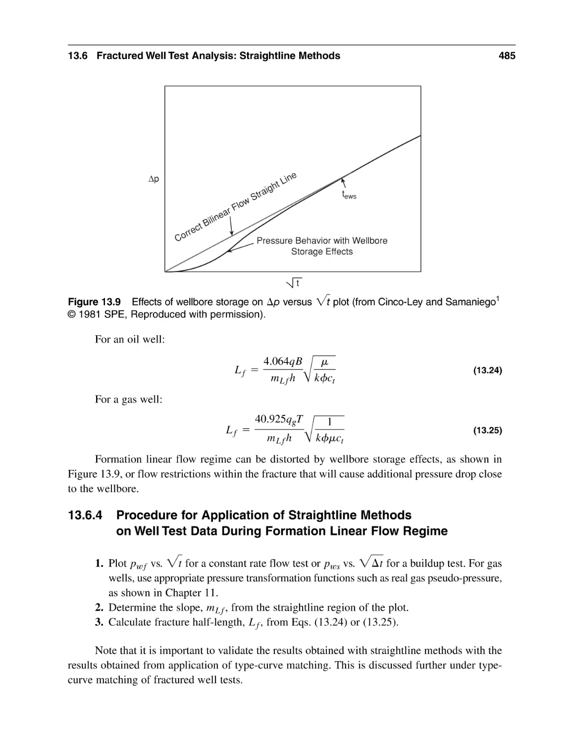


Text
P E T RO L E U M R E S E RVO I R
E N G I N E E R I N G P R AC T I C E
This page intentionally left blank
P E T RO L E U M R E S E RVO I R
E N G I N E E R I N G P R AC T I C E
Nnaemeka Ezekwe
Upper Saddle River, NJ • Boston • Indianapolis • San Francisco
New York • Toronto • Montreal • London • Munich • Paris • Madrid
Capetown • Sydney • Tokyo • Singapore • Mexico City
Many of the designations used by manufacturers and sellers to distinguish their products are claimed as trademarks. Where
those designations appear in this book, and the publisher was aware of a trademark claim, the designations have been
printed with initial capital letters or in all capitals.
The author and publisher have taken care in the preparation of this book, but make no expressed or implied warranty of any
kind and assume no responsibility for errors or omissions. No liability is assumed for incidental or consequential damages
in connection with or arising out of the use of the information or programs contained herein.
The publisher offers excellent discounts on this book when ordered in quantity for bulk purchases or special sales, which
may include electronic versions and/or custom covers and content particular to your business, training goals, marketing
focus, and branding interests. For more information, please contact:
U.S. Corporate and Government Sales
(800) 382-3419
corpsales@pearsontechgroup.com
For sales outside the United States please contact:
International Sales
international@pearson.com
Visit us on the Web: informit.com/ph
Library of Congress Cataloging-in-Publication Data
Ezekwe, Nnaemeka.
Petroleum reservoir engineering practice / Nnaemeka Ezekwe.
p. cm.
Includes bibliographical references and index.
ISBN 0-13-715283-3 (hardcover : alk. paper) 1. Oil reservoir
engineering. 2. Petroleum—Geology. I. Title.
TN870.57.E94 2011
622'.3382—dc22
2010024160
Copyright © 2011 Pearson Education, Inc.
All rights reserved. Printed in the United States of America. This publication is protected by copyright, and permission
must be obtained from the publisher prior to any prohibited reproduction, storage in a retrieval system, or transmission in
any form or by any means, electronic, mechanical, photocopying, recording, or likewise. For information regarding permissions, write to:
Pearson Education, Inc.
Rights and Contracts Department
501 Boylston Street, Suite 900
Boston, MA 02116
Fax: (617) 671-3447
ISBN-13: 978-0-13-715283-4
ISBN-10:
0-13-715283-3
Text printed in the United States on recycled paper at Courier in Westford, Massachusetts.
First printing, September 2010
To the memory of my parents, Vincent Nweke and Rosaline Oriaku, for
their sacrifices, commitment, courage, and unwavering support towards
my education and those of my brother and sisters. This book is the fruit
of the seed they planted and nurtured.
This page intentionally left blank
Contents
Preface
Acknowledgments
About the Author
xiii
xxv
xxix
Chapter 1 Porosity of Reservoir Rocks
1.1 Introduction
1.2 Total Porosity and Effective Porosity
1.3 Sources of Porosity Data
1.3.1 Direct Methods for Measurement of Porosity
1.3.2 Indirect Methods for Derivation of Porosity
1.4 Applications of Porosity Data
1.4.1 Volumetric Calculation
1.4.2 Calculation of Fluid Saturations
1.4.3 Reservoir Characterization
Nomenclature
Abbreviations
References
General Reading
1
1
1
3
3
4
10
10
11
11
12
13
13
14
Chapter 2 Permeability and Relative Permeability
2.1 Introduction
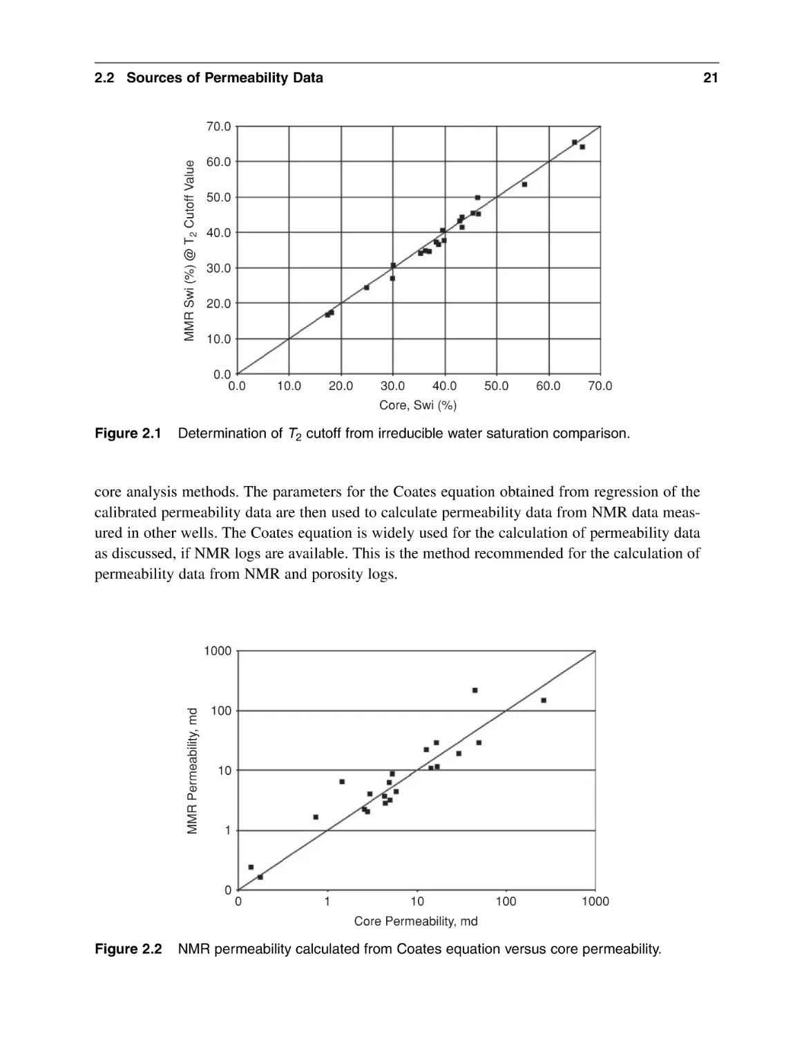
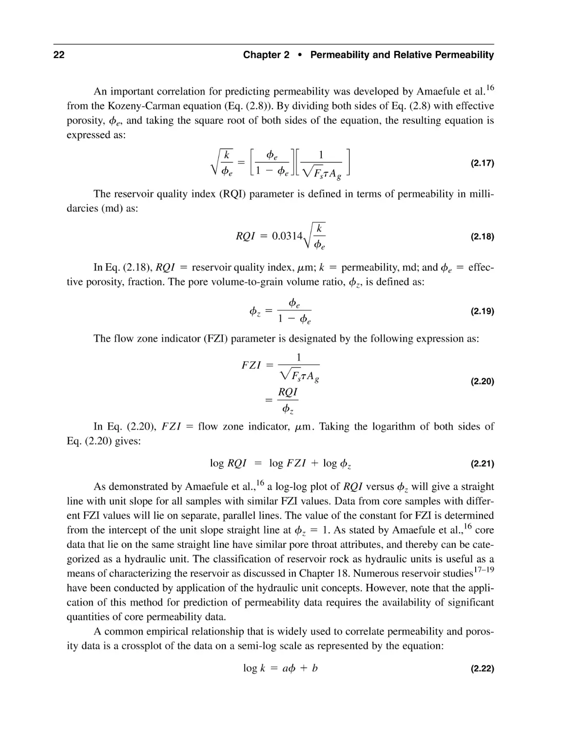
2.2 Sources of Permeability Data
2.2.1 Permeability from Core Samples
2.2.2 Permeability from Pressure Transient Tests
2.2.3 Permeability from Well Logs Based on Empirical Correlations
2.3 Relative Permeability
2.4 Sources of Relative Permeability Data
2.4.1 Laboratory Measurements of Relative Permeability Data
2.4.2 Estimations from Field Data
2.4.3 Empirical Correlations
15
15
16
17
18
18
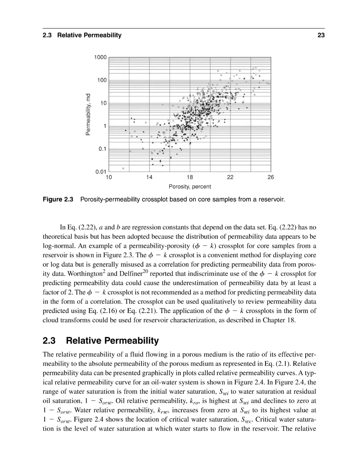
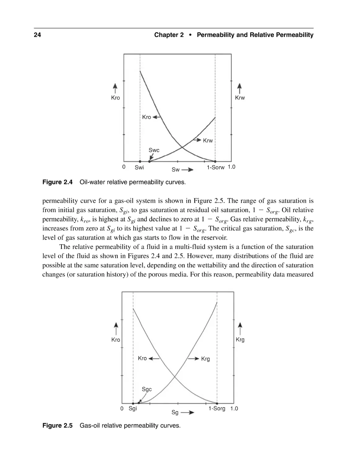
23
25
25
26
26
vii
viii
Contents
2.5 Three-Phase Relative Permeability
2.6 Applications of Permeability and Relative Permeability Data
Nomenclature
Abbreviations
References
General Reading
32
32
33
34
34
37
Chapter 3 Reservoir Fluid Saturations
3.1 Introduction
3.2 Determination of Water Saturations
3.2.1 Clean Sands
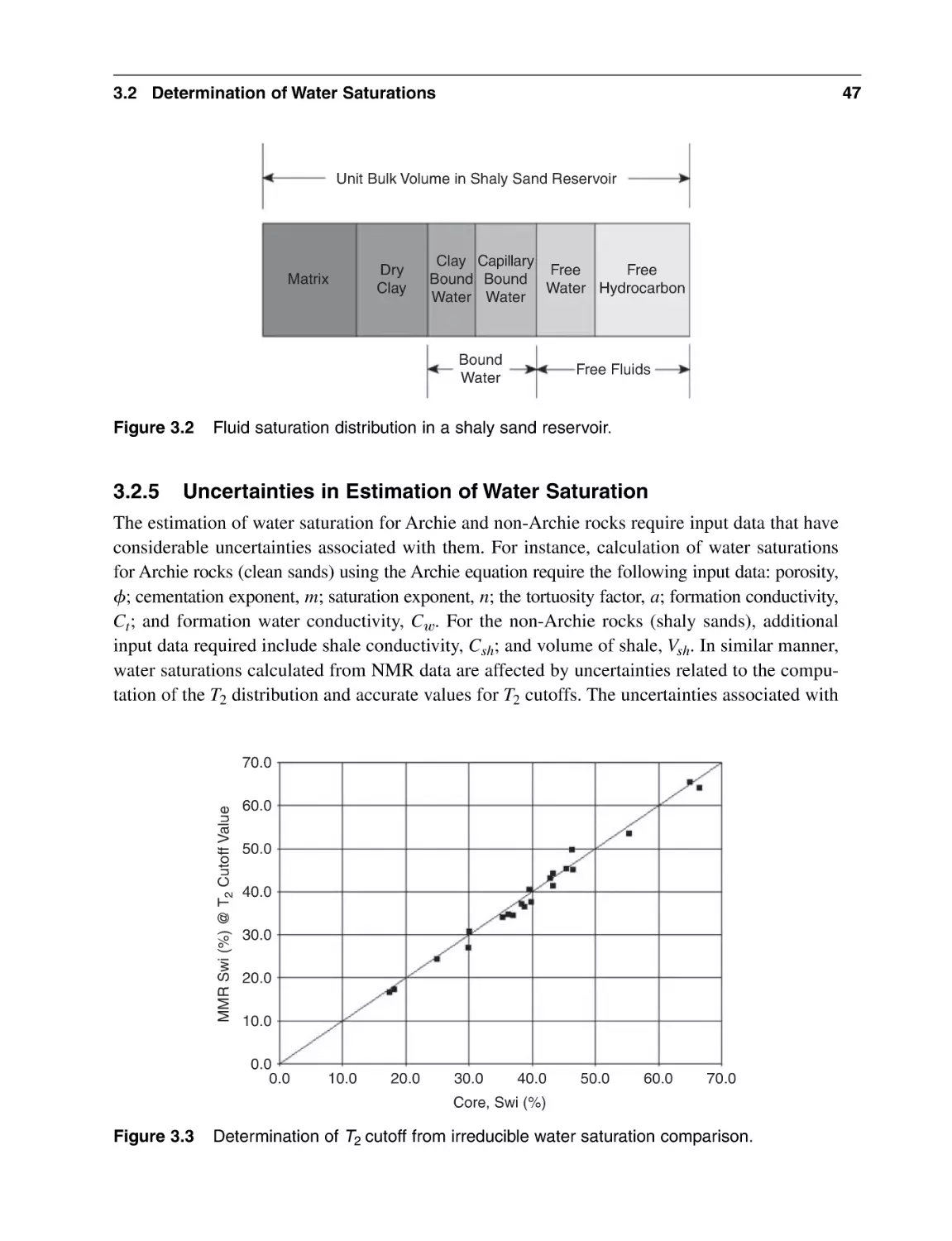
3.2.2 Shaly Sands
3.2.3 Carbonate Rocks
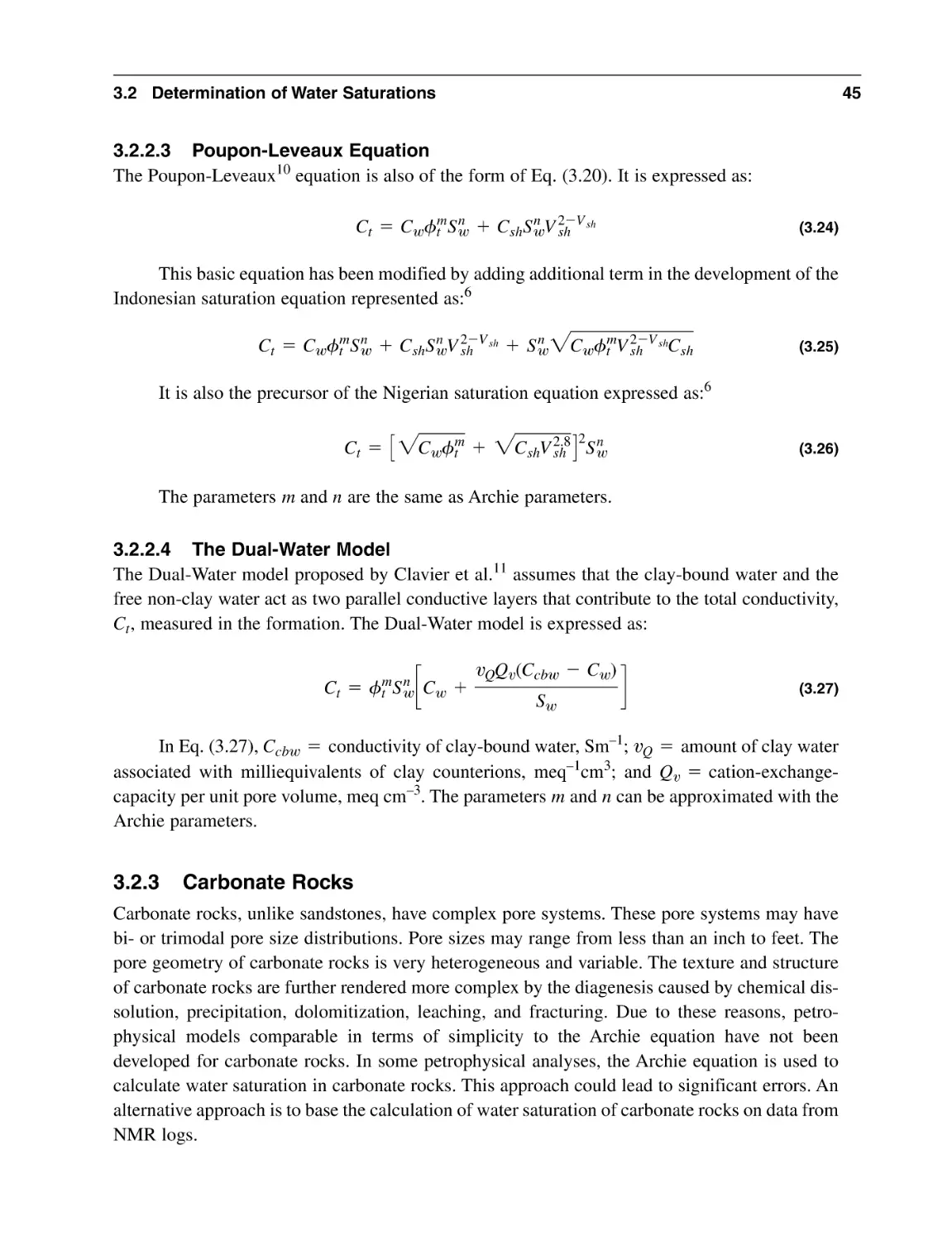
3.2.4 Water Saturations from Nuclear Magnetic Resonance Logs
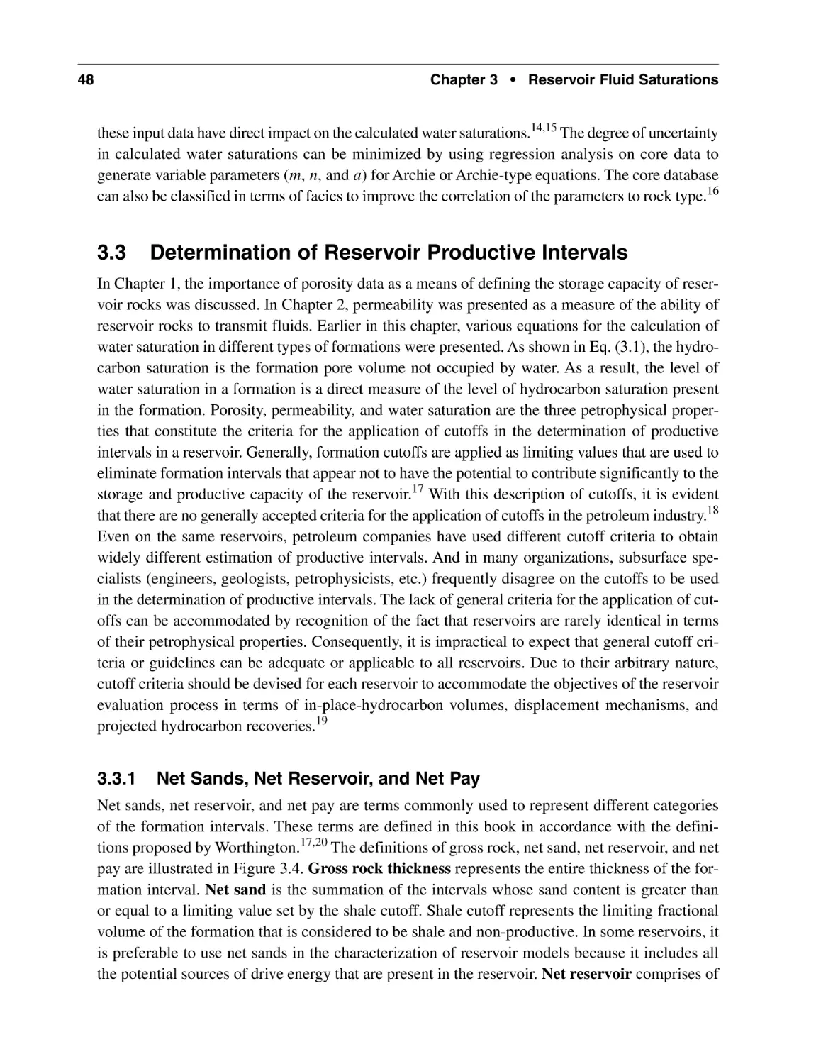
3.2.5 Uncertainties in Estimation of Water Saturation
3.3 Determination of Reservoir Productive Intervals
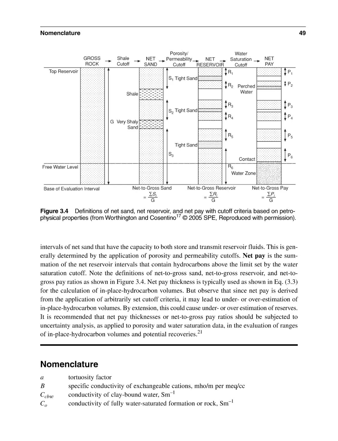
3.3.1 Net Sands, Net Reservoir, and Net Pay
Nomenclature
Abbreviations
References
General Reading
39
39
40
40
44
45
46
47
48
48
49
50
50
52
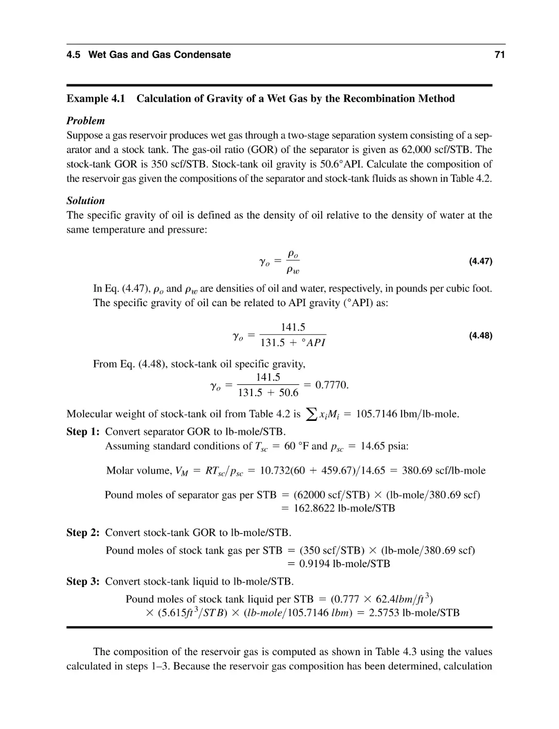
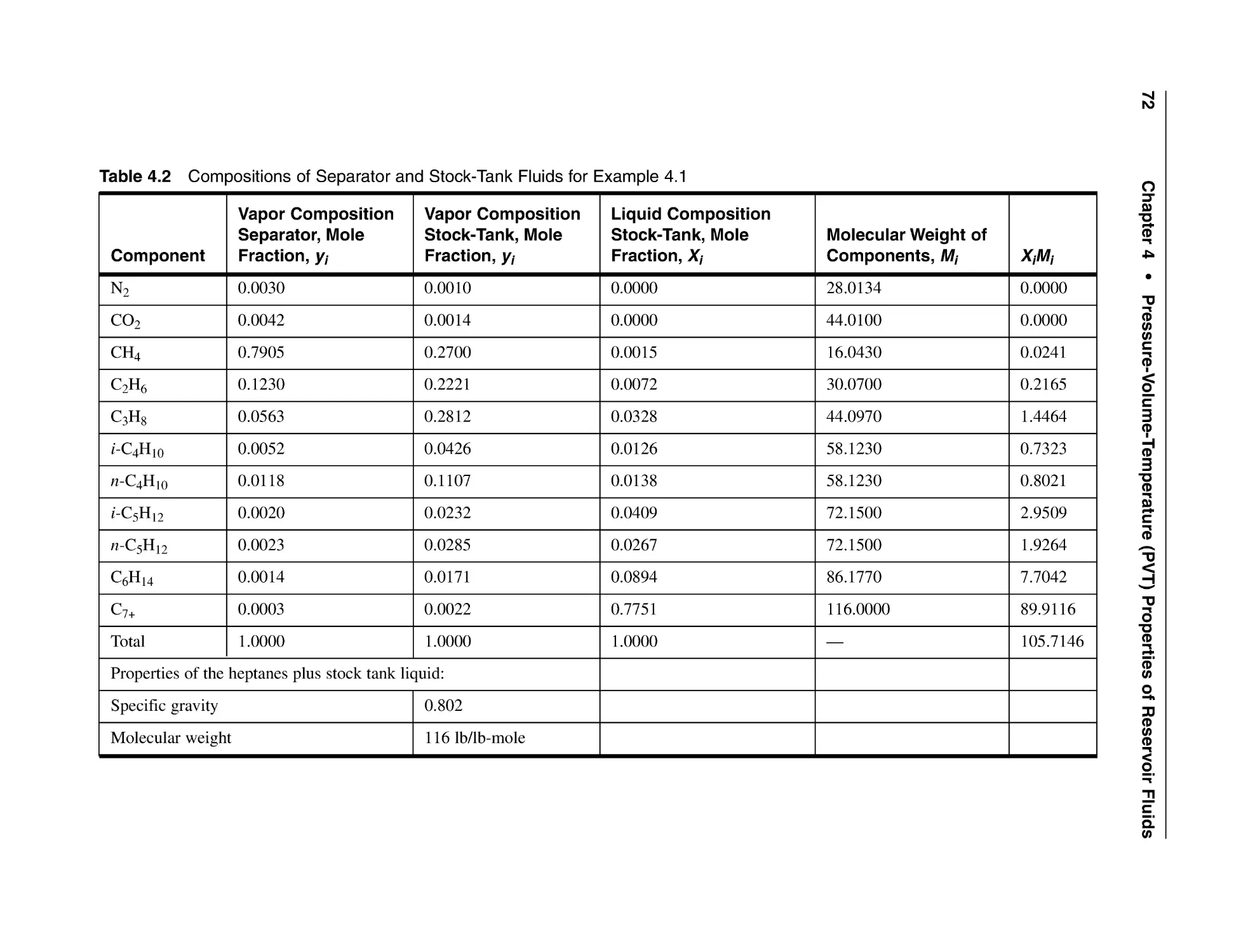
Chapter 4 Pressure-Volume-Temperature (PVT) Properties
of Reservoir Fluids
4.1 Introduction
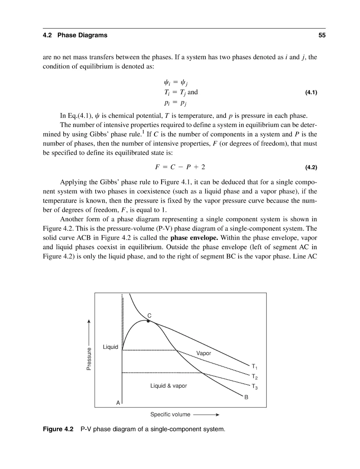
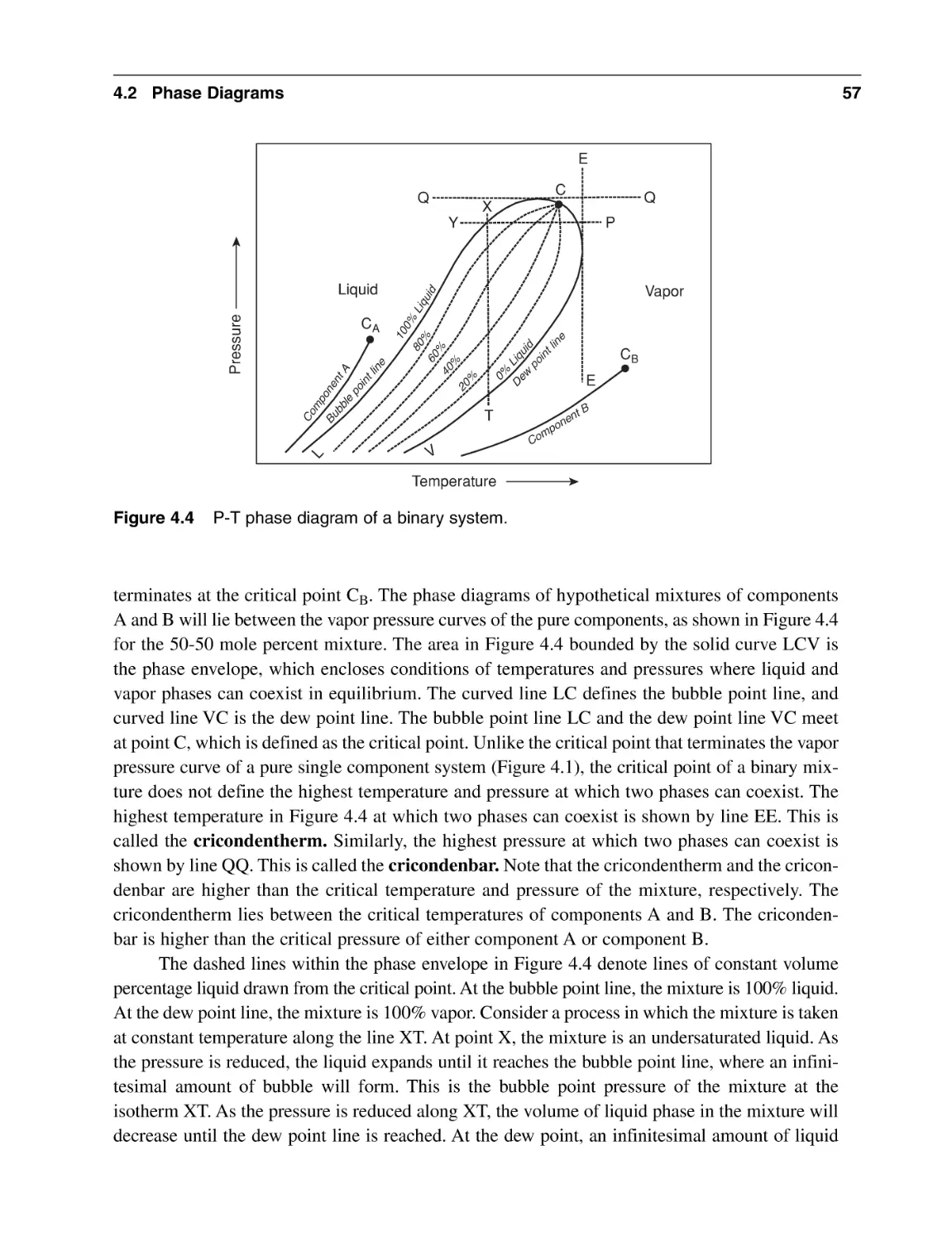
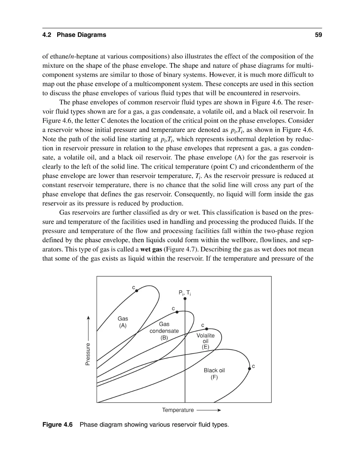
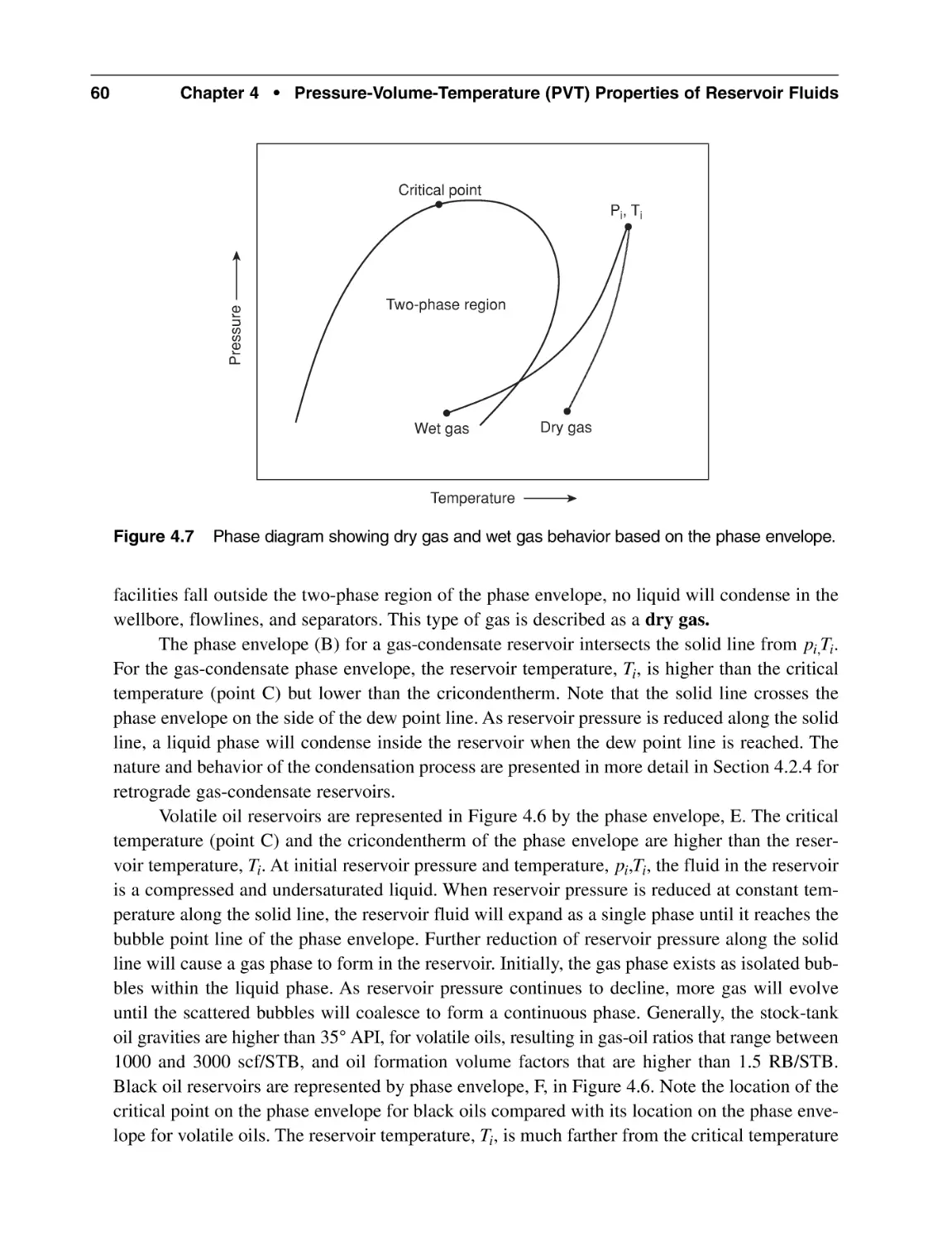
4.2 Phase Diagrams
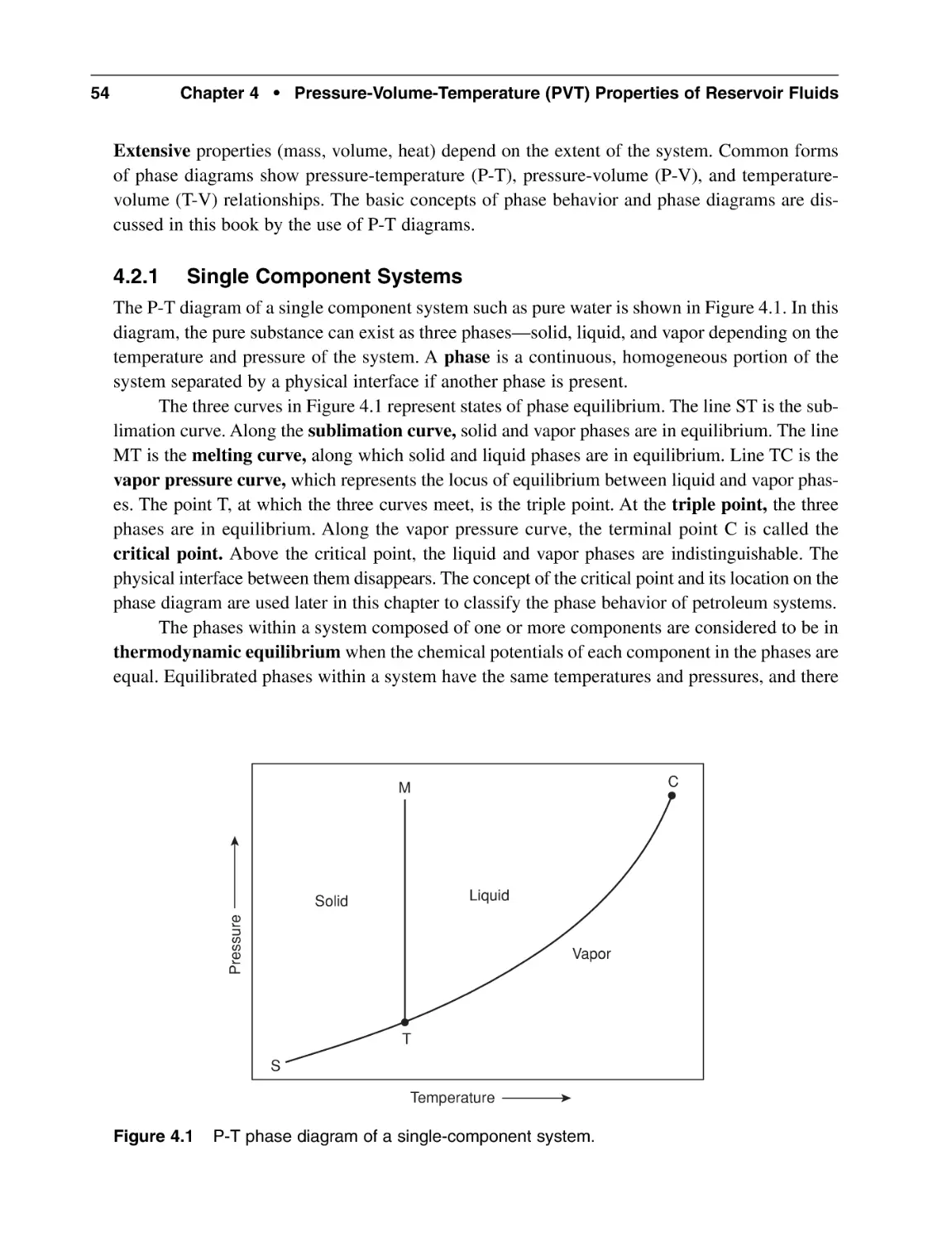
4.2.1 Single Component Systems
4.2.2 Binary Systems
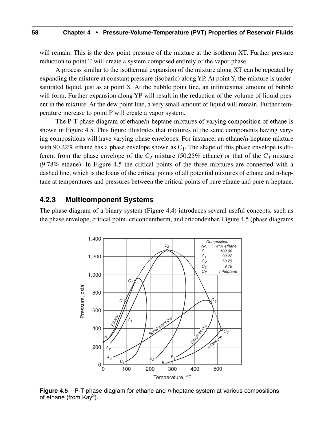
4.2.3 Multicomponent Systems
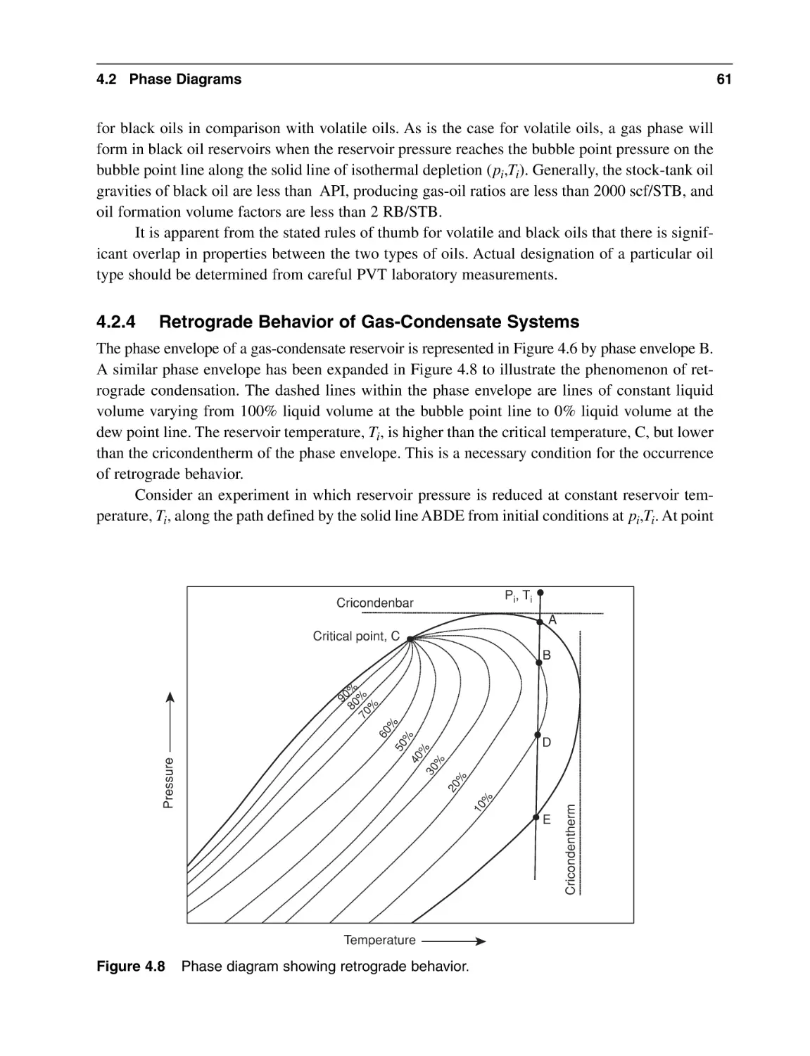
4.2.4 Retrograde Behavior of Gas-Condensate Systems
4.3 Gas and Gas-Condensate Properties
4.3.1 Ideal Gas Equation
4.3.2 Real Gas Equation
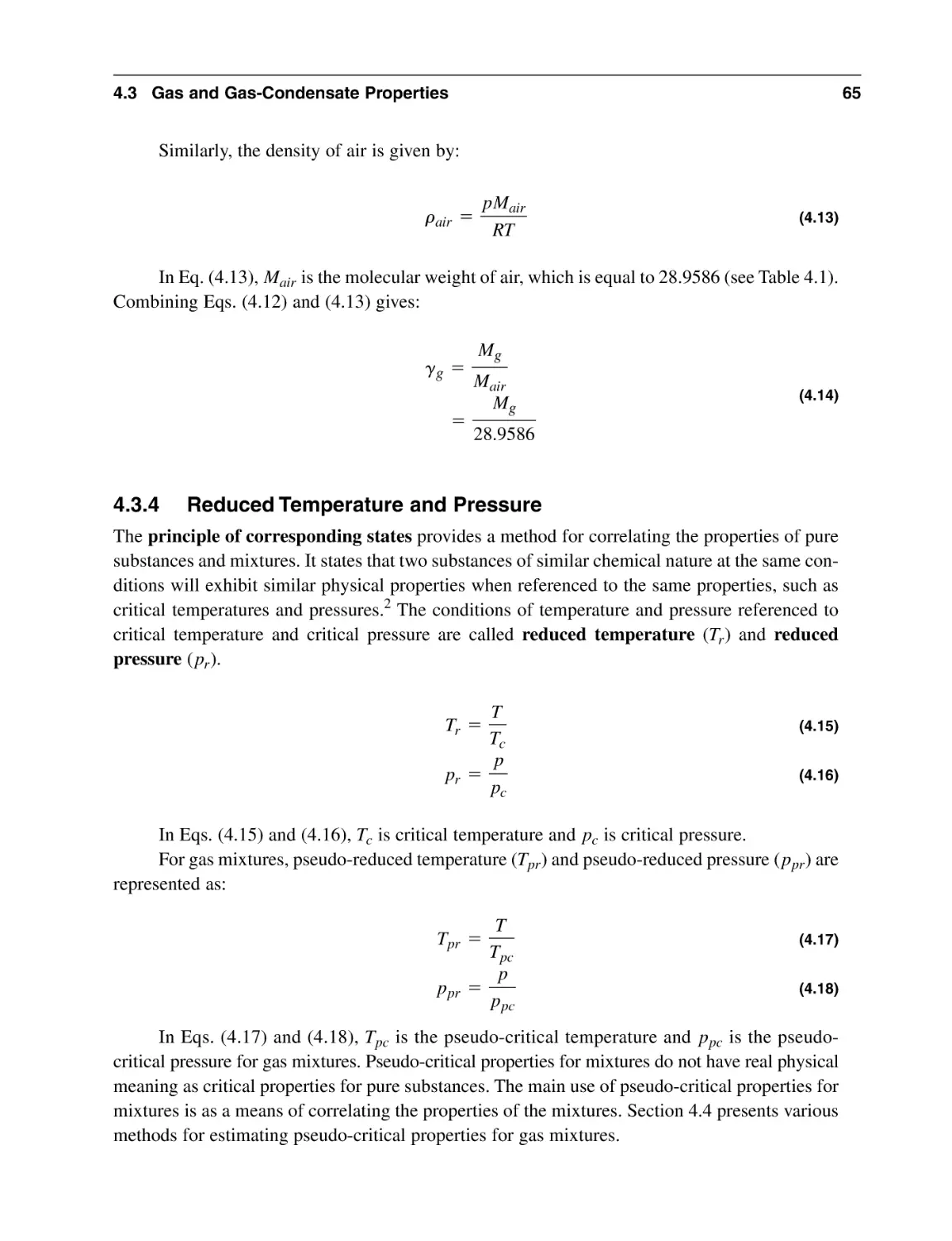
4.3.3 Gas Gravity
4.3.4 Reduced Temperature and Pressure
4.4 Pseudo-critical Properties of Gas Mixtures
4.4.1 Composition of Gas Mixtures Known
4.4.2 Correction for non-Hydrocarbon Gas Impurities
4.4.3 Composition of Gas Mixture Unknown
53
53
53
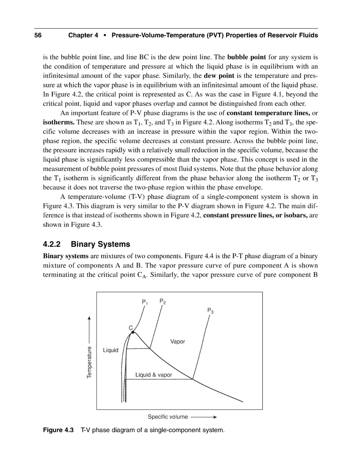
54
56
58
61
63
63
64
64
65
67
67
68
69
Contents
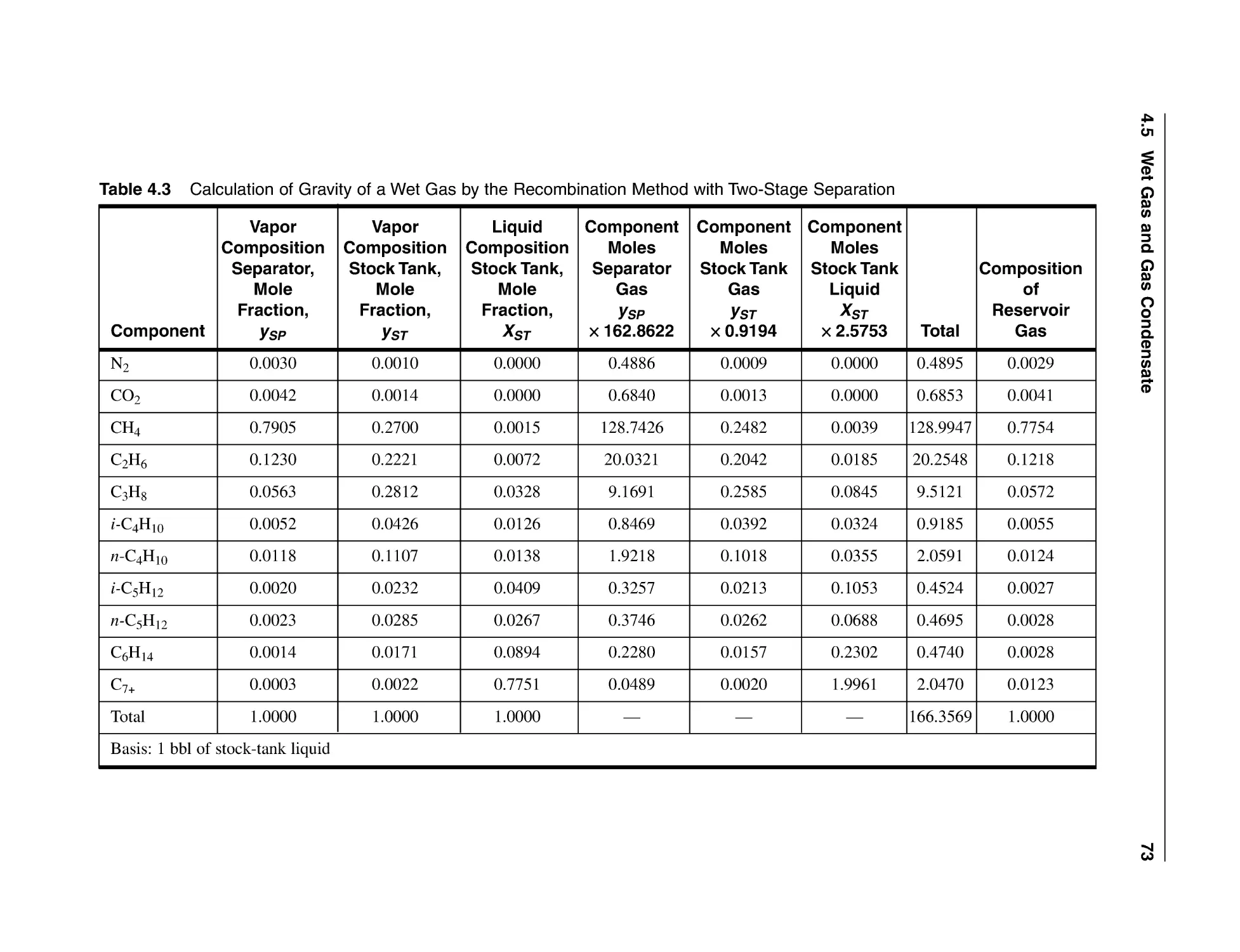
4.5
Wet Gas and Gas Condensate
4.5.1 Recombination Method
4.5.2 Correlation Method
4.6 Correlations for Gas Compressibility Factor
4.7 Gas Formation Volume Factor (FVF)
4.8 Gas Density
4.9 Gas Viscosity
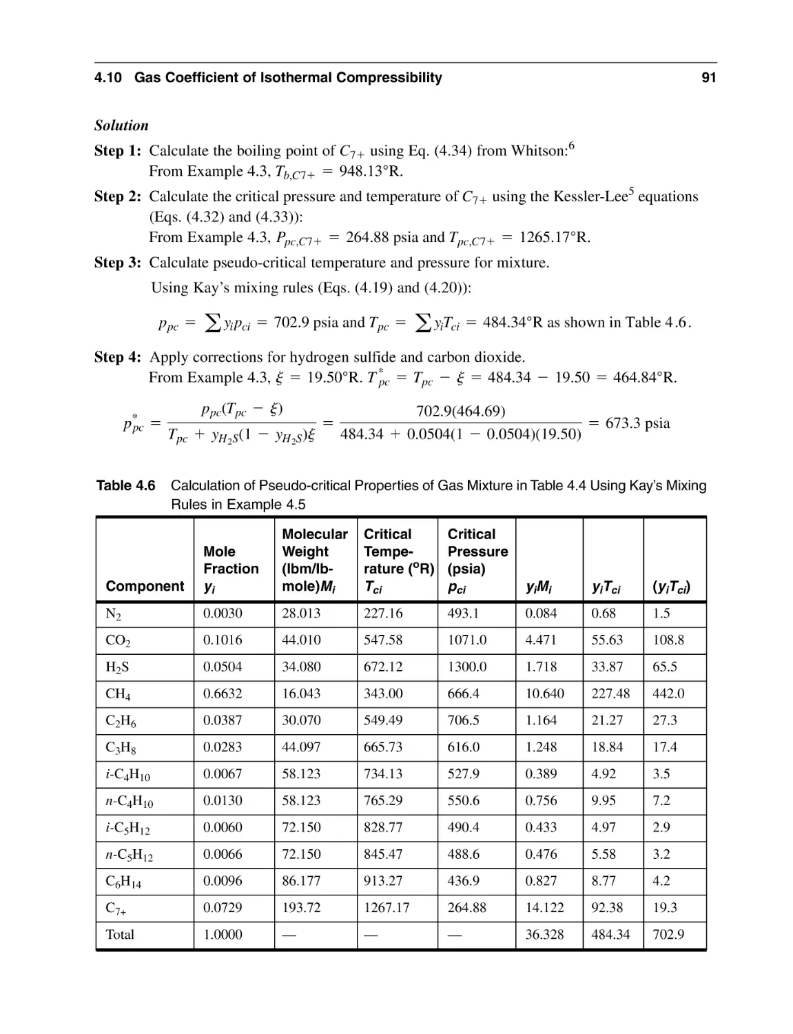
4.10 Gas Coefficient of Isothermal Compressibility
4.11 Correlations for Calculation of Oil PVT Properties
4.11.1 Bubble Point Pressure
4.11.2 Solution Gas-Oil Ratio (GOR)
4.11.3 Oil Formation Volume Factor (FVF)
4.11.4 Coefficient of Isothermal Compressibility of Oil
4.11.5 Oil Viscosity
4.12 Correlations for Calculation of Water PVT Properties
4.12.1 Water Formation Volume Factor (FVF)
4.12.2 Density of Formation Water
4.12.3 Coefficient of Isothermal Compressibility
of Formation Water
4.12.4 Viscosity of Formation Water
Nomenclature
Subscripts
References
General Reading
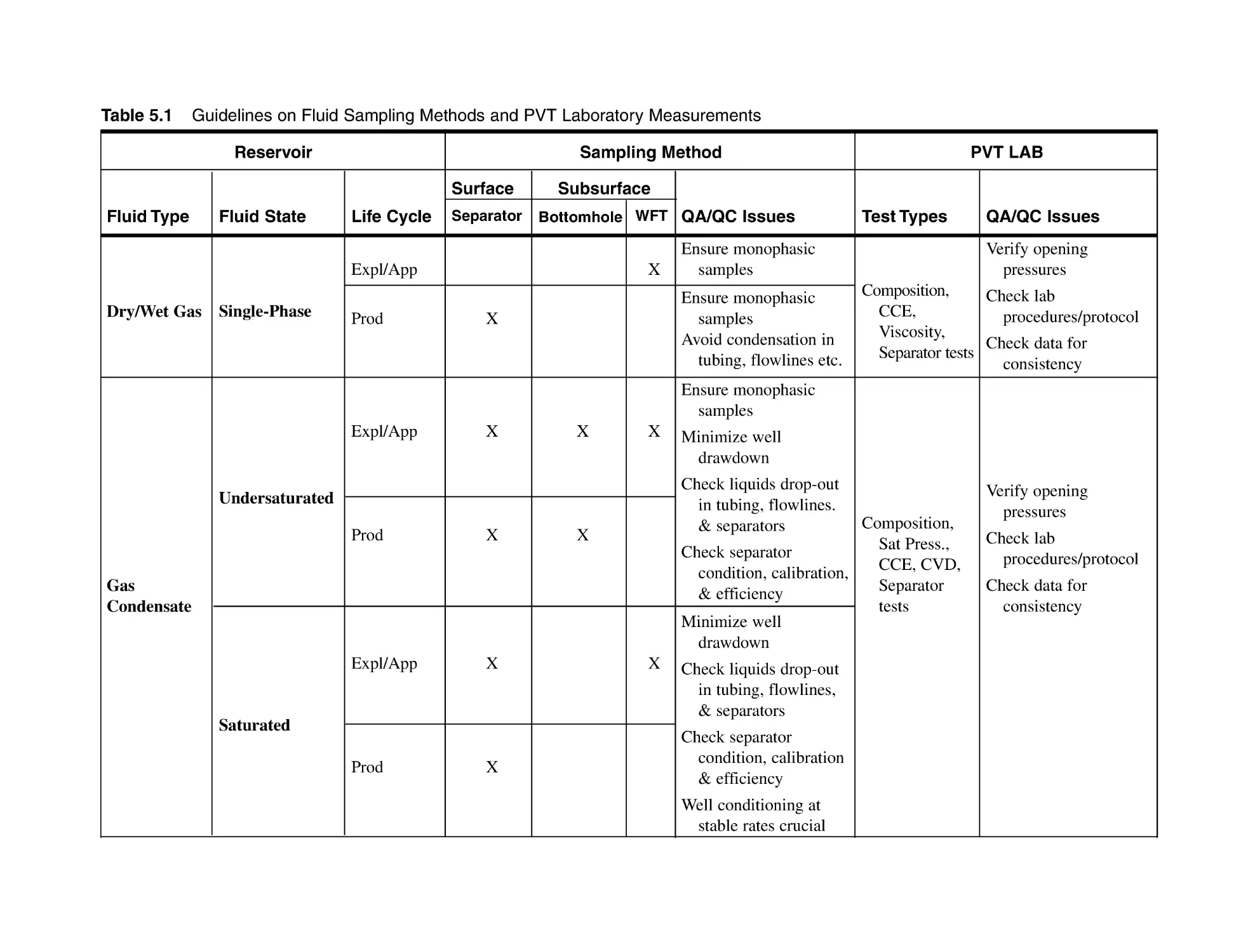
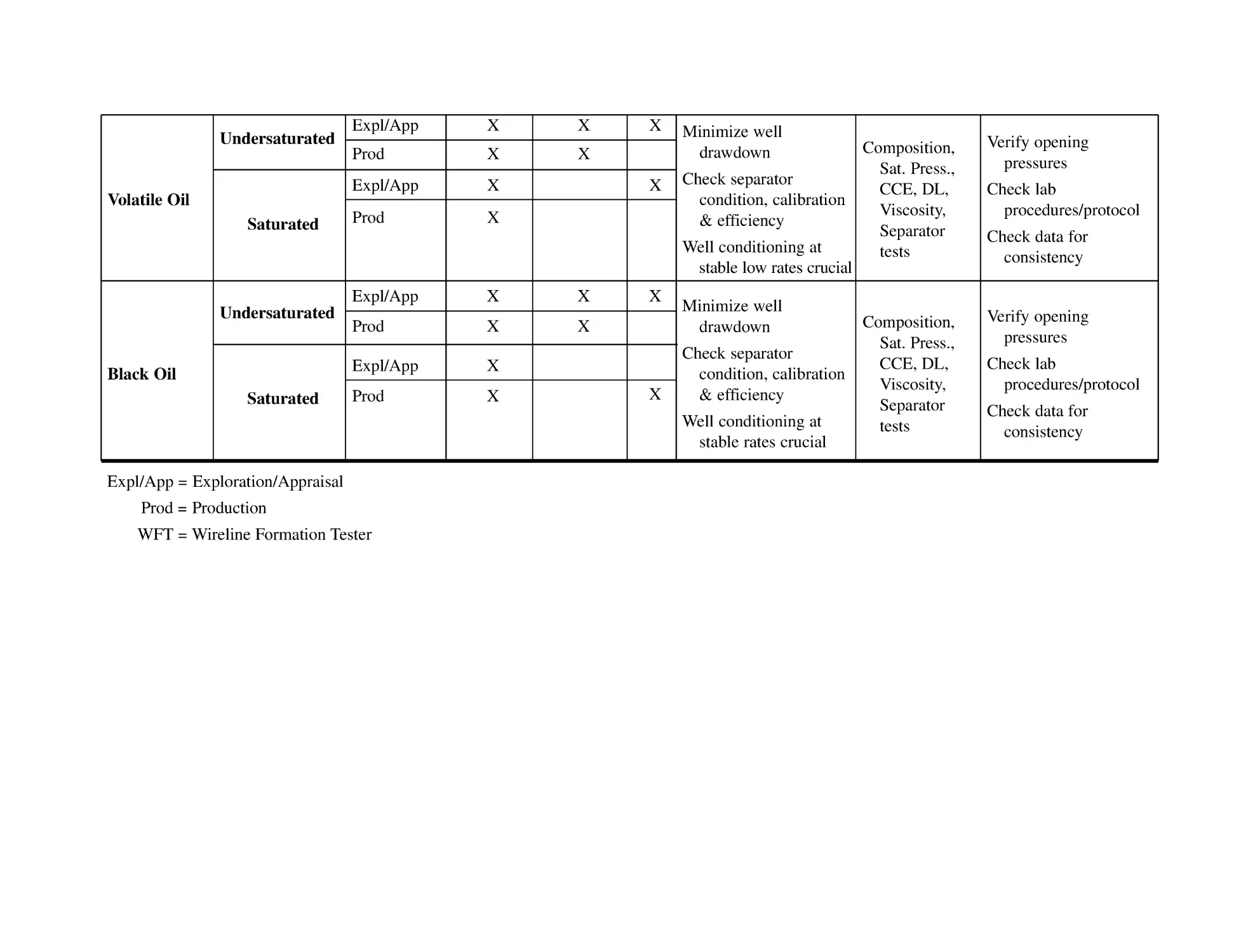
Chapter 5 Reservoir Fluid Sampling and PVT Laboratory Measurements
5.1 Overview of Reservoir Fluid Sampling
5.2 Reservoir Type and State
5.2.1 Undersaturated Oil Reservoirs
5.2.2 Undersaturated Gas Condensate Reservoirs
5.2.3 Saturated Oil Reservoirs
5.2.4 Saturated Gas Condensate Reservoirs
5.3 Well Conditioning
5.4 Subsurface Sampling Methods and Tools
5.4.1 Conventional Bottomhole Samplers
5.4.2 Pistonned Bottomhole Samplers
5.4.3 Single-Phase Samplers
5.4.4 Exothermic Samplers
ix
70
70
74
78
79
81
82
83
93
93
95
95
96
98
103
103
103
103
104
104
106
106
108
111
111
116
116
117
118
118
119
119
120
120
120
121
x
Contents
5.5
Wireline Formation Testers
5.5.1 Oil-Based Mud Contamination of WFT Samples
5.5.2 Formation Pressures from WFT
5.5.3 Capillary Effects on WFT Formation Pressures
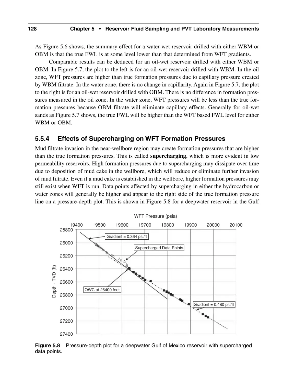
5.5.4 Effects of Supercharging on WFT Formation Pressures
5.5.5 Comments on Applications of WFT Pressure Data
5.6 PVT Laboratory Measurements
5.6.1 Fluid Composition
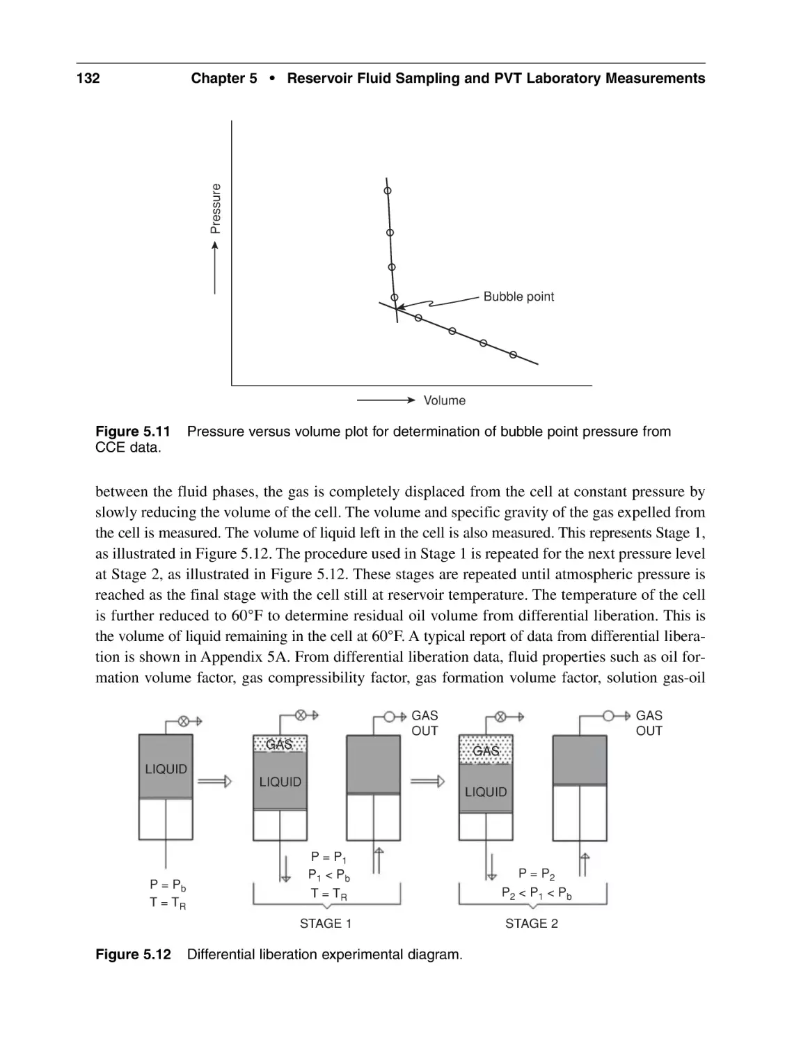
5.6.2 Constant Composition Expansion (CCE)
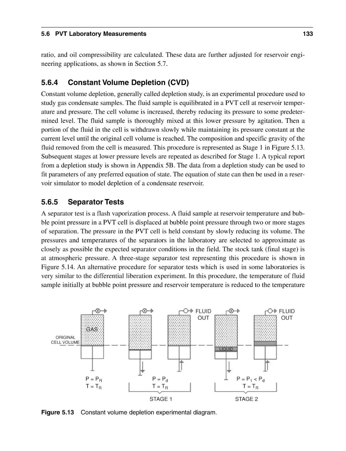
5.6.3 Differential Liberation (DL)
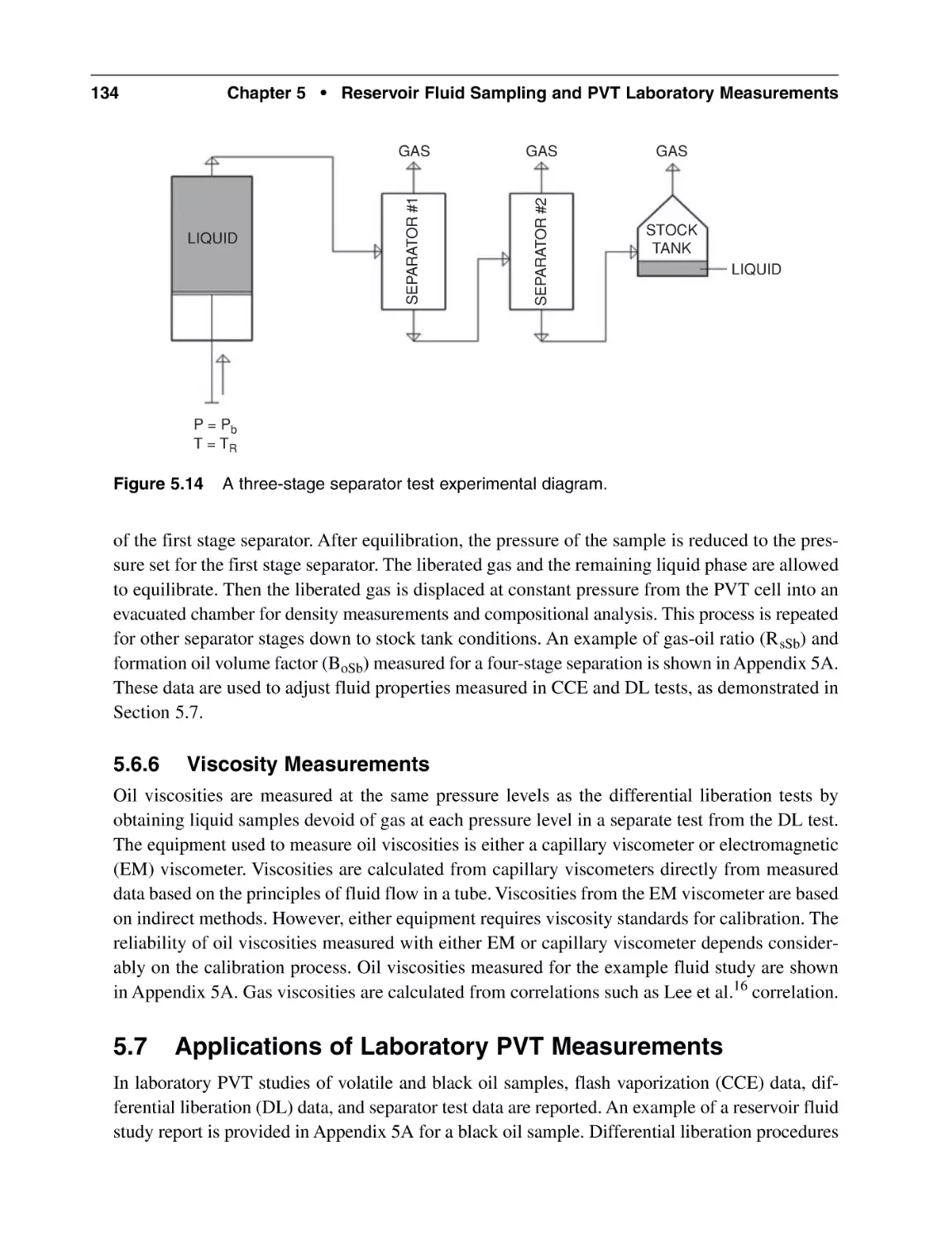
5.6.4 Constant Volume Depletion (CVD)
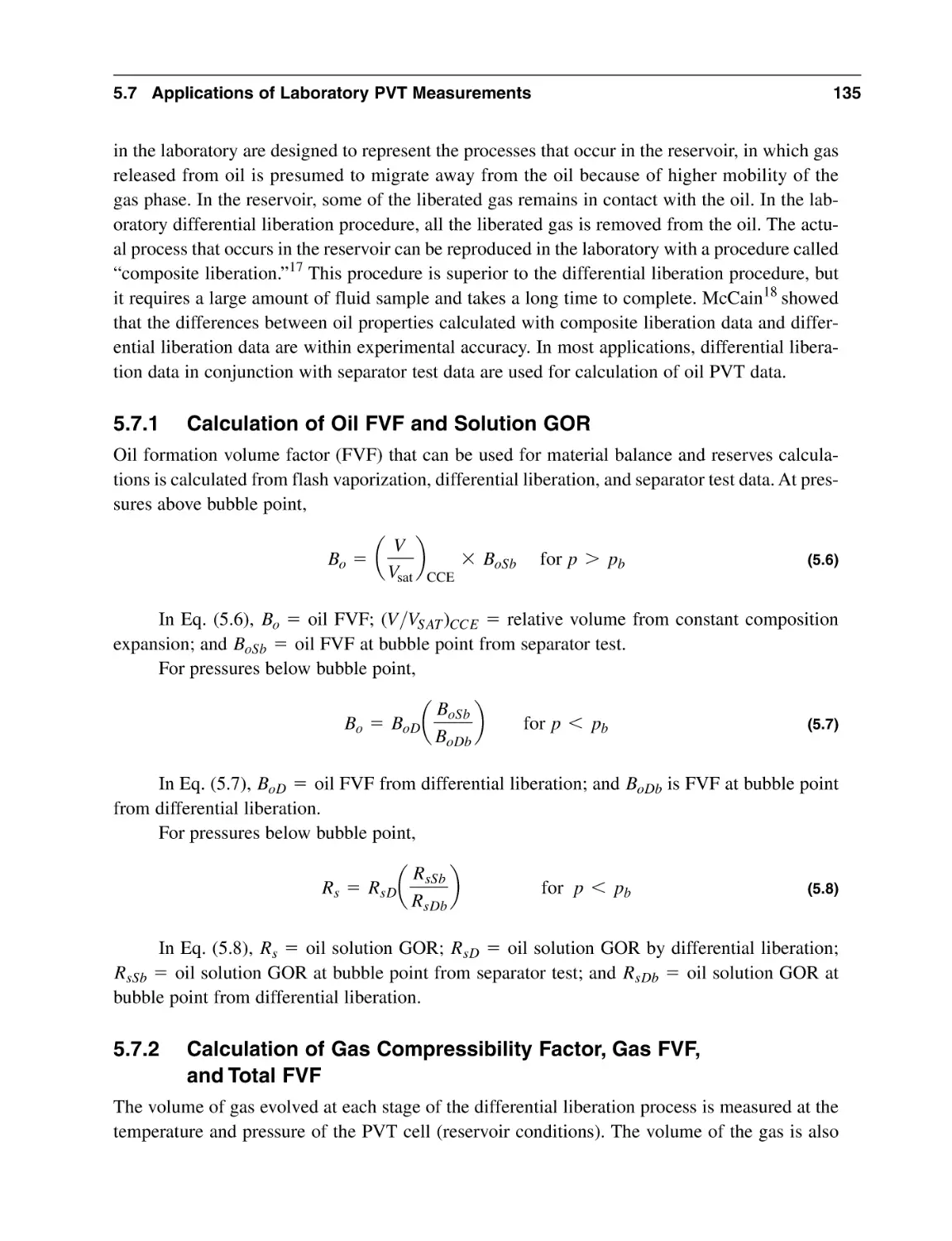
5.6.5 Separator Tests
5.6.6 Viscosity Measurements
5.7 Applications of Laboratory PVT Measurements
5.7.1 Calculation of Oil FVF and Solution GOR
5.7.2 Calculation of Gas Compressibility Factor, Gas FVF,
and Total FVF
5.7.3 Calculation of Oil Compressibility Factor
Nomenclature
Subscripts
Abbreviations
References
General Reading
121
121
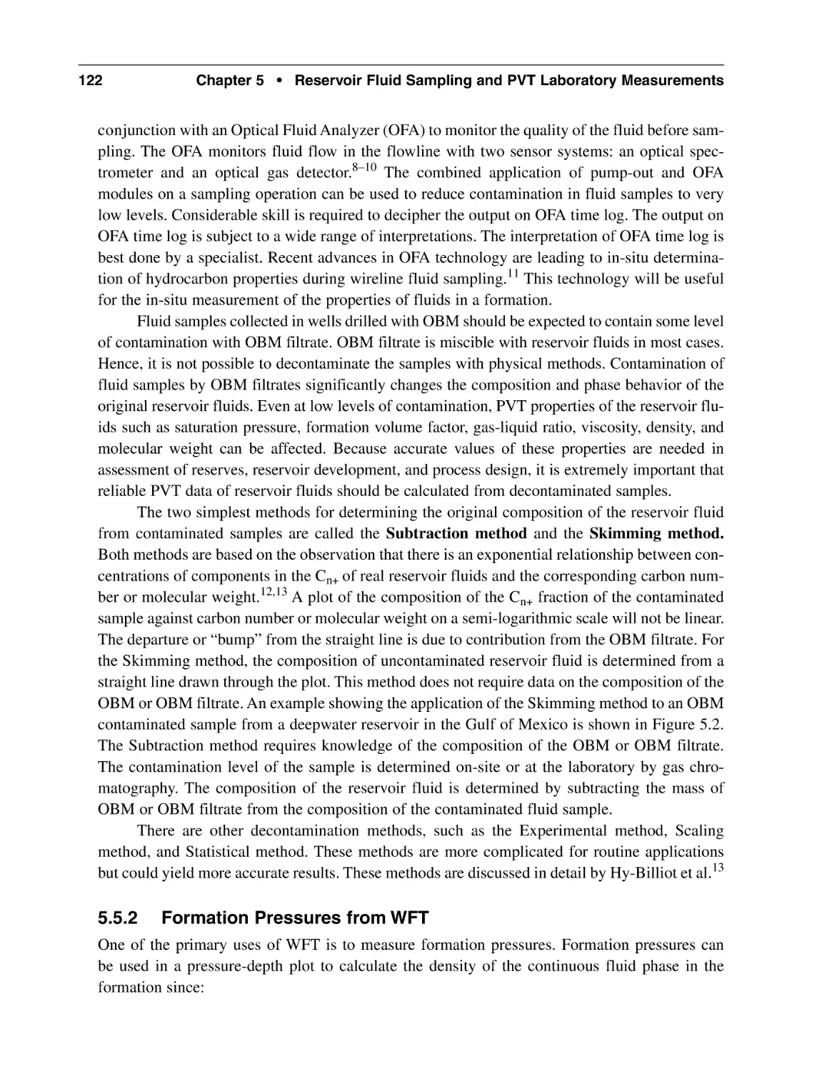
122
123
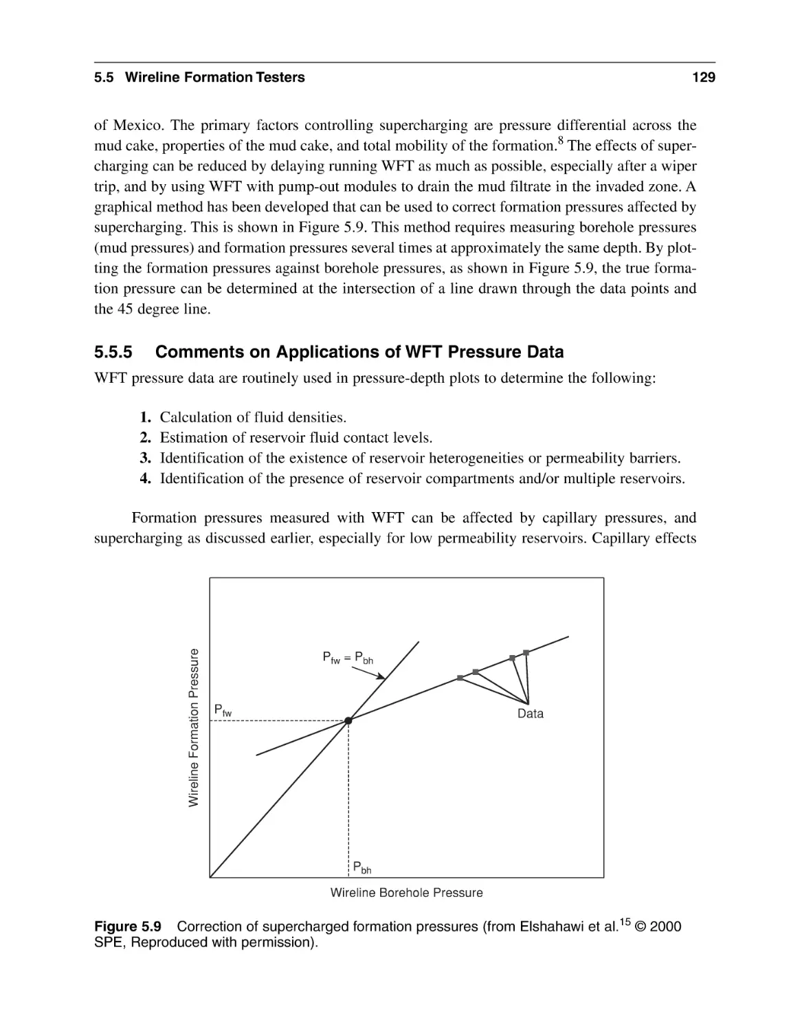
128
129
130
130
131
131
133
133
134
134
135
135
136
138
138
139
139
140
Appendix 5A Typical Reservoir Fluid Study for a Black Oil Sample
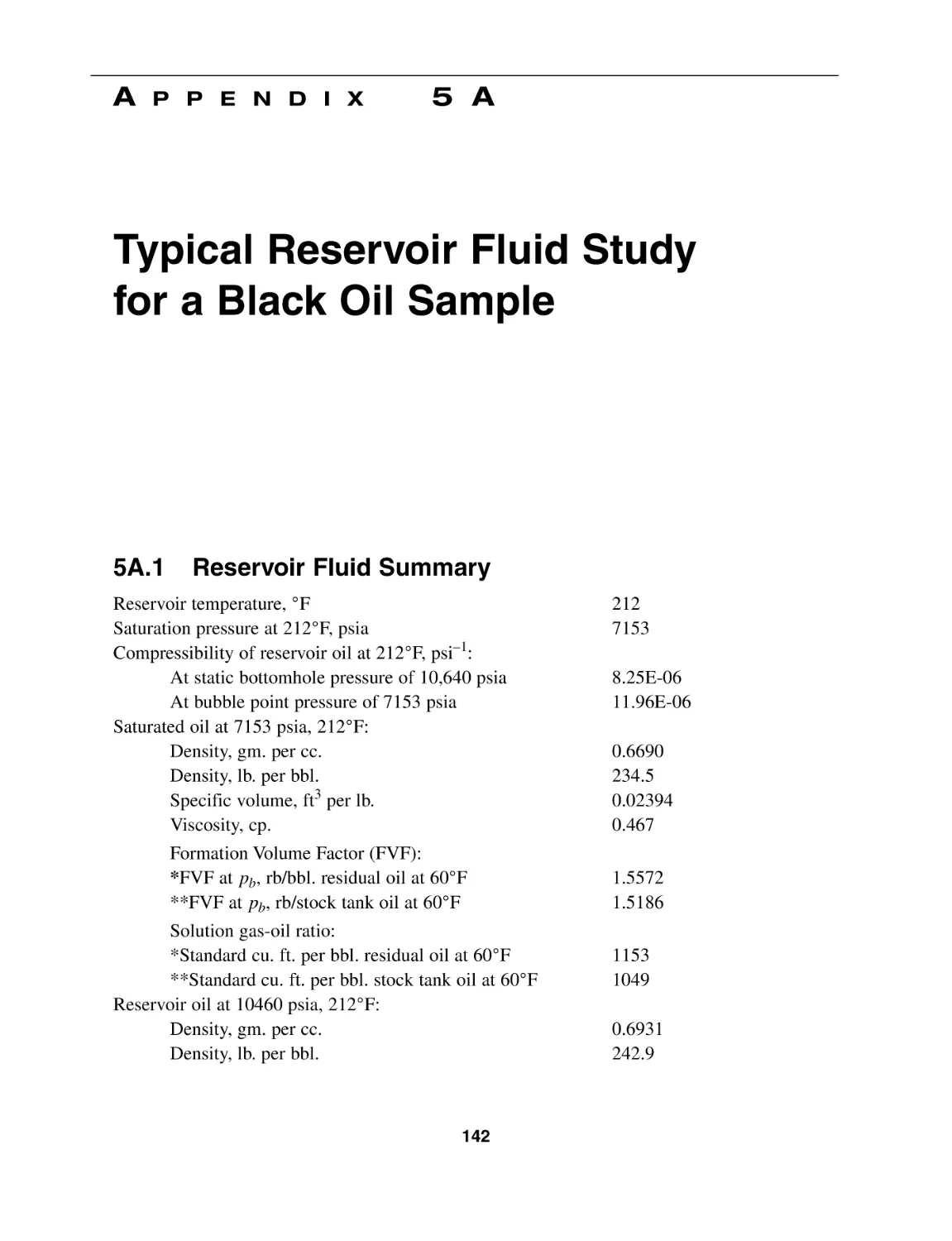
5A.1 Reservoir Fluid Summary
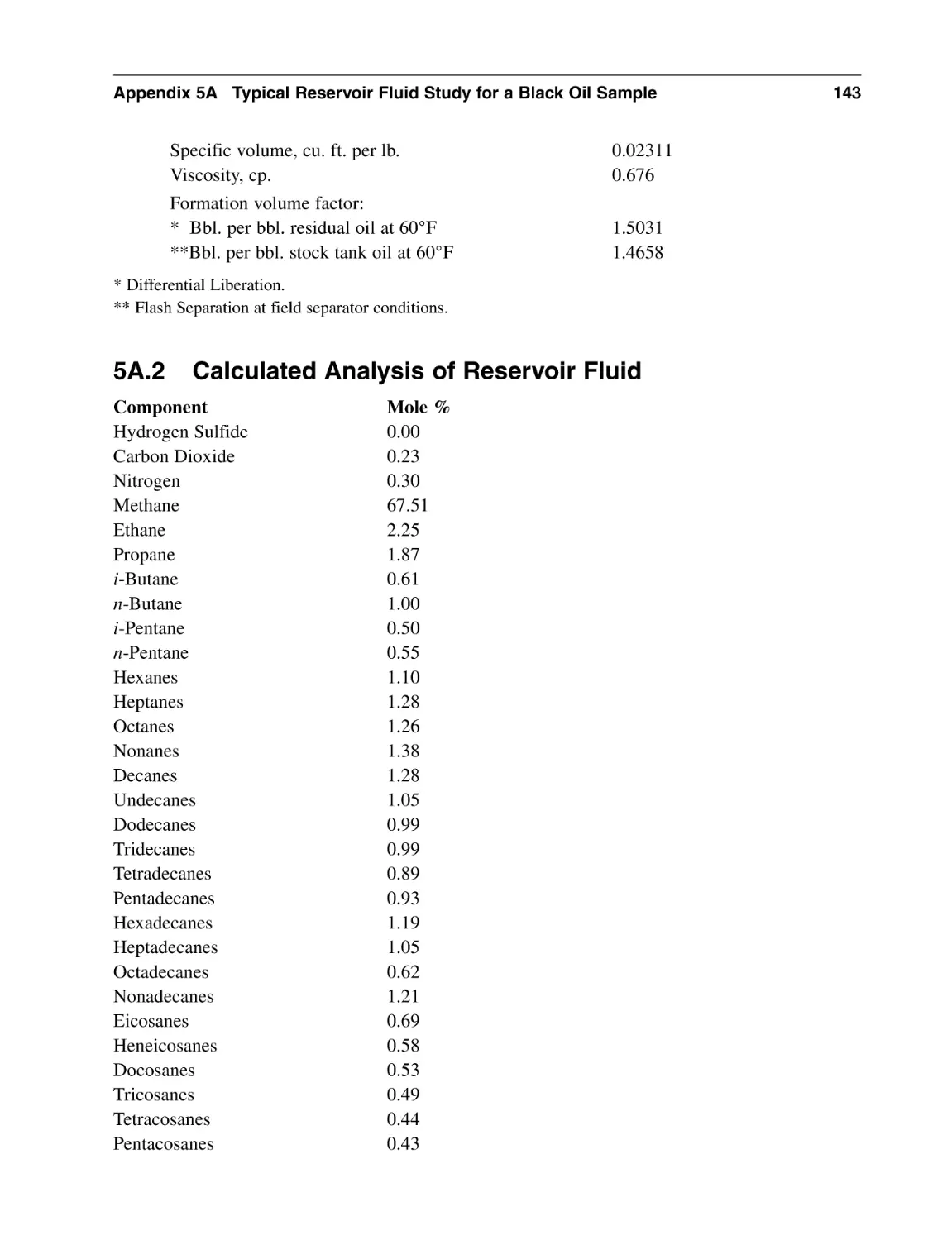
5A.2 Calculated Analysis of Reservoir Fluid
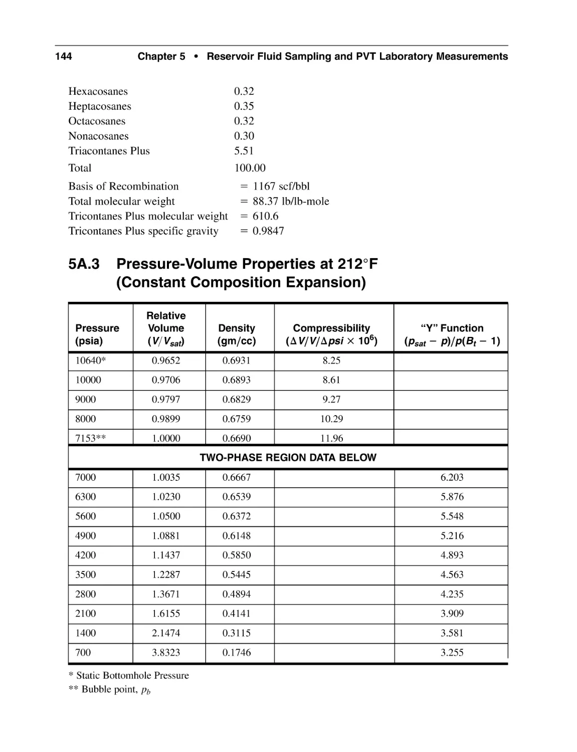
5A.3 Pressure-Volume Properties at 212°F
(Constant Composition Expansion)
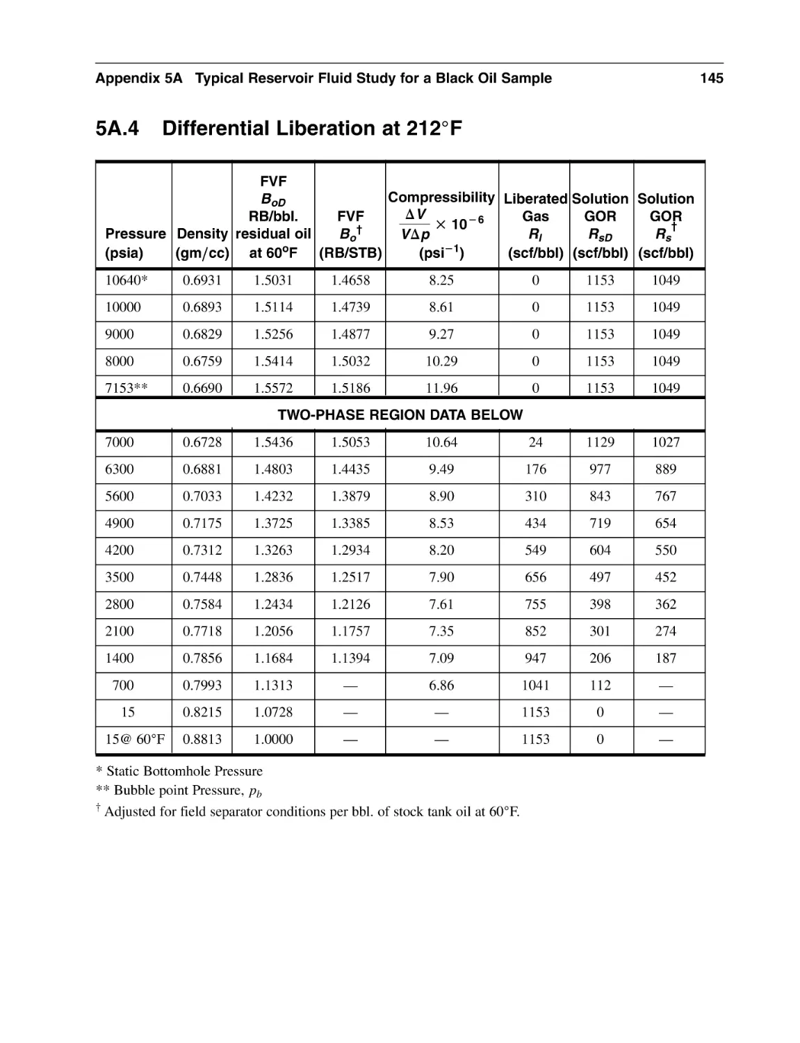
5A.4 Differential Liberation at 212°F
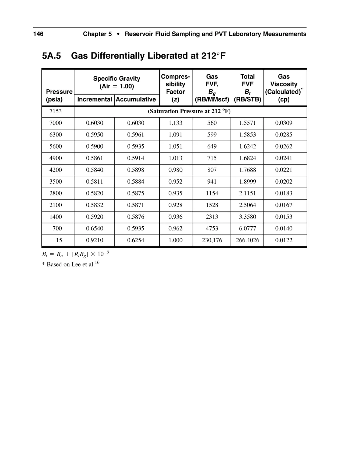
5A.5 Gas Differentially Liberated at 212°F
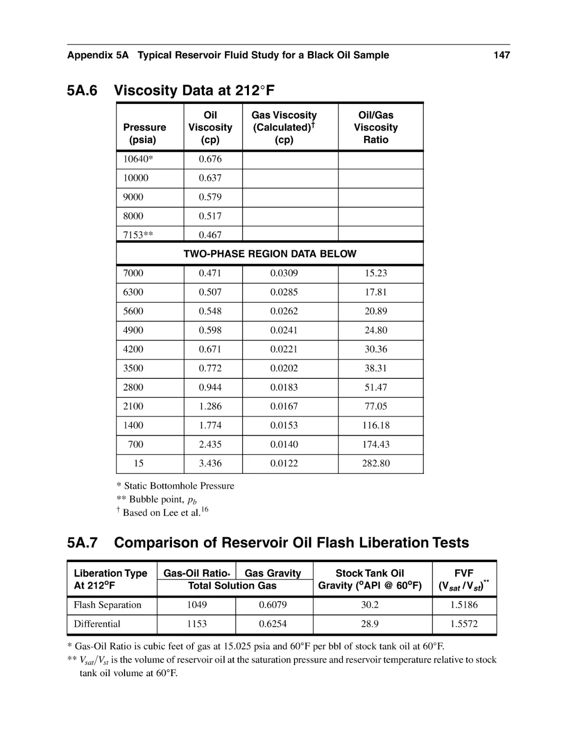
5A.6 Viscosity Data at 212°F
5A.7 Comparison of Reservoir Oil Flash Liberation Tests
142
142
143
Appendix 5B Typical Reservoir Fluid Study for a Gas Condensate Sample
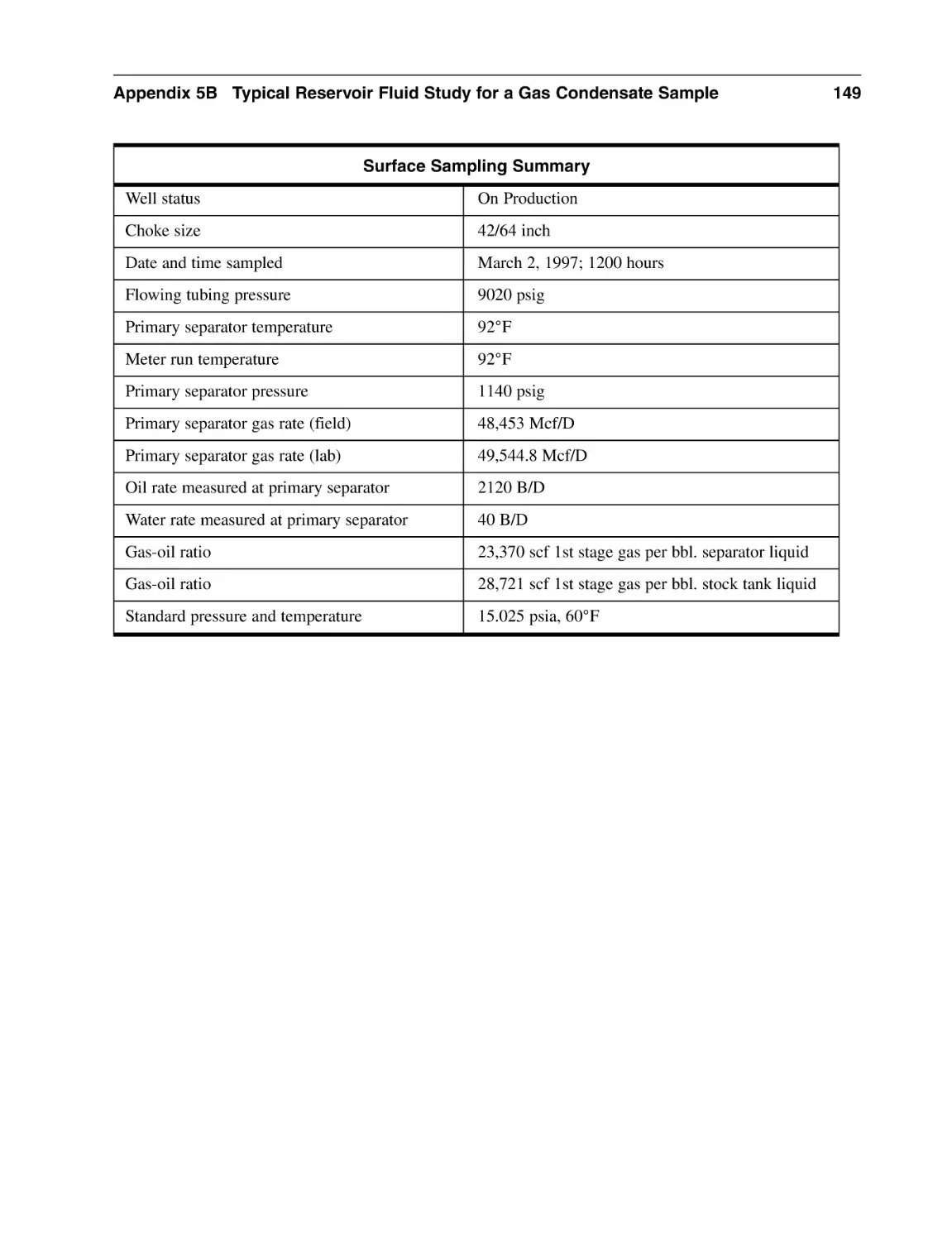
5B.1 Summary of Reservoir Data and Surface Sampling Conditions
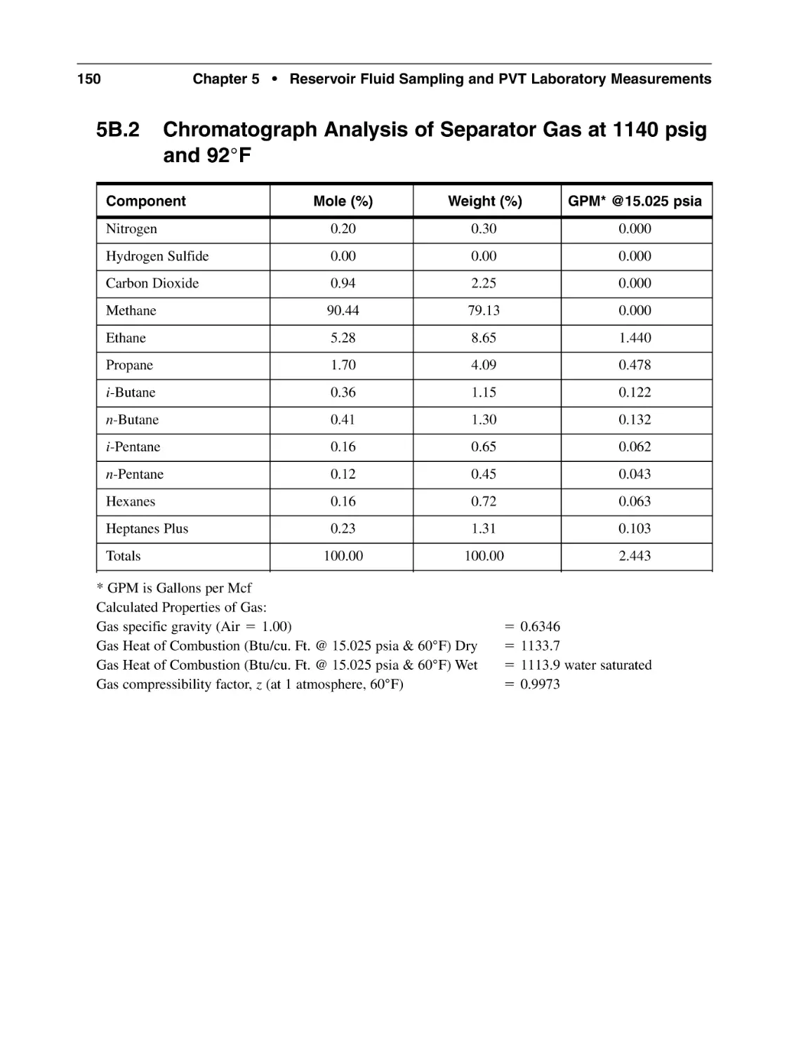
5B.2 Chromatograph Analysis of Separator Gas at 1140 psig and 92°F
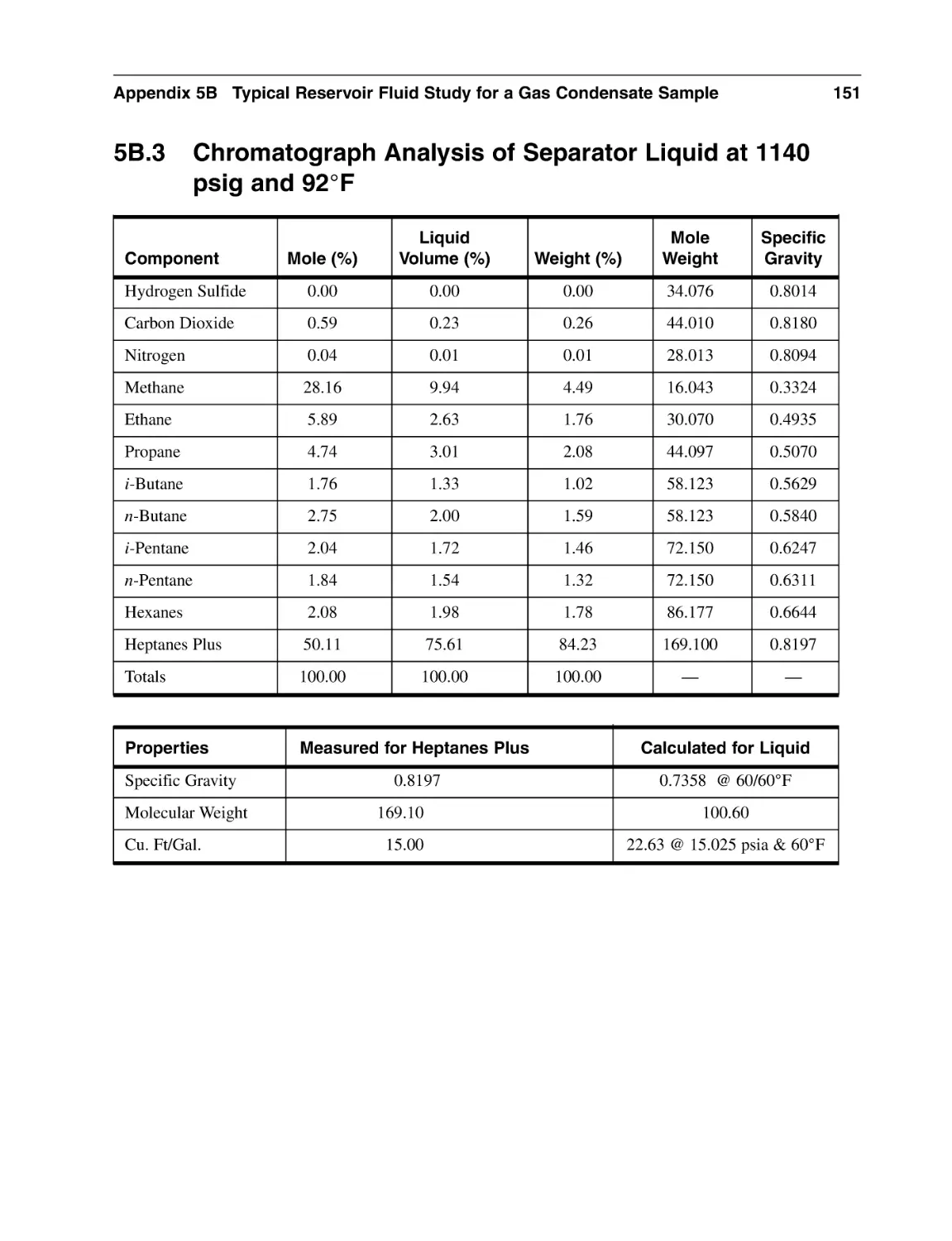
5B.3 Chromatograph Analysis of Separator Liquid at 1140 psig
and 92°F
148
148
150
144
145
146
147
147
151
Contents
5B.4
5B.5
5B.6
5B.7
5B.8
xi
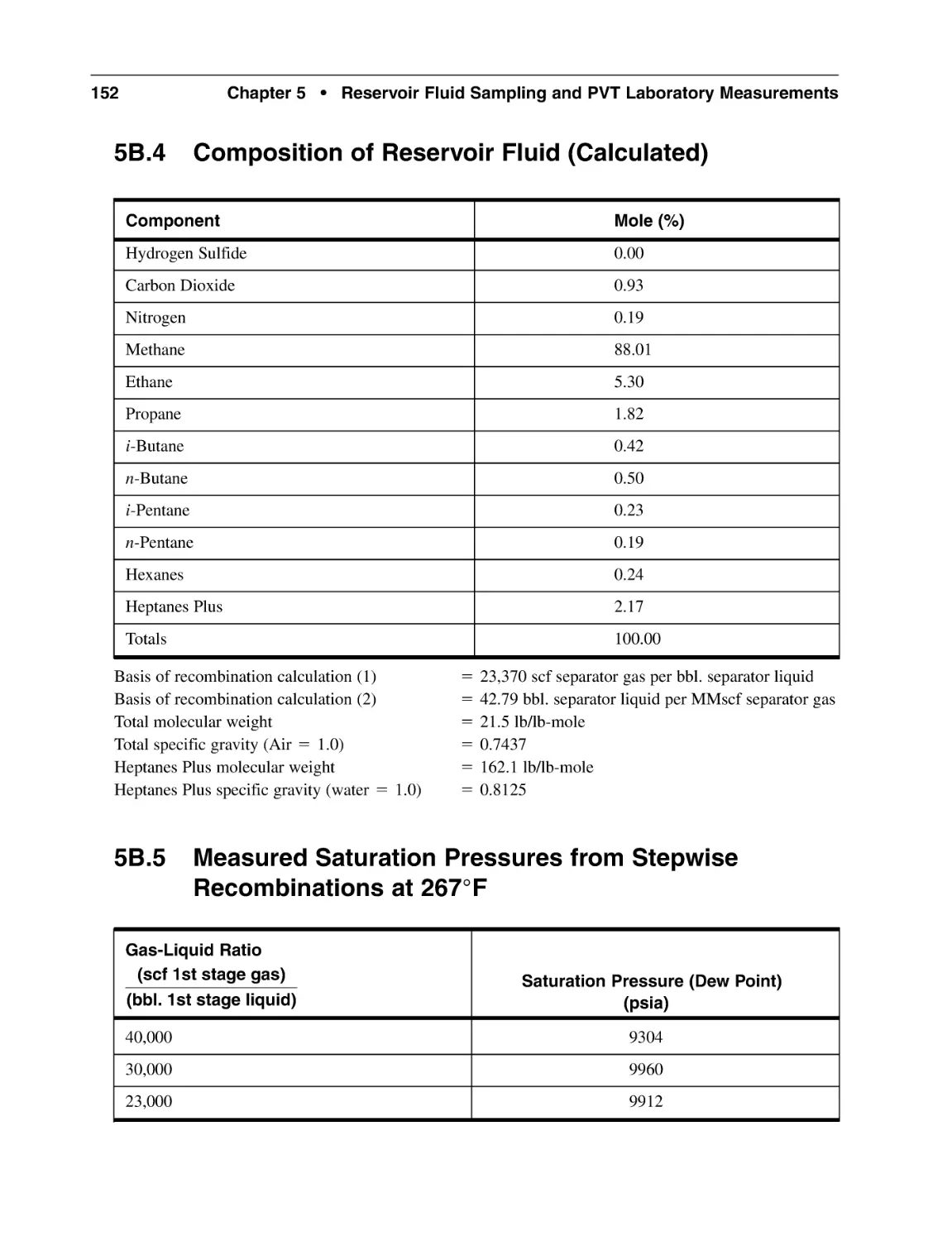
Composition of Reservoir Fluid (Calculated)
Measured Saturation Pressures from Stepwise
Recombinations at 267°F
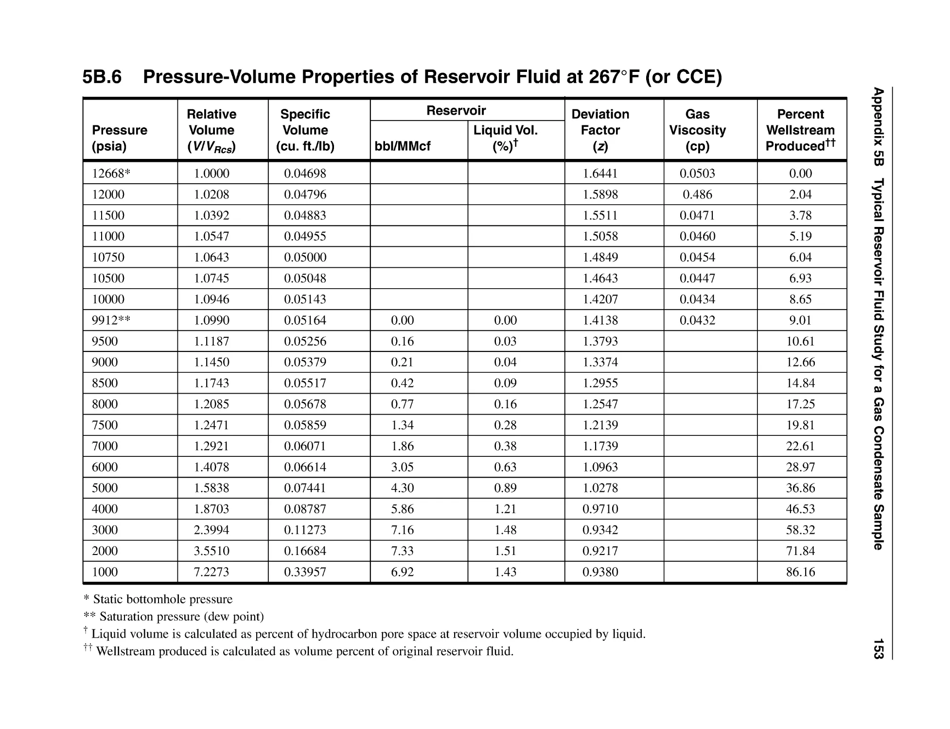
Pressure-Volume Properties of Reservoir Fluid at 267°F (or CCE)
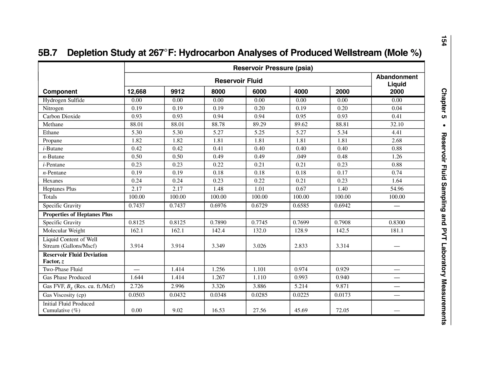
Depletion Study at 267°F: Hydrocarbon Analyses
of Produced Wellstream (Mole %)
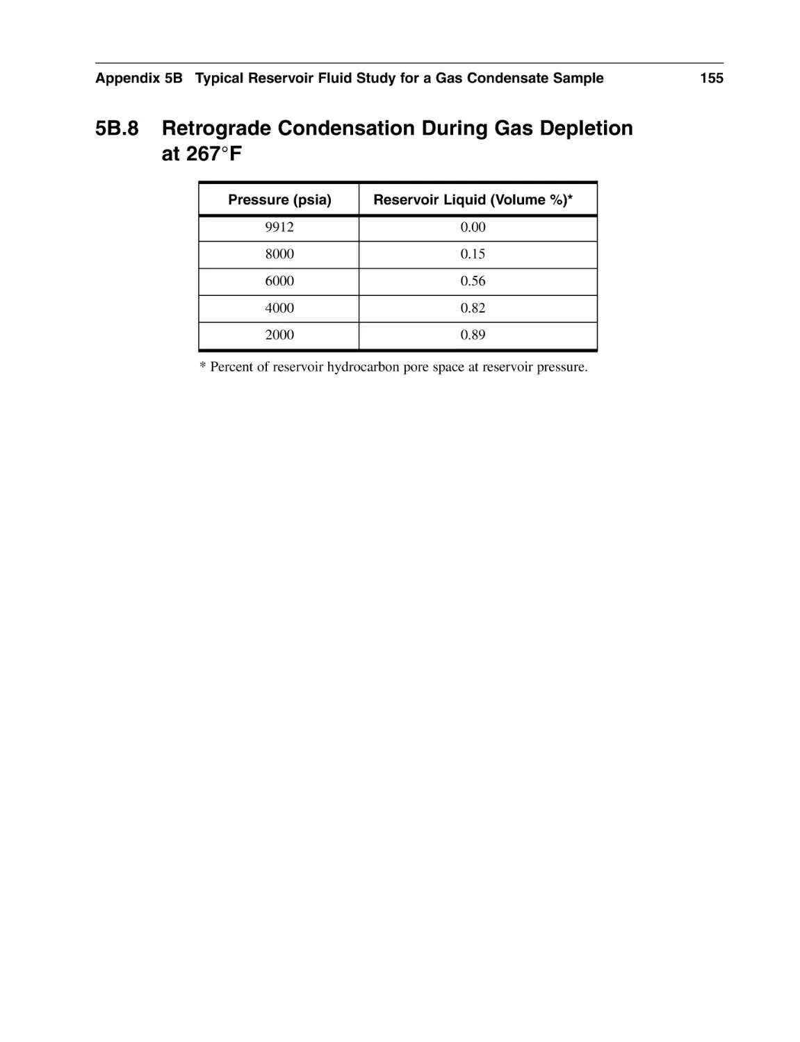
Retrograde Condensation During Gas Depletion at 267°F
152
152
153
154
155
Chapter 6 PVT Properties Predictions from Equations of State
6.1 Historical Introduction to Equations of State (EOS)
6.2 van der Waals (vdW) EOS
6.3 Soave-Redlich-Kwong (SRK) EOS
6.4 Peng-Robinson (PR) EOS
6.5 Phase Equilibrium of Mixtures
6.6 Roots from Cubic EOS
6.7 Volume Translation
6.8 Two-Phase Flash Calculation
6.8.1 Generalized Procedure for Two-Phase Flash Calculations
6.9 Bubble Point and Dew Point Pressure Calculations
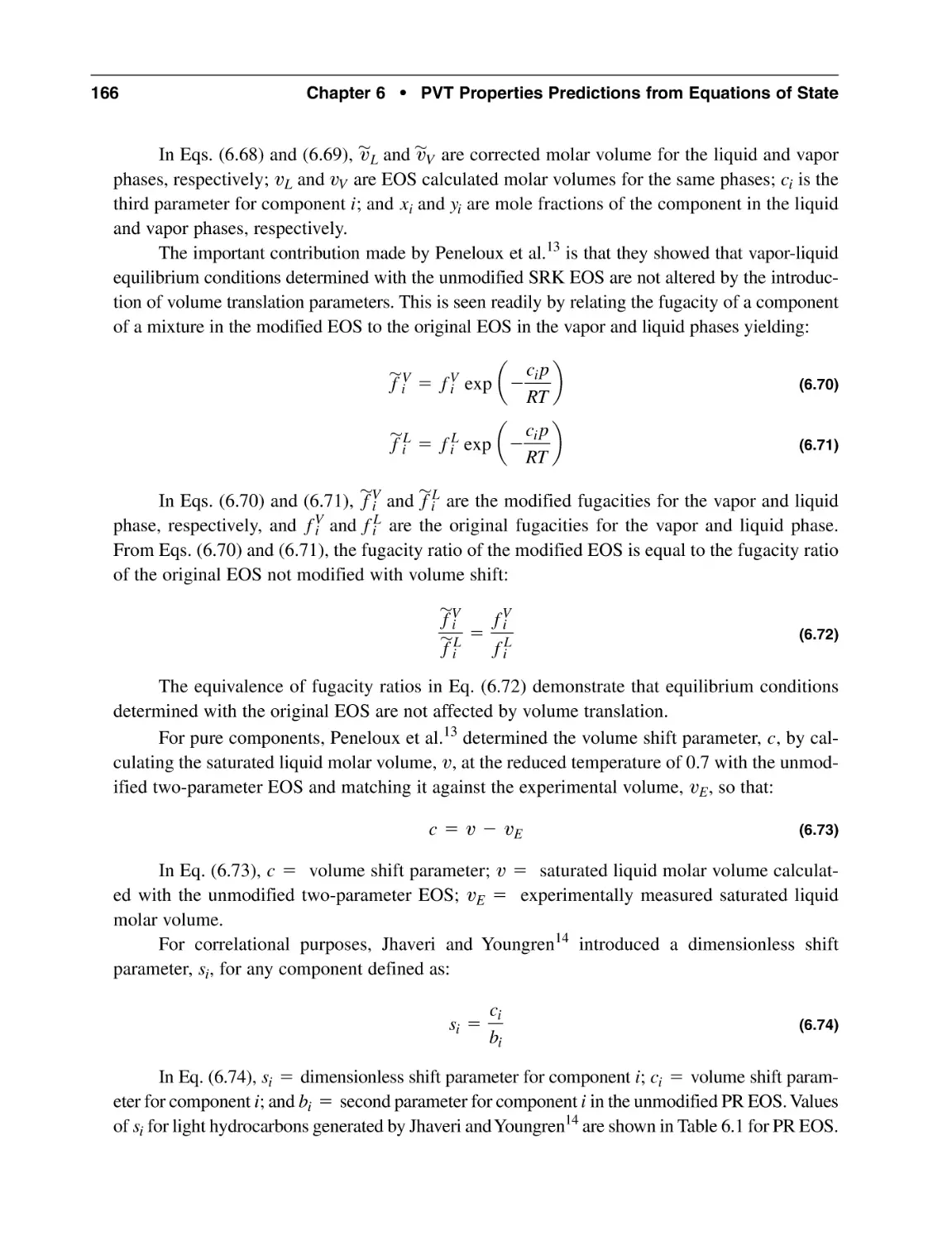
6.10 Characterization of Hydrocarbon Plus Fractions
6.11 Phase Equilibrium Predictions with Equations of State
Nomenclature
Subscripts
Superscripts
Abbreviations
References
157
157
158
159
162
162
164
165
168
169
170
171
174
178
179
179
179
180
Chapter 7 The General Material Balance Equation
7.1 Introduction
7.2 Derivation of the General Material Balance Equation (GMBE)
7.2.1 Development of Terms in the Expression of Equation (7.1)
7.3 The GMBE for Gas Reservoirs
7.4 Discussion on the Application of the GMBE
Nomenclature
Subscripts
Abbreviations
References
183
183
183
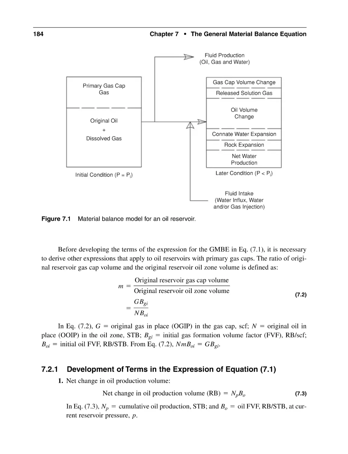
184
187
188
189
189
189
190
xii
Contents
Chapter 8 Gas Reservoirs
8.1 Introduction
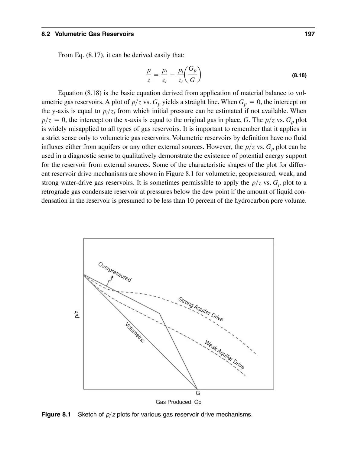
8.2 Volumetric Gas Reservoirs
8.2.1 Volumetric Calculations for Dry Gas Reservoirs
8.2.2 Volumetric Calculations for Wet Gas and Retrograde
Gas Condensate Reservoirs
8.2.3 Material Balance for Volumetric Dry Gas, Wet Gas,
and Retrograde Gas Condensate Reservoirs
8.3 Gas Reservoirs with Water Influx
8.3.1 Volumetric Approach
8.3.2 Material Balance Approach
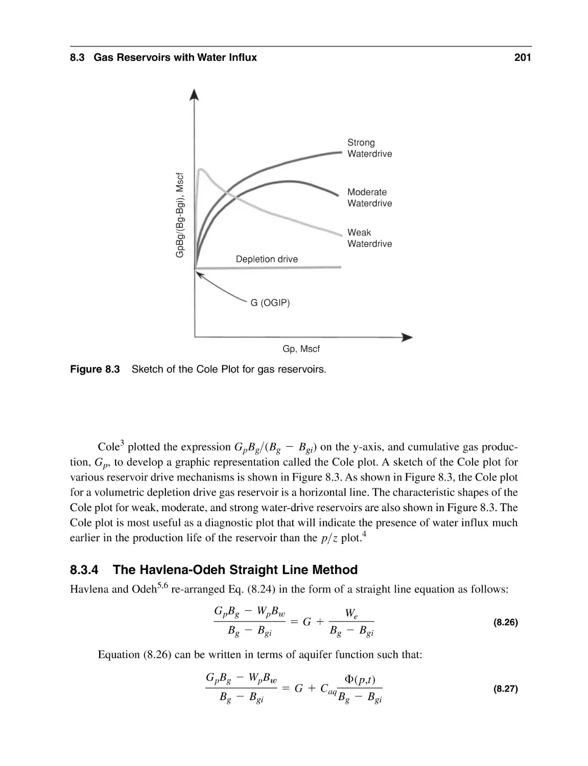
8.3.3 The Cole Plot
8.3.4 The Havlena-Odeh Straight Line Method
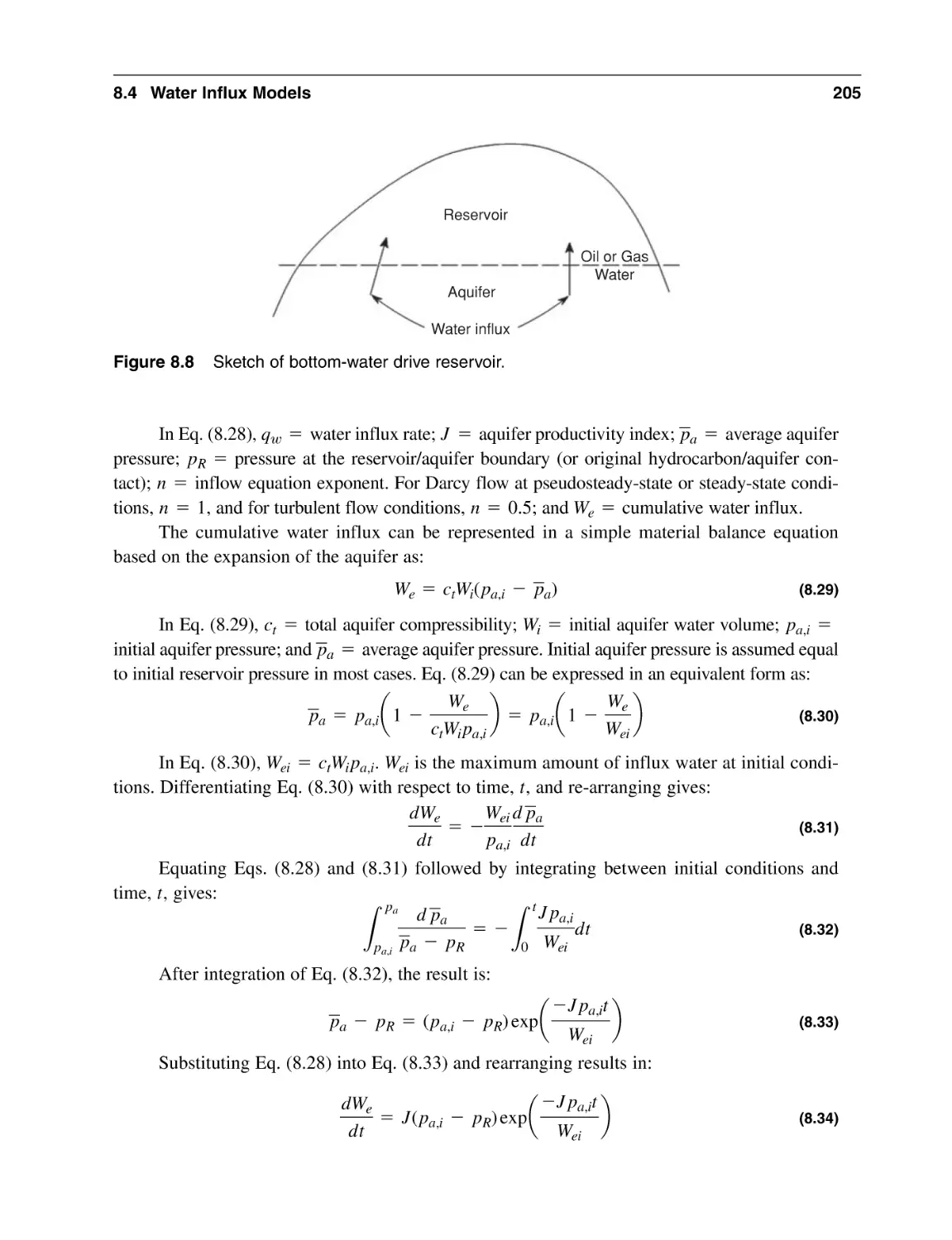
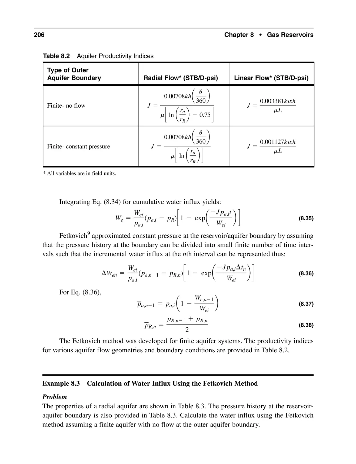
8.4 Water Influx Models
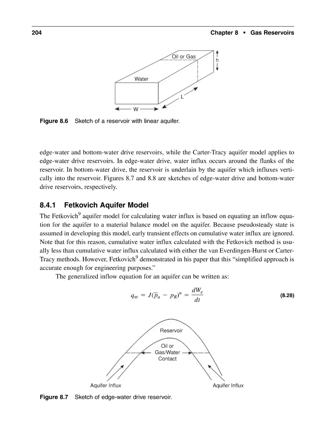
8.4.1 Fetkovich Aquifer Model
8.4.2 Carter-Tracy Aquifer Model
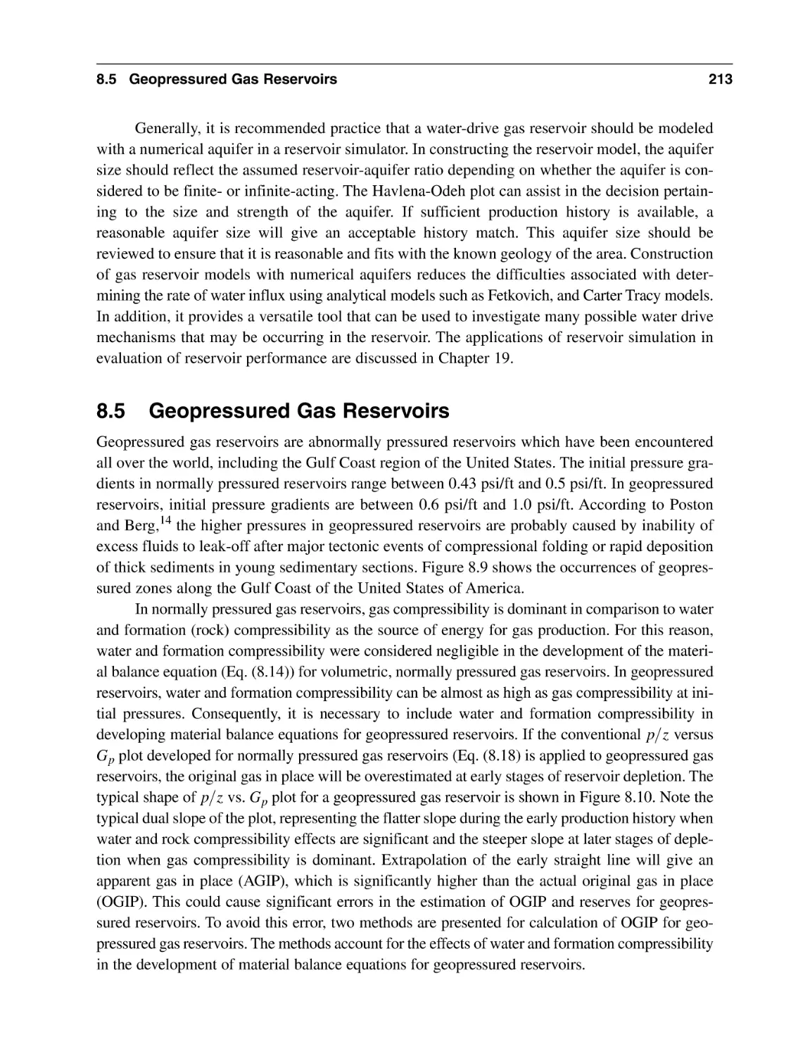
8.5 Geopressured Gas Reservoirs
8.5.1 The Ramagost and Farshad Method
8.5.2 The Roach Method
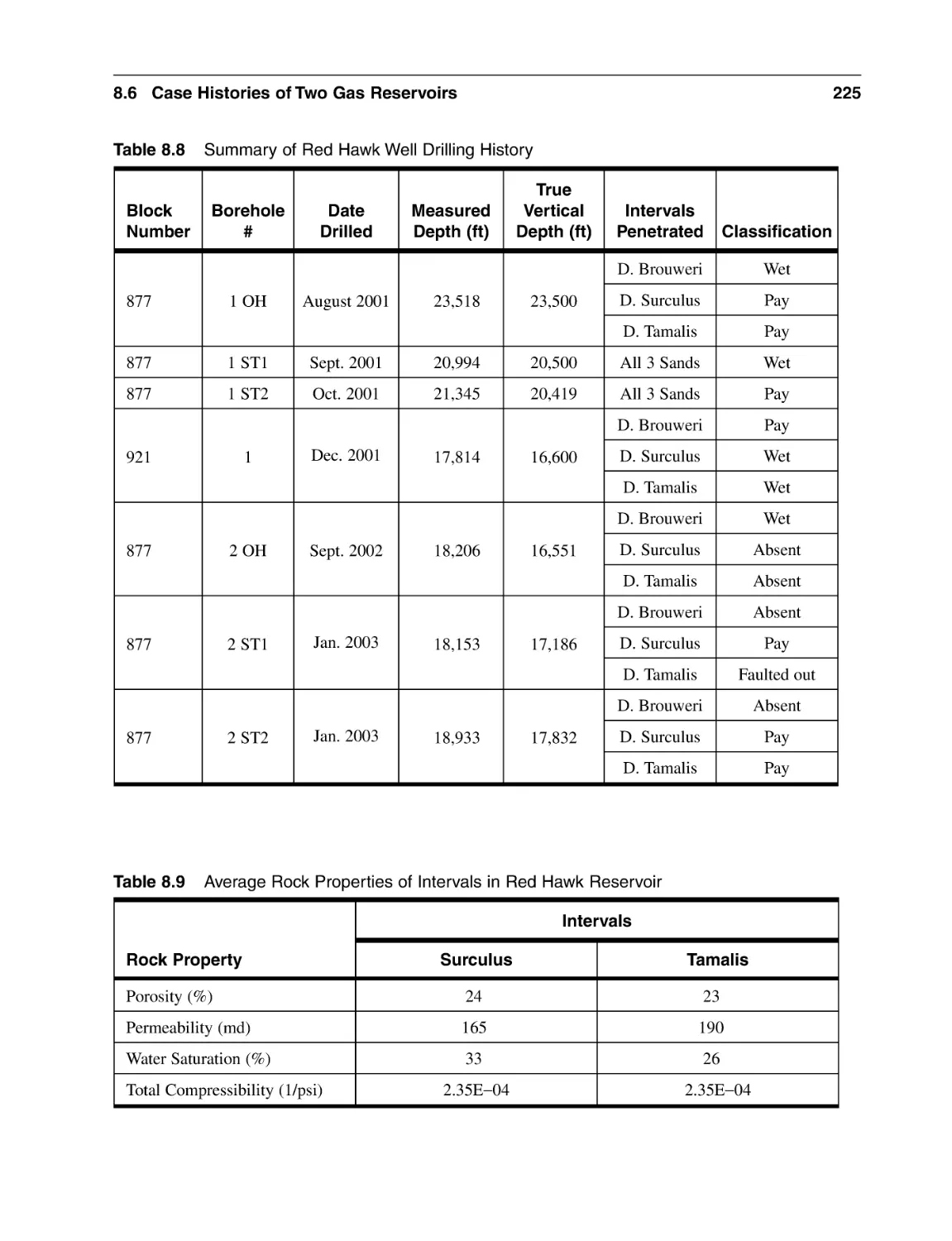
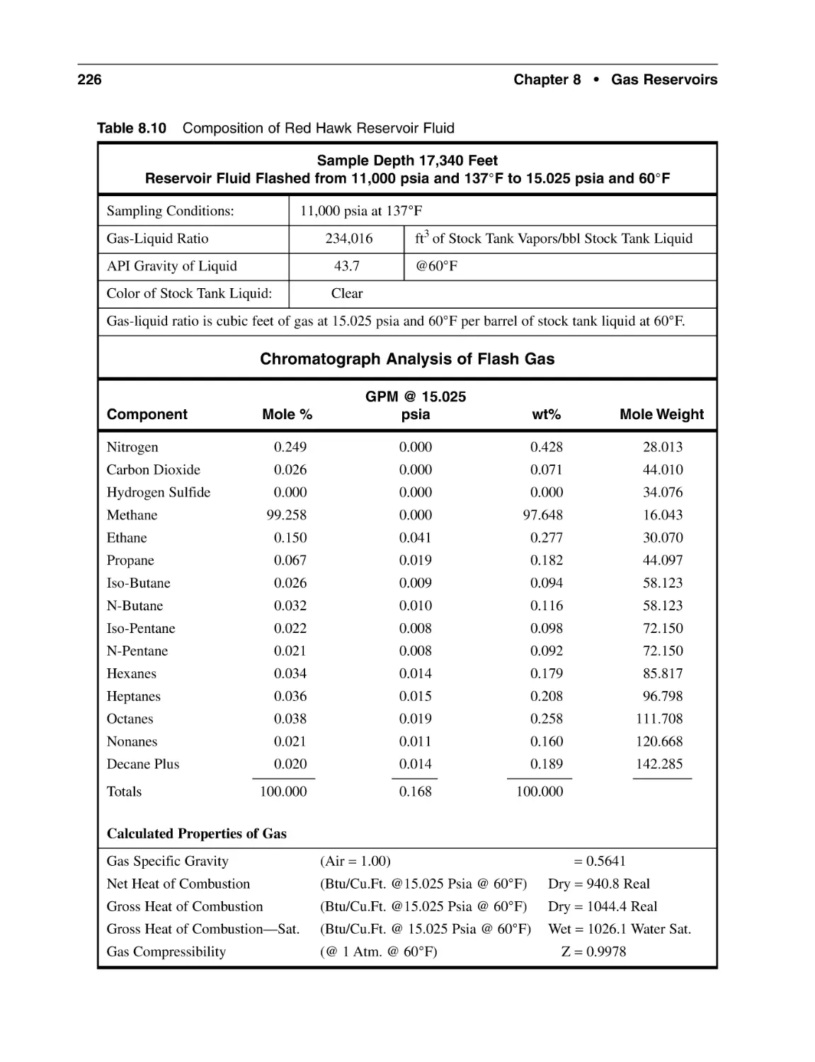
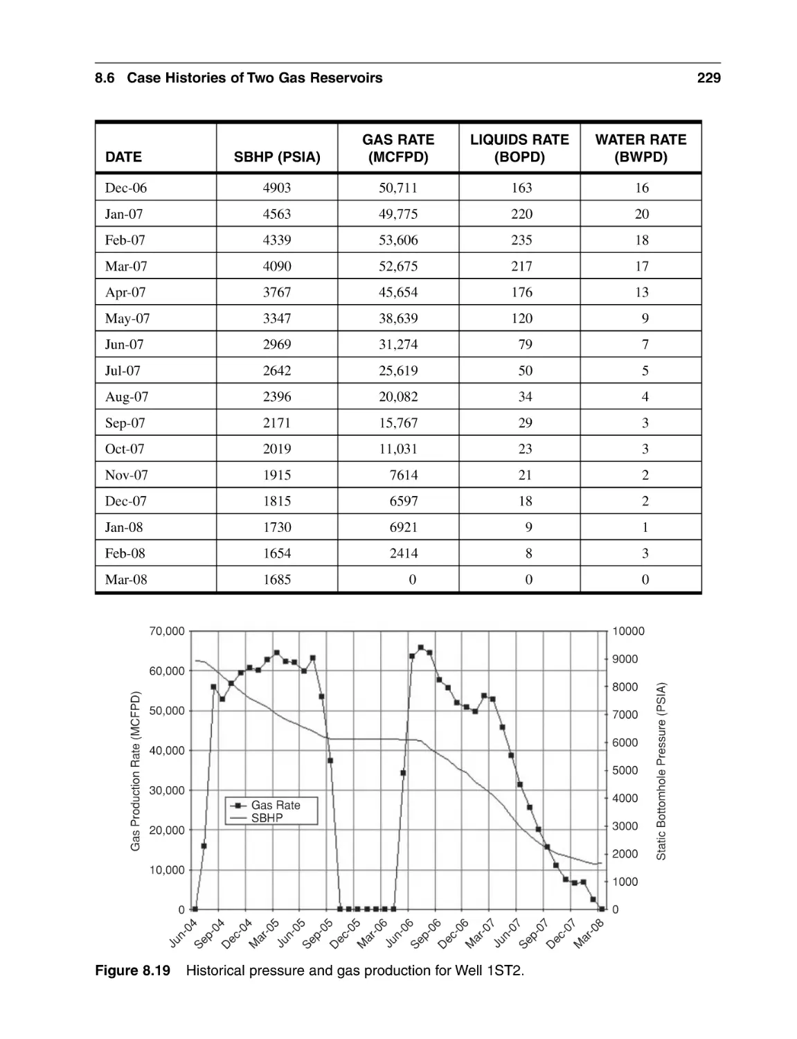
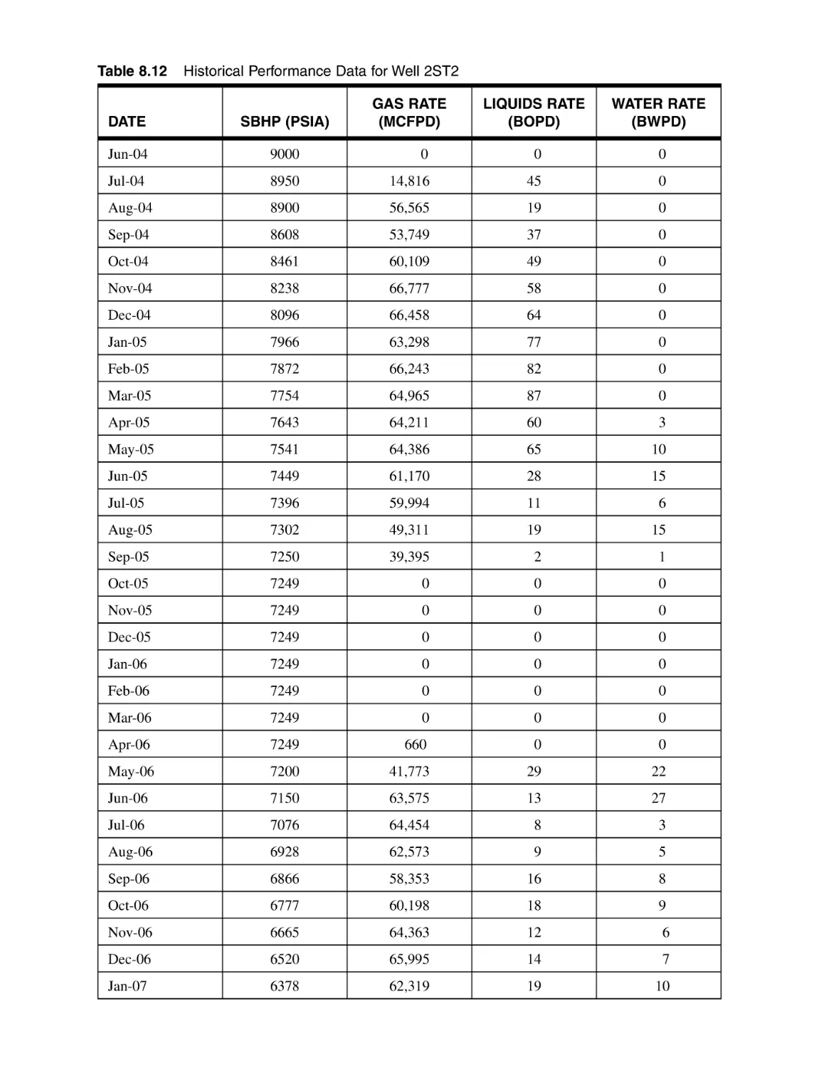
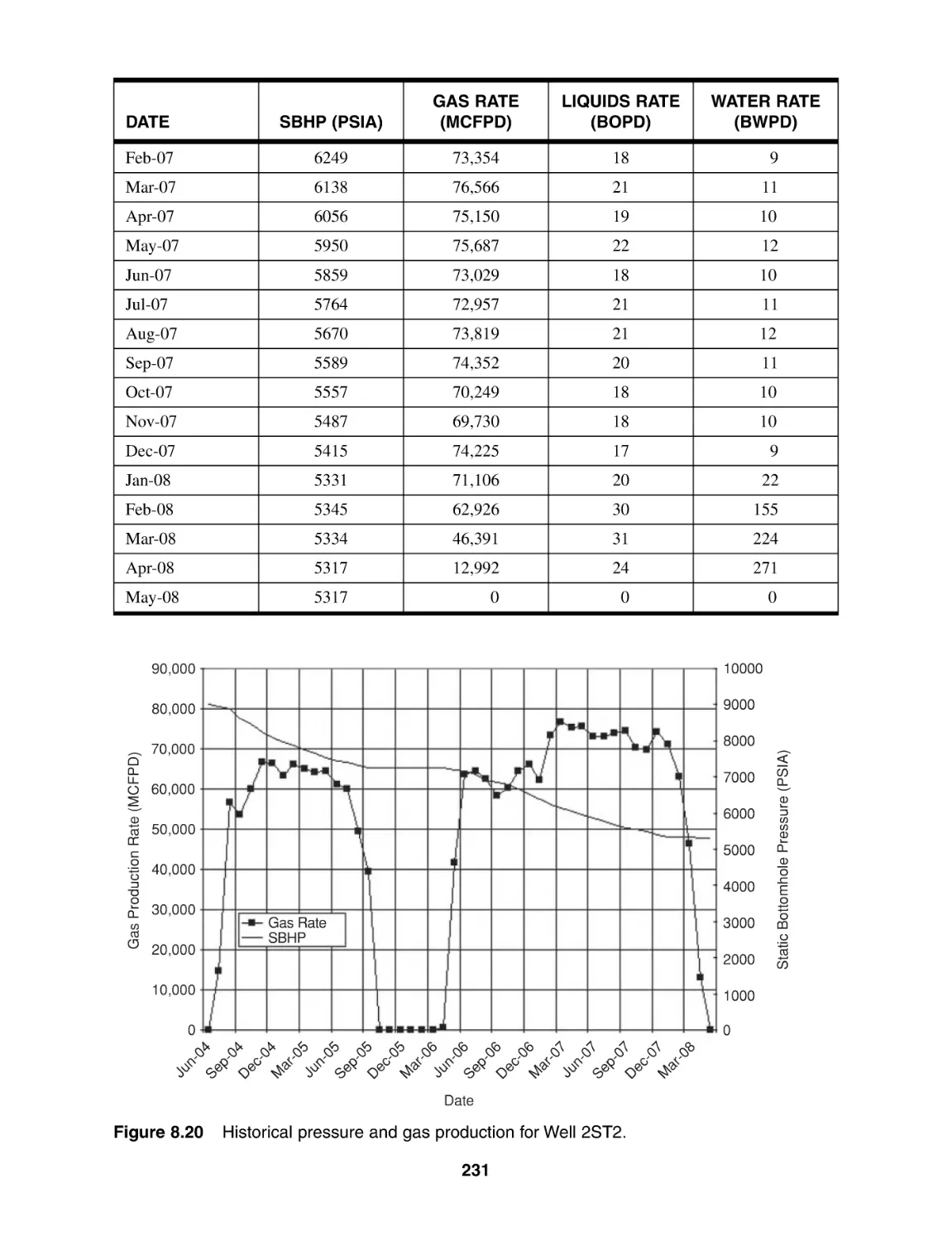
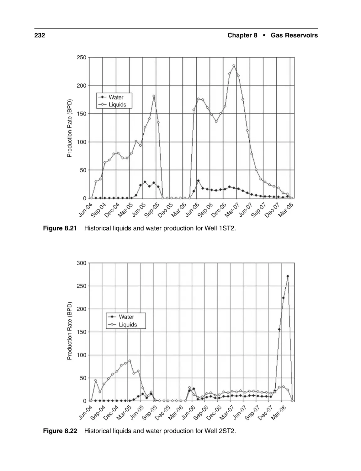
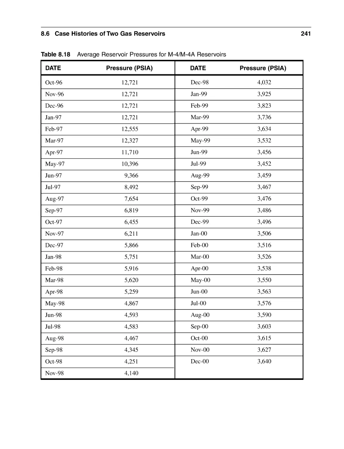
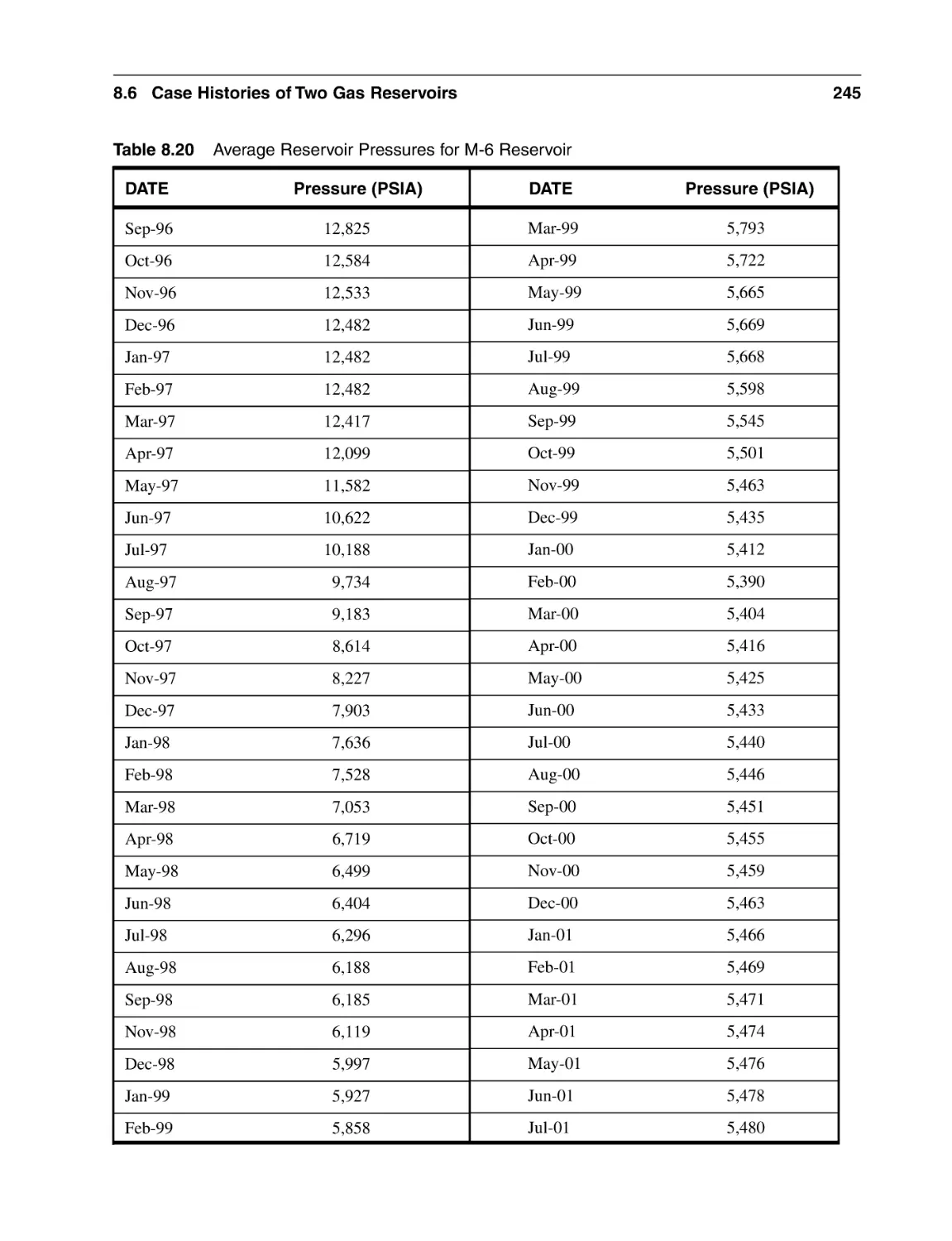
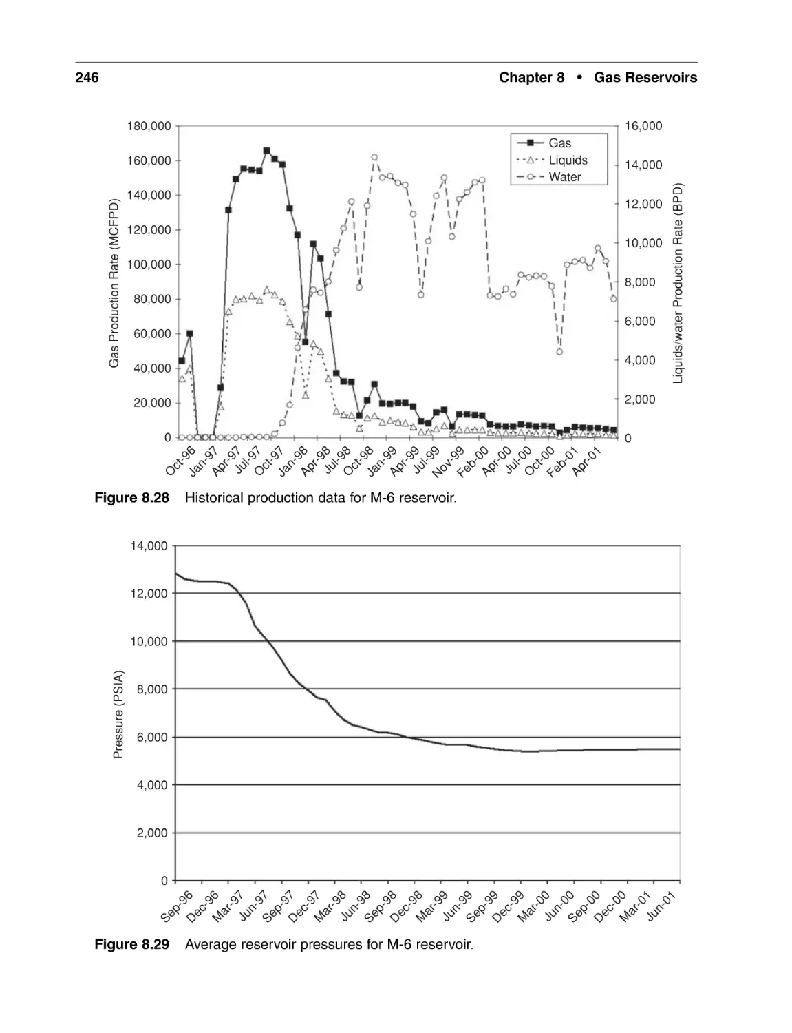
8.6 Case Histories of Two Gas Reservoirs
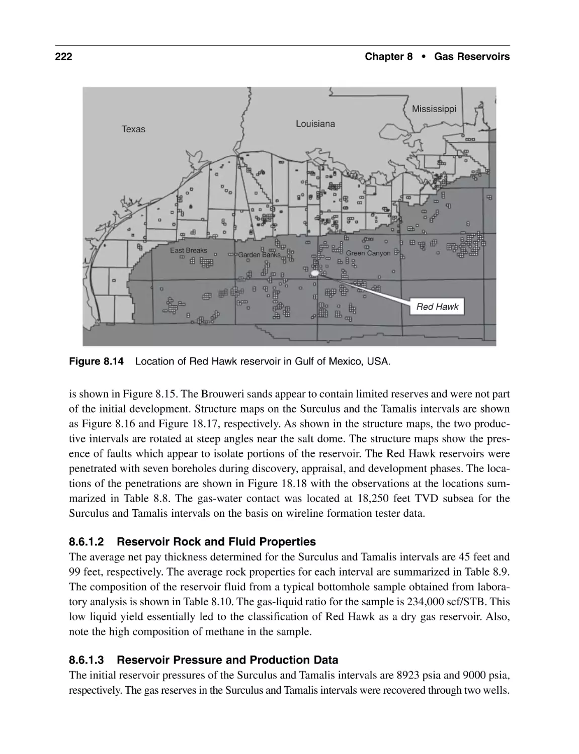
8.6.1 The Case History of Red Hawk Reservoir
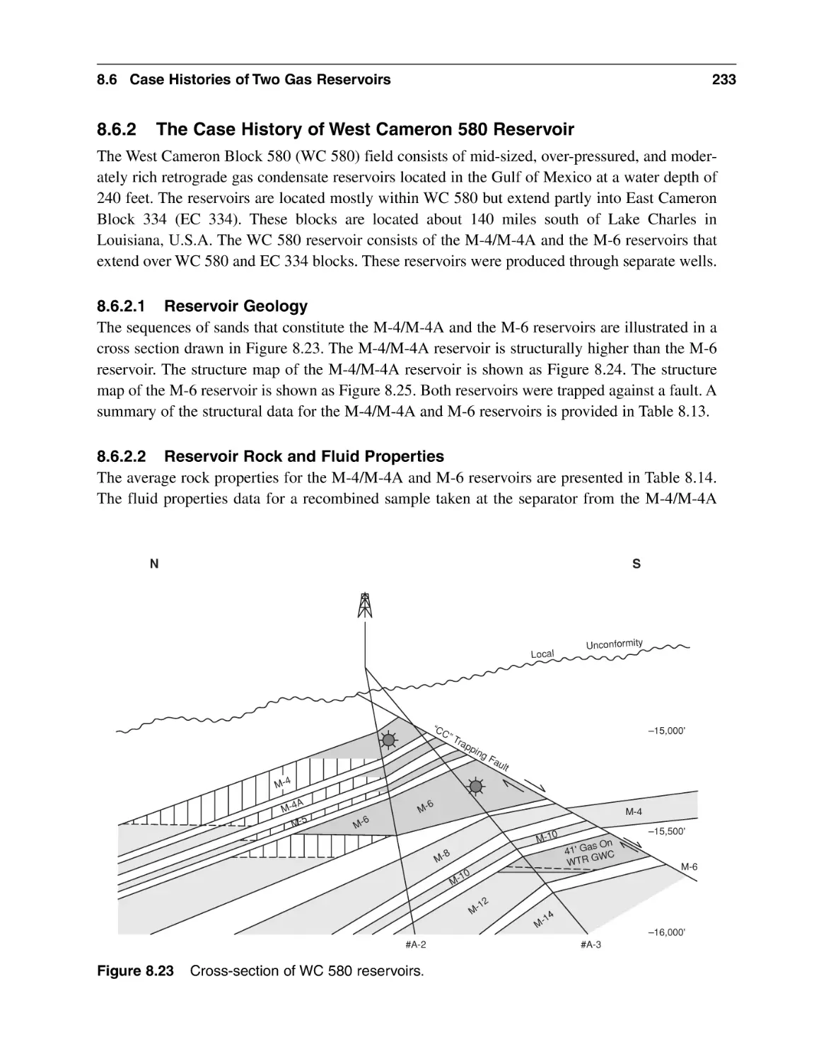
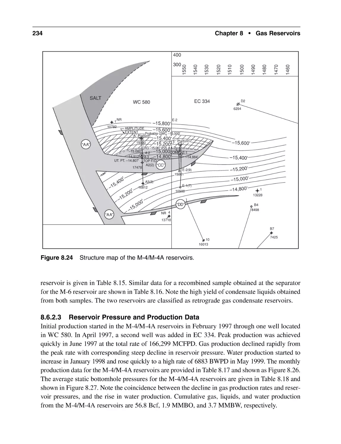
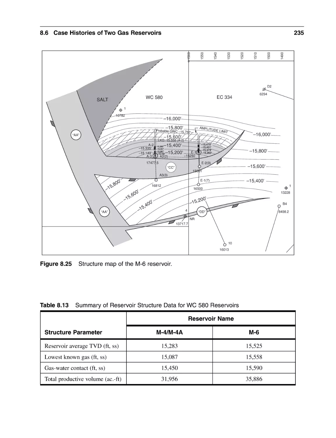
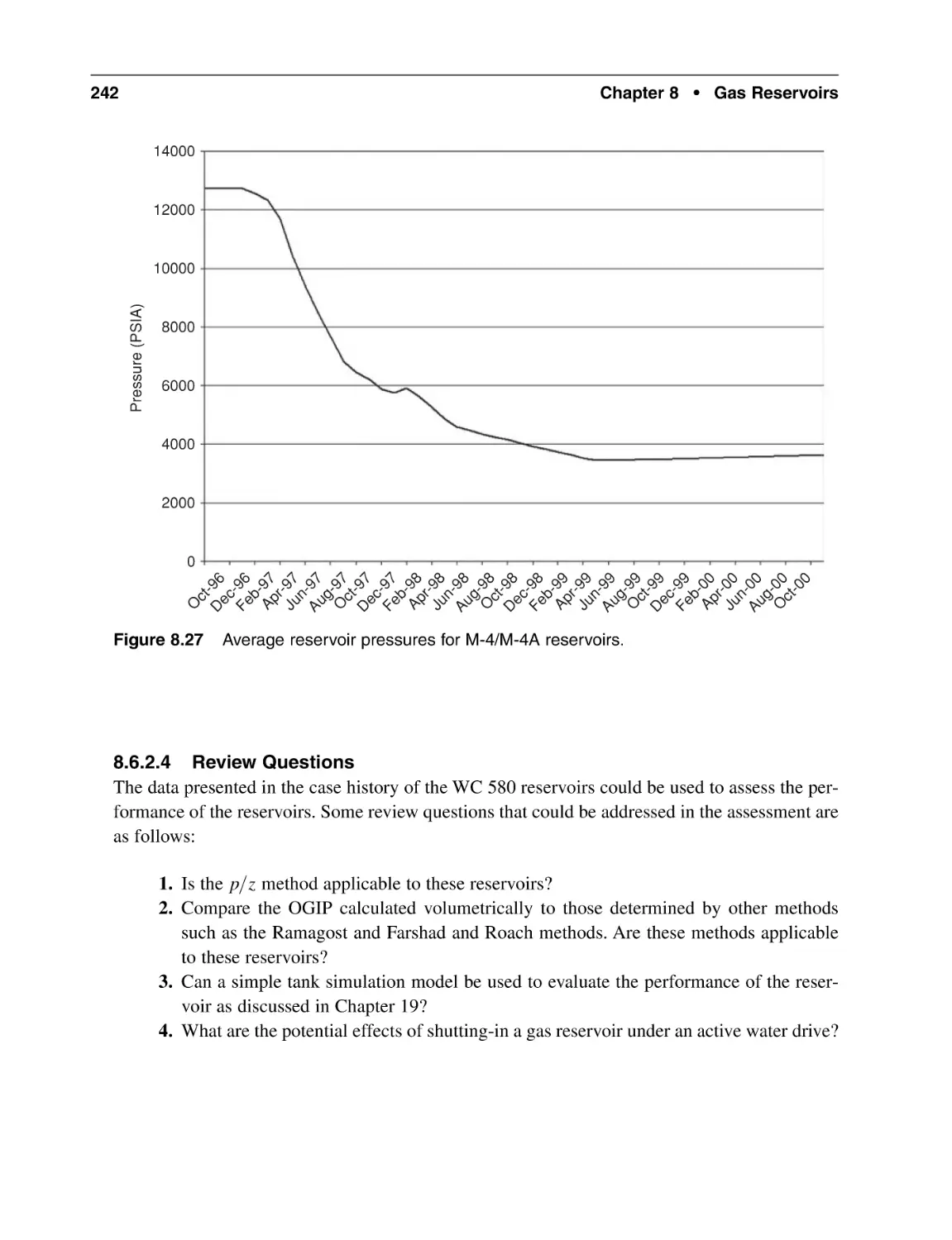
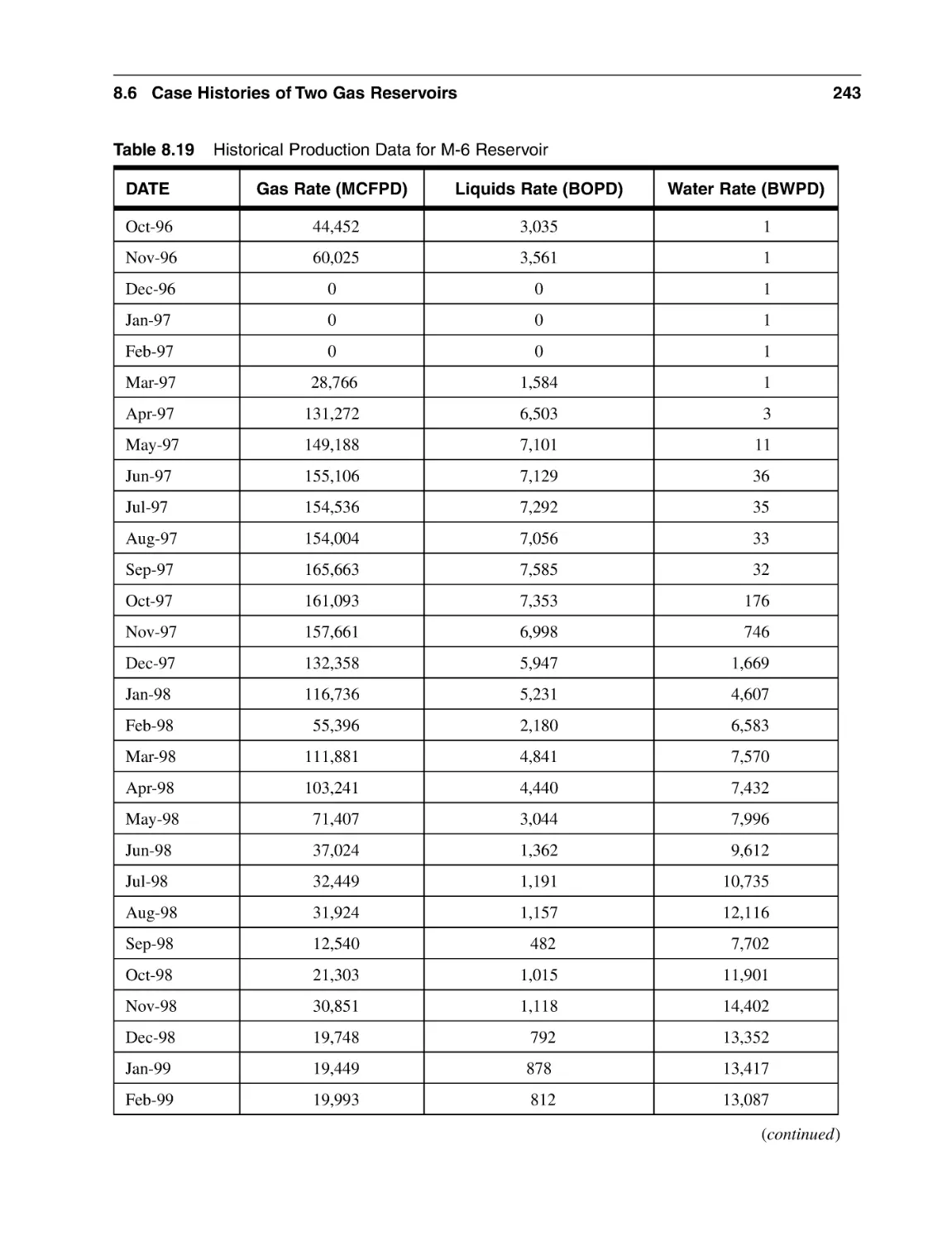
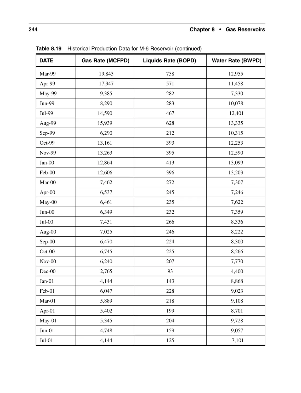
8.6.2 The Case History of West Cameron 580 Reservoir
Nomenclature
Subscripts
Abbreviations
References
General Reading
191
191
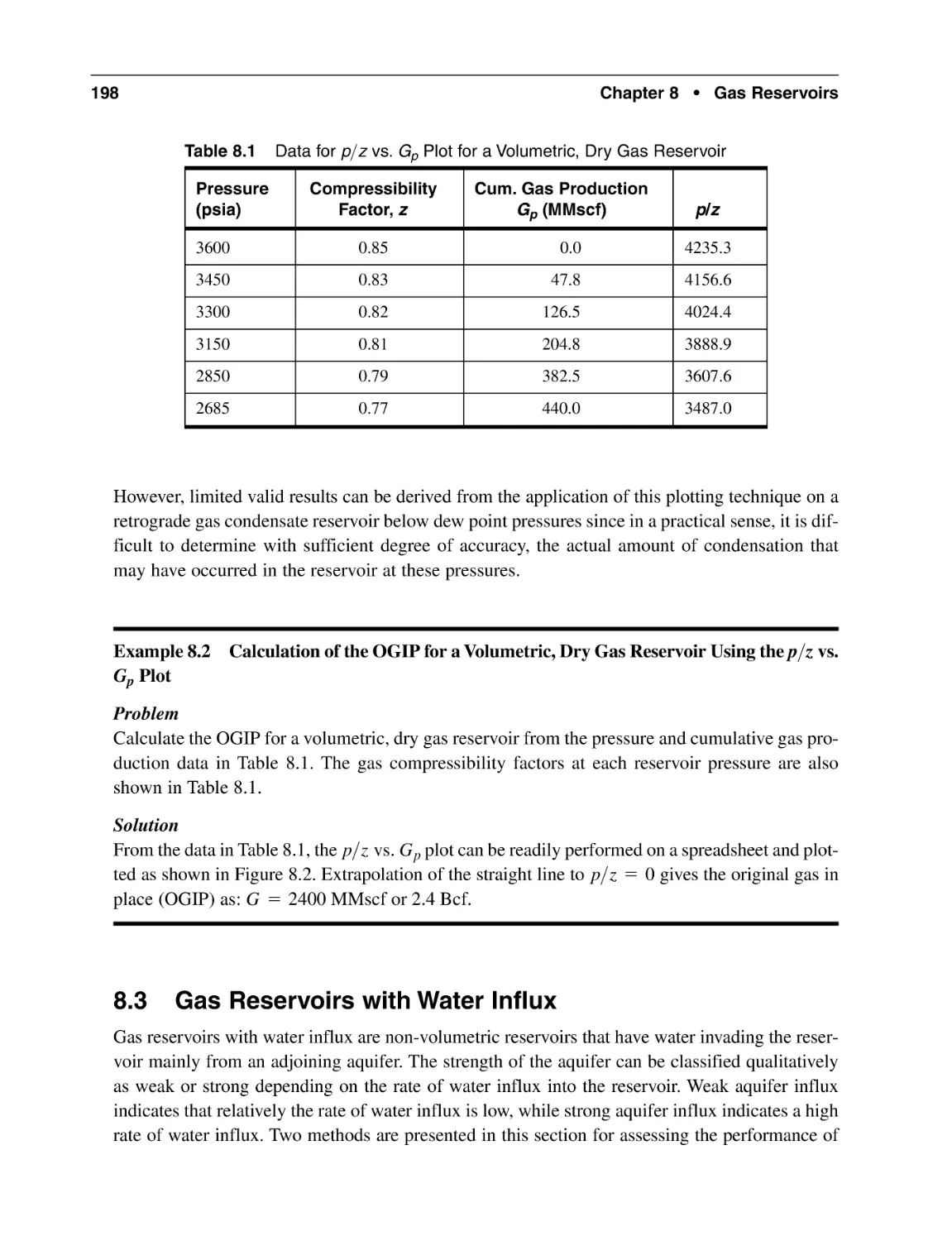
192
192
193
196
198
199
200
200
201
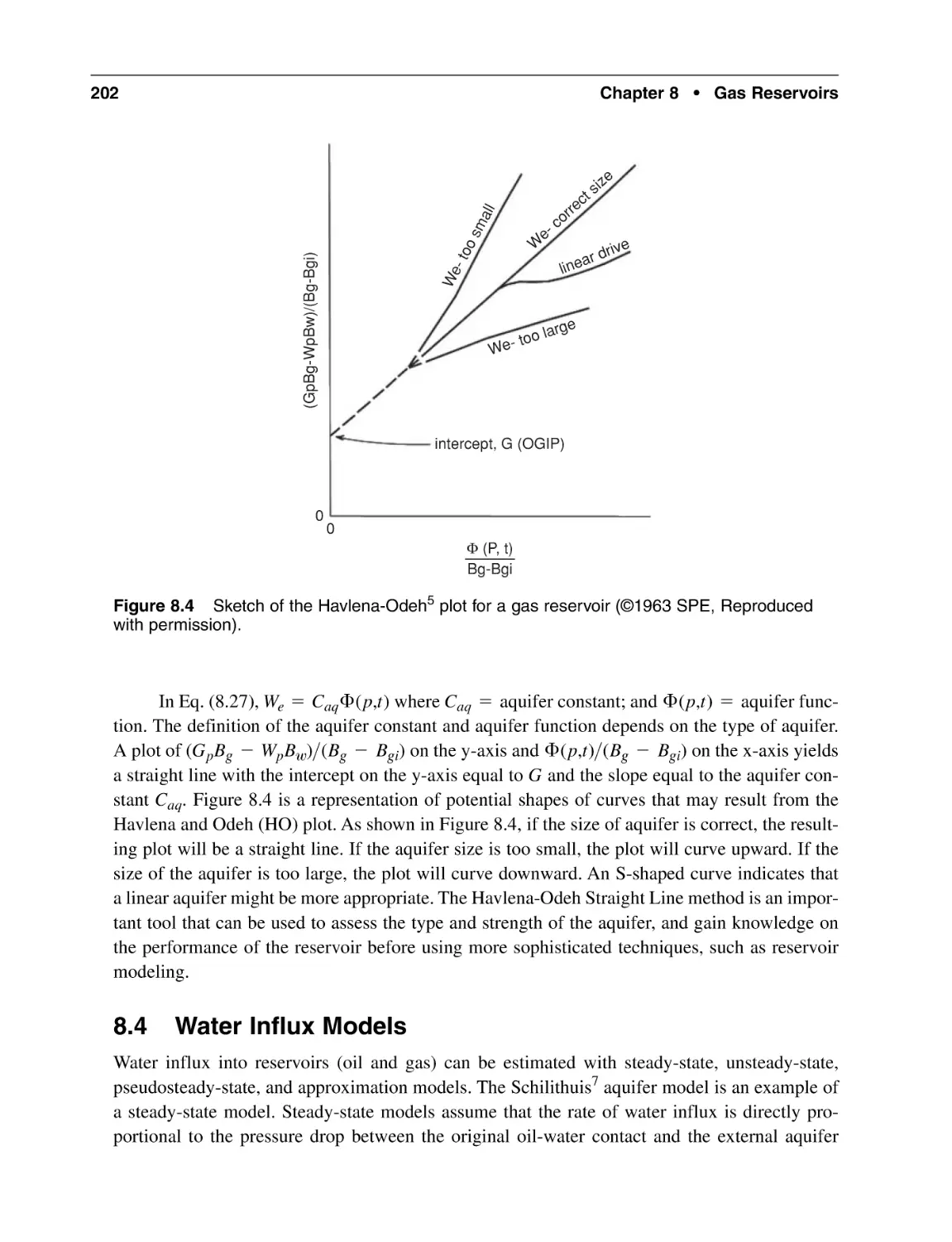
202
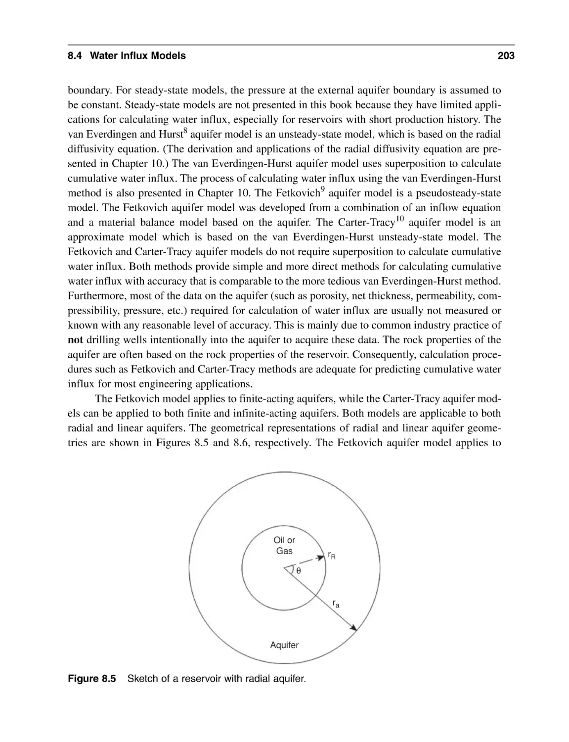
204
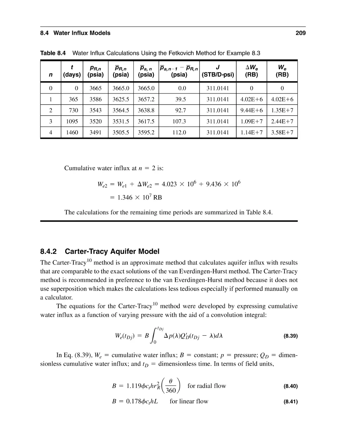
209
213
214
217
221
221
233
247
248
248
248
250
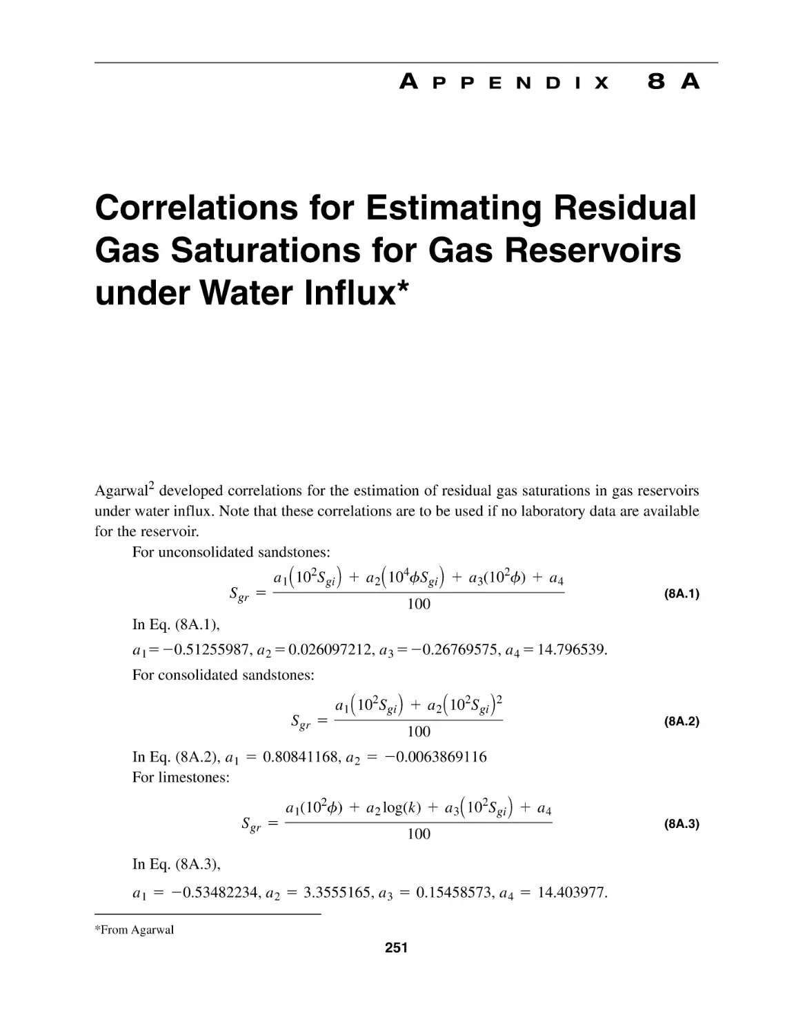
Appendix 8A Correlations for Estimating Residual Gas Saturations
for Gas Reservoirs under Water Influx
251
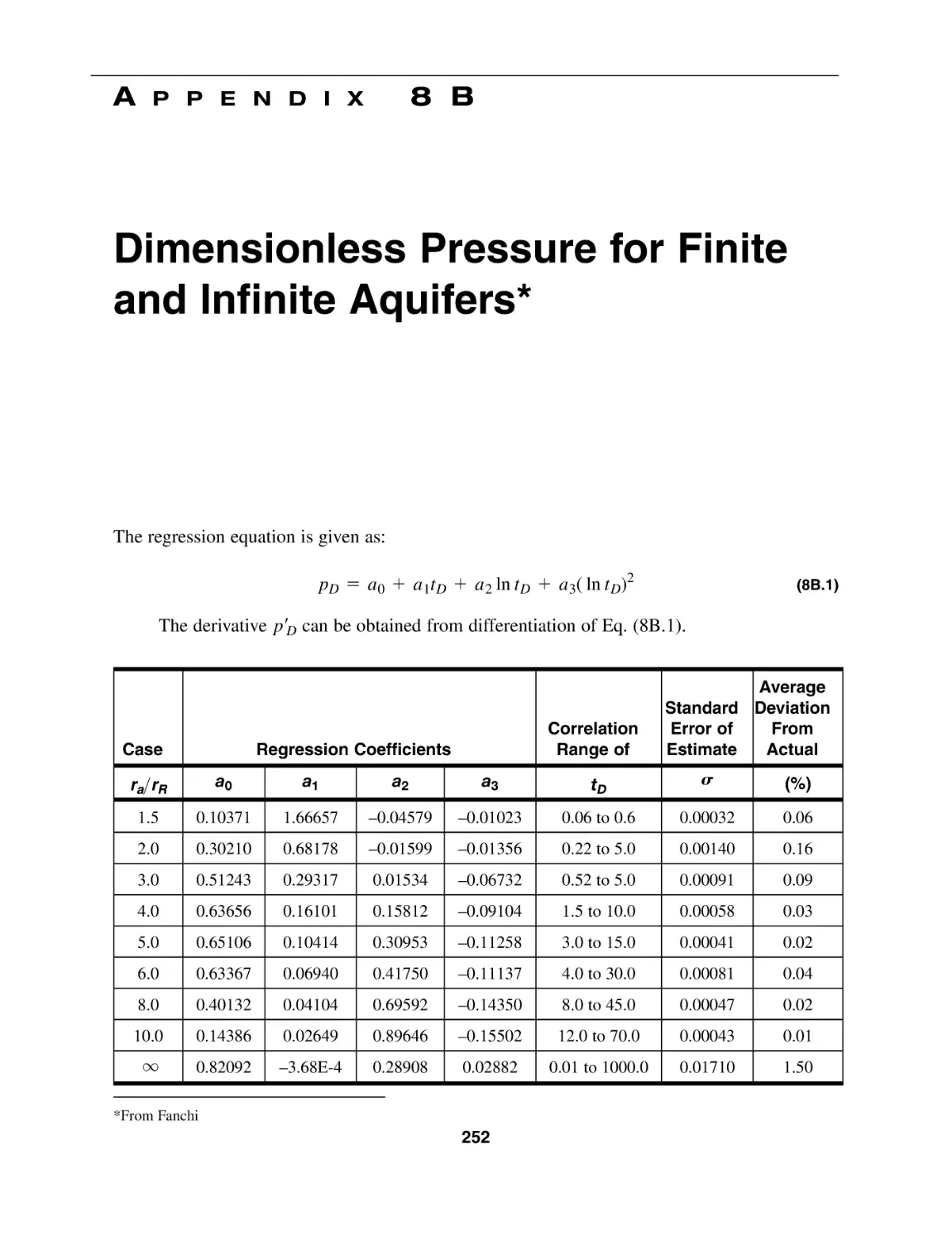
Appendix 8B
252
Dimensionless Pressure for Finite and Infinite Aquifers
Appendix 8C Dimensionless Pressure for Infinite Aquifers
253
Chapter 9 Oil Reservoirs
9.1 Introduction
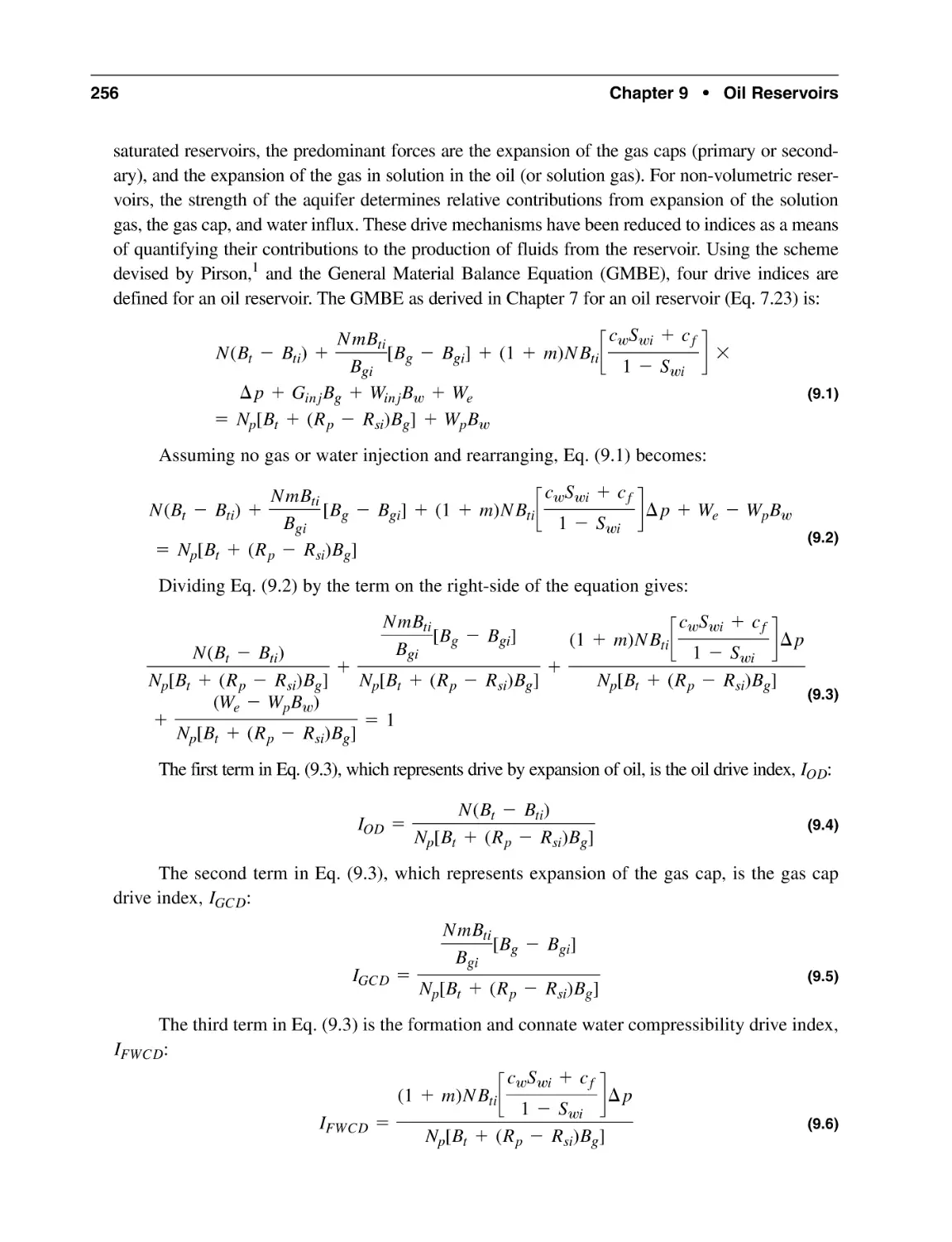
9.2 Oil Reservoir Drive Mechanisms
255
255
255
Contents
9.3
9.4
Gravity Drainage Mechanism
Volumetric Undersaturated Oil Reservoirs
9.4.1 Volume Calculations Above Bubble Point Pressure
9.4.2 Volume Calculations Below Bubble Point Pressure
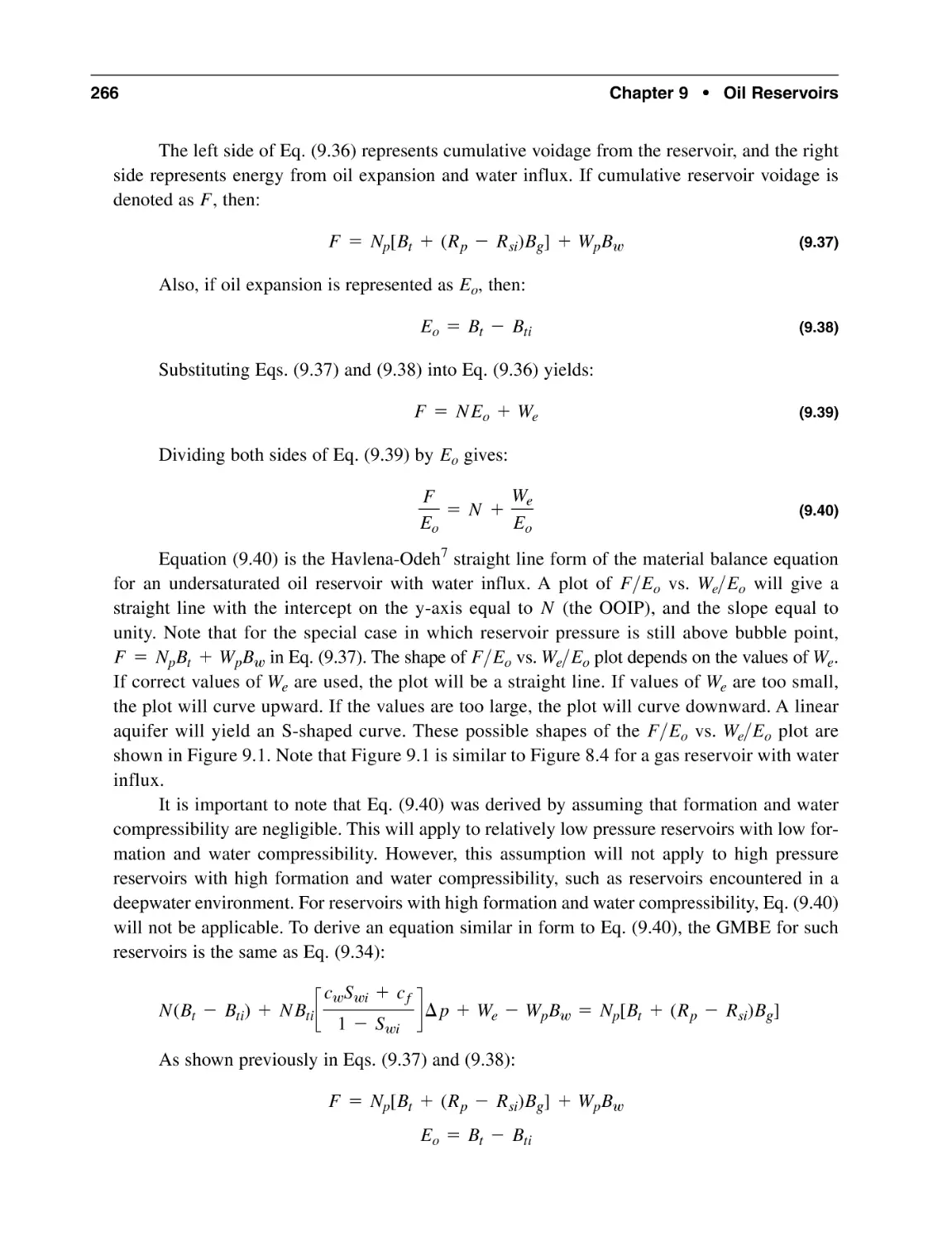
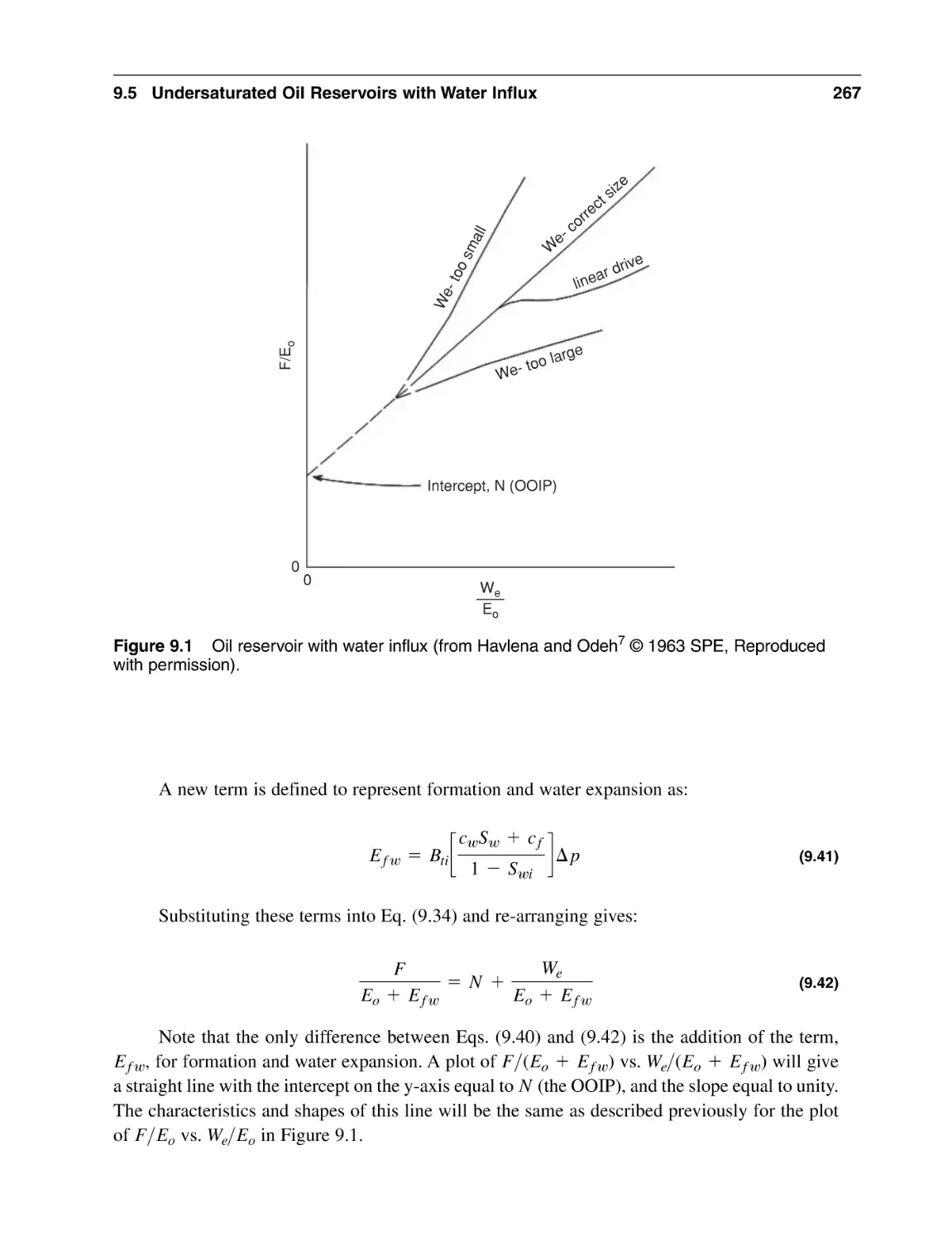
9.5 Undersaturated Oil Reservoirs with Water Influx
9.5.1 Volume Method
9.5.2 Material Balance Method
9.6 Volumetric Saturated Oil Reservoirs
9.6.1 Volume Method
9.6.2 Material Balance Method
9.7 Material Balance Approach for Saturated Oil Reservoirs
with Water Influx
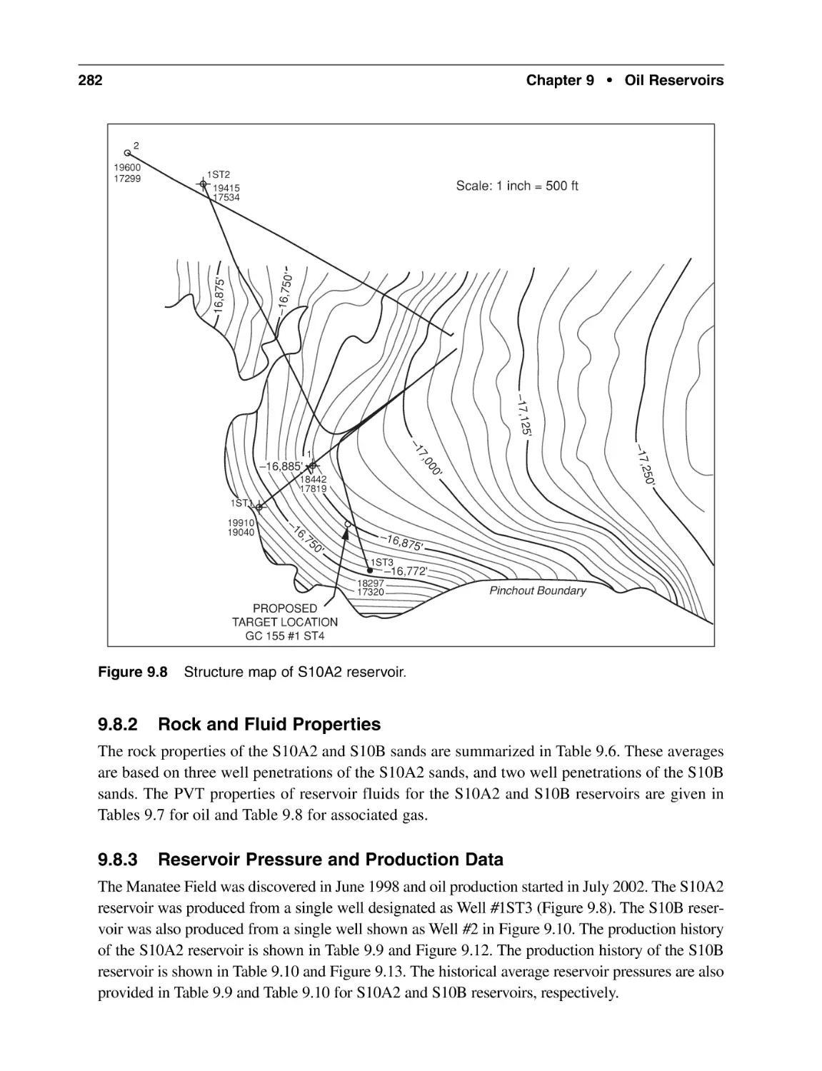
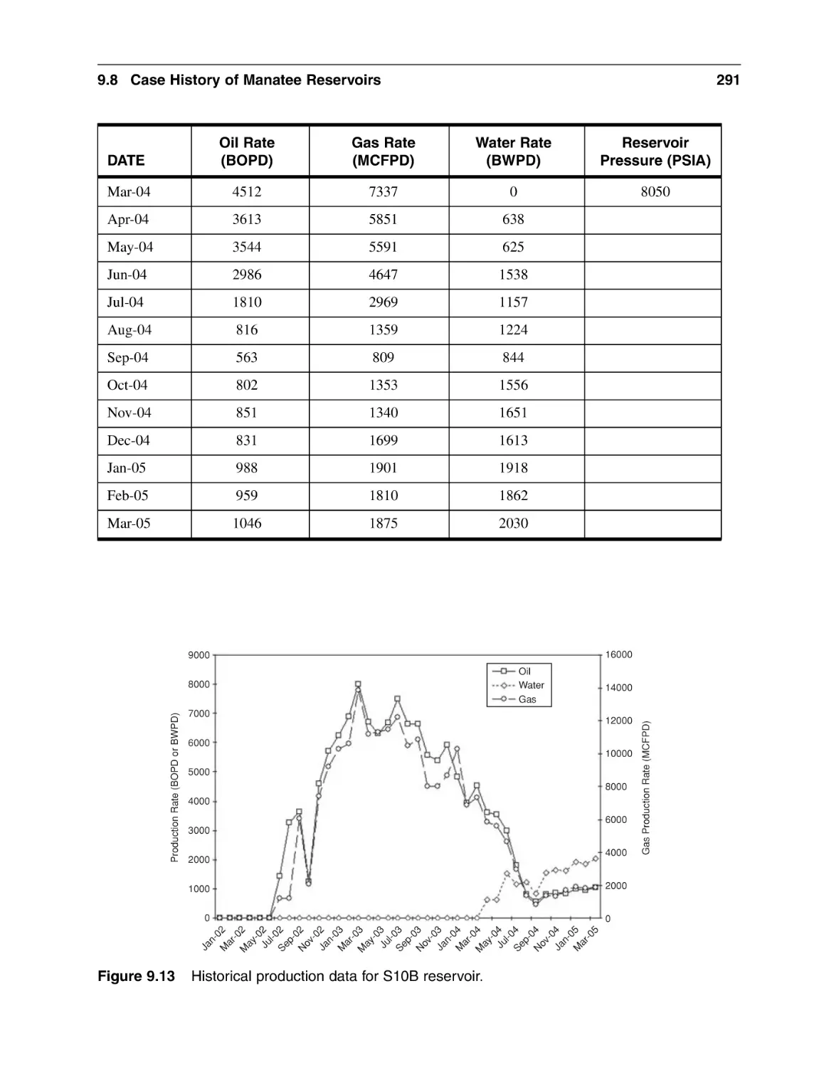
9.8 Case History of Manatee Reservoirs
9.8.1 Reservoir Geology
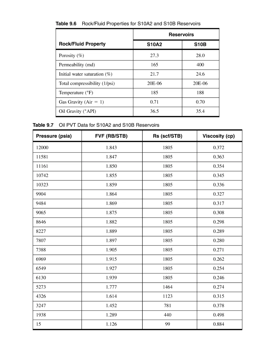
9.8.2 Rock and Fluid Properties
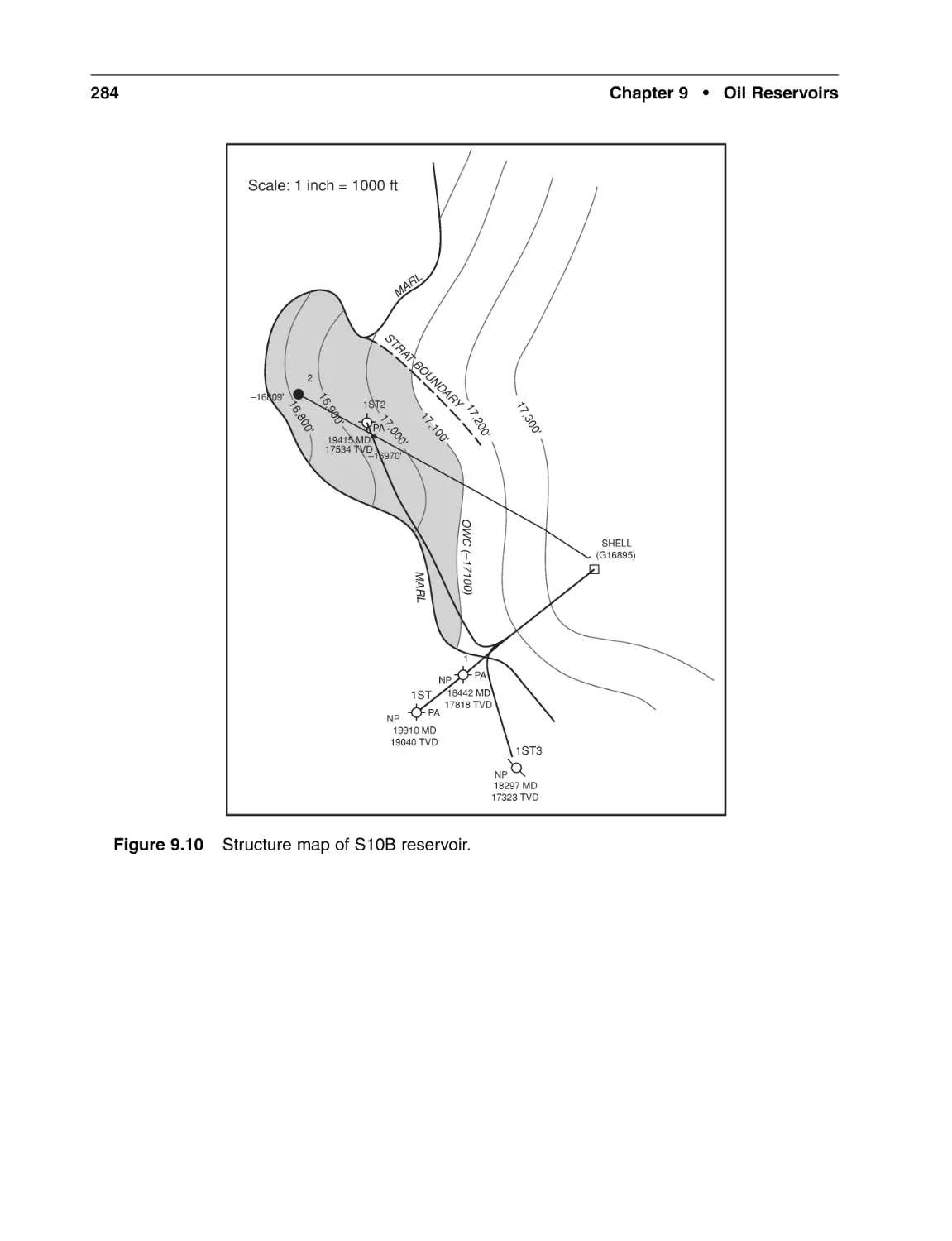
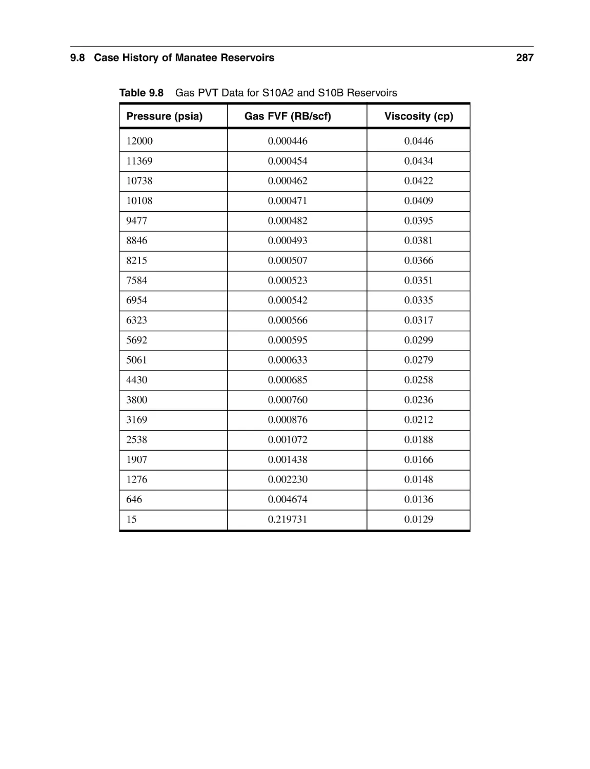
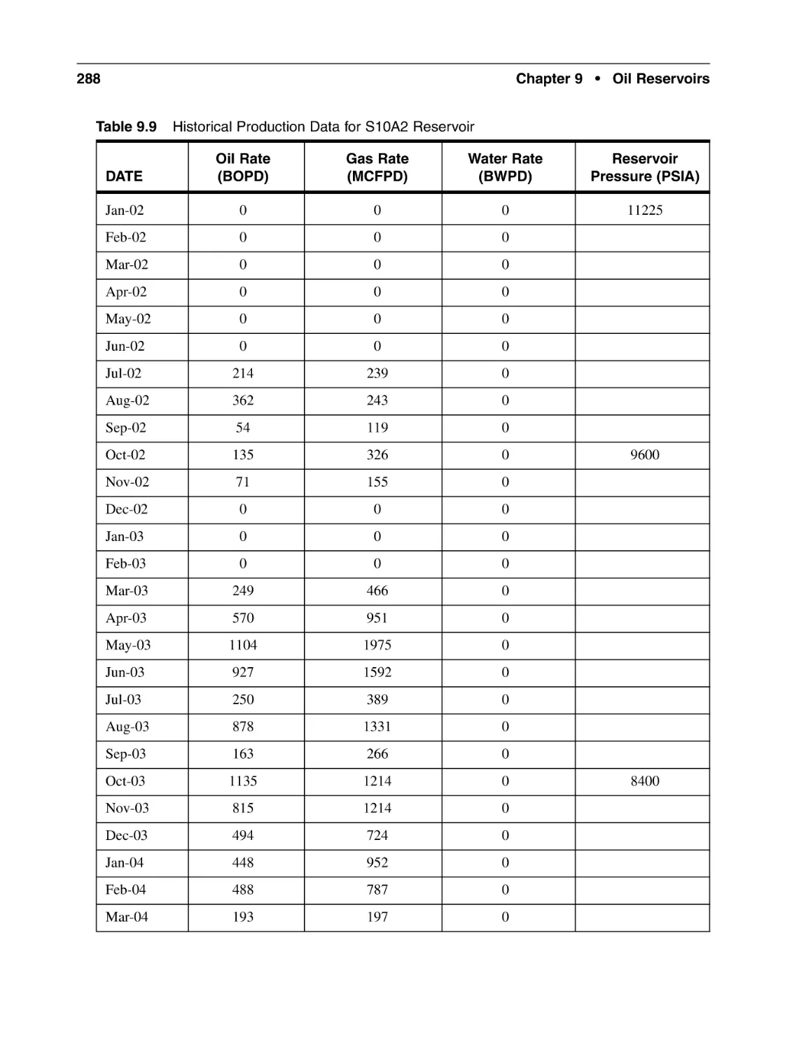
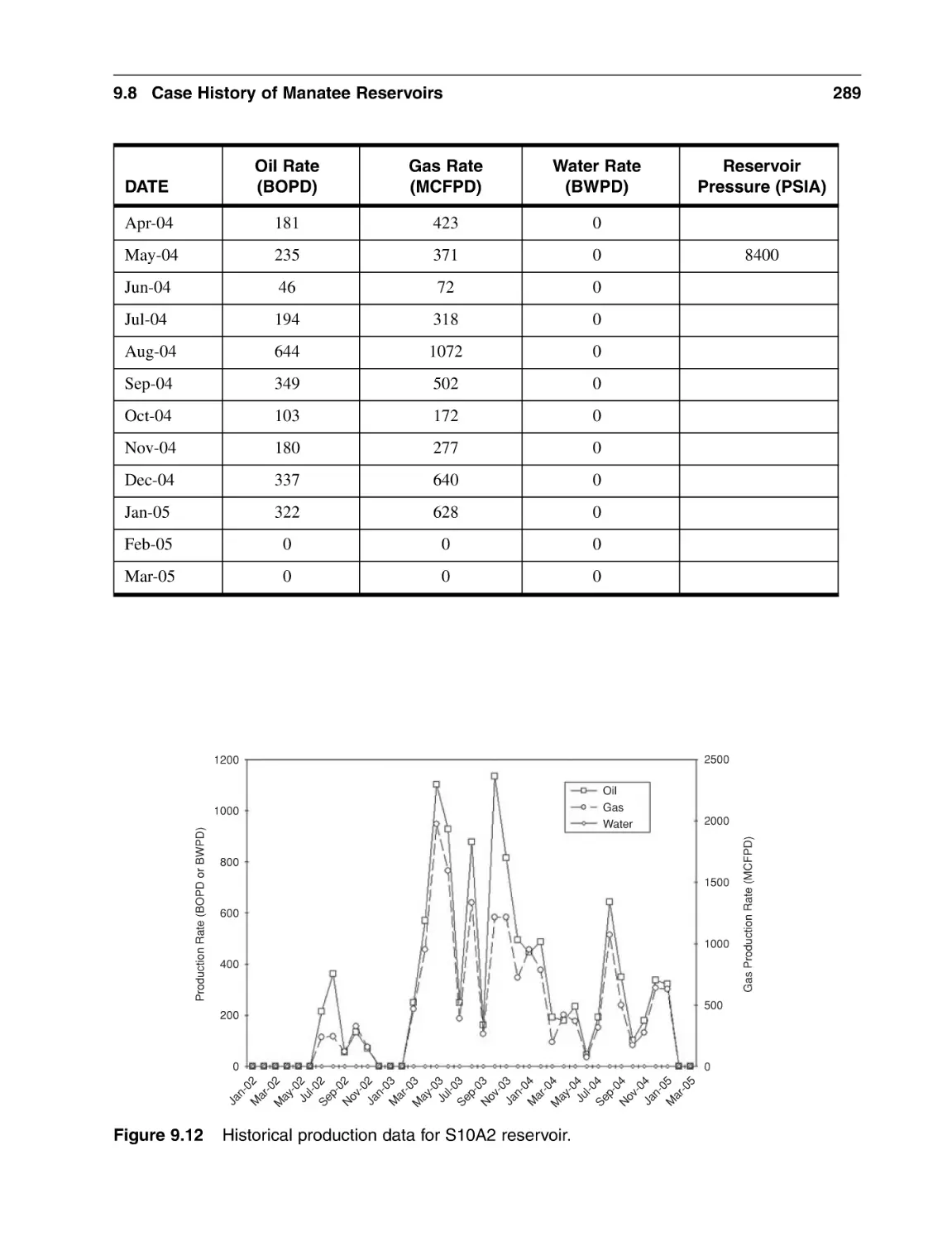
9.8.3 Reservoir Pressure and Production Data
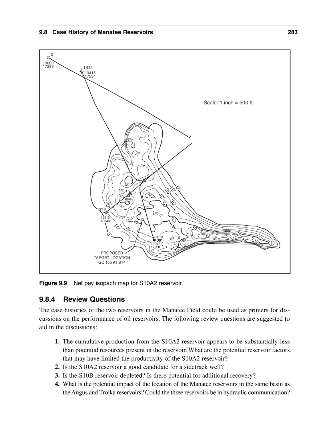
9.8.4 Review Questions
Nomenclature
Subscripts
Abbreviations
References
Chapter 10 Fluid Flow in Petroleum Reservoirs
10.1 Introduction
10.2 Fluid Types
10.2.1 Incompressible Fluids
10.2.2 Slightly Compressible Fluids
10.2.3 Compressible Fluids
10.3 Definition of Fluid Flow Regimes
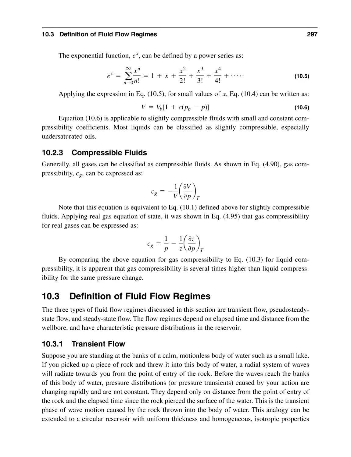
10.3.1 Transient Flow
10.3.2 Pseudosteady-State (PSS) Flow
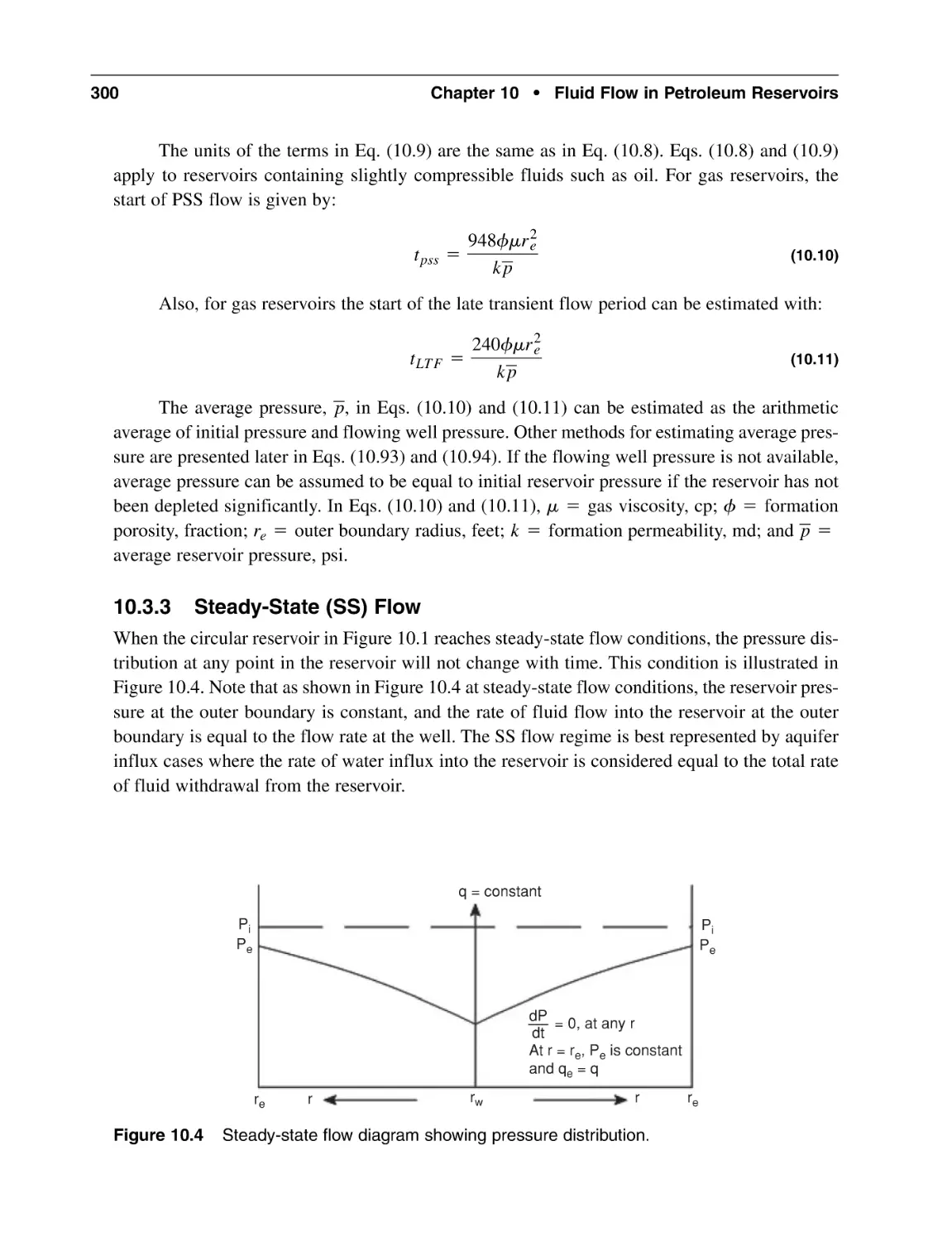
10.3.3 Steady-State (SS) Flow
10.4 Darcy Fluid Flow Equation
10.5 Radial Forms of the Darcy Equation
10.5.1 Steady-State Flow, Incompressible Fluids
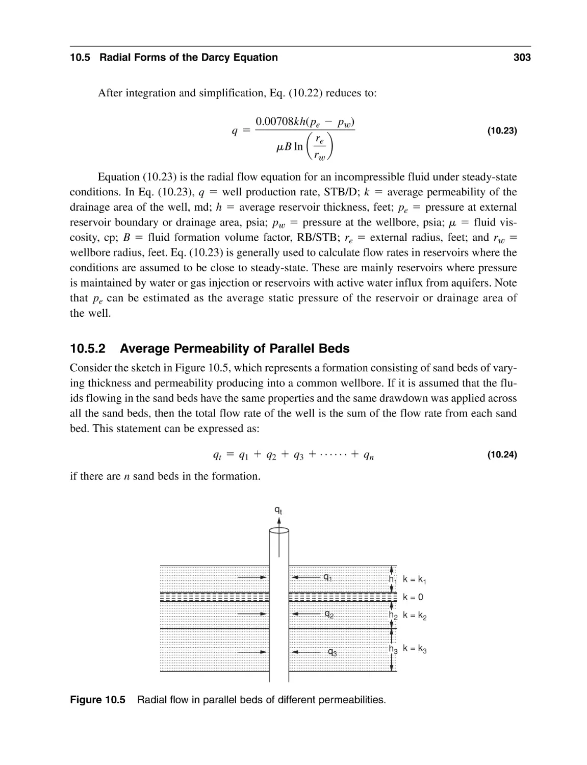
10.5.2 Average Permeability of Parallel Beds
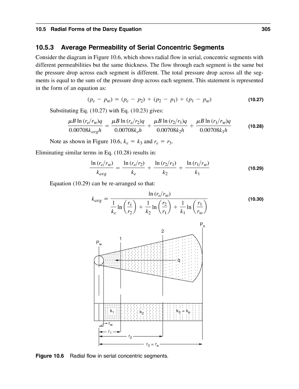
10.5.3 Average Permeability of Serial Concentric Segments
10.5.4 Pseudosteady State, Incompressible Fluids
10.5.5 Steady-State Flow, Compressible Fluids
xiii
257
258
258
263
264
264
265
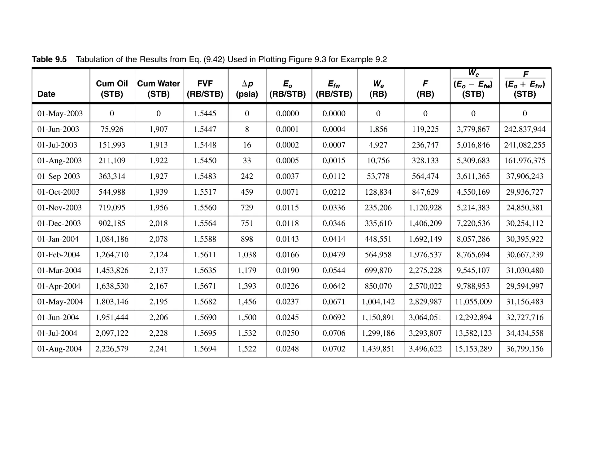
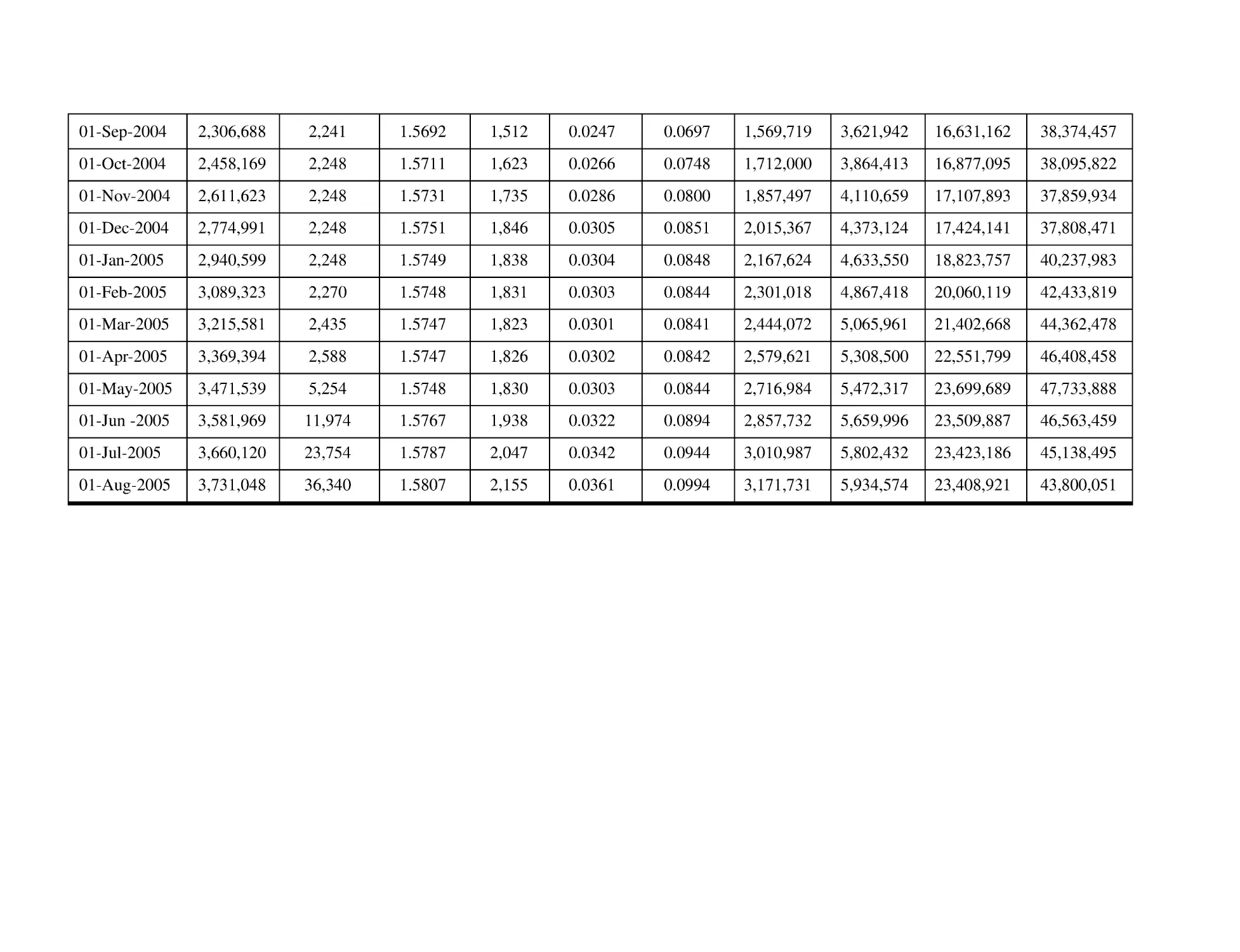
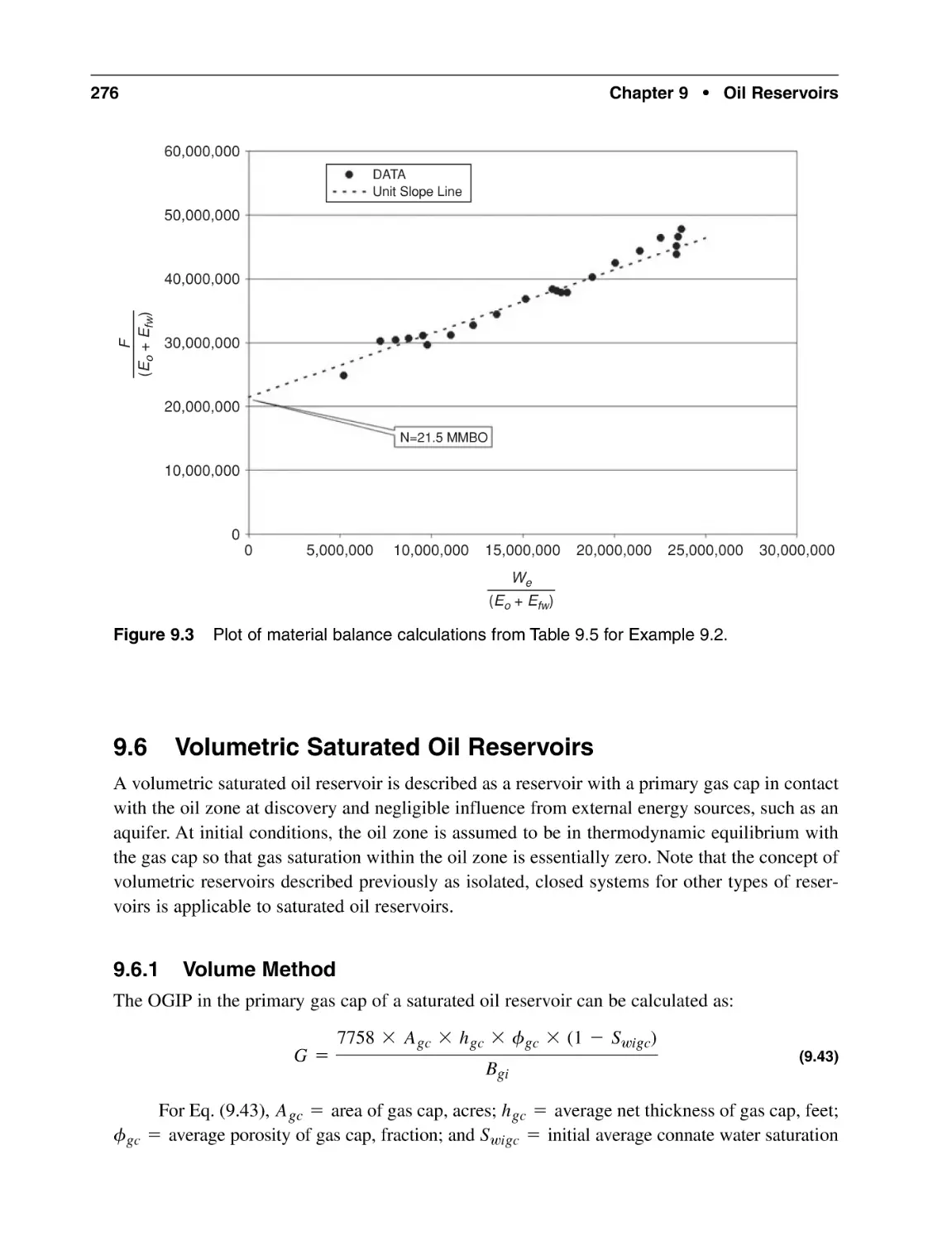
276
276
277
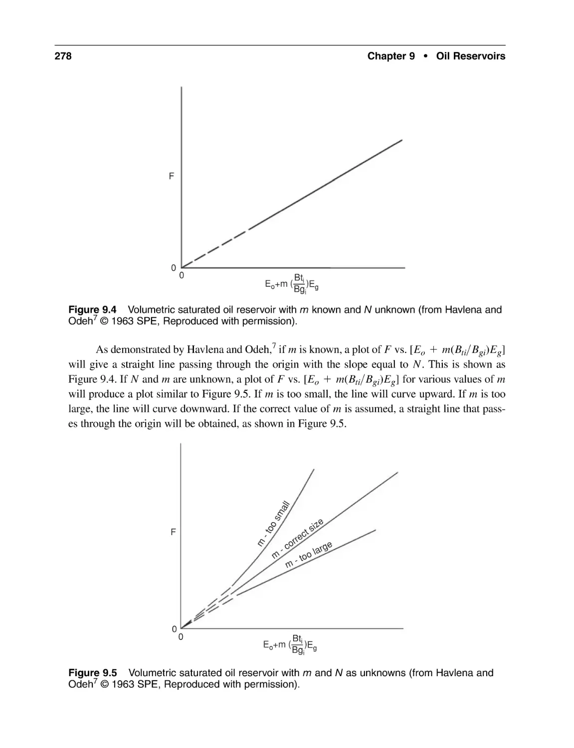
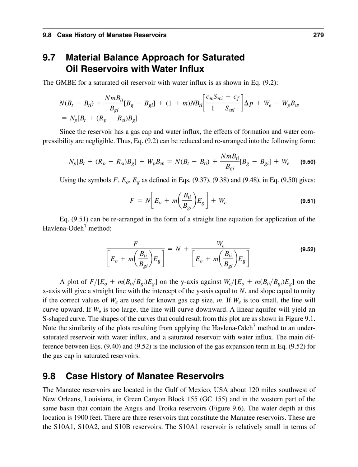
279
279
280
282
282
283
292
292
293
293
295
295
296
296
296
297
297
297
299
300
301
302
302
303
305
307
309
xiv
Contents
10.6
10.7
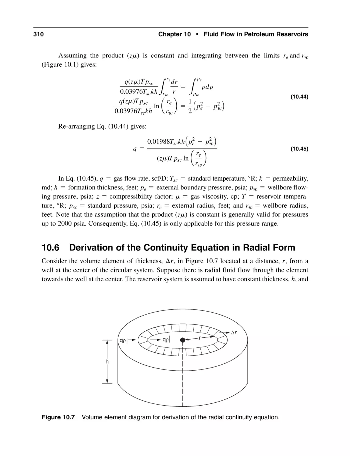
Derivation of the Continuity Equation in Radial Form
Derivation of Radial Diffusivity Equation for Slightly
Compressible Fluids
10.8 Solutions of the Radial Diffusivity Equation for Slightly
Compressible Fluids
10.8.1 Constant Terminal Rate Solution
10.8.2 Constant Terminal Pressure Solution
10.9 Derivation of the Radial Diffusivity Equation
for Compressible Fluids
10.10 Transformation of the Gas Diffusivity Equation with Real
Gas Pseudo-Pressure Concept
10.11 The Superposition Principle
10.11.1 Applications of Constant Terminal Rate Solutions
with Superposition Principle
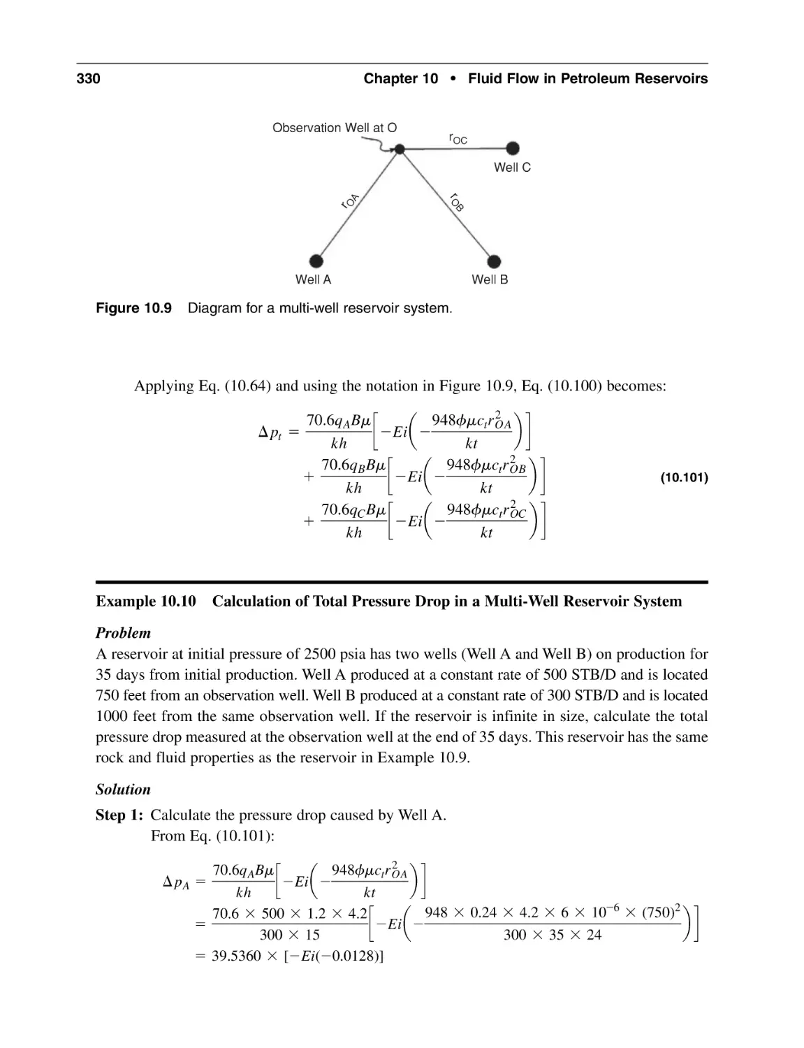
10.11.2 Applications of Constant Terminal Pressure Solution
with Superposition Principle
10.12 Well Productivity Index
10.13 Well Injectivity Index
Nomenclature
Subscripts
References
General Reading
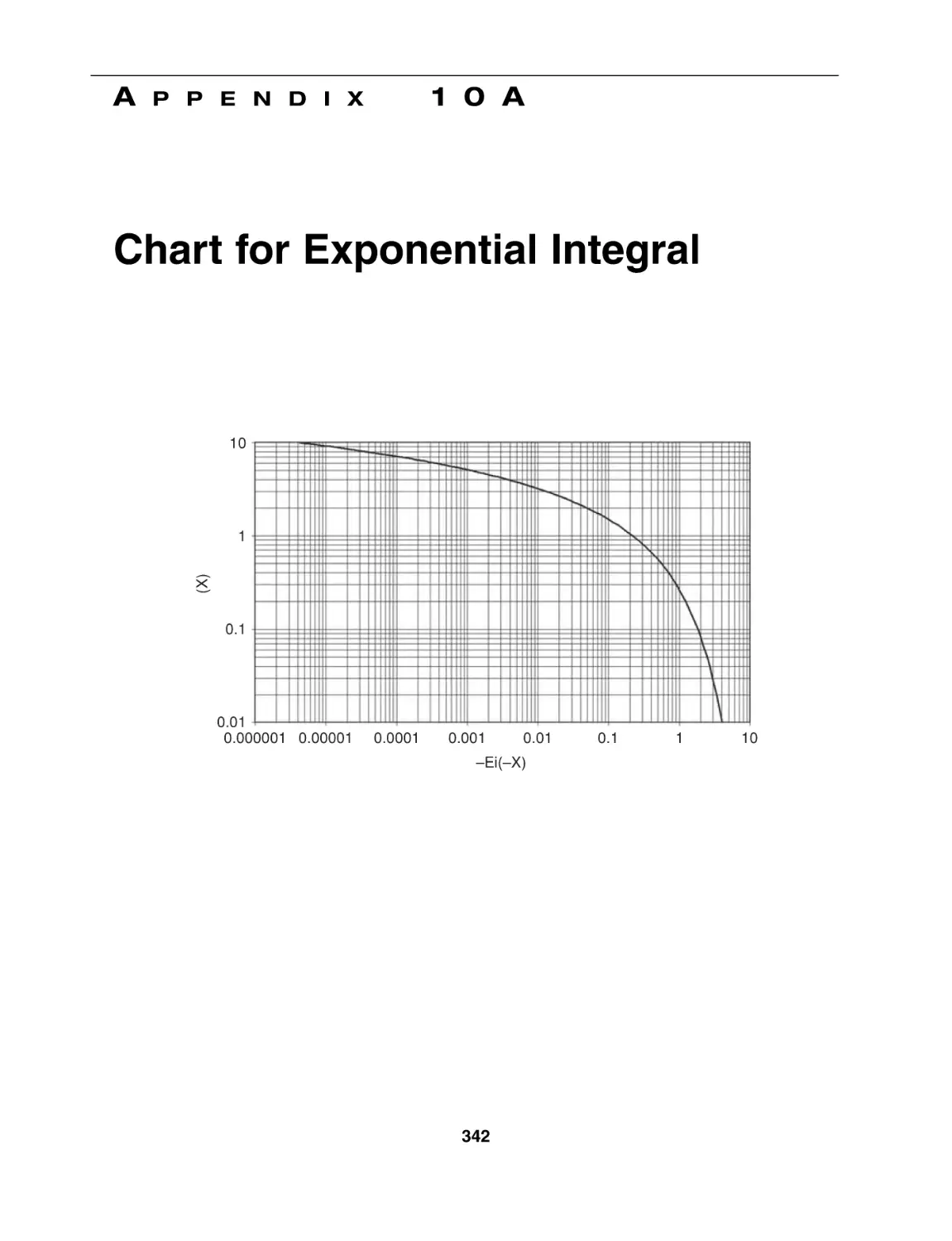
Appendix 10A
Chart for Exponential Integral
310
311
313
313
319
321
322
327
327
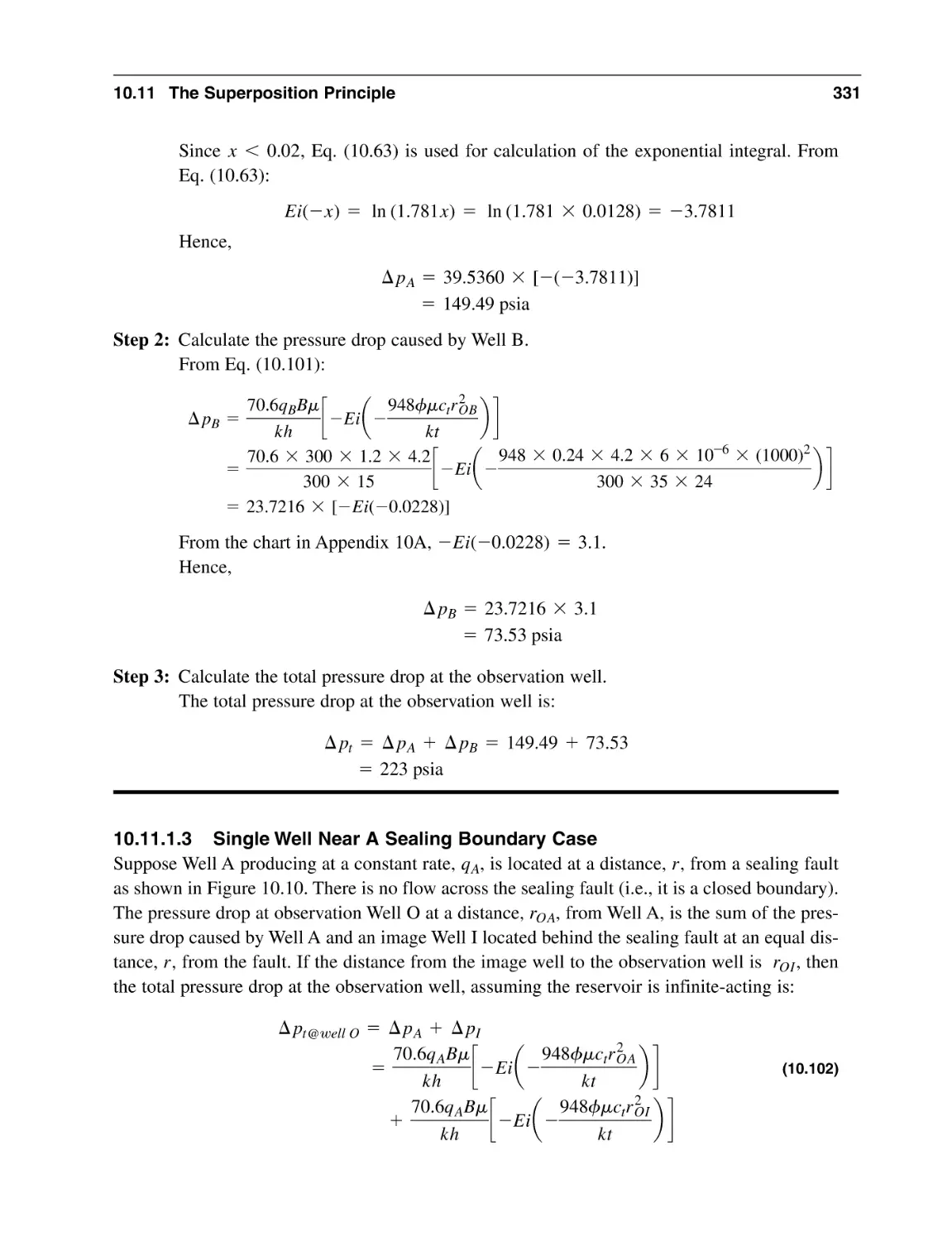
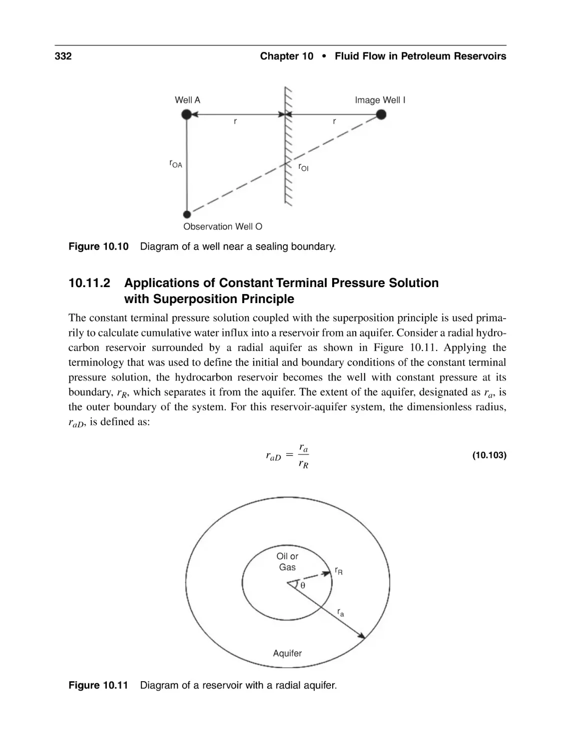
332
338
338
339
340
340
341
342
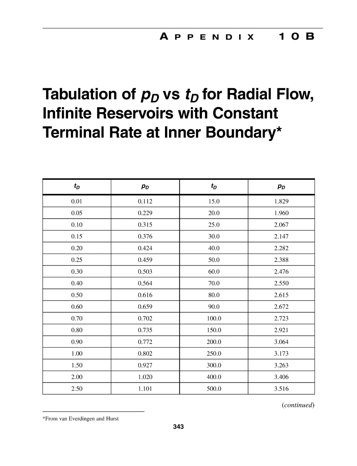
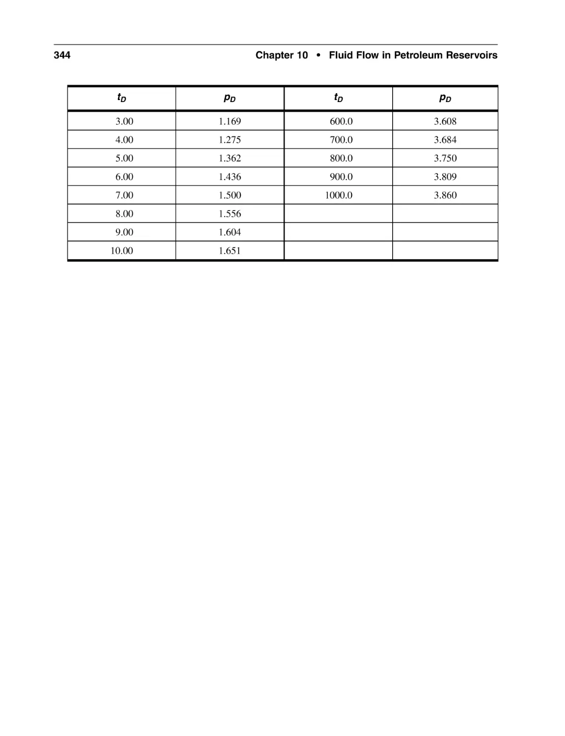
Appendix 10B Tabulation of pD vs tD for Radial Flow, Infinite
Reservoirs with Constant Terminal Rate at Inner Boundary
343
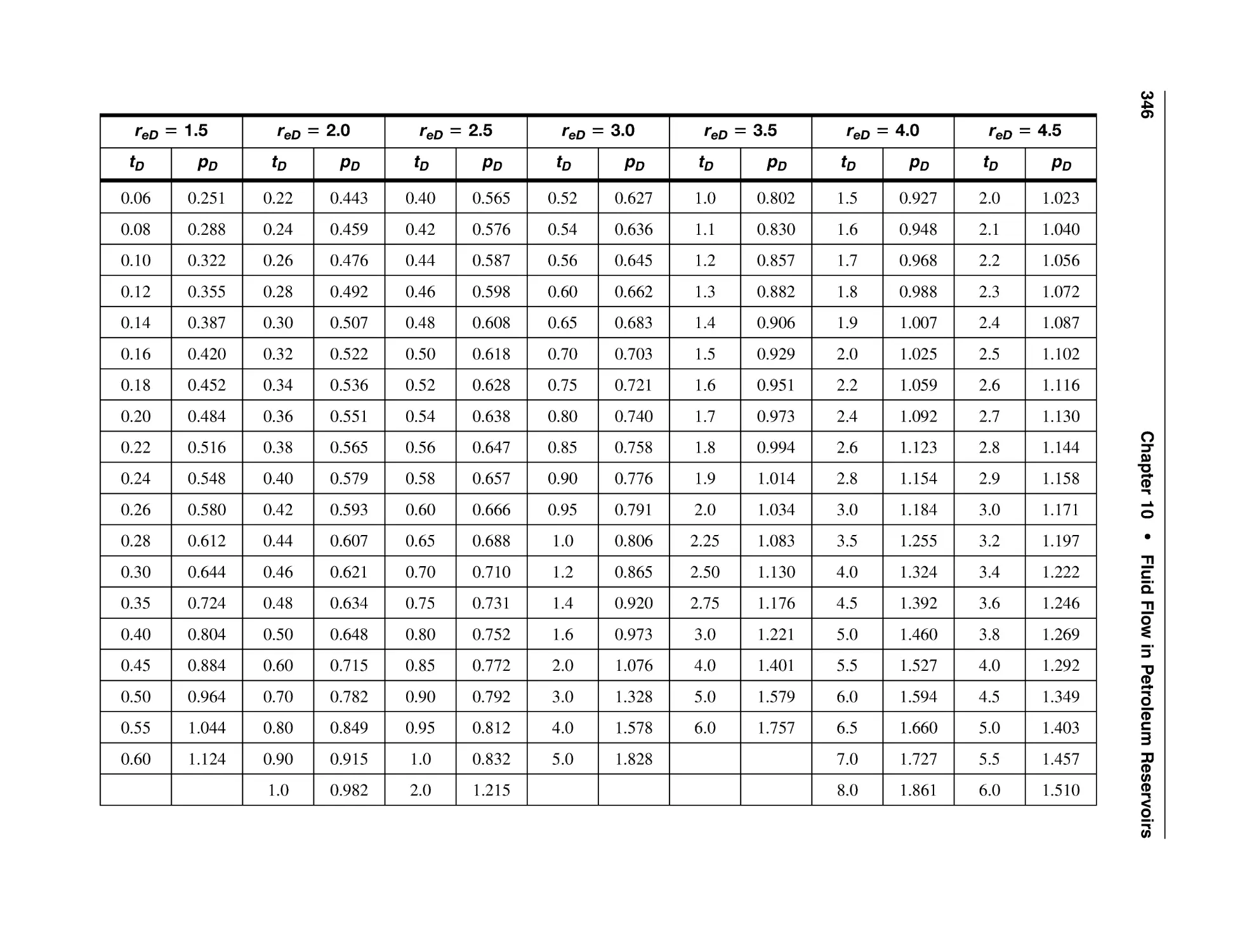
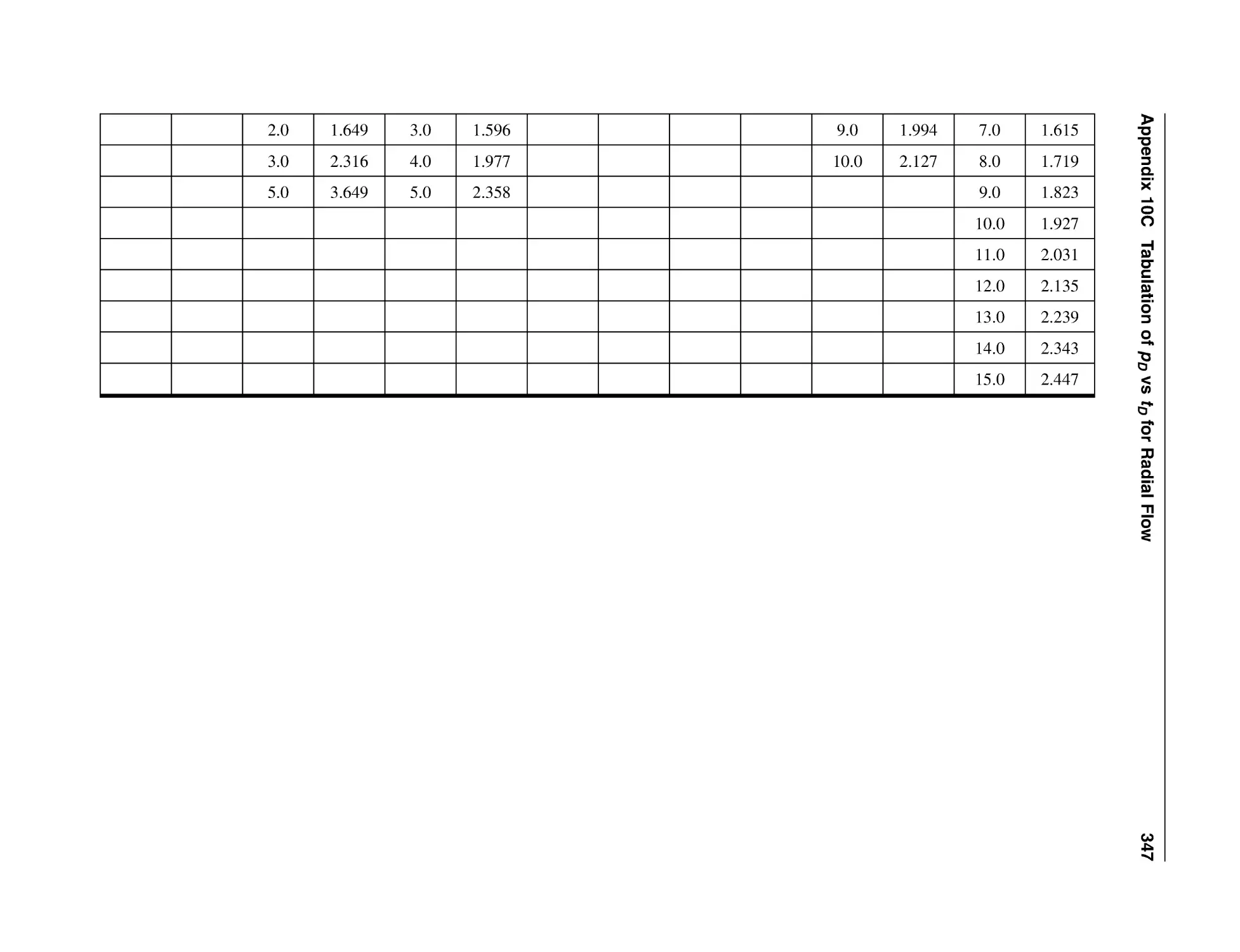
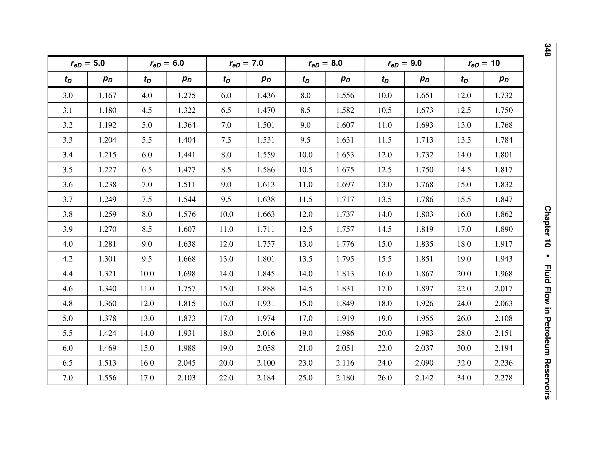
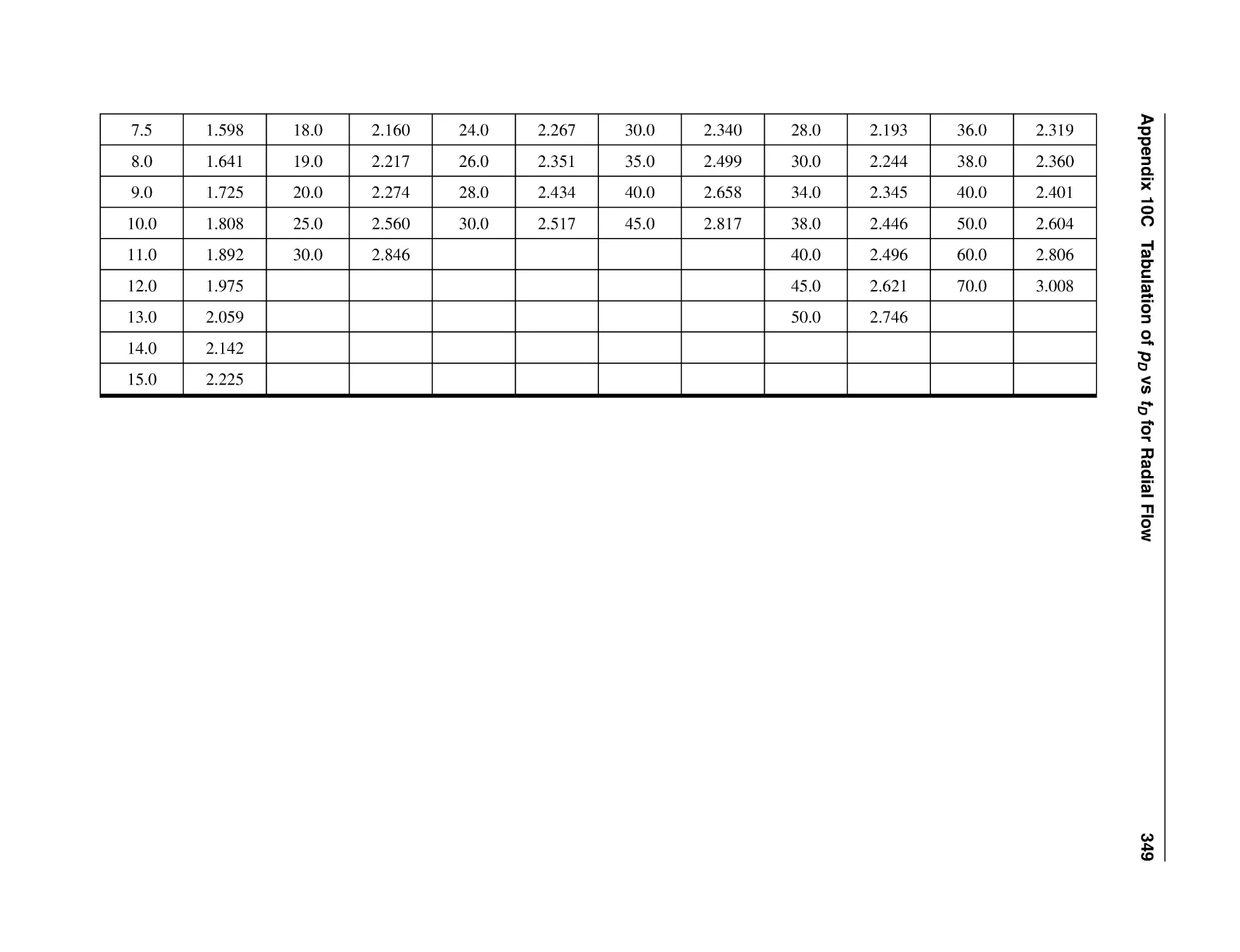
Appendix 10C Tabulation of pD vs tD for Radial Flow, Finite Reservoirs
with Closed Outer Boundary and Constant Terminal Rate at Inner
Boundary
345
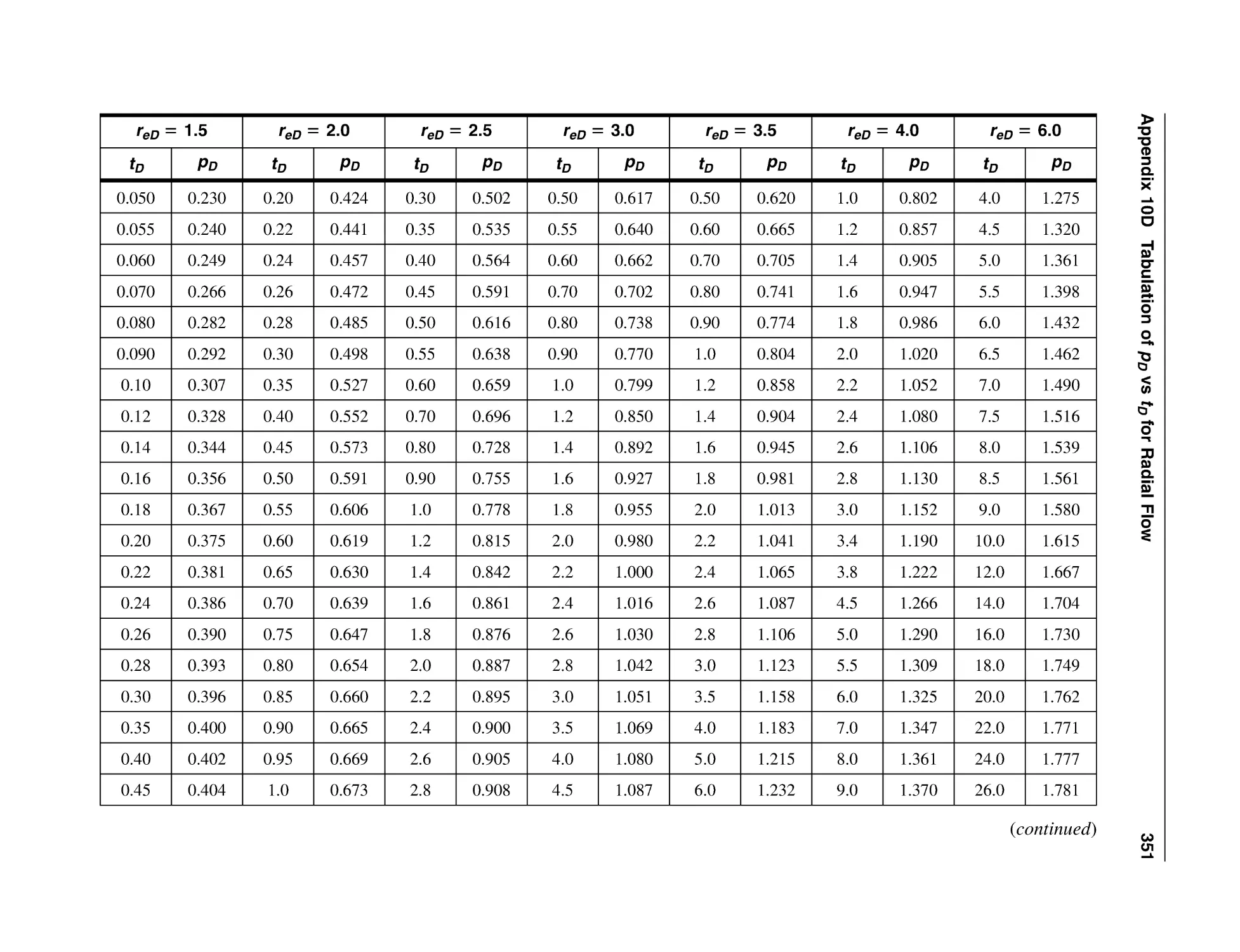
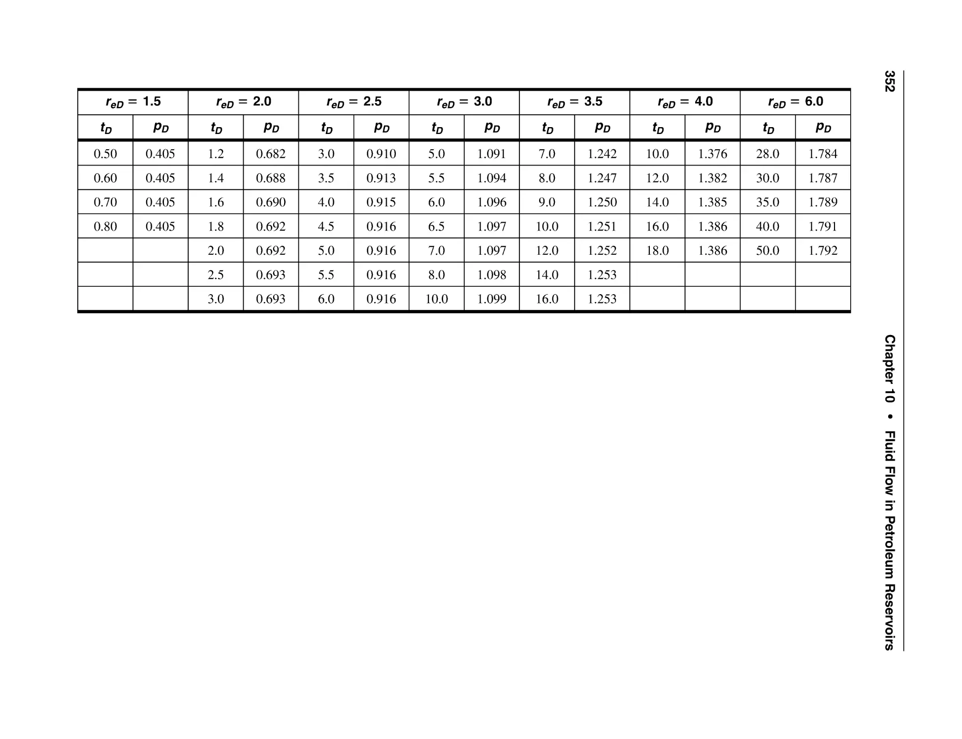
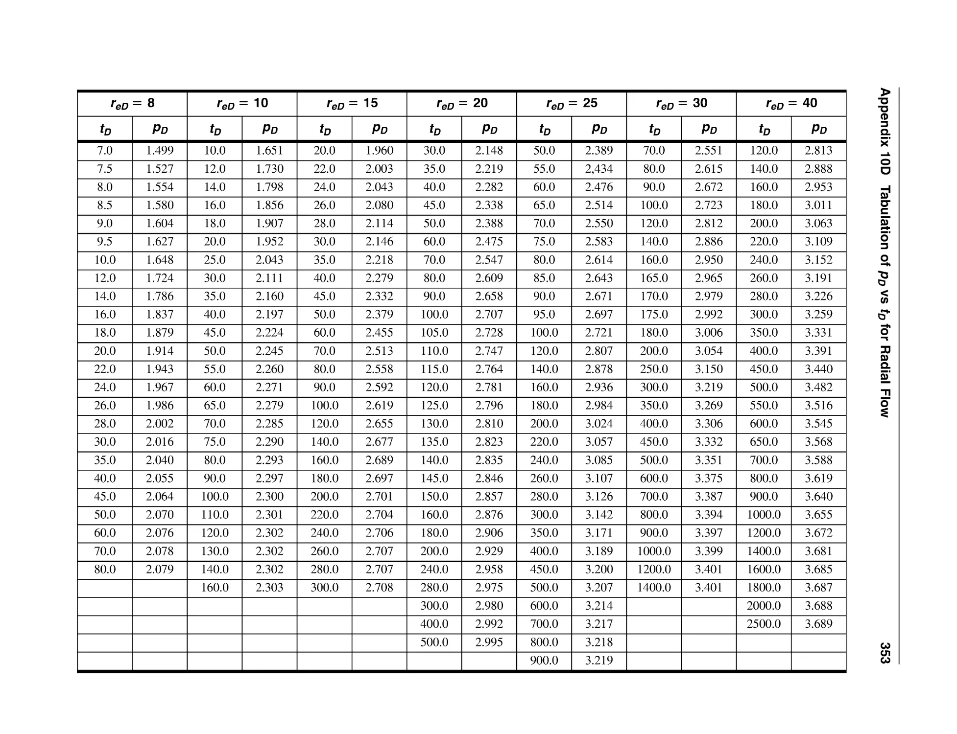
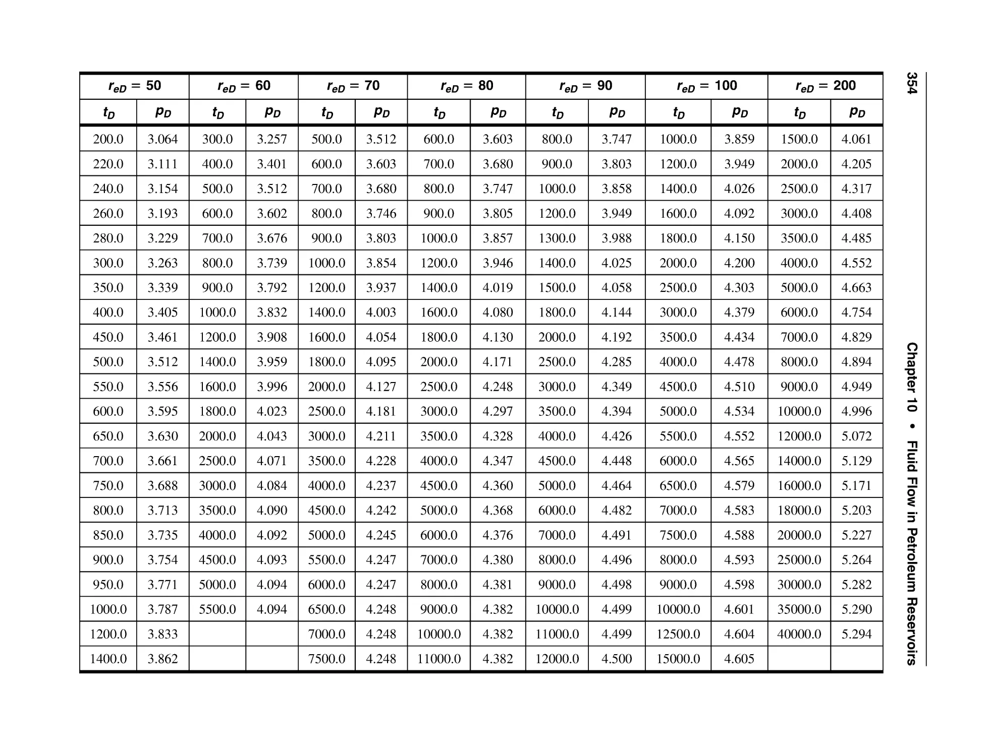
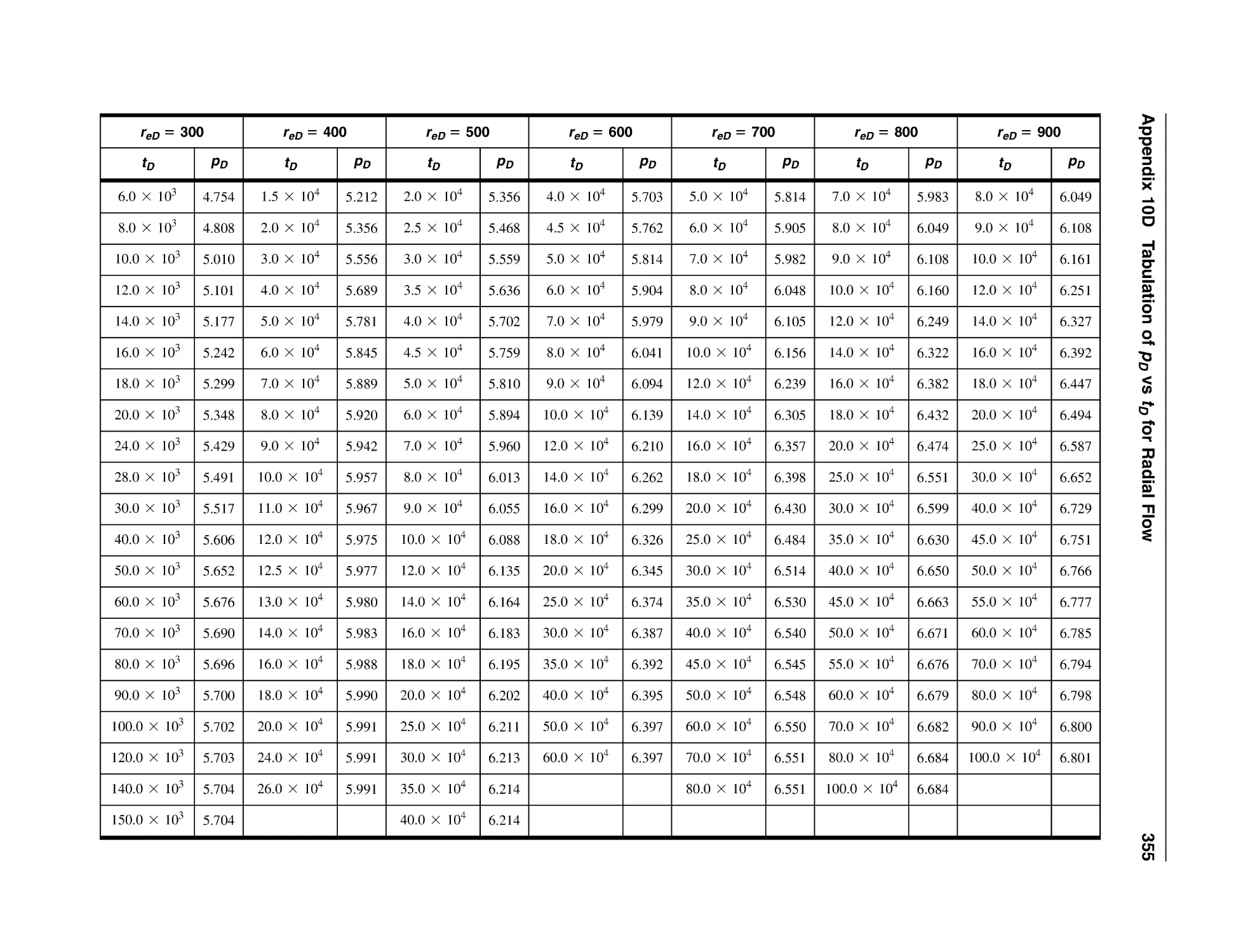
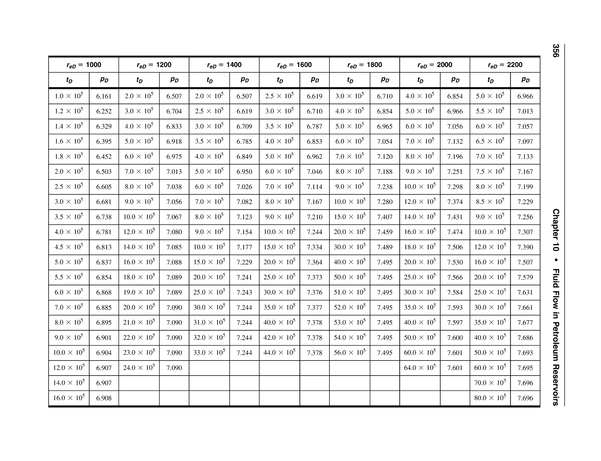
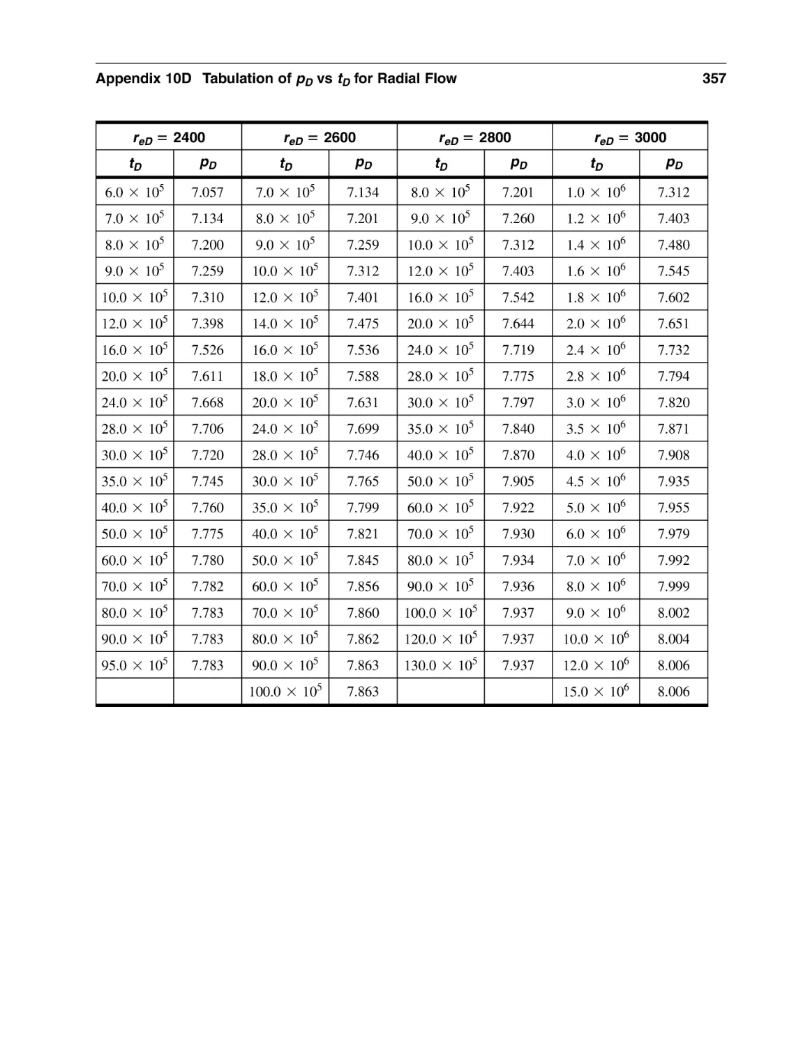
Appendix 10D Tabulation of pD vs tD for Radial Flow, Finite Reservoirs
with Constant Pressure Outer Boundary and Constant Terminal
Rate at Inner Boundary
350
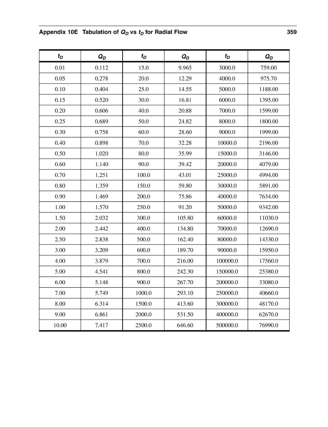
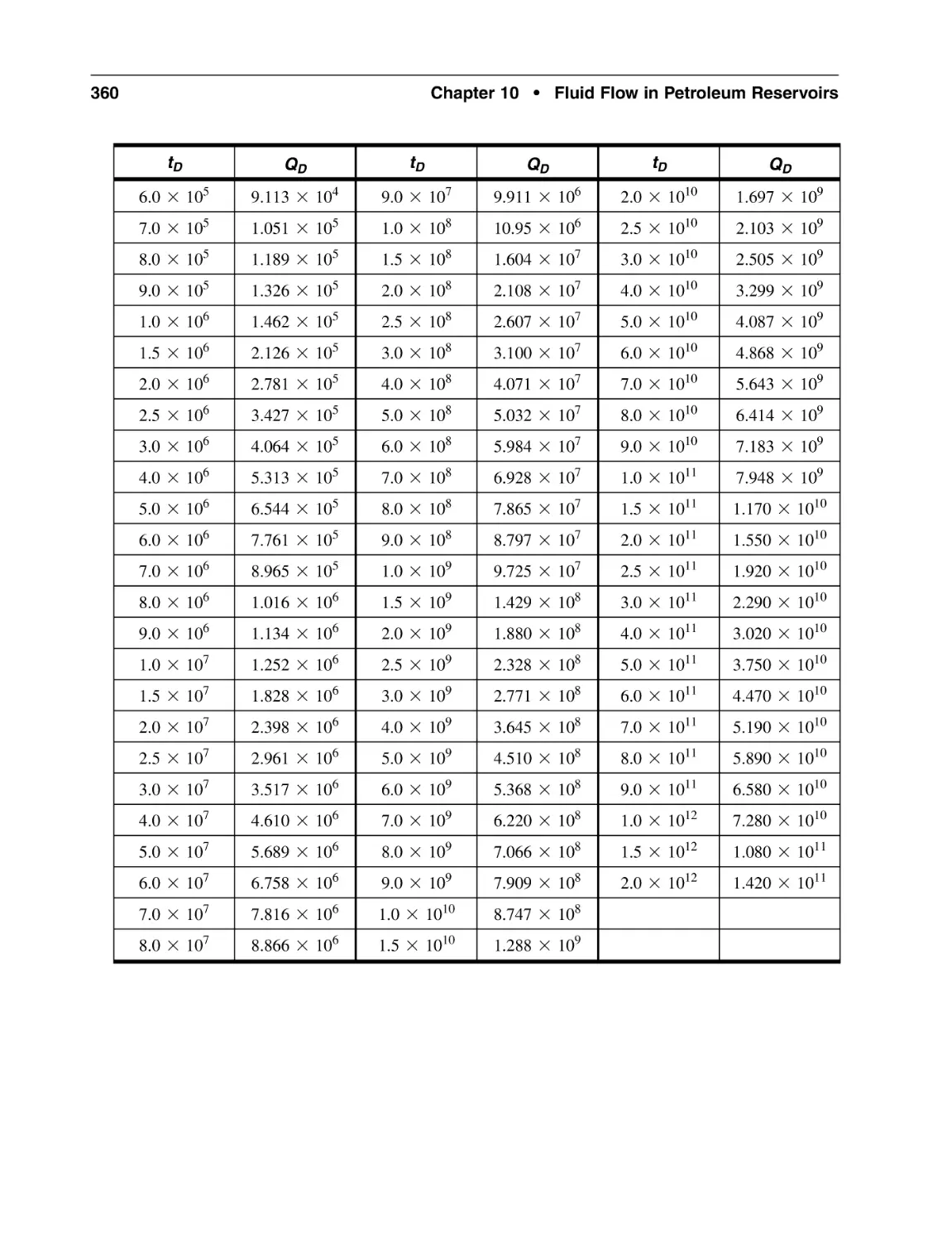
Appendix 10E Tabulation of QD vs tD for Radial Flow, Infinite
Reservoirs with Constant Terminal Pressure at Inner Boundary
358
Contents
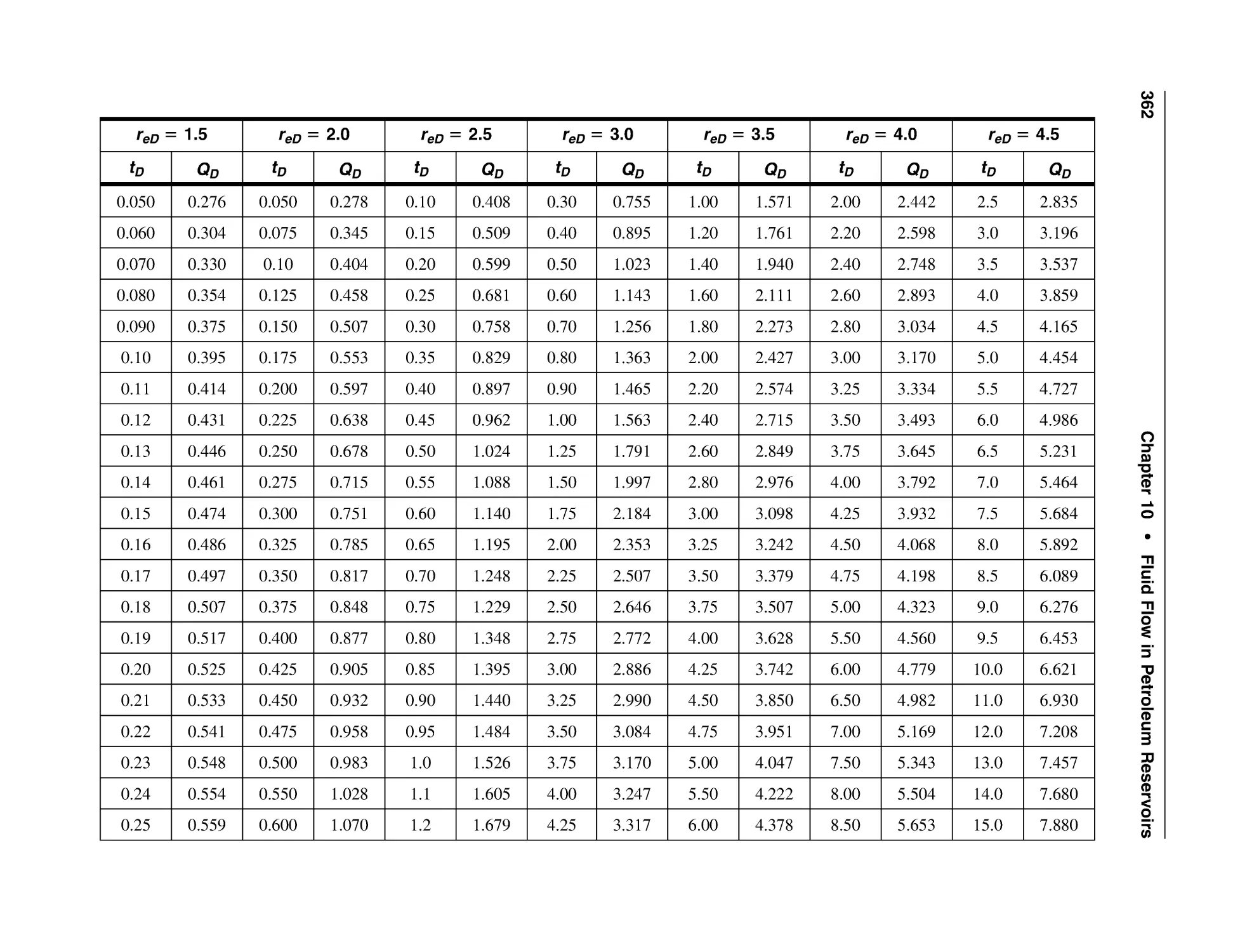
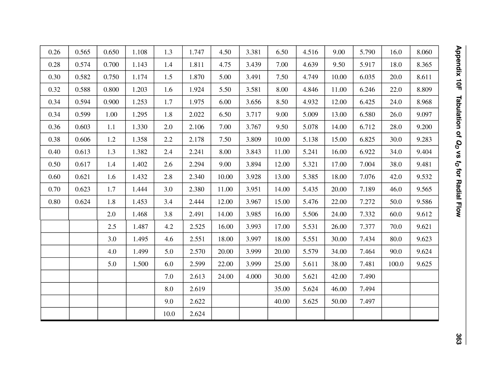
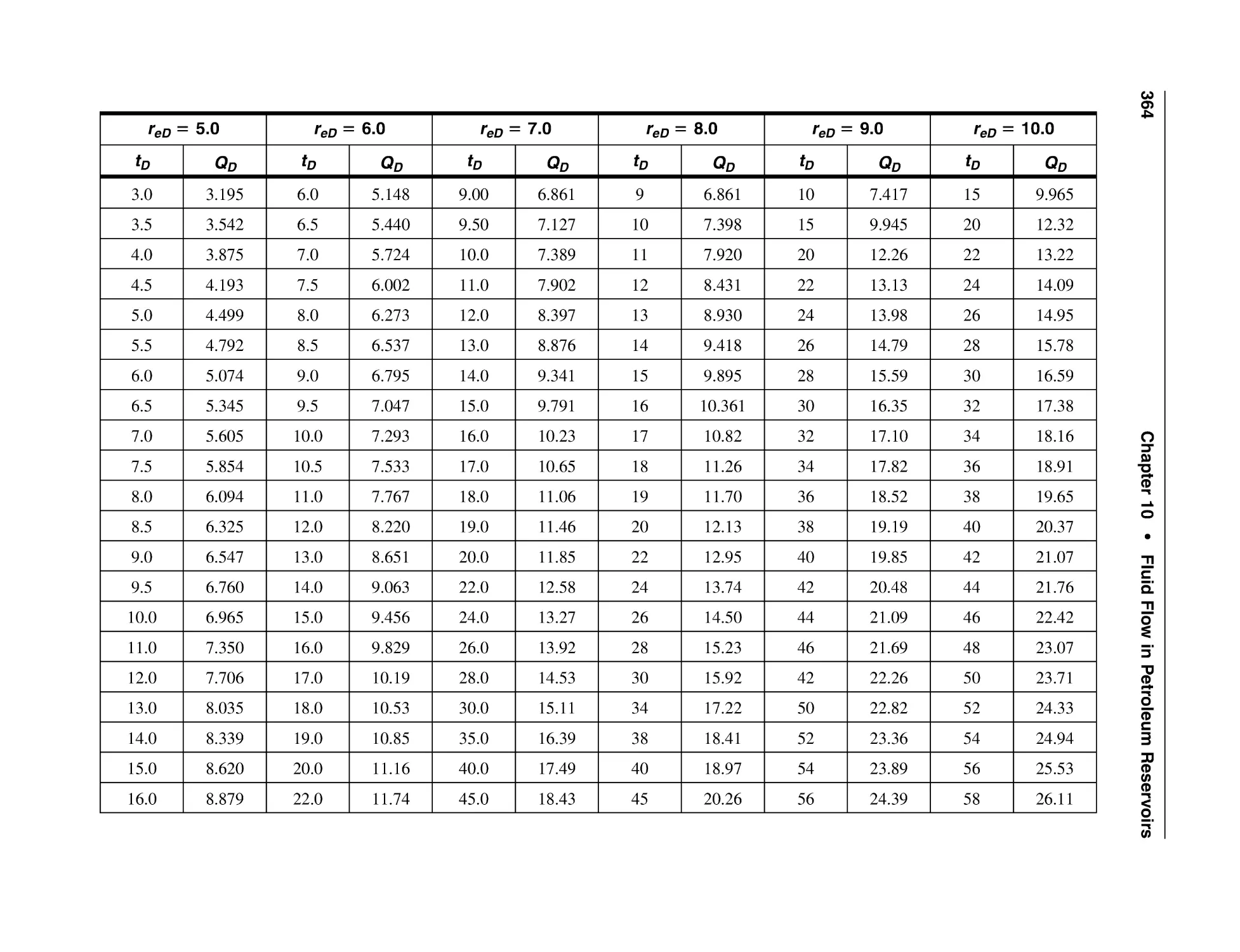
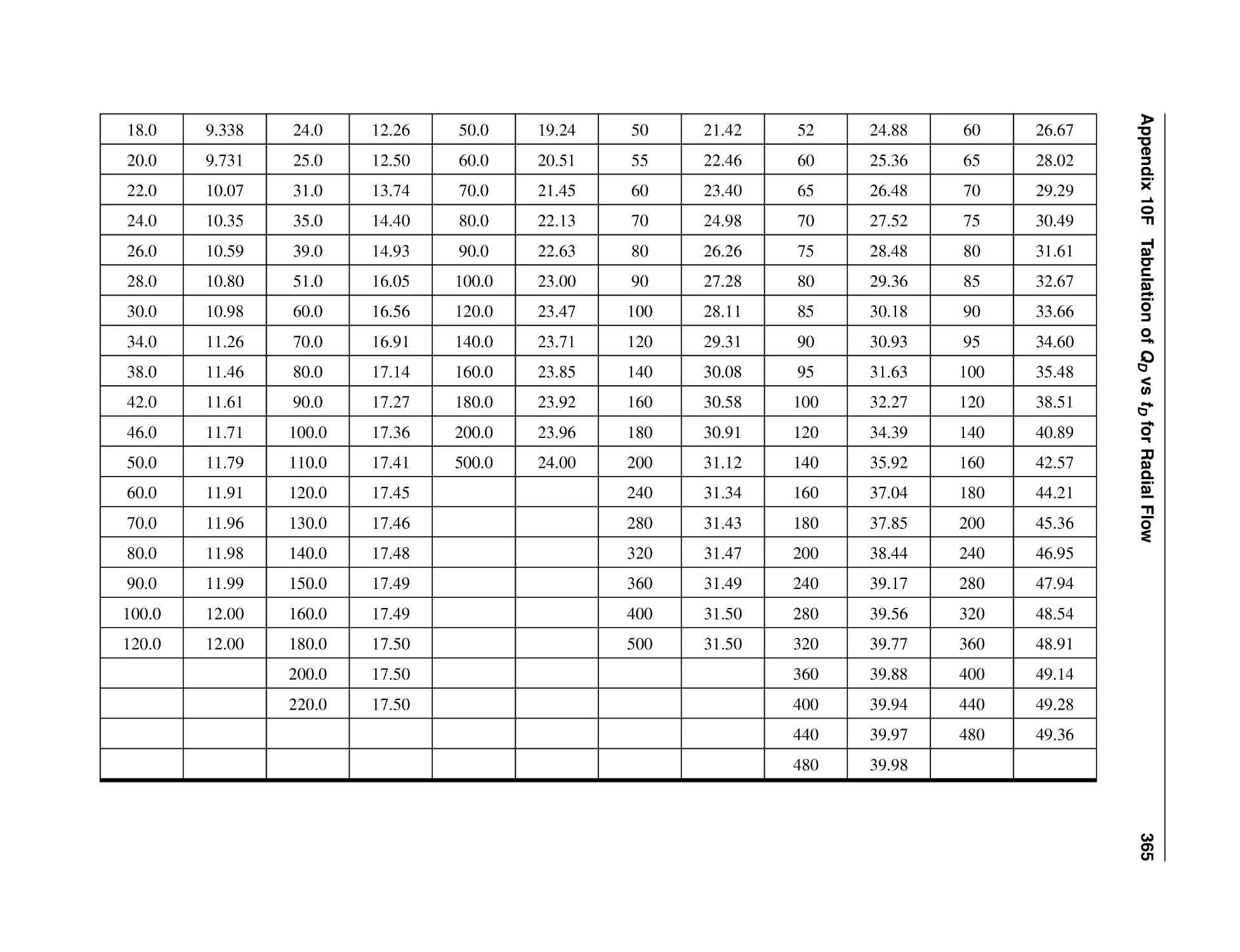
Appendix 10F Tabulation of QD vs tD for Radial Flow, Finite Reservoirs
with Closed Outer Boundary and Constant Terminal Pressure at
Inner Boundary
xv
361
Chapter 11 Well Test Analysis: Straightline Methods
11.1 Introduction
11.2 Basic Concepts in Well Test Analysis
11.2.1 Radius of Investigation
11.2.2 Skin and Skin Factor
11.2.3 Flow Efficiency and Damage Ratio
11.2.4 Effective Wellbore Radius
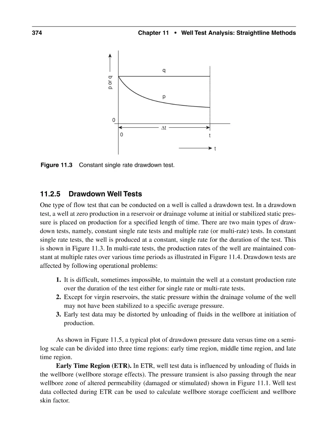
11.2.5 Drawdown Well Tests
11.2.6 Buildup Well Tests
11.2.7 Wellbore Storage
11.3 Line Source Well, Infinite Reservoir Solution of the
Diffusivity Equation with Skin Factor
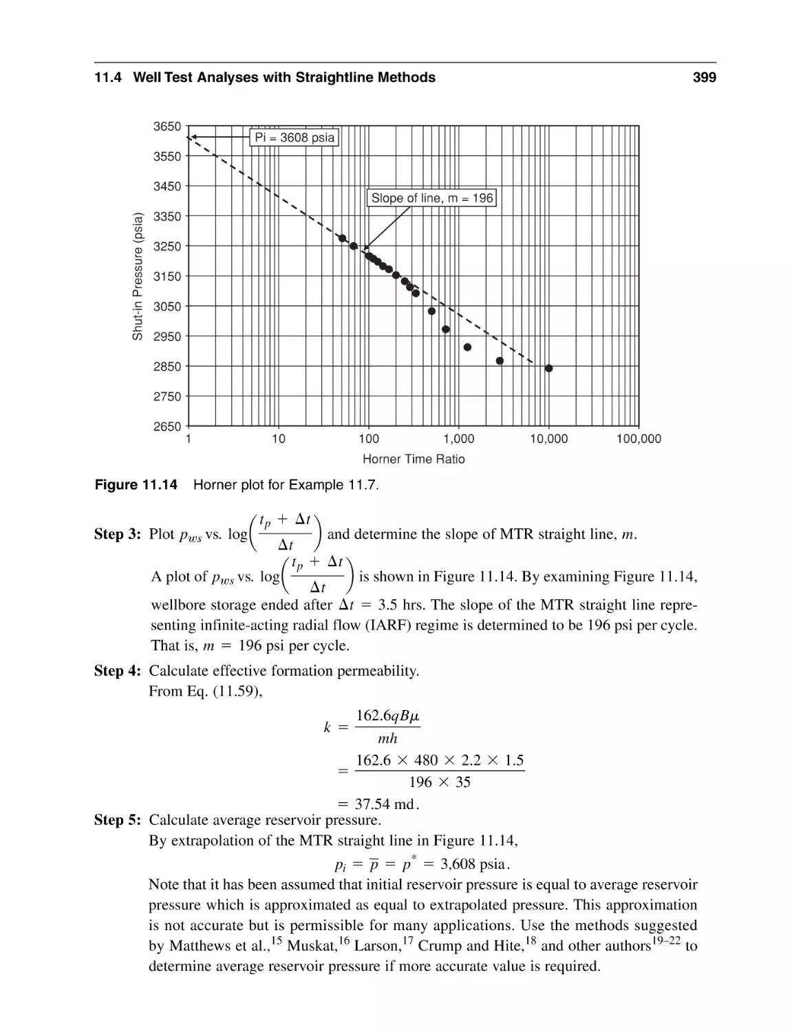
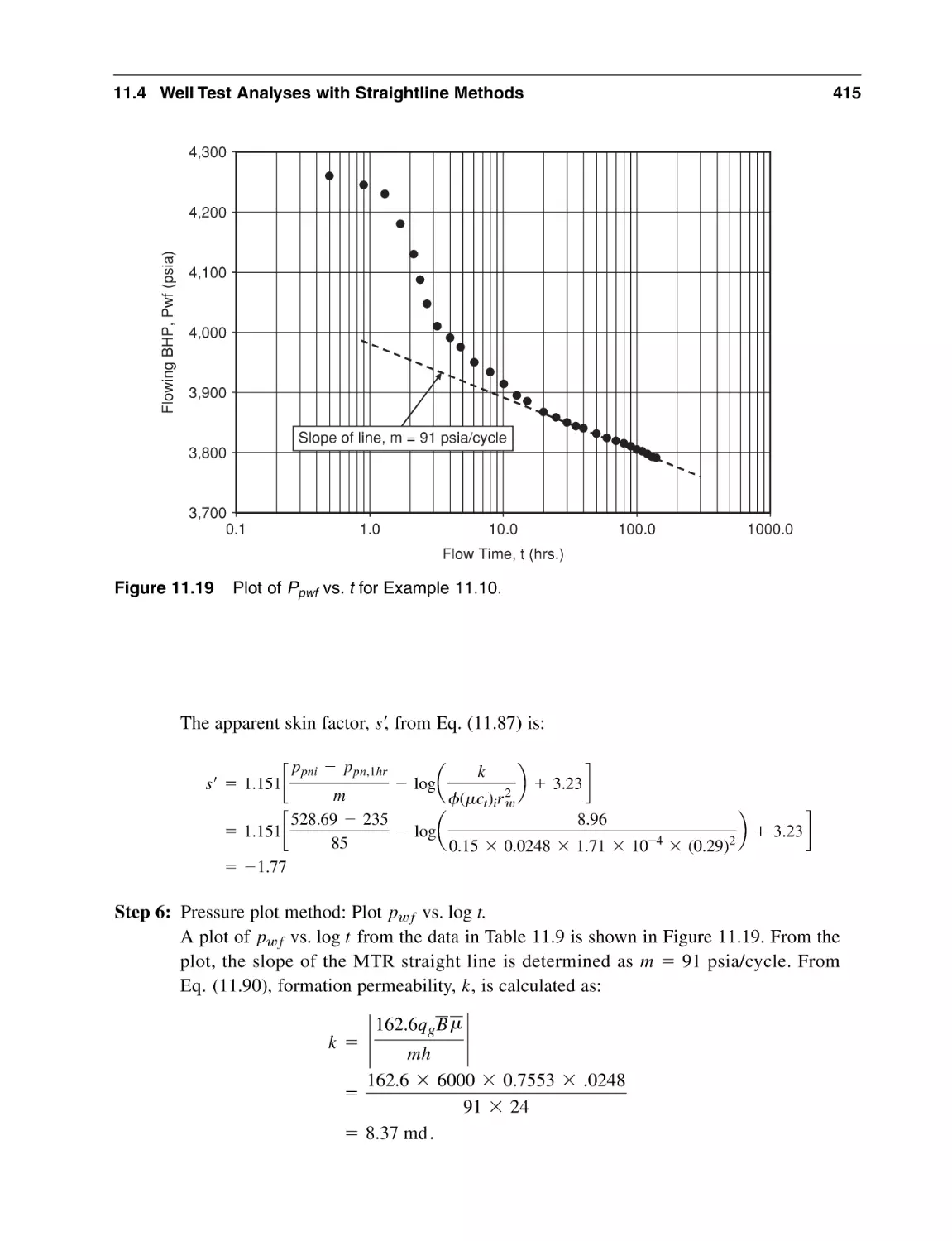
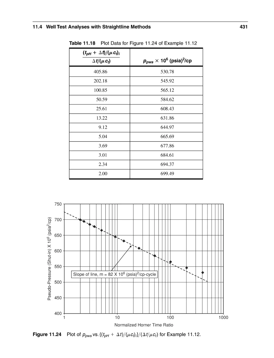
11.4 Well Test Analyses with Straightline Methods
11.4.1 Slightly Compressible Fluids
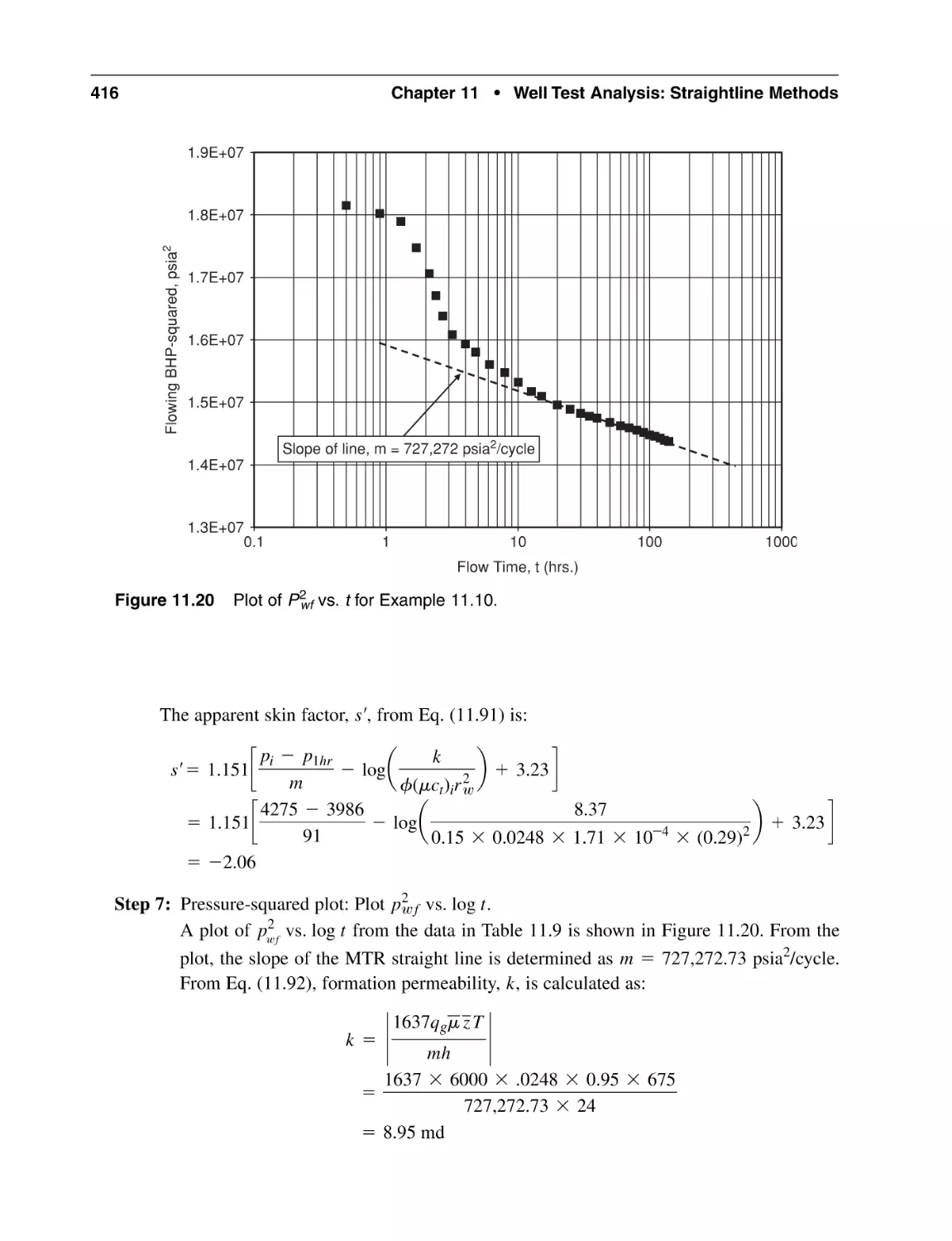
11.4.2 Compressible Fluids
11.5 Special Topics in Well Test Analyses
11.5.1 Multiphase Flow
11.5.2 Wellbore Storage Effects
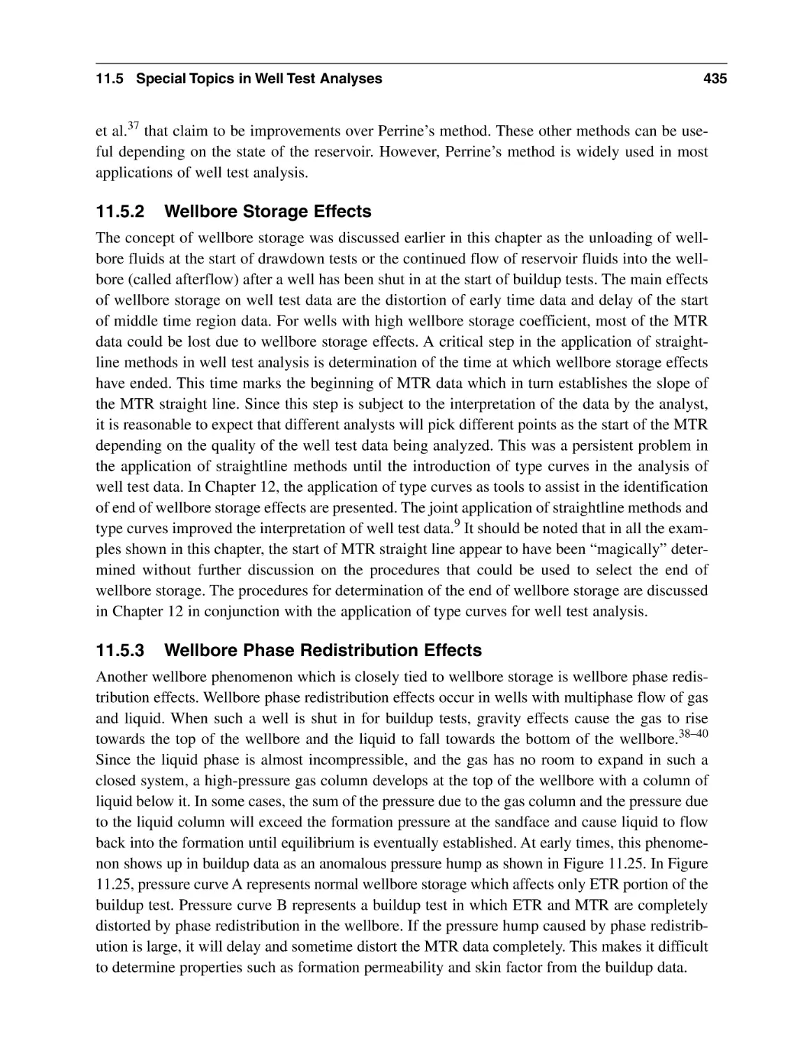
11.5.3 Wellbore Phase Redistribution Effects
11.5.4 Boundary Effects
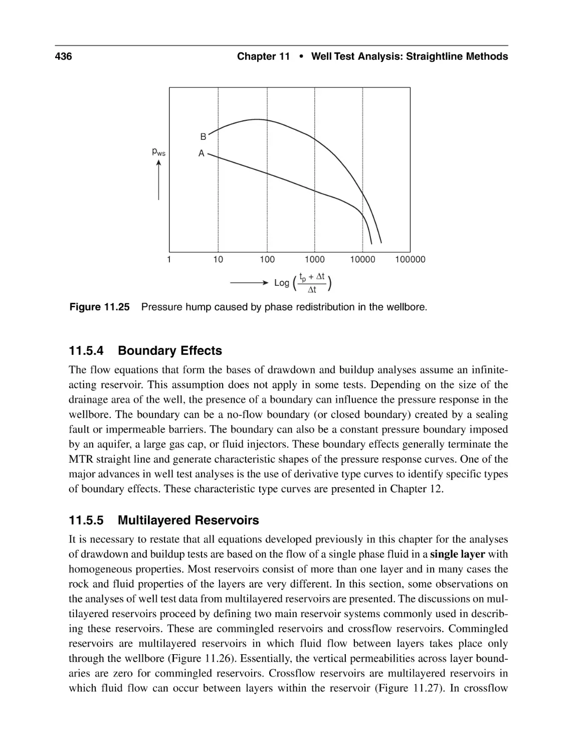
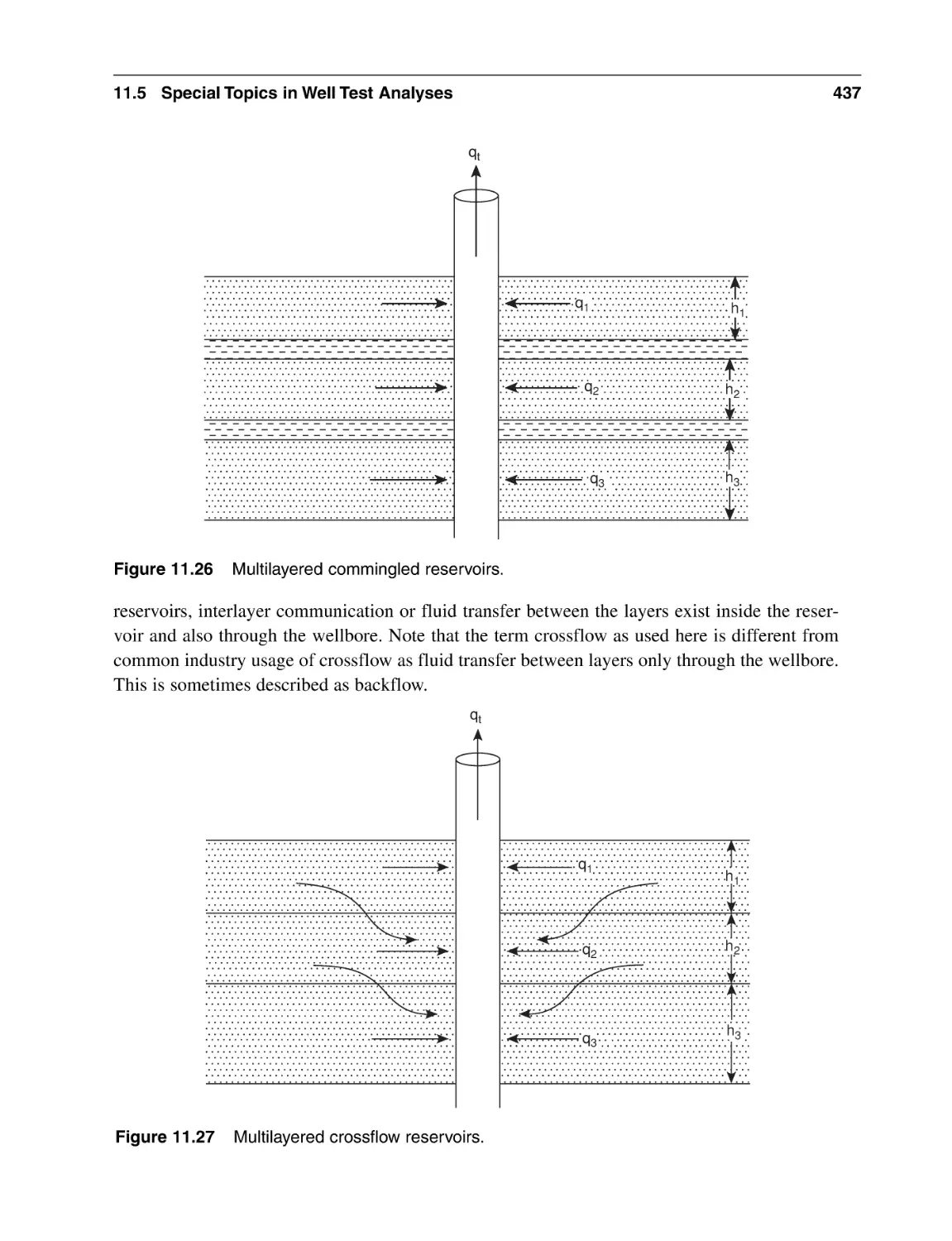
11.5.5 Multilayered Reservoirs
Nomenclature
Subscripts
Abbreviations
References
General Reading
367
367
368
368
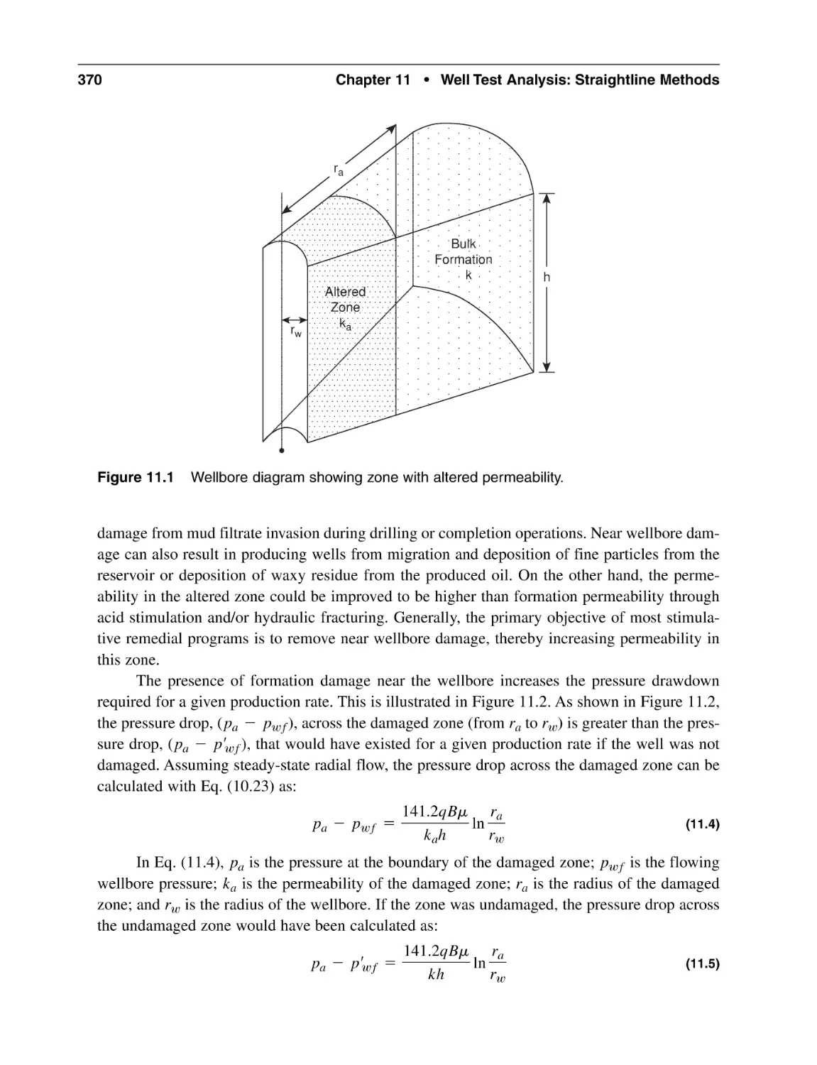
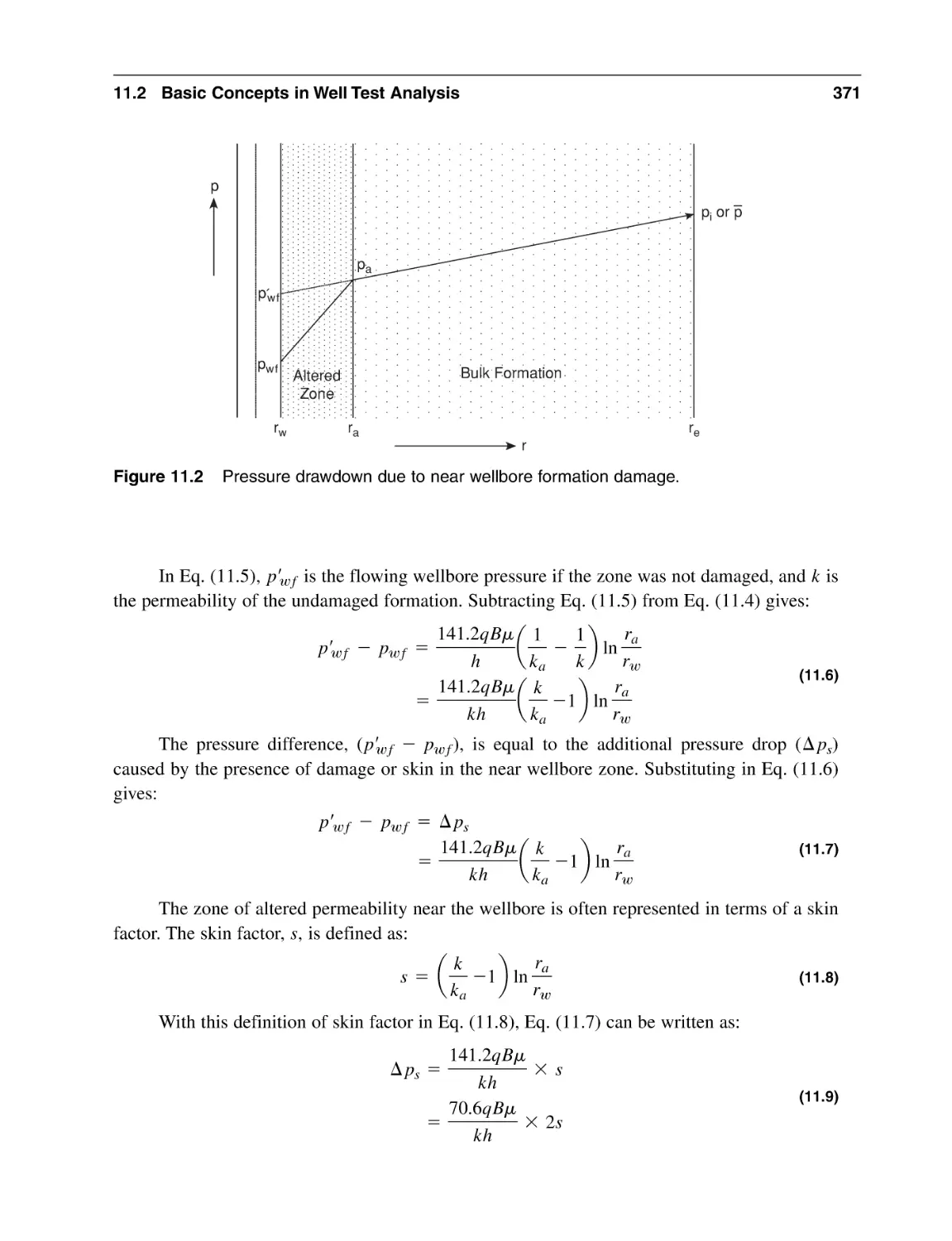
369
372
372
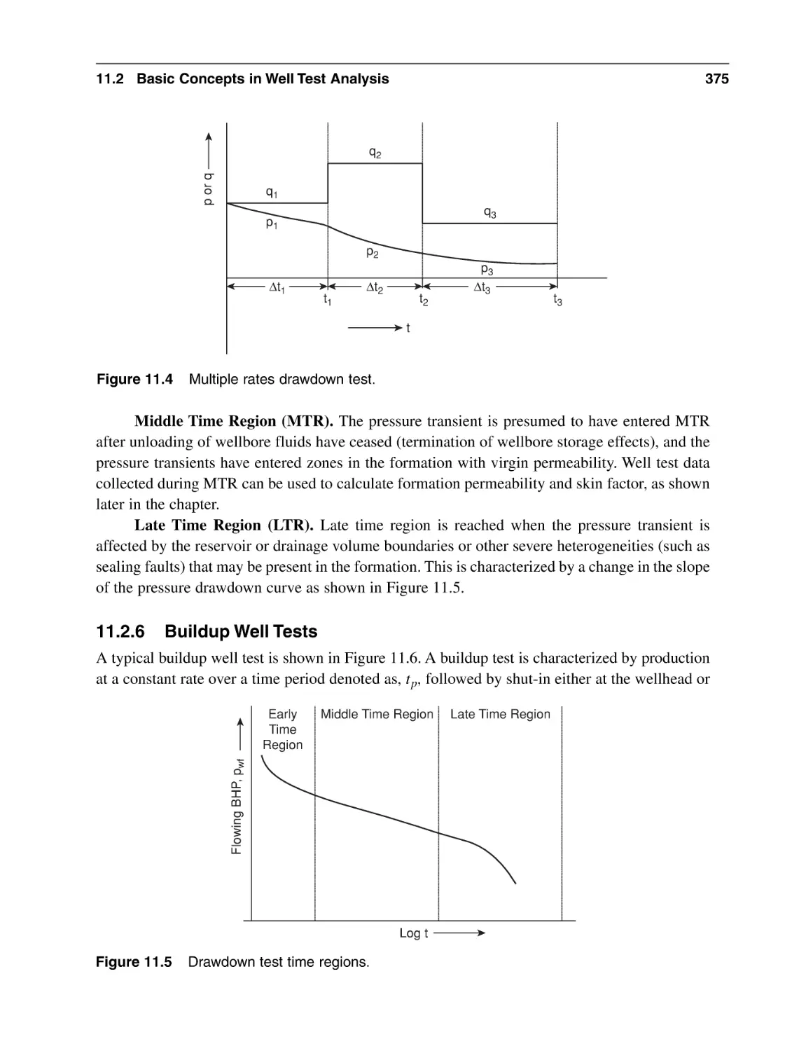
374
375
377
378
381
381
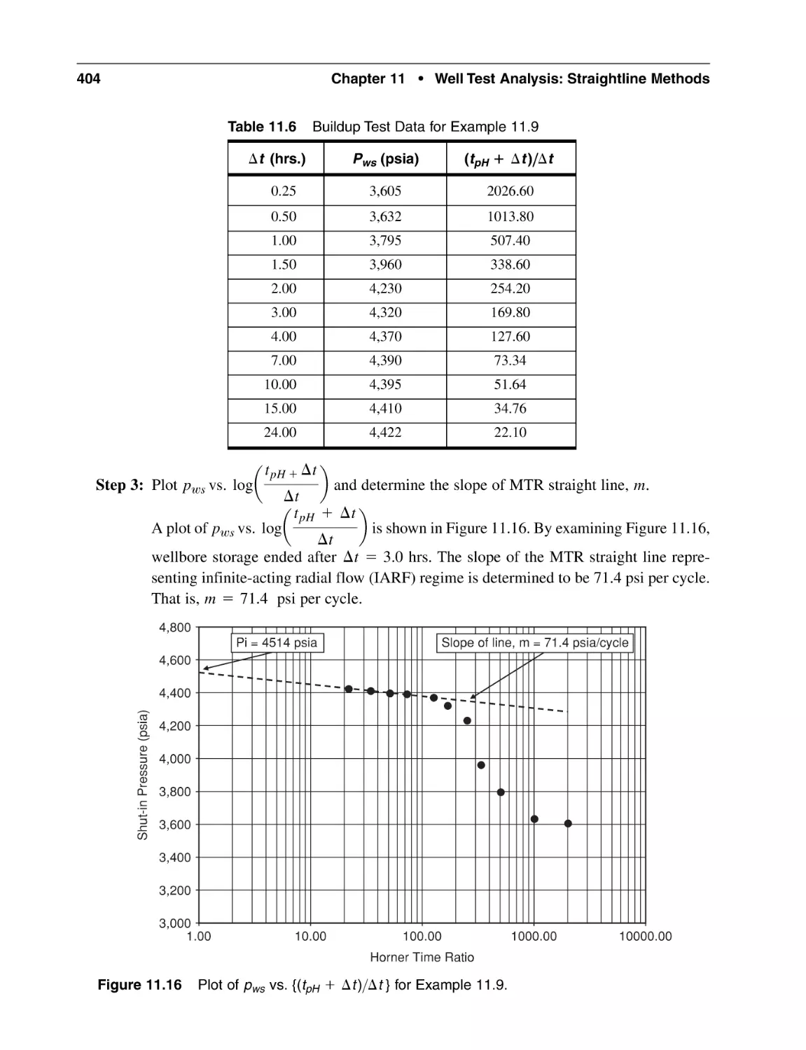
405
432
432
435
435
436
436
439
440
441
441
444
Chapter 12 Well Test Analysis: Type Curves
12.1 Introduction
12.2 What Are Type Curves?
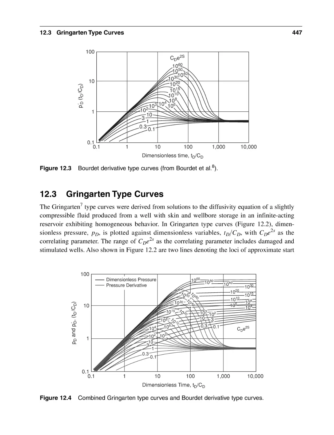
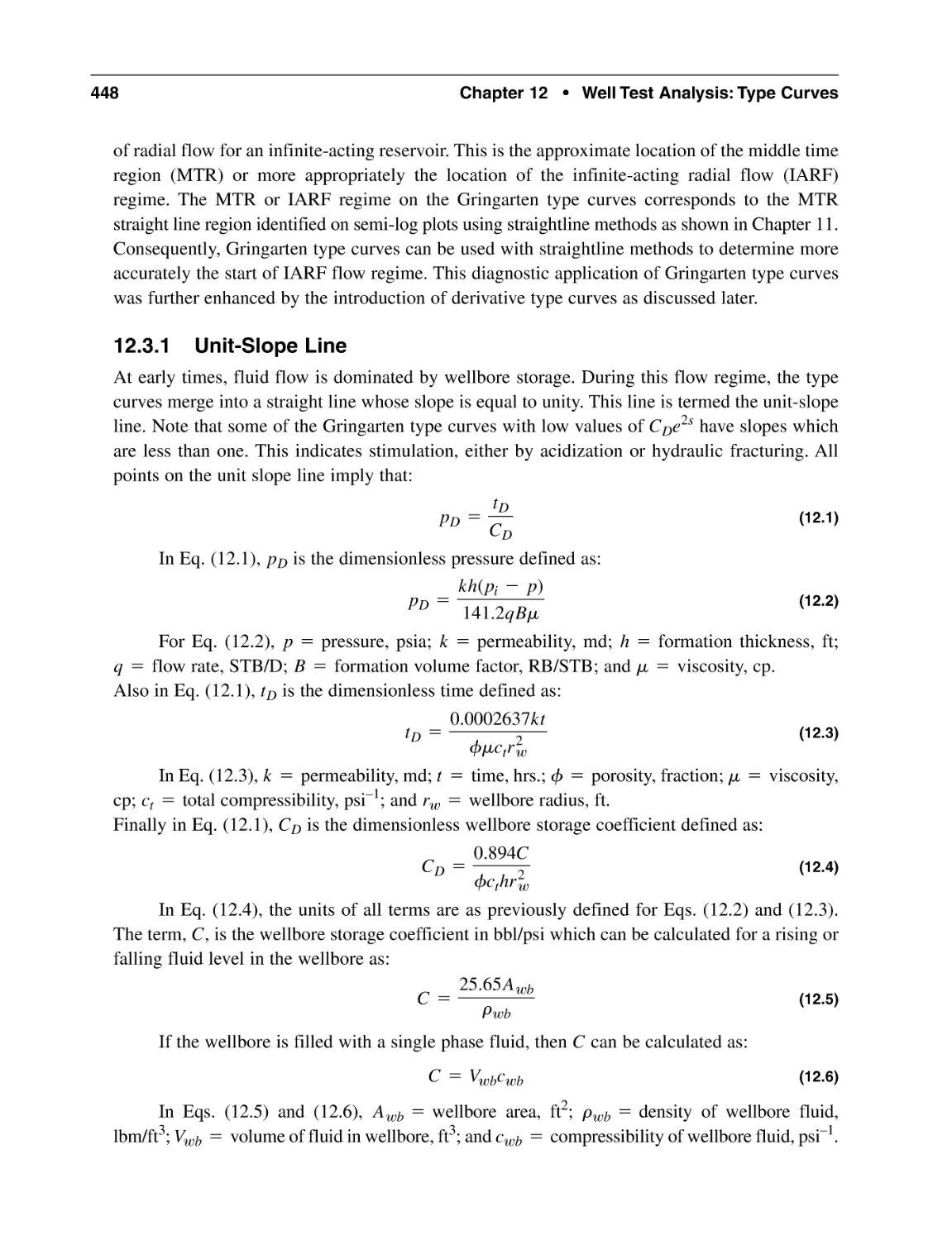
12.3 Gringarten Type Curves
12.3.1 Unit-Slope Line
12.4 Bourdet Derivative Type Curves
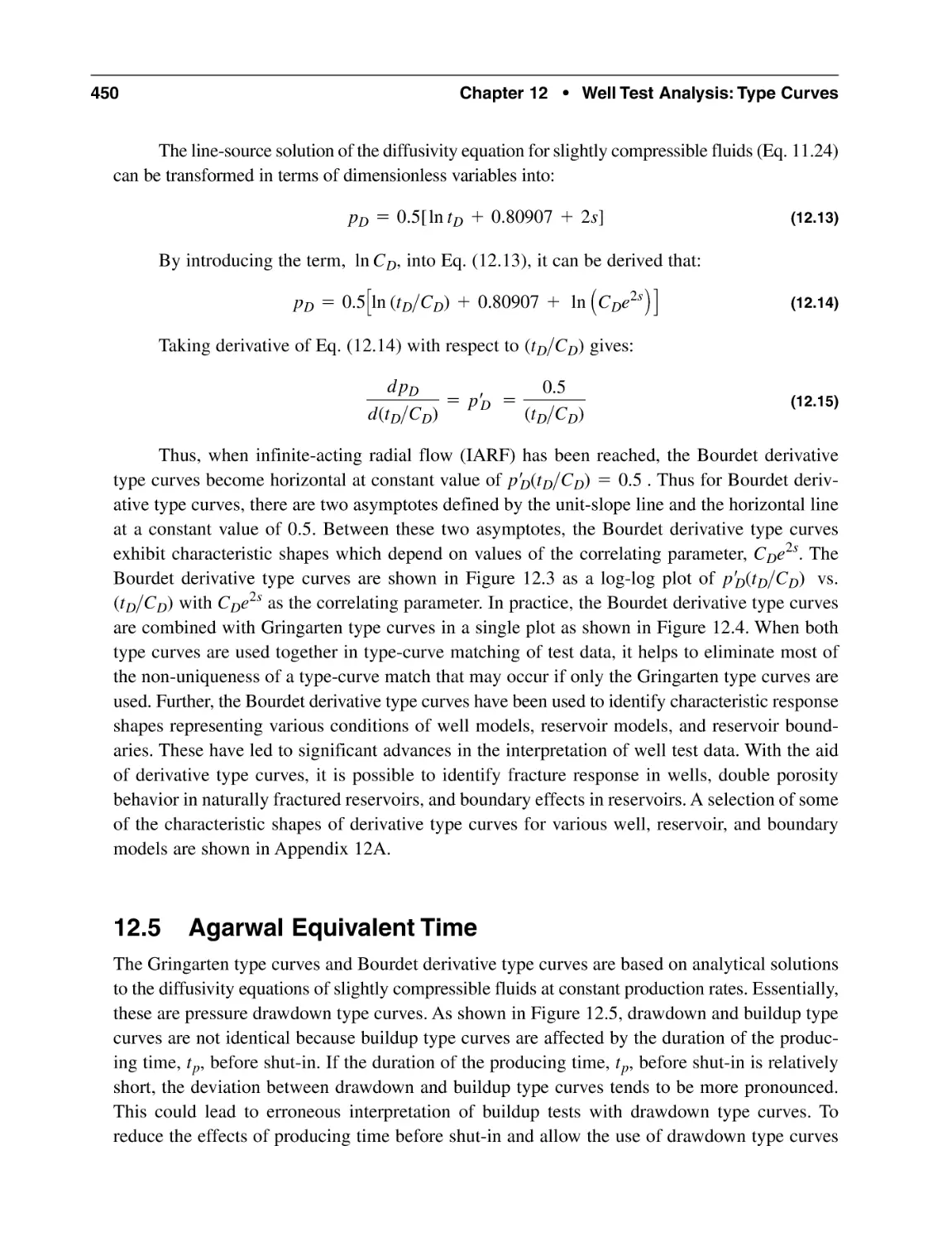
12.5 Agarwal Equivalent Time
445
445
445
447
448
449
450
xvi
Contents
12.6
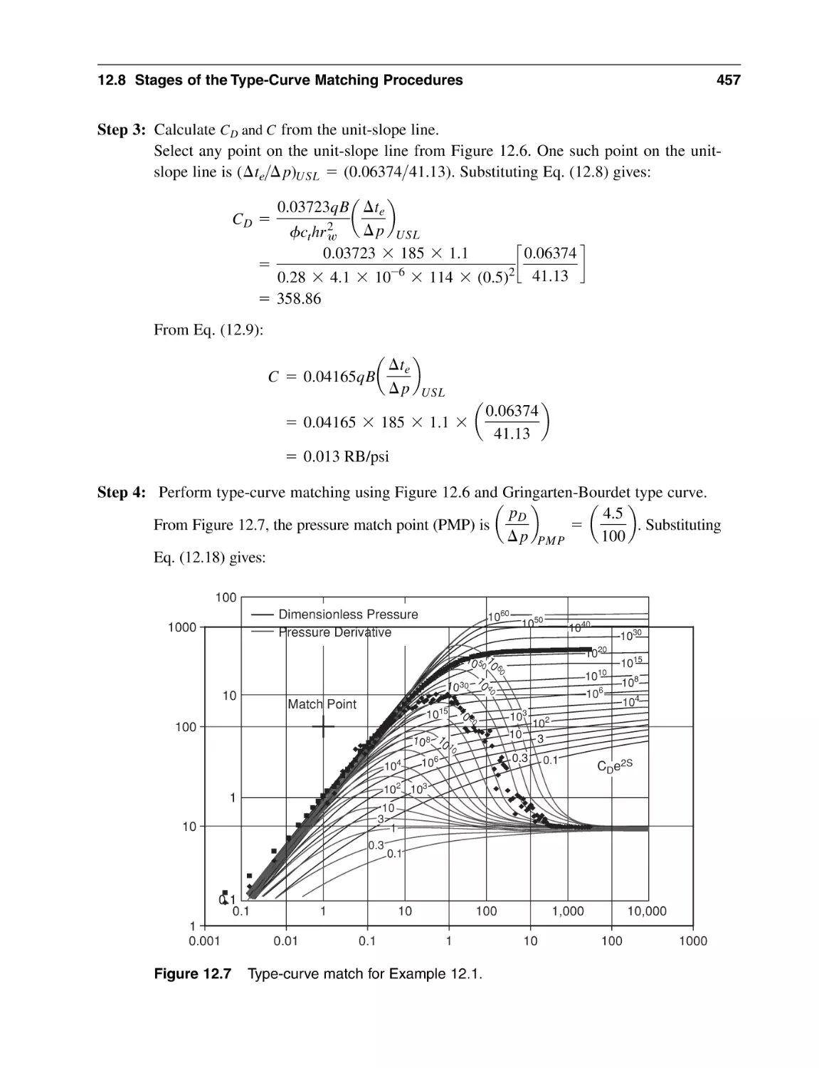
12.7
Type-Curve Matching
Procedures for Manual Application of Type-Curve
Matching in Well Test Analysis
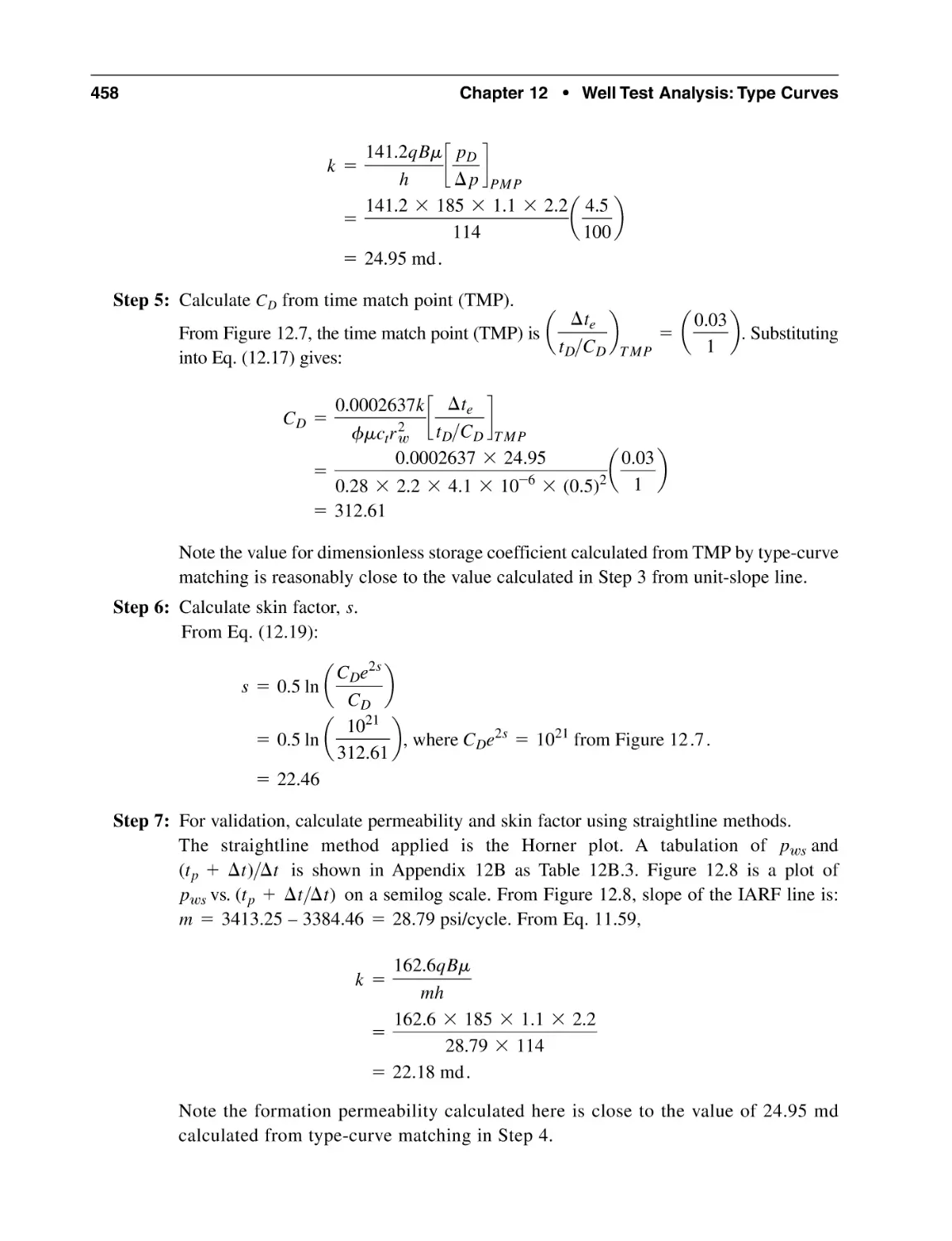
12.8 Stages of the Type-Curve Matching Procedures
12.8.1 Identification of the Interpretation Model
12.8.2 Calculation from Interpretation Model Parameters
12.8.3 Validation of the Interpretation Model Results
Nomenclature
Subscripts
Abbreviations
References
451
452
454
454
455
455
459
460
460
461
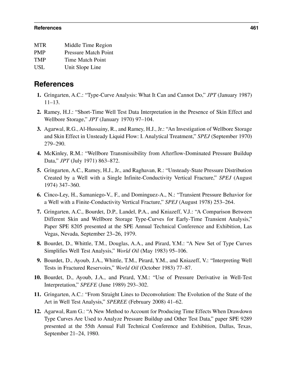
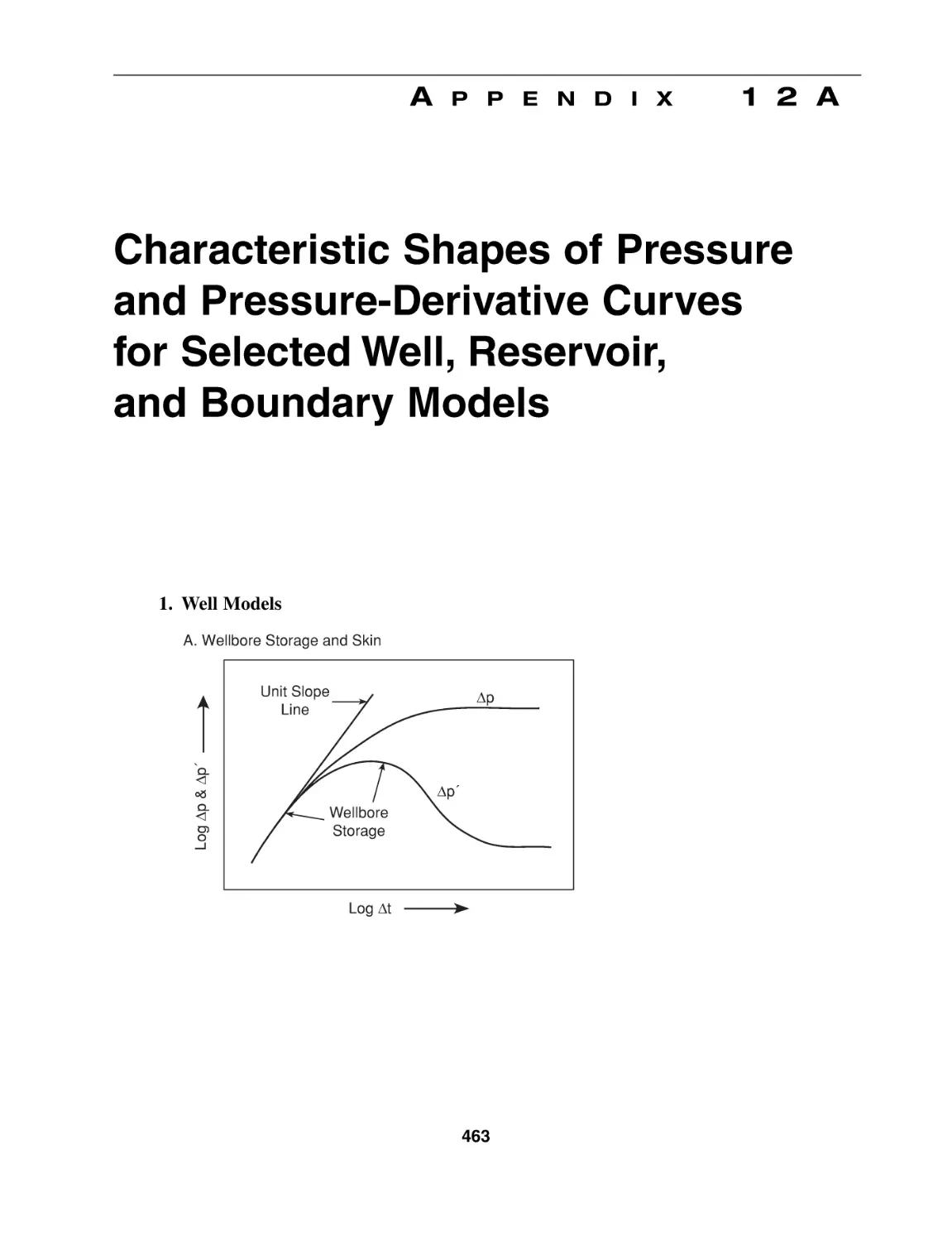
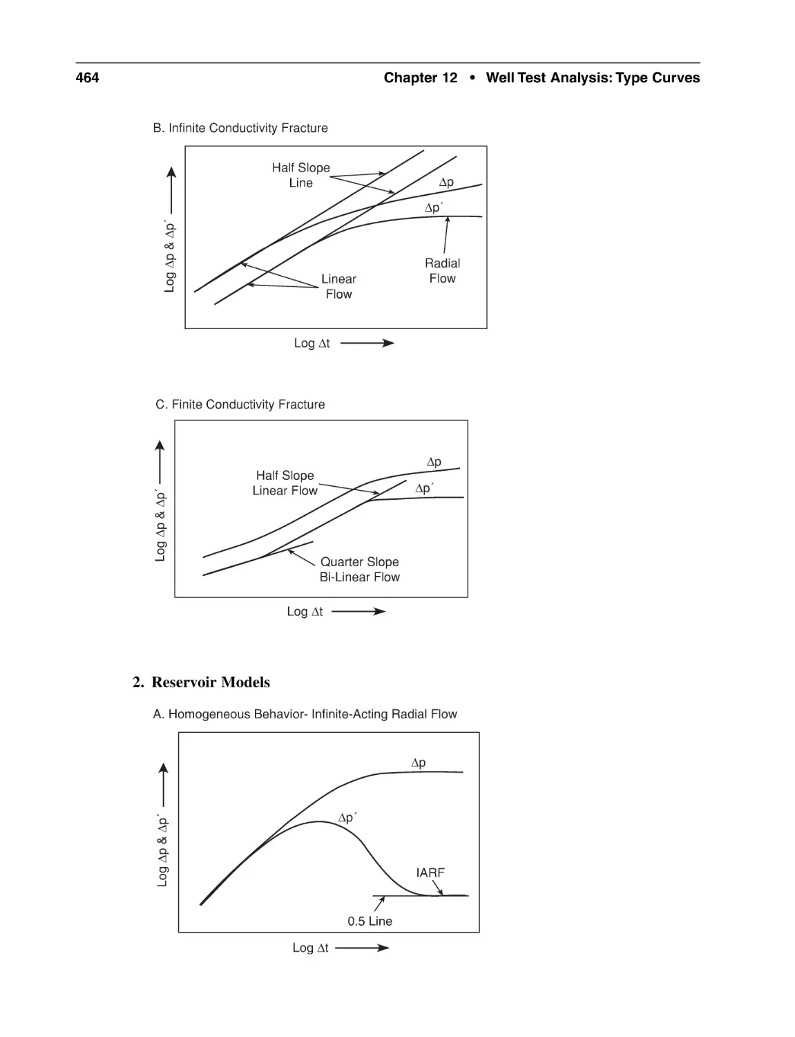
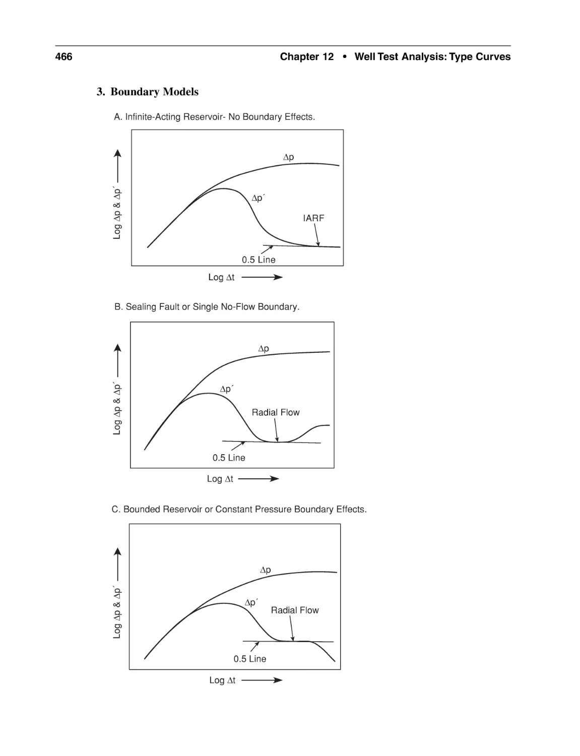
Appendix 12A Characteristic Shapes of Pressure and PressureDerivative Curves for Selected Well, Reservoir, and Boundary Models
463
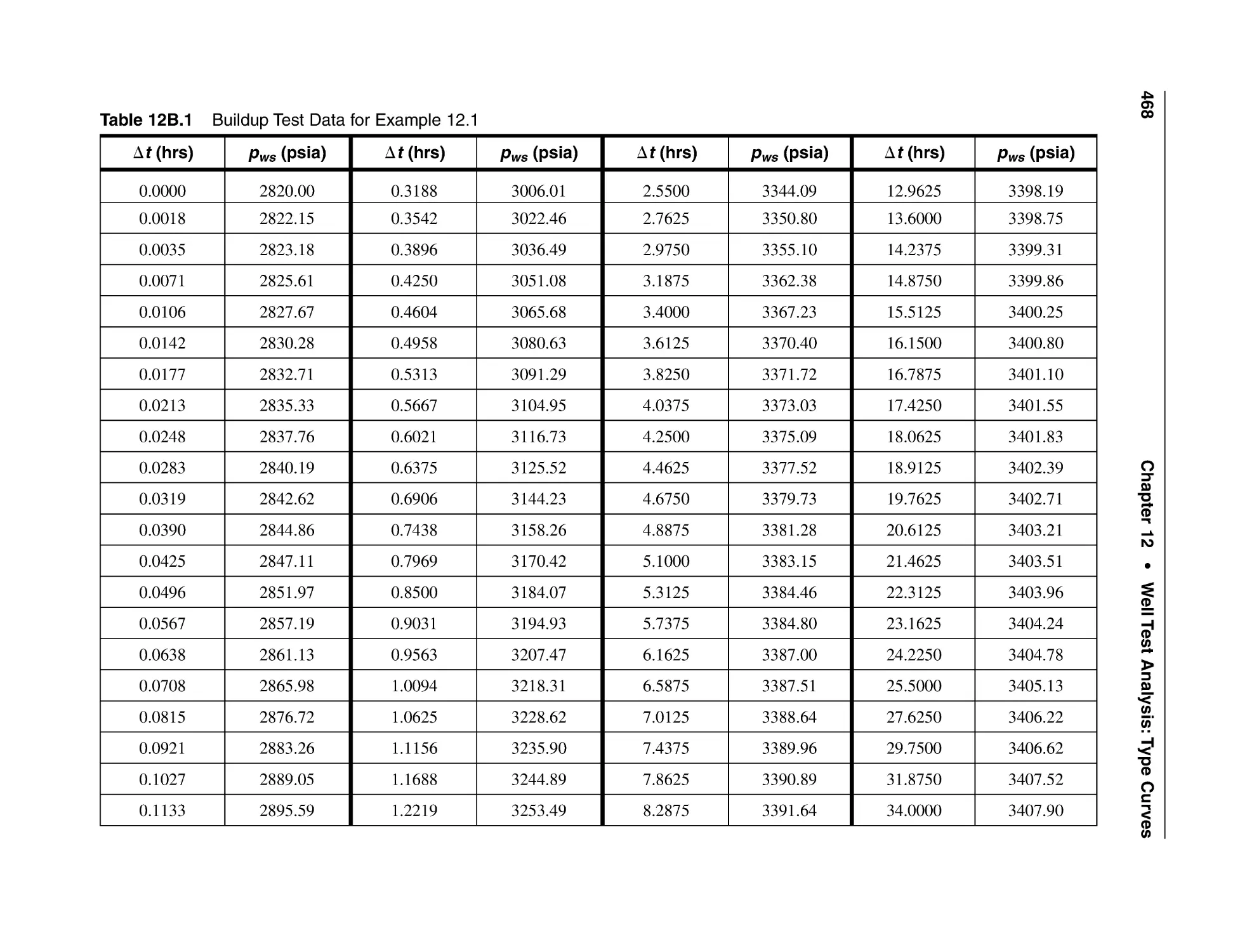
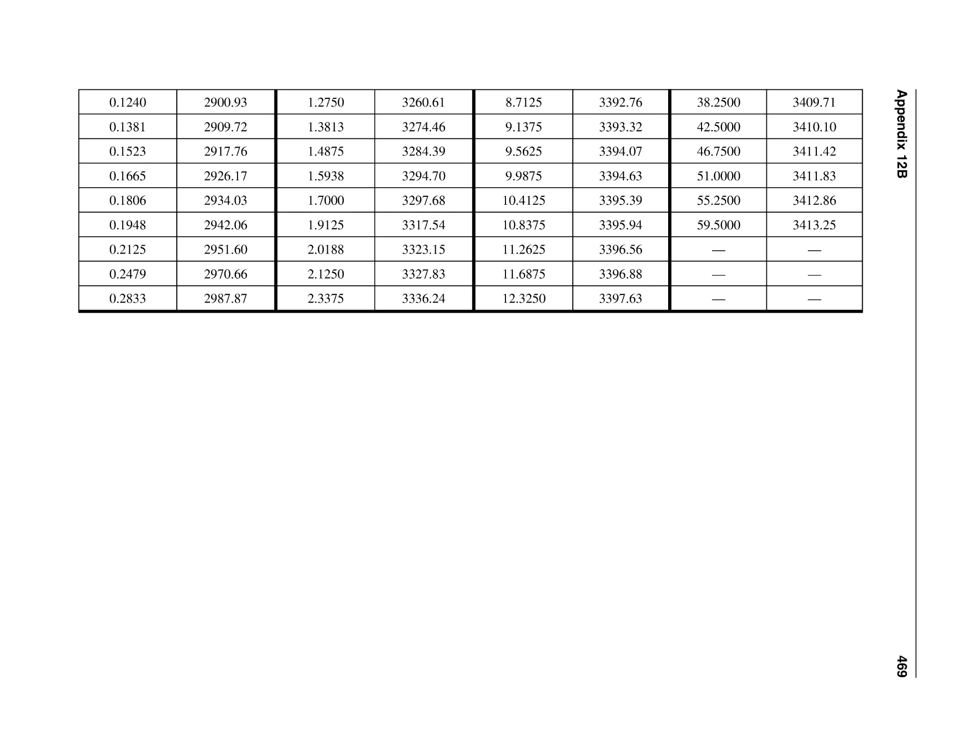
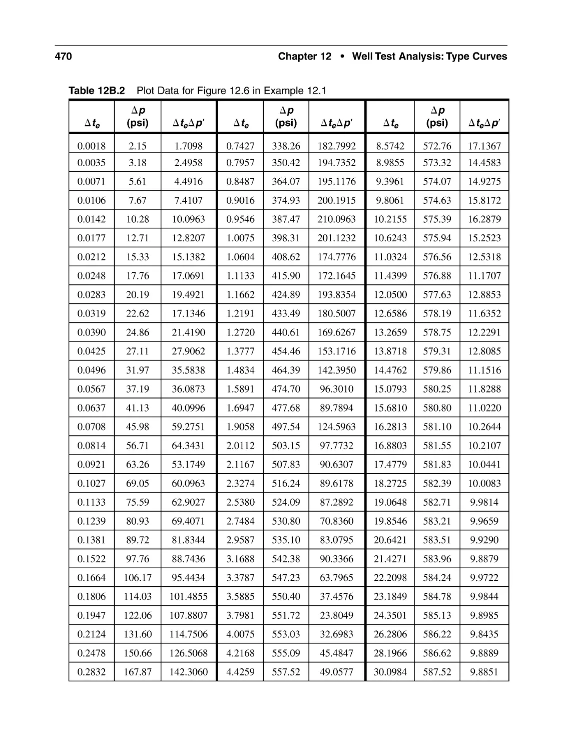
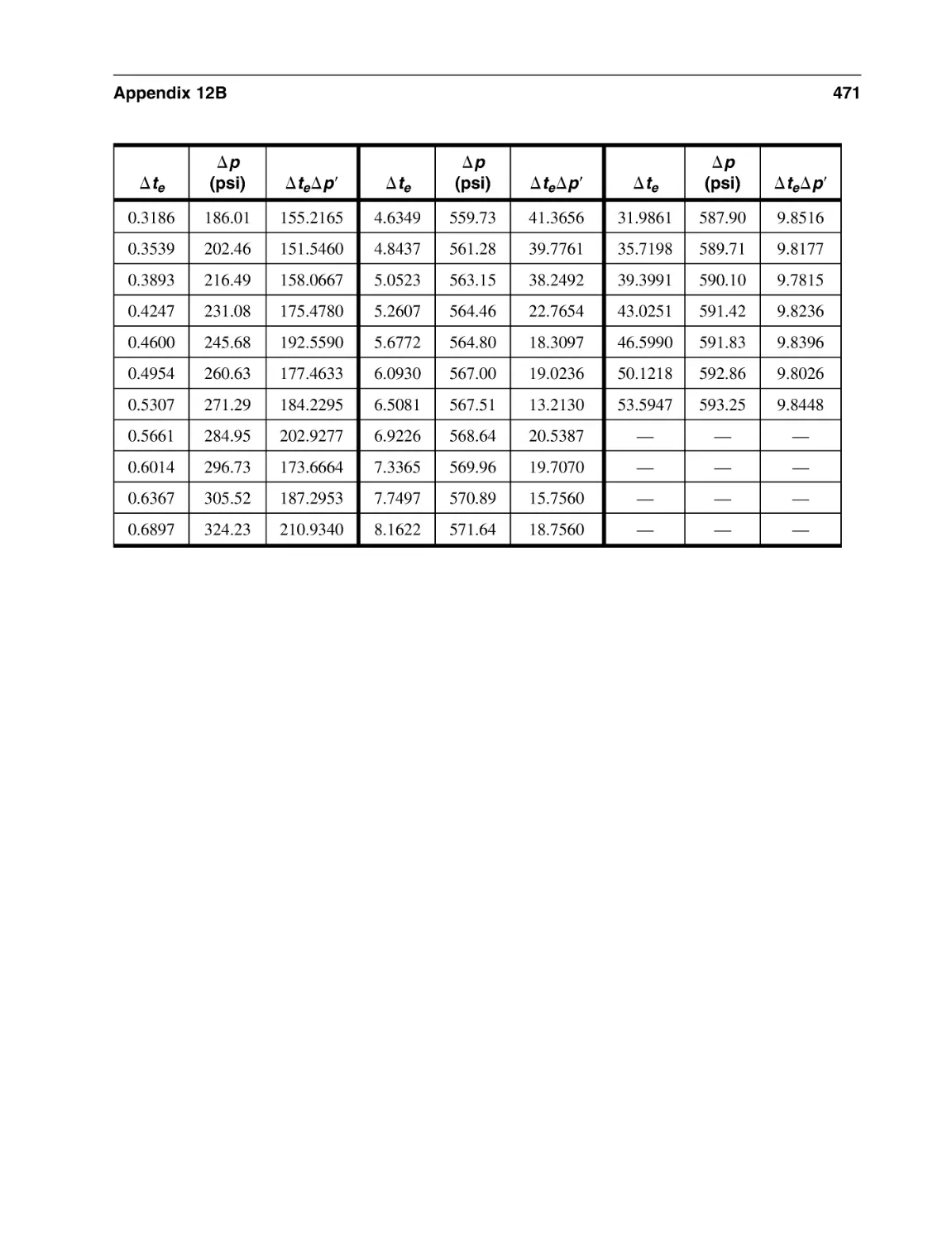
Appendix 12B Buildup Test Data for Example 12.1
467
Appendix 12C Calculation of Pressure Derivatives
Reference
473
474
Chapter 13 Well Test Analysis: Hydraulically Fractured Wells
and Naturally Fractured Reservoirs
13.1 Introduction
13.2 Hydraulically Fractured Wells
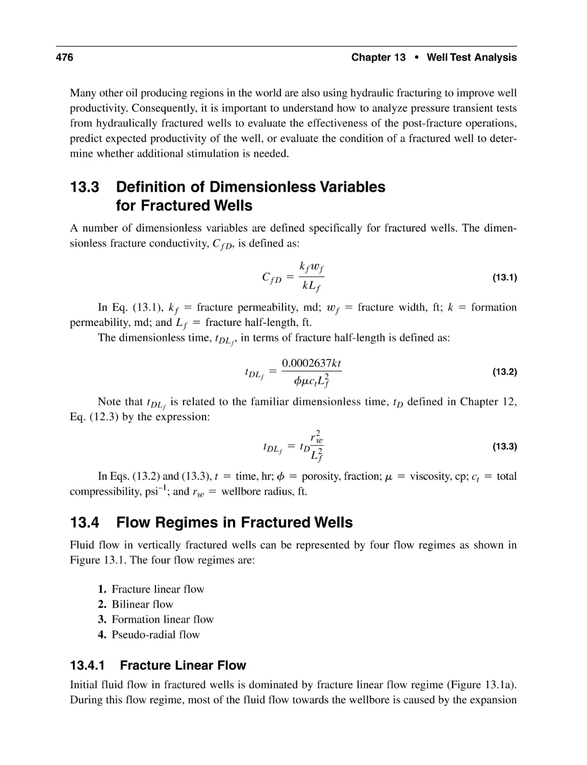
13.3 Definition of Dimensionless Variables for Fractured Wells
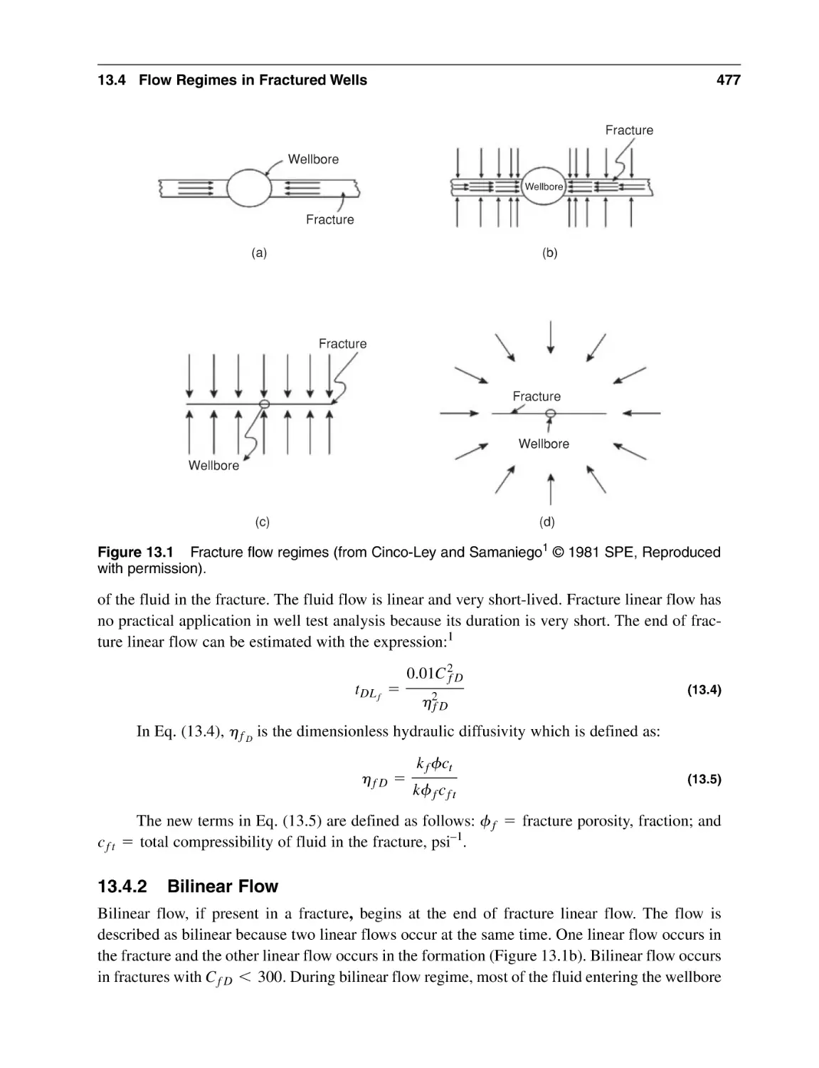
13.4 Flow Regimes in Fractured Wells
13.4.1 Fracture Linear Flow
13.4.2 Bilinear Flow
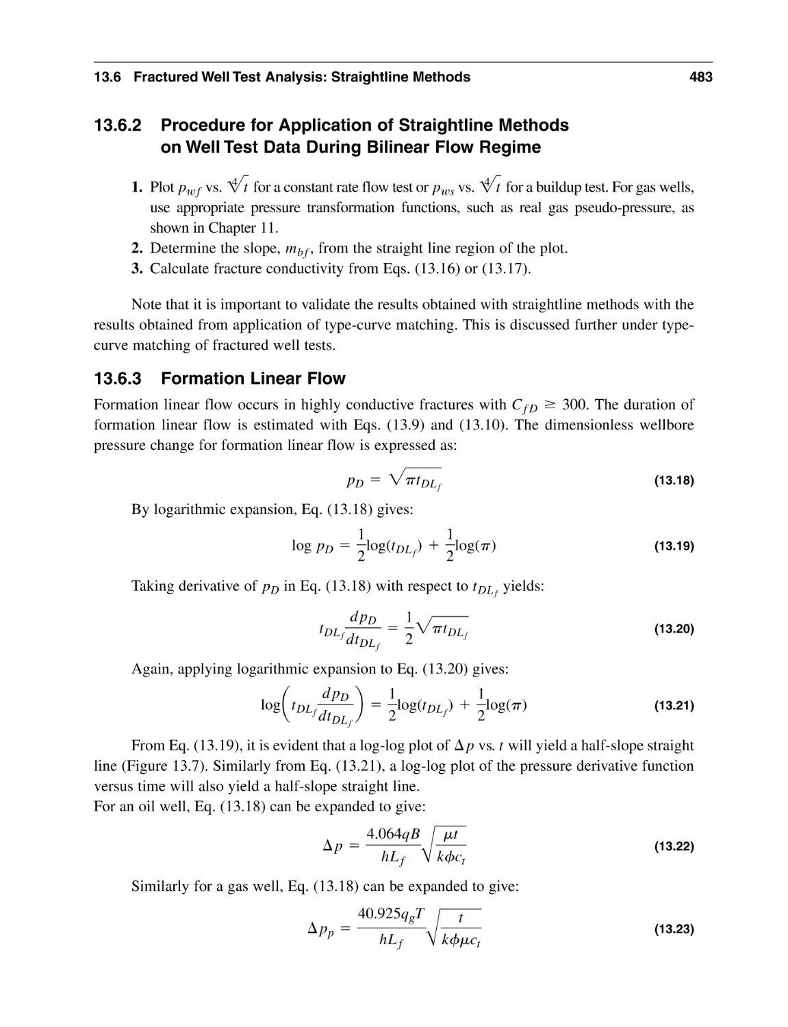
13.4.3 Formation Linear Flow
13.4.4 Pseudo-Radial Flow
13.5 Fractured Well Flow Models
13.5.1 Finite Conductivity Vertical Fracture
13.5.2 Infinite Conductivity Vertical Fracture
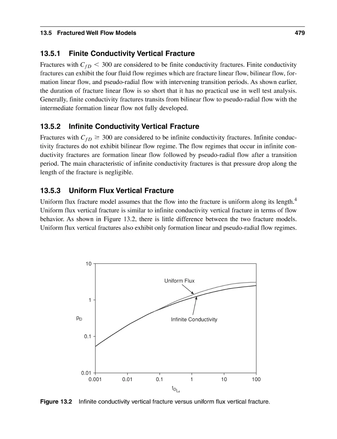
13.5.3 Uniform Flux Vertical Fracture
13.6 Fractured Well Test Analysis: Straightline Methods
13.6.1 Bilinear Flow
13.6.2 Procedure for Application of Straightline Methods
on Well Test Data During Bilinear Flow Regime
13.6.3 Formation Linear Flow
13.6.4 Procedure for Application of Straightline Methods on
Well Test Data During Formation Linear Flow Regime
475
475
475
476
476
476
477
478
478
478
479
479
479
480
480
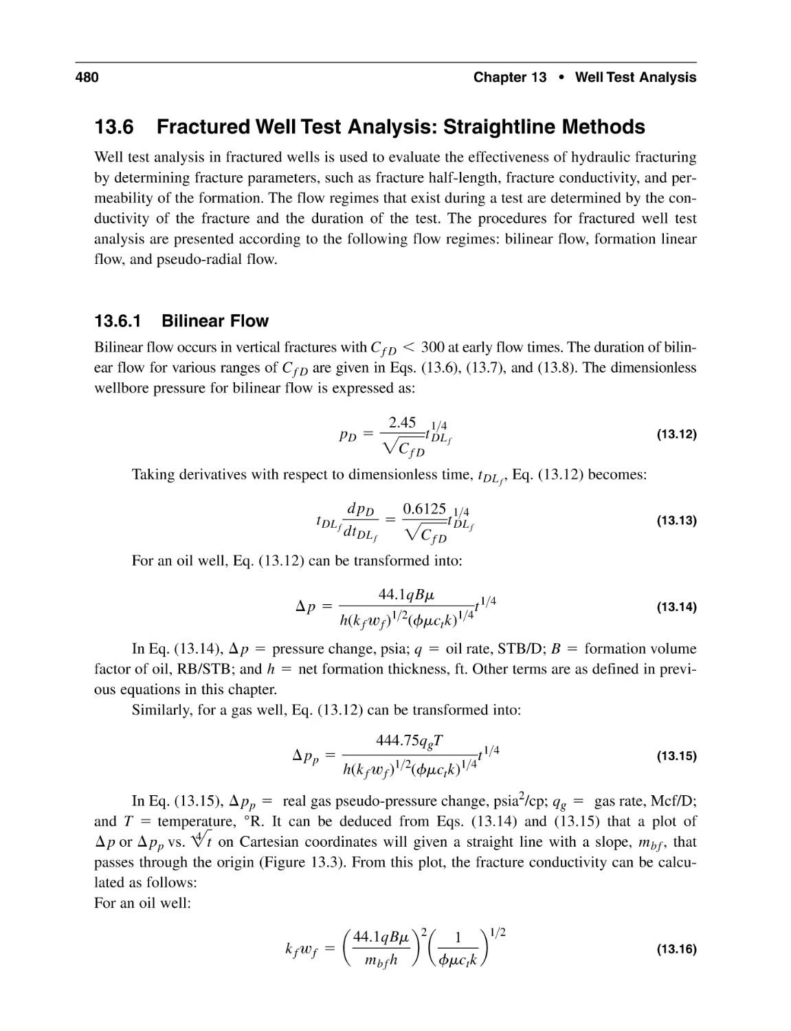
483
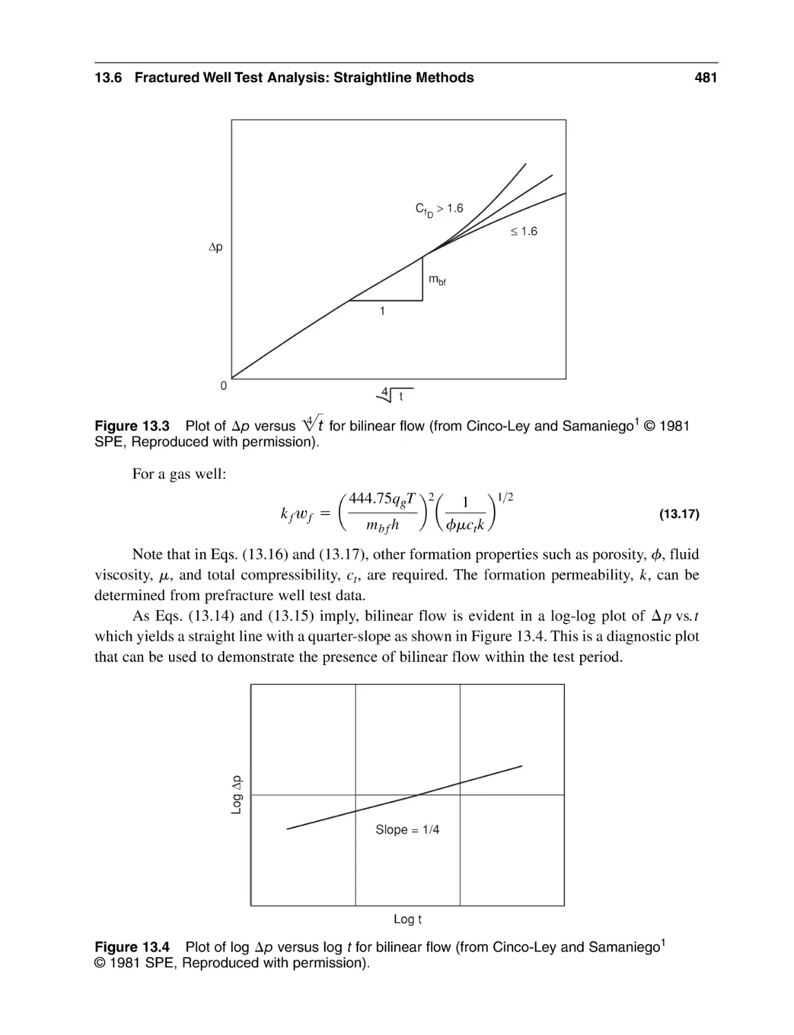
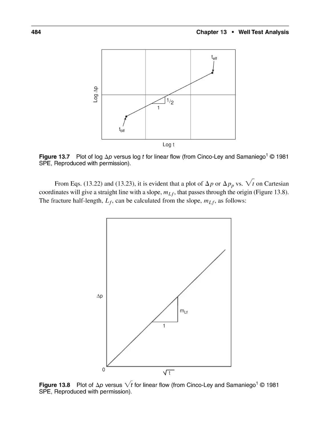
483
485
Contents
13.6.5
13.6.6
Pseudo-Radial Flow
Procedure for Application of Straightline Methods on
Well Test Data During Pseudo-Radial Flow Regime
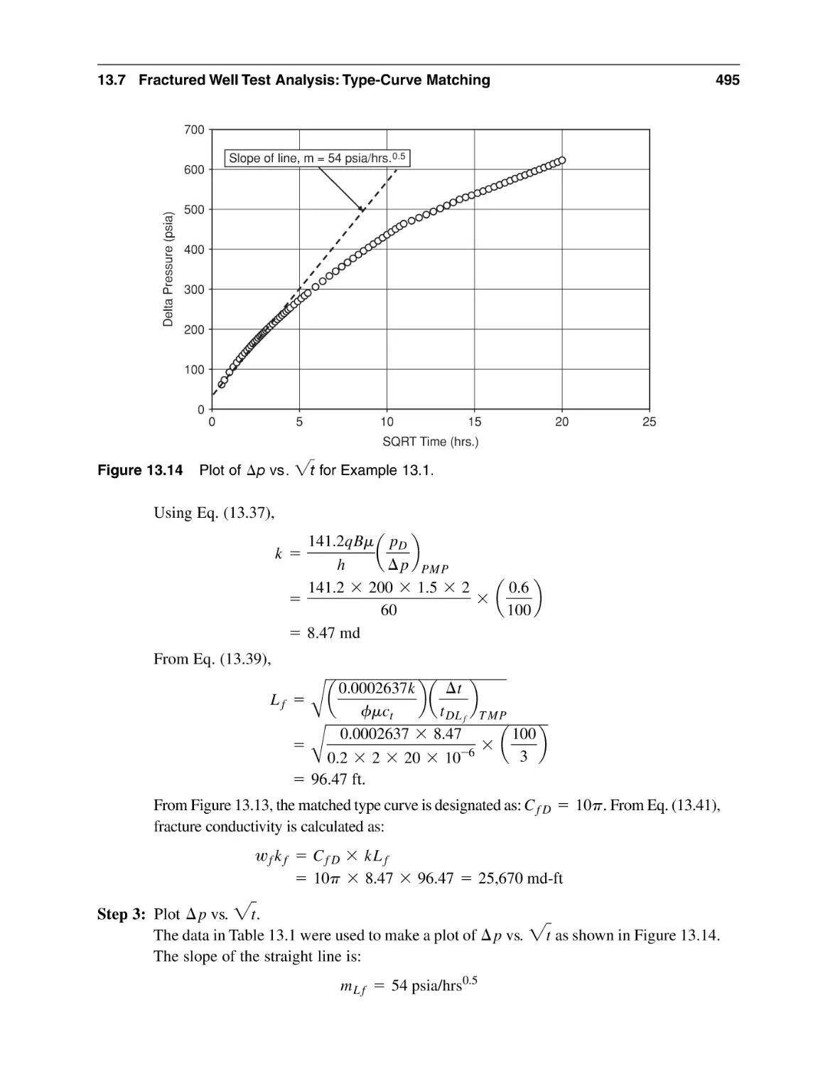
13.7 Fractured Well Test Analysis: Type-Curve Matching
13.7.1 Identification of the Interpretation Model
13.7.2 Calculation from Interpretation Model Parameters
13.7.3 Validation of the Interpretation Model Results
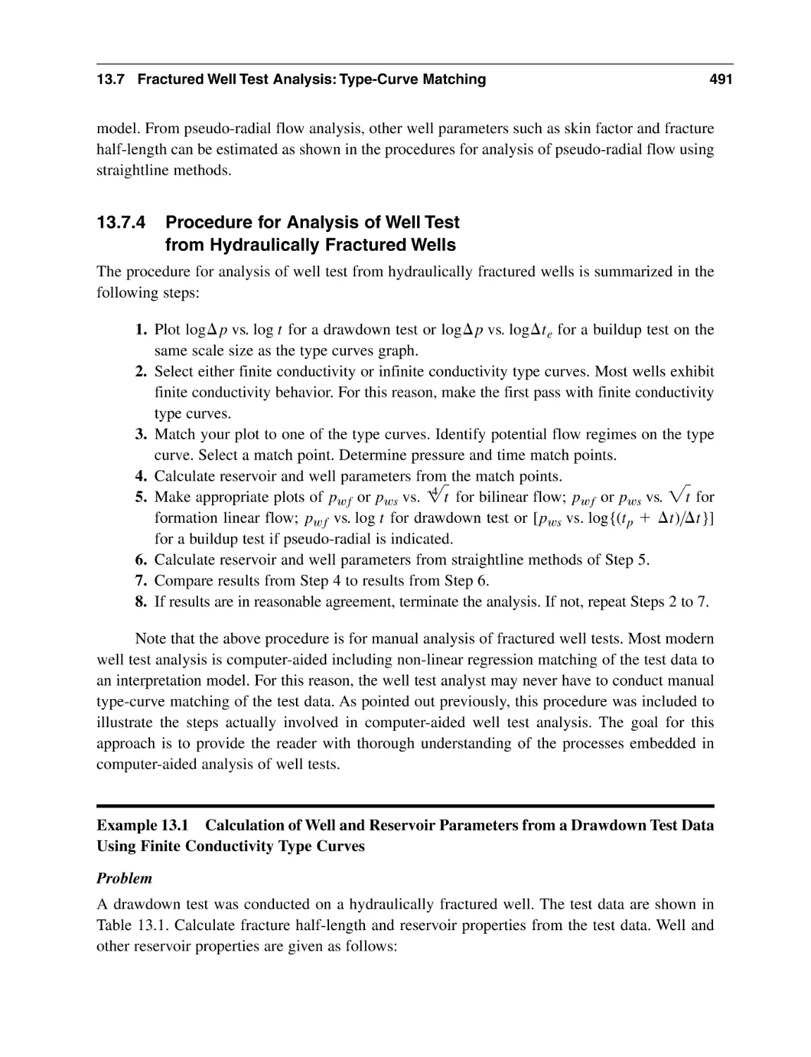
13.7.4 Procedure for Analysis of Well Test from Hydraulically
Fractured Wells
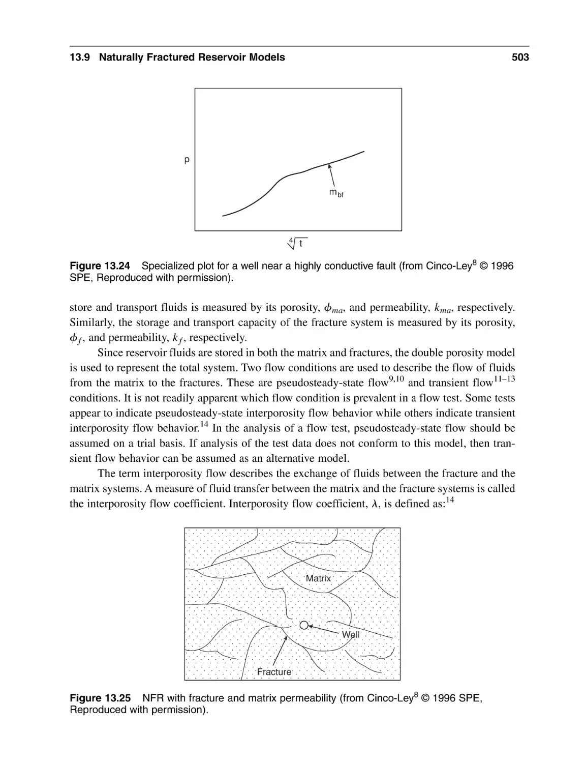
13.8 Naturally Fractured Reservoirs
13.9 Naturally Fractured Reservoir Models
13.9.1 Homogeneous Reservoir Model
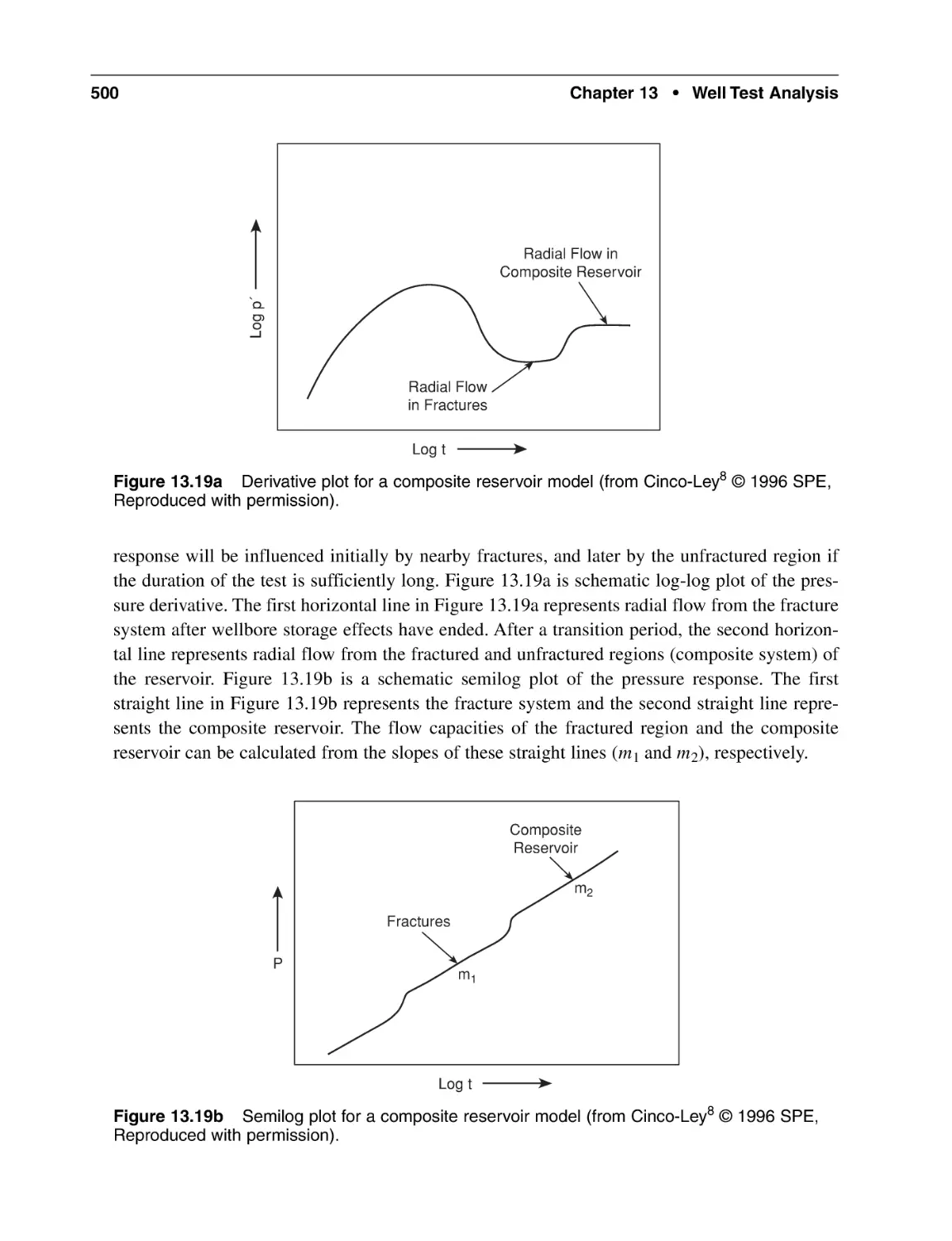
13.9.2 Multiple Region or Composite Reservoir Model
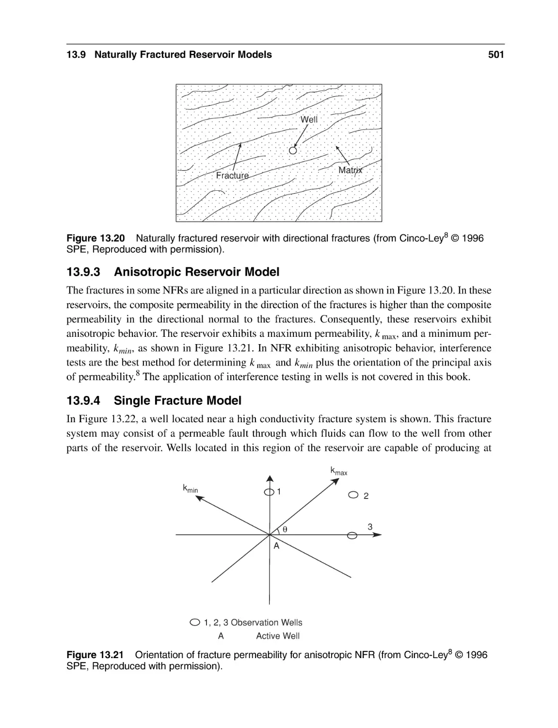
13.9.3 Anisotropic Reservoir Model
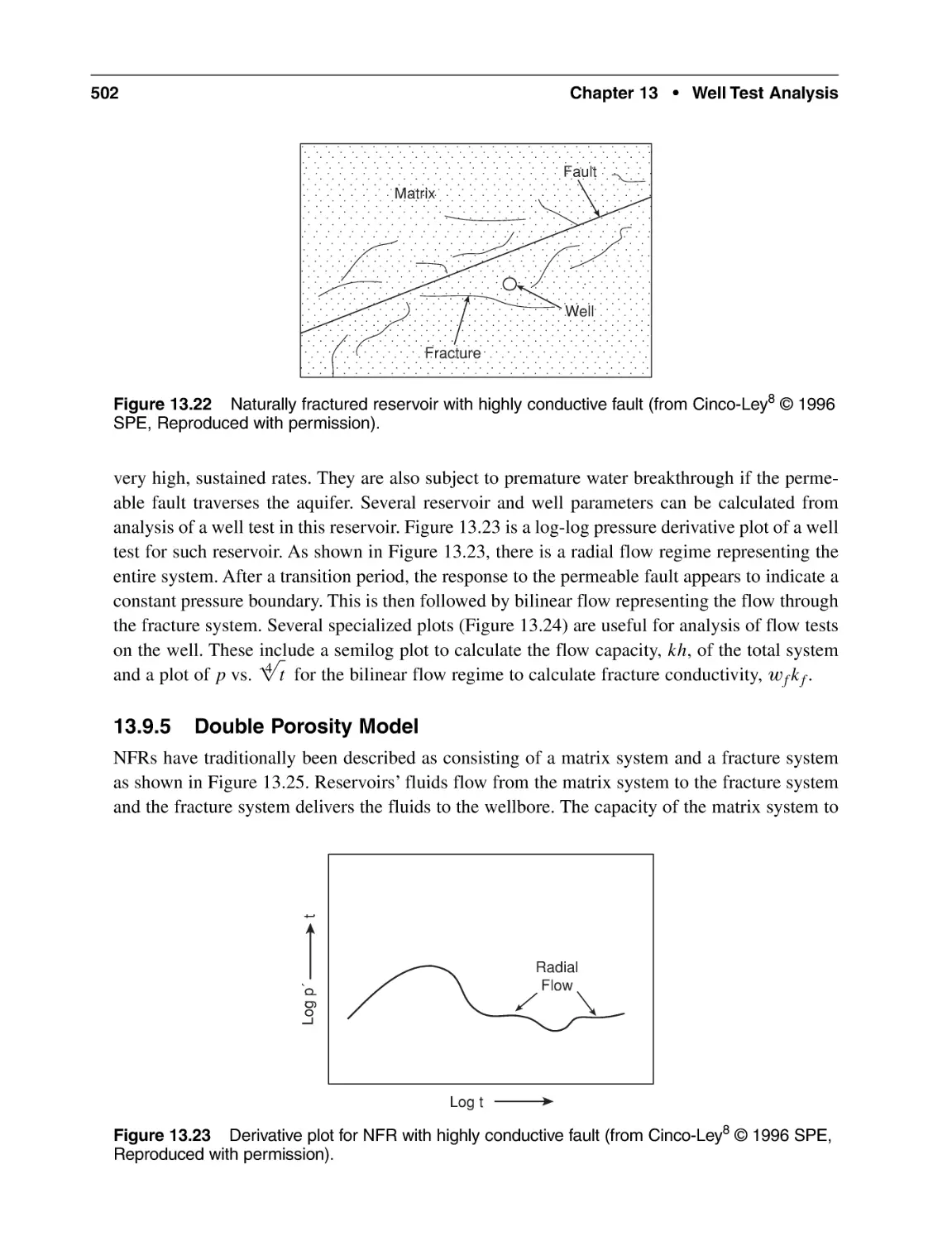
13.9.4 Single Fracture Model
13.9.5 Double Porosity Model
13.10 Well Test Analysis in Naturally Fractured Reservoirs
Based on Double Porosity Model
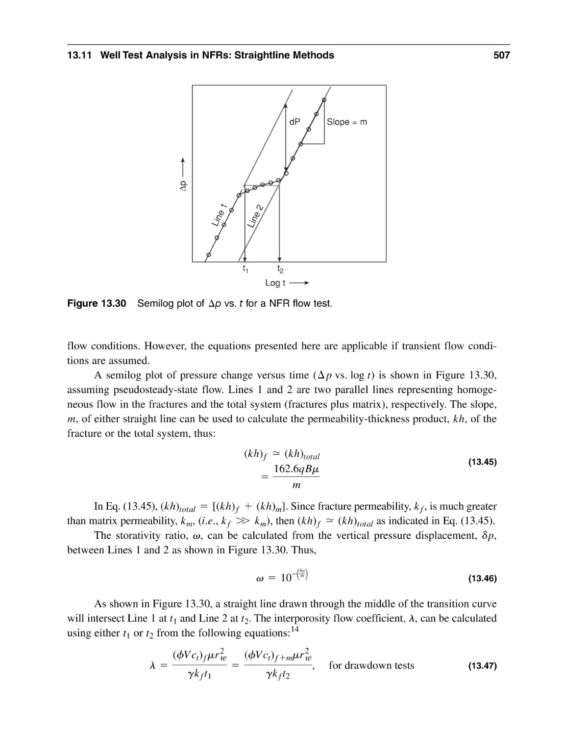
13.11 Well Test Analysis in NFRs: Straightline Methods
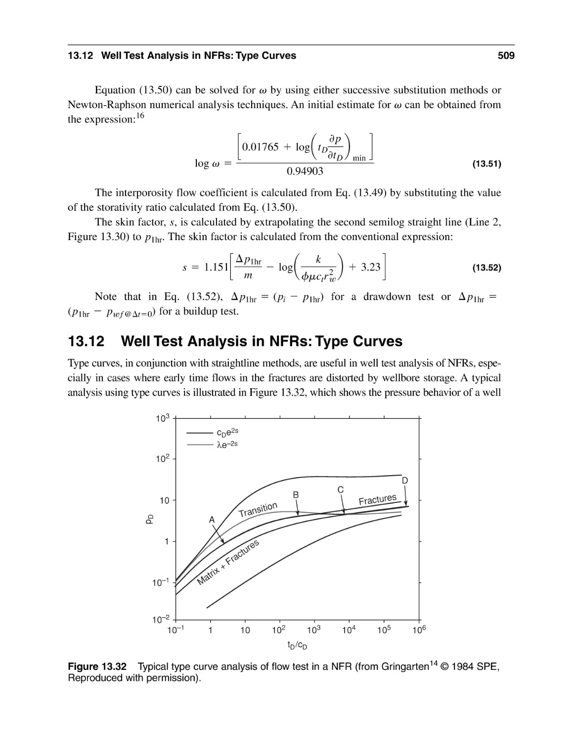
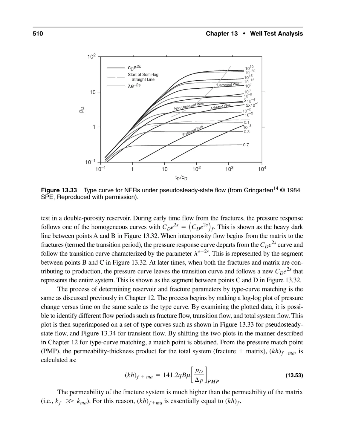
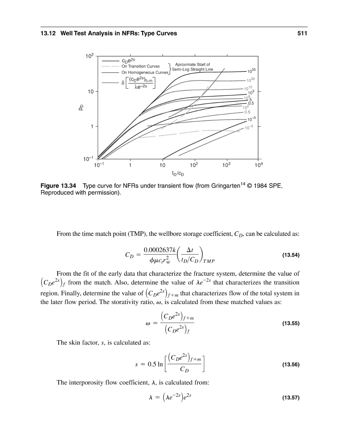
13.12 Well Test Analysis in NFRs: Type Curves
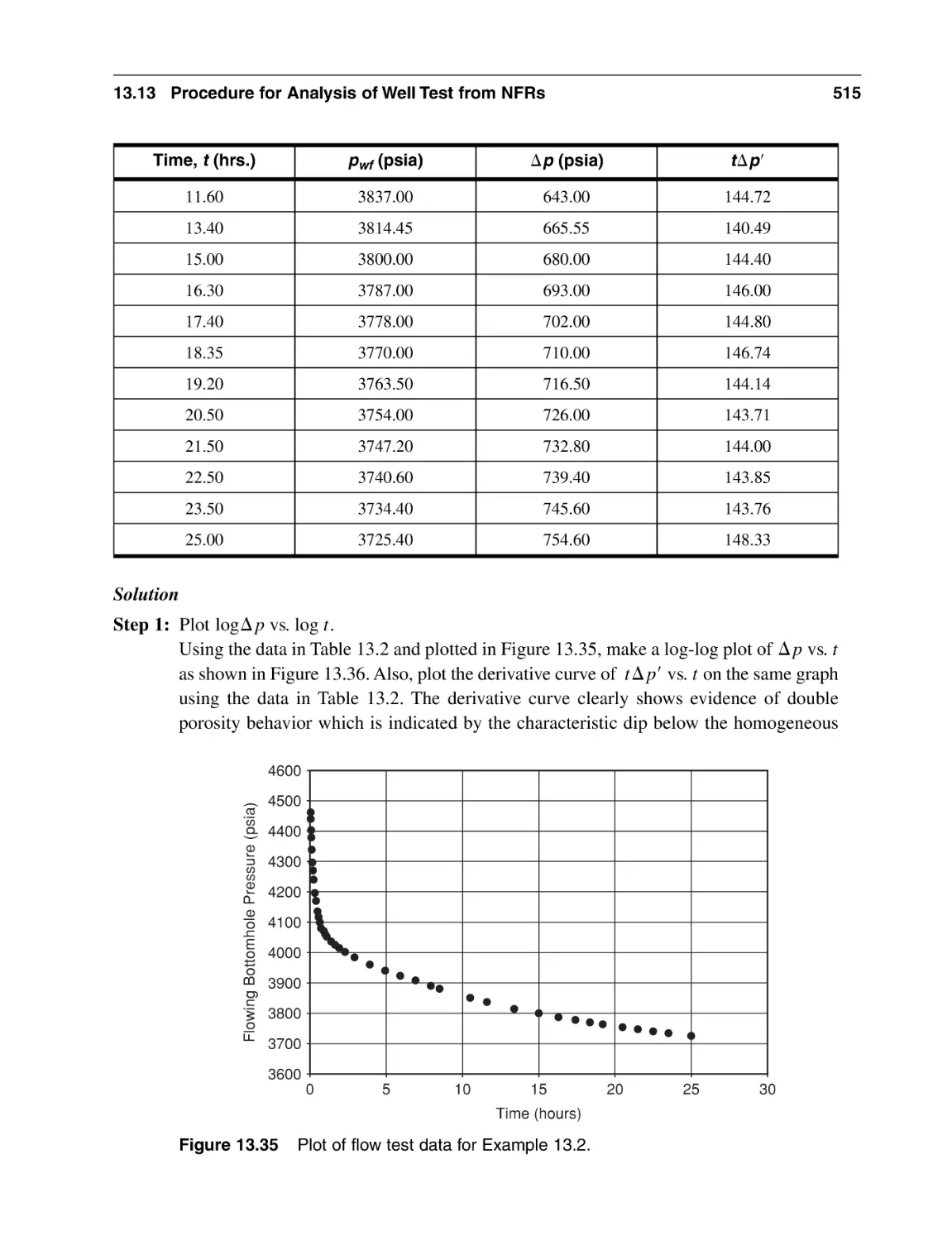
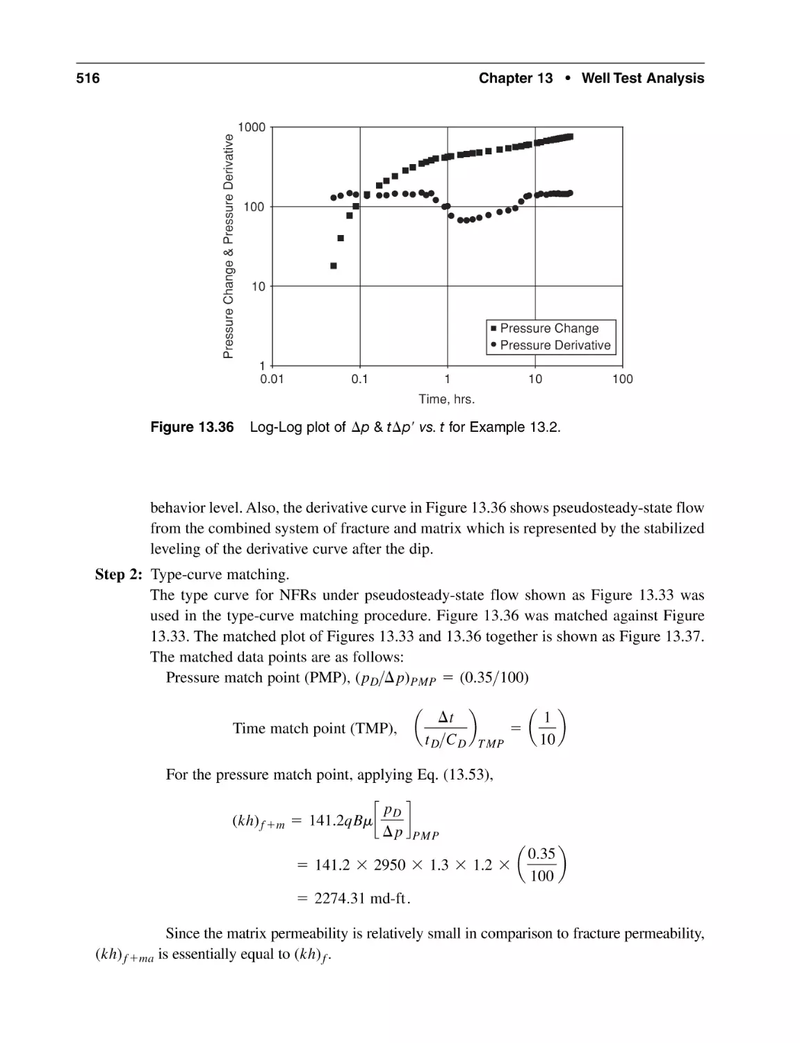
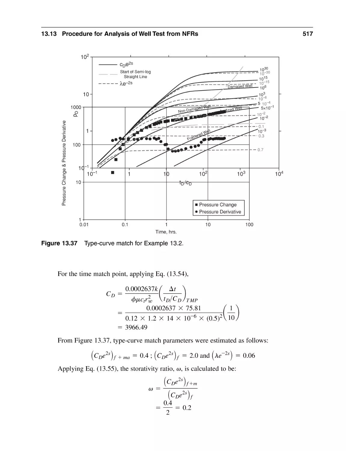
13.13 Procedure for Analysis of Well Test from NFRs Assuming
Double Porosity Behavior
13.13.1 Identification of Flow Periods
13.13.2 Calculation of Fracture and Reservoir Parameters
from Type Curves
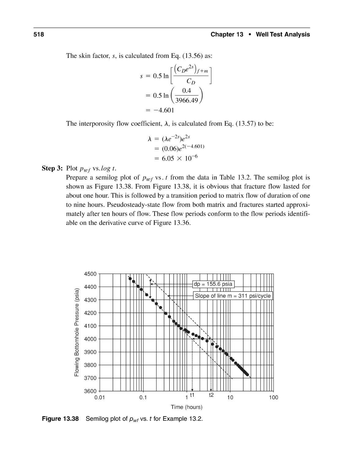
13.13.3 Validation of Results with Straightline Methods
Nomenclature
Subscripts
Abbreviations
References
General Reading
Chapter 14 Well Test Analysis: Deconvolution Concepts
14.1 Introduction
14.2 What Is Deconvolution?
14.3 The Pressure-Rate Deconvolution Model
14.3.1 The von Schroeter et al. Deconvolution Algorithm
14.4 Application of Deconvolution to Pressure-Rate Data
xvii
486
487
487
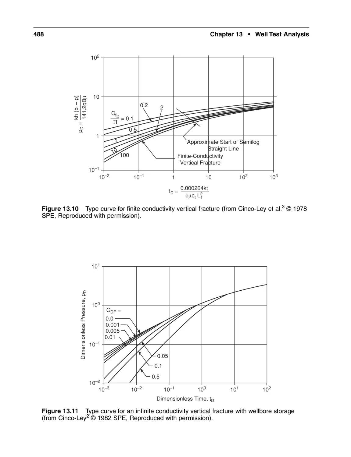
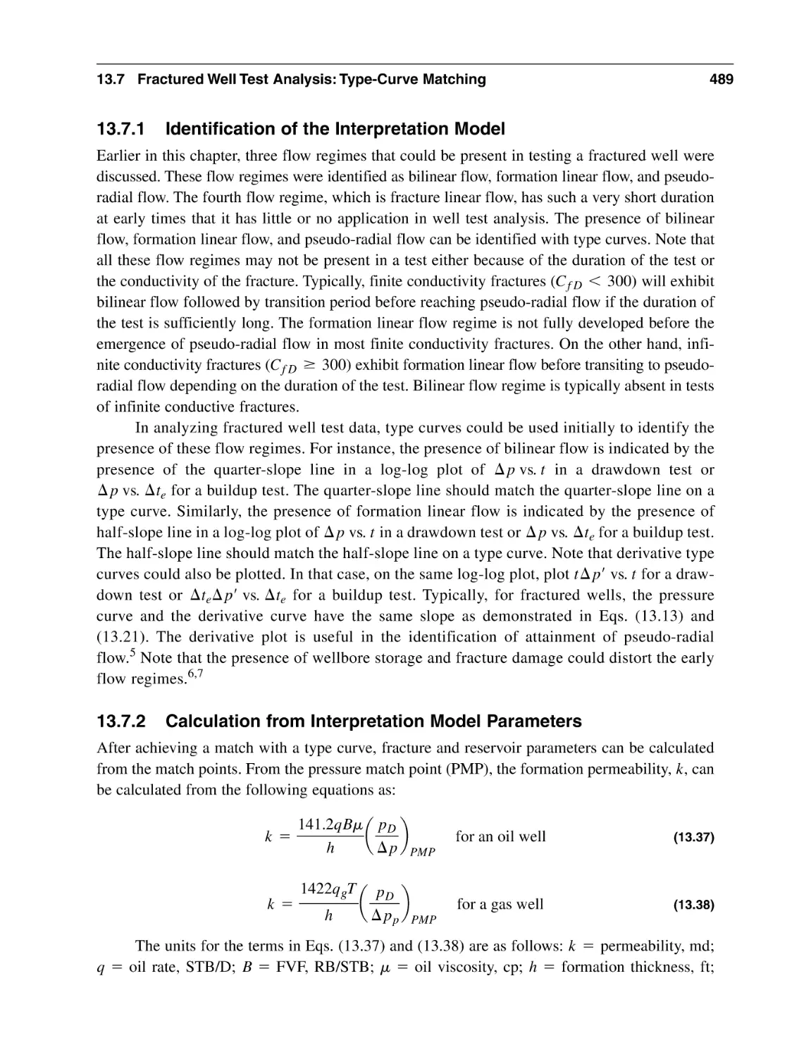
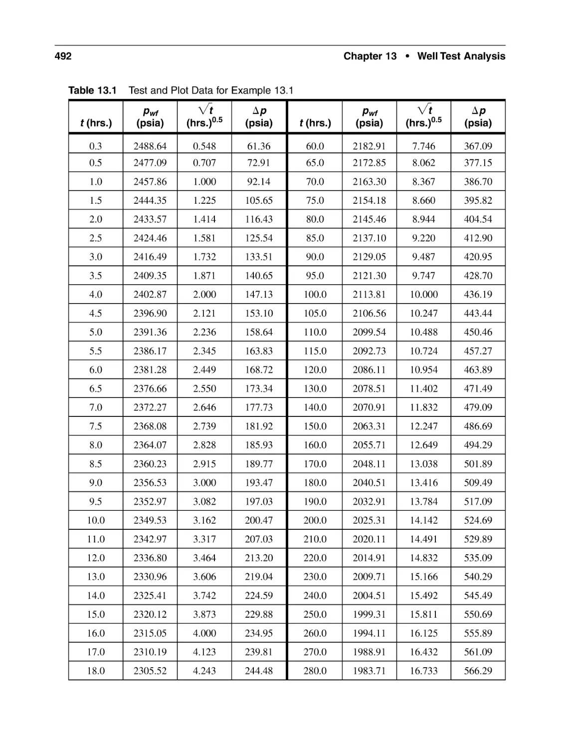
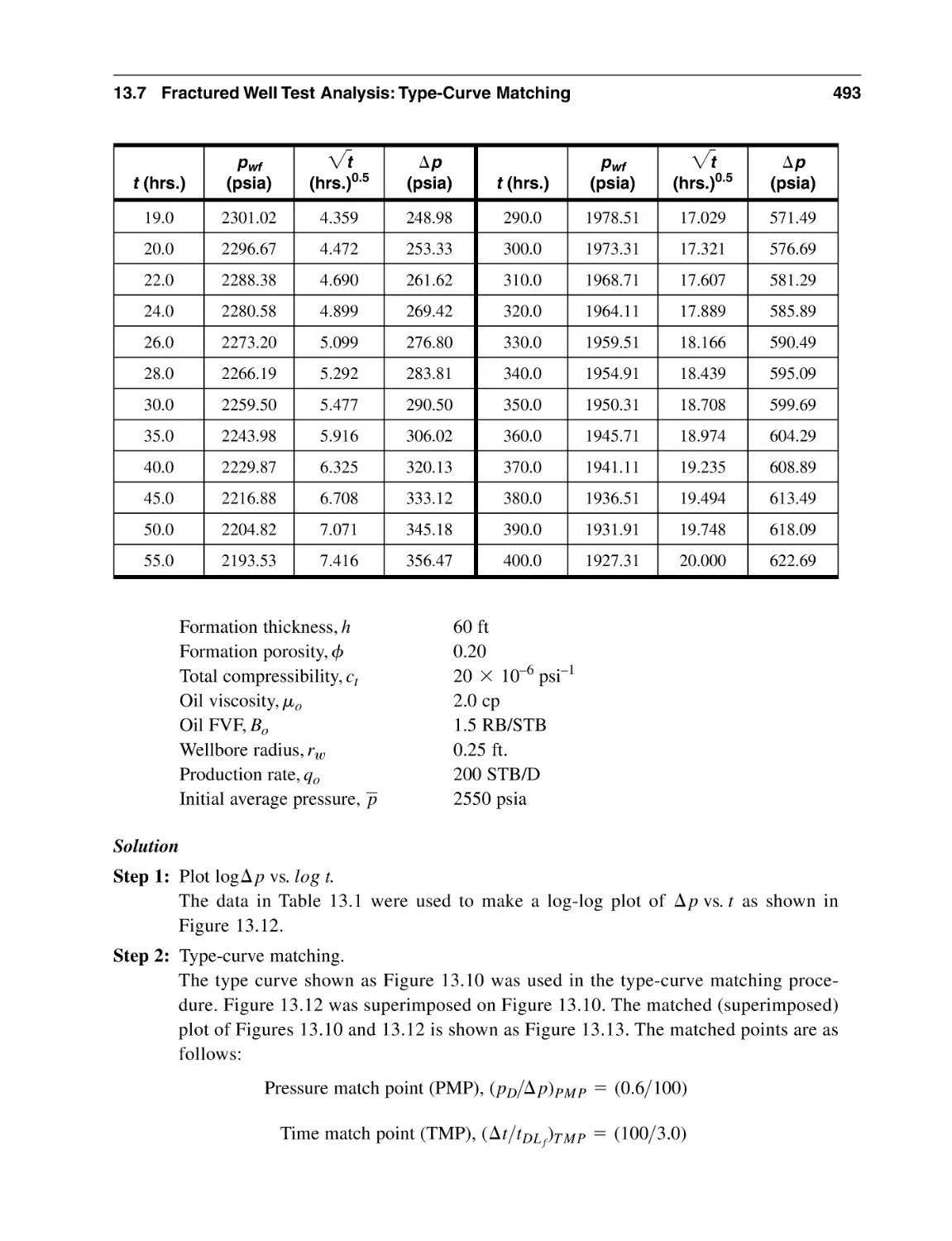
489
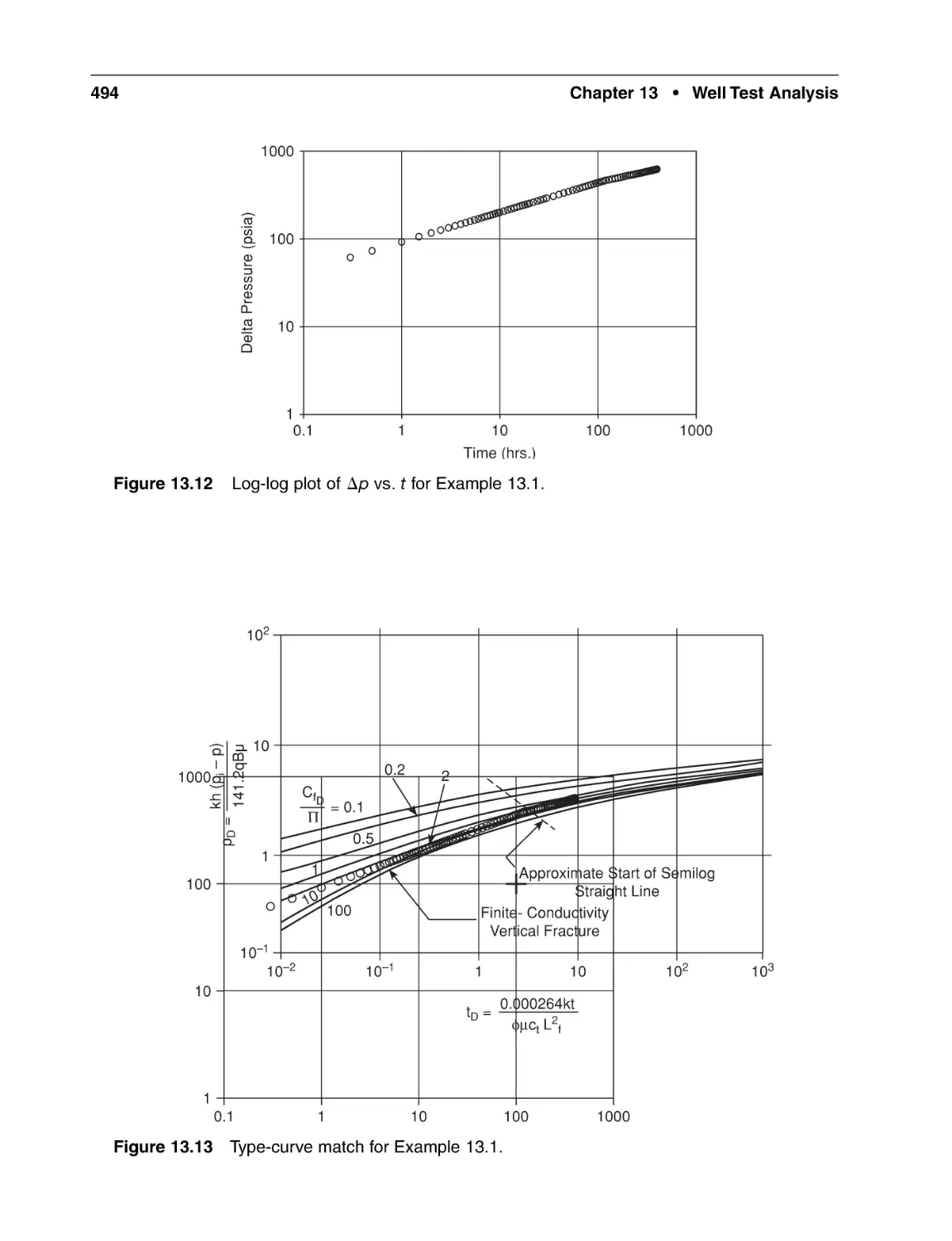
489
490
491
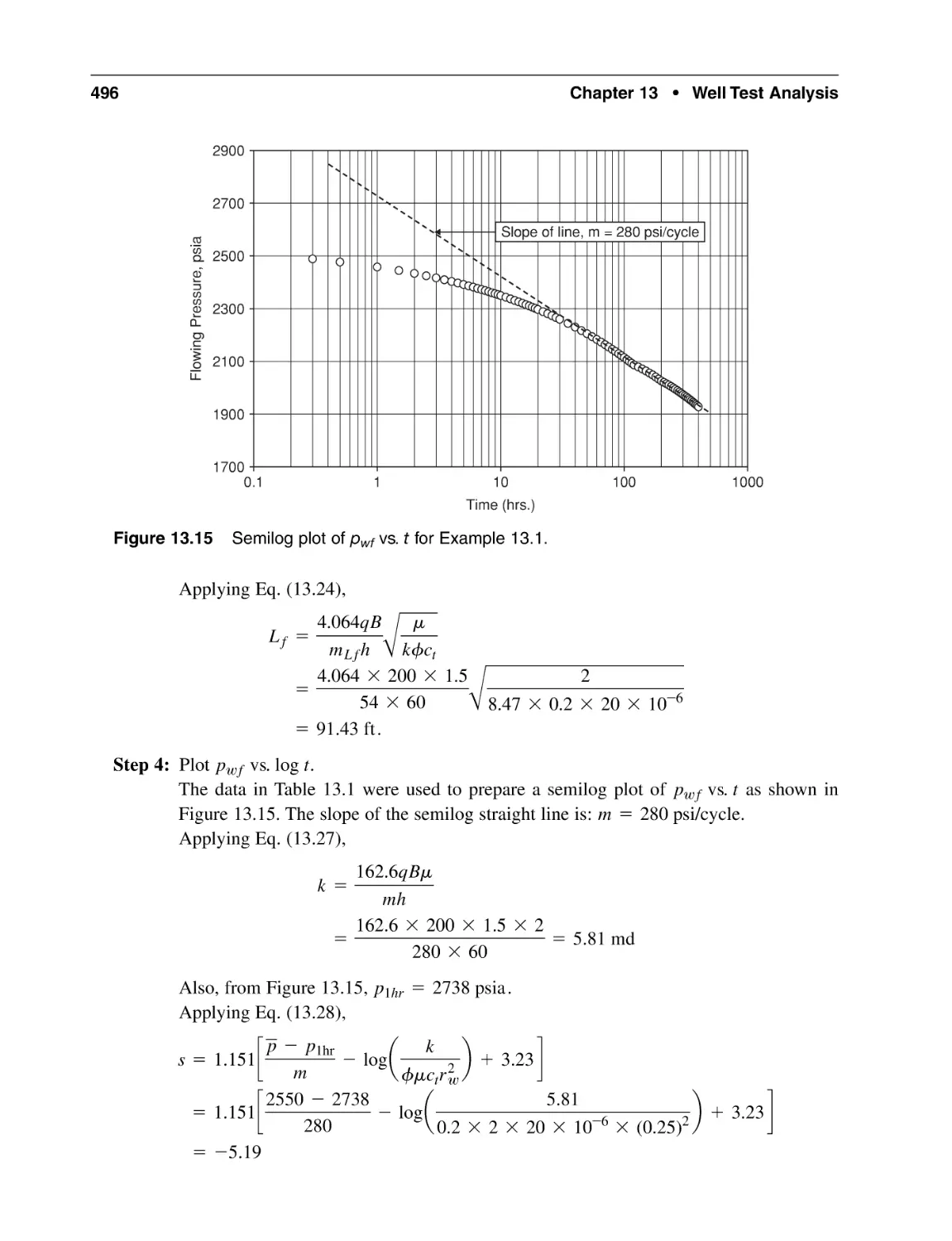
497
497
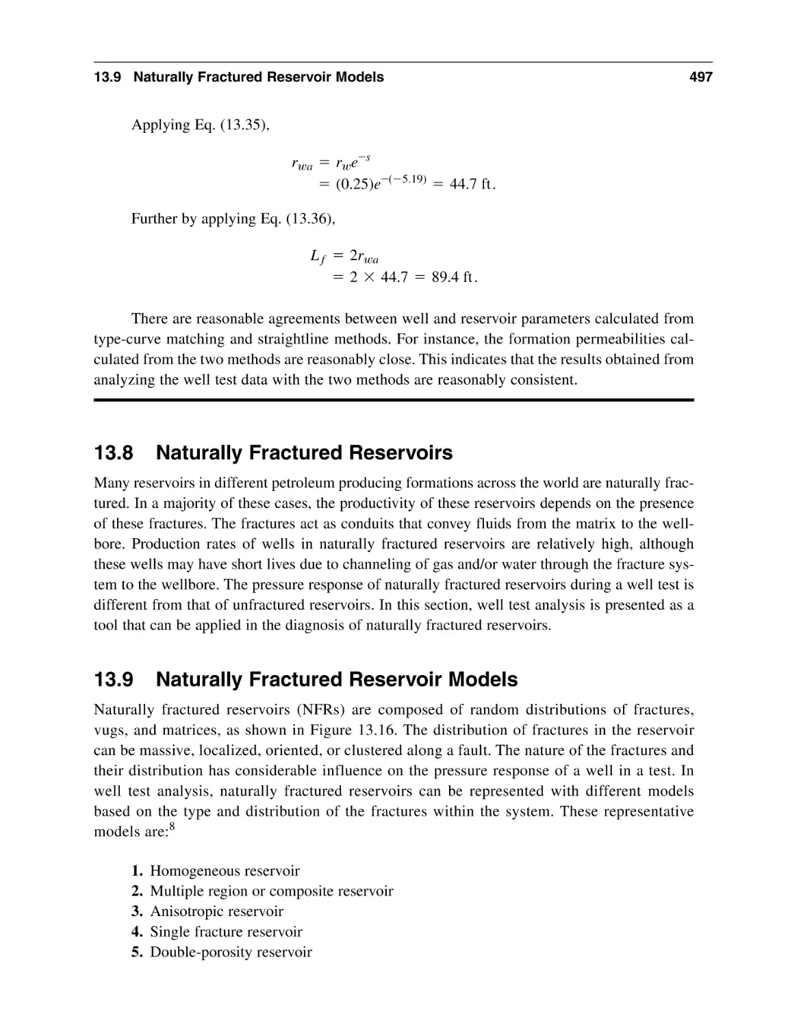
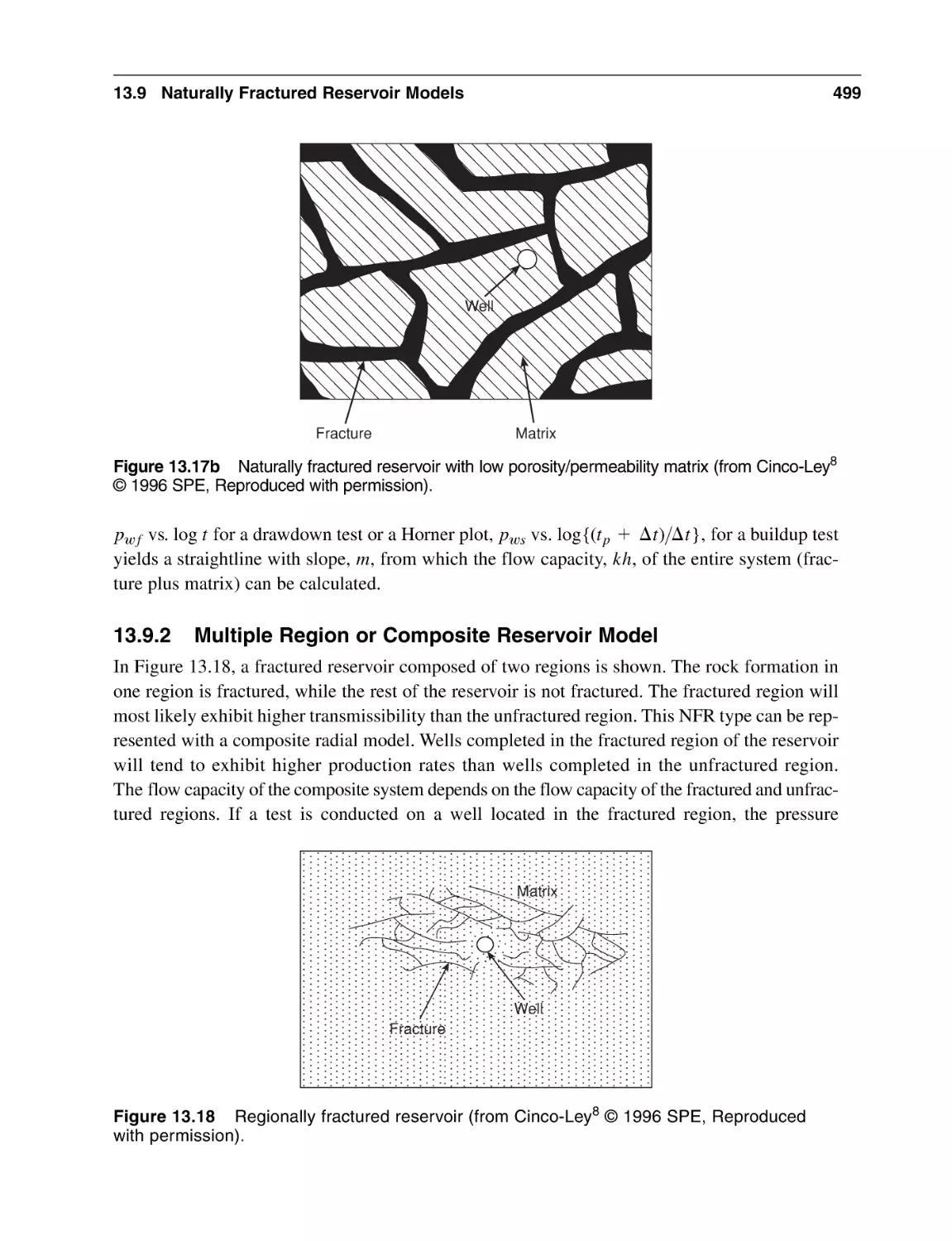
498
499
501
501
502
505
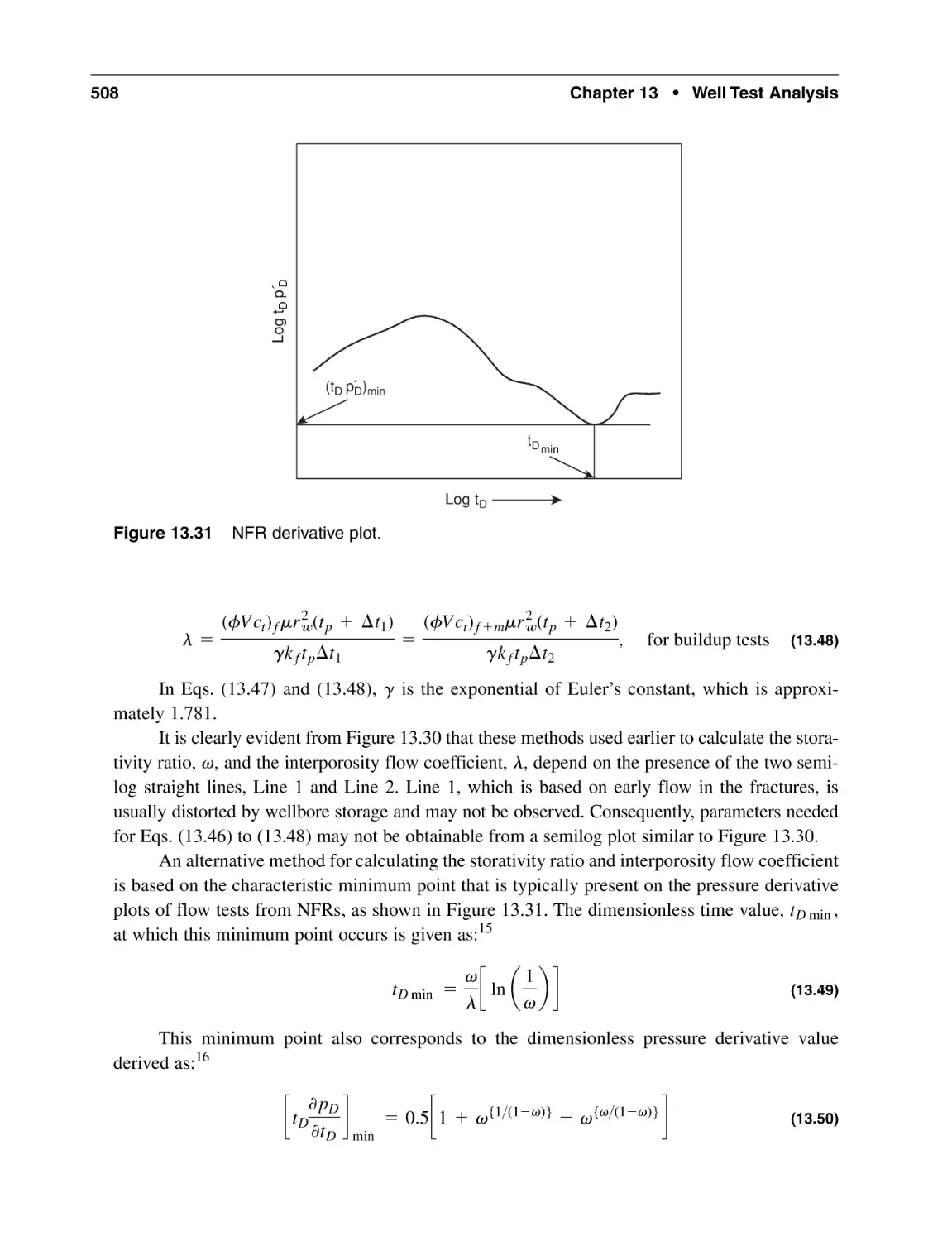
506
509
512
512
512
512
520
521
521
522
523
525
525
525
526
527
528
xviii
Contents
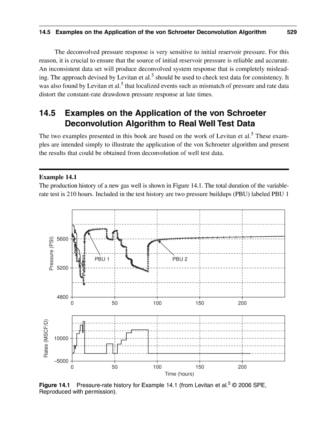
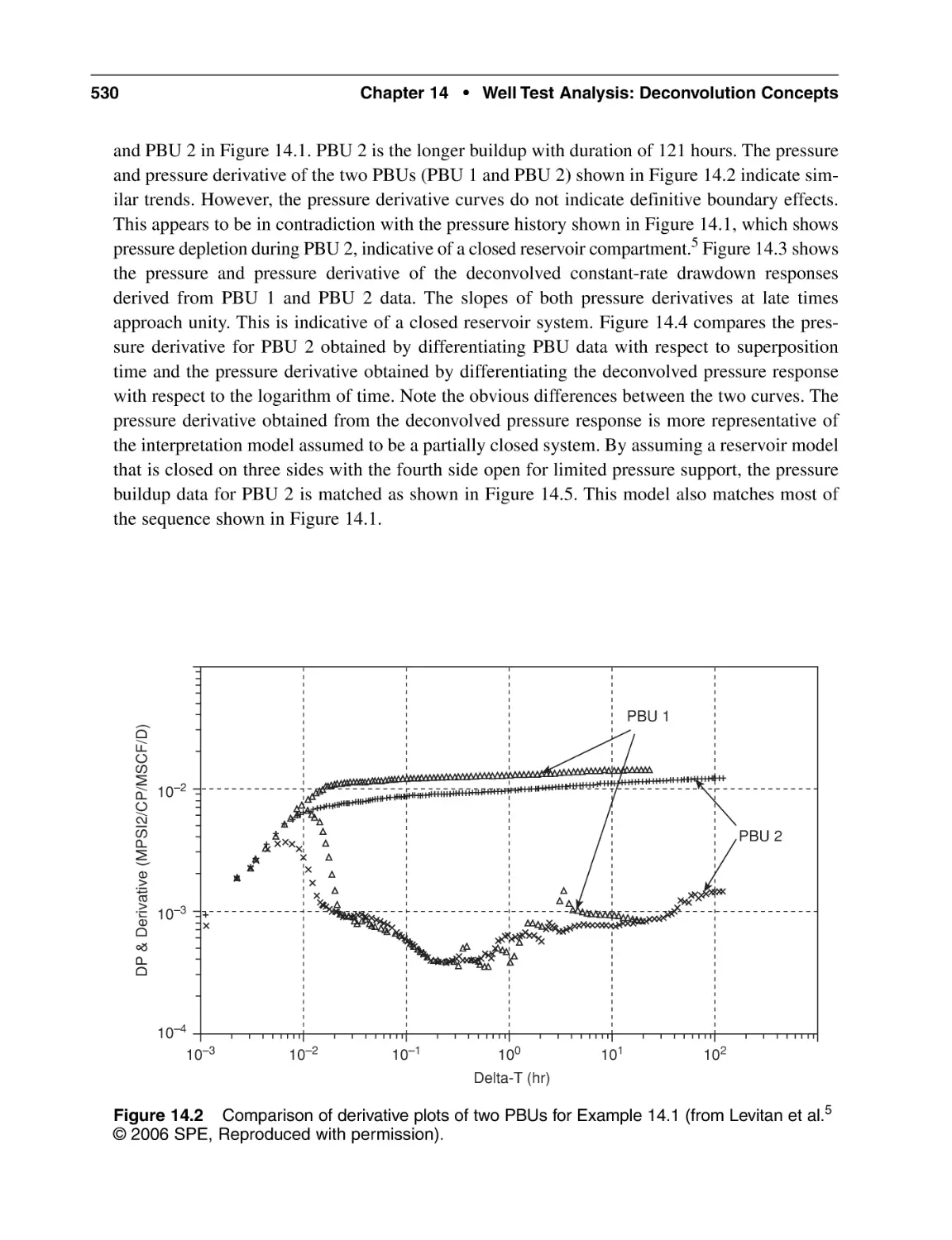
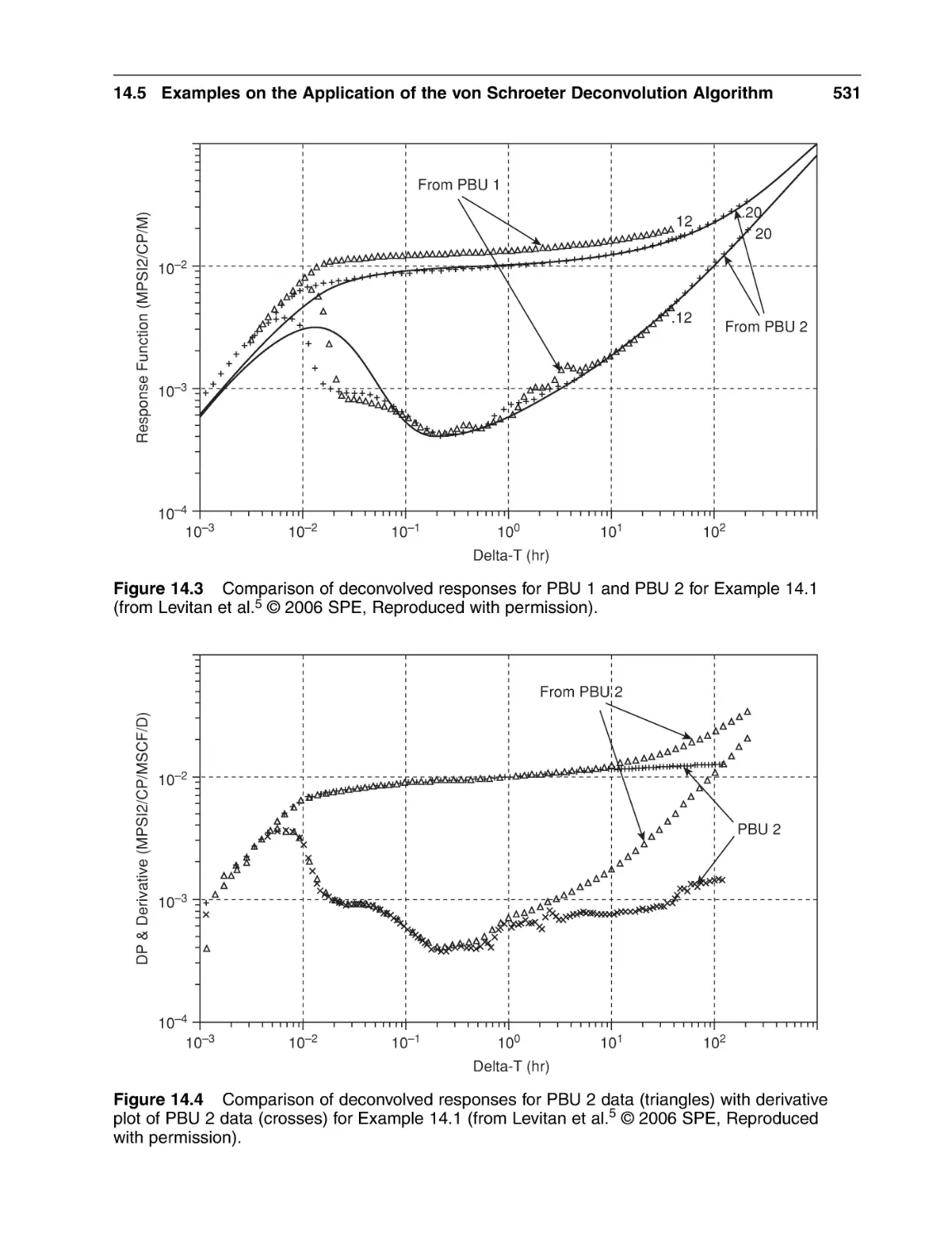
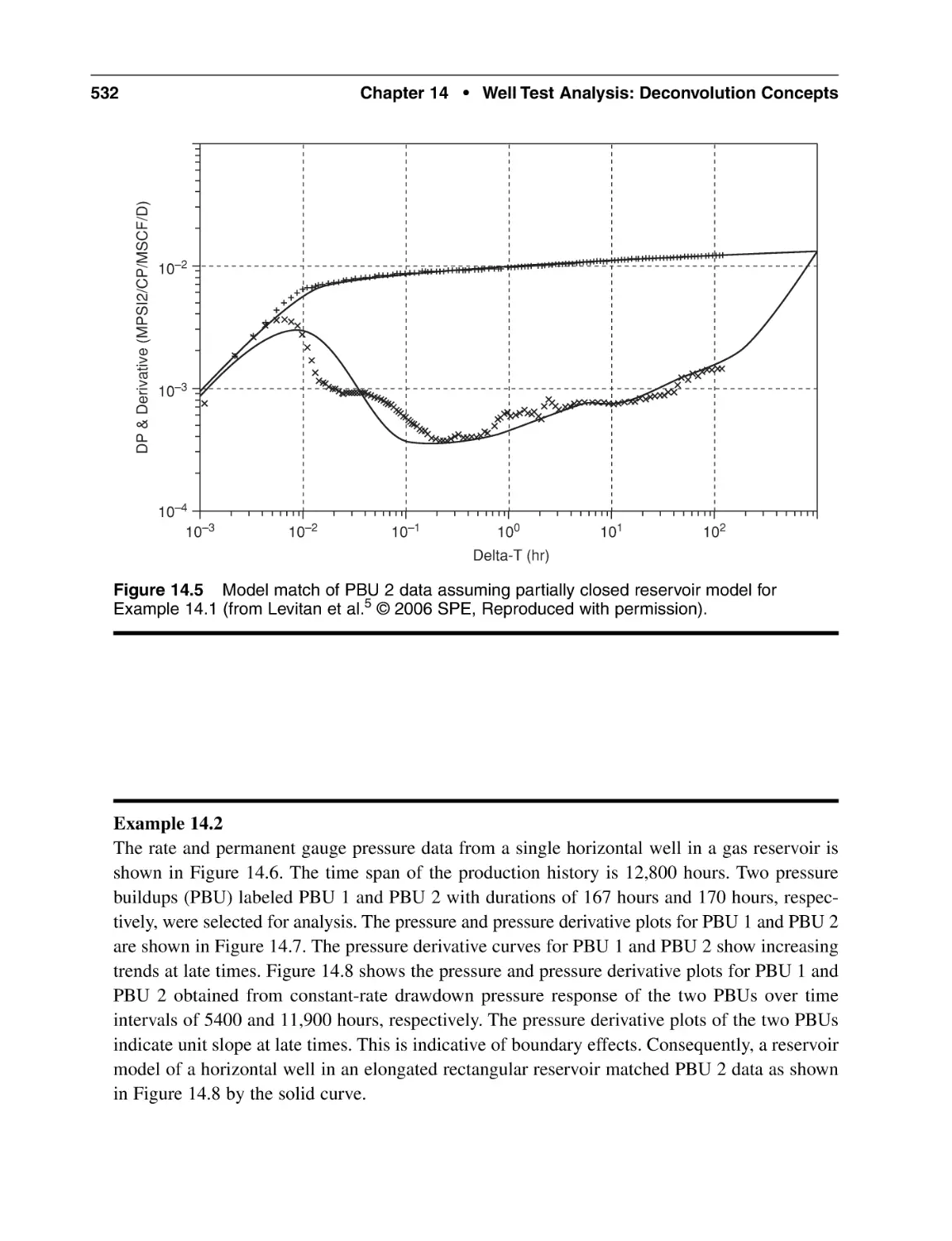
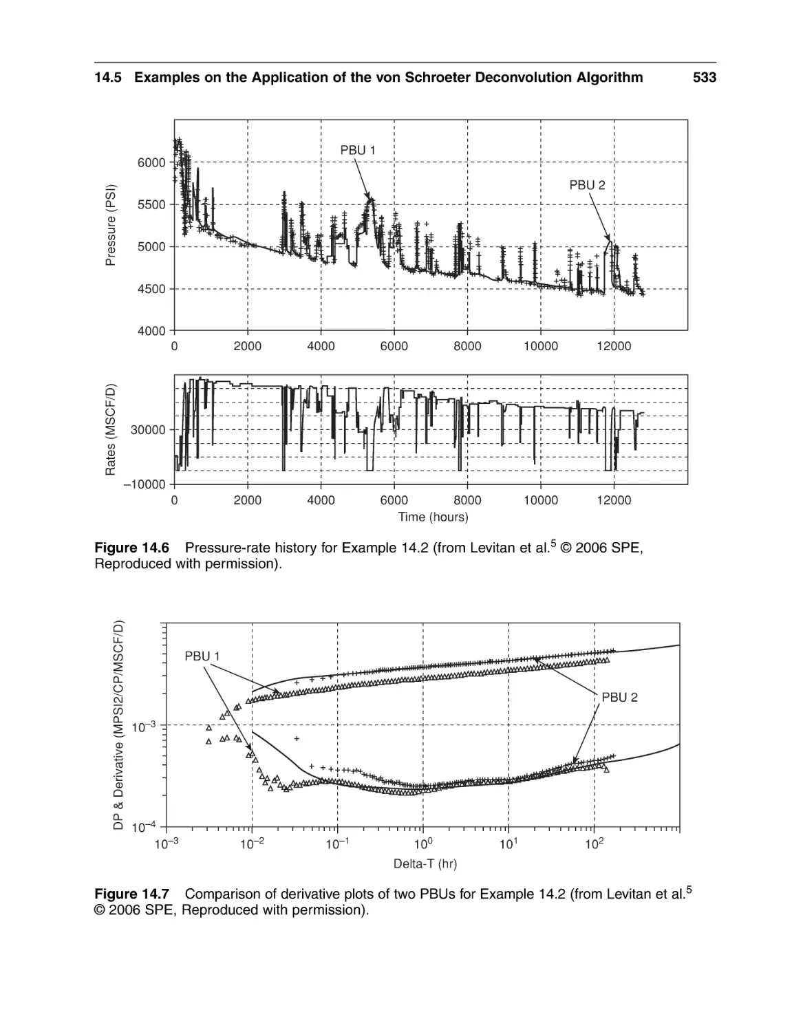
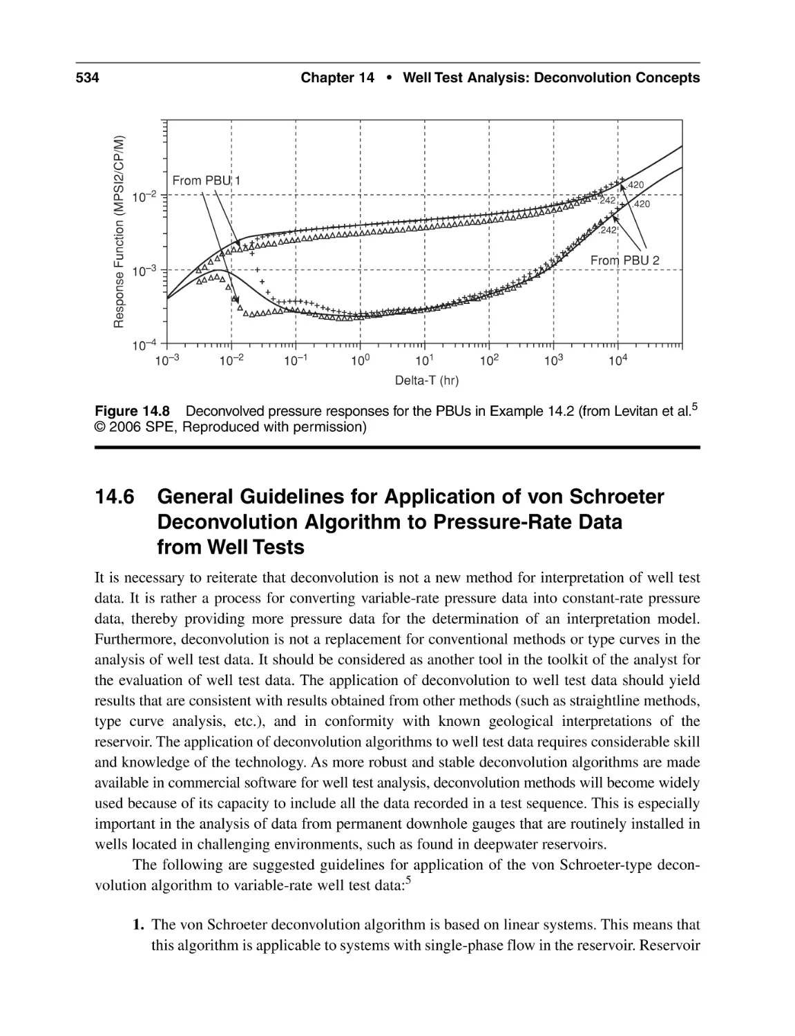
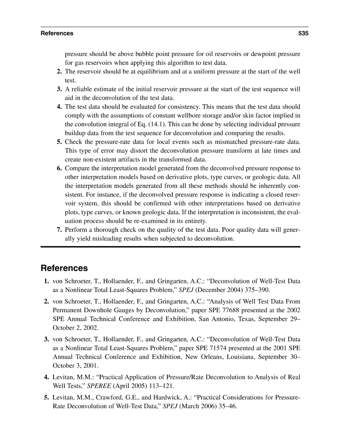
14.5
Examples on the Application of the von Schroeter
Deconvolution Algorithm to Real Well Test Data
14.6 General Guidelines for Application of von Schroeter
Deconvolution Algorithm to Pressure-Rate Datafrom Well Tests
References
General Reading
529
534
535
536
Chapter 15 Immiscible Fluid Displacement
15.1 Introduction
15.2 Basic Concepts in Immiscible Fluid Displacement
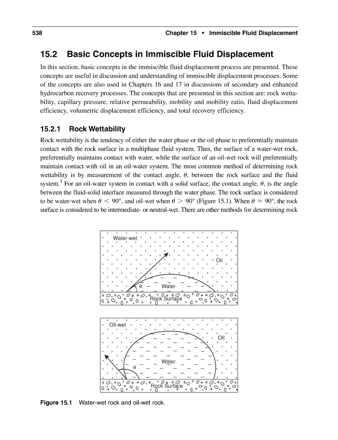
15.2.1 Rock Wettability
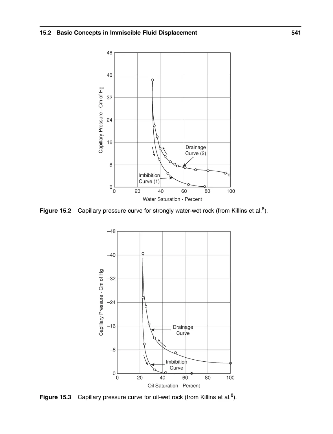
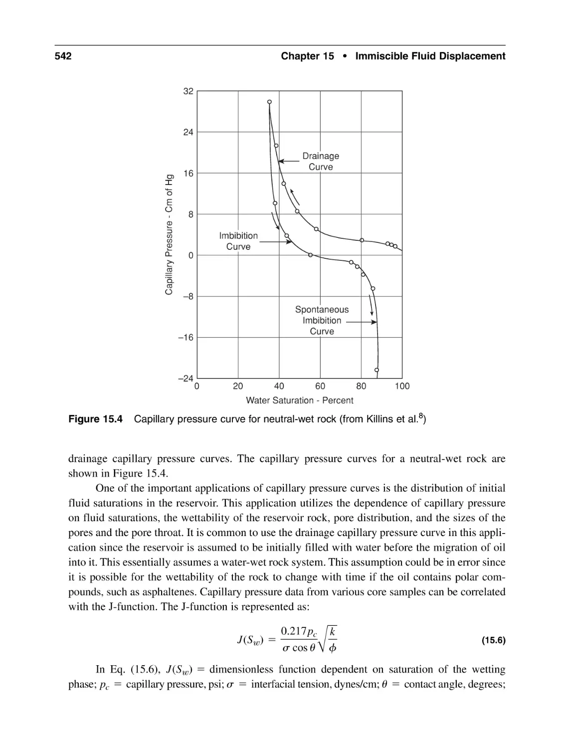
15.2.2 Capillary Pressure
15.2.3 Relative Permeability
15.2.4 Mobility and Mobility Ratio
15.2.5 Fluid Displacement Efficiency
15.2.6 Volumetric Displacement Efficiency
15.2.7 Total Recovery Efficiency
15.3 Fractional Flow Equations
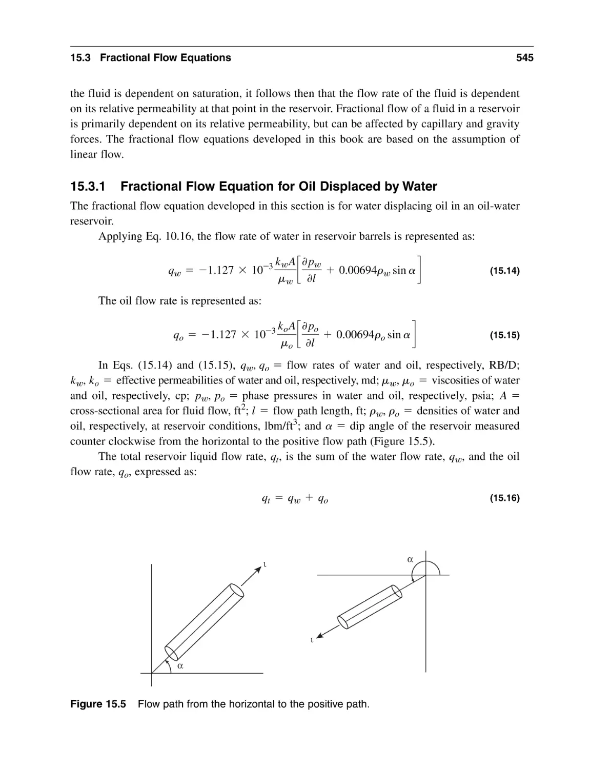
15.3.1 Fractional Flow Equation for Oil Displaced by Water
15.3.2 Fractional Flow Equation for Oil Displaced by Gas
15.4 The Buckley-Leverett Equation
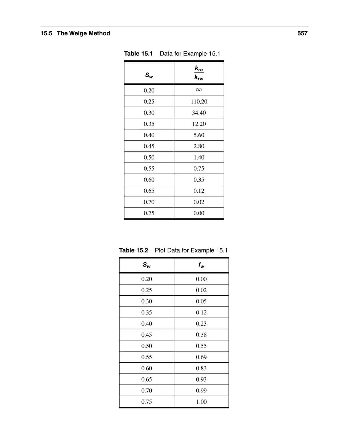
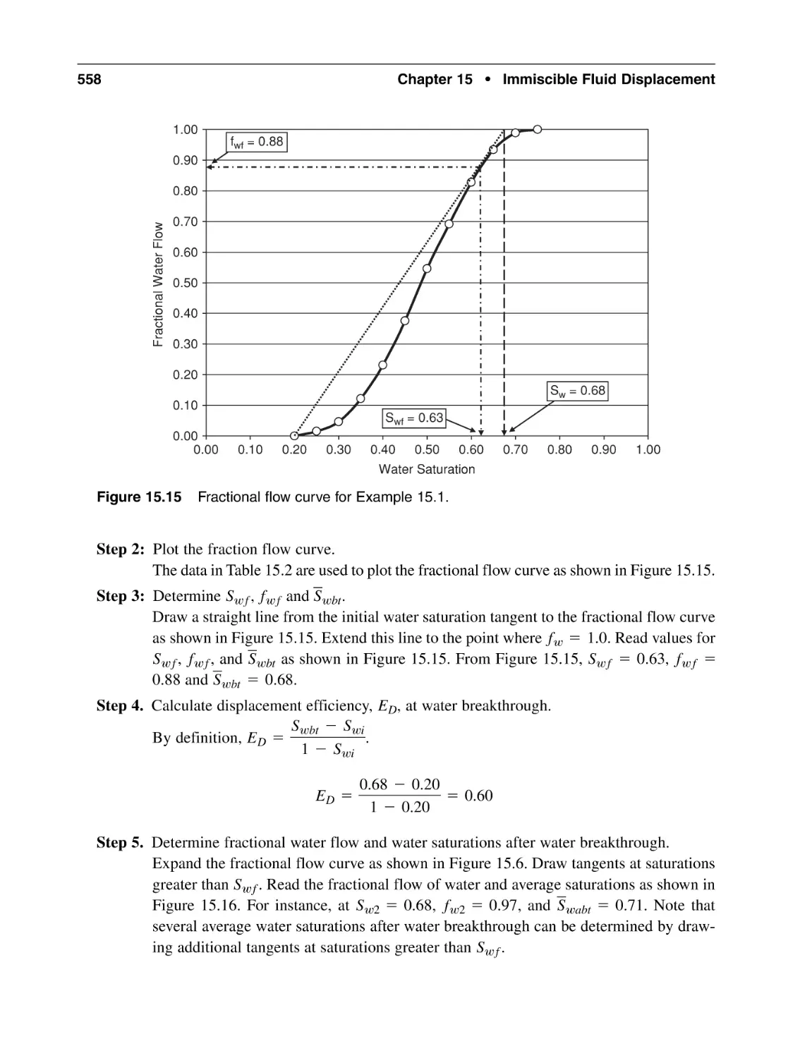
15.5 The Welge Method
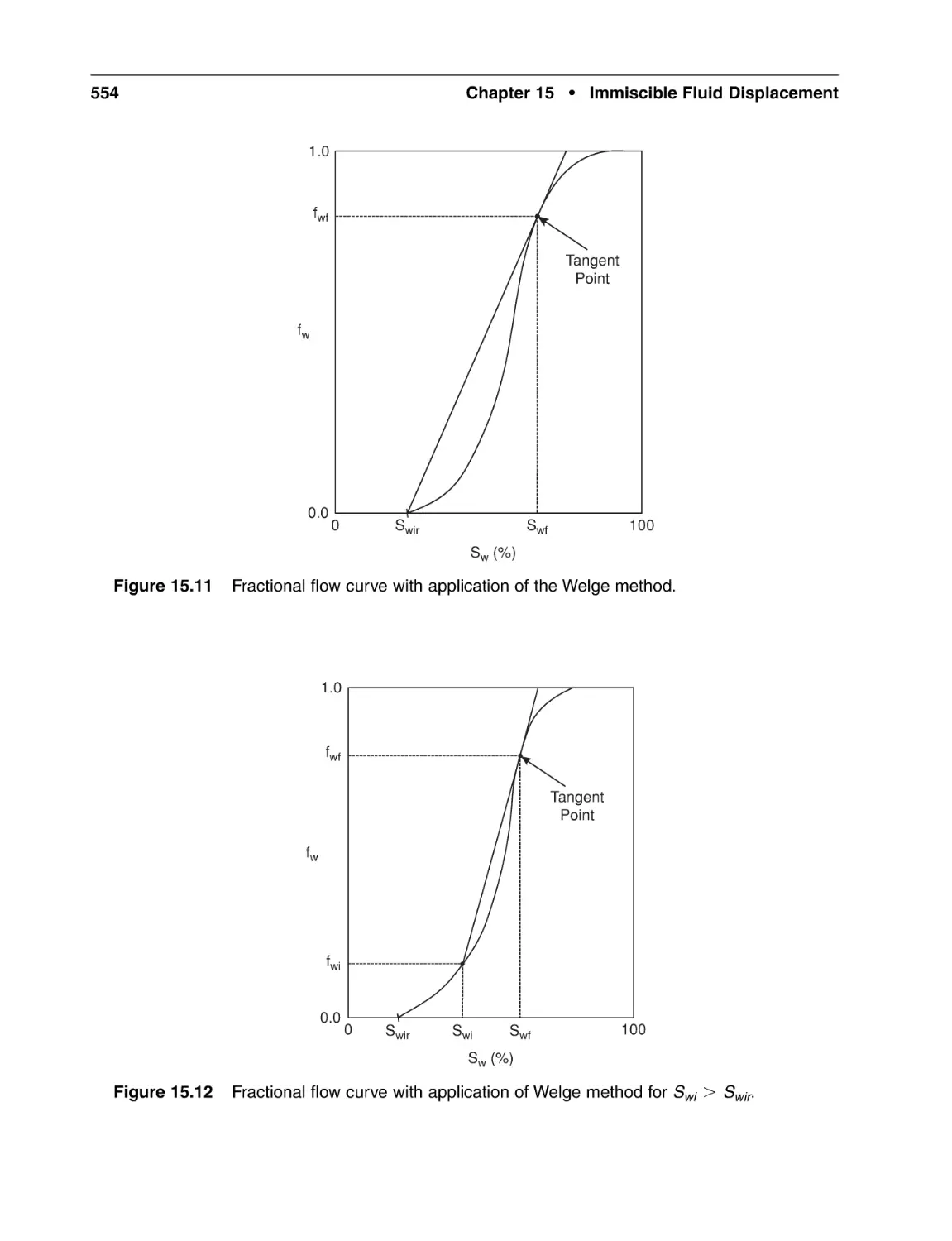
15.5.1 Water Saturation at the Flood Front
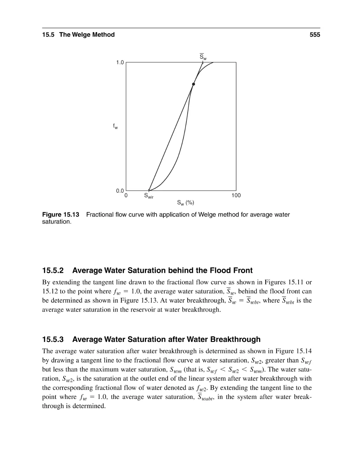
15.5.2 Average Water Saturation behind the Flood Front
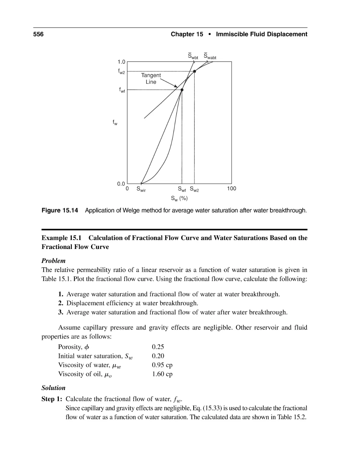
15.5.3 Average Water Saturation after Water Breakthrough
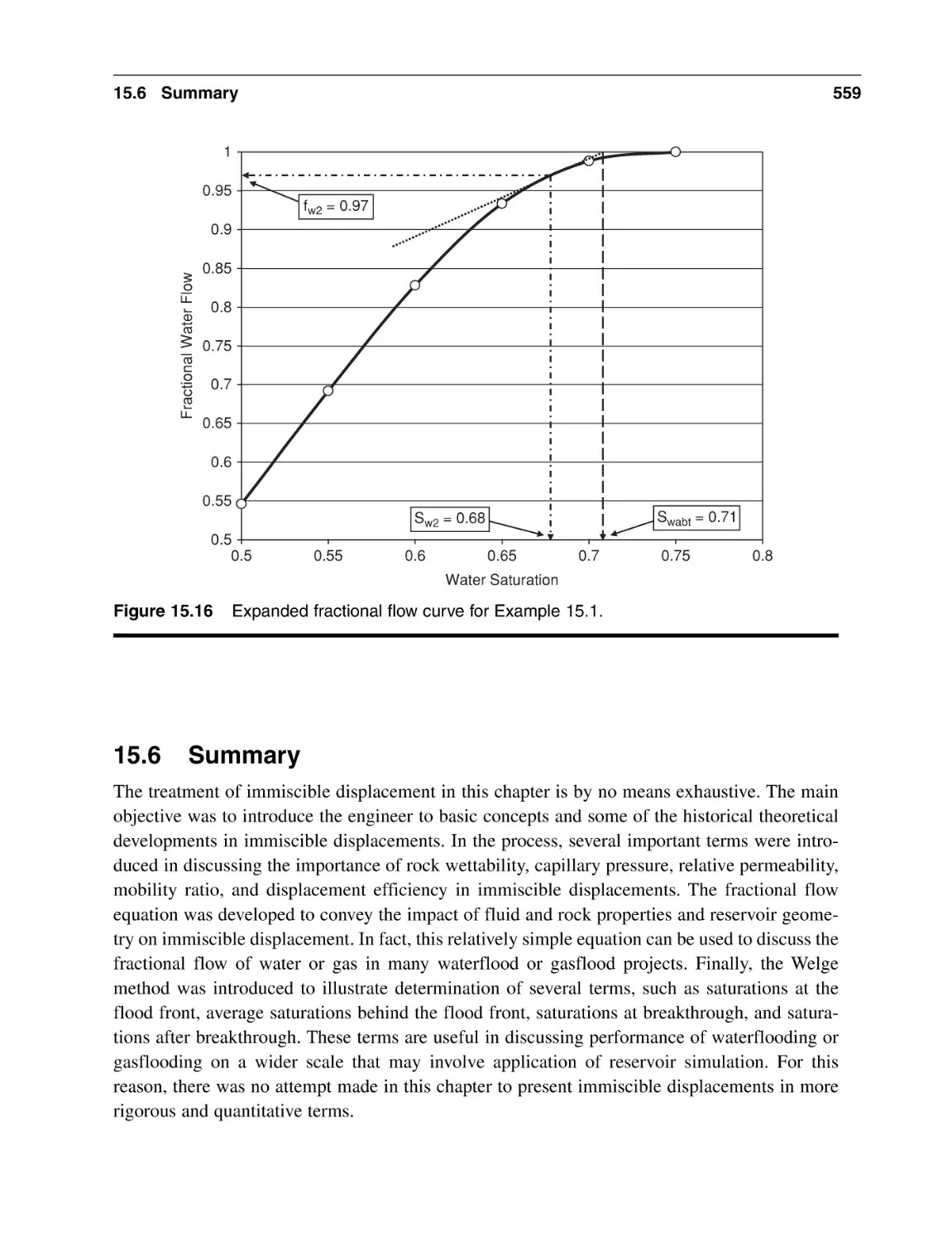
15.6 Summary
Nomenclature
References
General Reading
537
537
538
538
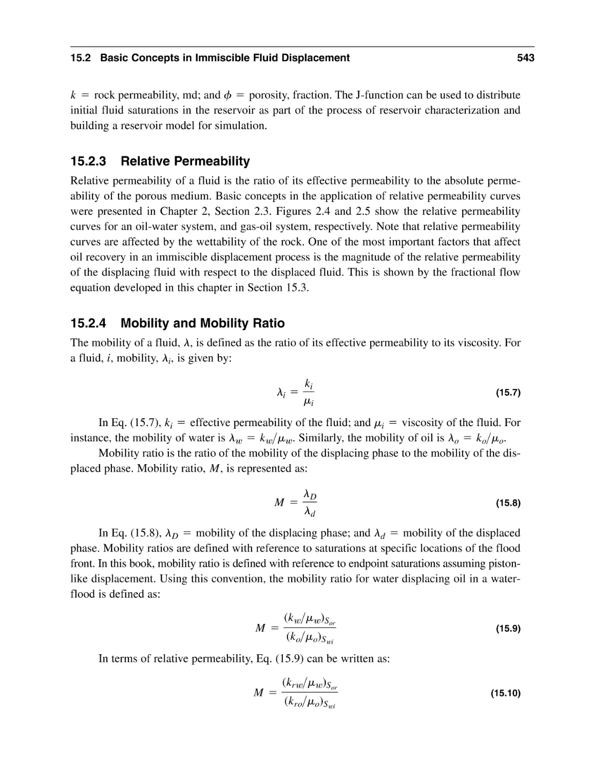
539
543
543
544
544
544
544
545
548
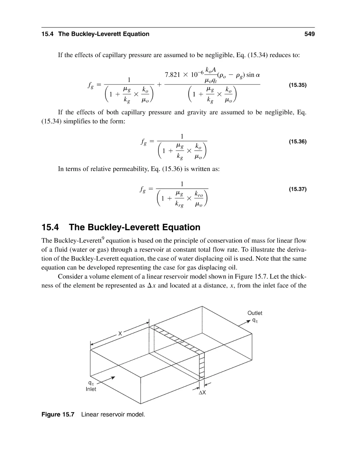
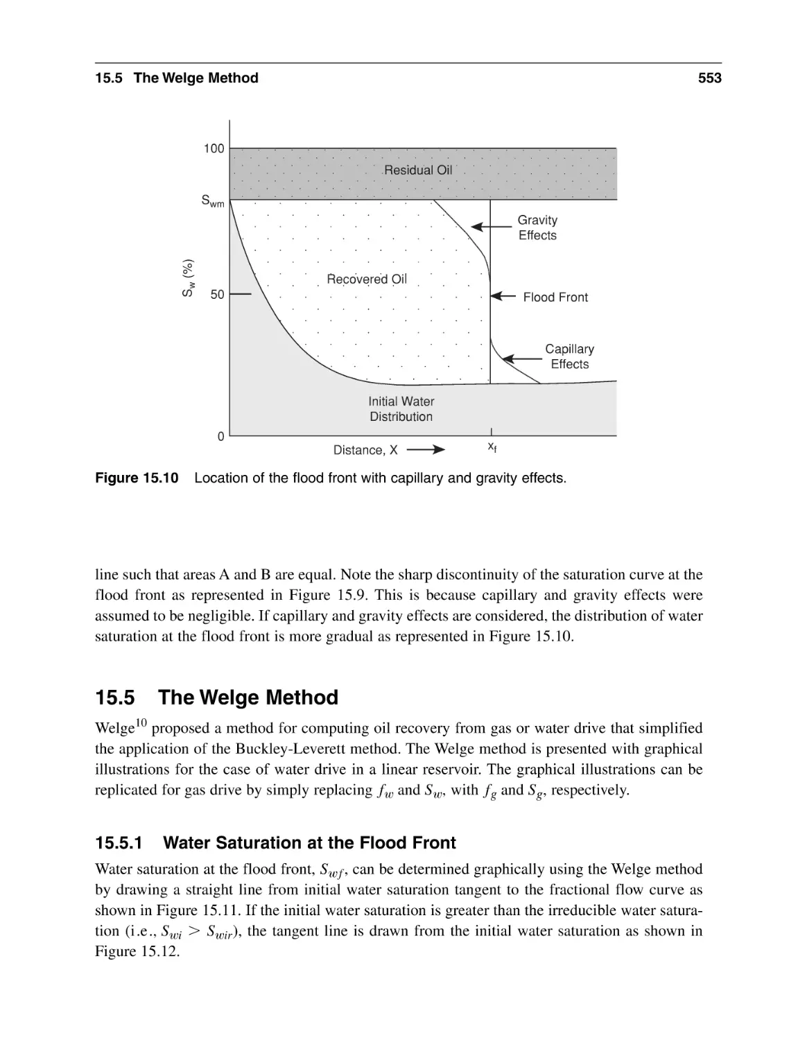
549
553
553
555
555
559
560
561
562
Chapter 16 Secondary Recovery Methods
16.1 Introduction
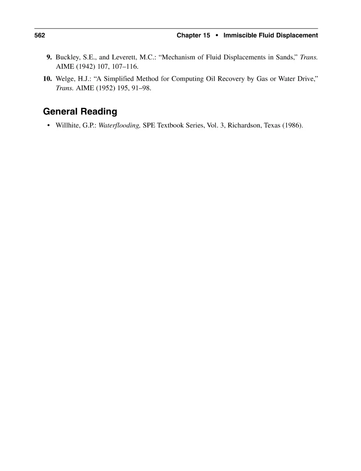
16.2 Waterflooding
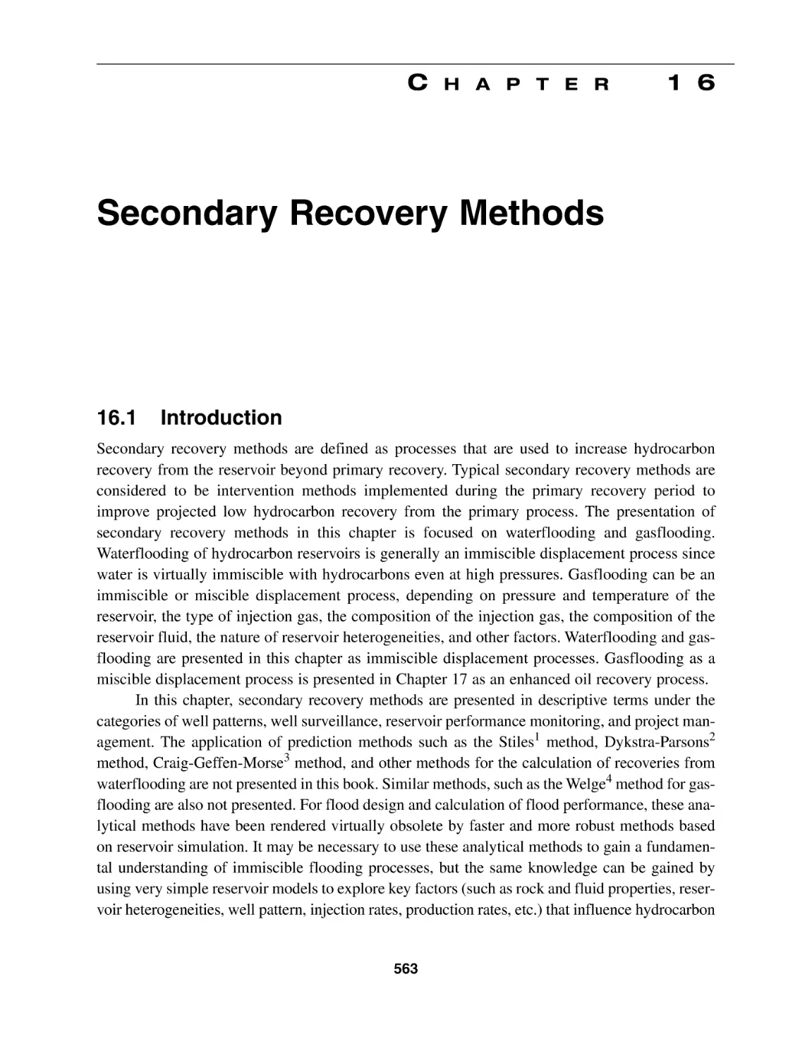
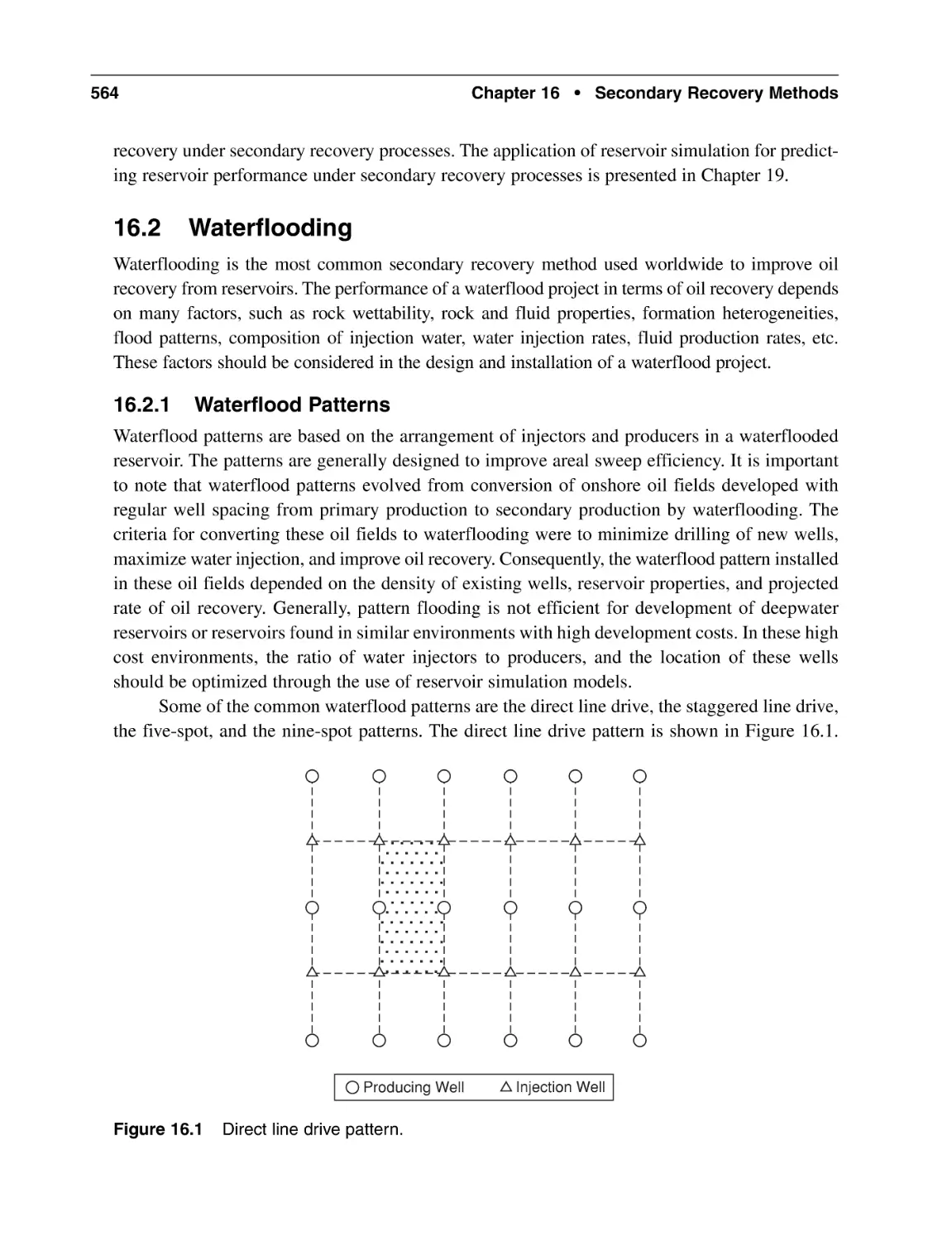
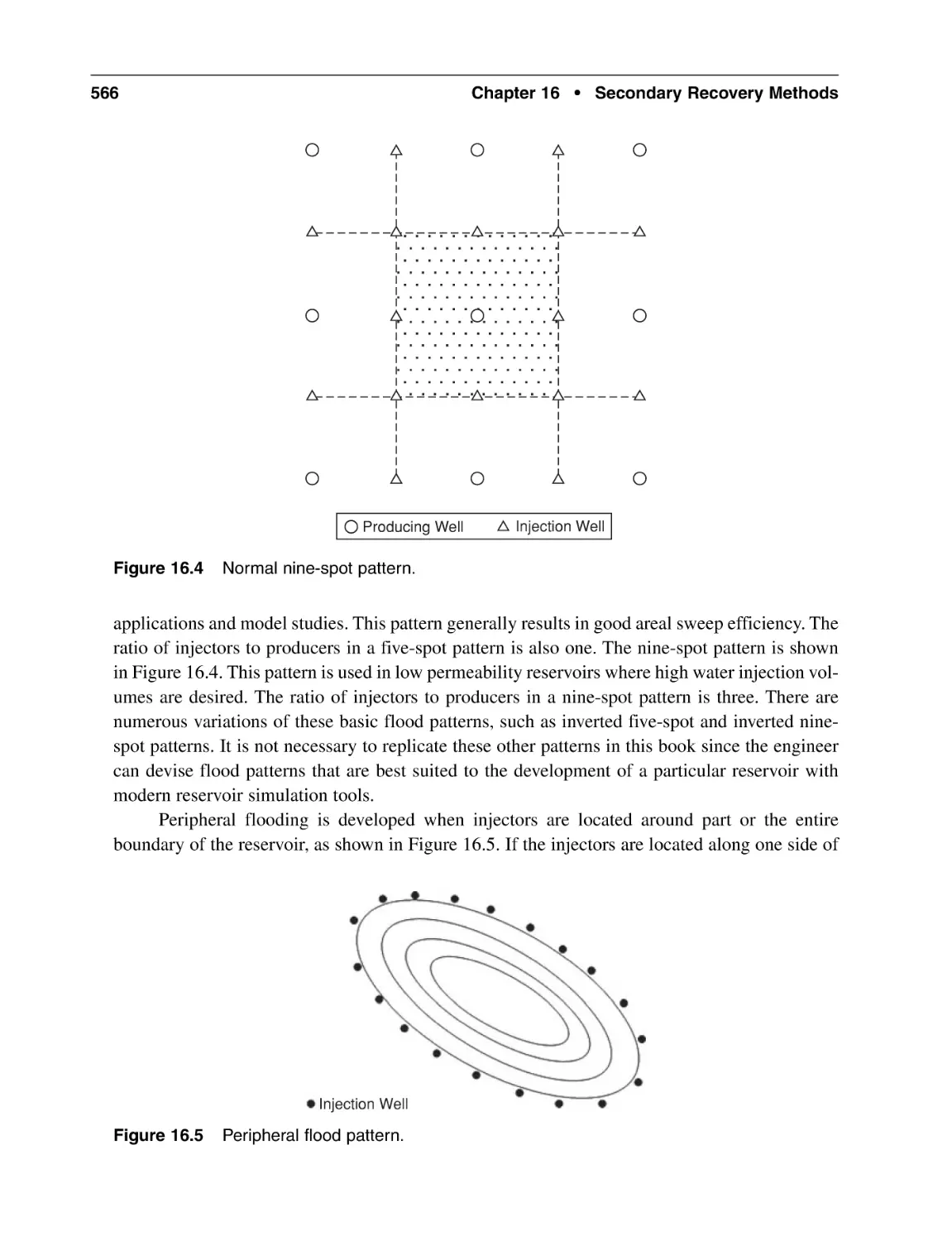
16.2.1 Waterflood Patterns
16.2.2 Waterflood Design
16.2.3 Recommended Steps in Waterflood Design
16.2.4 Waterflood Management
16.2.5 Management of Waterflooded Reservoirs
563
563
564
564
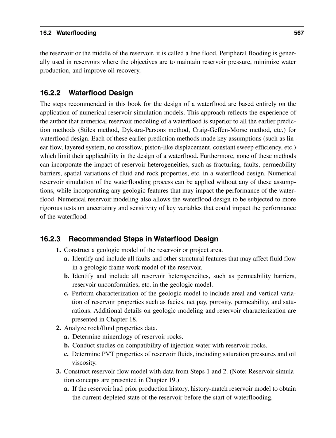
567
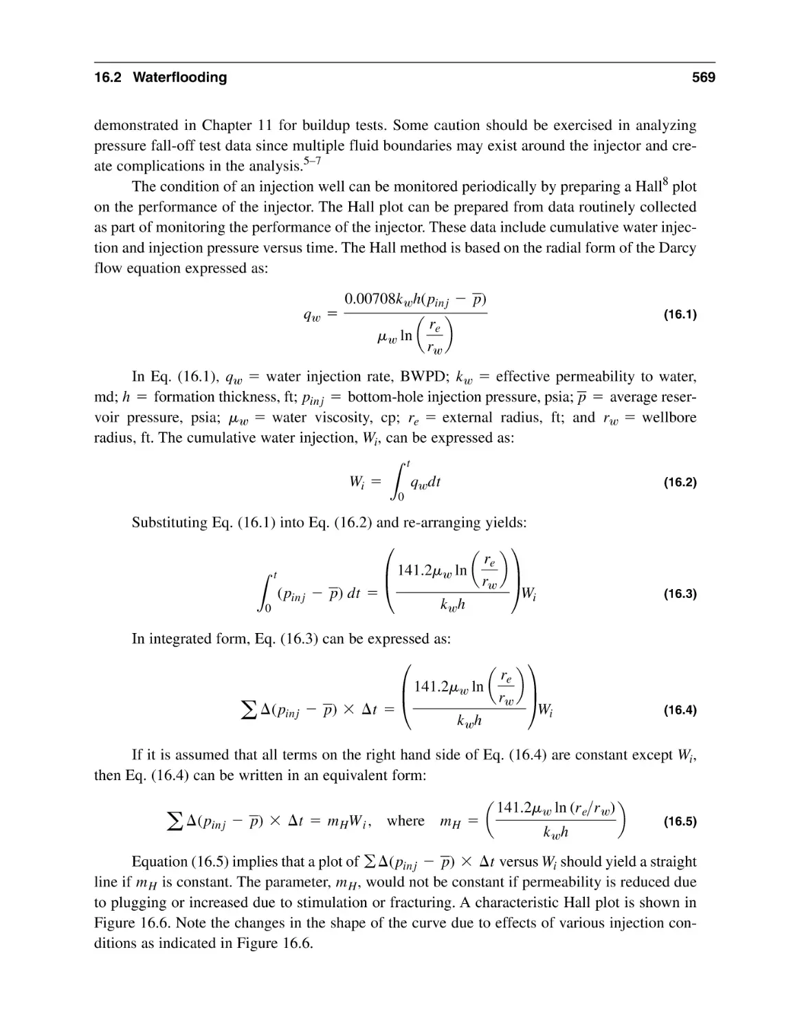
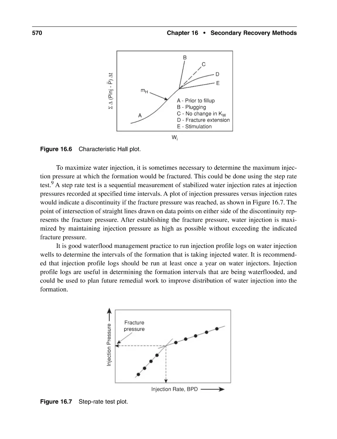
567
568
575
Contents
16.3 Gasflooding
16.3.1 Applications of Gasflooding
16.3.2 Gasflood Design
16.3.3 Recommended Steps in Gasflood Design
16.3.4 Gasflood Management
16.3.5 Management of Gasflood Reservoirs
Nomenclature
Abbreviations
References
General Reading
Chapter 17 Enhanced Oil Recovery
17.1 Introduction
17.2 EOR Processes
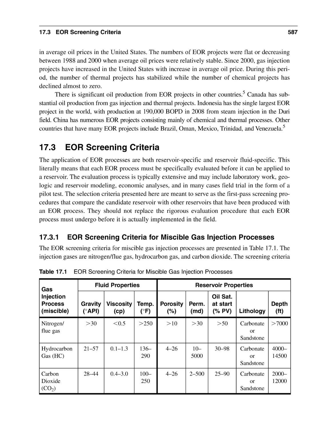
17.3 EOR Screening Criteria
17.3.1 EOR Screening Criteria for Miscible
Gas Injection Processes
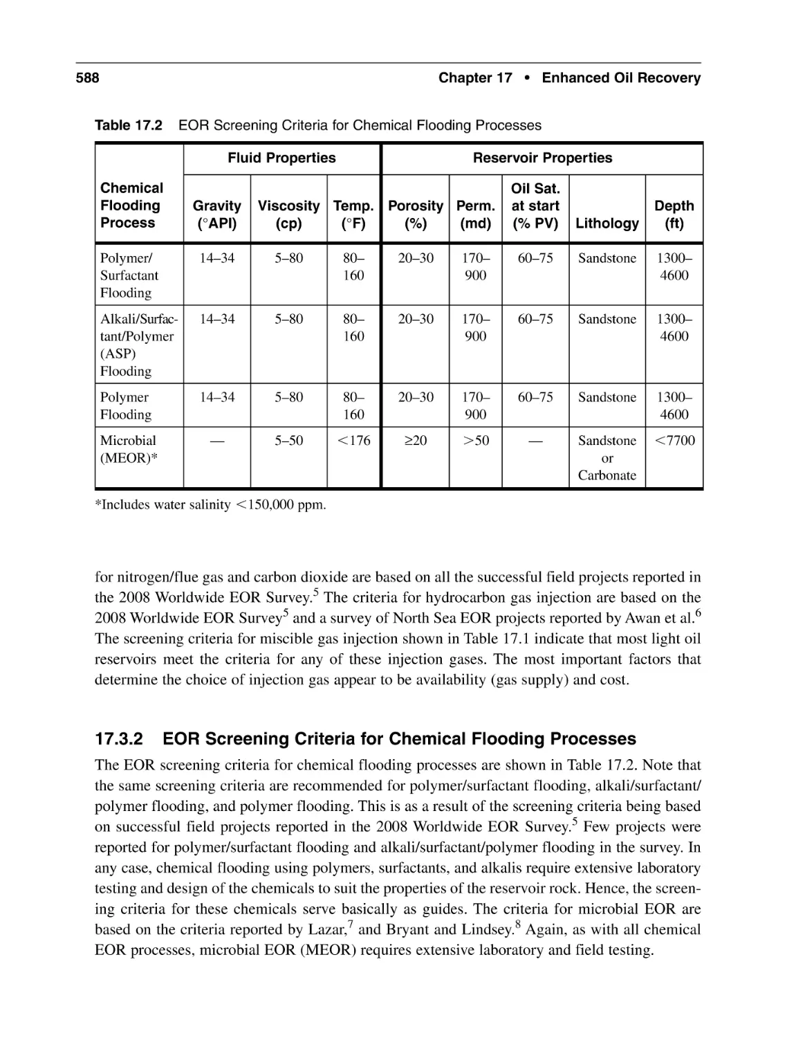
17.3.2 EOR Screening Criteria for Chemical
Flooding Processes
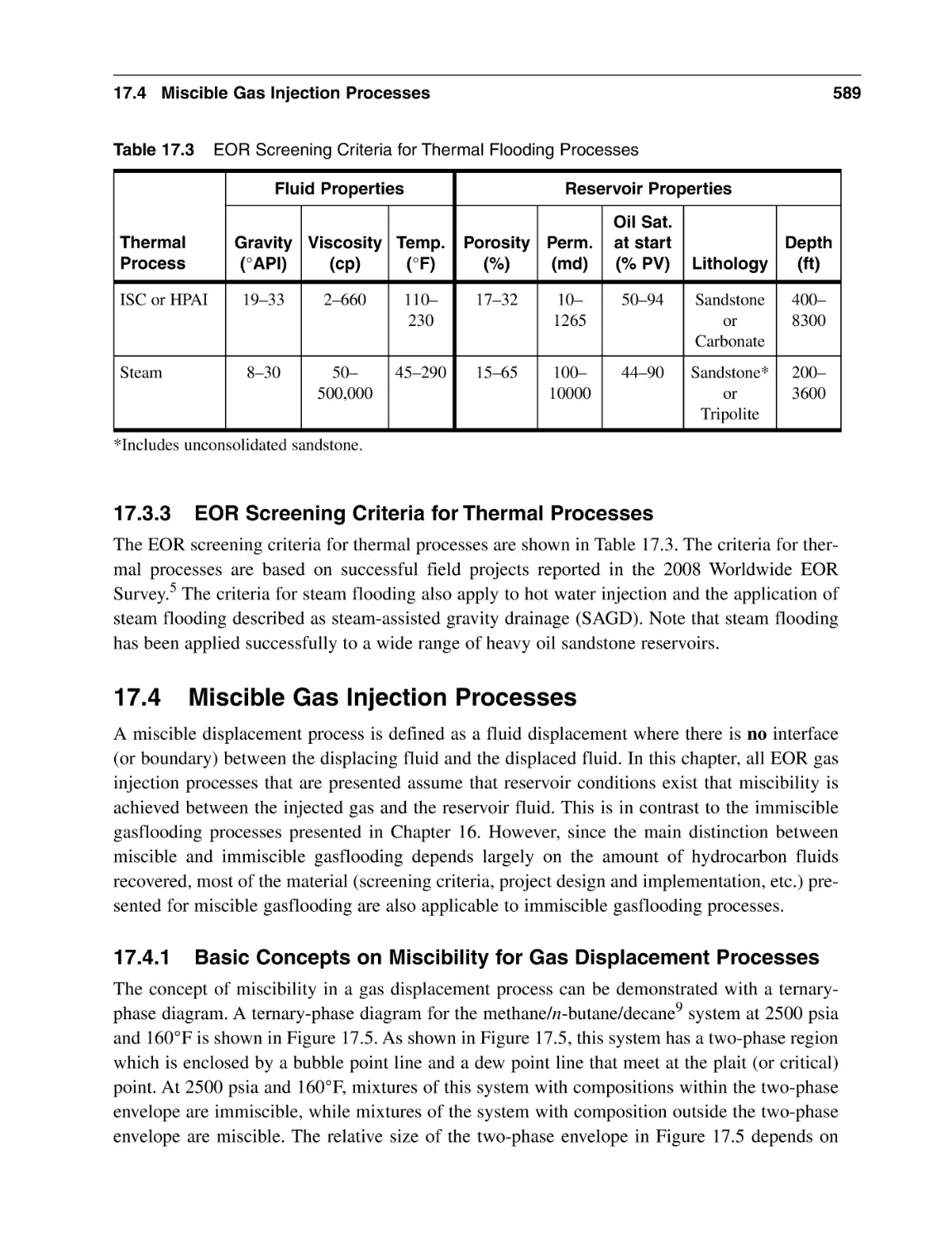
17.3.3 EOR Screening Criteria for Thermal Processes
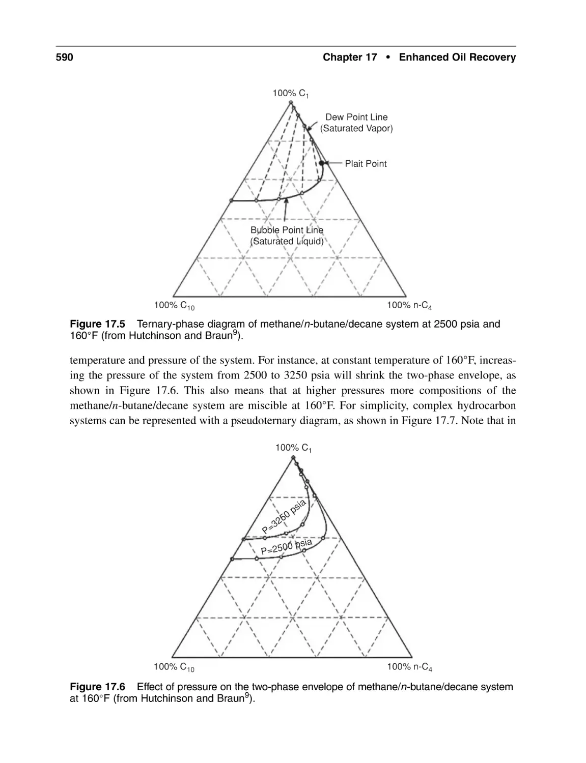
17.4 Miscible Gas Injection Processes
17.4.1 Basic Concepts on Miscibility
for Gas Displacement Processes
17.4.2 First-Contact Miscibility (FCM)
17.4.3 Multiple-Contact Miscibility (MCM)
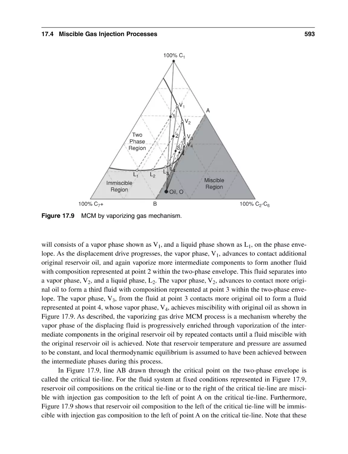
17.4.4 Vaporizing Gas Drive MCM Process
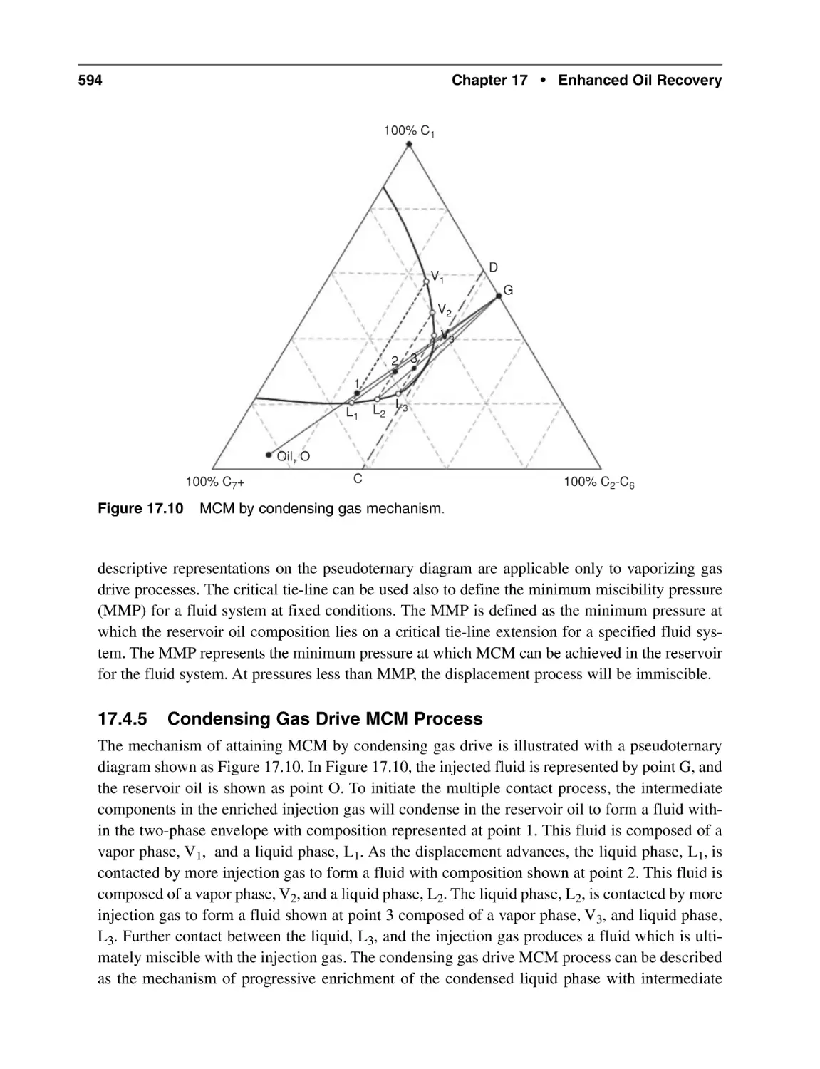
17.4.5 Condensing Gas Drive MCM Process
17.4.6 Combined Condensing/Vaporizing (CV) Gas Drive
MCM Process
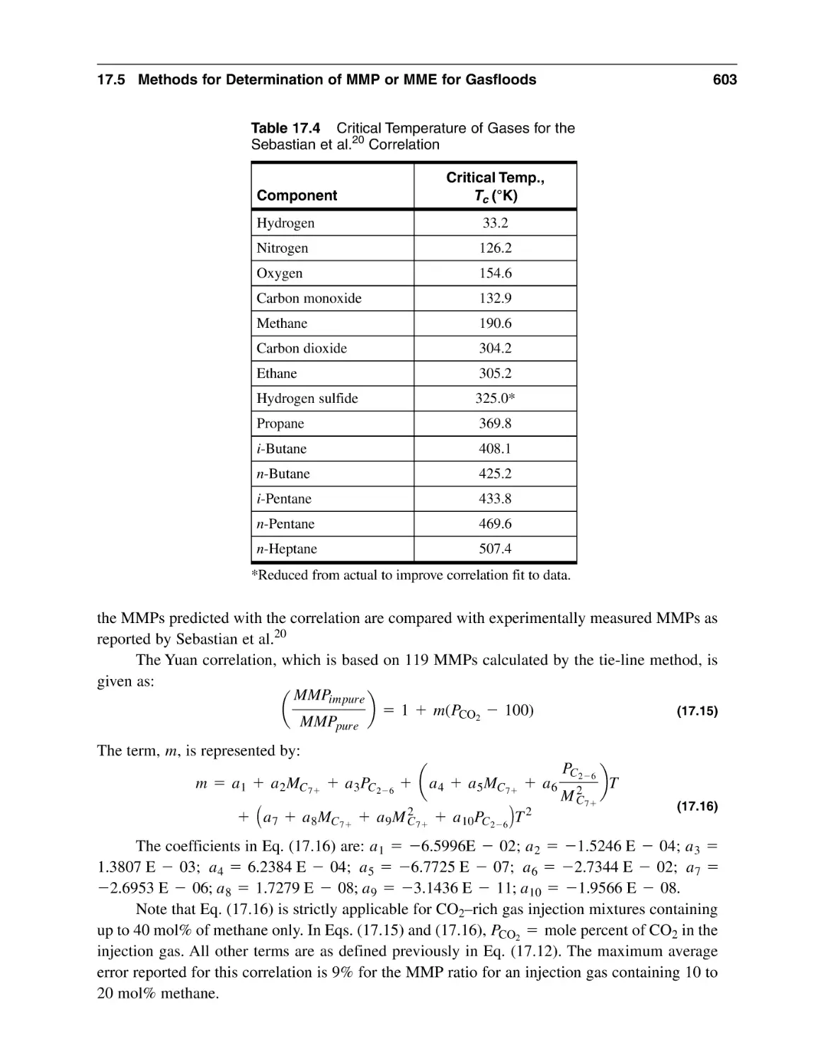
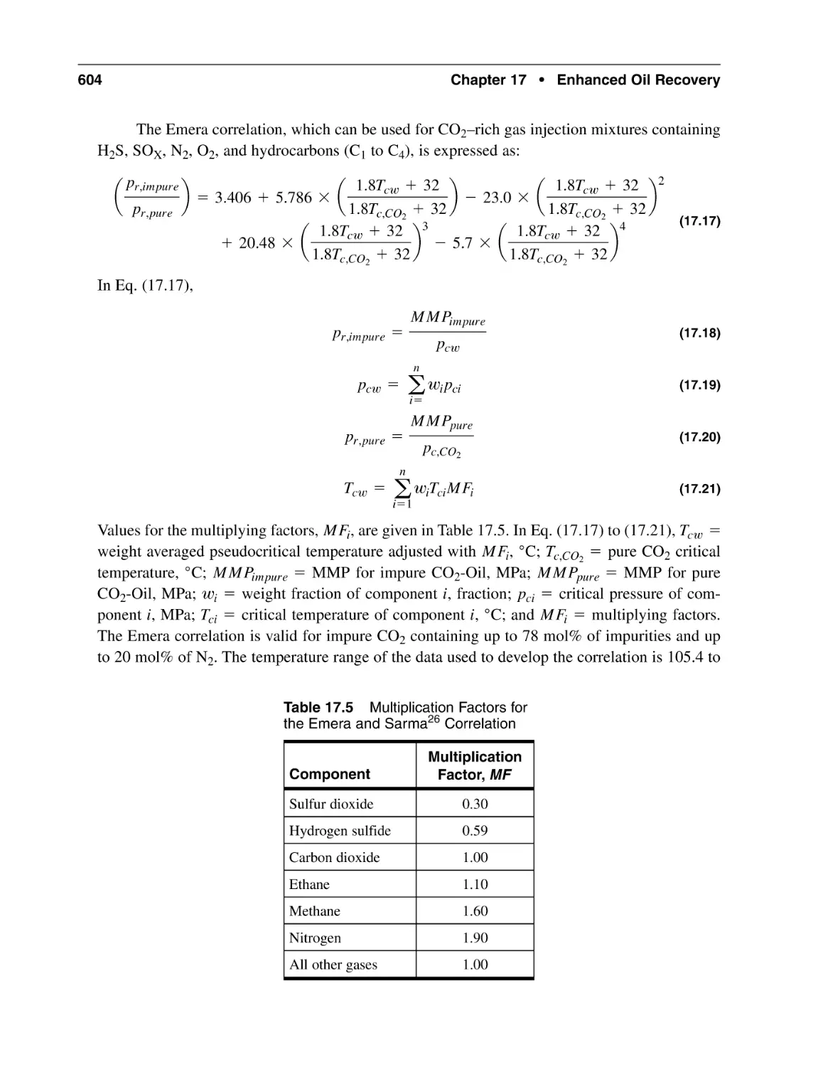
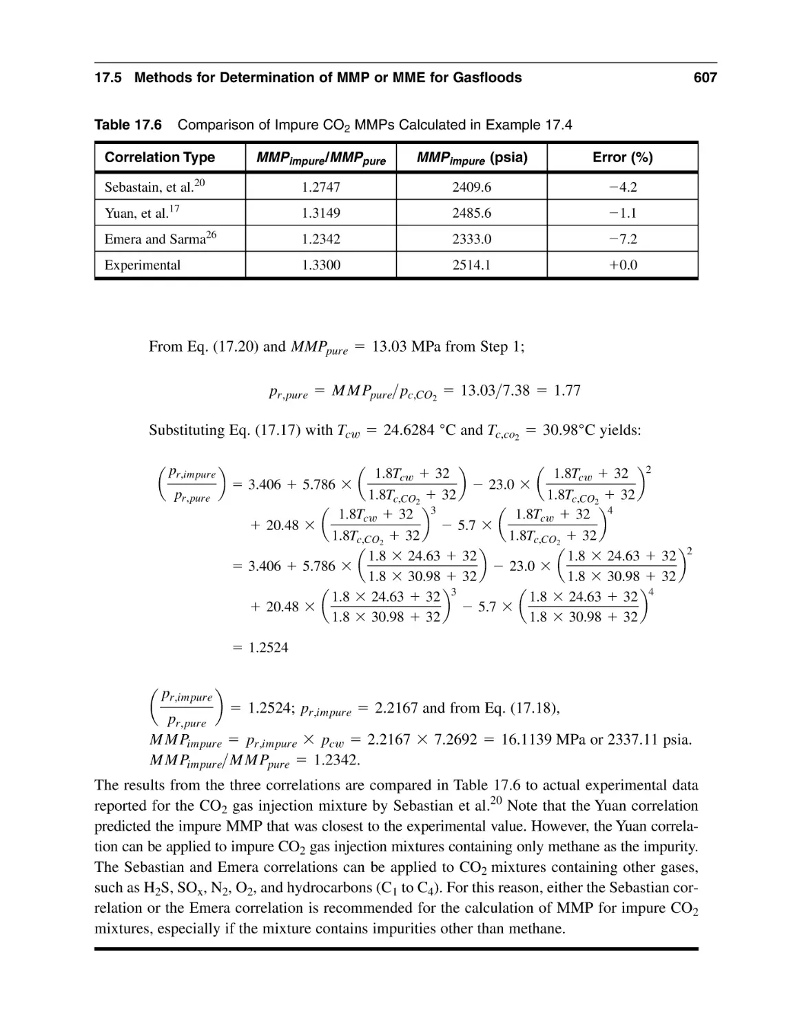
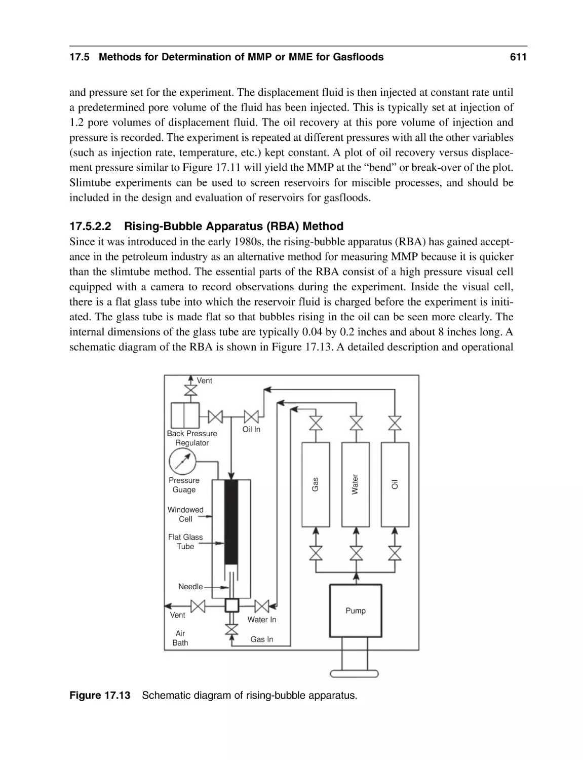
17.5 Methods for Determination of MMP or MME for Gasfloods
17.5.1 Analytical Techniques for Estimation of MMP
or MME
17.5.2 Experimental Methods
17.6 Types of Miscible Gas Flooding
17.6.1 Nitrogen/Flue-gas Miscible Gas Flooding
17.6.2 Hydrocarbon (HC) Miscible Gas Flooding
17.6.3 Carbon Dioxide Gas Flooding
17.6.4 Types of Miscible Gas Injection Strategies
xix
575
576
576
577
578
579
580
580
580
582
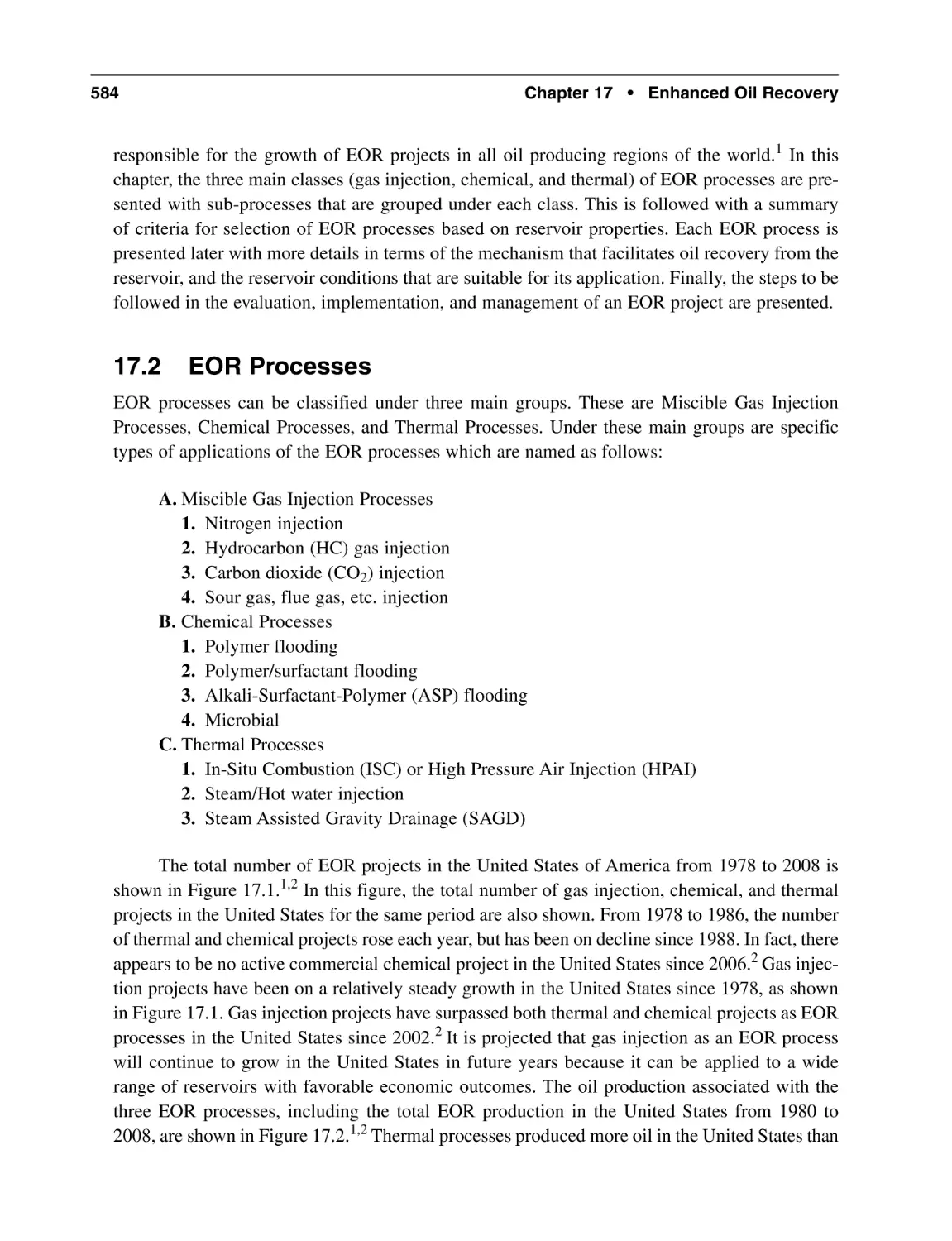
583
583
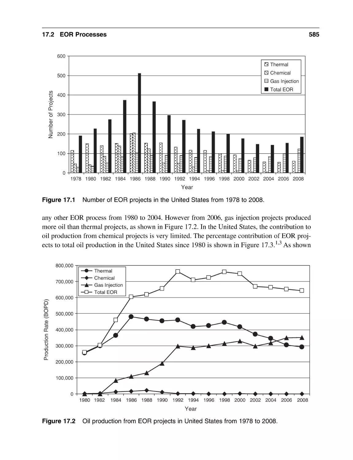
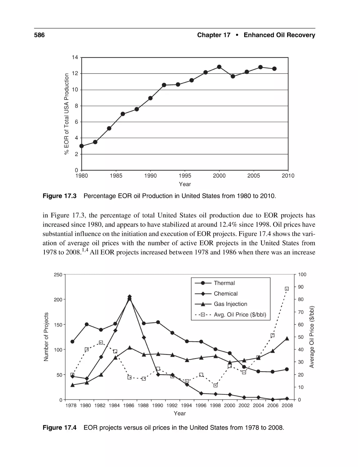
584
587
587
588
589
589
589
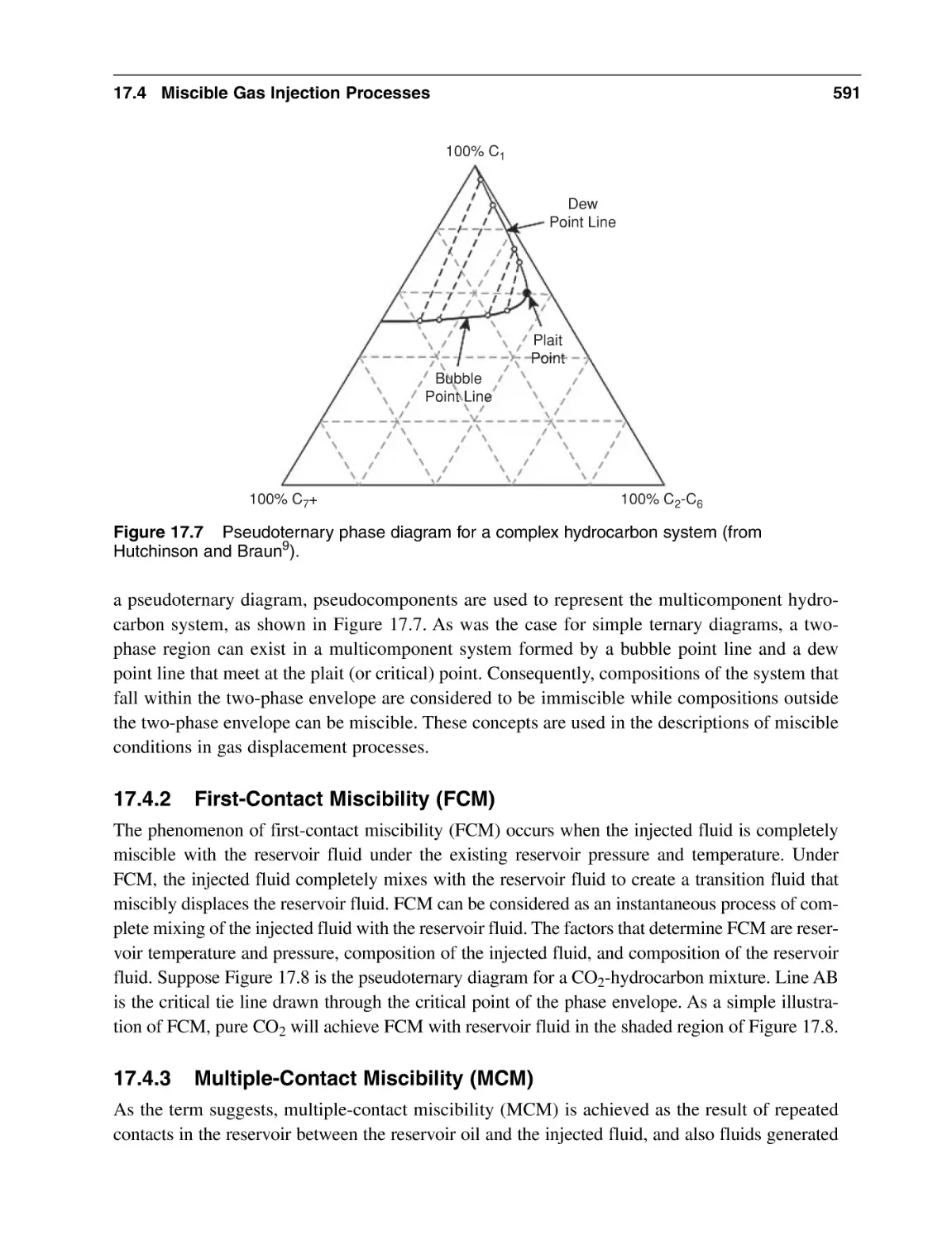
591
591
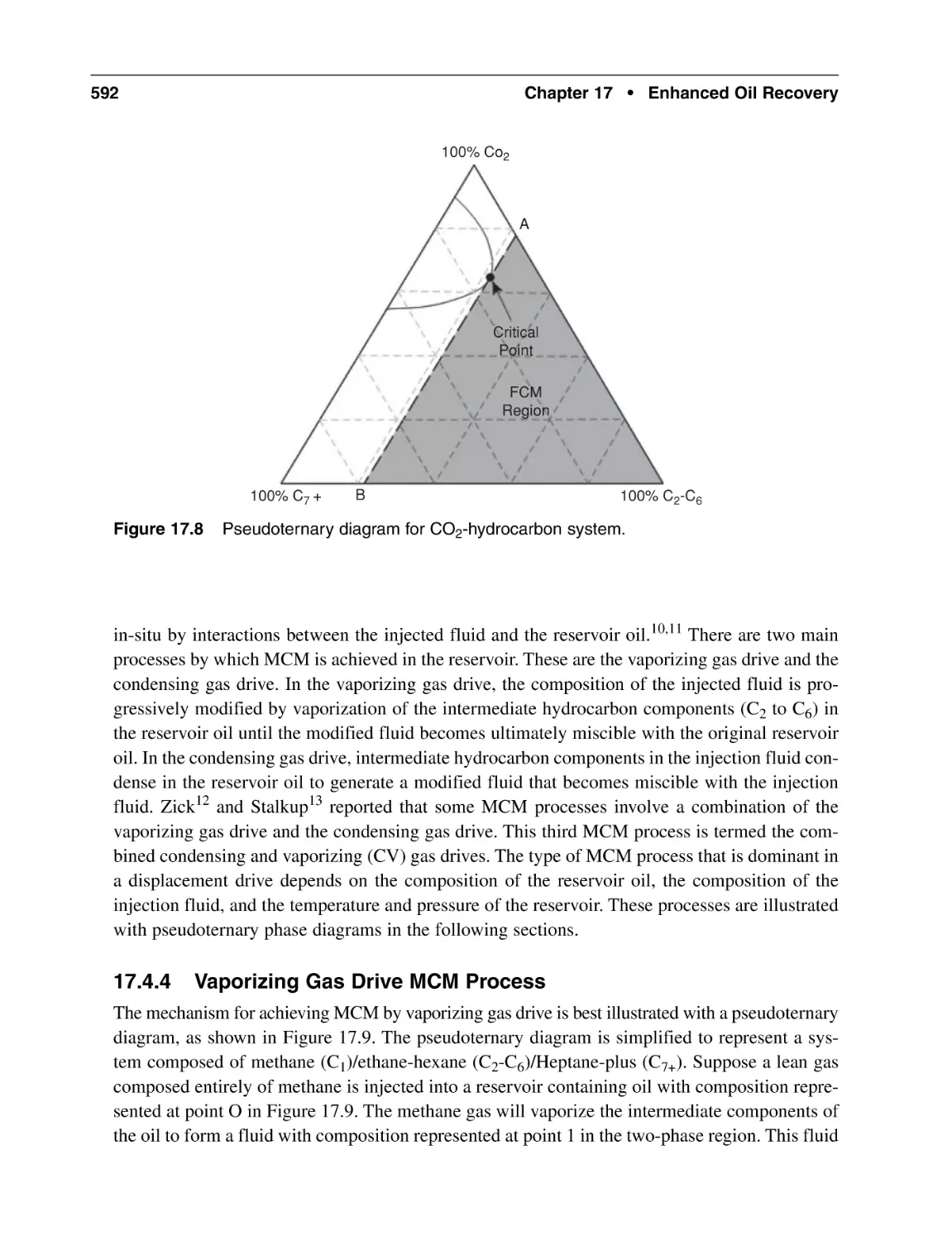
592
594
595
595
596
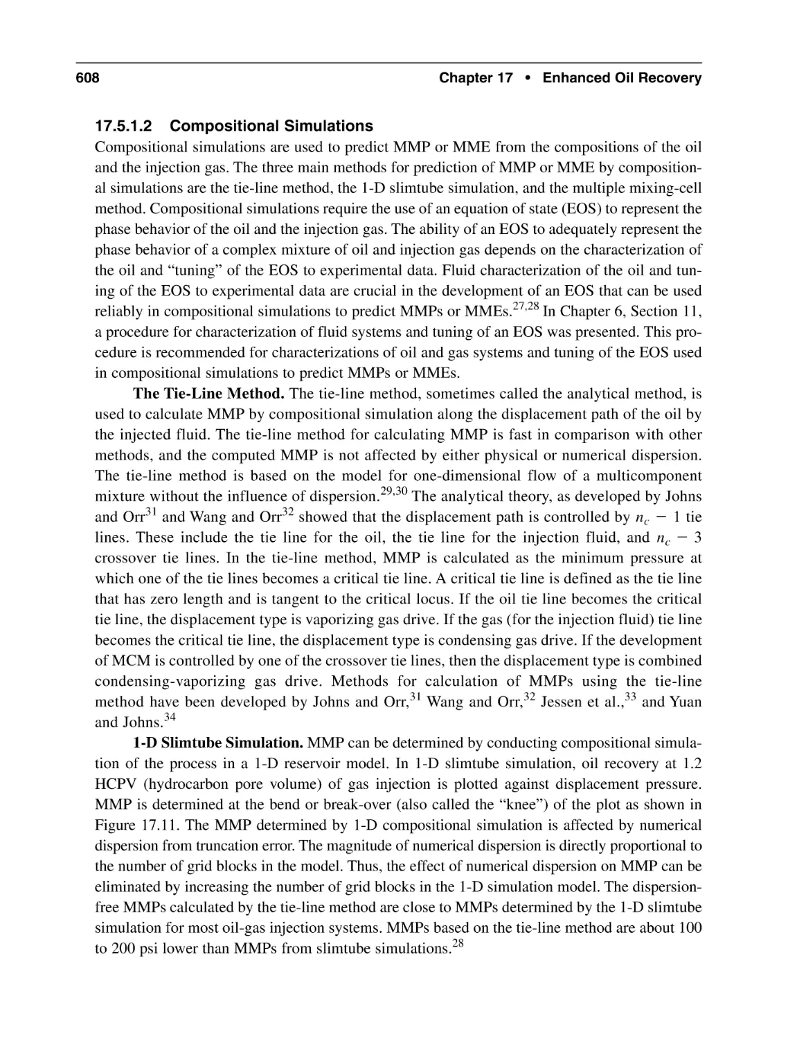
610
612
612
613
613
614
xx
Contents
17.7 Chemical Flooding Processes
17.7.1 Polymer/Surfactant Flooding
17.7.2 Alkali/Surfactant/Polymer (ASP) Flooding
17.7.3 Polymer Flooding
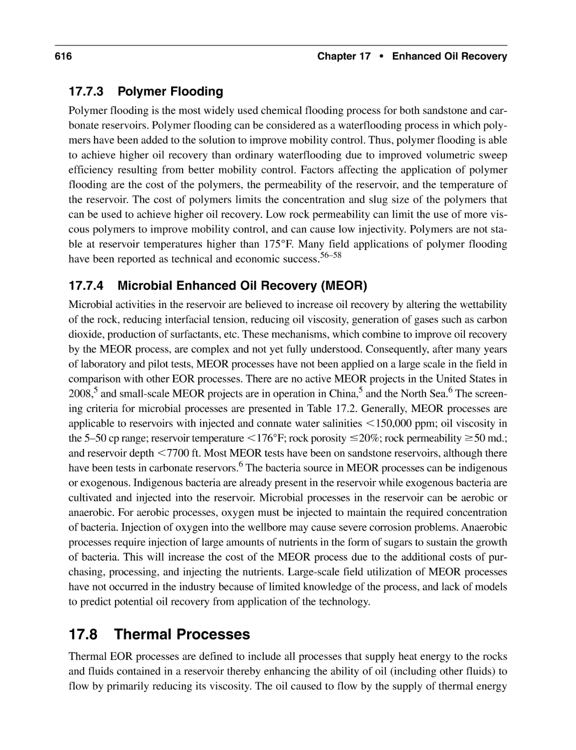
17.7.4 Microbial Enhanced Oil Recovery (MEOR)
17.8 Thermal Processes
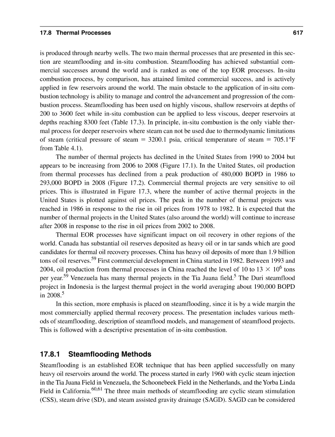
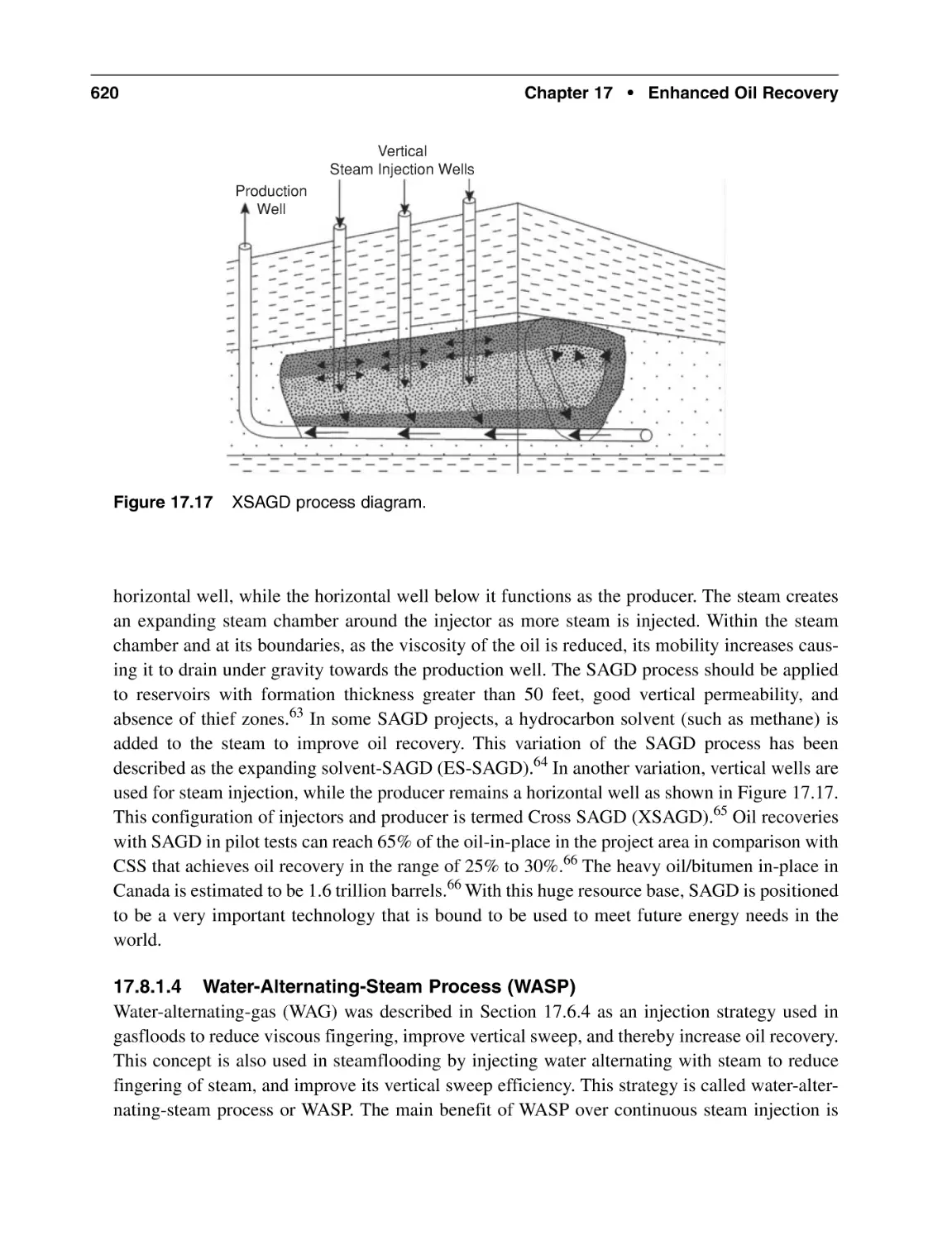
17.8.1 Steamflooding Methods
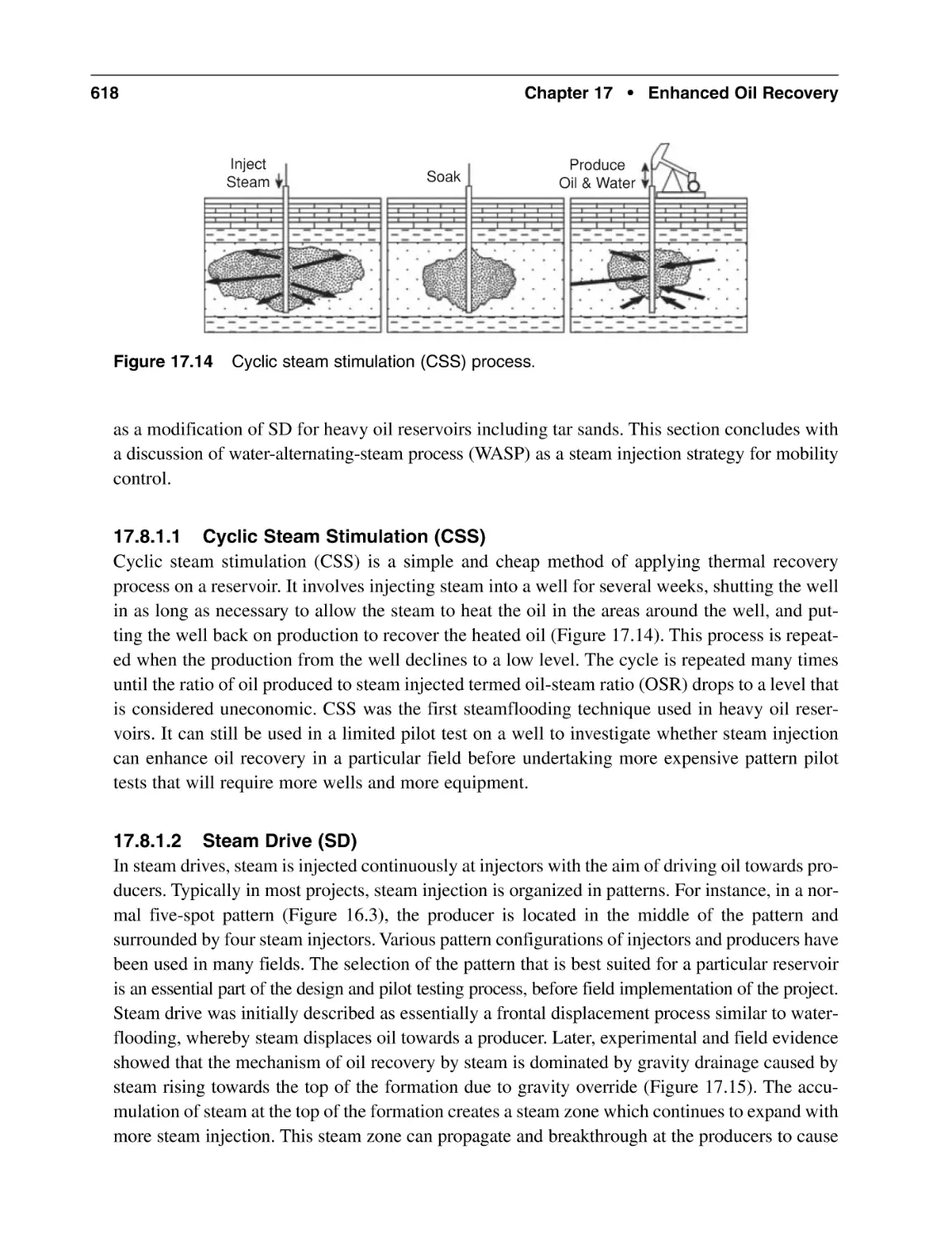
17.8.2 Steamflood Models
17.8.3 Management of Steamflood Projects
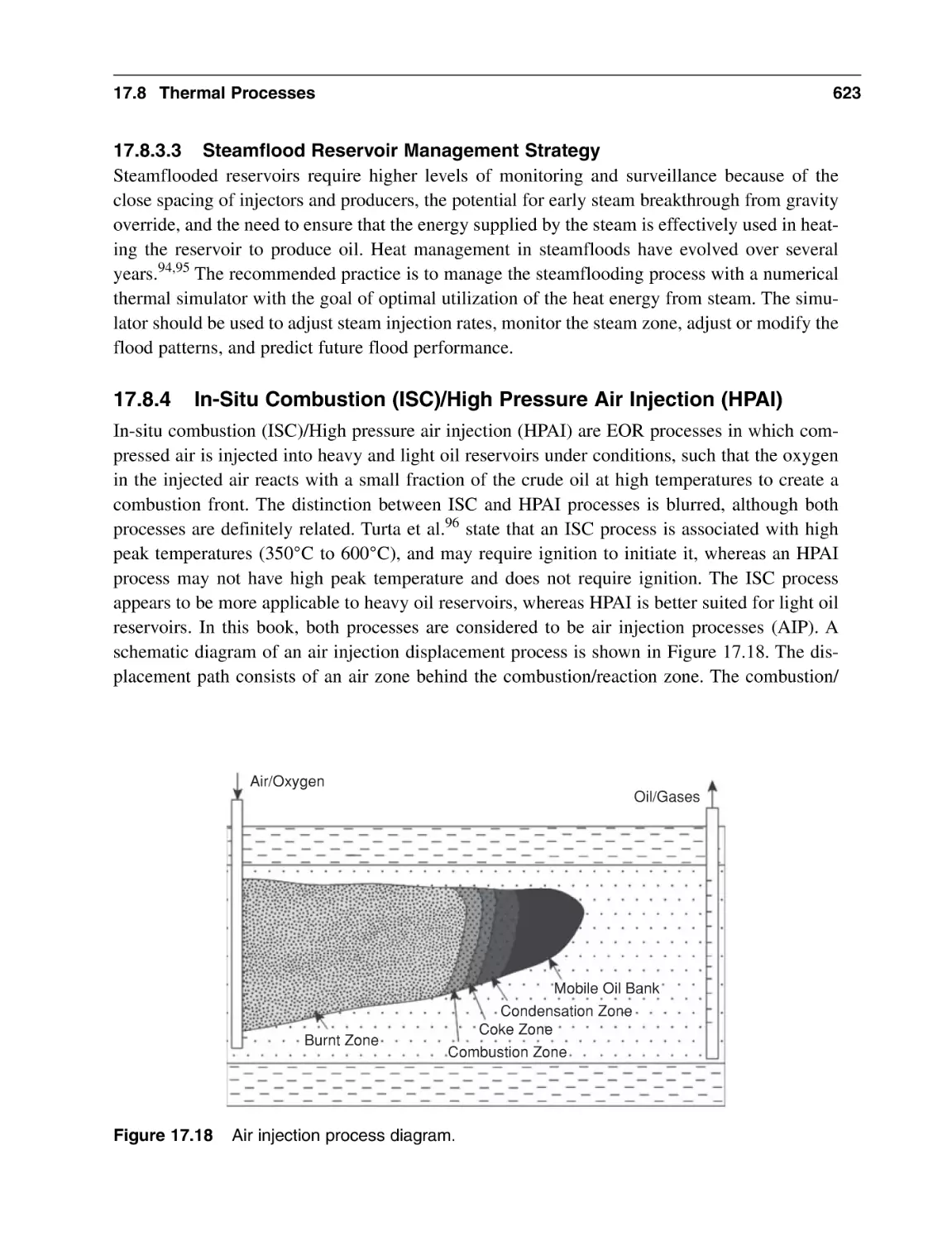
17.8.4 In-Situ Combustion (ISC)/High Pressure
Air Injection (HPAI)
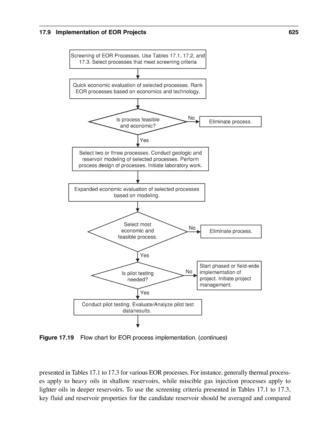
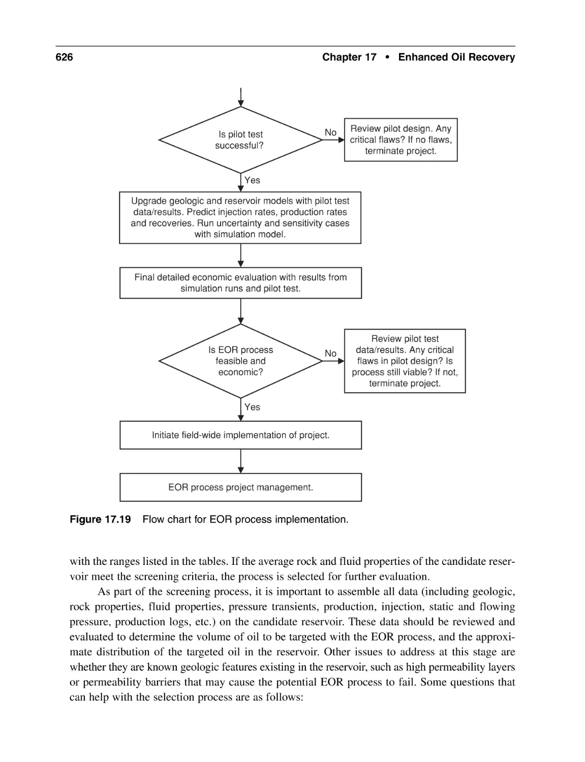
17.9 Implementation of EOR Projects
17.9.1 Process Screening and Selection
17.9.2 Quick Economic Evaluation of Selected Processes
17.9.3 Geologic and Reservoir Modeling of Selected Processes
17.9.4 Expanded Economic Evaluation of Selected Processes
17.9.5 Pilot Testing
17.9.6 Upgrade Geologic and Reservoir Models with Pilot
Test Data/Results
17.9.7 Final Detailed Economic Evaluation
17.9.8 Field-Wide Project Implementation
17.9.9 EOR Process Project Management
Nomenclature
Abbreviations
References
General Reading
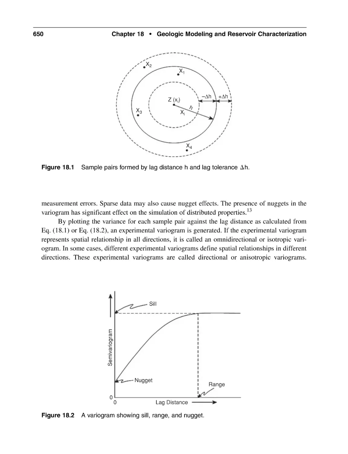
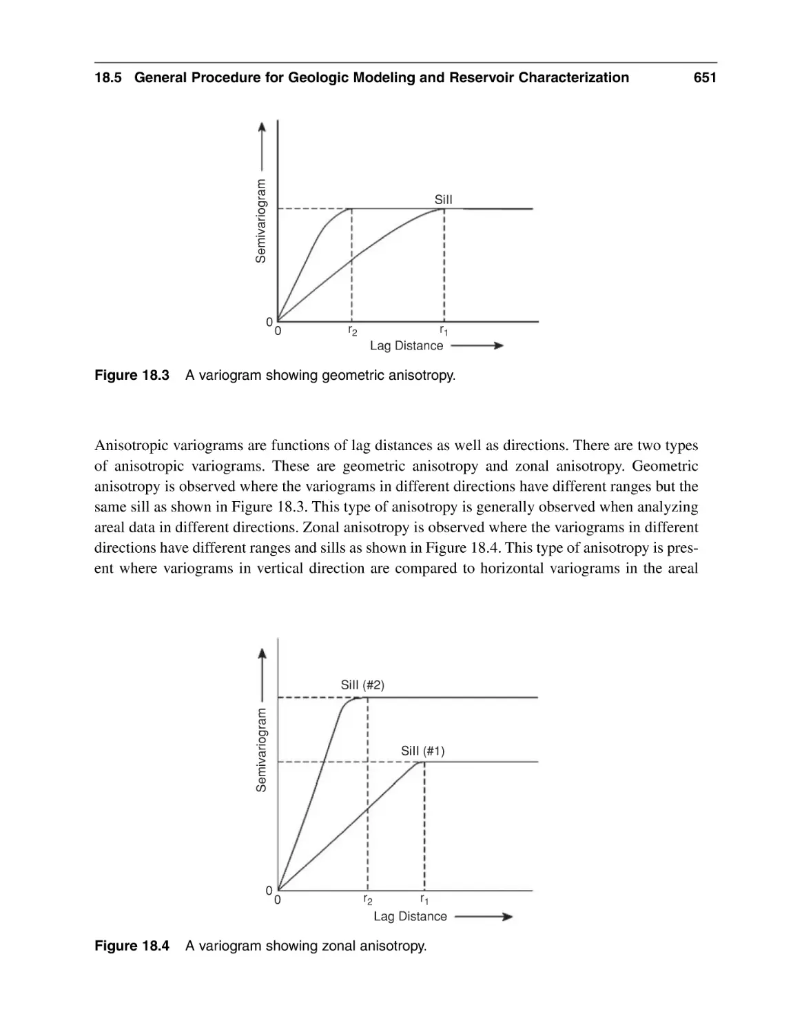
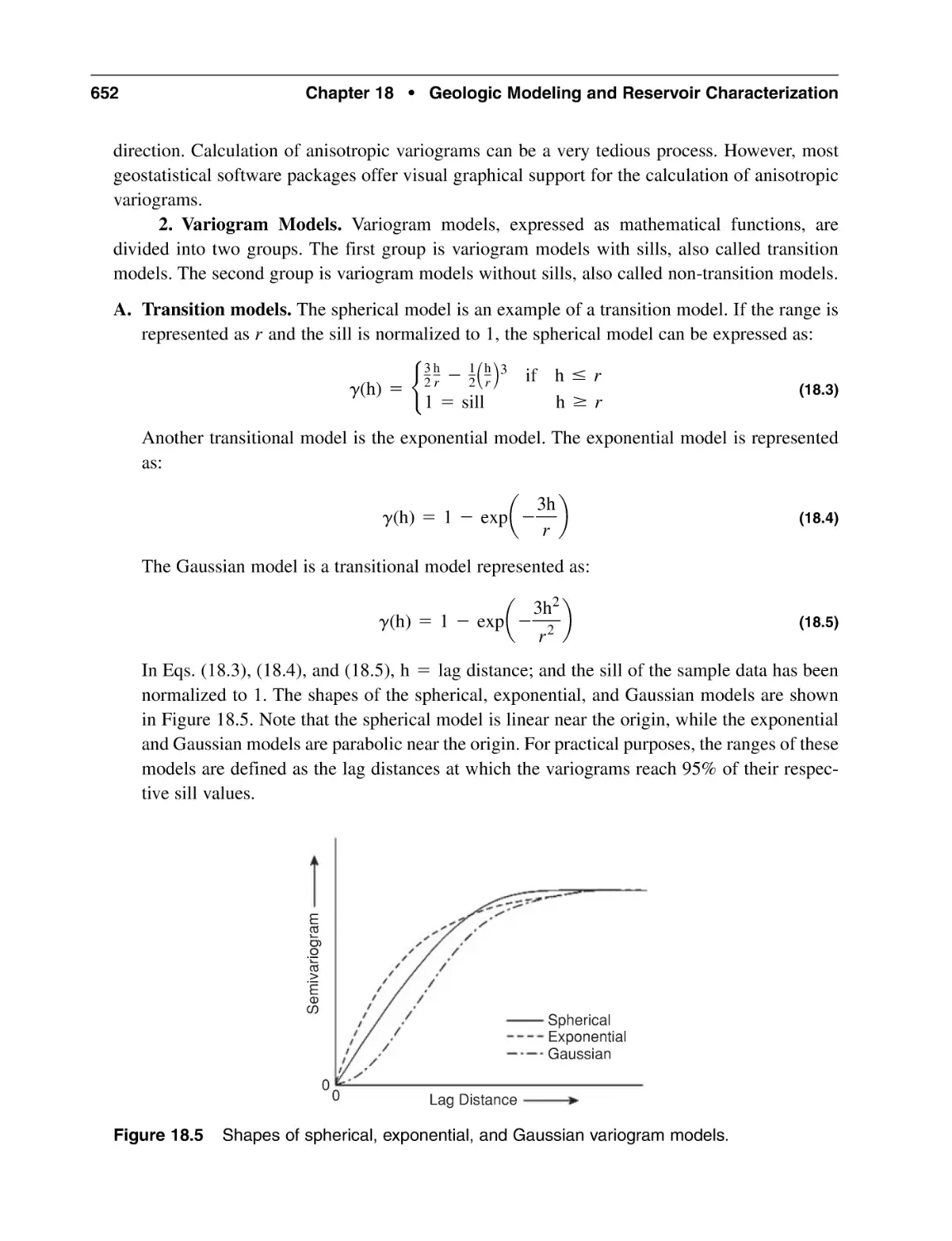
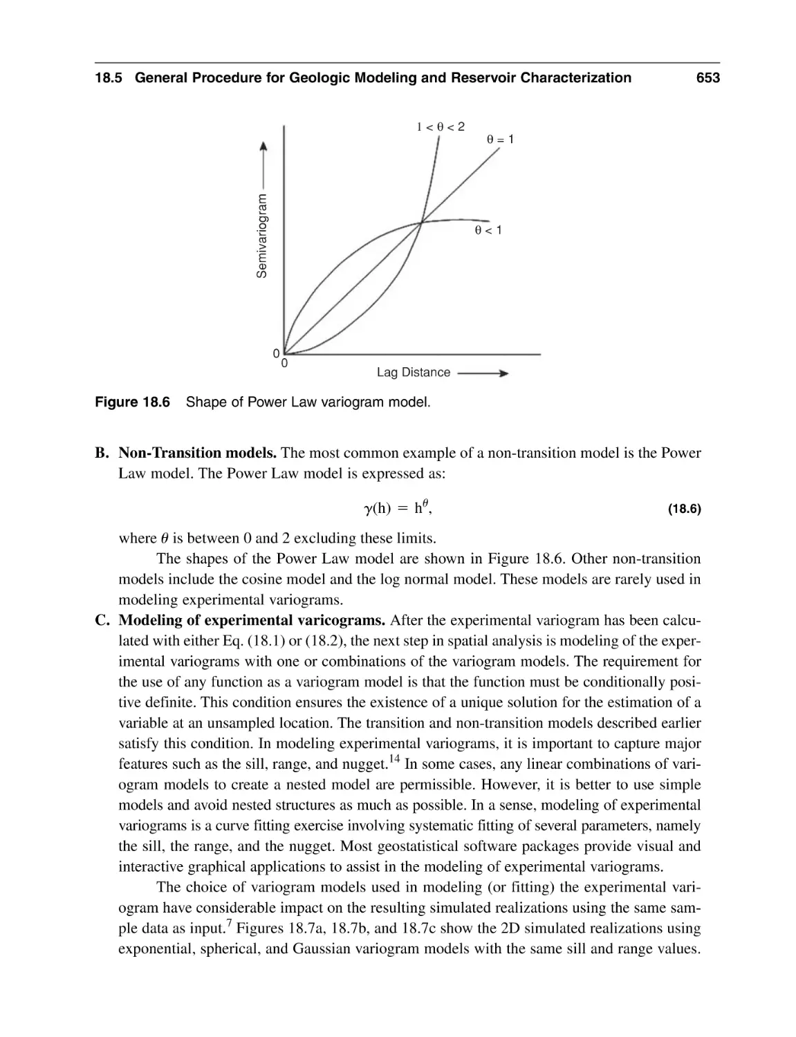
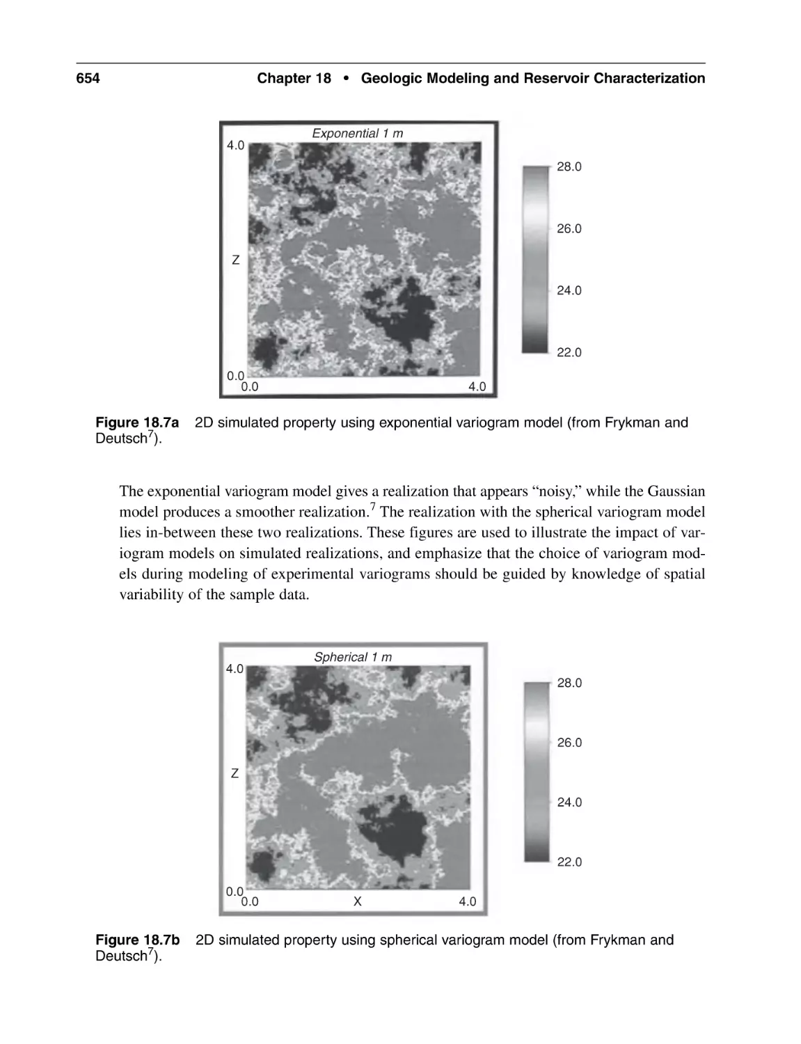
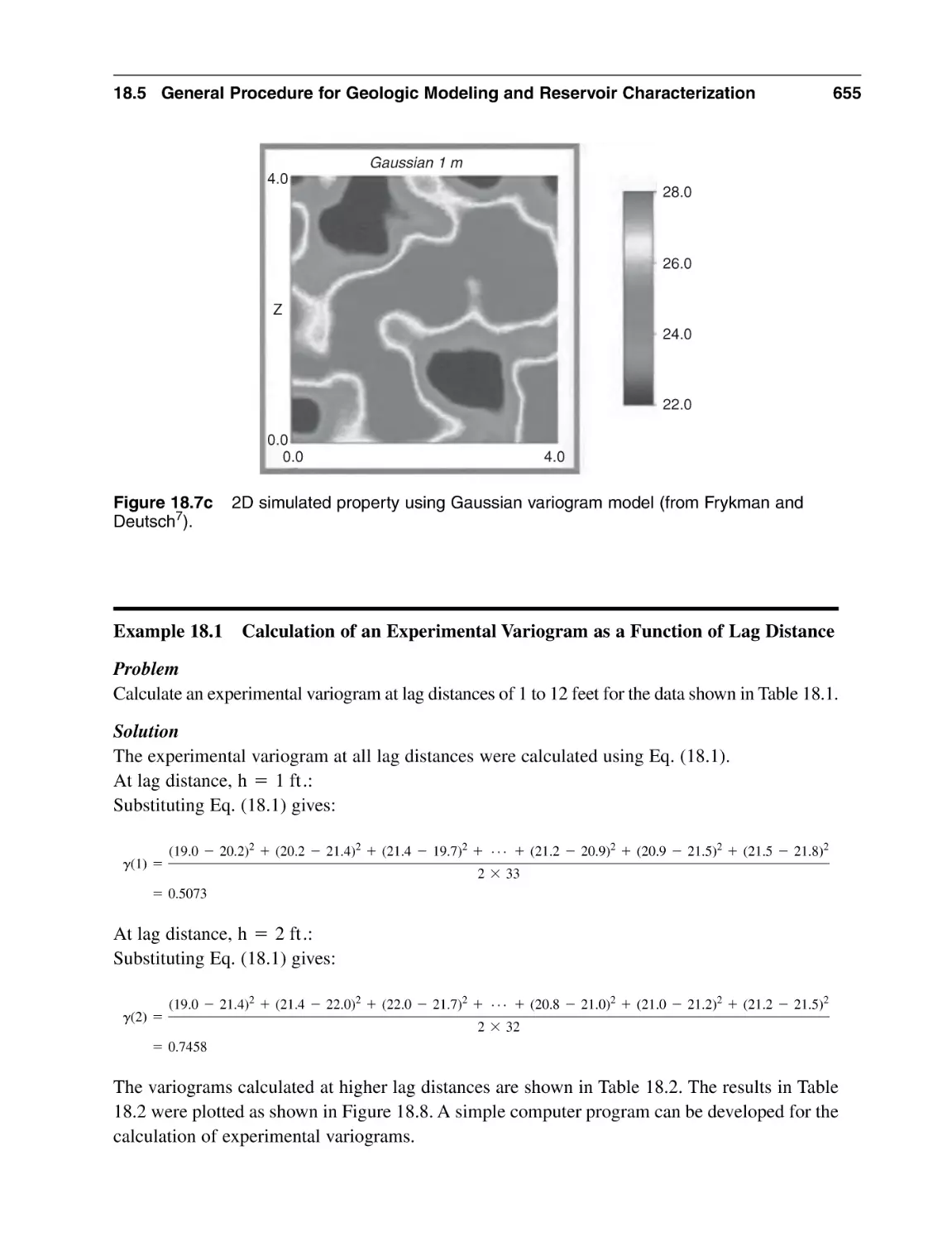
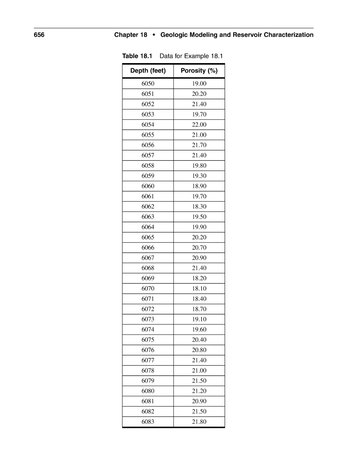
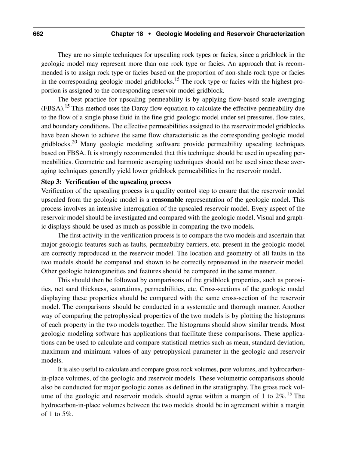
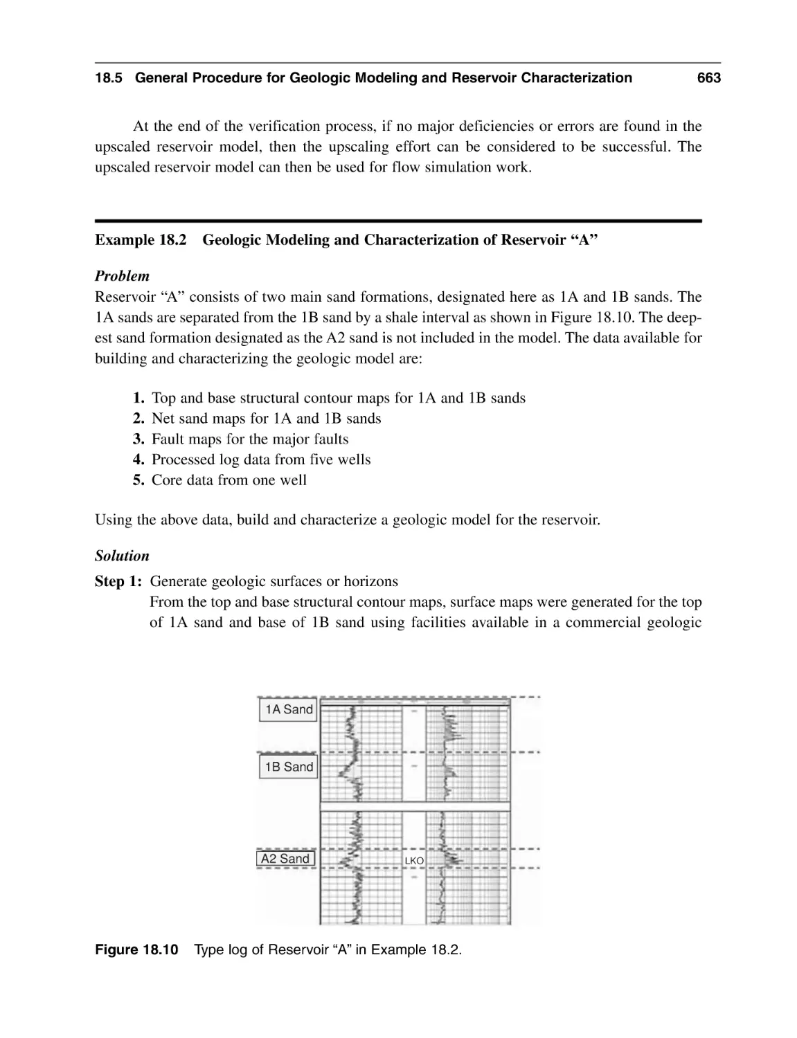
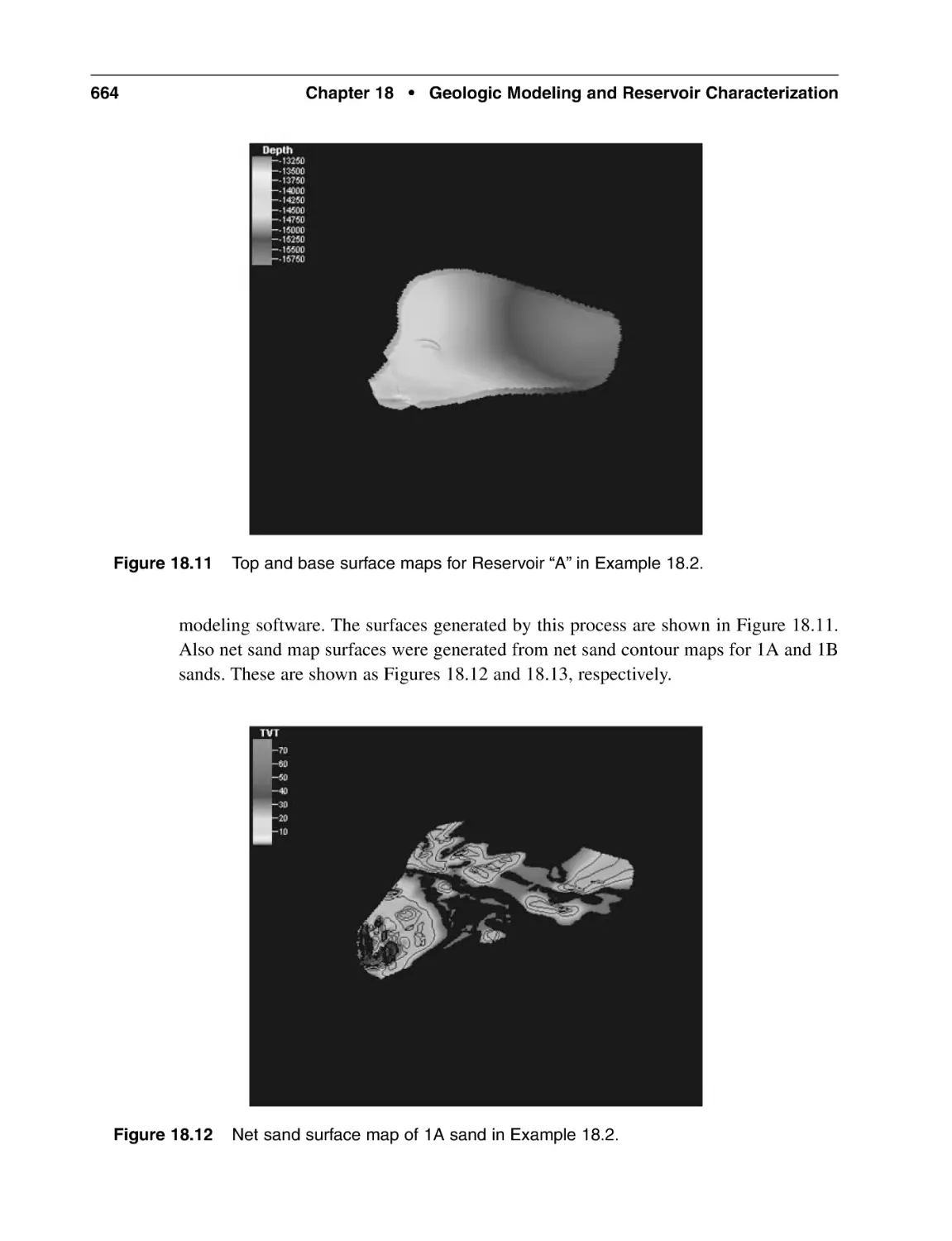
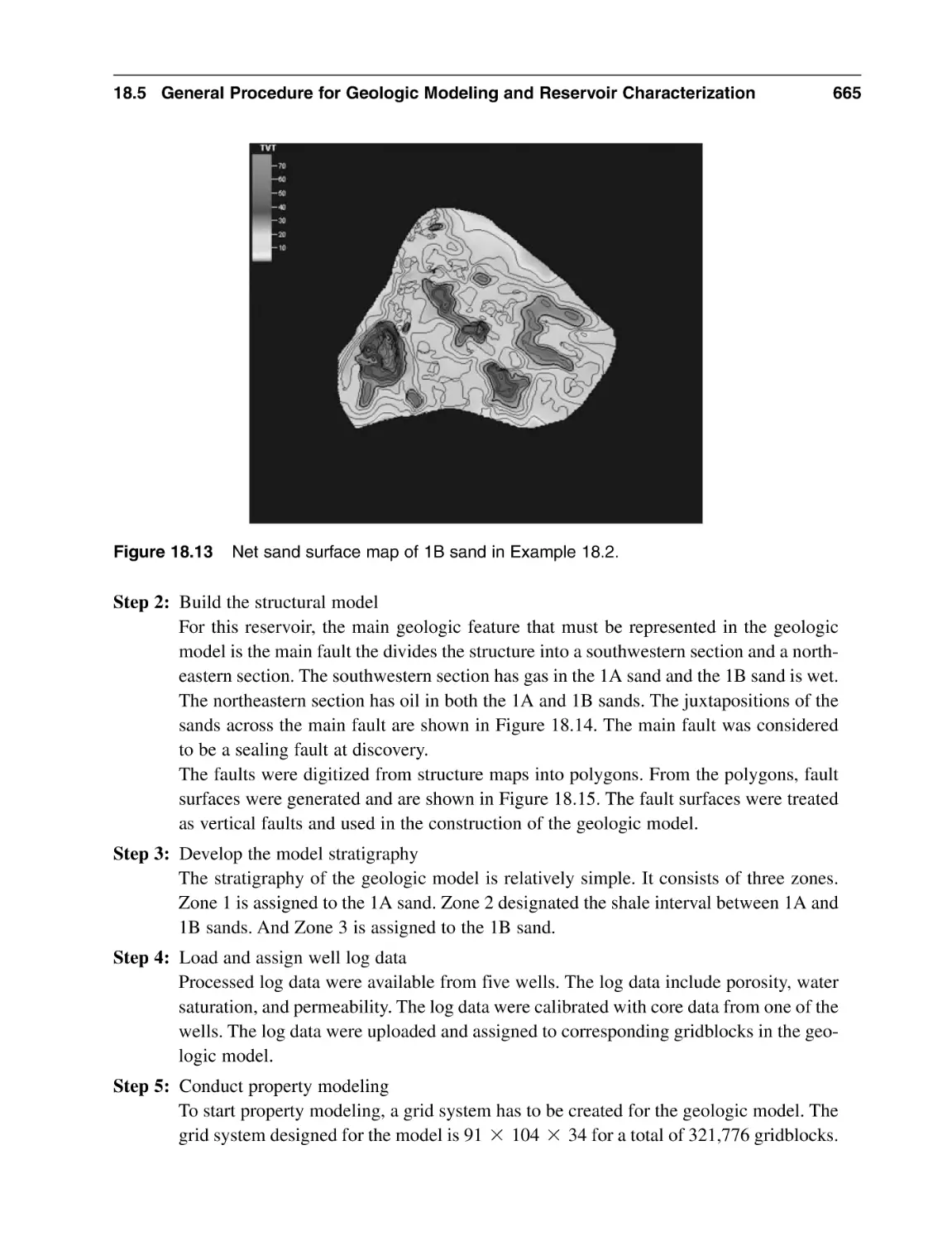
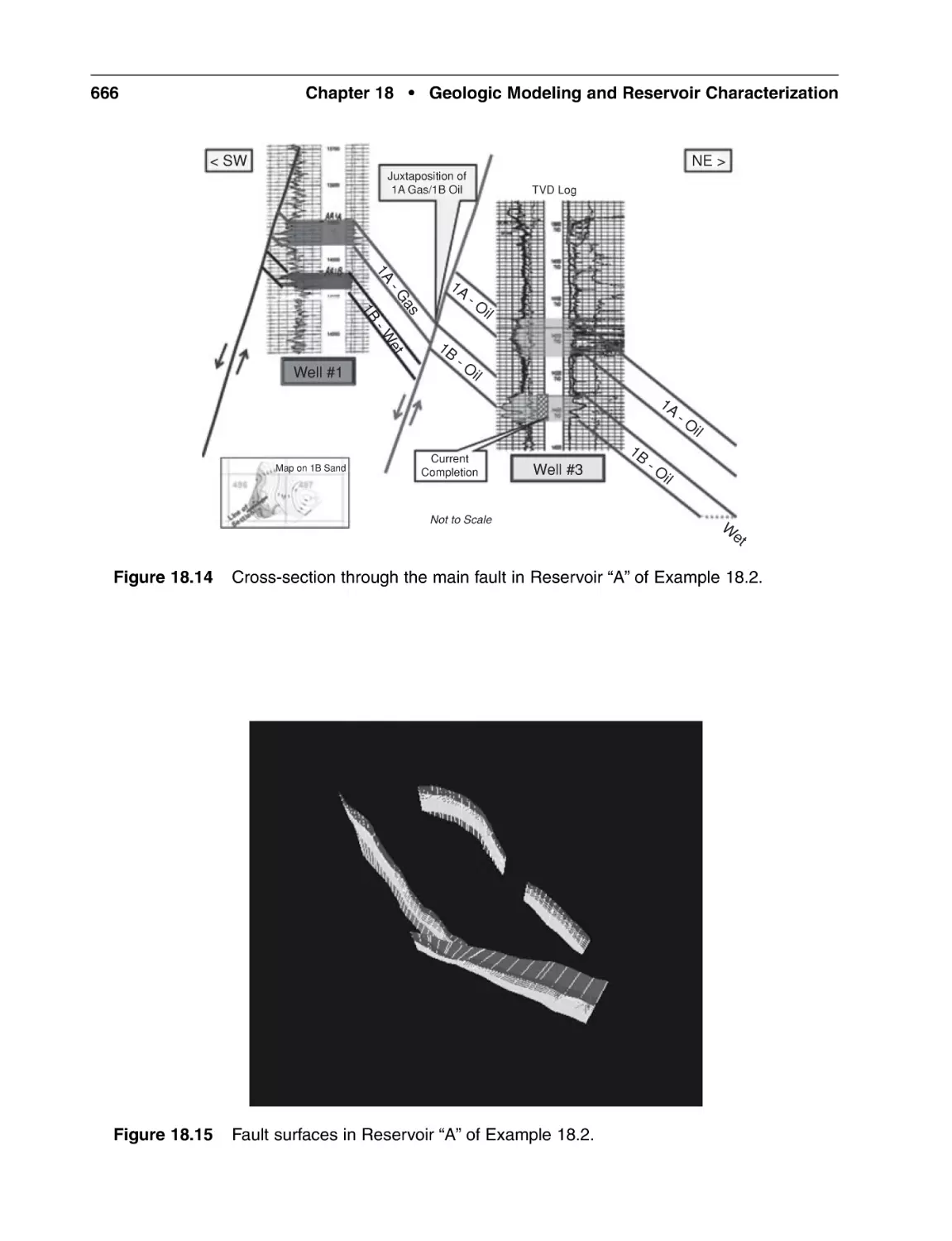
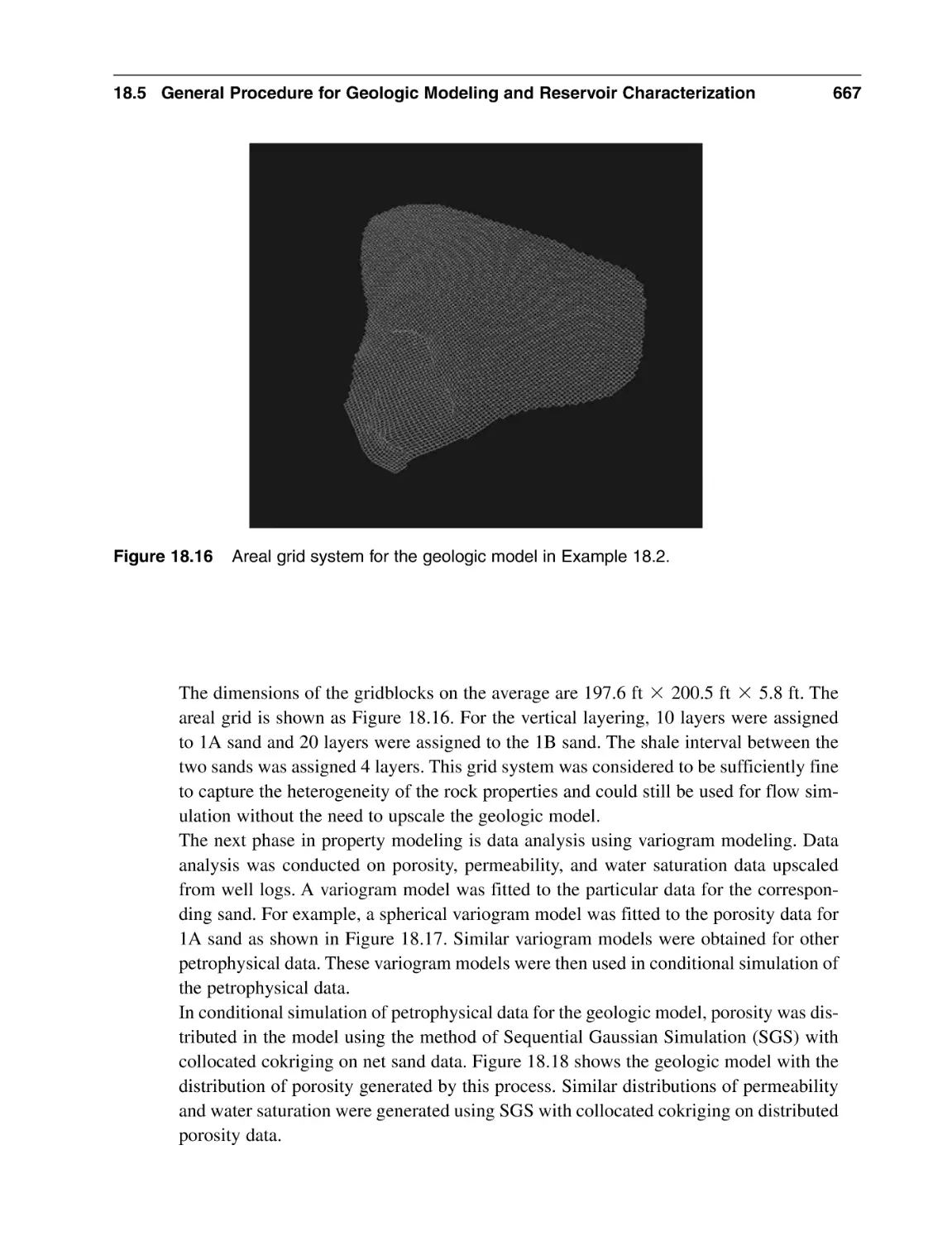
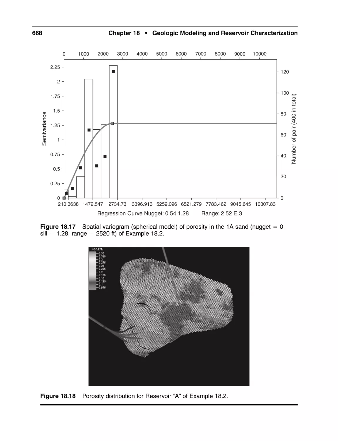
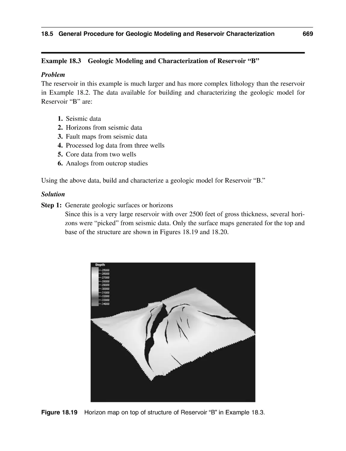
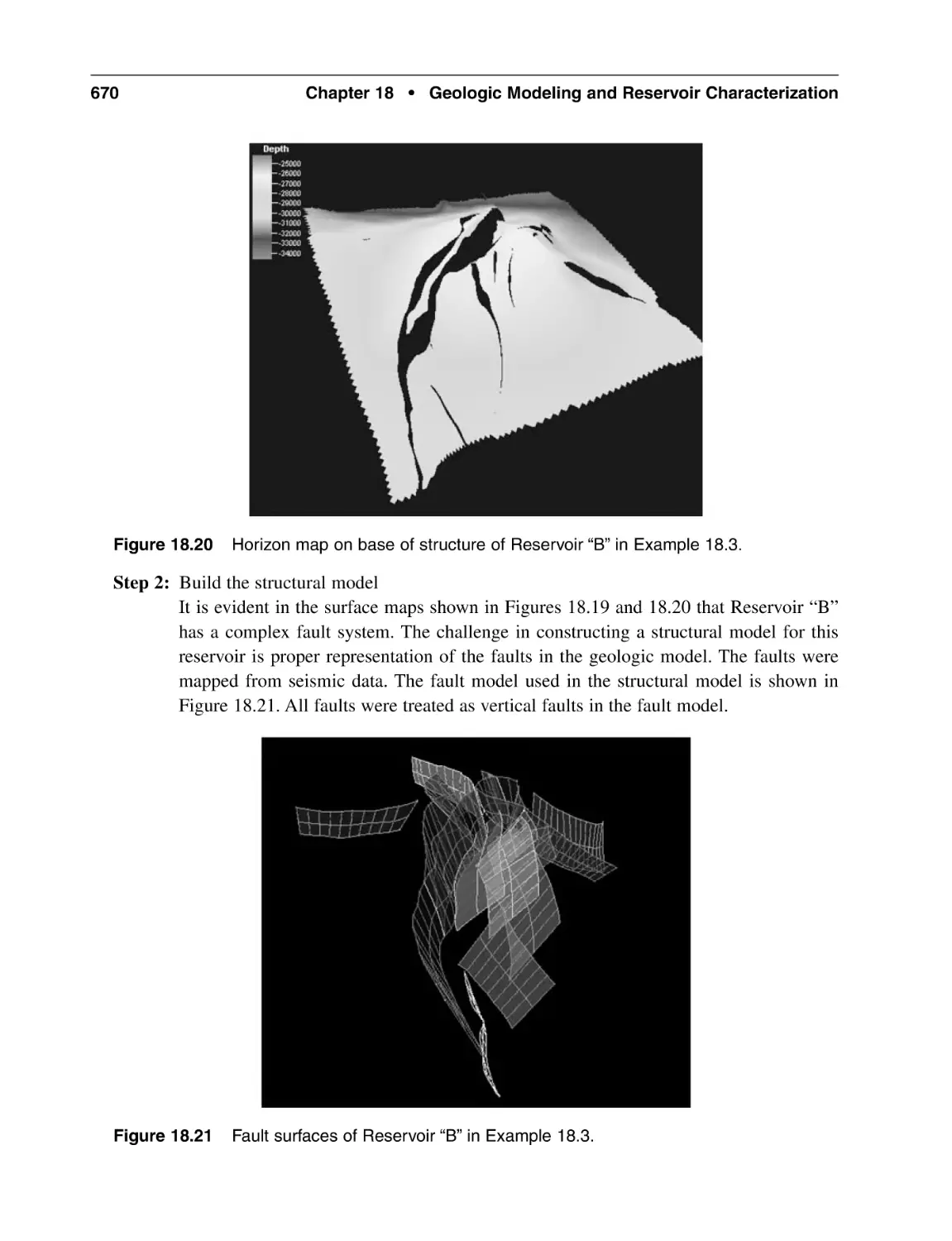
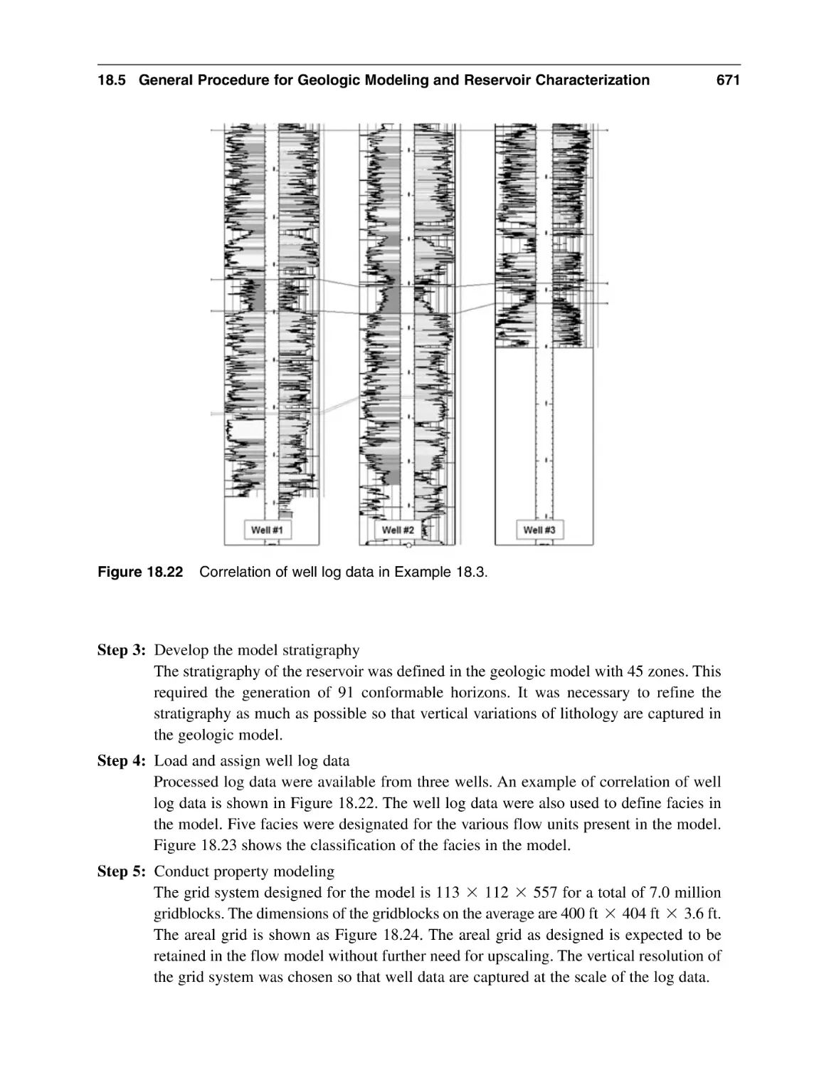
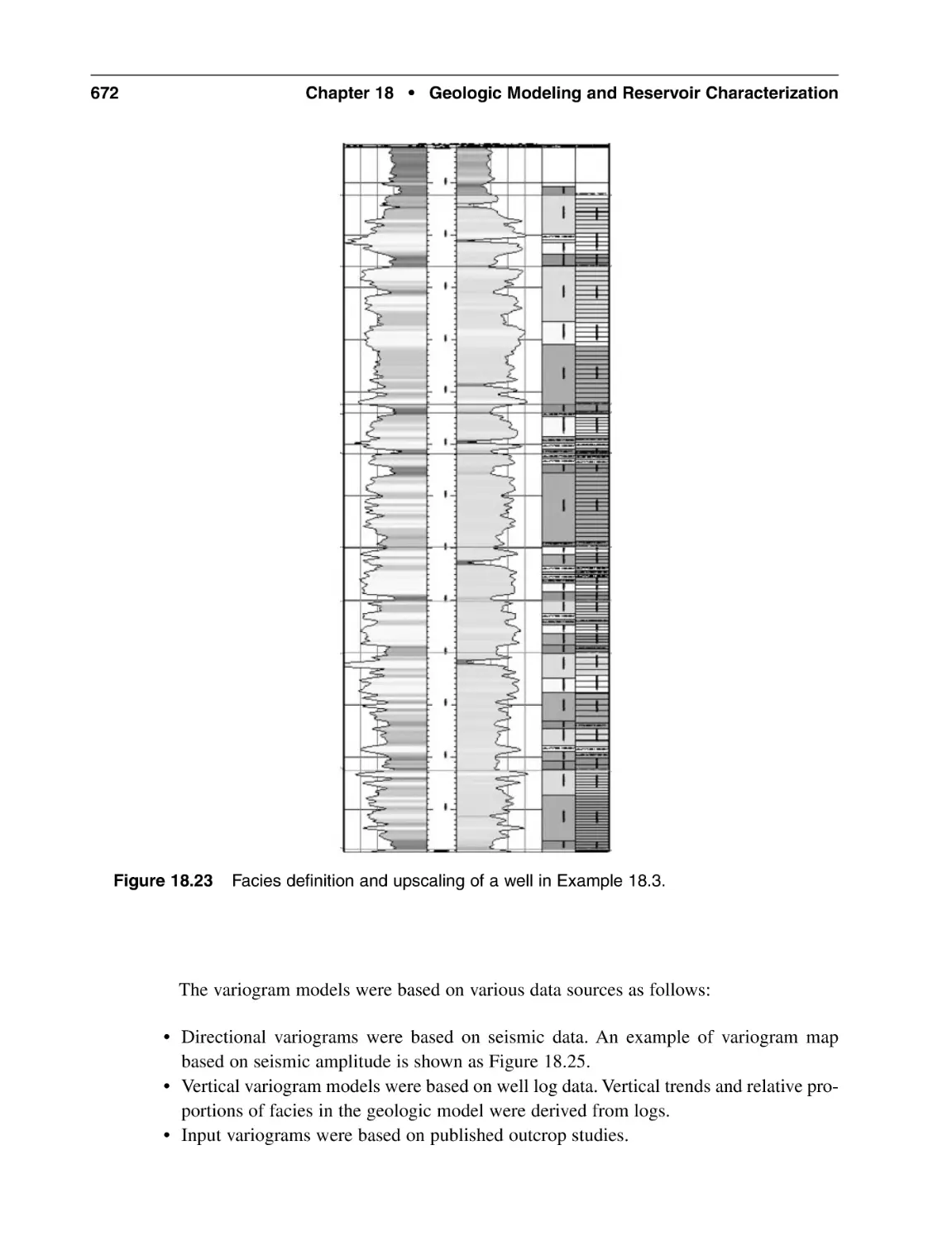
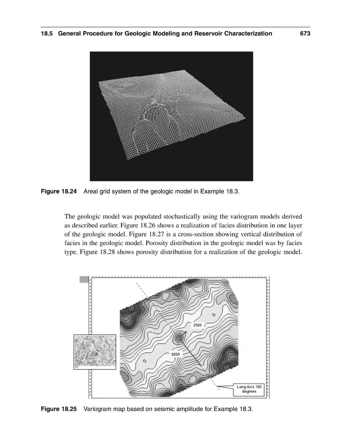
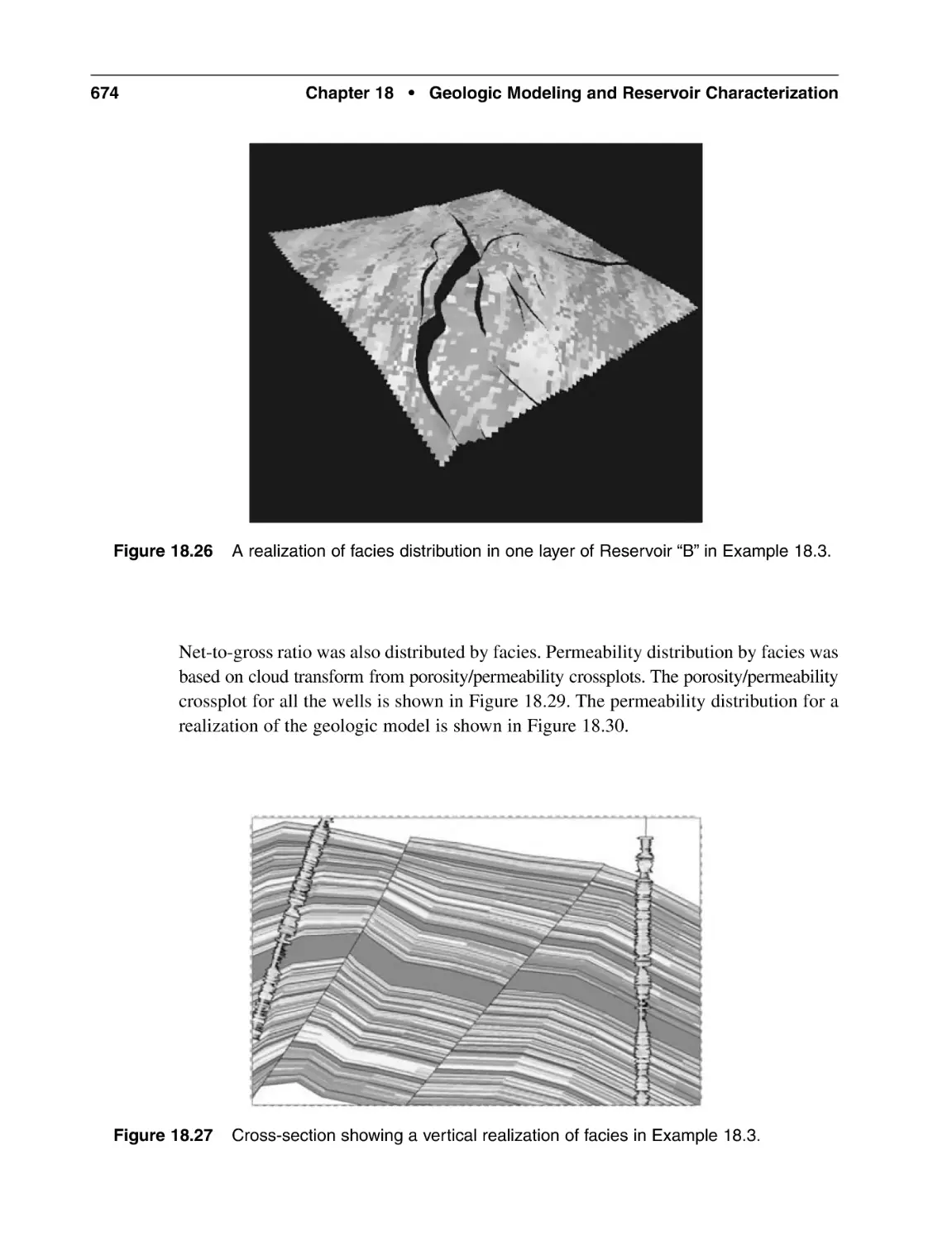
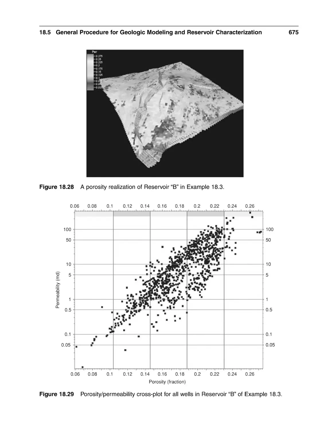
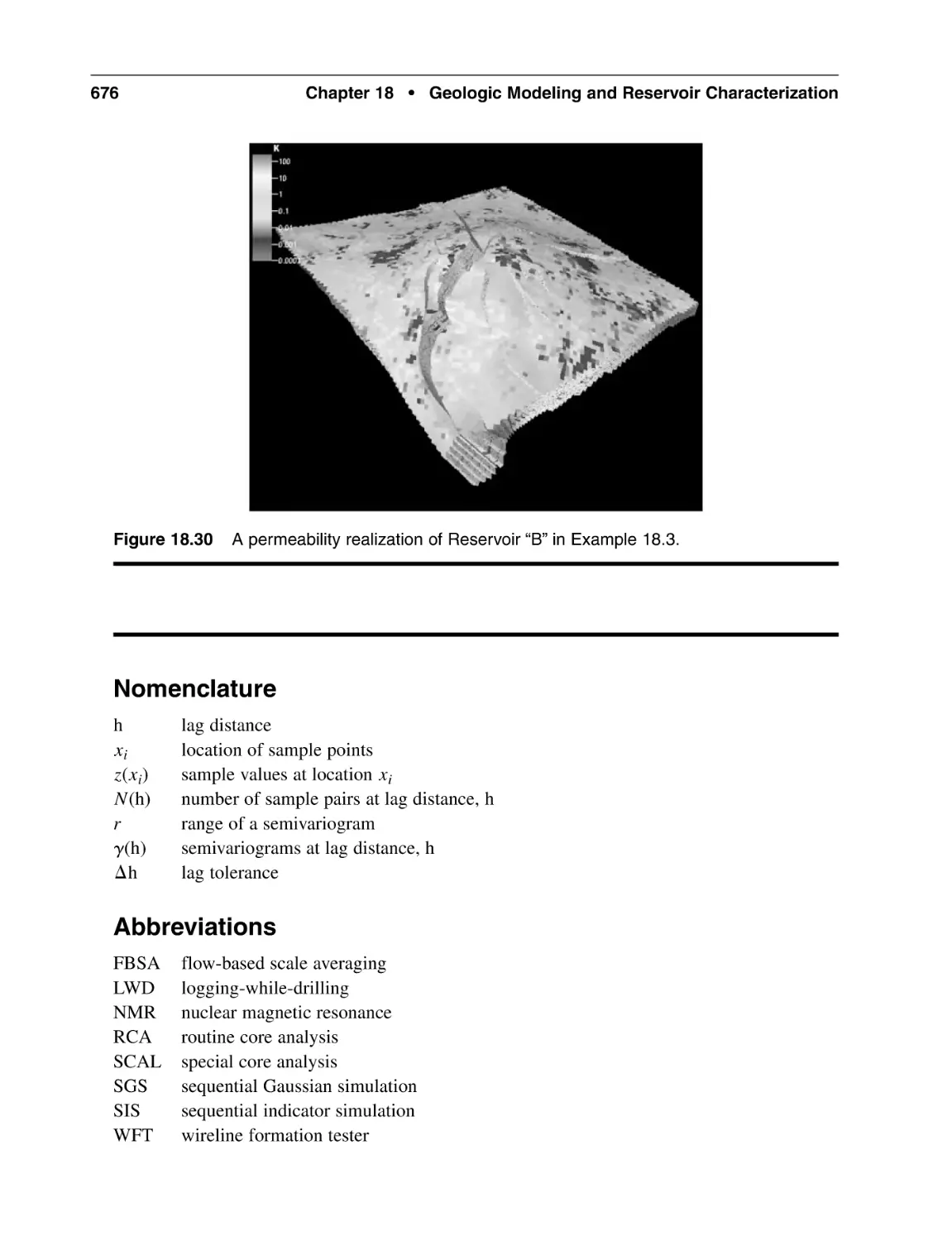
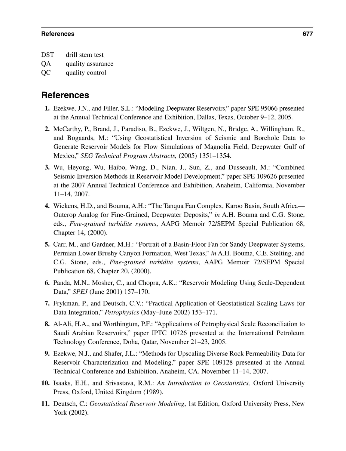
Chapter 18 Geologic Modeling and Reservoir Characterization
18.1 Introduction
18.2 Sources of Data for Geologic Modeling and Reservoir
Characterization
18.2.1 Seismic Data
18.2.2 Outcrop and Basin Studies
18.2.3 Well Log Data
18.2.4 Core Data
18.2.5 Formation Pressures and Fluid Properties Data
18.2.6 Pressure Transient Test Data
18.2.7 Reservoir Performance Data
18.3 Data Quality Control and Quality Assurance
614
615
615
616
616
616
617
621
622
623
624
624
627
627
628
628
629
630
630
630
630
630
631
638
641
641
641
642
642
642
643
643
643
644
644
Contents
18.4
18.5
xxi
Scale and Integration of Data
General Procedure for Geologic Modeling and
Reservoir Characterization
18.5.1 Generation of Geologic Surfaces or Horizons
18.5.2 Structural Modeling
18.5.3 Stratigraphic Modeling
18.5.4 Correlation and Assignment of Well Log Data
18.5.5 Property Data Modeling
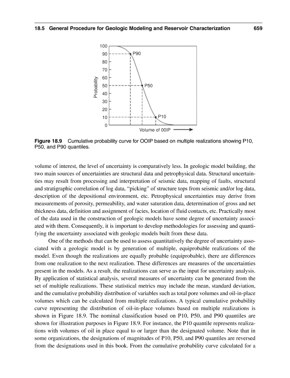
18.5.6 Uncertainty Analysis
18.5.7 Upscaling of Geologic Model to Reservoir Flow Model
Nomenclature
Abbreviations
References
General Reading
644
Chapter 19 Reservoir Simulation
19.1 Introduction
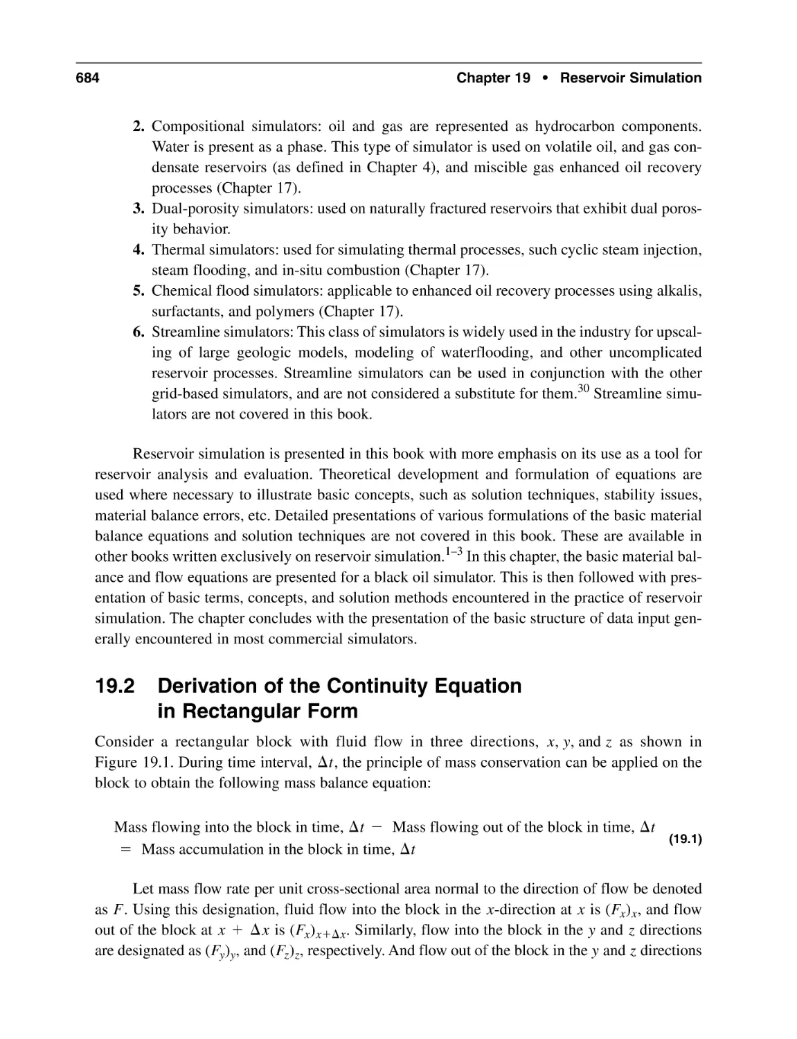
19.2 Derivation of the Continuity Equation in Rectangular Form
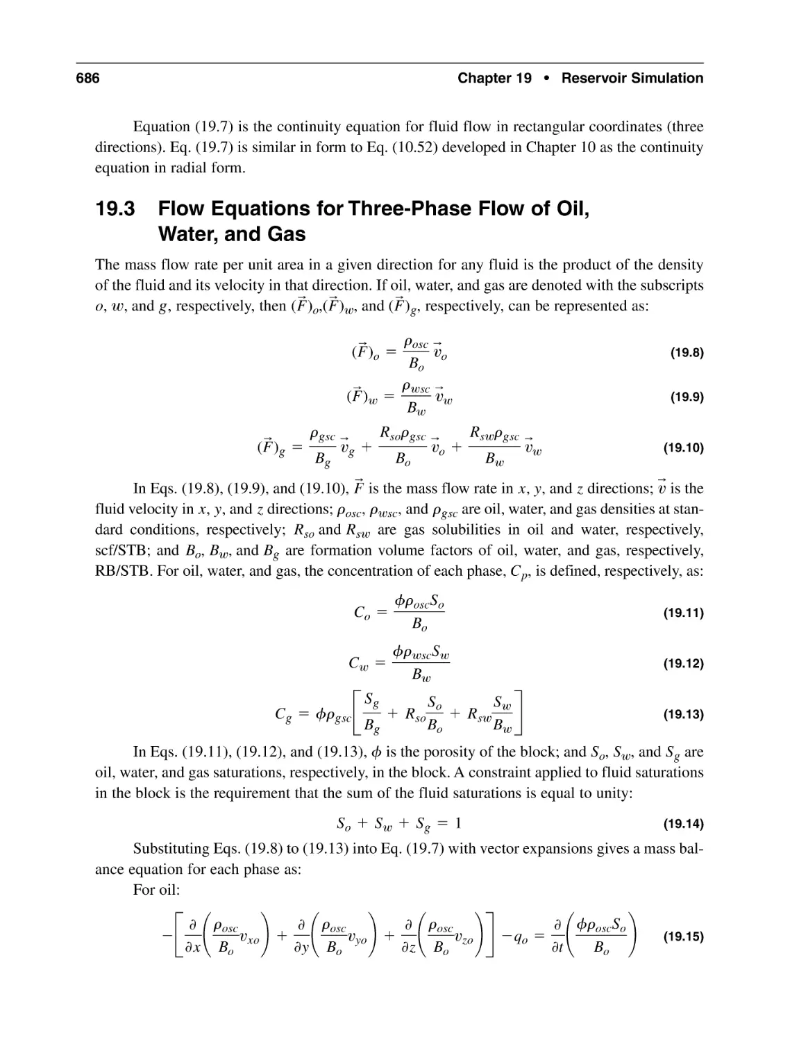
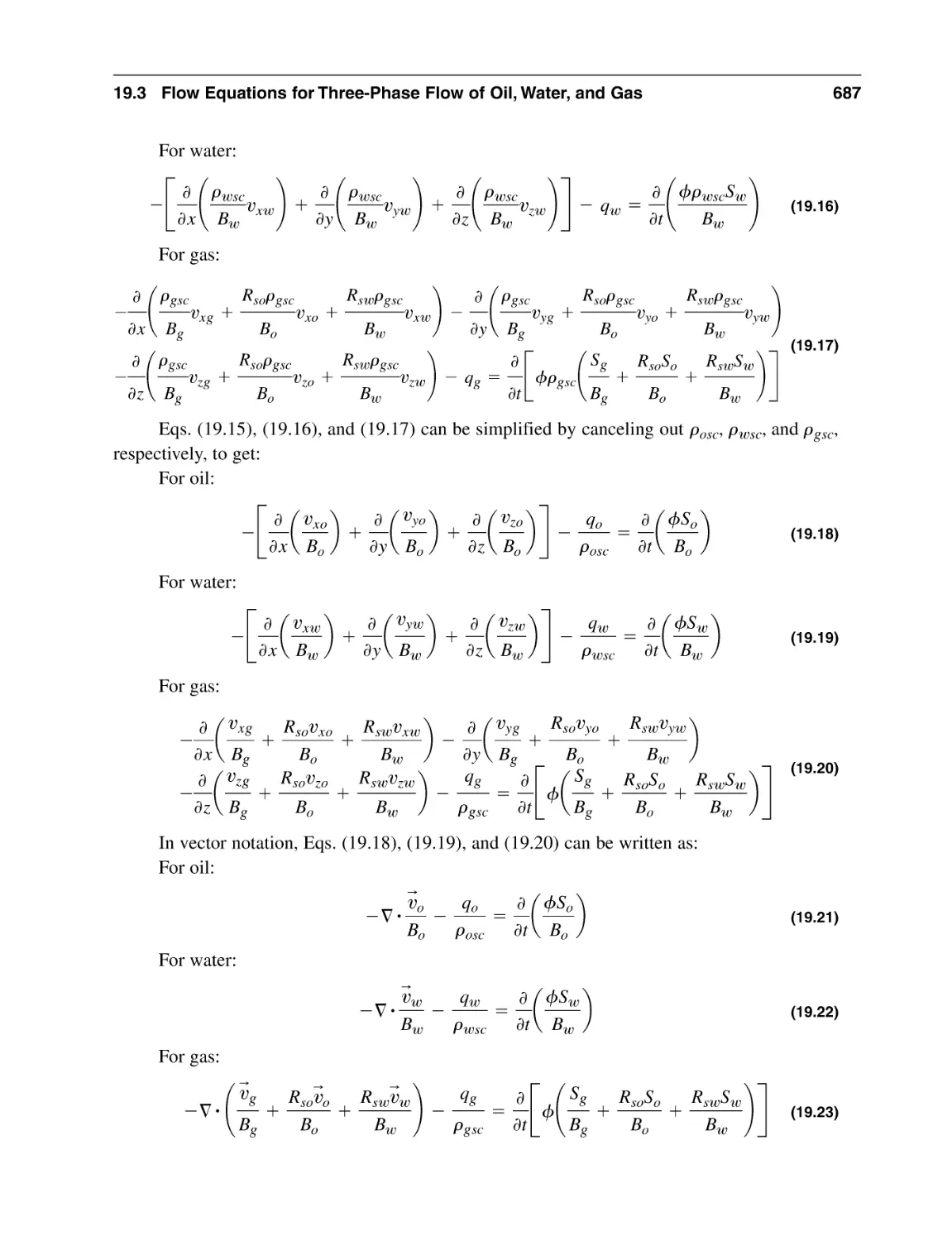
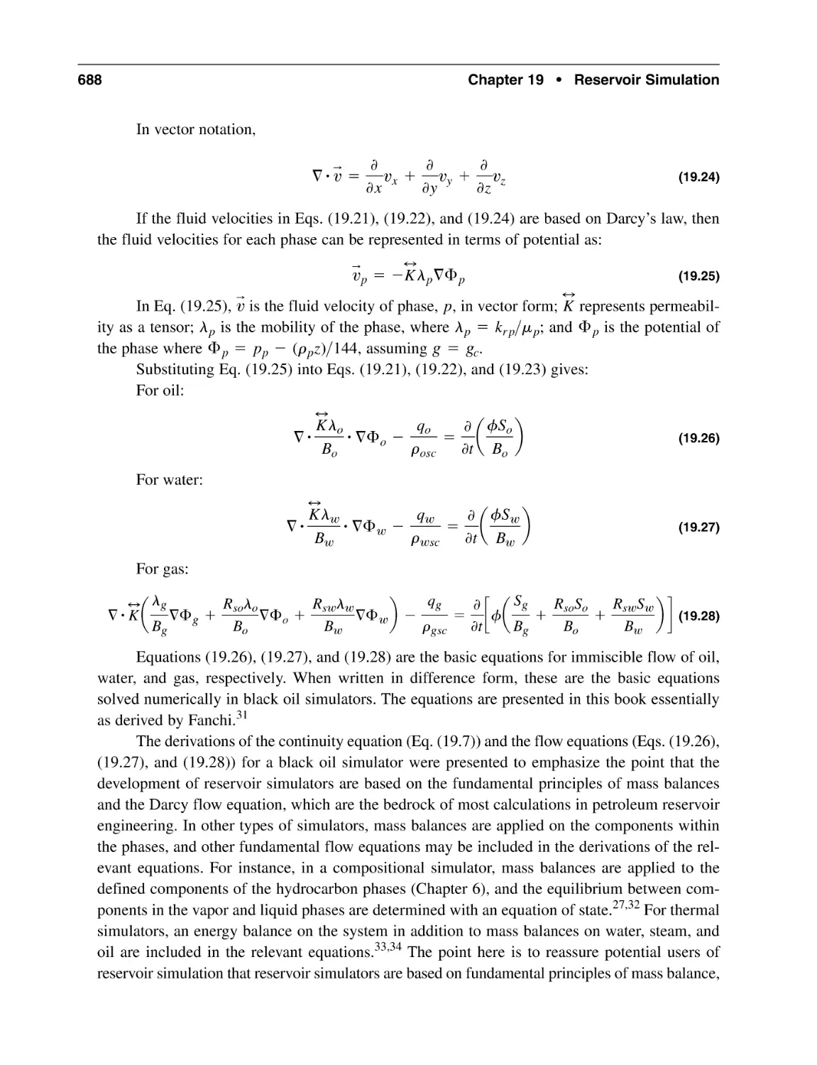
19.3 Flow Equations for Three-Phase Flow of Oil,Water, and Gas
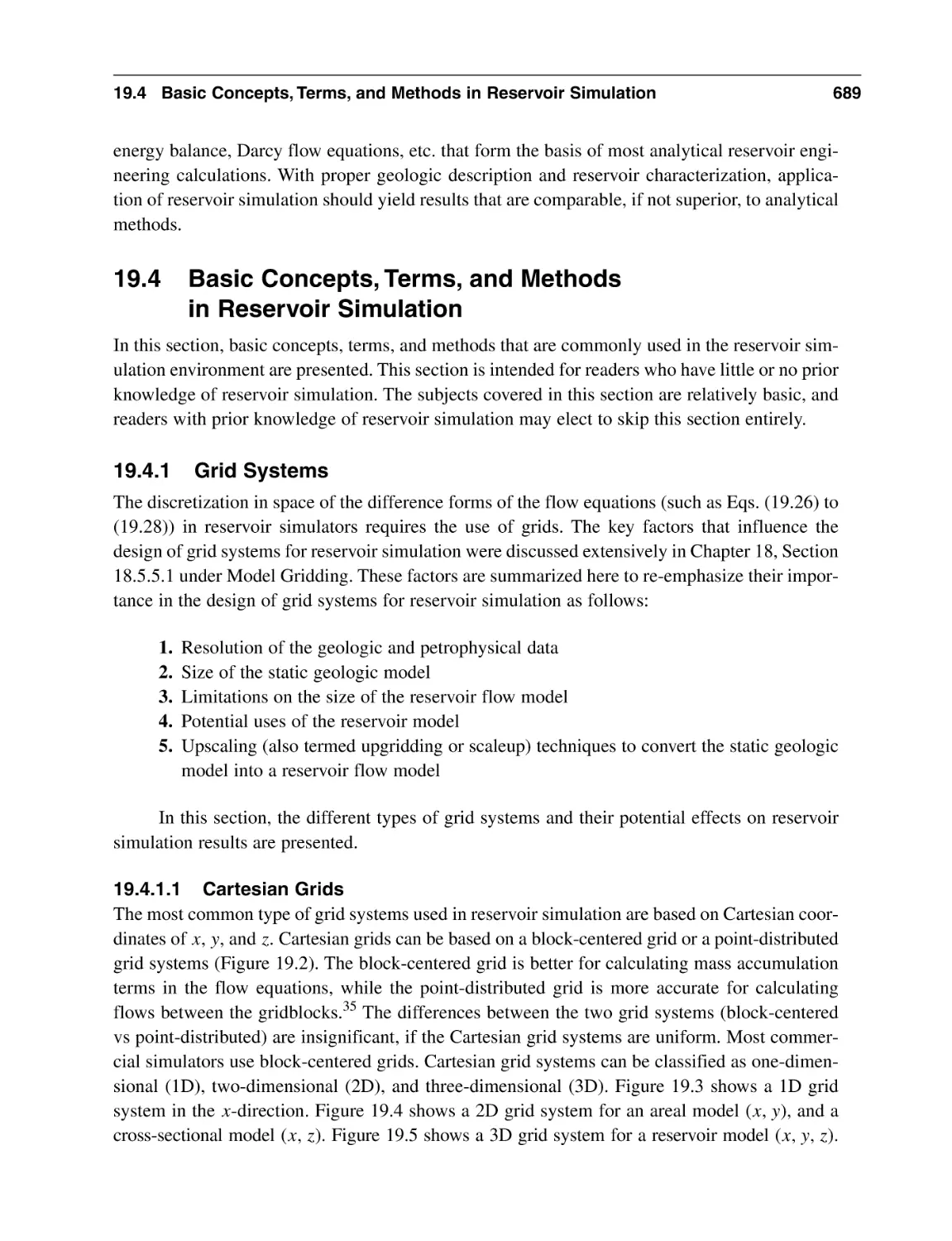
19.4 Basic Concepts, Terms, and Methods in Reservoir Simulation
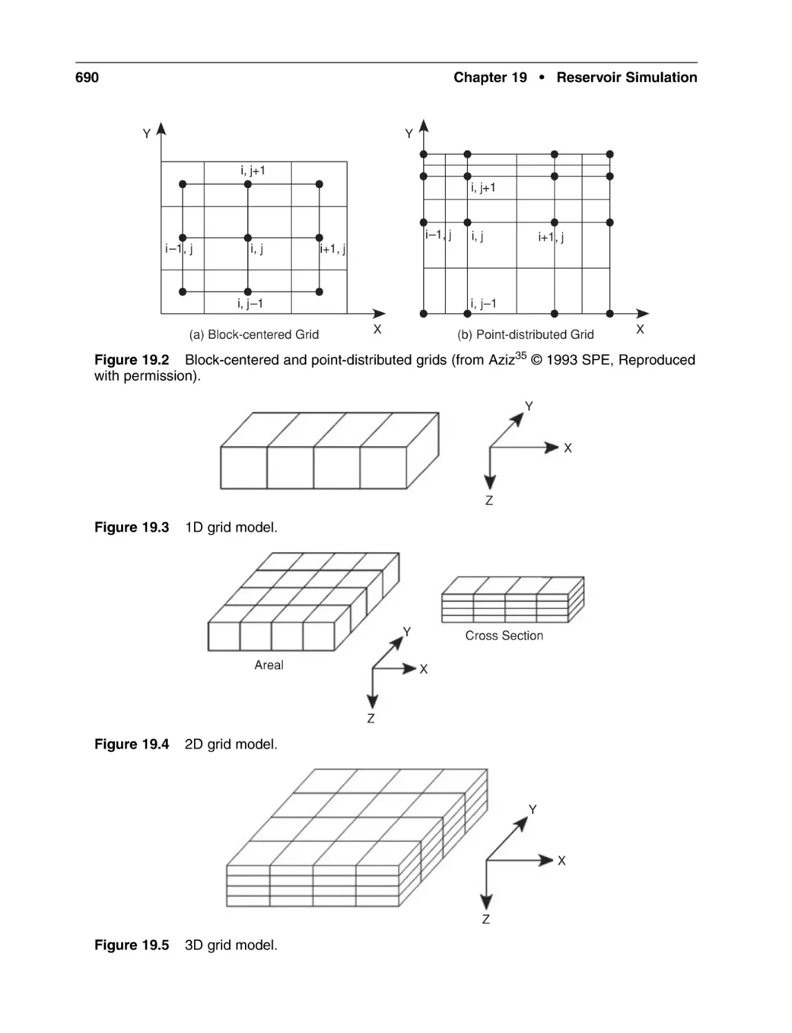
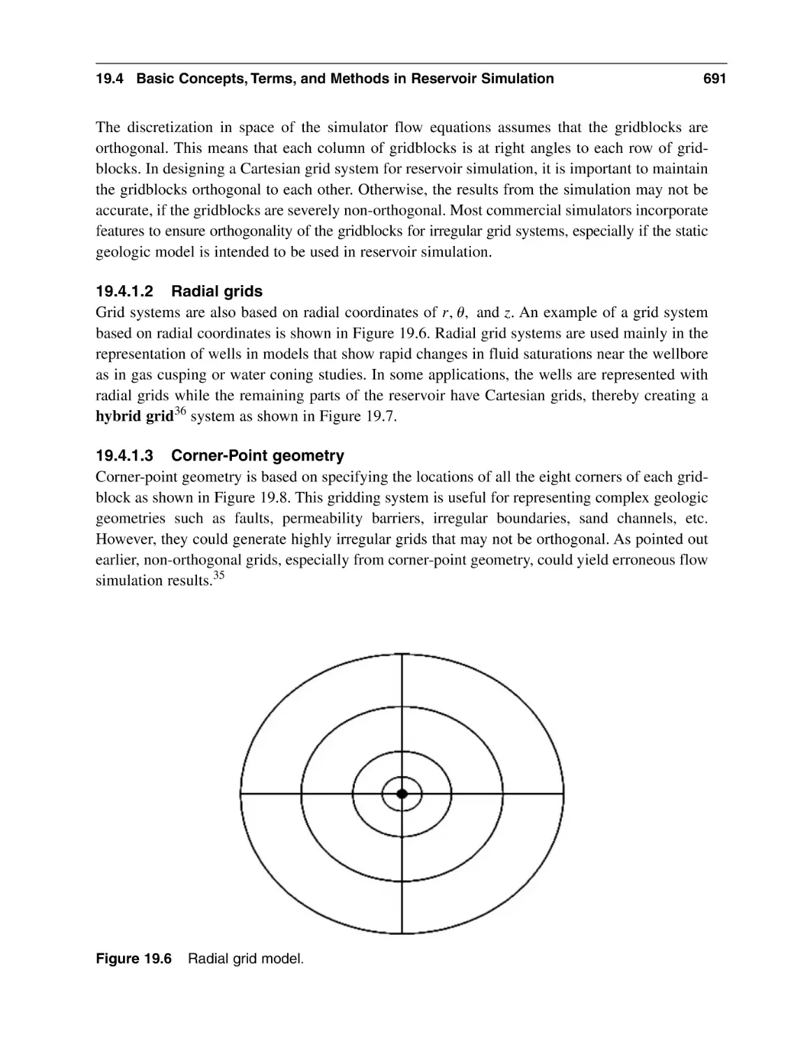
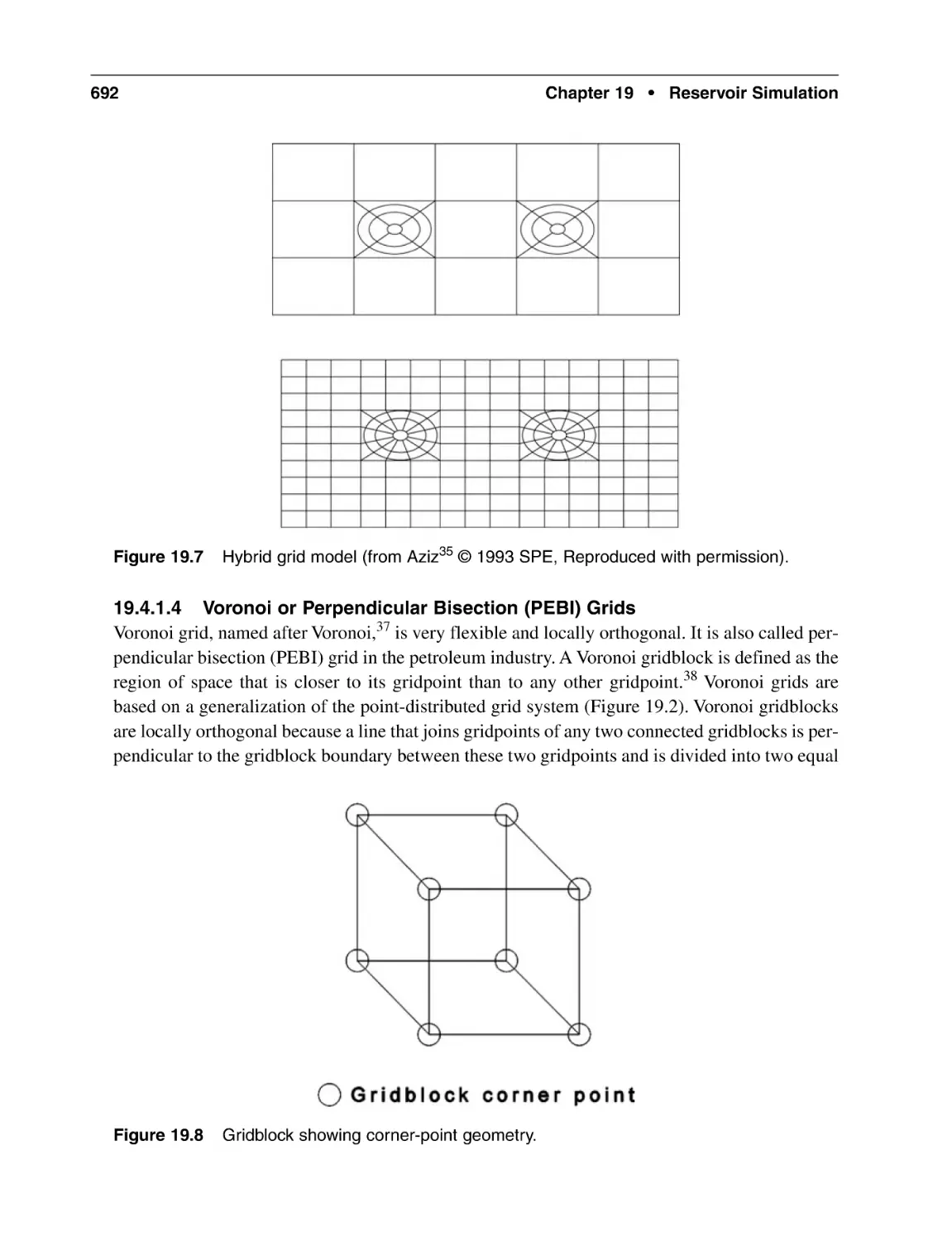
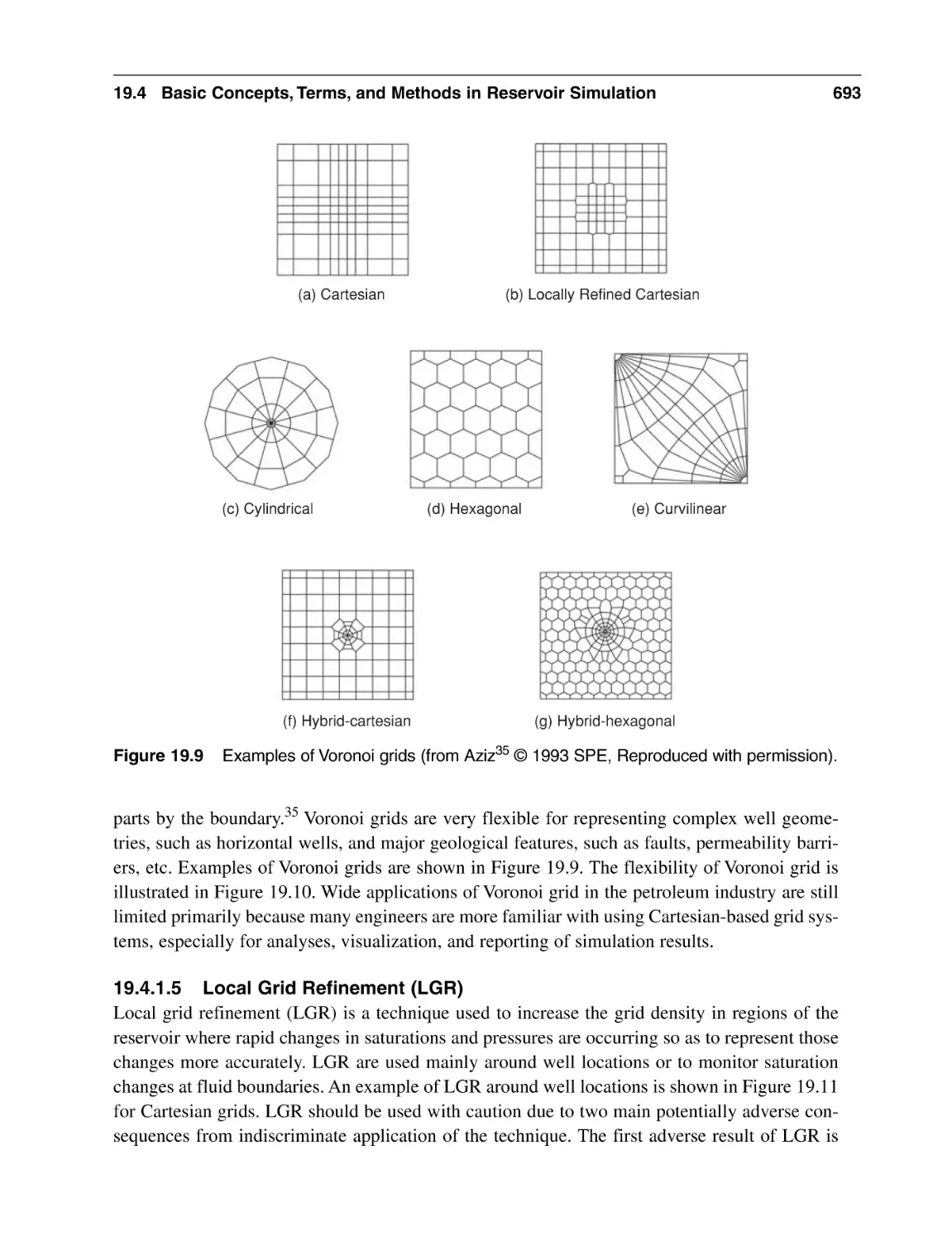
19.4.1 Grid Systems
19.4.2 Timesteps
19.4.3 Formulations of Simulator Equations
19.4.4 Material Balance Errors and Other
Convergence Criteria
19.4.5 Numerical Dispersion
19.4.6 Well Model
19.4.7 Model Initialization
19.4.8 History Matching
19.4.9 Predictions
19.4.10 Uncertainty Analysis
19.5 General Structure of Flow Reservoir Models
19.5.1 Definition of Model and Simulator
19.5.2 Geologic Model Data
19.5.3 Fluid Properties Data
19.5.4 Rock/Fluid Properties Data
19.5.5 Model Equilibration Data
19.5.6 Well Data
19.5.7 Simulator Data Output
681
681
684
686
689
689
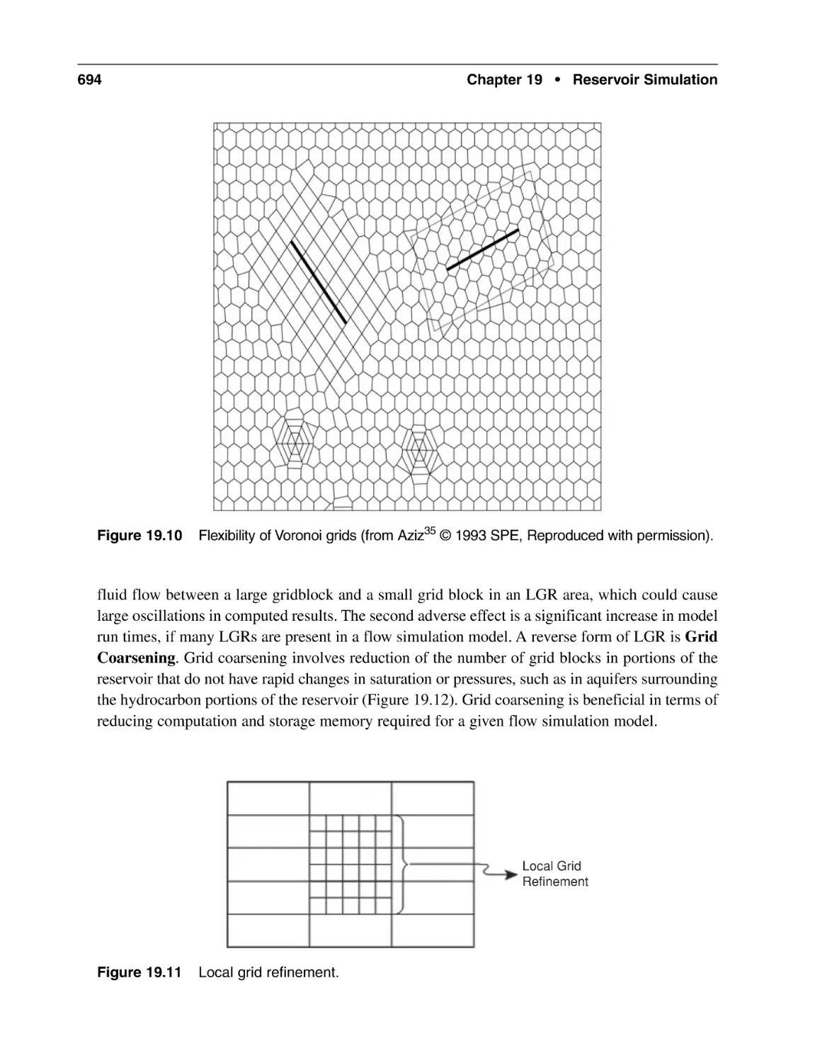
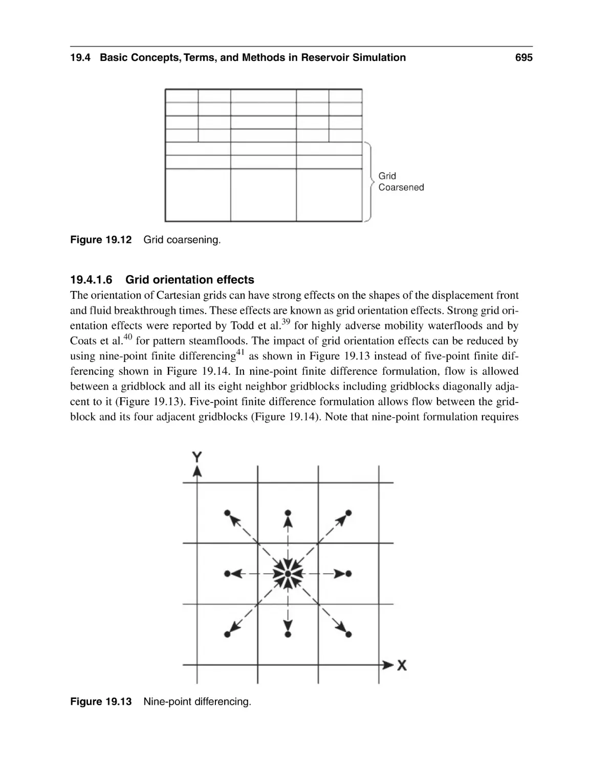
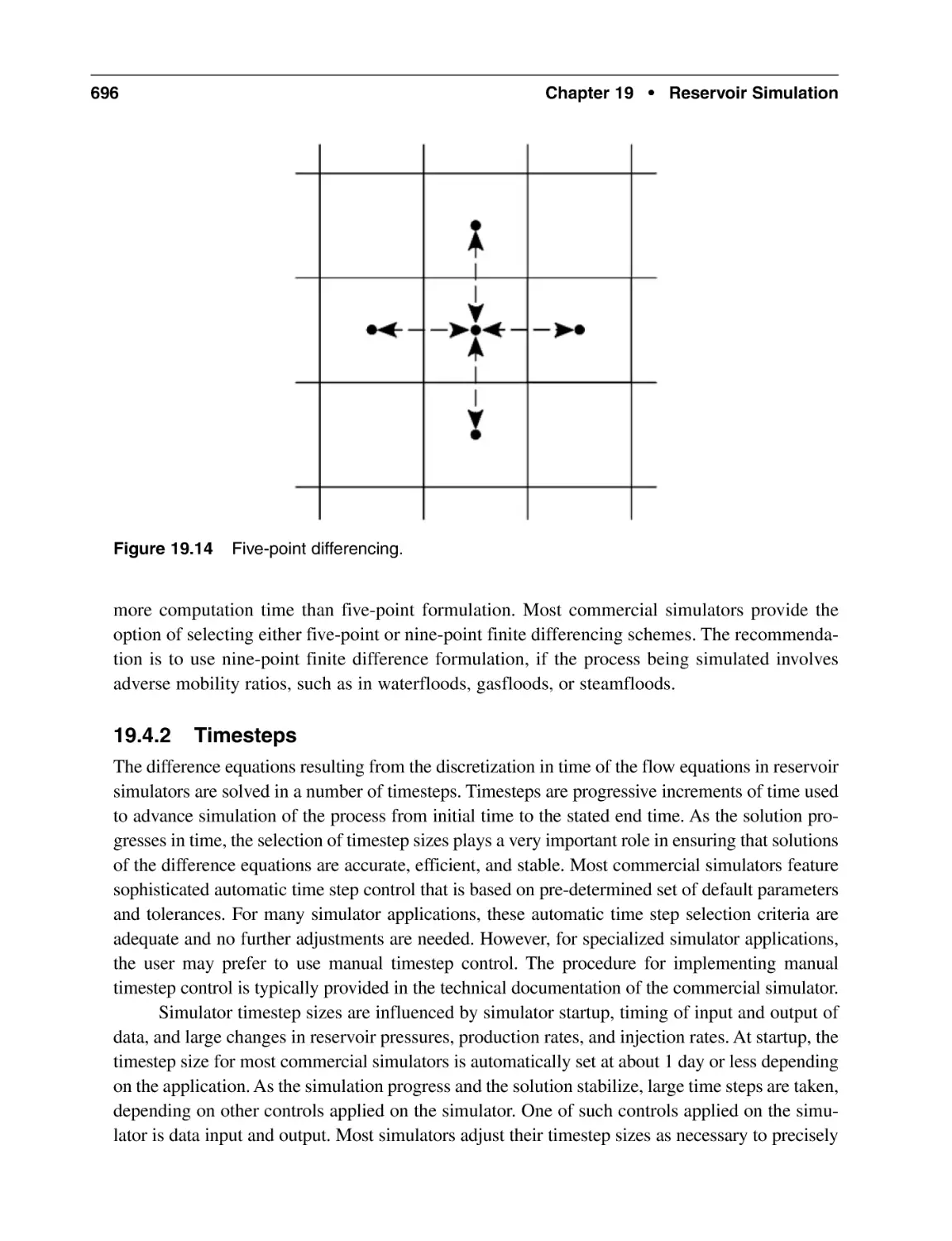
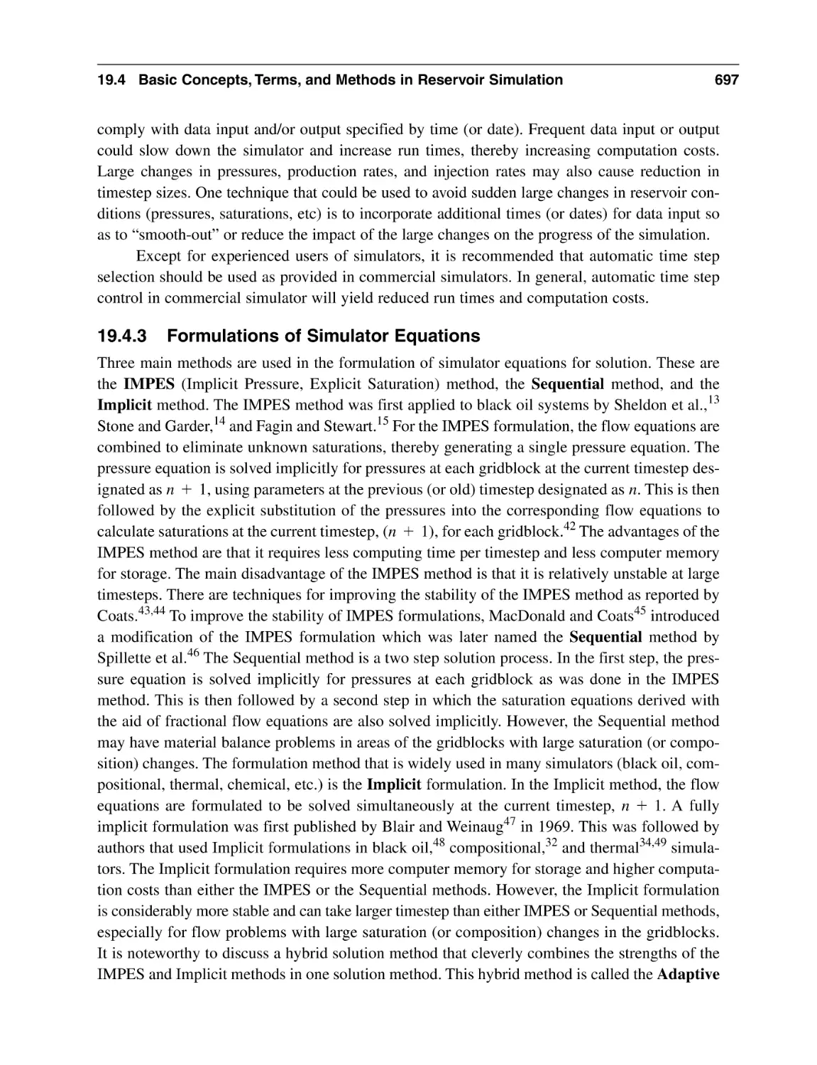
696
697
645
645
646
646
646
647
658
660
676
676
677
678
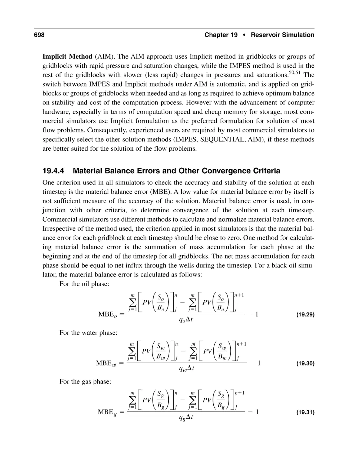
698
699
700
702
703
705
705
706
706
707
707
707
707
707
708
xxii
Contents
Nomenclature
Subscripts
Abbreviations
References
General Reading
Chapter 20 Reservoir Management
20.1 Introduction
20.2 Reservoir Management Principles
20.2.1 Conservation of Reservoir Energy
20.2.2 Early Implementation of Simple, Proven Strategies
20.2.3 Systematic and Sustained Practice of Data Collection
20.2.4 Application of Emerging Technologies for Improved
Hydrocarbon Recovery
20.2.5 Long Term Retention of Staff in Multi-Disciplinary Teams
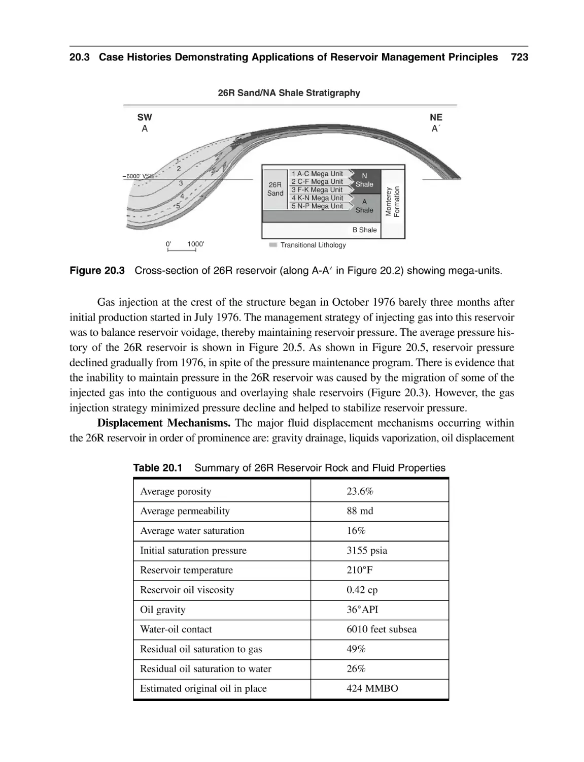
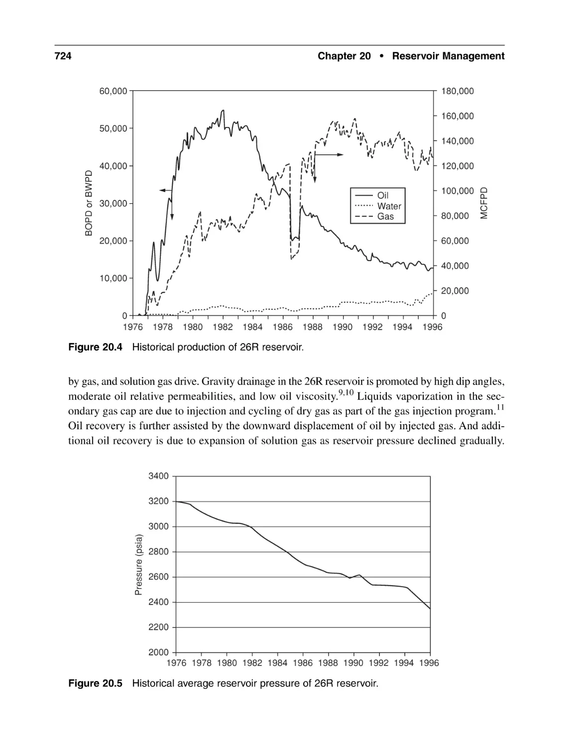
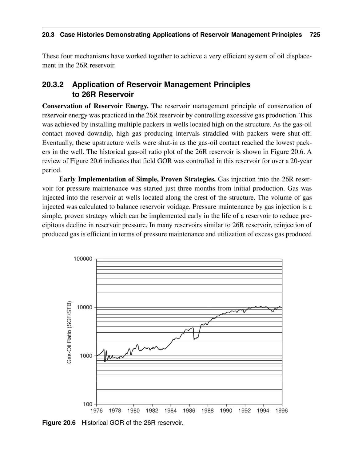
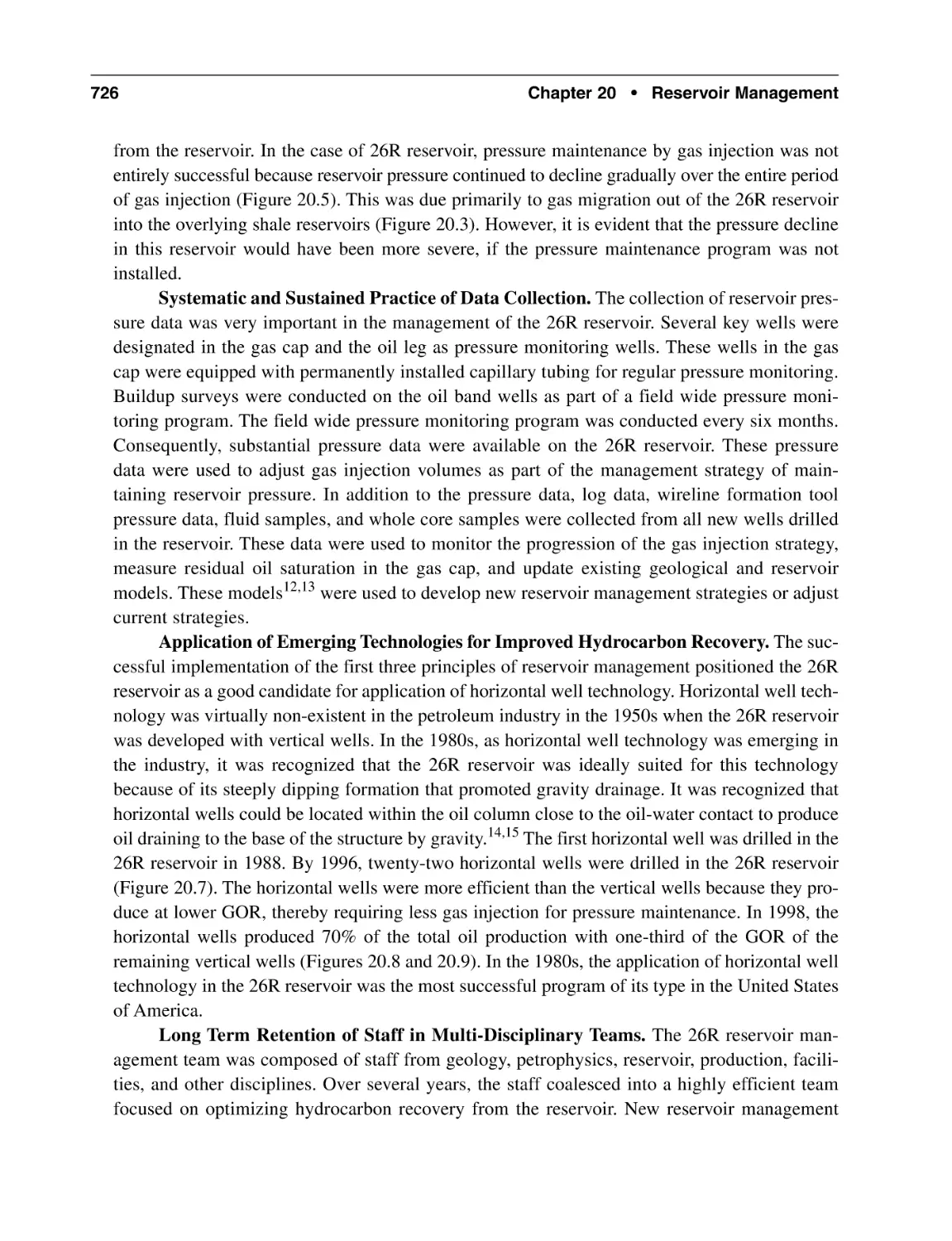
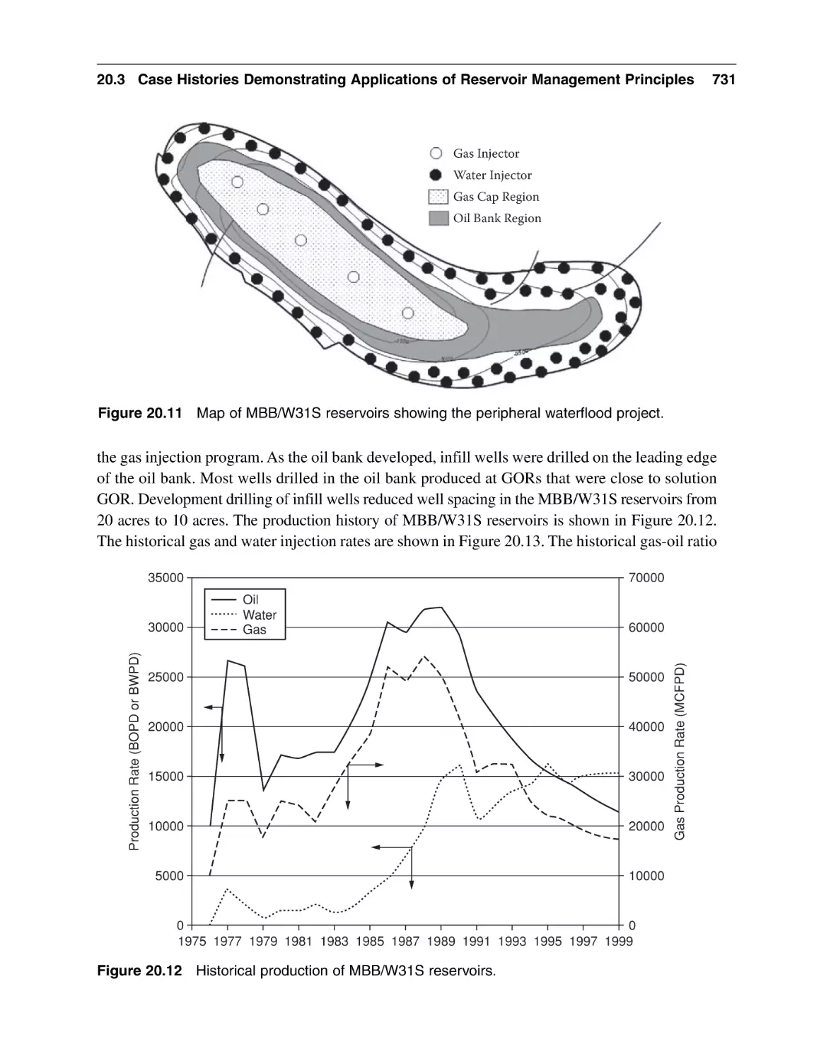
20.3 Case Histories Demonstrating Applications of Reservoir
Management Principles
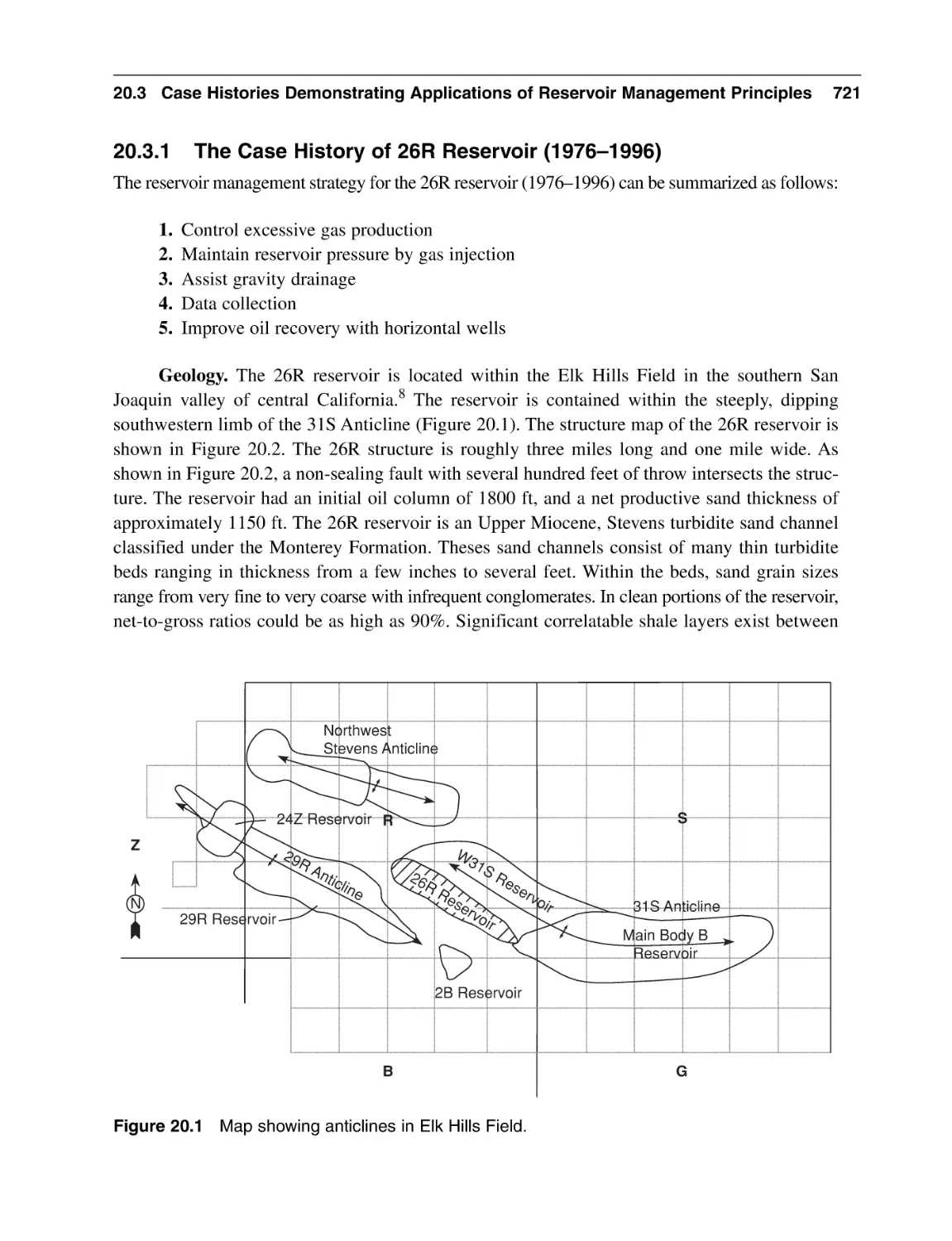
20.3.1 The Case History of 26R Reservoir (1976–1996)
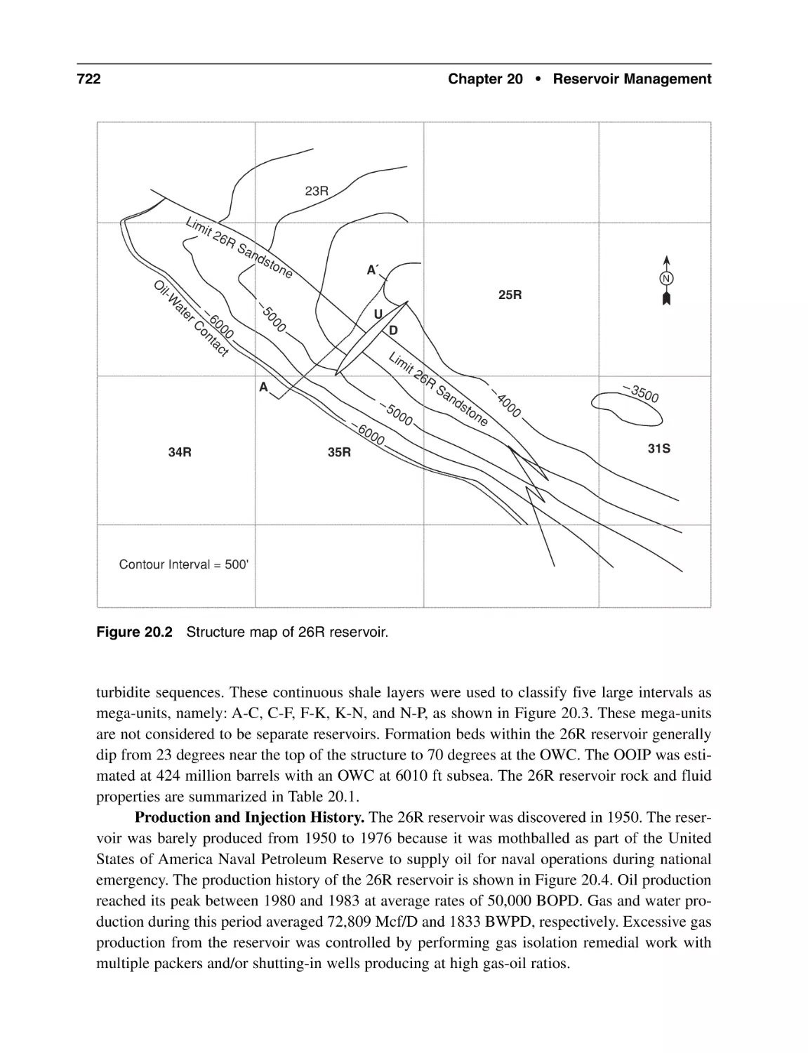
20.3.2 Application of Reservoir Management Principles
to 26R Reservoir
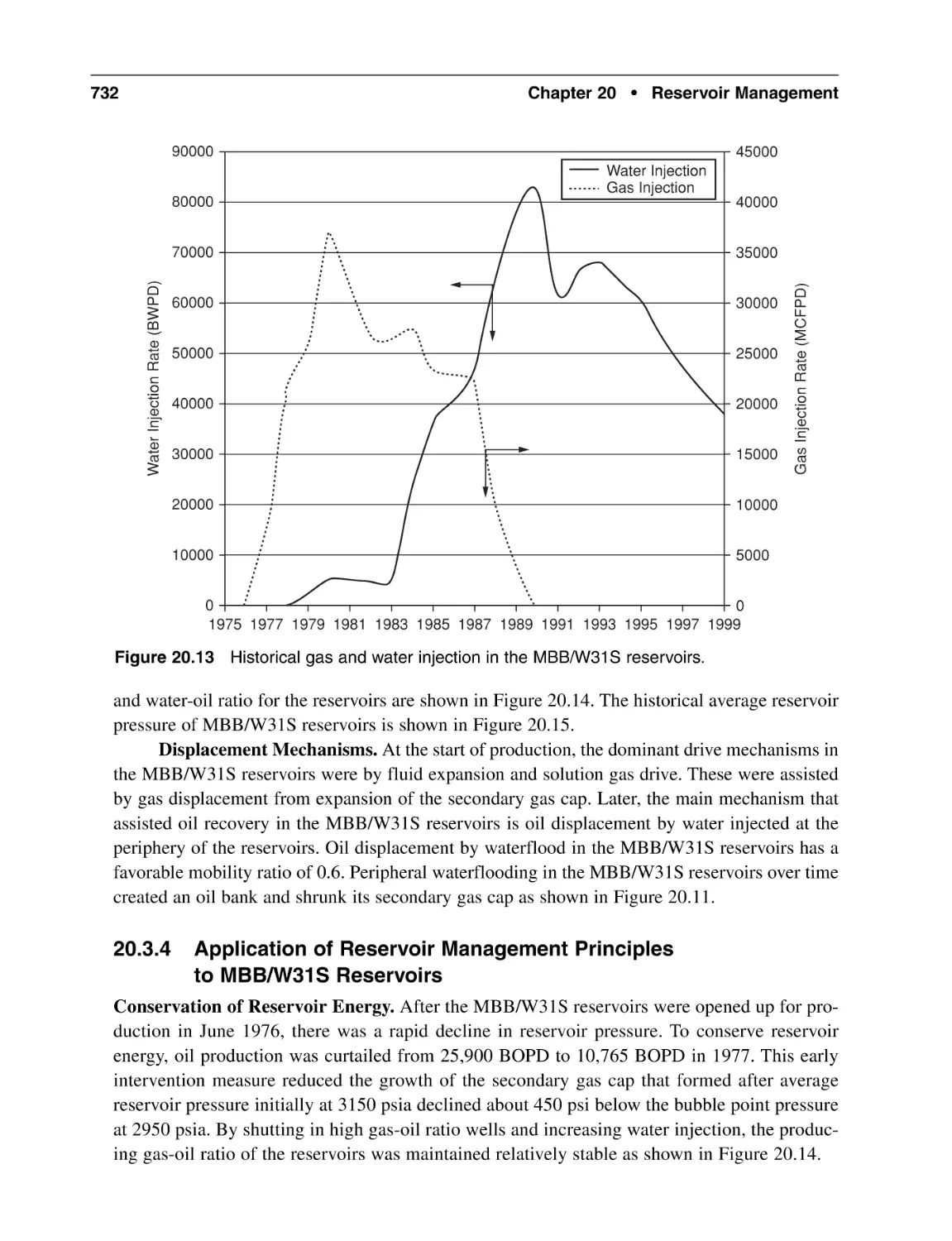
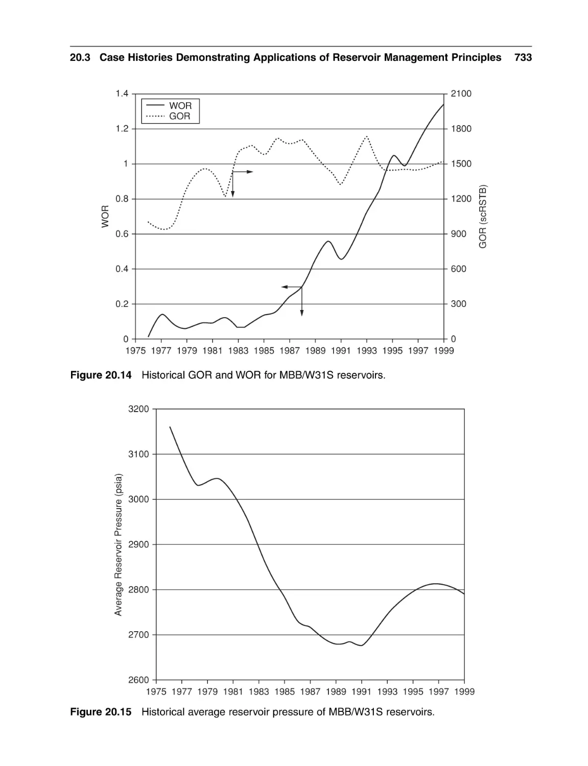
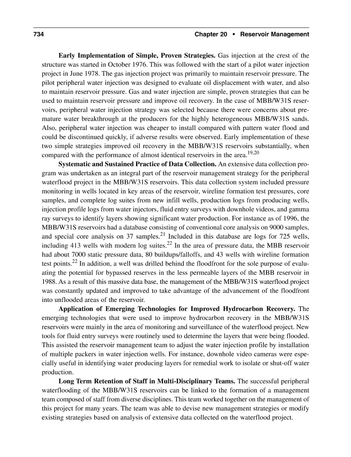
20.3.3 The Case History of MBB/W31S Reservoirs (1976–1999)
20.3.4 Application of Reservoir Management Principles
to MBB/W31S Reservoirs
20.3.5 The Case History of the Shaybah Field
20.3.6 Application of Reservoir Management Principles
to the Shaybah Field
References
General Reading
Index
708
709
709
710
714
717
717
718
719
719
719
720
720
720
721
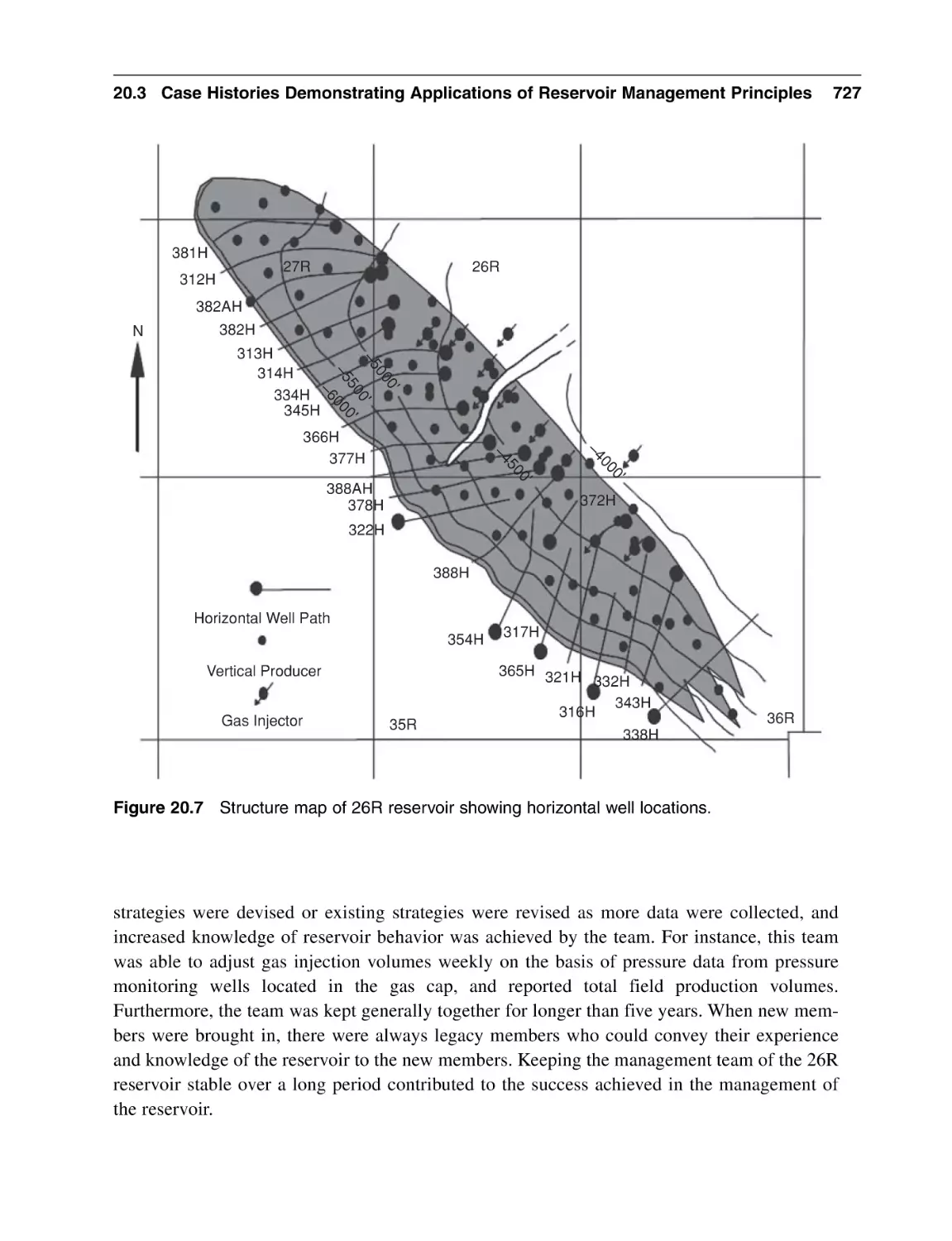
725
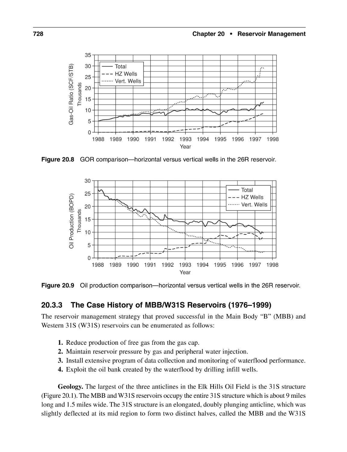
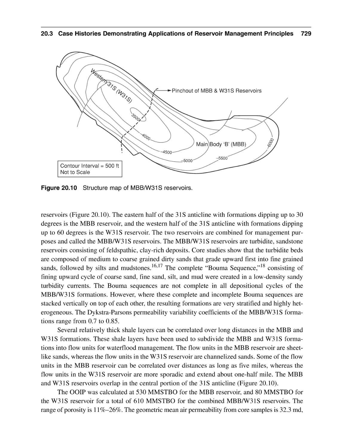
728
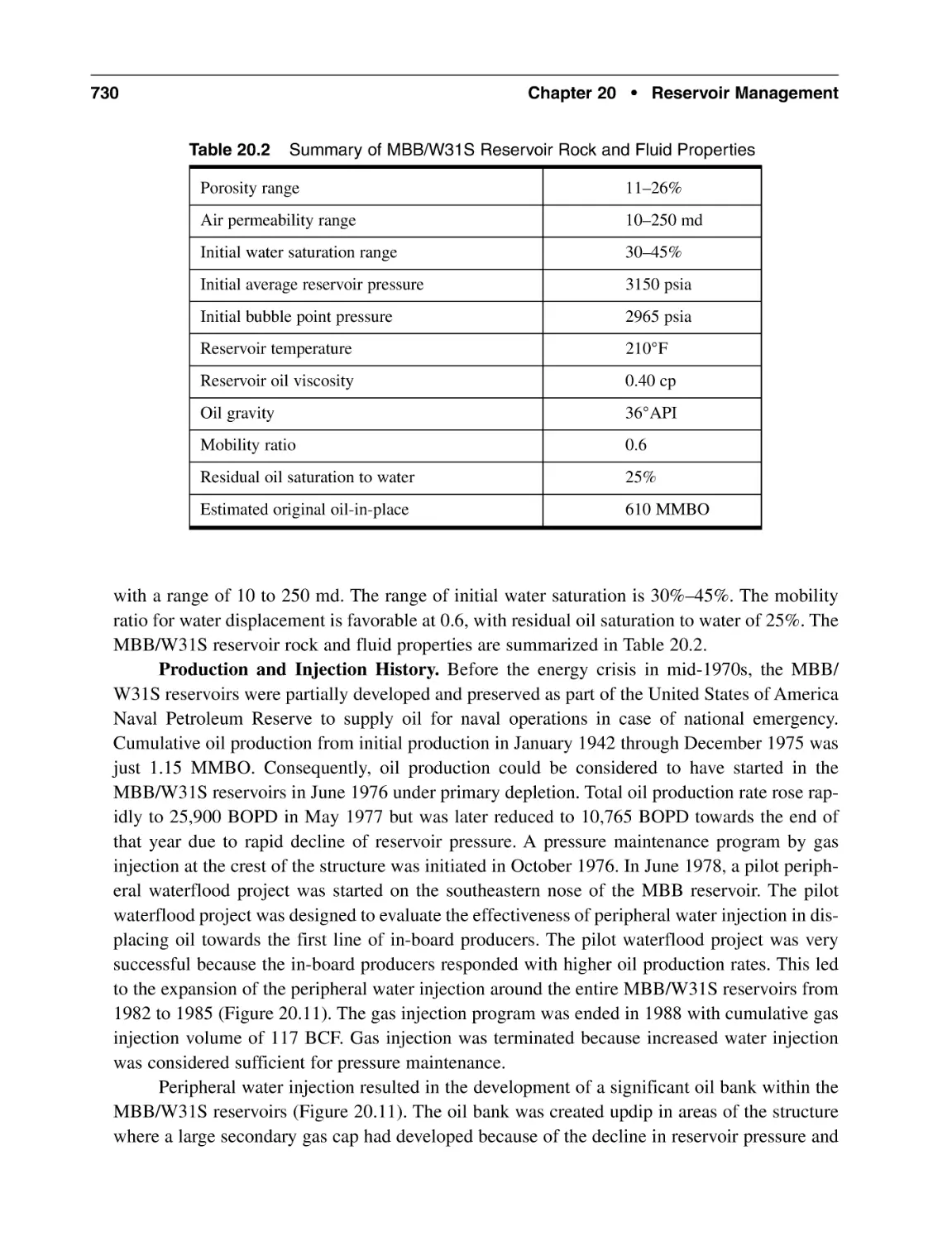
732
735
736
741
744
745
Preface
In writing any book, there is always a conflict in deciding the topics to include and the ones to
leave out. Of course there is the desire to present as many topics as possible, but that is not practical due to limitations on the physical size of the book. The scope and organization of this book
were conceived to cover petroleum reservoir engineering topics which will provide strong fundamentals to an engineer-in-training in a classroom setting, and at the same time be useful as a handbook to a practicing engineer.
Chapters 1 to 5 are devoted to discussing the sources and applications of basic rock and fluid
properties data which are the bedrock for all petroleum reservoir engineering calculations. In
Chapter 1, the porosity of reservoir rocks are presented. Chapter 2 discusses rock permeability and
relative permeability, and Chapter 3 discusses determination of fluid saturations and classification
of formation intervals of reservoir rocks. These chapters treat these topics at the introductory to
intermediate levels. They are designed to emphasize the importance of these types of data as basic
input for reservoir engineering calculations. Correlations and methods for calculation of PVT data
for reservoir fluids are presented in Chapter 4. Chapter 5 discusses reservoir fluid sampling methods and laboratory measurements of PVT data on reservoir fluid samples. Chapter 6 presents the
prediction of PVT properties with equations of state. This topic is presented at the intermediate-toadvance level because many engineers conduct compositional reservoir simulation work which
requires equations of state in most cases.
Basic reservoir engineering fundamentals are covered in Chapters 7 to 9. In Chapter 7, the
general material balance equation is presented as a fundamental tool which could be used for basic
reservoir analysis. Chapter 8 discusses different types of gas reservoirs and calculation of gas-inplace volumes with volumetric and graphical methods. Similar treatment of oil reservoirs are presented in Chapter 9. Case histories of gas and oil reservoirs are presented in Chapters 8 and 9 for
discussion and review purposes. I consider the use of case histories as more realistic examples and
effective tools for teaching of reservoir engineering fundamentals and practices than sanitized
problems included in many traditional petroleum engineering textbooks. Most real-life reservoir engineering problems are usually not encountered in these neatly encapsulated problem formats. For
these reasons, I have not presented end-of-chapter problems in this book. Instead, teachers are encouraged to use case histories as effective vehicles for teaching fundamental reservoir engineering
principles to students.
An introduction to fluid flow in petroleum reservoirs is presented in Chapter 10 with the
derivation of the continuity equation and the radial diffusivity equation. This chapter lays the
xxiii
xxiv
Preface
foundation for the fundamental equations used in the development of well test analysis by straightline methods presented in Chapter 11. In Chapter 12, the application of type curves, especially
Gringarten and Bourdet type curves, are presented with emphasis on procedures for type-curve
matching. The importance of hydraulically fractured wells and naturally fractured reservoirs in
the production of many reservoirs around the world is recognized by the presentation of well test
analysis methods for these well and reservoir types in Chapter 13. Chapter 14 presents deconvolution in a rather rudimentary form to acquaint the reader with this method for well test analysis.
The book introduces basic concepts in immiscible fluid displacement in Chapter 15, including the derivation of the fractional flow equation, the Buckley-Leverett equation, and the Welge
method. This lays the foundation for the introduction of secondary recovery methods in Chapter 16. In
Chapter 17, enhanced oil recovery methods are presented. Special emphasis is placed on screening criteria and field implementation of enhanced oil recovery processes. The main purpose of
Chapters 16 and 17 is to introduce the engineer to the fundamentals of secondary and enhanced oil
recovery processes, and also provide practical procedures for field implementation of these processes.
The availability of high speed computers has placed very powerful engineering tools in the
hands of modern petroleum engineers. These tools are readily available in applications of geologic
modeling, reservoir characterization, and reservoir simulation. Every practicing engineer has been
exposed to these tools in the form of commercial software readily available in the petroleum industry. In this book, I present introductory fundamentals on geologic modeling, reservoir characterization, and reservoir simulation in Chapters 18 and 19. On these topics, considerable emphasis
is placed on procedures for using these tools rather than an in-depth presentation of the theoretical
basis of the methods.
Finally in Chapter 20, I present fundamental principles of petroleum reservoir management
based on my experience. These principles are simple, practical, and can be applied in the management of reservoirs around the world. I encourage readers of this book to adopt these principles to
review current reservoir management strategies and in the implementation of new strategies in the
management of old and new reservoirs.
This book came into form with encouragement from Mr. Stuart Filler, who read the early
drafts of many chapters and gave me many useful suggestions. I thank him for his advice and encouragement that compelled me to continue work on the book. I also give thanks to my publisher,
Mr. Bernard Goodwin, for his unwavering support that made this book possible. Finally, I express
special thanks to my wife, Anulika, and my children (Nkem, Emeka, Chioma, Ifeoma, Obinna,
and Eze) for their patience, comfort, and the emotional support they provided to me during the
long hours and many years it took to write this book. This book would not have been completed
without their love and support.
Acknowledgments
The author gratefully thanks the Society of Petroleum Engineers for permissions to reprint the following tables and figures in this text:
Chapter 1
Figure 1.1
Al-Ruwaili, S. A., and Al-Waheed, H. H.: “Improved Petrophysical Methods and Techniques for
Shaly Sands Evaluation,” paper SPE 89735 presented at the 2004 SPE International Petroleum Conference in Puebla, Mexico, November 8–9, 2004.
Chapter 3
Figure 3.4
Worthington, P.F., and Cosentino, L.: “The Role of Cutoffs in Integrated Reservoir Studies,”
SPEREE (August 2005) 276–290.
Chapter 4
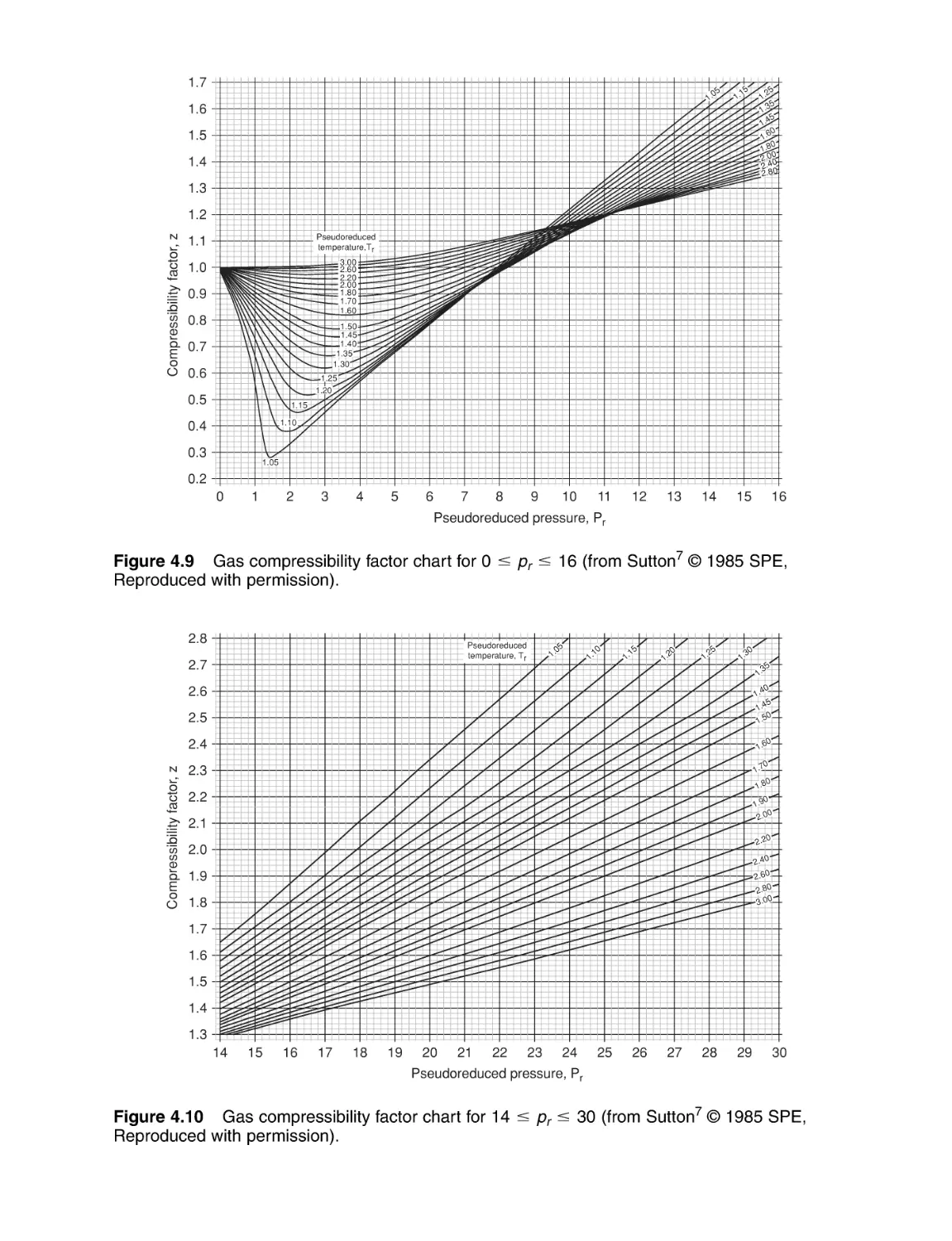
Figures 4.9, 4.10
Sutton, R.P.: “Compressibility Factors for High-Molecular-Weight Reservoir Gases,” paper SPE
14265 presented at the 60th Annual Technical Conference and Exhibition, Las Vegas, NV
(Sept. 22–25, 1985).
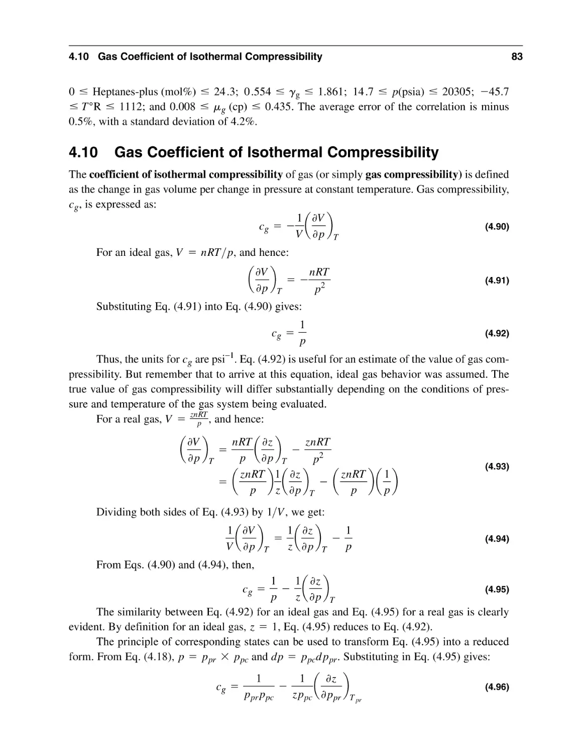
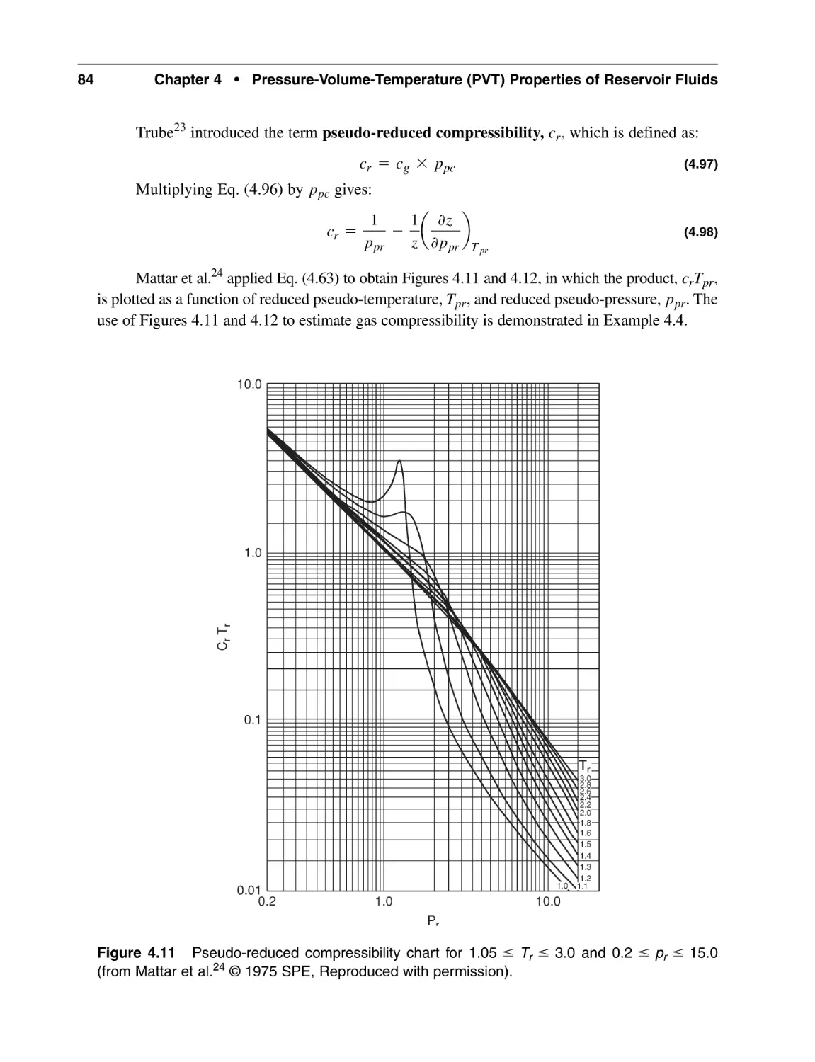
Figures 4.11, 4.12
Mattar, L., Brar, G.S., and Aziz, K.: “Compressibility of Natural Gases,” J. Cdn. Pet. Tech. (OctDec. 1975) 77–80.
Chapter 5
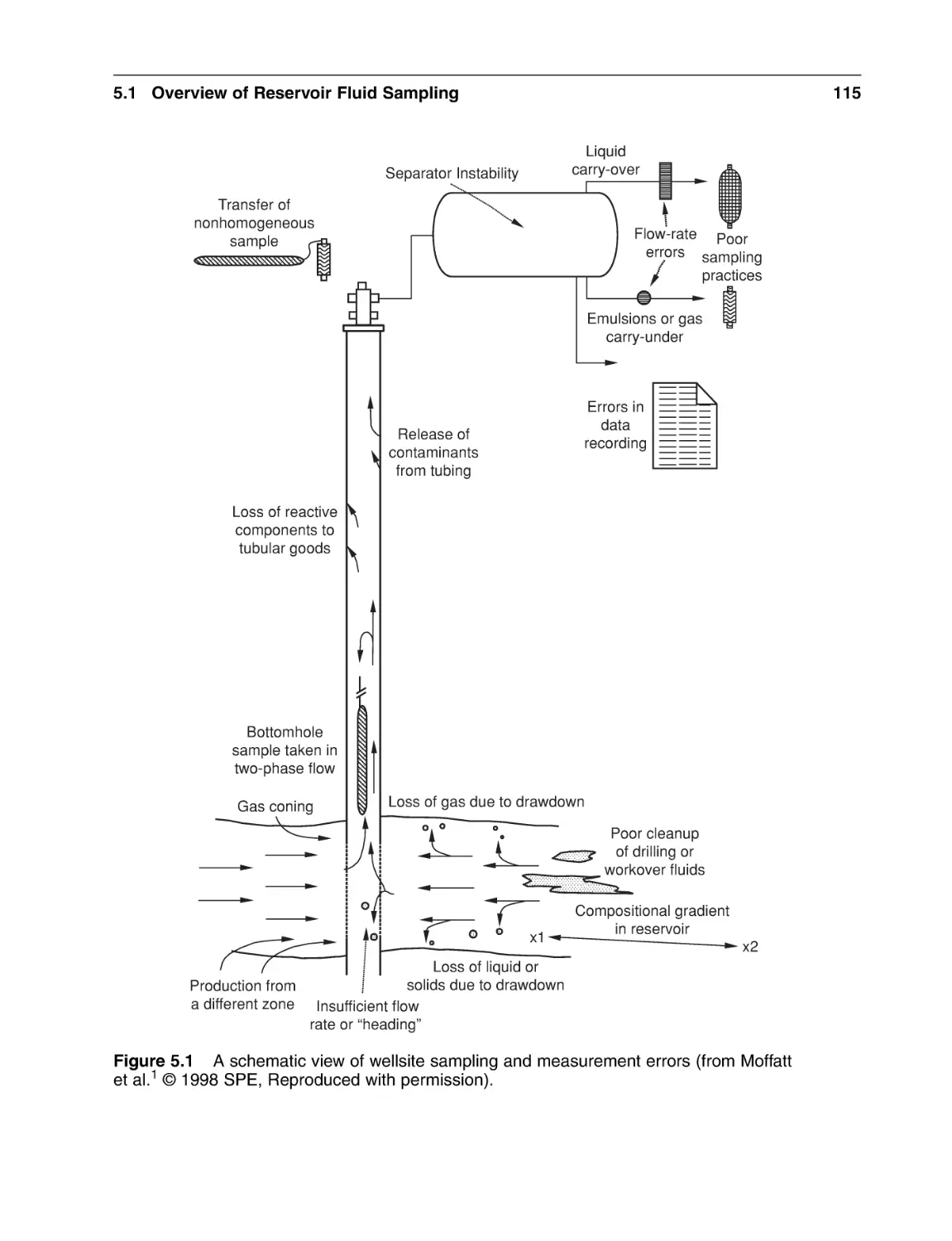
Figure 5.1
Moffatt, B.J. and Williams, J.M.: “Identifying and Meeting the Key Needs for Reservoir Fluid
Properties—A Multi-Disciplinary Approach,” paper SPE 49067 presented at the 1998 SPE
Annual Technical Conference and Exhibition, New Orleans, Louisiana, Sept. 27–30, 1998.
xxv
xxvi
Acknowledgments
Figures 5.4, 5.5, 5.6, 5.7, 5.9
Elshahawi, H., Samir, M., and Fathy, K.: “Correcting for Wettability and Capillary Pressure
Effects on Formation Tester Measurements,” paper SPE 63075 presented at the 2000 SPE
Annual Technical Conference and Exhibition, Dallas, Texas, Oct. 1–4, 2000.
Chapter 6
Tables 6.1, 6.2
Jhaveri, B.S., and Youngren, G.K.: “Three-Parameter Modification of the Peng-Robinson Equation of State to Improve Volumetric Predictions,” SPERE (August 1988) 1033–1040.
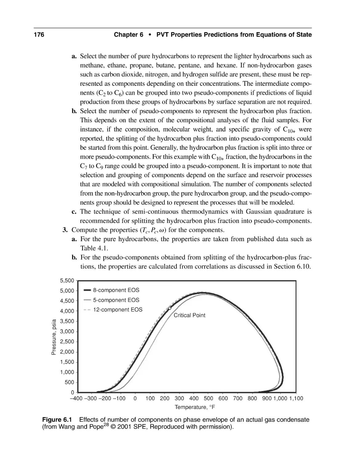
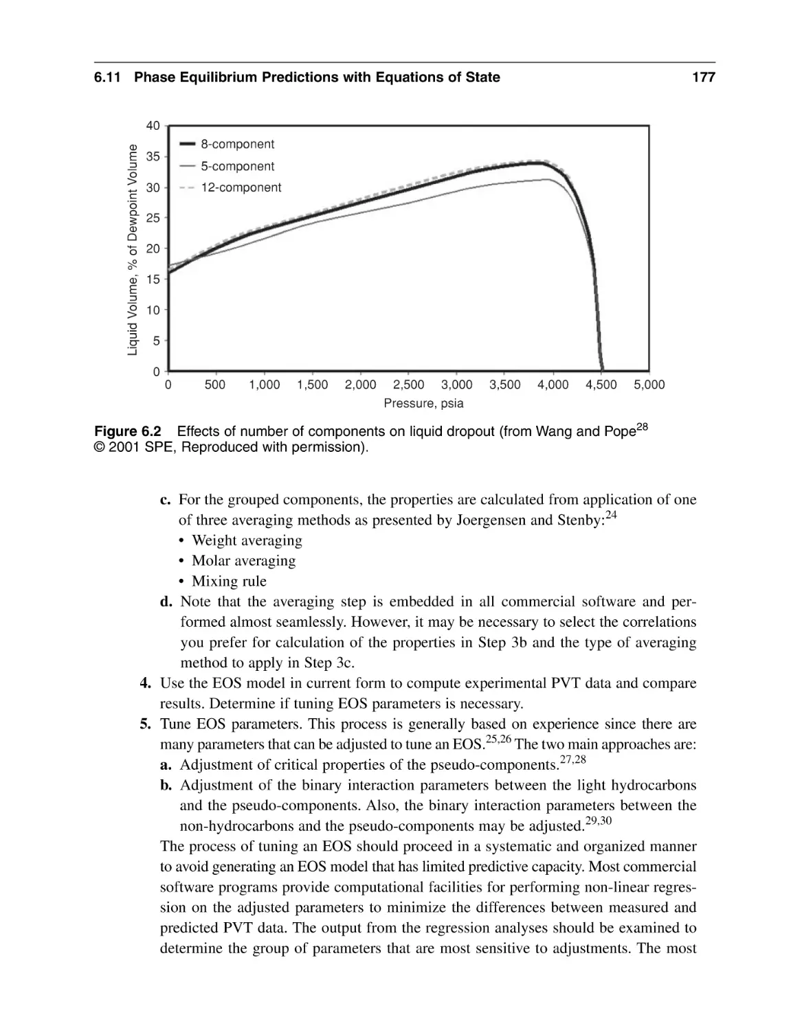
Figures 6.1, 6.2
Wang, P., and Pope, G.A.: “Proper Use of Equations of State for Compositional Reservoir Simulation,” SPE 69071, Distinguished Author Series, (July 2001) 74–81.
Chapter 8
Figure 8.4
Havlena, D., and Odeh, A.S.: “The Material Balance as an Equation of a Straight Line,” JPT (August
1963) 896–900.
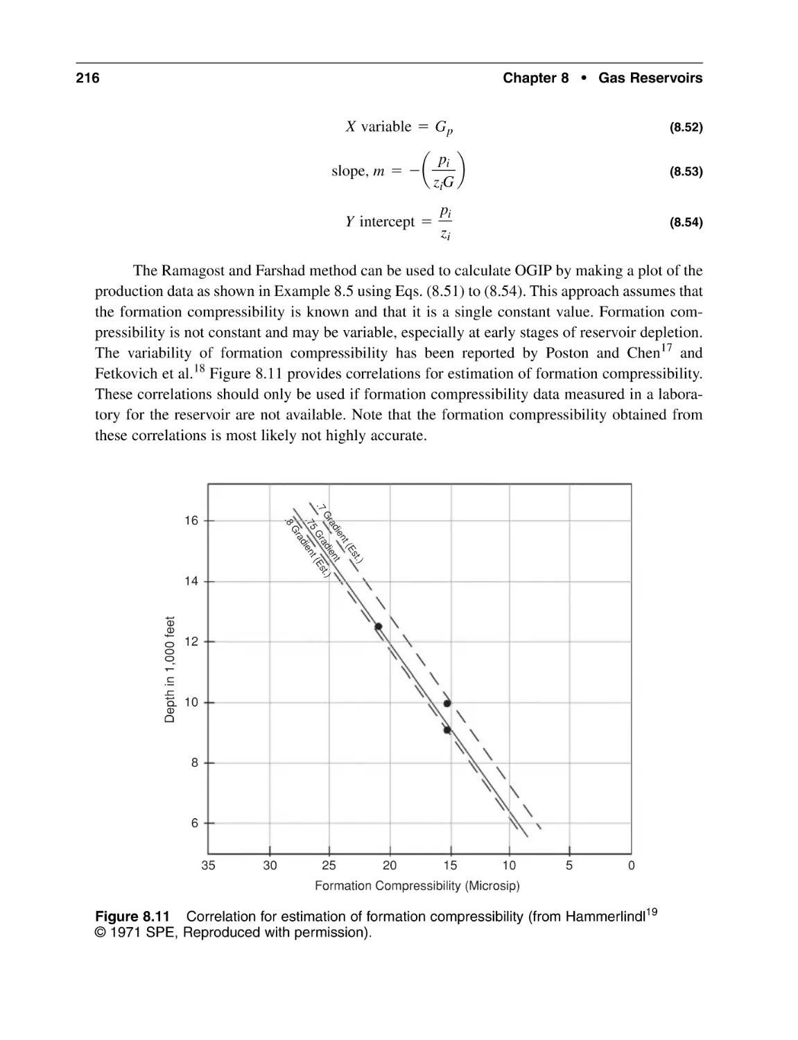
Figure 8.11
Hammerlindl, D.J.: “Predicting Gas Reserves in Abnormally Pressured Reservoirs,” paper SPE
3479 presented at the 1971 SPE Fall Meeting, New Orleans, October 3–5, 1971.
Chapter 9
Figures 9.1, 9.4, 9.5
Havlena, D., and Odeh, A.S.: “The Material Balance as an Equation of a Straight Line,” JPT
(August 1963) 896–900.
Chapter 10
Appendices 10B, 10C, 10D, 10E, 10F
van Everdingen, A.F., and Hurst, W.: “The Application of the Laplace Transformation to Flow
Problems in Reservoirs,” Trans., AIME (1949) 186, 305–324.
Chapter 11
Table 11.2
Tiab, D., Ispas, I.N., Mongi, A., and Berkat, A.: “Interpretation of Multirate Tests by the Pressure
Derivative. 1. Oil Reservoirs,” Paper SPE 53935 presented at the 1999 SPE Latin American
and Caribbean Petroleum Engineering Conference, Caracas, Venezuela, April 21–23, 1999.
Acknowledgments
xxvii
Chapter 12
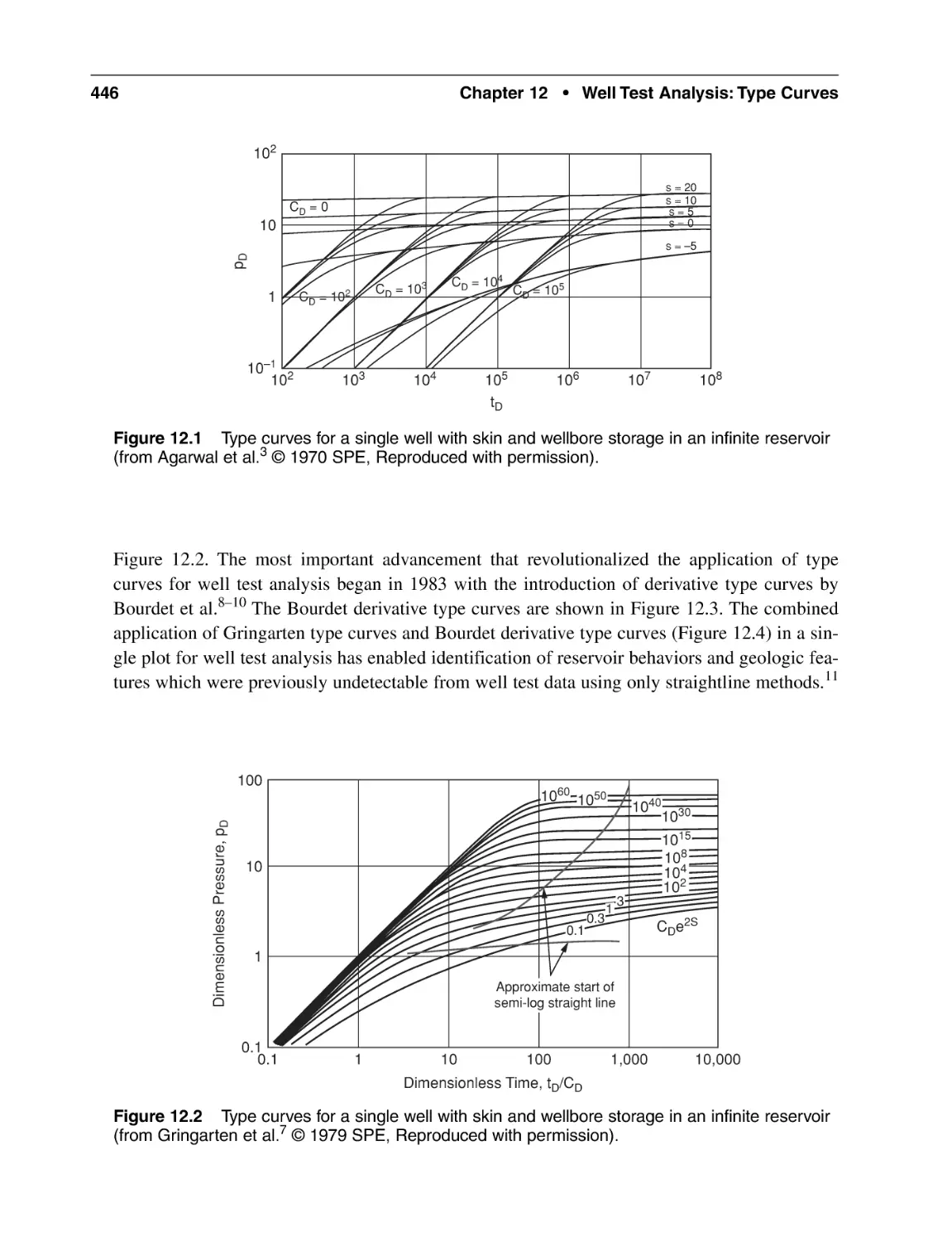
Figure 12.1
Agarwal, R.G., Al-Hussainy, R., and Ramey, H.J., Jr.: “An Investigation of Wellbore Storage and Skin
Effect in Unsteady Liquid Flow: I. Analytical Treatment,” SPEJ (September 1970) 279–290.
Figure 12.2
Gringarten, A.C., Bourdet, D.P., Landel, P.A., and Kniazeff, V.J.: “A Comparison Between Different Skin and Wellbore Storage Type-Curves for Early-Time Transient Analysis,” Paper SPE
8205 presented at the SPE Annual Technical Conference and Exhibition, Las Vegas, Nevada,
September 23–26, 1979.
Chapter 13
Figures 13.1, 13.3, 13.4, 13.5, 13.6, 13.7
Cinco-Ley, H., and Samaniego-V, F.: “Transient Pressure Analysis for Fractured Wells,” JPT,
(September 1981) 1749–1766.
Figures 13.8, 13.9, 13.11
Cinco, H.: “Evaluation of Hydraulic Fracturing By Transient Pressure Analysis Methods,” paper
SPE 10043 presented at the International Petroleum Exhibition and Technical Symposium,
Beijing, China, March 18–26, 1982.
Figure 13.10
Cinco-L, H., Samaniego-V, F., and Dominguez-A, N.: “Transient Pressure Behavior for a Well
With a Finite-Conductivity Vertical Fracture,” SPEJ (August 1978) 253–264.
Figures 13.16, 13.17a, 13.17b, 13.18, 13.19a, 13.19b, 13.20, 13.21, 13.22, 13.23,
13.24, 13.25
Cinco-Ley, H.: Well-Test Analysis for Naturally Fractured Reservoirs,” JPT (January 1996) 51–54.
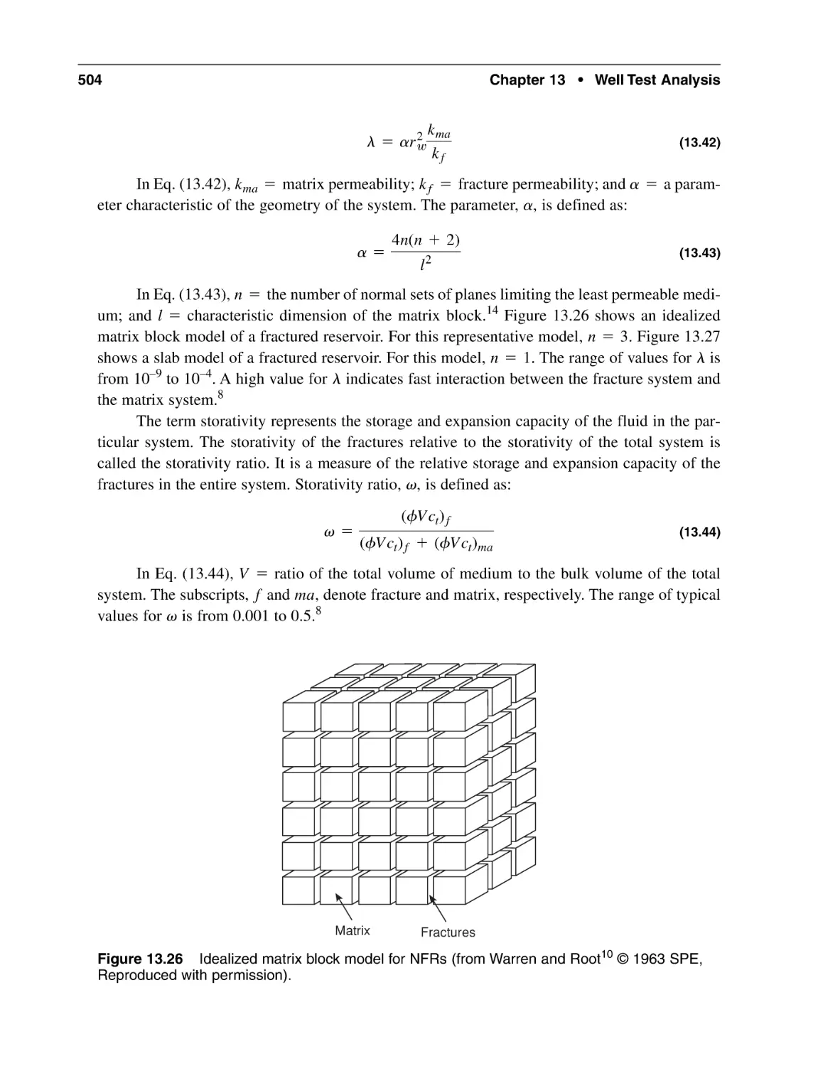
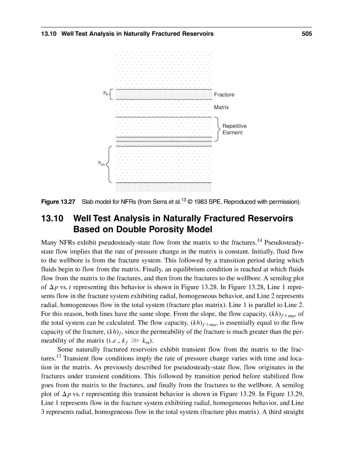
Figure 13.26
Warren, J.E., and Root, P.J.: “The Behavior of Naturally Fractured Reservoirs,” SPEJ (September
1963) 245–255.
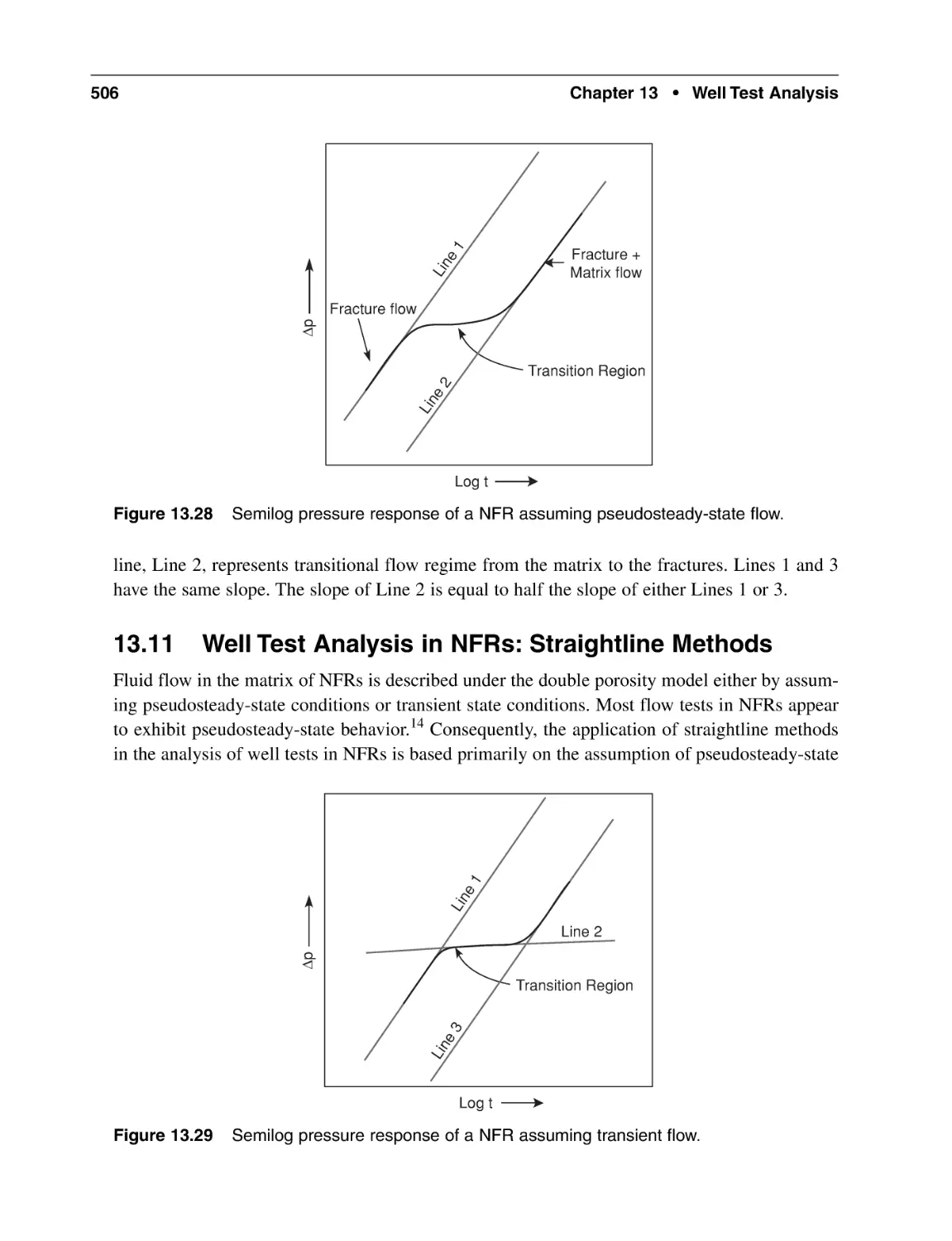
Figure 13.27
Serra, K., Reynolds, A.C., and Raghavan, R.: “New Pressure Transient Analysis Methods for Naturally
Fractured Reservoirs,” JPT (December 1983) 2271–2283.
Figure 13.32, 13.33, 13.34
Gringarten, A.C.: “Interpretation of Tests in Fissured and Multilayered Reservoirs with DoublePorosity Behavior: Theory and Practice,” JPT (April 1984) 549–564.
xxviii
Acknowledgments
Chapter 14
Figures 14.1, 14.2, 14.3, 14.4, 14.5, 14.6, 14.7, 14.8
Levitan, M.M., Crawford, G.E., and Hardwick, A.: “Practical Considerations for Pressure-Rate
Deconvolution of Well-Test Data,” SPEJ (March 2006) 35–46.
Chapter 19
Figures 19.2, 19.7, 19.9, 19.10
Aziz, K.: “Reservoir Simulation Grids: Opportunities and Problems,” JPT (July 1993) 658–663.
Chapter 20
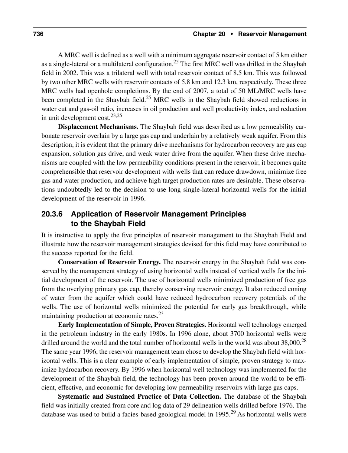
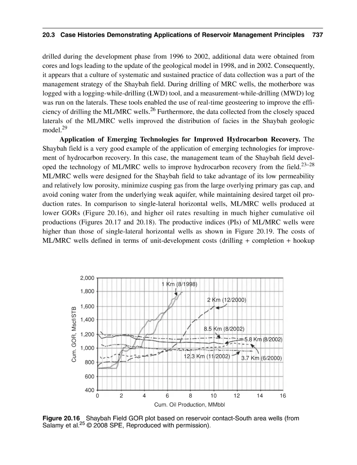
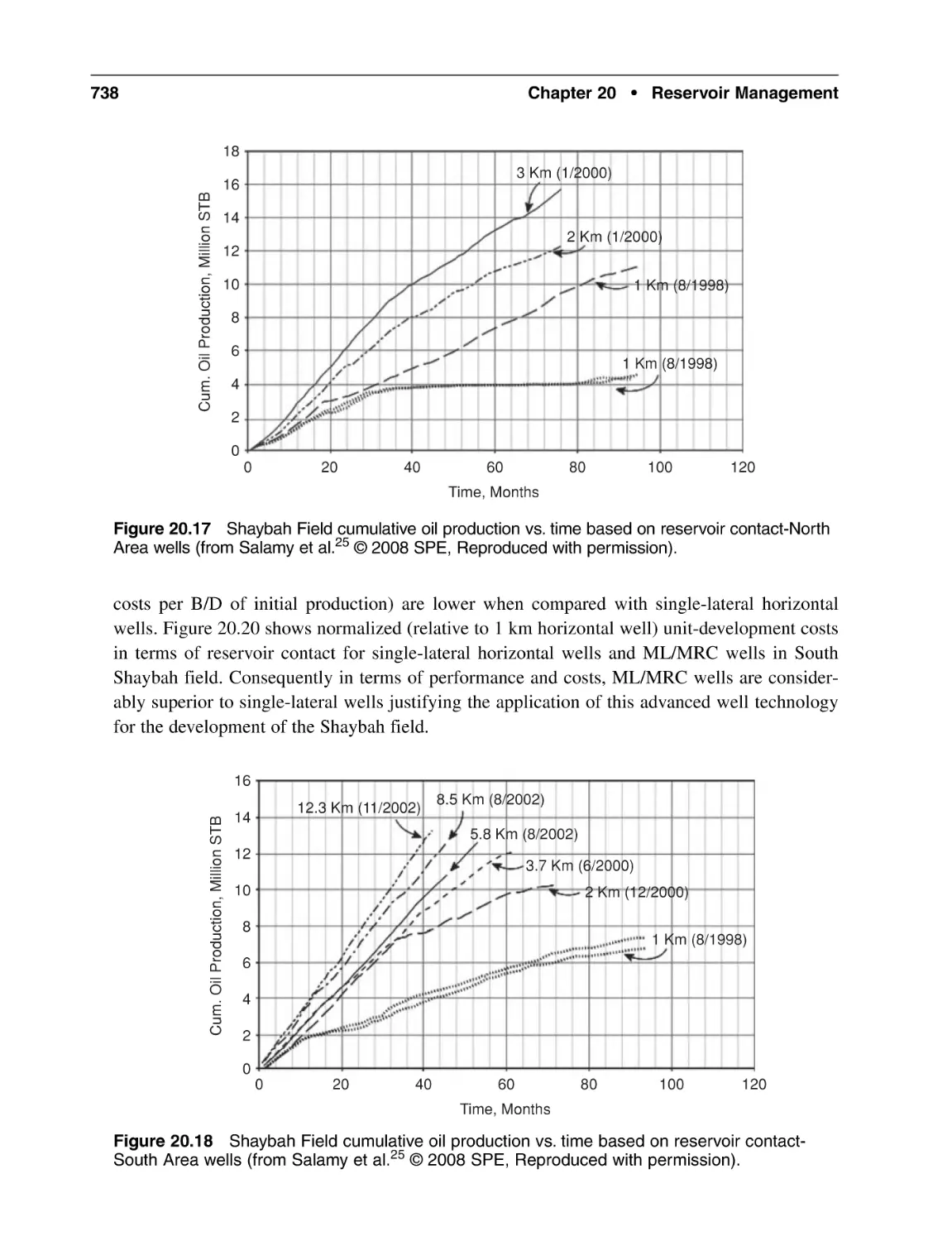
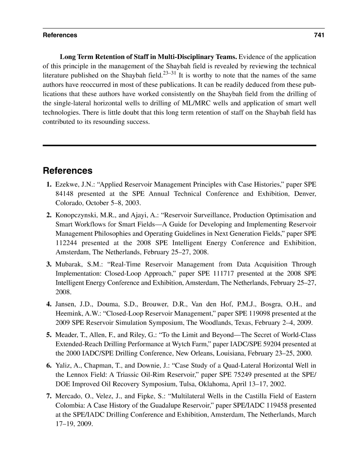
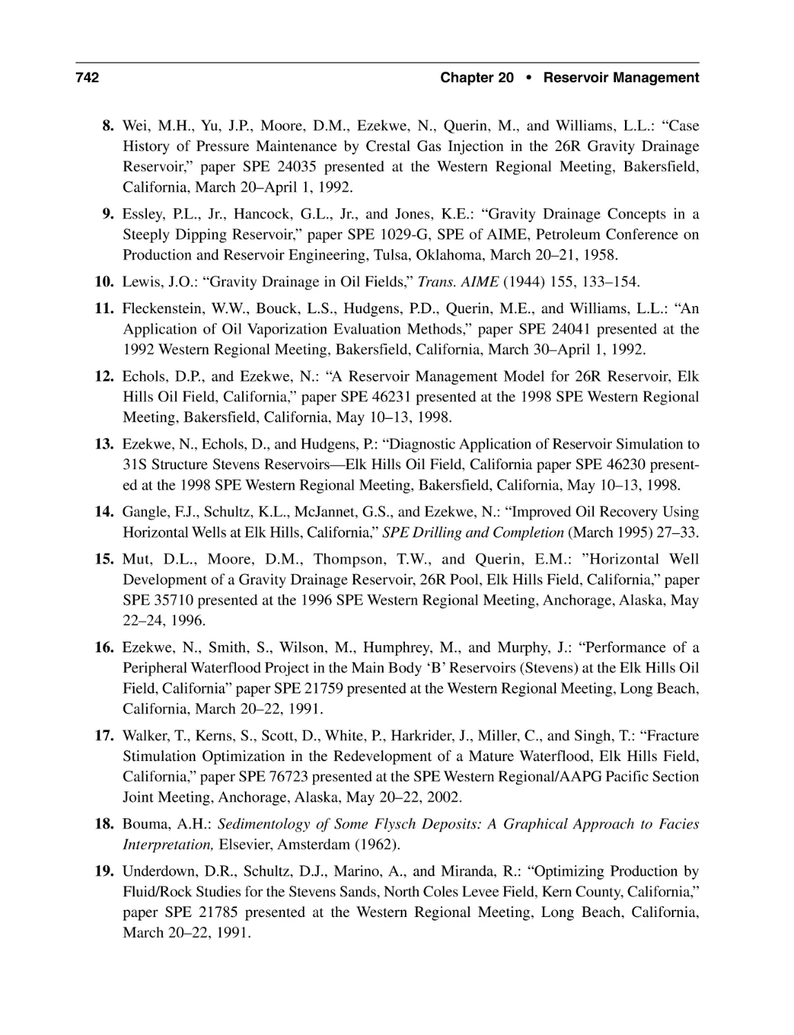
Figures 20.16, 20.17, 20.18, 20.21, 20.22
Salamy, S.P., Al-Mubarak, H.K., Ghamdi, M.S., and Hembling, D.: “Maximum-Reservoir-ContactWells Performance Update: Shaybah Field, Saudi Arabia,” SPE Production & Operation
(November 2008) 439–443.
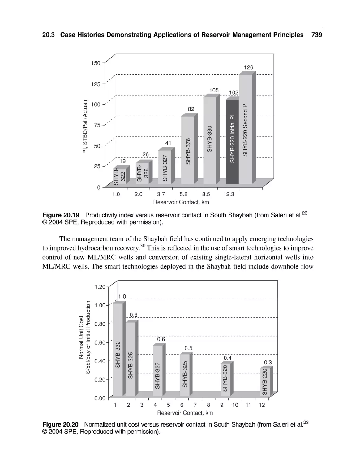
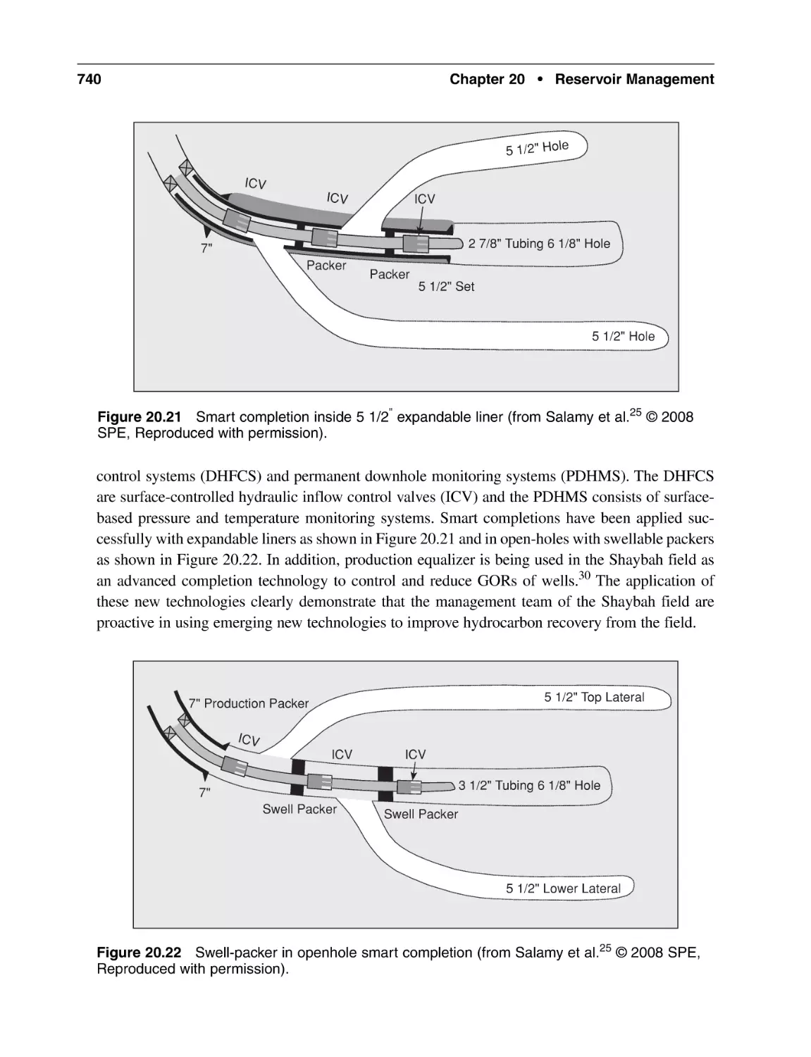
Figures 20.19, 20.20
Saleri, N.G., Salamy, S.P., Mubarak, H.K., Sadler, R.K., Dossary, A.S., and Muraikhi, A.J.: “Shaybah220: A Maximum-Reservoir-Contact (MRC) Well and its Implications for Developing TightFacies Reservoirs,” SPEREE (August 2004) 316–321.
About the Author
Nnaemeka Ezekwe holds B.S., M.S., and Ph.D. degrees in
chemical and petroleum engineering, and an MBA, all from
the University of Kansas. For many years, he worked in
several supervisory roles including manager of reservoir
evaluation and development for Bechtel Petroleum Operations. As a senior petroleum engineer advisor for Pennzoil
and later Devon Energy, he performed reservoir engineering analyses on many domestic and worldwide projects.
Nnaemeka was an SPE Distinguished Lecturer in 2004–
2005, during which he spoke on reservoir management
strategies and practices to audiences in 33 countries in Africa,
Asia, Europe, Middle East, and North and South America.
He has published numerous technical papers on chemical
and petroleum engineering topics. Nnaemeka is a registered
professional engineer in California and Texas.
xxix
This page intentionally left blank
C
H A P T E R
1
Porosity of Reservoir Rocks
1.1
Introduction
Porosity is defined as a measure of the capacity of reservoir rocks to contain or store fluids.
The fluids stored in the pore spaces within the reservoir rocks could be gas, oil, and water.
High porosity values indicate high capacities of the reservoir rocks to contain these fluids,
while low porosity values indicate the opposite. Consequently, porosity data are routinely used
qualitatively and quantitatively to assess and estimate the potential volume of hydrocarbons
contained in a reservoir. For instance, in a discovery well that shows the presence of hydrocarbons
in the reservoir rocks, the set of data that is reviewed at least qualitatively to evaluate reservoir
potential is porosity data acquired with either logging-while-drilling (LWD) tools or by running
wireline tools. Porosity data are obtained from direct measurements on core samples and/or indirectly from well logs. In most cases, porosity data from core samples are used to validate or
calibrate porosity data from well logs. Porosity data are also used in reservoir characterization
for the classification of lithological facies, and the assignment of permeabilities using porositypermeability transforms. Since porosity data are very important in many reservoir engineering
calculations, this book begins by reviewing basic concepts in the determination of rock porosities.
This review is concise and serves to refresh the reader with the many sources of porosity data
that exist through applications of different formation evaluation tools.
1.2
Total Porosity and Effective Porosity
The porosity of a rock is a measure of its capacity to contain or store fluids. Porosity is calculated as the pore volume of the rock divided by its bulk volume.
Porosity =
Pore Volume
Bulk Volume
1
(1.1)
2
Chapter 1 • Porosity of Reservoir Rocks
Expressed in terms of symbols, Eq. (1.1) is represented as:
VP
f =
VB
(1.2)
In Eq. (1.2), f = porosity; Vp = pore volume; and VB = bulk volume. Pore volume is the
total volume of pore spaces in the rock, and bulk volume is physical volume of the rock, which
includes the pore spaces and matrix materials (sand and shale, etc.) that compose the rock.
Two types of porosities can exist in a rock. These are termed primary porosity and secondary porosity. Primary porosity is described as the porosity of the rock that formed at the time of
its deposition. Secondary porosity develops after deposition of the rock. Secondary porosity
includes vugular spaces in carbonate rocks created by the chemical process of leaching, or fracture
spaces formed in fractured reservoirs. Porosity is further classified as total porosity and effective
porosity. Total porosity is defined as the ratio of the entire pore space in a rock to its bulk volume.
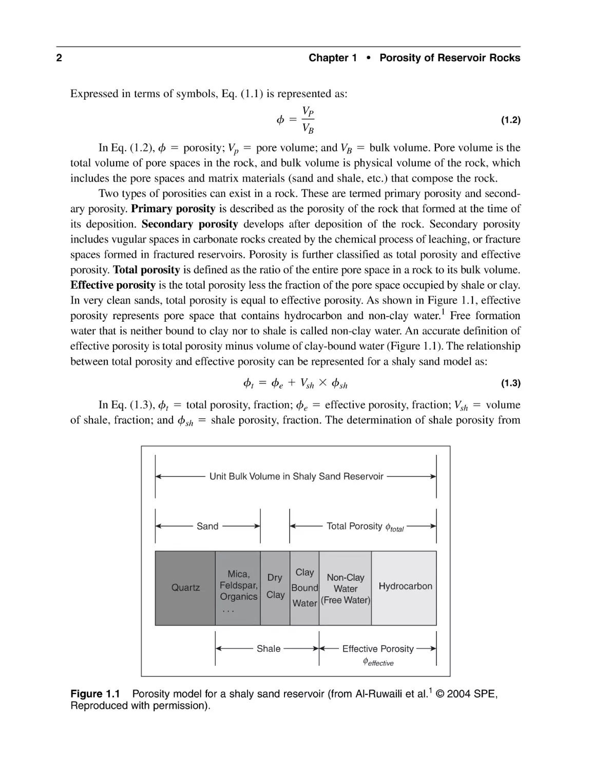
Effective porosity is the total porosity less the fraction of the pore space occupied by shale or clay.
In very clean sands, total porosity is equal to effective porosity. As shown in Figure 1.1, effective
porosity represents pore space that contains hydrocarbon and non-clay water.1 Free formation
water that is neither bound to clay nor to shale is called non-clay water. An accurate definition of
effective porosity is total porosity minus volume of clay-bound water (Figure 1.1). The relationship
between total porosity and effective porosity can be represented for a shaly sand model as:
ft = fe + Vsh * fsh
(1.3)
In Eq. (1.3), ft = total porosity, fraction; fe = effective porosity, fraction; Vsh = volume
of shale, fraction; and fsh = shale porosity, fraction. The determination of shale porosity from
Unit Bulk Volume in Shaly Sand Reservoir
Total Porosity ftotal
Sand
Quartz
Clay
Mica,
Dry
Non-Clay
Feldspar,
Hydrocarbon
Bound
Water
Organics Clay
(Free
Water)
Water
...
Shale
Effective Porosity
feffective
Figure 1.1 Porosity model for a shaly sand reservoir (from Al-Ruwaili et al.1 © 2004 SPE,
Reproduced with permission).
1.3 Sources of Porosity Data
3
well logs can be difficult and erroneous because the selection of the 100% shale section can be
wrong and subjective.1 For this reason, an approximate form of Eq. (1.3) is obtained by replacing shale porosity fsh with total porosity ft to get:
ft = fe + Vsh * ft
(1.4)
For a clay model, effective porosity is represented as:
ft = fe + Vcbw
(1.5)
In Eq. (1.5), Vcbw = volume of clay-bound water, fraction. The application of Eq. (1.5) for
calculation of accurate effective porosity depends on accurate quantification of the volume of claybound water. This can be determined from an elemental capture spectroscopy (ECS) well logs.1
1.3
Sources of Porosity Data
Rock porosity data are obtained by direct or indirect measurements. Laboratory measurements
of porosity data on core samples are examples of direct methods. Determinations of porosity data
from well log data are considered indirect methods.
1.3.1
Direct Methods for Measurement of Porosity
Direct measurements of porosity data on core samples in a laboratory typically require measurements of bulk and pore volumes of the core samples. For irregular-shaped core samples, the
bulk volume is determined by gravimetric or volumetric methods. In gravimetric methods, the
apparent loss in weight of the sample when immersed completely in a liquid of known density
is measured. Volumetric methods measure the volume of liquid displaced by the rock sample
when completely immersed in the liquid. These methods use specially designed equipment so
that the liquid is not absorbed by the rock sample. For regular-shaped samples, the bulk volume
is calculated from physical measurement of the dimensions of the core sample. For instance, if
the core plug is cylindrical in shape, the bulk volume is calculated as:
VB = pr2l
(1.6)
In Eq. (1.6), VB = bulk volume; r = radius of the core plug; and l = length of the core plug.
Other direct methods for measuring the porosity of a rock sample include use of mercury porosimeter or gas expansion porosimeter. The use of mercury porosimeter or gas expansion
porosimeter for measurement of porosity is not presented in this book because they are described
in many introductory textbooks2 on petroleum reservoir engineering.
Most laboratory routines based on direct methods measure total porosity. It is important to
remember to distinguish between total porosity data obtained from core samples and porosity
data derived from well logs, which may include effective porosities. Porosity data obtained from
core samples using direct methods are generally considered to be accurate and reliable. They are
used to calibrate and validate log-derived porosity data which are based on indirect methods.
4
Chapter 1 • Porosity of Reservoir Rocks
Example 1.1 Calculation of Porosity from Gravimetric Data
Problem
The dimensions of a cylindrical core sample are 10.16 cm long and 3.81 cm in diameter after it
was thoroughly cleaned and dried. The dried core sample weighed 365.0 g. The core sample was
then completely (100%) saturated with brine that has specific gravity of 1.04. The weight of the
saturated core sample is 390.0 g. Calculate the porosity of the core sample.
Solution
Using Eq. (1.6), the bulk volume of the core sample is:
VB = pr2l
= pa
3.81 2
b * 10.16 = 115.8333 cm3
2
The pore volume of the core sample is given by:
Vp =
=
wt. of saturated core - wt. of dried core
specific gravity of brine
390.0 - 365.0
= 24.0385 cm3
1.0400
Using Eq. (1.2), porosity of the core sample is:
f =
VP
VB
24.0385
115.8333
= 0.2075 or 20.75%
=
1.3.2
Indirect Methods for Derivation of Porosity
Indirect methods for derivation of porosity data are based on well log data. The well logs generally
used for this purpose are density, sonic, neutron, and nuclear magnetic response (NMR) logs. In
most formation evaluation programs, density, sonic, and neutron logs are routinely acquired. The
NMR log is frequently run in many wells because of its capability of providing other data for formation evaluation, in addition to porosity data. In most deepwater wells, it is common practice to
run NMR logs, in addition to density, sonic, and neutron logs. It is important to note that density,
sonic, and neutron logs are lithology-dependent, while the NMR logs are lithology-independent for
derivation of porosity.3 NMR data are very sensitive to environmental conditions. It is recommended that NMR tools should be run together with conventional logs, such as density logs or neutron logs for quality control and validation of the NMR data. A summary of the basic principles,
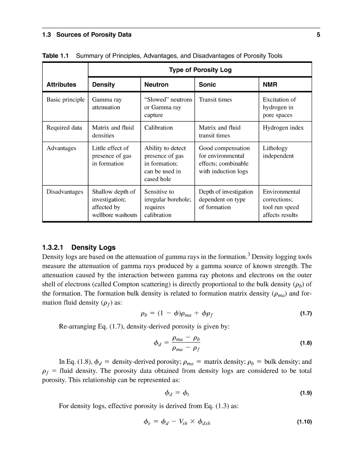
data requirements, advantages, and disadvantages of all the porosity tools is provided in Table 1.1.
1.3 Sources of Porosity Data
Table 1.1
5
Summary of Principles, Advantages, and Disadvantages of Porosity Tools
Type of Porosity Log
Attributes
Density
Neutron
Sonic
NMR
Basic principle
Gamma ray
attenuation
“Slowed” neutrons
or Gamma ray
capture
Transit times
Excitation of
hydrogen in
pore spaces
Required data
Matrix and fluid
densities
Calibration
Matrix and fluid
transit times
Hydrogen index
Advantages
Little effect of
presence of gas
in formation
Ability to detect
presence of gas
in formation;
can be used in
cased hole
Good compensation
for environmental
effects; combinable
with induction logs
Lithology
independent
Disadvantages
Shallow depth of
investigation;
affected by
wellbore washouts
Sensitive to
irregular borehole;
requires
calibration
Depth of investigation
dependent on type
of formation
Environmental
corrections;
tool run speed
affects results
1.3.2.1 Density Logs
Density logs are based on the attenuation of gamma rays in the formation.3 Density logging tools
measure the attenuation of gamma rays produced by a gamma source of known strength. The
attenuation caused by the interaction between gamma ray photons and electrons on the outer
shell of electrons (called Compton scattering) is directly proportional to the bulk density (rb) of
the formation. The formation bulk density is related to formation matrix density (rma) and formation fluid density (rf) as:
rb = (1 - f)rma + frf
(1.7)
Re-arranging Eq. (1.7), density-derived porosity is given by:
fd =
rma - rb
rma - rf
(1.8)
In Eq. (1.8), fd = density-derived porosity; rma = matrix density; rb = bulk density; and
rf = fluid density. The porosity data obtained from density logs are considered to be total
porosity. This relationship can be represented as:
fd = ft
(1.9)
For density logs, effective porosity is derived from Eq. (1.3) as:
fe = fd - Vsh * fdsh
(1.10)
6
Chapter 1 • Porosity of Reservoir Rocks
In Eq. (1.10), fdsh is the shale porosity derived from the density logs. The depth of investigation of density logging tools is shallow and typically within the zone invaded by mud filtrate. For
this reason, it is sometimes appropriate to assume that the density of formation fluid is equal to the
density of the mud filtrate. However, this assumption may cause errors in the density-derived
porosity data, if virgin formation fluid remains within the depth of investigation of the density tool.4
The matrix density can be determined from elemental capture spectroscopy (ECS) log, if available.
Example 1.2 Calculation of Porosity from Density Logs
Problem
The bulk density of a clean, sandy interval saturated with water was measured by the density logging tool to be 2.4 g/cm3. Assuming that the density of the formation water is 1.04 g/cm3 and the
density of the matrix is 2.67 g/cm3, calculate the density porosity of this interval.
Solution
Using Eq. (1.8), density porosity is calculated to be:
rma - rb
fd =
rma - rf
2.67 - 2.4
2.67 - 1.04
= 0.166 or 16.6%
=
1.3.2.2 Sonic (acoustic) Logs
In sonic (acoustic) logging, the formation is probed with sound waves. The time it takes the
sound waves to travel a given distance is measured. This interval transit time depends on the elastic properties of the rock matrix, the properties of the fluid in the rock, and the porosity of the
rock. Wyllie et al.5 proposed that the interval transit time (¢t) can be represented as the sum of
the transit time in the matrix fraction (¢tma) and the transit time in the liquid fraction (¢tf) thus:
¢t = (1 - f)¢tma + f¢tf
(1.11)
Re arranging Eq. (1.11), sonic-derived porosity is given by:
fs =
¢t - ¢tma
¢tf - ¢tma
(1.12)
In Eq. (1.12), fs = sonic-derived porosity; ¢t = transit time; ¢tf = fluid transit time;
and ¢tma = transit time for the rock matrix. Total porosity is related to porosity derived from
sonic logs as:
fs = ft + Vclay * fscl
(1.13)
1.3 Sources of Porosity Data
7
In Eq. (1.13), Vclay = the volume of clay; and fscl = sonic porosity derived in the clay.
Effective porosity as calculated from sonic logs as:
fe = fs - Vsh * fssh
(1.14)
In Eq. (1.14), Vsh = volume of shale; and fssh = sonic porosity derived for shale. Analysis
of sonic logs based on Eq. (1.12) gives reliable porosity data only for consolidated formations.
For unconsolidated sandstones and carbonates, Eq. (1.12) gives porosity values that are too high.
Other equations similar to Eq. (1.12) have been proposed for calculation of porosity for unconsolidated formations and carbonates by Raymer et al.6 These equations should be used for calculations of sonic porosities on unconsolidated formations and carbonates. Note that sonic logs
are well-compensated for environmental effects such as mud velocity, borehole diameter, etc.
and that its depth of investigation is dependent on the compactness of the formation.
Example 1.3 Calculation of Porosity from Sonic Logs
Problem
The transit time for a well-consolidated sandstone interval saturated with brine was measured to
be 82 * 10-6 sec/ft. The matrix transit time is 55.5 * 10-6 sec/ft and the brine transit time is
189 * 10-6 sec/ft. Calculate the sonic porosity for the interval.
Solution
Applying Eq. (1.12), sonic porosity is calculated to be:
fs =
=
¢t - ¢tma
¢tf - ¢tma
82 * 10-6 - 55.5 * 10-6
189 * 10-6 - 55 * 10-6
= 0.199 or 19.9%
1.3.2.3 Neutron Porosity Logs
The first logging tool that was used for the estimation of formation porosity is the neutron logging tool, which was introduced around 1940. The neutron porosity logging tool consists of
either a chemical source or an electrical source of fast neutrons, and detectors located some distance from the source. The fast neutrons from the neutron source are slowed down by successive
collisions with individual nuclei in the rock, thereby losing most of their energy. The detectors
in the neutron tool record either the “slowed” down neutrons directly or capture gamma radiation generated when the neutrons are captured by nuclei. The neutron porosity log is sensitive to
the amount of hydrogen in the formation because the neutrons interact most effectively with
hydrogen due to the closeness of their masses. Neutron logs estimate the amount of hydrogen in
8
Chapter 1 • Porosity of Reservoir Rocks
the rock, and relate it to the amount of fluid in the formation. From the amount of fluid in the formation, the porosity of the rock is estimated after calibration for different lithologies (sandstone,
dolomite, and limestone). Neutron porosity tools are sensitive to borehole conditions, especially
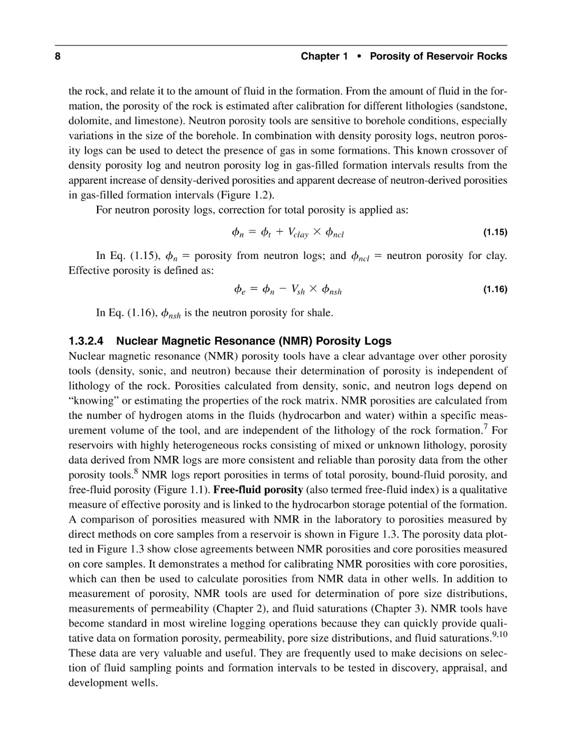
variations in the size of the borehole. In combination with density porosity logs, neutron porosity logs can be used to detect the presence of gas in some formations. This known crossover of
density porosity log and neutron porosity log in gas-filled formation intervals results from the
apparent increase of density-derived porosities and apparent decrease of neutron-derived porosities
in gas-filled formation intervals (Figure 1.2).
For neutron porosity logs, correction for total porosity is applied as:
fn = ft + Vclay * fncl
(1.15)
In Eq. (1.15), fn = porosity from neutron logs; and fncl = neutron porosity for clay.
Effective porosity is defined as:
fe = fn - Vsh * fnsh
(1.16)
In Eq. (1.16), fnsh is the neutron porosity for shale.
1.3.2.4 Nuclear Magnetic Resonance (NMR) Porosity Logs
Nuclear magnetic resonance (NMR) porosity tools have a clear advantage over other porosity
tools (density, sonic, and neutron) because their determination of porosity is independent of
lithology of the rock. Porosities calculated from density, sonic, and neutron logs depend on
“knowing” or estimating the properties of the rock matrix. NMR porosities are calculated from
the number of hydrogen atoms in the fluids (hydrocarbon and water) within a specific measurement volume of the tool, and are independent of the lithology of the rock formation.7 For
reservoirs with highly heterogeneous rocks consisting of mixed or unknown lithology, porosity
data derived from NMR logs are more consistent and reliable than porosity data from the other
porosity tools.8 NMR logs report porosities in terms of total porosity, bound-fluid porosity, and
free-fluid porosity (Figure 1.1). Free-fluid porosity (also termed free-fluid index) is a qualitative
measure of effective porosity and is linked to the hydrocarbon storage potential of the formation.
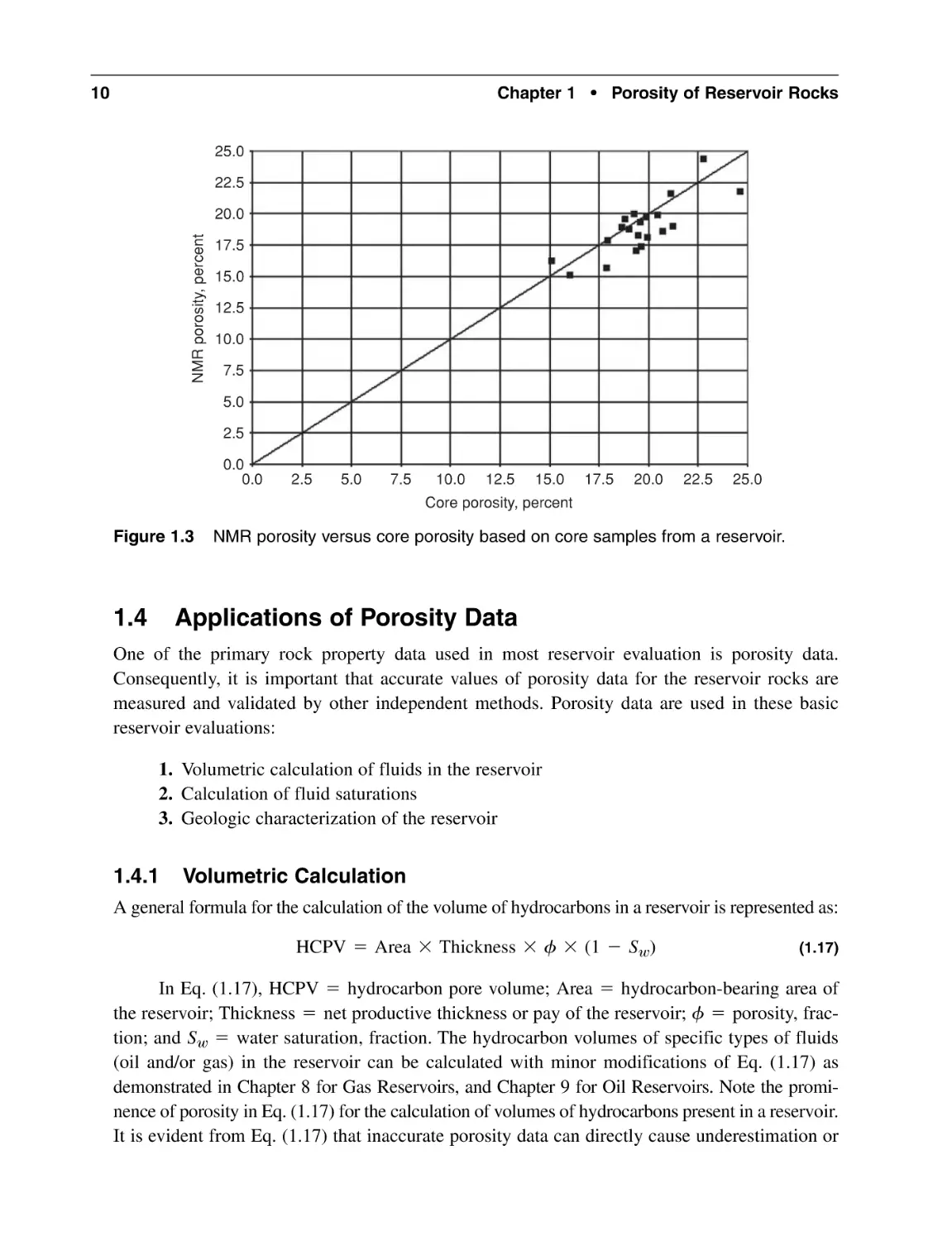
A comparison of porosities measured with NMR in the laboratory to porosities measured by
direct methods on core samples from a reservoir is shown in Figure 1.3. The porosity data plotted in Figure 1.3 show close agreements between NMR porosities and core porosities measured
on core samples. It demonstrates a method for calibrating NMR porosities with core porosities,
which can then be used to calculate porosities from NMR data in other wells. In addition to
measurement of porosity, NMR tools are used for determination of pore size distributions,
measurements of permeability (Chapter 2), and fluid saturations (Chapter 3). NMR tools have
become standard in most wireline logging operations because they can quickly provide qualitative data on formation porosity, permeability, pore size distributions, and fluid saturations.9,10
These data are very valuable and useful. They are frequently used to make decisions on selection of fluid sampling points and formation intervals to be tested in discovery, appraisal, and
development wells.
1.3 Sources of Porosity Data
9
CALIPER, INCHES
6
POROSITY INDEX (%)
COMPENSATED FORMATION DENSITY POROSITY
16
45
30
15
0
–15
GAMMA RAY
0
API UNITS
COMPENSATED NEUTRON POROSITY
200
45
30
15
0
–15
2000
2100
2200
Figure 1.2
Density and neutron well logs showing crossover in a gas interval.
Gas
10
Chapter 1 • Porosity of Reservoir Rocks
25.0
22.5
NMR porosity, percent
20.0
17.5
15.0
12.5
10.0
7.5
5.0
2.5
0.0
0.0
2.5
5.0
7.5
10.0
12.5
15.0
17.5
20.0
22.5
25.0
Core porosity, percent
Figure 1.3
1.4
NMR porosity versus core porosity based on core samples from a reservoir.
Applications of Porosity Data
One of the primary rock property data used in most reservoir evaluation is porosity data.
Consequently, it is important that accurate values of porosity data for the reservoir rocks are
measured and validated by other independent methods. Porosity data are used in these basic
reservoir evaluations:
1. Volumetric calculation of fluids in the reservoir
2. Calculation of fluid saturations
3. Geologic characterization of the reservoir
1.4.1
Volumetric Calculation
A general formula for the calculation of the volume of hydrocarbons in a reservoir is represented as:
HCPV = Area * Thickness * f * (1 - Sw)
(1.17)
In Eq. (1.17), HCPV = hydrocarbon pore volume; Area = hydrocarbon-bearing area of
the reservoir; Thickness = net productive thickness or pay of the reservoir; f = porosity, fraction; and Sw = water saturation, fraction. The hydrocarbon volumes of specific types of fluids
(oil and/or gas) in the reservoir can be calculated with minor modifications of Eq. (1.17) as
demonstrated in Chapter 8 for Gas Reservoirs, and Chapter 9 for Oil Reservoirs. Note the prominence of porosity in Eq. (1.17) for the calculation of volumes of hydrocarbons present in a reservoir.
It is evident from Eq. (1.17) that inaccurate porosity data can directly cause underestimation or
1.4 Applications of Porosity Data
11
overestimation of the hydrocarbon volumes in the reservoir. For marginal reservoirs, underestimation of in-place hydrocarbon volumes may contribute to a decision not to pursue development
of the reservoir. Overestimation of in-place hydrocarbon volumes may lead to economic losses,
if projected reserves estimated prior to development are far below actual reservoir performance.
Note that there are other geologic and reservoir factors (such as permeability barriers, faults,
compartments, recovery mechanisms) which can also cause reservoir performance to be below
projected levels. The impact of these other factors on reservoir performance are presented and
discussed in more details in several chapters in this book.
1.4.2
Calculation of Fluid Saturations
For clean, non-shaly rocks, water saturations can be calculated from the Archie equation1 as:
n
Ct = fm
t * Sw * Cw
(1.18)
In Eq. (1.18), Ct = formation conductivity; ft = total porosity; Sw = water saturation; Cw =
formation water conductivity; m = cementation factor; and n = saturation exponent. The parameters m and n are also called the electrical properties of the rock.
For shaly sands, water saturations can be calculated from modified forms1 of the Archie
equation, which are shown as:
v
v
v
fm
t
v
Snwt
n
Ct = fm
t * Swt * Cwe
Ct =
*
* (Cw + X)
(1.19)
(1.20)
In Eqs. (1.19) and (1.20), Cwe = effective conductivity; and mv, nv are general forms of
the electrical properties. In Eq. (1.19), Cwe is expressed in terms of Cw and a function of shale
(in the shale model) or a function of clay (in the clay model). In Eq. (1.20), X is a function that
accounts for the conductivity caused by shale or clay that occur in shaly sands. Note that in Eq.
(1.20) as X approaches zero, Eq. (1.20) becomes equivalent to Eq. (1.18).
The main point to note from Eqs. (1.18), (1.19), and (1.20) is that total porosity is an
important data input for calculation of water saturation with water saturation models. If errors
exist in the calculations of total porosity, these errors will be transferred to the calculation of
water saturations. This could ultimately lead to errors in the estimation of reservoir in place
hydrocarbon volumes as shown in Eq. (1.17). The calculation of water (fluid) saturation is presented in more detail in Chapter 3.
1.4.3
Reservoir Characterization
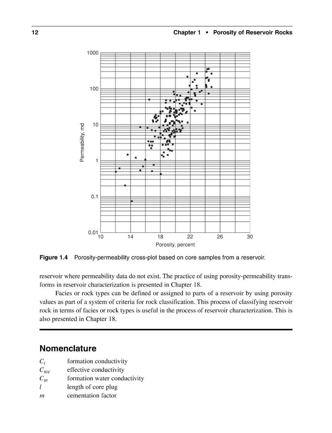
Porosities can be measured directly from cores or indirectly determined from well logs as discussed previously in this chapter. On the one hand, rock permeability can be measured most reliably from cores or in aggregate sense from well tests. Indirect methods for acquiring permeability
data are discussed in Chapter 2. There are usually more porosity data than permeability data available on a reservoir. A cross-plot of permeability versus porosity data (Figure 1.4) to create a porosity-permeability transform is sometimes used to assign permeability values to areas of the
12
Chapter 1 • Porosity of Reservoir Rocks
1000
Permeability, md
100
10
1
0.1
0.01
10
Figure 1.4
14
18
22
Porosity, percent
26
30
Porosity-permeability cross-plot based on core samples from a reservoir.
reservoir where permeability data do not exist. The practice of using porosity-permeability transforms in reservoir characterization is presented in Chapter 18.
Facies or rock types can be defined or assigned to parts of a reservoir by using porosity
values as part of a system of criteria for rock classification. This process of classifying reservoir
rock in terms of facies or rock types is useful in the process of reservoir characterization. This is
also presented in Chapter 18.
Nomenclature
Ct
Cwe
Cw
l
m
formation conductivity
effective conductivity
formation water conductivity
length of core plug
cementation factor
References
n
r
Sw
Vcbw
Vclay
VB
Vp
Vsh
X
f
fd
fdsh
fe
fn
fncl
fnsh
fs
fsh
fscl
fssh
ft
rb
rf
rma
¢t
¢tf
¢tma
saturation exponent
radius of core plug
water saturation, fraction
volume of clay-bound water
volume of clay
bulk volume
pore volume
shale volume
function in Eq. 1.20
porosity
density-derived porosity
density-derived shale porosity
effective porosity
neutron-derived porosity
neutron-derived porosity in clay
neutron-derived porosity in shale
sonic-derived porosity
shale porosity
sonic-derived porosity in clay
sonic-derived porosity in shale
total porosity
bulk density
fluid density
rock matrix density
formation interval transit time
fluid transit time
rock matrix transit time
Abbreviations
LWD
NMR
ECS
HCPV
Logging-While-Drilling
Nuclear Magnetic Resonance
Elemental Capture Spectroscopy
Hydrocarbon Pore Volume
References
1. Al-Ruwaili, S.A., and Al-Waheed, H.H.: “Improved Petrophysical Methods and Techniques
for Shaly Sands Evaluation,” paper SPE 89735 presented at the 2004 SPE International
Petroleum Conference in Puebla, Mexico, November 8–9, 2004.
2. Amyx, J.W., Bass, D.M., Jr., and Whiting, R.L.: Petroleum Reservoir Engineering, Physical
Properties, McGraw-Hill, New York, 1960.
13
14
Chapter 1 • Porosity of Reservoir Rocks
3. Coates, G.R., Menger, S., Prammer, M., and Miller, D.: “Applying NMR Total and Effective
Porosity to Formation Evaluation,” paper SPE 38736 presented at the 1997 SPE Annual
Technical Conference and Exhibition, San Antonio, Texas, October 5–8, 1997.
4. Ellis, D.: “Formation Porosity Estimation from Density Logs,” Petrophysics, (September–
October, 2003) 306–316.
5. Wyllie, M.R.J., Gregory, A.R., and Gardner, G.H.F.: “Elastic Wave Velocity in Heterogeneous and Porous Media,” Geophysics, (1956) 41–70.
6. Raymer, L.L., Hunt, E.R., and Gardner, J.S.: “An Improved Sonic Transit Time-To-Porosity
Transform,” SPWLA Twenty-First Annual Logging Symposium, July 8–11, 1980.
7. Freedman, R.: “Advances in NMR Logging,” SPE 89177, Distinguished Author Series, JPT,
(January 2006) 60–66.
8. Bachman, H.N., Crary, S., Heidler, R., LaVigne, J., and Akkurt, R.: “Porosity Determination
from NMR Log Data: The Effects of Acquisition Parameters,” paper SPE 110803 presented
at the 2007 SPE Annual Technical Conference and Exhibition, Anaheim, California, November
11–14, 2007.
9. Akkurt, R., Kersey, D.G., and Zainalabedin, K.: “Challenges for Everyday NMR: An
Operator’s Perspective,” paper SPE 102247 presented at the 2006 SPE Annual Technical
Conference and Exhibition, San Antonio, Texas, September 24–27, 2006.
10. Seifert, D.J., Akkurt, R., Al-Dossary, S., Shokeir, R., and Ersoz, H.: “Nuclear Magnetic
Resonance Logging: While Drilling, Wireline, and Fluid Sampling,” paper SPE 105605 presented at the 15th SPE Middle East Oil & Gas Show and Conference, Bahrain, Kingdom of
Bahrain, March 11–14, 2007.
General Reading
• Towler, B.F.: Fundamental Principles of Reservoir Engineering, SPE Textbook Series Vol. 8
(2002).
• Mezzatesta, A., Méndez, F., and Rodriguez, E.: “Effective and Total Porosities: Their
Reconciliation in Carbonate and Shaly-Sand Systems,” paper SPE 102811 presented at the
2006 SPE Annual Technical Conference and Exhibition, San Antonio, Texas, September
24–27, 2006.
• Wiltgen, N.: “Shale Volumes Have Large Uncertainties in the Lower Tertiary Deepwater,”
paper SPE 114775 presented at the 2008 SPE Annual Technical Conference and Exhibition,
Denver, Colorado, September 21–24, 2008.
• Wiltgen, N.: “The Contradiction in the Lower Tertiary Deepwater GoM,” paper SPE 114758
presented at the 2008 SPE Annual Technical Conference and Exhibition, Denver, Colorado,
September 21–24, 2008.
C
H A P T E R
2
Permeability and Relative
Permeability
2.1
Introduction
Permeability is a measure of the ability of a porous medium, such as reservoir rock, to transmit
fluids through its system of interconnected pore spaces. If the porous medium is completely saturated (100% saturated) with a single fluid, the permeability measured is the absolute permeability. Absolute permeability is an intrinsic property of the porous medium, and the magnitude
of absolute permeability is independent of the type of fluid in the pore spaces. When the pore
spaces in the porous medium are occupied by more than one fluid, the permeability measured is
the effective permeability of the porous medium to that particular fluid. For instance, the effective
permeability of a porous medium to oil is the permeability to oil when other fluids, including
oil, occupy the pore spaces. Relative permeability is defined as the ratio of effective permeability to absolute permeability of a porous medium. The relationship for relative permeability
is represented as:
kri =
ki
ka
(2.1)
In Eq. (2.1), kri = relative permeability of the porous medium to fluid i; ki = effective
permeability of the porous medium for fluid i; and ka = absolute permeability of the porous
medium. For instance, the relative permeability of a porous medium to oil is expressed in a form
similar to Eq. (2.1) as:
kro =
ko
ka
(2.2)
In Eq. (2.2), kro = relative permeability of the porous medium to oil; ko = effective permeability of the porous medium to oil; and ka = absolute permeability of the porous medium. Similarly,
15
16
Chapter 2 • Permeability and Relative Permeability
the relative permeability of the porous medium to water and gas are expressed in Eqs. (2.3) and
(2.4), respectively, as:
krw =
krg =
kw
ka
(2.3)
kg
(2.4)
ka
In Eq. (2.3), krw = relative permeability of the porous medium to water; and kw = effective permeability of the porous medium to water. In Eq. (2.4), krg = relative permeability of the
porous medium to gas; and kg = effective permeability of the porous medium to gas. Absolute permeability is measured in a laboratory by flowing a fluid of known viscosity through a core sample
from a porous medium while measuring the flow rates and pressure differences across the core
sample. The core sample must be totally saturated (100%) with the fluid. By definition, any fluid
can be used to measure absolute permeability. In practice, absolute permeability is measured by
flowing air through a core sample that has been completely dried. Core permeability measured with
air or any other gas must be reviewed and corrected for Klinkenberg1 effect, if necessary. At low
pressures, gas permeability can be higher than absolute permeability due to Klinkenberg effect, as
shown in Eq. (2.5):
kair = ka a1 +
b
b
P
(2.5)
In Eq. (2.5), kair = air (gas) permeability of core sample as measured; ka = absolute permeability of the core sample; b = Klinkenberg constant for a given gas in a given core sample;
and P = mean flowing pressure of the gas at which the gas permeability was measured.
Klinkenberg1 found that at low pressures gas permeability could be higher than absolute permeability of the porous medium due to interactions between gas molecules and the walls of the pore
spaces. This interaction is referred to as “slippage,” and is related to the molecular size and kinetic energy of the gas. The apparent increase in core air permeabilities at low measurement pressures due to this slippage is called the Klinkenberg effect. The standard unit of measure for
permeability in the petroleum industry is the darcy (d). The darcy is the permeability of a porous
medium with cross-sectional area of 1 cm2 through which a fluid with a viscosity of 1 cp is flowing at the volumetric rate of 1 cc/sec under a pressure gradient of 1 atm per 1 cm of length in the
direction of flow (see Eq. (2.6)). The millidarcy (md) is 1/1000th of a darcy.
2.2
Sources of Permeability Data
The main sources of permeability data are:
1. Core samples
2. Pressure transient tests
3. Well logs
2.2 Sources of Permeability Data
These sources of permeability data sample volumes of the reservoir at different scales.
Permeability data measured on core samples are at a different scale from permeability data calculated from pressure transient tests or well logs. A typical core plug is about 2 inches in diameter by 2 inches long, and is taken from a full-diameter core sample at every half-foot to 1 foot
frequency, depending on the sampling program. This represents a sample volume of 0.0036 ft3
for each core plug. In contrast, a typical well log, such as an NMR (Nuclear Magnetic Resonance)
log, has a vertical resolution of 2 to 5 ft, depending on the configuration of the tool. Consequently,
the volume of reservoir rock sampled by an NMR log is several orders of magnitude larger than
the volume of reservoir rock sampled by core plugs. Pressure transient tests are capable of achieving radii of investigation that extend several hundred feet away from the wellbore, depending on
rock and fluid properties of the reservoir and duration of the test. Clearly, the volume of reservoir rock sampled by pressure transient tests is much larger than the volume of reservoir rock
sampled by NMR logs. The differences in scale among the various sources of permeability data
should be considered before the data are integrated and used for reservoir analysis. Many techniques have been reported in the literature for integrating permeability data with different scales.
A method based on calculation of running averages was reported by Worthington.2 This method
was applied to Saudi Arabian reservoirs by Al-Ali and Worthington.3 Shafer and Ezekwe4 demonstrated that core and well log permeability data on different scales could be integrated by applying
regression analysis based on the Coates5 equation.
2.2.1
Permeability from Core Samples
The primary source of reliable permeability data is core samples. Ample permeability data are measured on core plugs taken from whole core samples. In the absence of whole cores, permeability data
can be obtained from sidewall core samples. Generally, permeability data from sidewall cores are
not as reliable as those measured on core plugs taken from whole core samples and should be
used with caution. Core plugs are usually taken parallel to the plane of deposition of the formation. Consequently, the permeability data measured on core plugs are horizontal permeability
data. To measure vertical permeability, the core plugs should be taken perpendicular to the plane
of deposition. In practice, vertical permeability data are seldom measured. However, if the dominant oil displacement mechanism (such as gravity drainage discussed in Chapter 9) is dependent on vertical permeability, extra effort should be made to obtain vertical permeability data from
laboratory core measurements. The typical permeability data measured under a routine core
analysis (RCAL) program is air permeability. Air permeability is calculated using the Darcy
equation Eq. (2.6) from data obtained by placing the core sample in a chamber and measuring
the pressure differential across it at stabilized air flow rates under steady-state conditions. Air
permeability should be measured at the net confining stress of the reservoir. Net confining stress
is the pressure difference between the overburden pressure and the pore pressure at the depth of the
reservoir. Air permeability data should be corrected for the Klinkenberg effect using Eq. (2.5).
As part of a quality control program, the core samples used in core permeability measurements
should be examined for the presence of induced fractures, fissures, or any deformations which could
influence the magnitude of the permeability data.
17
18
Chapter 2 • Permeability and Relative Permeability
2.2.2
Permeability from Pressure Transient Tests
Pressure transient tests are very important sources of permeability data for reservoirs. There are
various forms of pressure transient tests that are used to calculate permeability data. These tests
can be categorized in two groups, namely: wireline or tubing-conveyed openhole tests and traditional wellhead or down-hole well tests. The wireline or tubing-conveyed openhole tests
include wireline formation testers (WFT) (see Chapter 5) and drillstem tests. Traditional wellhead or down-hole well tests comprise of drawdown or buildup tests conducted on active wells,
as discussed in Chapter 11. Generally, permeability data from WFT or traditional well tests are
at different scales from permeability data measured from core samples or obtained from well
logs. The volume of reservoir rock sampled by pressure transient tests depends on the extent of
the interval tested, rock and fluid properties of the interval, and duration of the test. Pressure
transient tests measure effective permeability, and should be used to condition permeability
data from core samples and well logs as necessary to achieve observed well and reservoir
performance.
2.2.3
Permeability from Well Logs Based on Empirical Correlations
The concept of permeability as a proportionality constant that governs the rate of fluid flow is
demonstrated by Darcy’s equation for single phase, linear, horizontal flow in a porous medium as:
k =
q * m * L
A * ¢P
(2.6)
In Eq. (2.6), k = permeability, darcy; q = flow rate, cc/sec; m = viscosity, cp; L = length,
cm; A = cross-sectional area, cm2; and ¢P = pressure difference, atm. If a dimensionless
analysis is performed on Eq. (2.6) by substituting for the dimensions of permeability, the result is:
k =
rate * viscosity * length
area * pressure
a
=
force * time
L3
ba
b * L
time
L2
force
L2 * a 2 b
L
(2.7)
= L2
Eq. (2.7) shows that permeability has dimensions of area (L2) which are physically related
to the surface area of grains exposed to flow. The size and distribution of rock grains in a porous
medium are related to surface area, which affects the permeability of the porous medium. This
physical aspect of permeability has been used to create empirical equations for prediction of
permeabiliy.6
2.2 Sources of Permeability Data
19
An equation that predicts permeability from the porosity and surface area of grains
exposed to fluid flow was proposed by Kozeny7 and Carman8 as:
k =
f3
Fst2A 2g(1 - f)2
(2.8)
Eq. (2.8) is called the Kozeny-Carman equation. In Eq. (2.8), k = permeability, mm2;
f = porosity, fraction; Fs = shape factor; t = tortuosity; and A g = surface area per unit grain
volume, mm-1. The term, Fst2, is called the Kozeny constant. The Kozeny constant is variable and
has been shown by Rose and Bruce9 to vary from 5 to 100 for reservoir rocks. A modification of
the Kozeny-Carman equation was proposed by Wyllie and Rose10 by substituting irreducible
water saturation for specific surface area to get:
k1>2 =
C1f
Swir - C2
(2.9)
In Eq. (2.9), C1 and C2 are constants that vary depending on the rock and fluid properties
of the formation; and Swir = irreducible water saturation. A more generalized form of the
Wyllie-Rose correlation was proposed by Timur11 as:
k =
PfQ
SRwir
(2.10)
In Eq. (2.10), P, Q, and R are regression parameters to be determined by fitting the equation to core data. A form of Eq. (2.10) was developed for sandstones by Timur11 as:
k =
0.136f4.4
S2wir
(2.11)
In Eq. (2.11), k = permeability, md; f = porosity, percent; and Swir = irreducible water
saturation, percent. The Timur equation is based on 155 sandstone core samples from three different oil fields in North America. A modified form12 of the Timur equation which was in general
use is represented as:
k = c
100f2.25 2
d
Swir
(2.12)
In Eq. (2.12), k = permeability, md; f = porosity, fraction; and Swir = irreducible water
saturation, fraction. Eq. (2.12) was used to correlate actual data by adjusting the constant, 100,
20
Chapter 2 • Permeability and Relative Permeability
and the exponent, 2.25, as necessary. Coates and Denoo13 developed an equation that ensured
that permeability is zero at zero effective porosity and 100% irreducible water saturation. The
Coates-Denoo13 equation is represented as:
k = c
100f2e (1 - Swir) 2
d
Swir
(2.13)
In Eq. (2.13), k = permeability, md; fe = effective porosity, fraction; and Swir = irreducible water saturation, fraction. Bulk volume irreducible water can be represented as:
Vbwi = ftSwir
(2.14)
In Eq. (2.14), Vbwi = bulk volume irreducible water, fraction; and ft = total porosity,
fraction. Eq. (2.13) can be represented in terms of bulk-volume irreducible water by multiplying
the numerator and denominator of the equation with total porosity to get:
k = c
100f2e (ft - Vbwi) 2
d
Vbwi
(2.15)
The improved reliability of nuclear magnetic resonance (NMR) logs led to the reformulation of Eq. (2.15) by Coates et al.5 in terms of free-fluid index (FFI ) and bulk volume irreducible (BVI) saturations. FFI is the fractional part of the pore volume occupied by fluids that
are free to flow and BVI is the fractional part of the pore volume occupied by immobile bound
water. The Coates equation for calculation of permeability from NMR logs is expressed as:
f m FFI n
b
k = a b a
C
BVI
(2.16)
In Eq. (2.16), k = permeability, md; f = porosity, percent; C = 10; m = 4; and n = 2.
The values given for C, m, and n parameters are default values. Values of these parameters are
dependent on the core samples and can be regressed from actual data. FFI is obtained by summing the T2 distribution over T2 values greater than the T2 cutoff. The transverse relaxation time,
T2, is the characteristic time constant that represents the envelope of the spin-echo signal decay
in a NMR logging sequence.14 The main difficulty of using NMR logs to determine FFI is calibration of T2 cutoff. One of the procedures of calibrating T2 cutoff is to match irreducible water
saturations (Swir) obtained from an independent method, such as the Dean-Starks method or
Centrifugal method, with irreducible water saturations derived from NMR data.15 The irreducible water saturations of core samples shown in Figure 2.1 were measured by the centrifugal
method and matched against irreducible water saturations from NMR core laboratory data based
on T2 cutoffs. The T2 cutoffs were then used to determine FFI and BVI for the core samples.
NMR permeability for each core sample was then calculated from these data using Eq. (2.16).
The comparison of calculated NMR permeability versus core permeability measured by routine
core analysis method is shown in Figure 2.2. The approach discussed here is a method regularly
used to calibrate NMR calculated permeability with core permeability obtained through routine
2.2 Sources of Permeability Data
21
MMR Swi (%) @ T2 Cutoff Value
70.0
60.0
50.0
40.0
30.0
20.0
10.0
0.0
0.0
10.0
20.0
30.0
40.0
50.0
60.0
70.0
Core, Swi (%)
Figure 2.1
Determination of T2 cutoff from irreducible water saturation comparison.
core analysis methods. The parameters for the Coates equation obtained from regression of the
calibrated permeability data are then used to calculate permeability data from NMR data measured in other wells. The Coates equation is widely used for the calculation of permeability data
as discussed, if NMR logs are available. This is the method recommended for the calculation of
permeability data from NMR and porosity logs.
MMR Permeability, md
1000
100
10
1
0
0
1
10
100
1000
Core Permeability, md
Figure 2.2
NMR permeability calculated from Coates equation versus core permeability.
22
Chapter 2 • Permeability and Relative Permeability
An important correlation for predicting permeability was developed by Amaefule et al.16
from the Kozeny-Carman equation (Eq. (2.8)). By dividing both sides of Eq. (2.8) with effective
porosity, fe, and taking the square root of both sides of the equation, the resulting equation is
expressed as:
fe
1
k
= c
dc
d
A fe
1 - fe 2FstA g
(2.17)
The reservoir quality index (RQI) parameter is defined in terms of permeability in millidarcies (md) as:
k
A fe
RQI = 0.0314
(2.18)
In Eq. (2.18), RQI = reservoir quality index, mm; k = permeability, md; and fe = effective porosity, fraction. The pore volume-to-grain volume ratio, fz, is defined as:
fz =
fe
1 - fe
(2.19)
The flow zone indicator (FZI) parameter is designated by the following expression as:
FZI =
1
2FstA g
RQI
=
fz
(2.20)
In Eq. (2.20), FZI = flow zone indicator, mm. Taking the logarithm of both sides of
Eq. (2.20) gives:
log RQI = log FZI + log fz
(2.21)
As demonstrated by Amaefule et al.,16 a log-log plot of RQI versus fz will give a straight
line with unit slope for all samples with similar FZI values. Data from core samples with different FZI values will lie on separate, parallel lines. The value of the constant for FZI is determined
from the intercept of the unit slope straight line at fz = 1. As stated by Amaefule et al.,16 core
data that lie on the same straight line have similar pore throat attributes, and thereby can be categorized as a hydraulic unit. The classification of reservoir rock as hydraulic units is useful as a
means of characterizing the reservoir as discussed in Chapter 18. Numerous reservoir studies17–19
have been conducted by application of the hydraulic unit concepts. However, note that the application of this method for prediction of permeability data requires the availability of significant
quantities of core permeability data.
A common empirical relationship that is widely used to correlate permeability and porosity data is a crossplot of the data on a semi-log scale as represented by the equation:
log k = af + b
(2.22)
2.3 Relative Permeability
23
1000
Permeability, md
100
10
1
0.1
0.01
10
14
18
22
26
Porosity, percent
Figure 2.3
Porosity-permeability crossplot based on core samples from a reservoir.
In Eq. (2.22), a and b are regression constants that depend on the data set. Eq. (2.22) has no
theoretical basis but has been adopted because the distribution of permeability data appears to be
log-normal. An example of a permeability-porosity (f - k) crossplot for core samples from a
reservoir is shown in Figure 2.3. The f - k crossplot is a convenient method for displaying core
or log data but is generally misused as a correlation for predicting permeability data from porosity data. Worthington2 and Delfiner20 reported that indiscriminate use of the f - k crossplot for
predicting permeability data could cause the underestimation of permeability data by at least a
factor of 2. The f - k crossplot is not recommended as a method for predicting permeability data
in the form of a correlation. The crossplot can be used qualitatively to review permeability data
predicted using Eq. (2.16) or Eq. (2.21). The application of the f - k crossplots in the form of
cloud transforms could be used for reservoir characterization, as described in Chapter 18.
2.3
Relative Permeability
The relative permeability of a fluid flowing in a porous medium is the ratio of its effective permeability to the absolute permeability of the porous medium as represented in Eq. (2.1). Relative
permeability data can be presented graphically in plots called relative permeability curves. A typical relative permeability curve for an oil-water system is shown in Figure 2.4. In Figure 2.4, the
range of water saturation is from the initial water saturation, Swi to water saturation at residual
oil saturation, 1 - Sorw. Oil relative permeability, kro, is highest at Swi and declines to zero at
1 - Sorw. Water relative permeability, krw, increases from zero at Swi to its highest value at
1 - Sorw. Figure 2.4 shows the location of critical water saturation, Swc. Critical water saturation is the level of water saturation at which water starts to flow in the reservoir. The relative
24
Chapter 2 • Permeability and Relative Permeability
Kro
Krw
Kro
Krw
Swc
0
Figure 2.4
Swi
Sw
1-Sorw 1.0
Oil-water relative permeability curves.
permeability curve for a gas-oil system is shown in Figure 2.5. The range of gas saturation is
from initial gas saturation, Sgi, to gas saturation at residual oil saturation, 1 - Sorg. Oil relative
permeability, kro, is highest at Sgi and declines to zero at 1 - Sorg. Gas relative permeability, krg,
increases from zero at Sgi to its highest value at 1 - Sorg. The critical gas saturation, Sgc, is the
level of gas saturation at which gas starts to flow in the reservoir.
The relative permeability of a fluid in a multi-fluid system is a function of the saturation
level of the fluid as shown in Figures 2.4 and 2.5. However, many distributions of the fluid are
possible at the same saturation level, depending on the wettability and the direction of saturation
changes (or saturation history) of the porous media. For this reason, permeability data measured
Krg
Kro
Kro
Krg
Sgc
0 Sgi
Figure 2.5
Sg
Gas-oil relative permeability curves.
1-Sorg 1.0
2.4 Sources of Relative Permeability Data
for drainage displacements (decrease in saturation of the wetting phase) are usually different
from permeability data measured for imbibition displacement (increase in saturation of the wetting phase). This difference is described as the hysteresis of the permeability curves. It is similar
to the hysteresis of the capillary pressure curves discussed in Chapter 15, Section 15.2.2. Basic
concepts on rock wettability are presented in Chapter 15, Section 15.2.1.
2.4
Sources of Relative Permeability Data
Relative permeability data are obtained from many sources for hydrocarbon reservoirs. These
sources include laboratory measurements on core samples, calculations from field production
data, and empirical correlations. The most reliable source of relative permeability data are laboratory measurements on core samples.21 Some success has been reported on estimating relative
permeability data from field production data.22 In the absence of laboratory data, relative permeability data can be calculated from empirical correlations.
2.4.1
Laboratory Measurements of Relative Permeability Data
Laboratory methods used in measuring relative permeability data can be classified under two
groups, namely: steady-state methods and unsteady-state methods. Steady-state methods are more
widely used and are considered more reliable than unsteady-state methods.21 However, steadystate methods require more experimental time and more elaborate equipment than unsteady-state
methods. Some steady-state measurements may require days of experimental time in comparison to hours for unsteady-state methods. Both methods are affected by capillary end effects.
Capillary end effect is a phenomenon that causes the saturation of the wetting phase to be high
close to the inlet and outlet ends of the core sample. The higher saturations at the ends of the
cores are caused by the tendency of the wetting phase to remain in the core capillary spaces
rather than exit into a noncapillary space. Several measures are employed in relative permeability
measurements to reduce or eliminate capillary end effects in core samples. One of the methods
used to eliminate capillary end effects is the Hassler’s technique that involves the placement of
porous plates in contact with both ends of the core.21 Both steady-state and unsteady-state measurements should be conducted at reservoir conditions.
2.4.1.1 Steady-State Methods
Steady-state methods yield the most reliable relative permeability data because capillary equilibrium is achieved in the method, fluid saturations can be measured directly, and the calculation procedure is based on the Darcy equation (Eq. (2.6)). In the steady-state method, two or three fluids
are injected simultaneously at constant rates or pressures to achieve equilibrium inside the porous
medium.21 After equilibrium is achieved, the saturations, flow rates, and pressure gradients of each
phase are measured. Using the Darcy equation, the effective permeability of each phase is then calculated. The entire saturation range can be measured in a stepwise fashion by changing the ratio of
injection rates and repeating the procedure.23 Steady-state measurement requires many hours or
even days to complete because equilibrium conditions must be attained at each saturation level.
25
26
Chapter 2 • Permeability and Relative Permeability
2.4.1.2 Unsteady-State Methods
Unlike steady-state methods, relative permeability data can be obtained with unsteady-state methods very quickly. Because unsteady-state methods do not require the attainment of equilibrium in
the displacement process, many relative permeability data can be acquired in a few hours. In a typical unsteady-state method, the in-situ fluids are displaced by injection of the displacing fluid at
constant rate or pressure, while measuring the produced fluids continuously. The relative permeability data are calculated from the production data on the basis of the Buckley-Leverett equation.24,25 A widely used unsteady-state method is the use of centrifuge for measurement of relative
permeability data. In this method, saturated core samples are rotated at high angular speed, creating a known centrifugal force. The rate of fluid production is measured as a function of time.
Relative permeability data are then calculated from the measurements.26 The centrifuge method is
extremely fast and is not affected by the viscous fingering problems associated with other
unsteady-state methods. Permeability data from unsteady-state methods are affected by displacement problems, such as viscous fingering and channeling, including instability of the displacement
process.27 The method is recommended to be used to measure relative permeability at the saturation endpoints, while steady-state methods are used to infill the data between the endpoints.28
2.4.2
Estimations from Field Data
Relative permeability data can be estimated through history-matching of field production data
using reservoir simulators. The generation of relative permeability data from historical production
data have been reported by many authors, including Kulkarni and Datta-Gupta,22 Watson et al.,29
Yang and Watson,30 Reynolds et al.,31 and Eydinov et al.32 The agreement between permeability
data measured on core samples and those estimated from production data are generally not good.
This should be expected since cores are samples of very small volumes of the reservoir (microscopic scale), while production data are based on much larger volumes of the reservoir (macroscopic
scale). Relative permeability data calculated from field data should be used to adjust laboratoryderived relative permeability data for reservoir simulation applications.
2.4.3
Empirical Correlations
Several correlations are available for estimation of relative permeability data. These correlations
should be used in situations where measured relative permeability data are not available.
Reasonable caution should be exercised in applying these correlations because they may not be
representative of the rock systems that exist in the reservoir. The most widely used correlations
for the estimation of relative permeability data are modifications of the Corey equations.33
The basic Corey equations are represented as:
krwp = A S*wp B 4
(2.23)
krnwp = A 1 - S*wp B 2 C 1 - A S*wp B 2 D
(2.24)
2.4 Sources of Relative Permeability Data
27
In Eqs. (2.23) and (2.24), krwp = relative permeability of the wetting phase; krnwp = relative
permeability of the non-wetting phase; and S*wp = normalized saturation of the wetting phase.
For a drainage process, the normalized saturation of the wetting phase is expressed as:
S*wp =
Swp - Swpr
1 - Swpr
(2.25)
For an imbibition process, the normalized saturation of the wetting phase is expressed as:
S*wp =
Swp - Swpr
1 - Swpr - Snwpr
(2.26)
In Eqs. (2.25) and (2.26), Swp = saturation of the wetting phase; Swpr = residual saturation
of the wetting phase; and Snwpr = residual saturation of the non-wetting phase.
Applying the Corey equations to a water-wet, two-phase oil-water system, and assuming
oil displacement process is by imbibition, substituting Eq. (2.26) gives:
S*w =
Sw - Swi
1 - Swi - Sorw
(2.27)
From Eq. (2.27),
1 - S*w =
1 - Sw - Sorw
1 - Swi - Sorw
(2.28)
In Eqs. (2.27) and (2.28), Sw = water saturation, fraction; Sorw = residual oil saturation
to water, fraction; and Swi = initial water saturation, fraction. Substituting Eq. (2.27) into Eq. (2.23)
gives:
krw = a
4
Sw - Swi
b
1 - Swi - Sorw
(2.29)
In Eq. (2.29), krw = relative permeability of water. A generalized form of the equation can
be written by expressing the Corey exponent as N and including the endpoint of relative permeability of water at residual oil saturation, krw@Sorw, such that Eq. (2.29) becomes:
krw = krw@Sorw a
N
Sw - Swi
b
1 - Swi - Sorw
(2.30)
Eq. (2.24) can be simplified by dropping the second term in the equation to get:
krnwp = A 1 - S*wp B 2
(2.31)
Substituting Eq. (2.28) into Eq. (2.31) yields:
kro = a
1 - Sw - Sorw 2
b
1 - Swi - Sorw
(2.32)
28
Chapter 2 • Permeability and Relative Permeability
In Eq. (2.32), kro = relative permeability of oil. A generalized form of the equation can be
written by expressing the Corey exponent as N and including the endpoint of relative permeability of oil at initial water saturation, kro@Swi, such that Eq. (2.32) becomes:
kro = kro@Swi a
1 - Sw - Sorw N
b
1 - Swi - Sorw
(2.33)
Corey equations can also be derived for a water-wet, gas-oil system as follows. From
Eq. (2.27), it can be deduced that:
S*w =
1 - Sg - Swi - Sorg
(2.34)
1 - Swi - Sorg
Substituting Eq. (2.34) into Eq. (2.23) gives:
kro = a
1 - Sg - Swi - Sorg
1 - Swi - Sorg
b
4
(2.35)
A generalized form of the equation can be written by expressing the Corey exponent as N
and including the endpoint of relative permeability of oil at initial gas saturation, kro@Sgi, such
that Eq. (2.35) becomes:
kro = kro@Sgi a
1 - Sg - Swi - Sorg
1 - Swi - Sorg
b
N
(2.36)
The gas relative permeability, krg, can be derived by substituting Eq. (2.28) into Eq. (2.31)
to get:
krg = a
= a
1 - Sw - Sorg - Sgc
1 - Swi - Sorg - Sgc
Sg - Sgc
1 - Swi - Sorg - Sgc
b
2
b
2
(2.37)
A generalized form of the equation can be written by expressing the Corey exponent as N
and including the endpoint of relative permeability of gas at residual oil saturation, krg@Sorg, such
that Eq. (2.37) becomes:
krg = krg@Sorg a
Sg - Sgc
1 - Swi - Sorg - Sgc
b
N
(2.38)
Note that similar modified Corey equations can be derived for an oil-wet system assuming
drainage displacement process from Eqs. (2.23), (2.24), and (2.25).
In the absence of data, Corey exponent can be estimated for different rock formations as
follows: well consolidated sandstones, N = 3.0; poorly consolidated sandstones, N = 3.5;
cemented sandstone and limestones, N = 4.0; and fractured formations, N = 1.0.
2.4 Sources of Relative Permeability Data
29
Example 2.1 Calculation of Oil-Water and Gas-Oil Relative Permeability Curves Using
the Modified Corey Equations
Problem
Calculate the oil-water and gas-oil relative permeability data for a water-wet, poorly consolidated
rock with the following rock and fluid properties:
Initial water saturation, Swi
Residual oil saturation to water, Sorw
Residual oil saturation to gas, Sorg
Critical gas saturation, Sgc
Oil curve endpoint, kro@Swi
Oil curve endpoint, kro@Sgi
Water curve endpoint, krw@Sorw
Gas curve endpoint, krg@Sorg
Corey exponent
0.2
0.2
0.2
0.05
0.9
0.9
0.15
1.0
3.5
Solution
Using Eq. (2.30), the relative permeability of water at water saturation, Sw = 0.3 is calculated as:
krw = krw@Sorw a
= 0.15a
N
Sw - Swi
b
1 - Swi - Sorw
3.5
0.3 - 0.2
b
1 - 0.2 - 0.2
= 0.000284
Similarly, the remaining water relative permeabilities at other water saturations were calculated as shown in Table 2.1.
Using Eq. (2.33), the relative permeability of oil at water saturation, Sw = 0.3 is calculated as:
kro = kro@Swi a
= 0.9a
1 - Sw - Sorw N
b
1 - Swi - Sorw
1 - 0.3 - 0.2 3.5
b
1 - 0.2 - 0.2
= 0.4755
Similarly, the remaining oil relative permeabilities at other water saturations were calculated as shown in Table 2.1. The calculated relative permeability data for oil and water are shown
in Figure 2.6.
30
Chapter 2 • Permeability and Relative Permeability
Table 2.1 Oil-water relative permeabilities
calculated for Example 2.1
Sw
krw
kro
0.20
0.0000
0.9000
0.25
0.0000
0.6637
0.30
0.0003
0.4755
0.35
0.0012
0.3288
0.40
0.0032
0.2177
0.45
0.0070
0.1364
0.50
0.0133
0.0795
0.55
0.0227
0.0420
0.60
0.0363
0.0192
0.65
0.0548
0.0070
0.70
0.0792
0.0017
0.75
0.1106
0.0002
0.80
0.1500
0.0000
1.0000
0.9000
Krw
Krow
Relative Permeability
0.8000
0.7000
0.6000
0.5000
0.4000
0.3000
0.2000
0.1000
0.0000
0.00
0.10
0.20
0.30
0.40
0.50
0.60
Water Saturation
Figure 2.6
Oil-water relative permeability plot for Example 2.1.
0.70
0.80
0.90
2.4 Sources of Relative Permeability Data
31
Using Eq. (2.36), the relative permeability of oil at gas saturation, Sg = 0.4 is calculated as:
kro = kro@Sgi a
= 0.9a
1 - Sg - Swi - Sorg
1 - Swi - Sorg
b
N
1 - 0.4 - 0.2 - 0.2 3.5
b
1 - 0.2 - 0.2
= 0.01925
Similarly, the remaining oil relative permeabilities at other gas saturations were calculated
as shown in Table 2.2.
Using Eq. (2.38), the relative permeability of gas at gas saturation, Sg = 0.4 is calculated as:
krg = krg@Sorg a
= 1.0 * a
Sg - Sgc
1 - Swi - Sorg - Sgc
b
N
3.5
0.4 - 0.05
b
1 - 0.2 - 0.2 - 0.05
= 0.2056
Table 2.2 Gas-oil relative permeabilities
calculated for Example 2.1
kro
krg
0.05
0.6637
0.0000
0.10
0.4755
0.0002
0.15
0.3288
0.0026
0.20
0.2177
0.0106
0.25
0.1364
0.0290
0.30
0.0795
0.0633
0.35
0.0420
0.1199
0.40
0.0192
0.2056
0.45
0.0070
0.3281
0.50
0.0017
0.4954
0.55
0.0002
0.7164
0.60
0.0000
1.0000
Sg
32
Chapter 2 • Permeability and Relative Permeability
1.0000
0.9000
Relative Permeability
0.8000
0.7000
0.6000
Krog
Krg
0.5000
0.4000
0.3000
0.2000
0.1000
0.0000
0.00
0.10
0.20
0.30
0.40
0.50
0.60
0.70
Gas Saturation
Figure 2.7
Gas-oil relative permeability plot for Example 2.1.
The remaining gas relative permeabilities at other gas saturations were calculated as shown
in Table 2.2. The calculated relative permeability data for gas and oil are shown in Figure 2.7.
2.5
Three-Phase Relative Permeability
The relative permeability curves shown in Figures 2.4 and 2.5 are based on two-phase systems.
However, in many reservoirs, the flow of three phases (oil, water, and gas) is present during primary, secondary, and enhanced oil recovery processes. The simultaneous flow of three phases
requires the use of three-phase relative permeability data to represent fluid flow in the reservoir.
Three-phase relative permeability data are usually not measured in the laboratory because there
are expensive, tedious, and in some cases impractical. The current accepted engineering practice
for prediction of three-phase relative permeability is based on empirical models. Most of the
empirical models use data from two-phase relative permeabilities, capillary pressure, and saturation history to predict three-phase relative permeability data. Stone’s empirical models (Stone
I34 and Stone II35) are the two empirical models widely used in the petroleum industry for the
prediction of three-phase relative permeability data. Numerous other empirical models that
appear to be superior to Stone’s models have been published in the literature.36–38 However,
reviews of these models available in the literature indicate that the empirical models should be
tested for accuracy before using them for a specific application.36–38
2.6
Applications of Permeability and Relative
Permeability Data
Permeability and relative permeability data are two of the most important data that determine the
flow of fluids in the reservoir. Consequently, permeability and relative permeability data are very
important input in flow calculations, including reservoir simulation. As discussed in Chapter 19,
Nomenclature
it is common practice in reservoir simulation to adjust permeability and relative permeability
data to match performance history, achieve production targets and projected reservoir performance. This practice should be conducted with careful consideration of the reasonableness and
soundness of the data generated by this process. Permeability and relative permeability data
should not be adjusted to the extent that the resulting data violate known physical properties of
the rocks and fluids that are present in the reservoir.39,40
Nomenclature
A
Ag
b
Fs
k
ka
kair
kg
ki
ko
kw
krg
kri
kro
krw
krwp
krnwp
L
N
p
¢p
q
Sg
Sgc
Sw
S*w
Swc
Swi
Swir
Swp
Swpr
Snwpr
Area, cm2
surface area
Klinkenberg constant
shape factor
permeability
absolute permeability
permeability measured with air
effective permeability for gas
effective permeability for fluid, i
effective permeability for oil
effective permeability for water
relative permeability for gas
relative permeability for fluid, i
relative permeability for oil
relative permeability for water
relative permeability of the wetting phase
relative permeability of the non-wetting phase
length, cm
Corey’s exponent
mean flowing pressure
pressure difference, atm
flow rate, cc/sec
gas saturation, fraction
critical gas saturation, fraction
water saturation, fraction
normalized water saturation
critical water saturation, fraction
initial water saturation, fraction
irreducible water saturation, fraction
saturation of the wetting phase
residual saturation of the wetting phase
residual saturation of the non-wetting phase
33
34
Chapter 2 • Permeability and Relative Permeability
S*wp
Sorg
Sorw
T2
Vbwi
f
fe
ft
fz
m
t
normalized saturation of the wetting phase
residual oil saturation to gas
residual oil saturation to water
NMR characteristic time constant, milliseconds
bulk volume irreducible water
porosity
effective porosity
total porosity
pore volume-to-grain volume ratio
viscosity, cp
tortuosity
Abbreviations
BVI
FFI
FZI
NMR
RCAL
RQI
WFT
Bulk Volume Irreducible
Free Fluid Index
Flow Zone Indicator
Nuclear Magnetic Resonance
Routine Core Analysis
Reservoir Quality Index
Wireline Formation Tester
References
1. Klinkenberg, L.J.: “The Permeability of Porous Media to Liquids and Gases,” Drilling and
Production Practices, American Petroleum Institute, Washington, DC, 1941, 200–213.
2. Worthington, P.F.: “The Effect of Scale on the Petrophysical Estimation of Intergranular
Permeability,” Petrophysics (January–February 2004) 45, 1, 59–72.
3. Al-Ali, H.A., and Worthington, P.F.: “Applications of Petrophysical Scale Reconciliation to
Saudi Arabian Reservoirs,” paper IPTC 10726 presented at the International Petroleum
Technology Conference, Doha, Qatar, November 21–23, 2005.
4. Shafer, J.L., and Ezekwe, N.J.: “Methods for Upscaling Diverse Rock Permeability Data for
Reservoir Characterization and Modeling,” paper SPE 109128 presented at the Annual
Technical Conference and Exhibition, Anaheim, California, November 11–14, 2007.
5. Coates, G.R., Miller, M., and Henderson, G.: “The MRIL in Conoco 33—1: An Investigation
of a New Magnetic Resonance Imaging Log,” paper DD presented at the 32nd SPWLA
Annual Logging Symposium, Midland, Texas, June 16–19, 1991.
6. Shang, B.Z., Hamman, J.G., Chen, H., and Caldwell, D.H.: “A Model to Correlate Permeability
with Efficient Porosity and Irreducible Water Saturation,” paper SPE 84303 presented at
SPE Annual Technical Conference and Exhibition, Denver, Colorado, October 5–8, 2003.
References
7. Kozeny, J., 1927, Uber Kapillare Leitung des Wassers im Boden: Sitzungsber. Akad. Wiss.
Wien, 136, 271–306.
8. Carman, P. C.: “Fluid Flow through a Granular Bed,” Trans. Inst. Chem. Eng. London, 1937,
15, 150–156.
9. Rose, W., and Bruce, W.A.: “Evaluation of Capillary Character in Petroleum Reservoir Rock,”
Trans., AIME (1949) 127–142.
10. Wyllie, M.R.J., and Rose, W.D.: “Some Theoretical Considerations Related to the Quantitative
Evaluation of the Physical Characteristics of Reservoir Rock from Electrical Log Data,”
Trans., AIME (1950) 105–118.
11. Timur, A: “An Investigation of Permeability, Porosity, and Residual Water Saturation
Relationship for Sandstone Reservoirs,” The Log Analyst (July–August), 1968.
12. Coates, G.R., and Dumanoir, J.L.: “A New Approach to Improved Log-Derived Permeability,”
Proceedings, SPWLA 14th Annual Logging Symposium, Lafayette, Louisiana (May 6–9,
1973).
13. Coates, G., and Denoo, S.: “The Producibility Answer Product,” The Technical Review,
Schlumberger, Houston, Texas (June 1981) 29, 2, 55–63.
14. Freedman, R.: “Advances in NMR Logging,” Distinguished Author Series, JPT (January
2006) 60–66.
15. Shafer, J., Chen, S., Georgi, D., and Chen, J.: “Methods and Procedures for Calibrating
NMR Log Derived Permeabilities,” The 11th Formation Evaluation Symposium of Japan,
Chiba, Japan (October 5–6, 2005) 1–15.
16. Amaefule, J.O., Altunbay, M., Tiab, D., Kersey, D.G., and Keelan, D.K.: “Enhanced Reservoir
Description: Using Core and Log Data to Identify Hydraulic (Flow) Units and Predict
Permeability in Uncored Intervals/Wells,” paper SPE 26436 presented at the SPE 68th
Annual Technical Conference and Exhibition, Houston, Texas, October 3–6, 1993.
17. Abbaszadeh, M., Fujii, H., and Fujimoto, F.: “Permeability Prediction by Hydraulic Flow
Units—Theory and Applications,” SPEFE (December 1996) 263–271.
18. Soto B.R., Garcia, J.C., Torres, F., and Perez, G.S.: “Permeability Prediction Using Hydraulic
Flow Units and Hybrid Soft Computing Systems,” paper SPE 71455 presented at the 2001
SPE Annual Technical Conference and Exhibition, New Orleans, Louisiana, September
30–October 3, 2001.
19. Shenawi, S.H., White, J.P., Elrafie, E.A., and Kilany, A.: “Permeability and Water Saturation
Distribution by Lithologic Facies and Hydraulic Units: A Reservoir Simulation Case Study,”
paper SPE 105273 presented at the 15th SPE Middle East Oil & Gas Show and Conference,
Bahrain, March 11–14, 2007.
20. Delfiner, P.: “Three Statistical Pitfalls of Phi-K Transforms,” SPERE&E (December 2007)
609–617.
35
36
Chapter 2 • Permeability and Relative Permeability
21. Honapour, M., and Mahmood, S.M.: “Relative Permeability Measurements: An Overview,”
JPT (August 1988) 963–966.
22. Kulkarni, K.N., and Datta-Gupta, A.: “Estimating Relative Permeability From Production
Data: A Streamline Approach,” SPEJ (December 2000) 402–411.
23. Braun, E.M., and Blackwell, R.J.: “A Steady-State Technique for Measuring Oil-Water
Relative Permeability Curves at Reservoir Conditions,” paper SPE 10155 presented at the
56th Annual Technical Conference and Exhibitions, San Antonio, Texas, October 5–7, 1981.
24. Johnson, E.F., Bossler, D.P., and Naumann, V.O.: “Calculation of Relative Permeability
from Displacement Experiments,” SPE 1023G, Trans. AIME (1959) 370–372.
25. Batycky, J.P., McCaffery, F.G., Hodgins, P.K., and Fisher, D.B.: “Interpreting Relative
Permeability and Wettability from Unsteady-State Displacement Measurements,” SPEJ
(June 1981) 296–308.
26. Spronsen, E.V.: “Three-Phase Relative Permeability Measurements Using Centrifuge Method,”
paper SPE/DOE 10688 presented at the SPE/DOE Third Joint Symposium on Enhanced Oil
Recovery, Tulsa, Oklahoma, April 4–7, 1982.
27. Peters, E.J., and Khataniar, S.: “The Effect of Instability on Relative Permeability Curves
Obtained by the Dynamic-Displacement Method,” SPEFE (December 1987) 469–474.
28. Shafer, J.L., Braun, E.M., Wood, A.C., and Wooten, J.M.: “Obtaining Relative Permeability
Data Using a Combination of Steady-State and Unsteady-State Corefloods,” paper 9009
presented at the 1990 SCA Conference, Houston, Texas, August 14–16, 1990.
29. Watson, A.T, Seinfeld, J.H., Gavalas, G.R., and Woo, P.T.: “History Matching in Two-Phase
Petroleum Reservoirs,” SPEJ (December 1980) 521–532.
30. Yang, P-H., and Watson, A.T.: “A Bayesian Methodology for Estimating Relative Permeability
Curves,” SPERE (May 1991) 259–265.
31. Reynolds, A.C., Li, R., and Oliver, D.S.: “Simultaneous Estimation of Absolute and Relative
Permeability by Automatic History Matching of Three-Phase Flow Production Data,” JCPT
(2004) 43, 3, 37–46.
32. Eydinov, D., Gao, G., Li, G., and Reynolds, A.C.: “Simultaneous Estimation of Relative
Permeability and Porosity/Permeability Fields by History Matching Production Data,”
JCPT (December 2009) 48, 12, 13–25.
33. Corey, A.T.: “The Interrelation between Gas and Oil Relative Permeabilities,” Production
Monthly (1954) 19, 1, 38–41.
34. Stone, H.L.: “Probability Model for Estimating Three-Phase Relative Permeability,” JPT
(February 1970) 214–218.
35. Stone, H. L.: “Estimation of Three-Phase Relative Permeability and Residual Oil Data,” JCPT
(1973) 12, 53–61.
General Reading
36. Manjnath, A., and Honarpour, M.M.: “An Investigation of Three-Phase Relative
Permeability,” paper SPE 12915 presented at the 1984 Rocky Mountain Regional Meeting,
Casper, Wyoming, May 21–23, 1984.
37. Blunt, M.J.: “An Empirical Model for Three-Phase Relative Permeability,” SPEJ (December
2000) 435–445.
38. Ahmadloo, F., Asghari, K., and Jamaloei, B.Y.: “Experimental and Theoretical Studies of
Three-Phase Relative Permeability,” paper SPE 124538 presented at the 2009 SPE Annual
Technical Conference and Exhibition, New Orleans, Louisiana, October 4–7, 2009.
39. Coats, K.H.: “Use and Misuse of Reservoir Simulation Models,” JPT (1969) 183–190.
40. Wang, K., Killough, J.E., and Sepehrnoori, K.: “A New Upscaling Method of Relative
Permeability Curves for Reservoir Simulation,” paper SPE 124819 presented at the 2009
SPE Annual Technical Conference and Exhibition, New Orleans, Louisiana, October 4–7,
2009.
General Reading
• Babadagli, T., and Al-Salmi, S.: “A Review of Permeability-Prediction Methods for Carbonate
Reservoirs Using Well-Log Data,” SPEREE (April 2004) 75–88.
• Nelson, P.H.: “Permeability-Porosity Relationships in Sedimentary Rocks,” The Log Analyst
(May–June 1994) 38–62.
• Ahmed, U., Crary, S.F., and Coates, G.R.: “Permeability Estimation: The Various Sources
and Their Interrelationships,” JPT (May 1991) 578–587.
• Haddad, S., Cribbs, M., Sagar, R., Tang, Y., Viro, E., and Castelijins, K.: “Integrating
Permeabilities from NMR, Formation Tester, Well Test and Core Data,” paper SPE 71722
presented at the 2001 SPE Annual Technical Conference and Exhibition, New Orleans,
Louisiana, September 30–October 3, 2001.
• Haddad, S., Cribbs, M., Sagar, R., Viro, E., Castelijins, K., and Tang, Y.: “So What is the
Reservoir Permeability?” paper SPE 63138 presented at the 2000 SPE Annual Technical
Conference and Exhibition, Dallas, Texas, October 1–4, 2000.
• Heaviside, J., Black, C.J.J., and Berry, J.F.: “Fundamentals of Relative Permeability:
Experimental and Theoretical Considerations,” paper SPE 12173 presented at the 58th
Annual Technical Conference and Exhibition, San Francisco, California, October 5–8,
1983.
• Jones, S.C., and Roszelte, W.O.: “Graphical Techniques for Determining Relative
Permeability From Displacement Experiments,” JPT (May 1978) 807–817.
• Honarpour, M., Koederitz, L.F., and Harvey, A.H.: “Empirical Equations for Estimating
Two-Phase Relative Permeability in Consolidated Rock,” JPT (December 1982)
2905–2908.
37
38
Chapter 2 • Permeability and Relative Permeability
• Johnson, C.E., Jr.: “Graphical Determination of the Constants in the Corey Equation for
Gas-Oil Relative Permeability Ratio,” SPE 2346, JPT Forum (October 1968) 1111–1113.
• Grattoni, C.A., and Bidner, M.S.: “History Matching of Unsteady-State Corefloods for
Determining Capillary Pressure and Relative Permeabilities,” paper SPE 21135 presented at
the SPE Latin American Petroleum Engineering Conference, Rio de Janeiro, Brazil, October
14–19, 1990.
• Amabeoku, M.O., Kersey, D.G., BinNasser, R.H., and Belowi, A.R.: “Relative Permeability
Coupled Saturation-Height Models Based on Hydraulic (Flow) Units in a Gas Field,”
SPEREE (December 2008) 1013–1028.
• App, J.F., and Mohanty, K.K.: “The Benefit of Local Saturation Measurements in Relative
Permeability Estimation from Centrifuge Experiments,” SPEJ (September 2002) 288–298.
• Labban, Z.S., and Horne, R.N.: “Estimating Relative Permeabilities by Automated History
Matching Using Linear Modeling Techniques,” paper SPE 21206 presented at the 11th SPE
Symposium on Reservoir Simulation, Anaheim, California, February 17–20, 1991.
• Blunt, M.J.: “Effects of Heterogeneity and Wetting on Relative Permeability Using Pore
Level Modeling,” SPEJ (March 1997) 70–87.
• Kjosavik, A., Ringen, J.K., and Skjaeveland, S.M.: “Relative Permeability Correlation for
Mixed-Wet Reservoirs,” SPEJ (March 2002) 49–58.
• Corey, A.T., Rathjens, C.H., Henderson, J.H., and Wyllie, M.R.J.: “Three-Phase Relative
Permeability,” JPT (November 1956) 63–65.
C
H A P T E R
3
Reservoir Fluid Saturations
3.1
Introduction
The pore spaces in reservoir rocks are occupied by fluids. In petroleum reservoirs, the fluids are
usually water and hydrocarbons. The relative volumes of water and hydrocarbons in the pore volume of the reservoir rock are designated as saturations. Water saturation in the reservoir rock
is the fraction of the pore volume occupied by water. By the same definition, hydrocarbon saturation in the reservoir rock is the fraction of the pore volume occupied by hydrocarbons. The
sum of the water and hydrocarbon saturations in the reservoir rock is equal to unity. This relationship can be expressed simply as:
Sh + Sw = 1
(3.1)
In Eq. (3.1), Sh = hydrocarbon saturation, fraction; and Sw = water saturation, fraction.
If the hydrocarbon in the reservoir exists in oil and gas phases, Eq. (3.1) can be written as:
So + Sg + Sw = 1
(3.2)
In Eq. (3.2), So = oil saturation, fraction; and Sg = gas saturation, fraction. The importance of determining accurate data for water saturations in the reservoir, especially at discovery,
is evident from either Eq. (3.1) or Eq. (3.2). The presence of low water saturations in the reservoir indicates the presence of high hydrocarbon saturations. Conversely, high water saturations
are interpreted as representing the presence of low hydrocarbon saturations. This rule-of-thumb
is routinely applied qualitatively to assess the potential hydrocarbon contents of a reservoir after
it has been penetrated with a well, especially at discovery. For calculation of the volume of
hydrocarbons in a reservoir, a general equation that applies is expressed as:
HCPV = Area * Thickness * f * (1 - Sw)
39
(3.3)
40
Chapter 3 • Reservoir Fluid Saturations
In Eq. (3.3), HCPV = hydrocarbon pore volume; Area = hydrocarbon-bearing area of
the reservoir; Thickness = net productive thickness or pay of the reservoir; f = porosity, fraction; and Sw = water saturation, fraction. Water saturation is one of the key data required in Eq.
(3.3). If the water saturation data are incorrect, it could result in the over- or under-estimation of
the volume of hydrocarbon present in the reservoir. The economic impact of erroneous calculation of in-place-hydrocarbon volume can not be overstated. It could lead to execution of uneconomic projects with erroneously high estimated in-place-hydrocarbon volumes or lead to the
abandonment of projects with erroneously low estimates of in-place-hydrocarbon volumes.
In this chapter, various models and equations used for the calculation of water saturations
in clean sands, shaly sands, and carbonate reservoirs are presented. The widely used Archie
equation for clean sands is presented. This is followed with the presentation of models for shaly
sands, such as the Waxman-Smits model, Simandoux equation, Poupon-Leveaux equation, and
the Dual-Water model. The application of the Archie equation to carbonate reservoirs is discussed. This section ends with a presentation on the use of nuclear magnetic resonance (NMR)
logs for the determination of in-situ fluid saturations for most types of reservoirs.
Also in this chapter, the use of cutoffs in the determination of net pay thickness is discussed. As Eq. (3.3) shows, net pay thickness is a very important data required in the calculation
of in-place-hydrocarbon volumes. The impact of net pay thickness data on the calculation of
hydrocarbon volumes is as important as those of porosity and water saturation. The criteria generally used in the application of cutoffs are based on porosity, permeability, and water saturation
limiting values. There are no accepted industry-wide limits on the criteria used for the determination of net pay based on these petrophysical properties. This is because the application of cutoff criteria is by necessity reservoir-specific, since it is rare to encounter two reservoirs that have
identical petrophysical properties. Even in the same reservoir owned jointly by different companies, it is not uncommon to find that the cutoff criteria applied by each company are different.
This situation has resulted in partners on the same reservoir using different values of net pay in
calculating the in-place-hydrocarbon volumes. In this chapter, common practices and definitions
used in the application of cutoff criteria to determine net pay are presented.
3.2
Determination of Water Saturations
Many models and equations have been developed over many years for the determination of water
saturations in hydrocarbon-bearing formations. The models and equations vary in terms of complexity from the Archie equation developed for clean sands to more elaborate models developed
for shaly sands. In this section, the Archie equations for clean sands are presented followed by a
selection of models developed for shaly sands. The application of the Archie equations on carbonate reservoirs is discussed. Finally, the utility of nuclear magnetic resonance (NMR) logs in
the evaluation of water saturation for most types of reservoirs is discussed.
3.2.1
Clean Sands
Clean sands are classified as sands that satisfy the assumptions used in the development of the
Archie equations.1 These are sands that do not contain clays or clay minerals. In such sands,
3.2 Determination of Water Saturations
41
conduction of electricity occurs only through free ions within the formation water. There is an
absence of the “shale effect.” Archie equations are assumed to apply at these “perfect” rock conditions. In practice, Archie equations are generally applied under rock conditions that do not meet
these ideal conditions.
3.2.1.1 Archie Equations
The derivation of Archie equations1 follows from the definition of resistivity index (IR) as the
ratio of the resistivity of a reservoir rock partially saturated with water (Rt) to the resistivity of
the rock if fully saturated with water (Ro). Thus, the resistivity index is defined as:
IR =
Rt
Ro
(3.4)
In Eq. (3.4), IR = resistivity index; Rt = formation resistivity or resistivity of partially
water-saturated rock, Æ # m; and Ro = resistivity of fully (100%) water-saturated rock, Æ # m.
Resistivity index can also be related to water saturation as:
-n
IR = Sw
(3.5)
In Eq. (3.5), Sw = water saturation, fraction; and n = saturation exponent. Combining
Eqs. (3.4) and (3.5) gives:
-n
Sw
=
Rt
Ro
(3.6)
For a clean rock that is fully saturated with water, formation resistivity factor (sometimes
called formation factor), F, is defined as:
F =
Ro
Rw
(3.7)
In Eq. (3.7), F = formation factor; and Rw = resistivity of formation water, Æ # m.
Substituting Eq. (3.7) into Eq. (3.6) gives:
-n
Sw
=
Rt
FRw
(3.8)
Archie1 expressed the formation factor, F, as a function of total porosity, ft. thus:
F = ft-m
(3.9)
In Eq. (3.9), ft = total porosity, fraction; and m = cementation exponent. Winsauer et al.2
modified Eq. (3.9) later by inserting the tortuosity factor, a, to get:
F = aft-m
(3.10)
42
Chapter 3 • Reservoir Fluid Saturations
Substituting Eq. (3.10) into Eq. (3.8) gives:
-n
Sw
=
Rt
aft-mRw
(3.11)
Eq. (3.11) can be rearranged to give:
a Rw 1>n
b
(3.12)
fm
t Rt
Eq. (3.12) is the Archie equation for the calculation of water saturation in reservoir rocks.
Electrical conductivity of a material is the reciprocal of its resistivity. For example, the conductivity of a reservoir rock is the reciprocal of its resistivity. This can be expressed as:
Sw = a
Ct =
1
Rt
(3.13)
In Eq. (3.13), Ct = conductivity of the reservoir rock, Sm–1. Expressing Archie equation
(Eq. (3.12)) in terms of conductivities yields:
Sw = a
a Ct 1>n
b
fm
t Cw
(3.14)
In Eq. (3.14), Cw = conductivity of the formation water, Sm–1. If it is assumed that the
parameter a = 1, then Eq. (3.14) can be rearranged as:
n
Ct = fm
t * Sw * Cw
(3.15)
3.2.1.2 Determination of Archie Parameters n, m, and a
The Archie parameters n, m, and a can be determined by applying the expression derived by
rearranging Eq. (3.12) as:
log Rt = - n log Sw + log a
aRw
b
fm
t
(3.16)
A least-squares straight line fitted through a log-log plot of Rt versus Sw laboratory data
from core samples has a negative slope equal to the parameter, n. An alternative method that is
equivalent to Eq. (3.16) can be derived from Eq. (3.5) as:
log IR = - n log Sw
(3.17)
A least-squares straight line fitted through a log-log plot of IR versus Sw laboratory data
from core samples yields the same value of parameter, n.
The parameters m and a can be determined by application of Eq. (3.10) in the form:
log F = - m log ft + log a
(3.18)
3.2 Determination of Water Saturations
43
A least-squares straight line drawn through a log-log plot of F versus ft data based on core
samples has a negative slope equal to the parameter m, and an intercept equal to the parameter
a. Note that the entire core data used in this plot must be obtained at Sw = 1 as required by the
definition of formation factor in Eq. (3.7).
A mathematically rigorous method for determining Archie parameters was proposed by
Maute et al.3 This method determines Archie parameters n, m, and a by minimizing the meansquare water saturation error, e, represented as:
a Rwj 1>n 2
e = a a cSwij - a m
b d
ftj Rtij
j i
(3.19)
In Eq. (3.19), e = water saturation error, fraction; j = core sample index; i = index for
each core sample, j, data; Swij = ith laboratory-measured water saturation for core sample, j,
fraction; Rtij = ith laboratory-measured resistivity for core sample, j, Æ # m; Rwj = resistivity
of water used in core sample, j, Æ # m; and ftj = total porosity of core sample, j, fraction. Maute
et al.3 method uses all available core sample data in the regression of the Archie parameters n, m,
and a. Detailed procedure for the implementation of this method was provided by Maute et al.4
Example 3.1 Calculation of the Water Saturation Using the Archie Equation
Problem
Calculate the water saturation of clean consolidated sandstone given the following rock properties and Archie parameters:
Total porosity, ft
Resistivity of sandstone, Rt
Resistivity of formation water, Rw
Archie parameter, m
Archie parameter, n
Archie parameter, a
0.26
22.5 Æ # m
0.265 Æ # m
1.953
1.861
0.838
Solution
Substituting the given data and Archie parameters into Eq. (3.12), water saturation for the clean
sandstone is calculated as:
Sw = a
a Rw 1>n
b
fm
t Rt
= ca
0.838
0.265 1>1.861
b
a
bd
22.5
(0.26)1.953
= 0.344 or 34.4%
44
Chapter 3 • Reservoir Fluid Saturations
3.2.2
Shaly Sands
Shaly sands can be described as reservoir rocks that contain shales. These sands are sometimes
described as “non-Archie” rocks, and exhibit the effects of the presence of shales on the electrical conductivity of rocks. The presence of shales causes reservoir rocks to become conductive,
which adds to the conductivity of the formation water. Archie equation assumes that the formation
water is the only conductive phase in the formation and the reservoir rock is non-conductive. To
account for the effects of shales on the extra conductivity of reservoir rocks, many shaly sand
models have been proposed in the literature.5 Most of the shaly sand saturation models have the
following forms:5,6
v
v
n
Ct = fm
t * Sw * Cwe
v
(3.20)
v
n
Ct = fm
t * Sw * (Cw + X)
(3.21)
The forms of Eqs. (3.20) and (3.21) are similar to the Archie equation as shown in Eq. (3.15).
In Eq. (3.20), Cwe = effective conductivity that accounts for the extra conductivity caused by
the presence of shales in the rocks. In Eq. (3.21), X = a function that accounts for the extra conductivity caused by the presence of shales in the rocks. In Eqs. (3.20) and (3.21), mv and nvare
general forms of the electrical properties of the rock that correspond to the Archie parameters of
m and n. They reduce to Archie parameters as the shale function, X : 0.
3.2.2.1 Waxman-Smits Model
The Waxman-Smits7,8 model is based on the results of an extensive experimental study on the
effects of shales on the conductivity of shaly sands. The model takes the form of Eq. (3.21) and
is represented as:
Ct = fm*
* Sn*
t
w * aCw +
BQv
b
Sw
(3.22)
In Eq. (3.22), B = specific conductivity of exchangeable cations, mho/m per meq/cc. B is
also called counterion equivalent conductance; Qv = clay cation-exchange-capacity (CEC) in
milliequivalents per unit pore volume, meq/cc; The parameters m* and n* are the electrical
parameters for the Waxman-Smits equation. The experimental procedure for determining the
parameters m* and n* is very complicated.6 An approximate approach is to use Archie parameters
m and n to replace Waxman-Smits parameters m* and n* in Eq. (3.22).6
3.2.2.2 Simandoux Equation
The Simandoux9 equation takes the form of Eq. (3.20), and is represented as:
n
Ct = Cwfm
t Sw + eVshCsh
(3.23)
In Eq. (3.23), Vsh = wetted shale volume of rock, fraction; Csh = conductivity of wetted
shale, Sm–1. The shale-term coefficient, e, has a range of 0 … e … 1. As Sw : high, e : 1. The
parameters m and n are the same as Archie parameters.
3.2 Determination of Water Saturations
45
3.2.2.3 Poupon-Leveaux Equation
The Poupon-Leveaux10 equation is also of the form of Eq. (3.20). It is expressed as:
n
n 2 - Vsh
Ct = Cwfm
t Sw + CshSwVsh
(3.24)
This basic equation has been modified by adding additional term in the development of the
Indonesian saturation equation represented as:6
n
n 2 - Vsh
2 - Vsh
Ct = Cwfm
+ Snw 2Cwfm
Csh
t Sw + CshSwVsh
t Vsh
(3.25)
It is also the precursor of the Nigerian saturation equation expressed as:6
2.8
n
Ct = C 2Cwfm
t + 2CshVsh D Sw
2
(3.26)
The parameters m and n are the same as Archie parameters.
3.2.2.4 The Dual-Water Model
The Dual-Water model proposed by Clavier et al.11 assumes that the clay-bound water and the
free non-clay water act as two parallel conductive layers that contribute to the total conductivity,
Ct, measured in the formation. The Dual-Water model is expressed as:
n
Ct = fm
t Sw cCw +
vQQv(Ccbw - Cw)
Sw
d
(3.27)
In Eq. (3.27), Ccbw = conductivity of clay-bound water, Sm–1; vQ = amount of clay water
associated with milliequivalents of clay counterions, meq–1cm3; and Qv = cation-exchangecapacity per unit pore volume, meq cm–3. The parameters m and n can be approximated with the
Archie parameters.
3.2.3
Carbonate Rocks
Carbonate rocks, unlike sandstones, have complex pore systems. These pore systems may have
bi- or trimodal pore size distributions. Pore sizes may range from less than an inch to feet. The
pore geometry of carbonate rocks is very heterogeneous and variable. The texture and structure
of carbonate rocks are further rendered more complex by the diagenesis caused by chemical dissolution, precipitation, dolomitization, leaching, and fracturing. Due to these reasons, petrophysical models comparable in terms of simplicity to the Archie equation have not been
developed for carbonate rocks. In some petrophysical analyses, the Archie equation is used to
calculate water saturation in carbonate rocks. This approach could lead to significant errors. An
alternative approach is to base the calculation of water saturation of carbonate rocks on data from
NMR logs.
46
Chapter 3 • Reservoir Fluid Saturations
3.2.4
Water Saturations from Nuclear Magnetic Resonance Logs
The use of nuclear magnetic resonance (NMR) logging tools for determination of porosity and
permeability was described in Chapters 1 and 2, respectively. Data from NMR logging tools are
also used to determine water saturations. Water saturations in reservoir rocks are determined on
the basis of T2 distribution measured with NMR logging tools.12 The transverse relaxation time,
which is named T2, is the characteristic time constant that represents the envelope of the spin-echo
signal decay in a NMR response sequence.12 T2 distributions computed from NMR echo data are
used to determine total porosity, effective porosity, permeability, pore size distribution, and water
saturation. An example of a T2 distribution curve for typical fluid-saturated shaly sandstone is
shown in Figure 3.1. The T2 distribution curve can be divided into two regions representing bound
water and free fluids by application of a T2 cutoff (see Figure 3.1). For shaly sandstones, bound
water includes clay- and capillary-bound water, and free fluids include non-clay water (or free
water) and hydrocarbons as shown in Figure 3.2. A default value of 33 milliseconds is sometimes
applied as the T2 cutoff for sandstones in the absence of laboratory data. For carbonates, the
default T2 cutoff is 100 milliseconds or higher, depending on the heterogeneity of the rock. More
accurate T2 cutoffs for specific rock samples can be measured in the laboratory with NMR tools
after the samples are centrifuged. Another method for determining T2 cutoffs is by matching irreducible water saturation obtained from an independent source (such as using the Dean-Stark
method on core samples) with the irreducible water saturation derived from NMR data.13 The irreducible water saturations of core samples shown in Figure 3.3 were measured by the centrifugal
method and matched against irreducible water saturations from NMR core laboratory data for
determination of T2 cutoffs. In many formation evaluation processes, water saturations calculated
from Archie-type equations are compared with water saturations derived from NMR data. In highly
heterogeneous formations, such as carbonates, NMR-derived water saturations are considered
more reliable in comparison with saturations calculated with Archie-type equations.
Pore Size
T2 Distribution
Claybound
water
Capillarybound
water
3 ms
Free
Fluids
33 ms
T2 (ms)
Figure 3.1
T2 distribution curve for typical fluid-saturated shaly sandstone.
3.2 Determination of Water Saturations
47
Unit Bulk Volume in Shaly Sand Reservoir
Matrix
Dry
Clay
Clay Capillary
Free
Free
Bound Bound
Water Hydrocarbon
Water Water
Bound
Water
Figure 3.2
3.2.5
Free Fluids
Fluid saturation distribution in a shaly sand reservoir.
Uncertainties in Estimation of Water Saturation
The estimation of water saturation for Archie and non-Archie rocks require input data that have
considerable uncertainties associated with them. For instance, calculation of water saturations
for Archie rocks (clean sands) using the Archie equation require the following input data: porosity,
f; cementation exponent, m; saturation exponent, n; the tortuosity factor, a; formation conductivity,
Ct; and formation water conductivity, Cw. For the non-Archie rocks (shaly sands), additional
input data required include shale conductivity, Csh; and volume of shale, Vsh. In similar manner,
water saturations calculated from NMR data are affected by uncertainties related to the computation of the T2 distribution and accurate values for T2 cutoffs. The uncertainties associated with
MMR Swi (%) @ T2 Cutoff Value
70.0
60.0
50.0
40.0
30.0
20.0
10.0
0.0
0.0
10.0
20.0
30.0
40.0
50.0
60.0
70.0
Core, Swi (%)
Figure 3.3
Determination of T2 cutoff from irreducible water saturation comparison.
48
Chapter 3 • Reservoir Fluid Saturations
these input data have direct impact on the calculated water saturations.14,15 The degree of uncertainty
in calculated water saturations can be minimized by using regression analysis on core data to
generate variable parameters (m, n, and a) for Archie or Archie-type equations. The core database
can also be classified in terms of facies to improve the correlation of the parameters to rock type.16
3.3
Determination of Reservoir Productive Intervals
In Chapter 1, the importance of porosity data as a means of defining the storage capacity of reservoir rocks was discussed. In Chapter 2, permeability was presented as a measure of the ability of
reservoir rocks to transmit fluids. Earlier in this chapter, various equations for the calculation of
water saturation in different types of formations were presented. As shown in Eq. (3.1), the hydrocarbon saturation is the formation pore volume not occupied by water. As a result, the level of
water saturation in a formation is a direct measure of the level of hydrocarbon saturation present
in the formation. Porosity, permeability, and water saturation are the three petrophysical properties that constitute the criteria for the application of cutoffs in the determination of productive
intervals in a reservoir. Generally, formation cutoffs are applied as limiting values that are used to
eliminate formation intervals that appear not to have the potential to contribute significantly to the
storage and productive capacity of the reservoir.17 With this description of cutoffs, it is evident
that there are no generally accepted criteria for the application of cutoffs in the petroleum industry.18
Even on the same reservoirs, petroleum companies have used different cutoff criteria to obtain
widely different estimation of productive intervals. And in many organizations, subsurface specialists (engineers, geologists, petrophysicists, etc.) frequently disagree on the cutoffs to be used
in the determination of productive intervals. The lack of general criteria for the application of cutoffs can be accommodated by recognition of the fact that reservoirs are rarely identical in terms
of their petrophysical properties. Consequently, it is impractical to expect that general cutoff criteria or guidelines can be adequate or applicable to all reservoirs. Due to their arbitrary nature,
cutoff criteria should be devised for each reservoir to accommodate the objectives of the reservoir
evaluation process in terms of in-place-hydrocarbon volumes, displacement mechanisms, and
projected hydrocarbon recoveries.19
3.3.1
Net Sands, Net Reservoir, and Net Pay
Net sands, net reservoir, and net pay are terms commonly used to represent different categories
of the formation intervals. These terms are defined in this book in accordance with the definitions proposed by Worthington.17,20 The definitions of gross rock, net sand, net reservoir, and net
pay are illustrated in Figure 3.4. Gross rock thickness represents the entire thickness of the formation interval. Net sand is the summation of the intervals whose sand content is greater than
or equal to a limiting value set by the shale cutoff. Shale cutoff represents the limiting fractional
volume of the formation that is considered to be shale and non-productive. In some reservoirs, it
is preferable to use net sands in the characterization of reservoir models because it includes all
the potential sources of drive energy that are present in the reservoir. Net reservoir comprises of
Nomenclature
49
GROSS
ROCK
Shale
Cutoff
NET
SAND
Porosity/
Permeability
NET
Cutoff
RESERVOIR
Top Reservoir
Water
Saturation
Cutoff
R1
NET
PAY
P1
S1 Tight Sand
Shale
S2 Tight Sand
G Very Shaly
Sand
R2 Perched
Water
P2
R3
P3
R4
P4
R5
P5
Tight Sand
S3
Contact
P6
R6
Free Water Level
Water Zone
Base of Evaluation Interval
Net-to-Gross Sand
∑Si
=
G
Net-to-Gross Reservoir
∑Ri
=
G
Net-to-Gross Pay
∑Pi
=
G
Figure 3.4 Definitions of net sand, net reservoir, and net pay with cutoff criteria based on petrophysical properties (from Worthington and Cosentino17 © 2005 SPE, Reproduced with permission).
intervals of net sand that have the capacity to both store and transmit reservoir fluids. This is generally determined by the application of porosity and permeability cutoffs. Net pay is the summation of the net reservoir intervals that contain hydrocarbons above the limit set by the water
saturation cutoff. Note the definitions of net-to-gross sand, net-to-gross reservoir, and net-togross pay ratios as shown in Figure 3.4. Net pay thickness is typically used as shown in Eq. (3.3)
for the calculation of in-place-hydrocarbon volumes. But observe that since net pay is derived
from the application of arbitrarily set cutoff criteria, it may lead to under- or over-estimation of
in-place-hydrocarbon volumes. By extension, this could cause under- or over estimation of reserves.
It is recommended that net pay thicknesses or net-to-gross pay ratios should be subjected to
uncertainty analysis, as applied to porosity and water saturation data, in the evaluation of ranges
of in-place-hydrocarbon volumes and potential recoveries.21
Nomenclature
a
B
Ccbw
Co
tortuosity factor
specific conductivity of exchangeable cations, mho/m per meq/cc
conductivity of clay-bound water, Sm–1
conductivity of fully water-saturated formation or rock, Sm–1
50
Chapter 3 • Reservoir Fluid Saturations
Csh
Ct
Cw
Cwe
F
IR
m
mv
n
nv
Qv
Ro
Rt
Rw
Sg
Sh
So
Sw
T2
Vsh
vQ
X
e
f
fe
ft
conductivity of shale, Sm–1
conductivity of formation or rock, Sm–1
conductivity of formation water, Sm–1
effective conductivity of shaly sands, Sm–1
formation factor
resistivity index, ratio
cementation factor
cementation factor for shaly sands
saturation exponent
saturation exponent for shaly sands
clay cation-exchange-capacity, meq/cc
resistivity of fully water-saturated formation or rock, Æ # m
resistivity of formation or rock, Æ # m
resistivity of formation water, Æ # m
gas saturation, fraction
hydrocarbon saturation, fraction
oil saturation, fraction
water saturation, fraction
NMR characteristic time constant, milliseconds
rock shale volume, fraction
clay water associated with clay counterions, meq–1cm3
function to account for extra conductivity of shale
mean-square in water saturation regression
porosity
effective porosity
total porosity
Abbreviations
CEC
HCPV
NMR
Cation-Exchange-Capacity
Hydrocarbon Pore Volume
Nuclear Magnetic Resonance
References
1. Archie, G.E.: “The Electrical Resistivity Log as an Aid in Determining Some Reservoir
Characteristics,” Trans., AIME (1942) 146, 54–62.
2. Winsauer, W.O., Shearin, Jr., H.M., Masson, P.H., and Williams, M.: “Resistivity of BrineSaturated Sands in Relation to Pore Geometry,” AAPG Bulletin (1952) 36, 2, 253–277.
References
3. Maute, R.E., Lyle, W.D., and Sprunt, E.S.: “Improved Data-Analysis Method Determines
Archie Parameters from Core Data,” JPT (January 1992) 103–107.
4. Maute, R.E., Lyle, W.D., and Sprunt, E.S.: “Supplement to SPE 19399, Improved Data-Analysis
Method Archie Parameters from Core Data,” paper SPE 24223.
5. Worthington, P.F.: “The Evolution of Shaly-Sand Concepts in Reservoir Evaluation,” The Log
Analyst (January–February, 1985) 26, 1, 23–40.
6. Al-Ruwali, S.B., and Al-Waheed, H.H.: “Improved Petrophysical Methods and Techniques
for Shaly Sands Evaluation,” paper SPE 89735 presented at the 2004 SPE International
Petroleum Conference, Puebla, Mexico, November 8–9, 2004.
7. Waxman, M.H., and Smits, L.J.M.: “Electrical Conductivities in Oil-Bearing Shaly Sands,”
SPEJ (June 1968) 107–122.
8. Waxman, M.H., and Thomas, E.C.: “Electrical Conductivities in Shaly Sands—1. The Relation
Between Hydrocarbon Saturation and Resistivity Index; II. The Temperature Coefficient of
Electrical Conductivity,” JPT (February 1974) 213–223.
9. Simandoux, P.: “Dielectric Measurements on Porous Media: Application to the Measurement
of Water Saturations: Study of the Behaviour of Argillaceous Formations,” Revue de l’Institu
Francais du Petrole 18, supplementary issue (1963) 193–215 (Translated text in Shaly Sand
Reprint Volume, SPWLA, Houston, Texas, pp. IV 97–124).
10. Poupon, A., and Leveaux, J.: “Evaluation of Water Saturation in Shaly Formations,” The Log
Analyst (July–August, 1971) 3–8.
11. Clavier, C., Coates, G., and Dumanoir, J.: “Theoretical and Experimental Bases for the DualWater Model for Interpretation of Shaly Sands,” SPEJ (April 1984) 153–168.
12. Freedman, R.: “Advances in NMR Logging,” SPE 89177, Distinguished Author Series, JPT
(January 2006) 60–66.
13. Shafer, J., Chen, S., Georgi, D., and Chen, J.: “Methods and Procedures for Calibrating
NMR Log Derived Permeabilities,” The 11th Formation Evaluation Symposium of Japan,
Chiba, Japan (October 5–6, 2005) 1–15.
14. Worthington, P.F., and Pallatt, N.: “Effect of Variable Saturation Exponent on the Evaluation
of Hydrocarbon Saturation,” SPEFE (December 1992) 331–336.
15. Zeybek, A.D. Onur, M., Tureyen, O.I., Ma, S.M., Al-Shahri, A.M., and Kuchuk, F.J.:
“Assessment of Uncertainty in Saturation Estimated From Archie’s Equation,” paper SPE
120517 presented at the 2009 SPE Middle East Oil & Gas Show and Conference, Bahrain,
Kingdom of Bahrain, March 15–18, 2009.
16. Worthington, P.F.: “Improved Quantification of Fit-for-Purpose Saturation Exponents,”
SPEREE (August 2004) 270–284.
51
52
Chapter 3 • Reservoir Fluid Saturations
17. Worthington, P.F., and Cosentino, L.: “The Role of Cutoffs in Integrated Reservoir Studies,”
SPEREE (August 2005) 276–290.
18. Caldwell, R.H., and Heather, D.I.: “Characterizing Uncertainty in Oil and Gas Evaluations,”
paper SPE 68592 presented at the SPE Hydrocarbon Economics and Evaluation Symposium,
April 2–3, 2001, Dallas, Texas.
19. Worthington, P.F.: “The Application of Cutoffs in Integrated Reservoir Studies,” SPEREE
(December 2008) 968–975.
20. Worthington, P.F.: “Net Pay: What is it? What does it do? How do we quantify it? How do
we use it?” paper SPE 123561 presented at the 2009 SPE Asia Pacific Oil and Gas
Conference and Exhibition, August 4–6, 2009, Jakarta, Indonesia.
21. Egbele, E., Ezuka, I., and Onyekonwu, M.: “Net-To-Gross Ratios: Implications in Integrated
Reservoir Management Studies,” paper SPE 98808 presented at the Nigeria Annual
International Conference and Exhibition, August 1–3, 2005, Abuja, Nigeria.
General Reading
• Poupon, A., Clavier, C., Dumanoir, J., Gaymard, R., and Misk, A.: “Log Analysis of SandShale Sequences—A Systematic Approach,” JPT (July 1970) 867–881.
• Juhász, I.: “The Central Role of Qv and Formation-Water Salinity in the Evaluation of Shaly
Formations,” The Log Analyst (July–August, 1979) 3–13.
• Worthington, P.F.: “Petrophysical Type Curves for Identifying the Electrical Character of
Petroleum Reservoirs,” SPEREE (December 2007) 711–729.
• Worthington, P.F.: “Identifying the Potential Upside of Hydrocarbon Saturation from
Electric Logs,” SPEREE (February 2009) 53–67.
C
H A P T E R
4
Pressure-Volume-Temperature (PVT)
Properties of Reservoir Fluids
4.1
Introduction
Fluids exist in reservoirs as mixtures of gas, oil, and water. Some reservoirs may contain only gas
and water, only oil and water, or mixtures of gas, oil, and water. Irrespective of the proportions of
these fluids present in a reservoir, obtaining fluid samples and studying their phase behavior in a
laboratory are necessary for establishing reservoir type, devising strategies for reservoir management, and estimating expected hydrocarbon recovery. The importance of collecting representative
reservoir fluid samples (preferably early in the life of the reservoir) and having the samples analyzed in a reputable laboratory can not be over emphasized. It is one of the essential functions of
the engineers working on new or existing reservoirs as an integral part of a comprehensive data
collection program. Sampling methods for reservoir fluids and types of laboratory measurements
are presented in Chapter 5. This chapter begins by discussing basic concepts of phase diagrams
as tools for understanding the phase behavior of reservoir fluids. The chapter provides many
correlations for calculation of properties of reservoir fluids especially in circumstances where
laboratory data measured on reservoir fluid samples may not be available.
4.2
Phase Diagrams
The PVT properties of reservoir fluids are introduced by reviewing the basic concepts of phase
diagrams. Phase diagrams are graphical representations that relate the properties of a fluid
system. The properties used in the representation could be intensive or extensive properties.
Intensive properties (pressure, temperature, density) are independent of the extent of the system.
53
54
Chapter 4 • Pressure-Volume-Temperature (PVT) Properties of Reservoir Fluids
Extensive properties (mass, volume, heat) depend on the extent of the system. Common forms
of phase diagrams show pressure-temperature (P-T), pressure-volume (P-V), and temperaturevolume (T-V) relationships. The basic concepts of phase behavior and phase diagrams are discussed in this book by the use of P-T diagrams.
4.2.1
Single Component Systems
The P-T diagram of a single component system such as pure water is shown in Figure 4.1. In this
diagram, the pure substance can exist as three phases—solid, liquid, and vapor depending on the
temperature and pressure of the system. A phase is a continuous, homogeneous portion of the
system separated by a physical interface if another phase is present.
The three curves in Figure 4.1 represent states of phase equilibrium. The line ST is the sublimation curve. Along the sublimation curve, solid and vapor phases are in equilibrium. The line
MT is the melting curve, along which solid and liquid phases are in equilibrium. Line TC is the
vapor pressure curve, which represents the locus of equilibrium between liquid and vapor phases. The point T, at which the three curves meet, is the triple point. At the triple point, the three
phases are in equilibrium. Along the vapor pressure curve, the terminal point C is called the
critical point. Above the critical point, the liquid and vapor phases are indistinguishable. The
physical interface between them disappears. The concept of the critical point and its location on the
phase diagram are used later in this chapter to classify the phase behavior of petroleum systems.
The phases within a system composed of one or more components are considered to be in
thermodynamic equilibrium when the chemical potentials of each component in the phases are
equal. Equilibrated phases within a system have the same temperatures and pressures, and there
C
M
Liquid
Pressure
Solid
Vapor
T
S
Temperature
Figure 4.1
P-T phase diagram of a single-component system.
4.2 Phase Diagrams
55
are no net mass transfers between the phases. If a system has two phases denoted as i and j, the
condition of equilibrium is denoted as:
ci = cj
Ti = Tj and
pi = pj
(4.1)
In Eq.(4.1), c is chemical potential, T is temperature, and p is pressure in each phase.
The number of intensive properties required to define a system in equilibrium can be determined by using Gibbs’ phase rule.1 If C is the number of components in a system and P is the
number of phases, then the number of intensive properties, F (or degrees of freedom), that must
be specified to define its equilibrated state is:
F = C - P + 2
(4.2)
Applying the Gibbs’ phase rule to Figure 4.1, it can be deduced that for a single component system with two phases in coexistence (such as a liquid phase and a vapor phase), if the
temperature is known, then the pressure is fixed by the vapor pressure curve because the number of degrees of freedom, F, is equal to 1.
Another form of a phase diagram representing a single component system is shown in
Figure 4.2. This is the pressure-volume (P-V) phase diagram of a single-component system. The
solid curve ACB in Figure 4.2 is called the phase envelope. Within the phase envelope, vapor
and liquid phases coexist in equilibrium. Outside the phase envelope (left of segment AC in
Figure 4.2) is only the liquid phase, and to the right of segment BC is the vapor phase. Line AC
Pressure
C
Liquid
Vapor
T1
T2
Liquid & vapor
T3
B
A
Specific volume
Figure 4.2
P-V phase diagram of a single-component system.
56
Chapter 4 • Pressure-Volume-Temperature (PVT) Properties of Reservoir Fluids
is the bubble point line, and line BC is the dew point line. The bubble point for any system is
the condition of temperature and pressure at which the liquid phase is in equilibrium with an
infinitesimal amount of the vapor phase. Similarly, the dew point is the temperature and pressure at which the vapor phase is in equilibrium with an infinitesimal amount of the liquid phase.
In Figure 4.2, the critical point is represented as C. As was the case in Figure 4.1, beyond the
critical point, liquid and vapor phases overlap and cannot be distinguished from each other.
An important feature of P-V phase diagrams is the use of constant temperature lines, or
isotherms. These are shown as T1, T2, and T3 in Figure 4.2. Along isotherms T2 and T3, the specific volume decreases with an increase in pressure within the vapor region. Within the twophase region, the specific volume decreases at constant pressure. Across the bubble point line,
the pressure increases rapidly with a relatively small reduction in the specific volume, because the
liquid phase is significantly less compressible than the vapor phase. This concept is used in the
measurement of bubble point pressures of most fluid systems. Note that the phase behavior along
the T1 isotherm is significantly different from the phase behavior along the isotherm T2 or T3
because it does not traverse the two-phase region within the phase envelope.
A temperature-volume (T-V) phase diagram of a single-component system is shown in
Figure 4.3. This diagram is very similar to the P-V diagram shown in Figure 4.2. The main difference is that instead of isotherms shown in Figure 4.2, constant pressure lines, or isobars, are
shown in Figure 4.3.
4.2.2
Binary Systems
Binary systems are mixtures of two components. Figure 4.4 is the P-T phase diagram of a binary
mixture of components A and B. The vapor pressure curve of pure component A is shown
terminating at the critical point CA. Similarly, the vapor pressure curve of pure component B
P1
P2
P3
C
Temperature
Vapor
Liquid
Liquid & vapor
Specific volume
Figure 4.3
T-V phase diagram of a single-component system.
4.2 Phase Diagrams
57
E
C
Q
Q
X
Co
P
0%
L
ew iqui
po d
in
tl
in
e
Vapor
T
V
tB
en
on
p
om
L
CB
E
D
m
po
n
bb ent
A
le
po
in
tl
in
e
CA
Bu
Pressure
Liquid
10
0%
80
Liq
%
uid
60
%
40
%
20
%
Y
C
Temperature
Figure 4.4
P-T phase diagram of a binary system.
terminates at the critical point CB. The phase diagrams of hypothetical mixtures of components
A and B will lie between the vapor pressure curves of the pure components, as shown in Figure 4.4
for the 50-50 mole percent mixture. The area in Figure 4.4 bounded by the solid curve LCV is
the phase envelope, which encloses conditions of temperatures and pressures where liquid and
vapor phases can coexist in equilibrium. The curved line LC defines the bubble point line, and
curved line VC is the dew point line. The bubble point line LC and the dew point line VC meet
at point C, which is defined as the critical point. Unlike the critical point that terminates the vapor
pressure curve of a pure single component system (Figure 4.1), the critical point of a binary mixture does not define the highest temperature and pressure at which two phases can coexist. The
highest temperature in Figure 4.4 at which two phases can coexist is shown by line EE. This is
called the cricondentherm. Similarly, the highest pressure at which two phases can coexist is
shown by line QQ. This is called the cricondenbar. Note that the cricondentherm and the cricondenbar are higher than the critical temperature and pressure of the mixture, respectively. The
cricondentherm lies between the critical temperatures of components A and B. The cricondenbar is higher than the critical pressure of either component A or component B.
The dashed lines within the phase envelope in Figure 4.4 denote lines of constant volume
percentage liquid drawn from the critical point. At the bubble point line, the mixture is 100% liquid.
At the dew point line, the mixture is 100% vapor. Consider a process in which the mixture is taken
at constant temperature along the line XT. At point X, the mixture is an undersaturated liquid. As
the pressure is reduced, the liquid expands until it reaches the bubble point line, where an infinitesimal amount of bubble will form. This is the bubble point pressure of the mixture at the
isotherm XT. As the pressure is reduced along XT, the volume of liquid phase in the mixture will
decrease until the dew point line is reached. At the dew point, an infinitesimal amount of liquid
58
Chapter 4 • Pressure-Volume-Temperature (PVT) Properties of Reservoir Fluids
will remain. This is the dew point pressure of the mixture at the isotherm XT. Further pressure
reduction to point T will create a system composed entirely of the vapor phase.
A process similar to the isothermal expansion of the mixture along XT can be repeated by
expanding the mixture at constant pressure (isobaric) along YP. At point Y, the mixture is undersaturated liquid, just as at point X. At the bubble point line, an infinitesimal amount of bubble
will form. Further expansion along YP will result in the reduction of the volume of liquid present in the mixture. At the dew point line, a very small amount of liquid will remain. Further temperature increase to point P will create a vapor system.
The P-T phase diagram of ethane/n-heptane mixtures of varying composition of ethane is
shown in Figure 4.5. This figure illustrates that mixtures of the same components having varying compositions will have varying phase envelopes. For instance, an ethane/n-heptane mixture
with 90.22% ethane has a phase envelope shown as C1. The shape of this phase envelope is different from the phase envelope of the C2 mixture (50.25% ethane) or that of the C3 mixture
(9.78% ethane). In Figure 4.5 the critical points of the three mixtures are connected with a
dashed line, which is the locus of the critical points of all potential mixtures of ethane and n-heptane at temperatures and pressures between the critical points of pure ethane and pure n-heptane.
4.2.3
Multicomponent Systems
The phase diagram of a binary system (Figure 4.4) introduces several useful concepts, such as
the phase envelope, critical point, cricondentherm, and cricondenbar. Figure 4.5 (phase diagrams
1,400
Composition
No.
wt% ethane
C
100.00
C1
90.22
C2
50.25
C3
9.78
C7
n-heptane
C2
1,200
1,000
800
C3
C
ne
600
0
B1
100
B2
200
e
lin
e
an
pt
he
n-
A2
A3
0
C7
oin
t
Bu
A
200
t li
oin
lep
bb
De
wp
400
ne
A1
Eth
a
Pressure, psia
C1
B3
B
300
400
500
Temperature, °F
Figure 4.5 P-T phase diagram for ethane and n-heptane system at various compositions
of ethane (from Kay3).
4.2 Phase Diagrams
59
of ethane/n-heptane at various compositions) also illustrates the effect of the composition of the
mixture on the shape of the phase envelope. The shape and nature of phase diagrams for multicomponent systems are similar to those of binary systems. However, it is much more difficult to
map out the phase envelope of a multicomponent system. These concepts are used in this section
to discuss the phase envelopes of various fluid types that will be encountered in reservoirs.
The phase envelopes of common reservoir fluid types are shown in Figure 4.6. The reservoir fluid types shown are for a gas, a gas condensate, a volatile oil, and a black oil reservoir. In
Figure 4.6, the letter C denotes the location of the critical point on the phase envelopes. Consider
a reservoir whose initial pressure and temperature are denoted as pi,Ti, as shown in Figure 4.6.
Note the path of the solid line starting at pi,Ti, which represents isothermal depletion by reduction in reservoir pressure in relation to the phase envelopes that represent a gas, a gas condensate, a volatile oil, and a black oil reservoir. The phase envelope (A) for the gas reservoir is
clearly to the left of the solid line. The critical temperature (point C) and cricondentherm of the
phase envelope are lower than reservoir temperature, Ti. As the reservoir pressure is reduced at
constant reservoir temperature, there is no chance that the solid line will cross any part of the
phase envelope that defines the gas reservoir. Consequently, no liquid will form inside the gas
reservoir as its pressure is reduced by production.
Gas reservoirs are further classified as dry or wet. This classification is based on the pressure and temperature of the facilities used in handling and processing the produced fluids. If the
pressure and temperature of the flow and processing facilities fall within the two-phase region
defined by the phase envelope, then liquids could form within the wellbore, flowlines, and separators. This type of gas is called a wet gas (Figure 4.7). Describing the gas as wet does not mean
that some of the gas exists as liquid within the reservoir. If the temperature and pressure of the
c
Pi, Ti
c
Gas
condensate
(B)
Pressure
Gas
(A)
c
Volalite
oil
(E)
Black oil
(F)
Temperature
Figure 4.6
Phase diagram showing various reservoir fluid types.
c
Chapter 4 • Pressure-Volume-Temperature (PVT) Properties of Reservoir Fluids
Critical point
Pi, Ti
Pressure
60
Two-phase region
Wet gas
Dry gas
Temperature
Figure 4.7
Phase diagram showing dry gas and wet gas behavior based on the phase envelope.
facilities fall outside the two-phase region of the phase envelope, no liquid will condense in the
wellbore, flowlines, and separators. This type of gas is described as a dry gas.
The phase envelope (B) for a gas-condensate reservoir intersects the solid line from pi,Ti.
For the gas-condensate phase envelope, the reservoir temperature, Ti, is higher than the critical
temperature (point C) but lower than the cricondentherm. Note that the solid line crosses the
phase envelope on the side of the dew point line. As reservoir pressure is reduced along the solid
line, a liquid phase will condense inside the reservoir when the dew point line is reached. The
nature and behavior of the condensation process are presented in more detail in Section 4.2.4 for
retrograde gas-condensate reservoirs.
Volatile oil reservoirs are represented in Figure 4.6 by the phase envelope, E. The critical
temperature (point C) and the cricondentherm of the phase envelope are higher than the reservoir temperature, Ti. At initial reservoir pressure and temperature, pi,Ti, the fluid in the reservoir
is a compressed and undersaturated liquid. When reservoir pressure is reduced at constant temperature along the solid line, the reservoir fluid will expand as a single phase until it reaches the
bubble point line of the phase envelope. Further reduction of reservoir pressure along the solid
line will cause a gas phase to form in the reservoir. Initially, the gas phase exists as isolated bubbles within the liquid phase. As reservoir pressure continues to decline, more gas will evolve
until the scattered bubbles will coalesce to form a continuous phase. Generally, the stock-tank
oil gravities are higher than 35° API, for volatile oils, resulting in gas-oil ratios that range between
1000 and 3000 scf/STB, and oil formation volume factors that are higher than 1.5 RB/STB.
Black oil reservoirs are represented by phase envelope, F, in Figure 4.6. Note the location of the
critical point on the phase envelope for black oils compared with its location on the phase envelope for volatile oils. The reservoir temperature, Ti, is much farther from the critical temperature
4.2 Phase Diagrams
61
for black oils in comparison with volatile oils. As is the case for volatile oils, a gas phase will
form in black oil reservoirs when the reservoir pressure reaches the bubble point pressure on the
bubble point line along the solid line of isothermal depletion (pi,Ti). Generally, the stock-tank oil
gravities of black oil are less than API, producing gas-oil ratios are less than 2000 scf/STB, and
oil formation volume factors are less than 2 RB/STB.
It is apparent from the stated rules of thumb for volatile and black oils that there is significant overlap in properties between the two types of oils. Actual designation of a particular oil
type should be determined from careful PVT laboratory measurements.
4.2.4
Retrograde Behavior of Gas-Condensate Systems
The phase envelope of a gas-condensate reservoir is represented in Figure 4.6 by phase envelope B.
A similar phase envelope has been expanded in Figure 4.8 to illustrate the phenomenon of retrograde condensation. The dashed lines within the phase envelope are lines of constant liquid
volume varying from 100% liquid volume at the bubble point line to 0% liquid volume at the
dew point line. The reservoir temperature, Ti, is higher than the critical temperature, C, but lower
than the cricondentherm of the phase envelope. This is a necessary condition for the occurrence
of retrograde behavior.
Consider an experiment in which reservoir pressure is reduced at constant reservoir temperature, Ti, along the path defined by the solid line ABDE from initial conditions at pi,Ti. At point
Pi, Ti
Cricondenbar
A
Critical point, C
B
%
%
E
Temperature
Figure 4.8
Phase diagram showing retrograde behavior.
Cricondentherm
10
%
20
%
%
40
%
D
30
Pressure
50
60
%
80
70 %
%
90
62
Chapter 4 • Pressure-Volume-Temperature (PVT) Properties of Reservoir Fluids
A on the dew point line, a liquid phase will begin to form in the reservoir. As reservoir pressure
is reduced, more liquid will condense in the reservoir such that at point B, 10% of the reservoir
volume is occupied by the liquid phase. Further reduction in reservoir pressure will increase the
percentage of liquid volume to a maximum of about 12%. Beyond this maximum, as pressure is
reduced, the volume of liquid phase in the reservoir will begin to shrink until it reaches 10% again
at point D. From point D to point E, liquid volume will continue to shrink and will disappear completely at the lower dew point at point E. This condensation behavior, which begins with increasing liquid volume followed by a reversal of liquid volume with pressure reduction at constant
temperature in the reservoir, is described as retrograde condensation.
Generally, the liquid phase that forms in the reservoir rarely reaches the critical liquid saturation necessary to become mobile. The condensed liquid may appear as isolated “islands” of
the liquid phase scattered throughout the reservoir. In a strict sense, the process described along
the isotherm ABDE never occurs in an actual reservoir. As condensation occurs in a reservoir, the
liquid phase will contain the heavier components, and the vapor phase will contain fewer of the
heavier components. Because the liquid phase is not mobile, none of these heavier components
will be produced. Consequently, the composition of the fluid system remaining in the reservoir
is not constant but changes with production. As the composition changes, so does the phase envelope, resulting in retrograde behavior that is different from the process described here, which
assumes constant composition of the fluid system in the reservoir.
Proper management of retrograde gas-condensate reservoirs is very important if the goal
is to maximize hydrocarbon recovery. The key steps are identifying the gas-condensate system
as exhibiting retrograde behavior and quantifying the extent of retrograde condensation that
could occur either in the reservoir or within the production facilities. This can be done by taking
several representative samples of reservoir fluid as close to initial reservoir conditions as possible.
The samples should be analyzed by competent PVT laboratories, especially covering the range
of operating conditions expected during depletion. The PVT data should be modeled with an
equation of state. Further reservoir work should involve performing compositional simulation by
using a geological model of the reservoir. Geologic modeling and reservoir simulation are presented in Chapters 18 and 19, respectively.
Management of gas-condensate reservoirs may require pressure maintenance, usually by
gas injection, either to maintain reservoir pressure or to evaporate some of the condensed liquid.
Ideally, it will be more beneficial in terms of recovery to maintain reservoir pressure higher than
the dew point so that no condensation occurs within the reservoir. This will require initiating the
gas injection project as early as possible in the recovery process. The decision to undertake a
pressure maintenance or liquid recovery project depends on a number of factors, such as the
location of the reservoir, the availability of gas for injection, the cost of injected gas, the availability of facilities for recovery of liquids, and expected recovery from the project. Each of these
factors should be evaluated and combined in a comprehensive economic analysis of the project
as discussed in Chapter 20 on Petroleum Reservoir Management Strategies. More details in
designing gas cycling for gas-condensate reservoirs are presented in Chapter 16, Section 16.3
under Gasflooding.
4.3 Gas and Gas-Condensate Properties
4.3
63
Gas and Gas-Condensate Properties
This section presents equations and correlations that can be used to calculate thermodynamic
properties of dry, wet, or condensate gases. Recall that a dry gas is one in which no liquid forms
either in the reservoir, in flowlines, or in the separators during the entire depletion process
(Figure 4.7). A wet gas is one in which a liquid phase forms in the flowlines or separators, but
no liquid phase forms in the reservoir. For condensate gas, a liquid phase can precipitate in the
reservoir, the flowlines, and the separators (Figure 4.8).
4.3.1
Ideal Gas Equation
The ideal gas equation is derived from the combination of Boyle’s law and Charles’ law for ideal
gases. Boyle’s law states that the pressure of a given mass of gas is inversely proportional to its
volume if its temperature is kept constant:
pV = k, if T is constant
(4.3)
In Eq. (4.3), p is pressure, V is volume, T is temperature, and k is constant. Another form
of Eq. (4.3) that is sometimes useful is:
p1V1 = p2V2, at constant temperature, T
(4.4)
In Eq. (4.4), p1V1 and p2V2 are pressures and volumes at conditions 1 and 2, respectively.
Charles’ law states that the pressure of a given mass of gas is directly proportional to its
temperature if its volume is kept constant:
p
= k, if V is constant
T
(4.5)
Another way of expressing Charles’ law is:
p1
p2
=
at constant volume, V
T1
T2
(4.6)
Combining Boyle’s and Charles’ laws gives the ideal gas equation:
pV = nRT
(4.7)
In Eq. (4.7), n is the number of moles, and R is the gas constant. If p is in psia, V is in ft3,
n is in lbmol, and Tis in °R, then the gas constant R = 10.732 (psia # ft 3)>(lbmol # °R). The ideal
gas equation can be used to represent real gas behavior at low temperatures and pressures. The
ideal gas equation can be expressed in another useful form by combining Eqs. (4.4) and (4.6) or
derived from Eq. (4.7) as:
p1V1
p2V2
=
T1
T2
(4.8)
In Eq. (4.8), pressures, volumes, and temperatures are denoted at two thermodynamic states,
1 and 2, respectively.
64
Chapter 4 • Pressure-Volume-Temperature (PVT) Properties of Reservoir Fluids
4.3.2
Real Gas Equation
Gases, especially those found at reservoir conditions, do not exhibit ideal behavior. In fact, it can
be said that no gases exhibit true ideal behavior, primarily because of the conditions of the kinetic
theory (conditions that define ideal gas behavior). At low temperatures and pressures, low molecular weight gases approach ideal behavior. The thermodynamic behavior of real gases can be
represented with the real gas equation as:
pV = znRT
(4.9)
In Eq. (4.9), z is sometimes called the gas factor, gas deviation factor, or gas compressibility factor. The gas compressibility factor, z, is a modifying factor introduced to account for
the non-ideal behavior of real gases. When the compressibility factor, z, is equal to unity, the gas
behaves as an ideal gas. Eqs. (4.7) and (4.9) become identical. Values of the gas compressibility
factor vary over a wide range, depending on the pressure, temperature, and composition of the
gas. The gas compressibility factor is one of the key properties necessary to represent the thermodynamic behavior of a gas. In this chapter, methods of calculating the gas compressibility factor using correlations are presented. Calculation of gas compressibility factors using equations
of state is treated in Chapter 6.
4.3.3
Gas Gravity
The specific gravity of gas, known simply as gas gravity, is defined with reference to air. It is defined
as the ratio of the density of the gas to the density of air at the same temperature and pressure:
gg =
rg
rair
(4.10)
In Eq. (4.10), gg is gas gravity, rg is gas density, and rair is density of air.
Most of the petroleum industry has adopted the temperature of 60°F and the pressure of
14.65 psia as standard conditions. Unless otherwise stated, these standard conditions are adopted in this book.
Density is defined as mass per unit volume. Hence, gas density is defined as:
rg =
mg
Vg
(4.11)
In Eq. (4.11), mg is the mass of the gas, and Vg is the volume of the gas. mg = nMg, where
n is moles of gas and Mg is its molecular weight. If we assume ideal gas behavior at standard
conditions (Tsc = 60°F and psc = 14.65 psia), then we can apply Eq. (4.7) such that Eq. (4.11)
becomes:
rg =
pMg
RT
(4.12)
4.3 Gas and Gas-Condensate Properties
65
Similarly, the density of air is given by:
pMair
RT
rair =
(4.13)
In Eq. (4.13), Mair is the molecular weight of air, which is equal to 28.9586 (see Table 4.1).
Combining Eqs. (4.12) and (4.13) gives:
gg =
=
4.3.4
Mg
Mair
Mg
(4.14)
28.9586
Reduced Temperature and Pressure
The principle of corresponding states provides a method for correlating the properties of pure
substances and mixtures. It states that two substances of similar chemical nature at the same conditions will exhibit similar physical properties when referenced to the same properties, such as
critical temperatures and pressures.2 The conditions of temperature and pressure referenced to
critical temperature and critical pressure are called reduced temperature (Tr) and reduced
pressure (pr).
T
Tc
p
pr =
pc
Tr =
(4.15)
(4.16)
In Eqs. (4.15) and (4.16), Tc is critical temperature and pc is critical pressure.
For gas mixtures, pseudo-reduced temperature (Tpr) and pseudo-reduced pressure (ppr) are
represented as:
T
Tpc
p
=
ppc
Tpr =
(4.17)
ppr
(4.18)
In Eqs. (4.17) and (4.18), Tpc is the pseudo-critical temperature and ppc is the pseudocritical pressure for gas mixtures. Pseudo-critical properties for mixtures do not have real physical
meaning as critical properties for pure substances. The main use of pseudo-critical properties for
mixtures is as a means of correlating the properties of the mixtures. Section 4.4 presents various
methods for estimating pseudo-critical properties for gas mixtures.
66
Table 4.1
Physical Properties of Compounds
Critical
Temperature
(oF)
Critical
Volume
(ft3/lb)
Liquid Specific
Gravity
(Water ⴝ 1)
Gas
Specific
(Air ⴝ 1)
Acentric
Factor
Compound
Formula
Methane
CH4
16.042
667.0
–116.66
0.0985
(0.3)*
0.55400
0.0115
Ethane
C2H6
30.069
706.6
89.92
0.0775
0.35643
1.03830
0.0994
Propane
C3H8
44.096
615.5
205.92
0.0728
0.50738
1.52270
0.1529
Isobutane
C4H10
58.122
527.9
274.41
0.0715
0.56295
2.00710
0.1865
n-Butane
C4H10
58.122
550.9
305.55
0.0703
0.58408
2.00710
0.2003
Isopentane
C5H12
72.149
490.4
369
0.0685
0.62460
2.49140
0.2284
n-Pentane
C5H12
72.149
488.8
385.8
0.0676
0.63113
2.49140
0.2515
n-Hexane
C6H14
86.175
436.9
453.8
0.0688
0.66404
2.97580
0.2993
n-Heptane
C7H16
100.202
396.8
512.9
0.0682
0.68819
3.46020
0.3483
n-Octane
C8H18
114.229
360.7
564.2
0.0673
0.70698
3.94450
0.3977
n-Nonane
C9H20
128.255
330.7
610.8
0.0693
0.72186
4.42890
0.4421
n-Decane
C10H22
142.282
304.6
652.2
0.0703
0.73406
4.91330
0.4875
Carbon Monoxide
CO
28.01
506.7
–220.63
0.0527
0.79265
0.96720
0.0510
Carbon Dioxide
CO2
44.01
1070.0
87.76
0.0343
0.82203
1.51970
0.2239
Hydrogen Sulfide
H2S
34.082
1306.5
212.81
0.0462
0.80269
1.17690
0.1010
Air
—
28.9586
551.9
–220.97
0.0458
0.87603
1.00000
———
Hydrogen
H2
2.0159
190.7
–399.9
0.5319
0.07087
0.06961
–0.2140
Oxygen
O2
31.9988
731.4
–181.43
0.0367
1.14230
1.10500
0.0222
Nitrogen
N2
28.0135
492.5
–232.53
0.0511
0.80687
0.96740
0.0372
Water
H2O
18.0153
3200.1
705.1
0.04975
1.00000
0.62210
0.3443
Chapter 4 • Pressure-Volume-Temperature (PVT) Properties of Reservoir Fluids
Critical
Pressure
(psia)
Molecular
Weight
4.4 Pseudo-critical Properties of Gas Mixtures
4.4
67
Pseudo-critical Properties of Gas Mixtures
The methods for calculating the pseudo-critical properties of gas mixtures are presented under
two groups. These groups are:
1. Composition of gas mixtures known
2. Composition of gas mixtures unknown
4.4.1
Composition of Gas Mixtures Known
If the composition of the mixture is known, the pseudo-critical properties of gas mixtures can be
calculated by using various mixing rules. The simplest mixing rule was proposed by Kay.3 Kay’s
mixing rule is the molar weighted average of the critical properties of the pure components of
the gas mixture. It is written as:
ppc = a yipci
Tpc = a yiTci
(4.19)
(4.20)
In Eqs. (4.19) and (4.20), yi is the mole fraction of component i; pci and Tci are the critical
pressure and critical temperature, respectively, of component i. Eqs. (4.19) and (4.20) are suitable for low-molecular-weight, homologous gas mixtures with specific gravity less than 0.75.
These equations can be used for quick estimation of pseudo-critical properties and ultimately for
calculation of gas compressibility (z) factors. However, it should be noted that this method under
estimates gas compressibility factors, with errors as high as 15%.2
The mixing rules proposed by Stewart, Burkhart, and Voo (termed SBV)4 and modified by
Sutton (termed SSBV)2 improved the accuracy of calculating the pseudo-critical properties of
high molecular weight gas mixtures. The mixing rules proposed by Stewart et al.4 for high
molecular weight gas mixtures are:
J =
2
Tc
1 nc yTc
2 nc
a
b
+
c
ay
b
d
3 ia
3 ia
A pc i
= 1 pc i
=1
nc
yTc
i=1
2pc
K = aa
Tpc =
ppc =
K2
J
b
(4.21)
(4.22)
i
(4.23)
Tpc
J
(4.24)
In Eqs. (4.21) and (4.22), y = mole fraction of component, i, in mixture; Tc = critical
temperature of component, i, in °R; and pc = critical pressure of component, i, in psia.
68
Chapter 4 • Pressure-Volume-Temperature (PVT) Properties of Reservoir Fluids
Sutton2 modified the SBV equations (Eqs. (4.21) to (4.24)) for gas mixtures that contain
high concentrations of heptane plus fraction (up to 14.27 mole %). The SSBV modifications are:
Fj =
1 yTc
2 y2Tc
a
b
+ a
b
3 pc C7 +
3 pc C7 +
ej = 0.6081Fj + 1.1325F 2j - 14.004FjyC7 + + 64.434Fjy2C7 +
ek = a
Tc
b
* A 0.3129yC7 + - 4.8156y2C7 + + 27.3751y3C7 + B
2pc C7 +
(4.25)
(4.26)
(4.27)
J¿ = J - ej
(4.28)
K¿ = K - ek
(4.29)
Tpc =
ppc =
K¿ 2
J¿
Tpc
J¿
(4.30)
(4.31)
The critical properties of pure components in a mixture are provided in Table 4.1. The critical properties of the heptanes-plus fraction must be determined from correlations. Sutton2
reported that the Kessler-Lee5 equations provide the lowest error in comparison with other methods.
The Kessler-Lee5 equations are:
2.2898
0.11857 Tb,C7 +
0.0566
- a0.24244 +
+
b
+
gC7 +
gC7 +
g2C7 +
103
= exp ≥
¥ (4.32)
2
3
3.648
0.47227 Tb,C7 +
1.6977 Tb,C7 +
a1.4685 +
+
b
a
0.42019
+
b
gC7 +
g2C7 +
107
g2C7 +
1010
8.3634 -
ppc,C7 +
Tpc,C7 + = 341.7 + 811gC7 + + A 0.4244 + 0.1174gC7 + B Tb,C7 +
105
+ A 0.4669 - 3.2623gC7 + B
Tb,C7 +
(4.33)
The boiling point, Tb,C7 + , is estimated from the Whitson6 equation:
3
Tb,C7 + = A 4.5579 * M 0.15178
* g0.15427
C7 +
C7 + B
(4.34)
The application of the SSBV equations for calculation of pseudo-critical properties of a
mixture is shown in Example 4.3. The units of the terms in all the equations are as shown in the
example.
4.4.2
Correction for Non-Hydrocarbon Gas Impurities
Gas mixtures may contain varying amounts of hydrogen sulfide, carbon dioxide, nitrogen, and
water vapor as impurities. The critical properties of hydrocarbon mixtures should be corrected
4.4 Pseudo-critical Properties of Gas Mixtures
69
for the presence of these substances. Sutton7 reported that the correlations proposed by Wichert
and Aziz8 for correcting for the presence of hydrogen sulfide and carbon dioxide are superior to
other published methods. The Wichert and Aziz correlations are:
4
j = 120 C (yCO2 + yH2S)0.9 - (yCO2 + yH2S)1.6 D + 15 A y 0.5
H2S - y H2S B
T*pc
p*pc =
= Tpc - j
(4.35)
(4.36)
ppc(Tpc - j)
Tpc + yH2S(1 - yH2S)j
(4.37)
At present, there are no satisfactory published correlations for correcting for the presence
of nitrogen and water vapor. In Section 4.4.3, a method proposed by Standing9 that could be used
to correct for the presence of water and nitrogen in hydrocarbon gas mixtures is presented. The
units of the terms in all the equations are as shown in Example 4.3.
4.4.3
Composition of Gas Mixture Unknown
The critical properties of gas mixtures can be calculated from Sutton7 correlations when the composition of the mixture is not known. Sutton7 based the correlation on hydrocarbon gas gravity,
which is calculated using the method proposed by Standing:9
yHC = 1 - yH2S - yCO2 - yN2
(4.38)
The original Standing equation (Eq. (4.38)) can be modified slightly to account for the
presence of water vapor as with the other impurities:
yHC = 1 - yH2S - yCO2 - yN2 - yH2O
(4.39)
The hydrocarbon gas gravity, gg,HC, is calculated as:
gg,HC =
gg - (yH2SMH2S + yCO2MCO2 + yN2MN2 + yH2OMH2O)>MAIR
yHC
(4.40)
According to Standing,9 the mixture’s pseudo-critical properties are calculated as follows:
ppc = yHCppc,HC + yH2Spc,H2S + yCO2pc,CO2 + yN2pc,N2 + yH2Opc,H2O
(4.41)
Tpc = yHCTpc,HC + yH2sTc,H2S + yCO2Tc,CO2 + yN2Tc,N2 + yH2OTc,H2O
(4.42)
Note that if hydrogen sulfide and carbon dioxide are present in the gas mixture, then
ppc and Tpc calculated from Eqs. (4.41) and (4.42) should be corrected by using the Wichert and
Aziz correlations (Eqs. (4.35), (4.36), and (4.37)).
Sutton7 proposed two sets of correlations for calculating hydrocarbon pseudo-critical
properties based on hydrocarbon gas gravity. The first set of correlations is for associated gas
from oil reservoirs. The second set of correlations is to be used for gas condensates.
70
Chapter 4 • Pressure-Volume-Temperature (PVT) Properties of Reservoir Fluids
The correlations to be used for associated hydrocarbon gas gravity as proposed by Sutton
are:
ppc,HC = 671.1 + 14gg,HC - 34.3g2g,HC
(4.43)
Tpc,HC = 120.1 + 429gg,HC -
(4.44)
62.9g2g,HC
Equations (4.43) and (4.44) are applicable over a hydrocarbon gas gravity range of
0.554 … gg,HC … 1.862. The equations apply if the gas mixture contains less than 10 mol %
hydrogen sulfide, less than 55.8 mol % carbon dioxide, and less than 21.7 mol % nitrogen. The
correlations were derived from a database that contained 3256 compositions with 4817 gas compressibility factor measurements. The average absolute error reported by Sutton7 for compressibility factors calculated with the correlations is 0.80%.
The correlations for condensate hydrocarbon gas gravity proposed by Sutton7 are:
ppc,HC = 744 - 125.4gg,HC + 5.9g2g,HC
(4.45)
Tpc,HC = 164.3 + 357.7gg,HC - 67.7g2g,HC
(4.46)
Equations (4.45) and (4.46) are applicable over a hydrocarbon gas gravity range of
0.554 … gg,HC … 2.819. The composition of the gas mixture should contain less than 90 mole %
hydrogen sulfide, less than 89.9 mole % carbon dioxide and less than 33.3 mole % nitrogen. The
database for these correlations contained 2264 compositions with 10177 compressibility factor
measurements. The average absolute error reported by Sutton7 for compressibility factors calculated with the correlations is 1.11%.
4.5
Wet Gas and Gas Condensate
In this section, methods for calculating the specific gravities of wet and condensate gases are presented. As defined previously in Section 4.3, a wet gas forms no liquids inside the reservoir but
condenses liquids in the separators and flowlines. A condensate gas will condense liquids inside
the reservoir if reservoir pressure falls below the dew point. The methods presented here are not
applicable to a condensate reservoir if reservoir pressure falls below the dew point. Before these
methods are applied, it is important to ensure that excessive liquid condensation has not occurred
in the flowlines before the sampling point at the separators. The first method is a recombination
method that is used when the compositions of the gas and liquid phases sampled at the separators are determined from laboratory measurements. The second method is based on correlations
when the compositions of the produced phases are not known.
4.5.1
Recombination Method
The recombination method is illustrated with a two-stage separation system consisting of a separator and a stock tank. The compositions of the separator gas, stock-tank gas, and stock-tank oil
are known.
4.5 Wet Gas and Gas Condensate
71
Example 4.1 Calculation of Gravity of a Wet Gas by the Recombination Method
Problem
Suppose a gas reservoir produces wet gas through a two-stage separation system consisting of a separator and a stock tank. The gas-oil ratio (GOR) of the separator is given as 62,000 scf/STB. The
stock-tank GOR is 350 scf/STB. Stock-tank oil gravity is 50.6°API. Calculate the composition of
the reservoir gas given the compositions of the separator and stock-tank fluids as shown in Table 4.2.
Solution
The specific gravity of oil is defined as the density of oil relative to the density of water at the
same temperature and pressure:
go =
ro
rw
(4.47)
In Eq. (4.47), ro and rw are densities of oil and water, respectively, in pounds per cubic foot.
The specific gravity of oil can be related to API gravity (°API) as:
go =
141.5
131.5 + °API
(4.48)
From Eq. (4.48), stock-tank oil specific gravity,
141.5
go =
= 0.7770.
131.5 + 50.6
Molecular weight of stock-tank oil from Table 4.2 is a xiMi = 105.7146 lbm>lb-mole.
Step 1: Convert separator GOR to lb-mole/STB.
Assuming standard conditions of Tsc = 60 °F and psc = 14.65 psia:
Molar volume, VM = RTsc>psc = 10.732(60 + 459.67)>14.65 = 380.69 scf/lb-mole
Pound moles of separator gas per STB = (62000 scf>STB) * (lb-mole>380.69 scf)
= 162.8622 lb-mole/STB
Step 2: Convert stock-tank GOR to lb-mole/STB.
Pound moles of stock tank gas per STB = (350 scf>STB) * (lb-mole>380.69 scf)
= 0.9194 lb-mole/STB
Step 3: Convert stock-tank liquid to lb-mole/STB.
Pound moles of stock tank liquid per STB = (0.777 * 62.4lbm>ft 3)
* (5.615ft 3>STB) * (lb-mole>105.7146 lbm) = 2.5753 lb-mole/STB
The composition of the reservoir gas is computed as shown in Table 4.3 using the values
calculated in steps 1–3. Because the reservoir gas composition has been determined, calculation
72
Compositions of Separator and Stock-Tank Fluids for Example 4.1
Component
Vapor Composition
Separator, Mole
Fraction, yi
Vapor Composition
Stock-Tank, Mole
Fraction, yi
Liquid Composition
Stock-Tank, Mole
Fraction, Xi
Molecular Weight of
Components, Mi
XiMi
N2
0.0030
0.0010
0.0000
28.0134
0.0000
CO2
0.0042
0.0014
0.0000
44.0100
0.0000
CH4
0.7905
0.2700
0.0015
16.0430
0.0241
C2H6
0.1230
0.2221
0.0072
30.0700
0.2165
C3H8
0.0563
0.2812
0.0328
44.0970
1.4464
i-C4H10
0.0052
0.0426
0.0126
58.1230
0.7323
n-C4H10
0.0118
0.1107
0.0138
58.1230
0.8021
i-C5H12
0.0020
0.0232
0.0409
72.1500
2.9509
n-C5H12
0.0023
0.0285
0.0267
72.1500
1.9264
C6H14
0.0014
0.0171
0.0894
86.1770
7.7042
C7+
0.0003
0.0022
0.7751
116.0000
89.9116
Total
1.0000
1.0000
1.0000
—
105.7146
Properties of the heptanes plus stock tank liquid:
Specific gravity
0.802
Molecular weight
116 lb/lb-mole
Chapter 4 • Pressure-Volume-Temperature (PVT) Properties of Reservoir Fluids
Table 4.2
Calculation of Gravity of a Wet Gas by the Recombination Method with Two-Stage Separation
Vapor
Composition
Separator,
Mole
Fraction,
Component
ySP
Vapor
Composition
Stock Tank,
Mole
Fraction,
yST
Liquid
Component
Composition
Moles
Stock Tank,
Separator
Mole
Gas
Fraction,
ySP
XST
× 162.8622
Component Component
Moles
Moles
Stock Tank Stock Tank
Gas
Liquid
yST
XST
× 0.9194
× 2.5753
Total
Composition
of
Reservoir
Gas
N2
0.0030
0.0010
0.0000
0.4886
0.0009
0.0000
0.4895
0.0029
CO2
0.0042
0.0014
0.0000
0.6840
0.0013
0.0000
0.6853
0.0041
CH4
0.7905
0.2700
0.0015
128.7426
0.2482
0.0039
128.9947
0.7754
C2H6
0.1230
0.2221
0.0072
20.0321
0.2042
0.0185
20.2548
0.1218
C3H8
0.0563
0.2812
0.0328
9.1691
0.2585
0.0845
9.5121
0.0572
i-C4H10
0.0052
0.0426
0.0126
0.8469
0.0392
0.0324
0.9185
0.0055
n-C4H10
0.0118
0.1107
0.0138
1.9218
0.1018
0.0355
2.0591
0.0124
i-C5H12
0.0020
0.0232
0.0409
0.3257
0.0213
0.1053
0.4524
0.0027
n-C5H12
0.0023
0.0285
0.0267
0.3746
0.0262
0.0688
0.4695
0.0028
C6H14
0.0014
0.0171
0.0894
0.2280
0.0157
0.2302
0.4740
0.0028
C7+
0.0003
0.0022
0.7751
0.0489
0.0020
1.9961
2.0470
0.0123
Total
1.0000
1.0000
1.0000
—
—
—
166.3569
1.0000
4.5 Wet Gas and Gas Condensate
Table 4.3
Basis: 1 bbl of stock-tank liquid
73
74
Chapter 4 • Pressure-Volume-Temperature (PVT) Properties of Reservoir Fluids
of pseudo-critical properties can proceed as illustrated in Example 4.3. Note that a similar procedure can be used to calculate the specific gravity of the reservoir gas if fluid sampling was conducted only at the primary separator.
4.5.2
Correlation Method
The gas specific gravity of wet or condensate reservoirs can be calculated from production data
if the compositions of the fluid phases at the separators are not known. The production data
required for the calculation are the specific gravities of the fluids plus gas and liquid production
data at the separators. For instance, for a three-stage separation system, the gas gravities and gasliquid ratios from the primary separator, secondary separator, and stock tank, as well as the
stock-tank liquid gravity, are required. Thus, the expression for the gas specific gravity for a
three-stage separation system can be derived as reported by Gold et al.:10
gw =
R1g1 + 4602go + R2g2 + R3g3
R1 + (133,316go>Mo) + R2 + R3
(4.49)
In Eq. (4.49), gw is wellstream gas gravity (air = 1); R1, R2, and R3 are the gas-liquid
ratios in scf/STB for the primary separator, secondary separator, and stock tank, respectively;
g1, g2, and g3 are gas gravities for the primary separator, secondary separator, and stock tank,
respectively; Mo and go are the molecular weight and specific gravity, respectively, of the stocktank liquid.
For a two-stage separation system, the expression for the specific gravity is derived as:
gw =
R1g1 + 4602go + R3g3
R1 + (133,316go>Mo) + R3
(4.50)
Note the absence of the terms R2 and g2 to represent the secondary separator in Eq. (4.50)
because the primary separator and stock tank constitute a two-stage separation system. Eqs. (4.49)
and (4.50) can be used to calculate gas gravities accurately if all the terms in the equations are
available from production data. In most cases, only the primary separator and stock-tank production data are measured. From the production data, the primary separator gas-liquid ratio, R1, the
primary separator gas gravity, g1, and the gravity of the stock-tank liquid, go can be obtained.
All the other terms in Eqs. (4.49) and (4.50) are unknown. The gas produced at the secondary
separator and stock tank (for a three-stage separation system) or the stock tank (for a two-stage
separation system) is accounted for as additional gas produced, Gpa. Thus, for a three-stage separation system:10
Gpa = R2g2 + R3g3
(4.51)
For a two-stage separation system:
Gpa = R3g3
(4.52)
4.5 Wet Gas and Gas Condensate
75
Similarly, the vapor equivalent of the primary separator liquid, Veq, accounts for the stocktank liquid production and gas production beyond the primary separator. This is represented for
a three-stage separation system as:
Veq = (133,316go>Mo) + R2 + R3
(4.53)
For a two-stage separation system:
Veq = (133,316go>Mo) + R3
(4.54)
Using Eqs. (4.51) and (4.53), Eq. (4.49) can be rewritten for a three-stage separation
system as:
gw =
R1g1 + 4602go + Gpa
(4.55)
R1 + Veq
The expression for a two-stage separation system is identical to Eq. (4.55) except that Gpa
refers to Eq. (4.52), and Veq refers to Eq. (4.54).
Gold et al.10 proposed a correlation for estimating molecular weight, Mo, of the stock-tank
liquid as:
Mo =
42.43go
5954
=
°API - 8.811
1.008 - go
(4.56)
The additional gas produced, Gpa, and vapor equivalent, Veq, for a three-stage or a twostage separation system can be estimated with correlations proposed by Gold et al.10 The correlation for additional gas produced in a three-stage separation system is:
b4
b5 b6
Gpa = b 1(ps1 - 14.65)b2g1b3gAPI
Ts1
Ts2
(4.57)
In Eq. (4.57), b 1 = 2.9922, b 2 = 0.97050, b 3 = 6.8049, b 4 = 1.0792, b 5 = –1.1960,
and b 6 = 0.55367.
The correlation for the vapor equivalent in a three-stage separation system is:
b
b
b
b
b
4
Veq = b 0 + b 1p s12 g1 3 gAPI
Ts15 Ts26
(4.58)
For Eq. (4.58), b 0 = 535.92, b 1 = 2.6231, b 2 = 0.79318, b 3 = 4.6612, b 4 = 1.2094,
b 5 = –0.84911, and b 6 = 0.26987. In Eqs. (4.57) and (4.58), ps1 is the primary separator pressure in psia, g1 is the primary separator gas gravity, Ts1 is the primary separator temperature in
°F, gAPI is the API gravity of the stock-tank liquid, and Ts2 is the secondary separator temperature in °F.
Similar equations for a two-stage separation system were also correlated by Gold et al.10
The correlation for additional gas produced in a two-stage separation system is:
b4
b5
Gpa = b 1(ps1 - 14.65)b2g b1 3gAPI
Ts1
(4.59)
In Eq. (4.59), b 1 = 1.4599, b 2 = 1.3394, b 3 = 7.0943, b 4 = 1.1436, and b 5 = –0.93446.
76
Chapter 4 • Pressure-Volume-Temperature (PVT) Properties of Reservoir Fluids
The correlation for vapor equivalent in a two-stage separation system is:
b
b
b
b2 3 4
g1 gAPITs15
Veq = b 0 + b 1ps1
(4.60)
In Eq. (4.60), b 0 = 635.53, b 1 = 0.36182, b 2 = 1.0544, b 3 = 5.0831, b 4 = 1.5812, and
b 5 = –0.79130. Other terms in Eqs. (4.59) and (4.60) are as defined previously in Eq. (4.58).
According to Gold et al.,10 the average absolute error calculated for Gpa estimated with Eq.
(4.57) is 10.5%, and with Eq. (4.59) is 14.9%. The average absolute error calculated for Veq estimated with Eq. (4.58) is 5.8%, and with Eq. (4.60) is 6.3%. Eqs. (4.57) to (4.60) can be used for
reservoir gas with total non-hydrocarbon content up to 20 mole %. For reservoir gas with nonhydrocarbon content between 5 and 20 mole %, the average absolute error of gas gravity calculated
with the correlations is 0.95%, and the maximum error is 8.1%. The presence of non-hydrocarbon
content up to 20 mole % increased the average absolute error of the Veq correlation by 15 percentage
points from 6% to 21%.
The total reservoir fluid production rate for a wet gas or condensate reservoir can be estimated if we have the total gas production rate (separator plus stock-tank gas), stock-tank oil production rate, and properties of the stock-tank oil with Eq. (4.61).
q = qg + 133.316(goqo>Mo)
(4.61)
In Eq. (4.61), q = total reservoir fluid rate, Mscf/D; qg = gas production rate (separator
plus stock-tank gas), Mscf/D; go = stock-tank oil gravity; qo = stock-tank oil rate, STB/D;
Mo = molecular weight of stock-tank oil, lbm/lb-mole. Alternatively, if the vapor equivalent of
the primary separator liquid, Veq, is calculated from prior equations or correlations, then the total
reservoir fluid production rate can be estimated by using Eq. (4.62).
q = qs1(1 + Veq>R1)
(4.62)
In Eq. (4.62), q = total reservoir fluid rate, Mscf/D; qs1 = gas rate of the primary separator, Mscf/D; and R1 = gas-liquid ratio of the primary separator, scf/STB.
Example 4.2 Calculation of Gas Gravity and Total Reservoir Fluid Production Rate
Problem
The separator and stock tank conditions and production data of a condensate gas reservoir in the
Gulf of Mexico, USA, are as follows:
Primary separator pressure
Primary separator temperature
Primary separator gas rate
Primary separator GOR
Primary separator gas gravity
Stock-tank gas rate
1155 psia
92°F
49,545 Mcf/D
28,721 scf/STB
0.6346 (air ⫽ 1)
778 Mcf/D
4.5 Wet Gas and Gas Condensate
Stock-tank GOR
Stock-tank gas gravity
Stock-tank liquid gravity
Stock-tank pressure
Stock-tank temperature
Condensate production rate
77
451 scf/STB
0.9394 (air ⫽ 1)
44.8°API
15.025 psia
60°F
1725 STB/D
Solution
The surface rates and fluid properties of the primary separator and stock-tank are known. The
gas gravity can be calculated by using the recombination equation for two-stage separation
shown previously as Eq. (4.50):
gw =
R1g1 + 4602go + R3g3
R1 + (133,316go>Mo) + R3
141.5
141.5
=
= 0.8026
131.5 + °API
131.5 + 44.8
42.43go
42.43(0.8026)
From Eq. (4.56), Mo =
=
= 165.7951
1.008 - go
1.008 - 0.8026
Substituting,
From Eq. (4.48), go =
28721(0.6346) + 4602(0.8026) + 451(0.9394)
28721 + (133316) * 0.8026>165.7951 + 451
= 0.7493
Actual reported reservoir fluid gas gravity is 0.7437. The calculated error is 0.75%.
Assuming that surface rates and fluid properties are not available, gas gravity can still be
estimated from the operating parameters of the primary separator by using the correlations from
Gold et al.10
From Eq. (4.59),
b4
b
Gpa = b 1(ps1 - 14.65)b2g1b3gAPI
Ts15
gw =
= 1.4599(1155 - 14.65)1.3394(0.6346)7.0943(44.8)1.1436(92)-0.93446
= 814.9231 scf/STB
From Eq. (4.60),
b
b
b
b
4
Veq = b 0 + b 1ps12g1 3gAPI
Ts15
= 635.53 + 0.36182(1155)1.0544(0.6346)5.0831(44.8)1.5812(92)-0.79130
= 1328.673 scf/STB
Substituting Eq. (4.55):
R1g1 + 4,602go + Gpa
28721(0.6346) + 4601(0.8026) + 814.9231
=
gw =
R1 + Veq
28721 + 1328.673
= 0.7566
Actual reported reservoir fluid gas gravity is 0.7437. The calculated error is 1.7%.
78
Chapter 4 • Pressure-Volume-Temperature (PVT) Properties of Reservoir Fluids
The total reservoir fluid production rate is estimated by using Eq. (4.62):
q = qs1(1 + Veq>R1)
= 49545(1 + 1328.673>28721)
= 51,837 Mscf/D
4.6
Correlations for Gas Compressibility Factor
Standing and Katz (SK)11 developed a generalized chart for predicting the compressibility factors of gases using parameters of reduced pressure, pr, and reduced temperature, Tr, based on the
principle of corresponding states. The SK chart with extended ranges has been reproduced
numerically by many authors for computer applications. Takacs12 reviewed the accuracies of
these correlations for numerical representation of the SK chart. On the basis of the errors reported
by Takacs, the correlations of Dranchuk and Abou-Kassem (DAK)13 and Hall and Yarborough
(HY)14 give the most accurate representation of the SK chart over a wide range of temperatures
and pressures. Sutton7 also compared several methods developed by various authors for numerical representation of the SK chart. According to Sutton,7 the Dranchuk et al. (DPR) 15 method
shows the lowest average error but higher standard deviation, whereas the DAK method has
comparably low average error and low standard deviation. On the basis of these studies reported
by Takacs12 and Sutton,7 the DAK method was selected for the calculations of gas compressibility factors (z factor).
The DAK correlation is based on the 11-parameter Starling equation of state. Using nonlinear regression methods, Dranchuk and Abou-Kassem13 fitted the Starling equation of state to
1500 data points from the SK chart, with an average absolute error of 0.486%. The DAK correlation for calculating z factors is represented as follows:
z = 1 + c1(Tpr)rr + c2(Tpr)r2r - c3(Tpr)r5r + c4(rr,Tpr)
(4.63)
In Eq. (4.63):
rr = 0.27ppr>(z * Tpr)
(4.64)
c1(Tpr) = A 1 + A 2>Tpr + A 3>T3pr + A 4>T4pr + A 5>T5pr
(4.65)
c2(Tpr) = A 6 + A 7>Tpr + A 8>T2pr
(4.66)
c3(Tpr) = A 9(A 7>Tpr + A 8>T2pr)
(4.67)
c4(rr,Tpr) = A 10(1 + A 11r2r )(r2r >T3pr)exp(- A 11r2r )
The constants A 1 through A 11 are as follows:
A 1 = 0.3265 A 2 = - 1.0700 A 3 = - 0.5339 A 4 = 0.01569
A 5 = - 0.05165 A 6 = 0.5475
A 7 = - 0.7361 A 8 = 0.1844 A 9 = 0.1056 A 10 = 0.6134 A 11 = 0.7210
(4.68)
4.7 Gas Formation Volume Factor (FVF)
79
The DAK correlation is applicable over the following ranges of reduced pressure and temperature: 0.2 … ppr 6 30, 1.0 6 Tpr … 3.0 and ppr 6 1.0; 0.7 6 Tpr … 1.0. The correlation
gives poor results for Tpr = 1.0 and ppr 7 1.0.
Eq. (4.63) can be solved for z by using iterative techniques such as the Newton-Raphson
method. The form of the Newton-Raphson method is:
xn + 1 = xn -
fn
f¿n
(4.69)
By rearranging Eq. (4.63), fn is:
F(z) = z - (1 + c1(Tpr)rr + c2(Tpr)r2r - c3(Tpr)r5r + c4(rr,Tpr)) = 0
(4.70)
The derivative, f¿n, is the derivative of Eq. (4.70) with respect to z at constant reduced
temperature:
(0 F(z)> 0 z)Tpr = 1 + c1(Tpr)rr>z + 2c2(Tpr)r2r >z - 5c3(Tpr)r5r >z
2A 10r2r
+
A 1 + A 11r2r - AA 11r2rB2 B exp A -A 11r2r B
T3prz
(4.71)
The DAK correlations are also provided in Figures 4.9 and 4.10, which express z factors
as a function of reduced temperature and pressure. These figures should be used to obtain z factors in manual calculations as shown in Example 4.4.
4.7
Gas Formation Volume Factor (FVF)
The z factor calculated from Eq. (4.63) numerically or by using the graphs in Figures 4.9 and
4.10 can be used to calculate the gas formation volume factor (FVF). Gas FVF is defined as its
volume at reservoir conditions of temperature and pressure relative to its volume at standard temperature and pressure. Gas FVF, represented as Bg, is thus:
Bg =
VR
Vsc
(4.72)
In Eq. (4.72), VR is the gas volume at reservoir temperature and pressure, and Vsc is the gas
volume at standard temperature (60°F) and standard pressure (14.65 psia).
Applying Eq. (4.9) for real gases,
VR =
zRnRTR
pR
(4.73)
Vsc =
zscnRTsc
psc
(4.74)
1.7
05
1.
15
1.
1.6
1.5
1.4
25
1.
5
1.3
5
1.4
0
1.6
0
1.8
2.000
2.4
2.80
1.3
Compressibility factor, z
1.2
Pseudoreduced
temperature,Tr
3.00
2.60
2.20
2.00
1.80
1.70
1.60
1.1
1.0
0.9
0.8
1.50
1.45
1.40
1.35
1.30
0.7
0.6
1.25
1.20
0.5
1.15
1.10
0.4
0.3
1.05
0.2
0
1
2
3
4
5
6
7
8
9
10
11
12
13
14
15
16
Pseudoreduced pressure, Pr
Figure 4.9 Gas compressibility factor chart for 0 … pr … 16 (from Sutton7 © 1985 SPE,
Reproduced with permission).
2.8
Pseudoreduced
temperature, Tr
2.7
05
1.
10
1.
15
1.
20
1.
25
1.
30
1.
35
1.
2.5
0
1.4
5
1.4
0
1.5
2.4
1.6
2.3
0
1.7
Compressibility factor, z
2.6
1.8
2.2
0
0
0
1.9
0
2.0
2.1
0
2.2
2.0
2.40
2.60
1.9
2.80
3.00
1.8
1.7
1.6
1.5
1.4
1.3
14
15
16
17
18
19
20
21
22
23
24
25
26
27
28
29
30
Pseudoreduced pressure, Pr
Figure 4.10 Gas compressibility factor chart for 14 … pr … 30 (from Sutton7 © 1985 SPE,
Reproduced with permission).
4.8 Gas Density
81
At standard conditions, ideal gas behavior is assumed for most gases, and hence zsc = 1.0.
Substituting Eqs. (4.73) and (4.74) into Eq. (4.72) gives:
zRTR(14.65)
pR(519.67)
0.02819zRTR
=
,
pR
0.005021zRTR
=
,
pR
Bg =
ft 3
scf
RB
scf
(4.75)
Note that in Eq. (4.75), Tsc = absolute temperature in °R. This is calculated as: Tsc = 60°F +
Tabs = 60 + 459.67 = 519.67°R. In this book, absolute zero temperature, Tabs = 459.67°R
unless otherwise stated.
4.8
Gas Density
Density is mass per unit volume. Gas density is:
rg =
m
V
(4.76)
Assuming real gas behavior, gas volume, V, is given by Eq. (4.9) as:
V =
znRT
p
(4.77)
Substituting Eq. (4.77) into Eq. (4.76) gives:
rg =
mp
znRT
(4.78)
Because the molecular weight of gas, Mg = m>n, where m is the mass of gas, and n is the
number of moles of gas, Eq. (4.78) can be written as:
rg =
Mgp
zRT
(4.79)
From Eq. (4.14), gas gravity,gg = Mg>28.9586. Expressing Eq. (4.79) in terms of gas
gravity:
rg =
28.9586ggp
zRT
(4.80)
82
Chapter 4 • Pressure-Volume-Temperature (PVT) Properties of Reservoir Fluids
4.9
Gas Viscosity
Many correlations are available in the literature for estimation of gas viscosity. These include
correlations reported by Carr et al.,16 Jossi et al.,17 Dean and Stiel,18 Lohrenz et al.,19 Lee et al.,20
Lucas,21 Londono et al.,22 and Sutton.7 The correlations reported by Lee et al20 and Sutton7 for
calculations of gas viscosities are recommended.
The expression for the Lee et al.20 correlation is:
mg = 1 * 10-4K exp (XrYg)
(9.379 + 0.01607Mg)T1.5
where
K =
and
X = 3.448 + a
and
(4.81)
209.2 + 19.26Mg + T
986.4
b + 0.01009Mg
T
Y = 2.447 - 0.2224X
(4.82)
(4.83)
(4.84)
Note that in Eqs. (4.81) to (4.84), rg is gas density in g/cm3; Mg is gas molecular weight
in lbm/lb-mole; Tis temperature in °R, and mg is gas viscosity in centipoise (cp).
The Lee et al.20 correlation should be used for gases having a specific gravity less than
0.77. The ranges of applicability are as follows:100 … p (psia) … 8000; 200 … T(°F) … 340;
0.55 … N2(mol%) … 4.8; and 0.90 … CO2(mol%) … 3.20. The reported accuracy of the Lee
et al20 correlation was a standard deviation of ; 2.69% and a maximum deviation of 8.99%.
The Sutton7 correlation should be used for gases having gravity as high as 1.861. It is a
hybrid correlation that uses the Lucas21 method for low-pressure viscosity, and the Lee et al.20
method for the viscosity ratio. The Sutton7 correlation is expressed as follows:
mg = mgsc exp C XrYg D
(4.85)
In Eq. (4.85),
X = 3.47 +
1588
+ 0.0009Mg
T
Y = 1.66378 - 0.04679X
mgscj = 10-4 c
0.807T0.618
- 0.357 exp (- 0.449Tpr)
pr
d
+ 0.340 exp (- 4.058Tpr) + 0.018
j = 0.9490a
Tpc
M 3gP4pc
b
(4.86)
(4.87)
(4.88)
1>6
(4.89)
In Eqs. (4.85) to (4.89), rg is gas density in g/cm3; Mg is gas molecular weight in lbm/lb-mole;
T is temperature in °R; j is viscosity normalizing parameter; mgsc is low-pressure gas viscosity in
centipoise (cp); and mg is gas viscosity in centipoise (cp). The Sutton7 correlation applies under the
following conditions: 0 … H 2S(mol %) … 1.7; 0 … CO2(mol %) … 8.9; 0 … N2(mol %) … 5.2;
4.10 Gas Coefficient of Isothermal Compressibility
83
0 … Heptanes-plus (mol%) … 24.3; 0.554 … gg … 1.861; 14.7 … p(psia) … 20305; - 45.7
… T°R … 1112; and 0.008 … mg (cp) … 0.435. The average error of the correlation is minus
0.5%, with a standard deviation of 4.2%.
4.10
Gas Coefficient of Isothermal Compressibility
The coefficient of isothermal compressibility of gas (or simply gas compressibility) is defined
as the change in gas volume per change in pressure at constant temperature. Gas compressibility,
cg, is expressed as:
1 0V
cg = - a b
(4.90)
V 0p T
For an ideal gas, V = nRT>p, and hence:
a
0V
nRT
b = - 2
0p T
p
(4.91)
Substituting Eq. (4.91) into Eq. (4.90) gives:
cg =
1
p
(4.92)
Thus, the units for cg are psi−1. Eq. (4.92) is useful for an estimate of the value of gas compressibility. But remember that to arrive at this equation, ideal gas behavior was assumed. The
true value of gas compressibility will differ substantially depending on the conditions of pressure and temperature of the gas system being evaluated.
For a real gas, V = znRT
p , and hence:
a
0V
nRT 0z
znRT
b =
a b p 0p T
0p T
p2
znRT 1 0z
znRT
1
= a
b a b - a
ba b
p
z 0p T
p
p
(4.93)
Dividing both sides of Eq. (4.93) by 1>V, we get:
1 0V
1 0z
1
a b = a b z 0p T
p
V 0p T
(4.94)
From Eqs. (4.90) and (4.94), then,
1 0z
1
- a b
(4.95)
p
z 0p T
The similarity between Eq. (4.92) for an ideal gas and Eq. (4.95) for a real gas is clearly
evident. By definition for an ideal gas, z = 1, Eq. (4.95) reduces to Eq. (4.92).
The principle of corresponding states can be used to transform Eq. (4.95) into a reduced
form. From Eq. (4.18), p = ppr * ppc and dp = ppcdppr. Substituting in Eq. (4.95) gives:
cg =
cg =
1
1
0z
a
b
pprppc
zppc 0ppr Tpr
(4.96)
Chapter 4 • Pressure-Volume-Temperature (PVT) Properties of Reservoir Fluids
Trube23 introduced the term pseudo-reduced compressibility, cr, which is defined as:
cr = cg * ppc
(4.97)
Multiplying Eq. (4.96) by ppc gives:
cr =
1
1 0z
- a
b
ppr
z 0ppr Tpr
(4.98)
Mattar et al.24 applied Eq. (4.63) to obtain Figures 4.11 and 4.12, in which the product, crTpr,
is plotted as a function of reduced pseudo-temperature, Tpr, and reduced pseudo-pressure, ppr. The
use of Figures 4.11 and 4.12 to estimate gas compressibility is demonstrated in Example 4.4.
10.0
1.0
Cr Tr
84
0.1
Tr
0.01
0.2
1.0
1.0
3.0
2.8
2.6
2.4
2.2
2.0
1.8
1.6
1.5
1.4
1.3
1.2
1.1
10.0
Pr
Figure 4.11 Pseudo-reduced compressibility chart for 1.05 … Tr … 3.0 and 0.2 … pr … 15.0
(from Mattar et al.24 © 1975 SPE, Reproduced with permission).
4.10 Gas Coefficient of Isothermal Compressibility
85
10.0
Cr Tr
1.0
Tr
3.0
2.8
2.6
2.4
0.1
2.2
2.0
1.8
1.6
1.5
1.4
0.01
0.2
1.0
10.0
Pr
Figure 4.12 Pseudo-reduced compressibility chart for 1.4 … Tr … 3.0 and 0.2 … pr … 15.0
(from Mattar et al.24 © 1975 SPE, Reproduced with permission).
Example 4.3 Calculation of Pseudo-critical Properties of a Gas Mixture Using SSBV
Mixing Rules
Problem
Calculate the pseudo-critical properties of a gas mixture with composition shown in Table 4.4
using the SSBV mixing rules
Solution
Step 1: Calculate the boiling point of C7 + using Eq. (4.34) from Whitson:6
3
Tb,C7 + = A 4.5579 * M0.15178
* g0.15427
C7 +
C7 + B
= (4.5579 * 193.720.15178 * 0.8160.15427)3
= 948.13°R
86
Chapter 4 • Pressure-Volume-Temperature (PVT) Properties of Reservoir Fluids
Table 4.4
Properties and Compositions of Gas Mixture for Example 4.3
Component
Mole Fraction
Molecular
Weight
lbm/lb-mole
N2
0.0030
28.013
227.16
493.1
CO2
0.1016
44.010
547.58
1071.0
H2S
0.0504
34.080
672.12
1300.0
CH4
0.6632
16.043
343.00
666.4
C2H6
0.0387
30.070
549.49
706.5
C3H8
0.0283
44.097
665.73
616.0
i-C4H10
0.0067
58.123
734.13
527.9
n-C4H10
0.0130
58.123
765.29
550.6
i-C5H12
0.0060
72.150
828.77
490.4
n-C5H12
0.0066
72.150
845.47
488.6
C6H14
0.0096
86.177
913.27
436.9
C7+
0.0729
193.72
—
—
Total
1.0000
—
—
—
Molecular weight, C7+ =
193.72
Specific gravity, C7+ =
0.816
Critical
Temperature
o
R
Critical
Pressure
psia
Step 2: Calculate the critical pressure and temperature of C7 + using the Kessler-Lee5 equations
(Eqs. (4.32) and (4.33)):
0.0566
2.2898
0.11857 Tb,C7 +
- a0.24244 +
+
b
gC7 +
gC7 +
g2C7 +
103
= exp ≥
¥
2
3
3.648
0.47227 Tb,C7 +
1.6977 Tb,C7 +
+ a1.4685 +
+
b
- a0.42019 + 2
b
gC7 +
g2C7 +
107
gC7 +
1010
8.3634 -
ppc,C7 +
0.0566
2.2898
0.11857 948.13
- a0.24244 +
+
b
0.816
0.816
0.8162
103
= exp ≥
¥
3.648
0.47227 948.132
1.6977 948.133
+ a1.4685 +
+
b
a0.42019
+
b
0.816
0.8162
107
0.8162
1010
8.3634 -
= 264.88 psia
4.10 Gas Coefficient of Isothermal Compressibility
Tpc,C7 + = 341.7 + 811gC7 + + (0.4244 + 0.1174gC7 + )Tb,C7 +
105
+ (0.4669 - 3.2623gC7 + )
Tb,C7 +
= 341.7 + 811 * 0.816 + (0.4244 + 0.1174 * 0.816)948.13
105
+ (0.4669 - 3.2623 * 0.816)
948.13
= 1265.17°R
Step 3: Calculate the terms in SBV correlations (Eqs. (4.21) to (4.24)) as shown in Table 4.5:
2
Tc
1 nc yTc
2 nc
a
b + c a ay
b d
a
3 i = 1 pc i
3 i = 1 A pc i
1
2
= [0.8986] + [0.8632]2 = 0.7963
3
3
J =
nc
yTc
i=1
2pc
K = aa
Tpc =
ppc =
b = 20.2428
i
(20.2428)2
K2
=
= 514.59°R
J
0.7963
Tpc
J
=
514.59
= 646.23 psia
0.7963
Step 4: Apply Sutton’s corrections for high concentrations of heptane plus fraction (Eqs. (4.25)
to (4.31)):
Fj =
1 yTc
2 y2Tc
1
2
b
+ a
b
= (0.3482) + (0.0254) = 0.1330
a
3 pc C7 +
3 pc C7 +
3
3
ej = 0.6081Fj + 1.1325F 2j - 14.004FjyC7 + + 64.434Fjy2C7 +
= 0.6081(0.1330) + 1.1325(0.1330)2 - 14.004(0.1330)(0.0729) + 64.434(0.1330)(0.0729)2
= 0.0107
ek = a
= a
Tc
2pc
b
C7 +
1265.17
2264.88
* (0.3129yC7 + - 4.8156y2C7 + + 27.3751y3C7 + )
b * [0.3129(0.0729) - 4.8156(0.0729)2 + 27.3751(0.0729)3] = 0.6082
J¿ = J - ej = 0.7963 - 0.0107 = 0.7856
K¿ = K - ek = 20.2428 - 0.6082 = 19.6346
87
Table 4.5
Calculation of Pseudo-critical Properties of Gas Mixture Using SSBV Mixing Rules in Example 4.3
Component
Mole
Fraction
yi
Molecular
Weight
(lbm/lbmole)Mi
Critical
Temperature(oR)
Tci
Critical
Pressure
(psia)
pci
yiMi
yiTci
(Tci /pci)0.5
(pci)0.5
(yiTci)/
pci
yi(Tci /
pci)0.5
yiTci /
2pci
N2
0.0030
28.013
227.16
493.1
0.0840
0.6815
0.6787
22.2059
0.0014
0.0020
0.0307
CO2
0.1016
44.010
547.58
1071.0
4.4714
55.6341
0.7150
32.7261
0.0519
0.0726
1.7000
H2S
0.0504
34.080
672.12
1300.0
1.7176
33.8748
0.7190
36.0555
0.0261
0.0362
0.9395
CH4
0.6632
16.043
343.00
666.4
10.6397
227.4776
0.7174
25.8147
0.3414
0.4758
8.8119
C2H6
0.0387
30.070
549.49
706.5
1.1637
21.2653
0.8819
26.5801
0.0301
0.0341
0.8000
C2H6
0.0283
44.097
665.73
616.0
1.2479
18.8402
1.0396
24.8193
0.0306
0.0294
0.7591
i-C4H10
0.0067
58.123
734.13
527.9
0.3894
4.9187
1.1793
22.9761
0.0093
0.0079
0.2141
n-C4H10
0.0130
58.123
765.29
550.6
0.7556
9.9488
1.1789
23.4649
0.0181
0.0153
0.4240
i-C5H12
0.0060
72.150
828.77
490.4
0.4329
4.9726
1.3000
22.1450
0.0101
0.0078
0.2245
n-C5H12
0.0066
72.150
845.47
488.6
0.4762
5.5801
1.3154
22.1043
0.0114
0.0087
0.2524
C6H14
0.0096
86.177
913.27
436.9
0.8273
8.7674
1.4458
20.9022
0.0201
0.0139
0.4194
C7+
0.0729
193.72
1265.17
264.88
14.1222
92.2309
2.1855
16.2751
0.3482
0.1593
5.6670
Total
1.0000
—
—
—
36.3281
—
—
—
0.8986
0.8632
20.2428
4.10 Gas Coefficient of Isothermal Compressibility
Tpc =
ppc =
(19.6346)2
K¿ 2
=
= 490.73°R
J¿
0.7856
Tpc
J¿
=
490.73
= 624.66 psia
0.7856
Step 5: Adjust pseudo-critical properties from step 4 for the presence of hydrogen sulfide and carbon
dioxide in the mixture by using the Wichert and Aziz8 correlation (Eqs. (4.35) to (4.37)):
4
j = 120c A yCO2 + yH2S B 0.9 - A yCO2 + yH2S B 1.6 d + 15 A y 0.5
H2S - y H2S B
= 120c(0.1520)0.9 - (0.1520)1.6 d + 15c(0.0504)0.5 - (0.0504)4 d = 19.50
T*pc = Tpc - j = 490.73 - 19.50 = 471.23 °R
p*pc =
ppc(Tpc - j)
Tpc + yH2S(1 - yH2S)j
=
624.66(471.23)
490.73 + 0.0504(1 - 0.0504)(19.50)
= 598.70 psia
Example 4.4 Calculation of Gas Compressibility Factor, Gas Formation Volume Factor,
Gas Gravity, Gas Density, Gas Viscosity, and Gas Compressibility for the Gas Mixture in
Example 4.3
Given:
Reservoir pressure, p = 9620 psia
Reservoir temperature, T = 146°F
Solution
From Example 4.3, pseudo-critical temperature, Tpc = 471.23 °R and pseudo-critical pressure,
ppc = 598.70 psia.
From Eq. (4.17), Tpr =
T
459.67 + 146
=
= 1.28
Tpc
471.23
From Eq. (4.18), ppr =
p
9620
=
= 16.07
ppc
598.70
Using Figure 4.9, gas compressibility factor, z = 1.67
Gas formation volume factor, Bg, is expressed in Eq. (4.75) as:
0.005021zRTR
pR
0.005021(1.67)(605.67)
=
9620
= 0.00053 RB>scf
Bg =
89
90
Chapter 4 • Pressure-Volume-Temperature (PVT) Properties of Reservoir Fluids
From Table 4.5, the molecular weight of the gas mixture, Mg = 36.328 lbm/lb-mole. Gas
gravity, gg, is shown in Eq. (4.14) as
gg = Mg>28.9586
= 36.328>28.9586
= 1.254
Gas density, rg, is shown in Eq. (4.80) as:
rg =
=
=
=
28.9586ggp>zRT
(28.9586 * 1.254 * 9620)>(1.67 * 10.732 * 605.67)
32.182 lbm>ft 3
0.516 gm>cm3
Gas viscosity is calculated using the Sutton7 correlation because gas gravity is 1.254,
which is greater than the limit of 0.77 for the Lee et al.20 correlation.
From Eqs. (4.85) to (4.89):
j = 0.9490 a
Tpc
Mg3p4pc
mgscj = 10-4 c
b
1
>6
= 0.9490 C 471.44>(36.328)3(598.74)4 D
1
>6
= 0.006183
- 0.357 exp (-0.449Tpr)
0.807T0.618
pr
d
+ 0.340 exp (-4.058Tpr) + 0.018
= 10-4[0.807(1.28)0.618 - 0.357 exp (- 0.449 * 1.28) + 0.340 exp (- 4.058 * 1.28) + 0.018]
= 0.000076
mgsc = 0.000076>0.006183 = 0.01229 cp
X = 3.47 + 1588>T + 0.0009Mg = 3.47 + 1588>605.67 + 0.0009 * 36.328 = 6.1246
Y = 1.66378 - 0.04679X = 1.66378 - 0.04679 * 6.1246 = 1.3772
mg = mgsc exp C XrYg D = 0.01229 exp C 6.1246(0.5161)1.3772 D
= 0.1443 cp
The gas compressibility is calculated with the aid of Figure 4.11:
For ppr = 16.07 and Tpr = 1.28, crTpr = 0.02 (Fig. 4.11), cr = 0.02>1.28 = 0.01563
cr = cg * ppc or cg = cr>ppc = 0.01563>598.74
= 26 * 10-6 psi - 1 or 26 microsips
Example 4.5 Calculation of Pseudo-critical Properties Using Kay’s Mixing Rules
Problem
Calculate the pseudo-critical properties and gas compressibility factor of the gas mixture in
Table 4.4 using Kay’s mixing rules
4.10 Gas Coefficient of Isothermal Compressibility
91
Solution
Step 1: Calculate the boiling point of C7 + using Eq. (4.34) from Whitson:6
From Example 4.3, Tb,C7 + = 948.13°R.
Step 2: Calculate the critical pressure and temperature of C7 + using the Kessler-Lee5 equations
(Eqs. (4.32) and (4.33)):
From Example 4.3, Ppc,C7 + = 264.88 psia and Tpc,C7 + = 1265.17°R.
Step 3: Calculate pseudo-critical temperature and pressure for mixture.
Using Kay’s mixing rules (Eqs. (4.19) and (4.20)):
ppc = a yipci = 702.9 psia and Tpc = a yiTci = 484.34°R as shown in Table 4.6.
Step 4: Apply corrections for hydrogen sulfide and carbon dioxide.
From Example 4.3, j = 19.50°R. T*pc = Tpc - j = 484.34 - 19.50 = 464.84°R.
p*pc =
Table 4.6
ppc(Tpc - j)
Tpc + yH2S(1 - yH2S)j
=
702.9(464.69)
= 673.3 psia
484.34 + 0.0504(1 - 0.0504)(19.50)
Calculation of Pseudo-critical Properties of Gas Mixture in Table 4.4 Using Kay’s Mixing
Rules in Example 4.5
Component
Mole
Fraction
yi
Molecular
Weight
(lbm/lbmole)Mi
Critical
Temperature (oR)
Tci
Critical
Pressure
(psia)
pci
yiMi
yiTci
(yiTci)
N2
0.0030
28.013
227.16
493.1
0.084
0.68
1.5
CO2
0.1016
44.010
547.58
1071.0
4.471
55.63
108.8
H2S
0.0504
34.080
672.12
1300.0
1.718
33.87
65.5
CH4
0.6632
16.043
343.00
666.4
10.640
227.48
442.0
C2H6
0.0387
30.070
549.49
706.5
1.164
21.27
27.3
C3H8
0.0283
44.097
665.73
616.0
1.248
18.84
17.4
i-C4H10
0.0067
58.123
734.13
527.9
0.389
4.92
3.5
n-C4H10
0.0130
58.123
765.29
550.6
0.756
9.95
7.2
i-C5H12
0.0060
72.150
828.77
490.4
0.433
4.97
2.9
n-C5H12
0.0066
72.150
845.47
488.6
0.476
5.58
3.2
C6H14
0.0096
86.177
913.27
436.9
0.827
8.77
4.2
C7+
0.0729
193.72
1267.17
264.88
14.122
92.38
19.3
Total
1.0000
—
—
—
36.328
484.34
702.9
92
Chapter 4 • Pressure-Volume-Temperature (PVT) Properties of Reservoir Fluids
Step 5: Calculate the gas compressibility factor.
Reservoir pressure = 9620 psia Reservoir temperature = 146°F
Tpr =
p
T
459.67 + 146
9620
=
= 1.30 and ppr =
=
= 14.29
ppc
Tpc
464.84
673.3
Using Fig. 4.9, gas compressibility factor, z = 1.50.
The actual measured z factor for this mixture is 1.67. This was the value calculated using
SSBV mixing rules in Example 4.4. The error introduced by using Kay’s mixing rules is 10%.
This example demonstrates that the SSBV method is more accurate than Kay’s method.
However, Kay’s method is relatively simple and can be used for quick estimation.
Example 4.6 Calculation of Pseudo-critical Properties and Gas Compressibility Factor of
a Gas Mixture if the Composition is Unknown
Problem
The gas gravity of the gas mixture in Example 4.3 was calculated to be 1.254. Assuming that the gas
composition is not known, calculate the pseudo-critical properties of the mixture using Sutton’s
correlation and the gas compressibility factor.
Solution
Step 1: Calculate the hydrocarbon gas composition.
From Eq. (4.39):
yHC = 1 - yH2S - yCO2 - yN2 - yH2O = 1 - 0.0504 - 0.1016 - 0.003 = 0.8450
Step 2: Calculate the hydrocarbon gas gravity.
From Eq. (4.40):
gg,HC =
gg - (yH2SMH2S + yCO2MCO2 + yN2MN2 + yH2OMH2O)/MAIR
yHC
1.254 - (0.0504 * 34.08 + 0.1016 * 44.01 + 0.003 * 28.013)/28.963
0.845
= 1.228
=
Step 3: Calculate the hydrocarbon pseudo-critical properties.
Using Eqs. (4.45) and (4.46):
ppc,HC = 744 - 125.4gg,HC + 5.9g2g,HC = 744 - 125.4 * 1.228 + 5.9(1.228)2 = 598.91 psia
Tpc,HC = 164.3 + 357.7gg,HC - 67.7g2g,HC = 164.3 + 357.7 * 1.228 - 67.7(1.228)2
= 501.47 °R
4.11 Correlations for Calculation of Oil PVT Properties
Step 4: Calculate the pseudo-critical properties for the gas mixture.
Using Eqs. (4.41) and (4.42):
ppc = yHCppc,HC + yH2Spc,H2S + yCO2pc,CO2 + yN2pc,N2 + yH2Opc,H20
= 0.845 * 598.91 + 0.0504 * 1300 + 0.1016 * 1071 + 0.003 * 493.1 = 681.89 psia
Tpc = yHCTpc,HC + yH2sTc,H2S + yCO2Tc,CO2 + yN2Tc,N2 + yH2OTc,H2O
= 0.845 * 501.47 + 0.0504 * 672.12 + 0.1016 * 547.58 + 0.003 * 227.16 = 513.93°R
Step 5: Apply corrections for hydrogen sulfide and carbon dioxide.
From Example 4.3, j = 19.50°R. T*pc = Tpc - j = 513.93 - 19.50 = 494.43°R.
p*pc =
ppc(Tpc - j)
Tpc + yH2S(1 - yH2S)j
=
681.89(494.43)
= 654.83 psia
513.93 + 0.0504(1 - 0.0504)(19.50)
Step 6: Calculate the z factor.
Reservoir pressure = 9620 psia Reservoir temperature = 146°F
Tpr =
p
T
459.67 + 146
9620
=
= 1.22 and ppr =
=
= 14.69
p
Tpc
494.43
654.83
pc
Using Figure 4.10, the gas compressibility factor is calculated to be, z = 1.56. The actual
measured z factor for this mixture is 1.67. The error from using Sutton’s correlation for gases
with unknown composition is calculated to be 6.6% for this example.
4.11
Correlations for Calculation of Oil PVT Properties
The most reliable source of PVT data for oil mixtures is to conduct laboratory measurements on
fluid samples taken from the reservoir. Chapter 5 describes the methods used to obtain reservoir
fluid samples and the types of laboratory measurements that are conducted. However, in many circumstances, such as new reservoir discoveries, laboratory PVT data may not be available. To calculate early estimates of oil-in-place volumes, oil reserves, oil production rates, recovery factors,
etc, the engineer needs empirical correlations to estimate the PVT properties of the reservoir oil. In
this section, these empirical correlations are presented. Many empirical correlations for calculation
of oil properties exist in the literature.25,26 Some of the correlations are based on oil samples from
specific geographical regions: Africa,27,28 Gulf of Mexico,29,30 Middle East,31,32 North Sea,33 and
South America.34 According to the analyses conducted by Al-Shammasi25 and supported by the
work of Valko and McCain,35 correlations based on specific geographical regions are not better
than correlations based on a global data set. Consequently, the correlations recommended in this
section may have been derived from either a geographical or a global data set but have been deemed
most accurate based on published results. However, the user is encouraged to search for other correlations if not satisfied with the estimates calculated from the recommended correlations.
4.11.1
Bubble Point Pressure
Valko and McCain35 developed correlations for oil bubble point pressures at reservoir conditions. The correlating parameters are solution gas-oil ratio at bubble point,Rsb; oil API gravity,
gAPI; separator gas gravity, gsp; and reservoir temperature, TF, in °F.
93
94
Chapter 4 • Pressure-Volume-Temperature (PVT) Properties of Reservoir Fluids
The Valko and McCain35 correlations for bubble point pressure are as follows:
lnpb = 7.475 + 0.713Z + 0.0075Z2
(4.99)
4
Z = a Zn
(4.100)
n=1
Z1 = - 5.48 - 0.0378lnRsb + 0.281(lnRsb)2 - 0.0206(lnRsb)3
-4
-6
(4.101)
Z2 = 1.27 - 0.0449gAPI + 4.36 * 10 (gAPI) - 4.76 * 10 (gAPI)
2
3
(4.102)
Z3 = 4.51 - 10.84ggsp + 8.39(ggsp)2 - 2.34(ggsp)3
-3
-5
(4.103)
-8
Z4 = - 0.7835 + 6.23 * 10 TF - 1.22 * 10 (TF) + 1.03 * 10 (TF)
2
3
(4.104)
In Eqs. (4.99) to (4.104), pb = bubble point pressure, psia; Rsb = solution gas-oil ratio at bubble point, scf/STB; gAPI = stock-tank oil gravity, °API; ggsp = separator gas gravity (air = 1);
and TF = reservoir temperature, °F.
The average relative error and the absolute relative error reported for the Valko and
McCain35 correlations are 0.0% and 10.9%, respectively. The global data set (1745 records) used
to obtain these correlations has the following range:
10 … Rsb … 2216 scf/STB
6.0 … gAPI … 63.7 °API
0.555 … ggsp … 1.685 (air = 1)
60 … TF … 342 °F
82 … pb … 6700 psia
A simpler but less accurate correlation developed by Standing9 can be used to calculate oil
bubble point pressures at reservoir conditions. The Standing correlation has wide acceptance in
the petroleum industry. It was developed from data based on samples from California reservoirs.
The Standing correlation (valid to 325 °F) is as follows:
pb = 18.2(Cpb - 1.4)
and Cpb = (Rsb>gg)
0.83
(0.00091TF - 0.0125gAPI)
* 10
(4.105)
(4.106)
In Eqs. (4.105) and (4.106), gg = average gas gravity (separator plus stock-tank vent gas).
Average gas gravity can be calculated as shown in Eq. (4.110) or estimated as shown in Eq. (4.111).
All other terms have the same units as in the Valko and McCain35 correlations. The average relative
error and the average absolute relative error of the Standing9 correlation are - 2.1% and 12.7%,
respectively, when applied to the same global data set used for the Valko and McCain35 correlations.
The solution gas-oil ratio at bubble point, Rsb, in Eqs. (4.101) and (4.106) is the sum of the
producing gas-oil ratio from the separators and the stock-tank for a three or a two-stage separation system. Thus, for a two-stage separation system:
Rsb = Rsp + Rst
(4.107)
4.11 Correlations for Calculation of Oil PVT Properties
95
In most field operations, the separator gas and stock-tank oil production rates are measured. The stock-tank vent gas is rarely measured. As a result, the total solution gas-oil ratio as
represented in Eq. (4.107) is underreported. If the stock-tank vent gas is not included in the
reported total solution gas-oil ratio, then a simple correlation reported by Valko and McCain35
can be used to account for the deficiency. The correlation is:
Rsb = 1.1618Rsp
(4.108)
Equation (4.108) was based on a data set having 881 data points, with an average absolute
relative error of 9.9%.
4.11.2
Solution Gas-Oil Ratio (GOR)
At reservoir pressures equal to or less than bubble point pressures, solution gas-oil ratios can be
estimated by using Eqs. (4.105) and (4.106). The errors associated with using these equations are
the same as reported for bubble point pressure estimation using the same equations.
4.11.3
Oil Formation Volume Factor (FVF)
Oil formation volume factors (FVF) at or less than bubble point pressures can be estimated by
using the correlation obtained by Petrosky and Farshad29 from regression of data:
a
Bo = 1.0113 + 7.2046 * 10-5 cR0.3738
s
(gg)0.2914
g0.6265
o
b + 0.24626TF0.5371 d
3.0936
(4.109)
In Eq. (4.109), Bo = FVF, RB/STB; Rs = total solution gas-oil ratio (separator plus stocktank gas), scf/STB; gg = average gas gravity (separator plus stock tank), air = 1; go = oil
specific gravity (water = 1); and TF = temperature, °F.
The Petrosky and Farshad29 correlation was regressed from data taken from Gulf of
Mexico oil samples. However, the correlation was applied by Al-Shammasi25 to a global data set
and was found to have the lowest average absolute relative error and standard deviation when
compared with all other available correlations. Al-Shammasi25 reported average absolute relative
error of 1.728% and standard deviation of 1.92% for the Petrosky and Farshad correlation. The
global data set used by Al-Shammasi25 has 1345 points and the following ranges:
6.0 … Rs … 3298.6 scf/STB
0.51 … gg … 3.44 (air = 1)
6.0 … gAPI … 63.7°API
74 … TF … 341.6°F
1.02 … Bo … 2.916 RB/STB
31.7 … pb … 7127.0 psi
96
Chapter 4 • Pressure-Volume-Temperature (PVT) Properties of Reservoir Fluids
The average gas gravity in Eq. (4.109) is calculated as a weighted average as follows:
gg =
ggspRsp + ggstRst
Rsp + Rst
(4.110)
In Eq. (4.110), gg = average gas gravity; ggsp = separator gas gravity; ggst = stock-tank
gas gravity; Rsp = separator GOR, scf/STB; and Rst = stock-tank GOR, scf/STB. In most field
operations, stock-tank gas gravity and stock-tank GOR are not measured. In such circumstances,
average gas gravity can be estimated by using a correlation suggested by Valko and McCain:35
gg = 1.066ggsp
(4.111)
Eq. (4.111) was based on 626 data points, with an average absolute error of 3.8%. Note
that Eq. (4.110) or (4.111) is used to estimate average gas gravity where required in this book.
For pressures greater than bubble point pressure, oil FVF is calculated by using:
Bo = Bob exp [co(pb - p)]
(4.112)
Oil FVF at bubble point pressure, Bob, is calculated from Eq. (4.109). The coefficient of
oil isothermal compressibility, co, is calculated by using the correlation shown in Eq. (4.113).
4.11.4
Coefficient of Isothermal Compressibility of Oil
The coefficient of isothermal compressibility of oil (or simply oil compressibility) at bubble
point pressure or greater than bubble point pressure can be calculated by using correlations
developed by Spivey et al.:36
ln cob = 2.434 + 0.475Z + 0.048Z2
(4.113)
6
Z = a Zn
(4.114)
Z1 = 3.011 - 2.6254 ln gAPI + 0.497(ln gAPI)2
(4.115)
Z2 = - 0.0835 - 0.259 ln ggsp + 0.382(ln ggsp)2
(4.116)
Z3 = 3.51 - 0.0289 ln pb - 0.0584(ln pb)2
(4.117)
Z4 = 0.327 - 0.608 ln (p>pb) + 0.0911[ln (p>pb)]2
(4.118)
Z5 = - 1.918 - 0.642 ln Rsb + 0.154(ln Rsb)2
(4.119)
Z6 = 2.52 - 2.73 ln TF + 0.429(ln TF)2
(4.120)
n=1
In Eqs. (4.113) to (4.120), cob = oil compressibility in microsips; gAPI = stock-tank oil
gravity, °API; ggsp = separator gas gravity (air = 1); pb = bubble point pressure, psia; p = reservoir pressure, psia; Rsb = solution gas-oil ratio at bubble point, scf/STB; and TF = reservoir
temperature, °F.
4.11 Correlations for Calculation of Oil PVT Properties
97
The average relative error and average absolute relative error of the Spivey et al.36 correlations are 0.1% and 7.1%, respectively, for a global data set having 2433 data points from 369
reservoir samples. The applicable ranges of the data set are as follows:
11.6 … gAPI … 57.7 °API
0.561 … ggsp … 1.798 (air = 1)
120.7 … pb … 6658.7 psia
414.7 … p … 8014.7 psia
12 … Rsb … 1808 scf/STB
70.7 … TF … 320°F
3.6 … co … 50.3 microsips
Note that the units of oil compressibility calculated by using Eq. (4.113) are in microsips,
or 10 psi-1.
Al-Marhoun37 developed a simpler but less accurate correlation for oil compressibility at
pressures greater than the bubble point pressure. The Al-Marhoun37 correlation, which is based
on oil samples from the Middle East, is:
-6
ln co = - 14.1042 +
(p - pb)
2.7314
580.8778
- 56.0605 * 10-6
gob
(TF + 460)
g3ob
gob =
(4.121)
(go + 2.18 * 10-4Rsbgg)
Bob
(4.122)
In Eqs. (4.121) and (4.122), co = oil compressibility, psi–1; and gg = average gas gravity,
air = 1. All other terms are as previously defined for Eq. (4.113).
Spivey et al.36 reported average relative error and average absolute error of - 3.3% and
12.2%, respectively, when the Al-Marhoun37 correlation was applied to the same global data set
used in their work.
For pressures less than bubble point pressure, McCain et al.38 developed several correlations for oil compressibility depending on available data. If bubble point pressure and solution
gas-oil ratio are available, then oil compressibility can be calculated by using:
ln co = - 7.573 - 1.450 ln p - 0.383 ln pb + 1.402 ln T + 0.256 ln gAPI
+ 0.449 ln Rsb
(4.123)
If the bubble point pressure is not available, oil compressibility can be calculated by using:
ln co = - 7.633 - 1.497 ln p + 1.115 ln T + 0.533 ln gAPI + 0.184 ln Rsb
(4.124)
If bubble point pressure and solution GOR are not available, oil compressibility can be calculated by using:
ln co = - 7.114 - 1.394 ln p + 0.981 ln T + 0.770 ln gAPI + 0.446 ln gg
(4.125)
98
Chapter 4 • Pressure-Volume-Temperature (PVT) Properties of Reservoir Fluids
In Eqs. (4.123) to (4.125), co = oil compressibility, psi–1; p = reservoir pressure, psia;
pb = bubble point pressure, psia; T = reservoir temperature, °R; gAPI = stock-tank oil gravity,
°API; Rsb = solution gas-oil ratio at bubble point, scf/STB; and gg = weighted average of separator and stock-tank gas gravity.
The reported maximum absolute deviation for all the equations is 10.2% for pressures greater
than 500 psia. The ranges of data (2500 data points) used to generate these correlations are:
500 … p … 5300 psia
763 … pb … 5300 psia
78 … TF … 330°F
0.58 … gg … 1.2 (air = 1)
18 … gAPI … 52°API
15 … Rsb … 1947 scf/STB
31 … co … 6600 microsips
4.11.5
Oil Viscosity
The calculation of the viscosity of live oil (gas-saturated oil) at bubble point pressure or at pressures less than bubble point pressure is a two-step process. In the first step, the viscosity of the
dead oil (no dissolved gas) is calculated by using the correlation by Ng and Egbogah.39 In the
second step, the viscosity of the live oil is calculated by using the correlation by Beggs and
Robinson.40 The Ng-Egbogah39 dead oil viscosity correlation is:
log 10[log 10(mod + 1)] = 1.8653 - 0.025086gAPI - 0.5644 log 10(TF)
(4.126)
For Eq. (4.126), mod = dead oil viscosity, cp; gAPI = stock-tank oil gravity, °API; and
TF = temperature, °F.
The average absolute relative error reported by Ng and Egbogah39 for the correlation is
6.6% for 394 samples with the following property ranges:
59 … TR … 176°F
- 58 … Tpour … 59°F
5 … gAPI … 58°API
The Beggs and Robinson40 correlation for gas-saturated oil at or less than bubble point
pressures is:
mob = a(mod)b
where a = 10.715(Rs + 100)-0.515
and b = 5.44(Rs + 150)-0.338
(4.127)
4.11 Correlations for Calculation of Oil PVT Properties
99
In Eq. (4.127), mob = viscosity of gas-saturated oil, cp; and Rs = solution gas-oil ratio,
scf/STB.
The average error reported by Beggs and Robinson40 for the correlation is - 1.83%, with
standard deviation of 27.25%. The correlation was developed from a database of 2073 points
from 600 samples having the following ranges:
20 … Rs … 2070 scf/STB
16 … gAPI … 58 °API
70 … TF … 295 °F
0 … p … 5250 psig
For pressures greater than the bubble point, Bergman and Sutton41 developed the following correlation:
mo = mobea(p - pb)
where a = 6.5698 * 10-7 ln (mob)2 - 1.48211 * 10-5 ln (mob) + 2.27877 * 10-4
and b = 2.24623 * 10-2 ln (mob) + 0.873204
b
(4.128)
In Eq. (4.128), mo = undersaturated oil viscosity, cp; p = reservoir pressure, psia; and
pb = bubble point pressure, psia.
The Bergman and Sutton41 correlation is remarkable because of its applicability to severe
conditions of high pressures and high temperatures typically encountered in deepwater reservoirs.
The database consisted of 1399 oil samples and 10,248 data points having the following ranges:
115 … p … 25,015 psia
14.5 … pb … 11,195 psia
32 … TF … 425 °F
6 … gAPI … 61.2 °API
0 … Rs … 4630.6 scf/STB
0.204 … mod … 14,200 cp
0.063 … mob … 14,200 cp
0.067 … mo … 24,180 cp
The average absolute relative error reported by Berman and Sutton41 for the correlation is
3.88%, with standard deviation of 4.97%.
100
Chapter 4 • Pressure-Volume-Temperature (PVT) Properties of Reservoir Fluids
Example 4.7 Calculation of Bubble Point Pressure ( pb), Oil FVF at Bubble Point (Bob) ,
Oil Compressibility at Bubble Point (cob), and Oil Viscosity at Bubble Point (M ob)
Problem
Consider an oil sample from a reservoir that has the following properties:
Solution gas-oil ratio at bubble point, R sb
Average gas gravity, gg
Stock-tank oil gravity, gA PI
Reservoir temperature, TR
805 scf/STB
0.929 (air = 1)
39.1°API
200°F
Calculate bubble point pressure, oil formation volume factor at bubble point, oil compressibility at bubble point, and oil viscosity at bubble point.
Solution
To calculate bubble point pressure for the oil sample, use the Valko and McCain correlation given
in Eqs. (4.99) to (4.104):
Z1 = - 5.48 - 0.0378 ln Rsb + 0.281( ln Rsb)2 - 0.0206( ln Rsb)3
= - 5.48 - 0.0378 ln 805 + 0.281( ln 805)2 - 0.0206( ln 805)3 = 0.6764
Z2 = 1.27 - 0.0449gAPI + 4.36 * 10-4(gAPI)2 - 4.76 * 10-6(gAPI)3
= 1.27 - 0.0449(39.1) + 4.36 * 10-4(39.1)2 - 4.76 * 10-6(39.1)3 = - 0.1036
Z3 = 4.51 - 10.84ggsp + 8.39(ggsp)2 - 2.34(ggsp)3
= 4.51 - 10.84(0.929) + 8.39(0.929)2 - 2.34(0.929)3 = - 0.1956
Z4 = - 0.7835 + 6.23 * 10-3TF - 1.22 * 10-5(TF)2 + 1.03 * 10-8(TF)3
= - 0.7835 + 6.23 * 10-3(200) - 1.22 * 10-5(200)2 + 1.03 * 10-8(200)3 = 0.0569
n
Z = a Zn = Z1 + Z2 + Z3 + Z4 = 0.6764 - 0.1036 - 0.1956 + 0.0569 = 0.4341
n=1
ln pb = 7.475 + 0.7132Z + 0.0075Z2
= 7.475 + 0.7132(0.4341) + 0.0075(0.4341)2 = 7.7860
pb = exp (7.7860)
= 2406.7 psia
For comparison, the bubble point pressure calculations were repeated using the Standing
correlation given in Eqs. (4.105) to (4.106):
Cpb = (Rsb>gg)0.83 * 10(0.00091TF - 0.0125gAPI)
= (805>0.929)0.83 * 10(0.00091(200) - 0.0125(39.1)) = 135.3965
Pb = 18.2(Cpb - 1.4) = 18.2(135.3965 - 1.4)
= 2438.7 psia
4.11 Correlations for Calculation of Oil PVT Properties
101
Actual measured bubble point pressure for the oil sample is 2392 psia. The estimation error
for the Valko-McCain35 correlation for this example is 0.61%, and the error for the Standing9 correlation is 1.95%.
To calculate formation volume factor at bubble point, the correlation by Petrosky and
Farshad29 given in Eq. (4.109) is used:
a
Bo = 1.0113 + 7.2046 * 10-5 cR0.3738
s
(gg)0.2914
g0.6265
o
= 1.0113 + 7.2046 * 10-5 c(805)0.3738 a
b + 0.24626T0.5371
d
F
(0.929)0.2914
0.6265
(0.8294)
3.0936
b + 0.24626(200)0.5371 d
3.0936
= 1.5304 RB/STB
Note that oil specific gravity, go = 141.5>(131.5 + gAPI) = 141.5>(131.5 + 39.1) =
0.8294. The actual measured formation volume factor for the oil sample is 1.4790 rb/STB. The
error calculated for the Petrosky-Farshad29 correlation for this example is 3.5%.
The coefficient of isothermal compressibility of oil is calculated by using the Spivey et al.36
correlations shown in Eqs. (4.113) to (4.120):
Z1 = 3.011 - 2.6254 ln gAPI + 0.497( ln gAPI)2
= 3.011 - 2.6254 ln 39.1 + 0.497( ln 39.1)2 = 0.0659
Z2 = - 0.0835 - 0.259 ln ggsp + 0.382( ln ggsp)2
= - 0.0835 - 0.259 ln 0.929 + 0.382( ln 0.929)2 = - 0.0624
Z3 = 3.51 - 0.0289 ln pb - 0.0584( ln pb)2
= 3.51 - 0.0289 ln 2392 - 0.0584( ln 2392)2 = - 0.2496
Z4 = 0.327 - 0.608 ln (p>pb) + 0.0911[ ln (p>pb)]2
= 0.327 - 0.608 ln (2392>2392) + 0.0911[ ln (2392>2392)]2 = 0.3270
Z5 = - 1.918 - 0.642 ln Rsb + 0.154( ln Rsb)2
= - 1.918 - 0.642 ln 805 + 0.154( ln 805)2 = 0.6807
Z6 = 2.52 - 2.73 ln TF + 0.429( ln TF)2
= 2.52 - 2.73 ln 200 + 0.429( ln 200)2 = 0.0986
6
Z = a Zn = Z1 + Z2 + Z3 + Z4 + Z5 + Z6 = 0.0659 - 0.0624 - 0.2496 + 0.3270
n=1
+ 0.6807 + 0.0986 = 0.8602
ln cob = 2.434 + 0.475Z + 0.048Z2
= 2.434 + 0.475(0.8602) + 0.048(0.8602)2 = 2.8781
cob = exp (2.8781) = 17.78 * 10-6 psi-1
= 17.78 microsips
102
Chapter 4 • Pressure-Volume-Temperature (PVT) Properties of Reservoir Fluids
Alternatively, oil compressibility can be calculated by using the Al-Marhoun37 correlation
shown in Eqs. (4.121) and (4.122):
gob =
(go + 2.18 * 10-4Rsbgg)
Bob
=
(0.8294 + 2.18 * 10-4(805 * 0.929))
= 0.6710
1.479
(p - pb)
2.7314
580.8778
- 56.0605 * 10-6
3
gob
(TF + 460)
gob
(2392
2392)
2.7314
580.8778
= - 14.1042 +
- 56.0605 * 10-6
= - 10.9137
3
0.6710
(200 + 460)
(0.6710)
ln co = - 14.1042 +
cob = exp (-10.9137) = 18.21 * 10-6 psi-1
= 18.21 microsips
For this example, there is no significant difference between the oil compressibility at bubble
point calculated with the two correlations. But note the relative ease of using the Al-Marhoun correlation.
Calculation of oil viscosity for the sample at bubble point pressure is a two-step process.
In step 1, dead oil viscosity is calculated by using the Ng-Egbogah39 correlation. In step 2, oil
viscosity at bubble point is calculated by using the Beggs-Robinson40 correlation.
Step 1: Calculate dead oil viscosity using the Ng-Egbogah correlation.
From Eq. (4.126):
log 10 C log 10(mod + 1) D = 1.8653 - 0.025086gAPI - 0.5644 log 10(TF)
= 1.8653 - 0.025086 * 39.1 - 0.5644 log 10(200) = - 0.4143
mod = 1.4278 cp
Step 2: Calculate oil viscosity at bubble point by using the Beggs-Robinson correlation.
From Eq. (4.127):
a = 10.715(Rs + 100)-0.515 = 10.715(805 + 100)-0.515 = 0.3216
b = 5.44(Rs + 150)-0.338 = 5.44(805 + 150)-0.338 = 0.5350
mob = 0.3216(1.4278)0.5350
= 0.3891 cp
An additional exercise is to calculate oil viscosity for the sample at 4000 psia reservoir
pressure using the Bergman-Sutton41 correlation in Eq. (4.128).
a = 6.5698 * 10-7 ln (mob)2 - 1.48211 * 10-5 ln (mob) + 2.27877 * 10-4
= 6.5698 * 10-7 ln (0.3891)2 - 1.48211 * 10-5 ln (0.3891) + 2.27877 * 10-4
= 0.00024245
4.12 Correlations for Calculation of Water PVT Properties
103
b = 2.24623 * 10-2 ln (mob) + 0.873204
= 2.24623 * 10-2 ln (0.3891) + 0.873204 = 0.8520
Note that mob = 0.3891 cp from the Beggs-Robinson correlation, as shown earlier.
mo = mobea(p - pb) = 0.3891 exp 0.00024245(4000 - 2392)
= 0.4434 cp
b
0.8520
4.12
Correlations for Calculation of Water PVT Properties
4.12.1
Water Formation Volume Factor (FVF)
The formation volume factor of water, Bw, can be calculated by using a correlation reported by
McCain:26
Bw = (1 + ¢Vwp)(1 + ¢VwT)
where
¢VwT = - 1.0001 * 10-2 + 1.33391 * 10-4T + 5.50654 * 10-7T2
and
¢Vwp = - 1.95301 * 10-9pT - 1.72834 * 10-13p2T - 3.58922 * 10-7p
- 2.25341 * 10-10p2
(4.129)
(4.130)
(4.131)
For Eqs. (4.129) to (4.131), p = pressure in psia, and T = temperature in °F. The correlation is valid for temperatures up to 260°F and pressures up to 5000 psia. The reported error for
the correlation is within 2%.
4.12.2
Density of Formation Water
The density of formation water at standard conditions is calculated by using the McCain
correlation:26
rw = 62.368 + 0.438603S + 1.60074 * 10-3S2
(4.132)
In Eq. (4.132), rw = density in lbm/ft3, and S = salinity in weight percent. Water density
at reservoir temperature and pressure is calculated by dividing the density at standard conditions
by the formation volume factor at the same reservoir conditions.
4.12.3
Coefficient of Isothermal Compressibility of Formation Water
At pressures greater than bubble point, water compressibility can be calculated by using a correlation from Osif:42
1
= 7.033p + 0.5415C - 537T + 403,300
cw
(4.133)
104
Chapter 4 • Pressure-Volume-Temperature (PVT) Properties of Reservoir Fluids
In Eq. (4.133), cw = water compressibility, psi–1; p = pressure, psi; C = salinity, mg/L;
and T = temperature, °F. Equation (4.133) is valid for temperatures between 200 °F and 270°F,
pressures of 1000 to 20,000 psi, and salinities up to 200,000 mg/L. The accuracy of this correlation is not reported. Osif42 reported that water compressibility was independent of dissolved gas.
4.12.4
Viscosity of Formation Water
Water viscosity at reservoir temperature and 1 atm can be calculated by using a correlation from
McCain:26
mw1 = AT -B
where
and
A = 109.574 - 8.40564S + 0.313314S2 + 8.72213 * 10-3S3
B = 1.12166 - 2.63951 * 10-2S + 6.79461 * 10-4S2
+ 5.47119 * 10-5S3 - 1.55586 * 10-6S4
(4.134)
(4.135)
(4.136)
In Eqs. (4.134) to (4.136), mw1 = water viscosity at reservoir temperature and 1 atm, cp;
T = temperature, °F; and S = salinity in weight percent. McCain26 reported that the correlation
has an error of 5% when compared with graphical correlations shown by Matthews and Russell43
for temperatures between 100°F and 200°F and salinities up to 26 weight percent.
Water viscosity at reservoir pressure is calculated by adjusting water viscosity at 1 atm
using a correlation from Mathews and Russell:43
mw
= 0.9994 + 4.0295 * 10-5p + 3.1062 * 10-9p2
mw1
(4.137)
McCain26 reported that Eq. (4.137) had an error of 4% for data in the temperature range
of 86°F to 167°F and pressures less than 10,000 psia. The reported error is within 7% for pressures between 10,000 and 15,000 psia.??
Nomenclature
Bg
Bo
Bob
Bw
co
cob
cg
cr
cw
gas formation volume factor, RB/STB
oil formation volume factor, RB/STB
oil formation volume factor at bubble point pressure, RB/STB
water formation volume factor, RB/STB
isothermal oil compressibility, psi-1
isothermal oil compressibility at bubble point, psi-1
isothermal gas compressibility, psi-1
pseudo-reduced isothermal compressibility
isothermal water compressibility, psi-1
Nomenclature
C
m
M
Mi
n
p
pb
pc
pi
ppc
ppr
pr
P
R
Rs
Rsb
S
T
Tc
Ti
TF
Tpc
Tpr
Tr
xi
yi
z
Z
gAPI
gg
gg
go
gw
mg
mo
mod
mw
mw1
r
rr
c
salinity, mg/L
mass, lbm or gm
molecular weight, lbm/lb-mole
molecular weight of component i, lbm/lb-mole
moles of component
pressure
bubble point pressure, psia
critical pressure
initial reservoir pressure
pseudo-critical pressure
reduced pseudo-pressure, dimensionless
reduced pressure, dimensionless
phases
gas constant
solution gas-oil ratio, scf/STB
solution gas-oil ratio at bubble point, scf/STB
salinity, wt % solids
temperature
critical temperature
initial reservoir temperature
reservoir temperature, °F
pseudo-critical temperature
reduced pseudo-temperature, dimensionless
reduced temperature, dimensionless
mole fraction of component i in the liquid phase
mole fraction of component i in the vapor phase
gas compressibility factor
correlation parameter in Eq. (4.99) or (4.113)
stock-tank oil gravity, °API
gas gravity, air = 1
average gas gravity, air = 1
stock-tank oil specific gravity, water = 1
wellstream gas gravity, air = 1
gas viscosity, cp
oil viscosity, cp
dead-oil viscosity, cp
water viscosity, cp
water viscosity at 1 atm and reservoir temperature, cp
density, mass per unit volume
reduced density
chemical potential
105
106
Chapter 4 • Pressure-Volume-Temperature (PVT) Properties of Reservoir Fluids
Subscripts
b
g
HC
o
sc
sp
st
R
w
bubble point
gas
hydrocarbon
oil
standard conditions
separator
stock tank
reservoir
water
References
1. Gibbs, J.W.: “The Collected Works of J. Willard Gibbs,” Yale U. Press, New Haven, CT (1948).
2. Sutton, R.P.: “Compressibility Factors for High-Molecular-Weight Reservoir Gases,” paper
SPE 14265 presented at the 60th Annual Technical Conference and Exhibition, Las Vegas,
NV (Sept. 22–25, 1985).
3. Kay, W.B.: “Density of Hydrocarbon Gases and Vapors at High Temperature and Pressure,”
Ind. Eng. Chem. (Sept. 1936) 1014–1019.
4. Stewart, W.F., Burkhart, S.F., and Voo, D.: “Prediction of Pseudocritical Parameters for
Mixtures,” paper presented at the AICHE Meeting, Kansas City, MO (May 18, 1959).
5. Kessler, M.G., and Lee, B.I.: “Improve Prediction of Enthalpy of Fractions,” Hyd. Proc.
(March 1976) 153–158.
6. Whitson, C.H.: “Effect of C7+ Properties on Equation-of-State Predictions,” SPEJ (Dec.
1987) 685–696.
7. Sutton, R.P.: “Fundamental PVT Calculations for Associated and Gas/Condensate Natural
Gas Systems,” paper SPE 97099 presented at the 2005 SPE Annual Technical Conference
and Exhibition, Dallas, TX (Oct. 9–12, 2005).
8. Wichert, E., and Aziz, K.: “Calculate Z’s for Sour Gases,” Hyd. Proc. (May 1972) 119–122.
9. Standing, M.B.: Volumetric and Phase Behavior of Oil Hydrocarbon Systems, 9th Printing,
Society of Petroleum Engineers of AIME, Dallas, TX (1981).
10. Gold, D.K., McCain, W.D., and Jennings, J.W.: “An Improved Method for the Determination
of the Reservoir-Gas Specific Gravity for Retrograde Gases,” JPT (July 1989) 747–752.
11. Standing, M.B., and Katz, D.L.: “Density of Natural Gases,” Trans. AIME (1942) 146, 140.
12. Takacs, G.: “Comparisons Made for Computer Z-Factor Calculations,” Oil and Gas J. (Dec. 20,
1976) 64–66.
13. Dranchuk, P.M., and Abou-Kassem, J.H.: “Calculation of Z Factors for Natural Gases Using
Equations of State,” J. Cdn. Pet. Tech. (July-Sept. 1975) 34–36.
References
107
14. Hall, K.R., and Yarborough, L.: “A New Equation of State for Z-Factor Calculations,” Oil
and Gas J. (June 18, 1973) 82–92.
15. Dranchuk, P.M., Purvis, R.A., and Robinson, D.B.: “Computer Calculation of Natural Gas
Compressibility Factors Using the Standing and Katz Correlations,” Institute of Petroleum
Technical Series, No. IP74-008 (1974) 1–13.
16. Carr, N.L., Kobayashi, R., and Burrows, D.B.: “Viscosity of Hydrocarbon Gases Under
Pressure,” Trans. AIME (1954) 201, 264–272.
17. Jossi, J.A., Stiel, L.I., and Thodos, G.: “The Viscosity of Pure Substances in the Dense
Gaseous and Liquid Phases,” AICHE Journal (Mar. 1962) Vol. 8, No. 1, 59–62.
18. Dean, D.E., and Stiel, L.I.: “The Viscosity of Nonpolar Gas Mixtures at Moderate and High
Pressures,” AICHE Journal (May 1965) 526–532.
19. Lohrenz, J., Bray, B.G., and Clark, C.R.: “Calculating Viscosities of Reservoir Fluids from
Their Compositions,” JPT (Oct. 1964) 1171–1176.
20. Lee, A.L, Gonzalez, M.H., and Eakin, B.E.: “The Viscosity of Natural Gas,” Trans. AIME
(1966) Vol. 237, 997–1000.
21. Poling, B.E., Prausnitz, J.M., and O’Connell, J.P.: The Properties of Gases and Liquids,
Fifth Edition, McGraw-Hill (2001) Chapters 5 and 9.
22. Londono, F.E., Archer, R.A., and Blasingame, T.A.: “Correlations for Hydrocarbon-Gas
Viscosity and Gas Density-Validation and Correlation of Behavior Using a Large-Scale
Database,” SPEREE (Dec. 2005) 561–572.
23. Trube, A.S. “Compressibility of Natural Gases,” Trans. AIME (1957) 210, 61.
24. Mattar, L., Brar, G.S., and Aziz, K.: “Compressibility of Natural Gases,” J. Cdn. Pet. Tech.
(Oct-Dec. 1975) 77–80.
25. Al-Shammasi, A.A.: “A Review of Bubblepoint Pressure and Oil Formation Volume Factor
Correlations,” SPEREE (April 2001) 146–160.
26. McCain, W.D. Jr.: “Reservoir-Fluid Property Correlations: State of the Art,” SPERE (May 1991)
266.
27. Labedi, R.: “Use of Production Data to Estimate Volume Factor Density and Compressibility
of Reservoir Fluids,” J. Pet. Sci. Eng. (1990) 4, 357.
28. Obomanu, D.A., and Okpobori, G.A.: “Correlating the PVT Properties of Nigerian Crudes,”
Trans. ASME (1987) 109, 214.
29. Petrosky, G.E. Jr., and Farshad, F.: “Pressure-Volume-Temperature Correlations for Gulf of
Mexico Crude Oils,” SPEREE (Oct. 1998) 416–420.
30. Sutton, R.P., and Farshad, F.: “Evaluation of Empirically Derived PVT Properties for Gulf
of Mexico Crude Oils,” SPERE (Feb. 1990) 79–86.
31. Al-Marhoun, M.A.: “PVT Correlations for Middle East Crude Oils,” JPT (May 1988) 650–666.
108
Chapter 4 • Pressure-Volume-Temperature (PVT) Properties of Reservoir Fluids
32. Dokla, M., and Osman, M.: “Correlation of PVT Properties for UAE Crudes,” SPEFE
(March 1992) 41.
33. Glaso, O.: “Generalized Pressure-Volume-Temperature Correlations,” JPT (May 1980) 785.
34. Farshad, F., LeBlanc, J.L., Garber, J.D., and Osorio, J.G.: “Empirical PVT Correlations for
Colombian Crude Oils,” paper SPE 36105 presented at the 1996 SPE Latin American and
Caribbean Petroleum Engineering Conference, Port of Spain, Trinidad, and Tobago, April
23–26, 1996.
35. Valko, P.P., and McCain, W.D. Jr.: “Reservoir oil bubblepoint pressures revisited; solution
gas-oil ratios and surface gas specific gravities,” J. Pet. Sci. Eng. 37 (2003) 153–169.
36. Spivey, J.P., Valko, P.P., and McCain, W.D. Jr.: “Applications of the Coefficient of
Isothermal Compressibility to Various Reservoir Situations with New Correlations for Each
Situation,” paper SPE 96415 presented at the 2005 SPE Annual Technical Conference and
Exhibition, Dallas, TX (Oct. 9–12, 2005).
37. Al-Marhoun, M.A.: “The Coefficient of Isothermal Compressibility of Black Oils,” paper
SPE 81432 presented at the SPE 13th Middle East Oil Show & Conference, Bahrain, June
9–12, 2003.
38. McCain, W.D. Jr., Rollins, J.B., and Villena Lanzi, A.J.: “The Coefficient of Isothermal Compressibility of Black Oils at Pressures Below the Bubblepoint,” SPEFE (Sept. 1988) 659–662.
39. Ng, J.T.H., and Egbogah, E.O.: “An Improved Temperature-Viscosity Correlation for Crude
Oil Systems,” paper CIM 83-34-32 presented at the 1983 Annual Technical Meeting of the
Petroleum Soc. Of CIM, Banff, Alta. (May 10–13, 1983).
40. Beggs, H.D., and Robinson, J.R.: “Estimating the Viscosity of Crude Oil Systems,” JPT
(Sept. 1975) 1140–1141.
41. Bergman, D.F., and Sutton, R.P.: “Undersaturated Oil Viscosity Correlation for Adverse
Conditions,” paper SPE 103144 presented at the 2006 SPE Annual Technical Conference
and Exhibition, San Antonio, TX (Sept. 24–27, 2006).
42. Osif, T.L.: “The Effects of Salt, Gas, Temperature, and Pressure on the Compressibility of
Water,” SPERE (Feb. 1988) 175–181.
43. Matthews, C.S., and Russell, D.G.: Pressure Buildup and Flow Tests in Wells, Monograph
Series, SPE, Richardson, TX (1967) 1.
General Reading
• Borges, P.R.: “Correction Improves Z-Factor Values for High Gas Density,” Oil and Gas J.
(Mar. 4, 1991) 55.
• Eilerts, C.K.: Phase Relations of Gas-Condensate Fluids, Vol. II, Monograph 10, Bureau of
Mines, American Gas Association (1959) 764–770.
General Reading
109
• Elsharkawy, A.M., Hashem, Y.Kh., and Alikhan, A.A.: “Compressibility Factor for Gas
Condensates,” paper SPE 59702 presented at the SPE 2000 Permian Basin Oil and Gas
Conference, Midland, TX (Mar. 21–23, 2000).
• Elsharkawy, A.M., and Elkamel, A.: “Compressibility Factor for Sour Gas Reservoirs,”
paper SPE 64284 presented at the 2000 SPE Asia Pacific Oil & Gas Conference, Brisbane,
Australia (Oct. 16–18, 2000).
• Elsharkawy, A.M.: “Efficient Methods for Calculations of Compressibility, Density, and
Viscosity of Natural Gases,” Fluid Phase Equilibria 218 (2004) 1–13.
• Kay, W.B.: “The Ethane-Heptane System,” Ind. & Eng. Chem. (1938) 30, 459.
• Lee, J., and Wattenbarger, R.A.: Gas Reservoir Engineering, Soc. of Pet. Engrs., Richardson,
TX (1996).
• McCain, W.D. Jr.: The Properties of Petroleum Fluids, 2nd Ed., PennWell Publishing Co.,
Tulsa, OK (1990).
• Piper, L.D., McCain, W.D., and Corredor, J.H.: “Compressibility Factors for Naturally
Occurring Petroleum Gases,” paper SPE 26668 presented at the 68th Annual Technical
Conference and Exhibition, Houston, TX (Oct. 3–6, 1993).
• Whitson, C., and Brule, M.: Phase Behavior, Monograph Vol. 20, Soc. of Pet. Engrs.,
Richardson, TX (2000).
• Yarborough, L., and Hall, K.R.: “How to Solve Equation of State for Z-Factors,” Oil and
Gas J. (Feb. 18, 1974) 86–88.
• Bergman, D.F., and Sutton, R.P.: “An Update to Viscosity Correlations for Gas-Saturated
Crude Oils,” paper SPE 110195 presented at the SPE Annual Technical Conference and
Exhibition, Anaheim, CA (Nov. 11–14, 2007).
• Bergman, D.F., and Sutton, R.P.: “A Consistent and Accurate Dead-Oil-Viscosity Method,”
SPEREE (December 2009) 815–840.
• Engineering Data Book, 12th Edition, Gas Processors Suppliers Assn., Tulsa (2004).
This page intentionally left blank
C
H A P T E R
5
Reservoir Fluid Sampling and
PVT Laboratory Measurements
5.1
Overview of Reservoir Fluid Sampling
One of the important activities in reservoir management is to ensure that representative reservoir
fluid samples are obtained by sampling and proper laboratory measurements are conducted on
the samples. It is also equally important that reservoir fluid samples should be stored in containers and maintained under conditions that retain the composition of the original sample over
time. Laboratory measurements on reservoir fluid samples that are not representative of original
or current state of reservoir fluids at the time of sampling could yield erroneous data which could
adversely impact all engineering calculations on the reservoir. Considerable care and attention
should be spent in planning the sampling program, quality checking the samples at the site and
laboratory, and monitoring the actual laboratory process of obtaining data from the samples. This
chapter is devoted to the entire process of fluid sampling and PVT data measurements on fluid
samples to emphasize their importance in the overall process of reservoir management. A summary of guidelines on fluid sampling methods and PVT laboratory measurements for specific
reservoir condition is provided in Table 5.1.
The primary objective of sampling fluids from a reservoir is to obtain a sample that is representative of fluids existing in the reservoir at the time the samples were taken. Reservoir fluid
samples are used in one or combinations of the following important functions:
1. PVT studies under reservoir and surface operating conditions.
2. Reservoir fluid characterization or modeling.
3. Economic evaluations (studies of in-place volumes, reserves, etc.).
111
Table 5.1
Guidelines on Fluid Sampling Methods and PVT Laboratory Measurements
Reservoir
Sampling Method
Surface
Fluid Type
Fluid State
Life Cycle
Separator
Subsurface
Bottomhole WFT QA/QC Issues
Expl/App
Dry/Wet Gas
Single-Phase
Prod
PVT LAB
X
QA/QC Issues
Verify opening
pressures
Ensure monophasic
samples
Ensure monophasic
samples
Avoid condensation in
tubing, flowlines etc.
X
Test Types
Composition,
Check lab
CCE,
procedures/protocol
Viscosity,
Check data for
Separator tests
consistency
Ensure monophasic
samples
Expl/App
X
X
X
Check liquids drop-out
in tubing, flowlines.
& separators
Undersaturated
Prod
X
Composition,
Sat Press.,
Check separator
CCE, CVD,
condition, calibration,
Separator
& efficiency
tests
Minimize well
drawdown
X
Gas
Condensate
Expl/App
X
Saturated
Prod
X
Minimize well
drawdown
X
Check liquids drop-out
in tubing, flowlines,
& separators
Check separator
condition, calibration
& efficiency
Well conditioning at
stable rates crucial
Verify opening
pressures
Check lab
procedures/protocol
Check data for
consistency
Undersaturated
Volatile Oil
Saturated
Expl/App
X
X
Prod
X
X
Expl/App
X
Prod
X
X
X
Minimize well
drawdown
Check separator
condition, calibration
& efficiency
Well conditioning at
stable low rates crucial
Undersaturated
Black Oil
Saturated
Expl/App
X
X
Prod
X
X
Expl/App
X
Prod
X
X
X
Minimize well
drawdown
Check separator
condition, calibration
& efficiency
Well conditioning at
stable rates crucial
Expl/App = Exploration/Appraisal
Prod = Production
WFT = Wireline Formation Tester
Composition,
Sat. Press.,
CCE, DL,
Viscosity,
Separator
tests
Verify opening
pressures
Composition,
Sat. Press.,
CCE, DL,
Viscosity,
Separator
tests
Verify opening
pressures
Check lab
procedures/protocol
Check data for
consistency
Check lab
procedures/protocol
Check data for
consistency
114
Chapter 5 • Reservoir Fluid Sampling and PVT Laboratory Measurements
4.
5.
6.
7.
8.
9.
10.
11.
Geochemical analyses to determine fluid sources.
Areal and vertical stratification or compartmentalization issues (or reservoir continuity).
Evaluation of reservoir performance or management strategies.
Special core analyses or core flooding.
Design of gathering and separation facilities.
Flow assurance studies (flow potential, precipitation of wax, asphaltenes, hydrates etc.).
Processing plant design.
Early identification of corrosive and dangerous fluid components such as hydrogen
sulfide, and/or carbon dioxide. These will also influence the choice of materials used
for well tubulars (casing, tubing, etc.), surface equipment (pipelines, separators, tanks,
etc.), and processing plants.
12. Crude assays for refining plants.
Reservoir fluid sampling methods are generally divided into two categories: subsurface
sampling and surface sampling. Subsurface sampling (sometimes called bottom-hole sampling)
describes the collection of fluid samples downhole from cased or open-hole wellbores. In surface sampling, fluid samples are collected at various surface locations such as wellhead, pipelines,
separators, stock-tank, etc. The method selected for collection of reservoir fluid samples is
determined mainly by the type of reservoir. In Chapter 4, five reservoir types were identified
based on their initial conditions of temperature and pressure relative to their phase diagrams. The
five reservoir types were identified as: dry gas, wet gas, gas-condensate, volatile oil, and black
oil reservoirs. In general, dry or wet gas reservoirs can be sampled with subsurface or surface
methods. Gas-condensate and volatile oil reservoirs are typically sampled with surface methods.
Black oil reservoirs are sampled with subsurface and surface methods depending on the state of
the reservoir. Note that the sampling methods prescribed at this point for these reservoir types
are based on gross generalizations. There are numerous other factors that influence the selection
of sampling method for any reservoir, such as potential uses of the samples, the production characteristics of the wells, the type of mechanical equipment in the wellbore, the cost of preparing
the well for sampling, mechanical condition of surface separators, availability of sampling equipment, and safety issues. All these factors, in addition to the state of the reservoir, influence the
selection of the sampling method for any reservoir.
The entire process of collecting reservoir fluid samples either by surface or subsurface
methods is beset with opportunities for errors at every stage. The sources of these potential errors
which can affect the quality of the samples are illustrated in Figure 5.1. Common errors associated with subsurface sampling are:
1.
2.
3.
4.
5.
Contamination from drilling fluids, mud filtrates, and completion fluids.
Near wellbore phase separation due to excessive drawdown.
Commingled reservoir fluids.
Two-phase flow in the wellbore.
Intermittent flow or “heading” at low flow rates.
5.1 Overview of Reservoir Fluid Sampling
115
Liquid
carry-over
Separator Instability
Transfer of
nonhomogeneous
sample
Flow-rate Poor
errors sampling
practices
Emulsions or gas
carry-under
Errors in
data
recording
Release of
contaminants
from tubing
Loss of reactive
components to
tubular goods
Bottomhole
sample taken in
two-phase flow
Gas coning
Loss of gas due to drawdown
Poor cleanup
of drilling or
workover fluids
x1
Compositional gradient
in reservoir
x2
Loss of liquid or
solids due to drawdown
Production from
a different zone Insufficient flow
rate or “heading”
Figure 5.1 A schematic view of wellsite sampling and measurement errors (from Moffatt
et al.1 © 1998 SPE, Reproduced with permission).
116
Chapter 5 • Reservoir Fluid Sampling and PVT Laboratory Measurements
6.
7.
8.
9.
Loss of reactive components, such as sulfur compounds, to downhole tubular equipment.
Separation of phases in static well fluid columns.
Transfer and transportation of samples.
Errors in recording of subsurface conditions.
Common errors that are encountered in surface sampling are:
1. Fluid stream not equilibrated in the separator due to improper separator size, high throughput rates, insufficient residence time, improper operation, or poor mechanical condition.
2. Entrainment of liquid in the separator exit gas stream.
3. Gas “carry-under” in the separator exit liquid stream.
4. Emulsions in the separator exit liquid stream.
5. Poor sampling practices at the separator.
6. Transfer and transportation of samples.
7. Recording of data at the separator.
The most effective means of eliminating these common errors present in subsurface and
surface sampling methods is to devise a comprehensive and detailed sampling program with specific procedures at each major step, identification of well-trained personnel responsible for monitoring activities at the major steps, and verifiable means of quality checking data and samples
collected as prescribed in the sampling program.
The probability of capturing a representative reservoir fluid sample is largely influenced
by the type and state of the candidate reservoir, the procedures used in well conditioning, sampling methods, and type of sampling tools used. The roles played by these factors are discussed
in the following sections.
5.2
Reservoir Type and State
The five reservoir types identified in Chapter 4 are dry gas, wet gas, gas-condensate, volatile oil,
and black oil reservoirs. The states of gas-condensate, volatile, and black oil reservoirs are further classified as undersaturated or saturated reservoirs on the basis of initial or current reservoir
pressure and temperature. For undersaturated reservoirs, the initial or current reservoir pressure
and temperature are above the saturation conditions. In saturated reservoirs, initial or current
reservoir pressure and temperature are equal to or less than saturation conditions. It is very
important to emphasize that, irrespective of the type and state of a reservoir, the best opportunity to collect the most representative reservoir fluid sample exists early in the life of the reservoir
before substantial production has occurred.
5.2.1
Undersaturated Oil Reservoirs
In undersaturated oil reservoirs, initial or current pressures are higher than bubble point pressures
of the fluids at reservoir temperature. If the oil reservoir is highly undersaturated, then reservoir
5.2 Reservoir Type and State
117
pressures are considerably higher than bubble point pressures. For fluids to flow toward a well
in a reservoir, a pressure difference must be maintained between the wellbore and the drainage
boundary of the well. This pressure difference is called the drawdown. High flow rates can be
achieved at high drawdowns. Conversely, low flow rates can be maintained at low drawdowns.
This concept is utilized in the process of conditioning the well for sampling (termed “well conditioning”) and is generally applicable to all reservoir types.
High oil flow rates at high drawdown may cause flowing pressures within the drainage area
of the well to fall below bubble point pressure. If this happens, gas bubbles will form within the
oil phase in the drainage area. The formation of this gas phase within the drainage area of the well
could distort the true gas-oil ratio of the reservoir fluid either by promoting the flow of gas or limiting the flow of oil. In either case, the two-phase system created within the drainage area of the
well must be removed before sampling can take place. This is done through well conditioning by
systematically reducing the flow rate of the well while monitoring the producing gas-oil ratio. The
well is ready for sampling when the producing gas-oil ratio is stable (not changing) after an
extended period of flow at approximately constant rate. If there are no other adverse factors such
as mechanical condition of the wellbore, prohibitive sampling costs, safety issues, etc., the most
representative fluid samples of this type of reservoirs are captured with subsurface samplers.
5.2.2
Undersaturated Gas Condensate Reservoirs
In undersaturated gas condensate reservoirs, initial or current pressures are higher than dew point
pressures of the fluids at reservoir temperature. As illustrated in Figure 4.8, a liquid phase will
form in the reservoir when reservoir pressure falls below the dew point pressure. This generally
will occur if the drawdown applied to the well causes the flowing bottomhole pressure to fall
below the dew point pressure. This liquid phase in the near wellbore region must be removed or
stabilized by well conditioning prior to sampling. To obtain a sample from an undersaturated gas
condensate reservoir that is representative of the original reservoir fluid, it is important that the
following conditions are observed:
1. Reservoir pressure within the drainage area of the well must be above dew point.
2. Samples should be collected as early as possible before substantial production has
occurred.
3. Well conditioning should be conducted as long as possible until stable rates (gas and
condensate) are achieved at the separator.
The following procedure for sampling gas-condensate reservoirs proposed by McCain and
Alexander2 is recommended:
1.
2.
3.
4.
Produce at lowest initial rates to remove liquids from the production string.
Maintain that rate reasonably constant until well cleans up.
Stabilize separator gas and condensate rates.
Then sample.
118
Chapter 5 • Reservoir Fluid Sampling and PVT Laboratory Measurements
McCain and Alexander2 recommended that condensate reservoirs with high permeability which
had been produced at high rates should be stabilized over a period of days before sampling to
ensure that the spike in heptanes-plus fraction has subsided.
Sampling of gas-condensate reservoirs is typically conducted on the surface at the primary
separator. Gas and liquid samples obtained from the separator are recombined at the producing
gas-liquid ratio to obtain the composition of a representative reservoir fluid sample as shown in
Example 4.1.
5.2.3
Saturated Oil Reservoirs
Reservoir pressures in saturated oil reservoirs are below saturation or bubble point pressures at
reservoir temperature. In saturated oil reservoirs, a gas cap exists in equilibrium with an oil zone.
The pressure at the gas-oil contact is the saturation pressure of the system. It is questionable
whether a true representative sample of the original reservoir fluid could be collected from saturated oil reservoirs because of the relative mobilities of gas and oil, the potential effects of gas
cusping in the reservoir, and additional evolution of solution gas due to drawdown. Many procedures,3–6 which are heavily dependent on well conditioning, have been devised for sampling
saturated oil reservoirs. These procedures, when properly administered, eliminate gas cusping,
replace altered near-wellbore fluids with virgin reservoir fluids, and ensure that oil and gas are
flowing at rates that correspond to the gas-oil ratio of the virgin reservoir fluid. The main features of most well conditioning procedures for saturated oil reservoirs are:
1. Reduce well flow rate in a step-wise fashion.
2. Stabilize well at each flow rate and measure producing gas-oil ratio until relatively
constant.
3. Continue rate reduction until gas-oil ratio no longer changes with rate reduction.
4. Then sample.
It is considered best practice to sample saturated oil reservoirs at the primary separator. If
subsurface sampling is to be conducted, the properly conditioned well should be produced at
very low rates during the sampling process.
5.2.4
Saturated Gas Condensate Reservoirs
In saturated gas condensate reservoirs, reservoir pressures are or have declined below dew point
pressures to form a mobile or immobile liquid phase. As explained in Chapter 4, retrograde
behavior may occur as reservoir pressures continue to decline. The formation of a liquid phase
in a gas condensate reservoir continuously alters the composition of fluids remaining in the
reservoir because the condensed liquid is composed mostly of heavier hydrocarbons. Since the
liquid phase is usually less mobile than the gas phase, the fluids remaining in the reservoir will
be richer with heavier hydrocarbons. Consequently, it is doubtful that well conditioning will ever
produce a sample that is representative of the original reservoir fluid. Sampling of saturated gas
5.4 Subsurface Sampling Methods and Tools
119
condensate reservoirs is not recommended if the objective of the sampling program is to capture
a sample of the original reservoir fluid. However, a sampling program may be devised for other
reservoir management purposes, such as monitoring the progress of reservoir depletion.
5.3
Well Conditioning
Well conditioning is the process of preparing a well for sampling by removing near-wellbore
fluids which have been altered from virgin reservoir fluids by excessive drawdowns, or by invasion from drilling and remedial fluids. Well conditioning procedures usually (not always) involve
step-wise reduction of well flow rates accompanied with measurements of pressures, temperatures, and production rates after stabilization at each step. The well is considered to be properly
conditioned when producing gas-oil ratios as measured at appropriate surface locations do not
change appreciably with rate change. Generalized well conditioning procedures have been recommended earlier for undersaturated and saturated reservoirs. These generalized procedures
must be adapted and possibly revised depending on the specific conditions of the reservoir and
the well to be sampled. Detailed well conditioning procedures are also available in API Recommended Practice 44: Sampling Petroleum Reservoir Fluids.3
Getting a well to be properly conditioned takes time and patience. Conditioning wells in low
permeability reservoirs may take several weeks. In some cases, a combination of factors such as well
location, lost revenues, and rig cost may prevent adequate conditioning to be achieved on a well.
These adverse conditions should be taken into consideration in the preparation of the sampling program with adjustments made to obtain the best possible samples given the prevailing conditions.
The most important aspect of well conditioning is collection of data on the state of the
reservoir. The data to be collected should include bottomhole pressures and temperatures, wellhead pressures and temperatures, separator pressures and temperatures, separator gas and liquid
flow rates, and stock tank oil, gas and water production rates at each step change. These data are
necessary to assess the quality of the conditioning process and hence the quality of the samples
that were collected. It is recommended that the data collected during well conditioning should
be reviewed thoroughly to ensure that stabilized rates were achieved and actual sampling was
initiated at an appropriate point in the well conditioning process. Specially prepared tables
for data collection are normally provided by the service company. Other formats of tables that
could be used for data collection during well conditioning and sampling are provided in API
Recommended Practice 44: Sampling Petroleum Reservoir Fluids.3
5.4
Subsurface Sampling Methods and Tools
The subsurface sampling tools that are discussed in this section are:
1.
2.
3.
4.
Conventional bottomhole samplers
Pistonned bottomhole samplers
Single-phase samplers
Exothermic samplers
120
5.4.1
Chapter 5 • Reservoir Fluid Sampling and PVT Laboratory Measurements
Conventional Bottomhole Samplers
Conventional bottomhole samplers are chambers with valves that are used to capture a sample
of fluids, typically in cased holes at bottomhole conditions. They are usually run on a wireline.
These samplers use either the flow-through or evacuated chamber technique to capture samples.
For the flow-through technique, the tool is lowered into the well with the valves open. As the tool
descends downhole, the sample chamber is thoroughly flushed with wellbore fluids. At the
selected sampling depth, the valves are triggered to close by timing, or mechanical or electrical
mechanisms, depending on the type of tool. For the evacuated chamber technique, a vacuumed
chamber is positioned on a wireline at the desired sampling depth. The valves are opened and
the chamber is filled with fluids present in the wellbore at that depth. In either technique, the
sampler filled with fluids is retrieved to the surface and the fluid sample transferred to another
vessel for transportation to the laboratory. In most samplers, the displacing fluid for the transfer
has been mercury, water, and glycol. The use of mercury has declined considerably due to safety and environmental concerns. An alternative practice is to transport the sampler directly to the
laboratory where better equipment exists for reconstituting the sample before transferring it to
another container. This option is suitable for gas condensate samples or oil samples that contain
asphaltenes or waxes which can precipitate due to changes in pressures and temperatures.
5.4.2
Pistonned Bottomhole Samplers
Pistonned bottomhole samplers are a newer generation of conventional bottomhole samplers.
They are equipped with a displaceable piston in the sample chamber that separates the reservoir
fluid samples from a hydraulic fluid on the other side of the piston.7 This eliminates the use of
mercury or any other fluid for transfer of the sample into cylinders for transportation. Piston-type
samplers also allow the rate of fluid sampling to be controlled by applying a back-pressure during the sampling process. This enhances the chances of collecting the sample in a single-phase.
However, it is important to point out that this tool can leak hydraulic fluid past the piston and
contaminate the fluid sample. This is a potential risk of contamination posed by piston-type bottomhole samplers.
5.4.3
Single-Phase Samplers
Single-phase samplers are used to capture reservoir fluids which may contain asphaltenes in
solution.5 Asphaltenes may precipitate out of solution if the sampling conditions (temperature
and pressure) are reduced. Single-phase samplers are pressure-compensated by applying a backpressure with nitrogen against a piston in the sample chamber. By maintaining the back pressure
much higher than reservoir pressure, it is expected that monophasic conditions will be retained
in the sample chamber. However, since the sampler will undergo temperature reduction as it is
retrieved from the well, it is likely that some precipitation of asphaltenes will occur, depending
on the concentration of asphaltenes in the sample. The standard practice in most laboratories is
to restore the sample by reheating it and maintaining it at reservoir temperature and pressure over
several days with agitation to achieve thorough mixing of its contents. The process of asphaltene
5.5 Wireline Formation Testers
121
precipitation may not be completely reversible even after extended period of reheating and mixing. If asphaltenes precipitation could become critical for process design, it might be preferable
to collect the sample with exothermic samplers which are temperature compensated.
5.4.4
Exothermic Samplers
Exothermic samplers are similar to single-phase samplers except that they are also designed to
maintain the temperature of the sample. They are used mainly for samples that may contain
asphaltenes. The goal is to prevent asphaltenes from precipitating by maintaining temperatures
and pressures as close as possible to sampling conditions. Exothermic samplers are kept hot with
battery-operated heating jackets.
5.5
Wireline Formation Testers
Wireline Formation Tester (WFT) is the generic name used to describe wireline tools run usually
in an open-hole to measure formation pressures and temperatures, and collect fluid samples.
WFT in their current configurations are very technologically advanced tools. They have become
very useful tools for reservoir characterization. In their various industry configurations, the tool
consists of a probe and seal assembly that can be extended against the wellbore to create a flow
path between the formation and the tool which is isolated from drilling or completion fluids in
the wellbore. Fluids can then flow from the formation into several chambers within the tool that
can be selectively opened and closed by remote control from the surface. Most modern WFT are
equipped with samplers that can apply back pressure on the samples to maintain them in a singlephase if desired.
5.5.1
Oil-Based Mud Contamination of WFT Samples
Oil-based mud (OBM) systems are increasingly being used to drill wells because they yield better
wellbore quality, increased penetration rate, and reduced drilling time. Drilling of wells with
OBM typically causes the invasion of the near wellbore region by OBM filtrates. The depth and
extent of the zone invaded by OBM filtrates depend on a number of factors, such as type of rock,
formation permeability, buildup of mudcake, drilling operations, etc. Within the invaded zone,
formation fluids are contaminated with OBM filtrate. When WFT are used in wells drilled with
OBM, contamination of samples by OBM filtrates should be expected. This is the main risk of
running WFT in wellbores drilled with OBM.
Several techniques are employed to minimize the level of contamination in fluid samples
collected from wellbores drilled with OBM. One of these techniques is the use of pump-out
modules in WFT. Pump-out modules provide the option of dumping as much fluids as possible
from the invaded zone into the wellbore before samples are collected. The objective of the pumpout process is to replace the contaminated fluid in the invaded zone as much as possible with virgin fluid from the uninvaded parts of the formation. The degree to which the clean-up process is
achieved depends on the extent of the invaded zone, the duration of the pump-out period, and
mobilities of the fluids in the formation. In many cases, the pump-out module is used in
122
Chapter 5 • Reservoir Fluid Sampling and PVT Laboratory Measurements
conjunction with an Optical Fluid Analyzer (OFA) to monitor the quality of the fluid before sampling. The OFA monitors fluid flow in the flowline with two sensor systems: an optical spectrometer and an optical gas detector.8–10 The combined application of pump-out and OFA
modules on a sampling operation can be used to reduce contamination in fluid samples to very
low levels. Considerable skill is required to decipher the output on OFA time log. The output on
OFA time log is subject to a wide range of interpretations. The interpretation of OFA time log is
best done by a specialist. Recent advances in OFA technology are leading to in-situ determination of hydrocarbon properties during wireline fluid sampling.11 This technology will be useful
for the in-situ measurement of the properties of fluids in a formation.
Fluid samples collected in wells drilled with OBM should be expected to contain some level
of contamination with OBM filtrate. OBM filtrate is miscible with reservoir fluids in most cases.
Hence, it is not possible to decontaminate the samples with physical methods. Contamination of
fluid samples by OBM filtrates significantly changes the composition and phase behavior of the
original reservoir fluids. Even at low levels of contamination, PVT properties of the reservoir fluids such as saturation pressure, formation volume factor, gas-liquid ratio, viscosity, density, and
molecular weight can be affected. Because accurate values of these properties are needed in
assessment of reserves, reservoir development, and process design, it is extremely important that
reliable PVT data of reservoir fluids should be calculated from decontaminated samples.
The two simplest methods for determining the original composition of the reservoir fluid
from contaminated samples are called the Subtraction method and the Skimming method.
Both methods are based on the observation that there is an exponential relationship between concentrations of components in the Cn+ of real reservoir fluids and the corresponding carbon number or molecular weight.12,13 A plot of the composition of the Cn+ fraction of the contaminated
sample against carbon number or molecular weight on a semi-logarithmic scale will not be linear.
The departure or “bump” from the straight line is due to contribution from the OBM filtrate. For
the Skimming method, the composition of uncontaminated reservoir fluid is determined from a
straight line drawn through the plot. This method does not require data on the composition of the
OBM or OBM filtrate. An example showing the application of the Skimming method to an OBM
contaminated sample from a deepwater reservoir in the Gulf of Mexico is shown in Figure 5.2.
The Subtraction method requires knowledge of the composition of the OBM or OBM filtrate.
The contamination level of the sample is determined on-site or at the laboratory by gas chromatography. The composition of the reservoir fluid is determined by subtracting the mass of
OBM or OBM filtrate from the composition of the contaminated fluid sample.
There are other decontamination methods, such as the Experimental method, Scaling
method, and Statistical method. These methods are more complicated for routine applications
but could yield more accurate results. These methods are discussed in detail by Hy-Billiot et al.13
5.5.2
Formation Pressures from WFT
One of the primary uses of WFT is to measure formation pressures. Formation pressures can
be used in a pressure-depth plot to calculate the density of the continuous fluid phase in the
formation since:
5.5 Wireline Formation Testers
123
Contaminated Sample
Decontaminated Sample
Mole Percent
0.10
0.01
100
200
300
400
500
600
Mole Weight gm – mole
Figure 5.2 Determination of the composition of the uncontaminated reservoir fluid by the
Skimming method.
rfg cos u
dp
=
dz
144
(5.1)
In Eq. (5.1), p = pressure, psia; z = depth, ft; rf = fluid density, lbm/ft3; g = acceleration
due to gravity, ft/sec2; and u = well bore deviation, degrees. An example of pressure-depth plot
is shown in Figure 5.3 for a deepwater Gulf of Mexico reservoir. In addition to formation fluid
densities, pressure-depth plots can be used to determine fluid contacts, identify existence of
reservoir heterogeneities or permeability barriers, and presence of reservoir compartments,
and/or multiple reservoirs. However, before formation pressures from WFT are used for these
determinations, it is important to recognize that WFT formation pressures are affected by capillary pressure changes and the phenomenon of supercharging within the invaded zone close to the
wellbore.
5.5.3
Capillary Effects on WFT Formation Pressures
Capillary pressure is defined as the pressure difference between the non-wetting phase and the
wetting phase:
pc = pnw - pw
(5.2)
In Eq. (5.2), pc is capillary pressure; pnw is pressure in the non-wetting phase; and pw is pressure in the wetting phase. The magnitude of capillary pressure depends on the saturation of each
124
Chapter 5 • Reservoir Fluid Sampling and PVT Laboratory Measurements
WFT Pressure (psia)
10450
13650
10550
10650
10750
10850
10950
11050
11150
Gradient = 0.173 psi/ft
13850
GOC at 14,097 feet
14050
14250
Depth - TVD (ft)
Gradient = 0.297 psi/ft
14450
OWC at 14,706 feet
14650
14850
Gradient = 0.447 psi/ft
15050
15250
15450
15650
Figure 5.3
Pressure-depth plot for a deepwater Gulf of Mexico reservoir.
phase, on the nature of the continuous phase, and on the distribution, shape, and size of the pores
and pore throats.14 For a capillary tube, capillary pressure is represented as:
pc =
2s cos u
r
(5.3)
In Eq. (5.3), s is the interfacial tension between the two fluids; u is the angle of contact
which denotes the wettability of the capillary tube; and r is the radius of the capillary tube. Rock
wettability is described as the preference of either the water phase or the oil phase to adhere to
the surface of the rock. The wettability of a rock is denoted by a measure of its contact angle.
Values of contact angles less than 90 degrees indicate a water-wet system, while contact angles
greater than 90 degrees indicate an oil-wet system. The capillary pressure profile of a water-wet
system is different from that of an oil-wet system as defined by Eq. (5.3). Additional discussion
of rock wettability and capillary pressure concepts are presented in Chapter 15, Sections 15.2.1
and 15.2.2, respectively.
The distribution of fluid saturation in a reservoir is governed by capillary pressure, which
is dependent on depth. The Free Water Level (FWL) in a reservoir is the depth at which oil-water
5.5 Wireline Formation Testers
125
capillary pressure is non-existent, and Oil-Water Contact (OWC) is defined as the depth at
which oil saturation starts to increase from some level of minimum saturation.15 The FWL and
OWC are not generally at the same depth but are separated by a distance related to the capillary
displacement pressure. Capillary displacement is the threshold or entry capillary pressure needed for the non-wetting phase to displace the wetting phase from the largest pores.14 Capillary displacement pressure is calculated as:
pd = pnw - pw =
2s cos u
rL
(5.4)
In Eq. (5.4), pd is capillary displacement pressure; and rL is the radius of the largest pore
throat. In a water-wet reservoir, the FWL exists at a depth, dowc, below the OWC given by:15
dowc =
144 * pd
g(rnw - rw)
(5.5)
Depth
In Eq. (5.5), rnw and rw = densities of the non-wetting and wetting phases in lbm/ft3,
respectively; pd = displacement pressure in psi; and dowc is in feet. The location of the OWC
and FWL for a water-wet reservoir as illustrated by Elshahawi et al.15 is shown in Figure 5.4.
Note that in Figure 5.4, the FWL is at some distance, dowc, below the OWC. The transition zone
as shown in Figure 5.4 is the region above the OWC where water saturation will decrease from
a maximum value at the OWC to an irreducible value at some distance above the OWC. The
height of the transition zone depends on reservoir wettability, pore size distribution, fluid density
difference, and fluid interfacial tension.
Pc
Irreducible water
saturation, water may
become disconnected
Oil
Transition zone
Capillary
threshold
OWC
0
Sw (%)
100
FWL
Reservoir
Capillary curve
Figure 5.4 Location of OWC and FWL in a water-wet reservoir (from Elshahawi et al.15
© 2000 SPE, Reproduced with permission).
Chapter 5 • Reservoir Fluid Sampling and PVT Laboratory Measurements
Depth
126
Pc
Oil
Irreducible water
saturation, water may
become disconnected
FWL
0
Sw (%)
100
OWC
Water
Transition
zone
Reservoir
Capillary curve
Figure 5.5 Location of OWC and FWL in an oil-wet reservoir (from Elshahawi et al.15 © 2000
SPE, Reproduced with permission).
The location of the OWC and FWL for an oil-wet reservoir as illustrated by Elshahawi
et al.15 is reproduced in Figure 5.5. Note that for an oil-wet reservoir, the FWL is above the OWC,
in contrast to a water-wet reservoir. This is due to the profile of capillary pressure for an oil-wet
sand, which is generally negative. The locations of OWC and FWL in Figure 5.5 become evident when the concepts of these fluid levels as defined earlier is applied for an oil-wet reservoir.
The intersection of the pressure gradient lines drawn through hydrocarbon-bearing, and
water-filled (aquifer) sections of a reservoir as measured by WFT indicates an apparent location
of the FWL. In general, the apparent FWL location will differ from the true FWL in a direction
that reflects the wettability of the rock and by an amount that is dependent on the degree of wettability, magnitude of capillary pressure, and type of mud used in drilling the well.15 The differences between the apparent FWL from WFT measurements and the true FWL is illustrated in
Figures 5.6 and 5.7 for water-wet and oil-wet reservoirs, respectively, drilled with water-based
mud (WBM) or oil-based mud (OBM). In Figure 5.6, the pressure gradient plot on the left represents water-wet reservoir drilled with WBM. As the plot shows, formation pressures measured
by WFT in the oil zone are less (to the left) than true formation pressures because capillary pressure effects in the invaded zone have been eliminated by WBM filtrate. In the water zone, capillary pressure is zero, so WFT measures true formation pressures. Also in Figure 5.6, the
pressure gradient plot on the right denotes a water-wet reservoir drilled with OBM. In this case,
WFT measures true formation pressures in the oil zone. In the water zone, WFT pressures are
higher than the true formation pressures because OBM filtrates will introduce capillary effects.
5.5 Wireline Formation Testers
127
Depth
Oil-Based mud
Depth
Water-Based mud
True Pressure
Measured Pressure
Wireline tester interpretation
FWL
Pressure
Pressure
Figure 5.6 Pressure versus depth plot in a water-wet reservoir drilled with a WBM (left) and
with OBM (right) (from Elshahawi et al.15 © 2000 SPE, Reproduced with permission).
Depth
Oil-Based mud
Depth
Water-Based mud
True Pressure
Measured Pressure
FWL
Wireline tester interpretation
Pressure
Pressure
Figure 5.7 Pressure versus depth plot in an oil-wet reservoir drilled with WBM (left) and with
OBM (right) (from Elshahawi et al.15 © 2000 SPE, Reproduced with permission).
128
Chapter 5 • Reservoir Fluid Sampling and PVT Laboratory Measurements
As Figure 5.6 shows, the summary effect for a water-wet reservoir drilled with either WBM or
OBM is that the true FWL is at some level lower than that determined from WFT gradients.
Comparable results can be deduced for an oil-wet reservoir drilled with either WBM or
OBM. In Figure 5.7, the plot to the left is for an oil-wet reservoir drilled with WBM. In the oil
zone, WFT pressures are higher than true formation pressures due to capillary pressure created
by WBM filtrate. In the water zone, there is no change in capillarity. Again in Figure 5.7, the plot
to the right is for an oil-wet reservoir drilled with OBM. There is no difference in formation pressures measured in the oil zone. In the water zone, WFT pressures will be less than the true formation pressures because OBM filtrate will eliminate capillary effects. Generally for oil-wet
sands as Figure 5.7 shows, the true FWL will be higher than the WFT based FWL level for either
WBM or OBM.
5.5.4
Effects of Supercharging on WFT Formation Pressures
Mud filtrate invasion in the near-wellbore region may create formation pressures that are higher
than the true formation pressures. This is called supercharging, which is more evident in low
permeability reservoirs. High formation pressures due to supercharging may dissipate over time
due to deposition of mud cake in the wellbore, which will reduce or eliminate further invasion
of mud filtrate. Even if a mud cake is established in the wellbore, higher formation pressures may
still exist when WFT is run. Data points affected by supercharging in either the hydrocarbon or
water zones will generally be higher and appear to the right side of the true formation pressure
line on a pressure-depth plot. This is shown in Figure 5.8 for a deepwater reservoir in the Gulf
WFT Pressure (psia)
19400
25800
19500
19600
19700
19800
19900
20000
20100
Gradient = 0.364 psi/ft
26000
Supercharged Data Points
Depth - TVD (ft)
26200
26400
26600
OWC at 26400 feet
26800
27000
Gradient = 0.480 psi/ft
27200
27400
Figure 5.8 Pressure-depth plot for a deepwater Gulf of Mexico reservoir with supercharged
data points.
5.5 Wireline Formation Testers
129
of Mexico. The primary factors controlling supercharging are pressure differential across the
mud cake, properties of the mud cake, and total mobility of the formation.8 The effects of supercharging can be reduced by delaying running WFT as much as possible, especially after a wiper
trip, and by using WFT with pump-out modules to drain the mud filtrate in the invaded zone. A
graphical method has been developed that can be used to correct formation pressures affected by
supercharging. This is shown in Figure 5.9. This method requires measuring borehole pressures
(mud pressures) and formation pressures several times at approximately the same depth. By plotting the formation pressures against borehole pressures, as shown in Figure 5.9, the true formation pressure can be determined at the intersection of a line drawn through the data points and
the 45 degree line.
5.5.5
Comments on Applications of WFT Pressure Data
WFT pressure data are routinely used in pressure-depth plots to determine the following:
1.
2.
3.
4.
Calculation of fluid densities.
Estimation of reservoir fluid contact levels.
Identification of the existence of reservoir heterogeneities or permeability barriers.
Identification of the presence of reservoir compartments and/or multiple reservoirs.
Wireline Formation Pressure
Formation pressures measured with WFT can be affected by capillary pressures, and
supercharging as discussed earlier, especially for low permeability reservoirs. Capillary effects
Pfw = Pbh
Pfw
Data
Pbh
Wireline Borehole Pressure
Figure 5.9 Correction of supercharged formation pressures (from Elshahawi et al.15 © 2000
SPE, Reproduced with permission).
130
Chapter 5 • Reservoir Fluid Sampling and PVT Laboratory Measurements
can be corrected as suggested by Elshahawi et al.15 by using core capillary pressure data or capillary pressure data determined from nuclear magnetic resonance log (NMR). These methods
may not be available or at best may be difficult to apply. Supercharging effects can be corrected
as shown in Figure 5.9 if required data are available.
Capillary effects and supercharging are factors that should be considered when using WFT
data for interpretative purposes. Potential errors in actual measurements (from leaking seals, different hole conditions, accuracy of the pressure gauges, time allowed for pressure stabilization,
depth corrections, etc.) must also be taken into consideration. The engineer should avoid the
temptation to interpret every deviation from the apparent fluid gradient line as evidence for multiple fluid contacts, reservoir heterogeneities, reservoir compartments or multiple reservoirs, etc.
Interpretation of these geologic features from WFT data must be preceded by elimination of
potential effects of capillary pressure, supercharging, measurement errors, depth corrections, etc.
It is recommended practice to use independent geological interpretation as supporting evidence
and guide in the interpretation of WFT data especially with respect to the presence of compartments, and permeability barriers in the reservoir, or the existence of multiple reservoirs.
5.6
PVT Laboratory Measurements
After a representative sample of the reservoir fluid has been collected, the next step is measurement of the fluid properties in series of Pressure-Volume-Temperature (PVT) experiments. This
is a very important operation because the engineer should ascertain that the PVT laboratory chosen for the measurements has the necessary experimental equipment and proper procedures for
the prescribed reservoir fluid studies. For measurement of some critical data, it might be advisable to engage two separate PVT laboratories to conduct fluid properties studies on the same
samples for verification and quality checking of data reported on the samples.
Reservoir fluid studies typically involve combinations of the following six procedures:
1.
2.
3.
4.
5.
6.
5.6.1
Fluid composition.
Constant Composition Expansion (CCE).
Differential Liberation (DL).
Constant Volume Depletion (CVD).
Separator tests.
Viscosity measurements.
Fluid Composition
The composition of the reservoir fluid sample is usually measured to various levels of detail,
depending on the laboratory or as requested. Typically, the mole percent of each component in
the C1 to C9 range is measured. The average molecular weight and specific gravity of the decane+
plus (C 10
) fraction are reported. In some cases, the mole percent of the components in the C1 to
C6 hydrocarbon range are reported with the molecular weight and specific gravity of the heptaneplus (C 7+ ) fraction. The composition of the fluid sample can be used for phase calculations with
5.6 PVT Laboratory Measurements
131
an equation of state, if needed. The composition of a black oil sample from a typical reservoir
fluid study is shown in Appendix 5A. Note that for this study, component composition was determined for hydrocarbons in the C1 to C29 range.
5.6.2
Constant Composition Expansion (CCE)
This laboratory procedure is called various names, such as constant composition expansion, constant
mass expansion, flash expansion, flash vaporization or pressure-volume relations, etc. Irrespective
of what it is called, the actual laboratory procedure is the same. The reservoir fluid sample is placed
in a windowed PVT cell maintained at reservoir temperature and pressure. The pressure of the PVT
cell is reduced to a predetermined level by increasing the volume of the PVT cell. The contents of
the PVT cell are equilibrated at this pressure and volume by agitation. After equilibration, the cell
volume is increased until the next predetermined pressure level is reached. This is then followed with
equilibration at this pressure level. This procedure is followed until all the pressure stages have been
tested. At each equilibrated stage, the pressure and volume of the PVT cell are measured and
recorded. Note that no gas or liquid is removed from the PVT cell at any stage. This process is illustrated in Figure 5.10. A typical plot of pressure versus volume that results from this procedure is
shown in Figure 5.11. In this case, the bubble point is at the intersection of the compressed liquid
line and the two-phase line. Constant composition expansion experiments are conducted for gas condensate and oil samples. Typical reports for CCE experiments are shown in Appendix 5A for an oil
sample, and Appendix 5B for a gas condensate sample.
5.6.3
Differential Liberation (DL)
Differential liberation is also called differential vaporization or differential expansion. In this experiment procedure, the reservoir fluid sample is equilibrated in a windowed PVT cell at its bubble
point pressure and reservoir temperature. The pressure inside the cell is reduced by increasing its
volume. Since the cell pressure is now less than bubble point pressure, a gas phase will form. The
gas is equilibrated with the liquid in the cell by agitation. Once equilibrium has been established
GAS
LIQUID
LIQUID
PR > Pb
T = TR
PR > Pb
T = TR
PR = Pb
T = TR
PR < Pb
T = TR
P < Pb
T = TR
1
2
3
4
5
Figure 5.10
Constant composition expansion (CCE) experimental diagram.
Chapter 5 • Reservoir Fluid Sampling and PVT Laboratory Measurements
Pressure
132
Bubble point
Volume
Figure 5.11
CCE data.
Pressure versus volume plot for determination of bubble point pressure from
between the fluid phases, the gas is completely displaced from the cell at constant pressure by
slowly reducing the volume of the cell. The volume and specific gravity of the gas expelled from
the cell is measured. The volume of liquid left in the cell is also measured. This represents Stage 1,
as illustrated in Figure 5.12. The procedure used in Stage 1 is repeated for the next pressure level
at Stage 2, as illustrated in Figure 5.12. These stages are repeated until atmospheric pressure is
reached as the final stage with the cell still at reservoir temperature. The temperature of the cell
is further reduced to 60°F to determine residual oil volume from differential liberation. This is
the volume of liquid remaining in the cell at 60°F. A typical report of data from differential liberation is shown in Appendix 5A. From differential liberation data, fluid properties such as oil formation volume factor, gas compressibility factor, gas formation volume factor, solution gas-oil
GAS
OUT
GAS
GAS
OUT
GAS
LIQUID
LIQUID
P = Pb
T = TR
LIQUID
P = P1
P1 < Pb
T = TR
STAGE 1
Figure 5.12
Differential liberation experimental diagram.
P = P2
P2 < P1 < Pb
STAGE 2
5.6 PVT Laboratory Measurements
133
ratio, and oil compressibility are calculated. These data are further adjusted for reservoir engineering applications, as shown in Section 5.7.
5.6.4
Constant Volume Depletion (CVD)
Constant volume depletion, generally called depletion study, is an experimental procedure used to
study gas condensate samples. The fluid sample is equilibrated in a PVT cell at reservoir temperature and pressure. The cell volume is increased, thereby reducing its pressure to some predetermined level. The fluid sample is thoroughly mixed at this lower pressure by agitation. Then a
portion of the fluid in the cell is withdrawn slowly while maintaining its pressure constant at the
current level until the original cell volume is reached. The composition and specific gravity of the
fluid removed from the cell is measured. This procedure is represented as Stage 1 in Figure 5.13.
Subsequent stages at lower pressure levels are repeated as described for Stage 1. A typical report
from a depletion study is shown in Appendix 5B. The data from a depletion study can be used to
fit parameters of any preferred equation of state. The equation of state can then be used in a reservoir simulator to model depletion of a condensate reservoir.
5.6.5
Separator Tests
A separator test is a flash vaporization process. A fluid sample at reservoir temperature and bubble point pressure in a PVT cell is displaced at bubble point pressure through two or more stages
of separation. The pressure in the PVT cell is held constant by slowly reducing its volume. The
pressures and temperatures of the separators in the laboratory are selected to approximate as
closely as possible the expected separator conditions in the field. The stock tank (final stage) is
at atmospheric pressure. A three-stage separator test representing this procedure is shown in
Figure 5.14. An alternative procedure for separator tests which is used in some laboratories is
very similar to the differential liberation experiment. In this procedure, the temperature of fluid
sample initially at bubble point pressure and reservoir temperature is reduced to the temperature
FLUID
OUT
FLUID
OUT
GAS
ORIGINAL
CELL VOLUME
LIQUID
P = PR
T = TR
P = Pd
T = TR
STAGE 1
Figure 5.13
Constant volume depletion experimental diagram.
P = P 1 < Pd
T = TR
STAGE 2
LIQUID
GAS
GAS
SEPARATOR #2
Chapter 5 • Reservoir Fluid Sampling and PVT Laboratory Measurements
SEPARATOR #1
134
GAS
STOCK
TANK
LIQUID
P = Pb
T = TR
Figure 5.14
A three-stage separator test experimental diagram.
of the first stage separator. After equilibration, the pressure of the sample is reduced to the pressure set for the first stage separator. The liberated gas and the remaining liquid phase are allowed
to equilibrate. Then the liberated gas is displaced at constant pressure from the PVT cell into an
evacuated chamber for density measurements and compositional analysis. This process is repeated
for other separator stages down to stock tank conditions. An example of gas-oil ratio (R sSb) and
formation oil volume factor (BoSb) measured for a four-stage separation is shown in Appendix 5A.
These data are used to adjust fluid properties measured in CCE and DL tests, as demonstrated in
Section 5.7.
5.6.6
Viscosity Measurements
Oil viscosities are measured at the same pressure levels as the differential liberation tests by
obtaining liquid samples devoid of gas at each pressure level in a separate test from the DL test.
The equipment used to measure oil viscosities is either a capillary viscometer or electromagnetic
(EM) viscometer. Viscosities are calculated from capillary viscometers directly from measured
data based on the principles of fluid flow in a tube. Viscosities from the EM viscometer are based
on indirect methods. However, either equipment requires viscosity standards for calibration. The
reliability of oil viscosities measured with either EM or capillary viscometer depends considerably on the calibration process. Oil viscosities measured for the example fluid study are shown
in Appendix 5A. Gas viscosities are calculated from correlations such as Lee et al.16 correlation.
5.7
Applications of Laboratory PVT Measurements
In laboratory PVT studies of volatile and black oil samples, flash vaporization (CCE) data, differential liberation (DL) data, and separator test data are reported. An example of a reservoir fluid
study report is provided in Appendix 5A for a black oil sample. Differential liberation procedures
5.7 Applications of Laboratory PVT Measurements
135
in the laboratory are designed to represent the processes that occur in the reservoir, in which gas
released from oil is presumed to migrate away from the oil because of higher mobility of the
gas phase. In the reservoir, some of the liberated gas remains in contact with the oil. In the laboratory differential liberation procedure, all the liberated gas is removed from the oil. The actual process that occurs in the reservoir can be reproduced in the laboratory with a procedure called
“composite liberation.”17 This procedure is superior to the differential liberation procedure, but
it requires a large amount of fluid sample and takes a long time to complete. McCain18 showed
that the differences between oil properties calculated with composite liberation data and differential liberation data are within experimental accuracy. In most applications, differential liberation data in conjunction with separator test data are used for calculation of oil PVT data.
5.7.1
Calculation of Oil FVF and Solution GOR
Oil formation volume factor (FVF) that can be used for material balance and reserves calculations is calculated from flash vaporization, differential liberation, and separator test data. At pressures above bubble point,
Bo = a
V
b
* BoSb
Vsat CCE
for p 7 pb
(5.6)
In Eq. (5.6), Bo = oil FVF; (V>VSAT)CCE = relative volume from constant composition
expansion; and BoSb = oil FVF at bubble point from separator test.
For pressures below bubble point,
Bo = BoD a
BoSb
b
BoDb
for p 6 pb
(5.7)
In Eq. (5.7), BoD = oil FVF from differential liberation; and BoDb is FVF at bubble point
from differential liberation.
For pressures below bubble point,
Rs = RsD a
RsSb
b
RsDb
for p 6 pb
(5.8)
In Eq. (5.8), Rs = oil solution GOR; RsD = oil solution GOR by differential liberation;
RsSb = oil solution GOR at bubble point from separator test; and RsDb = oil solution GOR at
bubble point from differential liberation.
5.7.2
Calculation of Gas Compressibility Factor, Gas FVF,
and Total FVF
The volume of gas evolved at each stage of the differential liberation process is measured at the
temperature and pressure of the PVT cell (reservoir conditions). The volume of the gas is also
136
Chapter 5 • Reservoir Fluid Sampling and PVT Laboratory Measurements
measured at standard conditions (atmospheric pressure and 60°F). Gas compressibility factor is
calculated from these volumes as:
zR =
pRVRTsc
pscVscTR
(5.9)
In Eq. (5.9), pR = pressure of the cell; VR = volume of the gas at cell conditions; TR =
temperature of the cell; psc = pressure at standard conditions; Vsc = volume of gas at standard
conditions; and Tsc = temperature at standard conditions (or 60°F).
Gas formation volume factor is calculated from Eq. 4.75 as:
zRTR(14.65)
pR(519.67)
0.02819zRTR ft 3
=
,
pR
scf
0.005021zRTR RB
=
,
pR
scf
Bg =
Note that in Eq. 4.75, pressure at standard conditions is set at 14.65 psia.
Total formation volume factor for differential liberation data is calculated as:
Bt = BoD + RlBg
(5.10)
In Eq. (5.10), Bt = total formation volume factor, RB/STB; BoD = oil FVF from differential liberation, RB/STB; Rl = total liberated gas, scf/STB; and Bg = gas FVF, RB/scf.
The calculation of gas properties from differential liberation data is shown in Appendix 5A.
5.7.3
Calculation of Oil Compressibility Factor
If oil compressibility factor is not reported with differential liberation data in Appendix 5A, it
can be calculated from constant composition data for pressures above bubble point and differential liberation data for pressures below bubble point.
For pressures above bubble point, oil compressibility is represented as:
1 0V
co = - a b
V 0p T
(5.11)
By integrating Eq. (5.11), assuming co is constant as pressure changes, it can be shown
that:
co(p2 - p1) = - ln a
V2
b
V1
(5.12)
5.7 Applications of Laboratory PVT Measurements
137
Substituting relative volume (V>VSAT) from CCE for volume in Eq. (5.12), we obtain:
ln
co =
(V>Vsat)2
(V>Vsat)1
(5.13)
p1 - p2
Applying Eq. (5.13) to CCE data in Appendix 5A, (V>Vsat)8000 = 0.9899 and (V>Vsat)9000 =
0.9797. Hence,
ln a
0.9899
b
0.9797
co =
= 10.4 * 10-6psi-1 for 9000–8000 psia range
9000 - 8000
For pressures below bubble point, it was shown by McCain19 that oil compressibility can
be calculated as:
co = -
0Bo
0Rs
1
b - Bg a
b d
ca
Bo 0p T
0p T
for p 6 pb
(5.14)
Eq. (5.14) can be rearranged as:
co =
0Bo
1 0Rs
a
b d
b cBg - a
Bo 0p T
0Rs T
(5.15)
Eq. (5.15) can be rewritten in terms of differential liberation data as:
co =
0BoD
1 0RsD
a
b cBg - a
b d
BoD 0p T
0RsD T
(5.16)
As an example, Eq. (5.16) can be used to estimate oil compressibility at 5600 psia from
differential data in Appendix 5A. From Appendix 5A, BoD = 1.4232 RB/bbl and
0Bo
Bg = 649 * 10-6 RB/scf at 5600 psia. From a plot of Bo versus Rs,
= 0.000405 RB/scf.
0Rs
0RsD
= 0.1000 scf/(bbl = psi). Note that the plots are not shown
From a plot of RsD versus P,
0p
but can be easily generated from the data in Appendix 5A. Substituting in Eq. (5.16),
1
(0.1000)[649 * 10-6 - 0.000405]
1.4232
= 17.1 * 10-6 psi-1
co =
Note that the calculated oil compressibility is higher than the value reported at the same
pressure in Appendix 5A. The difference can be traced to the errors associated with calculating the
0RsD
slope of the tangent line at 5600 psia for the
term. But this method could be used to estimate
0P
oil compressibility below bubble point pressures from differential liberation data if actual data
are not reported.
138
Chapter 5 • Reservoir Fluid Sampling and PVT Laboratory Measurements
Nomenclature
Bg
Bo
BoDb
BoD
BoSb
Bw
co
cob
dowc
p
pb
pc
pd
R
Rl
Rs
RsSb
RsD
RsDb
V
Vsat
r
rL
T
z
r
s
u
gas formation volume factor, RB/STB
oil formation volume factor, RB/STB
oil formation volume factor at Pb for DL, RB/residual bbl
oil formation volume factor at P<Pb for DL, RB/residual bbl
oil formation volume factor at Pb in separator test, RB/STB
water formation volume factor, RB/STB
isothermal oil compressibility, psi-1
isothermal oil compressibility at bubble point, psi-1
depth below OWC
pressure
bubble point pressure, psia
capillary pressure
capillary displacement pressure or dew point pressure
gas constant, (psia * ft 3)>(lb-mol * °R)
total liberated gas in DL, scf/residual bbl
solution gas-oil ratio, scf/STB
solution gas-oil ratio at Pb in separator test, scf/STB
solution gas-oil ratio at P<Pb for DL, scf/residual bbl
solution gas-oil ratio at Pb for DL, scf/residual bbl
volume
volume at saturated pressure
radius of capillary tube
largest pore throat radius
temperature
gas compressibility factor
density, mass per unit volume|
interfacial tension
angle of contact
Subscripts
b
f
n
nw
o
sc
sp
bubble point
fluid
wetting phase
non-wetting phase
oil
standard conditions
separator
References
st
R
139
stock-tank
reservoir
Abbreviations
App
CCE
CVD
DL
EM
Expl
FVF
FWL
OBM
OFA
OWC
PVT
Prod
WBM
WFT
appraisal (Table 5.1)
constant composition expansion
constant volume depletion
differential liberation
electromagnetic viscometer
exploration (Table 5.1)
formation volume factor
free water level
oil-based mud
optical fluid analyzer
oil-water contact
pressure-volume-temperature
production (Table 5.1)
water-based mud
wireline formation tester
References
1. Moffatt, B.J., and Williams, J.M.: “Identifying and Meeting the Key Needs for Reservoir Fluid
Properties—A Multi-Disciplinary Approach,” paper SPE 49067 presented at the 1998 SPE
Annual Technical Conference and Exhibition, New Orleans, Louisiana, Sept. 27–30, 1998.
2. McCain Jr., W.D., and Alexander, R.A.: “Sampling Gas-Condensate Wells,” SPERE (August
1992) 358–362.
3. RP 44, Recommended Practice for Sampling Petroleum Reservoir Fluids, Second Edition,
API, Washington, DC (April 2003).
4. Williams, J.M., and Kokal, S.L.: Fluid Sampling, Petroleum Engineering Handbook,
General Engineering, Vol. 1, Chapter 4, SPE (2006).
5. Bon, J., Sarma, H.K., Rodrigues, J.T., and Bon, J.G.: “Reservoir Fluid Sampling Revisted—
A Practical Perspective,” paper SPE 101037 presented at the 2006 SPE Asia Pacific Oil &
Gas Conference and Exhibition, Adelaide, Australia, Sept. 11–13, 2006.
6. Towler, B.F.: “Reservoir Engineering Aspects of Bottomhole Sampling of Saturated Oils for
PVT Analysis,” paper SPE 19438, 1990.
7. Proett, M.A., Gilbert, G.N., Chin, W.C., and Monroe, M.L.: “New Wireline Formation
Testing Tool with Advanced Sampling Technology,” paper SPE 56711 presented at the 1999
SPE Annual Technical Conference and Exhibition, Houston, Texas, Oct. 3–6, 1999.
140
Chapter 5 • Reservoir Fluid Sampling and PVT Laboratory Measurements
8. Fundamentals of Formation Testing, Schlumberger, Sugar Land, Texas (2006).
9. Morris, C.W., Felling, M.M., Butsch, R.J., and Sass, W.: “Using Optical Fluid Analysis to
Evaluate Downhole Fluid Sample Contamination,” paper SPE 50603 presented at the 1998
SPE European Petroleum Conference, The Hague, The Netherlands, Oct. 20–22, 1998.
10. Smits, A.R., Fincher, D.V., Nishida, K., Mullins, O.C., Schroeder, R.J., and Yamate, T.: “Insitu Optical Fluid Analysis as an Aid to Wireline Formation Sampling,” SPEFE (June 1995)
91–98.
11. Van Dusen, A., Williams, S., Fadnes, F.H., and Irvine-Fortescue, J.: “Determination of
Hydrocarbon Properties by Optical Analysis During Wireline Fluid Sampling,” SPEREE
(August 2003) 286–292.
12. Gozalpour, F., Danesh, A., Tehrani, D.-H., Todd, A.C., and Tohidi, B.: “Predicting Reservoir
Fluid Phase and Volumetric Behavior from Samples Contaminated with Oil-Based Mud,”
SPEREE (June 2002) 197–205.
13. Hy-Billiot, J., Bickert, J., Montel, F., and Segalini, G.: “Getting the Best From Formation
Tester Sampling,” paper SPE 77771 presented at the 2002 SPE Annual Technical
Conference and Exhibition, San Antonio, Texas, Sept. 29–Oct. 2, 2002.
14. Elshahawi, H., Fathy, K., and Hiekel, S.: “Capillary Pressure and Rock Wettability Effects
on Wireline Formation Tester,” paper SPE 56712 presented at the 1999 SPE Annual
Technical Conference and Exhibition, Houston, Texas, Oct. 3–6, 1999.
15. Elshahawi, H., Samir, M., and Fathy, K.: “Correcting for Wettability and Capillary Pressure
Effects on Formation Tester Measurements,” paper SPE 63075 presented at the 2000 SPE
Annual Technical Conference and Exhibition, Dallas, Texas, Oct. 1–4, 2000.
16. Lee, A.L, Gonzalez, M.H., and Eakin, B.E.: “The Viscosity of Natural Gas,” Trans. AIME
(1966) Vol. 237, 997–1000.
17. Moses, P.L.: “Engineering Applications of Phase Behavior of Crude Oil and Condensate
Systems,” JPT (July 1986) 38, 715–723.
18. McCain, Jr., W.D.: “Analysis of Black Oil PVT Reports Revisited,” paper SPE 77386 presented at the 2002 SPE Annual Technical Conference and Exhibition, San Antonio, Texas,
Sept. 29–Oct. 2, 2002.
19. McCain, Jr., W.D.: The Properties of Petroleum Fluids, Second Edition, Pennwell Books,
Tulsa, OK, 1990.
General Reading
• Pham, T.R., Al-Afaleg, N.I., Kelder, O., Al-Otaibi, U.F., and Zeybek, M.: “Field Example of
Capillary Pressure Effects on Wireline Formation Tester Measurements and OWC
Estimation in a Mixed-Wettability Oil Reservoir,” paper SPE 93262 presented at the SPE
Middle East Oil & Gas Show and Conference, Bahrain, March 12–15, 2005.
General Reading
141
• Nagarajan, N.R, Honarpour, M.M., and Sampath, K.: “Reservoir Fluid Sampling and
Characterization—Key to Efficient Reservoir Management,” paper SPE 101517 presented
at the 2006 Abu Dhabi International Petroleum Exhibition and Conference, Abu Dhabi,
U.A.E. November 5–8, 2006.
• Michaels, J., Moody, M., and Shwe, T.: “Wireline Fluid Sampling,” paper SPE 30610 presented at the SPE Annual Technical Conference & Exhibition, Dallas, Texas, Oct. 22–25,
1995.
• Williams, J.M.: “Getting the Best Out of Fluid Samples,” JPT (September 1994) 752.
• El-Banbi, A., and McCain, Jr., W.D.: “Sampling Volatile Oil Wells,” paper SPE 67232 presented at the SPE Production and Operations Symposium, Oklahoma City, Oklahoma,
March 24–27, 2001.
• Felling, M.M. and Morris, C.W.: “Characterization of In-Situ Fluid Responses by Use of
Optical Fluid Analysis,” SPEREE (August 1998) 297–302.
A
P P E N D I X
5 A
Typical Reservoir Fluid Study
for a Black Oil Sample
5A.1
Reservoir Fluid Summary
Reservoir temperature, °F
Saturation pressure at 212°F, psia
Compressibility of reservoir oil at 212°F, psi–1:
At static bottomhole pressure of 10,640 psia
At bubble point pressure of 7153 psia
Saturated oil at 7153 psia, 212°F:
Density, gm. per cc.
Density, lb. per bbl.
Specific volume, ft3 per lb.
Viscosity, cp.
Formation Volume Factor (FVF):
*FVF at pb, rb/bbl. residual oil at 60°F
**FVF at pb, rb/stock tank oil at 60°F
Solution gas-oil ratio:
*Standard cu. ft. per bbl. residual oil at 60°F
**Standard cu. ft. per bbl. stock tank oil at 60°F
Reservoir oil at 10460 psia, 212°F:
Density, gm. per cc.
Density, lb. per bbl.
142
212
7153
8.25E-06
11.96E-06
0.6690
234.5
0.02394
0.467
1.5572
1.5186
1153
1049
0.6931
242.9
Appendix 5A Typical Reservoir Fluid Study for a Black Oil Sample
Specific volume, cu. ft. per lb.
Viscosity, cp.
Formation volume factor:
* Bbl. per bbl. residual oil at 60°F
**Bbl. per bbl. stock tank oil at 60°F
0.02311
0.676
1.5031
1.4658
* Differential Liberation.
** Flash Separation at field separator conditions.
5A.2
Calculated Analysis of Reservoir Fluid
Component
Hydrogen Sulfide
Carbon Dioxide
Nitrogen
Methane
Ethane
Propane
i-Butane
n-Butane
i-Pentane
n-Pentane
Hexanes
Heptanes
Octanes
Nonanes
Decanes
Undecanes
Dodecanes
Tridecanes
Tetradecanes
Pentadecanes
Hexadecanes
Heptadecanes
Octadecanes
Nonadecanes
Eicosanes
Heneicosanes
Docosanes
Tricosanes
Tetracosanes
Pentacosanes
Mole %
0.00
0.23
0.30
67.51
2.25
1.87
0.61
1.00
0.50
0.55
1.10
1.28
1.26
1.38
1.28
1.05
0.99
0.99
0.89
0.93
1.19
1.05
0.62
1.21
0.69
0.58
0.53
0.49
0.44
0.43
143
144
Chapter 5 • Reservoir Fluid Sampling and PVT Laboratory Measurements
Hexacosanes
Heptacosanes
Octacosanes
Nonacosanes
Triacontanes Plus
Total
0.32
0.35
0.32
0.30
5.51
100.00
Basis of Recombination
Total molecular weight
Tricontanes Plus molecular weight
Tricontanes Plus specific gravity
5A.3
=
=
=
=
1167 scf/bbl
88.37 lb/lb-mole
610.6
0.9847
Pressure-Volume Properties at 212°F
(Constant Composition Expansion)
Relative
Volume
(V>Vsat)
Density
(gm/cc)
Compressibility
( ≤V/V/≤psi : 106)
10640*
0.9652
0.6931
8.25
10000
0.9706
0.6893
8.61
9000
0.9797
0.6829
9.27
8000
0.9899
0.6759
10.29
7153**
1.0000
0.6690
11.96
Pressure
(psia)
“Y” Function
(psat ⴚ p)/p (Bt ⴚ 1)
TWO-PHASE REGION DATA BELOW
7000
1.0035
0.6667
6.203
6300
1.0230
0.6539
5.876
5600
1.0500
0.6372
5.548
4900
1.0881
0.6148
5.216
4200
1.1437
0.5850
4.893
3500
1.2287
0.5445
4.563
2800
1.3671
0.4894
4.235
2100
1.6155
0.4141
3.909
1400
2.1474
0.3115
3.581
700
3.8323
0.1746
3.255
* Static Bottomhole Pressure
** Bubble point, pb
Appendix 5A Typical Reservoir Fluid Study for a Black Oil Sample
5A.4
145
Differential Liberation at 212°F
FVF
Compressibility Liberated Solution Solution
BoD
≤V
RB/bbl.
FVF
Gas
GOR
GOR
: 10 ⴚ6
†
Pressure Density residual oil
Bo †
Rl
RsD
Rs
V≤p
o
ⴚ1
(psia)
(gm/ cc) at 60 F
(RB/STB)
(psi )
(scf/bbl) (scf/bbl) (scf/bbl)
10640*
0.6931
1.5031
1.4658
8.25
0
1153
1049
10000
0.6893
1.5114
1.4739
8.61
0
1153
1049
9000
0.6829
1.5256
1.4877
9.27
0
1153
1049
8000
0.6759
1.5414
1.5032
10.29
0
1153
1049
7153**
0.6690
1.5572
1.5186
11.96
0
1153
1049
TWO-PHASE REGION DATA BELOW
7000
0.6728
1.5436
1.5053
10.64
24
1129
1027
6300
0.6881
1.4803
1.4435
9.49
176
977
889
5600
0.7033
1.4232
1.3879
8.90
310
843
767
4900
0.7175
1.3725
1.3385
8.53
434
719
654
4200
0.7312
1.3263
1.2934
8.20
549
604
550
3500
0.7448
1.2836
1.2517
7.90
656
497
452
2800
0.7584
1.2434
1.2126
7.61
755
398
362
2100
0.7718
1.2056
1.1757
7.35
852
301
274
1400
0.7856
1.1684
1.1394
7.09
947
206
187
700
0.7993
1.1313
—
6.86
1041
112
—
15
0.8215
1.0728
—
—
1153
0
—
0.8813
1.0000
—
—
1153
0
—
15@ 60°F
* Static Bottomhole Pressure
** Bubble point Pressure, pb
†
Adjusted for field separator conditions per bbl. of stock tank oil at 60°F.
146
Chapter 5 • Reservoir Fluid Sampling and PVT Laboratory Measurements
5A.5
Gas Differentially Liberated at 212°F
CompresGas
Total
Gas
sibility
FVF,
FVF
Viscosity
Pressure
Factor
Bg
Bt
(Calculated)*
(psia)
Incremental Accumulative
(z )
(RB/MMscf) (RB/STB)
(cp)
Specific Gravity
(Air ⴝ 1.00)
(Saturation Pressure at 212 oF)
7153
7000
0.6030
0.6030
1.133
560
1.5571
0.0309
6300
0.5950
0.5961
1.091
599
1.5853
0.0285
5600
0.5900
0.5935
1.051
649
1.6242
0.0262
4900
0.5861
0.5914
1.013
715
1.6824
0.0241
4200
0.5840
0.5898
0.980
807
1.7688
0.0221
3500
0.5811
0.5884
0.952
941
1.8999
0.0202
2800
0.5820
0.5875
0.935
1154
2.1151
0.0183
2100
0.5832
0.5871
0.928
1528
2.5064
0.0167
1400
0.5920
0.5876
0.936
2313
3.3580
0.0153
700
0.6540
0.5935
0.962
4753
6.0777
0.0140
15
0.9210
0.6254
1.000
230,176
266.4026
0.0122
Bt = Bo + [RlBg] * 10-6
* Based on Lee et al.16
Appendix 5A Typical Reservoir Fluid Study for a Black Oil Sample
5A.6
147
Viscosity Data at 212°F
Pressure
(psia)
Oil
Viscosity
(cp)
10640*
0.676
10000
0.637
9000
0.579
8000
0.517
7153**
0.467
Gas Viscosity
(Calculated)†
(cp)
Oil/Gas
Viscosity
Ratio
TWO-PHASE REGION DATA BELOW
7000
0.471
0.0309
15.23
6300
0.507
0.0285
17.81
5600
0.548
0.0262
20.89
4900
0.598
0.0241
24.80
4200
0.671
0.0221
30.36
3500
0.772
0.0202
38.31
2800
0.944
0.0183
51.47
2100
1.286
0.0167
77.05
1400
1.774
0.0153
116.18
700
2.435
0.0140
174.43
15
3.436
0.0122
282.80
* Static Bottomhole Pressure
** Bubble point, pb
†
Based on Lee et al.16
5A.7
Comparison of Reservoir Oil Flash Liberation Tests
Liberation Type
At 212oF
Gas-Oil Ratio* Gas Gravity
Total Solution Gas
Stock Tank Oil
Gravity (oAPI @ 60oF)
FVF
(Vsat / Vst)**
Flash Separation
1049
0.6079
30.2
1.5186
Differential
1153
0.6254
28.9
1.5572
* Gas-Oil Ratio is cubic feet of gas at 15.025 psia and 60°F per bbl of stock tank oil at 60°F.
** Vsat>Vst is the volume of reservoir oil at the saturation pressure and reservoir temperature relative to stock
tank oil volume at 60°F.
A
P P E N D I X
5 B
Typical Reservoir Fluid Study
for a Gas Condensate Sample
5B.1
Summary of Reservoir Data and Surface Sampling
Conditions
Reservoir Data
Formation
Unknown
Perforated interval
15,390–15,516 feet
Flowing bottomhole pressure
Not available
Static bottomhole pressure
12,688 psia
Reservoir temperature
267°F
148
Appendix 5B Typical Reservoir Fluid Study for a Gas Condensate Sample
Surface Sampling Summary
Well status
On Production
Choke size
42/64 inch
Date and time sampled
March 2, 1997; 1200 hours
Flowing tubing pressure
9020 psig
Primary separator temperature
92°F
Meter run temperature
92°F
Primary separator pressure
1140 psig
Primary separator gas rate (field)
48,453 Mcf/D
Primary separator gas rate (lab)
49,544.8 Mcf/D
Oil rate measured at primary separator
2120 B/D
Water rate measured at primary separator
40 B/D
Gas-oil ratio
23,370 scf 1st stage gas per bbl. separator liquid
Gas-oil ratio
28,721 scf 1st stage gas per bbl. stock tank liquid
Standard pressure and temperature
15.025 psia, 60°F
149
150
Chapter 5 • Reservoir Fluid Sampling and PVT Laboratory Measurements
5B.2
Chromatograph Analysis of Separator Gas at 1140 psig
and 92°F
Component
Mole (%)
Weight (%)
GPM* @15.025 psia
Nitrogen
0.20
0.30
0.000
Hydrogen Sulfide
0.00
0.00
0.000
Carbon Dioxide
0.94
2.25
0.000
Methane
90.44
79.13
0.000
Ethane
5.28
8.65
1.440
Propane
1.70
4.09
0.478
i-Butane
0.36
1.15
0.122
n-Butane
0.41
1.30
0.132
i-Pentane
0.16
0.65
0.062
n-Pentane
0.12
0.45
0.043
Hexanes
0.16
0.72
0.063
Heptanes Plus
0.23
1.31
0.103
100.00
100.00
2.443
Totals
* GPM is Gallons per Mcf
Calculated Properties of Gas:
Gas specific gravity (Air = 1.00)
Gas Heat of Combustion (Btu/cu. Ft. @ 15.025 psia & 60°F) Dry
Gas Heat of Combustion (Btu/cu. Ft. @ 15.025 psia & 60°F) Wet
Gas compressibility factor, z (at 1 atmosphere, 60°F)
=
=
=
=
0.6346
1133.7
1113.9 water saturated
0.9973
Appendix 5B Typical Reservoir Fluid Study for a Gas Condensate Sample
5B.3
151
Chromatograph Analysis of Separator Liquid at 1140
psig and 92°F
Mole (%)
Liquid
Volume (%)
Weight (%)
Mole
Weight
Specific
Gravity
Hydrogen Sulfide
0.00
0.00
0.00
34.076
0.8014
Carbon Dioxide
0.59
0.23
0.26
44.010
0.8180
Nitrogen
0.04
0.01
0.01
28.013
0.8094
Methane
28.16
9.94
4.49
16.043
0.3324
Ethane
5.89
2.63
1.76
30.070
0.4935
Propane
4.74
3.01
2.08
44.097
0.5070
i-Butane
1.76
1.33
1.02
58.123
0.5629
n-Butane
2.75
2.00
1.59
58.123
0.5840
i-Pentane
2.04
1.72
1.46
72.150
0.6247
n-Pentane
1.84
1.54
1.32
72.150
0.6311
Hexanes
2.08
1.98
1.78
86.177
0.6644
Heptanes Plus
50.11
75.61
84.23
169.100
0.8197
Totals
100.00
100.00
100.00
—
—
Properties
Measured for Heptanes Plus
Calculated for Liquid
0.8197
0.7358 @ 60/60°F
Component
Specific Gravity
Molecular Weight
Cu. Ft/Gal.
169.10
100.60
15.00
22.63 @ 15.025 psia & 60°F
152
Chapter 5 • Reservoir Fluid Sampling and PVT Laboratory Measurements
5B.4
Composition of Reservoir Fluid (Calculated)
Component
Mole (%)
Hydrogen Sulfide
0.00
Carbon Dioxide
0.93
Nitrogen
0.19
Methane
88.01
Ethane
5.30
Propane
1.82
i-Butane
0.42
n-Butane
0.50
i-Pentane
0.23
n-Pentane
0.19
Hexanes
0.24
Heptanes Plus
2.17
Totals
100.00
Basis of recombination calculation (1)
Basis of recombination calculation (2)
Total molecular weight
Total specific gravity (Air = 1.0)
Heptanes Plus molecular weight
Heptanes Plus specific gravity (water = 1.0)
5B.5
=
=
=
=
=
=
23,370 scf separator gas per bbl. separator liquid
42.79 bbl. separator liquid per MMscf separator gas
21.5 lb/lb-mole
0.7437
162.1 lb/lb-mole
0.8125
Measured Saturation Pressures from Stepwise
Recombinations at 267°F
Gas-Liquid Ratio
(scf 1st stage gas)
(bbl. 1st stage liquid)
Saturation Pressure (Dew Point)
(psia)
40,000
9304
30,000
9960
23,000
9912
Pressure-Volume Properties of Reservoir Fluid at 267°F (or CCE)
Relative
Volume
(V /VRcs)
Specific
Volume
(cu. ft./lb)
12668*
1.0000
12000
11500
Reservoir
Deviation
Factor
(z)
Gas
Viscosity
(cp)
Percent
Wellstream
Produced††
0.04698
1.6441
0.0503
0.00
1.0208
0.04796
1.5898
0.486
2.04
1.0392
0.04883
1.5511
0.0471
3.78
11000
1.0547
0.04955
1.5058
0.0460
5.19
10750
1.0643
0.05000
1.4849
0.0454
6.04
10500
1.0745
0.05048
1.4643
0.0447
6.93
10000
1.0946
0.05143
1.4207
0.0434
8.65
9912**
1.0990
0.05164
0.00
0.00
1.4138
0.0432
9500
1.1187
0.05256
0.16
0.03
1.3793
10.61
9000
1.1450
0.05379
0.21
0.04
1.3374
12.66
8500
1.1743
0.05517
0.42
0.09
1.2955
14.84
8000
1.2085
0.05678
0.77
0.16
1.2547
17.25
7500
1.2471
0.05859
1.34
0.28
1.2139
19.81
7000
1.2921
0.06071
1.86
0.38
1.1739
22.61
6000
1.4078
0.06614
3.05
0.63
1.0963
28.97
5000
1.5838
0.07441
4.30
0.89
1.0278
36.86
4000
1.8703
0.08787
5.86
1.21
0.9710
46.53
3000
2.3994
0.11273
7.16
1.48
0.9342
58.32
2000
3.5510
0.16684
7.33
1.51
0.9217
71.84
1000
7.2273
0.33957
6.92
1.43
0.9380
86.16
Pressure
(psia)
bbl/MMcf
Liquid Vol.
(%)†
153
* Static bottomhole pressure
** Saturation pressure (dew point)
†
Liquid volume is calculated as percent of hydrocarbon pore space at reservoir volume occupied by liquid.
††
Wellstream produced is calculated as volume percent of original reservoir fluid.
9.01
Appendix 5B Typical Reservoir Fluid Study for a Gas Condensate Sample
5B.6
154
5B.7
Depletion Study at 267°F: Hydrocarbon Analyses of Produced Wellstream (Mole %)
Reservoir Pressure (psia)
12,668
9912
8000
6000
4000
2000
Hydrogen Sulfide
Nitrogen
Carbon Dioxide
Methane
Ethane
Propane
i-Butane
n-Butane
i-Pentane
n-Pentane
Hexanes
Heptanes Plus
Totals
Specific Gravity
Properties of Heptanes Plus
Specific Gravity
Molecular Weight
Liquid Content of Well
Stream (Gallons/Mscf)
Reservoir Fluid Deviation
Factor, z
Two-Phase Fluid
Gas Phase Produced
Gas FVF, Bg (Res. cu. ft./Mcf)
Gas Viscosity (cp)
Initial Fluid Produced
Cumulative (%)
0.00
0.19
0.93
88.01
5.30
1.82
0.42
0.50
0.23
0.19
0.24
2.17
100.00
0.7437
0.00
0.19
0.93
88.01
5.30
1.82
0.42
0.50
0.23
0.19
0.24
2.17
100.00
0.7437
0.00
0.19
0.94
88.78
5.27
1.81
0.41
0.49
0.22
0.18
0.23
1.48
100.00
0.6976
0.00
0.20
0.94
89.29
5.25
1.81
0.40
0.49
0.21
0.18
0.22
1.01
100.00
0.6729
0.00
0.19
0.95
89.62
5.27
1.81
0.40
.049
0.21
0.18
0.21
0.67
100.00
0.6585
0.00
0.20
0.93
88.81
5.34
1.81
0.40
0.48
0.23
0.17
0.23
1.40
100.00
0.6942
0.00
0.04
0.41
32.10
4.41
2.68
0.88
1.26
0.88
0.74
1.64
54.96
100.00
—
0.8125
162.1
0.8125
162.1
0.7890
142.4
0.7745
132.0
0.7699
128.9
0.7908
142.5
0.8300
181.1
3.914
3.914
3.349
3.026
2.833
3.314
—
—
1.644
2.726
0.0503
1.414
1.414
2.996
0.0432
1.256
1.267
3.326
0.0348
1.101
1.110
3.886
0.0285
0.974
0.993
5.214
0.0225
0.929
0.940
9.871
0.0173
—
—
—
—
0.00
9.02
16.53
27.56
45.69
72.05
—
Chapter 5 • Reservoir Fluid Sampling and PVT Laboratory Measurements
Component
Abandonment
Liquid
2000
Reservoir Fluid
Appendix 5B Typical Reservoir Fluid Study for a Gas Condensate Sample
5B.8
Retrograde Condensation During Gas Depletion
at 267°F
Pressure (psia)
Reservoir Liquid (Volume %)*
9912
0.00
8000
0.15
6000
0.56
4000
0.82
2000
0.89
* Percent of reservoir hydrocarbon pore space at reservoir pressure.
155
This page intentionally left blank
C
H A P T E R
6
PVT Properties Predictions
from Equations of State
6.1
Historical Introduction to Equations of State (EOS)
The most common and familiar equation of state (EOS) is the ideal gas EOS. This was derived
in Chapter 4 from the combination of Boyle’s and Charles’ Laws on gases. The ideal gas EOS
was represented in Eq. (4.7) as pV = nRT. The EOS for real gases was represented in Eq. (4.9)
as pV = znRT. As discussed in Chapter 4, the gas compressibility factor, z, is used to account
for the non-ideality of real gases. The gas compressibility factor is not constant but varies with
the temperature and pressure of the system. This imposes mathematical limitations on the direct
application of real gas EOS for representation of thermodynamic state of gases, since the gas
compressibility factor must be evaluated at each thermodynamic condition.
In 1873, van der Waals1 proposed an EOS that represented non-ideal behavior by accounting for finite volumes occupied by molecules of substances and the repulsive and attractive
forces between these molecules. The van der Waals EOS is shown as:
ap +
a
b(V - b) = RT
V2
(6.1)
In Eq. (6.1), p is pressure; V is volume; T is temperature; a is the attraction parameter to
correct pressures for attraction between molecules; b is the effective molecular volume to correct for volume occupied by the molecules; and R is the universal gas constant.
157
158
Chapter 6 • PVT Properties Predictions from Equations of State
Many EOS of varying degrees of complexity have been proposed since the emergence of
the van der Waals EOS. A summary of early equations of state as documented by Walas2 shows
the rich history of advancement in the development of equations of state.
The presentation of equations of state is limited to van der Waals–type EOS in this book.
These are generally called two-parameter equations of state because they have the form of the
original van der Waals EOS. In addition to the van der Waals (vdW) EOS, two other equations
of state presented in this book are the Soave-Redlich-Kwong (SRK) EOS and the Peng-Robinson
(PR) EOS. The reasons for the presentation of only these two other equations of state are that
most publications, research work, and software in the petroleum industry are based on the SRK
and PR equations of state or variants of these equations of state.
6.2
van der Waals (vdW) EOS
As shown in Eq. (6.1), the van der Waals (vdW) EOS is represented as:
ap +
a
b(V - b) = RT
V2
In cubic forms, it can be represented as:
V3 - ab +
z3 - z2 a
ab
RT 2
a
bV + V = 0
p
p
p
bp
ap
abp2
+ 1b + z
= 0
RT
(RT)2
(RT)3
(6.2)
(6.3)
The above representations of vdW EOS in cubic forms are the bases that these types of
equations of state are often referred to as cubic equations of state.
To derive formulas for the constants a and b in vdW EOS (Eq. (6.1)), it is useful to observe
that at the critical temperature, the first and second derivative of pressure with respect to volume is
zero for a pure substance. This means that for a pure substance, the critical temperature isotherm
on a pressure-volume (P-V) diagram has a zero gradient as it passes through the critical point. Thus,
a
0p
RTc
2a
b = + 3 = 0
2
0V Tc
(Vc - b)
Vc
a
0 2p
0V
2
b
=
Tc
2RTc
(Vc - b)
3
-
6a
= 0
V4c
(6.4)
(6.5)
Also, vdW EOS can be expressed in terms of critical properties as:
apc +
a
b(Vc - b) = RTc
V2c
(6.6)
6.3 Soave-Redlich-Kwong (SRK) EOS
159
Eqs. (6.4), (6.5), and (6.6) can be solved simultaneously for a and b as:
a = 3pcV2c =
27R2T2c
64pc
Vc
RTc
=
3
8pc
b =
(6.7)
(6.8)
zc = 0.375
(6.9)
For mixtures, the following mixing rules based on the pure component parameters may be
applied for vdW EOS:
NC NC
am = a a yiyj 2aiaj
i
(6.10)
j
NC
bm = a yibi
(6.11)
i
In Eqs. (6.10) and (6.11), am and bm are mixture parameters; yi and yj are compositions for
mixture components, i and j; ai, aj, and bi are parameters for the pure components, i and j; and
NC is the total number of components in the mixture.
6.3
Soave-Redlich-Kwong (SRK) EOS
The Soave-Redlich-Kwong (SRK) EOS is a modification of the Redlich-Kwong (RK) EOS. The
equations representing RK EOS are presented first followed by the modifications introduced in
the SRK EOS.
The RK EOS was proposed in 1949.3 It is a modification of the vdW EOS with the introduction of a temperature correction for the attraction parameter, a, in the original vdW EOS. The
equations representing the RK EOS are as follows:
a
p +
=
RT
V - b
2TV(V + b)
R2T2.5
R2T2.5
c
c
a = Æa
= 0.42748
pc
pc
b = Æb
A =
RTc
RTc
= 0.08664
pc
pc
ap
2 2.5
R T
B =
= 0.42748
pr
T2.5
r
bp
pr
= 0.08664
RT
Tr
(6.12)
(6.13)
(6.14)
(6.15)
(6.16)
160
Chapter 6 • PVT Properties Predictions from Equations of State
In cubic forms, the RK EOS is shown as:
V3 - V2
RT
V a
ab
+ a
- bRT - pb2 b = 0
p
p 2T
p2T
z3 - z2 + z (A - B - B2) - AB = 0
(6.17)
(6.18)
For mixtures, the following mixing rules for the parameters are applicable:
NC NC
am = a a yiyjaij where aij = 2aiaj
i
(6.19)
j
NC
bm = a yibi
(6.20)
A m = a a yiyjA ij where A ij = 2A iA j
(6.21)
i
NC NC
i
j
N
Bm = a yiBi
(6.22)
i
In Eqs. (6.19) to (6.22), am, bm, A m, and Bm are parameters for the mixture; yi and yj are
compositions of mixture components; ai, bi, A i, and Bi are parameters for the pure components;
aij and A ij are the cross parameter terms between components in the mixture.
In 1972, Soave4 modified the RK EOS by replacing the temperature-dependent term
a> 2T in the RK EOS with another term a(T,v) which defined the attraction term, a, as a function of temperature, T, and acentric factor, v. The SRK EOS is:
p +
a(T, v)
RT
=
V(V + b)
V - b
(6.23)
Using the coefficients published by Graboski and Daubert,5,6 the parameters in the SRK
EOS are defined as:
a(T,v) = aa = 0.42747
R2T2c
a
pc
(6.24)
2
a = C 1.0 + m A 1.0 - T0.5
r BD
(6.25)
m = 0.48508 + 1.55171v - 0.15613v2
(6.26)
b = 0.08664
RTc
pc
(6.27)
6.3 Soave-Redlich-Kwong (SRK) EOS
A =
161
aap
2 2
R T
B =
=
0.42747apr
T2r
bp
0.08664pr
=
RT
Tr
(6.28)
(6.29)
In Eq. (6.26), v is the Pitzer acentric factor. Pitzer et al.7 defined acentric factor as:
v = - alog a
p*v
T
b + 1b at Tr =
= 0.7
pc
Tc
(6.30)
In Eq. (6.30), p*v =vapor pressure at T = 0.7 Tc; Tc = critical temperature, and pc = critical pressure. Values of acentric factors for pure substances are given in Table 4.1.
In cubic forms, SRK EOS is represented as:
V3 - V2
V
RT
aab
+ (aa - bRT - pb2) = 0
p
p
p
z3 - z2 + (A - B - B2) z - AB = 0
(6.31)
(6.32)
For mixtures, as was the case for RK EOS, these mixing rules are applicable:
NC NC
(aa)m = a a yiyj(aa)ij
(6.33)
bm = a yibi
(6.34)
i
j
NC NC
A m = a a yiyjA ij
i
(6.35)
j
NC
Bm = a yiBi
(6.36)
i
The cross parameter terms are expressed as:
(aa)ij = (1 - kij)2(aa)i (aa)j
(6.37)
A ij = (1 - kij)2A iA j
(6.38)
The term kij is called the binary interaction parameter (BIP). By definition, kii = 0 and
kij = kji. Binary interaction parameters are sometimes adjusted during “tuning” of cubic equations of state to match experimental phase equilibria data.
162
6.4
Chapter 6 • PVT Properties Predictions from Equations of State
Peng-Robinson (PR) EOS
In 1976, Peng and Robinson8 introduced a new two-parameter equation of state developed primarily to improve calculations in the vicinity of the critical region, and also improve calculation
of liquid densities. The PR EOS is similar in form to the familiar RK and SRK equations of state.
The PR EOS is expressed as:
p +
a(T, v)
RT
=
V(V + b) + b(V - b)
V - b
(6.39)
The parameters for the PR EOS are as follows:
a(T, v) = aa = 0.45724
R2T2c
a
pc
(6.40)
2
a = C 1.0 + m A 1.0 - T0.5
r BD
(6.41)
m = 0.37464 + 1.54226v - 0.26992v2
(6.42)
b = 0.07780
A =
B =
aap
2 2
R T
=
RTc
pc
0.4572apr
T2r
bp
0.07780pr
=
RT
Tr
(6.43)
(6.44)
(6.45)
For heavier components, v 7 0.49:9,10
m = 0.3796 + 1.485v - 0.1644v2 + 0.01667v3
(6.46)
In cubic form, PR EOS is represented as:
z3 - (1 - B)z2 + (A - 3B2 - 2B)z - (AB - B2 - B3) = 0
(6.47)
For mixtures, the same mixing rules presented in Eqs. (6.33) to (6.38) for SRK EOS are
applicable to the PR EOS.
6.5
Phase Equilibrium of Mixtures
It was stated in Chapter 4 that the phases in a system composed of one or more components are
considered to be in equilibrium if the chemical potential of each component in all the phases are
equal at the same temperature and pressure. The chemical potential, m, of a pure substance is related
to temperature and pressure by the expression:
dm = - sdT + vdp
(6.48)
6.5 Phase Equilibrium of Mixtures
163
In Eq. (6.48), s is the molar entropy, and v is the molar volume. Chemical potential is
sometimes called Gibbs energy. For an ideal gas at constant temperature, Eq. (6.48) reduces to:
dm = vdp = RTd ln p
(6.49)
Eq. (6.49) can be applied to a real fluid by replacing the pressure term, p, with a new term,
f, called fugacity such that:
dm = RTd ln f = vdp
(6.50)
For an ideal gas, fugacity is equal to pressure and has pressure units. For a real fluid, fugacity approaches pressure at low pressure as defined by the limit:
lim f = p
(6.51)
p:0
The ratio of fugacity to pressure for a pure substance is called fugacity coefficient:
f =
f
p
(6.52)
The fugacity coefficient of a pure substance is expressed by the general thermodynamic
relationship:
ln f = ln
p
f
1
RT
=
bdp
aV p
p
RT L0
(6.53)
By substitution of the SRK EOS (Eq. (6.23)) into Eq. (6.53), the fugacity coefficient of a
pure substance is expressed as:
ln f = z - 1 - ln (z - B) -
A
z + B
ln a
b
z
B
(6.54)
Similarly for the PR EOS, by substituting Eq. (6.39) into Eq. (6.53), the fugacity coefficient for a pure substance is expressed as:
ln f = z - 1 - ln (z - B) -
A
222B
ln a
z + 2.414B
b
z - 0.414B
(6.55)
For a component in a mixture, the rigorous thermodynamic relationship for the fugacity coefficient is:
q
RT ln fi =
LV
c
0P
RT
ddV - RT ln z
0ni
V
(6.56)
In Eq. (6.56), fi is the partial fugacity coefficient of component i in the mixture where:
fi =
fi
xip
(6.57)
164
Chapter 6 • PVT Properties Predictions from Equations of State
In Eq. (6.57), fi is the partial fugacity of the component in the mixture; xi is the mole fraction of the component in the mixture; and p is the total pressure of the mixture.
For the SRK EOS, the thermodynamic expression for partial fugacity coefficient of a component
in a mixture as derived from Eq. (6.56) is:
ln fi =
Bi
A Bi
2
B
(z - 1) - ln (z - B) + c xj(aa)ij d ln a1 + b
aa a
z
B
B B
j
(6.58)
A similar expression for the PR EOS is:
ln fi =
Bi
Bi
2
A
z + 2.414B
(z - 1) - ln (z - B) +
c d
xj(aa)ij d ln c
aa a
B
2.828B B
z
- 0.414B
j
(6.59)
It was stated earlier that the chemical potentials of all components in all coexisting phases
at equilibrium are equal. From Eq. (6.50), chemical potential can be related directly to fugacity.
It thus follows that the fugacity of a component in a mixture is equal in all phases of the mixture
coexisting at equilibrium. For instance, if the mixture is composed only of a vapor phase and a
liquid phase, it means that the fugacity of a component in the vapor phase is equal to its fugacity
in the liquid phase. This statement can be expressed simply as:
L
fV
i = fi
(6.60)
In Eq. (6.60), fi is the partial fugacity of component i; V and L denote the vapor and liquid
phases, respectively. Eq. (6.60) is the fundamental equation that represents the condition of equilibrium
in a mixture. If the mixture consisted of NC components with N phases in equilibrium, Eq. (6.60) can
be extended to illustrate that the partial fugacity of a component in all the N phases are equal:
fki = fji, i = 1, Á , NC; k, j = 1, Á , N
(6.61)
Applying Eq. (6.57), Eq. (6.60) can be written as:
L
yipfV
i = xipfi
(6.62)
In Eq. (6.62), p is the pressure of the mixture; yi and xi are vapor and liquid phase compositions of component i in equilibrium; and fi is the corresponding partial fugacity coefficient
of the component in each phase. From Eq. (6.62), it is deduced that:
yi
fLi
= V = Ki
xi
fi
(6.63)
Ki is the equilibrium constant of component i.
6.6
Roots from Cubic EOS
The roots of the cubic forms of vdW, RK, SRK, and PR equations of state can be determined by
analytical or iterative methods. The solution may yield one or three real roots. When three real roots
are obtained, the smallest root is selected for the liquid phase and the largest root is selected for the
6.7 Volume Translation
165
vapor phase. The middle root is discarded because it has no physical significance. Michelsen11
devised a method for choosing the correct root for mixtures based on the phase with the lowest normalized Gibbs energy. For the vapor phase, normalized Gibbs energy, g*y is defined as:
N
g*y = a yi ln fi(y)
(6.64)
i=1
For the liquid phase, normalized Gibbs energy, g*x is defined as:
N
g*x = a xi ln fi(x)
(6.65)
i=1
In Eqs. (6.64) and (6.65), yi and xi are mole fractions of vapor and liquid, respectively, and
fi is the fugacity of the component in the mixture.
6.7
Volume Translation
In a very exhaustive effort to improve volumetric predictions with generalized cubic equations of
state, Martin12 introduced the concept of volume translation. He proved that no other two-parameter cubic equation of state can be developed to be superior to a two-parameter cubic equation with
volume translation. Working independently, Peneloux et al.13 applied volume translation to improve
volumetric predictions with SRK EOS with an approach that was directly applicable to phase equilibria and volumetric calculations in the petroleum industry. In 1988, Jhaveri and Youngren14 extended
the work of Peneloux et al.13 to the Peng-Robinson EOS. The concepts of volume translation are
presented as described by Peneloux et al.13 and extended by Jhaveri and Youngren.14
Peneloux et al.13 introduced a third term, c, into the two-parameter cubic equations of state
to correct the molar volume calculated with the cubic equations such that:
'
v = v - c
(6.66)
'
In Eq. (6.66), v = corrected (translated) molar volume; v = molar volume calculated
with EOS; and c = third (correction) component dependent parameter. For mixtures, the
parameter, c, is related to the third parameter, ci, for each component through a linear mixing
rule such that:
c = a cizi
(6.67)
i
In Eq. (6.67), zi is the mole fraction of the component in the mixture. For multicomponent systems, Peneloux et al.13 showed that volume correction can be applied to the liquid and
vapor phases (assuming a biphasic system) as:
N
C
'
vL = vL - a cixi
(6.68)
i
N
C
'
vV = vV - a ciyi
i
(6.69)
166
Chapter 6 • PVT Properties Predictions from Equations of State
'
'
In Eqs. (6.68) and (6.69), vL and vV are corrected molar volume for the liquid and vapor
phases, respectively; vL and vV are EOS calculated molar volumes for the same phases; ci is the
third parameter for component i; and xi and yi are mole fractions of the component in the liquid
and vapor phases, respectively.
The important contribution made by Peneloux et al.13 is that they showed that vapor-liquid
equilibrium conditions determined with the unmodified SRK EOS are not altered by the introduction of volume translation parameters. This is seen readily by relating the fugacity of a component
of a mixture in the modified EOS to the original EOS in the vapor and liquid phases yielding:
'
cip
f iV = fV
b
i exp a RT
(6.70)
'
cip
f Li = fLi exp a b
RT
(6.71)
'
'L
In Eqs. (6.70) and (6.71), f V
i and f i are the modified fugacities for the vapor and liquid
L
phase, respectively, and fV
i and fi are the original fugacities for the vapor and liquid phase.
From Eqs. (6.70) and (6.71), the fugacity ratio of the modified EOS is equal to the fugacity ratio
of the original EOS not modified with volume shift:
'
fV
fV
i
i
'L = L
fi
fi
(6.72)
The equivalence of fugacity ratios in Eq. (6.72) demonstrate that equilibrium conditions
determined with the original EOS are not affected by volume translation.
For pure components, Peneloux et al.13 determined the volume shift parameter, c, by calculating the saturated liquid molar volume, v, at the reduced temperature of 0.7 with the unmodified two-parameter EOS and matching it against the experimental volume, vE, so that:
c = v - vE
(6.73)
In Eq. (6.73), c = volume shift parameter; v = saturated liquid molar volume calculated with the unmodified two-parameter EOS; vE = experimentally measured saturated liquid
molar volume.
For correlational purposes, Jhaveri and Youngren14 introduced a dimensionless shift
parameter, si, for any component defined as:
si =
ci
bi
(6.74)
In Eq. (6.74), si = dimensionless shift parameter for component i; ci = volume shift parameter for component i; and bi = second parameter for component i in the unmodified PR EOS. Values
of si for light hydrocarbons generated by Jhaveri and Youngren14 are shown in Table 6.1 for PR EOS.
6.7 Volume Translation
167
Table 6.1 Volume Shift Parameter for
Hydrocarbons (from Jhaveri and Youngren14
© 1988 SPE, Reproduced with permission)
Si
Component
Methane
–0.15400
Ethane
–0.10020
Propane
–0.08501
Iso-Butane
–0.07935
n-Butane
–0.06413
Iso-Pentane
–0.04350
n-Pentane
–0.04183
n-Hexane
–0.01478
For heavier hydrocarbons (heptanes+), Jhaveri and Youngren14 developed a correlation that is
dependent on molecular weight. The correlation is:
si = 1 -
d
M ei
(6.75)
In Eq. (6.75), Mi = molecular weight of component i; and d and e are positive correlation coefficients. Values of d and e for paraffins, naphthenes, and aromatics are shown in Table
6.2 for the PR EOS.
In effect, application of volume translation converts two-parameter cubic equations of state
to essentially three-parameter equations. This has been shown by Peneloux et al.13 and Jhaveri
and Youngren14 to improve volumetric calculations with SRK and PR EOS, respectively.
Table 6.2 Volume Shift Parameter Correlation Coefficients for Hydrocarbons Heavier Than
Hexane (from Jhaveri and Youngren14 © 1988 SPE, Reproduced with permission)
Correlation Coefficient
d
e
Paraffins
2.258
0.1823
0.19
Napthenes
3.004
0.2324
0.28
Aromatics
2.516
0.2008
0.24
Component Type
Average Error (%)
168
6.8
Chapter 6 • PVT Properties Predictions from Equations of State
Two-Phase Flash Calculation
Consider a biphasic mixture consisting of vapor and liquid phases at equilibrium. Suppose nt is
the total moles in the mixture, with nV moles in the vapor phase and nL moles in the liquid phase.
If ⺪i is the mole fraction of component i in the mixture, yi is its mole fraction in the vapor phase,
and xi is its mole fraction in the liquid phase, the following equations represent the material balance of the component in the mixture:
nt = nV + nL
(6.76)
nt⺪i = nVyi + nLxi
(6.77)
For a system in equilibrium, the equilibrium constant, Ki, of a component i is the ratio of
the mole fraction of the component in the vapor phase to its mole fraction in the liquid phase, as
designated in Eq. (6.77). Thus as previously shown in Eq. (6.63),
Ki =
yi
xi
(6.78)
Substituting for yi in Eq. (6.77) with Eq. (6.78) and re arranging, gives:
xi =
nt ⺪i
nV Ki + nL
(6.79)
Substituting for nL in Eq. (6.79) with Eq. (6.76), we have:
xi =
nt⺪i
nV(Ki - 1) + nt
(6.80)
⺪i
Fv(Ki - 1) + 1
(6.81)
Dividing Eq. (6.80) by nt yields:
xi =
In Eq. (6.81), FV is the mole fraction of vapor in the mixture where FV = nV>nt.
Similarly, it can be shown that the mole fraction, yi, of the same component in the vapor phase
is represented by:
yi =
Ki⺪i
FV(Ki - 1) + 1
(6.82)
By definition, the sum of the mole fractions of the equilibrated phases and the entire mixture
must be equal to one. Hence for NC components in the mixture:
NC
NC
NC
i=1
i=1
i=1
a ⺪i = a yi = a xi = 1.0
(6.83)
6.8 Two-Phase Flash Calculation
169
From Eq. (6.83), a constraining equation can be obtained such that:
NC
NC
i=1
i=1
a yi - a xi = 0
(6.84)
Substituting Eqs. (6.81) and (6.82) into Eq. (6.84) yields the Rachford-Rice15 equation:
NC
⺪i(Ki -
1)
i=1
+
-
f(Fv) = a
1
Fv(Ki
1)
= 0.
(6.85)
Eq. (6.85) is a monotonically decreasing convergence function that can be solved by root
solving techniques, such as successive substitution or the Newton-Raphson method.
6.8.1
Generalized Procedure for Two-Phase Flash Calculations
Step 1: Conduct phase stability check on the mixture.
Phase stability of the mixture is based primarily on the minimization of Gibbs free energy as suggested by Michelsen.11 A procedure for phase stability check based on the
Michelsen’s method was presented by Whitson and Brule.16 If a phase is determined not
to be stable, then a flash calculation is initiated. Initial estimates of K-values can be
obtained from this step. This step may not be necessary if temperature and pressure conditions of the mixture suggest the existence of a biphasic mixture.
Step 2: Estimate initial K-values.
Initial K-values can be obtained from the Wilson17 equation:
Ki =
-1
exp C 5.37 A 1 + vi(1 - Tri
BBD
pri
(6.86)
This step can be skipped if K-values were obtained from Step 1.
Step 3: Calculate Fv from Eq. (6.85).
Solving Eq. (6.85) involves iteration, either by successive substitution or NewtonRaphson method, until convergence is reached at a set tolerance. A faster method for
performing flash calculations has been proposed by Li and Johns.18
Step 4: Compute phase compositions from Eqs. (6.81) and (6.82).
Step 5: Calculate phase molar volumes from Eqs. (6.32) or (6.47).
Step 6: Compute partial component fugacities from Eqs. (6.58) or (6.59).
Step 7: Check for equivalence of partial component fugacities.
In this step, the equality of partial component fugacity in each phase is checked to a set
tolerance level.
170
Chapter 6 • PVT Properties Predictions from Equations of State
Step 8: Convergence check.
If convergence is reached in Step 7, stop. If not, update K-values using Eq. (6.63) for
each component. Repeat Steps 3 to 7 until convergence is achieved.
6.9
Bubble Point and Dew Point Pressure Calculations
The bubble point pressure or the dew point pressure of a mixture is defined as the pressure at
constant temperature at which the mixture is in equilibrium with an infinitesimal amount of the
second phase, assuming a biphasic mixture. At bubble point, the mixture consists entirely of liquid
except for an infinitesimal amount of gas (vapor). Conversely, at the dew point, the mixture is
mostly gas (vapor) with an infinitesimal amount of liquid. At equilibrium, the sum of the mole
fractions of the infinitesimal phase is equal to one. Thus, at bubble point:
NC
a yi = 1.0
(6.87)
i=1
And at dew point:
NC
a xi = 1.0
(6.88)
i=1
For Eqs. (6.87) and (6.88), yi and xi are mole fractions of component i in the vapor and liquid phases, respectively, and NC is the total number of components in the mixture.
Substituting Eq. (6.78) into Eqs. (6.87) and (6.88), gives:
For bubble point:
NC
NC
NC
i=1
i=1
i=1
a yi = a Kixi = a Ki⺪i
=
1.0
(6.89)
In Eq. (6.89), ⺪i is the mole fraction of component i in the mixture, and xi L ⺪i at the bubble point.
Similarly at dew point:
NC
NC y
NC ⺪
i
i
x
=
=
= 1.0
a i
a
a
i=1
i = 1 Ki
i = 1 Ki
(6.90)
In Eq. (6.90), yi L ⺪i at the dew point.
Eqs. (6.89) and (6.90) can be converted to a form similar to Eq. (6.85) for convergence calculations. Thus, Eqs. (6.89) and (6.90) become, respectively:
NC
a Ki⺪i
i=1
NC ⺪
i
a
i = 1 Ki
-
1.0
=
0
(6.91)
- 1.0 = 0.
(6.92)
6.10 Characterization of Hydrocarbon Plus Fractions
6.10
171
Characterization of Hydrocarbon Plus Fractions
In many laboratory analyses of reservoir fluid samples, the heavy hydrocarbons are typically
lumped together and classified as C n+ fraction. In some PVT laboratory reports, the C n+ fraction
+
is represented as C 7+ fraction, while higher carbon number such as C 10
may be chosen to represent the hydrocarbon plus fractions in other reports. Typically, in most of these PVT reports, only
the molecular weight and specific gravity of the C n+ fraction are reported. Ideally, a complete
True-Boiling-Point (TBP) analyses by distillation should be performed on fluid samples to yield
boiling points, specific gravities, and molecular weights for Single-Carbon-Number (SCN)
groups, which could be used to characterize the fluid samples. TBP data are rarely available in
most PVT reports because of the prohibitive expense and time required to measure them.
Although the mole fraction of the hydrocarbon plus fraction in a fluid sample is relatively
small, it has a huge impact on the phase behavior of the fluid. In particular, the mole fractions
and properties assigned to pseudo-components that result from splitting the plus fraction can significantly influence the phase behavior predicted for the fluid sample. Numerous methods have
been used to split the hydrocarbon plus fraction into pseudo-components. In general, these can
be grouped into two methods:
Method 1: The hydrocarbon plus fraction is split into many SCN groups using a probability distribution function or some other criteria. The SCN groups are assigned properties from correlations and regrouped into a few Multiple-Carbon-Number groups (MCN)
with various averaging techniques. This method was proposed and applied by
Whitson.19,20
Method 2: The hydrocarbon plus fraction is split into pseudo-components using semi-continuous thermodynamics as proposed by Behrens and Sandler21 and adapted by Whitson and
Brule.16 The pseudo-components are assigned properties from correlations.
The splitting of the hydrocarbon plus fraction with semi-continuous thermodynamics has
wide appeal in the petroleum industry and is available in most commercial PVT software. Since
most engineers will most likely encounter this technique in commercial PVT software, the theoretical basis of the method is presented in this book. Semi-continuous thermodynamics is based
on representing a fluid mixture with identifiable, discrete components, and using a continuous
distribution function to represent the remaining components in the mixture. Behrens and
Sandler21 used a truncated exponential function as the continuous distribution function in their
work. The three-parameter gamma function that was first proposed by Whitson19 is the probability density function used for the description of the method. Note that any other continuous distribution function could be used in place of the three-parameter gamma function.
The three-parameter gamma function is represented as:
(M - h)(a - 1) exp c
h(M) =
b a≠(a)
M - h
d
b
(6.93)
172
Chapter 6 • PVT Properties Predictions from Equations of State
For Eq. (6.93), the distribution is defined by the three parameters, a,b, and h. The
parameter, a, represents the shape of the distribution. If a = 1, Eq. (6.93) reduces to an exponential distribution. The gamma function is represented as ≠. The parameter, b , is the normalized
condition, which is given by:
ab = MC+n - h
(6.94)
In Eq. (6.94), MC+n is the average molecular weight of the plus fraction; and h is the lowest
molecular weight in the plus fraction. Generally, h is approximated from the empirical relation:
h = 14n - 6
(6.95)
In Eq. (6.95), n is the first SCN group in the plus fraction.
The cumulative distribution function H(x) is the integral of h(x) from h to x:
x
H(x) =
Lh
h(x) dx`
(6.96)
The numerical form of Eq. (6.96) is given by:
q
H(x) = e -y a c
j=0
ya + j
d, where y = (x - h)>b
≠(a + j + 1)
(6.97)
The frequency, ji, of a component having molecular weight between boundaries
Mi - 1 and Mi is given by the integral:
Mi
ji =
h(M)dM = H(Mi) - H(Mi - 1)
LMi - 1
(6.98)
The mole fraction, zi, is calculated by multiplying the mole fraction of the plus fraction, zn+,
by the respective frequency from Eq. (6.98):
zi = zn+ * ji
(6.99)
The average molecular weight in the same interval is given by:
Mi = h + ab
H(Mi, a + 1) - H(Mi - 1, a + 1)
H(Mi, a) - H(Mi - 1, a)
(6.100)
The above equations represent the basic application of the three-parameter gamma function for splitting of plus fraction into many SCN groups.
Whitson et al.22 adapted the gamma distribution model with Gaussian quadrature using the
principles of semi-continuous thermodynamics to characterize multiple fluid samples from the
same reservoir simultaneously. Each fluid sample can have its own molecular weight and specific
gravity for the C n+ fraction before the split. After the split, each split fraction (pseudo-component)
will have the same molecular weight and specific gravity while the mole fraction distribution
6.10 Characterization of Hydrocarbon Plus Fractions
173
will be different for each fluid sample. The procedure for applying Gaussian quadrature to the
gamma distribution was modified from the procedure proposed by Whitson and Brule.16
1. Determine the number of C n+ split fractions, N. Obtain the quadrature values Xi and Wi
from Table 6.3.
2. Specify h and a. Assume h = 92 and a = 1.
3. Specify the heaviest molecular weight of fraction N as MN. A good estimate is
MN = 2.5MC+n.
ab *
4. Calculate the parameter d, where d = exp a
- 1b and b * =
MC+n - h
(MN - h)>XN
5. Calculate the, C n+, mole fraction, zi, and molecular weight, Mi, for each fraction
zi = zC+n * C Wif(Xi) D
(6.101)
Mi = h + b Xi
(6.102)
*
f(X) =
Table 6.3
(X)a - 1 (1 + ln d)a
≠(a)
dX
(6.103)
Gaussian Quadrature Variables and Weight Factors
Integration Points
(Pseudo-components)
Function Variables
Weight Factors
Xi
Wi
Two Quadrature Points
1
0.5858
0.8536
2
3.4142
0.1464
Three Quadrature Points
1
0.4158
0.7111
2
2.2943
0.2785
3
6.2899
0.0104
Five Quadrature Points
1
0.2636
0.5218
2
1.4134
0.3987
3
3.5964
0.07594
4
7.0858
0.003612
5
12.6408
0.00002337
174
Chapter 6 • PVT Properties Predictions from Equations of State
N
6. Check whether the condition a ziMi = MC+n is satisfied. Modify the value of d and
i=1
repeat Steps 5 and 6 until a reasonable match is achieved.
7. For each split fraction, calculate specific gravity assuming an average Watson
Characterization Factor, KW. From Whitson:20
-1.18241
gi = 6.0108M 0.17947
KW
i
(6.104)
In Eq. (6.104), KW is obtained from an approximation by Whitson:19
KW = 4.5579M 0.15178
gC-0.84573
+
C +n
n
(6.105)
8. Estimate boiling points for each split fraction from the equation:
Tbi = (Kwgi)3
(6.106)
9. With known boiling points, specific gravities, and molecular weights for each split
fraction (pseudo-component), the characterization of the hydrocarbon plus fractions is
completed by calculating critical properties for each pseudo-component using the
Kessler-Lee correlations (Eqs. 4.32 and 4.33). The Riazi-Daubert23 correlations can
also be used. From Riazi-Daudert correlations, the correlation for estimating critical
pressure is:
-2.3125
pci = (3.12281 * 109) * Tbi
* g2.3201
i
(6.107)
For critical temperature, the correlation is:
Tci = 24.27871 * T0.58848
* g0.3596
bi
i
(6.108)
In Eqs. (6.107) and (6.108), Tbi is the boiling point of the pseudo-component in degrees
Rankine; and gi is the specific gravity of the pseudo-component.
The above procedure is superior to other methods of splitting plus hydrocarbon fractions
because multiple fluid samples from the same reservoir could be split together to produce a common set of pseudo-components with the same molecular weights and critical properties but different mole fractions representing each fluid sample. This is essential for the generation of a
single “tuned” equation of state model for compositional simulation.
6.11
Phase Equilibrium Predictions with Equations of State
This section discusses the use of equations of state to predict phase equilibrium of reservoir fluids for compositional simulation. The PR EOS and SRK EOS were presented earlier in this chapter because of their simplicity, robustness, and popularity in the petroleum industry, especially in
applications that require compositional simulations of petroleum reservoirs. Many commercial
software programs that are available for analyses of fluid samples and generation of PVT data
input for simulators usually have options for selection of either equation of state. Fundamental
6.11 Phase Equilibrium Predictions with Equations of State
175
topics that laid the foundation for the use of PR and SRK equations of state in phase equilibrium calculations were presented in this chapter to improve understanding of commercial PVT
software programs. The key topics that were reviewed are as follows:
1. The concept of fugacity and equivalence of partial fugacity of all components in all
phases of a mixture in equilibrium.
2. The significance of calculation of roots of cubic equations of state.
3. Improvement of volumetric predictions with volume shifts from cubic equations of state.
4. The basic equations for flash calculations in compositional simulations.
5. Characterization of the hydrocarbon plus fractions to improve phase equilibrium predictions with equations of state.
Most equations of state used in compositional reservoir simulation are cubic in form.
These types of equations of state have been shown to adequately represent the phase behavior of
reservoir fluids over normal ranges of temperatures and pressures encountered in reservoir
processes. But before equations of state can be used in compositional reservoir simulations, they
must be adjusted to represent the reservoir fluids under varying processes as temperatures and
pressures change. The adjustments, sometimes called “tuning,” involve changing the physical
properties and other empirical parameters of the components of the fluid system that represent
the reservoir fluid mixture. But before getting to “tuning” of equations of state, there are basic
steps necessary in preparing an equation of state for use in analyses of PVT data. These steps are
summarized as follows:
1. Assemble the PVT data to be used in the analyses.
a. Evaluate the quality of the PVT data for consistency, errors, and poor laboratory
practice.
b. Check compositions of fluid samples for contamination with mud filtrate, especially if the sample was collected from a wellbore drilled with oil-based mud.
Decontaminate the fluid samples if necessary using the techniques described in
Chapter 5.
c. Tabulate the type of PVT data measured for each fluid sample, such as constant
composition expansion (CCE) data, constant volume depletion (CVD) data, differential liberation (DL) data, separator tests data, etc.
d. Decide the sets of data to be used in “tuning” the EOS, and the sets of data to be
used in validating the tuned EOS.
2. Estimate the total number of components to be used to model the reservoir fluid. An
initial estimate of twelve components is recommended. Note that the number of components could be increased or reduced during the process of matching experimental
PVT data by adjusting the properties of the components as represented in the equation
of state fluid model. The effects of number of components on phase equilibria predictions are illustrated in Figures 6.1 and 6.2.
176
Chapter 6 • PVT Properties Predictions from Equations of State
a. Select the number of pure hydrocarbons to represent the lighter hydrocarbons such as
methane, ethane, propane, butane, pentane, and hexane. If non-hydrocarbon gases
such as carbon dioxide, nitrogen, and hydrogen sulfide are present, these must be represented as components depending on their concentrations. The intermediate components (C2 to C6) can be grouped into two pseudo-components if predictions of liquid
production from these groups of hydrocarbons by surface separation are not required.
b. Select the number of pseudo-components to represent the hydrocarbon plus fraction.
This depends on the extent of the compositional analyses of the fluid samples. For
instance, if the composition, molecular weight, and specific gravity of C10+ were
reported, the splitting of the hydrocarbon plus fraction into pseudo-components could
be started from this point. Generally, the hydrocarbon plus fraction is split into three or
more pseudo-components. For this example with C10+ fraction, the hydrocarbons in the
C7 to C9 range could be grouped into a pseudo-component. It is important to note that
selection and grouping of components depend on the surface and reservoir processes
that are modeled with compositional simulation. The number of components selected
from the non-hydrocarbon group, the pure hydrocarbon group, and the pseudo-components group should be designed to represent the processes that will be modeled.
c. The technique of semi-continuous thermodynamics with Gaussian quadrature is
recommended for splitting the hydrocarbon plus fraction into pseudo-components.
3. Compute the properties (Tc, Pc, v) for the components.
a. For the pure hydrocarbons, the properties are taken from published data such as
Table 4.1.
b. For the pseudo-components obtained from splitting of the hydrocarbon-plus fractions, the properties are calculated from correlations as discussed in Section 6.10.
Pressure, psia
5,500
5,000
8-component EOS
4,500
5-component EOS
4,000
12-component EOS
Critical Point
3,500
3,000
2,500
2,000
1,500
1,000
500
0
–400 –300 –200 –100
0
100 200 300 400 500 600 700 800 900 1,000 1,100
Temperature, °F
Figure 6.1 Effects of number of components on phase envelope of an actual gas condensate
(from Wang and Pope28 © 2001 SPE, Reproduced with permission).
6.11 Phase Equilibrium Predictions with Equations of State
177
Liquid Volume, % of Dewpoint Volume
40
8-component
35
5-component
12-component
30
25
20
15
10
5
0
0
500
1,000
1,500
2,000
2,500 3,000
Pressure, psia
3,500
4,000
4,500
5,000
Figure 6.2 Effects of number of components on liquid dropout (from Wang and Pope28
© 2001 SPE, Reproduced with permission).
c. For the grouped components, the properties are calculated from application of one
of three averaging methods as presented by Joergensen and Stenby:24
• Weight averaging
• Molar averaging
• Mixing rule
d. Note that the averaging step is embedded in all commercial software and performed almost seamlessly. However, it may be necessary to select the correlations
you prefer for calculation of the properties in Step 3b and the type of averaging
method to apply in Step 3c.
4. Use the EOS model in current form to compute experimental PVT data and compare
results. Determine if tuning EOS parameters is necessary.
5. Tune EOS parameters. This process is generally based on experience since there are
many parameters that can be adjusted to tune an EOS.25,26 The two main approaches are:
a. Adjustment of critical properties of the pseudo-components.27,28
b. Adjustment of the binary interaction parameters between the light hydrocarbons
and the pseudo-components. Also, the binary interaction parameters between the
non-hydrocarbons and the pseudo-components may be adjusted.29,30
The process of tuning an EOS should proceed in a systematic and organized manner
to avoid generating an EOS model that has limited predictive capacity. Most commercial
software programs provide computational facilities for performing non-linear regression on the adjusted parameters to minimize the differences between measured and
predicted PVT data. The output from the regression analyses should be examined to
determine the group of parameters that are most sensitive to adjustments. The most
178
Chapter 6 • PVT Properties Predictions from Equations of State
sensitive parameters should be adjusted systematically to improve the match between
measured and predicted PVT data.
6. Validate the tuned EOS with other PVT data not used in the tuning process. It is
important to test the tuned EOS against other PVT data such as swelling test, multicontact, and slim-tube data if such data are available.31
Nomenclature
c
f
'
f
Fv
g*
K
KW
kij
M
N
NC
n
p
pc
pr
pv
R
s
T
Tb
Tc
Tr
V
Vc
v
v
x
y
z
⺪
zc
volume shift parameter
fugacity
modified fugacity
mole fraction of vapor in mixture
normalized Gibbs energy
equilibrium constant
Watson characterization factor
binary interaction parameter
molecular weight
number of phases
number of components
moles of substance
pressure
critical pressure
reduced pressure
vapor pressure
universal gas constant
molar entropy or dimensionless shift parameter in volume shift
temperature
boiling point temperature
critical temperature
reduced temperature
volume
critical volume
molar volume
corrected molar volume
liquid phase mole fraction
vapor phase mole fraction
gas compressibility factor
total mole fraction of component in mixture
critical compressibility factor
Abbreviations
a
b
b*
h
≠
f
m
v
g
j
shape parameter in gamma function
nomalization parameter in gamma function
modified nomalization parameter in gamma function
parameter in gamma function
gamma function
fugacity coefficient
chemical potential
acentric factor
specific gravity
frequency of a component having molecular weight between
certain boundaries
Subscripts
E
i,j
C
c
V
L
experimental data
components in mixture
component
critical property
vapor phase
liquid phase
Superscripts
V
L
vapor phase
liquid phase
Abbreviations
BIP
EOS
MCN
PR
PVT
RK
SCN
SRK
TBP
vdW
Binary Interaction Parameter
Equation of State
Multiple Carbon Number
Peng-Robinson
Pressure-Volume-Temperature
Redlich-Kwong
Single Carbon Number
Soave-Redlich-Kwong
True-Boiling-Point
van der Waals
179
180
Chapter 6 • PVT Properties Predictions from Equations of State
References
1. van der Waals, J.D.: On the Continuity of the Gas and Liquid State. Dissertation, Leiden,
The Netherlands (1873).
2. Walas, S.M.: Phase Equilibria in Chemical Engineering, Butterworth Publishers, Stoneham,
MA (1985).
3. Redlich, O., and Kwong, J.N.S.: “On the Thermodynamics of Solutions: V. An Equation of
State. Fugacities of Gaseous Solutions,” Chem. Review (1949) 44, 233–244.
4. Soave, G.: “Equilibrium Constants from a modified Redlich-Kwong Equation of State,”
Chem. Eng. Sci. (1972) 27, 6, 1197–1203.
5. Graboski, M.S., and Daubert, T.E.: “A Modified Soave Equation of State for Phase
Equilibrium Calculations. 1. Hydrocarbon Systems,” Ind. Eng. Chem. Process Des. Dev.
(1978) 17, 4, 443–448.
6. Graboski, M.S., and Daubert, T.E.: “A Modified Soave Equation of State for Phase
Equilibrium Calculations. 2. Systems Containing CO2, H2S, N2 and CO,” Ind. Eng. Chem.
Process Des. Dev. (1978) 17, 4, 448–454.
7. Pitzer, K.S., Lippmann, D.Z., Curl, R.F., Jr., Huggins, C.M., and Peterson, D.E.: “The
Volumetric and Thermodynamic Properties of Fluids. II. Compressibility Factor, Vapor
Pressure and Entropy of Vaporization,” J. Am. Chem. Soc. (1955) 77, 13, 3433–3440.
8. Peng, D.-Y., and Robinson, D.B.: “A New Two-Constant Equation of State,” Ind. Eng.
Chem. Fundamentals (1976) 15, 1, 59–64.
9. Robinson, D.B., Peng, D.-Y., and Ng, H.-Y: “Capabilities of the Peng-Robinson Programs,
Part 2: Three-Phase and Hydrate Calculations,” Hydrocarbon Proc. (1979) 58, 269.
10. Robinson, D.B., and Peng, D.-Y.: “The Characterizations of the Heptanes and Heavier
Fractions,” Research Report 28, Gas Producers Assn., Tulsa, Oklahoma (1978).
11. Michelsen, M.L.: “The Isothermal Flash Problem. Part II. Phase-Split Calculation,” Fluid
Phase Equilibria (1982) 9, 21.
12. Martin, J.J.: “Cubic Equations of State-Which?” Ind. & Eng. Chem. Fund. (1979) 18, 2, 81–97.
13. Peneloux, A., Rauzy, E., and Freze, R: “A Consistent Correction for Redlich-Kwong-Soave
Volumes,” Fluid Phase Equilibria (1982) 8, 7–23.
14. Jhaveri, B.S., and Youngren, G.K.: “Three-Parameter Modification of the Peng-Robinson
Equation of State to Improve Volumetric Predictions,” SPERE (August 1988) 1033–1040.
15. Rachford, H.H., and Rice, J.D.: “Procedure for Use of Electrical Digital Computers in
Calculating Flash Vaporization Hydrocarbon Equilibrium,” JPT (October 1952) 19; Trans.,
AIME, 195.
16. Whitson, C.H., and Brule, M.R.: Phase Behavior, SPE Monograph Volume 20, Society of
Petroleum Engineers, Richardson, Texas, 2000.
References
181
17. Wilson, G.M.: “A Modified Redlich-Kwong Equation of State, Application to General Physical
Data Calculations,” paper 15c presented at the 1969 AICHE Natl. Meeting, Cleveland, Ohio.
18. Li, Y., and Johns, R.T.: “Rapid Flash Calculations for Compositional Simulation,” SPEREE
(October 2006) 521–529.
19. Whitson, C.H.: “Characterizing Hydrocarbon Plus Fractions,” SPEJ. (August 1983) 683–694.
20. Whitson, C.H.: “Effect of C7+ Properties on Equation-of-State Predictions,” SPEJ
(December 1984) 685–696.
21. Behrens, R.A., and Sandler, S.I.: “The Use of Semicontinuous Description to Model the C7+
Fraction in Equation of State Calculations,” SPERE (August 1988) 1041–1047.
22. Whitson, C.H., Andersen, T.F., and Soreide, I.: “C7+ Characterization of Related
Equilibrium Fluids Using the Gamma Distribution,” C7+ Fraction Characterization, L.G.
Chorn, and G.A. Mansoori (eds.), Advances in Thermodynamics, Taylor and Francis, New
York (1989) 1, 35–56.
23. Riazi, M.R., and Daubert, T.E.: “Simplify Property Predictions,” Hydro. Proc. (March 1980) 115.
24. Joergensen, M., and Stenby, E.H.: “Optimization of Pseudo-component Selection for
Compositional Studies of Reservoir Fluids,” paper SPE 30789 presented at the 1995 SPE
Annual Technical Conference and Exhibition, Dallas, Texas, October 22–25.
25. Agarwal, R.K, Li, Y.-K., and Nghiem, L.: “A Regression Technique with Dynamic
Parameter Selection for Phase-Behavior Matching,” SPERE, (February 1990) 115–120.
26. Merrill, R.C., Hartman, K.J., and Creek, J.L.: “A comparison of Equation of State Tuning
Methods,” paper SPE 28589 presented at the 1994 SPE Annual Technical Meeting and
Exhibition, New Orleans, September 26–28.
27. Coats, K.H., and Smart, G.T.: “Application of a Regression-Based EOS PVT Program to
Laboratory Data,” SPERE (May 1986) 277–299.
28. Wang, P., and Pope, G.A.: “Proper Use of Equations of State for Compositional Reservoir
Simulation,” SPE 69071, Distinguished Author Series, (July 2001) 74–81.
29. Slot-Petersen, C: “A Systematic and Consistent Approach to Determine Binary Interaction
Coefficients for the Peng-Robinson Equation of State,” SPERE (November 1989) 488–494.
30. Ezekwe, J.N.: “Effect of Paraffinic, Naphthenic and Aromatic Distribution in the Hydrocarbon
Mixture and Water on the Phase Equilibria of Carbon Dioxide-Hydrocarbon Systems Over the
Temperature Range from 333 K TO 366 K,” Ph.D. Dissertation, University of Kansas, 1982.
31. Stalkup, F., and Yuan, H.: “Effect of EOS Characterization on Predicted Miscibility
Pressure,” paper SPE 95332 presented at the 2005 SPE Annual Technical Conference and
Exhibition, Dallas, October 9–12.
This page intentionally left blank
C
H A P T E R
7
The General Material
Balance Equation
7.1
Introduction
The General Material Balance Equation (GMBE) as developed in this book is based on an oil
reservoir with a primary gas cap at initial conditions and reservoir pressure designated as pi. At
a later time, t, reservoir pressure is assumed to have been reduced from pi to p from production
of oil, water, and gas. During the production period, it is assumed that there was water influx into
the reservoir from an aquifer. It is also assumed that water and/or gas was injected into the reservoir. These conditions are illustrated in Figure 7.1.
The description of the equation that is developed as a material balance equation is in a strict
sense not accurate. Actually, it is a volumetric balance based on reservoir barrels instead of a material balance based on mass. But in this book, it is called the GMBE to conform to the generally
accepted terminology used in the petroleum industry. The GMBE is derived from the basis that the
reservoir pore volume as existing at its initial conditions is constant. Thus, the sum of the volume
changes of gas, oil, water, and the formation rock caused by fluid production is equal to zero.
7.2
Derivation of the General Material
Balance Equation (GMBE)
The GMBE can be represented volumetrically in reservoir barrels as:
Net change in oil and = Gas cap volume change + Released solution gas
water production
+ Oil volume change + Connate water expansion
volume
+ Rock expansion
183
(7.1)
184
Chapter 7 • The General Material Balance Equation
Fluid Production
(Oil, Gas and Water)
Gas Cap Volume Change
Primary Gas Cap
Gas
Released Solution Gas
Oil Volume
Change
Original Oil
+
Connate Water Expansion
Dissolved Gas
Rock Expansion
Net Water
Production
Later Condition (P < Pi)
Initial Condition (P = Pi)
Fluid Intake
(Water Influx, Water
and/or Gas Injection)
Figure 7.1
Material balance model for an oil reservoir.
Before developing the terms of the expression for the GMBE in Eq. (7.1), it is necessary
to derive other expressions that apply to oil reservoirs with primary gas caps. The ratio of original reservoir gas cap volume and the original reservoir oil zone volume is defined as:
m =
=
Original reservoir gas cap volume
Original reservoir oil zone volume
(7.2)
GBgi
NBoi
In Eq. (7.2), G = original gas in place (OGIP) in the gas cap, scf; N = original oil in
place (OOIP) in the oil zone, STB; Bgi = initial gas formation volume factor (FVF), RB/scf;
Boi = initial oil FVF, RB/STB. From Eq. (7.2), NmBoi = GBgi.
7.2.1
Development of Terms in the Expression of Equation (7.1)
1. Net change in oil production volume:
Net change in oil production volume (RB) = NpBo
(7.3)
In Eq. (7.3), Np = cumulative oil production, STB; and Bo = oil FVF, RB/STB, at current reservoir pressure, p.
7.2 Derivation of the General Material Balance Equation (GMBE)
185
2. Net change in water production volume:
Net change in water production volume (RB) = WpBw - We - WinjBw
(7.4)
In Eq. (7.4), Wp = cumulative water production, STB; We = cumulative water influx,
RB; Winj = cumulative water injection, STB; and Bw = water FVF, RB/STB, at current
reservoir pressure, p.
3. Gas cap volume change;
Gas cap volume change (RB) = (G - Gp + Ginj)Bg - GBgi
(7.5)
In Eq. (7.5), Gp = cumulative gas production, scf; Ginj = cumulative gas injection,
scf; and Bg = gas FVF, RB/scf. Expressing Eq. (7.5) in terms of N by using Eq. (7.2)
and the relationship, Gp = NpRp:
Gas cap volume change (RB) = a
NmBoi
- NpRp + Ginj bBg - NmBoi
Bgi
(7.6)
In Eq. (7.6), Rp = cumulative production gas-oil ratio, scf/STB.
4. Solution gas released into the gas cap:
Released solution gas(RB) = [NRsi - (N - Np)Rs]Bg
= [N(Rsi - Rs) + NpRs]Bg
(7.7)
In Eq. (7.7), Rsi = initial solution gas-oil ratio (GOR), scf/STB; and Rs = solution
GOR, scf/STB, at current reservoir pressure, p.
5. Oil volume change:
Oil volume change (RB) = NBo - NBoi
(7.8)
6. Connate water and rock expansion:
Reduction in Hydrocarbon Pore Volume (HCPV) = Connate water and
rock expansion
(7.9)
-d(HCPV) = (cwVw + cfVp)(pi - p)
(7.10)
Vw = VpSwi
(7.11)
In Eqs. (7.10) and (7.11), cw = water compressibility, psi–1; cf = rock compressibility, psi–1;
Vw = connate water volume, RB; Vp = total pore volume, RB; pi = initial reservoir pressure,
psi; p = reservoir pressure in psi at time, t; and Swi = initial connate water saturation, fraction.
Vp =
HCPV
1 - Swi
(7.12)
HCPV = initial oil reservoir volume + initial reservoir gas volume
= NBoi + NmBoi = (1 + m)NBoi
(7.13)
186
Chapter 7 • The General Material Balance Equation
From Eqs. (7.12) and (7.13),
Vp =
(1 + m)NBoi
1 - Swi
(7.14)
Vw =
(1 + m)NBoiSwi
1 - Swi
(7.15)
Substituting Eqs. (7.14) and (7.15) into Eq. (7.10) give;
-d(HCPV) = (1 + m)NBoi c
cwSwi + cf
= (1 + m)NBoi c
cwSwi + cf
1 - Swi
1 - Swi
d(pi - p)
(7.16)
d ¢p
Substituting Eqs. (7.3), (7.4), (7.6), (7.7), (7.8) and (7.16) into Eq. (7.1) gives:
NpBo + WpBw - We - WinjBw = a
NmBoi
- NpRp + Ginj bBg - NmBoi
Bgi
+ [N(Rsi - Rs) + NpRs]Bg + NBo - NBoi
+ (1 + m)NBoi c
cwSwi + cf
1 - Swi
(7.17)
d ¢p
By expanding and arranging like terms, Eq. (7.17) becomes:
NBoi - NBo + NpBo + NmBoi -
NmBoiBg
Bgi
+ NpRpBg - NRsiBg + NRsBg - NpRsBg
= GinjBg + WinjBw + We - WpBw + (1 + m)NBoi c
cwSwi + cf
1 - Swi
(7.18)
d ¢p
Adding the expression NpBgRsi to both sides of Eq. (7.18) gives:
NBoi - NBo + NpBo + NmBoi -
NmBoiBg
Bgi
+ NpRpBg - NRsiBg + NRsBg - NpRsBg + NpBgRsi
= GinjBg + WinjBw + We - WpBw + (1 + m)NBoi c
cwSwi + cf
1 - Swi
d ¢p + NpBgRsi
(7.19)
Grouping terms in Eq. (7.19) yields:
NBoi + NmBoi - N[Bo + (Rsi - Rs)Bg] + Np[Bo + (Rsi - Rs)Bg] + Np(Rp - Rsi)Bg
-
NmBoiBg
Bgi
= GinjBg + WinjBw + We - WpBw + (1 + m)NBoi c
cwSwi + cf
1 - Swi
d ¢p
(7.20)
7.3 The GMBE for Gas Reservoirs
187
The two-phase FVF, Bt, is defined as:
Bt = Bo + (Rsi - Rs)Bg
(7.21)
and Bti = Boi at initial conditions
Substituting Eq. (7.21) into Eq. (7.20) gives:
N(Bti - Bt) + Np[Bt + (Rp - Rsi)Bg] + NmBti c1 = GinjBg + WinjBw + We - WpBw + (1 + m)NBoi c
Bg
Bgi
d
cwSwi + cf
1 - Swi
(7.22)
d ¢p
Eq. (7.22) is the General Material Balance Equation (GMBE). Further re-arrangement of
Eq. (7.22) gives a useful form of the GMBE:
N(Bt - Bti) +
cwSwi + cf
NmBti
[Bg - Bgi] + (1 + m)NBti c
d¢p + GinjBg + WinjBw + We
Bgi
1 - Swi
(7.23)
= Np[Bt + (Rp - Rsi)Bg] + WpBw
Another useful form of Eq. (7.22) is re-arranged as:
Np[Bt + (Rp - Rsi)Bg] + WpBw - GinjBg - WinjBw
= Nc (Bt - Bti) + (1 + m)Bti a
7.3
cwSwi + cf
1 - Swi
b ¢p +
mBti
(B - Bgi) d + We
Bgi g
(7.24)
The GMBE for Gas Reservoirs
The GMBE was developed for a saturated oil reservoir with a primary gas cap. However, it can
be modified to apply to gas reservoirs (dry gas, wet gas, and gas condensate reservoirs). For gas
condensate reservoirs, there is the requirement that the gas initially exists as a single phase (that
means no condensation has occurred in the reservoir) before the GMBE can be applied. Starting
from Eq. (7.24) and expanding all terms, the result is:
NpBt + NpRpBg - NpRsiBg + WpBw - GinjBg - WinjBw
= NBt - NBti + (NBti + NmBti) * c
cwSwi + cf
1 - Swi
d ¢p +
NmBti
(Bg - Bgi) + We
Bgi
(7.25)
From Eq. (7.2), NmBti = GBgi. Also, Gp = NpRp. Substituting in Eq. (7.25) gives:
NpBt + GpBg - NpRsiBg + WpBw - GinjBg - WinjBw
= NBt - NBti + (NBti + GBgi) * c
cwSwi + cf
1 - Swi
d ¢p + G(Bg - Bgi) + We
(7.26)
188
Chapter 7 • The General Material Balance Equation
Since at initial conditions, it is assumed there is no oil in the gas reservoir, N = 0 and
Np = 0. Also, it is assumed that there is no water or gas injection. Thus, Eq. (7.26) reduces to:
GpBg + WpBw = GBgi a
cwSwi + cf
1 - Swi
b ¢p + G(Bg - Bgi) + We
(7.27)
Eq. (7.27) is the general material balance equation for gas reservoirs. It is applied in
Chapter 8 to derive equations for volumetric and geopressured gas reservoirs.
7.4
Discussion on the Application of the GMBE
Schilthius1 published the first GMBE in 1936. In 1953, van Everdingen et al.2 applied a linear
form of the GMBE to a partial water-drive reservoir. The full potential of the GMBE as a straight
line equation was developed by Havlena and Odeh3,4 in classical papers published in 1963 and
1964. Since then, there has been a large body of work on the applications of the GMBE on many
reservoir engineering problems published in the literature.
The GMBE is a valuable, analytical tool for evaluation of reservoir drive mechanisms. Even
though it is zero dimensional, it offers tools for gaining diagnostic insights into the processes
occurring in the reservoir. Some of these diagnostic applications of the GMBE are presented in
Chapter 9 using the straight line method of Havlena and Odeh.3,4 Computerized applications of
the Havlena and Odeh3 method have been published in the literature by Wang and Teasdale5 for
gas reservoirs, and Wang et al.6 for oil reservoirs. Computer software for GMBE applications are
also available commercially. The applications provide the reservoir engineer with powerful tools
to gain in-depth knowledge of the key processes influencing reservoir performance before
embarking on more rigorous analyses.
The most rigorous method for reservoir evaluation and analyses is reservoir modeling (also
literally termed reservoir simulation). The application of reservoir modeling is widespread in the
petroleum industry. In contrast to GMBE, which is zero dimensional, reservoir modeling is
multi-dimensional. The application of reservoir modeling to petroleum reservoirs is presented in
Chapters 18 and 19.
With the availability of fast, powerful digital computers with large storage capacity for
reservoir modeling, questions have been raised on the utility of material balance methods for
reservoir analyses. The debate must be engaged bearing in mind that material balance methods
were mostly developed before the advent of modern computers. Furthermore, all the analyses
that can be performed with material balance methods can be replicated in many cases more rigorously with reservoir modeling.
However, material balance methods are still very useful and are incredibly simple tools for
gaining an understanding of the reservoir processes before undertaking the more elaborate and
time-consuming task of reservoir modeling. In practical terms, material balance methods and
reservoir modeling should be viewed as complementary tools in the toolkit of the engineer for
reservoir analyses. If the reservoir engineer is unsure of the reservoir drive mechanisms, it is
advisable to start the process of analyzing the performance of the reservoir with material balance
Abbreviations
189
methods, and later advance to reservoir modeling as more knowledge of the reservoir drive
mechanisms is gained. In practice, material balance methods can be of assistance in determining
the type of reservoir model to construct, and assessing the quality of reservoir performance data
to use in conducting reservoir modeling.
Nomenclature
Bg
Bo
Bt
Bw
cf
cw
G
Ginj
Gp
m
N
Np
p
Rp
Rs
Sw
Vp
Vw
We
Winj
Wp
gas formation volume factor, RB/scf
oil formation volume factor, RB/STB
two-phase formation volume factor, RB/STB
water formation volume factor, RB/STB
formation compressibility factor, psi⫺1
water compressibility factor, psi⫺1
original gas in place, scf
cumulative gas injection, scf
cumulative gas produced, scf
ratio original reservoir gas volume to original reservoir oil volume
original oil in place, STB
cumulative oil production, STB
pressure, psi
cumulative production gas-oil ratio, scf/STB
solution gas-oil ratio, scf/STB
water saturation, fraction
total pore volume, RB
connate water volume, RB
cumulative water influx, RB
cumulative water injection, STB
cumulative water production, STB
Subscripts
i
o
p
initial
oil or condensate
produced
Abbreviations
GMBE
HCPV
OGIP
General Material Balance Equation
Hydrocarbon pore volume
Original gas in place
190
Chapter 7 • The General Material Balance Equation
References
1. Schilthius, R.J.: “Active Oil and Reservoir Energy,” Trans. AIME (1936) 148, 33–51.
2. van Everdingen, A.F, Timmerman, E.H., and McMahon, J.J: “Application of the Material
Balance Equation to a Partial Water-Drive Reservoir,” Trans. AIME (1953) 198, 51–60.
3. Havlena, D., and Odeh, A.S.: “The Material Balance as an Equation of a Straight Line,” JPT
(August 1963) 896–900.
4. Havlena, D., and Odeh, A.S.: “The Material Balance as an Equation of a Straight Line—Part II,
Field Cases,” JPT (July 1964) 815–822.
5. Wang, B., and Teasdale, T.S.: “GASWAT-PC: A Microcomputer Program for Gas Material
Balance With Water Influx,” paper SPE 16484 presented at the 1987 SPE Petroleum Industry
Applications of Microcomputers, Lake Conroe, Montgomery, Texas, June 23–26, 1987.
6. Wang, B., Litvak, B.L., and Bowman, G.W.: “OILWAT: Microcomputer Program for Oil
Material Balance With Gas Cap and Water Influx,” paper SPE 24437 presented at the 1992
SPE Petroleum Computer Conference, Houston, Texas, July 19–22, 1992.
C
H A P T E R
8
Gas Reservoirs
8.1
Introduction
This chapter presents methods for calculations of in-place volumes and reserves for gas reservoirs.
Gas reservoirs are classified as dry, wet or condensate depending on path of depletion (in terms
of pressure and temperature) relative to the phase envelope of the reservoir fluids. In Chapter 4,
the characteristics of dry, wet, and retrograde condensate gas reservoirs were presented. For dry
gas reservoirs, no liquids are formed either in the reservoir or production facilities because the
path of depletion is completely outside the phase envelope (Figure 4.7). For wet gas reservoirs,
no liquids are condensed within the reservoir, but liquids may condense in the production facilities because temperature and pressure conditions in the production facilities may fall within the
two-phase region (Figure 4.7). Retrograde gas condensate reservoirs may initially exist as singlephase fluid systems but condense liquid phases in the reservoir as pressure is reduced by production (Figure 4.8). In this chapter, gas reservoirs are further classified as volumetric or
non-volumetric reservoirs. Volumetric gas reservoirs are defined as completely isolated, closed
systems with approximately constant hydrocarbon pore volumes. Volumetric gas reservoirs are
presumed not to gain significant pressure support or fluid influx from outside sources, such as
water influx from aquifers or neighboring shale (non-reservoir) layers. On the other hand, nonvolumetric gas reservoirs exhibit evidence of pressure support or influx of fluids (mostly water)
from outside sources, such as aquifers or neighboring shale intervals. A special group of gas
reservoirs are classified as overpressured gas reservoirs. These reservoirs are sometimes called
geopressured or abnormally pressured gas reservoirs. The term geopressured gas reservoir is
used to represent such reservoirs in this book. Geopressured gas reservoirs have pressure gradients that are sometimes approximately twice as high as those of normally pressured gas reservoirs.
191
192
8.2
Chapter 8 • Gas Reservoirs
Volumetric Gas Reservoirs
Volumetric gas reservoirs are considered as totally isolated, closed systems with approximately
constant hydrocarbon pore volume. For volumetric gas reservoirs, it is assumed that the reservoir does not receive significant pressure support or fluid from outside sources, such as water
influx from aquifers or neighboring shale (non-reservoir) layers. In practice, there are relatively
few gas reservoirs that are truly volumetric as defined. The classification of a gas reservoir as
volumetric allows the application of simplifying assumptions for the assessment of its in-placehydrocarbon volumes and prediction of reservoir performance. In this section, volumetric calculations for dry gas, wet gas, and retrograde gas condensate reservoirs are presented. This is then
followed by material balance on volumetric gas reservoirs.
8.2.1
Volumetric Calculations for Dry Gas Reservoirs
The original gas in place (OGIP) denoted as G in a dry gas reservoir can be calculated in terms
of standard cubic feet (scf) with a simple volumetric equation:
G =
7758 * A * h * f * (1 - Swi)
Bgi
(8.1)
In Eq. (8.1), A = reservoir area in acres; h = net sand thickness (or net pay), feet; f =
porosity, fraction; Swi = initial water saturation, fraction (and Sgi = 1 - Swi, where Sgi is initial gas saturation, fraction) ; and Bgi = initial gas formation volume factor (FVF), RB/scf. In
the units of RB/scf, initial gas FVF is shown in Eq. (4.75) as:
Bgi =
0.005021ziTR
pi
(8.2)
Methods for calculating Bgi for a gas mixture from its composition or gas gravity are
shown in example calculations in Chapter 4.
At any intermediate pressure, the cumulative volume of gas produced from the reservoir is
the difference between the OGIP and the volume of gas remaining in the reservoir. This is represented as:
Gp = G - Gr
(8.3)
In Eq. (8.3), Gp is the cumulative volume of produced gas, and Gr is the volume of gas
remaining in the reservoir at the intermediate pressure. From Eq. (8.1),
Gr =
7758 * A * h * f * (1 - Swi)
Bg
(8.4)
Note that in Eq. (8.4), Bg is the gas FVF at intermediate pressure, p. At an abandonment
pressure, pa, Eq. (8.3) is represented as:
Gp = G - Ga
(8.5)
8.2 Volumetric Gas Reservoirs
193
In Eq. (8.5), Ga is the gas remaining in the reservoir at abandonment pressure, pa.
Substituting Eqs. (8.1) and (8.4) into Eq. (8.5) gives:
Gp = 7758 * A * h * f * (1 - Swi)c
1
1
d
Bgi
Bga
(8.6)
The ultimate recovery factor, R, for a volumetric gas reservoir is defined as:
R =
G - Ga
GP
=
G
G
(8.7)
Substituting Eqs. (8.1) and (8.6) into Eq. (8.7), the ultimate gas recovery factor, R, is:
R = 1 -
Bgi
Bga
(8.8)
pazi
= 1 piza
Note that the basic assumption in developing the equations for a volumetric dry gas reservoir is that initial water saturation does not change over the productive life of the reservoir. Gas
recovery factors for volumetric dry gas reservoirs are usually high, approaching 90% in many
cases. Even at low reservoir pressures, recovery from volumetric gas reservoirs can be improved
by utilizing compressors to reduce well head pressures. However, it is important to be aware that
there are few true volumetric gas reservoirs. As reservoir pressures are reduced through production, limited migration of fluids, especially water from neighboring shale layers or aquifers, can
occur. These migrations may increase water saturations, and pressures in gas reservoirs. But if
fluid influx is insignificant relative to the size of the reservoir, the assumption of volumetric
behavior is considered valid and applicable even in such cases.
8.2.2
Volumetric Calculations for Wet Gas and Retrograde
Gas Condensate Reservoirs
The original gas in place for a wet or a retrograde gas condensate reservoir can be calculated
with the same equations as for a dry gas reservoir, but an important difference should be noted.
The equations that follow will apply to a retrograde condensate reservoir if reservoir pressure is
above its dew point pressure and no condensation has occurred in the reservoir. If the pressure
of a retrograde gas condensate reservoir is below its dew point pressure, volumetric calculation
of in-place volumes and reserves will be in error since condensation must have taken place in the
reservoir. Liquid condensation changes the volume and composition of gas remaining in the
reservoir. This affects the uniformity of the composition of gas in the reservoir, which is the basic
assumption in volumetric calculations. The best approach for estimating reserves for condensate
reservoirs in this condition is to conduct thorough constant volume depletion (CVD) experiments
(described in Chapter 5) with fluid samples obtained from the reservoir, and by performing compositional simulation of the depletion process with the CVD data.
194
Chapter 8 • Gas Reservoirs
The original wet gas or retrograde condensate gas in place, Gc, can be calculated volumetrically as:
7758 * A * h * f * (1 - Swi)
Gc =
(8.9)
Bgi
All the terms in Eq. (8.9) are as previously defined for Eq. (8.1). The main difference
between the application of the volumetric equation to a dry gas reservoir versus a wet gas or a
retrograde gas condensate reservoir is calculation of the initial gas FVF, Bgi. For wet or retrograde condensate gases, calculation of wellstream compositions should include all the liquids
condensed in the production facilities. The best approach is to sample the gas and liquid streams
at the separators and stock tank. The total composition of the reservoir gas (wet or condensate)
is then determined by the recombination method. This method was demonstrated in Example 4.1
in Chapter 4. If the compositions of the streams at the separators and stock tank are not available, the correlation method proposed by Gold et al.1 should be applied. This method was used
in Example 4.2 in Chapter 4 to calculate the gas gravity of a retrograde gas condensate reservoir.
With the gas gravity calculated from either example, the gas compressibility factor can be calculated as shown in Example 4.6 in Chapter 4. The cumulative wet or retrograde gas condensate
produced, Gcp, is given by:
Gcp = Gp +
133,316(goNp)
Mo
(8.10)
In Eq. (8.10), Gp is cumulative dry gas produced in scf; go is the specific gravity of stock
tank oil (condensate); Np is cumulative stock tank oil (condensate) produced in STB; and Mo is
the molecular weight of stock tank oil (condensate), lbm/lb-mole. Equations for calculating specific gravity of the oil and molecular weight of the oil are presented in Chapter 4 as Eqs. (4.48)
and (4.56), respectively.
Example 8.1 Calculation of Gas in Place for the Condensate Reservoir in Example 4.2
Problem
Calculate the gas in place for the condensate reservoir in Example 4.2. Additional data for the
condensate reservoir in Example 4.2 are as follows:
Initial reservoir pressure, pi
Reservoir temperature, TR
Area, A
Net thickness, h
Average porosity, f
Initial connate water saturation, Swi
Well stream gas gravity, gg
12,688 psia
267°F
297 acres
79 feet
21%
0.301
0.7437
8.2 Volumetric Gas Reservoirs
195
Solution
Step 1: Calculate pseudo-critical pressure and temperature of the gas.
From Eqs. 4.45 and 4.46 in Chapter 4:
ppc,HC = 744 - 125.4gg,HC + 5.9g2g,HC
= 744 - 125.4 * 0.7437 + 5.9 * (0.7437)2
= 654.0 psia
Tpc,HC = 164.3 + 357.7gg,HC - 67.7g2g,HC
= 164.3 + 357.7 * 0.7437 - 67.7 * (0.7437)2
= 392.9°R
Compositional analysis of the gas shows negligible amounts of nitrogen and carbon
dioxide. Consequently, no corrections are applied to the calculated critical properties
due to these non-hydrocarbons.
Step 2: Calculate pseudo-reduced pressure and temperature.
The pseudo-reduced pressure and temperature are calculated as:
p
12,688
=
= 19.4
ppc
654
T
459.67 + 267
= 1.85
=
=
Tpc
392.9
ppr =
Tpr
Step 3: Calculate gas compressibility factor.
From Figure 4.9, gas compressibility factor, z = 1.66. The initial gas formation volume
factor is calculated from Eq. (8.2):
Bgi =
=
0.005021ziTR
pi
0.005021 * 1.66 * (459.67 + 267)
12,688
= 4.77 * 10-4 RB/scf
Step 4: Calculate condensate gas in place.
The condensate gas in place is calculated from Eq. (8.9) as:
Gc =
=
7758 * A * h * f * (1 - Swi)
Bgi
7758 * 297 * 79 * 0.21 * (1 - .301)
4.77 * 10-4
= 56.0 * 109 scf or 56 Bcf
196
Chapter 8 • Gas Reservoirs
8.2.3
Material Balance for Volumetric Dry Gas, Wet Gas,
and Retrograde Gas Condensate Reservoirs
The material balance equations developed in this section will apply to volumetric dry gas, wet
gas, and retrograde gas condensate reservoirs. It is important to note that these equations are not
applicable to a retrograde gas condensate reservoir if reservoir pressure is below dew point pressure and condensation has occurred in the reservoir. In addition, for wet and retrograde gas condensate reservoirs, extreme care must be taken to ensure that the total gas produced from the
reservoir includes all the liquids condensed and produced from the production facilities and converted to its vapor equivalent volume. The equations for converting produced liquid volumes to
their vapor equivalent volumes were presented as Eqs. (4.53) and (4.54) in Chapter 4.
For any volumetric gas reservoir, a simple material balance equation for the reservoir can
be written as:
Initial Gas Moles = Gas Moles Remaining + Gas Moles Produced
(8.11)
Equation (8.11) can be written as:
ni = nr + np
(8.12)
In Eq. (8.12), n = moles of gas; and the subscripts i = initial, r = remaining, and p =
produced. Re-arranging Eq. (8.12), gives:
np = ni - nr
(8.13)
In terms of surface gas units (scf), Eq. (8.13) becomes:
Gp = G - Ga
Bgi
Bg
b
(8.14)
Alternatively, Eq. (8.14) can be derived from the General Material Balance Equation
(GMBE) for gas reservoirs developed in Chapter 7. The GMBE for gas reservoirs is shown in
Eq. (7.27) as:
GpBg + WpBw = GBgi a
cwSwi + cf
1 - Swi
b ¢p + G(Bg - Bgi) + We
(8.15)
Since for volumetric reservoirs, water influx and water production are assumed to be zero,
and water and formation compressibility are considered negligible, Eq. (8.15) can be reduced to
Eq. (8.14). From Eq. (8.2):
Bgi
zip
=
(8.16)
zpi
Bg
Substituting Eq. (8.16) into Eq. (8.14), yields:
Gp = G - Ga
zip
b
zpi
(8.17)
8.2 Volumetric Gas Reservoirs
197
From Eq. (8.17), it can be derived easily that:
pi
p
pi Gp
=
- a b
z
zi
zi G
(8.18)
Equation (8.18) is the basic equation derived from application of material balance to volumetric gas reservoirs. A plot of p>z vs. Gp yields a straight line. When Gp = 0, the intercept on
the y-axis is equal to pi>zi from which initial pressure can be estimated if not available. When
p>z = 0, the intercept on the x-axis is equal to the original gas in place, G. The p>z vs. Gp plot
is widely misapplied to all types of gas reservoirs. It is important to remember that it applies in
a strict sense only to volumetric gas reservoirs. Volumetric reservoirs by definition have no fluid
influxes either from aquifers or any other external sources. However, the p>z vs. Gp plot can be
used in a diagnostic sense to qualitatively demonstrate the existence of potential energy support
for the reservoir from external sources. Some of the characteristic shapes of the plot for different reservoir drive mechanisms are shown in Figure 8.1 for volumetric, geopressured, weak, and
strong water-drive gas reservoirs. It is sometimes permissible to apply the p>z vs. Gp plot to a
retrograde gas condensate reservoir at pressures below the dew point if the amount of liquid condensation in the reservoir is presumed to be less than 10 percent of the hydrocarbon pore volume.
Ov
erp
res
sur
ed
Str
p/z
ong
Aq
uife
rD
rive
ric
et
m
lu
Vo
W
ea
kA
qu
ife
rD
riv
e
G
Gas Produced, Gp
Figure 8.1
Sketch of p>z plots for various gas reservoir drive mechanisms.
198
Chapter 8 • Gas Reservoirs
Table 8.1
Pressure
(psia)
Data for p>z vs. Gp Plot for a Volumetric, Dry Gas Reservoir
Compressibility
Factor, z
Cum. Gas Production
Gp (MMscf)
p/z
3600
0.85
0.0
4235.3
3450
0.83
47.8
4156.6
3300
0.82
126.5
4024.4
3150
0.81
204.8
3888.9
2850
0.79
382.5
3607.6
2685
0.77
440.0
3487.0
However, limited valid results can be derived from the application of this plotting technique on a
retrograde gas condensate reservoir below dew point pressures since in a practical sense, it is difficult to determine with sufficient degree of accuracy, the actual amount of condensation that
may have occurred in the reservoir at these pressures.
Example 8.2 Calculation of the OGIP for a Volumetric, Dry Gas Reservoir Using the p>z vs.
Gp Plot
Problem
Calculate the OGIP for a volumetric, dry gas reservoir from the pressure and cumulative gas production data in Table 8.1. The gas compressibility factors at each reservoir pressure are also
shown in Table 8.1.
Solution
From the data in Table 8.1, the p>z vs. Gp plot can be readily performed on a spreadsheet and plotted as shown in Figure 8.2. Extrapolation of the straight line to p>z = 0 gives the original gas in
place (OGIP) as: G = 2400 MMscf or 2.4 Bcf.
8.3
Gas Reservoirs with Water Influx
Gas reservoirs with water influx are non-volumetric reservoirs that have water invading the reservoir mainly from an adjoining aquifer. The strength of the aquifer can be classified qualitatively
as weak or strong depending on the rate of water influx into the reservoir. Weak aquifer influx
indicates that relatively the rate of water influx is low, while strong aquifer influx indicates a high
rate of water influx. Two methods are presented in this section for assessing the performance of
8.3 Gas Reservoirs with Water Influx
199
4500
4000
3500
p/z. psia
3000
2500
2000
1500
1000
500
0
0
500
1000
1500
2000
2500
Cumulative Production, MMscf
Figure 8.2
p>z vs. Gp plot for Example 8.2.
gas reservoirs with water influx. These methods are the volumetric approach and the material balance approach. The volumetric method is presented first followed by the material balance method.
8.3.1
Volumetric Approach
Suppose water had invaded a gas reservoir from an adjoining aquifer. Let us assume that the
hydrocarbon pore volume of the gas reservoir had been occupied by the volume of water that
invaded the reservoir and was not produced. On the basis of these assumptions, volumetric methods can be used to estimate the total volume of gas produced from the reservoir and its recovery
factor. From Eq. (8.1), the original volume of gas in the reservoir is:
G =
7758 * A * h * f * (1 - Swi)
Bgi
(8.19)
At abandonment, the volume of gas remaining in the reservoir, Ga is given as:
Ga =
7758 * A * h * f * Sgr
Bga
(8.20)
In Eq. (8.20), Sgr = residual gas saturation at abandonment; and Bga = gas FVF at abandonment pressure. The cumulative gas produced, Gp, is equal to:
Gp = G - Ga
(8.21)
200
Chapter 8 • Gas Reservoirs
Substituting with Eqs. (8.19) and (8.20):
Gp = 7758 * A * h * f * c
Sgi
Bgi
Sgr
-
Bga
d
(8.22)
In Eq. (8.22), Sgi = 1 - Swi from Eq. (8.19). Gas recovery factor, R, is given by:
R =
=
Gp
G
Sgi
Bgi
Sgr
-
Bga
Sgi
= c1 -
SgrBgi
SgiBga
d
(8.23)
Bgi
Residual gas saturations are difficult to determine either from laboratory measurements or
correlations. At best, it can be estimated from laboratory core flood experiments. In absence of
any laboratory data, it can be estimated from Agarwal2 correlations provided in Appendix 8A.
These correlations should be used with extreme caution since they may not be representative of
the particular reservoir under analysis. Recoveries from gas reservoirs with water influx are generally less than recoveries from volumetric gas reservoirs. The recovery factors for gas reservoirs
with water influx range from 50 to 70 percent, while volumetric gas reservoirs could have recovery factors as high as 90 percent. The lower recoveries from gas reservoirs with water influx are
due to trapped or bypassed gas as water invades the reservoir. The general strategy for managing a gas reservoir with strong water drive is to produce the reservoir at high gas production rates
in an attempt to “out run” the water. In some cases, this strategy may require producing gas wells
at high gas-water ratios until the wells can no longer flow on their own energy. Even under such
circumstances, de-watering practices could be used to prolong the productive life of gas wells.
8.3.2
Material Balance Approach
The material balance equation for a gas reservoir with water influx can be derived readily from
the GMBE shown as Eq. (8.15). Assuming water and formation compressibilities are negligible, the material balance equation for a gas reservoir with water influx can be re-arranged from
Eq. (8.15) as:
GBgi - (G - Gp)Bg = We - WpBw
(8.24)
8.3.3
The Cole Plot
Equation (8.24) can be re-arranged into the following form:
GpBg
Bg - Bgi
= G +
We - WpBw
Bg - Bgi
(8.25)
8.3 Gas Reservoirs with Water Influx
201
GpBg/(Bg-Bgi), Mscf
Strong
Waterdrive
Moderate
Waterdrive
Weak
Waterdrive
Depletion drive
G (OGIP)
Gp, Mscf
Figure 8.3
Sketch of the Cole Plot for gas reservoirs.
Cole3 plotted the expression GpBg>(Bg - Bgi) on the y-axis, and cumulative gas production, Gp, to develop a graphic representation called the Cole plot. A sketch of the Cole plot for
various reservoir drive mechanisms is shown in Figure 8.3. As shown in Figure 8.3, the Cole plot
for a volumetric depletion drive gas reservoir is a horizontal line. The characteristic shapes of the
Cole plot for weak, moderate, and strong water-drive reservoirs are also shown in Figure 8.3. The
Cole plot is most useful as a diagnostic plot that will indicate the presence of water influx much
earlier in the production life of the reservoir than the p>z plot.4
8.3.4
The Havlena-Odeh Straight Line Method
Havlena and Odeh5,6 re-arranged Eq. (8.24) in the form of a straight line equation as follows:
GpBg - WpBw
Bg - Bgi
= G +
We
Bg - Bgi
(8.26)
Equation (8.26) can be written in terms of aquifer function such that:
GpBg - WpBw
Bg - Bgi
= G + Caq
£(p,t)
Bg - Bgi
(8.27)
202
Chapter 8 • Gas Reservoirs
ize
ts
ma
ll
c
rre
(GpBg-WpBw)/(Bg-Bgi)
We
- to
os
eW
co
rive
ar d
line
ge
o lar
to
We-
intercept, G (OGIP)
0
0
Φ (P, t)
Bg-Bgi
Figure 8.4 Sketch of the Havlena-Odeh5 plot for a gas reservoir (©1963 SPE, Reproduced
with permission).
In Eq. (8.27), We = Caq £(p,t) where Caq = aquifer constant; and £(p,t) = aquifer function. The definition of the aquifer constant and aquifer function depends on the type of aquifer.
A plot of (GpBg - WpBw)>(Bg - Bgi) on the y-axis and £(p,t)>(Bg - Bgi) on the x-axis yields
a straight line with the intercept on the y-axis equal to G and the slope equal to the aquifer constant Caq. Figure 8.4 is a representation of potential shapes of curves that may result from the
Havlena and Odeh (HO) plot. As shown in Figure 8.4, if the size of aquifer is correct, the resulting plot will be a straight line. If the aquifer size is too small, the plot will curve upward. If the
size of the aquifer is too large, the plot will curve downward. An S-shaped curve indicates that
a linear aquifer might be more appropriate. The Havlena-Odeh Straight Line method is an important tool that can be used to assess the type and strength of the aquifer, and gain knowledge on
the performance of the reservoir before using more sophisticated techniques, such as reservoir
modeling.
8.4
Water Influx Models
Water influx into reservoirs (oil and gas) can be estimated with steady-state, unsteady-state,
pseudosteady-state, and approximation models. The Schilithuis7 aquifer model is an example of
a steady-state model. Steady-state models assume that the rate of water influx is directly proportional to the pressure drop between the original oil-water contact and the external aquifer
8.4 Water Influx Models
203
boundary. For steady-state models, the pressure at the external aquifer boundary is assumed to
be constant. Steady-state models are not presented in this book because they have limited applications for calculating water influx, especially for reservoirs with short production history. The
van Everdingen and Hurst8 aquifer model is an unsteady-state model, which is based on the radial
diffusivity equation. (The derivation and applications of the radial diffusivity equation are presented in Chapter 10.) The van Everdingen-Hurst aquifer model uses superposition to calculate
cumulative water influx. The process of calculating water influx using the van Everdingen-Hurst
method is also presented in Chapter 10. The Fetkovich9 aquifer model is a pseudosteady-state
model. The Fetkovich aquifer model was developed from a combination of an inflow equation
and a material balance model based on the aquifer. The Carter-Tracy10 aquifer model is an
approximate model which is based on the van Everdingen-Hurst unsteady-state model. The
Fetkovich and Carter-Tracy aquifer models do not require superposition to calculate cumulative
water influx. Both methods provide simple and more direct methods for calculating cumulative
water influx with accuracy that is comparable to the more tedious van Everdingen-Hurst method.
Furthermore, most of the data on the aquifer (such as porosity, net thickness, permeability, compressibility, pressure, etc.) required for calculation of water influx are usually not measured or
known with any reasonable level of accuracy. This is mainly due to common industry practice of
not drilling wells intentionally into the aquifer to acquire these data. The rock properties of the
aquifer are often based on the rock properties of the reservoir. Consequently, calculation procedures such as Fetkovich and Carter-Tracy methods are adequate for predicting cumulative water
influx for most engineering applications.
The Fetkovich model applies to finite-acting aquifers, while the Carter-Tracy aquifer models can be applied to both finite and infinite-acting aquifers. Both models are applicable to both
radial and linear aquifers. The geometrical representations of radial and linear aquifer geometries are shown in Figures 8.5 and 8.6, respectively. The Fetkovich aquifer model applies to
Oil or
Gas
rR
θ
ra
Aquifer
Figure 8.5
Sketch of a reservoir with radial aquifer.
204
Chapter 8 • Gas Reservoirs
Oil or Gas
h
Water
L
W
Figure 8.6
Sketch of a reservoir with linear aquifer.
edge-water and bottom-water drive reservoirs, while the Carter-Tracy aquifer model applies to
edge-water drive reservoirs. In edge-water drive, water influx occurs around the flanks of the
reservoir. In bottom-water drive, the reservoir is underlain by the aquifer which influxes vertically into the reservoir. Figures 8.7 and 8.8 are sketches of edge-water drive and bottom-water
drive reservoirs, respectively.
8.4.1
Fetkovich Aquifer Model
The Fetkovich9 aquifer model for calculating water influx is based on equating an inflow equation for the aquifer to a material balance model on the aquifer. Because pseudosteady state is
assumed in developing this model, early transient effects on cumulative water influx are ignored.
Note that for this reason, cumulative water influx calculated with the Fetkovich method is usually less than cumulative water influx calculated with either the van Everdingen-Hurst or CarterTracy methods. However, Fetkovich9 demonstrated in his paper that this “simplified approach is
accurate enough for engineering purposes.”
The generalized inflow equation for an aquifer can be written as:
qw = J(pa - pR)n =
dWe
dt
(8.28)
Reservoir
Oil or
Gas/Water
Contact
Aquifer Influx
Figure 8.7
Sketch of edge-water drive reservoir.
Aquifer Influx
8.4 Water Influx Models
205
Reservoir
Oil or Gas
Water
Aquifer
Water influx
Figure 8.8
Sketch of bottom-water drive reservoir.
In Eq. (8.28), qw = water influx rate; J = aquifer productivity index; pa = average aquifer
pressure; pR = pressure at the reservoir/aquifer boundary (or original hydrocarbon/aquifer contact); n = inflow equation exponent. For Darcy flow at pseudosteady-state or steady-state conditions, n = 1, and for turbulent flow conditions, n = 0.5; and We = cumulative water influx.
The cumulative water influx can be represented in a simple material balance equation
based on the expansion of the aquifer as:
We = ctWi(pa,i - pa)
(8.29)
In Eq. (8.29), ct = total aquifer compressibility; Wi = initial aquifer water volume; pa,i =
initial aquifer pressure; and pa = average aquifer pressure. Initial aquifer pressure is assumed equal
to initial reservoir pressure in most cases. Eq. (8.29) can be expressed in an equivalent form as:
We
We
pa = pa,i a1 b = pa,i a1 b
(8.30)
ctWipa,i
Wei
In Eq. (8.30), Wei = ctWipa,i. Wei is the maximum amount of influx water at initial conditions. Differentiating Eq. (8.30) with respect to time, t, and re-arranging gives:
dWe
Wei dpa
= (8.31)
pa,i dt
dt
Equating Eqs. (8.28) and (8.31) followed by integrating between initial conditions and
time, t, gives:
pa
t
Jpa,i
d pa
= dt
(8.32)
Lpa,i pa - pR
L0 Wei
After integration of Eq. (8.32), the result is:
pa - pR = (pa,i - pR) exp a
-Jpa,it
b
Wei
Substituting Eq. (8.28) into Eq. (8.33) and rearranging results in:
-Jpa,it
dWe
b
= J(pa,i - pR) exp a
dt
Wei
(8.33)
(8.34)
206
Chapter 8 • Gas Reservoirs
Table 8.2
Aquifer Productivity Indices
Type of Outer
Aquifer Boundary
Radial Flow* (STB/D-psi)
0.00708kh a
J =
Finite- no flow
u
b
360
ra
mc ln a b - 0.75 d
rR
0.00708kh a
Finite- constant pressure
Linear Flow* (STB/D-psi)
J =
mc ln a
u
b
360
ra
bd
rR
J =
0.003381kwh
mL
J =
0.001127kwh
mL
* All variables are in field units.
Integrating Eq. (8.34) for cumulative water influx yields:
-Jpa,it
Wei
We =
(pa,i - pR)c1 - exp a
bd
pa,i
Wei
(8.35)
Fetkovich9 approximated constant pressure at the reservoir/aquifer boundary by assuming
that the pressure history at the boundary can be divided into small finite number of time intervals such that the incremental water influx at the nth interval can be represented thus:
¢Wen =
For Eq. (8.36),
-Jpa,i ¢tn
Wei
(pa,n - 1 - pR,n)c1 - exp a
bd
pa,i
Wei
pa,n - 1 = pa,i a1 pR,n =
pR,n - 1
We,n - 1
Wei
+ pR,n
b
2
(8.36)
(8.37)
(8.38)
The Fetkovich method was developed for finite aquifer systems. The productivity indices
for various aquifer flow geometries and boundary conditions are provided in Table 8.2.
Example 8.3 Calculation of Water Influx Using the Fetkovich Method
Problem
The properties of a radial aquifer are shown in Table 8.3. The pressure history at the reservoiraquifer boundary is also provided in Table 8.3. Calculate the water influx using the Fetkovich
method assuming a finite aquifer with no flow at the outer aquifer boundary.
8.4 Water Influx Models
207
Table 8.3 Aquifer/Reservoir Data and Pressure History
for Example 8.3
Initial reservoir pressure
3665 psia
Porosity, f
0.225
Permeability, k
669 md
Aquifer thickness, h
45 feet
Water viscosity, m
0.35 cp
Total aquifer compressibility, ct
6 ⫻ 10–6 psia–1
Reservoir radius, rR
8210 feet
Aquifer radius, ra
123,150 feet
Encroachment angle, u
360°
Pressure History at Reservoir/Aquifer Boundary
Time, t (days)
Pressure, p (psia)
0
3665
365
3586
730
3543
1095
3520
1460
3491
Solution
Step 1: Calculate the maximum water influx from the aquifer, Wei.
Initial volume of water in the aquifer, Wi, is calculated as:
p A r2a - r2R B hfa
Wi =
u
b
360
5.615
p[(123150)2 - (8210)2] * 45 * 0.225 * 1
5.615
= 85.53 * 109 RB
=
Wei = ctWipa,i = 6 * 10-6 * 85.53 * 109 * 3665
= 1.88 * 109 RB
208
Chapter 8 • Gas Reservoirs
Step 2: Calculate aquifer productivity index, J.
From Table 8.2,
u
0.00708kh
360
0.00708 * 669 * 45
J =
=
ra
123150
b - 0.75 d
mc ln a b - 0.75 d
0.35c ln a
rR
8210
= 311.0141 STB/D-psi
Step 3: Calculate incremental water influx for each time period, n.
From Eq. (8.36):
¢Wen =
-Jpa,i ¢tn
Wei
bd
A pa,n - 1 - pR,n B c1 - exp a
pa,i
Wei
From Eq. (8.37):
pa,n - 1 = pa,i a1 And from Eq. (8.38):
pR,n =
We,n - 1
Wei
b
pR,n - 1 + pR,n
2
Substituting above equations at n = 1 gives:
0
b = 3665 psia
1.88 * 109
3665 + 3586
=
= 3625.5 psia
2
= 3665 - 3625.5 = 39.5 psia
pa,0 = 3665a1 pR,1
pa,0 - pR,1
1.88 * 109
-311.0141 * 3665 * 365
* 39.5 * c1 - exp a
bd
3665
1.88 * 109
= 4.023 * 106 RB
¢We1 =
At n = 2:
4.023 * 106
b = 3657.16 psia
1.88 * 109
3586 + 3543
=
= 3564.5 psia
2
= 3657.16 - 3564.5 = 92.66 psia
pa,1 = 3665a1 pR,2
pa,1 - pR,2
¢We2 =
1.88 * 109
-311.0141 * 3665 * 365
* 92.66 * c1 - exp a
bd
3665
1.88 * 109
= 9.436 * 106 RB
8.4 Water Influx Models
Table 8.4
n
209
Water Influx Calculations Using the Fetkovich Method for Example 8.3
t
(days)
pR,n
(psia)
pR, n
(psia)
pa, n
(psia)
J
pa, n - 1 - pR, n
(psia)
(STB/D-psi)
¢We
(RB)
We
(RB)
0
0
3665
3665.0
3665.0
0.0
311.0141
0
0
1
365
3586
3625.5
3657.2
39.5
311.0141
4.02E + 6
4.02E + 6
2
730
3543
3564.5
3638.8
92.7
311.0141
9.44E + 6
1.35E + 7
3
1095
3520
3531.5
3617.5
107.3
311.0141
1.09E + 7
2.44E + 7
4
1460
3491
3505.5
3595.2
112.0
311.0141
1.14E + 7
3.58E + 7
Cumulative water influx at n = 2 is:
We2 = We1 + ¢We2 = 4.023 * 106 + 9.436 * 106
= 1.346 * 107 RB
The calculations for the remaining time periods are summarized in Table 8.4.
8.4.2
Carter-Tracy Aquifer Model
The Carter-Tracy10 method is an approximate method that calculates aquifer influx with results
that are comparable to the exact solutions of the van Everdingen-Hurst method. The Carter-Tracy
method is recommended in preference to the van Everdingen-Hurst method because it does not
use superposition which makes the calculations less tedious especially if performed manually on
a calculator.
The equations for the Carter-Tracy10 method were developed by expressing cumulative
water influx as a function of varying pressure with the aid of a convolution integral:
tDj
We(tDj) = B
L0
¢p(l)Q¿D(tDj - l)dl
(8.39)
In Eq. (8.39), We = cumulative water influx; B = constant; p = pressure; QD = dimensionless cumulative water influx; and tD = dimensionless time. In terms of field units,
B = 1.119fcthr2R a
B = 0.178fcthL
u
b
360
for radial flow
for linear flow
(8.40)
(8.41)
210
Chapter 8 • Gas Reservoirs
Also, in terms of field units, dimensionless time, tD, is defined as:
tD =
0.00633kt
fmctr2R
for radial flow
(8.42)
tD =
0.00633kt
fmctL2
for linear flow
(8.43)
In Eqs. (8.40) to (8.43), f = porosity, fraction; ct = total aquifer compressibility, psi-1; h =
net aquifer thickness, feet; rR = reservoir radius, feet; L = length of reservoir, feet; u = angle of
encroachment, degrees; k = permeability, md; and t = time, days.
By approximating water influx by a series of constant rate intervals, Eq. (8.39) can be represented with the following alternate forms:
j-1
We(tDj) = a qDn(tDn + 1 - tDn)
(8.44)
n=0
j-1
We(tDj) = We(tDi) + a qDn(tDn + 1 - tDn)
(8.45)
n=i
Combining Eqs. (8.39) and (8.45), Laplace transform techniques can be used to solve for
cumulative water influx in terms of pressure drop, ¢pn:
We(tDn) = We(tDn - 1) + c
B¢p(tDn) - We(tDn - 1)p¿D(tDn)
d * (tDn - tDn - 1)
pD(tDn) - tDn - 1p¿D(tDn)
(8.46)
The intermediate equations before arriving at Eq. (8.46) are shown in the paper by Carter
and Tracy.10 In Eq. (8.46),
¢p(tDn) = p0 - p(tDn)
(8.47)
In Eq. (8.46), n and n - 1 represent current and previous time intervals, respectively. Also
p(tDn) represents pressure at dimensionless time interval, tDn, and We(tDn - 1) represents cumulative water influx at dimensionless time interval, tDn - 1. In Eq. (8.47), p0 is initial aquifer pressure
at t = 0. In Eq. (8.46), pD(tDn) represents dimensionless pressure as a function of dimensionless
time, tDn, and p¿D represents the derivative of pD. pD and p¿D for finite and infinite acting aquifers
can be obtained from polynomials developed by Fanchi.11 The polynomials are provided in
Appendix 8B. Similar polynomials for infinite acting aquifers only were published by Edwardson
et al.12 These polynomials are also presented in Appendix 8C. Klins et al.13 published sets of polynomials for finite and infinite acting reservoirs. These were not provided in this book. For infinite
acting aquifers, the polynomials reported by Edwardson et al.12 are recommended because the
reported average error of 0.2% is less than the average error of 1.5% reported by Fanchi.11
However, for consistency and digital applications, the polynomials presented by Fanchi11 may be
preferable since the polynomials are also applicable to finite aquifers.
8.4 Water Influx Models
211
Example 8.4 Calculation of Water Influx Using the Carter-Tracy Method
Problem
Using the same data presented in Table 8.3 for the example on application of the Fetkovich
method, calculate the water influx using the Carter-Tracy method.
Solution
Step 1: Calculate the parameter B for radial flow.
From Eq. (8.40):
B = 1.119fcthr2R a
u
360
b = 1.119 * 0.225 * 6 * 10-6 * 45 * (8210)2 * a
b
360
360
= 4582.08 RB/psi
Step 2: Calculate dimensionless time, tD.
From Eq. (8.42):
0.00633kt
0.00633 * 669 * t
=
2
fmctrR
0.225 * 0.35 * 6 * 10-6 * (8210)2
= 0.1323t
tD =
Step 3: Calculate pressure change, ¢p(tDn).
From Eq. (8.47):
¢p(tDn) = p0 - p(tDn)
At n = 1,
At n = 2,
tD1 = 48.30.
tD2 = 96.62.
¢p(tD1) = 3665 - 3586 = 79 psia.
¢p(tD2) = 3665 - 3543 = 122 psia.
Step 4: Calculate dimensionless pressure for infinite acting aquifers at n = 1.
From Appendix 8C using the correlations by Edwardson et al.12 at tD1 = 48.3;
pD =
=
370.5292tD + 137.582tD + 5.69549tD 2tD
328.834 + 265.4882tD + 45.2157tD + tD 2tD
370.529248.3 + 137.582 * 48.3 + 5.69549 * 48.3248.3
328.834 + 265.488248.3 + 45.2157 * 48.3 + 48.3248.3
= 2.3718
Step 5: Calculate dimensionless pressure derivative for infinite acting aquifers at n = 1
From Appendix 8C using the correlations by Edwardson et al.12 at tD1 = 48.3;
¿ =
pD
=
716.441 + 46.79842tD + 270.038tD + 71.0098tD 2tD
1269.862tD + 1204.73tD + 618.618tD 2tD + 538.072t2D + 142.410t2D 2tD
716.441 + 46.7984 248.3 + 270.038 * 48.3 + 71.0098 * 48.3 248.3
1269.86248.3 + 1204.73 * 48.3 + 618.618 * 48.3 248.3 + 538.072(48.3)2 + 142.410(48.3)2 248.3
= 0 .0 0 9 8 7 8
212
Chapter 8 • Gas Reservoirs
Step 6: Calculate water influx at n = 1.
From Eq. (8.46):
We(tDn) = We(tDn - 1) + c
B¢p(tDn) - We(tDn - 1)p¿D(tDn)
d * (tDn - tDn - 1)
pD(tDn) - tDn - 1p¿D(tDn)
At tD1 = 48.3;
We(tD1) = 0 + c
4582.08 * 79 - 0
d * (48.3 - 0)
2.3718 - 0
= 7,371,829 RB
Step 7: Repeat Steps 4, 5, 6 at n = 2 and tD2 = 96.61.
pD =
370.529296.61 + 137.582 * 96.61 + 5.69549 * 96.61 296.61
328.834 + 265.488296.61 + 45.2157 * 96.61 + 48.3296.61
= 2.7061
p¿D =
716.441 + 46.7984296.61 + 270.038 * 96.61 + 71.0098 * 96.61 296.61
1269.86296.61 + 1204.73 * 96.61 + 618.618 * 96.61 296.61 + 538.072(96.61)2 + 142.410(96.61)2 296.61
= 0 .0 0 5 0 3 6
4582.08 * 122 - 7,371,829 * 0.005036
d * (96.61 - 48.3)
2.7061 - 48.3 * 0.005036
= 17,607,516 RB
We(tD2) = 7,371,829 + c
The calculations for the remaining time periods are summarized in Table 8.5. Note that
cumulative water influx predicted with the Fetkovich method is less than the influx calculated
with the Carter-Tracy method by comparing Tables 8.4 and 8.5. This is because the Fetkovich
method does not include transient effects for unsteady-state conditions in early time periods, and
is limited in its application to infinite-acting aquifers.
Table 8.5
n
Water Influx Calculations Using the Carter-Tracy Method for Example 8.4
t
(days)
pR,n
(psia)
tD
≤p(tD)
B
(RB/psi)
pD
P'D
We
(RB)
0
0
3665
0.00
0
4582.08
0.0000
0.0000
0
1
365
3586
48.30
79
4582.08
2.3718
0.0099
7.37E+6
2
730
3543
96.61
122
4582.08
2.7061
0.0050
1.76E+7
3
1095
3520
144.91
145
4582.08
2.9043
0.0034
2.89E+7
4
1460
3491
193.21
174
4582.08
3.0457
0.0025
4.20E+7
8.5 Geopressured Gas Reservoirs
213
Generally, it is recommended practice that a water-drive gas reservoir should be modeled
with a numerical aquifer in a reservoir simulator. In constructing the reservoir model, the aquifer
size should reflect the assumed reservoir-aquifer ratio depending on whether the aquifer is considered to be finite- or infinite-acting. The Havlena-Odeh plot can assist in the decision pertaining to the size and strength of the aquifer. If sufficient production history is available, a
reasonable aquifer size will give an acceptable history match. This aquifer size should be
reviewed to ensure that it is reasonable and fits with the known geology of the area. Construction
of gas reservoir models with numerical aquifers reduces the difficulties associated with determining the rate of water influx using analytical models such as Fetkovich, and Carter Tracy models.
In addition, it provides a versatile tool that can be used to investigate many possible water drive
mechanisms that may be occurring in the reservoir. The applications of reservoir simulation in
evaluation of reservoir performance are discussed in Chapter 19.
8.5
Geopressured Gas Reservoirs
Geopressured gas reservoirs are abnormally pressured reservoirs which have been encountered
all over the world, including the Gulf Coast region of the United States. The initial pressure gradients in normally pressured reservoirs range between 0.43 psi/ft and 0.5 psi/ft. In geopressured
reservoirs, initial pressure gradients are between 0.6 psi/ft and 1.0 psi/ft. According to Poston
and Berg,14 the higher pressures in geopressured reservoirs are probably caused by inability of
excess fluids to leak-off after major tectonic events of compressional folding or rapid deposition
of thick sediments in young sedimentary sections. Figure 8.9 shows the occurrences of geopressured zones along the Gulf Coast of the United States of America.
In normally pressured gas reservoirs, gas compressibility is dominant in comparison to water
and formation (rock) compressibility as the source of energy for gas production. For this reason,
water and formation compressibility were considered negligible in the development of the material balance equation (Eq. (8.14)) for volumetric, normally pressured gas reservoirs. In geopressured
reservoirs, water and formation compressibility can be almost as high as gas compressibility at initial pressures. Consequently, it is necessary to include water and formation compressibility in
developing material balance equations for geopressured reservoirs. If the conventional p>z versus
Gp plot developed for normally pressured gas reservoirs (Eq. (8.18) is applied to geopressured gas
reservoirs, the original gas in place will be overestimated at early stages of reservoir depletion. The
typical shape of p>z vs. Gp plot for a geopressured gas reservoir is shown in Figure 8.10. Note the
typical dual slope of the plot, representing the flatter slope during the early production history when
water and rock compressibility effects are significant and the steeper slope at later stages of depletion when gas compressibility is dominant. Extrapolation of the early straight line will give an
apparent gas in place (AGIP), which is significantly higher than the actual original gas in place
(OGIP). This could cause significant errors in the estimation of OGIP and reserves for geopressured reservoirs. To avoid this error, two methods are presented for calculation of OGIP for geopressured gas reservoirs. The methods account for the effects of water and formation compressibility
in the development of material balance equations for geopressured reservoirs.
214
Chapter 8 • Gas Reservoirs
Reservoir Pressure PSIG
0
5,000
10,000
15,000
20,000
0
Estimated Pressures
Measured Pressures
pro
Ap
ate
xim
al Hyd
Norm
den
re
ssu
ssure
Pre
c Pre
Depth in Feet
bur
rostati
er
Ov
5,000
10,000
15,000
1.000
0.900
0.800
0.700
0.600
0.465
Pressure Gradients PSI/FT
Figure 8.9
8.5.1
Geopressured zones along Gulf Coast, USA. (from Dickinson15).
The Ramagost and Farshad Method
The GMBE for a geopressured gas reservoir, assuming no water influx and negligible water production, can be derived from Eq. (8.15) as:
GpBg = GBgi a
cwSwi + cf
1 - Swi
b ¢p + G(Bg - Bgi)
(8.48)
8.5 Geopressured Gas Reservoirs
215
8000
7000
Geopressured Behavior
6000
p/z, psi
5000
4000
Normal Pressured Behavior
3000
AGIP = 575 Bscf
2000
OGIP = 325 Bscf
1000
0
0
100
200
300
400
500
600
Cumulative Gas Production, Gp (Bscf)
Figure 8.10
Typical p>z vs. Gp plot for a geopressured gas reservoir.
Equation (8.48) can be rearranged to get:
G =
GpBg
Bg - Bgi + c
Bgi(pi - p) * (cf + cwSwi)
1 - Swi
d
(8.49)
Equation (8.49) was further rearranged by Ramagost and Farshad16 to develop a useful form
of the material balance equation for geopressured reservoirs which is similar in form to Eq. (8.18)
for normally pressured gas reservoirs:
cf + cwSwi
p
pi
pi
c1 - a
b(pi - p) d =
- a
bG
z
zi
1 - Swi
ziG p
(8.50)
Equation (8.50) is different from Eq. (8.18) only by the expression: [1 - 5(cf + cwSwi)>
(1 - Swi)6(pi - p)]. This expression accounts for the effects of water and rock compressibility
on the p>z ratio of geopressured reservoirs. Eq. (8.50) is in the form of the equation for a straight
line where:
Y variable =
cf + cwSwi
p
b(pi - p) d
c1 - a
z
1 - Swi
(8.51)
216
Chapter 8 • Gas Reservoirs
X variable = Gp
slope, m = - a
Y intercept =
(8.52)
pi
b
ziG
(8.53)
pi
zi
(8.54)
The Ramagost and Farshad method can be used to calculate OGIP by making a plot of the
production data as shown in Example 8.5 using Eqs. (8.51) to (8.54). This approach assumes that
the formation compressibility is known and that it is a single constant value. Formation compressibility is not constant and may be variable, especially at early stages of reservoir depletion.
The variability of formation compressibility has been reported by Poston and Chen17 and
Fetkovich et al.18 Figure 8.11 provides correlations for estimation of formation compressibility.
These correlations should only be used if formation compressibility data measured in a laboratory for the reservoir are not available. Note that the formation compressibility obtained from
these correlations is most likely not highly accurate.
.7
t.)
Es
t(
ien
t
ien .)
t
Es
t(
Depth in 1,000 feet
ad
ien
ad
14
Gr
ad
Gr
Gr
.75
.8
16
12
10
8
6
35
30
25
20
15
10
5
0
Formation Compressibility (Microsip)
Figure 8.11 Correlation for estimation of formation compressibility (from Hammerlindl19
© 1971 SPE, Reproduced with permission).
8.5 Geopressured Gas Reservoirs
217
Example 8.5 Calculation of Original Gas in Place Using the Ramagost-Farshad Method
Problem
Calculate the OGIP with the Ramagost-Farshad method for a geopressured reservoir using the
reservoir data and production history of the Anderson “L” reservoir as reported by Duggan.20
The data summary for the Anderson “L” reservoir is as follows:
Depth
Porosity, f
Initial Water Saturation, Swi
Permeability, k
Estimated Dew Point Pressure
Initial Bottomhole Pressure
Initial Pressure Gradient
Bottom-hole Temperature
Volumetric OGIP
11,167 ft. (subsea)
24%
35%
0.7 to 791 md
6118 psia
9507 psia
0.843 psi/ft.
266°F
2240 Mcf/ac-ft. or 69.552 Bcf
Solution
The formation compressibility was estimated from Figure 8.11 as 19.3 * 10 - 6 psi–1 and the
compressibility of water was estimated as 3.2 * 10 - 6 psi–1. The calculations were performed on
a spreadsheet as shown in Table 8.6 using Eqs. (8.51) to (8.54). The data in Table 8.6 were used
to plot Figure 8.12. Note in Figure 8.12, the OGIP was shown to be 68 Bcf. This is comparable
to volumetrically calculated OGIP of 69.6 Bcf reported by Duggan.20 The AGIP was shown to
be 107 Bcf based on the p>z plot. This represents an error of about 54% if the p>z method was
used early in this reservoir to estimate OGIP.
8.5.2
The Roach Method
21
Roach re-arranged the familiar material balance equation for geopressured reservoir shown in
Eq. (8.49) in an alternative form that treats the formation compressibility and original gas in
place as the unknown variables. The Roach21 form of the material balance equation is as follows:
Gp
cf + cwSwi
piz
piz
1
1
a
- 1b = c
a
bd - c
d
(pi - p) pzi
G (pi - p) pzi
1 - Swi
(8.55)
Again, Eq. (8.55) is in the form of equation for a straight line where:
Y variable =
piz
1
a
- 1b
(pi - p) pzi
(8.56)
218
Chapter 8 • Gas Reservoirs
Table 8.6
Data and Calculations for Example 8.5 Using the Ramagost-Farshad method
Bottomhole
Pressure
(psia)
Compressibility
Factor, z
12/22/65
9507
1.440
03/01/66
9292
06/22/66
Cumulative
Gas
Production
(MMscf)
p/z
Y Variable
0.0
6602.1
6602.1
1.418
392.5
6552.9
6508.6
8970
1.387
1642.2
6467.2
6358.1
09/29/66
8595
1.344
3225.8
6395.1
6211.9
11/17/66
8332
1.316
4260.3
6331.3
6097.6
12/30/66
8009
1.282
5503.5
6247.3
5953.3
03/23/67
7603
1.239
7538.1
6136.4
5769.4
05/15/67
7406
1.218
8749.2
6080.5
5679.1
07/31/67
7002
1.176
10509.3
5954.1
5485.5
09/14/67
6721
1.147
11758.9
5859.6
5346.8
10/19/67
6535
1.127
12789.2
5798.6
5257.2
03/05/68
5764
1.048
17262.5
5500.0
4853.3
09/04/68
4766
0.977
22890.8
4878.2
4151.6
03/19/69
4295
0.928
28144.6
4628.2
3870.4
09/29/69
3750
0.891
32566.7
4208.8
3447.6
03/31/70
3247
0.854
36819.9
3802.1
3054.4
DATE
X variable = c
Gp
piz
a
bd
(pi - p) pzi
1
G
cf + cwswi
slope, m =
Y intercept = - c
1 - swi
(8.57)
(8.58)
d
(8.59)
Example 8.6 is the application of the Roach method to the same data used in Example 8.5.
Note that this method assumes that formation compressibility is constant although unknown. The
strength of the Roach method is that it can be applied without prior knowledge of the data for
formation compressibility.
8.5 Geopressured Gas Reservoirs
219
7000
p/z method
Ramagost-Farshad method
6000
p/z or Y variable
5000
4000
3000
AGIP = 107 Bcf
2000
OGIP = 68 Bcf
1000
0
0
20,000
40,000
60,000
80,000
100,000
120,000
140,000
Cumulative Gas Production (MMscf)
Figure 8.12 Comparison of p>z method and Ramagost-Farshad method for the Anderson “L”
Reservoir in Example 8.5.
Example 8.6 Calculation of the Original Gas in Place Using the Roach Method
Problem
Calculate the OGIP with the Roach method using the Anderson “L” reservoir data in Example 8.5.
Solution
The terms for the x-axis and the y-axis were calculated in a spreadsheet as shown in Table 8.7.
Figure 8.13 is the plot of the Roach method based on the data in Table 8.7. The slope of the
straight line in Figure 8.13 is m = 1.4082 * 10-5 MMscf -1. From Eq. (8.58):
1
G
1
1
or G =
=
m
1.4082 * 10-5
slope, m =
= 71 Bcf
The OGIP calculated with the Roach method compares favorably to the volumetric OGIP
(69 Bcf) reported by Duggan20 and the OGIP of 68 Bcf calculated in Example 8.5 using the
Ramagost-Farshad method.
Table 8.7
Data and Calculations for Example 8.6 Using the Roach Method
Bottomhole
Pressure
(psia)
Compressibility
Factor, z
12/22/65
9507
1.440
03/01/66
9292
06/22/66
Cumulative
Gas
Production
(MMscf)
X
Variable
Y Variable
0.0
0.00
0.00E+00
1.418
392.5
1.84
3.49E−05
8970
1.387
1642.2
3.12
3.88E−05
09/29/66
8595
1.344
3225.8
3.65
3.55E−05
11/17/66
8332
1.316
4260.3
3.78
3.64E−05
12/30/66
8009
1.282
5503.5
3.88
3.79E−05
03/23/67
7603
1.239
7538.1
4.26
3.99E−05
05/15/67
7406
1.218
8749.2
4.52
4.08E−05
07/31/67
7002
1.176
10509.3
4.65
4.34E−05
09/14/67
6721
1.147
11758.9
4.76
4.55E−05
10/19/67
6535
1.127
12789.2
4.90
4.66E−05
03/05/68
5764
1.048
17262.5
5.54
5.35E−05
09/04/68
4766
0.977
22890.8
6.53
7.45E−05
03/19/69
4295
0.928
28144.6
7.70
8.18E−05
09/29/69
3750
0.891
32566.7
8.87
9.88E−05
03/31/70
3247
0.854
36819.9
10.21
1.18E−04
DATE
1.3E-04
1.1E-04
Y variable (1/psi)
9.0E-05
7.0E-05
5.0E-05
3.0E-05
1.0E-05
–1.0E-05
2
4
6
8
10
12
–3.0E-05
X variable (MMscf/psi)
Figure 8.13
Plot of the Roach method for the Anderson “L” reservoir in Example 8.6.
8.6 Case Histories of Two Gas Reservoirs
221
The y-intercept in Figure 8.13 is ⫺2.2 ⫻ 10⫺5 psi–1. From the y-intercept, the formation
compressibility factor can be estimated from Eq. (8.59):
Yintercept = - c
- 2.2 * 10-5 = - c
cf + cwswi
d
1 - swi
cf + 3.2 * 10-6 * 0.35
d
1 - 0.35
cf = (1 - 0.35) * 2.2 * 10-5 - 3.2 * 10-6 * 0.35
= 13.18 * 10-6 psi-1
Note that the formation compressibility estimated from Figure 8.11 in Example 8.5 is
19.3 (10–6 psi–1). The difference illustrates the fact that formation compressibility data exhibit a
wide range of values and should be used with caution.
8.6
Case Histories of Two Gas Reservoirs
The case histories of two gas reservoirs are presented to serve as examples for discussions on
performance of gas reservoirs. These reservoirs were selected because they have been economically depleted and no additional production is expected. One of the reservoirs is classified as a
dry gas reservoir, and the other is classified as a retrograde gas condensate reservoir. The case
histories have been condensed from all the activities that occurred in these reservoirs and only
main events that could have affected reservoir performance are presented. The data presented are
considered sufficient for routine reservoir analyses and should provide some insights on the performance of the reservoirs. The case histories are presented under the following categories:
reservoir geology, reservoir rock and fluid properties, and reservoir pressure and production data.
For each case history, some review questions are suggested to assist in the discussion and analysis of reservoir performance.
8.6.1
The Case History of Red Hawk Reservoir
The Red Hawk gas reservoir is located in Garden Banks (GB) Block 877 in the Gulf of Mexico
(GOM), USA as shown in Figure 8.14. The water depth at GB Block 877 is about 5300 ft, which
is classified as deep water in the GOM. The Red Hawk gas reservoir was discovered in August
2001. Gas production began in July 2004 through the first cell spar facility built in the world.
The two main productive intervals in the Red Hawk reservoir were depleted in April 2008.
8.6.1.1 Reservoir Geology
The Red Hawk reservoir is composed of sands trapped on the west flank of a large salt dome. The
Upper Pliocene sands can be described as slope fans with imbedded channel/levee complex.
The three productive intervals present in the reservoir are named the Brouweri, the Surculus, and
the Tamalis, after the nanofossils found in each interval. The type log for the Red Hawk reservoir
222
Chapter 8 • Gas Reservoirs
Mississippi
Louisiana
Texas
East Breaks
Garden Banks
Green Canyon
Red Hawk
Figure 8.14
Location of Red Hawk reservoir in Gulf of Mexico, USA.
is shown in Figure 8.15. The Brouweri sands appear to contain limited reserves and were not part
of the initial development. Structure maps on the Surculus and the Tamalis intervals are shown
as Figure 8.16 and Figure 18.17, respectively. As shown in the structure maps, the two productive intervals are rotated at steep angles near the salt dome. The structure maps show the presence of faults which appear to isolate portions of the reservoir. The Red Hawk reservoirs were
penetrated with seven boreholes during discovery, appraisal, and development phases. The locations of the penetrations are shown in Figure 18.18 with the observations at the locations summarized in Table 8.8. The gas-water contact was located at 18,250 feet TVD subsea for the
Surculus and Tamalis intervals on the basis on wireline formation tester data.
8.6.1.2 Reservoir Rock and Fluid Properties
The average net pay thickness determined for the Surculus and Tamalis intervals are 45 feet and
99 feet, respectively. The average rock properties for each interval are summarized in Table 8.9.
The composition of the reservoir fluid from a typical bottomhole sample obtained from laboratory analysis is shown in Table 8.10. The gas-liquid ratio for the sample is 234,000 scf/STB. This
low liquid yield essentially led to the classification of Red Hawk as a dry gas reservoir. Also,
note the high composition of methane in the sample.
8.6.1.3 Reservoir Pressure and Production Data
The initial reservoir pressures of the Surculus and Tamalis intervals are 8923 psia and 9000 psia,
respectively. The gas reserves in the Surculus and Tamalis intervals were recovered through two wells.
8.6 Case Histories of Two Gas Reservoirs
223
Red Hawk Type Log
Regional unconformity
Brouweri
Surculus
Tamalis
Figure 8.15
Type log for Red Hawk reservoir.
Figure 8.16
Structure map for Surculus interval.
Figure 8.17
Structure map for Tamalis interval.
Redhawk Field
877
#2 OH
837
#2 ST2
Dt
#2 ST1
B
#1 ST1
#1 ST2
Ds + Dt
B´
#1 OH
921
Figure 8.18
#1 OH
Location of wellbores in Red Hawk reservoir.
881
8.6 Case Histories of Two Gas Reservoirs
Table 8.8
Block
Number
225
Summary of Red Hawk Well Drilling History
Borehole
#
877
1 OH
Date
Drilled
August 2001
Measured
Depth (ft)
23,518
True
Vertical
Depth (ft)
23,500
Intervals
Penetrated
Classification
D. Brouweri
Wet
D. Surculus
Pay
D. Tamalis
Pay
877
1 ST1
Sept. 2001
20,994
20,500
All 3 Sands
Wet
877
1 ST2
Oct. 2001
21,345
20,419
All 3 Sands
Pay
D. Brouweri
Pay
D. Surculus
Wet
D. Tamalis
Wet
D. Brouweri
Wet
D. Surculus
Absent
D. Tamalis
Absent
D. Brouweri
Absent
D. Surculus
Pay
D. Tamalis
Faulted out
D. Brouweri
Absent
D. Surculus
Pay
D. Tamalis
Pay
921
1
877
2 OH
877
2 ST1
877
Table 8.9
2 ST2
Dec. 2001
Sept. 2002
Jan. 2003
Jan. 2003
17,814
18,206
18,153
18,933
16,600
16,551
17,186
17,832
Average Rock Properties of Intervals in Red Hawk Reservoir
Intervals
Rock Property
Surculus
Tamalis
Porosity (%)
24
23
Permeability (md)
165
190
Water Saturation (%)
33
26
Total Compressibility (1/psi)
2.35E−04
2.35E−04
226
Chapter 8 • Gas Reservoirs
Table 8.10
Composition of Red Hawk Reservoir Fluid
Sample Depth 17,340 Feet
Reservoir Fluid Flashed from 11,000 psia and 137°F to 15.025 psia and 60°F
11,000 psia at 137°F
Sampling Conditions:
Gas-Liquid Ratio
234,016
API Gravity of Liquid
43.7
Color of Stock Tank Liquid:
Clear
ft3 of Stock Tank Vapors/bbl Stock Tank Liquid
@60°F
Gas-liquid ratio is cubic feet of gas at 15.025 psia and 60°F per barrel of stock tank liquid at 60°F.
Chromatograph Analysis of Flash Gas
Component
Mole %
GPM @ 15.025
psia
wt%
Mole Weight
0.249
0.000
0.428
28.013
Nitrogen
Carbon Dioxide
0.026
0.000
0.071
44.010
Hydrogen Sulfide
0.000
0.000
0.000
34.076
Methane
99.258
0.000
97.648
16.043
Ethane
0.150
0.041
0.277
30.070
Propane
0.067
0.019
0.182
44.097
Iso-Butane
0.026
0.009
0.094
58.123
N-Butane
0.032
0.010
0.116
58.123
Iso-Pentane
0.022
0.008
0.098
72.150
N-Pentane
0.021
0.008
0.092
72.150
Hexanes
0.034
0.014
0.179
85.817
Heptanes
0.036
0.015
0.208
96.798
Octanes
0.038
0.019
0.258
111.708
Nonanes
0.021
0.011
0.160
120.668
Decane Plus
0.020
0.014
0.189
142.285
100.000
0.168
100.000
Totals
Calculated Properties of Gas
Gas Specific Gravity
(Air = 1.00)
= 0.5641
Net Heat of Combustion
(Btu/Cu.Ft. @15.025 Psia @ 60°F)
Dry = 940.8 Real
Gross Heat of Combustion
(Btu/Cu.Ft. @15.025 Psia @ 60°F)
Dry = 1044.4 Real
Gross Heat of Combustion—Sat.
(Btu/Cu.Ft. @ 15.025 Psia @ 60°F)
Wet = 1026.1 Water Sat.
Gas Compressibility
(@ 1 Atm. @ 60°F)
Z = 0.9978
8.6 Case Histories of Two Gas Reservoirs
227
Well 1ST2 was completed in the Surculus and Tamalis intervals, and Well 2ST2 was completed
only in the Tamalis intervals (Figures 8.16, 8.17, and 8.18). A permanent downhole pressure
gauge was installed in each well. These gauges were used to measure flowing bottomhole pressures during production, and static bottomhole pressures during periodic shut-ins. From these
sources, historical static bottomhole pressures (SBHP) were estimated. The historical SBHP and
monthly gas production rates are presented in Table 8.11 and Figure 8.19 for Well 1ST2, and
Table 8.12 and Figure 8.20 for Well 2ST2. Gas production was initiated in the two wells in midJuly 2004 and climbed quickly to average above 56 MMCFPD in one month (Figures 8.19 and
8.20). These high gas production rates were maintained in the both wells until mid-September
2005, when both wells were shut-in due to damage to production facilities caused by the hurricane named Rita. The wells were returned to production in mid-May 2006 after eight months of
shut-in. There were signs of aquifer influx into the two producing intervals during the shut-in
period. These signs were reflected mostly in higher flowing bottomhole pressures measured after
the wells were returned to production. However, no sharp increases in water production rates
were observed in the two wells (Figures 8.21 and 8.22) after the shut-in period. Well 1ST2
showed steeper decline in reservoir pressures and productivity following the shut-in period due
to Rita. This was attributed to the possibility that the aquifer moved updip and isolated Well
1ST2 within a compartment created by faults (Figure 8.16). In effect, the updip movement of the
aquifer potentially reduced the effective drainage area of the well. There was no evidence of
communication between Well 1ST2 and 2ST2 based on interference tests. A compressor was
installed in October 2007 to assist production from both wells. Gas production from Well 1ST2
in the Surculus and Tamalis intervals was terminated in mid-February 2008. Cumulative gas production from Well 1ST2 is 49.84 Bcf. At this time also, Well 2ST2 was showing increased water
production from the Tamalis interval. The processing facilities were limited to handling no more
than 250 BWPD. In March 2008, the Surculus interval was tested in Well 2ST2. The tests
showed that the Surculus interval in this well was completely swept by aquifer influx because it
produced only water. Attempts to close the valve across the Surculus interval and re-open the
valve across the Tamalis interval were not successful. Gas production from Well 2ST2 in the
Tamalis interval was terminated in mid-April 2008. Cumulative gas production from Well 2ST2
is 73.02 Bcf.
8.6.1.4 Review Questions
The data presented in the case history of the Red Hawk reservoir could be used to assess the performance of the reservoir. Some review questions that could be addressed in the assessment are
as follows:
1. Is the p>z method applicable to this reservoir?
2. How can the OGIP be assessed using the Havlena-Odeh method?
3. Can a simple tank simulation model be used to evaluate the performance of the reservoir, as discussed in Chapter 19?
4. What are the potential effects of shutting-in a gas reservoir under an active water drive?
228
Chapter 8 • Gas Reservoirs
Table 8.11
Historical Performance Data for Well 1ST2
DATE
SBHP (PSIA)
GAS RATE
(MCFPD)
LIQUIDS RATE
(BOPD)
WATER RATE
(BWPD)
Jun-04
8923
0
0
0
Jul-04
8903
15,843
30
0
Aug-04
8640
55,955
34
0
Sep-04
8354
52,822
63
0
Oct-04
8100
56,730
68
0
Nov-04
7829
59,449
78
0
Dec-04
7585
60,677
80
0
Jan-05
7403
60,111
71
0
Feb-05
7265
62,611
71
0
Mar-05
6994
64,462
80
0
Apr-05
6805
62,332
102
5
May-05
6693
62,059
94
23
Jun-05
6515
59,756
126
29
Jul-05
6411
63,145
141
21
Aug-05
6221
53,395
181
27
Sep-05
6105
37,224
134
20
Oct-05
6105
0
0
0
Nov-05
6105
0
0
0
Dec-05
6105
0
0
0
Jan-06
6105
0
0
0
Feb-06
6105
0
0
0
Mar-06
6105
0
0
0
Apr-06
6105
0
0
0
May-06
6090
34,297
157
12
Jun-06
6075
63,666
176
31
Jul-06
6050
65,891
175
18
Aug-06
5778
64,536
161
16
Sep-06
5553
57,591
148
15
Oct-06
5350
55,544
136
14
Nov-06
5083
52,000
150
15
8.6 Case Histories of Two Gas Reservoirs
229
DATE
SBHP (PSIA)
GAS RATE
(MCFPD)
LIQUIDS RATE
(BOPD)
WATER RATE
(BWPD)
Dec-06
4903
50,711
163
16
Jan-07
4563
49,775
220
20
Feb-07
4339
53,606
235
18
Mar-07
4090
52,675
217
17
Apr-07
3767
45,654
176
13
May-07
3347
38,639
120
9
Jun-07
2969
31,274
79
7
Jul-07
2642
25,619
50
5
Aug-07
2396
20,082
34
4
Sep-07
2171
15,767
29
3
Oct-07
2019
11,031
23
3
Nov-07
1915
7614
21
2
Dec-07
1815
6597
18
2
Jan-08
1730
6921
9
1
Feb-08
1654
2414
8
3
Mar-08
1685
0
0
0
70,000
10000
9000
8000
50,000
7000
6000
40,000
5000
30,000
Gas Rate
SBHP
20,000
4000
3000
2000
10,000
1000
0
Figure 8.19
Ju 5
n0
Se 5
p0
D 5
ec
-0
M 5
ar
-0
Ju 6
n0
Se 6
p0
D 6
ec
-0
M 6
ar
-0
Ju 7
n0
Se 7
p0
D 7
ec
-0
M 7
ar
-0
8
4
-0
-0
M
ar
04
ec
D
p-
Se
Ju
n
-0
4
0
Historical pressure and gas production for Well 1ST2.
Static Bottomhole Pressure (PSIA)
Gas Production Rate (MCFPD)
60,000
Table 8.12
Historical Performance Data for Well 2ST2
LIQUIDS RATE
(BOPD)
WATER RATE
(BWPD)
0
0
0
8950
14,816
45
0
Aug-04
8900
56,565
19
0
Sep-04
8608
53,749
37
0
Oct-04
8461
60,109
49
0
Nov-04
8238
66,777
58
0
Dec-04
8096
66,458
64
0
Jan-05
7966
63,298
77
0
Feb-05
7872
66,243
82
0
Mar-05
7754
64,965
87
0
Apr-05
7643
64,211
60
3
May-05
7541
64,386
65
10
Jun-05
7449
61,170
28
15
Jul-05
7396
59,994
11
6
Aug-05
7302
49,311
19
15
Sep-05
7250
39,395
2
1
Oct-05
7249
0
0
0
Nov-05
7249
0
0
0
Dec-05
7249
0
0
0
Jan-06
7249
0
0
0
Feb-06
7249
0
0
0
Mar-06
7249
0
0
0
Apr-06
7249
660
0
0
May-06
7200
41,773
29
22
Jun-06
7150
63,575
13
27
Jul-06
7076
64,454
8
3
Aug-06
6928
62,573
9
5
Sep-06
6866
58,353
16
8
Oct-06
6777
60,198
18
9
Nov-06
6665
64,363
12
6
Dec-06
6520
65,995
14
7
Jan-07
6378
62,319
19
10
DATE
SBHP (PSIA)
Jun-04
9000
Jul-04
GAS RATE
(MCFPD)
SBHP (PSIA)
GAS RATE
(MCFPD)
LIQUIDS RATE
(BOPD)
Feb-07
6249
73,354
18
9
Mar-07
6138
76,566
21
11
Apr-07
6056
75,150
19
10
May-07
5950
75,687
22
12
Jun-07
5859
73,029
18
10
Jul-07
5764
72,957
21
11
Aug-07
5670
73,819
21
12
Sep-07
5589
74,352
20
11
Oct-07
5557
70,249
18
10
Nov-07
5487
69,730
18
10
Dec-07
5415
74,225
17
9
Jan-08
5331
71,106
20
22
Feb-08
5345
62,926
30
155
Mar-08
5334
46,391
31
224
Apr-08
5317
12,992
24
271
May-08
5317
0
0
0
WATER RATE
(BWPD)
90,000
10000
80,000
9000
8000
70,000
7000
60,000
6000
50,000
5000
40,000
4000
30,000
20,000
Gas Rate
SBHP
3000
2000
10,000
1000
0
Ju
n0
Se 4
p0
D 4
ec
-0
M 4
ar
-0
Ju 5
n0
Se 5
p0
D 5
ec
-0
M 5
ar
-0
Ju 6
n0
Se 6
p0
D 6
ec
-0
M 6
ar
-0
Ju 7
n0
Se 7
p0
D 7
ec
-0
M 7
ar
-0
8
0
Date
Figure 8.20
Historical pressure and gas production for Well 2ST2.
231
Static Bottomhole Pressure (PSIA)
Gas Production Rate (MCFPD)
DATE
n0
Se 4
p0
D 4
ec
-0
M 4
ar
-0
Ju 5
n0
Se 5
p0
D 5
ec
-0
M 5
ar
-0
Ju 6
n0
Se 6
p0
D 6
ec
-0
M 6
ar
-0
Ju 7
n0
Se 7
p0
D 7
ec
-0
M 7
ar
-0
8
Ju
Production Rate (BPD)
Figure 8.21
Figure 8.22
Historical liquids and water production for Well 2ST2.
8
-0
7
07
-0
ar
M
7
07
pec
D
Se
n-
Ju
-0
6
06
-0
ar
M
ec
D
06
p-
Se
6
-0
n-
Ju
5
05
-0
ar
M
ec
D
5
05
p-
Se
n-
Ju
4
-0
-0
ar
M
04
p-
ec
D
04
n-
Se
Ju
Production Rate (BPD)
232
Chapter 8 • Gas Reservoirs
250
200
Water
Liquids
150
100
50
0
Historical liquids and water production for Well 1ST2.
300
250
200
Water
Liquids
150
100
50
0
8.6 Case Histories of Two Gas Reservoirs
8.6.2
233
The Case History of West Cameron 580 Reservoir
The West Cameron Block 580 (WC 580) field consists of mid-sized, over-pressured, and moderately rich retrograde gas condensate reservoirs located in the Gulf of Mexico at a water depth of
240 feet. The reservoirs are located mostly within WC 580 but extend partly into East Cameron
Block 334 (EC 334). These blocks are located about 140 miles south of Lake Charles in
Louisiana, U.S.A. The WC 580 reservoir consists of the M-4/M-4A and the M-6 reservoirs that
extend over WC 580 and EC 334 blocks. These reservoirs were produced through separate wells.
8.6.2.1 Reservoir Geology
The sequences of sands that constitute the M-4/M-4A and the M-6 reservoirs are illustrated in a
cross section drawn in Figure 8.23. The M-4/M-4A reservoir is structurally higher than the M-6
reservoir. The structure map of the M-4/M-4A reservoir is shown as Figure 8.24. The structure
map of the M-6 reservoir is shown as Figure 8.25. Both reservoirs were trapped against a fault. A
summary of the structural data for the M-4/M-4A and M-6 reservoirs is provided in Table 8.13.
8.6.2.2 Reservoir Rock and Fluid Properties
The average rock properties for the M-4/M-4A and M-6 reservoirs are presented in Table 8.14.
The fluid properties data for a recombined sample taken at the separator from the M-4/M-4A
N
S
Local
Unconformity
“C
C”
–15,000'
Tra
p
pin
gF
au
lt
M-4
A
6
M-4
M-5
M-
M-4
6
M-
M-10
8
M-
–15,500'
s On
41' Ga
WC
G
R
T
W
10
M-6
M-
12
M-
#A-2
Figure 8.23
Cross-section of WC 580 reservoirs.
14
M-
–16,000'
#A-3
234
Chapter 8 • Gas Reservoirs
SALT
EC 334
WC 580
1460
1470
1480
1490
1500
1510
1520
1530
1540
300
1550
400
D2
6294
1
NR
–15,800'
10782
15900
“AA”
E-2
AMPLITUDE
–15,600'
EXTENT
Probable GWC –15,500'
“A” Platform
–15,400'
“E” Platform
–15,200'
–15,600'
LKG –15,087 (PZL # A-2)E-2
–15,080' A-2 –15,000'COMP E-1
–14,917' A-3 –14,800'
–14,884'
UT. PT. –14,807' TOP F/O
A2(2) “CC”
17478
E-2(9)
15801
00
5,4
–1
'
–15,200'
–15,000'
A3(3)
'
00
5,2
1
–
E-1(7)
16812
'
00
5,0
1
–
“AA”
–15,400'
–14,800'
16500
1
13228
“DD”
B4
8498
NR 4
13718
B7
10
16013
Figure 8.24
7425
Structure map of the M-4/M-4A reservoirs.
reservoir is given in Table 8.15. Similar data for a recombined sample obtained at the separator
for the M-6 reservoir are shown in Table 8.16. Note the high yield of condensate liquids obtained
from both samples. The two reservoirs are classified as retrograde gas condensate reservoirs.
8.6.2.3 Reservoir Pressure and Production Data
Initial production started in the M-4/M-4A reservoirs in February 1997 through one well located
in WC 580. In April 1997, a second well was added in EC 334. Peak production was achieved
quickly in June 1997 at the total rate of 166,299 MCFPD. Gas production declined rapidly from
the peak rate with corresponding steep decline in reservoir pressure. Water production started to
increase in January 1998 and rose quickly to a high rate of 6883 BWPD in May 1999. The monthly
production data for the M-4/M-4A reservoirs are provided in Table 8.17 and shown as Figure 8.26.
The average static bottomhole pressures for the M-4/M-4A reservoirs are given in Table 8.18 and
shown in Figure 8.27. Note the coincidence between the decline in gas production rates and reservoir pressures, and the rise in water production. Cumulative gas, liquids, and water production
from the M-4/M-4A reservoirs are 56.8 Bcf, 1.9 MMBO, and 3.7 MMBW, respectively.
1490
1500
1510
1520
1530
0
1540
1550
235
1560
8.6 Case Histories of Two Gas Reservoirs
D2
EC 334
WC 580
SALT
6294
1
10782
–16,000'
–15,800'
AMPLITU
DE LIM
Probable GWC –15,750'
“AA”
IT
–16,000'
–15,600'
LKG -15,558 (A-2)
–15,400'
A-2
–15,335'
–15,149'
A-3
–15,200'
A2(2)
–15,800'
E-1
–15250
17477.5
E-2(9)
–15,600'
“CC”
15001
A3(3)
0'
16812
–1
1
16500
0'
13228
0
5,6
–1
“AA”
–15,400'
E-1(7)
0
5,8
200'
–15,
0'
0
5,4
–1
4
B4
8498.2
“DD”
NR
13717.7
10
16013
Figure 8.25
Table 8.13
Structure map of the M-6 reservoir.
Summary of Reservoir Structure Data for WC 580 Reservoirs
Reservoir Name
Structure Parameter
M-4/M-4A
M-6
Reservoir average TVD (ft, ss)
15,283
15,525
Lowest known gas (ft, ss)
15,087
15,558
Gas-water contact (ft, ss)
15,450
15,590
Total productive volume (ac.-ft)
31,956
35,886
236
Chapter 8 • Gas Reservoirs
Table 8.14
Average Rock Properties for WC 580 Reservoirs
Reservoir
Rock Property
M-4/M-4A
M-6
Porosity (%)
21.3
23.0
Permeability (md)
58.6
117.5
Initial water saturation (%)
28.6
20.0
7E-06
7E-06
Rock compressibility (1/psi)
Table 8.15
Fluid Properties for M-4/M-4A Reservoirs
Sample Type:
Recombined fluid sample at primary separator
Separator Temperature:
92°F
Separator Pressure:
1155 psia
GOR at separator:
23,370 scf/bbl separator liquid
Stock tank pressure:
15.025 psia
Stock tank temperature:
60°F
GOR at stock tank:
451 scf/STB
Condensate yield:
36.43 STB/MMscf
Condensate gravity:
44.8° API
Initial reservoir pressure:
12,721 psia
Reservoir temperature:
267°F
Dewpoint pressure at 267°F:
9912 psia
Composition of Reservoir Fluid
Component
Mole (%)
Hydrogen Sulfide
0.00
Carbon Dioxide
0.93
Nitrogen
0.19
Methane
88.01
Ethane
5.30
8.6 Case Histories of Two Gas Reservoirs
237
Component
Mole (%)
Propane
1.82
i-Butane
0.42
n-Butane
0.50
i-Pentane
0.23
n-Pentane
0.19
Hexanes
0.24
Heptanes Plus
2.17
Total
100.00
Specific gravity of reservoir fluid:
0.7437 (Air = 1.0)
Heptanes Plus molecular weight:
162.1 lb/lbmol
Heptanes Plus specific gravity:
0.8125 (Water = 1.0)
Table 8.16
Fluid Properties for M-6 Reservoir
Sample Type:
Recombined fluid sample at primary separator
Separator Temperature:
70°F
Separator Pressure:
1075 psia
GOR at separator:
17,899 scf/bbl separator liquid
Stock tank pressure:
15.025 psia
Stock tank temperature:
60°F
GOR at stock tank:
417 scf/STB
Condensate yield:
3.48 STB/MMscf
Condensate gravity:
45.2° API
Initial reservoir pressure:
12,825 psia
Reservoir temperature:
272°F
Dewpoint pressure at 267°F:
9850 psia
(continued)
238
Chapter 8 • Gas Reservoirs
Table 8.16
Fluid Properties for M-6 Reservoirs (continued)
Composition of Reservoir Fluid
Component
Mole (%)
Hydrogen Sulfide
0.00
Carbon Dioxide
0.74
Nitrogen
0.17
Methane
87.85
Ethane
4.84
Propane
1.93
i-Butane
0.47
n-Butane
0.57
i-Pentane
0.25
n-Pentane
0.23
Hexanes
0.38
Heptanes Plus
2.57
Total
100.00
Specific gravity of reservoir fluid:
0.7714 (Air = 1.0)
Heptanes Plus molecular weight:
166.9 lb/lb-mol
Heptanes Plus specific gravity:
0.8140 (Water = 1.0)
Initial production in the M-6 reservoir started in October 1996 through a single well located
in WC 580. A second well was put in production in EC 334 in April 1997. Peak production at
the rate of 165,663 MCFPD was achieved in September 1997. The performance of the M-6 reservoir is very similar to the performance of the M-4/M-4A reservoirs. The M-6 reservoir also
shows rapid decline in gas production which is accompanied with rapid rise in water production.
The monthly production data for the M-6 reservoir are provided in Table 8.19 and shown as
Figure 8.28. The average static bottomhole pressures for the M-6 reservoir are given in Table 8.20
and shown in Figure 8.29. Cumulative gas, liquids, and water production from the M-6 reservoirs are 74.2 Bcf, 3.3 MMBO, and 13.0 MMBW, respectively.
8.6 Case Histories of Two Gas Reservoirs
Table 8.17
DATE
239
Historical Production Data for M-4/M-4A Reservoirs
Gas Rate (MCFPD)
Liquids Rate (BOPD)
Water Rate (BWPD)
Feb-97
12,381
577
1
Mar-97
42,633
1,784
1
Apr-97
137,111
5,054
9
May-97
163,106
6,409
4
Jun-97
166,299
5,790
20
Jul-97
163,112
5,586
27
Aug-97
148,001
4,829
24
Sep-97
128,068
4,216
17
Oct-97
81,525
2,859
87
Nov-97
73,940
2,573
1
Dec-97
64,649
2,229
48
Jan-98
76,924
2,284
363
Feb-98
45,577
1,307
352
Mar-98
75,475
2,348
885
Apr-98
71,929
1,962
1,018
May-98
73,953
1,896
1,115
Jun-98
57,066
1,460
1,419
Jul-98
27,560
856
1,691
Aug-98
26,414
810
1,908
Sep-98
22,468
651
2,063
Oct-98
23,469
683
2,535
Nov-98
22,937
726
3,026
Dec-98
21,803
691
3,437
Jan-99
19,751
649
3,797
Feb-99
18,721
636
4,345
Mar-99
19,374
612
5,402
Apr-99
18,666
599
6,415
May-99
14,438
584
6,883
Jun-99
6,493
231
3,758
Jul-99
3,144
140
3,848
(continued)
Historical Production Data for M-4/M-4A Reservoirs (continued)
DATE
Gas Rate (MCFPD)
Liquids Rate (BOPD)
Water Rate (BWPD)
Sep-99
2,845
80
3,751
Sep-99
3,149
117
3,781
Nov-99
3,994
62
4,629
Nov-99
2,480
65
4,489
Jan-00
1,970
68
5,012
Feb-00
2,136
30
5,626
Feb-00
2,076
42
5,607
Mar-00
1,952
42
4,423
Apr-00
1,803
33
3,922
May-00
2,475
43
4,259
Jun-00
2,444
37
4,105
Jul-00
1,348
13
2,835
Aug-00
2,131
13
3,442
Sep-00
2,146
11
3,570
Oct-00
1,792
10
3,933
Nov-00
0
12
4,418
180,000
8000
Gas
Liquids
Water
Gas Production Rate (MCFPD)
160,000
140,000
7000
6000
120,000
5000
100,000
4000
80,000
3000
60,000
2000
40,000
1000
20,000
0
Fe
b9
M 7
ay
-9
Au 7
g9
N 7
ov
-9
Fe 7
b9
M 8
ay
-9
Au 8
g9
N 8
ov
-9
Fe 8
b9
M 9
ay
-9
Se 9
p9
N 9
ov
-9
Fe 9
b0
M 0
ay
-0
Au 0
g0
N 0
ov
-0
0
0
Figure 8.26
Historical production data for M-4/M-4A reservoirs.
Liquids/Water Production Rate (BPD)
Table 8.17
8.6 Case Histories of Two Gas Reservoirs
Table 8.18
241
Average Reservoir Pressures for M-4/M-4A Reservoirs
DATE
Pressure (PSIA)
DATE
Pressure (PSIA)
Oct-96
12,721
Dec-98
4,032
Nov-96
12,721
Jan-99
3,925
Dec-96
12,721
Feb-99
3,823
Jan-97
12,721
Mar-99
3,736
Feb-97
12,555
Apr-99
3,634
Mar-97
12,327
May-99
3,532
Apr-97
11,710
Jun-99
3,456
May-97
10,396
Jul-99
3,452
Jun-97
9,366
Aug-99
3,459
Jul-97
8,492
Sep-99
3,467
Aug-97
7,654
Oct-99
3,476
Sep-97
6,819
Nov-99
3,486
Oct-97
6,455
Dec-99
3,496
Nov-97
6,211
Jan-00
3,506
Dec-97
5,866
Feb-00
3,516
Jan-98
5,751
Mar-00
3,526
Feb-98
5,916
Apr-00
3,538
Mar-98
5,620
May-00
3,550
Apr-98
5,259
Jun-00
3,563
May-98
4,867
Jul-00
3,576
Jun-98
4,593
Aug-00
3,590
Jul-98
4,583
Sep-00
3,603
Aug-98
4,467
Oct-00
3,615
Sep-98
4,345
Nov-00
3,627
Oct-98
4,251
Dec-00
3,640
Nov-98
4,140
242
Chapter 8 • Gas Reservoirs
14000
12000
Pressure (PSIA)
10000
8000
6000
4000
2000
O
ct
D -96
ec
Fe -96
b
Ap -97
r
Ju -97
nAu 97
g
O -97
ct
D -97
ec
Fe -97
b
Ap -98
r
Ju -98
nAu 98
g
O -98
ct
D -98
ec
Fe -98
b
Ap -99
r
Ju -99
nAu 99
g
O -99
ct
D -99
ec
Fe -99
b
Ap -00
r
Ju -00
nAu 00
g
O -00
ct
-0
0
0
Figure 8.27
Average reservoir pressures for M-4/M-4A reservoirs.
8.6.2.4 Review Questions
The data presented in the case history of the WC 580 reservoirs could be used to assess the performance of the reservoirs. Some review questions that could be addressed in the assessment are
as follows:
1. Is the p>z method applicable to these reservoirs?
2. Compare the OGIP calculated volumetrically to those determined by other methods
such as the Ramagost and Farshad and Roach methods. Are these methods applicable
to these reservoirs?
3. Can a simple tank simulation model be used to evaluate the performance of the reservoir as discussed in Chapter 19?
4. What are the potential effects of shutting-in a gas reservoir under an active water drive?
8.6 Case Histories of Two Gas Reservoirs
Table 8.19
243
Historical Production Data for M-6 Reservoir
DATE
Gas Rate (MCFPD)
Liquids Rate (BOPD)
Water Rate (BWPD)
Oct-96
44,452
3,035
1
Nov-96
60,025
3,561
1
Dec-96
0
0
1
Jan-97
0
0
1
Feb-97
0
0
1
Mar-97
28,766
1,584
1
Apr-97
131,272
6,503
3
May-97
149,188
7,101
11
Jun-97
155,106
7,129
36
Jul-97
154,536
7,292
35
Aug-97
154,004
7,056
33
Sep-97
165,663
7,585
32
Oct-97
161,093
7,353
176
Nov-97
157,661
6,998
746
Dec-97
132,358
5,947
1,669
Jan-98
116,736
5,231
4,607
Feb-98
55,396
2,180
6,583
Mar-98
111,881
4,841
7,570
Apr-98
103,241
4,440
7,432
May-98
71,407
3,044
7,996
Jun-98
37,024
1,362
9,612
Jul-98
32,449
1,191
10,735
Aug-98
31,924
1,157
12,116
Sep-98
12,540
482
7,702
Oct-98
21,303
1,015
11,901
Nov-98
30,851
1,118
14,402
Dec-98
19,748
792
13,352
Jan-99
19,449
878
13,417
Feb-99
19,993
812
13,087
(continued)
244
Chapter 8 • Gas Reservoirs
Table 8.19
Historical Production Data for M-6 Reservoir (continued)
DATE
Gas Rate (MCFPD)
Liquids Rate (BOPD)
Water Rate (BWPD)
Mar-99
19,843
758
12,955
Apr-99
17,947
571
11,458
May-99
9,385
282
7,330
Jun-99
8,290
283
10,078
Jul-99
14,590
467
12,401
Aug-99
15,939
628
13,335
Sep-99
6,290
212
10,315
Oct-99
13,161
393
12,253
Nov-99
13,263
395
12,590
Jan-00
12,864
413
13,099
Feb-00
12,606
396
13,203
Mar-00
7,462
272
7,307
Apr-00
6,537
245
7,246
May-00
6,461
235
7,622
Jun-00
6,349
232
7,359
Jul-00
7,431
266
8,336
Aug-00
7,025
246
8,222
Sep-00
6,470
224
8,300
Oct-00
6,745
225
8,266
Nov-00
6,240
207
7,770
Dec-00
2,765
93
4,400
Jan-01
4,144
143
8,868
Feb-01
6,047
228
9,023
Mar-01
5,889
218
9,108
Apr-01
5,402
199
8,701
May-01
5,345
204
9,728
Jun-01
4,748
159
9,057
Jul-01
4,144
125
7,101
8.6 Case Histories of Two Gas Reservoirs
Table 8.20
DATE
245
Average Reservoir Pressures for M-6 Reservoir
Pressure (PSIA)
DATE
Pressure (PSIA)
Sep-96
12,825
Mar-99
5,793
Oct-96
12,584
Apr-99
5,722
Nov-96
12,533
May-99
5,665
Dec-96
12,482
Jun-99
5,669
Jan-97
12,482
Jul-99
5,668
Feb-97
12,482
Aug-99
5,598
Mar-97
12,417
Sep-99
5,545
Apr-97
12,099
Oct-99
5,501
May-97
11,582
Nov-99
5,463
Jun-97
10,622
Dec-99
5,435
Jul-97
10,188
Jan-00
5,412
Aug-97
9,734
Feb-00
5,390
Sep-97
9,183
Mar-00
5,404
Oct-97
8,614
Apr-00
5,416
Nov-97
8,227
May-00
5,425
Dec-97
7,903
Jun-00
5,433
Jan-98
7,636
Jul-00
5,440
Feb-98
7,528
Aug-00
5,446
Mar-98
7,053
Sep-00
5,451
Apr-98
6,719
Oct-00
5,455
May-98
6,499
Nov-00
5,459
Jun-98
6,404
Dec-00
5,463
Jul-98
6,296
Jan-01
5,466
Aug-98
6,188
Feb-01
5,469
Sep-98
6,185
Mar-01
5,471
Nov-98
6,119
Apr-01
5,474
Dec-98
5,997
May-01
5,476
Jan-99
5,927
Jun-01
5,478
Feb-99
5,858
Jul-01
5,480
Figure 8.29
p-
p-
p-
Average reservoir pressures for M-6 reservoir.
p-
9
99
99
-9
M 9
ar
-0
Ju 0
n0
Se 0
p0
D 0
ec
-0
M 0
ar
-0
Ju 1
n01
ec
D
Se
n-
Ju
-9
8
98
-9
ar
M
ec
D
Se
98
8
7
97
-9
n-
Ju
7
97
-9
ar
M
ec
D
Se
n-
Ju
-9
6
-9
ar
M
96
Figure 8.28
ec
D
Se
Pressure (PSIA)
O
ct
-9
Ja 6
n9
Ap 7
r-9
Ju 7
l-9
O 7
ct
-9
Ja 7
n9
Ap 8
r-9
Ju 8
l-9
O 8
ct
-9
Ja 8
n9
Ap 9
r-9
Ju 9
l-9
N 9
ov
-9
Fe 9
b0
Ap 0
r-0
Ju 0
l-0
O 0
ct
-0
Fe 0
b0
Ap 1
r-0
1
Gas Production Rate (MCFPD)
180,000
160,000
Gas
Liquids
Water
140,000
12,000
120,000
100,000
10,000
80,000
8,000
60,000
6,000
40,000
4,000
20,000
0
Liquids/water Production Rate (BPD)
246
Chapter 8 • Gas Reservoirs
16,000
14,000
2,000
0
Historical production data for M-6 reservoir.
14,000
12,000
10,000
8,000
6,000
4,000
2,000
0
Nomenclature
Nomenclature
A
B
Bg
Bw
cf
cw
ct
G
Gcp
Gp
Gr
h
k
J
L
Mo
Np
n
p
pa,i
pa
pD
p¿D
p0
pR
qw
QD
qD
R
r
Sg
Sgi
Sgr
Sw
t
TR
tD
We
reservoir area, acres
constant in Eq. 8.39, RB/psi
gas formation volume factor, RB/scf
water formation volume factor, RB/STB
formation compressibility, psi-1
water compressibility, psi-1
total compressibility, psi-1
original gas in place, scf
cumulative wet or condensate gas produced
cumulative gas produced, scf
gas remaining in reservoir, scf
net sand thickness, feet
permeability, md
aquifer productivity index, STB/day-psi
length of linear reservoir or aquifer, feet
molecular weight of stock tank oil, lbm/lb-mole
cumulative condensate produced, STB
moles of gas
pressure, psia
initial aquifer pressure, psia
average aquifer pressure, psia
dimensionless pressure
derivative of pD
initial aquifer pressure at t = 0, psia
pressure at reservoir/aquifer boundary, psia
water influx rate, STB/day
dimensionless cumulative water influx
dimensionless aquifer rate
recovery factor
radius, feet
gas saturation, fraction
initial gas saturation, fraction
residual gas saturation, fraction
initial water saturation, fraction
time, days
reservoir temperature, °R
dimensionless time
cumulative water influx, RB
247
248
Chapter 8 • Gas Reservoirs
Wei
Wi
Wp
w
z
u
f
m
go
maximum volume of encroachable water at initial conditions, RB
initial aquifer water volume, RB
cumulative water produced, STB
width of linear reservoir or aquifer, feet
gas compressibility factor
aquifer encroachment angle
porosity, fraction
viscosity, cp
specific gravity of stock tank oil
Subscripts
a
g
i
c
o
p
r
R
w
abandonment or aquifer
gas
initial
condensate
oil or condensate
produced
remaining or residual
reservoir
water
Abbreviations
AGIP
GOR
GMBE
OGIP
HO
TVD
SS
Apparent Gas In Place
Gas-Oil Ratio
General Material Balance Equation
Original Gas In Place
Havlena-Odeh
True Vertical Depth
Sub-sea
References
1. Gold, D.K., McCain, W.D., and Jennings, J.W.: “An Improved Method for the Determination
of the Reservoir-Gas Specific Gravity for Retrograde Gases,” JPT (July 1989) 747–752.
2. Agarwal, R.G.: “Unsteady-State Performance of Water-Drive Gas Reservoir,” PhD dissertation,
Texas A&M University, College Station, Texas (1967).
3. Cole, F.W.: Reservoir Engineering Manual, Gulf Publishing Co., Houston, Texas (1969) 285.
4. Pletcher, J.L.: “Improvements to Reservoir Material-Balance Methods,” SPEREE (February
2002) 49–59.
References
249
5. Havlena, D., and Odeh, A.S.: “The Material Balance as an Equation of a Straight Line,” JPT
(August 1963) 896–900.
6. Havlena, D., and Odeh, A.S.: “The Material Balance as an Equation of a Straight Line- Part II,
Field Cases,” JPT (July 1964) 815–822.
7. Schilthuis, R.J.: “Active Oil and Reservoir Energy,” Trans. AIME (1936) 148, 33–51.
8. van Everdingen, A.F., and Hurst, W.: “The Application of the Laplace Transformation to
Flow Problems in Reservoirs,” Trans. AIME (1949) 186, 305–324.
9. Fetkovich, M.J.: “A Simplified Approach to Water Influx Calculations-Finite Aquifer
Systems,” JPT (July 1971) 814–828.
10. Carter, R.D., and Tracy, G.W.: “An Improved Method for Calculating Water Influx,” Trans.,
AIME (1960), 219, 415–417.
11. Fanchi, J.R.: “Analytical Representation of the van Everdingen-Hurst Aquifer Influence
Functions for Reservoir Simulation,” SPEJ (June 1985) 405–406.
12. Edwardson, M.J., Girner, H.M., Parkison, H.R., Williams, C.D., and Matthews, C.S.:
“Calculation of Formation Temperature Disturbances Caused by Mud Circulation,” JPT
(April 1962) 416–426.
13. Klins, M.A., Bouchard, A.J., and Cable, C.L.: “A Polynomial Approach to the van EverdingenHurst Dimensionless Variables for Water Encroachment,” SPERE (February 1988) 320–326.
14. Poston, S.W., and Berg, R.R.: Overpressured Gas Reservoirs, SPE, Richardson, Texas (1997).
15. Dickinson, G.: “Geological Aspects of Abnormal Reservoir Pressures in Gulf Coast
Louisiana,” AAPG Bull. (February 1953), 37, 2, 410.
16. Ramagost, B.P., and Farshad, F.F.: “P/Z Abnormally Pressured Gas Reservoirs,” paper SPE
10125 presented at the SPE 56th Annual Fall Technical Conference and Exhibition, San
Antonio, Texas, October 5–7, 1981.
17. Poston, S.W., and Chen, H.Y.: “Case History Studies: Abnormal Pressured Gas Reservoirs,”
paper SPE 18857 presented at the SPE Production Operations Symposium, Oklahoma City,
Oklahoma, March 13–14, 1989.
18. Fetkovich, M.J., Reese, D.E., and Whitson, C.H.: “Application of a General Material
Balance for High-Pressure Gas Reservoirs,” SPEJ (March 1998) 3–13.
19. Hammerlindl, D.J.: “Predicting Gas Reserves in Abnormally Pressured Reservoirs,” paper SPE
3479 presented at the 1971 SPE Fall Meeting, New Orleans, Louisiana, October 3–5, 1971.
20. Duggan, J.O.: “The Anderson “L”—An Abnormally Pressured Gas Reservoir in South
Texas,” JPT (February, 1972) 132–138.
21. Roach, R.H.: “Analyzing Geopressured Reservoirs—A Material Balance Technique,” paper
SPE 9968 available from SPE, Richardson, Texas, August 1981.
250
Chapter 8 • Gas Reservoirs
General Reading
• Ambastha, A.K.: “Evaluation of Material Balance Analysis Methods for Volumetric,
Abnormally-pressured Gas Reservoirs,” JCPT (October 1993) 32, 8, 19–24.
• Bruns, J.R., Fetkovich, M.J., and Meitzen, V.C.: “The Effect of Water Influx on p/zCumulative Gas Production Curves,” JPT (March 1965) 287–291.
• Bass, D.M.: “Analysis of Abnormally Pressured Gas Reservoirs with Partial Water Influx,”
paper SPE 3850 presented at the Abnormal Subsurface Pressure Symposium, Baton Rouge,
Louisiana, May 15–16, 1972.
• Bernard, W.J.: “Gulf Coast Geopressured Gas Reservoirs: Drive Mechanism and
Performance Prediction,” paper SPE 14362 presented at the 1985 Annual Technical
Conference, Las Vegas, Nevada, September 22–25, 1985.
• Begland, T.F., and Whitehead, W.R.: “Depletion Performance of Volumetric High-Pressured
Gas Reservoirs,” SPERE (August 1989) 279–282.
• Lee, J., and Wattenbarger, R.A.: Gas Reservoir Engineering, SPE Textbook Series, Vol. 5,
SPE, Richardson, Texas (1996).
• Wang, B., and Teasdale, T.S.: “GASWAT-PC: A Microcomputer Program for Gas Material
Balance with Water Influx,” paper SPE 16484 presented at the 1987 SPE Petroleum Industry
Applications of Microcomputers, Lake Conroe, Montgomery, Texas, June 23–26, 1987.
A
P P E N D I X
8 A
Correlations for Estimating Residual
Gas Saturations for Gas Reservoirs
under Water Influx*
Agarwal2 developed correlations for the estimation of residual gas saturations in gas reservoirs
under water influx. Note that these correlations are to be used if no laboratory data are available
for the reservoir.
For unconsolidated sandstones:
Sgr =
a1 A 102Sgi B + a2 A 104fSgi B + a3(102f) + a4
100
(8A.1)
In Eq. (8A.1),
a1 = - 0.51255987, a2 = 0.026097212, a3 = - 0.26769575, a4 = 14.796539.
For consolidated sandstones:
Sgr =
a1 A 102Sgi B + a2 A 102Sgi B 2
100
(8A.2)
In Eq. (8A.2), a1 = 0.80841168, a2 = - 0.0063869116
For limestones:
Sgr =
a1(102f) + a2 log(k) + a3 A 102Sgi B + a4
100
In Eq. (8A.3),
a1 = - 0.53482234, a2 = 3.3555165, a3 = 0.15458573, a4 = 14.403977.
*From Agarwal
251
(8A.3)
A
8 B
P P E N D I X
Dimensionless Pressure for Finite
and Infinite Aquifers*
The regression equation is given as:
pD = a0 + a1tD + a2 ln tD + a3( ln tD)2
(8B.1)
The derivative p¿D can be obtained from differentiation of Eq. (8B.1).
Case
Correlation
Range of
Regression Coefficients
Average
Standard Deviation
From
Error of
Actual
Estimate
ra>rR
a0
a1
a2
a3
tD
S
(%)
1.5
0.10371
1.66657
–0.04579
–0.01023
0.06 to 0.6
0.00032
0.06
2.0
0.30210
0.68178
–0.01599
–0.01356
0.22 to 5.0
0.00140
0.16
3.0
0.51243
0.29317
0.01534
–0.06732
0.52 to 5.0
0.00091
0.09
4.0
0.63656
0.16101
0.15812
–0.09104
1.5 to 10.0
0.00058
0.03
5.0
0.65106
0.10414
0.30953
–0.11258
3.0 to 15.0
0.00041
0.02
6.0
0.63367
0.06940
0.41750
–0.11137
4.0 to 30.0
0.00081
0.04
8.0
0.40132
0.04104
0.69592
–0.14350
8.0 to 45.0
0.00047
0.02
10.0
0.14386
0.02649
0.89646
–0.15502
12.0 to 70.0
0.00043
0.01
q
0.82092
–3.68E-4
0.28908
0.02882
0.01 to 1000.0
0.01710
1.50
*From Fanchi
252
A
P P E N D I X
8 C
Dimensionless Pressure for Infinite
Aquifers*
For 0.01 6 tD 6 500;
pD =
p¿D =
370.5292tD + 137.582tD + 5.69549tD 2tD
328.834 + 265.4882tD + 45.2157tD + tD 2tD
716.441 + 46.79842tD + 270.038tD + 71.0098tD 2tD
1269.862tD + 1204.73tD + 618.618tD 2tD + 538.072t2D + 142.410t2D 2tD
*From Edwardson et al
253
(8C.1)
(8C.2)
This page intentionally left blank
C
H A P T E R
9
Oil Reservoirs
9.1
Introduction
One of the important functions of a reservoir engineer is the estimation of oil-in-place (OIP) volumes, and the calculation of oil reserves thereafter. In this chapter, methods for estimating OIP
volumes are presented for volumetric reservoirs, reservoirs with primary gas caps, and reservoirs with
water influx. As was the case for gas reservoirs (Chapter 8), volumetric oil reservoirs are assumed
to have constant hydrocarbon pore volume. Oil reservoirs are discovered at undersaturated or saturated conditions. As discussed in Chapter 4, an undersaturated oil reservoir has no initial gas cap
at discovery, and reservoir pressure is at or above bubble point pressure. A saturated oil reservoir
has a primary gas cap at discovery, and reservoir pressure is below bubble point pressure. The
behavior of undersaturated reservoirs is remarkably different from those of saturated reservoirs in
terms of performance and oil recovery. For these reasons, oil reservoirs are classified as undersaturated or saturated for purposes of the calculation methods presented in the chapter. However, it is
worthy to note that most undersaturated reservoirs will ultimately become saturated reservoirs possibly with secondary gas caps, if reservoir pressure is allowed to fall below bubble point pressure
as a result of production of reservoir fluids. Reservoir fluids are produced either through the release
of energy stored in the fluids and the formation or supply of external energy from influx of fluids,
represented as water influx from aquifers or injection of fluids like water and/or gas injection. The
relative importance of these sources of drive energy varies over the life of the reservoir. The different drive mechanisms that exist in an oil reservoir are presented in the chapter.
9.2
Oil Reservoir Drive Mechanisms
Reservoir drive mechanism is a term that is used to describe the predominant force or forces that
push the production of reservoir fluids. For volumetric, undersaturated reservoirs, the predominant
forces that drive production are the expansion of the fluids and the formation rocks. For volumetric,
255
256
Chapter 9 • Oil Reservoirs
saturated reservoirs, the predominant forces are the expansion of the gas caps (primary or secondary), and the expansion of the gas in solution in the oil (or solution gas). For non-volumetric reservoirs, the strength of the aquifer determines relative contributions from expansion of the solution
gas, the gas cap, and water influx. These drive mechanisms have been reduced to indices as a means
of quantifying their contributions to the production of fluids from the reservoir. Using the scheme
devised by Pirson,1 and the General Material Balance Equation (GMBE), four drive indices are
defined for an oil reservoir. The GMBE as derived in Chapter 7 for an oil reservoir (Eq. 7.23) is:
cwSwi + cf
NmBti
[Bg - Bgi] + (1 + m)NBti c
d *
Bgi
1 - Swi
¢p + GinjBg + WinjBw + We
= Np[Bt + (Rp - Rsi)Bg] + WpBw
N(Bt - Bti) +
(9.1)
Assuming no gas or water injection and rearranging, Eq. (9.1) becomes:
cwSwi + cf
NmBti
[Bg - Bgi] + (1 + m)NBti c
d ¢p + We - WpBw
Bgi
1 - Swi
= Np[Bt + (Rp - Rsi)Bg]
N(Bt - Bti) +
(9.2)
Dividing Eq. (9.2) by the term on the right-side of the equation gives:
NmBti
[Bg - Bgi]
Bgi
N(Bt - Bti)
+
+
Np[Bt + (Rp - Rsi)Bg]
Np[Bt + (Rp - Rsi)Bg]
(We - WpBw)
+
= 1
Np[Bt + (Rp - Rsi)Bg]
(1 + m)NBti c
cwSwi + cf
d ¢p
1 - Swi
Np[Bt + (Rp - Rsi)Bg]
(9.3)
The first term in Eq. (9.3), which represents drive by expansion of oil, is the oil drive index, IOD:
IOD =
N(Bt - Bti)
Np[Bt + (Rp - Rsi)Bg]
(9.4)
The second term in Eq. (9.3), which represents expansion of the gas cap, is the gas cap
drive index, IGCD:
IGCD =
NmBti
[Bg - Bgi]
Bgi
Np[Bt + (Rp - Rsi)Bg]
(9.5)
The third term in Eq. (9.3) is the formation and connate water compressibility drive index,
IFWCD:
(1 + m)NBti c
IFWCD =
cwSwi + cf
d ¢p
1 - Swi
Np[Bt + (Rp - Rsi)Bg]
(9.6)
9.3 Gravity Drainage Mechanism
257
The fourth term in Eq. (9.3) is the water drive index, IWD:
IWD =
(We - WpBw)
Np[Bt + (Rp - Rsi)Bg]
(9.7)
As shown in Eq.(9.3), the sum of the indices is equal to one. Hence,
IOD + IGCD + IFWCD + IWD = 1
(9.8)
For oil reservoirs with gas cap and water influx, the formation and water compressibility
drive index is negligible. For such reservoirs, Eq. (9.8) reduces to:
IOD + IGCD + IWD = 1
(9.9)
Note that it is usually necessary to include formation and water compressibility drive index
in calculations involving undersaturated reservoirs, especially high pressure, undersaturated oil
reservoirs.
9.3
Gravity Drainage Mechanism
The gravity drainage mechanism is an effective and efficient means of oil production in many
reservoirs with steep dip angles of the formation. In this process, oil drains downdip from the gas
cap and gas migrate updip from the oil column in a system of counter-flow assuming the reservoir has sufficient vertical permeability for vertical flow. Gravity drainage mechanism is an
effective means of oil production if most of the following conditions exist in the reservoir:
1.
2.
3.
4.
5.
High formation dip angle
High effective oil permeability
Low oil viscosity
Low residual oil saturation
Large gas cap
Reservoirs under gravity drainage mechanism can achieve very high oil recoveries.
Dykstra2 reported an oil recovery of 64% for the Lakeview Pool in Midway Sunset Field after
40 years of production. Oil production from the Lakeview Pool was by free-fall gravity drainage
because the gravity head was the only remaining source of energy after extensive blow-out of the
discovery well. The key reservoir and fluid data for the Lakeview Pool are as follows: average
formation dip angle = 24 degrees; effective oil permeability = 1100 md; average oil
viscosity = 19 cp; and estimated residual oil saturation = 0.10. The gas cap was considered to
be large. Dykstra2 also reported oil recovery of 58.5% for the Mile Six Pool. Reservoir pressure
was maintained at about 800 psi during the reported 25-year history of the reservoir. The key
reservoir and fluid data for the Mile Six Pool are as follows: formation dip angle = 17.5
degrees; oil permeability = 300 md; oil viscosity = 1.05 cp; residual oil saturation = 0.20; and
a large gas cap. Wei et al.3 estimated ultimate oil recovery for the 26R Reservoir in Kern County,
258
Chapter 9 • Oil Reservoirs
California, at 50%. The 26R reservoir is a gravity drainage reservoir with pressure maintenance
by crestal gas injection. At the top of the 26R Reservoir, the average formation dip is 23 degrees
and increases to 62 degrees at the oil-water contact. Other key reservoir and fluid properties for
the 26R Reservoir are as follows: average formation permeability = 88 md; oil viscosity =
0.42 cp; and residual oil saturation = 0.49. The 26R reservoir had a very large gas cap. The 26R
Reservoir is an example of forced or assisted gravity drainage because of gas injection at the
crest of the structure for pressure maintenance.
The rate of gravity drainage is affected by reservoir pressure since fluid properties depend
on pressure. Essley et al.4 suggest that the benefits of gravity drainage can be improved by maintaining reservoir pressure through gas injection in the crestal areas of the reservoir. This mode of
operation can be described as gravity drainage with complete pressure maintenance. Gravity
drainage reservoirs can also be operated with declining gas-cap pressure either due to no gas
injection or insufficient gas injection into the gas-cap to maintain pressure (Hall5). Analyses of
the performance of gravity drainage reservoirs should consider the influence of pressure maintenance by gas injection on oil recoveries.
Many analytical models have been published on gravity drainage mechanism (Li and Horne6).
Most of these analytical models are complicated and do not adequately represent oil production
by gravity drainage. For these reasons, none of these analytical models is recommended or presented in this book. Rather, it is considered best practice to analyze the performance of reservoirs
whose recovery mechanism is dominated by gravity drainage with reservoir models on numerical simulators. Simulation of reservoirs is presented in Chapter 19.
9.4
Volumetric Undersaturated Oil Reservoirs
Volumetric undersaturated oil reservoirs are defined as reservoirs that are completely isolated
with constant hydrocarbon pore volume and whose pressures are above bubble point pressures.
Volumetric reservoirs may be considered closed systems that do not receive significant pressure support or fluid influx from outside sources, such as water influx from aquifers. In this
section, the discussions and equations that follow apply only to undersaturated, volumetric
reservoirs.
9.4.1
Volume Calculations Above Bubble Point Pressure
The original oil in place (OOIP), represented as N in an undersaturated oil reservoir, can be calculated in terms of stock tank barrels (STB) with the equation:
N =
7758 * A * h * f * (1 - Swi)
Boi
(9.10)
In Eq. (9.10), A = area in acres; h = average net thickness in feet; f = porosity, fraction; Swi = water saturation, fraction; and Boi = initial formation volume factor (FVF) in
RB/STB. Suppose the reservoir is depleted to a lower pressure which is still above bubble point
9.4 Volumetric Undersaturated Oil Reservoirs
259
pressure. The cumulative oil production, Np, is the difference between the OOIP and the oil
remaining in the reservoir, Nr:
Np = N - Nr
(9.11)
The oil remaining in the reservoir at this lower pressure is given by:
Nr =
7758 * A * h * f * (1 - Swi)
Bo
(9.12)
In Eq. (9.12), Bo is the FVF at the lower reservoir pressure. Note that the lower reservoir
pressure is still above bubble point pressure for this derivation. Substituting Eqs. (9.10) and (9.12)
into Eq. (9.11) gives:
Np = 7558 * A * h * f * (1 - Swi)c
1
1
d
Boi
Bo
(9.13)
The oil recovery factor, R, at pressures above bubble point is given by:
R =
Np
N
Boi
= c1 d
Bo
(9.14)
Equation (9.14) can also be derived starting from the GMBE shown as Eq. (9.2). Since this
is a volumetric reservoir, there is no water influx (We = 0), and water production is negligible
(Wp = 0). Also assume that water and formation compressibilities are negligible
(cw = 0, and cf = 0). (It is demonstrated later in this chapter that this assumption is not recommended, especially for reservoirs with high formation compressibility.) With these assumptions,
the GMBE reduces to:
N(Bt - Bti) = Np[Bt + (Rp - Rsi)Bg]
(9.15)
Above bubble point pressure, Rp = Rsi since all produced gas comes from the gas in solution. Also, above bubble point pressure, Bti = Boi and Bt = Bo since the amount of solution gas
is constant. Thus, Eq. (9.15) becomes:
N(Bt - Bti) = NpBt and transforms to:
N(Bo - Boi) = NpBo
(9.16)
From Eq. (9.16), oil recovery factor, R, above bubble point pressure is:
R = c1 -
Boi
d same as Eq. (9.14)
Bo
To estimate oil recovery above bubble point pressure based on oil expansion alone, contributions to oil recovery caused by formation and water expansion were ignored. This could lead
260
Chapter 9 • Oil Reservoirs
to large errors in the estimation of oil recovery at pressures above bubble point. Inclusion of formation and water compressibilities is necessary in the calculation of oil recovery above bubble
point pressure, especially for reservoirs with high formation compressibility. This type of reservoir is encountered frequently in high pressure, deepwater environments. The expression for oil
recovery above bubble point pressure that includes formation and water compressibilities can be
derived from the GMBE. Again since there is no water influx (volumetric reservoir), and water
production is negligible, Eq. (9.2) becomes:
N(Bt - Bti) + NBti c
cwSwi + cf
1 - Swi
d ¢p = Np[Bt + (Rp - Rsi)Bg]
(9.17)
Since the reservoir is above bubble point, Eq. (9.17) can be written in equivalent form as:
N(Bo - Boi) + NBoi c
cwSwi + cf
1 - Swi
d ¢p = NpBo
(9.18)
Oil compressibility, co, can be calculated from the expression:
co =
Bo - Boi
Boi ¢p
(9.19)
Substituting Eq. (9.19) into Eq. (9.18) gives:
NcoBoi ¢p + NBoi c
cwSwi + cf
1 - Swi
d ¢p = NpBo
(9.20)
Since for volumetric, undersaturated reservoirs So = 1 - Swi, Eq. (9.20) can be written
as:
NBoi c
coSo + cwSwi + cf
1 - Swi
d ¢p = NpBo
(9.21)
The reservoir effective compressibility, ce, is defined as:
ce = c
coSo + cwSwi + cf
1 - Swi
d
(9.22)
Substituting Eq. (9.22) into Eq. (9.21) gives:
NBoice ¢p = NpBo
(9.23)
By including formation and water compressibilities, oil recovery factor is expressed as:
R =
Np
N
Boi
= ce ¢pc
d
Bo
(9.24)
9.4 Volumetric Undersaturated Oil Reservoirs
261
Example 9.1 Calculation of Oil Recovery Factor for an Undersaturated Reservoir
Problem
Estimate oil recovery factors for a super-undersaturated reservoir in ultra-deepwater Gulf of
Mexico, USA by neglecting formation and water compressibility, and including formation and
water compressibility. The volumetric reservoir was produced from initial pressure and abandoned at average reservoir pressure of 12000 psia. The average reservoir properties are as follows:
Initial reservoir pressure, p
Temperature, T
Porosity, f
Initial water saturation, Swi
Permeability, k
Water compressibility, cw
Formation compressibility, cf
Bubble point pressure, pb
19600 psia
252 °F
0.22
0.38
42 md
4 × 10⁻⁶ psi–1
15 × 10–6 psi–1
1200 psia
The oil PVT properties are presented in Table 9.1.
Solution
Using Eq. (9.14), which neglects formation and water compressibility, and PVT data in Table 9.1:
R = c1 -
Boi
1.123
d = 1 Bo
1.159
= 0.031 or 3.1%
Using Eq. (9.24), which includes formation and water compressibility:
R = ce ¢p c
Boi
d
Bo
From Eq. (9.22), the reservoir effective compressibility is given by:
ce = c
coSo + cwSwi + cf
1 - Swi
d
From Eq. (9.19), oil compressibility is estimated as:
Bo - Boi
1.159 - 1.123
=
Boi ¢p
1.123 * (19600 - 12000)
= 4.218 * 10-6 psi-1
co =
262
Chapter 9 • Oil Reservoirs
Table 9.1
PVT Data of the Reservoir in Example 9.1
Pressure (psia)
FVF (RB/STB)
Rs (scf/STB)
19564
1.123
254
15000
1.143
254
14000
1.148
254
13000
1.153
254
12000
1.159
254
11000
1.165
254
10000
1.172
254
9000
1.178
254
8000
1.186
254
7000
1.193
254
6000
1.201
254
5000
1.210
254
4000
1.219
254
3000
1.229
254
2000
1.240
254
1240
1.248
254
By substituting with reservoir data, the reservoir effective compressibility is:
ce = c
coSo + cwSwi + cf
1 - Swi
= 3.086 * 10-5 psi-1
d =
4.218 * 10-6 * 0.62 + 4 * 10-6 * 0.38 + 15 * 10-6
(1 - 0.38)
The recovery factor is:
Boi
1.123
d = 3.086 * 10-5 * (19600 - 12000) * c
d
Bo
1.159
= 0.23 or 23%
R = ce ¢pc
This rather simple example illustrates the impact of formation and fluid compressibilities
on oil recovery, especially for reservoirs with high formation compressibility. These types of
reservoirs are encountered in high pressure conditions, which are prevalent in deepwater environments. The effect of formation compressibility on oil recovery is comparable to the effect
it has on the performance of geopressured gas reservoirs. This was discussed in Chapter 8.
9.4 Volumetric Undersaturated Oil Reservoirs
263
The intent of this example is to emphasize the importance of including formation and fluid compressibilities in the estimation of oil recovery for all undersaturated reservoirs.
9.4.2
Volume Calculations Below Bubble Point Pressure
Suppose the pressure of an oil reservoir at initial conditions was above bubble point pressure.
The OOIP can be calculated with Eq. (9.10). If the reservoir was produced until the pressure falls
below bubble point, gas will evolve and form a gas phase dispersed within the oil phase. As
reservoir pressure continues to fall due to production, gas saturation will continue to increase.
When the critical gas saturation is reached, gas will begin to flow either toward the producing
wells or migrate toward the top of the structure to form a secondary gas cap. Assuming the reservoir is volumetric (no water influx), the oil remaining in the reservoir at any pressure below the
bubble point can be estimated as:
Nr =
7758 * A * h * f * (1 - Swi - Sg)
Bo
(9.25)
In Eq. (9.25), Sg is the gas saturation at any pressure below the bubble point. From Eqs.
(9.10), (9.11), and (9.25), the oil recovery factor for the reservoir below bubble point is:
R =
Np
N
1 - Swi - Sg
1 - Swi
b - a
bd
Boi
Bo
=
1 - Swi
c
d
Boi
1 - Swi - Sg Boi
ba
bd
= c1 - a
1 - Swi
Bo
ca
(9.26)
Equation (9.26) is not in a very useful form because of the difficulty of determining gas saturation in the reservoir at any pressure below the bubble point. In some cases, gas saturations can
be estimated from core studies or material balance calculations. Note, however, that these sources
for gas saturation are unreliable and may lead to large errors in the application of Eq. (9.26).
The oil recovery factor for a reservoir below bubble point pressure can be determined from
the GMBE. Again, assuming the reservoir is volumetric (no water influx), and water production
is negligible, Eq. (9.2) reduces to Eq. (9.17):
N(Bt - Bti) + NBti c
cwSwi + cf
1 - Swi
d ¢p = Np[Bt + (Rp - Rsi)Bg]
Since gas is present in the reservoir, the compressibility of gas is much higher than the
combined compressibility of the formation and water. Hence, formation and water compressibility are considered negligible and Eq. (9.17) becomes:
N(Bt - Bti) = Np[Bt + (Rp - Rsi)Bg]
(9.27)
264
Chapter 9 • Oil Reservoirs
The oil recovery factor, R, can be derived from Eq. (9.27) as:
R =
(Bt - Bti)
[Bt + (Rp - Rsi)Bg]
(9.28)
In Eq. (9.28), Rp is the cumulative produced gas-oil ratio. Rp is calculated as:
Rp =
Gp
Np
(9.29)
Also, in Eq. (9.29), Gp = cumulative gas production, scf; and Np = cumulative oil production, STB. Note that all the other terms in Eq. (9.28) except Rp are based on the properties
of the reservoir fluid and are dependent on the pressure of the reservoir. In contrast to Eq. (9.26),
it is much easier to calculate the recovery factor for a reservoir below its bubble point by using
Eq. (9.28). The cumulative production gas-oil ratio can be calculated from production data,
although serious errors might occur if accurate production data are not maintained. The other
terms in Eq. can be determined from PVT data on the reservoir fluids. Again, if representative
samples were not taken from the reservoir and reliable PVT data were not measured, application
of Eq. (9.28) may lead to considerable errors.
By examining Eq. (9.28), it can be readily deduced that reducing the cumulative produced
gas-oil ratio, Rp, can lead to higher recovery factors. The cumulative produced gas-oil ratio can
be reduced in practice by isolating high gas producing intervals with packers, partially shuttingoff high gas producing intervals with cement, or simply shutting in high gas-oil ratio wells. If the
facilities are available, some or all of the produced gas can be returned to the reservoir through
the process of gas re-injection. The practice of reservoir management by gas re-injection for
pressure maintenance is discussed in Chapter 20.
9.5
Undersaturated Oil Reservoirs with Water Influx
Undersaturated oil reservoirs with water influx are treated differently from volumetric,
undersaturated oil reservoirs. Unlike volumetric reservoirs, pressures in reservoirs with water
influx could be supported completely or partially, depending on the strength of the aquifer.
Fluid saturations will also change within areas of the reservoir that had been invaded by water
influx from the aquifer.
9.5.1
Volume Method
At initial conditions, the OOIP in undersaturated reservoirs with water influx is determined with
Eq. (9.10). Suppose the aquifer influx is strong, and reservoir pressure is maintained at initial
levels, the oil remaining in the reservoir after a period of production is given by:
Nr =
7758 * A * h * f * (1 - Swi - Sor)
Boi
(9.30)
9.5 Undersaturated Oil Reservoirs with Water Influx
265
Combining Eqs. (9.10) and (9.30), oil recovery factor for this special case of no pressure
decline in the undersaturated reservoir is given by:
N - Nr
Nr
= 1 N
N
N
1 - Swi - Sor
= 1 - c
d
1 - Swi
Np
R =
=
(9.31)
In Eqs. (9.30) and (9.31), Sor is the residual oil saturation in the areas of the reservoir
invaded by water. Residual oil saturation can be determined from special core analyses. If it is
assumed that reservoir pressure declined from initial levels but still was maintained above the
bubble point, the oil remaining in the reservoir after a period of production will be:
Nr =
7758 * A * h * f * (1 - Swi - Sor)
Bo
(9.32)
For this case, the oil recovery factor is derived as:
R = 1 -
Nr
1 - Swi - Sor Boi
= 1 - c
dc
d
N
1 - Swi
Bo
(9.33)
Equations (9.31) and (9.33) are to be used only for estimation of oil recovery factors in
undersaturated reservoirs with water influx. The reasons are due to difficulties of obtaining reliable values for residual oil saturations, and the likelihood that some oil bearing intervals may
have been bypassed due to poor sweep efficiency. Consequently, these equations may yield high
estimates of oil recovery factors.
9.5.2
Material Balance Method
The GMBE can be applied to undersaturated oil reservoirs with water influx. Starting with
Eq. (9.2), the GMBE for an undersaturated reservoir with water influx is:
N(Bt - Bti) + NBti c
cwSwi + cf
1 - Swi
d ¢p + We - WpBw = Np[Bt + (Rp - Rsi)Bg]
(9.34)
Formation and water compressibility are considered negligible for undersaturated reservoirs with strong water influx. Hence, Eq. (9.34) becomes:
N(Bt - Bti) + We - WpBw = Np[Bt + (Rp - Rsi)Bg]
(9.35)
Re-arranging Eq. (9.35) gives:
Np[Bt + (Rp - Rsi)Bg] + WpBw = N(Bt - Bti) + We
(9.36)
266
Chapter 9 • Oil Reservoirs
The left side of Eq. (9.36) represents cumulative voidage from the reservoir, and the right
side represents energy from oil expansion and water influx. If cumulative reservoir voidage is
denoted as F, then:
F = Np[Bt + (Rp - Rsi)Bg] + WpBw
(9.37)
Also, if oil expansion is represented as Eo, then:
Eo = Bt - Bti
(9.38)
Substituting Eqs. (9.37) and (9.38) into Eq. (9.36) yields:
F = NEo + We
(9.39)
Dividing both sides of Eq. (9.39) by Eo gives:
We
F
= N +
Eo
Eo
(9.40)
Equation (9.40) is the Havlena-Odeh7 straight line form of the material balance equation
for an undersaturated oil reservoir with water influx. A plot of F>Eo vs. We>Eo will give a
straight line with the intercept on the y-axis equal to N (the OOIP), and the slope equal to
unity. Note that for the special case in which reservoir pressure is still above bubble point,
F = NpBt + WpBw in Eq. (9.37). The shape of F>Eo vs. We>Eo plot depends on the values of We.
If correct values of We are used, the plot will be a straight line. If values of We are too small,
the plot will curve upward. If the values are too large, the plot will curve downward. A linear
aquifer will yield an S-shaped curve. These possible shapes of the F>Eo vs. We>Eo plot are
shown in Figure 9.1. Note that Figure 9.1 is similar to Figure 8.4 for a gas reservoir with water
influx.
It is important to note that Eq. (9.40) was derived by assuming that formation and water
compressibility are negligible. This will apply to relatively low pressure reservoirs with low formation and water compressibility. However, this assumption will not apply to high pressure
reservoirs with high formation and water compressibility, such as reservoirs encountered in a
deepwater environment. For reservoirs with high formation and water compressibility, Eq. (9.40)
will not be applicable. To derive an equation similar in form to Eq. (9.40), the GMBE for such
reservoirs is the same as Eq. (9.34):
N(Bt - Bti) + NBti c
cwSwi + cf
1 - Swi
d ¢p + We - WpBw = Np[Bt + (Rp - Rsi)Bg]
As shown previously in Eqs. (9.37) and (9.38):
F = Np[Bt + (Rp - Rsi)Bg] + WpBw
Eo = Bt - Bti
9.5 Undersaturated Oil Reservoirs with Water Influx
267
e
t
ec
siz
r
or
sm
all
c
eW
too
We
F/Eo
rive
ar d
line
ge
o lar
to
We-
Intercept, N (OOIP)
0
0
We
Eo
Figure 9.1 Oil reservoir with water influx (from Havlena and Odeh7 © 1963 SPE, Reproduced
with permission).
A new term is defined to represent formation and water expansion as:
Efw = Bti c
cwSw + cf
1 - Swi
d ¢p
(9.41)
Substituting these terms into Eq. (9.34) and re-arranging gives:
We
F
= N +
Eo + Efw
Eo + Efw
(9.42)
Note that the only difference between Eqs. (9.40) and (9.42) is the addition of the term,
Efw, for formation and water expansion. A plot of F>(Eo + Efw) vs. We>(Eo + Efw) will give
a straight line with the intercept on the y-axis equal to N (the OOIP), and the slope equal to unity.
The characteristics and shapes of this line will be the same as described previously for the plot
of F>Eo vs. We>Eo in Figure 9.1.
268
Chapter 9 • Oil Reservoirs
Example 9.2 Calculation of OOIP for an Undersaturated Reservoir with Water Influx
Problem
Calculate the OOIP and water influx volumes for an undersaturated reservoir with water influx.
Calculate water influx volumes with the Carter-Tracy method assuming an infinite-acting
aquifer. The properties of the aquifer and reservoir are as follows:
Initial pressure, pi
Current reservoir pressure, p
Temperature, T
Porosity, f
Permeability, k
Net thickness, h
Water compressibility, cw
Water viscosity, mw
Water formation volume factor, Bw
Formation compressibility, cf
Total compressibility, ct
Aquifer encroachment angle, u
10,535 psia
9806 psia
212°F
0.275
36.5 md
12.5 ft
3 × 10⁻⁶ psi–1
0.588 cp
1.02 RB/STB
20 × 10–6 psi–1
23 × 10–6 psi–1
180°
Reservoir Properties:
Area of reservoir, A
Radius of reservoir, rR
Initial water saturation, Swi
Bubble point pressure, pb
1022 acres
3764.39 ft
0.30
8104 psia
The PVT properties of the oil above bubble point pressure are presented in Table 9.2 and Figure 9.2.
The production and pressure history of the reservoir are presented in Table 9.3.
Table 9.2
PVT Data of the Reservoir in Example 9.2
Pressure (psia)
FVF (RB/STB)
Rs (scf/STB)
10535
1.552
1417
10000
1.561
1417
9500
1.568
1417
9000
1.576
1417
8500
1.584
1417
8104
1.592
1417
9.5 Undersaturated Oil Reservoirs with Water Influx
269
Formation Volume Factor, RB/STB
1.605
1.595
Data
Poly. (Data)
1.585
1.575
1.565
y = 7E-10x2 – 3E-05x + 1.7829
R2 = 0.9989
1.555
1.545
6000
7000
8000
9000
10000
11000
12000
Pressure, psia
Figure 9.2
PVT data for the reservoir in Example 9.2.
Solution
Step 1: Calculate the parameter B for the Carter-Tracy method (see Example 8.4 in Chapter 8).
u
180
b = 1.119 * 0.275 * 23 * 10-6 * 12.5 * (3764.39)2 * a
b
360
360
= 626.8446 RB>psi
B = 1.119fcthr2R a
Step 2: Calculate the dimensionless time, tD:
0.00633kt
0.0063 * 36.5 * t
=
2
fmctrR
0.275 * 0.588 * 23 * 10-6 * (3764.39)2
= 0.00436t
tD =
Step 3: Calculate water influx volumes using the Carter-Tracy method as shown in Example 8.4
(Chapter 8):
The remaining procedure for calculating the water influx volumes are shown in Example
8.4 in Chapter 8. The water influx volumes are calculated as shown in Table 9.4. The results
in Table 9.4 were generated in a spreadsheet and are similar to Table 8.5 in Chapter 8.
Step 4: Calculation of the terms in Eq. (9.42):
For the production data of November 1, 2003 as example:
From Eq. (9.38):
Eo = Bt - Bti
= 1.5560 - 1.5445 = 0.0115 RB>STB
270
Chapter 9 • Oil Reservoirs
Table 9.3
Production Data for the Reservoir in Example 9.2
Cum
(days)
Res. Press
(psia)
Cum Oil
(STB)
Cum Gas
(Mcf)
Cum Water
(STB)
Cum GOR
(scf/STB)
1-May-2003
0
10,535
0
0
0
0
1-Jun-2003
30
10,527
75,926
46,419
1,907
611
1-Jul-2003
61
10,519
151,993
123,750
1,913
814
1-Aug-2003
92
10,502
211,109
188,814
1,922
894
1-Sep-2003
122
10,293
363,314
360,419
1,927
992
1-Oct-2003
153
10,076
544,988
580,480
1,939
1,065
1-Nov-2003
183
9,806
719,095
802,639
1,956
1,116
1-Dec-2003
214
9,784
902,185
1,044,303
2,018
1,158
1-Jan-2004
245
9,637
1,084,186
1,290,928
2,078
1,191
1-Feb-2004
274
9,497
1,264,710
1,539,785
2,124
1,218
1-Mar-2004
305
9,356
1,453,826
1,803,340
2,137
1,240
1-Apr-2004
335
9,142
1,638,530
2,092,009
2,167
1,277
1-May-2004
366
9,079
1,803,146
2,353,667
2,195
1,305
1-Jun-2004
396
9,035
1,951,444
2,589,641
2,206
1,327
l-Jul-2004
427
9,003
2,097,122
2,822,767
2,228
1,346
1-Aug-2004
458
9,013
2,226,579
3,024,247
2,241
1,358
1-Sep-2004
488
9,023
2,306,688
3,152,648
2,241
1,367
1-Oct-2004
519
8,912
2,458,169
3,387,957
2,248
1,378
1-Nov-2004
549
8,800
2,611,623
3,640,493
2,248
1,394
1-Dec-2004
580
8,689
2,774,991
3,908,663
2,248
1,409
1-Jan-2005
611
8,697
2,940,599
4,174,634
2,248
1,420
1-Feb-2005
639
8,704
3,089,323
4,417,571
2,270
1,430
1-Mar-2005
670
8,712
3,215,581
4,613,268
2,435
1,435
1-Apr-2005
700
8,709
3,369,394
4,860,906
2,588
1,443
1-May-2005
731
8,705
3,471,539
5,103,481
5,254
1,470
1-Jun-2005
761
8,597
3,581,969
5,275,471
11,974
1,473
1-Jul-2005
792
8,488
3,660,120
5,394,232
23,754
1,474
1-Aug-2005
823
8,380
3,731,048
5,498,702
36,340
1,474
Date
Calculation of Water Influx Volumes for the Reservoir in Example 9.2 Using the Carter-Tracy Method
¢p (tD)
n
t (days)
pR,n
(psia)
tD
(psia)
2tD
pD
p¿D
We (RB)
0
0
10535
0.00
0
0.0000
0.0000
0.0000
0
1
30
10527
0.13
8
0.3617
0.3535
1.1766
1,856
2
61
10519
0.27
16
0.5157
0.4780
0.7451
4,927
3
92
10502
0.40
33
0.6333
0.5652
0.5644
10,756
4
122
10293
0.53
242
0.7293
0.6320
0.4635
53,778
5
153
10076
0.67
459
0.8167
0.6897
0.3943
128,834
6
183
9806
0.80
729
0.8932
0.7379
0.3461
235,206
7
214
9784
0.93
751
0.9659
0.7820
0.3082
335,610
8
245
9637
1.07
898
1.0335
0.8216
0.2784
448,551
9
274
9497
1.19
1038
1.0930
0.8553
0.2558
564,958
10
305
9356
1.33
1179
1.1532
0.8885
0.2356
699,870
11
335
9142
1.46
1393
1.2086
0.9182
0.2191
850,070
12
366
9079
1.60
1456
1.2632
0.9468
0.2044
1,004,142
13
396
9035
1.73
1500
1.3140
0.9727
0.1921
1,150,891
14
427
9003
1.86
1532
1.3644
0.9979
0.1810
1,299,186
15
458
9013
2.00
1522
1.4131
1.0217
0.1712
1,439,851
16
488
9023
2.13
1512
1.4587
1.0435
0.1627
1,569,719
17
519
8912
2.26
1623
1.5043
1.0650
0.1548
1,712,000
18
549
8800
2.39
1735
1.5471
1.0847
0.1479
1,857,497
271
(continued)
9.5 Undersaturated Oil Reservoirs with Water Influx
Table 9.4
272
Table 9.4
Calculation of Water Influx Volumes for the Reservoir in Example 9.2 Using the Carter-Tracy Method (continued)
¢p (tD)
n
t (days)
pR,n
(psia)
tD
(psia)
2tD
pD
p¿D
We (RB)
19
580
8689
2.53
1846
1.5902
1.1043
0.1414
2,015,367
20
611
8697
2.66
1838
1.6322
1.1230
0.1355
2,167,624
21
639
8704
2.79
1831
1.6691
1.1392
0.1306
2,301,018
22
670
8712
2.92
1823
1.7092
1.1565
0.1256
2,444,072
23
700
8709
3.05
1826
1.7470
1.1727
0.1211
2,579,621
24
731
8705
3.19
1830
1.7853
1.1887
0.1168
2,716,984
25
761
8597
3.32
1938
1.8215
1.2038
0.1130
2,857,732
26
792
8488
3.45
2047
1.8583
1.2188
0.1092
3,010,987
27
823
8380
3.59
2155
1.8943
1.2333
0.1058
3,171,731
Chapter 9 • Oil Reservoirs
9.5 Undersaturated Oil Reservoirs with Water Influx
273
The values for Bt and Bti were calculated from a polynomial fit of the data
shown in Table 9.2 and Figure 9.2. The equation for the polynomial is: FVF =
7E - 10p2 - 3E - 05p + 1.7829.
From Eq. (9.41):
cwSw + cf
3 * 10-6 * 0.3 + 20 * 10-6
d
1 - Swi
1 - 0.3
* (10535 - 9806) = 0.0336 RB>STB
Efw = Bti c
d ¢p = 1.5445c
We = 235,206 RB, as shown in Table 9.4.
From Eq. (9.37):
F = NpBt + WpBw
= 719,095 * 1.5560 + 1956 * 1.02 = 1,120,928 RB
Values for the y - axis and the x - axis were calculated as follows:
F
(Eo + Efw)
1,120,928
=
= 24,850,381 STB
(0.0115 + 0.0336)
We
=
(Eo + Efw)
235,206
=
= 5,214,383 STB
(0.0115 + 0.0336)
yaxis =
xaxis
A plot of yaxis vs. xaxis for the results in Table 9.5 is shown in Figure 9.3. The intercept on the yaxis
shows the OOIP is estimated to be 21.5 MMBO. The volumetrically calculated OOIP for this example is 21 MMBO. Thus, the OOIP calculated from material balance, and volumetrically from geologic maps are remarkably close for this example. It is important to note that the material balance
calculations required many iterations on the estimated cumulative volume of water influx from the
aquifer. The cumulative water influx volume was the key variable that was systematically changed
iteratively before achieving the solution presented for this example. These iterations were not shown
in Table 9.4 and Table 9.5 due to limitations of space. Note that the early data points (June to October
2003) were not included in Figure 9.3 because of the large variability of the data. These might have
been caused by instability of production data, especially during the early stages of initiating production from the reservoir. Note also that toward the end of the production history (May to August 2005),
the plotted data points appear to have decreased. This may have been caused by using constant formation compressibility for the entire calculations. Formation compressibility is not typically constant,
but varies with depletion of the reservoir. The variability of formation compressibility was reported
by Poston and Chen8 and Fetkovich et al.9 An important requirement for using the material balance
method for estimating OOIP and We is that the plotted points must fall on the unit slope line as evident in Eq. (9.42). This condition is a necessary check at each iteration step.
Table 9.5
Tabulation of the Results from Eq. (9.42) Used in Plotting Figure 9.3 for Example 9.2
Date
Cum Oil
(STB)
Cum Water
FVF
(STB)
(RB/STB)
¢p
(psia)
Eo
(RB/STB)
Efw
(RB/STB)
We
(RB)
F
(RB)
We
(Eo ⴚ Efw)
(STB)
F
(Eo ⴙ Efw )
(STB)
01-May-2003
0
0
1.5445
0
0.0000
0.0000
0
0
0
0
01-Jun-2003
75,926
1,907
1.5447
8
0.0001
0,0004
1,856
119,225
3,779,867
242,837,944
01-Jul-2003
151,993
1,913
1.5448
16
0.0002
0.0007
4,927
236,747
5,016,846
241,082,255
01-Aug-2003
211,109
1,922
1.5450
33
0.0005
0,0015
10,756
328,133
5,309,683
161,976,375
01-Sep-2003
363,314
1,927
1.5483
242
0.0037
0,0112
53,778
564,474
3,611,365
37,906,243
01-Oct-2003
544,988
1,939
1.5517
459
0.0071
0,0212
128,834
847,629
4,550,169
29,936,727
01-Nov-2003
719,095
1,956
1.5560
729
0.0115
0.0336
235,206
1,120,928
5,214,383
24,850,381
01-Dec-2003
902,185
2,018
1.5564
751
0.0118
0.0346
335,610
1,406,209
7,220,536
30,254,112
01-Jan-2004
1,084,186
2,078
1.5588
898
0.0143
0.0414
448,551
1,692,149
8,057,286
30,395,922
01-Feb-2004
1,264,710
2,124
1.5611
1,038
0.0166
0,0479
564,958
1,976,537
8,765,694
30,667,239
01-Mar-2004
1,453,826
2,137
1.5635
1,179
0.0190
0.0544
699,870
2,275,228
9,545,107
31,030,480
01-Apr-2004
1,638,530
2,167
1.5671
1,393
0.0226
0.0642
850,070
2,570,022
9,788,953
29,594,997
01-May-2004
1,803,146
2,195
1.5682
1,456
0.0237
0,0671
1,004,142
2,829,987
11,055,009
31,156,483
01-Jun-2004
1,951,444
2,206
1.5690
1,500
0.0245
0.0692
1,150,891
3,064,051
12,292,894
32,727,716
01-Jul-2004
2,097,122
2,228
1.5695
1,532
0.0250
0.0706
1,299,186
3,293,807
13,582,123
34,434,558
01-Aug-2004
2,226,579
2,241
1.5694
1,522
0.0248
0.0702
1,439,851
3,496,622
15,153,289
36,799,156
01-Sep-2004
2,306,688
2,241
1.5692
1,512
0.0247
0.0697
1,569,719
3,621,942
16,631,162
38,374,457
01-Oct-2004
2,458,169
2,248
1.5711
1,623
0.0266
0.0748
1,712,000
3,864,413
16,877,095
38,095,822
01-Nov-2004
2,611,623
2,248
1.5731
1,735
0.0286
0.0800
1,857,497
4,110,659
17,107,893
37,859,934
01-Dec-2004
2,774,991
2,248
1.5751
1,846
0.0305
0.0851
2,015,367
4,373,124
17,424,141
37,808,471
01-Jan-2005
2,940,599
2,248
1.5749
1,838
0.0304
0.0848
2,167,624
4,633,550
18,823,757
40,237,983
01-Feb-2005
3,089,323
2,270
1.5748
1,831
0.0303
0.0844
2,301,018
4,867,418
20,060,119
42,433,819
01-Mar-2005
3,215,581
2,435
1.5747
1,823
0.0301
0.0841
2,444,072
5,065,961
21,402,668
44,362,478
01-Apr-2005
3,369,394
2,588
1.5747
1,826
0.0302
0.0842
2,579,621
5,308,500
22,551,799
46,408,458
01-May-2005
3,471,539
5,254
1.5748
1,830
0.0303
0.0844
2,716,984
5,472,317
23,699,689
47,733,888
01-Jun -2005
3,581,969
11,974
1.5767
1,938
0.0322
0.0894
2,857,732
5,659,996
23,509,887
46,563,459
01-Jul-2005
3,660,120
23,754
1.5787
2,047
0.0342
0.0944
3,010,987
5,802,432
23,423,186
45,138,495
01-Aug-2005
3,731,048
36,340
1.5807
2,155
0.0361
0.0994
3,171,731
5,934,574
23,408,921
43,800,051
276
Chapter 9 • Oil Reservoirs
60,000,000
DATA
Unit Slope Line
50,000,000
F
(Eo + Efw)
40,000,000
30,000,000
20,000,000
N=21.5 MMBO
10,000,000
0
0
5,000,000
10,000,000
15,000,000
20,000,000
25,000,000
30,000,000
We
(Eo + Efw)
Figure 9.3
9.6
Plot of material balance calculations from Table 9.5 for Example 9.2.
Volumetric Saturated Oil Reservoirs
A volumetric saturated oil reservoir is described as a reservoir with a primary gas cap in contact
with the oil zone at discovery and negligible influence from external energy sources, such as an
aquifer. At initial conditions, the oil zone is assumed to be in thermodynamic equilibrium with
the gas cap so that gas saturation within the oil zone is essentially zero. Note that the concept of
volumetric reservoirs described previously as isolated, closed systems for other types of reservoirs is applicable to saturated oil reservoirs.
9.6.1
Volume Method
The OGIP in the primary gas cap of a saturated oil reservoir can be calculated as:
G =
7758 * A gc * hgc * fgc * (1 - Swigc)
Bgi
(9.43)
For Eq. (9.43), A gc = area of gas cap, acres; hgc = average net thickness of gas cap, feet;
fgc = average porosity of gas cap, fraction; and Swigc = initial average connate water saturation
9.6 Volumetric Saturated Oil Reservoirs
277
in the gas cap, fraction. Similarly, the OOIP in the oil zone of a saturated reservoir can be calculated as:
N =
7758 * A oz * hoz * foz * (1 - Swioz)
Boi
(9.44)
For Eq. (9.44), A oz = area of the oil zone, acres; hoz = average net thickness of the oil
zone, feet; foz = average porosity in oil zone, fraction; and Swioz = average connate water saturation in the oil zone. For simplicity, it can be assumed that the initial connate water saturations
in the gas cap and oil zone are equal. Also, it can be assumed that the porosity of the formation
is the same in the gas cap and in the oil zone. With both assumptions, the ratio of the initial gas
cap volume to the initial oil volume can be derived from Eqs. (9.43) and (9.44) as:
m =
=
9.6.2
A gchgc
A ozhoz
GBgi
(9.45)
NBoi
Material Balance Method
The GMBE for a volumetric saturated oil reservoir is obtained from Eq. (9.2) as:
cwSwi + cf
NmBti
[Bg - Bgi] + (1 + m)NBti c
d ¢pe - WpBw
Bgi
1 - Swi
= Np[Bt + (Rp - Rsi)Bg]
N(Bt - Bti) +
(9.46)
For reservoirs with gas caps, formation and water compressibility are generally negligible
because of the higher compressibility of the gas in the gas cap. By re-arrangement, Eq. (9.46)
becomes:
Np[Bt + (Rp - Rsi)Bg] + WpBw = N(Bt - Bti) +
NmBti
[Bg - Bgi]
Bgi
(9.47)
As in Eq. (9.37), the cumulative voidage F = Np[Bt + (Rp - Rsi)Bg] + WpBw. The oil
expansion is represented in Eq. (9.38) as Eo = Bt - Bti. The gas expansion term is expressed as:
Eg = Bg - Bgi
(9.48)
Substituting Eq. (9.47) becomes:
F = NEo + Nm a
Bti
bE
Bgi g
Bti
= NcEo + m a
bE d
Bgi g
(9.49)
278
Chapter 9 • Oil Reservoirs
F
0
0
Eo+m (
Bti
)E
Bgi g
Figure 9.4 Volumetric saturated oil reservoir with m known and N unknown (from Havlena and
Odeh7 © 1963 SPE, Reproduced with permission).
os
ma
ll
As demonstrated by Havlena and Odeh,7 if m is known, a plot of F vs. [Eo + m(Bti>Bgi)Eg]
will give a straight line passing through the origin with the slope equal to N. This is shown as
Figure 9.4. If N and m are unknown, a plot of F vs. [Eo + m(Bti>Bgi)Eg] for various values of m
will produce a plot similar to Figure 9.5. If m is too small, the line will curve upward. If m is too
large, the line will curve downward. If the correct value of m is assumed, a straight line that passes through the origin will be obtained, as shown in Figure 9.5.
- to
m
0
0
ize
ts
c
rre
o
m
F
-c
rge
o la
to
m-
Eo+m (
Bti
)E
Bgi g
Figure 9.5 Volumetric saturated oil reservoir with m and N as unknowns (from Havlena and
Odeh7 © 1963 SPE, Reproduced with permission).
9.8 Case History of Manatee Reservoirs
9.7
279
Material Balance Approach for Saturated
Oil Reservoirs with Water Influx
The GMBE for a saturated oil reservoir with water influx is as shown in Eq. (9.2):
cwSwi + cf
NmBti
[Bg - Bgi] + (1 + m)NBti c
d ¢p + We - WpBw
Bgi
1 - Swi
= Np[Bt + (Rp - Rsi)Bg]
N(Bt - Bti) +
Since the reservoir has a gas cap and water influx, the effects of formation and water compressibility are negligible. Thus, Eq. (9.2) can be reduced and re-arranged into the following form:
Np[Bt + (Rp - Rsi)Bg] + WpBw = N(Bt - Bti) +
NmBti
[Bg - Bgi] + We
Bgi
(9.50)
Using the symbols F, Eo, Eg as defined in Eqs. (9.37), (9.38) and (9.48), in Eq. (9.50) gives:
F = NcEo + ma
Bti
bE d + We
Bgi g
(9.51)
Eq. (9.51) can be re-arranged in the form of a straight line equation for application of the
Havlena-Odeh7 method:
F
Bti
cEo + ma
bE d
Bgi g
= N +
We
Bti
cEo + m a
bE d
Bgi g
(9.52)
A plot of F>[Eo + m(Bti>Bgi)Eg] on the y-axis against We>[Eo + m(Bti>Bgi)Eg] on the
x-axis will give a straight line with the intercept of the y-axis equal to N, and slope equal to unity
if the correct values of We are used for known gas cap size, m. If We is too small, the line will
curve upward. If We is too large, the line will curve downward. A linear aquifer will yield an
S-shaped curve. The shapes of the curves that could result from this plot are as shown in Figure 9.1.
Note the similarity of the plots resulting from applying the Havlena-Odeh7 method to an undersaturated reservoir with water influx, and a saturated reservoir with water influx. The main difference between Eqs. (9.40) and (9.52) is the inclusion of the gas expansion term in Eq. (9.52) for
the gas cap in saturated reservoirs.
9.8
Case History of Manatee Reservoirs
The Manatee reservoirs are located in the Gulf of Mexico, USA about 120 miles southwest of
New Orleans, Louisiana, in Green Canyon Block 155 (GC 155) and in the western part of the
same basin that contain the Angus and Troika reservoirs (Figure 9.6). The water depth at this
location is 1900 feet. There are three reservoirs that constitute the Manatee reservoirs. These are
the S10A1, S10A2, and S10B reservoirs. The S10A1 reservoir is relatively small in terms of
280
Chapter 9 • Oil Reservoirs
Figure 9.6
Basin map showing Manatee, Angus, and Troika reservoirs.
oil-in-place volumes and was not part of initial development. The type log of the sands in the
Manatee reservoirs is shown as Figure 9.7. This case history is based on the S10A2 and S10B
reservoirs.
9.8.1
Reservoir Geology
The S10A2 and S10B reservoirs consist of turbidite sands trapped against marl and salt in a
mini-basin setting (Figure 9.6). The age of the pay intervals is lower Pliocene. The structure and
net pay isopach maps of the S10A2 reservoir are shown as Figures 9.8 and 9.9, respectively. The
planimetered reservoir volume of the S10A2 reservoir is 12,140 acre-ft. The structure and net
pay isopach maps of the S10B reservoir are shown as Figures 9.10 and 9.11, respectively.
9.8 Case History of Manatee Reservoirs
281
Manatee
Type Log
S10A1
S10A2
S10B
Marl
T Sd
Figure 9.7
Type log of Manatee reservoirs.
The planimetered reservoir volume of the S10B reservoir is 13,707 acre-ft. The Manatee sands
have five well penetrations (Wells #1, #1ST1, #1ST2, #1ST3, and #2) as shown in the maps. The
oil-water contacts in the S10A2 and S10B reservoirs were determined to be at 17,000 feet and
17,100 feet, respectively. In June 1998, original pressures measured in the S10A2 and S10B
reservoirs at the oil-water contact were 11,225 psia and 11,237 psia, respectively.
282
Chapter 9 • Oil Reservoirs
2
19600
17299
1ST2
19415
17534
–16,75
16,875'
0'
Scale: 1 inch = 500 ft
5'
–17,12
7,0
250'
–17,
–1
1
00
–16,885'
'
18442
17819
1ST1
19910
19040
–1
6,
75
0'
–16,
875'
1ST3
–16,772'
18297
17320
Pinchout Boundary
PROPOSED
TARGET LOCATION
GC 155 #1 ST4
Figure 9.8
9.8.2
Structure map of S10A2 reservoir.
Rock and Fluid Properties
The rock properties of the S10A2 and S10B sands are summarized in Table 9.6. These averages
are based on three well penetrations of the S10A2 sands, and two well penetrations of the S10B
sands. The PVT properties of reservoir fluids for the S10A2 and S10B reservoirs are given in
Tables 9.7 for oil and Table 9.8 for associated gas.
9.8.3
Reservoir Pressure and Production Data
The Manatee Field was discovered in June 1998 and oil production started in July 2002. The S10A2
reservoir was produced from a single well designated as Well #1ST3 (Figure 9.8). The S10B reservoir was also produced from a single well shown as Well #2 in Figure 9.10. The production history
of the S10A2 reservoir is shown in Table 9.9 and Figure 9.12. The production history of the S10B
reservoir is shown in Table 9.10 and Figure 9.13. The historical average reservoir pressures are also
provided in Table 9.9 and Table 9.10 for S10A2 and S10B reservoirs, respectively.
9.8 Case History of Manatee Reservoirs
283
2
19600
17299
1ST2
19415
17534
Scale: 1 inch = 500 ft
50'
'
40
40'
40'
50'
50'18442
'
17819
'
40
20'
1ST1
50
0'
'
'
10 ' 30
20
'
' 50
40
44' 1
60'
19910
19040
60'
40'
'
30
'
10
50'
0'
1ST3
39'
30'
60'
60'
18297
17320
70'
80'90'
50'
PROPOSED
TARGET LOCATION
GC 155 #1 ST4
Figure 9.9
9.8.4
Net pay isopach map for S10A2 reservoir.
Review Questions
The case histories of the two reservoirs in the Manatee Field could be used as primers for discussions on the performance of oil reservoirs. The following review questions are suggested to
aid in the discussions:
1. The cumulative production from the S10A2 reservoir appears to be substantially less
than potential resources present in the reservoir. What are the potential reservoir factors
that may have limited the productivity of the S10A2 reservoir?
2. Is the S10A2 reservoir a good candidate for a sidetrack well?
3. Is the S10B reservoir depleted? Is there potential for additional recovery?
4. What is the potential impact of the location of the Manatee reservoirs in the same basin as
the Angus and Troika reservoirs? Could the three reservoirs be in hydraulic communication?
284
Chapter 9 • Oil Reservoirs
Scale: 1 inch = 1000 ft
L
AR
M
ST
RA
T
0'
,20
17
'
00
,1
17
0'
PA
19415 MD
17534 TVD
–16970'
0'
,30
17
DA
RY
1ST2
'
00
,0
17
0'
,90
,80
16
16
–16809'
BO
UN
2
MARL
OWC (–17100)
SHELL
(G16895)
1
PA
NP
1ST 18442 MD
17818 TVD
PA
NP
19910 MD
19040 TVD
1ST3
NP
18297 MD
17323 TVD
Figure 9.10
Structure map of S10B reservoir.
9.8 Case History of Manatee Reservoirs
285
RL
MA
Scale: 1 inch = 1000 ft
2
56'
1ST2
'
0'
10
50
–104'
0'
PA
19415 MD
17534 TVD
SHELL
(G16895)
MARL
0'
1ST
PA
0'
19910 MD
19040 TVD
PA
18442 MD
17818 TVD
1ST3
0'
18297 MD
17323 TVD
Figure 9.11
Net pay isopach map for S10B reservoir.
Table 9.6
Rock/Fluid Properties for S10A2 and S10B Reservoirs
Reservoirs
Rock/Fluid Property
Table 9.7
S10A2
S10B
Porosity (%)
27.3
28.0
Permeability (md)
165
400
Initial water saturation (%)
21.7
24.6
Total compressibility (1/psi)
20E-06
20E-06
Temperature (°F)
185
188
Gas Gravity (Air = 1)
0.71
0.70
Oil Gravity (°API)
36.5
35.4
Oil PVT Data for S10A2 and S10B Reservoirs
Pressure (psia)
FVF (RB/STB)
Rs (scf/STB)
Viscosity (cp)
12000
1.843
1805
0.372
11581
1.847
1805
0.363
11161
1.850
1805
0.354
10742
1.855
1805
0.345
10323
1.859
1805
0.336
9904
1.864
1805
0.327
9484
1.869
1805
0.317
9065
1.875
1805
0.308
8646
1.882
1805
0.298
8227
1.889
1805
0.289
7807
1.897
1805
0.280
7388
1.905
1805
0.271
6969
1.915
1805
0.262
6549
1.927
1805
0.254
6130
1.939
1805
0.246
5273
1.777
1464
0.274
4326
1.614
1123
0.315
3247
1.452
781
0.378
1938
1.289
440
0.498
15
1.126
99
0.884
9.8 Case History of Manatee Reservoirs
Table 9.8
287
Gas PVT Data for S10A2 and S10B Reservoirs
Pressure (psia)
Gas FVF (RB/scf)
Viscosity (cp)
12000
0.000446
0.0446
11369
0.000454
0.0434
10738
0.000462
0.0422
10108
0.000471
0.0409
9477
0.000482
0.0395
8846
0.000493
0.0381
8215
0.000507
0.0366
7584
0.000523
0.0351
6954
0.000542
0.0335
6323
0.000566
0.0317
5692
0.000595
0.0299
5061
0.000633
0.0279
4430
0.000685
0.0258
3800
0.000760
0.0236
3169
0.000876
0.0212
2538
0.001072
0.0188
1907
0.001438
0.0166
1276
0.002230
0.0148
646
0.004674
0.0136
15
0.219731
0.0129
288
Chapter 9 • Oil Reservoirs
Table 9.9
Historical Production Data for S10A2 Reservoir
DATE
Oil Rate
(BOPD)
Gas Rate
(MCFPD)
Water Rate
(BWPD)
Reservoir
Pressure (PSIA)
Jan-02
0
0
0
11225
Feb-02
0
0
0
Mar-02
0
0
0
Apr-02
0
0
0
May-02
0
0
0
Jun-02
0
0
0
Jul-02
214
239
0
Aug-02
362
243
0
Sep-02
54
119
0
Oct-02
135
326
0
Nov-02
71
155
0
Dec-02
0
0
0
Jan-03
0
0
0
Feb-03
0
0
0
Mar-03
249
466
0
Apr-03
570
951
0
May-03
1104
1975
0
Jun-03
927
1592
0
Jul-03
250
389
0
Aug-03
878
1331
0
Sep-03
163
266
0
Oct-03
1135
1214
0
Nov-03
815
1214
0
Dec-03
494
724
0
Jan-04
448
952
0
Feb-04
488
787
0
Mar-04
193
197
0
9600
8400
9.8 Case History of Manatee Reservoirs
289
DATE
Oil Rate
(BOPD)
Gas Rate
(MCFPD)
Water Rate
(BWPD)
Apr-04
181
423
0
May-04
235
371
0
Jun-04
46
72
0
Jul-04
194
318
0
Aug-04
644
1072
0
Sep-04
349
502
0
Oct-04
103
172
0
Nov-04
180
277
0
Dec-04
337
640
0
Jan-05
322
628
0
Feb-05
0
0
0
Mar-05
0
0
0
8400
2500
Oil
Gas
Water
Production Rate (BOPD or BWPD)
1000
2000
800
1500
600
1000
400
500
200
0
2
-0
Ju 2
l-0
Se 2
p0
N 2
ov
-0
Ja 2
n0
M 3
ar
-0
M 3
ay
-0
Ju 3
l-0
Se 3
p0
N 3
ov
-0
Ja 3
n0
M 4
ar
-0
M 4
ay
-0
Ju 4
l-0
Se 4
p0
N 4
ov
-0
Ja 4
n0
M 5
ar
-0
5
ay
M
-0
nJa
M
ar
02
0
Historical production data for S10A2 reservoir.
Gas Production Rate (MCFPD)
1200
Figure 9.12
Reservoir
Pressure (PSIA)
290
Chapter 9 • Oil Reservoirs
Table 9.10
Historical Production Data for S10B Reservoir
DATE
Oil Rate
(BOPD)
Gas Rate
(MCFPD)
Water Rate
(BWPD)
Reservoir
Pressure (PSIA)
Jan-02
0
0
0
11237
Feb-02
0
0
0
Mar-02
0
0
0
Apr-02
0
0
0
May-02
0
0
0
Jun-02
0
0
0
Jul-02
1431
1193
0
Aug-02
3267
1212
0
Sep-02
3637
6049
0
Oct-02
1245
2052
0
Nov-02
4587
7406
0
Dec-02
5702
9213
0
Jan-03
6238
10265
0
Feb-03
6900
10611
0
Mar-03
8012
13838
0
Apr-03
6700
11190
0
May-03
6311
11291
0
Jun-03
6680
11457
0
Jul-03
7491
12199
0
Aug-03
6643
10491
0
Sep-03
6645
10825
0
Oct-03
5562
8005
0
Nov-03
5376
8005
0
Dec-03
5904
8653
0
Jan-04
4826
10260
0
Feb-04
3935
6871
0
9417
8350
9.8 Case History of Manatee Reservoirs
291
DATE
Oil Rate
(BOPD)
Gas Rate
(MCFPD)
Water Rate
(BWPD)
Reservoir
Pressure (PSIA)
Mar-04
4512
7337
0
8050
Apr-04
3613
5851
638
May-04
3544
5591
625
Jun-04
2986
4647
1538
Jul-04
1810
2969
1157
Aug-04
816
1359
1224
Sep-04
563
809
844
Oct-04
802
1353
1556
Nov-04
851
1340
1651
Dec-04
831
1699
1613
Jan-05
988
1901
1918
Feb-05
959
1810
1862
Mar-05
1046
1875
2030
16000
Oil
Water
Gas
Production Rate (BOPD or BWPD)
8000
7000
12000
6000
10000
5000
8000
4000
6000
3000
4000
2000
2000
1000
0
Ja
n02
ar
-0
M 2
ay
-0
Ju 2
l-0
Se 2
p0
N 2
ov
-0
Ja 2
n0
M 3
ar
-0
M 3
ay
-0
Ju 3
l-0
Se 3
p0
N 3
ov
-0
Ja 3
n0
M 4
ar
-0
M 4
ay
-0
Ju 4
l-0
Se 4
p0
N 4
ov
-0
Ja 4
n0
M 5
ar
-0
5
0
M
Figure 9.13
14000
Historical production data for S10B reservoir.
Gas Production Rate (MCFPD)
9000
292
Chapter 9 • Oil Reservoirs
Nomenclature
A
Bg
Bo
Bt
Bw
ce
cf
co
cw
Efw
Eg
Eo
F
G
Ginj
Gp
h
I
m
N
Np
Nr
p
pb
R
Rp
Rs
Sg
So
Sw
We
Winj
Wp
f
reservoir area, acres
gas formation volume factor, RB/scf
formation volume factor, RB/STB
two-phase formation volume factor, RB/STB
water formation volume factor, RB/STB
reservoir effective compressibility, psi-1
formation compressibility, psi-1
oil compressibility, psi-1
water compressibility, psi-1
formation and water expansion term in material balance equation
gas expansion term in material balance equation
oil expansion term in material balance equation
cumulative reservoir voidage, RB
original gas in place, scf
cumulative gas injection, scf
cumulative gas produced, scf
average net sand thickness, feet
drive index
ratio of original reservoir gas cap volume to original reservoir oil volume
original oil in place, STB
cumulative oil production, STB
oil remaining in reservoir, STB
pressure, psia
bubble point pressure, psia
oil recovery factor
cumulative production gas-oil ratio, scf/STB
solution gas-oil ratio, scf/STB
gas saturation, fraction
oil saturation, fraction
water saturation, fraction
cumulative water influx, RB
cumulative water injection, STB
cumulative water production, STB
porosity, fraction
Subscripts
i
g
initial
gas
References
gc
o
oz
p
r
w
FWCD
GCD
OD
WD
293
gas cap
oil
oil zone
produced
remaining or residual
water
formation and water compressibility drive
gas cap compressibility drive
oil drive
water drive
Abbreviations
GMBE
OIP
OOIP
General Material Balance Equation
Oil In Place
Original Oil In Place
References
1. Pirson, S.J.: Elements of Oil Reservoir Engineering, 2nd Edition, McGraw-Hill, New York
(1958).
2. Dykstra, H.: “The Prediction of Oil Recovery by Gravity Drainage,” JPT (May 1978) 818–830.
3. Wei, M.H., Yu, J.P., Moore, D.M., Ezekwe, N., Querin, M.E., and Williams, L.L.: “Case History
of Pressure Maintenance by Crestal Gas Injection in the 26R Gravity Drainage Reservoir,” paper
SPE 24035 presented at the Western Regional Meeting, Bakersfield, California, March 30–April
1, 1992.
4. Essley, P.L., Hancock, G.L., and Jones, K.E.: “Gravity Drainage Concepts in a Steeply
Dipping Reservoir,” paper SPE 1029-G presented at the SPE-AIME Petroleum Production
and Reservoir Engineering Conference, Tulsa, Oklahoma, March 20–21, 1958.
5. Hall, H.N.: “Analysis of Gravity Drainage.” JPT (September 1961) 927–936.
6. Li, K., and Horne, R.N.: “Prediction of Oil Production by Gravity Drainage,” paper SPE 84184
presented at the SPE Annual Technical Conference and Exhibition in Denver, Colorado,
October 5–8, 2003.
7. Havlena, D., and Odeh, A.S.: “The Material Balance as an Equation of a Straight Line,” JPT
(August 1963) 896–900.
8. Poston, S.W., and Chen, H.Y.: “Case History Studies: Abnormal Pressured Gas Reservoirs,”
paper SPE 18857 presented at the SPE Production Operations Symposium, Oklahoma City,
Oklahoma, March 13–14, 1989.
9. Fetkovich, M.J., Reese, D.E., and Whitson, C.H.: “Application of a General Material Balance
for High-Pressure Gas Reservoirs,” SPEJ (March 1998) 3–13.
This page intentionally left blank
C
H A P T E R
1 0
Fluid Flow in Petroleum Reservoirs
10.1
Introduction
In prior chapters, various methods for the calculation of volumes of hydrocarbons in place in
petroleum reservoirs and potential recoveries were presented. These methods do not provide the
engineer with techniques for estimating the rates at which the hydrocarbon reserves could be
produced. Determination of achievable production rates is a critical element in the economic
evaluation of hydrocarbon resources. If the predicted production rates are low due to geologic barriers and/or rock and fluid properties, economic development of the hydrocarbon resource may
be delayed or in some cases abandoned if these factors that limit capacity to produce are not
resolved in favor of the project. This requirement is especially important in high cost environments, such as deepwater reservoirs, where high production rates are generally required for economic viability of the project. The rate of fluid production at the wells is controlled by the rate
of fluid flow in the reservoir. The main factors that control fluid flow in petroleum reservoirs are
the permeability of the formation, the viscosity of the fluid, and the pressure difference between
the well and the reservoir. (This pressure difference is called the drawdown.) The relationship
between these factors and fluid flow in reservoirs was established in 1856 by Henry Darcy in an
equation that still bears his name. Most equations that represent fluid flow in petroleum reservoirs are based on the Darcy equation. In this chapter, the radial form of the Darcy flow equation is presented for single-phase flow of three main types of fluids. The three main types of
fluids that are considered are incompressible fluids, slightly compressible fluids, and compressible fluids. During fluid flow, the state of pressure distribution in the reservoir depends on duration of the flow (time) and distance from the well. Depending on flow time and size of the
reservoir, three flow regimes can be distinguished. These are transient flow (or unsteady-state flow),
pseudosteady-state flow (or semi-steady state flow), and steady-state flow. The characteristics of
295
296
Chapter 10 • Fluid Flow in Petroleum Reservoirs
each flow regime are presented in this chapter. The continuity equation that governs fluid flow in
a porous medium such as petroleum reservoirs is derived. From the continuity equations, diffusivity equations for slightly compressible fluids and compressible fluids are derived. Mathematical
solutions to the diffusivity equations for the two types of fluids are presented for transient and
pseudosteady-state flow regimes. The theory and application of the principle of superposition are
illustrated with examples for the single-well, multi-production rates case; the multi-well reservoir
system case; and the single well near a sealing boundary case.
10.2
Fluid Types
The three types of fluids discussed in this section are incompressible fluids, slightly compressible fluids, and compressible fluids. These classifications are based on the response of the fluid
types to pressure changes at constant temperature.
10.2.1
Incompressible Fluids
Incompressible fluids are described as fluids whose volume does not change with pressure at
constant temperature. However, all fluids are compressible to some degree. Hence, incompressible fluids do not exist in practice. This class of fluids has been defined to simplify the derivation of certain forms of the Darcy equation for radial flow. These equations are widely used to
represent fluid flow and are sufficiently accurate for most engineering applications.
10.2.2
Slightly Compressible Fluids
The coefficient of isothermal compressibility, c, of any fluid is expressed as:
1 0V
c = - a b
V 0p T
(10.1)
For slightly compressible fluids, it is assumed that the compressibility coefficient is small
and constant over the range of pressures under consideration. Eq. (10.1) can be integrated between
a low base pressure, pb, where the volume is Vb, and the pressure of interest, p, at volume, V, to
yield the expression:
p
Lpb
V
-cdp =
dV
LVb V
(10.2)
Integrating Eq. (10.2) gives:
c(pb - p) = ln a
V
b
Vb
(10.3)
Re-arranging Eq. (10.3) gives:
V = Vb C ec(pb - p) D
(10.4)
10.3 Definition of Fluid Flow Regimes
297
The exponential function, ex, can be defined by a power series as:
q
xn
x2
x3
x4 Á . .
= 1 + x +
+
+
+
ex = a
2!
3!
4!
n = 0 n!
(10.5)
Applying the expression in Eq. (10.5), for small values of x, Eq. (10.4) can be written as:
V = Vb[1 + c(pb - p)]
(10.6)
Equation (10.6) is applicable to slightly compressible fluids with small and constant compressibility coefficients. Most liquids can be classified as slightly compressible, especially
undersaturated oils.
10.2.3
Compressible Fluids
Generally, all gases can be classified as compressible fluids. As shown in Eq. (4.90), gas compressibility, cg, can be expressed as:
1 0V
cg = - a b
V 0p T
Note that this equation is equivalent to Eq. (10.1) defined above for slightly compressible
fluids. Applying real gas equation of state, it was shown in Eq. (4.95) that gas compressibility
for real gases can be expressed as:
cg =
1 0z
1
- a b
p
z 0p T
By comparing the above equation for gas compressibility to Eq. (10.3) for liquid compressibility, it is apparent that gas compressibility is several times higher than liquid compressibility for the same pressure change.
10.3
Definition of Fluid Flow Regimes
The three types of fluid flow regimes discussed in this section are transient flow, pseudosteadystate flow, and steady-state flow. The flow regimes depend on elapsed time and distance from the
wellbore, and have characteristic pressure distributions in the reservoir.
10.3.1
Transient Flow
Suppose you are standing at the banks of a calm, motionless body of water such as a small lake.
If you picked up a piece of rock and threw it into this body of water, a radial system of waves
will radiate towards you from the point of entry of the rock. Before the waves reach the banks
of this body of water, pressure distributions (or pressure transients) caused by your action are
changing rapidly and are not constant. They depend only on distance from the point of entry of
the rock and the elapsed time since the rock pierced the surface of the water. This is the transient
phase of wave motion caused by the rock thrown into the body of water. This analogy can be
extended to a circular reservoir with uniform thickness and homogeneous, isotropic properties
298
Chapter 10 • Fluid Flow in Petroleum Reservoirs
Pe
Pw
re
rw
h
Figure 10.1
Diagram of a circular reservoir with a well at center.
(means constant rock and fluid properties in all directions). Suppose a single well exists at the
center of this circular reservoir. The radius of the single wellbore is rw, and the radius of the outer
boundary of the circular reservoir is re. A schematic diagram of this simple reservoir is represented as Figure 10.1. If fluid production at a constant rate, qw, is initiated at this well at time,
t = 0, pressure transients will radiate from the well and travel towards the outer boundaries of
the reservoir. These pressure transients are similar to the waves caused by the rock you threw
travelling towards the banks of the lake. The rate of travel of the pressure transient is independent
of the production rate at the well but is proportional to a property of the reservoir termed formation diffusivity. The formation diffusivity, h, is defined as:
h =
k
fmct
(10.7)
In Eq. (10.7), k = formation permeability; f = formation porosity; m = fluid viscosity;
and ct = total compressibility of the system. As long as the leading front of the pressure transient has not reached the outer boundaries of the reservoir, fluid flow toward the well is in the
transient state, and the reservoir acts as if it is infinite in size in response to the well. During the
transient flow phase, pressure distribution in the reservoir is not constant and depends on elapsed
time and distance from the well. This transient flow regime is illustrated in Figure 10.2 for the
q = constant
Pi
Pi
P
P
dP = f (r, t)
dt
P = Pi at r = re
re
Figure 10.2
r
rw
r
Transient flow diagram showing pressure distribution.
re
10.3 Definition of Fluid Flow Regimes
299
q = constant
Pi
Pe
P
Pi
Pe
P
dP = constant
dt
dP = 0, at r = r
e
dr
qe = 0, at r = re
re
Figure 10.3
rw
r
r
re
Pseudosteady-State flow diagram showing pressure distribution.
circular reservoir in Figure 10.1. Note in Figure 10.2 that reservoir pressure at the outer boundary is still at initial pressure pi. Also note that transient flow is also called unsteady-state flow.
10.3.2
Pseudosteady-State (PSS) Flow
The pseudosteady-state (PSS) flow regime is sometimes called semi-steady-state flow. Using the
illustration in Figure 10.1, PSS flow is achieved in the reservoir after the pressure transient has
reached the outer boundaries of the reservoir and the pressure distribution is changing at a constant rate. This is illustrated in Figure 10.3. Note that as shown in Figure 10.3, pressure gradient
at the outer boundary is zero. Hence, fluid flow across the outer boundary is also zero. The time,
tpss, for the start of PSS flow is given by:
tpss =
948fmctr2e
k
(10.8)
In Eq. (10.8), tpss = time, hours; f = formation porosity, fraction; m = fluid viscosity,
cp; ct = total compressibility of system, psi–1; re = outer boundary radius, feet; and k = formation permeability, md.
Note that there is a short time period under most flow conditions between the end of the
transient flow regime and the establishment of the PSS flow regime. This time period has been
called the Late Transient Flow (LTF) regime. The duration of the late transient flow regime is
very short and is not considered in most flow systems. For these reasons, it is not covered in this
book. However, the time to reach the start of the late transient flow period can be estimated with
the following equation:
tLTF =
240fmctr2e
k
(10.9)
300
Chapter 10 • Fluid Flow in Petroleum Reservoirs
The units of the terms in Eq. (10.9) are the same as in Eq. (10.8). Eqs. (10.8) and (10.9)
apply to reservoirs containing slightly compressible fluids such as oil. For gas reservoirs, the
start of PSS flow is given by:
tpss =
948fmr2e
kp
(10.10)
Also, for gas reservoirs the start of the late transient flow period can be estimated with:
tLTF =
240fmr2e
kp
(10.11)
The average pressure, p, in Eqs. (10.10) and (10.11) can be estimated as the arithmetic
average of initial pressure and flowing well pressure. Other methods for estimating average pressure are presented later in Eqs. (10.93) and (10.94). If the flowing well pressure is not available,
average pressure can be assumed to be equal to initial reservoir pressure if the reservoir has not
been depleted significantly. In Eqs. (10.10) and (10.11), m = gas viscosity, cp; f = formation
porosity, fraction; re = outer boundary radius, feet; k = formation permeability, md; and p =
average reservoir pressure, psi.
10.3.3
Steady-State (SS) Flow
When the circular reservoir in Figure 10.1 reaches steady-state flow conditions, the pressure distribution at any point in the reservoir will not change with time. This condition is illustrated in
Figure 10.4. Note that as shown in Figure 10.4 at steady-state flow conditions, the reservoir pressure at the outer boundary is constant, and the rate of fluid flow into the reservoir at the outer
boundary is equal to the flow rate at the well. The SS flow regime is best represented by aquifer
influx cases where the rate of water influx into the reservoir is considered equal to the total rate
of fluid withdrawal from the reservoir.
q = constant
Pi
Pe
Pi
Pe
dP = 0, at any r
dt
At r = re, Pe is constant
and qe = q
re
Figure 10.4
r
rw
r
Steady-state flow diagram showing pressure distribution.
re
10.4 Darcy Fluid Flow Equation
10.4
301
Darcy Fluid Flow Equation
In 1856, Henry Darcy demonstrated through a series of experiments that the flow velocity of a
homogenous fluid through a porous medium under laminar (non-turbulent) conditions is proportional to the potential gradient. Darcy’s law is expressed for linear flow as:
n = -
kr d£
m dl
(10.12)
In Eq. (10.12), k = permeability; r = fluid density; m = fluid viscosity; £ = potential;
and l = length of flow path. If the fluid is assumed to be incompressible, the potential can be
represented as:
£ =
p
+ g⌮
r
(10.13)
In Eq. (10.13), p = pressure; ⌮ = elevation above a datum plane; and g = acceleration
due to gravity. Substituting Eq. (10.13) into Eq. (10.12) gives:
k dp
d⌮
n = - a
+ rg b
m dl
dl
(10.14)
In terms of Darcy units, Eq. (10.14) becomes:
rg
k dp
d⌮
n = - a
+
b
6
m dl
1.0133 * 10 dl
(10.15)
In Eq. (10.15), n = apparent fluid velocity, cm/sec; k = permeability, darcy; m = fluid
viscosity, cp; p = pressure, atm; l = length, cm; r = fluid density, gm/cm3; g = acceleration
due to gravity, cm/sec2; and ⌮ = elevation, cm. In field units, Eq. (10.15) converts to:
q = - 1.127 * 10-3
kA dp
c
+ 0.4335g sin u d
mB dl
(10.16)
There are several important terms to note in Eq. (10.16). The volumetric flow rate, q, is in
STB/D. The volumetric flow rate is related to the apparent fluid velocity by the expression:
q =
nA
B
(10.17)
In Eqs. (10.16) and (10.17), n = apparent fluid velocity, res bbl/day/ft2; A = total crosssectional area, ft2; and B = formation volume factor, RB/STB. Also in Eq. (10.16), k = permeability, md; m = fluid viscosity, cp; p = pressure, psia; l = flow path length, ft; g = fluid
specific gravity (water = 1); and u = dip angle of the reservoir or formation measured counterclockwise from the horizontal to the positive flow path. The negative sign in Eq. (10.16) accounts
for the sign convention that flow is considered positive in the positive direction of the flow path
302
Chapter 10 • Fluid Flow in Petroleum Reservoirs
length, l, and pressure decreases in the direction of flow. The constant 1.127 * 10-3 is the conversion term from Darcy units to field units. The gravity term (0.4335g sin u) in Eq. (10.16) is
small in comparison to the pressure gradient (dp>dl) in most petroleum engineering applications
of the linear form of the Darcy flow equation. For this reason, it is generally ignored. By ignoring the gravity term, Eq. (10.16) becomes:
q = - 1.127 * 10-3
kA dp
c d
mB dl
(10.18)
Assuming all the terms in Eq. (10.18) are constant except pressure, p, and length, l, of the
linear flow system and integrating between its limits, Eq. (10.18) becomes:
L
q
L0
dl = - 1.127 * 10-3
p
2
kA
dp where p1 7 p2
mB Lp1
(10.19)
Integration of Eq. (10.19) and re-arrangement of the terms gives:
q = 1.127 * 10-3
kA(p1 - p2)
mBL
(10.20)
Equation (10.20) is the steady-state, linear flow equation for incompressible fluids.
10.5
Radial Forms of the Darcy Equation
In this section, radial forms of the Darcy equation for incompressible and compressible fluids
are presented for pseudosteady-state and steady-state flows. Also methods for averaging permeabilities for parallel and serial beds are derived.
10.5.1
Steady-State Flow, Incompressible Fluids
Starting from Eq. (10.16) and assuming the gravity term is negligible, the Darcy equation can be
represented in radial form in field units as:
qB
k dp
= 1.127 * 10-3
m dr
2prh
(10.21)
Note that in Eq. (10.21), the negative sign was dropped because pressure is decreasing in
the same direction as decreasing radius (see Figure 10.1). Separating the variables and integrating between the wellbore radius, rw, and the external reservoir boundary, re, within the corresponding pressure limits, pw and pe, respectively, gives:
e
dr
1.127 * 10-3 * 2pkh
=
dp
mB
Lrw r
Lpw
re
q
p
(10.22)
10.5 Radial Forms of the Darcy Equation
303
After integration and simplification, Eq. (10.22) reduces to:
q =
0.00708kh(pe - pw)
re
mB ln a b
rw
(10.23)
Equation (10.23) is the radial flow equation for an incompressible fluid under steady-state
conditions. In Eq. (10.23), q = well production rate, STB/D; k = average permeability of the
drainage area of the well, md; h = average reservoir thickness, feet; pe = pressure at external
reservoir boundary or drainage area, psia; pw = pressure at the wellbore, psia; m = fluid viscosity, cp; B = fluid formation volume factor, RB/STB; re = external radius, feet; and rw =
wellbore radius, feet. Eq. (10.23) is generally used to calculate flow rates in reservoirs where the
conditions are assumed to be close to steady-state. These are mainly reservoirs where pressure
is maintained by water or gas injection or reservoirs with active water influx from aquifers. Note
that pe can be estimated as the average static pressure of the reservoir or drainage area of
the well.
10.5.2
Average Permeability of Parallel Beds
Consider the sketch in Figure 10.5, which represents a formation consisting of sand beds of varying thickness and permeability producing into a common wellbore. If it is assumed that the fluids flowing in the sand beds have the same properties and the same drawdown was applied across
all the sand beds, then the total flow rate of the well is the sum of the flow rate from each sand
bed. This statement can be expressed as:
qt = q1 + q2 + q3 + Á Á + qn
(10.24)
if there are n sand beds in the formation.
qt
q1
h1 k = k1
k=0
q2
q3
Figure 10.5
Radial flow in parallel beds of different permeabilities.
h2 k = k2
h3 k = k3
304
Chapter 10 • Fluid Flow in Petroleum Reservoirs
Applying Eq. (10.23) to Eq. (10.24) gives:
0.00708kavght(pe - pw)
mB ln (re>rw)
=
0.00708k1h1(pe - pw)
0.00708k2h2(pe - pw)
+
+Á
mB ln (re>rw)
mB ln (re>rw)
0.00708knhn(pe - pw)
+
mB ln (re>rw)
(10.25)
Cancelling like terms in Eq. (10.25) yields:
kavght = k1h1 + k2h2 + Á . . + knhn
(10.26)
n
a kihi
i
kavg =
n
a hi
i
The product (kh) is a measure of the productive capacity of a sand bed or an interval.
Assuming the intervals contain fluids with similar properties, the (kh) product is frequently used
in a qualitative sense to assess the relative productivity of intervals in a well or a reservoir.
Example 10.1 Calculation of Average Permeability for Parallel Beds
Problem
Calculate the average permeability of the reservoir in Figure 10.5 if the permeability and thickness of the three beds (intervals) are as follows:
Interval
Permeability (md)
Thickness (Feet)
1
500
15
2
350
17
3
200
22
Solution
Using Eq. (10.26), the average permeability of the reservoir is calculated as:
n
a kihi
kavg =
i
n
a hi
i
500 * 15 + 350 * 17 + 200 * 22
=
15 + 17 + 22
= 330.56 md
10.5 Radial Forms of the Darcy Equation
10.5.3
305
Average Permeability of Serial Concentric Segments
Consider the diagram in Figure 10.6, which shows radial flow in serial, concentric segments with
different permeabilities but the same thickness. The flow through each segment is the same but
the pressure drop across each segment is different. The total pressure drop across all the segments is equal to the sum of the pressure drop across each segment. This statement is represented
in the form of an equation as:
(pe - pw) = (pe - p2) + (p2 - p1) + (p1 - pw)
Substituting Eq. (10.27) with Eq. (10.23) gives:
mB ln (re>rw)q
0.00708kavgh
=
mB ln (re>r2)q
0.00708keh
+
mB ln (r2>r1)q
0.00708k2h
+
mB ln (r1>rw)q
0.00708k1h
(10.27)
(10.28)
Note as shown in Figure 10.6, ke = k3 and re = r3.
Eliminating similar terms in Eq. (10.28) results in:
ln (re>rw)
kavg
=
ln (re>r2)
ke
+
ln (r2>r1)
k2
+
ln (r1>rw)
k1
(10.29)
Equation (10.29) can be re-arranged so that:
kavg =
ln (re>rw)
re
r2
r1
1
1
1
ln a b +
ln a b +
ln a b
r2
r1
rw
ke
k2
k1
Pe
2
1
Pw
q
k1
k3 = ke
k2
rw
r1
r2
r3 = re
Figure 10.6
Radial flow in serial concentric segments.
(10.30)
306
Chapter 10 • Fluid Flow in Petroleum Reservoirs
A general form of Eq. (10.30) for n segments in series is:
re
ln a b
rw
kavg = n
ri
1
a k ln a r b
i-1
i=1 i
(10.31)
Example 10.2 Calculation of Average Permeability for Concentric Segments in Series
Problem
Suppose the drainage area of a well consists of three segments with different permeabilities. A
damaged zone extending 10 feet from the wellbore has a reduced permeability of 25 md. This is
followed by another segment extending 300 feet from the wellbore with a permeability of 350 md.
Beyond this segment, the permeability of the formation is 250 md. The drainage radius of the
well is 1000 feet and the wellbore radius is 0.5 feet. Calculate the average permeability of the
drainage area.
Solution
From Eq. (10.31), the average permeability of the drainage area is:
ln a
re
b
rw
kavg = n
ri
1
a k ln a r b
i-1
i=1 i
ln (re>rw)
=
re
r2
r1
1
1
1
ln a b +
ln a b +
ln a b
r2
r1
rw
ke
k2
k1
1000
ln a
b
0.5
=
1
1000
1
300
1
10
ln a
b +
ln a
b +
ln a
b
250
300
350
10
25
0.5
= 56.57 md
Example 10.3 Calculation of Well Production Rate in Steady-State Flow
Problem
Calculate the oil production rate of a well in reservoir whose pressure is maintained at 3500 psia by
water injection. The flowing well pressure is 500 psia. Other fluid and reservoir data are as given:
Wellbore radius, rw
External radius of reservoir, re
Average permeability, k
0.5 ft
2500 ft
300 md
10.5 Radial Forms of the Darcy Equation
Average reservoir thickness, h
Oil viscosity, mo
Oil FVF, Bo
307
25 ft
4.5 cp
1.25 RB/STB
Solution
Note that since reservoir pressure was maintained at 3500 psia, fluid properties (oil viscosity and
oil FVF) should be evaluated at this pressure and not at the average pressure of 2000 psia
between the well and the reservoir. Most of the pressure drop in a flowing well occurs close to
the wellbore. Hence, the volumetric average pressure of the reservoir is closer to 3500 psia than
2000 psia. Substituting Eq. (10.23) with the given data, the oil production rate of the well is:
0.00708 * 300 * 25 * (3500 - 500)
2500
4.5 * 1.25 * ln a
b
0.5
= 3325 STB/D
q =
10.5.4
Pseudosteady State, Incompressible Fluids
The radial form of the Darcy flow equation can be expressed as:
q =
2prkh dp
m dr
(10.32)
As discussed previously for pseudosteady-state flow, the flow rate is zero at the external
boundary of the reservoir and increases to the constant flow rate at the wellbore (Figure 10.3). Since
the compressibility of the fluid is constant, the flow rate at any radius, r, in the reservoir is proportional to the reservoir volume between the external radius, re, and radius, r. The flow rate, q, at
radius, r, can be related to the flow rate, qw, at the wellbore with radius, rw, by the expression:
A r2e - r2 B
q
=
qw
A r2e - r2w B
(10.33)
Substituting Eq. (10.33) into Eq. (10.32) gives:
qw a
r 2e - r2
r2e
-
r2w
b =
2prkh dp
m dr
(10.34)
The term, r2w, is very small in comparison to the term, r 2e . Neglecting the term, r2w, Eq. (10.34)
becomes:
qw a1 -
r2
2prkh dp
b =
2
m dr
re
(10.35)
308
Chapter 10 • Fluid Flow in Petroleum Reservoirs
Separating the variables in Eq. (10.35) and showing the limits of integration gives:
re
qw
pe
qw re
dr
2pkh
- 2
rdr =
dp
m Lpw
re Lrw
Lrw r
(10.36)
Integrating between the limits as shown in Eq. (10.36) gives:
qw ln
re
qw r2e
r2w
2pkh(pe - pw)
- 2a b =
rw
m
2
re 2
(10.37)
Again, the term, r2w is small compared with r2e . Neglecting r 2w, Eq. (10.37) becomes:
qw aln
re
2pkh(pe - pw)
1
- b =
rw
m
2
(10.38)
From Eq. (10.38), the flow rate at the wellbore is given by:
qw =
2pkh(pe - pw)
re
1
mcln a b - d
rw
2
(10.39)
In field units, Eq. (10.39) is converted to:
qw =
0.00708kh(pe - pw)
re
1
mBc ln a b - d
rw
2
(10.40)
The units of the variables in Eq. (10.40) are the same as the units of the variables in Eq. (10.23).
Note that Eq. (10.40) is very similar to Eq. (10.23) except for the constant term, (- 1>2), that
occurs in the denominator of Eq. (10.40). Because of the presence of this term in the denominator, it is obvious that well production rates calculated with Eq. (10.40) will be slightly higher that
the rates calculated with Eq. (10.23) using the same data. Eq. (10.40) is applicable to depletiondrive reservoirs producing by fluid and rock expansion above the bubblepoint at constant compressibility of the fluid.
Example 10.4 Calculation of Well Production Rate in Pseudosteady-State Flow
Problem
Calculate the oil production rate of a well in reservoir whose pressure at the reservoir boundary
is estimated to be 3500 psia. The flowing well pressure is 500 psia. Other fluid and reservoir data
are as given:
Wellbore radius, rw
External radius of reservoir, re
Average permeability, k
0.5 ft
2500 ft
300 md
10.5 Radial Forms of the Darcy Equation
Average reservoir thickness, h
Oil viscosity, mo
Oil FVF, Bo
Bubblepoint pressure, pb
309
25 ft
4.0 cp
1.26 RB/STB
1800 psia
Solution
Note that fluid properties in this example were evaluated at an arithmetic average reservoir pressure of 2000 psia. This approach is a quick approximation since reservoir pressure varies from
the wellbore to the boundary of the drainage area. Substituting Eq. (10.40) with the data provided, the well production rate is calculated as:
0.00708 * 300 * 25 * (3500 - 500)
2500
1
4.0 * 1.26 * cln a
b - d
0.5
2
= 3,942 STB/D
q =
10.5.5
Steady-State Flow, Compressible Fluids
Gas is the reservoir fluid that is highly compressible at reservoir conditions. Gas flow rate is typically measured in units of standard cubic feet per day (scf/D). This can be converted into flow
rate at reservoir conditions using the gas formation volume factor. Gas formation volume factor
was derived in Eq. (4.75) as:
zTpsc
ft 3
in
Tscp
scf
zTpsc
RB
in
=
5.615Tscp
scf
Bg =
Thus, gas flow rate q in scf/D is converted to RB/D by:
qBg = qa
zTpsc
b
5.615Tscp
(10.41)
Substituting Eq. (10.41) into Eq. (10.21) gives:
q
zTpsc
k dp
a
b = 1.127 * 10-3
m dr
2prh 5.615Tscp
(10.42)
Re-arranging Eq. (10.42) gives:
dp
q(zm)Tpsc
=
0.03976Tscpkhr
dr
(10.43)
310
Chapter 10 • Fluid Flow in Petroleum Reservoirs
Assuming the product (zm) is constant and integrating between the limits re and rw
(Figure 10.1) gives:
r
p
e
e
q(zm)Tpsc
dr
pdp
=
0.03976Tsckh Lrw r
Lpw
q(zm)Tpsc
re
1
ln a b = A p2e - p2w B
rw
0.03976Tsckh
2
(10.44)
Re-arranging Eq. (10.44) gives:
q =
0.01988Tsckh A p2e - p2w B
(zm)Tpsc ln a
(10.45)
re
b
rw
In Eq. (10.45), q = gas flow rate, scf/D; Tsc = standard temperature, °R; k = permeability,
md; h = formation thickness, feet; pe = external boundary pressure, psia; pw = wellbore flowing pressure, psia; z = compressibility factor; m = gas viscosity, cp; T = reservoir temperature, °R; psc = standard pressure, psia; re = external radius, feet; and rw = wellbore radius,
feet. Note that the assumption that the product (zm) is constant is generally valid for pressures
up to 2000 psia. Consequently, Eq. (10.45) is only applicable for this pressure range.
10.6
Derivation of the Continuity Equation in Radial Form
Consider the volume element of thickness, ¢r, in Figure 10.7 located at a distance, r, from a
well at the center of the circular system. Suppose there is radial fluid flow through the element
towards the well at the center. The reservoir system is assumed to have constant thickness, h, and
qρ
qρ
r
Δr
h
Figure 10.7
Volume element diagram for derivation of the radial continuity equation.
10.7 Derivation of Radial Diffusivity Equation for Slightly Compressible Fluids
311
constant rock and fluid properties. Over a time period, ¢t, the principle of mass conservation can
be applied over the volume element such that:
Mass flowing into volume element in ¢t - Mass flowing out of volume element in ¢t
(10.46)
= Rate of mass accumulation in volume element in ¢t
Mass rate IN = 2p(r + ¢r)hrn ƒ r + ¢r
(10.47)
Mass rate OUT = 2prhrn ƒ r
(10.48)
Rate of Accumulation =
2pr¢rh[{fr}t + ¢t - {fr}t]
¢t
(10.49)
Combining Eqs. (10.47), (10.48) and (10.49) into Eq. (10.46) gives:
2p(r + ¢r)hrn ƒ r + ¢r - 2prhrn ƒ r =
2pr¢rh[{fr}t + ¢t - {fr}t]
¢t
(10.50)
Dividing both sides of Eq. (10.50) by 2pr¢rh and taking limits as ¢r and ¢t approach
zero gives:
1
0
0
(rn) + (rn) = (fr)
r
0r
0t
(10.51)
Re-arranging Eq. (10.51) gives:
0(fr)
1 0(rrn)
c
d =
r 0r
0t
(10.52)
Equation (10.52) is the continuity equation which represents the conservation of mass for
flow in radial systems. In Eq. (10.52), r = fluid density; n = fluid flow velocity; and f =
porosity of the system.
10.7
Derivation of Radial Diffusivity Equation
for Slightly Compressible Fluids
In deriving the diffusivity equation for slightly compressible fluids, the following assumptions
are made:
1. Compressibility of the fluid is small and constant over the pressure range of interest.
2. Viscosity of the fluid is constant and independent of pressure.
3. Permeability of the medium is constant and isotropic.
The above assumptions are necessary to simplify the derivation of the diffusivity equation
for slightly compressible fluids.
312
Chapter 10 • Fluid Flow in Petroleum Reservoirs
The Darcy flow equation expressed in radial form in terms of fluid velocity is represented as:
n = 2.637 * 10-4
k 0p
m 0r
(10.53)
Note that in Eq. (10.53) the negative sign was not included because the pressure gradient
necessary for flow to the well decreases as radius, r, decreases. In Eq. (10.53), n = volumetric
fluid velocity, ft3/hr-ft2; k = permeability, md; m = fluid viscosity, cp; p = pressure, psia; and
r = radius, ft.
Substituting Eq. (10.53) into Eq. (10.52) and re-arranging gives:
0p
m 0(fr)
1 0
1
arr b =
-4
r 0r
0r
2.637 * 10 k 0t
(10.54)
Applying the chain rule to the right-side and left-side of Eq. (10.54) yields:
r 0
0p
0p 0r 0p
m
1
1 0f 0p
1 0r 0p
ar b +
=
fr a
+
b
-4
r 0r 0r
r 0p 0t
0r 0p 0r
f 0p 0t
2.637 * 10 k
(10.55)
From Eq. (10.1), fluid compressibility is expressed as:
1 0V
c = - a b
V 0p T
1 0r
= a b
r 0p T
For an isothermal system, the preceding equation can be re-arranged so that:
0r
= cr
0p
(10.56)
Note that the compressibility, c, in Eq. (10.56) is assumed to be small and constant.
Pore volume compressibility, cf, is defined by the following equation:
cf =
1 0f
f 0p
(10.57)
The total compressibility, ct, of the system is the sum of the fluid compressibility and formation compressibility:
ct = c + cf
(10.58)
Substituting Eqs. (10.56), (10.57) and (10.58) into Eq. (10.55) and dividing by r gives:
fmct
0p
0p 2
1 0 0p
ar b + ca b =
-4
r 0r 0r
0r
2.637 * 10 k 0t
(10.59)
10.8 Solutions of the Radial Diffusivity Equation for Slightly Compressible Fluids
313
The pressure gradient is assumed to be small, so the term (0p>0r)2 can be ignored. Hence,
Eq. (10.59) reduces to:
fmct
0p
1 0 0p
ar b =
r 0r 0r
2.637 * 10-4k 0t
(10.60)
Eq. (10.60) is the radial diffusivity equation for liquid flow in a porous medium. The
fmct
coefficient a
b is the reciprocal of the formation diffusivity, h, as defined in
2.637 * 10-4k
Eq. (10.7). The units of h in Eq. (10.60) are feet2 per hour.
10.8
Solutions of the Radial Diffusivity Equation
for Slightly Compressible Fluids
There are two main solutions to the diffusivity equation for slightly compressible fluids that have
wide applications in reservoir engineering. These are called the constant terminal rate solution
and the constant terminal pressure solution. These designations are based on the initial and
boundary conditions imposed on the diffusivity equation to achieve solutions. Note that these
solutions apply to a bounded, cylindrical (circular) reservoir with a well located at its center
(Figure 10.1). This model of the reservoir is modified as necessary for special cases.
10.8.1
Constant Terminal Rate Solution
For all the cases under the constant terminal rate solution, the following initial and boundary
conditions apply:
1. At time, t = 0, the reservoir is at uniform pressure, p = pi, for all r.
2. At time, t 7 0, a single well of radius, rw, at the center of the cylinder (reservoir) produces at a constant rate, q.
10.8.1.1 Case 1: Line Source Well, Infinite Reservoir
This is a special case of the constant terminal rate solution. This case assumes that the well located at the center of the cylinder has zero radius and the reservoir acts as if it is infinite in size.
Hence, in addition to the conditions stated for the constant terminal rate solution, the following
two conditions apply to this special case:
1. The well has zero radius, rw = 0.
2. The reservoir is infinite in size (i.e. p : pi as r : q for all t).
A solution to the diffusivity equation for a line source well in an infinite reservoir with the
stated initial and boundary conditions was given by Matthews and Russell1 as:
p(r, t) = pi -
qm
fmctr2
1
c - Ei a bd
2pkh 2
4kt
(10.61)
314
Chapter 10 • Fluid Flow in Petroleum Reservoirs
The exponential integral, Ei, function is defined as:
-Ei( -x) =
q -u
e
du
Lx u
(10.62)
For x 6 0.02,
Ei(-x) = ln (1.781x)
(10.63)
Other values of the exponential integral can be read from a chart in Appendix 10A.
In field units, Eq. (10.61) can be written as:
p(r, t) = pi -
70.6qBm
948fmctr2
c - Eia bd
kh
kt
(10.64)
In Eq. (10.64), p = pressure, psia; q = flow rate, STB/D; B = formation volume factor,
RB/STB; m = fluid viscosity, cp; k = permeability, md; h = formation thickness, ft; f =
porosity, fraction; ct = total compressibility, psi–1; r = radius, ft; and t = time, hr. Note that
Eq. (10.64) can be used to calculate pressures at any distance, r, from the wellbore if:
t 7
3.79 * 105fmctr2w
k
(10.65)
Also, Eq. (10.64) can be used to calculate pressure at any distance, r, from the wellbore if
the reservoir is assumed to be infinite-acting. The reservoir is assumed to be infinite-acting if:
t 6
948fmctr2e
k
(10.66)
Example 10.5 Calculation of Reservoir Pressure Assuming Line Source Well
Problem
A single well located in a deepwater reservoir is producing oil at a constant rate of 5500 STB/D.
Calculate the pressure at a location 500 feet away from the well after 5 days, and 10 days of production. The drainage boundary of the well is located 1000 feet away. Other rock and fluid properties of the reservoir are as follows:
Initial pressure, pi
Formation thickness, h
Formation permeability, k
Formation porosity, f
Total compressibility, ct
Oil viscosity, m
Oil FVF, Bo
Reservoir boundary, re
Wellbore radius, rw
19,250 psia
345 ft
7 md
0.19
4 * 10–6 psi–1
4.5 cp
1.1 RB/STB
1000 ft
0.5 ft
10.8 Solutions of the Radial Diffusivity Equation for Slightly Compressible Fluids
315
Solution
Step 1: Check that the conditions set by Eqs. (10.65) and (10.66) are satisfied.
Before using Eq. (10.64), it is important to check that the conditions set by Eqs. (10.65)
and (10.66) are met. Eq. (10.65) is used to check that the well has been on production
for sufficient length of time so that the accuracy of Eq. (10.64) is not affected. Equation
(10.66) is used to check that the reservoir is still infinite-acting.
The length of time the well is on production must be greater than the time calculated
from Eq. (10.65):
3.79 * 105fmctr2w
3.79 * 105 * 0.19 * 4.5 * 4 * 10-6 * (0.5)2
7
k
7
7 0.05 hrs
t 7
Typically, the time required to exceed this limit as is the case in this example is very
small. Since the calculations are performed after 5 and 10 days of production, the application of Eq. (10.64) is valid.
Next, it is important to check that the reservoir is infinite-acting after 10 days of production. This time of production must be less than the time calculated from Eq. (10.66):
948fmctr2e
948 * 0.19 * 4.5 * 4 * 10-6 * (1000)2
6
k
7
6 463 hrs or 19.3 days
t 6
The reservoir will cease to be infinite-acting after about 19.3 days of production. Hence,
after 10 days of production, the reservoir is still infinite-acting.
Step 2: Calculate reservoir pressure after 5 days, and 10 days of production at 500 feet from well.
Substituting Eq. (10.64) with the data provided gives:
948fmctr2
70.6qBm
c -Ei a bd
kh
kt
70.6 * 5500 * 1.1 * 4.5
= 19250 7 * 345
-948 * 0.19 * 4.5 * 4 * 10-6 * (500)2
c -Ei a
bd
7 * 24 * t
-4.8246
= 19250 - 795.89c - Eia
bd
t
p(r, t) = pi -
At 5 days of production, the -Ei( -x) integral is:
-Ei a
- 4.8246
-4.8246
b = - Ei a
b = - Ei(- 0.96)
t
5
316
Chapter 10 • Fluid Flow in Petroleum Reservoirs
From the chart in Appendix 10A, -Ei( - 0.96) = 0.24
p(r, t) = 19250 - 795.8944 * 0.24
= 19,059 psia
At 10 days of production, the -Ei( -x) integral is:
-Ei a
-4.8246
- 4.8246
b = - Ei a
b = - Ei(- 0.48)
t
10
From Appendix 10A, -Ei( -0.48) = 0.585
p(r, t) = 19250 - 795.8944 * 0.585
= 18,784 psia
10.8.1.2
Case 2: Bounded Cylindrical Reservoir, No Flow
at Outer Boundary
This case is a variation of the constant terminal rate solution. In addition to the initial and boundary
conditions stated earlier for the constant terminal rate solution, the following conditions apply to
this case:
1. The well has a radius, rw.
2. There is no flow across the outer boundary. Hence, at r = re, q = 0.
3. Since there is no flow across the outer boundary, the pressure gradient at the outer
0p
boundary is zero. Thus, at r = re,
= 0.
0r
The solution to the diffusivity equation at constant terminal rate under the stated initial and
boundary conditions was reported in the classical work of van Everdingen and Hurst.2 The solution is presented in terms of dimensionless variables of pressure, time, and radius. The dimensionless pressure variable, pD, is defined as:
pD =
0.007082kh(pi - p)
qBm
(10.67)
In Eq. (10.67), k = permeability, md; h = formation thickness, ft; pi = initial pressure,
psia: p = pressure at radius, r, and time, t; q = flow rate, STB/D; B = FVF, RB/STB; and
m = fluid viscosity, cp.
The dimensionless time variable, tD, is defined as:
tD =
0.0002637kt
fmctr2w
(10.68)
In Eq. (10.68), the same units apply as for Eq. (10.67). The units for time, t, are in hours.
10.8 Solutions of the Radial Diffusivity Equation for Slightly Compressible Fluids
317
The outer boundary radius as a dimensionless variable, reD, is defined as:
re
rw
The dimensionless radius variable, rD, is defined as:
reD =
r
rw
rD =
(10.69)
(10.70)
Note that at the wellbore, rD = 1.
An important solution by van Everdingen and Hurst2 is for pressure at the wellbore. This
is expressed as:
(pD)rD = 1 = f(tD, reD)
(10.71)
The tabulations of pD as functions of tD at fixed reD are provided in Appendix 10C for
finite systems. Before the pressure transient caused by production at the wellbore reaches the
outer boundary, the reservoir is acting as if it is infinite in size. For this condition, values of pD
as functions of tD are provided in Appendix 10B. In using Appendix 10B to obtain values of pD,
two possible extensions of the tabulations are worthy of note. For tD 6 0.01, pD can be estimated with the expression:
tD
Ap
pD ⬵ 2
(10.72)
For 100 6 tD 6 0.25r2eD, pD can be estimated from the expression:
pD ⬵ 0.5( ln tD + 0.80907)
(10.73)
Note that the reservoir is infinite-acting at a given reD if tD values are smaller than the values
listed in Appendix 10C. If this situation occurs, the tabulations in Appendix 10B should be used
instead.
Example 10.6 Calculation of Wellbore Pressure for the Well in Example 10.5
Problem
For the well in Example 10.5, calculate flowing wellbore pressure after 5 days, and 10 days of
production. The reservoir properties and conditions are as listed in Example 10.5.
Solution
Step 1: Calculate tD.
From Eq. (10.68),
0.0002637kt
fmctr2w
0.0002637 * 7 * 24 * t
=
0.19 * 4.5 * 4 * 10-6 * (0.5)2
= 51,814.74t
tD =
318
Chapter 10 • Fluid Flow in Petroleum Reservoirs
At t = 5 days, tD = 259,074
At t = 10 days, tD = 518,147
Step 2: Calculate reD.
From Eq. (10.69),
re
rw
1000
= 2000.
=
0.5
reD =
Step 3: Calculate pD.
Since 100 6 tD 6 0.25r2eD, use Eq. (10.73) to estimate pD:
pD ⬵ 0.5( ln tD + 0.80907)
At tD = 259,074, pD = 6.6370
At tD = 518,147, pD = 6.9835
Step 4: Calculate pwf.
From Eq. (10.67),
141.2qBm
* pD
kh
141.2 * 5500 * 1.1 * 4.5
= 19,250 * pD
7 * 345
= 19,250 - 1591.7888 * pD
pwf = pi -
At t = 5 days, pD = 6.6370, pwf = 8685 psia
At t = 10 days, pD = 6.9835, pwf = 8134 psia
10.8.1.3
Case 3: Bounded Cylindrical Reservoir, Constant Pressure
at Outer Boundary
This is another variation of the constant terminal rate solution. In addition to the initial and
boundary conditions stated earlier for the constant terminal rate solution, the following conditions apply to this case:
1. The well has a radius, rw.
2. At outer boundary where r = re, p = pi.
The dimensionless variables, pD, tD, reD, and rD as defined in Case 2 apply to Case 3. The
solution of the diffusivity equation for these conditions by van Everdingen and Hurst2 in terms
of pD at rD = 1 as a function of tD for fixed reD are tabulated in Appendix 10D. The reservoir
is infinite-acting at values of tD less than those listed in Appendix 10D. In such cases, pD should
10.8 Solutions of the Radial Diffusivity Equation for Slightly Compressible Fluids
319
be obtained from Appendix 10B. Case 3 conditions are applicable to waterflood reservoirs where
the pressure at reservoir boundary or drainage volume of the well can be assumed to be constant.
10.8.2
Constant Terminal Pressure Solution
For the constant terminal pressure solution, the following initial and boundary conditions apply:
1. At time, t = 0, the reservoir is at uniform pressure, p = pi, for all r.
2. At time, t 7 0, a single well of radius, rw, at the center of the cylinder (reservoir) produces at a constant pressure, pwf.
3. There is no flow across the outer boundary. Hence, at r = re, q = 0.
4. Since there is no flow across the outer boundary, the pressure gradient at the outer
boundary is zero. Thus, at r = re, 0p>0r = 0.
van Everdingen and Hurst2 published a solution of the diffusivity equation for slightly
compressible fluids for the constant terminal pressure conditions as stated above. The solution
provides the means for calculating the cumulative volume of fluid that will flow across any specified inner radius over a specified time interval in response to a specified drop in pressure
between an outer boundary and the specified inner radius. The solution is expressed in terms of
dimensionless variables, QD, tD, and reD. QD is the dimensionless cumulative flow across the
inner radius and is expressed as:
QD =
QB
1.119hfctr (pi - pat radius r)
2
(10.74)
In Eq. (10.74), Q = cumulative flow across radius, r, STB; B = FVF, RB/STB; h = formation thickness, ft.; f = porosity, fraction; ct = total compressibility, psi–1; r = inner radius,
ft.; pi = initial pressure, psia; and pat radius r = pressure at radius, r, psia. Note that for a well
producing at the center of a circular reservoir, pressure at radius, r, is the same as the flowing
bottomhole pressure, pwf.
The remaining dimensionless variables, tD and reD, are as defined previously in Eqs.
(10.68) and (10.69), respectively. Tabulations of QD as functions of tD for infinite systems are
presented in Appendix 10E. Further tabulations of QD as functions of tD for specific reD are provided in Appendix 10F. For reD = q (essentially reD 7 20) and tD Ú 200, QD can be estimated
with a correlation developed by Edwardson et al.3 as:
QD =
(-4.29881 + 2.02566tD)
ln tD
(10.75)
The constant terminal pressure method can be used to calculate cumulative production at
a well for a specified pressure drop. This is illustrated in Example 10.7. However, this method is
used primarily to calculate cumulative water influx from an aquifer into a reservoir. In this case,
the inner radius is the reservoir boundary and the outer boundary is the external boundary of
320
Chapter 10 • Fluid Flow in Petroleum Reservoirs
the aquifer. The cumulative flow, Q, is the same as the cumulative water influx, We, as designated
in Chapters 8 and 9. The use of Eq. (10.74) for calculating cumulative water influx into a reservoir
is presented in more detail under application of the superposition principle later in this chapter.
Example 10.7 Calculation of Cumulative Oil Production for the Well in Example 10.5
Problem
Suppose the well in Example 10.5 was produced at a constant flowing bottom-hole pressure of
13,500 psia starting from initial reservoir pressure of 19,250 psia. Calculate cumulative oil production after 5 days and 10 days of production. The reservoir properties and conditions are listed
in Example 10.5.
Solution
Step 1: Calculate tD.
From Eq. (10.68),
0.0002637kt
fmctr2w
0.0002637 * 7 * 24 * t
=
0.19 * 4.5 * 4 * 10-6 * (0.5)2
= 51,814.74t
tD =
At t = 5 days, tD = 259,074
At t = 10 days, tD = 518,147
Step 2: Calculate reD.
From Eq. (10.69),
re
rw
1000
=
= 2000.
0.5
reD =
Step 3: Calculate QD.
Since reD 7 20 and tD 7 200, use Eq. (10.75):
(-4.29881 + 2.02566tD)
ln tD
For tD = 259,074, QD = 42,101.65
For tD = 518,147, QD = 79,767.76
QD =
10.9 Derivation of the Radial Diffusivity Equation for Compressible Fluids
321
Step 4: Calculate cumulative production, Q.
From Eq. (10.74),
Q =
1.119hfct A r2w B (pi - pwf) * QD
B
1.119 * 345 * 0.19 * 4 * 10-6 * (0.5)2 * (19250 - 13500) * QD
=
1.1
= 0.3834 * QD
At t = 5 days, cumulative production:
Q = 0.3834 * QD
= 0.3834 * 42,101.65 = 16,142 STB.
At t = 10 days, cumulative production:
Q = 0.3834 * QD
= 0.3834 * 79,767.76 = 30,583 STB.
10.9
Derivation of the Radial Diffusivity Equation
for Compressible Fluids
In this derivation, compressible fluids are assumed to be gases. From Eq. (4.12), the real gas
equation of state is:
rg =
pMg
(10.76)
zRT
In terms of gas density, rg, Eq. (10.54) can be written as:
0p
m 0(frg)
1 0
1
arrg b =
-4
r 0r
0r
2.637 * 10 k 0t
(10.77)
Substituting Eq. (10.76) into Eq. (10.77) gives:
pMg 0p
m
1
1 0
cra
b d =
-4
r 0r
zRT 0r
2.637 * 10 k
Eliminating Mg>RT in Eq. (10.78) gives:
m
p 0p
1 0
1
cra b d =
-4
r 0r
z 0r
2.637 * 10 k
0 cfa
pMg
zRT
0t
p
0 cfa b d
z
0t
bd
(10.78)
(10.79)
322
Chapter 10 • Fluid Flow in Petroleum Reservoirs
Applying the product rule to right-side of Eq. (10.79) gives:
p
p 0f
0
0 p
cfa b d = f a b + a b
z
z 0t
0t
0t z
p 0f 0p
0 p 0p
= f a b
+ a b
z 0p 0t
0p z 0t
p 0p z 0 p
1 0f
= fa b c a b a b +
d
z 0t p 0p z
f 0p
(10.80)
Gas compressibility was derived in Eq. (4.95) as:
cg =
1 0z
1
- a b
p
z 0p T
Expansion of one of the terms in Eq. (10.80) gives:
p 0z
z 0 p
z
1
a b a b = a ba - 2 b
p 0p z
p
z
z 0p
1 0z
1
=
= cg
p
z 0p
(10.81)
Pore volume compressibility was defined in Eq. (10.57) as:
cf =
1 0f
f 0p
Replacing the terms in Eq. (10.80) with the expressions for cg and cf from Eqs. (10.81)
and (10.57), respectively, gives:
p 0p
p
0
cfa b d = fa b (cg + cf)
z
z 0t
0t
p 0p
= fct a b
z 0t
(10.82)
Substituting Eq. (10.82) into Eq. (10.79) gives:
p 0p
fmct
p 0p
1 0
cra b d =
a b
r 0r
z 0r
2.637 * 10-4k z 0t
(10.83)
Eq. (10.83) is the radial diffusivity equation in field units for compressible fluids such as gases.
10.10
Transformation of the Gas Diffusivity Equation
with Real Gas Pseudo-Pressure Concept
Al-Hussainy et al.4 introduced the concept of real gas pseudo-pressure to transform the gas diffusivity equation shown as Eq. (10.83) into a form that is suitable for solution and applicable to
gas reservoir engineering problems. The real gas pseudo-pressure approach has two major
10.10 Transformation of the Gas Diffusivity Equation
323
advantages over previous methods used to linearize the gas diffusivity equation. These advantages are:
1. Real gas flow equations based on real gas pseudo-pressure approach account for pressure dependent gas properties such as gas viscosity and gas compressibility factor.
2. No assumption of small pressure gradients in the entire flow system is necessary. This
means that the second degree pressure gradient terms (0p>0r)2 are not ignored as was
the case in the derivation of the diffusivity equation for liquids (see Eq. (10.59)).
Al-Hussainy et al.4 defined the real gas pseudo-pressure, pp, as:
p
pp = 2
p
dp
Lpb m(p)z(p)
(10.84)
In Eq. (10.84), gas viscosity, m, and gas compressibility factor, z, are shown as functions
of pressure, and pb is low reference base pressure, usually close to atmospheric pressure. Writing
Eq. (10.84) in differential form gives:
0pp
0p
=
2p
mz
(10.85)
Applying the chain rule to Eq. (10.85) yields the following equations:
0pp
0r
0pp
0t
=
=
0pp 0p
0p 0r
0pp 0p
0p 0t
(10.86)
(10.87)
Substituting for 0pp>0p in Eqs. (10.86) and (10.87) with Eq. (10.85) give:
0pp
0r
0pp
0t
=
2p 0p
mz 0r
(10.88)
=
2p 0p
mz 0t
(10.89)
Substituting Eqs. (10.88) and (10.89) into Eq. (10.83) gives:
0 2pp
0r2
+
0pp
fmct
1 0pp
=
r 0r
2.637 * 10-4k 0t
(10.90)
Equation (10.90) is the gas diffusivity equation in terms of real gas pseudo-pressure. This
equation is still non-linear since gas viscosity and gas compressibility are functions of pressure.
Al-Hussainy and Ramey5 achieved an approximate solution to Eq. (10.90) which can be used for
324
Chapter 10 • Fluid Flow in Petroleum Reservoirs
gas flow problems. For a radial infinite-acting reservoir with a well producing at a constant rate
at the center, the flowing pressure at the well in terms gas pseudo-pressure is given by:
1637qT
[log tD + 0.3513]
kh
ppwf = ppi -
(10.91)
In Eq. (10.91), q = gas flow rate, Mscf/D, at standard conditions of 60°F and 14.7 psia;
T = reservoir temperature, °R; k = permeability, md; h = formation thickness, ft; and tD =
dimensionless time. The dimensionless time, tD, was defined in Eq. (10.68) as:
tD =
0.0002637kt
fmctr2w
Note that to calculate the dimensionless time, tD, from the above equation, gas viscosity
and total compressibility should be evaluated at the initial pressure, pi.
For pseudosteady-state flow in a radial gas reservoir with closed outer boundary and a well
producing at the center at constant rate, the gas flow rate can be calculated with an approximate
equation from Al-Hussainy and Ramey5 as:
q =
1.987 * 10-3khTsc pp - ppwf
C
0.472re S
Tpsc
ln r
(10.92)
w
The units in Eq. (10.92) are the same as in Eq. (10.91). The average pressure, p, can be
evaluated rigorously from reservoir isobaric maps as the volume-weighted average pressure thus:
n
a pjVj
p =
j=1
n
(10.93)
a Vj
j=1
In Eq. (10.93), pj is the arithmetic average of pressure data in the jth drainage volume, Vj.
The average pressure, p, can also be calculated from a less rigorous method suggested by
Carter:6
p =
(p2i + p2wf)
B
(10.94)
2
Example 10.8 Calculation of the Flowing Bottomhole Pressure of a Gas Well
Problem
Calculate the flowing bottom-hole pressure of a gas well on production for 35 days at a constant
rate of 250 Mscf/D. The reservoir and fluid properties data are given below:
10.10 Transformation of the Gas Diffusivity Equation
Initial pressure, pi
Reservoir temperature, T
Formation thickness, h
Formation permeability, k
Formation porosity, f
Total compressibility, ct
Gas viscosity, m
Reservoir boundary, re
Wellbore radius, rw
325
3000 psia
121°F
125 ft
4 md
0.24
1.8 * 10–4 psi–1
0.021 cp
3100 ft
0.5 ft
The gas viscosity and compressibility data for the reservoir are provided in Table 10.1.
Solution
Step 1: Check that the reservoir is infinite-acting after 35 days of production.
Using Eq. (10.11), time for start of late transient flow is:
240mfr2e
240 * 0.021 * 0.24 * (3100)2
=
kp
4 * 3000
= 968.69 hours or 40.36 days
tLTF =
Since the reservoir was on production at this rate for 35 days and start of late transient
flow was calculated as 40.4 days, the reservoir was still infinite-acting. Hence, Eq. (10.91)
can be used to calculate flowing well pressure. Note that in estimating the time for start
of late transient flow, it was assumed that average reservoir pressure was equal to initial
reservoir pressure.
Table 10.1
Gas Properties for Example 10.8
Pressure,
p (psia)
Gas
Compressibility
factor, z
Gas
Viscosity,
M g (cp)
500
0.9380
0.01200
1000
0.8800
0.01300
1500
0.8230
0.01413
2000
0.7630
0.01600
2500
0.7018
0.01859
3000
0.6843
0.02086
3500
0.6818
0.02285
326
Chapter 10 • Fluid Flow in Petroleum Reservoirs
Table 10.2
Calculation of Real-Gas Pseudo-Pressure in Example 10.8
Pressure,
p (psia)
Gas
Compressibility
factor, z
Gas
Viscosity,
g (cp)
2p /(z )
(psia/cp)
⌬p
(psia)
pp
(psia2/cp)
500
0.9380
0.01200
88,842
500
22,210,377
1000
0.8800
0.01300
174,825
500
88,127,047
1500
0.8230
0.01413
257,976
500
196,327,334
2000
0.7630
0.01600
327,654
500
342,734,826
2500
0.7018
0.01859
383,246
500
520,459,742
3000
0.6843
0.02086
420,330
500
721,353,662
3500
0.6818
0.02285
449,319
500
938,765,931
Step 2: Calculate real gas pseudo-pressure, pp.
From Eq. (10.84),
p
p
dp
Lpb m(p)z(p)
The real gas pseudo-pressure is calculated as shown in Table 10.2 using the trapezoidal
rule for integration.
pp = 2
Step 3: Calculate dimensionless time, tD:
From Eq. (10.68):
0.0002637kt
fmctr2w
0.0002637 * 4 * 24 * 35
=
0.24 * 0.021 * 1.8 * 10-4 * (0.5)2
= 3.907 * 106
tD =
Step 4: Calculate flowing well pressure, pwf:
From Eq. (10.91),
1637qT
[log tD + 0.3513]
kh
1637 * 250 * 581
[log (3.907 * 106) + 0.3513]
= 721,353,662 4 * 125
= 718,051,878
Note that ppi was obtained from Table 10.2. Also, by interpolation in Table 10.2, the
flowing bottom-hole pressure at ppwf = 718,051,878 was transformed to be:
ppwf = ppi -
pwf = 2991.8 psia
10.11 The Superposition Principle
10.11
327
The Superposition Principle
The superposition principle states that a new solution (or equation) to a fluid flow problem can
be derived by the addition of solutions (or equations) to the original linear differential equation
that represents the fluid flow problem. Thus, the superposition principle can be used in conjunction with the constant terminal rate solutions or the constant terminal pressure solutions to
develop solutions to fluid flow problems on petroleum reservoirs.
10.11.1
Applications of Constant Terminal Rate Solutions
with Superposition Principle
For the purposes of the discussions that follow, the exponential integral solution (Eq. 10.64) to
the diffusivity equation for slightly compressible fluids is used. Remember that this particular
solution assumes that the reservoir is infinite-acting. This assumption is also made here.
However, other constant terminal rate solutions could be used instead of the exponential integral
solution in the application of the superposition principle. In the application of the superposition
principle, three special cases are presented for illustrations. These are:
1. Single well, multi-production rates case.
2. Multi-well reservoir system case.
3. Single well near a boundary (Image well) case.
10.11.1.1 Single Well, Multi-Production Rates Case
Suppose there is a single well producing at a constant rate, q1, at time, t = 0. At time, t = t1,
the production rate was increased to q2. The well was produced at this rate until time, t = t2,
when its rate was reduced to q3. The well was then kept at q3 for the total time, t = t. These flow
conditions are illustrated in Figure 10.8. Assume there is no near-wellbore damage in this well.
Applying the superposition principle, the total pressure drop in this well at time, t, is the sum of
the pressure drop caused by the production rate at q1 over time, t, and the pressure drop caused
q2
(q2 – q1)
q1
q
q3
(q3 – q2)
0
0
t1
t2
t
t
Figure 10.8
Diagram for a single well with multi-production rates.
328
Chapter 10 • Fluid Flow in Petroleum Reservoirs
by the production rate at (q2 - q1) over time, (t - t1), and the pressure drop caused by the production rate at (q3 - q2) over time, (t - t2). This is represented in the form of an equation as:
¢pt = ¢pq1@t + ¢p(q2 - q1)@(t - t1) + ¢p(q3 - q2)@(t - t2)
(10.95)
From Eq. (10.64),
¢pq1@t = (pi - pwf)q1@t =
948fmctr2
70.6q1Bm
c -Ei a bd
kh
kt
(10.96)
Similarly,
70.6(q2 - q1)Bm
948fmctr2
c - Eia bd
kh
k(t - t1)
948fmctr2
70.6(q3 - q2)Bm
c - Ei a bd
=
kh
k(t - t2)
¢p(q2 - q1)@(t - t1) = (pi - pwf)(q2 - q1)@(t - t1) =
(10.97)
¢p(q3 - q2)@(t - t2) = (pi - pwf)(q3 - q2)@(t - t2)
(10.98)
Substituting Eqs. (10.96), (10.97), and (10.98) into Eq. (10.95) gives:
¢pt =
70.6q1Bm
948fmctr2
c -Ei a bd
kh
kt
70.6(q2 - q1)Bm
948fmctr2
+
c - Ei a bd
kh
k(t - t1)
948fmctr2
70.6(q3 - q2)Bm
c - Ei a bd
+
kh
k(t - t2)
(10.99)
Example 10.9 Calculation of Total Pressure Drop due to Multi-Production Rates
Problem
Calculate the total pressure drop at an observation well located 1500 feet from a producing well
in a virgin reservoir. The single production well was maintained at a constant production rate of
300 STB/D for 10 days; then the rate was increased to a constant rate of 500 STB/D for an additional 25 days. The initial reservoir pressure was 2500 psia. Assume the reservoir was infiniteacting during this test. Other reservoir and fluid properties are as follows:
Initial pressure, pi
Formation thickness, h
Formation permeability, k
Formation porosity, f
Total compressibility, ct
Oil viscosity, m
Oil FVF, Bo
Wellbore radius, rw
2500 psia
15 ft
300 md
0.24
6 ⫻ 10–6 psi–1
4.2 cp
1.2 RB/STB
0.5 ft
10.11 The Superposition Principle
329
Solution
Step 1: Calculate pressure drop caused by initial production at 300 STB/D.
For this event, q1 = 300 STB/D and total time t = 35 * 24 = 840 hrs. Substituting
Eq. (10.96), the pressure drop is:
70.6q1Bm
948fmctr2
c - Eia bd
kh
kt
948 * 0.24 * 4.2 * 6 * 10-6 * (1500)2
70.6 * 300 * 1.2 * 4.2
c -Eia bd
=
300 * 15
300 * 840
= 23.7216[- Ei(- 0.0512)]
¢pq1@t = (pi - pwf)q1@t =
From the chart in Appendix 10A, -Ei( -0.0512) = 2.5.
Thus, ¢pq1@t = 23.7216 * 2.5 = 59.3 psia.
Step 2: Calculate the pressure drop caused by production increase to 500 STB/D after 10 days.
The production increment, q2 - q1 = 500 - 300 = 200STB/D and the duration is
t - t1 = (35 - 10) * 24 = 600 hrs. Substituting Eq. (10.97), the pressure drop is:
70.6(q2 - q1)Bm
948fmctr2
c - Ei a bd
kh
k(t - t1)
-6
948 * 0.24 * 4.2 * 6 * 10 * (1500)2
70.6 * 200 * 1.2 * 4.2
c - Ei a bd
=
300 * 15
300 * 600
= 15.8144 * [ -Ei( -0.0717)]
¢p(q2 - q1)@(t - t1) = (pi - pwf)(q2 - q1)@(t - t1) =
From the chart in Appendix 10A, - Ei( - 0.0717) = 2.2.
Thus, ¢p(q2 - q1)@(t - t1) = 15.8144 * 2.2 = 34.8 psia.
Step 3: Calculate the total pressure drop at the observation well.
The total pressure drop is:
¢pt = ¢pq1@t + ¢p(q2 - q1)@(t - t1) = 59.3 + 34.8 psia.
= 94.1 psia
10.11.1.2 Multi-Well Reservoir System Case
Consider three wells (A, B, C) in a reservoir (Figure 10.9) producing at constant rates,
qA, qB, and qC, respectively, from time, t = 0, and located at distances, rOA, rOB, and rOC, from an
observation well at location, O. By the superposition principle, the total pressure drop at the observation well located at O after time, t, is the sum of the pressure drops caused by Wells A, B, and
C, due to production at rates, qA, qB, and qC. In the form of an equation, this can be expressed as:
¢pt = ¢pA + ¢pB + ¢pC
(10.100)
330
Chapter 10 • Fluid Flow in Petroleum Reservoirs
Observation Well at O
rOC
rO
r OB
A
Well C
Well A
Figure 10.9
Well B
Diagram for a multi-well reservoir system.
Applying Eq. (10.64) and using the notation in Figure 10.9, Eq. (10.100) becomes:
¢pt =
70.6qABm
948fmctr2OA
c -Eia bd
kh
kt
70.6qBBm
948fmctr2OB
+
c -Ei a bd
kh
kt
70.6qCBm
948fmctr2OC
+
c -Ei a bd
kh
kt
(10.101)
Example 10.10 Calculation of Total Pressure Drop in a Multi-Well Reservoir System
Problem
A reservoir at initial pressure of 2500 psia has two wells (Well A and Well B) on production for
35 days from initial production. Well A produced at a constant rate of 500 STB/D and is located
750 feet from an observation well. Well B produced at a constant rate of 300 STB/D and is located
1000 feet from the same observation well. If the reservoir is infinite in size, calculate the total
pressure drop measured at the observation well at the end of 35 days. This reservoir has the same
rock and fluid properties as the reservoir in Example 10.9.
Solution
Step 1: Calculate the pressure drop caused by Well A.
From Eq. (10.101):
70.6qABm
948fmctr2OA
c - Ei a bd
kh
kt
948 * 0.24 * 4.2 * 6 * 10-6 * (750)2
70.6 * 500 * 1.2 * 4.2
=
c - Eia bd
300 * 15
300 * 35 * 24
= 39.5360 * [- Ei(- 0.0128)]
¢pA =
10.11 The Superposition Principle
331
Since x 6 0.02, Eq. (10.63) is used for calculation of the exponential integral. From
Eq. (10.63):
Ei( -x) = ln (1.781x) = ln (1.781 * 0.0128) = - 3.7811
Hence,
¢pA = 39.5360 * [-( -3.7811)]
= 149.49 psia
Step 2: Calculate the pressure drop caused by Well B.
From Eq. (10.101):
70.6qBBm
948fmctr2OB
c - Ei a bd
kh
kt
948 * 0.24 * 4.2 * 6 * 10-6 * (1000)2
70.6 * 300 * 1.2 * 4.2
=
c -Ei a bd
300 * 15
300 * 35 * 24
= 23.7216 * [ -Ei(-0.0228)]
¢pB =
From the chart in Appendix 10A, -Ei( -0.0228) = 3.1.
Hence,
¢pB = 23.7216 * 3.1
= 73.53 psia
Step 3: Calculate the total pressure drop at the observation well.
The total pressure drop at the observation well is:
¢pt = ¢pA + ¢pB = 149.49 + 73.53
= 223 psia
10.11.1.3 Single Well Near A Sealing Boundary Case
Suppose Well A producing at a constant rate, qA, is located at a distance, r, from a sealing fault
as shown in Figure 10.10. There is no flow across the sealing fault (i.e., it is a closed boundary).
The pressure drop at observation Well O at a distance, rOA, from Well A, is the sum of the pressure drop caused by Well A and an image Well I located behind the sealing fault at an equal distance, r, from the fault. If the distance from the image well to the observation well is rOI, then
the total pressure drop at the observation well, assuming the reservoir is infinite-acting is:
¢pt@well O = ¢pA + ¢pI
70.6qABm
948fmctr2OA
=
c -Ei a bd
kh
kt
70.6qABm
948fmctr2OI
+
c - Ei a bd
kh
kt
(10.102)
332
Chapter 10 • Fluid Flow in Petroleum Reservoirs
Well A
Image Well I
r
r
rOA
rOI
Observation Well O
Figure 10.10
10.11.2
Diagram of a well near a sealing boundary.
Applications of Constant Terminal Pressure Solution
with Superposition Principle
The constant terminal pressure solution coupled with the superposition principle is used primarily to calculate cumulative water influx into a reservoir from an aquifer. Consider a radial hydrocarbon reservoir surrounded by a radial aquifer as shown in Figure 10.11. Applying the
terminology that was used to define the initial and boundary conditions of the constant terminal
pressure solution, the hydrocarbon reservoir becomes the well with constant pressure at its
boundary, rR, which separates it from the aquifer. The extent of the aquifer, designated as ra, is
the outer boundary of the system. For this reservoir-aquifer system, the dimensionless radius,
raD, is defined as:
raD =
ra
rR
Oil or
Gas
(10.103)
rR
θ
ra
Aquifer
Figure 10.11
Diagram of a reservoir with a radial aquifer.
10.11 The Superposition Principle
333
The dimensionless time, tD, is defined as:
tD =
0.0002637kt
fmctr2R
(10.104)
Rewriting Eq. (10.74) in terms of the reservoir-aquifer system, the cumulative water influx,
We, in reservoir barrels (RB) is given by:
We = 1.119hfctr2R ¢pQD
(10.105)
In Eqs. (10.103), (10.104) and (10.105), r = radius, ft; k = permeability, md; t = time,
hours; f = porosity, fraction; m = fluid viscosity, cp; ct = total compressibility, psi–1; h = formation thickness, ft; ¢p = pressure drop, psi; and QD = dimensionless cumulative water influx
evaluated as a function of raD and tD. Note that all the fluid and rock properties in Eqs. (10.104)
and (10.105) are based on the aquifer.
In hydrocarbon reservoirs, pressure change occurs continuously over time. Sudden or step
pressure change as required by Eq. (10.105) does not occur under normal conditions. For a reservoir with a continuous pressure history as shown in Figure 10.12, the superposition principle is
used to transform the pressure history into a series of stair-step pressure changes which is kept
constant over a specific time interval. For instance, to calculate the cumulative water influx at
the end of four years for the reservoir with the pressure history shown in Figure 10.12, the first
5100
5000
ΔP1
4900
Pressure (psia)
ΔP2
4800
ΔP3
4700
4600
ΔP4
4500
4400
4300
0
1
2
3
4
5
Years
Figure 10.12
Typical pressure history profile at the reservoir/aquifer boundary.
6
334
Chapter 10 • Fluid Flow in Petroleum Reservoirs
pressure drop, ¢p1, is active for four years, the next pressure drop, ¢p2, is active for three years,
the next pressure drop, ¢p3, is active for two years, and the final pressure drop, ¢p4, is active
for one year. This concept can be translated into an equation for cumulative water influx after n
time periods on the basis of Eq. (10.105) as:
n
Wen = 1.119hfctr2R a ¢piQD@ tD(n - i + 1)
(10.106)
i=1
Equation (10.106) can be written in a more concise form as:
n
Wen = b a ¢piQD@tD(n - i + 1) where b = 1.119hfctr2R
(10.107)
i=1
In Eqs. (10.106) and (10.107), Wen = cumulative water influx at end of n time periods,
RB; ¢pi = pressure change at i time period, psi; QD = dimensionless cumulative water influx
evaluated as a function of raD and tD from Appendices 10E and 10F; and tD(n - i + 1) = dimensionless time at (n - i + 1) time period. If the angle of contact between the reservoir and the
aquifer is less than 360°, then b is calculated as:
b = 1.119hfctr2R a
u
b
360
(10.108)
In Eq. (10.108), u is the angle of contact between the reservoir and aquifer in degrees
(Figure 10.11).
The step-wise pressure change as illustrated in Figure 10.12 has been simplified for
demonstration purposes. The pressure change for each time period can be calculated with the
expression:
¢pi =
1
(p
- pi), for i = 1,2, Á . , n
2 i-2
(10.109)
For Eq. (10.109), p … 0 = p0 = pi, where pi is the initial pressure. The application of
Eq. (10.109) is illustrated in Example 10.11.
The application of the constant terminal pressure solution with superposition principle as
developed here is actually the van Everdingen-Hurst Method for calculating cumulative water
influx into a reservoir. It was considered appropriate to present this method in this chapter after
the introduction of the principle of superposition. It is an alternative method to the Carter-Tracy
and Fetkovich methods presented in Chapter 9 for calculating cumulative water influx.
Example 10.11
Hurst Method
Calculation of Cumulative Water Influx Using the van Everdingen-
Problem
Calculate the cumulative water influx after five years for the reservoir with pressure history at the
reservoir/aquifer boundary shown in Table 10.3 and Figure 10.13. Assume the aquifer is infiniteacting. Other properties of the aquifer are as follows:
10.11 The Superposition Principle
Formation thickness, h
Formation permeability, k
Formation porosity, f
Total compressibility, ct
Water viscosity, m
Reservoir radius, rR
Angle of contact, u
335
65 ft
150 md
0.20
7 * 10–6 psi–1
1.1 cp
3000 ft
360°
Table 10.3
Pressure History for Example 10.11
Time,
t (days)
Pressure,
p (psia)
0
5000
365
4804
730
4662
1095
4547
1460
4443
1825
4355
5100
5000
Pressure (psia)
4900
4800
4700
4600
4500
4400
4300
0
200
400
600
800
1,000 1,200 1,400 1,600 1,800 2,000
Time, days
Figure 10.13
Pressure history at the reservoir/aquifer boundary for Example 10.11.
336
Chapter 10 • Fluid Flow in Petroleum Reservoirs
Solution
Step 1: Calculate the pressure change for each time period.
From Eq. (10.109), the pressure change at each time period is given by:
¢pi =
1
(pi - 2 - pi), for i = 1, 2, Á . , n. Note that for p … 0 = p0 = pi
2
For i = 1, ¢p1 =
For i = 2, ¢p2 =
For i = 3, ¢p3 =
For i = 4, ¢p4 =
For i = 5, ¢p5 =
1
(p0
2
1
(p
2 0
1
(p
2 1
1
(p
2 2
1
(p
2 3
- p1) =
- p2) =
- p3) =
- p4) =
- p5) =
1
(5000
2
1
(5000
2
1
(4804
2
1
(4662
2
1
(4547
2
- 4804) = 98 psia.
- 4662) = 169 psia.
- 4547) = 128.5 psia.
- 4443) = 109.5 psia.
- 4355) = 96 psia.
Step 2: Calculate dimensionless time for each time period.
From Eq. (10.104), the dimensionless time is calculated as:
0.0002637kt
0.0002637 * 150 * 24 * t
=
2
fmctrR
0.20 * 1.1 * 7 * 10-6 * (3000)2
= 0.0685t
tD =
For i = 1, t = 365 days, tD = 0.0685 * 365 = 25.00
Values of tD for subsequent time periods are shown in Table 10.4.
Table 10.4
Calculation of Cumulative Water Influx in Example 10.11
Time Periods,
n
Time, t
(days)
Pressure,
p (psia)
⌬p
tD
QD
Cum.Water Influx,
We (RB)
0
0
5000
0
0
0.00
0
1
365
4804
98
25
14.55
1,306,780
2
730
4662
169
50
24.82
4,482,690
3
1095
4547
129
75
34.14
8,630,533
4
1460
4443
109
100
43.00
13,537,388
5
1825
4355
96
125
51.41
19,072,834
10.11 The Superposition Principle
337
Step 3: Calculate dimensionless cumulative water influx term, QD.
From Appendix 10E, obtain values of QD for infinite aquifer at each tD. Values of QD
are listed in Table 10.4 at each tD.
Step 4: Calculate cumulative water influx at each time period.
From Eq. (10.108),
b = 1.119hfctr2R a
u
360
b = 1.119 * 65 * 0.2 * 7 * 10-6 * (3000)2 *
360
360
= 916.46 rb/psi
From Eq. (10.107),
n
Wen = b a ¢piQD@ tD(n - i + 1)
i=1
For example at n = 1,
1
We1 = b a ¢p1QD@ tD(1 - 1 + 1) = b * ¢p1 * QD@tD1
i=1
= 916.46 * 98 * 14.55
= 1,306,780 rbbls.
Another example at n = 3,
3
We3 = b a ¢piQD@tD(3 - i + 1)
i=1
= b[¢p1QD@tD3 + ¢p2QD@tD2 + ¢p3QD@tD1]
= 916.46[98 * 34.14 + 169 * 24.82 + 129 * 14.55]
= 8,630,533 rbbls.
Similarly, at n = 5
5
We6 = b a ¢piQD@tD(5 - i + 1)
i=1
= b[¢p1QD@tD5 + ¢p2QD@tD4 + ¢p3QD@tD3 + ¢p4QD@tD2 + ¢p5QD@tD1]
= 916.46[98 * 51.41 + 169 * 43 + 129
* 34.14 + 109 * 24.82 + 96 * 14.55]
= 19,072,834 rbbls.
The cumulative water influxes at time periods, n = 2 and n = 4, are shown in Table 10.4.
338
Chapter 10 • Fluid Flow in Petroleum Reservoirs
10.12
Well Productivity Index
The productivity index (PI) of a well is the ratio of its production rate and the pressure drawdown taken at the midpoint of the producing interval. PI is expressed in equation form as:
J =
q
p - pwf
(10.110)
In Eq. (10.110), J = productivity index, STB/psia-day; q = production rate, STB/D;
p = average reservoir pressure, psia; and pwf = flowing bottom-hole pressure measured at
midpoint of the producing interval, psia. The average reservoir pressure can be estimated quickly
as equal to the arithmetic average of all current, static bottom-hole pressures corrected to a datum
or determined more rigorously with Eq. (10.93). Productivity index should be calculated after
production at the well has stabilized. Productivity index is typically used as a measure to monitor
the condition of the well. If the production rate of a well is falling, the productivity index will
also be in decline. Factors that affect the productivity index of a well are:
1. Near-wellbore reduction of permeability due to fines migration, evolution of free gas
due to pressure drop, and trapping of condensates for gas reservoirs.
2. Non-Darcy flow near the wellbore due to high pressure drawdown.
3. Increase in oil viscosity at pressures below bubblepoint for undersaturated reservoirs.
4. Reduction in reservoir pressure for depletion drive reservoirs.
5. Increase in multiphase flow.
Generally, in water drive reservoirs, productivity index will decline at water breakthrough if calculation of productivity was previously based only on oil production rate. To ensure that the productivity of such well has not declined, water production rate should be included in Eq. (10.110). In
reservoir simulation, productivity indices of wells are sometimes modified as necessary to historymatch the reported well production data.
10.13
Well Injectivity Index
For injection wells, injectivity index is used in place of productivity index. Injectivity index (I)
is expressed as:
I =
qinj
pwinj - p
(10.111)
In Eq. (10.111), I = injectivity index, STB/psia-day; qinj = injection rate, STB/D; pwinj =
injection pressure at midpoint of interval, psia; and p = average reservoir pressure, psia.
Injectivity index is a measure of the ability to inject fluid into a reservoir. A reduction of injectivity index with time is an indicator of near-wellbore reduction in permeability due to formation
damage.
Nomenclature
Nomenclature
A
B
Bg
c
cf
cg
ct
g
h
I
J
k
l
Mg
pp
p
p
pb
pD
pwf
¢p
q
Q
QD
r
raD
re
reD
rD
rw
R
t
tD
T
V
Vb
n
cross-sectional area, ft2
formation volume factor, RB/STB
gas formation volume factor, RB/scf
isothermal compressibility, psi-1
formation compressibility, psi-1
isothermal gas compressibility, psi-1
total compressibility, psi-1
acceleration due to gravity, ft/sec2
reservoir or formation thickness, ft
well injectivity index, STB/psi
well productivity index, STB/psi
permeability, md
length of flow path or linear reservoir
molecular weight of gas, lbm/lbmole
real gas pseudo-pressure, psia2>cp
pressure, psia
average pressure, psia
base low pressure, psia
dimensionless pressure
well bottom-hole flowing pressure, psia
pressure change, psi
volume flow rate, STB/D
cumulative flow or production, STB or MMscf
dimensionless cumulative flow or production
radius or distance, ft
dimensionless aquifer radius or distance
reservoir radius or distance, ft
dimensionless reservoir radius or outer boundary
dimensionless radius or distance
wellbore radius, ft
gas constant, 10.732 psia-ft 2>lbmol -°R
time, hours or days
dimensionless time
temperature, °R
volume, ft 2 or RB
volume at base low pressure, pb
apparent fluid velocity, ft/sec
339
340
Chapter 10 • Fluid Flow in Petroleum Reservoirs
We
z
Z
b
g
h
f
m
r
u
£
cumulative water influx, RB
gas compressibility factor
elevation above a datum plane, ft
constant in equation in Eq. (10.107)
fluid specific gravity, water = 1
formation diffusivity, ft 2>hr
porosity, fraction
fluid viscosity, cp
fluid density, lbm>ft 3
dip angle of formation or contact angle between reservoir and aquifer, degrees
potential
Subscripts
a
avg
g
i
inj
LTF
pss
R
sc
w
aquifer
average
gas
initial conditions
injection
late transient flow
pseudo steady state
reservoir
standard conditions
well
References
1. Matthews, C.S., and Russell, D.G.: Pressure Buildup and Flow Tests in Wells, Monograph
Volume 1, Society of Petroleum Engineering of AIME, Dallas, Texas (1967).
2. van Everdingen, A.F., and Hurst, W.: “The Application of the Laplace Transformation to
Flow Problems in Reservoirs,” Trans., AIME (1949) 186, 305–324.
3. Edwardson, M.J., Girner, H.M., Parkison, H.R., Williams, C.D., and Matthews, C.S.:
“Calculation of Formation Temperature Disturbances Caused by Mud Circulation,” JPT
(April 1962) 416–426.
4. Al-Hussainy, R., Ramey, H.J., Jr., and Crawford, P.R.: “The Flow of Real Gases Through
Porous Media,” JPT (May 1966) 624–636.
5. Al-Hussainy, R., and Ramey, H.J., Jr.: “Application of Real Gas Flow Theory to Well Testing
and Deliverability Forecasting,” JPT (May 1966) 637–642.
6. Carter, R.D.: “Solutions of Unsteady-State Radial Gas Flow,” JPT (May 1962) 549–554.
General Reading
341
General Reading
• Swift, G.W., and Kiel, O.G.: “The Prediction of Gas Well Performance Including the Effect
of Non-Darcy Flow,” JPT (July 1962) 791–798.
• Russell, D.G., Goodrich, J.H., and Bruskotter, J.F.: “Methods for Predicting Gas Well
Performance,” JPT (January 1966) 99–108.
• Bruce, G.H., Peaceman, D.W., Rachford, Jr., H.H., and Rice, J.D.: “Calculations of
Unsteady-State Gas Flow Through Porous Media,” Trans., AIME (1953) 198, 79–92.
• van Everdingen, A.F.: “The Skin Effect and its Influence on the Productive Capacity of a
Well,” Trans., AIME (1953) 198, 171–176.
A
1 0 A
P P E N D I X
Chart for Exponential Integral
10
(X)
1
0.1
0.01
0.000001 0.00001
0.0001
0.001
0.01
–Ei(–X)
342
0.1
1
10
A
P P E N D I X
1 0 B
Tabulation of pD vs tD for Radial Flow,
Infinite Reservoirs with Constant
Terminal Rate at Inner Boundary*
tD
pD
tD
pD
0.01
0.112
15.0
1.829
0.05
0.229
20.0
1.960
0.10
0.315
25.0
2.067
0.15
0.376
30.0
2.147
0.20
0.424
40.0
2.282
0.25
0.459
50.0
2.388
0.30
0.503
60.0
2.476
0.40
0.564
70.0
2.550
0.50
0.616
80.0
2.615
0.60
0.659
90.0
2.672
0.70
0.702
100.0
2.723
0.80
0.735
150.0
2.921
0.90
0.772
200.0
3.064
1.00
0.802
250.0
3.173
1.50
0.927
300.0
3.263
2.00
1.020
400.0
3.406
2.50
1.101
500.0
3.516
(continued)
*From van Everdingen and Hurst
343
344
Chapter 10 • Fluid Flow in Petroleum Reservoirs
tD
pD
tD
pD
3.00
1.169
600.0
3.608
4.00
1.275
700.0
3.684
5.00
1.362
800.0
3.750
6.00
1.436
900.0
3.809
7.00
1.500
1000.0
3.860
8.00
1.556
9.00
1.604
10.00
1.651
A
P P E N D I X
1 0 C
Tabulation of pD vs tD for Radial Flow,
Finite Reservoirs with Closed Outer
Boundary and Constant Terminal
Rate at Inner Boundary*
*From van Everdingen and Hurst
345
346
reD ⴝ 1.5
reD ⴝ 2.0
reD ⴝ 2.5
reD ⴝ 3.0
reD ⴝ 3.5
reD ⴝ 4.0
reD ⴝ 4.5
pD
tD
pD
tD
pD
tD
pD
tD
pD
tD
pD
tD
pD
0.06
0.251
0.22
0.443
0.40
0.565
0.52
0.627
1.0
0.802
1.5
0.927
2.0
1.023
0.08
0.288
0.24
0.459
0.42
0.576
0.54
0.636
1.1
0.830
1.6
0.948
2.1
1.040
0.10
0.322
0.26
0.476
0.44
0.587
0.56
0.645
1.2
0.857
1.7
0.968
2.2
1.056
0.12
0.355
0.28
0.492
0.46
0.598
0.60
0.662
1.3
0.882
1.8
0.988
2.3
1.072
0.14
0.387
0.30
0.507
0.48
0.608
0.65
0.683
1.4
0.906
1.9
1.007
2.4
1.087
0.16
0.420
0.32
0.522
0.50
0.618
0.70
0.703
1.5
0.929
2.0
1.025
2.5
1.102
0.18
0.452
0.34
0.536
0.52
0.628
0.75
0.721
1.6
0.951
2.2
1.059
2.6
1.116
0.20
0.484
0.36
0.551
0.54
0.638
0.80
0.740
1.7
0.973
2.4
1.092
2.7
1.130
0.22
0.516
0.38
0.565
0.56
0.647
0.85
0.758
1.8
0.994
2.6
1.123
2.8
1.144
0.24
0.548
0.40
0.579
0.58
0.657
0.90
0.776
1.9
1.014
2.8
1.154
2.9
1.158
0.26
0.580
0.42
0.593
0.60
0.666
0.95
0.791
2.0
1.034
3.0
1.184
3.0
1.171
0.28
0.612
0.44
0.607
0.65
0.688
1.0
0.806
2.25
1.083
3.5
1.255
3.2
1.197
0.30
0.644
0.46
0.621
0.70
0.710
1.2
0.865
2.50
1.130
4.0
1.324
3.4
1.222
0.35
0.724
0.48
0.634
0.75
0.731
1.4
0.920
2.75
1.176
4.5
1.392
3.6
1.246
0.40
0.804
0.50
0.648
0.80
0.752
1.6
0.973
3.0
1.221
5.0
1.460
3.8
1.269
0.45
0.884
0.60
0.715
0.85
0.772
2.0
1.076
4.0
1.401
5.5
1.527
4.0
1.292
0.50
0.964
0.70
0.782
0.90
0.792
3.0
1.328
5.0
1.579
6.0
1.594
4.5
1.349
0.55
1.044
0.80
0.849
0.95
0.812
4.0
1.578
6.0
1.757
6.5
1.660
5.0
1.403
0.60
1.124
0.90
0.915
1.0
0.832
5.0
1.828
7.0
1.727
5.5
1.457
1.0
0.982
2.0
1.215
8.0
1.861
6.0
1.510
Chapter 10 • Fluid Flow in Petroleum Reservoirs
tD
1.649
3.0
1.596
9.0
1.994
7.0
1.615
3.0
2.316
4.0
1.977
10.0
2.127
8.0
1.719
5.0
3.649
5.0
2.358
9.0
1.823
10.0
1.927
11.0
2.031
12.0
2.135
13.0
2.239
14.0
2.343
15.0
2.447
Appendix 10C Tabulation of pD vs tD for Radial Flow
2.0
347
348
reD ⴝ 5.0
reD ⴝ 6.0
reD ⴝ 7.0
reD ⴝ 8.0
reD ⴝ 9.0
reD ⴝ 10
pD
tD
pD
tD
pD
tD
pD
tD
pD
tD
pD
3.0
1.167
4.0
1.275
6.0
1.436
8.0
1.556
10.0
1.651
12.0
1.732
3.1
1.180
4.5
1.322
6.5
1.470
8.5
1.582
10.5
1.673
12.5
1.750
3.2
1.192
5.0
1.364
7.0
1.501
9.0
1.607
11.0
1.693
13.0
1.768
3.3
1.204
5.5
1.404
7.5
1.531
9.5
1.631
11.5
1.713
13.5
1.784
3.4
1.215
6.0
1.441
8.0
1.559
10.0
1.653
12.0
1.732
14.0
1.801
3.5
1.227
6.5
1.477
8.5
1.586
10.5
1.675
12.5
1.750
14.5
1.817
3.6
1.238
7.0
1.511
9.0
1.613
11.0
1.697
13.0
1.768
15.0
1.832
3.7
1.249
7.5
1.544
9.5
1.638
11.5
1.717
13.5
1.786
15.5
1.847
3.8
1.259
8.0
1.576
10.0
1.663
12.0
1.737
14.0
1.803
16.0
1.862
3.9
1.270
8.5
1.607
11.0
1.711
12.5
1.757
14.5
1.819
17.0
1.890
4.0
1.281
9.0
1.638
12.0
1.757
13.0
1.776
15.0
1.835
18.0
1.917
4.2
1.301
9.5
1.668
13.0
1.801
13.5
1.795
15.5
1.851
19.0
1.943
4.4
1.321
10.0
1.698
14.0
1.845
14.0
1.813
16.0
1.867
20.0
1.968
4.6
1.340
11.0
1.757
15.0
1.888
14.5
1.831
17.0
1.897
22.0
2.017
4.8
1.360
12.0
1.815
16.0
1.931
15.0
1.849
18.0
1.926
24.0
2.063
5.0
1.378
13.0
1.873
17.0
1.974
17.0
1.919
19.0
1.955
26.0
2.108
5.5
1.424
14.0
1.931
18.0
2.016
19.0
1.986
20.0
1.983
28.0
2.151
6.0
1.469
15.0
1.988
19.0
2.058
21.0
2.051
22.0
2.037
30.0
2.194
6.5
1.513
16.0
2.045
20.0
2.100
23.0
2.116
24.0
2.090
32.0
2.236
7.0
1.556
17.0
2.103
22.0
2.184
25.0
2.180
26.0
2.142
34.0
2.278
Chapter 10 • Fluid Flow in Petroleum Reservoirs
tD
1.598
18.0
2.160
24.0
2.267
30.0
2.340
28.0
2.193
36.0
2.319
8.0
1.641
19.0
2.217
26.0
2.351
35.0
2.499
30.0
2.244
38.0
2.360
9.0
1.725
20.0
2.274
28.0
2.434
40.0
2.658
34.0
2.345
40.0
2.401
10.0
1.808
25.0
2.560
30.0
2.517
45.0
2.817
38.0
2.446
50.0
2.604
11.0
1.892
30.0
2.846
40.0
2.496
60.0
2.806
12.0
1.975
45.0
2.621
70.0
3.008
13.0
2.059
50.0
2.746
14.0
2.142
15.0
2.225
Appendix 10C Tabulation of pD vs tD for Radial Flow
7.5
349
A
P P E N D I X
1 0 D
Tabulation of pD vs tD for Radial Flow,
Finite Reservoirs with Constant
Pressure Outer Boundary and
Constant Terminal Rate at Inner
Boundary*
*From van Everdingen and Hurst
350
reD ⴝ 2.0
reD ⴝ 2.5
reD ⴝ 3.0
reD ⴝ 3.5
reD ⴝ 4.0
reD ⴝ 6.0
tD
pD
tD
pD
tD
pD
tD
pD
tD
pD
tD
pD
tD
pD
0.050
0.230
0.20
0.424
0.30
0.502
0.50
0.617
0.50
0.620
1.0
0.802
4.0
1.275
0.055
0.240
0.22
0.441
0.35
0.535
0.55
0.640
0.60
0.665
1.2
0.857
4.5
1.320
0.060
0.249
0.24
0.457
0.40
0.564
0.60
0.662
0.70
0.705
1.4
0.905
5.0
1.361
0.070
0.266
0.26
0.472
0.45
0.591
0.70
0.702
0.80
0.741
1.6
0.947
5.5
1.398
0.080
0.282
0.28
0.485
0.50
0.616
0.80
0.738
0.90
0.774
1.8
0.986
6.0
1.432
0.090
0.292
0.30
0.498
0.55
0.638
0.90
0.770
1.0
0.804
2.0
1.020
6.5
1.462
0.10
0.307
0.35
0.527
0.60
0.659
1.0
0.799
1.2
0.858
2.2
1.052
7.0
1.490
0.12
0.328
0.40
0.552
0.70
0.696
1.2
0.850
1.4
0.904
2.4
1.080
7.5
1.516
0.14
0.344
0.45
0.573
0.80
0.728
1.4
0.892
1.6
0.945
2.6
1.106
8.0
1.539
0.16
0.356
0.50
0.591
0.90
0.755
1.6
0.927
1.8
0.981
2.8
1.130
8.5
1.561
0.18
0.367
0.55
0.606
1.0
0.778
1.8
0.955
2.0
1.013
3.0
1.152
9.0
1.580
0.20
0.375
0.60
0.619
1.2
0.815
2.0
0.980
2.2
1.041
3.4
1.190
10.0
1.615
0.22
0.381
0.65
0.630
1.4
0.842
2.2
1.000
2.4
1.065
3.8
1.222
12.0
1.667
0.24
0.386
0.70
0.639
1.6
0.861
2.4
1.016
2.6
1.087
4.5
1.266
14.0
1.704
0.26
0.390
0.75
0.647
1.8
0.876
2.6
1.030
2.8
1.106
5.0
1.290
16.0
1.730
0.28
0.393
0.80
0.654
2.0
0.887
2.8
1.042
3.0
1.123
5.5
1.309
18.0
1.749
0.30
0.396
0.85
0.660
2.2
0.895
3.0
1.051
3.5
1.158
6.0
1.325
20.0
1.762
0.35
0.400
0.90
0.665
2.4
0.900
3.5
1.069
4.0
1.183
7.0
1.347
22.0
1.771
0.40
0.402
0.95
0.669
2.6
0.905
4.0
1.080
5.0
1.215
8.0
1.361
24.0
1.777
0.45
0.404
1.0
0.673
2.8
0.908
4.5
1.087
6.0
1.232
9.0
1.370
26.0
1.781
351
(continued)
Appendix 10D Tabulation of pD vs tD for Radial Flow
reD ⴝ 1.5
352
reD ⴝ 1.5
reD ⴝ 2.0
reD ⴝ 2.5
reD ⴝ 3.0
reD ⴝ 3.5
reD ⴝ 4.0
reD ⴝ 6.0
tD
pD
tD
pD
tD
pD
tD
pD
tD
pD
tD
pD
tD
pD
0.50
0.405
1.2
0.682
3.0
0.910
5.0
1.091
7.0
1.242
10.0
1.376
28.0
1.784
0.60
0.405
1.4
0.688
3.5
0.913
5.5
1.094
8.0
1.247
12.0
1.382
30.0
1.787
0.70
0.405
1.6
0.690
4.0
0.915
6.0
1.096
9.0
1.250
14.0
1.385
35.0
1.789
0.80
0.405
1.8
0.692
4.5
0.916
6.5
1.097
10.0
1.251
16.0
1.386
40.0
1.791
2.0
0.692
5.0
0.916
7.0
1.097
12.0
1.252
18.0
1.386
50.0
1.792
2.5
0.693
5.5
0.916
8.0
1.098
14.0
1.253
3.0
0.693
6.0
0.916
10.0
1.099
16.0
1.253
Chapter 10 • Fluid Flow in Petroleum Reservoirs
reD ⴝ 10
reD ⴝ 15
reD ⴝ 20
reD ⴝ 25
reD ⴝ 30
reD ⴝ 40
pD
tD
pD
tD
pD
tD
pD
tD
pD
tD
pD
tD
pD
7.0
7.5
8.0
8.5
9.0
9.5
10.0
12.0
14.0
16.0
18.0
20.0
22.0
24.0
26.0
28.0
30.0
35.0
40.0
45.0
50.0
60.0
70.0
80.0
1.499
1.527
1.554
1.580
1.604
1.627
1.648
1.724
1.786
1.837
1.879
1.914
1.943
1.967
1.986
2.002
2.016
2.040
2.055
2.064
2.070
2.076
2.078
2.079
10.0
12.0
14.0
16.0
18.0
20.0
25.0
30.0
35.0
40.0
45.0
50.0
55.0
60.0
65.0
70.0
75.0
80.0
90.0
100.0
110.0
120.0
130.0
140.0
160.0
1.651
1.730
1.798
1.856
1.907
1.952
2.043
2.111
2.160
2.197
2.224
2.245
2.260
2.271
2.279
2.285
2.290
2.293
2.297
2.300
2.301
2.302
2.302
2.302
2.303
20.0
22.0
24.0
26.0
28.0
30.0
35.0
40.0
45.0
50.0
60.0
70.0
80.0
90.0
100.0
120.0
140.0
160.0
180.0
200.0
220.0
240.0
260.0
280.0
300.0
1.960
2.003
2.043
2.080
2.114
2.146
2.218
2.279
2.332
2.379
2.455
2.513
2.558
2.592
2.619
2.655
2.677
2.689
2.697
2.701
2.704
2.706
2.707
2.707
2.708
30.0
35.0
40.0
45.0
50.0
60.0
70.0
80.0
90.0
100.0
105.0
110.0
115.0
120.0
125.0
130.0
135.0
140.0
145.0
150.0
160.0
180.0
200.0
240.0
280.0
300.0
400.0
500.0
2.148
2.219
2.282
2.338
2.388
2.475
2.547
2.609
2.658
2.707
2.728
2.747
2.764
2.781
2.796
2.810
2.823
2.835
2.846
2.857
2.876
2.906
2.929
2.958
2.975
2.980
2.992
2.995
50.0
55.0
60.0
65.0
70.0
75.0
80.0
85.0
90.0
95.0
100.0
120.0
140.0
160.0
180.0
200.0
220.0
240.0
260.0
280.0
300.0
350.0
400.0
450.0
500.0
600.0
700.0
800.0
900.0
2.389
2,434
2.476
2.514
2.550
2.583
2.614
2.643
2.671
2.697
2.721
2.807
2.878
2.936
2.984
3.024
3.057
3.085
3.107
3.126
3.142
3.171
3.189
3.200
3.207
3.214
3.217
3.218
3.219
70.0
80.0
90.0
100.0
120.0
140.0
160.0
165.0
170.0
175.0
180.0
200.0
250.0
300.0
350.0
400.0
450.0
500.0
600.0
700.0
800.0
900.0
1000.0
1200.0
1400.0
2.551
2.615
2.672
2.723
2.812
2.886
2.950
2.965
2.979
2.992
3.006
3.054
3.150
3.219
3.269
3.306
3.332
3.351
3.375
3.387
3.394
3.397
3.399
3.401
3.401
120.0
140.0
160.0
180.0
200.0
220.0
240.0
260.0
280.0
300.0
350.0
400.0
450.0
500.0
550.0
600.0
650.0
700.0
800.0
900.0
1000.0
1200.0
1400.0
1600.0
1800.0
2000.0
2500.0
2.813
2.888
2.953
3.011
3.063
3.109
3.152
3.191
3.226
3.259
3.331
3.391
3.440
3.482
3.516
3.545
3.568
3.588
3.619
3.640
3.655
3.672
3.681
3.685
3.687
3.688
3.689
353
tD
Appendix 10D Tabulation of pD vs tD for Radial Flow
reD ⴝ 8
reD ⴝ 60
reD ⴝ 70
reD ⴝ 80
reD ⴝ 90
reD ⴝ 100
reD ⴝ 200
pD
tD
pD
tD
pD
tD
pD
tD
pD
tD
pD
tD
pD
200.0
3.064
300.0
3.257
500.0
3.512
600.0
3.603
800.0
3.747
1000.0
3.859
1500.0
4.061
220.0
3.111
400.0
3.401
600.0
3.603
700.0
3.680
900.0
3.803
1200.0
3.949
2000.0
4.205
240.0
3.154
500.0
3.512
700.0
3.680
800.0
3.747
1000.0
3.858
1400.0
4.026
2500.0
4.317
260.0
3.193
600.0
3.602
800.0
3.746
900.0
3.805
1200.0
3.949
1600.0
4.092
3000.0
4.408
280.0
3.229
700.0
3.676
900.0
3.803
1000.0
3.857
1300.0
3.988
1800.0
4.150
3500.0
4.485
300.0
3.263
800.0
3.739
1000.0
3.854
1200.0
3.946
1400.0
4.025
2000.0
4.200
4000.0
4.552
350.0
3.339
900.0
3.792
1200.0
3.937
1400.0
4.019
1500.0
4.058
2500.0
4.303
5000.0
4.663
400.0
3.405
1000.0
3.832
1400.0
4.003
1600.0
4.080
1800.0
4.144
3000.0
4.379
6000.0
4.754
450.0
3.461
1200.0
3.908
1600.0
4.054
1800.0
4.130
2000.0
4.192
3500.0
4.434
7000.0
4.829
500.0
3.512
1400.0
3.959
1800.0
4.095
2000.0
4.171
2500.0
4.285
4000.0
4.478
8000.0
4.894
550.0
3.556
1600.0
3.996
2000.0
4.127
2500.0
4.248
3000.0
4.349
4500.0
4.510
9000.0
4.949
600.0
3.595
1800.0
4.023
2500.0
4.181
3000.0
4.297
3500.0
4.394
5000.0
4.534
10000.0
4.996
650.0
3.630
2000.0
4.043
3000.0
4.211
3500.0
4.328
4000.0
4.426
5500.0
4.552
12000.0
5.072
700.0
3.661
2500.0
4.071
3500.0
4.228
4000.0
4.347
4500.0
4.448
6000.0
4.565
14000.0
5.129
750.0
3.688
3000.0
4.084
4000.0
4.237
4500.0
4.360
5000.0
4.464
6500.0
4.579
16000.0
5.171
800.0
3.713
3500.0
4.090
4500.0
4.242
5000.0
4.368
6000.0
4.482
7000.0
4.583
18000.0
5.203
850.0
3.735
4000.0
4.092
5000.0
4.245
6000.0
4.376
7000.0
4.491
7500.0
4.588
20000.0
5.227
900.0
3.754
4500.0
4.093
5500.0
4.247
7000.0
4.380
8000.0
4.496
8000.0
4.593
25000.0
5.264
950.0
3.771
5000.0
4.094
6000.0
4.247
8000.0
4.381
9000.0
4.498
9000.0
4.598
30000.0
5.282
1000.0
3.787
5500.0
4.094
6500.0
4.248
9000.0
4.382
10000.0
4.499
10000.0
4.601
35000.0
5.290
1200.0
3.833
7000.0
4.248
10000.0
4.382
11000.0
4.499
12500.0
4.604
40000.0
5.294
1400.0
3.862
7500.0
4.248
11000.0
4.382
12000.0
4.500
15000.0
4.605
Chapter 10 • Fluid Flow in Petroleum Reservoirs
tD
354
reD ⴝ 50
reD ⴝ 400
tD
pD
6.0 * 103
reD ⴝ 500
tD
5.212
2.0 * 104
4.808
2.0 * 10
4
10.0 * 103
5.010
12.0 * 103
8.0 * 10
4.754
1.5 * 104
reD ⴝ 600
pD
3
tD
pD
reD ⴝ 700
tD
pD
5.356
4.0 * 104
5.356
2.5 * 10
4
3.0 * 104
5.556
5.101
4.0 * 104
5.177
5.0 * 10
4
5.242
6.0 * 10
4
5.299
7.0 * 10
4
5.348
8.0 * 10
4
4
14.0 * 10
3
16.0 * 10
3
18.0 * 10
3
20.0 * 10
3
24.0 * 10
3
5.429
9.0 * 10
28.0 * 10
3
reD ⴝ 800
tD
pD
5.703
5.0 * 104
5.468
4.5 * 10
4
3.0 * 104
5.559
5.689
3.5 * 104
5.781
4.0 * 10
4
5.845
4.5 * 10
4
5.889
5.0 * 10
4
5.920
6.0 * 10
4
reD ⴝ 900
tD
pD
tD
5.814
7.0 * 104
5.983
8.0 * 104
6.049
5.762
6.0 * 10
4
5.905
8.0 * 10
4
6.049
9.0 * 10
6.108
5.0 * 104
5.814
7.0 * 104
5.982
9.0 * 104
6.108
10.0 * 104
6.161
5.636
6.0 * 104
5.904
8.0 * 104
6.048
10.0 * 104
6.160
12.0 * 104
6.251
5.702
7.0 * 10
4
5.979
9.0 * 10
6.105
12.0 * 10
4
6.249
14.0 * 10
4
6.327
5.759
8.0 * 10
4
6.041
10.0 * 10
4
6.156
14.0 * 10
4
6.322
16.0 * 10
4
6.392
5.810
9.0 * 10
4
6.094
12.0 * 10
4
6.239
16.0 * 10
4
6.382
18.0 * 10
4
6.447
5.894
10.0 * 10
4
6.139
14.0 * 10
4
6.305
18.0 * 10
4
6.432
20.0 * 10
4
6.494
6.587
4
pD
4
5.942
7.0 * 10
4
5.960
12.0 * 10
4
6.210
16.0 * 10
4
6.357
20.0 * 10
4
6.474
25.0 * 10
4
5.491
10.0 * 10
4
5.957
8.0 * 10
4
6.013
14.0 * 10
4
6.262
18.0 * 10
4
6.398
25.0 * 10
4
6.551
30.0 * 10
4
6.652
30.0 * 103
5.517
11.0 * 104
5.967
9.0 * 104
6.055
16.0 * 104
6.299
20.0 * 104
6.430
30.0 * 104
6.599
40.0 * 104
6.729
40.0 * 103
5.606
12.0 * 104
5.975
10.0 * 104
6.088
18.0 * 104
6.326
25.0 * 104
6.484
35.0 * 104
6.630
45.0 * 104
6.751
5.652
12.5 * 10
4
5.977
12.0 * 10
4
6.135
20.0 * 10
4
6.345
30.0 * 10
4
6.514
40.0 * 10
4
6.650
50.0 * 10
4
6.766
5.676
13.0 * 10
4
5.980
14.0 * 10
4
6.164
25.0 * 10
4
6.374
35.0 * 10
4
6.530
45.0 * 10
4
6.663
55.0 * 10
4
6.777
5.690
14.0 * 10
4
5.983
16.0 * 10
4
6.183
30.0 * 10
4
6.387
40.0 * 10
4
6.540
50.0 * 10
4
6.671
60.0 * 10
4
6.785
5.696
16.0 * 10
4
5.988
18.0 * 10
4
6.195
35.0 * 10
4
6.392
45.0 * 10
4
6.545
55.0 * 10
4
6.676
70.0 * 10
4
6.794
6.798
6.800
50.0 * 10
3
60.0 * 10
3
70.0 * 10
3
80.0 * 10
3
90.0 * 10
3
5.700
18.0 * 10
4
5.990
20.0 * 10
4
6.202
40.0 * 10
4
6.395
50.0 * 10
4
6.548
60.0 * 10
4
6.679
80.0 * 10
4
3
5.702
20.0 * 10
4
5.991
25.0 * 10
4
6.211
50.0 * 10
4
6.397
60.0 * 10
4
6.550
70.0 * 10
4
6.682
90.0 * 10
4
120.0 * 103
5.703
24.0 * 104
5.991
30.0 * 104
6.213
60.0 * 104
6.397
70.0 * 104
6.551
80.0 * 104
6.684
100.0 * 104
140.0 * 103
5.704
26.0 * 104
5.991
35.0 * 104
6.214
80.0 * 104
6.551
100.0 * 104
6.684
40.0 * 10
6.214
100.0 * 10
150.0 * 10
3
5.704
4
Appendix 10D Tabulation of pD vs tD for Radial Flow
reD ⴝ 300
6.801
355
356
reD ⴝ 1000
reD ⴝ 1200
reD ⴝ 1400
reD ⴝ 1600
reD ⴝ 1800
reD ⴝ 2000
reD ⴝ 2200
tD
pD
tD
pD
tD
pD
tD
pD
tD
pD
tD
pD
tD
pD
1.0 * 105
6.161
2.0 * 105
6.507
2.0 * 105
6.507
2.5 * 105
6.619
3.0 * 105
6.710
4.0 * 105
6.854
5.0 * 105
6.966
1.2 * 105
6.252
3.0 * 105
6.704
2.5 * 105
6.619
3.0 * 105
6.710
4.0 * 105
6.854
5.0 * 105
6.966
5.5 * 105
7.013
6.329
4.0 * 10
5
6.833
3.0 * 10
5
6.709
3.5 * 10
5
6.787
5.0 * 10
5
6.965
6.0 * 10
5
7.056
6.0 * 10
5
7.057
6.395
5.0 * 10
5
6.918
3.5 * 10
5
6.785
4.0 * 10
5
6.853
6.0 * 10
5
7.054
7.0 * 10
5
7.132
6.5 * 10
5
7.097
6.452
6.0 * 10
5
6.975
4.0 * 10
5
6.849
5.0 * 10
5
6.962
7.0 * 10
5
7.120
8.0 * 10
5
7.196
7.0 * 10
5
7.133
6.503
7.0 * 10
5
7.013
5.0 * 10
5
6.950
6.0 * 10
5
7.046
8.0 * 10
5
7.188
9.0 * 10
5
7.251
7.5 * 10
5
7.167
7.038
6.0 * 10
5
7.026
7.0 * 10
5
7.114
9.0 * 10
5
7.199
7.056
7.0 * 10
5
7.082
8.0 * 10
5
1.6 * 10
5
1.8 * 10
5
2.0 * 10
5
2.5 * 10
5
6.605
8.0 * 10
5
3.0 * 10
5
6.681
9.0 * 10
5
3.5 * 105
6.738
10.0 * 105
7.067
8.0 * 105
7.123
4.0 * 105
6.781
12.0 * 105
7.080
9.0 * 105
6.813
14.0 * 10
7.085
10.0 * 10
6.837
16.0 * 10
7.088
15.0 * 10
6.854
18.0 * 10
7.089
20.0 * 10
6.868
19.0 * 10
7.089
25.0 * 10
4.5 * 10
5
5.0 * 10
5
5.5 * 10
5
6.0 * 10
5
7.0 * 10
5
6.885
20.0 * 10
8.0 * 10
5
5
5
5
5
5
5
5
5
7.090
30.0 * 10
6.895
5
21.0 * 10
9.0 * 105
6.901
10.0 * 105
12.0 * 10
5
14.0 * 10
5
16.0 * 10
5
7.238
10.0 * 10
7.167
5
10.0 * 10
9.0 * 105
7.210
7.154
10.0 * 105
7.177
15.0 * 10
7.229
20.0 * 10
7.241
25.0 * 10
7.243
30.0 * 10
5
5
5
5
7.244
35.0 * 10
7.090
5
31.0 * 10
22.0 * 105
7.090
6.904
23.0 * 105
7.090
6.907
24.0 * 10
7.298
8.0 * 10
5
7.280
5
12.0 * 10
7.374
8.5 * 10
5
7.229
15.0 * 105
7.407
14.0 * 105
7.431
9.0 * 105
7.256
7.244
20.0 * 105
7.459
16.0 * 105
7.474
10.0 * 105
7.307
7.334
30.0 * 10
7.489
18.0 * 10
7.506
12.0 * 10
7.390
7.364
40.0 * 10
7.495
20.0 * 10
7.530
16.0 * 10
7.507
7.373
50.0 * 10
7.495
25.0 * 10
7.566
20.0 * 10
7.579
7.376
51.0 * 10
7.495
30.0 * 10
7.584
25.0 * 10
7.631
5
5
5
5
7.244
40.0 * 10
32.0 * 105
7.244
33.0 * 105
7.244
5
5
7.495
35.0 * 10
7.378
53.0 * 10
42.0 * 105
7.378
44.0 * 105
7.378
5
5
7.661
7.495
40.0 * 10
7.597
5
35.0 * 10
7.677
54.0 * 105
7.495
50.0 * 105
7.600
40.0 * 105
7.686
56.0 * 105
7.495
60.0 * 105
7.601
50.0 * 105
7.693
7.601
5
60.0 * 10
7.695
6.907
70.0 * 10
5
7.696
6.908
80.0 * 10
5
7.696
5
5
5
30.0 * 10
7.090
52.0 * 10
5
5
7.593
5
7.377
5
5
5
5
5
5
5
5
64.0 * 10
5
5
Chapter 10 • Fluid Flow in Petroleum Reservoirs
1.4 * 10
5
Appendix 10D Tabulation of pD vs tD for Radial Flow
reD ⴝ 2400
reD ⴝ 2600
pD
tD
5
7.0 * 105
tD
6.0 * 10
8.0 * 10
5
9.0 * 10
5
pD
tD
7.057
7.0 * 10
7.134
8.0 * 105
7.200
9.0 * 10
7.259
10.0 * 10
7.310
12.0 * 10
7.398
14.0 * 10
7.526
16.0 * 10
5
10.0 * 10
5
12.0 * 10
5
16.0 * 10
5
20.0 * 10
5
7.611
18.0 * 10
24.0 * 10
5
28.0 * 105
5
5
5
pD
tD
7.134
8.0 * 10
5
7.201
9.0 * 105
7.259
10.0 * 10
5
7.312
12.0 * 10
5
7.401
16.0 * 10
5
7.475
20.0 * 10
5
7.536
24.0 * 10
5
pD
7.201
1.0 * 10
6
7.312
7.260
1.2 * 106
7.403
7.312
1.4 * 10
6
7.480
7.403
1.6 * 10
6
7.545
7.542
1.8 * 10
6
7.602
7.644
2.0 * 10
6
7.651
7.719
2.4 * 10
6
7.732
7.794
7.588
28.0 * 10
7.775
2.8 * 10
6
7.668
20.0 * 10
5
7.631
30.0 * 10
5
7.797
3.0 * 10
6
7.820
7.706
24.0 * 105
7.699
35.0 * 105
7.840
3.5 * 106
7.871
7.720
28.0 * 10
7.746
40.0 * 10
5
7.870
4.0 * 10
6
7.908
7.745
30.0 * 10
7.765
50.0 * 10
5
7.905
4.5 * 10
6
7.935
7.760
35.0 * 10
7.799
60.0 * 10
5
7.922
5.0 * 10
6
7.955
7.775
40.0 * 10
7.821
70.0 * 10
5
7.930
6.0 * 10
6
7.979
7.780
50.0 * 10
7.845
80.0 * 10
5
7.934
7.0 * 10
6
7.992
5
7.999
8.002
30.0 * 10
35.0 * 10
5
40.0 * 10
5
50.0 * 10
5
60.0 * 10
5
70.0 * 10
5
7.782
60.0 * 10
80.0 * 10
5
90.0 * 105
95.0 * 10
reD ⴝ 3000
5
5
5
5
reD ⴝ 2800
5
5
357
5
5
5
5
5
7.856
90.0 * 10
7.783
70.0 * 10
5
7.783
80.0 * 105
7.783
90.0 * 10
5
5
100.0 * 10
5
7.936
8.0 * 10
6
7.860
100.0 * 10
5
7.937
9.0 * 10
6
7.862
120.0 * 105
7.937
10.0 * 106
8.004
7.863
130.0 * 10
7.937
12.0 * 10
6
8.006
15.0 * 10
6
8.006
7.863
5
A
P P E N D I X
1 0 E
Tabulation of QD vs tD for Radial
Flow, Infinite Reservoirs with
Constant Terminal Pressure at Inner
Boundary*
*From van Everdingen and Hurst
358
Appendix 10E Tabulation of QD vs tD for Radial Flow
359
tD
QD
tD
QD
tD
QD
0.01
0.112
15.0
9.965
3000.0
759.00
0.05
0.278
20.0
12.29
4000.0
975.70
0.10
0.404
25.0
14.55
5000.0
1188.00
0.15
0.520
30.0
16.81
6000.0
1395.00
0.20
0.606
40.0
20.88
7000.0
1599.00
0.25
0.689
50.0
24.82
8000.0
1800.00
0.30
0.758
60.0
28.60
9000.0
1999.00
0.40
0.898
70.0
32.28
10000.0
2196.00
0.50
1.020
80.0
35.99
15000.0
3146.00
0.60
1.140
90.0
39.42
20000.0
4079.00
0.70
1.251
100.0
43.01
25000.0
4994.00
0.80
1.359
150.0
59.80
30000.0
5891.00
0.90
1.469
200.0
75.86
40000.0
7634.00
1.00
1.570
250.0
91.20
50000.0
9342.00
1.50
2.032
300.0
105.80
60000.0
11030.0
2.00
2.442
400.0
134.80
70000.0
12690.0
2.50
2.838
500.0
162.40
80000.0
14330.0
3.00
3.209
600.0
189.70
90000.0
15950.0
4.00
3.879
700.0
216.00
100000.0
17560.0
5.00
4.541
800.0
242.30
150000.0
25380.0
6.00
5.148
900.0
267.70
200000.0
33080.0
7.00
5.749
1000.0
293.10
250000.0
40660.0
8.00
6.314
1500.0
413.60
300000.0
48170.0
9.00
6.861
2000.0
531.50
400000.0
62670.0
10.00
7.417
2500.0
646.60
500000.0
76990.0
360
Chapter 10 • Fluid Flow in Petroleum Reservoirs
tD
tD
QD
tD
QD
QD
6.0 * 10
9.113 * 10
9.0 * 10
7.0 * 105
1.051 * 105
1.0 * 108
10.95 * 106
2.5 * 1010
2.103 * 109
8.0 * 105
1.189 * 105
1.5 * 108
1.604 * 107
3.0 * 1010
2.505 * 109
9.0 * 105
1.326 * 105
2.0 * 108
2.108 * 107
4.0 * 1010
3.299 * 109
1.0 * 106
1.462 * 105
2.5 * 108
2.607 * 107
5.0 * 1010
4.087 * 109
1.5 * 106
2.126 * 105
3.0 * 108
3.100 * 107
6.0 * 1010
4.868 * 109
2.0 * 106
2.781 * 105
4.0 * 108
4.071 * 107
7.0 * 1010
5.643 * 109
2.5 * 106
3.427 * 105
5.0 * 108
5.032 * 107
8.0 * 1010
6.414 * 109
3.0 * 106
4.064 * 105
6.0 * 108
5.984 * 107
9.0 * 1010
7.183 * 109
4.0 * 106
5.313 * 105
7.0 * 108
6.928 * 107
1.0 * 1011
7.948 * 109
5.0 * 106
6.544 * 105
8.0 * 108
7.865 * 107
1.5 * 1011
1.170 * 1010
6.0 * 106
7.761 * 105
9.0 * 108
8.797 * 107
2.0 * 1011
1.550 * 1010
7.0 * 106
8.965 * 105
1.0 * 109
9.725 * 107
2.5 * 1011
1.920 * 1010
8.0 * 106
1.016 * 106
1.5 * 109
1.429 * 108
3.0 * 1011
2.290 * 1010
9.0 * 106
1.134 * 106
2.0 * 109
1.880 * 108
4.0 * 1011
3.020 * 1010
1.0 * 107
1.252 * 106
2.5 * 109
2.328 * 108
5.0 * 1011
3.750 * 1010
1.5 * 107
1.828 * 106
3.0 * 109
2.771 * 108
6.0 * 1011
4.470 * 1010
2.0 * 107
2.398 * 106
4.0 * 109
3.645 * 108
7.0 * 1011
5.190 * 1010
2.5 * 107
2.961 * 106
5.0 * 109
4.510 * 108
8.0 * 1011
5.890 * 1010
3.0 * 107
3.517 * 106
6.0 * 109
5.368 * 108
9.0 * 1011
6.580 * 1010
4.0 * 107
4.610 * 106
7.0 * 109
6.220 * 108
1.0 * 1012
7.280 * 1010
5.0 * 107
5.689 * 106
8.0 * 109
7.066 * 108
1.5 * 1012
1.080 * 1011
6.0 * 107
6.758 * 106
9.0 * 109
7.909 * 108
2.0 * 1012
1.420 * 1011
7.0 * 107
7.816 * 106
1.0 * 1010
8.747 * 108
8.0 * 107
8.866 * 106
1.5 * 1010
1.288 * 109
5
4
7
9.911 * 10
10
2.0 * 10
1.697 * 109
6
A
P P E N D I X
1 0 F
Tabulation of QD vs tD for Radial
Flow, Finite Reservoirs with Closed
Outer Boundary and Constant
Terminal Pressure at Inner
Boundary*
*From van Everdingen and Hurst
361
362
reD ⴝ 1.5
reD ⴝ 2.0
reD ⴝ 2.5
reD ⴝ 3.0
reD ⴝ 3.5
reD ⴝ 4.0
reD ⴝ 4.5
QD
tD
QD
tD
QD
tD
QD
tD
QD
tD
QD
tD
QD
0.050
0.276
0.050
0.278
0.10
0.408
0.30
0.755
1.00
1.571
2.00
2.442
2.5
2.835
0.060
0.304
0.075
0.345
0.15
0.509
0.40
0.895
1.20
1.761
2.20
2.598
3.0
3.196
0.070
0.330
0.10
0.404
0.20
0.599
0.50
1.023
1.40
1.940
2.40
2.748
3.5
3.537
0.080
0.354
0.125
0.458
0.25
0.681
0.60
1.143
1.60
2.111
2.60
2.893
4.0
3.859
0.090
0.375
0.150
0.507
0.30
0.758
0.70
1.256
1.80
2.273
2.80
3.034
4.5
4.165
0.10
0.395
0.175
0.553
0.35
0.829
0.80
1.363
2.00
2.427
3.00
3.170
5.0
4.454
0.11
0.414
0.200
0.597
0.40
0.897
0.90
1.465
2.20
2.574
3.25
3.334
5.5
4.727
0.12
0.431
0.225
0.638
0.45
0.962
1.00
1.563
2.40
2.715
3.50
3.493
6.0
4.986
0.13
0.446
0.250
0.678
0.50
1.024
1.25
1.791
2.60
2.849
3.75
3.645
6.5
5.231
0.14
0.461
0.275
0.715
0.55
1.088
1.50
1.997
2.80
2.976
4.00
3.792
7.0
5.464
0.15
0.474
0.300
0.751
0.60
1.140
1.75
2.184
3.00
3.098
4.25
3.932
7.5
5.684
0.16
0.486
0.325
0.785
0.65
1.195
2.00
2.353
3.25
3.242
4.50
4.068
8.0
5.892
0.17
0.497
0.350
0.817
0.70
1.248
2.25
2.507
3.50
3.379
4.75
4.198
8.5
6.089
0.18
0.507
0.375
0.848
0.75
1.229
2.50
2.646
3.75
3.507
5.00
4.323
9.0
6.276
0.19
0.517
0.400
0.877
0.80
1.348
2.75
2.772
4.00
3.628
5.50
4.560
9.5
6.453
0.20
0.525
0.425
0.905
0.85
1.395
3.00
2.886
4.25
3.742
6.00
4.779
10.0
6.621
0.21
0.533
0.450
0.932
0.90
1.440
3.25
2.990
4.50
3.850
6.50
4.982
11.0
6.930
0.22
0.541
0.475
0.958
0.95
1.484
3.50
3.084
4.75
3.951
7.00
5.169
12.0
7.208
0.23
0.548
0.500
0.983
1.0
1.526
3.75
3.170
5.00
4.047
7.50
5.343
13.0
7.457
0.24
0.554
0.550
1.028
1.1
1.605
4.00
3.247
5.50
4.222
8.00
5.504
14.0
7.680
0.25
0.559
0.600
1.070
1.2
1.679
4.25
3.317
6.00
4.378
8.50
5.653
15.0
7.880
Chapter 10 • Fluid Flow in Petroleum Reservoirs
tD
0.565
0.650
1.108
1.3
1.747
4.50
3.381
6.50
4.516
9.00
5.790
16.0
8.060
0.28
0.574
0.700
1.143
1.4
1.811
4.75
3.439
7.00
4.639
9.50
5.917
18.0
8.365
0.30
0.582
0.750
1.174
1.5
1.870
5.00
3.491
7.50
4.749
10.00
6.035
20.0
8.611
0.32
0.588
0.800
1.203
1.6
1.924
5.50
3.581
8.00
4.846
11.00
6.246
22.0
8.809
0.34
0.594
0.900
1.253
1.7
1.975
6.00
3.656
8.50
4.932
12.00
6.425
24.0
8.968
0.34
0.599
1.00
1.295
1.8
2.022
6.50
3.717
9.00
5.009
13.00
6.580
26.0
9.097
0.36
0.603
1.1
1.330
2.0
2.106
7.00
3.767
9.50
5.078
14.00
6.712
28.0
9.200
0.38
0.606
1.2
1.358
2.2
2.178
7.50
3.809
10.00
5.138
15.00
6.825
30.0
9.283
0.40
0.613
1.3
1.382
2.4
2.241
8.00
3.843
11.00
5.241
16.00
6.922
34.0
9.404
0.50
0.617
1.4
1.402
2.6
2.294
9.00
3.894
12.00
5.321
17.00
7.004
38.0
9.481
0.60
0.621
1.6
1.432
2.8
2.340
10.00
3.928
13.00
5.385
18.00
7.076
42.0
9.532
0.70
0.623
1.7
1.444
3.0
2.380
11.00
3.951
14.00
5.435
20.00
7.189
46.0
9.565
0.80
0.624
1.8
1.453
3.4
2.444
12.00
3.967
15.00
5.476
22.00
7.272
50.0
9.586
2.0
1.468
3.8
2.491
14.00
3.985
16.00
5.506
24.00
7.332
60.0
9.612
2.5
1.487
4.2
2.525
16.00
3.993
17.00
5.531
26.00
7.377
70.0
9.621
3.0
1.495
4.6
2.551
18.00
3.997
18.00
5.551
30.00
7.434
80.0
9.623
4.0
1.499
5.0
2.570
20.00
3.999
20.00
5.579
34.00
7.464
90.0
9.624
5.0
1.500
6.0
2.599
22.00
3.999
25.00
5.611
38.00
7.481
100.0
9.625
7.0
2.613
24.00
4.000
30.00
5.621
42.00
7.490
8.0
2.619
35.00
5.624
46.00
7.494
9.0
2.622
40.00
5.625
50.00
7.497
10.0
2.624
Appendix 10F Tabulation of QD vs tD for Radial Flow
0.26
363
reD ⴝ 6.0
reD ⴝ 7.0
reD ⴝ 8.0
reD ⴝ 9.0
reD ⴝ 10.0
QD
tD
QD
tD
QD
tD
QD
tD
QD
tD
QD
3.0
3.195
6.0
5.148
9.00
6.861
9
6.861
10
7.417
15
9.965
3.5
3.542
6.5
5.440
9.50
7.127
10
7.398
15
9.945
20
12.32
4.0
3.875
7.0
5.724
10.0
7.389
11
7.920
20
12.26
22
13.22
4.5
4.193
7.5
6.002
11.0
7.902
12
8.431
22
13.13
24
14.09
5.0
4.499
8.0
6.273
12.0
8.397
13
8.930
24
13.98
26
14.95
5.5
4.792
8.5
6.537
13.0
8.876
14
9.418
26
14.79
28
15.78
6.0
5.074
9.0
6.795
14.0
9.341
15
9.895
28
15.59
30
16.59
6.5
5.345
9.5
7.047
15.0
9.791
16
10.361
30
16.35
32
17.38
7.0
5.605
10.0
7.293
16.0
10.23
17
10.82
32
17.10
34
18.16
7.5
5.854
10.5
7.533
17.0
10.65
18
11.26
34
17.82
36
18.91
8.0
6.094
11.0
7.767
18.0
11.06
19
11.70
36
18.52
38
19.65
8.5
6.325
12.0
8.220
19.0
11.46
20
12.13
38
19.19
40
20.37
9.0
6.547
13.0
8.651
20.0
11.85
22
12.95
40
19.85
42
21.07
9.5
6.760
14.0
9.063
22.0
12.58
24
13.74
42
20.48
44
21.76
10.0
6.965
15.0
9.456
24.0
13.27
26
14.50
44
21.09
46
22.42
11.0
7.350
16.0
9.829
26.0
13.92
28
15.23
46
21.69
48
23.07
12.0
7.706
17.0
10.19
28.0
14.53
30
15.92
42
22.26
50
23.71
13.0
8.035
18.0
10.53
30.0
15.11
34
17.22
50
22.82
52
24.33
14.0
8.339
19.0
10.85
35.0
16.39
38
18.41
52
23.36
54
24.94
15.0
8.620
20.0
11.16
40.0
17.49
40
18.97
54
23.89
56
25.53
16.0
8.879
22.0
11.74
45.0
18.43
45
20.26
56
24.39
58
26.11
Chapter 10 • Fluid Flow in Petroleum Reservoirs
tD
364
reD ⴝ 5.0
9.338
24.0
12.26
50.0
19.24
50
21.42
52
24.88
60
26.67
20.0
9.731
25.0
12.50
60.0
20.51
55
22.46
60
25.36
65
28.02
22.0
10.07
31.0
13.74
70.0
21.45
60
23.40
65
26.48
70
29.29
24.0
10.35
35.0
14.40
80.0
22.13
70
24.98
70
27.52
75
30.49
26.0
10.59
39.0
14.93
90.0
22.63
80
26.26
75
28.48
80
31.61
28.0
10.80
51.0
16.05
100.0
23.00
90
27.28
80
29.36
85
32.67
30.0
10.98
60.0
16.56
120.0
23.47
100
28.11
85
30.18
90
33.66
34.0
11.26
70.0
16.91
140.0
23.71
120
29.31
90
30.93
95
34.60
38.0
11.46
80.0
17.14
160.0
23.85
140
30.08
95
31.63
100
35.48
42.0
11.61
90.0
17.27
180.0
23.92
160
30.58
100
32.27
120
38.51
46.0
11.71
100.0
17.36
200.0
23.96
180
30.91
120
34.39
140
40.89
50.0
11.79
110.0
17.41
500.0
24.00
200
31.12
140
35.92
160
42.57
60.0
11.91
120.0
17.45
240
31.34
160
37.04
180
44.21
70.0
11.96
130.0
17.46
280
31.43
180
37.85
200
45.36
80.0
11.98
140.0
17.48
320
31.47
200
38.44
240
46.95
90.0
11.99
150.0
17.49
360
31.49
240
39.17
280
47.94
100.0
12.00
160.0
17.49
400
31.50
280
39.56
320
48.54
120.0
12.00
180.0
17.50
500
31.50
320
39.77
360
48.91
200.0
17.50
360
39.88
400
49.14
220.0
17.50
400
39.94
440
49.28
440
39.97
480
49.36
480
39.98
Appendix 10F Tabulation of QD vs tD for Radial Flow
18.0
365
This page intentionally left blank
C
H A P T E R
1 1
Well Test Analysis:
Straightline Methods
11.1
Introduction
Well testing by activation of pressure transients in the wellbore is routinely conducted to collect
data which can be analyzed for well and reservoir properties. During drilling operations, well testing is conducted with drillstem tests (DST) or with openhole formation tester tools. For producing
wells, testing is typically performed with either flow (drawdown) or shut-in (buildup) tests depending on well conditions, and reservoir properties to be calculated from the test data. For injection
wells, test data can be obtained by changing injection rates (injection tests) or by shutting-down
injection (falloff tests). Well test data are analyzed with methods that have been developed over
time. In this chapter, these methods are reviewed in context of their historical development and significance. The first methods for well test analysis that gained wide acceptance in the petroleum
industry are the straightline methods, which were presented by Miller et al.1 and Horner.2 Straightline
methods (sometimes called conventional methods) are based on straight lines drawn over middle
time region data on semi-log plots of well test data, and are used primarily to calculate reservoir
permeability, skin factor, average reservoir pressure, and estimates of reservoir size or the drainage
area of the well. Straightline methods are still in use in well test analysis although as supplementary to other more advanced methods. In 1970, Ramey3 introduced the use of type curves for well
test analysis. Type curves are theoretical solutions to reservoir flow equations under specified initial and boundary conditions. The application of type curves for well test analysis was advanced by
Gringarten et al.4 with the introduction of a unified set of type curves and integrated methodologies for well test analysis that incorporated straightline methods. Further revolutionary advancement
in the application of type curves for well test analysis occurred in 1983 with the introduction of derivative type curves by Bourdet et al.5,6,7 The combined applications of log-log type curves by
Gringarten et al.4 and derivative type curves from Bourdet et al.5,6,7 for well test analysis have enabled
identifications of reservoir behaviors and geologic features which were previously undetectable
367
368
Chapter 11 • Well Test Analysis: Straightline Methods
from well test data analysis using straightline methods. Another major advancement in well test
analysis was initiated with the introduction of stable deconvolution methods by von Schroeter et al.8
Deconvolution is the process of converting variable rate pressure data into a constant rate pressure
data with duration equal to the duration of the test data. Deconvolution methods provide more data
for analyses which aid in the identification of geologic features that would have been remained
“hidden” with limited test data. A detailed historical account of the development of well test analysis methods has been documented by Gringarten.9 In this book, well test analysis methods are presented in the following order starting with straightline methods in this chapter, log-log type curves
and derivative type curves in Chapter 12, fractured wells and fractured reservoirs in Chapter 13,
and deconvolution methods in Chapter 14. The presentation in this chapter covers slightly compressible fluids (liquids) and compressible fluids (gases). Examples are presented to illustrate the
application of straightline solution methods. This chapter begins with reviews of basic concepts
commonly encountered in well test analysis.
11.2
Basic Concepts in Well Test Analysis
Basic concepts commonly encountered in the acquisition and analyses of pressure transient tests data
are reviewed in this section. The concepts that are presented include: radius of investigation, skin and
skin factor, flow efficiency and damage ratio, effective wellbore radius, drawdown well tests, buildup
well tests, and wellbore storage. These concepts are important in understanding the fundamental principles of pressure transient test analysis discussed in this chapter, and also in Chapters 12, 13, and 14.
11.2.1
Radius of Investigation
When a transient is introduced in a well by changing its production rate or wellbore pressure, the
transient will travel away from the wellbore towards the outer boundaries of the reservoir at a
rate which depends only on the diffusivity constant of the reservoir. In Chapter 10, the reservoir
diffusivity constant, h, was defined in Eq. (10.7) as:
k
h =
fmct
In Eq. (10.7) as shown here, k = permeability; f = porosity; m = fluid viscosity; and
ct = total compressibility. In field units, the reservoir diffusivity constant is given by:
0.00633k
h =
(11.1)
fmct
In Eq. (11.1), h = diffusivity constant, ft2/day; k = permeability, md; f = porosity, fraction; m = fluid viscosity, cp; and ct = total compressibility, psi⫺1. In well testing, the distance
a transient has travelled after it was initiated is termed its radius of investigation. It is a measure
of the extent of the reservoir through which the transient has travelled since it was initiated. The
radius of investigation, ri, for an oil reservoir is calculated with the expression:
kt
ri =
(11.2)
A 948fmct
11.2 Basic Concepts in Well Test Analysis
369
In Eq. (11.2), ri = radius of investigation, feet; k = permeability, md; t = time, hrs;
f = porosity, fraction; m = fluid viscosity, cp; and ct = total compressibility, psi–1. For a gas
reservoir, the radius of investigation is estimated with the expression:
ri =
ktp
A 948fm
(11.3)
Equation (11.3) has the same units as Eq. (11.2), and p is average reservoir pressure in
psia. Note that Eq. (11.3) is the same as Eq. (10.10) in Chapter 10. Note also that in Eqs. (11.2)
and (11.3), t is total elapsed time since initiation of the transient. The radius of investigation is
calculated in most commercial well test analysis reports.
Example 11.1 Calculation of Radius of Investigation for an Oil Reservoir
Problem
Calculate the radius of investigation of an oil well producing at a constant rate for 20 hours from
initial conditions in a reservoir with properties as follows:
Formation permeability, k
Oil viscosity, m
Formation porosity, f
Total formation compressibility, ct
200 md
2.5 cp
0.28
5 * 10⫺6 psi⫺1
Solution
By substituting Eq. (11.2) with the given reservoir properties, the radius of investigation is calculated as:
ri =
kt
A 948fmct
200 * 20
A 948 * 0.28 * 2.5 * 5 * 10-6
= 1097.97 feet.
=
11.2.2
Skin and Skin Factor
The use of the term “skin” to describe a zone close to the wellbore with altered permeability that
is different from the permeability of the formation was introduced by van Everdingen.10 This
concept is illustrated in Figure 11.1, showing a wellbore with a zone of altered permeability
close to the borehole. The permeability of the zone close to the wellbore can be reduced due to
370
Chapter 11 • Well Test Analysis: Straightline Methods
ra
Bulk
Formation
k
rw
Figure 11.1
h
Altered
Zone
ka
Wellbore diagram showing zone with altered permeability.
damage from mud filtrate invasion during drilling or completion operations. Near wellbore damage can also result in producing wells from migration and deposition of fine particles from the
reservoir or deposition of waxy residue from the produced oil. On the other hand, the permeability in the altered zone could be improved to be higher than formation permeability through
acid stimulation and/or hydraulic fracturing. Generally, the primary objective of most stimulative remedial programs is to remove near wellbore damage, thereby increasing permeability in
this zone.
The presence of formation damage near the wellbore increases the pressure drawdown
required for a given production rate. This is illustrated in Figure 11.2. As shown in Figure 11.2,
the pressure drop, (pa - pwf), across the damaged zone (from ra to rw) is greater than the pressure drop, (pa - p¿wf), that would have existed for a given production rate if the well was not
damaged. Assuming steady-state radial flow, the pressure drop across the damaged zone can be
calculated with Eq. (10.23) as:
pa - pwf =
141.2qBm ra
ln
rw
kah
(11.4)
In Eq. (11.4), pa is the pressure at the boundary of the damaged zone; pwf is the flowing
wellbore pressure; ka is the permeability of the damaged zone; ra is the radius of the damaged
zone; and rw is the radius of the wellbore. If the zone was undamaged, the pressure drop across
the undamaged zone would have been calculated as:
pa - p¿wf =
141.2qBm ra
ln
rw
kh
(11.5)
11.2 Basic Concepts in Well Test Analysis
371
p
pi or –
p
pa
p´wf
pwf
rw
Bulk Formation
Altered
Zone
ra
re
r
Figure 11.2
Pressure drawdown due to near wellbore formation damage.
In Eq. (11.5), p¿wf is the flowing wellbore pressure if the zone was not damaged, and k is
the permeability of the undamaged formation. Subtracting Eq. (11.5) from Eq. (11.4) gives:
141.2qBm 1
ra
1
a
- b ln
rw
h
ka
k
141.2qBm k
ra
=
a -1b ln
rw
kh
ka
p¿wf - pwf =
(11.6)
The pressure difference, (p¿wf - pwf), is equal to the additional pressure drop (¢ps)
caused by the presence of damage or skin in the near wellbore zone. Substituting in Eq. (11.6)
gives:
p¿wf - pwf = ¢ps
141.2qBm k
ra
(11.7)
=
a -1b ln
rw
kh
ka
The zone of altered permeability near the wellbore is often represented in terms of a skin
factor. The skin factor, s, is defined as:
s = a
ra
k
-1b ln
rw
ka
(11.8)
With this definition of skin factor in Eq. (11.8), Eq. (11.7) can be written as:
141.2qBm
* s
kh
70.6qBm
* 2s
=
kh
¢ps =
(11.9)
372
Chapter 11 • Well Test Analysis: Straightline Methods
As can be deduced from Eq. (11.8), a positive value for skin factor denotes that the near
wellbore zone is damaged, while a negative value for skin factor indicates that the near wellbore
zone is stimulated. A zero value for skin factor indicates that the near wellbore zone is neither
damaged nor stimulated. It is evident from Eq. (11.8) that skin factors representing damage in
wellbores can be very high because the damaged zone permeability is in the denominator. For
this reason, the magnitude of skin factors should be used qualitatively rather than quantitatively
to assess damage in the near wellbore zone. (For the remainder of this chapter, the near wellbore
zone is termed the wellbore for discussions of damage or stimulation.)
11.2.3
Flow Efficiency and Damage Ratio
Flow efficiency and damage ratio are two parameters that are used to measure the condition of
a wellbore. Flow efficiency is the productivity of a damaged wellbore relative to a wellbore that
is not damaged. Thus, flow efficiency, E, is calculated as:
E =
p - pwf - ¢ps
p - pwf
(11.10)
In Eq. (11.10), p = average reservoir pressure; pwf = flowing wellbore pressure; ¢ps =
pressure drop due to skin. As is evident from Eq. (11.10), if flow efficiency is less than one, the
well appears to be damaged, while flow efficiency greater than one represents a stimulated wellbore. Note that average reservoir pressure can be estimated as the arithmetic average of initial
reservoir pressure and flowing bottomhole pressure. However, it can be calculated more rigorously with either Eqs. (10.93) or (10.94).
Damage ratio is the reciprocal of flow efficiency. From Eq. (11.10), damage ratio, DR, is
represented as:
DR =
1
E
=
p - pwf
(11.11)
p - pwf - ¢ps
In contrast to flow efficiency, a damage ratio that is greater than one indicates a damaged
wellbore, whereas a damage ratio that is less than one indicates a stimulated wellbore.
11.2.4
Effective Wellbore Radius
Effective wellbore radius is a measure that can be used to denote the level of damage or stimulation existing in a wellbore. Effective wellbore radius, rwa, is defined as the radius of an undamaged well that exhibits the same pressure drawdown as a damaged or stimulated well. From
Eqs. (11.7) and (11.8), additional pressure drop across the damaged zone is given as:
¢ps =
141.2qBm
* s
kh
(11.12)
11.2 Basic Concepts in Well Test Analysis
373
For a reservoir exhibiting homogenous behavior, the same additional pressure drop would
be achieved if the wellbore radius was rwa instead of rw such that:
141.2qBm rw
ln
rwa
kh
From Eqs. (11.12) and (11.13), it follows that:
rw
s = ln
rwa
Re-arranging Eq. (11.14), effective wellbore radius is given by:
¢ps =
rwa = rwe -s
(11.13)
(11.14)
(11.15)
From Eq. (11.15), it can be deduced that the effective wellbore radius of a damaged well
is small, while that of a stimulated well is relatively large. For instance, the effective wellbore
radius of a vertically fractured well is one-half of the fracture length:
1
rwa = Lf
(11.16)
2
In Eq. (11.16), Lf is the length of one wing of the fracture assuming the fracture has two
wings of equal length.
Example 11.2 Calculation of Skin Factor and Effective Wellbore Radius
Problem
Calculate the skin factor and effective wellbore radius of a well with the following properties:
Formation permeability, k
Damaged zone permeability, ka
Wellbore radius, rw
Damaged zone radius, ra
250 md
50 md
0.5 ft
3.0 ft
Solution
From Eq. (11.8), skin factor is calculated using the given properties of the wellbore as:
s = a
ra
k
250
3
-1b ln
= a
-1b ln a
b
rw
ka
50
0.5
= 7.17
Using Eq. (11.15), effective wellbore radius is calculated as:
rwa = rwe -s = 0.5e -7.17
= 3.85 * 10-4 ft.
374
Chapter 11 • Well Test Analysis: Straightline Methods
p or q
q
p
0
Δt
0
t
t
Figure 11.3
11.2.5
Constant single rate drawdown test.
Drawdown Well Tests
One type of flow test that can be conducted on a well is called a drawdown test. In a drawdown
test, a well at zero production in a reservoir or drainage volume at initial or stabilized static pressure is placed on production for a specified length of time. There are two main types of drawdown tests, namely, constant single rate tests and multiple rate (or multi-rate) tests. In constant
single rate tests, the well is produced at a constant, single rate for the duration of the test. This
is shown in Figure 11.3. In multi-rate tests, the production rates of the well are maintained constant at multiple rates over various time periods as illustrated in Figure 11.4. Drawdown tests are
affected by following operational problems:
1. It is difficult, sometimes impossible, to maintain the well at a constant production rate
over the duration of the test either for single rate or multi-rate tests.
2. Except for virgin reservoirs, the static pressure within the drainage volume of the well
may not have been stabilized to a specific average pressure.
3. Early test data may be distorted by unloading of fluids in the wellbore at initiation of
production.
As shown in Figure 11.5, a typical plot of drawdown pressure data versus time on a semilog scale can be divided into three time regions: early time region, middle time region, and late
time region.
Early Time Region (ETR). In ETR, well test data is influenced by unloading of fluids in
the wellbore (wellbore storage effects). The pressure transient is also passing through the near
wellbore zone of altered permeability (damaged or stimulated) shown in Figure 11.1. Well test
data collected during ETR can be used to calculate wellbore storage coefficient and wellbore
skin factor.
11.2 Basic Concepts in Well Test Analysis
375
p or q
q2
q1
q3
p1
p2
Δt1
t1
Δt2
t2
p3
Δt3
t3
t
Figure 11.4
Multiple rates drawdown test.
Middle Time Region (MTR). The pressure transient is presumed to have entered MTR
after unloading of wellbore fluids have ceased (termination of wellbore storage effects), and the
pressure transients have entered zones in the formation with virgin permeability. Well test data
collected during MTR can be used to calculate formation permeability and skin factor, as shown
later in the chapter.
Late Time Region (LTR). Late time region is reached when the pressure transient is
affected by the reservoir or drainage volume boundaries or other severe heterogeneities (such as
sealing faults) that may be present in the formation. This is characterized by a change in the slope
of the pressure drawdown curve as shown in Figure 11.5.
11.2.6
Buildup Well Tests
A typical buildup well test is shown in Figure 11.6. A buildup test is characterized by production
at a constant rate over a time period denoted as, tp, followed by shut-in either at the wellhead or
Middle Time Region
Flowing BHP, pwf
Early
Time
Region
Log t
Figure 11.5
Drawdown test time regions.
Late Time Region
376
Chapter 11 • Well Test Analysis: Straightline Methods
p or q
q
p
0
Δt
0
tp
t
Figure 11.6
Typical buildup test.
downhole with tools over another time period denoted as, ¢t. Analyses of buildup test data are
affected by the following well conditions:
1. Difficulties of maintaining production at constant rate prior to shut-in.
2. For old producing wells or wells with extended production history, the challenge of
calculating production time, tp, prior to shut-in. The production time before shut-in, tp,
is needed as input for the preparation of the Horner plot.2
3. The distortion of early well test data by flows that occur (called afterflow) after the well
has been shut in.
A plot of shut-in pressure versus time on a semi-log scale of buildup test data can be divided
into time regions similar to a drawdown test as shown in Figure 11.7. The time regions are also
named as in drawdown tests as: early time region, middle time region, and late time region.
Middle Time Region
Shut-in BHP, Pws
Early
Time
Region
Log
Figure 11.7
Buildup test time regions.
tp + Δt
Δt
Late Time Region
11.2 Basic Concepts in Well Test Analysis
377
Early Time Region (ETR). Buildup data in this time region is affected by afterflow and
the altered permeability zone close to the wellbore (Figure 11.1). These data can be used to calculate wellbore storage coefficient and skin factor.
Middle Time Region (MTR). MTR is reached when afterflow ends (end of wellbore storage) and the pressure transient has entered the areas of the formation with virgin permeability.
The slope of the straight line drawn through MTR data on a semi-log plot similar to Figure 11.7
is used to calculate formation permeability, skin factor, and an estimate of average reservoir pressure. This application is demonstrated later in the chapter with the Horner Plot.2
Late Time Region (LTR). LTR data in buildup tests are affected by reservoir boundaries
and other reservoir heterogeneities, such as a sealing fault. The data from LTR can be used to
calculate the size of the drainage volume of the well.
11.2.7
Wellbore Storage
In drawdown flow tests, unloading of wellbore fluids at start of production affects early time test
data. Similarly, in buildup tests, continued flow of reservoir fluids into the wellbore after the well
has been shut in (called afterflow) affects early time test data. Well unloading and afterflow distortions of early time test data are collectively described as wellbore storage effects. Unloading
of wellbore fluids in drawdown tests ceases when the rate of fluid production at the wellhead
equals the rate of fluid entry from the reservoir. Afterflow in buildup tests ends when hydrostatic
pressure of the fluid flowing into the wellbore equals reservoir pressure at the sandface. Wellbore
storage coefficient, C, is a parameter used to quantify wellbore storage. It is defined as change
in volume of wellbore fluids per unit change in wellbore pressure. This is represented as:
¢V
C =
(11.17)
¢p
In Eq. (11.17), C is wellbore storage coefficient, bbl/psi; ¢V is in barrels; and ¢p is in psi.
For a well with a rising or falling liquid level, wellbore storage coefficient is calculated as:
144A wb ft 3
,
rwb psi
25.646A wb bbl
=
,
rwb
psi
C =
(11.18)
In Eq. (11.18), A wb is the area of the well bore, ft2; and rwb is the density of the fluid in
the wellbore, Ibm/ft3. For a wellbore filled with a single-phase fluid, wellbore storage coefficient
is given by:
C = Vwbcwb
(11.19)
For Eq. (11.19), Vwb = volume of fluid in wellbore, bbl; and cwb = compressibility of
fluid in the wellbore, psi–1. In dimensionless form, wellbore storage coefficient is defined as:
CD =
0.894C
fcthr2w
(11.20)
378
Chapter 11 • Well Test Analysis: Straightline Methods
In Eq. (11.20), CD = dimensionless wellbore storage coefficient; C = wellbore storage
coefficient, bbl/psi; f = porosity, fraction; ct = total compressibility, psi–1; h = interval thickness, ft.; and rw = wellbore radius, ft.
Wellbore storage effects can be reduced in drawdown tests by measuring flow rates downhole close to the producing interval rather at the wellhead. This could increase the cost of conducting drawdown tests. In buildup tests, wellbore storage effects can be minimized by using
downhole shut-in tools. This is common practice in conducting buildup tests if there are no
obstructions in the wellbore or no substantial risk of losing the tool in the wellbore. The use of
downhole shut-in tools reduces the time and cost of buildup tests, especially on wells with high
production rates.
11.3
Line Source Well, Infinite Reservoir Solution
of the Diffusivity Equation with Skin Factor
In Chapter 10, the constant terminal rate solution of the diffusivity equation for slightly compressible liquids assuming a line source well in an infinite reservoir was presented. The solution
presented as Eq. (10.64) in field units is:
p(r,t) = pi -
70.6qBm
948fmctr2
c - Eia bd
kh
kt
In the above equation, p = pressure, psia; q = flow rate, STB/D; B = formation volume
factor, RB/STB; m = fluid viscosity, cp; k = permeability, md; h = formation thickness, ft;
f = porosity, fraction; ct = total compressibility, psi–1; r = radius, ft; and t = time, hr.
It is important to observe that Eq. (10.64) does not include the pressure drop, ¢ps caused
by the zone of altered permeability close to the wellbore as shown in Figure 11.1. If the pressure
drop, ¢ps, caused by skin is included for calculation of wellbore pressure, pw, in a well, Eq. (10.64)
can be modified to be:
p(w, t) = pi -
70.6qBm
948fmctr2w
c -Ei a b d - ¢ps
kh
kt
(11.21)
Combining Eqs. (11.9) and (11.21) gives:
p(w, t) = pi -
70.6qBm
948fmctr2w
c - Ei a b + 2s d
kh
kt
(11.22)
Introducing the logarithmic approximation to the exponential integral for x 6 0.02 gives
the expression:
Ei( - x) L ln (1.781x)
(11.23)
Assuming the logarithmic approximation to the exponential integral applies, using Eq.
(11.23) in Eq. (11.22) yields:
p(w, t) = pi +
70.6qBm
1688fmctr2w
cln
- 2s d
kh
kt
(11.24)
11.3 Line Source Well, Infinite Reservoir Solution of the Diffusivity Equation
379
Converting from natural logarithm to base-10 logarithm, Eq. (11.24) becomes:
p(w, t) = pi -
162.6qBm
kt
clog
- 3.23 + 0.8691s d
kh
fmctr2w
(11.25)
Equation (11.25) is the basic equation used in the development of equations for drawdown
and buildup analyses. Consequently, note that the assumptions made to achieve the line source
solution of the diffusivity equation for slightly compressible fluids for an infinite reservoir apply
to drawdown and buildup analyses.
Example 11.3 Calculation of Total Pressure Drop of a Well in a Multi-Well Reservoir
System
Problem
A reservoir at initial pressure of 2500 psia has three wells (Wells A, B, C) as shown in Figure 11.8
on production for 45 days from initial conditions. Well A was produced at a constant rate of
600 STB/D. Well B was produced at a constant rate of 350 STB/D and is located 1000 feet from
Well A. Well C was produced at a constant rate of 150 STB/D and is located 750 feet from Well A.
Assuming the reservoir is infinite in size, calculate the total pressure drop in Well A at the end
of 45 days. Rock and fluid properties for the reservoir, including parameters for Well A, are as
follows:
Initial pressure, pi
Formation thickness, h
Formation permeability, k
Formation porosity, f
Total compressibility, ct
Oil viscosity, mo
Oil FVF, Bo
Wellbore radius, rw
Skin factor, Well A
2500 psia
15 ft
300 md
0.24
6 * 10–6 psi–1
4.2 cp
1.2 RB/STB
0.5 ft
4.5
Well A
rAC
rA
B
Well C
Well B
Figure 11.8
Diagram of well locations for Example 11.3.
380
Chapter 11 • Well Test Analysis: Straightline Methods
Solution
This example is similar to Example 10.10 in Chapter 10. It is presented in this chapter to illustrate the application of the superposition principle for calculation of pressure in a well with a
near wellbore zone of altered permeability. This application of the superposition principle was
deferred to this chapter because the concepts of skin and skin factor were not discussed in
Chapter 10. To calculate pressure in a well, it is important to include the pressure drop due to
presence of skin near the wellbore. This means that Eq. (11.22) should be used in the formulation of superposition equations. For calculations of pressures away from the wellbore, use
Eq. (10.64).
Step 1: Calculate the pressure drop caused by Well A.
From Eq. (11.22),
70.6qABm
c- Ei a-
948fmctr2w
b + 2s d
kh
kt
948 * 0.24 * 4.2 * 6 * 10-6 * (0.52)
70.6 * 600 * 1.2 * 4.2
c - Ei a
b + (2 * 4.5) d
=
300 * 15
300 * 45 * 24
-9
= 47.4432 * [-Ei(- 4.424 * 10 ) + 9]
¢pA =
Since x 6 0.2, use the logarithmic approximation for calculation of the exponential
integral.
Ei( -x) = ln (1.781x) = ln (1.781 * 4.424 * 10-9) = - 18.659
Thus,
¢pA = 47.4432 * [- (-18.659) + 9]
= 1312.2337 psia
Note that Eq. (11.24) could have been used instead to calculate ¢pA.
Step 2: Calculate the pressure drop caused by Well B.
From Eq. (10.64),
70.6qBBm
948fmctr2AB
c - Ei abd
kh
kt
948 * 0.24 * 4.2 * 6 * 10-6 * (1000)2
70.6 * 350 * 1.2 * 4.2
=
c-Ei abd
300 * 15
300 * 45 * 24
= 27.6752 * [ -Ei( - 0.017696)]
¢pB =
Since x 6 0.02, Ei( -x) = ln (1.781x) = ln (1.781 * 0.017696) = - 3.4572
Hence,
¢pB = 27.6752 * [ - (- 3.4572)]
= 95.6799 psia.
11.4 Well Test Analyses with Straightline Methods
381
Step 3: Calculate the pressure drop caused by Well C.
From Eq. (10.64),
948fmctr2AC
70.6qCBm
c-Ei a bd
kh
kt
948 * 0.24 * 4.2 * 6 * 10-6 * (750)2
70.6 * 150 * 1.2 * 4.2
=
c - Ei a bd
300 * 15
300 * 45 * 24
= 11.8608 * [-Ei( - 0.009954)]
¢pC =
Since x 6 0.02, Ei( -x) = ln (1.781x) = ln (1.781 * 0.009954) = - 4.0326
Hence,
¢pC = 11.8608 * [-( -4.0326)]
= 47.8299 psia.
The total pressure drop at Well A is:
¢pt = ¢pA + ¢pB + ¢pC
= 1312.23 + 95.68 + 47.83 psia.
= 1455.74 psia.
11.4
Well Test Analyses with Straightline Methods
In keeping with historical perspective, it is instructive to begin presentation of well test analysis
methods with straightline methods. The earliest techniques used to analyze well test data were
based on straightline methods. These methods gained wide acceptance in the petroleum industry with publications of the procedures by Miller et al.1 and Horner.2 Straightline methods are
based on the ability to identify the presence of a straight line on a plot of pressure data versus
prescribed function of elapsed time within the dominant flow regime. For instance, the slope of
the straight line representing radial flow regime (middle time region) in a drawdown test can be
used to calculate reservoir permeability, reservoir pressure, and skin factor, as shown later in this
chapter. Straightline methods are applicable to slightly compressible fluids (liquids) and compressible fluids (gases). The application of the method to slightly compressible fluids is presented first, followed by application to compressible fluids.
11.4.1
Slightly Compressible Fluids
In Chapter 10, the derivation of the diffusivity equation for slightly compressible fluids was presented. The constant terminal rate solution to the diffusivity equation assuming line source well
in an infinite reservoir was also presented. The key initial and boundary conditions for the solution are repeated in this section as follows:
1. The well has zero radius, rw = 0.
2. The reservoir is infinite in size (i.e., p : pi as r : q for all t).
382
Chapter 11 • Well Test Analysis: Straightline Methods
3. At time, t = 0, the reservoir is at uniform pressure, p = pi, for all r.
4. At time, t 7 0, a single well of radius, rw, at the center of the cylinder (reservoir)
produces at a constant rate, q.
It is important to remember the above initial and boundary conditions (especially items 2,
3, and 4) in the application of the solution of the diffusivity equation to drawdown and buildup
analyses.
11.4.1.1 Constant Rate Drawdown Tests
Consider a single well in a reservoir producing a single phase fluid at constant rate from initial conditions. The flowing bottomhole pressure of the well, pwf, can be calculated with Eq. (11.25) as:
162.6qBm
kt
- 3.23 + 0.8691s d
(11.26)
pwf = pi clog
kh
fmctr2w
Equation (11.26) can be re-arranged as:
pwf = pi -
162.6qBm
k
clog t + log
- 3.23 + 0.8691s d
kh
fmctr2w
(11.27)
Equation (11.27) is in the form of the equation for a straight line: y = b + mx.
Assigning terms in Eq. (11.27) to representative terms in the straight line equation gives:
y K pwf
(11.28)
x K log t
(11.29)
mK `
162.6qBm
`
kh
162.6qBm
k
b K pi - 3.23 + 0.8691s d
clog
kh
fmctr2w
(11.30)
(11.31)
A plot of pwf vs. log t produces a curve similar to Figure 11.5. The part of this curve in
the ETR is affected by wellbore storage and the altered permeability zone close to the wellbore.
The slope of the straight line representing the MTR is equal to m. Note that by convention the
absolute value of m is used as the slope of the line. The slope of the MTR line is simply determined as the absolute value of the difference between two pressure points, (pwf2 and pwf1),
exactly one log cycle apart. Reservoir permeability, k, or its productive capacity, kh, can be calculated from Eq. (11.30) given the slope of the MTR line as m. Generally, it is frequently difficult to determine precisely the end of wellbore storage effects or end of ETR. A rule of thumb
generally used in analyses of drawdown tests is that MTR begins approximately one-and-one-half
log cycles from the apparent end of ETR.
By substituting Eq. (11.30) into Eq. (11.26) and rearranging terms, skin factor, s, can be
represented as:
pi - pwf
kt
s = 1.151c
- log
+ 3.23 d
(11.32)
m
fmctr2w
11.4 Well Test Analyses with Straightline Methods
383
Using Eq. (11.32), the skin factor, s, can be calculated by selecting any point on the
straight line representing the MTR on the plot of pwf vs. log t. By convention however, pwf is
determined at t = 1 hour sometimes by extrapolation of the MTR straight line. With this
approach, Eq. (11.32) is re-written as:
pi - p1hr
k
- log
+ 3.23 d
(11.33)
s = 1.151c
m
fmctr2w
It is important to reiterate some of the assumptions (constant flow rate, infinite-acting
reservoir, and uniform initial pressure) made in achieving the exponential integral solution to the
diffusivity equation, which is the basis for the equations used in the analyses of constant rate
drawdown flow tests. In practice, some of these assumptions are difficult to achieve or maintain
for the duration of the test. Consequently, analyses of drawdown tests are affected because these
conditions are rarely achieved in an actual test.
Example 11.4 Calculation of Permeability and Skin Factor from Analyses of a Single,
Constant Rate Drawdown Test
Problem
The drawdown data of a discovery well in an oil reservoir are shown in Table 11.1. The well was
produced at a single, constant rate of 550 STB/D for a total time of 725 hrs. Other reservoir and
fluid properties data are as follows:
Formation thickness, h
Formation porosity, f
Initial water saturation, Swi
Total compressibility, ct
Oil viscosity, mo
Oil FVF, Bo
Wellbore radius, rw
20 ft
0.23
0.26
6 * 10–5 psi–1
0.42 cp
1.45 RB/STB
0.5 ft
Solution
Step 1: Plot pwf vs. log t.
From the data in Table 11.1, make a plot of pwf vs. t on a semilog graph. A plot of
pwf vs. t is shown as Figure 11.9. This can be done easily on an electronic spreadsheet
or with any graphing software.
Step 2: Determine the slope, m, of the MTR straight line.
By examining Figure 11.9, it is evident that wellbore storage effects ended approximately after one (1) hour of flow. Applying the one-and-half cycle rule of thumb, the
flow test was definitely in the MTR after 50 hours of flow. Boundary effects appear to
start after 200 hours of flow. Thus, the MTR straight line was drawn between flow times
384
Chapter 11 • Well Test Analysis: Straightline Methods
Table 11.1
Drawdown Flow Test Data for Example 11.4
Time, t (hrs.)
Pwf (psia)
0.00
5,665
0.12
5,645
0.22
5,615
0.42
5,590
0.62
5,577
1.10
5,566
2.05
5,548
4.20
5,525
8.40
5,493
10.20
5,481
15.50
5,462
24.50
5,438
36.20
5,417
48.40
5,405
72.50
5,385
97.00
5,368
122.00
5,359
146.00
5,350
196.00
5,335
244.00
5,320
300.00
5,305
370.00
5,293
485.00
5,265
608.00
5,237
725.00
5,209
11.4 Well Test Analyses with Straightline Methods
385
5700
5650
Slope of line, m = 115 psi/cycle
Flowing BHP, Pwf (psia)
5600
5550
5500
5450
5400
5350
5300
5250
5200
5150
0.1
1
10
100
1000
Flow Time, t (hrs.)
Figure 11.9
Plot of pwf vs. t for Example 11.4.
of 50 hrs and 200 hrs. The slope of the MTR straight line was determined one cycle
apart between t = 10 hrs. and t = 100 hrs. as:
m = ƒ pwf@10hrs. - pwf@100hrs. ƒ
= 5486 - 5371
= 115 psi/cycle
Step 3: Calculate formation permeability, k, from m.
Using Eq. (11.30):
162.6qBm
mh
162.6 * 550 * 1.45 * 0.42
=
115 * 20
= 23.68 md.
k =
Step 4: Calculate skin factor, s.
From Figure 11.9, pwf@1hr. = 5595 psia on the extrapolated MTR straight line. Using
Eq. (11.33):
pi - p1hr
k
s = 1.151c
- log
+ 3.23 d
m
fmctr2w
5665 - 5595
23.68
= 1.151c
- log
+ 3.23 d
115
0.23 * 0.42 * 6 * 10-5 * (0.5)2
= - 3.88
The negative skin indicates that this well may have a stimulated zone near the wellbore.
386
Chapter 11 • Well Test Analysis: Straightline Methods
q
q2
q1
qn
q3
0
0
t2
t1
t3
tn–1
tn
t
Figure 11.10
Multiple rate flow test.
11.4.1.2 Multi-Rate Drawdown Tests
It is difficult to maintain a single, constant production rate on a well during the duration of a
drawdown test. For this reason, it is more desirable to test a well at multiple flow rates of varying durations. This type of test at multiple flow rates is represented in Figure 11.10. As shown
in Figure 11.10, flow at constant rate, q1, starts at time, t = 0; increases to q2 at t1; changes to
q3 at t2; and finally changes to qn at tn - 1. Note that the flow rate is constant at each flow period.
An equation can be derived to represent the pressure at the well at any time period using the principle of superposition. To simplify the application of superposition principle, Eq. (11.26) can be
written in the following form:
pi - pwf = mmq[log(t) + bm]
(11.34)
where
mm =
162.6Bm
kh
(11.35)
and
bm = log a
k
b - 3.23 + 0.8691s
fmctr2w
(11.36)
Applying the superposition principle on the flow rates shown in Figure 11.10 for n rates
gives:
pi - pwf = mm q1[log(t) + bm] + mm(q2 - q1)[log(t - t1) + bm]
+ mm(q3 - q2)[log(t - t2) + bm] + Á Á
. Á + mm(qn - qn - 1)[log(t - tn - 1) + bm]
Equation (11.37) can be written as:
n (qj - qj - 1)
pi - pwf
= mm a c
log(tn - tj - 1) d + mmbm
q
q
n
j=1
n
for
qn Z 0
(11.37)
(11.38)
11.4 Well Test Analyses with Straightline Methods
387
Substituting for bm in Eq. (11.38) yields:
pi - pwf
qn
n
(qj - qj - 1)
j=1
qn
= mm a c
log(tn - tj - 1) d
k
b - 3.23 + 0.8691s d
+ mm clog a
fmctr2w
(11.39)
Equation (11.39) can be adapted for the analyses of multi-rate tests as illustrated with
Example 11.5. Note that because this equation is based on the line source solution for an infinite-acting reservoir, the condition of a reservoir or drainage volume that is infinite in size
applies for the entire duration of the test for the flow test to be valid. Also, note that Eq. (11.39)
is in the form of the equation for a straight line. If YF is used to represent values on the y-axis,
and XF for values on the x-axis, then Eq. (11.39) can be written as:
pi - pwf
YF K
(11.40)
qn
n (qj - qj - 1)
XF K a c
log(tn - tj - 1) d
(11.41)
q
j=1
n
162.6Bm
kh
k
Yintercept K bI = mm clog a
b - 3.23 + 0.8691s d
fmctr2w
slope, mm =
(11.42)
(11.43)
A Cartesian plot of YF vs. XF results in a straight line with slope, mm, and intercept, bI, if
the reservoir is infinite-acting. This type of plot is sometimes called rate-normalized plot or
multi-rate superposition plot.11 An expression for calculating skin factor can be derived by rearranging Eq. (11.43) to get:
bI
k
s = 1.151c
- log a
b + 3.23 d
(11.44)
mm
fmctr2w
Example 11.5 Calculation of Permeability and Skin Factor from a Multi-Rate Drawdown Test
Problem
A multi-rate test was conducted on an oil well at production rates and flowing bottom-hole pressures shown in Table 11.2. Other reservoir properties and well data are listed as follows:
Initial reservoir pressure, pi
Formation thickness, h
Formation porosity, f
Total compressibility, ct
Oil viscosity, mo
Oil FVF, Bo
Wellbore radius, rw
2906 psia
40 ft
0.24
5 * 10–5 psi–1
0.60 cp
1.27 RB/STB
0.5 ft
388
Chapter 11 • Well Test Analysis: Straightline Methods
Table 11.2
Multi-Rate Test Data and Plotting Functions for Example 11.5 (from Tiab et al.12
© 1999 SPE, Reproduced with permission)
n
t (hrs.)
qn (STB/D)
Pwf (psi)
YF (psi/STB-D)
XF
1
0
0
2906
—
—
1
1.00
1580
2023
0.5589
0.0000
1
1.50
1580
1968
0.5937
0.1761
1
1.89
1580
1941
0.6108
0.2765
1
2.40
1580
—
—
—
2
3.00
1490
1892
0.6805
0.5193
2
3.45
1490
1882
0.6872
0.5690
2
3.98
1490
1873
0.6933
0.6241
2
4.50
1490
1867
0.6973
0.6732
2
4.80
1490
—
—
—
3
5.50
1440
1853
0.7313
0.7870
3
6.05
1440
1843
0.7382
0.8193
3
6.55
1440
1834
0.7444
0.8485
3
7.00
1440
1830
0.7472
0.8739
3
7.20
1440
—
—
—
4
7.50
1370
1827
0.7876
0.9737
4
8.95
1370
1821
0.7920
1.0091
4
9.60
1370
—
—
—
5
10.00
1300
1815
0.8392
1.1242
5
12.00
1300
1797
0.8531
1.1535
6
14.40
1260
—
—
—
7
15.00
1190
1775
0.9504
1.3374
7
18.00
1190
1771
0.9538
1.3553
7
19.20
1190
—
—
—
8
20.00
1160
1772
0.9776
1.4225
8
21.60
1160
—
—
—
9
24.00
1137
1756
1.0114
1.4851
10
28.80
1106
—
—
—
11.4 Well Test Analyses with Straightline Methods
389
n
t (hrs.)
qn (STB/D)
Pwf (psi)
YF (psi/STB-D)
XF
11
30.00
1080
1751
1.0694
1.6067
11
33.60
1080
—
—
—
12
36.00
1000
—
—
—
13
36.20
983
1756
1.1699
1.7883
13
48.00
983
1743
1.1831
1.7995
Solution
Step 1: Calculate the YF function.
From Eq. (11.40), YF =
pi - pwf
qn
As example, at t = 1.89 hrs, pi = 2906 psi; pwf = 1941 psi; qn = 1580 STB/D
2906 - 1941
= 0.6108 psi/STB-D
1580
Similarly, at t = 20 hrs, pwf = 1772 psi; qn = 1160 STB/D
YF =
2906 - 1772
= 0.9776 psi/STB-D
1160
The remaining values for the YF function are shown in Table 11.2 for other test times.
YF =
Step 2: Calculate the XF function.
n
(qj - qj - 1)
j=1
qn
From Eq. (11.41), XF = a c
log(tn - tj - 1) d
As example, at t = 1.89 hrs,
1580 - 0
blog(1.89 - 0)
1580
= 0.2765
XF = a
At t = 20 hrs,
(1580 - 0) log(20 - 0) + (1490 - 1580) log(20 - 2.4)
1
+ (1440 - 1490) log(20 - 4.8) + (1370 - 1440) log(20 - 7.2)
XF =
* D
T
1160
+ (1300 - 1370) log(20 - 9.6) + (1260 - 1300) log(20 - 12)
+ (1190 - 1260) log(20 - 14.4) + (1160 - 1190) log(20 - 19.2)
= 1.4225
Values for XF are shown in Table 11.2 for the remaining data points. Calculation of XF
(superposition time) can be tedious if done manually. However, the calculation can be
performed quite readily on an electronic spreadsheet.
390
Chapter 11 • Well Test Analysis: Straightline Methods
1.4
Slope of second line, mm2 = 0.526
1.2
1
Y-Function
Slope of first line, mm1 = 0.194
0.8
0.6
0.4
0.2
0
0
Figure 11.11
0.2
0.4
0.6
0.8
1
1.2
X-Function
1.4
1.6
1.8
2
Plot of YF vs. XF for Example 11.5.
Step 3: Plot XF vs. YF on a Cartesian graph.
A plot of XF vs. YF based on the data in Table 11.2 is shown in Figure 11.11.
Step 4: Determine the slope, mm.
Note that Figure 11.11 has two straight lines. The slope of the first straight line is determined thus:
mm =
YF2 - YF1
XF2 - XF2
Using the values for YF and XF at t = 6.55 hrs and t = 3.00 hrs give:
0.7444 - 0.6805
mm =
= 0.194 psi/(STB/D-cycle)
0.8485 - 0.5193
Similarly the slope of the second line is determined to be 0.526 psi/(STB/D-cycle). It is
apparent that this second straight line represents late time region data that may have
been affected by boundary effects. The slope of this line is not used in the calculations
of permeability and skin factor since it is influenced by boundary effects.
Step 5: Calculate formation permeability.
From Eq. (11.42),
162.6Bm
mmh
162.6 * 1.27 * 0.6
=
= 15.97 md.
0.194 * 40
k =
11.4 Well Test Analyses with Straightline Methods
391
Step 6: Calculate skin factor.
Using Eq. (11.44),
s = 1.151c
bI
k
- log a
b + 3.23 d
mm
fmctr2w
From Figure 11.11, the intercept on the y-axis is bI = 0.5589. Substituting gives:
0.5589
15.97
s = 1.151c
b + 3.23 d
- log a
0.194
0.24 * 0.6 * 5 * 10-5 * (0.5)2
= - 0.96
11.4.1.3 Two-Rate Drawdown Tests
Russell13 proposed the two-rate test as a substitute for buildup tests, especially in wells where
long shut-in periods may result in severe economic losses. Other benefits of the two-rate test are
elimination of the effects of afterflow and phase redistribution in buildup tests. The equations
representing the two-rate test can be developed directly from Eq. (11.39). If q1 represents the
production rate of the first test of duration, t, as shown in Figure 11.12, and q2 is the production
rate of the second test which starts at t1, substitution of respective terms in Eq. (11.39) gives:
pi - pwf =
162.6q2Bm q1
q2 - q1
c a blog(t) + a
blog(t - t1) d
q2
q2
kh
162.6q2Bm
k
b - 3.23 + 0.8691s d
+
clog a
kh
fmctr2w
(11.45)
By setting ¢t = t - t1 and re-arranging, Eq. (11.45) becomes:
162.6q1Bm
t1 + ¢t
q2
clog a
b + a blog(¢t) d
q1
kh
¢t
162.6q2Bm
k
clog a
b - 3.23 + 0.8691s d
kh
fmctr2w
pwf = pi -
(11.46)
Equation (11.46) is in the form of a straight line equation such that the following assignments can be made for y and x axes:
YF K pwf
XF K clog a
t1 + ¢t
q2
b + a blog(¢t) d
q1
¢t
162.6q1Bm
kh
q2
k
Yintercept = pi + ma b clog a
b - 3.23 + 0.8691s d
q1
fmctr2w
slope, m = -
(11.47)
(11.48)
(11.49)
(11.50)
392
Chapter 11 • Well Test Analysis: Straightline Methods
q
q1
q2
0
0
t1
t
t
Figure 11.12
Two-rate flow test.
As shown by Russell,13 the skin factor for a two-rate test is calculated from the equation:
pwf1 - p1hr
q1
k
s = 1.151c
a
b - log a
b + 3.23 d
(11.51)
m
(q1 - q2)
fmctr2w
Note that in Eq. (11.51), p1hr is the pressure at ¢t = 1 hr on the straight line drawn on the
plot or extrapolation of the straight line. pwf1 is the flowing pressure at ¢t = 0 or the time of
the rate change to q2. The two-rate test is valid only if the rate of the second test q2 is maintained
constant for the duration of the test. This requirement is difficult to achieve in most tests. Odeh
and Jones14 proposed a method that can handle variable flow rate in the second flow period. Note
also that the two-rate flow test is accurate when the reservoir is assumed to be infinite-acting for
the entire duration of the test.
Example 11.6 Calculation of Permeability and Skin Factor from Two-Rate Drawdown Test
Problem
A two-rate drawdown test was conducted on a low permeability oil reservoir. The reservoir was
produced at the first rate of 220 STB/D. The cumulative production at the first rate is 50,985
STB. The production rate of the well was then reduced to 143 STB/D. The flowing bottom-hole
pressure of the well at this second rate versus time is shown in Table 11.3. Using data given for
this reservoir, calculate formation permeability and skin factor of the well.
Formation thickness, h
Formation porosity, f
Total compressibility, ct
Oil viscosity, mo
Oil FVF, Bo
Wellbore radius, rw
Flowing BHP at ¢t = 0
26 ft
0.09
24 * 10–6 psi–1
0.76 cp
1.24 RB/STB
0.25 ft
2925 psia
11.4 Well Test Analyses with Straightline Methods
Table 11.3
393
Two-Rate Test Data and Plotting Function for Example 11.6
Time, ¢t Hrs.
Pwf (psia)
XF
1.00
3075
3.7453
1.50
3082
3.6837
2.00
3088
3.6400
2.50
3100
3.6061
3.00
3110
3.5785
4.00
3125
3.5348
5.00
3138
3.5010
6.00
3148
3.4733
7.00
3155
3.4500
8.00
3162
3.4298
9.00
3169
3.4119
10.00
3175
3.3960
15.00
3197
3.3348
20.00
3212
3.2914
25.00
3225
3.2579
Solution
Step 1: Calculate production time, t1, at first rate.
t1 =
24Np
q1
24 * 50,985
=
= 5562 hrs.
220
Step 2: Calculate plotting function XF.
From Eq. (11.48),
XF = clog a
t1 + ¢t
q2
b + a blog(¢t) d
q1
¢t
As an example, at ¢t = 1.50, t1 = 5,562, q1 = 220 STB/D, q2 = 143 STB/D:
5562 + 1.50
143
XF = clog a
b + a
blog(1.5) d
1.50
220
= 3.6837
394
Chapter 11 • Well Test Analysis: Straightline Methods
3240
Flowing BHP, Pwf (psia)
3220
3200
Slope of line, m = –360
3180
3160
3140
3120
3100
3080
3060
3.20
3.30
3.40
3.50
3.60
3.70
3.80
X-Function
Figure 11.13
Two-rate flow test.
Step 3: Plot pwf vs. XF.
A plot of pwf vs. XF based on the data in Table 11.3 is shown in Figure 11.13. From the
plot, the slope of the line, m, is:
m =
pwf2 - pwf1
XF2 - XF1
Using data points at ¢t = 4 hrs and ¢t = 15 hrs,
m =
3,197 - 3,125
= - 360 psi/(STB/D-cycle)
3.3348 - 3.5348
Step 4: Calculate formation permeability, k.
From Eq. (11.49),
162.6q1Bm
mh
162.6 * 220 * 1.24 * 0.76
= (- 360) * 26
= 3.60 md.
k = -
Step 5: Calculate skin factor, s.
From Eq. (11.51),
s = 1.151c
pwf1 - p1hr
q1
k
b - log a
a
b + 3.23 d
m
(q1 - q2)
fmctr2w
11.4 Well Test Analyses with Straightline Methods
395
Substituting with pwf1 = 2925 psia and p1hr = 3075 psia gives:
s = 1.151 c
= - 3.60
2925 - 3075
220
3.6
a
b - log
+ 3.23 d
220 - 143
- 360
0.09 * 0.76 * 24 * 10-6 * (0.25)2
The negative skin factor calculated for this example indicates that the near wellbore
region may be stimulated.
11.4.1.4 Buildup Tests
Most engineers have encountered buildup tests rather than drawdown tests. In a typical buildup
test, a producing well is shut in and its bottomhole pressure (BHP) is measured as a function of
time. The production profile and pressure response of a typical buildup test was shown in
Figure 11.6. The ideal buildup test represented in Figure 11.6 assumes that the production rate
before the well was shut in is constant. This is rarely the case since it is extremely difficult to
maintain the production rate of a well constant for an extended period of time as was noted for
drawdown tests. The equations for analysis of buildup tests are derived based on the assumption of constant production rate before the well was shut in. This is followed with equations for
buildup tests with variable production rates before shut-in. Modification of the buildup analysis for wells with variable production rates or long production history before shut-in introduced
by Horner2 is then presented.
11.4.1.5 Buildup Tests with Constant Production Rate Before Shut-In
For this case, the basic assumption is that the well is producing at a constant rate before it was
shut in. The equation representing pressure drop in a well, assuming the logarithmic approximation to the line source solution of the radial diffusivity equation for slightly compressible fluids
applies, is obtained by re-arranging Eq. (11.25) as:
pi - p(w, t) =
162.6qBm
kt
- 3.23 + 0.8691s d
clog
kh
fmctr2w
(11.52)
Referring to Figure 11.6, suppose a well was produced at a constant rate, q, for a time
period, tp, before it was shut in for a duration represented as ¢t. Applying the principle of superposition in time, the production at rate, q, is presumed to have occurred for the total duration
of the test, tp + ¢t, and the shut-in at a rate equal to (- q) has a duration equal to the shut-in
time, ¢t. The total pressure drop at the wellbore, (pi - pws), is the sum of the pressure drop
caused by production at rate, q, over a time period of tp + ¢t and the pressure drop caused
by production at rate (-q) over a time period of ¢t. Expressing this statement in equation
form gives:
pi - pws = ¢p@q(tp + ¢t) + ¢p@-q(¢t)
(11.53)
396
Chapter 11 • Well Test Analysis: Straightline Methods
In Eq. (11.53), pws is the shut-in BHP measured over time, ¢t. Substituting Eq. (11.52)
into Eq. (11.53) gives:
k(tp + ¢t)
162.6qBm
clog
- 3.23 + 0.8691s d
pi - pws =
kh
fmctr2w
(11.54)
162.6(-q)Bm
k¢t
+
3.23
+
0.8691s
d
clog
kh
fmctr2w
Grouping and cancelling like terms in Eq. (11.54) yields:
(tp + ¢t)
162.6qBm
pi - pws =
clog
d
(11.55)
kh
¢t
Rearranging Eq. (11.55) gives:
(tp + ¢t)
162.6qBm
clog
d
pws = pi (11.56)
kh
¢t
Eq. (11.56) is the basic equation for buildup analysis assuming a constant production rate
before shut-in. Eq. (11.56) is in the form of an equation for a straight line, y = mx + b where:
y K pws
x K log
m = `
(11.57)
(tp + ¢t)
(11.58)
¢t
162.6qBm
`
kh
(11.59)
b K pi
As the above equations suggest, a plot of pws vs. log
(11.60)
tp + ¢t
gives a straight line with
¢t
slope, m, and intercept equal to pi at infinite shut-in time. This plot is widely known as the
Horner2 plot and the ratio, (tp + ¢t)>¢t, is called the Horner time ratio. The slope, m, is determined from the MTR straight line when the pressure transient is in the infinite-acting radial flow
(IARF) regime. On a semilog plot, this slope is the pressure difference between two points one
cycle apart on the MTR straight line. The permeability of the formation is calculated from the
slope of the MTR line as shown in Eq. (11.59).
Skin factor for the well can also be calculated from buildup tests. Starting with Eq. (11.25),
the equation for BHP at one hour of shut-in time is:
162.6qBm
k
pws@1hr = pwf +
clog
- 3.23 + 0.8691s d
(11.61)
kh
fmctr2w
Re-arranging Eq. (11.61) and solving for skin factor, s, gives:
p1hr - pwf
k
s = 1.151c
- log
+ 3.23 d
(11.62)
m
fmctr2w
Note that in Eq. (11.62), p1hr is the shut-in pressure at ¢t = 1 hr on the MTR straight line
or extrapolation of the MTR straight line representing IARF regime.
11.4 Well Test Analyses with Straightline Methods
397
Theoretically, if the reservoir is shut in for a very long time such that shut-in time approaches
infinity (¢t : q ), then the Horner time ratio approaches unity as: [{(tp + ¢t)>¢t} : 1]. Under
this condition, the shut-in pressure approaches initial reservoir pressure, pi, for a new reservoir
or extrapolated pressure, p*, for a partially depleted reservoir. The average reservoir pressure,
p, can be determined from the extrapolated pressure, p*, with a method developed by
Matthews et al.15 Using correlations by Matthews et al.,15 the average reservoir pressure is
calculated as:
p = p* -
m * fpf
2.303
(11.63)
In Eq. (11.63), m = slope of MTR line; and fpf = pressure function for the drainage area
of the well. Matthews et al.15 published pressure functions for well locations in various shapes
of the drainage area of the well. These pressure functions have not been reproduced in this book
because they are rarely used by engineers, since it is difficult to determine the appropriate shape
of the drainage area of the well. However, the pressure functions can be obtained from Matthews
et al.15 if needed. Another method for determining average reservoir pressure was proposed by
Muskat16 and later modified by Larson.17 A robust method that does require prior knowledge of
the reservoir and its fluid properties was proposed by Crump and Hite.18 These methods and
other similar methods19–22 in the petroleum literature provide alternative means of rigorously
calculating average reservoir pressure from buildup data. However, for many applications, many
engineers assume that the extrapolated pressure, p*, is a good estimate of the average reservoir
pressure of the drainage area of the well. This approximation may be permissible depending on
the application of the results from analysis of the buildup test but it can be improved with published methods15–22 as suggested earlier.
Example 11.7 Calculation of Permeability, Reservoir Pressure, and Skin Factor from
Buildup Tests
Problem
The discovery well in an oil reservoir was shut in for a buildup test after producing 20,000
STB at a constant rate of 480 STB/D. The shut-in pressures measured versus time are shown
in Table 11.4. Calculate the effective permeability of the formation, average reservoir pressure,
and the skin factor of the well using the following reservoir and well parameters:
Formation thickness, h
Formation porosity, f
Total compressibility, ct
Oil viscosity, mo
Oil FVF, Bo
Wellbore radius, rw
Flowing BHP at ¢t = 0
35 ft
0.18
2.6 * 10–5 psi–1
1.5 cp
2.2 RB/STB
0.50 ft
2832 psia
398
Chapter 11 • Well Test Analysis: Straightline Methods
Table 11.4
Buildup Test Data for Example 11.7
¢t (hrs.)
Pws (psia)
(tp ⴙ ¢t )/¢t
0.00
2,832
—
0.10
2,842
10,001
0.35
2,867
2,858
0.80
2,912
1,251
1.40
2,972
715
2.00
3,032
501
3.00
3,092
334
3.50
3,112
287
4.00
3,132
251
5.00
3,152
201
6.00
3,172
168
7.00
3,182
144
8.00
3,197
126
9.00
3,207
112
10.00
3,216
101
15.00
3,249
68
20.00
3,275
51
Solution
Step 1: Calculate the total production time, tp.
The total production time before shut-in is:
tp =
24Np
q
24 * 20,000
=
= 1000 hrs.
480
Step 2: Calculate Horner time ratio.
(tp + ¢t)
. For example, at shut-in time, ¢t = 0.35 hrs.,
The Horner time ratio is
¢t
Horner time ratio is:
(tp + ¢t)
(1,000 + 0.35)
= 2858.1
¢t
0.35
Horner time ratios for other shut-in times are shown in Table 11.4.
=
11.4 Well Test Analyses with Straightline Methods
3650
399
Pi = 3608 psia
3550
Shut-in Pressure (psia)
3450
Slope of line, m = 196
3350
3250
3150
3050
2950
2850
2750
2650
1
10
100
1,000
10,000
100,000
Horner Time Ratio
Figure 11.14
Horner plot for Example 11.7.
Step 3: Plot pws vs. log a
tp + ¢t
b and determine the slope of MTR straight line, m.
¢t
tp + ¢t
A plot of pws vs. log a
b is shown in Figure 11.14. By examining Figure 11.14,
¢t
wellbore storage ended after ¢t = 3.5 hrs. The slope of the MTR straight line representing infinite-acting radial flow (IARF) regime is determined to be 196 psi per cycle.
That is, m = 196 psi per cycle.
Step 4: Calculate effective formation permeability.
From Eq. (11.59),
162.6qBm
mh
162.6 * 480 * 2.2 * 1.5
=
196 * 35
= 37.54 md.
Step 5: Calculate average reservoir pressure.
By extrapolation of the MTR straight line in Figure 11.14,
pi = p = p* = 3,608 psia.
Note that it has been assumed that initial reservoir pressure is equal to average reservoir
pressure which is approximated as equal to extrapolated pressure. This approximation
is not accurate but is permissible for many applications. Use the methods suggested
by Matthews et al.,15 Muskat,16 Larson,17 Crump and Hite,18 and other authors19–22 to
determine average reservoir pressure if more accurate value is required.
k =
400
Chapter 11 • Well Test Analysis: Straightline Methods
Step 6: Calculate skin factor for the well.
From Eq. (11.62),
p1hr - pwf
k
s = 1.151c
- log
+ 3.23 d
m
fmctr2w
By extrapolation of the MTR straight line in Figure 11.14, p1hr = 3019 psia. Substituting
above equation gives:
s = 1.151c
3,019 - 2,832
37.54
- log a
b + 3.23 d
196
0.18 * 1.5 * 2.6 * 10-5 * (0.5)2
= - 3.62
The negative skin factor indicates that this well may be stimulated.
11.4.1.6 MDH Plot
Miller, Dyes, and Hutchinson1(MDH) proposed a method for analyzing buildup tests conducted
on old wells with long production period. The theoretical basis of the MDH method can be
derived from Eq. (11.56) which can be written as:
(tp + ¢t)
pws = pi - mclog
d
(11.64)
¢t
Expanding Eq. (11.64) gives:
pws = pi - m log(tp + ¢t) + m log(¢t)
(11.65)
If tp W ¢t, then log(tp + ¢t) M log(tp) = constant. Eq. (11.65) can then be written as:
pws = k + m log¢t, where k = pi - m log(tp) = constant.
(11.66)
A plot of pws vs. log¢t yields a straight line in the MTR region representing IARF regime.
The slope of this line on the MDH plot is equal to the slope of the line on the Horner plot over
the same time-function on the MTR straight line.
The MDH plot can be used to determine effective formation permeability and skin factors
for wells with long production history but can not be used to obtain extrapolated pressure, p*.
The MDH plot should be used as the last resort if it is difficult to estimate the length of time the
well has been on production before the buildup test.
Example 11.8 Calculation of Permeability and Skin Factor from Buildup Tests in
Example 11.7 Using the MDH Plot
Problem
Suppose the cumulative production of the well in Example 11.7 is not known. Calculate permeability of the formation and skin factor of the well using the buildup test data in Table 11.4.
Reservoir and fluid properties data are as given in Example 11.7.
11.4 Well Test Analyses with Straightline Methods
401
3650
3550
Shut-in Pressure, Pwf (psia)
3450
Slope of line, m =194 psi/cycle
3350
3250
3150
3050
2950
2850
2750
2650
0.10
1.00
10.00
100.00
Shut-in Time, hrs.
Figure 11.15
MDH plot for Example 11.8.
Solution
Step 1: Plot pws vs. log ¢t.
A plot of pws vs. log ¢t is shown in Figure 11.15.
Step 2: Determine the slope of the MTR straight line.
From Figure 11.15, the slope of the MTR line, m = 194 psi/cycle. Note that this is very
close to the slope of the MTR line of the Horner plot in Example 11.7.
Step 3: Calculate formation permeability, k.
Using Eq. (11.59),
162.6qBm
mh
162.6 * 480 * 2.2 * 1.5
=
194 * 35
= 37.93 md.
k =
Step 4: Calculate skin factor, s, for the well.
From Eq. (11.62),
p1hr - pwf
k
- log
+ 3.23 d
s = 1.151c
m
fmctr2w
402
Chapter 11 • Well Test Analysis: Straightline Methods
By extrapolation of the MTR straight line in Figure 11.15, p1hr = 3018 psia. Substituting
above equation gives:
3,018 - 2,832
37.93
s = 1.151c
- log a
b + 3.23 d
194
0.18 * 1.5 * 2.6 * 10-5 * (0.5)2
= - 3.62
11.4.1.7 Horner’s Time Approximation
In developing the equations for analyzing buildup tests, it was assumed that the well was produced at a constant rate throughout its production history before shut-in. In practice, it is very
difficult to maintain the production rate of a well relatively constant over a reasonable time period.
The production rates of most wells vary due to changing downhole and surface conditions. These
conditions are usually difficult to control over time in order to maintain a constant production
rate at the well. As a result, most wells have variable production rates over time. The production
histories of wells with variable production rates can be modeled accurately by application of
superposition principle as shown in Eq. (11.39). This approach can be very tedious, especially if
the well has a long production history with many variable rates. To simplify estimation of total
producing time in such situations, Horner2 introduced an approximation which is widely used in
place of superposition time. Horner’s pseudo-producing time, tpH, is defined as:
tpH =
24Np
qlast
(11.67)
In Eq. (11.67), Np = cumulative oil production before shut-in, STB; qlast = production
rate of the well just before shut-in, STB/D. In practice, qlast should be maintained constant and
stabilized as long as possible before starting the buildup phase of the test. Note that by definition, Horner’s pseudo-producing time, tpH, is different from tp used in Eq. (11.56). This tp
assumes a constant producing rate over the entire history of the well. However, tpH can be used
to replace tp and qlast to replace q in Eq. (11.56) to yield:
pws = pi -
A plot of pws vs. log
(tpH + ¢t)
162.6qlastBm
clog
d
kh
¢t
(11.68)
tpH + ¢t
gives a straight line with slope, m, and intercept equal to
¢t
pi, at infinite shut-in time. This is the same as the Horner plot. The slope of the MTR straight
line in the Horner plot, m, is given as:
m =
162.6qlastBm
kh
(11.69)
All other equations derived previously for the ideal case Horner plot apply to this case with
the Horner pseudo-producing time.
11.4 Well Test Analyses with Straightline Methods
403
Example 11.9 Calculation of Permeability, Reservoir Pressure, and Skin Factor from
Buildup Tests Using Horner Pseudo-Producing Time Approximation
Problem
The discovery well in an oil reservoir was tested at production rates and duration shown in Table 11.5.
The well was then shut in for a buildup test. The pressures versus time data recorded during the shutin period are shown in Table 11.6. If the flowing bottomhole pressure of the well before it was shut
in was 3535 psia, calculate the formation permeability, initial reservoir pressure, and skin factor of
the well from the buildup test data. Other reservoir and fluid properties data are given as follows:
Formation thickness, h
Formation porosity, f
Total compressibility, ct
Oil viscosity, mo
Oil FVF, Bo
Wellbore radius, rw
Flowing BHP at ¢t = 0
50 ft
0.20
2.4 * 10–5 psi–1
0.75 cp
1.25 RB/STB
0.50 ft
3535 psia
Solution
Step 1: Calculate Horner pseudo-producing time, tpH.
Using Eq. (11.67),
tpH =
24Np
qlast
24(450 * 7 + 600 * 4 + 500 * 10)
=
500
= 506.4 hrs.
Step 2: Calculate Horner time ratio.
The Horner time ratio is (tpH + ¢t)>¢t. For example, at shut-in time, ¢t = 0.50 hrs,
Horner time ratio is:
(tpH + ¢t)
(506.4 + 0.50)
=
= 1013.8
¢t
0.50
Horner time ratios for other shut-in times are shown in Table 11.6.
Table 11.5
Production History of the Well in Example 11.9
Production Rate, STB/D
Duration, days
450
7
600
4
500
10
404
Chapter 11 • Well Test Analysis: Straightline Methods
Table 11.6
Buildup Test Data for Example 11.9
¢t (hrs.)
Step 3: Plot pws vs. log a
Pws (psia)
(tpH ⴙ ¢t )/¢t
0.25
3,605
2026.60
0.50
3,632
1013.80
1.00
3,795
507.40
1.50
3,960
338.60
2.00
4,230
254.20
3.00
4,320
169.80
4.00
4,370
127.60
7.00
4,390
73.34
10.00
4,395
51.64
15.00
4,410
34.76
24.00
4,422
22.10
tpH + ¢t
b and determine the slope of MTR straight line, m.
¢t
tpH + ¢t
A plot of pws vs. log a
b is shown in Figure 11.16. By examining Figure 11.16,
¢t
wellbore storage ended after ¢t = 3.0 hrs. The slope of the MTR straight line representing infinite-acting radial flow (IARF) regime is determined to be 71.4 psi per cycle.
That is, m = 71.4 psi per cycle.
4,800
Pi = 4514 psia
Slope of line, m = 71.4 psia/cycle
4,600
Shut-in Pressure (psia)
4,400
4,200
4,000
3,800
3,600
3,400
3,200
3,000
1.00
10.00
100.00
Horner Time Ratio
Figure 11.16
Plot of pws vs. {(tpH + ¢t )>¢t } for Example 11.9.
1000.00
10000.00
11.4 Well Test Analyses with Straightline Methods
405
Step 4: Calculate effective formation permeability, k.
From Eq. (11.59),
162.6qBm
mh
162.6 * 500 * 1.25 * 0.75
=
71.4 * 50
= 21.35 md.
k =
Step 5: Calculate average reservoir pressure, p.
By extrapolation of the MTR straight line in Figure 11.16,
pi = p = p* = 4514 psia.
Step 6: Calculate skin factor, s, for the well.
From Eq. (11.62),
p1hr - pwf
k
- log
s = 1.151c
+ 3.23 d
m
fmctr2w
By extrapolation of the MTR straight line in Figure 11.16, p1hr = 4329 psia.
Substituting above equation gives:
4329 - 3535
21.35
s = 1.151c
- log a
b + 3.23 d
71.4
0.20 * 0.75 * 2.4 * 10-5 * (0.5)2
= 8.03
The positive skin factor calculated for the well indicates that it may be damaged in the
near wellbore region.
11.4.2
Compressible Fluids
In this section, the application of straightline methods for analyses of drawdown and buildup
tests in gas reservoirs is presented. It is worthwhile to note that notional forms of equations
developed for liquid reservoirs are applicable to gas reservoirs with slight or no modifications by
using transforming pressure functions which account for the variation of gas properties with
pressure. In Chapter 10, the concept of pseudo-pressure was introduced and used to linearize to
some extent the gas diffusivity equation. In this section, two additional concepts are introduced
that will assist in the manipulation of the equations that are used to represent gas flow equations
for drawdown and buildup tests.
11.4.2.1 Real Gas Pseudo-Pressure and Pseudo-Time
Real gas pseudo-pressure, pp, as defined by Al-Hussainy et al.23 is:
p
p
pp = 2
dp
Lpb m(p)z(p)
(11.70)
406
Chapter 11 • Well Test Analysis: Straightline Methods
Note that Eq. (11.70) is the same as Eq. (10.84). An analogous function called real gas
pseudo-time, tA, was defined by Agarwal24 as:
t
tA =
1
dt
m(p)c
L0
t(p)
(11.71)
The combined use of these pseudo-variables provides an “effective” linearization of the
gas diffusivity equations, especially in applications to type-curve analyses. The use of typecurves in well test analysis is discussed in Chapter 12.
Al-Hussainy and Ramey25 achieved an approximate solution to the gas diffusivity equation expressed in terms of pseudo-pressure as:
ppwf = ppi -
5.792 * 104qgpscT
khTsc
clog
kt
- 3.23 + 0.8691s¿ d
fmctr2w
(11.72)
In Eq. (11.72), s¿ is the apparent skin factor which is defined as:
s¿ = s + Dqg
(11.73)
In Eq. (11.73), s = skin factor due to formation damage or stimulation; D = non-Darcy
flow coefficient; and qg = gas flow rate.
If standard conditions are set at Tsc = 60°F and psc = 14.7 psia, Eq. (11.72) becomes:
ppwf = ppi -
1637qgT
kh
clog
kt
- 3.23 + 0.8691s¿ d
f(mct)ir2w
(11.74)
11.4.2.2 Normalized Gas Pseudo-Pressure and Gas Pseudo-Time
Meunier et al.26 proposed normalization of gas pseudo-pressure and pseudo-time at any arbitrary
reference pressure to produce pseudo-variables whose magnitudes are close to those of untransformed pressure and time, and have the same units. For gas pseudo-pressure, the normalized
pseudo-pressure is expressed as:
1 mz
a b p
2 p r p
p
mz
p
= a b
dp
p r Lpb m(p)z(p)
ppn =
(11.75)
For the gas pseudo-time, the normalized pseudo-time is expressed as:
t
1
dt
(11.76)
L0 m(p)ct(p)
= (mct)r tA
The choice of the reference pressure for the normalization of the pseudo-variables is completely arbitrary. Typically, the initial reservoir pressure or the average reservoir pressure is
tAn = (mct)r
11.4 Well Test Analyses with Straightline Methods
407
selected if known. If the average reservoir pressure is the reference pressure, then Eqs. (11.75)
and (11.76) can be written as:
ppn = a
p
mz
p
dp
b
p p Lp m(p)z(p)
(11.77)
and
t
tAn = (m ct)p
dt
mc
t
L0
(11.78)
Using Eq. (11.77), Eq. (11.74) can be written in terms of normalized pseudo-variables as:
ppnwf = ppni -
162.6qgB m
kh
clog
kt
- 3.23 + 0.8691s¿ d
fmctr2w
(11.79)
11.4.2.3 Pressure and Pressure-Squared as Variables in Gas Flow Equations
In Eqs. (11.74) and (11.79), gas flow equations were expressed as functions of pseudo-pressures
and normalized pseudo-pressures, respectively. As explained earlier, this transformation was
necessary because gas properties such as viscosity and compressibility factor vary with pressure.
However, under certain conditions, some assumptions can be made with respect to the variation
of gas viscosity and gas compressibility factor with pressure. The first assumption that can be
made is that at pressures above 3500 psia, the gas property, p>(mz), is constant. With this assumption, it can be written that at any pressure above the 3500 psia threshold that:
p
p
=
, at the average reservoir pressure, p
mz
mz
(11.80)
If the condition represented in Eq. (11.80) applies, then it can be derived from Eq. (11.70)
that:
pp =
2pp
mz
(11.81)
Substituting Eq. (11.81) into Eq. (11.74) and applying some conversions gives:
pwf = pi -
162.6qgB m
kh
clog
kt
- 3.23 + 0.8691s¿ d
fm ctr2w
(11.82)
Note that with the stated assumption, Eq. (11.82) is similar in form to Eq. (11.79) developed for normalized pseudo-pressures.
The second assumption that is applicable at low pressures, (p 6 2000 psia), is that the gas
property, (mz), is constant. With this assumption, it can be written that:
(mz) = (m z), at the average reservoir pressure, p
(11.83)
408
Chapter 11 • Well Test Analysis: Straightline Methods
If the condition expressed in Eq. (11.83) applies, then it can be derived from Eq. (11.70)
that:
pp =
p2
mz
(11.84)
Substituting Eq. (11.84) into Eq. (11.74) gives:
1637qgm zT
kt
p2wf = p2i c log
- 3.23 + 0.8691s¿ d
kh
fm ctr2w
(11.85)
11.4.2.4 Constant Rate Drawdown Tests for Gas Wells
In the previous section, several equations were derived for gas flow in porous media. It is important to note the various assumptions that were used to derive each equation. The most important
assumption that applies to all the gas flow equations is that the reservoir is radial and infiniteacting. This is the underlying assumption that applies to the solution of the radial diffusivity
equation for compressible fluids.
In this section, the gas flow equations derived in the previous section are applied in the
analysis of gas drawdown tests at constant rate. When drawdown tests at constant rate for oil
wells were discussed, it was pointed out that it is very difficult to maintain the production rate
of an oil well constant for the entire duration of a test. It is even more difficult to maintain the
production rate of a gas well constant for the duration of a test. Typically, gas wells are produced
at conditions that attempt to achieve constant pressures either at the wellhead or bottomhole.
These conditions will cause the production rate to vary with time. In the next section, methods
for analyzing gas wells with varying production rates are presented. However, it is instructive to
review methods for analyzing gas wells at constant production rates. These methods are applicable if the production rate of the gas well is assumed to be approximately constant.
In terms of pseudo-pressure, the expressions for analyses of drawdown tests on gas wells
at constant rate can be deduced from Eq. (11.74). On the basis of Eq. (11.74), a plot of
ppwf vs. log t gives a straight line. The slope of the straight line, m, is:
m = `
1637qgT
`
(11.86)
kh
It can be derived from Eq. (11.74) that the apparent skin is given by:
ppi - pp,1hr
k
s¿ = 1.151c
- log a
b + 3.23 d
(11.87)
m
f(mct)ir2w
In terms of normalized pseudo-pressure, the expressions for analysis of drawdown tests
on gas wells at constant rate can be deduced from Eq. (11.79). From Eq. (11.79), a plot of
ppnwf vs. log t gives a straight line. The slope of the straight line, m, is:
m = `
162.6qgB m
kh
`
(11.88)
11.4 Well Test Analyses with Straightline Methods
409
It can be derived from Eq. (11.79) that the apparent skin is given by:
ppni - ppn,1hr
k
b + 3.23 d
s¿ = 1.151c
- log a
m
f(mct)ir2w
(11.89)
In terms of pressure, the expressions for analyses of drawdown tests on gas wells at constant rate can be deduced from Eq. (11.82). From Eq. (11.82), a plot of pwf vs logt gives a
straight line. The slope of the straight line, m, is:
m = `
162.6qgB m
kh
`
(11.90)
It can be derived from Eq. (11.82) that the apparent skin is given by:
s¿ = 1.151c
pi - p1hr
k
- log a
b + 3.23 d
m
f(mct)ir2w
(11.91)
Similarly in terms of pressure-squared, the expressions for analyses of drawdown tests on
gas wells at constant rate can be deduced from Eq. (11.85). From Eq. (11.85), a plot of
p2wf vs. log t gives a straight line. The slope of the straight line, m, is:
m = `
1,637qgm zT
kh
`
(11.92)
It can be derived from Eq. (11.85) that the apparent skin is given by:
s¿ = 1.151c
p2i - p21hr
m
- log a
k
b + 3.23 d
f(mct)ir2w
(11.93)
Note that by convention, the absolute values of m are used as the slopes of the straight line
in Eqs. (11.86), (11.88), (11.90), and (11.92). It is important to observe that in all preceding
equations for gas flow, reservoir pressure was assumed to be at initial pressure, pi. Under this
condition, reservoir properties such as gas viscosity, gas formation volume factor, etc., should be
evaluated at initial reservoir pressure. In many applications, average reservoir pressure, p, at the
start of the flow test is used. In such cases, reservoir properties should be evaluated at the average reservoir pressure.
Example 11.10 Calculation of Permeability and Skin Factor from Analyses of Single,
Constant Rate Drawdown Test Using Pseudo-Pressure, Normalized Pseudo-Pressure,
Pressure, and Pressure-Squared Methods
Problem
The discovery well in a dry gas reservoir was produced at a constant rate of 6000 Mcf> D. The
flowing BHP measured at various time intervals are shown in Table 11.7. Initial reservoir pressure
410
Chapter 11 • Well Test Analysis: Straightline Methods
Table 11.7
Drawdown Flow Test Data for Example 11.10
Flowing Time t (hrs.)
Flowing BHP Pwf (psia)
0.0
4,275
0.5
4,260
0.9
4,245
1.3
4,230
1.7
4,180
2.1
4,130
2.4
4,087
2.7
4,047
3.2
4,010
4.0
3,991
4.8
3,975
6.1
3,950
8.0
3,934
10.1
3,914
12.7
3,895
15.2
3,885
20.0
3,867
25.0
3,858
30.0
3,850
35.0
3,844
40.0
3,840
50.0
3,831
60.0
3,824
70.0
3,819
80.0
3,815
90.0
3,810
100.0
3,805
110.0
3,802
120.0
3,798
130.0
3,793
140.0
3,791
11.4 Well Test Analyses with Straightline Methods
411
before the test was measured at 4275 psia. Reservoir temperature is 215°F. Assuming the reservoir gas has no non-hydrocarbon impurities, gas properties are summarized as follows:
Gas gravity, gg
Critical Pressure, pc
Critical Temperature, Tc
Gas FVF, Bgi
Gas compressibility, cg
Total compressibility, ct
0.70
660 psia
–78.5°F
0.7553 RB/Mcf
1.71 * 10–4 psi–1
1.71 * 10–4 psi–1
Reservoir and well data are as follows:
Porosity, f
Well radius, rw
Formation thickness, h
0.15
0.29 ft
24 ft
Solution
Step 1: Construct a table of gas properties consisting of gas compressibility factor and gas viscosity versus pressure using the procedure shown in Example 4.4. The calculated gas
properties are shown in Table 11.8.
Step 2: Calculate pseudo-pressure from data obtained in Step 1 using Eq. (11.70) as illustrated
in Example 10.8. The calculated pseudo-pressures are shown in Table 11.9.
Step 3: Calculate normalized pseudo-pressure from Eq. (11.75). The calculated normalized
pseudo-pressures are also shown in Table 11.9.
Step 4: Pseudo-pressure plot: Plot ppwf vs. log t.
A plot of ppwf vs. log t from the data in Table 11.9 is shown in Figure 11.17. From the
plot, the slope of the MTR straight line is determined as m = 32.5 * 106 psia2/cp-cycle.
From Eq. (11.86), formation permeability, k, is calculated as:
k = `
1637qgT
`
mh
1637 * 6000 * 675
=
32.5 * 106 * 24
= 8.50 md
The apparent skin factor, s¿, from Eq. (11.87) is:
s¿ = 1.151 c
ppi - pp,1hr
k
- log a
b + 3.23 d
m
f(mct)ir2w
6
(191.9 - 85.5) * 10
8.50
= 1.151 c
- log a
b + 3.23 d
6
32.5 * 10
0.15 * 0.0248 * 1.71 * 10-4 * (0.29)2
= - 1.9
412
Chapter 11 • Well Test Analysis: Straightline Methods
Table 11.8
Calculated Gas Properties for Example 11.10
Pressure (psia)
z-Factor z
Gas Viscosity M g (cp)
3750
0.91
0.0234
3775
0.91
0.0235
3800
0.91
0.0236
3825
0.91
0.0237
3850
0.92
0.0237
3875
0.92
0.0238
3900
0.92
0.0239
3925
0.92
0.0241
3950
0.92
0.0241
3975
0.92
0.0242
4000
0.92
0.0243
4025
0.93
0.0243
4050
0.93
0.0244
4075
0.93
0.0245
4100
0.93
0.0246
4125
0.93
0.0247
4150
0.93
0.0247
4175
0.94
0.0247
4200
0.94
0.0247
4225
0.95
0.0247
4250
0.95
0.0248
4275
0.95
0.0248
4300
0.96
0.0248
Step 5: Normalized pseudo-pressure plot: Plot ppnwf vs. log t.
A plot of ppnwf vs. log t from the data in Table 11.9 is shown in Figure 11.18. From the
plot, the slope of the MTR straight line is determined as m = 85 psia/cycle. From
Eq. (11.88), formation permeability, k, is calculated as:
k = `
162.6qgB m
`
mh
162.6 * 6000 * 0.7553 * .0248
=
85 * 24
= 8.96 md
Table 11.9
Plot Data for Example 11.10
t (hrs.)
Pwf (psia)
2
P wf
(psia)2
Ppwf (psia2/cp)
Ppnwf (psia)
0.0
4,275
18,275,625
191,862,124
528.69
0.5
4,260
18,147,600
186,434,492
513.73
0.9
4,245
18,020,025
181,013,842
498.79
1.3
4,230
17,892,900
175,607,153
483.89
1.7
4,180
17,472,400
157,566,955
434.18
2.1
4,130
17,056,900
139,546,662
384.53
2.4
4,087
16,703,569
124,121,092
342.02
2.7
4,047
16,378,209
109,821,590
302.62
3.2
4,010
16,080,100
96,621,360
266.24
4.0
3,991
15,928,081
89,833,919
247.54
4.8
3,975
15,800,625
84,114,523
231.78
6.1
3,950
15,602,500
75,197,224
207.21
8.0
3,934
15,476,356
69,514,380
191.55
10.1
3,914
15,319,396
62,419,441
172.00
12.7
3,895
15,171,025
55,686,205
153.45
15.2
3,885
15,093,225
52,142,781
143.68
20.0
3,867
14,953,689
45,770,988
126.12
25.0
3,858
14,884,164
42,589,073
117.36
30.0
3,850
14,822,500
39,760,705
109.56
35.0
3,844
14,776,336
37,637,140
103.71
40.0
3,840
14,745,600
36,221,431
99.81
50.0
3,831
14,676,561
33,036,084
91.03
60.0
3,824
14,622,976
30,558,224
84.20
70.0
3,819
14,584,761
28,786,744
79.32
80.0
3,815
14,554,225
27,369,560
75.42
90.0
3,810
14,516,100
25,598,080
70.54
100.0
3,805
14,478,025
23,826,600
65.66
110.0
3,802
14,455,204
22,763,712
62.73
120.0
3,798
14,424,804
21,348,185
58.83
130.0
3,793
14,386,849
19,580,849
53.96
140.0
3,791
14,371,681
18,873,914
52.01
414
Chapter 11 • Well Test Analysis: Straightline Methods
200
Pseudo-Pressure X 10 6 (psia2/cp)
180
160
140
120
100
80
60
40
Slope of line, m = 32.5E + 0.6 psia2/cp-cycle
20
0
0.1
1
10
100
1000
100
1000
Flow Time, t (hrs.)
Figure 11.17
Plot of Ppwf vs. t for Example 11.10.
Normalized Pseudo-Pressure, (psia)
600
500
400
300
200
100
Slope of line, m = 85 psia/cycle
0
0.1
1
10
Flow Time, t (hrs.)
Figure 11.18
Plot of Ppnwf vs. t for Example 11.10.
11.4 Well Test Analyses with Straightline Methods
415
4,300
Flowing BHP, Pwf (psia)
4,200
4,100
4,000
3,900
Slope of line, m = 91 psia/cycle
3,800
3,700
0.1
1.0
10.0
100.0
1000.0
Flow Time, t (hrs.)
Figure 11.19
Plot of Ppwf vs. t for Example 11.10.
The apparent skin factor, s¿, from Eq. (11.87) is:
ppni - ppn,1hr
k
- log a
b + 3.23 d
m
f(mct)ir2w
528.69 - 235
8.96
= 1.151c
- log a
b + 3.23 d
85
0.15 * 0.0248 * 1.71 * 10-4 * (0.29)2
= - 1.77
s¿ = 1.151 c
Step 6: Pressure plot method: Plot pwf vs. log t.
A plot of pwf vs. log t from the data in Table 11.9 is shown in Figure 11.19. From the
plot, the slope of the MTR straight line is determined as m = 91 psia/cycle. From
Eq. (11.90), formation permeability, k, is calculated as:
k = `
162.6qgB m
`
mh
162.6 * 6000 * 0.7553 * .0248
=
91 * 24
= 8.37 md.
416
Chapter 11 • Well Test Analysis: Straightline Methods
1.9E+07
Flowing BHP-squared, psia2
1.8E+07
1.7E+07
1.6E+07
1.5E+07
Slope of line, m = 727,272 psia2/cycle
1.4E+07
1.3E+07
0.1
1
10
100
1000
Flow Time, t (hrs.)
Figure 11.20
Plot of P 2wf vs. t for Example 11.10.
The apparent skin factor, s¿, from Eq. (11.91) is:
pi - p1hr
k
- log a
b + 3.23 d
m
f(mct)ir2w
4275 - 3986
8.37
b + 3.23 d
= 1.151c
- log a
91
0.15 * 0.0248 * 1.71 * 10-4 * (0.29)2
= - 2.06
s¿ = 1.151c
Step 7: Pressure-squared plot: Plot p2wf vs. log t.
2
vs. log t from the data in Table 11.9 is shown in Figure 11.20. From the
A plot of pwf
plot, the slope of the MTR straight line is determined as m = 727,272.73 psia2/cycle.
From Eq. (11.92), formation permeability, k, is calculated as:
k = `
1637qgm z T
`
mh
1637 * 6000 * .0248 * 0.95 * 675
=
727,272.73 * 24
= 8.95 md
11.4 Well Test Analyses with Straightline Methods
Table 11.10
417
Summary of Results from Example 11.10
Effective Gas
Permeability, k (md)
Skin Factor, s
pwf vs. log t
8.37
–2.06
p2wf
8.95
–2.00
ppwf vs. log t
8.50
–2.02
ppnwf vs. log t
8.96
–1.77
Method
vs. log t
The apparent skin factor, s¿, from Eq. (11.93 is:
2
p2i - p1hr
k
b + 3.23 d
f(mct)ir2w
(4275)2 - (3988.62)2
8.95
- log a
b + 3.23 d
= 1.151c
727,272.73
0.15 * 0.0248 * 1.71 * 10-4 * (0.29)2
= - 2.00
s¿ = 1.151c
m
- log a
A summary of the results from the four methods is shown in Table 11.10. The results in
Table 11.10 indicate that there are insignificant differences between the four methods for
this example problem. However, prior work reported by Al-Hussainy and Ramey,25
Meunier et al.,26 Aziz et al.,27 Reynolds et al.,28 and Wattenbarger and Ramey29 showed
that use of pseudo-pressures or normalized pseudo-pressure provides more accurate analyses of gas drawdown test data. Note also for the four methods, semilog analyses were
based on actual flow time instead of pseudo-time. The application of pseudo-pressure or
normalized pseudo-pressure versus actual flow time is the recommended practice for
analysis of gas well drawdown data.
11.4.2.5 Multi-Rate Drawdown Tests for Gas Wells
Multi-rate drawdown tests in gas wells are similar to the same type of tests in oil wells. As was
the case for oil wells, these multi-rate tests are conducted in gas wells to overcome the difficulty of maintaining the rate constant in a single rate test. A typical multi-rate test is shown in
Figure 11.10. As shown in Figure 11.10, flow at constant rate, q1, starts at time, t = 0; increases
to rate, q2, at time, t1; changes to rate, q3, at time, t2; and finally changes to rate, qn, at time, tn - 1.
Note that the flow rate is maintained constant at each flow period. The gas flow equation written in the form of normalized pseudo-pressures (Eq. (11.79) is used in the derivation of a general equation for calculation of the pressure at the well at any time period by applying the
principle of superposition. To simplify the application of the superposition principle, Eq. 11.79
can be written in the following form:
ppni - ppnwf = m¿mqg[log(t) + b¿m]
(11.94)
418
Chapter 11 • Well Test Analysis: Straightline Methods
where
162.6 B m
kh
m¿m =
(11.95)
and
b¿m = log a
k
b - 3.23 + 0.8691s¿
(11.96)
fmctr2w
Applying the superposition principle on the flow rates shown in Figure 11.10 for n rates
gives:
ppni - ppnwf = m¿mq1[log(t) + b¿m] + m¿m(q2 - q1)[log(t - t1) + b¿m]
+ m¿m(q3 - q2) [log(t - t2) + b¿m] + Á Á
Á . + m¿m(qn - qn - 1)[log(t - tn - 1) + b¿m]
Eq. (11.97) can be written as:
n (qj - qj - 1)
ppni - ppnwf
= m¿m a c
log(tn - tj - 1) d + m¿mb¿m for qn Z 0
qn
qn
j=1
Substituting for b¿m in Eq. (11.98) gives:
n (qj - qj - 1)
ppni - ppnwf
= m¿m a c
log(tn - tj - 1) d
q
q
j=1
n
n
+ m¿m clog a
k
b - 3.23 + 0.8691s¿ d
fmctr2w
(11.97)
(11.98)
(11.99)
Eq. (11.99) is similar in form to Eq. (11.39) derived for multi-rate tests in oil wells. Note
that Eq. (11.99) is valid only for an infinite-acting reservoir. Eq. (11.99) is in the form of the
equation for a straight line. If YF is used to represent values on the y-axis and XF for values on
the x-axis, then Eq. (11.99) can be written as:
ppni - ppnwf
YF K
(11.100)
qn
n (qj - qj - 1)
XF K a c
log(tn - tj - 1) d
(11.101)
q
j=1
n
162.6B m
(11.102)
kh
k
Yintercept = b¿I = m¿m clog a
b - 3.23 + 0.8691s¿ d
(11.103)
fmctr2w
A Cartesian plot of YF vs. XF results in a straight line with slope, m¿m, and intercept, b¿I, if
the reservoir is infinite-acting. This type of plot is sometimes called the rate-normalized plot or
multi-rate superposition plot.11 An expression for calculating skin factor, s¿, can be derived by
re-arranging Eq. (11.103) to get:
slope, m¿m =
b¿I
k
- log a
b + 3.23 d
(11.104)
m¿m
fmctr2w
The procedures for applying the above equations to multi-rate gas flow tests are the same
as were illustrated in Example 11.5 for multi-rate tests in oil wells.
s¿ = 1.151c
11.4 Well Test Analyses with Straightline Methods
419
11.4.2.6 Non-Darcy Flow Coefficient
In Eq. (11.73), the apparent skin factor, s¿, in gas flow equations was represented as
s¿ = s + Dqg, where s is the skin factor due formation damage or stimulation, D is the nonDarcy flow coefficient, and qg is the gas flow rate. Non-Darcy flow coefficient is used to account
for pressure loss due to non-Darcy (or turbulent) flow near the wellbore caused by high gas flow
velocities. The effects of non-Darcy flow depend on gas flow rate as shown in the above expression for apparent skin factor. The apparent skin factor can be separated into its components parts
by conducting two flow tests of equal duration (called isochronal tests) at different flow rates.
This yields two equations which can be solved simultaneously for the skin factor and non-Darcy
flow coefficient. This method is illustrated in Example 11.11. If only one flow-rate test is available, the non-Darcy coefficient can be estimated with the expression:30
D =
2.715 * 10-15 bkMpsc
hTscrwm@pwf
(11.105)
In Eq. (11.105, b = turbulence parameter; k = gas permeability, md; M = gas molecular weight, lbm/lb-mole; psc = pressure at standard conditions, psia; h = formation thickness,
feet; Tsc = temperature at standard conditions, °R; rw = wellbore radius, feet; and m@pwf =
gas viscosity, cp, evaluated at flowing BHP. The turbulence parameter, b, can be determined
experimentally or estimated from correlations31 as:
ln b = - 1.201 ln k + 23.83
(11.106)
The non-Darcy coefficient was assumed to be constant for the preceding presentation.
However, studies performed by Wattenbarger et al.,29 Firoozabadi et al.,31 and Swift and Kiel32
show that non-Darcy coefficient varies with gas flow rates. Rigorous procedures for calculating
the variation of non-Darcy coefficients with rate have been published by Fligelman et al.30 These
procedures can be used in analyzing gas flow tests if warranted by flow conditions.
Example 11.11 Calculation of Non-Darcy Flow Coefficient from Isochronal Tests
Problem
An isochronal flow test was conducted on a well in a dry gas reservoir at two flow rates of
2000 Mcf/D and 4000 Mcf/D. The measured flowing BHP at the two flow rates are shown in
Table 11.11. The properties of the reservoir gas are shown in Table 11.12. Calculate the formation gas permeability, skin factor, and non-Darcy flow coefficient of the well. Assume nonDarcy flow coefficient for the tests is constant. Other reservoir data are provided as follows:
Initial reservoir pressure, pi
Reservoir temperature, T
Formation thickness, h
Formation porosity, f
Total compressibility, ct
Wellbore radius, rw
3000 psia
121°F
15 ft
0.20
4.5 * 10–4 psi–1
0.50 ft
420
Chapter 11 • Well Test Analysis: Straightline Methods
Table 11.11
Isochronal Flow Test Data for Example 11.11
Flow #1
q1 = 2000 Mcf/D
Flow #2
q2 = 4000 Mcf/D
pwf (psia)
pwf (psia)
0.25
2,576
1,170
0.40
2,555
1,085
0.60
2,533
1,019
0.80
2,524
971
1.00
2,515
925
1.50
2,495
815
2.00
2,479
755
3.00
2,456
650
4.00
2,445
570
5.00
2,434
495
6.00
2,425
435
7.00
2,416
385
Time, t (hrs.)
Solution
Step 1: Using gas properties in Table 11.12, calculate pseudo-pressures for the reservoir
pressure range using Eq. (11.70). The results are shown in Table 11.13.
Step 2: Calculate pseudo-pressures for the two flow tests using Table 11.13. The results are
shown in Table 11.14.
Table 11.12
Gas Properties for Example 11.11
Pressure,
p (psia)
Gas Compressibility
factor, z
Gas Viscosity,
Mg (cp)
500
0.9380
0.01200
1,000
0.8800
0.01300
1,500
0.8230
0.01413
2,000
0.7630
0.01600
2,500
0.7018
0.01859
3,000
0.6843
0.02086
3,500
0.6818
0.02285
11.4 Well Test Analyses with Straightline Methods
Table 11.13
Pressure,
p (psia)
421
Calculation of Real Gas Pseudo-Pressure in Example 11.11
Gas Compressibility
factor, z
Gas
Viscosity, M g (cp)
2p /(M z)
¢p
pp
500
0.9380
0.01200
88,842
500
22,210,377
1,000
0.8800
0.01300
174,825
500
88,127,047
1,500
0.8230
0.01413
257,976
500
196,327,334
2,000
0.7630
0.01600
327,654
500
342,734,826
2,500
0.7018
0.01859
383,246
500
520,459,742
3,000
0.6843
0.02086
420,330
500
721,353,662
3,500
0.6818
0.02285
449,319
500
938,765,931
Step 3: For each flow rate, plot ppwf vs. log t. The plot for the flow rate at 2000 Mcf/D is
shown in Figure 11.21, and the plot for the 4000 Mcf/D is shown in Figure 11.22.
Step 4: Determine slope, m, of the MTR straight line for each plot. Calculate gas permeability
at each flow rate.
From Figure 11.21, m = 40 * 106 psia2/cp-cycle for Flow #1 at 2000 Mcf/D.
Table 11.14
Pseudo-Pressures for Flow Test Data for Example 11.11
Flow #1
q1 = 2000 Mcf/D
Flow #2
q2 = 4000 Mcf/D
Time, t (hrs.)
pwf (psia)
pp (psia)2/cp
pwf (psia)
pp (psia)2/cp
0.25
2,576
544,393,512
1,170
130,336,695
0.40
2,555
536,431,402
1,085
113,051,234
0.60
2,533
528,147,966
1,019
100,238,733
0.80
2,524
524,776,341
971
91,255,016
1.00
2,515
521,414,618
925
82,909,917
1.50
2,495
513,979,573
815
64,003,115
2.00
2,479
508,066,744
755
54,313,768
3.00
2,456
499,621,880
650
38,416,368
4.00
2,445
495,605,892
570
27,208,683
5.00
2,434
491,604,696
495
17,412,033
6.00
2,425
488,341,992
435
10,069,810
7.00
2,416
485,089,190
385
4,287,467
422
Chapter 11 • Well Test Analysis: Straightline Methods
550
Pseudo-Pressure X 106 (psia2/cp)
540
530
520
510
500
Slope of line, m = 40 X 106 psia2/cp-cycle
490
480
0.1
1
10
Flow Time, t (hrs.)
Figure 11.21
Plot of Ppwf vs. t for Flow #1 (2000 Mcf/D) in Example 11.11.
140
Pseudo-Pressure X 106 (psia2/cp)
120
100
80
60
40
Slope of line, m = 87 X 106 psia2/cp-cycle
20
0
0.1
1
Flow Time, t (hrs.)
Figure 11.22
Plot of Ppwf vs. t for Flow #2 (4000 Mcf/D) in Example 11.11.
10
11.4 Well Test Analyses with Straightline Methods
423
From Figure 11.22, m = 87 * 106 psia2/cp-cycle for Flow #2 at 4000 Mcf/D.
For Flow #1, using Eq. (11.86):
k =
1637qgT
mh
= 3.17 md.
For Flow #2, using Eq. (11.86):
k =
1637qgT
mh
= 2.91 md.
=
1637 * 2000 * 581
40 * 106 * 15
=
1637 * 4000 * 581
87 * 106 * 15
Step 5: Calculate apparent skin factor, s¿.
For Flow #1, applying Eq. (11.87),
ppi - pp,1hr
k
- log a
b + 3.23 d
m
f(mct)ir2w
(721.4 - 520.0) * 106
3.17
= 1.151c
- log a
b + 3.23 d
40 * 106
0.20 * 0.02086 * 4.5 * 10-4 * (0.50)2
= 1.6522
s¿ = 1.151 c
For Flow #2, applying Eq. (11.87),
ppi - pp,1hr
k
- log a
b + 3.23 d
m
f(mct)ir2w
(721.4 - 80.0) * 106
2.91
- log a
b + 3.23 d
= 1.151 c
6
87 * 10
0.20 * 0.02086 * 4.5 * 10-4 * (0.50)2
= 4.3853
s¿ = 1.151c
Step 6: Determine skin factor, s, and non-Darcy coefficient, D.
Using Eq. (11.73), the equations for the two flow rates are:
Flow #1: s + q1D = 1.6522 or s + 2000D = 1.6522
Flow #2: s + q2D = 4.3853 or s + 4000D = 4.3853
Solving the two equations simultaneously gives:
1.37 * 10-3 (Mcf/D)-1
s = - 1.0809, and D =
From the results of this test, it appears that the well is not damaged and all pressure
loss near the wellbore is caused by turbulent or non-Darcy flow.
11.4.2.7
Buildup Tests for Gas Wells with Constant Production Rate
Before Shut-In
The equations for analysis of buildup tests in gas wells with constant production rate before shutin are similar in form to the equations developed previously for oil wells. The equations for
424
Chapter 11 • Well Test Analysis: Straightline Methods
buildup analyses in gas wells are developed initially in terms of pseudo-pressure. Other forms of
the equations in terms of normalized pseudo-pressure, pressure, and pressure-squared are presented later.
From Eq. (11.74), the gas flow equation in terms of pseudo-pressure can be re-arranged
as:
1637qgT
kt
- 3.23 + 0.8691s¿ d
(11.107)
ppi - ppwf =
clog
kh
f(mct)ir2w
As shown in Figure 11.6, if a gas well was produced at constant rate, qg, for time period,
tp, before it was shut in for the duration designated as ¢t, the total pressure drop that occurred
in the wellbore can be represented by application of the superposition principle in time as:
ppi - ppws = ¢pp@qg(tp + ¢t) + ¢pp@ - qg(¢t)
In Eq. (11.108), ppws is the shut-in pseudo-pressure measured over time, ¢t.
Substituting Eq. (11.107) into Eq. (11.108) yields:
1637qgT
k(tp + ¢t)
ppi - ppws =
clog
- 3.23 + 0.8691s¿ d
kh
f(mct)ir2w
1637(-qg)T
k(¢t)
+
clog
- 3.23 + 0.8691s¿ d
kh
f(mct)ir2w
(11.108)
(11.109)
Grouping and eliminating similar terms in Eq. (11.109) and re-arranging gives:
(tp + ¢t)
1637qgT
clog
d
ppws = ppi (11.110)
kh
¢t
Eq. (11.110) is in the form of an equation for a straight line, y = mx + b where:
y K ppws
x K log
m = `
(11.111)
(tp + ¢t)
(11.112)
¢t
1637qgT
kh
`
b = ppi
(11.113)
(11.114)
tp + ¢t
As shown by the above equations, a plot of ppws vs. log
yields a straight line with
¢t
slope, m, and intercept, ppi, at infinite shut-in time.
The equation for calculating the apparent skin factor, s¿, for the well can be derived from
Eq. (11.107) as:
s¿ = 1.151c
pp,1hr - ppwf
m
- log a
k
b + 3.23 d
f(mct)ir2w
(11.115)
11.4 Well Test Analyses with Straightline Methods
425
The analysis of the buildup test for a gas well is identical to that of an oil well by using the
preceding equations and applying the procedures illustrated in Example 11.7.
The equations for analyses of buildup test in gas wells can be developed in terms of normalized pseudo-pressures. Starting with Eq. (11.79), the gas flow equation in terms of normalized pseudo-pressure can be re-arranged as:
162.6qgB m
kt
clog
- 3.23 + 0.8691s¿ d
(11.116)
ppni - ppnwf =
kh
fm ctr2w
Applying the same procedures used previously for derivation of buildup equations in
terms of pseudo-pressure, it can be shown that the corresponding equation in terms normalized
pseudo-pressure is:
(tp + ¢t)
162.6qgB m
clog
d
ppnws = ppni (11.117)
kh
¢t
tp + ¢t
b yields a straight line with slope, m, and intercept, ppni,
¢t
at infinite shut-in time. The slope of the straight line, m, is represented as:
A plot of ppnws vs. loga
m = `
162.6qgB m
`
(11.118)
kh
The apparent skin factor, s¿, of the well is calculated from the expression:
ppn,1hr - ppnwf
k
- log a
b + 3.23 d
(11.119)
s¿ = 1.151c
m
f(mct)ir2w
Analysis of buildup data from gas wells in terms of pseudo-pressure and normalized pseudotp + ¢t
pressure have been presented by plotting ppws or ppnws vs. log a
b. The ratio, (tp + ¢t)>¢t,
¢t
is the standard Horner time ratio. Wattenbarger and Ramey29 showed that buildup data on gas
tp + ¢t
wells can be analyzed accurately by plotting ppws or ppnws vs. log a
b if production rate
¢t
before shut-in is low. Production rate before shut-in is considered low if the dimensionless flow
rate, qD M 0.01. If the production rate before shut-in is high, the semilog slope, m, based on the
standard Horner time ratio could be approximately 10% higher than the “correct” slope. Production
rate before shut-in is considered high if the dimensionless flow rate, qD M 0.1. According to
Wattenbarger and Ramey,29 dimensionless flow rate is defined as:
qD =
qgpscT
1.987 * 10-5khTscppi
(11.120)
If psc = 14.7 psia and Tsc = 520°R (Tsc = 60°F), Eq. (11.120) becomes:
qD =
1422.7qgT
khppi
(11.121)
426
Chapter 11 • Well Test Analysis: Straightline Methods
Reynolds et al.28 recommended application of two types of Horner time ratios that could
be used to achieve accurate analysis of gas well buildup data. The first ratio is based on normalized shut-in time and represented as:
Horner Time Ratio =
(tp + ¢t)>(mct)i
(11.122)
¢t>(mct)
In Eq. (11.122), (mct)i is evaluated at initial pressure, pi, or average pressure, p. The term
in the denominator, (mct) is evaluated at the shut-in pressure, pws that is measured at shut-in
time, ¢t. The second ratio is based on shut-in pseudo-time and expressed as:
Horner Time Ratio =
(tp + ¢t)>(mct)i
(11.123)
¢tA
Eqs. (11.122) and (11.123) yield almost identical results, although it is easier in terms of
computation to apply Eq. (11.122).
Other equations for the analyses of gas well buildup data can be expressed in terms of pressure or pressure-squared from Eqs. (11.82) and (11.85), respectively. In terms of pressure, a plot
tp + ¢t
of pws vs. loga
b yields a straight line with slope, m. The slope of the straight line is
¢t
represented as:
m = `
162.6qgB m
kh
`
(11.124)
The apparent skin factor, s¿, is determined from the equation:
s¿ = 1.151c
p1hr - pwf
m
- log a
k
b + 3.23 d
f(mct)ir2w
In terms of pressure-squared, a plot of p2ws vs. log a
tp + ¢t
¢t
(11.125)
b gives a straight line with
slope, m. The slope of the straight line is expressed as:
m = `
1637qgTm z
`
kh
The apparent skin factor, s¿, for the well is calculated from the equation:
s¿ = 1.151C
p21hr - p2wf
m
- log a
k
b + 3.23 S
f(mct)ir2w
(11.126)
(11.127)
Analyses of gas well buildup data using the pressure or the pressure-squared technique is
not recommended. Studies performed by Al-Hussainy and Ramey,25 Meunier et al.,26 Aziz et al.,27
Reynolds et al.,28 and Wattenbarger and Ramey29 showed that use of the pseudo-pressure or
normalized pseudo-pressure techniques yield more accurate analyses of gas buildup data in comparison to either pressure or pressure-squared methods. The application of pseudo-pressure or
11.4 Well Test Analyses with Straightline Methods
427
normalized pseudo-pressure is the practice recommended for analyses of gas well buildup data,
irrespective of the gas flow rate before shut-in.
11.4.2.8 Horner’s Time Approximation
The equations developed previously for the analysis of buildup tests in gas wells assumed that
the wells were produced at constant rates before shut-in. As was discussed previously for oil
wells, it is even more difficult to maintain the production rate of a gas well constant over extended
time intervals. Following the approach developed for oil wells by Horner,2 an approximation
of total producing time for gas wells, also termed Horner’s pseudo-producing time, tpH, is
defined as:
tpH =
24Gp
(11.128)
qg,last
In Eq. (11.128), Gp = cumulative gas production before shut-in, Mscf; and qg,last = gas
production rate just before shut-in, Mcf/D. In practice, qlast should be maintained constant and
stabilized as long as possible before starting the buildup phase of the test. Note that by definition, Horner’s pseudo-producing time, tpH, is different from tp used in previous equations such
as Eq. (11.110). This tp assumes a constant producing rate over the entire history of the well.
However, tpH can be used to replace tp and qlast in place of q in Eq. (11.110) to yield:
ppws = ppi -
1637qg,lastT
kh
clog
(tpH + ¢t)
¢t
d
(11.129)
tpH + ¢t
A plot of ppws vs. log
gives a straight line with slope, m, and intercept equal to
¢t
ppi at infinite shut-in time. This is the same as the Horner plot. The slope of the Horner plot, m,
is given as:
m = `
1637qg,lastT
kh
`
(11.130)
All other equations derived previously for the ideal Horner plot can be modified accordingly as shown for the pseudo-pressure case with the Horner pseudo-producing time.
Example 11.12 Calculation of Permeability, Reservoir Pressure, and Skin Factor from
Gas Well Buildup Tests Using Horner Pseudo-Producing Time Approximation
Problem
A buildup test was conducted on a discovery well in a dry gas reservoir. The production history
of the well before the test is shown in Table 11.15. The data taken during the buildup test are
428
Chapter 11 • Well Test Analysis: Straightline Methods
Table 11.15
Production History of Gas Well in Example 11.12
Flow Time (Days)
Production Rate (Mcf/D)
0.5
3500
0.5
0
0.5
4500
0.5
0
0.5
9600
0.5
0
3.0
9000
shown in Table 11.16 as shut-in pressures versus time. The gas PVT data of the reservoir are the
same as in Example 11.11. Other reservoir data are presented as follows:
Reservoir temperature, T
Formation thickness, h
Formation porosity, f
Total compressibility, ct
Wellbore radius, rw
121 °F
30 ft
0.20
4.5 * 10–4 psi–1
0.50 ft
Table 11.16
Buildup Data for Example 11.12
¢ t (hrs.)
pws(psia)
0
2130
0.25
2540
0.5
2580
1
2630
2
2680
4
2740
8
2798
12
2830
24
2880
36
2909
48
2925
72
2948
96
2960
11.4 Well Test Analyses with Straightline Methods
429
Solution
Step 1: Calculate Horner’s pseudo-time, tpH.
Using Eq. (11.128) and production history in Table 11.15:
tpH =
=
24Gp
qg, last
(3500 * 0.5 + 0 * 0.5 + 4500 * 0.5 + 0 * 0.5 + 9600 * 0.5 + 0 * 0.5 + 9000 * 3) * 24
9000
= 95.47 hrs .
Step 2: Plot ppws vs. log a
tpH + ¢t
¢t
b from data in Table 11.17. Determine slope of MTR line.
From Figure 11.23, slope m = 85.72 * 106 psia2>cp-cycle.
Step 3: Calculate formation permeability, k, and apparent skin factor, s¿.
Using Eq. (11.130), formation permeability, k, is:
k = `
1637qg,lastT
`
mh
1637 * 9000 * 581
=
85.72 * 106 * 30
= 3.33 md.
Table 11.17
Plot Data for Figure 11.23 of Example 11.12
(tpH ⴙ ¢t)
¢t
ppws : 106 (psia)2/cp
382.88
530.78
191.94
545.92
96.47
565.12
48.74
584.62
24.87
608.43
12.93
631.86
8.96
644.97
4.98
665.69
3.65
677.86
2.99
684.61
2.33
694.37
1.99
699.49
430
Chapter 11 • Well Test Analysis: Straightline Methods
Pseudo-Pressure (Shut-in) X 106 (psia2/cp)
750
700
650
600
550
Slope of line, m = 86 X 106 (psia)2/cp-cycle
500
450
400
1
10
100
1000
Horner Time Ratio
Figure 11.23
Plot of ppws vs. {(tpH ⴙ ¢t )/¢t } for Example 11.12.
From Eq. (11.115), apparent skin factor, s¿, is calculated as:
s¿ = 1.151 c
pp,1hr - ppwf
k
b + 3.23 d
f(mct)ir2w
(559.52 - 386.88) * 106
3.33
- log a
b + 3.23 d
= 1.151c
85.72 * 106
0.20 * 0.02086 * 4.5 * 10-4 * (0.5)2
= -1.85
m
- log a
Step 4: Calculate initial reservoir pressure, pi.
From Figure 11.23, by extrapolation of the MTR straight line to Horner time ratio =1,
the intercept is . This translates to initial reservoir pressure, pi = 2993 psia.
Alternative Method: Using Normalized Horner Time Ratio
Step 1: Same as in previous method.
Step 2: Plot ppws vs. log
(tpH + ¢t)>(mct)i
¢t>(mct)
from data in Table 11.18. Determine slope of MTR line.
From Figure 11.24, slope, m = 82.43 * 106 psia2>cp-cycle.
Step 3: Calculate formation permeability, k, and apparent skin factor, s¿.
Using Eq. (11.130), formation permeability, k, is:
1637qg,lastT
k = `
`
mh
1637 * 9000 * 581
=
82.43 * 106 * 30
= 3.46 md.
11.4 Well Test Analyses with Straightline Methods
Table 11.18
431
Plot Data for Figure 11.24 of Example 11.12
(tpH ⴙ ¢t)/(Mct)i
¢t/(Mct)
ppws : 106 (psia)2/cp
405.86
530.78
202.18
545.92
100.85
565.12
50.59
584.62
25.61
608.43
13.22
631.86
9.12
644.97
5.04
665.69
3.69
677.86
3.01
684.61
2.34
694.37
2.00
699.49
Pseudo-Pressure (Shut-in) X 106 (psia2/cp)
750
700
650
600
550
Slope of line, m = 82 X 106 (psia)2/cp-cycle
500
450
400
1
10
100
Normalized Horner Time Ratio
Figure 11.24
Plot of ppws vs. {(tpH + ¢t )>(mct)i }>(¢t>mct ) for Example 11.12.
1000
432
Chapter 11 • Well Test Analysis: Straightline Methods
From Eq. (11.115), apparent skin factor, s¿ is calculated as:
pp,1hr - ppwf
k
- log a
b + 3.23 d
m
f(mct)ir2w
(559.46 - 386.88) * 106
3.46
= 1.151 c
- log a
b + 3.23 d
82.43 * 106
0.20 * 0.02086 * 4.5 * 10-4 * (0.5)2
= - 1.78
s¿ = 1.151c
Step 4: Calculate initial reservoir pressure, pi.
From Figure 11.24, by extrapolation of the MTR straight line to Horner time ratio =1,
the intercept is ppi = 718 * 106 (psia)2>cp. This translates to initial reservoir pressure,
pi = 2993 psia.
For this example, using the standard Horner time ratio or the normalized Horner time
ratio gave almost identical results. However, the normalized Horner time ratio was shown
by Reynolds et al.28 to give more accurate results. The application of normalized Horner
time ratio based on Eq. (11.122) or Eq. (11.123) is recommended.
11.5
Special Topics in Well Test Analyses
11.5.1
Multiphase Flow
All the equations developed previously in this chapter for analyses of drawdown and buildup
tests have been based on the assumption that only a single phase fluid (oil or gas) was flowing
in the reservoir. This could be the case if, for an oil reservoir, the pressure conditions during the
test were above the bubble point pressure. This single phase condition also applies to a gas reservoir if dry gas is present in the reservoir or for a condensate gas reservoir where the flowing pressure conditions are outside the retrograde condensation region. In either situation described
above for oil or gas reservoirs, connate water is assumed to be immobile in the reservoirs. When
more than one fluid phase is flowing in the reservoir at the same time, then multiphase interactions occur between the fluids and the equations developed assuming single-phase flow are rendered invalid, and are no longer applicable. Multiphase flow occurs in reservoirs under following
conditions:
1. Solution gas drive reservoirs below bubble point pressure with gas and/or water saturations above critical saturations. That is, gas and/or water are mobile in the reservoir.
2. Oil reservoirs above bubble point with mobile water saturations.
3. Gas condensate reservoirs with condensate and/or water saturations above critical
saturations. That is, condensate and/or water are mobile in the reservoir.
If a reservoir is under multiphase flow, the flow capacity of each fluid phase is reduced due
to relative permeability effects since the flow of any fluid phase impedes the flow of the other
11.5 Special Topics in Well Test Analyses
433
fluid phases. As discussed in Chapter 2, the relative permeability of a fluid is defined as the ratio
of its effective permeability to the absolute permeability of the porous medium. This can be
expressed for any fluid as:
ki
(11.131)
k
In Eq. (11.131), kri = relative permeability of the fluid, i; ki = effective permeability of
the fluid, i; and k = absolute permeability of the porous medium. For instance, if the fluid is oil,
the relative permeability of oil is given by kro = ko>k. As discussed in Chapter 2, relative permeability is a function of fluid saturation. Hence, effective permeability also depends on saturation. In a well test, the distribution of fluid saturations changes with time. Thus, effective
permeability, which affects flow, also changes with time. Furthermore, mobility of a fluid in a
porous medium is defined as the ratio of its effective permeability to its viscosity. In equation
form, this expressed as:
kri =
ki
(11.132)
mi
In Eq. (11.132), li = mobility of the fluid, i; and mi = viscosity of the fluid, i. If the fluid
is oil, the mobility of oil is expressed as lo = ko>mo. A fluid with high mobility flows faster than
a fluid with less mobility. Since fluid mobilities depend on effective permeability which varies
with saturation and time, it is important to consider multiphase flow in well test analyses.
Multiphase flow well test analysis is presented on the basis of an approximate method
developed by Perrine33 and later verified theoretically by Martin.34 This approach uses the concepts of total mobility, lt, and total compressibility, ct. Total mobility is defined as:
li =
lt =
kg
ko
kw
+
+
mo
mw
mg
(11.133)
Total compressibility is defined as:
ct = coSo + cwSw + cgSg + cf
(11.134)
Bg dRs
1 dBo
b +
Bo dp
1000Bo dp
(11.135)
where
co = aand
Bg dRsw
1 dBw
b +
(11.136)
Bw dp
1000Bw dp
In Eqs. (11.135) and (11.136), the units of Bg are RB/Mcf. The total flow rate, qt, under
reservoir conditions is defined thus:
cw = a-
(qB)t = qoBo + qwBw + a qg -
qoRs
qwRsw
bBg
1000
1000
(11.137)
434
Chapter 11 • Well Test Analysis: Straightline Methods
Application of the Perrine’s method to multiphase well test analyses makes the following
assumptions:
1. Pressure gradients in the drainage area of the well are small.
2. Saturation gradients in the same area are small.
3. Saturation changes during the test are negligible.
Assuming the above conditions are applicable, well test analyses equations and methods
developed earlier for single phase fluid systems are applicable to multiphase fluid systems. Thus,
to analyze test data from a well producing two or three phases at the same time, prepare a plot
of the test data as was described earlier for a single phase system. For instance, for a buildup
(tp + ¢t)>(mct)i
test, prepare a plot of ppws vs. log
as shown in Example 11.12. From the plot,
¢t>(mct)
determine the slope, m, of the MTR straight line. From the slope, calculate the effective permeabilities of each fluid phase as follows:
For oil:
162.6qoBomo
mh
(11.138)
162.6qwBwmw
mh
(11.139)
ko =
For water:
kw =
For gas:
kg =
162.6[qg - (qoRs>1000) - (qwRsw>1000)]Bgmg
(11.140)
mh
The total mobility, lt, is calculated from:
162.6(qB)t
mh
The absolute permeability, k, can be calculated from total mobility as:
lt =
k =
(11.141)
lt
c
krg
kro
krw
+
+
d
mo
mw
mg
(11.142)
The skin factor, s, is calculated in terms of total mobility from:
s = 1.151c
p1hr - pwf
m
- log
lt
fctr2w
+ 3.23 d
(11.143)
Perrine’s method for analysis of multiphase flow tests is simple and straight-forward but
approximate. There are other methods that have been proposed by Raghavan35,36 and Al-Khalifah
11.5 Special Topics in Well Test Analyses
435
et al.37 that claim to be improvements over Perrine’s method. These other methods can be useful depending on the state of the reservoir. However, Perrine’s method is widely used in most
applications of well test analysis.
11.5.2
Wellbore Storage Effects
The concept of wellbore storage was discussed earlier in this chapter as the unloading of wellbore fluids at the start of drawdown tests or the continued flow of reservoir fluids into the wellbore (called afterflow) after a well has been shut in at the start of buildup tests. The main effects
of wellbore storage on well test data are the distortion of early time data and delay of the start
of middle time region data. For wells with high wellbore storage coefficient, most of the MTR
data could be lost due to wellbore storage effects. A critical step in the application of straightline methods in well test analysis is determination of the time at which wellbore storage effects
have ended. This time marks the beginning of MTR data which in turn establishes the slope of
the MTR straight line. Since this step is subject to the interpretation of the data by the analyst,
it is reasonable to expect that different analysts will pick different points as the start of the MTR
depending on the quality of the well test data being analyzed. This was a persistent problem in
the application of straightline methods until the introduction of type curves in the analysis of
well test data. In Chapter 12, the application of type curves as tools to assist in the identification
of end of wellbore storage effects are presented. The joint application of straightline methods and
type curves improved the interpretation of well test data.9 It should be noted that in all the examples shown in this chapter, the start of MTR straight line appear to have been “magically” determined without further discussion on the procedures that could be used to select the end of
wellbore storage. The procedures for determination of the end of wellbore storage are discussed
in Chapter 12 in conjunction with the application of type curves for well test analysis.
11.5.3
Wellbore Phase Redistribution Effects
Another wellbore phenomenon which is closely tied to wellbore storage is wellbore phase redistribution effects. Wellbore phase redistribution effects occur in wells with multiphase flow of gas
and liquid. When such a well is shut in for buildup tests, gravity effects cause the gas to rise
towards the top of the wellbore and the liquid to fall towards the bottom of the wellbore.38–40
Since the liquid phase is almost incompressible, and the gas has no room to expand in such a
closed system, a high-pressure gas column develops at the top of the wellbore with a column of
liquid below it. In some cases, the sum of the pressure due to the gas column and the pressure due
to the liquid column will exceed the formation pressure at the sandface and cause liquid to flow
back into the formation until equilibrium is eventually established. At early times, this phenomenon shows up in buildup data as an anomalous pressure hump as shown in Figure 11.25. In Figure
11.25, pressure curve A represents normal wellbore storage which affects only ETR portion of the
buildup test. Pressure curve B represents a buildup test in which ETR and MTR are completely
distorted by phase redistribution in the wellbore. If the pressure hump caused by phase redistribution is large, it will delay and sometime distort the MTR data completely. This makes it difficult
to determine properties such as formation permeability and skin factor from the buildup data.
436
Chapter 11 • Well Test Analysis: Straightline Methods
B
pws
A
1
10
100
Log
Figure 11.25
11.5.4
1000
10000
100000
tp + Δt
Δt
Pressure hump caused by phase redistribution in the wellbore.
Boundary Effects
The flow equations that form the bases of drawdown and buildup analyses assume an infiniteacting reservoir. This assumption does not apply in some tests. Depending on the size of the
drainage area of the well, the presence of a boundary can influence the pressure response in the
wellbore. The boundary can be a no-flow boundary (or closed boundary) created by a sealing
fault or impermeable barriers. The boundary can also be a constant pressure boundary imposed
by an aquifer, a large gas cap, or fluid injectors. These boundary effects generally terminate the
MTR straight line and generate characteristic shapes of the pressure response curves. One of the
major advances in well test analyses is the use of derivative type curves to identify specific types
of boundary effects. These characteristic type curves are presented in Chapter 12.
11.5.5
Multilayered Reservoirs
It is necessary to restate that all equations developed previously in this chapter for the analyses
of drawdown and buildup tests are based on the flow of a single phase fluid in a single layer with
homogeneous properties. Most reservoirs consist of more than one layer and in many cases the
rock and fluid properties of the layers are very different. In this section, some observations on
the analyses of well test data from multilayered reservoirs are presented. The discussions on multilayered reservoirs proceed by defining two main reservoir systems commonly used in describing these reservoirs. These are commingled reservoirs and crossflow reservoirs. Commingled
reservoirs are multilayered reservoirs in which fluid flow between layers takes place only
through the wellbore (Figure 11.26). Essentially, the vertical permeabilities across layer boundaries are zero for commingled reservoirs. Crossflow reservoirs are multilayered reservoirs in
which fluid flow can occur between layers within the reservoir (Figure 11.27). In crossflow
11.5 Special Topics in Well Test Analyses
437
qt
q1
h1
q2
q3
Figure 11.26
h2
h3
Multilayered commingled reservoirs.
reservoirs, interlayer communication or fluid transfer between the layers exist inside the reservoir and also through the wellbore. Note that the term crossflow as used here is different from
common industry usage of crossflow as fluid transfer between layers only through the wellbore.
This is sometimes described as backflow.
qt
q1
q2
q3
Figure 11.27
Multilayered crossflow reservoirs.
h1
h2
h3
438
Chapter 11 • Well Test Analysis: Straightline Methods
The pressure response of commingled and crossflow reservoirs can be examined by comparing the transmissivities (kh>m) and storativities (fcth) of the composite layers. If the transmissivities and storativities of the composite layers are nearly the same, the reservoirs will
exhibit homogeneous behavior. On the other hand, if these properties are remarkably different,
the reservoirs will exhibit heterogeneous behavior. The derivative type curve from a test on a
reservoir that shows homogeneous behavior is identical to that of single layer reservoir. For a
reservoir that shows heterogeneous behavior, the derivative type curve has a characteristic shape.
The application of derivative type curves as diagnostic plots for well test analysis of heterogeneous reservoirs are presented in Chapter 12.
Numerous studies41–45 on commingled reservoirs concluded that conventional straightline
methods can be used to determine thickness-averaged formation flow capacity, kh, and equivalent total skin factor, st. The thickness-averaged formation permeability, k is defined as:
n
a kjhj
k =
j=1
n
(11.144)
a hj
j=1
Tariq46 showed that the equivalent total skin factor of well producing a commingled reservoir with different skin factor for each layer can be approximated by the following expression:
n kjhjsj
st = a
(11.145)
j = 1 kh
Published studies47–51 on crossflow reservoirs show that early-time well response of such
reservoirs are identical to that of comparably located commingled reservoirs. Russell and Prats47
reported that a multilayered crossflow reservoir will ultimately behave as a single layer reservoir
with equivalent pore volume and drainage area. Furthermore, the total flow capacity is equal to
the sum of the flow capacities of the composite layers (same as Eq. (11.144)) for commingled
reservoirs. The equivalent total skin factor for crossflow reservoirs can be estimated as reported
by Prijambodo et al.50 as:
sjqj
st = a
qt
(11.146)
In Eq. (11.146), sj and qj are the skin factor and flow rate for layer j, respectively, and qt
is the total flow rate.
The important decision to note on the testing of multilayered reservoir is whether to measure the total flow rate of all the layers or the flow rate of each layer. If total flow rate is measured, then only average reservoir properties for the multilayer system can be determined from
the well test. Testing individual layers will yield determination of individual layer properties
such as layer permeability and skin factor. Many studies52–54 have been published on methods
to test and analyze data from individual layers in a multilayer system. These methods are generally expensive but could be justified if the results will lead to improved and accelerated depletion of multilayered reservoirs.
Nomenclature
Nomenclature
A wb
B
c
cf
ct
cwb
C
CD
D
E
fpf
Gp
h
k
k
ka
ki
kri
Lf
m
Mg
Np
¢p
¢ps
p*
p
p
pa
pb
pp
ppn
ppnwf
ppnws
p¿wf
pwf
ppws
pws
q
area of wellbore, feet2
formation volume factor, RB/STB
compressibility, psi–1
formation compressibility, psi–1
total compressibility, psi–1
compressibility of wellbore fluid, psi–1
wellbore storage coefficient, bbl/psi
dimensionless wellbore storage coefficient
non-Darcy flow coefficient, D/Mcf
flow efficiency
pressure function of the drainage area as defined by Matthews et al.15
cumulative gas production, Mcf
reservoir or formation thickness, feet
permeability, md
thickness-averaged formation permeability, md
permeability of the altered zone, md
effective permeability of fluid, i
relative permeability of fluid, i
length of fracture wing, feet
slope of MTR straight line
molecular weight of gas, lbm/lb-mole
cumulative oil production, STB
pressure change
pressure change due to skin, psia
extrapolated pressure in buildup test, psia
pressure, psia
average pressure, psia
pressure at boundary of damaged zone, psia
low base pressure or reference pressure
real gas pseudo-pressure, psia2/cp
normalized gas pseudo-pressure, psia
normalized flowing bottomhole pseudo-pressure, psia
normalized shut-in bottomhole pseudo-pressure, psia
flowing bottom-hole pressure of undamaged zone
well bottom-hole flowing pressure
shut-in bottomhole pseudo-pressure, psia2/cp
shut-in bottomhole pressure, psia
volume flow rate, STB/D
439
440
qD
qlast
qg,last
r
ra
ri
rw
rwa
Rs
Rsw
s
s¿
S
¢t
t
tA
tAn
tp
tpH
T
V
Vwb
z
gg
h
f
m
rwb
b
l
Chapter 11 • Well Test Analysis: Straightline Methods
dimensionless flow rate
production rate before shut-in, STB/D
gas production rate before shut-in, Mcf/D
radius or distance, feet
radius of damaged zone, feet
radius of investigation, feet
wellbore radius, feet
effective wellbore radius, feet
solution gas-oil ratio, scf/STB
solution gas-water ratio, scf/STB
skin factor
apparent skin factor
fluid saturation
shut-in time in buildup test, hours
time, hours
real gas pseudo-time, hr-psi/cp
normalized real gas pseudo-time, hr
total producing time before shut-in, hours
Horner’s pseudo-producing time, hours
temperature, °F or °R
volume, feet3 or barrels
volume of wellbore, barrels
gas compressibility factor
gas gravity, air = 1
formation diffusivity, ft2> D
porosity
fluid viscosity, cp
density of fluid in wellbore, lbm> ft3
turbulence parameter
mobility, md/cp
Subscripts
g
f
i
o
sc
t
w
gas
formation
initial conditions
oil
standard conditions
total
water
References
441
Abbreviations
BHP
DR
ETR
FVF
IARF
LTR
MTR
Bottom Hole Pressure
Damage Ratio
Early Time Region
Formation Volume Factor
Infinite Acting Radial Flow
Late Time Region
Middle Time Region
References
1. Miller, C.C., Dyes, A.B., and Hutchinson, C.A.: “The Estimation of Permeability and
Reservoir Pressure From Bottom Hole Pressure Build-up Characteristics,” Trans. AIME
(1950) 189, 91–104.
2. Horner, D.R.: “Pressure Buildup in Wells,” Pressure Analysis Methods, Reprint Series, SPE,
Richardson, Texas (1967) 9, 25–43.
3. Ramey, H.J.: “Short-Time Well Test Data Interpretation in the Presence of Skin Effect and
Wellbore Storage,” JPT (January 1970) 97–104.
4. Gringarten, A.C., Bourdet, D.P., Landel, P.A., and Kniazeff, V.J.: “A Comparison Between
Different Skin and Wellbore Storage Type-Curves for Early-Time Transient Analysis,”
Paper SPE 8205 presented at the SPE Annual Technical Conference and Exhibition, Las
Vegas, Nevada, September 23–26, 1979.
5. Bourdet, D., Whittle, T.M., Douglas, A.A., and Pirard, Y.M.: “A New Set of Type Curves
Simplifies Well Test Analysis,” World Oil (May 1983) 95–106.
6. Bourdet, D., Ayoub, J.A., Whittle, T.M., Pirard, Y.M., and Kniazeff, V.: “Interpreting Well
Tests in Fractured Reservoirs,” World Oil (October 1983) 77–87.
7. Bourdet, D., Ayoub, J.A., and Pirard, Y.M.: “Use of Pressure Derivative in Well-Test
Interpretation,” SPEFE (June 1989) 293–302.
8. von Schroeter, T., Hollaender, F., and Gringarten, A.C.: “Deconvolution of Well-Test Data
as a Nonlinear Total Least-Squares Problem,” SPEJ (December 2004) 375–390.
9. Gringarten, A.C.: “From Straight Lines to Deconvolution: The Evolution of the State of the
Art in Well Test Analysis,” SPEREE (February 2008) 41–62.
10. van Everdingen, A.F.: “The Skin Effect and its Influence on the Productive Capacity of a
Well,” Trans. AIME (1953) 198, 171–176.
11. Horne, R.N.: Modern Well Test Analysis—A Computer-Aided Approach, 2nd Edition,
Petroway, Inc., California (2008).
12. Tiab, D., Ispas, I.N., Mongi, A., and Berkat, A.: “Interpretation of Multirate Tests by the
Pressure Derivative—1. Oil Reservoirs,” Paper SPE 53935 presented at the 1999 SPE Latin
442
Chapter 11 • Well Test Analysis: Straightline Methods
American and Caribbean Petroleum Engineering Conference, Caracas, Venezuela, April
21–23, 1999.
13. Russell, D.G.: “Determination of Formation Characteristics From Two-Rate Flow Tests,”
JPT (December 1963) 1347–1355.
14. Odeh, A.S., and Jones, L.G.: “Two-Rate Flow Test, Variable-Rate Case—Application to
Gas-Lift and Pumping Wells,” JPT (January 1974) 93–99.
15. Matthews, C.S., Brons, F., and Hazebroek, P.: A Method for Determination of Average
Pressure in a Bounded Reservoir,” Trans. AIME (1954) 201, 182–191.
16. Muskat, M.: “Use of Data on the Build-up of Bottom-Hole Pressures,” Trans. AIME (1937)
123, 44–48.
17. Larson, V.C.: “Understanding the Muskat Method of Analyzing Pressure Buildup Curves,”
J. Cdn. Pet. Tech. (Fall 1963) 2, 136.
18. Crump, J.G., and Hite, R.H.: “A New Method for Estimating Average Reservoir Pressure:
The Muskat Plot Revisited,” SPEREE (April 2008) 298–306.
19. Dietz, D.N.: “Determination of Average Reservoir Pressure from Buildup Surveys,” JPT
(1965) 955–959.
20. Mead, H.N.: “A Practical Approach to Transient Pressure Behavior,” Paper SPE 9901 presented at the SPE California Regional Meeting, Bakersfield, California, March 25–27, 1981.
21. Kabir, C.S., and Hasan, A.R.: “Estimating Average Reservoir Pressure Using the Hyperbola
Approach: New Algorithm and Field Examples,” Paper SPE 36255 presented at the SPE
Abu Dhabi International Petroleum Exhibition and Conference, Abu Dhabi, United Arab
Emirates, October 13–16, 1996.
22. Chacon, A., Djebrouni, A., and Tiab, D.: “Determining the Average Reservoir Pressure from
Vertical and Horizontal Well Test Analysis Using the Tiab’s Direct Synthesis Technique,”
Paper SPE 88619 presented at the SPE Asia Pacific Oil and Gas Conference and Exhibition,
Perth, Australia, October 18–20, 2004.
23. Al-Hussainy, R., Ramey, H.J., Jr., and Crawford, P.R.: “The Flow of Real Gases Through
Porous Media,” JPT (May 1966) 624–636.
24. Agarwal, Ram G.: “Real Gas Pseudo-Time—A New Function for Pressure Buildup Analysis
of MHF Gas Wells,” Paper SPE 8279 presented at the 54th Annual Fall Technical Conference
and Exhibition of SPE, Las Vegas, Nevada, September 23–26, 1979.
25. Al-Hussainy, R., and Ramey, H.J., Jr.: “Application of Real Gas Flow Theory to Well Testing
and Deliverability Forecasting,” JPT (May 1966) 637–642.
26. Meunier, D.F., Kabir, C.S., and Wittmann, M.J.: “Gas Well Test Analysis: Use of Normalized
Pseudovariables” SPEFE (December 1987) 629–636.
References
443
27. Aziz, K., Mattar, L., Ko, S., and Brar, G.S.: “Use of Pressure, Pressure-Squared or PseudoPressure in the Analysis of Transient Pressure Drawdown Data from Gas Wells,” J. Cdn. Pet.
Tech. (April–June 1976) 58–65.
28. Reynolds, A.C., Bratvold, R.B., and Ding, W.: “Semilog Analysis of Gas Well Drawdown
and Buildup Data,” SPEFE (December 1987) 657–670.
29. Wattenbarger, R.A., and Ramey, H.J.: “Gas Well Testing with Turbulence, Damage and
Wellbore Storage,” JPT (August 1968) 877–887.
30. Fligelman, H., Cinco-Ley, H., Ramey Jr., H.J., Braester, C., and Couri, F.: “PressureDrawdown Test Analysis of a Gas Well-Application of New Correlations,” SPEFE (September
1989) 406–412.
31. Firoozabadi, A., and Katz, D.L.: “An Analysis of High Velocity Gas Flow Through Porous
Media,” JPT (February 1979) 211–216.
32. Swift, G.W., and Kiel, O.G.: “The Prediction of Gas Well Performance Including the Effect
of Non-Darcy Flow,” JPT (July 1962) 791–798.
33. Perrine, R.L.: “Analysis of Pressure Buildup Curves,” Drill. and Prod. Prac., API (1956),
482–509.
34. Martin, J.C.: “Simplified Equations of Flow in Gas Drive Reservoirs and the Theoretical
Foundation of Multiphase Pressure Buildup Analyses,” Trans. AIME (1959) 216, 321–323.
35. Raghavan, R.: “Well Test Analysis: Wells Producing by Solution Gas Drive,” SPEJ (August
1976) 196–208.
36. Raghavan, R.: “Well Test Analysis for Multiphase Flow,” SPEFE (December 1989)
585–594.
37. Al-Khalifah, A-J.A., Aziz, K., and Horne, R.N.: “A New Approach to Multiphase Well Test
Analysis,” paper SPE 16473 presented at the 62nd Annual SPE Technical Conference and
Exhibition, Dallas, Texas, September 27–30, 1987.
38. Stegemeier, G.L., and Mathews, C.S.: “A Study of Anomalous Pressure Build-up Behavior,”
Trans. AIME (1958) 213, 44–50.
39. Fair, W.B.: “Pressure Buildup Analysis with Wellbore Phase Redistribution,” SPEJ (April
1981) 259–270.
40. Hegeman, P.S., Hallford, D.L., and Joseph, J.A.: “Well Test Analysis with Changing
Wellbore Storage,” SPEFE (September 1993) 201–207.
41. Lefkovits, H.C., Hazebroek, P., Allen, E.E., and Matthews, C.S.: “A Study of the Behavior
of Bounded Reservoirs Composed of Stratified Layers,” SPEJ (March 1961) 43–58.
42. Cobb, W.M., Ramey, H.J. Jr., and Miller, F.G.: “Well-Test Analysis for Wells Producing
Commingled Zones,” JPT (January 1972) 27–37.
444
Chapter 11 • Well Test Analysis: Straightline Methods
43. Raghavan, R., Topaloglu, H.N., Cobb, W.M., and Ramey, H.J. Jr.: “Well Test Analysis for
Wells Producing From Two Commingled Zones of Unequal Thickness,” JPT (September
1974) 1035–1043
44. Earlougher, R.C. Jr., Kersch, K.M., and Kunzman, W.J.: “Some Characteristics of Pressure
Buildup Behavior in Bounded Multiple-Layer Reservoirs Without Crossflow,” JPT (October
1974) 1178–1186.
45. Raghavan, R.: “Behavior of Wells Completed in Multiple Producing Zones,” SPEFE (June
1989) 219–230.
46. Tariq, S.M.: “A Study of the Behavior of Layered Reservoirs with Wellbore Storage and
Skin Effect,” PhD dissertation, Stanford University, Stanford, California (September 1977).
47. Russell, D.G., and Prats, M.: “Performance of Layered Reservoirs with Crossflow-SingleCompressible-Fluid Case,” SPEJ (March 1962) 53–67.
48. Katz, M.L., and Tek, M.R.: “A Theoretical Study of Pressure Distribution and Fluid Flux in
Bounded Stratified Porous Systems with Crossflow,” SPEJ (March 1962) 68–82.
49. Pendergrass, J.D., and Berry, V.J. Jr.: “Pressure Transient Performance of a Multilayered
Reservoir with Crossflow,” SPEJ (December 1962) 347–354.
50. Prijambodo, R., Raghavan, R., and Reynolds, A.C.: “Well Test Analysis for Wells Producing
Layered Reservoirs with Crossflow,” SPEJ (June 1985) 380–396.
51. Bourdet, D.: “Pressure Behavior of Layered Reservoirs with Crossflow,” paper SPE 13628
presented at the SPE California Regional Meeting, Bakersfield, California, March 27–29,
1985.
52. Dogru, A.H., and Seinfeld, J.H.: “Design of Well Tests to Determine the Properties of
Stratified Reservoirs,” paper SPE 7694 presented at the SPE Symposium on Reservoir
Simulation, Denver, Colorado, February 1–2, 1979.
53. Kuchuk, F., Karakas, M., and Ayestaran, L.: “Well Testing and Analysis Techniques for
Layered Reservoirs,” SPEFE (August 1986) 342–354.
54. Ehlig-Economides, C.A., and Joseph, J.: “A New Test for Determination of Individual Layer
Properties in a Multilayered Reservoir,” SPEFE (September 1987) 261–283.
General Reading
• Earlougher, R.C.: Advances in Well Test Analysis, SPE Monograph Volume 5, SPE,
Richardson, Texas (1977).
• Lee, J., Rollins, J.B., and Spivey, J.P.: Pressure Transient Testing, SPE Textbook Series Vol.
9, SPE, Richardson, Texas (2003).
C
H A P T E R
1 2
Well Test Analysis: Type Curves
12.1
Introduction
In Chapter 11, well test analysis with straightline methods were presented. In that chapter, the difficulties associated with correctly identifying the time region over which straightline methods are
applicable were discussed. In some cases, engineers analyzing the same well test data could identify different times for the start of the infinite-acting radial flow (IARF) regime, which is crucial
to the application of straightline methods for calculation of well and reservoir properties. Well test
analysis was improved tremendously by combined application of straightline methods and type
curves on the same well test data. In this chapter, representative type curves, such as Ramey type
curve, Gringarten type curve, and Bourdet derivative type curve are presented. The chapter concludes with a manual illustration of the application of type curves in well test analysis.
12.2
What Are Type Curves?
Type curves are graphic plots of theoretical solutions to flow equations under specific initial and
boundary conditions of the interpretation model representing a reservoir-well system.1 The most
common forms of type curves are presented in terms of dimensionless pressure versus dimensionless time. The use of type curves for well test analysis was introduced by Ramey2 in 1970.
Ramey type curves3 for a single well with skin and wellbore storage in an infinite system is
shown in Figure 12.1. Numerous type curves for various well and reservoir boundary conditions
were subsequently published by other authors. The best known of these type curves are the
McKinley4 type curves for wellbore storage effects, type curves for a well with infinite conductivity vertical fracture by Gringarten et al.,5 and type curves for a well with a finite conductivity
vertical fracture by Cinco-Ley et al.6 The application of type curves for well test analysis was
advanced by Gringarten et al.7 with the introduction of a unified set of type curves shown in
445
446
Chapter 12 • Well Test Analysis: Type Curves
102
s = 20
s = 10
s=5
s=0
CD = 0
10
pD
s = –5
1
10–1 2
10
CD = 103
CD = 102
103
CD = 104
104
CD = 105
105
tD
106
107
108
Figure 12.1 Type curves for a single well with skin and wellbore storage in an infinite reservoir
(from Agarwal et al.3 © 1970 SPE, Reproduced with permission).
Figure 12.2. The most important advancement that revolutionalized the application of type
curves for well test analysis began in 1983 with the introduction of derivative type curves by
Bourdet et al.8–10 The Bourdet derivative type curves are shown in Figure 12.3. The combined
application of Gringarten type curves and Bourdet derivative type curves (Figure 12.4) in a single plot for well test analysis has enabled identification of reservoir behaviors and geologic features which were previously undetectable from well test data using only straightline methods.11
Dimensionless Pressure, pD
100
1060 1050
1040 30
10
1015
108
104
102
10
0.1
0.3
1
3
CDe2S
1
Approximate start of
semi-log straight line
0.1
0.1
1
10
100
1,000
10,000
Dimensionless Time, tD/CD
Figure 12.2 Type curves for a single well with skin and wellbore storage in an infinite reservoir
(from Gringarten et al.7 © 1979 SPE, Reproduced with permission).
12.3 Gringarten Type Curves
447
100
p´D (tD /CD)
CDe2S
1060
1050 40
10
1030
1020
1015
1010
8
4 10
3 10 106
10
2
10
10
10
3
1
0.3 0.1
1
0.1
0.1
1
10
100
1,000
10,000
Dimensionless time, tD/CD
Figure 12.3
12.3
Bourdet derivative type curves (from Bourdet et al.8).
Gringarten Type Curves
The Gringarten7 type curves were derived from solutions to the diffusivity equation of a slightly
compressible fluid produced from a well with skin and wellbore storage in an infinite-acting
reservoir exhibiting homogeneous behavior. In Gringarten type curves (Figure 12.2), dimensionless pressure, pD, is plotted against dimensionless variables, tD>CD, with CDe2s as the
correlating parameter. The range of CDe2s as the correlating parameter includes damaged and
stimulated wells. Also shown in Figure 12.2 are two lines denoting the loci of approximate start
100
1060 1050
Dimensionless Pressure
Pressure Derivative
2
106
10 10
10
3
1
0.3
0.1
1
1
10
10
104
10
pD and pD́, (tD /CD)
40
10 15 10 20
10 8
0.1
0.1
10
10
1010
106
60
10 30
1020
10
10 50
1040
103 102
10 3
0.3 0.1
1030
1015
108
104
CDe2S
3
100
1,000
10,000
Dimensionless Time, tD/CD
Figure 12.4
Combined Gringarten type curves and Bourdet derivative type curves.
448
Chapter 12 • Well Test Analysis: Type Curves
of radial flow for an infinite-acting reservoir. This is the approximate location of the middle time
region (MTR) or more appropriately the location of the infinite-acting radial flow (IARF)
regime. The MTR or IARF regime on the Gringarten type curves corresponds to the MTR
straight line region identified on semi-log plots using straightline methods as shown in Chapter 11.
Consequently, Gringarten type curves can be used with straightline methods to determine more
accurately the start of IARF flow regime. This diagnostic application of Gringarten type curves
was further enhanced by the introduction of derivative type curves as discussed later.
12.3.1
Unit-Slope Line
At early times, fluid flow is dominated by wellbore storage. During this flow regime, the type
curves merge into a straight line whose slope is equal to unity. This line is termed the unit-slope
line. Note that some of the Gringarten type curves with low values of CDe2s have slopes which
are less than one. This indicates stimulation, either by acidization or hydraulic fracturing. All
points on the unit slope line imply that:
tD
pD =
(12.1)
CD
In Eq. (12.1), pD is the dimensionless pressure defined as:
kh(pi - p)
pD =
(12.2)
141.2qBm
For Eq. (12.2), p = pressure, psia; k = permeability, md; h = formation thickness, ft;
q = flow rate, STB/D; B = formation volume factor, RB/STB; and m = viscosity, cp.
Also in Eq. (12.1), tD is the dimensionless time defined as:
0.0002637kt
tD =
(12.3)
fmctr2w
In Eq. (12.3), k = permeability, md; t = time, hrs.; f = porosity, fraction; m = viscosity,
cp; ct = total compressibility, psi–1; and rw = wellbore radius, ft.
Finally in Eq. (12.1), CD is the dimensionless wellbore storage coefficient defined as:
0.894C
CD =
(12.4)
fcthr2w
In Eq. (12.4), the units of all terms are as previously defined for Eqs. (12.2) and (12.3).
The term, C, is the wellbore storage coefficient in bbl/psi which can be calculated for a rising or
falling fluid level in the wellbore as:
25.65A wb
C =
(12.5)
rwb
If the wellbore is filled with a single phase fluid, then C can be calculated as:
C = Vwbcwb
(12.6)
In Eqs. (12.5) and (12.6), A wb = wellbore area, ft ; rwb = density of wellbore fluid,
lbm/ft ; Vwb = volume of fluid in wellbore, ft3; and cwb = compressibility of wellbore fluid, psi–1.
2
3
12.4 Bourdet Derivative Type Curves
449
From Eq. (12.1):
CD =
tD
pD
(12.7)
Substituting Eq. (12.7) with Eqs. (12.2) and (12.3), it can be shown that for any point on
the unit-slope line:
CD =
0.03723qB ¢t
a
b
¢p USL
fcthr2w
(12.8)
Furthermore, substituting Eq. (12.4) into Eq. (12.8) gives:
C = 0.04165qB a
¢t
b
¢p USL
(12.9)
Equations (12.8) and (12.9) can be applied by making a log-log plot of ¢p vs. ¢t for any
test data. If a unit-slope line exists for the test data, any point on the line can be used to determine (¢t>¢p)USL .
12.4
Bourdet Derivative Type Curves
The Bourdet8–10 derivative type curves were developed from pressure derivatives of the analytical solutions of the same flow equations used in the generation of the Gringarten type curves.
Taking derivatives of Eq. (12.1) gives:
dpD
= p¿D = 1
d(tD>CD)
(12.10)
Also, differentiating dimensionless pressure with respect to logarithm of dimensionless
time yields:
dpD
= (tD>CD){dpD>[d(tD>CD)]}
[d ln (tD>CD)]
= (tD>CD)p¿D
(12.11)
Combining Eqs. (12.10) and (12.11) gives:
a
tD
tD
bp¿D =
CD
CD
(12.12)
As can be determined from Eq. (12.12), a plot of (tD>CD)p¿D vs. (tD>CD) gives a line with
slope equal to unity within the early time region (ETR). Thus, at early times when wellbore storage is dominant, the Bourdet derivative type curves coincides with the unit-slope lines of the
Gringarten type curves for damaged wellbores. Stimulated wellbores have low values of the correlating parameter, CDe2s, which indicate stimulation, either by acidization or hydraulic fracturing.
450
Chapter 12 • Well Test Analysis: Type Curves
The line-source solution of the diffusivity equation for slightly compressible fluids (Eq. 11.24)
can be transformed in terms of dimensionless variables into:
pD = 0.5[ ln tD + 0.80907 + 2s]
(12.13)
By introducing the term, ln CD, into Eq. (12.13), it can be derived that:
pD = 0.5 Cln (tD>CD) + 0.80907 + ln A CDe2s B D
(12.14)
Taking derivative of Eq. (12.14) with respect to (tD>CD) gives:
dpD
0.5
= p¿D =
d(tD>CD)
(tD>CD)
(12.15)
Thus, when infinite-acting radial flow (IARF) has been reached, the Bourdet derivative
type curves become horizontal at constant value of p¿D(tD>CD) = 0.5 . Thus for Bourdet derivative type curves, there are two asymptotes defined by the unit-slope line and the horizontal line
at a constant value of 0.5. Between these two asymptotes, the Bourdet derivative type curves
exhibit characteristic shapes which depend on values of the correlating parameter, CDe2s. The
Bourdet derivative type curves are shown in Figure 12.3 as a log-log plot of p¿D(tD>CD) vs.
(tD>CD) with CDe2s as the correlating parameter. In practice, the Bourdet derivative type curves
are combined with Gringarten type curves in a single plot as shown in Figure 12.4. When both
type curves are used together in type-curve matching of test data, it helps to eliminate most of
the non-uniqueness of a type-curve match that may occur if only the Gringarten type curves are
used. Further, the Bourdet derivative type curves have been used to identify characteristic response
shapes representing various conditions of well models, reservoir models, and reservoir boundaries. These have led to significant advances in the interpretation of well test data. With the aid
of derivative type curves, it is possible to identify fracture response in wells, double porosity
behavior in naturally fractured reservoirs, and boundary effects in reservoirs. A selection of some
of the characteristic shapes of derivative type curves for various well, reservoir, and boundary
models are shown in Appendix 12A.
12.5
Agarwal Equivalent Time
The Gringarten type curves and Bourdet derivative type curves are based on analytical solutions
to the diffusivity equations of slightly compressible fluids at constant production rates. Essentially,
these are pressure drawdown type curves. As shown in Figure 12.5, drawdown and buildup type
curves are not identical because buildup type curves are affected by the duration of the producing time, tp, before shut-in. If the duration of the producing time, tp, before shut-in is relatively
short, the deviation between drawdown and buildup type curves tends to be more pronounced.
This could lead to erroneous interpretation of buildup tests with drawdown type curves. To
reduce the effects of producing time before shut-in and allow the use of drawdown type curves
451
Log Δp
12.6 Type-Curve Matching
Drawdown
Build-up
tp
Log Δt
Figure 12.5
Drawdown and buildup type curves comparison.
for analysis of buildup tests, Agarwal12 proposed an equivalent drawdown time which is called
Agarwal equivalent time. Agarwal12 equivalent time, ¢te, is defined as:
¢te =
tp ¢t
tp + ¢t
(12.16)
Agarwal equivalent time is strictly applicable to infinite-acting radial flow reservoirs with
no wellbore storage. However, it has been shown to be applicable to wells with wellbore storage
and fracture effects.12
12.6
Type-Curve Matching
Type-curve matching is the methodical process of superimposing a plot of the test data on a set
of type curves on the same scale and using the characteristic shapes of the type curves to identify an interpretation model for the test data. The process of matching a plot of the test data to a
type curve can be done manually as demonstrated in Example 12.1 or by using graph fitting techniques based on regression analysis as implemented in most commercial software for well test
analysis. The identification of an interpretation model (or type curve) for the test data during
type-curve matching was enhanced considerably with the introduction of derivative type curves.
With application of derivative curves, an interpretation model can be selected that encompasses
the entire flow regimes of the test data. This means that by selecting an interpretation model that
fits the test data, the interpretation model also includes a well model that represents flow regimes
at the early times (ETR), a reservoir model for the flow regime at the intermediate times (MTR),
and a boundary model for the late times (LTR). Thus, the test data can be analyzed at various
flow regimes if the flow regimes are present. Note that selection of an interpretation model during type-curve matching is a non-unique solution because it is possible to find another interpretation model that can match the test data. In well test analysis using type-curve matching, it is
important to include a validation step that checks the results calculated from type curves against
other methods such as straightline methods.7,11 The validation step may incorporate data from
other external sources such as geological, petrophysical, and seismic data.
452
Chapter 12 • Well Test Analysis: Type Curves
Once a match has been achieved with a type curve, well and reservoir properties corresponding to the test data can be calculated from the dimensionless parameters of the type curve.
From the unit-slope line, it was shown previously in Eq. (12.8) that dimensionless wellbore storage coefficient can be calculated as:
CD =
0.03723qB ¢t
b
a
¢p USL
fcthr2w
Similarly, wellbore storage coefficient can be determined from Eq. (12.9) as:
C = 0.04165qB a
¢t
b
¢p USL
Starting with Eq. (12.3), it can be derived that at the Time Match Point (TMP) along the
x-axis, the dimensionless wellbore storage coefficient can be calculated from:
CD =
0.0002637k ¢t
c
d
fmctr2w tD>CD TMP
(12.17)
Note that it is common practice to check the values for CD calculated from Eqs. (12.8) and
(12.17) for consistency.
By rearranging Eq. (12.2), formation permeability, k, at the Pressure Match Point (PMP)
along the y-axis can be calculated from the expression:
k =
141.2qBm pD
c
d
h
¢p PMP
(12.18)
As part of the validation process, the formation permeability calculated from Eq. (12.18)
should be compared to the formation permeability calculated from straightline methods for the
same test data.
From the correlating parameter, CDe2s, for the type curve, the skin factor for the test data
can be calculated from the relationship:
s = 0.5 ln a
CDe2s
b
CD
(12.19)
Also, as part of the validation process, the skin factor calculated from Eq. (12.19) should
be compared to the skin factor calculated from straightline methods.
12.7
Procedures for Manual Application of Type-Curve
Matching in Well Test Analysis
The procedures presented here apply only to manual use of type-curve matching in analysis of
well test data. Since the advent of computer-aided well test analysis,13–15 type-curve matching is
generally accomplished in all commercial software through automatic fitting of the test data
12.7 Procedures for Manual Application of Type-Curve Matching in Well Test Analysis
453
using linear or non-linear regression techniques. Most engineers may never have to manually
plot the test data and match them against a set of type curves. However, these procedures are presented here to enable engineers to gain thorough understanding of the processes that have been
automated in computer-aided well test analysis. The procedures presented here are based on the
use of Gringarten-Bourdet combined type curves as shown in Figure 12.4. The procedures for
manual type-curve matching are as follows:
1. Prepare the test data for analysis by tabulating pressure change versus time. For drawdown test data, tabulate pressure change as ¢p = (pi or p) - pwf versus flowing time,
¢t. For buildup test data, tabulate pressure change as ¢p = (pws - pwf@¢t = 0) versus
equivalent shut-in time, ¢te, calculated from Eq. (12.16). Plot ¢p vs. ¢t or ¢te.
2. If a unit slope line is present on the plot of the test data, select any point
(¢p, ¢t or ¢te)USL on the unit slope line. Calculate dimensionless wellbore storage
coefficient from Eq. (12.8) as:
CD =
0.03723qB ¢t or ¢te
a
b
¢p
fcthr2w
USL
From Eq. (12.9), calculate wellbore storage coefficient as:
C = 0.04165qB a
¢t or ¢te
b
¢p
USL
3. For the derivative curve, calculate derivative of pressure with respect to natural logarithm of time. For drawdown test data, calculate the derivative as:
-
dpwf
d(ln t)
= -tc
dpwf
dt
d = t¢p¿
(12.20)
For buildup test data, calculate the derivative as:
dpws
dpws
= ¢te c
d = ¢te ¢p¿
d(ln ¢te)
d(¢te)
(12.21)
Plot t¢p¿(or ¢te ¢p¿) versus ¢t (or ¢te) on the same graph plotted in Step 1. An algorithm for calculation of the derivatives is provided in Appendix 12C.
4. Select a set of Gringarten-Bourdet type curves on the same scale as the graph plotted in
Steps 1 and 2. Note that it is important that the two graphs are on the same scale.
5. Superimpose the plot of the test data on the Gringarten-Bourdet type curves. Achieve a
match in the vertical direction by aligning the IARF stabilization line of the test data
with similar line on the type curve indicated by p¿D(tD>CD) = 0.5.
6. If a unit slope line is present on the plot of the test data, achieve a match in the horizontal direction by aligning the unit-slope line of the test data with the unit slope line
of the type curve.
454
Chapter 12 • Well Test Analysis: Type Curves
7. From the pressure match point (pD,¢p)PMP in Step 5, calculate formation permeability
from Eq. (12.18) as:
k =
141.2qBm pD
c
d
h
¢p PMP
8. From the time match point in Step 6, use the match point (tD>CD, ¢t or ¢te)TMP to
calculate dimensionless wellbore storage coefficient from Eq. (12.17) as:
CD =
0.0002637k ¢t or ¢te
c
d
tD>CD TMP
fmctr2w
Compare the values of CD calculated from Steps 2 and 8. If inconsistent, repeat match
and re-calculate.
9. Using the correlating parameter, CDe2s, of the match type curve and value for CD from
Step 8, calculate skin factor for the test data from Eq. (12.19) as:
s = 0.5 ln a
CDe2s
b
CD
10. Use straightline methods presented in Chapter 11 to prepare a plot of pwf vs. log t for
drawdown data, and pws vs. log(tp + ¢t>¢t) for buildup data. Determine formation
permeability from the time region defined by the stabilization line identified with the
derivative type curve in Step 4. Also, calculate skin factor from this MTR line.
Compare results from type curve matching and straightline methods. If results are
inconsistent, repeat the entire process until reasonable consistency is achieved.
12.8
Stages of the Type-Curve Matching Procedures
The procedures presented earlier for type-curve matching can be grouped into three stages as
suggested by Gringarten.11 These stages are:
1. Identification of interpretation model (Steps 1, 2, 3, 4, 5, 6).
2. Calculation from interpretation model parameters (Steps 7, 8, 9).
3. Validation of the interpretation model (Step 10).
12.8.1
Identification of the Interpretation Model
The key step in well test analysis is the identification of the interpretation model based on the
characteristic shapes of Bourdet derivative type curves. A sample of these characteristic shapes
is shown in Appendix 12A. In ETR, the characteristic shape may indicate a damaged well with
wellbore storage and skin or a fractured well with no wellbore storage. During the MTR flow
regime, the characteristic shape of the derivative curve may indicate double porosity reservoir or
double permeability reservoir. In the LTR, reservoir boundary effects may indicate a sealing fault
12.8 Stages of the Type-Curve Matching Procedures
455
or a constant pressure boundary. Each of these characteristic shapes may indicate an interpretation model that could assist in the complete analysis of the test data. However, it is important to
note that none of these characteristic shapes is unique to a particular well, reservoir, or boundary model. A characteristic shape of the derivative type curve may potentially represent two or
more well, reservoir, or boundary responses that are similar in appearance. For instance, the
characteristic shape of a double porosity (fractured) reservoir closely resembles the response of
a double permeability (multilayered) reservoir. Consequently, it is often necessary to incorporate
external data from geological, geophysical, and petrophysical sources to assist in the identification of an interpretation model.
12.8.2
Calculation from Interpretation Model Parameters
After an interpretation model has been selected and fitted to the test data either by type-curve
matching or regression analysis, the reservoir parameters can be calculated from the interpretation model parameters using equations developed in this chapter and Chapter 13. The results
from the analysis are independent of calculation methods as long as the calculations are based
on the same interpretation model.11 Consequently, calculation methods such as straightline methods and type-curve matching should yield the same result as long as they are based on the same
interpretation model.
12.8.3
Validation of the Interpretation Model Results
It is important to validate the results calculated with the interpretation model. This could be done
by comparing the results calculated from type-curve matching for instance, to results calculated
from straightline methods based on the same interpretation model. If the results are consistent,
then the interpretation model should be accepted as being representative of the test data at least
for that test period. However, if the results are grossly in disagreement, the entire process of analyzing the test data should be repeated.
Example 12.1 Calculation of Reservoir Parameters from Buildup Test Using the GringartenBourdet Type Curves
Problem
A well in a reservoir above its bubble point pressure was producing oil at a constant rate of
185 BOPD before it was shut-in for a buildup test. The buildup test data are given in Appendix
12B as Table 12B.1 showing elapsed shut-in time, ¢t, and shut-in pressure, pws. Other reservoir
and well data are given below:
Formation thickness, h
Formation porosity, f
Total compressibility, ct
Oil viscosity, mo
114 ft
0.28
4.1 * 10–6 psi–1
2.2 cp
456
Chapter 12 • Well Test Analysis: Type Curves
Oil FVF, Bo
Wellbore radius, rw
Flowing BHP, pwf at ¢t = 0
Producing time before shut-in, tp
1.1 RB/STB
0.50 ft
2820 psia
540 hrs
Calculate dimensionless wellbore storage, CD; wellbore storage coefficient, C; formation
permeability, k; and skin factor, s. Use the technique of type curve matching with the combined
Gringarten-Bourdet type curve. Compare the results from type curves to the results obtained
from using straightline methods based on the Horner plot.
Solution
Step 1: Prepare the test data for analysis.
Calculate Agarwal equivalent shut-in time, ¢te, and pressure change, ¢p =
(pws - pwf@¢t = 0). The calculated data are shown in Appendix 12B as Table 12B.2.
Plot ¢p vs. ¢te on a log-log scale as shown in Figure 12.6.
Step 2: Calculate pressure derivative with respect to natural logarithm of equivalent time.
Calculate pressure derivatives with the algorithm shown in Appendix 12C. The calculated derivatives are shown in Table 12B.2. Plot ¢p¿ vs. ¢te on a log-log scale as shown
in Figure 12.6.
Pressure Change & Pressure Derivative
1000
100
Pressure Derivative
Pressure Change
10
1
0.001
0.01
0.1
1
Time Function
Figure 12.6
Plot of ¢p & ¢p¿ vs. ¢te for Example 12.1.
10
100
1000
12.8 Stages of the Type-Curve Matching Procedures
457
Step 3: Calculate CD and C from the unit-slope line.
Select any point on the unit-slope line from Figure 12.6. One such point on the unitslope line is (¢te>¢p)USL = (0.06374>41.13). Substituting Eq. (12.8) gives:
0.03723qB ¢te
a
b
¢p USL
fcthr2w
0.03723 * 185 * 1.1
0.06374
d
CD =
c
-6
2 41.13
0.28 * 4.1 * 10 * 114 * (0.5)
CD = 358.86
CD =
From Eq. (12.9):
C = 0.04165qB a
¢te
b
¢p USL
C = 0.04165 * 185 * 1.1 * a
0.06374
b
41.13
C = 0.013 RB/psi
Step 4: Perform type-curve matching using Figure 12.6 and Gringarten-Bourdet type curve.
pD
4.5
From Figure 12.7, the pressure match point (PMP) is a
b
= a
b . Substituting
¢p PMP
100
Eq. (12.18) gives:
100
Dimensionless Pressure
Pressure Derivative
1000
1060
1050
1040
10
0.1
CDe2S
10
3
1
10
0.3
0.1
0.1
Figure 12.7
104
102
3
0.3
106
108
102 103
1
1
0.001
10
10
104
103
10
10 8
20
100
10
1015
106
40
Match Point
1015
1010
10
10 30
60
10
10 50
10
1030
20
1
0.01
0.1
10
0.1
100
1
Type-curve match for Example 12.1.
1,000
10
10,000
100
1000
458
Chapter 12 • Well Test Analysis: Type Curves
141.2qBm pD
c
d
h
¢p PMP
141.2 * 185 * 1.1 * 2.2 4.5
k =
a
b
114
100
k = 24.95 md.
k =
Step 5: Calculate CD from time match point (TMP).
¢te
0.03
From Figure 12.7, the time match point (TMP) is a
b
= a
b . Substituting
tD>CD TMP
1
into Eq. (12.17) gives:
0.0002637k ¢te
c
d
fmctr2w tD>CD TMP
0.0002637 * 24.95
0.03
CD =
a
b
-6
2
1
0.28 * 2.2 * 4.1 * 10 * (0.5)
CD = 312.61
CD =
Note the value for dimensionless storage coefficient calculated from TMP by type-curve
matching is reasonably close to the value calculated in Step 3 from unit-slope line.
Step 6: Calculate skin factor, s.
From Eq. (12.19):
CDe2s
b
CD
1021
s = 0.5 ln a
b , where CDe2s = 1021 from Figure 12.7.
312.61
s = 22.46
s = 0.5 ln a
Step 7: For validation, calculate permeability and skin factor using straightline methods.
The straightline method applied is the Horner plot. A tabulation of pws and
(tp + ¢t)>¢t is shown in Appendix 12B as Table 12B.3. Figure 12.8 is a plot of
pws vs. (tp + ¢t>¢t) on a semilog scale. From Figure 12.8, slope of the IARF line is:
m = 3413.25 – 3384.46 = 28.79 psi/cycle. From Eq. 11.59,
162.6qBm
mh
162.6 * 185 * 1.1 * 2.2
k =
28.79 * 114
k = 22.18 md.
k =
Note the formation permeability calculated here is close to the value of 24.95 md
calculated from type-curve matching in Step 4.
Nomenclature
459
3500
3400
Shut-in Pressure (psia)
3300
3200
3100
Slope of line, m = 28.79
3000
2900
2800
2700
2600
1
10
100
1000
10000
100000
1000000
Horner Time Ratio
Figure 12.8
Plot of pws vs. (tp + ¢t>¢t) for Example 12.1.
From Figure 12.8, p1hr = 3360 psia. From Eq. 11.62,
s = 1.151c
p1hr - pwf
- log
k
+ 3.23 d
fmctr2w
m
3360 - 2820
22.18
s = 1.151c
- log a
b + 3.23 d
28.79
0.28 * 2.2 * 4.1 * 10-6 * (0.5)2
s = 16.63
Again, note the skin factor calculated here is close to the value of 22.46 from type-curve
matching. This validation process indicates that the results obtained from analysis of the
test data are consistent.
Nomenclature
A wb
B
cf
ct
cwb
area of wellbore, feet
formation volume factor, RB/STB
formation compressibility, psi–1
total compressibility, psi–1
compressibility of wellbore fluid, psi–1
460
C
CD
h
k
m
¢p
¢p¿
p¿D
p
pD
pwf
pws
q
rw
s
¢t
¢te
t
tD
tp
Vwb
f
m
rwb
Chapter 12 • Well Test Analysis: Type Curves
wellbore storage coefficient, bbl/psi
dimensionless wellbore storage coefficient
reservoir or formation thickness, feet
permeability, md
slope of MTR straight line
pressure change
pressure change derivative
dimensionless pressure derivative
pressure, psia
dimensionless pressure
well bottomhole flowing pressure, psia
shut-in bottomhole pressure, psia
volume flow rate, STB/D
wellbore radius, feet
skin factor
shut-in time in buildup test, hours
Agarwal equivalent time
time, hours
dimensionless time
total producing time before shut-in, hours
volume of wellbore, barrels
porosity, fraction
fluid viscosity, cp
density of fluid in wellbore, lbm/ft3
Subscripts
g
f
i
o
t
w
gas
formation
initial conditions
oil
total
water
Abbreviations
BHP
ETR
FVF
IARF
LTR
Bottom Hole Pressure
Early Time Region
Formation Volume Factor
Infinite Acting Radial Flow
Late Time Region
References
MTR
PMP
TMP
USL
461
Middle Time Region
Pressure Match Point
Time Match Point
Unit Slope Line
References
1. Gringarten, A.C.: “Type-Curve Analysis: What It Can and Cannot Do,” JPT (January 1987)
11–13.
2. Ramey, H.J.: “Short-Time Well Test Data Interpretation in the Presence of Skin Effect and
Wellbore Storage,” JPT (January 1970) 97–104.
3. Agarwal, R.G., Al-Hussainy, R., and Ramey, H.J., Jr.: “An Investigation of Wellbore Storage
and Skin Effect in Unsteady Liquid Flow: I. Analytical Treatment,” SPEJ (September 1970)
279–290.
4. McKinley, R.M.: “Wellbore Transmissibility from Afterflow-Dominated Pressure Buildup
Data,” JPT (July 1971) 863–872.
5. Gringarten, A.C., Ramey, H.J., Jr., and Raghavan, R.: “Unsteady-State Pressure Distribution
Created by a Well with a Single Infinite-Conductivity Vertical Fracture,” SPEJ (August
1974) 347–360.
6. Cinco-Ley, H., Samaniego-V., F., and Dominguez-A., N.: “Transient Pressure Behavior for
a Well with a Finite-Conductivity Vertical Fracture,” SPEJ (August 1978) 253–264.
7. Gringarten, A.C., Bourdet, D.P., Landel, P.A., and Kniazeff, V.J.: “A Comparison Between
Different Skin and Wellbore Storage Type-Curves for Early-Time Transient Analysis,”
Paper SPE 8205 presented at the SPE Annual Technical Conference and Exhibition, Las
Vegas, Nevada, September 23–26, 1979.
8. Bourdet, D., Whittle, T.M., Douglas, A.A., and Pirard, Y.M.: “A New Set of Type Curves
Simplifies Well Test Analysis,” World Oil (May 1983) 95–106.
9. Bourdet, D., Ayoub, J.A., Whittle, T.M., Pirard, Y.M., and Kniazeff, V.: “Interpreting Well
Tests in Fractured Reservoirs,” World Oil (October 1983) 77–87.
10. Bourdet, D., Ayoub, J.A., and Pirard, Y.M.: “Use of Pressure Derivative in Well-Test
Interpretation,” SPEFE (June 1989) 293–302.
11. Gringarten, A.C.: “From Straight Lines to Deconvolution: The Evolution of the State of the
Art in Well Test Analysis,” SPEREE (February 2008) 41–62.
12. Agarwal, Ram G.: “A New Method to Account for Producing Time Effects When Drawdown
Type Curves Are Used to Analyze Pressure Buildup and Other Test Data,” paper SPE 9289
presented at the 55th Annual Fall Technical Conference and Exhibition, Dallas, Texas,
September 21–24, 1980.
462
Chapter 12 • Well Test Analysis: Type Curves
13. Gringarten, A.C.: “Computer-Aided Well Test Analysis,” paper SPE 14099 presented at the
SPE International Meeting on Petroleum Engineering, Beijing, China, March 17–20, 1986.
14. Ehlig-Economides, C.A., Joseph, J.A., Ambrose, R.W., Jr., and Norwood, C.: “A Modern
Approach to Reservoir Testing,” JPT (December 1990) 1554–1563.
15. Horne, R.N.: Modern Well Test Analysis-A Computer-Aided Approach, 2nd Edition,
Petroway, Inc., California (2008).
A
P P E N D I X
1 2 A
Characteristic Shapes of Pressure
and Pressure-Derivative Curves
for Selected Well, Reservoir,
and Boundary Models
1. Well Models
A. Wellbore Storage and Skin
Log Δp & Δp´
Unit Slope
Line
Δp
Δp´
Wellbore
Storage
Log Δt
463
464
Chapter 12 • Well Test Analysis: Type Curves
B. Infinite Conductivity Fracture
Half Slope
Line
Δp
Log Δp & Δp´
Δp´
Linear
Flow
Radial
Flow
Log Δt
C. Finite Conductivity Fracture
Log Δp & Δp´
Δp
Half Slope
Linear Flow
Δp´
Quarter Slope
Bi-Linear Flow
Log Δt
2. Reservoir Models
A. Homogeneous Behavior- Infinite-Acting Radial Flow
Δp
Log Δp & Δp´
Δp´
IARF
0.5 Line
Log Δt
Appendix 12A Characteristic Shapes of Pressure and Pressure-Derivative Curves
B. Heterogeneous Behavior- Pseudosteady-State Interporosity
Flow, Double Porosity Behavior.
Log Δp & Δp´
Δp
Radial Flow
in Total System
Δp´
Radial Flow
in Fractures
0.5 Line
Log Δt
C. Heterogeneous Behavior- Transient Interporosity Flow,
Double Porosity Behavior.
Radial Flow
in Total System
Log Δp & Δp´
Δp
Δp´
0.5 Line
0.25 Line
Log Δt
D. Heterogeneous Behavior- Double Permeability Behavior.
Log Δp & Δp´
Radial Flow
in Total System
Δp
Δp´
Log Δt
0.5 Line
465
466
Chapter 12 • Well Test Analysis: Type Curves
3. Boundary Models
A. Infinite-Acting Reservoir- No Boundary Effects.
Log Δp & Δp´
Δp
Δp´
IARF
0.5 Line
Log Δt
B. Sealing Fault or Single No-Flow Boundary.
Log Δp & Δp´
Δp
Δp´
Radial Flow
0.5 Line
Log Δt
C. Bounded Reservoir or Constant Pressure Boundary Effects.
Log Δp & Δp´
Δp
Δp´
0.5 Line
Log Δt
Radial Flow
A
P P E N D I X
1 2 B
Buildup Test Data for Example 12.1
467
468
Table 12B.1
Buildup Test Data for Example 12.1
pws (psia)
¢t (hrs)
pws (psia)
¢t (hrs)
pws (psia)
¢t (hrs)
pws (psia)
0.0000
2820.00
0.3188
3006.01
2.5500
3344.09
12.9625
3398.19
0.0018
2822.15
0.3542
3022.46
2.7625
3350.80
13.6000
3398.75
0.0035
2823.18
0.3896
3036.49
2.9750
3355.10
14.2375
3399.31
0.0071
2825.61
0.4250
3051.08
3.1875
3362.38
14.8750
3399.86
0.0106
2827.67
0.4604
3065.68
3.4000
3367.23
15.5125
3400.25
0.0142
2830.28
0.4958
3080.63
3.6125
3370.40
16.1500
3400.80
0.0177
2832.71
0.5313
3091.29
3.8250
3371.72
16.7875
3401.10
0.0213
2835.33
0.5667
3104.95
4.0375
3373.03
17.4250
3401.55
0.0248
2837.76
0.6021
3116.73
4.2500
3375.09
18.0625
3401.83
0.0283
2840.19
0.6375
3125.52
4.4625
3377.52
18.9125
3402.39
0.0319
2842.62
0.6906
3144.23
4.6750
3379.73
19.7625
3402.71
0.0390
2844.86
0.7438
3158.26
4.8875
3381.28
20.6125
3403.21
0.0425
2847.11
0.7969
3170.42
5.1000
3383.15
21.4625
3403.51
0.0496
2851.97
0.8500
3184.07
5.3125
3384.46
22.3125
3403.96
0.0567
2857.19
0.9031
3194.93
5.7375
3384.80
23.1625
3404.24
0.0638
2861.13
0.9563
3207.47
6.1625
3387.00
24.2250
3404.78
0.0708
2865.98
1.0094
3218.31
6.5875
3387.51
25.5000
3405.13
0.0815
2876.72
1.0625
3228.62
7.0125
3388.64
27.6250
3406.22
0.0921
2883.26
1.1156
3235.90
7.4375
3389.96
29.7500
3406.62
0.1027
2889.05
1.1688
3244.89
7.8625
3390.89
31.8750
3407.52
0.1133
2895.59
1.2219
3253.49
8.2875
3391.64
34.0000
3407.90
Chapter 12 • Well Test Analysis: Type Curves
¢t (hrs)
2900.93
1.2750
3260.61
8.7125
3392.76
38.2500
3409.71
0.1381
2909.72
1.3813
3274.46
9.1375
3393.32
42.5000
3410.10
0.1523
2917.76
1.4875
3284.39
9.5625
3394.07
46.7500
3411.42
0.1665
2926.17
1.5938
3294.70
9.9875
3394.63
51.0000
3411.83
0.1806
2934.03
1.7000
3297.68
10.4125
3395.39
55.2500
3412.86
0.1948
2942.06
1.9125
3317.54
10.8375
3395.94
59.5000
3413.25
0.2125
2951.60
2.0188
3323.15
11.2625
3396.56
—
—
0.2479
2970.66
2.1250
3327.83
11.6875
3396.88
—
—
0.2833
2987.87
2.3375
3336.24
12.3250
3397.63
—
—
Appendix 12B
0.1240
469
470
Chapter 12 • Well Test Analysis: Type Curves
Table 12B.2
Plot Data for Figure 12.6 in Example 12.1
¢te
¢p
(psi)
¢te ¢p¿
¢te
¢p
(psi)
¢te ¢p¿
¢te
¢p
(psi)
¢te ¢p¿
0.0018
2.15
1.7098
0.7427
338.26
182.7992
8.5742
572.76
17.1367
0.0035
3.18
2.4958
0.7957
350.42
194.7352
8.9855
573.32
14.4583
0.0071
5.61
4.4916
0.8487
364.07
195.1176
9.3961
574.07
14.9275
0.0106
7.67
7.4107
0.9016
374.93
200.1915
9.8061
574.63
15.8172
0.0142
10.28
10.0963
0.9546
387.47
210.0963
10.2155
575.39
16.2879
0.0177
12.71
12.8207
1.0075
398.31
201.1232
10.6243
575.94
15.2523
0.0212
15.33
15.1382
1.0604
408.62
174.7776
11.0324
576.56
12.5318
0.0248
17.76
17.0691
1.1133
415.90
172.1645
11.4399
576.88
11.1707
0.0283
20.19
19.4921
1.1662
424.89
193.8354
12.0500
577.63
12.8853
0.0319
22.62
17.1346
1.2191
433.49
180.5007
12.6586
578.19
11.6352
0.0390
24.86
21.4190
1.2720
440.61
169.6267
13.2659
578.75
12.2291
0.0425
27.11
27.9062
1.3777
454.46
153.1716
13.8718
579.31
12.8085
0.0496
31.97
35.5838
1.4834
464.39
142.3950
14.4762
579.86
11.1516
0.0567
37.19
36.0873
1.5891
474.70
96.3010
15.0793
580.25
11.8288
0.0637
41.13
40.0996
1.6947
477.68
89.7894
15.6810
580.80
11.0220
0.0708
45.98
59.2751
1.9058
497.54
124.5963
16.2813
581.10
10.2644
0.0814
56.71
64.3431
2.0112
503.15
97.7732
16.8803
581.55
10.2107
0.0921
63.26
53.1749
2.1167
507.83
90.6307
17.4779
581.83
10.0441
0.1027
69.05
60.0963
2.3274
516.24
89.6178
18.2725
582.39
10.0083
0.1133
75.59
62.9027
2.5380
524.09
87.2892
19.0648
582.71
9.9814
0.1239
80.93
69.4071
2.7484
530.80
70.8360
19.8546
583.21
9.9659
0.1381
89.72
81.8344
2.9587
535.10
83.0795
20.6421
583.51
9.9290
0.1522
97.76
88.7436
3.1688
542.38
90.3366
21.4271
583.96
9.8879
0.1664
106.17
95.4434
3.3787
547.23
63.7965
22.2098
584.24
9.9722
0.1806
114.03
101.4855
3.5885
550.40
37.4576
23.1849
584.78
9.9844
0.1947
122.06
107.8807
3.7981
551.72
23.8049
24.3501
585.13
9.8985
0.2124
131.60
114.7506
4.0075
553.03
32.6983
26.2806
586.22
9.8435
0.2478
150.66
126.5068
4.2168
555.09
45.4847
28.1966
586.62
9.8889
0.2832
167.87
142.3060
4.4259
557.52
49.0577
30.0984
587.52
9.8851
Appendix 12B
471
¢te
¢p
(psi)
¢te ¢p¿
¢te
¢p
(psi)
¢te ¢p¿
¢te
¢p
(psi)
¢te ¢p¿
0.3186
186.01
155.2165
4.6349
559.73
41.3656
31.9861
587.90
9.8516
0.3539
202.46
151.5460
4.8437
561.28
39.7761
35.7198
589.71
9.8177
0.3893
216.49
158.0667
5.0523
563.15
38.2492
39.3991
590.10
9.7815
0.4247
231.08
175.4780
5.2607
564.46
22.7654
43.0251
591.42
9.8236
0.4600
245.68
192.5590
5.6772
564.80
18.3097
46.5990
591.83
9.8396
0.4954
260.63
177.4633
6.0930
567.00
19.0236
50.1218
592.86
9.8026
0.5307
271.29
184.2295
6.5081
567.51
13.2130
53.5947
593.25
9.8448
0.5661
284.95
202.9277
6.9226
568.64
20.5387
—
—
—
0.6014
296.73
173.6664
7.3365
569.96
19.7070
—
—
—
0.6367
305.52
187.2953
7.7497
570.89
15.7560
—
—
—
0.6897
324.23
210.9340
8.1622
571.64
18.7560
—
—
—
472
Chapter 12 • Well Test Analysis: Type Curves
Table 12B.3
Plot Data for Figure 12.8 in Example 12.1
pws
(psia)
(tp ⴙ ¢t )
pws
(psia)
(tp ⴙ ¢t )
pws
(psia)
(tp ⴙ ¢t )
304990.97
2822.15
1525.70
3022.46
196.48
3350.80
40.71
3398.75
152471.10
2823.18
1387.10
3036.49
182.51
3355.10
38.93
3399.31
76236.32
2825.61
1271.59
3051.08
170.41
3362.38
37.30
3399.86
50824.53
2827.67
1173.85
3065.68
159.82
3367.23
35.81
3400.25
38118.57
2830.28
1090.08
3080.63
150.48
3370.40
34.44
3400.80
30495.17
2832.71
1017.47
3091.29
142.18
3371.72
33.17
3401.10
25412.76
2835.33
953.94
3104.95
134.75
3373.03
31.99
3401.55
21782.41
2837.76
897.89
3116.73
128.06
3375.09
30.90
3401.83
19059.84
2840.19
848.06
3125.52
122.01
3377.52
29.55
3402.39
16942.18
2842.62
782.90
3144.23
116.51
3379.73
28.32
3402.71
13861.97
2844.86
727.05
3158.26
111.49
3381.28
27.20
3403.21
12706.88
2847.11
678.65
3170.42
106.88
3383.15
26.16
3403.51
10891.76
2851.97
636.29
3184.07
102.65
3384.46
25.20
3403.96
9530.39
2857.19
598.92
3194.93
95.12
3384.80
24.31
3404.24
8471.59
2861.13
565.71
3207.47
88.63
3387.00
23.29
3404.78
7624.53
2865.98
535.98
3218.31
82.97
3387.51
22.18
3405.13
6630.16
2876.72
509.24
3228.62
78.01
3388.64
20.55
3406.22
5865.27
2883.26
485.03
3235.90
73.61
3389.96
19.15
3406.62
5258.61
2889.05
463.03
3244.89
69.68
3390.89
17.94
3407.52
4765.72
2895.59
442.94
3253.49
66.16
3391.64
16.88
3407.90
4357.31
2900.93
424.53
3260.61
62.98
3392.76
15.12
3409.71
3910.50
2909.72
391.95
3274.46
60.10
3393.32
13.71
3410.10
3546.82
2917.76
364.03
3284.39
57.47
3394.07
12.55
3411.42
3245.06
2926.17
339.82
3294.70
55.07
3394.63
11.59
3411.83
2990.62
2934.03
318.65
3297.68
52.86
3395.39
10.77
3412.86
2773.19
2942.06
283.35
3317.54
50.83
3395.94
10.08
3413.25
2542.18
2951.60
268.49
3323.15
48.95
3396.56
—
—
2179.14
2970.66
255.12
3327.83
47.20
3396.88
—
—
1906.88
2987.87
232.02
3336.24
44.81
3397.63
—
—
1695.12
3006.01
212.76
3344.09
42.66
3398.19
—
—
(tp ⴙ ¢t )
¢t
¢t
¢t
¢t
pws
(psia)
A
P P E N D I X
1 2 C
Calculation of Pressure Derivatives
The calculation of pressure derivatives is based on an algorithm recommended by Bourdet et al.1
The pressure derivative at a point of interest denoted as I in Figure 12C.1 is determined by using
a preceding point denoted as 1 and a succeeding point denoted as 2 to calculated a weighted
mean derivative which is placed at point I. Using the notation in Figure 12C.1, the algorithm can
be written as:
a
dp
b =
dX I
ca
¢p1
¢p2
b ¢X2 + a
b ¢X1 d
¢X1
¢X2
(¢X1 + ¢X2)
(12C.1)
This algorithm is illustrated by using a subset of the data from Example 12.1 shown in
Table 12B.2. This is shown in Table 12C.1. At ¢t = 0.1523, substituting equation (12C.1) gives:
dp
a
b
=
dX @¢t = 0.1523
ca
8.04
8.41
b * 0.0889 + a
b * 0.0976 d
0.0976
0.0889
(0.0976 + 0.0889)
= 88.7436
Bourdet et al.1 recommends using a smoothing parameter, L, to reduce the effects of noise
associated with pressure transient data on calculation of pressure derivatives. The smoothing
parameter, L, can be defined as ¢( ln t) for drawdown test data and ¢( ln te) for buildup test data.
The range of the smoothing parameter is 0 … L … 0.5. For the pressure derivative calculated as
shown earlier, no smoothing was applied, hence L = 0. The procedure for applying the smoothing parameter is as follows: For values of L 7 0, subtract L from I and add L to I, which creates
a “window” around the point of interest, I. Then use the data points just above and below this
“window” to calculate the derivative at I. The implementation of the procedure for calculation
473
474
Chapter 12 • Well Test Analysis: Type Curves
ΔP
2
ΔP2
I
ΔP1
1
Δx1
Figure 12C.1
Δx2
x
A sketch for calculation of pressure derivative.
of pressure derivatives with smoothing parameter L 7 0, requires additional programming steps
especially for large data sets.
Reference
1.
Bourdet, D., Ayoub, J.A., and Pirard, Y.M.: “Use of Pressure Derivative in Well-Test
Interpretation,” SPEFE (June 1989) 293–302.
Table 12C.1
Pressure Derivative Calculation (Subset of Data in Table 12B.2)
¢t
(hrs)
¢p
(psia)
¢te
ln ¢te
¢X1
¢X2
¢p1
¢p2
¢te ¢p¿
0.0921
63.26
0.0921
–2.3852
0.1226
0.1092
6.55
5.78
53.1749
0.1027
69.05
0.1027
–2.2761
0.1092
0.0984
5.78
6.55
60.0963
0.1133
75.59
0.1133
–2.1776
0.0984
0.0896
6.55
5.34
62.9027
0.1240
80.93
0.1239
–2.0880
0.0896
0.1082
5.34
8.79
69.4071
0.1381
89.72
0.1381
–1.9799
0.1082
0.0976
8.79
8.04
81.8344
0.1523
97.76
0.1522
–1.8822
0.0976
0.0889
8.04
8.41
88.7436
0.1665
106.17
0.1664
–1.7933
0.0889
0.0817
8.41
7.86
95.4434
0.1806
114.03
0.1806
–1.7117
0.0817
0.0755
7.86
8.03
101.4855
0.1948
122.06
0.1947
–1.6362
0.0755
0.0870
8.03
9.54
107.8807
0.2125
131.60
0.2124
–1.5492
0.0870
0.1541
9.54
19.07
114.7506
0.2479
150.66
0.2478
–1.3951
0.1541
0.1335
19.07
17.21
126.5068
0.2833
167.87
0.2832
–1.2617
0.1335
0.1177
17.21
18.14
142.3060
C
H A P T E R
1 3
Well Test Analysis: Hydraulically
Fractured Wells and Naturally
Fractured Reservoirs
13.1
Introduction
This chapter presents basic concepts on well test analysis of hydraulically fractured wells and
naturally fractured reservoirs. Hydraulically fractured wells and naturally fractured reservoirs
form a large part of hydrocarbon production capacity around the world. The well test analysis
methods presented for these wells and reservoir types emphasize applications of combined
straightline and type-curve matching techniques as previously recommended for unfractured
wells and reservoirs. In this chapter, well test analysis for hydraulically fractured wells is presented first followed by well test analysis for naturally fractured reservoirs.
13.2
Hydraulically Fractured Wells
Most wells completed in low permeability sand and shale formations in western regions of the
United States of America are hydraulically fractured to achieve commercial production. In fact,
many gas wells in this area of United States could be categorized as unproductive without the
application of hydraulic fracturing. Also, oil production has advanced into the deepwater regions
of the Gulf of Mexico, United States. Deepwater reservoirs are also on production in offshore
Brazil, West Africa, and other deepwater regions around the world. Most of the wells completed
in these deepwater reservoirs are hydraulically fractured to achieve and maintain production at
high commercial rates in consideration of the high cost of operations in the deepwater environment.
475
476
Chapter 13 • Well Test Analysis
Many other oil producing regions in the world are also using hydraulic fracturing to improve well
productivity. Consequently, it is important to understand how to analyze pressure transient tests
from hydraulically fractured wells to evaluate the effectiveness of the post-fracture operations,
predict expected productivity of the well, or evaluate the condition of a fractured well to determine whether additional stimulation is needed.
13.3
Definition of Dimensionless Variables
for Fractured Wells
A number of dimensionless variables are defined specifically for fractured wells. The dimensionless fracture conductivity, CfD, is defined as:
CfD =
kfwf
kLf
(13.1)
In Eq. (13.1), kf = fracture permeability, md; wf = fracture width, ft; k = formation
permeability, md; and Lf = fracture half-length, ft.
The dimensionless time, tDLf, in terms of fracture half-length is defined as:
tDLf =
0.0002637kt
fmctL2f
(13.2)
Note that tDLf is related to the familiar dimensionless time, tD defined in Chapter 12,
Eq. (12.3) by the expression:
tDLf = tD
r2w
L2f
(13.3)
In Eqs. (13.2) and (13.3), t = time, hr; f = porosity, fraction; m = viscosity, cp; ct = total
compressibility, psi–1; and rw = wellbore radius, ft.
13.4
Flow Regimes in Fractured Wells
Fluid flow in vertically fractured wells can be represented by four flow regimes as shown in
Figure 13.1. The four flow regimes are:
1.
2.
3.
4.
13.4.1
Fracture linear flow
Bilinear flow
Formation linear flow
Pseudo-radial flow
Fracture Linear Flow
Initial fluid flow in fractured wells is dominated by fracture linear flow regime (Figure 13.1a).
During this flow regime, most of the fluid flow towards the wellbore is caused by the expansion
13.4 Flow Regimes in Fractured Wells
477
Fracture
Wellbore
Wellbore
Fracture
(a)
(b)
Fracture
Fracture
Wellbore
Wellbore
(c)
(d)
Figure 13.1 Fracture flow regimes (from Cinco-Ley and Samaniego1 © 1981 SPE, Reproduced
with permission).
of the fluid in the fracture. The fluid flow is linear and very short-lived. Fracture linear flow has
no practical application in well test analysis because its duration is very short. The end of fracture linear flow can be estimated with the expression:1
tDLf =
0.01C 2fD
h2fD
(13.4)
In Eq. (13.4), hfD is the dimensionless hydraulic diffusivity which is defined as:
hfD =
cft
kffct
kffcft
(13.5)
The new terms in Eq. (13.5) are defined as follows: ff = fracture porosity, fraction; and
= total compressibility of fluid in the fracture, psi–1.
13.4.2
Bilinear Flow
Bilinear flow, if present in a fracture, begins at the end of fracture linear flow. The flow is
described as bilinear because two linear flows occur at the same time. One linear flow occurs in
the fracture and the other linear flow occurs in the formation (Figure 13.1b). Bilinear flow occurs
in fractures with CfD 6 300. During bilinear flow regime, most of the fluid entering the wellbore
478
Chapter 13 • Well Test Analysis
comes from the formation until fracture-tip effects begin to affect well behavior. The time for bilinear flow to end depends on dimensionless fracture conductivity. The dimensionless times for bilinear
flow to end for various ranges of dimensionless fracture conductivity are given as follows:1
tDLf =
0.1
,
C 2fD
for CfD Ú 3
tDLf = 0.0205[CfD - 1.5]-1.53
tDLf = c
13.4.3
4.55
2CfD
- 2.5 d
-4
(13.6)
for 1.6 … CfD … 3
(13.7)
for CfD … 1.6
(13.8)
Formation Linear Flow
Highly conductive fractures with CfD Ú 300 exhibit formation linear flow (Figure 13.1c).
Bilinear flow does not occur in these high conductive fractures. Formation linear flow is estimated to begin at:
tDLf M
100
C 2fD
(13.9)
The end of formation linear flow period is given by:
tDLf M 0.016
13.4.4
(13.10)
Pseudo-Radial Flow
All fractured wells eventually exhibit pseudo-radial flow (Figure 13.1d) provided the flow period
is sufficiently long and the fracture penetrates less than one-third of the drainage radius of the
well.2 Pseudo-radial flow is essentially equivalent to the radial flow used previously to represent
fluid flow in unfractured wells. Hence, all equations developed for radial flow also apply to pseudoradial flow. Pseudo-radial flow is estimated to begin for highly conductive fractures at:3
tDLf M 5 for CfD Ú 300
(13.11)
The range of dimensionless time for start of pseudo-radial flow for less conductive fractures is given by: 0.1 … CfD … 300 and 1 … tDLf … 5.
13.5
Fractured Well Flow Models
There are three main flow models used to represent fractured wells. These are:
1. Finite conductivity vertical fracture
2. Infinite conductivity vertical fracture
3. Uniform flux vertical fracture
13.5 Fractured Well Flow Models
13.5.1
479
Finite Conductivity Vertical Fracture
Fractures with CfD 6 300 are considered to be finite conductivity fractures. Finite conductivity
fractures can exhibit the four fluid flow regimes which are fracture linear flow, bilinear flow, formation linear flow, and pseudo-radial flow with intervening transition periods. As shown earlier,
the duration of fracture linear flow is so short that it has no practical use in well test analysis.
Generally, finite conductivity fractures transits from bilinear flow to pseudo-radial flow with the
intermediate formation linear flow not fully developed.
13.5.2
Infinite Conductivity Vertical Fracture
Fractures with CfD Ú 300 are considered to be infinite conductivity fractures. Infinite conductivity fractures do not exhibit bilinear flow regime. The flow regimes that occur in infinite conductivity fractures are formation linear flow followed by pseudo-radial flow after a transition
period. The main characteristic of infinite conductivity fractures is that pressure drop along the
length of the fracture is negligible.
13.5.3
Uniform Flux Vertical Fracture
Uniform flux fracture model assumes that the flow into the fracture is uniform along its length.4
Uniform flux vertical fracture is similar to infinite conductivity vertical fracture in terms of flow
behavior. As shown in Figure 13.2, there is little difference between the two fracture models.
Uniform flux vertical fractures also exhibit only formation linear and pseudo-radial flow regimes.
10
Uniform Flux
1
pD
Infinite Conductivity
0.1
0.01
0.001
0.01
0.1
1
10
100
tDL
f
Figure 13.2
Infinite conductivity vertical fracture versus uniform flux vertical fracture.
480
Chapter 13 • Well Test Analysis
13.6
Fractured Well Test Analysis: Straightline Methods
Well test analysis in fractured wells is used to evaluate the effectiveness of hydraulic fracturing
by determining fracture parameters, such as fracture half-length, fracture conductivity, and permeability of the formation. The flow regimes that exist during a test are determined by the conductivity of the fracture and the duration of the test. The procedures for fractured well test
analysis are presented according to the following flow regimes: bilinear flow, formation linear
flow, and pseudo-radial flow.
13.6.1
Bilinear Flow
Bilinear flow occurs in vertical fractures with CfD 6 300 at early flow times. The duration of bilinear flow for various ranges of CfD are given in Eqs. (13.6), (13.7), and (13.8). The dimensionless
wellbore pressure for bilinear flow is expressed as:
pD =
2.45
2CfD
1>4
tDLf
(13.12)
Taking derivatives with respect to dimensionless time, tDLf, Eq. (13.12) becomes:
tDLf
dpD
0.6125 1>4
=
tDLf
dtDLf
2CfD
(13.13)
For an oil well, Eq. (13.12) can be transformed into:
¢p =
44.1qBm
h(kfwf)1>2(fmctk)1>4
t1>4
(13.14)
In Eq. (13.14), ¢p = pressure change, psia; q = oil rate, STB/D; B = formation volume
factor of oil, RB/STB; and h = net formation thickness, ft. Other terms are as defined in previous equations in this chapter.
Similarly, for a gas well, Eq. (13.12) can be transformed into:
¢pp =
444.75qgT
h(kfwf)1>2(fmctk)1>4
t1>4
(13.15)
In Eq. (13.15), ¢pp = real gas pseudo-pressure change, psia2/cp; qg = gas rate, Mcf/D;
and T = temperature, °R. It can be deduced from Eqs. (13.14) and (13.15) that a plot of
4
¢p or ¢pp vs. 2t
on Cartesian coordinates will given a straight line with a slope, mbf, that
passes through the origin (Figure 13.3). From this plot, the fracture conductivity can be calculated as follows:
For an oil well:
kfwf = a
1>2
44.1qBm 2
1
b a
b
mbfh
fmctk
(13.16)
13.6 Fractured Well Test Analysis: Straightline Methods
481
CfD > 1.6
≤ 1.6
Δp
mbf
1
0
4 t
4
Figure 13.3 Plot of ¢p versus 2t
for bilinear flow (from Cinco-Ley and Samaniego1 © 1981
SPE, Reproduced with permission).
For a gas well:
kfwf = a
444.75qgT
mbfh
2
b a
1>2
1
b
fmctk
(13.17)
Log Δp
Note that in Eqs. (13.16) and (13.17), other formation properties such as porosity, f, fluid
viscosity, m, and total compressibility, ct, are required. The formation permeability, k, can be
determined from prefracture well test data.
As Eqs. (13.14) and (13.15) imply, bilinear flow is evident in a log-log plot of ¢p vs.t
which yields a straight line with a quarter-slope as shown in Figure 13.4. This is a diagnostic plot
that can be used to demonstrate the presence of bilinear flow within the test period.
Slope = 1/4
Log t
Figure 13.4 Plot of log ¢p versus log t for bilinear flow (from Cinco-Ley and Samaniego1
© 1981 SPE, Reproduced with permission).
482
Chapter 13 • Well Test Analysis
Δp
ine
ht L
tews
ig
tra
ar
ine
tL
rec
S
low
F
r
Co
Pressure Behavior with Wellbore
Storage Effects
t
4
Figure 13.5 Effects of Wellbore Storage on ¢p versus 2t
plot (from Cinco-Ley and Samaniego1
© 1981 SPE, Reproduced with permission).
Bilinear flow regime may be distorted by effects of wellbore storage as shown in Figure 13.5
or flow restriction within the fracture which causes additional pressure drop as shown in
Figure 13.6.
Δp
mbf
1
Δps
0
4
t
4
Figure 13.6 Additional pressure drop ¢ps due to fracture restriction on ¢p versus 2t
plot
(from Cinco-Ley and Samaniego1 © 1981 SPE, Reproduced with permission).
13.6 Fractured Well Test Analysis: Straightline Methods
13.6.2
483
Procedure for Application of Straightline Methods
on Well Test Data During Bilinear Flow Regime
4
4
1. Plot pwf vs. 2t
for a constant rate flow test or pws vs. 2t
for a buildup test. For gas wells,
use appropriate pressure transformation functions, such as real gas pseudo-pressure, as
shown in Chapter 11.
2. Determine the slope, mbf, from the straight line region of the plot.
3. Calculate fracture conductivity from Eqs. (13.16) or (13.17).
Note that it is important to validate the results obtained with straightline methods with the
results obtained from application of type-curve matching. This is discussed further under typecurve matching of fractured well tests.
13.6.3
Formation Linear Flow
Formation linear flow occurs in highly conductive fractures with CfD Ú 300. The duration of
formation linear flow is estimated with Eqs. (13.9) and (13.10). The dimensionless wellbore
pressure change for formation linear flow is expressed as:
pD = 2ptDLf
(13.18)
By logarithmic expansion, Eq. (13.18) gives:
log pD =
1
1
log(tDLf) + log(p)
2
2
(13.19)
Taking derivative of pD in Eq. (13.18) with respect to tDLf yields:
tDLf
dpD
1
= 2ptDLf
dtDLf
2
(13.20)
Again, applying logarithmic expansion to Eq. (13.20) gives:
log a tDLf
dpD
1
1
b = log(tDLf) + log(p)
dtDLf
2
2
(13.21)
From Eq. (13.19), it is evident that a log-log plot of ¢p vs. t will yield a half-slope straight
line (Figure 13.7). Similarly from Eq. (13.21), a log-log plot of the pressure derivative function
versus time will also yield a half-slope straight line.
For an oil well, Eq. (13.18) can be expanded to give:
¢p =
4.064qB mt
hLf A kfct
(13.22)
Similarly for a gas well, Eq. (13.18) can be expanded to give:
¢pp =
40.925qgT
hLf
t
A kfmct
(13.23)
484
Chapter 13 • Well Test Analysis
Log Δp
telf
1/2
1
tblf
Log t
Figure 13.7 Plot of log ¢p versus log t for linear flow (from Cinco-Ley and Samaniego1 © 1981
SPE, Reproduced with permission).
From Eqs. (13.22) and (13.23), it is evident that a plot of ¢p or ¢pp vs. 2t on Cartesian
coordinates will give a straight line with a slope, mLf, that passes through the origin (Figure 13.8).
The fracture half-length, Lf, can be calculated from the slope, mLf, as follows:
Δp
mLf
1
0
t
Figure 13.8 Plot of ¢p versus 2t for linear flow (from Cinco-Ley and Samaniego1 © 1981
SPE, Reproduced with permission).
13.6 Fractured Well Test Analysis: Straightline Methods
Δp
485
ine
tL
gh
rai
tews
t
wS
ea
ilin
B
ct
lo
rF
rre
Co
Pressure Behavior with Wellbore
Storage Effects
t
Figure 13.9 Effects of wellbore storage on ¢p versus 2t plot (from Cinco-Ley and Samaniego1
© 1981 SPE, Reproduced with permission).
For an oil well:
Lf =
4.064qB
m
mLfh A kfct
(13.24)
For a gas well:
Lf =
40.925qgT
mLfh
1
A kfmct
(13.25)
Formation linear flow regime can be distorted by wellbore storage effects, as shown in
Figure 13.9, or flow restrictions within the fracture that will cause additional pressure drop close
to the wellbore.
13.6.4
Procedure for Application of Straightline Methods
on Well Test Data During Formation Linear Flow Regime
1. Plot pwf vs. 2t for a constant rate flow test or pws vs. 2¢t for a buildup test. For gas
wells, use appropriate pressure transformation functions such as real gas pseudo-pressure,
as shown in Chapter 11.
2. Determine the slope, mLf, from the straightline region of the plot.
3. Calculate fracture half-length, Lf, from Eqs. (13.24) or (13.25).
Note that it is important to validate the results obtained with straightline methods with the
results obtained from application of type-curve matching. This is discussed further under typecurve matching of fractured well tests.
486
Chapter 13 • Well Test Analysis
13.6.5
Pseudo-Radial Flow
Finite and infinite conductivity fractures eventually exhibit pseudo-radial flow if the duration of
the test is sufficiently long. Infinite conductivity fractures with CfD Ú 300 will reach pseudoradial flow when tDLf M 5. Pseudo-radial flow for finite conductivity fractures is estimated to
begin at:2
tDLf M 5 expc - 0.5(CfD)-0.6 d for 0.1 … CfD 6 300.
(13.26)
Pseudo-radial flow is theoretically equivalent to the radial flow used previously to represent fluid flow in unfractured wells. Hence, all equations developed for radial flow and well test
analysis in Chapters 10 and 11, respectively, apply to pseudo-radial flow in fractured wells.
Consequently, a semilog plot of pwf vs. t for a drawdown test or pws vs. (tp + ¢t)>¢t for a
buildup test will yield a straight line. For a drawdown test in an oil well, the slope, m, of the
straightline can be used to calculate the following formation properties as shown in Chapter 11:
k = `
s = 1.151c
162.6qBm
`
mh
(13.27)
p - p1hr
k
- log a
b + 3.23 d
m
fmctr2w
(13.28)
For a buildup test in an oil well:
k = `
s = 1.151c
162.6qBm
`
mh
p1hr - pwf
- log a
m
(13.29)
k
b + 3.23 d
fmctr2w
(13.30)
For a drawdown test in a gas well using real gas pseudo-pressure, pp:
k = `
s¿ = 1.151c
1,637qgT
mh
pp - pp,1hr
m
- log a
`
(13.31)
k
b + 3.23 d
fmctr2w
(13.32)
For a buildup test in a gas well using real gas pseudo-pressure, pp:
k = `
s¿ = 1.151c
1,637qgT
pp,1hr - pp,wf
m
mh
`
- log a
(13.33)
k
b + 3.23 d
fmctr2w
(13.34)
13.7 Fractured Well Test Analysis: Type-Curve Matching
487
In Eqs. (13.32) and (13.34), s¿ = s + Dqg, where s¿ = apparent skin factor; s = skin
factor due to damage or stimulation; D = non-Darcy flow coefficient; and qg = gas flow rate,
Mcf/D. Gas properties are evaluated either at average reservoir pressure or initial pressure
(Chapters 10 and 11).
The effective wellbore radius, rwa, is related to skin factor, s, by:
rwa = rwe -s
(13.35)
The half-length of a vertical fracture, Lf, can be estimated from effective wellbore radius as:
Lf = 2rwa
(13.36)
Note that Eqs. (13.27) to (13.36) were previously derived and presented in Chapter 11.
13.6.6
Procedure for Application of Straightline Methods
on Well Test Data During Pseudo-Radial Flow Regime
1. Plot pwf vs. t for a constant rate drawdown test or pws vs. (tp + ¢t)>¢t for a buildup
test on a semilog scale. For gas wells, use appropriate pressure transformation functions, such as real gas pseudo-pressure, as shown in Chapter 11.
2. Determine the slope, m, from the straight line region of the plot.
3. Calculate formation properties from Eqs. (13.27) to (13.34) depending on the type of
test and the type of fluid in the reservoir.
Note that it is important to validate the results obtained with straightline methods with the
results obtained from application of type-curve matching. This is discussed further under typecurve matching of fractured well tests.
13.7
Fractured Well Test Analysis: Type-Curve Matching
In Chapter 12, analysis of well test data by type-curve matching was presented as consisting of
three main stages:
1. Identification of interpretation model.
2. Calculations from interpretation model parameters.
3. Validation of the interpretation model.
These stages are also applicable to analysis of test data from fractured wells by type-curve
matching. Fractured well type curves have similar shapes (Figures 13.10 and 13.11) and tend to
result in a match that is non-unique. Thus, a systematic application of the above three stages in
analyzing fractured well test data in an iterative mode leads ultimately to achievement of results
that are consistent with current knowledge of the well and the reservoir.
488
Chapter 13 • Well Test Analysis
10
0.2
CfD
2
= 0.1
Π
pD =
kh (pi – p)
141.2qBμ
102
0.5
1
1
10
Approximate Start of Semilog
Straight Line
Finite-Conductivity
Vertical Fracture
100
10–1
10–2
10–1
1
tD =
102
10
103
0.000264kt
φμct L2f
Figure 13.10 Type curve for finite conductivity vertical fracture (from Cinco-Ley et al.3 © 1978
SPE, Reproduced with permission).
Dimensionless Pressure, pD
101
100
CDF =
0.0
0.001
0.005
0.01
10–1
0.05
0.1
0.5
10–2
10–3
10–2
10–1
100
101
102
Dimensionless Time, tD
Figure 13.11 Type curve for an infinite conductivity vertical fracture with wellbore storage
(from Cinco-Ley2 © 1982 SPE, Reproduced with permission).
13.7 Fractured Well Test Analysis: Type-Curve Matching
13.7.1
489
Identification of the Interpretation Model
Earlier in this chapter, three flow regimes that could be present in testing a fractured well were
discussed. These flow regimes were identified as bilinear flow, formation linear flow, and pseudoradial flow. The fourth flow regime, which is fracture linear flow, has such a very short duration
at early times that it has little or no application in well test analysis. The presence of bilinear
flow, formation linear flow, and pseudo-radial flow can be identified with type curves. Note that
all these flow regimes may not be present in a test either because of the duration of the test or
the conductivity of the fracture. Typically, finite conductivity fractures (CfD 6 300) will exhibit
bilinear flow followed by transition period before reaching pseudo-radial flow if the duration of
the test is sufficiently long. The formation linear flow regime is not fully developed before the
emergence of pseudo-radial flow in most finite conductivity fractures. On the other hand, infinite conductivity fractures (CfD Ú 300) exhibit formation linear flow before transiting to pseudoradial flow depending on the duration of the test. Bilinear flow regime is typically absent in tests
of infinite conductive fractures.
In analyzing fractured well test data, type curves could be used initially to identify the
presence of these flow regimes. For instance, the presence of bilinear flow is indicated by the
presence of the quarter-slope line in a log-log plot of ¢p vs. t in a drawdown test or
¢p vs. ¢te for a buildup test. The quarter-slope line should match the quarter-slope line on a
type curve. Similarly, the presence of formation linear flow is indicated by the presence of
half-slope line in a log-log plot of ¢p vs. t in a drawdown test or ¢p vs. ¢te for a buildup test.
The half-slope line should match the half-slope line on a type curve. Note that derivative type
curves could also be plotted. In that case, on the same log-log plot, plot t¢p¿ vs. t for a drawdown test or ¢te ¢p¿ vs. ¢te for a buildup test. Typically, for fractured wells, the pressure
curve and the derivative curve have the same slope as demonstrated in Eqs. (13.13) and
(13.21). The derivative plot is useful in the identification of attainment of pseudo-radial
flow.5 Note that the presence of wellbore storage and fracture damage could distort the early
flow regimes.6,7
13.7.2
Calculation from Interpretation Model Parameters
After achieving a match with a type curve, fracture and reservoir parameters can be calculated
from the match points. From the pressure match point (PMP), the formation permeability, k, can
be calculated from the following equations as:
k =
k =
141.2qBm pD
a
b
h
¢p PMP
1422qgT
h
a
pD
b
¢pp PMP
for an oil well
(13.37)
for a gas well
(13.38)
The units for the terms in Eqs. (13.37) and (13.38) are as follows: k = permeability, md;
q = oil rate, STB/D; B = FVF, RB/STB; m = oil viscosity, cp; h = formation thickness, ft;
490
Chapter 13 • Well Test Analysis
qg = gas flow rate, Mcf/D; and T = temperature, °R. Eq. (13.38) is based on real gas pseudopressure, pp. From the time match point (TMP), the fracture half-length, Lf, can be calculated
from the following equations as:
Lf =
Lf =
¢t or ¢te
0.0002637k
ba
b
A
fmct
tDLf
TMP
for an oil well
(13.39)
¢t or ¢te
0.0002637k
ba
b
fmct
tDLf
TMP
for a gas well
(13.40)
a
A
a
In Eqs. (13.39) and (13.40), Lf = fracture half-length, ft; f = porosity, fraction; and ct = total
compressibility, psi–1. Gas properties are evaluated either at average reservoir pressure or initial
pressure (Chapters 10 and 11).
From the match of the dimensionless fracture conductivity, CfD, the fracture conductivity
can be calculated as:
wfkf = CfD * kLf
13.7.3
(13.41)
Validation of the Interpretation Model Results
The validation step involves using straightline methods to calculate fracture and reservoir properties as previously discussed and comparing them to the results obtained from type-curve
matching. If the results are reasonably close, then it can be presumed that the interpretation
model is representative of the test data, and that the results are inherently consistent. If the results
are widely divergent, then the analysis should begin again from type-curve matching by choosing another interpretation model, and repeating the entire process. This process is highly iterative and should be continued until reasonable agreement is achieved with the results from
type-curve matching and straightline methods.
For instance, if the interpretation model had indicated bilinear flow, use the procedures
presented earlier to calculate fracture conductivity. Compare it to the fracture conductivity calculated from type-curve matching. If the results are in reasonable agreement, then the analysis
is terminated. If not, repeat the entire process starting from selection of another interpretation
model.
Similarly, if the interpretation model had indicated formation linear flow, use the procedures
enumerated earlier to calculate the fracture half-length. Compare it to the fracture half-length
from type-curve matching. If the results are in reasonable agreement, then the analysis is terminated. If not, repeat the entire process starting from selection of another interpretation model.
If the duration of the test is sufficiently long to reach pseudo-radial flow, use the procedures enumerated above to calculate formation permeability. Compare it to the formation permeability from type-curve matching. If the results are in reasonable agreement, then the analysis
is terminated. If not, repeat the entire process starting from selection of another interpretation
13.7 Fractured Well Test Analysis: Type-Curve Matching
491
model. From pseudo-radial flow analysis, other well parameters such as skin factor and fracture
half-length can be estimated as shown in the procedures for analysis of pseudo-radial flow using
straightline methods.
13.7.4
Procedure for Analysis of Well Test
from Hydraulically Fractured Wells
The procedure for analysis of well test from hydraulically fractured wells is summarized in the
following steps:
1. Plot log¢p vs. log t for a drawdown test or log¢p vs. log¢te for a buildup test on the
same scale size as the type curves graph.
2. Select either finite conductivity or infinite conductivity type curves. Most wells exhibit
finite conductivity behavior. For this reason, make the first pass with finite conductivity
type curves.
3. Match your plot to one of the type curves. Identify potential flow regimes on the type
curve. Select a match point. Determine pressure and time match points.
4. Calculate reservoir and well parameters from the match points.
4
5. Make appropriate plots of pwf or pws vs. 2t
for bilinear flow; pwf or pws vs. 2t for
formation linear flow; pwf vs. log t for drawdown test or [pws vs. log{(tp + ¢t)>¢t}]
for a buildup test if pseudo-radial is indicated.
6. Calculate reservoir and well parameters from straightline methods of Step 5.
7. Compare results from Step 4 to results from Step 6.
8. If results are in reasonable agreement, terminate the analysis. If not, repeat Steps 2 to 7.
Note that the above procedure is for manual analysis of fractured well tests. Most modern
well test analysis is computer-aided including non-linear regression matching of the test data to
an interpretation model. For this reason, the well test analyst may never have to conduct manual
type-curve matching of the test data. As pointed out previously, this procedure was included to
illustrate the steps actually involved in computer-aided well test analysis. The goal for this
approach is to provide the reader with thorough understanding of the processes embedded in
computer-aided analysis of well tests.
Example 13.1 Calculation of Well and Reservoir Parameters from a Drawdown Test Data
Using Finite Conductivity Type Curves
Problem
A drawdown test was conducted on a hydraulically fractured well. The test data are shown in
Table 13.1. Calculate fracture half-length and reservoir properties from the test data. Well and
other reservoir properties are given as follows:
492
Chapter 13 • Well Test Analysis
Table 13.1
Test and Plot Data for Example 13.1
t (hrs.)
pwf
(psia)
2t
(hrs.)0.5
¢p
(psia)
t (hrs.)
pwf
(psia)
2t
(hrs.)0.5
¢p
(psia)
0.3
2488.64
0.548
61.36
60.0
2182.91
7.746
367.09
0.5
2477.09
0.707
72.91
65.0
2172.85
8.062
377.15
1.0
2457.86
1.000
92.14
70.0
2163.30
8.367
386.70
1.5
2444.35
1.225
105.65
75.0
2154.18
8.660
395.82
2.0
2433.57
1.414
116.43
80.0
2145.46
8.944
404.54
2.5
2424.46
1.581
125.54
85.0
2137.10
9.220
412.90
3.0
2416.49
1.732
133.51
90.0
2129.05
9.487
420.95
3.5
2409.35
1.871
140.65
95.0
2121.30
9.747
428.70
4.0
2402.87
2.000
147.13
100.0
2113.81
10.000
436.19
4.5
2396.90
2.121
153.10
105.0
2106.56
10.247
443.44
5.0
2391.36
2.236
158.64
110.0
2099.54
10.488
450.46
5.5
2386.17
2.345
163.83
115.0
2092.73
10.724
457.27
6.0
2381.28
2.449
168.72
120.0
2086.11
10.954
463.89
6.5
2376.66
2.550
173.34
130.0
2078.51
11.402
471.49
7.0
2372.27
2.646
177.73
140.0
2070.91
11.832
479.09
7.5
2368.08
2.739
181.92
150.0
2063.31
12.247
486.69
8.0
2364.07
2.828
185.93
160.0
2055.71
12.649
494.29
8.5
2360.23
2.915
189.77
170.0
2048.11
13.038
501.89
9.0
2356.53
3.000
193.47
180.0
2040.51
13.416
509.49
9.5
2352.97
3.082
197.03
190.0
2032.91
13.784
517.09
10.0
2349.53
3.162
200.47
200.0
2025.31
14.142
524.69
11.0
2342.97
3.317
207.03
210.0
2020.11
14.491
529.89
12.0
2336.80
3.464
213.20
220.0
2014.91
14.832
535.09
13.0
2330.96
3.606
219.04
230.0
2009.71
15.166
540.29
14.0
2325.41
3.742
224.59
240.0
2004.51
15.492
545.49
15.0
2320.12
3.873
229.88
250.0
1999.31
15.811
550.69
16.0
2315.05
4.000
234.95
260.0
1994.11
16.125
555.89
17.0
2310.19
4.123
239.81
270.0
1988.91
16.432
561.09
18.0
2305.52
4.243
244.48
280.0
1983.71
16.733
566.29
13.7 Fractured Well Test Analysis: Type-Curve Matching
493
t (hrs.)
pwf
(psia)
2t
(hrs.)0.5
¢p
(psia)
t (hrs.)
pwf
(psia)
2t
(hrs.)0.5
¢p
(psia)
19.0
2301.02
4.359
248.98
290.0
1978.51
17.029
571.49
20.0
2296.67
4.472
253.33
300.0
1973.31
17.321
576.69
22.0
2288.38
4.690
261.62
310.0
1968.71
17.607
581.29
24.0
2280.58
4.899
269.42
320.0
1964.11
17.889
585.89
26.0
2273.20
5.099
276.80
330.0
1959.51
18.166
590.49
28.0
2266.19
5.292
283.81
340.0
1954.91
18.439
595.09
30.0
2259.50
5.477
290.50
350.0
1950.31
18.708
599.69
35.0
2243.98
5.916
306.02
360.0
1945.71
18.974
604.29
40.0
2229.87
6.325
320.13
370.0
1941.11
19.235
608.89
45.0
2216.88
6.708
333.12
380.0
1936.51
19.494
613.49
50.0
2204.82
7.071
345.18
390.0
1931.91
19.748
618.09
55.0
2193.53
7.416
356.47
400.0
1927.31
20.000
622.69
Formation thickness, h
Formation porosity, f
Total compressibility, ct
Oil viscosity, mo
Oil FVF, Bo
Wellbore radius, rw
Production rate, qo
Initial average pressure, p
60 ft
0.20
20 * 10–6 psi–1
2.0 cp
1.5 RB/STB
0.25 ft.
200 STB/D
2550 psia
Solution
Step 1: Plot log¢p vs. log t.
The data in Table 13.1 were used to make a log-log plot of ¢p vs. t as shown in
Figure 13.12.
Step 2: Type-curve matching.
The type curve shown as Figure 13.10 was used in the type-curve matching procedure. Figure 13.12 was superimposed on Figure 13.10. The matched (superimposed)
plot of Figures 13.10 and 13.12 is shown as Figure 13.13. The matched points are as
follows:
Pressure match point (PMP), (pD>¢p)PMP = (0.6>100)
Time match point (TMP), (¢t>tDLf)TMP = (100>3.0)
494
Chapter 13 • Well Test Analysis
Delta Pressure (psia)
1000
100
10
1
0.1
1
10
100
1000
Time (hrs.)
Log-log plot of ¢p vs. t for Example 13.1.
Figure 13.12
10
0.2
CfD
Π
pD =
1000
141.2qBμ
kh (pi – p)
102
2
= 0.1
0.5
1
100
1
10
10–1
10–2
Approximate Start of Semilog
Straight Line
Finite- Conductivity
Vertical Fracture
100
10–1
1
10
tD =
102
10
0.000264kt
φμct L2f
1
0.1
1
10
Figure 13.13 Type-curve match for Example 13.1.
100
1000
103
13.7 Fractured Well Test Analysis: Type-Curve Matching
495
700
Slope of line, m = 54 psia/hrs. 0.5
Delta Pressure (psia)
600
500
400
300
200
100
0
0
5
10
15
20
25
SQRT Time (hrs.)
Figure 13.14
Plot of ¢p vs . 2t for Example 13.1.
Using Eq. (13.37),
141.2qBm pD
a
b
h
¢p PMP
141.2 * 200 * 1.5 * 2
0.6
k =
* a
b
60
100
k = 8.47 md
k =
From Eq. (13.39),
0.0002637k
¢t
ba
b
A
fmct
tDLf TMP
0.0002637 * 8.47
100
Lf =
* a
b
-6
A 0.2 * 2 * 20 * 10
3
Lf = 96.47 ft.
Lf =
a
From Figure 13.13, the matched type curve is designated as: CfD = 10p. From Eq. (13.41),
fracture conductivity is calculated as:
wfkf = CfD * kLf
wfkf = 10p * 8.47 * 96.47 = 25,670 md-ft
Step 3: Plot ¢p vs. 2t.
The data in Table 13.1 were used to make a plot of ¢p vs. 2t as shown in Figure 13.14.
The slope of the straight line is:
mLf = 54 psia/hrs0.5
496
Chapter 13 • Well Test Analysis
2900
Flowing Pressure, psia
2700
Slope of line, m = 280 psi/cycle
2500
2300
2100
1900
1700
0.1
1
10
100
1000
Time (hrs.)
Figure 13.15
Semilog plot of pwf vs. t for Example 13.1.
Applying Eq. (13.24),
m
4.064qB
mLfh A kfct
4.064 * 200 * 1.5
2
Lf =
54 * 60
A 8.47 * 0.2 * 20 * 10-6
Lf = 91.43 ft.
Lf =
Step 4: Plot pwf vs. log t.
The data in Table 13.1 were used to prepare a semilog plot of pwf vs. t as shown in
Figure 13.15. The slope of the semilog straight line is: m = 280 psi/cycle.
Applying Eq. (13.27),
162.6qBm
mh
162.6 * 200 * 1.5 * 2
k =
= 5.81 md
280 * 60
k =
Also, from Figure 13.15, p1hr = 2738 psia.
Applying Eq. (13.28),
p - p1hr
k
- log a
b + 3.23 d
m
fmctr2w
2550 - 2738
5.81
s = 1.151c
b + 3.23 d
- log a
280
0.2 * 2 * 20 * 10-6 * (0.25)2
s = - 5.19
s = 1.151c
13.9 Naturally Fractured Reservoir Models
497
Applying Eq. (13.35),
rwa = rwe -s
rwa = (0.25)e -( - 5.19) = 44.7 ft.
Further by applying Eq. (13.36),
Lf = 2rwa
Lf = 2 * 44.7 = 89.4 ft.
There are reasonable agreements between well and reservoir parameters calculated from
type-curve matching and straightline methods. For instance, the formation permeabilities calculated from the two methods are reasonably close. This indicates that the results obtained from
analyzing the well test data with the two methods are reasonably consistent.
13.8
Naturally Fractured Reservoirs
Many reservoirs in different petroleum producing formations across the world are naturally fractured. In a majority of these cases, the productivity of these reservoirs depends on the presence
of these fractures. The fractures act as conduits that convey fluids from the matrix to the wellbore. Production rates of wells in naturally fractured reservoirs are relatively high, although
these wells may have short lives due to channeling of gas and/or water through the fracture system to the wellbore. The pressure response of naturally fractured reservoirs during a well test is
different from that of unfractured reservoirs. In this section, well test analysis is presented as a
tool that can be applied in the diagnosis of naturally fractured reservoirs.
13.9
Naturally Fractured Reservoir Models
Naturally fractured reservoirs (NFRs) are composed of random distributions of fractures,
vugs, and matrices, as shown in Figure 13.16. The distribution of fractures in the reservoir
can be massive, localized, oriented, or clustered along a fault. The nature of the fractures and
their distribution has considerable influence on the pressure response of a well in a test. In
well test analysis, naturally fractured reservoirs can be represented with different models
based on the type and distribution of the fractures within the system. These representative
models are:8
1.
2.
3.
4.
5.
Homogeneous reservoir
Multiple region or composite reservoir
Anisotropic reservoir
Single fracture reservoir
Double-porosity reservoir
498
Chapter 13 • Well Test Analysis
Matrix
Fracture
Vug
Figure 13.16
13.9.1
Naturally fractured rock (from Cinco-Ley8 © 1996 SPE, Reproduced with permission).
Homogeneous Reservoir Model
Homogeneous reservoir model can be used to represent massively fractured formations with
small matrix blocks (Figure 13.17a) or fractured formations in which most of the fluids are
stored within the fractures (Figure 13.17b). In these types of NFRs, the fractures and the rock
matrix behave as a single indistinguishable system. Such NFRs exhibit homogeneous type of behavior in flow tests. Their pressure responses in well tests are similar to those of other homogeneousacting reservoirs previously described in Chapters 11 and 12. Consequently, all well test analysis
techniques composed of straightline methods and type-curve matching developed earlier in
Chapters 11 and 12 are equally applicable to these types of NFRs. For instance, a plot of
Well
Fracture
Matrix
Figure 13.17a Massively fractured reservoir (from Cinco-Ley8 © 1996 SPE, Reproduced
with permission).
13.9 Naturally Fractured Reservoir Models
499
Well
Fracture
Matrix
Figure 13.17b Naturally fractured reservoir with low porosity/permeability matrix (from Cinco-Ley8
© 1996 SPE, Reproduced with permission).
pwf vs. log t for a drawdown test or a Horner plot, pws vs. log{(tp + ¢t)>¢t}, for a buildup test
yields a straightline with slope, m, from which the flow capacity, kh, of the entire system (fracture plus matrix) can be calculated.
13.9.2
Multiple Region or Composite Reservoir Model
In Figure 13.18, a fractured reservoir composed of two regions is shown. The rock formation in
one region is fractured, while the rest of the reservoir is not fractured. The fractured region will
most likely exhibit higher transmissibility than the unfractured region. This NFR type can be represented with a composite radial model. Wells completed in the fractured region of the reservoir
will tend to exhibit higher production rates than wells completed in the unfractured region.
The flow capacity of the composite system depends on the flow capacity of the fractured and unfractured regions. If a test is conducted on a well located in the fractured region, the pressure
Matrix
Well
Fracture
Figure 13.18 Regionally fractured reservoir (from Cinco-Ley8 © 1996 SPE, Reproduced
with permission).
500
Chapter 13 • Well Test Analysis
Log p´
Radial Flow in
Composite Reservoir
Radial Flow
in Fractures
Log t
Figure 13.19a Derivative plot for a composite reservoir model (from Cinco-Ley8 © 1996 SPE,
Reproduced with permission).
response will be influenced initially by nearby fractures, and later by the unfractured region if
the duration of the test is sufficiently long. Figure 13.19a is schematic log-log plot of the pressure derivative. The first horizontal line in Figure 13.19a represents radial flow from the fracture
system after wellbore storage effects have ended. After a transition period, the second horizontal line represents radial flow from the fractured and unfractured regions (composite system) of
the reservoir. Figure 13.19b is a schematic semilog plot of the pressure response. The first
straight line in Figure 13.19b represents the fracture system and the second straight line represents the composite reservoir. The flow capacities of the fractured region and the composite
reservoir can be calculated from the slopes of these straight lines (m1 and m2), respectively.
Composite
Reservoir
m2
Fractures
P
m1
Log t
Figure 13.19b Semilog plot for a composite reservoir model (from Cinco-Ley8 © 1996 SPE,
Reproduced with permission).
13.9 Naturally Fractured Reservoir Models
501
Well
Matrix
Fracture
Figure 13.20 Naturally fractured reservoir with directional fractures (from Cinco-Ley8 © 1996
SPE, Reproduced with permission).
13.9.3
Anisotropic Reservoir Model
The fractures in some NFRs are aligned in a particular direction as shown in Figure 13.20. In these
reservoirs, the composite permeability in the direction of the fractures is higher than the composite
permeability in the directional normal to the fractures. Consequently, these reservoirs exhibit
anisotropic behavior. The reservoir exhibits a maximum permeability, k max, and a minimum permeability, kmin, as shown in Figure 13.21. In NFR exhibiting anisotropic behavior, interference
tests are the best method for determining k max and kmin plus the orientation of the principal axis
of permeability.8 The application of interference testing in wells is not covered in this book.
13.9.4
Single Fracture Model
In Figure 13.22, a well located near a high conductivity fracture system is shown. This fracture
system may consist of a permeable fault through which fluids can flow to the well from other
parts of the reservoir. Wells located in this region of the reservoir are capable of producing at
kmax
kmin
1
2
θ
3
A
1, 2, 3 Observation Wells
A
Active Well
Figure 13.21 Orientation of fracture permeability for anisotropic NFR (from Cinco-Ley8 © 1996
SPE, Reproduced with permission).
502
Chapter 13 • Well Test Analysis
Fault
Matrix
Well
Fracture
Figure 13.22 Naturally fractured reservoir with highly conductive fault (from Cinco-Ley8 © 1996
SPE, Reproduced with permission).
very high, sustained rates. They are also subject to premature water breakthrough if the permeable fault traverses the aquifer. Several reservoir and well parameters can be calculated from
analysis of a well test in this reservoir. Figure 13.23 is a log-log pressure derivative plot of a well
test for such reservoir. As shown in Figure 13.23, there is a radial flow regime representing the
entire system. After a transition period, the response to the permeable fault appears to indicate a
constant pressure boundary. This is then followed by bilinear flow representing the flow through
the fracture system. Several specialized plots (Figure 13.24) are useful for analysis of flow tests
on the well. These include a semilog plot to calculate the flow capacity, kh, of the total system
4
and a plot of p vs. 2t
for the bilinear flow regime to calculate fracture conductivity, wfkf.
13.9.5
Double Porosity Model
t
NFRs have traditionally been described as consisting of a matrix system and a fracture system
as shown in Figure 13.25. Reservoirs’ fluids flow from the matrix system to the fracture system
and the fracture system delivers the fluids to the wellbore. The capacity of the matrix system to
Log p´
Radial
Flow
Log t
Figure 13.23 Derivative plot for NFR with highly conductive fault (from Cinco-Ley8 © 1996 SPE,
Reproduced with permission).
13.9 Naturally Fractured Reservoir Models
503
p
m bf
4
t
Figure 13.24 Specialized plot for a well near a highly conductive fault (from Cinco-Ley8 © 1996
SPE, Reproduced with permission).
store and transport fluids is measured by its porosity, fma, and permeability, kma, respectively.
Similarly, the storage and transport capacity of the fracture system is measured by its porosity,
ff, and permeability, kf, respectively.
Since reservoir fluids are stored in both the matrix and fractures, the double porosity model
is used to represent the total system. Two flow conditions are used to describe the flow of fluids
from the matrix to the fractures. These are pseudosteady-state flow9,10 and transient flow11–13
conditions. It is not readily apparent which flow condition is prevalent in a flow test. Some tests
appear to indicate pseudosteady-state interporosity flow behavior while others indicate transient
interporosity flow behavior.14 In the analysis of a flow test, pseudosteady-state flow should be
assumed on a trial basis. If analysis of the test data does not conform to this model, then transient flow behavior can be assumed as an alternative model.
The term interporosity flow describes the exchange of fluids between the fracture and the
matrix systems. A measure of fluid transfer between the matrix and the fracture systems is called
the interporosity flow coefficient. Interporosity flow coefficient, l, is defined as:14
Matrix
Well
Fracture
Figure 13.25 NFR with fracture and matrix permeability (from Cinco-Ley8 © 1996 SPE,
Reproduced with permission).
504
Chapter 13 • Well Test Analysis
l = ar2w
kma
kf
(13.42)
In Eq. (13.42), kma = matrix permeability; kf = fracture permeability; and a = a parameter characteristic of the geometry of the system. The parameter, a, is defined as:
a =
4n(n + 2)
l2
(13.43)
In Eq. (13.43), n = the number of normal sets of planes limiting the least permeable medium; and l = characteristic dimension of the matrix block.14 Figure 13.26 shows an idealized
matrix block model of a fractured reservoir. For this representative model, n = 3. Figure 13.27
shows a slab model of a fractured reservoir. For this model, n = 1. The range of values for l is
from 10–9 to 10–4. A high value for l indicates fast interaction between the fracture system and
the matrix system.8
The term storativity represents the storage and expansion capacity of the fluid in the particular system. The storativity of the fractures relative to the storativity of the total system is
called the storativity ratio. It is a measure of the relative storage and expansion capacity of the
fractures in the entire system. Storativity ratio, v, is defined as:
v =
(fVct)f
(fVct)f + (fVct)ma
(13.44)
In Eq. (13.44), V = ratio of the total volume of medium to the bulk volume of the total
system. The subscripts, f and ma, denote fracture and matrix, respectively. The range of typical
values for v is from 0.001 to 0.5.8
Matrix
Fractures
Figure 13.26 Idealized matrix block model for NFRs (from Warren and Root10 © 1963 SPE,
Reproduced with permission).
13.10 Well Test Analysis in Naturally Fractured Reservoirs
hf
505
Fracture
Matrix
Repetitive
Element
hm
Figure 13.27
13.10
Slab model for NFRs (from Serra et al.13 © 1983 SPE, Reproduced with permission).
Well Test Analysis in Naturally Fractured Reservoirs
Based on Double Porosity Model
Many NFRs exhibit pseudosteady-state flow from the matrix to the fractures.14 Pseudosteadystate flow implies that the rate of pressure change in the matrix is constant. Initially, fluid flow
to the wellbore is from the fracture system. This followed by a transition period during which
fluids begin to flow from the matrix. Finally, an equilibrium condition is reached at which fluids
flow from the matrix to the fractures, and then from the fractures to the wellbore. A semilog plot
of ¢p vs. t representing this behavior is shown in Figure 13.28. In Figure 13.28, Line 1 represents flow in the fracture system exhibiting radial, homogeneous behavior, and Line 2 represents
radial, homogeneous flow in the total system (fracture plus matrix). Line 1 is parallel to Line 2.
For this reason, both lines have the same slope. From the slope, the flow capacity, (kh)f + ma, of
the total system can be calculated. The flow capacity, (kh)f + ma, is essentially equal to the flow
capacity of the fracture, (kh)f, since the permeability of the fracture is much greater than the permeability of the matrix (i.e., kf W km).
Some naturally fractured reservoirs exhibit transient flow from the matrix to the fractures.13 Transient flow conditions imply the rate of pressure change varies with time and location in the matrix. As previously described for pseudosteady-state flow, flow originates in the
fractures under transient conditions. This followed by transition period before stabilized flow
goes from the matrix to the fractures, and finally from the fractures to the wellbore. A semilog
plot of ¢p vs. t representing this transient behavior is shown in Figure 13.29. In Figure 13.29,
Line 1 represents flow in the fracture system exhibiting radial, homogeneous behavior, and Line
3 represents radial, homogeneous flow in the total system (fracture plus matrix). A third straight
Chapter 13 • Well Test Analysis
Lin
e
1
506
Fracture +
Matrix flow
Δp
Fracture flow
Lin
e
2
Transition Region
Log t
Figure 13.28
Semilog pressure response of a NFR assuming pseudosteady-state flow.
line, Line 2, represents transitional flow regime from the matrix to the fractures. Lines 1 and 3
have the same slope. The slope of Line 2 is equal to half the slope of either Lines 1 or 3.
13.11
Well Test Analysis in NFRs: Straightline Methods
Lin
e1
Fluid flow in the matrix of NFRs is described under the double porosity model either by assuming pseudosteady-state conditions or transient state conditions. Most flow tests in NFRs appear
to exhibit pseudosteady-state behavior.14 Consequently, the application of straightline methods
in the analysis of well tests in NFRs is based primarily on the assumption of pseudosteady-state
Δp
Line 2
Lin
e3
Transition Region
Log t
Figure 13.29
Semilog pressure response of a NFR assuming transient flow.
13.11 Well Test Analysis in NFRs: Straightline Methods
Slope = m
Lin
e2
Lin
e1
Δp
dP
507
t1
t2
Log t
Figure 13.30
Semilog plot of ¢p vs. t for a NFR flow test.
flow conditions. However, the equations presented here are applicable if transient flow conditions are assumed.
A semilog plot of pressure change versus time (¢p vs. log t) is shown in Figure 13.30,
assuming pseudosteady-state flow. Lines 1 and 2 are two parallel lines representing homogeneous flow in the fractures and the total system (fractures plus matrix), respectively. The slope,
m, of either straight line can be used to calculate the permeability-thickness product, kh, of the
fracture or the total system, thus:
(kh)f M (kh)total
162.6qBm
=
m
(13.45)
In Eq. (13.45), (kh)total = [(kh)f + (kh)m]. Since fracture permeability, kf, is much greater
than matrix permeability, km, (i.e., kf W km), then (kh)f M (kh)total as indicated in Eq. (13.45).
The storativity ratio, v, can be calculated from the vertical pressure displacement, dp,
between Lines 1 and 2 as shown in Figure 13.30. Thus,
v = 10- A m B
dp
(13.46)
As shown in Figure 13.30, a straight line drawn through the middle of the transition curve
will intersect Line 1 at t1 and Line 2 at t2. The interporosity flow coefficient, l, can be calculated
using either t1 or t2 from the following equations:14
l =
(fVct)fmr2w
gkft1
=
(fVct)f + mmr2w
gkft2
,
for drawdown tests
(13.47)
Chapter 13 • Well Test Analysis
Log tD p´D
508
(tD p´D)min
tD min
Log tD
Figure 13.31
l =
NFR derivative plot.
(fVct)fmr2w(tp + ¢t1)
gkftp ¢t1
=
(fVct)f + mmr2w(tp + ¢t2)
gkftp ¢t2
,
for buildup tests
(13.48)
In Eqs. (13.47) and (13.48), g is the exponential of Euler’s constant, which is approximately 1.781.
It is clearly evident from Figure 13.30 that these methods used earlier to calculate the storativity ratio, v, and the interporosity flow coefficient, l, depend on the presence of the two semilog straight lines, Line 1 and Line 2. Line 1, which is based on early flow in the fractures, is
usually distorted by wellbore storage and may not be observed. Consequently, parameters needed
for Eqs. (13.46) to (13.48) may not be obtainable from a semilog plot similar to Figure 13.30.
An alternative method for calculating the storativity ratio and interporosity flow coefficient
is based on the characteristic minimum point that is typically present on the pressure derivative
plots of flow tests from NFRs, as shown in Figure 13.31. The dimensionless time value, tD min ,
at which this minimum point occurs is given as:15
tD min =
v
1
c ln a b d
v
l
(13.49)
This minimum point also corresponds to the dimensionless pressure derivative value
derived as:16
ctD
0pD
d
= 0.5c1 + v{1>(1 - v)} - v{v>(1 - v)} d
0tD min
(13.50)
13.12 Well Test Analysis in NFRs: Type Curves
509
Equation (13.50) can be solved for v by using either successive substitution methods or
Newton-Raphson numerical analysis techniques. An initial estimate for v can be obtained from
the expression:16
c0.01765 + log atD
log v =
0p
b
d
0tD min
(13.51)
0.94903
The interporosity flow coefficient is calculated from Eq. (13.49) by substituting the value
of the storativity ratio calculated from Eq. (13.50).
The skin factor, s, is calculated by extrapolating the second semilog straight line (Line 2,
Figure 13.30) to p1hr. The skin factor is calculated from the conventional expression:
¢p1hr
k
- log a
b + 3.23 d
m
fmctr2w
s = 1.151c
(13.52)
Note that in Eq. (13.52), ¢p1hr = (pi - p1hr) for a drawdown test or ¢p1hr =
(p1hr - pwf@¢t = 0) for a buildup test.
13.12
Well Test Analysis in NFRs: Type Curves
Type curves, in conjunction with straightline methods, are useful in well test analysis of NFRs, especially in cases where early time flows in the fractures are distorted by wellbore storage. A typical
analysis using type curves is illustrated in Figure 13.32, which shows the pressure behavior of a well
103
cDe2s
λe–2s
102
D
C
B
10
F
pD
ition
s
Tran
A
1
ractures
s
re
tu
ac
r
10–1
10–2
10–1
ix
atr
+F
M
1
10
102
103
104
105
106
tD /cD
Figure 13.32 Typical type curve analysis of flow test in a NFR (from Gringarten14 © 1984 SPE,
Reproduced with permission).
510
Chapter 13 • Well Test Analysis
102
cDe2s
Start of Semi-log
Straight Line
λe–2s
10
pD
Non-D
amage
1
d Well
1030
10–30
1015
10–15
Damaged Well
106
103
10–6
5 10–4
5×10⁻¹
Well
d
e
iz
d
Aci
10–2–2
10
0.1
10–3
0.3
ell
dW
ure
act
Fr
0.7
10–1
10–1
1
102
10
103
104
tD /cD
Figure 13.33 Type curve for NFRs under pseudosteady-state flow (from Gringarten14 © 1984
SPE, Reproduced with permission).
test in a double-porosity reservoir. During early time flow from the fractures, the pressure response
follows one of the homogeneous curves with CDe2s = A CDe2s B f. This is shown as the heavy dark
line between points A and B in Figure 13.32. When interporosity flow begins from the matrix to the
fractures (termed the transition period), the pressure response curve departs from the CDe2s curve and
follow the transition curve characterized by the parameter le - 2s. This is represented by the segment
between points B and C in Figure 13.32. At later times, when both the fractures and matrix are contributing to production, the pressure curve leaves the transition curve and follows a new CDe2s that
represents the entire system. This is shown as the segment between points C and D in Figure 13.32.
The process of determining reservoir and fracture parameters by type-curve matching is the
same as discussed previously in Chapter 12. The process begins by making a log-log plot of pressure
change versus time on the same scale as the type curve. By examining the plotted data, it is possible to identify different flow periods such as fracture flow, transition flow, and total system flow. This
plot is then superimposed on a set of type curves such as shown in Figure 13.33 for pseudosteadystate flow, and Figure 13.34 for transient flow. By shifting the two plots in the manner described
in Chapter 12 for type-curve matching, a match point is obtained. From the pressure match point
(PMP), the permeability-thickness product for the total system (fracture + matrix), (kh)f + ma, is
calculated as:
pD
(kh)f + ma = 141.2qBmc
d
(13.53)
¢p PMP
The permeability of the fracture system is much higher than the permeability of the matrix
(i.e., kf W kma). For this reason, (kh)f + ma is essentially equal to (kh)f.
13.12 Well Test Analysis in NFRs: Type Curves
102
cDe2s
On Transition Curves
On Homogeneous Curves
(cDe2s)f+m
δ
λe–2s
Aproximate Start of
Semi-Log Straight Line
1030
1030
1015 3
10
1065
0.5
102
0.5
pD
10
511
–3
10
1
10–1
–3
10
10–1
1
102
10
103
104
tD /cD
Figure 13.34 Type curve for NFRs under transient flow (from Gringarten14 © 1984 SPE,
Reproduced with permission).
From the time match point (TMP), the wellbore storage coefficient, CD, can be calculated as:
CD =
0.0002637k
¢t
a
b
tD>CD TMP
fmctr2w
(13.54)
From the fit of the early data that characterize the fracture system, determine the value of
A CDe B f from the match. Also, determine the value of le -2s that characterizes the transition
2s
region. Finally, determine the value of A CDe2s B f + m that characterizes flow of the total system in
the later flow period. The storativity ratio, v, is calculated from these matched values as:
v =
A CDe2s B f + m
A CDe2s B f
(13.55)
The skin factor, s, is calculated as:
s = 0.5 ln c
A CDe2s B f + m
CD
d
(13.56)
The interporosity flow coefficient, l, is calculated from:
l = A le -2s B e2s
(13.57)
512
Chapter 13 • Well Test Analysis
13.13
Procedure for Analysis of Well Test
from NFRs Assuming Double Porosity Behavior
The procedure for analysis of well test data from NFRs can be classified as consisting of three
main processes:
1. Identification of flow periods
2. Calculation of fracture and reservoir parameters from type curves
3. Validation of results with straightline methods
13.13.1
Identification of Flow Periods
As discussed earlier, there are potentially three flow periods in the test data from NFRs. These
are fracture flow at early times, transition flow period marking the onset of fluid flow from the
matrix, and stabilized flow from both fracture and matrix at later times. In many cases, fracture
flow and transition flow periods may be distorted or masked by wellbore storage. The presence
of these flow regimes can be identified on a plot of pressure change and pressure-derivative versus
time. The pressure-derivative plot yields the characteristic dip below the homogeneous behavior
level which is indicative of double porosity behavior.
1. Plot log¢p vs. log t for flow test or log ¢p vs. log ¢te for a buildup test. Plot
t¢p¿(or ¢te ¢p¿) versus t (or ¢te) on the same graph. Use the same scale size as the
type curves graph to be used later for type-curve matching.
2. Identify any flow periods that may be present. Note if double porosity behavior is present.
13.13.2
Calculation of Fracture and Reservoir Parameters
from Type Curves
Fracture and reservoir parameters can be calculated by matching the plot from Step 1 to the type
curves in Figure 13.33 or Figure 13.34. Since most test data from NFRs appear to indicate
pseudosteady-state flow conditions, use Figure 13.33 for the first trial.
1. Match the flow test data plot of log¢p vs. log t for flow test or log ¢p vs. log ¢te for a
buildup test against type curves of Figure 13.33.
2. Determine pressure and time match points (PMP and TMP, respectively). Also determine A CDe2s B f for the fracture flow period, le -2s for the transition flow period, and
A CDe2s B f + m for the stabilized flow from the combined system (fracture plus matrix).
3. Calculate fracture and reservoir parameters using Eqs. (13.53) to (13.57).
13.13.3
Validation of Results with Straightline Methods
The validation step involves using straightline methods to calculate fracture and reservoir parameters, and comparing them to the results obtained with type-curve matching. If the results are reasonably close, then it can be presumed that the type curves selected from type-curve matching
13.13 Procedure for Analysis of Well Test from NFRs
513
are representative of the test data and that the results are inherently consistent. If the results are
widely divergent, then the analysis should begin again from type-curve matching by choosing
another set of type curves and repeating the entire process. This process is highly iterative and
should be continued until reasonable agreement is achieved with the results from type-curve
matching and straightline methods.
1. Plot pwf vs. t for a drawdow test or pws vs. (tp + ¢t)>¢t for a buildup test on a semilog
scale.
2. Identify flow periods present in plot using the knowledge gained from type-curve
matching.
3. If the flow periods illustrated in Figure 13.30 are present, use Eqs. (13.45) to (13.48) to
calculate fracture and reservoir parameters.
4. Use the derivative plot to obtain tD min. Calculate v and l from Eqs. (13.49) and (13.50).
5. Calculate skin factor from Eq. (13.52).
6. Compare the results obtained from straightline methods to the results obtained from
type-curve analysis.
7. If the results are in reasonable agreement, then the analysis is internally consistent. If
not, repeat process by using another interpretation model.
The discussions on analysis of test data from NFRs have been conducted on the basis of
slightly compressible fluids such as oil reservoirs. For gas reservoirs, it is necessary to use appropriate pressure transformation functions such as real gas pseudo-pressure, as demonstrated in
Chapter 11.
Example 13.2 Calculation of Fracture and Reservoir Parameters from the Test Data of a
Well in a Naturally Fractured Reservoir (NFR)
Problem
A drawdown test was conducted on a well in a naturally fractured reservoir. The test data are
shown in Table 13.2. Calculate fracture and reservoir parameters from the test data. Well and
other reservoir properties are given as follows:
Formation thickness, h
Formation porosity, fm
Total compressibility, ct
Oil viscosity, mo
Oil FVF, Bo
Wellbore radius, rw
Production rate, qo
Initial average pressure, p
30 ft
0.12
14 * 10–6 psi–1
1.2 cp
1.3 RB/STB
0.5 ft
2950 STB/D
4480 psia
514
Chapter 13 • Well Test Analysis
Table 13.2
Test and Plot Data for Example 13.2
Time, t (hrs.)
pwf (psia)
¢p (psia)
t¢p¿
0.00
4480.00
0.00
—
0.05
4462.00
18.00
128.87
0.06
4440.00
40.00
136.28
0.08
4403.00
77.00
147.34
0.09
4379.20
100.80
141.03
0.12
4338.50
141.50
135.82
0.17
4296.50
183.50
137.56
0.20
4270.00
210.00
138.68
0.25
4240.00
240.00
145.16
0.33
4196.00
284.00
144.70
0.40
4170.00
310.00
141.94
0.51
4135.00
345.00
149.17
0.57
4117.00
363.00
139.44
0.65
4100.00
380.00
146.64
0.74
4080.00
400.00
120.92
0.92
4070.00
410.00
99.51
1.00
4060.00
420.00
101.18
1.10
4052.40
427.60
76.42
1.40
4036.00
444.00
67.38
1.65
4025.00
455.00
67.00
1.93
4014.49
465.51
69.02
2.30
4002.00
478.00
72.41
2.93
3984.07
495.93
78.05
3.93
3959.73
520.27
85.48
4.93
3939.90
540.10
89.70
5.93
3923.00
557.00
95.16
6.93
3907.69
572.31
115.62
7.93
3890.08
589.92
134.18
8.50
3880.64
599.36
137.50
10.50
3850.62
629.38
138.42
13.13 Procedure for Analysis of Well Test from NFRs
515
Time, t (hrs.)
pwf (psia)
¢p (psia)
t¢p¿
11.60
3837.00
643.00
144.72
13.40
3814.45
665.55
140.49
15.00
3800.00
680.00
144.40
16.30
3787.00
693.00
146.00
17.40
3778.00
702.00
144.80
18.35
3770.00
710.00
146.74
19.20
3763.50
716.50
144.14
20.50
3754.00
726.00
143.71
21.50
3747.20
732.80
144.00
22.50
3740.60
739.40
143.85
23.50
3734.40
745.60
143.76
25.00
3725.40
754.60
148.33
Solution
Step 1: Plot log¢p vs. log t.
Using the data in Table 13.2 and plotted in Figure 13.35, make a log-log plot of ¢p vs. t
as shown in Figure 13.36. Also, plot the derivative curve of t¢p¿ vs. t on the same graph
using the data in Table 13.2. The derivative curve clearly shows evidence of double
porosity behavior which is indicated by the characteristic dip below the homogeneous
Flowing Bottomhole Pressure (psia)
4600
4500
4400
4300
4200
4100
4000
3900
3800
3700
3600
0
5
10
15
Time (hours)
Figure 13.35
Plot of flow test data for Example 13.2.
20
25
30
Chapter 13 • Well Test Analysis
Pressure Change & Pressure Derivative
516
1000
100
10
Pressure Change
Pressure Derivative
1
0.01
0.1
1
10
100
Time, hrs.
Figure 13.36
Log-Log plot of ¢p & t¢p¿ vs. t for Example 13.2.
behavior level. Also, the derivative curve in Figure 13.36 shows pseudosteady-state flow
from the combined system of fracture and matrix which is represented by the stabilized
leveling of the derivative curve after the dip.
Step 2: Type-curve matching.
The type curve for NFRs under pseudosteady-state flow shown as Figure 13.33 was
used in the type-curve matching procedure. Figure 13.36 was matched against Figure
13.33. The matched plot of Figures 13.33 and 13.36 together is shown as Figure 13.37.
The matched data points are as follows:
Pressure match point (PMP), (pD>¢p)PMP = (0.35>100)
Time match point (TMP),
a
¢t
1
b
= a b
tD>CD TMP
10
For the pressure match point, applying Eq. (13.53),
(kh)f + m = 141.2qBmc
pD
d
¢p PMP
(kh)f + m = 141.2 * 2950 * 1.3 * 1.2 * a
0.35
b
100
(kh)f + m = 2274.31 md-ft.
Since the matrix permeability is relatively small in comparison to fracture permeability,
(kh)f + ma is essentially equal to (kh)f.
13.13 Procedure for Analysis of Well Test from NFRs
517
102
cDe2s
Start of Semi-log
Straight Line
λe–2s
Damaged Well
103
10–6
5 10–4
5×10⁻¹
10
1000
maged
Pressure Change & Pressure Derivative
pD
Non-Da
1
Well
1030
10–30
1015
10–15
106
d Well
Acidize
10–2
10–2
0.1
10–3
0.3
ell
dW
re
actu
Fr
100
0.7
10–1
10–1
1
102
10
103
tD /cD
10
Pressure Change
Pressure Derivative
1
0.01
0.1
1
10
100
Time, hrs.
Figure 13.37
Type-curve match for Example 13.2.
For the time match point, applying Eq. (13.54),
0.0002637k
¢t
a
b
2
tD>CD TMP
fmctrw
0.0002637 * 75.81
1
=
a b
-6
2 10
0.12 * 1.2 * 14 * 10 * (0.5)
= 3966.49
CD =
CD
CD
From Figure 13.37, type-curve match parameters were estimated as follows:
A CDe2s B f + ma = 0.4 ; A CDe2s B f = 2.0 and A le -2s B = 0.06
Applying Eq. (13.55), the storativity ratio, v, is calculated to be:
v =
v =
A CDe2s B f + m
A CDe2s B f
0.4
= 0.2
2
104
518
Chapter 13 • Well Test Analysis
The skin factor, s, is calculated from Eq. (13.56) as:
s = 0.5 ln c
A CDe2s B f + m
CD
0.4
b
s = 0.5 ln a
3966.49
s = - 4.601
d
The interporosity flow coefficient, l, is calculated from Eq. (13.57) to be:
l = (le -2s)e2s
l = (0.06)e2( - 4.601)
l = 6.05 * 10-6
Step 3: Plot pwf vs.log t.
Prepare a semilog plot of pwf vs. t from the data in Table 13.2. The semilog plot is
shown as Figure 13.38. From Figure 13.38, it is obvious that fracture flow lasted for
about one hour. This is followed by a transition period to matrix flow of duration of one
to nine hours. Pseudosteady-state flow from both matrix and fractures started approximately after ten hours of flow. These flow periods conform to the flow periods identifiable on the derivative curve of Figure 13.36.
Flowing Bottomhole Pressure (psia)
4500
dp = 155.6 psia
4400
Slope of line m = 311 psi/cycle
4300
4200
4100
4000
3900
3800
3700
3600
0.01
0.1
1 t1
Time (hours)
Figure 13.38
Semilog plot of pwf vs. t for Example 13.2.
t2
10
100
13.13 Procedure for Analysis of Well Test from NFRs
519
The slope of the semilog straightline in Figure 13.38 is m = 311 psi/cycle.
Applying Eq. (13.45), the total flow capacity of the formation is:
162.6qBm
m
162.6 * 2950 * 1.3 * 1.2
=
311
= 2406.06 md-ft
(kh)total =
(kh)total
(kh)total
From Figure 13.38, the vertical pressure displacement, dp, is 155.56 psia. Applying Eq.
(13.46), the storativity ratio, v, is calculated to be:
v = 10- A m B
155.6
v = 10- A 311 B = 0.32
dp
A straight line through the middle of the transition curve intersects the two parallel
straight lines as shown in Figure 13.38 at t1 = 1.7 hrs and t2 = 3.7 hrs, respectively.
From Eq. (13.47), the interporosity flow coefficient, l, at t2 is calculated as:
l =
(fVct)f + m mr2w
gkft2
0.12 * 14 * 10-6 * 1.2 * (0.5)2
l =
1.78 * 80.2 * 3.7
l = 9.54 * 10-10
Note that Vf + m is essentially equal to 1.0. Also, kf = (kh)f>h = 2406.1>30 = 80.2 md.
Re-arranging Eq. (13.44) yields:
v
(fVct)ma
1 - v
0.32
(fVct)f =
A 0.12 * 14 * 10-6 B
1 - 0.32
(fVct)f = 7.9059 * 10-7 psi-1
(fVct)f =
Applying Eq. (13.47), the interporosity flow coefficient, l, at t1 is calculated to be:
l =
(fVct)fmr2w
gkft1
7.9059 * 10-7 * 1.2 * (0.5)2
l =
1.78 * 80.2 * 1.7
l = 9.77 * 10-10
520
Chapter 13 • Well Test Analysis
From Figure 13.38, p1hr = 4190 psia. The skin factor, s, is given by Eq. (13.52) as:
¢p1hr
k
- log a
b + 3.23 d
m
fmctr2w
80.2
4480 - 4190
- log
+ 3.23 d
s = 1.151c
311
0.12 * 1.2 * 14 * 10-6 * (0.5)2
s = - 4.65
s = 1.151c
For this example, the flow capacities calculated from type-curve matching and straightline
methods are reasonably in close agreement. The same close agreement was achieved for the skin
factors calculated from both methods. However, there are poor agreement between the storativity ratios and interporosity flow coefficients calculated from type-curve matching and straightline methods. The storativity ratio and interporosity flow coefficient calculated from type-curve
matching should at best be considered as gross estimates because of the difficulties associated
with estimating the correct values for the type-curve parameters A CDe2s B f + ma, A CDe2s B f, and
le -2s. Under these circumstances, the storativity ratio and interporosity flow coefficient calculated from straightline methods should be considered to be more representative of the actual values.
Nomenclature
B
cft
ct
CD
CDf
CfD
h
k
kf
kma
Lf
m
mbf
mLf
¢p
¢ps
¢p¿
p¿ D
p
pD
pp
formation volume factor, RB/STB
total compressibility of fluid in fracture, psi–1
total compressibility, psi–1
dimensionless wellbore storage coefficient
dimensionless fracture storage coefficient, CDf = 0.894C> A fcthL2f B
dimensionless fracture conductivity
reservoir or formation thickness, feet
permeability, md
fracture permeability, md
matrix permeability, md
fracture half-length, feet
slope of straight line during pseudo-radial flow
slope of straight line during bilinear flow
slope of straight line during formation linear flow
pressure change, psia
pressure drop due to skin, psia
pressure change derivative
dimensionless pressure derivative
pressure, psia
dimensionless pressure
real gas pseudo-pressure, psia2/cp
Abbreviations
pwf
pws
q
qg
rw
rwa
s
s¿
¢t
¢te
t
tblf
telf
tews
tD
tDLf
tp
T
V
wf
f
ff
m
l
a
v
hfD
g
well bottom-hole flowing pressure, psia
shut-in bottomhole pressure, psia
volume flow rate, STB/D
gas volume flow rate, Mcf/D
wellbore radius, feet
effective wellbore radius, feet
skin factor
apparent skin factor.
shut-in time in buildup test, hours
Agarwal equivalent time
time, hours
time, begining of linear flow
time, end of linear flow
time, end of wellbore storage
dimensionless time
dimensionless time defined in terms of Lf
total producing time before shut-in, hours
temperature, °R
ratio of the total volume of medium to the bulk volume of the total system
fracture width, feet
porosity, fraction
fracture porosity, fraction
fluid viscosity, cp
interporosity flow coefficient
characteristic parameter of geometry of system
storativity ratio
dimensionless hydraulic diffusivity
exponential Euler’s constant approximately 1.781
Subscripts
g
f
i
o
ma
t
w
gas
fracture
initial conditions
oil
matrix
total
water
Abbreviations
PMP Pressure Match Point
TMP Time Match Point
521
522
Chapter 13 • Well Test Analysis
References
1. Cinco-Ley, H., and Samaniego-V, F.: “Transient Pressure Analysis for Fractured Wells,” JPT
(September 1981) 1749–1766.
2. Cinco-Ley, H.: “Evaluation of Hydraulic Fracturing By Transient Pressure Analysis
Methods,” paper SPE 10043 presented at the International Petroleum Exhibition and
Technical Symposium, Beijing, China, March 18–26, 1982.
3. Cinco-Ley, H., Samaniego-V, F., and Dominguez-A, N.: “Transient Pressure Behavior for a
Well with a Finite-Conductivity Vertical Fracture,” SPEJ (August 1978) 253–264.
4. Gringarten, A.C., Ramey, H.J., Jr., and Raghavan, R.: “Applied Pressure Analysis for
Fractured Wells,” JPT (July 1975) 887–892.
5. Wong, D.W., Harrington, A.G., and Cinco-Ley, H.: “Application of the Pressure-Derivative
Function in the Pressure-Transient Testing of Fractured Wells,” SPEFE (October 1986) 470–480.
6. Cinco-Ley, H., and Samaniego-V., F.: “Effect of Wellbore Storage and Damage on the
Transient Pressure Behavior of Vertically Fractured Wells,” paper SPE 6752 presented at the
52nd Annual Technical Conference and Exhibition, Denver, Colorado, October 9–12, 1977.
7. Cinco-Ley, H., and Samaniego-V., F.: “Transient Pressure Analysis: Finite Conductivity
Fracture Case Versus Damaged Fracture Case,” paper SPE 10179 presented at the 56th
Annual Fall Technical Conference and Exhibition, San Antonio, Texas, October 5–7, 1981.
8. Cinco-Ley, H.: “Well-Test Analysis for Naturally Fractured Reservoirs,” JPT (January 1996)
51–54.
9. Barenblatt, G.E., Zheltov, I.P., and Kochina, I.N.: “Basic Concepts in the Theory of
Homogeneous Liquids in Fissured Rocks,” J. Appl. Math. Mech. (1960) 24, 852–864.
10. Warren, J.E., and Root, P.J.: “The Behavior of Naturally Fractured Reservoirs,” SPEJ
(September 1963) 245–255.
11. de Swaan-O., A.: “Analytical Solutions for Determining Naturally Fractured Reservoir
Properties by Well Testing,” SPEJ (June 1976) 117–122.
12. Najurieta, H.L.: “A Theory for Pressure Transient Analysis in Naturally Fractured
Reservoirs,” JPT (July 1980) 1241–1250.
13. Serra, K., Reynolds, A.C., and Raghavan, R.: “New Pressure Transient Analysis Methods for
Naturally Fractured Reservoirs,” JPT (December 1983) 2271–2283.
14. Gringarten, A.C.: “Interpretation of Tests in Fissured and Multilayered Reservoirs with
Double-Porosity Behavior: Theory and Practice,” JPT (April 1984) 549–564.
15. Tiab, D., Restrepo, D.P., and Igbokoyi, A.: “Fracture Porosity of Naturally Fractured
Reservoirs,” paper SPE 104056 presented at the First International Oil Conference and
Exhibition, Cancun, Mexico, August 31–September 2, 2006.
16. Horne, R.N.: Modern Well Test Analysis—A Computer-Aided Approach, 2nd Edition,
Petroway, Inc., California (2008).
General Reading
523
General Reading
• Bourdet, D., Ayoub, J.A., and Pirard, Y.M.: “Use of Pressure Derivative in Well-Test
Interpretation,” SPEFE (June 1989) 293–302.
• Tiab, D., and Puthigai, S.K.: “Pressure-Derivative Type Curves for Vertically Fractured
Wells,” SPEFE (March 1988) 156–158.
• Bourdet, D., and Gringarten, A.C.: “Determination of Fissure Volume and Block Size in
Fractured Reservoirs by Type-Curve Analysis,” paper SPE 9293 presented at the 55th Annual
Fall Technical Conference and Exhibition, Dallas, Texas, September 21–24, 1980.
• Gringarten, A.C.: “How to Recognize ‘Double-Porosity’ Systems from Well Tests,” JPT
(June 1987) 631–633.
• de Swaan, A.: “Analysis of Well Tests in Multiple Fractured Reservoirs—Field Case
Applications,” paper SPE 59015 presented at the 2000 SPE International Petroleum
Conference and Exhibition, Villarhermosa, Mexico, February 1–3, 2000.
• Cinco-Ley, H.: “Pressure Transient Analysis of Wells with Finite Conductivity Vertical
Fractures in Double Porosity Reservoirs,” paper SPE 18172 presented at the 63rd Annual
Technical Conference and Exhibition, Houston, Texas, October 2–5, 1988.
• Okoye, C.U., Oshinuga, A.D., and Ghalambor, A.: “Pressure Transient Behavior in
Multilayer Vertically Fractured Gas Reservoir with Finite Conductivity,” paper SPE 18960
presented at the SPE Joint Rocky Mountain Region/Low Permeability Reservoirs
Symposium and Exhibition, Denver, Colorado, March 6–8, 1989.
• Tiab, D.: “Multi-Rate Testing for Vertical Wells in Naturally Fractured Reservoirs,” paper
SPE 88558 presented at the SPE Asia Pacific Oil and Gas Conference and Exhibition, Perth,
Australia, October 18–20, 2004.
• Gringarten, A.C.: “From Straight Lines to Deconvolution: The Evolution of the State of the
Art in Well Test Analysis,” SPEREE (February 2008) 41–62.
• Lee, J., Rollins, J.B., and Spivey, J.P.: Pressure Transient Testing, SPE Textbook Series Vol.
9, SPE, Richardson, Texas (2003).
This page intentionally left blank
C
H A P T E R
1 4
Well Test Analysis:
Deconvolution Concepts
14.1
Introduction
In the preceding chapters on well test analysis, applications of conventional methods on the
analyses of well test data were presented. These conventional methods include straightline methods discussed in Chapter 11 and the application of type curves discussed in Chapter 12. In
Chapter 13, analysis of well test data from hydraulically fractured wells and naturally fractured
reservoirs using both straightline methods and type curves were presented. In this chapter,
deconvolution is introduced as another tool which can be used in the analysis of well test data.
It is important to note that deconvolution is not a new interpretation method or a replacement for
conventional methods in the analysis of well test data. It is rather a process that is used to convert variable-rate pressure data into constant-rate pressure data, thereby providing more pressure
data for the determination of an interpretation model. Deconvolution is rapidly gaining wide
application, especially on extensive well test data collected from permanent downhole gauges
installed in deepwater wells, and other wells where constant pressure monitoring is desired. In
this book, basic concepts of deconvolution are presented with examples and guidelines for application of deconvolution method.
14.2
What Is Deconvolution?
Deconvolution is the process of transforming variable-rate pressure data into a constant-rate drawdown pressure response data with duration equal to the total duration of the test. A corresponding
pressure derivative normalized to a unit rate is also obtained during the deconvolution process.
525
526
Chapter 14 • Well Test Analysis: Deconvolution Concepts
The process of deconvolving pressure-rate data is not simply an advanced numerical analysis
technique, but requires considerable skill and knowledge of the deconvolution algorithm.
In the application of conventional methods (semilog and derivative type plots), well test
analysis is generally limited to transient pressure behavior for a specific test period. This could be
either a drawdown or a buildup test period. The rate history of the well is typically accounted for
with a superposition-time transform which is meant to remove the effects of variability present in
the production rates before the test period. The superposition-time transforms do not remove all the
effects due to variability of production rates prior to either drawdown or buildup tests. These residual
superposition effects sometimes distort and complicate analysis of well test data with conventional
methods. Furthermore, analysis of well test data based on individual test periods using conventional methods are sometimes inconclusive if the test was terminated before characteristic curve
shapes evident in conventional plots (semilog or log-log derivative plots) have been reached.
The deconvolution process, on the other hand, incorporates all pressure-rate data obtained
during a well test sequence. This includes all the variable rate flow periods and shut-in periods
of varying durations. Consequently, the deconvolution process removes the effects of rate variations from the pressure-rate data and yields a constant-rate drawdown pressure response which
could be more representative of the well/reservoir system. The deconvolved pressure response
typically has a much longer time span and may reveal characteristic features of the reservoir
which will not be evident, if only conventional methods had been used in the test analysis. It is
important to note that the deconvolution process helps in the identification of an interpretation
model for the test data rather than the direct calculation of reservoir parameters. However, once
an acceptable interpretation model has been identified through application of deconvolution,
reservoir parameters can be estimated based on the interpretation model.
Deconvolution techniques have been applied to variable-rate test data since 1959 with limited
success. These techniques can be classified into two methods, namely:1 Time-domain methods
and Spectral Methods. Time-domain methods use various interpolation schemes to evaluate the
convolution integral directly in the time domain.1 Spectral methods are based on Laplace transform
techniques.1 The detailed mathematical application of either of these methods is not covered in this
book. However, it is important to observe that application of robust and stable deconvolution techniques were not available until von Schroeter et al.1–3 introduced a new time-domain based method
in 2001. This method is based on a regularized, nonlinear total least squares (TLS) formulation of
the deconvolution problem. The von Schroeter et al.3 deconvolution method was evaluated by
Levitan,4 Levitan et al.,5 and Onur et al.,6 and found to be relatively stable under certain guidelines.
14.3
The Pressure-Rate Deconvolution Model
The pressure-rate deconvolution model used by von Schroeter et al.,1–3 Levitan,4 and Levitan et al.5
is based on the following convolution integral for a single well during a variable well test:
t
p(t) = p0 -
L0
q(t)
dpu(t - t)
dt
dt
(14.1)
14.3 The Pressure-Rate Deconvolution Model
527
In Eq. (14.1), q(t) is the measured well rate, p(t) is the measured bottomhole pressure, and
p0 is the initial reservoir pressure. Also in Eq. (14.1), pu(t) is the drawdown pressure response
of the well/reservoir system at a constant unit rate production, assuming that the reservoir is in
equilibrium and pressure is also uniform throughout the reservoir at start of production. Eq.
(14.1) is valid only for linear systems (that is, single phase flow of slightly compressible fluid in
a porous medium). Extension of Eq. (14.1) to multiwell test data has been reported by Levitan.7
Deconvolution is the process of reconstructing the constant-rate drawdown pressure
response, pu(t), together with the initial pressure, p0, from the pressure, p(t), and rate, q(t), data
measured in a variable-rate well test.4 The deconvolution problem is the same as solving Eq. (14.1)
for pu(t) and p0 given the measured data of p(t) and q(t). Thus, the deconvolution problem as
defined is an inverse problem. The solution of an inverse problem is non-unique.8 This means
that different interpretation models can produce the same constant-rate drawdown pressure
response, pu(t), from the same input of pressure, p(t), and rate, q(t), data measured in a variablerate well test. It is important to remember this point when evaluating the pressure response data
from the deconvolution process.
The deconvolution problem is also ill-conditioned. This means that slight variations in the
input data (measured pressure and rate data) can cause large changes in the output data (deconvolved pressure response and initial pressure). The ill-conditioned form of the deconvolution problem combined with errors typically present in measurements of pressure and rate data make the
solution of the deconvolution problem very unstable. As reported by von Schroeter et al.,3 several
deconvolution algorithms proposed in the literature were not sufficiently stable in the solution of
the deconvolution problem. The algorithm proposed by von Schroeter et al.1–3 and evaluated by
Levitan,4 Levitan et al.,5 and Onur et al.6 have been found to be stable under certain guidelines.
14.3.1
The von Schroeter et al.3 Deconvolution Algorithm
The von Schroeter algorithm is summarized under three novel concepts as proposed in the work
by Levitan:4
1. Implicit Constraint Encoding. For this approach, Eq. (14.1) is solved in terms of the
function:
z(s) = ln c
dpu(t)
dpu(s)
d = ln c
d
d ln t
ds
(14.2)
In Eq. (14.2), s = ln (t). In terms of the function, z(s), Eq. (14.2) becomes:
ln t
p(t) = p0 -
L- q
q(t - es) ez(s)ds
(14.3)
The selection of z(s) as the new solution variable ensures that the term, dpu(t)>d ln t,
is positive. This condition should be satisfied by the constant-unit-rate response of the
system. The use of the variable, z(s) makes Eq. (14.3) non-linear.
528
Chapter 14 • Well Test Analysis: Deconvolution Concepts
2. Regularization Based on Curvature. The deconvolution problem is ill-conditioned and
very sensitive to errors in measured pressure and rate data. Regularization based on the
curvature of z(s) is imposed to attain some degree of smoothness of the solution and
improve the conditioning of the deconvolution problem.
3. Total Least Squares Error Model. The deconvolution problem is formulated as unconstrained nonlinear minimization with the objective function defined to include errors in the
pressure and rate data, residuals of Eq. (14.3), and regularization curvature constraints.
A detailed presentation of the mathematical formulation and implementation of the von
Schroeter deconvolution algorithm is not presented in this book. Additional details on the implementation of the algorithm were documented by von Schroeter et al.,3 and Levitan.4
14.4
Application of Deconvolution to Pressure-Rate Data
The convolution integral as written in Eq. (14.1) is valid for a single well producing a single-phase
fluid in a variable-rate well test. It is also assumed that wellbore storage and/or skin factor are constant for the entire duration of the well test. This is the model on which the von Schroeter deconvolution algorithm is based. Consequently, for well tests in which these conditions are not met, the
deconvolved constant-rate drawdown pressure response may yield erroneous results. In extended well
tests, it is possible for wellbore storage and skin factor to change over the duration of the test. If the
reservoir pressure is close to saturation pressure of the fluids within the reservoir, multiphase flow will
occur when reservoir pressure falls sufficiently below the saturation pressure. These constraining conditions should be observed when subjecting pressure-rate data to the deconvolution process.
Levitan4 proposed a novel procedure for checking the consistency of the variable-rate test
data and ensuring the successful application of the von Schroeter deconvolution algorithm.
Inconsistent test data sets are defined as data sets that do not conform to the conditions stipulated
for the deconvolution model of Eq. (14.1) as stated earlier. This includes data sets obtained under
conditions in which wellbore storage and/or skin factor changed or multiphase flow occurred
during the duration of the test. For an inconsistent data set, Levitan4 applied a variant of the von
Schroeter deconvolution algorithm on pressure-rate data from individual flow periods within the
test sequence while specifying initial pressure as input. Typically, pressure buildup (PBU) data
from the individual flow periods are preferable because PBU data generally have fewer errors
associated with them. Levitan4 found that for a consistent data set, the constant-rate drawdown
pressure response deconvolved from PBU data of individual flow periods appear to be identical
or show similar trends. This procedure could be used to check variable-rate test data for consistency. Levitan et al.5 listed three factors that could affect pressure response obtained from applying the von Schroeter deconvolution algorithm on well test data. These are:
1. Accuracy of initial reservoir pressure.
2. Consistency of test data.
3. Effects of local events on deconvolved pressure response.
14.5 Examples on the Application of the von Schroeter Deconvolution Algorithm
529
The deconvolved pressure response is very sensitive to initial reservoir pressure. For this
reason, it is crucial to ensure that the source of initial reservoir pressure is reliable and accurate.
An inconsistent data set will produce deconvolved system response that is completely misleading. The approach devised by Levitan et al.5 should be used to check test data for consistency. It
was also found by Levitan et al.5 that localized events such as mismatch of pressure and rate data
distort the constant-rate drawdown pressure response at late times.
14.5
Examples on the Application of the von Schroeter
Deconvolution Algorithm to Real Well Test Data
The two examples presented in this book are based on the work of Levitan et al.5 These examples are intended simply to illustrate the application of the von Schroeter algorithm and present
the results that could be obtained from deconvolution of well test data.
Pressure (PSI)
Example 14.1
The production history of a new gas well is shown in Figure 14.1. The total duration of the variablerate test is 210 hours. Included in the test history are two pressure buildups (PBU) labeled PBU 1
5600
PBU 1
PBU 2
5200
Rates (MSCF/D)
4800
0
50
100
0
50
100
150
200
150
200
10000
–5000
Time (hours)
Figure 14.1 Pressure-rate history for Example 14.1 (from Levitan et al.5 © 2006 SPE,
Reproduced with permission).
530
Chapter 14 • Well Test Analysis: Deconvolution Concepts
DP & Derivative (MPSI2/CP/MSCF/D)
and PBU 2 in Figure 14.1. PBU 2 is the longer buildup with duration of 121 hours. The pressure
and pressure derivative of the two PBUs (PBU 1 and PBU 2) shown in Figure 14.2 indicate similar trends. However, the pressure derivative curves do not indicate definitive boundary effects.
This appears to be in contradiction with the pressure history shown in Figure 14.1, which shows
pressure depletion during PBU 2, indicative of a closed reservoir compartment.5 Figure 14.3 shows
the pressure and pressure derivative of the deconvolved constant-rate drawdown responses
derived from PBU 1 and PBU 2 data. The slopes of both pressure derivatives at late times
approach unity. This is indicative of a closed reservoir system. Figure 14.4 compares the pressure derivative for PBU 2 obtained by differentiating PBU data with respect to superposition
time and the pressure derivative obtained by differentiating the deconvolved pressure response
with respect to the logarithm of time. Note the obvious differences between the two curves. The
pressure derivative obtained from the deconvolved pressure response is more representative of
the interpretation model assumed to be a partially closed system. By assuming a reservoir model
that is closed on three sides with the fourth side open for limited pressure support, the pressure
buildup data for PBU 2 is matched as shown in Figure 14.5. This model also matches most of
the sequence shown in Figure 14.1.
PBU 1
10–2
PBU 2
10–3
10–4
10–3
10–2
10–1
100
101
102
Delta-T (hr)
Figure 14.2 Comparison of derivative plots of two PBUs for Example 14.1 (from Levitan et al.5
© 2006 SPE, Reproduced with permission).
14.5 Examples on the Application of the von Schroeter Deconvolution Algorithm
Response Function (MPSI2/CP/M)
From PBU 1
.20
20
12
10–2
.12
From PBU 2
10–3
10–4
10–3
10–2
10–1
100
101
102
Delta-T (hr)
Figure 14.3 Comparison of deconvolved responses for PBU 1 and PBU 2 for Example 14.1
(from Levitan et al.5 © 2006 SPE, Reproduced with permission).
DP & Derivative (MPSI2/CP/MSCF/D)
From PBU 2
10–2
PBU 2
10–3
10–4
10–3
10–2
10–1
100
101
102
Delta-T (hr)
Figure 14.4 Comparison of deconvolved responses for PBU 2 data (triangles) with derivative
plot of PBU 2 data (crosses) for Example 14.1 (from Levitan et al.5 © 2006 SPE, Reproduced
with permission).
531
Chapter 14 • Well Test Analysis: Deconvolution Concepts
DP & Derivative (MPSI2/CP/MSCF/D)
532
10–2
10–3
10–4
10–3
10–2
10–1
100
101
102
Delta-T (hr)
Figure 14.5 Model match of PBU 2 data assuming partially closed reservoir model for
Example 14.1 (from Levitan et al.5 © 2006 SPE, Reproduced with permission).
Example 14.2
The rate and permanent gauge pressure data from a single horizontal well in a gas reservoir is
shown in Figure 14.6. The time span of the production history is 12,800 hours. Two pressure
buildups (PBU) labeled PBU 1 and PBU 2 with durations of 167 hours and 170 hours, respectively, were selected for analysis. The pressure and pressure derivative plots for PBU 1 and PBU 2
are shown in Figure 14.7. The pressure derivative curves for PBU 1 and PBU 2 show increasing
trends at late times. Figure 14.8 shows the pressure and pressure derivative plots for PBU 1 and
PBU 2 obtained from constant-rate drawdown pressure response of the two PBUs over time
intervals of 5400 and 11,900 hours, respectively. The pressure derivative plots of the two PBUs
indicate unit slope at late times. This is indicative of boundary effects. Consequently, a reservoir
model of a horizontal well in an elongated rectangular reservoir matched PBU 2 data as shown
in Figure 14.8 by the solid curve.
14.5 Examples on the Application of the von Schroeter Deconvolution Algorithm
PBU 1
6000
Pressure (PSI)
PBU 2
5500
5000
4500
Rates (MSCF/D)
4000
0
2000
4000
6000
8000
10000
12000
0
2000
4000
6000
8000
Time (hours)
10000
12000
30000
–10000
DP & Derivative (MPSI2/CP/MSCF/D)
Figure 14.6 Pressure-rate history for Example 14.2 (from Levitan et al.5 © 2006 SPE,
Reproduced with permission).
PBU 1
PBU 2
10–3
10–4
10–3
10–2
10–1
100
101
102
Delta-T (hr)
Figure 14.7 Comparison of derivative plots of two PBUs for Example 14.2 (from Levitan et al.5
© 2006 SPE, Reproduced with permission).
533
Chapter 14 • Well Test Analysis: Deconvolution Concepts
Response Function (MPSI2/CP/M)
534
From PBU 1
.420
10–2
.242
.420
.242
From PBU 2
10–3
10–4
10–3
10–2
10–1
100
101
102
103
104
Delta-T (hr)
Figure 14.8 Deconvolved pressure responses for the PBUs in Example 14.2 (from Levitan et al.5
© 2006 SPE, Reproduced with permission)
14.6
General Guidelines for Application of von Schroeter
Deconvolution Algorithm to Pressure-Rate Data
from Well Tests
It is necessary to reiterate that deconvolution is not a new method for interpretation of well test
data. It is rather a process for converting variable-rate pressure data into constant-rate pressure
data, thereby providing more pressure data for the determination of an interpretation model.
Furthermore, deconvolution is not a replacement for conventional methods or type curves in the
analysis of well test data. It should be considered as another tool in the toolkit of the analyst for
the evaluation of well test data. The application of deconvolution to well test data should yield
results that are consistent with results obtained from other methods (such as straightline methods,
type curve analysis, etc.), and in conformity with known geological interpretations of the
reservoir. The application of deconvolution algorithms to well test data requires considerable skill
and knowledge of the technology. As more robust and stable deconvolution algorithms are made
available in commercial software for well test analysis, deconvolution methods will become widely
used because of its capacity to include all the data recorded in a test sequence. This is especially
important in the analysis of data from permanent downhole gauges that are routinely installed in
wells located in challenging environments, such as found in deepwater reservoirs.
The following are suggested guidelines for application of the von Schroeter-type deconvolution algorithm to variable-rate well test data:5
1. The von Schroeter deconvolution algorithm is based on linear systems. This means that
this algorithm is applicable to systems with single-phase flow in the reservoir. Reservoir
References
2.
3.
4.
5.
6.
7.
535
pressure should be above bubble point pressure for oil reservoirs or dewpoint pressure
for gas reservoirs when applying this algorithm to test data.
The reservoir should be at equilibrium and at a uniform pressure at the start of the well
test.
A reliable estimate of the initial reservoir pressure at the start of the test sequence will
aid in the deconvolution of the test data.
The test data should be evaluated for consistency. This means that the test data should
comply with the assumptions of constant wellbore storage and/or skin factor implied in
the convolution integral of Eq. (14.1). This can be done by selecting individual pressure
buildup data from the test sequence for deconvolution and comparing the results.
Check the pressure-rate data for local events such as mismatched pressure-rate data.
This type of error may distort the deconvolution pressure transform at late times and
create non-existent artifacts in the transformed data.
Compare the interpretation model generated from the deconvolved pressure response to
other interpretation models based on derivative plots, type curves, or geologic data. All
the interpretation models generated from all these methods should be inherently consistent. For instance, if the deconvolved pressure response is indicating a closed reservoir system, this should be confirmed with other interpretations based on derivative
plots, type curves, or known geologic data. If the interpretation is inconsistent, the evaluation process should be re-examined in its entirety.
Perform a thorough check on the quality of the test data. Poor quality data will generally yield misleading results when subjected to deconvolution.
References
1. von Schroeter, T., Hollaender, F., and Gringarten, A.C.: “Deconvolution of Well-Test Data
as a Nonlinear Total Least-Squares Problem,” SPEJ (December 2004) 375–390.
2. von Schroeter, T., Hollaender, F., and Gringarten, A.C.: “Analysis of Well Test Data From
Permanent Downhole Gauges by Deconvolution,” paper SPE 77688 presented at the 2002
SPE Annual Technical Conference and Exhibition, San Antonio, Texas, September 29–
October 2, 2002.
3. von Schroeter, T., Hollaender, F., and Gringarten, A.C.: “Deconvolution of Well-Test Data
as a Nonlinear Total Least-Squares Problem,” paper SPE 71574 presented at the 2001 SPE
Annual Technical Conference and Exhibition, New Orleans, Louisiana, September 30–
October 3, 2001.
4. Levitan, M.M.: “Practical Application of Pressure/Rate Deconvolution to Analysis of Real
Well Tests,” SPEREE (April 2005) 113–121.
5. Levitan, M.M., Crawford, G.E., and Hardwick, A.: “Practical Considerations for PressureRate Deconvolution of Well-Test Data,” SPEJ (March 2006) 35–46.
536
Chapter 14 • Well Test Analysis: Deconvolution Concepts
6. Onur, M., Cinar, M., IIk, D., Valko, P.P., and Blasingame, T.A.: “An Investigation of Recent
Deconvolution Methods for Well-Test Data Analysis,” SPEJ (June 2008) 226–247.
7. Levitan, M.M.: “Deconvolution of Multiwell Test Data,” SPEJ (December 2007) 420–428.
8. Gringarten, A.C.: “From Straight Lines to Deconvolution: The Evolution of the State of the
Art in Well Test Analysis,” SPEREE (February 2008) 41–62.
General Reading
• Kuchuk, F.J., Carter, R.G., and Ayestaran, L.: “Deconvolution of Wellbore Pressure and
Flow Rate,” SPEFE (March 1990) 53–59.
• Baygun, B., Kuchuk, F.J., and Arikan, O.: “Deconvolution Under Normalized Autocorrelation
Constraints,” SPEJ (September 1997) 246–253.
• Gringarten, A.C., von Schroeter, T., Rolfsvaag, T., and Bruner, J.: “Use of Downhole
Permanent Gauge Data to Diagnose Production Problems in a North Sea Horizontal Well,”
paper SPE 84470 presented at the SPE Annual Technical Conference and Exhibition,
Denver, Colorado, October 5–8, 2003.
• Du, K.: “The Determination of Tested Drainage Area and Reservoir Characterization from
Entire Well-Test History by Deconvolution and Conventional Pressure-Transient Analysis
Techniques,” paper SPE 115720 presented at the 2008 SPE Annual Technical Conference
and Exhibition, Denver, Colorado, September 21–24, 2008.
• Whittle, T., and Gringarten, A.: “The Determination of Minimum Tested Volume from the
Deconvolution of Well Test Pressure Transients,” paper SPE 116575 presented at the 2008
SPE Annual Technical Conference and Exhibition, Denver, Colorado, September 21–24, 2008.
C
H A P T E R
1 5
Immiscible Fluid Displacement
15.1
Introduction
Most of the oil and gas recovered from reservoirs is displaced immiscibly by water and/or gas.
The displacement could be in the form of solution gas drive, gas cap expansion, water influx
from aquifers or injection of water and/or gas. Solution-gas drive, gas cap expansion, and water
influx from aquifers are essentially natural processes that supply energy to the reservoir for
hydrocarbon recovery. Gas and water injection are designed and installed to artificially supply
energy to the reservoir and thereby improve hydrocarbon recovery. It is important to understand
the fundamental processes that occur when reservoir fluids are displaced immiscibly by gas or
water. The displacement process is affected by the wettability of the rock, and the mobility ratio
between the displaced and the displacing fluids. The total efficiency of the displacement process
is measured in terms of the effectiveness of water or gas in displacing the reservoir fluids, and
the proportion of the reservoir actually contacted by the displacing fluids. In this chapter, basic
concepts in immiscible fluid displacement are presented. These are then followed with the presentation of the fractional flow equation, the Buckley-Leverett equation, and the Welge method
for estimating average water saturation in a water displacement process. These equations are presented to familiarize the engineer with some of the classical developments in the analysis of
immiscible displacement processes before the advent and widespread application of reservoir
simulation techniques. This approach is intended to enable the engineer to become conversant
with some of the terms generally used in the industry to analyze and discuss the results from
reservoir simulation when applied to immiscible displacement processes.
537
538
15.2
Chapter 15 • Immiscible Fluid Displacement
Basic Concepts in Immiscible Fluid Displacement
In this section, basic concepts in the immiscible fluid displacement process are presented. These
concepts are useful in discussion and understanding of immiscible displacement processes. Some
of the concepts are also used in Chapters 16 and 17 in discussions of secondary and enhanced
hydrocarbon recovery processes. The concepts that are presented in this section are: rock wettability, capillary pressure, relative permeability, mobility and mobility ratio, fluid displacement
efficiency, volumetric displacement efficiency, and total recovery efficiency.
15.2.1
Rock Wettability
Rock wettability is the tendency of either the water phase or the oil phase to preferentially maintain
contact with the rock surface in a multiphase fluid system. Thus, the surface of a water-wet rock,
preferentially maintains contact with water, while the surface of an oil-wet rock will preferentially
maintain contact with oil in an oil-water system. The most common method of determining rock
wettability is by measurement of the contact angle, u, between the rock surface and the fluid
system.1 For an oil-water system in contact with a solid surface, the contact angle, u, is the angle
between the fluid-solid interface measured through the water phase. The rock surface is considered
to be water-wet when u 6 90°, and oil-wet when u 7 90° (Figure 15.1). When u L 90°, the rock
surface is considered to be intermediate- or neutral-wet. There are other methods for determining rock
Water-wet
Oil
θ
Water
Rock Surface
Oil-wet
Oil
θ
Water
Rock Surface
Figure 15.1
Water-wet rock and oil-wet rock.
15.2 Basic Concepts in Immiscible Fluid Displacement
539
wettability based on displacement studies. These are the Amott2 wettability test and the United
States Bureau of Mines (USBM)3 wettability test. The Amott and USBM methods are relatively fast,
with tests completed in a few days, in comparison to the contact angle method, which may require
several months for completion. Additional methods for determining rock wettability are: Imbibition
rate test,4 Hysteresis of relative permeability curve,5 and Nuclear Magnetic Relaxation (NMR).6
Rock wettability is classified into uniform or homogeneous wetting, and non-uniform or
heterogeneous wetting. Uniform wetting, in contrast to non-uniform wetting, assumes that the
entire reservoir rock has a single form of wettability. Non-uniform wettability is characterized
by distinct zones within the reservoir rock system that are preferentially water-wet or oil-wet.
The distribution and extent of wetting heterogeneity is determined by the variation of the reservoir rock minerals. Heterogeneous wettability consists of wetting states that have been described
as mixed wettability, fractional wettability, “Dalmatian” wetting, and speckled wetting.7
The composition of the reservoir oil affects the wettability of the rock. The wetting state
of reservoir rock is affected by the presence of polar compounds such as asphaltenes, film forming components, and high molecular weight paraffins. Other factors that may affect rock wettability include the type of minerals present in the rock, the reservoir rock type (quartz, silica,
calcite, etc.), and salinity of the connate water.
Rock wettability is usually measured from core plugs or whole length cores. The wettability of the core samples can be altered during preparation of the core samples before testing.
Furthermore, in-situ rock wettability may be different from laboratory measured rock wettability
due to the following reasons:
1. Flash vaporization of reservoir fluids from cores due to depressurization as the cores are
retrieved from the reservoir.
2. Invasion of mud filtrate.
3. Asphaltenes deposition or wax precipitation in the cores due to pressure and temperature changes.
4. Drying of cores during storage.
It is important to ensure that the wettability of the core samples is not altered during handling. In cases where the wettability of the core may have been altered, procedures should be
undertaken to restore it as close as possible to its native state before initiating the wettability tests.
15.2.2
Capillary Pressure
Capillary pressure, pc, is commonly defined as the difference in the pressure of the non-wetting
phase and the pressure of the wetting phase. This is represented as:
pc = pnw - pw
(15.1)
In Eq. (15.1), pnw = pressure in the non-wetting phase; and pw = pressure in the wetting
phase. As defined in Eq. (15.1), it is evident that capillary pressure is related to the wettability
540
Chapter 15 • Immiscible Fluid Displacement
of the rock as discussed in Section 15.2.1. For a water-wet rock in an oil/water system, the capillary pressure derived from Eq. (15.1) is:
pc = po - pw
(15.2)
Similarly, for an oil-wet rock in an oil/water system, the capillary pressure is:
pc = pw - po
(15.3)
By convention, the capillary pressure in a water-wet rock as represented in Eq. (15.2) is
designated as positive. Hence, capillary pressure in an oil-wet rock is designated as negative.
The phenomenon of capillarity in reservoirs can be discussed in terms of capillary pressure as measured in capillary tubes. For a capillary tube, capillary pressure is determined as:
pc =
2s cos u
r
(15.4)
In Eq. (15.4), pc = capillary pressure, dynes/cm2; s = the interfacial tension between the
two immiscible phases, dynes/cm; u = contact angle, degrees; and r = radius of the capillary
tube, cm. As shown by Eq. (15.4), capillary pressure is inversely proportional to the radius of the
capillary tube. This means that capillary tubes with smaller radii will result in higher capillary
pressures if other terms in Eq. (15.4) remain the same. A reservoir can be considered as a porous
medium consisting of pores of different sizes. Since the sizes of these pores are at dimensions of
capillary tubes, it is easily deduced by application of Eq. (15.4) that capillary pressure will be
higher in pores with smaller radii. Capillary pressure can also be related to height above the free
water level in a reservoir. The free water level (FWL) is defined as the depth at which oil-water
capillary pressure is zero. Applying these definitions, capillary pressure in an oil/water system
can be represented also as:
pc = ¢rgH
(15.5)
In Eq. (15.5), ¢r = rw - ro, where rw is the density of water, and ro is the density of
oil; g = acceleration due to gravity; and H = height above the FWL. By applying Eqs. (15.4)
and (15.5), it can be deduced that reservoirs with relatively high capillary pressure also have
large transition zone. Transition zone is defined as height between the FWL and irreducible connate water saturation. The effects of capillary pressure on the interpretation of FWL and transition zone were presented in Chapter 5 (Section 5.5.3).
The capillary pressure curves for a strongly water-wet rock are shown in Figure 15.2.
Curve 1 is the imbibition curve and Curve 2 is the drainage curve. Imbibition is described as the
process that results in the increase of the saturation of the wetting phase, while drainage is the
process that leads to decrease in the saturation of the wetting phase. Figure 15.2 illustrates the pathdependent hysteresis that exists between the imbibition and drainage capillary pressure curves.
The capillary pressure curves of an oil-wet rock are shown in Figure 15.3. Note that the capillary pressures are negative by convention. Also, note the hysteresis between the imbibition and
15.2 Basic Concepts in Immiscible Fluid Displacement
541
48
Capillary Pressure - Cm of Hg
40
32
24
16
Drainage
Curve (2)
8
Imbibition
Curve (1)
0
0
20
40
60
80
100
Water Saturation - Percent
Figure 15.2
Capillary pressure curve for strongly water-wet rock (from Killins et al.8).
–48
Capillary Pressure - Cm of Hg
–40
–32
–24
–16
Drainage
Curve
–8
Imbibition
Curve
0
0
20
40
60
80
100
Oil Saturation - Percent
Figure 15.3
Capillary pressure curve for oil-wet rock (from Killins et al.8).
542
Chapter 15 • Immiscible Fluid Displacement
32
Capillary Pressure - Cm of Hg
24
Drainage
Curve
16
8
Imbibition
Curve
0
–8
Spontaneous
Imbibition
Curve
–16
–24
0
20
40
60
80
100
Water Saturation - Percent
Figure 15.4
Capillary pressure curve for neutral-wet rock (from Killins et al.8)
drainage capillary pressure curves. The capillary pressure curves for a neutral-wet rock are
shown in Figure 15.4.
One of the important applications of capillary pressure curves is the distribution of initial
fluid saturations in the reservoir. This application utilizes the dependence of capillary pressure
on fluid saturations, the wettability of the reservoir rock, pore distribution, and the sizes of the
pores and the pore throat. It is common to use the drainage capillary pressure curve in this application since the reservoir is assumed to be initially filled with water before the migration of oil
into it. This essentially assumes a water-wet rock system. This assumption could be in error since
it is possible for the wettability of the rock to change with time if the oil contains polar compounds, such as asphaltenes. Capillary pressure data from various core samples can be correlated
with the J-function. The J-function is represented as:
J(Sw) =
0.217pc k
s cos u A f
(15.6)
In Eq. (15.6), J(Sw) = dimensionless function dependent on saturation of the wetting
phase; pc = capillary pressure, psi; s = interfacial tension, dynes/cm; u = contact angle, degrees;
15.2 Basic Concepts in Immiscible Fluid Displacement
543
k = rock permeability, md; and f = porosity, fraction. The J-function can be used to distribute
initial fluid saturations in the reservoir as part of the process of reservoir characterization and
building a reservoir model for simulation.
15.2.3
Relative Permeability
Relative permeability of a fluid is the ratio of its effective permeability to the absolute permeability of the porous medium. Basic concepts in the application of relative permeability curves
were presented in Chapter 2, Section 2.3. Figures 2.4 and 2.5 show the relative permeability
curves for an oil-water system, and gas-oil system, respectively. Note that relative permeability
curves are affected by the wettability of the rock. One of the most important factors that affect
oil recovery in an immiscible displacement process is the magnitude of the relative permeability
of the displacing fluid with respect to the displaced fluid. This is shown by the fractional flow
equation developed in this chapter in Section 15.3.
15.2.4
Mobility and Mobility Ratio
The mobility of a fluid, l, is defined as the ratio of its effective permeability to its viscosity. For
a fluid, i, mobility, li, is given by:
li =
ki
mi
(15.7)
In Eq. (15.7), ki = effective permeability of the fluid; and mi = viscosity of the fluid. For
instance, the mobility of water is lw = kw>mw. Similarly, the mobility of oil is lo = ko>mo.
Mobility ratio is the ratio of the mobility of the displacing phase to the mobility of the displaced phase. Mobility ratio, M, is represented as:
M =
lD
ld
(15.8)
In Eq. (15.8), lD = mobility of the displacing phase; and ld = mobility of the displaced
phase. Mobility ratios are defined with reference to saturations at specific locations of the flood
front. In this book, mobility ratio is defined with reference to endpoint saturations assuming pistonlike displacement. Using this convention, the mobility ratio for water displacing oil in a waterflood is defined as:
M =
(kw>mw)Sor
(ko>mo)Swi
(15.9)
In terms of relative permeability, Eq. (15.9) can be written as:
M =
(krw>mw)Sor
(kro>mo)Swi
(15.10)
544
Chapter 15 • Immiscible Fluid Displacement
In Eq. (15.10), (krw)Sor = water relative permeability at residual oil saturation, Sor; and
(kro)Swi = oil relative permeability at initial water saturation, Swi.
From Eq. (15.8), it is evident that when M … 1, the displacement process is considered
favorable because the displaced fluid is more mobile than the displacing fluid. When M is much
greater than one, the displacement process is considered to be unfavorable. High mobility ratios
could lead to viscous fingering, resulting in significant amounts of bypassed hydrocarbon reserves.
15.2.5
Fluid Displacement Efficiency
Fluid displacement efficiency, ED, is sometimes called microscopic displacement efficiency. It
is defined as the volume of oil displaced from the invaded region divided by the volume of oil
initially in place in the invaded region. Fluid displacement efficiency is affected by rock wettability, capillary pressure, relative permeability, and mobility ratios of the fluids. If reservoir pressure is maintained at initial conditions and saturation within the invaded region is reduced to
residual oil saturation, the displacement efficiency can be estimated with the expression:
ED = 1 -
Sor
Soi
(15.11)
In Eq. (15.11), Sor = residual oil saturation in the swept (invaded) region; and Soi = initial
oil saturation in the swept region.
15.2.6
Volumetric Displacement Efficiency
Volumetric displacement efficiency, EV, is sometimes termed macroscopic displacement efficiency. It is the fraction of the reservoir volume swept by the displacing fluid. It is composed of
two parts, namely, areal sweep efficiency, EA, and vertical sweep efficiency, EI. Areal sweep efficiency is the fraction of the reservoir area contacted by the displacing fluid. Vertical sweep efficiency is the fraction of the vertical reservoir cross-section contacted by the displacing fluid.
Volumetric displacement efficiency is the product of areal and vertical sweep efficiencies:
EV = EA * EI
15.2.7
(15.12)
Total Recovery Efficiency
Total recovery efficiency, ER, is the volume of oil displaced divided by the initial volume of oil
in place in the swept portion of the reservoir. Thus, total recovery efficiency is given by:
ER = ED * EV
15.3
(15.13)
Fractional Flow Equations
The fractional flow equation is used to calculate the flow rate of a fluid as a fraction of the total
fluid flow rate when only two fluids are flowing in the reservoir. The flow rate of the fluid at
any point in the reservoir depends on its saturation at that point. Since relative permeability of
15.3 Fractional Flow Equations
545
the fluid is dependent on saturation, it follows then that the flow rate of the fluid is dependent
on its relative permeability at that point in the reservoir. Fractional flow of a fluid in a reservoir
is primarily dependent on its relative permeability, but can be affected by capillary and gravity
forces. The fractional flow equations developed in this book are based on the assumption of
linear flow.
15.3.1
Fractional Flow Equation for Oil Displaced by Water
The fractional flow equation developed in this section is for water displacing oil in an oil-water
reservoir.
Applying Eq. 10.16, the flow rate of water in reservoir barrels is represented as:
qw = - 1.127 * 10-3
kwA 0pw
c
+ 0.00694rw sin a d
mw 0l
(15.14)
koA 0po
c
+ 0.00694ro sin a d
mo 0l
(15.15)
The oil flow rate is represented as:
qo = - 1.127 * 10-3
In Eqs. (15.14) and (15.15), qw, qo = flow rates of water and oil, respectively, RB/D;
kw, ko = effective permeabilities of water and oil, respectively, md; mw, mo = viscosities of water
and oil, respectively, cp; pw, po = phase pressures in water and oil, respectively, psia; A =
cross-sectional area for fluid flow, ft2; l = flow path length, ft; rw, ro = densities of water and
oil, respectively, at reservoir conditions, lbm/ft3; and a = dip angle of the reservoir measured
counter clockwise from the horizontal to the positive flow path (Figure 15.5).
The total reservoir liquid flow rate, qt, is the sum of the water flow rate, qw, and the oil
flow rate, qo, expressed as:
qt = qw + qo
α
ι
ι
α
Figure 15.5
(15.16)
Flow path from the horizontal to the positive path.
546
Chapter 15 • Immiscible Fluid Displacement
The fractional flow of water, fw, as a fraction of the total flow rate is:
fw =
qw
qt
(15.17)
The fractional flow of oil, fo, as fraction of the total flow rate is:
fo =
qo
qt
(15.18)
Re-arranging Eqs. (15.17) and (5.18) yields:
fwqt = qw
(15.19)
(1 - fw)qt = qo
(15.20)
and
Substituting Eq. (15.14) into Eq. (15.19) and re-arranging gives the following equations:
fwqt = - 1.127 * 10-3
-
kwA 0pw
c
+ 0.00694rw sin a d
mw 0l
0pw
fwqtmw
= 1.127 * 10-3 c
+ 0.00694rw sin a d
kwA
0l
(15.21)
(15.22)
Substituting Eq. (15.15) into Eq. (15.20) and re-arranging gives the following equations:
(1 - fw)qt = - 1.127 * 10-3
-
koA 0po
c
+ 0.00694ro sin a d
mo 0l
(1 - fw)qtmo
0po
= 1.127 * 10-3 c
+ 0.00694ro sin a d
koA
0l
(15.23)
(15.24)
Subtracting Eq. (15.22) from Eq. (15.24) yields:
-
fwqtmw
0pw
(1 - fw)qtmo
0po
+
= 1.127 * 10-3 c
+ 0.00694(ro - rw) sin a d
koA
kwA
0l
0l
(15.25)
Applying Eq. (15.2), pc = po - pw and taking derivatives gives:
0pc
0po
0pw
=
0l
0l
0l
(15.26)
Substituting Eq. (15.26) into Eq. (15.25) and simplifying yields:
-
fwqt mo
qtmo
mw
0pc
+
a
+ 0.00694(ro - rw) sin a d
+
b = 1.127 * 10-3 c
koA
A ko
kw
0l
(15.26)
15.3 Fractional Flow Equations
547
Re-arranging Eq. (15.27) gives:
fwqt mo
mw
qtmo
0pc
a
+ 1.127 * 10-3 c
+ 0.00694(ro - rw) sin a d
+
b =
A ko
kw
koA
0l
(15.27)
Solving for fw from Eq. (15.28) gives:
fw =
mo
ko
a
1.127 * 10-3
+
mo
mw
+
b
ko
kw
A 0pc
c
+ 0.00694(ro - rw) sin a d
qt 0l
mo
mw
a
+
b
ko
kw
(15.29)
Multiplying the right side of Eq. (15.29) by ko>mo yields:
fw =
1.127 * 10-3
1
mw
ko
a1 +
*
b
mo
kw
+
koA 0pc
c
+ 0.00694(ro - rw) sin a d
moqt 0l
mw
ko
a1 +
*
b
mo
kw
(15.30)
Equation (15.30) is the complete form of the fractional flow equation for water flowing
linearly in an oil-water reservoir. A quick examination of Eq. (15.30) shows that it has all the factors that affect the flow of water in an oil-water reservoir. These factors are fluid properties (viscosities, densities), rock properties (effective permeabilities, saturations, capillary pressure),
total flow rate, and structural inclination of the reservoir (dip angle, a). If it is assumed that fluid
properties and total flow rate are constant, then fractional flow of water is only a function of
water saturation in the reservoir. A plot of fw versus Sw shown in Figure 15.6 is commonly
called the fractional flow curve. The fractional flow curve can be used to calculate the flow rate
of water in the reservoir at any water saturation.
The effect of capillary pressure can be assumed to be negligible. In such cases, Eq. (15.30)
reduces to the following form:
fw =
1
a1 +
koA
(r - rw) sin a
moqt o
mw
ko
a1 +
*
b
mo
kw
7.821 * 10-6
mw
ko
*
b
mo
kw
+
(15.31)
Equation (15.30) can be simplified further by assuming that both capillary and gravity
effects are negligible to give:
fw =
1
mw
ko
a1 +
*
b
mo
kw
(15.32)
548
Chapter 15 • Immiscible Fluid Displacement
Swm
1.0
fw
0.0
0
Swir
100
Sw (%)
Figure 15.6
Fractional flow curve for water in an oil-water system.
In terms of relative permeabilities, Eq. (15.32) can be written as:
fw =
15.3.2
1
mw
kro
a1 +
*
b
mo
krw
(15.33)
Fractional Flow Equation for Oil Displaced by Gas
For reservoirs in which oil is displaced by gas, a comparable set of equations can be written for
fractional flow of gas. The fractional flow equation for gas flow is:
fg =
1
mg
ko
a1 +
*
b
mo
kg
1.127 * 10-3
+
koA 0pc
c
+ 0.00694(ro - rg) sin a d
moqt 0l
mg
ko
a1 +
*
b
mo
kg
(15.34)
Equation (15.34) shows that the flow of a gas in a reservoir is affected by fluid properties,
rock properties, total flow rate, and structural inclination of the reservoir. If it is assumed that
fluid properties and total flow rate are constant, then fractional flow of gas is only a function of
gas saturation in the reservoir. A fractional flow curve of fg versus Sg similar to Figure 15.6 can
be generated for gas flow in a reservoir.
15.4 The Buckley-Leverett Equation
549
If the effects of capillary pressure are assumed to be negligible, Eq. (15.34) reduces to:
fg =
a1 +
1
mg
kg
koA
(r - rg) sin a
moqt o
mg
ko
a1 +
*
b
mo
kg
7.821 * 10-6
*
ko
b
mo
+
(15.35)
If the effects of both capillary pressure and gravity are assumed to be negligible, Eq.
(15.34) simplifies to the form:
fg =
1
mg
(15.36)
ko
a1 +
*
b
mo
kg
In terms of relative permeability, Eq. (15.36) is written as:
fg =
15.4
a1 +
1
mg
krg
*
(15.37)
kro
b
mo
The Buckley-Leverett Equation
The Buckley-Leverett9 equation is based on the principle of conservation of mass for linear flow
of a fluid (water or gas) through a reservoir at constant total flow rate. To illustrate the derivation of the Buckley-Leverett equation, the case of water displacing oil is used. Note that the same
equation can be developed representing the case for gas displacing oil.
Consider a volume element of a linear reservoir model shown in Figure 15.7. Let the thickness of the element be represented as ¢x and located at a distance, x, from the inlet face of the
Outlet
qt
X
qt
Inlet
Figure 15.7
Linear reservoir model.
ΔX
550
Chapter 15 • Immiscible Fluid Displacement
linear model. A volumetric balance in terms of the water phase (assuming density of water is
constant) for the element of the reservoir model can be written as:
c
Vol. of water flowing
Vol. of water flowing out
Accumulation of
d-c
d=c
d
into element in time, ⌬t
of element in time, ⌬t
water in element, ⌬x
(15.38)
Equation (15.38) can be expressed algebraically as:
[fwqt ¢t]x - [fwqt ¢t]x + ¢x = c
fA¢x
¢Sw d
5.615
(15.39)
In Eq. (15.39), fw = fraction of water in flow stream; qt = constant total flow rate, RB/D;
¢t = time interval, days; f = porosity, fraction; A = cross-sectional area of flow, ft2; and
Sw = water saturation in the element. Re-arranging Eq. (15.39) gives:
c
fA ¢Sw
[fw]x + ¢x - [fw]x
d = 5.615qt ¢t
¢x
(15.40)
Taking limits as ¢t : 0 and ¢x : 0 yields the continuity equation:
fA
0Sw
0fw
a
b = -a
b
5.615qt 0t x
0x t
(15.41)
As stated in Section 15.3.1, the fractional flow of water is a function of water saturation
only if fluid properties and total flow rate are constant. By application of chain rule,
fw = fw(Sw) can be expressed as:
a
0fw
0Sw
0fw
b a
b = a
b
0x t
0Sw t 0x t
(15.42)
Substituting Eq. (15.42) into Eq. (15.41) and re-arranging gives:
c
0Sw
5.615qt 0fw
0Sw
d = ca
b a
b d
0t x
fA
0Sw t 0x t
(15.43)
Equation (15.43) gives water saturation as a function of time at a given location. A more
useful equation expressing water saturation as a function of location at a given time can be developed from Eq. (15.43). For any displacement, the distribution of water saturation is a function of
both location and time. This is represented as:
Sw = Sw(x, t)
(15.44)
0Sw
0Sw
b dx + a
b dt
0x t
0t x
(15.45)
The total derivative of Sw is then:
dSw = a
15.4 The Buckley-Leverett Equation
551
Since the focus is on a fixed water saturation, then dSw = 0. And Eq. (15.45) becomes:
0 = a
0Sw
0Sw
b dx + a
b dt
0x t
0t x
(15.46)
By re-arrangement, Eq. (15.46) becomes:
a
dx
b
dt Sw
0Sw
b
0t x
= 0Sw
a
b
0x t
a
(15.47)
Substituting Eq. (15.47) into Eq. (15.43) gives:
a
5.615qt 0fw
dx
b
b =
a
dt Sw
fA
0Sw t
(15.48)
Since the total flow rate is assumed to be constant, then fractional flow of water is independent of time. Hence,
0fw
dfw
b =
0Sw t
dSw
(15.49)
5.615qt dfw
dx
b =
dt Sw
fA dSw
(15.50)
a
Equation (15.48) then becomes:
a
Equation (15.50) is the Buckley-Leverett equation. It is also called the frontal advance
equation. Integration of Eq. (15.50) yields a useful form of the Buckley-Leverett equation:
x =
5.615qtt dfw
a
b
fA
dSw Sw
(15.51)
In Eq. (15.51), x = distance travelled by a fixed saturation in time t, feet; qt = total flow
rate, RB/D; t = time interval, days; f = porosity, fraction; A = cross-sectional area of flow,
ft2; and (dfw>dSw)Sw = slope of the fractional flow curve at Sw.
A similar equation can be written for gas displacement of oil as follows:
x =
5.615qtt dfg
a
b
fA
dSg Sg
(15.52)
In Eq. (15.52), fg = fractional flow of gas; and Sg = gas saturation. All previous definitions of terms in Eq. (15.51) apply.
Equation (15.51) can be used to calculate the distribution of water saturation as a function of
time in a linear reservoir under water injection or aquifer influx. The distance travelled by a given
552
Chapter 15 • Immiscible Fluid Displacement
100
Oil Distribution
Sw(%)
Swm
50
t2
t1
Flood Water
Initial Water
Distribution
0
Distance, X
Figure 15.8
Saturation distribution based on frontal advance equation.
saturation in a specified time interval is proportional to the slope of the fractional flow curve at
that saturation assuming the total flow rate and reservoir properties are constant. Using this
approach, the distribution of water saturation in the reservoir as a function of time can be calculated by determining the slope of the fractional flow curve at that saturation. However, because
of the shape of the fractional flow curve (Figure 15.6), it is possible that two slopes of equal
value can exist for two different water saturations. Appling Eq. (15.51), this is interpreted to indicate that two different water saturations can exist at the same location in the reservoir at the same
time. The appearance of this contradiction in the application of the frontal advance equation is
illustrated in Figure 15.8. Buckley and Leverett9 recognized that a portion of the saturation distribution curve is imaginary and that the real curve is discontinuous at the flood front. The location of the flood front as determined by material balance is represented in Figure 15.9 by a solid
100
Sw(%)
Swm
Oil Distribution
50
Flood Water
A
B
Initial Water
Distribution
0
Distance, X
Figure 15.9
Xf
Location of the flood front as determined by material balance.
15.5 The Welge Method
553
100
Residual Oil
Swm
Sw (%)
Gravity
Effects
Recovered Oil
50
Flood Front
Capillary
Effects
Initial Water
Distribution
0
Distance, X
Figure 15.10
xf
Location of the flood front with capillary and gravity effects.
line such that areas A and B are equal. Note the sharp discontinuity of the saturation curve at the
flood front as represented in Figure 15.9. This is because capillary and gravity effects were
assumed to be negligible. If capillary and gravity effects are considered, the distribution of water
saturation at the flood front is more gradual as represented in Figure 15.10.
15.5
The Welge Method
10
Welge proposed a method for computing oil recovery from gas or water drive that simplified
the application of the Buckley-Leverett method. The Welge method is presented with graphical
illustrations for the case of water drive in a linear reservoir. The graphical illustrations can be
replicated for gas drive by simply replacing fw and Sw, with fg and Sg, respectively.
15.5.1
Water Saturation at the Flood Front
Water saturation at the flood front, Swf, can be determined graphically using the Welge method
by drawing a straight line from initial water saturation tangent to the fractional flow curve as
shown in Figure 15.11. If the initial water saturation is greater than the irreducible water saturation (i.e., Swi 7 Swir), the tangent line is drawn from the initial water saturation as shown in
Figure 15.12.
554
Chapter 15 • Immiscible Fluid Displacement
1.0
fwf
Tangent
Point
fw
0.0
0
Swir
Swf
100
Sw (%)
Figure 15.11
Fractional flow curve with application of the Welge method.
1.0
fwf
Tangent
Point
fw
fwi
0.0
0
Swir
Swi
Swf
100
Sw (%)
Figure 15.12
Fractional flow curve with application of Welge method for Swi 7 Swir.
15.5 The Welge Method
555
Sw
1.0
fw
0.0
0
Swir
100
Sw (%)
Figure 15.13
saturation.
15.5.2
Fractional flow curve with application of Welge method for average water
Average Water Saturation behind the Flood Front
By extending the tangent line drawn to the fractional flow curve as shown in Figures 15.11 or
15.12 to the point where fw = 1.0, the average water saturation, Sw, behind the flood front can
be determined as shown in Figure 15.13. At water breakthrough, Sw = Swbt, where Swbt is the
average water saturation in the reservoir at water breakthrough.
15.5.3
Average Water Saturation after Water Breakthrough
The average water saturation after water breakthrough is determined as shown in Figure 15.14
by drawing a tangent line to the fractional flow curve at water saturation, Sw2, greater than Swf
but less than the maximum water saturation, Swm (that is, Swf 6 Sw2 6 Swm). The water saturation, Sw2, is the saturation at the outlet end of the linear system after water breakthrough with
the corresponding fractional flow of water denoted as fw2. By extending the tangent line to the
point where fw = 1.0, the average water saturation, Swabt, in the system after water breakthrough is determined.
556
Chapter 15 • Immiscible Fluid Displacement
Swbt
1.0
fw2
Swabt
Tangent
Line
fwf
fw
0.0
0
Swir
Swf Sw2
100
Sw (%)
Figure 15.14
Application of Welge method for average water saturation after water breakthrough.
Example 15.1 Calculation of Fractional Flow Curve and Water Saturations Based on the
Fractional Flow Curve
Problem
The relative permeability ratio of a linear reservoir as a function of water saturation is given in
Table 15.1. Plot the fractional flow curve. Using the fractional flow curve, calculate the following:
1. Average water saturation and fractional flow of water at water breakthrough.
2. Displacement efficiency at water breakthrough.
3. Average water saturation and fractional flow of water after water breakthrough.
Assume capillary pressure and gravity effects are negligible. Other reservoir and fluid
properties are as follows:
Porosity, f
0.25
Initial water saturation, Sw
0.20
Viscosity of water, mw
0.95 cp
Viscosity of oil, mo
1.60 cp
Solution
Step 1: Calculate the fractional flow of water, fw.
Since capillary and gravity effects are negligible, Eq. (15.33) is used to calculate the fractional
flow of water as a function of water saturation. The calculated data are shown in Table 15.2.
15.5 The Welge Method
557
Table 15.1
Data for Example 15.1
Sw
kro
krw
0.20
q
0.25
110.20
0.30
34.40
0.35
12.20
0.40
5.60
0.45
2.80
0.50
1.40
0.55
0.75
0.60
0.35
0.65
0.12
0.70
0.02
0.75
0.00
Table 15.2
Plot Data for Example 15.1
Sw
fw
0.20
0.00
0.25
0.02
0.30
0.05
0.35
0.12
0.40
0.23
0.45
0.38
0.50
0.55
0.55
0.69
0.60
0.83
0.65
0.93
0.70
0.99
0.75
1.00
558
Chapter 15 • Immiscible Fluid Displacement
1.00
fwf = 0.88
0.90
Fractional Water Flow
0.80
0.70
0.60
0.50
0.40
0.30
0.20
Sw = 0.68
0.10
Swf = 0.63
0.00
0.00
0.10
0.20
0.30
0.40
0.50
0.60
0.70
0.80
0.90
1.00
Water Saturation
Figure 15.15
Fractional flow curve for Example 15.1.
Step 2: Plot the fraction flow curve.
The data in Table 15.2 are used to plot the fractional flow curve as shown in Figure 15.15.
Step 3: Determine Swf, fwf and Swbt.
Draw a straight line from the initial water saturation tangent to the fractional flow curve
as shown in Figure 15.15. Extend this line to the point where fw = 1.0. Read values for
Swf, fwf, and Swbt as shown in Figure 15.15. From Figure 15.15, Swf = 0.63, fwf =
0.88 and Swbt = 0.68.
Step 4. Calculate displacement efficiency, ED, at water breakthrough.
Swbt - Swi
By definition, ED =
.
1 - Swi
ED =
0.68 - 0.20
= 0.60
1 - 0.20
Step 5. Determine fractional water flow and water saturations after water breakthrough.
Expand the fractional flow curve as shown in Figure 15.6. Draw tangents at saturations
greater than Swf. Read the fractional flow of water and average saturations as shown in
Figure 15.16. For instance, at Sw2 = 0.68, fw2 = 0.97, and Swabt = 0.71. Note that
several average water saturations after water breakthrough can be determined by drawing additional tangents at saturations greater than Swf.
15.6 Summary
559
1
0.95
fw2 = 0.97
Fractional Water Flow
0.9
0.85
0.8
0.75
0.7
0.65
0.6
0.55
Swabt = 0.71
Sw2 = 0.68
0.5
0.5
0.55
0.6
0.65
0.7
0.75
0.8
Water Saturation
Figure 15.16
15.6
Expanded fractional flow curve for Example 15.1.
Summary
The treatment of immiscible displacement in this chapter is by no means exhaustive. The main
objective was to introduce the engineer to basic concepts and some of the historical theoretical
developments in immiscible displacements. In the process, several important terms were introduced in discussing the importance of rock wettability, capillary pressure, relative permeability,
mobility ratio, and displacement efficiency in immiscible displacements. The fractional flow
equation was developed to convey the impact of fluid and rock properties and reservoir geometry on immiscible displacement. In fact, this relatively simple equation can be used to discuss the
fractional flow of water or gas in many waterflood or gasflood projects. Finally, the Welge
method was introduced to illustrate determination of several terms, such as saturations at the
flood front, average saturations behind the flood front, saturations at breakthrough, and saturations after breakthrough. These terms are useful in discussing performance of waterflooding or
gasflooding on a wider scale that may involve application of reservoir simulation. For this
reason, there was no attempt made in this chapter to present immiscible displacements in more
rigorous and quantitative terms.
560
Chapter 15 • Immiscible Fluid Displacement
Nomenclature
A
EA
ED
EI
ER
Ev
fg
fo
fw
fwf
fw2
g
H
k
kg
ko
kw
krg
kro
krw
l
M
pc
pnw
pw
po
qo
qt
qw
r
Soi
Sor
Sw
Sw2
Swi
Swm
Swir
cross-sectional area to flow, ft2
areal sweep efficiency
fluid displacement efficiency
vertical sweep efficiency
total recovery efficiency
volumetric sweep efficiency
fractional flow of gas
fractional flow of oil
fractional flow of water
fractional flow of water at the flood front
fractional flow of water at the outlet after water breakthrough
acceleration due to gravity
height above the free water level
absolute permeability, md
effective gas permeability, md
effective oil permeability, md
effective water permeability, md
relative gas permeability
relative oil permeability
relative water permeability
flow path length, ft.
mobility ratio
capillary pressure, psia
pressure in the non-wetting phase, psia
pressure in the wetting phase or water, psia
pressure in the oil phase, psia
oil flow rate, RB/D
total flow rate, RB/D
water flow rate, RB/D
radius of the capillary tube, cm
initial oil saturation, fraction
residual oil saturation, fraction
water saturation, fraction
water saturation at the outlet after water breakthrough, fraction
initial water saturation, fraction
maximum water saturation, Swm = 1 - Sor, fraction
irreducible water saturation, fraction
References
Sw
Swabt
Swbt
Swf
t
a
f
m
mg
mo
mw
r
rg
ro
rw
u
l
s
561
average water saturation, fraction
average water saturation after water breakthrough, fraction
average water saturation at water breakthrough, fraction
water saturation at the flood front, fraction
time, days
dip angle of reservoir or formation, degrees
porosity, fraction
fluid viscosity, cp
gas viscosity, cp
oil viscosity, cp
water viscosity, cp
fluid density, lbm/ft3
gas density, lbm/ft3
oil density, lbm/ft3
water density, lbm/ft3
contact angle, degrees
fluid mobility, md/cp
interfacial tension, dynes/cm
References
1. Treiber, L.E., Archer, D.L., and Owens, W.W.: “A Laboratory Evaluation of the Wettability
of Fifty Oil-Producing Reservoirs,” SPEJ (Dec. 1972) 531–540.
2. Amott, E.: “Observations Relating to the Wettability of Porous Rock,” Trans. AIME (1959)
216, 156–192.
3. Donaldson, E.C., Thomas, R.D., and Lorenz, P.B.: “Wettability Determination and Its Effect
on Recovery Efficiency,” SPEJ (March 1969) 13–20.
4. Morrow, N.R.: “Wettability and Its Effect on Oil Recovery,” JPT (Dec. 1990) 1476–1484.
5. Owens, W.W., and Archer, D.L.: “The Effect of Rock Wettability on Oil-Water Relative
Permeability Relationships,” JPT (July 1971) 873–878.
6. Brown, R.J., and Fatt, I.: “Measurements of Fractional Wettability of Oilfield Rocks by
Nuclear Magnetic Relaxation Method,” Trans. AIME (1956) 207, 262–264.
7. Agbalaka, C., Dandekar, A.Y., Patil, S.L., Khataniar, S., and Hemsath, J.R.: “The Effect of
Wettability on Oil Recovery: A Review,” paper SPE 114496 presented at the 2008 SPE Asia
Pacific Oil & Gas Conference and Exhibition, Perth, Australia, October 20–22, 2008.
8. Killins, C.R., Nielson, R.F., and Calhoun, J.C., Jr.: “Capillary Desaturation and Imbibition
in Rocks,” Prod. Monthly (Feb. 1953) 18, 2, 30–39.
562
Chapter 15 • Immiscible Fluid Displacement
9. Buckley, S.E., and Leverett, M.C.: “Mechanism of Fluid Displacements in Sands,” Trans.
AIME (1942) 107, 107–116.
10. Welge, H.J.: “A Simplified Method for Computing Oil Recovery by Gas or Water Drive,”
Trans. AIME (1952) 195, 91–98.
General Reading
• Willhite, G.P.: Waterflooding, SPE Textbook Series, Vol. 3, Richardson, Texas (1986).
C
H A P T E R
1 6
Secondary Recovery Methods
16.1
Introduction
Secondary recovery methods are defined as processes that are used to increase hydrocarbon
recovery from the reservoir beyond primary recovery. Typical secondary recovery methods are
considered to be intervention methods implemented during the primary recovery period to
improve projected low hydrocarbon recovery from the primary process. The presentation of
secondary recovery methods in this chapter is focused on waterflooding and gasflooding.
Waterflooding of hydrocarbon reservoirs is generally an immiscible displacement process since
water is virtually immiscible with hydrocarbons even at high pressures. Gasflooding can be an
immiscible or miscible displacement process, depending on pressure and temperature of the
reservoir, the type of injection gas, the composition of the injection gas, the composition of the
reservoir fluid, the nature of reservoir heterogeneities, and other factors. Waterflooding and gasflooding are presented in this chapter as immiscible displacement processes. Gasflooding as a
miscible displacement process is presented in Chapter 17 as an enhanced oil recovery process.
In this chapter, secondary recovery methods are presented in descriptive terms under the
categories of well patterns, well surveillance, reservoir performance monitoring, and project management. The application of prediction methods such as the Stiles1 method, Dykstra-Parsons2
method, Craig-Geffen-Morse3 method, and other methods for the calculation of recoveries from
waterflooding are not presented in this book. Similar methods, such as the Welge4 method for gasflooding are also not presented. For flood design and calculation of flood performance, these analytical methods have been rendered virtually obsolete by faster and more robust methods based
on reservoir simulation. It may be necessary to use these analytical methods to gain a fundamental understanding of immiscible flooding processes, but the same knowledge can be gained by
using very simple reservoir models to explore key factors (such as rock and fluid properties, reservoir heterogeneities, well pattern, injection rates, production rates, etc.) that influence hydrocarbon
563
564
Chapter 16 • Secondary Recovery Methods
recovery under secondary recovery processes. The application of reservoir simulation for predicting reservoir performance under secondary recovery processes is presented in Chapter 19.
16.2
Waterflooding
Waterflooding is the most common secondary recovery method used worldwide to improve oil
recovery from reservoirs. The performance of a waterflood project in terms of oil recovery depends
on many factors, such as rock wettability, rock and fluid properties, formation heterogeneities,
flood patterns, composition of injection water, water injection rates, fluid production rates, etc.
These factors should be considered in the design and installation of a waterflood project.
16.2.1
Waterflood Patterns
Waterflood patterns are based on the arrangement of injectors and producers in a waterflooded
reservoir. The patterns are generally designed to improve areal sweep efficiency. It is important
to note that waterflood patterns evolved from conversion of onshore oil fields developed with
regular well spacing from primary production to secondary production by waterflooding. The
criteria for converting these oil fields to waterflooding were to minimize drilling of new wells,
maximize water injection, and improve oil recovery. Consequently, the waterflood pattern installed
in these oil fields depended on the density of existing wells, reservoir properties, and projected
rate of oil recovery. Generally, pattern flooding is not efficient for development of deepwater
reservoirs or reservoirs found in similar environments with high development costs. In these high
cost environments, the ratio of water injectors to producers, and the location of these wells
should be optimized through the use of reservoir simulation models.
Some of the common waterflood patterns are the direct line drive, the staggered line drive,
the five-spot, and the nine-spot patterns. The direct line drive pattern is shown in Figure 16.1.
Producing Well
Figure 16.1
Direct line drive pattern.
Injection Well
16.2 Waterflooding
565
Producing Well
Figure 16.2
Injection Well
Staggered line drive pattern.
For this pattern, the injectors and producers offset each other directly. This could lead to early
water breakthrough if the distances between the injectors and producers are small. The impact
of early water breakthrough on sweep efficiency for the direct line drive pattern can be reduced
somewhat by using the staggered line drive pattern, as shown in Figure 16.2. As seen in Figure
16.2, the alternate rows of injectors and producers are displaced so that the wells do not offset
each other directly. Note that the ratio of injectors to producers in both patterns is one. The fivespot pattern is shown in Figure 16.3. The five-spot pattern has been used widely in many field
Producing Well
Figure 16.3
Normal five-spot pattern.
Injection Well
566
Chapter 16 • Secondary Recovery Methods
Producing Well
Figure 16.4
Injection Well
Normal nine-spot pattern.
applications and model studies. This pattern generally results in good areal sweep efficiency. The
ratio of injectors to producers in a five-spot pattern is also one. The nine-spot pattern is shown
in Figure 16.4. This pattern is used in low permeability reservoirs where high water injection volumes are desired. The ratio of injectors to producers in a nine-spot pattern is three. There are
numerous variations of these basic flood patterns, such as inverted five-spot and inverted ninespot patterns. It is not necessary to replicate these other patterns in this book since the engineer
can devise flood patterns that are best suited to the development of a particular reservoir with
modern reservoir simulation tools.
Peripheral flooding is developed when injectors are located around part or the entire
boundary of the reservoir, as shown in Figure 16.5. If the injectors are located along one side of
Injection Well
Figure 16.5
Peripheral flood pattern.
16.2 Waterflooding
567
the reservoir or the middle of the reservoir, it is called a line flood. Peripheral flooding is generally used in reservoirs where the objectives are to maintain reservoir pressure, minimize water
production, and improve oil recovery.
16.2.2
Waterflood Design
The steps recommended in this book for the design of a waterflood are based entirely on the
application of numerical reservoir simulation models. This approach reflects the experience of
the author that numerical reservoir modeling of a waterflood is superior to all the earlier prediction methods (Stiles method, Dykstra-Parsons method, Craig-Geffen-Morse method, etc.) for
waterflood design. Each of these earlier prediction methods made key assumptions (such as linear flow, layered system, no crossflow, piston-like displacement, constant sweep efficiency, etc.)
which limit their applicability in the design of a waterflood. Furthermore, none of these methods
can incorporate the impact of reservoir heterogeneities, such as fracturing, faults, permeability
barriers, spatial variations of fluid and rock properties, etc. in a waterflood design. Numerical
reservoir simulation of the waterflooding process can be applied without any of these assumptions, while incorporating any geologic features that may impact the performance of the waterflood. Numerical reservoir modeling also allows the waterflood design to be subjected to more
rigorous tests on uncertainty and sensitivity of key variables that could impact the performance
of the waterflood.
16.2.3
Recommended Steps in Waterflood Design
1. Construct a geologic model of the reservoir or project area.
a. Identify and include all faults and other structural features that may affect fluid flow
in a geologic frame work model of the reservoir.
b. Identify and include all reservoir heterogeneities, such as permeability barriers,
reservoir unconformities, etc. in the geologic model.
c. Perform characterization of the geologic model to include areal and vertical variation of reservoir properties such as facies, net pay, porosity, permeability, and saturations. Additional details on geologic modeling and reservoir characterization are
presented in Chapter 18.
2. Analyze rock/fluid properties data.
a. Determine mineralogy of reservoir rocks.
b. Conduct studies on compatibility of injection water with reservoir rocks.
c. Determine PVT properties of reservoir fluids, including saturation pressures and oil
viscosity.
3. Construct reservoir flow model with data from Steps 1 and 2. (Note: Reservoir simulation concepts are presented in Chapter 19.)
a. If the reservoir had prior production history, history-match reservoir model to obtain
the current depleted state of the reservoir before the start of waterflooding.
568
Chapter 16 • Secondary Recovery Methods
4.
5.
6.
7.
16.2.4
b. At the completion of step 3a, determine gas cap size if a gas cap is present and extent
of aquifer influx if reservoir has an active aquifer.
c. Compare pressure distribution in model after step 3a to actual pressure data. Identify
state of reservoir depletion.
d. Explore distribution of fluid saturation in the model after step 3a to identify potential undepleted areas of the reservoir that would be targets for waterflooding.
Run prediction cases.
a. Run a base prediction case assuming continuation of current depletion strategy.
b. Run several predictive cases assuming the reservoir is waterflooded with different
numbers and locations of water injectors and producers.
c. Compare results from step 4a and step 4b. If the waterflood cases indicate substantial improvement in total oil recovery, then proceed to Step 5.
Optimize waterflood design.
a. Choose the cases from step 4b with the “best” reservoir performance and optimize
the numbers and locations of injectors and producers.
b. Optimize injection and production rates for each case.
c. Rank the cases by incorporating project economics.
Perform sensitivity analyses.
a. Select two or three cases from step 5 and perform sensitivity analyses on key reservoir and operational variables of the waterflood design.
b. Repeat economic analyses of the entire project based on results from step 6a.
Conduct a pilot waterflood project.
a. For large waterflood projects, it is recommended that a pilot project should be
installed. The pilot waterflood project would provide data, such as water injection
rates, that could be used to adjust the waterflood design and improve predictions
before implementation of the project over the entire reservoir.
Waterflood Management
In many cases, proper management of a waterflood project is as important as designing the
waterflood. A well-designed waterflood can become an engineering and economic failure if several important surveillance practices are not implemented in the management of the project.
Monitoring and surveillance practices are presented for injection wells, injection water, production wells, production water, facilities, and the reservoir.
A. Injection Wells. One of the key measures of a successful waterflood project is achieving and maintaining the desired levels of water injection rates. Water injection wells may exhibit reduced injectivity over time due to scale buildup and plugging of the formation from solid
deposits. It is important to test the injection wells periodically to ensure that injectivity had not
declined substantially. The most common test that can be used to gauge well injectivity is the
fall-off test. Pressure fall-off tests on injectors are similar and are conducted in the same manner
as buildup tests on producers. Data from pressure fall-off tests are analyzed with the same techniques
16.2 Waterflooding
569
demonstrated in Chapter 11 for buildup tests. Some caution should be exercised in analyzing
pressure fall-off test data since multiple fluid boundaries may exist around the injector and create complications in the analysis.5–7
The condition of an injection well can be monitored periodically by preparing a Hall8 plot
on the performance of the injector. The Hall plot can be prepared from data routinely collected
as part of monitoring the performance of the injector. These data include cumulative water injection and injection pressure versus time. The Hall method is based on the radial form of the Darcy
flow equation expressed as:
qw =
0.00708kwh(pinj - p)
(16.1)
re
mw ln a b
rw
In Eq. (16.1), qw = water injection rate, BWPD; kw = effective permeability to water,
md; h = formation thickness, ft; pinj = bottom-hole injection pressure, psia; p = average reservoir pressure, psia; mw = water viscosity, cp; re = external radius, ft; and rw = wellbore
radius, ft. The cumulative water injection, Wi, can be expressed as:
t
Wi =
L0
qwdt
(16.2)
Substituting Eq. (16.1) into Eq. (16.2) and re-arranging yields:
t
L0
141.2mw ln a
(pinj - p) dt = P
re
b
rw
kwh
Q Wi
(16.3)
In integrated form, Eq. (16.3) can be expressed as:
141.2mw ln a
a ¢(pinj - p) * ¢t = P
kwh
re
b
rw
Q Wi
(16.4)
If it is assumed that all terms on the right hand side of Eq. (16.4) are constant except Wi,
then Eq. (16.4) can be written in an equivalent form:
a ¢(pinj - p) * ¢t = mHWi , where mH = a
141.2mw ln (re>rw)
kwh
b
(16.5)
Equation (16.5) implies that a plot of g ¢(pinj - p) * ¢t versus Wi should yield a straight
line if mH is constant. The parameter, mH, would not be constant if permeability is reduced due
to plugging or increased due to stimulation or fracturing. A characteristic Hall plot is shown in
Figure 16.6. Note the changes in the shape of the curve due to effects of various injection conditions as indicated in Figure 16.6.
570
Chapter 16 • Secondary Recovery Methods
B
C
–
Σ Δ (Pinj - P) Δt
D
E
mH
A
A - Prior to fillup
B - Plugging
C - No change in KW
D - Fracture extension
E - Stimulation
Wi
Figure 16.6
Characteristic Hall plot.
Injection Pressure
To maximize water injection, it is sometimes necessary to determine the maximum injection pressure at which the formation would be fractured. This could be done using the step rate
test.9 A step rate test is a sequential measurement of stabilized water injection rates at injection
pressures recorded at specified time intervals. A plot of injection pressures versus injection rates
would indicate a discontinuity if the fracture pressure was reached, as shown in Figure 16.7. The
point of intersection of straight lines drawn on data points on either side of the discontinuity represents the fracture pressure. After establishing the fracture pressure, water injection is maximized by maintaining injection pressure as high as possible without exceeding the indicated
fracture pressure.
It is good waterflood management practice to run injection profile logs on water injection
wells to determine the intervals of the formation that is taking injected water. It is recommended that injection profile logs should be run at least once a year on water injectors. Injection
profile logs are useful in determining the formation intervals that are being waterflooded, and
could be used to plan future remedial work to improve distribution of water injection into the
formation.
Fracture
pressure
Injection Rate, BPD
Figure 16.7
Step-rate test plot.
16.2 Waterflooding
571
Example 16.1 Preparation of the Hall Plot from Well Injection Data
Problem
Prepare a Hall plot from the data for an injection well shown in Table 16.1. Determine the condition of the well from the Hall plot. Estimate permeability of the well. Other well and reservoir
data are as follows:
Formation thickness, h
Reservoir radius, re
Well radius, rw
Water viscosity, mw
50 ft
1000 ft
0.5 ft
1.15 cp
Solution
Step 1: Prepare data for Hall plot.
Applying Eq. (16.5), use the data from Table 16.1 to prepare the data for Hall plot as
shown in Table 16.2.
Step 2: Make Hall plot.
Use the data in Table 16.2 to make a Hall plot as shown in Figure 16.8. Note that the y-axis
is represented as Y-Function in Figure 16.8 where the Y-Function = g(¢p * ¢t).
Step 3: Evaluate the Hall plot.
Table 16.1
Injection Well Data for Example 16.1
N
≤t
(days)
Injection
Pressure,
pinj (psia)
Average
Pressure,
p (psia)
Injection
volume,
(bbls)
1
25
4260
3205
25,000
2
20
4295
3215
19,800
3
30
4285
3210
29,250
4
22
4279
3211
22,220
5
28
4295
3225
27,500
6
30
4305
3230
25,500
7
31
4322
3232
24,025
8
29
4328
3233
22,765
9
24
4343
3227
19,200
10
27
4338
3229
21,465
11
30
4353
3234
23,400
12
21
4360
3236
16,695
572
Chapter 16 • Secondary Recovery Methods
Table 16.2
Plot Data for Example 16.1
N
Injection
Pressure,
pinj (psia)
Average
Pressure,
p (psia)
≤p
(psia)
≤t
(days)
g(≤p : ¢t)
Injection
volume,
(bbls)
Cumulative
Injection,
Wi (bbls)
1
4260
3205
1055
25
26,375
25,000
25,000
2
4295
3215
1080
20
47,975
19,800
44,800
3
4285
3210
1075
30
80,225
29,250
74,050
4
4279
3211
1068
22
103,721
22,220
96,270
5
4295
3225
1070
28
133,681
27,500
123,770
6
4305
3230
1075
30
165,931
25,500
149,270
7
4322
3232
1090
31
199,721
24,025
173,295
8
4328
3233
1095
29
231,476
22,765
196,060
9
4343
3227
1116
24
258,260
19,200
215,260
10
4338
3229
1109
27
288,203
21,465
236,725
11
4353
3234
1119
30
321,773
23,400
260,125
12
4360
3236
1124
21
345,377
16,695
276,820
Review the Hall plot diagnostically using the characteristic shapes shown in Figure 16.6.
For this example, there is no change in the slope of the plot after fill-up of the area
around the injector. For this reason, the injector does not appear to be damaged.
Step 4: Estimate the permeability of the formation around the water injector.
From Figure 16.8, the slope of the line, mH = 1.4152
From Eq. (16.5),
re
141.2mw ln
rw
mH =
kwh
Therefore,
re
141.2mw ln
rw
kw =
mHh
1000
141.2 * 1.15 * ln
0.5
=
1.4152 * 50
= 17.44 md
This is the average effective permeability to water within the area taking water from the
injector.
16.2 Waterflooding
573
400000
350000
Y-Function
300000
250000
200000
150000
100000
50000
0
0
50000
100000
150000
200000
250000
300000
Cumulative Water Injection, bbls
Figure 16.8
Hall plot for Example 16.1.
B. Injection Water. The source and quality of injection water is another key component in the
management of a waterflood project. The source of injection water should be sufficient to supply as
much water as needed during the early stages of the waterflood project. Later on, as the project
matures, produced water could be recycled and used to make up the required volumes of injection
water. The quality of injection water should be determined by performing complete water analysis
on all sources of water. The water analysis process should evaluate the compatibility of source water
with reservoir formation water and swelling clays or other minerals in the reservoir rock, the type of
injection facility (open or closed), and the extent of water treatment required before the water can be
used safely for injection. Extensive water treatment should be avoided because it could be expensive, and adversely impact the economics of the project. Water analysis should be performed regularly throughout the life of the waterflood project to monitor the quality of injection water.
Injection water, if not treated, could cause corrosion, solid precipitation, and promote growth
of bacteria. The major cause of corrosion in injection water is dissolved gases in the form of oxygen, carbon dioxide, and hydrogen sulfide. Oxygen in injection water is very corrosive, and may
cause precipitation of ferrous hydroxide, if the injection water contains iron. If oxygen is present
in injection water, it should be removed by stripping or other processes. Solid precipitation can be
avoided by minimizing the presence of iron, manganese, and barium in the injection water. Water
containing barium is likely to precipitate barium sulfate, if injected into a reservoir containing sulfate. Barium sulfate can cause severe plugging of production wells and production facilities.10,11
Bacteria growth should be controlled by treating injection water with chlorine or other bactericides.
The most important bacteria that should be controlled are the iron bacteria and sulfate reducing
bacteria. The iron bacteria cause precipitation of iron and manganese hydroxides which can plug
the formation. The sulfate reducing bacteria react with sulfate ion to create iron sulfide which can
also plug the formation. Hydrogen sulfide is also generated as a by-product of the reaction.
574
Chapter 16 • Secondary Recovery Methods
Hydrogen sulfide is a very corrosive and toxic substance that can pose serious problems on the
operation of the waterflood project. The generation of hydrogen sulfide by sulfate reducing bacteria should be controlled and eliminated.
C. Production Wells. Production wells must be monitored regularly in a waterflood project just as injection wells. They are equally important for achieving engineering and economic
success on the waterflood project. Each production well should be tested frequently (depending
on the availability of test equipment) to measure fluid production rates. The measured production rates should be plotted on various graphs to monitor the response of the well to water injection. Typical graphs commonly used are plots of fluid production rates versus time, percent oil
cut versus cumulative oil produced, or water-oil ratio versus cumulative oil produced. There are
numerous other types of plots that can be used to monitor well performance. These plot types
can be tailored to suit the particular needs of the project.
If the production well appears to be damaged, a pressure buildup test should be conducted
on the well to determine the extent of damage. Methods for analysis of pressure buildup tests
were presented in Chapters 11, 12, and 13. A common cause of reduction in well productivity is
deposition of scale on the sandface and in the production string. Some types of scale can be
removed by simulation of the wells with acid.
Profile (fluid entry) logs should be run periodically on production wells. These profile logs
are extremely important in monitoring the intervals that are contributing to production. Historical
reviews of profile production logs can be used to determine intervals that have been flooded, and
intervals that were not affected by water injection. These reviews are useful in reallocation of
water injection, and targeting of specific formation intervals for water injection.
D. Produced Water. Water analysis should be performed regularly on produced water as
a means of monitoring the progress of the waterflood, and tracking potential problems with
solids deposition caused by mixing of source water and formation water. At early stages of the
waterflood project, produced water consists mostly of formation water. Later, as production
wells are affected by water breakthrough, produced water will contain increasing amounts of
injected water. The proportion of injected water in produced water is sometimes used as an indicator in monitoring the location of the floodfront.
In many waterflood projects, some of the produced water is recycled and used as injection
water. This reduces the amount of produced water to be disposed, thereby reducing the environmental impact of the project. Produced water recycled for re-injection should be treated to remove
harmful substances, and improve its quality, as was the case for the source injection water. In
some operations, produced water is also treated to remove harmful substances before disposal.
E. Facilities. The facilities used in a waterflood project should be able to withstand potential threat from massive corrosion caused by the water. Protection of injection and production
facilities from corrosion begins with careful water analysis, and selection of equipment with
proper metallurgy. It is recommended that major waterflood projects should retain the services
of a corrosion prevention department. The corrosion engineers should routinely monitor all facilities used in the project for corrosion, and implement preventative measures to forestall onset of
corrosion in these facilities.
16.3 Gasflooding
16.2.5
575
Management of Waterflooded Reservoirs
Several elements of proper management of waterflooded reservoirs were presented previously
under management of injection wells, injection water, production wells, produced water, and
facilities. This approach was taken to emphasize the importance of these key sectors in the successful operation of a waterflood project. In addition to these key sectors, the waterflooded reservoir should be managed as a whole. This means that the reservoir should be monitored regularly
to determine the location of the floodfront, evaluate the distributions of reservoir pressure and
fluid saturations, and exploit opportunities for re-alignment of injectors and producers to improve
sweep efficiency and hydrocarbon recovery.
Successful management of waterflooded reservoirs must include sustained programs for gathering data on the reservoir.12–16 Pressure data should be obtained regularly from producers, injectors,
and observation wells, if available. The pressure data should be analyzed and used to track the movement of injected water in the reservoir. The pressure data are also used to monitor reservoir voidage
balance, and ensure that reservoir pressure is maintained for waterflood projects designed primarily
for pressure maintenance. In addition to pressure data, fluid saturations can be monitored with
carbon/oxygen logs.17 Injection and production profile logs should be obtained regularly and assembled with the fluid saturations data to develop a comprehensive view of the status of the project.
A reservoir model is typically used to design the waterflood project as discussed in Section
16.2.2. This model should be used to manage the waterflood project. The model should be updated
with pressure data, injection and production data, and other data acquired as part of a monitoring
program. In some cases, it might be necessary to reconstruct the reservoir model entirely, if new
data indicate substantial new knowledge on reservoir geology and architecture. The functional
reservoir model should be used to locate infill wells, allocate water injection, re-align wells, and
predict future performance of the waterflood project. In general, waterflood projects should
adopt the principles stated in Chapter 20 for sound management of petroleum reservoirs.
16.3
Gasflooding
Gasflooding is presented in this chapter as an immiscible displacement process. Immiscible displacement occurs in a displacement process where a distinct interface (or boundary) exists
between the displaced fluid and the displacing fluid. This includes displacement processes that
are described as near-miscible. The key factors that determine whether a gasflooding process is
immiscible or miscible are reservoir pressure, reservoir temperature, composition of injection
gas, composition of reservoir fluid, and reservoir heterogeneities such as faults and permeability
barriers. The impact of each factor can be determined with laboratory measurements and modeling of the displacement process. Gas miscible displacement processes are presented under
enhanced oil recovery methods in Chapter 17.
The injection gas in immiscible gasflooding could be nitrogen, hydrocarbon gas, flue gas, carbon dioxide, or any other gas mixtures. In a typical displacement process, sufficient quantities of the
gas are injected into the reservoir to displace the reservoir fluid to the producing wells. Gasflooding
is sometimes used instead of waterflooding because the fluid displacement (microscopic) efficiency
576
Chapter 16 • Secondary Recovery Methods
of gas is superior in some applications. In addition, some of the injection gas (such as hydrocarbon
gas and carbon dioxide) can dissolve in the reservoir fluid to reduce its viscosity and density, thereby
improving its mobility in the reservoir. On the other hand, the volumetric sweep efficiency (composed of areal and vertical sweep efficiencies) of gas displacement processes is generally low due to
gravity over-ride, and viscous fingering caused by higher mobility ratios of gas in comparison to
liquids. This effect can be compounded in low permeability reservoirs, or reservoirs with severe heterogeneities, such as faults and permeability barriers. Mobility ratios of gas displacement processes
can be reduced by alternately injecting water and gas. This is described as a WAG (water-alternatinggas) displacement process. Volumetric sweep efficiency can be improved by application of WAG
displacement process. This has been shown to improve oil recovery based on field results.18
16.3.1
Applications of Gasflooding
The primary applications of gas injection into a hydrocarbon reservoir are pressure maintenance,
gas cycling, and fluid displacement. In many gas injection projects, these three primary functions
are achieved at the same time to some degree.19 Pressure maintenance by gas injection is routinely
implemented in many reservoirs. Reservoirs that are good candidates for pressure maintenance
may have experienced steep, rapid pressure decline during primary depletion accompanied with
the development of a secondary gas cap, or enlargement of a primary gas cap. For such reservoirs,
gas is injected into the gas cap at sufficient volumes to reduce or stop the decline of reservoir pressure. In some cases, gas injection for pressure maintenance is initiated early close to start of production to prevent any decline in reservoir pressure. This practice is used, in some cases, to keep
reservoir pressure from falling below bubble point for oil reservoirs, or dew point for gas reservoirs. Gas cycling is used to improve recovery from condensate reservoirs by vaporizing fluids
that may have condensed in the reservoir with injected gas. Gas cycling can be used also to
improve hydrocarbon recovery from secondary gas caps in oil reservoirs. In many steeply dipping
reservoirs, gas is injected at the crest of the structure to assist in displacing oil towards downdip
wells.19 The volumetric sweep efficiency can be high for such gravity stable processes.20
Gasflooding in horizontal reservoirs can lead to gravity over-ride, where the injected gas rises to
the top of the reservoir because it is less dense than oil. Severe cases of gravity over-ride can lead
to low volumetric sweep efficiencies leaving large portions of the reservoir unswept by injected
gas. The effects of gravity over-ride and viscous fingering (early gas breakthrough) can be mitigated by using mobility control measures such as WAG as part of the injection strategy.
16.3.2
Gasflood Design
This section on gasflood design begins with an overview of two main factors that determine the
performance of a gas flood. The first key factor in gasflood design is obtaining a fluid property
model that represents the interactions that occur between the reservoir fluids and the injected gas.
These interactions can be both physical and chemical in nature. For instance, lean hydrocarbon gas
is capable of physically vaporizing light hydrocarbons from reservoir oil.21 Carbon dioxide can dissolve chemically in reservoir oil to reduce its density and viscosity, and improve its ability to flow.
16.3 Gasflooding
577
These changes can be measured in the laboratory by conducting PVT studies, slim-tube tests, and
core floods with the injection gas and the reservoir fluids.22 The data from these studies can be used
to modify the parameters of an equation of state (EOS) which can then be used to simulate and
reproduce the phase behavior resulting from the interaction between the injected gas and reservoir
fluids. A procedure for regression of the parameters of an EOS was presented in Chapter 6.
The second key factor in gasflood design is proper geologic modeling and characterization
of the reservoir that is the candidate for gasflooding.23 Geologic modeling and characterization
of a reservoir for gasflooding should begin with the construction of a geologic model that incorporates all available geologic data. The geologic model is the framework that includes all structural, stratigraphic, and lithological data. It is important that the geologic model should include
all known faults, fractures, and reservoir heterogeneities, including variation of rock properties
such as permeability, porosity and saturations.24,25 The geologic model should represent all
reservoir conditions and properties that could impact the gasflooding process. A general procedure for geologic modeling and reservoir characterization is presented in Chapter 18.
The geologic model is then coupled with the EOS fluid model to create a compositional
simulation model for the gasflooding process. Note that the compositional simulation model as
recommended here can be used to investigate the performance of the gasflooding process under
immiscible as well as miscible conditions.
16.3.3
Recommended Steps in Gasflood Design
1. Perform comprehensive PVT studies.
a. Obtain PVT data on the reservoir fluids.
b. Measure PVT data on mixtures of reservoir fluids with the injection gas at different
compositions.
c. Conduct multicontact miscibility tests to establish the conditions at which immiscible displacement can occur.
2. Conduct slim tube and core flood tests.
a. Establish displacement efficiencies with slim tube tests.
b. Verify results of slim tube tests with core flood tests if whole core samples of the
reservoir are available.
c. Obtain relative permeability data from the slim tube or the core flood tests.
3. Build a fluid properties predictor from an EOS.
a. Use the data from step 1 to build a fluid properties predictor with an EOS. The procedures for regression of the parameters of an EOS from PVT data are provided in
Chapter 6.
b. Enhance the predictive capabilities of the EOS with the data from slim tube tests and
the core flood tests conducted in step 2.
4. Perform geologic modeling and characterization of the reservoir.
a. Construct a geologic model of the reservoir using all available data. Include all faults
and other geologic structures that can affect fluid flow.
578
Chapter 16 • Secondary Recovery Methods
5.
6.
7.
8.
9.
16.3.4
b. Define reservoir stratigraphic framework. Incorporate lithological data from petrophysical analysis. Detailed analysis should include definition of facies and assignment of rock properties based on facies.
c. Apply geostatistics to populate reservoir properties.
d. Generate several realization of the geologic model using uncertainty analysis. (Note:
Detailed geologic modeling and reservoir characterization procedures are presented in
Chapter 18.)
Construct compositional reservoir flow models with fluid properties model from step 3
and geologic models from step 4. (Note: Reservoir simulation is presented in Chapter 19.)
a. If the reservoir had prior production history, history-match flow models to obtain
current state of the reservoir.
b. Review pressure and saturation distributions in history-matched models. Compare
results to actual data.
c. Select two or more flow models for prediction of gasflood performance.
Run prediction cases.
a. Make prediction runs assuming several gas injection rates.
b. Make prediction runs by changing location and number of gas injection wells.
c. Make prediction runs by applying mobility control measures such as the WAG injection strategy.
d. Compare results and select the cases with the optimum hydrocarbon recoveries.
Rank gasflood design.
a. Rank cases from step 6d after performing economic analysis.
Perform sensitivity analyses.
a. Select two or more cases from step 7 and conduct sensitivity analyses on key reservoir and operational variables of the gasflood project.
b. Incorporate economic analyses in the sensitivity runs.
c. Select a prediction case for project implementation.
Conduct a pilot gasflood project.
a. A pilot gasflood project is recommended, especially for large projects. The pilot
project is essential for testing the data and the results generated with the reservoir
models. It also provides the opportunity to check the hydrocarbon recoveries predicted for the project before implementing the project on the entire reservoir. A pilot
project is necessary in major projects as a field test that can be used to avoid disastrous outcomes in terms of technical and economic performance of gasflood projects. More details on applications of pilot floods are presented in Chapter 17.
Gasflood Management
The main requirement for sound management of gasflood projects is extensive surveillance and
monitoring of gas injectors, producers, gas processing facilities, and the reservoir.26 The gas
injectors, producers, and processing facilities should be maintained in good condition for the
project to be successful. The reservoir should be monitored closely to ensure that the gasflood is
16.3 Gasflooding
579
achieving recoveries as projected in designing the process. The surveillance and monitoring
practices for gas injectors, producers, processing facilities, and the reservoir are presented.
A. Gas Injectors. It is essential to maintain the gas injectors in good conditions so that the
required gas volumes are injected. This is particularly important for pressure maintenance projects. Gas injectivity may decline with time due to plugging of perforations from deposition of
wax, asphaltene, and hydrates. Loss of gas injectivity can be remediated by stimulating the well
with acids, solvents, or other agents for removal of well damage. It is also important to run injection profile logs periodically on gas injectors to evaluate the distribution of the injected gas over
the perforated interval. If the profile injection logs indicate unfavorable distribution of injection
gas across the perforated interval, then the gas injector should undergo remedial work to direct
injected gas to the intended formation intervals. If the injected gas is carbon dioxide or flue gas,
the injector should be completed with equipment that can resist corrosion, and the well should
be inspected regularly for corrosion. Inspection of well equipment for corrosion also applies to
wells used in WAG operations.
B. Producers. Producers in gasflood projects should be monitored regularly to prevent excessive production of injected gas which could result from early gas breakthrough due to channeling,
or gravity override.27 If injected gas is allowed to flow to producers without contacting unswept portions of the reservoir, the volumetric sweep efficiency will be reduced resulting in poor hydrocarbon
recovery. Gas overrides or channeling is particularly detrimental to gas cycling or gas displacement
projects. This problem can be remedied at the producers by isolating intervals showing high gas production with packers, or by squeezing them with cement. As recommended for injectors, producers
should be under surveillance regularly for corrosion, especially if the injection gas is carbon dioxide or flue gas. In most gasfloods containing carbon dioxide or other corrosive injectants, producers
are outfitted with subsurface and surface equipment that are resistant to corrosion.
C. Processing Facilities. All facilities used in the injection of gas and processing of produced fluids are grouped under the umbrella of processing facilities. These are gas injection
facilities, production separators and stock tanks, flow lines, gas plants (for processing, separation and recycling of injection gas), and storage tanks. These facilities must be fitted to resist corrosion, and inspected regularly to avoid the initiation of corrosion in the equipment, especially
if the injection gas contains carbon dioxide or other corrosive agents.
16.3.5
Management of Gasflood Reservoirs
Reservoirs under gasflood require extensive program of monitoring and surveillance. The program depends on the type of the gasflood project. For instance, if the gas injection project is for
pressure maintenance, extensive program for gathering pressure data across the reservoir should
be implemented. In addition, gas production should be monitored and controlled to limit excessive production of injected gas. If gas cycling is the objective of the project, then the surveillance
program should ensure that the injected gas is controlled to sweep a large portion of the reservoir. This will require monitoring of the intervals taking gas at the injectors, and measuring the
liquid content of produced gas at the producers. The surveillance and monitoring program should
be adapted to meet the stated objectives of the gasflood project.
580
Chapter 16 • Secondary Recovery Methods
The progression of a gasflood project is rapid because of the high mobility of gas.
Consequently, it is highly recommended that the gasflood project should be managed with a
reservoir model.28 The reservoir model should be the same model used in designing the project
or an updated version of it. The reservoir model should be updated and refined with data gathered from the monitoring and surveillance programs. If actual performance of the gasflood is
substantially different from model predictions, the entire project should be re-evaluated. The
reservoir model should be used to adjust injection and production volumes, and predict future
performance of the gasflood project. In general, gasflood projects should adopt the principles
stated in Chapter 20 for sound management of petroleum reservoirs.
Nomenclature
h
kw
p
pinj
qw
re
rw
t
Wi
mw
formation thickness, ft
water effective permeability, md
average reservoir pressure, psia
injection pressure, psia
water injection rate, STB/D
reservoir radius, ft
wellbore radius, ft
time, days
cumulative water injection, bbls
viscosity of water, cp
Abbreviations
EOS
PVT
WAG
equation of state
pressure-volume-temperature
water-alternating-gas
References
1. Stiles, W.E.: “Use of Permeability Distribution in Waterflood Calculations,” Trans. AIME (1949)
186, 9–13.
2. Dykstra, H., and Parsons, R.L.: “The Prediction of Oil Recovery by Waterflood,” Secondary
Recovery of Oil in the United States, 2nd Ed., API (1950) 160–174.
3. Craig, F.F., Jr., Geffen, T.M., and Morse, R.A.: “Oil Recovery Performance of Pattern Gas
or Water Injection Operations from Model Tests,” Trans. AIME (1955) 204, 7–15.
4. Welge, H.J.: “A Simplified Method for Computing Oil Recovery by Gas or Water Drive,”
Trans. AIME (1952) 195, 91–98.
References
581
5. Earlougher, R.C., Jr.: Advances in Well Test Analysis, Monograph Series, SPE, Richardson,
Texas (1977).
6. Hazebroek, P., Rainbow, H., and Mathews, C.S.: “Pressure Falloff in Water Injection Wells,”
Trans. AIME (1958) 213, 250–260.
7. Merrill, L.S., Kazemi, H., and Gogarty, W.B.: “Pressure Falloff Analysis in Reservoirs with
Fluid Banks,” JPT (July 1974) 809–818.
8. Hall, H.N.: “How to Analyze Injection Well Performance,” World Oil (October 1963) 128–130.
9. Felsenthal. M.: “Step Rate Tests Determine Safe Injection Pressures in Floods,” The Oil and
Gas Journal (October 28, 1974) 49–54.
10. Vetter, O.J.: “Oilfield Scale—Can We Handle It?,” JPT (December 1976) 1402–1408.
11. Vetter, O.J., Kandarpa, V. and Harauka, A.: “Prediction of Scale Problems Due to Injection
of Incompatible Waters,” JPT (February, 1982) 273–284.
12. Stiles, L.H.: “Optimizing Waterflood Recovery in a Mature Waterflood, The Fullerton
Clearfork Unit,” paper SPE 6198 presented at the 51st SPE Annual Technical Conference
and Exhibition, New Orleans, October 3–6, 1976.
13. Ghauri, W.K.: “Production Technology Experience in a Large Carbonate Waterflood,
Denver Unit, Wasson San Andres Field,” JPT (September 1980) 1493–1502.
14. Langston, E.P., Shirer, J.A., and Nelson, D.E.: “Innovative Reservoir Management—Key to
Highly Successful Jay/LEC Waterflood,” JPT (May 1981) 783–791.
15. Ezekwe, N., Smith, S., Wilson, M., Humphrey, M., and Murphy, J.: “Performance of a
Peripheral Waterflood Project in the Main Body ‘B’ Reservoirs (Stevens) at the Elk Hills Oil
Field, California,” paper SPE 21759 presented at the SPE Western Regional Meeting, Long
Beach, California, March 20–21, 1991.
16. Kenawy, F.A., Bibars, O.A., Hanafy, H.H., and Rezk, A.S.: “Waterflood Strategy,
Challenges and Innovations,” paper SPE 53136 presented at the 1999 Middle East Oil Show,
Bahrain, February 20–23, 1999.
17. Weiland, J., Mikulencak, D., Fox, P., Frisch, G., and Azari, M.: “Waterflood Surveillance
in the Mars Field Deepwater GOM: Mississippi Canyon Block 807,” paper SPE 115365
presented at the 2008 Annual Technical Conference and Exhibition, Denver, Colorado,
September 21–24, 2008.
18. Christensen, J.R., Stenby, E.H., and Skauge, A.: “Review of WAG Field Experience,”
SPEREE (April 2001) 97–106.
19. Wei, M.H., Yu, J.P., Moore, D.M., Ezekwe, N., Querin, M.E., and Williams, L.L.: “Case
History of Pressure Maintenance by Crestal Gas Injection in the 26R Gravity Drainage
Reservoir,” paper SPE 24035 presented at the SPE Western Regional Meeting, Bakersfield,
California, March 30–April 1, 1992.
20. Naylor, P., and Frorup, M.: “Gravity-Stable Nitrogen Displacement of Oil,” paper SPE
19641 presented at the 64th Annual Technical Conference and Exhibition of SPE, San
Antonio, Texas, October 8–11, 1989.
582
Chapter 16 • Secondary Recovery Methods
21. Shyeh, J.J., and Stadler, M.P.: “Effect of Injectant Composition and Pressure on
Displacement of Oil by Enriched Hydrocarbon Gases,” SPERE (May 1995) 109–115.
22. Egemann, P., Lombard, J.-M., Modavi, A., and Kalam, M.Z.: “Gas Process Displacement
Efficiency Comparisons on a Carbonate Reservoir,” SPEREE (December 2006) 621–629.
23. Thawer, R., Alhendi, A., Al Mazroui, Y., Boyd, D., Masuzawa, T., Sugawara, Y., Hollis, C.,
and Lowden, B.: “Controls on Vertical and Horizontal Flow in a Carbonate Reservoir that
Impact Gasflooding and Waterflooding,” paper SPE 87237 presented at the 9th Abu Dhabi
International Petroleum Exhibition and Conference, October 15–18, 2000.
24. Wylie, P.L., and Mohanty, K.K.: “Effect of Wettability on Oil Recovery by Near-Miscible
Gas Injection,” SPEREE (December 1999) 558–563.
25. Wylie, P. and Mohanty, K.K.: “Effect of Water Saturation on Oil Recovery by Near-Miscible
Gas Injection,” SPERE (November 1997) 264–268.
26. Young, R.E., Fairfield, W.H., and Dykstra, H.: “Performance of a High-Pressure Gas
Injection Project, Swanson River Field, Alaska,” JPT (February 1977) 99–104.
27. Ruhovets, N., and Wyatt, D.F.: “Quantitative Monitoring of Gasflooding in Oil-Bearing
Reservoirs by Use of a Pulsed Neutron Tool,” SPEFE (December 1995) 255–258.
28. Lawrence, J.J., Teletzke, G.F., Hutfliz, J.M., and Wilkinson, J.R.: “Reservoir Simulation of Gas
Injection Processes,” paper SPE 81459 presented at the SPE 13th Middle East Oil Show &
Conference, Bahrain, April 5–8, 2003.
General Reading
• Willhite, G.P.: Waterflooding, SPE Textbook Series, Vol. 3, Richardson, Texas (1986).
• Jackson, R.: “Why Waterfloods Fail,” World Oil (March 1968) 65.
• Shirer, J.A., Ainsworth, W.J., and White, R.W.: “Selection of a Waterflood Pattern for the
Jay-Little Escambia Creek Fields,” paper SPE 4978 presented at the 49th Annual Fall
Meeting of SPE, Houston, Texas, October 6–9, 1974.
• Kumar, M., Hoang, V., Satik, C., and Rojas, D.: “High-Mobility-Ratio-Waterflood Performance
Prediction: Challenges and New Insights,” SPEREE (February 2008) 186–196.
• Brice, B.W., and Renouf, G.: “Increasing Oil Recovery from Heavy Oil Waterfloods,” paper
SPE 117327 presented at the 2008 SPE International Thermal Operations and Heavy Oil
Symposium, Calgary, Alberta, Canada, October 20–23, 2008.
• Rossen, W.R., and Shen, C.: “Gravity Segregation in Gas-Injection IOR,” paper SPE 107262
presented at the SPE Europe/EAGE Annual Conference and Exhibition, London, United
Kingdom, June 11–14, 2007.
• Burger, J.E. and Mohanty, K.K.: “Mass Transfer From Bypassed Zones During Gas
Injection,” SPERE (May 1997) 124–130.
C
H A P T E R
1 7
Enhanced Oil Recovery
17.1
Introduction
Enhanced oil recovery (EOR) is sometimes called tertiary oil recovery or improved oil recovery.
In this book, EOR processes are defined to include all processes that increase oil recovery
beyond primary or secondary recovery processes. This definition was broadened to include EOR
processes that have been used to improve oil recovery beyond the primary stage of reservoir
depletion, such as steam flooding, or at the end of secondary recovery processes that involve
waterflooding. This definition of EOR processes might appear to be in conflict with the inclusion of immiscible gasflooding as a secondary recovery process in Chapter 16. Immiscible gasflooding was presented in Chapter 16 as a matter of convenience since the immiscible process
of waterflooding was also presented in that chapter. A case can be made that immiscible gasflooding is an EOR process. Such classification is also acceptable.
A typical EOR process involves injecting a fluid other than water into the reservoir. These
injectants usually have economic values either as marketable fluids or the cost incurred to procure and process them for injection. Consequently, EOR processes are very sensitive to oil
prices. The price of oil on a sustainable basis must exceed the cost of the injectant plus operating costs by a sizeable margin for an EOR process to be considered economical. For this reason,
an EOR process must be efficient in terms of cost per barrel of oil recovered and also effective
in substantially increasing the volume of oil recovered beyond the current recovery process.
Economic evaluation is the key important step in the selection of an EOR process and is emphasized throughout the selection process.
EOR processes are important as technologies that could help meet the growing demand for
oil in the world. It is estimated that roughly 65% of the original oil in place (OOIP) remains in
the reservoir after primary and secondary recoveries. This remaining oil can be recovered by
applying suitable EOR processes. The potential for EOR processes is clearly substantial and is
583
584
Chapter 17 • Enhanced Oil Recovery
responsible for the growth of EOR projects in all oil producing regions of the world.1 In this
chapter, the three main classes (gas injection, chemical, and thermal) of EOR processes are presented with sub-processes that are grouped under each class. This is followed with a summary
of criteria for selection of EOR processes based on reservoir properties. Each EOR process is
presented later with more details in terms of the mechanism that facilitates oil recovery from the
reservoir, and the reservoir conditions that are suitable for its application. Finally, the steps to be
followed in the evaluation, implementation, and management of an EOR project are presented.
17.2
EOR Processes
EOR processes can be classified under three main groups. These are Miscible Gas Injection
Processes, Chemical Processes, and Thermal Processes. Under these main groups are specific
types of applications of the EOR processes which are named as follows:
A. Miscible Gas Injection Processes
1. Nitrogen injection
2. Hydrocarbon (HC) gas injection
3. Carbon dioxide (CO2) injection
4. Sour gas, flue gas, etc. injection
B. Chemical Processes
1. Polymer flooding
2. Polymer/surfactant flooding
3. Alkali-Surfactant-Polymer (ASP) flooding
4. Microbial
C. Thermal Processes
1. In-Situ Combustion (ISC) or High Pressure Air Injection (HPAI)
2. Steam/Hot water injection
3. Steam Assisted Gravity Drainage (SAGD)
The total number of EOR projects in the United States of America from 1978 to 2008 is
shown in Figure 17.1.1,2 In this figure, the total number of gas injection, chemical, and thermal
projects in the United States for the same period are also shown. From 1978 to 1986, the number
of thermal and chemical projects rose each year, but has been on decline since 1988. In fact, there
appears to be no active commercial chemical project in the United States since 2006.2 Gas injection projects have been on a relatively steady growth in the United States since 1978, as shown
in Figure 17.1. Gas injection projects have surpassed both thermal and chemical projects as EOR
processes in the United States since 2002.2 It is projected that gas injection as an EOR process
will continue to grow in the United States in future years because it can be applied to a wide
range of reservoirs with favorable economic outcomes. The oil production associated with the
three EOR processes, including the total EOR production in the United States from 1980 to
2008, are shown in Figure 17.2.1,2 Thermal processes produced more oil in the United States than
17.2 EOR Processes
585
600
Thermal
Chemical
500
Number of Projects
Gas Injection
Total EOR
400
300
200
100
0
1978 1980 1982 1984 1986 1988 1990 1992 1994 1996 1998 2000 2002 2004 2006 2008
Year
Figure 17.1
Number of EOR projects in the United States from 1978 to 2008.
any other EOR process from 1980 to 2004. However from 2006, gas injection projects produced
more oil than thermal projects, as shown in Figure 17.2. In the United States, the contribution to
oil production from chemical projects is very limited. The percentage contribution of EOR projects to total oil production in the United States since 1980 is shown in Figure 17.3.1,3 As shown
800,000
Production Rate (BOPD)
700,000
Thermal
Chemical
Gas Injection
Total EOR
600,000
500,000
400,000
300,000
200,000
100,000
0
1980 1982
1984 1986 1988 1990 1992 1994 1996 1998 2000 2002 2004 2006
Year
Figure 17.2
Oil production from EOR projects in United States from 1978 to 2008.
2008
586
Chapter 17 • Enhanced Oil Recovery
% EOR of Total USA Production
14
12
10
8
6
4
2
0
1980
Figure 17.3
1985
1990
1995
Year
2000
2005
2010
Percentage EOR oil Production in United States from 1980 to 2010.
in Figure 17.3, the percentage of total United States oil production due to EOR projects has
increased since 1980, and appears to have stabilized at around 12.4% since 1998. Oil prices have
substantial influence on the initiation and execution of EOR projects. Figure 17.4 shows the variation of average oil prices with the number of active EOR projects in the United States from
1978 to 2008.1,4 All EOR projects increased between 1978 and 1986 when there was an increase
100
250
Thermal
90
Chemical
Gas Injection
Avg. Oil Price ($/bbl)
80
70
60
150
50
40
100
30
20
50
10
0
0
1978 1980 1982 1984 1986 1988 1990 1992 1994 1996 1998 2000 2002 2004 2006 2008
Year
Figure 17.4
EOR projects versus oil prices in the United States from 1978 to 2008.
Average Oil Price ($/bbl)
Number of Projects
200
17.3 EOR Screening Criteria
587
in average oil prices in the United States. The numbers of EOR projects were flat or decreasing
between 1988 and 2000 when average oil prices were relatively stable. Since 2000, gas injection
projects have increased in the United States with increase in average oil price. During this period, the number of thermal projects has stabilized while the number of chemical projects has
declined almost to zero.
There is significant oil production from EOR projects in other countries.5 Canada has substantial oil production from gas injection and thermal projects. Indonesia has the single largest EOR
project in the world, with production at 190,000 BOPD in 2008 from steam injection in the Duri
field. China has numerous EOR projects consisting mainly of chemical and thermal processes. Other
countries that have many EOR projects include Brazil, Oman, Mexico, Trinidad, and Venezuela.5
17.3
EOR Screening Criteria
The application of EOR processes are both reservoir-specific and reservoir fluid-specific. This
literally means that each EOR process must be specifically evaluated before it can be applied to
a reservoir. The evaluation process is typically extensive and may include laboratory work, geologic and reservoir modeling, economic analyses, and in many cases field trial in the form of a
pilot test. The selection criteria presented here are meant to serve as the first-pass screening procedures that compare the candidate reservoir with other reservoirs that have been produced with
an EOR process. They should not replace the rigorous evaluation procedure that each EOR
process must undergo before it is actually implemented in the field.
17.3.1
EOR Screening Criteria for Miscible Gas Injection Processes
The EOR screening criteria for miscible gas injection processes are presented in Table 17.1. The
injection gases are nitrogen/flue gas, hydrocarbon gas, and carbon dioxide. The screening criteria
Table 17.1
Gas
Injection
Process
(miscible)
EOR Screening Criteria for Miscible Gas Injection Processes
Fluid Properties
Gravity Viscosity Temp.
(°API)
(cp)
(°F)
Reservoir Properties
Porosity Perm.
(%)
(md)
Oil Sat.
at start
(% PV)
Lithology
Depth
(ft)
7 30
6 0.5
7 250
7 10
7 30
7 50
Carbonate
or
Sandstone
7 7000
Hydrocarbon
Gas (HC)
21–57
0.1–1.3
136–
290
4–26
10–
5000
30–98
Carbonate
or
Sandstone
4000–
14500
Carbon
Dioxide
(CO2)
28–44
0.4–3.0
100–
250
4–26
2–500
25–90
Carbonate
or
Sandstone
2000–
12000
Nitrogen/
flue gas
588
Chapter 17 • Enhanced Oil Recovery
Table 17.2
EOR Screening Criteria for Chemical Flooding Processes
Fluid Properties
Chemical
Flooding
Process
Gravity
(°API)
Reservoir Properties
Viscosity Temp. Porosity Perm.
(cp)
(°F)
(%)
(md)
Oil Sat.
at start
(% PV)
Lithology
Depth
(ft)
Polymer/
Surfactant
Flooding
14–34
5–80
80–
160
20–30
170–
900
60–75
Sandstone
1300–
4600
Alkali/Surfactant/Polymer
(ASP)
Flooding
14–34
5–80
80–
160
20–30
170–
900
60–75
Sandstone
1300–
4600
Polymer
Flooding
14–34
5–80
80–
160
20–30
170–
900
60–75
Sandstone
1300–
4600
Microbial
(MEOR)*
—
5–50
6 176
≥20
7 50
—
Sandstone
or
Carbonate
6 7700
*Includes water salinity 6 150,000 ppm.
for nitrogen/flue gas and carbon dioxide are based on all the successful field projects reported in
the 2008 Worldwide EOR Survey.5 The criteria for hydrocarbon gas injection are based on the
2008 Worldwide EOR Survey5 and a survey of North Sea EOR projects reported by Awan et al.6
The screening criteria for miscible gas injection shown in Table 17.1 indicate that most light oil
reservoirs meet the criteria for any of these injection gases. The most important factors that
determine the choice of injection gas appear to be availability (gas supply) and cost.
17.3.2
EOR Screening Criteria for Chemical Flooding Processes
The EOR screening criteria for chemical flooding processes are shown in Table 17.2. Note that
the same screening criteria are recommended for polymer/surfactant flooding, alkali/surfactant/
polymer flooding, and polymer flooding. This is as a result of the screening criteria being based
on successful field projects reported in the 2008 Worldwide EOR Survey.5 Few projects were
reported for polymer/surfactant flooding and alkali/surfactant/polymer flooding in the survey. In
any case, chemical flooding using polymers, surfactants, and alkalis require extensive laboratory
testing and design of the chemicals to suit the properties of the reservoir rock. Hence, the screening criteria for these chemicals serve basically as guides. The criteria for microbial EOR are
based on the criteria reported by Lazar,7 and Bryant and Lindsey.8 Again, as with all chemical
EOR processes, microbial EOR (MEOR) requires extensive laboratory and field testing.
17.4 Miscible Gas Injection Processes
Table 17.3
589
EOR Screening Criteria for Thermal Flooding Processes
Fluid Properties
Thermal
Process
Gravity Viscosity Temp.
(°API)
(cp)
(°F)
Reservoir Properties
Porosity Perm.
(%)
(md)
Oil Sat.
at start
(% PV)
Lithology
Depth
(ft)
ISC or HPAI
19–33
2–660
110–
230
17–32
10–
1265
50–94
Sandstone
or
Carbonate
400–
8300
Steam
8–30
50–
500,000
45–290
15–65
100–
10000
44–90
Sandstone*
or
Tripolite
200–
3600
*Includes unconsolidated sandstone.
17.3.3
EOR Screening Criteria for Thermal Processes
The EOR screening criteria for thermal processes are shown in Table 17.3. The criteria for thermal processes are based on successful field projects reported in the 2008 Worldwide EOR
Survey.5 The criteria for steam flooding also apply to hot water injection and the application of
steam flooding described as steam-assisted gravity drainage (SAGD). Note that steam flooding
has been applied successfully to a wide range of heavy oil sandstone reservoirs.
17.4
Miscible Gas Injection Processes
A miscible displacement process is defined as a fluid displacement where there is no interface
(or boundary) between the displacing fluid and the displaced fluid. In this chapter, all EOR gas
injection processes that are presented assume that reservoir conditions exist that miscibility is
achieved between the injected gas and the reservoir fluid. This is in contrast to the immiscible
gasflooding processes presented in Chapter 16. However, since the main distinction between
miscible and immiscible gasflooding depends largely on the amount of hydrocarbon fluids
recovered, most of the material (screening criteria, project design and implementation, etc.) presented for miscible gasflooding are also applicable to immiscible gasflooding processes.
17.4.1
Basic Concepts on Miscibility for Gas Displacement Processes
The concept of miscibility in a gas displacement process can be demonstrated with a ternaryphase diagram. A ternary-phase diagram for the methane/n-butane/decane9 system at 2500 psia
and 160°F is shown in Figure 17.5. As shown in Figure 17.5, this system has a two-phase region
which is enclosed by a bubble point line and a dew point line that meet at the plait (or critical)
point. At 2500 psia and 160°F, mixtures of this system with compositions within the two-phase
envelope are immiscible, while mixtures of the system with composition outside the two-phase
envelope are miscible. The relative size of the two-phase envelope in Figure 17.5 depends on
590
Chapter 17 • Enhanced Oil Recovery
100% C1
Dew Point Line
(Saturated Vapor)
Plait Point
Bubble Point Line
(Saturated Liquid)
100% n-C4
100% C10
Figure 17.5 Ternary-phase diagram of methane/n -butane/decane system at 2500 psia and
160°F (from Hutchinson and Braun9).
temperature and pressure of the system. For instance, at constant temperature of 160°F, increasing the pressure of the system from 2500 to 3250 psia will shrink the two-phase envelope, as
shown in Figure 17.6. This also means that at higher pressures more compositions of the
methane/n-butane/decane system are miscible at 160°F. For simplicity, complex hydrocarbon
systems can be represented with a pseudoternary diagram, as shown in Figure 17.7. Note that in
100% C1
ia
50
ps
32
P=
0 psia
P=250
100% C10
100% n-C4
Figure 17.6 Effect of pressure on the two-phase envelope of methane/n -butane/decane system
at 160°F (from Hutchinson and Braun9).
17.4 Miscible Gas Injection Processes
591
100% C1
Dew
Point Line
Plait
Point
Bubble
Point Line
100% C7+
100% C2-C6
Figure 17.7 Pseudoternary phase diagram for a complex hydrocarbon system (from
Hutchinson and Braun9).
a pseudoternary diagram, pseudocomponents are used to represent the multicomponent hydrocarbon system, as shown in Figure 17.7. As was the case for simple ternary diagrams, a twophase region can exist in a multicomponent system formed by a bubble point line and a dew
point line that meet at the plait (or critical) point. Consequently, compositions of the system that
fall within the two-phase envelope are considered to be immiscible while compositions outside
the two-phase envelope can be miscible. These concepts are used in the descriptions of miscible
conditions in gas displacement processes.
17.4.2
First-Contact Miscibility (FCM)
The phenomenon of first-contact miscibility (FCM) occurs when the injected fluid is completely
miscible with the reservoir fluid under the existing reservoir pressure and temperature. Under
FCM, the injected fluid completely mixes with the reservoir fluid to create a transition fluid that
miscibly displaces the reservoir fluid. FCM can be considered as an instantaneous process of complete mixing of the injected fluid with the reservoir fluid. The factors that determine FCM are reservoir temperature and pressure, composition of the injected fluid, and composition of the reservoir
fluid. Suppose Figure 17.8 is the pseudoternary diagram for a CO2-hydrocarbon mixture. Line AB
is the critical tie line drawn through the critical point of the phase envelope. As a simple illustration of FCM, pure CO2 will achieve FCM with reservoir fluid in the shaded region of Figure 17.8.
17.4.3
Multiple-Contact Miscibility (MCM)
As the term suggests, multiple-contact miscibility (MCM) is achieved as the result of repeated
contacts in the reservoir between the reservoir oil and the injected fluid, and also fluids generated
592
Chapter 17 • Enhanced Oil Recovery
100% Co2
A
Critical
Point
FCM
Region
100% C7 +
Figure 17.8
B
100% C2-C6
Pseudoternary diagram for CO2-hydrocarbon system.
in-situ by interactions between the injected fluid and the reservoir oil.10,11 There are two main
processes by which MCM is achieved in the reservoir. These are the vaporizing gas drive and the
condensing gas drive. In the vaporizing gas drive, the composition of the injected fluid is progressively modified by vaporization of the intermediate hydrocarbon components (C2 to C6) in
the reservoir oil until the modified fluid becomes ultimately miscible with the original reservoir
oil. In the condensing gas drive, intermediate hydrocarbon components in the injection fluid condense in the reservoir oil to generate a modified fluid that becomes miscible with the injection
fluid. Zick12 and Stalkup13 reported that some MCM processes involve a combination of the
vaporizing gas drive and the condensing gas drive. This third MCM process is termed the combined condensing and vaporizing (CV) gas drives. The type of MCM process that is dominant in
a displacement drive depends on the composition of the reservoir oil, the composition of the
injection fluid, and the temperature and pressure of the reservoir. These processes are illustrated
with pseudoternary phase diagrams in the following sections.
17.4.4
Vaporizing Gas Drive MCM Process
The mechanism for achieving MCM by vaporizing gas drive is best illustrated with a pseudoternary
diagram, as shown in Figure 17.9. The pseudoternary diagram is simplified to represent a system composed of methane (C1)/ethane-hexane (C2-C6)/Heptane-plus (C7+). Suppose a lean gas
composed entirely of methane is injected into a reservoir containing oil with composition represented at point O in Figure 17.9. The methane gas will vaporize the intermediate components of
the oil to form a fluid with composition represented at point 1 in the two-phase region. This fluid
17.4 Miscible Gas Injection Processes
593
100% C1
V1
1
Two
Phase
Region
A
V2
2
V3
V4
3
4
L1
L2
Immiscible
Region
100% C7+
Figure 17.9
L3
L4
Oil, O
B
Miscible
Region
100% C2-C6
MCM by vaporizing gas mechanism.
will consists of a vapor phase shown as V1, and a liquid phase shown as L1, on the phase envelope. As the displacement drive progresses, the vapor phase, V1, advances to contact additional
original reservoir oil, and again vaporize more intermediate components to form another fluid
with composition represented at point 2 within the two-phase envelope. This fluid separates into
a vapor phase, V2, and a liquid phase, L2. The vapor phase, V2, advances to contact more original oil to form a third fluid with composition represented at point 3 within the two-phase envelope. The vapor phase, V3, from the fluid at point 3 contacts more original oil to form a fluid
represented at point 4, whose vapor phase, V4, achieves miscibility with original oil as shown in
Figure 17.9. As described, the vaporizing gas drive MCM process is a mechanism whereby the
vapor phase of the displacing fluid is progressively enriched through vaporization of the intermediate components in the original reservoir oil by repeated contacts until a fluid miscible with
the original reservoir oil is achieved. Note that reservoir temperature and pressure are assumed
to be constant, and local thermodynamic equilibrium is assumed to have been achieved between
the intermediate phases during this process.
In Figure 17.9, line AB drawn through the critical point on the two-phase envelope is
called the critical tie-line. For the fluid system at fixed conditions represented in Figure 17.9,
reservoir oil compositions on the critical tie-line or to the right of the critical tie-line are miscible with injection gas composition to the left of point A on the critical tie-line. Furthermore,
Figure 17.9 shows that reservoir oil composition to the left of the critical tie-line will be immiscible with injection gas composition to the left of point A on the critical tie-line. Note that these
594
Chapter 17 • Enhanced Oil Recovery
100% C1
V1
D
G
V2
V3
2 3
1
L1
L2 L3
Oil, O
100% C7+
Figure 17.10
C
100% C2-C6
MCM by condensing gas mechanism.
descriptive representations on the pseudoternary diagram are applicable only to vaporizing gas
drive processes. The critical tie-line can be used also to define the minimum miscibility pressure
(MMP) for a fluid system at fixed conditions. The MMP is defined as the minimum pressure at
which the reservoir oil composition lies on a critical tie-line extension for a specified fluid system. The MMP represents the minimum pressure at which MCM can be achieved in the reservoir
for the fluid system. At pressures less than MMP, the displacement process will be immiscible.
17.4.5
Condensing Gas Drive MCM Process
The mechanism of attaining MCM by condensing gas drive is illustrated with a pseudoternary
diagram shown as Figure 17.10. In Figure 17.10, the injected fluid is represented by point G, and
the reservoir oil is shown as point O. To initiate the multiple contact process, the intermediate
components in the enriched injection gas will condense in the reservoir oil to form a fluid within the two-phase envelope with composition represented at point 1. This fluid is composed of a
vapor phase, V1, and a liquid phase, L1. As the displacement advances, the liquid phase, L1, is
contacted by more injection gas to form a fluid with composition shown at point 2. This fluid is
composed of a vapor phase, V2, and a liquid phase, L2. The liquid phase, L2, is contacted by more
injection gas to form a fluid shown at point 3 composed of a vapor phase, V3, and liquid phase,
L3. Further contact between the liquid, L3, and the injection gas produces a fluid which is ultimately miscible with the injection gas. The condensing gas drive MCM process can be described
as the mechanism of progressive enrichment of the condensed liquid phase with intermediate
17.5 Methods for Determination of MMP or MME for Gasfloods
595
hydrocarbons in the injection gas resulting from multiple contacts that ultimately produces a
fluid that is miscible with the injection gas. Note that this description of the condensing gas drive
MCM process assumes that reservoir conditions are fixed, and local thermodynamic equilibrium
is attained between the intermediate liquid and vapor phases.
In Figure 17.10, the critical tie-line is shown as line CD. Any injection fluid composition
to the left of point D will not achieve miscibility with the oil composition to the left of point C.
The oil composition to the left of point C can achieve MCM with injection fluid composition at
point D or to the right of point D. For the condensing gas drive, the MMP is defined as the minimum pressure at which the injection fluid composition lies on the extension of a critical tie-line.
For the condensing gas drive, the injection fluid composition must lie on the critical tie-line or
to the right of the critical tie-line and the oil composition must lie on the opposite (left) side of
the critical tie-line as shown in Figure 17.10 for MCM to be achieved. Another important parameter that can be used to define the condensing gas MCM process is the minimum miscibility
enrichment (MME). This describes the process of enriching the composition of the injection gas
with intermediate hydrocarbons (C2 to C6) to achieve miscibility with the reservoir oil. The
MME at a given pressure is defined as the minimum enrichment of the injection gas composition, such that the gas composition lies on an extension of a critical tie-line. Thus for a condensinggas drive process, miscibility can be achieved either by increasing pressure or by enriching the
composition of the injection fluid with intermediate hydrocarbons.
17.4.6
Combined Condensing/Vaporizing (CV)
Gas Drive MCM Process
Zick12 reported that a combined condensing/vaporizing gas drive mechanism rather than the traditional condensing gas drive alone is the key mechanism in the displacement of real reservoir
oil by enriched fluids. This observation was supported by the work done by Stalkup.13 The
importance of the observation is that MMPs and MMEs estimated by pseudoternary methods are
different from MMPs and MMEs observed for combined CV drives. This development should
be expected since pseudoternary diagrams are inadequate for representation of a complex fluid
system, such as reservoir hydrocarbon systems.
17.5
Methods for Determination of MMP
or MME for Gasfloods
The two main techniques used in the determination of MMP or MME can be broadly classified
as analytical techniques and experimental methods. Analytical techniques, which are based on
numerical computations, can be subdivided further into empirical correlations and compositional
simulations. Empirical correlations are based on fitting equations to MMP data obtained from
experimental methods, and/or computed from compositional simulations. Compositional simulations methods generally use equations of state to predict MMP or MME from the compositions
of the injection gas and the reservoir oil. The three common analytical techniques that use
596
Chapter 17 • Enhanced Oil Recovery
compositional simulations are the tie-line method, the 1-D slimtube simulation, and the mixing
cell method. The two most common experimental methods are the slimtube method and the rising bubble apparatus method.
17.5.1
Analytical Techniques for Estimation of MMP or MME
Analytical techniques for the estimation of MMPs or MMEs include all computational methods
that do not involve laboratory experiments. Analytical techniques can be subdivided into empirical correlations and compositional simulations. Compositional simulations usually require the
use of an equation of state for prediction of phase equilibria, and are comprised of the tie-line
method, the 1-D slimtube simulation method, and the multiple mixing-cell method.
17.5.1.1 Empirical Correlations for MMP
Empirical correlations are sets of equations generated from MMP data measured by experimental methods and/or MMP data calculated from compositional simulations. Empirical correlations
are used to predict the MMPs for reservoir oils with various types of gas injection. These correlations provide quick estimates of MMPs which can be useful during screening of various gas
injection processes for the reservoir. The MMPs calculated from empirical correlations can have
large errors and should not replace MMPs obtained from experimental or compositional simulation methods. Empirical correlations should be used to predict MMPs during the early stages of
screening the reservoir for various types of miscible gas injection processes. Empirical correlations for prediction of MMPs have been developed on the basis of type and composition of the
injection gas. This classification is used in their presentation.
MMP Correlations for Hydrocarbon Injection Gases. A set of equations for prediction
of MMPs for hydrocarbon injection gases was presented by Glasø.14 These equations were
derived from the graphical correlations developed by Benham et al.10 The Glasø correlations
state MMP as a function of reservoir temperature, molecular weight of the C7+ in the oil, the
mole percent of methane in the injection gas, and the molecular weight of the intermediates (C2
through C6) in the injection gas. The Glasø correlations for predicting MMP for hydrocarbon
gas/oil systems are as follows:
MMPx = 34 = 6329.0 - 25.410y - z(46.745 - 0.185y)
-1.703
MMPx = 34 = + T A 1.127 * 10-12y5.258e319.8zy
B
(17.1)
MMPx = 44 = 5503.0 - 19.238y - z(80.913 - 0.273y)
-1.058
MMPx = 44 = + T A 1.700 * 10-9y3.730e13.567zy
B
(17.2)
MMPx = 54 = 7437.0 - 25.703y - z(73.515 - 0.214y)
-1.109
MMPx = 54 = + T A 4.920 * 10-14y5.520e21.706zy
B
(17.3)
In Eqs. (17.1) to (17.3), MMP = minimum miscibility pressure, psig; x = molecular
weight of C2 through C6 in the injection gas, lbm/lb-mole; y = corrected molecular weight of
17.5 Methods for Determination of MMP or MME for Gasfloods
597
-0.846 6.588
C7+ in the stock-tank oil, where y = A 2.622>go,C
and go,c7 + is the specific gravity of
B
7+
stock-tank oil; z = methane in injection gas, mole percent; and T = reservoir temperature, °F.
Glasø14 reported a deviation of 2 to 8 percent between the MMP calculated from Eqs. (17.1) to
(17.3) and experimentally determined MMP data.
Example 17.1 Calculation of MMP from the Glasø Correlations for Hydrocarbon Gas
Injection
Problem
Calculate the MMP for a reservoir oil and hydrocarbon gas injection mixture with the following
properties:
Molecular weight of C2 through C6 in injection gas
Mole percent of methane in injection gas
Corrected molecular weight of C7+ in stock-tank oil
Reservoir temperature
32 lbm/lb-mole
65.2
224 lbm/lb-mole
160°F
Solution
Using Eq. (17.1),
MMPx = 34 = 6329.0 - 25.410y - z(46.745 - 0.185y)
-1.703
MMPx = 34 = + T A 1.127 * 10-12y5.258e319.8zy
B
MMPx = 34 = 6329.0 - 25.410 * 224 - 65.2(46.745 - 0.185 * 224)
-1.703
MMPx = 34 = + 160 A 1.127 * 10-12 * 2245.258e319.8 * 65.2 * 224
B
MMPx = 34 = 3557.55 psig
Using Eq. (17.2),
MMPx = 44 = 5503.0 - 19.238y - z(80.913 - 0.273y)
-1.058
MMPx = 44 = + T A 1.700 * 10-9y3.730e13.567zy
B
MMPx = 44 = 5503.0 - 19.238 * 224 - 65.2(80.913 - 0.273 * 224)
-1.058
MMPx = 44 = + 160 A 1.70 * 10-9 * 2243.730e13.567 * 65.2 * 224
B
MMPx = 44 = 2749.74 psig
By extrapolation, MMPx = 32 = 3719.26 psig.
The experimental MMP reported in the literature for this system by Glasø14 is 3700 psig. This
represents an error of + 0.52%.
MMP Correlations for Nitrogen Injection Gases. Two correlations are presented for
prediction of MMP when the injection gas is nitrogen. These correlations were developed by
Glasø14 and Firoozabadi and Aziz.15 The Glasø correlation for nitrogen/oil systems are based on
limited experimental data and should be used with caution. The MMP correlations for nitrogen
gas injection by Glasø are expressed as functions of molecular weight of the C7+ in the stocktank oil, mole percent of the intermediates (C2 through C6) in the reservoir oil, and reservoir temperature. The Glasø MMP correlations for nitrogen gas injection are as follows:
598
Chapter 17 • Enhanced Oil Recovery
For molecular weight of C7+ 7160 and mole percent of intermediates 7 28, the correlation to
use is:
23,025.0MC7 +
MMP = 6364.0 - 12.090MC7 + + T A 1.127 * 10-12M 5.258
- 20.80 B
C7 + e
-1.703
(17.4)
For molecular weight of C7+ 6160 and mole percent of intermediates 7 28, the correlation to
use is:
23,025.0MC7 +
MMP = 7695.1 - 12.090MC7 + + T A 1.127 * 10-12M 5.258
C7 + e
-1.703
- 39.77 B
(17.5)
If the mole percent of intermediates 6 28, the correlation to use is:
23,025.0MC7 +
MMP = 9364.0 - 12.090MC7 + + T A 1.127 * 10-12M 5.258
- 20.80 B
C7 + e
- 99.3C2 - 6
-1.703
(17.6)
In Eqs. (17.4) to (17.6), MMP = minimum miscibility pressure, psig; MC7 + = molecular
weight of the C7+ in the stock-tank oil, lbm/lb-mole; T = reservoir temperature, °F; and C2 - 6 =
mole percent of the intermediates (C2 through C6) in the reservoir oil.
The Firoozabadi and Aziz15 correlation for prediction of MMP for nitrogen/oil systems is
based on experimental data and compositional simulation using the Peng-Robinson equation of
state. This correlation can also be used to predict MMP for lean-gas injection. (A lean gas is
composed mostly of methane gas.) There was no accuracy reported for this correlation in comparison with experimental data. This correlation should be used with caution. The Firoozabadi
and Aziz15 correlation for prediction of MMP for nitrogen or lean gas injection is:
MMP = 9433 - 188 * 103 a
b + 1430 * 103 a
0.25
b
0.25
C2 - 5
C2 - 5
MC7 + T
MC7 + T
2
(17.7)
In Eq. (17.7), MMP = minimum miscibility pressure, psia; MC7 + = molecular weight of
C7+, lbm/lb-mole; C2 - 5 = mole percent of C2 through C5 including CO2 and H2S in the reservoir fluid; and T = reservoir temperature, °F.
Example 17.2 Calculation of MMP from the Glasø, and Firoozabadi and Aziz Correlations
for Nitrogen Gas Injection
Problem
Calculate the MMP for a reservoir oil and nitrogen gas injection mixture with the following
properties:
Mole percent of C2 through C5 in reservoir oil
Molecular weight of C7+ in reservoir oil
Reservoir temperature
Bubble point pressure of reservoir oil
25.17
193.3 lbm/lb-mole
164°F
4000 psi
17.5 Methods for Determination of MMP or MME for Gasfloods
599
Solution
To apply the Glasø correlations to this nitrogen/oil system, Eq. (17.4) was selected because the
molecular weight of the C7+ fraction was 7 160 lbm/lb-mole and the mole percent of the intermediates was assumed 7 25.17. Note that the Glasø correlations are based on intermediate composition of C2 through C6, whereas the Firoozabadi and Aziz correlation is based on
intermediates composition of C2 through C5.
Using Eq. (17.4) of the Glasø correlation:
23,025.0MC7 +
MMP = 6364.0 - 12.090MC7 + + T A 1.127 * 10-12M 5.258
- 20.80 B
C7 + e
-1.703
-12
MMP = 6364.0 - 12.090 * 193.3 + 164 A 1.127 * 10
* 193.35.258 * e23,025 * 193.3
MMP = - 20.8 B
MMP = 4295.19 psig
-1.703
Applying the Firoozabadi and Aziz correlation, Eq. (17.7) gives:
MMP = 9433 - 188 * 103 a
b + 1430 * 103 a
0.25
C2 - 5
b
0.25
C2 - 5
2
MC7 + T
MC7 + T
2
25.17
25.17
3
MMP = 9433 - 188 * 103 a
b
+
1430
*
10
a
b
193.3 * 1640.25
193.3 * 1640.25
MMP = 4485.62 psia
The reported experimental MMP for this system is 4280 psi. For screening purposes, both correlations gave very good MMP estimates for this nitrogen/reservoir oil system, although the
Glasø correlation appears to be superior for this system.
MMP Correlations for Pure Carbon Dioxide Injection Gases. Many correlations have
been published in the literature for the prediction of MMP for pure carbon dioxide (CO2)-oil systems.16 Three of these correlations were selected on the basis of simplicity, and accuracy as
reported by their authors for presentation in this book. The three correlations that are recommended for prediction of MMP for pure CO2-Oil systems are the Glasø14 correlation, the Emera
and Sarma16 correlation, and the Yuan et al.17 correlation. Glasø14 correlated MMP for pure CO2Oil systems as a function of molecular weight of the C7+ fraction in the stock-tank oil, the mole
percent of the intermediates (C2 through C6) in the oil, and reservoir temperature. For mole composition of C2 through C6 greater than 18%, the Glasø correlation for pure CO2-Oil systems is:
786.8MC7 +
MMPpure = 810.0 - 3.404MC7 + + T A 1.700 * 10-9M 3.730
C7 + e
-1.058
B
(17.8)
For mole composition of C2 through C6 less than 18%, the Glasø correlation for pure CO2-Oil
systems is:
786.8MC7 +
MMPpure = 2947.9 - 3.404MC7 + + T A 1.700 * 10-9M 3.730
B - 121.2C2 - 6
C7 + e
-1.058
(17.9)
In Eqs. (17.8) and (17.9), MMPpure = minimum miscibility pressure for pure CO2 gas injection,
psig; MC7 + = molecular weight of the C7+ in the stock-tank oil, lbm/lb-mole; T = reservoir
600
Chapter 17 • Enhanced Oil Recovery
temperature, °F; and C2 - 6 = mole percent of the intermediates (C2 through C6) in the reservoir
oil. For a pressure range of 900 to 4400 psig, Glasø14 reported an average deviation of - 4.41%
and standard deviation of 11.68% for MMP predicted with these correlations and experimental
MMP data reported in the literature.
The Emera16 correlation for pure CO2 injection is represented as:
MMPpure = 5.0093 * 10-5 * (1.8T + 32)1.164 * M 1.2785
* a
C5 +
CC1 + N2
CC2 - 4 + H2S
+ CO2
b
0.1073
(17.10)
If the bubble point pressure (pb) of the oil is less than 50 psi, the Emera16 correlation for pure
CO2 injection becomes:
MMPpure = 5.0093 * 10-5 * (1.8T + 32)1.164 * M 1.2785
C5 +
(17.11)
Note that for the Emera correlations, if the MMP is less than pb, then MMPpure = pb. In Eqs.
(17.10) and (17.11), MMPpure = minimum miscibility pressure for pure CO2 , MPa; MC5 + =
molecular weight of the C5+ in the stock-tank oil, lbm/lb-mole; T = reservoir temperature, °C;
CC1 + N2 = mole fraction of the volatiles (C1 and N2) in the reservoir oil; and CC2 - 4 + H2S + CO2 =
mole fraction of the intermediates (C2, C3, C4, H2S, and CO2) in the reservoir oil. Emera and
Sarma16 reported an average deviation of 5.86% and standard deviation of 7.96% for MMP
predicted with their correlations when compared with experimental MMP data available in the
literature.
The Yuan et al.17 correlation is based on analytical MMPs calculated using the tie-line
method.18 The expression of the Yuan correlation for pure CO2 gas injection is given by:
MMPpure = a1 + a2MC7 + + a3PC2 - 6 + aa4 + a5MC7 + + a6
MMPpure = + A a7 + a8MC7 + + a9M 2C7 + + a10PC2 - 6 B T2
PC2 - 6
M 2C7 +
bT
(17.12)
The coefficients in Eq. (17.12) are: a1 = - 1.4364E + 03; a2 = 0.6612 E + 01; a3 =
-4.4979 E + 01; a4 = 0.2139 E + 01; a5 = 1.1667 E - 01; a 6 = 8.1661 E + 03; a7 =
-1.2258 E - 01; a8 = 1.2883 E - 03; a9 = - 4.0152 E - 06; a 10 = - 9.2577 E - 04.
In Eq. (17.12), MMPpure = minimum miscibility pressure for pure CO2 gas injection,
psia; MC7 + = molecular weight of C7+ fraction in reservoir oil, lbm/lb-mole; PC2 - 6 = mole
percent of C2 to C6 in reservoir oil; and T = reservoir temperature, °F. The range of the molecular weight of the C7+ of all the reservoir oils used in the regression of the correlations is 139 to
319 lbm/lb-mole. The mole composition of C2 to C6 in the oil has a range of 2.0 to 40.3%, and
the reservoir temperature ranged from 71 to 300 °F. Yuan et al.17 reported an average absolute
error of 11.9%, when MMPs computed with the correlation are compared with 41 slimtube
MMPs. Also, the Yuan correlation is applicable over a wider temperature range than other existing
correlations.17
17.5 Methods for Determination of MMP or MME for Gasfloods
601
Example 17.3 Calculation of MMP for Pure CO2 Gas Injection Using the Glasø, Emera,
and Yuan Correlations
Problem
Calculate the MMP for pure CO2 gas injection into a reservoir containing oil with the following
properties:
Mole percent of C1 in reservoir oil
Mole percent of C2 through C6 in reservoir oil
Molecular weight of C5+ in reservoir oil
Molecular weight of C7+ in reservoir oil
Reservoir temperature
4.4
24.0
185 lbm/lb-mole
234 lbm/lb-mole
180°F
Solution
For the Glasø correlation, since mole percent of C2 to C6 is 7 18, using Eq. (17.8) gives:
786.8MC7 +
MMPpure = 810.0 - 3.404MC7 + + T A 1.700 * 10-9M3.730
B
C7 + e
-1.058
MMPpure = 810.0 - 3.404 * 234 + 180 A 1.700 * 10-9 * 2343.730e786.8 * 234
B
MMPpure = 2451.75 psig
For the Emera correlation, substituting the given properties in Eq. (17.10) gives:
-1.058
MMPpure = 5.0093 * 10-5 * (1.8T + 32)1.164 * M 1.2785
* a
C5 +
MMPpure = 5.0093 * 10-5 * (180)1.164 * (185)1.2785 * a
CC1 + N2
CC2 - 4 + H2S + CO2
b
0.1073
4.4 0.1073
b
24
MMPpure = 13.9457 MPa
MMPpure = 2022.63 psia
For the Yuan correlation, substituting the given properties in Eq. (17.2) gives:
MMPpure = a1 + a2MC7 + + a3PC2 - 6 + aa4 + a5MC7 + + a6
MMPpure = + (a7 + a8MC7 + + a9M 2C7 + + a10PC2 - 6)T2
MMPpure = - 1436.4 + 6.612 * 234 - 44.979 * 24
PC2 - 6
M 2C7 +
bT
MMPpure = + a2.139 + 0.11667 * 234 + 8166.1 *
24
b * 180
(234)2
MMPpure = + [-0.12258 + 0.0012883 * 234 - 4.0152E - 06(234)2 - 9.257E
MMPpure = - 04 * 24](180)2
MMPpure = 2927.30 psia
The experimental MMP from slimtube measurements for this system was reported by Yuan et al.17
as 3250 psia. The Yuan correlation prediction of 2927.30 psia is the closest to the experimental
result of 3250 psia.
602
Chapter 17 • Enhanced Oil Recovery
MMP Correlations for Impure Carbon Dioxide Injection Gases. In actual field applications, CO2 injection gas is not available at 100% purity. CO2 injection gas contains impurities
such as H2S, SOX, N2, O2, and hydrocarbons (C1 to C4). Some of the impurities such as H2S and
SOX could lower the MMP for the CO2-Oil system, while impurities such as N2 and CH4 could
increase the MMP for the system. For these reasons, it is important to account for the effect of
impurities present in the CO2 injection gas on achieving miscibility for the CO2-Oil system. This
impact is reflected in the calculation of MMPs for impure CO2 injection gas. Numerous correlations have been published for the calculation of MMP for impure CO2-Oil systems. These
include correlations by Yuan et al.,17 Johnson and Pollin,18 Alston et al.,19 Sebastian et al.,20
Kovarik,21 Orr and Silva,22 Enick et al.,23 Eakin and Mitch,24 Dong,25 and Emera and Sarma.26
Only three of these correlations were selected on the basis of simplicity, and accuracy as reported
by their authors for presentation in this book. The recommended correlations for calculation of
MMP for impure CO2 gas injection mixtures are the Sebastian et al.20 correlation, Yuan et al.17 correlation, and the Emera and Sarma26 correlation. The Sebastian correlation was selected because
of its simplicity and ability to handle CO2-rich injection gas containing up to 55 mol% of impurities such as H2S, N2, and hydrocarbons (C1 to C4). The Yuan correlation was selected because it
covers a wider temperature range, especially when applied with the Yuan correlation for pure CO2.
Note however, that the Yuan correlation was derived for impure CO2 containing only methane as
the impurity. The Emera and Sarma correlation was selected because it can be used for gas mixture containing up to 78 mol% of impurities such as H2S, SOX, N2, O2, and hydrocarbons (C1 to
C4), and was claimed to be more accurate than all the other correlations by its authors.
The Sebastian correlation is expressed as a function of pseudocritical temperature, TcM, of
the drive gas mixture in the following form:
b = 1.0 - 2.13 * 10-2 A TcM - 304.2 B
MMPpure
MMPimpure
a
b = + 2.51 * 10-4 A TcM - 304.2 B 2 - 2.35 * 10-7 A TcM - 304.2 B 3
MMPpure
a
MMPimpure
(17.13)
The pseudocritical temperature, TcM, is expressed as:
TcM = a xiTci
(17.14)
i
In Eq. (17.13) and (17.14), MMPimpure = minimum miscibility pressure for impure CO2, psi;
MMPpure = minimum miscibility pressure for pure CO2, psi; TcM = pseudocritical temperature
for impure CO2 injection gas mixture, °K; xi = mole fraction of component, i, in the injection
gas mixture; and Tci = critical temperature of component, i, in the injection gas mixture, °K.
Values of critical temperatures for various gases are given in Table 17.4. Note that the critical
temperature for H2S was reduced from the actual value by Sebastian et al.20 to improve the accuracy of the correlation. The temperature range of the experimental data used to develop the
Sebastian correlation is 100 to 160 °F, and the pressure range is 1000 to 3000 psi. The accuracy
of the correlation is an average absolute deviation of 12% and a standard deviation of 17%, when
17.5 Methods for Determination of MMP or MME for Gasfloods
603
Table 17.4 Critical Temperature of Gases for the
Sebastian et al.20 Correlation
Component
Hydrogen
Critical Temp.,
Tc (°K)
33.2
Nitrogen
126.2
Oxygen
154.6
Carbon monoxide
132.9
Methane
190.6
Carbon dioxide
304.2
Ethane
305.2
Hydrogen sulfide
325.0*
Propane
369.8
i-Butane
408.1
n-Butane
425.2
i-Pentane
433.8
n-Pentane
469.6
n-Heptane
507.4
*Reduced from actual to improve correlation fit to data.
the MMPs predicted with the correlation are compared with experimentally measured MMPs as
reported by Sebastian et al.20
The Yuan correlation, which is based on 119 MMPs calculated by the tie-line method, is
given as:
MMPimpure
b = 1 + m(PCO2 - 100)
(17.15)
a
MMPpure
The term, m, is represented by:
m = a1 + a2MC7 + + a3PC2 - 6 + aa4 + a5MC7 + + a6
m = + A a7 + a8MC7 + + a9M 2C7 + + a10PC2 - 6 B T2
PC2 - 6
M 2C7 +
bT
(17.16)
The coefficients in Eq. (17.16) are: a1 = - 6.5996E - 02; a 2 = - 1.5246 E - 04; a3 =
1.3807 E - 03; a4 = 6.2384 E - 04; a5 = - 6.7725 E - 07; a6 = - 2.7344 E - 02; a7 =
-2.6953 E - 06; a8 = 1.7279 E - 08; a9 = - 3.1436 E - 11; a 10 = - 1.9566 E - 08.
Note that Eq. (17.16) is strictly applicable for CO2–rich gas injection mixtures containing
up to 40 mol% of methane only. In Eqs. (17.15) and (17.16), PCO2 = mole percent of CO2 in the
injection gas. All other terms are as defined previously in Eq. (17.12). The maximum average
error reported for this correlation is 9% for the MMP ratio for an injection gas containing 10 to
20 mol% methane.
604
Chapter 17 • Enhanced Oil Recovery
The Emera correlation, which can be used for CO2–rich gas injection mixtures containing
H2S, SOX, N2, O2, and hydrocarbons (C1 to C4), is expressed as:
1.8Tcw + 32
1.8Tcw + 32 2
b - 23.0 * a
b
pr,pure
1.8Tc,CO2 + 32
1.8Tc,CO2 + 32
pr,impure
1.8Tcw + 32 3
1.8Tcw + 32 4
a
b = + 20.48 * a
b - 5.7 * a
b
pr,pure
1.8Tc,CO2 + 32
1.8Tc,CO2 + 32
a
pr,impure
b = 3.406 + 5.786 * a
(17.17)
In Eq. (17.17),
pr,impure =
MMPimpure
(17.18)
pcw
n
pcw = a wipci
(17.19)
i=
pr,pure =
MMPpure
(17.20)
pc,CO2
n
Tcw = a wiTciMFi
(17.21)
i=1
Values for the multiplying factors, MFi, are given in Table 17.5. In Eq. (17.17) to (17.21), Tcw =
weight averaged pseudocritical temperature adjusted with MFi, °C; Tc,CO2 = pure CO2 critical
temperature, °C; MMPimpure = MMP for impure CO2-Oil, MPa; MMPpure = MMP for pure
CO2-Oil, MPa; wi = weight fraction of component i, fraction; pci = critical pressure of component i, MPa; Tci = critical temperature of component i, °C; and MFi = multiplying factors.
The Emera correlation is valid for impure CO2 containing up to 78 mol% of impurities and up
to 20 mol% of N2. The temperature range of the data used to develop the correlation is 105.4 to
Table 17.5 Multiplication Factors for
the Emera and Sarma26 Correlation
Component
Multiplication
Factor, MF
Sulfur dioxide
0.30
Hydrogen sulfide
0.59
Carbon dioxide
1.00
Ethane
1.10
Methane
1.60
Nitrogen
1.90
All other gases
1.00
17.5 Methods for Determination of MMP or MME for Gasfloods
605
234.0°F. The range of molecular weight of C5+ fraction in the oils used to develop and test the
correlation is 166.2 to 267.5. The average error reported for the correlation is 4.7% with a standard deviation of 6.3%, when compared with experimental data.
Example 17.4 Calculation of MMP for Impure CO2 Gas Injection Using the Sebastian,
Yuan, and Emera Correlations
Problem
Calculate the MMP for impure CO2 gas injection into reservoir oil with the following properties:
Mole percent of CO2 in injection gas mixture
Mole percent of CH4 in injection gas mixture
Mole percent of C2 to C6 in the oil
Molecular weight of C7+ fraction in the oil
Reservoir temperature
90
10
23.62
240 lbm/lb-mole
106°F
Solution
Step 1: Calculate MMP for pure CO2 gas injection.
The Yuan correlation is used to calculate the MMP for pure CO2 gas injection because
it appears to be superior to other correlations for this purpose as shown in Example 17.3.
Substituting the properties given for the oil into Eq. (17.12) for the Yuan correlation,
MMPpure = 1890.32 psia or 13.03 MPa.
Step 2: Calculate MMP for impure CO2 gas injection using the Sebastian correlation.
Using Eq. (17.14) to calculate the mole average critical temperature for the injection gas
mixture:
TcM = a xiTci
i
TcM = 0.9 * 304.2 + 0.1 * 190.6 = 292.84°K
Values for Tci were taken from Table 17.4.
Substituting the value for TcM in Eq. (17.13) gives:
a
MMPimpure
MMPpure
b = 1.0 - 2.13 * 10-2(TcM - 304.2) + 2.51 * 10-4(TcM - 304.2)2
=
=
=
=
- 2.35 * 10-7(TcM - 304.2)3
1.0 - 2.13 * 10-2(292.84 - 304.2) + 2.51 * 10-4(292.84 - 304.2)2
- 2.35 * 10-7(292.84 - 304.2)3
1.2747
Using the MMP for pure CO2 gas injection calculated in Step 1, MMPimpure = 2409.59
psia.
606
Chapter 17 • Enhanced Oil Recovery
Step 3: Calculate MMP for impure CO2 gas injection using the Yuan correlation.
Substituting the given properties of the oil into Eq. (17.16) gives:
m = a1 + a2MC7 + + a3PC2 - 6 + aa4 + a5MC7 + + a6
PC2 - 6
M 2C7 +
bT
m = + A a7 + a8MC7 + + a9M 2C7 + + a10PC2 - 6 B T2
m = - 0.065996 - 0.00015246 * 240 + 0.0013807 * 23.62 +
23.62
m = a0.00062384 - 6.7725E - 07 * 240 - 0.027344 *
b * 106
(240)2
m = + [- 2.6953E - 06 + 1.7279E - 08 * 240 - 3.1436E
m = - 11 * (240)2 - 1.9566E - 08 * 23.62](106)2
m = - 0.0315
For the Yuan correlation, Eq. (17.15) gives:
a
MMPimpure
b = 1 + m(PCO2 - 100)
MMPpure
MMPimpure
a
b = 1 - 0.0315(90 - 100)
MMPpure
MMPimpure
a
b = 1.315
MMPpure
MMPimpure = 2485.77 psia.
Step 4: Calculate MMP for impure CO2 gas injection using the Emera correlation.
The critical properties for carbon dioxide and methane were obtained from Table 4.1.
Thus, pc,co2 = 1070 psia; Tc,co2 = 87.76°F; pc,c1 = 667 psia; and Tc,c1 = - 116.66°F.
Using Eq. (17.19) to calculate weight average pseudocritical pressure for the impure
CO2 injection gas gives:
n
pcw = a wipci
i=
pcw = 0.9611 * 7.3774 + 0.03892 * 4.5988
pcw = 7.2694 MPa
Also, using Eq. (17.21) and Table 17.5 to calculate the weight average pseudocritical
temperature for the impure CO2 injection gas yields:
n
Tcw = a wiTciMFi
i=1
Tcw = 0.9611 * 30.98 * 1.0 + 0.0389 * - 82.59 * 1.6
Tcw = 24.6345°C
17.5 Methods for Determination of MMP or MME for Gasfloods
Table 17.6
607
Comparison of Impure CO2 MMPs Calculated in Example 17.4
MMPimpure /MMPpure
MMPimpure (psia)
Error (%)
1.2747
2409.6
- 4.2
1.3149
2485.6
- 1.1
Emera and Sarma
1.2342
2333.0
- 7.2
Experimental
1.3300
2514.1
+ 0.0
Correlation Type
Sebastain, et al.20
17
Yuan, et al.
26
From Eq. (17.20) and MMPpure = 13.03 MPa from Step 1;
pr,pure = MMPpure>pc,CO2 = 13.03>7.38 = 1.77
Substituting Eq. (17.17) with Tcw = 24.6284 °C and Tc,co2 = 30.98°C yields:
1.8Tcw + 32
1.8Tcw + 32 2
b - 23.0 * a
b
pr,pure
1.8Tc,CO2 + 32
1.8Tc,CO2 + 32
1.8Tcw + 32 3
1.8Tcw + 32 4
+ 20.48 * a
b - 5.7 * a
b
1.8Tc,CO2 + 32
1.8Tc,CO2 + 32
pr,impure
1.8 * 24.63 + 32 2
1.8 * 24.63 + 32
b - 23.0 * a
b
a
b = 3.406 + 5.786 * a
pr,pure
1.8 * 30.98 + 32
1.8 * 30.98 + 32
1.8 * 24.63 + 32 3
1.8 * 24.63 + 32 4
b - 5.7 * a
b
+ 20.48 * a
1.8 * 30.98 + 32
1.8 * 30.98 + 32
pr,impure
a
b = 1.2524
pr,pure
a
a
pr,impure
b = 3.406 + 5.786 * a
pr,impure
b = 1.2524; pr,impure = 2.2167 and from Eq. (17.18),
pr,pure
MMPimpure = pr,impure * pcw = 2.2167 * 7.2692 = 16.1139 MPa or 2337.11 psia.
MMPimpure>MMPpure = 1.2342.
The results from the three correlations are compared in Table 17.6 to actual experimental data
reported for the CO2 gas injection mixture by Sebastian et al.20 Note that the Yuan correlation
predicted the impure MMP that was closest to the experimental value. However, the Yuan correlation can be applied to impure CO2 gas injection mixtures containing only methane as the impurity.
The Sebastian and Emera correlations can be applied to CO2 mixtures containing other gases,
such as H2S, SOx, N2, O2, and hydrocarbons (C1 to C4). For this reason, either the Sebastian correlation or the Emera correlation is recommended for the calculation of MMP for impure CO2
mixtures, especially if the mixture contains impurities other than methane.
608
Chapter 17 • Enhanced Oil Recovery
17.5.1.2 Compositional Simulations
Compositional simulations are used to predict MMP or MME from the compositions of the oil
and the injection gas. The three main methods for prediction of MMP or MME by compositional simulations are the tie-line method, the 1-D slimtube simulation, and the multiple mixing-cell
method. Compositional simulations require the use of an equation of state (EOS) to represent the
phase behavior of the oil and the injection gas. The ability of an EOS to adequately represent the
phase behavior of a complex mixture of oil and injection gas depends on the characterization of
the oil and “tuning” of the EOS to experimental data. Fluid characterization of the oil and tuning of the EOS to experimental data are crucial in the development of an EOS that can be used
reliably in compositional simulations to predict MMPs or MMEs.27,28 In Chapter 6, Section 11,
a procedure for characterization of fluid systems and tuning of an EOS was presented. This procedure is recommended for characterizations of oil and gas systems and tuning of the EOS used
in compositional simulations to predict MMPs or MMEs.
The Tie-Line Method. The tie-line method, sometimes called the analytical method, is
used to calculate MMP by compositional simulation along the displacement path of the oil by
the injected fluid. The tie-line method for calculating MMP is fast in comparison with other
methods, and the computed MMP is not affected by either physical or numerical dispersion.
The tie-line method is based on the model for one-dimensional flow of a multicomponent
mixture without the influence of dispersion.29,30 The analytical theory, as developed by Johns
and Orr31 and Wang and Orr32 showed that the displacement path is controlled by nc - 1 tie
lines. These include the tie line for the oil, the tie line for the injection fluid, and nc - 3
crossover tie lines. In the tie-line method, MMP is calculated as the minimum pressure at
which one of the tie lines becomes a critical tie line. A critical tie line is defined as the tie line
that has zero length and is tangent to the critical locus. If the oil tie line becomes the critical
tie line, the displacement type is vaporizing gas drive. If the gas (for the injection fluid) tie line
becomes the critical tie line, the displacement type is condensing gas drive. If the development
of MCM is controlled by one of the crossover tie lines, then the displacement type is combined
condensing-vaporizing gas drive. Methods for calculation of MMPs using the tie-line
method have been developed by Johns and Orr,31 Wang and Orr,32 Jessen et al.,33 and Yuan
and Johns.34
1-D Slimtube Simulation. MMP can be determined by conducting compositional simulation of the process in a 1-D reservoir model. In 1-D slimtube simulation, oil recovery at 1.2
HCPV (hydrocarbon pore volume) of gas injection is plotted against displacement pressure.
MMP is determined at the bend or break-over (also called the “knee”) of the plot as shown in
Figure 17.11. The MMP determined by 1-D compositional simulation is affected by numerical
dispersion from truncation error. The magnitude of numerical dispersion is directly proportional to
the number of grid blocks in the model. Thus, the effect of numerical dispersion on MMP can be
eliminated by increasing the number of grid blocks in the 1-D simulation model. The dispersionfree MMPs calculated by the tie-line method are close to MMPs determined by the 1-D slimtube
simulation for most oil-gas injection systems. MMPs based on the tie-line method are about 100
to 200 psi lower than MMPs from slimtube simulations.28
17.5 Methods for Determination of MMP or MME for Gasfloods
609
110
100
90
Oil Recovery (% OOIP)
80
70
60
50
40
30
20
10
MMP
0
1800 2000 2200 2400 2600 2800 3000 3200 3400 3600 3800 4000 4200 4400 4600 4800 5000
Pressure (psia)
Figure 17.11
Determination of MMP from 1-D slimtube simulation or experiments.
Multiple Mixing-Cell Method. The multiple mixing-cell method can be used to estimate
MMP. It is similar to other computational methods because it relies on an EOS to predict the
equilibrated compositions of the mixtures from flash calculations. There have been many variations of the multiple mixing-cell method published in the literature.35 However, the basic model
of the method involves analytically mixing injection gas with reservoir oil, separating the equilibrated mixture into vapor and liquid phases, and further analytically mixing fresh oils with
either the vapor phase or the liquid phase. To simulate vaporizing gas drive, the equilibrated
vapor phase from the previous cell is contacted with fresh oil in the next cell. This process of
multiple contacts is repeated for several steps until the resultant vapor phase is miscible with
fresh oil. Similarly, for condensing gas drive, the equilibrated liquid phase from the previous cell
is contacted with fresh injection gas. Miscibility is achieved when the condensed liquid phase is
miscible with injection gas after several steps in the multi-cell mixing process. This procedure
can be used to predict reliable MMPs for either purely vaporizing gas drive or condensing gas
drive. However, Zick12 and Stalkup13 have demonstrated that most real oil displacements are
combined condensing-vaporizing gas drive processes. Ahmadi and Johns35 have published a
multiple mixing-cell method that calculates MMPs for condensing-vaporizing gas drives using
a modification of the tie-line method. They claim that the accuracy of MMP predicted with their
method is comparable to MMP predicted by the tie-line method.
610
17.5.2
Chapter 17 • Enhanced Oil Recovery
Experimental Methods
Two experimental methods are used in the measurement of MMP or MME. These are slimtube
and the rising-bubble apparatus (RBA) methods. The slimtube method is by far more widely
used than the RBA method. However, the RBA method can be used to obtain comparable MMP
data in much less time than the slim tube method.
17.5.2.1 Slimtube Method
The slimtube equipment consists of a 40–60 feet long, 0.25 inch internal diameter, stainless steel
tubing, packed with either fine sands or glass beads of a size in the range of 100–200 mesh. This
tubing is spirally coiled to render gravity effects insignificant in the displacement process. Also,
viscous fingering is considered negligible because of the small diameter of the tubing. Fluids
stored in stainless cylinders are injected into the coiled tubing at a constant rate by an injection
pump. Pressure across the coiled tubing is controlled by a backpressure regulator. A sight glass
is used to monitor fluids flowing out of the coiled tube. The effluent fluids are measured with
simple equipment that range from a wet-test meter to more elaborate equipment that may include
a gas chromatograph. Most of the slimtube apparatus is enclosed in an air-bath maintained at any
desired constant temperature. A schematic diagram of a typical slimtube apparatus is shown in
Figure 17.12. Slimtube measurements are affected by the length and diameter of the tube, the
type of packing material, particle size of the packing material, and the rate of displacement.36–38
In a typical slimtube experiment, the packed medium in the coiled tube is saturated with
the oil that is the subject of the experiment. The apparatus is maintained at the desired temperature
Temperature
Controlled Air-Bath
Back-Pressure
Regulator
Sight
Glass
Slim Tube
Gas
Oil
Pressure
Transducer
Solvent
Positive
Displacement
Pump
Figure 17.12
Wet
Test
Meter
Schematic diagram of slimtube apparatus.
Liquid
Separator
17.5 Methods for Determination of MMP or MME for Gasfloods
611
and pressure set for the experiment. The displacement fluid is then injected at constant rate until
a predetermined pore volume of the fluid has been injected. This is typically set at injection of
1.2 pore volumes of displacement fluid. The oil recovery at this pore volume of injection and
pressure is recorded. The experiment is repeated at different pressures with all the other variables
(such as injection rate, temperature, etc.) kept constant. A plot of oil recovery versus displacement pressure similar to Figure 17.11 will yield the MMP at the “bend” or break-over of the plot.
Slimtube experiments can be used to screen reservoirs for miscible processes, and should be
included in the design and evaluation of reservoirs for gasfloods.
17.5.2.2 Rising-Bubble Apparatus (RBA) Method
Since it was introduced in the early 1980s, the rising-bubble apparatus (RBA) has gained acceptance in the petroleum industry as an alternative method for measuring MMP because it is quicker
than the slimtube method. The essential parts of the RBA consist of a high pressure visual cell
equipped with a camera to record observations during the experiment. Inside the visual cell,
there is a flat glass tube into which the reservoir fluid is charged before the experiment is initiated. The glass tube is made flat so that bubbles rising in the oil can be seen more clearly. The
internal dimensions of the glass tube are typically 0.04 by 0.2 inches and about 8 inches long. A
schematic diagram of the RBA is shown in Figure 17.13. A detailed description and operational
Vent
Gas
Pressure
Guage
Windowed
Cell
Flat Glass
Tube
Needle
Vent
Air
Bath
Figure 17.13
Pump
Water In
Gas In
Schematic diagram of rising-bubble apparatus.
Oil
Oil In
Water
Back Pressure
Regulator
612
Chapter 17 • Enhanced Oil Recovery
procedure for the RBA is provided by Novosad et al.,39 Christiansen and Haines,40 Elsharkawy
et al.,41 and Thomas et al.42 Measurements of MMP with RBA are very dependent on monitoring and interpretation of the shapes of bubbles formed as the gas bubbles travel through the oil
column in the glass tube. Data reported in the literature by Novosad et al.,39 Elsharkawy et al.,41
Thomas et al.,42 Zhou and Orr,43 and Bon et al.44 show that MMPs measured with RBA are comparable in magnitude with those measured with slimtubes. The key advantage of the RBA is that
it can be used to determine MMP at approximately one-tenth of the time required for a slimtube
experiment.
17.6
Types of Miscible Gasflooding
Miscible displacement can be achieved by injecting different types of gases or gas mixtures,
depending on the composition of fluids in the reservoir, reservoir conditions, and injection pressure. The types of gases used for miscible flooding include nitrogen, flue gas, light hydrocarbons
(C1 to C6), and carbon dioxide. Flue gas is generated from power plants, internal combustion
engines, etc. and contains a mixture of gases including a high percentage of nitrogen ( 7 66%),
carbon dioxide (9%–12%), and other gases, such as sulfur dioxide and oxygen in smaller
amounts. The MMP required for flue gas injection is close to the requirements for nitrogen injection. For this reason, flue gas is grouped with nitrogen in the discussion of miscible gasflooding.
Note however that flue gas is very corrosive because it contains carbon dioxide and sulfur dioxide. The manner by which miscibility is achieved depends on the type of injection gas. Generally,
nitrogen and flue-gas achieve MCM by the vaporizing gas drive mechanism. Hydrocarbon gas
and carbon dioxide can achieve MCM by vaporizing gas drive, condensing gas drive or combined condensing-vaporizing gas drive mechanisms, depending on the compositions of the reservoir fluid and injection gas, and injection pressure. In this section, the nature of miscible
gasflooding with the different gases is presented. This is followed by a presentation on different
types of gas injection strategies.
17.6.1
Nitrogen/Flue-gas Miscible Gasflooding
Nitrogen/flue-gas is sometimes selected as the injection gas for miscible flooding because it is
relatively cheap and abundantly available in comparison with other potential injection gases such
as hydrocarbon (HC) gas or carbon dioxide. Nitrogen/flue-gas can achieve miscibility at higher
MMP than either HC gas or CO2 at the same reservoir conditions. This condition limits the application of nitrogen/flue gas to reservoirs with relatively high pressures. The mechanism by which
nitrogen/flue-gas achieves miscibility with oil is through vaporization of the light intermediate
components present in the oil. This is essentially the mechanism of vaporizing gas drive. For this
reason, nitrogen/flue-gas is suitable for light oil reservoirs as candidates for miscible flooding.
The criteria for screening reservoirs for miscible flooding with nitrogen were given in Table 17.1.
The correlations for predicting MMP with nitrogen as the injection gas were provided as Eqs. (17.4)
to (17.7). Evaluation of nitrogen for use as an injection gas should include the cost of removing
17.6 Types of Miscible Gasflooding
613
nitrogen from the produced gas before it can be sold. Note that flue-gas is corrosive and may not
be suitable for application in many reservoirs without preventative procedures implemented to
combat corrosion in processing equipment.
17.6.2
Hydrocarbon (HC) Miscible Gasflooding
In hydrocarbon (HC) miscible gasflooding, light hydrocarbons (C1 to C6) are injected into the
reservoir at pressures sufficiently high to achieve miscibility with the reservoir oil. Many pressure
maintenance projects with HC gas injection involve some aspects of miscible gasflooding, if
reservoir pressures are maintained above MMP. HC gas injection can be classified broadly into
three categories. The first category involves the injection of liquefied petroleum gas (LPG), such
as propane at pressures sufficiently high to achieve FCM. The second category involves the
injection of enriched gas (containing C2 to C6 at enriched levels) to achieve MCM by predominantly condensing gas drive mechanism. The third category entails the injection of lean gas (containing mostly methane) at high pressures to achieve MCM by vaporizing the light components
(C2 to C6) in the oil using predominantly the vaporizing drive mechanism. In most real applications, the drive mechanisms for the second and third categories involve some degree of combination of condensing-vaporizing gas drives. The criteria for screening reservoirs for miscible
flooding with HC gas were given in Table 17.1. The correlations for predicting MMP with light
hydrocarbons as the injection gas were provided as Eqs. (17.1) to (17.3). In addition to enhanced
oil recovery due to miscible conditions, HC gasflood improves oil recovery by swelling the oil,
reducing oil viscosity, and physical displacement of the oil from the pore spaces. The application of HC gasflooding is limited by poor sweep efficiencies due to potential for viscous fingering, and the high economic value of hydrocarbon gases.
17.6.3
Carbon Dioxide Gasflooding
Carbon dioxide (CO2) gas is a very effective agent for miscible displacement of oil. In most
cases, CO2 achieves miscibility with reservoir oil by extracting light to intermediate (C1 to C6)
components of the oil in a MCM, vaporizing gas drive mechanism. Also, CO2 improves oil
recovery by swelling the oil, reducing its viscosity, and lowering interfacial tension between the
oil and the CO2-enriched fluid. The criteria for screening reservoirs for miscible flooding with
CO2 gas were given in Table 17.1. The correlations for predicting MMP with CO2 as the injection gas were provided as Eqs. (17.8) to (17.12) for pure CO2, and Eqs. (17.13) to (17.21) for
CO2 containing impurities. CO2 can cause extensive corrosion and should be used in a field project after extensive corrosion preventative measures have been implemented. Carbon dioxide can
be obtained from naturally occurring CO2 reservoirs or separated from flue gases for injection.
There is a persistent clamor around the world to reduce the amount of carbon dioxide in the
atmosphere which is considered as a major contributor to climate change. The amount of carbon
dioxide emitted into the atmosphere can be reduced by removing carbon dioxide from flue gas
and injecting it into reservoirs to improve oil recovery. This a novel proposal which can contribute
614
Chapter 17 • Enhanced Oil Recovery
to solving the dangers posed to the entire world by climate change, and at the same time contribute to meeting the increasing need around the world for additional oil supply. Oil and gas
reservoirs are good candidates for storage or sequestration of carbon dioxide because these reservoirs had geologic seals that originally trapped the hydrocarbons provided the seals had not been
breached by field operations.45,46 It is anticipated that large-scale operations in the future will
combine the use of carbon dioxide for oil recovery and sequestration of large volumes of carbon
dioxide in the same reservoir and its associated aquifers. A model that estimates the cumulative
oil recovery from CO2 flooding and CO2 storage potential for a given reservoir has been provided by Wood et al.47 This model can be used to screen many reservoirs to determine the best
candidates for CO2 flooding and storage.
17.6.4
Types of Miscible Gas Injection Strategies
Mobility control is a major concern in miscible gas injection processes because of the relatively
low viscosity of the injected gas. The mobility ratio between injected gas and displaced oil is
unfavorable in most applications. This causes viscous fingering which creates low volumetric
sweep efficiency. To remedy this condition, most miscible gas injection processes, inject gas and
water to improve volumetric sweep of the reservoir. If water and gas are injected in alternating
cycles, the process is called water-alternating-gas (WAG) injection strategy. In some application,
water and gas are injected simultaneously. This injection strategy is called simultaneous-waterand-gas (SWAG). SWAG injection strategy is considered to be a variant of WAG. WAG injection
strategy is used in most miscible flood projects around the world. A WAG ratio of 1:1 (pore volume
of water injected versus pore volume of gas injected) is used in most field applications. Note that
application of WAG results in loss of injectivity of water and gas over time. Some miscible gasfloods are initiated with the strategy of continuous gas injection (CGI) which can be switched
later to WAG or SWAG to achieve better mobility control. The volume of gas injected can be
reduced as the flood progresses to reduce cost and improve mobility control. This injection strategy is described as tapering. Tapering is used in most carbon dioxide and hydrocarbon injection
projects to reduce the cost of injecting these gases into reservoirs for hydrocarbon recovery.
17.7
Chemical Flooding Processes
Chemical flooding processes are displacement processes that improve oil recovery from reservoirs with the aid of chemicals that are generally called surfactants, polymers, and alkalis. These
chemicals are combined in various proportions to create injection systems which are termed
polymer/surfactant (micellar) process, and alkali/surfactant/polymer (ASP) process. Only polymers are injected for mobility control and improved oil recovery in polymer flooding. Chemical
flooding processes improve oil recovery by lowering the interfacial tension (IFT) between oil
and water, solubilization of the oil in the micelles, emulsification of the oil and water, alteration
of the wettability of the rock, and enhancement of the mobility of the displacing fluids. For each
application of chemical flooding, the chemicals must be formulated and tailored to the properties
17.7 Chemical Flooding Processes
615
of the reservoir rock and its fluid system. This usually requires extensive testing of various combinations of the chemicals in laboratory coreflood tests followed with a pilot test in the field.48
There are few field-wide chemical flooding projects in the world in comparison with either CO2
or HC gas injections projects. The decline of chemical flooding can be attributed to the high cost
of the chemicals and higher risk associated with achieving predicted oil recoveries with
field-wide projects. The chemical flooding processes that have been applied in the field are
surfactant/polymer floods, ASP floods, and polymer floods. In some fields, microbial flooding
has been tested. These chemical flooding processes are discussed in more detail in the following
sections.
17.7.1
Polymer/Surfactant Flooding
In a typical polymer/surfactant flood (also called micellar/polymer flood), a slug of micellar
solution (consisting of water, surfactant, electrolytes, etc.) is injected into the reservoir. The size
of the micellar slug can vary from 3% to 30% of the flood pattern pore volume (PV) depending
on the flood design. The micellar slug is followed with a mobility buffer slug made up of polymer and water for mobility control. The entire micellar/polymer slug is then chased with drive
water. The polymer solution sometimes contains a biocide to control microorganisms that can
degrade the polymer and reduce the viscosity of the solution. The micellar slug is formulated
such that a favorable mobility ratio exists between the slug and the oil bank that is formed by the
flooding process. This sometimes requires the addition of small amounts of polymers in the composition of the micellar solution. The micellar slug is usually the most expensive solution used
in micellar/polymer flooding. The surfactants in the micellar slug are degraded with the advancement of the flood due to adsorption on rock surfaces and trapping of some of the micellar solution as a residual phase. Adsorption of surfactants on rock surfaces can be reduced by preflushing
the flood zone with fresh water. Preflushing with fresh water also reduces incompatibilities
between the surfactant and formation brine. The application of micellar/polymer floods have
declined because of the high cost of micellar solution and limited economic success of the
process in field tests.49
17.7.2
Alkali/Surfactant/Polymer (ASP) Flooding
Alkali/surfactant/polymer (ASP) flooding is more widely used than micellar/polymer flooding
in field applications. ASP formulation utilizes the favorable mechanisms of its key components
(alkali, surfactant and polymer) to improve oil recovery.50 The main functions of the alkaline
component are to promote emulsification of the crude oil, reduce IFT, reduce adsorption of the
surfactants, and regulate phase behavior of the mixtures. The main function of the surfactants is
to reduce IFT between the oil and the injected slugs. The polymers are used for mobility control
and improvement of sweep efficiencies. The favorable attributes of ASP formulations have been
tested and proven in many laboratory and field tests.51–53 ASP flooding has been applied in most
cases to sandstone reservoirs but laboratory and pilot tests suggest that it can also be applied to
carbonate reservoirs.54,55
616
17.7.3
Chapter 17 • Enhanced Oil Recovery
Polymer Flooding
Polymer flooding is the most widely used chemical flooding process for both sandstone and carbonate reservoirs. Polymer flooding can be considered as a waterflooding process in which polymers have been added to the solution to improve mobility control. Thus, polymer flooding is able
to achieve higher oil recovery than ordinary waterflooding due to improved volumetric sweep
efficiency resulting from better mobility control. Factors affecting the application of polymer
flooding are the cost of the polymers, the permeability of the reservoir, and the temperature of
the reservoir. The cost of polymers limits the concentration and slug size of the polymers that
can be used to achieve higher oil recovery. Low rock permeability can limit the use of more viscous polymers to improve mobility control, and can cause low injectivity. Polymers are not stable at reservoir temperatures higher than 175°F. Many field applications of polymer flooding
have been reported as technical and economic success.56–58
17.7.4
Microbial Enhanced Oil Recovery (MEOR)
Microbial activities in the reservoir are believed to increase oil recovery by altering the wettability
of the rock, reducing interfacial tension, reducing oil viscosity, generation of gases such as carbon
dioxide, production of surfactants, etc. These mechanisms, which combine to improve oil recovery
by the MEOR process, are complex and not yet fully understood. Consequently, after many years
of laboratory and pilot tests, MEOR processes have not been applied on a large scale in the field in
comparison with other EOR processes. There are no active MEOR projects in the United States in
2008,5 and small-scale MEOR projects are in operation in China,5 and the North Sea.6 The screening criteria for microbial processes are presented in Table 17.2. Generally, MEOR processes are
applicable to reservoirs with injected and connate water salinities 6 150,000 ppm; oil viscosity in
the 5–50 cp range; reservoir temperature 6 176°F; rock porosity … 20%; rock permeability Ú 50 md.;
and reservoir depth 6 7700 ft. Most MEOR tests have been on sandstone reservoirs, although there
have been tests in carbonate reservors.6 The bacteria source in MEOR processes can be indigenous
or exogenous. Indigenous bacteria are already present in the reservoir while exogenous bacteria are
cultivated and injected into the reservoir. Microbial processes in the reservoir can be aerobic or
anaerobic. For aerobic processes, oxygen must be injected to maintain the required concentration
of bacteria. Injection of oxygen into the wellbore may cause severe corrosion problems. Anaerobic
processes require injection of large amounts of nutrients in the form of sugars to sustain the growth
of bacteria. This will increase the cost of the MEOR process due to the additional costs of purchasing, processing, and injecting the nutrients. Large-scale field utilization of MEOR processes
have not occurred in the industry because of limited knowledge of the process, and lack of models
to predict potential oil recovery from application of the technology.
17.8
Thermal Processes
Thermal EOR processes are defined to include all processes that supply heat energy to the rocks
and fluids contained in a reservoir thereby enhancing the ability of oil (including other fluids) to
flow by primarily reducing its viscosity. The oil caused to flow by the supply of thermal energy
17.8 Thermal Processes
617
is produced through nearby wells. The two main thermal processes that are presented in this section are steamflooding and in-situ combustion. Steamflooding has achieved substantial commercial successes around the world and is ranked as one of the top EOR processes. In-situ
combustion process, by comparison, has attained limited commercial success, and is actively
applied in few reservoirs around the world. The main obstacle to the application of in-situ combustion technology is ability to manage and control the advancement and progression of the combustion process. Steamflooding has been used on highly viscous, shallow reservoirs at depths of
200 to 3600 feet while in-situ combustion can be applied to less viscous, deeper reservoirs at
depths reaching 8300 feet (Table 17.3). In principle, in-situ combustion is the only viable thermal process for deeper reservoirs where steam can not be used due to thermodynamic limitations
of steam (critical pressure of steam = 3200.1 psia, critical temperature of steam = 705.1°F
from Table 4.1).
The number of thermal projects has declined in the United States from 1990 to 2004 but
appears to be increasing from 2006 to 2008 (Figure 17.1). In the United States, oil production
from thermal processes has declined from a peak production of 480,000 BOPD in 1986 to
293,000 BOPD in 2008 (Figure 17.2). Commercial thermal projects are very sensitive to oil
prices. This is illustrated in Figure 17.3, where the number of active thermal projects in the
United States is plotted against oil prices. The peak in the number of thermal projects was
reached in 1986 in response to the rise in oil prices from 1978 to 1982. It is expected that the
number of thermal projects in the United States (also around the world) will continue to increase
after 2008 in response to the rise in oil prices from 2002 to 2008.
Thermal EOR processes have significant impact on oil recovery in other regions of the
world. Canada has substantial oil reserves deposited as heavy oil or in tar sands which are good
candidates for thermal oil recovery processes. China has heavy oil deposits of more than 1.9 billion
tons of oil reserves.59 First commercial development in China started in 1982. Between 1993 and
2004, oil production from thermal processes in China reached the level of 10 to 13 * 106 tons
per year.59 Venezuela has many thermal projects in the Tia Juana field.5 The Duri steamflood
project in Indonesia is the largest thermal project in the world averaging about 190,000 BOPD
in 2008.5
In this section, more emphasis is placed on steamflooding, since it is by a wide margin the
most commercially applied thermal recovery process. The presentation includes various methods of steamflooding, description of steamflood models, and management of steamflood projects.
This is followed with a descriptive presentation of in-situ combustion.
17.8.1
Steamflooding Methods
Steamflooding is an established EOR technique that has been applied successfully on many
heavy oil reservoirs around the world. The process started in early 1960 with cyclic steam injection
in the Tia Juana Field in Venezuela, the Schoonebeek Field in the Netherlands, and the Yorba Linda
Field in California.60,61 The three main methods of steamflooding are cyclic steam stimulation
(CSS), steam drive (SD), and steam assisted gravity drainage (SAGD). SAGD can be considered
618
Chapter 17 • Enhanced Oil Recovery
Inject
Steam
Figure 17.14
Soak
Produce
Oil & Water
Cyclic steam stimulation (CSS) process.
as a modification of SD for heavy oil reservoirs including tar sands. This section concludes with
a discussion of water-alternating-steam process (WASP) as a steam injection strategy for mobility
control.
17.8.1.1 Cyclic Steam Stimulation (CSS)
Cyclic steam stimulation (CSS) is a simple and cheap method of applying thermal recovery
process on a reservoir. It involves injecting steam into a well for several weeks, shutting the well
in as long as necessary to allow the steam to heat the oil in the areas around the well, and putting the well back on production to recover the heated oil (Figure 17.14). This process is repeated when the production from the well declines to a low level. The cycle is repeated many times
until the ratio of oil produced to steam injected termed oil-steam ratio (OSR) drops to a level that
is considered uneconomic. CSS was the first steamflooding technique used in heavy oil reservoirs. It can still be used in a limited pilot test on a well to investigate whether steam injection
can enhance oil recovery in a particular field before undertaking more expensive pattern pilot
tests that will require more wells and more equipment.
17.8.1.2 Steam Drive (SD)
In steam drives, steam is injected continuously at injectors with the aim of driving oil towards producers. Typically in most projects, steam injection is organized in patterns. For instance, in a normal five-spot pattern (Figure 16.3), the producer is located in the middle of the pattern and
surrounded by four steam injectors. Various pattern configurations of injectors and producers have
been used in many fields. The selection of the pattern that is best suited for a particular reservoir
is an essential part of the design and pilot testing process, before field implementation of the project.
Steam drive was initially described as essentially a frontal displacement process similar to waterflooding, whereby steam displaces oil towards a producer. Later, experimental and field evidence
showed that the mechanism of oil recovery by steam is dominated by gravity drainage caused by
steam rising towards the top of the formation due to gravity override (Figure 17.15). The accumulation of steam at the top of the formation creates a steam zone which continues to expand with
more steam injection. This steam zone can propagate and breakthrough at the producers to cause
17.8 Thermal Processes
619
Steam
Injection Well
Production
Well
Steam
Injection Well
Displacement Front
Displacement Front
Steam
+
Hot Water
Oil at
Near Reservoir
Temperature
Frontal Advance Model
Figure 17.15
Production
Well
Steam
+
Hot Water
Oil at
Near Reservoir
Temperature
Gravity Override Model
Steam drive models.
inefficient utilization of the energy from the steam due to cycling. The main challenges of managing a steam drive project are monitoring the size and growth of the steam zone, monitoring producers for early steam breakthrough, adjusting steam inject rates, and measuring the trend of
oil-steam ratio for each pattern.
17.8.1.3 Steam-Assisted Gravity Drainage (SAGD)
The concept of steam-assisted gravity drainage (SAGD) was tested and shown to be successful
by the Alberta Oil Sands Technology and Research Authority (AOSTRA) at the Underground
Test Facility in Fort McMurray, Alberta, Canada between 1987 and 2004.62,63 In 2008, more than
ten commercial SAGD projects were in operation in the Athabasca area of Canada, and SAGD
has quickly become the preferred thermal recovery process for oil sands in the area.63 The SAGD
process is applicable to other heavy oil and oil sands deposits in other countries such as China,
Venezuela, and Russia. The SAGD process consists of two horizontal wells about 15 feet apart
located close to the bottom of the formation (Figure 17.16). Steam is injected into the top
Production
Well
Steam Injection
Well
Figure 17.16
SAGD process diagram.
620
Chapter 17 • Enhanced Oil Recovery
Vertical
Steam Injection Wells
Production
Well
Figure 17.17
XSAGD process diagram.
horizontal well, while the horizontal well below it functions as the producer. The steam creates
an expanding steam chamber around the injector as more steam is injected. Within the steam
chamber and at its boundaries, as the viscosity of the oil is reduced, its mobility increases causing it to drain under gravity towards the production well. The SAGD process should be applied
to reservoirs with formation thickness greater than 50 feet, good vertical permeability, and
absence of thief zones.63 In some SAGD projects, a hydrocarbon solvent (such as methane) is
added to the steam to improve oil recovery. This variation of the SAGD process has been
described as the expanding solvent-SAGD (ES-SAGD).64 In another variation, vertical wells are
used for steam injection, while the producer remains a horizontal well as shown in Figure 17.17.
This configuration of injectors and producer is termed Cross SAGD (XSAGD).65 Oil recoveries
with SAGD in pilot tests can reach 65% of the oil-in-place in the project area in comparison with
CSS that achieves oil recovery in the range of 25% to 30%.66 The heavy oil/bitumen in-place in
Canada is estimated to be 1.6 trillion barrels.66 With this huge resource base, SAGD is positioned
to be a very important technology that is bound to be used to meet future energy needs in the
world.
17.8.1.4 Water-Alternating-Steam Process (WASP)
Water-alternating-gas (WAG) was described in Section 17.6.4 as an injection strategy used in
gasfloods to reduce viscous fingering, improve vertical sweep, and thereby increase oil recovery.
This concept is also used in steamflooding by injecting water alternating with steam to reduce
fingering of steam, and improve its vertical sweep efficiency. This strategy is called water-alternating-steam process or WASP. The main benefit of WASP over continuous steam injection is
17.8 Thermal Processes
621
reduction or elimination of premature steam breakthrough at producing wells. Early steam
breakthrough at producers wastes heat energy, and reduces productivity of the wells.
17.8.2
Steamflood Models
Steamflood models are used to predict the performance of the process in terms of oil production
rates, oil-steam ratios, cumulative oil recovery, steam zone size, etc. Consequently, steamflood models
are essential tools used in the screening, pilot testing, field implementation, and management of
steamflood projects. The two main mathematical steamflood models widely used in the industry are
analytical models and numerical simulation models. Analytical steamflood models are based on heat
flow and energy balance equations, assuming uniform reservoir properties and shape of the steam
zone. Numerical steamflood simulation models are based on simultaneous solutions of material balance and energy balance equations, including possibly an equation of state for component phase
equilibrium calculations. Numerical simulation models can incorporate most of the known geologic
features (such as structures, faults, permeability barriers, etc.) and spatial variation of rock and fluid
properties for the reservoir. Numerical models are more rigorous than analytical models in representing the physical processes of steamflooding, and achieving results that include the impact of
geological heterogeneities on the performance of steamfloods. Consequently, numerical simulation
models are recommended as the preferred method for prediction of steamflood performance.
17.8.2.1 Analytical Steamflood Models
With the introduction of steamflooding technology in 1960, analytical models were developed
to predict the performance of steamfloods. The complexity of published analytical models has
grown over many years with the spread of steamflooding. The first steamflood analytical model
was published by Marx and Langenheim in 1959.67 Analytical or semi-analytical models published by other authors in chronological order are as follows: Boberg and Lantz, 1966;68 Mandl
and Volek, 1967;69 Farouq Ali, 1970;70 Myhill and Stegemeir, 1978;71 Gomaa, 1980;72 Rhee and
Doscher, 1980;73 Jones, 1981;74 Aydelotte and Pope, 1983;75 van Lookeren, 1983;76 Vogel, 1984;77
Neuman, 1985;78 Miller and Leung, 1985;79 and Chandra and Mamora, 2007.80 This list is not
meant to include all analytical steamflood models ever published in the petroleum literature, but
to serve to illustrate the historical development work performed on this application. The theoretical development and applications of any of these analytical models are not presented in this
book. This is because the utility of these models has been surpassed by numerical steamflood
simulation models as pointed out in the previous section.
17.8.2.2 Numerical Steamflood Simulation Models
Early works on the development of numerical simulators for steamfloods were published by
Shutler,81,82 Abdalla and Coats,83 Weinstein et al.,84 Coats et al.,85 Coats,86,87 and Grabowski et al.88
The application of numerical simulators on steamfloods was boosted with the publication of the
Fourth SPE Comparative Solution Project on steamflood simulators in 1987.89 Because of the
complexities of the physical processes involved in steamflooding, numerical simulation of
steamfloods require smaller grid sizes and large computation times, in comparison with black oil
622
Chapter 17 • Enhanced Oil Recovery
simulators. However, recent advances in computer hardware and improvements in formulation
of solution algorithms have made it possible to construct very heterogeneous reservoir models for simulation of steam floods, and achieve considerable reduction in computation times.
For instance, parallel computing and dynamic gridding are some of the advances in application
of numerical steamflood simulators.90,91 The development of material and energy balance equations representing numerical simulators for steamfloods are not presented in this book. However,
the interested reader is encouraged to consult published literature that is referenced in this book
and other books that have been published on numerical simulations. In addition, there are several competent thermal numerical simulators available commercially in the petroleum industry
which can be used to model any of the described steamflood processes.
17.8.3
Management of Steamflood Projects
Management of a steamflood project offers unique challenges because the heat energy supplied
to the reservoir must be utilized efficiently and effectively to maximize oil recovery. The management of steamflood projects can be subdivided into the management of three interrelated
areas: surface equipment management, well management, and reservoir management. These
areas are presented briefly in the next sections.
17.8.3.1 Surface Equipment Management
The key objective of surface equipment management in steamfloods is to minimize heat losses
and optimize the process of generating steam. To minimize heat losses, most projects use insulated tubing and coupling joints coated with Teflon. Many projects have also incorporated cogeneration of steam and power using cogeneration plants as a cost effective means of improving the
economics of steamflooding.
17.8.3.2 Well Management
The well system in a typical steamflood project consists of steam injectors, oil producers, and
observation wells. Management of steam injectors usually requires profile control so that the
steam can reach the targeted intervals. This is achieved by using surfactants or high temperature
polymers to reduce mobility of steam and re-direct steam to unswept intervals, thereby improving
sweep efficiency. Another practice is the use of multizone completion techniques to isolate and
inject steam into separate target zones. Steam injectors can be remediated by cementing existing
perforated intervals, and recompleting the well in other intervals that has not been flooded with
steam. Similar remedial practice is conducted at the producers by either shutting-in updip producers as steam breaks through their perforated intervals or recompleting them to produce from
lower intervals. Producers should be monitored regularly to measure fluid production rates and
detect steam breakthrough. One of the important activities in managing steamfloods is the use of
observation wells to monitor the temperature and growth of the steam zone. This can be accomplished by running frequent temperature surveys or equipping the observation wells with fiberoptic distributed temperature sensing (DTS) technology.92,93
17.8 Thermal Processes
623
17.8.3.3 Steamflood Reservoir Management Strategy
Steamflooded reservoirs require higher levels of monitoring and surveillance because of the
close spacing of injectors and producers, the potential for early steam breakthrough from gravity
override, and the need to ensure that the energy supplied by the steam is effectively used in heating the reservoir to produce oil. Heat management in steamfloods have evolved over several
years.94,95 The recommended practice is to manage the steamflooding process with a numerical
thermal simulator with the goal of optimal utilization of the heat energy from steam. The simulator should be used to adjust steam injection rates, monitor the steam zone, adjust or modify the
flood patterns, and predict future flood performance.
17.8.4
In-Situ Combustion (ISC)/High Pressure Air Injection (HPAI)
In-situ combustion (ISC)/High pressure air injection (HPAI) are EOR processes in which compressed air is injected into heavy and light oil reservoirs under conditions, such that the oxygen
in the injected air reacts with a small fraction of the crude oil at high temperatures to create a
combustion front. The distinction between ISC and HPAI processes is blurred, although both
processes are definitely related. Turta et al.96 state that an ISC process is associated with high
peak temperatures (350°C to 600°C), and may require ignition to initiate it, whereas an HPAI
process may not have high peak temperature and does not require ignition. The ISC process
appears to be more applicable to heavy oil reservoirs, whereas HPAI is better suited for light oil
reservoirs. In this book, both processes are considered to be air injection processes (AIP). A
schematic diagram of an air injection displacement process is shown in Figure 17.18. The displacement path consists of an air zone behind the combustion/reaction zone. The combustion/
Air/Oxygen
Oil/Gases
Mobile Oil Bank
Burnt Zone
Figure 17.18
Condensation Zone
Coke Zone
Combustion Zone
Air injection process diagram.
624
Chapter 17 • Enhanced Oil Recovery
reaction zone is preceded by a coke zone, a condensation zone, and mobilized oil bank. High oil
recoveries have been reported from laboratory and field tests of AIP.97–99 However, there are few
air injection projects around the world. In the United States, the remaining few air injection projects are based on relatively small reservoirs located in North and South Dakota.5 Steamflooding
have surpassed air injection as the preferred EOR process even though both processes can satisfy
the screening criteria for the same light or heavy oil reservoirs. This is the result of air injection
being considered as more risky than steamflooding because the propagation of its combustion/
reaction front is more difficult to predict and control.
17.9
Implementation of EOR Projects
Taking an EOR project from initial screening to field implementation is a long, labor-intensive
process.100 It is one of the most elaborate processes in project management and execution that
requires the involvement of all the major areas of petroleum engineering. EOR projects require
input from reservoir engineers, geologists, petrophysicists, geophysicists, drilling engineers, production engineers, facilities engineers, field personnel, economists, etc. for proper evaluation and
implementation of the process. Assembling these professionals in a functional team is more efficient and effective for execution of the project.
The procedure of screening, testing, and implementing an EOR process is divided into
stages. The stages are organized sequentially as follows:
1.
2.
3.
4.
5.
6.
7.
8.
9.
Process screening and selection.
Quick economic evaluation of selected processes.
Geologic and reservoir modeling of selected processes.
Expanded economic evaluation of processes.
Pilot testing, if necessary.
Update/upgrade simulation models with pilot test data/results.
Detailed economic evaluation of selected process.
Field implementation of process.
Project management.
These stages should not be followed rigidly as enumerated. The exchange of data and
knowledge between the stages as the evaluation progresses should be incorporated as an integral
part of the process. The stages for evaluation and implementation of an EOR process have been
organized into a flowchart shown as Figure 17.19. Additional suggestions and guidance on work
required at each stage are provided in the following sections. These suggestions and guidance
are not exhaustive by any measure. Potential users are advised to use them as starting points for
more detailed investigation at each stage of the process.
17.9.1
Process Screening and Selection
EOR processes tend to be specific to geologic characteristics of the reservoir and the type of fluid
present in the reservoir. These observations are evident by reviewing the screening criteria
17.9 Implementation of EOR Projects
625
Screening of EOR Processes. Use Tables 17.1, 17.2, and
17.3. Select processes that meet screening criteria
Quick economic evaluation of selected processes. Rank
EOR processes based on economics and technology.
Is process feasible
and economic?
No
Eliminate process.
Yes
Select two or three processes. Conduct geologic and
reservoir modeling of selected processes. Perform
process design of processes. Initiate laboratory work.
Expanded economic evaluation of selected processes
based on modeling.
Select most
economic and
feasible process.
No
Eliminate process.
Yes
Is pilot testing
needed?
No
Start phased or field-wide
implementation of
project. Initiate project
management.
Yes
Conduct pilot testing. Evaluate/Analyze pilot test
data/results.
Figure 17.19
Flow chart for EOR process implementation. (continues)
presented in Tables 17.1 to 17.3 for various EOR processes. For instance, generally thermal processes apply to heavy oils in shallow reservoirs, while miscible gas injection processes apply to
lighter oils in deeper reservoirs. To use the screening criteria presented in Tables 17.1 to 17.3,
key fluid and reservoir properties for the candidate reservoir should be averaged and compared
626
Chapter 17 • Enhanced Oil Recovery
Is pilot test
successful?
No
Review pilot design. Any
critical flaws? If no flaws,
terminate project.
Yes
Upgrade geologic and reservoir models with pilot test
data/results. Predict injection rates, production rates
and recoveries. Run uncertainty and sensitivity cases
with simulation model.
Final detailed economic evaluation with results from
simulation runs and pilot test.
Is EOR process
feasible and
economic?
No
Review pilot test
data/results. Any critical
flaws in pilot design? Is
process still viable? If not,
terminate project.
Yes
Initiate field-wide implementation of project.
EOR process project management.
Figure 17.19
Flow chart for EOR process implementation.
with the ranges listed in the tables. If the average rock and fluid properties of the candidate reservoir meet the screening criteria, the process is selected for further evaluation.
As part of the screening process, it is important to assemble all data (including geologic,
rock properties, fluid properties, pressure transients, production, injection, static and flowing
pressure, production logs, etc.) on the candidate reservoir. These data should be reviewed and
evaluated to determine the volume of oil to be targeted with the EOR process, and the approximate distribution of the targeted oil in the reservoir. Other issues to address at this stage are
whether they are known geologic features existing in the reservoir, such as high permeability layers
or permeability barriers that may cause the potential EOR process to fail. Some questions that
can help with the selection process are as follows:
17.9 Implementation of EOR Projects
627
1. Do the rock and fluid properties of the reservoir match the screening criteria for the
selected process as listed in Tables 17.1 to 17.3?
2. Are there known geologic features such as faults, high permeability layers, permeability barriers, thief zones, etc. in the reservoir that might be detrimental to the selected
process?
3. Is the target oil volume in the reservoir sufficient for this process?
4. Can the selected process recover the targeted oil?
5. What additional data are needed to improve the evaluation of the process?
Addressing these and many other questions will lay the groundwork necessary for evaluation of the EOR processes before proceeding to the next stage of the evaluation process.
17.9.2
Quick Economic Evaluation of Selected Processes
In this stage, the selected EOR processes are subjected to quick economic evaluation. The objective of this exercise is to check which processes are economically viable. Some of the data needed
for the economic evaluation are:
1.
2.
3.
4.
5.
Sources and costs of the gas, chemicals, and steam to be used for injection.
Estimates of expected hydrocarbon recoveries.
Market prices for the hydrocarbons recovered from the process.
Cost of processing produced fluids.
Cost of facilities for the EOR process.
Most of the required data can be estimated from analogue fields, if available. Alternatively,
industry rule-of-thumb estimates can be used. The goal at this stage is to quickly eliminate
processes that are clearly uneconomic and do not merit further evaluations.
17.9.3
Geologic and Reservoir Modeling of Selected Processes
Geologic and reservoir modeling of selected processes is a very important stage of the evaluation process. Geologic models of the reservoir are constructed from all available geologic data
including structural, stratigraphic, seismic, rock properties, fluid data, etc. The geologic models
should be reviewed in recognition of historical production data. The geological models should
be characterized and populated with reservoir properties. Representative geologic models are
then converted to reservoir models for simulation. The reservoir models should be subjected to
a history-matching process, if the reservoir has historical production data. The history-matching
process should serve as a test of the geologic models, and could be used to rank the geologic
models in terms of how closely they match historical reservoir performance.
The most representative geologic model is then used to evaluate the selected EOR processes.
This requires incorporating laboratory data that are specific to the EOR process in constructing
the simulation model. Using the simulation models, each selected EOR processes is evaluated in
628
Chapter 17 • Enhanced Oil Recovery
terms of injection rates, production rates, displacement efficiency, cumulative recovery, etc.
depending on the process design. The output from this stage is the used in an expanded economic
evaluation in the next stage.
17.9.4
Expanded Economic Evaluation of Selected Processes
In the expanded economic evaluation, the outputs from the design of the simulated EOR processes are used. These outputs are primarily injection rates and production rates from process design.
Development costs, such as the costs to install flood patterns, drill new wells (producers, injectors, and observation wells), install specialized facilities for fluid processing, etc. are included.
At this stage, the cost of injectants and selling prices of produced hydrocarbons are upgraded to
reflect market rates. All the relevant costs that could significantly impact the economic viability
of the processes must be included in the analyses at this stage. At the conclusion of the stage,
one process is chosen for pilot testing or field implementation, if pilot testing is not needed. Pilot
testing may not be necessary, if the EOR process have been applied successfully in an analogue
field or if it was decided that conducting a pilot test will not reduce the risks and uncertainties
associated with the project. In that case, a phased field implementation of the project should be
used to mitigate risks.
17.9.5
Pilot Testing
Pilot testing is very important in the evaluation of an EOR process. Pilot tests are typically
designed to reduce the risks and uncertainties associated with an EOR process. Some of these
risks and uncertainties may have been identified during simulation of the EOR process. Risks
and uncertainties associated with EOR processes are typically elevated because of limited data
on the impact of well spacing, pattern configuration, injection and production rates, injection
strategy, vertical and areal sweep efficiencies, gravity override, viscous fingering, thief zones,
mobility control, etc. Pilot testing can be used to assess the impact of these factors on the EOR
process before embarking on a field-wide implementation. For a pilot test to be successful, the
objectives of the test must be clearly defined.101 Some key objectives of a pilot test that should
be considered are:
1. Acquisition of geologic and performance data to improve the process simulation model
developed in the earlier stage.
2. Evaluation of the impact of geology on volumetric sweep efficiency in the target area.
3. Assessment of the efficiency of the selected process in increasing hydrocarbon recovery.
4. Validation of predicted injection and production rates.
5. Testing processing facilities and identifying potential problems with handling injection
fluids or processing produced fluids.
The pilot test should be designed with the simulation model in terms of selection of well
type, well spacing, pattern configuration, well completion, injection strategy, injection and
17.9 Implementation of EOR Projects
629
production rates, injection volumes, etc. The data acquired from the pilot should be compared
with predictions from the simulation model. This comparison should serve as guide on the reliability of the simulation model, and the level of confidence that could be placed on its predictions.
Pilot tests can be classified according to well configurations.101 The four common configurations are:
1.
2.
3.
4.
Non-producing pilot.
Small-scale unconfined pilot.
Small-scale confined pilot.
Multi-pattern producing pilot.
A non-producing pilot consists of one injector, and is used primarily for injectivity tests.
If observation wells are added to the configuration, the system can be used for vertical conformance tests. Small-scale unconfined/confined and multi-pattern pilots have producing wells (and
in many cases observation wells) in their configurations. These types of pilot tests yield valuable
data on process efficiency, reservoir conformance, performance data, and overall direct assessment of the EOR process.101
Acquisition of accurate and reliable data during pilot testing is important for assessment
of the success of the EOR process and future utilization of the data in field implementation.
Frequent and regular monitoring of all wells involved in the pilot testing should include measurements of injection and production rates, bottomhole pressure surveys, running of injection
and production profiles, pressure transient tests, temperature surveys, time-lapse logging, coring,
use of chemical or radioactive tracers, etc. The nature and frequency of the well tests depend on
the type of EOR process. For instance, installation of permanent downhole gauges for continuous monitoring of reservoir pressure may be desirable for miscible injection processes. The surveillance and monitoring program for the pilot test should be as extensive as necessary to acquire
the data needed to meet the stated objectives for the test.
17.9.6
Upgrade Geologic and Reservoir Models
with Pilot Test Data/Results
The geologic and reservoir models used in designing the pilot test should be upgraded with the
data and results from the pilot test. In practice, this activity should be conducted almost simultaneously with the pilot test. As soon as data are collected from the pilot test, comparisons should
be conducted between predictions from the simulation model and the results from the test.
Severe divergence between model predictions and pilot test results should be investigated thoroughly. This may be an indication that the reservoir model is not a good representation of the
actual reservoir, and should be reviewed. Actually, there are many other issues that could cause
the difference between predictions and actual results other than the reservoir model. These issues
must be resolved before using the model for future predictive work. Future predictive work
should include extensive uncertainty analysis on critical parameters identified by the pilot test.
This should be accompanied with sensitivity analysis on injectant costs and product prices.
630
17.9.7
Chapter 17 • Enhanced Oil Recovery
Final Detailed Economic Evaluation
The final detailed economic evaluation incorporates the data from the pilot test and predicted
rates from the upgraded simulation model. Further detailed costs of equipment and facilities,
projected costs of injectants, future product prices, production costs, etc. should be included in
the final economic analysis. This is the last economic evaluation of the entire project before proceeding to field implementation.
17.9.8
Field-Wide Project Implementation
Commercial field implementation of an EOR process is capital intensive. It demands careful planning and budgeting so that the project is installed in a timely manner. It is advantageous to use the
team that installed and managed the pilot test for the field implementation. Also, field personnel
trained in the operation of the pilot should be retained for the field implementation phase.
17.9.9
EOR Process Project Management
Proper management of EOR projects requires an intensive program of monitoring and surveillance of reservoir performance. The monitoring and surveillance practices that were proven during the pilot testing phase should be adopted for the field implementation of the EOR process.
Well surveillance and monitoring should be conducted regularly by a team dedicated to this
activity. The data gathered by the team should be used in frequent well and project reviews.
The simulation model history-matched with the results from the pilot tests should be used
in the management of the project. Data gathered from field surveillance of the project should be
used to update the model as necessary. The simulation model should be used in a predictive
mode to adjust injection and production rates, pattern configuration, well locations, injection
strategy, and other activities which will optimize the management of the EOR process.
Nomenclature
MC5 +
MC7 +
T
Tci
go
molecular weight of C5+ fraction, lbm/lb-mole
molecular weight of C7+ fraction, lbm/lb-mole
reservoir temperature, °F
critical temperature of component i in the gas mixture
specific gravity of stock tank oil
Abbreviations
AIP
ASP
CGI
air injection process
alkali-surfactant-polymer
continuous gas injection
References
CSS
CV
DTS
EOS
EOR
ES-SAGD
FCM
HC
HCPV
HPAI
IFT
ISC
MCM
MEOR
MME
MMP
OOIP
OSR
RBA
SAGD
SD
SWAG
WAG
WASP
XSAGD
631
cyclic steam stimulation
combined condensing and vaporizing
distributed temperature sensing
equation of state
enhanced oil recovery
expanding solvent steam assisted gravity drainage
first-contact miscibility
hydrocarbon
hydrocarbon pore volume
high pressure air injection
interfacial tension
in-situ combustion
multiple-contact miscibility
microbial enhance oil recovery
minimum miscibility enrichment
minimum miscibility pressure
original oil in place
oil-steam ratio
rising-bubble apparatus
steam assisted gravity drainage
steam drive
simultaneous-water-and-gas
water-alternating-gas
water-alternating-steam process
cross steam assisted gravity drainage
References
1. Moritis, G.: “California Steam EOR Produces Less; Other EOR Continues,” Oil and Gas
Journal (April 15, 2002) 100, 15.
2. Moritis, G.: “SPECIAL REPORT: More US EOR Projects Start but EOR Production
Continues Decline,” Oil and Gas Journal (April 21, 2008) 106, 15.
3. Energy Information Administration—Annual Energy Review: “Crude Oil Domestic First
Purchase Prices, 1949–2007,” http://www.eia.doe.gov/emeu/aer/petro.html.
4. Energy Information Administration—Annual Energy Review: “Crude Oil Production and
Crude Oil Well Productivity, 1954–2007,” http://www.eia.doe.gov/emeu/aer/petro.html.
5. Koottungal, L: “2008 Worldwide EOR Survey,” Oil and Gas Journal (April 21, 2008) 47–59.
6. Awan, A.R., Teigland, R., and Kleppe, J.: “A Survey of North Sea Enhanced–Oil–Recovery
Projects Initiated During the Years 1975 to 2005,” SPEREE (June 2008) 497–512.
632
Chapter 17 • Enhanced Oil Recovery
7. Lazar, I: “MEOR Field Trials Carried Out Over the World During the Last 35 Years,”
International Conference on MEOR, Norman, Oklahoma, May 27–June 1, 1990.
8. Bryant, R.S., and Lindsey, R.P.: “World-Wide Applications of Microbial Technology for
Improving Oil Recovery,” paper SPE/DOE 35356 presented at the SPE/DOE Improved Oil
Recovery Symposium, Tulsa, Oklahoma, April 21–24, 1998.
9. Hutchinson, C.A., and Braun, P.H.: “Phase Relations of Miscible Displacement in Oil
Recovery,” AICHEJ (March 1961) 7, 64–72.
10. Benham, A.L., Dowden, W.E., and Kunzman, W.J.: “Miscible Fluid Displacement—
Prediction of Miscibility,” Trans., AIME (1960) 219, 229–237.
11. Stalkup, F.I.: “Status of Miscible Displacement,” JPT (April 1983) 815–826.
12. Zick, A.A.: “A Combined Condensing/Vaporizing Mechanism in the Displacement of Oil by
Enriched Gases,” paper SPE 15493 presented at the SPE 61st Annual Technical Conference
and Exhibition, New Orleans, Louisiana, October 5–8, 1986.
13. Stalkup, F.I.: “Displacement Behavior of the Condensing/Vaporizing Gas Drive Process,”
paper SPE 16715 presented at the SPE 62nd Annual Technical Conference and Exhibition,
Dallas, Texas, September 27–30, 1987.
14. Glasø, Ø: “Generalized Minimum Miscibility Pressure Correlation,” SPEJ (December 1985)
927–934.
15. Firoozabadi, A., and Aziz, K.: “Analysis and Correlation of Nitrogen and Lean-Gas
Miscibility Pressure,” SPERE (November 1986) 575–582.
16. Emera, M.K., and Sarma, H.K: “Use of Genetic Algorithm to Estimate CO2-Oil Minimum
Miscibility Pressure—A Key Parameter in Design of CO2 Miscible Flood,” Journal of
Petroleum Science & Engineering (2005) 46, 37–52.
17. Yuan, H., Johns, R.T., Egwuenu, A.M., and Dindoruk, B.: “Improved MMP Correlations for
CO2 Floods Using Analytical Gasflooding Theory,” SPEREE (October 2005) 418–425.
18. Johnson, J.P., and Pollin, J.S.: “Measurement and Correlation of CO2 Miscibility Pressures,”
paper SPE 9790 presented at the SPE/DOE Enhanced Oil Recovery Symposium, Tulsa,
Oklahoma, April 5–8, 1981.
19. Alston, R.B., Kokolis, G.P., and James, C.F.: “CO2 Minimum Miscibility Pressure: A
Correlation for Impure CO2 Streams and Live Oil Systems,” SPEJ (April 1985) 268–274.
20. Sebastian, H.M., Wenger, R.S., and Renner, T.A.: “Correlation of Minimum Miscibility
Pressure for Impure CO2 Streams,” JPT (November 1985) 2076–2082.
21. Kovarik, F.S.: “A Minimum Miscibility Pressure Study Using Impure CO2 and West Texas Oil
Systems: Data Base, Correlations, and Compositional Simulation,” paper SPE 14689 presented
at the SPE Production Technology Symposium, Lubbock, Texas, November 11–12, 1981.
22. Orr, F.M., Jr., and Silva, M.K.: “Effect of Oil Composition on Minimum Miscibility
Pressure—Part 2: Correlation,” SPERE (November 1987) 479–491.
References
633
23. Enick, R.M., Holder, G.D., and Morsi, B.I.: “A Thermodynamic Correlation for the
Minimum Miscibility Pressure in CO2 Flooding of Petroleum Reservoir,” SPERE (February
1988) 81–92.
24. Eakin, B.E, and Mitch, F.J.: “Measurement and Correlation of Miscibility Pressures of
Reservoir Oils,” paper SPE 18065 presented at the SPE Annual Technical Conference and
Exhibition, Houston, Texas, October 2–5, 1988.
25. Dong, M.: Potential of Greenhouse Gas Storage and Utilization Through Enhanced Oil
Recovery—Task 3: Minimum Miscibility Pressure Studies. Final Report (SRC Publication
No. P-110-468-C-99), September 1999.
26. Emera, M. K., and Sarma, H.K.: “A Reliable Correlation to Predict the Change in Minimum
Miscibility Pressure When CO2 Is Diluted with Other Gases,” SPEREE (August 2006)
366–373.
27. Egwuenu, A.M, and Johns, R.T.: “Improved Fluid Characterization for Miscible Gasfloods,”
SPEERE (August 2008) 655–665.
28. Yuan, H., Chopra, A., Marwah, V., and Stalkup, F.: “Fluid Characterization for Miscible
Floods,” paper SPE 114913 presented at the SPE Annual Technical Conference and
Exhibition, Denver, Colorado, September 21–24, 2008.
29. Monroe, W.W., Silva, M.K., Larsen, L.L., and Orr, F.M., Jr.: “Composition Paths in FourComponent Systems: Effect of Dissolved Methane on 1D CO2 Flood Performance,” SPERE
(August 1990) 423–432.
30. Johns, R.T., Dindoruk, B., and Orr, F.M., Jr.: “Analytical Theory of Combined Condensing/
Vaporizing Gas Drive,” SPE Advanced Technical Series (1993) 1, No. 2.
31. Johns, R.T., and Orr, F.M., Jr.: “Miscible Gas Displacement of Multicomponent Oils,” SPEJ
(March 1996) 39–50.
32. Wang, Yun, and Orr, F.M., Jr.: “Calculation of Minimum Miscibility Pressure,” paper SPE
39683 presented at the SPE/DOE Improved Oil Recovery Symposium, Tulsa, Oklahoma,
April 19–22, 1998.
33. Jessen, K., Michelsen, M.L., and Stenby, E.H.: “Effective Algorithm for Calculation of
Minimum Miscibility Pressure,” paper SPE 50632 presented at the SPE European
Petroleum Conference, Hague, The Netherlands, October 20–22, 1998.
34. Yuan, H., and Johns, R.T.: “Simplified Method for Calculation of Minimum Miscibility
Pressure or Enrichment,” SPEJ (December 2005) 416–425.
35. Ahmadi, K., and Johns, R.T.: “Multiple Mixing-Cell Method for MMP Calculations,” paper
SPE 116823 presented at the SPE Annual Technical Conference and Exhibition, Denver,
Colorado, September 21–24, 2008.
36. Orr, F.M., Jr., Silva, M.K., Lien, C.L., and Pelletier, M.T.: “Laboratory Experiments to
Evaluate Field Prospects for CO2 Flooding,” JPT (April 1982) 888–898.
634
Chapter 17 • Enhanced Oil Recovery
37. Randall, T.E., and Bennion, D.B.: “Laboratory Factors Influencing Slim Tube Results,” The
Journal of Canadian Petroleum Technology (July–August, 1989) 28, 4, 60–70.
38. Flock, D.L., and Nouar, A.: “Parametric Analysis on the Determination of the Minimum
Miscibility Pressure in Slim Tube Displacements,” The Journal of Canadian Petroleum
Technology (September–October, 1984) 80–88.
39. Novosad, Z., Sibbald, L.R., and Costain, T.G.: “Design of Miscible Solvents for a Rich Gas
Drive—Comparison of Slim Tube and Rising Bubble Tests,” The Journal of Canadian
Petroleum Technology (January–February, 1990) 29, 1, 37–42.
40. Christiansen, R.L., and Haines, H.K.: “Rapid Measurement of Minimum Miscibility
Pressure with the Rising-Bubble Apparatus,” SPERE (November 1987) 523–527.
41. Elsharkawy, A.M., Poettmann, F.H., and Christiansen, R.L.: “Measuring Minimum Miscibility
Pressure: Slim-Tube or Rising-Bubble Method?,” paper SPE/DOE 24114 presented at the
SPE/DOE Eight Symposium on Enhanced Oil Recovery, Tulsa, Oklahoma, April 22–24, 1992.
42. Thomas, F.B., Zhou, X.L., Bennion, D.B., and Bennion, D.W.: “A Comparative Study of
RBA, P-x, Multicontact, and Slim Tube Results,” The Journal of Canadian Petroleum
Technology (February, 1994) 33, 2, 17–26.
43. Zhou, D., and Orr, F.M., Jr.: “Analysis of Rising–Bubble Experiments to Determine
Minimum Miscibility Pressures,” SPEJ (March 1998) 19–25.
44. Bon, J., Sarma, H.K., and Theophilos, A.M.: “An Investigation of Minimum Miscibility
Pressure for CO2-Rich Injection Gases with Pentanes-Plus Fraction,” paper SPE 97536 presented at the SPE International Improved Oil Recovery Conference in Asia Pacific, Kuala
Lumpur, Malaysia, December 5–6, 2005.
45. Orr, F.M., Jr.: “Storage of Carbon Dioxide in Geologic Formations,” SPE 88842,
Distinguished Author Series (September 2004) 90–97.
46. Qi, R., Laforce, T.C., and Blunt, M.J.: “Design of Carbon Dioxide Storage in Oilfields,”
paper SPE 115663 presented at the Annual Technical Conference and Exhibition, Denver,
Colorado, September 21–24, 2008.
47. Wood, D.J., Lake, L.W., Johns, R.T., and Nunez, V.: “A Screening Model for CO2 Flooding
and Storage in Gulf Coast Reservoirs Based on Dimensionless Groups,” SPEERE (June
2008) 513–520.
48. Flaaten, A.K., Nguyen, Q.P., Pope, G.A., and Zhang, J.: “A Systematic Laboratory Approach
to Low-Cost, High Performance Chemical Flooding,” paper SPE 113469 presented at the
2008 SPE/DOE Improved Oil Recovery Symposium, Tulsa, Oklahoma, April 19–23, 2008.
49. Manrique, E.J., Muci, V.E., and Gurfinkel, M.E.: “EOR Field Experiences in Carbonate
Reservoirs in the United States,” SPEREE (December 2007) 667–686.
50. Arihara, N., Yoneyama, T., Akita, Y., and XiangGuo, L.: “Oil Recovery Mechanisms of
Alkali-Surfactant-Polymer Flooding,” paper SPE 54330 presented at the SPE Asia Pacific
Oil and Gas Conference and Exhibition, Jakarta, Indonesia, April 20–22, 1999.
References
635
51. Vargo, J., Turner, J., Vergnani, B., Pitts, M.J., Wyatt, K., Surkalo, H., and Patterson, D.:
“Alkaline-Surfactant-Polymer Flooding of the Cambridge Minnelusa Field,” SPEREE
(December 2000) 552–558.
52. Hernández, C., Chacón, L.J., Anselmi, L., Baldonedo, A., Qi, J., Dowling, P.C., and Pitts,
M.J.: “ASP System Design for an Offshore Application in La Salina Field, Lake
Maracaibo,” SPEREE (June 2003) 147–156.
53. Jiechang, C., Xu, D., and Bai, W.: “Commercial ASP Flood Test in Daqing Oil Field,” paper
SPE 117824 presented at the Abu Dhabi International Petroleum Exhibition and
Conference, Abu Dhabi, United Arab Emirates, November 3–6, 2008.
54. Zhang, D.L., Liu, S., Yan, W., Puerto, M., Hiraski, G.J., and Miller, C.A.: “Favorable
Attributes of Alkali-Surfactant-Polymer Flooding,” paper SPE 99744 presented at the
SPE/DOE Symposium on Improved Oil Recovery, Tulsa, Oklahoma, April 22–26, 2006.
55. Zubari, H.K., and Babu, V.C.: “Single Well Tests to Determine the Efficiency of
Alkaline–Surfactant Injection in a Highly Oil–Wet Limestone Reservoir,” paper SPE 81464
presented at the SPE Middle East Oil Show and Exhibition, Bahrain, April 5–8, 2003.
56. Taber, J.J., Martin, F.D., and Seright, R.S.: “EOR Screening Criteria Revisited—Part 1:
Introduction to Screening Criteria and Enhanced Recovery Field Projects,” SPERE (August
1997) 189–198.
57. Wang, D., Jiechang, C., Junzheng, W., and Gang, W.: “Experiences Learned After
Production More Than 300 Million Barrels of Oil by Polymer Flooding in Daqing Oil
Field,” paper SPE 77693 presented at the SPE Annual Technical Conference and Exhibition,
San Antonio, Texas, September 29–October 2, 2002.
58. Wang, D., Seright, R.S., Shao, Z., and Wang, J.: “Key Aspects of Project Design for Polymer
Flooding at the Daqing Oil Field,” SPEREE (December 2008) 1117–1124.
59. Shouliang, Z., Yitang, Z., Shuhong, W., Shangqi, L., Xiuluan, L., and Songlin, L.: “Status of
Heavy-Oil Development in China,” Paper SPE 97844 presented at the 2005 SPE International
Thermal Operations and Heavy Oil Symposium, Calgary, Alberta, November 1–3, 2005.
60. Matthews, C.S.: “Steamflooding,” JPT (March 1983) 465–471.
61. Blevins, T.R.: “Steamflooding in the U.S.: A Status Report,” JPT (May 1990) 548–554.
62. Nasr, T.N., and Ayodele, O.R.: “Thermal Techniques for the Recovery of Heavy Oil and
Bitumen,” paper SPE 97488 presented at the SPE International Improved Oil Recovery
Conference in Asia Pacific, Kuala Lumpur, Malaysia, December 5–6, 2005.
63. Jimenez, J.: “The Field Performance of SAGD Projects in Canada,” paper SPE 12860 presented at the International Petroleum Technology Conference, Kuala Lumpur, Malaysia,
December 3–5, 2008.
64. Das, S.: “Improving the Performance of SAGD,” paper SPE 97921 presented at the SPE
International Thermal Operations and Heavy Oil Symposium, Calgary, Alberta, Canada,
November 1–3, 2005.
636
Chapter 17 • Enhanced Oil Recovery
65. Stalder, J.L.: “Thermal Efficiency and Acceleration Benefits of Cross SAGD (XSAGD),”
paper SPE 117244 presented at the SPE International Thermal Operations and Heavy Oil
Symposium, Calgary, Alberta, Canada, October 20–23, 2008.
66. Gupta, S.: “Unlocking the Planet’s Heavy Oil and Bitumen Resources—A Look at SAGD,”
SPE 108799, Distinguished Lecture Series, 2005.
67. Marx, J.W., and Langenheim, R.H.: “Reservoir Heating by Hot Fluid Injection,” Trans.
AIME (1959) 216, 312–315.
68. Boberg, T.C., and Lantz, R.B.: “Calculation of the Production Rate of a Thermally
Stimulated Well,” JPT (December 1966) 1613–1623.
69. Mandl, G., and Volek, C.W.: “Heat and Mass Transport in Steam-Drive Processes,” paper
SPE 1896 presented at the 42nd SPE Annual Fall Meeting, Houston, Texas, October 1–4,
1967.
70. Farouq Ali, S.M.: “Graphical Determination of Oil Recovery in a Five-Spot Steamflood,”
paper SPE 2900 presented at the SPE Rocky Mountain Regional Meeting, Casper,
Wyoming, June 8–9, 1970.
71. Myhill, N.A., and Stegemeier, G.L.: “Steam-Drive Correlation and Prediction,” JPT (February
1978) 173–182.
72. Gomaa, E.E.: “Correlations for Predicting Oil Recovery by Steamflood,” JPT (February
1980) 325–332.
73. Rhee, S.W., and Doscher, T.M.: “A Method for Predicting Oil Recovery by Steamflooding
Including the Effects of Distillation and Gravity Override,” SPEJ (August 1980) 249–266.
74. Jones, J: “Steam Drive Model for Hand-Held Programmable Calculators,” JPT (September
1981) 1583–1598.
75. Aydelotte, S.R., and Pope, G.A.: “A Simplified Predictive Model for Steamdrive
Performance,” JPT (May 1983) 991–1002.
76. van Lookeren, J.: “Calculation Methods for Linear and Radial Steam Flow in Oil
Reservoirs,” SPEJ (June 1983) 427–439.
77. Vogel, J.V.: “Simplified Heat Calculations for Steamfloods,” JPT (July 1984) 1127–1136.
78. Neuman, C.H.: “A Gravity Override Model of Steamdrive,” JPT (January 1985) 163–169.
79. Miller, M.A., and Leung, W.K.: “A Simple Gravity Override Model of Steamdrive,” paper
SPE 14241 presented at the 60th SPE Annual Technical Conference and Exhibition,
Las Vegas, Nevada, September 22–25, 1985.
80. Chandra, S., and Mamora, D.D.: “Improved Steamflood Analytical Model,” SPEREE
(December 2007) 638–643.
81. Shutler, N.D.: “Numerical Three-Phase Simulation of the Linear Steamflood Process,” SPEJ
(June 1969) 232–246.
References
637
82. Shutler, N.D.: “Numerical Three-Phase Model of the Two-Dimensional Steamflood
Process,” SPEJ (December 1970) 405–417.
83. Abdalla, A., and Coats, K.H.: “A Three-Phase, Experimental and Numerical Simulation
Study of the Steamflood Process,” paper SPE 3600 presented at the SPE-AIME 46th Annual
Fall Meeting, New Orleans, Louisiana, October 3–6, 1971.
84. Weinstein, H.G., Wheeler, J.A., and Woods, E.G.: “Numerical Model for Steam
Stimulation,” paper SPE 4759 presented at the SPE–AIME Third Improved Oil Recovery
Symposium, Tulsa, Oklahoma, April 22–24, 1974.
85. Coats, K.H., George, W.D., Chu, Chieh, and Marcum, B.E.: “Three-Dimensional Simulation
of Steamflooding,” SPEJ (December 1974) 573–592.
86. Coats, K.H.: “Simulation of Steamflooding with Distillation and Solution Gas,” SPEJ
(October 1976) 235–247.
87. Coats, K.H.: “A Highly Implicit Steamflood Model,” SPEJ (October 1978) 369–383.
88. Grabowski, J.W., Vinsome, P.K., Lin, R.C., Behie, A., and Rubin, B.: “A Fully Implicit
General Purpose Finite–Difference Thermal Model for In Situ Combustion and Steam,”
paper SPE 8396 presented at the 54th Annual Fall Technical Conference and Exhibition, Las
Vegas, Nevada, September 23–26, 1979.
89. Aziz, K., Ramesh, A.B., and Woo, P.T.: “Fourth SPE Comparative Solution Project:
Comparison of Steam Injection Performance,” JPT (December 1987) 1576–1584.
90. Kumar, M., Satik, C., and Hoang, V.: “New Developments in Steamflood Modeling,” paper
SPE 97719 presented at the 2005 SPE International Thermal Operations and Heavy Oil
Symposium, Calgary, Alberta, Canada, November 1–3, 2005.
91. Shi, X., Chang, Y., Muller, M., Obi, E., and Lim, K.: “A General Unstructured Grid, Parallel,
Thermal Simulator and its Application for Large Scale Thermal Models,” paper SPE 119172
presented at the 2009 SPE Reservoir Simulation Symposium, The Woodlands, Texas,
February 2–4, 2009.
92. Johnson, D.O., Sugianto, R., Mock, P.H., and Jones, C.H.: “Identification of SteamBreakthrough Intervals with DTS Technology,” SPEPF (February 2004) 41–48.
93. Nath, D.K., Sugianto, R., and Finley, D.: “Fiber-Optic Distributed-Temperature-Sensing
Technology Used for Reservoir Monitoring in an Indonesian Steamflood,” SPEDC (June
2007) 149–156.
94. Hanzlik, E.J., and Mims, D.S.: “Forty Years of Steam Injection in California—The Evolution
of Heat Management,” paper SPE 84848 presented at the SPE International Improved Oil
Recovery Conference in Asia Pacific, Kuala Lumpur, Malaysia, October 20–21, 2003.
95. Ziegler, V.M., Crookston, R.B., Sanford, S.J., and Merrell, J.M.: “Recommended Practices for
Heat Management of Steamflood Projects,” paper SPE 25808 presented at the International
Thermal Operations Symposium, Bakersfield, California, February 8–10, 1993.
638
Chapter 17 • Enhanced Oil Recovery
96. Turta, AT., and Singhai, A.K.: “Reservoir Engineering Aspects of Light-Oil Recovery by
Air Injection,” SPEREE (August 2001) 336–344.
97. Fassihi, M.R., Yannimaras, D.V., and Kumar, V.K.: “Estimation of Recovery Factor in
Light-Oil Air-Injection Projects,” SPERE (August 1997) 173–178.
98. Kumar, V.K., Gutierrez, D., Moore, R.G., and Mehta, S.A.: “Case History and Appraisal of
the West Buffalo Red River Unit High-Pressure Air Injection Project,” paper SPE 107715
presented at the 2007 SPE Hydrocarbon Economics and Evaluation Symposium, Dallas,
Texas, April 1–3, 2007.
99. Gutierrez, D., Taylor, A.R., Kumar, V.K., Ursenbach, M.G., Moore, R.G., and Mehta, S.A.:
“Recovery Factors in High-Pressure Air Injection Projects Revisited,” SPEREE (December
2008) 1097–1106.
100. Hite, J.R., Avasthi, S.M., and Bondor, P.L.: “Planning EOR Projects,” paper SPE 92006
presented at the 2004 SPE International Petroleum Conference, Puebla, Mexico,
November 8–9, 2004.
101. Teletzke, G.F., Wattenbarger, R.C., and Wilkinson, J.R.: “Enhanced Oil Recovery Pilot
Testing Best Practices,” paper SPE 118055 presented at the 2008 Abu Dhabi International
Petroleum Exhibition and Conference, Abu Dhabi, UAE, November 3–6, 2008.
General Reading
• Jensen, T.B., Harpole, K.J., and Østhus, A.: “EOR Screening for Ekofisk,” paper SPE 65124
presented at the SPE European Petroleum Conference, Paris, France, October 24–25, 2000.
• Hammershaimb, E.C., and Kuuskraa, V.A.: “Recovery Efficiency of Enhanced Oil Recovery
Methods: A Review of Significant Field Tests,” paper SPE 12114 presented at the 58th
Annual Technical Conference and Exhibition, San Francisco, California, October 5–8, 1983.
• Rathmell, J.J., Stalkup, F.I., and Hassinger, R.C.: “A Laboratory Investigation of Multiple
Displacement by Carbon Dioxide,” paper SPE 3483 presented at the SPE 46th Annual Fall
Meeting, New Orleans, Louisiana, October 3–6, 1971.
• Holm, L.W., and Josendal, V.A.: “Mechanism of Oil Displacement by Carbon Dioxide,” JPT
(December 1974) 1427–1436.
• Yellig, W.F., and Metcalfe, R.S.: “Determination and Prediction of CO2 Minimum
Miscibility Pressure, JPT (January 1980) 160–168.
• Holm, L.W., and Josendal, V.A.: “Effect of Oil Composition on Miscible-Type
Displacement by Carbon Dioxide,” paper SPE 8814 presented at the SPE-DOE Enhanced
Oil Recovery Symposium, Tulsa, Oklahoma, April 20–23, 1980.
• Stalkup, F.I.: “Carbon Dioxide Miscible Flooding: Past, Present, and Outlook for the
Future,” JPT (August 1978) 1102–1112.
General Reading
639
• Stalkup, F.I.: “Status of Miscible Displacement,” JPT (April 1983) 815–826.
• Stalkup, F.: “Predicting the Effect of Continued Gas Enrichment Above the MME on Oil
Recovery in Enriched Hydrocarbon Gasfloods,” paper SPE 48949 presented at the SPE
Annual Technical Conference and Exhibition, New Orleans, Louisiana, September 27–30,
1998.
• Dindoruk, B., Orr, F.M., Jr., and Johns, R.T.: “Theory of Multicontact Miscible
Displacement with Nitrogen,” SPEJ (September 1997) 268–279.
• Johns, R.T., Yuan, H., and Dindoruk, B.: “Quantification of Displacement Mechanisms in
Multicomponent Gasfloods,” SPEJ (September 2004) 314–321.
• Wu, R.S, and Batycky, J.P.: “Evaluation of Miscibility from Slim Tube Tests,” The Journal
of Canadian Petroleum Technology (November–December 1990) 29, 6, 63–70.
• Taber, J.J., Martin, F.D., and Seright, R.S.: “EOR Screening Criteria Revisited—Part 2:
Applications and Impact of Oil Prices,” SPERE (August 1997) 199–205.
• Akin, S.: “Mathematical Modeling of Steam–Assisted Gravity Drainage,” SPEREE
(October 2005) 372–376.
• Gates, I.D., Kenny, J., Hernandez-Hdez, I.L., and Bunio, G.L.: “Steam–Injection Strategy
and Energetics of Steam-Assisted Gravity Drainage,” SPEREE (February 2007) 19–34.
• Collins, P.M.: “Geomechanical Effects on the SAGD Process,” SPEREE (August 2007)
367–375.
• Chen, Q., Gerritsen, M.G., and Kovscek, A.R.: “Effects of Reservoir Heterogeneities on the
Steam-Assisted Gravity-Drainage Process,” SPEREE (October 2008) 921–932.
• Neuman, C.H.: “A Mathematical Model of the Steam Dive Process—Derivation,” paper
SPE 5495.
• Jones, J.: “Why Cyclic Steam Predictive Models Get No Respect,” SPERE (February 1992)
67–74.
• Abou-Kassem, J.H., and Aziz, K.: “Sensitivity of Steamflood Model Results to Grid and
Timestep Sizes,” SPEJ (February 1984) 65–74.
• Satik, C., Kumar, M., Defrancisco, S., Hoang, V., and Basham, M.: “Important Modeling
Parameters for Predicting Steamflood Performance,” SPEREE (October 2007) 508–513.
• Hong, K.C.: “Recent Advances in Steamflood Technology,” paper SPE 54078 presented at
the 1999 International Thermal Operations and Heavy Oil Symposium, Bakersfield,
California, March 17–19, 1999.
This page intentionally left blank
C
H A P T E R
1 8
Geologic Modeling
and Reservoir Characterization
18.1
Introduction
Geologic modeling is the art of constructing a structural and stratigraphic model of a reservoir
from analyses and interpretations of seismic data, log data, core data, fluid production data, etc.,
plus inclusion of knowledge on geologic structures acquired by geoscientists from basin sedimentology and outcrop studies of similar formations. Reservoir characterization can be described
as the process by which various rock definitions and petrophysical properties (such as facies,
flow units, porosity, permeability, net sand, saturations, etc.) are distributed in the geologic
model in a consistent and logical manner to obtain a probable representation of the reservoir.
Geologic modeling and reservoir characterization are processes that require extensive knowledge
and experience before they can be applied properly on a reservoir. The tools and techniques used
in geologic modeling and reservoir characterization are numerous, varied, and intricate. Due to
these reasons, this chapter serves mainly as an introduction to these subjects.
The basic concepts in geologic modeling and reservoir characterization presented in this
chapter include the types and sources of data, scale and integration of data, and data quality and
control. This is followed with a general procedure for conducting geologic modeling and characterization of a reservoir. The chapter concludes with examples on the application of geologic
modeling and characterization on two reservoirs.
18.2
Sources of Data for Geologic Modeling
and Reservoir Characterization
There are many sources of data for geologic modeling and reservoir characterization. These
depend on the stages of exploration, appraisal, and development of the reservoir. At the exploration
stage, data sources are limited to seismic, analogue reservoirs, and outcrops. In the appraisal
641
642
Chapter 18 • Geologic Modeling and Reservoir Characterization
stage, data sources expand to include cores, logs, fluids, and other subsurface data acquired
from wells drilled into the reservoir. During the development stage, additional data may be
available from fluid production tests, and other tests designed to assess the extent and productive potential of the reservoir. These sources of data should be integrated at each stage to construct and characterize reservoir models that are based on all available data. A brief description
of the various sources of data for geologic modeling and reservoir characterization is presented
in this section. This list is not considered to be complete and exhaustive. It is provided as a
guide to some of the data that are generally used for geologic modeling and reservoir characterization. Advancements in the technology for data acquisition from reservoirs and transformation of these data into quantities that are useful for geologic modeling and reservoir
characterization are making significant progress in the industry. It is expected that the list of
data sources presented in this book will continue to grow as more data sources become available in the future.
18.2.1
Seismic Data
One of the important sources of data for geologic modeling and reservoir characterization is seismic data. Seismic data can be used in geologic modeling to map the structure and stratigraphy
of the reservoir, as well as designate the locations of faults, if any are present. The applications
of seismic data in geologic modeling are especially important in deepwater reservoirs, where due
to few well penetrations, seismic data are used almost exclusively in the construction of the geologic models.1 Another important use of seismic data is in reservoir characterization. Seismic
impedance data obtained from seismic inversion processes are widely used in reservoir characterization.2,3 The seismic inversion data are typically integrated with well log and other petrophysical data to improve reservoir characterization.
18.2.2
Outcrop and Basin Studies
Knowledge and experience gained from outcrop and basin studies by the geoscientist generally
aid in the construction of the geologic model and characterization of the reservoir. During field
trips, geoscientists gain valuable visual description of the structure and stratigraphy of outcrops
which could be analogous to subsurface structures that are the candidates for geologic modeling.
Another practice that aids geologic modeling is basin studies. Generally, the depositional environment described in basin studies can aid in defining the structure and stratigraphy of geologic
structures located in similar basins.4,5
18.2.3
Well Log Data
Well log data are obtained from running tools in wells drilled in the reservoir or analogue reservoirs. These include well log data obtained from logging-while-drilling (LWD), wireline logs,
and any other means of running tools in wells. These log data may include gamma ray, resistivity,
density, neutron, sonic, nuclear magnetic resonance (NMR), image logs, vertical seismic profile, etc.
18.2 Sources of Data for Geologic Modeling and Reservoir Characterization
643
The log data are correlated, processed, and interpreted. They are then used in the determination
of the structure and stratigraphy of the reservoir in concert with other data, such as seismic data.
Further petrophysical analyses of the log data provide data for facies description, and other rock
properties data (such as porosity, permeability, water saturation, formation thickness, etc.) for
reservoir characterization. Well log data are very important in the process of geologic modeling
and reservoir characterization.
18.2.4
Core Data
Samples of the reservoir rock are obtained from whole and sidewall cores. From these core samples, direct data on many rock properties can be measured in the laboratory. Core plugs taken
from whole core samples can be used in routine core analysis (RCA) programs to measure basic
rock properties, such as porosity, permeability, and water saturation. Some of the core plugs are
used in special core analysis (SCAL) programs to measure capillary pressures and relative permeability data. In addition, high density profile permeability data can be obtained from whole
core samples at close intervals using the mini-permeameter tool. Other data obtained from core
samples include detailed core descriptions, geomechanical data, x-ray diffraction data, sand particle size distribution, geochemical data, etc. All these data are integrated and used in geologic
modeling and characterization of the reservoir.
18.2.5
Formation Pressures and Fluid Properties Data
Formation pressures and fluid samples are obtained from the reservoir using wireline formation
tester (WFT) tools. More details on the use of WFT to measure formation pressures and obtain
fluid samples are presented in Chapter 5, Section 5.5. Formation pressures can be used in pressuredepth plots to determine fluid contacts, identify existence of reservoir heterogeneities or permeability barriers, and evaluate the presence of reservoir compartments and/or multiple reservoirs.
These data can supplement other data in geologic modeling of the reservoir. Fluid properties,
such as bubble point pressure, formation volume factor, solution gas-oil ratio, oil viscosity, oil
gravity, etc. can be measured from fluid samples. Vertical and spatial variation of fluid properties can be incorporated in the characterization of the reservoir.
18.2.6
Pressure Transient Test Data
Pressure transient test data include data obtained from drillstem tests (DST), and conventional
drawdown and buildup tests. Procedures for the analysis of pressure transient test data are presented in Chapters 11 to 14. Analyses of pressure transient tests generally provide data on formation permeability, location of faults, and presence of reservoir boundaries. The permeability
data obtained from pressure transient tests are at different scale from permeability data obtained
from well logs and core measurements. These permeability data should be reconciled before they
can be used in the characterization of the reservoir. Further discussions on scales of different data
sources are presented in Section 18.4.
644
18.2.7
Chapter 18 • Geologic Modeling and Reservoir Characterization
Reservoir Performance Data
Reservoir performance data include all fluid production and pressure data measured after the
reservoir has been placed on production. These include data from well production rates, flowing
and static bottomhole pressures, production logs, injection logs, etc. These data are complied and
compared with assumptions made during construction of the geologic model and characterization of the reservoir. For instance, performance data can be used to verify whether a fault
assumed to be a sealing fault in the geologic model is acting as a sealing fault based on actual
performance data. If it appears that the fault is not sealed on the basis of performance data, the
geologic model should be modified.
18.3
Data Quality Control and Quality Assurance
Data quality control and quality assurance (QC/QA) are essential for execution of successful
geologic modeling and reservoir characterization programs. The data acquired or collected at all
stages of exploration, appraisal, development, and fluid production should be subjected to rigorous QC/QA procedures. These data should be organized and stored in a data management system
that is accessible to a multidisciplinary team. The QA/QC program applied to each data set varies
with the type of data. It is important to emphasize that a comprehensive QA/QC program should
be devised for each data type discussed earlier, and the program should be under the management of a professional with experience in the acquisition, collection, and processing of that particular type of data.
18.4
Scale and Integration of Data
Petrophysical data used in reservoir characterization are measured at different scales. For
instance, petrophysical data measured on core plugs are at a different scale from similar data
obtained from well logs. Typically, the dimensions of a core plug are two inches diameter by two
inches length to give a core volume of 0.0036 ft.3 Most modern well logs measure petrophysical
properties as an average over an interval in the range from 2 to 10 feet along the wellbore. It is
rather obvious then that the volume of rock sampled by well logs is several orders of magnitude
larger than the volume of rock sampled by core plugs. The difference in scale is even higher when
data from well tests and seismic interpretations are included. The dependence of petrophysical
data on scale is described as the support effect. The support for core, well log, well test, and seismic data ranges from a few inches to thousands of feet. These differences in scale should be
taken into account before petrophysical data from these sources are integrated and used for reservoir
characterization.6–8
Many techniques have been used to reconcile petrophysical data with different scales or
supports. Frykman and Deutsch7 used volume-variance scaling techniques to integrate data of
different scales. Al-Ali and Worthington8 used averaging techniques to reconcile core plug and
well log data. Shafer and Ezekwe9 applied regression analysis in the integration of core and well
log permeability data. The methods that have been reported to be successful appear to apply to
18.5 General Procedure for Geologic Modeling and Reservoir Characterization
645
specific data types and data sets. Consequently, no particular method for reconciling petrophysical data with different supports is recommended. Different methods should be tried and
reviewed to find a method that is applicable to the data set. It is important to recognize that petrophysical data with different scales or supports should be integrated before using them in characterizing the reservoir.
18.5
General Procedure for Geologic Modeling
and Reservoir Characterization
A general procedure for geologic modeling and reservoir characterization is presented in this
section. This general procedure is designed to function as a guide in devising workflows for geologic modeling and reservoir characterization. The approach recognizes that the quantity, quality,
and type of data available for the process vary from one reservoir to the other. For this reason,
all the steps in the general procedure are described in generic terms, and may not apply in all
cases. The workflow captures all the essential steps that are applicable in a geologic modeling
and reservoir characterization process. The workflow could be modified and changed as necessary to meet specific requirements of a project. The general procedure recommended for geologic modeling and reservoir characterization is presented under the following processes:
1.
2.
3.
4.
5.
6.
7.
Generation of geologic surfaces or horizons
Structural modeling
Stratigraphic modeling
Correlation and assignment of well log data
Property modeling
Uncertainty analysis
Upscaling of geologic model to reservoir flow model
The application of the general procedure for geologic modeling and reservoir characterization is illustrated with two examples at the end of the chapter.
18.5.1
Generation of Geologic Surfaces or Horizons
Geologic surfaces or horizons can be mapped from seismic data or correlation of formation tops
from well logs. In some cases, seismic and well log data are used together to map geologic surfaces that define the geologic structure. The number of geologic surfaces generated depends on
the complexity of the structure. In simple structures, two geologic surfaces representing the top
and base of the structure may be sufficient. In complex geologic structures, additional surfaces
may be added to capture geologic features (such as faults, permeability barriers, unconformities,
truncations, etc.) that are necessary in the construction of the geologic model. Additional surfaces may also be added to serve as guides in defining the stratigraphy of the geologic model.
The number of geologic surfaces used in developing the geologic model is typically determined
by the geoscientists responsible for the construction of the model.
646
18.5.2
Chapter 18 • Geologic Modeling and Reservoir Characterization
Structural Modeling
Structural modeling involves the design and definition of geologic features within the geologic
model. Structural modeling generally includes modeling of faults and other geologic structures
that were observed or mapped from seismic data, well log data, and performance data, if available. Fault modeling is a very important process under structural modeling. The faults represented in the geologic model may include vertical, inclined, curved, or reverse faults. The fault
system may consist of a single fault, crossing faults, branching faults, truncated faults, eroded
faults, etc. The complexity of the fault system is a major consideration in the determination of
the appropriate fault models to use in the representation of the faults. The potential impact of the
faults on reservoir performance is also a major consideration in the selection of the fault models.
The capability of the software available for the fault modeling exercise is part of the consideration. Selection of fault models and modeling of faults are processes that are highly dependent on
the particular geologic model, features available in the fault modeling software, and experience
of the modeler. For these reasons, no specific fault modeling process is recommended. However
the geoscientists and engineers should work closely together to devise fault models that represent the fault system structurally as envisioned by the geoscientists, while including the impact
of the faults on reservoir performance as recognized by the engineers.
18.5.3
Stratigraphic Modeling
The stratigraphy of the geologic model is determined from seismic and well log data. Seismic
data can be used to define the stratigraphy of the geologic structure, depending on the quality of
the data. The most reliable means of defining the stratigraphy of the structure is correlation of
formation tops determined from well logs. By correlating formation tops, the stratigraphy of the
structure can be defined and categorized into zones. The geologic zones should represent geologic units separated by recognizable geologic features, such as correlated shale intervals. These
geologic zones can be subdivided further into geologic layers either to represent flow units or
facies. The use of stratigraphic modeling to create geologic zones which can be subdivided further into geologic layers should precede the definition of facies or flow (hydraulic) units during
the reservoir characterization step.
18.5.4
Correlation and Assignment of Well Log Data
Well log data are processed with petrophysical models to generate rock properties, such as
porosity, permeability, water saturation, formation thickness, etc. before they are loaded into the
geologic model. Also, the well logs may have been used to define and assign facies or flow units
to specific formation intervals. Classification of the formation into facies or flow units are based
on well log data, studies of mud log data, and analogous studies of outcrops and depositional
basins.
The processed well log data, comprising of rock property data and facies designations, are
loaded into the geologic model. The processed well log data are tied to well tops previously used
in defining the stratigraphy of the geologic model. Consequently, the processed well log data are
18.5 General Procedure for Geologic Modeling and Reservoir Characterization
647
correlated in depth to the geologic zones created in the geologic model. The processed well log data
can then be used in characterizing the geologic model as discussed in property data modeling.
18.5.5
Property Data Modeling
In property data modeling, some of the methods that can be used to populate the geologic model
with rock, fluid, or any property data are presented. There are many different property data modeling techniques. These include techniques as simple as direct assignment of properties to the
gridblocks in the geologic model to sophisticated methods based on geostatistics. Geostatistics
can be described as the application of mathematical methods based on statistics in analyzing,
integrating, interpreting, and distributing geologic, petrophysical, or any other property-based
data in a geologic model. Geostatistics is presented in this book as a methodology widely used
in the petroleum industry for reservoir characterization. An introduction to basic concepts in
geostatistics, such as variogram analysis, stochastic, and object modeling are presented. The
reader is advised to consult text books10–12 on geostatistics for more detailed and comprehensive
treatments of these topics. Property modeling is generally based on the grid system applied on
the geologic model. In this section, model gridding is presented followed by the application of
geostatistical methods.
18.5.5.1 Model Gridding
One of the critical processes in property modeling is the design of the grid system for the geologic
model. The design of the grid system for the model should be the joint effort of the geoscientists
and reservoir engineers involved in the project. The key factors that should be considered in the
design of the grid system are:
1.
2.
3.
4.
5.
Resolution of the geologic and petrophysical data
Size of the static geologic model
Limitations on the size of the reservoir flow model
Potential uses of the reservoir model
Upscaling (also termed upgridding or scaleup) techniques to convert the static geologic
model into a dynamic reservoir model
1. Resolution of the geologic and petrophysical data. One of the key factors in the
design of the model grid system is the resolution or scale of the available geologic and petrophysical data. The grid system should be designed at a scale that reflects the scale of the data to
be used in the construction of the geologic model. This approach enables data used in the modeling process to be captured at the scale of the original data, while avoiding potential “smoothing” effects caused by applying averaging techniques to the original data in order to fit the grid
system. For instance, in designing the areal grid system, the grid dimensions should be selected
to ensure that important geologic features, such as faults, permeability barriers, unconformities,
etc. are represented adequately in the geologic model. If the areal grid dimensions are too large,
these geologic features could be poorly represented or actually absent in the geologic model.
648
Chapter 18 • Geologic Modeling and Reservoir Characterization
Similarly, the vertical grid dimensions should be as close as possible to the scale of the available
vertical data. For instance, if log data are available at half-foot intervals, the vertical grid dimensions should be at this resolution or as close as possible to this scale to avoid excessive smoothing of the vertical data caused by averaging to fit a much larger vertical grid scale.
2. Size of the static geologic model. The selection of the grid system is sometimes determined by the desired size of the static geologic model. Some conditions that may cause the size
of the geologic model to be limited include potential applications of the model, quality and quantity of available data, resources assigned to the project, and time constraints. For instance, if the
geologic model is a conceptual model and very little data are available, there is little or no need
to construct a geologic model with millions of gridblocks in this case, since a geologic model
with a few thousand gridblocks is sufficient for the application. Similarly, if limited human
resources and time are available for work on the project, a smaller geologic model with few thousand gridblocks could be adequate due to limited resources. The key point is that the grid system should be designed to fit the intended applications of the geologic model and at the same
time accommodate utilization of available resources.
3. Limitations on the size of the flow reservoir model. In most cases, geologic models
are converted into flow models for simulation of reservoir processes. This should be taken into
consideration in designing a grid system for the geologic model. A large geologic model will
convert into a large reservoir flow model, if excessive upscaling is not applied. Excessive upscaling will lead to loss of the detailed geologic features present in the geologic model. The key message is that if the objective is to obtain a reservoir flow model with a few thousand gridblocks,
it is adequate to construct a geologic model that is at most five times the expected size of the
reservoir flow model.
4. Potential uses of the reservoir model. Reservoir simulation models are typically
designed to achieve specific objectives. These objectives generally define the potential uses of
the reservoir model which may include investigations of reservoir drive mechanisms, effect of
rock and fluid properties on hydrocarbon recovery, impact of faults on reservoir performance,
incremental recoveries from secondary and/or enhanced oil recovery processes, etc. These potential uses of the reservoir model can directly influence the design of its grid system. For instance,
a reservoir model designed to evaluate the impact of fluid properties on hydrocarbon recovery
may require a finer grid system than a reservoir model designed to investigate the effects of faults
on reservoir performance. Since reservoir models are based on geologic models, the potential uses
of the reservoir model should be considered in the design of the grid system for the geologic
models.
5. Upscaling (also termed upgridding or scaleup) techniques to convert the static geologic model into a reservoir flow model. A general rule of thumb is to minimize the extent of
upscaling required to convert the static geologic model to a reservoir flow model. Upscaling generally results in some loss of heterogeneities built into the larger geologic model. This should be
borne in mind in designing a grid system for the geologic model. Irrespective of the upscaling
techniques used to convert the geologic model into a reservoir model, the objective should be to
select a grid system for the geologic model that should be retained as much as feasible in the
18.5 General Procedure for Geologic Modeling and Reservoir Characterization
649
reservoir model. Additional details on upscaling are presented in this chapter as part of the workflow in geologic modeling and reservoir characterization.
18.5.5.2 Geostatistical Methods
Geostatistical methods are presented in this book as part of the workflow in geologic modeling
and reservoir characterization. Some prior knowledge and exposure to geostatistical methods is
assumed. It is recommended that the reader consult text books10–12 for detailed presentations of
geostatistical methods. In this section, an overview on spatial analysis using semivariograms
(called variograms hereafter) is presented, followed by a brief presentation of geostatistical estimation and conditional simulation methods.
1. Spatial analysis with variograms. Many geostatistical methods are based on variograms. The variogram is a geostatistical tool widely used for spatial analysis of the variability
of facies, porosity, permeability, and any other petrophysical and geologic data. The semivariogram function can be defined as one-half of the squared difference between random variables
separated by a distance. It is represented mathematically as:
g(h) =
1 N(h)
[z(xi) - z(xi + h)]2
2N(h) ia
=1
(18.1)
In Eq. (18.1), g(h) = the semivariogram at the lag distance, h; N(h) is the number of sample pairs at lag distance, h; and z(xi) and z(xi + h) are the sample values at locations xi and
(xi + h), respectively. Note that by definition, the semivariogram, g(h), is one-half of the variogram, 2g(h). But the term variogram is used in spatial analysis generally instead of the more
correct term semivariogram. In many practical applications of Eq. (18.1), the number of pairs at
a given lag distance may not be statistically significant. To increase the number of sample pairs
at any lag distance, a tolerance, (; ¢h), is often added to the lag distance. The modified semivariogram with the added tolerance is represented as:
g(h ; ¢h) =
1 N(h)
[z(xi) - z(xi + h)]2
2N(h) ia
=1
(18.2)
As Eq. (18.2) indicates, sample pairs are collected within a band represented by the lag distance, h ; ¢h. This is illustrated in Figure 18.1 in which four sample pairs were formed by
using the tolerance, ¢h.
A diagram showing all the features of a simple variogram is shown in Figure 18.2. The features shown in Figure 18.2 are the sill, the range, and the nugget. The point at which the variability
between the sample pairs becomes flat is called the sill. The sill is equal to the variance of the sample data. The distance at which the sill is reached is called the range. Beyond the range, the sample
data are no longer correlated. The nugget is the point at which the variogram intersects the y-axis
above the origin. The nugget effect is caused by the combination of geologic microstructures and
650
Chapter 18 • Geologic Modeling and Reservoir Characterization
X2
X1
–Δh
Z (xi)
+Δh
h
X3
Xi
X4
Figure 18.1
Sample pairs formed by lag distance h and lag tolerance ¢ h.
measurement errors. Sparse data may also cause nugget effects. The presence of nuggets in the
variogram has significant effect on the simulation of distributed properties.13
By plotting the variance for each sample pair against the lag distance as calculated from
Eq. (18.1) or Eq. (18.2), an experimental variogram is generated. If the experimental variogram
represents spatial relationship in all directions, it is called an omnidirectional or isotropic variogram. In some cases, different experimental variograms define spatial relationships in different
directions. These experimental variograms are called directional or anisotropic variograms.
Semivariogram
Sill
Nugget
0
Figure 18.2
0
Range
Lag Distance
A variogram showing sill, range, and nugget.
Semivariogram
18.5 General Procedure for Geologic Modeling and Reservoir Characterization
0
Figure 18.3
651
SiII
0
r2
r1
Lag Distance
A variogram showing geometric anisotropy.
Anisotropic variograms are functions of lag distances as well as directions. There are two types
of anisotropic variograms. These are geometric anisotropy and zonal anisotropy. Geometric
anisotropy is observed where the variograms in different directions have different ranges but the
same sill as shown in Figure 18.3. This type of anisotropy is generally observed when analyzing
areal data in different directions. Zonal anisotropy is observed where the variograms in different
directions have different ranges and sills as shown in Figure 18.4. This type of anisotropy is present where variograms in vertical direction are compared to horizontal variograms in the areal
Semivariogram
SiII (#2)
0
Figure 18.4
SiII (#1)
0
r2
r1
Lag Distance
A variogram showing zonal anisotropy.
652
Chapter 18 • Geologic Modeling and Reservoir Characterization
direction. Calculation of anisotropic variograms can be a very tedious process. However, most
geostatistical software packages offer visual graphical support for the calculation of anisotropic
variograms.
2. Variogram Models. Variogram models, expressed as mathematical functions, are
divided into two groups. The first group is variogram models with sills, also called transition
models. The second group is variogram models without sills, also called non-transition models.
A. Transition models. The spherical model is an example of a transition model. If the range is
represented as r and the sill is normalized to 1, the spherical model can be expressed as:
3h
- 12 A hr B 3 if h … r
g(h) = b 2 r
1 = sill if
h Ú r
(18.3)
Another transitional model is the exponential model. The exponential model is represented
as:
g(h) = 1 - exp a -
3h
b
r
(18.4)
The Gaussian model is a transitional model represented as:
g(h) = 1 - exp a -
3h2
b
r2
(18.5)
Semivariogram
In Eqs. (18.3), (18.4), and (18.5), h = lag distance; and the sill of the sample data has been
normalized to 1. The shapes of the spherical, exponential, and Gaussian models are shown
in Figure 18.5. Note that the spherical model is linear near the origin, while the exponential
and Gaussian models are parabolic near the origin. For practical purposes, the ranges of these
models are defined as the lag distances at which the variograms reach 95% of their respective sill values.
Spherical
Exponential
Gaussian
0
Figure 18.5
0
Lag Distance
Shapes of spherical, exponential, and Gaussian variogram models.
18.5 General Procedure for Geologic Modeling and Reservoir Characterization
Semivariogram
1<θ<2
θ=1
θ<1
0
Figure 18.6
653
0
Lag Distance
Shape of Power Law variogram model.
B. Non-Transition models. The most common example of a non-transition model is the Power
Law model. The Power Law model is expressed as:
g(h) = hu,
(18.6)
where u is between 0 and 2 excluding these limits.
The shapes of the Power Law model are shown in Figure 18.6. Other non-transition
models include the cosine model and the log normal model. These models are rarely used in
modeling experimental variograms.
C. Modeling of experimental varicograms. After the experimental variogram has been calculated with either Eq. (18.1) or (18.2), the next step in spatial analysis is modeling of the experimental variograms with one or combinations of the variogram models. The requirement for
the use of any function as a variogram model is that the function must be conditionally positive definite. This condition ensures the existence of a unique solution for the estimation of a
variable at an unsampled location. The transition and non-transition models described earlier
satisfy this condition. In modeling experimental variograms, it is important to capture major
features such as the sill, range, and nugget.14 In some cases, any linear combinations of variogram models to create a nested model are permissible. However, it is better to use simple
models and avoid nested structures as much as possible. In a sense, modeling of experimental
variograms is a curve fitting exercise involving systematic fitting of several parameters, namely
the sill, the range, and the nugget. Most geostatistical software packages provide visual and
interactive graphical applications to assist in the modeling of experimental variograms.
The choice of variogram models used in modeling (or fitting) the experimental variogram have considerable impact on the resulting simulated realizations using the same sample data as input.7 Figures 18.7a, 18.7b, and 18.7c show the 2D simulated realizations using
exponential, spherical, and Gaussian variogram models with the same sill and range values.
654
Chapter 18 • Geologic Modeling and Reservoir Characterization
Exponential 1 m
4.0
28.0
26.0
Z
24.0
22.0
0.0
0.0
Figure 18.7a
Deutsch7).
4.0
2D simulated property using exponential variogram model (from Frykman and
The exponential variogram model gives a realization that appears “noisy,” while the Gaussian
model produces a smoother realization.7 The realization with the spherical variogram model
lies in-between these two realizations. These figures are used to illustrate the impact of variogram models on simulated realizations, and emphasize that the choice of variogram models during modeling of experimental variograms should be guided by knowledge of spatial
variability of the sample data.
Spherical 1 m
4.0
28.0
26.0
Z
24.0
22.0
0.0
0.0
Figure 18.7b
Deutsch7).
X
4.0
2D simulated property using spherical variogram model (from Frykman and
18.5 General Procedure for Geologic Modeling and Reservoir Characterization
655
Gaussian 1 m
4.0
28.0
26.0
Z
24.0
22.0
0.0
0.0
Figure 18.7c
Deutsch7).
4.0
2D simulated property using Gaussian variogram model (from Frykman and
Example 18.1 Calculation of an Experimental Variogram as a Function of Lag Distance
Problem
Calculate an experimental variogram at lag distances of 1 to 12 feet for the data shown in Table 18.1.
Solution
The experimental variogram at all lag distances were calculated using Eq. (18.1).
At lag distance, h = 1 ft.:
Substituting Eq. (18.1) gives:
g(1) =
(19.0 - 20.2)2 + (20.2 - 21.4)2 + (21.4 - 19.7)2 + Á + (21.2 - 20.9)2 + (20.9 - 21.5)2 + (21.5 - 21.8)2
2 * 33
g(1) = 0.5073
At lag distance, h = 2 ft.:
Substituting Eq. (18.1) gives:
g(2) =
(19.0 - 21.4)2 + (21.4 - 22.0)2 + (22.0 - 21.7)2 + Á + (20.8 - 21.0)2 + (21.0 - 21.2)2 + (21.2 - 21.5)2
2 * 32
g(2) = 0.7458
The variograms calculated at higher lag distances are shown in Table 18.2. The results in Table
18.2 were plotted as shown in Figure 18.8. A simple computer program can be developed for the
calculation of experimental variograms.
656
Chapter 18 • Geologic Modeling and Reservoir Characterization
Table 18.1
Data for Example 18.1
Depth (feet)
Porosity (%)
6050
19.00
6051
20.20
6052
21.40
6053
19.70
6054
22.00
6055
21.00
6056
21.70
6057
21.40
6058
19.80
6059
19.30
6060
18.90
6061
19.70
6062
18.30
6063
19.50
6064
19.90
6065
20.20
6066
20.70
6067
20.90
6068
21.40
6069
18.20
6070
18.10
6071
18.40
6072
18.70
6073
19.10
6074
19.60
6075
20.40
6076
20.80
6077
21.40
6078
21.00
6079
21.50
6080
21.20
6081
20.90
6082
21.50
6083
21.80
18.5 General Procedure for Geologic Modeling and Reservoir Characterization
Table 18.2
Variogram Data Calculated from Data in Table 18.1
Lag distance, h (ft)
Variogram, ␥ (h)
1
0.5073
2
0.7458
3
1.0752
4
1.4928
5
1.6659
6
1.9164
7
1.7024
8
1.7160
9
1.3986
10
1.3554
11
1.1913
12
1.2559
2.50
Variogram
2.00
1.50
1.00
0.50
0.00
0
1
2
3
4
5
6
7
8
9
10
11
12
Lag Distance (feet)
Figure 18.8
Plot of the Experimental Variogram Calculated in Example 18.1.
13
657
658
Chapter 18 • Geologic Modeling and Reservoir Characterization
3. Geostatistical Estimation and Conditional Simulation Methods. They are many
estimation and conditional simulation methods that can be used to assign values at unsampled
locations. For reservoir characterization, kriging is the most applied estimation method. Kriging
is different from conditional simulation in three key areas:
a. Kriging yields the best local estimate of the unsampled value without considering the resulting spatial variability. In conditional simulation, global features and spatial statistics take
precedence over local accuracy.
b. Kriging tends to produce a “smoothing” effect unlike conditional simulation.
c. Kriging produces a single model (realization) of the attribute. Conditional simulation produces many alternate models (probable realizations) of the attribute.
The development of estimation and conditional simulation methods involve complex statistical and mathematical equations. Furthermore, implementations of these methods for analysis of real data require in-depth knowledge of geostatistics. Due to these reasons, the statistical
theories and mathematics that are the bases of estimation and conditional simulation methods are
not presented. These topics are available in several geostatistical books.10–12 For the purposes of
this book, estimation methods are limited to a listing of commonly used kriging methods.
Similarly, conditional simulation methods are limited to a listing of methods commonly used in
reservoir characterization.
A. Kriging methods. Kriging is a minimum variance estimator based on variograms. It is an unbiased estimator that accounts for the configuration of the sampled data. There are many variation of the kriging method. The kriging methods most used in reservoir characterization are:
• Ordinary kriging
• Kriging with external drift
• Cokriging
• Collocated cokriging
• Indicator kriging
B. Conditional simulation methods. Conditional simulation methods are stochastic processes
of building alternative, equiprobable models (realizations) using the spatial distribution of the
attribute. The simulation process is described as conditional if it produces realizations that
honor sample data at their locations. The attributes simulated can be either continuous or categorical. Conditional simulation methods commonly used in reservoir characterization are:
• Sequential Gaussian simulation (SGS)
• Sequential Indicator simulation (SIS)
• Object-based modeling
18.5.6
Uncertainty Analysis
There is some degree of uncertainty inherent in any geologic model because of the differences (or
errors) between the true and sampled values of data used in building the model. If the amount of
sample data available for constructing the model is sparse, the level of uncertainty is expected to
be high. Conversely, if the amount of sample data available is large and well distributed across the
18.5 General Procedure for Geologic Modeling and Reservoir Characterization
659
100
90
P90
80
Probability
70
60
50
P50
40
30
20
10
P10
0
Volume of 00IP
Figure 18.9 Cumulative probability curve for OOIP based on multiple realizations showing P10,
P50, and P90 quantiles.
volume of interest, the level of uncertainty is comparatively less. In geologic model building, the
two main sources of uncertainties are structural data and petrophysical data. Structural uncertainties may result from processing and interpretation of seismic data, mapping of faults, structural
and stratigraphic correlation of log data, “picking” of structure tops from seismic and/or log data,
description of the depositional environment, etc. Petrophysical uncertainties may derive from
measurements of porosity, permeability, and water saturation data, determination of gross and net
thickness data, definition and assignment of facies, location of fluid contacts, etc. Practically most
of the data used in the construction of geologic models have some degree of uncertainty associated with them. Consequently, it is important to develop methodologies for assessing and quantifying the uncertainty associated with geologic models built from these data.
One of the methods that can be used to assess quantitatively the degree of uncertainty associated with a geologic model is by generation of multiple, equiprobable realizations of the
model. Even though the realizations are equally probable (equiprobable), there are differences
from one realization to the next realization. These differences are measures of the uncertainties
present in the models. As a result, the realizations can serve as the input for uncertainty analysis.
By application of statistical analysis, several measures of uncertainty can be generated from the
set of multiple realizations. These statistical metrics may include the mean, standard deviation,
and the cumulative probability distribution of variables such as total pore volumes and oil-in-place
volumes which can be calculated from multiple realizations. A typical cumulative probability
curve representing the distribution of oil-in-place volumes based on multiple realizations is
shown in Figure 18.9. The nominal classification based on P10, P50, and P90 quantiles are
shown for illustration purposes in Figure 18.9. For instance, the P10 quantile represents realizations with volumes of oil in place equal to or larger than the designated volume. Note that in
some organizations, the designations of magnitudes of P10, P50, and P90 quantiles are reversed
from the designations used in this book. From the cumulative probability curve calculated for a
660
Chapter 18 • Geologic Modeling and Reservoir Characterization
variable, the probability of achieving any level of outcome for that variable can be estimated. The
cumulative probability curve can also be used to select specific realizations (geologic models) at
the P10, P50, and P90 quantiles for further analyses in reservoir flow simulations.
18.5.7
Upscaling of Geologic Model to Reservoir Flow Model
The term upscaling (also called upgridding or scaleup) is used to describe the systematic
process of building a coarse-gridded reservoir flow (simulation) model from a fine-gridded
geologic model.15 The objective in the upscaling process is to reduce the number of gridblocks
in the geologic model by a factor of two or more in converting it into a reservoir flow model,
and still retain important characteristics of the geologic model. Upscaling is sometimes necessary because geologic model with multimillion gridblocks are routinely constructed in many
projects with the advent of advanced techniques for geologic modeling and reservoir characterization. The sizes of these geologic models are in some cases too large to simulate as reservoir models because of the need to reduce model run times, evaluate alternative reservoir
management strategies, or conduct iterative simulation runs in a history matching process.
Other reasons for scaling up geologic models include limitations on computer memory storage required for large simulation models, and the cost of processing the output from large
models. However, it is relevant to observe that recent advances in computer hardware and simulation software technologies indicate that the practice of upscaling geologic models to simulation models is expected to decline with time. In other words, it is expected that geologic
models will be converted into reservoir simulation models without the need for upscaling as
computer hardware and simulation software technologies advance over time. This view is supported by the construction and simulation of billion-cell reservoir models as reported in the
literature.16–18
18.5.7.1
Recommended Steps for Upscaling a Geologic Model
to a Reservoir Model
The following steps are recommended for upscaling a geologic model to a reservoir model:
1. Grid construction for the reservoir model
2. Generation of properties for reservoir model gridblocks
3. Verification of the upscaling process
Step 1: Grid construction for the reservoir model
The goal in designing a grid system for the reservoir simulation model is to retain the major geologic features and heterogeneities built into the geologic model. It is also important to consider
the potential uses of the reservoir model in designing the grid system. Major geologic features
that should be preserved in the reservoir model include faults, fault geometry, permeability barriers, location of fluid contacts, stratigraphy of the geologic model, and variability of rock and
fluid properties. Potential applications of the reservoir model that can depend on the grid system
18.5 General Procedure for Geologic Modeling and Reservoir Characterization
661
include monitoring rapid changes in fluid saturations and pressures, fluid flow around wells, and
microscopic displacement processes as observed in enhanced oil recovery processes.
The areal grid system determines the location of geologic features in the X,Y coordinates.
Consequently, it is important to select an areal grid system for the reservoir model that closely
mirrors the areal grid system of the geologic model. This approach ensures that the location of
major geologic features in the geologic model is maintained in the simulation model. A common
practice that is recommended is to use the same areal grid system of the geologic model for the
reservoir model.19 If it is necessary to use a different areal grid system for the reservoir model,
it is recommended that the new areal grid system should be devised to encompass consistent
multiples of the geologic model gridblocks, and have the same orientation as the areal grid of the
geologic model.
By using the same or similar areal grid system for the reservoir model as present in the
geologic model, most of the upscaling exercise is focused on selecting the vertical grid system
or layering for the reservoir model. In upscaling the vertical grids from the geologic model to
the reservoir model, it is important to maintain the stratigraphy developed for the geologic
model. The recommended practice is to reduce the number of layers in the reservoir model
by combining similar layers in the geologic model within the same zone, while retaining
geologic layers that mark the location of permeability barriers such as identifiable shale layers.
Proper upscaling of the vertical grid system can be achieved by close inspection of the
geologic model coupled with a thorough understanding of the stratigraphy used in its
construction.
The reservoir engineers and the geoscientists who constructed the geologic model should
work closely together to obtain a representative reservoir model from the geologic model. This
cooperative effort should begin at the initial construction of the grid system for the geologic
model. With proper input from the reservoir engineer, the areal grid system for the geologic
model should be devised with the intention that the same grid system is retained for the reservoir model. Similarly, the vertical grid system for the geologic model should be devised to capture the high resolution of data at the geologic level, while retaining the ease of combining
vertical layers that exhibit similar characteristics during the upscaling process.
Step 2: Generation of properties for reservoir model gridblocks
The reservoir model gridblocks are populated with rock properties, such as porosity, net sand
thickness, water saturation, permeability, rock types or facies based on the properties of the gridblocks in the geologic model. The method of upscaling rock properties from the geologic model
to the reservoir model depends on the type of rock property to be upscaled. Static rock properties such as porosity, net sand thickness, and water saturation are scaled-up using averaging techniques for the corresponding properties in the geologic model. For instance, gridblock porosities
in the reservoir model can be upscaled as the bulk volume weighted averages of the porosities of
corresponding geologic model gridblocks. Net sand thickness of gridblocks in the reservoir
model can be upscaled as the sum of the net sand thickness of the corresponding gridblocks in
the geologic model. Water saturations can be upscaled as pore volume weighted averages of the
corresponding gridblock water saturations in the geologic model.
662
Chapter 18 • Geologic Modeling and Reservoir Characterization
They are no simple techniques for upscaling rock types or facies, since a gridblock in the
geologic model may represent more than one rock type or facies. An approach that is recommended is to assign rock type or facies based on the proportion of non-shale rock type or facies
in the corresponding geologic model gridblocks.15 The rock type or facies with the highest proportion is assigned to the corresponding reservoir model gridblock.
The best practice for upscaling permeability is by applying flow-based scale averaging
(FBSA).15 This method uses the Darcy flow equation to calculate the effective permeability due
to the flow of a single phase fluid in the fine grid geologic model under set pressures, flow rates,
and boundary conditions. The effective permeabilities assigned to the reservoir model gridblocks
have been shown to achieve the same flow characteristic as the corresponding geologic model
gridblocks.20 Many geologic modeling software provide permeability upscaling techniques
based on FBSA. It is strongly recommended that this technique should be used in upscaling permeabilities. Geometric and harmonic averaging techniques should not be used since these averaging techniques generally yield lower gridblock permeabilities in the reservoir model.
Step 3: Verification of the upscaling process
Verification of the upscaling process is a quality control step to ensure that the reservoir model
upscaled from the geologic model is a reasonable representation of the geologic model. This
process involves an intensive interrogation of the upscaled reservoir model. Every aspect of the
reservoir model should be investigated and compared with the geologic model. Visual and graphic displays should be used as much as possible in comparing the two models.
The first activity in the verification process is to compare the two models and ascertain that
major geologic features such as faults, permeability barriers, etc. present in the geologic model
are correctly reproduced in the reservoir model. The location and geometry of all faults in the
two models should be compared and shown to be correctly represented in the reservoir model.
Other geologic heterogeneities and features should be compared in the same manner.
This should then be followed by comparisons of the gridblock properties, such as porosities, net sand thickness, saturations, permeabilities, etc. Cross-sections of the geologic model
displaying these properties should be compared with the same cross-section of the reservoir
model. The comparisons should be conducted in a systematic and thorough manner. Another
way of comparing the petrophysical properties of the two models is by plotting the histograms
of each property in the two models together. The histograms should show similar trends. Most
geologic modeling software has applications that facilitate these comparisons. These applications can be used to calculate and compare statistical metrics such as mean, standard deviation,
maximum and minimum values of any petrophysical parameter in the geologic and reservoir
models.
It is also useful to calculate and compare gross rock volumes, pore volumes, and hydrocarbonin-place volumes, of the geologic and reservoir models. These volumetric comparisons should
also be conducted for major geologic zones as defined in the stratigraphy. The gross rock volume of the geologic and reservoir models should agree within a margin of 1 to 2%.15 The
hydrocarbon-in-place volumes between the two models should be in agreement within a margin
of 1 to 5%.
18.5 General Procedure for Geologic Modeling and Reservoir Characterization
663
At the end of the verification process, if no major deficiencies or errors are found in the
upscaled reservoir model, then the upscaling effort can be considered to be successful. The
upscaled reservoir model can then be used for flow simulation work.
Example 18.2 Geologic Modeling and Characterization of Reservoir “A”
Problem
Reservoir “A” consists of two main sand formations, designated here as 1A and 1B sands. The
1A sands are separated from the 1B sand by a shale interval as shown in Figure 18.10. The deepest sand formation designated as the A2 sand is not included in the model. The data available for
building and characterizing the geologic model are:
1.
2.
3.
4.
5.
Top and base structural contour maps for 1A and 1B sands
Net sand maps for 1A and 1B sands
Fault maps for the major faults
Processed log data from five wells
Core data from one well
Using the above data, build and characterize a geologic model for the reservoir.
Solution
Step 1: Generate geologic surfaces or horizons
From the top and base structural contour maps, surface maps were generated for the top
of 1A sand and base of 1B sand using facilities available in a commercial geologic
1A Sand
1B Sand
A2 Sand
Figure 18.10
LKO
Type log of Reservoir “A” in Example 18.2.
664
Chapter 18 • Geologic Modeling and Reservoir Characterization
Figure 18.11
Top and base surface maps for Reservoir “A” in Example 18.2.
modeling software. The surfaces generated by this process are shown in Figure 18.11.
Also net sand map surfaces were generated from net sand contour maps for 1A and 1B
sands. These are shown as Figures 18.12 and 18.13, respectively.
Figure 18.12
Net sand surface map of 1A sand in Example 18.2.
18.5 General Procedure for Geologic Modeling and Reservoir Characterization
Figure 18.13
665
Net sand surface map of 1B sand in Example 18.2.
Step 2: Build the structural model
For this reservoir, the main geologic feature that must be represented in the geologic
model is the main fault the divides the structure into a southwestern section and a northeastern section. The southwestern section has gas in the 1A sand and the 1B sand is wet.
The northeastern section has oil in both the 1A and 1B sands. The juxtapositions of the
sands across the main fault are shown in Figure 18.14. The main fault was considered
to be a sealing fault at discovery.
The faults were digitized from structure maps into polygons. From the polygons, fault
surfaces were generated and are shown in Figure 18.15. The fault surfaces were treated
as vertical faults and used in the construction of the geologic model.
Step 3: Develop the model stratigraphy
The stratigraphy of the geologic model is relatively simple. It consists of three zones.
Zone 1 is assigned to the 1A sand. Zone 2 designated the shale interval between 1A and
1B sands. And Zone 3 is assigned to the 1B sand.
Step 4: Load and assign well log data
Processed log data were available from five wells. The log data include porosity, water
saturation, and permeability. The log data were calibrated with core data from one of the
wells. The log data were uploaded and assigned to corresponding gridblocks in the geologic model.
Step 5: Conduct property modeling
To start property modeling, a grid system has to be created for the geologic model. The
grid system designed for the model is 91 * 104 * 34 for a total of 321,776 gridblocks.
666
Chapter 18 • Geologic Modeling and Reservoir Characterization
< SW
NE >
Juxtaposition of
1A Gas/1B Oil
1A
as
-G
1B
et
-W
Well #1
1A
TVD Log
-O
il
1B
-O
il
1A
-O
il
Map on 1B Sand
Current
Completion
1B
Well #3
Not to Scale
-O
il
W
et
Figure 18.14
Cross-section through the main fault in Reservoir “A” of Example 18.2.
Figure 18.15
Fault surfaces in Reservoir “A” of Example 18.2.
18.5 General Procedure for Geologic Modeling and Reservoir Characterization
Figure 18.16
667
Areal grid system for the geologic model in Example 18.2.
The dimensions of the gridblocks on the average are 197.6 ft * 200.5 ft * 5.8 ft. The
areal grid is shown as Figure 18.16. For the vertical layering, 10 layers were assigned
to 1A sand and 20 layers were assigned to the 1B sand. The shale interval between the
two sands was assigned 4 layers. This grid system was considered to be sufficiently fine
to capture the heterogeneity of the rock properties and could still be used for flow simulation without the need to upscale the geologic model.
The next phase in property modeling is data analysis using variogram modeling. Data
analysis was conducted on porosity, permeability, and water saturation data upscaled
from well logs. A variogram model was fitted to the particular data for the corresponding sand. For example, a spherical variogram model was fitted to the porosity data for
1A sand as shown in Figure 18.17. Similar variogram models were obtained for other
petrophysical data. These variogram models were then used in conditional simulation of
the petrophysical data.
In conditional simulation of petrophysical data for the geologic model, porosity was distributed in the model using the method of Sequential Gaussian Simulation (SGS) with
collocated cokriging on net sand data. Figure 18.18 shows the geologic model with the
distribution of porosity generated by this process. Similar distributions of permeability
and water saturation were generated using SGS with collocated cokriging on distributed
porosity data.
668
Chapter 18 • Geologic Modeling and Reservoir Characterization
0
1000
2000
3000
4000
5000
6000
7000
8000
9000
10000
2.25
120
100
Semivariance
1.75
1.5
80
1.25
60
1
0.75
40
0.5
20
0.25
0
210.3638 1472.547
0
2734.73
3396.913 5259.096 6521.279 7783.462 9045.645 10307.83
Regression Curve Nugget: 0 54 1.28
Range: 2 52 E.3
Figure 18.17 Spatial variogram (spherical model) of porosity in the 1A sand (nugget = 0,
sill = 1.28, range = 2520 ft) of Example 18.2.
Figure 18.18
Porosity distribution for Reservoir “A” of Example 18.2.
Number of pair (400 in total)
2
18.5 General Procedure for Geologic Modeling and Reservoir Characterization
669
Example 18.3 Geologic Modeling and Characterization of Reservoir “B”
Problem
The reservoir in this example is much larger and has more complex lithology than the reservoir
in Example 18.2. The data available for building and characterizing the geologic model for
Reservoir “B” are:
1.
2.
3.
4.
5.
6.
Seismic data
Horizons from seismic data
Fault maps from seismic data
Processed log data from three wells
Core data from two wells
Analogs from outcrop studies
Using the above data, build and characterize a geologic model for Reservoir “B.”
Solution
Step 1: Generate geologic surfaces or horizons
Since this is a very large reservoir with over 2500 feet of gross thickness, several horizons were “picked” from seismic data. Only the surface maps generated for the top and
base of the structure are shown in Figures 18.19 and 18.20.
Figure 18.19
Horizon map on top of structure of Reservoir “B” in Example 18.3.
670
Figure 18.20
Chapter 18 • Geologic Modeling and Reservoir Characterization
Horizon map on base of structure of Reservoir “B” in Example 18.3.
Step 2: Build the structural model
It is evident in the surface maps shown in Figures 18.19 and 18.20 that Reservoir “B”
has a complex fault system. The challenge in constructing a structural model for this
reservoir is proper representation of the faults in the geologic model. The faults were
mapped from seismic data. The fault model used in the structural model is shown in
Figure 18.21. All faults were treated as vertical faults in the fault model.
Figure 18.21
Fault surfaces of Reservoir “B” in Example 18.3.
18.5 General Procedure for Geologic Modeling and Reservoir Characterization
Figure 18.22
671
Correlation of well log data in Example 18.3.
Step 3: Develop the model stratigraphy
The stratigraphy of the reservoir was defined in the geologic model with 45 zones. This
required the generation of 91 conformable horizons. It was necessary to refine the
stratigraphy as much as possible so that vertical variations of lithology are captured in
the geologic model.
Step 4: Load and assign well log data
Processed log data were available from three wells. An example of correlation of well
log data is shown in Figure 18.22. The well log data were also used to define facies in
the model. Five facies were designated for the various flow units present in the model.
Figure 18.23 shows the classification of the facies in the model.
Step 5: Conduct property modeling
The grid system designed for the model is 113 * 112 * 557 for a total of 7.0 million
gridblocks. The dimensions of the gridblocks on the average are 400 ft * 404 ft * 3.6 ft.
The areal grid is shown as Figure 18.24. The areal grid as designed is expected to be
retained in the flow model without further need for upscaling. The vertical resolution of
the grid system was chosen so that well data are captured at the scale of the log data.
672
Chapter 18 • Geologic Modeling and Reservoir Characterization
Figure 18.23
Facies definition and upscaling of a well in Example 18.3.
The variogram models were based on various data sources as follows:
• Directional variograms were based on seismic data. An example of variogram map
based on seismic amplitude is shown as Figure 18.25.
• Vertical variogram models were based on well log data. Vertical trends and relative proportions of facies in the geologic model were derived from logs.
• Input variograms were based on published outcrop studies.
18.5 General Procedure for Geologic Modeling and Reservoir Characterization
Figure 18.24
673
Areal grid system of the geologic model in Example 18.3.
The geologic model was populated stochastically using the variogram models derived
as described earlier. Figure 18.26 shows a realization of facies distribution in one layer
of the geologic model. Figure 18.27 is a cross-section showing vertical distribution of
facies in the geologic model. Porosity distribution in the geologic model was by facies
type. Figure 18.28 shows porosity distribution for a realization of the geologic model.
Figure 18.25
Variogram map based on seismic amplitude for Example 18.3.
674
Chapter 18 • Geologic Modeling and Reservoir Characterization
Figure 18.26
A realization of facies distribution in one layer of Reservoir “B” in Example 18.3.
Net-to-gross ratio was also distributed by facies. Permeability distribution by facies was
based on cloud transform from porosity/permeability crossplots. The porosity/permeability
crossplot for all the wells is shown in Figure 18.29. The permeability distribution for a
realization of the geologic model is shown in Figure 18.30.
Figure 18.27
Cross-section showing a vertical realization of facies in Example 18.3.
18.5 General Procedure for Geologic Modeling and Reservoir Characterization
Figure 18.28
Permeability (md)
0.06
675
A porosity realization of Reservoir “B” in Example 18.3.
0.08
0.1
0.12
0.14
0.16
0.18
0.2
0.22
0.24
0.26
100
100
50
50
10
10
5
5
1
1
0.5
0.5
0.1
0.1
0.05
0.05
0.06
0.08
0.1
0.12
0.14
0.16
0.18
0.2
0.22
0.24
0.26
Porosity (fraction)
Figure 18.29
Porosity/permeability cross-plot for all wells in Reservoir “B” of Example 18.3.
676
Chapter 18 • Geologic Modeling and Reservoir Characterization
Figure 18.30
A permeability realization of Reservoir “B” in Example 18.3.
Nomenclature
h
xi
z(xi)
N(h)
r
g(h)
¢h
lag distance
location of sample points
sample values at location xi
number of sample pairs at lag distance, h
range of a semivariogram
semivariograms at lag distance, h
lag tolerance
Abbreviations
FBSA
LWD
NMR
RCA
SCAL
SGS
SIS
WFT
flow-based scale averaging
logging-while-drilling
nuclear magnetic resonance
routine core analysis
special core analysis
sequential Gaussian simulation
sequential indicator simulation
wireline formation tester
References
DST
QA
QC
677
drill stem test
quality assurance
quality control
References
1. Ezekwe, J.N., and Filler, S.L.: “Modeling Deepwater Reservoirs,” paper SPE 95066 presented
at the Annual Technical Conference and Exhibition, Dallas, Texas, October 9–12, 2005.
2. McCarthy, P., Brand, J., Paradiso, B., Ezekwe, J., Wiltgen, N., Bridge, A., Willingham, R.,
and Bogaards, M.: “Using Geostatistical Inversion of Seismic and Borehole Data to
Generate Reservoir Models for Flow Simulations of Magnolia Field, Deepwater Gulf of
Mexico,” SEG Technical Program Abstracts, (2005) 1351–1354.
3. Wu, Heyong, Wu, Haibo, Wang, D., Nian, J., Sun, Z., and Dusseault, M.: “Combined
Seismic Inversion Methods in Reservoir Model Development,” paper SPE 109626 presented
at the 2007 Annual Technical Conference and Exhibition, Anaheim, California, November
11–14, 2007.
4. Wickens, H.D., and Bouma, A.H.: “The Tanqua Fan Complex, Karoo Basin, South Africa—
Outcrop Analog for Fine-Grained, Deepwater Deposits,” in A.H. Bouma and C.G. Stone,
eds., Fine-grained turbidite systems, AAPG Memoir 72/SEPM Special Publication 68,
Chapter 14, (2000).
5. Carr, M., and Gardner, M.H.: “Portrait of a Basin-Floor Fan for Sandy Deepwater Systems,
Permian Lower Brushy Canyon Formation, West Texas,” in A.H. Bouma, C.E. Stelting, and
C.G. Stone, eds., Fine-grained turbidite systems, AAPG Memoir 72/SEPM Special
Publication 68, Chapter 20, (2000).
6. Panda, M.N., Mosher, C., and Chopra, A.K.: “Reservoir Modeling Using Scale-Dependent
Data,” SPEJ (June 2001) 157–170.
7. Frykman, P., and Deutsch, C.V.: “Practical Application of Geostatistical Scaling Laws for
Data Integration,” Petrophysics (May–June 2002) 153–171.
8. Al-Ali, H.A., and Worthington, P.F.: “Applications of Petrophysical Scale Reconciliation to
Saudi Arabian Reservoirs,” paper IPTC 10726 presented at the International Petroleum
Technology Conference, Doha, Qatar, November 21–23, 2005.
9. Ezekwe, N.J., and Shafer, J.L.: “Methods for Upscaling Diverse Rock Permeability Data for
Reservoir Characterization and Modeling,” paper SPE 109128 presented at the Annual
Technical Conference and Exhibition, Anaheim, CA, November 11–14, 2007.
10. Isaaks, E.H., and Srivastava, R.M.: An Introduction to Geostatistics, Oxford University
Press, Oxford, United Kingdom (1989).
11. Deutsch, C.: Geostatistical Reservoir Modeling, 1st Edition, Oxford University Press, New
York (2002).
678
Chapter 18 • Geologic Modeling and Reservoir Characterization
12. Kelkar, M., and Perez, G.: Applied Geostatistics for Reservoir Characterization, SPE,
Richardson, Texas (2002).
13. Yarus, J.M., and Chambers, R.L.: “Practical Geostatistics—An Armchair Overview for
Petroleum Reservoir Engineers,” paper SPE 103357, Distinguished Author Series, JPT
(November 2006) 78–87.
14. Gringarten, E., and Deutsch, C.V.: “Methodology for Variogram Interpretation and
Modeling for Improved Reservoir Characterization,” paper SPE 56654 presented at the 1999
SPE Annual Technical Conference and Exhibition, Houston, Texas, October 3–6, 1999.
15. Stern, D.: “Practical Aspects of Scaleup of Simulation Models,” paper SPE 89032,
Distinguished Author Series (September 2005) 74–81.
16. Dogru, A.H., Fung, L.S.K., Middya, U., Al-Shaalan, T.M., Pita, J.A., Kumar, K.H., Su, H.J.,
Tan, J.C.T., Hoy, H., Dreiman, W.T., Hahn, W.A., Al-Harbi, R., Al-Youbi, A., Al-Zamel,
N.M., Mezghani, M., and Al-Mani, T.: “A Next-Generation Parallel Reservoir Simulator for
Giant Reservoirs,” paper SPE 119272 presented at the SPE Reservoir Simulation
Symposium, The Woodlands, Texas, February 2–4, 2009.
17. Dogru, A.H, Fung, L.S.K., Al-Shaalan, T.M., Middya, U., and Pita, J.A.: “From Mega-Cell
to Giga-Cell Reservoir Simulation,” paper SPE 116675 presented at the SPE Annual
Technical Conference and Exhibition, Denver, Colorado, September 21–24, 2008.
18. Saggaf, M.M.: “A Vision for Future Upstream Technologies,” paper SPE 109323,
Distinguished Author Series (March 2008) 94–98.
19. Brown, J.M.G., and Ezekwe, N.: “Improved Reservoir Management Using Geostatistical
Reservoir Description, 24Z Stevens Reservoir, Elk Hills Oilfield, California,” SPE 46232
presented at the Western Regional Meeting in Bakersfield, California, May 10–13, 1998.
20. Peaceman, D.W.: “Effective Transmissibilities of a Gridblock by Upscaling—Comparison
of Direct Methods with Renormalization,” paper SPE 36722, SPEJ (September 1997)
338–349.
General Reading
• Worthington, P.F.: “The Effect of Scale on the Petrophysical Estimation of Intergranular
Permeability,” SPWLA 44th Annual Logging Symposium, June 22–25, 2003.
• Slatt, R.M., Browne, G.H., Davis, R.J., Clemenceau, G.R., Colbert, J.R., Young, R.A.,
Anxionnaz, H., and Spang, R.J.: “Outcrop–Behind Outcrop Characterization of Thin-bedded
Turbidites for Improved Understanding of Analog Reservoirs: New Zealand and Gulf of
Mexico,” paper SPE 49563 prepared for presentation at the 1998 SPE Annual Technical
Conference and Exhibition, New Orleans, Louisiana, 27–30 September, 1998.
• Stewart, J., Dunn, P., Lyttle, C., Campion, K., Oyerinde, A., and Fischer, B.: “Improving
Performance Prediction in Deep-Water Reservoirs: Learning From Outcrop Analogues,
General Reading
679
Conceptual Models and Flow Simulation,” paper IPTC 12892 presented at the International
Petroleum Technology Conference, Kuala Lumpur, Malaysia, December 3–5, 2009.
• Bogan, C., Johnson, D., Litvak, M., and Stauber, D.: “Building Reservoir Models Based on
4D Seismic & Well Data in Gulf of Mexico Fields,” paper SPE 84370 presented at the 2003
SPE Annual Technical Conference and Exhibition, Denver, Colorado, October 5–8, 2003.
• Aniekwena, A.U., McVay, D.A., Ahr, W.M., and Watkins, J.S.: “Integrated Characterization
of the Thin-Bedded 8 Reservoir, Green Canyon 18, Gulf of Mexico”: paper SPE 84051 presented at the 2003 SPE Annual Technical Conference and Exhibition, Denver, Colorado,
October 5–8, 2003.
• Strebelle, S., Payrazyan, K., and Caers, J.: “Modeling of a Deepwater Turbidite Reservoir
Conditional to Seismic Data Using Multiple-Point Geostatistics,” paper SPE 77425 presented at the 2002 SPE Annual Technical Conference and Exhibition, San Antonio, Texas,
September 29–October 2, 2002.
• Caers, J., Asveth, P., and Mukerji, T.: “Geostatistical integration of rock physics, seismic
amplitudes and geological models in North-Sea turbidite systems,” paper SPE 71321 presented at the 2001 SPE Annual Technical Conference and Exhibition, New Orleans,
Louisiana, September 30–October 3, 2001.
• Shmaryan, L.E. and Deutsch, C.V.: “Object–Based Modeling of Fluvial/Deepwater
Reservoirs with Fast Data Conditioning: Methodology and Case Studies,” paper SPE 56821
presented at the 1999 SPE Annual Technical Conference and Exhibition, Houston, Texas,
October 3–6, 1999.
• Shew, R.D., Tiller, G.M., Hackbarth, C.J., Rollins, D.R., and White, C.D.: “Characterization
and Modeling of Channel and Thin-Bedded Turbidite Prospects in the Gulf of Mexico:
Integration of Outcrops, Modern Analogs, and Subsurface Data,” paper SPE 30535 presented
at the 1995 SPE Annual Technical Conference and Exhibition, Dallas, Texas, October
22–25, 1995.
• Al-Aziz, S.A., Al-Rowyeh, A., AL-Enezi, T., Chetri, H.B., and AL-Anzi, E.: “Sabiriyah
Upper Burgan Geological Model and Reservoir Characterization,” paper SPE 120380 presented at the 2009 SPE Middle East Oil & Gas Show and Conference, Bahrain, March
15–18, 2009.
• Camey, S., Chai, S.N., Abu Bakar, M.F., Barr, D., and Leal, L.: “Reservoir Characterization
of the Miocene Reservoirs of the North Malay Basin, Malaysia-Thailand Joint Development
Area (MTJDA)”, paper SPE 116311 presented at the 2008 SPE Asia Pacific Oil & Gas
Conference and Exhibition, Perth, Australia, October 20–22, 2008.
• Al Maskeen, A.M.A.: “Advanced Geological Modeling and Uncertainty Analysis in a
Complex Clastic Gas Reservoir from Saudi Arabia,” paper SPE 109275 presented at the
2007 Asia Pacific Oil & Gas Conference and Exhibition, Jakarta, Indonesia, October 30–
November 1, 2007.
680
Chapter 18 • Geologic Modeling and Reservoir Characterization
• Lerat, O., Nivlet, P., Doligez, B., Lucet, N., Roggero, F., Berthet, P., Lefeuvre, F., and
Vittori, J.: “Construction of a Stochastic Geological Model Constrained by High–Resolution
3D Seismic Data—Application to the Girassol Field, Offshore Angola,” paper SPE 110422
presented at the 2007 SPE Annual Technical Conference and Exhibition, Anaheim,
California, November 11–14, 2007.
• Christie, M.A.: “Upscaling for Reservoir Simulation,” JPT (November 1996) 1004–1010.
• Christie, M.A.: “Tenth SPE Comparative Solution Project: A Comparison of Upscaling
Techniques,” SPEREE (August 2001) 308–317.
• Salazar, M.O., and Villa, J.R.: “Permeability Upscaling Techniques for Reservoir
Simulation,” paper SPE 106679 presented at the 2007 SPE Latin America and Carribean
Petroleum Engineering Conference, Buenos Aires, Argentina, April 15–18, 2007.
• Delfiner, P.: “Three Statistical Pitfalls of Phi-K Transforms,” paper SPE 102093 presented
at the 2006 SPE Annual Technical Conference and Exhibition, San Antonio, Texas,
September 24–27, 2006.
C
H A P T E R
1 9
Reservoir Simulation
19.1
Introduction
The term “reservoir simulation” is generally used to describe the activities involved in the building and execution of a model that represents the reservoir, such that the behavior of the model
mirrors or “simulates” as much as possible the observed behavior of the reservoir. The model
built in this case consists of sets of mathematical equations that represent material balance, fluid
flow, and other physical processes occurring in the reservoir, subject to some defined constraints
and conditions. Many forms of the mathematical model that represent the reservoir can be developed, depending on the nature of the reservoir, physical data available to describe the reservoir,
processes occurring within the reservoir, and the objectives of simulating the behavior of the
reservoir. In this book, three-dimensional, three-phase mathematical reservoir models (called
black oil models) are used almost exclusively to describe the general principles and practice of
reservoir simulation. This approach was taken to limit the scope of the material covered on reservoir simulation in this book, and also in recognition of the extensive body of work and books
already published on reservoir simulation. These books1–3 and literature4–6 are recommended as
additional sources of material for acquiring more knowledge on the principles and applications
of petroleum reservoir simulation.
Why is it necessary to conduct numerical simulations of petroleum reservoirs? The
answers to this cogent question can be approached in a variety of ways. But the simplest, most
straightforward answer to the question was provided by Coats7 with this statement: “Whereas
the field can be produced only once—and at considerable expense—a model can be produced or
‘run’ many times at low expense over a short period of time.” In other words, reservoir simulation provides a powerful tool for evaluating alternative reservoir management strategies, thereby
making it possible to select an optimum management strategy, based on existing reservoir and
operating conditions. Since the above statement was made by Coats7 in 1969, the application of
reservoir simulation as a tool for reservoir management, and for assessments of uncertainty and
681
682
Chapter 19 • Reservoir Simulation
risks associated with reservoir development, has become widespread in the petroleum industry.
There is scarcely any recent major field development or project that is not evaluated or assessed
with some form of reservoir simulation. The reach of project evaluation with reservoir simulation is quite extensive from the development of deepwater reservoirs to the improvement of
hydrocarbon recovery with secondary or enhanced oil recovery processes. The relevant question
in the industry is no longer why simulate, but rather how to effectively and efficiently apply the
technology of reservoir simulation to develop reservoir management strategies, optimize reservoir development, and improve hydrocarbon recovery.
Reservoir simulation is applied on the evaluation or assessment of key reservoir management issues, problems or operating questions such as:
1. What are the expected hydrocarbon recoveries under current and alternative reservoir
management strategies? Can the expected hydrocarbon recovery be improved?
2. Is the reservoir a good candidate for pressure maintenance? Should gas or water injection be used for pressure maintenance?
3. For gas condensate reservoirs, will gas cycling improve total hydrocarbon recovery
from the reservoir?
4. What is the optimum well count and well locations for development of new reservoirs?
5. Is the development of a new discovery economic under prevailing drilling and completion costs, operating costs, and product prices? What management strategies can be
used to change or improve the economic outcomes of new projects?
6. What is the optimum producing rate for each well in the reservoir? What is the effect
of producing rate on hydrocarbon recovery? Can the reservoir sustain production at
levels necessary to maintain profitability?
7. Is the reservoir a good candidate for secondary recovery processes? If so, when is the
proper time to initiate the secondary recovery process? What type of secondary recovery process to implement; for instance, pattern waterflooding versus peripheral (flank)
waterflooding? What is the expected incremental hydrocarbon recovery from secondary recovery processes?
8. What types of enhanced oil recovery processes will be suitable for the reservoir? What
is the ranking of various enhanced oil recovery processes when applied to the reservoir? What is the expected incremental recovery and profitability of the selected
enhanced oil recovery process?
9. How is the reservoir performing under current operating strategy? Are they indications
from current performance data of future problems? How can those problems be avoided
or alleviated by modifying current practices and/or management strategies?
10. What are the uncertainties and risks associated with planned or current reservoir management strategies? Are those uncertainties and risks acceptable? How can those uncertainties and risks be improved by adopting alternative reservoir management strategies?
These are some of the problems of reservoir management that can be evaluated with reservoir simulation. Clearly, there are many more problems of reservoir management that can be
19.1 Introduction
683
addressed with reservoir simulation. Consequently, reservoir simulation has developed over
many years to finally become an indispensible tool in modern reservoir engineering practice.
The material balance equations for three-dimensional, three-phase immiscible flow of oil,
water, and gas were derived by Muskat.8 These material balance equations are the fundamental
equations used in black oil simulators. There are no analytical solutions of these non-linear, partial differential equations. Solutions of these equations are generally based on numerical methods. Advancement of numerical reservoir simulation has depended on the development of
numerical methods to solve these partial differential equations, and availability of high speed
digital computers for implementation of the solution techniques. Douglas et al.9 proposed an
Implicit (simultaneous) method for solving two-dimensional, two-phase flow problems. This
method was used later by Coats et al.10 on three-dimensional, two-phase flow problems, and by
Coats11,12 on three-dimensional, three-phase flow of incompressible and compressible fluids,
respectively. An alternative solution technique described as Implicit-Pressure, Explicit
Saturation (IMPES) method was proposed by Sheldon et al.13 and Stone and Garder.14 The
method was later used on a two-dimensional, multiphase flow simulator by Fagin and Stewart15
in 1966. The differences between these two solution methods (Implicit and IMPES) are discussed later. The above account is meant to provide a historical perspective and is not considered
an accurate historical account of the development of numerical reservoir simulators. Many other
pioneers contributed in various ways to the development of this technology. It is not possible to
provide a complete list of these pioneers, but their contributions to the development of reservoir
simulation is hereby acknowledged.
The use of numerical methods to solve the equations formulated to represent material balance and fluid flow in reservoirs leads to non-exact solutions. Moreover, application of different
numerical solution techniques on the same set of equations will generally yield solutions that are
slightly different, including associated errors. In addition, solutions can be achieved by making
different sets of assumptions in the process of formulating the equations for solution. The point
is that numerical simulators generally yield results that may vary when applied to the same reservoir problem, depending on the formulation of the equations and the numerical technique used
in solving these equations. For many years, the non-uniqueness of solutions provided by numerical simulators undermined its acceptability as a valuable tool for reservoir analyses. These skepticisms on the applicability of numerical reservoir simulators have been erased gradually over
the years in the petroleum industry through publication of sponsored comparative studies using
reservoir simulators built by various groups,16–25 and availability of a large body of work on
reservoir simulation in the literature.1–7, 26–29
Numerical reservoir simulators are classified on the basis of reservoir type, reservoir
process, and formulation of the simulator. The following types of reservoir simulators are commercially available in the petroleum industry:
1. Black oil simulators: oil, water, and gas are treated as separate immiscible phases. This
simulator can be used on dry gas, and black oil reservoirs (as defined in Chapter 4), and
immiscible recovery processes (Chapters 15 and 16). The black oil simulator is the
“work-horse” of the petroleum industry with respect to reservoir simulation.
684
Chapter 19 • Reservoir Simulation
2. Compositional simulators: oil and gas are represented as hydrocarbon components.
Water is present as a phase. This type of simulator is used on volatile oil, and gas condensate reservoirs (as defined in Chapter 4), and miscible gas enhanced oil recovery
processes (Chapter 17).
3. Dual-porosity simulators: used on naturally fractured reservoirs that exhibit dual porosity behavior.
4. Thermal simulators: used for simulating thermal processes, such cyclic steam injection,
steam flooding, and in-situ combustion (Chapter 17).
5. Chemical flood simulators: applicable to enhanced oil recovery processes using alkalis,
surfactants, and polymers (Chapter 17).
6. Streamline simulators: This class of simulators is widely used in the industry for upscaling of large geologic models, modeling of waterflooding, and other uncomplicated
reservoir processes. Streamline simulators can be used in conjunction with the other
grid-based simulators, and are not considered a substitute for them.30 Streamline simulators are not covered in this book.
Reservoir simulation is presented in this book with more emphasis on its use as a tool for
reservoir analysis and evaluation. Theoretical development and formulation of equations are
used where necessary to illustrate basic concepts, such as solution techniques, stability issues,
material balance errors, etc. Detailed presentations of various formulations of the basic material
balance equations and solution techniques are not covered in this book. These are available in
other books written exclusively on reservoir simulation.1–3 In this chapter, the basic material balance and flow equations are presented for a black oil simulator. This is then followed with presentation of basic terms, concepts, and solution methods encountered in the practice of reservoir
simulation. The chapter concludes with the presentation of the basic structure of data input generally encountered in most commercial simulators.
19.2
Derivation of the Continuity Equation
in Rectangular Form
Consider a rectangular block with fluid flow in three directions, x, y, and z as shown in
Figure 19.1. During time interval, ¢t, the principle of mass conservation can be applied on the
block to obtain the following mass balance equation:
Mass flowing into the block in time, ¢t - Mass flowing out of the block in time, ¢t
= Mass accumulation in the block in time, ¢t
(19.1)
Let mass flow rate per unit cross-sectional area normal to the direction of flow be denoted
as F. Using this designation, fluid flow into the block in the x-direction at x is (Fx)x, and flow
out of the block at x + ¢x is (Fx)x + ¢x. Similarly, flow into the block in the y and z directions
are designated as (Fy)y, and (Fz)z, respectively. And flow out of the block in the y and z directions
19.2 Derivation of the Continuity Equation in Rectangular Form
FY+ΔY
685
Y
FZ
X
Z
FX
ΔZ
FX+ΔX
ΔY
ΔX
FY
FZ+ΔZ
Figure 19.1
A gridblock showing fluid flow in three directions.
are designated as (Fy)y + ¢y, and (Fz)z + ¢z, respectively. The length, width, and height of the block are
designated as ¢x, ¢y, and ¢z, respectively, as shown in Figure 19.1. Using these definitions, it
can be written from Eq. (19.1) that:
Mass flowing into block in time, ¢t = [(Fx)x ¢y¢z + (Fy)y ¢x¢z + (Fz)z ¢x¢y]¢t
(19.2)
Mass flowing out
= [(Fx)x + ¢x ¢y¢z + (Fy)y + ¢y ¢x¢z + (Fz)z + ¢z ¢x¢y]¢t
of block in time, ⌬t = + q¢x¢y¢z¢t
(19.3)
Mass accumulation in block in time, ¢t = [(Cp)t + ¢t - (Cp)t]¢x¢y¢z
(19.4)
In Eq. (19.3), q is a source/sink term that represents mass flow into or out of the block primarily through a well. For a well that is a producer, q 7 0 (or positive), and for a well that is an
injector, q 6 0 (or negative) by convention. In Eq. (19.4), Cp is the concentration of any phase
(oil, water, and gas) in the block defined in mass per unit volume.
Substituting Eqs. (19.2), (19.3), and (19.4) into Eq. (19.1) gives:
[(Fx)x ¢y¢z + (Fy)y ¢x¢z + (Fz)z ¢x¢y]¢t
- [(Fx)x + ¢x ¢y¢z + (Fy)y + ¢y ¢x¢z + (Fz)z + ¢z ¢x¢y]¢t
- q¢x¢y¢z¢t = [(Cp)t + ¢t - (Cp)t]¢x¢y¢z
(19.5)
Dividing Eq. (19.5) with ¢x¢y¢z¢t and collecting like terms yields:
-
(Fy)y + ¢y - (Fy)y
(Cp)t + ¢t - (Cp)t
(Fz)z + ¢z - (Fz)z
(Fx)x + ¢x - (Fx)x
- q =
¢x
¢y
¢z
¢t
(19.6)
Taking limits as ¢x, ¢y, ¢z, and ¢t approach zero gives:
-
0Fy
0Cp
0Fz
0Fx
- q =
0x
0y
0z
0t
(19.7)
686
Chapter 19 • Reservoir Simulation
Equation (19.7) is the continuity equation for fluid flow in rectangular coordinates (three
directions). Eq. (19.7) is similar in form to Eq. (10.52) developed in Chapter 10 as the continuity
equation in radial form.
19.3
Flow Equations for Three-Phase Flow of Oil,
Water, and Gas
The mass flow rate per unit area in a given direction for any fluid is the product of the density
of the fluid and its velocity in that direction. If oil, water, and gas are denoted with the subscripts
B
B
B
o, w, and g, respectively, then (F)o,(F)w, and (F)g, respectively, can be represented as:
rosc B
v
Bo o
rwsc B
=
v
Bw w
B
(F)o =
B
(F)w
B
(F)g =
rgsc
Bg
B
vg +
Rsorgsc
Bo
B
vo +
(19.8)
(19.9)
Rswrgsc
Bw
B
vw
B
(19.10)
B
In Eqs. (19.8), (19.9), and (19.10), F is the mass flow rate in x, y, and z directions; v is the
fluid velocity in x, y, and z directions; rosc, rwsc, and rgsc are oil, water, and gas densities at standard conditions, respectively; Rso and Rsw are gas solubilities in oil and water, respectively,
scf/STB; and Bo, Bw, and Bg are formation volume factors of oil, water, and gas, respectively,
RB/STB. For oil, water, and gas, the concentration of each phase, Cp, is defined, respectively, as:
Co =
froscSo
Bo
(19.11)
Cw =
frwscSw
Bw
(19.12)
Cg = frgsc B
Sg
Bg
+ Rso
So
Sw
+ Rsw R
Bo
Bw
(19.13)
In Eqs. (19.11), (19.12), and (19.13), f is the porosity of the block; and So, Sw, and Sg are
oil, water, and gas saturations, respectively, in the block. A constraint applied to fluid saturations
in the block is the requirement that the sum of the fluid saturations is equal to unity:
So + Sw + Sg = 1
(19.14)
Substituting Eqs. (19.8) to (19.13) into Eq. (19.7) with vector expansions gives a mass balance equation for each phase as:
For oil:
-B
0 rosc
0 rosc
0 rosc
0 froscSo
v ≤ +
v ≤ +
v ≤ R - qo = ¢
¢
¢
¢
≤
0x Bo xo
0y Bo yo
0z Bo zo
0t
Bo
(19.15)
19.3 Flow Equations for Three-Phase Flow of Oil, Water, and Gas
687
For water:
-B
0 rwsc
0 rwsc
0 rwsc
0 frwscSw
v ≤ +
v ≤ +
v ≤ R - qw = ¢
¢
¢
¢
≤
0x Bw xw
0y Bw yw
0z Bw zw
0t
Bw
(19.16)
For gas:
-
0
0x
0
0z
¢
¢
rgsc
Bg
rgsc
Bg
vxg +
Rsorgsc
Bo
Rsorgsc
vzg +
Bo
vxo +
vzo +
Rswrgsc
Bw
Rswrgsc
Bw
vxw ≤ -
0
0y
¢
vzw ≤ - qg =
rgsc
Bg
0
0t
vyg +
Rsorgsc
B frgsc ¢
Bo
Sg
Bg
+
vyo +
RsoSo
Bo
Rswrgsc
Bw
+
vyw ≤
RswSw
Bw
(19.17)
≤R
Eqs. (19.15), (19.16), and (19.17) can be simplified by canceling out rosc, rwsc, and rgsc,
respectively, to get:
For oil:
qo
0 vxo
0 vyo
0 vzo
0 fSo
a
b +
a
b +
a
bR = a
b
r
0x Bo
0y Bo
0z Bo
0t Bo
osc
(19.18)
qw
0 vxw
0 vyw
0 vzw
0 fSw
a
b +
a
b +
a
bR = a
b
rwsc
0x Bw
0y Bw
0z Bw
0t Bw
(19.19)
-B
For water:
-B
For gas:
Rsovyo
Rswvyw
Rsovxo
Rswvxw
0 vxg
0 vyg
a
a
+
+
b +
+
b
0x Bg
Bo
Bw
0y Bg
Bo
Bw
qg
Sg
Rsovzo
Rswvzw
RsoSo
RswSw
0
0 vzg
+
+
b = B fa
+
+
bR
- a
rgsc
0z Bg
Bo
Bw
0t
Bg
Bo
Bw
-
(19.20)
In vector notation, Eqs. (19.18), (19.19), and (19.20) can be written as:
For oil:
B
vo
-§ #
Bo
-
qo
0 fSo
= a
b
rosc
0t Bo
(19.21)
-
qw
0 fSw
= a
b
rwsc
0t Bw
(19.22)
For water:
B
vw
-§ #
Bw
For gas:
-§ # ¢
B
vg
Bg
+
B
B
qg
Sg
Rsovo
Rswvw
RsoSo
RswSw
0
+
= Bf¢
+
+
≤ ≤R
rgsc
Bo
Bw
0t
Bg
Bo
Bw
(19.23)
688
Chapter 19 • Reservoir Simulation
In vector notation,
§#v =
B
0
0
0
v + vy + vz
0x x
0y
0z
(19.24)
If the fluid velocities in Eqs. (19.21), (19.22), and (19.24) are based on Darcy’s law, then
the fluid velocities for each phase can be represented in terms of potential as:
B
4
vp = - Klp §£ p
(19.25)
4
B
In Eq. (19.25), v is the fluid velocity of phase, p, in vector form; K represents permeability as a tensor; lp is the mobility of the phase, where lp = krp>mp; and £ p is the potential of
the phase where £ p = pp - (rpz)>144, assuming g = gc.
Substituting Eq. (19.25) into Eqs. (19.21), (19.22), and (19.23) gives:
For oil:
4
Klo #
§#
§£ o Bo
qo
0 fSo
= a
b
rosc
0t Bo
(19.26)
For water:
§#
4
Klw #
qw
0 fSw
§£ w = a
b
rwsc
Bw
0t Bw
(19.27)
For gas:
§ # Ka
4
lg
Bg
§£ g +
Sg
qg
Rsolo
Rswlw
RsoSo
RswSw
0
§£ o +
§£ w b = cf a
+
+
b d (19.28)
Bo
Bw
rgsc
0t
Bg
Bo
Bw
Equations (19.26), (19.27), and (19.28) are the basic equations for immiscible flow of oil,
water, and gas, respectively. When written in difference form, these are the basic equations
solved numerically in black oil simulators. The equations are presented in this book essentially
as derived by Fanchi.31
The derivations of the continuity equation (Eq. (19.7)) and the flow equations (Eqs. (19.26),
(19.27), and (19.28)) for a black oil simulator were presented to emphasize the point that the
development of reservoir simulators are based on the fundamental principles of mass balances
and the Darcy flow equation, which are the bedrock of most calculations in petroleum reservoir
engineering. In other types of simulators, mass balances are applied on the components within
the phases, and other fundamental flow equations may be included in the derivations of the relevant equations. For instance, in a compositional simulator, mass balances are applied to the
defined components of the hydrocarbon phases (Chapter 6), and the equilibrium between components in the vapor and liquid phases are determined with an equation of state.27,32 For thermal
simulators, an energy balance on the system in addition to mass balances on water, steam, and
oil are included in the relevant equations.33,34 The point here is to reassure potential users of
reservoir simulation that reservoir simulators are based on fundamental principles of mass balance,
19.4 Basic Concepts, Terms, and Methods in Reservoir Simulation
689
energy balance, Darcy flow equations, etc. that form the basis of most analytical reservoir engineering calculations. With proper geologic description and reservoir characterization, application of reservoir simulation should yield results that are comparable, if not superior, to analytical
methods.
19.4
Basic Concepts, Terms, and Methods
in Reservoir Simulation
In this section, basic concepts, terms, and methods that are commonly used in the reservoir simulation environment are presented. This section is intended for readers who have little or no prior
knowledge of reservoir simulation. The subjects covered in this section are relatively basic, and
readers with prior knowledge of reservoir simulation may elect to skip this section entirely.
19.4.1
Grid Systems
The discretization in space of the difference forms of the flow equations (such as Eqs. (19.26) to
(19.28)) in reservoir simulators requires the use of grids. The key factors that influence the
design of grid systems for reservoir simulation were discussed extensively in Chapter 18, Section
18.5.5.1 under Model Gridding. These factors are summarized here to re-emphasize their importance in the design of grid systems for reservoir simulation as follows:
1.
2.
3.
4.
5.
Resolution of the geologic and petrophysical data
Size of the static geologic model
Limitations on the size of the reservoir flow model
Potential uses of the reservoir model
Upscaling (also termed upgridding or scaleup) techniques to convert the static geologic
model into a reservoir flow model
In this section, the different types of grid systems and their potential effects on reservoir
simulation results are presented.
19.4.1.1 Cartesian Grids
The most common type of grid systems used in reservoir simulation are based on Cartesian coordinates of x, y, and z. Cartesian grids can be based on a block-centered grid or a point-distributed
grid systems (Figure 19.2). The block-centered grid is better for calculating mass accumulation
terms in the flow equations, while the point-distributed grid is more accurate for calculating
flows between the gridblocks.35 The differences between the two grid systems (block-centered
vs point-distributed) are insignificant, if the Cartesian grid systems are uniform. Most commercial simulators use block-centered grids. Cartesian grid systems can be classified as one-dimensional (1D), two-dimensional (2D), and three-dimensional (3D). Figure 19.3 shows a 1D grid
system in the x-direction. Figure 19.4 shows a 2D grid system for an areal model (x, y), and a
cross-sectional model (x, z). Figure 19.5 shows a 3D grid system for a reservoir model (x, y, z).
690
Chapter 19 • Reservoir Simulation
Y
Y
i, j+1
i, j+1
i–1, j
i–1, j
i, j
i, j–1
(a) Block-centered Grid
i, j
i+1, j
i+1, j
i, j–1
X
(b) Point-distributed Grid
X
Figure 19.2 Block-centered and point-distributed grids (from Aziz35 © 1993 SPE, Reproduced
with permission).
Y
X
Z
Figure 19.3
1D grid model.
Y
Areal
Cross Section
X
Z
Figure 19.4
2D grid model.
Y
X
Z
Figure 19.5
3D grid model.
19.4 Basic Concepts, Terms, and Methods in Reservoir Simulation
691
The discretization in space of the simulator flow equations assumes that the gridblocks are
orthogonal. This means that each column of gridblocks is at right angles to each row of gridblocks. In designing a Cartesian grid system for reservoir simulation, it is important to maintain
the gridblocks orthogonal to each other. Otherwise, the results from the simulation may not be
accurate, if the gridblocks are severely non-orthogonal. Most commercial simulators incorporate
features to ensure orthogonality of the gridblocks for irregular grid systems, especially if the static
geologic model is intended to be used in reservoir simulation.
19.4.1.2 Radial grids
Grid systems are also based on radial coordinates of r, u, and z. An example of a grid system
based on radial coordinates is shown in Figure 19.6. Radial grid systems are used mainly in the
representation of wells in models that show rapid changes in fluid saturations near the wellbore
as in gas cusping or water coning studies. In some applications, the wells are represented with
radial grids while the remaining parts of the reservoir have Cartesian grids, thereby creating a
hybrid grid36 system as shown in Figure 19.7.
19.4.1.3 Corner-Point geometry
Corner-point geometry is based on specifying the locations of all the eight corners of each gridblock as shown in Figure 19.8. This gridding system is useful for representing complex geologic
geometries such as faults, permeability barriers, irregular boundaries, sand channels, etc.
However, they could generate highly irregular grids that may not be orthogonal. As pointed out
earlier, non-orthogonal grids, especially from corner-point geometry, could yield erroneous flow
simulation results.35
Figure 19.6
Radial grid model.
692
Figure 19.7
Chapter 19 • Reservoir Simulation
Hybrid grid model (from Aziz35 © 1993 SPE, Reproduced with permission).
19.4.1.4 Voronoi or Perpendicular Bisection (PEBI) Grids
Voronoi grid, named after Voronoi,37 is very flexible and locally orthogonal. It is also called perpendicular bisection (PEBI) grid in the petroleum industry. A Voronoi gridblock is defined as the
region of space that is closer to its gridpoint than to any other gridpoint.38 Voronoi grids are
based on a generalization of the point-distributed grid system (Figure 19.2). Voronoi gridblocks
are locally orthogonal because a line that joins gridpoints of any two connected gridblocks is perpendicular to the gridblock boundary between these two gridpoints and is divided into two equal
Figure 19.8
Gridblock showing corner-point geometry.
19.4 Basic Concepts, Terms, and Methods in Reservoir Simulation
(b) Locally Refined Cartesian
(a) Cartesian
(c) Cylindrical
(d) Hexagonal
(e) Curvilinear
(g) Hybrid-hexagonal
(f) Hybrid-cartesian
Figure 19.9
693
35
Examples of Voronoi grids (from Aziz
© 1993 SPE, Reproduced with permission).
parts by the boundary.35 Voronoi grids are very flexible for representing complex well geometries, such as horizontal wells, and major geological features, such as faults, permeability barriers, etc. Examples of Voronoi grids are shown in Figure 19.9. The flexibility of Voronoi grid is
illustrated in Figure 19.10. Wide applications of Voronoi grid in the petroleum industry are still
limited primarily because many engineers are more familiar with using Cartesian-based grid systems, especially for analyses, visualization, and reporting of simulation results.
19.4.1.5 Local Grid Refinement (LGR)
Local grid refinement (LGR) is a technique used to increase the grid density in regions of the
reservoir where rapid changes in saturations and pressures are occurring so as to represent those
changes more accurately. LGR are used mainly around well locations or to monitor saturation
changes at fluid boundaries. An example of LGR around well locations is shown in Figure 19.11
for Cartesian grids. LGR should be used with caution due to two main potentially adverse consequences from indiscriminate application of the technique. The first adverse result of LGR is
694
Figure 19.10
Chapter 19 • Reservoir Simulation
Flexibility of Voronoi grids (from Aziz35 © 1993 SPE, Reproduced with permission).
fluid flow between a large gridblock and a small grid block in an LGR area, which could cause
large oscillations in computed results. The second adverse effect is a significant increase in model
run times, if many LGRs are present in a flow simulation model. A reverse form of LGR is Grid
Coarsening. Grid coarsening involves reduction of the number of grid blocks in portions of the
reservoir that do not have rapid changes in saturation or pressures, such as in aquifers surrounding
the hydrocarbon portions of the reservoir (Figure 19.12). Grid coarsening is beneficial in terms of
reducing computation and storage memory required for a given flow simulation model.
Local Grid
Refinement
Figure 19.11
Local grid refinement.
19.4 Basic Concepts, Terms, and Methods in Reservoir Simulation
695
Grid
Coarsened
Figure 19.12
Grid coarsening.
19.4.1.6 Grid orientation effects
The orientation of Cartesian grids can have strong effects on the shapes of the displacement front
and fluid breakthrough times. These effects are known as grid orientation effects. Strong grid orientation effects were reported by Todd et al.39 for highly adverse mobility waterfloods and by
Coats et al.40 for pattern steamfloods. The impact of grid orientation effects can be reduced by
using nine-point finite differencing41 as shown in Figure 19.13 instead of five-point finite differencing shown in Figure 19.14. In nine-point finite difference formulation, flow is allowed
between a gridblock and all its eight neighbor gridblocks including gridblocks diagonally adjacent to it (Figure 19.13). Five-point finite difference formulation allows flow between the gridblock and its four adjacent gridblocks (Figure 19.14). Note that nine-point formulation requires
Figure 19.13
Nine-point differencing.
696
Chapter 19 • Reservoir Simulation
Figure 19.14
Five-point differencing.
more computation time than five-point formulation. Most commercial simulators provide the
option of selecting either five-point or nine-point finite differencing schemes. The recommendation is to use nine-point finite difference formulation, if the process being simulated involves
adverse mobility ratios, such as in waterfloods, gasfloods, or steamfloods.
19.4.2
Timesteps
The difference equations resulting from the discretization in time of the flow equations in reservoir
simulators are solved in a number of timesteps. Timesteps are progressive increments of time used
to advance simulation of the process from initial time to the stated end time. As the solution progresses in time, the selection of timestep sizes plays a very important role in ensuring that solutions
of the difference equations are accurate, efficient, and stable. Most commercial simulators feature
sophisticated automatic time step control that is based on pre-determined set of default parameters
and tolerances. For many simulator applications, these automatic time step selection criteria are
adequate and no further adjustments are needed. However, for specialized simulator applications,
the user may prefer to use manual timestep control. The procedure for implementing manual
timestep control is typically provided in the technical documentation of the commercial simulator.
Simulator timestep sizes are influenced by simulator startup, timing of input and output of
data, and large changes in reservoir pressures, production rates, and injection rates. At startup, the
timestep size for most commercial simulators is automatically set at about 1 day or less depending
on the application. As the simulation progress and the solution stabilize, large time steps are taken,
depending on other controls applied on the simulator. One of such controls applied on the simulator is data input and output. Most simulators adjust their timestep sizes as necessary to precisely
19.4 Basic Concepts, Terms, and Methods in Reservoir Simulation
697
comply with data input and/or output specified by time (or date). Frequent data input or output
could slow down the simulator and increase run times, thereby increasing computation costs.
Large changes in pressures, production rates, and injection rates may also cause reduction in
timestep sizes. One technique that could be used to avoid sudden large changes in reservoir conditions (pressures, saturations, etc) is to incorporate additional times (or dates) for data input so
as to “smooth-out” or reduce the impact of the large changes on the progress of the simulation.
Except for experienced users of simulators, it is recommended that automatic time step
selection should be used as provided in commercial simulators. In general, automatic time step
control in commercial simulator will yield reduced run times and computation costs.
19.4.3
Formulations of Simulator Equations
Three main methods are used in the formulation of simulator equations for solution. These are
the IMPES (Implicit Pressure, Explicit Saturation) method, the Sequential method, and the
Implicit method. The IMPES method was first applied to black oil systems by Sheldon et al.,13
Stone and Garder,14 and Fagin and Stewart.15 For the IMPES formulation, the flow equations are
combined to eliminate unknown saturations, thereby generating a single pressure equation. The
pressure equation is solved implicitly for pressures at each gridblock at the current timestep designated as n + 1, using parameters at the previous (or old) timestep designated as n. This is then
followed by the explicit substitution of the pressures into the corresponding flow equations to
calculate saturations at the current timestep, (n + 1), for each gridblock.42 The advantages of the
IMPES method are that it requires less computing time per timestep and less computer memory
for storage. The main disadvantage of the IMPES method is that it is relatively unstable at large
timesteps. There are techniques for improving the stability of the IMPES method as reported by
Coats.43,44 To improve the stability of IMPES formulations, MacDonald and Coats45 introduced
a modification of the IMPES formulation which was later named the Sequential method by
Spillette et al.46 The Sequential method is a two step solution process. In the first step, the pressure equation is solved implicitly for pressures at each gridblock as was done in the IMPES
method. This is then followed by a second step in which the saturation equations derived with
the aid of fractional flow equations are also solved implicitly. However, the Sequential method
may have material balance problems in areas of the gridblocks with large saturation (or composition) changes. The formulation method that is widely used in many simulators (black oil, compositional, thermal, chemical, etc.) is the Implicit formulation. In the Implicit method, the flow
equations are formulated to be solved simultaneously at the current timestep, n + 1. A fully
implicit formulation was first published by Blair and Weinaug47 in 1969. This was followed by
authors that used Implicit formulations in black oil,48 compositional,32 and thermal34,49 simulators. The Implicit formulation requires more computer memory for storage and higher computation costs than either the IMPES or the Sequential methods. However, the Implicit formulation
is considerably more stable and can take larger timestep than either IMPES or Sequential methods,
especially for flow problems with large saturation (or composition) changes in the gridblocks.
It is noteworthy to discuss a hybrid solution method that cleverly combines the strengths of the
IMPES and Implicit methods in one solution method. This hybrid method is called the Adaptive
698
Chapter 19 • Reservoir Simulation
Implicit Method (AIM). The AIM approach uses Implicit method in gridblocks or groups of
gridblocks with rapid pressure and saturation changes, while the IMPES method is used in the
rest of the gridblocks with slower (less rapid) changes in pressures and saturations.50,51 The
switch between IMPES and Implicit methods under AIM is automatic, and is applied on gridblocks or groups of gridblocks when needed and as long as required to achieve optimum balance
on stability and cost of the computation process. However with the advancement of computer
hardware, especially in terms of computation speed and cheap memory for storage, most commercial simulators use Implicit formulation as the preferred formulation for solution of most
flow problems. Consequently, experienced users are required by most commercial simulators to
specifically select the other solution methods (IMPES, SEQUENTIAL, AIM), if these methods
are better suited for the solution of the flow problems.
19.4.4
Material Balance Errors and Other Convergence Criteria
One criterion used in all simulators to check the accuracy and stability of the solution at each
timestep is the material balance error (MBE). A low value for material balance error by itself is
not sufficient measure of the accuracy of the solution. Material balance error is used, in conjunction with other criteria, to determine convergence of the solution at each timestep.
Commercial simulators use different methods to calculate and normalize material balance errors.
Irrespective of the method used, the criterion applied in most simulators is that the material balance error for each gridblock at each timestep should be close to zero. One method for calculating material balance error is the summation of mass accumulation for each phase at the
beginning and at the end of the timestep for all gridblocks. The net mass accumulation for each
phase should be equal to net influx through the wells during the timestep. For a black oil simulator, the material balance error is calculated as follows:
For the oil phase:
m
a B PV ¢
MBE o =
j=1
m
So n
So n + 1
≤ R - a B PV ¢ ≤ R
Bo j
Bo j
j=1
qo ¢t
- 1
(19.29)
For the water phase:
MBE w =
m
m
Sw n
Sw n + 1
a B PV ¢ B ≤ R - a B PV ¢ B ≤ R
j=1
w
j
j=1
w
j
qw ¢t
- 1
(19.30)
For the gas phase:
MBE g =
m
m
Sg n
Sg n + 1
a B PV ¢ B ≤ R - a B PV ¢ B ≤ R
j=1
g
j
j=1
qg ¢t
g
j
- 1
(19.31)
19.4 Basic Concepts, Terms, and Methods in Reservoir Simulation
699
In Eqs. (19.29) to (19.31), PV = pore volume of the gridblock, j; So, Sw, and Sg, are saturations of oil, water, and gas, respectively, in gridblock, j; Bo, Bw, and Bg are formation volume factors for oil, water, and gas, respectively, in gridblock, j; qo, qw, and qg are net influx
through wells for oil, water, and gas, respectively, in gridblock, j; ¢t = length of timestep;
m = total number of gridblocks in reservoir model; n = previous timestep; and n + 1 = current timestep. Many commercial simulators consider material balance errors to be sufficiently
small for all the phases, if less than 1 * 10-7.
Other measures that are used to check stability and accuracy of the solutions are changes
in saturations of the phases in iteration at each timestep. The iteration is considered to have converged, if maximum changes in the saturation of each phase for each gridblock is less than a preset maximum saturation change for the timestep. Many commercial simulators set the largest
convergence error for any phase in any grid block at less than 0.001. If the conditions for the
material balance error for each phase and the convergence error for phase saturations are not met
for the timestep size, the calculations and iterations are repeated with a reduction in the size of
the timestep until convergence is achieved. The amount of reduction of timestep size applied
automatically due to convergence failure varies among commercial simulators. Some commercial simulators automatically reduce the timestep size by half after a convergence failure. This
can drastically slow down the speed of the simulation run. Note that the amount of cut applied
to timestep size due to convergence failure can be specified by the user in most commercial simulators, in addition to changes on the convergence criteria. However, these options should be
used as necessary with considerable caution and only by very experienced users of simulators
because they can lead to simulation results that are unstable and erroneous.
19.4.5
Numerical Dispersion
Numerical dispersion is a term generally used to describe the false appearance of smeared spatial gradients of saturation or concentration arising from time and space discretizations of the
flow equations in simulators based on finite differences.52 In simpler terms, numerical dispersion describes the smearing of saturation or concentration of the displacing phase ahead of the
actual front. Numerical dispersion generally increases with increases in the areal sizes of the
model gridlocks, (¢x, ¢y),and increases in timestep sizes, ¢t. Consequently for the same areal
grid sizes, numerical dispersion is likely to be larger with Implicit solution methods that use
larger timestep sizes than IMPES solution methods that use smaller timestep sizes. For both
IMPES and Implicit solution techniques, numerical dispersion can be reduced by increasing the
number of areal gridblocks. This approach is expected to create larger simulation models.
However, if accurate prediction of water, steam, or solvent breakthrough is an objective for simulation of the displacement process, then it is necessary to use as many areal gridblocks as necessary in order to minimize the effects of numerical dispersion. Other methods for reducing
numerical dispersion include use of pseudofunctions as demonstrated by Kyte and Berry,53 and
mobility weighting techniques such as the two-point, upstream mobility weighting scheme proposed by Todd et al.39
700
19.4.6
Chapter 19 • Reservoir Simulation
Well Model
A well model is used in simulation to represent the flow between the well bore and the reservoir
gridblock in which the well is located. Assuming the well is producing from a single gridblock,
the flow rate of a phase, p (oil, water, or gas), into the well is given by:
qp, j =
WIj
mp
(pj - pwf)
(19.32)
In Eq.(19.32), qp,j = the flow rate of phase, p, in gridblock, j; WIj = well index; mp =
viscosity of phase, p; pj = gridblock pressure; and pwf = flowing bottomhole pressure of the
well. For the sign convention, the flow is considered positive from the gridblock into the well,
and negative from the well into the gridblock. For Cartesian grids, the well index, WIj (also
called connection transmissibility factor), was derived by Peaceman54 as:
WIj =
2p2kxkyh
ro
ln
+ s
rw
(19.33)
In Eq. (19.33), WIj = well index for gridblock, j; kx, ky = permeabilities in the x and y
directions, respectively; h = net thickness of the gridblock; ro = equivalent radius of the gridblock; rw = wellbore radius; and s = skin factor. The equivalent radius of the gridblock, ro, is
defined as the distance from the well at which the flowing wellbore pressure is equal the average pressure of the gridblock.55,56 According to Peaceman,56 equivalent wellbore radius, ro, for
an anisotropic reservoir in Cartesian grids is given by:
ro = 0.28
2(ky>kx)1>2 ¢x2 + (kx>ky)1>2 ¢y2
(ky>kx)1>4 + (kx>ky)1>4
(19.34)
In Eq. (19.34), ro = equivalent wellbore radius; kx, ky = permeabilities in the x and y
directions, respectively; ¢x, ¢y = x and y dimensions of the gridblock, respectively. For an
isotropic reservoir, the equivalent well bore radius, ro, in Cartesian grids is given by:
ro = 0.142(¢x2 + ¢y2)
(19.35)
It is important to note that the well index, WIj, for a gridblock is not the same as the productivity (or injectivity) index of the well. The productivity index, J, of a well is defined as:
J =
qp
p - pwf
(19.36)
In Eq. (19.36), qp = production rate of phase p (oil, water, or gas); p = average reservoir
pressure or pressure at the drainage radius of the well; and pwf = flowing bottomhole pressure
19.4 Basic Concepts, Terms, and Methods in Reservoir Simulation
701
of the well. Assuming steady-state, radial Darcy flow within the drainage radius of the well, a
relationship between the well index and the productivity index of the well is expressed as:
WIj ln (ro>rw) + s
J = aB
b
rR
mp ln (rd>rw) + s
j
(19.37)
In Eq. (19.37), WIj = well index for gridblock, j; mp = viscosity of phase, p; ro =
equivalent wellbore radius; rw = wellbore radius; s = skin factor; and rd = drainage radius of
the well. The summation is over all the gridblocks connected to the well. If the drainage radius
of the well is assumed to be equal to equivalent wellbore radius, Eq. (19.37) reduces to:
WIj
J = aB
R
mp
j
(19.38)
Note that all the equations developed in this section for well models apply only to vertical
wells located in rectangular gridblocks in Cartesian grids. They are not applicable to wells located in radial gridblocks or advanced wells. Advanced wells are described as wells with complex
trajectories such as horizontal wells and multilateral wells, and wells with dowhhole control
devices (sensors, flow control valves, etc.) called “smart” wells.57 Peaceman58 proposed a
method for representing a horizontal well in reservoir models with Cartesian grids. The modeling of vertical and horizontal wells in unstructured grids was presented by Palagi and Aziz.59 A
technique for modeling an advanced well that is available in most commercial simulators consists of building a well model by subdividing the wellbore into segments as described by Stone
et al.,60 and Holmes et al.61 Detailed presentations of these techniques for modeling advanced
wells in reservoir simulators are not covered in this book. However, since many reservoirs are
produced with horizontal wells, multilateral wells, or “smart” wells, it is important to note that
these wells require advanced well models for accurate representation of their productivity.
Example 19.1 Calculation of Well Index
Problem
Calculate the well index for a vertical well located completely in a single rectangular gridblock in
an areal Cartesian grid system. The dimensions and properties of the gridblock are given as follows:
Gridblock dimension, ¢x
Gridblock dimension, ¢y
Gridblock dimension, ¢z
Gridblock permeability, kx
Gridblock permeability, ky
Wellbore radius, rw
Skin factor, s
=
=
=
=
=
=
=
150 ft
100 ft
5 ft
350 md
225 md
0.5 ft
2.3
Assume the net thickness of gridblock, h, is equal to gridblock dimension, ¢z.
702
Chapter 19 • Reservoir Simulation
Solution
Step 1. Calculate equivalent radius of the gridblock, ro.
Using Eq. (19.34),
ro = 0.28
ro = 0.28
2(ky>kx)1>2 ¢x2 + (kx>ky)1>2 ¢y 2
(ky>kx)1>4 + (kx>ky)1>4
2(225>350)1>2(150)2 + (350>225)1>2(100)2
(225>350)1>4 + (350>225)1>4
ro = 24.3065 ft
Step 2. Calculate well index for gridblock.
Using Eq. (19.33),
2p2kxkyh
WIj =
ro
ln
+ s
rw
2p2350 * 225 * 5
WIj =
24.3065
ln
+ 2.3
0.5
WIj = 1425.6513 md-ft
19.4.7
Model Initialization
The initial conditions in the reservoir based on the input data are established during model initialization. These initial conditions are distributions of phase pressures and saturations for each
gridblock in the reservoir model. Generally, two methods are used for model initialization. These
are simulator generated initial conditions or user specified initial conditions. Under simulator
generated initial conditions, the simulator uses the input data to generate equilibrated distributions of phase pressures and saturations at initial conditions. The input data consist of specification of pressure at a given datum depth, depth of fluid contacts (water-oil, gas-oil, or gas-water
contacts), capillary pressure at the contacts, fluid densities at datum, and saturation endpoints
and capillary pressure data in the relative permeability tables. For the user-specified initial
conditions, the distributions of pressure and saturations at initial conditions for each gridblock
are provided and set by the user. Note that user specified initial conditions may cause a nonequilibrated model at initial conditions. The user should verify that these conditions actually exist
in the reservoir at initial conditions as a non-equilibrated model may lead to erroneous results.
After initializing the model, one of the key activities at this stage of model building is to
check the quality of the model. A very important measure of model quality is to compare the inplace fluid volumes calculated by the simulator against volumes calculated volumetrically from the
geologic models. The fluid-in-place volumes from the two methods should be in close agreement.
A good rule-of-thumb is that the deviation between the two methods should be less than 2 percent.
19.4 Basic Concepts, Terms, and Methods in Reservoir Simulation
703
The initialized model is typically the model which is used for simulation of the reservoir
process. At this stage it should be reviewed completely before proceeding with the simulation.
All the input data should be compared with model data for consistency and reliability. These
include checking the model pressure and saturation data, gridblock properties (porosity, permeability, net thickness, etc.), well completion data, production, and injection data, if applicable.
The objective of thoroughly checking the model at this stage is to ensure that the initialized
model is an accurate representation of the reservoir model before proceeding with the time consuming process of history matching and predictions.
19.4.8
History Matching
History matching is the process of adjusting the properties and parameters of the reservoir model
to match past actual performance data measured on the reservoir. The performance data may
include pressure data (such as static bottomhole pressures, flowing bottomhole pressures, tubing
head pressures, average reservoir pressures, etc.), production and injection data (such as oil,
water, and gas production rates and water and gas injection rates), well completion data (such as
perforated and isolated intervals), production and injection profile data (from production logs
and injection logs), etc. A large variety of performance data can be used in the history matching
process. It depends on reservoir type, and methods being used to deplete or improve production
from the reservoir. The history matching process is a classical example of an inverse problem
which leads to a non-unique solution or response. This means that different history matched
models of a reservoir can be achieved by applying the same input data. The history matched
models are non-unique solutions or responses to the applied performance data and may yield different predictions of the future performance of the reservoir.
The process of history matching a reservoir model varies from one practitioner to the other,
and depends largely on experience and knowledge of reservoir engineering principles. The history matching process also depends considerably on the reservoir model type, the quality and
quantity of available performance data, and the objectives of the study. For instance, if the reservoir model was constructed from sparse data, and limited performance data are available, it is
reasonable to expect that the history matched model is likely to be limited in its application on
prediction of the future performance of the reservoir.
Generally, the history matching process can be divided into two phases, namely the pressure match phase, and the saturation match phase. The pressure match phase normally precedes
the saturation match phase. During the pressure match phase, the history matching process is
focused on matching the net voidage (in reservoir barrels) from the reservoir with the aim of
matching pressure distribution in the reservoir over the specified time period. In some cases, only
a match of the trend in pressure distribution can be achieved during this phase. The goal during
the pressure match phase is to obtain a reservoir model that has approximately the appropriate net
volume of fluids in place over the duration of its known history. During the pressure match phase,
minimal effort is applied in the validation of the distribution of phases or saturations in the model.
At the end of the pressure match phase, the history matching process proceeds to the saturation
match phase. During the saturation match phase, attention is then directed toward specifying the
704
Chapter 19 • Reservoir Simulation
actual phases of fluids produced and/or injected into the reservoir. For instance, in history matching black oil reservoir models, oil production rates are typically specified and the model yields the
corresponding water and gas production rates. The water and gas production rates generated from
the model are then compared with the actual water and gas production rates. Also, pressures and
other performance data generated from the model are compared with actual data. Different forms
of the actual data may be used for this comparison during the history matching process. Some
practitioners use production rates, cumulative production volumes, producing gas-oil ratios and
water-oil ratios, flowing bottomhole pressures, tubing head pressures, average reservoir pressures,
etc. The matching of data predicted by the model to actual data can be performed at the level of
the field, well groups, or individual well. Again, the choice of actual data to match depends on the
quality and quantity of the data, and the objectives of the simulation study. At the end, the saturation match phase generally produces a history matched model with appropriate distribution of
pressures and saturations in the reservoir. Generally, the history matching process is terminated at
the point where the team engaged in the effort decides that an acceptable history matched model
has been obtained. History matched models are ruled to be acceptable, if they are adequate to meet
the objectives of the simulation study, and further adjustments to the models do not result in significant changes on the history matched variables.
The following best practices are recommended to enhance the efficiency and effectiveness
of the history matching process:
1. Make a log of all activities and changes made on the model during the history matching process. This log should be maintained preferably within the model. If the history
match activities are conducted by a team, all members of the team should adhere to
these guidelines to ensure that all changes made on the model are documented in this
historical record. No changes made on the model should be left out of this record.
2. The changes made on the model during the history match process should be graduated
and systematic. Avoid making changes in a haphazard manner. Clear and defined results
expected from the changes must be understood before the adjustments to the model are
made at each stage.
3. The results from previous changes or adjustments to the model should be analyzed and
understood before proceeding with the next set of changes or adjustments. If a team is
working cooperatively on the project, it is advantageous for members of the team to
reach consensus on the next set of changes or adjustments to be made.
4. The least reliable input data should be modified first during the history match process.
For instance, if permeability data are the least reliable data, then permeability data
should be changed systematically at the inception of the history match process. If further changes to permeability data lead to unreasonable results, then the next set of input
data considered to be unreliable should be changed in a systematic manner.
5. Recognition of the point in the history matching process when further changes on the
input data cause insignificant improvement on the state of the history matched model is
important. This is the point of diminishing return and should be recognized as the end
of the history matching process to save money and resources.
19.4 Basic Concepts, Terms, and Methods in Reservoir Simulation
19.4.9
705
Predictions
The future performance of the reservoir is predicted with the history matched models or with the
initialized model in the case that the reservoir has no historical production. For a history matched
model, it is usually necessary to adjust individual well productivity index so that a smooth transition is achieved from the history matching phase to the prediction phase. The process of tuning the well productivity indices to achieve the desired smooth transition may require an iterative
process. For new reservoirs with no production history, initial well production rates may be
adjusted with productivity index from drill stem tests, extended well tests, or production data
from analogue reservoirs. The predicted performance of new reservoirs is subject to a much
higher level of uncertainty due to lack of historical performance data from the reservoir to guide
or condition predicted future performance as is the case with history matched models.62
The most effective application of reservoir models is to compare alternative management
strategies or to rank competing management strategies. This is actually the understated power of
reservoir simulation. The actual reservoir can be produced one time at considerable cost over an
extended period of time in many cases, whereas a reservoir model can be “produced” (or run) as
many times as needed at a tiny fraction of the cost.7 With the aid of reservoir models, it is possible to investigate the potential outcome of many reservoir management strategies without conducting actual field or pilot tests. It is reasonable to assert that learned application of reservoir
simulation technology should lead to better reservoir management practices when compared
with cases where the technology was not applied.
For a typical comparison of alternative reservoir management strategies, it is useful to create a base case that is focused on current operating strategy. For instance, the base case may consist of current operations based on depletion drive mechanism. This can then be compared with
other alternative strategies based on fluid injection. The injected fluid could be gas, and/or water.
The important point is that predicted performances of the model under various alternative management strategies can be compared with the base case leading to the selection of an optimum
management strategy.63 Note that the use of reservoir models to rank competing strategies were
presented in Chapter 16 for secondary recovery methods, and Chapter 17 for enhanced oil recovery
methods.
19.4.10
Uncertainty Analysis
The presence of uncertainties in the geologic and petrophysical data used in constructing the
geologic model was discussed in Chapter 18, Section 18.5.6. Uncertainty analysis of geologic
models was performed by generation of multiple realizations and application of statistical analysis on the realizations to create a cumulative distribution curve. It was suggested then that the
cumulative probability curve can be used to select models at the P10, P50, and P90 quantiles for
use in reservoir flow simulations. The decision to select geologic models for flow simulation
only at the P10, P50, and P90 quantiles is based largely on limitation of resources which can be
devoted to the project. In other words, the team may choose to use additional geologic models
including the P10, P50, and P90 models, if all the models can be processed at the same time with
available resources.
706
Chapter 19 • Reservoir Simulation
The level of uncertainties present in the geologic models is increased by introducing additional variable parameters during the process of transforming the static geologic model into a
reservoir simulation model. These additional variable parameters include fluid properties (oil
viscosity, oil gravity, saturation pressures, solution gas-oil ratios, etc.), rock/fluid properties (relative permeability data, rock compressibility data, etc.), fluid contacts (oil-water contact, gas-oil
contact, gas-water contact, etc.), well locations, and performance data (production rates, pressures, completion data, etc.). These uncertainties present in the reservoir model from geological
data, petrophysical data, fluid properties data, rock/fluid properties data, etc. compound the
problem of uncertainty analysis in reservoir simulation models.
One of the processes widely used in the petroleum industry to systematically evaluate the
impact of uncertainty on flow simulation outcomes is called Experimental Design (ED).
Experimental Design is also called Design of Experiments (DOE). ED is a statistically based
procedure that systematically evaluates the effects of these uncertain variables on dependent outcomes such as hydrocarbon recovery. Commercial software based on Plackett–Burman or Latin
Hypercube methods for designing the experiments are readily available in the industry. They are
copious documentations of these methods available in the technical manual provided by the vendors of the commercial software. Interested readers are encouraged to consult these technical
documents for further details on these methods. It is important to note that the commercial ED
software have been configured to facilitate input for most commercial reservoir simulators.
19.5
General Structure of Reservoir Flow Models
The structures of input data in most reservoir flow simulators are remarkably similar. The general
structure of reservoir simulation models is described here to acquaint the reader with sequence of
data input in most simulators. Obviously, the structure of input data will vary slightly between different simulators. But in many cases, the differences are minor and can be quickly reconciled
between simulators from different sources. The purpose of this section is to familiarize the reader
with a readily available data structure that can be used to transfer data from one simulator to the other.
19.5.1
Definition of Model and Simulator
The entry of data into every simulator begins with definition of the size of the reservoir model and
the type of simulator to be used for modeling the reservoir. The key entry that defines the size of
the reservoir model is the number of gridblocks in the model. For instance, in the Cartesian system, the number of gridblocks in the x, y, and z directions for a 3D model is specified. Also defined
in this data entry section is the number of wells in the model, the number of tabular data (PVT, relative permeability, equilibration regions, etc.), and the number of initialization regions, etc. The
type of simulator to be used including the formulation (solution) type is specified in this section.
For instance, a black oil model based on the Implicit formulation may be selected. Most important,
the date for start of simulation is specified. This section may be considered as the section in which
the scope of the simulation problem is specified for the simulator. In many ways, this section
defines the amount of computer memory that will be required to run the reservoir model.
19.5 General Structure of Flow Reservoir Models
19.5.2
707
Geologic Model Data
All the structural and petrophysical data in the geological model are typically assembled as data
input for the gridblocks in a section of the simulator. The structure of the geologic model is represented by geometrical data on the gridblocks in terms of location and dimensions. This is usually
accompanied with separate specifications of the petrophysical data for each gridblock. The petrophysical data usually specified for each gridblock include porosity, permeability, and net sand
thickness or net-to-gross ratio data. Initial fluid saturations for each gridblock may also be specified in some models. These data are then followed with modifications to the grid system (such as
local grid refinement), and modifications to the petrophysical data specified for the gridblocks.
19.5.3
Fluid Properties Data
This section of the model data set contains data that represent the PVT properties of the fluids
present in the reservoir. The PVT data are usually presented in a tabular form for black oil models. For compositional simulators, the PVT data are represented in a compatible form as output
generated with an equation of state.
19.5.4
Rock/Fluid Properties Data
Rock/fluid properties data in the form of relative permeability data and capillary pressure data
are represented in the model as functions of fluid saturations. These data are usually presented
in the simulator in a tabular form. Note that the data in these tables are sometimes used by the
simulator to establish initial conditions in the reservoir model, if the option for simulator generated initial conditions is selected.
19.5.5
Model Equilibration Data
Model equilibration data include fluid contact depths (oil-water contact, gas-oil contact, or gaswater contact), capillary pressures at the fluid contacts, and reservoir pressure at a selected
datum depth. The model equilibration data are in some cases used by the simulator to establishing initial reservoir conditions.
19.5.6
Well Data
In the section of the model data for wells, the locations of the wells in the grid system are
specified. Also, the gridblocks in which the wells are completed are specified. The production or
injection rates of the wells including the type of fluid produced or injected are specified. The progression of the simulation in terms of time is defined in this section in the form of time steps,
cumulative time, or dates. These time-based data are very important because the speed and duration of the simulation are controlled by these data. For reservoirs with production history, the
production data are provided at specific time intervals which could be daily, monthly, quarterly,
semi-annually, or annually. The frequency of production data entry is totally at the discretion of
the user. However, note that higher frequency of production data specifications reduces the speed
708
Chapter 19 • Reservoir Simulation
of the simulator during history match. Additional data that may be specified at progressive time
periods include introduction of new wells, recompletion of existing wells, and changes to well
fluid production or injection rates.
19.5.7
Simulator Data Output
All simulators are capable of generating large amounts of output data, especially for large models. This should be controlled by the user to avoid being overwhelmed by the simulator data
input/output.64 In most cases, the amount of simulator data output can be controlled by the user.
The minimum output that can be specified by the user may include well performance data and
distributions of pressures and saturations over time. Most simulators are equipped with powerful graphical software that can assists in the evaluation and presentation of the output from the
simulator.
Nomenclature
Bg
Bo
Bw
Cg
Co
Cw
F
B
F
h
J
B
K
krp
kx
ky
kz
n
pj
pwf
p
q
rd
ro
rw
Rso
gas formation volume factor
oil formation volume factor
water formation volume factor
concentration of gas, mass per unit volume
concentration of oil, mass per unit volume
concentration of water, mass per unit volume
mass flow rate per unit cross sectional area normal to the direction of flow
mass flow rate per unit cross sectional area in the x, y, and z directions
net thickness of gridblock, j
productivity index
permeability tensor
relative permeability of phase, p
permeability in x-direction
permeability in y-direction
permeability in z-direction
timestep
pressure in gridblock, j
flowing bottomhole pressure
average reservoir pressure
mass flow rate per unit volume
well drainage radius
equivalent radius of gridblock
wellbore radius
gas solubility in oil
Abbreviations
Rsw
s
Sg
So
Sw
B
vg
B
vo
B
vw
¢x
¢y
¢z
¢t
lp
mp
rgsc
rosc
rwsc
f
£p
gas solubility in water
skin factor
gas saturation
oil saturation
water saturation
gas velocity in x, y, and z directions
oil velocity in x, y, and z directions
water velocity in x, y, and z directions
grid length in the x-direction
grid width in the y-direction
grid height in the z-direction
time interval
mobility of phase, p
fluid viscosity of phase, p
gas density at standard conditions
oil density at standard conditions
water density at standard conditions
porosity
potential of phase, p
Subscripts
g
o
w
x
y
z
t
sc
gas
oil
water
x-direction
y-direction
z-direction
time
standard conditions
Abbreviations
AIM
DOE
ED
IMPES
MBE
PV
PVT
WI
Adaptive Implicit Method
Design of Experiments
Experimental Design
Implicit Pressure Explicit Saturation
Material Balance Error
Pore Volume
Pressure Volume Temperature
Well Index
709
710
Chapter 19 • Reservoir Simulation
References
1. Aziz, K., and Settari, A: Petroleum Reservoir Simulation, Applied Science Publishers Ltd.,
London (1979).
2. Mattax, C.C., and Dalton, R.L.: Reservoir Simulation, SPE Monograph Volume 13, Society
of Petroleum Engineers, Richardson, Texas (1990).
3. Erketkin, T., Abou-Kassem, J.H., and King, G.R.: “Basic Applied Reservoir Simulation,”
SPE Textbook Series, Vol. 7, Society of Petroleum Engineers, Richardson, TX (2001).
4. Coats, K.H.: “Reservoir Simulation: State of the Art,” paper SPE 10020, Distinguished
Author Series (August 1982) 1633–1642.
5. Numerical Simulation II, SPE Reprint Series No. 20, Society of Petroleum Engineers,
Richardson, Texas (1986).
6. Dogru, A.H., Fung, L.S.K., Middya, U., Al-Shaalan, T.M., Pita, J.A., Kumar, K.H., Su,
H.J., Tan, J.C.T., Hoy, H., Dreiman, W.T., Hahn, W.A., Al-Harbi, R., Al-Youbi, A., AlZamel, N.M., Mezghani, M., and Al-Mani, T.: “A Next-Generation Parallel Reservoir
Simulator for Giant Reservoirs,” paper SPE 119272 presented at the SPE Reservoir
Simulation Symposium, The Woodlands, Texas, February 2–4, 2009
7. Coats, K.H.: “Use and Misuse of Reservoir Simulation Models,” JPT (November 1969)
1391–1398.
8. Muskat, M.: Physical Principles of Oil Production, McGraw-Hill Book Co., New York (1949).
9. Douglas, J., Jr., Peaceman, D.W., and Rachford, H.H., Jr.: “A Method for Calculating MultiDimensional Immiscible Displacement,” Trans. AIME (1959) 216, 297–308.
10. Coats, K.H., Nielsen, R.L., Terhune, M.H., and Weber, A.G.: “Simulation of ThreeDimensional, Two-Phase Flow in Oil and Gas Reservoirs,” SPEJ (Dec. 1967) 377–388.
11. Coats, K.H.: “An Analysis for Simulating Reservoir Performance Under Pressure
Maintenance by Gas and/or Water Injection,” SPEJ (Dec. 1968) 331–340.
12. Coats, K.H.: “A Mathematical Model for Simulating Three-Dimensional Three-Phase Fluid
Flow in Reservoirs,” The University of Texas, Austin, Texas, November 1968.
13. Sheldon, J.W., Harris, C.D., and Bavly, D.: “A Method for General Reservoir Behavior
Simulation on Digital Computers,” paper 1521-G presented at SPE 35th Annual Fall Meeting,
Denver, Colorado, October 2–5, 1960.
14. Stone, H.L., and Garder, A.O., Jr.: “Analysis of Gas Cap or Dissolved-Gas Drive Reservoirs,”
SPEJ (June 1961) 92–104.
15. Fagin, R.G., and Stewart, C.H., Jr.: A New Approach to the Two-Dimensional Multiphase
Reservoir Simulator,” SPEJ (June 1966) 175–182.
16. Odeh, A.S.: “Comparison of Solutions to a Three-Dimensional Black Oil Reservoir
Simulation Problem,” JPT (Jan. 1981) 13–25.
References
711
17. Chappelear, J.E., and Nolen, J.S.: “Second Comparative Solution Project: A Three-Phase
Coning Study,” JPT (March 1986) 345–353.
18. Kenyon, D.E., and Behie, A.: “Third SPE Comparative Solution Project: Gas Cycling of
Retrograde Condensate Reservoirs,” JPT (August 1987) 981–997.
19. Aziz, K., Ramesh, A.B., and Woo, P.T.: “Fourth SPE Comparative Solution Project:
Comparison of Steam Injection Simulators,” JPT (December 1987) 1576–1584.
20. Killough, J., and Kossack, C.: “Fifth SPE Comparative Solution Project: Evaluation of
Miscible Flood Simulators,” paper SPE 16000 presented at the Ninth SPE Symposium on
Reservoir Simulation, San Antonio, Texas, February 1–4, 1987.
21. Firoozabadi, A., and Thomas, L.K.: “Sixth SPE Comparative Solution Project: DualPorosity Simulators,” JPT (June 1990) 710–715, and 762–763.
22. Nghiem, L., Collins, D.A., and Sharma, R.: “Seventh SPE Comparative Solution Project:
Modeling of Horizontal Wells in Reservoir Simulation,” paper SPE 21221 presented at the
11th SPE Symposium on Reservoir Simulation, Anaheim, California, February 17–20, 1991.
23. Quandalle, P.: “Eighth SPE Comparative Solution Project: Gridding Techniques in Reservoir
Simulation,” paper SPE 25263 presented at the 12th SPE Symposium on Reservoir
Simulation, New Orleans, Louisiana, February 28–March 3, 1993.
24. Killough, J.E.: “Ninth SPE Comparative Solution Project: A Reexamination of Black Oil
Simulation,” paper SPE 29110 presented at the 13th SPE Symposium on Reservoir
Simulation, San Antonio, Texas, February 12–15, 1995.
25. Christie, M.A., and Blunt, M.J.: “Tenth SPE Comparative Solution Project: A Comparison
of Upscaling Techniques,” SPEREE (August 2001) 308–317.
26. Odeh, A.S.: “RESERVOIR SIMULATION...What is it?” JPT (November 1969) 1383–1388.
27. Coats, K.H., Thomas, L.K., and Pierson, R.G.: “Compositional and Black Oil Reservoir
Simulation,” SPEREE (August 1998) 372–379.
28. Varavei, A., and Sepehrnoori, K.: “An EOS-Based Compositional Thermal Reservoir
Simulator,” paper SPE 119154 presented at the 2009 SPE Reservoir Simulation Symposium,
The Woodlands, Texas, February 2–4, 2009.
29. Mishev, I., Beckner, B., Fedorova, N., and Terekhov, S.: “Linear Solver Performance
Optimization in Reservoir Simulation Studies, paper SPE 119266 presented at the 2009 SPE
Reservoir Simulation Symposium, The Woodlands, Texas, February 2–4, 2009.
30. Datta-Gupta, A.: “Streamline Simulation: A Technology Update,” paper SPE 65604,
Distinguished Author Series (December 2000) 68–74.
31. Fanchi, J.R.: Principles of Applied Reservoir Simulation, Gulf Publishing Co., Houston,
Texas (1997).
32. Coats, K.H.: “An Equation of State Compositional Model,” SPEJ (October 1980) 363–376.
712
Chapter 19 • Reservoir Simulation
33. Coats, K.H., George, W.D., Chu, Chieh, and Marcum, B.E.: “Three-Dimensional Simulation
of Steamflooding,” SPEJ (December 1974) 573–592.
34. Coats, K.H.: “A Highly Implicit Steamflood Model,” SPEJ (October 1978) 369–383.
35. Aziz, K.: “Reservoir Simulation Grids: Opportunities and Problems,” JPT (July 1993) 658–663.
36. Pedrosa, O.A., Jr., and Aziz, K.: “Use of Hybrid Grid in Reservoir Simulation,” SPERE
(November 1986) 611–621.
37. Voronoi, G.: “Nouvelles applications des parameters continues a la teorie des formes quadratiques,” J. Reine Angew. Math. (1908) 134, 198–287.
38. Palagi, C.L., and Aziz, K.: “Use of Voronoi Grid in Reservoir Simulation,” paper SPE 22889
presented at the 1991 SPE Annual Technical Conference and Exhibition, Dallas, Texas,
October 6–9, 1991.
39. Todd, M.R., O’Dell, P.M., and Hirasaki, G.J.: “Methods for Increased Accuracy in
Numerical Reservoir Simulators,” SPEJ (December 1972) 515–530.
40. Coats, K.H., George, W.D., Chu, C., and Marcum, B.E.: “Three-Dimensional Simulation of
Steamflooding,” SPEJ (December 1974) 573–592.
41. Yanosik, J.L., and McCracken, T.A.: “A Nine-Point, Finite-Difference Reservoir Simulator for
Realistic Prediction of Adverse Mobility Ratio Displacements,” SPEJ (August 1979) 253–262.
42. Coats, K.H.: “A Note on IMPES and Some IMPES-Based Simulation Models,” SPEJ
(September 2000), 245–251.
43. Coats, K.H.: “IMPES Stability: Selection of Stable Timesteps,” SPEJ (June 2003) 181–187.
44. Coats, K.H.: “IMPES Stability: The CFL Limit,” SPEJ (September 2003) 291–297.
45. MacDonald, R.C., and Coats, K.H.: “Methods for Numerical Simulation of Water and Gas
Coning,” SPEJ (December 1970) 425–436.
46. Spillette, A.G., Hillestad, J.G., and Stone, H.L.: “A High-Stability Sequential Solution
Approach to Reservoir Simulation,” paper SPE 4542 presented at the SPE 48th Annual Fall
Meeting, Las Vegas, Nevada, September 30–October 3, 1973.
47. Blair, P.M., and Weinaug, C.F.: “Solution of Two-Phase Flow Problems Using Implicit
Difference Equations,” SPEJ (December 1969) 417–424.
48. Bansal, P.P., Harper, J.L., McDonald, A.E., Moreland, E.E., Odeh, A.S., and Trimble, R.H.:
“A Strongly Coupled, Fully Implicit, Three Dimensional, Three Phase Reservoir Simulator,”
paper SPE 8329 presented at the 54th Annual Fall Technical Conference and Exhibition, Las
Vegas, Nevada, September 23–26, 1979.
49. Coats, K.H.: “In-Situ Combustion Model,” SPEJ (December 1980) 533–553.
50. Thomas, G.W., and Thurnau, D.H.: “Reservoir Simulation Using an Adaptive Implicit
Method,” SPEJ (October 1983) 759–768.
References
713
51. Thomas, G.W., and Thurnau, D.H.: “The Mathematical Basis of the Adaptive Implicit
Method,” paper SPE 10495 presented at the Sixth SPE Symposium on Reservoir
Simulation, New Orleans, Louisiana, January 31–February 3, 1982.
52. Lantz, R.B.: “Quantitative Evaluation of Numerical Diffusion (Truncation Error),” SPEJ
(September 1971) 351–320.
53. Kyte, J.R., and Berry, D.W.: “New Pseudo Functions to Control Numerical Dispersion,”
SPEJ (August 1975) 269–276.
54. Peaceman, D. W.: “A New Method for Calculating Well Indexes for Multiple Wellblocks
with Arbitrary Rates in Numerical Reservoir Simulation,” paper SPE 79687 presented at the
SPE Reservoir Simulation Symposium, Houston, Texas, February 3–5, 2003.
55. Peaceman, D.W.: “Interpretation of Well-Block Pressures in Numerical Reservoir
Simulation,” SPEJ (June 1978) 183–194.
56. Peaceman, D.W.: “Interpretation of Well-Block Pressures in Numerical Reservoir
Simulation with Nonsquare Grid Blocks and Anisotropic Permeability,” SPEJ (June 1983)
531–543.
57. Holmes, J.A.: “Modeling Advanced Wells in Reservoir Simulation,” paper SPE 72493,
Distinguished Author Series, November 2001.
58. Peaceman, D.W.: “Representation of a Horizontal Well in Numerical Reservoir Simulation,”
paper SPE 21217, SPE Advanced Technology Series, Vol. 1, No. 1 (1993) 7–16.
59. Palagi, C.L., and Aziz, K.: “Modeling Vertical and Horizontal Wells with Voronoi Grid,”
SPERE (February 1994) 15–21.
60. Stone, T.W., Edmunds, N.R., and Kristoff, B.J.: “A Comprehensive Wellbore/Reservoir
Simulator,” paper SPE 18419 presented at the 1989 SPE Reservoir Simulation Symposium,
Houston, Texas, February 6–8, 1989.
61. Holmes, J.A., Barkve, T., and Lund, O.: “Application of a Multisegment Well Model to
Simulate Flow in Advanced Wells,” paper SPE 50646 presented at the 1998 European
Petroleum Conference, The Hague, The Netherlands, October 20–22, 1998.
62. Ezekwe, J.N.: “Comparison of Predictions from Reservoir Models to Actual Production
Data: Field Examples,” SPE 77972 presented at the Annual Technical Conference and
Exhibition in San Antonio, Texas, September 29–October 2, 2002.
63. Echols, D.P., and Ezekwe, N.: “A Reservoir Management Model for 26R Reservoir, Elk
Hills Oil Field, California,” SPE 46231 presented at the Western Regional Meeting in
Bakersfield, California, May 10–13, 1998.
64. Gencer, S.C., Ketcherside, B.P., Morrell, G.O., Mulkay, E.L., and Wiegand, K.D.: “Data
Management in Reservoir Simulation,” paper SPE 106075 presented at the 2007 SPE
Reservoir Simulation Symposium, Houston, Texas, February 25–28, 2007.
714
Chapter 19 • Reservoir Simulation
General Reading
• Wong, T.W., Firoozabadi, A., Nutakki, R., and Aziz, K.: “A Comparison of Two Approaches
to Compositional and Black Oil Simulation,” paper SPE 15999 presented at the Ninth SPE
Symposium on Reservoir Simulation, San Antonio, Texas, February 1–4, 1997.
• Coats, K.H.: “Simulation of Steanflooding With Distillation and Solution Gas,” SPEJ
(October 1976) 235–247.
• Coats, K.H.: “A Highly Implicit Steamflood Model,” SPEJ (October 1978) 369–383.
• Vestergaard, H., Olsen, H., Sikandar, A.S., and Noman, R.: “The Application of
Unstructured-Gridding Techniques for Full-Field Simulation of a Giant Carbonate
Reservoir Developed with Long Horizontal Wells,” SPEREE (December 2008) 958–967.
• Hammersley, R.P., and Ponting, D.K.: “Solving Linear Equations in Reservoir Simulation
Using Multigrid Methods,” paper SPE 115017 presented at the 2008 SPE Russian Oil & Gas
Technical Conference and Exhibition, Moscow, Russia, October 28–30, 2008.
• Nolen, J.S., and Berry, D.W.: “Tests of the Stability and Time-Step Sensitivity of
Semi–Implicit Reservoir Simulation Techniques,” SPEJ (June 1972) 253–266.
• Mehra, R., Hadjitofi, M., and Donnelly, J.K.: “An Automatic Time-Step Selector for
Reservoir Models,” paper SPE 10496 presented at the Sixth SPE Symposium on Reservoir
Simulation, New Orleans, Louisiana, January 31–February 3, 1982.
• Dogru, A.H.: “Megacell Reservoir Simulation,” paper SPE 57907, Distinguished Author
Series, May 2000.
• Mattax, C.C., and Dalton, R.L.: “Reservoir Simulation,” JPT (June 1990) 692–695.
• Williamson, A.S., and Chappelear, J.E.: “Representing Wells in Numerical Reservoir
Simulation: Part 1—Theory,” SPEJ (June 1981) 323–338.
• Chappelear, J.E., and Williamson, A.S.: “Representing Wells in Numerical Reservoir
Simulation: Part 2—Implementation,” SPEJ (June 1981) 339–344.
• Abou-Kassem, J.H., and Aziz, K: “Analytical Well Models for Reservoir Simulation,” SPEJ
(August 1985) 573–580.
• Peaceman, D.W.: “A New Method for Calculating Well Indexes for Multiple Wellblocks
with Arbitrary Rates in Reservoir Simulation,” paper SPE 79687 presented at the SPE
Reservoir Simulation Symposium, Houston, Texas, February 3–5, 2003.
• Najafabadi, N.F., Han, C., Delshad, M., and Sepehrnoori, K,: “Development of a Three Phase,
Fully Implicit, Parallel Chemical Flooding Simulator,” paper SPE 119002 presented at the
2009 SPE Reservoir Simulation Symposium, The Woodlands, Texas, February 2–4, 2009.
• Varavei, A., and Sepehrnoori, K.: “An EOS-Based Compositional Thermal Reservoir
Simulator,” paper SPE 119154 presented at the 2009 SPE Reservoir Simulation Symposium,
The Woodlands, Texas, February 2–4, 2009.
General Reading
715
• Iranshahr, D.V., Voskov, D.V., and Tchelepi, H.A.: “Phase Equilibrium Computations Are
No Longer the Bottleneck in Thermal Compositional EoS Based Simulation,” paper SPE
119166 presented at the 2009 SPE Reservoir Simulation Symposium, The Woodlands,
Texas, February 2–4, 2009.
• Mishev, I., Beckner, B., Fedorova, N., and Terekhov, S.: “Linear Solver Performance
Optimization in Reservoir Simulation Studies,” paper SPE 119266 presented at the 2009
SPE Reservoir Simulation Symposium, The Woodlands, Texas, February 2–4, 2009.
• Fung, L.S.K., and Dogru, A.H.: “Parallel Unstructured-Solver Methods for Simulation of
Complex Giant Reservoirs,” SPEJ (December 2008) 440–446.
• Frost, R.J., Parker, M.J., and Ponting, D.K.: “Scalability and Usability Aspects of Reservoir
Simulation,” paper SPE 115015 presented at the 2008 SPE Russian Oil & Gas Technical
Conference and Exhibition, Moscow, Russia, October 28–30, 2008.
• Rietz, D., and Usmani, A.: “Case Studies Illustrating the Use of Reservoir Simulation
Results in the Reserves Estimation Process,” SPEREE (February 2009) 149–158.
• Ezekwe, N., Echols, D., and Hudgens, P.: “Diagnostic Application of Reservoir Simulation
to 31S Structure Stevens Reservoirs—Elk Hills Oil Field, California,” SPE 46230 presented
at the Western Regional Meeting in Bakersfield, California, May 10–13, 1998.
This page intentionally left blank
C
H A P T E R
2 0
Reservoir Management
20.1
Introduction
Reservoir management is a term which can be described as consisting of operational plans or strategies, based on analyses of current geologic, reservoir, and production data, designed to optimize
the development and exploitation of a reservoir with the goal of achieving the maximum efficient
and economic recovery of its hydrocarbons. The most important ingredient necessary for the creation of sound reservoir management strategies is the collection and analyses of key geologic,
reservoir, and performance data.1 For this reason, this book has emphasized in previous chapters,
the importance of collection and analyses of basic geologic, rock, fluid properties and reservoir
production data, the construction and characterization of geologic models with these data, and use
of reservoir flow models in simulation to devise reservoir management strategies. But depending on
the quantity and quality of available data, it is not always necessary to use reservoir models in devising effective reservoir management strategies. Other methods such as the general material balance
equation presented in Chapter 7, and other analytical methods presented in Chapters 8 and 9 can be
used in gaining knowledge and understanding of the important recovery mechanisms occurring in
the reservoir. These methods can also be used to develop short term reservoir management strategies
based on operational activities like curtailing production from high gas-oil ratio wells or high watercut wells to reduce costs. As additional data are collected from the reservoir, models can then be constructed which could be used to generate long term management strategies for the reservoir which
may include initiation of pressure maintenance by gas and/or water injection and other strategies.
The collection, analyses, and assimilation of data should be at the center of any sound reservoir management process. The traditional process of creating reservoir management strategies had
relied on somewhat regular periods of collecting reservoir and well performance data. These data are
then analyzed, and eventually used to generate or modify strategies for managing the reservoir. The
petroleum field of current era is rapidly embracing the digital age. This has led to the installation of
717
718
Chapter 20 • Reservoir Management
permanent downhole gauges and control devices in wells, thereby creating the so-called “smart” or
“intelligent” wells. Also, petroleum fields are equipped with sensors, real-time data communication
systems, massive data storage capacities, reservoir simulators, and data visualization centers to create the “intelligent” field.2 The combination of “smart” wells and “intelligent” fields is leading the
development of a new concept in reservoir management which has been termed “closed-loop reservoir management.”3,4 Closed-loop reservoir management can be described as a process that seeks to
maximize reservoir performance in terms of hydrocarbon recovery or net present value for the
remaining projected life of the reservoir by changing production operations based on near real-time
processes. In applying closed-loop reservoir management, a combination of reservoir model-based
optimization and data assimilation are used. As the use of flow control, flow monitoring, and flow
optimization devices continue to spread throughout the petroleum industry, more reservoirs will
become candidates for application of closed-loop reservoir management.
To assist reservoir management teams in crafting and implementing sound reservoir management strategies, five reservoir management principles are enunciated. The five reservoir management principles are:1
1.
2.
3.
4.
5.
Conservation of reservoir energy.
Early implementation of simple, proven strategies.
Systematic and sustained practice of data collection.
Application of emerging technologies for improved hydrocarbon recovery.
Long term retention of staff in multi-disciplinary teams.
In this chapter, the concepts behind the five reservoir management principles are explored
further. The chapter is concluded by presenting case histories of three reservoirs where by using
these principles it is demonstrated that the applied reservoir management strategies can be pronounced as successful.
20.2
Reservoir Management Principles
The reservoir management principles proposed in this chapter are designed to guide reservoir
management teams in the development, implementation, and monitoring of sound reservoir management strategies. The principles are simple, easy to understand, and can be applied to practically all reservoirs. The five principles can be used as a checklist by reservoir management teams
to ensure that they are doing all the “right things” in managing their reservoirs. The five reservoir management principles are:
1.
2.
3.
4.
5.
Conservation of reservoir energy.
Early implementation of simple, proven strategies.
Systematic and sustained practice of data collection.
Application of emerging technologies for improved hydrocarbon recovery.
Long term retention of staff in multi-disciplinary teams.
20.2 Reservoir Management Principles
20.2.1
719
Conservation of Reservoir Energy
The central principle of the five reservoir management principles is conservation of reservoir
energy. This principle applies to controlled and optimized use of the energy stored in the reservoir at discovery or at any stage of depletion to maximize economic and efficient recovery of its
hydrocarbons. The principle should not be interpreted to mean that the reservoir should not
be produced until the “correct” strategies for managing it have been devised. It does require,
however, that management strategies applied on the reservoir should avoid depleting reservoir
energy inefficiently, especially during the early stages of reservoir development and production.
Common production practices that should be avoided because they could deplete reservoir energy
include excessive production of gas from the gas cap of a saturated reservoir, high production
rates due to excessive pressure drawdown, comingling of production from separate reservoirs, as
examples. In applying this principle, the reservoir management teams should strive to achieve a
balance between conserving reservoir energy and maximizing economic recovery of hydrocarbons
from the reservoir.
20.2.2
Early Implementation of Simple, Proven Strategies
The principle of early implementation of simple, proven strategies is directed at supporting the
concept of conserving reservoir energy. Simple, proven strategies are reservoir management practices that are known from industry experience to conserve reservoir energy. Some of these simple,
proven strategies include some form of pressure maintenance by fluid injection, limited pressure
drawdown at production wells, isolation of separate reservoirs at producers, optimal well spacing, and selective perforation of productive zones. The costs of implementing these strategies
should be weighed against their expected benefits by the reservoir management teams so
that economic recovery of hydrocarbons is always maintained.
20.2.3
Systematic and Sustained Practice of Data Collection
The collection, analysis, and assimilation of data can be considered as the foundation on which
sound reservoir management strategies can be devised and implemented. The culture of data collection should start at discovery of the reservoir and maintained throughout its life, as long as it is
economic. This means that the value of information gained from the data should outweigh the
cost of collecting and analyzing the data. The data collection process should include geologic,
geophysical, petrophysical, pressure, production/injection data, and any other data to support reservoir development and management. The objectives of the data collection program should target
continuously improving knowledge on reservoir processes, and applying that knowledge on devising improved reservoir management strategies. The petroleum industry is rapidly adopting the
practice of sustained data collection by installing monitored downhole gauges and flow control
devices on key wells. This has led to substantial increase in the amount of data available on many
reservoirs. It is expected that this practice will continue to increase in the industry with the ultimate
result of key reservoir data available in real time for improved reservoir management decisions.
720
20.2.4
Chapter 20 • Reservoir Management
Application of Emerging Technologies
for Improved Hydrocarbon Recovery
Reservoirs that have been properly managed on the basis of the first three principles of reservoir
management discussed earlier are good candidates for application of emerging technologies for
improved hydrocarbon recovery. In general, reservoirs whose energies have been conserved with
simple, proven strategies and have ample data acquired are good candidates for application of
emerging technologies for improved hydrocarbon recovery. These new technologies include
advances in well architecture, drilling and completion of wells, applications of new chemicals for
improved recovery, equipment for production operations, and any other technology that improves
the hydrocarbon recovery process. For instance, an emerging technology in well architecture that
is expected to substantially improve productivity is application of multilateral wells.5–7 Multilateral
wells have been used in many well-managed reservoirs with long production history to improve
hydrocarbon recovery. The reservoir management team should monitor the industry regularly for new emerging technologies, and assess the potential of these technologies for
improving recovery from the reservoir. The benefits of applying sound reservoir management
strategies are realized by positioning the reservoir ready to take advantage of new technologies
as they emerge in the industry.
20.2.5
Long Term Retention of Staff in Multi-Disciplinary Teams
In many organizations, reservoir management teams are composed of reservoir engineers, geologists, geophysicists, petrophysicists, production engineers, drilling engineers, facilities engineers,
and other staff. These multi-disciplined teams have been recognized in the industry as being very
effective in fashioning sound reservoir management strategies. This final principle of reservoir
management is necessary because it puts emphasis on the importance of keeping members
of the team together long enough to gain critical understanding of the reservoir. After this
critical level of knowledge has been achieved, management teams function more efficiently in
crafting new strategies or altering existing strategies for improved reservoir management. When
staff changes are necessary or mandated, it is recommended that at least one or two key members of the reservoir management team should be retained to train and transfer knowledge and
experience on the reservoir to the new team members.
20.3
Case Histories Demonstrating Applications
of Reservoir Management Principles
The applications of the reservoir management principles can be demonstrated by reviewing the
case histories of three reservoirs, and discussing the strategies used to manage the reservoirs on
the basis of these principles. The case histories were selected as examples of reservoirs which
have long histories of sound reservoir management practices. Many other case histories reported
in the literature or constructed from the histories of reservoirs in many organizations can be used
as examples.
20.3 Case Histories Demonstrating Applications of Reservoir Management Principles
20.3.1
721
The Case History of 26R Reservoir (1976–1996)
The reservoir management strategy for the 26R reservoir (1976–1996) can be summarized as follows:
1.
2.
3.
4.
5.
Control excessive gas production
Maintain reservoir pressure by gas injection
Assist gravity drainage
Data collection
Improve oil recovery with horizontal wells
Geology. The 26R reservoir is located within the Elk Hills Field in the southern San
Joaquin valley of central California.8 The reservoir is contained within the steeply, dipping
southwestern limb of the 31S Anticline (Figure 20.1). The structure map of the 26R reservoir is
shown in Figure 20.2. The 26R structure is roughly three miles long and one mile wide. As
shown in Figure 20.2, a non-sealing fault with several hundred feet of throw intersects the structure. The reservoir had an initial oil column of 1800 ft, and a net productive sand thickness of
approximately 1150 ft. The 26R reservoir is an Upper Miocene, Stevens turbidite sand channel
classified under the Monterey Formation. Theses sand channels consist of many thin turbidite
beds ranging in thickness from a few inches to several feet. Within the beds, sand grain sizes
range from very fine to very coarse with infrequent conglomerates. In clean portions of the reservoir,
net-to-gross ratios could be as high as 90%. Significant correlatable shale layers exist between
Northwest
Stevens Anticline
S
24Z Reservoir R
Z
W3
29
RA
ntic
R
line
N
1S
26
Re
se
se
29R Reservoir
Re
rvo
ir
rvo
ir
31S Anticline
Main Body B
Reservoir
2B Reservoir
B
Figure 20.1 Map showing anticlines in Elk Hills Field.
G
722
Chapter 20 • Reservoir Management
23R
Lim
it 2
6R
Sa
nd
sto
ne
A´
N
O
il-
25R
00 ct
60 nta
o
C
0
00
–5
–
er
at
W
U
D
Lim
it 2
6R
A
–5
–6
34R
00
0
35R
00
Sa
–
nd
0
sto
ne
– 35
40
00
00
31S
Contour Interval = 500'
Figure 20.2 Structure map of 26R reservoir.
turbidite sequences. These continuous shale layers were used to classify five large intervals as
mega-units, namely: A-C, C-F, F-K, K-N, and N-P, as shown in Figure 20.3. These mega-units
are not considered to be separate reservoirs. Formation beds within the 26R reservoir generally
dip from 23 degrees near the top of the structure to 70 degrees at the OWC. The OOIP was estimated at 424 million barrels with an OWC at 6010 ft subsea. The 26R reservoir rock and fluid
properties are summarized in Table 20.1.
Production and Injection History. The 26R reservoir was discovered in 1950. The reservoir was barely produced from 1950 to 1976 because it was mothballed as part of the United
States of America Naval Petroleum Reserve to supply oil for naval operations during national
emergency. The production history of the 26R reservoir is shown in Figure 20.4. Oil production
reached its peak between 1980 and 1983 at average rates of 50,000 BOPD. Gas and water production during this period averaged 72,809 Mcf/D and 1833 BWPD, respectively. Excessive gas
production from the reservoir was controlled by performing gas isolation remedial work with
multiple packers and/or shutting-in wells producing at high gas-oil ratios.
20.3 Case Histories Demonstrating Applications of Reservoir Management Principles
723
26R Sand/NA Shale Stratigraphy
NE
A´
1
2
– 6000' VSS
3
26R
Sand
4
5
1 A-C Mega Unit
2 C-F Mega Unit
3 F-K Mega Unit
4 K-N Mega Unit
5 N-P Mega Unit
N
Shale
A
Shale
Monterey
Formation
SW
A
B Shale
0'
1000'
Transitional Lithology
Figure 20.3 Cross-section of 26R reservoir (along A-A ¿ in Figure 20.2) showing mega-units.
Gas injection at the crest of the structure began in October 1976 barely three months after
initial production started in July 1976. The management strategy of injecting gas into this reservoir
was to balance reservoir voidage, thereby maintaining reservoir pressure. The average pressure history of the 26R reservoir is shown in Figure 20.5. As shown in Figure 20.5, reservoir pressure
declined gradually from 1976, in spite of the pressure maintenance program. There is evidence that
the inability to maintain pressure in the 26R reservoir was caused by the migration of some of the
injected gas into the contiguous and overlaying shale reservoirs (Figure 20.3). However, the gas
injection strategy minimized pressure decline and helped to stabilize reservoir pressure.
Displacement Mechanisms. The major fluid displacement mechanisms occurring within
the 26R reservoir in order of prominence are: gravity drainage, liquids vaporization, oil displacement
Table 20.1
Summary of 26R Reservoir Rock and Fluid Properties
Average porosity
23.6%
Average permeability
88 md
Average water saturation
16%
Initial saturation pressure
3155 psia
Reservoir temperature
210°F
Reservoir oil viscosity
0.42 cp
Oil gravity
36°API
Water-oil contact
6010 feet subsea
Residual oil saturation to gas
49%
Residual oil saturation to water
26%
Estimated original oil in place
424 MMBO
724
Chapter 20 • Reservoir Management
180,000
60,000
160,000
50,000
120,000
40,000
100,000
Oil
Water
Gas
30,000
80,000
20,000
MCFPD
BOPD or BWPD
140,000
60,000
40,000
10,000
20,000
0
1976
1978
1980
1982
1984
1986
1988
1990
1992
1994
0
1996
Figure 20.4 Historical production of 26R reservoir.
by gas, and solution gas drive. Gravity drainage in the 26R reservoir is promoted by high dip angles,
moderate oil relative permeabilities, and low oil viscosity.9,10 Liquids vaporization in the secondary gas cap are due to injection and cycling of dry gas as part of the gas injection program.11
Oil recovery is further assisted by the downward displacement of oil by injected gas. And additional oil recovery is due to expansion of solution gas as reservoir pressure declined gradually.
3400
3200
Pressure (psia)
3000
2800
2600
2400
2200
2000
1976 1978 1980 1982 1984 1986 1988 1990 1992 1994 1996
Figure 20.5 Historical average reservoir pressure of 26R reservoir.
20.3 Case Histories Demonstrating Applications of Reservoir Management Principles
725
These four mechanisms have worked together to achieve a very efficient system of oil displacement in the 26R reservoir.
20.3.2
Application of Reservoir Management Principles
to 26R Reservoir
Conservation of Reservoir Energy. The reservoir management principle of conservation of
reservoir energy was practiced in the 26R reservoir by controlling excessive gas production. This
was achieved by installing multiple packers in wells located high on the structure. As the gas-oil
contact moved downdip, high gas producing intervals straddled with packers were shut-off.
Eventually, these upstructure wells were shut-in as the gas-oil contact reached the lowest packers in the well. The historical gas-oil ratio plot of the 26R reservoir is shown in Figure 20.6. A
review of Figure 20.6 indicates that field GOR was controlled in this reservoir for over a 20-year
period.
Early Implementation of Simple, Proven Strategies. Gas injection into the 26R reservoir for pressure maintenance was started just three months from initial production. Gas was
injected into the reservoir at wells located along the crest of the structure. The volume of gas
injected was calculated to balance reservoir voidage. Pressure maintenance by gas injection is a
simple, proven strategy which can be implemented early in the life of a reservoir to reduce precipitous decline in reservoir pressure. In many reservoirs similar to 26R reservoir, reinjection of
produced gas is efficient in terms of pressure maintenance and utilization of excess gas produced
Gas-Oil Ratio (SCF/STB)
100000
10000
1000
100
1976
1978
1980
1982
1984
1986
Figure 20.6 Historical GOR of the 26R reservoir.
1988
1990
1992
1994
1996
726
Chapter 20 • Reservoir Management
from the reservoir. In the case of 26R reservoir, pressure maintenance by gas injection was not
entirely successful because reservoir pressure continued to decline gradually over the entire period
of gas injection (Figure 20.5). This was due primarily to gas migration out of the 26R reservoir
into the overlying shale reservoirs (Figure 20.3). However, it is evident that the pressure decline
in this reservoir would have been more severe, if the pressure maintenance program was not
installed.
Systematic and Sustained Practice of Data Collection. The collection of reservoir pressure data was very important in the management of the 26R reservoir. Several key wells were
designated in the gas cap and the oil leg as pressure monitoring wells. These wells in the gas
cap were equipped with permanently installed capillary tubing for regular pressure monitoring.
Buildup surveys were conducted on the oil band wells as part of a field wide pressure monitoring program. The field wide pressure monitoring program was conducted every six months.
Consequently, substantial pressure data were available on the 26R reservoir. These pressure
data were used to adjust gas injection volumes as part of the management strategy of maintaining reservoir pressure. In addition to the pressure data, log data, wireline formation tool
pressure data, fluid samples, and whole core samples were collected from all new wells drilled
in the reservoir. These data were used to monitor the progression of the gas injection strategy,
measure residual oil saturation in the gas cap, and update existing geological and reservoir
models. These models12,13 were used to develop new reservoir management strategies or adjust
current strategies.
Application of Emerging Technologies for Improved Hydrocarbon Recovery. The successful implementation of the first three principles of reservoir management positioned the 26R
reservoir as a good candidate for application of horizontal well technology. Horizontal well technology was virtually non-existent in the petroleum industry in the 1950s when the 26R reservoir
was developed with vertical wells. In the 1980s, as horizontal well technology was emerging in
the industry, it was recognized that the 26R reservoir was ideally suited for this technology
because of its steeply dipping formation that promoted gravity drainage. It was recognized that
horizontal wells could be located within the oil column close to the oil-water contact to produce
oil draining to the base of the structure by gravity.14,15 The first horizontal well was drilled in the
26R reservoir in 1988. By 1996, twenty-two horizontal wells were drilled in the 26R reservoir
(Figure 20.7). The horizontal wells were more efficient than the vertical wells because they produce at lower GOR, thereby requiring less gas injection for pressure maintenance. In 1998, the
horizontal wells produced 70% of the total oil production with one-third of the GOR of the
remaining vertical wells (Figures 20.8 and 20.9). In the 1980s, the application of horizontal well
technology in the 26R reservoir was the most successful program of its type in the United States
of America.
Long Term Retention of Staff in Multi-Disciplinary Teams. The 26R reservoir management team was composed of staff from geology, petrophysics, reservoir, production, facilities, and other disciplines. Over several years, the staff coalesced into a highly efficient team
focused on optimizing hydrocarbon recovery from the reservoir. New reservoir management
20.3 Case Histories Demonstrating Applications of Reservoir Management Principles
381H
27R
312H
727
26R
382AH
N
382H
0'
00
–5
0'
50 0'
00
–6
–5
313H
314H
334H
345H
0'
388AH
378H
00
–4
0'
50
–4
366H
377H
372H
322H
388H
Horizontal Well Path
354H
Vertical Producer
Gas Injector
35R
317H
365H 321H
332H
343H
316H
36R
338H
Figure 20.7 Structure map of 26R reservoir showing horizontal well locations.
strategies were devised or existing strategies were revised as more data were collected, and
increased knowledge of reservoir behavior was achieved by the team. For instance, this team
was able to adjust gas injection volumes weekly on the basis of pressure data from pressure
monitoring wells located in the gas cap, and reported total field production volumes.
Furthermore, the team was kept generally together for longer than five years. When new members were brought in, there were always legacy members who could convey their experience
and knowledge of the reservoir to the new members. Keeping the management team of the 26R
reservoir stable over a long period contributed to the success achieved in the management of
the reservoir.
728
Chapter 20 • Reservoir Management
30
25
Thousands
Gas-Oil Ratio (SCF/STB)
35
Total
HZ Wells
Vert. Wells
20
15
10
5
0
1988 1989 1990 1991 1992 1993 1994 1995 1996 1997 1998
Year
Figure 20.8 GOR comparison—horizontal versus vertical wells in the 26R reservoir.
25
Thousands
Oil Production (BOPD)
30
20
Total
HZ Wells
Vert. Wells
15
10
5
0
1988 1989 1990 1991 1992 1993 1994 1995 1996 1997 1998
Year
Figure 20.9 Oil production comparison—horizontal versus vertical wells in the 26R reservoir.
20.3.3
The Case History of MBB/W31S Reservoirs (1976–1999)
The reservoir management strategy that proved successful in the Main Body “B” (MBB) and
Western 31S (W31S) reservoirs can be enumerated as follows:
1.
2.
3.
4.
Reduce production of free gas from the gas cap.
Maintain reservoir pressure by gas and peripheral water injection.
Install extensive program of data collection and monitoring of waterflood performance.
Exploit the oil bank created by the waterflood by drilling infill wells.
Geology. The largest of the three anticlines in the Elk Hills Oil Field is the 31S structure
(Figure 20.1). The MBB and W31S reservoirs occupy the entire 31S structure which is about 9 miles
long and 1.5 miles wide. The 31S structure is an elongated, doubly plunging anticline, which was
slightly deflected at its mid region to form two distinct halves, called the MBB and the W31S
20.3 Case Histories Demonstrating Applications of Reservoir Management Principles
W
es
729
te
rn
31
S
(W
Pinchout of MBB & W31S Reservoirs
31
S)
35
00
–4
00
–6
Main Body ‘B’ (MBB)
00
0
0
–4500
–5000
–5500
Contour Interval = 500 ft
Not to Scale
Figure 20.10 Structure map of MBB/W31S reservoirs.
reservoirs (Figure 20.10). The eastern half of the 31S anticline with formations dipping up to 30
degrees is the MBB reservoir, and the western half of the 31S anticline with formations dipping
up to 60 degrees is the W31S reservoir. The two reservoirs are combined for management purposes and called the MBB/W31S reservoirs. The MBB/W31S reservoirs are turbidite, sandstone
reservoirs consisting of feldspathic, clay-rich deposits. Core studies show that the turbidite beds
are composed of medium to coarse grained dirty sands that grade upward first into fine grained
sands, followed by silts and mudstones.16,17 The complete “Bouma Sequence,”18 consisting of
fining upward cycle of coarse sand, fine sand, silt, and mud were created in a low-density sandy
turbidity currents. The Bouma sequences are not complete in all depositional cycles of the
MBB/W31S formations. However, where these complete and incomplete Bouma sequences are
stacked vertically on top of each other, the resulting formations are very stratified and highly heterogeneous. The Dykstra-Parsons permeability variability coefficients of the MBB/W31S formations range from 0.7 to 0.85.
Several relatively thick shale layers can be correlated over long distances in the MBB and
W31S formations. These shale layers have been used to subdivide the MBB and W31S formations into flow units for waterflood management. The flow units in the MBB reservoir are sheetlike sands, whereas the flow units in the W31S reservoir are channelized sands. Some of the flow
units in the MBB reservoir can be correlated over distances as long as five miles, whereas the
flow units in the W31S reservoir are more sporadic and extend about one-half mile. The MBB
and W31S reservoirs overlap in the central portion of the 31S anticline (Figure 20.10).
The OOIP was calculated at 530 MMSTBO for the MBB reservoir, and 80 MMSTBO for
the W31S reservoir for a total of 610 MMSTBO for the combined MBB/W31S reservoirs. The
range of porosity is 11%–26%. The geometric mean air permeability from core samples is 32.3 md,
730
Chapter 20 • Reservoir Management
Table 20.2
Summary of MBB/W31S Reservoir Rock and Fluid Properties
Porosity range
11–26%
Air permeability range
10–250 md
Initial water saturation range
30–45%
Initial average reservoir pressure
3150 psia
Initial bubble point pressure
2965 psia
Reservoir temperature
210°F
Reservoir oil viscosity
0.40 cp
Oil gravity
36°API
Mobility ratio
0.6
Residual oil saturation to water
25%
Estimated original oil-in-place
610 MMBO
with a range of 10 to 250 md. The range of initial water saturation is 30%–45%. The mobility
ratio for water displacement is favorable at 0.6, with residual oil saturation to water of 25%. The
MBB/W31S reservoir rock and fluid properties are summarized in Table 20.2.
Production and Injection History. Before the energy crisis in mid-1970s, the MBB/
W31S reservoirs were partially developed and preserved as part of the United States of America
Naval Petroleum Reserve to supply oil for naval operations in case of national emergency.
Cumulative oil production from initial production in January 1942 through December 1975 was
just 1.15 MMBO. Consequently, oil production could be considered to have started in the
MBB/W31S reservoirs in June 1976 under primary depletion. Total oil production rate rose rapidly to 25,900 BOPD in May 1977 but was later reduced to 10,765 BOPD towards the end of
that year due to rapid decline of reservoir pressure. A pressure maintenance program by gas
injection at the crest of the structure was initiated in October 1976. In June 1978, a pilot peripheral waterflood project was started on the southeastern nose of the MBB reservoir. The pilot
waterflood project was designed to evaluate the effectiveness of peripheral water injection in displacing oil towards the first line of in-board producers. The pilot waterflood project was very
successful because the in-board producers responded with higher oil production rates. This led
to the expansion of the peripheral water injection around the entire MBB/W31S reservoirs from
1982 to 1985 (Figure 20.11). The gas injection program was ended in 1988 with cumulative gas
injection volume of 117 BCF. Gas injection was terminated because increased water injection
was considered sufficient for pressure maintenance.
Peripheral water injection resulted in the development of a significant oil bank within the
MBB/W31S reservoirs (Figure 20.11). The oil bank was created updip in areas of the structure
where a large secondary gas cap had developed because of the decline in reservoir pressure and
20.3 Case Histories Demonstrating Applications of Reservoir Management Principles
731
Gas Injector
Water Injector
Gas Cap Region
Oil Bank Region
Figure 20.11 Map of MBB/W31S reservoirs showing the peripheral waterflood project.
the gas injection program. As the oil bank developed, infill wells were drilled on the leading edge
of the oil bank. Most wells drilled in the oil bank produced at GORs that were close to solution
GOR. Development drilling of infill wells reduced well spacing in the MBB/W31S reservoirs from
20 acres to 10 acres. The production history of MBB/W31S reservoirs is shown in Figure 20.12.
The historical gas and water injection rates are shown in Figure 20.13. The historical gas-oil ratio
35000
60000
25000
50000
20000
40000
15000
30000
10000
20000
5000
10000
0
0
1975 1977 1979 1981 1983 1985 1987 1989 1991 1993 1995 1997 1999
Figure 20.12 Historical production of MBB/W31S reservoirs.
Gas Production Rate (MCFPD)
Production Rate (BOPD or BWPD)
30000
70000
Oil
Water
Gas
732
Chapter 20 • Reservoir Management
90000
45000
80000
40000
70000
35000
60000
30000
50000
25000
40000
20000
30000
15000
20000
10000
10000
5000
Gas Injection Rate (MCFPD)
Water Injection Rate (BWPD)
Water Injection
Gas Injection
0
0
1975 1977 1979 1981 1983 1985 1987 1989 1991 1993 1995 1997 1999
Figure 20.13 Historical gas and water injection in the MBB/W31S reservoirs.
and water-oil ratio for the reservoirs are shown in Figure 20.14. The historical average reservoir
pressure of MBB/W31S reservoirs is shown in Figure 20.15.
Displacement Mechanisms. At the start of production, the dominant drive mechanisms in
the MBB/W31S reservoirs were by fluid expansion and solution gas drive. These were assisted
by gas displacement from expansion of the secondary gas cap. Later, the main mechanism that
assisted oil recovery in the MBB/W31S reservoirs is oil displacement by water injected at the
periphery of the reservoirs. Oil displacement by waterflood in the MBB/W31S reservoirs has a
favorable mobility ratio of 0.6. Peripheral waterflooding in the MBB/W31S reservoirs over time
created an oil bank and shrunk its secondary gas cap as shown in Figure 20.11.
20.3.4
Application of Reservoir Management Principles
to MBB/W31S Reservoirs
Conservation of Reservoir Energy. After the MBB/W31S reservoirs were opened up for production in June 1976, there was a rapid decline in reservoir pressure. To conserve reservoir
energy, oil production was curtailed from 25,900 BOPD to 10,765 BOPD in 1977. This early
intervention measure reduced the growth of the secondary gas cap that formed after average
reservoir pressure initially at 3150 psia declined about 450 psi below the bubble point pressure
at 2950 psia. By shutting in high gas-oil ratio wells and increasing water injection, the producing gas-oil ratio of the reservoirs was maintained relatively stable as shown in Figure 20.14.
20.3 Case Histories Demonstrating Applications of Reservoir Management Principles
1.4
2100
1800
1
1500
0.8
1200
0.6
900
0.4
600
0.2
300
WOR
1.2
0
0
1975 1977 1979 1981 1983 1985 1987 1989 1991 1993 1995 1997 1999
Figure 20.14 Historical GOR and WOR for MBB/W31S reservoirs.
3200
Average Reservoir Pressure (psia)
3100
3000
2900
2800
2700
2600
1975 1977 1979 1981 1983 1985 1987 1989 1991 1993 1995 1997 1999
Figure 20.15 Historical average reservoir pressure of MBB/W31S reservoirs.
GOR (scRSTB)
WOR
GOR
733
734
Chapter 20 • Reservoir Management
Early Implementation of Simple, Proven Strategies. Gas injection at the crest of the
structure was started in October 1976. This was followed with the start of a pilot water injection
project in June 1978. The gas injection project was primarily to maintain reservoir pressure. The
pilot peripheral water injection was designed to evaluate oil displacement with water, and also
to maintain reservoir pressure. Gas and water injection are simple, proven strategies that can be
used to maintain reservoir pressure and improve oil recovery. In the case of MBB/W31S reservoirs, peripheral water injection strategy was selected because there were concerns about premature water breakthrough at the producers for the highly heterogeneous MBB/W31S sands.
Also, peripheral water injection was cheaper to install compared with pattern water flood and
could be discontinued quickly, if adverse results were observed. Early implementation of these
two simple strategies improved oil recovery in the MBB/W31S reservoirs substantially, when
compared with the performance of almost identical reservoirs in the area.19,20
Systematic and Sustained Practice of Data Collection. An extensive data collection program was undertaken as an integral part of the reservoir management strategy for the peripheral
waterflood project in the MBB/W31S reservoirs. This data collection system included pressure
monitoring in wells located in key areas of the reservoir, wireline formation test pressures, core
samples, and complete log suites from new infill wells, production logs from producing wells,
injection profile logs from water injectors, fluid entry surveys with downhole videos, and gamma
ray surveys to identify layers showing significant water production. For instance as of 1996, the
MBB/W31S reservoirs had a database consisting of conventional core analysis on 9000 samples,
and special core analysis on 37 samples.21 Included in this database are logs for 725 wells,
including 413 wells with modern log suites.22 In the area of pressure data, the MBB reservoir
had about 7000 static pressure data, 80 buildups/falloffs, and 43 wells with wireline formation
test points.22 In addition, a well was drilled behind the floodfront for the sole purpose of evaluating the potential for bypassed reserves in the less permeable layers of the MBB reservoir in
1988. As a result of this massive data base, the management of the MBB/W31S waterflood project
was constantly updated and improved to take advantage of the advancement of the floodfront
into unflooded areas of the reservoir.
Application of Emerging Technologies for Improved Hydrocarbon Recovery. The
emerging technologies that were used to improve hydrocarbon recovery in the MBB/W31S
reservoirs were mainly in the area of monitoring and surveillance of the waterflood project. New
tools for fluid entry surveys were routinely used to determine the layers that were being flooded.
This assisted the reservoir management team to adjust the water injection profile by installation
of multiple packers in water injection wells. For instance, downhole video cameras were especially useful in identifying water producing layers for remedial work to isolate or shut-off water
production.
Long Term Retention of Staff in Multi-Disciplinary Teams. The successful peripheral
waterflooding of the MBB/W31S reservoirs can be linked to the formation of a management
team composed of staff from diverse disciplines. This team worked together on the management of
this project for many years. The team was able to devise new management strategies or modify
existing strategies based on analysis of extensive data collected on the waterflood project.
20.3 Case Histories Demonstrating Applications of Reservoir Management Principles
20.3.5
735
The Case History of the Shaybah Field
The Shaybah field in Saudi Arabia is a low permeability carbonate reservoir overlain by a large
gas cap and underlain by a relatively weak aquifer. The Shaybah field was developed initially
with massive application of single lateral horizontal wells. Later to improve well productivity,
multilateral wells with maximized reservoir contact (MRC) were used to develop the reservoir.
The use of horizontal wells and later multilateral wells with MRC as reservoir management
strategies were successful in this reservoir due to the following reasons:
1.
2.
3.
4.
5.
6.
7.
The formations in the reservoir have low permeability and porosity.
Ability to control and reduce producing gas-oil ratio.
Ability to control and reduce producing water cut.
The need to improve well productivity index.
The requirement of achieving production targets.
Reduction of unit development cost.
Use of smart completion technology.
Geology. The Shaybah field in the Rub’ al-Khali desert of Saudi Arabia is about 40 miles
long and 8 miles wide.23 The structure of the field is described as a gently folded northeast/southwest-trending anticline. The formation consists primarily of Cretaceous age sandstones, shales,
and carbonates with rudist buildups that change laterally into barrier and shelf slope facies.23 The
average matrix porosity is 25% with no lateral variations. The matrix permeability is faciesdependent and has spatial variations. In south Shaybah, matrix permeability has a range of 5 to
10 md, whereas in the north Shaybah the range of matrix permeability is from 50 to 200 md.
Three-dimensional seismic data show that the Shu’aiba carbonate reservoir in the Shaybah field
contains a number of faults. These faults have been identified from openhole logs and are more
prevalent in the northern part of the reservoir. The Shu’aiba formation contains Arabian Extra
Light oil with average API of 42°, and solution gas-oil ratio of 750 scf/STB. The Shaybah field
was discovered in 1968 and placed on production in July 1998.
Development History. The surface terrain of the Rub’ al-Khali desert, where the Shaybah
field is located, comprises of salt flats area called sabkhahs and mountainous sand dunes which
are as high as 650 feet. Due to the rugged character of the terrain, the Shaybah field was developed from the flat sabkhahs. This required the use of highly directional wells to reach formation
targets. The Shaybah field was developed in 1996 with 1-km long, single-lateral horizontal wells
designed to drain the oil effectively, while reducing cusping of gas from the gas cap. From 1998
to 2001, reservoir contact was increased by drilling single-lateral wells with lengths of 2 to 3 km
based on well and field performance of the 1-km horizontal wells. The longer, single-lateral horizontal wells resulted in significant improvements in well performance, in terms of higher productivity indices, lower drawdowns, and further delays of gas cusping into wells.23–25 To
capitalize on the success of drilling these extra long, single-lateral horizontal wells, the concept
of drilling multilateral (ML) and maximum reservoir contact (MRC) wells was developed in
Saudi Aramco.23,26,27
736
Chapter 20 • Reservoir Management
A MRC well is defined as a well with a minimum aggregate reservoir contact of 5 km either
as a single-lateral or a multilateral configuration.25 The first MRC well was drilled in the Shaybah
field in 2002. This was a trilateral well with total reservoir contact of 8.5 km. This was followed
by two other MRC wells with reservoir contacts of 5.8 km and 12.3 km, respectively. These three
MRC wells had openhole completions. By the end of 2007, a total of 50 ML/MRC wells have
been completed in the Shaybah field.25 MRC wells in the Shaybah field showed reductions in
water cut and gas-oil ratio, increases in oil production and well productivity index, and reduction
in unit development cost.23,25
Displacement Mechanisms. The Shaybah field was described as a low permeability carbonate reservoir overlain by a large gas cap and underlain by a relatively weak aquifer. From this
description, it is evident that the primary drive mechanisms for hydrocarbon recovery are gas cap
expansion, solution gas drive, and weak water drive from the aquifer. When these drive mechanisms are coupled with the low permeability conditions present in the reservoir, it becomes quite
comprehensible that reservoir development with wells that can reduce drawdown, minimize free
gas and water production, and achieve high target production rates are desirable. These observations undoubtedly led to the decision to use long single-lateral horizontal wells for the initial
development of the reservoir in 1996.
20.3.6
Application of Reservoir Management Principles
to the Shaybah Field
It is instructive to apply the five principles of reservoir management to the Shaybah Field and
illustrate how the reservoir management strategies devised for this field may have contributed to
the success reported for the field.
Conservation of Reservoir Energy. The reservoir energy in the Shaybah field was conserved by the management strategy of using horizontal wells instead of vertical wells for the initial development of the reservoir. The use of horizontal wells minimized production of free gas
from the overlying primary gas cap, thereby conserving reservoir energy. It also reduced coning
of water from the aquifer which could have reduced hydrocarbon recovery potentials of the
wells. The use of horizontal wells minimized the potential for early gas breakthrough, while
maintaining production at economic rates.23
Early Implementation of Simple, Proven Strategies. Horizontal well technology emerged
in the petroleum industry in the early 1980s. In 1996 alone, about 3700 horizontal wells were
drilled around the world and the total number of horizontal wells in the world was about 38,000.28
The same year 1996, the reservoir management team chose to develop the Shaybah field with horizontal wells. This is a clear example of early implementation of simple, proven strategy to maximize hydrocarbon recovery. By 1996 when horizontal well technology was implemented for the
development of the Shaybah field, the technology has been proven around the world to be efficient, effective, and economic for developing low permeability reservoirs with large gas caps.
Systematic and Sustained Practice of Data Collection. The database of the Shaybah
field was initially created from core and log data of 29 delineation wells drilled before 1976. The
database was used to build a facies-based geological model in 1995.29 As horizontal wells were
20.3 Case Histories Demonstrating Applications of Reservoir Management Principles
737
drilled during the development phase from 1996 to 2002, additional data were obtained from
cores and logs leading to the update of the geological model in 1998, and in 2002. Consequently,
it appears that a culture of systematic and sustained practice of data collection was a part of the
management strategy of the Shaybah field. During drilling of MRC wells, the motherbore was
logged with a logging-while-drilling (LWD) tool, and a measurement-while-drilling (MWD) log
was run on the laterals. These tools enabled the use of real-time geosteering to improve the efficiency of drilling the ML/MRC wells.26 Furthermore, the data collected from the closely spaced
laterals of the ML/MRC wells improved the distribution of facies in the Shaybah geologic
model.29
Application of Emerging Technologies for Improved Hydrocarbon Recovery. The
Shaybah field is a very good example of the application of emerging technologies for improvement of hydrocarbon recovery. In this case, the management team of the Shaybah field developed the technology of ML/MRC wells to improve hydrocarbon recovery from the field.23–28
ML/MRC wells were designed for the Shaybah field to take advantage of its low permeability
and relatively low porosity, minimize cusping gas from the large overlying primary gas cap, and
avoid coning water from the underlying weak aquifer, while maintaining desired target oil production rates. In comparison to single-lateral horizontal wells, ML/MRC wells produced at
lower GORs (Figure 20.16), and higher oil rates resulting in much higher cumulative oil
productions (Figures 20.17 and 20.18). The productive indices (PIs) of ML/MRC wells were
higher than those of single-lateral horizontal wells as shown in Figure 20.19. The costs of
ML/MRC wells defined in terms of unit-development costs (drilling + completion + hookup
2,000
1 Km (8/1998)
1,800
Cum. GOR, Mscf/STB
2 Km (12/2000)
1,600
1,400
8.5 Km (8/2002)
1,200
5.8 Km (8/2002)
1,000
12.3 Km (11/2002)
3.7 Km (6/2000)
800
600
400
0
2
4
6
8
10
12
14
16
Cum. Oil Production, MMbbl
Figure 20.16 Shaybah Field GOR plot based on reservoir contact-South area wells (from
Salamy et al.25 © 2008 SPE, Reproduced with permission).
738
Chapter 20 • Reservoir Management
Cum. Oil Production, Million STB
18
3 Km (1/2000)
16
14
2 Km (1/2000)
12
10
1 Km (8/1998)
8
6
1 Km (8/1998)
4
2
0
0
20
40
60
80
100
120
Time, Months
Figure 20.17 Shaybah Field cumulative oil production vs. time based on reservoir contact-North
Area wells (from Salamy et al.25 © 2008 SPE, Reproduced with permission).
costs per B/D of initial production) are lower when compared with single-lateral horizontal
wells. Figure 20.20 shows normalized (relative to 1 km horizontal well) unit-development costs
in terms of reservoir contact for single-lateral horizontal wells and ML/MRC wells in South
Shaybah field. Consequently in terms of performance and costs, ML/MRC wells are considerably superior to single-lateral wells justifying the application of this advanced well technology
for the development of the Shaybah field.
Cum. Oil Production, Million STB
16
12.3 Km (11/2002)
14
8.5 Km (8/2002)
5.8 Km (8/2002)
12
3.7 Km (6/2000)
10
2 Km (12/2000)
8
1 Km (8/1998)
6
4
2
0
0
20
40
60
80
100
120
Time, Months
Figure 20.18 Shaybah Field cumulative oil production vs. time based on reservoir contactSouth Area wells (from Salamy et al.25 © 2008 SPE, Reproduced with permission).
20.3 Case Histories Demonstrating Applications of Reservoir Management Principles
150
739
126
125
SHYB-327
SHYB326
SHYB-380
26
19
SHYB-378
41
50
SHYB-220 Initial PI
82
75
25
102
SHYB-220 Second PI
100
SHYB322
PI, STBD/Psi (Actual)
105
0
1.0
2.0
3.7
5.8
8.5
Reservoir Contact, km
12.3
Figure 20.19 Productivity index versus reservoir contact in South Shaybah (from Saleri et al.23
© 2004 SPE, Reproduced with permission).
The management team of the Shaybah field has continued to apply emerging technologies
to improved hydrocarbon recovery.30 This is reflected in the use of smart technologies to improve
control of new ML/MRC wells and conversion of existing single-lateral horizontal wells into
ML/MRC wells. The smart technologies deployed in the Shaybah field include downhole flow
1.20
0.8
0.80
0.4
0.3
SHYB-220
SHYB-320
SHYB-325
0.20
0.5
SHYB-327
0.40
0.6
SHYB-325
0.60
SHYB-332
Normal Unit Cost
S/bbl/day of Initial Production
1.0
1.00
0.00
1
2
3
4
5
6
7
8
Reservoir Contact, km
9
10
11
12
Figure 20.20 Normalized unit cost versus reservoir contact in South Shaybah (from Saleri et al.23
© 2004 SPE, Reproduced with permission).
740
Chapter 20 • Reservoir Management
5 1/2" Hole
ICV
ICV
ICV
2 7/8" Tubing 6 1/8" Hole
7"
Packer
Packer
5 1/2" Set
5 1/2" Hole
Figure 20.21 Smart completion inside 5 1/2" expandable liner (from Salamy et al.25 © 2008
SPE, Reproduced with permission).
control systems (DHFCS) and permanent downhole monitoring systems (PDHMS). The DHFCS
are surface-controlled hydraulic inflow control valves (ICV) and the PDHMS consists of surfacebased pressure and temperature monitoring systems. Smart completions have been applied successfully with expandable liners as shown in Figure 20.21 and in open-holes with swellable packers
as shown in Figure 20.22. In addition, production equalizer is being used in the Shaybah field as
an advanced completion technology to control and reduce GORs of wells.30 The application of
these new technologies clearly demonstrate that the management team of the Shaybah field are
proactive in using emerging new technologies to improve hydrocarbon recovery from the field.
5 1/2" Top Lateral
7" Production Packer
ICV
ICV
ICV
3 1/2" Tubing 6 1/8" Hole
7"
Swell Packer
Swell Packer
5 1/2" Lower Lateral
Figure 20.22 Swell-packer in openhole smart completion (from Salamy et al.25 © 2008 SPE,
Reproduced with permission).
References
741
Long Term Retention of Staff in Multi-Disciplinary Teams. Evidence of the application
of this principle in the management of the Shaybah field is revealed by reviewing the technical
literature published on the Shaybah field.23–31 It is worthy to note that the names of the same
authors have reoccurred in most of these publications. It can be readily deduced from these publications that these authors have worked consistently on the Shaybah field from the drilling of
the single-lateral horizontal wells to drilling of ML/MRC wells and application of smart well
technologies. There is little doubt that this long term retention of staff on the Shaybah field has
contributed to its resounding success.
References
1. Ezekwe, J.N.: “Applied Reservoir Management Principles with Case Histories,” paper SPE
84148 presented at the SPE Annual Technical Conference and Exhibition, Denver,
Colorado, October 5–8, 2003.
2. Konopczynski, M.R., and Ajayi, A.: “Reservoir Surveillance, Production Optimisation and
Smart Workflows for Smart Fields—A Guide for Developing and Implementing Reservoir
Management Philosophies and Operating Guidelines in Next Generation Fields,” paper SPE
112244 presented at the 2008 SPE Intelligent Energy Conference and Exhibition,
Amsterdam, The Netherlands, February 25–27, 2008.
3. Mubarak, S.M.: “Real-Time Reservoir Management from Data Acquisition Through
Implementation: Closed-Loop Approach,” paper SPE 111717 presented at the 2008 SPE
Intelligent Energy Conference and Exhibition, Amsterdam, The Netherlands, February 25–27,
2008.
4. Jansen, J.D., Douma, S.D., Brouwer, D.R., Van den Hof, P.M.J., Bosgra, O.H., and
Heemink, A.W.: “Closed-Loop Reservoir Management,” paper SPE 119098 presented at the
2009 SPE Reservoir Simulation Symposium, The Woodlands, Texas, February 2–4, 2009.
5. Meader, T., Allen, F., and Riley, G.: “To the Limit and Beyond—The Secret of World-Class
Extended-Reach Drilling Performance at Wytch Farm,” paper IADC/SPE 59204 presented at
the 2000 IADC/SPE Drilling Conference, New Orleans, Louisiana, February 23–25, 2000.
6. Yaliz, A., Chapman, T., and Downie, J.: “Case Study of a Quad-Lateral Horizontal Well in
the Lennox Field: A Triassic Oil-Rim Reservoir,” paper SPE 75249 presented at the SPE/
DOE Improved Oil Recovery Symposium, Tulsa, Oklahoma, April 13–17, 2002.
7. Mercado, O., Velez, J., and Fipke, S.: “Multilateral Wells in the Castilla Field of Eastern
Colombia: A Case History of the Guadalupe Reservoir,” paper SPE/IADC 119458 presented
at the SPE/IADC Drilling Conference and Exhibition, Amsterdam, The Netherlands, March
17–19, 2009.
742
Chapter 20 • Reservoir Management
8. Wei, M.H., Yu, J.P., Moore, D.M., Ezekwe, N., Querin, M., and Williams, L.L.: “Case
History of Pressure Maintenance by Crestal Gas Injection in the 26R Gravity Drainage
Reservoir,” paper SPE 24035 presented at the Western Regional Meeting, Bakersfield,
California, March 20–April 1, 1992.
9. Essley, P.L., Jr., Hancock, G.L., Jr., and Jones, K.E.: “Gravity Drainage Concepts in a
Steeply Dipping Reservoir,” paper SPE 1029-G, SPE of AIME, Petroleum Conference on
Production and Reservoir Engineering, Tulsa, Oklahoma, March 20–21, 1958.
10. Lewis, J.O.: “Gravity Drainage in Oil Fields,” Trans. AIME (1944) 155, 133–154.
11. Fleckenstein, W.W., Bouck, L.S., Hudgens, P.D., Querin, M.E., and Williams, L.L.: “An
Application of Oil Vaporization Evaluation Methods,” paper SPE 24041 presented at the
1992 Western Regional Meeting, Bakersfield, California, March 30–April 1, 1992.
12. Echols, D.P., and Ezekwe, N.: “A Reservoir Management Model for 26R Reservoir, Elk
Hills Oil Field, California,” paper SPE 46231 presented at the 1998 SPE Western Regional
Meeting, Bakersfield, California, May 10–13, 1998.
13. Ezekwe, N., Echols, D., and Hudgens, P.: “Diagnostic Application of Reservoir Simulation to
31S Structure Stevens Reservoirs—Elk Hills Oil Field, California paper SPE 46230 presented at the 1998 SPE Western Regional Meeting, Bakersfield, California, May 10–13, 1998.
14. Gangle, F.J., Schultz, K.L., McJannet, G.S., and Ezekwe, N.: “Improved Oil Recovery Using
Horizontal Wells at Elk Hills, California,” SPE Drilling and Completion (March 1995) 27–33.
15. Mut, D.L., Moore, D.M., Thompson, T.W., and Querin, E.M.: ”Horizontal Well
Development of a Gravity Drainage Reservoir, 26R Pool, Elk Hills Field, California,” paper
SPE 35710 presented at the 1996 SPE Western Regional Meeting, Anchorage, Alaska, May
22–24, 1996.
16. Ezekwe, N., Smith, S., Wilson, M., Humphrey, M., and Murphy, J.: “Performance of a
Peripheral Waterflood Project in the Main Body ‘B’ Reservoirs (Stevens) at the Elk Hills Oil
Field, California” paper SPE 21759 presented at the Western Regional Meeting, Long Beach,
California, March 20–22, 1991.
17. Walker, T., Kerns, S., Scott, D., White, P., Harkrider, J., Miller, C., and Singh, T.: “Fracture
Stimulation Optimization in the Redevelopment of a Mature Waterflood, Elk Hills Field,
California,” paper SPE 76723 presented at the SPE Western Regional/AAPG Pacific Section
Joint Meeting, Anchorage, Alaska, May 20–22, 2002.
18. Bouma, A.H.: Sedimentology of Some Flysch Deposits: A Graphical Approach to Facies
Interpretation, Elsevier, Amsterdam (1962).
19. Underdown, D.R., Schultz, D.J., Marino, A., and Miranda, R.: “Optimizing Production by
Fluid/Rock Studies for the Stevens Sands, North Coles Levee Field, Kern County, California,”
paper SPE 21785 presented at the Western Regional Meeting, Long Beach, California,
March 20–22, 1991.
References
743
20. MacAllister, D.J.: “Evaluation of CO2 Flood Performance: North Coles Levee CO2 Pilot,
Kern County, California,” paper SPE 15499 presented at the 61st Annual Technical
Conference and Exhibition, New Orleans, Louisiana, October 5–8, 1986.
21. Starcher, M.G., Engineer, R., and Wilson, M.: “Case History of the 31S Peripheral
Waterflood Project, Stevens Zone, Elk Hills Field, California,” paper SPE 35673 presented
at the 1996 SPE Western Regional Meeting, Anchorage, Alaska, May 22–24, 1996.
22. Hampton, T.J., Danielli, C., McChesney, D., and Singh, S.P.: “Fullfield Numerical
Simulation Using Geostatistical Reservoir Model of Upper Main Body “B” Reservoir,
Monterey Formation, Elk Hills, California,” paper SPE 68879 presented at the SPE Western
Regional Meeting, Bakersfield, California, March 26–30, 2001.
23. Saleri, N.G., Salamy, S.P., Mubarak, H.K., Sadler, R.K., Dossary, A.S., and Muraikhi, A.J.:
“Shaybah-220: A Maximum-Reservoir-Contact (MRC) Well and its Implications for
Developing Tight-Facies Reservoirs,” SPEREE (August 2004) 316–321.
24. Saleri, N.G.: “‘Learning Reservoirs’: Adapting to Disruptive Technologies,” JPT (March 2002)
57–60.
25. Salamy, S.P., Al-Mubarak, H.K., Ghamdi, M.S., and Hembling, D.: “Maximum-ReservoirContact-Wells Performance Update: Shaybah Field, Saudi Arabia,” SPE Production &
Operation (November 2008) 439–443.
26. Dossary, A.S., and Mahgoub, A.A.: “Challenges and Achievements of Drilling Maximum
Reservoir Contact (MRC) Wells in Shaybah Field,” paper SPE 85307 presented at the SPE/
IADC Middle East Drilling Technology Conference and Exhibition, Abu Dhabi, UAE,
October 20–22, 2003.
27. Saleri, N.G., Salamy, S.P., and Al-Otaibi, S.S.: “The Expanding Role of the Drill Bit in
Shaping the Subsurface,” JPT (December 2003) 53–58.
28. Salamy, S.P.: “A New Generation of Wells for Developing Tight Reservoir Facies,” Paper
SPE 108806, SPE Distinguished Lecture Series Program, 2004–2005.
29. Al-Awami, F., Hemanthkumar, K., Salamy, S., and Sadler, R.: “A Mega-Cell Simulation
Model of the Shaybah Field,” paper IPTC 10240 presented at the International Petroleum
Technology Conference, Doha, Qatar, November 21–23, 2005.
30. Salamy, S.P., Al-Mubarak, H.K., Hembling, D.E., and Al-Ghamdi, M.S.: “Deployed Smart
Technologies Enablers for Improving Well Performance in Tight Reservoirs—Case:
Shaybah Field, Saudi Arabia,” paper SPE 99281 presented at the SPE Intelligent Energy
Conference and Exhibition, Amsterdam, The Netherlands, April 11–13, 2006.
31. Salamy, S.P., Al-Mubarak, S., Al-Mubarak, H., Al-Dawood, N., and Al-Alawi, A.:
“Maximum Reservoir Contact Wells: Six Years of Performance-Lessons Learned and Best
Practices,” paper SPE 118030 presented at the 2008 Abu Dhabi International Petroleum
Exhibition and Conference, Abu Dhabi, UAE, November 3–6, 2008.
744
Chapter 20 • Reservoir Management
General Reading
• Saputelli, L., Nikolaou, M., and Economides, M.J.: “Self-Learning Reservoir Management,”
SPEREE (December 2005) 534–547.
• Wang, C., Li, G., and Reynolds, A.C.: “Production Optimization in Closed-Loop Reservoir
Management,” paper SPE 109805 presented at the 2007 SPE Annual Technical Conference
and Exhibition, Anaheim, California, November 11–14, 2007.
• Al-Hussainy, R., and Humphreys, N.: “Reservoir Management: Principles and Practices,”
JPT (December 1996) 1129–1135.
• Hill, A.D., Zhu, D., and Economides, M.J.: Multilateral Wells, SPE, Richardson, Texas
(2008).
• Hembling, D., Salamy, S., Qatani, A., Carter, N., and Jacob, S.: “Swell Packers: Enabling
Openhole Intelligent and Multilateral Well Completions for Enhanced Oil Recovery,” paper
IADC/SPE 100824 presented at the IADC/SPE Asia Pacific Drilling Technology Conference
and Exhibition, Bangkok, Thailand, November 13–15, 2006.
• Mubarak, S., Dawood, N., and Salamy, S.: “Lessons Learned from 100 Intelligent Wells
Equipped with Multiple Downhole Valves,” paper SPE 126089 presented at the 2009 SPE
Saudi Arabia Section Technical Symposium, Al Khobar, Saudi Arabia, May 9–11, 2009.
Index
A
infinite-acting, 203, 212, 213, 252, 253, 268
linear, 202, 203, 204f, 266, 279
productivity indices, 206, 206t
radial, 203, 206, 206t, 332, 332f
Archie equations, 41–43
Archie parameters, 42–43
area, cm2, 18
ASP flooding. See alkali/surfactant/polymer
flooding
asphaltenes, 120, 121, 539, 542, 579
average gas gravity, 94, 95, 96, 97, 105
average net pay thickness
Surculus interval, 222
Tamalis interval, 222
average net sand thickness, 247, 292
average permeability
of parallel beds, 303–304, 303f
of serial concentric segments,
305–307
average reservoir pressures
M-4/M-4A reservoirs, 241t, 242f
M-6 reservoirs, 238, 245t, 246f
average rock properties
M-4/M-4A reservoirs, 233, 236t
M-6 reservoirs, 233, 236t
Surculus interval, 225t
Tamalis interval, 225t
average water saturation (Welge method)
after water breakthrough, 555–556
behind flood front, 555
averaging techniques, 644
Aziz and Firoozabad correlation, 597, 598, 599.
See also MMP
Aziz and Wichert correlations, 69, 89
abnormally pressured gas reservoirs. See
geopressured gas reservoirs
Abou-Kassem. See DAK correlation
absolute permeability, 15, 16, 23, 33, 433, 434,
543, 560
acentric factors, 66t, 160, 161, 179
acoustic logs. See sonic logs
Adaptive Implicit Method (AIM), 697–698
afterflow, 376, 377, 391, 435
Agarwal equivalent time, 450–451, 456, 460, 521
AIM. See Adaptive Implicit Method
air (physical constants), 66t
alkali/surfactant/polymer (ASP) flooding, 615
Al-Marhoun correlation, 97, 102
altered zone, permeability of, 370, 439
Amott wettability test, 539
analytical steamflood models, 621
analytical techniques (for estimation of
MME/MMP), 596–609
angle of contact, 134, 138, 334
Angus reservoir, 279, 280, 280f, 283
anisotropic reservoir model, 501
API Recommended Practice 44: Sampling
Petroleum Reservoir Fluids, 119
application of emerging technologies for
improved hydrocarbon recovery, 720, 726,
734, 737–741. See also reservoir
management principles
approximation models (water influx models), 202
aquifer models. See also water influx
Carter-Tracy aquifer model, 203, 204,
209–213, 212t, 268, 269, 271–272, 334
Fetkovich aquifer model, 203, 204–209, 207t,
209t, 211, 212, 213, 216, 334
Schilithuis aquifer model, 202
van Everdingen-Hurst aquifer model, 203,
204, 209, 334–337
aquifers
finite-acting, 203, 252
B
basin studies, 642
Beggs-Robinson correlation, 98–99, 102, 103
Bergman-Sutton correlation, 99, 102
745
746
bilinear flow
defined, 477–478
fractured well test analysis (straightline
methods) and, 480–483
binary interaction parameter (BIP), 161, 178, 179
binary systems, 56–58
defined, 56
P-T (pressure-temperature) phase diagram of,
57, 57f
BIP (binary interaction parameter), 161, 179
black oil reservoirs, 59, 60, 61, 114, 116
saturated, 118
undersaturated, 116–117
black oil sample (reservoir fluid study), 142–147
calculated analysis, 143–144
differential liberation, 145
gas differentially liberated, 146
pressure-volume properties (CCE), 144
reservoir oil flash liberation tests
(comparison), 147
summary, 142–143
viscosity data, 147
black oil simulators, 683, 684, 688, 698
bottomhole sampling. See subsurface sampling
bottom-water drive reservoirs, 204, 205f
boundary effects, 436
bounded cylindrical reservoir
constant pressure (case 3), 318–319
no flow (case 2), 316–318
Bourdet
calculation of pressure derivatives, 453, 456,
473–474
derivative type curves, 449–450, 455–459
/Gringarten type curves (example), 455–459,
467–472
Boyle’s law, 63, 157
Brouweri sands, 221, 222, 223, 225t
bubble point
calculations (example), 100–103
defined, 56
pressure, 93–95
bubble point pressure calculation (EOS), 170
Buckley-Leverett equation, 26, 537, 549–553
buildup well tests
with constant production rate before shut-in,
395–397
with constant production rate before shut-in
(gas wells), 423–427
data (Gringarten-Bourdet type curves
example), 455, 456, 458, 467–472
defined, 375–377, 395
Index
Horner’s time approximation and, 402–405,
427–432
MDH plot and, 400–402
permeability/reservoir pressure/skin factor
(example) and, 397–400
time regions, 376–377, 376f
bulk density, 5, 6, 13
bulk volume, 2, 3, 4, 13
bulk volume irreducible (BVI), 20
bulk volume irreducible water, 20, 34
BVI. See bulk volume irreducible
C
calculation from interpretation model parameters
(type-curve matching stage), 455, 489–490
capillary displacement pressure, 125, 138
capillary end effects, 25
capillary pressure, 125, 128, 129, 130, 138
defined, 123–124
immiscible fluid displacement and, 539–543
capillary tubes, 124, 128, 540, 560
capillary viscometer, 134
carbonate rocks, 45
carbon dioxide (physical constants), 66t
carbon dioxide injection gases, correlations for,
599–601, 602–607
carbon dioxide miscible gas flooding, 613–614
carbon monoxide (physical constants), 66t
Carter-Tracy aquifer model, 203, 204, 209–213,
212t, 268, 269, 271–272, 334
Cartesian grids, 689–691
case histories, 221–246
Manatee reservoirs, 279–291
MBB/W31S reservoirs, 728–734
Red Hawk gas reservoir, 221–232
reservoir management, 721–741
Shaybah field, 735–741
26R reservoir, 721–728
West Cameron 580 reservoir, 233–246
Cation-Exchange-Capacity (CEC), 44, 50
CCE. See Constant Composition Expansion
CEC (Cation-Exchange-Capacity), 44, 50
cementation factor, 11, 12, 41, 47, 50
cementation factor for shaly sands, 11, 44, 50
centrifugal method, 20, 26, 46
channeling, 26, 497, 579
characteristic time constant, NMR, 20, 34, 46, 50
Charle’s law, 63, 157
chemical flooding processes, 584, 614–616
Index
ASP flooding, 615
EOR screening criteria for, 588, 588t
MEOR and, 616
polymer flooding, 616
polymer/surfactant flooding, 615
chemical flood simulators, 684
chemical potential, 55, 105, 162, 164, 179.
See also Gibbs energy
chromatograph analysis, 122
of flash gas, 226
of separator gas, 150
of separator liquid, 151
slimtube method and, 610
clay, volume of, 7, 13
clay-bound water, volume of, 2, 3, 13
clay cation-exchange-capacity, 44, 45, 50
clay water associated with clay counterions, 45, 50
clean sands, 40–43
closed loop reservoir management, 718, 741, 744
cloud transforms, 23
Coates-Denoo equation, 20
Coates equation, 17, 20, 21
coefficient of isothermal compressibility
of formation water, 103–104
of gas, 83–95
of oil, 96–98
cokriging, 658
Cole Plot, 200–201, 201f
collocated cokriging, 658, 667
complex hydrocarbon system (pseudoternary
phase diagram), 590–591, 591f
composite reservoir or multiple region reservoir
model, 499–500
compositional simulations (MMP/MME),
608–609
multiple mixing-cell method, 596, 609
1-D slimtube simulation, 596, 600, 601, 608,
609f
tie-line method, 596, 600, 603, 608, 609
compositional simulators, 684
compounds, physical constants of, 66t
compressibility of wellbore fluid, 377, 439,
448, 459
compressible fluids, 297
radial diffusivity equation and, 321–322
straightline methods and, 405–432
condensate gases. See also gas-condensate
reservoirs
correlation method, 74–78
properties, 63–65
recombination method and, 70–74, 72t, 73t
747
condensing gas drive MCM process,
594–595
condensing/vaporizing (CV) gas drive MCM
process, 595
conditional simulation methods
object-based modeling, 658, 679
SGS, 658, 667, 676
SIS, 658, 678
conditional stimulation methods, 658
conductivity
of clay-bound water, 45, 49
of formation or rock, 11, 12, 42, 50
of formation water, 11, 12, 42, 44, 45,
47, 50
of fully water-saturated formation or
rock, 49
of shale, 44, 50
connate water volume, 185, 189
conservation of reservoir energy, 719, 725,
732–733, 736. See also reservoir
management principles
Constant Composition Expansion (CCE), 131
black oil sample, 144
experimental diagram, 131f
gas condensate sample, 153
constant pressure lines, 56
constant production rate before shut-in (buildup
tests), 395–397, 423–427
constant single rate drawdown well tests
defined, 374, 374f
for gas wells, 408–417
slightly compressible fluids and, 382–385
constant temperature lines, 56
constant terminal pressure solution, 319–321
cumulative oil production for well (example)
and, 320–321
superposition principle and, 332–337
constant terminal rate solution
bounded cylindrical reservoir, constant
pressure (case 3), 318–319
bounded cylindrical reservoir, no flow
(case 2), 316–318
line source well, infinite reservoir (case 1),
313–316
superposition principle and, 327–331
constant volume depletion (CVD), 133, 155
continuity equation, radial, 310–311
continuity equation in rectangular form,
684–686
conventional bottomhole samplers, 120
core data, 643
748
core plugs, 3
length of, 12
NMR logs v., 17
permeability data and, 17
radius of, 3, 13
rock wettability and, 539
core porosity, NMR porosity v., 8, 10f
core samples, permeability from, 17
Corey equations, 26–29
Corey’s exponent, 27, 28, 29, 33
corner-point geometry, 691
correlation method, 74–78
correlations
Al-Marhoun, 97, 102
Beggs-Robinson, 98–99, 102, 103
Bergman-Sutton, 99, 102
for calculation of oil PVT properties, 93–103
for calculation of water PVT properties,
103–104
DAK, 78–79
Emera, 599, 600, 601, 602, 604, 605, 606, 607
Firoozabadi and Aziz, 597, 598, 599
for gas compressibility factor, 78–79
Glasø, 596, 597, 598, 599, 600, 601
for hydrocarbon injection gases (MMP),
596–597
for impure carbon dioxide injection gases
(MMP), 602–607
Lucas, 82
Ng-Egbogah, 98, 102
for nitrogen injection gases (MMP), 597–599
Petrosky and Farshad, 95, 101
for pure carbon dioxide injection gases
(MMP), 599–601
for residual gas saturations in gas reservoirs
under water influx, 251
Sarma, 599, 600, 602, 604, 607
Sebastian, 602, 603, 605, 607
Sutton, 69, 70, 78, 80, 82, 90
Valko and McCain, 93–95, 96, 100, 101
Wichert and Aziz, 69, 89
Yuan, 599, 600, 601, 602, 603, 605, 607, 608
corresponding states, principle of, 65, 78, 83
Craig-Geffen-Morse method, 563, 567
cricondenbar, 57, 58
cricondentherm, 57, 58, 59, 60, 61
critical compressibility factor, 159, 178
critical gas saturation, 24, 33, 263
critical point, 54
critical pressures (for compounds), 66t
critical temperatures (for compounds), 66t
Index
critical volumes (for compounds), 66t
critical water saturation, fraction, 23, 33
Cross SAGD (XSAGD), 620, 631, 636
cross-sectional area, cm2, 18
CSS (cyclic steam simulation), 617, 618, 620, 631
cubic EOS, roots from, 164–165
cumulative gas injection, 185, 189, 292, 730
cumulative gas produced, 189, 199, 218, 247,
264, 292, 427, 439
cumulative oil production, 184, 189, 259, 264,
292, 320, 402, 439, 738
cumulative oil production for well (example),
320–321
cumulative production gas-oil ratio, 185, 189,
264, 292
cumulative reservoir voidage, 266, 292
cumulative water influx, 185, 189, 203, 204, 205,
206, 209, 210, 212, 247, 292, 319, 320,
332, 333, 334
cumulative water influx (van Everdingen-Hurst
method), 334–337
cumulative water injection, 185, 189, 292, 569,
573, 580
cumulative water production, 185, 189, 292
cutoff criteria, 40, 48, 49, 49f
CVD. See constant volume depletion
CV (condensing/vaporizing) gas drive MCM
process, 595
cyclic steam simulation (CSS), 617, 618, 620, 631
D
DAK (Dranchuk and Abou-Kassem) correlation,
78–79
Dalmation wetting, 539
damage ratio (DR), 368, 372, 440
darcy, 16, 18, 301
Darcy fluid flow equation, 17, 18, 25, 295, 296,
301–310
average permeability of parallel beds,
303–304, 303f
average permeability of serial concentric
segments, 305–307
PSS state/incompressible fluids, 307–309
radial forms of, 302–310
SS flow, incompressible fields, 302–303
SS flow/compressible fluids, 309–310
well production rate in SS flow, 306–307
data (for geologic modeling and reservoir characterization). See also specific types of data
Index
core data, 643
fluid properties data, 643, 707
quality control/quality assurance, 644
scale/integration of, 644–645
sources of, 641–644
well log data, 642–643, 646–647
dead-oil viscosity, 98, 99, 102, 105
Dean-Starks method, 20, 46
deconvolution concepts (well test analysis), 368,
525–536. See also well test analysis
defined, 525–526
pressure-rate deconvolution model and,
526–529
von Schroeter deconvolution algorithm and,
527–535
density, 64, 81
of formation water, 103
of gas, 81
reduced, 78, 79, 105
density-derived porosity, 5, 6, 13
density-derived shale porosity, 5, 6, 13
density logs, 5–6, 5t
crossover in gas interval, 8, 9f
depletion study (CCD), 133, 155
depth below OWC, 125, 138
derivative type curves. See type curves
Design of Experiments (DOE), 706
de-watering practices, 200
dew point, 56
dew point pressure calculation (EOS), 170
differential liberation (DL)
black oil sample, 145
defined, 131–133
experimental diagram, 132f
dimensionless pressure (for finite/infinite
aquifers), 252–253
dimensionless variables, for hydraulically
fractured wells, 479
dimensionless wellbore storage coefficient, 378,
439, 448, 452, 453, 454, 459, 520
directional fractures, NFR with, 501f
direct line drive pattern, 564–565, 564f
displacement mechanisms
MBB/W31S reservoirs, 732
Shaybah field, 736
26R reservoir, 723–725
distributed temperature sensing (DTS), 622,
631, 637
DL. See differential liberation
DOE. See Design of Experiments
double porosity behavior, NFRs and, 512–520
749
double porosity model, 502–506
DPR method, 78
DR (damage ratio), 368, 372, 440
drainage area, pressure function of, 397, 439
drainage displacements, 25, 28
Dranchuk and Abou-Kassem (DAK) correlation,
78–79
drawdown, 117, 295
drawdown well tests, 374–375
constant single rate, 374, 374f, 382–385,
408–417
multi-rate, 374, 374f, 386–391, 386f, 417–418
time regions, 375, 375f
two-rate, 391–395
drillstem tests (DST), 18, 367, 643, 677
drive index, 292
formation and connate water compressibility
drive index, 256
formation and water compressibility drive
index, 256, 257, 293
gas cap drive index, 256
oil drive index, 256
water drive index, 257
dry gas, 63, 114, 116, 187, 191, 192, 193,
194, 196, 221, 222, 409, 419, 427, 432,
683, 724
dry gas reservoirs, 116, 191
characteristics, 191
dry gas behaviors (phase diagram), 59, 60f
volumetric, material balance for, 196–198
volumetric calculations for, 192–193
DST. See drillstem tests
DTS (distributed temperature sensing), 622,
631, 637
dual-porosity simulators, 684
Dual-Water model, 40, 45
Dykstra-Parsons method, 563, 567
Dykstra-Parsons permeability variability
coefficient, 729
E
early implementation of simple, proven strategies,
719, 725–726, 734, 736. See also reservoir
management principles
early time region. See ETR
economic evaluation (EOR projects), 627, 628, 630
ECS well logs. See elemental capture
spectroscopy well logs
ED. See Experimental Design
750
edge-water drive reservoirs, 204, 204f
effective compressibility, reservoir, 260, 261,
262, 292
effective conductivity (of shaly sands), 11, 12,
44, 50
effective permeability
for fluid, 15, 33
for gas, 16, 33
for oil, 15, 33
for water, 16, 33
effective porosity, 2–3, 5, 7, 8, 13, 20, 22, 34,
46, 50
effective wellbore radius, 372–373
electromagnetic (EM) viscometer, 134
elemental capture spectroscopy (ECS) well logs,
3, 6
Elk Hills Oil Field, 721, 728. See also
MBB/W31S reservoirs; 26R reservoir
Emera correlation, 599, 600, 601, 602, 604, 605,
606, 607. See also MMP
emerging technologies for improved hydrocarbon
recovery, application of, 720, 726, 734,
737–741
empirical correlations. See also correlations
for MMP, 596–607
relative permeability data and, 26–32
empirical models, Stone’s, 32
EM (electromagnetic) viscometer, 134
energy conservation (reservoirs), 719, 725,
732–733, 736. See also reservoir
management principles
enhanced oil recovery. See EOR
EOR (enhanced oil recovery), 583–639
chemical flooding processes, 584, 614–616
defined, 586
improved oil recovery and, 583
introduction to, 583–584
microbial, 588, 616, 631, 632
miscible gas injection processes, 584, 589–614
processes, 584–587
stages of, 624–630
tertiary oil recovery and, 583
thermal processes, 584, 618–624
EOR projects
economic evaluation and, 627, 628, 630
geologic/reservoir modeling and, 627–628
implementation of, 624–630
management, 630
oil prices v., 586–587, 586f
oil production from, 585–586, 585f, 586f
pilot testing and, 628–629
Index
process screening/selection, 624–627
total number of, 584–585, 585f
EOR screening criteria
for chemical flooding processes, 588, 588t
for miscible gas injection processes,
587–588, 587t
for thermal EOR processes, 589, 589t
EOS (equations of state), 157–181
bubble point pressure calculation and, 170
cubic, roots from, 164–165
dew point pressure calculation and, 170
historical introduction to, 157–158
hydrocarbon plus fractions and, 171–174
ideal gas, 157
phase equilibrium of mixtures and,
162–164
phase equilibrium predictions with,
174–178
PR, 158, 162, 164–165
preparing for use (in analyses of PVT data),
175–177
real gas, 157
RK, 159–160
SRK, 158, 159–161
tuning of, 175, 177–178
two-phase flash calculation and, 168–170
vdW, 157–159, 164–165
volume translation and, 165–167
equations of state. See EOS
equilibrium constant, 164, 168, 178
ES (expanding solvent)-SAGD, 620, 631
estimation methods, 658
ethane (physical constants), 66t
ethane/n-heptane mixtures (P-T phase diagram),
58–59, 58f
ETR (early time region), 375, 377, 382, 435, 449,
451, 454
examples
average permeability of parallel beds, 304
average permeability of serial concentric
segments, 306
bubble point calculations, 100–103
constant rate drawdown test, 383–385
cumulative oil production for well, 320–321
cumulative water influx (van
Everdingen-Hurst method), 334–337
experimental variogram, 655–657
flowing bottomhole pressure of gas well,
324–326
fractional flow curve calculation,
556–559
Index
fracture and reservoir parameters from type
curves in NFR, 512–520
gas gravity/total reservoir fluid production rate
(calculation), 76–78
gas in place, 194–195
gas mixture pseudo-critical properties
(SSBV mixing rules), 85–89
geologic modeling, 663–676
Gringarten/Bourdet type curves, 455–459,
467–472
Hall plot, 571–573
Horner’s time approximation, 403–405,
427–432
hydraulically fractured well (type curves),
491–497
multi-rate drawdown test, 387–391
non-Darcy flow coefficient, 419–423
OGIP (for volumetric dry gas reservoir), 198
OOIP (undersaturated oil reservoir with water
influx), 268–276
radius of investigation, 369
recombination method (wet gas gravity), 71,
72t, 73t
reservoir “A,” 663–668
reservoir “B,” 669–676
reservoir pressure calculation, 314–316
skin factor/effective wellbore radius, 373
total pressure drop of well in multi-well
reservoir, 379–381
two-rate drawdown test, 392–395
von Schroeter deconvolution algorithm,
529–534
water influx calculation (Carter-Tracy method),
211–213, 212t
water influx calculation (Fetkovich method),
206–209, 207t, 209t
water saturation calculation (Archie
equation), 43
wellbore pressure calculation, 317–318
well index calculation, 701–702
well production rate in PSS
flow, 308–309
well production rate in SS flow, 306–307
exothermic samplers, 12
expanding solvent (ES)-SAGD, 620, 631
Experimental Design (ED), 706
experimental method, 122
experimental methods (for MME/MMP
measurement), 595–596, 610–612
RBA method, 611–612
slimtube method, 610–611
751
experimental variogram models, 653–657
exponential integral, 314, 327, 331, 378,
380, 383
chart for, 314, 316, 329, 331, 342f
exponential variogram model, 654, 654f
extensive properties, 54
F
facies (rock types), 12
facilities
gasflood management, 579
waterflood projects, 574
Farshad and Petrosky correlation, 95, 101
FBSA (flow-based scale averaging), 662, 676
FCM (first-contact miscibility), 591, 592,
613, 631
Fetkovich aquifer model, 203, 204–209, 207t,
209t, 211, 212, 213, 216, 334
FFI. See free-fluid index
field data, relative permeability data
and, 26
finite-acting aquifers, 203, 252
finite conductivity vertical fracture
defined, 479
type curve for, 488f
finite reservoirs. See van Everdingen-Hurst entries
Firoozabadi and Aziz correlation, 597, 598, 599.
See also MMP
first-contact miscibility. See FCM
five-point differencing, 695, 696f
five-spot pattern, 565–566, 565f
flash gas (chromatograph analysis), 226
flow-based scale averaging (FBSA),
662, 676
flow efficiency, 368, 372, 439
flow equations for three-phase flow of oil/water/
gas, 686–689
flowing bottomhole pressure of gas well (example),
324–326
flow models, of hydraulically fractured wells,
478–479
flow periods (NFRs), 510, 512, 513
flow rate, cc/sec, 18, 33
flow regimes (in hydraulically fractured wells),
476–478
bilinear flow, 477–478, 480–483
formation linear flow, 478, 483–485
fracture linear flow, 476–477
pseudo-radial flow, 478, 486–487
752
flow simulators (general structure), 706–708
flow zone indicator (FZI), 22
fluid composition (reservoir fluid study), 130–131
fluid density, 5, 6, 13, 123
fluid displacement efficiency, 544
fluid flow (in petroleum reservoirs), 295–365
Darcy fluid flow equation, 17, 18, 25, 295,
296, 301–310
PSS flow, 299–300
radial continuity equation and, 310–311
radial diffusivity equation and, 311–322
real gas pseudo-pressure concept and, 322–326
SS flow, 300
superposition principle and, 327–337
transient flow, 297–299
well injectivity index and, 338
well productivity index and, 338
fluid properties data, 643, 707. See also formation
pressures; reservoir rock/fluid properties
fluids
compressible, 297
incompressible, 296
slightly compressible, 296–297, 311–321,
381–405
fluid transit time, 6, 7, 13
formation and connate water compressibility drive
index, 256
formation and water compressibility drive
(FWCD) index, 256, 257, 293
formation compressibility factor, 185, 186,
189, 221
formation conductivity, 11, 12, 47
formation factor, 41, 43, 50
formation interval transit time, 6, 7, 13
formation linear flow
defined, 478
fractured well test analysis (straightline
methods) and, 483–485
formation pressures (from WFTs), 122–129
capillary pressure and, 123–128
fluid properties data and, 643
supercharging and, 128–129
formation resistivity factor, 41
formation water
coefficient of isothermal compressibility
of, 103–104
conductivity, 11, 12, 47
density, 103
viscosity of, 104
formulas (for compounds), 66t
Index
formulations, of simulator equations, 697–698
fractional flow curve, 548, 551, 552, 553, 554, 555
calculation (example), 556–559
defined, 547
fractional flow equations, 544–549
for oil displaced by gas, 548–549
for oil displaced by water, 545–548
fractional wettability, 539
fracture and reservoir parameters from type
curves in NFR (example), 512–520
fractured well flow models, 478–479. See also
hydraulically fractured wells
finite conductivity vertical fracture, 479
infinite conductivity vertical fracture,
479, 488f
uniform flux vertical fracture, 479
fracture linear flow, 476–477
fracture permeability, 476, 501, 504, 507, 516, 520
free-fluid index (FFI), 8, 20
free-fluid porosity, 8
Free Water Level (FWL), 124, 125, 126
frontal advance equation, 551, 552. See also
Buckley-Leverett equation
fugacity, 163, 164, 165, 166, 169, 175, 178
fugacity coefficient, 163, 164, 179
function to account for extra conductivity of
shale, 11, 13, 44, 50
FWCD (formation and water compressibility
drive) index, 256, 257, 293
FWL. See Free Water Level
FZI (flow zone indicator), 22
G
gamma distribution model, 172
gamma function, 171, 172, 179
gas cap drive index, 256
gas compressibility, 83–93
gas compressibility factor, 64, 67, 70
calculation of, 135–136
charts, 80f
correlations for, 78–79
defined, 64
gas condensate. See condensate gases
gas-condensate reservoirs, 60, 61, 114, 116, 117,
118. See also retrograde gas condensate
reservoirs
gas cycling (designing) for, 62
management of, 62
Index
retrograde behavior of, 61–63
saturated, 118–119
undersaturated, 117–118
gas condensate sample (reservoir fluid study),
148–155
chromatograph analysis of separator gas, 150
hydrocarbon analyses of produced
wellstream, 154
pressure-volume properties (CCE), 153
reservoir fluid composition, 152
retrograde condensation during gas
depletion, 155
saturation pressures from stepwise
recombinations, 152
summary, 148–149
gas constant, 63, 105, 138, 157, 178, 339
gas density, 81
gas deviation factor, 64
gas diffusivity equation
real gas pseudo-pressure concept and,
322–326, 405
real gas pseudo-pressure/pseudo-time and,
405–406
gases
properties, 63–65
real gas equation, 64
gas factor, 64
gasflooding, 575–580. See also immiscible fluid
displacement
applications of, 576
design steps for, 576–578
immiscible, 575–576
management of, 578–580
miscible, types of, 612–614
MMP/MME and, 595–612
gasflood reservoirs, 579–580
gas flow equations
normalized pseudo-pressure/pseudo-time,
406–407
pressure/pressure-squared as variables in,
407–408
real gas pseudo-pressure/pseudo-time,
405–406
gas formation volume factor, 79–81, 89, 104, 136,
137, 138, 184, 189, 192, 195, 247, 292,
309, 339, 409, 708
gas gravity
defined, 64–65
/total reservoir fluid production rate
(calculation), 76–78, 194
753
gas injectors (gasflood management), 579
gas in place (example), 194–195
gas mixtures (pseudo-critical properties), 67–70
known composition, 67–68
non-hydrocarbon gas impurities and, 68–69
SSBV mixing rules (example), 85–89
unknown composition, 69–70
gas-oil ratio (GOR), 71. See also solution gas-oil
ratios
gas-oil relative permeability curves, 23–24, 24f,
31–32, 31f, 32f, 543
gas pseudo-pressure concept (real gas), 322–326
gas pseudo-pressure/pseudo-time
normalized, 406–407
real, 405–406
gas PVT data (S10A2/S10B reservoirs), 287t
gas reservoirs, 191–253
case histories of, 221–246
classification of, 191
Cole plot for, 200–201, 201f
geopressured, 213–221
GMBE for, 187–188
Havlena-Odeh straight line method for,
201–202, 202f
overpressured, 191
Red Hawk gas reservoir, 221–232
volumetric, 192–198
with water influx, 198–202
water influx models and, 202–213
West Cameron 580 reservoir, 233–246
gas saturation, fraction, 24, 28, 31, 33, 39, 50,
247, 263, 292, 548, 551, 553
gas specific gravity (of compounds), 66t
gas viscosity, 82–83
gas wells
constant rate drawdown tests for, 408–417
de-watering practices and, 200
flowing bottomhole pressure of, 324–326
multi-rate drawdown tests for, 417–418
Gaussian quadrature, 172, 173, 173t, 176
Gaussian simulation, sequential, 658, 667, 676
Gaussian variogram model, 652, 653, 654
General Material Balance Equation. See GMBE
generation of geologic surfaces/horizons, 645
geologic model data, 707
geologic modeling (and reservoir
characterization), 641
examples, 663–676
gasflood design and, 577
general procedure for, 645–676
754
geologic modeling (continued )
object-based, 658, 679
property data modeling, 647–658
QC/QA programs, 644
reservoir “A” (example), 663–668
reservoir “B” (example), 669–676
scale/integration of data, 644–645
sources of data for, 641–644
stratigraphic modeling, 646
structural modeling, 646
uncertainty analysis and, 658–660
geologic/reservoir modeling (EOR projects),
627–628
geologic surfaces/horizons, generation of, 645
geology. See reservoir geology
geometric anisotropy, variogram and, 651f
geopressured gas reservoirs, 191, 197
Ramagost and Farshad method and, 214–217
Roach method and, 217–221
geopressured zones (along Gulf Coast), 213, 214f
geostatistical methods, 649–658
conditional stimulation methods, 658
estimation methods, 658
spatial analysis with variograms, 649–652
variogram models, 652–657
Gibbs energy, 163, 165, 169, 178. See also
chemical potential
Gibbs’ phase rule, 55
Glasø correlations, 596, 597, 598, 599, 600, 601.
See also MMP
GMBE (General Material Balance Equation),
183–190
application of, 188–189
derivation of, 183–187
for gas reservoirs, 187–188
Ramagost and Farshad method and, 214–217
saturated oil reservoirs with water influx
and, 279
undersaturated oil reservoirs (with water
influx) and, 265–276
volumetric gas reservoirs and, 196–198
volumetric saturated oil reservoirs and, 277–278
GOR. See gas-oil ratio
gravity drainage mechanism (oil reservoirs),
257–258
grid coarsening, 694, 695f
grid orientation effects, 695–696
grid systems, 689–696
Cartesian grids, 689–691
corner-point geometry, 691
LGR technique, 693–694
Index
PEBI grids, 692–693
radial grids, 691
Voronoi, 692–693
Gringarten/Bourdet type curves (example),
455–459, 467–472
Gringarten type curves, 447–449, 455–459
gross rock thickness, 48, 49f
Gulf Coast, geopressured zones along, 213, 214f
Gulf of Mexico. See also Red Hawk gas reservoir;
retrograde gas condensate reservoirs; WC
580 reservoir
condensate gas reservoir in, 76
deepwater reservoirs in, 122, 123, 124, 128,
261, 475
Manatee reservoirs in, 279–291
oil PVT properties calculations and, 93, 95
Red Hawk reservoir in, 222f
WC 580 reservoir in, 233
H
Hall plot, 569, 570, 571–573
Havlena-Odeh straight line method, 201–202,
202f, 213, 227, 248, 266, 279
HCPV. See hydrocarbon pore volume
heterogeneous (non-uniform) wetting, 539
high hydrocarbon saturations, 39
highly conductive fault, NFR and, 502f, 503f
high water injection volumes, 566
high water saturations, 39
historical liquids and water production (Well
1ST2, Well 2ST2), 232f
historical performance data
for Well 1ST2, 228t–229t
for Well 2ST2, 230t–231t
historical pressure and gas production
for Well 1ST2, 229f
for Well 2ST2, 231f
historical production data
M-4/M-4A reservoirs, 239t–240t, 240f
M-6 reservoirs, 238, 243t–244t, 246f
S10A2 reservoir, 288t–289t, 289f
S10B reservoir, 290t–291t, 291f
history matching, 703–704
homogeneous reservoir model, 498–499
homogeneous (uniform) wetting, 539
horizontal permeability data, 17
Horner’s pseudo-producing time approximation,
427–432
Horner’s time approximation, 402–405, 427–432
Index
Hurst aquifer model. See van Everdingen-Hurst
aquifer model
hydraulically fractured well flow models,
478–479
finite conductivity vertical fracture, 479
infinite conductivity vertical fracture,
479, 488f
uniform flux vertical fracture, 479
hydraulically fractured wells (well test analysis),
475–497. See also well test analysis
dimensionless variables for, 479
flow regimes in, 476–478
procedure steps for, 491
straightline methods and, 480–487
type-curve matching and, 487–497
type curves (example) and, 491–497
hydraulic units, 22
hydrocarbon analyses of produced wellstream
(gas condensate sample), 154
hydrocarbon injection gases, correlations for,
596–597
hydrocarbon miscible gas flooding, 613
hydrocarbon plus fractions, 171–174
hydrocarbon pore volume (HCPV), 10, 13, 39, 40,
50, 185, 186, 189
hydrocarbon recovery, emerging technologies for,
720, 726, 734, 737–741
hydrocarbons
volume shift parameter correlation coefficients
for, 167t
volume shift parameter for, 167t
hydrocarbon saturation, 39
hydrocarbon saturation, fraction, 39, 45, 50
hydrogen (physical constants), 66t
hydrogen sulfide (physical constants), 66t
hysteresis, 25, 539, 540
I
IARF. See infinite-acting radial flow
ideal gas EOS, 157
ideal gas equation, 63
identification of flow periods, 512
identification of interpretation model (type-curve
matching stage), 454–455, 489
IFT. See interfacial tension
imbibition curve, 540, 541, 542
imbibition displacement, 25
imbibition process, 27, 540
imbibition rate test, 539
755
immiscible fluid displacement, 537–562. See also
capillary pressure; relative permeability;
rock wettability
basic concepts in, 538–544
Buckley-Leverett equation and, 26, 537,
549–553
fluid displacement efficiency and, 544
fractional flow equations and, 544–549
gasflooding and, 575–580
introduction to, 537
mobility/mobility ratio and, 543–544
relative permeability and, 543
total recovery efficiency and, 538, 544, 560
volumetric displacement efficiency and, 544
Welge method and, 553–559, 563
IMPES (Implicit Pressure, Explicit Saturation)
method, 697–698
implementation of simple, proven strategies, 719,
725–726, 734, 736. See also reservoir
management principles
implicit constraint encoding, 527
Implicit method, 697–698
Implicit Pressure, Explicit Saturation method.
See IMPES method
improved hydrocarbon recovery, emerging
technologies for, 720, 726, 734, 737–741
improved oil recovery, 583. See also EOR
impure carbon dioxide injection gases, correlations
for, 602–607
incompressible fluids, 296. See also radial forms
of Darcy fluid flow equation
indicator kriging, 658
infinite-acting aquifers, 203, 212, 213, 252,
253, 268
infinite-acting radial flow (IARF), 396, 399, 400,
404, 441, 445, 448, 450, 453, 458, 460,
464, 466
infinite conductivity vertical fracture
defined, 479
type curve for, 488f
infinite reservoirs. See line source well, infinite
reservoir; van Everdingen-Hurst entries
initial reservoir pressure, 60, 105
initial reservoir temperature, 59, 60, 61, 105
initial water saturation, fraction, 27, 28, 29, 33
injection history. See production/injection history
injection water (waterflood projects), 573–574
injection wells
tests for, 367
waterflood management and, 568–573
well injectivity index and, 338
756
in-situ combustion (ISC)/high pressure air injection
(HPAI), 623–624
intelligent fields, 718
intensive properties, 53
interfacial tension (IFT), 124, 125, 138, 540, 542,
561, 614, 616, 631
interporosity flow, 503
interporosity flow coefficient, 503, 507, 508, 509,
511, 518, 519, 520, 521
irreducible water saturation, fraction, 19, 20, 553,
554, 555, 556, 560
ISC (in-situ combustion)/HPAI (high pressure air
injection), 623–624
isobars, 56
isobutane (physical constants), 66t
isochronal flow tests, 419–423
isopentane (physical constants), 66t
isothermal gas compressibility, 83, 84, 90, 104,
297, 322, 339, 411
isothermal oil compressibility, 96, 97, 98, 102,
104, 136, 137, 138
isothermal oil compressibility at bubble point, 96,
100, 101, 102, 138
isothermal water compressibility, 103, 104, 185,
189, 247, 259, 261, 268, 292
isotherms, 56
K
Katz chart. See Standing and Katz chart
Kay’s mixing rule, 67, 90–92
Kessler-Lee equations, 68, 86, 91, 174
Klinkenberg constant, 16, 33
Klinkenberg effect, 16, 17
Kozeny-Carman equation, 19, 22
Kozeny constant, 19
kriging methods, 658
collocated cokriging, 658, 667
L
lag distance, 649, 650, 651, 652, 653, 655, 657,
676
lag tolerance, 650, 676
largest pore throat radius, 125, 138
late time region. See LTR
Late Transient Flow (LTF) regime, 299
length, cm, 18, 33, 301
Index
LGR (local grid refinement) technique, 693–694
linear aquifers, 202, 203, 204f, 266, 279
line source well, infinite reservoir
(case 1), 313–316
with skin factor, 378–381
liquid phase mole fraction, 105, 178
liquid specific gravity (for compounds), 66t
local grid refinement (LGR) technique, 693–694
logging-while-drilling (LWD) tools, 1, 13, 642,
676, 737
long term retention of staff in multi-disciplinary
teams, 720, 726–727, 734, 741. See also
reservoir management principles
low hydrocarbon saturations, 39
low water saturations, 39
LTF (Late Transient Flow) regime, 299
LTR (late time region), 375, 377, 441, 451,
454, 460
Lucas method, 82
LWD tools. See logging-while-drilling tools
M
M-4/M-4A reservoirs
average reservoir pressures for, 241t, 242f
average rock properties, 233, 236t
fluid properties for, 236t–237t
historical production data for, 239t–240t, 240f
structure data for, 235t
structure map of, 233, 234f
M-6 reservoirs
average reservoir pressures for, 238, 245t, 246f
average rock properties, 233, 236t
fluid properties for, 237t–238t
historical production data for, 238,
243t–244t, 246f
structure data for, 235t
structure map of, 233, 235f
management principles. See reservoir management
principles
Manatee reservoirs, 279–291
geology, 280–281
map of, 280f
reservoir pressure/production data, 282
review questions, 283
type log for, 281f
material balance errors (MBEs), 698–699
material balance methods, 188–189.
See also GMBE
Index
for gas reservoir with water influx, 200
Roach method and, 217–221
for saturated oil reservoirs with water
influx, 279
for undersaturated oil reservoirs (with water
influx), 265–276
for volumetric gas reservoirs, 196–198
for volumetric saturated oil reservoirs,
277–278
material balance model (for oil reservoir), 184f
matrix block model, 504, 504f
matrix permeability, 503, 504, 507, 516, 520
NFR and, 503f
Shaybah field and, 735
MBB/W31S reservoirs
displacement mechanisms, 732
historical gas/water injection in, 732f
historical production of, 731f
management principles applied to, 732–734
map of, 731f
MBB/W31S reservoirs (case history), 728–734
geology, 728–730
production/injection history, 730–732
reservoir rock and fluid properties, 730t
structure map of, 729f
MBEs. See material balance errors
McCain correlations. See Valko and McCain
correlations
MCM (multiple contact miscibility)
condensing gas drive MCM process, 594–595
CV (condensing/vaporizing) gas drive MCM
process, 595
defined, 591–592
vaporizing gas drive MCM process, 592–594
MCN (Multiple-Carbon-Number) groups,
171, 179
MDH (Miller, Dyes, Hutchinson) plot, 400–402
mean flowing pressure, 16, 33
mean-square in water saturation regression, 43, 50
melting curve, 54
MEOR. See microbial EOR
methane (physical constants), 66t
methane/n-butane/decane system
effect of pressure on two-phase envelope of,
590, 590f
ternary phase diagram for, 589–590, 590f
microbial EOR (MEOR), 588, 616, 631, 632
middle time region. See MTR
Miller, Dyes, Hutchinson (MDH) plot, 400–402
millidarcies, 16, 22
757
minimum miscibility enrichment. See MME
minimum miscibility pressure. See MMP
miscible gas flooding
carbon dioxide, 613–614
hydrocarbon, 613
nitrogen/flue-gas, 612–613
types, 612–614
miscible gas injection processes, 584, 589–614
basic concepts, 589–591
condensing gas drive MCM process, 594–595
CV gas drive MCM process, 595
EOR screening criteria for, 587–588, 587t
FCM and, 591, 592, 613, 631
MCM and, 591–592
types of, 614
vaporizing gas drive MCM process, 592–594
mixed wettability, 539
mixing rules
Kay’s, 67, 90–92
SBV, 67, 68, 87
SSBV, 67–68, 85–89, 92
MME (minimum miscibility enrichment)
analytical techniques for estimation of,
596–609
defined, 595
experimental methods in measurement of,
595–596, 610–612
methods for determination of, 595–612
MMP (minimum miscibility pressure)
analytical techniques for estimation of,
596–609
correlations for hydrocarbon injection gases,
596–597
correlations for impure carbon dioxide
injection gases, 602–607
correlations for nitrogen injection gases,
597–599
correlations for pure carbon dioxide injection
gases, 599–601
defined, 594
empirical correlations for, 596–607
experimental methods in measurement of,
595–596, 610–612
methods for determination of, 595–612
mobility, 543–544
mobility ratio, 543–544
model equilibration data, 707
model gridding, 647–649
modeling. See geologic modeling; reservoir
simulation
758
model initialization (reservoir simulation), 702–703
models. See also aquifer models
anisotropic reservoir model, 501
approximation models (water influx models),
202
double porosity model, 502–506
Dual-Water model, 40, 45
gamma distribution model, 172
Gaussian variogram model, 652, 653, 654
homogeneous reservoir model, 498–499
hydraulically fractured well flow models,
478–479
hydraulically fractured wells, 478–479
material balance model (for oil reservoir), 184f
matrix block model, 504, 504f
multiple region or composite reservoir model,
499–500
naturally fractured reservoir models, 497–506
porosity model, for shaly sand reservoir, 2f
pressure-rate deconvolution model, 526–529
pseudosteady-state models (water influx
models), 202, 203, 204, 205
single fracture model, 501–502
slab model, 504, 505f
steamflooding, 621–622
Stone’s empirical models, 32
total least squares error model, 528
variogram, 652–657
water influx models, 202–213
Waxman-Smits model, 40, 44
well, 700–701
modified fugacity, 166, 178
molar entropy, 163, 178
molar volume, 71, 163, 165, 166, 169, 178
molecular weight, lbm/lb mole, 86, 88, 90, 91, 105
molecular weights (for compounds), 66t
mole fraction of component i
in liquid phase, 105, 164
in vapor phase, 67, 72
mole fraction of vapor in mixture, 168, 169, 178
MTR (middle time region), 375, 377, 382, 383,
385, 396, 397, 399, 400, 401, 402, 404,
405, 411, 412, 416, 421, 429, 430, 432,
434, 435, 436, 439, 448, 451, 454
MTR line, slope of, 397, 399, 404, 429, 430,
439, 460
multicomponent systems, 58–61
multi-disciplinary teams, 720, 726–727, 734, 741.
See also reservoir management principles
multilayered reservoirs, 436–438, 437f
multiphase flow, 432–435
Index
Multiple-Carbon-Number (MCN) groups, 171, 179
multiple contact miscibility. See MCM
multiple mixing-cell method, 596, 609
multiple region or composite reservoir model,
499–500
multi-rate drawdown well tests, 374, 374f,
386–391, 386f
for gas wells, 417–418
N
naturally fractured reservoir models, 497–506
anisotropic reservoir model, 501
double porosity model, 502–506
homogeneous reservoir model, 498–499
multiple region or composite reservoir model,
499–500
single fracture model, 501–502
naturally fractured reservoirs (NFRs), 475,
497–520. See also well test analysis
with directional fractures, 501f
double porosity behavior and, 512–520
flow periods and, 510, 512, 513
fracture and reservoir parameters from type
curves (example) in, 512–520
highly conductive fault and, 502f, 503f
matrix block model for, 504, 504f
matrix permeability and, 503f
semilog pressure response of, 506, 506f
slab model for, 504, 505f
straightline methods and, 506–509
type curves and, 509–511
n-butane (physical constants), 66t
n-decane (physical constants), 66t
near wellbore zone. See wellbore
net confining stress, 17
net pay isopach maps
S10A2 reservoir, 283f
S10B reservoir, 285f
net pay thickness, 40, 49, 49f
net reservoir, 48–49, 49f
net sand, 48, 49f
neutron-derived porosity, 8, 13
in clay, 8, 13
in shale, 8, 13
neutron porosity logs, 5t, 7–8
crossover in gas interval, 8, 9f
Newton-Raphson method, 79, 169, 509
NFRs. See naturally fractured reservoirs
Ng-Egbogah correlation, 98, 102
Index
n-heptane (physical constants), 66t
n-hexane (physical constants), 66t
Nigerian saturation equation, 45
nine-point differencing, 695, 695f
nine-spot pattern, 566, 566f
nitrogen (physical constants), 66t
nitrogen/flue-gas miscible gas flooding, 612–613
nitrogen injection gases, correlations for, 597–599
NMR characteristic time constant, 20, 34, 46, 50
NMR (Nuclear Magnetic Relaxation) Method, 539
NMR (nuclear magnetic resonance) porosity
logs, 5t, 8
core plugs v., 17
core porosity v., 8, 10f
water saturations from, 46–47
n-nonane (physical constants), 66t
n-octane (physical constants), 66t
non-Archie rocks, 44, 47. See also shaly sands
non-Darcy flow coefficient, 419–423, 439, 443, 487
non-hydrocarbon gas impurities, 68–69
non-transition variogram models, 653
non-uniform (heterogeneous) wetting, 539
normal five-spot pattern, 565–566, 565f
normalization parameter in gamma function,
171, 179
normalized gas pseudo-pressure/pseudo-time,
406–407
normalized Gibbs energy, 165, 178
normalized saturation of the wetting phase, 26,
27, 34
normalized water saturation, 27, 33
normal nine-spot pattern, 566, 566f
n-pentane (physical constants), 66t
Nuclear Magnetic Relaxation (NMR) Method,
539
nuclear magnetic resonance porosity logs.
See NMR porosity logs
numerical dispersion, 699
numerical reservoir simulators, 683–684.
See also reservoir simulation
numerical steamflood simulation models,
621–622
O
object-based modeling, 658, 679
OBM (oil-based mud) systems, 121–122, 126,
127, 128
Odeh method. See Havlena-Odeh straight
line method
759
OFA (Optical Fluid Analyzer), 122, 139
OGIP. See original gas in place
oil
effective permeability, 15, 33
oil compressibility, 96–98
oil compressibility factor (calculation),
136–137
oil displaced by gas, fractional flow equation
for, 548–549
oil displaced by water, fractional flow equation
for, 545–548
oil drive index, 256
oil prices, EOR projects v., 586–587, 586f
oil production (from EOR projects), 585–586,
585f, 586f
oil PVT data (S10A2/S10B reservoirs), 286t
oil reservoir drive mechanisms, 255–257
oil saturation, fraction, 39, 50, 292, 560
oil viscosity, 98–103
relative permeability, 15, 23, 24, 27, 28, 29,
30, 31, 33, 433, 544, 548, 549, 557, 560
oil-based mud systems. See OBM systems
oil formation volume factor, 95–96, 104, 135,
137, 138, 189, 708
at bubble point pressure, 96, 97, 100, 102, 104
/solution GOR, calculation of, 135
oil reservoirs, 255–293. See also black oil
reservoirs; volatile oil reservoirs
gravity drainage mechanism, 257–258
material balance model for, 184f
saturated, 118, 255
undersaturated, 116–117, 255
Oil-Water Contact (OWC), 125, 126
oil-water relative permeability curves, 23–24, 24f,
29–31, 30f, 543
1-D slimtube simulation, 596, 600, 601, 608, 609f
OOIP (original oil in place)
GMBE and, 184
in undersaturated oil reservoir, 258–259, 263
in undersaturated reservoirs with water influx,
264, 266, 267, 268–276
Optical Fluid Analyzer (OFA), 122, 139
original gas in place (OGIP), 184, 192, 198, 201,
202, 213, 215, 216, 217, 219, 227, 242,
248, 276
original oil in place. See OOIP
outcrop studies, 642
overpressured gas reservoirs, 191. See also
geopressured gas reservoirs
OWC. See Oil-Water Contact
oxygen (physical constants), 66t
760
P
parallel beds, average permeability of, 303–304,
303f
pD and tD for radial flow (van Everdingen and
Hurst)
finite reservoirs with closed outer boundary,
317, 345–349
finite reservoirs with constant pressure outer
boundary, 318, 350–357
infinite reservoirs with constant terminal rate
at inner boundary, 317, 319, 343t–344t
PEBI (perpendicular bisection) grids, 692–693
Peng-Robinson (PR) EOS. See PR EOS
peripheral flood pattern, 566–567, 566f
permeability, 15–23. See also effective
permeability; relative permeability
absolute, 15, 16, 23, 33, 433, 434, 543, 560
applications of, 32–33
from core samples, 17
fracture permeability, 476, 501, 504, 507, 516,
520
gas-oil relative permeability curves, 23–24,
24f, 31–32, 31f, 32f, 543
horizontal, 17
matrix permeability, 503, 503f, 504, 507, 516,
520, 735
measured with air, 16, 33
from pressure transient tests, 17, 18
sources of, 16–23
vertical, 17, 257
vertical permeability data, 17, 257
from well logs, 18–23
permeability of the altered zone, 370, 439
perpendicular bisection (PEBI) grids, 692–693
petroleum reservoir fluid flow regimes.
See fluid flow
Petrosky and Farshad correlation, 95, 101
phase, 54
phase diagrams, 53–62
binary systems and, 56–58
multicomponent systems and, 58–61
pseudoternary phase diagram for complex
hydrocarbon system, 590–591, 591f
reservoir fluid types and, 59, 59f
retrograde behavior and, 61, 61f
single component systems and, 54–56
ternary phase diagram for methane/
n-butane/decane system, 589–590, 590f
wet gas/dry gas behaviors, 59, 60f
Index
phase envelopes, 55, 56, 57, 58, 59, 60, 61, 62,
176, 191
phase equilibrium of mixtures, 162–164
phase equilibrium predictions (with EOS),
174–178
physical constants of compounds, 66t
pilot testing (EOR projects), 628–629
pistonned bottomhole samplers, 120
Pitzer acentric factor, 161
Pliocene
lower Pliocene, 280
upper Pliocene sands, 221
PMP (Pressure Match Point), 452, 454, 457, 458,
460, 489, 493, 495, 510, 512, 516, 521
polymer flooding, 616
polymer/surfactant flooding, 615
pore throat radius, 125, 138
pore volume, 2, 3, 4, 13
pore volume-to-grain volume ratio, 22, 34
porosity, 1–14
effective, 2–3, 5, 7, 8, 13, 20, 22, 34, 46, 50
free-fluid, 8
primary, 2
secondary, 2
total, 2–3, 5, 6, 8, 11, 13, 20, 34, 41, 43, 46, 50
porosity data
applications of, 10–12
direct measurements of, 3–4
indirect measurements of, 3, 4–10
sources of, 3–10
porosity model, for shaly sand reservoir, 2f
porosity-permeability crossplot, 23, 23f
porosity-permeability transforms (in reservoir
characterization), 11–12, 12f
Poupon-Leveaux equation, 40, 45
Power Law variogram model, 653, 653f
predictions, reservoir simulation and, 705
PR (Peng-Robinson) EOS, 158, 162
cubic form, roots of, 164–165
pressure data applications (WFT), 129–130
pressure derivative calculations (Bourdet), 453,
456, 473–474
pressure difference, atm, 18, 33
pressure function of drainage area, 397, 439
Pressure Match Point. See PMP
pressure/pressure-squared as variables in gas flow
equations, 407–408
pressure/production data. See reservoir
pressure/production data
pressure-rate deconvolution model, 526–529
Index
pressure response, von Schroeter deconvolution
algorithm and, 528–529
pressure-temperature diagrams. See
P-T phase diagrams
pressure transient test data, 643
pressure transient tests, 17, 18, 368, 476, 629,
643. See also well test analysis
pressure-volume phase diagrams. See P-V phase
diagrams
pressure-volume-temperature properties. See PVT
properties
primary porosity, 2
principle of corresponding states, 65, 78, 83
processing facilities (gasflood management), 579
process screening/selection (EOR projects),
624–627
produced water (waterflood projects), 574
producers (gasflood management), 579
production/injection history
MBB/W31S reservoirs, 730–732
26R reservoir, 722–723
production/pressure data. See reservoir
pressure/production data
production wells (waterflood projects), 574
propane (physical constants), 66t
property data modeling, 647–658
geostatistical methods and, 649–658
model gridding in, 647–649
pseudo-critical pressure, 89, 105, 195
pseudo-critical properties, of gas mixtures, 67–70
pseudo-critical temperature, 65, 67, 68, 69, 70,
82, 87, 91, 92, 93, 105, 195
pseudo-pressure/pseudo-time
normalized gas, 406–407
real gas, 405–406
pseudo-radial flow
defined, 478
fractured well test analysis (straightline methods) and, 486–487
radial flow v., 478, 486–487
pseudo-reduced compressibility, 84, 84f, 85f
pseudo-reduced isothermal compressibility, 84,
90, 104, 312
pseudo-reduced temperature/pressure, 65, 195
pseudosteady-state (PSS) flow, 299–300
/incompressible fluids (Darcy flow equation),
307–309
well production rate in, 308–309
pseudosteady-state models (water influx models),
202, 203, 204, 205
761
pseudoternary phase diagram for complex
hydrocarbon system, 590–591, 591f
pseudo time. See real gas pseudo-pressure/
pseudo-time
PSS flow. See pseudosteady-state flow
P-T (pressure-temperature) phase diagrams, 54,
56, 57, 57f, 58, 58f
of binary system, 57, 57f
for ethane/n-heptane mixtures, 58–59, 58f
pure carbon dioxide injection gases, correlations
for, 599–601
P-V (pressure-volume) phase diagrams, 54, 55,
55f, 56, 158
PVT laboratory measurements (reservoir fluid
studies), 130–137
applications of, 134–137
black oil sample, 142–147
gas condensate sample, 148–155
guidelines, 112t–113t
PVT (pressure-volume-temperature) properties
(reservoir fluids), 53–109
from EOS, 157–181
water, 103–104
Q
QC (quality control)/QA (quality assurance)
programs (geologic modeling), 644
QD and tD for radial flow (van Everdingen-Hurst)
finite reservoirs with closed outer boundaries,
319, 361–365
infinite reservoirs with constant terminal
pressure, 319, 337, 358–360
quality control/quality assurance for data, 644
R
radial aquifers, 203, 206, 206t, 332, 332f
radial continuity equation, 310–311
radial diffusivity equation, 203. See also gas
diffusivity equation
compressible fluids and, 321–322
slightly compressible fluids and, 311–321
radial flow. See also radial forms of Darcy fluid
flow equation; van Everdingen-Hurst
aquifer model
IARF, 396, 399, 400, 404, 441, 445, 448, 450,
453, 458, 460, 464, 466
762
radial flow (continued )
incompressible fluids and, 296
parallel beds and, 303–304, 303f
pseudo-radial flow v., 478, 486–487
serial concentric segments and, 305–307
radial forms of Darcy fluid flow equation,
302–310
average permeability of parallel beds,
303–304, 303f
average permeability of serial concentric
segments, 305–307
PSS state/incompressible fluids, 307–309
SS flow, incompressible fields, 302–303
SS flow/compressible fluids, 309–310
well production rate in SS flow, 306–307
radial grids, 691
radius of capillary tube, 124, 138, 540, 560
radius of investigation, 368–369
Ramagost and Farshad method, 214–217
Raphson method. See Newton-Raphson method
RBA (rising-bubble apparatus) method, 611–612
RCAL (routine core analysis), 17
real gas EOS, 157
real gas equation, 64
real gas pseudo-pressure concept, 322–326
real gas pseudo-pressure/pseudo-time, 405–406
recombination method, 70–74, 72t, 73t
Red Hawk gas reservoir, 221–232
drilling history (summary) for, 225t
location of, 222f
reservoir pressure/production data, 222, 227
reservoir rock/fluid properties, 222, 226t
review questions, 227
rock properties of intervals in, 225t
Surculus interval, 221, 222, 223, 225t, 227
Tamalis interval, 221, 222, 223, 224, 225t, 227
type log for, 223f
wellbores in, 224f
Redlich-Kwong EOS. See RK EOS
reduced density, 78, 79, 105
reduced pressure, 65, 78, 79, 105, 178
reduced pseudo-pressure, 84, 105
reduced temperature, 65, 78, 79, 105, 166, 178
regression analysis, 644
regularization based on curvature, 528
relative permeability, 23–33
applications of, 32–33
defined, 15, 543
for fluid, 15, 33, 433, 439
for gas, 16, 24, 28, 29, 31
immiscible fluid displacement and, 543
Index
of non-wetting phase, 26, 27, 33
for oil, 15, 23, 24, 27, 28, 29, 30, 31, 33, 433,
544, 548, 549, 557, 560
sources of, 25–32
three-phase, 32
two-phase, 24f, 32
for water, 16, 23, 27, 29, 30, 33, 434, 543,
544, 548, 557, 560
of wetting phase, 26, 27, 33
relative permeability curves, 23, 24, 29, 32,
539, 543
gas-oil system, 23–24, 24f, 31–32, 31f,
32f, 543
oil-water system, 23–24, 24f, 29–31,
30f, 543
reservoir “A” (example), 663–668
reservoir area, acres, 247, 292
reservoir “B” (example), 669–676
reservoir characterization, 11–12. See also
geologic modeling
defined, 641
geologic modeling and, 641–677
porosity-permeability transforms in,
11–12, 12f
reservoir effective compressibility, 260, 261,
262, 292
reservoir energy conservation, 719, 725, 732–733,
736. See also reservoir management
principles
reservoir fluids. See also PVT properties
PVT laboratory measurements, 130–137,
142–155
types (phase diagram), 59, 59f
reservoir fluid sampling, 111–116
errors associated with, 114–116
guidelines, 112t–113t
subsurface sampling, 114–116, 119–121
surface sampling, 114–116
uses of, 111, 114
reservoir fluid saturations. See water saturations
reservoir fluid studies. See PVT laboratory
measurements
reservoir geology
Manatee reservoirs, 280–281
MBB/W31S reservoirs, 728–730
Red Hawk gas reservoir, 221–222,
224f, 225t
Shaybah field, 735
26R reservoir, 721–722
West Cameron 580 reservoir, 233, 233f, 234f,
235f, 235t
Index
reservoir management, 717–744
case histories, 721–741
closed loop, 718, 741, 744
defined, 717–718
introduction to, 717–718
MBB/W31S reservoirs, 728–734
problems, reservoir simulation
and, 682–683
Shaybah field, 735–741
26R reservoir, 721–728
reservoir management principles, 718–720
application of emerging technologies for
improved hydrocarbon recovery, 720, 726,
734, 737–741
applied to 26R reservoir, 725–728
applied to MBB/W31S reservoirs, 732–734
applied to Shaybah field, 736–741
conservation of reservoir energy, 719, 725,
732–733, 736
early implementation of simple, proven
strategies, 719, 725–726, 734, 736
long term retention of staff in multidisciplinary teams, 720, 726–727, 734, 741
systematic and sustained practice of data
collection, 719, 726, 734, 736–737
reservoir oil flash liberation tests
(comparison), 147
reservoir or formation thickness, feet, 339, 439,
460, 520
reservoir performance data, 644
reservoir pressure calculation (example),
314–316
reservoir pressure/production data
Manatee reservoirs, 282
Red Hawk gas reservoir, 222, 227
West Cameron 580 reservoir, 234, 238,
239t–240t, 240f, 241t, 242f
reservoir productive intervals, 48–49, 221, 222
reservoir quality index (RQI), 22
reservoir rock/fluid properties
MBB/W31S reservoirs, 730t
Red Hawk gas reservoir, 222, 226t
S10A1/S10B reservoirs, 282, 286t
26R reservoir, 723t
West Cameron 580 reservoir, 233–234,
236t–238t
reservoirs. See also black oil reservoirs; dry gas
reservoirs; gas-condensate reservoirs; gas
reservoirs; oil reservoirs; volatile oil
reservoirs; specific reservoirs
multilayered, 436–438, 437f
763
Saudi Arabian, 17
single layer, 436, 438
types, 114, 116–119
reservoir simulation, 681–715
concepts/terms/methods in, 689–706
continuity equation in rectangular form,
684–686
flow equations for three-phase flow of
oil/water/gas, 686–689
general structure of flow simulators,
706–708
GMBE v., 188
grid systems and, 689–696
history matching and, 703–704
introduction to, 681–684
MBEs and, 698–699
model initialization and, 702–703
numerical dispersion and, 699
predictions and, 705
reservoir management problems and,
682–683
reservoir performance and, 213
timesteps and, 696–697
types of, 683–684
uncertainty analysis and, 705–706
well model and, 700–701
reservoir simulation models (data structure),
706–708
reservoir temperature, 93, 94, 95, 96, 97, 98, 99,
100, 101, 102, 105
residual gas saturations in gas reservoirs under
water influx (correlations), 251
residual oil saturation to gas, 24, 28, 29,
31, 34
residual oil saturation to water, 23, 24, 27, 28,
29, 34
residual saturation of the non-wetting phase,
27, 33
residual saturation of the wetting phase,
27, 33
resistivity index, ratio, 41, 42, 50
resistivity of formation or rock, 41, 42, 43, 50
resistivity of formation water, 41, 42, 43, 50
resistivity of fully water-saturated formation or
rock, 41, 50
retention of staff in multi-disciplinary teams,
720, 726–727, 734, 741. See also reservoir
management principles
retrograde condensation, 61, 62, 432
retrograde condensation during gas depletion
(gas condensate sample), 155
764
retrograde gas condensate reservoirs, 61–62,
61f, 118
characterization of, 191
gas gravity (example), 76–78, 194
gas in place (example), 194–195
volumetric, material balance for, 196–198
volumetric calculations for, 193–195
rising-bubble apparatus (RBA) method, 611–612
RK (Redlich-Kwong) EOS, 159–160
cubic form, roots of, 164–165
Roach method, 217–221
Robinson correlation. See Beggs-Robinson
correlation
rock/fluid properties data, 707. See also reservoir
rock/fluid properties
rock matrix, 498
density, 5, 6, 8, 13
transit time, 6, 7, 13
rock shale volume, fraction, 2, 3, 5, 7, 8, 13, 44,
45, 47, 50
rock types. See facies
rock wettability, 25, 124, 538–539
classification of, 539
core plugs and, 539
defined, 124
immiscible fluid displacement and, 538–539
roots from cubic EOS, 164–165
routine core analysis (RCAL), 17
RQI (reservoir quality index), 22
S
S10A1 reservoir, 279
gas PVT data for, 287t
oil PVT data for, 286t
reservoir rock/fluid properties for, 282, 286t
S10A2 reservoir, 279–280
historical production data for, 288t–289t, 289f
net pay isopach map for, 283f
structure map for, 282f
S10B reservoir, 279–280
gas PVT data for, 287t
historical production data for, 290t–291t, 291f
net pay isopach map for, 285f
oil PVT data for, 286t
reservoir rock/fluid properties for, 282, 286t
structure map for, 284f
SAGD (steam-assisted gravity drainage), 619–620
salinity, mg/L, 103, 104, 105
Index
Sarma correlation, 599, 600, 602, 604, 607.
See also MMP
saturated gas-condensate reservoirs, 118–119
saturated oil reservoirs, 118, 255
volumetric, 276–278
with water influx (material balance
approach), 279
saturation exponent, 11, 13, 41, 47, 50
saturation exponent for shaly sands, 44, 50
saturation of the wetting phase, 27, 33
Saudi Arabian reservoirs, 17
SBV mixing rules, 67, 68, 87
SCAL (special core analysis), 643, 676
scaleup. See upscaling
scaling method, 122, 644
Schilithuis aquifer model, 202
SCN (single carbon number), 171, 172, 179
screening criteria. See EOR screening criteria
SDs (steam drives), 618–619
Sebastian correlation, 602, 603, 605, 607.
See also MMP
secondary porosity, 2
secondary recovery methods, 563–582
defined, 563
gasflooding, 575–580
introduction to, 563–564
waterflooding, 564–575
seismic data, 642
semi-continuous thermodynamics, 171,
172, 176
semilog pressure response, of NFR, 506, 506f
semivariograms, 649, 650, 651, 652, 653, 676.
See also variograms
separator/stock-tank fluids (compositions), 71, 72t
separator tests, 133–134, 134f
sequential Gaussian simulation (SGS), 658,
667, 676
sequential indicator simulation (SIS), 658, 678
Sequential method, 697–698
serial concentric segments, average permeability
of, 305–307
SGS (sequential Gaussian simulation), 658,
667, 676
shale (function to account for extra conductivity
of shale), 11, 13, 44, 50
shale effect, 41
shale porosity, 2, 3, 13
shale volume, fraction, 2, 3, 5, 7, 8, 13, 44, 45,
47, 50
shaly sand reservoir, porosity model for, 2f
Index
shaly sands, 44–45
cementation factor for, 11, 44, 50
effective conductivity of, 11, 12, 44, 50
saturation exponent for, 44, 50
shape factor, 19, 33
shape parameter in gamma function, 171, 172, 179
Shaybah field (case history), 735–741
development history, 735–736
displacement mechanisms, 736
geology, 735
management principles applied to, 736–741
Simandoux equation, 40, 44
simple, proven strategies, 719, 725–726, 734, 736.
See also reservoir management principles
simulations. See also reservoir simulation
compositional (MMP/MME), 608–609
SGS, 658, 667, 676
SIS, 658, 678
simulator data output, 708
simulator equations, 697–698
simultaneous-water-and-gas (SWAG), 614, 631
single carbon number (SCN), 171, 172, 179
single component systems, 54–56
single fracture model, 501–502
single layer reservoir, 436, 438
single-phase samplers, 120–121
SIS (sequential indicator simulation), 658, 678
SK chart. See Standing and Katz chart
skimming method, 122, 123
skin, 369–372
skin factor
buildup well test (example) and, 397–400
constant rate drawdown test (example) and,
383–385
defined, 371–372
/effective wellbore radius (example), 373
Horner’s time approximation (examples) and,
403–405, 427–432
line source well, infinite reservoir solution
and, 378–381
MDH plot and, 400–402
multi-rate drawdown test (example) and,
387–391
two-rate drawdown test (example) and, 392–395
slab model (for NFRs), 504, 505f
slightly compressible fluids, 296–297
radial diffusivity equation and, 311–321
straightline methods and, 381–405
slimtube method, 610–611
slippage, 16
765
slope of MTR line, 397, 399, 404, 429, 430,
439, 460
smart wells, 718
Soave-Redlich-Kwong (SRK) EOS, 158, 159–161
cubic form, roots of, 164–165
solution gas-oil ratios, 95
at bubble point, 93, 94, 95, 96, 97, 98, 100,
101, 105
/oil FVF, calculation of, 135
scf/STB, 95, 98, 99, 102, 135, 137, 138, 189,
292, 440
sonic-derived porosity, 6, 7, 13
in clay, 6, 7, 13
in shale, 7, 13
sonic (acoustic) logs, 5t, 6–7
spatial analysis with variograms, 649–652
special core analysis (SCAL), 643, 676
specific conductivity of exchangeable cations,
44, 49
speckled wetting, 539
spherical variogram model, 654, 654f
spin-echo signal decay, 20, 46
SRK EOS. See Soave-Redlich-Kwong EOS
SSBV mixing rules, 85, 88, 92
defined, 67–68
gas mixture (pseudo-critical properties)
example, 85–89
SS flow. See steady-state flow
staggered line drive pattern, 565, 565f
Standing and Katz (SK) chart, 78
Standing correlation, 94, 100
Standing equation, 69
Starling equation, 78
steady-state (SS) flow
/compressible fluids (Darcy equation), 309–310
defined, 300
/incompressible fluids (Darcy equation),
302–303
well production rate in, 306–307
steady-state methods, relative permeability data
and, 25
steady-state models (water influx model),
202–203
steam-assisted gravity drainage (SAGD), 619–620
steam drives (SDs), 618–619
steamflooding methods, 617–621
CSS, 617, 618, 620, 631
SAGD, 619–620
SD, 618–619
WASP, 620–621
766
steamflooding models, 621–622
steamflood projects management, 622–624
steamflood reservoir management strategy, 623
step-rate test plot, 570, 570f
Stiles method, 563, 567
stock-tank oil gravity, 76, 94, 98, 105
stock-tank oil specific gravity, 71, 105
stock-tank/separator fluids (compositions), 71, 72t
Stone’s empirical models, 32
straightline methods, 367–444. See also
well test analysis
compressible fluids, 405–432
historical perspective, 381
hydraulically fractured well test analysis,
480–487
NFRs and, 506–509
slightly compressible fluids, 381–405
stratigraphic modeling, 646
streamline simulators, 684
structural modeling, 646
structure data (M-6, M-4/M-4A reservoirs), 235t
structure maps
M-4/M-4A reservoirs, 233, 234f
M-6 reservoirs, 233, 235f
of MBB/W31S reservoirs, 729f
S10A2 reservoir, 282f
S10B reservoir, 284f
Surculus interval, 222, 223f
Tamalis interval, 222, 224f
26R reservoir, 722f
sublimation curve, 54
subsurface sampling (bottomhole sampling),
114–116
errors associated with, 114–116
methods/tools, 119–121
subtraction method, 122
superposition principle, 327–337
constant terminal pressure solution and,
332–337
constant terminal rate solution and, 327–331
total pressure drop of well in multi-well
reservoir (example), 379–381
Surculus interval, 221, 222, 223, 225t, 227.
See also Well 1ST2
average net pay thickness of, 222
average rock properties of, 225t
reservoir pressure and production data for,
222, 227
structure map, 222, 223f
surface area, 18, 19, 33
Index
surface equipment management (steamflood
projects), 622
surface sampling, 114–116
sustained and systematic practice of data collection,
719, 726, 734, 736–737. See also reservoir
management principles
Sutton-Bergman correlation, 99, 102
Sutton correlation, 69, 70, 78, 80, 82, 90
SWAG (simultaneous-water-and-gas), 614, 631
systematic and sustained practice of data collection,
719, 726, 734, 736–737. See also reservoir
management principles
T
Tamalis interval, 221, 222, 223, 224, 225t, 227.
See also Well 1ST2; Well 2ST2
average net pay thickness of, 222
average rock properties of, 225t
reservoir pressure and production data for,
222, 227
structure map, 222, 224f
TBP (True-Boiling-Point) analyses, 171, 179
temperature-volume phase diagrams. See T-V
phase diagrams
ternary phase diagram for methane/n-butane/
decane system, 589–590, 590f
tertiary oil recovery, 583. See also EOR
thermal EOR processes, 584, 618–624
EOR screening criteria for, 589, 589t
steamflooding methods, 617–621
steamflooding models, 621–622
steamflood projects management, 622–624
thermal simulators, 684
thermodynamic equilibrium, 54–55
thermodynamics, semi-continuous, 171, 172, 176
thickness-averaged formation permeability,
438, 439
three-parameter gamma function, 171–172
three-phase relative permeability, 32
three-stage separator test experimental diagram,
134f
tie-line method, 596, 600, 603, 608, 609
Time Match Point (TMP), 452, 454, 458, 460,
490, 493, 511, 512, 516, 521
time regions
buildup well tests, 376–377, 376f
drawdown tests, 375, 375f
ETR, 375, 377, 382, 435, 449, 451, 454
Index
LTR, 375, 377, 441, 451, 454, 460
MTR, 375, 377, 382, 383, 385, 396, 397, 399,
400, 401, 402, 404, 405, 411, 412, 416,
421, 429, 430, 432, 434, 435, 436, 439,
448, 451, 454
timesteps, 696–697
Timur equation, 19
TMP. See Time Match Point
tortuosity, 19, 34
tortuosity factor, 41, 47, 49
total least squares error model, 528
total liberated gas in DL, 136, 138, 145
total mole fraction of component in mixture, 178
total pore volume, 185, 189, 659
total porosity, 2–3, 5, 6, 8, 11, 13, 20, 34, 41, 43,
46, 50
total pressure drop of well in multi-well reservoir
(example), 379–381
total recovery efficiency, 538, 544, 560
transient flow, 297–299
transition variogram models, 652–653
triple point, 54
Troika reservoir, 279, 280, 280f, 283
True-Boiling-Point (TBP) analyses, 171, 179
T-V (temperature-volume) phase diagrams, 54,
56, 56f
26R reservoir (case history), 721–728
cross-section of, 723f
displacement mechanisms, 723–725
geology, 721–722
historical average reservoir pressure of, 724f
historical production of, 724f
management principles applied to, 725–728
production/injection history, 722–723
rock and fluid properties, 723t
structure map, 722f
two-phase envelope, 589, 590, 591, 593, 594
two-phase flash calculation (EOS), 168–170
two-phase formation volume factor, 189, 292
two-phase relative permeability, 24f, 32
two-rate drawdown tests, 391–395
type-curve matching
calculation from interpretation model parameters
(stage), 455, 489–490
defined, 451–452
hydraulically fractured well test analysis and,
487–497
identification of interpretation model (stage),
454–455, 489
procedures for manual application of, 452–454
767
stages of procedures, 454–459, 487
validation of interpretation model results
(stage), 455, 490–491
type curves (well test analysis), 367, 445–474.
See also well test analysis
Agarwal equivalent time and, 450–451, 456,
460, 521
boundary effects and, 436
Bourdet derivative, 449–450, 455–459
characteristic shapes of, 450, 454, 463–466
definition of, 445–447
for finite conductivity vertical fracture, 488f
Gringarten, 447–449, 455–459
hydraulically fractured well (example) and,
491–497
for infinite conductivity vertical fracture, 488f
NFRs and, 509–511
type log
Manatee reservoirs, 281f
Red Hawk gas reservoir, 223f
U
uncertainty analysis
geologic modeling and, 658–660
reservoir simulation and, 705–706
undersaturated gas condensate reservoirs, 117–118
undersaturated oil reservoirs, 116–117, 255
volumetric, 258–264
undersaturated oil reservoirs with water influx,
264–276
example, 268–276, 268t, 269f, 270t,
271t–272t, 273t, 274t–275t, 276f
GMBE and, 265–276
material balance method and, 265–276
OOIP and, 264, 266, 267, 268–276
volume method and, 264–265
uniform flux vertical fracture, 479
uniform (homogeneous) wetting, 539
United States Bureau of Mines wettability
test, 539
Unit Slope Line (USL), 449, 452, 453, 457, 460
universal gas constant, 157, 178
unsteady-state methods, relative permeability data
and, 26
unsteady-state models (water influx models), 202,
203, 212
upgridding. See upscaling
upper Pliocene sands, 221
768
upscaling (upgridding, scaleup), 660–663
USL (Unit Slope Line), 449, 452, 453, 457, 460
V
validation of interpretation model results
(type-curve matching stage), 455,
490–491
Valko and McCain correlations, 93–95, 96,
100, 101
van der Waals (vdW) EOS, 157–159
cubic form, roots of, 164–165
van Everdingen-Hurst aquifer model, 203, 204,
209, 334–337
van Everdingen-Hurst—pD and tD for radial flow
finite reservoirs with closed outer boundary,
317, 345–349
finite reservoirs with constant pressure outer
boundary, 318, 350–357
infinite reservoirs with constant terminal rate
at inner boundary, 317, 319, 343t–344t
van Everdingen-Hurst—QD and tD for radial
flow
finite reservoirs with closed outer boundaries,
319, 361–365
infinite reservoirs with constant terminal
pressure, 319, 337, 358–360
vapor phase mole fraction, 165, 178
vapor pressure curve, 54
variogram models, 652–657
experimental, 653–657
exponential, 654, 654f
non-transition models, 653
Power Law, 653, 653f
spherical, 654, 654f
transition models, 652–653
variograms
Gaussian variogram model, 652, 653, 654
geometric anisotropy and, 651f
semivariograms and, 649, 650, 651, 652,
653, 676
spatial analysis with, 649–652
zonal anisotropy and, 651f
vdW EOS. See van der Waals EOS
vertical permeability data, 17, 257
viscometers, 134
viscosities
data, black oil sample, 147
dead-oil, 98, 99, 102, 105
Index
of formation water, 104
gas, 82–83
measurements, 134
oil, 98–103
viscosity, cp, 18, 34
water, 104, 105, 207, 268, 335, 561, 569, 571
viscous fingering, 26, 544, 576
volatile oil reservoirs, 59, 60, 61, 114, 116, 684
saturated, 118
undersaturated, 116–117
volume method
undersaturated oil reservoirs with water influx,
264–265
volumetric saturated oil reservoirs, 276–278
volume shift parameter, 166, 178
correlation coefficients for hydrocarbons, 167t
for hydrocarbons, 167t
volume translation (EOS), 165–167
volumetric approach (gas reservoirs with water
influx), 199–200
volumetric calculation, 10–11
volumetric displacement efficiency, 544
volumetric gas reservoirs, 192–198
dry, OGIP for, 198
material balance equations for, 196–198
volumetric saturated oil reservoirs, 276–278
volumetric sweep efficiency, 560, 576, 579, 614,
616, 628
volumetric undersaturated oil reservoirs, 258–264
volume calculations (above bubble point
pressure), 258–263
volume calculations (below bubble point
pressure), 263–264
volume-variance scaling techniques, 644
von Schroeter deconvolution algorithm,
527–535
application examples for, 529–534
guidelines for application of, 534–535
implicit constraint encoding, 527
pressure response and, 528–529
regularization based on curvature, 528
total least squares error model, 528
Voronoi grid system, 692–693
W
W31S reservoir. See MBB/W31S reservoirs
WAG (water-alternating-gas), 576, 578, 579, 580,
581, 614, 620, 631
Index
WASP (water-alternating-steam process),
620–621
water (physical constants), 66t
water-alternating-gas. See WAG
water-alternating-steam process (WASP),
620–621
water-based mud (WBM), 126, 127,
128, 139
water drive index, 257
waterflooded reservoirs, 564, 575
waterflooding, 564–575
waterflood patterns, 564–567
direct line drive pattern, 564–565, 564f
five-spot pattern, 565–566, 565f
nine-spot pattern, 566, 566f
peripheral flood pattern, 566–567, 566f
staggered line drive pattern, 565, 565f
waterflood projects
design steps for, 567–568
facilities and, 574
injection water and, 573–574
management of, 568–575
produced water and, 574
production wells and, 574
water formation volume factor, 103, 104, 138,
189, 247, 292, 708
water influx. See also aquifer models
calculation (Carter-Tracy method),
211–213, 212t
calculation (Fetkovich method), 206–209,
207t, 209t
gas reservoirs with, 198–202
models, 202–213
residual gas saturations in gas reservoirs
(correlations), 251
saturated oil reservoirs with (material balance
approach), 279
undersaturated oil reservoirs with, 264–276
water injection rates, 564, 568, 569, 570, 580,
731, 732
water PVT properties, 103–104
water saturation, fraction, 10, 13, 39, 41, 50
water saturation at the flood front
(Welge method), 553–555
water saturations, 39–52
carbonate rocks and, 45
clean sands and, 40–43
defined, 39
estimation of, 11, 40–48
from NMR logs, 46–47
769
shaly sands and, 44–45
uncertainties in estimation of, 47–48
water viscosity, 104, 105, 207, 268, 335, 561,
569, 571
Watson characterization factor, 174, 178
Waxman-Smits model, 40, 44
WBM. See water-based mud
WC (West Cameron) 580 reservoir, 233–246. See
also M-4/M-4A reservoirs; M-6 reservoirs
cross section of, 233f
reservoir geology, 233, 233f, 234f, 235f, 235t
reservoir pressure/production data, 234, 238,
239t–240t, 240f, 241t, 242f
reservoir rock/fluid properties, 233–234,
236t–238t
review questions, 242
Welge method, 553–559, 563
average water saturation after water breakthrough, 555–556
average water saturation behind flood
front, 555
water saturation at the flood front, 553–555
Well 1ST2, 227. See also Surculus interval;
Tamalis interval
historical liquids and water production, 232f
historical performance data, 228t–229t
historical pressure and gas production, 229f
Well 2ST2, 227
historical liquids and water production, 232f
historical performance data, 230t–231t
historical pressure and gas production, 231f
wellbore (near wellbore zone), 370–372
formation damage near wellbore,
370–372, 371f
zone with altered permeability, 370f, 375, 380,
395, 405
wellbore fluid, compressibility of, 377, 439, 448,
459
wellbore phase redistribution effects, 435, 436f
wellbore pressure calculation (example), 317–318
wellbores, in Red Hawk reservoir, 224f
wellbore storage, 377–378, 382, 383, 399, 404
effects, 435
wellbore storage coefficient, 375, 377, 378,
435, 439, 448, 452, 453, 454, 456, 459,
511, 520
wellbore storage coefficient, dimensionless, 378,
439, 448, 452, 453, 454, 459, 520
well conditioning, 119
well data, 707–708
770
well index (WI), 700, 701, 702
well index calculation (example), 701–702
well injectivity index, 338
well log data, 642–643
correlation/assignment of, 646–647
well logs
ECS, 3, 6
permeability from, 18–23
well management (steamflood projects), 622
well model, 700–701
well production rate
in PSS flow, 308–309
in SS flow, 306–307
well productivity index, 338
wellstream gas gravity, 74, 105
well test analysis. See also deconvolution concepts; hydraulically fractured wells; naturally fractured reservoirs; straightline
methods; type curves
advancements in, 367–368
basic concepts in, 368–378
boundary effects, 436
deconvolution concepts, 368, 525–536
historical account, 368
hydraulically fractured wells, 475–497
multilayered reservoirs, 436–438, 437f
multiphase flow, 432–435
naturally fractured reservoirs, 475, 497–520
pressure transient tests, 17, 18, 368, 476,
629, 643
radius of investigation, 368–369
special topics in, 432–438
straightline methods, 367–444
type curves, 367, 436, 445–474
wellbore phase redistribution effects, 435, 436f
wellbore storage effects, 435
Index
West Cameron 580 reservoir. See WC 580
reservoir
wet gas, 59, 60, 60f, 63, 70, 71, 76, 114, 116,
187, 191, 192, 194, 196
correlation method, 74–78
defined, 59
recombination method and, 70–74, 72t, 73t
wet gas reservoirs, 253
volumetric, material balance for, 196–198
volumetric calculations for, 193–195
wet gas behaviors (phase diagram), 59, 60f
wettability. See rock wettability
WFTs (wireline formation testers), 18, 121–130
formation pressures from, 122–129
OBM systems, 121–122
pressure data applications, 129–130
WI (well index), 700, 701, 702
Wichert and Aziz correlations, 69, 89
wireline formation testers. See WFTs
Wyllie-Rose correlation, 19
X
XSAGD (Cross SAGD), 620, 631, 636
Y
Yuan correlation, 599, 600, 601, 602, 603, 605,
607, 608. See also MMP
Z
zonal anisotropy, variogram and, 651f