/


Author: Lake L. W.
Tags: physics engineering chemistry mathematical physics handbook organic chemistry petroleum engineering
Year: 2007


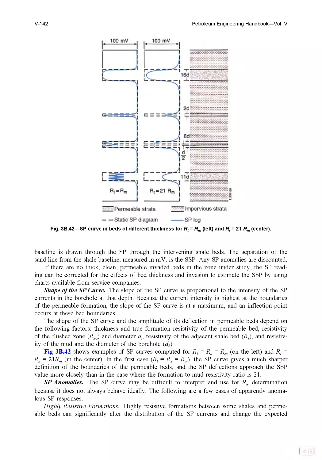
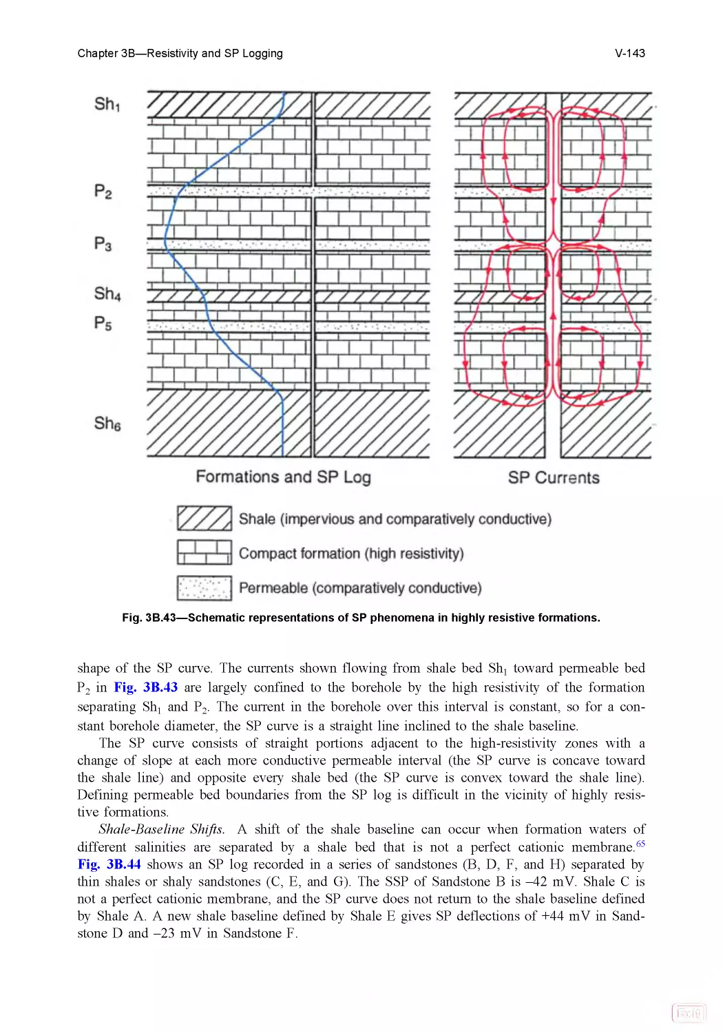
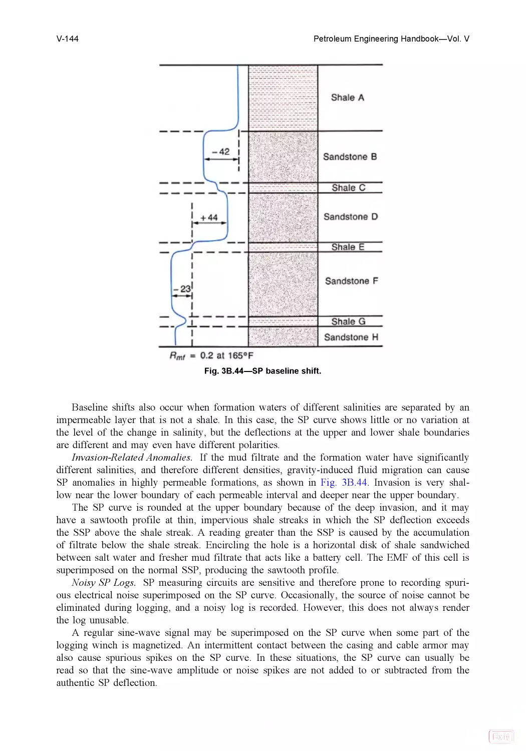
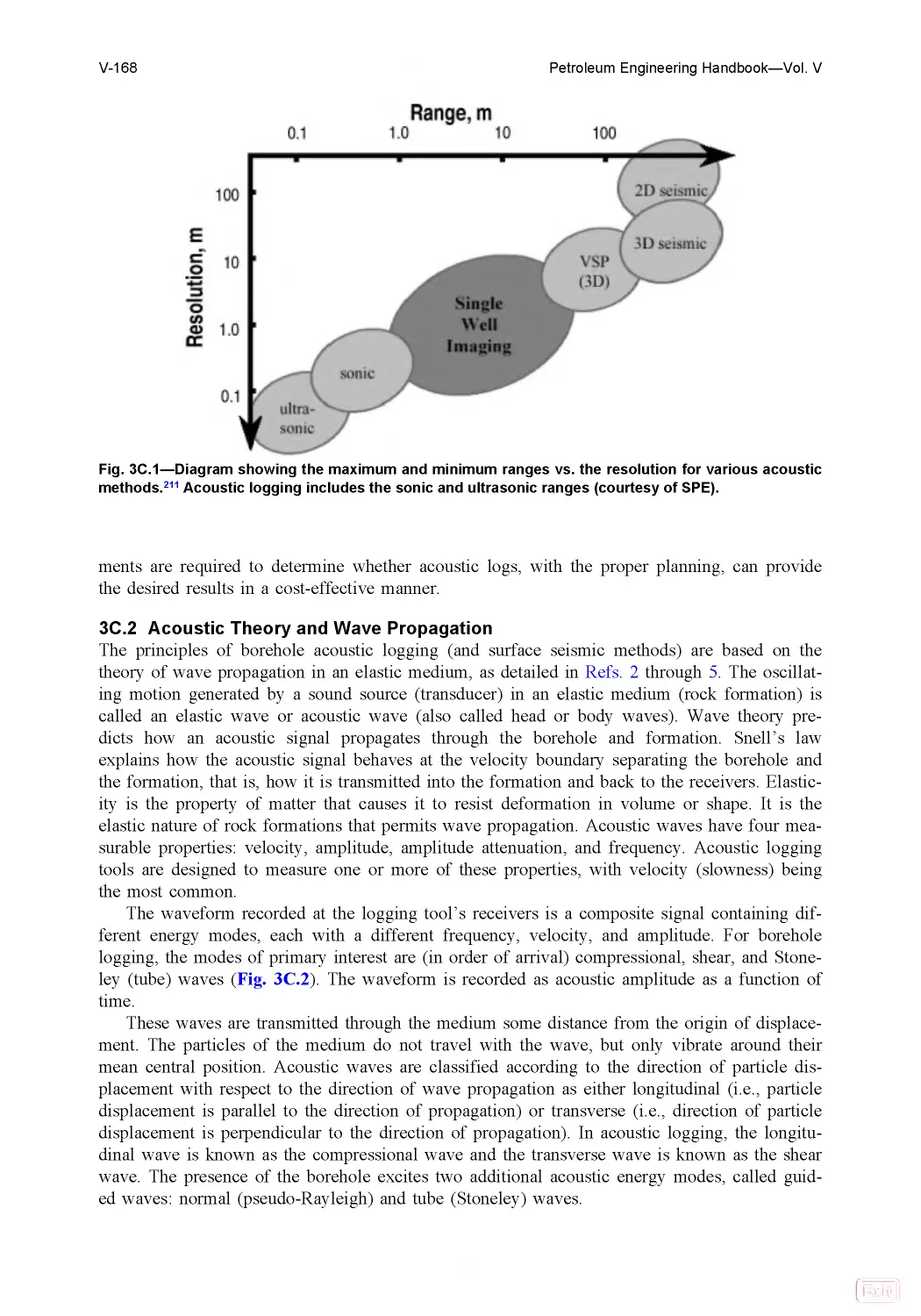
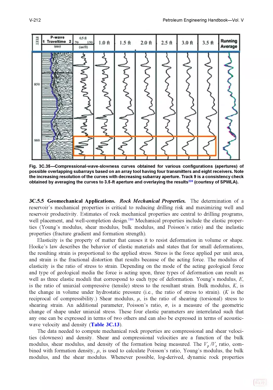
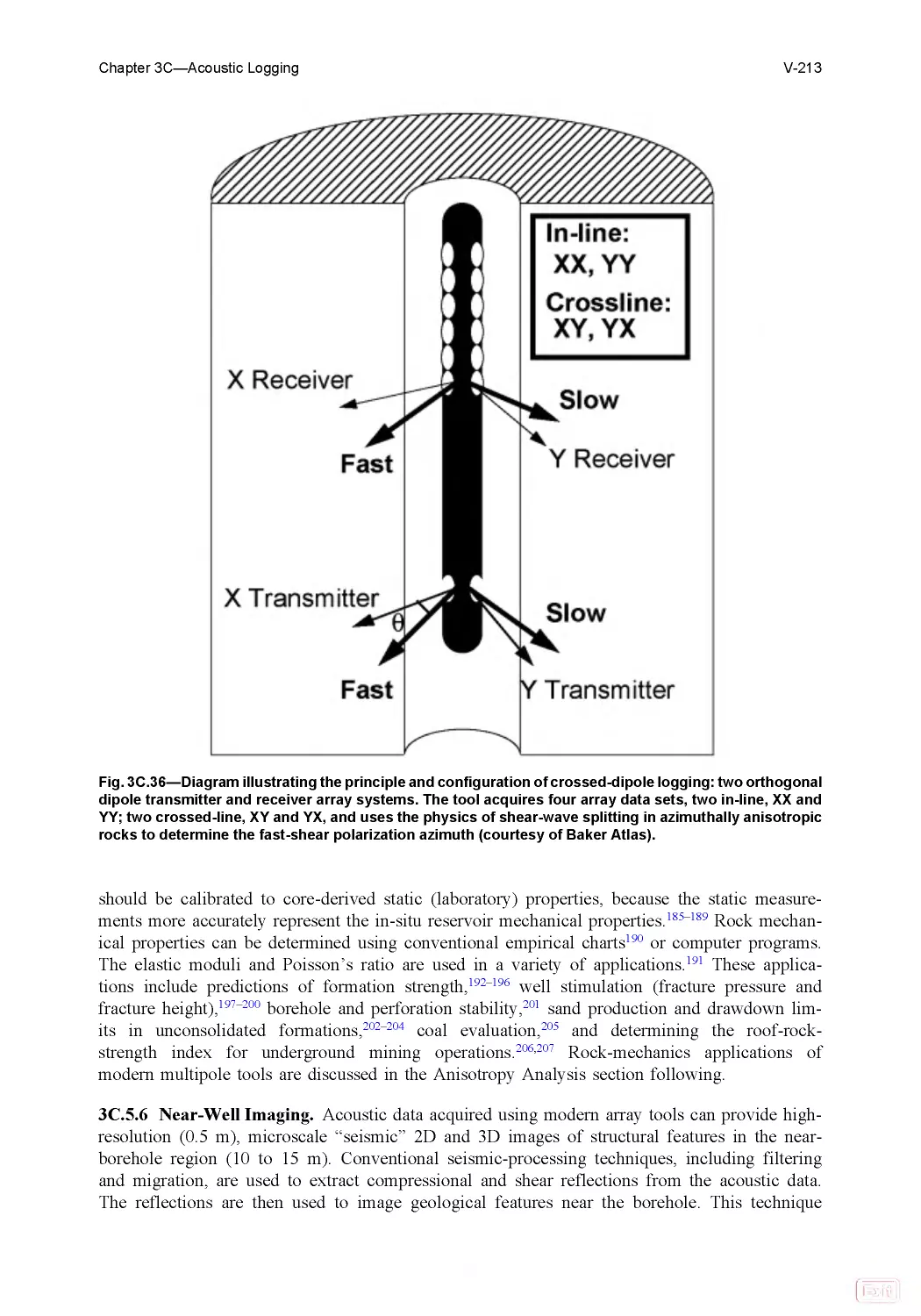
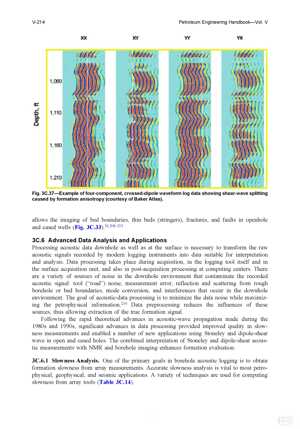
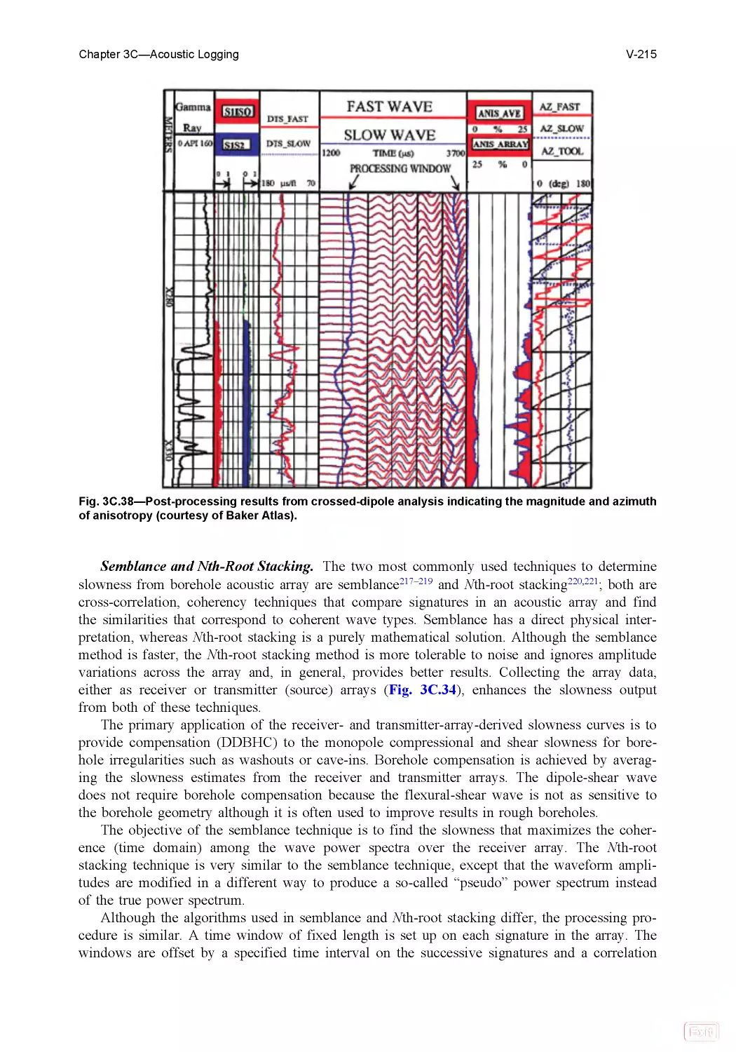
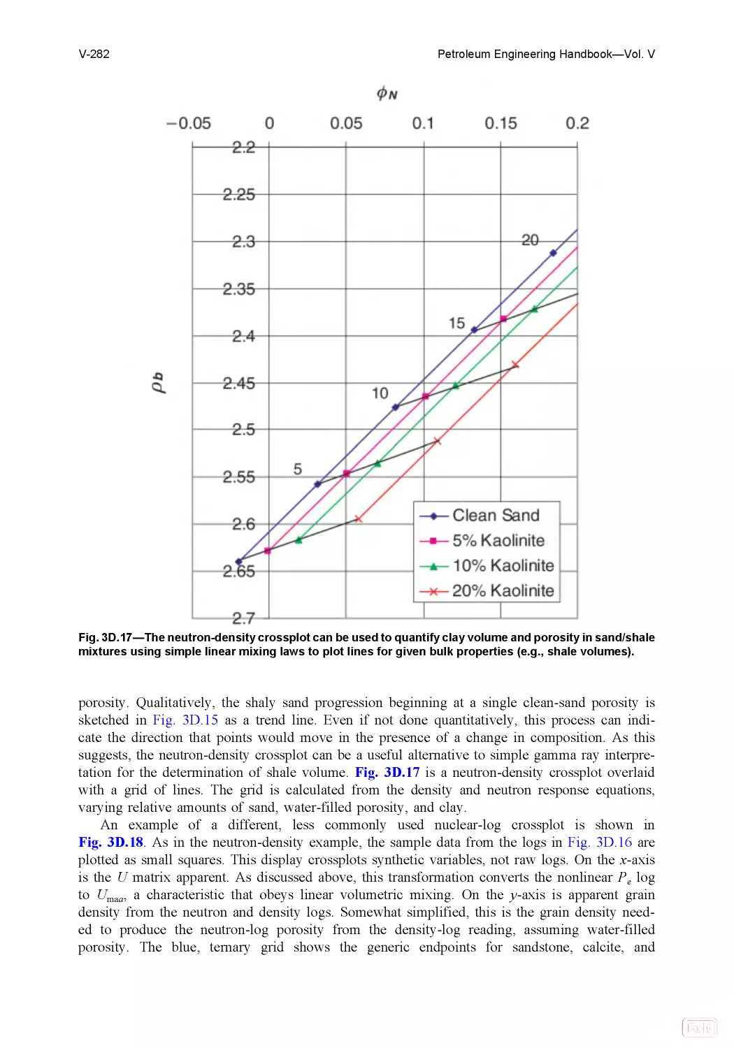
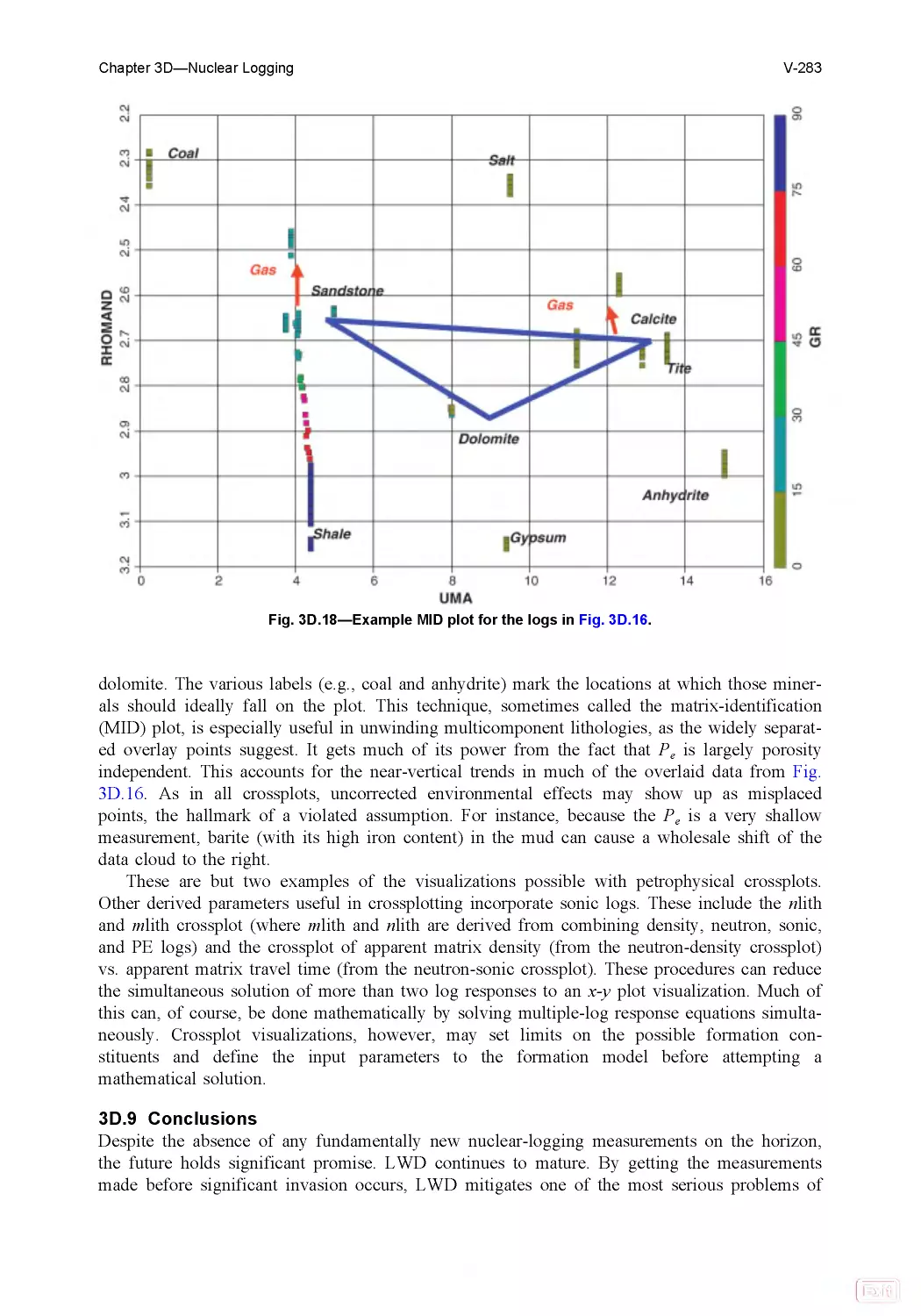
Text
PETROLEUM
ENGINEERING
HANDBOOK
Larry W. Lake, Editor-in-Chief
Volume V
RESERVOIR
ENGINEERING
and PETROPHYSICS
Edward D. Holstein, Editor
SOCIETY OF PETROLEUM ENGINEERS
Welcome to the Petroleum Engineering Handbook
How to use the Handbook:
Use to navigate forward and backward through the Handbook.
Press at any point to be taken back to the Contents page.
Perform a word or phrase search of the entire Handbook.
Press to launch the print dialog box.
View an extended list of chapter and section bookmarks.
View the Adobe® Reader® help file.
Press to exit out of the Handbook.
Use the tool bar at the bottom of the screen to jump to a specific page.
Contents Next
PETROLEUM
ENGINEERING
HANDBOOK
Larry W. Lake, Editor-in-Chief
Volume V
RESERVOIR
ENGINEERING
and PETROPHYSICS
Edward D. Holstein, Editor
SOCIETY OF PETROLEUM ENGINEERS
Petroleum Engineering Handbook
Larry W. Lake, Editor-in-Chief
I General Engineering John R. Fanchi, Editor
II Drilling Engineering Robert F. Mitchell, Editor
III Facilities and Construction Engineering Kenneth E. Arnold, Editor
IV Production Operations Engineering Joe Dunn Clegg, Editor
V Reservoir Engineering and Petrophysics Edward D. Holstein, Editor
VI Emerging and Peripheral Technologies H.R. Warner Jr., Editor
VII Indexes and Standards
Back
Next
Contents
PETROLEUM
ENGINEERING
HANDBOOK
Larry W. Lake, Editor-in-Chief
Volume V
RESERVOIR
ENGINEERING
and PETROPHYSICS
Edward D. Holstein, Editor
SOCIETY OF PETROLEUM ENGINEERS
Petroleum Engineering Handbook
Larry W. Lake, Editor-in-Chief
U. of Texas at Austin
Volume V
Reservoir Engineering and Petrophysics
Edward D. Holstein, Editor
Consultant
Society of Petroleum Engineers
Back
Next
Contents
PETROLEUM
ENGINEERING
HANDBOOK
Larry W. Lake, Editor-in-Chief
Volume V
RESERVOIR
ENGINEERING
and PETROPHYSICS
Edward D. Holstein, Editor
SOCIETY OF PETROLEUM ENGINEERS
© Copyright 2007 Society of Petroleum Engineers
All rights reserved. No portion of this publication may be reproduced in any form or by any means, including electronic
storage and retrieval systems, except by explicit, prior written permission of the publisher except for brief passages
excerpted for review and critical purposes.
Manufactured in the United States of America.
ISBN 978-1 -55563-120 -8 (print)
ISBN 978-1 -55563-121 -5 (CD)
ISBN 978-1 -55563-132 -1 (print and CD)
ISBN 978-1 -55563-126 -0 (Complete 7-Vol. Set, print)
ISBN 978-1 -55563-127 -7 (Complete 7-Vol. Set, CD)
ISBN 978-1 -55563-135 -2 (Complete 7-Vol. Set, print and CD)
0708091011121314/987654321
Society of Petroleum Engineers
222 Palisades Creek Drive
Richardson, TX 75080-2040 USA
http://store.spe.org/
service@spe.org
1.972 .952.9393
Back
Next
Contents
PETROLEUM
ENGINEERING
HANDBOOK
Larry W. Lake, Editor-in-Chief
Volume V
RESERVOIR
ENGINEERING
and PETROPHYSICS
Edward D. Holstein, Editor
SOCIETY OF PETROLEUM ENGINEERS
Foreword
This 2006 version of SPE’s Petroleum Engineering Handbook is the result of several years of effort by technical editors, copy edi-
tors, and authors. It is designed as a handbook rather than a basic text. As such, it will be of most benefit to those with some experience
in the industry who require additional information and guidance in areas outside their areas of expertise. Authors for each of the more
than 100 chapters were chosen carefully for their experience and expertise. The resulting product of their efforts represents the best
current thinking on the various technical subjects covered in the Handbook.
The rate of growth in hydrocarbon extraction technology is continuing at the high level experienced in the last decades of the 20th
century. As a result, any static compilation, such as this Handbook, will contain certain information that is out of date at the time of pub-
lication. However, many of the concepts and approaches presented will continue to be applicable in your studies, and, by documenting
the technology in this way, it provides new professionals an insight into the many factors to be considered in assessing various aspects
of a vibrant and dynamic industry.
The Handbook is a continuation of SPE’s primary mission of technology transfer. Its direct descendents are the “Frick” Handbook,
published in 1952, and the “Bradley” Handbook, published in 1987. This version is different from the previous in the following ways:
• It has multiple volumes in six different technical areas with more than 100 chapters.
• There is expanded coverage in several areas such as health, safety, and environment.
• It contains entirely new coverage on Drilling Engineering and Emerging and Peripheral Technologies.
• Electronic versions are available in addition to the standard bound volumes.
This Handbook has been a monumental undertaking that is the result of many people’s efforts. I am pleased to single out the con-
tributions of the six volume editors:
General Engineering—John R. Fanchi, Colorado School of Mines
Drilling Engineering—Robert F. Mitchell, Landmark Graphics Corp.
Facilities and Construction Engineering—Kenneth E. Arnold, AMEC Paragon
Production Operations Engineering—Joe D. Clegg, Shell Oil Co., r etired
Reservoir Engineering and Petrophysics—Ed Holstein, Exxon Production Co., r etired
Emerging and Peripheral Technologies—Hal R. Warner, Arco Oil and Gas, retired
It is to these individuals, along with the authors, the copy editors, and the SPE staff, that accolades for this effort belong. It has been
my pleasure to work with and learn from them.
—Larry W. Lake
Back
Next
Contents
PETROLEUM
ENGINEERING
HANDBOOK
Larry W. Lake, Editor-in-Chief
Volume V
RESERVOIR
ENGINEERING
and PETROPHYSICS
Edward D. Holstein, Editor
SOCIETY OF PETROLEUM ENGINEERS
Preface
This volume consists of 27 chapters that deal with the many aspects of reservoir engineering. The chapters
were assembled to provide information on acquiring and interpreting data that describe reservoir rock and fluid
properties; acquiring, understanding, and predicting fluid flow in the reservoir; interpreting measurements of well
performance; calculating the factors that impact both primary and improved recovery mechanisms from oil and gas
reservoirs; estimating reserves and calculating project economics; simulating reservoir performance; and structuring
and measuring the effectiveness of a reservoir management system.
These chapters have been written as a handbook and, as such, assume that the reader has a familiarity with
fundamentals and some experience in the production of hydrocarbons and will use this publication as a refresher
or to expand knowledge in certain areas of technology. Extensive references in each chapter indicate the amount of
material that has been considered and distilled.
This updated version of SPE’s Petroleum Engineering Handbook contains information on many of the subjects
covered by the 1962 and 1987 versions. All chapters in this version are new and greatly expanded; chapters existing
in the older versions have been revised extensively or rewritten completely, and new chapters have been added on
geophysics; geology; petrophysics; production logs; chemical tracers; foam, polymer, and resin injection; miscible
processes; valuation; and reservoir management.
The high quality of this volume is a credit to the authors of each chapter; they were chosen for their extensive
knowledge and experience. Special recognition and thanks go to E.C. Thomas, who is responsible for the quality
and thoroughness of the chapters contained in the petrophysical section. The resulting product contains many good
tips and guidelines that represent lessons learned in the practice of applying various technologies to a wide range of
actual field conditions. Numerous field examples have been included to illustrate these applications.
—Edward D. Holstein
Back
Next
Contents
PETROLEUM
ENGINEERING
HANDBOOK
Larry W. Lake, Editor-in-Chief
Volume V
RESERVOIR
ENGINEERING
and PETROPHYSICS
Edward D. Holstein, Editor
SOCIETY OF PETROLEUM ENGINEERS
1 Reservoir Geology - click to view
F. Jerry Lucia
2 Fundamentals of Geophysics - click to view
Bob A. Hardage
3A Petrophysics - click to view
E.C. Thomas
3B Resistivity and SP Logging - click to view
T.D. Barber, A . Brie, and B.I . Anderson
3C Acoustic Logging - click to view
Doug Patterson and Stephen Prensky
3D Nuclear Logging - click to view
Gary D. Myers
3E Nuclear Magnetic Resonance Applications in
Petrophysics and Formation Evaluation - click to view
Stephen Prensky and Jack Howard
3F Mud Logging - click to view
Dennis E. Dria
3G Specialized Well-Logging Topics - click to view
Paul F. Worthington
3H Petrophysical Applications - click to view
H.R . Warner Jr. and Richard Woodhouse
4 Production Logging - click to view
R.M. McKinley and Norman Carlson
5 The Single-Well Chemical Tracer Test—A Method
for Measuring Reservoir Fluid Saturations In Situ
Harry Deans and Charles Carlisle - click to view
6 Well-To-Well Tracer Tests - click to view
Øyvind Dugstad
7 Reservoir Pressure and Temperature - click to view
David Harrison and Yves Chauvel
8 Fluid Flow Through Permeable Media - click to view
John Lee
9 Oil Reservoir Primary Drive Mechanisms - click to view
Mark P. Walsh
10 Gas Reservoirs - click to view
Mark A. Miller and E.D. Holstein
11 Waterflooding - click to view
H.R . Warner Jr.
12 Immiscible Gas Injection in Oil Reservoirs - click to view
H.R . Warner Jr. and E.D. Holstein
13 Polymers, Gels, Foams, and Resins - click to view
Robert D. Sydansk
Contents
Back
Next
Search
Help
PETROLEUM
ENGINEERING
HANDBOOK
Larry W. Lake, Editor-in-Chief
Volume V
RESERVOIR
ENGINEERING
and PETROPHYSICS
Edward D. Holstein, Editor
SOCIETY OF PETROLEUM ENGINEERS
14 Miscible Processes - click to view
E.D. Holstein and Fred I. Stalkup
15 Thermal Recovery by Steam Injection - click to view
Jeff Jones
16 In-Situ Combustion - click to view
William E. Brigham and Louis Castanier
17 Reservoir Simulation - click to view
Rod P. Batycky, Marco R. Thiele, K.H. Coats,
Alan Grindheim, Dave Ponting, John E. Killough,
Tony Settari, L . Kent Thomas, John Wallis,
J.W . Watts, and Curtis H. Whitson
18 Estimation of Primary Reserves of Crude Oil,
Natural Gas, and Condensate - click to view
Ron Harrell and Chap Cronquist
19 Valuation of Oil and Gas Reserves - click to view
D.R . Long
20 Reservoir Management Programs - click to view
E.D. Holstein and E.G. Woods
Author Index - click to view
Subject Index - click to view
Contents
Back Search
Help
Chapter 1
Reservoir Geology
F. Jerry Lucia, SPE, U. of Texas at Austin
1.1 Introduction
The efficient extraction of oil and gas requires that the reservoir be visualized in 3D space.
Engineers need a conceptual model of reservoirs, an integral part of the decision-making pro-
cess, whether it be selecting perforations or forecasting future production. However, most
engineering measurements made on reservoirs have little or no spatial information. For exam-
ple, a core measurement has no dimensional information, wireline logs and continuous core
measurements are 1D, and production data and pressure information are volumetric but with
unconstrained spatial information. Geologic information, on the other hand, contains valuable
spatial information that can be used to visualize the reservoir in 3D space. Therefore, engineers
should understand the geologic data that can improve their conceptual model of the reservoir
and, thus, their engineering decisions.
The first and most important geologic information is the external geometry of the reservoir,
which is defined by seals or flow barriers that inhibit the migration of hydrocarbons, forming a
hydrocarbon trap. The buoyancy force produced by the difference in density between water and
hydrocarbons drives migration. Migration will cease, and a hydrocarbon reservoir will form,
only where hydrocarbons encounter a trap. Traps are composed of top, lateral, and bottom
seals; the geometry of traps can have structural, sedimentary, or diagenetic origins.
The second most important geologic information is the internal reservoir architecture. A
reservoir is composed of rock types of varying reservoir quality that are systematically stacked,
according to stratigraphic and diagenetic principles. The lateral distribution of depositional tex-
tures is related to depositional environments, and the vertical stacking of textures is described
by stratigraphy, which is the geological study of the form, arrangement, geographic distribu-
tion, chronologic succession, classification, and correlation of rock strata. Diagenesis, changes
that happen to the sediment after deposition, can also control the lateral continuity and vertical
stacking of reservoir rock types. This fact is most important in carbonate reservoirs, in which
the conversion of limestone to dolostone and the dissolution of carbonate have a large effect
on internal reservoir architecture.
The most basic concern for most engineers is the spatial distribution of petrophysical prop-
erties, such as porosity, permeability, water saturation, and relative permeability. To visualize
the reservoir in petrophysical terms, the engineer must be able to equate measurements (log,
core, or production) with geologic models because the measurements themselves do not contain
Print
Search Contents
Home
Chapter 2 Bookmarks
Help
spatial information. Linking engineering measurements with geologic descriptions is best done
at the rock-fabric level because rock fabric controls pore-size distribution, which, in turn, con-
trols porosity, permeability, and capillary properties. Rock fabrics can be tied directly to
stratigraphic models and, thus, to 3D space.
1.2 External Geometry—Reservoir Traps
1.2 .1 Introduction. Hydrocarbons are formed by anaerobic decomposition of organic matter
that accumulates from the deposition of plankton in deep ocean basins. Oil and gas are generat-
ed as the sediments are buried and the temperature rises. Oil is the first hydrocarbon to be
generated, followed by wet gas, and lastly by dry gas. Once generated, oil and gas flow verti-
cally and laterally through overlying sediments because of the density difference between
hydrocarbons and formation water and they migrate through permeable formations until they
encounter a reservoir trap in which oil and gas accumulate. Oil will fill the traps first because
it is first to be generated. Higher temperatures resulting from continued burial cause gas to be
generated. Migrating gas will displace oil from the traps because gas has a lower density. The
displaced oil will migrate further updip and fill any trap encountered.1
Traps filled with hydrocarbons are often referred to as pools. However, engineers normally
use the term reservoir instead of pool for an oil and gas accumulation, and reservoir will be
used throughout this chapter. A field is composed of one or more reservoirs in a single area. A
trap is defined by the geometry of its seals, which are formations with very low permeability
and very small pores that will impede or stop the flow of hydrocarbons. To trap migrating
hydrocarbons, seals must contain flow in 3D: the seals must form a closure. In the simplest
terms, a trap is similar to a box with its bottom removed. The box is the seal composed of top
and lateral seals. A trap may also contain a bottom seal. Imagine a smaller box inserted into
the base of the original box. The smaller box is also a seal and confines the reservoir to a
layer within the larger box.
Seals may be in the form of impermeable lithologies or faults. The simplest traps are con-
vex structures in which the sealing layer dips in all directions from a central structural high,
forming domes or doubly dipping anticlines. More complex structural traps are formed when
convex structures are truncated by faults or when faulting occurs around a piercement struc-
ture. Many traps are combinations of structural uplift, faulting, and stratigraphy, such as an
updip pinchout of a sand body into an impermeable shale. A purely stratigraphic trap may
form when deposition creates a topographic high that is encased by impermeable lithology,
such as shale or salt.
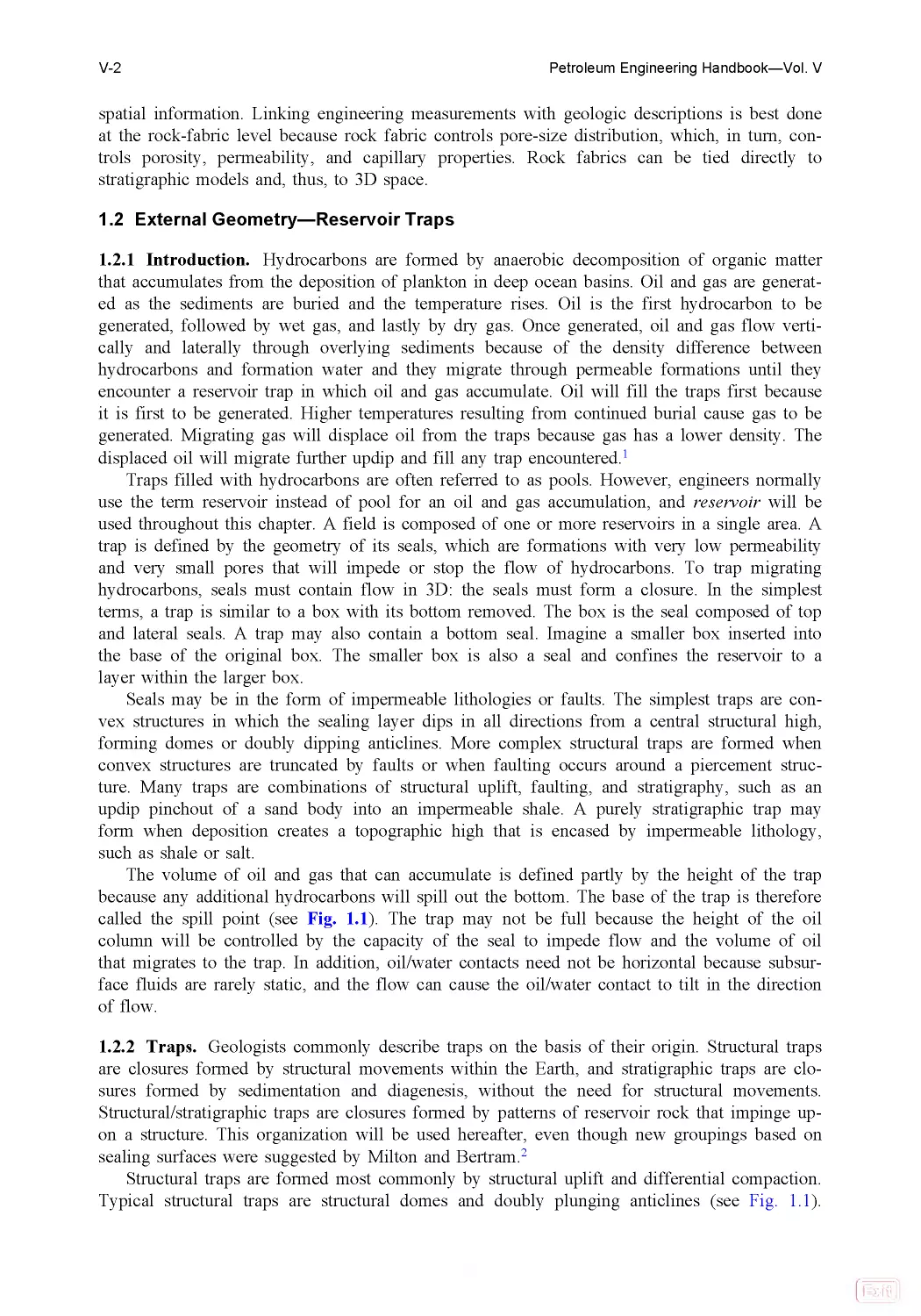
The volume of oil and gas that can accumulate is defined partly by the height of the trap
because any additional hydrocarbons will spill out the bottom. The base of the trap is therefore
called the spill point (see Fig. 1 .1). The trap may not be full because the height of the oil
column will be controlled by the capacity of the seal to impede flow and the volume of oil
that migrates to the trap. In addition, oil/water contacts need not be horizontal because subsur-
face fluids are rarely static, and the flow can cause the oil/water contact to tilt in the direction
of flow.
1.2.2 Traps. Geologists commonly describe traps on the basis of their origin. Structural traps
are closures formed by structural movements within the Earth, and stratigraphic traps are clo-
sures formed by sedimentation and diagenesis, without the need for structural movements.
Structural/stratigraphic traps are closures formed by patterns of reservoir rock that impinge up-
on a structure. This organization will be used hereafter, even though new groupings based on
sealing surfaces were suggested by Milton and Bertram.2
Structural traps are formed most commonly by structural uplift and differential compaction.
Typical structural traps are structural domes and doubly plunging anticlines (see Fig. 1 .1).
V-2
Petroleum Engineering Handbook—Vol. V
Print
Search
Home
Bookmarks
Help
Contents
Chapter 2
These traps have a structural high and quaquaversal dips (the seal dips away from a structural
high in all directions). The bulk of the world’s oil is found in these four-way-closure traps,3
which were the first type to be exploited by surface mapping. Many major oil fields in the
world were discovered by using surface mapping to locate domal structures.
A more complex method of forming a structural trap is by faulting and structural uplift (see
Fig. 1.1). Faulted structures can vary from a simple faulted anticline to complex faulting
around piercement structures and domal uplifts. Faulted structures are very common and form
some of the most complex reservoirs known. Types of faults include normal, listric, reverse,
and thrust, which are related to the stress fields generated during structural movement. Pierce-
ment traps (diapirs) are formed typically by salt moving up through a stack of sediment driven
by the density difference between salt and quartz or carbonate. Closure is achieved by the up-
lift of sediments juxtaposed to the piercement dome, by the top seal being an overlying
impervious bed and the lateral seals being formed by structural dip, by sealing faults, or by the
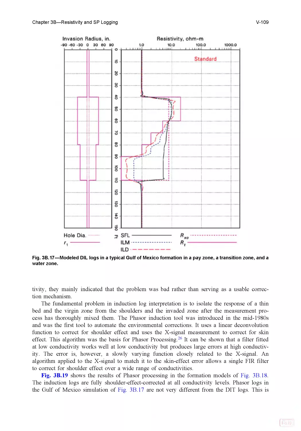
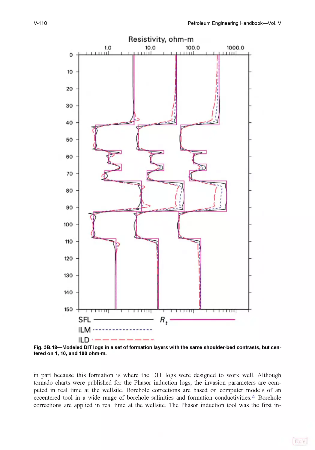
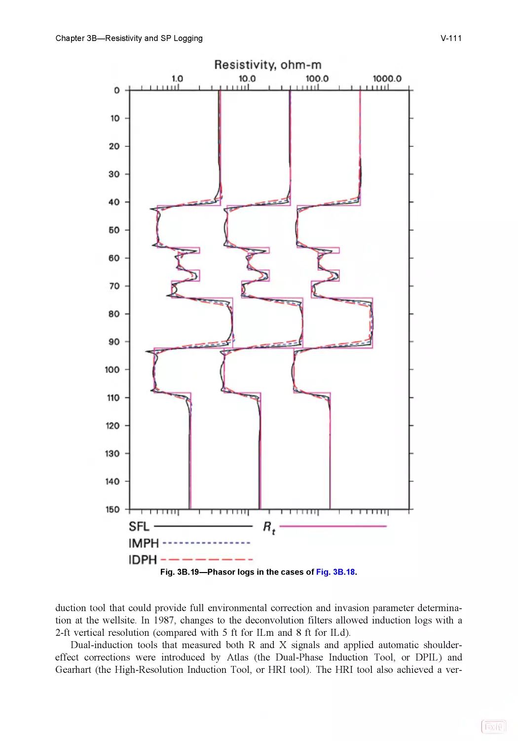
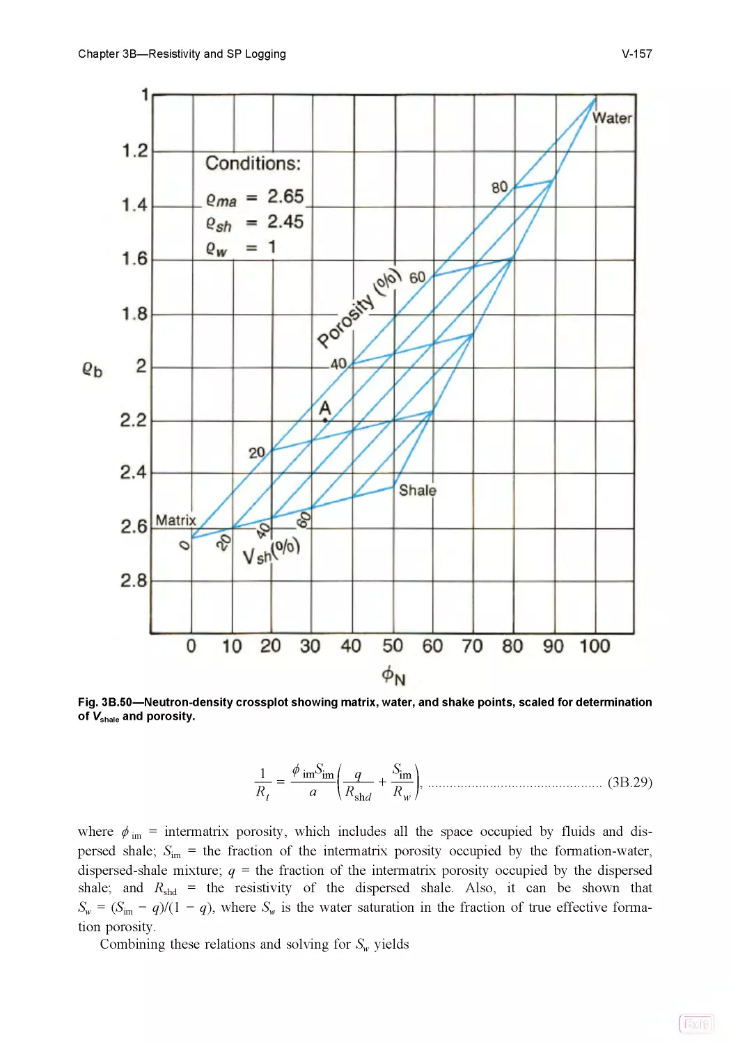
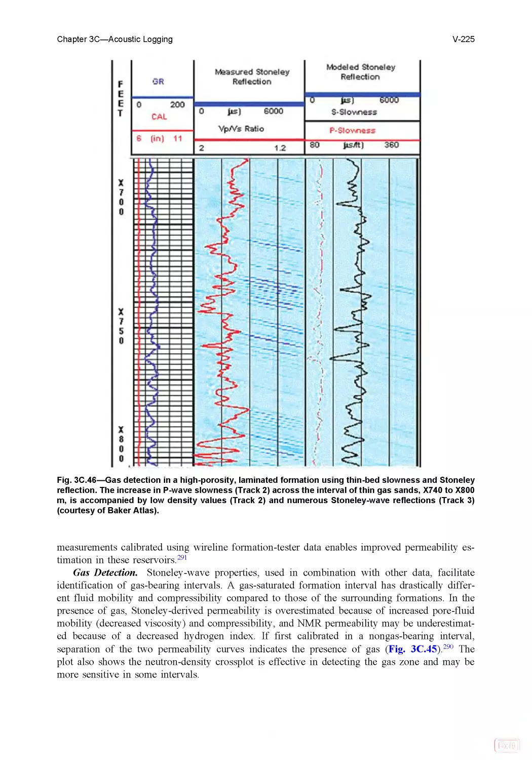
Fig. 1.1—Diagram description of hydrocarbon traps.
Chapter 1—Reservoir Geology
V-3
Print
Search
Home
Bookmarks
Help
Contents
Chapter 2
piercement salt. Faulted reservoirs commonly have a bottom seal formed by the lower contact
of sand with shale. The bottom seal, along with the oil/water contact within the sand body,
forms the base of the reservoir.
Structural/stratigraphic traps are formed by a combination of structure, deposition, and dia-
genesis. The most common form, the updip pinchout of reservoir lithology into a sealing
lithology (see Fig. 1 .1), is found in the flanks of structures. The top and updip seal is normally
an impervious rock type, and the lateral seals are formed by either structural dip or the lateral
pinchout of reservoir rock into seal material. The base of the reservoir is defined by a bottom
seal composed of impervious rock and by an oil/water contact. During relative sea-level fall,
streams may erode deep valleys, thus forming lateral seals for fluvial sediments. Onlap of sand
onto a paleotopographic high during relative sea-level rise can produce an updip seal for a
sand body. Unconformity traps are formed by the truncation of dipping strata by overlying
bedded sealing lithology. The reservoir rock may be found in the form of buried hills formed
by erosion during the time of the unconformity. The oil/water contact forms the base of these
reservoirs. A stratigraphic trap may be partly related to diagenetic processes; for example, the
updip seal for the supergiant Coalinga field, California, is tar- and asphalt-filled sandstone and
conglomerate. Many traps in the Permian reservoirs of west Texas, are formed by lateral
changes related to stratigraphy from porous to dense dolomite in an updip direction.
Stratigraphic traps are formed by depositional processes that produce paleotopographic
highs encased in impermeable material, such as evaporite or shale (Fig. 1 .1). Closure occurs
when there is contact between seal material and underlying sediment. The most common type
is a carbonate buildup, usually erroneously called a “reef.” Piles of sand deposited on the
seafloor by density currents often form broad topographic highs that, in turn, form stratigraphic
traps. Structure may also play a part in the geometry of stratigraphic traps, although the defin-
ing characteristic is that structure is not required to form the trap.
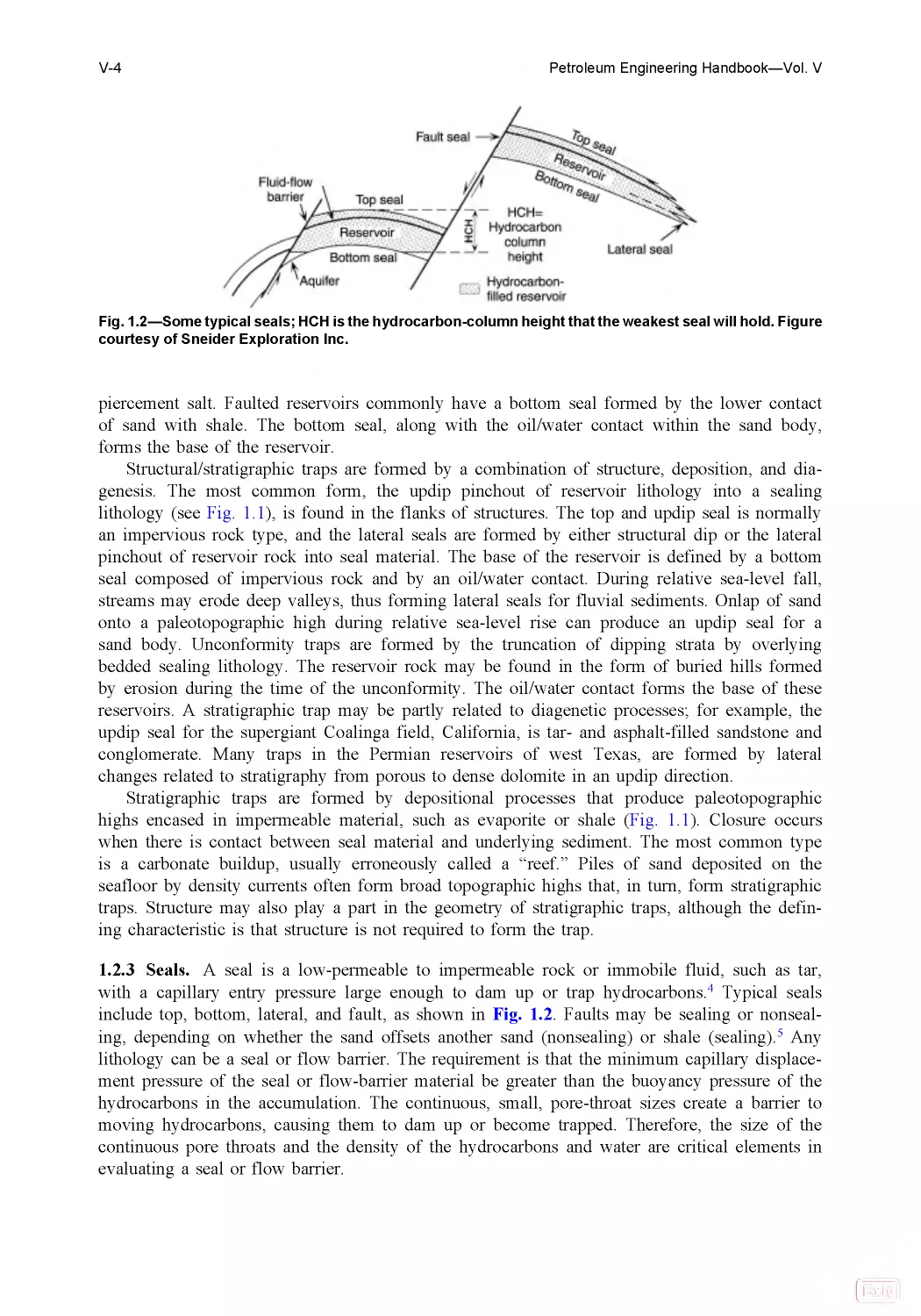
1.2.3 Seals. A seal is a low-permeable to impermeable rock or immobile fluid, such as tar,
with a capillary entry pressure large enough to dam up or trap hydrocarbons.4 Typical seals
include top, bottom, lateral, and fault, as shown in Fig. 1 .2 . Faults may be sealing or nonseal-
ing, depending on whether the sand offsets another sand (nonsealing) or shale (sealing).5 Any
lithology can be a seal or flow barrier. The requirement is that the minimum capillary displace-
ment pressure of the seal or flow-barrier material be greater than the buoyancy pressure of the
hydrocarbons in the accumulation. The continuous, small, pore-throat sizes create a barrier to
moving hydrocarbons, causing them to dam up or become trapped. Therefore, the size of the
continuous pore throats and the density of the hydrocarbons and water are critical elements in
evaluating a seal or flow barrier.
Fig. 1 .2 —Some typical seals; HCH is the hydrocarbon-column height that the weakest seal will hold. Figure
courtesy of Sneider Exploration Inc.
V-4
Petroleum Engineering Handbook—Vol. V
Print
Search
Home
Bookmarks
Help
Contents
Chapter 2
Porosity and permeability are not the best criteria for evaluating seal and flow-barrier behav-
ior. The seal capacity of a rock can be best evaluated with a mercury porosimeter that can
inject mercury into material using pressures as high as 60,000 psi. The key equation used in
capillary pressure/saturation evaluation of reservoir rocks, seals, and flow barriers is:
hc
=
(pc
ρw
−
ρhc
)0.433 ft, ..................................................... (1.1)
in which hc = the maximum hydrocarbon column held, pc = the capillary entry pressure, ρw=
the density of water, and ρhc = the density of the hydrocarbon. The capillary pressure used is
usually not the capillary entry pressure but the capillary pressure at a mercury saturation of
between 5 and 10% because of closure effects.
Effective hydrocarbon seals for exploration plays and reservoirs must be laterally continu-
ous. Some typical seal lithologies, illustrated in Fig. 1 .3, have entry pressures ranging from 14
to 20,000 psi. With data from more than 3,000 seals, we can group the data into Classes A
through E to categorize the typical lithologies listed in Fig. 1 .3 from most to least ductile. Fig.
1.3 also illustrates the hydrocarbon column that can be held, assuming that the fluid is 35°API
oil and saline water. Evaporite and kerogen-rich shale can hold the greatest oil column—from
1,000 to more than 5,000 ft. Clay-mineral-rich shale, silty shales, and dense mudstones can
hold between 500 and 1,000 ft of oil column. Sandy shales are ranked next, with a 100- to 500-
ft capacity, whereas very shaly siltstone and sandstone, anhydrite-filled dolostones, and cement-
ed sandstone each have between 50 and 100 ft of capacity. In addition, immobile fluids, such
as tar, bitumen, and asphalt, can be effective seals and barriers. For example, the updip seal for
the supergiant Coalinga field, California, is tar- and asphalt-filled sandstone and conglomerate.
1.3 Reservoir Base
Whereas structure and stratigraphy most often define the reservoir trap or top of the reservoir,
factors controlling the base of a petroleum reservoir include seal capacity, spill point, capillary
forces, and hydrodynamics.6 ,7 The reservoir base is defined as the zero capillary pressure level,
also referred to as the free-water level. Reservoir height is determined by the height from seal
to spill point, if seal capacity is large enough. If the height is less than that from seal to spill
point, seal capacity or hydrocarbon charge will determine the position of the reservoir base.
Subsurface groundwater is seldom static. Differences in water density, structural tilting, tec-
tonic forces, and other factors combine to create a difference in hydrodynamic potentials that
result in the movement of fluids in the subsurface. Fluid movement is controlled by the fluid
potential as defined by Hubbert6 and illustrated by the following formula8:
H=Z+
P
ρwg
, .............................................................. (1.2)
in which Z = elevation relative to a datum (sea level), P = measured static pressure, and ρ =
density of the fluid (water).
A potentiometric map is a map that connects points of equal fluid potential within an
aquifer. If the potentiometric surface is not horizontal, the aquifer will flow in the direction of
lowest potential. Calculating fluid potential requires accurate subsurface pressure measurements
in the aquifer. The flow of water under a reservoir will cause the zero-capillary-pressure level
to tilt, referred to as a tilted water table. The degree of tilt can be estimated from the following
equation.
Chapter 1—Reservoir Geology
V-5
Print
Search
Home
Bookmarks
Help
Contents
Chapter 2
tanθ=
ΔZ
x
=
(ρw
ρw
−
ρo
)dhdx
, ................................................. (1.3)
in which
ΔZ
x
= change in reservoir height for distance x (tilt in water table), ρ
w
= density of
water in aquifer, ρ
o
= density of hydrocarbon, and
dh
dx
= change in potentiometric surface for
distance x.
Fig. 1 .3 —(a) Air/mercury capillary pressure curves of seal lithologies. The ordinate is a log scale. (b) Typ-
ical seal lithologies. (c) Sneider et al.3 classification of seals and flow barriers. The hydrocarbon column
that can be held assumes that the fluids in the reservoirs are 35°API oil and saline water. Types are keyed
to Figs. 3a and 3b. Figure courtesy of Sneider Exploration Inc.
V-6
Petroleum Engineering Handbook—Vol. V
Print
Search
Home
Bookmarks
Help
Contents
Chapter 2
During primary development, the economic base of the reservoir is normally defined as the
producing oil/water contact, or the level at which oil and water are first coproduced. This level
is generally assumed to be at approximately 50% water saturation, according to relative perme-
ability considerations. During tertiary development, the economic base of the reservoir may be
defined as the level of zero oil saturation. However, because pore size can vary with stratigra-
phy, 50 or 100% water saturation may not occur at the same height throughout the reservoir.
The economic base of the reservoir will not be horizontal.
Defining the base of a reservoir is often made difficult by the presence of residual-oil and
tar zones below the producing oil/water contact. Residual-oil and tar zones can be as thick as
300 ft and are thought to form by a variety of processes, including biodegradation of hydrocar-
bons, flushing of part of the oil column as a result of hydrodynamic forces, and remigrating of
hydrocarbons because of leaky seals and structural tilting. The presence of this material may
indicate that the reservoir is in an imbibition rather than a drainage mode. Estimates of the
original oil in place will depend on which capillary pressure model is assumed. An incorrect
model can lead to large errors in estimates of the original oil in place.
1.4 Internal Geometry—Reservoir Architecture
1.4 .1 Introduction. Information that defines the external reservoir geometry, including trap
configuration, seal capacity, and the base of the reservoir, is of primary importance during ex-
ploration and initial development of a reservoir. As development continues, reservoir architec-
ture becomes key to predicting the distribution of reservoir quality so that primary- and secondary-
development programs can be planned. Reservoir architecture is important because it provides
a basis for distributing petrophysical properties in 3D space. In most cases, this operation is
done by relating lithofacies to petrophysical properties because lithofacies can be directly
linked to depositional processes for prediction.
We commonly correlate lithofacies from one well to the next by assuming a degree of hori-
zontality and continuity of similar facies. This approach leads to images with highly continuous
lithofacies and porosity zones. Many depositional facies, however, are known to be highly dis-
continuous laterally and vertically, and correlating similar lithofacies from one well to the next
can lead to unrealistic displays of reservoir architecture. Modern correlation methods rely more
on the chronostratigraphic approach, one that uses time stratigraphy rather than lithostratigra-
phy to determine continuity between wells. This approach is referred to as sequence stratigra-
phy and provides a basis for correlating time surfaces between which lithofacies are distributed
systematically in a predictable pattern.
1.4 .2 Sequence Stratigraphy. Sequence stratigraphy is a chronostratigraphic method of corre-
lation. It groups lithofacies into time-stratigraphic units between chronostratigraphic surfaces,
which are sometimes defined by unconformities and facies shifts. A key premise is that the
surfaces are formed in response to eustatic sea-level changes of various scales and periodicity
(eustatic refers to worldwide sea-level changes affecting all oceans). It is thought that eustatic
sea-level changes can be linked to climatic changes and to eccentricities in the Earth’s orbit.
The Russian astronomer Milanovitch defined cyclic variation in the shape of the Earth’s orbit
and in the tilt and wobble of the axis. These Earth cycles are precession (19,000 to 23,000
years), obliquity (41,000 years), and eccentricity (1,000,000 to 4,000,000 years) and are
thought to cause changes in the Earth’s climate, resulting in more or less water trapped as ice
at the poles. The trapping or release of water from the ice caps is thought to result in sea-level
rise and fall, referred to as eustasy.
Sequence stratigraphy is important for reservoir modeling because a chronostratigraphic sur-
face is present in every well in the reservoir. This fact provides geologists with a powerful tool
for correlating packages of lithofacies between wells. A more realistic image of reservoir archi-
Chapter 1—Reservoir Geology
V-7
Print
Search
Home
Bookmarks
Help
Contents
Chapter 2
tecture can, therefore, be constructed by distributing lithofacies and petrophysical properties
within a detailed sequence-stratigraphic framework.
The terminology of sequence stratigraphy, like most geologic terminology, is complex and
constantly evolves as concepts and ideas change.9 ,10 It is the intent here to present a basic
overview of the terminology to provide the reader with sufficient understanding to communi-
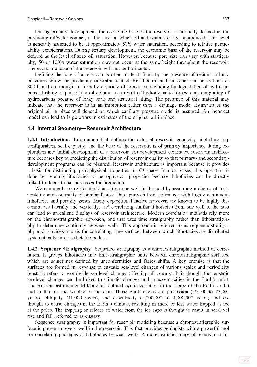
cate with reservoir geologists. The classic Exxon model (see Fig. 1 .4) shows the terminology
used in siliciclastic stratigraphy. The terms used in carbonate stratigraphy, although similar,
have important differences because carbonates are organic in origin and clastics are terrigenous
in origin. The terminology used in carbonate stratigraphy is illustrated in Fig. 1 .5 .
The smallest time-stratigraphic unit is the high-frequency cycle (HFC), or parasequence, a
unit composed of genetically related lithofacies deposited during one basic sea-level rise and
fall. Assuming a constant rate of subsidence, each cycle begins with a flooding event as sea
level rises. The flooding event is also referred to as transgression or retrogradation, the back-
ward and landward movement or retreat of a shoreline or coastline. The sea transgresses the
land, the shoreline retreats, and the space for sediment to accumulate increases. The space cre-
ated by the transgression is referred to as accommodation space. Sea-level rise is followed by a
stillstand, during which sediment completely or partly fills the accommodation space. The
buildup of sediment by deposition is referred to as aggradation. The stillstand is followed by a
relative sea-level fall during which accommodation space is reduced, forcing sediment to be
transported into the basin and resulting in progradation of the sediment body. Progradation
refers to the building forward and outward toward the sea of a shoreline or body of sediment.
During sea-level fall, the most-landward sediment may become subaerially exposed, forming an
unconformity. Farther basinward the water is deeper, and the shallowing event is identified by
a facies shift in the vertical stacking of lithofacies. The next sea-level rise produces another
flooding event, and the depositional cycle is repeated. Flooding events approximate chronostrati-
graphic surfaces and define the HFC as a time-stratigraphic unit.
Repeated eustatic sea-level cycles result in the vertical stacking of HFC. Cycles are stacked
vertically into retrogradational cycles, aggradational cycles, and progradational cycles. Retrogra-
dational cycles are formed when the eustatic sea-level rise for each cycle is much more than
the fall. The shoreline will move farther landward with each successive cycle, a pattern de-
scribed as back stepping or transgression. The sediments are said to be deposited in the
transgressive system’s track (TST). Aggradational cycles are formed when eustatic rise and fall
are equal, and the resulting facies will stack vertically. These cycles are defined as part of the
highstand system’s tract (HST). Progradational cycles form when the eustatic fall for each cy-
cle is greater that the rise. The shoreline for each successive cycle will move seaward, a
pattern described as progradation or regression, and the sediments are said to be deposited in
the HST. Sediments deposited when relative sea level is lowest are said to be deposited in the
Fig. 1.4—Exxon idealized depositional-sequence cross-sectional model for siliciclastic sediments. Se-
quence boundary (SB), LST composed of basin-floor fan (bf), slope fan (sf), and lowstand prograding
wedge (LSW), TST, HST, and shelf-margin wedge (SMW). Maximum flooding surface (mfs) separates the
TST from the HST. Taken from Kerans and Tinker.10
V-8
Petroleum Engineering Handbook—Vol. V
Print
Search
Home
Bookmarks
Help
Contents
Chapter 2
lowstand system’s track (LST). The sequence from TST to HST to LST defines a larger-scale
sea-level signal referred to as a high-frequency sequence (HFS). The turnaround from transgres-
sion to aggradation and progradation is termed the maximum flooding surface (MFS). HFSs
can be packaged into longer-term signals called composite sequences on the basis of the obser-
vation that they tend to stack vertically into transgressive, progradational, and lowstand sequences.
The terminology and duration of the cycle hierarchies estimated by Goldhammer11 are
shown in Fig. 1 .6 . HFC, HFS, and composite sequences are commonly referred to as fifth-,
fourth-, and third-order cycles, respectively, with characteristic durations ranging from 0.01 to
10 million years (m.y .) . First- and second-order cycles, or supersequences, have much longer
durations, from 10 to more than 100 m.y ., and are related more to structural movements than
to eustasy. These major sequences are useful not only for regional but also for worldwide cor-
relations. The durations of all these cycles and sequences are approximate and are based on
radiogenic dates extrapolated to the numbers of cycles and sequences of various scales.
1.5 Carbonate Reservoirs
1.5 .1 Introduction. A basic overview of carbonate-reservoir model construction was presented
by Lucia,12 and much of what is presented herein is taken from that book. Carbonate sediments
are commonly formed in shallow, warm oceans either by direct precipitation out of seawater or
by biological extraction of calcium carbonate from seawater to form skeletal material. The re-
sult is sediment composed of particles with a wide range of sizes and shapes mixed together to
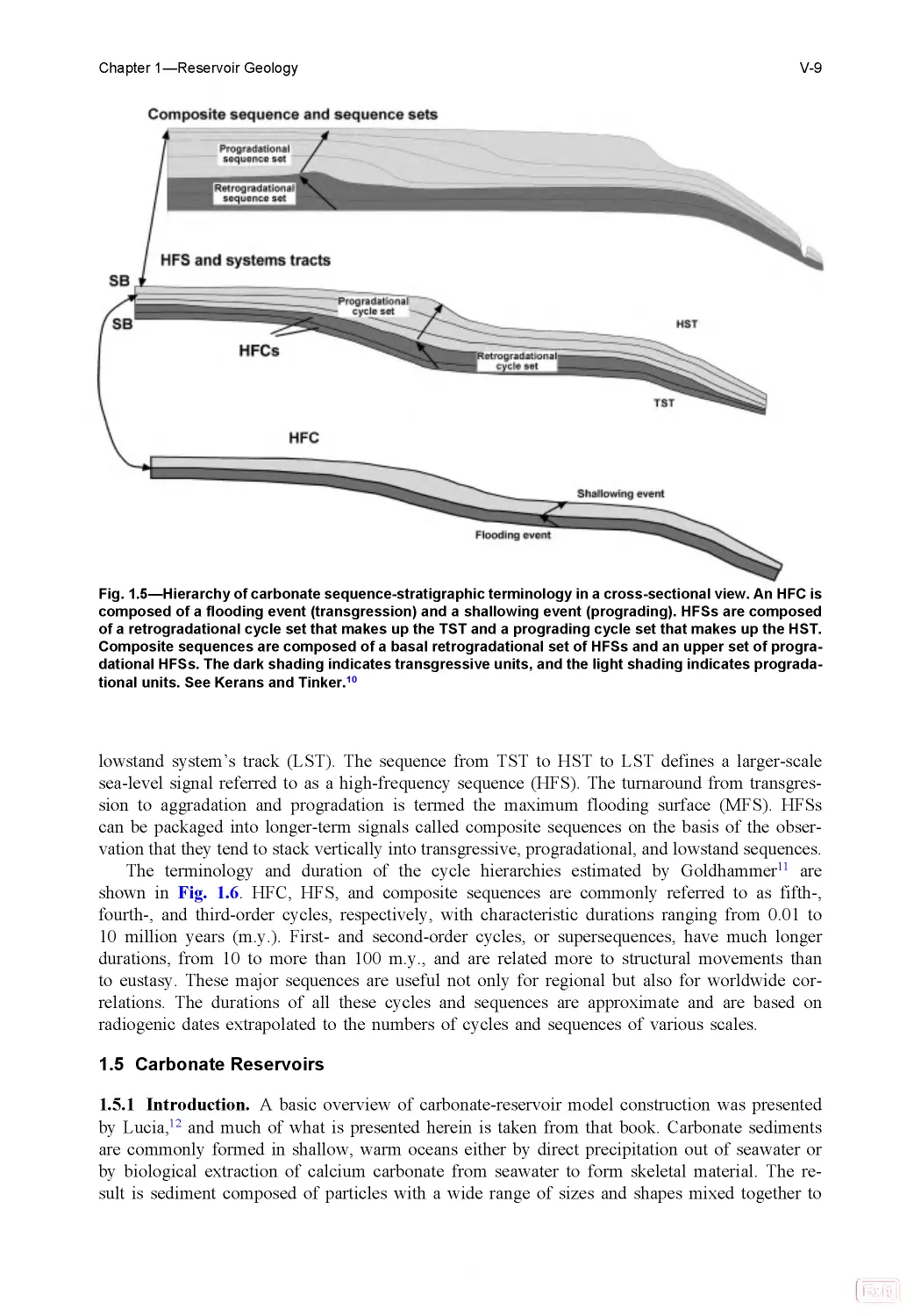
Fig. 1.5 —Hierarchy of carbonate sequence-stratigraphic terminology in a cross-sectional view. An HFC is
composed of a flooding event (transgression) and a shallowing event (prograding). HFSs are composed
of a retrogradational cycle set that makes up the TST and a prograding cycle set that makes up the HST.
Composite sequences are composed of a basal retrogradational set of HFSs and an upper set of progra-
dational HFSs. The dark shading indicates transgressive units, and the light shading indicates prograda-
tional units. See Kerans and Tinker.10
Chapter 1—Reservoir Geology
V-9
Print
Search
Home
Bookmarks
Help
Contents
Chapter 2
form a multitude of depositional textures. The sediment may be bound together by encrusting
organisms or, more commonly, deposited as loose sediment subject to transport by ocean currents.
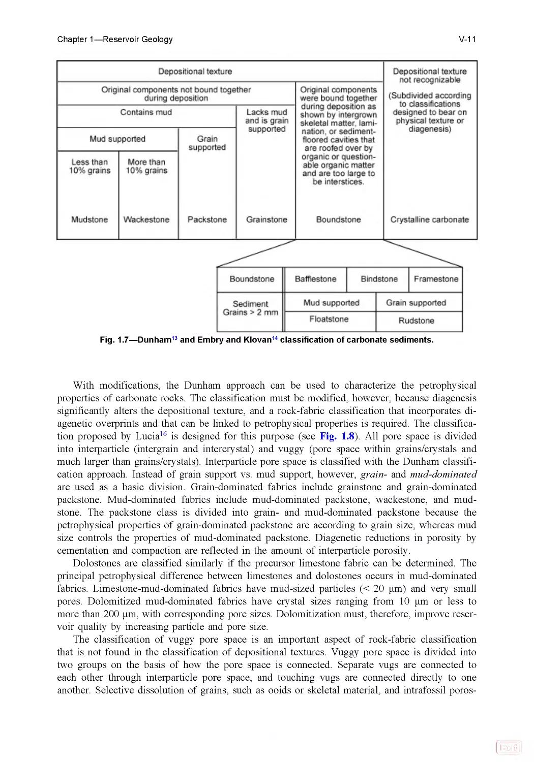
Depositional textures are described using a classification developed by Dunham.13 The Dun-
ham classification divides carbonates into organically bound and loose sediments (see Fig. 1 .7).
The loose sediment cannot be described in simple terms of grain size and sorting because
shapes of carbonate grains can vary from spheroid ooids to flat-concave and high-spiral shells
having internal pore space. The grain content of a grain-supported sediment composed of shells
can be as little as 30% of the bulk volume because the shells occupy less space than spheroids.
Loose sediment is, therefore, described on the basis of the concept of mud vs. grain support.
Mud refers to mud-size carbonate particles, not to mud composed of clay minerals. Grain-sup-
ported textures are grainstone, which lacks carbonate mud, and packstone, which contains mud.
Mud-supported textures are referred to as wackestone, which contains more than 10% grains,
and mudstone, which contains less than 10% grains. To complete the description, generic
names are modified according to grain type such as “fusulinid wackestone” or “ooid grainstone.”
Dunham’s boundstone class was further divided by Embry and Klovan14 because carbonate
reefs are commonly composed of large reef-building organisms, such as corals, sponges, and
rudists, which form sediments composed of very large particles. They introduced the terms baf-
flestone, bindstone, and framestone to describe autochthonous (in-place) boundstone reef mate-
rial. Floatstone and rudstone are used to describe allochthonous, (transported) reef sediment
with particles larger than 2 mm in diameter. Rudstone is grain-supported, whereas floatstone is
mud-supported sediment.
Enos and Sawatsky15 measured the porosity and permeability of modern carbonate sedi-
ments. The average porosity and permeability of grainstone are approximately 45% and 10
darcies, respectively, whereas the average porosity and permeability of a wackestone are approx-
imately 65% and 200 md, respectively. The higher porosity in mud-supported sediments is
caused by the needle shape of small aragonite crystals that make up the carbonate mud, and
the decrease in permeability is caused by the small pore size found between mud-sized parti-
cles. An important observation based on this data is that all carbonate sediments have sufficient
porosity and permeability to qualify as reservoir rocks.
Fig. 1.6 —Terminology of cycle hierarchies and order of cyclicity from Goldhammer.11
V-10
Petroleum Engineering Handbook—Vol. V
Print
Search
Home
Bookmarks
Help
Contents
Chapter 2
With modifications, the Dunham approach can be used to characterize the petrophysical
properties of carbonate rocks. The classification must be modified, however, because diagenesis
significantly alters the depositional texture, and a rock-fabric classification that incorporates di-
agenetic overprints and that can be linked to petrophysical properties is required. The classifica-
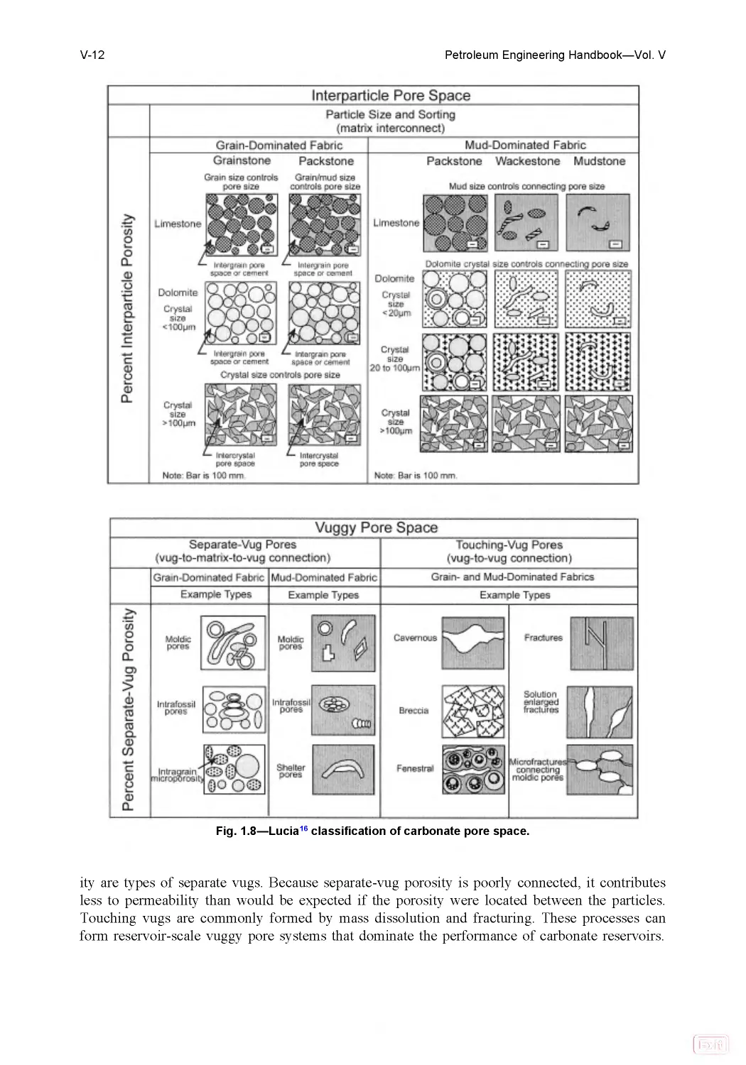
tion proposed by Lucia16 is designed for this purpose (see Fig. 1 .8). All pore space is divided
into interparticle (intergrain and intercrystal) and vuggy (pore space within grains/crystals and
much larger than grains/crystals). Interparticle pore space is classified with the Dunham classifi-
cation approach. Instead of grain support vs. mud support, however, grain- and mud-dominated
are used as a basic division. Grain-dominated fabrics include grainstone and grain-dominated
packstone. Mud-dominated fabrics include mud-dominated packstone, wackestone, and mud-
stone. The packstone class is divided into grain- and mud-dominated packstone because the
petrophysical properties of grain-dominated packstone are according to grain size, whereas mud
size controls the properties of mud-dominated packstone. Diagenetic reductions in porosity by
cementation and compaction are reflected in the amount of interparticle porosity.
Dolostones are classified similarly if the precursor limestone fabric can be determined. The
principal petrophysical difference between limestones and dolostones occurs in mud-dominated
fabrics. Limestone-mud-dominated fabrics have mud-sized particles (< 20 μm) and very small
pores. Dolomitized mud-dominated fabrics have crystal sizes ranging from 10 μm or less to
more than 200 μm, with corresponding pore sizes. Dolomitization must, therefore, improve reser-
voir quality by increasing particle and pore size.
The classification of vuggy pore space is an important aspect of rock-fabric classification
that is not found in the classification of depositional textures. Vuggy pore space is divided into
two groups on the basis of how the pore space is connected. Separate vugs are connected to
each other through interparticle pore space, and touching vugs are connected directly to one
another. Selective dissolution of grains, such as ooids or skeletal material, and intrafossil poros-
Fig. 1 .7 —Dunham13 and Embry and Klovan14 classification of carbonate sediments.
Chapter 1—Reservoir Geology
V-11
Print
Search
Home
Bookmarks
Help
Contents
Chapter 2
ity are types of separate vugs. Because separate-vug porosity is poorly connected, it contributes
less to permeability than would be expected if the porosity were located between the particles.
Touching vugs are commonly formed by mass dissolution and fracturing. These processes can
form reservoir-scale vuggy pore systems that dominate the performance of carbonate reservoirs.
Fig. 1 .8 —Lucia16 classification of carbonate pore space.
V-12
Petroleum Engineering Handbook—Vol. V
Print
Search
Home
Bookmarks
Help
Contents
Chapter 2
1.5 .2 Depositional Environments. Carbonate sediments accumulate in depositional environ-
ments that range from tidal flats to deepwater basins. Most carbonate sediments originate on a
shallow-water platform, shelf, or ramp and are transported landward and basinward. “Platform”
is a general term for the shallow-water environment, whereas “shelf” and “ramp” refer to topog-
raphy—shelves with flat platform tops and steep foreslopes and ramps having gently dipping
platform tops and slightly steeper foreslopes.
The lateral distribution of depositional environments reflects energy levels, topography, and
organic activity. These changes can be related to the geometry of the carbonate platform.
Ocean currents are produced by tides and waves and are concentrated at major topographic
features, such as ramp and shelf margins, islands, and shorelines. Grainstones and boundstones
are concentrated in the areas of highest energy, commonly at ramp and shelf margins. Sedi-
ment is transported from the shelf edge onto the shelf slope and into the basin environment.
This transport occurs primarily during highstand and results in progradation of the shelf mar-
gin. Calcareous plankton is deposited in the basinal environment as well. Sediment is also
transported landward onto the shoreline, creating tidal-flat deposits that prograde, primarily dur-
ing regression. Transgressive sediments are generally wackestones and mudstones at all loca-
tions because rising sea level typically creates a low-energy depositional environment.
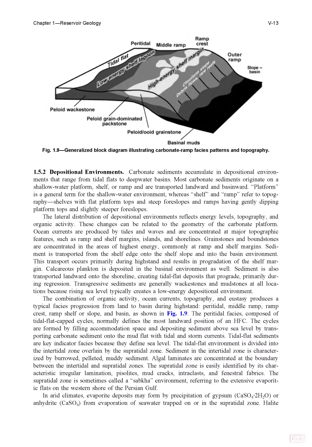
The combination of organic activity, ocean currents, topography, and eustasy produces a
typical facies progression from land to basin during highstand: peritidal, middle ramp, ramp
crest, ramp shelf or slope, and basin, as shown in Fig. 1 .9 . The peritidal facies, composed of
tidal-flat-capped cycles, normally defines the most landward position of an HFC. The cycles
are formed by filling accommodation space and depositing sediment above sea level by trans-
porting carbonate sediment onto the mud flat with tidal and storm currents. Tidal-flat sediments
are key indicator facies because they define sea level. The tidal-flat environment is divided into
the intertidal zone overlain by the supratidal zone. Sediment in the intertidal zone is character-
ized by burrowed, pelleted, muddy sediment. Algal laminates are concentrated at the boundary
between the intertidal and supratidal zones. The supratidal zone is easily identified by its char-
acteristic irregular lamination, pisolites, mud cracks, intraclasts, and fenestral fabrics. The
supratidal zone is sometimes called a “sabkha” environment, referring to the extensive evaporit-
ic flats on the western shore of the Persian Gulf.
In arid climates, evaporite deposits may form by precipitation of gypsum (CaSO4·2H2O) or
anhydrite (CaSO4) from evaporation of seawater trapped on or in the supratidal zone. Halite
Fig. 1 .9—Generalized block diagram illustrating carbonate-ramp facies patterns and topography.
Chapter 1—Reservoir Geology
V-13
Print
Search
Home
Bookmarks
Help
Contents
Chapter 2
(NaCl) is normally found in isolated basins similar to the Dead Sea. Sulfate minerals are found
as deposits in hypersaline lakes and as beds and crystals within the peritidal sediments. Sul-
fates found within carbonate sediments are properly classified as diagenetic minerals and
cannot be used to describe the depositional environment, but sulfate deposited out of a standing
body of water, is properly classified as sediment and is characteristic of the depositional envi-
ronment as well as the climate. For sulfate to precipitate from seawater, three conditions must
be met:
1. The body of seawater must be highly restricted from the ocean.
2. The hypersaline water must be able to escape either by returning to the ocean or by
seeping into the underlying sediment (seepage reflux), otherwise large volumes of Halite will
precipitate forming a bed of salt.
3. The climate must be sufficiently arid to allow the seawater to evaporate to at least one-
third its original volume.
The middle-ramp facies is characterized by quiet-water deposits typically composed of skele-
tal wackestones and mudstones. Burrowing organisms churn the muddy sediment and produce
fecal pellets that, together with skeletal material, comprise the grain fraction of the sediment.
During highstand, accommodation space may be reduced and water depth lessened to the point
at which wave and storm energy increase, lime mud is winnowed out, and a packstone texture
is produced. The increase in grain content, possibly capped by packstone, is used to define sea-
level changes in this environment.
The ramp-crest facies is characterized by high-energy deposits, typically grainstones and
packstones. The classic upward-shoaling succession of wackestone to packstone and grainstone
typifies this environment. Typical high-energy deposits are as follows:
• Shelf-margin, tidal-bar, and marine-sand belts.
• Back-reef sands associated with landward transport of sediment for fringing reefs.
• Local middle-shelf deposits associated with gaps between islands or tidal inlets forming
lobate tidal deltas.
Packstones are typically churned by burrowing organisms and show no evidence of current
transport. Grainstones are commonly crossbedded, often in multiple directions, indicating depo-
sition out of tidal currents. Reefs are also found in the ramp-crest facies. The term reef has
been much misused in the petroleum industry. At one time, all carbonate reservoirs were re-
ferred to as reefs, and the term is commonly used today to describe any carbonate buildup.
However, the term should be restricted to carbonate bodies composed of bindstone, bafflestone,
and associated float- and rudstones.
The outer-ramp, or slope, facies is formed by transport of shelf-margin and inner-shelf sedi-
ment onto the shelf slope. Sediments are typically wackestones and mudstones, along with
occasional packstones and grainstones, in channels associated with density flows into the basin.
On steep slopes, sediments may be dominated by sedimentary breccias and debris flows pro-
duced by the collapse of a steep shelf margin. The basin facies is typically composed of thin-
bedded, quiet-water lime muds that contain planktonic organisms. Wackestones are often
punctuated by debris and grain flows. Classic turbidite textures and cycles are also found in
basinal carbonate deposits.
1.5.3 Diagenetic Environments. Because all carbonate-reservoir rocks have undergone signifi-
cant diagenesis, understanding their diagenetic history can be as important as understanding
their depositional history. Modern carbonate sediments have sufficient porosity and permeabili-
ty to qualify as reservoir rocks. Many ancient carbonates, however, lack the porosity and
permeability needed to produce hydrocarbons economically. Loss of reservoir quality occurs
when sediment changes after deposition. The processes that cause these changes are referred to
as diagenetic processes, and the resulting fabric is often referred to as the diagenetic overprint.
V-14
Petroleum Engineering Handbook—Vol. V
Print
Search
Home
Bookmarks
Help
Contents
Chapter 2
Carbonate diagenetic processes include calcium-carbonate cementation; mechanical and
chemical compaction; selective dissolution; dolomitization; evaporite mineralization; and mas-
sive dissolution, cavern collapse, and fracturing. Whereas sedimentation is a one-time event,
diagenesis is a continuing process, and diagenetic processes interact with one another in time
and space. Thus, a sequence of diagenetic events may be extremely complicated and the pat-
tern of diagenetic products difficult to predict if they are not related to depositional patterns.
The process of diagenetic overprinting of depositional textures must be understood to pre-
dict the distribution of petrophysical properties in a carbonate reservoir. To this end, diagenetic
processes are grouped according to their conformance to depositional patterns. Calcium-carbon-
ate cementation, compaction, and selective dissolution form the first group. These processes
have the highest conformance to depositional patterns. Reflux dolomitization and evaporite min-
eralization form the second group. Although these processes depend greatly on geochemical
and hydrological considerations, they are often predictable because they can be related to tidal-
flat and evaporite depositional environments. Massive dissolution, collapse brecciation and
fracturing, and late dolomitization form the third group. These processes have the lowest con-
formance to depositional patterns, and their products are quite unpredictable.
Calcium-carbonate cementation, compaction, and selective dissolution can often be linked
to depositional textures. Because calcium-carbonate cementation begins soon after deposition, it
is often connected to the depositional environment. It continues as the sediment is buried, so
the distribution of late cements is often unpredictable. Cementation fills pore space from the
pore walls inward, reducing both pore size and porosity in proportion to the amount of cement.
Compaction and associated cementation are a function of depositional texture and the time-over -
burden history. Compaction is both a physical and a chemical process resulting from increased
overburden pressure caused by burial. Textural effects include porosity loss; pore-size reduc-
tion; grain penetration, breaking, and deformation; and microstylolites. Compaction does not
require the addition of material from an outside source and is often related to depositional tex-
tures. Experiments and observations have shown that mud-supported sediments compact more
readily than those that are grain-supported.
Selective dissolution occurs when one fabric element is selectively dissolved in preference
to others. Carbonate sediments are composed of three varieties of calcium carbonate—low-mag-
nesium calcite, high-magnesium calcite (magnesium substituted for some calcium in the crystal
lattice), and aragonite. Aragonite, in particular, is an unstable form and is rarely found in car-
bonate rocks. Grains composed of aragonite tend to be dissolved, and the carbonate is deposit-
ed as calcite cement. This distribution of aragonite grains can be predicted on the basis of
depositional models.
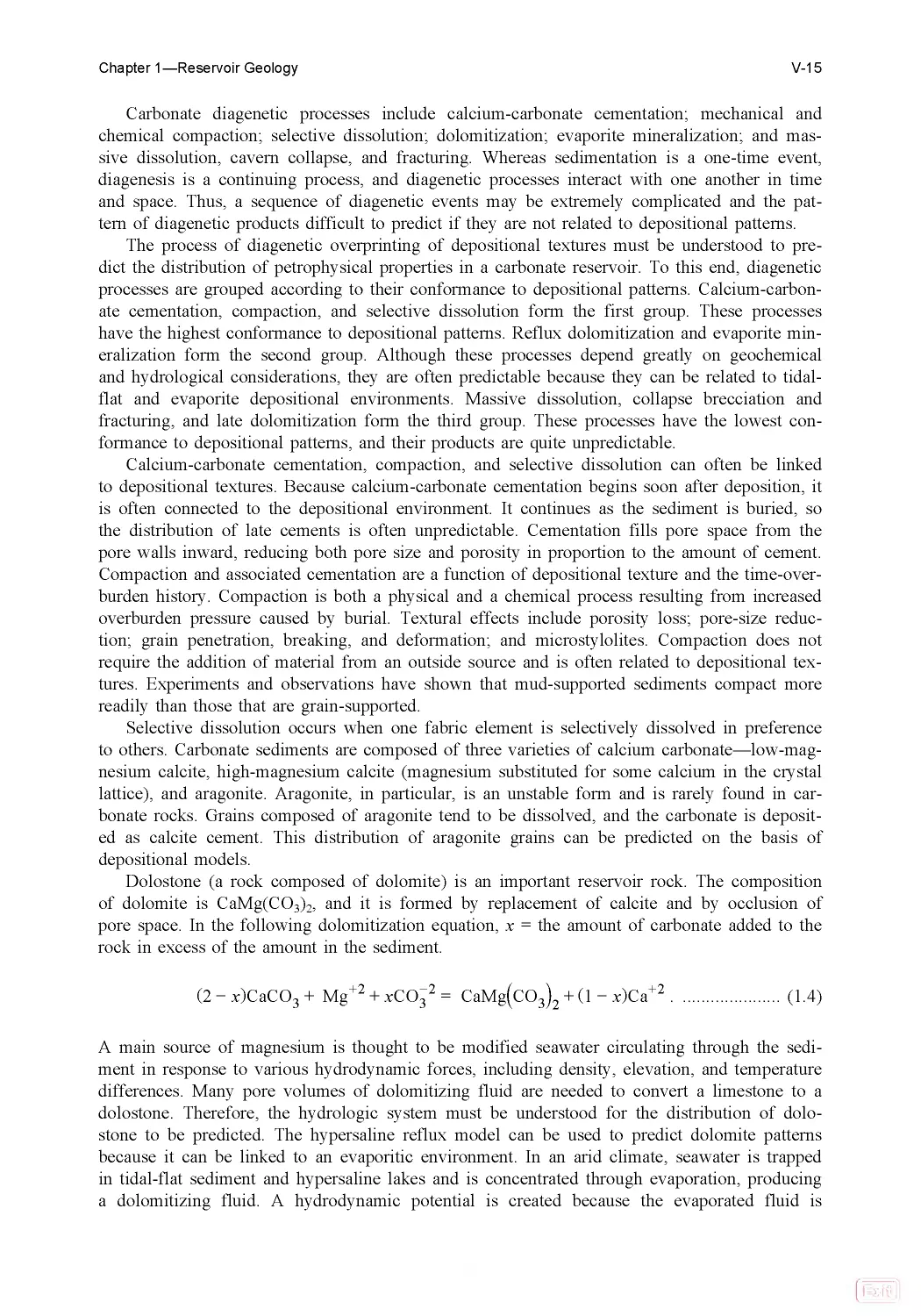
Dolostone (a rock composed of dolomite) is an important reservoir rock. The composition
of dolomite is CaMg(CO3)2, and it is formed by replacement of calcite and by occlusion of
pore space. In the following dolomitization equation, x = the amount of carbonate added to the
rock in excess of the amount in the sediment.
(2 − x)CaCO3 + Mg
+2
+ xCO3
−2
= CaMg(CO3)2 + (1 − x)Ca
+2
.
.....................
(1.4)
A main source of magnesium is thought to be modified seawater circulating through the sedi-
ment in response to various hydrodynamic forces, including density, elevation, and temperature
differences. Many pore volumes of dolomitizing fluid are needed to convert a limestone to a
dolostone. Therefore, the hydrologic system must be understood for the distribution of dolo-
stone to be predicted. The hypersaline reflux model can be used to predict dolomite patterns
because it can be linked to an evaporitic environment. In an arid climate, seawater is trapped
in tidal-flat sediment and hypersaline lakes and is concentrated through evaporation, producing
a dolomitizing fluid. A hydrodynamic potential is created because the evaporated fluid is
Chapter 1—Reservoir Geology
V-15
Print
Search
Home
Bookmarks
Help
Contents
Chapter 2
denser than seawater or groundwater and the tidal flats are at a slightly higher elevation than
sea level. As a result, the hypersaline fluid will reflux down through the underlying sediment,
converting it to dolomite. The geometries of dolostone bodies formed by this mechanism can
be predicted if the distribution of evaporitic tidal-flat facies is known.
The hypersaline reflux model also accounts for the addition of CaSO4, commonly an evap-
orite mineral in carbonate reservoirs. CaSO4 is most commonly formed near the Earth’s surface
in its hydrous form, gypsum (CaSO4·2H2O). However, at higher temperatures, the stable form
is anhydrite CaSO4, which is the form most commonly found in carbonate reservoirs. In some
locations, tectonics has uplifted carbonate strata into a cooler temperature, and anhydrite has
hydrated, forming gypsum.
Four types of anhydrite are commonly found in dolostone reservoirs. Pore-filling anhydrite
is typically composed of large crystals filling interparticle and vuggy pore space. Poikilotopic
anhydrite is found as large crystals with inclusions of dolomite scattered throughout the dolo-
stone. They are both replacive and pore filling. Nodules of anhydrite are composed of micro-
crystalline anhydrite, often showing evidence of displacing sediment. They make up a small
percentage of the bulk volume and have little effect on reservoir quality. Bedded anhydrite is
found as beds composed of both coalesced nodules and laminations. Anhydrite beds are flow
barriers and seals in reservoirs.
Massive dissolution, collapse brecciation and fracturing, and late dolomitization are the
most unpredictable diagenetic processes. Massive dissolution refers to nonfabric selective disso-
lution, including cavern formation at any scale, collapse brecciation and fracturing, solution
enlargement of fractures, and dissolution of bedded evaporites. This process is thought to be
most commonly related to the flow of near-surface groundwater, referred to as meteoric diagen-
esis but often included under the general heading of karst. The products of this diagenetic
environment are controlled by precursor diagenetic events, tectonic fracturing, and groundwater
flow and show little relationship to depositional environments. Reservoirs of this type are, there-
fore, difficult to model.
1.6 Siliciclastic Reservoirs
1.6 .1 Introduction. Siliciclastic rocks are composed of terrigenous material formed by the
weathering of pre-existing rocks, whereas carbonate rocks are composed principally of sedi-
ment formed from seawater by organic activity. Clastic sediments are composed of grains and
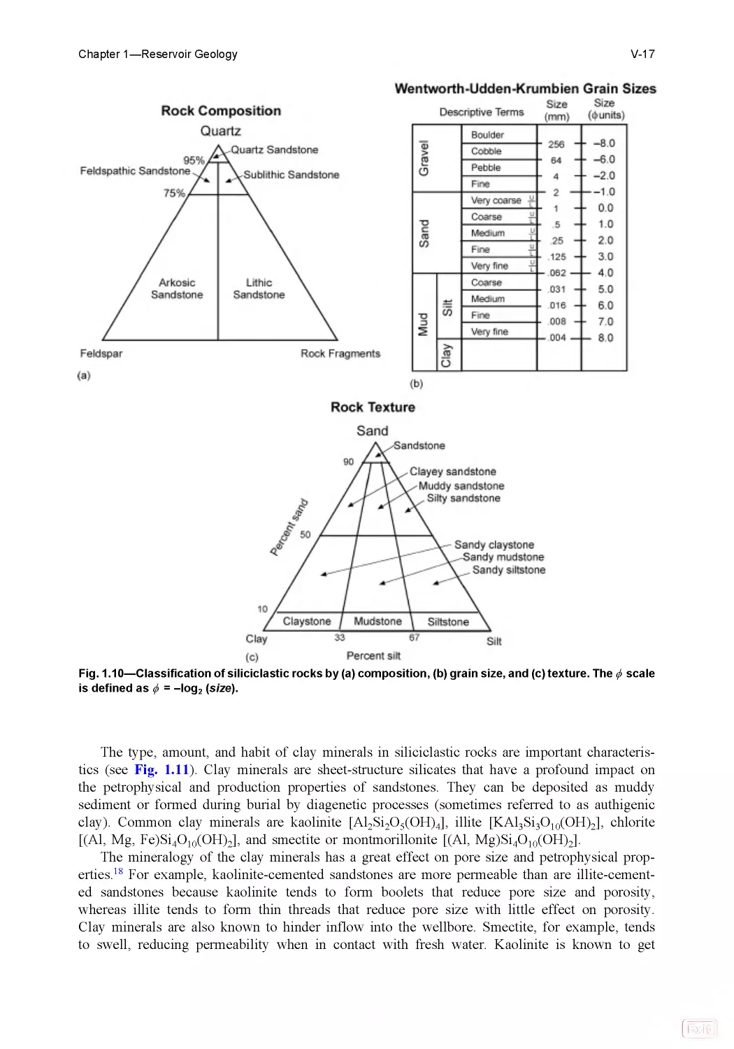
clay minerals, and siliciclastic sediments are first classified according to grain type. The three
basic grain types are quartz, feldspar, and rock fragments, and the end members are quartz
sandstone, arkosic sandstone, and lithic sandstone, as shown in Fig. 1 .10a. Second, siliciclas-
tics are described in terms of grain size (Fig. 1 .10b). Grain-size classes include gravels
(boulder size to 2 mm in diameter), sands (2 to 0.0625 mm), and mud, which includes silts
(0.0625 to 0.004 mm) and clay (< 0.004 mm). Mixtures are described with a modifying term
for a less-abundant size, such as clayey sandstone, sandy siltstone, or muddy sandstone (Fig.
1.10c). Mudstone, composed of clay and silt, is not to be confused with carbonate mudstone.
In this classification, mud and clay are terms used to indicate size, not mineralogy.
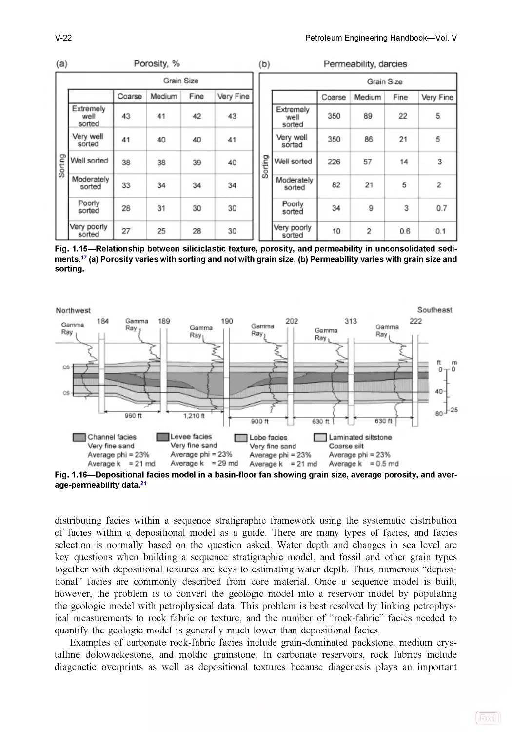
The porosity and permeability of unconsolidated siliciclastic sediments were measured by
Beard and Weyl.17 Porosity varies from 45% for well-sorted sands to 25% for very poorly sort-
ed sands and does not vary with changes in grain size for well-sorted media. Permeability
ranges from 400 darcies in well-sorted, coarse-grained sands to 0.1 darcies (100 md) in very
poorly sorted, fine-grained sands. Permeability varies with grain size and sorting because it is
controlled by pore-size distribution. Most modern sands are reservoir-quality rock. Modern clay-
stones and mudstones, which are composed primarily of clay minerals, have little permeability
and are not reservoir quality.
V-16
Petroleum Engineering Handbook—Vol. V
Print
Search
Home
Bookmarks
Help
Contents
Chapter 2
The type, amount, and habit of clay minerals in siliciclastic rocks are important characteris-
tics (see Fig. 1 .11). Clay minerals are sheet-structure silicates that have a profound impact on
the petrophysical and production properties of sandstones. They can be deposited as muddy
sediment or formed during burial by diagenetic processes (sometimes referred to as authigenic
clay). Common clay minerals are kaolinite [Al2Si2O5(OH)4], illite [KAl3Si3O10(OH)2], chlorite
[(Al, Mg, Fe)Si4O10(OH)2], and smectite or montmorillonite [(Al, Mg)Si4O10(OH)2].
The mineralogy of the clay minerals has a great effect on pore size and petrophysical prop-
erties.18 For example, kaolinite-cemented sandstones are more permeable than are illite-cement-
ed sandstones because kaolinite tends to form boolets that reduce pore size and porosity,
whereas illite tends to form thin threads that reduce pore size with little effect on porosity.
Clay minerals are also known to hinder inflow into the wellbore. Smectite, for example, tends
to swell, reducing permeability when in contact with fresh water. Kaolinite is known to get
Fig. 1 .10—Classification of siliciclastic rocks by (a) composition, (b) grain size, and (c) texture. The f scale
is defined as f = –log2 (size).
Chapter 1—Reservoir Geology
V-17
Print
Search
Home
Bookmarks
Help
Contents
Chapter 2
dislodged by high-velocity flow and plug pore throats near the wellbore, reducing permeability.
The iron in chlorite is commonly released during acid treatments, plugging perforations.
1.6 .2 Depositional Environments. The following discussion is taken primarily from Galloway
and Hobday.19 Grain type, size, and sorting, as well as other characteristics of siliciclastic reser-
voirs are most commonly controlled by the depositional environment. Many siliciclastic reser-
voirs are geologically young, and the sediment has undergone only moderate compaction and
cementation. Therefore, diagenesis is not a major factor, and petrophysical properties can be
predicted on the basis of sedimentology.
Siliciclastic sediments are transported and deposited by wind and flowing water. On land,
clastics are deposited by wind and stream flow. In the marine environment, they are transport-
ed by tidal, wave, ocean, and density currents. Land-based environments are grouped into alluvial-
fan, fluvial, and eolian systems. Ocean-center environments include delta systems and barrier
bars, which are transitional between land and marine environments, and shelf, slope, and basi-
nal systems, which are marine (see Fig. 1.12).20
Alluvial fans are conical, lobate, or arcuate accumulations of predominately coarse-grained
clastics extending from a mountain front or escarpment across an adjacent lowland. Some fans
terminate directly in lakes or ocean basins as fan deltas, which generally show some degree of
distal modification by currents or waves. Most sediment is deposited by stream and debris
flow. Stream flow is commonly confined to one or two channels but may spread across the fan
as sheet-flow. Debris flows result when clay and water provide a low-viscosity medium of high
yield strength capable of transporting larger particles under gravity. Wave and tidal currents
modify the distal terminations of fans that build into lakes or the ocean, improving sorting and
reservoir quality.
Eolian deposits are typically fine- to medium-grained, well-sorted, quartzose sand with pro-
nounced crossbedding. The sand is transported and deposited by wind currents, which are the
most effective agents for sorting clastic particles. Hot, arid regions are the most favored locales
for eolian accumulation. Eolian environments can be divided into dune and interdune facies.
Dunes are large bed forms that come in an array of forms. Barchans, barchanoid ridges, and
transverse dunes form in response to essentially unidirectional winds. Longitudinal dunes arise
from varying wind directions. Draas comprise large stellate rosettes with a high central peak
and radiating arms and form in response to intense, multidirectional wind systems. The inter-
dune environment is generally a broad, featureless plain covered by lag gravels resulting from
Fig. 1.11—Diagrammatic illustration of the basic, different types of clay habit in siliciclastic rocks. Figure
courtesy of Sneider Exploration Inc.
V-18
Petroleum Engineering Handbook—Vol. V
Print
Search
Home
Bookmarks
Help
Contents
Chapter 2
deflation (erosion). Deposition in the interdune area results from rainfall in desert highlands,
promoting ephemeral streams that deposit sediment in streambeds and small alluvial fans. Flood-
ing may produce interdune braided-stream deposits. Ponding of water between dunes can create
lakes that can precipitate evaporite minerals if the groundwater is sufficiently saline.
Fluvial systems are a collection of stream channels and their floodplains. The channels are
sinuous (meandering), with the degree of sinuosity increasing seaward. Braided streams are the
result of sand-rich channels. Channel deposits are composed of sand bars and lag deposits. The
point bar, a major feature of a high-sinuosity channel, forms by lateral accretion of sediment in
the lower-energy, leeward side of a meander. Deposition normally occurs during the ebbing
phase of a flood. The highest energy, found in the channel proper, erodes the channel bank,
causing the channel to shift constantly; lag deposits are characteristic of the channel. Aban-
doned channels are commonly clay filled.
Floodplain deposits are deposited as levees, crevasse splays, and flood-basin sediments. Lev-
ee deposits are fine sand, silt, and clay deposited along the margins of the channels, when
decelerating water rich in suspended sediment spills over the banks during flood stage.
Crevasse splays are formed when local breaches in the levees funnel floodwater into near-chan-
Fig. 1 .12—Range of sandstone depositional systems that typically host hydrocarbon resources.20
Chapter 1—Reservoir Geology
V-19
Print
Search
Home
Bookmarks
Help
Contents
Chapter 2
nel parts of the flood plain. These sediments tend to be highly heterogeneous, composed of
sand of variable size, plant debris, and mud clasts. Flood-basin deposits are broad, clay-rich
sediments that have been reworked by burrowing animals, plant growth, and pedogenic (soil-
forming) processes.
Delta systems form when a river transporting sediment enters a standing body of water,
commonly an ocean or a lake, and consist of both fluvial and marine sediments. The deposition-
al architecture of a delta system is characteristically progradational and may fill a small basin.
The combination of fluvial and marine processes creates a unique facies assemblage and reser-
voir architecture. Deltaic sediments are deposited as channel fills, channel-mouth sands,
crevasse splays, and delta-margin sand sheets. Together, these facies compose a delta lobe,
which is a fundamental building block of a delta system. Delta systems are divided into flu-
vial-, wave-, and tidal-dominated deltas according to major energy type. Each system has a
unique depositional architecture.
Shore-zone systems, excluding deltas, compose a narrow transitional environment that ex-
tends from wave base (≈50 ft of water) to the seaward edge of the alluvial coastal plain. They
include shoreface, beach, barrier, lagoon, and tidal-flat facies. These systems are supplied prin-
cipally by onshore transport of river-derived and shelf sediments. Sands are concentrated in
barrier-island complexes and tidal sand bodies, with finer sediment landward. Accretion of
beach ridges seaward can form a sheetlike sand body referred to as a strandplain sand. The
“shoreface facies” refers to that part of the shore zone that is below the zone of wave swash. It
is commonly divided into lower-, middle-, and upper-shoreface deposits partly on the basis of
water depth and associated energy levels, the highest energy level being the surf zone (upper
shoreface). Beach facies includes wave swash and dune zone, all deposited above mean tide.
The barrier is formed by aggradation or by progradation of shoreface sands seaward. The la-
goon facies, located behind the barrier, is generally composed of clay and fine sand. The
barrier may be breached during storms, allowing tidal currents to transport coarser sediment
from the ocean into the lagoon, forming tidal deltas.
Shelf systems are broad, deepwater platforms covered by terrigenous sediment. Sediment
distribution is controlled by ocean currents, including tidal, wave, storm surge, and density.
Facies are defined by bed form and include sand ribbon, wave, ridge, storm, and mud.
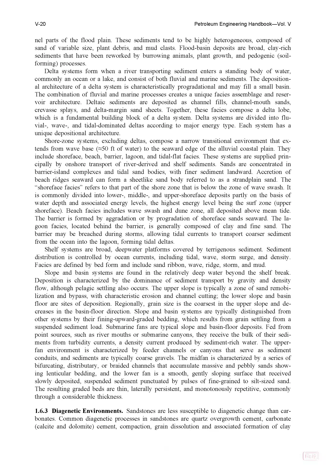
Slope and basin systems are found in the relatively deep water beyond the shelf break.
Deposition is characterized by the dominance of sediment transport by gravity and density
flow, although pelagic settling also occurs. The upper slope is typically a zone of sand remobi-
lization and bypass, with characteristic erosion and channel cutting; the lower slope and basin
floor are sites of deposition. Regionally, grain size is the coarsest in the upper slope and de-
creases in the basin-floor direction. Slope and basin systems are typically distinguished from
other systems by their fining-upward-graded bedding, which results from grain settling from a
suspended sediment load. Submarine fans are typical slope and basin-floor deposits. Fed from
point sources, such as river mouths or submarine canyons, they receive the bulk of their sedi-
ments from turbidity currents, a density current produced by sediment-rich water. The upper-
fan environment is characterized by feeder channels or canyons that serve as sediment
conduits, and sediments are typically coarse gravels. The midfan is characterized by a series of
bifurcating, distributary, or braided channels that accumulate massive and pebbly sands show-
ing lenticular bedding, and the lower fan is a smooth, gently sloping surface that received
slowly deposited, suspended sediment punctuated by pulses of fine-grained to silt-sized sand.
The resulting graded beds are thin, laterally persistent, and monotonously repetitive, commonly
through a considerable thickness.
1.6.3 Diagenetic Environments. Sandstones are less susceptible to diagenetic change than car-
bonates. Common diagenetic processes in sandstones are quartz overgrowth cement, carbonate
(calcite and dolomite) cement, compaction, grain dissolution and associated formation of clay
V-20
Petroleum Engineering Handbook—Vol. V
Print
Search
Home
Bookmarks
Help
Contents
Chapter 2
minerals, and alteration of sedimentary clay minerals. Many of these products can be related to
the burial history. Pore space is reduced by mechanical and chemical compaction, resulting in
more closely spaced grains and smaller pores, and by quartz overgrowths, which are commonly
sourced from chemical dissolution of quartz grains during burial. Carbonate cements are
formed by dissolution and precipitation of indigenous carbonate shell material and by importa-
tion of carbonate from a more distant source. Iron-rich, pore-filling dolomite is not uncommon.
Feldspar minerals found in rock fragments are commonly unstable in the burial environ-
ment and are susceptible to dissolution, forming grain molds similar to those in carbonate
rocks. Clay minerals (commonly chlorite) are deposited in the intergrain spaces associated with
this dissolution process. Chlorite linings of pore space are thought to inhibit burial cementation
and compaction and preserve porosity at depth. Clay minerals are altered during burial diagene-
sis, and authigenic (diagenetic) clay minerals are formed. Clay-mineral diagenesis causes large
increases in surface area and microporosity that, in turn, have large effects on reservoir perfor-
mance and log analysis.
1.6 .4 Reservoir Models. Reservoir models are constructed by distributing petrophysical prop-
erties in 3D space with geologic models as a template. Geologic models are constructed by
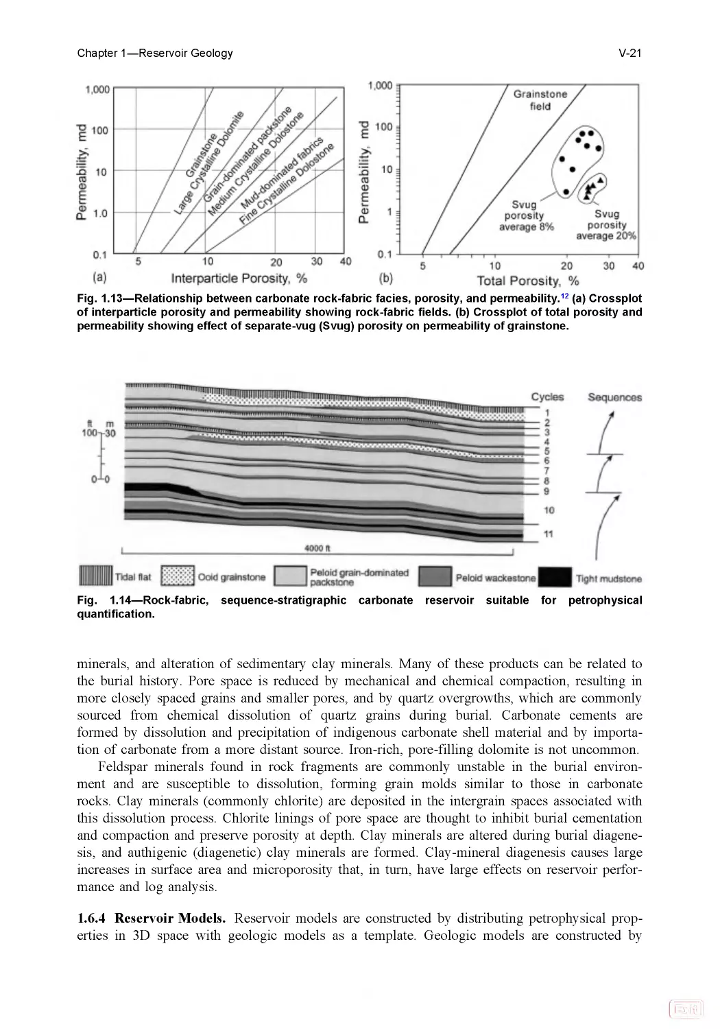
Fig. 1.13—Relationship between carbonate rock-fabric facies, porosity, and permeability.12 (a) Crossplot
of interparticle porosity and permeability showing rock-fabric fields. (b) Crossplot of total porosity and
permeability showing effect of separate-vug (Svug) porosity on permeability of grainstone.
Fig. 1.14—Rock-fabric, sequence-stratigraphic carbonate reservoir suitable for petrophysical
quantification.
Chapter 1—Reservoir Geology
V-21
Print
Search
Home
Bookmarks
Help
Contents
Chapter 2
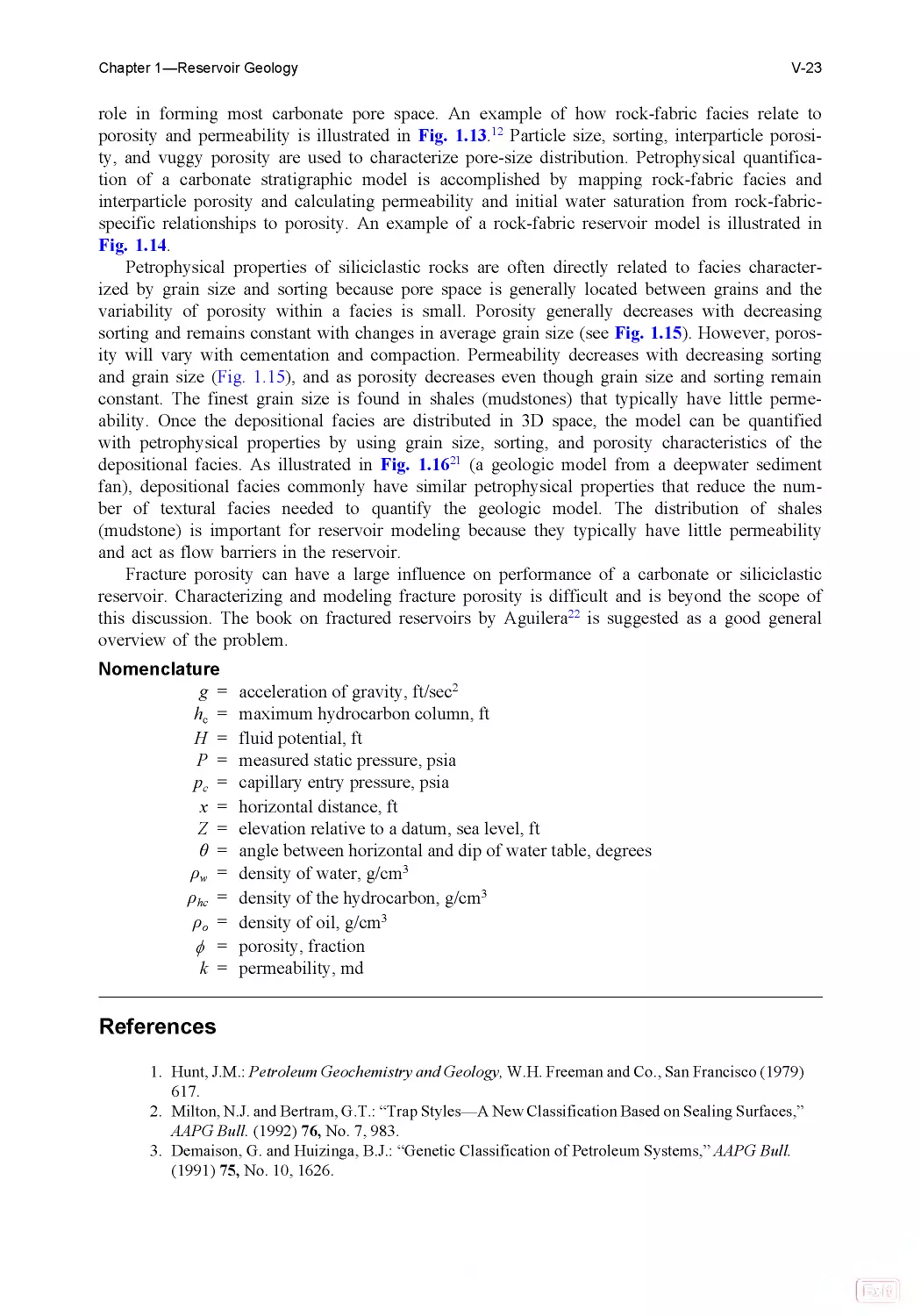
distributing facies within a sequence stratigraphic framework using the systematic distribution
of facies within a depositional model as a guide. There are many types of facies, and facies
selection is normally based on the question asked. Water depth and changes in sea level are
key questions when building a sequence stratigraphic model, and fossil and other grain types
together with depositional textures are keys to estimating water depth. Thus, numerous “deposi-
tional” facies are commonly described from core material. Once a sequence model is built,
however, the problem is to convert the geologic model into a reservoir model by populating
the geologic model with petrophysical data. This problem is best resolved by linking petrophys-
ical measurements to rock fabric or texture, and the number of “rock-fabric” facies needed to
quantify the geologic model is generally much lower than depositional facies.
Examples of carbonate rock-fabric facies include grain-dominated packstone, medium crys-
talline dolowackestone, and moldic grainstone. In carbonate reservoirs, rock fabrics include
diagenetic overprints as well as depositional textures because diagenesis plays an important
Fig. 1.15 —Relationship between siliciclastic texture, porosity, and permeability in unconsolidated sedi-
ments.17 (a) Porosity varies with sorting and not with grain size. (b) Permeability varies with grain size and
sorting.
Fig. 1 .16—Depositional facies model in a basin-floor fan showing grain size, average porosity, and aver-
age-permeability data.21
V-22
Petroleum Engineering Handbook—Vol. V
Print
Search
Home
Bookmarks
Help
Contents
Chapter 2
role in forming most carbonate pore space. An example of how rock-fabric facies relate to
porosity and permeability is illustrated in Fig. 1 .13 .12 Particle size, sorting, interparticle porosi-
ty, and vuggy porosity are used to characterize pore-size distribution. Petrophysical quantifica-
tion of a carbonate stratigraphic model is accomplished by mapping rock-fabric facies and
interparticle porosity and calculating permeability and initial water saturation from rock-fabric-
specific relationships to porosity. An example of a rock-fabric reservoir model is illustrated in
Fig. 1.14.
Petrophysical properties of siliciclastic rocks are often directly related to facies character-
ized by grain size and sorting because pore space is generally located between grains and the
variability of porosity within a facies is small. Porosity generally decreases with decreasing
sorting and remains constant with changes in average grain size (see Fig. 1 .15). However, poros-
ity will vary with cementation and compaction. Permeability decreases with decreasing sorting
and grain size (Fig. 1 .15), and as porosity decreases even though grain size and sorting remain
constant. The finest grain size is found in shales (mudstones) that typically have little perme-
ability. Once the depositional facies are distributed in 3D space, the model can be quantified
with petrophysical properties by using grain size, sorting, and porosity characteristics of the
depositional facies. As illustrated in Fig. 1 .1621 (a geologic model from a deepwater sediment
fan), depositional facies commonly have similar petrophysical properties that reduce the num-
ber of textural facies needed to quantify the geologic model. The distribution of shales
(mudstone) is important for reservoir modeling because they typically have little permeability
and act as flow barriers in the reservoir.
Fracture porosity can have a large influence on performance of a carbonate or siliciclastic
reservoir. Characterizing and modeling fracture porosity is difficult and is beyond the scope of
this discussion. The book on fractured reservoirs by Aguilera22 is suggested as a good general
overview of the problem.
Nomenclature
g = acceleration of gravity, ft/sec2
hc = maximum hydrocarbon column, ft
H = fluid potential, ft
P = measured static pressure, psia
pc = capillary entry pressure, psia
x = horizontal distance, ft
Z = elevation relative to a datum, sea level, ft
θ = angle between horizontal and dip of water table, degrees
ρw = density of water, g/cm3
ρhc = density of the hydrocarbon, g/cm3
ρo = density of oil, g/cm3
f = porosity, fraction
k = permeability, md
References
1. Hunt, J.M .: Petroleum Geochemistry and Geology, W.H. Freeman and Co., San Francisco (1979)
617.
2. Milton, N.J . and Bertram, G.T .: “Trap Styles—A New Classification Based on Sealing Surfaces,”
AAPG Bull. (1992) 76, No. 7, 983.
3. Demaison, G. and Huizinga, B.J .: “Genetic Classification of Petroleum Systems,” AAPG Bull.
(1991) 75, No. 10, 1626.
Chapter 1—Reservoir Geology
V-23
Print
Search
Home
Bookmarks
Help
Contents
Chapter 2
4. Sneider, R.M. et al.: “Comparison of Seal Capacity Determinations: Conventional Cores Versus
Cuttings,” Seals, Traps, and the Petroleum System, R.C. Surdam (ed.), AAPG Memoir 67 (1997)
12.
5. Smith, D.A.: “Theoretical Considerations of Sealing and Non-Sealing Faults,” AAPG Bull. (1966)
50, No. 2, 363.
6. Hubbert, M.K .L .: “Entrapment of Petroleum under Hydrodynamic Conditions,” AAPG Bull.
(1953) 37, No. 8, 1954.
7. Schowater, T.T .: “Mechanics of Secondary Hydrocarbon Migration and Entrapment,” AAPG
Bull. (1979) 63, No. 5, 723.
8. North, F.K.: Petroleum Geology, Unwin Hyman Inc., Boston, Massachusetts (1985) 631.
9. Von Wagoner, J.C.: “Overview of Sequence Stratigraphy of Foreland Basin Deposits:
Terminology, Summary of Papers, and Glossary of Sequence Stratigraphy,” Sequence
Stratigraphy of Foreland Basin Deposits; Outcrop and Subsurface Examples from the Cretaceous
of North America: J.C. Van Wagoner and G.T . Bertram (eds.), AAPG Memoir 64 (1995) 4.
10. Kerans, C. and Tinker, S.W .: “Sequence Stratigraphy and Characterization of Carbonate
Reservoirs,” SEPM Short Course Notes No. 40 (1997) 130.
11. Goldhammer, R.K.: “Hierarchy of Stratigraphic Forcing: Example from Middle Pennsylvanian
Shelf Carbonates of the Paradox Basin,” Sedimentary Modeling: Computer Simulations and
Methods for Improved Parameter Definition, E .K. Franseen, et al. (eds.) Kansas Geological
Survey Bull. 233 (1991) 361.
12. Lucia, F.J.: Carbonate Reservoir Characterization, Springer, New York (1999) 226.
13. Dunham, R.J .: “Classification of Carbonate Rocks According to Depositional Texture,”
Classification of Carbonate Rocks—A Symposium, W.E. Ham (ed.), AAPG Memoir No. 1 (1962)
108.
14. Embry, A.J . and Klovan, R.E .: “A Late Devonian Reef Tract of Northeastern Banks Island,
N.W.T .,” Bulletin of Canadian Petroleum Geology (1971) 19, No. 4, 730.
15. Enos, P. and Sawatsky, L.H.: “Pore networks in Holocene carbonate sediments,” J. of Sedimentary
Petrology (1981) 51, No. 3, 961.
16. Lucia, F.J.: “Rock-Fabric/Petrophysical Classification of Carbonate Pore Space for Reservoir
Characterization,” AAPG Bull. (1995) 79, No. 9, 1275.
17. Beard, D.C. and Weyl, P.K.: “Influence of Texture on Porosity and Permeability of
Unconsolidated Sand,” AAPG Bull. (1973) 57, No. 2, 349.
18. Neasham, J.W .: “The Morphology of Dispersed Clay in Sandstone Reservoirs and Its Effect on
Sandstone Shaliness, Pore Space and Fluid Flow Properties,” paper SPE 6858 presented at the
1977 SPE Annual Technical Conference and Exhibition, Denver, 9–12 October.
19. Galloway, W.E . and Hobday, D.K.: Terrigenous Clastic Depositional Systems; Applications to
Petroleum, Coal, and Uranium Exploration, Springer-Verlag, New York (1983) 423.
20. Galloway, W.E . et al.: Atlas of Major Texas Oil Reservoirs, U. of Texas at Austin, Bureau of
Economic Geology (1983) 139.
21. Dutton, S.P ., Barton, M.D., Asquith, G.B., Malik, M.A., Cole, A.G., Gogas, J., Guzman, J.I., and
Clift, S.J.: Geologic and Engineering Characterization of Turbidite Reservoirs, Ford Geraldine
Unit, Bell Canyon Formation, West Texas, The U. of Texas at Austin, Bureau of Economic
Geology Report of Investigations No. 255 (1999) 88.
22. Aguilera, R.: Naturally Fractured Reservoirs, PennWell Publishing Co., Tulsa (1995).
SI Metric Conversion Factors
°API
141.5/(131.5 + °API)
= g/cm3
ft × 3.048*
E−01 =m
g/cm3 × 1.0*
E+03 =kg/m3
mm × 2.54*
E+01 =in.
psi × 6.894 757
E+00 =kPa
*Conversion factor is exact.
V-24
Petroleum Engineering Handbook—Vol. V
Print
Search
Home
Bookmarks
Help
Contents
Chapter 2
Chapter 2
Fundamentals of Geophysics
Bob A. Hardage, U. of Texas at Austin
2.1 Introduction
Geophysics is a broad subject that encompasses potential field theory (gravity and electromag-
netic fields) and seismic technology. Potential field data are valuable in many studies, but
seismic data are used in more reservoir characterization and reservoir management applications.
This chapter focuses on seismic fundamentals and does not consider gravity, magnetic, or elec-
trical concepts.
Seismic data have been used for many years to guide exploration. More recently, seismic
data have been used to support reservoir characterization in field development planning and
subsequent reservoir management. As the technology in equipment and interpretation tech-
niques has advanced, so has the ability to define the size, shape, fluid content, and variation of
some petrophysical properties of reservoirs. This chapter provides insight into the fundamentals
of seismic data acquisition, interpretation techniques, and the types of information that can be
derived. See the chapter on reservoir geophysics in the Emerging and Peripheral Technologies
section of this Handbook for information on emerging technologies that apply geophysical data.
Most seismic data are acquired with surface-positioned sources and receivers. For the first
4 or 5 decades that seismic-reflection data were acquired, sources and receivers were deployed
along the same straight line to create 2D seismic profiles. Two-dimensional seismic data do not
yield a correct image of subsurface stratigraphy when a 2D seismic line crosses a complex
subsurface structure because the acquisition geometry cannot distinguish reflections that origi-
nate from outside the profile plane from reflections that occur within the 2D vertical image plane.
This imaging deficiency of 2D seismic profiling has been remedied by the implementation
of 3D seismic data acquisition, which allows data processing to migrate reflections to their
correct image coordinates in 3D space. Industry largely abandoned 2D seismic profiling in the
1990s and now relies almost entirely on 3D seismic data acquisition. This chapter covers the
basics of 3D seismic technology, but does not consider 2D seismic technology involving surface-
positioned equipment.
In some reservoir applications, seismic data are acquired with downhole sources and re-
ceivers. If the receiver is stationed at various depth levels in a well and the source remains on
the surface, the measurement is called vertical seismic profiling (VSP). This technique pro-
duces a high-resolution, 2D image that begins at the receiver well and extends a short distance
(a few tens of meters or a few hundred meters, depending on the source offset distance) to-
Print
Search
Home
Bookmarks
Help
Chapter 1
Chapter 3A
ward the source station. This image, a 2D profile restricted to the vertical plane passing
through the source and receiver coordinates, is useful in tying seismic responses to subsurface
geologic and engineering control.
If the source is deployed at various depth levels in one well and the receiver is placed at
several depth stations in a second well, the measurement is called crosswell seismic profiling
(CSP). Images made from CSP data have the best spatial resolution of any seismic measure-
ment used in reservoir characterization because a wide range of frequencies is recorded. CSP
data are useful for creating high-resolution images of interwell spaces and for monitoring fluid
movements between wells. However, a CSP image is also a 2D profile with the image limited
to the vertical plane that passes through the source and receiver coordinates. This chapter in-
cludes brief descriptions of the fundamentals of subsurface VSP and CSP technologies to
complement the descriptions of surface-positioned seismic technology.
2.2 Impulsive Sources
A variety of seismic sources exist that can apply vertical impulse forces to the surface of the
ground. These devices are viable energy sources for onshore seismic work. Included in this
source category are gravity-driven weight droppers and other devices that use explosive gases
or compressed air to drive a heavy pad vertically downward. Refs. 1 through 3 describe these
types of sources.
Chemical-explosive energy sources are popular for onshore seismic surveys but are prohibit-
ed at some sites because of environmental conditions, cultural restrictions, or federal and state
regulations. Chemical explosives are no longer used as marine energy sources for environmen-
tal and ecological reasons.
Field tests should always be made before an extensive seismic program is implemented.
First, it should be determined whether the selected impulsive source creates adequate energy
input to provide data with an appropriate signal-to-noise ratio and a satisfactory signal band-
width at appropriate offset distances. Second, it is important to determine whether an impulsive
source causes unwanted reverberations in shallow strata.
2.3 Vibrators
VibroseisTM energy sources are some of the more popular seismic source options for onshore
hydrocarbon exploration. The generic term vibrator refers to these types of seismic sources.
Vibrators have several features that make them attractive for seismic data acquisition. They are
quite mobile and allow efficient and expeditious illumination of subsurface targets from many
different shotpoint locations. Also, the frequency content of a vibrator signal often can be ad-
justed to better meet resolution requirements needed for a particular target. In addition, the
magnitude of the energy input into the Earth can be tailored for optimal signal-to-noise condi-
tions by varying the size and number of vibrators or by altering the output drive of individual
vibrators. For these reasons, vibrators are one of the most versatile onshore seismic energy
sources.
Vibrators work on the principle of introducing a user-specified band of frequencies, known
as the sweep, into the Earth and then crosscorrelating that sweep function with the recorded
data to define reflection events. The parameters of a vibrator sweep are start frequency, stop
frequency, sweep rate, and sweep length. A vibrator can do an upsweep that starts with a fre-
quency as low as 8 to 10 Hz and stops at a high value of 80, 100, or 120 Hz. Alternatively,
vibrators can do a downsweep that starts with a high frequency and finishes with a low frequen-
cy. Most Vibroseis data are generated with upsweeps.
Sweep rate can be linear or nonlinear. A linear rate causes the vibrator to dwell for the
same length of time at each frequency component. Nonlinear sweeps are used to emphasize
higher frequencies because the vibrator dwells longer at higher frequencies than it does at low-
er frequencies.
V-26
Petroleum Engineering Handbook—Vol. V
Print
Search
Home
Bookmarks
Help
Chapter 1
Chapter 3A
Sweep length defines the amount of time required for the vibrator to transverse the frequen-
cy range between the start and stop frequencies. As sweep length is increased, more energy is
put into the Earth because the vibrator dwells longer at each frequency component. Sweep
length is usually in the range of 8 to 14 seconds.
If a vibrator sweep is 12 seconds long, then each reflection event also spans 12 seconds in
the raw, uncorrelated data. It is not possible to interpret uncorrelated Vibroseis data because all
reflection events overlay each other and individual reflections cannot be recognized. The data
are reduced to an interpretable form by a crosscorrelation of the known input sweep with the
raw data recorded at the receiver stations. Each time the correlation process finds a replication
of the input sweep, it produces a compact symmetrical correlation wavelet centered on the long
reflection event. In this correlated form, Vibroseis data exhibit a high signal-to-noise ratio, and
reflection events are robust wavelets spanning only a few tens of milliseconds.
As a general observation, if an area is plagued by random noise, vibrators are an excellent
energy source because the correlation process used to reduce the vibrator sweep to an inter-
pretable form discriminates against noise frequencies that are outside the source sweep range.
If several sweeps are summed, unorganized noise within the sweep range is attenuated. Howev-
er, if coherent noise with frequencies within the vibrator sweep frequency range is present,
then the correlation process may accentuate these noise modes. Refs. 4 through 13 are a por-
tion of the available literature that describes the operating characteristics of vibrators and their
ability to optimize signal-to-noise ratios.
Probably the most important improvement in vibrator operations has been the development
of ground-force phase-locking technology.13 Application of this technology results in the same
ground-force function (i.e ., the same basic seismic wavelet) being generated during hundreds of
successive sweeps by vibrators positioned over a wide range of ground-surface and soil condi-
tions and by all vibrators in a multivibrator array. All aspects of seismic data processing
benefit when a source generates consistent output wavelets throughout a seismic survey, hence
the appeal of vibrators as the source of choice for most onshore surveys.
2.4 Shear Wave Sources
All seismic energy sources generate compressional (P) and shear (S) body waves. To study the
physics and exploration applications of S-waves, it is often necessary to increase the amount of
S-wave energy in the downgoing wavefield and to produce a shear wavefield that has a known
vector polarization. These objectives can be accomplished with sources that apply horizontally
directed impulses to the Earth or by vibrators that oscillate their baseplates horizontally rather
than vertically. In either case, a heavy metal pad is used to impart horizontal movement to the
Earth by means of cleats on the bottom side of the pad that project into the Earth. A specific
design for a horizontal shear-wave vibrator can be found in a patent issued to Fair.14
Horizontal vibrators have also been improved with the introduction of ground-force phase-
locking technology that results in more consistent shear wavelets from sweep to sweep as
horizontal vibrators move across a prospect. Surface damage has been minimized by reducing
the size of the cleats underneath the baseplate so that they make only shallow ground depressions.
2.5 Marine Air Guns
Air guns are now the primary energy sources used in offshore seismic profiling. Chemical ex-
plosives are no longer used for safety reasons and because of their adverse effects on marine
biology. Modern seismic vessels tow multiple arrays of air guns, and each array sometimes has
10 or more air guns. The size and position of each air gun in the array are engineered so that
the output wavelet has minimal bubble oscillations and optimal peak-to-peak amplitude. Fig .
2.1 shows map and section views of the deployment of air guns from a seismic vessel. The air
guns and hydrophone cable are positioned at proper lateral offsets from each other by steering
Chapter 2—Fundamentals of Geophysics
V-27
Print
Search
Home
Bookmarks
Help
Chapter 1
Chapter 3A
vanes. Combinations of depth-control vanes and surface buoys keep the air guns and hy-
drophones at a constant depth as they are towed across a survey area.
The air-gun arrays are powered by large onboard compressors that allow the guns to fire
and repressure (to approximately 2,000 psi) at intervals of 8 to 10 seconds as the vessel steams
along a prescribed course at constant speed. These high-repetition firing rates create shotpoints
at regular spacings of 20 to 100 m, depending on boat speed, along the length of the source
line. In wide-line profiling, a vessel tows several air-gun arrays spaced 50 to 100 m apart later-
ally to create parallel source lines in one traverse of the vessel across a prospect area (Fig. 2 .1).
Fig. 2 .2 shows the raypaths involved in air-gun illumination of a geologic target. The seis-
mic energy produced by an air-gun shot propagates up and down from the source array. The
downgoing raypath creates the primary arrival. The upgoing raypath reflects from the water
surface (where the reflection coefficient is –1 for an upgoing pressure wave) and travels down-
ward as a time-delayed ghost event. Reduced-amplitude versions of the primary and ghost
events follow at later times as the air bubble created by the shot oscillates and decays. These
three components—primary arrival, ghost arrival, and bubble oscillations—combine to form the
air-gun source wavelet.
The effectiveness of air-gun array parameters is tested in deepwater environments in which
a hydrophone can be positioned at a deep, far-field station to record the source output wavelet,
as shown in Fig. 2 .2 . The term far field refers to that part of wavefield propagation space that
Fig. 2 .1 —Equipment deployed by marine seismic vessel with towed-cable technology.
V-28
Petroleum Engineering Handbook—Vol. V
Print
Search
Home
Bookmarks
Help
Chapter 1
Chapter 3A
is several seismic wavelengths away from the source. This far-field requirement means that the
hydrophone depth, D, shown in Fig. 2 .2 is several hundreds of meters.
Air-gun arrays are designed to create source wavelets that are as compact in time as possi-
ble and that have minimal bubble oscillations. Compact wavelets are desired because such
wavelets have wide signal-frequency spectra; minimal bubble oscillations are desired so that
the signal spectrum will be as smooth as possible.
Fig. 2.3 shows an ideal source wavelet. The vertical dash line marks the arrival time of the
bulk of the energy that travels the primary raypath (Fig. 2 .2). The energy that travels the ghost
raypath (Fig. 2.2) arrives at a time delay, 2d/v, where v is the velocity of the pressure pulse in
seawater and d is the depth of the air-gun array. The ghost event has a polarity opposite that of
the primary arrival because the reflection coefficient for an upgoing pressure wave at the air/
water interface is –1 . The primary and ghost arrivals define the peak-to-peak amplitude of the
source wavelet. Small-amplitude events occur at later times in the source wavelet because the
air bubble produced by the air-gun discharge oscillates as it decays (Fig. 2.3). The number,
sizes, and relative separations of the guns in the array control the amplitude of these residual
bubble oscillations.
The two wavelet properties of greatest interest are its peak-to-peak strength (PTP) and its
primary-to-bubble ratio (PBR). The objectives of air-gun array design are to maximize the PTP
property of an air-gun wavelet, which is the difference, A–B, in Fig. 2 .4, and to minimize the
PBR parameter, which is the ratio (A–B)/(C–D).
Many factors, such as the number of guns in the array, the volume of the guns, and the
depth of the guns, affect the amplitude, phase, and frequency character of an air-gun array
wavelet. Table 2.1 summarizes Dragoset’s15 analysis of air-gun array parameters and their ef-
fects on the fundamental PTP and PBR properties of air-gun wavelets. A key point in this
Fig. 2.2 —Seismic raypaths involved in air-gun illumination of geologic targets.15
Chapter 2—Fundamentals of Geophysics
V-29
Print
Search
Home
Bookmarks
Help
Chapter 1
Chapter 3A
table is that the number of guns in an array has a greater impact on the peak-to-peak amplitude
(or wavelet energy) than does the volume of the guns.
2.6 Seismic Sensors
Two classes of seismic sensors are used to acquire seismic data: scalar sensors and vector sen-
sors. A scalar sensor measures the magnitude of Earth motion created by a seismic disturbance
but does not indicate the direction of that motion. A hydrophone is an example of a popular
scalar sensor used throughout the seismic industry. Hydrophones measure pressure variations
(scalar quantities) associated with a seismic disturbance. A hydrophone cannot distinguish a
pressure variation caused by a downgoing wavefield from a pressure change created by an up-
going wavefield. Hydrophones provide no directional (vector) information about a propagating
seismic event.
A vector sensor indicates the direction that a seismic event causes the Earth to move. The
classic example of a vector sensor is the moving-coil geophone that has been used for decades
to record onshore seismic data. The principal of a moving-coil geophone is that a lightweight
coil, with several hundred turns of thin copper wire, is suspended by springs that are, in turn,
Fig. 2.3—Key features of an air-gun wavelet.15
Fig. 2.4 —Two important properties of an air-gun wavelet: peak-to-peak strength (A to B) and primary-to-
bubble ratio [(A–B)/(C–D)].15
V-30
Petroleum Engineering Handbook—Vol. V
Print
Search
Home
Bookmarks
Help
Chapter 1
Chapter 3A
attached to the case of the geophone. The springs are designed to allow the geophone case and
the lightweight coil to move independently of each other over a frequency band of interest.
Permanent magnets are attached to the geophone case to create a strong internal magnetic field.
When the case is moved by a seismic disturbance, an electrical voltage is created as the coils
cut the magnetic lines of force. The magnitude of the voltage output is proportional to the
number of magnetic lines of force cut per unit time; thus, geophone response indicates the
velocity of the geophone case, which, in turn, is proportional to Earth particle velocity at the
geophone station.
The polarity of the geophone output voltage depends on the direction that the electrical
conductors are moving as they cut across the magnetic lines of force. If an upward movement
creates a positive voltage, a downward movement produces a negative voltage. Thus, a geo-
phone is a vector sensor that defines not only the magnitude of Earth motion, but also the
direction of that motion.
Because geophones are directional sensors and can distinguish between vertical and horizon-
tal Earth motions, they are used to record multicomponent seismic data. Three-component (3C)
geophones are used to record compressional and shear seismic data onshore. Shear waves do
not propagate in fluids. In marine environments, geophones have to be placed in direct contact
with the Earth sediment on the seafloor, with data-recording cables connected to surface-posi-
tioned ships or telemetry buoys. Four-component (4C) sensors used for this service are encased
in large, robust, watertight enclosures that include a hydrophone and a 3C geophone. Fig . 2 .5
illustrates a segment of an ocean-bottom cable (OBC) used for deploying 4C marine seismic
sensors. In this cable design, a 4C sensor station is positioned at intervals of 50 m along the 150-
m cable segment. A large number of these segments, each containing three receiver stations,
are connected end to end to make a continuous OBC receiver line several kilometers long. The
exact length of the receiver line is determined by the depth of the target that is to be imaged.
Fig. 2 .6 shows an OBC line deployed on the seafloor and connected to a stationary data-
recording vessel. A second boat towing an air-gun array traverses predesigned source lines
either parallel to, or orthogonal to, the OBC cable. The 4C sensors remain motionless on the
seafloor as data are recorded, just as onshore geophones do when onshore seismic data are
acquired. Seafloor sensors are not towed as are the conventional marine hydrophone cables
shown in Fig. 2.1.
Chapter 2—Fundamentals of Geophysics
V-31
Print
Search
Home
Bookmarks
Help
Chapter 1
Chapter 3A
2.7 Seismic Wave Propagation
The full elastic seismic wavefield that propagates through an isotropic Earth consists of a P-
wave component and two shear (SV and SH) wave components. Marine air guns and vertical
onshore sources produce reflected wavefields that are dominated by P and SV modes. Much of
the SV energy in these wavefields is created by P-to-SV-mode conversions when the downgo-
ing P wavefield arrives at stratal interfaces at nonnormal angles of incidence (Fig. 2 .6).
Horizontal-dipole sources can create strong SH modes in onshore programs. No effective seis-
mic horizontal-dipole sources exist for marine applications.
A principal difference among P, SV, and SH wavefields is the manner in which they cause
rock particles to oscillate. Fig . 2 .7 illustrates the relationships between propagation direction
and particle-displacement direction for these three wave modes. A compressional wave causes
rock particles to oscillate in the direction that the wavefront is propagating. In other words, a P-
wave particle displacement vector is perpendicular to its associated P-wave wavefront. In
contrast, SV and SH waves cause rock particles to oscillate perpendicular to the direction that
the wavefront is moving, with the SH and SV displacement vectors orthogonal to each other.
Fig. 2 .5 —Segment of ocean-bottom cable with three 4C sensor stations spaced 50 m apart.
Fig. 2 .6—Basic elements of ocean-bottom cable data acquisition. P denotes a seismic compressional
wave; SV is a converted shear mode.
V-32
Petroleum Engineering Handbook—Vol. V
Print
Search
Home
Bookmarks
Help
Chapter 1
Chapter 3A
A shear-wave particle-displacement vector is thus tangent to its associated wavefront. In a flat-
layered isotropic Earth, the SH displacement vector is parallel to stratal bedding, and SV
displacement is in the plane that is perpendicular to bedding.
To create optimal images of subsurface targets, a seismic wavefield must be segregated into
its P, SV, and SH component parts so that a P-wave image can be made that has minimal
contamination from interfering SV and SH modes. Likewise, an SV image must have no inter-
fering P and SH modes, and an SH image must be devoid of P and SV contamination.
A P wave travels at velocity Vp in consolidated rocks, which is approximately two times
faster than velocity Vs of either the SH or SV wave. In carbonates, the velocity ratio (Vp /Vs)
tends to be approximately 1.7 or 1.8. In siliciclastics, Vp /Vs varies from approximately 1.6 in
hard sandstones to approximately 3 in some shales. This velocity difference aids in separating
interfering P and S wave modes during data processing. An equally powerful technique for
separating a seismic wavefield into its component parts is to use data-processing techniques
that concentrate on the distinctions in the particle displacements associated with the P, SH, and
SV modes (Fig. 2 .7).
The P, SH, and SV particle displacements shown in Fig. 2 .7 form an orthogonal coordinate
system. The fundamental requirement of multicomponent seismic imaging is that reflection
wavefields must be recorded with orthogonal 3C sensors that allow these P, SH, and SV parti-
cle motions to be recognized. To date, most exploration seismic data have been recorded with
single-component sensors that emphasize P-wave modes and do not capture SH or SV wave
modes.
2.8 Body Waves and Surface Waves
Seismic wavefields propagate through the Earth in two ways: body waves and surface waves.
Body waves propagate in the interior (body) of the Earth and illuminate deep geologic targets.
Fig. 2.7 —Distinction between the three components of an elastic wavefield.
Chapter 2—Fundamentals of Geophysics
V-33
Print
Search
Home
Bookmarks
Help
Chapter 1
Chapter 3A
These waves generate the reflected P, SH, and SV signals that are needed to evaluate prospects
and to characterize reservoirs. Reflected (or scattered) body waves are the fundamental signals
sought in seismic data-acquisition programs.
Surface waves travel along the Earth/air interface and do not illuminate geologic targets in
the interior of the Earth. Surface waves are noise modes that overlay the desired body-wave
reflections. Surface waves can be a serious problem in onshore seismic surveys. Surface waves
do not affect towed-cable marine data because they require some shear-wave component to
propagate, and shear waves cannot propagate along the air/water interface. An exception in the
marine case is sometimes encountered when data are recorded with ocean-bottom sensors
(OBS) because interface waves can propagate along the water/sediment boundary and become
a type of surface-wave noise that degrades OBS marine seismic data.
There are two principal surface waves: Love waves and Rayleigh waves (Fig. 2 .8). Love
waves are an SH-mode surface wave and do not affect conventional P-wave seismic data. Love
waves are a serious noise mode only when the objective is to record reflected SH wavefields.
The more common surface wave is the Rayleigh wave, which combines P and SV motions and
is referred to as ground roll on P-wave seismic field records. Love waves create particle dis-
placements in the horizontal plane; Rayleigh wave displacements are in the vertical plane (Fig.
2.8).
Much of the field effort in onshore seismic programs concentrates on designing and deploy-
ing receiver arrays that can attenuate horizontally traveling surface waves (ground-roll noise)
and, at the same time, amplify upward-traveling reflection signals. The most effective field tech-
nique is to deploy 10, 12, 16, or more geophones at a uniform spacing at each receiver station
so that the distance from the first geophone to the last geophone is the same as the dominant
wavelength of the ground-roll event. All geophone responses are then summed to create a sin-
gle output response at that receiver station. The idea is to create a sensor array length such that
Fig. 2.8—Particle motions produced by the two principal seismic surface-wave noise modes: the Love
wave and the Rayleigh wave.
V-34
Petroleum Engineering Handbook—Vol. V
Print
Search
Home
Bookmarks
Help
Chapter 1
Chapter 3A
half of the geophones are moving up and half are moving down as the horizontally traveling
ground roll passes the receiver station. The summed output of the geophone array is essentially
zero because of the passage of the ground-roll event. In contrast, upward-traveling reflections
arriving at this same receiver array are not attenuated because such events cause all geophones
to move up and down in unison. The summed output of the array for an upward-traveling re-
flection wavefield is thus a strong voltage signal.
2.9 Seismic Impedance
The concept of acoustic (or seismic) impedance is critical to understanding seismic reflectivity.
Seismic impedance controls the seismic reflection process in the sense that seismic energy is
reflected only at rock interfaces in which there are changes in impedance across the interface.
Seismic impedance is defined as
I = ρV, .................................................................... (2.1)
where I = impedance, ρ = the bulk density of the rock, and V = the velocity of seismic wave
propagation through the rock. V is set to Vp if the wave mode of interest is a P wave; it is set
to Vs if S-wave reflectivity is being considered. Any alteration in rock properties that causes ρ
and/or V to change can be the genesis of a seismic reflection event; therefore, areal and verti-
cal variations in seismic reflectivity can be used to infer spatial distributions of rock types and
porosity trends.
2.10 Reflection Coefficients
Seismic reflectivity is best explained with a simple two-layer Earth model in which Layer 1 is
above Layer 2 (Fig. 2 .9). The seismic reflection coefficient, R, for a downgoing particle-veloci-
ty wave mode that arrives perpendicular to the interface between the two layers is
R=
I1−I2
I1+I2
=
ρ1V1 − ρ2V2
ρ1V1 + ρ2V2
.
...................................................
(2.2)
A negative algebraic sign has to be inserted on the right side of Eq. 2.2 if the downgoing
wavefield is a pressure wavefield (hydrophone measurement) rather than a particle-velocity
wavefield (geophone measurement). The velocity parameters, V1 and V2, are P-wave velocities
if P-wave reflectivity is being calculated; they are S-wave velocities if S-wave reflectivity is to
be determined. At any interface, R can be positive, negative, or zero, depending on the
impedance contrast (ρ1V1 – ρ2V2) across the interface.
A seismic reflection/transmission process is indicated in Fig. 2 .9 by the raypaths labeled Ao,
Ar, and At. For nonnormal incidence angles, the expression for reflection coefficient involves
trigonometric functions that ensure that horizontal slowness (the inverse of horizontal velocity)
is conserved and is a more complex expression than that given in Eq. 2 .2 . Ref. 16 gives a
detailed mathematical treatment. The seismic reflection, Ar, is given by
Ar
= RAo
, ................................................................. (2.3)
and the transmitted seismic event, At, is given by
At =(1+R)Ao
.
............................................................
(2.4)
The magnitude and algebraic sign of Ar depends on R and, in turn, the basic control on R is
the variation of impedance ρV across the interface (Eq. 2 .2). Table 2.2 lists the common geo-
Chapter 2—Fundamentals of Geophysics
V-35
Print
Search
Home
Bookmarks
Help
Chapter 1
Chapter 3A
logic conditions that often create impedance contrasts that result in nonzero reflection coeffi-
cients at rock interfaces.
Two types of petrophysical properties control the value of acoustic impedance in individual
rock layers: elastic properties of the rock matrix and properties of the fluid in the pore spaces
of the rock. P-waves travel through elastic materials and fluids; thus, any change in either the
rock matrix (such as a change in mineralogy or porosity) or in the type of fluid occupying the
pore spaces will create a discontinuity in the P-wave seismic impedance of the rock system.
Fig. 2 .10 illustrates the relationships between petrophysical conditions that occur at an im-
pendance boundary and the existence of P and S reflections at that boundary. A P-wave
reflection will occur at boundaries at which there is a change in either the rock matrix or the
pore fluid, or both. In constrast, S-waves are not affected by changes in pore fluid or are only
weakly affected. Consequently, a change in the properties of the rock matrix can create a re-
Fig. 2 .9 —Two-layer Earth model describing seismic reflectivity parameters.
V-36
Petroleum Engineering Handbook—Vol. V
Print
Search
Home
Bookmarks
Help
Chapter 1
Chapter 3A
flecting boundary for S-waves, but a change in pore fluid will create only a small (usually
negligible) S-wave reflection boundary (Fig. 2 .10). If a small, nonzero S-wave reflection coeffi-
cient occurs at a fluid boundary, that reflection coefficient usually exists because the bulk
density of the rock system varies across the fluid boundary.
These wave physics provide valuable geologic insights when both P and S reflection data
are acquired across a prospect area. When P and S reflections occur at the same depth coordi-
nate, the reflecting boundary at that depth is associated with a change in the rock matrix (that
is, with a lithological change). There may or may not be a change in pore fluid at that bound-
ary. When a P reflection occurs at a boundary but there is no S reflection, that boundary quite
likely marks a change in pore fluid and not a change in rock matrix. (That is, the lithology
probably does not change at that depth, but the type of pore fluid does.)
2.11 Seismic Attributes
The fundamental properties of processed seismic data that are used in interpretation are tempo-
ral and spatial variations of reflection amplitude, reflection phase, and wavelet frequency.
Structural and stratigraphic interpretations of 3D seismic data are inferences of geologic condi-
tions made by analyzing areal patterns of these three seismic attributes—amplitude, phase, and
frequency—across selected seismic time surfaces. Any procedure that extracts and displays
these seismic parameters in a convenient, understandable format is an invaluable interpretation
tool.
Taner and Sheriff 18 and Taner et al.19 began using the Hilbert transform to calculate seis-
mic amplitude, phase, and frequency instantaneously, meaning that a value of amplitude, phase,
and frequency is calculated for each time sample of a seismic trace. Since that introduction,
numerous Hilbert transform algorithms have been implemented to calculate these useful seis-
mic attributes (e.g ., Hardage20).
2.12 Complex Seismic Trace
Fig. 2 .11 illustrates the concept of a complex seismic trace in which x(t) represents the real
seismic trace and y(t) is the Hilbert transform of x(t). In this discussion, we ignore what a
Hilbert transform is and how the function y(t) is calculated. Most modern seismic data-process-
Fig. 2 .10 —Relationships between petrophysical conditions that occur at an impedance boundary and the
existence of P and S reflections at that boundary.17
Chapter 2—Fundamentals of Geophysics
V-37
Print
Search
Home
Bookmarks
Help
Chapter 1
Chapter 3A
ing software packages provide Hilbert transform algorithms and allow processors to create the
function y(t) shown in Fig. 2 .11 easily. These two data vectors are displayed in a 3D (x, y, t)
space in which t is seismic traveltime, x is the real data plane, and y is the imaginary plane. In
this complex trace format, the actual seismic trace, x(t), is confined to the real x plane, and y
(t), the Hilbert transform of x(t), is confined to the imaginary y plane. When x(t) and y(t) are
added vectorally, the result is a complex seismic trace, z(t), in the shape of a helical spiral
extending along, and centered about, the time axis t. The projection of this complex function z
(t) onto the real plane is the real seismic trace, x(t), and the projection of z(t) onto the imagi-
nary plane is y(t), the calculated Hilbert transform of x(t).
Fig. 2 .12 illustrates the reason for converting the real seismic trace, x(t), into what first
appears to be a more mysterious complex seismic trace, z(t), in which the attributes known as
instantaneous seismic amplitude, instantaneous phase, and instantaneous frequency are intro-
duced. At any point on the time axis of this complex seismic trace, a vector a(t) can be
calculated that extends away from the t axis in a perpendicular plane to intersect the helically
shaped complex seismic trace, z(t). The length of this vector is the amplitude of the complex
trace at that particular instant, hence the term instantaneous amplitude. This amplitude value is
calculated with the equation for a(t) shown in Fig. 2 .12 .
The orientation angle, f (t), of the amplitude vector, a(t), at time t, which is generally mea-
sured relative to the positive axis of the real x-plane, is defined as the phase of z(t) at that
moment in time. Numerically, the phase angle is calculated from the equation for f (t) defined
in Fig. 2 .12 . As seismic time progresses, vector a(t) moves along the time axis and rotates
continually about the time axis to maintain contact with the spiraling complex trace, z(t). Each
full rotation of the vector around the time axis increases the phase value by 360°.
Fig. 2 .11—A complex seismic trace.21
V-38
Petroleum Engineering Handbook—Vol. V
Print
Search
Home
Bookmarks
Help
Chapter 1
Chapter 3A
In any oscillating system, and specifically for a seismic trace, frequency can be defined as
the time rate of change of the phase angle. This fundamental definition describes the frequency
of the complex seismic trace so that the instantaneous frequency, ω(t), at any seismic time
sample is given by the time derivative of the phase function specified by the equation in Fig.
2.12.
2.13 Instantaneous Phase and Instantaneous Frequency Calculations
Fig. 2.13 illustrates calculations of the instantaneous phase associated with a typical seismic
trace. The figure’s bottom panel shows the actual seismic trace, and the center panel shows the
real and imaginary components of the associated complex trace. Applying the second equation
of Fig. 2 .12 to the real and imaginary components of the complex seismic trace (center panel)
produces the instantaneous phase function at the top of Fig. 2 .13 . The phase behavior at times
t1, t2, t3 is critical to understanding the geologic significance of anomalous frequencies. Al-
though phase is a positive function that monotonically increases in magnitude with seismic
time, it is customarily plotted as a repetitive, wraparound function with plot limits of 0 to 360°
(or –180° to +180°). Each wraparound of 360° corresponds to a full rotation of vector a(t)
around the seismic time axis while the vector stays in contact with the spiraling complex seis-
mic trace z(t) (see Fig. 2 .12).
The top panel of Fig. 2 .14 shows the instantaneous frequencies calculated for the seismic
trace presented in Fig. 2 .13 . Although the calculated frequency values at times t1 and t2 shown
by the solid-line curve are physically impossible because they are negative, these anomalous
frequency behaviors are some of the most useful seismic attributes that an interpreter can use.
They should be preserved because, when displayed in an eye-catching, contrasting color, they
Fig. 2.12 —Key seismic attributes (instantaneous amplitude, instantaneous phase, and instantaneous
frequency) that can be calculated once a complex seismic trace is created.21
Chapter 2—Fundamentals of Geophysics
V-39
Print
Search
Home
Bookmarks
Help
Chapter 1
Chapter 3A
serve to shift an interpreter’s attention quickly to subtle structural and stratigraphic discontinu-
ities in a seismic image.
Comparing the time coordinates of these anomalous frequency values with the time coordi-
nates of the instantaneous phase function in Fig. 2 .13 shows that rather than exhibiting its
typical, monotonically increasing behavior in these time intervals, the phase momentarily de-
creases in magnitude. This causes the time rate of change of phase (or the slope of the phase
function), which is the instantaneous frequency, to be negative at time samples t1 and t2. Numer-
ical algorithms should not camouflage these unrealistic frequency values, which some algo-
rithms do by arbitrarily reversing the algebraic sign of any negative frequency. The dashed-
curve segments in the enlargement show how some software algorithms change the algebraic
sign of negative frequency values to positive values. Although this seems like a logical correc-
tion, it should be avoided because it reduces the interpretive value of a 3D volume of
instantaneous frequencies.
At times t1, t2, and t3, some type of wavelet interference (that is, a wavelet distortion) oc-
curs in the seismic trace (bottom panel). As a result, the reflection waveform at times t1, t2,
and t3 is slightly distorted (bottom panel) because of the destructive interference of two or
more overlapping wavelets, demonstrating that anomalous frequencies tend to coincide with,
and emphasize, distorted wavelets such as are produced at structural and stratigraphic disconti-
nuities. High positive frequency values also occur at 1580, 1650, 1740, and 1840 milliseconds,
but these values are not anomalous in the sense that they do not exceed the Nyquist limit (125
Hz). However, they too coincide with distorted wavelets (bottom panel).21
Fig. 2.13 —Instantaneous phase seismic attribute function.21
V-40
Petroleum Engineering Handbook—Vol. V
Print
Search
Home
Bookmarks
Help
Chapter 1
Chapter 3A
2.14 Applications of Seismic Attributes
All instantaneous seismic attributes (amplitude, phase, frequency) can be used in interpretation.
In practice, most interpreters use instantaneous amplitude, or some variation of an amplitude
attribute, as their primary diagnostic tool. Amplitude is related to reflectivity, which in turn is
related to subsurface impedance contrasts. Thus, amplitude attributes provide information about
all the rock, fluid, and formation-pressure conditions listed in Table 2.2 .
Instantaneous phase is useful for tracking reflection continuity and stratal surfaces across low-
amplitude areas where it is difficult to see details of reflection waveform character. In general,
instantaneous phase is the least used of the seismic attributes.
Fig. 2.14 —Instantaneous frequency seismic attribute function calculated for the same seismic trace
discussed in Fig. 2 .13.
Chapter 2—Fundamentals of Geophysics
V-41
Print
Search
Home
Bookmarks
Help
Chapter 1
Chapter 3A
Instantaneous frequency sometimes aids in recognizing changes in bed thickness and bed
spacing. Anomalous values of instantaneous frequency (negative values or unbelievably high
positive values) are particularly useful for recognizing edges of reservoir compartments, subtle
faults, and stratigraphic pinchouts. Hardage22 demonstrated these applications of instantaneous
frequency.
2.15 Seismic Interpretation
A stratal surface is a depositional bedding plane: a depositional surface that defines a fixed
geologic time. A siliciclastic rock deposited in a high-accommodation environment contains
numerous vertically stacked stratal surfaces. A fundamental thesis of seismic stratigraphy is
that a seismic reflection event follows an impedance contrast associated with a stratal surface;
that is, a seismic reflection is a surface that represents a fixed point in geologic time.23 ,24 The
term chronostratigraphic defines this type of seismic reflection event. Because lithology varies
across the area spanned by a large depositional surface, the implication of this interpretation
principle is that an areally pervasive seismic reflection event does not necessarily mark an
impedance contrast boundary between two fixed rock types as that reflection traverses an area
of interest. The application of this fundamental concept about the genetic origin of seismic
reflections to seismic interpretation is referred to as stratal-surface seismic interpretation.
Tipper25 illustrated and discussed situations in which a seismic reflection can be either
chronostratigraphic or diachronous (meaning that the event moves across depositional time sur-
faces), depending on the vertical spacings between beds, the lateral discontinuity between
diachronous beds, and bed thickness. The conclusion that a seismic reflection is chronostrati-
graphic or diachronous needs to be made with caution because the answer depends on the local
stratigraphy, the seismic bandwidth, and the horizontal and vertical resolution of the seismic data.
If two seismic reflection events, A and B, are separated by an appreciable seismic time
interval (a few hundred milliseconds) yet are conformable to each other (that is, they parallel
each other), then the uniform seismic time thickness between these two events represents a
constant and fixed period of geologic time throughout the seismic image space spanned by
reflectors A and B. An implication of seismic stratigraphy that can be invoked in such an in-
stance is that any seismic surface intermediate to A and B, which is also conformable to A and
B, is also a stratal surface.
A key first step in seismic interpretation is to use well logs and cores to identify the three
types of stratal interfaces that exist in geologic intervals of interest: flooding surfaces, maxi-
mum flooding surfaces, and erosion surfaces. Flooding surfaces are widespread interfaces that
contain evidence of an upward, water-deepening facies dislocation, such as contact between
rooted, unfossiliferous floodplain mudstones and overlying fossiliferous marine shale. A ravine-
ment surface is a specific type of flooding surface that suggests that transgressive passage of a
surf zone has eroded underlying shallower-water facies.
Maximum flooding surfaces are interfaces that contain evidence of a widespread, upward,
water-deepening facies dislocation that is associated with the inferred, deepest water facies en-
countered in a succession of strata. A maximum flooding surface is commonly represented by
a thin condensed section, typically a black, organic-rich shale with a low-diversity fossil assem-
blage representing deepwater, sediment-starved conditions.
Maximum flooding surfaces bound and define upward-coarsening facies successions that
are called genetic sequences by Galloway.26 These genetic sequences are similar to cycles or
cyclothems in other terminology.27 ,28
An erosion surface is an interface in which there is evidence of a facies offset that indi-
cates that an abrupt decrease in water depth occurred. If an erosion surface is widespread,
truncation of older strata can be documented on well log cross sections. Some of these surfaces
may be disconformities representing downcutting during periods of subaerial exposure caused
by allocyclic (extrabasinal) mechanisms, such as eustatic sea-level changes. These major
V-42
Petroleum Engineering Handbook—Vol. V
Print
Search
Home
Bookmarks
Help
Chapter 1
Chapter 3A
chronostratigraphic surfaces are often manifested as mappable seismic reflections. All 3D seis-
mic data volumes should be calibrated with mappable, key surfaces recognized from cores and
well logs, with priority given to flooding surfaces, maximum flooding surfaces, and erosion
surfaces. See the chapter on reservoir geology in this volume for more discussion on sequence
stratigraphy and depositional environments.
2.16 Structural Interpretation
The original use of seismic reflection data (circa 1930 through 1960) was to create maps depict-
ing the geometry of a subsurface structure. Because many of the world’s largest oil and gas
fields are positioned on structural highs, structural mapping has been, in a historical sense, the
most important application of exploration seismic data. When the seismic industry converted
from analog to digital data recording in the mid-1960s, digital technology increased the dynam-
ic range of reflected seismic signals and allowed seismic data to be used for applications other
than structural mapping, such as stratigraphic imaging, pore-fluid estimation, and lithofacies
mapping. These expanded seismic applications have led to the discovery of huge oil and gas
reserves confined in subtle stratigraphic traps, and seismic exploration is now no longer limited
to just “mapping the structural highs.” However, even with the advances in seismic technology,
structural mapping is still the first and most fundamental step in interpretation. When 3D seis-
mic data are interpreted with modern computer workstations and interpretation software, struc-
tural mapping can be done quickly and accurately.
Different seismic interpreters use different approaches and philosophies in their structural
interpretations. The technique described here is particularly robust and well documented.29 The
first step of the procedure is to convert the 3D seismic data volume that has to be interpreted
to a 3D coherency volume. Coherency is a numerical measure of the lateral uniformity of seis-
mic reflection character in a selected data window. As the waveform character of side-by-side
seismic traces becomes more similar, the coherency value for the traces approaches a value of
+1.0; as the traces become more dissimilar, the coherency of the traces approaches zero. All
modern seismic interpretation software can perform the numerical transform that converts 3D
seismic wiggle-trace data into a 3D coherency volume.
Fig. 2 .15 shows an example of a horizontal time slice through a 3D coherency volume
from the Gulf of Mexico. This figure is also discussed in the chapter on reservoir geophysics
in the Emerging Technologies volume of this Handbook. The narrow bands of low coherency
values that extend across this time slice are created by faults that disrupt the lateral continuity
of reflection events. Fault mapping is a major component of structural mapping, and this type
of coherency display can be used to create fast, accurate fault maps. Coherency technology has
evolved into the optimal methodology for detecting and mapping structural faults in 3D seismic
image space.
The second step of the structural interpretation procedure is to transfer the fault pattern
defined by coherency data to the associated 3D seismic wiggle-trace data volume. Fig. 2.16
illustrates the projection of the faults in Fig. 2 .15 onto a vertical profile through 3D seismic
image space. The coherency time slice in Fig. 2 .15 defines the X, Y coordinates of each inter-
sected fault at one constant, image-time coordinate across the image space. Additional coheren-
cy time slices are made at image-time intervals of 100 or 200 milliseconds to define the X, Y
coordinates of each fault as a function of imaging depth. This procedure causes the orientations
and vertical extents of faults transferred to a 3D seismic wiggle-trace volume to be quite accurate.
The first-order fault labeled in Fig. 2 .16 extends through the entire stratigraphic column and
create large vertical displacements of strata. The second-order faults have less vertical extent
and cause less vertical displacement than the first-order faults. Other structural and stratigraph-
ic features that are common in Gulf of Mexico geology are labeled. These features are
identified to indicate the imaging capabilities of seismic data. Rollover indicates fault-related
flexing of bedding, which results in structural trapping of hydrocarbons. The bright spot is an
Chapter 2—Fundamentals of Geophysics
V-43
Print
Search
Home
Bookmarks
Help
Chapter 1
Chapter 3A
example of reflection amplitude reacting as a direct hydrocarbon indicator (see changes in pore
fluid in Table 2.2). The velocity sag feature is a false structural effect caused by anomalously
low seismic propagation velocity that delays reflection arrival times, leaving the misleading
appearance of a structural sag.
The third step of this approach to structural mapping is to interpret a series of chronostrati-
graphic surfaces across the seismic image space. These surfaces can be any of the chronostrati-
graphic surfaces (flooding surfaces, maximum flooding surfaces, and erosion surfaces)
described in Sec. 2.15, depending on the amount and quality of subsurface well control avail-
able to the interpreter. If there is no well control, interpreters must use their best judgment as
to how to correlate equivalent strata across a seismic image space and then adjust their interpre-
tation, if necessary, as wells are drilled.
When a selected stratal surface is extended across the complete seismic image space, the
geometrical configuration of that chronostratigraphic surface can be displayed as a structure
map. The structure map in Fig. 2 .17 is one of the chronostratigraphic surfaces interpreted
across this Gulf of Mexico prospect with the fault geometry information defined by coherency
slices (Fig. 2 .15) and vertical slices (Fig. 2 .16). The producing fields shown in the map are
positioned on local structural highs associated with one or more first-order faults.
In the lower left of the map in Fig. 2 .17, an arbitrary profile XX′ is shown crossing the
fault swarm. Fig . 2 .18 displays a vertical section along this profile to demonstrate the degree
to which faults compartmentalize producing strata. This expanded view of the seismic reflec-
tion character also reveals critical stratigraphic features, such as lowstand wedges, that are
embedded in the faulted structure. (A lowstand wedge is a sedimentary wedge deposited during
a period of low sea level.) This type of seismic interpretation allows stratigraphers to construct
detailed models of the internal architecture of targeted reservoir systems.
Fig. 2 .15 —Horizontal slice through a 3D coherency volume imaging a producing area in the Gulf of
Mexico.29
V-44
Petroleum Engineering Handbook—Vol. V
Print
Search
Home
Bookmarks
Help
Chapter 1
Chapter 3A
Fig. 2.19 shows a second structural map constructed from a shallower chronostratigraphic
surface to illustrate that less fault compartmentalization is in shallow reservoirs than in the deep-
er reservoirs associated with the structure shown in Fig. 2 .17 . The first-order faults still
displace strata at this shallow level, but most second-order faults have terminated at deeper
depths and no longer cause reservoir compartmentalization.
The structure maps shown in Figs. 2 .17 and 2.19 are time-structure maps. These maps can
be converted to depth maps once seismic propagation velocities are determined through the
stratigraphic column.
2.17 Imaging Reservoir Targets
Fig. 2 .20 shows a data window from a vertical slice of a 3D seismic data volume that is cen-
tered on a targeted channel system. These data include a good-quality reflection peak labeled
“reference surface.” The reference surface is a reference seismic stratal surface used to con-
struct additional stratal surfaces that pass through the targeted thin-bed interval.30 The fluvial
system is embedded in the reflection peak that occurs at 0.73 seconds at inline coordinate 120.
Fig. 2 .16 —Vertical seismic slice along crossline T600 of Fig. 2 .15.29
Chapter 2—Fundamentals of Geophysics
V-45
Print
Search
Home
Bookmarks
Help
Chapter 1
Chapter 3A
This particular reflection peak satisfies the fundamental criteria required of a reference stratal
surface used to study thin-bed sequences: the event extends over the total 3D image space and
has a high signal-to-noise character; the event is reasonably close to the targeted thin-bed se-
quences that need to be studied (i.e., the strata related to the anomalous reflection waveforms
labeled “Channel 1” approximately 90 milliseconds above the reference surface); and the event
is conformable to (i.e., parallel to) this targeted thin-bed sequence. The third criterion is the
most important requirement for any seismic stratal surface that is to be used as a reference
surface. Because this reference surface follows the apex of an areally continuous reflection
peak, the basic premise of seismic stratigraphy is that this reference surface follows an
impedance contrast that coincides with a stratal surface.
Fig. 2 .21 displays this crossline section view with four conformable surfaces (A, B, C, and
D) that pass through the targeted thin-bed interval added to the profile. These four surfaces are,
respectively, 92, 90, 88, and 86 milliseconds above—and conformable to—the reference sur-
face. Visual inspection of the reflection events above and below surfaces A, B, C, and D
shows that all these reflection peaks and/or troughs are reasonably conformable to the reference
surface event. Surfaces A, B, C, and D can thus be assumed to be stratal surfaces, or constant-
depositional-time surfaces, because they are conformable to a known stratal surface (the
reference surface) and are embedded in a 200-millisecond seismic window in which all reflec-
tion events are approximately conformable to the selected reference surface. The highlighted
data window encircles subtle changes in reflection waveform that identify the seismic channel
facies.30
Fig. 2 .17 —Time-structure map of a deep reservoir system exhibiting considerable fault-induced compart-
mentalization.29
V-46
Petroleum Engineering Handbook—Vol. V
Print
Search
Home
Bookmarks
Help
Chapter 1
Chapter 3A
The circled features in Fig. 2 .21 identify locations where stratal surfaces A, B, C, and D
intersect obvious variations in reflection waveform. These waveshape changes are the critical
seismic reflection character that distinguishes channel facies from nonchannel facies, as can be
verified by comparing the inline coordinates spanned by the circled features (coordinates 60 to
70) with these same inline coordinates where this crossline (number 174) intersects the channel
features labeled “Channel 1” in Fig. 2.22.
Fig. 2 .22 shows reflection-amplitude behavior on stratal surface B, which is 90 millisec-
onds above, and conformable to, the selected seismic reference surface. This surface shows
portions of the Channel 1 system in the lower right quadrant of the image. A second channel
system (Channel 2) is located in the upper right quadrant.30 The channel-system image shown
in Fig. 2 .22 is a surface-based image; that is, the seismic attribute that is displayed (which is
reflection amplitude in this instance) is limited to a data window that vertically spans only one
data sample. When a 1-point-thick data window is a good approximation of a stratal surface
that passes through the interior of a targeted thin-bed sequence, then the seismic attributes de-
fined on that surface can be important depictions of facies distributions within the sequence, as
the image in this figure demonstrates.
An alternate, and usually more rigorous, way of determining facies distributions within a thin-
bed sequence is to calculate seismic attributes in a data window that spans several data points
vertically, yet is still confined (approximately) to only the thin-bed interval that needs to be
Fig. 2.18 —Vertical seismic slice along profile XX′ (Fig. 2 .17) showing faulted stratigraphic features.29
Chapter 2—Fundamentals of Geophysics
V-47
Print
Search
Home
Bookmarks
Help
Chapter 1
Chapter 3A
studied. The bottom stratal surface of this data window must reasonably coincide with the on-
set depositional time of the sequence, and the top stratal surface must be a good approximation
of the shutoff depositional time of the sequence. Such a data window is called a stratal-bound-
ed seismic analysis window.
Stratal surfaces A and D shown in the section view in Fig. 2 .21 are examples of surfaces
that define a stratal-bounded data analysis window that spans a targeted thin-bed sequence,
specifically a thin-bed fluvial channel system that was the interpretation objective of this 3D
seismic program. In this instance, the analysis window is 4 data points (8 milliseconds) thick.
As stated in the discussion of Fig. 2.21, surfaces A, B, C, and D are good-quality stratal sur-
faces because each horizon images a significant part of the thin-bed fluvial system that was
deposited over a “short” geological time period. Because each of these four seismic horizons is
a good approximation of a constant-depositional-time surface, the four surfaces collectively are
a good representation of the facies distribution within the total thin-bed sequence that they span.
One way to evaluate facies-sensitive seismic information spanned by surfaces A and D is
to calculate some type of an averaged seismic attribute in each stacking bin (the concept of a
stacking bin is described in Sec. 2 .18 .1) of the 4-point-thick data analysis window bounded by
horizons A and D. For example, the average peak amplitude between A and D could be used
to show an alternate image of the total channel system.
In thin-bed interpretations such as the fluvial channel system considered here, it is impor-
tant to try to define two seismic reference surfaces that bracket the thin-bed system to be
interpreted: one reference surface below the interpretation target and the second reference sur-
face above the target. By creating conformable reference stratal surfaces above and below a thin-
Fig. 2 .19—Shallow time-structure map showing reduced influence of second-order faults compared with
the deeper structure of Fig. 2 .17.29
V-48
Petroleum Engineering Handbook—Vol. V
Print
Search
Home
Bookmarks
Help
Chapter 1
Chapter 3A
bed system, an interpreter can extend a series of conformable seismic stratal surfaces from two
directions to sweep across a thin-bed target. A set of seismic stratal surfaces extended across
an interval from above the interval is often a better approximation of constant-depositional-time
surfaces within a targeted thin-bed sequence than is a set of stratal surfaces extended across the
interval from below the interval (or vice versa). The more accurate set of surfaces will produce
more reliable images of facies patterns within the thin-bed unit.
To illustrate the advantage of this opposite-direction convergence of seismic stratal surfaces
onto a thin-bed target, a second reference surface was interpreted above (and, in this case, clos-
er to) the targeted fluvial system studied in Figs. 2 .20 through 2.22 . Specifically, this second
stratal reference surface followed the apex of the reflection troughs immediately above the thin-
bed channels. Fig . 2 .23 shows the location of reference surface 2 on a second vertical slice
(crossline 200) through the 3D seismic data volume. Reference surface 1 is the horizon labeled
“reference surface” in Fig. 2.20 . Reference surface 2 is an alternate seismic stratal surface posi-
Fig. 2.20 —Data window from a vertical slice of a 3D seismic data volume that is centered on a targeted
channel system (Channel 1).
Chapter 2—Fundamentals of Geophysics
V-49
Print
Search
Home
Bookmarks
Help
Chapter 1
Chapter 3A
tioned above the Channel 1 thin-bed target.30 The targeted fluvial system referred to as
Channel 1 is approximately 24 to 30 milliseconds below this second reference surface.
Fig. 2 .24 displays the reflection-amplitude response across the channel systems observed on
a stratal surface 26 milliseconds below and conformable to reference surface 2, as defined in
Fig. 2 .23 . An improved channel image occurs, when compared with the image in Fig. 2 .22,
because in this case stratal surfaces that are conformable to the overlying seismic stratal sur-
face happen to be better approximations of constant-depositional-time surfaces for this channel
system than are stratal surfaces that are conformable to the deeper reference surface. This re-
sult illustrates that the combination of upward and downward extrapolations of conformable
stratal surfaces across a thin-bed target is a good interpretation procedure, especially in those
instances in which valid stratal reference surfaces can be interpreted both above and below the
targeted thin bed.
Fig. 2.21 —Data window from the selected vertical slice showing stratal surfaces that traverse the channel
system.30
V-50
Petroleum Engineering Handbook—Vol. V
Print
Search
Home
Bookmarks
Help
Chapter 1
Chapter 3A
In summary, a good technique for interpreting thin-bed targets in 3D seismic data volumes
is to interpret a reference surface that is conformable to the areal geometry of the thin-bed
sequence and then to create seismic stratal surfaces conformable to this reference surface that
pass through the thin-bed target. If the seismic stratal surfaces constructed according to this
logic are satisfactory approximations of constant-depositional-time surfaces that existed during
the deposition of the thin-bed sequence, the seismic attributes across these stratal surfaces are
usually valuable indicators of facies distributions within the sequence.
A second technique is to expand the application of this stratal-surface concept by calculat-
ing seismic attributes inside a thin, stratal-bounded analysis window that is centered vertically
on the thin-bed target. Facies-sensitive attributes extracted from carefully constructed stratal-
bounded windows are often better indicators of facies distributions within a thin-bed target than
are attributes that are restricted to a 1-point-thick stratal surface that passes through the target.
This fact implies that the geologic time interval during which a thin-bed sequence is deposited
can sometimes be portrayed satisfactorily by a stratal-bounded data window, whereas a fixed
geologic time during the thin-bed deposition is not well approximated by a 1-point-thick seis-
mic stratal surface. Interpreters have to try both approaches to determine an optimal procedure.
Fig. 2 .22 —Reflection-amplitude behavior on stratal surface B, which is 90 milliseconds above, and con-
formable to, the selected seismic reference surface.30
Chapter 2—Fundamentals of Geophysics
V-51
Print
Search
Home
Bookmarks
Help
Chapter 1
Chapter 3A
A third technique is to extend a series of conformable seismic stratal surfaces and stratal-
bounded windows onto the thin-bed target from opposite directions, that is, from both below
and above the thin-bed target. The logic in this dual-direction approach is that one of the seis-
mic reference surfaces may be more conformable to the thin-bed sequence than the other
reference surface and that this improved conformability will lead to improved attribute imaging
of facies distributions within the thin bed.
2.18 Three-Dimensional Seismic Survey Design
2.18.1 Stacking Bins. The horizontal resolution a 3D seismic image provides is a function of
the trace spacing within the 3D data volume. As the separation between adjacent traces decreas-
es, horizontal resolution increases. At the conclusion of 3D data processing, the area spanned
by a 3D seismic image is divided into a grid of small, abutted subareas called stacking bins.
Each trace in a 3D seismic data volume is positioned so that it passes vertically through the
midpoint of a stacking bin.
Fig. 2 .23—Location of reference surface 2 on a second vertical slice (crossline 200) through the 3D seismic
data volume.30
V-52
Petroleum Engineering Handbook—Vol. V
Print
Search
Home
Bookmarks
Help
Chapter 1
Chapter 3A
In Fig. 2 .25, each stacking bin has lateral dimensions of Δx and Δy. The horizontal separa-
tions between adjacent processed traces in the 3D data volume are also Δx and Δy. The term
inline is defined as the direction in which receiver cables are deployed, which is north/south in
this example. Inline coordinates increase from west to east as shown. Crossline refers to the
direction that is perpendicular to the orientation of receiver cables; thus, the crossline coordi-
nates increase from south to north.31 These stacking bins can be square or rectangular, depend-
ing on an interpreter’s preferences. The dimension of the trace spacing in a given direction
across a 3D image is the same as the horizontal dimension of the stacking bin in that direction.
As a result, horizontal resolution is controlled by the areal size of the stacking bin.32
The imaging objective dictates how small a stacking bin should be. Smaller stacking bins
are required if the resolution of small stratigraphic features is the primary imaging requirement.
As a general rule, there should be a minimum of three stacking bins, and preferably at least
four bins, across the narrowest stratigraphic feature that needs to be resolved in the 3D data
volume. This imaging principle causes the targeted stratigraphic anomaly to be expressed on
three or four adjacent seismic traces.
As Fig. 2 .26 illustrates, the critical parameter to be defined in 3D seismic design is the
smallest (narrowest) horizontal dimension of a stratigraphic feature that must be seen in the 3D
Fig. 2 .24 —Three-dimensional seismic image of the targeted thin-bed fluvial channel system.30
Chapter 2—Fundamentals of Geophysics
V-53
Print
Search
Home
Bookmarks
Help
Chapter 1
Chapter 3A
data volume. For purposes of illustration, it is assumed that the narrowest feature to be inter-
preted is a meander channel. At least three, and ideally four, stacking bins (that is, seismic
traces) must lie within the narrowest dimension, W, of this channel if the channel is to be
reliably seen in the seismic image during workstation interpretation. Once W is defined, the
dimensions of the stacking bins are also defined. The bin dimensions should be no wider than
W/3. Ideally, they should be approximately W/4.31 A variation in seismic reflection character
on three to four adjacent traces is usually noticed by most interpreters, whereas anomalous
behavior on fewer traces tends to be ignored or may not even be seen when a 3D data volume
is viewed.
For example, if the interpretation objective is to image meandering channels that are as
narrow as 200 ft, then the stacking bins should have lateral dimensions of approximately 50 ft
(Fig. 2 .26). This would cause a 200-ft channel to affect four adjacent traces. One of the first
3D design parameters to define, therefore, is the physical size of the stacking bin to be created.
The bin size, in turn, can be determined by developing a stratigraphic model of the target that
is to be imaged and then using that model to define the narrowest feature that needs to be
seen. Once this minimum target dimension is defined, stacking bins with lengths and widths
that are approximately one-fourth the minimum target width must be created if the target is to
be recognized in a 3D data volume. Conversely, once a stacking-bin size is established, the
narrowest stratigraphic feature that most interpreters can recognize will be a facies condition
that spans at least three or four adjacent stacking bins.
2.18.2 Station Spacings. The distance between adjacent source points along a seismic line is
the source-station spacing; the distance between adjacent receiver arrays along that same line is
the receiver-station spacing. Previous publications on the topic of seismic acquisition33,34 show
that the trace spacing (i.e., the stacking-bin dimension) along a 2D seismic profile is one-half
the receiver-station spacing (assuming the usual condition that the source-station spacing along
the line is equal to or greater than the receiver-station spacing). Applying this principle to 3D
seismic design leads to the following: the dimension of a 3D stacking bin in the direction in
which receiver lines are deployed in a 3D grid is one-half the receiver-station spacing along
these receiver lines, and the dimension of the stacking bin in the direction in which source
lines are oriented is one-half the source-station spacing along the source lines.
Fig. 2.25 —Oblique view of 3D stacking bins.
V-54
Petroleum Engineering Handbook—Vol. V
Print
Search
Home
Bookmarks
Help
Chapter 1
Chapter 3A
As stated previously, once a decision has been made about the narrowest target that must
be imaged, the required size of a stacking bin is automatically set at one-third or one-fourth
that target dimension (Fig. 2 .26). As a result, the source-station and receiver-station spacings
are also defined because source-station spacing is twice the horizontal dimension of the chosen
stacking bin in the source-line direction, and receiver-station spacing is twice the dimension of
the stacking bin in the receiver-line direction. Stated another way, the source-station and receiver-
station spacings should be one-half the narrowest horizontal dimension that needs to be
interpreted from the 3D data.
When the geology involves steep dips or large changes in rock velocity across a fixed hori-
zontal plane, rigorous calculations of station spacing (or bin size) should be made with
commercial 3D seismic design software rather than by following the simple relationships de-
scribed here.
2.18.3 Stacking Fold. The stacking fold associated with a particular 3D stacking bin is the
number of field traces that are summed during data processing to create the single image trace
positioned at the center of that bin (Fig. 2.25). In other words, the stacking fold is the number
Fig. 2.26—Example of the narrowest feature that must be seen in a 3D image.31
Chapter 2—Fundamentals of Geophysics
V-55
Print
Search
Home
Bookmarks
Help
Chapter 1
Chapter 3A
of distinct reflection points that are positioned inside a bin because of the particular source-
receiver grid that is used.
At any given stacking-bin coordinate, the stacking fold inside that bin varies with depth.
Fig. 2.27 illustrates vertical variation in stacking fold. The source-station and receiver-station
spacings along this 2D profile both have the same value for Δx, which results in a stacking bin
width of Δx/2. The vertical column shows the coordinate position of one particular stacking
bin. For a deep target at depth Z2, the stacking fold in this bin is a high number because there
is a large number, N2, of source-receiver pairs that each produce a raypath that reflects from
subsurface point B. Only one of these raypaths, CBG, is shown. For a shallow target depth, Z1,
the stacking fold is low because there is only a small number, N1, of source-receiver pairs that
can produce individual raypaths that reflect from point A. One of these shallow raypaths, DAF,
is shown. When a 3D seismic data volume is described as a 20-fold or 30-fold volume, the
designers are usually referring to the maximum stacking fold created by the 3D geometry,
which is the stacking fold at the deepest target.31
In Fig. 2 .27, when the stacking bin is centered around deep reflection point B, the stacking
fold is at its maximum because the largest number of source and receiver pairs can be used to
produce individual reflection field traces that pass through the bin. The number of source-receiv-
er pairs that can contribute to the image at B is typically confined to those source and receiver
stations that are offset horizontally from B by a distance that is no larger than depth Z2 to
reflection point B. Thus, the distances CE and EG are each equal to Z2.
With this offset criterion to determine the number of source-receiver pairs that can con-
tribute to the seismic image at any subsurface point, we see that the stacking fold at depth Z2
would be N2, as Fig. 2.27 shows, because N2 unique source-receiver pairs can be found that
produce N2 distinct field traces that reflect from point B. When the stacking bin is kept at the
same x and y coordinates but moved to shallower depth, Z1, the stacking fold decreases to the
smaller number, N1. Only N1 source-receiver pairs generate field traces that reflect from A and
still satisfy the geometrical constraint that these pairs are offset by distance DE (or EF) that
does not result in critical wavefield refractions at interfaces above A. When critical refraction
occurs, the transmitted raypath, bent at an angle of 90°, follows a horizontal interface rather
than continuing to propagate downward and illuminating deeper targets.
Fig. 2.27 —Vertical variation in stacking fold.31
V-56
Petroleum Engineering Handbook—Vol. V
Print
Search
Home
Bookmarks
Help
Chapter 1
Chapter 3A
In 2D acquisition geometry, the inline stacking fold, FIL, is a function of two geometrical
properties: the number of active receiver channels and the ratio between the source-station inter-
val and the receiver-station interval. The raypath diagrams in Figs. 2 .28 and 2.29 illustrate the
manner in which each of these geometrical parameters affects inline stacking fold. Fig. 2.28
establishes the principle that inline stacking fold is one-half of the active receiver stations
when the source-station interval equals the receiver-station interval.
FIL =
nc
2
.
.................................................................
(2.5)
The raypaths in Fig. 2 .28a show the distribution of reflection points (the solid circles on
the subsurface interface) when there are four active receiver channels and the source-station
interval is the same as the receiver-station interval. The vertical dashed lines pass through suc-
cessive reflection points. The stacking-fold numbers at the bottom of the diagram define the
number of distinct source-receiver pairs that create a reflection image at each subsurface point,
that is, the number of reflection points that each vertical dashed line intersects.
The maximum stacking-fold for this four-receiver situation is 2. The raypaths in Fig. 2 .28b
show the distribution of reflection points and the stacking fold that results when there are six-
receiver channels. The maximum stacking fold for this six-receiver geometry is 3.31
Fig. 2 .29 expands the inline stacking-fold analysis to show that for geometries in which the
source-station interval does not equal the receiver-station interval, then
Fig. 2.28 —Effect of number of active receivers on inline stacking fold.31
Chapter 2—Fundamentals of Geophysics
V-57
Print
Search
Home
Bookmarks
Help
Chapter 1
Chapter 3A
FIL ~
ir
is
, ................................................................... (2.6)
where ~ means “is proportional to.”
The raypath diagram in Fig. 2 .29a shows the distribution of subsurface reflection points
(the solid circles on the subsurface interface) when there are four active receiver channels and
the source-station spacing equals the receiver-station spacing. The inline stacking fold is the
number of independent reflection points that occur at the same subsurface coordinates, which is
the same as the number of reflection points intersected by each vertical dashed line. The stack-
ing fold is shown by the sequence of numbers at the base of the diagram and, in this
geometry, the maximum fold is 2.
The raypath picture in Fig. 2 .29b shows the distribution of reflection points when the num-
ber of active receiver channels is the same as in Fig. 2 .29a; that is, there are four receiver
groups, but the source-station spacing is now twice the receiver-station spacing. (Note that the
incremental movement of the source-station flag in Fig. 2 .29b is two times greater than the
flag movement in Fig. 2 .29a.) The resulting stacking fold is shown by the number written be-
low each vertical dashed line, which is the number of reflection points intersected by each of
those lines. The maximum stacking fold in this geometry is only 1. These two diagrams estab-
lish the principle that inline stacking fold is proportional to the ratio of the receiver-station
interval to the source-station interval.
Combining Eqs. 2.5 and 2.6 leads to the design equation for inline stacking fold:
Fig. 2.29 —Effect of source-station spacing on inline stacking fold.31
V-58
Petroleum Engineering Handbook—Vol. V
Print
Search
Home
Bookmarks
Help
Chapter 1
Chapter 3A
FIL =
1
2
(nc) ×
ir
is
.
.........................................................
(2.7)
In 2D seismic profiling, the source-station interval is usually the same as the receiver-station
interval, making the ratio term in the brackets in Eq. 2 .7 equal to 1. However, in 3D profiling,
the source-station spacing along a receiver line is the same as the source-line spacing, which is
several times larger than the receiver-station spacing. Crossline fold, FXL, is given by
FXL =
1
2
nl . ............................................................... (2.8)
In a 3D context, the stacking fold is the product of the inline stacking fold (the fold in the
direction in which the receiver cables are deployed) and the crossline stacking fold (the fold
perpendicular to the direction in which the receiver cables are positioned). This principle leads
to the important design equation:
F = FIL × FXL . ............................................................ (2.9)
To build a high-quality 3D image, it is critical not only to create the proper stacking fold
across the image space but also to ensure that the traces involved in that fold have a wide
range of offset distances and azimuths. Eq . 2 .9 provides no information about the distribution
of either the source-to-receiver offset distances or azimuths that are involved in the stacking
fold. When it is critical to know the magnitudes and azimuth orientations of these offsets, com-
mercial 3D seismic design software must be used. Offset analysis is a technical topic that goes
beyond the scope of this discussion. Ref. 35 describes the parameters involved in onshore 3D
seismic survey design.
2.19 Vertical Seismic Profiling
In vertical seismic profiling (VSP), a seismic sensor is lowered to a sequence of selected
depths in a well by wireline. Fig . 2.30 shows the source-receiver geometry involved in VSP. A
wall-locked seismic sensor is manipulated downhole by wireline so that the receiver occupies a
succession of closely spaced vertical stations. This receiver records the total seismic wavefield,
both downgoing and upgoing events, produced by a surface-positioned energy source. Only 6
receiver stations are indicated here for simplicity, but a typical VSP consists of 75 to 100 re-
ceiver stations. The vertical spacing between successive stations is a few tens of feet. A
common receiver spacing is 50 ft (15 m). The horizontal distance, X, between the surface
source and the downhole receiver is the offset and can assume different magnitudes, depending
on the specific VSP imaging application. Fig. 2 .30 depicts a VSP measurement made in a verti-
cal wellbore, but the VSP technique can also be implemented in deviated wells.37
Because the receiver stations are aligned vertically, the data-recording procedure is called
VSP to distinguish the technique from conventional horizontal seismic profiling, in which seis-
mic receivers are deployed across the surface of the Earth. In horizontal seismic profiling along
the Earth surface, only upgoing seismic wavefields are recorded. The crucial information of the
downgoing wavefields is not available to assist seismic data processors and interpreters. Seis-
mic data recorded with a vertical receiver array have many valuable applications,36,37 but the
only uses stressed here are the abilities of such data to calibrate stratigraphic depth to specific
waveform features of surface-recorded seismic reflection data and to provide an independent,
high-resolution image of the subsurface in close proximity to the VSP receiver well.
Velocity check-shot data are recorded with the same source-receiver geometry used for
VSP data recording (Fig. 2 .30). However, the vertical distance between successive receiver sta-
Chapter 2—Fundamentals of Geophysics
V-59
Print
Search
Home
Bookmarks
Help
Chapter 1
Chapter 3A
tions is on the order of 500 ft (150 m) or more, compared with a smaller station spacing of
approximately 50 ft (15 m) used to record VSP data. This order-of-magnitude difference in the
spatial sampling of subsurface seismic wavefields is the principal difference between VSP and
velocity check-shot data. The primary use of velocity check-shot data is to create a rigorous
relationship between stratigraphic depth coordinates and seismic image-time coordinates. These
depth-to-time relationships are critical for transforming log data and engineering data from the
depth domain to the seismic image-time domain. This coordinate transformation allows critical
geologic and engineering information to be associated with proper data windows in the seismic
image.
Because equivalent source-receiver recording geometries are used, velocity check-shot data
can provide a rigorous relationship between stratigraphic depth and seismic travel-time, just as
VSP data do. One shortcoming of check-shot data, however, is that they do not provide an
independent seismic image that can be correlated with surface-recorded seismic reflection im-
ages. Such a correlation can verify the precise amount of time shift that should be imposed to
bring subsurface stratigraphy into exact phase agreement with a surface-recorded 3D seismic
image. To a seismic interpreter, two images are in phase agreement when the peaks and
troughs of the two sets of wiggle-trace data occur at the same time coordinates over a window
of interest and the waveshapes of key events in the two images are similar over that window.
In contrast to check-shot data, VSP data provide an independent seismic image, and this VSP
image is the unique feature of the VSP technique that allows subsurface stratigraphy to be
inserted into 3D seismic image volumes at precise seismic travel-time coordinates.38
Fig. 2 .30—Source-receiver geometry used in vertical seismic profiling.38
V-60
Petroleum Engineering Handbook—Vol. V
Print
Search
Home
Bookmarks
Help
Chapter 1
Chapter 3A
2.19.1 Synthetic Seismograms. Some seismic interpreters argue that a synthetic seismogram
made from sonic and density log data can provide an independent image that can be used to
determine the proper time shift between surface-recorded seismic data and check-shot-posi-
tioned stratigraphy encountered in the check-shot well. Fig . 2 .31 illustrates the steps taken to
create a synthetic seismogram and to use that synthetic model in interpretation.
First, sonic log data and density log data recorded in a chosen calibration well are multi-
plied to create a log of the layer impedances penetrated by the well (left three curves of Fig.
2.31). Eq . 2 .1 describes this calculation. Either before or after this multiplication, these log
data have to be converted from functions of depth to functions of vertical seismic travel time.
Such a transformation is done with a simple equation:
D = v × t . ................................................................ (2.10)
The velocity function in this equation is provided by the sonic log used in the calculation.
Sonic log data usually have to be adjusted by small percentage amounts so that the integrated
sonic log time agrees with seismic check-shot time. With Eq. 2 .2, the time-based layer
impedance wave is converted to a time series of reflection coefficients, and an estimated seis-
mic wavelet is convolved with this reflectivity series. The result is the synthetic seismogram
trace shown in Fig. 2.31 . The interpretation step is done by comparing the synthetic seismo-
gram with real seismic traces near the calibration well (last step of Fig. 2.31). During this
comparison, the synthetic trace is shifted up and down in time to determine what time shift, if
any, is required to create an optimal alignment of reflection peaks and troughs between the
synthetic and real traces. Most geophysicists would describe the wiggle-trace alignment shown
in Fig. 2 .31 as a good phase tie.
There are instances in which synthetic seismograms are a poor match to seismic data.
When there are only a few well penetrations, this can be a problem best addressed with VSP
Fig. 2 .31—Computational steps involved in calculating a synthetic seismogram.
Chapter 2—Fundamentals of Geophysics
V-61
Print
Search
Home
Bookmarks
Help
Chapter 1
Chapter 3A
data. As the number of wells increase and greater areal coverage is provided, poor synthetic
data can be eliminated and reliable synthetic seismograms can be used to leverage a limited
number of VSP surveys. There are several reasons that synthetic seismograms sometimes fail
to provide the reliability needed for calibrating thin-bed stratigraphy with seismic reflection
character.39 The more common failures are usually related to one or more of the following factors:
• The log-determined velocity and density values used in a synthetic seismogram calcula-
tion represent petrophysical properties of rocks that have been mechanically damaged by
drilling and altered by the invasion of drilling fluids. In addition, irregular changes in borehole
diameter sometimes induce false log responses. As a result, well log determinations of rock
velocity and density, which are the fundamental data used to produce the reflection coefficients
needed for a synthetic seismogram calculation, may not represent the velocity and density val-
ues in undrilled rocks near the logged well, which are the fundamental rock properties that
determine the reflection waveshape character of seismic data recorded at the wellsite.
• A synthetic seismogram represents an estimate of the seismic image that would result if
the imaging raypath traveled vertically downward from a source and then reflected vertically
upward along that same travel path to a receiver located exactly at the source position. In con-
trast, each trace of an actual seismic profile is a composite of many field traces that represent
wavefield propagation along a series of oblique raypaths between sources and receivers that are
laterally displaced from each other, with each of these raypaths reflecting from the same subsur-
face point. These two images (synthetic seismogram and actual seismic trace) thus involve
raypaths that travel through different portions of the Earth.
• Even when log-determined velocity and density values (and any synthetically calculated
seismic reflectivity derived from these log data) represent the correct acoustic impedances of a
stratigraphic succession, that stratigraphy may be localized around the logged well and not be
areally large enough to be a reflection boundary for a surface-generated seismic wavefield.
This situation may be more common in heterogeneous rock systems than many interpreters
may appreciate.
• The effects of the near surface are not included in a synthetic seismogram calculation
because logs are not recorded over shallow depths. At some wellsites, the near surface can
induce significant effects into the waveform character of surface-recorded seismic data. In con-
trast, near-surface effects, such as peg-leg multiples, frequency absorption, and phase shifting,
are included in VSP data because VSP wavefields propagate through the total stratigraphic sec-
tion, including the near surface, just as surface-recorded seismic wavefields do.
2.20 Calibrating Seismic Image Time to Depth
VSP recording geometry causes the stratigraphy at the VSP well, where sequence boundaries
are known as a function of depth from well log and core control, to be locked to the VSP
image. This stratigraphy, in turn, is also known as a function of VSP reflection time. This
fixed relationship between stratigraphy and the VSP image results because VSP receivers are
distributed vertically through the seismic image space. This data-recording geometry allows
both stratigraphic depth and seismic traveltime to be known at each receiver station. The dual-
coordinate domain (depth and time) involved in a VSP measurement means that any geologic
property known as a function of depth at the VSP well can be accurately positioned on, and
rigidly welded to, the time-coordinate axis of the VSP image.
Fig. 2 .32 illustrates the VSP depth-to-time calibration. VSP data are unique in that they are
the only seismic data that are recorded simultaneously in the two domains critical to geologic
interpretation: stratigraphic depth and seismic reflection time (Fig. 2 .32a). As a result, specific
stratigraphic units, known as a function of depth from well log data, can be positioned precise-
ly in their correct VSP-image time windows (Fig. 2 .32b). Each numbered stratigraphic unit
shown in Fig. 2 .32b is a thin-bed reservoir penetrated by the VSP well. When the VSP image
is shifted up or down to correlate better with a surface-recorded seismic reflection image that
V-62
Petroleum Engineering Handbook—Vol. V
Print
Search
Home
Bookmarks
Help
Chapter 1
Chapter 3A
crosses the VSP well, the VSP-defined time window that spans each stratigraphic unit should
be considered to be welded to the VSP data. This causes the stratigraphy to move up and
down in concert with the VSP image during the VSP-to-surface seismic correlation process.
The seismic time scale involved in the depth-to-time calibration illustrated here is VSP image
time, which may be different from the image time for surface-recorded reflection data. Fig .
2.33 illustrates the transformation of stratigraphy from VSP image time to 3D seismic image
time.
The reverse situation is also true; that is, the VSP image could be positioned on, and weld-
ed to, the depth-coordinate axis of the stratigraphic column at the VSP wellsite. This option of
transforming a VSP image to the stratigraphic depth domain is not often done because the com-
mon objective of seismic interpretation is to insert stratigraphy into 3D seismic data volumes
that are defined as functions of seismic traveltime, not as functions of stratigraphic depth.
The concept of a welded bond between a VSP image and the stratigraphy at the VSP well-
site means that whenever a VSP image is moved up to better correlate with a 3D seismic
image, the stratigraphy moves up by that same amount of time in the 3D image. If the VSP
image has to be moved down to create a better waveform character match with the 3D data,
then the stratigraphy shifts down by the same amount in the 3D data volume. The fact that
VSP data provide an independent image that can be moved up and down to find an optimal
match between VSP and 3D reflection character is the fundamental property of the VSP-to-seis-
mic calibration technique, which establishes the correct time shift between 3D seismic reflec-
tion time and VSP reflection time.
When the time shift between these two images is determined, the correct time shift between
the 3D seismic image and the stratigraphy at the VSP-calibration well is also defined because
that stratigraphy is welded to the VSP traveltime scale and moves up and down in concert with
the VSP image time coordinate. Fig. 2 .33 shows a specific example of a VSP-based stratigraph-
ic calibration of a 3D data volume. The rigid welding of stratigraphic depth to VSP traveltime
as described in Fig. 2 .32 is repeated here as Fig. 2 .33a. In this example, the VSP image must
be advanced (moved up) by 18 milliseconds to optimally align with the 3D seismic image at
Fig. 2 .32 —Concept of VSP depth-to-time calibration.38
Chapter 2—Fundamentals of Geophysics
V-63
Print
Search
Home
Bookmarks
Help
Chapter 1
Chapter 3A
the VSP well (Fig. 2 .33b). Because the stratigraphy penetrated by the VSP well is welded to
the VSP image, the positions of the targeted thin-bed time windows in the 3D image also
move up by 18 milliseconds to align with their positions in the VSP image. The VSP tech-
nique provides not only a time-vs .-depth calibration function but also an independent reflection
image that can be time shifted to correlate with a surface-recorded image in the manner shown
here. This is the unique feature that makes a VSP calibration of stratigraphy to 3D seismic
image time more reliable than a check-shot-based stratigraphic calibration.38
This VSP image was produced from a large-offset VSP survey in which the offset distance,
X (Fig. 2 .30), was a little more than 2,000 ft (600 m). In Fig. 2 .33, the VSP-based interpreta-
Fig. 2 .33 —VSP-based calibration of thin-bed stratigraphy in 3D seismic images.38
V-64
Petroleum Engineering Handbook—Vol. V
Print
Search
Home
Bookmarks
Help
Chapter 1
Chapter 3A
tion procedure leads to the conclusion that although the tops of thin-bed reservoirs 19C and 15
are positioned at VSP travel times of 1.432 and 1.333 seconds, they have to be inserted into
the 3D data volume at 3D seismic travel times of 1.414 and 1.315 seconds.
Three-dimensional VSP data can be acquired when many source stations encircle a receiver
well. Technically, there is no barrier to 3D VSP imaging. The major industry objection to 3D
VSP technology is the relatively high cost of data acquisition and processing compared with
the cost of conventional 3D surface-based seismic imaging. In special cases that have justified
the cost, 3D VSP imaging has been done to create high-resolution images around a receiver
well. To date, only a few such surveys have been done worldwide.
2.21 Crosswell Seismic Profiling
Fig. 2 .34 shows distinctions among the source-receiver geometries involved in vertical seismic
profiling (VSP), reverse vertical seismic profiling (RVSP), and crosswell seismic profiling
(CSP). Fig. 2 .34a shows the field geometry used in conventional VSP. Source S is positioned
on the surface of the Earth, and seismic receiver R is lowered into the well where the data are
to be recorded. The direct arrival path is SR, and the reflected travel path is SPR. The position
of reflection point P can be varied by moving either source S or receiver R. If the source is
directly above the receiver, the measurement is called a zero-offset VSP. If the source is not
directly above the receiver, the measurement is called an offset VSP.
In RVSP, the positions of the source and receiver are exchanged. As Fig. 2.34b shows,
receiver R is on the surface for an RVSP, and source S is located in the well. The offset in
this diagram has the same meaning as it does for a conventional VSP. (Offset is the lateral
distance between a vertical line passing through the source position and a vertical line passing
through the receiver position.) In a vertical well, offset can be measured relative to the well-
head, if desired. In nonvertical wells, offset must be measured strictly between the coordinates
of the source and the receiver. Three-dimensional RVSP data can be acquired at rather low
cost because it is not difficult to distribute a large number of receiver stations on the Earth’s
surface in an areal pattern around a source well.
In a CSP measurement, both the source and the receiver are below the surface and in sepa-
rate wells, as Fig. 2 .34c shows. The direct travel path is again SR, and the reflected path is
SPR. One of the attractions of CSP data is that no part of either path SR or path SPR passes
through the near-surface weathered layer, as occurs when VSP and RVSP data are recorded.
As a result, crosswell data do not suffer a significant loss of the higher-frequency components
of the source wavefield. These components are usually attenuated as they pass through the sur-
face weathered layer to complete any of the VSP-type travel paths. Because spatial resolution
improves as the frequency content of the signal is increased, crosswell data reveal greater reser-
voir detail than do either type of VSP measurement.
In crosswell data acquisition, two types of source-receiver offsets can be considered, depend-
ing on whether the direct or the reflected wavefield is being analyzed. These two offsets are
transmission offset and reflection offset, respectively. Transmission offset in a crosswell geom-
etry (Fig. 2 .34c) is measured orthogonal to the direction in which reflection offset (Figs. 2 .34a
and 2.34b) is measured and can be defined as the vertical distance between a horizontal line
passing through the source position and a horizontal line passing through the receiver position.
There are three techniques by which the interwell space of a reservoir system can be inves-
tigated using CSP data: attenuation tomography, for which the basic measurement is the
amplitude of the direct seismic arrival wavelet; velocity tomography, for which the principal
measurement is the traveltime required for the direct seismic arrival to propagate across the
interwell space; and elastic wavefield imaging.
In velocity and attenuation tomography, the only information in the crosswell wavefield
that is used are the travel times and amplitudes of the seismic direct arrival. In elastic wave-
Chapter 2—Fundamentals of Geophysics
V-65
Print
Search
Home
Bookmarks
Help
Chapter 1
Chapter 3A
field imaging, the complete seismic wavefield is used. The major imaging contributions come
from the scattered wavefield that occurs after the direct arrival.
Tomographic data are used to infer spatial distributions of rock and fluid properties in inter-
well spaces. Velocity tomograms are more widely used than are attenuation tomograms. Table
2.2 lists several reservoir properties (lithological variations, porosity, pore fluid) that affect seis-
mic wave velocity. In concept, crosswell velocity tomograms can define the spatial patterns of
these properties in the 2D vertical plane passing through the source and receiver wells.
Elastic wavefield imaging of CSP data provides more information about interwell condi-
tions than do velocity tomograms because the images are presented in wiggle-trace format
similar to surface-recorded seismic data. Interpreters can use standard seismic interpretation soft-
ware to analyze these images, calculate amplitude and frequency attributes, and map stratal
surfaces.
Fig. 2.34 —Source-receiver geometries involved in VSP, RVSP, and CSP data acquisition.40
V-66
Petroleum Engineering Handbook—Vol. V
Print
Search
Home
Bookmarks
Help
Chapter 1
Chapter 3A
Because CSP technology provides data with signal frequencies as high as 1000 to 2000 Hz,
some CSP data have dominant wavelengths as short as 3 m [10 ft]. Thus, CSP technology
provides a better spatial resolution of reservoir properties than does surface-based seismic tech-
nology. By acquiring CSP data in a time-lapse sequence (usually 12 to 15 months between
surveys), engineers can often track fluid movements in interwell spaces to determine if sec-
ondary recovery processes are performing as planned.
Fig. 2 .35 gives a visualization of the portions of a crosswell wavefield that are involved in
these approaches to CSP imaging. In this measurement, a source was kept at the depth labeled
“Source” in a well that was 1,800 ft [550 m] away from the receiver well in which the data
were recorded. A wall-clamped 3C geophone was then positioned in the receiver well at depth
stations 25 ft apart, starting at a depth of 6,100 ft and extending up to a depth of 500 ft. Fig.
2.35 displays the response of the vertical geophone in the top wavefield, and the bottom wave-
field shows the summed response of both horizontal geophones. It is probably not wise to sum
the responses of the two horizontal geophones into a single wavefield because then the SV and
SH shear modes (see Fig. 2.7) cannot be distinguished. As a result of this summation, all shear
events in Fig. 2 .35 are labeled as S, not as SH or SV.
The compressional (P) wavefield arrives first and is followed by the shear (S) wavefield.
The arrival times of these wavefields are labeled on the shallow geophone trace. The S wave-
front has more curvature than the P wavefront because S velocity is less than P velocity. CSP
data record both downgoing reflection events (when the reflecting interface is above the receiv-
er depth) and upgoing reflection events (when the reflecting interface is below the receiver
depth). The opposite traveling reflection events create a crisscross pattern in the data, an effect
that is pronounced in the S wavefield. The depth at which each S reflection occurs can be
determined by extending each of these crisscrossing events back to its point of origin on the S
first-arrival wavefront. Many P reflection events exist in the data at times later than the P first-
arrival wavefront, but they are difficult to see in these unprocessed data. The labeled linear
events sloping up and down behind the P first-arrival wavefront are SV events created by P-to-
SV mode conversions at stratal interfaces. These events are better seen on the display of the
horizontal-geophone data. The depth at which a reflection occurs can be determined by extrapo-
lating a linear event to intersect the P-wave first arrival. The interpreted reflector depths can
then be compared with the depths of rock and fluid interfaces defined by logs recorded in the
receiver well and with the formation depths calculated from surface-recorded seismic data.
For a velocity tomography analysis of the interwell space illuminated by the wavefields in
Fig. 2 .35, the P and S first-arrival times can be picked at each depth station. These travel times
then can be used to synthesize the interwell velocity structure by some type of iterative travel-
path reconstruction technique. The particular downhole source used in this instance was a
vibrator that produced a symmetrical wavelet. In this example, the data are not deconvolved to
reduce the wavelet side lobes; thus, the arrival times would be the center point of the long,
ringing, symmetrical direct arrivals.
To produce an estimate of the spatial distribution of seismic attenuation properties of the
interwell space, amplitudes of the P and S direct arrivals have to be analyzed with other fac-
tors such as the consistency of the receiver couplings, the shot-to-shot energy levels, and the
geometric shapes of the source radiation and receiver antenna patterns.
To produce P and S seismic images of the interwell space, the reflection portions of the
wavefields that are noted need to be processed with interwell velocities determined by the ve-
locity tomography analysis to position each reflection wavelet at its subsurface point of origin.
The vertical axis of images created from CSP data is true stratigraphic depth, not image time,
because the source and receiver stations are distributed over known depth coordinates. CSP
images can be correlated to surface-based seismic images only if the surface data are trans-
formed from the image-time domain to the depth domain.
Chapter 2—Fundamentals of Geophysics
V-67
Print
Search
Home
Bookmarks
Help
Chapter 1
Chapter 3A
Fig. 2 .35—Crosswell seismic wavefield that allows velocity tomograms, amplitude attenuation tomo-
grams, and elastic wavefield (P and S) images of the interwell space between a source well and a receiver
well to be constructed.40
V-68
Petroleum Engineering Handbook—Vol. V
Print
Search
Home
Bookmarks
Help
Chapter 1
Chapter 3A
Nomenclature
a(t) = seismic trace amplitude value
Ao = incident seismic amplitude
Ar = seismic reflection amplitude
At = transmitted seismic amplitude
d = depth of air-gun array, L, ft or m
D= depth,L,ftorm
F = 3D stacking fold
FIL = inline stacking fold
FXL = crossline stacking fold
ir = receiver-station interval, L, ft or m
is = source-station interval, L, ft or m
I = seismic impedance, (g·m)/(cm3· sec)
nc = number of receiving channels
nl = number of receiver lines in the recording patch
N1 = number of source-receiver pairs that image target at depth Z1
N2 = number of source-receiver pairs that image target at depth Z2
R = seismic reflection coefficient or seismic receiver
t = seismic traveltime, t, second
v = velocity, L/t
V = velocity of seismic wave propagation, L/t
Vp = propagation velocity of a compressional (P) wave, L/t
Vs = propagation velocity of a shear (S) wave, L/t
W = minimum target width, L, ft or m
x = real data plane
x(t) = real seismic trace
X = offset distance, L, ft or m
y = imaginary plane
y(t) = Hilbert transform of x(t)
z(t) = complex seismic trace
Z1 = shallow target depth, L, ft or m
Z2 = deep target depth, L, ft or m
Δx = inline dimension of stacking bin, L, ft or m
Δy = crossline dimension of stacking bin, L, ft or m
ρ = bulk density of the rock, m/L3, g/cm3
f (t) = phase angle
ω(t) = instantaneous frequency, cycles/sec
References
1. Dobrin, M.B.: Introduction to Geophysical Prospecting, McGraw-Hill Book Co., New York City
(1976) 630.
2. Telford, W.M. et al.: Applied Geophysics, Cambridge U. Press, Cambridge, U.K. (1976) 860.
3. Cholet, J. and Pauc, A.: “Device for Generating Seismic Waves by Striking a Mass Against a
Target Member,” U.S . Patent No. 4,205,731 (1980).
4. Crawford, J.M., Doty, W.E.N., and Lee, M.R.: “Continuous Signal Seismograph,” Geophysics
(1960) 25, 95.
5. Geyer, R.L .: “Vibroseis Parameter Optimization,” Oil & Gas J. (1971) 68, No. 15, 116, and (1971)
68, No. 17, 114.
Chapter 2—Fundamentals of Geophysics
V-69
Print
Search
Home
Bookmarks
Help
Chapter 1
Chapter 3A
6. Geyer, R.L .: “The Vibroseis System of Seismic Mapping,” Canadian J. of Exploration
Geophysics (1970) 6, No.1, 39.
7. Seriff, A.J. and Kim, W.H.: “The Effect of Harmonic Distortion in the Use of Vibratory Surface
Sources,” Geophysics (1970) 35, 234.
8. Goupillaud, P.L .: “Signal Design in the Vibroseis Technique,” Geophysics (1976) 41, 1291.
9. Bernhardt, T. and Peacock, J.H.: “Encoding Techniques for the Vibroseis System,” Geophysical
Prospecting (1978) 26, 184.
10. Waters, K.H.: Reflection Seismology—A Tool for Energy Resource Exploration, John Wiley &
Sons, New York City (1978).
11. Cunningham, A.B.: “Some Alternate Vibrator Signals,” Geophysics (1979) 44, 1901.
12. Edelmann, H.A.K., and Werner, H.: “The Encoded Sweep Technique for Vibroseis,”
Geophysics (1982) 47, 809.
13. Sallas, J.J .: “Seismic Vibrator Control and the Downgoing P-Wave,” Geophysics (1984) 49, 732.
14. Fair, D.W.: “Shear Wave Transducer,” U.S . Patent No. 3,159,232 (1964).
15. Dragoset, W.H.: “Air-Gun Array Specs—A Tutorial,” The Leading Edge (1990) 9, No. 1, 24.
16. Aki, K. and Richards, P.G.: Quantitative Seismology—Theory and Methods, W.H. Freeman and
Co., New York City (1980).
17. Hardage, B.A.: “Combining P-Wave and S-Wave Seismic Data To Improve Prospect Evaluation,”
Bureau of Economic Geology Report of Investigations, No. 237, U. of Texas, Austin, Texas
(1996).
18. Taner, M.T . and Sheriff, R.E.: “Application of Amplitude, Frequency, and Other Attributes to
Stratigraphic and Hydrocarbon Determination,” American Assn. of Petroleum Geologists
Memoir (1977) 26, 301.
19. Taner, M.T ., Koehler, F., and Sheriff, R.E .: “Complex Seismic Trace Analysis,” Geophysics
(1979) 44, 1041.
20. Hardage, B.A.: Seismic Stratigraph, Geophysical Press, London (1987).
21. Hardage, B.A.: “Instantaneous Frequency—A Seismic Attribute Useful in Structural and
Stratigraphic Interpretation,” technical summary, GRI-96/0019, Bureau of Economic Geology
(1996).
22. Hardage, B.A. et al.: “3-D Instantaneous Frequency Used as a Coherency/Continuity Parameter
To Interpret Reservoir Compartment Boundaries Across an Area of Complex Turbidite
Deposition,” Geophysics (1998) 63, 1520.
23. Mitchum, R.M . Jr., Vail, P.R., and Thompson, S. III: “Seismic Stratigraphy and Global Changes
in Sea Level, Part 2, The Depositional Sequence as a Basic Unit for Stratigraphic Analysis,”
Seismic Stratigraphy—Applications to Hydrocarbon Exploration, C.E . Payton (ed.), American
Assn. of Petroleum Geologists, Memoir 26 (1977) 53.
24. Vail, P.R. and Mitchum, R.M. Jr.: “Seismic Stratigraphy and Global Changes of Sea Level, Part
1, Overview,” Seismic Stratigraphy—Applications to Hydrocarbon Exploration, C.E . Payton
(ed.), American Assn. of Petroleum Geologists, Memoir 26 (1977) 51–52 .
25. Tipper, J.C.: “Do Seismic Reflections Necessarily Have Chronostratigraphic Significance?”
Geology (1993) 130, 47.
26. Galloway, E.W .: “Genetic Stratigraphic Sequences in Basin Analysis I: Architecture and Genesis
of Flooding-Surface Bounded Depositional Units,” American Assn. of Petroleum Geologists
Bull. (1989) 73, No. 2, 125.
27. Wanless, H.R. and Weller, J.M .: “Correlation and Extent of Pennsylvanian Cyclothems,” Geol.
Soc. Am. Bull. (1932) 43, 1003.
28. Moore, R.C. et al.: “Correlation of Pennsylvanian Formations in North America,” Geol. Soc. Am.
Bull. (1944) 55, No.6, 657.
29. De Angelo, M.V. and Wood, L.J .: “3-D Seismic Detection of Undrilled Prospective Areas in a
Mature Province, South Marsh Island, Gulf of Mexico,” The Leading Edge (2001) 20, 1282.
30. Hardage, B.A. and Remington, R.L .: “3-D Seismic Stratal Surface Concepts Applied to the
Interpretation of a Fluvial Channel System Deposited in a High-Accommodation Environment,”
Geophysics (1999) 64, 609.
31. Hardage, B.A.: “Principles of Onshore 3-D Seismic Design,” Geological Circular 97–5, Bureau
of Economic Geology, U. of Texas, Austin, Texas (1997).
V-70
Petroleum Engineering Handbook—Vol. V
Print
Search
Home
Bookmarks
Help
Chapter 1
Chapter 3A
32. Ebrom, D., Li, X., and McDonald, J.: “Bin Spacing in Land 3-D Seismic Surveys and Horizontal
Resolution in Time Slices,” The Leading Edge (1995) 14, No. 1, 37.
33. Stone, D.G.: Designing Seismic Surveys in Two and Three Dimensions, Soc. of Exploration
Geophysicists, Geophysical References Series (1994).
34. Cordsen, A., Galbraith, M., and Peirce, J.: Planning Land 3-D Seismic Surveys, Geophysical
Developments, Soc. of Exploration Geophysicists, Tulsa (2000) 9.
35. Galbraith, M.: Land 3-D Survey Design by Computer, Exploration Geophysics, Australian Soc.
of Exploration Geophysicists (1994) 25, 71–77.
36. Balch, A.H. and Lee, M.W.: Vertical Seismic Profiling—Technique, Applications, and Case
Histories, Intl. Human Resources Development Corp., Boston, Massachusetts (1984).
37. Hardage, B.A.: Vertical Seismic Profiling—Principles, third edition, Amsterdam, Elsevier (2000).
38. Hardage, B.A.: “A Practical Use of Vertical Seismic Profiles—Stratigraphic Calibration of 3-D
Seismic Data,” Geological Circular 97–4, Bureau of Economic Geology, U. of Texas, Austin,
Texas (1997).
39. Geotz, J.F ., Dupal, L., and Bowler, J.: “An Investigation Into Discrepancies Between Sonic Log
and Seismic Check-Shot Velocities,” Australian Petroleum Exploration Assoc. J. (1979) 19, part
1, 131–141 .
40. Hardage, B.A.: Crosswell Seismology and Reverse VSP, Geophysical Press, London (1992).
Glossary
2D (two-dimensional) is an adjective used to describe seismic data acquisition when a sin-
gle vertical plane can pass through all source and receiver stations. The resulting image is
restricted to the vertical plane passing through the source and receiver stations.
3D (three-dimensional) is an adjective used when seismic receivers are distributed across
an expansive area surrounding a seismic source station. The point of origin of a reflection
event recorded by this areal receiver patch can then be positioned correctly in x, y, z space.
3C (three-component) is an adjective used to describe seismic data acquired with three
orthogonal sensors at each receiver station. These sensors measure Earth movement as a vector
quantity in x, y, z coordinate space.
4C (four-component) is an adjective used to describe seismic data acquired on the seafloor.
These seafloor receivers consist of a 3C geophone that measures vector movement of the
seafloor in x, y, z space plus a hydrophone that measures scalar pressure variations at the seafloor.
Air gun is a marine seismic energy source that releases a high-pressure (~2,000 psi) pulse
of compressed air to produce a robust, high-resolution seismic wavelet.
Body wave is a seismic wave that propagates in the interior (body) of the Earth. See sur-
face wave.
Bright spot is a dramatic increase in seismic reflection amplitude that makes a subsurface
object the dominant feature on any amplitude-based data display. A “true” bright spot is caused
by gas replacing liquid in the pore spaces of a reservoir rock. A “false” bright spot is caused
by a change in the rock matrix, such as a lateral transition from sand to coal.
Check-shot survey is a seismic measurement involving a seismic source on the Earth sur-
face and a seismic sensor suspended by wireline in a well. The objective is to measure the
travel time required for a seismic wavelet to travel from the Earth’s surface to the downhole
receiver. Check-shot data allow interpreters to convert seismic image times to stratigraphic
depth (or vice versa).
Chapter 2—Fundamentals of Geophysics
V-71
Print
Search
Home
Bookmarks
Help
Chapter 1
Chapter 3A
Chronostratigraphic is an adjective meaning “time layer” (chrono=time, strata=layer). In-
terpreters must define the context in which they are using the term “time” (i.e ., geologic time
or seismic image time).
Coherency is a numerical measure of the similarity of reflection wave shapes in a user-
specified data window. Coherency values are scaled to the numerical range +1 to –1 . A value
near +1 means the comparison wave shapes are identical; a value near –1 means the wave
shapes are identical but have opposite polarities. A value near zero means the comparison
wave shapes have little similarity.
Complex seismic trace is the result of applying a Hilbert transform to a seismic trace. A
complex seismic trace consists of a real part (the input seismic trace) and an imaginary part
produced by the Hilbert transform. The reason for transforming seismic data from the “real”
domain to the “complex” domain is that reflection amplitude, phase, and frequency can then be
calculated at each time sample point of the seismic wiggle trace.
Crossline is the direction that is perpendicular to seismic receiver lines. See inline.
Crosswell seismic profiling (CSP) data are acquired with a downhole seismic source in
one well and downhole seismic sensors in a second well. CSP data provide high-resolution 2D
images of geologic conditions across interwell spaces.
Depth-structure map is a seismic-derived map showing the geometry of subsurface struc-
ture in terms of depth coordinates. See time-structure map.
Diachronous is a term used to describe a surface or a seismic reflection that cuts across
geologic time (dia=across, chrono=time). See chronostratigraphic and stratal surface.
Erosion surface (ES) is a subsurface interface marking an ancient erosional event that has
removed portions of one or more stratigraphic units.
Far field is that portion of a seismic propagation medium that is a distance of at least 3 or
4 wavelengths away from a source station.
Flooding surface is a depositional surface marking the transgression of a flooding event
across an area. Deeper-water fauna occur above a flooding surface; shallower-water fauna exist
below that surface.
Genetic sequence is a package of stratigraphic units that are genetically related. Genetic
sequences are bounded by erosional surfaces, flooding surfaces, or maximum flooding surfaces.
Ground force phase locking is a technology that ensures each vibrator in an array of vibra-
tors generates the same source wavelet regardless of variations in soil conditions beneath the
vibrator base plates.
Ground roll is a robust, high-amplitude wave produced by onshore seismic sources that
travels along the Earth/air interface. A ground-roll wave does not propagate in the interior
(body) of the Earth. See Rayleigh wave.
Impedance is the product of bulk density and seismic propagation velocity in the medium
in which the wavefield propagates.
Inline is the direction in which receiver lines are deployed. See crossline.
V-72
Petroleum Engineering Handbook—Vol. V
Print
Search
Home
Bookmarks
Help
Chapter 1
Chapter 3A
Instantaneous amplitude is the amplitude of a complex seismic trace at a specified time
coordinate along that trace. Instantaneous amplitude is not the same as trace amplitude. See
complex seismic trace.
Instantaneous frequency is the frequency of a complex seismic trace at a specified time
coordinate along that trace. Instantaneous frequency is the time derivative of instantaneous
phase. See complex seismic trace.
Instantaneous phase is the phase of a complex seismic trace at a specified time coordinate
along that trace. Instantaneous phase is the inverse tangent of the ratio: real part of the com-
plex trace divided by imaginary part of the complex trace. See complex seismic trace.
Love wave is a surface wave that propagates along the Earth/air interface and creates a
particle displacement that is tangent to the Earth surface and also perpendicular to the direction
of wave propagation. A Love wave does not propagate in the interior of the Earth. See body
wave, ground roll, Rayleigh wave, and surface wave.
Low-stand wedge is an asymmetrical accumulation of sediment and strata occurring dur-
ing a period of lower sea level.
Maximum flooding surface (MFS) is a depositional surface that marks conditions associat-
ed with the deepest water depth occurring in a geologic time period of interest.
Ocean-bottom cable (OBC) is a cable-based seismic receiver system that is positioned on
the seafloor so shear-wave data can be acquired in addition to compressional wave data. OBC
technology usually involves 4C sensors. See 4C.
P wave is a compressional wave. It is sometimes called a primary (P) wave because it is
the portion of a seismic wavefield that arrives first at an observation point. A P wave causes
rock particles to oscillate in a direction that is perpendicular to its wavefront.
Peak-to-peak (PTP) is a parameter used to describe air-gun performance. An air-gun
wavelet consists of a high-amplitude peak followed by a high-amplitude trough. The parameter
PTP defines the magnitude of the source wavelet amplitude measured from the apex of the
leading peak of the wavelet to the apex of the following trough. A high PTP value indicates a
high energy output.
Primary-to-bubble ratio (PBR) is a parameter used to define the performance of a marine
airgun array. “Primary” refers to the amplitude of the wavelet created by the output pulse of
high-pressure air. “Bubble” refers to the amplitude of the wavelet created by the subsequent
collapse of the air bubble in the water column. A high PBR value (~30) is desired.
Rayleigh wave is the correct name for a ground-roll wave. A Rayleigh wave is a surface
wave that propagates along the Earth/air interface, not in the body of the Earth. A Rayleigh
wave creates an elliptical motion of Earth particles along its propagation path. The horizontal
particle displacement associated with this ellipse is oriented in the direction of wave propaga-
tion. The horizontal displacements associated with Love waves and Rayleigh waves are orthog-
onal to each other.
Reflection coefficient is a parameter that defines the amplitude of the wave that reflects
from an interface. The magnitude of a reflection coefficient at an interface is linearly propor-
Chapter 2—Fundamentals of Geophysics
V-73
Print
Search
Home
Bookmarks
Help
Chapter 1
Chapter 3A
tional to the difference in seismic impedance across that interface. The algebraic sign of a
reflection coefficient defines the polarity of the reflection event.
Rollover is a downward bending of strata that often forms a structural trap for oil and gas.
The bending movement is initiated by tectonic forces.
S wave is a shear wave. It is sometimes called a secondary (S) wave because it arrives
later than the primary wave (see P wave). The term S wave needs to be used carefully because
there are several types of shear waves. S waves include SH and SV modes and, in a complex
anisotropic Earth, each of these modes (SH and SV) divides into a fast and slow component.
Converted SV waves (called C waves) that result when P waves arrive at interfaces at nonnor-
mal angles of incidence are another type of S wave. The term “S wave” spans a large family
of distinct wave types.
SH is a shear wave mode that has its particle-displacement vector oriented perpendicular
to the vertical plane passing through the source and receiver stations. In a flat-layered isotropic
Earth, an SH mode has its particle-displacement vector oriented parallel to horizontal inter-
faces. See SV.
Stacking bin is the smallest definable area within a 3D seismic image space. The number
of stacking bins in a 3D seismic volume is the same as the number of seismic traces in that
volume. At the conclusion of 3D data processing, one image trace passes vertically through the
center of each stacking bin. The lateral dimension of a stacking bin is the same as the spacing
between adjacent traces in the 3D volume.
Stacking fold is a number that specifies how many seismic field traces are summed to
create a final image trace in a 3D seismic volume. A stacking fold of 20 means that 20 field
traces were summed to create one stacked trace.
Stratal surface is a depositional surface associated with a fixed geologic time. Geologic
time is constant along a stratal surface, but the rock types above and below the surface can vary.
Surface wave is a seismic wave that trends along an interface, particularly along the Earth/
air interface. Surface waves do not enter the body of the Earth and image deep targets. See
ground roll, Love wave, and Rayleigh wave.
SV is a shear-wave mode that has its particle-displacement vector oriented in the vertical
plane passing through the source and receiver stations. An SV displacement vector is orthogo-
nal to an SH displacement vector. See SH.
Synthetic seismogram is a mathematical construction of a seismic wavefield. Synthetic
seismograms can be calculated in 1D, 2D, or 3D data space. Either downgoing wavefields,
upgoing wavefields, or both can be included in the calculation.
Thin bed is a sedimentary layer with a thickness less than one-fourth of the length of the
dominant wavelength in the illuminating seismic wavefield. Typical dominant wavelengths can
be 200 to 300 ft (~65 to 100 m); therefore, many thin beds have thicknesses of 50 to 75 ft
(~15 to 22 m). The top and base of a thin bed cannot be resolved in a seismic image.
Time slice is a horizontal slice through a 3D seismic data volume. Seismic image time is
constant across a time slice, but geologic time is not, unless the stratigraphy is perfectly flat.
V-74
Petroleum Engineering Handbook—Vol. V
Print
Search
Home
Bookmarks
Help
Chapter 1
Chapter 3A
Time-structure map is a map identifying the seismic image times at which subsurface
structure is located. Time-structure maps can be converted into depth-structure maps if seismic
propagation velocity can be defined throughout 3D seismic image space. See depth-structure
maps.
Tomograms are popular products produced by crosswell seismic profiling. A CSP velocity
tomogram shows the spatial distribution of seismic propagation velocities in the interwell space
between a source well and a receiver well.
Vibrator is a popular onshore seismic energy source. Vibrators are large vehicles weigh-
ing 60,000 lbs or more. They transmit seismic energy into the Earth through a heavy baseplate
that is pressed to the ground and then vibrated over a prescribed frequency range.
Vertical seismic profile (VSP) data are acquired with an energy source on the Earth’s
surface and a vertical array of closely spaced receiver stations in a well. VSP receiver stations
are positioned vertically at increments of approximately 50 ft (15 m). This small spatial sam-
pling allows all wave modes (downgoing, upgoing, shear, compressional) to be separated from
the raw data.
SI Metric Conversion Factors
ft × 3.048*
E−01=m
mile × 1.609 344*
E+00=km
psi × 6.894 757
E+00=kPa
*Conversion factor is exact.
Chapter 2—Fundamentals of Geophysics
V-75
Print
Search
Home
Bookmarks
Help
Chapter 1
Chapter 3A
Print
Search
Home
Bookmarks
Help
Chapter 1
Chapter 3A
Chapter 3A
Petrophysics
E.C. Thomas, Bayou Petrophysics
3A.1 Introduction
3A.1 .1 Definitions. The term “petrophysics” was coined by G.E. Archie and J.H.M.A. Thome-
er in a quiet bistro in The Hague.1 By their definition, petrophysics is the study of the physical
and chemical properties of rocks and their contained fluids. It emphasizes those properties relat-
ing to the pore system and its fluid distribution and flow characteristics. These properties and
their relationships are used to identify and evaluate hydrocarbon reservoirs, hydrocarbon
sources, seals, and aquifers.
The petrophysicist or petrophysical engineer practices the science of petrophysics as a mem-
ber of the reservoir management team (RMT). (See the chapter on reservoir management in
this section of the Handbook.) The petrophysicist provides answer products needed and used
by team members, as well as physical and chemical insights needed by other teammates. The
reservoir and fluid characteristics to be determined are thickness (bed boundaries), lithology
(rock type), porosity, fluid saturations and pressures, fluid identification and characterization,
permeability (absolute), and fractional flow (oil, gas, water).
It is easy to define these characteristics and to appreciate their part in the assessment of
reserves. The difficult part comes in determining their actual value at a level of certainty need-
ed to make economic decisions leading to development and production. The seven characteris-
tics listed are interdependent (i.e., to properly determine porosity from a wireline log, one must
know the lithology, fluid saturations, and fluid types). The science of petrophysics is then used
to unscramble the hidden world of rock and fluid properties in reservoirs from just below the
Earth’s surface to ones more than four miles deep. The petrophysicist then takes on many char-
acteristics of the fictional sleuth Sherlock Holmes to extrapolate, from the most meager of
clues, the true picture of the subsurface reservoir using dogged determination to wrest all possi-
ble information from the available data, all the while enjoying the thrill of the hunt.
How does the petrophysicist solve this difficult problem? Archie’s general method is to
subdivide the problem into smaller segments and iterate using all data until all data agree. One
starting point is to determine rock types (petrofacies) wherein we identify pore type, pore size
distribution, pore throat type, and pore throat distribution. When coupled with fluid type, one
can establish a capillary pressure model that will lead to understanding in-situ fluid saturations
and fluid flow. The discussion of the process is lengthy and is covered here and throughout the
Print
Search
Home
Bookmarks
Help
Chapter 2
Chapter 3B
Handbook. However, the tools available to the petrophysicist are mud logging (solids, liquids,
gasses, volumes, rates, concentrations, and temperature); measurements while drilling (MWD)
and logging while drilling (LWD); wireline logging (open- and cased-hole); core sampling
[(wireline (percussion and drilled) and whole] and core analysis; and fluid sampling (wireline
and/or drillstem tests). This list is arranged in order of the usual acquisition sequence. The
economics of a given evaluation may restrict the application of any of these tools.
These topics are discussed in further detail in this and other sections of the Handbook.
These chapters explain how to make the necessary measurements and how to ensure that the
resulting data are accurate enough. We will now demonstrate how to choose the appropriate
tools to determine the required reservoir and fluid characteristics.
3A.1 .2 Choosing Tools. The choices of tools for the evaluation program are usually made by
the RMT with recommendations from the petrophysicist. Cost and accuracy are usually highly
correlated; thus, the team’s choices quickly become one of finding the maximum allowable risk
for the minimum cost (time and money) of the evaluation. Table 3A.1 summarizes the typical
evaluation program choices and can be used as a reference duringsubsequent discussions on
determination of various reservoir properties.
3A.1 .3 Determining Layer Thickness. Bed boundaries are usually the easiest of all reservoir
properties to measure; however, there are some fatal traps that await the unwary. The
geologist’s knowledge of the rock types in the play, in general (and in the well of interest, in
particular) can be used. By convention, reservoir thickness is expressed in feet and is rounded
to the nearest foot, even though most modern wireline logs are recorded digitally every 6 in.
Many of the world’s reservoirs are logged in metric units, and thickness is expressed in meters.
In this regime, thickness is rounded to the nearest 0.1 m.
Sands and Shales. The term sand is used generically and can also refer to sandstone or
other siliciclastic formations. The term shale is used generically and can also refer to mudrock
or claystone. When the reservoir beds are mostly sand [typically low gamma ray (GR)] and
shale (typically high GR), then the GR log can usually be used to select bed boundaries. The
inflection point of the GR count rate expressed in American Petroleum Institute (API) units is
V-78
Petroleum Engineering Handbook—Vol. V
Print
Search
Home
Bookmarks
Help
Chapter 2
Chapter 3B
selected as the bed boundary. (See examples in the chapter on nuclear logging in this section
of the Handbook.) The choice of which bed thickness is to be determined is usually made by
the geologist largely on the basis of pattern recognition skills developed during the play defini-
tion. Not all sand beds have low GR levels. If the sand bed contains sizable amounts of
potassium feldspar, mica, or volcanic debris, the sands may be as radioactive as the shales and
difficult to tell apart. In this case, the spontaneous potentials (SP) log is often used if the well
is drilled in water-based mud. Again, the inflection point of the log is used to denote the bed
boundary. (See examples in the chapter on resistivity and SP logging in this section of the
Handbook.) However, in low-porosity and high-resistivity environments, the SP is suppressed
and cannot be relied on as a bed boundary indicator.
Another tool that can be used to mark bed boundaries is the electric (resistivity or conduc-
tivity) log. This log is most useful when the shales are water-bearing and the sands are shale-
free and hydrocarbon bearing. However, the bed boundary is no longer at the inflection point
on the log, but is offset by one-half of the electrode spacing of the tool used to measure resis-
tivity. Each service company has charts to aid the petrophysicist in determining the correct
offset, while many wellsite computer products take this offset into account automatically. The
finest resolution of all is afforded by electric or acoustic borehole image logs, but these logs
are not routinely run because of their expensive acquisition and processing costs. The chapter
on specialized logging topics in this section of the Handbook shows examples of borehole im-
age logs. If the well is drilled in oil-based mud, then the SP log is not available and the density/
neutron log can be used to define sand from shale. If the density/neutron log is a modern digi-
tally sampled tool, then the inflection point can be used as the bed boundary. If, however, the
density/neutron log is an older analog tool, the bed boundary can be offset because of drag
settings. Vendor publications are available to aid the user in determining the offset. Acoustic
borehole image logs are an option in small boreholes and lightweight oil-based muds. Nuclear
magnetic resonance (NMR) logs are also useful in distinguishing zones that have movable flu-
ids from those containing bound fluids (examples are shown in the chapter on NMR logging in
this section of the Handbook).
Carbonates. When the reservoir beds are generally composed of carbonates (i.e ., lime-
stones and/or dolomites), bed definition becomes more complex. In this case, the presence and
absence of porosity defines the reservoir from the seal; thus, the GR log may not be useful in
demarking bed boundaries. Likewise, carbonates are generally in a higher resistivity regime,
and the SP log is of little use. Thus, in this environment, one relies on a tool sensitive to
porosity to delineate the bed boundaries, such as the density, neutron, or acoustic log. Borehole
image logs are also useful when the borehole is relatively smooth. Large vugs and washouts
invalidate readings from these tools. (The chapter on specialized logging topics in this section
of the Handbook includes an example of a borehole image log in a carbonate formation.)
What To Count. Determining gross bed thickness is straightforward; however, determining
what part of a given bed contains producible hydrocarbons is tricky. At present, there is no
single standard sanctioned by SPE or API as to the definition of, or the method for determin-
ing, net pay. One of the more common complications is a result of the small thickness of
layers containing hydrocarbons. Some common depositional environments can result in sands
and shales being laid down into zones thinner than the resolving power of almost all wireline
logs. One cannot count directly what one cannot see. In this case, we settle for thicker aver-
ages that mathematically equate to correct fluid volumes (i.e., calculate that from depth X to
depth X+30 ft, the ratio of sand to shale is 0.5; thus, it contains 15 ft of reservoir-quality rock
in layers too thin to individually resolve). Finally, one can cut a continuous core from the top
through the bottom of the reservoir in question and, given the good fortune to recover 100% of
the core at the surface, one can use sophisticated core-analysis techniques to determine the
thickness of the layers with a precision and accuracy better than any other part of the reservoir
Chapter 3A—Petrophysics
V-79
Print
Search
Home
Bookmarks
Help
Chapter 2
Chapter 3B
remaining in the Earth. Because of the high cost of cutting and analyzing whole core, this
method is seldom used, unless no other method can be proven to work.
3A.1 .4 Determining Lithology and Rock Type. The identification of a bed’s lithology is fun-
damental to all reservoir characterization because the physical and chemical properties of the
rock that holds hydrocarbons and/or water affect the response of every tool used to measure
formation properties.
Definitions. The term lithology is used as a gross identification for a rock layer in the
subsurface and uses familiar names such as sandstone (or sand), limestone, dolostone (or
dolomite), claystone (or clay), chert, coal, shale (or mudrock), diatomite, halite, anhydrite, gyp-
sum, and tuff. (The preceding list is not exhaustive. For detailed lists, see Ref. 2 .) The term
rock type is a more detailed description than lithology because it reflects the natural groupings
of pore systems that produce recognizable properties used to predict flow properties, volumes,
and fluid saturations. Lithology focuses on grains, while rock type focuses on pores. The list of
rock types contains more than 250 classifications.
*
(See the chapter on petroleum geology in
this section of the Handbook.) Another term used in the literature is the Greek equivalent
“petrofacies.” (Another term that is finally dropping from use is the incorrectly named “electro-
facies.”)
Direct Determination. Obtaining a physical sample of the reservoir is the surest way to
unambiguously determine lithology and rock type, but obtaining this physical sample is not
always easy. Mud logs are the first choice in wildcat wells, but exact assignment of a rock
fragment to a particular depth is not without error. The size of the individual rock sample ex-
amined at the surface is rather small because it is limited by the size of drill cuttings and rock
strength. Weak rocks, ones without cement, are often reduced to original detrital grain size by
the drilling process, making it difficult to determine rock type, but still possible to determine
lithology. Once the well is drilled and logged and rock layers are marked for further study,
rock samples can be obtained through the use of wireline core takers or sidewall core drills.
Recovery of sidewall samples is not always a sure thing, and we often fail to get rock
samples from zones of interest. In a wildcat well with a zone of high interest identified with
logs, rock samples, and fluid samples, we can plug back the well several hundred feet, set a
whipstock, perform a parallel sidetrack (called a bypass hole), and then take a whole core
across the zone of interest. Because the two holes are parallel, we know exactly at which depth
to swap out the drill bit with a core barrel. The resulting whole core can be sampled, and
sophisticated core analysis can be used to identify the rock type of each zone and determine
petrophysical parameters, which are used to refine the formation evaluation from the log data.
Indirect Determination. If no direct rock sample is available in a given zone, log responses
must be used alone to simultaneously determine lithology, porosity, and fluid saturations. Rock
typing is much more involved and requires the use of commercially available catalogs of ana-
log data3,4 or locally collected data to pinpoint petrophysical properties that can be used to
refine porosity and fluid-saturation calculations. If, in a given wellbore, one is lucky enough to
encounter parts of the desired reservoir below the free-water level, then fluid saturation is
known and gross lithology can be determined from routine wireline logs such as density, neu-
tron, and acoustic tools. All wireline service companies provide charts and answer products
that convert wireline logging data into lithology; however, few beds are simple homogeneous
layers. (See the chapter on Reservoir Geology in this section of the Handbook.) If some of the
layers are beneath the resolving thickness of the tool, some average response of the layers,
depending on bed and borehole geometry, can be observed. Single layers of salt (NaCl), anhy-
drite, gypsum, coal, or tuft are easily identified when several feet thick or thicker; however, salt-
* Personal communication with R.M . Sneider, R.M . Sneider Exploration Inc., Houston (1990).
V-80
Petroleum Engineering Handbook—Vol. V
Print
Search
Home
Bookmarks
Help
Chapter 2
Chapter 3B
plugged sandstone can mimic gas-filled clean sandstone, or a very shaly rock type can hide the
presence of gas.
Mica or potassium feldspar, when abundant in sandstones, can confuse lithology determina-
tion on the basis of the GR response. The more sophisticated GR spectroscopy tools can help
to identify the chemical species in a given rock and often can lead to deducing its lithology.
(See the chapter on nuclear logging in this section of the Handbook.) However, no single wire-
line log or set of logs can determine pore size distribution and pore throat size distribution.
These data are used to establish rock type, resulting fluid flow characteristics, and other petro-
physical parameters needed to determine fluid saturation. If every reservoir in our wildcat well
is hydrocarbon filled, the problem of quantification becomes more difficult, particularly when
formation water resistivity, Rw, is unknown. In difficult areas, a follow-up well and a whole
core, drilled with oil-based mud that is taken high in the hydrocarbon column, must be drilled
to guarantee no in-situ water displacement. Subsequent sophisticated core analysis can deter-
mine the value of in-situ water salinity. (See the chapter on petrophysical applications in this
section of the Handbook). If coring is not an option, a well will have to make a significant
amount of water to test. In pressure-depletion reservoirs that never produce much water, the
accurate determination of water salinity may never happen if the reservoir is drilled with oil-
based mud, negating the use of the SP log.
3A.1 .5 Determination of Porosity. The determination of porosity is paramount because it de-
termines the ultimate volume of a rock type that can contain hydrocarbons. The value and
distribution of porosity, along with permeability and saturation, are the parameters that dictate
reservoir development and production plans. Determination of porosity from a wireline log is
only part of the problem, because the values determined in one well must be upscaled into the
space between wells. To extrapolate correctly, the team must identify depositional environ-
ments and rock types and then have access to analog data sets. Only then can the correct
statistical distributions be extrapolated across the reservoir. (See the chapter on geostatistics in
the Emerging and Peripheral Technology section of the Handbook.)
Direct Determination. If one has access to an undamaged whole core from the reservoir in
question, direct measurement of the porosity is possible, if care is taken. Some profess that all
cores are damaged by the coring process, thus no accurate assessment of porosity is possible
by coring. This author does not agree with that premise. X-ray computerized tomography
scans, thin sections, and scanning electron microscope examination can verify that grain con-
tacts are unmoved, authigenic pore linings are undamaged, and heavy-weight drilling fluids and/
or particles are absent. Thus, given a satisfactory core, porosity can be determined accurately
by several different methods specified in API RP 40.5
There are a number of pitfalls to avoid. One pitfall is that cleaning the core of crude and
brine must be both thorough and gentle. One must remove all the heavy ends of the crude
(typically asphaltenes) but not damage the authigenic minerals. NaCl crystals left from the in-
situ brine when the water is removed must also be removed, but the authigenic clay minerals
must not be removed or disturbed. Tar must not be removed if it occurs naturally in situ, and
NaCl pore linings must not be removed if it occurs naturally in situ. Gypsum, when present,
must not be dehydrated during the determination of porosity, and hydroxyl water of clay miner-
als must not be removed and counted as part of the pore space. Pore space must not be created
during the cleaning process by flowing large volumes of fluid through rocks with soluble
grains, such as gypsum, anhydrite, limestone, or salt.
Another pitfall to avoid is that some rock samples are mechanically weak and uncompact
when brought to the surface and freed from the overburden load. These rock samples must be
returned to in-situ conditions of effective stress to return the rock sample to its in-situ value of
porosity. Correct procedures to make these measurements have been published by several
Chapter 3A—Petrophysics
V-81
Print
Search
Home
Bookmarks
Help
Chapter 2
Chapter 3B
authors.6,7 Typically, stressed porosity measurements are more time consuming and more cost-
ly. If the core is subdivided into rock types, empirical correlations between stressed and
unstressed measurements on a given rock type can be used to extrapolate to a larger data set.
An additional pitfall is that some sandstones contain fibrous pore-bridging clay minerals.
These clay types are fragile and are damaged by most routine methods used to clean the core
before porosity determination. When this type of clay is determined to be present, all subse-
quent core cleaning must be done using critical point drying methods.8 In addition to the
methods defined in API RP 40, NMR spectroscopy methods can be used to determine porosity
on small core samples, When care is taken to ensure that the core sample is 100% saturated
with water and or liquid hydrocarbon, the NMR method yields an accurate value of porosity.
The NMR method for porosity determination can also be used in the borehole using wireline
NMR tools with excellent results. The chapter on NMR logging in this section of the Hand-
book shows examples.
Indirect Determination. Direct determination of porosity by core analysis is the “gold stan-
dard” and is used where available to calibrate all indirect measurements. Indirect methods
allow leveraging of limited core data to provide more information on areal and vertical varia-
tions in porosity when coring is too expensive and/or only partial cores are recovered.
Sands. Patchett and Coalson9 determined that the density log is the most accurate method
to determine porosity when one has knowledge of grain density and fluid density. While this
method is standard in production wells, these parameters are often unknown for wildcats. Grain
density can change rapidly along the borehole as lithology changes. Fluid types and saturations
change more slowly, except at fluid contacts. Thus, we have four unknowns: porosity, grain
density, hydrocarbon saturation, and water saturation, and one measurement: bulk density. A
statistical method would be used to combine the environmentally corrected log readings from
the density, neutron, acoustic, and GR to solve for the four unknowns. Often, a shallow resistiv-
ity log is included in the mix, and the acoustic log is dropped. Every logging vendor provides
an answer product that uses this type of method, and most larger oil companies have published
their own method.10 If we are certain that we are below the free water level and if we assume
that we know the rock type is sand with a grain density of 2.65 g/cm3, the measured density
log reading of bulk density can be converted into porosity, as the chapter on nuclear logging in
this section of the Handbook shows.
Another simplified method is to use the density-neutron crossplot provided by each of the
logging vendors. Patchett and Coalson9 found no benefit to using the density-neutron crossplot
over a density log if one used known and variable grain density. The novice often uses a sim-
ple method with little regard for changes in rock type, fluid type, or borehole conditions, and
the result is considerable error in the determination of porosity. The density log can be quite
accurate when logged in ideal to semi-ideal borehole conditions. However, in rugose boreholes,
extremely thick mudcakes, or unusual weighting materials in the mudcake (e.g ., hematite), the
bulk density readings seen on the log will no longer reflect those of the borehole wall, and
these readings must be discarded and the value of porosity determined by other methods. The
borehole caliper and density correction curves are used to validate the quality of the bulk densi-
ty readings.
Heterogeneity. The foregoing discussion on sands provides an answer for porosity that is
correct, but it reflects the average porosity over the depth of resolution of the tools (i.e ., approx-
imately 3 ft). Sophisticated digital processing can increase the resolution to approximately 1 ft.
Thus, when the reservoir is heterogeneous on a scale smaller than 1 ft, one must use other
methods to deconvolve the resulting averages into values that reflect the true porosity of the
individual rock types. One of the most common heterogeneous reservoirs is the laminated sand-
shale sequence, in which the shale layers are often less than 1 in. thick. One published method
used to determine the porosity of the sand layers free of the unresolved shale layers is the Thomas-
V-82
Petroleum Engineering Handbook—Vol. V
Print
Search
Home
Bookmarks
Help
Chapter 2
Chapter 3B
Stieber method.11 In a sand-shale reservoir in which the shale laminations have a porosity
lower than the sand layers, one will consistently understate the value of reservoir porosity if
the unresolved shale laminations are not properly accounted for. Furthermore, if one is using
porosity-to-permeability transforms, the value of permeability will be underpredicted.
Carbonates. Determination of porosity in carbonates is generally straightforward unless the
rock type is one with large vugs (i.e ., fist-sized or larger) or fractures. Density-neutron and
neutron-acoustic crossplot have been historically useful and accurate when calibrated to core
measurements. When the rock types become complex and numerous, then statistical, multiple-
log methods that match the number of unknowns to independent log measurements are re-
quired. Every logging vendor provides an answer product to produce a reasonable value of
porosity when all logs are environmentally corrected and validated. Large vugs can be spotted
with borehole image logs (see the chapter on specialized logging topics in this section of the
Handbook) and with large diameter cores (see the chapter on relative permeability and capil-
lary pressure in the General Engineering section of the Handbook). With appropriate sampling,
the borehole readings can be corrected for the effects of large vugs. Logging tools that investi-
gate larger volumes are given higher weights in the analysis.
Fractured Reservoirs. The dual-porosity system that exists in a fractured matrix reservoir
provides a challenge in the opposite direction in that often the overall value of porosity is quite
low (2 to 3%). Because most wireline porosity logs have random statistical error of 1 to 2%,
the error is as big as the value being measured. Under these conditions, reservoir simulation
and history match is the most reliable method to determine storage capacity and reserves, and
porosity becomes moot. Borehole image logs are used to locate the fractures and provide prob-
able production intervals.
3A.1 .6 Oil, Gas, and Water Saturation. The determination of in-situ saturations relies on in-
terpretations of logging devices that read far from the borehole and away from any fluid
alterations caused by invasion during drilling.
The workhorse tools are the deep induction and deep laterolog. All other tools such as den-
sity, neutron, acoustic, NMR, shallow laterologs, and GR provide readings from the flushed
zone that has altered saturations. The most important transform that converts resistivity read-
ings into water saturation is the well-known Archie relationship, which is discussed in the
chapter on resistivity and SP logging in this section of the Handbook. The Archie relationship
has many unknowns [i.e ., porosity (which may have three or four unknowns itself), Rw (resistiv-
ity of the in-situ water), m (an empirical fitting parameter between porosity and resistivity,
often called Archie’s cementation exponent), and n (an empirical fitting parameter between wa-
ter saturation and resistivity often called Archie’s saturation exponent)], and one measured
parameter, the formation resistivity, often called the true resistivity. Thus, we have six or seven
unknowns and one measurement, which is why a standard is needed (but a standard is rarely
available).
In most cases, the saturations in a core have been flushed by the mud filtrate and are not
representative of the in-situ reservoir value. Only when we drill with oil-based mud and core
high in the oil column where the relative permeability to water is quite low (practically zero)
do we recover a core with a value of water saturation at in-situ conditions, after we correct for
blowdown from dissolved gas and stress effects on the pore volume of the core sample. The
result is an accurate value of in-situ water saturation for zones with less than Sw=50%.12 ,13
Even under these ideal conditions, we have to make empirical corrections to our gold standard.
The other case that can be used to calibrate Archie’s relationship is when heavy crude or tar
does not move when we core. These cores usually have little or no blowdown because there is
little or no dissolved gas. The only correction that is needed is for a stress correction to the
pore volume; the result is an accurate value of in-situ oil saturation.
Chapter 3A—Petrophysics
V-83
Print
Search
Home
Bookmarks
Help
Chapter 2
Chapter 3B
Calibration. Because the Archie method relies on so many adjustable and often unknown
parameters, a calibration step is required to ensure that saturation values are accurate. The
method of choice is calibration to a capillary model, which uses multiple core samples for each
rock type to provide statistical precision. For a given rock type, several capillary pressure
curves are averaged to provide a capillary pressure vs. saturation relation. With some informa-
tion about the type of hydrocarbon in the reservoir, this relation can be converted into
saturation vs. height above the free water level relation. With this model, we can predict, for a
given rock type, the hydrocarbon saturation at any elevation in the reservoir and compare it
with that computed from the Archie method. Discrepancies between the methods must be re-
solved by further study, but typically they result in adjustment to one of the many parameters
in the Archie method.
Invaded Zone Saturations. The near-wellbore environment is usually altered by the drilling
process in several ways, one of which is mud filtrate invasion as a result of overbalance and/or
imbibition. The size of the invaded zone depends on many parameters. Some are overbalance
magnitude, mud-fluid-loss parameters, mudcake permeability, formation porosity, formation per-
meability, and in-situ fluid viscosity. The exact shape of the invaded zone is unknown but is
assumed to be cylindrical. (This cylindrical assumption is not as robust when the borehole en-
counters dipping beds or is drilled as a deviated hole.)
The radial extent of this invaded zone can be determined with multiple-spaced resistivity
tools if the invasion process has altered resistivity, unless the depth of invasion is beyond the
zone of investigation of the resistivity tool. If one is comfortable that the shallow-reading resis-
tivity device responds solely from the invaded zone, then one can use the Archie relationship
to compute water saturation, as discussed previously. One must take care to determine if the n
parameter has changed because the invaded zone is on the imbibition cycle, rather than the
drainage cycle usually observed deep within the reservoir. NMR is another method that can be
used to determine the invaded zone saturation. Wireline NMR tools do not see deeply into the
formation and usually read invaded zone values. The chapter on NMR logging in this section
of the Handbook shows examples of these responses. Generally, filtrate invasion results from
the use of either water-based or oil-based mud. Filtrate invasion from water-based mud into the
water leg of a reservoir makes no change in Sw. It remains at 100%.
Water-based mud filtrate invasion into the hydrocarbon leg of the reservoir can dramatical-
ly decrease the hydrocarbon saturation caused by imbibition, viscous stripping, and gas dissolu-
tion. The measured value of fluid saturations in the invaded zone should not be used to predict
the residual hydrocarbon saturation by water displacement within the body of the reservoir be-
cause the dynamics of displacement are too different.
In the case of oil-based mud filtrate invasion, water saturation will remain immobile if Sw
is less than 50% and mild surfactants are used in the mud. There will be no change in oil
saturation in the invaded zone when compared with that deeper in the reservoir, unless extreme
overbalance is being used. Shallow resistivity logs and NMR logs can be used to determine oil
saturation in the invaded zone. These values can then be extrapolated to similar rock types
throughout the reservoir.
3A.1 .7 Fluid Identification and Characterization. Detection of a change in fluid type in the
rocks while drilling is usually straightforward with the use of gas and chromatographic measure-
ments. The chapter on mud logging in this section of the Handbook discusses these methods.
Gas shows and oil shows while drilling are time-honored indicators of zones that need further
investigation through logs, testers, and cores. In the rare case of gas-bearing, high-permeability
rock drilled with high overbalance, gas will be flushed from the rock ahead of the bit, will not
be circulated to the surface in the mud, and will not produce a gas show.
Water-Based Drilling Mud. Because hydrocarbons are not always part of a water-based-
mud formulation, sophisticated analytical chemical techniques can be used on the oil and gas
V-84
Petroleum Engineering Handbook—Vol. V
Print
Search
Home
Bookmarks
Help
Chapter 2
Chapter 3B
samples circulated to the surface and captured to determine the properties of hydrocarbons in a
given zone penetrated by the drill bit. Occasionally, small amounts of hydrocarbons are added
to water-based mud to reduce friction on the drillpipe. This hydrocarbon response must be ac-
counted for in any analysis. Sidewall samples will contain some remaining hydrocarbons when
brought to the surface. If promptly wrapped, frozen, and analyzed, the crude remaining in the
core can be used to characterize density, gas/oil ratio, viscosity, and other fluid properties. Com-
panion sidewall samples can be analyzed at the wellsite for odor, color, fluorescence, and cut-
fluorescence, which can be used to distinguish oil/water and gas/oil contacts. If one is
uncomfortable predicting reservoir fluid properties from such a small sample, the zone in ques-
tion can be sampled with a wireline formation tester or ultimately subjected to a drillstem test.
Wireline formation testers are often unsuccessful in obtaining a hydrocarbon sample because of
the extent of the invaded zone. The low oil saturation in the invaded zone has a low relative
permeability resulting in little oil production and little, if any, movement while being sampled
by a wireline tester tool until all of the invaded, water-based fluid has been removed.
The other fluid in the rock of interest is water. The value of the water resistivity in the
virgin reservoir is needed to interpret the deep-reading resistivity tools. However, the water-
based mud filtrate dilutes the in-situ water, making its characterization problematic. Some
authors have proposed a method to tag the mud filtrate with radioactive tritium while coring
the reservoir. The resulting core is sampled, its water extracted and analyzed for tritium. The
measured concentration of tritium is used with the measured porosity to compensate the fluid
properties for the effect of dilution from mud filtrate. Other methods use an uncommon anion
as the tagged material to avoid radiation-based methods. The formation tester tool can also be
used to obtain a water sample in the water leg of the reservoir. Although the zone is invaded
with mud filtrate, we can use the pump-out feature available on all vendors’ tools to pump
fluid from the invaded zone into the wellbore until the entire invasion has been removed. At
this point, a water sample can be taken. The tester tool has an onboard water resistivity cell
that is used to monitor the change in resistivity as the invasion fluid is pumped. When this
value no longer changes, we switch over and take a water sample for analysis.
Oil-Based Drilling Mud. The overwhelming presence of oil in this type of mud dilutes the
hydrocarbon in the invaded zone to such a point that analysis of the hydrocarbon in sidewall
samples can no longer be used to predict hydrocarbon fluid properties. On the other hand, the
water phase is now intact and can be sampled and analyzed with usual methods.
To determine hydrocarbon properties, wireline formation testers must be used. Two meth-
ods are useful. One method requires that many judiciously placed pressure tests be taken in the
wellbore. This will permit the determination of the fluid-pressure gradient and density, which
can be used to identify gas, oil, or water. Another method requires the use of the pump-out
feature available on all wireline vendor tester tools to pump invaded zone fluid into the well-
bore until the invading fluid has been reduced to a sufficiently low value, and then switches
the pump to capture fluids in a removable, transportable fluid chamber. The feature of these
tester tools that makes this possible is onboard spectrometers that have the ability to discern oil-
based mud filtrate from in-situ hydrocarbons that guide the changeover from pumping into the
wellbore to the sample chamber. Pressure/volume/temperature laboratories for the required fluid
properties can then analyze these fluids. The operation of wireline formation testers is neither
cheap nor without risk of tool sticking; thus, some operators choose not to run these wireline
tools and opt instead for a drillstem test. All wireline tester tools can be used to take a water
sample in the water leg, and this practice is encouraged. Not only are errors in water resistivity
reduced, but possible incompatibilities between in-situ water and completion fluids are discov-
ered before completion attempts.
3A.1 .8 Determination of Absolute Permeability. The “gold” standard for permeability is to
make measurements on core samples and to determine permeability with the methods outlined
Chapter 3A—Petrophysics
V-85
Print
Search
Home
Bookmarks
Help
Chapter 2
Chapter 3B
in API RP 40.5 All other techniques are calibrated back to core measurements. However, be-
cause core measurements sample such a minute part of the reservoir, we must rely on
techniques that can be applied in a widespread fashion across the reservoir. These methods rely
on measurements on sidewall samples, correlation to wireline logging responses, interpretation
of NMR logs, wireline formation tester pressure responses, and drillstem tests.
Sidewall Samples. This technique is valid for slightly to unconsolidated sandstone rock
types. Carbonate rock types are generally too heterogeneous for small samples to provide any
meaningful reservoir-wide value for permeability. Sidewall samples of sandstone rock types are
inherently contaminated with drilling mud particles and are of little use for direct measurement
of permeability. However, we can inspect the rock sample with a binocular microscope to esti-
mate median grain size, sorting, and degree of consolidation, and to characterize pore fills.
With these data, we can develop correlations to permeability on the basis of whole core mea-
surements. An alternative is to disaggregate the sample and determine a grain size analysis
with laser light scattering, which can then be correlated to permeability on the basis of whole
core analysis.
Wireline Logging Correlations. Permeabilities measured in cores can be correlated to wire-
line measurements taken in the cored borehole. At various times and places, almost every
wireline log has been used to correlate to permeability. The porosity-permeability crossplot is,
perhaps, the most used; however, it is subject to considerable error. In select basins, the GR
log response can be used to correlate to permeability while, in other basins, the neutron log or
acoustic log seems to provide the correlation with least statistical scatter.
NMR Logs. Interpretation of NMR logging responses provides a volumetric distribution of
pore sizes. If the pores are assumed to be spherical in shape, a value for permeability can be
computed. These size-dependent data have been coupled with NMR pore volumes and NMR
fluid saturations to produce an NMR permeability log. The chapter on NMR logging in this
section of the Handbook shows examples of these techniques.
Wireline Formation Testers. All wireline tester vendors provide answer products that take
the drawdown and buildup pressure vs. time responses and compute mobility. Mobility can be
converted into permeability if a value of fluid viscosity is assumed. This permeability must be
used with some caution. First, the pressure measurements are made on the borehole wall that
has suffered possible drilling damage and pore throat plugging from mud solids. Second, one
must take note if the measurement is in an invaded zone with two phases and, hence, the per-
meability determined is an effective permeability, not an absolute permeability. Depending on
rock type and fluid saturations, the effective permeability may be an order of magnitude too
small. The chapter on fluid sampling in the General Engineering section of this Handbook
presents examples of wireline formation tester responses and derived permeability and the use
of these pressure measurements to determine fluid gradients.
Drillstem Tests. These measurements are covered in the chapter on data acquisition and
interpretation in the Drilling section of this Handbook.
3A.1.9 Fractional Flow. To predict the fractional flow from a given zone in a wellbore, the
absolute and relative permeability of the rock types open to flow in the wellbore must be char-
acterized. Determining the complete relative permeability function vs. fluid saturations mea-
sured on cores maintained at reservoir conditions of temperature, pressure, and the use of live
reservoir crude is a daunting task. Most reservoirs never have these measurements performed
on them. Usually, we take small snippets of these curves and attempt to characterize their en-
tire response with various models. Proof of success is often taken to be a successful history
match; others prefer to look for agreement between future predictions and future performance.
Regardless of our ability to measure these parameters in the laboratory, the scaleup to a
heterogeneous, faulted reservoir is a challenge of immense proportions. These subjects are cov-
V-86
Petroleum Engineering Handbook—Vol. V
Print
Search
Home
Bookmarks
Help
Chapter 2
Chapter 3B
ered in the chapter on reservoir simulation in this section and the chapter on relative permeabil-
ity and capillary pressure in the General Engineering section of this Handbook.
3A.1 .10 How To Put It Into Use. This chapter is designed to show the reader how to use
petrophysics in a general sense—how the many facets of petrophysics are tied together and
how they relate to other elements of petroleum engineering. However, there is nothing like
examples to show new practitioners how petrophysics really works and how they may put it to
use themselves. The chapter on petrophysical applications provides these examples.
Nomenclature
m = Archie’s cementation exponent
n = Archie’s saturation exponent
Rw = resistivity of the in-situ water, ohm m2/m
Sw = water saturation, fraction of pore volume
X = a specific depth
References
1. Thomas, E.C.: “50th Anniversary of the Archie Equation: Archie Left More Than Just an
Equation,” The Log Analyst (May–June 1992) 199.
2. Deeson, A.F .L .: The Collector’s Encyclopedia of Rocks & Minerals, Clarkson N. Potter Inc., New
York City (1973).
3. A Catalog of Petrophysical and Geological Properties of Typical Reservoir Rocks, Shell Oil Co.,
Houston (1995).
4. The World Wide Rock Catalog, Reservoirs Inc., Houston (1990).
5. RP 40, Recommended Practices for Core Analysis, second edition, API, Washington, DC (1998).
6. Swanson, B.F . and Thomas, E.C.: “The Measurement of Petrophysical Properties of
Unconsolidated Sand Cores,” The Log Analyst (September–October 1980) 22.
7. Wei, K.K., Morrow, N.R., and Brower, K.R.: “The Effect of Fluid, Confining Pressure, and
Temperature on Absolute Permeabilities of Low-Permeability Sandstones,” SPEFE (August
1986) 413.
8. Wawak, B.E . and Campbell, W.L .: “Characterization of Clay Fabric Using Critical Point Drying
to Preserve Clay Texture and Morphology,” Scanning Electron Microscopy (1986) 4, 1323.
9. Patchett, J.G. and Coalson, E.B.: “The Determination of Porosity in Sandstone: Part Two, Effects
of Complex Mineralogy and Hydrocarbons,” paper T presented at the 1982 Annual Soc. of
Professional Well Log Analysts Symposium, Corpus Christi, Texas, 6–9 July.
10. Peeters, M. and Visser, R.: “A Comparison of Petrophysical Evaluation Packages: LOGIC,
FLAME, ELAN, OPTIMA and ULTRA,” The Log Analyst (1991) 32, No. 4, 350.
11. Thomas, E.C. and Stieber, S.J.: “The Distribution of Shale in Sandstones and Its Effect on
Porosity,” paper presented at the 1975 Annual Soc. of Professional Well Log Analysts
Symposium, New Orleans, 4–7 June.
12. Richardson, J.G. et al.: “Investigation of As-Received Oil-Base-Core Water Saturation From the
Ivishak Reservoir, Prudhoe Bay Field,” paper SPE 28592 presented at the 1994 SPE Annual
Technical Conference and Exhibition, New Orleans, 25–28 September.
13. Holstein, E.D . and Warner, H.R. Jr.: “Overview of Water Saturation Determination for the Ivishak
(Sadlerochit) Reservoir, Prudhoe Bay Field,” paper SPE 28573 presented at the 1994 SPE Annual
Technical Conference and Exhibition, New Orleans, 25–28 September.
SI Metric Conversion Factors
bbl × 1.589873
E−01 =m3
ft × 3.048*
E−01=m
*Conversion factor is exact.
Chapter 3A—Petrophysics
V-87
Print
Search
Home
Bookmarks
Help
Chapter 2
Chapter 3B
Print
Search
Home
Bookmarks
Help
Chapter 2
Chapter 3B
Chapter 3B
Resistivity and SP Logging
T.D. Barber, A. Brie, and B.I . Anderson, Schlumberger
3B.1 Fundamentals
Resistivity logging is an important branch of well logging. Essentially, it is the recording, in
uncased (or, recently, even cased) sections of a borehole, of the resistivities (or their recipro-
cals, the conductivities) of the subsurface formations, generally along with the spontaneous
potentials (SPs) generated in the borehole. This recording is of immediate value for geological
correlation of the strata and detection and quantitative evaluation of possibly productive hori-
zons. The information derived from the logs may be supplemented by cores (whole core or
sidewall samples of the formations taken from the wall of the hole).
As will be explained later, several types of resistivity measuring systems are used that have
been designed to obtain the greatest possible information under diverse conditions (e.g ., induc-
tion devices, laterolog, microresistivity devices, and borehole-imaging devices). Many service
companies offer resistivity-logging services, and most offer a Web-based catalog that describes
each service.
3B.1 .1 Earth Resistivity. Formation resistivity is a key parameter in determining hydrocarbon
saturation. An electric current can pass through a formation because it contains water with
enough dissolved ions to be conductive. With a few rare exceptions, such as metallic sulfides
and graphite, dry rock matrix is a good electrical insulator. However, perfectly dry rocks sel-
dom occur below ground level, so nearly all subsurface formations have finite, measurable
resistivities because of the water in their pores, adsorbed onto their grain surfaces, or absorbed
into a clay structure.
The resistivity of a formation depends on the resistivity of the formation water, the amount
of water present, and the structure and geometry of the pores. The resistivity (specific resis-
tance) of a substance is the electrical resistance measured between opposite faces of a unit
cube of the substance at a specified temperature or, generally,
R=r
A
L
, ................................................................. (3B.1)
where R = resistivity in ohm·m, r = resistance in ohm, A = area in m2, and L = length in m.
Print
Search
Home
Bookmarks
Help
Chapter 3A
Chapter 3C
Conductivity, σ, is the reciprocal of resistivity, expressed in Siemens/m. To avoid the exces-
sive use of small decimal numbers in well logging, conductivity is expressed in milliSiemens/
m (mS/m), where 1000 mS/m = 1 Siemen/m, so
σ=
1000
R
.
...............................................................
(3B.2)
Formation resistivities are usually in the range of 0.2 to 1000 ohm·m . Resistivities higher
than 1000 ohm·m are uncommon in most permeable formations but are observed in impervi-
ous, low-porosity formations such as evaporites. A few low-porosity hydrocarbon-bearing
formations with almost no formation water can have resistivities as high as 20 000 ohm·m.
Formation resistivities are measured either by passing a known current through the forma-
tion and measuring the electrical potential (electrode or galvanic devices) or by inducing a
current distribution in the formation and measuring its magnitude (induction devices).
Because resistivities cannot be read accurately over the entire measurement range when dis-
played on a linear scale, all resistivity logs are now presented on logarithmic grids, usually in
4 decades across two log tracks. This allows the display of readings from 0.2 to 2000 ohm·m,
with a single curve covering the useful range of nearly all logs. A backup curve is used in the
exceptional cases of readings outside that range. As resistivity data are used more and more
digitally, and the log plots are mostly for reference, other formats are in wide use.
Most wireline resistivity-logging tools also have the ability to measure and record small
differences in electrical potential that occur spontaneously in conductive muds as a continuous
SP curve. The SP curve records the electrical potential differences generated by the interaction
of formation water, conductive drilling fluid, and ion-selective shales. It has a wide range of
formation-evaluation applications, including differentiating potentially porous and permeable
reservoir rocks from impermeable clays and shales, defining bed boundaries, correlating nearby
wells, indicating the shaliness of shaly formations, and estimating formation-water resistivity,
Rw.
3B.2 The Logging Environment
Measuring the resistivity of formations of interest is complicated by the invasion of drilling
fluids into permeable rocks. The invaded fluid can displace some or all of the connate water or
hydrocarbon present. The resistivity of the borehole is often much less than the formations of
interest, sometimes by orders of magnitude. In addition, the formation often consists of rock
layers with widely varying resistivity. Fig . 3B .1 shows these factors.
To measure the uninvaded portion of the rock from the borehole, a resistivity device must
include a large volume of formation—there must be adequate sensitivity to the region of inter-
est. Over the years, the main developments in resistivity-logging tools have been targeted at
eliminating response from unwanted parts of the formation and recovering the resistivity of the
uninvaded portion of a single layer. The response from unwanted parts of the formation is
lumped under the term “environmental effects.”
The main objectives of resistivity logs are the determination of Rt and Rxo and, for the new-
er imaging devices, the mapping of resistivity profiles into and around the borehole. This is
accomplished by incorporating devices with at least three, and preferably more, depths of inves-
tigation. The deep-reading focused devices include the deep laterolog device (LLd) and the
deep induction (ILd) device. Medium-depth devices include the shallow laterolog (LLs) and the
medium induction (ILm). The shallow devices include the microresistivity device or the spheri-
cally focused log (SFL). The latest laterolog and induction tools include arrays focused at
many depths of investigation—from five to eight depths—measured simultaneously. These al-
V-90
Petroleum Engineering Handbook—Vol. V
Print
Search
Home
Bookmarks
Help
Chapter 3C
Chapter 3A
low a better description of the invaded zone and allow for interpretation of complex invasion
profiles.
3B.3 Electrode Resistivity Devices
3B.3.1 Normal and Lateral Devices. During the first quarter century of well logging, the only
electrical surveys (ES) available were the resistivity logs made with so-called lateral and nor-
mal devices plus the SP. Thousands of them were run each year all over the world. Since then,
new logging methods have been developed to measure values much closer to Rxo and Rt. Never-
theless, the conventional ES logs (consisting of SP; 16-in. normal; 64-in. normal; and 18-ft, 8-
in. lateral) are stored in log archives all over the world. Because new information can often be
obtained by reinterpreting old ES logs, this chapter includes discussion of the principles and
responses of the ES measurements.
The first resistivity devices were the normals and laterals.1 –3 These were, in concept, exten-
sions to laboratory four-terminal resistivity-measuring cells. Current is injected in the formation
from a single electrode and returned to a point remote from the well. The current near the
injection electrode spread out radially from the electrode. Two voltage–measuring electrodes
(M and N) on the sonde approximated the measurement of a constant-voltage spherical shell
around the injection electrode. The measurements of voltage and current are converted to a
resistivity measurement.
For normal devices (Fig. 3B .2), the distance AM is small: 1 to 6 ft as compared with MN,
MB, and BN. In practice, N or B may be placed in the hole at a large distance above A and M
Fig. 3B.1—The borehole/formation environment for well logging.
Chapter 3B—Resistivity and SP Logging
V-91
Print
Search
Home
Bookmarks
Help
Chapter 3C
Chapter 3A
[the voltage measured is practically the potential of M (because of current from A), referred to
an infinitely distant point]. The distance AM of a normal device is its spacing. The point of
measurement is midway between A and M. The most common normal spacings were 16 and
64 in.
The lateral device was designed to provide a deeper resistivity measurement than the nor-
mal tools, while at the same time improving the detection of thin beds. For lateral devices
(Fig. 3B.3), measuring electrodes M and N are close to each other and located several feet
below current electrode A. Current-return electrode B is at a great distance above A or at the
surface. The voltage measured is approximately equal to the potential gradient at the point of
measurement 0, midway between M and N. The distance AO is the spacing of the lateral device.
In an alternate version of the lateral, the positions of the current and voltage electrodes are
interchanged. A and B are moved to M and N, and N and M are moved to B and A. This tool
is called the “inverse,” and it records the same resistivity values as the lateral by reciprocity.
The inverse arrangement made it more practical to record measurements by the two normals
and the lateral simultaneously.
Interpretation of laterals and normals is very complicated because the response is a compli-
cated function of the formation being measured.4 Fig. 3B .4 shows a computed response of the
16- and 64-in. normals for a series of beds with and without invasion. The separation is not a
clear function of invasion, but is also a function of bed thickness. Fig . 3B .5 shows the 18-ft, 8-
in. lateral tool in the same series of beds. The relation of the curve to the bed is not clear at
all. Many charts (called departure curves) were published to aid in interpretation of the ES
logs. Modern interpretation methods include 2D inversion (after the curves are digitized) and
iterative forward modeling for when they are not digitized.5
Fig. 3B.2—Schematic representation of the normal device.
V-92
Petroleum Engineering Handbook—Vol. V
Print
Search
Home
Bookmarks
Help
Chapter 3C
Chapter 3A
3B.3.2 Laterologs. Laterolog devices are designed to minimize the influence of near-tool ef-
fects (i.e., the borehole and the invaded zone) for a deep laterolog measurement, as well as to
reduce the response from adjacent beds.6
To estimate Rt under a variety of different logging conditions and in different formations, a
simple three-parameter, step-profile invasion model is often used. This model consists of a
flushed zone of resistivity Rxo and a sharp boundary at diameter di, with the uninvaded zone of
resistivity Rt. Three independent, borehole-corrected resistivity measurements with appropriately
chosen depths of investigation contain enough information from the formation to reliably solve
for Rt using this model. Measurements with the following features should be chosen: small,
correctable borehole effects; similar vertical resolutions; and well-distributed radial depths of
investigation—one reading as deep as practical, one very shallow reading, and one intermediate
reading.
In conductive muds, the Dual Laterolog (DLL) Resistivity–Rxo combination tool provides
simultaneous measurements suitable for evaluating Rt, Rxo, and di.7 It should be said that the
value of Rt in a given bed is an interpreted parameter, and is almost never measured. As long
as the formation is invaded, assumptions about the invasion profile must be made to estimate
Rt.
Dual Laterolog Resistivity Measurements. Fig . 3B .6 shows the electrode array used for
deep and shallow laterolog measurements (LLd and LLs, respectively). Both logs share the
same electrodes and have the same current-beam thickness, but different focusing currents give
them different depths of investigation. The measure current (I0) is emitted from the central A0
electrode, returning to an “infinitely distant” electrode, usually at the surface. The focusing cur-
rent (Ia) flows from the A1 and A2 (and A1′ and A2′) electrodes to a distant electrode for the
Fig. 3B.3 —Schematic representation of the lateral device.
Chapter 3B—Resistivity and SP Logging
V-93
Print
Search
Home
Bookmarks
Help
Chapter 3C
Chapter 3A
LLd measurement and from A1 to A2 (and A1′ to A2′) for the LLs measurement. The focus-
ing current is adjusted so that electrodes M1 and M2 (and M1′ and M2′) remain at the same
potential.
A constant-power measuring system ensures measurement accuracy over a wide range of
resistivities (from 0.2 to 40,000 ohm·m). Both the measure current and measure voltage (V0)
are varied and measured, but their product power I0V0 is kept constant.
Long guard electrodes are required to achieve the desired depth of investigation and mea-
surement range. For electrode tools focused using guard electrodes, the depth of investigation
increases only as the square root of the length of the guard electrodes. This requirement results
in the 28-ft [8.5 -m] total length of the LLd electrode array. A beam thickness of only 28 in.
[0.7 m], however, ensures good vertical resolution.
The LLs measurement shares most of the electrodes with the deeper measurement. This is
achieved by operating LLs and LLd at different frequencies. The LLs and LLd measurements
have the same vertical resolution, but the LLs device uses a less constrained focusing condition
in which the focusing current returns to electrodes on the array instead of to a remote elec-
trode. The LLs measurement therefore has a shallower depth of investigation and responds
more strongly to the region around the borehole that is usually affected by invasion.
Laterolog Anomalies. The Groningen effect was named after the large Dutch gas field
where the anomaly was first identified. The effect8 is an anomalously high resistivity reading
that occurs for approximately 100 ft [30 m] below a thick, highly resistive bed such as the
thick evaporitic Zechstein caprock at the Groningen field. The effect is maximum around 1
ohm·m. Because the DLL measure current is AC (albeit very low frequency), skin effect re-
Fig. 3B.4 —Computed response of 16- and 64-in. normals in beds of varying thickness.
V-94
Petroleum Engineering Handbook—Vol. V
Print
Search
Home
Bookmarks
Help
Chapter 3C
Chapter 3A
duces the volume around the well where the measure and focusing current can flow. Little of
the current is able to return to the remote electrodes through the highly resistive formation,
with the majority flowing in the conductive mud in the borehole. This creates a negative poten-
tial at the far reference electrode used as the potential reference for the laterolog measurement.
If casing has been set in or below the resistive zone, it accentuates the “short circuit” effect of
the borehole, and the Groningen effect is more pronounced. Drillpipe conveyance produces the
same effect, with the drillpipe becoming the “short circuit.” This problem severely limits the
use of drillpipe conveyance of the DLL in high-angle or horizontal wells in many reservoirs.
A mild Groningen effect may be difficult to identify from the LLd curve alone. The Schlum-
berger DLL has a modified-geometry measurement that can also be recorded. This provides an
LLg curve that separates from the LLd curve when Groningen effect is present. If the Gronin-
gen effect is positively identified, an estimate of its magnitude can be made by analyzing the
signal phases in the tool, and an approximate correction can be applied to the log. The LLs
measurement uses different current paths and does not suffer from the Groningen effect. The
array laterolog (see the following) is not affected by Groningen effect.
Azimuthal Dual Laterologs. In the early 1990s, a new dual laterolog that had an additional
azimuthally segmented current electrode was introduced.9 The Schlumberger ARI* Azimuthal
Resistivity Imager has a set of segmented azimuthal electrodes incorporated in a conventional
dual laterolog array. The tool records azimuthal resistivity variations around the borehole and
Fig. 3B.5—The 18-ft, 8-in. lateral in the same series of beds as in Fig. 3B.4.
* Throughout this chapter, tool names are service marks of the referenced companies.
Chapter 3B—Resistivity and SP Logging
V-95
Print
Search
Home
Bookmarks
Help
Chapter 3C
Chapter 3A
produces an image of the variations. The azimuthal electrodes are placed at the center of the
A2 electrode of the DLL tool and do not interfere with the standard LLd and LLs measurements.
The deep azimuthal measurement operates at the same frequency as the deep laterolog mea-
surement, and the currents flow from 12 azimuthal current electrodes to the surface. They are
focused by the current from the A2 electrode’s upper and lower portions and by currents from
the other current electrodes. In addition, the current from each azimuthal electrode is focused
passively by the currents from its neighbors. The resulting operation of the azimuthal array has
no effect on the LLd and LLs measurements.
Twelve azimuthal resistivities are computed, and from their sum, a high-resolution resistivi-
ty measurement, LLhr, is derived. This is equivalent to replacing the azimuthal electrodes with
a single cylindrical electrode of the same height.
The high-resolution LLhr curve reads almost as deeply into the formation as a deep lat-
erolog LLd curve, particularly when Ryo is less than Rt. An LLhr log can therefore replace an
LLd log for interpretation, especially where its vertical resolution is an advantage. Individually
selected azimuthal resistivities can be used in the same manner where the logged interval is
azimuthally anisotropic or includes highly dipping thin beds.
The azimuthal resistivity measurements are sensitive to tool eccentering in the borehole and
to irregular borehole shape. Auxiliary measurements are made that are very shallow, with cur-
rent paths close to the tool. Most of the current returns to the A2 electrode near the azimuthal
Fig. 3B.6 —The dual laterolog array layout.
V-96
Petroleum Engineering Handbook—Vol. V
Print
Search
Home
Bookmarks
Help
Chapter 3C
Chapter 3A
array. Because the borehole is generally more conductive than the formation, the current tends
to stay in the mud, and the measurement responds primarily to the volume of mud in front of
each azimuthal electrode. The measurement is therefore sensitive to borehole size and shape
and to eccentering of the tool in the borehole. However, for best use of the azimuthal measure-
ments, the tool should be well centralized in the borehole.
A High-Resolution Azimuthal Laterolog Sonde (HALS) resembles an ARI or a dual lat-
erolog array.10 Although it is shorter than either of these tools, the HALS is not just a scaled-
down version. Its dimensions are optimized to achieve similar performance as an ARI sonde
with a tool that is only approximately one-half its overall length.
Like the ARI tool, the azimuthal array of the HALS makes deep and shallow resistivity
measurements around the borehole with a 1- or 2-ft [0.3 - or 0.6 -m] vertical resolution. (In this
chapter, vertical resolution is defined as the 90% width of the vertical response function.) For-
mation resistivity images can be derived from either the deep or the shallow measurements.
Mud resistivity and tool standoff are also measured. In addition to providing a visual image of
formation lamination and anisotropy, the azimuthal images can be used to estimate the gross
formation dip and to correct deep resistivity measurements in dipping beds.
Because the HALS is shorter than ARI and DLL sondes, the borehole effect of the shallow
measurement is larger. Combined with the slightly reduced depth of investigation of the deep
array, this reduces the precision of the invasion correction in cases of invasion where di > 50
in. [1.3 m]. The inherent vertical resolution is sharper—24 in. [0.6 m] for the HALS deep and
shallow resistivity curves (HLLD and HLLS, respectively) compared with 40 in. [1 m] for the
LLd and LLs curves of the DLL log. The HALS provides high-resolution deep and shallow
curves (HRLd and HRLs, respectively) with the same 12-in. vertical resolution as the LLhr
curve of an ARI log.
Real-time corrections can be made for Groningen effect, electrical path changes imposed by
tough logging conditions (TLC) logging in which the logging tool is transported on drillpipe,
and borehole effects. A two-parameter inversion model can also be used in real time to solve
for Rt and di, with Rxo provided by the microcylindrically focused log (MCFL) measurements
of the Platform Express tool.
3B.3.3 Array Electrode Tools. The most recent development in electrode tools is the array
laterolog or array lateral tools. These combine multiple depths of investigation with 2D inver-
sion of the data to give much improved response in invaded thin beds with conductive mud.
The Schlumberger high-resolution laterolog array (HRLA) tool consists of five laterolog
arrays with different depths of investigation.11 All current is returned to electrodes above and
below the array, so no bridle is used. Because it has no bridle, it does not suffer from Gronin-
gen effect.
Borehole and shoulder effects are minimized by the use of laterolog-style focusing. Focus-
ing involves injecting current from guard or bucking electrodes to ensure that the current from
the central measure electrode flows into the formation rather than along the borehole. By hav-
ing all currents return to the tool body rather than surface, Groningen effect is eliminated and
shoulder-bed effect reduced. More importantly, the surface current return and insulating bridle
are no longer needed. All signals are measured at the same time and logging position. This
avoids horns or oscillations caused by irregular tool motion and ensures that the measurements
are always exactly depth-aligned.
The HRLA tool uses segmented bucking electrodes and multifrequency operation (ranging
from 75 to 270 Hz) to acquire six simultaneous measurements. The six modes are focused by a
combination of hardware and software focusing. The hardware injects the currents in a way
that is as close to focused as possible. The shallowest mode, RLA0, is mostly sensitive to the
borehole and is used to estimate the mud resistivity. The apparent resistivities RLA1 through
RLA5 are all sensitive to the formation, becoming progressively deeper in investigation.
Chapter 3B—Resistivity and SP Logging
V-97
Print
Search
Home
Bookmarks
Help
Chapter 3C
Chapter 3A
Fig. 3B .7 shows the radial response of the optimized HRLA tool compared to the HLLd and
HLLs measurements from the HALS tool. Fig. 3B.8 shows the HRLA logs compared to the
DLL, LLd, and LLs logs.
The shoulder-bed and invasion responses of laterolog tools are combined in the tool re-
sponse in ways that are difficult to separate. For this reason, some sort of 2D inversion is
necessary to determine the formation parameters accurately in the case of invaded thin beds.
An automatic 2D inversion is available that yields the best results from the data in invaded
thin beds. Fig . 3B .9 shows the field logs, 1D inversion results, and 2D inversion results in the
same well.
The Baker Atlas high-definition lateral log (HDLL) tool12 acquires 8 potential and 16 first
differences, and computes 14 second differences. These are used as inputs to a 2D inversion to
solve for formation resistivities. The inversion process begins with the raw data input and an
initial estimate of a parametric model describing the formation resistivity distribution. Simulat-
ed logs or synthetic tool responses for each of the array sensors are derived for the selected
initial formation parameters as a solution to Maxwell’s equations.
The inversion process is initiated by using the shallow measurements (associated with short-
spacing sensors) to identify and evaluate the shallow-formation resistivity structure. Deep
measurements (associated with the longest sensor spacings) are used in evaluating the uncon-
taminated formation resistivity structure. The intermediate measurements are used to derive the
radial-invasion profile. Using inversion processing, measurements of different vertical resolu-
tion and depths of investigation are combined in a single interpretation process to provide an
accurate resistivity distribution image.
Final inversion results consist of the estimated resistivity structure satisfying all HDLL data
and the statistical quality indicators represented in terms of the importance of the formation
Fig. 3B.7 —Computed radial response of the HRLA logs compared to the HALS, HLLD, and HLLS.
V-98
Petroleum Engineering Handbook—Vol. V
Print
Search
Home
Bookmarks
Help
Chapter 3C
Chapter 3A
parameter along with its corresponding error bounds. Fig . 3B.10 shows a comparison of HDLL
Rt and Rxo inversion results with conventional Dual Laterolog (RS is DLL shallow and RD is
DLL deep) and Micro Laterolog (MLL) measurements.
3B.3.4 SFLs. The SFL device measures the conductivity of the formation near the borehole. It
uses small electrodes that can be combined with the dual-induction tool to provide shallow-in-
vestigation data for invasion evaluation.
The SFL device uses two independent current systems. A focusing current system establish-
es constant-potential spherical “shells” around the current electrode, even in the presence of a
conductive borehole, and the I0 survey current flows through the volume of investigation.
The SFL electrode array consists of current-emitting, current-return, and measure elec-
trodes. Two equipotential spheres are established around the I0 survey current electrode; the
first sphere is approximately 9 in. [0.2 m] from the electrode, and the other is approximately
50 in. [1.3 m] from it. The volume of formation between these two surfaces is constant, and
Fig. 3B.8—A log showing the high resolution of the HRLA vs. DLL.
Chapter 3B—Resistivity and SP Logging
V-99
Print
Search
Home
Bookmarks
Help
Chapter 3C
Chapter 3A
because a potential difference of 2.5 mV is maintained between the spheres, the conductivity
of this volume of formation is proportional to the I0 survey current intensity.
3B.3.5 Cased-Hole Resistivity Tools. Despite the apparent paradox of measuring formation
resistivity through the highly-conductive steel casing, tools are now available that can measure
the formation resistivity to considerable accuracy. The idea originated in the 1930s13 and was
revisited by Kaufman14 and Vail15 in the late 1980s. Commercial tools were introduced in 2000
by Schlumberger16 and Baker Atlas.17 Both of these tools operate on the Kaufman-Vail principles.
The Schlumberger cased-hole formation resistivity (CHFR) tool has three sets of four arms
that contain electrodes that are forced into contact with the inside of the casing. A current
generator on the surface is connected to an electrode at the top of the tool. The current is
injected into the casing and returns to an electrode in the earth some distance from the casing.
Although most of the current returns through the casing, some small fraction of it will leak off
from the outside of the casing and will return through the earth. This leakoff current forms the
basis for the CHFR measurement.
The leakoff current is determined by measuring the voltage drop along a section of the
casing. The double-differenced voltage Δ contains both the leakoff term and the voltage drop
Fig. 3B.9—HRLA field logs, 1D real-time inversion results, and 2D inversion results.
V-100
Petroleum Engineering Handbook—Vol. V
Print
Search
Home
Bookmarks
Help
Chapter 3C
Chapter 3A
Fig. 3B.10—HDLL 2D inversion results compared with DLL logs.
Chapter 3B—Resistivity and SP Logging
V-101
Print
Search
Home
Bookmarks
Help
Chapter 3C
Chapter 3A
produced by the current flowing through the casing and the resistance, R, of the casing. The
current switch is changed to position 2. Now a current from inside the tool is sent from the
upper electrode to a lower electrode. The voltage difference is now measuring the resistance of
the casing, R1. All of the measurements are combined in the equation
If=(
1
R1
)Δ−E(
I2
I0
) ....................................................... (3B.3)
to produce a formation resistivity measurement. The measurements are taken while the tool is
stationary and take approximately a minute per station.
Fig. 3B .11 shows a log of the CHFR in a newly cased well compared with open-hole
HALS and AIT logs. The comparison is very good, and in the zone from 865 to 900 ft, with
Rxo > Rt, the CHFR agrees well with the AIT 90-in. log, showing the great depth of investiga-
tion of the CHFR log.
Cased-hole resistivity is becoming accepted for applications including contingency logging,
reservoir monitoring, and evaluation of old producing wells. One application combines CHFR
with pulsed-neutron logs to do cased-hole formation evaluation.
The Baker Atlas Through-Casing Resistivity (TCR) tool operates on a similar measurement
principle as the CHFR. It is smaller in diameter (21⁄8 vs. 33⁄8 in. for the CHFR).
GVR Resistivity-at-the-Bit Tool. The Schlumberger Geovision Resistivity (GVR) tool18 is
an electrode resistivity tool that measures five resistivity values—bit, ring, and three button
resistivities—as well as gamma-ray and shock measurements.
A 1500-Hz alternating current passes through the toroidal-coil lower transmitter that is 1 ft
from the bottom of the tool, inducing a voltage in the collar below. Current flows through the
collar and bit and into the formation in front of the bit, returning to the collar farther up the
drillstring. The resistivity at the bit is derived from the axial current, which is measured by a
ring monitor toroid, and the induced voltage, which is a function of the transmitter current.
When the GVR tool is positioned directly above the bit, the resistivity measurement has a
resolution of approximately 2 ft [61 cm], which is usually adequate for “geostopping”—stop-
ping drilling precisely at casing or coring depths.
Focused Multidepth Resistivity. There are four focused-resistivity measurements incorporat-
ed in the RAB tool. These include the ring electrode measurement, with a depth of investiga-
tion of approximately 9 in. [0.23 m], and three button electrode measurements, with depths of
approximately 1, 3, and 5 in. [2.5, 8, and 13 cm, respectively] into the formation.
The button measurements are radial, acquiring azimuthal resistivity profiles as the tool ro-
tates in the borehole. A rotational speed of at least 30 rpm is required for full profile
recording, with each button recording 56 resistivity measurements per rotation. The data are
usually stored downhole for later retrieval, although a compressed image and selected button
data may be transmitted to the surface in real time together with the ring and bit resistivities
and gamma-ray measurements. Fig . 3B .12 shows a recorded GVR image compared with an
image from the wireline FMI borehole resistivity image tool (see the following for a descrip-
tion of this tool).
All four focused resistivities use the same measurement principle: Current from the upper
transmitter flows down the collar and out into the formation, leaving the collar perpendicular to
its surface and returning to the collar above the transmitter. Low-impedance circuits measure
the current at each button electrode, and the axial current flowing down the collar is measured
at the ring electrode by the ring monitor toroid and at the lower transmitter by the lower moni-
tor toroid. These resistivity measurements are repeated using current from the lower transmitter.
In a homogeneous formation, the equipotential surfaces near the button and ring electrodes
on the RAB tool are cylindrical. However, in layered formations, there is a tendency for cur-
V-102
Petroleum Engineering Handbook—Vol. V
Print
Search
Home
Bookmarks
Help
Chapter 3C
Chapter 3A
rent to flow preferentially in the more conductive beds and avoid the more resistive beds. This
effect is known as “squeeze” for conductive beds and “antisqueeze” for resistive beds, and it
leads to horn-like distortion of resistivity readings at bed boundaries.
A cylindrical focusing technique (CFT) is used to measure and compensate for this distor-
tion by restoring the cylindrical geometry of the equipotential surfaces in front of the measure-
ment electrodes. This is achieved by regulating the currents generated by the upper and lower
transmitters for zero axial current flow at the ring monitor electrode, which avoids current flow
along the borehole and focuses the ring current into the formation. This focusing technique
produces a response very similar to that of a wireline laterolog.
Fig. 3B.11—CHFR log vs. HALS laterolog and array induction openhole logs.
Chapter 3B—Resistivity and SP Logging
V-103
Print
Search
Home
Bookmarks
Help
Chapter 3C
Chapter 3A
3B.4 Environmental Effects on Laterolog Tools. Laterolog and SFL log readings are influ-
enced by the borehole mud, adjacent shoulder beds, and the invaded zone as well as the
uninvaded formation. If automatic corrections are not available, log-interpretation charts provid-
ed by the service company are used to manually correct the log readings for these influences.
The borehole corrections must always be made first, followed by bed-thickness corrections and
finally invasion corrections of the determination of Rt, Rxo, and di.
Invasion Corrections. The “geometric factor” relates the effect of a portion of formation
on the logging tool reading to its position relative to the tool in an infinite homogeneous medi-
um. It has a particular application to induction logging tools, but pseudogeometrical factors are
a useful comparative tool for other resistivity devices.
Fig. 3B .13 is a plot of integrated pseudogeometrical factors for several focused resistivity
logs. It graphically compares the relative contributions of the invaded zone to the tool respons-
es and their relative depths of investigation. The good spread in radial characteristics of the
LLd and LLs measurements enables accurate resistivity analysis over a wide range of invasion
conditions.
To evaluate the three unknowns of the simple step-profile invasion model (Rxo, Rt, and di),
a combination of at least three carefully chosen resistivity measurements is required. LLd and
LLs curves, with a very shallow resistivity measurement that reads Rxo directly, may be suffi-
cient. See the section on invasion interpretation for more details on the determination of Rt,
Rxo, and di.
3B.4 Induction Logging
Induction logging19 was originally developed to measure formation resistivities in boreholes con-
taining oil-based muds and in air-drilled boreholes because electrode devices could not work in
these nonconductive boreholes. However, because the tools were easy to run and required
much less in the way of chart corrections than laterals or normals, induction tools were used in
a wide range of borehole salinity soon after their introduction.
3B.4 .1 Principles. Commercial induction tools consist of multiple coil arrays designed to opti-
mize vertical resolution and depth of investigation. However, to illustrate induction-tool funda-
Fig. 3B.12 —GVR button measurements image compared with wireline FMI tool images.
V-104
Petroleum Engineering Handbook—Vol. V
Print
Search
Home
Bookmarks
Help
Chapter 3C
Chapter 3A
mentals, it is instructive to first examine the basic building block of multiple-coil arrays, the two-
coil sonde.
Fig. 3B .14 shows that a two-coil sonde consists of a transmitter and receiver mounted coax-
ially on a mandrel. Typical coil separations range from 1 to 10 ft apart. In practice, each coil
can consist of from several to 100 or more turns, with the exact number of turns determined
by engineering considerations. The operating frequency of commercial induction tools is in the
tens to hundreds of kilohertz range, with 20 kHz being the most commonly used frequency
before 1990.
The induction transmitter coil is driven by an alternating current that creates a primary mag-
netic field around the transmitter coil. The primary magnetic field causes eddy currents to flow
in a continuous circular distribution (often mistakenly called “ground loops”) centered around
the borehole axis. The color contours in Fig. 3B.14 show the current distribution. These eddy
currents are proportional to the formation conductivity, and they in turn generate a secondary
magnetic field, which induces an alternating voltage in the receiver coil. This receiver voltage
is first-order proportional to the conductivity of the formation.20
Because the transmitter current is alternating, there is a phase shift between the transmitter
current and the current density in the formation. This phase shift is not the same in all parts of
the formation—it increases with distance into the formation (Fig. 3B .14). Similarly, the phase
in the receiver is even further shifted. At very low conductivities, the total phase shift is approx-
imately 180° and increases with increasing formation conductivity. Induction tools have always
Fig. 3B.13 —Pseudogeometrical factors, or radial response functions, for several laterolog tools.
Chapter 3B—Resistivity and SP Logging
V-105
Print
Search
Home
Bookmarks
Help
Chapter 3C
Chapter 3A
measured the part of the voltage that is exactly 180° phase-shifted from the transmitter current
(called the R-signal). As the conductivity increased, and the phase shifted, the voltage was a
bit less than expected from a linear relationship. This difference is called skin effect. Modern
induction tools make an additional measurement at a phase shift of 270° from the transmitter
current (called the X-signal). These two measurements, being in quadrature, allow precise
phase and amplitude measurement of the receiver voltage.
3B.4.2 Induction Response. To produce adequate sensitivity to the uninvaded zone, induction
tools perforce include signals from a large volume of formation. The challenge is to determine
exactly where the measurement is coming from in the formation. Doll defined the geometrical
factor as a 2D function g(ρ,z), which defines the part of the total signal that comes from an
infinitesimally thin loop around the borehole. This definition is valid only at very low conduc-
tivities. Moran defined a modification of the geometrical factor that is valid in low contrast
formations at any conductivity. This response is known as the Born response.21
The response to formation layers is given by the vertical response function gV(z), which is
defined as the integral of the 2D response function g(ρ,z) over radius ρ. The response to radial
variations in a thick bed is given by the radial response function gR(ρ), which is defined as the
integral of g(ρ,z) over z. The response of the array to invasion in a thick bed is characterized
by the integrated radial response GR, which is the cumulative integral of gR(ρ) over radius.
3B.4.3 Multicoil Arrays. Because the direct transmitter-receiver mutual coupling of a two-coil
array can produce a voltage several thousand times that from a formation, two-coil arrays are
Fig. 3B .14 —Schematic representation of a two-coil induction array showing the distribution of the currents
induced in the formation by the transmitter coil.
V-106
Petroleum Engineering Handbook—Vol. V
Print
Search
Home
Bookmarks
Help
Chapter 3C
Chapter 3A
not practical. The simplest practical array is a three-coil array with a transmitter and two re-
ceivers. The second receiver is placed between the transmitter and main receiver, and is wound
oppositely so that the voltages in the two receivers exactly cancel when the array is in free
space. The response is the sum of the coil-pair responses.
One of the most successful induction arrays was the 6FF40 array introduced in 1960.22 It
had three transmitters and three receivers, with a symmetric Born response g. Figs. 3B .15 and
3B.16 show its vertical and radial responses. The array was designed to achieve deep investiga-
tion, reasonable vertical resolution, and a low borehole effect. However, the large peaks in the
2D response along the tool resulted in sensitivity to borehole washouts, called cave effect.
3B.4.4 Dual-Induction Tools. One of the challenges of measuring formation resistivity is to
sort out the resistivity of the invaded zone from that of the virgin zone. The earliest concept to
successfully solve the problem (at least in thick beds with uncomplicated invasion profiles) was
the dual-induction tool. This tool combined a 6FF40 array as a deep-induction measurement
(ID or ILD) with a set of receivers that worked with the 6FF40 transmitters to produce a shal-
lower measurement. This was referred to as the medium-depth induction (IM or ILm).23 ,24
Because there are three parameters in the simplest step-profile invasion model, at least
three measurements are required to solve for these parameters. The shallow measurement was a
shallow laterolog (LL8 or SFL) colocated with the induction arrays. The radial response func-
tion involves very complicated mathematics, and the solution offered to users of the dual
induction logs was a graphical solver called the tornado chart.
The ILD-ILM-SFL logs separate when there is invasion, and this separation is what allows
interpretation for invasion parameters. Fig 3B .17 shows the modeled response of the dual induc-
tion-SFL tool (DIT) in a typical Gulf of Mexico pay zone with a transition over a water zone.
Fig. 3B.15 —Vertical response function G(R) for the 6FF40 array at several formation conductivities.
Chapter 3B—Resistivity and SP Logging
V-107
Print
Search
Home
Bookmarks
Help
Chapter 3C
Chapter 3A
The ILm and ILd measurements do not respond linearly to the formation conductivity. This
nonlinearity is closely related to the changes in the response shape and depth of investigation
with increasing conductivity. This nonlinear response of an induction array is called skin effect
because it is related to the “skin depth” effect of AC current flowing in conductors.
Some sort of function must be applied to the tool voltages to correct for this nonlinearity.
The processing applied to the Schlumberger DIT25 consisted of a skin-effect function (“boost”)
applied to the measured R-signals from the induction arrays. This was based on computations
of the response in an infinite homogeneous medium. The ILd was further processed using a three-
station deconvolution filter to slightly sharpen the bed-boundary transition and to correct for
shoulder effect over a limited resistivity range (1 to 10 ohm·m). At other formation-resistivity
ranges, the response either produced horns or large shoulder effects. Fig. 3B .18 shows the DIT
logs in a set of formation layers with the same shoulder-bed contrasts, but centered on 1, 10,
and 100 ohm·m.
Borehole correction was also hand-applied to the induction and SFL logs. The borehole
correction chart was derived from measurements made with a DIT in plastic pipes full of salt
water. The 6FF40-based dual induction-shallow electrode tool was offered by most service com-
panies.
3B.4 .5 Phasor Induction. The DIT tool became the standard resistivity tool and remained
virtually unchanged for more than 20 years. However, as its application moved from the origi-
nal Gulf of Mexico formation contrasts to higher-resistivity formations, the shoulder-effect
problem became much worse. Although shoulder-correction charts were provided for high resis-
Fig. 3B.16 —Integrated radial response function G(R) for the 6FF40 at several conductivities.
V-108
Petroleum Engineering Handbook—Vol. V
Print
Search
Home
Bookmarks
Help
Chapter 3C
Chapter 3A
tivity, they mainly indicated that the problem was bad rather than serving as a usable correc-
tion mechanism.
The fundamental problem in induction log interpretation is to isolate the response of a thin
bed and the virgin zone from the shoulders and the invaded zone after the measurement pro-
cess has thoroughly mixed them. The Phasor induction tool was introduced in the mid-1980s
and was the first tool to automate the environmental corrections. It uses a linear deconvolution
function to correct for shoulder effect and uses the X-signal measurement to correct for skin
effect. This algorithm was the basis for Phasor Processing.26 It can be shown that a filter fitted
at low conductivity works well at low conductivity but produces large errors at high conductiv-
ity. The error is, however, a slowly varying function closely related to the X-signal. An
algorithm applied to the X-signal to match it to the skin-effect error allows a single FIR filter
to correct for shoulder effect over a wide range of conductivities.
Fig. 3B .19 shows the results of Phasor processing in the formation models of Fig. 3B .18 .
The induction logs are fully shoulder-effect-corrected at all conductivity levels. Phasor logs in
the Gulf of Mexico simulation of Fig. 3B .17 are not very different from the DIT logs. This is
Fig. 3B.17 —Modeled DIL logs in a typical Gulf of Mexico formation in a pay zone, a transition zone, and a
water zone.
Chapter 3B—Resistivity and SP Logging
V-109
Print
Search
Home
Bookmarks
Help
Chapter 3C
Chapter 3A
in part because this formation is where the DIT logs were designed to work well. Although
tornado charts were published for the Phasor induction logs, the invasion parameters are com-
puted in real time at the wellsite. Borehole corrections are based on computer models of an
eccentered tool in a wide range of borehole salinities and formation conductivities.27 Borehole
corrections are applied in real time at the wellsite. The Phasor induction tool was the first in-
Fig. 3B.18 —Modeled DIT logs in a set of formation layers with the same shoulder-bed contrasts, but cen-
tered on 1, 10, and 100 ohm-m.
V-110
Petroleum Engineering Handbook—Vol. V
Print
Search
Home
Bookmarks
Help
Chapter 3C
Chapter 3A
duction tool that could provide full environmental correction and invasion parameter determina-
tion at the wellsite. In 1987, changes to the deconvolution filters allowed induction logs with a
2-ft vertical resolution (compared with 5 ft for ILm and 8 ft for ILd).
Dual-induction tools that measured both R and X signals and applied automatic shoulder-
effect corrections were introduced by Atlas (the Dual-Phase Induction Tool, or DPIL) and
Gearhart (the High-Resolution Induction Tool, or HRI tool). The HRI tool also achieved a ver-
Fig. 3B.19 —Phasor logs in the cases of Fig. 3B.18.
Chapter 3B—Resistivity and SP Logging
V-111
Print
Search
Home
Bookmarks
Help
Chapter 3C
Chapter 3A
tical resolution of 2 ft. It was also the first dual-induction tool to be based on a different array
from the 6FF40. Its deep array had a median depth of investigation of approximately 90 in.
After the breakup of Gearhart, Halliburton acquired the HRI tool and commercialized it.
However, all of these tools are based on two induction arrays—a shallow array and a deep
array. Performance in complex invasion profiles is limited by the small number of measure-
ments. Fig . 3B .20 shows the Phasor logs in a simulation taken from a field log in a gas
reservoir. Here an annulus has developed, and the deep log reads much less than Rt. In this
well, the three-parameter invasion model will not return the correct value of Rt.
In the case of oil-based mud (OBM), the SFL is not usable. Separation between the medi-
um and deep logs is only a qualitative indication of invasion and is not quantitatively interpretable.
Fig. 3B.20 —Phasor logs in a simulation of a gas-bearing formation where an annulus has formed.
V-112
Petroleum Engineering Handbook—Vol. V
Print
Search
Home
Bookmarks
Help
Chapter 3C
Chapter 3A
3B.4.6 Array-Induction Tools. With the Phasor Induction tool, the dual-induction concept
had reached its limits. In particular, improvements were needed in better estimates of Rt in the
presence of deep-invasion or complex transition zones. As the grosser environmental distortions
were corrected by Phasor Processing or similar processing, annulus profiles and other transi-
tions were encountered more often.
These response problems, coupled with an increasing use of OBM, led to the concept of
using several induction arrays with different depths of investigation. With the problems of ap-
plying linear deconvolution filters solved, then Doll’s approach of using a simple array was
applicable. The Schlumberger AIT was designed with eight simple three-coil arrays ranging in
length from 6 in. to 6 ft.28
Array-Induction Principles. The first step in log formation in the AIT family of tools is to
correct all raw array signals for borehole effects. This process is based on a forward model of
the arrays in a circular borehole, and it includes an exact description of the tool in the model.29
The signal measured by an induction sonde eccentered in a borehole can be described math-
ematically as a function of four parameters. These are the borehole radius r, the mud conductiv-
ity σm, the formation conductivity σf, and the tool position x with respect to the borehole wall
(commonly referred to as the “standoff”).
The correction algorithm is designed to solve for some of these parameters by minimizing
the difference between the modeled and actual logs from the four shortest arrays. The informa-
tion content of these measurements is not sufficient to solve for all the borehole parameters at
the same time. In practice, two of the four parameters can be reliably determined by this
method. The other two parameters have to be either measured or fixed. The equivalent homoge-
neous formation conductivity σf must always be solved for because no measurement is closely
enough related to it. This leaves one of the other parameters to be determined, and the remain-
ing two parameters must be entered as measurements. This leads to the three borehole correc-
tion methods to compute mud resistivity, hole diameter, and standoff. All of the AITs except
the original AIT-B have integral mud resistivity sensors,30 and “compute standoff” is the de-
fault borehole-correction method in water-based mud (WBM).
A method was developed31 to combine these array measurements to focus the resulting log
to the desired depth of investigation, while at the same time doing so with a high vertical reso-
lution and minimizing cave effect. The log-formation process is described by the equation
σlog(z)=∑
n=1
N
∑
Z=Z
min
Zmax
wn(z′)σa
(n)(z − z
′
) . ....................................... (3B.4)
In this equation, σlog is the recorded AIT log, σa
(n) is the measured log from the nth channel,
and N is the total number of measure channels. This process produces a log that is different
from that produced by any of the individual arrays. It is still characterized by a response func-
tion. This response function is a weighted sum of the response functions of each of the
individual channels n. Skin effect is handled in a manner similar to the Phasor tool.
The result of this equation is a combination of the logs from the eight array that “distills”
the radial information from the eight arrays into five independent logs with depths of investiga-
tion of 10, 20, 30, 60, and 90 in. Each of these five logs is available at a resolution of 1, 2,
and 4 ft. The radial profile is identical at all resolutions, and the vertical resolution is identical
for all radial depths. The set of weights w in Eq. 3B .1 determines which log is produced.
If the mud is very salty, or if the borehole is very large, the signal in the AIT arrays from
the borehole will be very large. With salty mud, even normal variations in the borehole surface
from the drilling operation can cause “wiggles” on the short array data. Several years of prac-
tice have shown that these can affect the final logs, especially the 1-ft logs. This experience
Chapter 3B—Resistivity and SP Logging
V-113
Print
Search
Home
Bookmarks
Help
Chapter 3C
Chapter 3A
has shown that in an 8-in. borehole with 11⁄2-in. standoffs, the 1-ft logs are normally usable at
Rt / Rm contrasts up to 100; the 2-ft logs are usable up to a contrast of 450, and the 4-ft logs
are usable up to contrasts of 1000. Algorithms based on the real-time use of a chart and “road-
noise” analysis of the 6-in. array allow real-time selection of the appropriate resolution based
on actual logging conditions.
AIT logs separate in invaded zones and give a good visual indication of invasion, even
with OBM. Fig. 3B .21 shows the AIT logs in the same formation as Fig. 3B.17 (left). In the
annulus case, Fig. 3B .21 (right), the AIT logs are “out of order,” clearly indicating the nonstep
nature of the invasion profile.
With the additional curves, the invasion profile parameters can be solved for using inverse
methods. AIT invasion processing has three models that can be selected: step, ramp, and annu-
lus. All are available at the computing center, while the ramp profile is used for real-time logs.
Interpretation of logs in deviated wells or where the apparent dip is high is considerably
complicated. First, one has to recognize that the logs are at high apparent dip. Fig . 3B.22
shows AIT logs in a formation with an apparent dip of 85°. Although this is high, the charac-
teristics that appear here—horns and strange log order—appear in logs with dips as low as 40°.
In many fields, faults and slumping of young sediments can produce high apparent dips that
are not detectable on seismic profiles. Merlin processing has been developed to produce logs
fully corrected for dip effect.32 Recently, real-time high-angle processing was made available.33
This processing produces logs that are independent of dip angle. However, the resulting logs
are also shallow. Fig . 3B .23 shows dip-invariant processing (Grimaldi) on the right.
Users of induction logs should be very careful making quantitative analyses in wells that
are deviated, or if the formation is dipping. If the shoulder-bed contrast is 20 or less, then the
minimum angle where dip correction is needed is approximately 30°. At shoulder-bed contrast
of over 100, the logs will need correction at dips as low as 10°.
3B.4 .7 Field-Log Examples. A few field-log examples will illustrate the richness of informa-
tion available in array-induction logs. The first example, Fig. 3B .24, is a comparison of AIT
and Phasor induction logs in a gas zone from Canada. The AIT shows a nonmonotonic curve
order, indicating an annulus profile. If the data from this zone is inverted into an annulus pro-
file using material-balance constraints to determine the thickness of the annulus, then the
complete annulus parameters can be recovered (Fig. 3B .25).
The next example is from south Texas, and is in a well drilled with oil-based mud.
Fig. 3B .26 shows the AIT logs compared to the Phasor logs in this well. Because of the OBM,
only the induction logs from the DIT are available. In the lower zone, the AIT logs show a
conductive invasion profile, suggesting that the OBM has broken down as it has invaded into
the formation.34 The invasion profile is much clearer with the AIT logs.
The final example is from a deviated well in Canada in a 43⁄4-in. borehole drilled with
OBM (Fig. 3B .27). The well was air-drilled and turned horizontal. This part was at a deviation
of approximately 60°—going “round the bend.” The 2-ft field logs in the left track have a
scrambled curve order—shallow logs are higher than deep in the resistive beds and then re-
versed in the conductive beds. This is a signature of high-dip response. The dip-invariant logs
in the center track do not exhibit the curve scrambling. The Merlin logs also show no scram-
bling and high resolution as well.
3B.4 .8 Other Array Induction Tools. Baker Atlas introduced its High-Definition Induction
Log (HDIL) array induction tool in 1996.35 It is a seven-array tool that operates at eight fre-
quencies. This information can be processed in a variety of ways, depending on the environ-
ment. The multiple frequencies are used for skin-effect correction. This algorithm is developed
by computing the R signal measured by a given array at each frequency at a wide range of
V-114
Petroleum Engineering Handbook—Vol. V
Print
Search
Home
Bookmarks
Help
Chapter 3C
Chapter 3A
Fig. 3B.21 —Phasor logs in the cases of Fig. 3B.18.
Chapter 3B—Resistivity and SP Logging
V-115
Print
Search
Home
Bookmarks
Help
Chapter 3C
Chapter 3A
formation conductivities. The data at each frequency are fitted to the true formation conductivi-
ty. The resulting function is used for the skin-effect correction.
The skin-effect-corrected conductivities are then deconvolved with filters to form six logs
at depths of 10, 20, 30, 60, 90, and 120 in., and at three matched resolutions of 1, 2, and 4 ft.
An additional presentation is the “true resolution” log set. This has the same six depths, but the
resolution of each depends on the depth of investigation. This presents the resolution informa-
tion content that actually comes from the formation region near the midpoint of the integrated
radial response function. Dip correction is provided at the computing center. Fig . 3B .28 shows
an example. Fig. 3B .29 shows a 2D inversion available at the computing center.
Halliburton introduced its High-Resolution Array Induction (HRAI) tool in 2000.36 It is a six-
array tool based on the array layout of the HRI. Standard HRAI tool logs present resistivities
at vertical resolutions of 4, 2, and 1 ft, each with six depths of investigation (10, 20, 30, 60,
90, and 120 in.) . The log resistivities are inverted to yield true resistivities of the formation in
the virgin zone, Rt, and in the invaded zone, Rxo, near the borehole. Invasion diameters (Di)
corresponding with Rt and Rxo are also presented. HRAI tool answer products are available in
real time while logging.
A variant on the array induction principle was introduced by Weatherlord (previously
Reeves Wireline).37 The array induction donde (AIS) combines four simple induction arrays
with a shallow focused-electrode array. The induction data have been presented in two ways.
Originally, the four arrays were combined in software to match the response of the ILd and
ILm arrays. Later, the Vectar processing was introduced to produce a higher-resolution log.38
Data from each array is skin-effect-corrected and then resolution-matched to the shortest array.
Up to six curves are presented from the four arrays.
Fig. 3B.22—Modeled AIT logs in a formation with a relative dip of 85°.
V-116
Petroleum Engineering Handbook—Vol. V
Print
Search
Home
Bookmarks
Help
Chapter 3C
Chapter 3A
3B.5 LWD Induction Tools
3B.5.1 Induction Tools on the Drillpipe. Commercial resistivity measurements made while
drilling first became available in the late 1970s. Because the drilling environment is much
more adverse than the wireline logging environment, a simple short normal tool mounted be-
hind the drill bit was used as the first LWD resistivity tool.39 However, short normal tools
were only able to provide information for basic interpretation, such as correlation of geological
markers and estimation of gross water saturation,40 because of their shallow depth of investiga-
Fig. 3B.23 —AIT dip-invariant logs.
Chapter 3B—Resistivity and SP Logging
V-117
Print
Search
Home
Bookmarks
Help
Chapter 3C
Chapter 3A
tion and relatively poor vertical resolution. Being DC electrode devices, normal tools are also
limited to conductive mud environments.
To expand the LWD resistivity market to OBM environments, induction-type propagation
measurements were introduced in the early 1980s. The first commercial device was the electro-
magnetic wave resistivity (EWR)41,42 tool from NL Information Services (later merged with
Sperry-Sun). Shortly after this, Schlumberger introduced the compensated dual resistivity
(CDR)43,44 tool. All LWD propagation tools are run with a gamma ray tool for lithology estima-
Fig. 3B.24 —Comparison of AIT and Phasor logs in a gas zone in Canada.
V-118
Petroleum Engineering Handbook—Vol. V
Print
Search
Home
Bookmarks
Help
Chapter 3C
Chapter 3A
tion and correlation. Log data are transmitted uphole in real time using mud-pulse telemetry.
Downhole memory and batteries allow raw and processed data to be stored for later retrieval.
3B.5.2 Principles of the Propagation Measurement. Because the CDR is a simple tool that
measures both attenuation and phase shift, it is used to demonstrate the basic concepts of prop-
agation measurements. Conventional induction measurements are made with mutually balanced
arrays of transmitter and receiver coils operating in the kilohertz frequency range and that phase-
lock measurement electronics. Because it was difficult to engineer this type of measurement on
a steel drill collar using the technology of the early 1980s, a higher-frequency propagation mea-
surement was considered to be more practical for LWD. A frequency of 2 MHz was chosen
Fig. 3B.25—Radial inversion of the AIT logs in Fig. 3B.24 for invasion parameters using the annulus model.
Chapter 3B—Resistivity and SP Logging
V-119
Print
Search
Home
Bookmarks
Help
Chapter 3C
Chapter 3A
because it was the lowest frequency at which accurate propagation measurements could be
made on a drill collar at that time.
The CDR tool broadcasts a 2-MHz electromagnetic wave. A propagation measurement is
made by taking the difference between the phases (phase shift) and amplitudes (attenuation) of
the voltages recorded at the two receivers. Attenuation increases as a function of increasing
conductivity, while the wavelength decreases as conductivity increases. Thus, the two measure-
ments are proportional to formation conductivity and can be used to generate resistivity logs.
Fig. 3B.26—AIT and Phasor logs in a south Texas well drilled with OBM. Note the conductive invasion
profile despite the OBM.
V-120
Petroleum Engineering Handbook—Vol. V
Print
Search
Home
Bookmarks
Help
Chapter 3C
Chapter 3A
Note that the CDR tool has two transmitters. The phase-shift and attenuation measurements
generated by the upper transmitter between the two receivers, and by the lower transmitter be-
tween the two receivers, are averaged to symmetrize the tool response. This averaging is
known as borehole compensation because it also reduces the effect of borehole rugosity. The
transmitter-to-receiver spacings for the CDR tool are 25 and 31 in.
The phase-shift and attenuation measurements are transformed to two independent resistivi-
ties, which for the CDR tool are known as RPS (phase shift, shallow) and RAD (attenuation,
deep). Because at 2 MHz dielectric effect can be significant at high resistivity levels, a dielec-
tric correction is performed before the raw data are converted to apparent resistivity. Most
service companies have developed their own proprietary algorithms to perform dielectric correc-
tion. Joint inversion for both resistivity and dielectric constant is also possible with today’s
multiarray propagation tools. The dielectric-corrected phase shift and attenuation are converted
to resistivity using a table look-up algorithm based on computed tool response in homogeneous
isotropic media of known resistivity, Rt.
The phase-shift and attenuation measurements are both relatively insensitive to borehole
size and mud resistivity. Borehole correction is only necessary in conductive holes with large
washouts when the Rt /Rm contrast is greater than 100 to 1.
Invasion is usually quite shallow at the time of drilling when most LWD logs are run. How-
ever, LWD logs may also be recorded each time that the drillstring is pulled to replace the
Fig. 3B.27—Slim-access AIT logs from a well in Canada. Relative dip is approximately 60°. Field process-
ing, dip-invariant processing, and Merlin logs are shown.
Chapter 3B—Resistivity and SP Logging
V-121
Print
Search
Home
Bookmarks
Help
Chapter 3C
Chapter 3A
drill bit. At these later times, invasion can be much deeper. The two resistivity values, RPS
and RAD, provide two independent depths of investigation as an indication of invasion.
The reason that two depths of investigation can be obtained from a single measurement is
made clearer by examining the behavior of the electromagnetic field. The surfaces of constant
phase are spheres because the wave travels with the same speed in all directions. The surfaces
of constant amplitude are toroids because the wave is stronger in the radial direction than in
the vertical direction, which is a normal characteristic of vertical magnetic dipole antennas. If
we compare the phase and amplitude contour lines passing through the receivers, the amplitude
extends to a significantly deeper region of the formation than the phase.
Depth of investigation can also be studied by modeling tool response in invaded forma-
tions. Fig . 3B .30 shows CDR radial response for a case with Rxo > Rt, and Fig. 3B .31 shows
the radial response for Rxo < Rt. In both figures, RPS and RAD are plotted as a function of
increasing invasion radius. In Fig. 3B .30, RPS reads consistently closer to Rxo, indicating that
RPS is the shallower of the two measurements. In Fig. 3B .31, RPS is again consistently shal-
lower than RAD. In this case, the RPS curve extends below the value of Rxo between radii of
Fig. 3B.28 —HDIL logs in a formation with 45° relative dip before and after dip correction.
V-122
Petroleum Engineering Handbook—Vol. V
Print
Search
Home
Bookmarks
Help
Chapter 3C
Chapter 3A
30 and 50 in. because of wave reflection at the invasion front. In general, the depth of investi-
gation of RPS is 10 to 20 in. shallower than that of RAD.
The depth of investigation and vertical resolution of 2-MHz tools is influenced to a signifi-
cant degree by skin effect. 2D tool response can be characterized using Born response
functions,45 which are geometrical factors that take skin effect into account. They show the
amount of tool signal coming from a specific volume of the formation. The depths of investiga-
tion of both the phase-shift and attenuation measurements are shallower at lower formation-
resistivity levels (higher conductivities) because the electromagnetic signal is more attenuated
because of skin effect. In general, 2-MHz tools have a shallower depth of investigation and
higher vertical resolution in low-resistivity formations, and a deeper depth of investigation and
lower vertical resolution in high-resistivity formations.
Vertical resolution is characterized in more detail in Fig. 3B .32, which compares CDR and
Phasor induction logs. In this low-resistivity formation, the vertical resolution of CDR log is
slightly sharper than that of the Phasor log. (The SFL log indicates that shallow invasion has
taken place at wireline time.) However, the vertical resolution of 2-MHz logs deteriorates as
the formation resistivity level increases. Because conventional induction logs always undergo
vertical processing, while 2-MHz logs are seldom processed because their depth sampling is
irregular, care must be taken when comparing wireline induction and 2-Mhz logs in resistive
Fig. 3B.29 —HDIL logs with 2D inversion for invasion parameters.
Chapter 3B—Resistivity and SP Logging
V-123
Print
Search
Home
Bookmarks
Help
Chapter 3C
Chapter 3A
formations. Fig . 3B .33 shows the variation in CDR vertical resolution as a function of resistivi-
ty level.
3B.5.3 Multiarray Propagation Tools. During the 1990s, all major service companies devel-
oped multiarray versions of 2-MHz tools. Schlumberger introduced the array resistivity compen-
sated tool (ARC5)46 as a replacement for the CDR tool and to accommodate the increasing
Fig. 3B.30—CDR radial response for Rxo < Rt.
Fig. 3B.31—CDR radial response for Rxo > Rt.
V-124
Petroleum Engineering Handbook—Vol. V
Print
Search
Home
Bookmarks
Help
Chapter 3C
Chapter 3A
number of slimholes being drilled. The ARC5 tool makes five independent phase-shift and at-
tenuation measurements. The number of measurements was deliberately chosen to be the same
as that of wireline array-induction tools to allow the sharing of interpretation methods for ana-
lyzing complex invasion profiles and estimating Rt.
The ARC5 antenna configuration has five transmitters and two receivers. The phase shift
and attenuation of the signal broadcast by each transmitter is measured between the two re-
ceivers for a total of five raw phase shifts and five raw attenuations. Because the transmitters
are not arranged symmetrically above and below the receivers, conventional borehole compen-
sation cannot be performed. Instead, the ARC5 relies on linear combinations of three transmit-
ters to provide “mixed borehole compensation.”
46 This process results in five calibrated phase-
shift and attenuation-resistivity logs which are characterized by the antenna spacings: 10, 16,
22, 28, and 34 in. The 28-in. spacing yields a log identical to a CDR tool.
Fig. 3B.32—Comparison of CDR and Phasor induction wireline logs in a Gulf of Mexico well at low resis-
tivity. The “permeability flag” is a function of separation between the phase and attenuation resistivities.
Chapter 3B—Resistivity and SP Logging
V-125
Print
Search
Home
Bookmarks
Help
Chapter 3C
Chapter 3A
Vertical resolution is related to the 6-in. receiver spacing that is common to all the measure-
ments, but the depth of investigation increases as the transmitter spacing increases. The result
is five phase-shift resistivity logs with different depths of investigation, and five deeper attenu-
ation-resistivity logs, also with different depths of investigation. The phase-shift logs are
matched in vertical resolution in conductive beds, but not in resistive beds. Similarly, the atten-
uation logs are better matched in conductive beds than resistivity beds. This difference in
apparent vertical resolution is shown in Fig. 3B .32 .
The ARC5 makes a set of measurements at 2 MHz. Larger versions of the tool (63⁄4 and
81⁄4 in.) make measurements at both 2 MHz and 400 kHz. The 400-kHz measurement provides
higher signal level in conductive formations (less than 1 ohm·m) and is less sensitive to bore-
hole conditions, particularly in formations where Rt < 1 ohm·m and with OBM. It also has a
deeper depth of investigation than the 2-MHz measurement in conductive formations. However,
400-kHz measurements have less sensitivity to Rt in resistive formations than 2-MHz measure-
ments.
Fig. 3B .34 compares ARC5 phase shift and wireline AIT logs. The vertical resolution of
both sets of logs is similar, with the deeper AIT 90-in. curve giving a slightly higher value for
Rt in the resistive beds. Fig . 3B .35 shows a comparison with the ARC and the ARI dual lat-
erolog in very nonconductive mud. In the bottom track, the ARC logs are inverted for invasion
parameters.
In addition to the tools described here, the following LWD resistivity services are also avail-
able. References describing early versions of current tools are listed because old logs are
sometimes used to interpret existing reservoirs. In 1991, Sperry-Sun introduced a version of the
EWR tool with three phase-shift measurements and three attenuation measurements.47 In 1993,
it introduced the EWR-Phase 448 tool with four phase-shift measurements and four attenuation
measurements, giving a total of eight apparent-resistivity curves. The three shortest measure-
ments are made at 2 MHz, while the longest measurement is made at 1 MHz. Both versions of
the EWR are run without borehole compensation.
Fig. 3B.33 —Vertical resolution of CDR measurements as a function of formation resistivity compared with
Phasor and enhanced Phasor induction. The highly nonlinear response of propagation measurements
makes resolution-matching and shoulder-effect correction difficult.
V-126
Petroleum Engineering Handbook—Vol. V
Print
Search
Home
Bookmarks
Help
Chapter 3C
Chapter 3A
In 1989, Teleco introduced the 2-MHz Dual Propagation Resistivity (DPR)49 tool. This tool
measured the phase shift and attenuation at receivers located 27 and 35 in. from a single trans-
mitter (borehole compensation was not used). Teleco was taken over by Baker Hughes, and in
1993 the DPR tool was replaced by the multiple propagation-resistivity (MPR)50 tool. The
MPR configuration consists of upper and lower long- and short-spaced transmitters surrounding
a central receiver pair. Antenna spacings range from 23 to 35 in. The two receivers measure
the phase shift and attenuation of 2-MHz and 400-kHz signals broadcast by each transmitter.
Borehole compensation is performed by averaging the measurements from the symmetrically
opposed long and short transmitter pairs. This yields a total of eight logs (long-spaced and short-
spaced phase shift and attenuation at 2 MHz and 400 kHz). Resistivity is calculated and
displayed either as “apparent” or “borehole-corrected” (hole size and mud-resistivity corrected).
Further processing of the logs is available in the MPRteq processing. This processing corrects
for a variety of environmental effects. Fig. 3B.36 compares the processed logs with unpro-
cessed logs.
In 1993, Halliburton introduced the 2-MHz compensated wave-resistivity (CWR)51 tool. Af-
ter Halliburton’s acquisition of Sperry-Sun, the existing Halliburton business was spun off as
PathFinder. The CWR tool makes a set of shallow and deep phase-shift and attenuation mea-
surements with borehole compensation. The transmitter to receiver spacing is approximately 40
in. for the deep mode and 20 in. for the shallow mode.
Geosteering With LWD Propagation Tools. Because 2-MHz resistivity measurements are
made behind the bit and can be sent uphole in real time, they are often used to steer the
drilling of horizontal wells. Before drilling a horizontal well, potential hydrocarbon-bearing
zones are first identified using vertical exploration wells. Then the horizontal well is drilled
toward a target bed, with marker beds used to maintain the wellbore trajectory. 2 -MHz resistiv-
ity logs recorded behind the bit are compared to logs from the exploration wells to identify the
Fig. 3B.34—Comparison of ARC5 phase shift and wireline AIT logs at 2-ft vertical resolution.
Chapter 3B—Resistivity and SP Logging
V-127
Print
Search
Home
Bookmarks
Help
Chapter 3C
Chapter 3A
marker beds. Computer modeling of predicted resistivity-tool response at different well devia-
tion angles is used to modify the well path. This process is called geosteering.
When comparing resistivity logs in a horizontal well to logs from a vertical exploration
well in the same zone, the resistivity value often differs in shales and in laminated formations.
This difference is caused by anisotropy (the variation of resistivity with direction). In addition
to particle-size anisotropy, formations consisting of a series of thin beds of different lithology
(such as sequences of sand and shales) also behave anisotropically if a logging tool is signifi-
cantly longer than the bed thickness. In vertical wells, resistivity tools (conventional induction,
2-MHz and laterologs) read the effective horizontal resistivity, Rh, which can be calculated
from the volume average of the layer conductivities (inverse resistivities),
σh =V
sandσsand + Vshaleσ
shale
, ................................................. (3B.5)
Fig. 3B.35 —ARC logs compared with wireline ARI dual laterolog logs. In the bottom track, the ARC logs
are inverted for invasion parameters.
V-128
Petroleum Engineering Handbook—Vol. V
Print
Search
Home
Bookmarks
Help
Chapter 3C
Chapter 3A
Fig. 3B.36—Comparison of unprocessed MPR logs and MPRteq processed logs (courtesy of Baker Inteq).
Chapter 3B—Resistivity and SP Logging
V-129
Print
Search
Home
Bookmarks
Help
Chapter 3C
Chapter 3A
where conductivities are expressed in mS/m. Vsand and Vshale are the bulk volume fractions (per-
centages) distributed throughout the layered region (layers are all assumed to be approximately
uniform in thickness). The effective vertical resistivity, Rv, can be calculated in a similar man-
ner from the volume average of the layer resistivities,
Rv
=V
sandRsand + VshaleR
shale
.
................................................
(3B.6)
In deviated wells, the apparent resistivity Ra in anisotropic media can be calculated using the
approximation
Ra
=
R
sin
2
α+λ
2
cos
2
α
, ..................................................... (3B.7)
where α is the angle between the tool axis and vertical,
λ=
Rv
Rh
, ................................................................ (3B.8)
and
R=R
v
Rh . .............................................................. (3B.9)
For α = 90° (horizontal wells), Ra = R. For α = 0° (vertical wells), Ra = Rh. Thus, the vertical
resistivity cannot be detected at all by conventional resistivity logging tools in vertical wells.
Fig. 3B .37 shows a modeled tool response illustrating differences caused by anisotropy be-
tween CDR logs in a vertical well (0° dip) and in a highly deviated well (80° dip). At 0° dip,
the CDR log reads Rh. At 80°, the two CDR curves increase in the direction of Rv in the
anisotropic bed, with the phase-shift resistivity reading higher than the attenuation resistivity.
Induction and 2-MHz tools both generate azimuthally polarized electric fields that induce
current loops that are tilted with respect to the bedding anisotropy. These tilted current loops
sense a weighted average of Rv and Rh that depends on dip angle. Extensive modeling and
analysis of 2-MHz tool response has demonstrated that radiation effects control the phase-shift
measurement more strongly than the attenuation measurement. Thus, separation between 2-
MHz phase-shift and attenuation logs provides a good indication of anisotropy (in the absence
of invasion and shoulder-bed effect). There is sufficient sensitivity to invert for Rh and Rv only
at considerable distances from bed boundaries. Also, note the polarization horn that occurs near
the bed boundary at 80°. Polarization horns are a common occurrence at high dip angles, and
are an indication in geosteering that the well has crossed into a target bed.
3B.6 Induction vs. Laterolog Measurements
Laterolog and induction logging tools each have unique characteristics that favor their use in
specific situations and applications.
The induction log is generally recommended for holes drilled with only moderately conduc-
tive drilling muds or nonconductive muds (e.g ., OBM) and for empty or air-drilled holes. The
laterolog is generally recommended for holes drilled with very conductive drilling muds (i.e.,
salt muds).
Induction tools are conductivity-sensitive devices, which are most accurate in low- to medium-
resistivity formations. Laterolog tools are resistivity devices, which are most accurate in
V-130
Petroleum Engineering Handbook—Vol. V
Print
Search
Home
Bookmarks
Help
Chapter 3C
Chapter 3A
medium- to high-resistivity formations. In practice, both modern laterolog and induction-log-
ging tools are suitable for most logging conditions, and it is no longer practical to make a
specific recommendation for one type in preference to the other, except in extreme conditions.
Laterolog devices see the more resistive zones, and induction tools see the more conductive
zones. Therefore, when Rxo is greater than Rt, an induction tool is preferred for Rt determina-
tion because laterolog tools will be affected mostly by Rxo. Conversely, a laterolog tool is
preferred when Rxo is less than Rt. Conductivity in the borehole has a strong influence on an
induction measurement, but little influence on a laterolog measurement.
Starting with the Phasor Induction tool, borehole-corrected logs for induction tools have
been available at the wellsite. A caliper and estimate of mud resistivity is essential for induction-
borehole correction, either by hand using a chart or automatically.
The AITs have only automatic borehole correction—no charts exist. An analytic forward
model was used to compute thousands of cases for the AIT covering the range of each of these
parameters. At the wellsite, a caliper and accurate measurement of Rm are used as inputs, and
the other two parameters are solved for in a least-squares inversion through the computed ta-
ble. This method is essential to produce an accurate 10-in. log over a wide range of borehole
sizes and mud resistivities.
The following are guidelines for running induction logs, especially array-induction tools:
1. A caliper is required in the same toolstring as the induction tool.
2. Rm must be measured adequately, preferably downhole, using an accurate sensor. There
can be large errors in values of mud resistivity based on surface measurements.
3. Adequate standoff is essential. Never run slick.
If these guidelines are followed, modern AITs can give accurate estimates of Rt even when
Rxo/Rt is as low as 0.2 .
Fig. 3B.37 —CDR response at different dips as the tool logs an isotropic bed above an anisotropic bed.
Chapter 3B—Resistivity and SP Logging
V-131
Print
Search
Home
Bookmarks
Help
Chapter 3C
Chapter 3A
The HRLA array laterolog tool with its inversion of the five array logs has extended the
usability of laterolog tools further into the Rxo > Rt region. The AITs, again with inversion of
the logs, have extended the induction range in the Rxo < Rt region. Fig. 3B .38 shows the range
of usability of the AIT and HRLA tools. In the broad overlap region, both tools can be used.
In this region, the HRLA array laterolog tool can be combined with the AIT to determine
anisotropic resistivity—Rv and Rh in vertical wells.52
When looking at both induction and laterolog logs from the same well or the same field,
do not expect the logs to overlay. The Rt values for both tools should be close, but the logs
themselves, uncorrected for environmental effects, can be quite different.53
When working with older logs, one must keep in mind that both laterolog and induction
measurements are influenced by the borehole and by surrounding beds. Surprisingly, thick beds
may have some effect on their measurements, depending on shoulder-bed contrast. The measure-
ments of both devices should always be corrected for borehole and surrounding bed effects.
Although these corrections are in many cases small, it is good practice to make them routinely.
This will ensure that they are not overlooked in the larger number of cases where they are
significant.
With either laterolog or induction deep-resistivity measurements, it is essential to record at
least three resistivity-log curves with different depths of investigation. With fewer than three
competent measurements, it is not possible to make an estimate of the invasion parameters, and
Rt and Rxo become guesses. Array-induction and array-laterolog tools make a sufficient number
of measurements to use the more rigorous inversion solutions, deriving even more reliable val-
ues of Rt and Rxo.
Fig. 3B.38 —Chart showing the usable range of the AIT and HRLA logs.
V-132
Petroleum Engineering Handbook—Vol. V
Print
Search
Home
Bookmarks
Help
Chapter 3C
Chapter 3A
3B.7 Microresistivity Logs
Microresistivity devices measure the resistivity of the flushed zone and delineate permeable
beds by detecting the presence of mudcake.
When invasion is moderate to deep, knowledge of Rxo is required to derive Rt from the deep-
resistivity measurement. To evaluate a formation with logs, the Rxo/Rt ratio is required for some
saturation-estimation methods. In clean formations, a value of the formation resistivity factor F
can be computed from Rxo and Rmf if Sxo is known or can be estimated.
Tools designed to measure Rxo have a very shallow depth of investigation, because the
flushed zone may extend only a few inches beyond the borehole wall. To avoid the effect of
the borehole, a sidewall-pad tool is used. The pad, carrying an array of closely spaced elec-
trodes, is pressed against the formation to minimize the short-circuiting effect of the mud.
Currents from the electrodes on the pad must pass through any mudcake to reach the flushed
zone.
Microresistivity readings are affected by mudcake; the effect depends on the mudcake resis-
tivity and thickness (hmc). Mudcakes are usually anisotropic, with the resistivity parallel to the
borehole wall lower than the resistivity across the mudcake. This increases the mudcake effect
on microresistivity readings to make the effective, or electrical, mudcake thickness greater than
the physical thickness indicated by the caliper.
Microresistivity measurements have evolved from the first microlog, through the obsolete
microlaterolog54 and proximity-log devices, to the current MicroSFL and Platform Express
MCFL microresistivity measurements.
3B.7 .1 Microlog. The microlog55 is still used qualitatively for its ability to detect permeable
intervals with a fine vertical resolution, but not for the evaluation of Rxo. The measurement
comprises two short-spaced devices with different depths of investigation, providing resistivity
measurements of small volumes of mudcake and formation adjacent to the borehole. The pres-
ence of a mudcake, identified by a “positive” separation of the two curves, indicates an
invaded and, therefore, permeable formation. As a qualitative log, the microlog is usually pre-
sented on a linear grid.
Principles. The flexible oil-filled microlog pad is pressed against the borehole wall by
arms and springs. The face of the pad has three small in-line electrodes spaced 1 in. [2.5 cm]
apart. The electrodes record a 1×1-in. “microinverse” log and a 2-in. “micronormal” log simul-
taneously.
In an invaded permeable zone, Rmc is usually significantly lower than Rxo. The 2-in. mi-
cronormal device has a greater depth of investigation than the microinverse. It is, therefore,
less influenced by the mudcake and reads a higher resistivity when mudcake is present. In im-
permeable formations, the two curves read approximately the same resistivity or have a small
negative separation, and the resistivities are usually much greater than in permeable formations.
Positive separation occurs in a permeable zone. Although the microlog curves identify per-
meable formations, quantitative inferences of permeability are not possible.
Under favorable circumstances, Rxo values can be derived from microlog measurements us-
ing charts provided by the service companies. Rmc values for this purpose can be measured
directly or estimated from other charts, and hmc is obtained from comparing the caliper curve to
bit size. The limitations of the method are as follows:
1. The ratio Rxo/Rmc must be less than approximately 15 (porosity more than 15%).
2. The value of hmc must be no greater than 0.5 in. [1.3 cm].
3. Depth of invasion must be greater than 4 in. [10 cm]; otherwise, the microlog readings
are affected by Rt.
Chapter 3B—Resistivity and SP Logging
V-133
Print
Search
Home
Bookmarks
Help
Chapter 3C
Chapter 3A
3B.7.2 MicroSFL Log. The MicroSFL (MSFL) device56 is a pad-mounted spherically focused
logging sensor with two distinct advantages over the microlaterolog and proximity tools it re-
placed. Unlike these earlier Rxo devices, the MSFL tool is combinable with other logging tools,
which eliminates the necessity of a separate logging run to obtain Rxo information. The MSFL
log also performs better in shallow invaded zones in the presence of mudcake.
Fig. 3B .39 shows the electrode arrangement (right) and current patterns (left) of the MSFL
tool. The surveying current flows outward from a central electrode, A0. Bucking currents, pass-
ing between electrodes A0 and A1, flow in the mudcake and the formation. The measuring
current, I0, is confined to a path directly into the formation, where it quickly spreads and re-
turns to a remote electrode. By forcing the measure current to flow initially directly into the
formation, the effect of mudcake resistivity on the tool response is minimized, yet the tool still
has a very shallow depth of investigation.
Synthetic microlog curves (microinverse and micronormal) can be computed from MSFL
parameters, because the measure current sees mostly flushed zone and the bucking current sees
primarily mudcake.
Environmental Corrections. Although the influence of mudcake on the readings is relative-
ly small, MSFL measurements must be corrected for thickness. Mudcake thickness is normally
deduced from a comparison of the actual borehole size, as measured with the caliper, to the
known bit size.
3B.7.3 MCFL Log. The Schlumberger MCFL microresistivity measurements57 made with Plat-
form Express tool strings are different from previous measurements in several respects:
1. Electrodes are mounted on a rigid, mostly metal pad that is not deformed by the bore-
hole wall, allowing a more consistent standoff measurement.
Fig. 3B.39 —Pad layout of the MicroSFL tool.
V-134
Petroleum Engineering Handbook—Vol. V
Print
Search
Home
Bookmarks
Help
Chapter 3C
Chapter 3A
2. Survey currents are independently focused in planes parallel and perpendicular to the
tool axis, reducing the sensitivity to borehole geometry.
3. Three measurements are made with different depths of investigation, which allows a
more reliable resolution of mudcake and formation properties with independent response equa-
tions.
4. The microresistivity sensors are interlaced with the density sensors, so both measure-
ments sample the same volume of formation at the same time.
A vertical resolution of the raw measurements better than 1 in. [2.5 cm] is achieved, and
Rxo, Rmc, and hmc are solved simultaneously. Two curves can be displayed in a microlog-like
presentation. When the two curves are superimposed, they both read Rxo. Any separation indi-
cates pad standoff from the formation, which is usually caused by mudcake and indicates a
permeable formation.
Because Rxo, Rmc, and hmc are obtained directly from the Platform Express microresistivity
measurements by inversion processing, no mudcake thickness corrections are required. The val-
ues of Rxo can be used directly with medium and deep-resistivity measurements (or array-
resistivity measurements) to derive Rt.
3B.8 Formation-Resistivity Determination
Resistivity is the one of the most difficult formation parameters to measure accurately because
of the complex changes that occur during and after drilling a well and that may still be occur-
ring during logging. The various components of the downhole environment may have strongly
contrasting resistivities, some of which cannot be measured directly, and their physical dimen-
sions may not be readily available. Fig. 3B .1 shows an idealized relationship of the main
environmental components. The resistivities and dimensions of all these “layers” (mud, mud-
cake, flushed zone, and zone of transition) influence all deep-reading resistivity measurements.
There is no direct measurement of Rt. It must be inferred from the multiple-depth resistivity
measurements.
In a permeable formation, mud resistivity is commonly 1 to 3 orders of magnitude lower
than the formation resistivity, or, in the case of OBM, it can be much higher. The downhole
mud resistivity can be estimated approximately by measuring the resistivity of a surface sample
taken just before mud circulation was stopped before logging and adjusting it for the difference
in temperature using an appropriate chart or equation. The shape and size of the borehole and
the position of the logging tool in the hole have an influence on resistivity measurements that
will not be apparent from a single hole-size measurement.
Attempts to measure the resistivity of an artificially formed sample of mudcake is unlikely
to represent in-situ mudcake resistivity accurately. Mudcake thickness cannot be directly mea-
sured with current logging tools; it can only be estimated with some uncertainty.
The resistivity of the flushed zone can be measured with reasonable precision if the depth
of invasion is greater than the depth of investigation of the Rxo logging tool, but the depth of
invasion and the resistivity profile and geometry of the zone of transition are difficult to estimate.
3B.9 Traditional Rt Methods
Evaluation of the uninvaded formation resistivity Rt is sometimes referred to as invasion correc-
tion. It is usually performed assuming a simple three-parameter, step-profile invasion model
consisting of a flushed zone of uniform resistivity Rxo with a sharp boundary at the diameter of
invasion di to resistivity Rt. This is clearly not realistic, but it allows a complex problem to be
solved relatively simply, usually with acceptable accuracy, by using a minimum of three resis-
tivity measurements with different depths of investigation.5
A shallow microresistivity measurement, such as the MicroSFL log, is corrected for the
influence of the mudcake by using the best available estimates of mudcake thickness and resis-
tivity. It is assumed that di is greater than the depth of investigation of the MicroSFL, so that
Chapter 3B—Resistivity and SP Logging
V-135
Print
Search
Home
Bookmarks
Help
Chapter 3C
Chapter 3A
the MicroSFL log reads only the flushed zone and the mudcake-corrected MicroSFL reading is
Rxo.
Next, the deep- and medium-resistivity measurements are corrected for environmental ef-
fects using the charts for the tool used. These effects are always corrected in the following
order: borehole effect, bed thickness, and shoulder effect. Then the invasion parameters (Rxo,
Rt, di) can be found for induction tools using tornado charts. For laterolog tools, butterfly
charts are used. Some service companies offer charts for Rt and di when Rxo is known from a
microresistivity device.
3B.9.1 Inversion for Invasion Parameters. The latest array-induction and array-electrode
tools all use some form of inversion (rather than charts) to estimate the invasion parameters—
invasion radius or diameter, di, Rxo, and Rt. There are two types of inversion used: 1D and 2D.
The formation geometry of each is shown in Fig. 3B .9 .
Inversion means first building a parametric model of the formation, then estimating from
the log values a “first guess” of the parameter values. Then, a modeling code is used to com-
pute the log response to the model. This is compared with the actual logs. The difference
between modeled and measured is used to pick a new set of model parameters, and the log
response computed. Again, the modeled logs are compared to the actual logs. This continues
until the difference reaches some preset minimum, and then the model parameters are output as
the invasion parameters.
Induction response is mostly a function only of coil spacings, with a weak response to the
large-scale average formation conductivity. If we can assume that each formation layer is more
or less uniformly invaded, then an inversion through a 1D radial forward model58 will give a
close estimate of invasion parameters Rxo and Rt. This is most often true when Rxo > Rt.
Laterolog tools are much more affected at the same time by both bed thickness and inva-
sion parameters in that bed. For this reason, when the formation of interest consists of thin
(< 30 ft [10 m]) beds, 2D inversion is necessary for accurate estimation of Rxo, Rt, and di. 1D
inversion tends to be used in real-time processing, and 2D inversion is used at the computing
center. Some commercial 2D-inversion applications allow very sophisticated choices of paramet-
ric models, including transition zones and annulus models.
Inversion methods also return “goodness-of-fit” criteria. At the same time, the modeled logs
can be compared with the actual logs as a quality control. Inversion methods also allow the
parametric model to be selected to better fit the situation at hand. A four-parameter inversion
model, with a zone of transition defined from di to the diameter of the limit of invasion at dj,
gives reliable answers in a much wider range of conditions than the traditional three-parameter
model. It also generates “quality-of-fit” parameters that indicate when the log readings are not
consistent with the model.
Annulus formation is a common phenomenon, caused by the sweeping of conductive ions
from the formation by the invading borehole fluid. Fluid-flow models predict annulus forma-
tion in a wide range of formation/borehole fluid conditions. Annulus formation has been
observed with both WBM and OBM. Even with five or six depths of investigation, the informa-
tion content is not sufficient to solve for the five annulus parameters (Rxo, Rann, Rt, r1
, and r2)
independently. However, by invoking the constraint of material balance59 and supplying an esti-
mate of Rw, the annulus problem can be reduced to three parameters: Rxo, r1
, andRt.r2istied
to r1 through the material-balance constraint, and Rann can be estimated from Rmf, Rxo, and Rw.
Invasion also changes with time, sometimes rapidly. For this reason, the combination of
data taken at different times (e.g ., wireline and LWD, or LWD time-lapse), must be done with
care. One method that has shown promise is to use a consistent parametric model (step or
annulus) and assume Rxo and Rt are constant, allowing only for the invasion radius to change.
V-136
Petroleum Engineering Handbook—Vol. V
Print
Search
Home
Bookmarks
Help
Chapter 3C
Chapter 3A
Before performing an inversion for invasion parameters, be sure the cause of curve separa-
tion is actually invasion. Causes of curve separation include tool-response effects such as
shoulder effect, not matching the resolution of the curves, and improper borehole correction.
Other formation effects that can cause curve separation include dipping beds and drilling-in-
duced fractures.
The introduction of array-resistivity tools has clearly delineated invasion profiles that were
not as expected, even after years of logging in a region. In some regions, it was assumed that
the formation was uninvaded because the ILd, ILm, and SFL logs all were very close in pay
zones. Logs made by an array-induction tool showed an Rxo < Rt profile. The discrepancy ex-
ists because the SFL, being a laterolog, can have a depth of investigation as deep as ILd under
Rxo < Rt conditions. The ILm was long considered an inferior measurement to ILd because it
would lie lower in resistivity than either SFL or ILd. Modeling shows that either an annulus or
Rxo < Rt will produce this curve order.
A powerful method for handling the fundamentally underdetermined problem of invasion
correction of resistivity logs is iterative forward modeling.5 Complex formation geometries and
invasion profiles can be worked out by building a model of the best estimate of formation
parameters from logs, field knowledge, and petrophysical constraints; modeling the resistivity
logs; and varying the parameters until a fit is obtained.
Finally, keep in mind that Rt cannot be measured directly, but must be inferred from multiple-
depth resistivity measurements.
3B.9 .2 Resistivity Imaging. Many modern resistivity- and microresistivity-logging tools have
arrays of sensors that make multiple measurements, enabling the creation of 2D images of for-
mation resistivity. The images represent resistivity variations with the azimuth around the
borehole or with distance away from the borehole.
Inspired by the images produced by early acoustic borehole televiewer tools, borehole resis-
tivity imaging was developed to see actual formation variations, rather than the surface effects
that the acoustic images depicted. The first practical resistivity images were produced by an
array of closely spaced, shallow-reading button electrodes applied to the borehole wall.
The borehole coverage of this high-resolution microresistivity image was increased on later
tools, and deeper reading tools with imaging capabilities have been subsequently developed.
Microresistivity Images. The first microelectrical imaging tool had an array of button elec-
trodes mounted on an enlarged section of the tool mandrel. Electrodes were then placed on two
of the four pads of the Dual Dipmeter tool. The Fullbore Formation MicroImager (FMI) tool62
has button electrodes on all four pads, with extension flaps on each pad to increase the bore-
hole coverage.
FMI image data have sufficient resolution and character to allow using selected electrode
signals for conventional dipmeter computations, and the tool’s borehole coverage provides a
detailed visual appreciation of geologic features, Fig. 3B.40 . Formation dips and fracture orien-
tations can also be derived directly from the images.
Seeing the shape of formation-resistivity variations often provides understanding of the lack
of coherent dip found by a dipmeter computation program.
Halliburton’s Electromagnetic MicroImager (EMI) tool is a six-arm resistivity borehole im-
ager tool. Its principle of operation is similar to the FMI tool. Baker Atlas’ Simultaneous
Acoustic and Resistivity (STAR) Imager tool integrates resistivity and acoustic borehole imag-
ing sensors into one instrument. The resistivity imager is a six-arm device with powered
centralization to keep the acoustic transducer centered. The acoustic sensor also works in OBM
where the resistivity imager performance is poor.
ARI Images. The formation resistivity around the borehole is displayed in ARI images as a
2D azimuthal image, with the same dimensions of well depth and azimuthal angle around the
Chapter 3B—Resistivity and SP Logging
V-137
Print
Search
Home
Bookmarks
Help
Chapter 3C
Chapter 3A
well as FMI images. This image has much lower spatial resolution than acoustic or microelec-
trical images from the UBI and FMI tools, but it complements them well because of its
sensitivity to features beyond the borehole wall and its lower sensitivity to shallow features.
AIT Images. The AIT provides images of variations in formation resistivity or conductivity
with distance away from the borehole. This capability brings a new dimension to formation
image data, because the image contains invasion information useful for understanding how
deeply the formation can be invaded.
Radial response functions are used to invert the set of matched vertical resolution logs in
the four-parameter invasion model, producing a detailed description of the radial resistivity.
Introducing other petrophysical parameters, such as F, Rw, and Rt, and a suitable saturation
equation (see Saturation Determination section) allows imaging-computed virgin and invaded-
zone saturations.
3B.9.3 LWD Resistivity Images. The GVR tool incorporates three 1-in.-diameter azimuthal
button electrodes that produce borehole resistivity images during rotary drilling by recording 56
resistivity measurements per rotation with each electrode. The data are processed and recorded
downhole for later retrieval.
Because the GVR button electrodes are larger than FMI electrodes and are not in contact
with the formation, GVR images are less sharp than FMI images, as seen in Fig. 3B .12 . How-
ever, often the timeliness of the images more than makes up for the resolution. A compression
algorithm allows the images to be sent up in real time for geosteering.
Fig. 3B.40 —FMI images in four different geological settings.
V-138
Petroleum Engineering Handbook—Vol. V
Print
Search
Home
Bookmarks
Help
Chapter 3C
Chapter 3A
Formation Dip From LWD Images. Dip computation by conventional dipmeter data process-
ing is most effective when the apparent dips (i.e., dips relative to tool inclination) are less than
approximately 70°, which is suitable for most vertical and normally deviated wells. LWD has
major applications (e.g ., geosteering) in highly deviated and horizontal wells, where apparent
dips are commonly greater than 70°. A dip-computation process that returns dip from the GVR
in real time was developed for high-angle wells.61 The dip-azimuth and magnitude computa-
tions are performed by a robust algorithm in the downhole tool, allowing real-time transmis-
sion of the dip data. Although the well deviation is accurately measured by instruments in the
drill collar, the relative dip with respect to the bedding is important for geosteering wells along
the bedding planes. This method allows improved well placement.
The confidence in computed GVR dips is increased by using data from all three electrodes.
Because the electrodes are at fixed distances from each other, irregular tool movement in the
hole is unimportant.
3B.10 SP Log
The SP curve is a continuous recording vs. depth of the electrical potential difference between
a movable electrode in the borehole and a surface electrode.1 Adjacent to shales, SP readings
usually define a straight line known as the shale baseline. Next to permeable formations, the
curve departs from the shale baseline; in thick permeable beds, these excursions reach a con-
stant departure from the shale baseline, defining the “sand line.” The deflection may be either
to the left (negative) or to the right (positive), depending on the relative salinities of the forma-
tion water and the mud filtrate. If the formation-water salinity is greater than the mud-filtrate
salinity (the more common case), the deflection is to the left.
The relevant features of the SP curve are its shape and the size of its departure from the
shale baseline. Because the absolute reading and position of the shale baseline on the log are
irrelevant, the SP sensitivity scale and shale-baseline position are selected by the logging engi-
neer for convenience. The SP log is typically scaled at 100 mV per log track. If the resistivi-
ties of the mud filtrate and formation water are similar, the SP deflections are small and the
curve is rather featureless. An SP curve cannot be recorded in holes filled with nonconductive
muds, such as OBMs.
3B.10 .1 Origin of the SP. Deflections of the SP curve are the result of electrochemical and
electrokinetic potentials in the formations that cause electric currents to flow in the mud in the
borehole.
Electrochemical Component. Membrane Potential. The structure of clay minerals in shales
and the concentration of negative electric charges on the clay particle surfaces give shales a
selective permeability to electrically charged ions. Most shales act as “cationic membranes”
that are permeable to positively charged ions (cations) and impermeable to negative ions
(anions).62
The upper part of Fig. 3B .41 shows saline formation water in a sandstone formation and
mud in the borehole separated by a shale. Sodium chloride, which is usually present in both
the formation water and the drilling mud, separates into charged ions (Na+ and Cl–) in solution
in water. The Na+ and Cl– ions tend to migrate from a more-concentrated to a less-concentrated
solution, but because the intervening shale is a cationic membrane, impervious to Cl– ions,
only the Na+ ions can migrate. If, as usual, the formation water is a more concentrated NaCl
solution than the mud, there is a net flow of positive ions through the shale from the sandstone
to the borehole. This corresponds to a positive electric current in the same direction (indicated
by the curved arrow) driven by an electric potential, or electromotive force (EMF), across the
shale. Because the shale acts as an ion-selective membrane, the electric potential is known as
the membrane potential.
Chapter 3B—Resistivity and SP Logging
V-139
Print
Search
Home
Bookmarks
Help
Chapter 3C
Chapter 3A
Liquid-Junction Potential. At the edge of the invaded zone, where the mud filtrate and
formation water are in direct contact, Na+ and Cl– ions can move freely from one solution to
the other. But Cl– ions are smaller and have greater mobility than Na+ ions, so the net diffu-
sion of ions from the more-concentrated formation water to the less-concentrated mud filtrate
includes a greater number of Cl– ions than Na+ ions. This is equivalent to a positive current
flow in the opposite direction (indicated by the straight arrow at A in Fig. 3B .41 .)
The current flowing across the junction between solutions of different salinity is driven by
an EMF called the liquid-junction potential. The magnitude of the liquid-junction potential is
only approximately one-fifth of the membrane potential.
Fig. 3B.41—Schematic representation of potential and current distribution in and around a permeable bed.
V-140
Petroleum Engineering Handbook—Vol. V
Print
Search
Home
Bookmarks
Help
Chapter 3C
Chapter 3A
If the solutions contain substantial amounts of salts other than NaCl, the value of K at 77°F
may not be 71. If the permeable formation contains some shale or dispersed clay, the total
electrochemical potential, and therefore the SP deflections, is reduced.
Electrokinetic Component. An electrokinetic potential (Ek, also called the streaming poten-
tial or electrofiltration potential) is produced when an electrolyte flows through a permeable
medium.63 ,64 The size of the electrokinetic potential is determined mainly by the differential
pressure producing the flow and the resistivity of the electrolyte.
In the borehole, the electrokinetic potential Ekmc is produced by the flow of mud filtrate
through the mudcake deposited on the borehole wall opposite permeable formations. Little or
no electrokinetic potential is generated across the permeable formation itself because the differ-
ential pressure is usually low. The electrokinetic potential Eksh may, however, be produced
across a shale if it has any permeability.
Typically, Ekmc and Eksh are similar in magnitude, and the net electrokinetic contribution to
the SP deflection is negligible. If the formation water is fairly saline (resistivity less than 0.1
ohm·m) and the differential pressure is in the normal range of only a few hundred psi, the
contribution of the electrokinetic potential can usually be ignored.
Electrokinetic effects may be significant in highly depleted formations or when heavy
drilling muds are used because of unusually large differential pressures. Significant electrokinet-
ic effects may also occur in very-low-permeability formations, where an appreciable part of the
pressure differential occurs in the formation itself, especially if little or no mudcake is formed.
If the formation water is brackish, the mud is resistive, and the low-permeability formation is
clean and has some porosity, the electrokinetic effect could be as large as –200 mV.
3B.10 .2 SP and Permeability. The movement of ions, essential to develop an SP, is possible
only in formations with some permeability, however small—a small fraction of a millidarcy is
sufficient. There is no direct relationship between the magnitude of the SP deflection and the
value of either the formation’s permeability or its porosity.
3B.10 .3 Static SP. The lower part of Fig. 3B .41 shows SP currents in the borehole and forma-
tions. The current directions indicated correspond to the more usual case of formation-water
salinity greater than mud-filtrate salinity, producing a potential by the permeable bed lower
than the potential by the shale. This corresponds to a deflection to the left on the SP log by
the permeable bed.
If the mud-filtrate salinity is greater than the formation-water salinity, the currents flow in
the opposite direction, producing positive SP deflections. If the salinities of the mud filtrate
and formation water are similar, no SP is generated.
The SP currents flow through four different media: borehole fluid, the invaded zone, the
uninvaded part of the permeable formation, and surrounding shales. The SP log measures only
the potential drop from the SP currents in the borehole fluid, which may not represent the total
SP because there are also potential drops in the formation. If the currents could be interrupted
by hypothetical insulating plugs (see the upper part of Fig. 3B .41), the potential observed in
the mud would be the total spontaneous potential. This idealized SP deflection is called the
static SP (or SSP). The SP deflection practically reaches the SSP in a thick, clean formation.
The borehole presents a much smaller cross-sectional area to current flow than the forma-
tions around it, so the resistance of the borehole part of the SP current loop is much higher
than the formation part. Nearly all the SP potential drop, therefore, occurs in the borehole if
formation resistivities are low-to-moderate and formation beds are thick, so, in practice, the
recorded SP deflection approaches the static SP value in thick, permeable beds.
Determination of SSP. To determine the SSP, a sand line is drawn through the maximum
(usually negative) excursions of the SP curve adjacent to the thickest permeable beds. A shale
Chapter 3B—Resistivity and SP Logging
V-141
Print
Search
Home
Bookmarks
Help
Chapter 3C
Chapter 3A
baseline is drawn through the SP through the intervening shale beds. The separation of the
sand line from the shale baseline, measured in mV, is the SSP. Any SP anomalies are discounted.
If there are no thick, clean, permeable invaded beds in the zone under study, the SP read-
ing can be corrected for the effects of bed thickness and invasion to estimate the SSP by using
charts available from service companies.
Shape of the SP Curve. The slope of the SP curve is proportional to the intensity of the SP
currents in the borehole at that depth. Because the current intensity is highest at the boundaries
of the permeable formation, the slope of the SP curve is at a maximum, and an inflection point
occurs at these bed boundaries.
The shape of the SP curve and the amplitude of its deflection in permeable beds depend on
the following factors: thickness and true formation resistivity of the permeable bed, resistivity
of the flushed zone (Rxo) and diameter di, resistivity of the adjacent shale bed (Rs), and resistiv-
ity of the mud and the diameter of the borehole (dh).
Fig 3B.42 shows examples of SP curves computed for Rt = Rs = Rm (on the left) and Rt =
Rs = 21Rm (in the center). In the first case (Rt = Rs = Rm), the SP curve gives a much sharper
definition of the boundaries of the permeable beds, and the SP deflections approach the SSP
value more closely than in the case where the formation-to-mud resistivity ratio is 21.
SP Anomalies. The SP curve may be difficult to interpret and use for Rw determination
because it does not always behave ideally. The following are a few cases of apparently anoma-
lous SP responses.
Highly Resistive Formations. Highly resistive formations between some shales and perme-
able beds can significantly alter the distribution of the SP currents and change the expected
Fig. 3B.42 —SP curve in beds of different thickness for Rt = Rm (left) and Rt = 21 Rm (center).
V-142
Petroleum Engineering Handbook—Vol. V
Print
Search
Home
Bookmarks
Help
Chapter 3C
Chapter 3A
shape of the SP curve. The currents shown flowing from shale bed Sh1 toward permeable bed
P2 in Fig. 3B .43 are largely confined to the borehole by the high resistivity of the formation
separating Sh1 and P2. The current in the borehole over this interval is constant, so for a con-
stant borehole diameter, the SP curve is a straight line inclined to the shale baseline.
The SP curve consists of straight portions adjacent to the high-resistivity zones with a
change of slope at each more conductive permeable interval (the SP curve is concave toward
the shale line) and opposite every shale bed (the SP curve is convex toward the shale line).
Defining permeable bed boundaries from the SP log is difficult in the vicinity of highly resis-
tive formations.
Shale-Baseline Shifts. A shift of the shale baseline can occur when formation waters of
different salinities are separated by a shale bed that is not a perfect cationic membrane.65
Fig. 3B .44 shows an SP log recorded in a series of sandstones (B, D, F, and H) separated by
thin shales or shaly sandstones (C, E, and G). The SSP of Sandstone B is –42 mV. Shale C is
not a perfect cationic membrane, and the SP curve does not return to the shale baseline defined
by Shale A. A new shale baseline defined by Shale E gives SP deflections of +44 mV in Sand-
stone D and –23 mV in Sandstone F.
Fig. 3B.43—Schematic representations of SP phenomena in highly resistive formations.
Chapter 3B—Resistivity and SP Logging
V-143
Print
Search
Home
Bookmarks
Help
Chapter 3C
Chapter 3A
Baseline shifts also occur when formation waters of different salinities are separated by an
impermeable layer that is not a shale. In this case, the SP curve shows little or no variation at
the level of the change in salinity, but the deflections at the upper and lower shale boundaries
are different and may even have different polarities.
Invasion-Related Anomalies. If the mud filtrate and the formation water have significantly
different salinities, and therefore different densities, gravity-induced fluid migration can cause
SP anomalies in highly permeable formations, as shown in Fig. 3B .44 . Invasion is very shal-
low near the lower boundary of each permeable interval and deeper near the upper boundary.
The SP curve is rounded at the upper boundary because of the deep invasion, and it may
have a sawtooth profile at thin, impervious shale streaks in which the SP deflection exceeds
the SSP above the shale streak. A reading greater than the SSP is caused by the accumulation
of filtrate below the shale streak. Encircling the hole is a horizontal disk of shale sandwiched
between salt water and fresher mud filtrate that acts like a battery cell. The EMF of this cell is
superimposed on the normal SSP, producing the sawtooth profile.
Noisy SP Logs. SP measuring circuits are sensitive and therefore prone to recording spuri-
ous electrical noise superimposed on the SP curve. Occasionally, the source of noise cannot be
eliminated during logging, and a noisy log is recorded. However, this does not always render
the log unusable.
A regular sine-wave signal may be superimposed on the SP curve when some part of the
logging winch is magnetized. An intermittent contact between the casing and cable armor may
also cause spurious spikes on the SP curve. In these situations, the SP curve can usually be
read so that the sine-wave amplitude or noise spikes are not added to or subtracted from the
authentic SP deflection.
Fig. 3B.44 —SP baseline shift.
V-144
Petroleum Engineering Handbook—Vol. V
Print
Search
Home
Bookmarks
Help
Chapter 3C
Chapter 3A
Direct currents flowing through formations near the SP electrode can cause erroneous SP
readings, particularly where formation resistivities are high. These currents may be caused by
“bimetallism,” when the logging tool has exposed metal housings. The currents are small and
have a significant effect on the SP only in highly resistive formations. If an SP curve looks
questionable in highly resistive formations, it should be relied on only in lower-resistivity inter-
vals.
The offshore logging environment is notorious for its ample supply of sources of electrical
noise, such as wave motion, cathodic protection systems, rig welding, onboard generators, and
leaky power sources. On land, proximity to power lines and pumping wells may have a similar
effect on the SP curve, but the effects can usually be minimized by carefully choosing the ground-
electrode location.
3B.11 Uses and Interpretation of Well Logs
3B.11 .1 Determination of Saturation. Water saturation is the fraction of the pore volume of
the reservoir rock that is filled with water. It is generally assumed, unless otherwise known,
that the pore volume not filled with water is filled with hydrocarbons. Determining water and
hydrocarbon saturation is one of the basic objectives of well logging.
Clean Formations. All water saturation determinations from resistivity logs in clean (non-
shaly) formations with homogeneous intergranular porosity are based on Archie’s water satura-
tion equation, or variations thereof.66 ,67 The equation is
Sw
n
=
FRw
Rt
.
.............................................................
(3B.10)
Rw is the formation water resistivity, Rt is the true formation resistivity, and F is the formation
resistivity factor. F is usually obtained from the measured porosity of the formation through
the relationship
F=a/fm
.
.............................................................
(3B.11)
For Sxo, the water saturation in the flushed zone, a similar expression exists:
Sxo
n
=
F Rmf
Rxo
, ............................................................ (3B.12)
where Rmf is the mud filtrate resistivity and Rxo is the flushed zone resistivity.
For simplicity, the saturation exponent n is usually taken as 2. Laboratory experiments have
shown that this is a reasonable value for average cases. For more exacting work, electrical
measurements on cores will produce better numbers for n, a, and m. When core measured val-
ues are unavailable, the values of a and m in Eq. 3B .7 can be estimated as follows: in
carbonates, F = 1 / f 2 is usually used; in sands, F = 0.62 / f 215 (Humble formula), or
F = 0.81 / f 2(a simpler form practically equivalent to the Humble formula). These equations
are easily programmed into spreadsheets and are available in most log interpretation software.
The accuracy of the Archie equation, Eq. 3B .10 and its derivatives, depends in large mea-
sure, of course, on the accuracy of the fundamental input parameters: Rw, F, and Rt. The deep
resistivity measurement (induction or laterolog) must be corrected, therefore, for borehole, bed
thickness, and invasion (see Sections 3B.8 and 3B.9). It is almost never safe to make the as-
sumption “deep = Rt.” The most appropriate porosity log (sonic, neutron, density, magnetic
Chapter 3B—Resistivity and SP Logging
V-145
Print
Search
Home
Bookmarks
Help
Chapter 3C
Chapter 3A
resonance, or other) or combination of porosity and lithology measurements must be used to
obtain porosity, and the proper porosity-to-formation factor relationship must be used. Finally,
the Rw value should be verified in as many ways as possible: calculation from the SP curve,
water catalog, calculation from nearby water-bearing formation, and/or water sample measure-
ment.
Alternate methods for determining water saturation include analysis of cores cut with low-
invasion OBMs and single-well chemical-tracer tests (described in the chapter on single-well
chemical-tracer testing in this section of the Handbook). These independent methods can be
used to calibrate log analyses.
Resistivity-vs. -Porosity Crossplots. Combining Eqs. 3B .10 and 3B.11, the Archie saturation
equation may be written
Sw
n
=
aRw
f mRt
.
............................................................
(3B.13)
Ifnandmareequalto2,anda=1,then
fSw
=
Rw / Rt . ......................................................... (3B.14)
Eq. 3B .14 shows that for Rw constant, f Sw is proportional to 1 / Rt ; f Sw is the quantity of
water per unit volume of formation. To emphasize the proportionality between f and 1 / Rt,
Eq. 3B.14 may be rewritten:
f=
Rw
Sw
1
Rt
.
..........................................................
(3B.15)
For a 100% water-saturated formation, Sw = 1 and Rt = R0. If R0 for water-saturated formations
is plotted on an inverse square-root scale vs. f , all points should fall on a straight line given
byf=R
w
/ R0.
Furthermore, the points corresponding to any other constant value of Sw will also fall on a
straight line, because in Eq. 3B .14 the coefficient is constant for constant values of Rw and Sw.
Fig. 3B.45 shows several points plotted over an interval in which formation-water resistivi-
ty is constant (as indicated by constant SP deflections opposite the thick, clean permeable
beds). Assuming that at least some of the points are from 100% water-bearing formations, the
line for Sw = 1 is drawn from the pivot point (f = 0, Rt = ∞) through the most northwesterly
plotted points. The slope of this line defines the value of Rw as shown on Fig. 3B .45, for f =
10%, R0 = 6.5 ohm·m . For this formation, the most appropriate F–f relation is F = 1/f 2.
Thus, for f = 10%, F = 100. Because Rw =R0/F, Rw = 0.065 ohm·m, as shown.
For other Sw values, Rt and R0 are related by the equation Rt = R0 / Sw
2
.
For Sw = 50%, and
1/Sw
2
= 4, and Rt = 4 R0. This relation establishes the line for Sw = 50%. Other Sw lines may be
defined in a similar manner.
If the matrix composition remains constant over the formations under investigation, the ba-
sic measurement from the sonic, density, or neutron logs can be plotted directly vs. Rt with
similar results.68 This is possible because of the linear relationship between porosity and bulk
density, sonic transit time, or neutron-hydrogen index response. An example of a sonic-induc-
tion crossplot is shown in Fig. 3B.46 . The transit time has been plotted against the induction
resistivity for several levels. The northwesterly points define the 100% water saturation line.
V-146
Petroleum Engineering Handbook—Vol. V
Print
Search
Home
Bookmarks
Help
Chapter 3C
Chapter 3A
The transit-time value at the point where this line intersects the horizontal line of infinite resis-
tivity is the matrix-transit time, tma In Fig. 3B .46, tma is found to be approximately 47.5 μs/ft
(156 μs/m). This corresponds to a matrix velocity of 21,000 ft/sec (6,400 m/s).
By knowing tma, a porosity scale, a scale of formation factor (e.g ., from F = 1/f 2) can be
easily derived. A vertical line drawn through F = 100 (or f = 10) intersects the water line at
R0 = 5 ohm·m; accordingly, Rw (= R0/F) is 0.05 ohm·m .
The lines for other Sw values are straight lines, determined as previously described, radiat-
ing out from the Rt =∞, tma = 47.5 pivot point.
Density and neutron logs can be crossplotted against resistivity in a manner identical to the
sonic logs. For density logs, the intersection of the 100% water line with the infinite-resistivity
line yields the matrix-density value, ρma. For neutron logs, the intersection defines the matrix-
hydrogen index, or apparent matrix porosity. Knowledge of matrix density or hydrogen index
permits the ρB or f N scale to be rescaled in f and F units. With the F scale defined, Rw can
Fig. 3B.45—Resistivity-porosity crossplot for determining Rw and Sw.
Chapter 3B—Resistivity and SP Logging
V-147
Print
Search
Home
Bookmarks
Help
Chapter 3C
Chapter 3A
be calculated as for the sonic-resistivity crossplot, and lines of constant water saturation can be
constructed in a similar manner.
These resistivity-vs. -porosity crossplots require that formation water resistivity be constant
over the interval plotted, that lithology be constant, that invasion not be deep, and that the
measured-porosity log parameter (i.e ., t, ρB, or f N) can be linearly related to porosity. This last
condition implies that the time-average transform for the conversion of t into porosity is appro-
priate.
The neutron-resistivity crossplot is not as satisfactory in gas-bearing formations as are the
sonic- or density-resistivity crossplots. The apparent porosity measured by the neutron log in
gas zones is often much too low. This results in overstated Sw values in gas zones. Indeed, in a
gas zone, the neutron resistivity may indicate a porous gas-bearing zone to be near zero porosi-
ty and 100% water bearing. In contrast, the sonic- or density-resistivity tends to be slightly
optimistic in gas zones (i.e ., porosities may be slightly high and water saturations slightly low).
Microresistivity-vs.- Porosity Crossplots. This method is particularly useful for older logs or
cases in which the analyst has only a paper copy of the log. A resistivity-porosity plot can also
be made using the values from a shallow-investigation resistivity log such as the micro-
laterolog, MSFL, or MCFL log. If the microresistivity log reads approximately Rxo, then a line
through points of mud-filtrate-saturated formations (Sxo = 1) should have a slope related to Rmf.
Rmf is an important parameter, and this check of its value by means of a sonic-microresistivity
or density-microresistivity crossplot is often useful.
These plots are also valuable for improved determinations of matrix parameters (either tma
or ρma), particularly in cases where the sonic-resistivity or density-resistivity plot does not give
Fig. 3B.46—Acoustic-induction crossplot.
V-148
Petroleum Engineering Handbook—Vol. V
Print
Search
Home
Bookmarks
Help
Chapter 3C
Chapter 3A
a clear answer because of hydrocarbon saturation. The F Rmf line should be easier to determine
because Sxo is usually fairly high even in hydrocarbon-bearing formations.
Fig. 3B .47 shows a resistivity-porosity plot in which both the deep induction reading and
the microlaterolog at the same levels are plotted in a series of water-bearing formations. The
porosity values were derived in this case from a neutron-density crossplot. The plots from the
two logs define two trends corresponding respectively to Sw = 1 (using deep induction) and Sxo
= 1 (using microlaterolog data). The points not in these trends can be divided into two groups:
1. Points whose microlaterolog readings fall on the Sxo = 1 line but whose deep induction
log readings fall below the Sw = 1 line (Points 2, 9, and 10) are probably the result of either
deep invasion or adjacent-bed effect in which deep resistivity is greater than Rt.
2. Points whose induction log readings fall on the Sw = 1 line but whose microlaterolog
points fall above the Sxo = 1 line are possibly a result of shallow invasion in which RMLL is
lower than Rxo.
Fig. 3B.47 —Resistivity-porosity crossplot showing points from deep-induction and microlaterolog.
Sw=1andSxo=1linesareshown.
Chapter 3B—Resistivity and SP Logging
V-149
Print
Search
Home
Bookmarks
Help
Chapter 3C
Chapter 3A
Resistivity-porosity plots are thus often more informative if the short-spaced resistivity or
medium-induction values are also plotted. Not only does this permit an appreciation of inva-
sion effects, but it may also indicate moved oil.
3B.11 .2 Rwa Comparison. If water saturation is assumed to be 100%, the Archie water satura-
tion equation (Eq. 3B .10) reduces to
Rwa
=
Rt
F
≈
RID
F
.
.......................................................
(3B.16)
The term Rwa is used in Eq. 3B .16 rather than Rw to indicate that this is an apparent formation
water resistivity. It is only equal to Rw in 100% water-bearing formations. In hydrocarbon-bear-
ing formations, Rwa computed from Eq. 3B.12 will be greater than Rw. Indeed, by combining
Eqs. 3B .16 and 3B.10, the relationship between Sw, Rwa, and, Rw can be shown to be
Sw
=
Rw/Rwa
.
.........................................................
(3B.17)
The Rwa technique can, therefore, be useful for identifying potential hydrocarbon-bearing
zones and for obtaining Rw values.
In practice, Rwa is obtained by simply dividing the deep induction resistivity (or deep lat-
erolog resistivity) by the formation factor obtained from a porosity log or a combination of
porosity logs. Today, a continuous Rwa computation is made over a long interval of the bore-
hole in real time. If one has only paper logs, many individual manual computations are made
so as to approximate a continuous computation.
Resistivity-Ratio Methods. In resistivity-ratio methods, it is assumed that a formation is
divided into two distinct regions—a flushed zone and a noninvaded zone. Both zones have the
same F, but each contains water of a distinct resistivity (Rmf in the invaded zone and Rw in the
noninvaded zone). The resistivities of the two zones must be measurable or derivable from
logs, and methods for determining the resistivity of the water in each zone must be available.
Because of the necessary assumptions, the resistivity-ratio methods have limitations, but
when no porosity or formation factor data are available, they are sometimes the only choice.
The principal limitation arises from the inability of any resistivity device to measure either Rx
or R, totally independent of the other. Simply put, invasion must be deep enough to allow a
shallow investigating resistivity device to measure Rxo but not so deep that a deep-resistivity
device cannot measure Rt.
Another difficulty appears when hydrocarbons are present. In this case, some knowledge or
assumption of the value of the flushed or invaded zone saturation is necessary.
Flushed-Zone Method. If n = 2 is assumed and Eq. 3B .10 is divided by Eq. 3B .12,
(Sw
Sxo
)2
=
Rxo/Rt
Rmf/Rw
.
......................................................
(3B.18)
This equation gives the ratio of Sw to Sxo, and no knowledge of formation factor or porosity is
needed. Rxo may be found from a microresistivity log, Rt from an induction or laterolog, and
Rmf/Rw from measured values or from the SP curve.
The ratio is valuable in itself as an index of oil movability. If Sw /Sxo = 1, then no hydrocar-
bons have been moved by invasion, whether or not the formation contains hydrocarbons. If Sw /
V-150
Petroleum Engineering Handbook—Vol. V
Print
Search
Home
Bookmarks
Help
Chapter 3C
Chapter 3A
Sxo is approximately 0.7 or less, movable hydrocarbons are indicated. The value of Sw /Sxo,
along with f and Swo, is useful in evaluating reservoirs.
To determine Sw from Eq. 3B .18, Sxo must be known. For moderate invasion and average
residual oil saturation, an empirical relation between Sw and Sxo has been found useful: Sxo =
Sw
1/5. Inserting this into Eq. 3B .18 gives:
Sw
=
(Rxo/Rt
Rmf/Rw
)0.625
.
.....................................................
(3B.19)
Service companies provide charts for graphical solution of this equation, or it can be easily
programmed into a spreadsheet.
Invaded-Zone Method. The invaded-zone method is useful for water saturation determina-
tion when only an ES, IES, or other early-resistivity log is available and no porosity-log or
formation-factor data exist. (This section also uses some early nomenclature.) For application
of the method, Ri /Rm must be at least 10.
Archie’s equation for the invaded zone is
Si
2
=
FRz
Rt
, .............................................................. (3B.20)
where Rz is the resistivity of the water in the invaded zone. Because of incomplete flushing, Rz
is a mixture of mud filtrate, Rmf, and formation water, Rw.
Studies of many logs suggest that Si and Sw are related by
Si= S
w
.
...............................................................
(3B.21)
Dividing the noninvaded-zone water saturation equation (Eq. 3B .10) by Eq. 3B .20 and using
the relationship presented in Eq. 3B.21 yields an expression for Sw:
Sw
=
Ri/Rt
Rz/Rw
.
...........................................................
(3B.22)
To use Eq. 3B .22, Rt is taken from a deep resistivity device such as a deep induction or deep
laterolog (corrected for borehole effect and bed thickness). Ri is taken from a shallow resistivi-
ty device such as a Laterolog 8, 16-in. normal, or SFL (corrected for borehole effect and bed
thickness).
Rz is given by the relationship
1
Rz
=
z
Rw
+
(1−z)
Rmf
, ...................................................... (3B.23)
where z is the fraction of the invaded zone pore water, which is formation water, and 1 – z is
the fraction that is mud filtrate. Experience has indicated that z varies from 0.075 in cases of
normal invasion to 0.035 in cases of deep invasion or vuggy formations.
Fig. 3B .48 solves Eq. 3B.22. It is entered with Rmf /Rw on the appropriate z scale and Ri /Rt
(oblique lines) to determine Sw. When Ri /Rt is close to unity, some caution is required. The
formation may be extremely invaded or there may be little invasion, or it may be dense and
Chapter 3B—Resistivity and SP Logging
V-151
Print
Search
Home
Bookmarks
Help
Chapter 3C
Chapter 3A
impermeable. On the other hand, many good hydrocarbon-bearing reservoirs will have
Ri/Rt≈1.
3B.11 .3 Rxo/Rt Quicklook. The Rxo /Rt quicklook method can be used to identify hydrocarbon-
bearing formations and to indicate hydrocarbon movability (producibility). When Sw /Sxo is 1 in
a permeable zone, the zone will produce water or be nonproductive regardless of water satura-
tion. A value Sw /Sxo significantly less than 1 indicates that the zone is permeable and contains
some hydrocarbons, and that the hydrocarbons have been flushed (moved) by invasion. Thus,
the zone contains producible hydrocarbon.
Eq. 3B .18 can be written as
Fig. 3B.48 —Empirical resistivity-ratio method.
V-152
Petroleum Engineering Handbook—Vol. V
Print
Search
Home
Bookmarks
Help
Chapter 3C
Chapter 3A
Sw
Sxo
=
Rxo/Rt
(Rmf / R)SP
/2
1
, .................................................... (3B.24)
which shows that an indication of Sw /Sxo can be obtained by comparing Rxo /Rt with Rmf /Rw,
where the subscript SP emphasizes that Rmf /Rw is derivable from the SP. Equivalently, the
comparison can be between log Rxo /Rt and the SP curve for an indication of log Sw /Sxo.
The value of log Rxo /Rt is computed from solving the three or more resistivity logs for
invasion parameters. It is used as an overlay comparison curve with the SP. Separations be-
tween the log Rxo /Rt curve, properly scaled to match the SP, and the SP curve provide a quick-
look location of producible hydrocarbons.
Originally, log Rxo /Rt was computed from RLL8 /RID or RSFL /RID. Use was made of the
observation that over a wide range of invasion diameters (from approximately 20 to 100 in.),
Rxo /Rt depends primarily on the value of RLL8 /RID or RSFL /RID. The relationship used for the
LL8 device was
Rxo/Rt = 1.85(RLL8/RID)−0.85. ............................................ (3B.25)
For the SFL device, it was
Rxo/Rt = 1.45(RSFL/RID)−0.45. ............................................ (3B.26)
Much more sophisticated algorithms are now used to obtain Rxo /Rt. These values are output in
real time as separate logs.
To interpret the Rxo /Rt quick-look curve, the impermeable zones must be eliminated by
reference to the SP, GR, or microlog curves or by resistivity ratios. Then, if the SP and Rxo /Rt
(actually –K log Rxo /Rt) curves coincide in a permeable zone, the zone will most probably
produce water. If, however, the Rxo /Rt curve reads appreciably lower (i.e ., to the right) than
the SP, the zone should produce hydrocarbons. An Rxo /Rt value less than the SP amplitude
indicates movable hydrocarbons are present.
The Rxo /Rt quick-look technique is applicable to fresh mud conditions (Rxo > Rt) in forma-
tions where invasion falls within the limits demanded by the Rxo /Rt computation. For the
simpler computation technique using Eq. 3B.25 and –25, that is for di 30 to 70 in.; for the
more sophisticated techniques, that is, between 20 and 120 in. Even in the more restrictive
case, however, any errors are optimistic. In other words, water zones may appear to be hydro-
carbon-productive. This constitutes a safeguard against overlooking pay zones, and it is consid-
ered a desirable feature in any quick-look approach.
The Rxo /Rt technique efficiently handles variations in formation water resistivity, Rw, and in
shaliness. Any change in Rw is reflected similarly into both the computed Rxo /Rt and the SP
amplitude. Thus, comparing the two curves still permits formation-fluid identification. Shali-
ness also affects the two curves in a similar manner. All other things remaining constant,
shaliness reduces the Rxo /Rt value and the SP amplitude. Finally, the Rxo /Rt quick-look tech-
nique does not require porosity data, nor use of any F–f relationships.
Fig. 3B.49 is an example of a shaly gas sand at 3,760 through 3,788 ft and several water-
productive sands with varying amounts of shaliness. The productive-gas sand is identified by
the separation between the Rxo /Rt and SP curves. Water-productive zones are shown by lack of
separation. In shaly water zones, the variation in the SP curve is essentially the same as the
variation in the Rxo /Rt ratio—a result of the same shale. Therefore, the comparison is not sig-
nificantly disturbed by shaliness. Neither is it disturbed by variations in Rw.
Chapter 3B—Resistivity and SP Logging
V-153
Print
Search
Home
Bookmarks
Help
Chapter 3C
Chapter 3A
Estimates of water saturation and saturation ratio in clean formations can be made by com-
paring the Rxo /Rt and SP curves. Eq . 3B .24 permits Sw /Sxo to be estimated, and then Eq. 3B .
19 allows Sw to be estimated.
3B.12 Shaly Formations
Shaly-sand analysis has been the subject of much continuing work over the past 20 years, and
a detailed coverage of that work is far beyond the scope of this Handbook. We will present the
problem to be solved and a couple of methods that can be applied to older logs where detailed
information is not available.
Shales are one of the more important common constituents of rocks in log analysis. Aside
from their effects on porosity and permeability, this importance stems from their electrical prop-
erties, which have a great influence on the determination of fluid saturations.
Shales are loose, plastic, fine-grained mixtures of clay-sized particles or colloidal-sized par-
ticles and often contain a high proportion of clay minerals. Most clay minerals are structured in
sheets of alumina-octahedron and silica-tetrahedron lattices. There is usually an excess of nega-
Fig. 3B.49—Examples of Rxo /Rt quick-look curve used for comparison with SP to identify zones with mov-
able hydrocarbons.
V-154
Petroleum Engineering Handbook—Vol. V
Print
Search
Home
Bookmarks
Help
Chapter 3C
Chapter 3A
tive electrical charges within the clay sheets. The substitution of Al+++ by ions of lower valence
is the most common cause of this excess; the structure of the crystal remains the same. This
local electrical imbalance must be compensated to maintain the electrical neutrality of the clay
particle. The compensating agents are positive ions—cations or counterions—which cling to the
surface of the clay sheets in a hypothetical dry state. The positive surface charge is usually
measured in terms of milli-ions equivalents per 100 grams of dry clay minerals and is called
the cation exchange capacity (CEC). When the clay particles are immersed in water, the
Coulomb forces holding the positive surface ions are reduced by the dielectric properties of
water. The counterions leave the clay surface and move relatively freely in a layer of water
close to the surface (the electrical balance must be maintained so that the counterions remain
close to the clay water interface) and contribute to the conductivity of the rock.
The Archie water saturation equation, which relates rock resistivity to water saturation, as-
sumes that the formation water is the only electrically conductive material in the formation.
The presence of another conductive material (i.e ., shale) requires either that the Archie equa-
tion be modified to accommodate the existence of another conductive material, or that a new
model be developed to relate rock resistivity to water saturation in shaly formations. The pres-
ence of clay also complicates the definition or concept of rock porosity. The layer of closely
bound surface water on the clay particle can represent a very significant amount of porosity.
However, this porosity is not available as a potential reservoir for hydrocarbons. Thus, a shale
or shaly formation may exhibit a high total porosity, yet a low effective porosity as a potential
hydrocarbon reservoir.
The way shaliness affects a log reading depends on the amount of shale and its physical
properties. It may also depend on the way the shale is distributed in the formation. Shaly mate-
rial can be distributed in the formation in three ways:
• Shale can exist in the form of laminae between which are layers of sand. The laminar
shale does not affect the porosity or permeability of the sand streaks themselves. However,
when the amount of laminar shale is increased and the amount of porous medium is correspond-
ingly decreased, overall average effective porosity is reduced in proportion.
• Shale can exist as grains or nodules in the formation matrix. This matrix shale is termed
structural shale; it is usually considered to have properties similar to those of laminar shale and
nearby massive shales.
• The shaly material can be dispersed throughout the sand, partially filling the intergranular
interstices. The dispersed shale may be in accumulations adhering to or coating the sand
grains, or it may partially fill the smaller pore channels. Dispersed shale in the pores markedly
reduces the permeability of the formation.
All these forms of shale can, of course, occur simultaneously in the same formation.
Over the years, a large number of models relating resistivity and fluid saturations have
been proposed. Many have been developed assuming the shale exists in one of the three specif-
ic geometric forms. All these models are composed of a clean sand term, described by the
Archie water saturation equation, plus a shale term. The shale term may be fairly simple or
quite complex; the shale term may be relatively independent of, or it may interact with, the
clean sand term. All the models reduce to the Archie water saturation equation when the frac-
tion of shale is zero; for relatively small amounts of shaliness, most models and methods yield
quite similar results.
Only a very few of these models will be reviewed here to provide some flavor and under-
standing for the evolution of shaly-sand interpretation logic.
3B.12 .1 Laminated Sand/Shale—Simplified Model. In this laminar shale model, Rt, the resis-
tivity in the direction of the bedding planes, is related to Rsh (the resistivity of the shale
laminae) and to Rsd (the resistivity of the clean sand laminae) by a parallel resistivity relationship,
Chapter 3B—Resistivity and SP Logging
V-155
Print
Search
Home
Bookmarks
Help
Chapter 3C
Chapter 3A
1
Rt
=
1−Vlam
Rsd
+
Vlam
Rsh
, ..................................................... (3B.27)
where Vlam is the bulk-volume fraction of the shale, distributed in laminae, each of more-or -less
uniform thickness.
For clean-sand laminae, R
sd
=F
sdRw/S
w
2
, where Fsd is the formation resistivity factor of the
clean sand. Because Fsd
= a/fsd
2
(where f sd is the sand-streak porosity) and f = (1– Vlam)f sd
(where f is the bulk-formation porosity), then
1
Rt
=
f 2Sw
2
(1 −Vlam)aRw
+
Vlam
Rsh
.
...............................................
(3B.28)
To evaluate Sw by the laminated model, Rt, Rw, f , Vlam, and Rsh must be determined.
For the determination of Rt, the problem is the same as for clean formations. If Rw is not
known, its determination usually involves looking at a nearby clean sand and solving for Rw
using the SP measurement. If the formation is water-bearing, the resistivity and porosity mea-
surements can be used.
For the determination of f and Vlam, a combination of porosity logs can be used. For exam-
ple, as illustrated in Fig. 3B .50, a crossplot of f N and f B from a density log is effective. The
triangle of the figure is defined by the matrix point, water point, and shale point. In this exam-
ple, the matrix point is at f N = 0 (the neutron log was scaled in apparent sandstone porosity)
and f ma = 2.65 g/cm3 (quartz matrix). The shale point is at f N = 50 p.u . and f sh = 2.45 g/cm3.
These values were taken in a nearby thick shale bed; it is assumed that shale laminae in the
shaly sand under investigation are similar to the nearby massive shale beds. The water point is,
of course, located at f N = 100 p.u . and f B = 1 g/cm3. The matrix-water line and shale-water
line are linearly divided into porosity; the matrix-shale line and water-shale line are linearly
divided into shale percentages.
Point A, plotted as an example, corresponds to log readings of f B = 2.2 g/cm3 and f N =
33 p.u . Interpretation by the lines on the plot yields 23% and Vsh (or Vlam) = 16 %.
Direct use of this crossplot assumes 100% water saturation in the zone investigated by the
tools. Because oil has a density and hydrogen content normally not greatly different from wa-
ter, this crossplot technique can be used with acceptable accuracy in oil-bearing formations.
The presence of gas or light hydrocarbon, however, decreases f N and decreases f B. This
would cause the point to shift in a northwesterly direction. When gas or light hydrocarbons are
present, an additional shaliness indicator, such as GR or SP data, is needed to evaluate the
amount of the shift.
Using the laminated model, an equation for Rxo analogous to Eq. 3B .28 could be written.
Sxo would replace Sw, and Rmf would replace Rw. The other terms (f , Vlam, and Rsh) remain the
same in the two equations. Assuming Sxo = Sw
1/5 (as in the flushed-zone ratio method) and the
ratio of the PSP (SP deflection in the shaly sand) to the SSP (SP deflection in a nearby clean
sand of similar formation water) is a measure of shaliness, Vlam, water saturation could be cal-
culated from Rxo /Rt and PSP in the shaly sand and SSP (or Rmf /Rw) in a nearby clean sand.
3B.12 .2 Dispersed Clay. In this model, the formation conducts electrical current through a
network composed of the pore water and dispersed clay. As suggested by de Witte,67 it seems
acceptable to consider that the water and the dispersed shale conduct an electrical current like
a mixture of electrolytes. Development of this assumption yields
V-156
Petroleum Engineering Handbook—Vol. V
Print
Search
Home
Bookmarks
Help
Chapter 3C
Chapter 3A
1
Rt
=
f imSim
a
(q
Rshd
+
Sim
Rw
), ................................................ (3B.29)
where f im = intermatrix porosity, which includes all the space occupied by fluids and dis-
persed shale; Sim = the fraction of the intermatrix porosity occupied by the formation-water,
dispersed-shale mixture; q = the fraction of the intermatrix porosity occupied by the dispersed
shale; and Rshd = the resistivity of the dispersed shale. Also, it can be shown that
Sw = (Sim − q)/(1 − q), where Sw is the water saturation in the fraction of true effective forma-
tion porosity.
Combining these relations and solving for Sw yields
Fig. 3B.50 —Neutron-density crossplot showing matrix, water, and shake points, scaled for determination
of Vshale and porosity.
Chapter 3B—Resistivity and SP Logging
V-157
Print
Search
Home
Bookmarks
Help
Chapter 3C
Chapter 3A
Sw
=
aR
w
fim
2
Rt
+
q(Rshd
−
Rw)
2 Rshd
2
−
q(Rshd
+R
w)
2 Rshd
1−q
.
...............................
(3B.30)
Usually, f im can be obtained directly from a sonic log because dispersed clay in the rock pores
is seen as water by the sonic measurement. The value of q can be obtained from a comparison
of a sonic and density log. Indeed, if ρshd =
~
ρma, thenqsvf (fSV − fD)/fSV, wherefSV and
f D are the sonic and density derived porosities, respectively. In this case, f D approximates f ,
the effective porosity available for fluid saturation.
The value of Rsh is more difficult to evaluate. It is usually taken as equal to Rsh in nearby
shale beds. Fortunately, its value is not too critical if it is at least several times greater than Rw.
In fact, when Rw is small compared to Rsh and the sand is not too shaly, Eq. 3B.30 can be
simplified to a form independent of Rsh:
Sw
=
aR
w
fim
2
+
q2
4
−
q
2
1−q
.
...................................................
(3B.31)
3B.12 .3 Total Shale Relationship. Based upon the previously described ideas, laboratory in-
vestigations, and field experience, it has been found that a simple relationship of the following
form works well for many shaly formations independent of the distribution of the shale and
over the range of Sw values encountered in practice:
1
Rt
=
f 2Sw
2
(1−V
sh)aRw
+
VshSw
Rsh
.
...............................................
(3B.32)
In using this equation, Rsh is taken equal to the resistivity of the adjacent shale beds, and Vsh is
the shale fraction as determined from a total shale indicator.
Before the Waxman-Smits formulation, equations of the form of Eq. 3B .29 and 3B.32
gained wide acceptance in the evaluation of shaly sands. These equations have a general form
of
1
Rt
= αSw
2
+ γSw
, .......................................................... (3B.33)
where α denotes a predominant sand term that is dependent on the amount of sand, its porosi-
ty, and the resistivity of the saturating water. The sand term always reduces to Archie’s water
saturation equation when the shale fraction is zero. γ denotes a predominant shale term that
depends on the amount and resistivity of the shale.
3B.13 Dual Water Models
In 1968, Waxman and Smits proposed, based on extensive laboratory work and theoretical
study, a saturation-resistivity relationship for shaly formations that related the resistivity contri-
bution of the shale (to the overall resistivity of the formation) to the CEC of the shale.69 The
Waxman-Smits relationship is
V-158
Petroleum Engineering Handbook—Vol. V
Print
Search
Home
Bookmarks
Help
Chapter 3C
Chapter 3A
1
Rt
=
Sw
2
F*R
w
+
BQvS
w
F*
, ................................................... (3B.34)
where F* is the formation factor of the interconnected porosity, Sw also relates to the intercon-
nected pores, B is the equivalent conductance of the sodium clay-exchange cations as a
function of the formation water conductivity, and Qv is the CEC of the rock per unit pore volume.
Unfortunately, a continuous in-situ measurement of rock CEC was not available when this
study was presented. As a result, the dual water model was developed as a practical solution.70
The dual water method is based on three premises:
• The conductivity of clay is because of its CEC.
• The CEC of pure clays is proportional to the specific surface area of the clay.
• In saline solutions, the anions are excluded from a layer of water around the surface of
the grain. The thickness of this layer expands as the salinity of the solution (below a certain
limit) decreases, and the thickness is a function of salinity and temperature.
Therefore, because CEC is proportional to specific area (area per unit weight) and to the
volume of water in the counter-ion exclusion layer per unit weight of clay. Consequently, the
conductivity of clay is proportional to the volume of the counter-ion exclusion layer, this layer
being “bound” to the surface of the clay grains. For clays, this very thin sheet of bound water
is important because of the large surface areas of clays relative to sand grains (several magni-
tudes greater). Therefore, in the dual water model, a clay is modeled as consisting of two
components: bound water and clay minerals.
The clay minerals are modeled as being electrically inert; the clay electrical conductivity is
modeled as being derived from the conductivity of the bound water, Cwb. Cwb is assumed to be
independent of clay type (from the second postulate described previously). The amount of
bound water varies according to clay type, being higher for the finer clays (with higher surface
areas), such as montmorillonite, and lower for coarser clays, such as kaolinite. Salinity also has
an effect; in low-salinity waters (roughly < 20,000 ppm NaCl), the diffuse layer expands.
The bound water is immovable under normal conditions; therefore, the volume it occupies
cannot be displaced by hydrocarbons. Because the clay minerals (dry colloids) are considered
electrically inert, they may be treated just as other minerals. Schematically, shaly formations
are modeled with the dual water model, as illustrated in Table 3B.1 .
For most rocks (except for conductive minerals such as pyrite, which cannot be treated in
this way) only the porous part needs to be considered when discussing electrical properties,
and it is treated according to the Archie water-saturation equation. The equation becomes
σt=
ft
m
Swt
m
a
σwe
, .......................................................... (3B.35)
where a, m, and n have the usual Archie connotations. σt is the conductivity of the noninvaded,
virgin formation (1/Rt ), and σwe is the equivalent conductivity of the waters in the pore space.
Chapter 3B—Resistivity and SP Logging
V-159
Print
Search
Home
Bookmarks
Help
Chapter 3C
Chapter 3A
Note that f t and Swt refer to total pore volume; this includes the pore volumes saturated
with the bound water and the formation connate water (sometimes called the “free” water). The
equivalent water conductivity, σwe, is
σwe
=
Vwσ
w
+ Vwbσwb
Vw+Vwb
, ..................................................... (3B.36)
where Vw and Vwb are the bulk volumes of formation water and bound water, respectively, and
σw and σwb are their conductivities.
In terms of saturation, Eq. 3B .36 becomes
σwe
=
ftσw(Swt
−
Swb) + ftσwbSwb
ft(Swt
−
Swb) + ftSwb
, .......................................... (3B.37)
or
σwe
=σ
w
Swt
−
Swb
Swt
+ σwb
Swb
Swt
, .............................................. (3B.38)
or
σwe
=σ
w
+ (σwb
−
σw)
Swb
Swt
, ................................................. (3B.39)
where Swb is the bound water saturation (i.e ., the fraction of the total pore volume occupied by
the bound water).
Eq. 3B .39 describes the equivalent-water conductivity as a function of the formation water
conductivity plus the bound-water conductivity. The saturation equation (Eq. 3B.35) becomes
σt=
ft
m
Swt
n
a
σw+
Swb
Swt
(σwb − σw) . ........................................... (3B.40)
The porosity and water saturation of the sand (clean formation) phase (that is, the nonclay
phase) of the formation is obtained by subtracting the bulk-volume fraction of bound water (f t
Swb). Therefore, the effective porosity is
f=σt(1−S
wb), .......................................................... (3B.41)
and the water saturation is
Sw
=
Swt
−
Swb
1−S
wb
.
.........................................................
(3B.42)
To evaluate a shaly formation using the dual water model, four parameters must be deter-
mined. They are σw (or Rw), σwb (or Rwb), f t, and Swb. A neutron-density crossplot provides a
good value of f t. Swb is obtainable from a variety of shale-sensitive measurements (SP, GR,
V-160
Petroleum Engineering Handbook—Vol. V
Print
Search
Home
Bookmarks
Help
Chapter 3C
Chapter 3A
f N, Rt, f N – ρB, t – ρB, etc.). Rwb and Rw are usually determined by the log analyst and entered
as input parameters.
3B.14 Summary
This chapter presents the fundamentals of the various logging tools used to measure formation
resistivities, conductivities, and naturally occurring currents that normally exists in wellbores
containing conductive fluids. The borehole and formation environments are described, along
with their effect on log response and what can be done to determine true formation resistivity.
Simplified manual methods for interpreting log responses are presented, along with a descrip-
tion of the expanded amount of information that can now be generated with sophisticated
computer programs. It has been the objective to provide sufficient insight to use existing log
data and to indicate what tools are available to capture data in new wells. Other sections in
this petrophysics chapter contain information on other types of logs that are needed in conjunc-
tion with resistivity logs to obtain an understanding of reservoir rock and fluid properties.
Service companies, oil companies, and many third parties have developed software to calcu-
late Sw, in most situations. Planning logging jobs will always be a balance of the types of tools
available, the data needed, and the costs of acquisition. In the long run, it is best to include all
tools that provide sufficient data for the formation at hand.
Nomenclature
amf = mud filtrate chemical activity
aw = formation water chemical activity
A= area,m2
di = diameter of invasion (in., m)
Ek = electrokinetic potential
Ekmc = electrokinetic potential of the mudcake
Eksh = electrokinetic potential of shale
F = formation factor relating resistivity to porosity
g = induction-response function
G = induction integrated radial-response function
hmc = mudcake thickness
I = electrical current, Amperes
L = length, m
r = resistance, ohm
R = resistivity (ohm·m)
Rann = resistivity of the annulus
Rh = resistivity in the horizontal direction (ohm·m)
Rm = resistivity of the mud column (ohm·m)
Rmc = resistivity of the mudcake
Rmf = resistivity of the mud filtrate
Rxo = resistivity of the invaded zone
Rt = resistivity of the uninvaded formation
Rv = resistivity in the vertical direction (ohm·m)
Rw = resistivity of the formation connate water (ohm·m)
Rwa = apparent water resistivity from deep resistivity and porosity
Sxo = water saturation of the invaded zone
Sw = water saturation in the uninvaded zone
t = acoustic travel time (μs/ft)
tma = acoustic travel time of the rock matrix(μs/ft)
Chapter 3B—Resistivity and SP Logging
V-161
Print
Search
Home
Bookmarks
Help
Chapter 3C
Chapter 3A
V = electrical voltage, volts
Vsd = fraction of the total formation volume that is sand
Vsh = fraction of the total formation volume that is shale
ρ = density
ρma = density of the rock matrix
σ = conductivity, mS/m
σm = conductivity of the mud column, mS/m
f = porosity
References
1. Schlumberger, C., Schlumberger, M., and Leonardon, E.G.: “A New Contribution to Subsurface
Studies by Means of Electrical Measurements in Drill Holes,” Trans., AI ME (1933) 103.
2. Schlumberger, C., Schlumberger, M., and Leonardon, E.G.: “Electrical Coring; A Method of
Determining Bottom-Hole Data by Electrical Measurements,” Trans., AI ME (1932).
3. Schlumberger, C., Schlumberger, M., and Leonardon, E.G.: “Some Observations Concerning
Electrical Measurements in Anisotropic Media and Their Interpretation,” Trans. , AIM E (1934).
4. Lynch, E.J .: “Formation Evaluation,” Harper’s Geoscience Series, Harper and Row, New York
City (1962).
5. Anderson, B.I .: Modeling and Inversion Methods for the Interpretation of Resistivity Logging
Tool Response, Delft U. Press, Delft, The Netherlands (2001).
6. Doll, H.G.: “The Laterolog: A New Resistivity Logging Method With Electrodes Using an
Automatic Focusing System,” Trans., AI ME (1951) 192, 305.
7. The Dual Laterolog, Schlumberger, Houston (1970).
8. Woodhouse, R.: “The Laterolog Groningen Phantom Can Cost You Money,” paper R presented
at the 1978 SPWLA Annual Logging Symposium.
9. Davies, D.H . et al.: “Azimuthal Resistivity Imaging: A New Generation Laterolog,” paper SPE
24676 presented at the 1992 SPE Annual Technical Conference and Exhibition, Washington, DC,
4–7 October.
10. Smits, J.W. et al.: “High Resolution From a new Laterolog With Azimuthal Imaging,” paper SPE
30584 presented at the 1995 SPE Annual Technical Conference and Exhibition, Dallas, 22–25
October.
11. Smits, J.W . et al.: “Improved Resistivity Interpretation Utilizing a New Array Laterolog Tool and
Associated Inversion Processing,” paper SPE 49328 prepared for presentation at the 1998 SPE
Annual Technical Conference and Exhibition, New Orleans, 27–30 September.
12. Iskovick, G.B . et al.: “High Definition Lateral Log,” paper PP presented at the 1998 SPWLA
Annual Logging Symposium, Keystone, Colorado, 6–9 June.
13. Alpin, L.: “The Method of Electric Logging in the Borehole With Casing,” U.S . Patent 56,026
(1939).
14. Kaufman, A.A.: “Conductivity Determination in a Formation Having a Cased Well,” U.S . Patent
4,796,186 (1989).
15. Vail, W.B.: “Method and Apparatus for Measurement of Resistivity of Geological Formations
From Within Cased Boreholes,” U.S . Patent 4,820,989 (1989).
16. Béguin, P. et al.: “Recent Progress on Formation Resistivity Through Casing,” paper CC presented
at the 2000 SPWLA Annual Logging Symposium, Dallas, 4–7 June.
17. Maurer, H.M. and Hunziker, J.: “Early Results of Through-Casing Field Tests,” paper DD
presented at the 2000 SPWLA Annual Logging Symposium, Dallas, 4–7 June.
18. Rosthal, R.A. et al.: “Formation Evaluation and Geological Interpretation From the Resistivity-
at-the-Bit Tool,” paper SPE 30550 presented at the 1995 SPE Annual Technical Conference and
Exhibition, Dallas, 22–25 October.
19. Doll, H.G.: “Introduction to Induction Logging and Application to Wells Drilled With Oil Base
Mud,” JPT (June 1949) 148; Trans. , AI ME, 186.
V-162
Petroleum Engineering Handbook—Vol. V
Print
Search
Home
Bookmarks
Help
Chapter 3C
Chapter 3A
20. Moran, J.H. and Kunz, K.S.: “Basic Theory of Induction Logging and Application to Study of
Two-Coil Sondes,” Geophysics (December 1962) 44, No. 7, 829.
21. Anderson, B. and Barber, T.: Induction Logging, Schlumberger, Houston (1995).
22. Tanguy, D.R.: “Induction Well Logging,” U.S . No. Patent 3,067,383 (1962).
23. Tanguy, D.R.: “Methods and Apparatus for Investigating Earth Formations Featuring
Simultaneous Focused Coil and Electrode System Measurements,” U.S . Patent No. 3,329,889
(1967).
24. Attali, G.: “Methods and Apparatus for Investigating Earth Formations Including Measuring the
Resistivity of Radially Different Formation Zones,” U.S . Patent No. 3,453,530 (1969).
25. Anderson, B.I . and Barber, T.D.: “Deconvolution and Boosting Parameters for Obsolete
Schlumberger Induction Tools,” The Log Analyst (1999) 40, No. 1, 133.
26. Barber, T.: “Introduction to the Phasor Dual Induction Tool,” JPT (September 1985) 1699.
27. Kienitz, C. et al.: “Accurate Logging in Large Boreholes,” paper III presented at the 1986 SPWLA
Annual Logging Symposium, Houston, 9–13 June.
28. Hunka, J.F . et al.: “A New Resistivity Measurement System for Deep Formation Imaging and
High-Resolution Formation Evaluation,” paper SPE 20559 presented at the 1990 SPE Annual
Technical Conference and Exhibition, New Orleans, 23–26 September.
29. Grove, G.P . and Minerbo, G.N.: “An Adaptive Borehole Correction Scheme For Array Induction
Tools,” paper P presented at the 1991 SPWLA Annual Logging Symposium, Midland, Texas, 16–
19 June.
30. Barber, T.D. et al.: “A Multiarray Induction Tool Optimized for Efficient Wellsite Operation,”
paper SPE 30583 presented at the 1995 SPE Annual Technical Conference and Exhibition, Dallas,
22–25 October.
31. Barber, T.D. and Rosthal, R.A.: “Using a Multiarray Induction Tool To Achieve Logs With
Minimum Environmental Effects,” paper SPE 22725 presented at the 1991 SPE Annual Technical
Conference and Exhibition, Dallas, 6–9 October.
32. Barber, T.D.: “Interpretation of AIT-Family Logs in Invaded Formations at High Relative Dip
Angles,” paper A presented at the 1998 SPWLA Annual Logging Symposium, Keystone,
Colorado, 26–29 May.
33. Barber, T.D. and Minerbo, G.N.: “An Analytic Method of Producing Multiarray Induction Logs
That Are Free of Dip Effect,” paper SPE 77718 presented at the 2002 SPE Annual Technical
Conference and Exhibition, San Antonio, Texas, 29 September–2 October.
34. La Vigne, J., Barber, T., and Bratton, T.: “Strange Invasion Profiles: What Multiarray Induction
Logs Can Tell Us About How Oil-based Mud Affects the Invasion Process and Wellbore
Stability,” paper B presented at the 1997 SPWLA Annual Logging Symposium, Houston, 15–18
June.
35. Beard D.R., Zhou, Q., and Bigelow, E.L .: “Practical Application of a New Multichannel and Fully
Digital Spectrum Induction System,” paper SPE 36504 presented at the 1996 SPE Annual
Technical Conference and Exhibition, Denver, 6–9 October.
36. Beste, T. et al.: “A New High Resolution Array Induction Tool,” paper C presented at the 2000
SPWLA Annual Logging Symposium, Dallas, 4–7 June.
37. Martin, D.W ., Spencer, M.C., and Patel, H.K.: “The Digital Induction—A New Approach To
Improving the Response of the Induction Measurement,” paper M presented at the 1984 SPWLA
Annual Logging Symposium, New Orleans, 10–13 June.
38. Samworth, J.R. et al.: “The Array Induction Tool Advances Slim-hole Logging Technology,”
paper Y presented at the 1994 SPWLA European Formation Evaluation Symposium, Aberdeen,
11–13 October.
39. Tanguy, D.R. and Zoeller, W.A.: “Applications of Measurements While Drilling,” paper SPE
10324 presented at the 1981 SPE Annual Technical Conference and Exhibition, San Antonio,
Texas, 5–7 October.
40. Jan, Y.M . and Campbell, R.L .: “Borehole Correction of MWD Gamma Ray and Short Normal
Resistivity Logs,” paper PP presented at the 1984 SPWLA Annual Logging Symposium, New
Orleans, 10–13 June.
41. Rodney, P.F . et al.: “The Electromagnetic Wave Resistivity MWD Tool,” SPEDE (October 1986)
337.
Chapter 3B—Resistivity and SP Logging
V-163
Print
Search
Home
Bookmarks
Help
Chapter 3C
Chapter 3A
42. Coope, D., Shen, L.C., and Huang, F.S .: “The Theory of 2 MHz Resistivity Tool and Its
Application to Measurement While Drilling,” The Log Analyst (May/June 1984) 35.
43. Clark, B. et al.: “Electromagnetic Propagation Logging While Drilling: Theory and Experiment,”
SPEFE (September 1990) 263.
44. Clark, B. et al.: “A Dual Depth Resistivity Measurement for Formation Evaluation While
Drilling,” paper A presented at the 1988 SPWLA Annual Logging Symposium, San Antonio,
5–8 June.
45. Habashy, T. and Anderson, B.: “Reconciling Differences in Depth of Investigation between
2-MHz Phase Shift and Attenuation Resistivity Measurements,” paper E presented at the 1991
SPWLA Annual Logging Symposium, Midland, Texas, 16–19 June.
46. Bonner, S.D. et al.: “New 2-MHz Multiarray Borehole-Compensated Resistivity Tool Developed
for MWD in Slimholes,” paper SPE 30547 presented at the1995 SPE Annual Technical
Conference and Exhibition, Dallas, 22–25 October.
47. Rodney, P.F . et al.: “An MWD Multiple Depth of Investigation Electromagnetic Wave Resistivity
Sensor,” paper D presented at the 1991 SPWLA Annual Logging Symposium, Midland, Texas,
16–19 June.
48. Oberkircher, J., Steinberger, G., and Robbins, B.: “Applications for a Multiple Depth of
Investigation MWD Resistivity Measurement Device,” paper OO presented at the 1993 SPWLA
Annual Logging Symposium, Calgary, 13–16 June.
49. Fredericks, P.D., Hearn, F.D., and Wisler, M.M .: “Formation Evaluation While Drilling With a
Dual Propagation Resistivity Tool,” paper SPE 19622 presented at the 1989 SPE Annual Technical
Conference and Exhibition, San Antonio, Texas, 8–11 October.
50. Meyer, W.H. et al.: “A New Slimhole Multiple Propagation Resistivity Tool,” paper NN presented
at the 1994 SPWLA Annual Logging Symposium, Tulsa, 19–22 June.
51. Gianzero, S. et al.: “New Developments in 2 MHz Electromagnetic Wave Resistivity
Measurements,” paper MM presented at the 1994 SPWLA Annual Logging Symposium, Tulsa,
19–22 June.
52. Griffiths, R., Barber, T., and Faivre, O.: “Optimal Evaluation of Formation Resistivities Using
Array Induction and Array Laterolog Tools,” paper BBB presented at the 2000 SPWLA Annual
Logging Symposium, Dallas, 4–7 June.
53. Crary, S. et al.: “Effect of Resistive Invasion on Resistivity Logs,” paper SPE 71708 presented
at the 2001 SPE Annual Technical Conference and Exhibition, New Orleans, 30 September–3
October.
54. Doll, H.G.: “The Microlaterolog,” JPT (January 1953) 17; Trans., AI ME, 198.
55. Doll, H.G.: “The MicroLog: A New Electrical Logging Method for Detailed Determination of
Permeable Beds,” Trans., AIM E (1950) 189, 155.
56. Suau, J. et al.: “The Dual Laterolog-Rxo Tool,” paper SPE 4018 presented at the 1972 SPE Annual
Meeting, Dallas, 8–11 October.
57. Eisenmann, P. et al.: “Improved Rxo Measurements Through Semi-Active Focusing,” paper SPE
28437 presented at the 1994 SPE Annual Technical Conference and Exhibition, New Orleans,
25–28 September.
58. Howard, A.Q.: “A New Invasion Model for Resistivity Log Interpretation,” The Log Analyst
(March–April 1992) 33, No. 2, 96.
59. Singer, J. and Barber, T.: “The Effect of Transition Zones on the Response of Induction Logs,”
paper L presented at the 1988 SPWLA Annual Logging Symposium, San Antonio, Texas, 5–8
June.
60. Ekstrom, M. et al.: “Formation Imaging With Microelectrical Scanning Arrays,” The Log
Analyst (March 1987) 294.
61. Rosthal, R. et al.: “Real-Time Formation Dip From a Logging-While-Drilling Tool,” paper SPE
38647 presented at the 1997 SPE Annual Technical Conference and Exhibition, San Antonio,
Texas, 5–8 October.
62. Gondouin, M., Hill, H.J., and Waxman, M.H.: “A Tri-Chemical Component of the SP Curve,”
JPT (March 1962) 301.
63. Gondouin, M. and Scala, C.: “Streaming Potential and the SP Log,” JPT (August 1958) 170;
Trans., AIM E, 213.
V-164
Petroleum Engineering Handbook—Vol. V
Print
Search
Home
Bookmarks
Help
Chapter 3C
Chapter 3A
64. Wyllie, M.R.J.: “A Quantitative Analysis of the Electro-Chemical Component of the SP Curve,”
JPT (1949) 17; Trans. , AI ME, 186.
65. Pied, B. and Poupon, A.: “SP Base Line Shifts in Algeria,” presented at the 1966 SPWLA Annual
Logging Symposium, Tulsa, 9–11 May.
66. Archie, G.E .: “Electrical Resistivity Log as an Aid in Determining Some Reservoir
Characteristics,” Trans., AI ME (1942) 146.
67. de Witte, L.: “Relations Between Resistivities and Fluid Contents of Porous Rocks,” Oil & Gas
J. (24 August 1950).
68. Lindley, R.H.: “Use of Differential Sonic-Resistivity Plots to Find Movable Oil in Permian
Formations,” JPT (August 1961) 749.
69. Waxman, W.H. and Smits, L.J .M.: “Electrical Conductivities in Oil-Bearing Sands,” SPEJ (June
1968) 107.
70. Clavier, C., Coates, G., and Dumanoir, J.: “Theoretical and Experimental Bases for the Dual-
Water Model for Interpretation of Shaly Sands,” JPT (April 1984) 153.
SI Metric Conversion Factors
cycles/sec × 1.0*
E+00 =Hz
ft × 3.048*
E−01 =m
ft2 × 9.290 304*
E−02 =m2
in. × 2.54*
E+00 =cm
in.3 × 1.638 706
E+01 =cm3
*Conversion factor is exact.
Chapter 3B—Resistivity and SP Logging
V-165
Print
Search
Home
Bookmarks
Help
Chapter 3C
Chapter 3A
Print
Search
Home
Bookmarks
Help
Chapter 3C
Chapter 3A
Chapter 3C
Acoustic Logging
Doug Patterson, Baker Hughes and Stephen Prensky, SPE, Consultant
3C.1 Introduction
Petroleum applications of acoustic-wave -propagation theory and physics include both surface-
and borehole-geophysical methods. These data-acquisition methods cover a broad range of
scales from millimeters to hundreds of meters (Fig. 3C.1). Acoustic logging is a subset of bore-
hole-geophysical acoustic techniques. This chapter provides an overview of borehole acoustic-
logging theory, modern tool design, data processing methods, and data applications.
Table 3C.1 lists other common surface- and borehole-geophysical methods. The chapter on the
Fundamentals of Geophysics, in this volume, and the chapter on Reservoir Geophysics, in the
Emerging and Peripheral Technologies volume of this Handbook, also discuss these methods.
A virtual explosion in the volume of acoustic research conducted over the past 20 years has
resulted in significant advances in the fundamental understanding of downhole acoustic measure-
ments. These advances, in turn, have greatly influenced practical logging technology by
allowing logging-tool designs to be optimized for specific applications.1
Borehole acoustic-logging measurements are used in a wide variety of geophysical, geologi-
cal, and engineering applications and play an important role in evaluating reservoirs, reducing
exploration and production risks, selecting well locations, designing completions, and increas-
ing hydrocarbon recovery (Table 3C.2).
Modern logging tools include conventional borehole-compensated (BHC) monopole devices
as well as the newer array devices—both monopole and multipole (monopole/dipole)—and log-
ging-while-drilling (LWD) acoustic services. These logging tools provide acoustic measure-
ments in all borehole mud types (but not in air- or foam-filled boreholes) in vertical, deviated,
and horizontal wells, in both open and cased hole. They are combinable with other logging
devices and are available in a variety of sizes to accommodate a range of borehole and casing
diameters. Specialized tool designs are used for cement and casing evaluation and borehole
imaging.
Historically, the primary and the most routine uses of acoustic logs in reservoir engineering
have been porosity determination, identification of gas-bearing intervals, and cement evalua-
tion. Continuing developments in tool hardware and in interpretation techniques have expanded
the utility of these logs in formation evaluation and completion (fracture) design and evalua-
tion. This chapter discusses the potential applications of these logs to allow the reader to
evaluate the appropriate applications for a particular well or field. However, site-specific assess-
Print
Search
Home
Bookmarks
Help
Chapter 3D
Chapter 3B
ments are required to determine whether acoustic logs, with the proper planning, can provide
the desired results in a cost-effective manner.
3C.2 Acoustic Theory and Wave Propagation
The principles of borehole acoustic logging (and surface seismic methods) are based on the
theory of wave propagation in an elastic medium, as detailed in Refs. 2 through 5. The oscillat-
ing motion generated by a sound source (transducer) in an elastic medium (rock formation) is
called an elastic wave or acoustic wave (also called head or body waves). Wave theory pre-
dicts how an acoustic signal propagates through the borehole and formation. Snell’s law
explains how the acoustic signal behaves at the velocity boundary separating the borehole and
the formation, that is, how it is transmitted into the formation and back to the receivers. Elastic-
ity is the property of matter that causes it to resist deformation in volume or shape. It is the
elastic nature of rock formations that permits wave propagation. Acoustic waves have four mea-
surable properties: velocity, amplitude, amplitude attenuation, and frequency. Acoustic logging
tools are designed to measure one or more of these properties, with velocity (slowness) being
the most common.
The waveform recorded at the logging tool’s receivers is a composite signal containing dif-
ferent energy modes, each with a different frequency, velocity, and amplitude. For borehole
logging, the modes of primary interest are (in order of arrival) compressional, shear, and Stone-
ley (tube) waves (Fig. 3C.2). The waveform is recorded as acoustic amplitude as a function of
time.
These waves are transmitted through the medium some distance from the origin of displace-
ment. The particles of the medium do not travel with the wave, but only vibrate around their
mean central position. Acoustic waves are classified according to the direction of particle dis-
placement with respect to the direction of wave propagation as either longitudinal (i.e ., particle
displacement is parallel to the direction of propagation) or transverse (i.e., direction of particle
displacement is perpendicular to the direction of propagation). In acoustic logging, the longitu-
dinal wave is known as the compressional wave and the transverse wave is known as the shear
wave. The presence of the borehole excites two additional acoustic energy modes, called guid-
ed waves: normal (pseudo-Rayleigh) and tube (Stoneley) waves.
Fig. 3C.1 —Diagram showing the maximum and minimum ranges vs. the resolution for various acoustic
methods.211 Acoustic logging includes the sonic and ultrasonic ranges (courtesy of SPE).
V-168
Petroleum Engineering Handbook—Vol. V
Print
Search
Home
Bookmarks
Help
Chapter 3D
Chapter 3B
Acoustic-wave velocity is controlled by a number of factors: lithology (mineralogy), cemen-
tation, clay content, texture, porosity, pore-fluid composition and saturation, overburden-and pore-
fluid pressure (stress), and temperature. The rock’s mechanical properties, elastic dynamics,
and density are a constant for a particular homogeneous and isotropic material. Acoustic-wave
velocity can be related to rock elastic properties through three constants of proportionality, elas-
tic moduli (e.g ., Young’s, shear, and bulk), and Poisson’s ratio. This serves as the basis for
mechanical-property evaluation by acoustic logs (see the additional discussion under Geome-
chanical Applications—Rock Mechanical Properties). In reality, most petroleum reservoirs
contain varying pore sizes, pore fill (e.g., clays), fractures, etc. and consequently, are neither
truly isotropic nor homogeneous. Furthermore, in fluid-saturated rocks, these acoustic proper-
ties also depend on the type and volume of fluids present.
3C.2 .1 Compressional Waves. Compressional (P, primary, or pressure) waves are longitudinal
waves that are transmitted through an elastic formation by compression or pressure. Particle
motion is parallel to the direction of wave propagation (Fig. 3C.3). They can travel through
solids, liquids, and gases and are the fastest wave type—they represent the acoustic first ar-
rival. Of all acoustic wave types, they are least affected by faults, unconsolidated formations,
and borehole fluids, and are, therefore, the most reliable. The wave is transmitted by both the
Chapter 3C—Acoustic Logging
V-169
Print
Search
Home
Bookmarks
Help
Chapter 3D
Chapter 3B
rock matrix (i.e ., the framework) and the fluid present in the pore throats. A compression, to-
gether with an adjacent rarefaction preceding or following it, constitutes a complete cycle. The
distance between complete cycles is called the wave length and the number of cycles propagat-
ing through a point in the medium per unit time is the frequency. The velocity of elastic-wave
propagation in an isotropic homogeneous medium can be derived from a combination of the
theory of elasticity with Newton’s law of motion. Compressional-wave velocity (or travel time)
is a function of the density and elasticity of the medium and is a constant for a given material.
3C.2 .2 Shear and Borehole Flexural Waves. Shear (S, secondary) waves are transverse
waves that are transmitted by lateral displacement of particles in a rigid elastic formation. Parti-
cle motion is perpendicular to the direction of motion (Fig. 3C .3). Normally, shear waves are
the second arrival in an acoustic wave train. In most reservoir rocks, shear waves generally
have higher amplitudes than compressional waves but lower velocities, by as much 40 to 50%.
There are two types of borehole shear waves—direct and indirect, also known as refracted or
induced. Indirect shear waves are induced in a formation through a process known as mode
conversion in which some of the compressional energy is transferred from the borehole fluid
into the rock formation. Monopole transmitters generate these indirect shear waves while
dipole transmitters generate direct shear waves by inducing a flexural (asymmetric mode) in
the borehole. Shear-wave propagation requires a medium that has shear strength (rigidity). Con-
sequently, shear waves can only travel in solids, not in liquids or gas. In liquids and gas, the
shear head-wave generated within the formation is converted into a compressional wave and
propagated back across the borehole fluid to the acoustic receivers as a later-arriving compres-
sional wave.
Unconsolidated or poorly consolidated sandstones (“soft” or “slow” rocks) are less rigid
and more compressible than well-consolidated (“hard” or “fast”) rocks. When the formation shear-
wave velocity is less than the acoustic velocity of the borehole fluid (Vs < Vf), a rock
formation is called “slow.” There is no refracted shear-wave from monopole devices in slow
formations and low-frequency dipole transmission and reception is required to adequately de-
Fig. 3C.2—Generalized acoustic waveform showing the wave signature of different energy modes
(courtesy of Baker Atlas).
V-170
Petroleum Engineering Handbook—Vol. V
Print
Search
Home
Bookmarks
Help
Chapter 3D
Chapter 3B
tect low-frequency flexural arrivals for the shear-wave slowness determination. However, if a
monopole-array tool is used in these conditions, a shear-wave slowness can be estimated from
Stoneley-wave velocity dispersion.6 In very slow formations, where Vc < Vf, special processing
may be required to extract the formation compressional signal.7
Flexural-wave velocity varies with frequency—a phenomenon called dispersion. In contrast,
the compressional and shear headwaves generated by monopole sources are generally not dis-
persive. At very low frequencies, the flexural wave travels at the formation shear velocity. This
dispersion effect diminishes as the wavelength of the flexural-wave increases and is generally
minimal when the wavelength is at least three times the borehole diameter. Fast formations
exhibit a center frequency slightly greater than 3 kHz, while slow formations exhibit a center
frequency of ≈ 1 kHz, or less. The received frequency spectrum of a dipole array is a function
of transmitter frequency, rock properties, and borehole size. Modern dipole transmitters are
broadband transmitters, i.e ., they operate over a range of frequencies, to account for dispersion
and to accommodate different formation types.
3C.2 .3 Stoneley Waves. Stoneley (tube) waves are high-amplitude guided waves that are gen-
erated by a radial (symmetric) flexing of the borehole as the acoustic energy passes from the
borehole fluid into the rock formation. They propagate at low frequencies along the fluid-rock
interface at the borehole wall; hence, they are sensitive to the rock properties adjacent to the
borehole wall. They are the slowest acoustic mode. They can be measured in both open and
cased boreholes, but in cased holes Stoneley-wave features are primarily controlled by the cas-
ing rigidity. Similarly to shear waves, Stoneley waves are also dispersive; i.e., wave velocity
varies with frequency—the amount of dispersion is related to formation rock properties. How-
ever, Stoneley waves are notable for several special properties: there is no cut-off frequency;
dispersion is very mild; for all frequencies, Stoneley-wave velocity is less than fluid velocity;
and group velocity nearly equals phase velocity over the frequency range.
All acoustic waves undergo attenuation, a reduction in signal amplitude away from the
source. For logging devices this means radially away from the borehole wall. Signal attenua-
tion results from the geometric spread of energy through reflection, refraction, and scattering,
and through absorption by the medium through which the acoustic energy travels. Attenuation,
Fig. 3C.3 —Direction of particle motion in compressional and shear waves and wave motion generated by
monopole and dipole transmitters (courtesy of Baker Atlas).
Chapter 3C—Acoustic Logging
V-171
Print
Search
Home
Bookmarks
Help
Chapter 3D
Chapter 3B
usually expressed in dB/ft, is characteristic of different materials and increases with frequency
of the acoustic wave. Generally, attenuation is large in slow formations and very small to negli-
gible in fast formations. Because of these features, Stoneley waves are used to identify acoustic
leakage away from the borehole that may be caused by formation permeability or the presence
of fractures.
3C.3 Acoustic-Logging Tools
Acoustic-logging devices are comprised of transmitters (sources), receiver arrays, and accompa-
nying electronics. They have been designed to measure one or more acoustic-wave properties.
Acoustic sources (transmitters) generally consist of piezoelectric transducers that generate the
acoustic signal by converting electrical signals into a sonic vibration that travels through the
borehole and adjacent rock formations. Monopole (axisymmetric) transducers generate omnidi-
rectional acoustic waves around the tool circumference, while dipole (nonaxisymmetric) trans-
ducers generate azimuthally oriented acoustic waves (Fig. 3C .3).
Modern receivers are piezoelectric crystals that transform the received (measured) acoustic
signal back into electrical signals. Different logging tools use different piezoelectric materials
and operate at different frequencies to measure different energy modes (wave types). The pres-
sure variation produced by an acoustic wave displaces the piezoelectric material causing it to
ring or oscillate. When the receiver oscillates, it develops a small voltage. This voltage is am-
plified and the raw data are processed downhole and sent to the surface-acquisition system in
the form of a waveform signal (wireline) or acoustic slowness (wireline and LWD). Digital
data are stored, either at the surface (wireline) or downhole (LWD), for wellsite log presenta-
tions and post-acquisition processing and playback.
The energy (amplitude) of acoustic waves is lost (attenuated or dispersed) primarily by trav-
el through the borehole fluid and rock matrix. Additional attenuation may result from a number
of other factors that include internal particle friction within the propagation medium, changes
in acoustic impedance [the product of density (ρ) and acoustic velocity (V)] at interfaces (bound-
aries) between different mediums, borehole rugosity, and signal cancellation resulting from tool
eccentering. In general, the largest signal possible occurs when the instrument is in the center
of the hole; a dipole tool in an extremely large borehole may be exception to this rule. For
high frequencies, the monopole signal is reduced by as much 50% of the centralized value by
displacing the instrument only inches from the center of the hole. Consequently, whenever pos-
sible, centralizers should be used with acoustic-logging tools.
3C.3 .1 Critical Spacing. The acoustic wave travels through the formation much faster than it
does through the borehole fluid and reaches the receiver by the longer formation route first.
This is true as long as the critical spacing is less than actual spacing. Critical spacing is the
transmitter-to-receiver spacing at which the fluid-signal and formation-signal arrive at the receiv-
er at the same time. The critical-spacing value depends on the diameter of the logging sonde,
the diameter of the borehole, the time of travel through the fluid, and the time of travel
through the rock.
In soft formations, and under certain conditions, the critical spacing can exceed actual spac-
ing and the fluid arrival, which exists for a noncentralized tool, can interfere with the acoustic
signal. When this occurs, data-processing methods can exclude this fluid arrival, thereby reduc-
ing or possibly eliminating interference from the fluid arrival. Longer transmitter-receiver
spacings are used to minimize this occurrence.
The transmitter-to-receiver spacing in modern monopole tools is set to enable separation of
the compressional- and shear-energy packets to allow for accurate measurement of both in fast
formations. When logging with an array-acoustic device, the receivers nearest the transmitter
see stronger acoustic waves than the more distant receivers.
V-172
Petroleum Engineering Handbook—Vol. V
Print
Search
Home
Bookmarks
Help
Chapter 3D
Chapter 3B
3C.3 .2 Monopole Excitation. The transmitter emits acoustic energy uniformly around the
tool. In fast formations, this energy excites three waves that travel down the borehole wall:
compressional, shear, and Stoneley. The compressional wave travels away from the transmitter
with a velocity, Vf, in the mud. When these waves reach the borehole face, they are reflected,
refracted, and converted according to Snell’s law (Fig. 3C.4).
For angles of incidence less than the compressional-wave critical angle (θc, Fig. 3C.4), part
of the energy is transmitted into the formation in the form of compressional wave (Wave A,
Fig. 3C .4), another part is converted as a (refracted) shear wave (Wave B, Fig. 3C .4), and the
remainder is reflected back into the mud as a compressional wave (Wave C, Fig. 3C .4). The
transmitted waves travel at velocity Vp and Vs in the formation, close and parallel to the bore-
hole wall, while continuously radiating energy back into the mud as converted compressional-
waves, at the same compressional-wave critical angle at which it entered. It is this radiated
energy that is detected by the receivers.
If the formation shear-wave velocity is slower than borehole-fluid compressional velocity
(Vs < Vf), shear waves cannot be refracted along the borehole wall, and no shear wave is mea-
sured. Beyond the shear-wave critical angle, all the incident energy is reflected back into the
mud to form the guided waves. The Stoneley wave travels at approximately the velocity of
compressional waves in the borehole fluid. Compressional and Stoneley arrivals are always
present. In the absence of a refracted shear-wave arrival (i.e., in formations in which Vp < Vf),
the Stoneley wave can be used to estimate formation shear-wave velocity when a formation bulk-
density measurement is available, using certain assumptions. However, because of the uncertain-
ty associated with these assumptions, dipole shear-wave measurements are recommended in
slow formations. Stoneley-wave amplitude decreases (attenuates) significantly at high frequen-
Fig. 3C.4—Illustration of Snell’s law showing how acoustic waves are refracted (wave A), reflected (wave
C), or converted (wave B) as they encounter a boundary separating media having different velocities
(indices of refraction) (courtesy of Baker Atlas).
Chapter 3C—Acoustic Logging
V-173
Print
Search
Home
Bookmarks
Help
Chapter 3D
Chapter 3B
cies and modern tools use low-frequency transmitters (< 1 to 12 kHz) to ensure acquisition of
the Stoneley arrival in slow formations.8
3C.3 .3 Dipole Excitation. The dipole transmitter exerts a differential pressure on one side of
the transmitter element that creates a flexural wave in the borehole, much like the wave pro-
duced when a vertical rope is shaken from side to side. The flexural wave is dispersive, but at
low frequencies this wave travels down the borehole at the formation shear velocity. Receivers,
sensitive only to differential pressures, are used to detect this flexural wave. Because the re-
ceivers are not sensitive to axially symmetric pressure fields, both the compressional head
wave and the Stoneley waves are suppressed. This is desirable because it simplifies data pro-
cessing. The desired output is the velocity of the formation shear wave. If the wavelength of
the flexural wave is at least three times the diameter of the borehole, the flexural wave travels
at very nearly the formation bulk-shear velocity. However, because this is a dispersive mode, if
V-174
Petroleum Engineering Handbook—Vol. V
Print
Search
Home
Bookmarks
Help
Chapter 3D
Chapter 3B
the wavelength is shorter (because of higher frequency), this flexural mode will travel slower
than the shear velocity and dispersion corrections are needed.
3C.3 .4 Logging Documentation. All types of well logs, both open- and cased-hole, should be
accompanied by complete documentation to ensure good-quality logs and sound interpretation.
It is important to remember that any acoustic analysis represents an interpretation of measured
acoustic waves. The wellsite engineer or geologist must ensure that all data pertaining to a
particular log run, including borehole information (bit and casing sizes and depths), tool config-
uration, borehole fluid, formation parameters, and tool centralization are recorded in the well-
log header for future reference. Cased-hole logs should also contain information on cement
composition, casing weight and thickness, if the log was run with pressure, and the amount of
that pressure.
3C.4 Evolution of Acoustic-Logging Tools
The most commonly used acoustic-wave property acquired in borehole logging is the compres-
sional-wave velocity. Modern velocity-logging tools measure the time, Δt, required for a
compressional or shear wave to travel through a fixed distance of formation; it is recorded as a
function of depth. This parameter, Δt, referred to as the interval transit time, transit time, travel
time, or slowness, is the reciprocal of the velocity of the compressional waves, Δt = 1/Vp. For
Chapter 3C—Acoustic Logging
V-175
Print
Search
Home
Bookmarks
Help
Chapter 3D
Chapter 3B
the formations typically encountered in acoustic logging, travel times range from 40 to 250 μsec/
ft, corresponding to velocities ranging from 25,000 to 4,000 ft/sec (Table 3C.3).
The resolution of any acoustic method is a function of the signal wavelength; the lower
limit is one-quarter of the propagating wavelength. Seismic-reflection exploration methods typi-
cally operate in the frequency range of 10 to 50 Hz. In typical petroleum reservoir rocks, the
resolution of these methods is approximately 30 to 160 ft (10 to 50 m), depending on depth
(signal strength). In contrast, conventional BHC logging tools operate within the frequency
range of 10 to 40 kHz, while newer array devices operate at even lower frequencies, 1 to 12
kHz. Logging-tool resolution is also a function of both the array aperture and the methodology
employed for the array processing. Consequently, acoustic-logging tools typically have resolu-
tions on the order of 1.0 to 4.0 ft (0.3 to 1.2 m) (see the section on Resolution Enhancement in
this chapter).
3C.4 .1 Velocity/Porosity Logging. Acoustic well logging developed out of the need for down-
hole velocity (time-depth) measurements to improve the accuracy (calibrate) of surface seismic
measurements. Surface seismic maps out sub-surface structures referenced to time and borehole
acoustic tools provide a bridge to understand how time is related to depth. Downhole geo-
phones were introduced in the 1930s to provide acoustic travel times to the surface, and
continuous-velocity-logging tools were introduced in the 1950s (Table 3C.4). Soon after the
introduction of the continuous-velocity log, it was recognized that these data also provided an
excellent means for stratigraphic correlation, lithologic identification, and for evaluation of for-
mation porosity.
The first acoustic-logging tools used a single monopole transmitter and a single receiver.
Tool designs rapidly evolved to improve the accuracy of the velocity measurement by minimiz-
ing or eliminating influences related to borehole effects, i.e ., fluid, geometry, and tool position
Fig. 3C.5—Two-transmitter, two-receiver scheme used for borehole compensation (courtesy of Baker
Atlas).
V-176
Petroleum Engineering Handbook—Vol. V
Print
Search
Home
Bookmarks
Help
Chapter 3D
Chapter 3B
(tilt) within the borehole (see the next section of this chapter); and to measure additional acoustic-
wave properties.
These simple devices were soon replaced by two receiver designs that had the advantage of
eliminating the need to correct for travel time in the drilling mud (for more on the historical
development of acoustic logging, consult Refs. 10 through 13). Modern borehole-compensated
designs, introduced in the 1960s, use two transmitters and two receivers to compensate for vari-
ations in borehole diameter and tool position within the borehole (Fig. 3C.5). Two separate
values of two receiver (R1 and R2) and two transmitters (T1 and T2) interval-transit times are
provided, and an average of the two effectively compensates for any problems (Eq. 3C .1).
Δt=
(t1−t2)+(t4−t3)
2 X12
, ..................................................... (3C.1)
where t1 = travel time between T2 and R1; t2 = travel time between T2 and R2; t3 = travel time
between T1 and R1; t4 = travel time between T1 and R2; and X12 = distance between R1 and R2.
Fig. 3C .5 illustrates travel paths that show that the averages of AA′, BB′, and CC′ are essential-
ly equal.
The BHC tools’ velocity measurements may be affected by a variety of factors including
borehole diameter, signal noise, cycle skipping, Δt stretch, velocity inversion, gas effect, and
dip angle, with respect to the borehole (Table 3C.5). Modern digital-circuitry and array-tool
designs reduce or eliminate many of these problems, but they may still be present on older logs.
Conventional BHC monopole-acoustic logs, with their short transmitter-to-receiver spacing,
have shallow depths of investigation and they largely measure mud filtrate that fills the pore
space in the invaded (flushed) zone around the borehole. Long-spaced and array devices can
acquire measurements beyond the filtrate and altered zone.
3C.4 .2 Long-Spaced Acoustic Tools. Typical BHC devices have a transmitter-to-receiver spac-
ing (TR) of 3 to 5 ft. These work well in many circumstances; however, in cases which
borehole enlargement prevents acquisition of reliable data, due to the increase of the critical
spacing, or in which the drilling process damages or alters the shales surrounding the borehole,
long-spacing tools (TR = 8 to 15 ft) may be necessary, or advised, to obtain accurate measure-
ments. In contrast to conventional BHC devices, in which the transmitters and receivers are
Chapter 3C—Acoustic Logging
V-177
Print
Search
Home
Bookmarks
Help
Chapter 3D
Chapter 3B
arranged symmetrically, long-spacing tools use an asymmetric arrangement with the receivers
at varying distances from the monopole transmitter (Fig. 3C.6). Consequently, these devices
have deeper depths of investigation that make them less susceptible to borehole conditions such
as enlargement and shale alteration. These tools operate in both open and cased holes.
Because long-spaced and array tools use an asymmetric configuration of transmitters and
receivers, borehole compensation is achieved through a process called depth-derived borehole
compensation (DDBHC)14 (Fig. 3C .6). The processing is accomplished downhole by either the
tool’s electronics or in the surface recording system and uses a depth-based delay to create
synthetic transmitter arrays from multiple tool positions. The compensated travel-time measure-
ment, Δt, is determined through the following procedure. At position three (Fig. 3C .6), the
Fig. 3C.6 —Schematic illustration of the asymmetric TR arrangement used by long-spaced acoustic and
array acoustic tools and the depth-derived borehole-compensation (DDBHC) method (courtesy of Baker
Atlas).
V-178
Petroleum Engineering Handbook—Vol. V
Print
Search
Home
Bookmarks
Help
Chapter 3D
Chapter 3B
transmitter (T) is at the depth where the far receiver (R2) will be when the tool is moved to
position one. The interval-transit time (A) between the transmitter (T) and near receiver (R1),
which includes mud and formation signals, is recorded and delayed (memorized). At position
two (Fig. 3C .6), the transmitter (T) is at the same depth the near receiver (R1) will be when the
tool moves to position one. The interval transit time or waveform (B) between T and R2 is
recorded and delayed. When the tool reaches position one, the two interval transit times (A and
B) are equal to the interval transit time that would result if a second transmitter were below
the receivers. The correct compensated value of Δt is obtained by combining the two delayed
values of transit time (recorded at positions two and three) with transit times C and D, record-
ed at position one. Compensated transit time (Δt) is then correctly represented by
Δt=
(B−A)+(C−D)
2x
, .................................................... (3C.2)
where x = the distance between R1 and R2.
Analog recording of full acoustic waveforms, called “amplitude” logging, was developed in
the 1960s. However, it was not until digital technology, instrumentation, and signal-processing
methods were introduced in the late 1970s that the recording of full-waveform data became
routine. While these techniques enabled the extraction of shear-wave data from conventional
BHC acoustic data, determination of shear arrivals using conventionally spaced BHC tools (TR
= 3 to 5 ft) suffers from interference between late-arriving compressional waves and shear-
wave arrivals. The use of long-spaced tools reduced this problem by allowing greater temporal
separation between the different wave packets and provided accurate estimates of shear–wave
slowness.15–18
3C.4 .3 Monopole Array Devices. Modern array tools are a natural outgrowth of the long-
spaced tool design. Additional receivers (4 to 13) were added to provide the statistical redun-
dancy needed to enhance extraction of wave arrival times; some designs also include multiple
transmitters. The monopole transmitters in these tools use lower frequencies (e.g ., 1 to 12 kHz
vs. 20 to 40 kHz) and have broader frequency ranges than earlier tools to permit acquisition of
high-quality acoustic waveforms. These devices are typically comprised of several sections or
subs that house the tool components: electronics, receiver array, acoustic isolator, and transmit-
ters. The acoustic isolator, placed between the transmitter and receiver sections, prevents or
minimizes and delays direct sound transmission between transmitters and receivers. The elec-
tronics section provides timing and control for the transmitter and receiver sections, digitizes
the received acoustic waves, analyzes the acquired waveforms, and transmits the data to the
surface-data-acquisition system, all in real time.
Array tools can record full waveforms: compressional, shear, and Stoneley arrivals. These
tools operate in either a single or a variety of combination-acquisition modes that include full
waveform, compression Δt, and cement-bond logging. The number of modes that can be activat-
ed during a single log run is a function of the logging speed. Acquisition of full waveforms
permits the use of waveform-correlation techniques for waveform amplitude, coherent slowness
from the coherent-wave moveout, arrival-time processing, and most importantly, allows for de-
tailed post-acquisition processing that improves the interpreted results. Because these tech-
niques are insensitive to cycle skipping, they are particularly effective in gas-saturated, rugose,
and washed-out boreholes.
3C.4 .4 Through-Casing Acoustic Measurements. The extended transmitter-to-receiver offset
(6 to 19 ft) provided by array instruments allows them to quantify formation-compressional and
shear-wave energy through casing. Successful cased-hole operation requires a good cement
bond to provide the necessary acoustic coupling to the formation and to minimize or eliminate
Chapter 3C—Acoustic Logging
V-179
Print
Search
Home
Bookmarks
Help
Chapter 3D
Chapter 3B
the casing arrival.19 –21 New processing techniques may allow valid acoustic evaluation even in
cases of poor bonding.22
3C.4 .5 Dipole and Multipole Array Devices. In hard (fast) formations, monopole array tools
can acquire a refracted shear wave but not in soft and unconsolidated (slow) formations. Be-
fore the introduction of dipole transmitters, processing techniques were developed to derive shear-
wave transit time from Stoneley-wave data.1,23,24
Tools using dipole transmitters were conceived as early as the 1960s,25 but were not actual-
ly developed until the 1980s.26 In contrast to monopole logging tools, dipole acoustic devices
can excite a low-frequency flexural wave in the borehole at shear velocity. Low-frequency (< 1
kHz) dipole sources allow for shear-velocity determination that is much closer to seismic shear
waves and permits acquisition of direct-shear velocities in slow and fast formations. However,
increased noise (i.e., a lower signal-to-noise ratio) is one limitation of low-frequency operation.
Noise has been reduced through improved acquisition electronics, the use of semi-rigid tool
designs, and by choosing the operational mode of the dipole source. A semi-rigid tool body not
only reduces the influence of the tool body on the measurement but also permits operation in
deviated wells.
At high frequencies, or when the borehole diameter is large, flexural-mode propagation is
slower and a dispersion correction is needed to obtain the shear velocity from the measured
flexural velocity. This dispersion correction is a function of mud compressional velocity, forma-
tion compressional and shear velocities, the ratio of formation and mud densities, and the
product of borehole diameter and processing frequency. Few, if any corrections are required if
the flexural wavelength (velocity/frequency) is at least three times the borehole diameter,
which is why low frequencies (< 1 kHz) are used. Where a correction is necessary, it is typical-
ly only a few percent, but can be higher under certain conditions.
The latest commercial tool designs are multipole array devices that operate in open and
cased hole. These tools typically integrate multiple transmitters (monopole and dipole) and one
or more arrays of monopole and dipole receivers. Multiple monopole transmitters, or a single
“programmable” transmitter,19,27 ,28 provide the preferred frequency-range for optimal acquisition
of conventional BHC and long-spaced compressional, shear, low-frequency Stoneley modes
along with cement-bond logs. The dipole transmitter, more recently a variable-frequency (wide
bandwidth) transmitter, provides the crossed-dipole mode.28–32 The receivers are positioned axi-
ally along the length of the tool, for short- and long-spaced measurements, and may be
interlaced or independent. At each axial position a group of receivers (e.g ., 4 or 8) is posi-
tioned azimuthally around the circumference of the sonde. The receivers are oriented with the
transmitter to allow for alignment of directional (multimode) source excitation and data acquisi-
tion. This allows radial imaging of acoustic parameters and measured properties.33 ,34 The dipole
receivers may be aligned inline with the dipole transmitters or orthogonal (crossed) to them for
crossed-dipole analysis.
Multipole tools provide enhanced Stoneley-wave and crossed-dipole shear-wave data for
analysis of formation permeability and anisotropy (e.g., stress and fractures) (see later discussion).
3C.4 .6 Logging While Drilling. Acoustic slowness measurements are a relatively recent addi-
tion to the suite of LWD measurements.35 ,36 Similar to wireline devices, LWD tools consist of
transmitter, isolator, and receiver-array sections contained in either a single or separate drill-
collars and use monopole-type (axisymmetric) transmitters. However, unlike wireline devices,
which are small relative to the borehole size, the rigid collar, structural design, and large diam-
eter of acoustic LWD drill collars may actually interfere with the physics of acoustic-energy
propagation, making it more difficult to decouple the transmitter-to-receiver signal traveling
along the tool body and complicating generation of borehole guided modes, such as Stoneley
and flexural.
V-180
Petroleum Engineering Handbook—Vol. V
Print
Search
Home
Bookmarks
Help
Chapter 3D
Chapter 3B
Downhole processing provides acoustic slowness data in real time and also allows for stor-
age of raw waveform data in downhole memory that can be downloaded during bit trips. The
receiver array provides data redundancy and is coupled with a much narrower recording band-
width to enhance the signal-to-noise ratio in the presence of the drilling-related noise. This
results in more accurate measurements of acoustic slowness. As with all types of LWD tools,
the primary advantage of LWD acoustic measurements is the acquisition of data before signifi-
cant fluid invasion or alteration of the formation can occur, and providing the data in sufficient
time to influence drilling decisions for improved safety, well placement, and well
productivity.37 ,38 Table 3C.6 summarizes the advantages and disadvantages of LWD acoustic
measurements. LWD acoustic data recorded in casing during bit trips offers the potential for
cased-hole evaluation, e.g. formation velocity and cement-evaluation, during bit trips.39
Multipole tools (monopole and pseudo-dipole or quadrupole) have recently been introduced
and continue to be developed.40 –43 These devices use the monopole transmitter for compressional-
slowness and shear-slowness in fast formations. Similar to wireline tools, these tools may
include an azimuthal receiver array.42,43 With these tools, the compressional-slowness measure-
ment is obtained in fast and slow formations by summing the azimuthal measurements at each
receiver level. Fig. 3C.7 illustrates the excellent agreement between LWD data and wireline
Fig. 3C .7—Comparison of LWD (red, Track 3) and wireline (blue, Track 3) acoustic slowness in a fast
formation (courtesy of Baker Atlas).
Chapter 3C—Acoustic Logging
V-181
Print
Search
Home
Bookmarks
Help
Chapter 3D
Chapter 3B
data. Measurement of compressional and shear slowness in slow formations is especially impact-
ed as the diameter of the LWD drill collar approaches the borehole diameter. Because the
drilling environment precludes propagation of a true dipole flexural mode, different methodolo-
gies are being used to obtain a pseudo-shear measurement using other borehole-guided modes,
either through tool design, data processing, or both.41 ,44–51 Current solutions include multiple-
frequency and higher-frequency dipole-type transmitters, and quadrupole transmitters. These
measurements require corrections for frequency dispersion and eccentering.52 –55
Acoustic LWD can provide a limited real-time seismic-while-drilling capability in combina-
tion with a surface source.56 –58 There is also great interest among drillers and geophysicists to
develop a viable drilling-based system in which the drillbit acts as the acoustic source and the
sensors (ruggized geophones) are located in the borehole, as part of an LWD bottomhole assem-
bly. Both types of systems provide checkshot surveys for time-depth correlation with pre-drill
surveys and look-ahead seismic capability.59
3C.4 .7 Ultrasonic Reflection (Pulse/Echo) Acoustic Devices. Reflection (pulse/echo) acoustic
devices were introduced in 1967 with the borehole televiewer (BHTV).60 In contrast to conven-
tional acoustic-logging devices, which record the transmission of acoustic waves through the
formation, pulse/echo devices record the travel time, amplitude, and azimuth of ultrasonic acous-
tic pulses (echoes) that are reflected off the formation wall in openhole or off the casing or
cement in cased hole (Fig. 3C.8). The difference between the acoustic impedance of the bore-
hole fluid and formation determines the magnitude (amplitude) of the transmitted ultrasound
pulse that is reflected off the formation and back to the transducer. A portion of the transmit-
ted signal is not reflected and continues to travel into the formation (openhole) or casing
(cased hole) (Fig. 3C .8).
Fig. 3C.8—A simplified representation of the path of the televiewer pulse-echo signal (upper) and the
measurements made (lower) (courtesy of Baker Atlas).
V-182
Petroleum Engineering Handbook—Vol. V
Print
Search
Home
Bookmarks
Help
Chapter 3D
Chapter 3B
Televiewer-type devices use a rotating transducer that acts as both transmitter and receiver,
to acquire as many as 250 samples per revolution. Because the tool is moving uphole continu-
ously, data are acquired as a helical scan along the borehole (Fig. 3C.9). Magnetometers
provide azimuthal information for each scan. Acoustic devices operate in both conductive (water-
based) and nonconductive (oil-based) muds. Televiewer-type tools cannot operate in air- or gas-
filled boreholes.
The ultrasonic pressure pulses transmitted from the front face of the transducer form a
beam pattern that defines the resolution and detection capabilities of the tool. While image
resolution is directly proportional to signal frequency, the operating frequency (200 to 650
kHz) is a compromise between the desire for high image resolution and the need to operate in
high-density muds in which signal attenuation is directly related to the frequency. In openhole,
in which high-resolution, focused transducers are used, resolution may be as fine as 0.2 in.
Image resolution in cased hole, in which unfocused transducers may be used, is generally lower.
The peak amplitude of the reflected signal is used to generate a 360° image of the borehole
wall and the travel-time measurements are used as a caliper to provide a measurement of bore-
hole geometry or casing corrosion. The primary factors that contribute to the measured pulse/
echo amplitude are borehole-fluid ultrasonic attenuation, borehole-fluid/formation reflection co-
efficient, physical features of the formation, and transducer-beam angle of incidence on the
formation. Loss in signal amplitude (image quality) results from conditions that either scatter,
absorb, or spread the acoustic energy, such as tool eccentering, irregularities in the borehole
shape and surface, high-density and some oil-based drilling muds, and contrasts in acoustic
impedance between the borehole fluid and borehole wall or casing (Table 3C.7). A separate
transducer, commonly in the “mud-sub,” continually measures the borehole-fluid velocity for
the caliper measurement.
In openhole, amplitude images of the borehole wall are used for fracture analysis, stress
analysis (borehole breakouts), and formation evaluation. Cased-hole applications include ce-
ment evaluation (distribution and quality), casing evaluation (wear and damage), and perfora-
Fig. 3C.9—Figure illustrating the helical-scan data-acquisition path used by pulse/echo tools (courtesy of
Baker Atlas).
Chapter 3C—Acoustic Logging
V-183
Print
Search
Home
Bookmarks
Help
Chapter 3D
Chapter 3B
tion control.61 Smooth casing or borehole walls produce high-amplitude reflections (light),
whereas openings (e.g., fractures or vugs) or imperfections (e.g ., rugosity or pitting) in the bore-
hole wall or casing result in low-amplitude reflections (dark). These images are displayed in
the typical open-cylinder image presentation (Fig. 3C.10).
Fig. 3C.10 —Typical televiewer “open-cylinder” image presentation; Track 1 contains the gamma ray curve
and acoustic caliper; Track 2 is the reflected acoustic amplitude; and Track 3 is acoustic travel time (cour-
tesy of Baker Atlas).
V-184
Petroleum Engineering Handbook—Vol. V
Print
Search
Home
Bookmarks
Help
Chapter 3D
Chapter 3B
3C.4 .8 Cement-Bond Logging. Proper cement placement between the well casing and the for-
mation is essential to support the casing (shear bond), to prevent fluid from leaking to the
surface, and for isolating producing zones from water-bearing zones (hydraulic bond). Acoustic
logs provide the primary means for evaluating the mechanical integrity and quality of the ce-
ment bond.62–66 Acoustic logs do not measure cement quality directly, rather, this value is
inferred from the degree of acoustic coupling of the cement to the casing and to the formation.
Properly run and interpreted, cement-bond logs (CBL) provide highly reliable estimates of well
integrity and zone isolation. Just as filtrate invasion and formation alteration may produce
changes in formation acoustic properties, and thus variation in acoustic logs over time,67–69 so
too, cement-bond logs may vary over time as the cement cures and its properties change.
Modern acoustic cement-evaluation (bond) devices are comprised of monopole (axisymmet-
ric) transmitters (one or more) and receivers (two or more). They operate on the principle that
acoustic amplitude is rapidly attenuated in good cement bond but not in partial bond or free
pipe. These cased-hole wireline tools measure compressional-wave travel time (transit time),
Fig. 3C.11—Typical cement-bond log presentation (courtesy of Baker Atlas).
Chapter 3C—Acoustic Logging
V-185
Print
Search
Home
Bookmarks
Help
Chapter 3D
Chapter 3B
amplitude (first pipe arrival), and attenuation per unit distance. Conventional CBL tools pro-
vide omnidirectional measurements, while the newer radial cement-evaluation tools provide
azimuthally sensitive measurements for channel evaluation.
When the acoustic wave generated by the transmitter reaches the casing, part is refracted
down the casing (amplitude and travel-time measurement), part travels through the mud (fluid
arrival), and other parts are refracted into the annulus and the formation and received back
(formation arrival). Amplitude, measured directly or as an attenuation ratio, is the primary
bond measurement and is used to provide quantitative estimations of cement compressive
strength, bond index, and qualitative interpretation of the cement-to-formation interface. Tool
response depends on the acoustic impedance of the cement, which, in turn is function of densi-
ty and velocity. On the basis of empirical data, the log can be calibrated directly in terms of
cement compressive strength. However, in foamed cements or when exotic additives are used,
these calibrations can be inaccurate. In these situations, users are advised to consult with the
logging service company regarding the appropriate calibrations.
A typical cement-log presentation includes a correlation curve (gamma ray), travel time
(μsec), amplitude (mV), and attenuation (dB/ft) curves, and a full-waveform display (μsec). Pre-
sentation of the full acoustic waveform assists in resolving bond ambiguities arising from use
of an amplitude measurement alone and provides qualitative information about the cement-to-
formation bond. Waveform displays may be in variable density (VDL) or intensity (also called
microseismograms) formats, oscilloscope waves (also known as x-y or “signature”), or both
(Fig. 3C.11).
Variable density is a continuous-depth time display of full-waveform amplitude presented
as shades of black and white. Positive waveform amplitudes are shown as dark bands and neg-
ative amplitudes as gray or white bands; contrast is proportional to amplitude. On a variable-
density log, free pipe and fluid arrivals (if present) are easily identified as straight dark and
light lines (indicating homogenous acoustic properties) at either side of the display
(Fig. 3C.12). The zigzag, wavy, or chevron pattern between these two arrivals is the formation
signal (indicating varying acoustic transit time). In cases of poor bonding, casing-collar signals
may also be identified as “w” patterns (anomalies) (Fig. 3C.13).70
Fig. 3C.12 —Identification of important features on a variable-density log (courtesy of Baker Atlas).
V-186
Petroleum Engineering Handbook—Vol. V
Print
Search
Home
Bookmarks
Help
Chapter 3D
Chapter 3B
Conventional Cement-Bond Devices. Early CBL designs (1960s) used a single transmitter
and single receiver for an amplitude measurement. In an evolution similar to that of openhole
acoustic logs (Table 3C.4), new designs were subsequently introduced that measured signal am-
Fig. 3C.13—Casing-collar arrivals indicated on peak amplitude curve (Track 2) and variable density (Track
3). The height of the collar disturbance is a function of measurement TR spacing (amplitude, 3-ft interval;
variable density, 5-ft interval) (courtesy of Baker Atlas).
Chapter 3C—Acoustic Logging
V-187
Print
Search
Home
Bookmarks
Help
Chapter 3D
Chapter 3B
plitude at a near receiver and a full waveform from a far receiver. Eventually, borehole-
compensated devices using dual transmitters and dual receivers were introduced in the 1980s,
and today most commercial devices use multiple transmitters and receivers in a variety of ar-
rangements to provide compensated measurements. These devices measure the attenuation
between two transmitters and receivers as a way of eliminating, or at least minimizing, the
Fig. 3C.14 —Effects of tool eccentering (courtesy of Baker Atlas).
V-188
Petroleum Engineering Handbook—Vol. V
Print
Search
Home
Bookmarks
Help
Chapter 3D
Chapter 3B
effects of tool eccentering, fluid attenuation, receiver sensitivity, temperature drift, and calibra-
tion. In addition to specialized cement-bond devices, modern openhole array tools are designed
to also provide conventional cement-evaluation measurements in cased hole. The cement-bond
instrument sleeve is typically slotted to suppress and delay the tool signal that might otherwise
be confused with the important casing signals.
TR spacing typically ranges from 3 to 5 ft. The shorter spacing (e.g., 3 ft) provides opti-
mum signal level and resolution at high attenuation rates and is normally used for amplitude
and travel-time (TT) measurements. A longer spacing, commonly ≥ 5 ft, is used for the full-
waveform recording because longer TR spacing provides greater separation of the casing and
formation-signal arrival times. This separation allows for easier analysis of the formation-signal
strength and is used to monitor cement-to-formation bonding.
These tools typically operate at higher frequencies than conventional openhole tools—be-
tween 20 and 30 kHz. As with openhole tools, cement-bond tools require centralization to
ensure accurate measurements. Centering in the cased hole is more critical because the higher-
operating frequencies (i.e., shorter wavelengths) and the tool measurement are based on signal
amplitude. Tool eccentering reduces signal amplitude and travel time (Fig. 3C.14).
Cement-bond logging tools use gated systems to measure the specific parts of the acoustic
waveform needed for the primary bond-amplitude measurement. Gates are time periods during
which measurements are made—they can be either fixed or sliding (floating). Fixed-gate sys-
tems are commonly used for amplitude measurements and floating gates for travel-time mea-
surements. Fixed gates are set (generally at the wellsite) to open, remain open, and close at
designated times; opening time for the gate is a function of the casing size and the borehole-
fluid velocity. If the gate opening is too large, there may be interference between early and late-
arriving signals. Floating gates remain open, but recording is only triggered by an amplitude
value greater than a designated threshold value.
A casing cement job can result in one or more of the following situations: free pipe, good
bond, bond to casing only, and partial bond. In the first scenario, free pipe, there is no cement
bond between the casing and cement. Consequently, there is no acoustic coupling with the for-
mation and most of the transmitted acoustic energy is confined to the casing and the borehole
Fig. 3C.15—Field example showing microannulus effect on amplitude and VDL log displays (courtesy of
Baker Atlas).
Chapter 3C—Acoustic Logging
V-189
Print
Search
Home
Bookmarks
Help
Chapter 3D
Chapter 3B
fluid. As a result, a free-pipe acoustic signal is long-lived, high-amplitude, and of uniform fre-
quency.
In the second scenario, good bond, cement is properly bonded to casing and to the forma-
tion. This provides good acoustic coupling and most of the acoustic energy is transmitted to
the formation, resulting in little (weak) to no casing signals and little amplitude until the ar-
rival of the strong formation signal.
Fig. 3C.16—Summary of qualitative interpretation based on the amplitude curve (courtesy of Baker Atlas).
V-190
Petroleum Engineering Handbook—Vol. V
Print
Search
Home
Bookmarks
Help
Chapter 3D
Chapter 3B
The third scenario, bond to casing only, is a common condition in which cement is bonded
to the casing but not to the formation. This can occur because the mudcake dries and shrinks
away from cement, or because the cement did not bond with mudcake in poorly consolidated
formations. In this situation, energy traveling through the casing is attenuated drastically be-
cause of the highly attenuating cement sheath. At the same time, the annulus outside the
cement sheath provides poor acoustic coupling. The result is that little energy is transferred to
the annular fluid and virtually none is transferred to the formation. This condition is indicated
by the lack of later-arriving formation energy. A similar response can be caused by the pres-
ence of formation gas in shallow, high-porosity zones.
In the last scenario, partial bond, a space exists within an otherwise well-bonded casing.
This may occur with the presence of a microannulus or channels within the cement. The result-
ing waveform is comprised of a casing signal and a formation signal; the casing signal arrives
first, followed by the formation signal.
When channeling occurs, it is generally localized and nonuniform; that is, it occurs over
relatively short intervals and can frequently be identified by variations in the amplitude re-
sponse. Channeling is significant because it prevents a hydraulic seal. In contrast, a microannu-
lus (a small gap between the casing and cement sheath) may extend over long sections of
casing but may not prevent a hydraulic seal. Microannulus may result from thermal expansion
or contraction of the pipe during cementing or to the presence of contaminants, such as grease
or mill varnish, on the casing’s exterior surface. A common practice is to run cement-bond
logs with the casing under pressure to expand the casing against the cement, thereby decreas-
ing any microannulus that might exist. If the initial log run was not under pressure and the log
indicates poor bond, the presence of a microannulus can be evaluated by running a second
bond log under pressure to see if there is a difference. Pressuring the casing improves the acous-
tic coupling to the formation and the casing signal will decrease and the formation signal will
become more obvious (Fig. 3C.15). However, if only channeling exists, pressuring the casing
will not significantly change the log. When conducting a cement evaluation, information on the
type of cement used is essential. For example, foam cements, which intentionally create void
spaces in the cured cement, can be misinterpreted as partial bond if normal cement is assumed.
Fig. 3C.16 summarizes this discussion, and Table 3C.8 lists additional factors that may affect
interpretation of bond quality from the amplitude response.
One caveat regarding the use of the amplitude curve for bond evaluation: pipe amplitude
represents the quality of the bond of pipe to cement but provides no indication of the quality
of the bond between the cement and the formation. Whenever possible, amplitude data should
be used in conjunction with the other measurements presented on the log (e.g., travel time or
full waveform) for a more-reliable bond evaluation. For example, the presence of shear-wave
amplitudes on the full-waveform display is an indication of good acoustic coupling to the for-
mation. Table 3C.9 lists the limitations of conventional cement-bond logs.
Chapter 3C—Acoustic Logging
V-191
Print
Search
Home
Bookmarks
Help
Chapter 3D
Chapter 3B
Formations with transit times less than casing (57 μsec/ft) can cause problems when inter-
preting the amplitude curves because the formation signal can arrive in the amplitude gate. The
VDL should be examined to ensure that the formation arrival is impacting the amplitude curve.
The bond index (BI) is a qualitative measure of cement bond based on signal amplitude.
This dimensionless quantity is the ratio of measured attenuation to maximum attenuation:
Attenuation = 20 / TR log (measured amplitude / free-pipe amplitude) . .............. (3C.3)
Fig. 3C.17 —Log presentation for the Baker Atlas SBT tool containing individual log curves, cement map,
and VDL display (courtesy of Baker Atlas).
V-192
Petroleum Engineering Handbook—Vol. V
Print
Search
Home
Bookmarks
Help
Chapter 3D
Chapter 3B
A BI value of 1.0 represents a perfect cement bond. A value of less than 1.0 indicates an
incomplete bond. This technique requires attenuation measurements in zones with 100% bond
and in free pipe.
Radial-Cement Evaluation. Radial-cement-evaluation devices were developed to overcome
some limitations of conventional cement-bond tools and to permit more accurate evaluation of
cement distribution behind casing by providing the precise location of partial bond and channel-
ing. These tools use one or more azimuthally sensitive transducers to evaluate cement quality
around the circumference of the casing. Data from these tools are presented as individual log
curves or as azimuthal images (“maps”) of cement quality generated by interpolating between
the individual azimuthal measurements (Fig. 3C.17). In addition, each tool design also provides
a conventional 5-ft VDL waveform measurement to provide information about the cement-to-
formation bond.
There are four radial-evaluation-tool designs in current use: televiewer-types that use a sin-
gle rotating ultrasonic transducer,72,73 circular ultrasonic pulse/echo transducers arranged in a
fixed helical pattern around the sonde,74,75 a multipad device that provides six compensated
attenuation measurements,76 and an array of eight TR pairs, arranged azimuthally around the
sonde, that provide compensated CBL amplitude.77,78
The ultrasonic tools compute the acoustic impedance of the material beyond the casing. To
do this, repeated acoustic pulses are directed at the casing to make it resonate in its thickness
mode and the energy level (attenuation) of the decaying reflected wave is measured. Good ce-
ment bond to casing produces a rapid damping (higher impedance) of this resonance; poor
cement bond results in longer resonance decay (lower impedance). Measurements from these
devices are influenced by the same factors as openhole televiewer devices.
The pad device makes multiple short-spaced, compensated, azimuthal-attenuation measure-
ments. Because the pads are in direct contact with the casing—in contrast to ultrasonic
measurements—measurements are unaffected by gas in the borehole, fast formations, heavy-
mud conditions, or minor tool eccentricity. The attenuation in each segment is measured in two
directions using a pair of acoustic receivers and two transmitters. The two measurements are
Chapter 3C—Acoustic Logging
V-193
Print
Search
Home
Bookmarks
Help
Chapter 3D
Chapter 3B
combined to form a result that compensates for surface roughness and the effects of minor
residual cement on the inside of the casing. Transmitting elements and the firing sequence are
controlled to direct (steer) and enhance the acoustic-energy output of both the pad transmitters
and the VDL transmitter. This has the effect of improving the signal strength of both the cas-
ing and cement-to-formation arrivals, respectively. This technique improves VDL interpretation,
particularly in soft formations in which the standard VDL may wash out.
The use of new high-performance low-density, foam, and complex cements is increasing.
However, the presence of gas in cement slurries, as an inert component or as contamination,
may seriously affect ultrasonic-tool interpretation. New interpretation methods integrate ultrason-
ic and attenuation measurements from conventional tools to provide improved cement evalua-
tion in these conditions.79–82 The latest ultrasonic tool has a conventional pulse-echo transducer
plus a flexural transmitter and two flexural receivers that provide greater depth of investigation.
Interpretation techniques combining these different measurements provide improved evaluation
in lightweight cements, especially in the annulus, beyond the casing-cement bond.83
Table 3C.10 summarizes the capabilities and guidelines for running the different types of cement-
bond evaluation tools.
Casing Evaluation. Preventing casing failure caused by deformation, physical wear, or cor-
rosion is critical to maintaining well production. Ultrasonic radial-cement-evaluation devices
and modified openhole-imaging devices are also used to evaluate casing for indications of po-
tential collapse, thinning, and internal or external metal loss.73 ,84–86 Echo amplitude and travel
time provide images of the condition of the inside casing surface (e.g ., buildup, defects, and
roughness such as pitting and gouges) (Fig. 3C.18), and travel-time and resonant-frequency
analysis provide casing thickness (Fig. 3C.19).
The acoustic caliper generated from the pulse/echo travel time provides the casing inside
diameter (an average of all transducers or a single circumferential scan). An estimate of casing
ovality is obtained using only the maximum and minimum measurements. Then, if the nominal
value of the outside casing diameter is assumed, changes in thickness can be calculated and
internal defects identified. Frequency analysis determines the casing resonant frequency from
Fig. 3C.18—Casing-evaluation log display. Holes in the casing are visible in the series of ultrasonic images
that are based on amplitude (left) and corrected travel time (right). The center 3D images show the pipe in
90° quadrants. The image shading is generated from the amplitude data86 (courtesy of SPE).
V-194
Petroleum Engineering Handbook—Vol. V
Print
Search
Home
Bookmarks
Help
Chapter 3D
Chapter 3B
the acoustic waveform; casing thickness is inversely related to the resonant frequency. By com-
bining travel time and resonant-frequency measurements and using data from all available
transducers (or a single scan), presentations showing casing cross sections are used to highlight
casing damage such as thinning, corrosion metal loss, and collapse (Fig. 3C .19).
3C.5 Conventional Applications
Interpretation of acoustic-log data begins with the slowness values obtained from processing
the recorded waveforms. Slowness, or porosity derived from slowness, may be corrected for
additional factors (discussed below) before use in applications. Today, log analysis and interpre-
tation is routinely performed by computers during data acquisition (in real time) or in post-
acquisition processing in offices and computing centers. Modern interpretation software is built
on algorithms derived from the empirical relationships originally used to create a variety of
graphical solutions contained in crossplots and nomograms.87 Because porosity tools vary in
their sensitivity to lithology, porosity, and fluid properties, the combination of different measure-
ments allows more-accurate determination of porosity, petrophysical, and geological characteris-
tics. The logging service companies issue chartbooks with tool-specific charts to facilitate rapid
manual determination of porosity, lithology, shaly-sand analysis, saturation, mechanical proper-
ties, and cement-bond evaluation. These charts, which are accompanied by instructions for their
use, form the basis for quick-look interpretations and for quality control of computer interpreta-
tions.88 ,89
The earliest applications of acoustic-logging measurements made use of compressional slow-
ness, used alone or in combination with resistivity logs and other porosity logs. This group of
applications, which includes velocity, porosity, gas identification, lithology, fluid saturation,
and rock strength, still comprises the basic set of applications for acoustic-log data. In the
1960s, laboratory studies indicated that shear-wave data could also prove useful in formation
evaluation.90 The development and introduction of reliable shear-wave acquisition and full-wave-
Fig. 3C .19 —Ultrasonic casing-evaluation display. In this example, casing radius and shape are presented
as log curves and image maps and deformed casing is easily identified (courtesy of Baker Atlas).
Chapter 3C—Acoustic Logging
V-195
Print
Search
Home
Bookmarks
Help
Chapter 3D
Chapter 3B
form logging in the late 1970s and 1980s resulted in improved accuracy in these conventional
applications.91 Further advances throughout the 1980s and 1990s, in both basic and applied re-
search as well as in tool technology, led to new and advanced applications, e.g ., permeability
estimation, anisotropy determination, and direct hydrocarbon indicators, that use shear- and
Stoneley-wave amplitude and attenuation (Table 3C.11).
3C.5 .1 Petrophysical Applications. Porosity Evaluation. The compressional velocity of
sound in fluid is less than the velocity in rock. If there is pore space in the rock, and it is fluid-
filled, the acoustic energy will take longer to get from the transmitter to the receiver (i.e., low
velocity indicates high porosity). The recorded velocity or travel time represents the sum of the
velocity of the solid part or framework of the rock (i.e ., the rock matrix), the rock lining the
pores, and the fluid filling the pore space. In turn, travel time in the rock matrix, Δtma, is influ-
enced by variations in lithology (i.e ., the chemical composition) and confining pore pressure
(i.e ., compaction).92 These factors are related through an empirical relationship known as the
Wyllie time-average equation.93 When the velocity (transit time, Δt, or travel time, t) of the
rock matrix and borehole fluids are known, porosity can be computed the following ways (Eq.
3C.4 to Eq. 3C .7).
• In terms of velocity, v:
V-196
Petroleum Engineering Handbook—Vol. V
Print
Search
Home
Bookmarks
Help
Chapter 3D
Chapter 3B
1
v
=
f
vf
+
(1−f)
vma
, ........................................................ (3C.4)
where f = fractional porosity of the rock, v = velocity of the formation (ft/sec), vf = velocity
of interstital fluids (ft/sec) and, vma = velocity of the rock matrix (ft/sec).
• In terms of transit time (Δt):
Δt=fΔtf +(1−f)Δtma
, .................................................... (3C.5)
or
Fig. 3C.20—Graphical solutions of the Wyllie and Raymer velocity-porosity relationships (sandstone
matrix) (courtesy of Baker Atlas).
Chapter 3C—Acoustic Logging
V-197
Print
Search
Home
Bookmarks
Help
Chapter 3D
Chapter 3B
f=
Δt − Δtma
Δtf − Δtma
, ........................................................... (3C.6)
where Δt = acoustic transit time (μsec/ft), Δtf = acoustic transit time of interstitial fluids (μsec/
ft), and Δtma = acoustic transit time of the rock matrix (μsec/ft). (See Table 3C.3 for typical
values of Δtma and Δtf.)
• In terms of travel time:
t log
= tff+tma(1−f)
t log
= tff+tma
−
tmaf
t log
−
tma
= tff−t
maf
t log
−
tma
=(tf−t
ma)f
∴
f=
t log
−
tma
tf−t
ma
.
........................................................... (3C.7)
Fig. 3C.21 —Chart used to predict productivity in shaly-sand reservoirs (courtesy of Baker Atlas).
V-198
Petroleum Engineering Handbook—Vol. V
Print
Search
Home
Bookmarks
Help
Chapter 3D
Chapter 3B
The velocity of most borehole and reservoir fluids (except gas) does not vary greatly and a
fluid velocity (Δtf) of 189 μsec/ft (5,300 ft/sec) is generally assumed for fresh drilling fluids; a
slightly lower value, 185 μsec/ft, is used for salt muds. Fluid type becomes more of a concern
when oil-based mud (OBM) is used if the formation of interest is not invaded or if invasion is
very shallow. The lithology must be known or estimated in order to select the appropriate ma-
trix velocity.
The Wyllie equation represents consolidated and compacted formations. In poorly consoli-
dated or unconsolidated rocks, a correction factor is necessary (Eq. 3C .8). Also, the presence
of shale or clay within the sand matrix will increase Δt by an amount proportional to the bulk-
volume fraction of the clay. An empirical equation is used for calculating porosity in sand-
stones in which adjacent shale values (Δtsh) exceed 100 μsec/ft (Eq. 3C .9):
f=
Δt − Δtma
Δtf − Δtma
×
1
Cp
, ..................................................... (3C.8)
where the compaction correction factor Cp is
Fig. 3C.22—Generalized comparison of acoustic-, neutron-, and density-log responses in common reser-
voir lithologies and to gas (courtesy of Baker Atlas).
Chapter 3C—Acoustic Logging
V-199
Print
Search
Home
Bookmarks
Help
Chapter 3D
Chapter 3B
Cp=
Δtsh(C)
100
, ............................................................ (3C.9)
where Δtsh = specific acoustic transit time in adjacent shales (μsec/ft), and 100 = acoustic tran-
sit time in compacted shales (μsec/ft). The shale compaction coefficient (C) generally ranges
from 1.0 to 1.3, depending on the regional geology.
Fig. 3C.23—Δtp vs. Δts crossplot demonstrates sensitivity to variations in lithology90 (courtesy of SPE).
Fig. 3C.24—Shear slowness as a lithology indicator. The cased-hole apparent compensated-neutron
porosity (Track 2) appears to increase with depth, while the dipole tool shear-velocity data decrease with
depth. This indicates a lithology change rather than a porosity change, which is confirmed in the lithology
track (courtesy of Baker Atlas).
V-200
Petroleum Engineering Handbook—Vol. V
Print
Search
Home
Bookmarks
Help
Chapter 3D
Chapter 3B
The highest velocities observed in sandstones approach 20,000 ft/sec (50 μsec/ft), but most
sandstones have a lower matrix velocity. Velocities in adjacent shales are used to adjust the
matrix velocity for sands with velocities lower than 18,000 ft/sec. Table 3C.12 provides guide-
lines for selecting the appropriate value of Δtma. If the lithology of carbonate rocks can be
reasonably estimated and if the porosity distribution is fairly uniform, the Wyllie time-average
formula can provide reliable determination of porosity for this group.
Fig. 3C.25 —Vp / Vs vs. Δtp crossplot. In addition to the low-saturation sands identified in (a), the high-
resolution result (b) also resolves turbidite and dry sand intervals224 (courtesy of SPWLA).
Chapter 3C—Acoustic Logging
V-201
Print
Search
Home
Bookmarks
Help
Chapter 3D
Chapter 3B
A second empirical velocity/porosity relationship, the Raymer-Hunt-Gardner equation,94 was
introduced to correct for observed anomalies and shortcomings of the Wyllie time-average for-
mula (Eq. 3C .10). It provides improved porosity correlation over the entire porosity range and
is applicable to both consolidated and some unconsolidated formations, thus eliminating the
need for a compaction correction. However, in high-porosity, unconsolidated, and uncemented
(slow) rocks, neither of the empirical velocity/porosity transforms may be adequate95
flog= −α
−
α
2
+(Δtma/Δtlog)−1
0.5
, ...................................... (3C.10)
where α = (Δtma/2Δtf) − 1.
Graphical solutions for both algorithms for a sandstone matrix are compared in Fig. 3C.20 .
One caveat regarding the use of empirically derived porosity transforms: they do not account
for all the factors influencing acoustic velocity. Consequently, these relationships may not be
valid for all reservoirs.
In fast formations, the shear velocity can also be used for porosity evaluation in a manner
similar to that described above for compressional velocity.91 Further, the combination of com-
pressional and shear slowness can provide an enhanced porosity determination.96 Using shear
velocity for porosity determination offers several distinct advantages because shear velocity is:
generally more sensitive to porosity than compressional velocity, insensitive to gas effects, less
affected by borehole washout, can be used to replace nuclear porosity in some situations,97 and
porosity evaluation can be conducted in cased hole using dipole tools (or in some cases,
monopole-array tools using special processing).98 ,99
These velocity/porosity methods are for clean (shale free), water-filled formations. The cal-
culated apparent porosity must still be corrected for the volume of pore-filling material (shale).
If the formation contains shale or dispersed-clay particles, or is hydrocarbon bearing and invad-
ed to only a very shallow depth, corrections to the basic log data are necessary before
reasonable porosity values can be calculated.
Fig. 3C.26 —Example of a Pickett plot, including a saturation scaler (courtesy of Baker Atlas).
V-202
Petroleum Engineering Handbook—Vol. V
Print
Search
Home
Bookmarks
Help
Chapter 3D
Chapter 3B
Because shale transit times range from 62 to 167 μsec/ft, failure to correct for the presence
of shale may result in overly optimistic porosity calculations. The acoustic measurement is also
influenced by the way the shale is distributed within the sandstone reservoirs. The fraction of
shale, or shale volume, can be estimated using a combination of log measurements that are
influenced by shale, such as neutron porosity, density, gamma ray, or spontaneous potential
(SP). Chartbook nomograms developed for porosity determination include graphical solutions
for both undercompaction and shale volume.
In some producing regions, producibility indexes based on the volume of shale in produc-
ing sandstone reservoirs have been developed. The fraction of total porosity occupied by
dispersed clay (q factor) is empirically related to effective and total porosity and production
characteristics. Local experience is used to create permeability cutoffs using the q factor (Fig.
3C.21).87
Acoustic travel time in gas and oil is higher than in water. The presence of unflushed hy-
drocarbons in an interval can result in high values of apparent formation porosity. Commonly
used correction factors are 0.9 in oil zones and 0.7 in gas zones.92 More recently, a gas-zone
porosity-correction technique using shear slowness has been developed.100
An additional empirical velocity-porosity predictive model has recently been proposed and
is still in the experimental phase.101,102
Carbonate and complex lithology reservoirs are generally comprised of varying proportions
of limestone, dolomite, chert, quartzite, and occasionally, evaporites. The primary influences on
porosity in these rocks are lithology and pore type. Generally, any shale present is in dispersed
form and in small amounts that do not significantly impact porosity calculations. Acoustic poros-
Fig. 3C.27—Log presentation illustrating the use of Δtc and Δts curves as a quick-look gas indicator
(courtesy of Baker Atlas).
Chapter 3C—Acoustic Logging
V-203
Print
Search
Home
Bookmarks
Help
Chapter 3D
Chapter 3B
ity is a measure of the primary or intergranular (matrix) porosity. In dual-porosity reservoirs,
the secondary porosity (e.g., isolated pores, vugs, and fractures) may significantly influence the
rock-pore distribution, but may be overlooked by acoustic-log measurements. This topic is the
subject of ongoing research.103 In contrast, nuclear-porosity devices, such as density and neu-
trons, measure total porosity. The difference between the nuclear-porosity and acoustic-porosity
measurements is an approximation of the secondary porosity.
Lithology Identification. Acoustic velocity is primarily a function of the rock matrix and
can be used to identify different lithologies and for stratigraphic correlations. A variety of cross-
plot techniques, using acoustic measurements alone, or in combination with other porosity logs
(neutron and density), have been devised to assist in lithologic identification (Fig. 3C.22). In
particular, the M-N and mineral-identification-plot (MID) techniques use all three porosity logs
in different combinations.104 ,105 Before lithology determination, the individual log measurements
must be corrected for influences of gas effect, secondary porosity, bad hole conditions, and
shaliness. In general, the MID plot is more sensitivity to lithology, gas, and secondary porosity
and provides superior results to M-N plots. Crossplots, using a variety of log measurements or
combinations of measurements can be used to resolve specific lithologic problems related to
local or regional geology.87,106
The ratio of compressional to shear velocity, Vp /Vs, is an effective lithology indicator be-
cause each lithology exhibits a defined trend that is independent of porosity and depth
(Fig. 3C .23).90 ,107,108 However, because the Vp /Vs ratio is affected by formation anisotropy, the
ratio values may not be absolute indicators of a particular lithology.109
The addition of shear slowness to lithology identification provides a more robust result that
can be particularly useful in cased-hole evaluations where density logs are not available. In
Fig. 3C.24, the combined use of shear slowness and cased-hole neutron porosity results in en-
Fig. 3C.28—Crossplot of shear slowness vs. Vp / Vs serves as a quick-look hydrocarbon indicator. Com-
pressional-slowness travel times increase where the rock pore space is occupied by more compressible
fluid81 (modified from original, courtesy of Baker Atlas).
V-204
Petroleum Engineering Handbook—Vol. V
Print
Search
Home
Bookmarks
Help
Chapter 3D
Chapter 3B
hanced-porosity determination in a complex lithology. Crossplots of Vp /Vs ratio vs. compres-
sional travel time, Δtc, facilitate identification of lithology trends with respect to porosity and
lithology (Fig. 3C.25). Recent studies of complex carbonate reservoirs indicate that the Vp /Vs
ratio is a function of porosity and in some cases, can differentiate higher-permeability
facies.110 ,111
Saturation Determination. The potential of acoustic velocity for determination of fluid sat-
uration was recognized soon after development of the first logging devices and quickly became
a staple input for log-interpretation methods and software. Acoustic-derived porosity serves as
one variable, together with resistivity, in a variety of graphical and empirical methods used for
solving the Archie saturation equation. Hingle and Pickett plots are the two most commonly
used resistivity-porosity plots. Depending on the data available, the Hingle plot112,113 can solve
for Rw, Δtma, and water saturation (Sw). Pickett plots114,115 (Fig. 3C.26) solve for Archie parame-
ters a and m, formation factor, resistivity index, and Sw. A new technique using an empirical
equation based on acoustic- and resistivity-log parameters is reported to successfully estimate
water saturation in clean and shaly sandstones.116
Hydrocarbon Identification. Gas. Acoustic coupling between solid and gas or fluid and
gas is poor, resulting in a high loss of energy. A sudden loss of energy (amplitude) in the
measured acoustic signal, primarily in the compressional wave and only secondarily in the
shear wave: (e.g ., the cycle skipping or high slowness values) may indicate gas-filled pore
space (gas effect). In the cased of gas-filled porosity, the acoustic-neutron crossplot can be
useful for this purpose because neutron porosity is lower than acoustic porosity in gas zones.
Compressional velocities are affected (slowed) by the compressive fluids in the pore space,
while shear velocity is affected only by the rock matrix. Consequently, the presence of gas is
especially noticeable in compressional-wave slowness. The combination of compressional and
Fig. 3C .29 —Semi-log plot illustrating acoustic detection of geopressure by use of shale slowness148
(courtesy of SPE).
Chapter 3C—Acoustic Logging
V-205
Print
Search
Home
Bookmarks
Help
Chapter 3D
Chapter 3B
shear slowness, either as a ratio or as a log overlay, provides a quick-look gas indicator (Fig.
3C.27).
The ratio of Vp /Vs offers a quicklook technique to distinguish between reservoir fluids117–120
and is especially effective in identifying light hydrocarbons (gas).121,122 When Δts is plotted
against the Vp /Vs ratio, water-bearing sands and shales show a linear relationship and points
falling below matrix lines result from the slowing effect of Δtp in light hydrocarbons
(Fig. 3C.28). These relationships are used for correcting porosity in gas-bearing intervals.100
Further, laboratory investigations suggest that the Vp /Vs ratio can be used for saturation deter-
mination in some situations123 as well as time-lapse changes accompanying steam flood of heavy-
oil reservoirs.124
Oil. Recent work suggests that the Vp /Vs ratio may also serve as an indicator of bypassed
oil in cased wells.125,126 Research on the acoustic properties of heavy oils indicates that under
the proper conditions of temperature and viscosity, these oils may behave as solids and gener-
ate shear waves that may be detectable at logging-tool frequencies.127
3C.5 .2 Geophysical Applications. The higher operating frequency of acoustic-logging tools
and the smaller TR distances allows for higher-quality velocity data and finer vertical resolu-
tion than surface reflection techniques. Acoustic-velocity logs were originally developed for
calibrating surface seismic velocities and reflectors. Acoustic-log interval travel time or transit
time, Δt, can be summed, i.e ., integrated, over the entire logged interval to provide the equiva-
Fig. 3C.30—Relationship between fluid-pressure gradient (FPG) and the acoustic slowness difference for
U.S. Gulf Coast148 (courtesy of SPE).
V-206
Petroleum Engineering Handbook—Vol. V
Print
Search
Home
Bookmarks
Help
Chapter 3D
Chapter 3B
lent of seismic one-way time which is compared to borehole seismic surveys and reflection
seismic two-way time.
Acoustic-log data are commonly calibrated using checkshot (velocity) or vertical seismic
profile (VSP) surveys prior to use in geophysical applications. Data from these surveys, which
use downhole receivers and surface acoustic sources, are used to adjust the log data for drift
and borehole conditions and result in improved time-depth correlation. Acoustic-log data are
combined with density-log data, to generate an impedance log that in turn is used to produce a
synthetic seismogram. Synthetic seismograms are artificial seismic records that tie seismic time
to log depth and are also used to match well-log quantities to seismic attributes for distinguish-
ing primary seismic events (geologic structure and stratigraphy). It is possible, however, that a
synthetic seismogram may not provide a very good match to the seismic field data. Disagree-
ments commonly result from the differences scale and acquisition physics used in seismic and
well-log measurement; for example, operational frequency (wavelength), borehole condition,
and angle of measurement (particularly in the presence of anisotropy).128 –132 Acoustic-log data
provide a fundamental and essential element of modern seismic reservoir characterization.133
The chapter on Fundamentals of Geophysics in this volume of the Handbook contains more
information on the determination and use of these types of analyses.
3C.5 .3 Drilling and Reservoir Engineering Applications. Pore Pressure and Overpressure De-
tection and Evaluation. Abnormal pressure is defined as any departure from normal hydrostat-
ic pressure at a given depth.134 Abnormal subsurface pressures, either overpressure
(geopressure) or underpressure, are encountered in hydrocarbon basins throughout the world in
Fig. 3C.31 —Identification of source-rock potential using a sonic transit-time-resistivity crossplot—points
plotted above the line are source rocks, while those below are not.181 R75°F is well-log resistivity corrected
to 75°F (courtesy of AAPG).
Chapter 3C—Acoustic Logging
V-207
Print
Search
Home
Bookmarks
Help
Chapter 3D
Chapter 3B
all lithologies, all geologic ages, and at all depths.135 Early and reliable detection of geopres-
sure is vital to avoid or mitigate potential drilling and safety hazards, e.g ., shallow water flow,
blowouts, and shale instability. During drilling, advanced warning of approaching geopressur-
ing enables the mud weight to be adjusted to avoid well and reservoir damage and to
determine casing points. This is a particular concern in deepwater wells in which the pressure
difference; i.e., the operating window, between the hydrostatic gradient and the fracture gradi-
ent can be very narrow.
Geopressuring in hydrocarbon reservoirs may result from a variety of geologic and tectonic
processes.135–137 Borehole-acoustic detection methods using compressional and shear slowness
can identify abnormally pressured zones before they are drilled and can quantify pressure gradi-
ents. These methods, discussed below, are used in conventional borehole logging (wireline and
LWD), new seismic-while-drilling techniques, and more recently, surface seismic
data.37,56,136 ,138 –147
Fig. 3C.32—Source-rock identification and assessment using an acoustic/resistivity overlay technique.
Separation of the acoustic and resistivity curves (Track 2), labeled Δ log R, indicates organic-rich intervals
as shown by the core analyses in Tracks 3 and 4. The amount of separation is directly related to the amount
of total organic carbon and is a function of thermal maturity182 (courtesy of AAPG).
V-208
Petroleum Engineering Handbook—Vol. V
Print
Search
Home
Bookmarks
Help
Chapter 3D
Chapter 3B
Undercompaction is the primary mechanism for creating overpressure, particularly in deltaic
basins in which high rates of deposition commonly prevent the escape of pore water trapped in
shales. Undercompacted shales have higher acoustic transit times (i.e., higher apparent porosi-
ty) than normally pressured shales at the same depth.148 –151 With the onset of overpressuring, a
semi-logarithmic plot of acoustic slowness with depth will diverge from a normal (hydrostatic)
straight-line trend of decreasing slowness (increasing velocity) with depth (Fig. 3C .29).
The “normal,” or hydrostatic, trend for the well, which may vary with different geologic
provinces, is defined by plotting slowness values for shale beds (> 10-ft thickness) in the well.
A constant overburden gradient of 1.0 psi/ft is generally assumed. The difference in acoustic
slowness between the normal and abnormal trends can be converted to an equivalent fluid-pres-
Fig. 3C.33 —Near-well acoustic image of a fractured reservoir using direct (compressional) (right panel)
and converted (shear) (left panel) acoustic modes. The fractures indicated in the converted mode data are
more apparent than in the direct data and also correlate better with fractures seen on the televiewer im-
age211 (not shown) (courtesy of SPE).
Chapter 3C—Acoustic Logging
V-209
Print
Search
Home
Bookmarks
Help
Chapter 3D
Chapter 3B
sure gradient and formation pressure for a given depth (Fig. 3C.30). This method may not be
applicable or effective in all areas or where undercompaction is not the mechanism for overpres-
suring.152 ,153 More-general approaches to determination of pore pressure and fracture gradient
use an effective-stress, rock-mechanics approach.152 ,154,155
Recent investigations into the effects of pressure on shale porosity suggest that the relation-
ship is more complex than previously thought. While additional study is necessary, the results
to-date suggest that it may be necessary to reconsider or revise the well-log methods currently
used in pore pressure and exhumation analysis (see section on Geological Applications
below).147,156 –158
Fracture Identification. Locating fractures, recognizing fracture morphology, and identify-
ing fluid-flow properties in the fracture system are important criteria in characterizing reser-
voirs that produce predominantly from fracture systems. However, fracture identification and
evaluation using conventional resistivity and compressional-wave acoustic logs is difficult, in
part because fracture recognition is very dependent on the dip angle of fractures with respect to
the borehole.
Fractures are physical discontinuities that generate acoustic reflection, refraction, and mode
conversion—all of which contribute to a loss of transmitted acoustic energy. In particular, com-
pressional- and shear-wave amplitude and attenuation and Stoneley-wave attenuation are signif-
icantly affected by the presence of fractures. Compressional waves are primarily affected by
oblique fractures—those with dip angles between 15° and 85°—while shear waves are primari-
ly affected by horizontal or near-horizontal fractures.159 On conventional-velocity logs, fracture-
induced attenuation may be evidenced as cycle skipping, variations in the Vp /Vs ratio and on
VDL presentations, or as chevron (crisscross) patterns caused by mode-conversion
interference.160,161 Borehole-televiewer-type imaging devices provide a higher degree of success
in identifying fractures and determining whether or not they are open (producible) or closed.
V-210
Petroleum Engineering Handbook—Vol. V
Print
Search
Home
Bookmarks
Help
Chapter 3D
Chapter 3B
The development of reliable full-waveform shear- and borehole-imaging devices enabled en-
hanced fracture identification and evaluation.61 ,162 Aguilera163 summarizes the use of convention-
al acoustic-log methods for fracture identification.
Recently developed anisotropy-analysis methods use crossed-dipole shear, Stoneley-wave,
and acoustic-imaging data—individually or in combination—to provide reliable identification
and evaluation of in-situ and induced fractures (see the Crossed-Dipole Anisotropy Analysis
section of this chapter).
3C.5 .4 Geological Applications. Estimates of Erosion and Uplift (Exhumation). The amount
of erosion that has occurred in a region that has been uplifted can be estimated from the de-
gree of shale compaction measured by acoustic travel time.164–166 This technique assumes that
shale compaction is irreversible and that the shale retains the degree of compaction it gained at
its maximum burial depth. Uplift and erosion will result in lower porosities than expected for
the current burial depth (i.e ., a shale will appear to be overcompacted).147 ,167–177
Determination of Organic Richness and Source-Rock Potential. Acoustic slowness, used
alone or in conjunction with formation resistivity, can provide qualitative indications and quan-
titative determination of source-rock potential (when calibrated to laboratory data). The identifi-
cation of potential petroleum-source rocks and characterizing the thermal maturity of these
rocks is important for assessing petroleum potential (risking) and for basin modeling.
Studies of coals and organic-rich shales have demonstrated that acoustic velocity is reduced
by the presence of organic material, that changes in velocity are proportional to the volume of
organic material present, and that increases in thermal maturity (largely a function of burial
depth and temperature) are accompanied by increases in acoustic velocity (decreases in transit
time, Δt). Total organic carbon and the level of organic thermal maturation, expressed in terms
of vitrinite reflectance, are two key parameters used for determining the potential of a forma-
tion to source hydrocarbons, and each can be mathematically related to Δt.178–180 Because
acoustic velocity is influenced by a number of factors in addition to organic carbon content, a
combination of log measurements can provide improved results when other factors do not mask
responses. In particular, acoustic-resistivity crossplot techniques (Fig. 3C.31) and log overlays
(Fig. 3C.32) have proved successful.181–183
Fig. 3C.34 —Diagram showing the gather of array acoustic data into either common-source subarrays or
common-receiver subarrays. These subarrays cover the same depth interval. Data grouping is in the ver-
tical direction for the source gather, and in the horizontal direction for the receiver gather224 (courtesy of
SPWLA).
Chapter 3C—Acoustic Logging
V-211
Print
Search
Home
Bookmarks
Help
Chapter 3D
Chapter 3B
3C.5 .5 Geomechanical Applications. Rock Mechanical Properties. The determination of a
reservoir’s mechanical properties is critical to reducing drilling risk and maximizing well and
reservoir productivity. Estimates of rock mechanical properties are central to drilling programs,
well placement, and well-completion design.184 Mechanical properties include the elastic proper-
ties (Young’s modulus, shear modulus, bulk modulus, and Poisson’s ratio) and the inelastic
properties (fracture gradient and formation strength).
Elasticity is the property of matter that causes it to resist deformation in volume or shape.
Hooke’s law describes the behavior of elastic materials and states that for small deformations,
the resulting strain is proportional to the applied stress. Stress is the force applied per unit area,
and strain is the fractional distortion that results because of the acting force. The modulus of
elasticity is the ratio of stress to strain. Depending on the mode of the acting geological force
and type of geological media the force is acting upon, three types of deformation can result as
well as three elastic moduli that correspond to each type of deformation. Young’s modulus, E,
is the ratio of uniaxial compressive (tensile) stress to the resultant strain. Bulk modulus, K, is
the change in volume under hydrostatic pressure (i.e., the ratio of stress to strain). (K is the
reciprocal of compressibility.) Shear modulus, μ, is the ratio of shearing (torsional) stress to
shearing strain. An additional parameter, Poisson’s ratio, σ, is a measure of the geometric
change of shape under uniaxial stress. These four elastic parameters are interrelated such that
any one can be expressed in terms of two others and can also be expressed in terms of acoustic-
wave velocity and density (Table 3C.13).
The data needed to compute mechanical rock properties are compressional and shear veloci-
ties (slowness) and density. Shear and compressional velocities are a function of the bulk
modulus, shear modulus, and density of the formation being measured. The Vp /Vs ratio, com-
bined with formation density, ρ, is used to calculate Poisson’s ratio, Young’s modulus, the bulk
modulus, and the shear modulus. Whenever possible, log-derived, dynamic rock properties
Fig. 3C.35 —Compressional-wave-slowness curves obtained for various configurations (apertures) of
possible overlapping subarrays based on an array tool having four transmitters and eight receivers. Note
the increasing resolution of the curves with decreasing subarray aperture. Track 9 is a consistency check
obtained by averaging the curves to 3.5 -ft aperture and overlaying the results224 (courtesy of SPWLA).
V-212
Petroleum Engineering Handbook—Vol. V
Print
Search
Home
Bookmarks
Help
Chapter 3D
Chapter 3B
should be calibrated to core-derived static (laboratory) properties, because the static measure-
ments more accurately represent the in-situ reservoir mechanical properties.185–189 Rock mechan-
ical properties can be determined using conventional empirical charts190 or computer programs.
The elastic moduli and Poisson’s ratio are used in a variety of applications.191 These applica-
tions include predictions of formation strength,192–196 well stimulation (fracture pressure and
fracture height),197–200 borehole and perforation stability,201 sand production and drawdown lim-
its in unconsolidated formations,202–204 coal evaluation,205 and determining the roof-rock-
strength index for underground mining operations.206 ,207 Rock-mechanics applications of
modern multipole tools are discussed in the Anisotropy Analysis section following.
3C.5 .6 Near-Well Imaging. Acoustic data acquired using modern array tools can provide high-
resolution (0.5 m), microscale “seismic” 2D and 3D images of structural features in the near-
borehole region (10 to 15 m). Conventional seismic-processing techniques, including filtering
and migration, are used to extract compressional and shear reflections from the acoustic data.
The reflections are then used to image geological features near the borehole. This technique
Fig. 3C.36—Diagram illustrating the principle and configuration of crossed-dipole logging: two orthogonal
dipole transmitter and receiver array systems. The tool acquires four array data sets, two in-line, XX and
YY; two crossed-line, XY and YX, and uses the physics of shear-wave splitting in azimuthally anisotropic
rocks to determine the fast-shear polarization azimuth (courtesy of Baker Atlas).
Chapter 3C—Acoustic Logging
V-213
Print
Search
Home
Bookmarks
Help
Chapter 3D
Chapter 3B
allows the imaging of bed boundaries, thin beds (stringers), fractures, and faults in openhole
and cased wells (Fig. 3C .33).32 ,208–215
3C.6 Advanced Data Analysis and Applications
Processing acoustic data downhole as well as at the surface is necessary to transform the raw
acoustic signals recorded by modern logging instruments into data suitable for interpretation
and analysis. Data processing takes place during acquisition, in the logging tool itself and in
the surface acquisition unit, and also in post-acquisition processing at computing centers. There
are a variety of sources of noise in the downhole environment that contaminate the recorded
acoustic signal: tool (“road”) noise, measurement error, reflection and scattering from rough
borehole or bed boundaries, mode conversion, and interferences that occur in the downhole
environment. The goal of acoustic-data processing is to minimize the data noise while maximiz-
ing the petrophysical information.216 Data preprocessing reduces the influences of these
sources, thus allowing extraction of the true formation signal.
Following the rapid theoretical advances in acoustic-wave propagation made during the
1980s and 1990s, significant advances in data processing provided improved quality in slow-
ness measurements and enabled a number of new applications using Stoneley and dipole-shear
wave in open and cased holes. The combined interpretation of Stoneley and dipole-shear acous-
tic measurements with NMR and borehole imaging enhances formation evaluation.
3C.6 .1 Slowness Analysis. One of the primary goals in borehole acoustic logging is to obtain
formation slowness from array measurements. Accurate slowness analysis is vital to most petro-
physical, geophysical, and seismic applications. A variety of techniques are used for computing
slowness from array tools (Table 3C.14).
Fig. 3C.37—Example of four-component, crossed-dipole waveform log data showing shear-wave splitting
caused by formation anisotropy (courtesy of Baker Atlas).
V-214
Petroleum Engineering Handbook—Vol. V
Print
Search
Home
Bookmarks
Help
Chapter 3D
Chapter 3B
Semblance and Nth-Root Stacking. The two most commonly used techniques to determine
slowness from borehole acoustic array are semblance217–219 and Nth-root stacking220,221; both are
cross-correlation, coherency techniques that compare signatures in an acoustic array and find
the similarities that correspond to coherent wave types. Semblance has a direct physical inter-
pretation, whereas Nth-root stacking is a purely mathematical solution. Although the semblance
method is faster, the Nth-root stacking method is more tolerable to noise and ignores amplitude
variations across the array and, in general, provides better results. Collecting the array data,
either as receiver or transmitter (source) arrays (Fig. 3C.34), enhances the slowness output
from both of these techniques.
The primary application of the receiver- and transmitter-array-derived slowness curves is to
provide compensation (DDBHC) to the monopole compressional and shear slowness for bore-
hole irregularities such as washouts or cave-ins. Borehole compensation is achieved by averag-
ing the slowness estimates from the receiver and transmitter arrays. The dipole-shear wave
does not require borehole compensation because the flexural-shear wave is not as sensitive to
the borehole geometry although it is often used to improve results in rough boreholes.
The objective of the semblance technique is to find the slowness that maximizes the coher-
ence (time domain) among the wave power spectra over the receiver array. The Nth-root
stacking technique is very similar to the semblance technique, except that the waveform ampli-
tudes are modified in a different way to produce a so-called “pseudo” power spectrum instead
of the true power spectrum.
Although the algorithms used in semblance and Nth-root stacking differ, the processing pro-
cedure is similar. A time window of fixed length is set up on each signature in the array. The
windows are offset by a specified time interval on the successive signatures and a correlation
Fig. 3C.38—Post-processing results from crossed-dipole analysis indicating the magnitude and azimuth
of anisotropy (courtesy of Baker Atlas).
Chapter 3C—Acoustic Logging
V-215
Print
Search
Home
Bookmarks
Help
Chapter 3D
Chapter 3B
is computed over these windows. The windows on all but the first signature are then stepped a
certain distance out in time and another correlation value is computed. The process continues
for the range of anticipated slowness in the well. This process is repeated as the window is
progressively stepped on the first signature.
The group of correlation values obtained is known as a correlogram, in which the wave-
form coherence or correlation values either from semblance or Nth root method are displayed
as a function of slowness and arrival time creating a 3-D surface. The correlation values in a
range of arrival times are further combined to form a “combined correlogram,” which is a pro-
jection of the 3-D surface on the slowness axis. The correlogram peak at each measured-depth
level is used to obtain the Δt slowness for the wave type. These individual slowness values are
then displayed as a continuous log curve. Filtering for the compressional wave or for the disper-
sive shear wave is normally required before using either method. As a quality check, the
Fig. 3C.39—The results of anisotropy analysis displayed as an anisotropy map (courtesy of Baker Atlas).
V-216
Petroleum Engineering Handbook—Vol. V
Print
Search
Home
Bookmarks
Help
Chapter 3D
Chapter 3B
Fig. 3C.40 —Crossed-dipole logging determines a fast shear azimuth of 51° before fracture treatment. The
maximum stress direction of 46°, determined after the fracture job, is in good agreement with the stress
direction from the crossed-dipole log results (courtesy of Baker Atlas).
Chapter 3C—Acoustic Logging
V-217
Print
Search
Home
Bookmarks
Help
Chapter 3D
Chapter 3B
slowness results of semblance or Nth-root stack processing can also be plotted in the combined
correlogram together with a “computed travel time” which is plotted against the waveform.
The computed travel time represents the sum of the transit-time measurements from the trans-
mitter to the receiver along with the mud travel time. Dipole shear-slowness processing must
Fig. 3C.41 —Comparison between shear-wave attenuation logs and core permeability in a permeable oil
zone. The two attenuation curves agree in high-permeability zones278 (courtesy of SEG).
V-218
Petroleum Engineering Handbook—Vol. V
Print
Search
Home
Bookmarks
Help
Chapter 3D
Chapter 3B
also take into account dispersion of the flexural wave.222 Depending on the frequency of the
flexural mode, a correction may be required to obtain shear-wave slowness.
Resolution Enhancement. The aperture (vertical resolution) of array tools is typically 3.5
ft. This means that a bed must be at least that thickness to measure true acoustic slowness,
although such tools can detect (resolve) beds down to 2-ft thickness. To meet the need for the
higher resolution necessary for thin-bed evaluation, waveform-matching (multishot) processing
techniques use the redundant information contained in overlapping receiver subarrays to im-
Fig. 3C.42 —Correlation between compressional- and shear-wave attenuation and fracture location. The
interval of 2920 to 2930 m in which P- and S-wave attenuation curves overlay corresponds to the interval
of high acoustic reflectivity (Track 4) and fractures identified by the down-going Stoneley-wave reflectivity
(Track 5)278 (courtesy of SEG).
Chapter 3C—Acoustic Logging
V-219
Print
Search
Home
Bookmarks
Help
Chapter 3D
Chapter 3B
prove vertical resolution (Fig. 3C .34).223 Recently introduced processing techniques reduce the
aperture to 0.5 ft and thus achieve a true vertical resolution of 1.0 ft (Fig. 3C.35).224 However,
reducing the aperture makes the measurements more susceptible to noise.
3C.6 .2 Anisotropy Analysis. Formation anisotropy—the directional variation of physical prop-
erties—can be the result of depositional processes (intrinsic) or tectonic processes (stress-
induced). Formation anisotropy is evidenced through variations in permeability, rock strength,
fractures, and borehole failure. In acoustic/seismic terms, intrinsic anisotropy is structural in
nature and is commonly seen as transverse isotropy (TI or vertical transverse isotropy, VTI), in
which properties differ in the vertical or horizontal planes, such as in shales or thinly bedded
intervals.225 Stress-induced anisotropy is known as azimuthal anisotropy (or horizontal trans-
verse isotropy, HTI), in which acoustic parameters in a vertical borehole vary with azimuthal
orientation, such as the case of fractures parallel to the borehole.
Analyses of in-situ anisotropy (primarily stress induced) are made using direct or derived
shear-wave velocity and provide the magnitude and azimuth of anisotropy (i.e ., direction of the
maximum and minimum horizontal stresses as well as an indication of their difference).
Anisotropy analysis has been widely used in solid-earth seismology, geothermal studies, and
more recently, in exploration geophysics (see summaries in Crampin and Chastin226 and Helbig
and Thomsen227). In the petroleum industry, these results are used in well design and well place-
ment for optimum reservoir drainage,228 to detect and characterize faults and fractures in
openhole and cased hole,229 to predict borehole instability and sand production,230 and for opti-
mizing the design and evaluation of well completions (perforations and hydraulic fracturing)
(see following section on Crossed-Dipole Anisotropy Analysis).
Compressional-, shear- and Stoneley-wave properties are each affected, to some degree, by
the presence and type of formation anisotropy. While the shear-wave response to azimuthal
anisotropy (see the following section on Crossed-Dipole Anisotropy Analysis) and Stoneley
waves to VTI anisotropy is well known, the effect on compressional-wave energy is less well
characterized.231 –234 In some situations, information from additional measurements, such as bore-
hole images, dip logs, or both, may be necessary for relating the measured anisotropy to
geological features.
Borehole acoustic azimuthal and VTI anisotropy analysis is an advance made possible by
the recent introduction of new inversion methods.235–242 These methods use the crossed-dipole
shear to derive azimuthal anisotropy and the Stoneley wave to derive TI anisotropy in slow
formations, or a combination of these modes in deviated wells. A reasonable shear velocity can
be derived using inversion techniques with low-frequency Stoneley-wave dispersion which is
sensitive to the horizontal shear (in contrast to the dipole’s sensitivity to the vertical
shear).6,23,243
Several new applications have been made possible by anisotropy analysis: identification of
formation alteration using dipole-shear dispersion,33,237,244,245 stress estimation,239 and distinguish-
ing between intrinsic and stress-induced anisotropy using dispersion crossover.246 –249Anisotropy
analysis can also be conducted using shear-wave parameters derived from Stoneley-wave disper-
sion.242 ,250
Crossed-Dipole Anisotropy Analysis. In anisotropic media, shear waves (both monopole re-
fracted and dipole flexural) split into orthogonally polarized components having different
velocities. This is known as shear-wave splitting, shear-wave birefringence, or shear-wave ve -
locity anisotropy.251 –254 The difference in fast and slow shear-wave slowness provides a mea-
sure of the magnitude of anisotropy. Shear-wave splitting is useful for evaluating fractures,
faults, bedding planes that intersect the borehole at an angle, and unbalanced tectonic stresses
perpendicular to the borehole.
V-220
Petroleum Engineering Handbook—Vol. V
Print
Search
Home
Bookmarks
Help
Chapter 3D
Chapter 3B
Because the flexural waves induced by dipole-acoustic sources have a directional compo-
nent, the use of mutually perpendicular (crossed) pairs of dipole transmitters and receivers can
detect and measure dipole shear-wave splitting.255 –258 In isotropic formations, both receiver com-
Fig. 3C.43—Stoneley-derived-permeability processing flow (courtesy of Baker Atlas).
Chapter 3C—Acoustic Logging
V-221
Print
Search
Home
Bookmarks
Help
Chapter 3D
Chapter 3B
ponents (X and Y) will measure the same shear-wave arrival time. However, in an azimuthally
anisotropic formation, the shear wave measured at the X-component of the receiver pair will be
different from the one measured at the Y-component; one is called the fast shear component,
the other, the slow shear component (Fig. 3C.36). To measure the fast and slow shear-wave
slowness, four components are measured: two inline components, X-X and Y-Y, and two
crossline components, XY and YX (Fig. 3C.37).
The dipole flexural shear mode is affected by a variety of factors including formation
anisotropy. Significant borehole ellipticity (the result of borehole failure or breakouts)259 and
high relative inclination between the borehole and formation260,261 may result in erroneous inter-
pretation of dipole-derived anisotropy and must be accounted for during data processing.262
Additionally, the presence of shale anisotropy in high-angle and horizontal wells, can signifi-
cantly influence compressional velocity, which must be corrected for this effect.263
Initially, mathematical rotation methods originally developed for use in processing surface
seismic data264 were used to determine the fast-wave direction together with the slowness val-
ues for the fast and slow shear wave. More recently, inversion methods265 are being applied to
the four data sets to simultaneously determine the azimuth and magnitude of the anisotropy
(Fig. 3C.38).
An anisotropy map (Fig. 3C.39) combines the derived average anisotropy and its azimuth
to generate an azimuthal image. This display facilitates interpretation by allowing the analyst to
Fig. 3C.44 —Comparison of Stoneley-, NMR- and core-permeability profiles. The agreement of these fun-
damentally different measurements confirms the validity of each (courtesy of Baker Atlas).
V-222
Petroleum Engineering Handbook—Vol. V
Print
Search
Home
Bookmarks
Help
Chapter 3D
Chapter 3B
quickly assess depth intervals of interest by looking at the brightness, direction, and continua-
tion of the features on the map. The map also facilitates comparison with borehole-image logs.
Rose diagrams (Track 3) provide an accurate indication of the fast shear azimuth over each
labeled depth interval. The integration of monopole and dipole measurements yields improved
estimates of anisotropy, magnitude of anisotropy, and permeability.243,266
Horizontal Stress and Hydraulic Fracturing. Fractures, both natural and hydraulically in-
duced, develop in relation to regional or localized stress patterns and play a major role in
optimizing production and reservoir drainage. An estimate of the magnitude and azimuth of the
horizontal stresses surrounding a borehole is needed for accurately placing wells to take advan-
tage of existing fracture patterns and for artificially inducing fracture patterns during well
completion through hydraulic stimulation.228,267
The stresses operating on a rock formation are described by a triaxial coordinate system
that consists of two principal horizontal stresses, σx and σy, and a vertical stress component, σz,
which is the overburden. In a borehole, these downhole stresses are expressed as radial compo-
nents at the borehole wall: the vertical component, σz, the radial component, σr, and the
tangential component, σθ , and the (azimuthal) shear component, σrθ.
Unbalanced-formation-stress components produce distortion around the borehole (stress-in-
duced anisotropy) that results in shear-wave splitting. The azimuth of the fast-shear wave
parallels the direction of maximum horizontal stress and the azimuth of the slow-shear wave
parallels the direction of the minimum horizontal stress. Hydraulic-fracture azimuth is parallel
to the direction of maximum horizontal stress.268
Fig. 3C.45 —Stoneley-NMR-permeability gas indicator (courtesy of Baker Atlas).
Chapter 3C—Acoustic Logging
V-223
Print
Search
Home
Bookmarks
Help
Chapter 3D
Chapter 3B
Hydraulic well stimulation consists of perforating an interval, then packing and pressuring
these perforations to create fractures behind casing to allow increased production. Crossed-
dipole anisotropy logging can estimate the vertical extent of the formation-stress fracture along
the borehole and its azimuth in the formation (Fig. 3C.40).34,239 –241 ,258,269 –274
3C.6 .3 Attenuation Analysis. Acoustic-wave attenuation correlates with a variety of petrophys-
ical parameters, including formation lithology and pore-fluid permeability, the degree of fluid
saturation, and fractures type.275–278 A recent study suggests that the combination of compres-
sional- and shear-wave attenuation logs may provide a potential formation-evaluation tool
(Figs. 3C.41 and 3C.42).278
3C.6 .4 Stoneley-Wave Analysis. Permeability. Stoneley-wave velocity and attenuation are sen-
sitive to formation and fracture permeability, particularly at low frequencies.2,279 –281 Stoneley-
wave velocity decreases, and its attenuation increases, as permeability increases. Initial efforts
(begun in the 1970s) to derive permeability information from Stoneley data were unsuccessful
because neither the necessary low-frequency tools nor the appropriate processing methods had
been developed. The parallel development of modern multipole array tools and sophisticated
semblance- and inversion-processing methods enable computation of continuous profiles of for-
mation permeability from monopole Stoneley-wave data.282 –284 Typically, these methods first
model the nonpermeability effects using the elastic-wave theory and then relate differences be-
tween the modeled and the measured data to formation permeability. One approach to Stoneley-
wave processing is comprised of three parts284,285: slowness analysis, reflectance mapping, and
permeability estimation (Fig. 3C .43).
Stoneley-wave data are typically presented as an interval transit time, Δtt and as a ratio of
the amplitudes for the two receivers used. Both traces have been shown to correlate well with
permeability changes and compare well with core data, when it is available. Stoneley-wave
amplitude can be computed and used in conjunction with the slowness and the signatures to
analyze dispersion and attenuation characteristics. Use of the attenuation (center-frequency
shift) and dispersion (travel-time delay) provide good permeability indication and better quality
control for permeability estimation.
Wave-separation processing minimizes the effects of nonpermeability-related influences
(e.g ., road noise and borehole scattering) and yields reflectance logs for the direct and reflected
Stoneley-wave data. The center-frequency log for the reflected wave data characterizes the
Stoneley-wave attenuation and can be used to indicate fractures, vugs, and bed boundaries. The
center-frequency log for the direct (transmitted) data is used to estimate formation permeabili-
ty. Knowledge of the formation-fluid properties (viscosity and compressibility from core or
NMR) enables quantitative estimates. Without this information log-derived permeability esti-
mates are only qualitative.
These models require sophisticated computer processing. A simplified, field-oriented tech-
nique based on Stoneley amplitude286 has so far provided good results in ideal conditions and
when calibrated to core or NMR data.
Stoneley-derived formation permeability compares well with estimates obtained by nonacous-
tic methods, including core analysis and NMR logs (Fig. 3C.44).287 ,288 Additional improvement
in permeability estimation is possible when anisotropy information is incorporated in the
process.289 Formation evaluation is further enhanced when these diverse measurements are inte-
grated through joint interpretation.290 As indicated by the plots in Fig. 3C.44, calibration of log
responses to core data would improve log-predicted values in noncored intervals.
The Stoneley wave measures total permeability and NMR measures vuggy permeability. A
comparison of these two measurements in carbonate formations makes it possible to evaluate
the permeability contributions arising from fractures and vugs.290 A combination of these two
V-224
Petroleum Engineering Handbook—Vol. V
Print
Search
Home
Bookmarks
Help
Chapter 3D
Chapter 3B
measurements calibrated using wireline formation-tester data enables improved permeability es-
timation in these reservoirs.291
Gas Detection. Stoneley-wave properties, used in combination with other data, facilitate
identification of gas-bearing intervals. A gas-saturated formation interval has drastically differ-
ent fluid mobility and compressibility compared to those of the surrounding formations. In the
presence of gas, Stoneley-derived permeability is overestimated because of increased pore-fluid
mobility (decreased viscosity) and compressibility, and NMR permeability may be underestimat-
ed because of a decreased hydrogen index. If first calibrated in a nongas-bearing interval,
separation of the two permeability curves indicates the presence of gas (Fig. 3C.45).290 The
plot also shows the neutron-density crossplot is effective in detecting the gas zone and may be
more sensitive in some intervals.
Fig. 3C.46 —Gas detection in a high-porosity, laminated formation using thin-bed slowness and Stoneley
reflection. The increase in P-wave slowness (Track 2) across the interval of thin gas sands, X740 to X800
m, is accompanied by low density values (Track 2) and numerous Stoneley-wave reflections (Track 3)
(courtesy of Baker Atlas).
Chapter 3C—Acoustic Logging
V-225
Print
Search
Home
Bookmarks
Help
Chapter 3D
Chapter 3B
Fig. 3C.47 —Stoneley-wave and NMR permeability profiles in the presence of borehole fractures. Stoneley-
wave results are dominated by the fracture-system contribution, while the NMR results are dominated by
the matrix-based permeability. The fractured sandstone interval, indicated by separation of the two per-
meability curves (Tracks 2 and 6), is confirmed by Stoneley-wave reflection data (Track 3) and the acoustic
image log (Track 5) (courtesy of Baker Atlas).
V-226
Petroleum Engineering Handbook—Vol. V
Print
Search
Home
Bookmarks
Help
Chapter 3D
Chapter 3B
Fig. 3C.48 —Correlation between azimuthal anisotropy and Stoneley reflections. A fracture zone in a U.S .
mid-continent well causes both shear-wave splitting and Stoneley-wave reflections—in the anisotropy
map (left), brighter colors represent higher anisotropy. The azimuth of the fast shear arrival is east/west
(center). The fractures intersecting the borehole cause significant up- and down-going Stoneley-wave
reflections seen in Stoneley-waveform amplitudes (right) (courtesy of Baker Atlas).
Chapter 3C—Acoustic Logging
V-227
Print
Search
Home
Bookmarks
Help
Chapter 3D
Chapter 3B
The significant contrast in fluid mobility and compressibility in a gas zone also generates a
measurable Stoneley-wave reflection. The presence of these reflections, together with an in-
crease in compressional slowness or a decrease in the Vp /Vs ratio, identifies a gas-bearing zone
(Fig. 3C.46).292 This type of joint interpretation is particularly effective in thin-bed evaluation.
Fracture Evaluation. The pressure-driven, fluid-borne nature of Stoneley waves makes
them sensitive to fluid movement, and thus, to open fractures. The effects of open fractures on
Stoneley waves are amplitude reduction, an increase in Stoneley slowness, the occurrence of
mode conversion, and the occurrence of Stoneley reflections.162 ,293 ,294
The Stoneley wave responds to fracture permeability while NMR does not, thus, the Stoneley-
wave permeability is greater in the presence of fractures than NMR permeability. The com-
bined use of Stoneley- and NMR-derived permeability provides a fracture indicator in both
sandstones (Fig. 3C.47) and carbonates (Fig. 3C.48).290
3C.7 Summary
This chapter has summarized the characteristics and capabilities of acoustic-logging tools. Al-
though determination of geophysical (seismic) and petrophysical (porosity) properties have
traditionally been the most widely used applications for acoustic-log data, new and advanced
applications in geomechanics (anisotropy, fracture, and stress evaluation) and petrophysics (per-
meability) have been made possible by the multiarray tools and inversion processing methods
now available. Interpretation methods that combine acoustic data with core and other log data,
such as resistivity, nuclear, NMR, and borehole images, facilitate determination of fluid satura-
tion and typing when logging conditions provide reliable data. For all applications of acoustic
logging careful planning is critical to ensure successful acquisition of the desired data.
Nomenclature
a = Archie parameter
C = shale compaction coefficient
Cp = compaction correction factor
E = Young’s modulus
K = bulk modulus
m = Archie parameter
R = resistivity, ohm-m
R1 = receiver one in a two-receiver tool configuration
R2 = receiver two in a two-receiver tool configuration
Sw = water saturation, fraction
t = travel time
t1 = travel time between T2 and R1
t2 = travel time between T2 and R2
t3 = travel time between T1 and R1
t4 = travel time between T1 and R2
T = transmitter
TR = transmitter-to-receiver spacing (ft)
T1 = transmitter one in a two-transmitter tool (BHC) configuration
T2 = transmitter two in a two-transmitter tool (BHC) configuration
v = velocity of the formation
V = velocity, ft/sec
x = distance between R1 and R2
X12 = distance between R1 and R2
α = porosity correction factor
Δt = transit time, sec
V-228
Petroleum Engineering Handbook—Vol. V
Print
Search
Home
Bookmarks
Help
Chapter 3D
Chapter 3B
Δtc = compressional travel time
f = fractional porosity of rock
θ = angle, degrees
ρ = formation density, lbm/ft3
μ = shear modulus
σ = Poisson’s ratio
σr = borehole radial stress
σx = principal horizontal stress x-direction
σy = principal horizontal stress y-direction
σz = principal vertical stress z-direction
σθ = borehole tangential stress
Subscripts
c = compressional wave
c′ = critical
f = fluid
ma = rock matrix
p = compressional wave
s = shear wave
sh = shale
w = water
References
1. Paillet, F.L ., Cheng, C.H., and Pennington, W.D.: “Acoustic-Waveform Logging—Advances in
Theory and Application,” The Log Analyst (1992) 33, No. 3, 239.
2. Paillet, F.L . and Cheng, C.H.: Acoustic Waves in Boreholes, CRC Press, Boca Raton, Florida
(1991) 1–264.
3. Mavko, G., Mukerji, T., and Dvorkin, J.: The Rock Physics Handbook—Tools for Seismic Analysis
in Porous Media, Cambridge U. Press, Cambridge, England (1998) 1–329 .
4. Hearst, J.R., Nelson, P.H., and Paillet, F.L .: “Acoustic Logging,” Well Logging for Physical
Properties, second edition, Wiley and Sons Inc., New York City (2000) Chap. 8, 257–303 .
5. Tang, X.-M. and Cheng, A.: “Quantitative Borehole Acoustic Methods,” Handbook of
Geophysical Exploration, Seismic Exploration 24, Pergamon Press (Elsevier) (2004).
6. Cheng, C.H. and Toksoz, M.N.: “Determination of Shear Wave Velocities in ‘Slow’ Formation,”
paper V, Trans. , 1 9 8 3 Annual Logging Symposium, Soc. of Professional Well Log Analysts
(SPWLA) 1–18 .
7. Valero, H.P . et al.: “Processing of Monopole Compressional in Slow Formation,” paper BG 2.5,
in Expanded Abstracts, 2004 Annual Meeting Technical Program, Soc. of Exploration
Geophysicists (SEG) 318–321.
8. Wu, P.T ., Darling, H.L ., and Scheibner, D.: “Low-Frequency P-Wave Logging for Improved
Compressional Velocity in Slow Formation Gas Zones,” paper BG1.3, Expanded Abstracts, 1995
Annual Meeting Technical Program, SEG, 9–12 .
9. Handbook of Physical Properties of Rocks, R.S . Carmichael (ed.) CRC Press Inc., Boca Raton,
Florida (1982) 2, 1–228.
10. Leonardon, E.G.: “Logging, Sampling, and Testing,” History of Petroleum Engineering,
American Petroleum Inst., Div. of Production, Dallas (1961) Chap. 8, 493–578.
11. Snyder, D.D. and Fleming, D.B.: “Well-Logging—A Twenty-Five-Year Perspective,”
Geophysics (1985) 50, No. 12, 2,504–2,529.
12. Jorden, J.R. and Campbell, F.L .: Well Logging II—Electric and Acoustic Logging, Monograph
Series, SPE, Richardson, Texas (1986) 10, 95–151 .
Chapter 3C—Acoustic Logging
V-229
Print
Search
Home
Bookmarks
Help
Chapter 3D
Chapter 3B
13. Timur, A.: “Acoustic Logging,” Petroleum Engineering Handbook, H.B. Bradley (ed.), SPE,
Richardson, Texas (1987) Chap. 7, 51-1 –51-52.
14. Liu, O.Y.: “The Sources of Errors in Slowness Measurements and an Evaluation of Full Waveform
Compensation Techniques,” paper SPE 16772 presented at the 1987 SPE Annual Technical
Conference and Exhibition, Dallas, 27–30 September.
15. Aron, J., Murray, J., and Seeman, B.: “Formation Compressional and Shear Interval Transit Time
Logging by Means of Long Spacings and Digital Techniques,” paper SPE 7446 presented at the
1978 SPE Annual Technical Conference and Exhibition, Houston, 1–3 October.
16. Koerperich, E.A.: “Shear Wave Velocities Determined from Long- and Short-Spaced Borehole
Acoustic Device,” SPEJ (October 1980) 317.
17. Morris, C.F ., Little, T.M., and Letton, W. III: “A New Sonic Array Tool for Full Waveform
Logging,” paper SPE 13285 presented at the 1984 SPE Annual Technical Conference and
Exhibition, Houston, 16–19 September.
18. Williams, D.M . et al.: “The Long Spaced Acoustic Logging Tool,” paper T, Trans., 19 8 4 Annual
Logging Symposium, SPWLA, 1–15.
19. Chen, S.T . and Eriksen, E.A.: “Compressional- and Shear-Wave Logging in Open and Cased
Holes Using a Multipole Tool,” Geophysics (1991) 56, No. 4, 550–557 .
20. Georgi, D.T . et al.: “Application of Shear and Compressional Transit-Time Data to Cased-Hole
Carbonate Reservoir Evaluation,” The Log Analyst (1991) 32, No. 3, 129.
21. Valero, H.P ., Skelton, O., and Cao, H.: “An Overview of Sonic Slowness Evaluation Behind
Casing,” paper I, Trans. , 2 0 0 0 Well Logging Symposium Japan, SPWLA, Japan Chapter, 1–8.
22. Tang, X., and Patterson, D.: “Analyzing and Processing Acoustic Logging Data for Poorly Bonded
Cased Boreholes,” paper OO, Trans., 2 00 5 Annual Logging Symposium, SPWLA, 1–11.
23. Stevens, J.L. and Day, S.M .: “Shear Velocity Logging in Slow Formations Using the Stoneley
Wave,” Geophysics (1986) 51, No. 1, 137–147 .
24. Liu, O.Y.: “Stoneley Wave-Derived Delta-T Shear Log,” paper ZZ, Trans., 19 8 4 Annual Logging
Symposium, SPWLA, 1–14 .
25. White, J.E .: “The HULA Log—A Proposed Acoustic Tool,” paper I, Trans., 19 6 7 Annual Logging
Symposium, SPWLA, 1–30 .
26. Zemanek, J. et al.: “Continuous Acoustic Shear Wave Logging,” paper U, Trans. , 1 9 8 4 Annual
Logging Symposium, SPWLA, 1–14.
27. Kessler, C. et al.: “New Development in Monopole Acoustic Logging,” paper Z, Trans. , 2 0 0 4
Annual Logging Symposium, SPWLA, 1–12 .
28. Harrison, A.R. et al.: “Acquisition and Analysis of Sonic Waveforms from a Borehole Monopole
and Dipole Source for the Determination of Compressional and Shear Speeds and Their Relation
to Rock Mechanical Properties and Surface Seismic Data,” paper SPE 20557 presented at the
1990 SPE Annual Technical Conference and Exhibition, New Orleans, 23–26 September.
29. Tello, L.N. et al.: “A Dipole Array Sonic Tool for Vertical and Deviated Wells,” paper SPE 56790
presented at the 1999 SPE Annual Technical Conference and Exhibition, Houston, 3–6 October.
30. Oden, C.P., Stowell, J.R., and LoCoco, J.J .: “Variable Frequency Monopole-Dipole Sonic
Logging for Shear Velocity—Applications and Test Results,” Proc. , 2 0 0 0 Intl. Symposium on
Borehole Geophysics for Minerals, Geotechnical, and Groundwater Applications, Minerals, and
Geotechnical Logging Soc., SPWLA, 71–76 .
31. Kessler, C. et al.: “A New Generation Crossed Dipole Logging Tool: Design and Case Histories,”
paper SPE 71740 presented at the 2001 SPE Annual Technical Conference and Exhibition, New
Orleans, 30 September–3 October.
32. Pistre, V. et al.: “A Modular Wireline Sonic Tool for Measurements of 3D (Azimuthal, Radial,
and Axial) Formation Acoustic Properties,” paper P, Trans. , 20 0 5 Annual Logging Symposium,
SPWLA, 1–13 .
33. Plona, T. et al.: “Mechanical Damage Detection and Anisotropy Evaluation Using Dipole Sonic,”
paper F, Trans., 2 0 02 Annual Logging Symposium, SPWLA, 1–14.
34. Sinha, B. et al.: “Optimal Well Completions Using Radial Profiling of Formation Shear
Slownesses,” paper SPE 95837 presented at the 2005 SPE Annual Technical Conference and
Exhibition, Dallas, 9–12 October.
35. Aron, J. et al.: “Sonic Compressional Measurements While Drilling,” paper SS, Trans., 1 99 4
Annual Logging Symposium, SPWLA, 1–17 .
V-230
Petroleum Engineering Handbook—Vol. V
Print
Search
Home
Bookmarks
Help
Chapter 3D
Chapter 3B
36. Minear, J. et al.: “Compressional Slowness Measurements While Drilling,” paper VV, Trans.,
1995 Annual Logging Symposium, SPWLA, 1–12 .
37. Hsu, K. et al.: “Interpretation and Analysis of Sonic While Drilling Data in Overpressured
Formations,” paper FF, Trans., 1 9 97 Annual Logging Symposium, SPWLA, 1–14 .
38. Hashem, M. et al.: “Seismic Tie Using Sonic-While-Drilling Measurements,” paper I, Trans. ,
1999 Annual Logging Symposium, SPWLA, 1–13 .
39. Market, J., Schmitt, D., and Deady, R.: “LWD Sonic Logging in Cased Holes,” paper U,
Trans., 2 00 4 Annual Logging Symposium, SPWLA, 1–14 .
40. Varsamis, G. et al.: “A New MWD Full Wave Dual Mode Sonic Tool Design and Case Histories,”
paper F, Trans., 1 9 99 Annual Logging Symposium, SPWLA, 1–12 .
41. Varsamis, G.L . et al.: “LWD Shear Velocity Logging in Slow Formations—Design Decisions
and Case Histories,” paper O, Trans., 2 00 0 Annual Logging Symposium, SPWLA, 1–13.
42. Joyce, B. et al.: “Introduction to a New Omni-Directional Acoustic System for Improved Real
Time LWD Sonic Logging—Tool Design and Field Test Results,” paper SS, Trans., 2 0 0 1 Annual
Logging Symposium, SPWLA, 1–14.
43. Leggett, J.V . III et al.: “Field Test Results Demonstrating Improved Real-Time Data Quality in
an Advanced LWD Acoustic System,” paper SPE 71732 presented at the 2001 SPE Annual
Technical Conference and Exhibition, New Orleans, 30 September–3 October.
44. Tang, X. et al.: “Shear-Velocity Measurement in the Logging-While-Drilling Environment—
Modeling and Field Evaluations,” Petrophysics (2003) 44, No. 2, 79–90.
45. Market, J. et al.: “Processing and Quality Control of LWD Dipole Sonic Measurements,” paper
PP, Trans. , 2 0 0 2 Annual Logging Symposium, SPWLA, 1–14 .
46. Dubinsky, V. et al.: “Engineering Aspects of LWD Quadrupole Measurements and Field Test
Results,” paper SPE 84248 presented at the 2003 SPE Annual Technical Conference and
Exhibition, Denver, 5–8 October.
47. Goldberg, D. et al.: “Analysis of LWD Sonic Data in Low-Velocity Formations,” paper BH 1.5,
Expanded Abstracts, 2003 Annual Meeting Technical Program, SEG, 301–304.
48. Boonen, P. and Yogeswaren, E.: “A Dual-Frequency LWD Sonic Tool Expands Existing Unipolar
Transmitter Technology to Supply Shear Wave Data in Soft Formations,” paper X, Trans., 2 0 04
Annual Logging Symposium, SPWLA, 1–11 .
49. Endo, T., Yoneshima, S., and Valero, H.-P .: “Analysis of LWD Sonic Data in Very Slow
Formation—Compressional Processing and Indirect Vp /Vs Estimation,” paper G, Proc., 2 0 04
Formation Evaluation Symposium of Japan, SPWLA Japan Chapter, 1–8 .
50. Tang, X., Zheng, Y., and Dubinsky, V.: “Logging While Drilling Acoustic Measurement in
Unconsolidated Slow Formations,” paper R, Trans., 20 0 5 Annual Logging Symposium, 1–13.
51. Zhu, Z. et al.: “Experimental Studies of Multipole Acoustic Logging with Scaled Borehole,” paper
BG 2.6, Expanded Abstracts, 2005 Annual Meeting Technical Program, SEG, 376–379 .
52. Tang, X. et al.: “Logging-While-Drilling Shear and Compressional Measurements in Varying
Environments,” paper II, Trans., 2 0 03 Annual Logging Symposium, SPWLA, 1–13.
53. Wang, T., and Tang, X.: “Investigation of LWD Quadrupole Shear Measurement in Real
Environments,” paper KK, Trans., 2 0 03 Annual Logging Symposium, SPWLA, 1–12 .
54. Haugland, S.: “Frequency Dispersion Effects on LWD Shear Sonic Measurements in Acoustically
Slow Environments,” paper SPE 90505 presented at the 2004 SPE Annual Technical Conference
and Exhibition, Houston, 26–29 September.
55. Huang, X., Zheng, Y., and Toksoz, N.M.: “Effects of Tool Eccentricity on Acoustic Logging
While Drilling (LWD) Measurements,” paper BG 1.4, Expanded Abstracts, 2004 Annual Meeting
Technical Program, SEG, 290–293 .
56. Underhill, W. et al.: “Demonstrations of Real-Time Borehole Seismic from an LWD Tool,” paper
SPE 71365 presented at the 2001 SPE Annual Technical Conference and Exhibition, New Orleans,
30 September–3 October.
57. Haldorsen, J.B.U. et al.: “Optimizing the Well Construction Process: Full-Waveform Data from
While-Drilling Seismic Measurements in the South Caspian Sea,” paper SPE 79844 presented at
the 2003 SPE/IADC Drilling Conference, Amsterdam, 19–21 February.
58. Esmersoy, C. et al.: “Seismic MWD: Drilling in Time, on Time, It’s About Time,” The Leading
Edge (2005) 24, No. 1, 56–62 .
Chapter 3C—Acoustic Logging
V-231
Print
Search
Home
Bookmarks
Help
Chapter 3D
Chapter 3B
59. Althoff, G. et al.: “New Concepts for Seismic Surveys While Drilling,” paper SPE 90751
presented at the 2004 SPE Annual Technical Conference and Exhibition, Houston, 26–29
September.
60. Zemanek, J. et al.: “The Borehole Televiewer: A New Logging Concept for Fracture Location
and Other Types of Borehole Inspection,” JPT (June 1969) 762.
61. Prensky, S.: “Advances in Borehole Imaging Technology and Applications,” Borehole Imaging
— Applications and Case Histories, M.A . Lovell, G. Williamson, and P.K. Harvey (eds.),
Geological Soc., London, Special Publication No. 159 (1999) 1–44.
62. Bigelow, E.L .: Cement Evaluation, Atlas Wireline Services, Houston (1990) 1–142 .
63. Hill, A.D.: “Cement-Quality Logging,” Production Logging—Theoretical and Interpretative
Elements, Monograph Series, SPE, Richardson, Texas (1990) 14, 123–140 .
64. Jutten, J. and Morriss, S.L .: “Cement Job Evaluation,” Well Cementing, E .B. Nelson (ed.),
Elsevier, Amsterdam, Developments in Petroleum Science No. 28 (1990) Chap. 16, 16-1 –16 -44 .
65. Rouillac, D.: Cement Evaluation Logging Handbook, Editions Technip, Paris (1994) 1–176 .
66. Smolen, J.J .: Cased Hole and Production Log Evaluation, PennWell Publishing Co., Tulsa (1996)
Chaps. 10 and 11, 161–213 .
67. Baker, L.J.: “The Effect of the Invaded Zone on Full Wavetrain Acoustic Logging,”
Geophysics (1984) 49, No. 6, 796–809.
68. Alberty, M.: “The Influence of the Borehole Environment upon Compressional Sonic Logs,” The
Log Analyst (1996) 37, No. 4, 30–44 .
69. Chi, S. et al.: “Assessment of Mud-Filtrate Invasion Effects on Borehole Acoustic Logs and Radial
Profiling of Formation Elastic Parameters,” paper SPE 90159 presented at the 2004 SPE Annual
Technical Conference and Exhibition, Houston, 26–29 September.
70. Walker, T.: “Origin of the ‘W’ Pattern on Cased Hole Micro-Seismogram Logs,” The Log
Analyst (1968) 9, No. 2, 30–32 .
71. Pilkington, P.E .: “Cement Evaluation—Past, Present, and Future,” JPT (February 1992) 132.
72. Hayman, A.J., Hutin, R., and Wright, P.V.: “High-Resolution Cementation and Corrosion Imaging
by Ultrasound,” paper KK, Trans. , 1 9 9 1 Annual Logging Symposium, SPWLA, 1–25 .
73. Graham, W.L . et al.: “Cement Evaluation and Casing Inspection with Advanced Ultrasonic
Scanning Methods,” paper SPE 38651 presented at the 1997 SPE Annual Technical Conference
and Exhibition, San Antonio, Texas, 5–8 October.
74. Froelich, B. et al.: “Cement Evaluation Tool: A New Approach to Cement Evaluation,” JPT
(August 1982) 1835.
75. Sheives, T.C. et al.: “A Comparison of New Ultrasonic Cement and Casing Evaluation Logs with
Standard Cement Bond Logs,” paper SPE 15436 presented at the 1986 SPE Annual Technical
Conference and Exhibition, New Orleans, 5–8 October.
76. Bigelow, E.L ., Domangue, E.J., and Lester, R.A.: “A New Innovative Technology for Cement
Evaluation,” paper SPE 20585 presented at the 1990 SPE Annual Technical Conference and
Exhibition, New Orleans, 23–26 September.
77. Schmidt, M.G .: “The Micro CBL—A Second Generation Radial Cement Evaluation Instrument,”
paper Z, Trans., 1 9 89 Annual Logging Symposium, SPWLA, 1–16 .
78. Tello, L.N. et al.: “New Efficient Method for Radial Cement Bond Evaluation,” Canadian Well
Logging Soc. J . (1995) 20, 60–69 .
79. Butsch, R.J .: “Overcoming Interpretation Problems of Gas-Contaminated Cement Using
Ultrasonic Cement Logs,” paper SPE 30509 presented at the 1995 SPE Annual Technical
Conference and Exhibition, Dallas, 22–25 October.
80. Frisch, G.J ., Graham, W.L ., and Griffith, J.: “Assessment of Foamed-Cement Slurries Using
Conventional Cement Evaluation Logs and Improved Interpretation Methods,” paper SPE 55649
presented at the 1999 SPE Rocky Mountain Regional Meeting, Gillette, Wyoming, 15–18 May.
81. Frisch, G., Graham, L., and Griffith, J.: “A Novel and Economical Processing Technique Using
Conventional Bond Logs and Ultrasonic Tools for Enhanced Cement Evaluation,” paper EE,
Trans., 2 00 0 Annual Logging Symposium, SPWLA, 1–14.
82. Frisch, G. et al.: “Advances in Cement Evaluation Tools and Processing Methods Allow Improved
Interpretation of Complex Cements,” paper SPE 97186 presented at the 2005 SPE Annual
Technical Conference and Exhibition, Dallas, 9–12 October.
V-232
Petroleum Engineering Handbook—Vol. V
Print
Search
Home
Bookmarks
Help
Chapter 3D
Chapter 3B
83. Van Kuijk, R. et al.: “A Novel Ultrasonic Cased-Hole Imager for Enhanced Cement Evaluation,”
paper IPTC 10546 presented at the 2005 International Petroleum Technology Conference, Doha,
Qatar, 21–23 November.
84. Dumont, A., Patin, J.-B., and Le Floch, G.: “A Single Tool for Corrosion and Cement Evaluation,”
paper SPE 13140 presented at the 1984 SPE Annual Technical Conference and Exhibition,
Houston, 16–19 September.
85. Roberts, D.L . and Richards, J.W .: “Casing Corrosion Evaluation Using Ultrasonic Techniques:
A Unique Approach for West Texas Wells,” Proc., 1 98 7 Annual Short Course, Southwestern
Petroleum Short Course Association, Lubbock, Texas, 20–33 .
86. Frisch, G. and Mandal, B.: “Advanced Ultrasonic Scanning Tool and Evaluation Methods Improve
and Standardize Casing Inspection,” paper SPE 71399 presented at the 2001 SPE Annual
Technical Conference and Exhibition, New Orleans, 30 September–3 October.
87. Fertl, W.H.: “Openhole Crossplot Concepts: A Powerful Technique in Well Log Analysis,”
JPT (March 1981) 535.
88. Bigelow, E.L .: Introduction to Wireline Log Analysis, Baker Atlas, Houston (1995) 1–312 .
89. Boyer, S. and Mari, J.-L .: Seismic Surveying and Well Logging Oil and Gas Exploration
Techniques, Editions Technip, Paris (1997) 1–192 .
90. Pickett, G.R.: “Acoustic Character Logs and Their Applications in Formation Evaluation,” JPT
(June 1963) 659.
91. Medlin, W.L . and Alhilali, K.A.: “Shear-Wave Porosity Logging in Sands,” SPEFE (March 1992)
106.
92. Tixier, M.P ., Alger, R.P., and Doh, C.A..: “Sonic Logging,” JPT (1959) 106; Trans. , AI ME, 216.
93. Wyllie, M.R.J ., Gregory, A.R., and Gardner, L.W .: “Elastic Wave Velocities in Heterogeneous
and Porous Media,” Geophysics (1956) 21, No. 1, 41–70 .
94. Raymer, L.L ., Hunt, E.R., and Gardner, J.S .: “An Improved Sonic Transit Time-to-Porosity
Transform,” paper P, Trans., 1 98 0 Annual Logging Symposium, SPWLA, 1–12 .
95. Dvorkin, J. and Nur, A.: “Time-Average Equation Revisited,” Geophysics (1998) 63, No. 2, 460–
464.
96. Krief, M. et al.: “A New Petrophysical Interpretation Using the Velocities of P and S Waves (Full
Waveform Sonic),” The Log Analyst (1990) 31, No. 6, 355–369.
97. Spears, R., and Nicosia, W.: “Porosity Estimation from Shear Wave Interval Transit Time in the
Norphlet Aeolian Jurassic Sandstone of Southern and Offshore Alabama,” paper N, Trans., 2 00 3
Annual Logging Symposium, SPWLA, 1–12 .
98. Valero, H.-P ., Skelton, O., and Almeida, C.M .: “Processing of Monopole Sonic Waveforms
Through Cased Hole,” paper BH 1.1, Expanded Abstracts, 2003 Annual Meeting Technical
Program, SEG, 285–288 .
99. Tello, L.N. et al.: “Through-Tubing Hostile-Environment Acoustic Logging Tool,” paper Y,
Trans., 2 00 4 Annual Logging Symposium, SPWLA, 1–11 .
100. Smith, J., Fisburn, T., and Bigelow, E.: “Acoustic Porosity Corrections for Gas and Light
Hydrocarbon-Bearing Sandstones,” paper AAA, Trans., 1 9 96 Annual Logging Symposium,
SPWLA, 1–9 .
101. Knackstedt, M.A., Arns, C.H., and Pinczewski, W.V.: “Velocity-Porosity Relationships, Part 1:
Accurate Velocity Model for Clean Consolidated Sandstones,” Geophysics (2003) 68, No. 6,
1822–1834 .
102. Knackstedt, M.A., Arns, C.H., and Pincsewski, W.V.: “Velocity-Porosity Relationship: Predictive
Velocity Model for Cemented Sands Composed of Multiplemineral Phases,” Geophysical
Prospecting (2005) 53, No. 3, 349–372 .
103. Kazatchenko, E., Markov, M., and Mousatov, A.: “Determination of Primary and Secondary
Porosity in Carbonate Formations Using Acoustic Data,” paper SPE 84209 presented at the 2003
SPE Annual Technical Conference and Exhibition, Denver, 5–8 October.
104. Burke, J.A., Campbell, R.L . Jr., and Schmidt, A.W.: “The Litho-Porosity Cross Plot—A Method
of Determining Rock Characteristics for Computation of Log Data,” paper SPE 2771 presented
at the 1969 SPE Illinois Basin Regional Meeting, Evansville, Indiana, 30–31 October.
105. Clavier, C. and Rust, D.H.: “MID Plot: A New Lithology Technique,” The Log Analyst (1976)
17, No. 6, 16–24 .
Chapter 3C—Acoustic Logging
V-233
Print
Search
Home
Bookmarks
Help
Chapter 3D
Chapter 3B
106. Robert, H.V. and Campbell, R.L . Jr.: “Applications of CORIBAND to the Evaluation of
Sandstones Containing Mica,” The Log Analyst (1976) 17, No.1, 33–40 .
107. Nations, J.F.: “Lithology and Porosity from Acoustic Shear and Compressional Wave Transit
Time Relationships,” The Log Analyst (1974) 15, No. 6, 3–8.
108. Eastwood, R.L . and Castagna, J.P.: “Interpretation of Vp /Vs Ratios from Sonic Logs,” Shear-Wave
Exploration, S.H. Danbom and S.N. Domenico (eds.), SEG, Geophysical Development Series
No. 1 (1987) 139–153.
109. Johnston, J.E . and Christensen, N.I.: “Compressional to Shear Velocity Ratios in Sedimentary
Rocks,” Intl. J . of Rock Mechanics and Mining Sciences and Geomechanical Abstracts (1993)
30, No. 7, 751–754 .
110. Assefa, S., McCann, C., and Sothcott, J.: “Velocities of Compressional and Shear Waves in
Limestone,” Geophysical Prospecting (2003) 51, No. 1, 1–13 .
111. Tsuneyama, F. et al.: “Vp /Vs Ratio as a Rock Frame Indicator for a Carbonate Reservoir,” First
Break (2003) 21, No. 7, 53–58 .
112. Hingle, A.T . Jr.: “The Use of Logs in Exploration Problems,” Technical Program, 1959 Annual
Meeting, SEG, 38.
113. Berry, J.E .: “Acoustic Velocity in Porous Media,” JPT (1959) 262; Trans. , AI ME, 216.
114. Pickett, G.R.: “A Review of Current Techniques for Determination of Water Saturation from
Logs,” JPT (November 1966) 1425.
115. Pickett, G.R.: “Pattern Recognition as a Means of Formation Evaluation,” The Log Analyst (1973)
14, No. 4, 3–11.
116. Kamel, M.H., and Mabrouk, W.M .: “An Equation for Estimating Water Saturation in Clean
Formations Utilizing Resistivity and Sonic Logs: Theory and Application,” J. of Petroleum
Science and Engineering (2002) 36, No. 3–4, 59–168 .
117. Souder, W.W.: “Using Sonic Logs to Predict Fluid Type,” Petrophysics (2002) 43, No. 5, 412–
419.
118. Chardac, O., Brie, A., and Chouker, A.C.: “Correlations of Shear vs. Compressional in Shaly
Sands and Application to Quicklook Hydrocarbon Detection,” paper SPE 84205 presented at the
2003 SPE Annual Technical Conference and Exhibition, Denver, 5–8 October.
119. Hamada, G.M .: “Vp /Vs Crossplots Identify Reservoir Fluids,” Oil & Gas J. (28 June 2004)
102, No. 24, 41–44 .
120. Khazanehdari, J., and McCann, C.: “Acoustic and Petrophysical Relationships in Low-Shale
Sandstone,” Geophysical Prospecting (2005) 53, No. 4, 447–462 .
121. Williams, D.M.: “The Acoustic Log Hydrocarbon Indicator,” paper W, Trans. , 19 9 0 Annual
Logging Symposium, SPWLA, 1–22.
122. Brie, A. et al.: “Shear Sonic Interpretation in Gas-Bearing Sands,” paper SPE 30595 presented at
the 1995 SPE Annual Technical Conference and Exhibition, Dallas, 22–25 October.
123. Rogen, B. et al.: “Ultrasonic Velocities of North Sea Chalk Samples: Influence of Porosity,”
Geophysical Prospecting (2005) 53, No. 4, 481–496 .
124. Watson, I.A., Lines, L.R., and Brittle, K.F .: “Heavy-Oil Reservoir Characterization Using Elastic
Wave Properties,” The Leading Edge (2002) 21, No. 8, 736–739 .
125. Gutierrez, M., Dvorkin, J., and Nur, A.: “In-Situ Hydrocarbon Identification and Reservoir
Monitoring Using Sonic Logs, La Cira-Infantas Oil Field (Colombia),” paper RPB 2.6, Expanded
Abstracts, 2000 Annual Meeting Technical Program, SEG, 1727–1730 .
126. Gutierrez, M.A., Dvorkin, J., and Nur, A., “Theoretical Rock Physics for Bypassed Oil Detection
Behind the Casing—La Cira-Infantas Oil Field,” The Leading Edge (2001) 20, No. 2, 192–198 .
127. Batzle, M. et al.: “Heavy Oils: Seismic Properties,” paper RP P2.2, Expanded Abstracts, 2004
Annual Meeting Technical Program, SEG, 1762–1765 .
128. Thomas, D.H.: “Seismic Applications of Sonic Logs,” The Log Analyst (1978) 19, No. 1, 23–32 .
129. Liner, C.L .: “Interpreting Seismic Data,” Exploring for Oil and Gas Traps, Treatise of Petroleum
Geology, Handbook of Petroleum Geology E.A. Beaumont, and N.H. Foster (eds.), AAPG (1999)
Chap. 12, 12-13 –12 –17.
130. Bork, J. and Wood, L.C.: “Seismic Interpretation of Sonic Logs,” paper INT 1.4, Expanded
Abstracts, 2001 Annual Meeting Technical Program, SEG, 510–513 .
131. Box, R., and Lowrey, P.: “Reconciling Sonic Logs with Check-Shot Surveys; Stretching Synthetic
Seismograms,” The Leading Edge (2003) 22, No. 6, 510–517 .
V-234
Petroleum Engineering Handbook—Vol. V
Print
Search
Home
Bookmarks
Help
Chapter 3D
Chapter 3B
132. White, R.E .: “Tying Well-Log Synthetic Seismograms to Seismic Data: The Key Factors,” paper
W-3 .7, Expanded Abstracts, 2003 Annual Meeting Technical Program, SEG, 2449–2452.
133. Walls, J., Dvorkin, J., and Carr, M.: “Well Logs and Rock Physics in Seismic Reservoir
Characterization,” paper OTC 16921 presented at the 2004 Offshore Technology Conference,
Houston, 3–6 May.
134. Bruce, B. and Bowers, G.: “Pore Pressure Terminology,” The Leading Edge (2002) 21, No. 2,
170–173.
135. Fertl, W.H ., Chapman, R.E ., and Holz, R.F . (eds.): Studies in Abnormal Pressure, Developments
in Petroleum Science No. 38, Elsevier, Amsterdam (1994) 1–454 .
136. Bowers, G.L .: “Detecting High Pressure,” The Leading Edge (2002) 21, No. 2, 174–177 .
137. Chilingar, G.V., Serebryakov, V.A. and Robertson, J.O. Jr. (eds.): Origin and Prediction of
Abnormal Formation Pressures, Developments in Petroleum Science No. 50, Elsevier,
Amsterdam (2002) 1–390 .
138. Evans, B.J .: “Developments in Pore Pressure Prediction Using Seismic-While-Drilling
Technology,” Australian Petroleum Production and Exploration Assn. J . (1999) 39, Part 1,
461–474.
139. Walls, J. et al.: “Use of Compressional and Shear Wave Velocity for Overpressure Detection,”
paper OTC 11912 presented at the 2000 Offshore Technology Conference, Houston, 1–4 May.
140. Badri, M.A. et al.: “Pore Pressure Prediction Data Using Seismic Velocities and Log Data in the
Offshore Nile Delta, Egypt,” paper SPE 68195 presented at the 2001 SPE Middle East Oil Show,
Bahrain, 17–20 March.
141. Carcione, J.M . and Tinivella, U.: “The Seismic Response to Overpressure—A Modelling Study
Based on Laboratory, Well and Seismic Data,” Geophysical Prospecting (2001) 49, No. 5, 523–
539.
142. Huffman, A.R.: “The Future of Pore-Pressure Prediction Using Geophysical Methods,” paper
OTC 13041 presented at the 2001 Offshore Technology Conference, Houston, 30 April–3 May.
143. Sayers, C.M . and Woodward, M.J .: “Seismic Pore-Pressure Prediction Using Reflection
Tomography and 4-C Seismic Data,” The Leading Edge (2002) 21, No. 2, 188–192 .
144. Citta, F. et al.: “Deepwater Hazard Avoidance in a Large Top-Hole Section Using LWD Acoustic
Data,” The Leading Edge (2004) 23, No. 6, 566–573 .
145. Althoff, G. et al.: “New Concepts for Seismic Surveys While Drilling,” paper SPE 90751
presented at the 2004 SPE Annual Technical Conference and Exhibition, Houston, 26–29
September.
146. Mancilla-Castillo, J., Mendez-Hernandez, E., and Santana-Fernandez, J.: “Geopressure
Evaluation from Seismic Data and Its Application for Exploratory Wells in Mexico,” paper OTC
15250 presented at the 2003 Offshore Technology Conference, Houston, 5–8 May.
147. Storvoll, V., Bjorlykke, K., and Mondol, N.M .: “Velocity-Depth Trends in Mesozoic and
Cenozoic Sediments from the Norwegian Shelf,” AAPG Bulletin (2005) 89, No. 3, 359–381 .
148. Hottman, C.E. and Johnson, R.K.: “Estimation of Formation Pressures from Log-Derived Shale
Properties,” JPT (June 1965) 717; Trans. , AIME, 234.
149. Ham, H.H.: “A Method of Estimating Formation Pressures from Gulf Coast Well Logs,” Trans.,
Gulf Coast Assn. of Geological Soc. (1966) 16, 185–197 .
150. Japsen, P.: “Overpressured Cenozoic Shale Mapped from Velocity Anomalies Relative to a
Baseline for Marine Shale, North Sea,” Petroleum Geoscience (1999) 5, 321–336 .
151. Draou, A. and Osisanya, S.O.: “New Methods for Estimating Formation Pressures and Fracture
Gradients from Well Logs,” paper SPE 63263 presented at the 2000 SPE Annual Technical
Conference and Exhibition, Dallas, 1–4 October.
152. Bowers, G.L .: “Pore Pressure Estimation from Velocity Data: Accounting for Overpressure
Mechanisms Besides Undercompaction,” SPEDC (June 1995) 89.
153. Swarbrick, R.E .: “Pore-Pressure Prediction—Pitfalls in Using Porosity,” paper OTC 13045
presented at the 2001 Offshore Technology Conference, Houston, 30 April–3 May.
154. Eaton, B.A.: “The Equation for Geopressure Prediction from Well Logs,” paper SPE 5544
presented at the 1975 SPE Annual Technical Conference and Exhibition, Dallas, 28 September–
1 October.
155. Eaton, B.A. and Eaton, T.L .: “Fracture Gradient Prediction for the New Generation,” World Oil
(1997) 218, No. 10, 93–94 and 96–100.
Chapter 3C—Acoustic Logging
V-235
Print
Search
Home
Bookmarks
Help
Chapter 3D
Chapter 3B
156. Lahann, R.W., McCarty, D.K., and Hsieh, J.C.C.: “Influence of Clay Diagenesis on Shale
Velocities and Fluid-Pressure,” paper OTC 13046 presented at the 2001 Offshore Technology
Conference, Houston, 30 April–3 May.
157. Domnesteanu, P., McCann, C., and Sothcott, J.: “Velocity Anisotropy and Attenuation of Shale
in Under- and Overpressured Conditions,” Geophysical Prospecting (2002) 50, No. 5, 487–503 .
158. Dewhurst, D.N., Siggins, A.F ., and Raven, M.D.: “Influence of Pore Pressure, Composition, and
Microstructure on the Acoustic Properties of Shales,” paper SPE 78197 presented at the 2002
SPE/ISRM Rock Mechanics Conference, Irving, Texas, 20–23 October.
159. Morris, R.L ., Grine, D.R., and Arkfeld, T.E .: “Using Compressional and Shear Acoustic
Amplitudes for the Location of Fractures,” JPT (June 1964) 623.
160. Minne, J.-C. and Gartner, J.: “Fracture Detection in the Middle East,” paper SPE 7773 presented
at the 1979 SPE Middle East Technical Conference and Exhibition, Bahrain, 25–28 February.
161. Cheung, P.S .V.: “Fracture Detection Using the Sonic Tool,” paper 42, Trans. , 1 98 4 Intl. Formation
Evaluation Symposium, SPWLA, Paris Chapter (SAID) 1–8.
162. Paillet, F.L .: “Qualitative and Quantitative Interpretations of Fracture Permeability by Means of
Acoustic Full-Waveform Logs,” The Log Analyst (1991) 32, No. 3, 256–270 .
163. Aguilera, R.: “Formation Evaluation by Well Log Analysis,” Naturally Fractured Reservoirs,
second edition, PennWell Publishing Co., Tulsa (1995) Chap. 3, 181–315.
164. Magara, K.: “Thickness of Removed Sedimentary Rocks, Paleopore Pressure, and
Paleotemperature, Southwestern Part of Western Canada Basin,” AAPG Bulletin (1976) 60,
No. 4, 554–565.
165. Magara, K.: “Thickness of Erosion,” Geological Models of Petroleum Entrapment, Elsevier
Applied Science Publishers, London (1986) Chap. 7, 129–151.
166. Bulat, J., and Stoker, J.S .: “Uplift Determination from Interval Velocity Studies, UK Southern
North Sea,” Petroleum Geology of North West Europe, Brooks, J. and Glennie, K. (eds.), Graham
and Trottman, London (1987) 1, 293–305 .
167. Hillis, R.R.: “Quantifying Erosion in Sedimentary Basins from Sonic Velocities in Shales and
Sandstones,” Exploration Geophysics (1993) 24, 561–566 .
168. Hillis, R.R., Thomson, K., and Underhill, J.R.: “Quantification of Tertiary Erosion in the Inner
Moray Firth Using Velocity Data from the Chalk and the Kimmeridge Clay,” Marine and
Petroleum Geology (1994) 11, No. 3, 283–293 .
169. Hansen, S.: “A Compaction Trend for Cretaceous and Tertiary Shales on the Norwegian Shelf
Based on Sonic-Transit Times,” Petroleum Geoscience (1996) 2, No. 1, 59–68 .
170. Heasler, H.P. and Kharitonova, N.A.: “Analysis of Sonic Well Logs Applied to Erosion Estimates
in the Bighorn Basin, Wyoming,” AAPG Bulletin (1996) 80, No. 5, 630–646 .
171. Evans, D.J .: “Estimates of the Eroded Overburden and the Permian-Quaternary Subsidence
History of the Area West of Orkney,” Scottish J. of Geology (1997) 33, Part 2, 169–181 .
172. Japsen, P.: “Regional Velocity-Depth Anomalies, North Sea Chalk—A Record of Overpressure
and Neogene Uplift and Erosion,” AAPG Bulletin (1998) 82, No. 11, 2,031–2,074.
173. Densley, M.R., Hillis, R.R., and Redfearn, J.E.P .: “Quantification of Uplift in the Carnarvon Basin
Based on Interval Velocities,” Australian J. of Earth Sciences (2000) 47, No. 1, 111–122.
174. Fuh, S.-C.: “Magnitude of Cenozoic Erosion from Mean Sonic Transit Time, Offshore, Taiwan,”
Marine and Petroleum Geology (2000) 17, No. 9, 1,011–1,028.
175. Al-Chalabi, M.: “The Use of Instantaneous Velocity in Uplift Investigation,” Geophysical
Prospecting (2001) 49, 645–655 .
176. Ware, P.D. and Turner, J.P .: “Sonic Velocity Analysis of the Tertiary Denudation of the Irish Sea
Basin,” Exhumation of The North Atlantic Margin; Timing, Mechanisms and Implications for
Petroleum Exploration, Dore, A.G., Cartwright, J.A., Stoker, M.S., Turner, J.P ., and White, N.J .
(eds.), Special Publication 196, Geological Society, London (2002) 355–370 .
177. Mavromatidis, A., and Hillis, R.: “Quantification of Exhumation in the Eromanga Basin and Its
Implications for Hydrocarbon Exploration,” Petroleum Geoscience (2005) 11, No. 1, 79–92 .
178. Stocks, A.E . and Lawrence, S.R.: “Identification of Source Rocks from Wireline Logs,”
Geological Applications of Wireline Logs, A. Hurst, M.A . Lovell, and A.C. Morton (eds.),
Geological Soc. of London Special Publication No. 48 (1990) 241–252 .
V-236
Petroleum Engineering Handbook—Vol. V
Print
Search
Home
Bookmarks
Help
Chapter 3D
Chapter 3B
179. Herron, S.L .: “In Situ Evaluation of Potential Source Rocks by Wireline Logs,” Source and
Migration Processes and Evaluation Techniques, Treatise of Petroleum Geology, R.K. Merrill
(ed.), Handbook of Petroleum Geology, AAPG (1991) Chap. 13, 127–134.
180. Lang, W.H.: “The Determination of Thermal Maturity in Potential Source Rocks Using Interval
Transit Time/Interval Velocity,” The Log Analyst (1994) 35, No. 6, 47–59.
181. Meyer, B.L ., and Nederlof, M.H.: “Identification of Source Rocks on Wireline Logs by Density/
Resistivity and Sonic Transit Time/Resistivity Crossplots,” AAPG Bulletin (1984) 68, No. 2, 121–
129.
182. Passey, Q.R. et al.: “A Practical Model for Organic Richness from Porosity and Resistivity Logs,”
AAPG Bulletin (1990) 74, No. 12, 1,777–1,794.
183. Huang, Z. et al.: “Cyclicity in the Egret Member (Kimmeridgian) Oil Source Rock, Jeanne d’Arc
Basin, Offshore Eastern Canada,” Marine and Petroleum Geology (1996) 13, No. 1, 91–105 .
184. Fjaer, E. et al.: Petroleum Related Rock Mechanics, Developments in Petroleum Science No. 33,
Elsevier, Amsterdam (1992) 1–338.
185. Montmayeur, H. and Graves, R.M .: “Prediction of Static Elastic/Mechanical Properties of
Consolidated and Unconsolidated Sands from Acoustic Measurements: Basic Measurements,”
paper SPE 14159 presented at the 1985 SPE Annual Technical Conference and Exhibition, Las
Vegas, Nevada, 22–26 September.
186. Montmayeur, H. and Graves, R.M .: “Prediction of Static Elastic/Mechanical Properties of
Consolidated and Unconsolidated Sands from Acoustic Measurements: Correlations,” paper SPE
15644 presented at the 1986 SPE Annual Technical Conference and Exhibition, New Orleans, 5–
8 October.
187. Holt, R.M., Ingsoy, P., and Mikkelsen, M.: “Rock Mechanical Analysis of North Sea Reservoir
Formations,” SPEFE (March 1989) 33.
188. Gatens, J.M. III et al.: “In-Situ Stress Tests and Acoustic Logs Determine Mechanical Properties
and Stress Profiles in the Devonian Shales,” SPEFE (September 1990) 248.
189. Yale, D.P . and Jamieson, W.H. Jr.: “Static and Dynamic Rock Mechanical Properties in the
Hugoton and Panoma Fields, Kansas,” paper SPE 27939 presented at the 1994 SPE Mid-Continent
Gas Symposium, Amarillo, Texas, 22–24 May.
190. Kowalski, J.J .: “Formation Strength Parameters from Well Logs,” paper N, Trans., 1 9 78 Annual
Logging Symposium, SPWLA, 1–19.
191. Sethi, D.K.: “Well Log Applications in Rock Mechanics,” paper SPE 9833 presented at the 1981
SPE/DOE Low Permeability Gas Reservoirs Symposium, Denver, 27–29 May.
192. Tixier, M.P ., Loveless, G.W., and Anderson, R.A.: “Estimation of Formation Strength from the
Mechanical Properties Log,” JPT (March 1975) 283.
193. Stein, N.: “Mechanical Properties of Friable Sands from Conventional Log Data,” JPT (July 1976)
757.
194. Onyia, E.C.: “Relationships Between Formation Strength, Drilling Strength, and Electric Log
Properties,” paper SPE 18166 presented at the 1988 SPE Annual Technical Conference and
Exhibition, Houston, 2–5 October.
195. Stein, N.: “Sonic Log Data Help Determine Formation Strength,” Oil & Gas J. (28 December
1992) 96.
196. Raaen, A.M. et al.: “FORMEL—A Step Forward in Strength Logging,” paper SPE 36533
presented at the 1996 SPE Annual Technical Conference and Exhibition, Denver, 6–9 October.
197. Anderson, T. and Walker, T.: “Log-Derived Rock Properties for Use in Well Stimulation Design,”
paper SPE 4095 presented at the 1972 SPE Annual Meeting, San Antonio, Texas, 8–11 October.
198. Anderson, R.A ., Ingram, D.S ., and Zanier, A.M.: “Determining Fracture Pressure Gradients from
Wells Logs,” JPT (November 1973) 1259.
199. Newberry, B.M ., Nelson, R.F ., and Ahmed, U.: “Prediction of Vertical Hydraulic Fracture
Migration Using Compressional and Shear Wave Slowness,” paper SPE 13895 presented at the
1985 SPE/DOE Low Permeability Gas Reservoirs Symposium, Denver, 19–22 May.
200. Stein, N.: “How to Calculate Fracture Pressures from Well Logs,” Petroleum Engineer Intl. (1988)
60, No. 8, 36–38.
201. Bruce, S.: “A Mechanical Stability Log,” paper IADC/SPE 19942 presented at the 1990 IADC/
SPE Drilling Conference, Houston, 27 February–2 March.
Chapter 3C—Acoustic Logging
V-237
Print
Search
Home
Bookmarks
Help
Chapter 3D
Chapter 3B
202. Stein, N. and Hilchie, D.W.: “Estimating the Maximum Production Rate Possible from Friable
Sandstones Without Using Sand Control,” JPT (September 1972) 1157.
203. Edwards, D.P., Sharma, Y., and Charron, A.: “Zones of Sand Production Identified by Log-
Derived Mechanical Properties—A Case Study,” paper S, Trans., 19 8 3 European Formation
Evaluation Symposium, SPWLA, London Chapter, 1–23.
204. Ong, S. et al.: “An Accurate Characterization of Sand Strength in Weak and Unconsolidated
Formations Aids Offshore Production Test Designs—A Bohai Bay Case Study,” paper SPE 64738
presented at the 2000 SPE International Oil and Gas Conference and Exhibition in China, Beijing,
7–10 November.
205. Fertl, W.H. and DeVries, M.R.: “Coal Evaluation Using Geophysical Well Logs,” paper F,
Trans., 1 99 7 Formation Evaluation Symposium, Canadian Well Logging Society, 1–17 .
206. Bond, L.O ., Alger, R.P ., and Schmidt, A.W.: “Well Log Applications in Coal Mining and Rock
Mechanics,” Trans., AIM E (1971) 250, 355–362.
207. Kowalski, J. and Fertl, W.H.: “Application of Geophysical Well Logging to Coal Mining
Operations,” Energy Sources (1977) 3, No. 2, 133–147 .
208. Hornby, B.E .: “Imaging of Near-Borehole Structure Using Full-Waveform Sonic Data,” paper
SPE 19872 presented at the 1989 SPE Annual Technical Conference and Exhibition, San Antonio,
Texas, 8–11 October.
209. Hornby, B.E .: “Use of Full-Wave Sonic Data to Image Near-Borehole Structural Features,”
Petroleum Geoscience (1995) 1, No. 2, 109–114 .
210. Esmeroy, C. et al.: “Sonic Imaging—A Tool for High-Resolution Reservoir Description,” paper
BH 2.7, Expanded Abstracts, 1997 Annual Meeting Technical Program, SEG, 1, 278–281 .
211. Coates, R. et al.: “Single-Well Sonic Imaging: High-Definition Reservoir Cross-Sections from
Horizontal Wells,” paper SPE 65457 presented at the 2000 SPE/PS-CIM International Conference
and Exhibition on Horizontal Well Technology, Calgary, 6–8 November.
212. Chabot, L. et al.: “Single-Well Imaging Using the Full Waveform of an Acoustic Sonic,” paper
BH 3.7, Expanded Abstracts, 2001 Annual Meeting Technical Program, SEG, 420–423.
213. Yamamoto, H. et al.: “Borehole Acoustic Reflection Survey Experiments in Horizontal Wells for
Accurate Well Positioning,” paper SPE 65538 presented at the 2000 SPE/CIM International
Conference on Horizontal Well Technology, Calgary, 6–8 November.
214. Tang, X.M .: “Imaging Near-Borehole Structure Using Directional Acoustic-Wave
Measurement,” Geophysics (2004) 69, No. 6, 1378–1386.
215. Zheng, Y., and Tang, X.: “Imaging Near-Borehole Structure Using Acoustic Logging Data with
Prestack F-K Migration,” paper BG 2, Expanded Abstracts, 2005 Annual Meeting Technical
Program, SEG, 360–363 .
216. Mari, J.-L ., Glangeaud, F., and Coppens, F.: Signal Processing for Geologists and
Geophysicists, Editions Technip, Paris (1999) 1–458 .
217. Neidell, N.S . and Taner, M.T .: “Semblance and Other Coherency Measures for Multichannel
Data,” Geophysics (1971) 36, No. 3, 482–497 .
218. Kimball, C.B. and Marzetta, T.M.: “Semblance Processing of Borehole Acoustic Array Data,”
Geophysics (1984) 49, No. 3, 274–281.
219. Kimball, C.V.: “Shear Slowness Measurements by Dispersive Processing of the Borehole Flexural
Mode,” Geophysics (1998) 63, No. 2, 337–344 .
220. McFadden, P.L ., Drummond, B.J ., and Kravis, S.: “The Nth-Root Stack—Theory, Applications,
and Examples,” Geophysics (1986) 51, No. 10, 1,879–1,892.
221. Kravis, S.: “The Nth Root Slant Stack—A New Method of Coherency Enhancement,” First
Break (1990) 8, No. 9, 339–344.
222. Brie, A. et al.: “Shear Slowness Determination from Dipole Measurements,” paper F, Trans. ,
1997 Annual Logging Symposium, SPWLA, 1–14 .
223. Hsu, K. and Chang, S.K.: “Multiple-Shot Processing of Array Sonic Waveforms for High
Resolution Sonic Logs,” Geophysics (1987) 52, No. 10, 1,376–1,390.
224. Zhang, T., Tang, X.M., and Patterson, D.: “Evaluation of Laminated Thin Beds in Formations
Using High-Resolution Acoustic Slowness Logs,” paper XX, Trans., 2 00 0 Annual Logging
Symposium, SPWLA, 1–14 .
225. Wang, Z.: “Seismic Anisotropy in Sedimentary Rocks, Part 1—A Single-Plug Laboratory
Method; Part 2—Laboratory Data,” Geophysics (2002) 67, No. 5, 1415–1440.
V-238
Petroleum Engineering Handbook—Vol. V
Print
Search
Home
Bookmarks
Help
Chapter 3D
Chapter 3B
226. Crampin, S. and Chastin, S.: “A Review of Shear Wave Splitting in the Crack-Critical Crust,”
Geophysical J. Intl. (2003) 155, 221–240 .
227. Helbig, K. and Thomsen, L.: “75-plus Years of Anisotropy in Exploration and Reservoir Seismics:
A Historical Review of Concepts and Methods,” Geophysics (2005) 70, No. 6, 9ND–23ND.
228. Franco, J.L .A.: “Using Shear-Wave Anisotropy to Optimize Reservoir Drainage and Improve
Production in Low-Permeability Formations in the North of Mexico,” paper SPE 96808 presented
at the 2005 SPE Annual Technical Conference and Exhibition, Dallas, 9–12 October.
229. Klimentos, T.: “Shear-Wave Anisotropy Applications for Perforation Strategy and Production
Optimization in Oil Bearing Porous Sands,” paper LL, Trans., 2 0 03 Annual Logging Symposium,
SPWLA, 1–12 .
230. Klimentos, T., Farghaly, A., and Qleibo, M.: “Finding Faults with Shear-Wave Anisotropy,” paper
F, Trans. , 2 0 0 3 Annual Logging Symposium, SPWLA, 1–12 .
231. Furre, A.-K. and Brevik, I.: “Characterization of Angle Dependency in Sonic Logs,” paper BH
2.1, Expanded Abstracts, 1998 Annual Meeting Technical Program, SEG, 292–295 .
232. Hornby, B., Howie, J., and Ince, D.: “Anisotropy Correction for Deviated Well Sonic Logs—
Application to Seismic Well Tie,” paper BH/RP 4.7, Expanded Abstracts, 1999 Annual Meeting
Technical Program, SEG, 112–115 .
233. Wang, Z.: “Seismic Anisotropy in Sedimentary Rocks,” paper RP 2.4, Expanded Abstracts, 2001
Annual Meeting Technical Program, SEG, 1740–1743 .
234. Sun, Y. et al.: “Effects of Stress-Induced Anisotropy on Monopole and Dipole Logging,” paper
RBG P1.2, Expanded Abstracts, 2003 Annual Meeting Technical Program, SEG, 1282–1285 .
235. Koster, K. et al.: “Applied Production Geophysics Using Shear-Wave Anisotropy—Production
Applications for the Dipole Shear Imager and the Multicomponent VSP,” paper DP1.1, Expanded
Abstracts, 1994 Annual Meeting Technical Program, SEG, 233–235 .
236. Esmersoy, C. et al.: “Fracture and Stress Evaluation Using Dipole-Shear Anisotropy Logs,” paper
J, Trans., 1 9 95 Annual Logging Symposium, SPWLA, 1–12 .
237. Tang, X.: “Processing Dipole Waveform Logs for Formation Alteration Identification,” paper BG
3.4, Expanded Abstracts, 1996 Annual Meeting Technical Program, SEG, 1, 162–165.
238. Huang, X. et al.: “Formation Stress Estimation Using Standard Acoustic Logging,” paper BH/RP
2.6, Expanded Abstracts, 1999 Annual Meeting Technical Program, SEG, 53–56 .
239. Tang, X., Cheng, N., and Cheng, A.: “Identifying and Estimating Formation Stress from Borehole
Monopole and Cross-Dipole Acoustic Measurements,” paper QQ, Trans., 1 99 9 Annual Logging
Symposium, SPWLA, 1–14 .
240. Badri, M., Sousa, S., and Klimentos, T.: “Shear Anisotropy Applications in Production
Optimization, Western Desert, Egypt,” paper RPB 1.5, Expanded Abstracts, 2000 Annual Meeting
Technical Program, SEG, 1695–1698 .
241. Tang, X., Patterson, D., and Markovic, M.: “Fracture Measurements in Open/Cased Holes Using
Cross-Dipole Logging—Theory and Field Results,” paper RPB 1.6, Expanded Abstracts, 2000
Annual Meeting Technical Program, SEG, 1699–1702 .
242. Tang, X.M .: “Determining Shear-Wave Transverse Isotropy from Borehole Stoneley Waves,”
Geophysics (2003) 68, No. 1, 118–126.
243. Cheng, N. and Cheng, C.H.: “Estimations of Formation Velocity, Permeability, and Shear-Wave
Velocity Using Acoustic Logs,” Geophysics (1996) 61, No. 2, 437–443 .
244. Murray, D., Plona, T., and Valero, H.P.: “Case Study of Borehole Sonic Dispersion Curve
Analysis,” paper BB, Trans., 2 00 4 Annual Logging Symposium, SPWLA, 1–14.
245. Sinha, B. et al.: “Near-Wellbore Alteration and Formation Stress Parameters Using Borehole
Sonic Data,” paper SPE 95841 presented at the 2005 SPE Annual Technical Conference and
Exhibition, Dallas, 9–12 October.
246. Plona, T.J. et al.: “Measurement of Stress Direction and Mechanical Damage Around Stressed
Boreholes Using Dipole and Microsonic Techniques,” paper SPE 47234 presented at the 1998
SPE/ISRM Rock Mechanics in Petroleum Engineering Conference, Trondheim, Norway, 8–10
July.
247. Plona, T. et al.: “Stress-Induced Dipole Anisotropy—Theory, Experiment and Field Data,” paper
RR, Trans. , presented at the 1999 Annual Logging Symposium, SPWLA, 1–14 .
248. Plona, T.J. et al.: “Using Acoustic Anisotropy,” paper H, Trans. , 2 0 0 0 Annual Logging
Symposium, SPWLA, 1–12 .
Chapter 3C—Acoustic Logging
V-239
Print
Search
Home
Bookmarks
Help
Chapter 3D
Chapter 3B
249. Sinha, B.K., Kane, M.R ., and Frignet, B.: “Dipole Dispersion Crossover and Sonic Logs in
Limestone Reservoir,” Geophysics (2000) 65, No. 2, 390–407 .
250. Xu, S., Wu, X., Huang, X., and Yin, H.: “Evaluation of Anisotropic Rock Properties in
Sedimentary Rocks from Well Logs,” paper OTC 17251 presented at the 2005 Offshore
Technology Conference, Houston, 2–5 May.
251. Crampin, S.: “Evaluation of Anisotropy by Shear-Wave Splitting,” Geophysics (1985) 50, No 1,
142–152.
252. Rai, C.S . and Hanson, K.E .: “Shear-Wave Velocity Anisotropy in Sedimentary Rocks—A
Laboratory Study,” Geophysics (1988) 53, 800–806 .
253. Yale, D.P . and Sprunt, E.S .: “Prediction of Fracture Direction Using Shear Acoustic Anisotropy,”
The Log Analyst (1989) 30, No. 2, 65–70 .
254. Winkler, K.W .: “Azimuthal Velocity Variations Caused by Borehole Stress Concentrations,” J.
of Geophysical Research (1996) 101, No. B4, 8,615–8,621.
255. Esmersoy, C. et al.: “Dipole Shear Anisotropy Logging,” paper SL 3.7, Expanded Abstracts, 1994
Annual Meeting Technical Program, SEG, 1,139–1,142.
256. Hatchell, P.J . et al.: “Quantitative Comparison Between a Dipole Log and VSP in Anisotropic
Rocks from Cymric Oil Field, California,” paper BG1.4, Expanded Abstracts, 1995 Annual
Meeting Technical Program, SEG, 13–16 .
257. Beckham, W.E .: “Seismic Anisotropy and Natural Fractures from VSP and Borehole Sonic Tools
—A
Field Study,” Geophysics (1996) 61, No. 2, 456–466 .
258. Walls, J.D., Dvorkin, J., and Mavko, G.: “In-Situ Stress Magnitude and Azimuth from Well Log
Measurements, Final Report,” Report GRI-95/0356, Gas Research Inst., Chicago (1996) 1–147 .
259. Grandi, S.K. et al.: “In Situ Stress Modeling at a Borehole—A Case Study,” paper BH 1.4,
Expanded Abstracts, 2003 Annual Meeting Technical Program, SEG, 297–300.
260. De, G.S . and Schmitt, D.P .: “Issues with Shear-Wave Azimuthal Anisotropy in Highly Deviated
Wells,” paper OTC 17647 presented at the 2005 Offshore Technology Conference, Houston, 2–
5 May.
261. Tang, X.M . and Patterson, D.: “Characterizing Seismic Anisotropy Using Cross-Dipole
Measurement in Deviated Wells,” paper BG 2.5, Expanded Abstracts, 2005 Annual Meeting
Technical Program, SEG, 372–375 .
262. Patterson, D.J . and Tang, X.: “Pit Falls in Dipole Logging—Anisotropy: Cause of Discrepancy
in Borehole Acoustic Measurements,” paper OTC 17644 presented at the 2005 Offshore
Technology Conference, Houston, 2–5 May.
263. Hornby, B.E ., Howie, J.M., and Ince, D.W .: “Anisotropy Correction for Deviated-Well Sonic
Logs—Application to Seismic Well Tie,” Geophysics (2003) 68, No. 2, 464–471 .
264. Alford, R.M .: “Shear Data in the Presence of Azimuthal Anisotropy—Dilley, Texas,” paper S9.6,
Expanded Abstracts, 1986 Annual Technical Meeting Program, SEG.
265. Tang, X.M. and Chunduru, R.K.: “Simultaneous Inversion of Formation Shear-Wave Anisotropy
Parameters from Cross-Dipole Acoustic Array Waveform Data,” Geophysics (1999) 64, No. 5,
1,502–1,511.
266. Gelinsky, S. et al.: “Anisotropic Permeability in Fractured Reservoirs from Integrated Acoustic
Measurements,” paper RC 3.5, Expanded Abstracts, 1998 Annual Meeting Technical Program,
SEG, 956–959 .
267. Smith, M.B.: “Effect of Fracture Azimuth on Production with Application to the Wattenburg Gas
Field,” paper SPE 8298 presented at the 1979 SPE Annual Technical Conference and Exhibition,
Las Vegas, Nevada, 23–26 September.
268. Hubbert, M.K. and Willis, D.G.: “Mechanics of Hydraulic Fracturing,” Trans., AIM E (1957)
210, 153–166.
269. Cipolla, C.L ., Liu, D., and Kyte, D.G .: “Practical Application of In-Situ Stress Profiles,” paper
SPE 28607 presented at the 1994 SPE Annual Technical Conference and Exhibition, New Orleans,
25–28 September.
270. Cipolla, C.L .: “Hydraulic Fracture Technology in the Ozona Canyon and Penn Sands,” SPE 35196
presented at the 1996 SPE Permian Basin Oil and Gas Recovery Conference, Midland, Texas,
27–29 March.
271. De, G.S . et al.: “Predicting Natural or Induced Fracture Azimuths from Shear-Wave Anisotropy,”
SPEREE (August 1998) 311.
V-240
Petroleum Engineering Handbook—Vol. V
Print
Search
Home
Bookmarks
Help
Chapter 3D
Chapter 3B
272. Garg, A., Desai, A.M., and Towler, B.F .: “Horizontal Stresses in Anisotropic Formation and
Prediction of Hydraulic Fracture Direction,” paper SPE 38342 presented at the 1997 SPE Western
Regional Meeting, Long Beach, California, 25–27 June.
273. Aguila, F.J .: “Using Cross-Dipole Sonic-Anisotropy Data to Improve Reservoir Understanding
in the Southern/Marine Areas of Mexico,” paper SPE 84204 presented at the 2004 SPE
International Symposium and Exhibition on Formation Damage Control, Lafayette, Louisiana,
18–20 February.
274. Barajas, J.: “Case History—Cased Hole Dipole Sonic Applications in Mexico,” paper SPE 90703
presented at the 2004 SPE Annual Technical Conference and Exhibition, Houston, 26–29
September.
275. Klimentos, T. and McCann, C.: “Relationships Between Compressional Wave Attenuation,
Porosity, Clay Content, and Permeability in Sandstones,” Geophysics (1990) 55, 998–1,014.
276. Klimentos, T.: “Attenuation of P- and S-Waves as a Method of Distinguishing Gas from Oil and
Water,” Geophysics (1995) 60, No. 2, 447–458.
277. Akbar, N., Dvorkin, J., and Nur, A.: “Relating P-Wave Attenuation to Permeability,”
Geophysics (1993) 58, No. 1, 20–29 .
278. Sun, X. et al.: “P- and S-Wave Attenuation Logs from Monopole Sonic Data,” Geophysics (2000)
65, No. 3, 755–765 .
279. Burns, D.R.: “Predicting Relative and Absolute Variations of In-Situ Permeability from Full-
Waveform Acoustic Logs,” The Log Analyst (1991) 32, No. 3, 246–255 .
280. Tang, X.M ., Cheng, C.H., and Toksoz, M.N.: “Dynamic Permeability and Borehole Stoneley
Waves—A Simplified Biot-Rosenbaum Model,” J. of the Acoustical Soc. of America (1991) 90,
No. 3, 1,632–1646.
281. Tang, X., Cheng, C.H ., and Toksoz, M.N.: “Stoneley-Wave Propagation in a Fluid Filled Borehole
with a Vertical Fracture,” Geophysics (1991) 56, 447–460 .
282. Saxena, V.: “Permeability Quantification from Borehole Stoneley Waves,” paper T, Trans. , 1 99 4
Annual Logging Symposium, SPWLA, 1–22 .
283. Kimball, C.V. and Endo, T.: “Quantitative Stoneley Mobility Inversion,” paper BH 1.1, Expanded
Abstracts, 1998 Annual Meeting Technical Program, SEG, 252–255 .
284. Tang, X.M . et al.: “Permeability from Borehole Acoustic Logs—An Overview with Recent
Advances,” paper BH 2.6, Expanded Abstracts, 1997 Annual Meeting Technical Program, SEG,
274–277.
285. Sinha, A. et al.: “A New Method for Deriving Permeability from Borehole Stoneley Waves and
Its Application in the North Mongas Field of Eastern Venezuela,” paper P, Trans., 19 9 8 Annual
Logging Symposium, SPWLA, 1–12.
286. Canaday, W., Spooner, P., and Vasquez, R.: “Permeability Estimation from Stoneley Amplitude,
Corrected for Borehole Geometry and Rugosity,” paper SPE 96598 presented at the 2005 SPE
Annual Technical Conference and Exhibition, Dallas, 9–12 October.
287. Geerits, T. et al.: “Comparison Between Stoneley, NMR, and Core-Derived Permeabilities,” paper
TT, Trans. , 1 9 9 9 Annual Logging Symposium, SPWLA, 1–14 .
288. Qobi, L. et al.: “Permeability Determination from Stoneley Waves in the Ara Group,” paper SPE
63140 presented at the 2000 SPE Annual Technical Conference and Exhibition, Dallas, 1–4
October.
289. Tang, X.M ., and Patterson, D.: “Estimating Formation Permeability and Anisotropy from
Borehole Stoneley Waves,” paper W, Trans., 2004 Annual Logging Symposium, SPWLA, 1–14 .
290. Tang, X.M., Altunbay, M., and Shorey, D.: “Joint Interpretation of Formation Permeability from
Wireline Acoustic NMR, and Image Log Data,” paper KK, Trans. , 1 9 9 8 Annual Logging
Symposium, SPWLA, 1–13 .
291. Aladeddin, E., Tchambaz, M., and Al-Adani, N.: “Combining NMR and Stoneley Analysis for a
Better Estimation of Permeability in Carbonate Reservoirs,” paper E, Proceedings, 2004
Formation Evaluation Symposium of Japan, Society of Petrophysicists and Well Log Analysts,
Japan Chapter, 7 p.
292. Tang, X.M . and Patterson, D.: “Detecting Thin Gas Beds in Formations Using Stoneley Wave
Reflection and High-Resolution Slowness Measurements,” paper OO, Trans., 2 00 1 Annual
Logging Symposium, SPWLA, 1–14.
Chapter 3C—Acoustic Logging
V-241
Print
Search
Home
Bookmarks
Help
Chapter 3D
Chapter 3B
293. Hornby, B.E . et al.: “Fracture Evaluation Using Reflected Stoneley-Wave Arrivals,”
Geophysics (1989) 54, No. 10, 1,274–1,288.
294. Medlin, W.L .: “Fracture Diagnostics with Tube-Wave Reflection Logs,” JPT (March 1994) 239.
SI Metric Conversion Factors
dB/ft × 3.048*
E−01 =dB/m
ft × 3.048*
E−01=m
ft/sec × 3.048*
E−01 =m/sec
in. × 2.54*
E+00=cm
psi/ft × 2.262 059
E+01=kPa/m
μsec/ft × 3.280 840
E+00=μsec/m
*Conversion factor is exact.
V-242
Petroleum Engineering Handbook—Vol. V
Print
Search
Home
Bookmarks
Help
Chapter 3D
Chapter 3B
Chapter 3D
Nuclear Logging
Gary D. Myers, ConocoPhillips Inc.
3D.1 Introduction
Nuclear logging has been used in some form since the late 1920s to provide information on
lithology and rock characteristics. Continued technological advances have provided improved
methods for analyzing the measurements of natural and induced nuclear readings. Even with
better tool designs, the long-standing problem remains that logging tools do not directly mea-
sure the formation properties that engineers, geologists, and petrophysicists need to describe a
reservoir. The goal of log analysis is to map out the downhole values of reservoir characteris-
tics chiefly as porosity, fluid saturations, and permeability. Unfortunately, nuclear-logging tools
only measure gamma ray or neutron count rates at cleverly positioned detectors. Inference, em-
piricism, experience, and alibis bridge these count rates to the rocks and fluids in the reservoir.
Nuclear-log interpretation rests on smarter processing of these tool readings. Understanding
what the tools really measure is the key to better log analysis.
Consider some of the limitations of the current technology. Grouping nuclear logs accord-
ing to their underlying nuclear physics highlights the blurry relationship between what they
measure and what we expect from them. Table 3D.1 summarizes such a classification scheme.
Two types of problems skew tool measurements away from their targets. First, because a nucle-
ar tool averages over a shallow bulk volume, the borehole often represents a major part of the
tool’s response. Second, even if all borehole effects can be removed, the fact remains that nu-
clear tools do not respond directly to reservoir properties. Sometimes, the reservoir parameter
of interest does not even dominate the underlying physics of the tool. Historically, such prob-
lems have been addressed with calibrations at a few points accessible in the laboratory; these
are then generalized into correction charts. Two books1,2 serve as excellent general introduc-
tions to the convoluted physics of logging tools.
Nuclear logs work because gamma rays and neutrons are penetrating radiation. Unlike visi-
ble light, they can traverse tool housings and boreholes and still sample a significant volume of
the formation. They can even penetrate casing, giving them a near monopoly in cased-hole
formation evaluation. They also respond to different properties than resistivity logs, which mere-
ly measure the conductivity of a formation.
To exploit a reservoir, the engineer must characterize it. That basically means building an
understanding of two things: the amount and distribution of hydrocarbons and the recoverabili-
Print
Search
Home
Bookmarks
Help
Chapter 3E
Chapter 3C
ty of those hydrocarbons. Amount and distribution starts with a description of hydrocarbon
volume in place. To the first order, this means bulk volume hydrocarbon:
Vbh=f(1−S
w)hV A . ....................................................... (3D.1)
Estimating porosity requires detailed knowledge of rock fabric, one of the primary uses of nu-
clear logs. Rock-fabric information runs the gamut from primary lithology (e.g ., sandstone vs.
limestone) to diagenesis to clay volume and distribution. Nuclear logs can provide estimates of
bulk formation properties such as density and hydrogen content. With some geologic insight
and simplifications, these bulk properties can be related to reservoir fabric through simple bulk
mixing laws. One of the virtues of nuclear tools is that they are bulk-averaging devices. They
average formation properties over a volume on the order of 1 ft3. While nuclear logs are much
less sensitive to the difference between water and liquid hydrocarbons than resistivity logs,
they are very sensitive to the difference between liquid- and gas-phase fluids.
The second class of reservoir properties, the actual production of hydrocarbons, is less di-
rectly accessible to nuclear measurements. Producibility depends on two broad factors: hetero-
geneity and permeability. At some level, log measurements can give insight into heterogeneity.
Laterally, multiple wells can be correlated and overlaid on seismic cross sections to track the
continuity of layers of similar properties. Logs certainly can speak to vertical continuity, at
least within the limitations of their vertical resolutions. Nuclear logs do provide the best verti-
cal resolution of any of the standard suite of log measurements (as fine as 6 in. for gamma ray-
based measurements). Bedding thinner than that can be assessed only with some sort of special
borehole-imaging log. In electrical logs, thin bedding may manifest itself as anisotropy, but
nuclear logs’ bulk-averaging nature removes most sensitivity to the detailed internal structure
of the volume they investigate. This also means that nuclear logs cannot speak directly to per-
meability because that does depend on the microscopic details of grain shape and size, the
arrangement of the grains, clay minerals, and their distributions, nor can nuclear logs discrimi-
nate secondary porosity in vugs or fractures from primary intergranular porosity. In the end,
nuclear-log interpretation is a matter of model choice as much as tool reading.
3D.2 The Physics of Nuclear Logs
3D.2 .1 Nuclear Measurements and Statistics. For logging purposes, all nuclear radiation be-
haves as particles, and all nuclear-log measurements are particle-counting experiments. There is
randomness to the arrival of the particles, so accurate count-rate measurements need to be very
long-term averages. As a result, fluctuations in radioactive logs may be statistical rather than
V-244
Petroleum Engineering Handbook—Vol. V
Print
Search
Home
Bookmarks
Help
Chapter 3E
Chapter 3C
the result of a real change in formation properties. This accounts for the apparent chatter in
most nuclear logs. Because of this, nuclear logs almost always set the maximum logging speed
of a simple quad-combo logging suite [i.e., a tool string with no specialty logs like borehole
images, nuclear magnetic resonance (NMR), or waveform sonic].
Counting experiments obey Poisson statistics. A Poisson distribution, as Fig. 3D.1 shows,
characterizes such experiments. If the expected value of the number of counts received in a
given period of time is μ, then the probability of obtaining a particular number of counts, x, on
a given repetition of the experiment is given by
Px
=μ
xe
−μ
x!
.
.............................................................
(3D.2)
This is the familiar bell-shaped curve, with its width or standard deviation, σ, given by
σ = μ . ................................................................. (3D.3)
(Generally, a Poisson distribution applies to discrete events like nuclear counting experiments,
while a Gaussian or normal distribution applies to continuous properties like the length of a
rod; shapes and moments are nearly identical.) This means that unlike sonic- or resistivity-log
measurements, nuclear-log measurements do not have a fixed precision. The precision of a nu-
clear measurement depends on the number of counts received. If the expected value of the
nuclear counts is N, then approximately 32% of all attempts to measure N will fall outside the
range N ± N . Realizing that the number of counts is simply the count rate times the integra-
tion time, to improve the precision of a nuclear-log measurement by a factor of two, one must
count four times longer. Log measurements are depth-based (i.e., measurements are made ap-
proximately twice per foot). To count four times longer, one needs to log four times slower
(e.g ., 5 ft/min instead of 20).
3D.3 Nuclear Radiation Transport
Nuclear logs are based on the interaction of nuclear radiation with matter—materials like sand,
clay, water, and hydrocarbons that together make up a reservoir. For logging, the interactions
are primarily particle-scattering interactions. Even though gamma rays are usually discussed as
electromagnetic radiation, for nuclear logging they are treated as photons—classical particles.
Even in well logging, quantum mechanics rears its head.
Well logs exploit two types of nuclear radiation: gamma rays and neutrons. Depending on
the type and energy of the particle, different scattering processes predominate. Fig . 3D.2 shows
a beam of particles impinging on a slab of formation from the left. Particle beams are charac-
terized in terms of their flux, which has units of particles per unit area per unit time. The
incoming flux is labeled fi. For scattering, the slab is characterized by the number density of
potential scattering particles within it (in other words, the number of atoms per cm3). Suppose
the slab in the figure has an average of Np atoms/cm3. If the slab is h cm thick, a beam of unit
area will encounter and have a chance to interact with Np × h atoms as it passes through the
slab. The actual probability of a given radiation particle interacting with a given atom in the
slab of formation depends on a number of factors, including the nature and energy of the radia-
tion and the characteristics of the target atom. Physicists lump these probabilities as cross
sections, typically labeled σ(E), where E refers to the energy dependence of the cross section.
A cross section has the units of area because it corresponds to the apparent size of the scatter-
ing target as seen by the incoming particle. Because these are atomic-scale interactions, the
apparent target sizes are on the order of 10–29 cm2. Because humans relate best to numbers
Chapter 3D—Nuclear Logging
V-245
Print
Search
Home
Bookmarks
Help
Chapter 3E
Chapter 3C
they can count on their fingers, a special unit of cross section, the barn, equal to 10–24 cm2,
was created.
The number of particles that will be scattered out of the original beam of radiation as it
passes through the slab of formation can be written as
δf = f i N pσ(E)h . ......................................................... (3D.4)
f i Npσ is interpreted as a reaction rate per unit volume of formation resulting from the incident
beam of radiation. Number density can be calculated from bulk density, ρb, average atomic
weight, A, and Avogadro’s number, NA, according to the formula
Np=
NA
A
ρb . ............................................................. (3D.5)
In practice, cross sections are measured experimentally and tabulated as a function of ener-
gy for various reaction types and target nuclei. The discussion above is simplified to a slab of
formation made up of a single type of atom. For real formations with a variety of atoms, the
actual amount of scattering is just a volume-weighted sum of the various atoms in the forma-
tion. Many times, as Tables 3D.2 through 3D.4 show, only one type of atom will account for
the vast majority of the scattering. This is in fact the basis of nuclear logging.
Fig. 3D.1 —The Poisson distributions capture how the statistical nature of nuclear counting measurements
influences the precision of such measurements.
V-246
Petroleum Engineering Handbook—Vol. V
Print
Search
Home
Bookmarks
Help
Chapter 3E
Chapter 3C
Integrating the differential flux equation, Eq. 3D.4, produces the unscattered flux that
emerges through a thickness of formation, h, as Fig. 3D.2 shows.
fo=fie
−N
pσh
.
..........................................................
(3D.6)
This leads naturally to the concept of mean free path. The mean free path, λ, is the thickness
of formation that will reduce a beam of radiation to 1/e (approximately 37%) of its original value.
Fig. 3D.2—A schematic of a beam of radiation passing through a uniform slab of material.
Chapter 3D—Nuclear Logging
V-247
Print
Search
Home
Bookmarks
Help
Chapter 3E
Chapter 3C
λ=
1
Npσ
.
................................................................
(3D.7)
It depends on the amount of material in the formation and its cross section. The mean free
path of radiation in a formation determines its depth of investigation and its vertical resolution.
V-248
Petroleum Engineering Handbook—Vol. V
Print
Search
Home
Bookmarks
Help
Chapter 3E
Chapter 3C
Density tools and neutron-porosity tools simply measure the drop-off in radiation with dis-
tance from the source of radiation. While this can be done with a single detector at an
appropriate distance from a source of known strength, all modern tools use at least two detec-
tors at different distances from the source. These designs are referred to as compensated. With
a near and a far detector, it is possible for the tool designer to compensate for the borehole
effects and variations in source strength.
Nuclear-logging tools exploit only two types of radiation: gamma rays and neutrons. Both
follow the basic scattering principles defined above but have unique reaction types and cross
sections.
3D.4 Single-Log Interpretation
Nuclear log interpretation is simply the practice of solving tool-response mixing-law equations
with the judicious application of some assumptions and constraints.
3D.4 .1 The Generalized Interpretation Process. All interpretation is an approximate model.
As more factors are taken into account, the interpretation usually improves, but the model be-
comes more complicated.
For the neutron-porosity log, the simplest interpretation model is to naively accept the raw
log reading. This is acceptable in a clean, water-filled reservoir, with a single known matrix
lithology:
f o = f CNL . ............................................................. (3D.8)
If the reservoir is shaly, or if the fluid density is not the same as water, a hydrogen-index linear-
mixing law will generally do.
fCNL=fCNLma× (1−V
sh
−
fe)+fCNLsh ×V
sh
+f e × IH _hc × (1 − Sw) + IH _w × Sw . ......................................... (3D.9)
This equation can be solved for f e given the neutron-tool response to each of the various for-
mation components. If Sw is not known and the hydrogen index of the hydrocarbon and
connate water phases differ appreciably, it may be necessary to solve for porosity and fluid
content simultaneously or at least iteratively.
Invasion adds the next level of complexity. Depending on the degree of invasion, the ana-
lyst may need to generate an average fluid hydrogen index, weighted by the invasion diameter
and the corresponding radial geometric function for the logging tool. If the porosity is gas-
filled, the simple bulk mixing law fails because the neutron response becomes nonlinear. In
that case, the next level of interpretation sophistication accounts for this nonlinearity through
an “excavation effect,” another term added to Eq. 3D.9 .
As the lithology becomes more complex, the analyst can move to a macroparameter ap-
proach characterized by a neutron migration length. Finally, if the standard environmental
correction charts do not cover borehole effects, a full-blown Monte Carlo model may be need-
ed. Fortunately, this is a very rare circumstance.
3D.4 .2 Single-Log Interpretation—More Details. Even though log analysts’ primary interest
is only in virgin formation properties, there are at least three regions that contribute to a nucle-
ar log measurement: the borehole (including borehole size, composition, temperature, and even
the tool body), the invaded zone, and the real target, the virgin formation. The tool will re-
spond to a weighted average of all three. For nuclear tools, the weights given to the borehole
and invaded zone may be large because they are closer to the sources and detectors.
Chapter 3D—Nuclear Logging
V-249
Print
Search
Home
Bookmarks
Help
Chapter 3E
Chapter 3C
Log analysts typically divide the problem into three corresponding parts and attempt to han-
dle them sequentially. First, one compensates for borehole effects by applying semiempirical
environmental corrections, either from chart books or equivalent computerized correction formu-
las. Second, one finesses the invaded-zone problem if possible. For liquids, the density and
hydrogen index of the mud filtrate may be similar enough to those of the formation fluids that
the effect of invasion can be ignored, and average fluid properties can be assigned with little
damage to the accuracy of the calculated porosity. If all of the potential fluid properties are not
similar enough, analysts frequently assume that a log responds primarily to either the invaded
zone or the deeper, uninvaded zone. The gamma-gamma scattering density log’s depth of inva-
sion may be less than 6 in. Because of this very shallow penetration, it is usually safe to
assume that the density tool responds only to the invaded zone. The neutron log is often prob-
lematic. With shallow invasion, it may primarily see the virgin formation. With deep invasion,
even the neutron log may be responding only to the invaded zone. If the formation fluid is gas,
the fluid density and hydrogen index differ wildly from those of a typical drilling mud. This is
especially the case at shallow depths, where gas density is low. In this case, partial saturation
may also feed into the solution of the log’s response. While iterative solutions for light hydro-
carbons frequently work well enough, the simultaneous solution of all the log responses
(including resistivity logs and saturation equations) gives the best result in these cases. While
there are numerous commercial simultaneous-solver computer programs, an interesting treat-
ment, including the effects of invasion, was given by Patchett and Wiley.3
To put depths of investigation for nuclear tools in perspective, it is useful to introduce the
concept of integrated radial geometric factors, or J-factors.4 This is a method of standardizing
the data from tools with different depths of investigation. The function is a measure of what
fraction of a tool’s response comes from inside a certain radius, x, defined by
J(x) =
(Ux
−
UT)
(Ui − UT)
.
.......................................................
(3D.10)
Here, Ux refers to the tool response integrated out to some distance x into the formation, UT is
the tool’s full response out to infinity in the absence of invasion, and Ui is the tool response to
a fully invaded formation. Depth of investigation is commonly defined as the radial distance
into the borehole wall at which the tool response reaches 90% of the final value.
Fig. 3D.3 compares the radial geometric response functions for the three basic nuclear logs.
The radial geometric function is a quick, approximate contrivance for determining whether tool
response is predominantly coming from the invaded zone or the virgin formation. The curve
labeled “gr-reservoir” corresponds to a bulk density of 2.35 g/cm3. For comparison, a deep
induction log does not reach its 50% response point until approximately 150 radial in. The
base case shown is for a 20% porosity limestone. Obviously, the depth of investigation varies
with formation composition, which is, after all, the principle on which density and neutron
tools are based. The depth of investigation of a density log ranges from 4.4 in. at 5% porosity
to 5.0 in. at 40%. For compensated neutron logs, depth of investigation ranges from 9.5 in. at
40% porosity limestone to 16 in. at 2.5 p.u . (porosity unit or % porosity). Note that increasing
porosity increases the depth of investigation of the density log but decreases the depth of inves-
tigation of the neutron log. This makes sense in light of the different dominant scattering
processes for neutrons (as opposed to gamma rays). A passive gamma ray response function
for 100% water is shown for comparison. Even though it is stretched somewhat, as expected,
the difference is not nearly as large as between nuclear measurements, and a deep induction
log with a 90% response point may be deeper than 20 ft.
No matter what the approach, the trick is estimating the invasion diameter so that it can be
compared to the tool’s depth of investigation. Invasion is a complicated function of mud
V-250
Petroleum Engineering Handbook—Vol. V
Print
Search
Home
Bookmarks
Help
Chapter 3E
Chapter 3C
weight, mud composition, formation pressure, porosity, and permeability, so a quick and dirty
estimate of its extent is rarely possible. If the standard three resistivity logs with three different
depths of investigation have been run, a rough estimate of the diameter of invasion can be
made from so-called tornado-chart calculations. In addition to refined estimates of the true for-
mation resistivity and the invaded-zone resistivity, a diameter of invasion also will be derived.
This is based on the assumption of piston displacement of formation fluids by drilling mud, as
suggested schematically in Fig. 3D.4 . This step-function invasion model is far from physically
correct, but at least it is a step in the right direction. As a first hurdle, this diameter of inva-
sion can be compared to the appropriate integrated radial geometric function to confirm (or
contradict) the validity of assumptions that a log’s response is predominantly from the invaded
zone or the unadulterated formation. While modern array resistivity tools can produce much
more detailed descriptions of the invaded zone, the response to an equivalent step-invasion pro-
file is much more tractable. If a log’s response includes significant elements of both zones
(i.e ., the diameter of invasion lies somewhere between the 10 and 90% points on the J-func-
tion), then its response can be weighted to the two regions. For step invasion, this is simply
R = J(x)I + 1 − J(x) T, ................................................... (3D.11)
where R = the tool reading, I = the tool’s bulk response in the case of complete invasion, and
T = the likely bulk response to no invasion.
Fig. 3D.3 —Nuclear radial geometric functions: comparison of radial geometric functions for various
nuclear logs in a 20-p.u. limestone.
Chapter 3D—Nuclear Logging
V-251
Print
Search
Home
Bookmarks
Help
Chapter 3E
Chapter 3C
The third and final step, and the one on which the log analyst spends the most time, is the
understanding of the tool’s bulk response to a formation, the T in Eq. 3D.11 . Consider a small
cube of formation. While the cube is heterogeneous on the microscopic scale, it can be treated
as uniform on the scale of nuclear scattering. At the scale of 10 cm, the exact arrangement of
crystalline rock and fluids does not matter, only the bulk average number of scattering centers
of a given type. Tool response is determined by these bulk averages. Fortunately, these can be
related to bulk average formation properties. Fig . 3D.5 summarizes the process. Mathematical-
ly, this bulk averaging corresponds to a linear mixing law:
R=∑
i=1
n
ViRi, ............................................................. (3D.12)
where R is the bulk tool response, Vi is the fractional volume of the ith material, Ri is the
response to that material only, and n is the total number of materials present. For example, if
water occupies 10% of the pore space and the porosity is 20%, the fractional volume of water
(also known as bulk volume water) is 0.1 × 0.2 = 0.02 . For a density, log Ri is the density of
the ith component. Pure water has a density of 1.0 g/cm3, so R of water is 1.0 g/cm3. The
Fig. 3D.4 —Monte Carlo modeling predicts tool response from a detailed description of geometry and
composition.
V-252
Petroleum Engineering Handbook—Vol. V
Print
Search
Home
Bookmarks
Help
Chapter 3E
Chapter 3C
contribution of that water to the tool response is Vi × Ri = 0.02 × 1.0 = 0.02 g/cm3. Similarly,
for a neutron-porosity log, Ri is the hydrogen index of material i.
More generally, the responses may not be linear, but there is still an equation or mixing law:
R = R(Vi, Ri) . ........................................................... (3D.13)
An example of this would be the nonlinear response of a neutron-porosity log to gas, referred
to as the excavation effect or any of the numerous ad hoc, nonlinear gamma ray models.
Single-log interpretation amounts to the assumption that considering just two components
(or at least only two at a time) can capture the log’s response to a formation. Examples include
the determination of shale volume or total porosity from a single log curve. As an example,
consider calculating shale volume from a gamma ray curve. According to the linear mixing-law
equation, the gamma ray tool’s response can be written as
γ=γ
shVsh + γnsV
ns
.
........................................................
(3D.14)
This seems to be one equation in two unknowns, but there is another, implicit equation, name-
ly that the formation is composed entirely of shale and nonshale (or reservoir or clean sand);
that is,
Vsh + Vns
= 1. ............................................................. (3D.15)
This really amounts to an assumption. Most importantly, it assumes that there is such a thing
as “reservoir rock” characterized by a single bulk gamma ray response. Even in the simplest
case, reservoir rock consists of matrix- and water-filled porosity.
Fig. 3D.5 —Bulk formation volumes and their properties are the key to the interpretation of nuclear logs.
Chapter 3D—Nuclear Logging
V-253
Print
Search
Home
Bookmarks
Help
Chapter 3E
Chapter 3C
3D.5 Logs Exploiting Gamma Rays and Gamma Ray Transport
3D.5 .1 Gamma Ray Interactions With Formations. Gamma rays interact with formations in
three different ways: photoelectric absorption, Compton scattering, and, to a limited extent, pair
production. One of these will dominate depending on the energy of the gamma ray, as
Fig. 3D.6 shows.
Compton Scattering. The most important interaction for logging measurements involving
gamma rays is Compton scattering, which dominates in the middle energy range. The density
log itself is designed to exploit Compton scattering. Compton scattering also controls the trans-
port of natural gamma rays through a formation to the standard gamma ray tool. Compton
scattering is scattering off an atomic electron. In the process, the gamma ray loses some of its
energy to the electron. Compton scattering is the dominant form of gamma ray interaction with
a formation, from several hundred keV (kilo electron volts, a unit of energy) all the way to 10
MeV (mega electron volts). The cross section for Compton scattering changes very little with
energy. The loss of gamma rays is proportional to
σco
NA
A
ρbZ, .............................................................. (3D.16)
where Z is the average atomic number of the formation. The attenuation law for gamma ray
intensity falloff is then
Fig. 3D.6—Illustration of dominant gamma-ray interactions with a formation as a function of gamma-ray
energy.
V-254
Petroleum Engineering Handbook—Vol. V
Print
Search
Home
Bookmarks
Help
Chapter 3E
Chapter 3C
fo=fie
ρb
Z
A NAσco h
.
.....................................................
(3D.17)
For Compton scattering to be a true measure of bulk density, ρb, Z/A must be a constant. For
almost all formation elements, Z/A = 1⁄2, and a measurement of gamma ray attenuation in the 1-
to 10-MeV range can indeed be calibrated to bulk density. The notable exception is hydrogen,
for which Z/A=1. Table 3D.5 lists some density values for comparison.
Photoelectric (PE) Absorption. Not surprisingly, the PE log is based on the photoelectric
absorption of gamma rays, the scattering process that dominates at low energy. In this process,
the incoming gamma ray is absorbed by an atomic electron, giving up all its energy to the
electron in the process. If the gamma ray is energetic enough, the added energy causes the
electron to break free from its atom. As another electron falls into the vacancy, a characteristic
X-ray, generally less than 100 keV, is emitted. These X-rays are too low in energy to con-
tribute to logging measurements.
The PE cross section falls off very strongly as the energy of the incoming gamma ray in-
creases. The cross section is proportional to
Z4.6
EGR
3.15
.
.................................................................
(3D.18)
It is a significant factor in gamma ray scattering only for energies less than 100 keV. This
means that it is easy to separate the effects of PE absorption from those of Compton scattering
by simply windowing the energies of the gamma rays detected. The same tool can make both
measurements simultaneously. By examining the falloff of low-energy gamma ray flux, a log-
ging tool can be calibrated to measure the PE factor (PEF). The PEF, in turn, is primarily
sensitive to the average atomic number, Z, of the formation. Because hydrocarbons and water
have very low Z values, they contribute very little to the average PE of a formation. Converse-
ly, because the major rock matrices have very different Zs, the PE factor is a nearly porosity-
independent lithology indicator.
Pair Production. The final process by which gamma rays interact with a formation needs
only a passing comment because its impact on logging measurements is minimal. This process,
pair production, occurs only at very high gamma ray energies. It is another absorption process,
with a threshold of 1.022 MeV. The incoming gamma ray interacts with the electric field of
the nucleus and is absorbed if it has enough energy. This generates an electron-positron pair.
The positron (actually just an antimatter electron) is quickly annihilated, yielding two 511-keV
Chapter 3D—Nuclear Logging
V-255
Print
Search
Home
Bookmarks
Help
Chapter 3E
Chapter 3C
gamma rays. This has little impact on passive gamma ray or gamma-scattering density measure-
ments but does play a role in the appearance and analysis of gamma ray spectra from neutron-
induced gamma ray logs.
3D.6 Passive Gamma Ray Tools
Conceptually, the simplest tools are the passive gamma ray devices. There is no source to deal
with and generally only one detector. They range from simple gross gamma ray counters used
for shale and bed-boundary delineation to spectral devices used in clay typing and geochemical
logging. Despite their apparent simplicity, borehole and environmental effects, such as naturally
radioactive potassium in drilling mud, can easily confound them.
The gamma ray tool was the first nuclear log to come into service, around 1930 (see Fig.
3D.7). Gamma ray logs are used primarily to distinguish clean, potentially productive intervals
from probable unproductive shale intervals. The measurement is used to locate shale beds and
quantify shale volume. Clay minerals are formed from the decomposition of igneous rock. Be-
cause clay minerals have large cation exchange capacities, they permanently retain a portion of
the radioactive minerals present in trace amounts in their parent igneous micas and feldspars.
Thus, shales are usually more radioactive than sedimentary rocks. The movement of water
through formations can complicate this simple model. Radioactive salts (particularly uranium
salts) dissolved in the water can precipitate out in a porous formation, making otherwise clean
sands appear radioactive.
There are only three radioactive elements that occur naturally: potassium, uranium, and tho-
rium. Thorium and uranium both decay to daughters that are also radioactive, and those
daughter elements in turn decay to other radioactive daughters, and so on for several genera-
tions. Most of these decays result in gamma rays. The energies of the gamma rays are
characteristic of the element decaying. This leads to a characteristic pattern or spectrum of gam-
ma ray energies for thorium and uranium, as shown in Fig. 3D.8 . Potassium, for example,
decays directly to a stable daughter, argon, emitting a single gamma ray with energy 1.46 MeV.
Fig. 3D.7 —A timeline of nuclear logging highlights the introduction and evolution of commercial nuclear-
logging measurements.
V-256
Petroleum Engineering Handbook—Vol. V
Print
Search
Home
Bookmarks
Help
Chapter 3E
Chapter 3C
Before getting into how to use the log readings, let us consider the workings of the tool.
Unlike all other nuclear tools (and, in fact, all other logging measurements), it is completely
passive. It emits no radiation. Instead, it simply detects incoming gamma rays from the forma-
tion and (unfortunately) the borehole. Gamma rays are electromagnetic radiation, generally in
the energy range 0.1 to 100 MeV. As light, this would correspond to very short wavelengths
indeed. The difference between gamma rays and X-rays is largely semantic because they over-
lap in energy.
Originally, the detector was a Geiger-Müeller tube, just as in the Geiger counter. More re-
cently, the detectors have been switched to solid-state scintillation crystals such as NaI. When
a gamma ray strikes such a crystal, it may be absorbed. If it is, the crystal produces a flash of
light. This light is “seen” by a photomultiplier staring into the end of the crystal. The photomul-
tiplier shapes the light into an electrical pulse that is counted by the tool. Hence, like all
nuclear tools, the raw measured quantity in a gamma ray log is counts. As discussed above,
this means that the precision of gamma ray log measurements is determined by Poisson statis-
tics. The precision is the square root of the total number of counts recorded at a given depth.
Counts recorded are basically proportional to the volume of the detector crystal times its densi-
ty (which determine the probability that a gamma ray will be captured within the crystal) times
the length of time counted. As with all nuclear-logging measurements, the only part of this that
the logger controls is the counting time. Because log measurements are depth driven, the
length of time the logger counts is inversely proportional to the logging speed.
Historically, gamma ray sondes have recorded the total flux of gamma radiation integrated
over all energies emanating from a formation as a single count rate, the gamma ray curve.
Logging tools are not uniform in their energy sensitivity. No detector responds to all the gam-
ma rays that impinge on it. Many pass through with no effect. The sizes of a detector, the
solid angle it subtends, and its thickness, as well as its composition (particularly its density),
all affect its efficiency for detecting gamma rays. The tool housing around the detector, the
casing, and even the density of the borehole fluid can all filter the gamma rays coming from
the formation. All these factors not only lower the overall tool efficiency, they also lead to
variations in efficiency for gamma rays of different energies. In short, the count rate recorded
Fig. 3D.8 —The spectra of gamma rays emitted by the three naturally occurring radioactive measurements
(MeV) and, in the case of uranium and thorium, their daughters.
Chapter 3D—Nuclear Logging
V-257
Print
Search
Home
Bookmarks
Help
Chapter 3E
Chapter 3C
in a particular radioactive shale bed is not a unique property of the shale. It is a complex func-
tion of tool design and borehole conditions as well as the actual formation’s radioactivity. Even
though gamma ray readings are generally used only in a relative sense, with reservoir (clean)
and shale values determined in situ, there are advantages to a common scale. In the U.S. and
most places outside the former Soviet Union, gamma ray logs are scaled in American
Petroleum Inst. (API) units. This harkens back to a desire to compare logs from tools of differ-
ent designs. Tools with different detector sizes and compositions will not have the same
efficiency and thus will not give the same count rate even in the same hole over the same
interval. To provide a common scale, API built a calibration facility at the U. of Houston. It
consists of a concrete-filled pit, 4 ft in diameter, with three 8-ft beds penetrated by a 51⁄2-in.
hole cased with 17-lbm casing. The top and bottom beds are composed of extremely-low-ra -
dioactivity concrete. The middle bed was made approximately twice as radioactive as a typical
midcontinent U.S. shale, resulting in the zone containing 13 ppm uranium, 24 ppm thorium,
and 4% potassium. The gamma ray API unit is defined as 1/200 of the difference between the
count rate recorded by a logging tool in the middle of the radioactive bed and that recorded in
the middle of the nonradioactive bed.
While it has served fairly well for more than 40 years, this is a poor way to define a funda-
mental unit. Different combinations of isotopes, tool designs, and hole conditions may give the
same count rate, so the calibration does not transfer very far from the calibration-pit condi-
tions. In contrast, Russian gamma ray logs are typically scaled in microroentgens (μR)/hr,
which does correspond to a specific amount of radiation. Converting this to API units is a bit
vaguely defined, but it is often suggested that the conversion factor is 1 μR/hr = 10 API units
for Geiger tube detectors, but 15 μR/hr = 10 API for scintillation detectors. This falls in with
the previous discussion of the many factors that can affect gamma ray readings. As will be
seen later, the problem is further aggravated in logging-while-drilling (LWD) measurements.
The API unit provides a degree of standardization, but despite the best efforts of tool design-
ers, one cannot expect tools of different designs to read exactly the same under all conditions.
Fortunately, none of this is very important because gamma ray measurements are generally
used only in a relative way.
Because we use gamma ray logs as relative measures, precise calibration is not very impor-
tant except as a visual log display feature. Environmental effects are much more important.
Consider a radioactive volume of rock traversed by a borehole. Referring back to the bit of
nuclear physics above, gamma rays are absorbed as they pass through the formation. For typi-
cal formations, this limits the depth of investigation to approximately 18 in. Considering only
the geometry, the count rate opposite a given rock type will be much lower in a larger bore-
hole in which the detector is effectively farther from the source of gamma rays. In an open
hole, borehole size almost always has the greatest effect on the count-rate calibration. This
problem can go well beyond changes in bit size. Especially if shales or sands are selectively
washed out, borehole size can imprint itself of the expected gamma ray contrast between shales
and sands. If the borehole is large enough, the density of the fluid filling the borehole can also
impact the calibration by absorbing some of the gamma rays before they get to the tool.
Barite in the mud is another complication, filtering the incoming gamma rays. Thus, the
gamma ray borehole size and fluid corrections are often very important and should be made if
at all possible. Obviously, casing absorbs a large fraction of the gamma rays traversing it on
their way to the borehole, so if the tool is run in a cased hole, casing corrections are very
important. Tool design has a large impact on environmental corrections. The housing and loca-
tion of the detectors all filter the incoming gamma rays. It is important to use the right
environmental corrections for the tool being run. This is especially true for LWD tools that
may consist of multiple detectors embedded in large, heavy drill collars that filter the incoming
gamma rays in unique ways.
V-258
Petroleum Engineering Handbook—Vol. V
Print
Search
Home
Bookmarks
Help
Chapter 3E
Chapter 3C
Now that we know how the tools work, we are ready to discuss how gamma ray logs are
used in log analysis. While the gamma ray log traditionally has been used primarily for well-to-
well correlation, it also plays a role in quantitative log analysis. As mentioned at the outset,
gamma ray logs are used primarily to define and quantify productive intervals. As discussed
above, there are only three naturally occurring radioactive elements—potassium, uranium, and
thorium (or K, U, and Th by their elemental symbols)—and all of these tend to be associated
with shales, not clean matrix minerals (e.g ., quartz sand, SiO2, limestone CaCO3).
The most common interpretation method is the simple bulk linear mixing law presented
previously.
γ=∑
i
Viγi . ............................................................... (3D.19)
Even though we know that the distribution of clays in shales and reservoir rocks is quite com-
plex, to first order, log analysts frequently simplify the linear bulk mixing law to the determina-
tion of shale volume:
γ=γ
shVsh + γmaV
ma
+ γ f Vf . ................................................. (3D.20)
Standard log analysis separates the log-analysis problem into a series of sequential, indepen-
dent steps. Because shale-volume determination is usually the first step in the sequential
process of formation evaluation from logs, porosity and fluid volumes are not yet known. As a
result, the equation is further simplified to
γ=γ
shVsh + γcnV
cn
.
.......................................................
(3D.21)
Adding closure,
Vsh + Vma
= 1............................................................. (3D.22)
leads to the familiar formula for calculating shale volume from a borehole-corrected gamma
ray log:
Vsh
=
γlog
−
γcn
γsh
−
γcn
, .......................................................... (3D.23)
where the “clean” terms represent the lumped response to the matrix grains and the fluids in
the porosity. Further complications arise because the shale values are taken from overlying
shale beds. The clays distributed in the reservoir rock are almost certainly not simply dispersed
versions of the shales, unless they occur as thin laminations. At the very least, there will be
differences between shale, made up of clay minerals, clay bound water, and silt-size particles,
and the clay minerals alone distributed in the matrix. Worse, because of differences in the pro-
cesses at work when the shales were laid down vs. the shaly sands, the clay minerals in the
sands may not be the same as those in the matrix. To compensate for this, numerous nonlinear
relationships have been proposed. These have geologically significant-sounding names like Lar-
inov older rocks but are simply empirical and have no physical basis.5 They are used to
improve the correlation between gamma ray-derived shale volumes and other estimates of the
shale volume, especially from core. The equations all start with the linear gamma ray index
discussed above and reduce the intermediate values from there. Fig . 3D.9 lists a few of the
Chapter 3D—Nuclear Logging
V-259
Print
Search
Home
Bookmarks
Help
Chapter 3E
Chapter 3C
more common equations. Fig . 3D.10 illustrates the degree of shale reduction that the various
models afford. If one of these models must be used, select the one that best fits other available
estimates of clay volume.
One disadvantage of the various empirical, nonlinear models is that they generally require
core data for calibration or at least justification. This is a generic problem with more complex
models; they require more parameters to characterize them. To set or calibrate those parameters
in turn requires more independent log or core measurements.
It is also assumed that the clean reservoir material (the sum of the pore fluids and matrix
minerals) has a fixed amount of radiation associated with it. As long as the gamma ray reading
associated with the clean reservoir material is small compared to the shales, this assumption is
safe. As the sands become hotter (more radioactive), lumping the fluids and matrix together
becomes problematic, particularly if the porosity is large.
Fig. 3D.9 —A summary of various nonlinear shale-volume models used to reduce the amount of shale
below the linear, bulk mixing-law prediction.
Fig. 3D.10 —Illustration of the amount of shale reduction predicted by various nonlinear shale-volume
models listed in Fig. 3D.9 .
V-260
Petroleum Engineering Handbook—Vol. V
Print
Search
Home
Bookmarks
Help
Chapter 3E
Chapter 3C
The latest variant on the gamma ray log is the spectral gamma ray log. This starts out
exactly the same as the standard gross gamma ray count log discussed above. Gamma rays
from the formation are counted in a detector system. However, there is an added level of so-
phistication. The energy of the gamma ray captured by the detector is proportional to the
brightness of the light pulse it produces, and this brightness, in turn, determines the size of the
electrical pulse produced by the photomultiplier. By sorting the pulses from the photomultiplier
into bins by their size, a spectrum equivalent to the energy spectrum of the incoming gamma
rays is produced. As noted above, the energy of the gamma rays is determined by which ele-
ment emitted them.
Spectral gamma ray measurements offer several advantages. They can help with clay typ-
ing. Variations of the relative amounts of potassium, thorium, and uranium are associated with
specific shale minerals. As is so often the case in log analysis, crossplots are used to highlight
these differences. Different clay minerals may (sometimes) array themselves in the pie slices of
a thorium/potassium crossplot. Clays of different types also may plot in different regions on a
crossplot of potassium or the thorium/potassium ratio against Pe, the PE factor. For the mathe-
matically inclined, the same relationships may be captured in an equation of the form
γAPI=ATh
γAPI = A Th(ppm) + B U(ppm) + C K(wt % ) . ................................... (3D.24)
For a typical shale, the coefficients are in the ratio of A:B:C=1:2:4. Uranium is more often
associated with fluid movement in porous rocks than shale minerals. At the very least, the ef-
fects of uranium can be removed. In other cases, potassium may be associated with feldspar
rather than shale. Differences in the ratios between the overlying reference shale and the shaly
sands may highlight the problems with carrying clay properties from the overlying shale into
the shaly-sand interval.
3D.6 .1 Precision. Consider briefly some details of how a standard, gross-count-rate gamma
ray tool works. Most modern tools (in nuclear logging, “modern” means within the past 25
years) use a solid-state scintillator crystal (most often sodium iodide, NaI) to detect gamma
rays. When a gamma ray strikes the crystal, there is some probability that it will be captured.
That probability is mostly proportional to the size and density of the crystal. If it is captured, it
gives off a flash of light. A photomultiplier mounted on one end of the crystal converts that
light to an electrical pulse, which is then fed to an electronic pulse counter. To measure a
count rate with a given precision in the laboratory, one counts until enough counts are regis-
tered to give the desired level of precision (see the discussion of counting statistics above).
Then, one divides that number of counts by the time it took to get that many to obtain a count
rate. Unfortunately, in a logging tool, all measurements are depth-based. To measure a count
rate, the tool counts for the length of time it takes the tool to move 1⁄2 ft (or whatever the
depth increment is), then divides by the length of time it took the tool to move that distance.
This means that the precision of a nuclear-logging measurement in a given lithology is propor-
tional to one over the square root of the logging speed. Remember that the number of counts
received crossing a clean 1⁄2 ft will be much less than the number when crossing a shaly 1⁄2 ft.
3D.6.2 Environmental Effects. The simple consideration of the discussion of radiation trans-
port above helps clarify which environmental effects most seriously distort the gamma ray log.
Imagine what happens as borehole size increases. There is less of the radiating radioactive ma-
terial near the detector, and the measured count rate goes down, even though the actual level
of radioactivity in the formation remains the same. Further imagine the rather typical case in
which the shales are eroded and broken out while the sands remain in gauge. This would sup-
Chapter 3D—Nuclear Logging
V-261
Print
Search
Home
Bookmarks
Help
Chapter 3E
Chapter 3C
press the apparent gamma ray count rate in the eroded shales much more than in the sands,
suppressing the gamma ray contrast between eroded shales and sands. This is typically one of
the largest environmental effects on the gamma ray count rate. Again from the discussion of
radiation transport, heavier materials in the path that the gamma rays must follow from the
formation through the detector will absorb more gamma rays than lighter materials (as will be
seen in a later section, this is the basis for the bulk density log, but that is another story and a
different log). Worse yet, barite is a big absorber of gamma rays. The lesson to carry away is
that borehole size and fluid corrections are almost always important when running the gamma
ray log.
3D.6 .3 Spectral Gamma Ray Logs. As we saw earlier, the energy of a gamma ray depends
on its source. Each of the standard naturally occurring radioactive elements (K, U, and Th)
gives off a gamma ray of a unique energy when it decays. Potassium gives off only a gamma
ray. The other elements give off a gamma ray, then decay to other elements called daughters,
which, because they are still radioactive, give off other gamma rays, and so on. This gives rise
to the pattern of gamma ray energies in Fig. 3D.8 . These are called spectra of the elements and
are as unique as fingerprints. It is not surprising that the brightness of a light pulse produced in
a scintillator crystal is proportional to the energy of the gamma ray. The amount of current in
the electrical pulse from the photomultiplier is in turn proportional to the brightness of the
pulse of light. It is a simple matter to sort the pulses coming out of the photomultiplier into
bins according to their pulse size before counting them. This is called pulse-height spectrum
analysis and gives rise to a histogram of count rates such as those in Fig. 3D .8 instead of a
single count rate. Common scintillators lack the resolution to break the gamma rays into fine
enough bins to reproduce the spectra in Fig. 3D.8, so some sophisticated mathematical decon-
volution is needed to infer proportions of uranium, potassium, and thorium from broadly
windowed pulse-height spectra.
There are several new things that can be done once we have K, U, and Th count rates
rather than just total gamma ray. The most important is that we can produce a count rate only
because of potassium and thorium. This is very useful because these elements most often tag
only clays, while uranium salts can be associated with moved water. These uranium salts can
be precipitated out in porous reservoir rock, especially at the wellbore, where pressure changes
may occur. This uranium can produce what appear to be hot sands on a gross gamma ray log.
Using the uranium-free gamma ray curve from a spectral tool (CGR, in Schlumberger’s mnemon-
ics) can circumvent this problem and improve sand/shale discrimination in such environments.
Occasionally, the ratio of thorium to potassium can be exploited in clay typing. The downside
of spectral gamma ray curves is reduced count rate and the accompanying reduced precision.
By dividing the spectra into three components, the count rate for any one component may be
less than one-third that of the total gamma ray measurement. Further errors occur in the math
of deconvolution. If high-precision spectral gamma ray measurements are needed, reduced log-
ging speed is required. The service companies have charts and computer programs that can
help in the selection of logging speeds to achieve specific precisions.
3D.6 .4 LWD. LWD gamma ray tools typically embed the detector inside of a drill collar.
Two to three inches of steel are interposed between the detectors and the formation. That steel
acts as an energy-cutoff filter, passing high-energy gamma rays better than lower-energy ones.
As a result, these tools are more sensitive to the high-energy potassium gamma rays than the
lower-energy uranium and thorium. The API gamma ray unit defined in the U. of Houston
facility fails to recognize that different gamma ray energy distributions (arising from different
relative concentrations of potassium, uranium, and thorium in the formation, as well as differ-
ent borehole conditions and detector response functions) can cause the same counting rate at
the detector in the borehole. In addition, the borehole diameter of the calibration pit is too
V-262
Petroleum Engineering Handbook—Vol. V
Print
Search
Home
Bookmarks
Help
Chapter 3E
Chapter 3C
small to accommodate most measurement-while-drilling (MWD) tools. To allow direct compar-
ison with familiar wireline gamma ray logs, MWD contractors have attempted to transfer the
API unit to the new (and larger-diameter) spectral gamma ray calibration pits, also at the U. of
Houston. Because of the differences in spectral response between wireline and MWD tools,
there is no unambiguous way to transfer the API unit to MWD tools. This problem is not
unique to MWD tools, but because of their suppressed low-energy sensitivity, it is particularly
severe for them.
To offset these effects, most MWD gamma ray tools are spectral gamma ray tools that
divide the spectrum into 256 channels downhole. The precise use of these windows is still
evolving, but they clearly can be used for K-U-Th determination. In one case, the shielding
provided by the drill collar is turned to an advantage to produce a directional gamma ray log.
As the tool rotates in the hole, it looks in different directions. At a dipping bed boundary with
gamma ray contrast, such as when entering or leaving a shale bed, the gamma ray reading
oscillates as the tool first sees the bed on the top of the hole and then the bottom. This fact
can be used to estimate the angle at which the drillstring is striking the bed and to keep
drilling within a bed.
3D.6 .5 Other Applications. Gamma ray logs have a number of other niche applications. For
example, injected fluids can be tagged with radioactive tracers and their progress through a
field monitored with gamma ray logs in wells adjacent to the injection site.
Spectral natural gamma ray systems designed for K-U -Th logging have been applied to
evaluate stimulations and completions.6 One or more radioactive isotopes tag the various mate-
rials sent downhole. From a spectral log that separates the different isotopes, engineers estab-
lish the vertical zones of each of the different phases of the treatment. By examining peak-to-
Compton-background ratios from the spectra, it is also possible to discriminate material inside
the borehole from that outside the borehole. The same data yield a feeling for how far into the
formation (remembering that gamma rays penetrate reservoir rocks only approximately 6 in.)
the materials extend. By applying directional gamma ray detection schemes, it is also possible
to infer fracture direction.
3D.6 .6 Gamma-Gamma Scattering Density Tools. A density-logging tool sends gamma rays
into a formation and detects those that are scattered back. Typical logging sondes use a Ce-
sium-137 source, which emits gamma rays of 0.66MeV. At this high energy level, Compton
scattering dominates. The average electron density in the volume of formation probed by the
tool controls the scattered gamma ray count rates at the detectors. As we saw above, average
electron density, in turn, correlates strongly (but not perfectly) with bulk density. Because the
gamma rays cannot penetrate far into the formation, the volume of investigation is small. Mud-
cake and tool standoff have particularly strong effects on this measurement. For less energetic
gamma rays, PE absorption controls the observed count rates. Here, the average atomic number
(which correlates with rock type) sets the amount of PE absorption that a formation exhibits.
Again, all the bulk average effects accrue, with special problems posed by barium-weighted mud.
The depth of investigation of a density tool decreases with increasing density and never
exceeds 6 in., as the pseudogeometric factor in Fig. 3D.3 shows. The log almost always mea-
sures the invaded zone, at least in porous, permeable formations. As is typical of the nuclear
scattering family of measurements, the density tool uses two detectors at progressively longer
distances from the source. The distance between the near and far detectors sets the vertical
resolution, approximately 10 in. typically. Correction is by the spine-and-ribs technique. The
spine is the normal calibrated relationship between the density measured by the near-spaced
and far-spaced detectors in the absence of any gap between the tool and the borehole wall.
Gaps cause departures from this spine and lead to density corrections that are applied to the
density from the long-space detector. This correction is presented as a curve with the density
Chapter 3D—Nuclear Logging
V-263
Print
Search
Home
Bookmarks
Help
Chapter 3E
Chapter 3C
log. Above an inch or so of standoff, the compensation fails. There is no universal correction
threshold, but corrections greater than 0.05 to 0.1 g/cm3 are suspicious. Unfortunately, a low
correction does not guarantee a good measurement. Connecting a particular rib back to the
correct location on the spine (and, hence, to the correct bulk density) requires that the density
pad be parallel to the borehole wall. Likewise, very small water-filled gaps can give rise to
large corrections that are perfectly correct.
3D.6 .7 LWD. This is the one case in which the difference in design between wireline and
LWD tools is significant. Wireline tools use a skid-mounted pad that is pressed directly against
the borehole wall. The pad follows hole rugosity, at least at the 1- to 2-ft vertical frequency
level, minimizing the tool standoff. Because this is a very shallow measurement, minimizing
the thickness of the layer of mud and borehole fluid between the tool and the formation is very
important. The location of the sensor in the rotating drill collar precludes pad mounting of the
LWD gamma ray density sensor. Thus, direct contact with the formation is eliminated, and a
large and variable mud layer is introduced into the volume of investigation. Two different ap-
proaches are used to compensate for this mud effect. One design places the source and detector
in stabilizer blades. These blades displace the drilling mud, providing a nearly direct path to
the formation for the probing gamma rays. Because a stabilizer can steer the bit, tool subs
using them must be run several joints behind the bit to maintain directional control. The blades
are also subject to wear that can affect the tool calibration. A focused source and careful detector-
window design further minimize borehole effects. Measurements generally use tool rotation to
correct for hole-size variations. Spectral detection of scattered gamma rays is exploited in com-
bination with low-density windows to produce a PE measurement. In an alternate approach to
solving the mud problem, multiple detectors are placed radially around the collar, and the re-
sults are averaged to remove mud effects when the mud density is known. Of course, the tool
may undergo complex motion, requiring a more sophisticated algorithm. This procedure can be
misled by tool precession in nearly vertical holes.
3D.6 .8 Density-Porosity Interpretation. In the standard sequential interpretation process, the
analyst determines porosity directly from the density log. It is conceptually the easiest of the
porosity logs to interpret because, if ever a tool obeyed a linear bulk mixing law, it is the
density logs.
In a simple clean reservoir, the interpretation model is:
ρb=fρfl+(1−f)ρma
.
...................................................
(3D.25)
Solved for porosity, this yields
fT=
ρma
−
ρb
ρma
−
ρfl
.
.........................................................
(3D.26)
This porosity is subscripted with a T for total porosity because it draws no distinction between
pore fluid and fluid possibly bound in shales. As mentioned in the general interpretation discus-
sion, the density log rarely sees past the invaded zone, so ρfl = ρmf, the mud-filtrate density.
Even if shale is present, the interpretation merely requires an additional term:
ρb=feρfl+(1−fe−V
sh)ρma + Vsh ρsh
, ....................................... (3D.27)
V-264
Petroleum Engineering Handbook—Vol. V
Print
Search
Home
Bookmarks
Help
Chapter 3E
Chapter 3C
and the corresponding shale correction to turn total porosity into effective porosity is straight-
forward. Again, more sophisticated formation descriptions require more parameters, which in
turn require more measured data for calibration.
In known lithology, the grain density, ρma, can be chosen from a table like Table 3D.5 .
Sensitivity can be analyzed directly by taking the partial derivative of the response equation
with respect to grain density. For a 30-p .u ., water-filled sandstone, an error of 0.05 g/cm3 in
the supposed grain density will only alter the calculated porosity by 2 p.u. A similar analysis
of the sensitivity to fluid density shows that a variation of more than 0.1 g/cm3 in the fluid
density corresponds to a similar 2-p .u. error in the calculated porosity.
This is fortunate because fluid density within the density tool’s volume of investigation
may be very difficult to estimate. As already discussed, because of its shallow depth of investi-
gation, the density log is commonly a flushed-zone device, and the fluid density that it sees
may be taken to be that of the mud filtrate. The effect of a small amount of immovable hydro-
carbon or connate water can, more often than not, be ignored. If gas is present, its low density
will produce an apparent increase in porosity. Here, we could have a case in which, to calcu-
late density porosity, we must first know the average flushed-zone fluid saturation.
As discussed in the section about radiation transport, the biggest hitch in gamma-gamma
scattering density evaluation is the difference between bulk density and electron density. The
device measures electron density. As Table 3D.5 shows, this matters only for fluids. Knowing
that the tool will be used in fluid-filled rocks, the service companies transform the electron
density to a water-filled, porous limestone, calibrated bulk density. The apparent density as
read by the tool is thus altered to read:
ρb_log
= 1.0704ρe
−
0.188. .................................................. (3D.28)
In the principal lithologies of interest, this transformed density departs less than 0.004
g/cm3 from the true bulk density. The case of a high-porosity reservoir filled with gas (and
with minimal invasion) may require additional correction beginning with the removal of this
“calibration.” In those cases, the analyst should use the apparent density rather than the true
bulk density in any mixing-law equation.
3D.6 .9 PE . In addition to gamma ray scattering, modern density tools also analyze the low-
energy region of the scattered gamma ray spectrum separately. These low-energy gamma rays
are subject to photoelectric absorption, which is controlled by the atomic number, Z. Z, in turn,
strongly correlates with lithology (see Fig. 3D.11). The length of the lines represents a varia-
tion from 0 (top) to 40 p.u. Note how effectively the lithologies are discriminated independent
of porosity.
The PE absorption cross section, in barns (10–24 cm2), is strongly dependent on the energy
of the gamma rays, E, as well as the average atomic number, Z.
σ = 12.1E
–
3.15
Z–4.6
.
....................................................
(3D.29)
This means that low-energy gamma ray flux is attenuated according to
Φ=Φ
o
e
–
nτx
.
...........................................................
(3D.30)
To suppress this energy dependence, the PE log is scaled as a PE index or factor:
Chapter 3D—Nuclear Logging
V-265
Print
Search
Home
Bookmarks
Help
Chapter 3E
Chapter 3C
Pe
≡ Fpe
≡
Z
10
3.6
.
......................................................
(3D.31)
So, in terms of Pe, the attenuation (which is what the tool actually measures) of low-energy
gamma rays is simply
ΦμΦoe
–
n
e
Pex
, ......................................................... (3D.32)
where ne is the electron-number density.
3D.6 .10 U. Unfortunately, Pe does not obey a linear, volumetric mixing law on which log
analysis thrives. To get around this, a new parameter, U, was developed.
U=Fpeρ
e
=
Fpe(ρb + 0.1883)
1.0704
, ............................................. (3D.33)
where ρb is the formation density in g/cm3. In terms of multiple components,
UT =∑
i
Pe,i ρe,iVi =∑
i
UiVi, .................................................. (3D.34)
Fig. 3D.11 —Z and, hence, the PEF measurement, discriminates lithologies, largely independent of poros-
ity. The line lengths represent ranges of porosity from 0 to 40% in the respective lithologies. (There are
three vertical lines corresponding to the porosity, ranging from 0 p.u. at the top to 40 p.u. at the bottom
for each of the three common reservoir matrix lithologies. This illustrates that Z and, hence, PE is nearly
porosity independent while strongly discriminating lithology. The x-axis takes on only three discrete val-
ues for each of the three lithologies.)
V-266
Petroleum Engineering Handbook—Vol. V
Print
Search
Home
Bookmarks
Help
Chapter 3E
Chapter 3C
which is a linear bulk mixing equation. Table 3D.6 shows typical values of PEF and U for
some common formation constituents.
3D.7 Neutron Logs
3D.7 .1 Neutron-Scattering Porosity Tools. By far, the most difficult nuclear logs to interpret
are those that exploit neutron scattering to estimate porosity. The log targets the average hydro-
gen density of the volume investigation. If all the hydrogen in the formation is in the form of
porosity-filling liquid, in particular water or oil, the hydrogen index will track the porosity. A
modern, compensated tool actually estimates the size of a cloud of neutrons around a source by
measuring the ratio of count rates at two different distances from the source. The straight-line
distance that the average neutron travels away from the source before collisions with formation
atoms slow it down to thermal energy sets the size of the neutron cloud. Once a neutron slows
to thermal energy and is thus in equilibrium with the rock matrix, it diffuses only very slowly
away from the source. This forms the static cloud of neutrons whose size the tool measures.
This characteristic distance is called the slowing-down length. Neutrons slow down through
elastic, billiard-ball-type collisions. Conservation of momentum requires that they lose the most
speed in collisions with nuclei of nearly their own mass (e.g ., hydrogen). Obviously, collisions
with other nuclei also slow neutrons, but less effectively than those with hydrogen. Table 3D.2
summarizes just how dominant hydrogen is at slowing down neutrons compared to the other
common formation elements. Ideally, a porosity tool would count only epithermal neutrons be-
cause the slower thermal neutron population depends as much on the absorption cross section
of the formation as it does on the slowing-down length. To get count rates high enough for
statistical accuracy, logging tools typically count all neutrons, epithermal and thermal. Thus,
the tool reading must be corrected for the effects of neutron capture in the formation.
Fig. 3D.12 outlines the conversion from tool reading to porosity.
The neutron-porosity log first appeared in 1940. It consisted of an isotopic source, most
often plutonium-beryllium, and a single detector. Many variations were produced exploiting
both thermal and epithermal neutrons. In most of the early tools, neutrons were not detected
directly. Instead, the tools counted gamma rays emitted when hydrogen and chlorine capture
thermal neutrons. Because hydrogen has by far the greatest effect on neutron transport, the
borehole effects on such a tool are large. Until recently, this type of tool was still in common
use in the former Soviet Union. The now-standard compensated neutron-porosity logging
(CNL) tool, in common use since the 1970s, is still a very simple tool. Like a density tool, it
Chapter 3D—Nuclear Logging
V-267
Print
Search
Home
Bookmarks
Help
Chapter 3E
Chapter 3C
consists of an isotopic source (now most often americium-beryllium, although at least one tool
uses an accelerator source) and two neutron detectors. The tool measures the size of the neu-
tron cloud by characterizing the falloff of neutrons between the two detectors. Because neu-
trons penetrate considerably further than gamma rays, the design is much simpler than that of a
density tool. It requires little collimation and does not need to be pressed against the borehole
wall. The size of the fluid-filled borehole is obviously an important environmental effect that
must be taken into account. As a result, even “raw” CNL porosities are reported with a borehole-
size correction already applied.
3D.7 .2 LWD. As expected, some of the most interesting variations in design occur for the
most troublesome measurement, the LWD tools. Although all MWD devices share the basic
wireline configuration of a neutron source and two differently spaced detectors, the drillstring
environment forces changes. Again, a pad-mounted tool is not possible, increasing potential
borehole effects. He-3 detectors with long central wires, the standards in wireline tools, are
sensitive to the effects of vibration that can cause false counts. One service company uses a
new neutron detector, an Li-6 scintillator. Because this detector can respond to gamma rays as
well as neutrons, spectral processing is required to strip out the gamma ray counts that show
up as low-height pulses. The detector absorbs essentially all incident thermal neutrons, result-
ing in a high counting efficiency, but the metal hatch over the detector acts as a filter, giving a
substantial epithermal character to the response, which lies somewhere between the thermal
and epithermal responses of a wireline tool. In another novel approach, multiple Geiger Mars-
den tubes arrayed around the circumference of the collar detect capture gamma rays. In
Fig. 3D.12—The nuclear-log-interpretation process can be seen as a chain of inferences, as illustrated by
the neutron-porosity log.
V-268
Petroleum Engineering Handbook—Vol. V
Print
Search
Home
Bookmarks
Help
Chapter 3E
Chapter 3C
principle, most detected gamma rays come not from neutron capture in the formation, but from
capture in the iron of the collar. They thus reflect the neutron population near the detector as if
they were neutron detectors. In practice, this tool can exhibit lithology and salinity effects. In
formations containing siderite, some correlation between porosity and grain density has been
observed from this design. This indicates that some of the gamma rays recorded by the detec-
tor do indeed come from the formation. A third design takes a wireline-like approach. The
primary measurement uses banks of He-3 detectors at two different spacings from an americium-
beryllium source. The source is centered in the drill collar rather than near the formation.
Although this makes the source separately retrievable, it also filters and lowers the neutron flux
at the formation. Source-to-detector spacings are similar to wireline tools. Porosity is calculated
much as it is for wireline logs. A near-to-far count-rate ratio is taken. Shop calibration factors,
borehole diameter, mud weight, salinity, temperature, pressure, and matrix corrections are ap-
plied to the ratio before finally calculating porosity. This procedure is superior to correcting
porosities for these effects in that it reflects perturbations on what the tool measures: neutron
slowing-down length, not porosity. Because of absorption of thermal neutrons by the drill col-
lar, the measurement has an epithermal flavor. Each bank of detectors consists of three
detectors distributed radially around the circumference of the drill collar. Examining the count
rates from the three detectors allows for correction for tool position in the borehole.
Like the gamma ray API unit, some historical baggage accompanies the presentation and
scaling of neutron-porosity logs. The curve is presented as porosity, frequently without refer-
ence to the matrix, even though the matrix does matter. Although the curve is most often
scaled as apparent limestone porosity, as we have seen earlier, it is actually a measurement of
the distance required for a neutron to slow down, referred to by physicists as the slowing-down
length, Ls. Neutrons produced by an americium-beryllium (Am241Be9) isotopic source have an
energy of approximately 4.3 MeV, corresponding to a speed of more than 2000 cm/μs (44 mil-
lion mph). Above approximately 0.1 eV (a mere 6,000 mph), neutrons slow down primarily
through elastic collisions with the nuclei of atoms in the formation. Elastic collisions are like
billiard-ball collisions: the nearer the nucleus struck is to the mass of the neutron, the more
energy the neutron loses in the collision. This means that hydrogen, the nucleus of which has
only a single proton (and which has altogether the same mass as the incoming neutron), is by
far the most effective atom at slowing down a neutron (see Table 3D.2). Neutron slowing
down by elastic collisions (thermalization) may be visualized as a random walk (see
Fig. 3D.13). The average straight-line distance that a neutron manages to get from the source
before it comes to thermal equilibrium with the reservoir is the slowing-down length, Ls. Note
how much longer the slowing-down length for limestone is than for water, as shown in the figure.
Logging tools measure the size of the neutron cloud by looking at the falloff in neutron
flux between two detectors. The falloff is inferred from a ratio of near-to-far neutron counting
rates. As shown in the top half of Fig. 3D.14, this ratio can be uniquely related to slowing-
down length. The data points in the plot represent a variety of lithologies and porosites, but all
fall along the same trend line. Although it depends on details of lithology and fluid composi-
tion, conversion of slowing-down length to porosity is straightforward, as will be seen in the
discussion of macroparameters later.
The standard neutron-porosity measurement counts all neutrons, not just the unthermalized
or epithermal ones. They are designed this way because the epithermal count rate represents
only a small fraction of the neutrons at a distance from the source. To get the count rate (and
the precision) up, all available neutrons are counted. This is a textbook example of trading
accuracy for precision. While elastic scattering and, thus, the hydrogen content of the forma-
tion control epithermal neutron flux, thermal neutrons can interact with the formation in other
ways. In particular, they can be captured by other elements in the formation. Neutron capture
is not dominated by hydrogen, as Table 3D.3 shows. This means that the standard thermal
Chapter 3D—Nuclear Logging
V-269
Print
Search
Home
Bookmarks
Help
Chapter 3E
Chapter 3C
neutron porosity is contaminated by the subsequent diffusion distance, Ld, that the thermalized
neutrons travel before they are finally captured. This is illustrated by the vector sum in
Fig. 3D.13 . This total distance the neutron travels, slowing down plus diffusion, is called the
migration length, Lm. Because of the enduring confusion around the matrix assumed for a par-
ticular display of neutron porosity and the tenuous relationship between what the tool measures
and porosity, values would be better reported in migration length than apparent porosity. It is
as if density logs were always displayed as density porosity without always reporting the as-
sumed matrix and fluid densities.
These problems with the interpretation of the standard compensated thermal neutron log
have started a search for a new neutron-porosity tool with a more epithermal character. Accel-
erator neutron sources have begun to appear in commercial porosity tools. These tools take a
more sophisticated approach than the simple CNL-like count-rate ratios used by current pulsed-
neutron lifetime tools to obtain porosity. For example, Schlumberger has fielded a neutron
generator-based porosity sonde that measures several different “neutron porosities” with both
thermal and epithermal characters. These different measurements of porosity can be compared
and combined to improve the final porosity estimate. While the measurement may be a better
hydrogen-index porosity measurement, it is not the same as a standard compensated thermal
neutron-porosity log.
3D.7 .3 Log Interpretation. Because we are stuck with values reported in apparent neutron
porosity, that is how we typically interpret them. Most interpretation schemes assume that the
neutron porosity is scaled in apparent limestone units; that means a limestone matrix and water-
filled porosity. If the neutron matrix is not known for certain, but the actual formation matrix
Fig. 3D.13 —Neutron scattering determines the size of a cloud of neutrons surrounding a source embedded
in a formation.
V-270
Petroleum Engineering Handbook—Vol. V
Print
Search
Home
Bookmarks
Help
Chapter 3E
Chapter 3C
is, the matrix on which the neutron-porosity log was recorded can be verified by making a density-
neutron crossplot. Fig . 3D.15 shows a schematic example. If the points fall along the overlay
line for the actual formation matrix, the neutron log is most likely in limestone (calcite) units.
If the points fall along the calcite overlay line, the log matrix is the same as the formation
matrix. In particular, if the points fall along the limestone line and the reservoir is known to be
Fig. 3D.14—In an alternate neutron-porosity log-interpretation process, the intermediate response
parameter, slowing-down length, relates better to basic tool response. The data points in the top plot
represent a variety of lithologies and porosities, but all fall on a single trend.
Chapter 3D—Nuclear Logging
V-271
Print
Search
Home
Bookmarks
Help
Chapter 3E
Chapter 3C
sandstone, the neutron log is in sandstone units and should be transformed to limestone units
before proceeding with interpretation. As the schematic shows, gas and shale can obscure these
trends.
To first order, once the log has been environmentally corrected, its reading can be character-
ized by a linear mixing law
fCNL=∑
i
Vif appi ≈∑
i
ViIH_i
.
...............................................
(3D.35)
In the case of a purely epithermal neutron log, the approximately equal sign can be replaced
by an equal sign. Because most logs encountered are thermal neutron logs, the rest of the dis-
cussion will center on thermal neutron interpretation.
The linear mixing law implies that matrix and shale effects can be handled by a simple
apparent porosity of a 0-p .u . mineral. Some examples of apparent neutron porosity (on a lime-
stone matrix) for a number of materials are given in Table 3D.7. As can be seen from the
matrix overlays on the density-neutron crossplot (Fig. 3D.15), this mixing law is not quite lin-
ear, and these apparent porosities vary with true porosity. While they are correct at 0 p.u ., by
the time true porosity reaches 10 p.u ., quartz’s apparent porosity has climbed to –4 p .u . and
dolomite’s to +6 p.u. These values also can vary somewhat with tool design. In a known, sin-
gle clean lithology, it is best to use the contractor’s more elaborate transforms. However, in
shaly sands or dolomitized limestone, canned transforms will not exist, and the analyst falls
back on the linear mixing law. In the shaly sand case, the mixing law is of the form
fCNL=(1−V
sh
−
f e)f ma,app + Vshf sh,app + f eIH_ pf , ........................... (3D.36)
Fig. 3D.15—Neutron-density crossplot showing where the common lithologies in Fig. 3D.16 fall.
V-272
Petroleum Engineering Handbook—Vol. V
Print
Search
Home
Bookmarks
Help
Chapter 3E
Chapter 3C
where f app and IH are used interchangeably because both are calibrated to the apparent neutron
porosity of pure water.
Fluid Effects. The hydrogen index of the pore fluid (see Table 3D.4) and its equivalent
apparent neutron porosity (Table 3D.7) can have a much bigger effect. The difference between
pure water, most brines, and typical oils is small, but as the table shows, gas can have much
different neutron-response properties. While the presence of gas increases the apparent porosity
seen by a density log, it decreases the apparent porosity seen by the neutron log. This is the
source of “gas crossover” on neutron density-log displays (see Fig. 3D .16). Moreover, the shal-
low-reading density log frequently is an invaded-zone measurement, completely masking the
gas effect on it. Because the neutron porosity is deeper reading, it is often the only log that
can be used for gas detection. Even when not completely reading the invaded zone, the neutron-
porosity log probably reads a mixture of invaded and virgin formation. This leads to a very
complex response equation, even in a clean reservoir:
fCNL = (1−f e)fma,app + f(ri)feSxoIH_mf +(1−Sxo)feIH_hc
+ 1 − f (ri) f eSwIH _w + (1 − Sw)f eIH _hc , ..................................... (3D.37)
where f (ri
) is the radial geometric function discussed above, ri is the step-invasion profile ap-
proximation for the radius of invasion, mf refers to mud filtrate, hc refers to hydrocarbon, and
w refers to formation water. Of course, shaly or multimineral interpretations add additional
terms.
Furthermore, the response equation becomes decidedly nonlinear when gas is introduced.
To compensate for this, an additional term was introduced to the response equation. This arti-
fact of the gas is labeled the excavation effect.
Chapter 3D—Nuclear Logging
V-273
Print
Search
Home
Bookmarks
Help
Chapter 3E
Chapter 3C
Advanced Processing. The effect of formation absorption has long been recognized. Chart-
book corrections for environmental effects on the thermal neutron log are extensive but
confusing. This situation reflects more on the futility of attempts to handle every downhole
situation with a handful of correction charts rather than any real error by service companies or
log analysts. Clearly, a new approach is needed.
New log-processing methods that extend laboratory benchmark data with a more detailed
mathematical description of the tool’s response have been developed. Such methods replace one-
size-fits-all correction charts. Effectively, log analysts using such techniques generate custom
correction charts that exactly match their downhole situations. In lithologies that depart signifi-
cantly from the standard limestone/sandstone/dolomite triplet, most particularly those with high
capture cross-sectional minerals or fluids, the results can be dramatically different from chart-
book values. With such model-based processing, corrections need not be made serially, nor are
they limited to a few cases. Using laboratory benchmarked forward modeling, analysts can gen-
erate a broader range of corrections for complex lithologies and fluids. These procedures
permit access to temperature and pressure regimes unattainable in laboratory formation models.
This is especially important for neutron-porosity tools, whose response to porosity is both com-
plex and tenuous (Fig. 3D.12).
Unfortunately, this approach requires iterative, forward modeling. Logging-tool response is
rarely unique; many different lithology/fluid/borehole combinations can produce the same log
reading. The availability of other well information and the judgment of the analyst becomes
important. Such other reservoir knowledge limits the inputs to the forward model and reduces
the number of trial-and-error cycles required to interpret logs with this method.
For neutron tools, there is a need to rethink what the tools measure and how we parameter-
ize the measurement. The tools measure the size of a neutron cloud, expressed as a function of
Fig. 3D.16—Schematic nuclear-log responses for some common lithologies.
V-274
Petroleum Engineering Handbook—Vol. V
Print
Search
Home
Bookmarks
Help
Chapter 3E
Chapter 3C
a neutron macroparameter, migration length. In the past, several analysts have formulated the
use of forward tool-response modeling to improve neutron-log interpretation in greater detail
and include field examples. They range from mixing-law treatments7 to more elaborate use of
neutron transport properties.8
There are two broad approaches to forward modeling of nuclear-tool response: macroparam-
eters such as neutron migration length and Monte Carlo modeling. Macroparameters character-
ize tool response to bulk average formation composition (Fig. 3D.5), while Monte Carlo
models treat geometry as well as composition (Fig. 3D.4).
Macroparameters. For porosity tools, macroparameters include such things as slowing-
down length (when only epithermal neutrons are considered) and migration length (when
thermal neutrons are considered as well). They are averaged over composition, geometry, and
energy. This approach uses simplified but physically realistic theory to calculate bulk tool re-
sponse. It is important to recognize that porosity tools measure neutron migration length, not
porosity. A macroparameter model calculates migration length from average porosity, matrix,
and fluid types. Macroparameter methods are fast, particularly compared to Monte Carlo meth-
ods, and are tractable as part of the routine interpretation process.9 Schlumberger published the
SNUPAR program,10 which generates macroparameters for a variety of neutron and gamma ray
transport tools. Once the macroparameters are understood, it is necessary to map them into the
count-rate-ratio response of a particular tool design to complete the analysis. This mapping can
be accomplished by regression analysis of laboratory data taken with the particular tool.9
Monte Carlo Modeling. When the detailed effects of geometry cannot be ignored, service
companies (and, occasionally, even log analysts) resort to Monte Carlo modeling. It can ac-
count for borehole effects, standoff, invasion, thin beds, and tool design. All effects are
calculated simultaneously as they occur physically and account for interactions and interdepen-
dencies that are ignored in the serial chart-book approach. The problem is not artificially
divided into independent, noninteracting regimes, and no effects need be ignored.
In its most straightforward form, analog Monte Carlo modeling simulates millions of parti-
cle trajectories, tracing the progress of every particle emitted by the source. It begins with their
emission at the source and follows their movement in straight-line segments. Probability distri-
butions for interactions are accessed with random numbers generated by the computer (hence
the name Monte Carlo, like a roll of the dice). These simulate particle collisions (i.e., mean
distance between collisions, what the particle collides with, and its direction and speed after
the collision). It is a brute-force, but fairly intuitive, approach. The models are limited primari-
ly by the quality of the input data, particularly the nuclear cross sections of the materials
involved. For real-world tools, the considerable amount of information about tool design that
must be included in the model may also limit the accuracy of the Monte Carlo method.
The problem with analog Monte Carlo is that very few of the particles traced end up at the
detector. Therefore, enormous numbers of particle histories must be followed to score enough
counts at the detector to be statistically significant; even on fast computers, days of computa-
tions may be required. The answer is a mixed bag of tricks for ignoring some particles,
steering others toward the detectors, and counting still others more than once. This approach
can be mathematically valid but is quite tricky, especially with general-purpose codes like Los
Alamos’ Monte Carlo Nuclear Parameters (MCNP).
The biggest problem is that the models run very slowly, far too slowly to be used as the foot-
by-foot forward model in an iterative interpretation process. Geometric effects are still separat-
ed from the interpretation process into the environmental-correction process. Monte Carlo
modeling is generally confined to creating special-purpose correction charts. Indeed, most cur-
rent service-company correction charts are generated by Monte Carlo modeling benchmarked to
a few lab measurements.
Chapter 3D—Nuclear Logging
V-275
Print
Search
Home
Bookmarks
Help
Chapter 3E
Chapter 3C
3D.7 .4 Pulsed-Neutron-Lifetime (PNL) Devices. PNL logs measure the die-away time of a
short-lived neutron pulse. They probe the formation with neutrons but detect gamma rays. Chlo-
rine has a particularly large capture cross section for thermal neutrons. If the chlorine in the
formation brine dominates the total neutron capture losses, a neutron-lifetime log will track
chlorine concentration and, thus, the bulk volume of water in the formation. For constant poros-
ity, the log will track water saturation, Sw. The neutrons are little affected by steel casing, so
this is the standard cased-hole saturation tool. Like other nuclear tools, modern PNL tools incor-
porate two detectors for borehole compensation. These detectors also permit the calculation of
a ratio porosity. This ratio porosity is similar, but not identical, to that of a compensated neutron-
porosity tool. They differ because the energy of the neutrons from the pulsed accelerator
source is higher than the energy from the isotopic source used in compensated neutron logging.
Also, the neutron-lifetime tools detect capture gamma rays rather than direct neutrons.
The basis of operation is similar to the other nuclear radiation transport tools in that the
tool infers a cross section. In this case, the tool measures the time required for a pulse of neu-
trons to be absorbed by a formation. The mechanism by which the neutrons disappear is
primarily thermal neutron capture. The time evolution of a pulse of neutrons follows the usual
exponential decay law:
Nt=N
o
e
−
Σabs
4550 t
, .......................................................... (3D.38)
where Σabs is the total neutron capture cross section of the formation expressed in capture units
(c.u . = 1000 × cm2/cm3, which has units of cross-sectional area per unit volume). The total
capture cross section for a formation follows the standard linear volumetric mixing law dis-
cussed above:
Σabs
=∑
i=1
n
ViΣi, ........................................................... (3D.39)
where Vi is the volume of a particular constituent (mineral or fluid) of a formation and Σi is
the capture cross section of that constituent. Because the corrected tool reads the total capture
cross of the formation, this equation forms the basis of interpretation. For example, in the case
of a clean sand with a porosity that is filled with oil and water, the tool reading will be
Σabs
= (1−f)Σquartz+fSwΣ
w
+f(1−S
w
)Σo
.
.................................
(3D.40)
If porosity is known either from openhole logging or the ratio porosity measured by the
pulsed neutron tool itself, the various cross sections can be looked up in a table, and it is a
simple matter to solve for Sw. Table 3D.8 lists the capture cross sections for several materials
that commonly make up reservoirs. Several things can be observed on the basis of this table
and the response equation above. First and foremost, for this measurement to be very sensitive
to replacing oil by water in the pore space, the water salinity needs to be higher than 50,000
ppm NaCl. Otherwise, the oil and water capture cross sections are so similar that the measured
formation cross section will not change perceptibly when one is substituted for the other. These
sensitivities can be evaluated easily by setting up a simple spreadsheet and varying the values
in the equation above. Eq . 3D.40 also suggests the value of running this log in a baseline mon-
itor mode or time-lapse mode. Differences between successive logging runs will depend only
on differences in fluid volumes because the terms involving the unchanging rock matrix will
V-276
Petroleum Engineering Handbook—Vol. V
Print
Search
Home
Bookmarks
Help
Chapter 3E
Chapter 3C
subtract out. In this way, no explicit knowledge of the capture cross sections of the minerals
and clays is required to interpret saturation changes.
Sw1
−
Sw2
=
Σ1−Σ2
f (Σw
−
Σo)
.
..................................................
(3D.41)
While it is rarely done, this method is particularly valuable if a baseline run is made early in
the production history of the well before Sw has had a chance to change significantly.
Other Applications. Pulsed-neutron logging tools have been applied in nonconventional
ways to solve several production-logging problems. Not all of these applications make use of
neutron die-away time. Instead, they monitor gamma rays from neutron activation of specific
elements that can be thought of as tracers. In other applications, the pulsed-neutron ratio poros-
ity can be used for excavation-effect-style gas interpretations.
3D.7 .5 Log-Inject-Log Measurements for Residual Oil Saturation. In a variation on the base-
line monitor mode of operation suggested above, residual oil saturation can be determined by a
log-inject-log procedure. In this procedure, a pulsed neutron log is run over a zone of interest
to get a baseline reading. Then, a brine of contrasting salinity is injected into the formation
while logging pass after pass with the pulsed neutron tool. Over time, all of the movable, origi-
nal formation fluids are displaced by the new brine until Sorw (residual oil saturation to
waterflood) is achieved. Differences between the preinjection-pass and the final-pass formation
capture cross sections give direct access to Sorw. As a bonus, changes in the capture cross-sec -
tion profile over time during injection highlight permeability variations in the formation.
3D.7 .6 Mechanical Integrity. Oxygen-activation flow logging may be used as a test of well
integrity and zonal isolation. This is a stopwatch measurement. The neutron generator activates
the oxygen in a slug of water. The time it takes the slug to move from its birthplace at the
generator until it is opposite one of several remote detectors is measured. The flow velocity is
just the distance from source to detector divided by the transit time. Because of the short half-
life of oxygen, a particular source-to-detector spacing will be optimal only for a narrow range
Chapter 3D—Nuclear Logging
V-277
Print
Search
Home
Bookmarks
Help
Chapter 3E
Chapter 3C
of flow rates. This procedure works equally well for flow inside and behind pipe. In principle,
similar measurements can discern distance to the flow.
Boron has a very high neutron-absorption cross section that greatly reduces the neutron
lifetime measured by a pulsed-neutron tool. This makes it a useful tracer when used in conjunc-
tion with pulsed-neutron logging. It has been exploited in mechanical-integrity testing by
injecting borated water into a well. Any place to which the boron-tagged water finds its way
will stand out on the pulsed-neutron log.
Gravel-Pack Logs. In another example, silicon activation is used to evaluate gravel-pack
quality.11 Gravel packs are placed in oil and gas wells to prevent the accumulation of forma-
tion material that otherwise would clog wellbores and production facilities. In the conventional
logging method for gravel-pack evaluation, a nonfocused density tool detects the density con-
trast between packing material and completion fluid. When a pulsed-neutron log is used, it
detects activation gamma rays from silicon and aluminum in the packing material that have a
half-life of approximately 2.24 minutes. Of the other common downhole elements, oxygen has
a much shorter half-life (7.2 seconds), and chlorine, sodium, and iron have half-lives of 30
minutes or longer. Thus, a judicious choice of logging speed can maximize sensitivity to sili-
con and aluminum. Because the threshold for silicon activation is high (4 to 5 MeV), the
measurement is very shallow, maximizing sensitivity to the gravel-pack region.
3D.7 .7 Induced Gamma Ray Spectroscopy Tools. A final class of neutron logs, neutron-in-
duced gamma ray logging, records the energy spectra of the induced gamma rays. Because
elements excited by neutrons emit characteristic gamma rays, such spectra can be analyzed for
elemental concentrations. Most commonly, carbon and oxygen concentrations are used to deter-
mine oil saturation, although more detailed geochemical information lies buried in the spectra.
3D.7 .8 Carbon/Oxygen (C/O) Logs. Recompletion of existing wells and the search for by-
passed oil in established fields require knowledge of the current oil saturation behind pipe. In
fields with connate water salinity > 20,000 ppm chlorides, PNL logs provide a convenient mea-
surement of water saturation through tubing and casing. If the salinity is low, the neutron
lifetime is not determined by the chlorine concentration in the formation. If the salinity is vari-
able, the chlorine concentration does not track the water saturation. In both cases, a PNL log
fails to give useful fluid saturations. C/O logging was developed for these situations. The tools
exploit inelastic scattering of high-energy neutrons off carbon and oxygen to induce gamma
rays. Spectral analysis of the resulting gamma rays yields the amounts of oxygen and carbon in
the volume of investigation. Unfortunately, the carbon sensitivity of the measurement is low.
The depth of investigation is extremely shallow (only a few inches into the formation). Such a
small volume necessarily includes a large percentage of borehole compared to the amount of
formation. It is also true that although carbon is present in oil but not in water, and oxygen is
present in water but not in oil, the rock matrix (particularly carbonates) may contain significant
amounts of both. Together, these result in substantial borehole and formation effects that must
be accounted for in the C/O log-interpretation process. To obtain a lithology compensation,
most C/O tools also record neutron capture spectra in which elements such as calcium, silicon,
and iron reveal themselves. Neutron capture only occurs shortly after the neutrons have slowed
down to thermal energies. Buffer timing separates inelastic C/O spectra (during the neutron
burst) from capture spectra (slightly after the burst). Experience with C/O logging has been
uneven at best.
3D.7 .9 Geochemical Logs. Geochemical logging is still struggling to find applications.
Schlumberger’s latest incarnation is called the environmental capture sonde (ECS).12 Applica-
tions lie primarily in rock and clay typing for reservoir description. The goal is to add
additional elemental concentrations to the formation model. Natural gamma ray spectroscopy
V-278
Petroleum Engineering Handbook—Vol. V
Print
Search
Home
Bookmarks
Help
Chapter 3E
Chapter 3C
measurements provide potassium, uranium, and thorium data. The capture spectroscopy tool
detects silicon, calcium, iron, sulfur, gadolinium, titanium, chlorine, and hydrogen.
In analyzing the data, elemental concentrations are derived and processed to obtain a com-
plete mineralogical description. There are several sources of ambiguity. Most importantly,
uncertainties in the measurements of the elemental concentrations are not explicitly accounted
for. Because elemental concentrations derive from least-squares deconvolution of unresolved
gamma ray spectra, they are not determined independently. Furthermore, sensitivities to differ-
ent elements vary by orders of magnitude and often are very small, requiring large integration
times. Finally, element-to-mineral mapping is not sufficiently unique. For best results, a limited
suite of minerals must be selected before analyzing the data. The correct choice of a mineral
suite depends on knowledge of local mineralogy from other experiences, such as core in an
offset well. This arises in part from incomplete and inaccurate elemental analysis and partly
from the nearly infinite variety of minerals and the small number of elements. As an example,
quartz and opal contain the same elements but are quite different in their impact on a reservoir.
Mineralogy can in turn be related to such properties as permeability, porosity, and cation/ion-
exchange capacity. Unfortunately, the minerals-to-petrophysical-properties inversion is not
unique either, partly because the tool has no information about the physical configuration of
the minerals (for example, grain size or fractures). Even when geochemical logging can give
accurate elemental abundances, conversion of those numbers to mineralogy and petrophysical
parameters such as permeability still requires a locally calibrated interpretation model. With
limited goals and careful local calibration, geochemical logs do provide useful information. The
logs remain tied to a local database and ad hoc knowledge to relate mineralogy to petrophysi-
cal properties.
3D.8 Multiple-Log Interpretation
3D.8 .1 Visualization—The Multitrack Log Display. Multiple-log interpretation began with,
and still revolves around, simple, quick-look visual displays. The familiar third track on a stan-
dard log display is the best example. At first glance, it may seem strange and the product of
hidebound tradition. The familiar and seemingly arcane display and scales provide a great deal
of information at a glance. The three principal porosity logs (density, neutron, and sonic) are
scaled and placed so that they overlay and track one another in a particular clean matrix. Vio-
lated assumptions as to matrix and fluids stand out when the logs do not overlay. A particular
matrix must, of course, be chosen. Most often, all logs are displayed on a limestone matrix.
The standard scales are 1.95 to 2.95 g/cm3 for the density log and 0.45 to −0 .15 for the neu-
tron log. Running the density/porosity response equation presented above for water-filled
limestone confirms that 1.95 g/cm3 does indeed correspond to 0.45 porosity, and 2.95 corre-
sponds to the curious number −0 .15; 140 and 40 μs/ft also correspond, but that is the subject
of another chapter.
Fig. 3D.16 shows how the various nuclear-log curves would overlay on these scales for a
variety of common lithologies. Note the several porosity units (1 p.u. = 1% = 0.01 fractional)
of mismatch between the density and neutron logs when the matrix is sandstone instead of
limestone, as is implicit in this choice of scales. This positive crossover corresponds to the
apparent density porosity being larger than the apparent neutron porosity. The word “apparent”
is belabored on purpose. As discussed above, logs do not read porosity until they have been
passed through an interpretation model, and that interpretation model requires assumptions
about rock and fluid type. In these examples, the logs are plotted as if they were water-filled
limestone. If they are not, assumptions have been violated, and logs will not overlay. The 5 to
7 p.u . of matrix crossover in sandstones plotted as if they were limestones is often mistaken
for a gas effect. As the simulated logs show, gas effect is in the same direction but should
result in even more crossover depending on the gas properties. In gas crossover, the violated
Chapter 3D—Nuclear Logging
V-279
Print
Search
Home
Bookmarks
Help
Chapter 3E
Chapter 3C
assumptions are fluid properties. The pore space is filled with gas, not water. Gas has a lower
density than water, so apparent density porosity will calculate higher than the true porosity.
Neutron porosity calculates lower because gas also has a lower hydrogen index than water.
Thus, apparent density and neutron porosity are “off” in opposite directions in a gas zone, re-
sulting in large crossover in the conventional log display. As in the discussion of gas response
with the individual logs, invasion often confuses the matter. The shallow penetrating density
log may be reading entirely from the invaded zone, where mud filtrate (not gas) fills the poros-
ity. With luck, the neutron log may be seeing at least some distance beyond the invasion front,
so at least part of its response includes gas-filled porosity. In any case, gas crossover may be
largely a neutron-log artifact, and the amount often will be less than expected. Depth (or, more
precisely, pressure) also suppresses the gas crossover because gas fluid properties depend strong-
ly on pressure.
In a known sandstone reservoir, the third track is sometimes displayed on a sandstone ma-
trix. In this case, the density log is scaled from 1.65 to 2.65 g/cm3, and the neutron log is
scaled from 60 to 0% porosity, in sandstone units. As above, 1.65 g/cm3 does indeed corre-
spond to 60% porosity, assuming a quartz matrix density (2.65 g/cm3) and freshwater-filled
porosity (fluid density equal to 1.0 g/cm3). In similar fashion to the limestone display, the
curves will overlay each other exactly in clean sandstone. Generally, the neutron porosity will
read to the left of the density in shales and to the right in gas-affected intervals.
3D.8 .2 Visualization—Crossplots. The crossplot is another method for visualizing petrophysi-
cal data. A clever crossplot can reveal even more about a formation than a standard log-depth
display. In a crossplot, the analyst plots one log value on the x-axis against a different log
value, at the same depth, on the y-axis. This is repeated for all depths of interest, creating a
scatterplot such as that shown in Fig. 3D.15 . With luck, the location of points on such a plot
can discriminate underlying mineralogy and reveal trends such as shaliness or porosity. Each
pure mineral will plot as a single point. The power to discriminate depends on the indepen-
dence and uniqueness of log responses to the lithologies of interest. Crossplots frequently
include calculated overlay points and lines. The points locate various lithologic endpoints of
interest, while the lines track the simultaneous solution of the response equations for the two
logs over a range variable such as porosity, or percentage of one mineral vs. another. These
response equations are simply the linear mixing-law response equations discussed in the sec-
tions above on the individual logs. With only two variables—the two logs—only two un-
knowns can be extracted. For example, one could determine matrix type (and its associated
endpoint-log readings) and the amount of water-filled porosity.
In crossplots, nuclear logs have a clear advantage over sonic or resistivity laws. As we
have seen, nuclear logs generally obey simple, linear, bulk mixing laws that have a firm basis
in physics. The mixing laws for sonic and resistivity measurements are not only nonlinear but
also largely empirical, with only weak connections to theory. Nonlinear terms in a mixing law
show up on crossplots as curved lines (the simultaneous solution for a given set of conditions
corresponds to a line). In this section, the discussion will be confined to crossplots involving
only nuclear logs, although many other useful combinations are possible.
A third variable is sometimes displayed as a z-axis in the form of a color scale. In the
example, the color of each point represents its gamma ray log reading according to the key
along the right side. This highlights the location of shales and facilitates the selection of shale
properties. This highlights the location of shales and facilitates the selection of shale properties
needed in further log analysis. For example, the shale density and apparent neutron porosity of
the shale can be read off the plot as the values corresponding to the cluster of shale points (in
this case, approximately 2.5 g/cm3 and 40 p.u .) .
Perhaps the most useful crossplot in log analysis is an old standard, the neutron-density
crossplot. An example based on the synthetic-type logs in Fig. 3D.16 is shown in Fig. 3D.15 .
V-280
Petroleum Engineering Handbook—Vol. V
Print
Search
Home
Bookmarks
Help
Chapter 3E
Chapter 3C
By convention (and convention is very important to quick-look, visual techniques), the neutron
log, expressed in limestone porosity units, is plotted on the x-axis against the density log in
g/cm3 on the y-axis, with the scales reversed (i.e., from highest to lowest density). Ideally,
because both are porosity logs, points of a given porosity in a pure lithology will fall along a
diagonal line. Such a line represents the simultaneous solution of the density and neutron mix-
ing laws as a function of varying porosity. Three such lines are generally plotted as overlays
on this crossplot. They correspond to a calcite, dolomite, or quartz matrix with water-filled
porosity. If the neutron log were a true hydrogen index log, the lines would extend from a y-
intercept corresponding to the grain density of the particular lithology (the zero-porosity limit)
to a common upper-right point corresponding to 100% water (i.e ., 1.0 g/cm3 density and 100%
neutron porosity). While this is largely true, neutron logs are not perfect hydrogen index measures.
As discussed above, the most commonly run compensated neutron log actually measures
neutron migration length, which is a mixture of a large hydrogen index-controlled term and a
smaller term controlled by neutron capture that is matrix- and fluid-type dependent. The mix of
the two terms in a given tool is design dependent. For example, epithermal neutron porosity is
a nearly perfect hydrogen index log. The more commonly used thermal neutron porosity in-
cludes some capture effect. This superimposes a linear, matrix-dependent term on the neutron
response and a small amount of nonlinearity when hydrogen index is low, such as in gas. Be-
cause tool design affects the relative contribution of these terms, each service company
generates its own, slightly different overlays for the neutron-density crossplot. This also ex-
plains apparent differences between wireline and LWD neutron-porosity measurements.
Returning to the example in Fig. 3D.15, the location of points on the neutron-density cross-
plot can be mapped to specific lithologies, a number of which are shown on the figure. Other
lithology points can be plotted from their neutron- and density-log readings taken from Tables
3D.7 and 3D.5, respectively. Edmundson and Raymer13 present a more complete tabulation of
pure mineral-log readings, as do most service-company chart books. Lines connecting two
points on a crossplot represent the mixing of the two lithologies. Remember that water can be
used as a lithology endpoint on a crossplot. This creates a porosity trend line from the pure,
0% porosity point for a given matrix to the 100% water point. Lines and points on the cross-
plot represent specific, simultaneous solutions of the neutron and density mixing for specific
supposed lithologies. Cross-cutting lines may represent lithology trends—changes from one
lithology to another or simultaneous changes in lithology and porosity. Violated assumptions
can be especially revealing. A given formation thought to be a limestone may actually lie
along the dolomite line, indicating that it is a dolomite or a sand plot to the lower right of the
sand line and, thus, may not be as clean as hoped. The most commonly violated assumption is
that the pore space is filled with a liquid (specifically water, although liquid hydrocarbons do
not fall very far from the water-filled porosity line). If it were filled with gas instead, the
points on the crossplot would move to the upper left, away from the water-filled porosity line.
This is the same effect demonstrated by neutron-density crossover on a standard log display.
More subtly, a neutron-density crossplot can flag diagenesis. For instance, dolomitization of a
limestone might reveal itself as a trail of points scattering from the tight end of the limestone
line to the moderate-porosity region of the dolomite one. This can be a very beneficial process,
increasing the porosity of the formation. If this process were missed and the formation treated
as a pure limestone, much lower porosity would be calculated, and the reservoir might be by-
passed. Examination of the neutron-density crossplot should often be one of the first steps in
reconnaissance log analysis. A crossplot can help the analyst identify rock types and porosity
ranges and guide the selection of facies and zones.
By exploiting the principal of closure (the fact that the volume percentages of all the con-
stituents of a formation must add up to exactly 1), three components can be extracted from a
2D crossplot. Consider a three-component system composed of sand, shale, and water-filled
Chapter 3D—Nuclear Logging
V-281
Print
Search
Home
Bookmarks
Help
Chapter 3E
Chapter 3C
porosity. Qualitatively, the shaly sand progression beginning at a single clean-sand porosity is
sketched in Fig. 3D.15 as a trend line. Even if not done quantitatively, this process can indi-
cate the direction that points would move in the presence of a change in composition. As this
suggests, the neutron-density crossplot can be a useful alternative to simple gamma ray interpre-
tation for the determination of shale volume. Fig . 3D.17 is a neutron-density crossplot overlaid
with a grid of lines. The grid is calculated from the density and neutron response equations,
varying relative amounts of sand, water-filled porosity, and clay.
An example of a different, less commonly used nuclear-log crossplot is shown in
Fig. 3D.18 . As in the neutron-density example, the sample data from the logs in Fig. 3D.16 are
plotted as small squares. This display crossplots synthetic variables, not raw logs. On the x-axis
is the U matrix apparent. As discussed above, this transformation converts the nonlinear Pe log
to Umaa, a characteristic that obeys linear volumetric mixing. On the y-axis is apparent grain
density from the neutron and density logs. Somewhat simplified, this is the grain density need-
ed to produce the neutron-log porosity from the density-log reading, assuming water-filled
porosity. The blue, ternary grid shows the generic endpoints for sandstone, calcite, and
Fig. 3D.17 —The neutron-density crossplot can be used to quantify clay volume and porosity in sand/shale
mixtures using simple linear mixing laws to plot lines for given bulk properties (e.g ., shale volumes).
V-282
Petroleum Engineering Handbook—Vol. V
Print
Search
Home
Bookmarks
Help
Chapter 3E
Chapter 3C
dolomite. The various labels (e.g., coal and anhydrite) mark the locations at which those miner-
als should ideally fall on the plot. This technique, sometimes called the matrix-identification
(MID) plot, is especially useful in unwinding multicomponent lithologies, as the widely separat-
ed overlay points suggest. It gets much of its power from the fact that Pe is largely porosity
independent. This accounts for the near-vertical trends in much of the overlaid data from Fig.
3D.16. As in all crossplots, uncorrected environmental effects may show up as misplaced
points, the hallmark of a violated assumption. For instance, because the Pe is a very shallow
measurement, barite (with its high iron content) in the mud can cause a wholesale shift of the
data cloud to the right.
These are but two examples of the visualizations possible with petrophysical crossplots.
Other derived parameters useful in crossplotting incorporate sonic logs. These include the nlith
and mlith crossplot (where mlith and nlith are derived from combining density, neutron, sonic,
and PE logs) and the crossplot of apparent matrix density (from the neutron-density crossplot)
vs. apparent matrix travel time (from the neutron-sonic crossplot). These procedures can reduce
the simultaneous solution of more than two log responses to an x-y plot visualization. Much of
this can, of course, be done mathematically by solving multiple-log response equations simulta-
neously. Crossplot visualizations, however, may set limits on the possible formation con-
stituents and define the input parameters to the formation model before attempting a
mathematical solution.
3D.9 Conclusions
Despite the absence of any fundamentally new nuclear-logging measurements on the horizon,
the future holds significant promise. LWD continues to mature. By getting the measurements
made before significant invasion occurs, LWD mitigates one of the most serious problems of
Fig. 3D .18 —Example MID plot for the logs in Fig. 3D.16.
Chapter 3D—Nuclear Logging
V-283
Print
Search
Home
Bookmarks
Help
Chapter 3E
Chapter 3C
nuclear logs: their limited depths of investigation. New array resistivity measurements better
map the invaded zone. This better understanding of the invaded zone should benefit nuclear-
log interpretation by letting the analyst better deconvolve the invaded-zone and virgin-zone
portions of the tool response. More generally, the evolution and application of simultaneous
solver techniques is accelerating. It may soon be common to solve the invasion problem explic-
itly, simultaneously getting all the invaded and virgin formation fluids correct while interpret-
ing porosity and ensuring consistent solution of all of the log-response equations. This is, after
all, where environmental corrections, multiple-log overlays, and crossplots have been heading
all along. Nuclear logging is about tools and response models, and for the foreseeable future,
progress may come more from more sophisticated handling of the response models than from
better measurements. Several once-promising nuclear-log measurements failed to gain traction
over the last decade. The passive spectral gamma ray measurement remains a niche tool. Geo-
chemical logging (neutron-induced gamma ray spectroscopy) failed to mature.
Nomenclature
A= area,L2
A = atomic weight
e = natural logarithm base
E = energy dependence of the cross section
EGR = gamma ray energy
Fpe = photoelectric factor
h = thickness traversed
hV = vertical thickness, L2
IH = hydrogen index
IH_hc = hydrogen index hydrocarbon
IH_pf = hydrogen index pore fluid
IH_w
= hydrogen index water
J = radial geometric function
Ld = neutron diffusion length
Lm = neutron migration length
Ls = neutron slowing-down length
ne = electron-number density
N = a counting number
NA = Avogadro’s number = 6.02 × 10²³ molecules/gram molecular weight
Np = particle number density
Pe = the photoelectric factor
Px = Poisson probability distribution
R = tool reading
Ri = tool reading for pure material
So = oil saturation
Sorw = residual oil saturation to waterflood
Sw = water saturation
Sxo = flush zone water saturation
U = density-weighted Fpe
Ui = tool response to flushed zone
Umaa = U matrix apparent
UT = tool response integrated to infinity
Ux = tool response integrated out to a radial distancex
V-284
Petroleum Engineering Handbook—Vol. V
Print
Search
Home
Bookmarks
Help
Chapter 3E
Chapter 3C
Vbh = bulk volume of hydrocarbon
Vcn = volume of clean formation
Vf = volume of fluid
Vi = volume of a particular constituent (mineral or fluid) of a formation
Vma = volume fraction of matrix mineral
Vns = nonshale volume
Vsh = volume of shale
x = particular number of counts
Z = average atomic number
γ = gamma ray tool reading in API units
γcn = gamma ray flux from 100% clean formation component
γf = gamma ray flux from 100% fluid
γma = gamma ray flux from 100% matrix
γns = gamma ray tool reading in nonshale
γsh = gamma ray tool reading in 100% shale
δf = a change in flux
λ = mean free path
μ = mean or expected value of a quantity
ρb = bulk density
ρe = electron number density
ρfl = bulk density of fluid
ρg = gas density
ρma = bulk density of matrix mineral
ρmf = bulk density of mud filtrate
ρsh = shale density
σ = standard deviation of a Poisson distribution
σ(E) = energy-(E) dependent scattering cross section
σco = Compton scattering cross section
Σabs = total neutron capture cross section
Σi = capture cross section of ith formation component
Σw = capture cross section of water
τ = decay time
f = porosity
f appi = apparent porosity measured by a CNL in lithology i
f CNL = porosity measured by a compensated neutron-logging tool
f CNLx
= apparent porosity measured by a CNL in lithology x(e.g ., shale)
fe
= effective porosity
f i = initial particle flux
f ma = apparent matrix porosity
f N = neutron porosity
fo
= unscattered particle flux
f sh = shale porosity
f T = total porosity
Subscripts
GR = gamma ray
Chapter 3D—Nuclear Logging
V-285
Print
Search
Home
Bookmarks
Help
Chapter 3E
Chapter 3C
hc = hydrocarbon
i = item count or index
t=time
References
1. Hearst, J.R., Nelson, P.H., and Paillet, F.L .: Well Logging for Physical Properties, second edition,
John Wiley & Sons, New York City (2000).
2. Ellis, D.V.: Well Logging for Earth Scientists, Elsevier Science Publishing, New York City (1987).
3. Patchett, J.G. and Wiley, R.: “Inverse Modeling Using Full Nuclear Response Functions Including
Invasion Effects Plus Resistivity,” paper H presented at the 1994 SPWLA Annual Logging
Symposium, Tulsa, 19–22 June.
4. Sherman, H. and Locke, S.: “Effect of Porosity on Depth of Investigation of Neutron and Density
Sondes,” paper SPE 5510 presented at the 1975 SPE Annual Technical Conference and Exhibition,
Dallas, 28 September–1 October.
5. Katahara, K.: “Gamma Ray Log Response in Shaly Sands,” The Log Analyst (1995) 36, No. 4,
50.
6. Gadeken, L.L . et al.: “The Interpretation of Radioactive Tracer Logs Using Gamma ray
Spectroscopy Measurements,” The Log Analyst (1991) 32, No. 1, 24.
7. Dahlberg, K.E .: “A Practical Model for Analysis of Compensated Neutron Logs in Complex
Formations,” paper PP presented at the 1989 SPWLA Annual Logging Symposium, Denver, June
1989.
8. Wiley, R. and Pachett, J.G.: “CNL (Compensated Neutron Log) Neutron Porosity Modeling, A
Step Forward,” The Log Analyst (1990) 31, No. 3, 133.
9. Tittle, C.W.: “Prediction of Compensated Neutron Response Using Neutron Macroparameters,”
Nuclear Geophysics (1988) 2, No. 2, 95.
10. McKeon, D.C. and Scott, H.D.: “SNUPAR (Schlumberger nuclear parameters)—A nuclear
parameter code for nuclear geophysics applications,” Nuclear Geophysics (1988) 2, No. 4, 215.
11. Olesen, J.R., Hudson, T.E ., and Carpenter, W.W.: “Gravel Pack Quality Control by Neutron
Activation Logging,” paper SPE 19739 presented at the 1989 SPE Annual Technical Conference
and Exhibition, San Antonio, Texas, 8–11 October.
12. Herron, S.L . and Herron, M.M .: “Quantitative Lithology—An Application for Open and Cased
Hole Spectroscopy,” paper E presented at the 1996 SPWLA Annual Logging Symposium.
13. Edmundson, H.N. and Raymer, L.L .: “Radioactive Logging Parameters for Common Minerals,”
The Log Analyst (1979) 19, No. 1, 38.
General References
This is a small bibliography of papers and books that compose a basic library in nuclear well
logging.
Bibliographies
Mills, W.R ., Stromswold, D.C., and Allen, L.S.: “Advances in Nuclear Oil Well Logging,”
Nuclear Geophysics (1991) 5, No. 3, 209.
Myers, G.D.: “A Review of Nuclear Logging,” The Log Analyst (1992) 33, No. 3, 228.
Density Logs
Bertozzi, W., Ellis, D.V., and Wahl, J.S.: “The Physical Foundations of Formation Litholo-
gy Logging with Gamma Rays,” Geophysics (October 1981) 46, No. 10, 1439.
Tittman, J. and Wall, J.S.: “Formation Density Logging (Gamma-Gamma) Principles and
Practice,” Society of Professional Well Log Analysts; Gamma Ray, Neutron and Density Log-
ging Reprint Volume, SPWLA (1978) paper D.
V-286
Petroleum Engineering Handbook—Vol. V
Print
Search
Home
Bookmarks
Help
Chapter 3E
Chapter 3C
Gamma Ray Logs
Wahl, J.S.: “Gamma ray Logging,” Geophysics (1983) 48, No. 11, 1536.
General
Ellis, D.V.: “Neutron and Gamma Ray Scattering Measurements for Subsurface Geochem-
istry,” Science (5 October 1990) 250, 82.
Patchett, J.G. and Wiley, R.: “The Effects of Invasion on Density/Thermal Neutron Porosi-
ty Interpretation,” paper G presented at the 1994 SPWLA Annual Logging Symposium, Tulsa,
19–22 June.
Tingey, J.C., Nelson, R.J., and Newsham, K.E.: “Comprehensive Analysis of Russian Petro-
physical Measurements,” paper S presented at the 1995 SPWLA Annual Logging Symposium,
Paris, June 1995.
Tittle, C.W.: “A History of Nuclear Well Logging in the Oil Industry,” Nuclear Geophysics
(1989) 32, No. 2, 75.
Neutron-Induced Gamma Ray Logs
Oliver, D.W ., Frost, E., and Fertl, W.H.: “Continuous Carbon/Oxygen (C/O) Logging—In-
strumentation, Interpretive Concepts and Field Applications,” paper TT presented at the 1981
SPWLA Annual Logging Symposium, Mexico City, June 1981.
Woodhouse, R. and Kerr, S.A.: “The Evaluation of Oil Saturation Through Casing Using
Carbon/Oxygen Logs,” The Log Analyst (1992) 33, No. 1, 1.
Youmans, A.H. et al.: “Neutron Lifetime, A New Nuclear Log,” Society of Professional
Well Log Analysts; Pulsed Neutron Logging Reprint Volume, revised edition, SPWLA (1979) 3.
Neutron-Porosity Logs
Ellis, D.V.: “Some Insights on Neutron Measurements,” IEEE Trans. on Nuclear Science
(1990) 37, No. 2, 959.
Tittle, C.W.: “Porosity—An Improved Porosity Code for Processing CNL Data on Desktop
Computers,” The Log Analyst (1994) 35, No. 1, 27.
Textbooks
Doveton, J.H.: Geologic Log Analysis Using Computer Methods, AAPG, Tulsa (1994).
Tittman, J.: Geophysical Well Logging, Academic Press, New York City (1986).
SI Metric Conversion Factors
barns × 1.0
E−24 =cm2
ft × 3.048*
E−01=m
in. × 2.54*
E+00=cm
in.2 × 6.451 6*
E+00=cm2
in.3 × 1.638 706
E+01=cm3
psi × 6.894 757
E+00=kPa
*Conversion factor is exact.
Chapter 3D—Nuclear Logging
V-287
Print
Search
Home
Bookmarks
Help
Chapter 3E
Chapter 3C
Print
Search
Home
Bookmarks
Help
Chapter 3E
Chapter 3C
Chapter 3E
Nuclear Magnetic Resonance Applications in Petrophysics
and Formation Evaluation
Stephen Prensky, SPE, Consultant and Jack Howard, SPE, Halliburton
3E.1 Introduction
Nuclear magnetic resonance (NMR) has been, and continues to be, widely used in chemistry,
physics, and biomedicine and, more recently, in clinical diagnosis for imaging the internal struc-
ture of the human body. The same physical principles involved in clinical imaging also apply
to imaging any fluid-saturated porous media, including reservoir rocks. The petroleum industry
quickly adapted this technology to petrophysical laboratory research and subsequently devel-
oped downhole logging tools for in-situ reservoir evaluation (see the next section of this chapter).
NMR logging, a subcategory of electromagnetic logging, measures the induced magnet mo-
ment of hydrogen nuclei (protons) contained within the fluid-filled pore space of porous media
(reservoir rocks). Unlike conventional logging measurements (e.g., acoustic, density, neutron,
and resistivity), which respond to both the rock matrix and fluid properties and are strongly
dependent on mineralogy, NMR-logging measurements respond to the presence of hydrogen
protons. Because these protons primarily occur in pore fluids, NMR effectively responds to the
volume, composition, viscosity, and distribution of these fluids (i.e., oil, gas, and water). NMR
logs provide information about the quantities of fluids present, the properties of these fluids,
and the sizes of the pores containing these fluids. From this information, it is possible to infer
or estimate the volume (porosity) and distribution (permeability) of the rock pore space, rock
composition, type and quantity of fluid hydrocarbons, and hydrocarbon producibility
(Fig. 3E .1).
NMR logging provides measurements of a variety of critical rock and fluid properties in
varying reservoir conditions (e.g ., salinity, lithology, and texture), some of which are unavail-
able using conventional logging methods (Fig. 3E.1) and without requiring radioactive sources
(Table 3E.1). Whether run independently as a standalone service or integrated with convention-
al log and core data for advanced formation and fluid analyses, NMR logging has significantly
contributed to the accuracy of hydrocarbon-reservoir evaluation. During the past decade, a new
generation of wireline-logging devices has been introduced into commercial service. In the past
few years, logging-while-drilling (LWD) devices and downhole NMR spectrometers have also
been introduced.
Print
Search
Home
Bookmarks
Help
Chapter 3F
Chapter 3D