/


Text
--
FLUID " .
PO W E R . .
'e. J
. .
. .
CONTROL . . . IV'
. .
. .
. .
.
.
Edited by
John F. Blackburn
Gerhard Reelhof
J. Lowtn Shear"
. or I .
I ""
. I. " .
.
....
. -.
An onolyticol ond
J:
irM'ntol
xposition of basic
cone.ph for th. rOhonal de,;gn 0' hydrQulic and pneuMa'ic
powor-control 'yst"",
FLUID
PO W E R
CONTROL
Edited by
John F. Blackburn
Gerhard Reethof
J. Lowen Shearer
contri.buting
author.
. JOHN F. BLACKBURN
JA.MES L. COA.KLEY
FREDDIE D. EZEKIEL
RICHARD H. FRAZIER
THOMAS E. HOFFMAN
JOHN A. HRONES
SHIH-TING LEE
HENRY M. PAYNTER
GERHARD REETHOF
J. LOWEN SHEARER
ALAN H. STENNlNG
Staff Members oj
the Dynamic A. naly8is and Control Laboratory
of the M a8sachU8etts Institute oJ Technology
Fluid Power Control
Published .ioinay by
The Technology Press ol M.I.T.
and
John Wiley & Sons, Inc.
New York and London
Copyrigh' @ 1960 by Tlae Mauaelaua.u ,..,,,..,. 01 Teehnolon
AU Rights Reserved
This book or any part thereof must Dot
be reproduced in any form without the
written permission of the pubJisher.
Library of Coqre.. Ca.al06 Card Number: 59 759
Prinled in ,he United S'a'. 0/ Amerlea
Foreword
Fluid power has long been used by man. Sailboats were in use ap-
proximately 5000 years ago, and there is evidence that the first water
whtJe1s were built between 200 and 100 B.C. Indeed, before the develop-
ment of the steam engine the only sources of mechanical power were
b nman or a nimA} muscle, and moving ftuids--water or wind power.
The steam boiler and engine made possible the conversion to mechanical
'power-via a fluid-power link---cl' tJ:le energy stored in fossil fuels, but
this naturally increased man's interest in the problems and possibilities
of 6.uid power.
Since the t ransmiRfi1i on of water power over relatively long distances
is difficult and expensive, power-using operations were origina.lly looated
on rivers near the sources of power. The development of the techniques
of electric-pow r transmission has permitted power-using industries to
locate in spots most convenient from other standpoints, and has also
permitted the utilizati n of many water-power sources that wo d other-
wise have been wasted. In connection with this utilization, the hydraulic
engineer has had to deal with the problems of using water and
power. He has developed the theoretiooJ background, 'Supported by
extensive measurements, to deal with steady-flow situations. Only in.
recent years, however, has it become necessary to analyze the dyriamics
of sYstems within which the rate of flow of fluid power is rapidly varying.
The outbreak. of World War II forced an enormoUS acceleration of re-
search and development effort, aimed at the rapid evolution of arma-
ment and strategy.. One important aspect of this work W$i the develop.
k
x
FOREWORD
ment of automatic fire-control systems, including mechanisms that
would cause heav.y guns to respond accurately and rapidly to positioning
signals from a control center or director. Similar mechanisms with very
high speeds of response were needed to permit the required rapid increase
in the speeds of operation of military aircraft. In both of these fields,
hydraulic systems proved to be particularly u'seful because of their very
fast response and their great stiffness as seen by the load.
The Servomechanisms Laboratory of the Massachusetts Institute of
Technology began work in this general area in 1939 with a very sinall
staff. During the war it grew rapidly and made major contributions,
not only in the development of new mechanisms for military uses but
also in the application to the problems- of high-performance control sys-
tems of many mathematical and analytical techniques, some already
widely' used in other areas and others entirely new. The close association
of people trained in a wide variety 'of disciplines, including electrical,
mechanical, and aeronautical engineering, mathematics, and physics,
greatly facilitated the analysis of the dynamics of complicated systems
and the application of the results of this analysis to the design of actual
hf\rdware, whose performance far exceeded that previously attained.
As the required level of performance of these systems increased, limita-
tions in our knowledge of the dynamic characteristics of the hydraulic
components of the systems became apparent. Toward the end of the
war, the gathering momentum of the missile program accentuated the
need for further and more penetrating research into the dynamics of
systems in which fluid flow occurs. In addition, the operational require-
ments of missiles placed, tremendous emphasis on the saving of weight
and volume but at the same time on much higher performance. In
1945, Dr. A. C. Hall and some of his associates at the Servomechanisms
Laboratory formed the Dynamic Analysis and Control Laboratory.
One of the early acts of this laboratory was the initiation of a program.
of basic research on fluid power. This program, continuil;lg over the
intervening years, has grown in size and has made very significant con-
trib tionsJ both in new knowledge and in the development of highly
trained, competent people. Much of the material upon which this book
is based has come from this program.
Under Dr. Hall's leadership and encouragement, Dr. J. F. Blackburn
and Dr. S.-Y. Lee carried on the research and development work neces-
'sary for the construction of a high-speed flight table, an essential cOIl\-
ponent of the M.I.T. Flight Simulator, which was a new analogue com-
puter designed, developed, and constructed in the Laboratory for the
study of the dynamics of large and co plex systems. Both Dr. BIack-
burn 'and Dr. Lee have been members of. the organization ever since
FOREWORD
xi
....
Dr. Lee's creative .approach to diffiault problems, his ability to apply
fundamental relationships to problems of design, and his patience and
skill in the laboratory have been invaluable assets. Dr. Blackburn's
wealth of knowledge and experience in many diverse fields of activity,
his ability to make critical appraisals, and'his talent for exposition have
made possible the dissemination of much information to a considerably
larger d,udience than would otherwise have been possible.
During recent years the Fluid PO\ver Research Group in DACL has
been supervised by Dr. J. Lowen Shearer. is able leadership of the
research work, his own outstanding technical contributions, particularly
in the area of high':pressure pneumatic systems, and his remarkable
capacity for writing and edijiingllave been indispensable in preparing
the manuscript. for much of this book.
A large part of the material was initially presented in special summer
coUrses held at M.LT. for representatives of industrial organizations.
Dr. Shearer and Dr. Gerhard Reethof played major roles in organizing
these courses and in preparing the notes which were essential to their
success. The interchanges between our own staff and th representa-
tives of industry who came to the courses were enormously profitable to
us both in evaluating our own work and in supplemeI).ting it with their
experience.
., It is impossible to acknowledge individually the contributions made
by many people, and only a few can be meritioned here. Beside his
. work in organizing the notes for the summer courses and in writing
several important sections of the manuscript, Dr. Reethof ably led the
. earJier work on hot-gas servos. Other contributions were made by Dr.
W. W. Seifert, Associate Director of DACL, by Mr. Emery.st. George,
Jr., and Dr. Thomas C. Searle, Assistant Direct s, and by Prof. Richard
H. Frazier, Prof. Robert w Mann, Prof. J. B. Reswick, Prof. Freddie
Ezekiel, Mr. James L. Coakley, and Mr. Herbert H. Richardson. Much
of the work was made possible by the co-operation and support of the
United States Navy and the United States Air Force.
The role of a Laboratory in an educational institution is not only to
cont ibutellew knowledge but also to provide an environment in which
tudents can rapidly grow in maturity and in professional stature. The
DYnamic AJlalysis and Control Laboratory of M.LT. has been out-
standingly successful in providing this environment for gradu te stu-.
dents in mechanical and electrical engineering, and has provided a place
for the exchange of ideas and information between people in these two
disciplines. It has enabled them to carry on research and development
in the very forefronts of the fields of their interests. Such men have
contributed much to this book. Many of them have gone on to ra--
,
.1J
'"
xii
FOREWORD
sponsible positions in industry, with a maturity at an' early age that can
only result from the unusual opportunity which they had at DACL to
assume major responsibility for challenging engineering work during
their years of graduate study.,. , ,
Full recognition is given to Dr. J. F. Blackburn for his work in editing \
and rearranging the material and for adding his own ide in many spots.
Finally, I must expres..q nlY own appreciation for having been fortunate
enough to serve the Laboratory as its Director during the. period 1950
through 1957, when this manuscript was prepared. It has been a
stimulating and richly rewarding experience.
,.
JOHN A. HRONES ,
.
.......
J
...
"
Preface
The preface of a technical book is traditionally the editor's only oppor-
tunity to explain to such of his readers as see it (1) the book's history
and rai80n d'&re, (2) his indebtedness to those wb:o have helped to pro-
duce it, and (3) his excuses for its shortcomings, in the hope that this
may somewhat soften the hearts of the reviewers. In the present case
part of this explanation is given in Dr. Hrones's Foreword and in Chap-
ter 1, so this preface can be correspondingly brief. 0
The book is the successor of several sets of mimeographed notes for
M.I.T. Summer Courses 2.781 and 2.789, refresher courses for engineers
from industry. The courses have been given four times since 1951, and
have been well received, as evidenced by the number of subsequent re-
o quests for reprintshf the notes. Like the course notes, the book is based
largely upon the 0 experience of the fluid-power group of the Dynamic
Analysis and Control Laboratory (referred to herein as DACL) and of
the Department of Mechanical Engineering at M.I.T. For this reason
it does not give a complete or balanced picture of the state of the art
and sci nce of fluid-power control, but it does reflect. more or less accu-
rately the collective experience and accomplishments of the DACL staff.
The engineers who attended the courses seemed to think that this body
of lore was useful, and we hope that the readers of the book will feel the
same way.
Undoubtedly one complaint will be that of a lack of uniformity in
treatment, or even of consistency in notation, from one chapter to an-
other. We can only plead guilty to this accusati ')n, pointing out in
:dii
xiv
PREFACE
extenuation that the material was taken from many different sources,
that our knowledge of the subject is constantly growing-several of the
chapters were completely rewritten in the light of new knowledge when
the manuscript was almost ready for the publisher-and that we felt
that the limited time which the editors could spare from their other
duties would be more profitably expended filling in gaps i;n the stoI'Y.
than on polishing a text that said much less. Current research and de-
velopment work in the regrouped DACL, ow part of the Department
of Mechanical Engineering at l\I.I.T., is concentrated on filling some of
these gaps, thus providing an undiminished flow of graduate theses and
professional papers of the .type that led to the writing of this book.
In a co-operative effort such as the present one, it is obviously out of
the question to enumerate all the individuals and organizations to whom
we are indebted for help, and we can only thank them as a group. We
feel, however, thai in addition to the persons mentioned in the Foreword,
we should at least acknowledge our special indebtedness to the Bureau
of Ordnance, United States Navy, the Air Research and Development
Command, United States Air Force, the lVIoog Valve Company of East
Aurora, New York, and the Pantex l\1anufacturing Company of Paw-
tucket, Rhode Island, for financial support of much of the work repoJ;ted
herein, and to the Raytheon Company, WaItham, Massachusettsj for
contributing secretarial help and Blackburn's time during the later
phases of editing, and to Vickers, Inc., division of Sperry Rand Corpo-
ration, Detroit, Michigfln, for a similar contribution for Dr. Reethof.
Finally we must mention the efficient a3Sistance of Miss Constance D.
Boyd of The Technology Press, formerly of the DACL.
JOHN F, BLACKBURN
GERHARD REE1'HOF'
J. LoWEN SHEARER
Belmont, Massachusetts, and
Green Hilk, Ohio
October 1969
.
Contents
Foreword
ix .
Preface
xiii
Chapter 1 Fluid Power
J. F. BlOckburn
1.1 Introduction-
1.2 Why Fluid ;Power?
1.3 Plan and Scope of This Book
1
1
3
7
Chapter 2 Properties of Fluids
Gerhard ReethoJ
2.1 Introduction
2.2 . Density
2.8 Viscosity
2.4 Chemical Properties
. 2.5. Surface Properties
2.6 TJ?erinal and Miscellaneous Properties
2.7 The Choice of a Fluid-Power ledium
11
11
12
18
28
32
34
36
Chapter 3 Fundamentals of Fluid Flow
A. H. Stenning and J. L. Shearer
3.1 Introduction
43
43
sri CONTDT8
3.2 Derivation of Fundamental Relatio1i8hips '44
3.3 Steady Flow -of Fluids in Closed Passages 51
Chapter" Characteristics of Positive-Displacement
Pumps and Moton
Gerhard ReethoJ. 90
4.1 Introduction 90
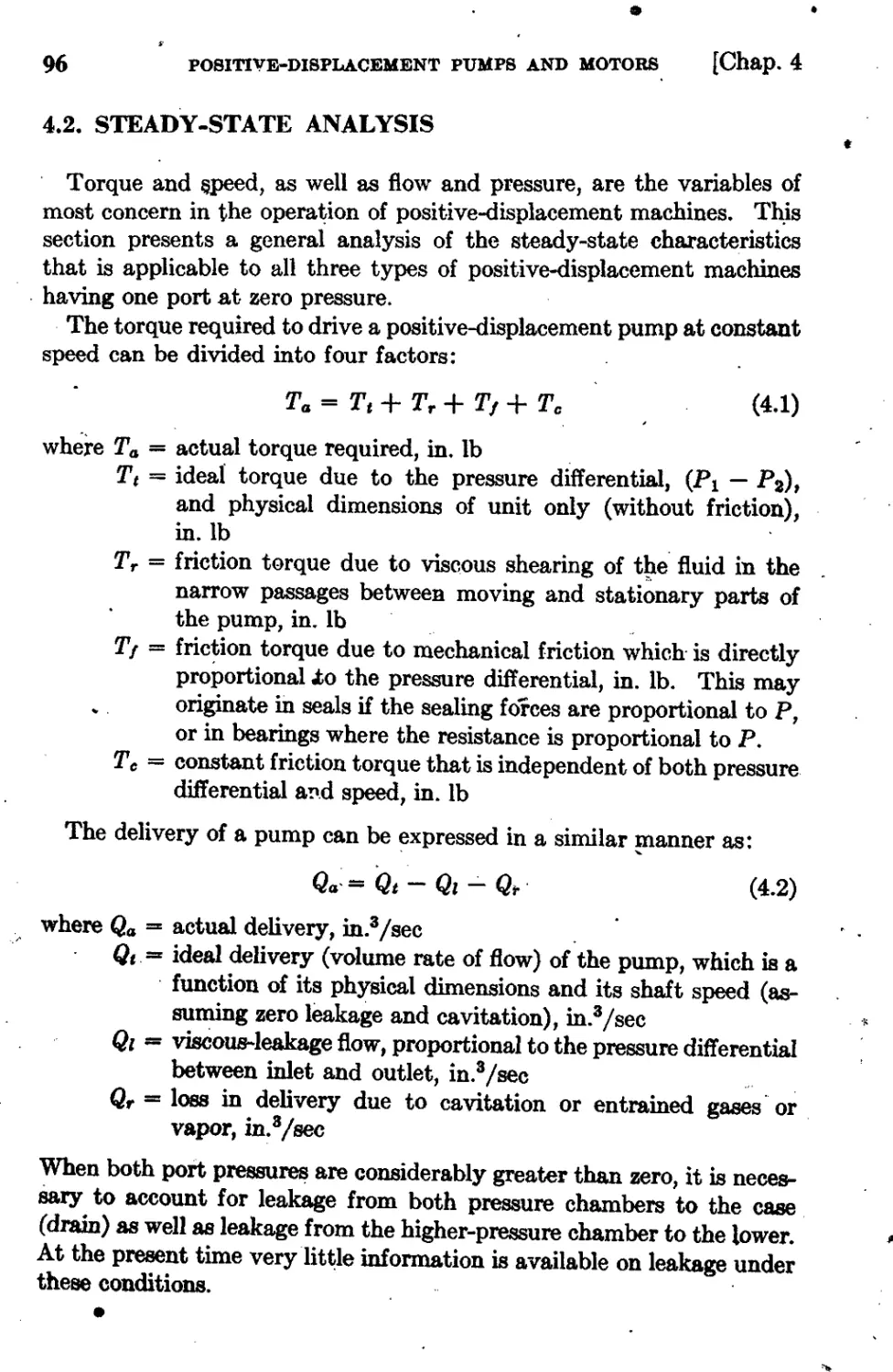
4.2 Steady-State Analysis 96
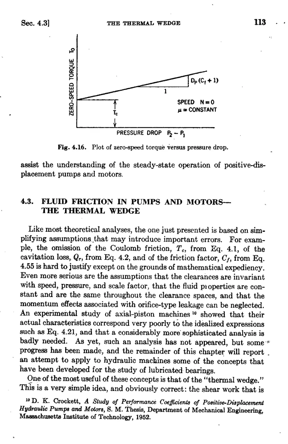
4.3 Fluid Friction in Pump& and Motors-
The Thermal Wedge 113'
Chapter 5 Fluid-Power Transmission
F. D. &ekiel and H. M. Paynter 130
5.1 Basic Concepts 131,
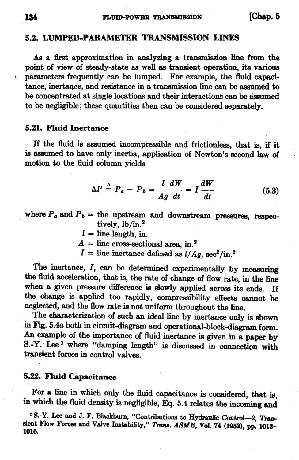
5.2 Lumped-Parameter 1)AmiRSi on Lines 134
5.3 Distributed-Fluid Systems 137
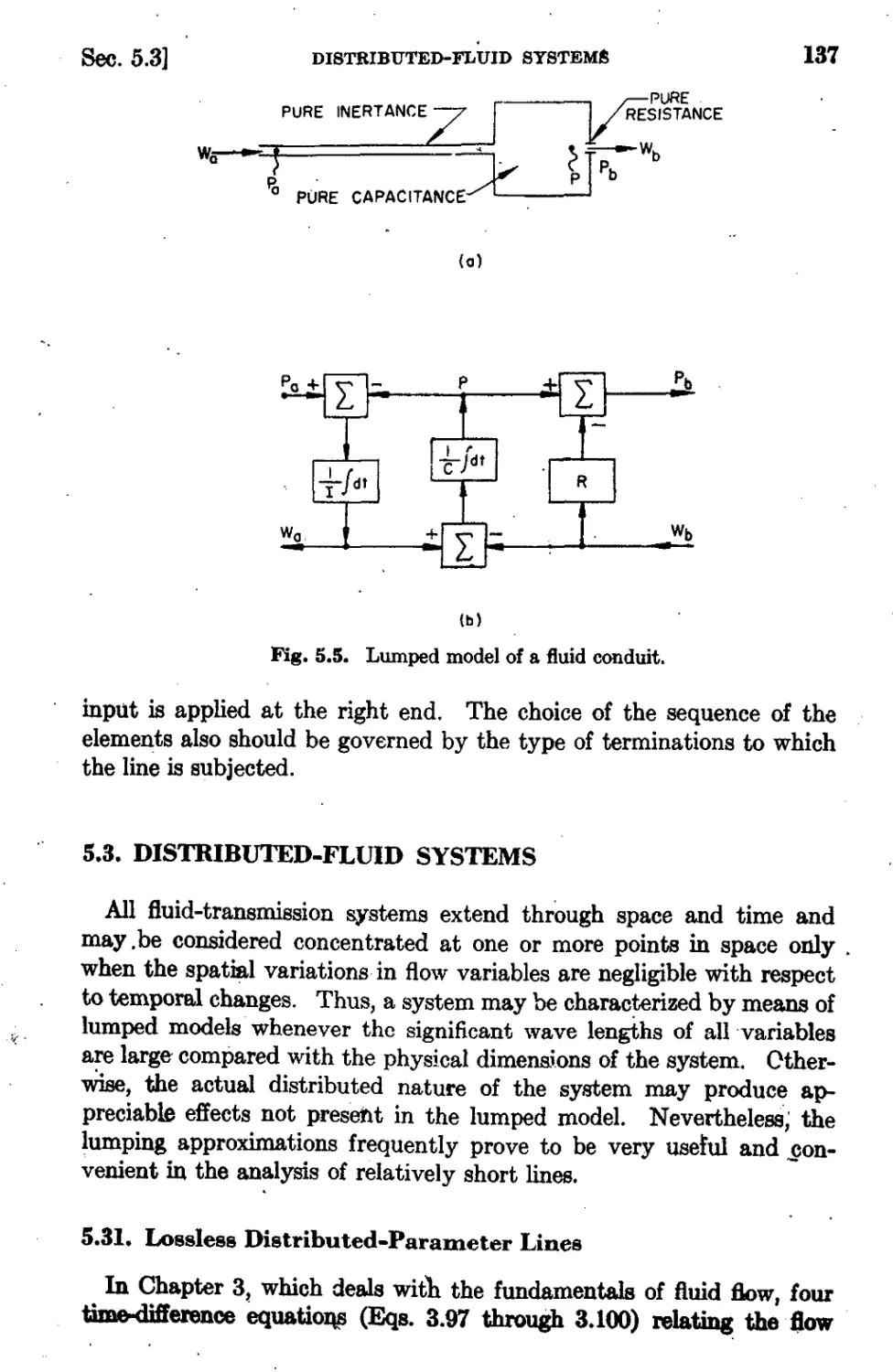
5.4 Frequency-Resp<:>nse Characteristics 140
Chapter 6 On Valve Control
J. F. BlGckburn 1-"
6.1 Introduction 144
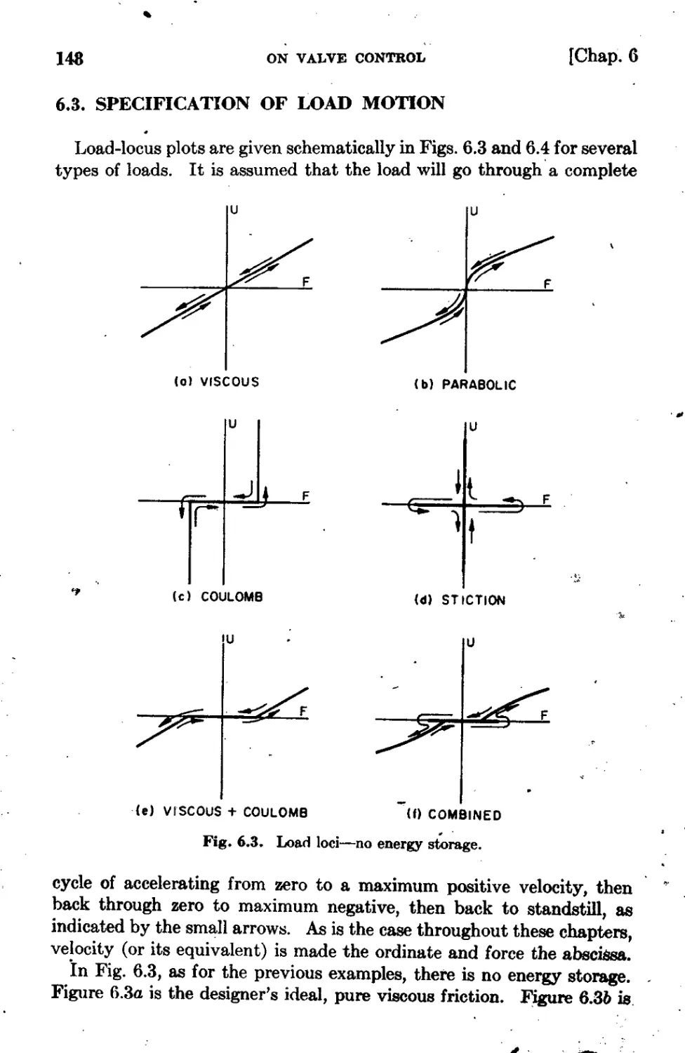
6.2 Description of the Load 144
6.3 Specification of L6ad Motion 148
6.4 Types of Drives 152
6.5, Valve-Controlled 'Drives 154
6.6 Typical Simple Drives 160
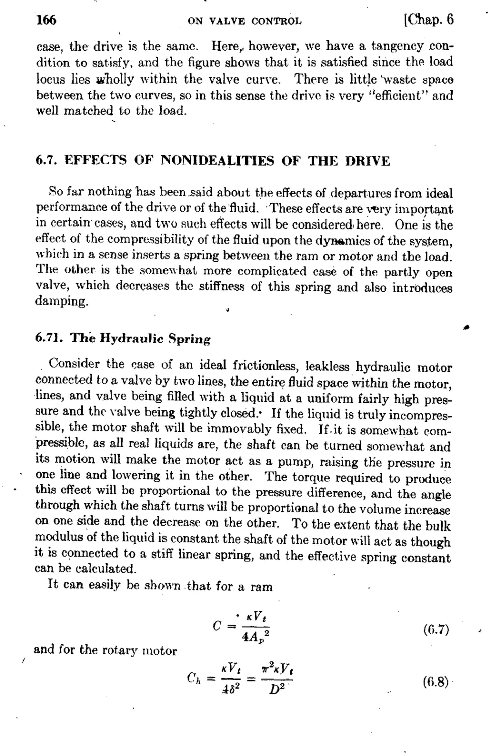
6.7 Effects of N onidealities of the Drive 166
6.8 More Complicated Systems 170
Chapter 7 Pressure-Flow RelatioD8hi.ps for Hydraulic
Valves
J. F. Blockburn 178
7.1 Introduction 178
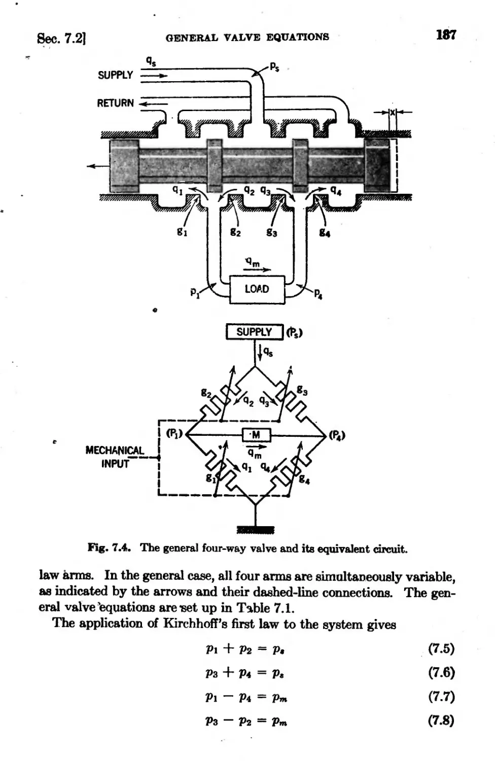
7.2 General Valve Equations 184
7.3 Constant-Presaure Operation 189
7.4 Constant-Flow OPeration 198
7.5 Effects of Asymmetry 002,
7.6 Differential Coefficients-Valve l'Gain" 204
7.7 Port Shaping 206
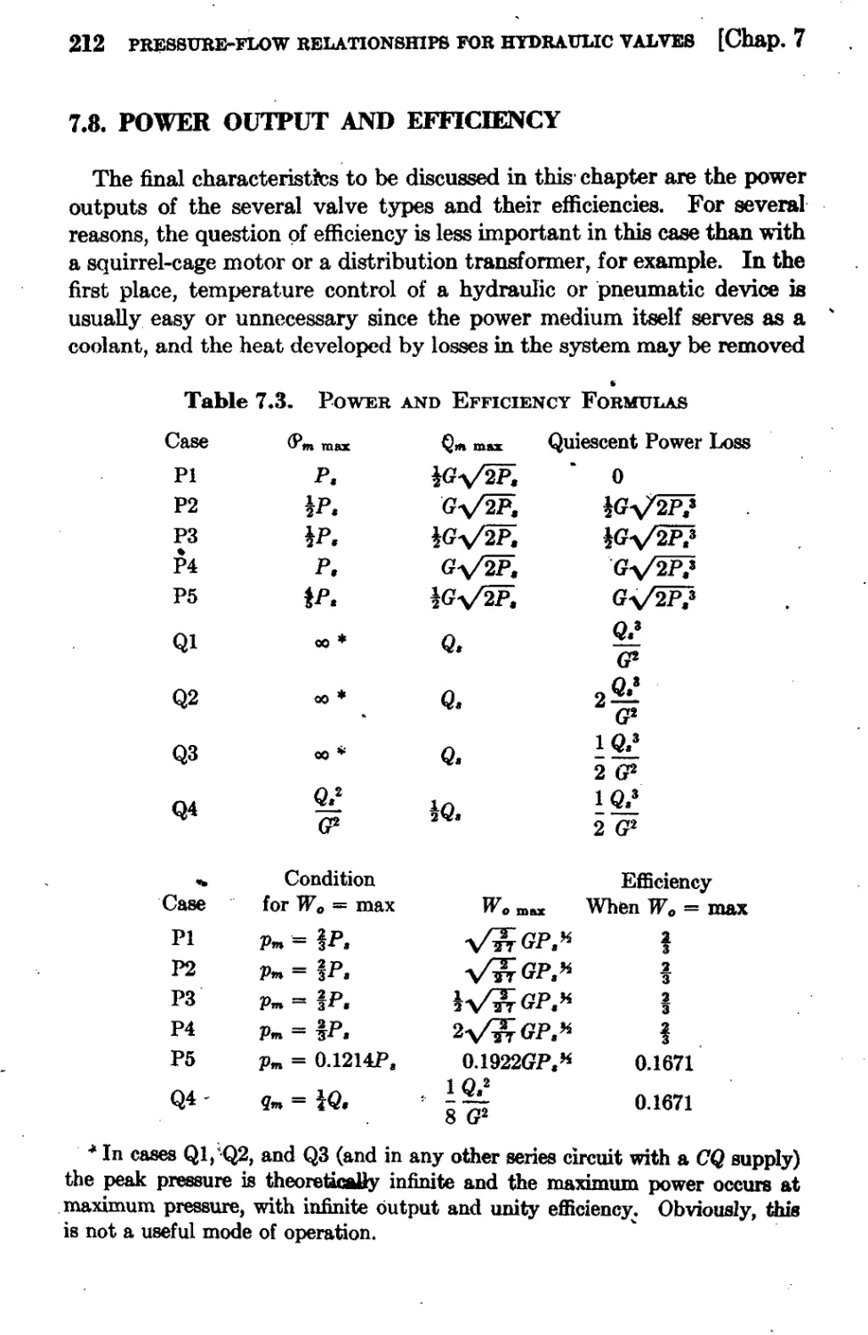
7.8 Power Output and Efficiency 212
CONTENTS xvii
Chapter 8 8ure-F1ow Ch8l'acteristics of Pneumatic
Valves
F. D. Esekiel and 1. L. Shearer 214
8.1 Introduction 214
8.2 Flow through & Single Orifice 215
8.3 caSe l-Constant Upstream Pressure. 220
8.4 Case 2-Constant Downstream Pressure . 220
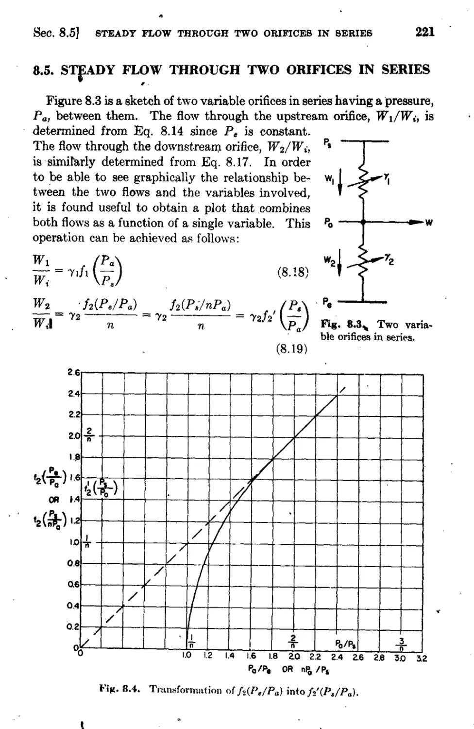
8.5 . Steady Flow through Two Orifices in Series 221
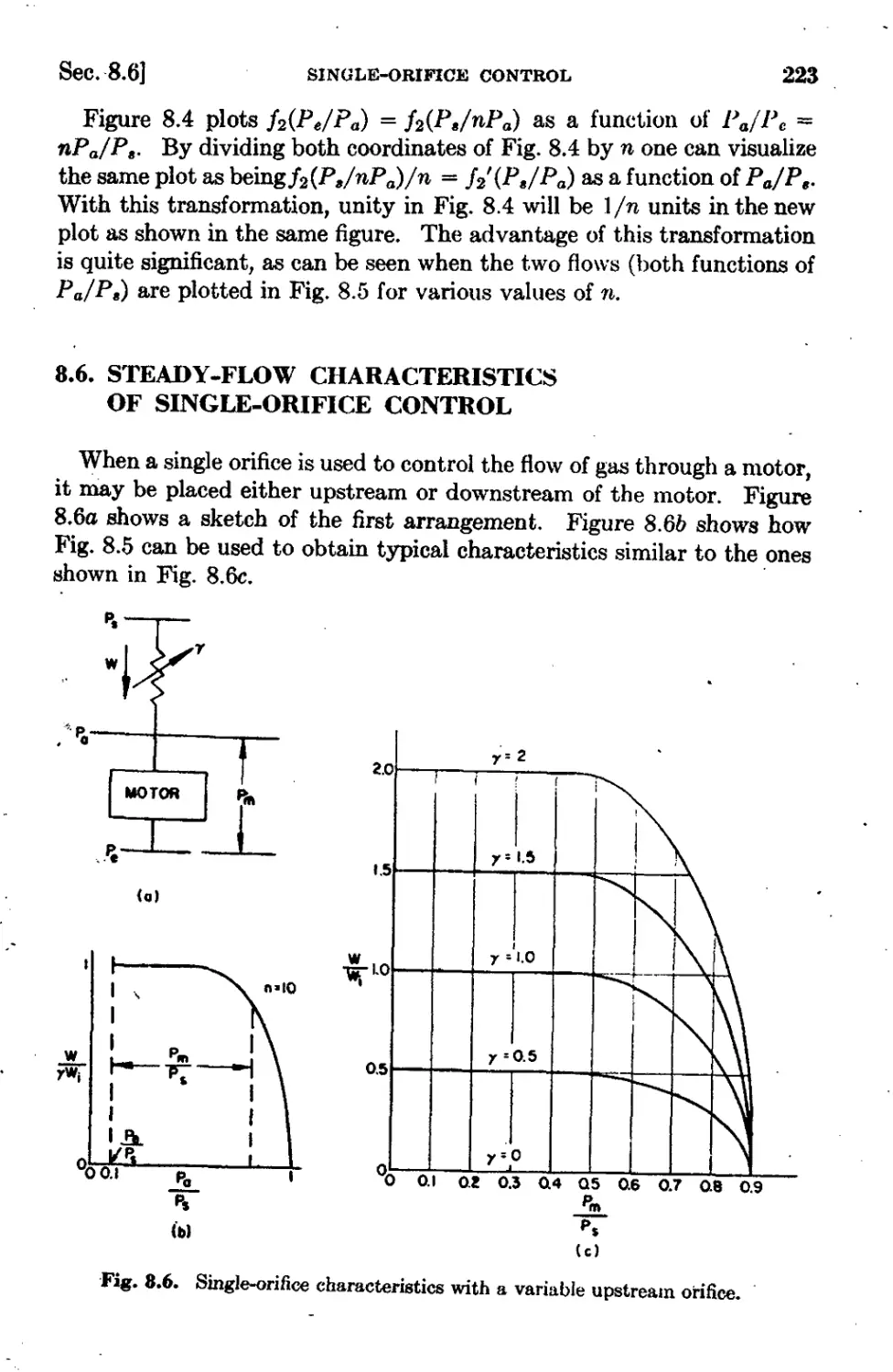
8.6 Steady-Flow Characteristics of Sitigle-Orifice Control '223
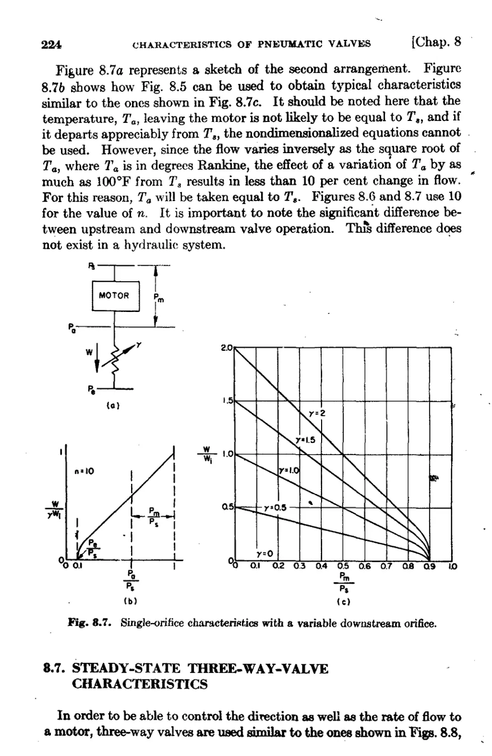
8.7 Steady tate Three-\¥ay-Valve Characteristics 224
8.8 Steady tate Four- W ay- V alve Characteristi 228
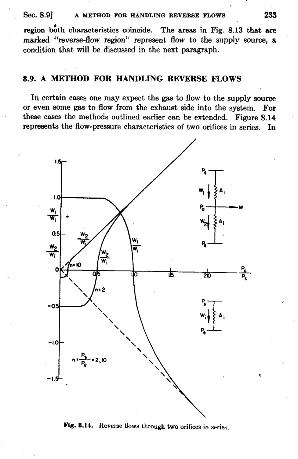
8.9 A'Method for Handling Reverse Fl0W8233
'Chapter 9 Valve Configurations and Constructions .
S.- ¥. Lee and 1. F. BlGckburn. 235
9.1 Introduction 235 .
9.2 . Basic Valve Configurations 235
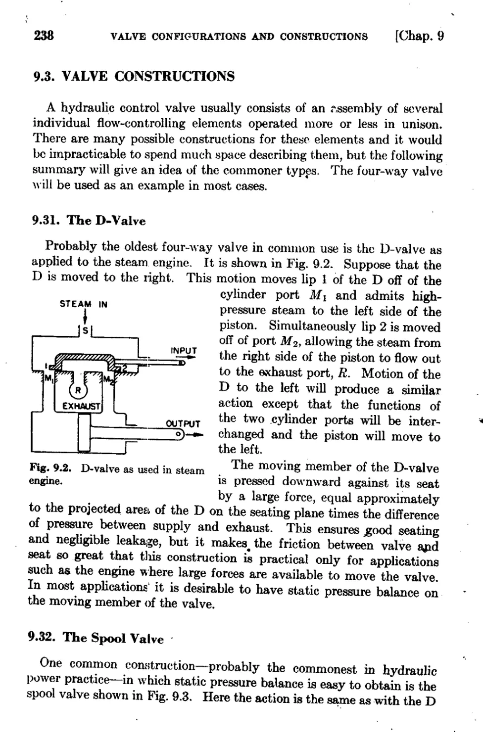
9.3 Valve Constructions 238
9.4' . .valve Design 246
9.0 Experimental Fabrication of ValVe$ . 259
9.6 Special Featu,res of Pneumatic Valvea . Z15
'Chapter 10 Steady-State Operating Forces
1. F. Blackburn 278
10.1 Introduction 278
10.2 Lateral Forces-Friction and Hydraulic.Lock 279
'10.3 Axial Forees 297
10.4 Fmoos on Flapper Valves-Pressure Feedback ,313
l(}.S' Forces on Other Types of Valves 318
Chapter 11 Electromagnetic. Actuato:r;s
R. H. FraRer 322
. 11.1 Valve Actuators 322
11.2 Electric Actuators 323
Chapter 12 Transient Forces 1and V alve InstabUi
J. F. Blackburn, J. L. CoaIde2, and
F.' D. &seidel . 359 .
12.1 Introduction 359
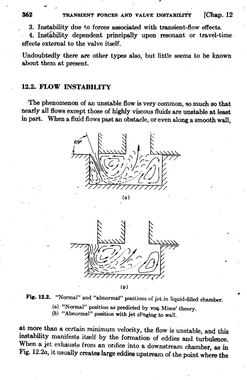
12.2 Flow Instability 362
nili
CONTENTS
12.3 Instability Caused by Steady..state Forces.
12.4 Transient-Flow Instability
12.5 Resonant Instability
. 864
.
868
.- 377
Chapter 13 Electrohydraulic Actuation
S.- ¥. Lee and J. L. Shearer 401
13.1 Introduction 401
13.2 Practical Tw tage Valves 403
13.3 A Miniature Electrohydraulic Actuator 408
13.4 Appendix 428
Chapter 14 The Analysis of the Dynamic Performailce
of Physical Systems
J. ;f. Hrones 433
\
14.1 Introduction 433
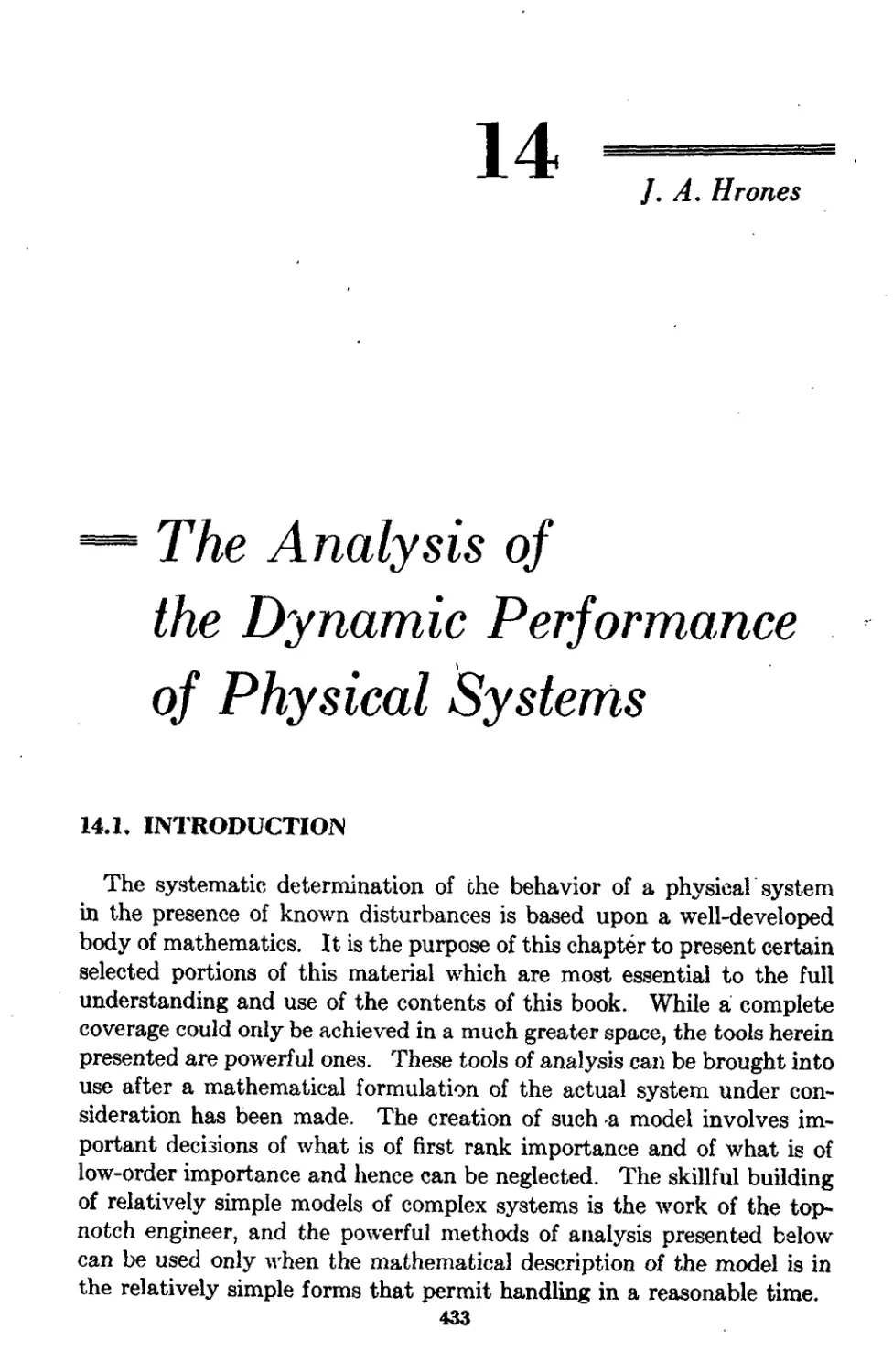
14.2 Linear Elements 434
14.3 Definitions 435
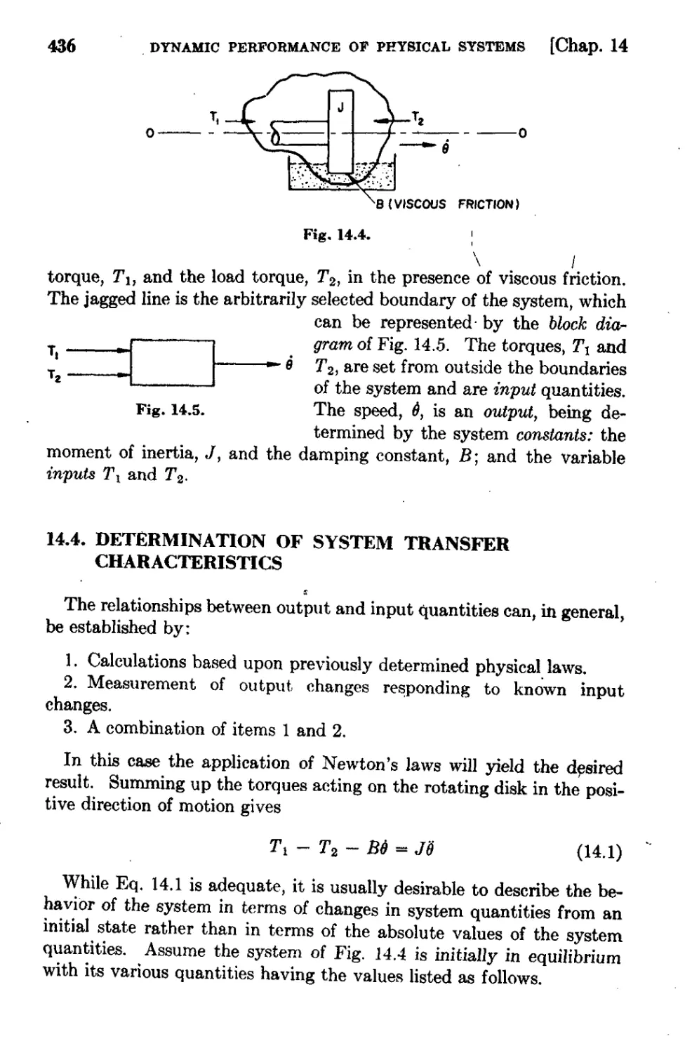
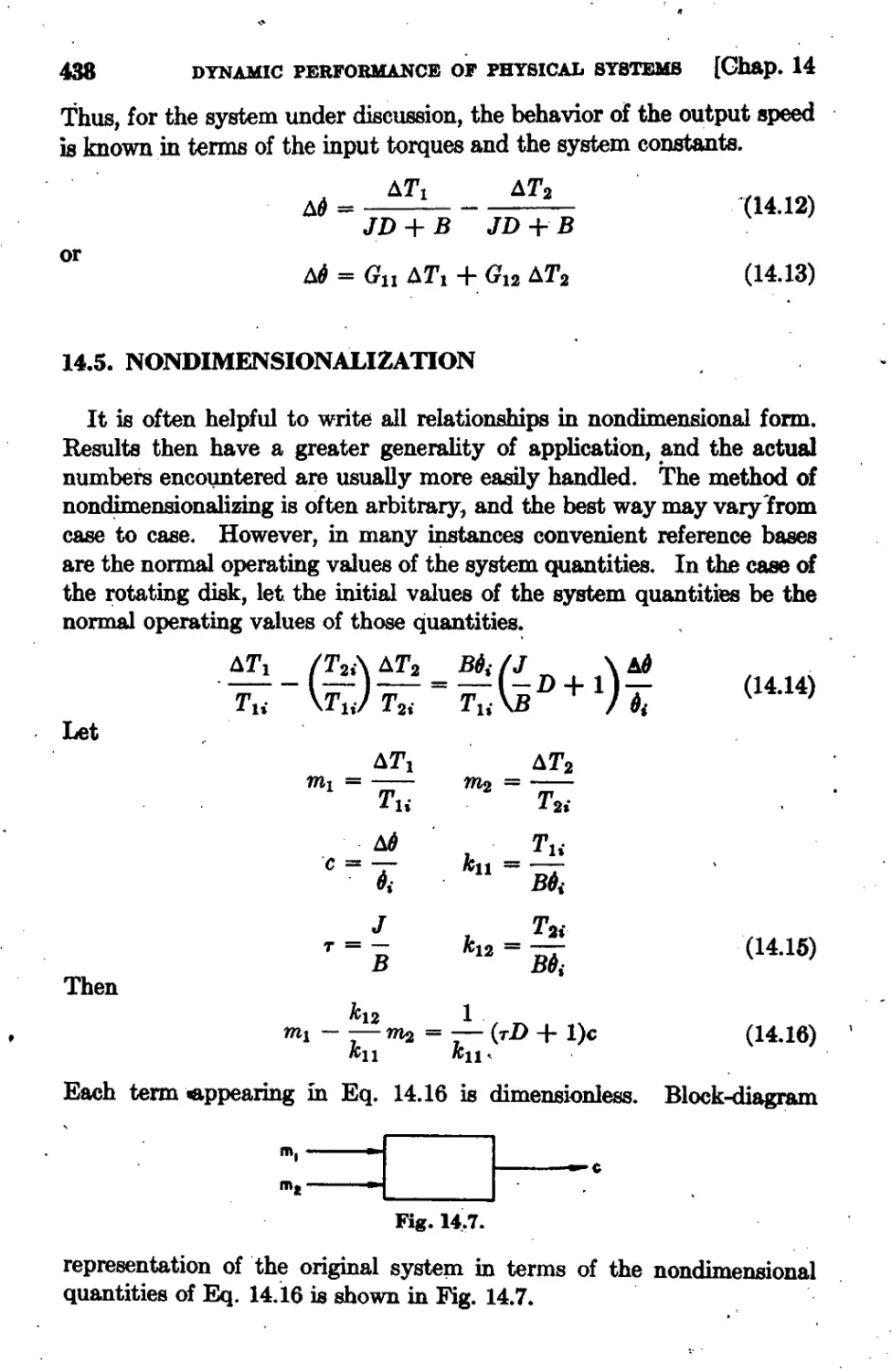
.14.4 Determination of System Transfer Characteristics 486
14.5 Nondimensionalization 438
14.6 . amic Response of a Syste to Disturbances 439
14.7 The Single-Capacity ystem 441
14.8 The Solution of the FirstrOrder Differential EquQ.tion 441
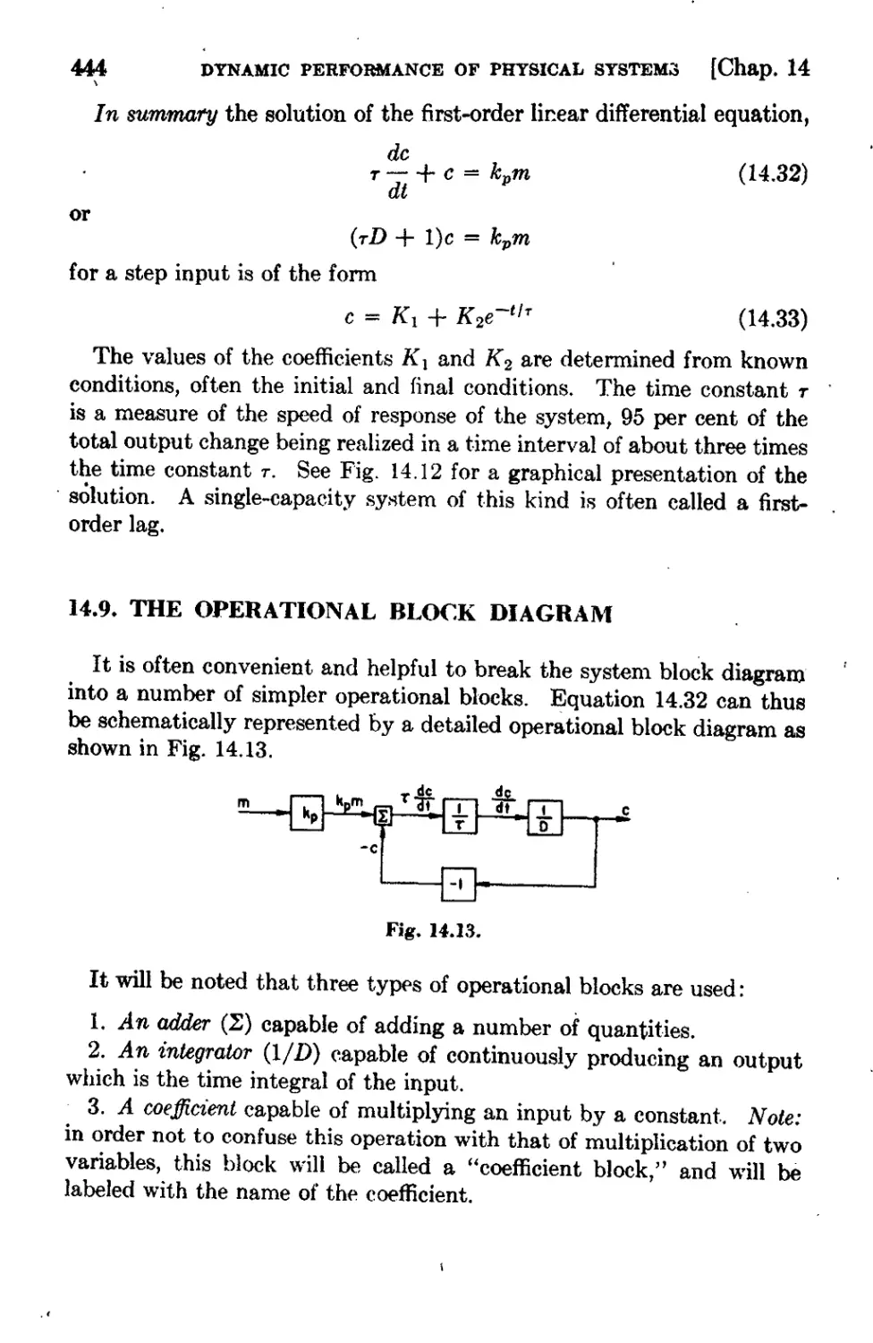
.14.9 The Operational Block Diagram' 444
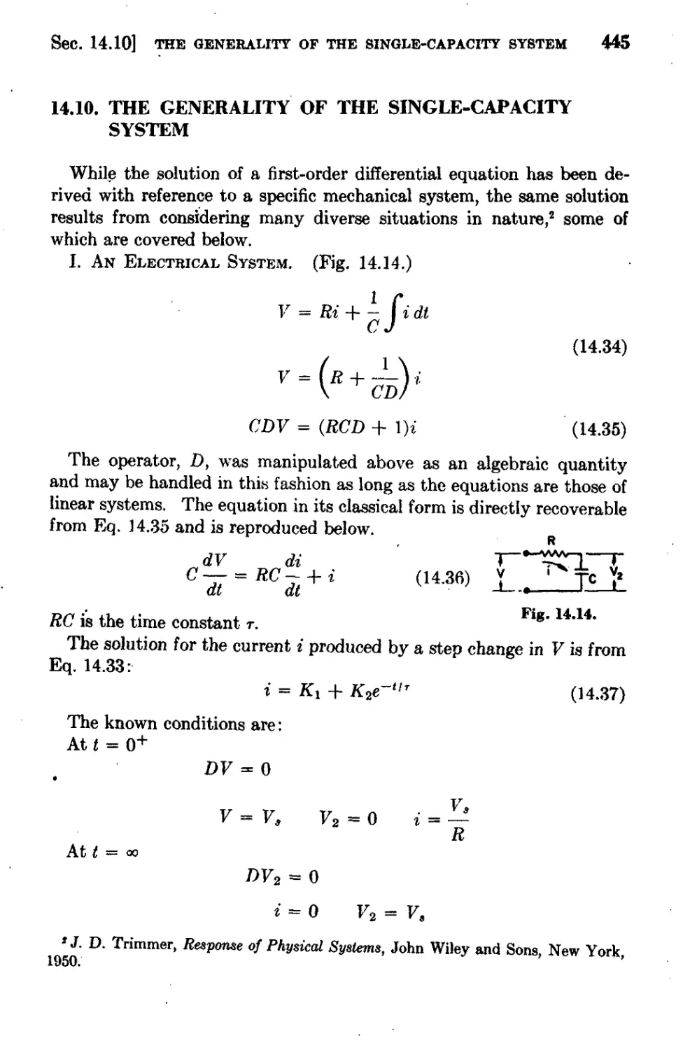
14.10 The Generality of the Single-Capacity System 445
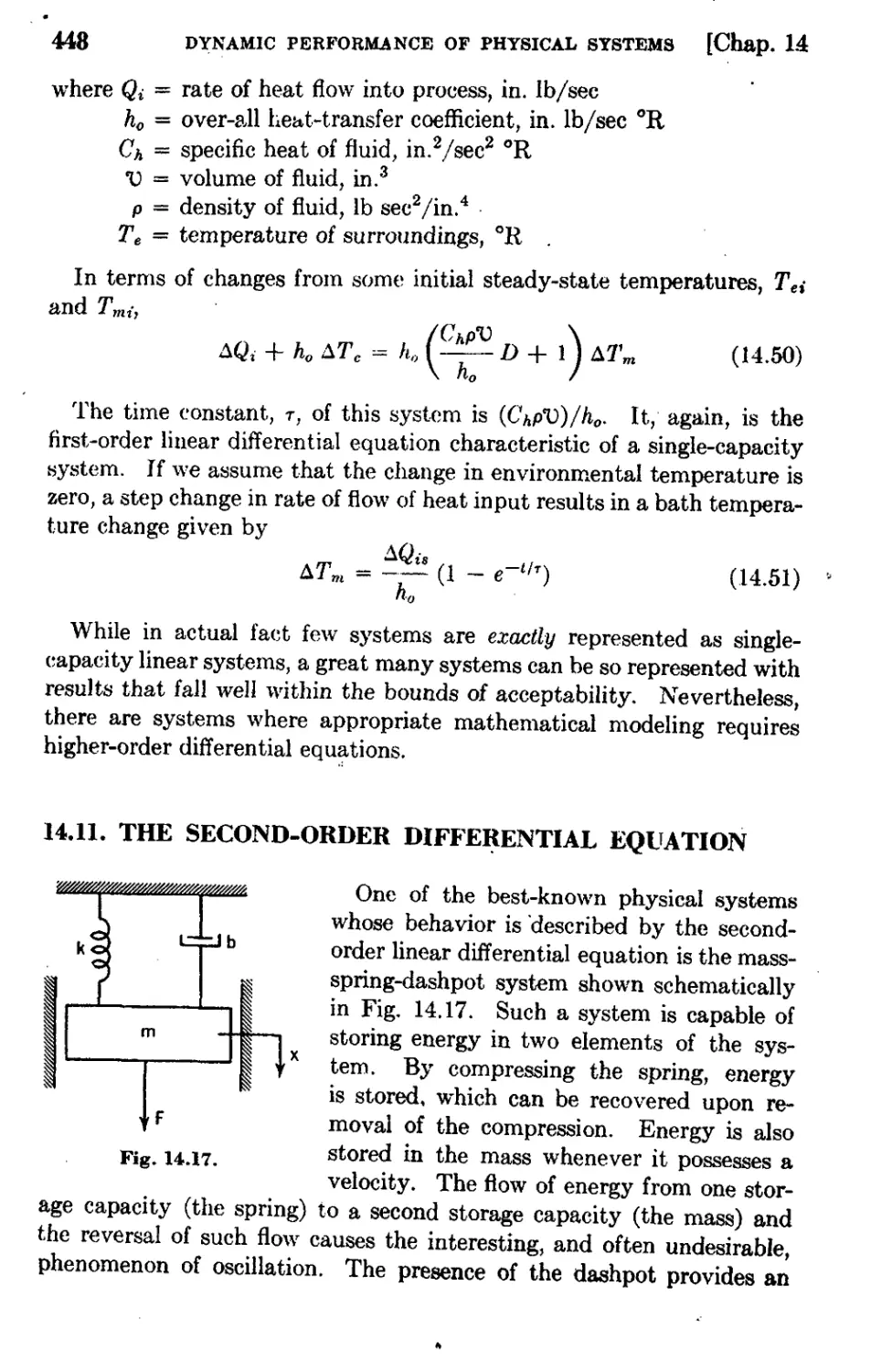
14.11 The Second-Order Differential Equation 448
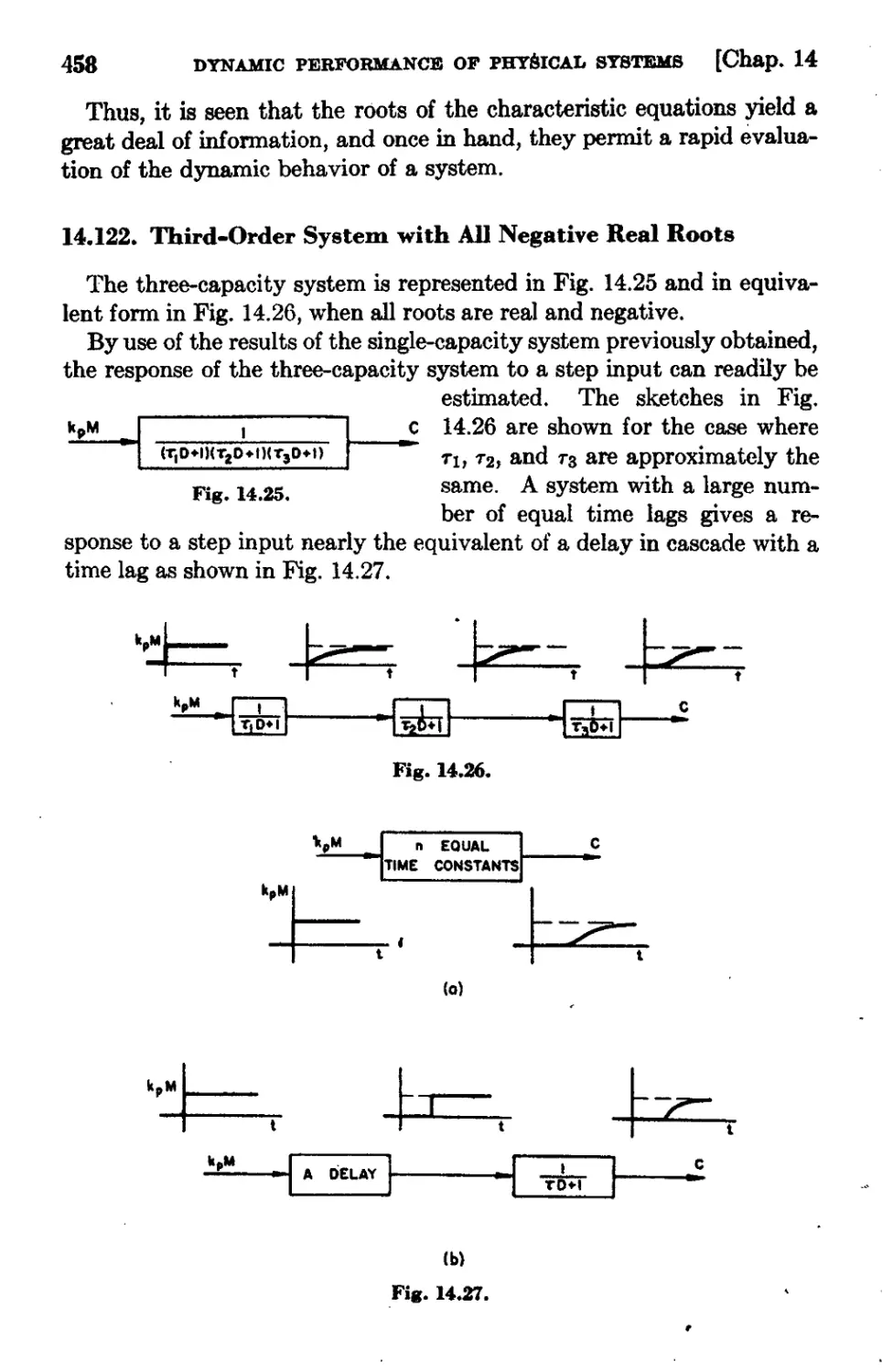
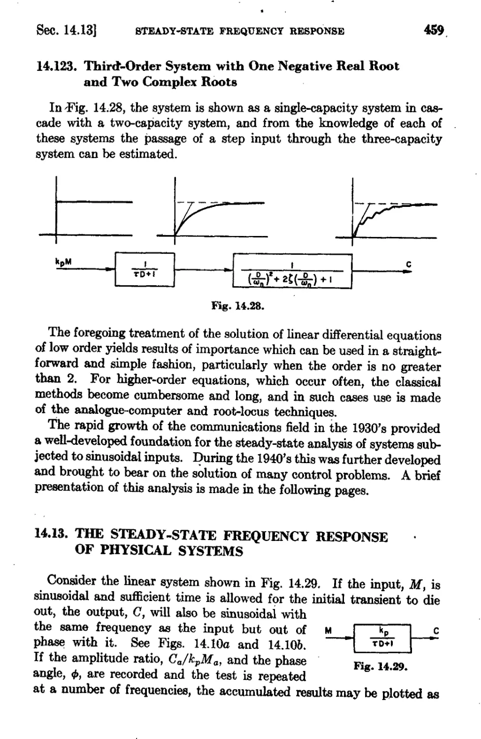
14.12 The Solution of Higher-Order Differential Equations 456
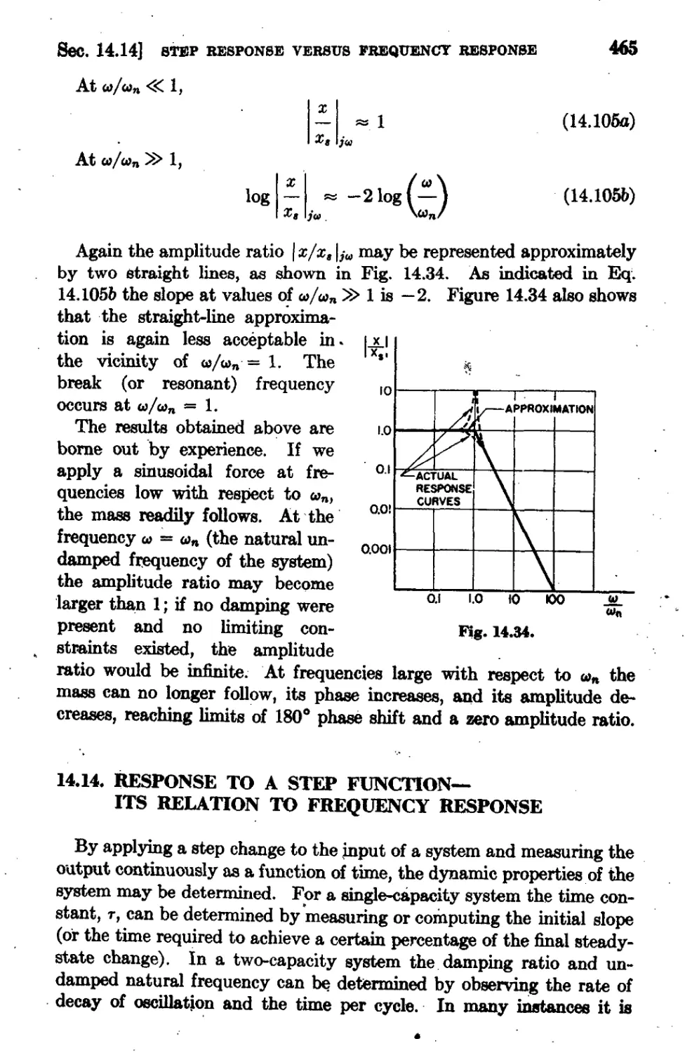
14.13 The Steady-State Frequency Response of Physical Systems 459
14.14 Response to a Step Function-Its Relation to
'OO 4M
14.15 Fr uency Response of Cascaded Elements .466
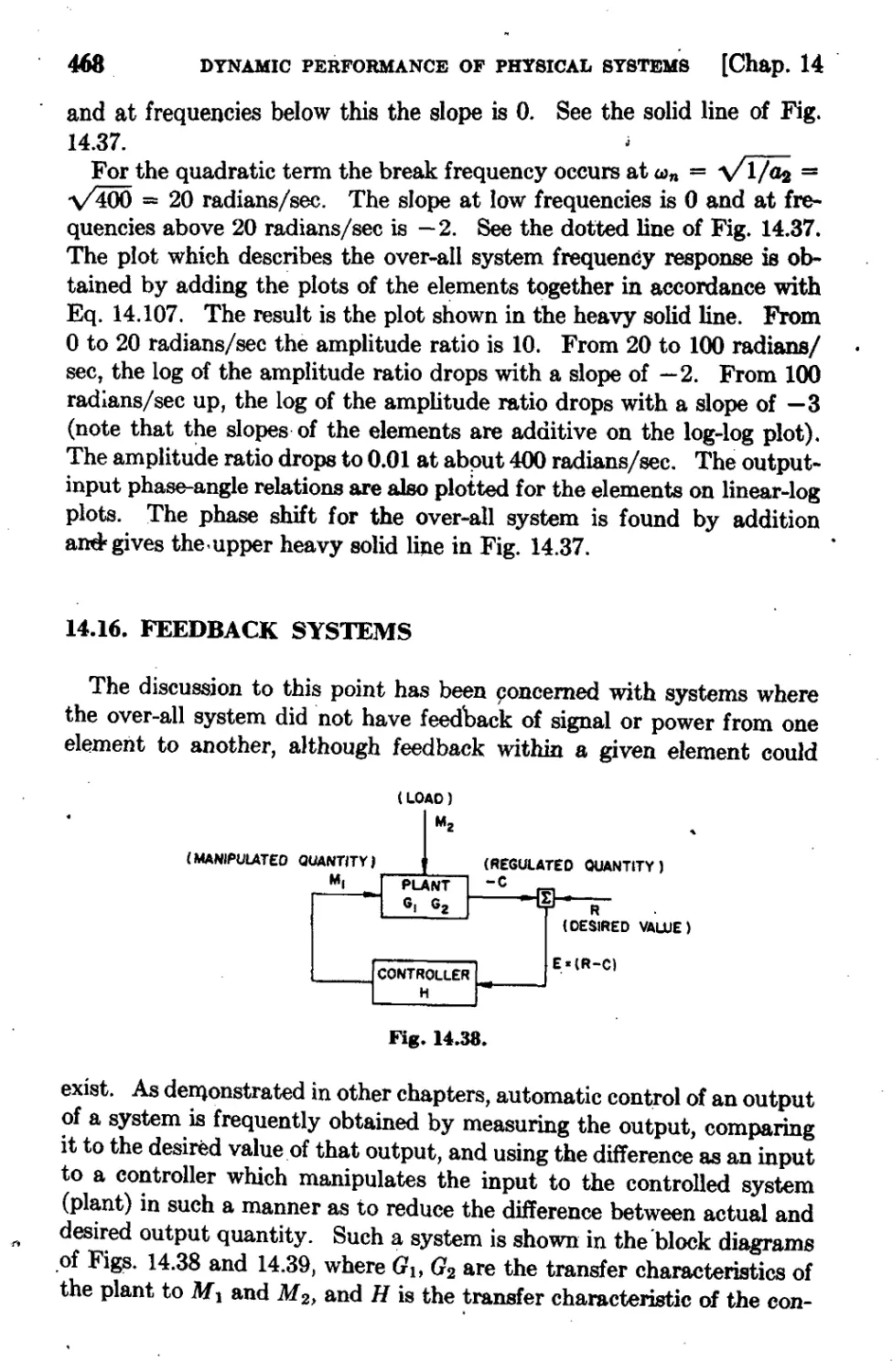
14.16 Feedback Systems 468
14.17 Criteria of Performance of Closed-Loop Control Systems' 469
14.18 The Analysis of the Performance of Feedback Systems 471
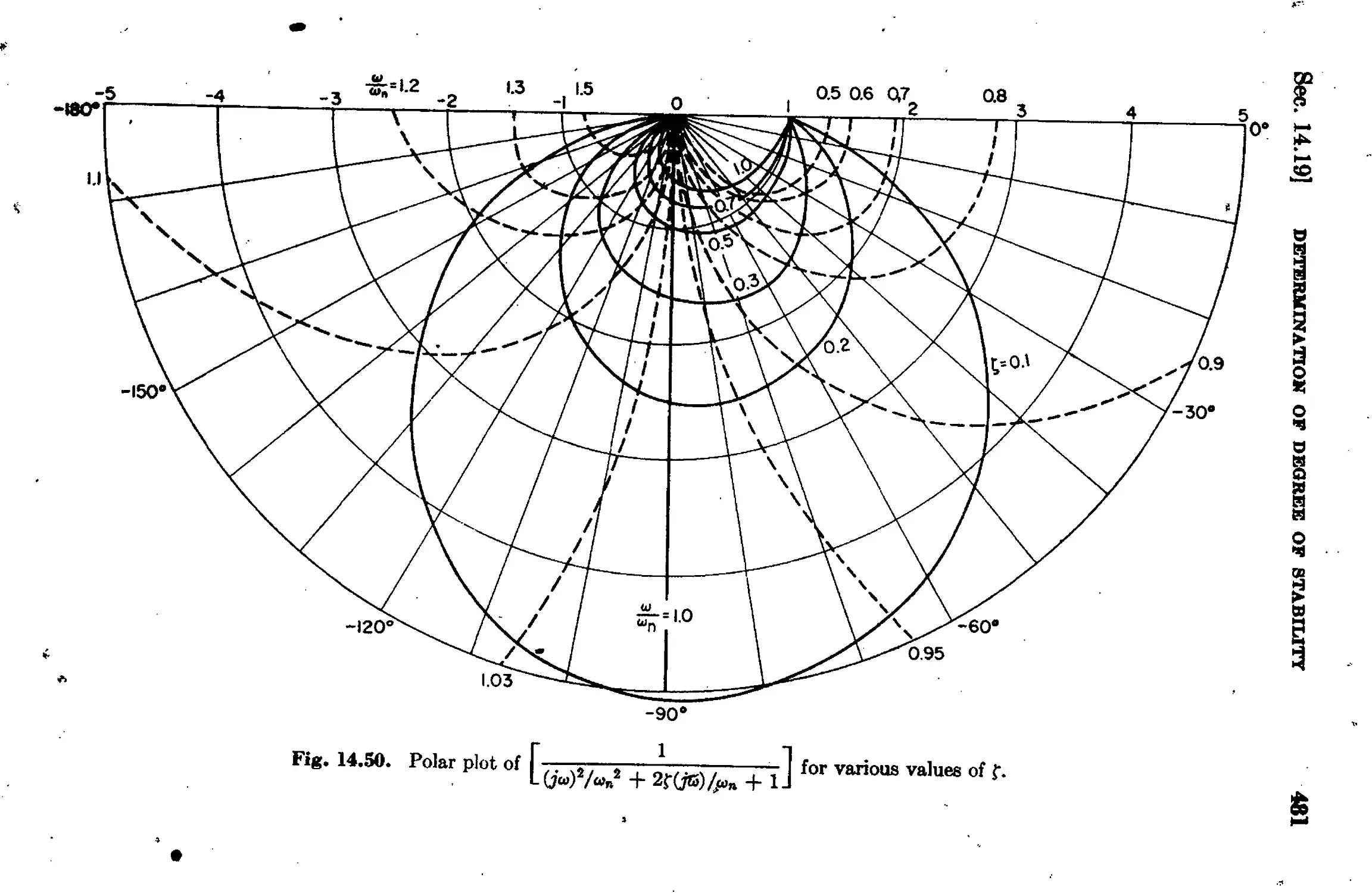
14.19 Determination of Degree of Stability 472
i4.20 Root-Locus Method 486
14.21 Summary of Techniques Co:q.sidered 495
Chapter 15 Hydraulic Drives
J. L. Shearer 498
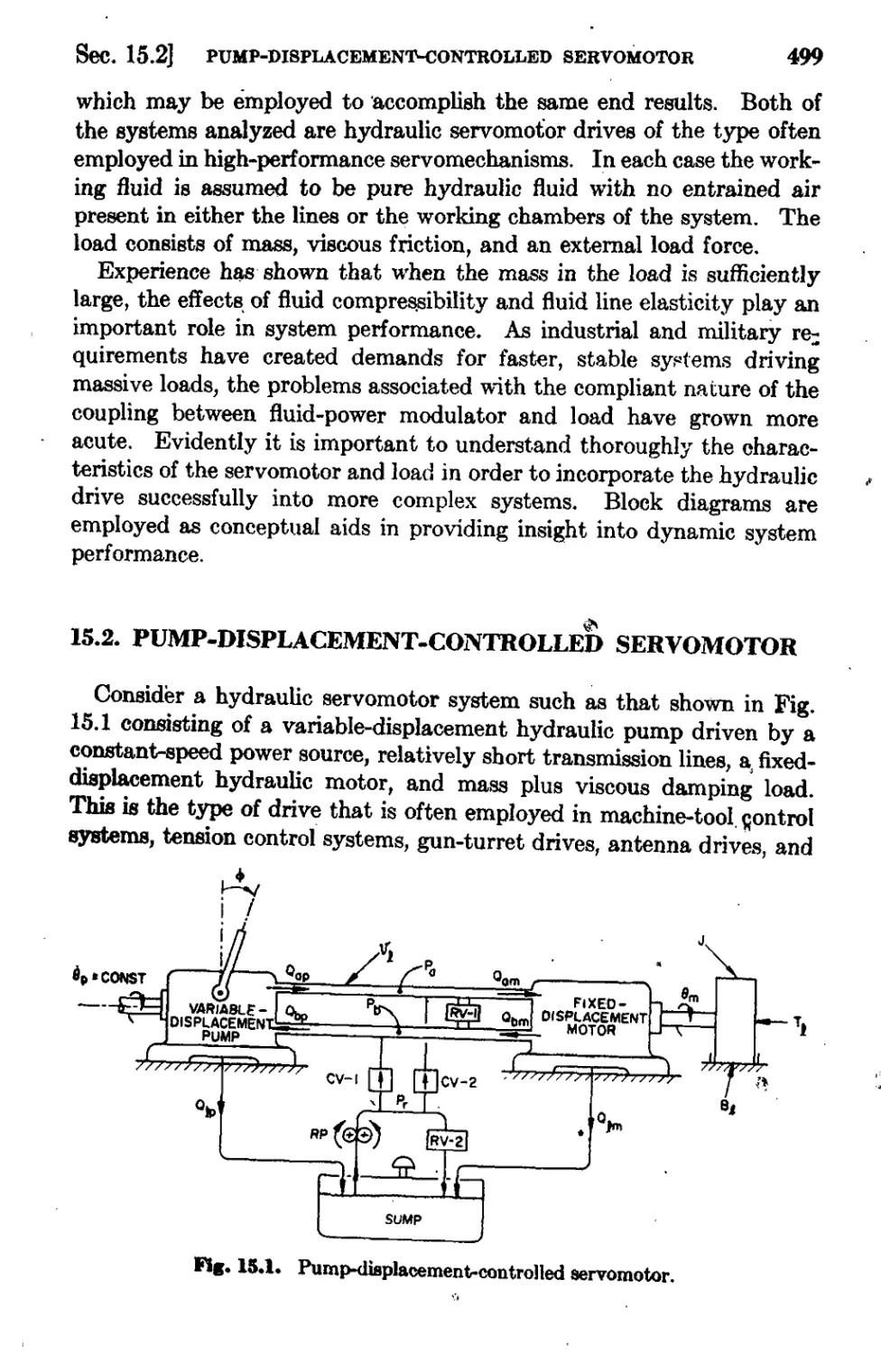
15.1 Introduction 498
15.2 Pump-DisplacementrControlled Servomotor 499
. '
CONTENTS
m
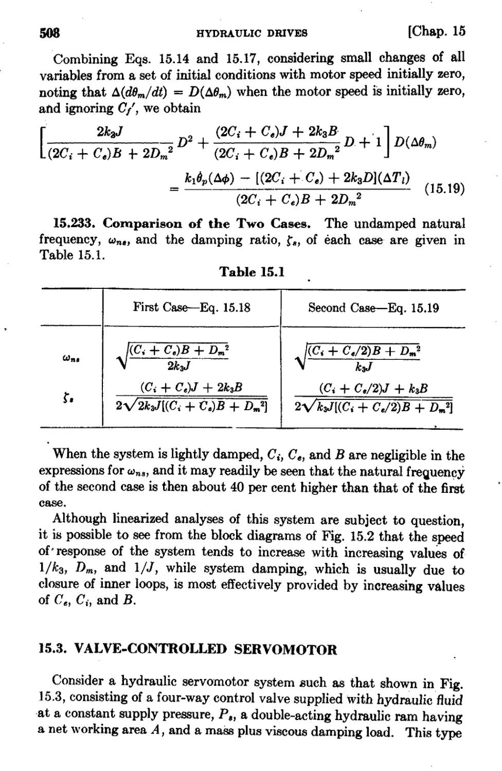
508
516
15.1 Valve-Controlled Servomotor
15.4 Conclusiol18 '"
Chapter 16 Pneumatic Drives
J. L. Shearer
16.1 Introduction
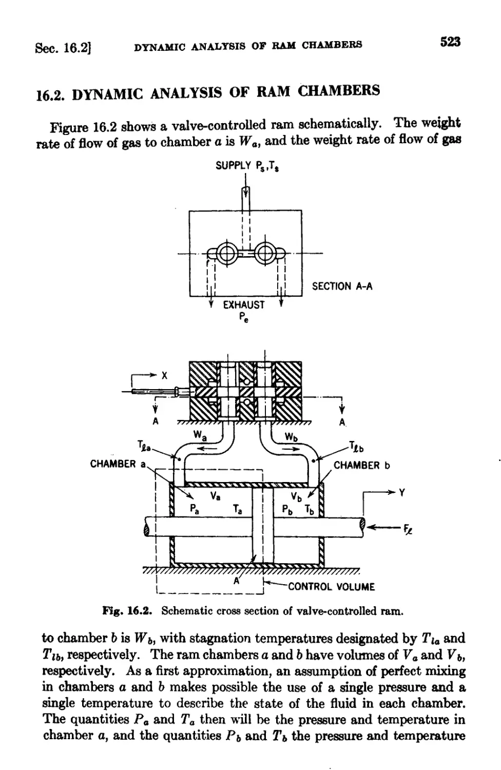
16.2 Dynamic Analysis of Ram Chambers
16.3 Control-Valve Characteristics
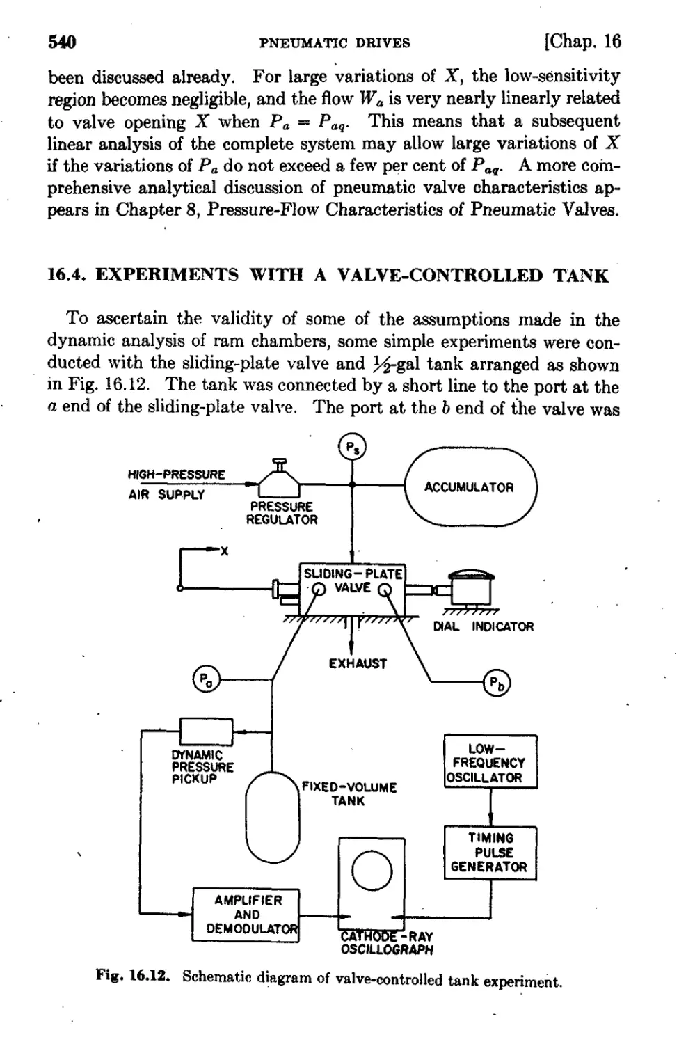
16.4 Experiments with a Valve-Controlled Tank
18.5 Analysis of Valve, Rani, and Load System
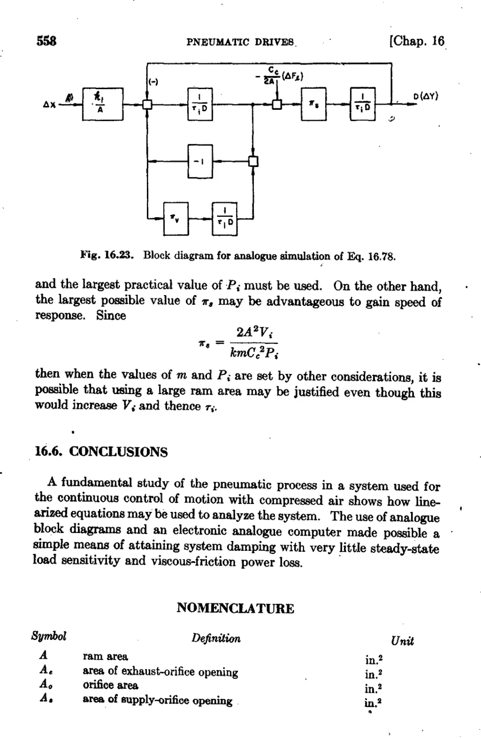
16.6 Conclusions
521
521
523
5Z1
540
543
558
Chapter 17 Closed-Loop Systems
Gerhard ReethoJ and J. L. Shearer
17.1 Introduction
17.2 Proportional Control of Rate-Type Servomotors
17.3 Dynamic Study of Pressure-Controlled Hydraulic
Systems
17.4 Analogue Computer Study of a Velocity-Control
Hydraulic System
17.5 Nonlinear Analogue Study of a High-Pressure
Pneumatic Servomechanism
562
562
56
575
591 '
,
616
Chapter 18 Power Steering
T. E. Hoffman
18.1 Introduction
18.2 The Fluid-Power Source
18.3 The Actuator Unit
,
631
631
633
635
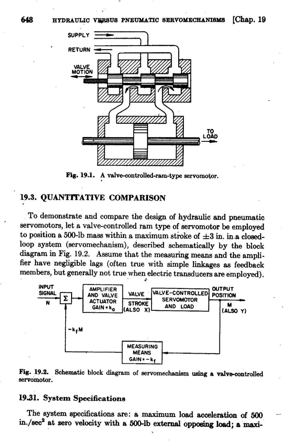
Chapter 19 Comparison of Hydraulic and Pneumatic
Servomechanisms
J. L. Shearer 647
19.1 Introduction 647
.
19 2' Qualitative Comparison 647
19.3 Quantitative Comparis )D ,.t' 648
s
Chapter 20 Analysis and Design of Servomotors Operating
on High-Pressure Hot Gas
Gerhard ReethoJ 659
20.1 Introduction 659
....
,
;'.:
u
CONTENTS
.20.2 System Considerations
20.3 Pneumatic-Power Generation .
20.4 Power Control
20.5 Power T ranAm1AAio n and Conversion
20.6 Description of the System
20.7 Component Analysis
20.8 System Analysis
.20.9 Design Example
Index
'.
...
'"
660
661
663.
663
667
667
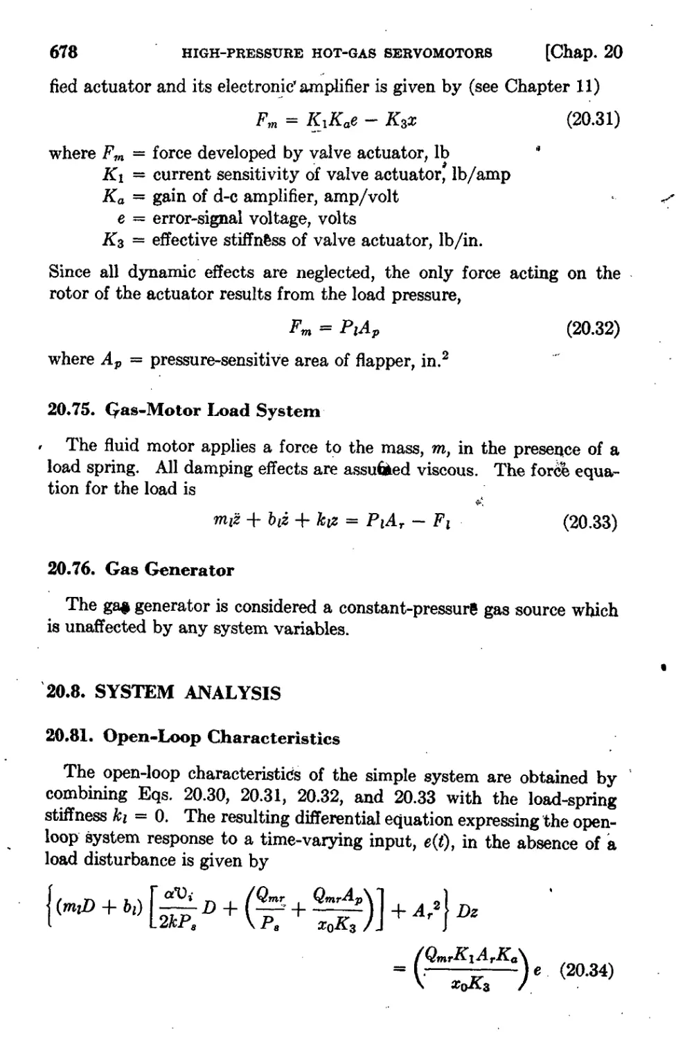
678
681
695
.
1
I. F. Blackburn
Fluid Power
1.1. INTRODUCTION
The subject of fluid power control offers an excellent example of the
development of & btanch of engineering. With the invention of eco-
nomicaJly useful p e movers such as Watt's steam engine and the
development of the factory system, there arose a need for a method of
t nnsmit ting power from the point of generation to & more or leas distant
power-using machine.. This t ra."$I'I1 on could be accomplished me-
chanica.lly, as by lineshaft and belting, but mechanical t ransmiARi on was
often expensive and inponvenient. Probably its greatest inconvenience
was the difficulty of c ntrolling the flow of power accurately and cheaply,
and one solution to the problem lay in transmi on by & fl d under
pressure.
This development was pushed baud for & time, and in some industrial
cities, particularly in England, l regular networks of high-pressure water
'piPes were 'laid between central nerating statioDB, which contained
-driven pumps, and the mills which used the power. In order to
make such systems . practical, it was necessary to invent a large numbe
of auxiliary devices, such as hydraulic accumula.tors and various control
and regwating valves, and to amaee & considerable body of information
about how the commoner problems of operation could be met. The
de d produced the supply; numerous hydraulic devices, many of
1 Ian McNeil, HgdrtIulic tIftd Cmdrol aJ'Jlat:l&it&a, Bona1d Pre., New
York, 19M, pp. 187-140.
1
2
FLUID POWER
[Chap. 1
them most ingenious, appeared on the market or in the pages .of the
newly founded engineering magazines, and there arose a class of fluid-
power specialists who were skilled in the art of generating, transmitting, .
and controlling power by means of high-pressure water.
Unfortunately, as is usually the case with a rapidly developing subject, .
this new art remained largely a.n' art; practice far outran theory, and
much of the lore remained qualitative rather than quantitative. The
situation no doubt would have been remedied in time except that the
. .
ec.onomic foundation for the whole art was swept away by the phe-
nomenal growth of the electric-power industry. Electrical power can
be transmitted much more economically and .efficiently and. to vastly
greater distances than the power produced by any hydraulic or 'pneu-
matic technique ever can, and as this was obvious from the beginning,
the fluid-power aJ1i withered and nearly died for some. generations.
For several decades now it has been undergoing a rebirth, however, .
and at the present time it is a subject of great interest and importance.
This is due not to any recently discovered deficiencies in the electrical
techniques of power transmission, but to the rapid rise in the. demand
for types of performance that are difficult or impossible to obtain from
electromagnetic devices alone. In particular, the need for servo-
mechanisms of large power and exceedingly rapid response fQr both
military and industrial Applications requires motors with torque-to-
inertia ratios several orders of magnitude higher than can. be obtained
from an electric motor. In spite of its relatively great cost. and its
numerOJls inconveniences, the use of fluid power has been forced upon
us, and we must learn how best to use it.
Now, as in the nineteenth century, much of'the demand is being
satisfied onan empirical basis; many current hydraulic devices are being
designed but not engineered. The designer of today has innumerable
advantages over his predecessor of a century ago, but like him he suffers
""from the-lack of a unified and organized presentation of the basis of hiS .
work. This statement does not imply that the knowledge of the physical
phenomena is lacking j alter all, hydrodynamics is one of the older
branches of physics, and within the last generation it has put on working.
c10thes and changed its !lame to fluid mechanics, and there are excene t .
texts on the subject. The trouble with most of these te is that they
oover all of hydrodynamics, and many of them cover aerodYnamics also.
With such a vast field it is impossible to dig very deeply at anyone spot,
and current texts make no attempt to do so.
In this book only as much theory is given as is necessary for the exposi-.
tion of the subject. It is assumed that other books are available to
remedy any deficiencies in this respect. Comparatively few formulas
......
"
Sec. 1.2]
WHY FLUID POWER?
8
are derived and there is little attempt at mathematical rigor or elegance.
Thi is a book for the practicing engineer, and we hope that the informa
tion is presented in a way which will make it most useful to him, and be
least likely to lead him astray through concealed assumptions or logical
booby traps. .
Throughout the. book the theory is supplemented as far as is practi-
cable by present practice in the field of fluid power. Because this
field is developing very rapidly, its center of gravity is constantly shift-
ing arid it is impossible to give a truly balanced presentation of the
subject. For the same reason the part of the book that applies to practice
is somewhat ephemeral, but the fundamental part is of permanent value,
and it is this fundamental part that makes present-day fluid-power
control an engineering scienc rather than an art. .
1.2. WHY FLUID POWER?
.It has already been stated that there is a rapidly growing. interest
in fluid power, and since this is the primary concern of this book, it is
in order to explain this interest and to compare fluid power with elec-
tri l and mechanical power.
In most respects fluid power occupies a position somewhere between
electrical and mechanical power. It is easier to transmit over appreci-
able distances than mechanical power, but far.more.difficult to transmit
than electrical power. Both fluid power and electrical .power are much
more easily and accurately controllable than mechanical power; elec-
trical power is the best in this respect at low power ievels, but its superi-
ority is much leas marked at higher pOWer levels. From the standpoint
of safety the three are about equal, except that it is somewhat harder
to guard mechanical power-tra mitting elements from accidental human
contact. From the standpoint of efficiency when long-distance trans-
mission is not involved, mechanical power is usually superior and the
other two about equal. Cost comparisons are difficult to make since
they depend so much upon each individual case. At low power leve\a
.lectrical devices are much cheaper than those of the other two classes;
at high power levels there is probably not much difference on the whole.
From the standpoint of availability af a wide variety of components,
electricity is far better than the others; furthennore, this abundance of
. components and techniques is reflected in a flexibility of application
that they cannot claim. The same is true of .speed of response, except
for the all-importttnt limitation that applies to electromechanical devices.
This J.in.rltation a.nd its consequences will be discussed later.
" FLUID POWER [Chap. 1
On the basis of the foregoing paragraph alone it might be concluded
that there is little difference among the three types of power but that
perhaps electricity is better on the whole. In the average case if there
is an average caa&-this is probably true, and it is for this reason that
electrical techniques and equipment have been so ,much further de-
veloped than the others. Within a comparatively fe,! years, however,
advancing technology has forced the 'electrical designer againSt an ap-
, parently impenetrable bamer in his efforts to improve his eq pment
still further, and since to date he has been unable to penetrate the barrier,
it is necessary to seek a path around it. The easiest and mOst direct
path appears to be the use of 8uid power. ,
The barrier just referred to is a property of. matter, the fact that any
known ferromagnetic material saturates at an inconveniently I w fI
density. This means that' no more than a certain torque ea.n be obta.ined .
from 8 pound of iron in a motor armature. rms fact in turn puts a direct
limit on the ratio of torque to inertia that can be obtained with an
electromagnetic device such as a torquer, a motor, or a tractive mag_
net.
A few decades ago this limitation was .of little interest. Recently,
however, there has been a great and ever-increasing demand for sys-
teins of very'high response speeds, which demand fast components, that
is, components with high ratios of torque to inertia. Electromagnetic
devices, at least in the higher power ranges, simply are not fast enough
to _tisfy these requirements
A rough numerical calculation 'will support this statement. Suppose
we compare two' RimiJa r devices, a r and a tractive electromagnet.
The saturation density of good electrical steels is about 135 kiIomaxwel1s
per square inch, which gives a tractive force of about 250 pounds per
square inch for the magnet. This cannot be greatly increased by a
change to other materials; even if the very costly Permendur (cobalt-iron
alloy) is used, the attainable force increases only to about 315 psi. These
are extreme cases; practical limits would be probably one..ha1f' to twO'i
thirds of these values.
. With a hydraulic ram the attainable pressure would usually be given
· "by the safe working pressures of other parts of the system rather thaJ{
, that of the ram itself unless it were very large. At present,hydraulic'
./ ' systems operating at 5000 psi are not uncommon, and cowPderabty ,
-' higher pressures can be used where necessary. Thus it can be seen that '
forces can be obiained from fluid-power devices that are at least ten...
to twenty times larger than those obtained from,electromagnets. '
This calculation is ultraconservative also since the designer of fluid-
powered, equipment does not have to contend with the rather serious
'f
..
Sec. 1.2]
WHY FLUID POW'ER?
5
design limitations that are imposed by magnetic design requirements.
He has a far wider range of materials to choose from and he can nearly
always use his Inaterials more effectively, thus greatly decreasing his
moving mass from that which the ele trical designer has to use. There-
fore there is a very large increase in torque-to-inertia ratio in going from
an electrical to a hydraulic motor; in practical cases this increase might
be several thousand times in the larger-horsepower range. With small
power the increase would be :much less because it is practical to build
- electric motors of only a few watts' output, but the smallest economically
feasible'hydraulic motor would have a rating of, say, half a horsepower
if it were :1t a11 efficiently designed.
We may now consider the advantages and disadvantages of fluid
power in somewhat greater detail. To consider the disadvantages first,
probably the greatest one is ths,t power-transmitting liquids are messy.
Good design, good workmanship, ar. d good maintenance can keep leak-
age and spillage to a minimum] but a completely clean nd leakproof
system probably does not exist. With reasonably good housekeeping
the hazard is probably more psych.ological than real, but it exists. Of
(,ourse this limitation does not apply' to gas-powered systems, but at
present these are relatively in their infancy. They will be considered
in Cha ters 8, 16, 17, 19, and 20 of this book.
A'second and serious disadvantage of both hydraulic and pneumatic
systems is their great vulnerability to <:lirt"or other contamination of the.
fluid medium. Again the elimination of this trouble demands good
design, good WOi'kmanBhip, and good maintenance, particularly the last,
but at best a hydraulic system will not stand neglect or abuse as will a
mechanical or electrical system.
A third disadvantage is the danger of bursts. This is more often
given as an argument against high-pressure pneumatic than against
hydraulic systems, though actually one seems tq have little advantage
over the other; most practical systems normally have a good deal of
energy stored e her in accumulators or in pressure bottles, and the
effects of a burst will depend a great deal on where the burst occurs in
the system. In most cases the danger is greatly exaggerated, but it is
certainly real.
The most serious danger of hydraulic systems, is that of fire and ex- .
pIomon. Even without an actual burst, a pinhole leak of liquid under
high pressure will disperse the liquid into a fog of very minute droplets,
. a d if the liquid is even slightly combustible this fog can explode vio-
lently. Explosions and fires from this cause have been sufficiently
common and sufficiently serious to produce a great demand for a satis-
factory nonHanunable hydraulic fluid. At the time of writing there
I
,
6
FJ UID POWER
(Chap. 1
seems to be no such fluid; except for its flammability, .petroleum-b
fluid still seems to be our nearest approach to an all-around pressure
medium. Progress is being made 1 however, and it is very likely
that satisfactory non:f1a,mmab1e flu ds will become available in the
future. .
To turn now to the all vantages, one of the most important is the fact
that a m.aterial mediUi.n, unlike electricity, serves to carry off the heat
produced by power losf;cs from the- point where it is produced.. This
permits a. great redu.etionin the size of a component for a given power, .
or conversely it perrnits a much higher power density in the system.
Obviously, the losses must be dissipated somewhere, .but in a hydraulic
or pneumatic system this dissipation can be done with a heat exchanger
Iocated at any convenient point. The mipim Uln size for an electric l.
component is usuaUy determined. by the maximum usable magnetic
flux density and by heating; the niinimum size of a hydraulic or pneu-
matic component is normally governed only by structural considera-
tions. Currently produced aircraft hydraulic motors, for example,
weigh well under 1 Ib per tp, which is a figure that electrical machines
cannot even approach) and the hydraulic motors are correspondingly
compact.
A second major advantage of hydraulic systems is the fact' that as
seen from the ]oad they are mechanically stiff. Ideally (though cer-
tainly not in pract.ice) a cy1m.der full of oil looks infinitely stiff to the
piston, while either a cylinder of gM (except at very high pressures) or.
a magnetic field looks very soft and springy. If it is necessary, as it
usually is, to hold the load fixed in position until it is desired to move it,
far less loop gain will be required with a hydrauJic servo than with either
a low-preasure pneumatic or a.n electric one. Also, since a major limits.-
. tioD in speed of response is the resonant frequency of the load acting
against the equivalent spring of the driver, it is desirable that this
spring be as stiff as }Jossible 1 which is another point in favor of hy-
draulics.
The third and usually the conclusive advantage is the high attainable
speed of response; stated concisely, in the present state of the art there
a.-e many important jobs that can be done only by fluid power, and many
others where it is gr( atly to be preferred. Thus the system'designer is
often stuck with hYdm,uUcs whether he Jikes it or not. In the recent
past most of the lore of t.he hydraulic designer was empirical, but that
situation is rapidly changing; hydraulic design is becoming an engineer-
ing science rather tha.n an art, and pneumatics is just be gjn1)1'O g to
follow suit. This book is an attempt to accelerate this process.
....
Sec. 1.3]
1.3. PLAN AND SCOPE OF THIS BOOK
PLAN AND SCOPE OF THIS BOOK
7
Since in certain respects this volume is the jirst in its field, it seems
worth while to define the limits of the field and to describe briefly the
. way in which it will be covered. Out of the vastly la.rger fie d o fluid
mechanics this field concerns itself only with the use of HUlds m the
transmission of power at elevated pressures-pressUres great enou,gh
so that gravitational effects are negligible-and with the control and,
to some extent, the utilization. of the power thus transmitted. Tbi8
restriction of field permits us to ignore the flow of fluids in open channels,
and also practically all of the subject of aerodynamics. Furthermore,
for much of the book we can neglect he effects of Ciompressibility on
flow, though tbese effects are very important with g8BeOUS media and
.even with liquid media when the compliance of trapped oil volumes
affects the dynamic characteristics of the system. We also. omit the
consideration of non-Newtonian flow, in which the effective viscosity
depends upon the rate of shear. This type of flow is ilery important in
some applications, as in petroleum refineries and in many chemical
proceSses, but the fluids used as power-transmitting media are at 1east
approximately Newtonian.
At the present'time there are very few books on fluid power and these '
few are largely or entirely descriptive. Our experience at DACL, par-
ticularly some years ago when even less information was available than
at present, madeu8 fee] that there was a need for a book in which the
emphasis would be not on the description of hydraulic or pneumatic
components and systems, but upon the princip)es of operation, design,
and application, and particularly upon the quantitative factors that are
all-imp<>rtant to the engineer who wishes to put fluid-power devices and.
techniques to work. This book is very far from being a complete answer
to this requirement-indeed, no one could satisfy it completely in the
. present state c;>f the art-but we believe that it is at least a step in that
direction.
The book divides itself natur&.TIy into three more-or-Iess distinct pa.rts.
The first is introductory, the second discusses in considerable detail
, the design of hydraulic and pneumatic drives and particularly valve-
controlled drives, and the third deals with the applications of such
drives'to actual systems, with special emphasis on system dYnamics.
The first part consists of five chapters. After the present explanation
,and apologia, Chapter 2 gives a brief summary of tha properties of com-
mercial fluid media, and some comments as to the chuice of a medium.
It is difficult a.t th present time to make this choice intelligently since
..
..
8
FLUID POWER
(Chap. 1
hydraulic fluids are being very actively developed, the available in-
formation is abundant but rather uninformative, and the claims for the
various proprietary products are confusing d sometimes controversial. .
In these circumstances, it is impossible to do more than to list a number
of properties on the basis of which a choice should be made and (at some
risk of being drawn into the fray) to give a rough indication of the
relative ranks of the several products according to these criteria.
Chaper 3 is a brief review of those parts of the field of fluid mechanics
which are of most interest to the fluid-power engineer. It has been in..
luded in spite of the general availability of excellent texts on the sub-
ject because we have found such a review to be very useful in refresher
courses on the subJect of fluid power and to be generaJIy approved by the
practicing engineers who attended the courses.
Chapter 4 deals with the generation and the utilization of fluid power.
After a very brief descriptive section, it reviews briefly the W. E. Wilson
theory of the operation of positive-displacement pumps and motors and
then describes the effects of the "thermal wedge" on pump operation.
This chapter is not intended to be a complete or balanced presentation
of its subject, which can be found elsewhere, but to summarize these
tvo more specialized and less well-known topics. .
Chapter 5, which concludes the first part of the book, is even leJ38'
exhaustive. It is intended primarily to suggest further work in the field
of fluid-power transmission and is supplemented by a short bibliography.
The second part, consisting of eight chapters on the general subject
of drive and valve design, is in some respects the heart of the book. It
starts with Chapter 6, which discuss s the way hi which it is necessary to
specify to a drive designer the character of a mechanical load and the
motion which that load must be forced to execute. This information is
applicable to all kinds of drives, but primarily to valve-controlled rams
or motors.
Chapter 7 discusses the perlormance characteristics of hydraulic
valves, various methods of expressing and presenting these c arac-
teristics, and the choice of a type of va ve for various applications. The
following chapter, Chapter 8, is a closely parallel exposition of the'
characteristics of pneumatic valves, which differ significantly from hy-
draulic valves because of the occurrence of the critical-flow phenomenon
Nith gases.
Chapter 9 describes the commoner types of control valves and the
simpler circuits in which they are used, outlines methods of spuol-valve
design, and gives. some comments on techniques of manufac,ture.
Chapter 10 discusses the steady-state forces that are exe on the
moving members of valves by the working fluid. Its coverage of spool..,
. .
,
.
/
Sec. 1.3] PLAN AND SCOPE OF THIS BOOK
plate-, and flapper-type valve forces is fairly complete; very little is
known at present about the forces on poppet or jet-pipe valves.
Chapter 11 presents a very complete and detailed theory of the
moving-iron electromagnetic valve actuator, or "torque motor" as it is
inappropriately known in the trade.
Chapter 12 deals with a number of types of valve instability, a phe-
nomenon that has plagued every user of valves and that has been very
difficult to diagnose or cure. We believe that the specific examples given
in this chapter 'Yill be useful in themselves and that the general method
of analysis will be widely applicable. .
Finally, Chapter 13 closes the second part of the book with a short
description of several two-stage valves, followed by a detailed account
of the design of a miniature hydraulic servo which was intended for use
as an actuator for larger valves.
The third and last part of the book consists of seven 'chapters in the
general field of fluid-power appli tioD&. For the same reasons that led
. to the inclusion of Chapter 3, t part leads off with Chapter 14, a re-
view of system dynamics, hich presents certain tools that are indis-
pensable to the worker in the field of system analysis and design.
Chapters' 15 and 16 are companion chapters, the nrst on hydraulic
and the second on pneumatic drives, and were included to fill gaps in
the stOry. Chapter 15 is the only one in the book which does more th
. refer to e very important case of a variable-stroke pump driving a
rotary motor, usually kn,own as the hydraulic transmission. Omission
of this chapter would have given the impression that the only feasible
driV(! is the valve-controlled drive and would have made the book more
onHided than it is. Chapter 16 describes the analysis and design of
high-performance drive using high-pressure compressed air as a flUid
medium. Gases have certain IQajor advantages over liquids as fluid-
power media, 8.8 well as great disadvantages, and the demonstration
that good servo performance is obtainable with a gas is important and
convincing.
In all the aforeme:p.tioned chapters of the book, the possibility of
closing'a feedback loop around the drive is touched upon very lightly.
Chapter 17 presents four examples of the analySis of closed-loop fluid-
power systems, with particular emphasis on the dynamic performance
"and the stability of these systems. Its companion chapter, 18, describes
the analysis, the paper design, and the performance of an automobile
fluid-pOwer steering mechanism; an excellent example of the application
of the techniques of this book to a practical problem.
Chapter 19 gives a brief comparison of hydraulic and pneUmatic power
and discusses the factors which tend to make one or the other preferable
9
10
FLUID POWER
[Chap. 1
in a particular application. \Vith the rapid increase of interest in pneu-
matic systems, particularly in airborne applications, this chap9ter is
significant and, we hope, useful.
. The final chapter, Chapter 20: describes a particular application in
. which the pneumatic rather than the hydraulic approach was chosen,
in contrast to previous practice in the field. This application was a. '
control-surface actuator for a (hypothetical) guided missile, which . ,
. derived its power from a pyrotechnic cartridge, the power medium being
the hot, dirty products of combustion of the propellant. The high tem-
perature, the dirt content, and the compressibility of the medium; the
uncontrollable nature of the rate of power generation, and the excellent'
dYnamic response required all added up to a difficult design problem,
which was successfully solved in prot.otype form.
,
..
........
i
.I
,', .......
2
Gerhard Reethof
Properties of Fluids
2.1. INTRODUCTION
Since a fluid-power device requires a physical fluid for its operation,
knowledge of the properties of the fluid in considerable detail is impor-
tant. This chapter discusses those properties which are of greatest
importance to the fluid-power engineer and the' effects upon them of
variations in temperature, pressure, and so on. Since both gaseous and
liquid media are useful, the discussion will cover both, endeavoring to
. bl'ing out arities as well as contrasts. .
'. The trend of the last few years toward operation over a much wider
range of temperature than was formerly required has emphasized the
shortcomings of the usual hydrocarbon-base "hydraulic fluid" and the
importance of finding acceptable sUbstitutes. At the present time (1959)
there seems to be no universally applicable fluid. There are, however, a
great many liquids which have properties or combinations of properties
that are useful for particular types of service, and much effort is being
expended on the evaluation and improvement- of these liquids and on
the development of new ones. This situation means that any compila-
tion of numerical data will inevitably become obsolete within a few
years, while the sheer abundance of the available data makes it im-
practi able to present them all here. It has been necessary therefore
'to confine this chapter to a discussion of the more important properties
of fluid-power media, plus a brief discusaion of the b for choosing one
11
12
PROPERTIES OF FLUIDS
[Chap. 2
fluid rather than another for a particular application. Typical values
for some of the properties are given for illustrative purposes, but the
chapter makes. no attempt to give complete information on anyone
topic.
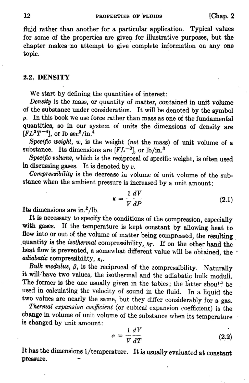
2.2. DENSITY
We start by defining the quantities of interest:
Density is the mass, or quantity of matter, contained in unit volume
of the substance under consideration. It will be denoted by the symbol
p. In this book we use force rather than mass as one of the fundamental
quantities, so in our system of units the dimensions of density are
[FL 2 T- 4 ], or Ib sec 2 jin. 4
Specific weight, w, is the weight (not the mass) of unit volume of a
substance. Its dimensions are (FL -31, or Ibjin. 3 .
Specific volume, which is the reciprocal of specific weight, is often used
in discussing gases. It is denoted by v.
Compre8sibility is the decrease in volume of unit volume of the sub-
stance when the ambient pressure is increased by a unit amount:
1 dV
Ie = --
VdP
(2.1)
Its dimensions are in. 2 lib.
It is necessary to specify the conditions of the compression, especially
with gases. If the temperature is kept constant by allowing heat to
flow into or out of the volume of matter being compressed, the resulting:
.quantity is the isothermal compressibility, "T. If on the other hand the
heat flow is prevented, a somewhat different value will be obtained, the ·
adiabatic compressibility, Ie,.
Bulk modulus, fJ, is the reciprocal of the compressibility. Naturally
it will/have two values, the isothermal and the adiabatic bulk moduli.
The former is the one usuaHy given in the tables; the latter ShOU1 be
used in calculating the velocity of sound in the fluid. In a liquid the
two values are nearly the same, but they differ considerably for a gas.
Thermal expansion coefficient (or cubical expansion coefficient) is the
change in volume of unit volume of the substance when its temperature
is changed by unit amount:
1 dV
a=--
VdT
(2 2)
It has the dimensions Ijtemperature. It is usuaHy evaluated at constant
.pressure.
Sec. 2.2]
DENSITY
13
2.21. Density. of Gases; Equation of State
For any quantitatively definable property of a physical substance,
an equation c.an be written which expresses the relationship between
that property and the ambient pressure, temperature, or other condi-
tions to which the substance is exposed. When the given property is
the density (or some equivalent quantity) the equation is called the
equ.ation of sta.te. For many substances this equation is too complicated
for convenient use, or it.s constants have never been accurately de-
termined, but for gases and vapors it is' a very useful and concise way
of expressing a large amount of information.
For a "perfect" gas the equation of state is
p
- = RT
p
(2.3)
where P = pressure, Ibjin. 2
p = density, Ib sec 2 jin. 4
R = a constant, characteristic for the gas, in. 2 jsec 2 oR
T = absolute temperature, oR (Rankine; of + 458.6)
Frequently the specific volume is used instead of the density and the
equation becomes the perfect-ga. law in its usual form:
RT
Pv=-
g
(2.4)
where g is the acceleration of gravity.
If we differentiate Eq. 2.4 and combine it with Eq. 2.1, we get the
isothermai compressibility
1
"T = -
p
(2.5)
If the compression is carried out isentropically (adiabatically) it can
be shown that
1
K, =
kP
(2.6)
h k h . specific heat at constant pressure, C p
were = t e ratto
specific heat at constant volume, C 11
For the isentropic process the quantity (P j p)" remains constant.
14
PROPERTIES OF FLUIDS
[Chap. 2
0.8
0.7
0.6
Q.I
II
ll 0.5
II
:l
0.4
0.3
0.2
0.1
T R = 2.00
1.80
1.60
1.50
1.40
0.5
1.0 1.5 2.0 2.5 3.0 3.5
REDUCED PRESSURE:I; P R
Fig. 2.1. The generaJized p. chart.
4.0 .4.5
5.0
For most pneumatic processes, especia.lly those using llpermanent"
gases such as air or nitrogen, th perfect-gas law is followed fairly ac-
curately. This is the case if:
1. The pressures are not excessive (up to perhaps 3000 psi) and the
temperatures are above the critical temperatures; or
2. The temperatures are subcritical but the pressures do not exceed
about 100 psi.
Instead of using separate charts for each gas, it is much more eco-
nomical of space to use a generalized chart such as those of Figs. 2.1 and
2.2. 1 . 2 The variables used in these charts are the reduced temperature,
T R = TITc; the reduced pressure, PH = PIPe; and the volume factor
1 J. H. Keenan, Th.ermOOynamia, John Wiley and Sons, New York, 1941.
2 H. C. Weber, Thermodynamica Jor Chemical Engineers, John Wiley and Sons,
Ne.w York, 1939, p. 109. .
Sec. 2.21
DENSITY
15
.
JJ. = P / pRT; where T c and P c a the critical tem ratu and pressure
for the gas in question. The chart can be used With fall' accuracy: not .
only for the "pennanent" gases but also for easily condensable ones .
such as organic vapOrs. .
As an example of the accuracy of these charts, consider the case
of nitrogen, for which 1'c = 227°R and Pc = 493 psig (gage pressure)
= 508"psia (absolute pressure). At 70°F (530 0 R) TR = 2.34, and at .
5000 psia P R = 9.84. From the chart we see that JJ = 1.15. An error
1.0
: I ' ./
-t-, : , ,,/
I I I. V ".,.-"
i..+- ./ ...-
- i 'b/ V V ".,.-
".,.- --- /'
; v ".,.-
-.- v 9
V ".,.- ---
k-' .. --
:.::: V I. ---
3 L. I.-
- V v I .
--- -
-- -
,. --- 10--"
e. v f-- -
.....- -
-- - ro- 10.0
I
] 15.0
1:6
- '" 1.8
I
10
20
30
40
50
3.5
3;0.
2.5
Q.I
u
a:lio 2.0
II
::1
1.5
0.5
o
P R
Fig. 2.2. j.. chart for high pressures and temPeratures.
.
of 15 per cent is not bad for the perfect-gas law under these rather
- extreme conditions. If we doubl the pressure to 10,000 psia, however,
p. = .1.65 and the actual density is 65 per cent higher than that cal-
cuIatee,J from the perfect-gas law.
For many gases the charts give excellent accuracy. Thus for steam
at 1200°F and 5500 psia, the error from the chart is 1.7 per cent while
'. that from the penect-gaslaw is 17 per cent. For some gases, particularly.
hydrogen, helium, and neon, the chart is inaccurate if the actual critical
constants are used in computing the reduced parameters but is fairly
accurate if these constants are slritably altered. Even with mixtures
of gases, pseudocritical constants tan be calculated that will still pennit
the use of the charts. 3,"
.
I Lione) S. Marks, Meduiniool Engineer's Handbook, 5th ed., McGraw-Bin Book
Co., New York, 1951, pp. 291-293.
'A. J. Rutgers, PhyS'irol Chemistry, Interscience PubJishers. New York, 19M.
16
PROPERTIES OF FLUIDS
[Chap. 2
2.22. Density of Liquids
For liquids the equations of state are considerably more complica!;ed
than for gases, but fortunately the sman values of the coefficients in-
volved make simplified linear expressions sufficiently accurate. for most
purposes. To a first approximation, liquids are incompressib . and
are so considered in many of the expressions in this book. Actually, -,
over the usual range of operating pressures a quadratic expression is
required for good accuracy since the effective compressibility decreases
appreciably at higher pressures. Thus
p = po(l + aP + bP2)
(2.7)
where a and b are empirical constants which depend upon the liquid and
also somewhat upon temperature. For most mineral and .vegetable
oils at. temperatures not too far removed from lOO°F their values are ,
approximately
a = 4.38 X 10- 6
and
...
b = 5.65 X 10- 11
when P is given in psi.
Different.iat. on of Eq. 2.7 gives the compressibility as
.
a + 2bP
1(=
1 + aP + bP2
.
(2.8)
At zero p essure the compressibility from. Eq. 2.8 would be simplya,
or 4.38 X 10- 6 in. 2 lIb. lncreasing temperature increases the values of
both a and b, as can be seen from Table 2.1.
Table 2.1. COMPRESSIBILITY OF MINERAL..OILS
(IN UNITS OF 10 . IN..2 ILB)
".
Temperature, of
P = 0 psig
P = 5000 psig
20
3.96
. 3.17
220
4.70
4.15
440
4.80
4.45
In general the compressibilities of heavy oils are somewhat greater
than those of light oils of the same types. Most solids are much less
compressible than oils; on the other hand, some Jlquids are considerably
.'
Sec. 2.2}
DENSITY
17
more SO.6 These relatively compressible liquids are of little interest as
hydraulic fluids, but they might make very good liquid springs. Ii
, he values of compressibility given in tables such as Table 2.1 or
calculated from the various formulas given in the literature are not,
necessarily the values which are effective in a particular application.
They make no allowance for the effect of stretching of the containing
walls, ;which is small for heavy-walled steel tubing but may be large for
high-pressure hose, and ihey neglect the effect of entrained air. Almost
every hydraulic system dra,vs in at least a little air and mixes it thor-
Qughly with the oil, which becomes saturated with the dissolved air.
and may also carry appreciable volumes of bubbles. This effect is
greater if the liquid has a tendency to foam. The air that is in, true
solution apparently has little effect in most cases, but air bubbles may
cause rouble. If the 'entrainment problem is serious it may be neces-
sary to provide for deaeration of the oil.
At low pressures even a small bubble of air will greatly increase the
effective compressibility of a considerable volume of oil. .Since as the
pressure increases much of the air will dissolve in the oil and since accord-
ing to Eq. 2.5 the compressibility of a gas varies inversely as the pres-
sure, the effect of bubbles' is much Jess at the higher operating pressures.
Since the effects of air bubbles and of stretch of the walls are somewhat
indeterminate, it is common practice to assume that the effective com-
pressibility is 5 X 10- 6 in. 2 lIb. The logical basis of the practice is
open to question but it seems to work.
In hydraulic work the thermal-expansion coefficient of a liquid is
occasion Ily important, particulariy in cases where a volume of liquid is
trapped between two shutoff valves. Here a rise in temperature can
cause a dangerous pressure rise if there is no leakage. Another pertinent
case is that of the parallel-plate hydrodynamic bearing, where a sig-,
nificant effect on the load-carrying capacity is produced by the Uthermal
wedge." This is further discussed in Sec. 4.3l.
Thennal expansion is usually expressed as a power series:
P = Pl(l - aAT - (311T2 + ...) (2.9)
where AT = T - T 1
"'For most liquids,. powers of AT higher than the Second can be neglected,
and for engineering purposes it is usually sufficient to neglect the term in
T 2 also. For MIL-O-5606 aircraft hydraulic fluid, a . 4 26 X lO-4/°F.
t orahani W. Marks, HVa.riation o{ Acoustic Velocity with Temperatme in Some
Low Velocity Liquids and Solutions," 1. ACOOBtical Soc. of America, Vol. 27 (July
1955), pp. 680-688. One liquid reported was 3 times as compressible &9 water.
· A. E. Bingham, "Liquid Springs: Progrees in Design and Applicatioo," Proc.
1'Mt. Mech. Eng, (London), Vol. 169, No. 43 (1965), pp. 881-893.
18'
PROPERTIES OP FLUIDS
[Chap. 2
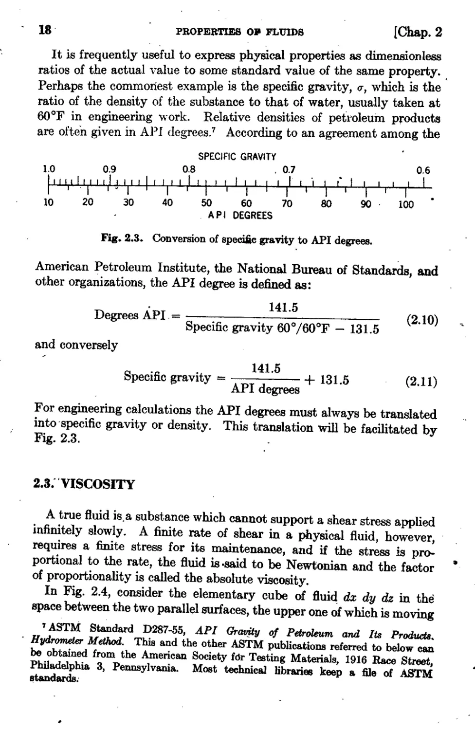
It is frequently useful to express physical properties as dimensionless
ratios of the actual value to some standard value of the same property.
Perhaps the commonest example is the specific gravity, (}", which is the
ratio of the density of the substance to that of water, . usually taken at
60°F in engineering work. Relative densities of petroleum products
are often given in API degrees. 7 According to an agreement among the
SPECIFIC GRAVITY
ns . Q7
I I I III I I I I I I I J I I
I 1 '1 I I r I
40 50 60 70
. A P I DEGREES
1.0 0.9
11111111111111111
, . I I I
10 20 30
I t I
I I
80
I I I
I I
90.
0.6
I I
I
100
Fig. 2.3. Conversion of speciic gravity to API degrees.
American Petroleum Institute, the National Bureau of Standards, and
other organizations, the API degree is defined as:
. 141.5
Degrees API. =
Specific gravity 60° /60°F - 131.5
and conversely
(2.10)
..
141.5
Specific gravity = + 131.5 (2.11)
API degrees
For engineering calculations the API degrees must always be translated
into' specific gravity or density. This translation will be facilitated by
Fig. 2.3.
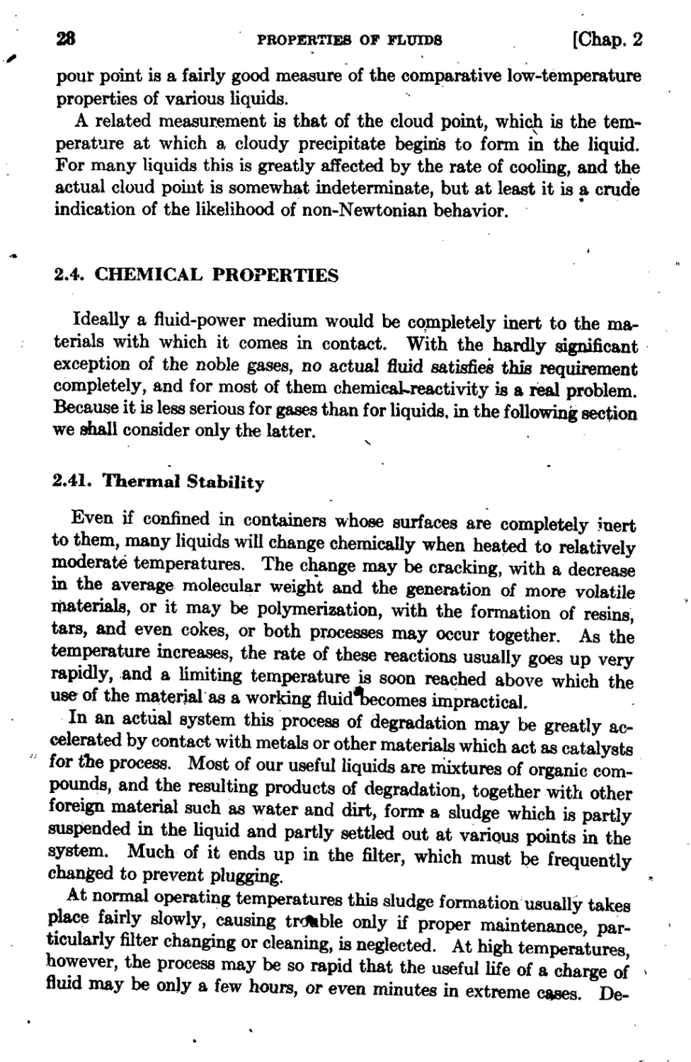
2.3: 'VISCOSITY
A true fluid iS,a substance which cannot support a shear stress applied
infinitely slowly. A finite rate of shear in a physical fluid, however,
requires a finite stress for its maintenance, and if the stress is pro-
portional to the rate, the fluid is .said to be Newtonian and the factor
of proportionality is called the absolute viscosity.
In Fig. 2.4, consider the elementary cube of flui dx dy dz in the
space between the two parallel surfaces, the upper one of which is moving
7 ASTM Standard D287-55, API Gravjty of Petroleum and Its Prod/uclB.
. Hydrometer Method. This and the other ASTM publications referred to below can
be obtained from the American Society fdr Testing Materials, 1916 Race Street,
Philadelphia 3, Pennsylvania. Most technicaJ libraries keep a file of ASTM
standards..
It
"
Sec. 2.3) VISCOSITY 19
to the right with 'the velocity U. The force dF on the upper face f the
cube will be T dx dz where r is the shear stress. The rate of shear IS the
. , .....
same as the velocity gradient dU jdy. If the fluid is Newtoman,
dU
rdxdz = p,dxdz-
dy
Canceling the area term from each side and rearran ing, we have
(2.12)
T
p.= dUjdy'
The absolute viscosity therefore haa the dimensions [FT j £2], or in
(2.13)
u .....
//////////////////////
rn dF a:.
d u+ du
, dz u
dx
y ,
J-.
z
/////// /// // / / / //////
Fig. 2.4. Fluid shear diagram.
English units, lb sec/in. 2 This unit is frequently called the Reyn, after
Osborne Reynolds.
The Reyn is a very large fjnit; a liquid with a viscosity of 1 Reyn would
be almost a solid, like tar. A much more convenient unit is the centi-
poise (1 cp = O.Ol poise; 1 poise = 1 dyne sec/cm 2 ), which is ap-
proximately the viscosity of water at 68°F. 1 cp = 1.45 X 10- 7 Reyn;
1 Reyn = 6.9 X 10 6 cpo
For a series of liquids of the same chemical type the absolute viscosity
increases (somewhat irregularly) with the molecular weight. For hy-
drocarbon mixturcS' at about 70°F, the viscosity ranges are about as
follows: .
1!
Gasolines
Kerosenes
Light lubricating 9ils
Heavy oils
0.35 to 1 cp
1.5 to 2
10 to 100
100 to 1000
Most "hydrauHc fluids" fan in the 10-to-l00 cp range. At iOO°F the
standard MIL-0-5606 aircraft hydraulic fluid has a viscosity of about
1.7 X 10⁻⁶ Reyn or 12 cpo
20
PROPERTIES OF FLUIDS
[Chap. 2
Most liquids which are used as hydraulic fluids are at least approxi-
mately Newtonian, -but many other common s':1bs,tances a.re not.
'GreaSes, for example, act as plastic solids for small strains but as liquids
for higher strain rates. Gases are almost perfectly Newtonian, with
viscosities at room temperature in the range 0.1 to 0.25 millipoise.
In many of the equations of fluid mechanics the viscosity occurs as
the ratio of absolute viscosity to fluid density, and this ratio is usually
.
called ,the kinematic viscosity. (The absolute viscosity is sometimes
called the dynamic viscosity, though it is not imme<;liately obvious just
what is dynamic or kinematic about either of the quantities.) The
usual unit of kinematic viscosity is the stoke, which is equal to 1 cm 2 /sec.
It is numerically equal to the absolute viscosity in poises divided by the
'specific gravity. The corresponding English unit (in. 2 /sec) is sometimes
used but has never been named. The viscosities .)f petroleum products
were f{)rmerly determined by the nmv..obsolete Saybolt efflux viscom-
eter,S and the industry still reports viscosities in seconds Saybolt
Universal (SSU). The British use the very similar RedwoO{l-instrument,
and the Germans and [flost other Europeans the Engler. N one of these
gives meaningful result.s for liquids with viscosities under a few centi-
,stokes, and up to perhaps 30 cs the conversion is a nnisance to use.
For high efflux times the viscosity is proportional to the time. The
usdal formulas for the Saybolt instrument are: 9
For efflux times from 32 to 100 SSU
'"
.
195
11 = 0.2261 - -
t
(2.14)
and for efflux times greater than 100 RS£;
135
II =O.220t - -
t $
(2.15)
where t is the efflux time in seconds and v is the kinema.tic viscosity in
centistokes. Obviously for viscous liquids the efflux times are long
and the second t( rm becomes negligible.
Since the Saybolt second is physically meaningless, it will not be
used in this book. As in the case of the API degree, the formulas are
included as a c.onvenience, and the translation from the arbit&ry to
the physical language will be aided by Fig. 2.5. Of the meaningful
units the centistoke has the most convenient size, and it and the centi-'
S ASTM Standard D88--53, Vi8C()8i y by Means of the Saybolt Vuoo$imeter.
· ASTM Standard D44&-f>3 1 Conversilm of Kinematic Viscosity to SayboU Univer al
ViscORUy. .
. 4
SL"C. 2.3j
..
V 1l:;COSITY
21
poise will be frequently used hereafter -even in expre ions involving
English units. A great deal of time and confusion would be saved if
this practice were universal.
KINEMATIC VISCOSITY. CENTISTOKES
3 5 10 ZO 50 100 200 500 Ik 2k 511 10k
,l",tl"'d ,I 1,llt"lu.uJ '\t' r l"td
1('f"'I'r I"/'I'! 'fTTTI l' ''''''''
3740 50 100 200 500 III 211 511 IOk 201c Olc
SAYBOLT
SECONDS
UMVERSAL
IS.$.UJ
0.2 0.5 I 2 5 10 20 50 100 200
106. ABSOLUTE VISCOSITY, LB SEC/IN. 2 (FOR FLUID OF S. G. s 1.0)
\.
I<'ig. 2.5. Viscosity conversion diagram.
2.31. Effect of Pressure
According to the kinetic theory of gases, the viscosity of a perfect
gas would be independent of pressure. Real gases obey this rule fairly,
accurately over the ranges f temperature and pressure where they also
obey the equation of state of a perfect gas. The viscosity does increase
for very high pressures at which the molecular'mean free path is no
longer large compared to the diameter of the molecules. For most
gases the viscosit,y can be considered to be independe:1t of pressure from'
about 1.4 to about 1000 psia. Above this pressure the viscosity increases
very rapidly. Thus carbon dioxide at 20°C has a viscosity of 0.16 milli-.,
poise ::I:: 10 per cent from 15 to 750 psia., but at 1245 psia the viscosity
rises to 0.823 Inp.l0
The viscosities of liquids increase considerably with increasing pr ,s-
sure, usually approximately according to the expression 11
'.
IJ
log]Q - = cP
}.to
Most J>ctroleuIJl products at room temperature increase in viscosity bY'
a factor of about 2.25 when the pressure is raised t.o 5000 psi. This gives
a value of c = 7 X lO-4/ ps i.
(2.16)
2.32. Effect of Temperature
,The viscosities of both gases and liquids are considerably affected by
changes of temperature. In the case of gases the cnange is described
10 International Critical Table8, VoJ. 5, McGraw-Hj}J Book Co., New York, 1929,
p.4.
, 11 "Viscosity and Density of Over 40 Lubricating F'luids of Known Composition
at Pressures to 150,000 Psi an Temperatures to 425°F," VoIs. I and II, ASME Re-
8«Jrcn. &port, 1953. '
22
PROPERT1E8 OF. FLUIDS
[Chap. 2
fairly accurately by Sutherland's formula:
( TO + C\ ( T )
/J = 1JO T + C J To
where p. = viscosity at (absolute) temperature, T
JJo = viscosity at reference temperature, To
C = a constant, characteristic f r the gas in question
Sutherland's equation can also be written
AT
P.=T+C
(2.17)
(2.18)
where
1JO ( C ) '
A=- 1+-
To To
This form of the equation shows more clearly than the other that the
viscosity of a gas rises rapidly with temperature.
All liquids show the opposite effect, except for molten sulfur and a
few other materials where chemical changes such as association ,or re-
versible polymerization are caused by increasing temperature. Many.
empirical formulas have been proposed to describe. the variation of
. viscosity with temperature, but no fully satisfactory one exists, even for
a pure chemical compound. In view of the inherent complexity of the
phenomenon it ms unlikely that one will ever be found, especially for
liquids as complex and variable in composition as commercial oils and
hydraulic fluids.
When an empirical expression is used, it is very desirable that it be in
a fonn convenient for mathematical analysis. One which is useful over
a restricted temperature range is
....
JJT = p.oe-A{T......T o )
where /JT = viscosity at temperature T
1JO = viscosity at reference temperature To
X = a constant characteristic of the particular liquid
T expression wi1l be used in Sec. 4.32, where the actual and the as-
sumed viscosity-temperature curves for seven. typical hydraulic fluids
are plotted in Fig. 4.18.
With actual liquids no reasonable form of equation seems to fit OVer
more than an inconveniently narrow temperature range. 12 Th one
11 R. HouwWc, Ela8t lI, PlMticity, and the Structure of Malter, Cambridge Uni..
versity Press, 1937. '
(2.19)
.
Sec. 2.3] VISCOSITY
which fits best for certain types of petroleum-base :fluids is the WaJther
formula:
IOglO loglo (v + c) . n 10glO T + C (2.20)
where v is given in centistokes, c := 0.8 (usually), and n. and C are
characteristic of the given oil. Beside being phenomenally poorly'
adapted to mathematical manipulation, this equation and the ASTM. .
charts 13 based on it have the following disadvantages: 14.15
1. It is completely devoid of physical meaning; if any other unit,
such as stokes or Reyns, were used the resulta.nt curve would no longer
be even approximately linear, nor would the curves for severaJ liquids
of the same family intersect in a "pole."
2. It applies 'fairly accurately over the range of temperatures en...
countered in automobile engines but comparatively poorly outside this
ran l .
3. 1\ is reasonably accurate for "straight" petroleum-base lubricating
oils, but not for solvent-refined oils, nor for those with appreciable per-
centages of. certain common types of additivet!, especially the so-called
viscoaity-index imp overs.
4. It is fairly accurate for some types of synthetic liquids but not for.
other equally important 'types. .
5. Because of the nature' of . the log-log ordinate scale it tends to
exaggerate the proportional change of viscosity with temperature at low
viscosities but to minimize it for viscous liquids.
23
In spite of these and other.disadvantages the Walther equation and
its various descendants have been and still are the most common
methods of representing viscosity-temperature data. The commonest
of these, at least in the United States, is the ,ASTM chart. Figure 2.6
Shows on an approximation of such a chart the viscoaity-temperature
curves for several different grades of the Univis series of lubricatin o
of the Esso Standard Oil Company. Figure 2.7 shows the characteristics
of hydraulic fluids of several different chemical classes. 16 It can be seen
that some of these deviate from linearity much more than others but
that none is truly straight at extreme temperatures.
11 A8TM D341-43, Standard Visoosity-Temperature Charts Jor Liquid Petroleum
Producta.
: .. H. B. Zuidema, TM. Perjormanci: of Lubricating 0il8, Reinhold Publishing Corp.,
New York, 1962, pp. 29-37.
11 A. Bondi, Phy8iaJl' Chemi3try of Lubricating Oils, Reinhold PublishiJig Corp.,
New York, 1951, pp. 50-59.
1" C. M. Murphy, J. B. Romans, and W. A. Zisman, "Viscosities and Densities of
Lubricating Fluids from -40 to 700°F," Trans. ASME, Vol. 71, No.5 (July 1949),"
MHU .,
.
. .
24
. PROPERTIES OF FLUIDS
[Chap_ 2
5
10,000
1000
: 200
l; 100
t;
50
z
'"
CJ 20
;
t:
.(1)
o
u
(I)
>
!:?
.....
2
&AI
!:
11:
10
I
.:'1:
2
.40 0 40
TEMPERATURE. .,
Fig. 2.6. Viscosity-temper8.ture charact.eristics of six petroleum-base hydraulic
J fluids.
100
2D
Typical Univis Fluids, Made by Esso Standard Oil Co.
Curve Grade of Fluid
A P-38
B 40
C J.43
D P-48
E PJ-59
F 60
(The J .prefix indicates the use of a viscosity-improving additive. J-43 is one type
of MIL-O-5606 aircraft hydrauJic fluid.) ·
.
,. Ii. would be very convenient if the effect. of temperature on viscosity
could be described by a singl number, and many attempts have been
made to devise such a quantity. In Europe the Walther-Ub lohde
pole-height has been used, and in the United States the Dean and Davis .
Viscosity Index 17 is the most popular. Both are derived from the
Walther equation and inherit its defects, and the viscosity index in
particular greatly exaggerates small changes in the temperature effect
in certain ranges while minimizing those in other ranges. Unfortunately
for our purposes, although it has been useful in the past in the field of
automotive lubrica.nts, it is almost completely useless when' applied to
. 17 ASTM Standard D567-53, Calc'lIlming Viscosity lndez.
Sec. 2.31
VISCOSITY
25
most practical hydraulic fluids, whether petroleum.based or synthetic.
It is still ouoted but the fluid-power engineer should analyze the quo-
tation with some' care to determine if the proposed fluid is actually suit-
able r.r his application. ,
Perhaps the simplest criterion of viscosity chang would be the tetp-
perature drop required to double the viscosity from that at a suitable
20k
10k
5k
2k
(I) lk
500
200
(I)
100
50
20
... 10
5
L4I
Z
52
2
-40 -20 0
32
A
100 130 210 250 300 350 400
TEMPERATURE, .F
1"'i8.2.7. Viscosity-temperature curves for various aircraft hydrauJic fluids.
Curve Material
A. FJuoro lubric.ant FCD-331
B Di(2-ethyJhexyl) sebacate
C Poly(methyl-phenyl) 'siloxane DC-702
· D Polypropylene glycol derivative LB-lOO-X
:E Petroleum-base Univis J-43
F Polymethyl siloxane DC-I?OO-A
.,
referen e temperature, say 210°F for usual conditions. For the Univis
fluids of Fig. 2.6 this temperature drop runs from 50 to 6O°F, being less
.Jor the more viscous fluids. Viscosity-index improvers increase this by
about 40 per cent.
2 33. Effect of Shear
For a Newtonian fluid, the viscosity is independent of the rate of
shear, and many liquids are almost perfectly Newtonian. Many otherS,
however, re not, and among these are some of our most useful hydraulic
26
PROPEBTIES OJt.FLVD>8
[Chap. 2
ftuids, especially those which contain appreciable amounts of comp unds
of high molecular weight. These compounds may be natural components
of the fluid, or they may be additives, especially the viscosity-index
improvers., .
When a fluid of this type is subjected to shear, the effective viscosity
decreases with increasing rate of shear. This increase appears to be
instantaneously reversible for moderate shear rates and for most fluids.
As the shear rate in reases, however, the viscosity change also increases,
and persists for a time after the flow ceases. At extremely high rates
of shea!' the decrease of viscosity may be as much as 40 per cent, and
part of this decrease is permanent. .
One plausible explanation of these effects is that these three tyPeS of
viscosity decrease are due respectively to increasing orientation of
elongat d molecules parallel to the flow lines, to uncoiling and orienta-
tion of coiled large molecules, and to actual fracturing of large molecules,
accompanied by oxidation and other chemical reactions. This last
explanation is supported by the fact that for some oils antioxidants help
to increase the shear stability.
The rate of shear necessary to cause appreciable changes in viscosity,
either transient or permanent, naturally varies with the liquid. Tem-
. porary changes may occur with many commercial hydraulic fluids and
with many types of machines, such as positive-displacement pumps and
motors, in piston or high-speed-bearing clearances. 1S - 22 The higher shear
stresses necessary to cause permanent viscosity changes are ordinarily
attained only under conditions of extreme turbulence, 88 in ,throttling
valves and orifices under high pressure drops. The effects are greater
for oils containing high-polymer thickeners; this shoul be kept in mind
when making detailed analyses of viscous-flow phenomena for such
oils. The effective viscosities may be very different from those measure
at low rates of shear in conventional viscometers.
The considerable changes in effective viscosity produced by shear,
as well as by changes in temperature and pressure, the variabiftty in
la E. E. Klaus and M. R. Fenske, "Some Viscosity-Shear Characteristics of Lubri-
cants," Lubricatioo Eng., Vol. 11, No.2 (March-ApriJ 1955}, pp. 101-1OB.
11 N. D. Lawson, UDetermination of the Shear StabiJity of Non-Newtonian
Liquidl:l," ASTM Spec. Tech.. Publ. No. 182.
JO uSymposium on Methods of Measuring Viscosity at High Rates" of Shea.r,"
ASTM Spec. Tech. Publ. No. 111.
a R. N. WeJtmann, ItThbcotropic Behavior of Oils," Ind. Eng. Chern., Anal. Ed.,
VoJ. 15 (1943), p. 424.
ja N. W. Furby, R. L. Peeler, and R. I. Stirton, ItOronite High Temperature
Hydraulic FJuids 8200 and 8515," Trans. ASM'E, Vol. 79, No. 5 (July 1957),
pp. 1029-1038.
..
Sec. 2.31
VISCOSITY .
...
2'1
"
the properties of 'commercial fluids as received by the user, and the
effects of aging and contamination, suggest that there is really little
point in trying.to predict viscosity (or othe properties) with high ac-
cur y. This is true from a purely empirical standpoint, but there are
two arguments against this point of view. One is that eventually we
shall know more about all of these effec s, and this gre ter knowledge
will permit better control of the performance of our hydraulic systems.
The other argument is that the constant improvement in. the fluids
themselves, and still more in the quality of maintenance of the average l>
hydraulic system, will greatly decrease the variability of the fluid
properties. In any given case it is necessary for the engineer to deotde
for himself how much importance he must attach to the considerations
that have .been outlined here.
2.34. Dilatational Viscosfiy
/
One fluid property that is not now known to be of importance to the
hydraulic ngineer, but which may eventually prove to be so, is dil-
atational viscosity, or "second" viscosity. Ordinary viscOsity represents
the loss of mechanical energy consequent upon deformation of the shape
of a volUme of fluid by shearing. If the volume is expanded or com-
pressed without change of shape there is no. shear, but energy may be
dissipated in the change of volume, aJ1.d this dissipation is presented
by the dilatational viscoaity.2i.24 At the present time this phenomenon
appears to be somewhat obscure, at least in its relationship to hydraulic
machinery, but it may be significant. both for the transmission of very
rapidly varying pressure waves through conduits and for certain types
of valve instability.
.
2.35. Pour Point
One rough but practical measure of the low-temperature limit of use-
fulness of a liquid is its pour point. AB the name indicates, this is the
temperature a.t which it will no longer pour from a beaker when tested
according to a standard procedure. Actually it will be too viscou.s. a.t
considerably. higher temperatures for use in a hydraulic system, but the
II S. M. Karim and L. Rosenhead, "Second Coefficient of Viscosity of Liquids and
Gases," Rer1a. Modern PkY8., Vol. 24, No.2 (jpriI1952), pp. IP8-116. This article
includes an exceUent bibliography.
If L. M. Liebermann, "The Second Viscosity of Liquids," Pky". Rev., Vol. 75 (May
J 1949), pp. 1415-1422.
· ABT Standard 007-47, Cloud and Poor Point&.
28
. PROPERTIES OF FLUIDS
[Chap. 2
.'
. .
pour point is a fairly good measure 'of the comparative low-temperature
properties of various liquids. "... .
A related measur.ement is that of the cloud pomt, Whlc!I IS the tem..
perature at which 8, cloudy precipitate begilis to form in the liquid.
For many liquids this is greatly affected by the rate of cooling, and t e
actual cloud point is somewhat indeterminate, but at least it is crude
indication of the likelihood of non-Newtonian behavior.
..
2.4. CHEMICAL PROPERTIES
Idea.11y a fluid-power medium would be c mpletely inert to the ma-
terials with which it comes in contact. With the hardly signifi ca.nt .
exception of the noble gases, no actual fluid satisfieS this requirement
completely, and for most of them chemical..reactivity is & real problem.
Because it is less serious for gases than for liquids. in the following section
we shall consider only the latter.
""
2.41. Thermal Stability
Even if confined in containers whose surfaces are completely hlert
to them, many liquids will change chemically when heated to relatively
moderate temperatures. The change may be cracking, with a decrease
in the average molecular weight and the generation of more volatile
:Qlateria1a, or it may be polYmerization, with the formation of resina,
tars, and even cokes, or both processes may OCcur together. As the
temperature increases, the rate of these reactions usually goes up very
rapidly, .and a limiting temperature is soon reached above which the
U8e' of the teria1" as a working fluid omes impracticaL .
. In an actual system this 'process of degradation may be greatly ac-
celerated by contact with metals or other materials which act as catalysts
". for t1te process. Most of our useful liquids are nUxtures of organic com-
pounds, and the resulting products of degradation, together with other
foreign material such as water and dirt, form a sludge which is partly
suspended in the liquid and partly settled out at variQUS points in the
system. Much of it ends up in the filter, which must frequently
changed to prevent plugging.
At nonnaI operating temperatures this sludge formation;usually takes
place fairly slowly, Causing tr ble only if proper maintenance, pa;r-
ticularly filter changing or cleaning, is neglected. At high temperatures,
however, the process may be so rapid that the useful life of & charge of \
fluid may be onJy a few hours, or even minutes in extreme cases. De-
"
Sec. 2.4J
CHEMICAL PROPERTIES
29
nds for higher-temperature operation ar becoming more nd ?rc
insistent- there is therefore a very active program for developIng hlgh-
. tempera.;ure fluids. Some of these will be very briefly discussed later
in this chapter.
2.42. Oxidative Stability
.
More serious than pyrolysis, in general, is the reaction of the fluid
with atmospheric air or other oxidizing agents. The pr:oducts of th
reaction are usually more or less acidic in nature and often cause serious
cOlTosion of some of the Dletals of which the hydraulic system is ade.
In addition, oxidized compounds are usually more reactive than the
products of pyrolysis, and therefore are Hkely to form sludge more
rapidly. .
Much mQre serious than the slow oxidation of fluid at norm81 tem-
peratures is the possibility of fire or explosion. This is actually the
- principal weakness of hydrocarbon-base fluids; if they were not oxidizable
the incentive for the development of synthetic hydraulic' fluids would
be much less. The occasional spectacular and disastrous event which
can be charged to flammable fluids is sufficient to keep this 'development.
active.
The relative likelihood of trouble from the ignition of petroleum
produc has for many years been evaluated by three somewhat arbitrary
tests.- The oil is heated in a cup and a small open pilot flame is peri-
odically lowered to the liquid surface. The temperature at which
enough va.por is evolved to cause a transient flame is ca\led the flash
point. .As the temperature rises, the evolution of vapor becomes more
rapid until finally the vapor will continue to. burn after removal of the
pilot flame. This temperature is the fire point. At a considerably higher
temperature (determined by a different test procedure), called the autog-
enoU8 igR,itiun (or autoi tion) t€mperature, the liquid {)f vapor will
catch fire upon contact with air, without a pilot flame or other means of
ignition. These three' temperatures cannot be rela to the actual
..
, probabilit)f of fire or explosion in a given situation, but they are indica-
tions of the relative hazards of various fluids.
The. autoignition . temperature, in particular, is greatly affected by
the conditions of the test, such as the nature of the heated surface with
which. the liquid or por comes in contact, the oxygen content and
pressure of the air, the pressure with which the liquid is sprayed agBjnst
the su:rface, a.nd the degree of atomization. Perhaps the greatest hazard
.
II ABTM Standard D92--52, Flash and Fire Poinl8 by Means ()f Ckveland oPim Cup.
.'
30
PROPERTIES OP FLUIDS
(Chap. 2
in the operation of a hydraulic system arises not from the evolution of
inflammable vapors but from the possibility of creating an explosive
mixture of finely dispersed droplets of oxidizable liquid in air. Such a
mixture can explode with great violence even if the bulk liquid is com-
paratively inert. The danger is particularly great in vehicles, where
hot exhaust pipes setve as ignitors for the vapor or fog, and in industrial
applications such as furnace controls or diecasting machines, wllere the
hydraulic fluid must be brought into the immediate proximity of highly.
heated metal surfaces if not of actual flames. In either case a burst OP
even a pinhole leak may cause disaster.
2.43. Hydrolytic Stability
... Except in carefully sealed 'hydraulic systems, water of condensation
will usually accumulate more or less rapidly in the fluid. < Much of it
will remain in the bottom of the sump, at least with petroleum fluids,
but a certain amount will circulate as an emulsion, or will become one
of the constituents of the sludge. "The water will also cause a consider-
able increase in the corrosive power of the acidic oxidation products of
the oil. .
With nonhydrocarbon fluids, particularly with some types of esters
such 88 the silicates, the water will react with the fluid itself, hydrolyzing
it into alcoholic and acidic fractions. These fractions may dissolve in I
the fluid or they may form separate liquid. or solid phases. Because the
organic silicates seem to be particularly susCeptible to hydrolysis, con-
siderable .care should be employed to exclude water from systems in
which they are used.
2.44. Compatibility
Besides being I!fi'ected by other materials in a hydraulic system,
hydraulic fluid"" itself affects them. These effects are of various kinds.
The fluid or its ation.products, particularly the acids produced by
oxidation, will corrode many metals, sometimes very rapidly.. "This cor-
rosion can be min1m1 by careful choice of the metals used, by the
use of anticorrosion devices such 88 sacrificial. anodes and bichromate
cartridges, and most of all by good maintenance of the system. Filtel'8
should be chaDged before sludge has a chance build up, condensed
water and "sludge should be removed from the sump, and in extreme
cases the system should be completely drained and flushed at suitable
intervals. " .
Nearly all hydraulic systems use robber-like 8U ces extensively
.
Sec. 2.4]
CHEMICA.L PROPERTIES
31
in seals hoses, accumulator bladd rs, and so on. Several types of
elastom rs have been developed that are compatible with hydrocarbons
and give very good service. When synthetic fluids are used, however,
trouble is frequently. encountered since some of these fluids seriously
affect the usual synthetic rubbers. If the base compound of t.he rubber
is even slightly soluble in the fluid, the part will swell and sotten and .
may even dissolve. (This has been one fruitful cause of sludge forma-
tion.) In other cases the fluid will dissolve plasticizers ironl the rubber
part, which will shrink and become horny or brittle. In either case
the part becomes useless and the system usually becomes inoperative.
Special elastomers have been developed for use with the synthetic
fluids, and if & system is changed from one fluid to another it will often
be necessary to change all of the seals and hoses and the accumulator
bladder. The maker of the particular fluid can usually supply informa
tion about sources of molded parts with which his fluid will be com
patible.
When changing fluids, great care often must be taken to clean the
system thoroughly of the last traces of the old fluid before putting in
the new since some pairs of fluids are mutually incompatible. The
glycols, for example, are alleged to precipitate out the viscosity index-
improving additive from petroleum-base aircraft oil, and there is some
,
evidence that something in the oil catalyzes the polymerization of the
polyglycol. In either case the result of mixing even small amounts of
one fluid with the other is the formation of large quantities of a materiat
much like a very soft chewing gum, which can effectively disable the
system and is very hard to J:emove.
Other organic materials which are used in hydraulic systems include
paints, varnishes, and enamels of various types, and electrical insula-
tion. Again there is the problem of compatibility of the fluid with
these materials, which is serious because of their great diversity and
because of the diffic,:!lty of obtaining information about them. In some
cases it is necessary to run compatibility tests with the proposed fluid
on the paints and plastics which are to be used in or in close proximity
to the system.
2.45. . Toxicity
Since it is almost impossible to avoid at least occasional personal
. contact with it, the hydraulic fluid should not be poisonous. Some
hydraulic fluids are somewhat toxic themselves, and their degradation
products may be more so. For most fluids and in most circumstances
the danger is v niAhiu gly small, but in exceptional cases it may be sig-
32
PROPERTIES 01<' FLUIDS
lChap. 2
nificant. For example: tricresyl phosphate is a very common additive
to petroleum oils. It i highly toxic when taken internally, and there
have been a few cases of poisoning from the vapor. It is not known to
be ingested through the skin but enough possibility of poisoning by
this route exists to make one some\vhat suspicious of the material.
Again the actual danger is small, but should be considered if extensive
contact of the fluid. with th( skin is likely.
One not uneom:m.on a('eident \V'ith high-pressure systems is the piercing
of the skin by a jet of liquid, Even with a biologically inert material
this may cause extensive mechanical damage to the tissues, with con-
sequent necrosis. If the liquid contains appreciable percentages of
toxic material, whether additives or degradation products, the danger
is naturally greater.
2.5. SURFACE PROPERTIES
The study of t ht sHl'faee properties of hydraulic fluids has just begun,
and the probl\ mH involvt d ar so complicated that firm conclusions are
difficult to draw e','cn in" the simplest situations. 27 A good deal is known
about surface phel1oITwnu. n-jt,h carefully cleaned surfaces and highly
purified single chemic al compounds, but many important surface phe-
nomena are reatly affected by even very small roncentrations of foreign
molecules, and eondu::;ions drawn from experiments made under sim-
plified conditions cannot safely be extended to cover phenomena in the
operation of praetical hydraulic systems. About an that can be done is
to use the re ults of the id('alized experiments to suggest remedies for
act.ual operating troubles. .
When two different phases are in contact-say a liquid and a gas, or
two differPTJt liquids--a pertain amount of energy will be associated with
each unit area of the surface which separates the two. This energy per
unit area is dimensionally, though not physically, the same as a force per.
unit distance, and it i , convenient at times to speak of the latter. When
the interface eparates a liquid and a gas, it is called a free surface, and
the force is caned surface tension. It is usually given in dynes/em.
Free surfp.ces are unimportant in pressure hydraulic systems except
for the phenomenon of ff)aming. 28 , 29 A foam is an emulsion of gas bubbles
27 N. K. Adam, The J>h.y.'dc. and Chet1u'slry of Surfaces, Oxford University Press,
1941. See also Bondi, Hderence 15 above, Chapter 3.
28 A. M. Schwartz and J. 'V. Perry, Surfact" Active Agents, Interscience Publishers,
New York, J9,1}J.
2i S. Ross and J. W. McBain, "Inhibition of Foaming in Solvents Containing
Known Foamers," Ind. Eng. Chern., VoL 36 (1944), p. 570.
"
..
Sec. 2.5]
SURFACE PROPERTIES
33
in a liquid, and under some circumstances it may be very stable and per-
sistent. Naturally it is far more compressible than the liquid itself, and
if it is drawn into the pump and injected into the hydraulic system, it
may seriously disturb system operation. Also, because of the large
liquid-gas interfacial areas in a foam, oxidation and similar reactions
ma.y be considerably accelerated by its presence.
The mechanism of foam formation and st.abilization is little under-
stood, and that of foam destabilization by defoaming agents is even
less so. It is known that for a given liquid there may be several classes
of compounds that aid in foam formation and preservation and that
other compounds, sometimes even in very small concentrations, act
as effective agents' to prevent foaming. The same agent may even act
as a foamer in one concentration and as a defoamer in another. One
plausible explanation for foam formation is that the additive concen..
trates preferentially at the gas..Iiquid interface but is sufficiently mobile
to increase the surface tension at thin points of the film &ond to decrease
it at thick ones so as to keep the film thickness uniform and the film
stable. A defoame.r is less mobile under the same conditions and forms
weak patches, thus rupturing the film and destroying the foam.
Several classes of defoaming agents hav been used with varying
success on the various hydraulic fluids. Among the more successful of
th se agents are dimethyl silicones, dialkyl orthophosphates, trialkyl
thiophosphates, fluorin ted oils, sulfonated fatty acids and their amino
salts, and certain soaps. Some hydraulic fluids are much more subject
to foaming than others, and some (unfortunately not necessarily the
same ones) are. relatively easy to defoam by the use of the proper addi..
tives. In cases of trouble from foaming, if there is no obvious mechanical
reason for the excessive foam, the manufacturer of the fluid should be
consulted for recommendations.
Generally speaking, the surfaces between fluid and solid in a hydraulic
system are much more important than the free surfaces. This is espe-
. cially true where neighboring solid surfaces are in relative motion, with
a thin film of liquid between. In such a sit.uation the molecular st.ructure
of the interfaces will largely determine t.he nature and amount (\f friction
and wear and thus the performance and useful life of the system.
It would be very convenient if true hydrodynamic lubrication could
be provided at all times and at all wearing areas in a hydraulic system.
Unfortunately this is t;lsually impractical and there is always a certain
amount of boundary-layer friction. 30 The base matE-rials of most hy..
»M. C. Shaw and E. F. Macks, l'Anftlysis and Lubrication of Be rjpgs" McGraw-
HiJJ Book Co., New York, 1949. There is also a brief dif1('ussioj) of b t lldary-]ayer
friction and related phenomena in Sec. 10.22.
M
PROPERTIE8 OF FLUIDS
[Chap. 2
draulic fluids are poor boundary-layer formers; for this reason, so--called
lubricity additives are often provided to assist in the layer formation.
These are usually long-chain polar compounds, such as long-chain fatty
acids or their esters, which migrate to the metal surfaces and stick
tightly. If the surface finish is poor enough or the nonnal forces are
great enough, under load the boundary layer on the high spots will be
torn off and destroyed. In such cases it is customary, and usually
fairly effectual, to add one of the so-called extra-pressure (EP) additives,
such as tricresyl phosphate or an organic halogen compound. Under
,the high instantaneous temperatures which occur at points of metal-to-
m tal friction, these compounds decompose and attack the metal, form-
ing soft low-melting phosphides or halides, which are smeared down into
the valleys of the metal surface. In this way the higher asperities are
rounded and removed, the surface finish is improved, and the boundary
layer can renew itself with a better chance of survival. For petroleum
oils and at normal operating temperatures both lubricity and EP addi-
tives are effective and useful. For some other fluids, particularly the
fluorocarbons and silicones, and at high temperatures, suitable additives
are difficult to find. Unfortunately it is just these classes of fluids that
are most in need of improvement.
2.6. THERMAL AND MISCELLANEOUS PROPERTIES
Two of the thermal properties of fluids are of considerable importance'
to the fluid-power engineer, namely the specific heat aI)d the thermal
conductivity.
The specific heat of a material is the derivative with respect to tem-
perature of its enthalpy (if the pressure is kept constant) or of its
internal energy (for constant volume). Less rigorously but more com-
monly, specific heat is defined as the amount of heat which must be
supplied to unit weight of a substance to raise its temperature by unit
amount. Water is taken as the standard substance, and 1 British
thermal unit (Btu) is the heat required to raise the temperature of 1
lb of water by 1. of, at the freezing point of 32°F.
The defining equations of specific heat are
and
( a" )
c - -
P - aT
p
C v = ( au )
aT v
!!
(2.21)
(2.22)
Sec. 2.61
THERMAL AND MISCELLANEOUS PROPERTIES
35
where C p = specific heat at constant pressure, Btujlb mole of
C v = specific heat at constant volume, Btujlb Inole of
h = enthalpy, Btujlb mole
u = internal energy, BtujIb mole
- -
The subscript denotes the condition held constant. 1 Btu = 9339 in. lb.
For real fluids the specific heats are not constants but vary with tem-
perature, as indicated in Tables 2.2 and 2.3. For most fluids the spe-
cific heats increase considerably with the temperature.
:For gases the two specific heats are considerably different, and their
ratio (usually designated k in engineering work), CpjC v, is an important
quantity in most gas-dynam1cs equations. Because of the high bulk
modulus of a normal liquid, its two specific heats are nearly the same.
The thermal conductivity of a gas increases with temperature but is
Table 2.2. C p AND k VERSUS TEMPERATURE FOB NITROGEN *
Absolute
Temperature, oR
400
600
800
tooo
2000
C p ,
Btujlb molp. of
.6.950
6.961
7.012
7.132
7.962
k
1.400
1.399
1.395
1.386
1.332
* J. H. Keenan and J. !{aye, Ga8 Tables, John Wiley and Sons, New York,
1948, p. 102.
Table 2.3. SPECIFIC HEAT OF PETROLEUM OILS * (IN BTUjLB OF)
Absolute Specific Gravity at 60/60°F
Temperature,
oR 1.000 O. 934 0.876 0.825
460 0.388 0.410 0.416 0.427
" 560 0.432 0.448 0.463 0.477
660 0.478 0.495 0.512 0.526
760 0.523 0.542 0.558 0.576
860 0.568 0.588 Q.608 0.626
960 0.612 0.633 0.656 0.676
1060 0.659 0.682 0.703 0.724 .
1160 0.704 0.726 0.798
· Adapted from J.C. Hunsaker and B. G. Rightmire, Engineering Applica-
tions 01 Fluid MecJw.nic8, McGraw-Hill Book Co., Ne'Y' York, 1947, p. 285. ,
.
36
PROPKR1'IES . OF FLUIDS
[Chap. 2
almost independen t of pressure. I t is related to viscosity by the eqila-
tion
kt = 1(9k - 5) Cv
(2.23)
.,
This equation rnak('s it possible to calculat.e thermal conductivity from
. Sutherland's equation or from tabulated values of the viscosity of a gas.
Since the vi cosity inereases with temperat.ure, the conductivity does
also. The 1hermal conductivit.y of air at 32°F is 0.314 X 10- 6 Btu in./
in. 2 see of.
Under lno:;t ('onditions the transfer of heat takes place much more
rapidly through fluids than through solids of the same condu@tivities
because of the additional transport by convection.
The thermal eonductivities of liquids are greater than that of air and
decrease with increasing temperature. For most petroleum products
the thermal conductivity is about 1.5 to 1.8 X 10- 6 Btu in./iP. 2 sec of.
Other nonpolar organic liquids show similar values; strongly polar ones
such. as the glycols may be twice as conductive
The electrical properties of fluids are of some interest. It is often
convenient and sometimes necessary to have electrical elements such as
solenoid and torque-motor coils and motor windings within the spaces
normally filled with the working fluid. If the fluid is a sufficiently good
insulator, the coils and their leads need not be sealed or specially in-
sulated, 'which fact is a great convenience. Most commercial hydraulic
fluids are good to excellent insulators when pure-the hydrolubes are
naturally a conspicuous exception-and it is often permissible to omit
the extra insulation. This omission s impractical if the system mainte-
nance is not good, in which case the coils and terminals will become
covered with a sludge of relatively high conductivity. This may lead
to flashovers, and perhaps to fire or explosion. Also, if the coils are not
carefully impregnated, they will absorb water from the fluid, if any is
present; and this will lead to electrolytic corrosion and open circuiting,
or to insulation breakdown. The characteristics of interest are the
insulation resistance and the breakdown voltage gradi nt of the fluid,
and in som cases the dielectric constant also. Conductivities are
given for six of the fluids in Table 2.5.
2.1. THE ,CHOICE OF A }"'LUID-:.POWER MEDIUM
As in any design problem, the choice of the fluid-power medium for
a particular .system depends upon a large number of factors which Dlust
be . weighted according to their relative importance for the paFticular
Sec. 2.7]
THE CHOICE OF A FLUID-POWER MEDIUM
37
application. One choice must be made at the start, that of a liquid
versus a gaseous medium. Chapters 8, 16, and 20 of this book, and
pArts of some of the other chapters, are concerned directly with pneu-
matic operation, and Chapter 19 is devoted to -a comparison of hy-
draulics and pneuinatics; so for'the purposes of this sectio we may omit
gaseous media and consider only liquids.
Probably no two experienced hydraulic engineers would draw up
exactly the same }ist of requirements for a good hydraulic fluid, but all
- of the lists would be more or less similar. The list in Table 2.4 is pre-
sented because it is fairly all-inclusive and represents a great deal of
oPerating experience.
,
Table 2.4. RECOMMENDED CHARACTERISTICS
OF HYDRAULIC FLUIDS *
1. Good lubricity with presently available materials for bearings and sealing
surfaces.
2. Small change in viscosity over a wide temperature range (hopefully
-70 to 5OO°F, at present).
3. Inertness to presently used materials for hydraulic equipment, :ncluding
m tals, paints, plastics, and elastomers.
4. A viscosity value. compatible with present hydraulic fits and clearanc .
5. Long service life; stability against heat, water, oxidation, and shear.
6. Very low toxicity of the liquid and its vapor, even after decomposition
in service.
7 High bulk modulus.
8. Low tendency to foam.
9. Low specific gravity.
;0. Low cost and higb availability.
11. NO nftAI':)Jua bility (high but not necessarily complete).
12. Low air absorption or solubility.
13. High hea tra.nsfer coefficient. .
14.. Low vapor pressure and high boiling point, with oily residual film.
15. Low thermal-expansion coefficient.
16. Good dielectric properties, even if contaminated.
17. Nonhydroscopicity and very low mutual solubility with water.
18. Compatibility with present hydraulic fluids up to at least 10 per cent
dilution.
19. Ibgh specifi:c heat.
20. Lack of odor, or at least a pleasant odor.
. 21. Small change of viscosity with change of pressure and raJ;e of shear.
. 22. Transparency and distinctive color.
· This list was originally compiled at Vickel'8, Inc." and is quoted with slight
modification from Reference 22. .
, .
.
;
,.
38 PROPERTIES OF FLUIDS [Chap. 2
Table 2.5. PROPER'l'IES OF' COMMERCIAL
.
Fluf-d Deaianation U via J--43 DC-200 Oronite 8515
Manufacturer Eeeo Standard Oil Co. Dow Chemical Co. Calif. Reeearoh Corp.
Baee Material Petroleum Dimethyl Siloxane Di8iloJ:ane
Specifio gravity, 6O/60 o F 0.848 0.955 0.93
10- 3 X bulk modulws, psi 270 170 218
- 10 1 X thermal upansion co-
efficient/oF 0.50 0.57 0.445
Viacoeity, centipoisea, at
-63 of 2130 2367
-40 466 126 600'
0 96 60 160 \
60 26 26 40
100 1..3 15.5 24.3
210 6.1 6.8 8.1
1.9 2.6 · 2.6
Pour point. OF -90 -78 <-100
Flash point, of 225 520 410
. Fire point. of 460
Autogenous ianition temp, OF 700 890 760
10' X thermal conduotivity, _
Btu In./iD.'180 OF 1.85 1.87 2.1
Speoific heat. Btullb of,
at (T) of 0.60 (100) 0.35 (68) 0.47 (68)
Surface tension, c1yn8ll/cm 31.5 20.5
· Values doubtful: obtained by extrapolation on ASTM chart.
t Values for the very similar material Pydraul F-9.
.- .
There are many Uhydraulic fluids" available on the U.S. market, and
it is a matter of considerable difficulty to obtain adequate and accurate
information on more than a.few of them, or to evaluate the claims that
are made for them. Table 2.5 lists some of the properties of fluids of
seVen different chemical types in an attempt to assist in the. selection' of ,
a fluid for a particular application. The fluids listed are all "aircraft
typa/' and in many cases other fluids of the same class are available with
propertieS varying somewhat from the values given'. ·
Inspection of the table will show that many of - the properties are
nearly the same for all of the fluids listed. Other properties, however,
vary considerably.from one class to another; it is -these properties that
must 'form the criteria. of selection. Without having a specific applica-
tio in mind it is impossible to go into detail concerning the selection
process,. but '8, rough comparison can be made with the aid of Table 2.6,
which compares eight fluids with respect to eight factors. There seems,
to be approximate agreement on the relative rat.ings - of 'the several
fluids with respect to eacp. of these factors, though there are occasional
,
"
Sec. 2.7]
THE CHOICE OF A. FLUID-POWER MEDIUM
39
AIRCRAFT-TYPE HYDRAULIC FLUIDS
.
1. 086
387
Aroolor 1242
MODMDto Chemical Co.
Chlorinated Biphenyl
1.41
UconU-4
Union Carbide
Water
Koolanol 45
Moneapto Chemical' Co.
Ortho.irilicate Ester
SkydroJ
Monsanto Chemical Co.
Phosphate Ester
0.892
253
1. 064
2Z:W
1980
125 * 240 262
25 * 37 150 39
12.1 15.5 18 16.6
3.95 3.85 2 (Boils)
1.2
-85 -70 +2 -60
365 430 t 348
425 675t "None"
705 1100 t
1.84 1.1 1.6
0.45 (68) 0.42 (68) 0.285 (68)
50.3
Table 2.6. CHARACTERISTICS OF HYDRAULIC-FLUID BASE
STOCKS *
ViscO&- VisC08- Hydro- · Addi-
ity ity Thermal lytic Fire tive Coat,
Tempera- Volatil- Stabil- Stabil- Reaiat- Lubric- Re- <. dolJars/
Claaa ture ity ity ity ance ity aponse gal
Silicate E G E F F G G 10-20
esters
Dielltera G G F G F G G 5-10
Silicones E E G E F P P 3()-4()
Pboephate G F F F E E G 4-12
eaters \
Po1yalycoJ G G G G F G F 2-6
eetere
Chlorinated P F E G E .F G 2-10
hydrooarbona
Fluorolubes P P E G E }O' P 1 250
Petrol;um G P <1 E P F E 0.5-2
E "" Excellent
G = Good
F...Fair
P = Poor
* Reprinted with the permission of Monsanto Chemical Co.
,
...
40
PROPERTIES OF FLUIDS
[Chap. 2
cases of disagreement. 81 This disagreement is only to be expected in a
field as new and as rapidly developing 8.i this one. Time will un-
doubtedly eliminate some of the present contenders and bring forw&l'
n w ones, but at present the only Sijre test for a satisfactory fluid is
successful operation in the system in question.
Demands for hydraulic fluids to cover wider and wider ranges of
operating temperatures are rising rapidly, and will undoubtedly con-
tinue to rise. At the present time aircraft operation requires a tem-
perature range of - 65 to 275 t)F, and with the newer planes now in
production the upper limit must be raised still higher. ,Future planes
and gui ed missiles, and industrial applications such as furnace controls"
and diecasting machines, demand an uPPer limit of 400°, and 700 or"
even lOOO°F will be required soon. Fortunately the low-temperature
limit for industria] operation is much more reasonable; 32°F, with no .'
damage on storage at O°F, is fairly realistic. This relaxation of the
lower limit permits the use of fluids that would solidify completely at
the lower aircraft temPeratures.
Parallel with the demand for wide temperature ranges is that for
complete nonflammability, or at least a much reduced likelihood of
fire or explosion in case of an accidental burst. This demand has n
met in two ways; by the use of base materials that ar inherent,br
difficult to oxidize, such as chlorinated or Perfluorinated compounds Qr
phosphate esters, and by the use of a double-base liquid, where one
principal component acts as a "snuffer" and thus prevents the other
from burning. The snuffer, liquid is usually water, and' when it
evaporates t.we fluid may no longer be fireproof. The high vola,tility
of wafGr naturally limits the oPerating temperature of these fluids to
about 150°F, but in spite of this handicap they have been used to some
extent in aircraft and extensively in industry.
Perhaps one of the easiest ways to select a fluid is by a process of
elimination. To this end we may list the major disadvantages of the
various classes:
1. Petroleum-base fluids have rather poor viscosity indices and ate
comparatively volatile and highly flammable. It should be noted"
however, that when used in a pressurized system at very high tempera-'
tures, good mineral oils will outlast aJiy other fluid now available:U
II Anon., USynthetic Oils Start Moving," Chem. Eng. N,ewtJ, Vol.. 34, No 36 (Sept.-3,
1956), pp. 4244-4248. .
'. E. Erwin Klaus and Merrell R. Fenske, "Minera1 Oils 88 High Temperat
Fluids and Lubricants," W ADC Tech. Rept. 66-M4 (Wright Air Development
Center), August 1956.
\
41'
See. 2.7] THE CHOICE OF A FLUID-POWER MEDIUM
2. . Esters of dibasic organic acids have poor low-temperature viscosity'"
characteristics, poor thermal stability, and poor compatibility with
elastome1'8 and other organic materials. (Some of them make excellent
paint removers.)' .
.3. Phosphate esters are good in many.respects and have n much
used in both aircraft and industrial applications but their thermal
stability is very poor above 250°F.
4. Poly glycols have poor thenna.l stability above 400°F and their
decomposition is catalyzed by many metals. They are incompatible
with even trace amounts of hydrocarbon oils, and this incompatibility,
which results in the formation of a voluminous gummy precipitate, has
caused a great deal of trouble in the field.
5. Fluorocarbons are fantastically expensive (though the pric would .
fall rapidly if there were enougb. demand to warrant quantity manu-
facture), their viscosity indices are exceedingly poor, it is almost impos-
sible. to find satisfactory- additives, and they are heavy. Chlorinated
hydrocarbons are generally similar, but much cheaper. Neither cl
seems promising for most applications.
6. Silicones are very expensive and seeD). likely to remain so, their
lubricit .is poor, and they are comparatively unresPonsive to additives.
Two of the most promising classes of fluids for wide-teMperature-range
operation are the polysiloxanes developed by the. California Reaeal'Ch .
Corporation aDd the orthosili te esters II developed by the Monsanto
ChemieaI Company. . Both of these seem to be fairly 'satisfactory over
the range of -65 to 400 of. Th ir biggest 'disadvantage. is poor. hy-
drolytic stability, which requires that water be rigorously excluded
from systems in which they are used.. They are about as flammable as
petroleum (indeeF moat organic compoun are unless they contain
built-in snuffers) and their thermal and oxidation stabilities and their
lubricities should be improved. Thelr relatively good operating tem-
perature ranres compared to those of other cOI!mercial fluids can be
seen in Fig. 2 8.
There is one other class of fluid that has received little attention until
. .
recently but now is much in the news. This class is that' of the liquid
II H. S. Litlainger and R. E. Hatton, leThe TecbnicaJ Appr&isa1 of the Performance
of 0S-45 and/or QS...46..1 High Temperature Hydraulic Fluids," presented .at the
Vickers Turbojet Engine HydrauJics Symposium, Detroit, Michigan, February 2,
1956.
M B. Rubin and H. M. Schiefer, "Hydraulic Fluids for High Temperature. Sys-
tems," presented at the Vickers Turbojet Engine Hydraulics Symparium, Detroit,
Michigan, February 2, 1956
.
..
$.'
.
,.
:f.2
PROPERTIES OJ!' FLUIDS
[Chap. 2
.., metals which are already in use 88 he&t-transf r media in nuclear reac-
tors. Besides mercury, sodium or the liquid sodium-pota.ssium eutectic
and various alloys of lead, bismuth, and other low-melting metals have
been used, at least .on an experimental basis. The use of metals, whose
5000
3.00 350 400 450 500 550 600
VISCOSITY-VOLATIUTY INDEX
= (BOILING POINT, eF, AT . MM) MINUS (TEMPERATURE, er
, AT 10,000 tS VISCOSITY) .
Fig. 2.8. . VisCosity-volatility characteristics of synthetic hydraulic ftuids. (Cour-
tesy of California Research Corp.)
MINERAL Oil
.-
0;' MIL-L-6081A.
2000 GRADE 1010
1000
I-
< 200
CiS
o
fA 100
:>
50
.
20
properties differ radically from those of the. organic liquids ordinarily
used as hydraulic fluitl}s; brings a whole series of new proble in the
choice of materials and the design of components for the systems in which
they will be used, but at least at extreme .temperatures or ih other
very unfavorable environments. there seem. t() be few substitutes
in sight. One good alternative in many respects is the use. of gases,
which introduces a similar set of problems. Both offer a major challenge
to the fluid...power engineel'.
,
""'<
."
3
.
..
Fundamentals
of Fluid, Flow
3.1. INTRODUCTION
A. H. Stenning
]. L..Shearer
.-
..
To design fluid machinery, or to predict its penonnance, it is ecessary
to ':1nderstand and to able to apply the fundamental laws" of fluid
mechanics. Frequently a machine which will do its job fairly well can
be produced by trial and er'or, and with no analysis. Ind d, much of
present-day engineering achievement would not exist if engineers always
waited until a satisfactory theory were available to explain the operation
of a new device, idea, or system. Nevertheless, an optimum. design can
be achieved economically only by intelligent application of existing
th oretical and empirical knowledge. Few' systems are pure enough or
. simple enough to 'conform very closely to basic theoretical concepts.
Most fluid-flow systems are sufficiently complex to' require a great deal
of judgment in applying the theoretical concepts (often called funda..
mental laws or basic principles) to them. Experience in the form of
empirical data taken by others and. in the form of personal observations
from everyday life and engineering practice is a. vital factor in most
successful engineering analy es. This chapter presents the basic prin..
ciples of fluid flow, together with some examples of how they may be
app]ied to simI>le systems.
.
..
..,
44
FUNDAMENTALS OF FLUID FLOW
[Chap. 3
.".
"
};
3.11. The Variables
The condition or state of a fluid at any point in a region is defined
in terms of certain properties such as pressure, temperature, density,
viscosity, 'etc. In addition, if the fluid is not at rest, it is neces ry o
.... know its velocity and direction of motion as a function of time. Applica-
tion of the laws of fluid mechanics, together with the relationships which
exist between interdependent properties of the fluid, makes it possible
to describe a system with a number of equations equal to the number
of variables. For the general case of a compressible fluid in three di-
mensions with friction arid heat transfer, it is difficult to obtain an exact
solution in many important problems. It then becomes necessary to
simplify the system of equations by making intelligent approximations
to the system so that a simple solution sufficiently accurate for the
purpose is obtainable. The limitations of this approach must always be
kept in mind lest erroneous conclusions be drawn from an analysis so
simplified that some of the important factors have been left out.
".
,
8.2. DERIVATION OF FUNDAMENTAL RELATIONSHIPS
.,.
8.21. The "Control Volume" MetJiod
Fluid mechanics employs the same basic laws which Newton and
later mathematicians applied to'systems of particles and rigid b--odies of
fixed identity.l.2 However, many proble ft1 fluid mechanics can be
more readily handled by use of the "control volume concept." a.. The
..
reason for this is that when studying fluid motion we are not so often "
interested in following' particles of fixed identity- as in observing how the
flow varies at one particular point in space, or withjn a given volume-
as for example the space within the blades of a fan, or within a heat-
exchanger tube. Accordingly, we use the basic laws to develop equa-
tions which apply to flow through a fixed space called a control volume,
whose surface is called a control surface.
1 F. B. Seeley and N. E. Ensign, Analytical Mechanics for Engineer8, John Wiley
and Sons, New York, 1952.
I J. P. Den Hartog, Mechanics, McGraw-HilI Book Co., :New York, 1948.
· J. C. Humiaker and B. G. Rightmire, Engineering Applicati&n8 of Fluid Me-
chania, McGra.w-HilI Book Co., New York, 1947. . .
R. C. Binder, Advanced Fluid Mechanics and. Fluid M ac1&i'M71l, Prentice-Hall,
New York, 1951.
Sec. 3.21
DERIVATION OF FUNDAMENTAL RELATIONSHIPS
".45
3.22. Conservation of Mass
If in the flow which we consider) fluid is neither created nor destroyed)
, .
then material flowing into the control volume must eIther flow out
again or stay inside; that is, rate of mass. flow inw the volume equals ra
oj 8 flow out plm rare at which mass accumuta,tes inside.
v
fLOW FIELD "
118. 3.1. Control volume in a Bow field.
Expressed mathematically, the law of the conservation of mass ap-
plied to 8. control volume such 88 that shown in Fig. 3.1 becomes the
continuity equation
" f dmcv d L
pVndA s =--=-- Pd:O
A, dt dt \)
where p :a:: density at a point, lb sec 2 /in. 4
V n = velocity normal to surface (+ when directed outward), in./sec
dA.. = element of area. of control surface, in. 2
. d"{) = element of control volume, in. 3
m C11 = mass in control volume, lb sec 2 /in.
(3.1)
3.221. Applicationa.
(a) Steady flow of liquid into and out of a tank as 'Shown in Fig. 3.2.
Al = area of inlet flow passage, in. 2
A 2 = area of exit flow passage, in. 2
" VI = inlet velocity, in.1sec
. V 2 = exit velocity, in./sec
L = height of water in tank) in.
At = cross-sectional area of tank, in. 2
Since the flow is steady) L does not vary and the mass in the tank is
constant. Hence, rate. of Dl8S8 flow in. is equal to rate of mass flow out;
that is,
. pV I A 1 = pV 2 A 2
.
or
VIAl = V 2 A 2
(3.2)
46
.I
FUNDAMENTALS OF FLUID, PLOW
[Chap. 3 '
(b) Unsteady flow into a tank (L may now vary with time). If the
liquid revel is rising at the rate dLI dt, then the mass inside the tank in-
creases at.the rate pAt(dL/dt). Hence, the rate at which mass of liquid
'"
At
---\:_-
"".... , --.
Al Az
Fig. 3.2. Storage of liquid in a tank.
flows out must be pAt(dL/dt) less than the rate at which mass of liquid
enters.
or
dL
P VIAl - P V 2 A 2 = pAt'-
dt
dL
VIAl - V 2 A 2 = At- ,
dt
(3.3)
3.23. Conservation of Momentum
Newton's second law states that rate of change of momentum of a
system of fixed identity is equal to the net force
acting on it. This may be applied as follows
when dealing with a control volume as shown.
in Fig. 3.3.
Consider a system of fixed identity com-
prising a quantity of fluid which at time tu
occupies the space in a control volume "Va. At
time tb = t a + dt, a little later, this system of
fluid particles will occupy the space "Vb. Part
of the fluid will have moved out of the control
volume "Va. Other fluid will have moved in
to replace -it. The momentum in the x-direc-
t on of that part of the system lying outside \>(1 at tb we shaU call dR:eo
and the momentum in the x-direction of the new matter inside \>(1
CONTROL
YOLUME 'lI G
dMx i
, -
'/ /J dMao
,' L
Ie
Fig. 3.3. Conservation of
momentum applied to a
control vo]ume.
"
.
",
Sec. 3 2J DERIVATION OF FUNDAMENTAL RELATiONSHIPS 41
at tb but not included in the systeD;l we shall call dJl , presenting
the x momentum of all the matter inside the control volume of 'Oa at
any time by Jl ' and representing the x...:momentum of the system of
fixed identity at any time by M x, we see that the initial and final mo-
menta of the system of fixed identity are, respectively,
Jl xa = M%(J' Eld := M b' - dg o - dM i
..
whence
dJl
-=
dt
Md - M a
dt
M b' - M za ' dll zD - dR zi
dt + dt
...
dMz' dM :codM i
---;u- + -;u -'- -;u (3.4)
The rate of change of x.,.momentum of the system is thus expressed as
the sum of the fate of change of x-momentum of the material inside the
control volume and the net rate of outflow of momentum through the
control.surface. The instantaneous force acting in the x-direction on
the matter momentarily occupying the fixed volume'Oa equals the rate
o! change of x-momentum inside plus the net rate of outflow of x- .
momentum through the control surface. This may be expressed mathe- .
matically as
Similarly
F = - d d r pVzd'U a + r pV Vn dAB
t J'U a J At
(3.5)
F1I = d d r pV 1l d"Oa + r pV 1I V n dAB
t J'U o JAB
(3.6)
Fz = d d r pV t dV a + r pVzV n dAB
tJ'U o J A .
(3.7).
For 8teadY-8tate conditions, the first tenn on the right-hand side of each
of the above uatioD8 is 'zero, and the
.force equals the net outflow of momen-
tum from the control volume. '.
3.231. Steady-Flow Exam p le. VI
At
What is t e external force, F , required
.lor equilibrium of the container shown
in Fig. 3.4 under steady-flow cordi-
tiODB if PI = P2?
FX
_ L
>",,
'2
- V2
A?,..
Fig. 3.4. Propulsion th,rust de-
veloped as the resuJt of a steady
flow.
..
..,
48
FUNDAMENTALS 01' PLUID PLOW
Inflow of x-momentum = VI'PIA I VI
= PIAl V l 2
Outflow of x-momentum = P2A2 V 2 2
Net outflow = P2A 2 V 2 2 -. PIAl V I 2
[Chap. 3
(3.8) .
(3.9)
(3.10)
If PI = P 2 , F = net outflow of x-momentum:
. 2 2
F = P2A 2 V 2 - PIAl VI
From continuity considerations
PIAl VI = P2A2 V ' (3.12)
F% = PIAl V I (V 2 - VI) _. (3.13)
3.232. UD8teady-FJow Example. Find how the pressure difference
(P I P 2) is related to the rate of change of flow rate of a frictionless, \
(3.11)
AAEA-A
RIGID TUBE
°1
I
t _ 0
: 2
.
-c
I
P2
'2
118. 3.5. Unsteady flow of a frictionless, incompressible fluid through a constant-
area tube.
incompre88Wle fluid in a uniform tube of length L such as that shown
in Fig. 3.5.
. Applying the continuity equation to the volume bounded by the tube
. of len,gth L, we obtain
...
pQI ..... pQ2 0
QI = Q2 = Q
The momentum equation gives
" d
PIA - P 2 A = pQV - pQV + - ( pAL V)
dt .
(PI - P 2 )A = pAL !!.. I Q ) = pL dQ
dt \A dt
. 'pLdQ
P I "":"'P 2 =--
. A dt
(3.14)
(3.15)
(3.16) .
(3.17) .
(3.18)
. .
-
Sec. 3.21
DERIVATION OF FUNDAMENTAL RELATIONSHIPS
49
3.24. nservation of Angular Momentum .
AnguJar momentum of particle m about an axis through P is defined
as mVr COB a, as shown in Fig. 3.6. An analysiS similar to that used in
the preceding section will show that under steady-
state conditions the net rate of outflow of angular
. momentum from a. control volume equals the net
torque acting on the control volume. When un-
steady flow exists, the net torque is equal to the
net rate. of outftow of angular momentum plus the
rate of change of angu.lb,r momentum within the
control v91ume.
3.241. Application of the Law of Conser..
vation or AaauJar Momentwn to a Pump
(Steady "ow).. Consider a centrifugal pump in
which the' fluid enters at a radius rl with a tangen-
tial velocity VII and leaves at. a radius r2 with a tangential velocity
V'2, 88 shown in Fig. 3.7. Then, entering angular momentum per
unit mass of fluid about C is given by rl Vn, and leaving angular
momentum per unit mass of fluid is given"by r2 V 12. . Change in angu1ar
momentum per unit mass of fluid flowing i,s (r2 V t2 - :r1 V n ). But torque.
is equal to net rate of outflow of angular momentum:
T = (r2Vt2 - rl Vn)pQ
,
where T = torque exerted by impeller on the fluid, lb-in.
Vr2 f
Vt2
Vrt
"tITI\ .
--+---+----
I'
PUMP 'MPELLER
Fi8. 3.7. Ve)ocity diagPam for a centrifugal pump.
r!\
r
P
Fig. 3.6. Conser-
va.tion of angular
momentum of & par-
tic]e, m.
(3.19)
3.25. Conservation of Energy
The first law of thennodynamics states that the increase in internal
energy Q,f & system of fixed identity is equal to the work done on the
system plus the heat added to the system. Extension of this law. to
flow through a control vol e by the method used previously for the
so
J'UNDAKENTA.L8 OF lI'LUID lI'LOW
[Chap. 3
law of conservation of momentum gives for the system. shown in Fig.
3.8
dQh dW z dE f ( p )
----,-=-+ -+e pVndA
dt dt dt Al P
where W:e = sh8.ft and shear work done by the system on its surround-
ings, in. lb
QA = heat flow to the control volume, in. Ih (1 Btu = 9336 in. lb)
E = total internal energy of the fluid inside the control volume,
in. lb
e = 1.1. + gz + y2/2 .. total interna.1(> energy per unit mass of
fluid, in. 2 /sec 2
1.1. == intrinsic internal' energy per unit mass of fluid; in.2/sec 2
(a function of the state of the fluid)
g = acceleration due to gravity, 386 in./sec 2
z = height above datum, in. (gz = potential energy per unit
mass of fluid, in. 2 / sec 2 ) .
Y n = velocity normal to the surface of the control vohpne, in. /sec
P = pressure on an element of area at the surface, Ib/in. 2
This is often called the energy equation.
1 dW.
, dt
(3.20)
u.
PI
VI
'1
W
AI
. .
I
U2
P 2
V2
'2
W.
A 2
dOh
dt
Fig. 3.8. Conservatio of energy applied to a simple control volume.
For the case of steady flow in which changes in height are unimporta t
and in which the fluid enters the volume at only one place and leaves
a.t only one other place, the equation simplifies to
d d ( P2 PI V 2 2 - ¥1 2 ) W
- d QA--Wz= --+U2-Ul+ - (3.21)..
t dt P2 PI 2 g
.
W
waere- = PI VIAl = P2Y 2 A 2 (3.22)
g .
W = weight flow rate of fluid, lb/sec (a pound of fluid is the mass
of that fluid which is held in equilib"rium by a 1-1b force when
it is in a gravitational field of 386 in./aec .
Sec. 3.3]
Or
STEADY FLOW OF FLUIDS IN CLOS P.A88AGES
51
, .
PI V 1 2 P 2 V 2 2 (dW /dt) - (dQh/ dt ) ( 3 , .23 )
- + Ul + - = - + 112 + _ 2 + WI .
PI 2 P2 g
It is important to note that the rates of flow of both heat and work, as
well as the rate of flow of fluid, must be constant for the flow to be trnly
steady. _ .
The relationships that have just been derived for a control volume
which is fix d in space may also be applied without modification to a
control volume that is moving along a straight line at constant velocity.
These relationships do not apply to a control volume that is undergoing
.
any kind of acceleration.
....
3.3. STEADY FWW OF FLUIDS IN CLOSED PASSAGES
In the previous paragraphs dealing with the equations of conservation
of mass, momentum, and energy, it has been .shown that if conditions
within the control volume do not change with time, the equations are
greatly simplified. '
Of course, in most practical cases conditions do not remain the same
indefinitely, and .frequently the flow changes continuously. However,
if the changes occur slowly, then the terms representing time rates of
.. change of mass, energy, or momentum within the control volume con-
sidered may . so small as to be negligible compared with the other
terms. Such a flow is said to be quasi-steady.
STEADY FLOW OF AN INCOMPRESSIBLE FLUID. It is often possible to
consider the fluid density as constant thr()ughout the region under
examination. This is almost always true for steady flow of liquids and
frequently for low-speed gas flows. In these circumstances the equa-
tions are greatly simplified and satisfactory solutions may be obtained
with little effort.
Special cases are discussed later for which eVEm small density changes
must be included.
One of the most important fundamental examples of a steady-state
incompressible flow is that of frictionless flow through a passage of
changing area, in which fluid properties are approximately constant
over any cross sectioIl"and vary only in the di tion of flow.
-/
52
FUNDAMENTALS OF FLUID FLOW
-.
[Chap. 3
3.31. One-Dimensional, Frictionless, Incompressible, Streamline
. Flow with Area Change
C nsider flow through a passage in which property changes occur only
in the direction of motion and in which the curvature is sinall, as shoWn
in Fig. 3.9.
@
J
/'
.
z z+dz
-L. -- -- -L.-DATUM
Fig. 3.9. One-dimensional, frictionless, steady, streamline flow of an incompressible
fluid with area change.
At 8ection 1 :
Let the area be A, velocity V, pressure P, height above datum %, and
density p.
At section 2:
Let the area be A + dA, velocity V + dV, pressure P + dP, height
above datum z + dz, and density p. .
Let the distance between 1 and 2 be dl.
Let the control volume be bounded by section 1, section 2, and the'
wall of the passage. ,
From continuity considerations
C!
pV A = p(V + dV)(A + dA)
V dA + A dV = 0
(3.24)
(3.25)
If there is no fnction, then the only forces acting on the fluid inside
the control volume are pressure forces and gravity forces. Pressure
forces in the direction of flow are
( dP ) . -
.F p . 'PA + P + 2 dA - (P + dP)(A + dA) .-A dP (3.26)
Gravity forCes in the direction of flow are'
dz
F, = -gpA dl- = -gpA dz
dl
(3.27)
Sec. 3.31
STEADY FLOW OF FLUIDS IN CLOsED 8SAGES
53
Net momentum outflow from the control volume is
d d
-M - -Mi
dt (1 dt
= p(V + dV)2(A + dA) - peA) v 2 p v 2 dA + 2Ap V dV (3.28)
Therefore
-gpA dz - A dP = pV 2 dA + 2ApV dV
2 dA
-gp dz - dP = p V - + p V dV
A
(3.29)
(3.30)
But from continuity
..
Therefore
(dAIA) = -(dV/V)
.(3.31)
-gp dz - dP = -pV dV + 2pV dV (3.32)
-gp dz - dP = p V dV (3.33)
Dividing the above equation by p gives Euler's equation for. steady
Row,
dP
V dV + - + g dz = 0
p .
Since p is constant, Euler's equation can be integrated to give
y2 P
- + - + z = constant (3.35)
2g PO
The quantity ( V 2 + p + z' is called the total head of the fluid stream.
W ) .
. Equation 3.35 is known as Bernoulli's equation for' an incompressible
fluid. Note that it was possible to obtain a solution relating velocity,
presSure, and height by using only the continuity ,and' momentum ua-
tions. By integrating between limits for flow between sections 1 and
2 alon the passage, we obtain
PI V 1 2 P2 V 2 2
- + - + Zl = - + - + 1,2 (3.36)
PO 2g pg 2g
(3.34)
Introducing the energy equation and using as the control volume the
space bounded by sections 1 and 2 and the walls of the passage, we have
PI V 1 2 P 2 V 2 2 (dWzldt) - (dQh/dt)
-+Ul +-+ gZI = - +U2 +-+g1,2 +
p 2 p 2 Wig
--
(3.37)---
"
,J'UNDAllENTALS 01' FLUID FLOW
[Chap. 3
But
PI Vi 2 P2 V 2 2 ) (3 38)
- + - + UZI = - + - + gZ2 (Bernoulli's equation .
p 2 p 2
And in developing Bernoulli's equation we stated that the only forces
acting were pressure and gravity forces. Therefore
dW z
-=0
dt
..
And hence
(3.39)
dQA W W.-
- = - (U2 - Ut) = - C,,(T 2 - T I )
dt g g
(3.40)
where Cia is the specific heat of the fluid. This equation enables us to
solve for temperature changes due to heat transfer. If there is no heat
transfer, Tl = T 2 = constant. Note that in this case temperature
changes are independent of pre&-
sure, velocity, and-height changes.
This'is generaJIy true for friction- _
less, incompressible flow because
temperature changes have small
effect on the density and hence
little effect on the flow (except
for free-convection flows).
3.311. Frictionless Flow
thrQ!Ugh Nozzles and Orifices.
Consider the How from a reser-
voir as shown in Fig. 3.10, where
the velocity is negligible, through
an o ce or nozzle into a chamber. Let the conditions in the reservoir
. .
be represented by suffix 1. Let the conditions at exhaust be repre-
sented by suffix 2. At 2 the fluid properties are uniform across the
stream and fluid pressure.. in the stream is equal to the pressure'.in. the
downstream chamber. The velocity at 1 is negligible.
Then froin Bernoulli's equation
cP (f:>
' t
I I
I I
: ' I
I I
: T :
I I
I ,
I I
<D (i)
L
I
(a) (b)
FJC. S.IO. Frictionless Bow through DOZ-
slee and orifices.
. (a) Nozzle or round-edged orifice.
. (b) S ged orifice.
PI P2 _ V 2 2
-=.:-+-
p p 2
2 2
V 2 = - (PI - P2)
p
(3.41')
'(3.42)
'.
Sec. 3.31
STEADY FLOW OF FLUIDS IN CLOSED PASSA.GES
55
.".
V 2 = V (2jp)(Pl - P 2 )
w
PQ = mass flow rate = pA 2 V 2 = -
g
pQ = pA 2 V (2jp)(PI - P2) = A 2 V Zp(P I - P 2 ) (3.45)
For nozzles and rounded-edge orificp-s A 2 is very nearly equal to the
nozzle exit area, Ao. Hence
pQ = A o V2 p(P I - P2) (3.46)
(3.43)
(3.44)
For a .sharp.-edged orifice, A 2 is less than Ao, and
pQ = CdAo V Zp(P t - P 2 )
(3.47)
where the discharge coefficient, Cd, varies from 0.6 to 1.0, depending
on the geometry of the upstream passage.
AlthoughEqs. 3.46 arid 3.47 indicate that the flow rate, Q, is instan-
taneously reI8.ted to the orifice area, A'o, and pressure drop, (P, - PI),
it d take some time to es blish a new flow regime in the orifice if
either Aoor (P2 - PI) is changed suddenly. This time-lag effect is
very small and is usually negligible compared .with the other lags in-
herent in fluid-power-control systems. The reader who may be con-
cerned with the Jag effects within an orifice configuration should refer
to the paper by Daily, Hankey, . Olive, and Jordan." In this paper
Daily and. his 8ssociateS' discuss the fluid accelerations in unsteady
flow and show how the lag effect is caused by changes in the fluid kinetic
energy within the orifice' passages as the pressure drop across the orifice
changes.
..'
3.32. Mects of Friction in a One-Dimensional Flow
If we consider, in addition, & friction stress, T, acting on the boundaries
.
v
-. r
{; . 1
L v+ .J
."...
dl
FJc. 3.11. Effects of friction in a one-dimensional incompressible flow.
of the fluid at the wall of the passage as shown in .Fig. 3.11, we have
I J. W. Daily, W. L. Hankey, Jr., R. W. Olive, and J. M. Jordan) Jr.) ''ReSistance
Coefficients for Accelerated and Decelerated Flows Through Smooth Tubes and
Orifices," TrcIM. A8ME, Vol. 78, No.5 (July 1956), pp. 1071-1077.
.
-56
FUNDAMENTALS OF FLUID FLOW
. [Chap. 3
.#
from the momentum equation
-A dP - 1'8 dl- Agpdz = pV 2 dA + 2ApV dV (3.48)
where 8 = average perimeter of tube wa.ll, inches
And since the continuity equation gives
(dAI A) = - (dV IV)
(3.49)
then
8
-gpdz - dP - l' A dl = pV dV (3.50)
V.I.
8
gp dz + dP + l' - dl + p V dV = 0
A
(3.51)
If 1'(81 A) constant along a tube of length 1 we may integrate and
obtain
P 1'8l y2
gz + - + -- + - = constant
p pA 2
Or between sections 1 and 2 a distance of (l2 - ll) apart
22.
( PI + VI + gZI ) = ( P 2 + V 2 + gZ2 ) + 1'8 ( _ II)' (3.53)
p 2 p 2 pA
Thus the total head, (Pip) + (V 2 /2) + gz, decre8ses in the direction of
flow.
The energy equation may now be applied to the control volume
shown in Fig. 3.12 in order to determine how the temperature varies
along the PMS&ge.
2' 2
PI VI P 2 V 2 (dW /dt) - (dQ,.ldt)
-+UI + -+ gZI = - + U2 +- +gZ2 +
p 2 p 2 Wig
(3.52)
(3.54)
: As 1>efo're, dW /dt = 0 since we are taking the control surface outside
the channel. But
( PI VI2 ) ( P2 V22 ) 1'8
- + - + gZI = - + - + gZ2 + - ( -it)
p 2 p 2 pA
dQ,. . TS( - ll) w W
-+ . = -(1l2 - Ut)
dt pA g g
(3.55)
(3.56)
.
Sec.3.3J STEADY FLOW OF FLUIDS IN CLO$ED PA..8SAGES
and even if dQ't./ dt == 0, Uz is greater than Ul. Thus friction in a steady
incompressible flow caU8 8 an internal energy rise in the direction of flow,
an explanation of the temperature rise observed with many liqui s.
In the preceding analysis it was
assumed that the flow Wll.S" one-
dimensional, that is, that the fluid
properties were constant t.hrough-
out any cross section of the flow.
Such a one-dimensional flow with
friction can exist only when friction
effects are concentrated in a very
thin layer at the wall of the passage..
This condition is encountered only
with very short passages in hy-
. draulic systems. However, the one-
dimensional Analysis does give a qualitative picture of the effects of
friction even if it occurs throughout the fluid stream, and Eq. 3.53 may
still be employed if appropriate average velocities are used for V 1 2 and
V 2 2.
3.321. Friction and Viscosity. When a real fluid flows steadily
past a stationary wall, the particles next to the wall adhere to it, and
thereds in the fluid a velocity gradient normal to the direction of flow.
The retarding force exerted by the boundary on the fluid depends on
both the velocity gr dient at the boundary and
the viscosity of the fluid. For Reynolds numbers
less than 2000, Re = pVDIp., where D is the
p age diame r, V is the average velocity,
p is the density, and p. is the viscosity of the
it fluid-the flow in a' passage is not turbulent,
so the path followed by each particle is a smooth
Fig.3.13. T Amin ar llow
past a stationary walt curve called a streamline. This type of flow is
desigJ;18.ted as laminar, or viscous, flow, .and for "
the type of unidirectional flow shown in Fig. 3.13, the friction force per
unit a.rea. at any point of the flow isT = p. aV liJy. .
In many cases of leakage flow past pistons, glands, etc., the flow is'
laminar and may be readily analyzed in this way. Results for sev ral
such cases are shown in Table 3.1. For larger Reynolds numbers, the
flow may consist of random lateral motions superimposed on the main
forward motion. The" flow no longer consists of steady streamlines;
Under these conditions the relation$ip between shear stress and velocity
gradient is very complex, and no exact theory exists to describe it It
Us mOBt convenient to define 'T' = Ip(V 2 /2) " where I is called the friction
,
v
.
<)
TUBE WALL
57
CONTROL SURFA 2 E " I.,
cp . :
" --- -----l-
VI -IIo.J ' l----'-v 2
PI I- J P2
I I
,... l2 ll-----f
." "
Fig. 3.12. 1noompre&3ib]e flow througl;l "
a passage with friction and heat tranS-
fer.
..
58
FUNDAMENTA.LS OF FLUID FLOW
[Chap. 3
Table 3.1. EQUATIONS OF FULLY DEVELOPED LAMINAR FLow FOB
SEVERAL TYPICAL CASES (THE TEMPERATURE AND THE-.
VISCOSITY OF THE FLUID E ASSUMED ,CONSTA.NT)
A) STEADY FLOW THROUGH CIRCULAR PIPE
.
.,
o
SlOE VIEW
. .
,; / / / / /, , , ,, .' ' £ "
I I .
, t r _
..-: ' ----!. - T
.. I
I .
r:':f. ..
P pt of
t2P 128 0 32 VQve
d'X= "'04 - 01-
" 0 4
o :I '28f1L (PU -P d )
END VIEW
u
I'
. 4r 2
VELOCITY PROFllE'u: 2V ave (l-""2)
o
- .iQ.....
"ove- ...
,,0'
..
.
B) STEADY FLOW BETWEEN STATIONARY FLAT PLATES
,
L r u t :: :: :::i
' /
..
., PROFILE: u:: t ve -( fJ
VELOCITY
dP 12! Q 12 \love V ave :I Q
-;;-: =- b 2 klw
wb'3 (ONLY' IF w))b)
Q a 12 L (Pu-P d )
..
C) STEADY FLOW INANNLlLUS BETWEEN CIRCULAR SHAFT AND CYLINDER
t . I
1 , n/ //,;/ /// ,;// }
Q I ' Q
...L-- .
. !
..
IC- dJl ---
I .
P P+dP
dP 12 Q
d; : 1rO Et 1.5 { b ) 3J
.. Ob 3 IT+ 1.5(1;->:1 (Pu -Pd
Qa-
1 IiL
f
59.
Sec. 3.31
STEADY FLOW OF FLUIDS IN CLOSED PASSAGES
Table 3.1. (CONTINUED)
D) STEADY FLOW BETWEEN STATIONARY AND MOVING FLAT, PARALLEL PLATES
SIDE VIEW
,
I
.. TU
I " V
.. · -'-1- J T
. , .
,
END VIEW
f-- w -I
v 1j 0 \o
b PLATE
o
---i dx ---
P Pt- dP
l' . - ..JL £ - p. .:i.
" 2dX b
._.i.£+p.L
1 2. da b
o . C b 3 + Vb] w
r 12p. chI 2}
dP Pu -P d
era · --c-
,.0 IS MEASURED RELATIVE TO A POINT ON. THE FIXED PlATE
"'T
!
f/UFIXEO'P(./;fi "'
VELOCITY PROF I LE p ' 2
v I d 2 b
. U :(..l-+.,...)V+ -(Y --)
b l; l;Jl dx' 4
(ONLY .IF w»b) 1;
"
NOMENCLATURE
po : FLUID VISCOSITY, LB SEC/ SO IN.
o II VOLUME fLOW RATE, CU IN/SEC
P PRESSURE, LB/SQ IN.
· : DISTANCE ALONG PASSAGE, IN.
D :: DIAMETER OF PASSAGE, IN.
V : VELOCITY. IN. SEC
w SSAGE WIDTH. IN
'b PASSAGE HEIGHT, IN.
"y II SHEAR STRESS AT UPPER WALL, LB/SO IN.
l' a II SttEAR STRESS AT LOWER WALL, LB/SO IN.
Pu : UPSTREAM. PRESS E. LB/SQ IN. ,
P d · DOWNSTREAM PRE SURE, LB/SO IN.
L II PASSAGE LENGTH (IN DIRECTION OF FLOW), IN.
J
. factor. For a pipe, the friction factor, f, is a function of Reynolds num-
, ber, surface roughness, and distance from the pipe inlet. A considers.bIe
body of information on turbulent friction factors has been amassed.
experimentally. This friction factor f usually is between 0.002 and 0.01.'
For. greater detail, the reader is referred to a good fluid mechanics
text' (fns. a and 4).
3.322. Friction at' the Entrance to a Pipe. If a fluid Bows into
a pipe from a large chamber, as shown in Fig. 3.!4, the velocity distribJJ-
tionover the cross section will be very nearly unifonn at the entrance..
. , At the entrance there will be a very strong ah ring action between th
. .
60
FUNDAMENTALS OF FLtJ'ID FLOW
[Chap. 3
.
pipe' wall and the fluid next to it, but the. etrect of this shearing actio
will be felt only a short distance from the wall, in a region caJled the
. . boundary layer, where the velocity
rapidly changcs from zero at the
wall to the free-stream value . a
short distance in from the wall..
The boundary layer thickens along
the pipe as the :retarded fluid near
the wall acts upon the free stream,
F.i.. 3.14. Change of velocity profile until, after many diameters ,@long
near the entrance of a pipe. t.he pipe, the whole flow is affected
and a velocity profile develo a'
which does not change along the pipe, as shown in Fig. 3.15.
For Reynolds numbers jess than 2000, the flow development will
usually be laminar and the fully <J.eveloped profile will usually be para-
bolic. For Reynolds numbers greater than 2000, transition from laminar
cp
I
$
..,"
8()I.WDARY
/ LAYER
/
1
,FULLY DEVELOPEO
FLOW
I,
o
I
-
.... v
!
Fie. 3.15. Growth of laminar boundary layer at the entrance of a pipe.
.
.I to turbulent flow may occur at some point before the boundary lay r
; . fills the pipe, as shown in Fig. 3.16, and the final velocity distribution
. will be that of turbulent How. If the Reynolds number is veJ;y nigh,
..
L v ---
r /////WUUU//7
, TURBUlENT BOUNQARY LAVER
. LAMINAR BOUNDARY LAYER
.Fia. 3.16. Transition from laminar to turbulent boundary-layer ftow near the
entrance of a pipe.
. .
Gee. 3.3]
STEADY FLOW OF FLUIDS IN CLOSED PASSAGES
61
transition may occur very close to the entrance of the pipe, so for
purposes of calculation the boundary layer may be assumed turbulent
along the entire pipe. '
3.323. Development of Laminar Flow in a Pipe.
5
VpVx//J.
(Holds only for 0 < D /20)
(3.57)
- =
x
,
l
- = O.058R e
D
(Rt = P:D)
(3.58)
I
whe l = distance required to attain fully developed flow (parabolic
profile)
3.324. Development of Turbulent Flow in a ipe.
'.
01 5
Xl = v'pVx/p,
(Holds only for laminar bound-
ary layer with 0 < D /20)
(3.59)
For high Reynolds numbers (R e =' pVD/p.) greater than 2000 and very
turbulent chamber conditions, Xt is negligible and 02 may be obtained
from the following equation:
02 0.376 ..
--
X2 (pVx/p)
(3.60)
3.33. Steady F10w of a Compressible Fluid
From the previous section, the general characteristics of incompres..
sible, one-dimensional, streamline flows are as follows:
1. Decreasing the flow area increases the velocity.
2. Dec'reasing pressure accompanies increasing velocity if the height
changes are negligible.
3. 'In flow with friction, the total head decreases in the direction of
motion and the int internal energy increases.
4. Heat transfer does not affect the velocity distribution along the
pipe.
The main objective of the next section is to find the extent to which
these effects are also tme of flows with considerable density changes,.
and in what circumstances they are no longer true. It will be shown
that when the stream velocities are small, there are many simi]arities
between incompressible and ,compressible flows and that when. the
62
FUNDAMENTALS OF FLUID FLOW
[Chap. 3
velocity is greater than the speed of sound (supersonic), most of the
effects are reversed. For example, in supersonic flow, increasing area
is accompanied by increasing velocity.
Before a mathematical treat.ment of compressible flow is begun, it is
profitable to consider this subject from a qualitative point of view.
In any flow, increasing velocity means increasing momentum, and in
con.;;equence a force must act in the direction of motion.' Where there
are no changes in height, this force must be provided by a presSure
drop. We would therefore expect a negative pressure gradient to ac-
company a positive veloc:ity gradient no matter how great the density
changes. The continuity equation for flow through a passage requires
that pA V be a constant. If the density is constant, then velocity is
inversely proportional to area. However, if density changes are c >n-
siderable, it is no longer possible to tell immediately how the velocity
will respond to varying flow area.
It will be shown for a compressible fluid when veloci ies are low, that
density changes are small and the velocity-area relation is nearly the
same as for incompressible flow. The greater the velocity, the more the
area-velocity relation diverges from that for incompressible flow until
at sonic speed 6-8 the nature of the flow changes completely.
Since density and temperature are closely related for a compressible
fluid, heat transfer can no longer be neglected in solving for the velocity
distribution in'even a one-dimensional flow'problem.
In the next section are considered the pressure-velocity relation and
the velocity-area relation for frictionless, compressible flow without
heat transfer and also for flow with the
added effects of friction and heat trans-
fer.
The mathematical a.nalyses are con-
siderably simplified by assu ing that
the fluid is a perfect gas, that is, a gas
obeying the perfect-gas law, p = pRT,
and having constant specific heat at
constant pressure C p , and constant
specific heat at constant volume C v so
that R = C p - C v , 17se of the perfect gas equations is justified for
many gas flows. n.nd the analytical results give a goOd qualitative
\.
P+dP
P+dp
V+dV
A+dA
Fig. 3.17. One-dimensional, adia
batie, frictionless flow of a oompres--
sible flJ.Iid with negligible changes in
height.
· A.. H. Shapiro, The Dynamics and Thermodynamics of Compres8ible Fluid Flow,
Vols. I and II, Ronald Press, New York, 1958.
'1 H. W. Liepmann and A.' E. Puckett, Int,.odu.ctum to Aerodynamics QJ a Ctmr
pressible Fluid, John Wiley and Sons, New York, 1947.
8 N. A. Hall, Thermodynamics of Fluid Flow, Prentice-HalJ, New York, 1951.
'.
Sec. 8.81
STEADY FLOW OF FLUIDS'IN CLOSED PASSAGES
63
picture of important effects that can be expected with nonperfect
ga dlows.
3.331. One-Dimensional, Adiabatic, Frictionless Flow of a Per-
lect Gas with Negligible Changes in Heipt. The only forces acting
on an element of fluid (Fig. 3.17) are pressure forces. The net force
on the control volume in direction of motion = - dP A. The net efIlux
of momentum is given by
dM
- = (p +dp)(A + dA)(Y + dy)2 - pA V 2 (3.61)
dt
aM
- = Ay 2 dp + 2AVpdV + py 2 dA (3.62)
dt . .
dJ1
- = d(pA y2) = V d(pA Y) + pA Y dY (3.63)
dt
From continuity
..
pA Y = A +.. dA)(p + dp)(V + dV)
d(pA V) :c 0
(3.64)
(3.65)
Substituting in the equation for efflux of momentum gives dMjdt =
pA V dV. -Therefore
#
dM
-AdP=-=pAYdV
dt
(3.66)
dP
- + V dV --:- 0
p
This equation (3.67), known as Euler's equation, is the same a the one
obtained for an ncompr ssible fluid, but now p is not consta,t. Hence
(3.67)
;i
,,>
1 J dP
- y 2 + _ = constant
2 p.
(3.68)
and it is necessary to know the pressure-density relationship to find
the integral of dP j p. or an adiabatic, frictionless process in a perfect.
gas, we know that P = Cp'c, where C is a constant and k is the ratio of.
the specific heat at constant pressure to the specific heat at constant
volume. Therefore
.
..
.p = C- 1/i pl/i
(3.69)
,
Ii.
64
FUNDAMENTALS OF FLUID FLOW
[Chap. 3
Substituting in Eq. 3.68 gives
: Vi + f C I /1# dP = constant
2 pl/i .
Or, using limits representing two points in such a flow, we have
V 2 2 V l 2 = Pll/i ( k ) [PI (i-l)/Ic _ P2 (Ic-l)/ij (3.71)
2 PI k - 1
This is the expression relating velocity and pressure for JrictWnle88 flow
of a compressible fluid with no heat transfer.
I t should be noted that an increase in vel,oc#y .is accompanied by.a' .
decrease in pressure as for an incompressible flow.
In order to find how velocity is related to area it is also :i1ecessary to
include the continuity equation .
(3.70)
d(pVA) = 0
dp dA dV
-+-+-=0
p A V
SiD?ilarly, the logarithmic differential form of Eq. 3.69 is
or
(3.72)
(3.73)
I
dP dp
-=k-
P p
Combining Eqs. 3.67, 3.73, and 3.74 gives
pVdV dA dV
kP +T+Y-=O
(3.74)
.
(3.75)
Or, since P = pRT,
VdV dA dV
-:- 'kRT +T+Y-=O
dA dV ( V2 )
-=- --1
A V kRT
(3.76)
(3.77)
<>
It is convenient to work with a dimensionless parameter called the
Mach number, named after the Austrian physicist. The Mach number
'is defined as (fluid velocity)j(Iocal speed of sound). The speed of sound,
c, is also the speed at which small disturbances are propagated through
.
a fluid. The speed of sound in a perfe'ct gas is given by . .
irl p I
c = - = VkRT
iJp oonat entropy
. (3.78) .
..
Sec. 3.3]
STEADY FLOW OF FLUIDS .IN CLOSED PASSAGES
6S
where k = ratio of specific heats
R = gas constant, in. 2 / sec 2 OR
T ::;: absolute local temperature, oR
. ,
And the Mach number is then given by
V
M = V kRT
(3.79)
The speed of sound is discussed in detail in a later section dealing w.ith
unsteady flows.
Combining Eqs. 3.77 and3.79 gives
dA dV 2
- = - (M - 1)
A V
or .
dA
--
A
dV 2
- - (1 - M )
.V
(3.80Y
(3.81)
This relationship shows very clearly the influence of the Mach Dumber.
If M < 1, dA I A is negative for positive values of dV IV; that is, in-
creasing velocity corresponds to del:reasing area. If M > 1, dAI A is posi-
tive for positive value of dV IV; that is, Ule must increase the area of
flow to increase velocity. .
If M = 1, dAIA = 0 for dV/V positive or negative. This indicates
that to obtain a high Mach number in a nozzle, the area must first
decrease until M = 1 is reached and then increase again as shown in
Fig. 3.18. Furthermore, if M 2 is small compared with unity (M = 0.2
say), then dAI A - (dV IV) as for frictionless, incompressible flow.
Hence, a compressible fluid behaves very much
like a.n incompressible fluid for low Mach num-
bers, that is, when the density change is small.
The velocity of sound in air at room tempera-
tUres is approximately 13,000 in./sec. M == 0.2
corresponds then to a flow velocity of about
2640 in.jsec. Thus, for velocities less than 200
ft/sec, incompressible theory may often be em-
ployed.. Consequently, most pipe-flow problems
in pneumatic systems I,»ay be treated by the methods used for incom-
pressible flow for computations of velocity, pressure, and area changes.
On the other hand, where high velocities accompanying large press
changes occur, 88 in valves and orifices, the errors associated with
Mal
M<I M>f
t
Fig. 3.18. Change of
Mach number with area
in a converging-diverg-
ing nozzle.
66
FUNDAMENTALS OF FLUID FLOW
[Chap. 3
neglecting density changes are too great for this practice to be accept-
able.
3.332. Flow through Orifices and Converging Nozzles. It hat;
been observed experimentally that if air is supplied at constant inlet
conditions to a converging nozzle and the exhaust pressure. is decreased
gradually, the weight rate of flow * of air through the nozzle increases
until the pressure ratio, P viP cl, reaches the critical value 1.89. There-
after, further decrease in the exhaust pressure has no effect on the flow, .
and the flow is said to be "choked," as shown in Fig. 3.19. Thus for
Pd
(a)
w _____
"CHOKEO" FLOW
1.895 Pu P d
(b)
""
Fig. 3.19. (4) Converging nozzle.
(b) Weight rate of flow, W, versus Pu.IPd when Pu. and T. are heJd con-
stant.
P ul P d > 1.89 or Pd! P u < 0.528, the weight rate of flow of air is given
.
(W ) Pu
\A = 0.532 _ 1m-
max V T u
(3.82)
where W = weight rate of flow, lb/sec
A = area at throat of nozzle, in. 2
Pu = upstream stagnation pressure, Ib/in. 2
Tv = upstream stagnation temperature, oR
· The phrase "weight rate of flow" is synonymouS with the phrase "maBs rate of
flow" when fluid mass is reckoned in terms of fluid weight in a gravitaiional fieJd of
386 in./sec'. .
....
Sec. 3.3]
,
STEADY FLOW OF FLUIDS IN CI.oSED PASSAGES
67
The explanation for this phenomenon is readily obtained from Eq.
3.81. For the nozzle, dA is negative in" the direc ion of flow. As the
exhaust PWSSUre decr , the exit velocity increases until at the criticaJ-
pressure ratio the Mach number at the exit becomes equal to one. For
high Mach numbers at the exit it would be necessary to have M = 1 at
80me intermediate peint between 1 and 2. But from the relation dAj A
= - (dV jV)(l -' M 2 ), it is obvious that for M = 1 arid dAj A = 0,
the area must be a minimum a.t the point where M = 1; and since no
throat exists in the nozzle passage, between 1 and 2, the throat is at or
very nea.r the exit, and its area is very nearly the same as th exit area.
An analytical expression for the weight rate of Bow through a nozzle
may be derived from Eq. 3.71. In the case of nozzle and orifice flows,
the velocity at a point (1) well upstream from tbe throat is negligible
if Ute throat area is small compared to the approaching passage &rea.
Thus, VI . VII == O and the velocity at the throat, V e = V 2 , is given
by
,..
.
.
V e =
2k P l/k
II ( p (k-l)/k _ P (11;-1) I" )
k - 1 Pu' u d
(3.83)
The weight rate of flow through the nozzle is then found to be
,
W ;!:; p,gA V,
(3.84)
where Pt P.. (Jd)' '' <¥Jnsity of the fluid at the throat of
u the noz.zIe (3.85)
'.
. .
Thus the following equation hoJds whenever the {low is not ik'choked":
- k Pu (J d ) llk J ( Pd ) (k-01k -
W-gA - 1- - (386)
. R(k- 1) VT: u Pu .
Choked flow occurs when this expression reaches a maximum that IS .
, ,
when
P d = 2 ) 1I;I<k-l)
(3.87)
Pu +.1
and the flow is said to be choked whenever
P d < ( 2 ) k/(1I;-1)
Pu \k + 1
(3.88)
*
68
FUN1>.AMENTALB OF FLum FLOW
[Chap. 3
Let the critical weight rate of Bow per unit area occurring at the
throat be (WI A)max and the weight rate of flow per unit area at the
throat for a pressure drop less than the critical be W / A. 1hen W / A .
is smaller than (W / A )max and the ratio (W / A) / (W / A )max will be a
function or" the pressure ratio. IIi the graph of Fig. 3.20 this ratio,
together with the exit Mach number, is plotted against the nozzle-
pressure ratio for air. For any nozzle the weight flow rate"for a given
:'pressure ratio may be computed by calculating (W / A)max = O..532P vi
VT: and multiplying it by the value of (W / A)/(W I A)max obtained
from the graph. Corresponding information on many 'other gases, as
wen as air, is given in Reference 9. It is interesting to note that the
pressure in the air stream as it leaves the nozzle with Pd/P u < 0.528
is always equal to O.528P u.
3.333. Example. Find the weight flow rate of air through a nozzle
of throat area 1 sq in. when the supply pressure is 100 psia, the tem-
perature is 5OO o R, and the exhaust pressure is 80 psia.
Pd 80
- = - = 0.8
Pu 100
From the graph, for PdlP u = 0.8
..
(W/A) = 0.82
(WfA)max
and
( W ) Pu
-- = 0 532
A max . VT:
( W ) .. _ 0.532 X 100
A max v500
( ) = 2.381b/sec/sq in.
A max
...
: =' 0.82 ( B """, '= 1.95 !h/sec/sq in.
"!-
'"
..
If A =: 1 sq in.
W = 1.95lb/aec
For an. orifice the preceding results and methods of calculation also
hold, except that a discharge coeflicien must be used in cMculating
weight flow rate because the throat is web downstream from the orifice
edge and has less area than the orifice.
"
.
St:c. 3.3]
"BTEADY FLOW OF FLUIDS IN CLOSED PASSAGES
69
3.0
114
M - V M*= V
- .fki:IT' V O.83kRT u .
A" w ( W ). = 0. 532 .-i
T
A:: (-f): AX, A MAX -IT;
\ V :: STREAM VELOCITY ..!!!:....
\
.. SEC
\ g =: ACCELERATION OOE TO GRAVITY. 386 i
. R :: GAS CONSTANT.. SEC I I G R
\ \ W :: W£IGHT RATE OF FLOW. S C
\ \ A :: STREAM AREA. IN
r...tI' i\ .. AREA AT THROAT. IN
A . = STREAM
\ \ T = STREAM TEMPERATURE t OEG R
\ T y = UPSTREAM STAGNATION TEMP, DEG R
'" , P d:: DOWNSTREAM PRESSURE. L8 2
'-
IN.
"- Py:: UPSTREAM STAGNATION PRESSURE t I-'
" .
""
A*
f-- A
,.".,- - r --. ..........
-
V
- ..."'"
JI V --T""" "
I
/ / Tu I '" '\
.i'
I \
VI I \
Ijlf I \
'I I
,
0.1
0.2
. 0.4
0.7
0.8
0.9
1.0
2.8
.2.6
2:4
2,2
2.0
1.8
1.6
1.2
1.0
0.8
0.6
01'4
,..
0.2
°0
0.5 0.6
P d
Fig. 3.20. Isentropic flow Of a perfect gas for which. k .... 1.4.
..
t.
....
..-.
.
..
...
70
FUNDAMENTALS OF FLUID FLOW
[Chap..3
3.34. The Energy Equation
So far we have used only the momentum and continuity equations,
together with the pressure-volume relationship for isentropic proc s.
If there is no heat transfer or external work, the energy equation,
when used to study changes between two points in a steady-ffow p ss,
. -
l 17 1 2 j02 17 2 2
Ul +-+- = U2 +-+-
PI 2 P2 2
For a compressible fluid it is more convenient to write the eqt'ntion
in the form '.
17 1 2 V 2 2
hi + - = h 2 + - (3.90)
2 2
(3.89)
where h == U + jO = enthalpy, in. 2 /sec 2
P
(3.91)
.....
.
For a perfect gas
h = CpT
(3.92)
where C p =. specific heat at constant pressure, in. 2 /sec 2 oR
Note that Eq. 3.89, which is one form of the energy equation, applies
to flow with or without friction. Substituting Eq. 3.90 in Eq. 3.92 gives
v 2' TT 2
. l r2
CpT I + - = C p T 2 + -
. 2 2
.
(3.93)
Thus it i seen that the temperature of a perfect gas is related to stream
velocity and does "'Mt depend solely on whether or not friction is present
in the flow. This means that the temperatures are the same at points
in an adiabatic, compressible flow having the same velocity as long as
no shaft w{)rk is done at any place along the flow path.
3.341. Compressible Flow with Friction and Heat Transfer.
I t is possible to analyze the one-dimensional flow of a compressible fluid
with area change, friction, and heat. transfer occurring sUnultaneously,
but the analysis is lengthy and involved. By studying individually
the effects of each, of these variables on the flow, a good qualitative
understanding may be obtained of their combined actions.
FrictionleSs flow with area change and no heat transfer has already
n considered, and the same method of approach will be applied to
flow with no area. change, but with either friction or heat transfer.
.
.
..
..
..
tt
Sec. 3.3]
.
STEADY FLOW OF FLuIDs IN CLOSED PASSAGES
71
3.342. Compressible One-Dimensiop.al Flow through a Con-
stant-Area Pipe with Wall Friction O y. Experienc has shown
that most of the effects of friction in turbulent flow occur very near
the wall, so it is reasonable to assume a one-dimensional flow to exist
in the pipe, as in Fig. 3.21. The mOIIlentum equation gives
.
PA - (P + dP)A - rS dx = (p + dp)A(V + dV)2 - pA V 2 (3.94)
. or
TS
-dP - - dx = 2p V dV + V2 dp
A
From the continwty equation
!
V dp + p dV = 0
(3.96)
(3.97)
or
p dV = - V dp
Substituting for p dV in Eq. 3.95 gives
,
rS
-dP - A dx = -2V 2 dp + V 2 dp (3. 8)
rS
dP + - dx = V 2 dp (3.99)
A
. ,
. (3;95)
I .......- T Sdx ,
/ / / / / / /.... / /./ /./ A / /.-' / /
I t
I I
P.I IP+dP
P I I p+ dp
T I .. I T+ dT
I I
V I I V t dV
I I
/ / / /" / / /1/ / / / / / .. " / A / / / /- / /
d.
I I
Fig. 3.21. One-dimensional
flow of a oonu>ressible fluid
through a constant-area pipe
with wall friction only.
In order to find how dp is" related to .dP, we may use the perfect-gas
equation, the energy equa;t!on, and the continuity equations as follows.
Perfect gas:
Energy :
.,
.P P
dP=-dp+-dT
p
C p tiT = - V dV
Combining ft qs. 3.97 and 3.101 gives
V 2
dT = - dp
CpP
Now Eqs. 3.100 and 3.102 yield
(3.100)
(: .'OJ)
(3.102)
( p P V 2 )
dP= -+-- dp
p 'p CpT
Noting that C p .= kRj(k - 1) and P . pRT, we finq that rearrange-
,.
(3.103)
.
...
.
72
FUNDAMENTALS OF FLUID FLOW
[Chap. 3
ment gives
dP
dp =. RTf! + (k - 1)M 2 ]
(3.104)
or
Substituting for dp in Eq. 3.99, we have
y 2 I rS
{ -I f dP = - dx
RT[l + (k - 1)J[2) A
dP = [ 1 + (k - 1)l\tf 2 ] rS
dx .!.Vl 2 - 1 A
;,
(3.105)
(3.106)
.
Hence when A-f < 1, dP Idx wilJ be negative (pressure decreasing in the
direction of motion); when 1.\[ > 1, dPjdx will be positive; and when
M 1, dPjdx 00.
Similarly, from Eqs. 3.95 and 3.97,
rS ,
-dP - - dx = p Y dV ..
A
(3.107)
And combining this equation with Eq. 3.106, we find that
[ 1 + (k - 1) 1'1 2 ] rS
'. . - 1 - dx = p Y dY
. 1 - Jvf2 A.
d V = ( _ k 111 2 ) _ rS
£Ix 1 - M 2 W jg
Hence when j11 < 1, dV Idx will be positive (velocity increasing in the
directio l or motion); whe f > j, dV jdx will be negative; when M -+ 1.,
dYldx 00; and when Al 0, dY/dx O.
Combining Eqs. 3.101 and 3.109 gives
(3.108)
or
(3.109)
dT V ( kJf2 ) rS
dx = C: ][2 - 1 tV / g
Hen e when Al < I," d7'/dx will be negative, and when Iv! > 1, dT Idx
will be positive.
In order to see how the l\fach number itself changes along the pipe, .
we may differentiate the identity for the 1ach number afte.r taking'its'
logarithm. .
y 2
Af 2 = - (3.111)
kRT
(3.11 0)
.
. ,
Sec. 3.3)
STEADY FLOW OF FLUIDS IN CLOSED PASSAGES '
73
or
dT dM dV
-+2-=2-
T 'M V
dM M dV M dT
-=-----
dx V dx 2T dx
'(3.112)
(3.113)
This, together with Eq. 3.101, gives
.'
dM [ M M ( -V )] dV
dx = V -. 2T C p dx
(3.114)
.
dM M ( y2 } dV
--- 1+ -
dx V 2C p T dx
(3.115)
..
dM = M [ 1 + ( k - 1 ) M2 ] dV
dx V 2 dx
(3.116)
Comb n$ Eqs. 3.109 and 3.116'gives
dM = if [ 1 ( k - 1 ) M2 ] ( kM2 )
dx V + 2 1 - M 2 Wjg
(3.117)
... . .
Hen when M < 1, dMjdx is pOE;itive, a.nd when M > 1, dMjdx is
.
To summarize these results for compressible flow 'with friction but
with no area change and no heat transfer: for subsonic flow, the velocity.
and Mach number gradients are positive, and the temperature and
pressure gradients are negative; for supersonic flow, the velocity and
. Mach number gradients are negative, and the temperature and pres-
sure gradients are positive. The tendency then is for the Mach number
to become unity, regardless of its initial value.
Equations 3.106, 3.109, 3.110, and 3.117 may be readily integrated'
w en the friction factor is cons ant along a pipe, These equations
have been systematically integrated for: wide range of boundary condi-
tions, and the results are tabulated in Tables 42 through 47 in the Gas
Tables. 9
Thus, the results for a compressible fluid are radically different from
those' for an incompressible fluid, if M is large; however, if il1 is small
compared to unity, the compressible"fluid behaves very much like an
incompressible fluid.
· J. H. Keenan and J. Kaye, Ga8 Tahle8, John Wiley and Sons, New York, 1948.
.
74
J'UNDAMENTALS 01' J'LUID PLOW
e
, [Chap. 3
. Thus, if M 2 is small compared with 1,
dV
-=0
dx
(3.118)
and'
dP .,.S
(3.119)
."
- --
dx A
, These results are the same as those for a fluid with constant density.
Experimental data on friction. coefficients for fully .de e1oped com...
pressible flow in smooth tubes show t.hat the von Karman-Mikuradse
fontlula for incompressible flows may be used for subsonic compressible
flows at points located farther than 50 diameters from the inlet:
= -0.8 + 21og,o (R.v'4I)
4/ ..'
where Re is the Reynolds number and J is the friction factor required
in the following equation for the wall shear stress, '1': .,
(3.120)
..
1
T =,-fpy2..
2
'" .
, (3.121)
For a penect ga.
· l' y2 1
'1' = -l"pkRT- = - kPM2
2" tfA 2 J ' .
.
(3.122)
a.n
," pVD ( PMD )( P ( V'kR ! ) ,PMD k WD .
.Re =.- = - = - = - (3.123)
. po 'po P V p RT gpA
'--
Id , qh ' For a Mach number larger than unity and
, a Reynolds number varying from 25,000
////// '///////// /////<'{ to 7,000,000, "the friction factor varies
p : : P+ dP between 0.002 and 0.003. For fully d.e-
.. ' 1 : -- : . p+ d, , veloped incom p ressible flow in the same
I I T+ dT
V : : v + d V range of ReYnolds number, the friction
/ // / / / ? / / d{// / / // I a coefficients vary from 0.003 to 0.0065. For
I ' I
supersonic flow, t4erefore, the friction
Fig. 3.22. One-dimensiona1 coefficients are only about half as great as
... flow of a. compressible fluid
through a constant-area pipe the coefficients for incompressible flow.
with heat transfer only through 3.343. Frict onle8S' One..Dimensional
the wa.11. Flo1f through a Constant-Area Pipe
with Heat Transfer Only. Although it
is likely that the temperature may vary considerably across any given
section of the flow when heat. is being added to the stream, it is possible
. ,..,. .
'..
.
I '
.
Boo. 3:3J
STEADY FLOW OF FLUIDS IN CLOSED PASSAGES
1f
to use .an average.temperature for the e:ltire section as long as the flow
is one-dimensional. The qualitative reSults obtained from an analysis
oa.sed on uniform temperature across vch section of the Bow (that is,
perfect transverse mixing) are very useful in gaining an insight mto ""
the actual behavior of a stream which receives heat through the pipe
'" wall, as in Fig. 3.22.
The momentum equation gives
t'
-A dP = Ad(pV 2 ) = A V 2 ap + 2pA V dV
-dP = V 2 dp + 2pYdV
And the continuity equation (3.97) I';till holds.
Vdp=-pdV
(3.124)
(3.125)
.
(3.97)
The energy equation gives
"
d(h+ ) =dh+VdV=dqA
.,
(3.126)
"
where dqh = inorement of he t flow per unit mass of fluid flowing,
(in. Ib)/(Ib sec 2 /in.) = in.»'/aec 2
,
If it is more convem"ent to use the hea flow rate per uni,t surfar-e area, .
we may write
Sth
dqh = qa-
pAY
,
(3.127)
where qa = heat':fbw per unit surface area, in. Ib/sec in. 2 = Ib/sec il).
Cot:nbining Eqs. 3.126 and 3.127 gives
Sdx
dh + V dV = qa--:-
pAY
(3.128)
When the fluid is a perfect gas,
dh = C p dT
and P; p, and T are relater{, by Eq. 3.100:
. P P
dP = - dp + - dT
p T
Com1?ining Eqs. 3.128 and 3.129 gives
(8.129)
(3.100)
16
..
. Sdx
C p dT + V dV = qo-
pAY
01
l
(3.130)
.,
.' .,
'76 FUNDAMENTALS OF FLUID FLOW [Chap. 3
Combining Eqs. '3.100 and 3;125, we )lave
P p (3.131)
- dp + - d1'$= - y 2 dp - 2p V dV
.,
" pT'
or dT .. - ; [( : + V 2 )dP+2 P VdV]
(3.132) '"
'.
Using Eq. 3
97 to substitute for dp gives
dT = - ; [( : + V 2 )( - ; dV)+ 2 P VdVJ (3.133)
or
( TpV) . (3.134)
dT = - - - dY
V. P
Substitut.ing for dT in Eq. 3.130 yields
[ ( T T P ) . 1 qaS dx
C --- + I J VdY=--
p y 2 P pA Y.
[ ( 1 l
) ] Sdx
CpO 2 -- +1 y 2 dY=qa-
. kRM R
. pA
[ Cp ( 1 ) ] 2 S dx
- - - 1 + 1 kM dV = q -
. R k
U2 . a P A
(3.135) .
I-
(3.136)
"
(3.] 37)
Noting that
C k
p
-
R k - 1
(3.138)
we see that
[ k ( 1 ) ] S dx
--.- - 1 + 1 kjtf2 dV = q'-
k - 1 k.M 2 a P A
k q ,(! dx
(1 - J1 2 ) dV = aJJ
k - 1 ' PA
(3.139)
(3.140)
Rearranging gives
d.Y k - 1 qaS
.--
dx k(1 - M 2 ) PA
(3.141)
Thus when M <'J, dVldx will be positive; when M > 1, dV'ldx will'
be 1')egative; and when l
f
1, dV Idx ---?
.
. In order to find how the pressure gradient, dP Idx,' is 'related to the
Mach number, M, it is convenient to uSe the momentum equation
.;
..
Sec. 3.31 8TEADT FLOW OF FLUIDS IN CLOSED PASSAGES
(3.125) and the ontinuity equation (3.97)' to obtain
-dP = pVdV
77
(3.142)
or
"
'dP dV
- = -pV-
dx dx
(3.143)
Combining Eqs. 3.141 and 3.143 gives
..
dP - p V(k - l)qczS
-=
dx k(1 - M 2 )P A
(3.144)
Thus when M < 1, dPjd:Ji will be negative; when M > 1, dPjdx will
be poSitive; and when M 1, dP/dx 00.
By combining Eqs. 3.134 and 3.141, we find that the temperature
gradient is given by .
.
dT (k - 1)(1 - kM2) Vqa S
-=
dx k 2 M2(1 - M2) RPA
\
.
(3.145)
.
Thus dT /dx will always be positive except when Vi7k < M < 1;
dT Idx o when M = v 1lk ; and dT Idx 00 when },f 1 or when
M O. '_,
It may also be shown that when M < 1, the Mach number gradient"
dMldx, will be positive, while when M > 1, dMjdx will be negative.
When cooling takes .place instead of heating, the effects are reversed.
3.344. Comparison of Flow with Friction and Flow with Heat
;, Transfer. Consider the flow of air through a long pipe of constant a.rea.
If there is wall friction but no heat transfer to the fluid, an initially sub-
sonic flow will have greater velocity and a greater Mach number in
the downstream direction, and the pressure and temperature will be
lower in the downstream direction. If the pipe is long enough, the
exit velocity may equal the velocity oi sound but will never exceed it.
On the other hand, an initially supersonic flow will exhibit decrea:red
velocity and Mach number in the downstream. direction, accompanied
'by increased temperature and pressure:
If heatt is added along the pipe but t.he flow is frictionless, the velocity,
Mach number,' and pressure gradients will be the same as with wall,
friction, but the temperature will always increase e cept when Ilk <
J.'if < 1.
The results of the preceding discussion of one-dimensional compressible
flows with area change, friction, and heat transfer are given qualita-
, .
.
...
78
FUNDAMENTALS 011' PLum FLOW
. [Chap 3
tively in Table 3.2. It is important to note that no mention has been
made of sudden discontinuities (shock waves of various kinds) that
occur in some supersonic flows. For a more detailed discussion of com-
pressible floW with area change, friction, and heating, the reader is
referred to The Dynamics and Thermodynamics of Compre88ible Fluid
Flow, by A. H. Shapiro (fn. 6).
3.345. F10w of Gases in Narrow Passages. In the precedin
section it was assumed that the effects of friction were concentrated
Table 3.2. QUALITATIVE RESULTS FOR FLow 011' A COMPRESSIBLE
FLUID
Heating Cooling An. __I An. n- Friction
J M>l
M < 1 M>l M< 1 M<l M>lIM<l M:>lIM<l
M + - - + -* -
V + - - + - + + -1+ ,...
I ,
P - + + - - [-=--;-
1 1 1 1 I
M<- j;<M<l M>l M<- -<M<l M> 1 I
k 1 k ,
- - - i
T + - + r + ] - - + i + - - +
I
I
+ me&II8 increalKt in down8treall)'(lirec ioD.
- means decrease in doWDStream difectioD.
'in a relatively ,small por.tion of the fluid at the wall of the pipe. There
are instances when the effects of friction are important throughout the
cross section of the flow passage. This is especially true 'in the con-'
sideration of the flow in small clearance spaces of the type encountered
between moving and fixed parts of a valve, around rotating and sliding
shafts, past p tons, and so on. This type of flow is often called capillary
flow but is not to be confused with the type of flow associated with
surface-tension effects (capillary attraction).
In certain circumstances, the fluid velocities in the passage are small
enough to pemiit neglecting the momentum effects in analyzing the
:flow (that is, the kinetic energy of the,fluid stream is negligible). Neg-
lecting momentum effects leads to less than 13 per ent error when the
Mach num r M is less than 0.3. .
When momentum effects may be neglected, only pressure and friction
effects remain; so the analysis of fully developed flow in a smaIl elemental
lengt)l of duct Or passage results in the same equation for v<?lume rate
Sec. 3.3)
STEADY FLOW OF P'LUIDS IN CLOSED PASSAGES
79
of flow that is used for an incompressible flow. For example, a
circular passage of diameter D (see Fig. 3.23).
-rD 4 dP
Q = - (3.146)
128JL dx
and the velocity profile is parabolic.
Fj.g. 3.23. Flow of gas in a
However , ' the volume rate of flow, Q, is
. narrow passage.
not constant along .the passage because the .
fluid expands as- its pressure decreases. Because of continuity,
though,' the weight rate of flow is constant along.. the passage. In
fact, the weight rate of flow is often a better measure of flow ra
than volume rate 'of flow when one is working with pneumatic systems.
The equation for weight rate of flow is
-'If'D4 gp dP
W = gpQ = - (3.147)
128#l dx
Noting that p = P /RT, we find that
rD4g dP
W = P- (3.148)
128jlRT dx
From the energy equation, it is readily n that the stream temperature,
T, will not change along the passs.ge ui1less heat js added to the fluid
along the passage because C p dT = (Jq". Thus, a gas which. flows in a
pasaage with wall temperatures the same as the entering gas will not
undergo a, temperature change along the passage.
If Tis coDBtant, Eq. 3.148 may be integrated over a passage of length
Lw w '
. rD4g
W(X 2 - XI) = WL = (P1 2 - P2 2 ) (3.149)
256p.RT
or
'If'D4 g
w- ( P2 P2 )
.- 256p.RT L U - d
where P u = upstream pressure, Ibjin. 2
. Pd = downstream pressure, Ibjin. 2
L = length of passage, in.
D = passage diameter, in.
g = acceleration of gravity, 386 in./sec 2
p = fluid viscosity, lb see/in. 2
R = gas constant, in. 2 /sec 2 C7R,
For air at room temperature: p. = 2.65 X 10- 9 Ib sec/in. 2
R = 247,000 in. 2 /sec 2 OR
(3.150)
r
.. \
FUNDAMENTALS OF FftUID FLOW [Chap. 3
.-
It is important to remember that this equation holds only for fully
developed laminar flow with negligible changes of fluid velocities. .
. Similarly, for funy developed laminar flow between flat plates, and
flow in annular clearance spaces (see illustrations in Table 3.1), the
following equations may be used:
Between flat plates:
80.
wb 3 g 2 . 2
W = (P - P d ),
24pRT L u
(3.151)
Through annular clearance space:
*"
rDb 3 [1 + 1.5(f/b)]2 2 2
W = (Pu - P d )
12pL
(8.152)
Between Bat plates with one plate moving at velocity V (fl w is
relative to nonmoving plate): .
[ WbVP Wb3 ] g
W = +-(Pu 2 - Pi) -
, 2 24/olL RT
...'
(3.153)
"
where P = fluid pressure at point of observation
3.346. Limitations of Capillary-F1ow Equa\ioDs. In order to
detennine whether Eqs. 3.150 through 3.153 may be successfully applied,
it is important to have a ReYnolds number) R, = PVD/RTp, I S8"'than
2000 as well as to have a negligible velocity gradient along t:q pasSage .
under consideration. ,It is possible to have low Reynold number
but a high velocity gradient in the direction of flow. When this happens,
the momentum equation must be included in the analysis. A qualitative
,insight into such a problem often may be gained by assu ngthe effects
of friction to be concentrated at the'wall, by working with the average
stream velocity, and by using laminar-flow friction coefficients in equa-
tions of the type developed in Sec. 3.342.
Experimental and analytical work by Egli,10 Grinnell,l1 and Too 11
should be studied by anyone interested in this work.
10 A. Egli, "The Leakage of Gases Through Narrow Channels," J. Appl.. Mechan ,
Vol. 4, No.2 (June 1937), p. A-63.
n 8. K. GrinneJI, "FJow of a Compfe&'Jible Fluid in a Thin Passage," Tmna. A8MB,
Vol. 78, No.4 (May 1956), pp. 765-771. .
U L. N. 1'30 an W. F. Donavan, "Through Flow in Concentric and Eccentric
Annuli of Fine CJearance With and Without Relative Motion of the Boundaries,"
Tram. ABMB, Vol. 77, No.8 (Nov. 1955), pp. 1291-1301.
..
"
.
· 'u
Sec. 3.3) , STEADY FLOW OF FLUIDS I C ED p aES
.. 3. . Unsteady Frictionless Compressible Flows
3.35-1. Unsteady Flow with Negfigible Momentum Effects.
Many of the dynamic problems encountered in the design, dev lopment, ..
and operation of fluid-power control systemS are associated with the
increase of energy stored in the working fluid when its. pressure increases.
Although this elastic effect is more predominant in pneumatic systems, ,-
it is also important in many hydraulic systems where fast dynamic
response is' required. Lines, ,passages, and working chambers of various
kinds are places where fluid compliance' can often be considered to the
,0
MOVING PISTON
PA
.
Fi._ 3,,24,. ,U flow in a sys m having compliance due to fluid oomp bility.
an<\ elastic pipe wa11B.
tII:
/
exclusion' of mQmentum effects. In some caseS, $e boundaries of the
system containing the fluid are also elastic, or movable in BOme other
way; therefore the following analysis includes the effects of moving
walls. ,;,
Consider the system compOsed of an elaStic pi , a cylinder with
rigid walls, and a moving piston, shown in Fig. 3.24, which receives a
fluid flow at rate pQ at the left end of the pipe. If momentum and
friction effects can be neglected, the fluid pressure, P, will be uniform
throughout the system. The volume of the elastic pipe may be pven by
the equation
"
1)p = ApL = V pi + keP
(3.154)
where "OJ» = volume of fluid in pipe, in. 3
AJ» = crosS-sectional area of pipe, in. 2
L = length of pipe, in.
"Op; = volume of pipe at zero pressure, in. a
k. 'JII= elasticity coefficient of pipe, in. 5 /lb
P = system pressure, Ibjin. 2
J
.,
.
82 FUNDAMENTALS OF FLtm> FLOwrchap 3
'The volume of the chamber in the cylinder is ..
= Ac Y , (3.155)
where."U e = volume of fluid in cylinder, in. 3
Y = distance from end of cylinder to piston, in.
.
Applying the continuity equation to the control volume which .includes
the pipe. cylinder, and piston gives
q
d d
pQ = - (P'Ot) = - [p('Op + "Oc)]
dt dt
where 'Ot = total volume of fluid, in. 3
Differentiating gives
,.
(3.156) ,
( d"Op d"O C ) dp
pQ = P - + - + ("01' + -oc) -
dt dt. dt
When the fluid is a pure liquid, at constant temperature" the fluid
density is related to fluid pressure by
(:t.l57)
Pi p
P = Pi + -:-
.
where Pi = fluid densit at zero pressure, lb 8OO 2 /in. 4
fJ = bulk modulus of' elasticity of liquid, Ib/iD.. 2
,When the'fluid is a perf t gas, . '
(3.1 58)
,/
p
p=-
, RT
, (3.159)
_ The two types of fluid may be compared a.t constant temperature by
c:titterentiating Eqs. 3.158 and 3.159 with respect to time.
Liqw.lI :
dp Pi dP
-=--
dt dt
dp 1 dP p dP
dt = RT di = P di (3:161)
, .
Thus, the bulk odu1us of elasticity of a perfect gas at constant tem-
perature is equal to its pressure whereas the bulk moduluS . lastici
is independent of pressure. in a liquid' at constant temperature. The ..
gas behave like a nonlinear" "spring" compared to the linear "spring"
, (3.160)
Gas:'
..
Sec. 3.3] STEADY FLOW OF FLUIDS IN CLOSED PASSAGES 83
characteristic' of a pure liquid. On the other hand, the bulk modulus
of a perfect gas is independent of temperature while the bulk modulus
of most liquids is very dependent upon temperature.
b . . dp d . E 3 1 - .
Su stltutmg -, \)p, an 'Dc m q... 01 gIves
& .
( dP dY ) paP
pQ = P k - + A - '+ ( \.'J + \.'J c ) --
e dt C dt P dt
(3.162)
or
( tOt ) dP dY
Q = ke + {i dt - + Ac di
(3.163)
In some dynamic studies, 'Dt varies by orily small amo,unts, so B,n average
value may be substituted for \.'J t in Eq. 3.163. Int.egrating Eq. 3.163
with respe t to time' with 1Jt!{3 = constant gives
p = ( 1 ) ( Ac y + 1 tQ dt )
ke + \.'Jt//3 0
(3.164)
.
Thus, the pressure, P, varies directly with ram position, Y, and the
time integral of volume rate of flow, Q.
The effects of temperature variations ir.. the working fluid, which
are sometimes important in pneumatic systems, are discussed in a later
chapter dealing with pneumatic processes. Whenever the systeln is
subjected to disturbances varying at frequencies approaching the lowest
natural frequency of the pipe itself, the above analysis cannot be used.
(See Chapter 5, Fluid-Power Transmission.)
3.352. Unsteady, Frictionless, Compressible Flow in a Uniform '
Elastic Pipe. In some unsteady flows in lines and passages the dis-
tributed mass of the, working fluid is as important a.s the fluid compres-
sibility because of momentum effects that cannot be neglected., When
.
.'
CONTROL VOlUME
---,
Po
I
P I
V .
P :
.
II
I P+ x dx
I ... v
: '!p V+"'iX dx
: P + ?Ix dx
P b
Qo
Qb
.')
t
:=j
L
.I
Fig. 3.25. Unsteady, frictionless, compressible flow in a uniform elastic pipe.
...
84
FUNDAMENTALS OF FLUID FLOW
[Chap. 3
.
such a situation occurs, the pressure is not the same throughout the
passage, and both t.he fluid mass and the fluid compressibility must be
considered simultaneously as distributed characteristics. Similltrly, the
density, velocity, and flow rate differ from one point to another in the
system as well as varying from one time to another at each point. For
generality, the ensuing analysis includes the effects of elasticity in the
passage wall. ,
Consider first the events that occur in a small control volume of
length dx in the uniform pipe of iength L shown in Fig. 3.25. Using the
continuity equation gives
-a(pV A) dx
ax
iJ(pA) dx
at
(3.165)
( op <IV OA ) op aA
- VA-+pA-+pV- =A-+p-
ax ax ax at at
(3.166)
From the equation of state of a compressible fluid
p
dp = - dP
(3
(3.167)
and for a thin-walled elastic pipe
A
dA= dP
E(Do/ D i - 1)
(3.168)
where Do = outside diameter of pipe, in.
. D i = in...,ide diameter of pipe, in.
E = Young's modulus of elasticity of pipe material, Ibjin. 2
Combining Eqs. 3.166, 3.167, and 3.168, we have
_ [ + 1 ] V ap _ a17 _ [ 1 + 1 ] aP
fJ E(DD/ D i - 1) ax ax - E(Do/ D i - 1) at
(3.169)
Defining an equivalent bulk modulus, f3e, such that
1 1 1
-=-+
fJe 11 ECDo/Di - 1)
(3.170)
we may write
v ap a V ] ap
8e dx ax fJ. at
(3.171) "
-----=--
,.
Sec. 3.3] STEADY FLOW OF FLUIDS IN CLOSED PASSAGES
Now the momentum equation may be a.pplied.
ap a(p y2 A) a(p y A) .3_
-A -dx = dx + u.tl'
dx ax ' at
Co:&.ljning Eqs. 3.172, 3.167: and 3.168 gives ·
, ( pV2 ) l1P av avpvap
- 1+- -=p-+2pV---+--
ptJ ax at ax fJtJ at
.In tn&D.y problems the velocity, V, is always small enough to be neg-
lilible, 80 the two basic equations, 3.171 and 3.J73, may be simp
fi
to give
Continuity:
85
(3.172)
(3.173)
av 1 ap
ax fJe at
(3.174)
- - = --
and
Momentum:
..
ap av
--=p-
ax at
(3.17.5)
This pair of simultaneous partial-differential equations is often known
. as the wave equations because their solutions have been found to
describe
he traveling waves that have been observed in a wide variety
. of distributed-parameter systems. . In working with systems of this
\ kind it is often sufficient to consider the pressure and flow effects at.
each
nd 'and to determine the functionaJ relationships between P a, Qa,
Pb, and Qb (see Fig. 3.25). Thus, the distributed-parameter line is.
' considered simply as a four-terminal
network or device as shown in. Fig. Po P b
3.26. . Two of the four variables, P a, FOU;:;;=NAL.
Qa, P b , f\nd Qb, may be considered as OEC:CE
independent while the other two are 0 0 Qb
dependent. Experience has shown Fig. 3.26. Block representation of
that any two of these variables may a fow:-terminal network.
be independent as long as both do not ,
occur at the same end of the system. In other words, it is impossible,
for instance, to vary P a and Qa independently by external means, but
it is pQSSible to vary Pa and either P b or Qb independently as inputs to
the system.'
There are two different forms in which the solutions of the wave
. equations may be expressed. The first, but perhaps less useful, form
".
86
FUNDAMENTALS OF FLUID FLOW
[Chap. 3
is a set of ifferentiai equations with hyPerbolic sine and cosine functions.
The second form is a set of time-difference equations.
The set of four differential equations is as follows:
P b = [cosh r]p a - [Z. sinh r]QG
. ..
Q1> = -[Y. sinh r]P a + [cosh r]QG
Pa = [cosh r]Pb + [Z, Sinh.r]Qb
QG = [Y, sinh r]P b + [cosh r]Qb
wherer = L D
.,
,(3. 176}
,
'(3.177)
(3.178)
(3.179)
,
(3.180)
D = differential operator, dldt
Y, = characteristic admittance, V A2jpf3
Z, = characteristic impedance, V pf3e/ A 2 .
(3.181)
(3.182)
These equations are basically the same equations that have bee1\. used
to characterize lossless electric transmission lines and lossless pneumatic
,transmission lines. 13 - 16
The set of time-difference equations is as follows:
vi A2jp{3e [Pb(t - 2Te) + Pb(t) - 2PG(t - Te)J.
= Qb(t - 2Te)- Qb(t) (3.183)
V PI3./ A lQb(t - 2Te) + Qb(t) - 2Qa(t - T e )l
= P 6 (t - 2Te) - Pb(t) (3.184)
V A 2 /p{3e [PaCt - 2Te) + PaCt) - 2Pb(l - Te)J
/
= QG(t) - Qa(t - 2Te)
V Pf3eIA 2 [Qa(t - 2Te) + Qa(t) - 2Qb(t - Te)]
== PG(t) -' PaCt - 2Te)
(3.185)
.
(3.186)
U L. F. Woodruff, Principle8 of Electric Power Transmis8ioo., 2nd ed., John WHey
and Sons, New York, 1938.
14 A. E. Knowlton, Standard Handbook fqr, Electmaz Engineer8, McGraw-HilI Book
Co., New York, 1949, pp. H77-1200.
11 W. L. Emery, Ultra-High Frequency Radio Engineering, The Macmillan Co..
New York, 19 , p..l40.
1. J. C. Moise, "Pneumatic Transmission Lines," J. Imtr. Soc. Am., Vol. 1, No.4
(April 1954), pp. 36-40. . ,
...
Sec. 3.3]
STEADY FLOW OF FLUIDS IN CLOSED PASSAGES
87
where Te = L v';!l3e = time for pressure disturbance to travellengtb
of tube, see (3.187)
ViJp = C = velocity of sound, in'; sec
(3.188)
When the fluid is a perfect gas and the flow is frictionless and adiabatic,
aPI .
- = -,i = kRT = (speed of sound)2, constant entropy
P cp (for small pressure variations) ,
When large pressure variations occur with gases, the flow is usually
not frictionless, and in addition V is not negJigible in Eqs. 3.174 and
3.175, so the solutions obtained above do not hold. For work with
large pressure disturbances, the reader is referred. to discussions by
Shapiro and others on shock waves (fns. 6, 7, ,and 8).
3.353. Example of Flow through a Hydraulic Transmission
Line. Consider the problem of finding how Qa and Qb vary with time
p
Po
P b
t .
Qa
.
Fig. 3.27. Time variation of flow rates in a pipe for a step change in pressure at end a.
if a step change in Pc occurs while P b is held constant. Using the first
and third time-difference equations and solving for Qa and Qb give the
results sh,oWD in Fig. 3.27. It may be seen that the flow Qa changes
immediately when the step change in P a occurs, while Qb does not change
until T. seconds later, and moreover, the pressure wave wmch required ·
T 6 seconds to travel down the pipe in order to bring about a change in
Qb requires another T 6 seconds to travel back and again change Qat and
88
F'UNDAMENTALS OF FLUID FLOW
{Chap. 3
so on. The time-difference equations have proved very useful in graph-
ical solutions of hydraulic transient problem8.17 1
,
Symbol
A
b
C
Cd
CA
C p
C.
.
D
D
D,
Do
e
E
E
f
F
g
h
k
k.
l
L
m
NOMENCLATURE'
Defini.tion
Units
area
depth
constant
discharge coefficicll t
specific heat of liquid
specific heat of a gas at constant
pressure
specific heat of a gas at constant
volume
differential operator, d/dt
diameter
inside diameter of pipe
outside diameter of pipe
total specific internal energy
Young's modulus of elasticity
total internal energy of fluid
friction factor
force
standard acceleration of gravity
specific enthalpy
ratio of specific heats of a perfect gas,
CI/C.,
elasticity coofflcient of pipe
length
length
mass = weight/acceleration of
gravity
in."
in.
in. 2 /sec" oR
in. 2 /sec 2 oR
in. 2 /soo 2 oR
l/sec
m.
.
m.
in.
in. "/sec 2 .
Ib/in. 2
in.lb
If:)
386 in./aec 2
in./sec 2
in.l/lb
in.
in.
lb sec 2 /in.
17 H. M. Paynter, UMethods d ResuJts from M.I.T.Studies in Unsteady Flow,"
J. Boston Soc. Civil Engrs., Vol. XXXIX, No.2 (April 1952), pp. 13&-148.
I' K. DeJ 88Z, uGraphiceJ Analysis of Transient Phenomena in Linear Flow,'"
J. Franklin [mt., Vol. 223, No.4 (April 1937), pp. 463-494; Vol. 223, No.5 (May
1937), pp. 643-654; Vol. 223, No.6 (June 1937), pp. 751-778.
l' K. E. Sorensen, "Graphical Solution of Hydraulic Problems'" Proc. Am. Soc.
Cim? Engrs., Vol. 78, No. 116 (1952), pp. 1-17. !
10 C. A. M. Gray, "Analysis of Water Hammer by Characteristics," Tram. A"".
Soc. Civil Engrs., Vol. 119 (1954), pp. 1176-1194.
21 G. EvangeJisti, La Rego delk turbine idraulicM, ZanicheUi, Bologna, Italy,
1947.
NOM'ENCLATURE 89
Symbol Definition Units
M Mach number
Jl momentum lb see
p pressure Ib/in. 2
Pd, downstream pressure Ib/in. 2
t. Pu upstream pressure Ib/in. 2
Q volume rate of 1l0w iri;! lsec
Q" heat in. lb
r radius in.
B gas constant iri. 2 /sec 2 oR
.(For air R = 2..47 X 10' in.2/secL..°R.)
B. Reynolds number ....
8 perimeter in.
t time see
T absolute temperature oR
T torque lb in.
0' transmission tjme
: T. see
Tu upstream stagnation temperature oR
u specific internal energy in. t /sec t
V veloci ty in/see
V r relative velocity in./sec
'0 volume . a
m.
'0 0 volume of fluid in cylinder in. 1
'OJ) volume of fluid in pipe in"
"0 pi volume of pipe at Z&o pressure in.'
"0, total volume . 8
m.
10 width in.
W weight rate of flow Ib/sec
w. work in. lb
Z, y, II tundamenta.llinear dimensions in.
y. characteristic admittance in. 6 /lb 'see
II height above datum in.
Z. .characteristic impedance Ib sec/in. i
a angle radians
a angular acceleration radians/sec 2
P bulk modulus of elasticity lb/in.'
P. equivalent modulus of elasticity Ib/in. 2
r propagation characteristic, L v'Pii.D
8 boundary-layer thickness in.
e eccentricity in.
JIo absolute viscosity lb seclin. 2
(For air at 53 oR, }l. = 2.65 X 10- 9 lb sec/in.2)
P fluid density Ib sec 2 /in."
Pi fluid density at. zero pressure lb sec 2 /in."
T friction force per unit area lb/in. t
....
4
Gerhard Reethof
Characteristics
of Positive- Displacement
Pumps and M olors
4.1. INTRODUCTION
In the rapidly expanding field of hydraulic power, positive-displace-
ment pumpS and motors of widely varying designs have been developed
to meet the demands of high-pressure, high-speed applications. These
designs are based upon three main types, which may be designated as
vane, gear, and piston machines, illustrated in Figs. 4.1 through 4.4.
Because of strength limitations and unbalanced pressure effects, the
gear-type units have been largely confined in operating range to rela-
tively low pressures (under 1500 psi). Vane pumps and motors are
subject to much the same limitat.ions as the gear types, but with proper
balancing of preS$Ure forces they have achieved higher pressure ranges
(1500 to 2500 psi). The piston-type units, radial or a.''{ial, a.re the most
versatile of the three basic types and are being used in most high-
pressure applications (3000 psi and up). The piston designs a.re also
the most readily available for variable-displacement applications at
present, although some vane unite are available. (Figs. 4.5 and 4.6.)
90
OUTlET
t
TIUE CIICLI ues In.nll
PORTS PREYERT laDIAL YARE
IOrEIERT WRitE CAiTILUEI
pUMPIRe LOAD IS IIPDSED
UPON nilE
I
IIORU 10TOI IEAliias PIOVIDE
SUSpENSIOI IRDEPEIDEHT Of
OUTSIDE S8AfT LDAIS
¥
\.
;' '.
\
.."
.."
.
-
..
\
\"
,
...
.
,":I'""'"
1.
,
\
'- .'--: RDTDI IOTATED
-' BY A -fLOAT/IIG.
. SPLINE OliVE
18DEPERD:.T SlAFT BEAlIIiGS
¥AlES
INLET
110 MOYUIG PAIITS COlnACT PUI.. loUSIJlG
Fig. 4.1.' Vane pump. (Courtesy of Vickers, Inc., Detroit, 'Mich.)
#
, ,
,
.",
""
" . !
\
,
',
"" I.
'. .
...""
I
.---
.-
.
.0
,
...........
118. ..2. Gear pump. (Courtesy. of Pesco Products Div., Borg:. Warner Corp.,
Bedford, Ohio.)
.
,
....
91
92
POSITIVE-DI PLACEMENT PuKPS AND MOTORS
[Chap. 4
The combination of.a fluid pump, a fluid motor, and the necessary
accessory equipment forms a variable-speed drive, often termed a h -
draulic transmission. Variable-displacement pumps or motors find theIr
primary use in such applications. (Fig. 4.7.)
Positive-displacement pumps and motors are energy-conversion de-
vices with the motion of a shaft or lever acting against a load as one
-"
---
1 t i
,--... ...
.
..
(
, ,'. ,
.
.....
., t .
,T'
. "
, '. . . ...
.... .
-\'
...
\. ),
.J
.
- I.')". .
}'.. , .- .. t'l
. S ' . -
, . , ' .
.,. , ":l"
"- ' "" # .'
. " ,",
I
. .
:'0. .
"
Fig. 4.3. Axial-piston pump. (Courtesy of Vickers, Inc., Detroit, Mich.)
form of energy, and displacement of hydraulic fluid under high pres-
sures (and large pressure differentials) and low velocities as the other
form of energy. In many instances the change in kinetic energy of
either medium (shaft or fluid) is small in comparison with the energy
being transmitted and can be safely' neglected. Thus the energy-
conversion process is not affected appreciably by fluid velocities, the
density of the hydraulic fluid, or shaft inertia.
In contrast, hydrokinetic or hydrodynamic energy-conversion devices
such as fans, centrifugal pumps, ttirbines, fluid clu hes, and torque
.
I
Sec. 4.1] INTRoDUCTION
.
conve rs utilize the motion of the hydraulic fluid at high velocities,
but under very low pressures (and low pressure difJerent ). Here the
kinetic energy of the fluid is of the same order of ml\gm tude as the
9S
.
-
o
.
-
-.
.
"-
. .
,"o1 0R .
'i-
. -.
,. .
".
- \
CJ-: '
. l.11t.
o 1I1
"I- .
. \. \ . I
. \
J.....
'\) .
. "..,.
RU' . "
. J
, . . .
- . ,
.:
. 4.... Radial-piston pump. (Courtesy of The Oilgear Co., Milwaukee, W"IS.)
.
.
energy being t ransmi tted. Thus the process of conversion is very
sensitive- to velocity changes and the density of the fluid, but in-
sensitive to the viscosity of the fluid. Hydrokinetic pumps and motors
operate at low pressures compared with positive-displacement machines.
fuurifugal p pe operating at exceptionally high speed caAl develop
. up to 1000 psi per stage, whereas positive-dispIacement pumps are used
primariIy for higher-pressure applications.
-
94
POSITIVE-DISPLACEMENT P'tTMPS AND MOTORS
. .
.
.2
. I
-r
..
:. .
:' t: "'
..... "
-4:':...
.
\- .
\. < :
...
eo
"- "; - f it
" .
[Chap. 4
.
. --
"
,
..
'"
., -
" ,
A .
"f' ,.
: .. ...
- \ .J"
. "-'
"
)
/
t"
Fig. .4.5. Variable-di placement vane pump. (Courtesy of Racine Hydraulics and
Machinery, Inc., Racine, Wis.)
.',
..
,
\.,
...
..
". I
......
<
"-
.
0:"
"-
..
"
'-
..
_.
1
y L',
j \
L_ [\
,.
\
.,-
.
-
',-
.
\ 01 , . " ,
{-
.. .
-
- :.. -' --- -.,
- r- :...-
..... I '"
Fi8. 4.6. Variable-displacement piston pump. (Courtesy of Vickers, Inc., Detroit,
Mich.)
-,
')
\
"
.
........
...
"II
.... .... t...L
I
....
-"
' ..
.,. .
r
.
Fig. 4.7. Hydraulic tra nsmiAAi on. (Courtesy of Vickent, Inc., Detroit.; Mi ) ,
9S
.
r
.
.
96
POSITIVE-DISPLACEMENT PUMPS AND MOTORS
[Chap. 4
4.2. STEADY-STATE ANALYSIS
..
, Torque and peed, as well as flow and pressure, are the variables of
most concern in the operation of positive-displacement machines. T is
section presents a generai analysis of the steady-state characteristics
that is applicable to all three types of positive-displacement machines
, having one port at zero pressure.
The torque required to drive a positive-displacement pump at constant
speed can be divided into four fa.ctors:
T Q = T, + Tr + TI + Tc
(4.1)
where T Q = a.ctual torque required, in. lb
Tt = ideal torque due to the pressure differential, (PI - P 2 ),
and physical dimensions of unit only (without friction),
in. lb
Tr = friction terque due to viscous shearing of tpe' fluid in the
narrow passages between moving and stationary parts of
the pump, in. lb
T, = friction torque due to mechanical friction which is directly
proportional .to the pressure differential, in. lb. This may
originate in seals if the sealing forces are proportional to P,
or in bearings where the resistance is proportional to P.
Tc = constant friction torque that is independent of both pressure.
differential a"d speed, in. lb
The delivery of a pump can be expressed in a similar manner as:
, ,
QQ' = Qt - Qz ...:... Qr'
(4.2)
p where QQ = actual delivery, in. 3 /sec ,
Q,= ideal delivery (volume rate of flow) of the pump, which is a
, function of its physical dimensions and its shaft speed (as-
suming zero leakage and cavitation), in. 3 /sec '
Q, = visCowrleakage flow, proportional to the pressure differential
between inlet and outlet, in. 3 / see
Qr = loss in delivery due to cavitation or entrained gases' or
vapor, in.B/see
When both port pressu are considerably greater than zero, it is neces-
Sary to account for leakage from both pressure chambers to the case
(drain) as well as leakage from the higher-pressure chamber to the lower.
At the present time very lit le information is available on leakage under
these conditions.
.
".
Sec. 4.2]
STEADY-STATE ANALYSIS
91
4.21. Definition of EfRciencies
The various efficiencies are defined as follows:
1. Volumetric efficiency.
II"
actual flow
l1vp = . for the puinp
ideal flow
ideal flow
l1vm = for the motor
actual flow .
l1vp =
Qt - Qz - Qr
Qt
. (4.3)
In well-designed units cavitation losses are at a minimum, and the term
Qr is neglected. Thus ·
TJ = Qt - Qz = 1 _ Q, ( 4.4 )
vp Qt Qt
2. Torque .ejJiciency or mechanical ejJiciency.
and
ideal torque required
l1mp = for the pUlnp
actual torque required
actual torque output
l1mm = d for the motor
i eal torque output
Therefore, for the pump
Tt
1Jmp =
Tt+T'IJ+TI+Tc
3. Over-all effteiency. This is defined as
(4.5)
OJ.
power out .
l1p = " for both pump and motor
power In
An expression for the torque of positive-displacement units can be
obtained from a somewhat idealized consideration.
98
POSITIVE-DISPLACEMENT PUMPS AND MOTORS
[Chap. 4
Consider an ideal pU!Ilp consisting of a pistgn moving in a cylinder,
as shown in Fig. 4.8. If F is the force required to move the piston, "in
traveling a length L, the pump displacement D p = AL, and
(PI - P2)D p
F = A(P I - P2) = (4.6)
L
The work, W, required to give this displacement is
W = FL = D p (P l - P 2 )
(4.7)
This is the work delivered by any pump in displacing a quantity of
Pz
-F
Fig. 4.8. Idealized pump.
liquid, D p , at a pressure differential (PI - P 2 ) regardless of pump con-
figuration..
If D p is defined as the displacement per radian in an ideal rotary
'pump, the work per radian, Dp(P I - P 2 ) = Tt, where Tt is the torque
. applied to the shaft, is "
Tt = Dp(P I - P 2 )
. The power required to drive the shaft is
1I t = 21rNT t = 21rND p (P l - P2)
(4.8)
(4.9)
where N is the angular speed in rev/sec.
This is the expression for the ideai power. It is apparent that the
ideal flow will be
Qt = 21rND p
and the ideal power delivered to the fluiq .is
Ht = Qt(P l - P 2 )
The actual usable power delivered to the fluid is
Ha = Qa(Pl - P 2 )
( 4.10)
( 4.11)
(4.12)
Then, returning to the expression for the over-all efficiency, we find that
Qa(Pl - P 2 )
TJp =
27rNTq.p
. (4.13)
Sec. 4.2] STEADY-8TATE ANALYSIS
where Q(J is the actual flow out of the pump and Tap the actual torque.
required to drive the pump.
Since
99
#
T, D p (Pl - P2)
T - -
a---
11,"p 11,"1'
(4.14)
and
Qa = 11vpQ, = 21rND p 'l"P
( 15)
it follows that
2rND p (Pl - P 2 )'l/mp1111fJ
111' = 21rND p (Pl _ P 2 ) = 11v1'11mp
(4.16)
4.22. Derivation of Flow and Torque Equations
We shall next express each loss term in the flow and torque equations
for the pump in terms of the physical characteristics of the unit, using
nondimensional coefficients wherever possible. I-'/'
The delivery (the actual flow) from a positive-displacement hydraulic
pump IS
Qa = Qt - Qz - Qr
. (4.2)
The leakage that takes place in positive-displacement hydraulic com-
ponents is caused primarily by the flow through the small clearance
spaces between the various parts that separate high-pressure and low-
pressure regions. The small spaces are often referred to as capillary
· passages. Most of these Jeakage paths are essentially two flat parall l
plates with the flow occurring through the clearance space. It is, there-
fore, reasonable to apply the fundamental relationships for flow between
flat plates. It was shown in Chapter 3 that, if the force balance is written
, 1 W. "E. Wilson, "Rotary Pump Theory," Trans. ASME, Vol. 68 (May 1946),
pp. 371:-384.
. 2 W. E. Wilson, uPerformance Criteria for Positive-Displacement Pumps and
Fluid Motors," Tram. ASME, Vo1. 71 (February 1949), pp. 115-120.
3 W. E. WiJson, UMethod of Evaluating Test Da.ta Aids Vesign of Rotary Pumps,"
Prod. Eng., Vol. 16 (October 1945), pp. 653-656.
4 W. E. Wilson, "Design Analysis of Ro ary Pumps to Obtain Maximum Effi-
ciency," Prod. Eng., Vol. 17 (February 1946), pp. 138-141.
f W. E. Wilson, ullydraulic Pumps and Motors," MacMne Delu:gn, Vol. 21 (JanUary
1949), pp. 133-138.
· W. E. Wilson, rtpositive Displacement Pumps and Fluid Motors," Pitman Pub...
Iishing Corp., New York, 1950.
7 W. E. Wilson, "Clearance Design in Positive--Displacement Pumps," Machi'M
Deaign, Vol. 25 (February 1953), pp. 127-130.
, 100
P08IT1VFrDI8PLACEMENT PUMPS AND MOTOBS
[Chap., 4
. for a fluid element in a two-dimensional flow where the relative mo' ion
of the surfaces is neglected, the pressure-induced Bow becomes. (see
Fig. 4.9):
h 3 w{Pl - P 2 )
Q, =. 12Lp (4.17)
where Q, = leakage' flow between flat plates for zero pressure gradient
in the w direction, in. 3 / sec
..
w = width of the flow, in.
L = length of the leakage path, in.'
h =: thickness of the clearance space, in.
p = average viscosity of the fluid, lb sec/in. 2
If a series of geometrically similar units is considered, the physical
dimensions of anyone unit are by definition proportional to a charac-
rr1
., I
V
-4
-I
1-
m
r
I _ Pz J-)- h'
I -- I
.
I
(2)
Capillary flow between flat paraUel plates.
L
,
Fig. 4.9.
.
teristic dimension, A. The introduction of a slip coefficient, C., has
been found convenient. It is defined in such a way that the charac-
teristic exp on for the capillary flow becomes
.
21l'D,,(Pl - P 2 )
Qz = C.
J.I
.,
(4.18)
The slip coefficient) C., is g ven by
k 1 h 3
C - .
,--
D"
where D" is the pump displacement per radian a.nd k 1 is a constant..
- This procedure is permissible because of the assumed similarity of the
series of pumps under consideration. Thus the displacement, Dp, is
· See Table 3.1 of Chapter 3, Fundamentals of Fluid Flow,
(4.19)
Sec. 4.2]
STEADY-STATE ANALYSIS
101
proportional to the cube of the charac1;e1istic dimension. The slip coef-
ficient is tJ,1erefore
C, = k. (':J 3
(4.20)
Thus the slip coefficient varies as the cube of the clearance ratio and
. can be expected to be very sensitive to manufacturing tolerances.
It should be noted that the derivation of the leakage flow and the
subsequent definition of the slip coefficient are based on one leakage path.
In. actual units several different paths exist, each having different di-
mensions but basically similar charact.eristics. Therefore all these paths
can be combined into one composite or equivalent. path without de-
tracting from the generality of the discussioa. Variation of all clearances
- in a. pUmp by the same percentage would thus vary the composite by
the saine percentage.
A question may be raised as to the effect of pump or motor size on
the slip coefficient. For a series of geometrically similar units, it appears
· somewhat farfetched to assume that clearanceS will be directi y pro-
portional to a characteristic dimension. Since sim.ilar 'machine opera-
tioilB are used' to produce the series of pumps, it would be far more
realistic to predict that the clearances will not change so much as size
on a percentage basis. It would, therefore, seem reasonable that the
larger' pumps should exhibit a consistently lower slip coefficient than
the smaller pumps of a series.
The exp ion for the delivery of a pump then becomes, from Eq. 4.2,
- ...
27fC,D p (P 1 - P 2 )
Qap = 21rND p - - Qf'
p.
(4.21)
.
The equivalent expression for the hydraulic motor is
21rC,Dm(Pl - P2)
Qam c::: 27fND m + (4.22)
'
It should be noted that these expressions are based on the 'assumption
that clearances between bearing surfaces, and 80 on, remain fixed; but
in some units, such as those employing pressure-loaded bsaring surfaces,
and in piston-type units where the pistons are neither constrained
from moving normal to their axis nor prevented from cocking in the
clearance space, the clearances may vary with pressure and -in some
cases with speed., These variations are often significant because C,
is extremely sensitive to clearances. A further deviation from the ideal
leakage equations results from the occurrence of som orifice-type lea.k-
.
,
102
POSITIVE-DISPLACEMENT PUMPS AND MOTORS
[Chap. 4
. age in certain gear and vane units. The leakage flow across the vane
tips and the gear teeth c&n be expected to vary roughly as the square
root of the pressure drop because the length-to-thickness ratio of these
clearance spaces is small. A later section will deal with some of these
deviations from the ideal case.
As shown previously, the torque required to drive a pump can be
expressed in terms of the theoretical torque and the loss terms. Thus
,
Tap = Tt + T r + T f + T c
(4.,1)
The first term on the right-hand side of the equation is the ideal torque
require to obtain the desired pressure rise. The second term is the
';##////#<jW
Q I f y 1 I
Fj - I h IPt
i I!
. . I ---u
!- l .1
:t
Fig. 4.10. Forces in the capillary flow between paralle) moving plates.
visceus-friction term which is the result of the shearing of the oil in
clearance passages between moving and stationary surfaces.
The shearing stress in the"" fluid between two flat parallel moving
plates which are separated by a small distance, h, (as in Fig. 4.10) is
given by
T = - - p ( - Y )
h dx 2 .
f".
(4.23)
At thE!' surface where y = h, the unit force due to viscous friction which
retards the moving plate is equal to .
Jj.U h dP
T u = -....:... + --
h 2 dx
The total force on the mOVi g plate then becomes
(4.24)
( PI - P 2 ' h p.l. )
F= - .-+- Lw
. L 2 h
(4.25)
.
-
. Sec. 4.2J
. STEADY-STATE ANALYSIS
103
and the torque at some radiu , r, becomes
."
( PI - P 2 h J.L U )
Tr = - L .. 2 + h Lwr
(4.26)
,'
Because the clearance spaces in which this viscousfri tion is developed
are generally much more extensive than the regions which allow leak-
age, and lso because the leakage is often normal to the velocity in
these regions, the pressure-drop term in Eq. 4.26 usually is negligible.
The torque due to viscQus shear, therefore, simplifies to
J.L1V r 2 Lw
Tr = (4.27)
h
Rearrangement of terms permits us to say that
p.NA 4
Tr a:
h
(4.28)
A drag coeffir.ient is introduced which is such that
T,. = CdDpN J.L
(4.29)
Because D p varies directly as D3, the drag coefficient Cd must satisfy the
relationship
A
Cd ex: -
h
(4.30)
Cd is therefore inversely proportional to the clearance ratio, which has
been defined as b / D.
The existence of sealing element and bearings, both of which exert
retarding torques that are related to working pressures, makes necessary'
the. inclusion of. a pressure-dependent friction-torque term. Experi-
mental work on pumps and motors with one port at zero pressure has
shown that this friction torque, to a first approximation, is proportional
to the pressure drop across the unit.
By selecting a dimensionless parameter containing (Pi - P2), we
obtain
T f = Cf(Pl -, P2)D p
(4.31)
where C, is a dimensi<;mless coefficient relating the. friction-torque param-
eter to the ideal torque. It should be noted that C, is not related t
the clearances of the pumping members and differs from one to another
of a series of geometrically similar units, and that large values of C J
1M
POSITIVE-DISPLACEMENT PU:U:P AND }lOTORS
.
[chap. 4
are an indication of considerable metal-to-metal contact aJ?d probably
.J!
of serious wear. "
The resultant expression for the torque required to drive a positive-
displacement pump is
Tap = (PI - P 2 )D p + CdlJpp.N + CJ(PI - P 2 )D p +Tc (4".32)
For the motor the equivalent torque output is
Tam = (PI - P2)D m - CdDmP-N - CJ(PI - P 2 )D m - Tc (4.33)
Equation 4.33 is based on the assumption that one of the ports is at
zero pressure. In many applications, both ports of the fluid motor are
at high pressures and the pressure differential exists between these high",
port pressures. The breakaway torque, Tc, increases rapidly with in-
creasing mean port pressure for moSt piston and some vane motors.
Because these expressions also are based on the assumption that
clearances remain fixed, the same reservations apply as were encountered
in the leakage analysis. 'However, in the present case the clearance
ratio enters only as a first power, and therefore" any clearance va.riation
as a function of pressure or speed results in only minor varia.tions in
the torque coefficients. Of more importance in applications to high-
performance control systems is: the fact that Eqs. 4.32 and 4.33 apply
only to pumps and motors having one port at zero pressure.
4.23. Derivation of Efficiency Equations
The efficiencies, previousll defined, can now be derived with the aid
of the pertinent dimensionless coefficients.
4.231. Volumetric Efficiency. Because
Qt - Ql - 'Qr
71up =
Qt
(4.3)
..
the volumetric efficiency of a pump becomes
, ( PI - P 2 ) Qr
71vp = ] - C s -"
pN '27rD p N
For well-designed pumps the losses in flow due to cavitation are small '
a]1d the last term in' the expression can be neglected. Therefore
(4.34)
( PI - P 2 )
fJtJp = 1 - C. p.N
( 4.35)
:
Sec. 4.2]
STEADY-STATE ANALYSIS
105
As already noted, the slip cOefficient is proportional to the cube of the
clea ance ratio, so the volumetric efficiency should be expected to be
, the same in various-si-zed units of a geometric lly similar series of pumps,
'operating with fluids of the same viscosity.
4.232. Mechanical Efficiency. Because
Tt
llmp =
Tt + Tr + TI + Tc
(4.5)
the mechttIDcaI efficiency of a pump becomes
(PI - P 2 )D p
1Jmp = , (4.36),
(Pt - P2)D p + CdDpJlN + CI(p! - P 2 )D p + Tc
1
(4.37)
1Jmp =
1 + Cd JlN' 1- C I + Tc
(PI - P 2 ) , (PI - P 2 )D p
..
.
The drag C'oefficiEmt, Cd:is inversely proportional to the first power eI
the clea.rance ratio and therefore is independent of the characteristic
dimension for units in a geometrically similar series of pumps.
. Similar conclusions cannot be reached regarding either Cl'or Tc, which
are more likely to depend on size alone.
4.233. Over-an PUmp Efficiency. The output power of a pump
is equal to
Power out = Qap(P l - P 2 )
. (4.38)
,
, The power quired to rive the pump is equal to '
Power in = 2rMTap
(4.39)
Substituting the previously obtained.expressions for Qap and Tap gives
... ' [ 21l'Dp(PI - P2) ]
Power out = (Pl' - P 2 ) 2rND p - C. P
, (4.40)
Power in = 2rN[(Pl - P 2 )D p + Cc1lJ p pN + C,(P 1 tit- P2)D p + Pc]
(4.41)
The ideal output power, of the pump is given by:
Htp = 2rNDp(Pl - PI)
(4.42)
,
11
106
- POSITIVE-DISPLACEMENT PUMPS AND MOTORS
[Chap_ 4
Thus
Power out = 2nrND p (P 1 - P 2 ) (I - C, PI P2 )
Power in = 2".ND.(P, - P2) [1 + Cd l p. + C,
( 4.43)
I' ]
+ Tc
(PI - P 2 )D p
Tnen, since, 1/p (power out)j(power in), the over-all pump effi-
ciency is 1/p = 1/mp1/vp, in agreement with Eq. 4.16. If Tc can also be
neglected, the efficiencie,s become
(4.44)
( PI - P 2 )
1/vp = 1 - C 4 IJN (as before)
(4.35)
,.and
[ p..N ] -1
, '1tp = 1 + Cd (PI _ P2) + C,
.
, (4.45)
(PI - P 2 )
1 - C. -'
. p..N
1 + Cd ( p.N , ) + C 1
PI - P 2
Thus the efficiencies of a series of geometrically simila r pumps are largely
determined by four parameters: C., Cd, 0;, and p..N j(P I - P 2 ). .
It should be mentioned that when clearances do not :remain consta.nt
during operation, the efficiency expression is more complicated.
1/p =
(4.46)
4.24. Dimensional Analysis
.
The concepts of dimensional analysis can be employed to substantiate
th results just stated. First, consider a.ll the variables that will affect
the e iency of a hydraulic pump:
1/p = !2[N, (PI - P 2 ), p., c, A]
(4.47)
where c is now a composite measure of clearances.
It is to be noted that the density of the hydraulic fluid is omitted from
this expression. The reason for this omission "is that neither leakage
nor viscous shear depends upon the density of the fluid, since laminar
flow is assumed to exist in the clearance spaces.
i:;
Sec. 4.2]
/
107
STEADY-8TATE ANALYSIS
'In this array of variables we have six pa ameters and only three
prime dimensions: namely, force, time, and length; therefore it sh.ould
be possible to form three nondimensional coefficients, according to
Buckingham's pi theorem. 8 A convenient set is
Jl.N
ITl=
(PI - P 2 )
( 4.48)
C
IT2 =-
A
I (4.49)
therefore
ITa = 711'
(4.50)
" IT g z:: f3(IT I1 II2)
p . fa [ ( PI p) CnJ
(4.51)
or.
This method has been found to be extremely useful in experimental
work, as the amount of data which must be taken can be reduced con-
siderably by judicious choice of the coefficients.
4.25. Optimization of Efficiencies
The pump efficiency can be maximized with respect to the dimensi6n-
less parameter ITl' Differentiating Eq. 4.46 with respect to ITl and
setting it equal to zero gives
d'1p G\/ IT 12 [1 - (C 8 /nd]C d
- - - = 0 - (4'.52)'
dll l 1 + CdITl + 0 1 (1 + CdIT l +-C,)2
- The critical value oS ITI is found to be
TIl crit = C 8 ( 1 + / 1 + 1 + OJ )
C 8 Cd
(4.53)
With this result' the maximum efficiency becomes
1
1 + CJ + 2C 8 Cd ( 1 + / 1 + 1 + C J ) "
'\j CsO d
1
'1p max =
'-
= .
1 + C J + 2C d ll l crit
. · J. C. Hunsaker and B. G. Rightmire, Engineering Applicaticn8 of Fluid M"..
chanics, McGraw-HilJ Book Co., New York, 1947.
(4.54)
,;,
,;-
108
"POSITIVE--DISPLACEMENT PUKPS AND MOTORS
[Chap. 4
The important, result obtained from these calculations is that the maxi-
mum efficiency is a function of only the product C.C d and the coef-
.
ficient C/. '. .
The effect of varying the clearance ratio w.ill next be studied. H
we neglect C" the maximum efficiency becomes
1
fJp max = 1 + 2C.Cd[1 +' V I + (I/C.C d ) ]
(4.55)
If C. o and C do are reference values, then the clearance, c, is varied
from CO) from Eq. 4.20, .
( C ) 3 , .
C. =' Co C. o = Jl3C ao
(4.5q) ,
and similarly, from Eq.' 4.30, .
( CO ) Cdo
Cd = Cd; = R".
(4.57)
where R = clc o . The maximum efficiency, fJp.max, then becomes
"
1
fJp max = I + 2C so C d oR 2 {l + V I + (IjC"oC do R2)]
(4.58)
The effect of changes of the clearance ratio o either side of the referenee
value Co now can be,studied conveniently. Typical values of C. o and CtltJ
are C. o = 5 X 10⁻⁷ 1ID d Cdo = 10 5 . For this case
I
fJp max = 1 + 0.10R 2 [1 + V I + (20IR2) ]
· (4.59)
and the value ef ill for which maximum efficiency is attained is
TII crit = C.oR 3 {l + VI + (201 R2) J
(4.60)
A warning should be given concerning the range of validity of Eqs.
4.59 and.4.60, which is limited by the nature of the assumptions on which
they are based. I t would be erroneous to extrapolate them to extremely
large' or extremely small clearance ratios. A realistic study will not, of
course, consider unattain bly s ll clearances. TQe minimum clearance
is limited by manufacturing tolerances and also oy the particle sizes
of contaminants in the hydraulic fluid.
!"
(
Boo. 4.2] STEADY.STATE ANALYSIS
The plots of pump efficiency versus n l , the coefficient pN /(P l - P2),
for various clearance ratios (Fig. 4:11), show the sensitivity of the peak
efficiency to variations in the parameters. Th
s the clearance, .for
example, can
increased by 40 per cent, but ]f the same operat
ng
output is required, a higher-viscosit.y oil should be used to allow operatIon
near the
ak efficiency.
70
65
60
.109
}
"
.
! I I
I
. ........
; ,
r--- I. 0) --.. ..... I
</ <::)' c /"-! ;..........
.... i
.: q'
:J- " ,
,
! ,Q:/ 1/...... l\, , -t-....: -
i II
..-- I--- -- 1--1 -
_ ,--Q:: ..... L.
I //
'
J .
//...... PLOT OF PUMP EFFICIENCY VS.
/ / / YJ
N _
P _ p. FOR VARIOUS C.LEARANCE
I Ii / I 1 2
RATIOS USING' t= 1 AS A
/ / 1/ ' .
REFERENCE
I II I I
I R=
C so =5xlO- 7
r D
, CGG = 10+ 5 > (Cr I
, C,*,= Coo D
I Cf=O (C t 3
Cs=C so D
I-
L1 55
(.)
a:: 50
w
I 45
40
C3
Ci: 35
It
30
::)
Q.. 25
...J
...,I
4= 20
a::
15
10
5
0 0 5 10 15 20 25 30 35 40 45 50 55 60 65 70 75 80 85
.uN 7
P _ P. x 10
1 2
Fig. 4.11. Plot of over-all pump efficiency veI'!;;US p.N /(P 1 - P2) for various clear-
ance ratios.
The effect of the omission of C f from the analysis is shown in Fig.
4.12 for both a pump and a. motor. Characteristic values of CI for
either pump or motor range from 0.04 to about 0.10 with the majority
at approtimately 0.07. As previously pointed out, a high value of CI
is an indic:ltion of excessive wear and should aid in the evaluation of
the merit of any particular pump or motor. Similarly, a very low value
of tJ1e parameter JtN /(P 1 - P 2 ) due to low viscosity tends to indicate
poor Iubrt1ation, which causes high friction torque, Te. The cavitation
losses m
y become large- (Q1' increases) for high values of flow. Thus,
considerable judgment must be exercised in using this type of analysis.
110
POSITIVE-DISPLACEMENT PUMPS AND MOTORS
[Chap. 4
-100
-
90
u..
4J
...j 80
-J Cf=P
<C
I C f =1),1
Q::
LLJ Cf =0.2
60 Cf = 0.3
50 I
:E 0 0.004 0.008 0.012 0:016
CsC d
(a) Pump.
-- 100
t)
'-'
u.. 90
u..
w
...j
...j Cf=O
<C
I 70
Q:: C f = 0.1
UJ
>
0 60 Cf = 0.2
x
<C 50 0
::ii: 0.004 0008 0.012 0.016 C f = 0.3
CsC d
(b) Motor.
Fig. 4.12. Plot of maximum over-all efficiency of positive-dispJacement machines
as a function of CBCd for various values of C/.
4.26. Experimental Determination of Performance Coefficients
The experimental evaluation of the analysis just given requires both
care and ingenuity. The quantities to be measured are:
Qa = the actual flow of hydraulic fluid through the pump or
motor, L.1.3 jsec
(Pt - P 2 ) .- the pressure drop between outlet and inlet ports of the
pump or motor, lbjin. 2
T a = the torque in the pump or motor shaft, in. lb
N = the speed of rotation of pump or motor, rps
p. = the mean viscosity of the hydraulic fluid, Ib secjin. 2
. .
The actual delivery of a pump is
21rC a Dp(Pl - P2)
Qap = 21f'ND p - - - Qr (4.61)
p.
tJ
A series of runs must be made, measuring the output flow as a function
.
t Wilson, ro. 6.
Sec. 4.21
STEADY-STATE ANALYSIS
III
of speed while I;loIding the pressure drop and the viscosity co t.
A theoretical delivery curve can be plotted for zero pressure drop across
the pump; it will be a straight line with a slope equal to the displacement
of the pump per revolution. The cavitation loss, Q , is assumed to be
0'
P = CONSTANT
JJ = CONST AIH
LlP=Q
0::
w
>
::i
UJ
o
0.-
::)
Q.
'----- f i
Pl
-t.
IJ
N
..
0'
I
...
SPEED N
Fig. 4.18. Plot of pump delivery versus pump speed.
.
zero. The runs for different pressure drops are plotted as sbown in
Fig. 4.13. Oil temperature must be carefully controlled in order to
keep the viscosity constant. Very high flows should be avoided as'
. cavitation and turbulence losses will cause large errors.
-
0-
9
..
C1.
...J
1
./
",
./
./
./
I/o = CONSTANT
N=O
PRESSURE DROP P2 - p]
Fig. 4.14. Plot of leakage flow versus pressure drop.
.,
If the constant-pressure-drop curves are extended to the zero-speed
ordinate, the deviation from the ideal delivery must be the leakage
flow due to the capillary passages. The leakage flows are then plotted
against.the pr SBure drops which cause them, as in Fig. 4.14. According
112
POSITIVE-DISPLACEMENT PUMPS AND MOTORS
IChap.4
to Eq. 4.18, the slope of this plot will be 2nC II D p /p, 811d from the meas-
ured value of this slope the value of the slip coefficient, C I, can be cal-
culated.
From Eq. 4.32 the torque input to the pump is:
T tJP = (Pt - P 2 )D p + CdDpp.N + C/(P t - P 2 )D p + Te (4.32)
(For the motor, from Eq. 4.33, the signs of all terms a.fter the first are
reversed.) The torque required to drive the pump at various shaft
Q.
LLI
::)
0-
0::
f?
C t Dp(P2 - P 1 ) + Me
,,-CONSTANT
(P 2 -P 1 )D p
To
Ta
.
SPEED N
Fig. 4.15. Plot of torque to drive pump versus pump speed.
speeds for a constant pressure drop and 8 constant viscosity is meas-
ured, the process is repeated at other values of the pressure drop, and
a plot is prepared, as shown in Fig. 4.15. The curves for constant
P 2 - PI are extrapolated to zero speed. The zero-speed .torque, To, is
plotted against the pressure drop.
From Eq. 4.32 4
To = (Pt - P2)D p (C, + 1) + Tc
(4.62)
The zero-pressure intercept of the curve of To versus (PI - P2) is Te,
and the slope is equal to Dp(C/ + 1), as shown in Fig. 4.16. J'he value
of C/ can therefore be found. The slope of the curve of Tap versus speed
for a constant pressure drop must be equal to
Tap
- = CJ) II.
lV p,..
(4.63)
..
The drag coefficient, Cd, can now be obtained. .
All the pertinent coefficients have now been evaluated and it has
beco e possible to plot the efficiencies on a nondimensionaI basis to
Sec. 4.3]
THE THERMAL WEDGE
113 .'
LIJ
;:)
0'
a:
o
o
w
W
0..
r/)
I
o
a:
w
r-..t
1
Tc:
SPEED N = 0
1J. ::I: CONSTANT
PRESSURE DROP P2 - p]
Fig. 4.16. Plot of zero-speed torque versus pressure drop.
assist the understanding of the steady-state operation of positive-dis-
placement pumps and motors.
4.3. FLUID FRICTION IN PUl\lPS AND l\10TORS-
THE THERMAL WEDGE
Like most theoretical analyses, the one just presented is based on sim-
plifying assumptions. that may introduce important errors. For exam-
ple, the omission of the Coulomb friction, Te, from Eq. 4.1, of the
cavitation loss,. Qr, from Eq. 4.2, and of the frilJtion factor, Cf, from Eq.
4.55 is hard to justify except on the grounds of mathematical expediency.
Even more serious are the assumptions that the clearances are invariant
with speed, pressure, and scale factor, that the fluid plopertieR are con-
stant and are the same throughout the clearance spaces, and that the
momentum effects associated with orifice-type leakage can be neglected.
An experimental study of axial-piston machines 10 showed that their
actual characteristics correspond very poorly to the idealized expressions
such as Eq. 4.21, and that a considerably more'sophisticated analysis is
badly needed. As yet, such an analysis has not appeared, but some ."'
progress has been made, and the remainder of this chapte will report .
an attempt to apply to hydraulic machines some of the concepts that
have been developed for the study of lubricated. bearings.
One of the most useful of these concepts is that of the "thermal wedge."
This is a very simple idea, and obviously correct: the shear work that is
10 D. K. Crockett, A Study oj Performana Coejficien.i8 of Positive-Displacement
Hydraulic Pumps and Mo/,Qrs, 8. M. Thesis, Department of Mechanical Engineering,
Massachusetts Institute of Technology, 1952.
"
114
POSITIVE-DISPLACEMENT PUMPS AND MOTORS
[Chap. 4
done on the thin film of fluid which fills the clearance space betFeen the
· two surfaces in relatiye motion heats the fluid .and causes it to expand;
this expansion is accommodated by a flow outward through the clear-
ance, and the flow causes a pressure which, under conditions of nonnal
hydrodynamic lubrication, sustains the.load on the bearing. The work
done on the fluid as it flows along the clearance space produces a tem-
perature gradient, a thermal wedge, which is analogous to the physical
wedge of the tilted-pad hydrodynamic bearing. The load-carrying
capacity of parailel-plate bearings has been studied in England by Fogg 11
and in this country by Shaw and uthers. 12 - 15
4.31. Theory of the Thern1al Wedge
In the remainder of this chapter we shall apply some of the ideas
developed in the lubrication studies just cited. to the problem of the
Pi ! < L I P2
J.L . I
U j%?$j2{@}j:;;jJj _
. ! h
///////r://-'l'/. ' X %. W///// YvY'l''f
z
Fig. 4.17. Clearance space between two surfaces in relative motion.
m.otions of typical elements of a hydraulic pump or motor, such as
pistons, vanes; and so on. We assume the following:
a. The geometry is ideal, as sketched in Fig. 4.17. The adjacent sur-
faces are smooth and parallel, and the slider moves parallel to the plane
of the clearance with a velocity U.
11 A. Fogg) UFluid film Lubrication of Parallel Thrust Surfaces," PrQc. Imt. ...Meek.
Engrs. (London)) Vol. 155) No. 14 (1946), pp. 49-53.
12 M. C. Shaw and E. F. Macks, Analysis and Lubrication of Bearings) McGraw-
HiIJ ook Co,) New York, 1949.
1. M. C. Shaw) "An Analysi13 of the Para le1-Surface Thrust Bearing/' Tram.
ASME) Vol. 69 (May 1947), pp. 381-387.
14 F. OsterJe, A. Charnes) and E. Saibel, "On the Solutjon of the Reynolds Equation
for Slider-Bearing Lubl'ication-VI, The Parallel-Surface Slider Bearing Without
Side Leakage,') TH:.ns. ASAfE! Vol. 75 (August. 195.'3), pp. 1133-1136.
16 G. ethof, C. Goth, and H. Kord, "Thermal Effects in the FIQW of Fluids
Between Two Pa.rallel Plates in ReJative Motion," Am. Soc. Lubri<.'.a.tion Engrs.)
Pa.per 58 AM 4A-1. .
Sec. 4.3J THE THERMAL WEDGE
b. There are no edge or end effects. This is very nearly true because ,
. the height, h, of the clearance is very small compared with its other
dimensions.
c. The fluid is Newtonian, and its properties are independent of y
and z. This may not be strictly true, but for all practical purpose we
may assume an average value of
the propeQ;y, which is what is ordi-
narily measured anyway.
d. The steady state has been
established. This 88SUIIlption is
reasonable since in most cases the
flow changes much more rapidly
tlian does the motion of the slider.
e. The flow tln:ough the clear-
ance space is everywhere laminar
and parallel to x. This also is true
or nearly so because of the small
-
value of h.
These three flows and their sum t
Fig. 4.18. Component-How fields for
are indicated symbQlically in Fig.
case of Fig. 4.17.
4.18. /
It should be noted that this figure must be used with some care for
two reasons. First, the superposition theorem is valid only to the extent
that it is valid in any other physical situation. If we have both a d-c
and an a-c current flowing through a physical resistor, for example, the
two c ta will be independent only if both are too small to oauee ap-
...
The assumption of laminar flow
permits the use of the principle of
superposition, according to which
we' can consider the actual flow as
being the sqm of three separate.
and' independent flows, and can
study each t)ne separately. These
flows are:
".
1. The pure shear flow caused
by tlie velocity, U, of the slider.
'2. The pr e how cadsed by
the static-pressure difference be-
tween the two ends of the slider.
3. The thermal flow caused by
the thermal expansion of the fluid.
.
...
:.
115
P I
-
r .,
I
r
(a) SHEAR FIELD.
l----.:-J .
J
l
t
(b) PRESSURE FIELD.
v 1
.
j . I l
(c) THERMAL FIELD.
Pl r . P'
J .
ld) TOTAL FiElD.
\0
.
"
()
116
POSITIVE-DISPLACEMENT PUMPS AND MOTORS
[Chap. 4
preciable heating of the resistor. If the resistan echanges b cause of
this heating, one current does affect the other; this is the principle of
the bolometer. In the present case the same thing is true; tp.e several
flows and pressures are independent only to the extent that they do not
affect the properties of the fluid. .
In the second place, in many practical cases such as that of a !>ump
or motor piston, the static-pressure difference is so large th,.t the prEfs-
SUre flow is much larger than either of the other two. The derivations
that follow would Qe made considerably more complicated by including
the effects of this pressure flow. Accordingly, at some cost of generality,
we shall assume (f) that the pressures at the ends of the slider,' PI and
P2, are both zero. This implies that the pressure gradient dp/dx is only
that due to the thermal flow. The effects of the static-pressure difference
can be i..n£luded in the theory, but so doing would invalidate several con-
venient approximations and. would greatly complicate the matliematics
with little added understanding of the phenomena.
We consider an elementary slice of the flow of fjg. 4.17, with height h,
width w normal .to the plane of the figure, and length . The power
input to this slic will be .
oE dp
- = TUW 8x - q 8x-
ot dx
(4.64)
where E = energy content of slice, in. lb
T = sh ar s6-ess on top surface, Ib/in. 2
q = rate of flow through slice, in. 3 /sec
p = pressure, psi
For the conditions given,
and
pU h dp..
r=-+--
h 2dx
.
(4.65)
t
hwU haw dp
q = - ---
2 12 dx
(4. 6)
where p = vlscosity of fluid, lb see/in. 2
U = velocity of slider, in. / see .
Substituting Eqs. 4.65 and 4.66 int.o Eq. 4.64, we get
oE = pU 2 w ox haw &t ( d P ) 2
&t h + .12p. th
(4.67)
,
Sec. 4.3]
(
THE THERMAL WEDGE
.17
We now assume (g) that the thermal flow is negligible in comparison
to the drag flow. This is true for a real liquid with praQti ratios bf
clearance to length. In this case we can write for the average fluid
velocity
oX U
-::=-
t 2
,
(4.68)
.
t
Dividing Eq. 4.67 by Eq. 4.68, we obtain
oE = . !!. = 2p,w &t [ U 2 + h' ( dP ) 2 ]
oX t x hU 12 dx ,
According to the principle of continuity, (pq) = constant.
d .
dx (pq) = 0
where p = fluid denSity, lb sec 2 /in.'
. Multiplying Eq. 4.66 by 12p/h 3 p. and differertiating, we get
6U dp _ !:...Ll dP )
h 2 dx "dx dx
Integration of Eq. 4.71 yields
6U p p dp
----+01 =0
h 2 P, dx
(4.69)
Therefore
(4.79)
(4.71)
(4.72)
Now consider the point at which the pressure is a maxim'Um. Desig-
nate values of the \rariables at this point by the subscript m. Then
when x = X m , dp / dx = 0 and C 1 = - 6 U Pm/h2. Substituting this value
for C 1 in Eq. i.72 and rearranging, we get "
dp = 6U ( 1 _ Pm )
. "p, dx h 2 p
4.73, substituting iD: Eq. 4.69,
(4.73)
p.
Squaring Eq.
finally obtain
and rearranging, we
oE = 2p.wU oX [ 1 + 3 ( 1 _ Pm ) 2 ]
oX hop
We must now make some assumptions concerning the effects of pres-
sure and temperature on the properties of the' fluid. Again, in order to
simplify the derivation but at the cost of generality, we assume (h) that
pressure has no effect. This is false, and. would intrcluce appreciable
errors when the pressure change is large. In the present case, however,
(4.74)
\:
118 .
.
POSITIVE-DISPLACEMENT- PUMPS .AND MOTORS
...
[Chap. 4
it is small, and the error is negligible. With respect to temperature, we
assume '( ') t t.the following three expressions hold:
P = Pl (1 - a AT)
E = El + Cf} AT
P :::z !lle-X AT
(4.75)
(4.76)
(4.77)
.
'
where AT == T -- Tl = temperature change fr m temperature at % == 0, .
of; Cf} = specific heat per unit volume, in. Ib/in. 3 of.
\
30 120
'Ii' Mil-O-5606
25 100
..
20 80
....
.... 0
0 -
.... 15 )(60
)(
::s. ::s.
10 '40
. - 20
0 0 0
0 70 105 140 175 210
TEMP. .F
120 600
DTE UGHT
100 SOO
,80 400
'0 "
0
-
; 60 )( 300
:a. :::a.
40 200
20 100
.....
SAE 10
70 105 140 175 210
TEMP, .F
1 DC-200 - E
.
0 0 70 105 140 PS 210 0 0 70 105 140 175
TEMPi .F TEMP, .F
- ACTUAll'SCOSlTY-TEMPERATURE RELATIONSHIP
- -,- ASSUMdt VISCOSITY-TEMPERATURE RELATIONSHIP
Fla. ..19. ViscOsity-temperature abaraoteristics of seVen hydrauHo ,uide.
21()'
.. Sec. 4.31 THE '.l'fI"ItmVAL WEDGE 119
120 30
UCON LB-lOO-X 05-45
100 25
80 20
.... ....
60 S 15
)( )(
:s. ::t.
40 10
20 5
!!Ooo.
0 0 . 70 105 140 175 210 °0 70 105 140 175 210.
TEMP, of TEMP, -F
60
UNIVIS 40
50
40
....
0
-30
)(
:t
20
10
.....
°0 70 105 140 175 210
TEMP. of
Fie. 4.19. (ContinwA). (08-45 now known as Kool&nol 45.)
Of these three equations, the first is fairly a.ccurate, since in most
practical cases the total temperature change is not large. The second,
which implies that C tI is constant, is also reasonably well satisfied. It
should' be noted that for many liquids the specific heat per unit weight
increases with temperature more rapidly than the density decreases, so
that the net change in' C tI is positive, but it is not large. The third
equation is less accurate than the other two, but it is much better than
a linear approximation, and it is amenable to mathematical manipula-
tion, which the Walther formula (given in Eq. 2.20, Sec. 2.32) decidedly
is not. Figure 4.19 shows the remperature-viscosity characteristics of
seven typical ft.uids; the solid cUrves give the tual characteristics, and
120
POSITIVE-DISPLACEMENT PUMPS AND MOTORS
[Chap. 4
the dashed curves are calculated from Eq. 4.77. As can be seen, the
correspondence is far from perfect, but a.t least for moderate ranges of
temperature it is not much worse than the errors introduced by some of
our other assuIilptions; Typical values of pg, J.&, a, X, and C" for these
fluids are given in Table 4.1.
Table 4.1. PROPERTIES OF' SEVEN HYDRAULIC FLUIDS
Specific Viecaeity- Specifio
Weight, PI, Viaooeity, E pal\8ion Temperature Heat per Unit
at 70 of, , at 70 0p. Coefficient. Coefficjent. V oIwne. 0",
Fluid lb 1m. 3 lb Bee /in. t a. 11°F X, 11°F in. Ib rF in.
Petroleum base fl.uids;
Aircraft hydraulic
" oU, MIL-H-
'. 5606 . 0.0312 2.6 X 10-' 4.26 X 10⁻⁴- 1.037 X 10⁻² 149
Light motor oil,
SAB 10 0.0816 11.5 X 10-' 4.21 X 10⁻⁴- 1.937 X 10- t 1..
Liiht turbine oil.
DTE light. 0.0316 9.0 X ro-' 4.21 X 10- 4 1.85 X IO- J 144
Hydraulic oii. X 10
Univia to . 0.0310 4.56 X 10-' 4.29 X W- 4 1.59 142
Synthetic fl.uida:
Dimethyl ailicone,
DC-200-E 0.0351 56.7 X 10-' 4.67 X 10- 4 0..972 X 10-2 112
Po1yalkylene glycol,
UconLB-lOO-X 0.0353 6.4 X 10-' 4.45 X 10- 4 1.74 X lO- t 151
OrthOllilicate ester.
KoolanoI45 . 0.0321 2.59 X 10-' 3.77 X 10- 4 UJ58 X 10- 2 140
· NoIe: Thee6 fl.uida are non-Newtonian: their effective viaooeities decreue with increasing shear
rate. The decreue may be l01I muoh as 50 per cent for shear rates of IS X 10' laec.
From Eq. 4.76 we get the deriva.tive form
dE dT
- = Ctfiw6x-
dx dx
Combining this with Eq. 4.74, we finally obtain for the temperature
gradient
(4.78)
dT = 2p.U [ 1 + 3 ( 1 _ Pm ) ' ] 2
dx h 2 C v P
We now express Pm/Pas a. binomial-series expansion:
(4.79)
Pm .2
- = 1 - a AT + a AT m + cr(AT AT m) +. . .
P .
Since a is small, T moderate, a.nd AT m less than AT, the products
a AT and a AT m, as well as the higher-order terms, can be neglected
without introducing an error of more than a few per cent in most cases.
(4.80)
-'"
Sec. 4.3]
THE THERMAL WEDGE
121
Accordingly, we can write .
dT 2p.U
dx - h 2 C 11
Substituting Eq. 4.77 into Eq. 4.81 and integrating, we get
eX AT = 2 JLIX x + C 2 (4.82)
h C 11
But when x = 0, T = Tl and dT = 0, whence C 2 = 1. Therefore
(4.81)
1 -
AT = -In (1 + K 2 x)
A
(4.83)
where
K 2U}..JLl
2 - h 2 C 11
Differentiating Eq. 4.83, we get for the temperature gradient
(4.84)
dT 1 ( K2 )
dx = >: 1 + K 2 x
This gradient is greatest when x = 0; that is, at the leading edge of the
slider where the fluid is the coolest and most viscous. At this point
(4.85)
dT I . K 2 2UP.l
dx z-o = >: = 120. (4.86)
In order to get a feel for the problem we. insert some typical values
into Eq. 4.86. Suppose we uSe MIL-H-5606 oil at 70 of, for which
P.I = '26 X 10- 1 lb secjin. 2 and Cf) = 149 in. Ibjin. 3 OFt and that U =
100 in./see and h = 10- 3 in. Then dT /dx = 3.5 of jin. If the clear-
ance had been ten times smaller, or 10-4 in , however, the gradient
would have been 350 of/in., and the temperature rise would have been
.excessive in even a very short J:>earing.
We now wish to determine the pressure distribution. From Eqs. 4.73
and 4.81, discarding higher powers of a AT, 'we obtain
dp 6p.Ua
dx = h2 (ATm - dT)
(4.87)
Substituting Eq. 4.83 into Eq. 4.87, we get
dp -6p.Ua
dx = h2'A. [In (1 + K 2 x) .:- In (1 + K 2 x m )] (4.88)
122
POSITIVE-DISPLACEMENT PUIIPS AND MOTORS
[Chap. 4
But from Eqs. 4.77 and 4.85,
P.I
= " e- X AT = II e- 1n (1+Kt ) = (4.89)
p..,...1,...1 1 + K 2 x
From combining Eqs. 4.88 and 4.89, we have
. dp
-= -
dx
6p.. 1 Ua 1
[In (1 + K 2 x) - In (1 + K 2 x m )}
h 2 ). (1 + K 2 x) .
( 4.90)
Integrating Eq. 4.90 from X m to x, we get
3aG. [ ( 1 +.K 2 x )] 2
P =p -- In
m 2).2 1 + K 2 x m
(4.91)
The total upward force on a strip of width wand length L will be
i L 3aG 'IJW
F = w p dx = Pm wL - 2 I
o' 2).
(4.92)
where
L L [ ( 1 + K 2 x )] 2
I = In dx
o 1 + K 2 x m
(4.93)
. The evaluation of I is straightforward but 80mewhat complicated.
The resulting expression may take several forms. One of these is
where
[ 2). TL ]
F = Ka AT . +). TL - 2
e L - 1
(4:94)
3aG;Lw
K a ==
2).2
(4.95)
. H we use the re,tion
.
). 4TL = In (1 + K 2 L)
.
(4.96)
Eq. 4.94 can be transformed to
[ (2 + K 2 L) ]
F = Ka In (1 + K 2 L) - 2
K 2 L
(4.97)
,,.
Sec. 4.81
THE THERMAL WEDGE
123
which in some respects is more useful than Eq. 4.94 since it does not
involve the temperature. For small values of K 2 L a more convenient
fonn is
3 2 3 ]
F = - [(K 2 L) - (K 2 L)
6
(4.98)
This approximation introduces less than 1 per cent error for values of
K 2 L up to about 0: 1.
From the definition of K 2 (Eq. 4.84) we.obtain
2"AP-IL U
K 2 L = -
C v h 2
(4.99)'
From this equation and Eq. 4.95 we see that
a. F is proportional to a and to w.
b. It is a complicated function of "A,
, L, C v , and U Jh 2 . "
c. At constant load, h will be proportional to the square root. of the
velocity, U.
It is instructive to plot clearance, temperature rise, and K 2 L against
the force. These plots will be most useful if we normalize the quantities
involved. We define them by the equations .
F F
F*--=-
FI K3
(4.100)
1
h* =
VK;i
(4.101)
and
t:J.T* = "A t:J.T L = In (1 + K 2 L)
(4.102) ,
Here F I and hi are the force and clearance for which K 2 L = 1. In
Fig. 4.20, h*, K 2 L.. and AT* are plotted ag3.il1st F*, using logarithmic
scales to cover the wide range of values involved.
The logad thmic scalp tends to obscure the relatbnship between F*
and h*. Accordingly, thi
relationship is plottf
d in Fig. 4.21, using two
linear scales. This figure shows that as the clearance decreases, the
initially small sustaining force increases enormously and rather suddenly.
It is instructive to calculate the force and the temperature rise for a
typical case. Suppose that we have a slider 1 in. square and moving at.
124
POSITIVE-DISPLACEMENT PmDs AND MOTORS
[Chap. 4
10
7
5
2
--.;;;;;.: ...... ......
r-- I ____ t-. 1/
; ---!( I V
i"oo...
---
V P<-
o 7 "'" ..............
I 11
I
I I
T I AI I i
i I i i ! !
t i I
f :
I ,/ !
.... --1" +-- i !
/ I i I I
, , I
i ! I 0
I I
I I
I ! : i I
I ! : I
, !
. f
0.5 0.7 1.0 2.0
5.0 7.0 10 20
F* X 10 3
50 70 100 200
500 1000
1.0
0.7
0.5
0.2
0.1
0.07
0.05
0.02
O.OJ
0.1 0.2
Fig. 4.20. Log-log plots of &T*, KiL, and h * versus F*.
. ,
20
i I
! I!
1 18 6 ----r l : : -- - r- t ! i r I
'__"n --- >- --r---1--- -+-1',--+-
I ! I I I ! ' !
14 -h'1--' - u--i --r----+ I - '-1' . -. 1 ----+..--:-
! I I' , ! i
12 .----r--.. r--r i- u -r"j---'j-I--+
10 -- t - ----1- '-r--T-i+
8 ,. I
-- - t- .----t---
I . I ' .
6 _L, --i-: -+ I
4H - , +-i t.X10'
2r---i l ;
cL , I
012345678 g
h*
I
1
10
Fig. 4.21. Variation of load with clea.rance.
, .
'"
.
Sec. 4.3] THE THERMAL WEDGE
100 in./sec, lubricated with MIL-H-5606 oil at 70 of.
Table 4.1, we have
125
.
Then, using
Jl.l = 2.6 X 10 ib secjin. 2
X = 0.0104jOF
a = 4.2 < 10-4jOF
C v = 149 in. IbjOF in. s
L = 1 in.
w = 1 in.
U = 100 in.jsec
Using these values we find that Ka = 940 Ib and that K 2 L = 3.5 X
10-8jh 2 . If we assume that h = 0.001 in., then K 2 L = 0.035, IlTL =
3 of, and F = 0.185 lb. If we decrease the clearance to 0.0002 in.,
then K 2 L = 0.875, ATL = 60 of, and F = 61 lb. .
I
4.32. Experimental Vermcation
The theory just outlined was tested experimentally 16 using the test
fixture shown in :Fig. 4.22. A polished disc 4 in. in diameter and flat
within 5 pin. was rotated at various controlled speeds. Bearing against
the. disc were three pads in the form of segments of a ring concentric
with the disc, each in. in radial width and 1 in. long. The pads were
attached to the three arms of a spider at a radius of 1.5 in. The spider
was restrained from rotating by three piano wires attached to the spider
arms and to the housing. The pads were loaded by cylindrical weights
stacked on the spider stem. A fine probe 'extended through an axial
hole in the stem and rested upon the disc. An extension of the probe
carried a fine scribed line,. and another was placed upon a window in
the spid r stem. The relative separation of these two lines gave the
vertical displacement of the pads with respect to the disc. The separa..;.
tion was measured with a 750-power microscope furnished with a vertical
illuminator and a calibrated micrometer eyepiece. The repeatability of
a measurement was about ::!::4 #lin.; the accuracy is believed to be about
10 Jl.m.
An attempt was made to measure the difference in temperature be-
tween the l ding and trailing edges of the pads. Small thermocouples
were placed in pockets machined in the pads, and temperature differences
were observed, but the measurements appeared to be untrustworthy
because of the extreme thinness of the oil film.
The test results are plotted in Fig. 4.23. The general;y good agree-
ment between experiment and theory is gratifying and shows that the
18 Reethof, Goth, and Kord, rn. 15.
126
::-- '"
..
. ..
'I
,.
---
'.
POSITIVE-DISPLACEMENT PUMPS AND MOTORS
,
'I
.
f
... .
7
..
",
. ,
'\; .
t -,
-.-..........
-\
* J
'-. to)..
- ,
. I.
.. :;.
"
"
..
-.
I
I ,
'-
... r
..
; .
. -" "- . -
"
. .
..
. .
..
[Chap. 4
..
---------..
.
-....
".- -
-J.('!
,
J
,
l
(a) Test fixture assembled.
. "\ "':. }
.
,
"
I ....
,_ -I'-
".
..
\.
.a
. \ .
f . .
. '-
.. .
"--Jl .
.
.
.".
.
--..,
, , ....'
.,.
.
. ...- \. '.
.
.'
(b) Pads and disc.
Fig. 4.22.
.
\
...
-C'
.
.
..
r
'!'-
l'o'
..
....
,
"
iii- ....
"
.,.
-J '
Sec. 4.8]
THE THERMAL WEDGE
127
.... 14
o
....
12
10
-
(/)
8
z
6
.....
:5 4
I
== 2
o
I I X
r- 0.46 LB PER PAD
.J_
'/....
}. ,r
'/
,/>
/ "
£.
x
)C --t--
14
I . .'
1.13 LB PER PAD
I
x
..... ./
X ./"
V
./>
Y IX
y/ x
/X
X'"
12
10
8
6
4
2
0 0 100 200 300 400 500 600 700 0 0 100 200 300 400 500 600 700
PAD VELOCITY. IN./SEC PAD VELOCITY, IN./SEC
I' I I t
1.79 LB PER PAD I
--1
I
d' ....
.....-:
V
y
L'
.
.... 14
0
-
12
z
10
-
8
I.IJ
Z
(.) 6
:i:
...
:E 4
Ii:
..!z 2
(5
o
o 100 200 300 400 500 600 709
PAD VELOCITY. IN./SEC
THEORETICAL: -
MEASURED: )(
14
I I I I
2.71 LB PER PAD
7' IX
"'1
./ )
)(/
/x ....
v
12
10
8
6
4
2
(} 0 100 200 300 400 500 600 ,700
PAD VELOCITY, IN./SEC
FLUID. MIL-H-5606A
PAD-INLET TEMP. 120. F
Fi,J. 4.23. Pad clearance versus velocity for various loads.
effects of side leakage were small. The measured clearance at lower
speeds was slightly less than the calculated value. :The high values
. meastired at high speeds and light loads are believed to be due to vortex -
motioD; of the flUid, although many attempts were made to reduce this
. eft' t by shielding.
4.33. Application to Pumps
The theory outlined in Sec. 4.31 can be 'applied to several of t.he
clearances of various types of hydraulic pumps and motors. Two exam-
ples will be described. briefly: the valving surface of a rotating-cylinder
axial-piston 'pumPt and the rotor nd surfaces of a. vane or gear pump.
128 'POSITIVE-DISPLACEMENT PUMPS AND MOTORS [Chap. 4
Consider the pump of Fig. 4.24. The cylinder block rotates against
the stationary valve plate, separated from it by a thin film of the fluid
being pumped. It is desired to design the bearing surfaces of the outer
rim, the scallops, in such a way as to ensure a minimum safe separation
CYLINDER BLOCK
STATIONARY
VALVE PLATE
I
LEAKAGE PAST \
, )
PISTONS TO CASf'.
"':::::
://
LEAKAGE FROM HIGH-PRESSURE
PORT TO CASE
LEAKAGE FROM
HIGH-PRESSURE I
TO lOW-
PRESSURE PORT
VIEW OF CYLINDER-BLOCK
VALVING SURFACE
VIEW OF VALVE-PLATE
VALVING SURFACE
Fig. 4.24. Schematic diagram of piston pump.
between cylinder and va]ve plate. This minimum separation is particu-
larly important when pumping fluids of poor lubricity, such as some of
the newer synthetic hydraulic fluids, or propellants such as hydrogen
peroxide, hydrazine, or ethylene oxide. If the minimum separation is
not maintajned
the cylinder and valve-plate faces will make contact,
gall, and wear excessively.
With a reasonable allowance for side leakage, the operating clearance
can be calcula.ted from the known scallop dimensions, loading, and fluid
properties, and either Eq. 4.97, or Eqs. 4.94 and 4.96, or Fig. 4.21.
Temperature" rise can be checked against Eq. 4.96.
.
Sec. 4.31
THE THE L WEDGE
129
The theory of Sec. 4.31 can be used to correct that given in earlier
'sections of this chapter. For example, since the speed does not occur
in Ka, Eq. 4.94 shows that (within the accuracy of our theory) the t,em-
perature rise depends upon the loading but not on the speed. Also SInce
hand U occur only as the ratio U /h 2 , 'it becomes possible to correct
expressions such as Eq. 4.21 for the increase of clearance with speed.
If the loading, F, remains constant, it will in the case of Fig. 4.24 80
long as the input, output, and case pressures remain constant, h will be
12
10
8
'"
0
....
)( 6
.
u..
4
2
"
\
1\ j
\ V
..... ......... .,
-
.
o
-1.0 -0.75 -0.50 -0.25 0 0.25 0.50 0.75 1.0
e
ho
Fig. 4.25. Axia) centering. force versus dispJacement.
proportional to v'1J. Since the leakages from the high-pressure port to
the low-pressure port and. to the case are proportional to h 3 , it follows
that the expression for'the leakage will include a term containing the
% power of the sPeed. This %-power 'variation has been observed
experimentally with pumps of the construction shown.
A second examf.tle of the application of the theory of the thermal
wedge is the calculation of the force that tends to center the rotor and
vanes of a vane pump, or the gears of a gear pump, axially between the
pressure and wear plates. Figure 4.25 gives the nondimensional center-
ing forc in terms of the displacement ratio e/ho, where e is the axial dis-
,placement from the center position and 'h o . is the clearance at each aide
when the rotor is centered.
It has been found experimentally that vane and gear pumps follow
fairly accurately the theory which assumes constant clearance; this fact
indicates strongly that the centerinJl; process just described is fairly
effective.
5
F. D. E%e1riel
H. M. Paynter
.,.
Fluid-Power
Transmission
In transmitting fhdd power from one point to another in space, a
number of challenging problems confront the user of fluid-power-control
equipment. The conduit is subjected to many types of.stress and strain
owing to the pressure of the fluid it carries or to end conditions, inter-
mediate mounting conditions, or simply to mecha.nical vibration. Many
types of fittings and joints have been devised for assembling the com-
ponents of fluid-power-transmission lines, yet no completely satisfactory
scheme has been devised to transmit fluid power from power source to
load. The'mechanical problems associated with providing a dependable
conduit for fluid-power transmission are not considered in detail because,
if the fluid pressures and mounting conditions are. knoWll, it is usually
possible to obtain a reasonable conduit design based on available strength
theories and knowledge of applied mechanics. Ill.' tead, an att,empt is
made to understand and characterize the dynamic behavior of the fluid
hi the line in order to study interactions between the line and associated
components, to predict pressure traI12ients in the transmission line, to
detennine the effects of the dyn8.mic ('haracteristics of the line on the
over-all performance of complete systems, and to learn which factors
may tend to limit the power transmissibility of fluid lines.
130
..,;
Sec. 5.1]
'BASIC OONOEPTS
III
S.I. BASIC CONCEPTS
From the standpoint of power and energy transfer, the various ele-
ments in any control system may be classified as follows:
1. Energy transducers, such as pumps, motors, and actuators.
2. Energy modulators, ,such as valves and throttles.
3. Energy t ra.nsmi tters, such as fluid pipes and tanks.
Figure 5.1a shows schematically the interrelationship of these elements
in a simple type of hydraulic control system.
.
TRANSDUCE-R I
,
,
.
TRANSMISSION
LINE
PIPE _
MODULATOR
!S ji1 !
I .
I I
VALVE
TRANSMISSION
LINE
PIPE -
,
: TRANSDUCER
I
.
(0) .
STROKE X FORCE F
TORQUE . F\ il fie P d TORQUE M 2
.. ':. PtPE -... .8.. -
SPEED N I We wI> We W d SPEED N 2
(b)
...... 5.1. Schematic and block-diagram representations of a hydraulic control
, eynem;
The available mechanical energy of a fluid stream at a. given point
can be measured in terins of the total pressure, P, as indicated by
Eq. 3.35 of Chapter 3, ,
A pV 2
P = p. + pgz + - (5.1)
2
where p.. is the static pressure at the given point in the' flow, p is the
fluid density, and g is the acceleration of gravity. Because changes in
. elevation, z, and stream velocity, V, constitute neg1igible fractions of
the energy content of the stream in most high-pressure control systems,
y measurement of only the static pressure in a line is needed to
determine its total pressure. However, changes in elevation and stream
velocity may be important in some instances, and their effects should
not be overlooked.
The rate of mechanica1-energy transfer or fluid-power transfer acr088
132
FLUID-POWER TB.A.NSJ4ISSION
[Chap.5 .
any nonnal section of a fluid stream is given by
PW
H=-
pg
where H is the. power and W is the weight rate of flow in pounds per
second.
Equation 5.2 deals only with available fluid power and neglects in..
. temal-energy and heat-transfer effects. In other words, systems in
(5.2)
(0)
LOAD
END'
lOAD I
b
SOURCE
, END
ISOURCE
PIPE
Q.
W
a:
::>
(h
en
w
f
<"\.
LINE DROP
POWER
OPT IMUM
LOAD
} CONSTANT-
POWER CURVES
(HYPERBOLAS)
FLOW RATE W
(c)
o INDICATES STEADY- STATE OPERATING POINT
Fig. 5.2. Effect of steady-state pipe loeaes on system cbaracteristi
.
Sec. 5.1J
BABIC CONCEPTS
133
. which heat inputs or losses produce significant changes in ailable
energy re not being considered. Fluid friction and dissipation losses
are assumed to take the form of a decrease in available eD rgy. Thus,
the discussion is limited to liquid systems and to gaseous systems for
which f1uid-density changes are smaH.
Figure 5.1b shows one of several possible block diagrams for the
physical system of Fig. 5.la.
Under steady-flow conditions, the effect of a pipe can be taken into
account in the way shown in Fig. 5.2. The characteristics of the general
source and load system shown in
Fig. 5.2a can be modified by line
drop to yield a new set of character-
istics that are applicable either to
the load end or to the source end of
the system, as shown in Fig. 5.2b.
Figure 5.2c shows graphically how
an ideal load characteristic can be
selected to derive inaximum power
from a given source and a giyen line.
However, this procedure Yields de-
sign criteria covering static perform-
ance only and does not necessarily
ensure satisfactory dynamic charac-
teristics for transient operation.
Satisfactory transient behavior for
small changes can be obtained by
using the slopes of characteristic
curves and certain pipe character-
istics.
A tra nsmi on system can be rep-
resented by a four-terminal element
having two inputs and two outputs.
Figure 5.3 shows. four different con-
figurations that can be used, de-
pending on whether each of the four
quantities involved is to 00 considered an input or an output. In all
cases, however, either the total pressure, P, or the flow, W, (but not
both) can be considered as an input at each end of the system. These
representations can be used to describe an actual transmission system
for both steady-state and transient operation. The selection- of a par-
ticular configuration and its contents depen on many factors, some of
which are discussed and analyzed in the following sections. .
CONFIGURATION J:
p .INPUT
o TRANSMISSION
W 0 TPUT SYSTEM OUTPUT W
o b
("IMPEDANCE" FORM)
INPU1Po
CONFIGURATION ]I
P. INPUT OUTPUT P b
o TRANSMISSION
OUTPUT SYSTEM INPUT UI..
Wg ::0 "'"
OUTPUTi CONFIGURA nON ]I[ INPUT
Po TRANSMISSION Pb
W. INPUT SYSTEM OUTPUT
Q -
OUTPUT CONFIGURATION DlOUTPUT
Po -' TRANSMISSION f\
INPUT SYSTEM INPUT
W o W b
('ADMITTANCE" FORM)
Fig. .5.3. Block diagram of fluid.
transmisSion systems. .
1M
J'LU1D-POWEB TBANS¥ISSION
[Chap. 5
5.2. LUMP
-PARAMETER TRANSMISSION LINES
As a first approximation in analyzing a t rausmi$Si on line from the
point of view of steady-state as well 88 transient operation, its various
\ parameters frequently can be lumped. For example, the fluid capaci-
tance, inertance, and resistance in a transmission line can be assumed to
be concentrated at single locations and their interactioWJ can be assumed
to be negligible; these quantities then can be considered separately.
5.21. Fluid Inertance
If the fluid is assumed incompressible and frictionless, that is, if it
is-assumed to have only inertia, application of Newton's second law of
motion to the fluid column yields
.6 l dW dW
b,P=Pa-Pb=--=I-
Ag dt dt
(5.3)
where Po and P b = the upstream and downstream pressuI'e8, respec-
tively, Ib/in. 2
l = line length, in.
A = line cross-sectional area, in. 2
I = line inertance defined as 11 Ag, sec 2 /in. 2
The inertance, I, can be determined experimentally by measuring
the fluid acceleration, that is, the rate of change of flow rate, in the line
when a given pressure difference is slowly applied across its ends. . If
the change is applied too rapidly, compressibility effects cannot be
neglected, and the flow rate is not unifonn throughout the line.
The characterization of such an ideal line by inertance only is shown
in Fig. 5.4a both in circuit-diagram and operational-block-diagram form.
An example of the importance of fluid inertance is given in a paper by
S.-Y. Lee 1 where "dampmg length" is discussed in connection with
transient forces in control valves.
5.22. F1uid Capacitance
For a line in which only the fluid capacitance is considered, that is,
in which the fluid density is negligible, Eq. 5.4 relates the incoming and
1 S.-Y. Lee and J. F. Blackburn, HContributionsto Hydraulic Control-2, Tran-
sient Flow Forces and Valve Instability," Tram. A8ME, Vol. "4 (1952), pp.10l3-
1016. .
Sec. 5.2] LUMPED-PARAMETER TRANSMISSION LINES
OUtgoing flow rates with the time rate of change of the pressure:
-yAldP dP
W -Wb==--=C-
tJ P dt dt
where -y = p g = specific weight of the fluid. Ib/in. 3
fJ = fluid bulk modulus in the line, Ib/in. 2
C == line capacitance, defined as -yAl/ p, in. 2
The capacitance, C, can be determined experimentally by mea wring the
weight of fluid that must be introduced slowly into the line to produce
135
(5.4)
CIRCUITS BLOCK DIAGRAMS
W "' Wb Po P b
J: F
Pot tP b
W o Wb
0 0
(0) INERTANCE
W a
Po Pb
-
Pg=p t t p :Pb
W o Ytb
(b} CAPACITANCE
W 'F
R
Po t tpb
0 0
(c) RESISTANCE
Fi.. 5.4. Block diagram of ftuid elements..
a unit pressure rise. II the fluid is introduced too rapidly, fluid-density
effects cannot be neglected, and the pressure is not unifonn throughout
the line.
A characterization of capacitance, similar to that for inertance, is
given in Fig. 5.4b. An analysis by Shearer 2 gives an example in which
fluid capacitance only is considered in a hydraulic conduit.
I J. L. Shearer, "l:>ynamic Characteristics of Valve-Controlled Hydraulic Servo-
moton," TI'GftI. ABMB, Vol. !6, No. 6 (A
1954), pp. 89&-903.
t
136
FLUID-POWER "TRANSMISSION
[Chap. 5
5.23. Fluid Resistance .
The effects 0' resistance can be lumped by establishing a hypothetica1
"resistance joint" wItere aU the losses are a
umed to occur. These
Io.sses manifest themselves in the form of a pressure drop in the direction
of flow. Figure 5.4c shows how such a resistance element can be charac-
- terized. The exact function, R, in Fig. 5.4c that relates the flow to
the pressure drop is difficult to establish for either steady-state or
transient operation.. However, the pressure drop usually is assumed to
be proportional to the square of the flow rate. Thus
p
!:.P=Cz-IVjV
2
{5.5) .
where the loss coefficient, C l , is given in Table 5.1. Because the pres-
sure drop is in the direction of fluid flow, the velocity term is written
I vi V i!lstead of V 2 to allow for reverse flows. .
Table 5.1. Loss COEFFICIENTS FOR FITTINGS
:Fitting
!.,Qss Coefficient, C ,
0.3 to 0.6
0.7 to 1.2
1
0.5
O.Olljd to O.04ljd
4.')0 elbows':
90° elbows (standard radius) \
Sudden expansion to h,lfinitely large pipe
Sudden contraction [mm infinitely large pipe
Straight pipe of diameter d and length l
. The block diagrams shown in Figs. 5.4a, b, and c are by no means
the only possible ones.
, Depending on \vhich quantities are considered
inputs and 6 outputs, several others can be construct.ed. Differ
ntiation
should be. avoided if lumped elements are to be used for computation.
Because the various parameters have been analyzed separately, a
complete transmission-line model having lumped inertance, capacitance..,.
and resistance now can be set up by assembling the various elements in
series. Figure 5.5a shows such a hypothetical model, and Fig. 5.5b
sho
s
ne corresponding four-terminal representation in the form of an
operational block diagram.
The most important effect of lumping the various elements in a line
is to replace a system having an infinite number of degrees of freedom
with a system having only one degree of freedom. Although in many
cases the error .involved is not excessive, in others the model bears little
resemblance to the actual line. In Figs. 5.5
and b, the sequence of the
three elements was chosen arbitrarily; the resulting system may be a
suitable model when a pressure input is applied at the left p.nd and a.llow
. .
.
Sec. 5.3]
DISTRIBUTED-FLUID SYSTEM
137
PURE INERTANCE
PURE
SJSTANCE
=---- W b
PORE CAPACITANC P I P b
Wo-----
Po
(0)
P b '
Wb
(b)
Fig. 5.5. Lumped model of a fluid conduit.
input is applied at the right end. The choice of the sequence of the
elements also should be governed by the type of terminations to which
the line is subjected.
5.3. DISTRIBUTED-FLUID SYSTEMS
,( "
All fluid-transmission s.ystems extend through space and time and
may.be considered concentrated at one or more points in space only.
when the spatial variations in flow variables are negligible with respect
to temporal changes. Thus, a system may be characterized by means of
lumped models whenever the significant wave lengths of aU "variables
are large- compared with the physical dimensions of the system. Other-
Wise, the actual distributed nature of the system may produce ap-
preciable effects not present in the lumped model. Nevertheless; the
lumping approximations frequently prove to be very usetul and ,9on-
venient in the analysis of relatively short lines.
5.31. Lossless Distributed-Parameter Lines
In Chapter 3, which deals with the fundamentals of fluid flow, fOUl
time-ditlerence equatiollB (Eqs. 3.97 through 3.1(0) relating the flow
, .
. .
138
. FLUID-powER TR.Uftb.t:ISBION
[Chap. 5
and the pressure in a distributed-paJ8meter line are derived. By adding
Eqs. 3.97 and 3.9 and subtracting Eq. 3.100 from Eq. 3.99, we obtain
a new pair of equations:
P b + Z.Qb = Pa(t - T.) + Z.Qa(t - T.) (5.6)
.
Pa -IZ.Qa = Pb(t -' T 6 ) - Z.Qb(t -:- T.) (5.7)
where Z. is the line surge impedance, Qa and 9b are volumetric ratd of
flow, t is time, and T. is tile wave travel time along the pipe. These
two equations now can be represented by suitable block diagrams in
terms of four different configurations, as shown in Fig. 5.6. In these
Po
W o
-
.-;J
p
P
l
CONFIGURATION I
ii
Pb
,
CONFIGURATION n
, .
Po
PI)
-
CONFIGURATION 'Dr
Po
P b
CONFIGURATION nz.
i
I!
= ELEMENT WITH TIME DE,LAY Te
Fig. 5.6. Models of distributdtl-parameter JOElldeas conduits
,
.
Sec. 5.3] DISTRIBUTED-FLUID SYSTEMS 1 9
block diagrams, the weight rate of flow, W, is used tead of the volu-
metric rate Q with appropriate modifications oi the nnpedance, Z., and
the admit nc , Y.. The general representation of a line with distributed
parameters is 1.lseful, especially when computers are. used to solve a
complicated problem in which the line plays only a small "part. Of
course, the analytical solution is available in tenns of hyperbolic func-
tions of the pressure-flow relationship in a line with distributed param-
eters (see Eqs. 3.93 through 3.96 of Chapter 3). For very simp "
configurations, the analytical solution may be preferred.
Po
(CONST.)
P b
\¥t)
Fig. 5.7. Special case "of a lossless conduit with constant upstream pressure.
The configurations shown in Fig. 5.6 can be simplified if either the
. pressure or the flow at one end is held constant. 8 For example, when
Pais constant and the magnitude of Qa is not required, configuration II
simplifies to that shown in Fig. 5.7, where only One time-delay"element
of duration 2T. is used instead of two separate ones having T. each..
For a composite line, that is, a line made up of two sections having dif-
" ferent diameters and different le gths, two similar representations of
ither configurations II or III can be connected together. The final
representation takes into account all reflected waves, even though this
, feature cannot be seen readily from the block diagram.
5.32. Distributed-Parameter Lines with Resistance
As yet, no exact, simple block-diagram repreSentation of a line having
. distributed inertance, capacitance, and resistance is" available. How-
ever, when frictional effects must be included, they y be lumped at
either end, or both ends, of any of the configurations shown in Fig. 5.6.
For many engineering applications, such a procedure is adequate.
· F. D. Ezekiel, Effect oj a Hydraul:k Crmduit with DiBtributed Parameters on Con-
trol-Valve Stability, Be. D. Thesis, Department of Mechanical Engineering, Massachu-
setts Institute Qf Technology, 1955. "
140
FLUID-i»OWER TRANSMISSION
{Chap. 5
5.4. FREQUENCY-RESPONSE CHARACTERISTICS
The formulas in the preceding sections have immediate application
to the determination of the transfer characteristics of a fluid pipeline
subjected to sinusoidal inputs. For example, for a lossless line, the
/'y C! ,IGII
/ : \
I
I
+1 _...J - - - - -_
- -
o
..L.
3
5
2 ell T e
.L__
1f
fG!
-180 0
. Pb l
GJ(Jw)=- p . :sec(..T e )
Q Jell
2,.,T e
11'
-90 0
LG 2
G2(j"')= z: ljw= -j ton(,.,T e )
Fig. 5.8. Frequency response of a lossless conduit.
situation depicted as configuration II in Fig. 5.6 is governed by the
equation
Pb(t) = [sech TeDJPa(t) - [Z" tanh TflDIWbCt) (5.8)
where D is the differential operator djdt. In terms of sinusoidal inputs
of angular frequency, w, represented by P a(jW) and W b(jW) , the response
Pb(jW) can be dttermined simply by substituting D = jw to obtain
/>'6(jW) = sec (wTe)Pa(j(JJ) - j tan «(JJTe)Z.Wb(iCd) . (5.9)
Sec. 5.4] .
FREQUENCY-RESPONSE CHA.RACTERI8TICS
141
This equation may be written . tI
Pb(j(J) = Gt(jW)PaUW) + G2(jW)Z8Wb(jW)
where the functions G t and G 2 are, respectively,
(5.10)
.
G C . ) - Pb(jW) ",
IJW = .
Pa(Jw) wl)(j(lt)-O
Pb(j
O 2 iiiII . .
Z.Wb(JW) Pa(jlll)-o
I;
"
These transfer ratios are plotted in Fig. 5.8, where the resonances at
a.ll odd harmonics are identical with the acoustic resonances in org n
. . .
PIpeS.
and
STROKE X .
.
p
Po · COOST.
PIPE
VALVE
W b
.
(0)
IMAGINARY
(b) .. !
FI8. 5.9. Preuure, flow, and powerpha8e relationships in a. limple conduit-valve
l)'ltem.
.,;
.
The signifi cance of these relations is illustrated by an example where
the pipe described in Fig. 5.9, which is supplied from a constant-pressure
source (P. - cOD8tant), is terminated by a valve 888Umed to be governed
by the relation
,--
W. .. KXV P"
(5.11)
...
142
FLUID-POWER TRANSMISSION
[Chap. 5
.
where K is a constant and X is the valve stroke. Because the downstream
power transfer is
WbP b
H=
pg
(5.12)
<'I
'and
small incremental changes result in
Wb AX l b
-=-+--
Wi' Xi 2 Pi
Mlb Wb b
-=-+-
Hi Wi Pi
(5.13)
1
(5.14)
where the subscript i refers to the initial steady-state condition. By
combining Eqs. 5.10, 5.13, and 5.14, frequency-dependent transfer
ratios can be determined for variations in power,H b; flow W b; and
pressure, Pb, due tp sinusoidal c anges in the valve stroke, X. Tqese
may be defiried in the form
.:1 AHb/Hi .:1 AWbjWi .:1 t:,.Pb/P i
G H = G w = Gp =
t:,.X/X i t:,.X/X i AX/Xi
and are plotted as polar frequency loci in Fig. 5.9b. This,graph shows
that, ev n in the simplest situation, the power transfer, Hb, varies widely
as the frequency changes. Moreover, there are frequencies at which the
power transfer is in direct phase .opposition to the valve motion, X.
These frequencies are precisely the resonant frequencies indicated in
Fig. 5.8.
NOMENCLATURE
"
f Symbol · Definition Unit
A line cross-sectional area iu. 2
C line capacitance in. 2
C z loss coefficient
D differential operator (djdt) sec- 1
d pipe diameter in.
G function
g acceleration of gravity in.jsec 2
H power in. Ibjsec ,
I line inertance sec 2 jin. 2
K constant
l conduit length in.
NO EN'CLATURE
Symbol * Definition . Unit
p total pressure psia
P, static pressure psiS.
Q volumetric rate of flow in.l/see
Te wave travel time along a pipe see
t time see
V fluid velocity in./sec
W weight rate of flow lb/sec
X valve troke in.
y. line surge admittance in 2/sec
Z, line surge impedance sec/in. 2
z height above a datum leyel In.
{3 fluid bulk modulus Ib/in. 2
'Y fluid specific weight Ib/in. 3
p fluid density Ib sec 2 fin. 4
6J frequency radians/see
143
...
. .'SUbscripts a, h, and i denote upstream, downstream,. and initial Rt.eady stat.e,
rf> pe('tiveJy :
ADDITIONAL REFERENCES
EvangeJisti, G., La Regoro.zione delle turbine idrauliche, N.-ZanicheIli, ed., Societa
Tippgrafica Eaitrice Bo!ognf'.-Se, Bologna, ItaJy, 1947, Chapter 4.
Ezekiel, F. 'D.,.and H. M. Paynter, "Computer Representations of Engineering
Systems Involving Fluid 1fi\nsients," 7'rans. ASME, Vol. 79, NO.,8 (Nov. 1957),
pp. .1840-1850.
Fredriksen, 'E., Pulsating A r Flow in Pipe Systems, I. Kommission Hos Teknisk
ForJag, Copenhagen, 1954.
Parmakian, J., Waterhammer Analysis, Prentice-Hall, New York, 1955.
Paynter, H. M., "Electrical AnalQgies arid'Electronic Computers: Surge and Water-
Hammer ProbJeIM," .Trans. Am. Soc. Civil Engrs., VoL 118 (1953)"pp. 962-1009.
SOroka, W. W" Analog M ethod.. in Computatiofl. and Simulation, :\fcGraw-Hill Book
(Jo., ew'Y ork, '1954.
. .
If
,
.
6
J. F. Blackburn
I
On Valve Control
6.1. INTRODUCTION
So far in this book we have discussed the fundamentals of flow, the
characteristics of fluids, and the methods of transforming mechanical
to fluid power and vice versa and of transmitting fluid power from one
place to another. We have also mentioned very briefly (and shall,
discuss furtHer in Chapter 15) the control of fluid power by controlling
the rate at which it is generated, but have. neglected the method of
control which involves placing a restriction-a control valve-in the
.fluid transmission line. In practice, particularly in recent years, the
latter method has been used much more widely than the former, and
the following eight chapters will be devoted to it. Before considering
the details of valves, however, we must define what they are called upon
to do. This' chapter is an attempt at such a definition. It 'is very easy
'to give a general statement of the task of a fluid drive; it is to cause a
given load to move in a prescribed fashion. The difficulty arises in the
giving of the load and the prescribing of the fashiQn. .
6.2. DESCRIPTION OF THE WAD
Actual mechanical loads, as encountered in practice, may have widely
varying characteristics, .and it is not always obvious "how to describe
them most fully. Probably the best descriptio.- in m08i cases is to
, 144
",.
Sec. 6.2] DESCRIPTION 01' THE LOAD
specify the required force in terms of the position, velocity, and ac-
celeration of the load itself. This description may be in analytical fonn,.
. but it is often very ful, especially for purposes of visualization, to
use graphical representation also. .
Omitting for the moment those components of the force which depend
upon position or acceleration, and therefore upon the storage of energy,
the dissipative portion of the load may be written
Fa = F, + Fc '+ F,,+ Fw
14.5
(6.1)
where Fa -= total "frictional" load
F, = "stiction" = force required to break the load loose arid get
. . .
It movmg .
Fc = Coulomb friction, which is independ nt of velocity
F" = viscous friction, proportional to velocity
F w = windage, proportional to (velOcity) 2
"-. .
There may be other terms, such as higher-order velocity effects, but the
four types given are the commonest ones.
Fortunately, stiction, by i very nature, is effective only at zero
velocity, or at leaBt only at "very small" velocities and therefore may
be omitted from consideration as soon as the load. starts moving. . With
tJ;iis omission, the friction becomes
...-:'-.., Fd = Fe + bIv + b 2 v 2 (6.2)
...' where the values .of Fc and the b's depend upon the particular load .
In one actual case-a fairly high-speed rotating antenna-the numbers
were
'"
. F. = 175 in. lb
Fc = 105 in. lb
b l = 12.25 in. lb/
b 2 = 9 in. Ib/(rps)2 in,still air
, and, for completeness, the moment of inertia, J = 450 in. lb Sec 2 .. In
\, this example, the load rotated instead of moving fuiearly; the transiation
from linear to rotary motion should be obvious. '
The "constants" are often far from constant, and the designer must
ofte include a margin of safety to take c,re" of this variation. Thus,
stiction is very erratic and un.predilttable. Coulomb friction is usually
less erratic than'" stiction but is not accurately predictable.' ViscoUs
friction is usually fairly consistent but may vary greatly with tem-
. , perature if it is caused primarily by Shear of a liquid in narrow clearance
spaces. Quasi viscoos friction. caused by grease in bearings 'may be
.w
.
..
.
..
"
..
.
146
ON VALVE CONTROL
[Chap. 6
relatively little affected. by temperature changes; for example, in a par-
ticular optical tracker, the train bearing used several hundred small-
diameter rollers on a wide training ring and was lubricated with a light
grease. In spite of the large mass of the mount (about 8 tons) the inertia
force was negligible and the load looked like almost pure viscous friction
up to at least 10 cycles per second. The coefficient of viscous fric ion
changed little with temperature; measured torques were nearly the same
CDZ -
Q::
(/)z 2Ow-
=:)Q Op" cf IIJ
(.) cf ...I ...I=:)
O =:) - O..J cfP.
uo oct: z- ct:
(/)-
_ct: Uu.. - 00
4 >..... 3=.!!2 t-
00
...--.....
(.)3
w
(I)
"-
>
UJ
Q: 2
o
LtJ .
UJ
Q.
(I)
...
...-
100
500
Fig. 6.1. Load curves for. Example I-rotating antenna.
'.
..
in winter as in summer, with a temperature change at the bearing of
about 150°F. Again, windage is ected by the. veloCity of the wind
past the rotating object; in the case of the antenna previously mentioned
the windage coefficient was about 9 in still air but doubled in a 70-kn t
gale. In this . , the speed of rotation was such that the windage was
by far t e largest term.
The behavior of the fri tional part of a load can be most easily visu.-
alized by plotting the torque (or force) against the rotational (or tFaDS-
, lational) velocity. In Figs. 6.1 an<fi 6.2, this has been, done for the two
cases just mentioned. It can be seen that for the antenna the windage
, is the important term ven in stilt air, that Coulomb friction and stiction
are appreciable, and that viscou& friction is rather small. For the tracker
befo modification the stiction was very large, Couloxnb friction moder..;
. .. '. t .'
Sec. 6.21
020
4.1
(/)
"
4.1
4.1
Q::
<:)
tu
o
o
tu
tu
Q.
(/)1
DESCRIPTION OF THE LOAD
147
3
CDZ
O
:)...
00
...J-
00:
O\L
/ STICTION BEFORE
MODIFICATION
4 ' 8 '12X'I0 4
LOA£;) TORQUE. IN. LB
Fig. 6.2. Load curves for Example 2-opticaI tracking instrwnent.
00
ate, wihdage negligible, and viscous friction predominant. For the
antenna the stiction was unimportant since there was no requirement
for operation at very low velocities. For the tracker this was the all-
important feature and the very high stiction caused by the original
weather seal would have seriously degraded the performance. Replace-
ment of this seal by a light felt dust ring reduc d Jihe stiction to a toler-
able amount.
The use of diagrams such as those of Figs. 6.1 and 6. is of considerable
value as an aiq to visualization of the load, and as will be seen later;
the same representation can help greatly in designing the drive.
The two examples just given represent probably the si.mplest types of.
loads from the standpoint of the drive designer, since the required ac-
celerations were low and offered no difficulty. In many cases, however,
this is not true As soon as energy-storing elements-':'masses nr springs
-are introduced, th system becomes much more complicated and the
design of the drive more difficult. This difficulty arises in part from
the fact that the force required at a given instal1t de nds no longer
merely 'upon what the system is now doing, but also upon what it has
been doing and what it must do in the future. It therefore becomes
necessary to prescribe the desired motion in considerable detail.,
,
148
ON VALVE CONTROL
[Chap. 6
6.3. SPECIFICATION OF WAD MOTION
Load-loc s plots are given schematically in Figs. 6.3 and 6. for several
types of loads. It is assumed that the load will go through a complete
u
u
F
F
+
(0) VISCOUS
(b) PARABOLIC
"
U
U
F
F
.-t-.
,.
"7
(c) COULOMB
(d) ST tCTlON
,..
IU
u
(e) VISCOUS + COULOMB
(f) COMBINED
'
Fig. 6.3. Load loci-no energy storage.
cycle of accelerating from zero to a maximum positive velocity, then
back through zero to maximum negative, then back to standstill, as
indicated by the smaIl arrow . As is the case throughout these chapters,
velocity (or its equivalent) is made the ordinate and force the abscissa..
in Fig. 6.3, as for the previous examples, there is no energy storage. ,
Figure 6.3a is the designer's ideal, pure viscous friction. Figure 6.3b is,
.'
J, ,'
-
Sec. 6.3]
SPECIFICATION OF LOAD M<Y,rION
..
149
the parabolic plot of pure windage or square-law friction. Figure 6.,3c
represents pure Coulom friction; the force is independent of the velocity
--and reverses direction when the velocity goes through zero. Figure' 6.3d
represents the hypothetical case of pure Stiction; the force is inde-
tenninate between two limits so long as the'velocity is zero but drops
to zero as soon as there is a finite velocity. The last two sketches,rep- .
u
(a)
u
h/2
(c)
;J
u
(b)
u .' ......
:.3: ;.(jj 1 %u. :/.
LINEAR APPROXIMATION
(d)
Fig. 6.4. Load loci--energy storage prcI$Cllt.
resent somewhat more realistic cases wherc two or more t YIWH of fri('t.ioH
are simultaneously active,
Pure energy storage results in a closed ,loop with equal ai.'eas in the
four quadr3Jlts, as shown in Fig. tiAa, If the motion is sinusoidal and
the elements are lineal', the locus is a cirdc for some partieular frequeney
which depends upon the ratio of the scales of ordtnate and abscissa.
(If the amplitude is kept constant, the ve]oeity will \'ary as wand t.he
force as w 2 " where w is the angular frequency in radians per second, so
the circle will become elliptical 3:S the frequency is changed. This effect
can be eliminated by using U /w and F /w 2 as ordillatt:: and abscissa.)
For a prass oad the load point traverses the circle counterclockwise; for
a spring it goes clockwise.
.
..
150
ON VALVE CONTROL
[Chap. 6
If we 'combine mass (or spring) with viscous friction, we have a. case
analogous to the combination of pure inductance afld pHre resistance in
the electrical example, an4 the figure is again elliptical. As .the fre:-
q ncy increases, the effect of the mass becomes relatively grea r and
the ellipse becomes fatter; Fig. 6.4b shows the effect. of varyIng the
frequency at constant peak velocity, and Fig. 6.4c the effect with. the
amplitude kept constant.
In actual practice the motion of the load is often incompletely speci-
fied, sometimes very much so, and the designer must guess what the
eventual 'requirements 'will be. As an aid to determining whether the
requirements have been met, it is necess ry to predict what the response
of the system will be to hypothetical input signals; The techniques of
making this prediction are discussed in Chapter 14, and only some
general remarks need be given here.
6.31. Types of Inputs
The servomechanism art. and science originally received its' principal
impetus from communication engineers, for whom it was natural to
use the familiar method of frequency analysis. This met}lOd makes the
implicit assumption that the load will be forced to move sinusoidally,
at, a varying frequency but with an amplitude sufficiently small so that
the..system can be assumed to be linear. This is a poor representa;tion
of the actual state of affairs in many practical cases, but it does penrut
the use of the numerous and powerful tools that ht1Ve been developed
by the communicatioI18 engineer. In the past, most servos have been
designed by these methods, and on the whole they have ,'wrked pretty
well. .
,A sOlnewhat more recent techniqtie assumes that the input remains
constant at one value until at a particuJar instant. it jumps suddenly to
8 second value and remains constant thereafter. The output attempts
to follow the input, but since in a physical system it cannot do so exactly,
the design'er tries to make it go from the initial to the final state as
rapidly and as smoothly as possible. For linear systems, it can be shown
that the second method is exaetly equh'alent to the first and now days
ostservo enginee.r are trained to think in both systems and to translate
easily from the language of one to that of the other. For nonlinear sys-
tems, the equivalence is not demonstrable, and most of the tools of "
botb methods. become inapplicable. FoOr -this' case about all that could
be done in the past was to pretend that the system was linear or nearly
, so, and to hope that the errors introduced by this 8ssumption,_ would
not be too great. In many cases they were not; even such violently
Sec. 6.3]
. .
SPECIFICATION OF LOAD MOTION
151
.
nonlinear systems as ntactor-type servos can be Buccessfully designed.
by linear methods. I. 2 In many important cases, however, the linea
approximation simply is not good enough. '. ; .
One method which makes no linearizing assumptions and whicb offers
considerable promise is the use of random signals or "white noise" as a
test input, rather than the -sinusoids or step functions of the older
methods. 3. 4 It is stili too new to pennit complete evaluatio , but it
has worked very well so far.
With a random input, or equally with a poorly defined one, the load.
locus becomes indeterminate and degcrnerates into a patch of fog without
sharp edges, somewhat like the picture of an elementary particle so
beloved by certain current "popularizers" of theoretical physics. This
fog patch is symbolized by Fig. 6.4d, and at first sight would seem to
have no features useful to the d signer. . .
This is not necessarily true, however, simply be usel if a mechanism
can' be made which is capable of operation at all points.on the boundary
of some area in the U-F -plane, it will also be capa le of operation at all
points within that boundary unless ex luded from parts of the interior
by additional constraints. Since this is so, we need worry only about
the boundary, and it is usually possi1;>le to esta.blish performance limits
and to design to them. The three most u efu1 maxima are the Peak
horsepower, the runaway speed, an the stalled torque (or force).
Usually the power requirement is the most difficult to meet and therefore
the most important.. . '.
1 R. J Kochenburger, "A Frequency Response Method for Analyzing and Synthe-
sizing Contactor Servomechanisms," Trans. AlEE, Vol. 69 (1950), Part I, pp. 270-
284.
2 For other applications of Hnear methods.to.non1in r systems, see:
E. C. Johnson, ':Sinusoidal Analysis of Feedback-ControI Systems Containing
Nonlinea.r Elements," 1'ran,.<s. AlEE, Vol. 71 (1952), Part II, Applirations and Indus-
try, pp. 169-181. .
E. I. Reeves, /lAna]ysis of the Effects of Nonlinearity in a Valve-Contro]]ed Hy-
draulic Drive," Tr.ans. ASME, Vol. 79, No.2 Webruary 1957), pp. 427-432.,
J. G. Truxal, Automatic Feed1xu:k ConJ.rol System Synthesis, McGra.w- ill Book.
Co., New York, 1955, Chapter 10, HNonlinear Systems and Describing-function
Analysis" and Chapter 11, "Phase-pla.ne Analysis."
'W. W. Seifert, tlExpedmental Evaluation of Control Systems by Random-Signal
Measurements," Convention Record oj the IRE 1963 National Convention, Part t.-:-
Radar and Telemetry, pp. 9+-:98. . .
4 R. C. Booton, Jr., "An Optimization Theory for Time-Varying Linear Systems
with Nonstationary Statistical Inputs," Prot:. IRE, Vol. 40 (August 952), pp. 077-
981.
.:..,
.
J52
ON VALVE CONTROL
[Chap. 6
"'"
6.4. TYPES OF DRIVES
It is essential to point out at this Point that throughout this book the
term "drive" implies the controllability and variability at will of the
position, velocity, or acceleration of the load; constant-speed drives are
not considered. With this limitation of the field of interest, nearly all
drives will fall into one or another of the following classes:
TYPES OF DRIVEs
..
Mechanical
Clutch ontrolled: dog clutches, friction clutches, fluid or powder clutches
Variable-speed friction drives: wheel-and-disc, and 80 on
Electrical
Direct-current
Rheostatic control. ohmic rheostats, high-vacuum series tubes, thyratrons,
;magnetic Aibplifiers plus rectifiers
Generative control: Ward-Leonard drives, Amplidynes, and so on
Alternating-current
Rileosts.tic control, as with direct current
phase motor with controlled excitation oC one phase
Vanable-frequency excitation
Hydrokinetic
Fluid drive, torque converter, pump plus turbine .
Pofttive..diBplacement (either hydraulic or pneumatic)
Generative control using variable-displacement pump
Rheostatic control using control valve
.
The available space does not permit an adequate discussion of the
relative merits of the various types of drives, but a few comments may
be made.
In general, except for essentially on-off control, as in the automobile,
mechanical drives have been little used. Positively acting clutches
such as the dog clutch can usually be engaged only at very low speeds
because of their high accelerations. . Or.dinary friction clutches of various
types, particularly air-loaded clutches, are occasionally useful, especially
at high power levels, when the number of engagements is small; and
. . the clutch servo probably has the highest potential torque-to-inertia
ratio of all types of drives, but the relatively short life and the highly
variable and generally undependable nature of the friction process make
the clutch servo unattractive. The magnetic-fluid or magnetic-powder
clutch is smoother and more controllable than the ordinary tYpe, but
it bas a short life and very high qu,iescent losses since the ratio of maxi-
mUJ)1 to minimum drag is comparatively smal1.
, .
.,
Sec. 6.4]
..
TYPES OF DRIVES
153
,
Vanable-speed {riction drives are very useful in certain instrument
applications and can be made to have ac u tely re table pe r -
anee, but their poor load-carrYing characteristIcs and their ,susceptibility
to danlage by overload eliminates them from the power-drive field:
, Vanable-ratio belt drives might be considered a sPecial variety of this
class; they are very useful as speed-setting devices but their control-
lability is r ther poor, especially with respect to the ratio of maximum
to minimum speed.
" The general availability and the flexibility of application of electrical
'power have produced a host of variable-speed electrical drives. Among
the direct-current drives we may distinguish two main classes, rheostatic
and generative control. Rheostatic control is accompliShed by placing
'in series with the line and the' armature or field (or sometimes both)' of
the motor a variable resistance element. This element may be s me-
chanically operated ohmic rheostat, or it may be a triode or other
vacuum tube, the motor current passing through t,he plate circuit and
the control being accomplished 'by varying the grid voltage. This gives
very good control' but is expensive and 'comparatively inefficient be-
cause of its use of large high-vacuum tubes. These two disadvantages
may be mitigated at some cost of controllability by using thYrstrons or
inagnetic amplifiers plus rectifiers.
Generative control of direct-current motors may be accomplished by
the use of the Ward-Leonard system or any of its various relatives such
as the Amplidyne. These systems give excellent control but are expen-
sive and comparatively slow to respond to input signals. A system that
might be considered ither rheostatic or generative is the use of a con-
tinuously-variable-ratio transformer plus a rectifier as a source of control
current. This is limited by the transformer to a few tens of kilowatts
output, but within its limits it is very useful. A line of such devices in
various ratings is sold by the -General Radio Company under the name
, of Variac Motor SPeed Controls.
A-c motors may be controlled by most of the methods used for d-c
motors, plus a few others. Rheostatic co.ntrol may be accomplished by a
series resistor, or the control may be placed in series with the rotor
windings of a wound-rotor motor, in which case it for a fairly effective
limited-range torque control. The speed of an a-c motor may be varied
by varying the frequency of the current which supplies it; this scheme
allows accurate speed control but is very expensive because of the high
'cost of the variable-frequency generator. One of the commonest and most
-. ' useful a-c motor controls is the system whereby one phase of a two-phase
motor is ,supplied with exciting current from the line, and the current
for the other phase comes from a control device, such as a servoamplifier.
..
154
ON VALVE CONTROL
[Chap. 6
.
This scheme is very expensive in the higher power ratin though this
situation may be changing with the more general availability of magnetic
amplifiers-but is extremely useful for instrument servos; .
Orie of the principal limitations of the .electrical drive is he limited
torque of any electromagnetic device. This limits the torque-to-ine ia-
ratio and therefore the available acceleration and the speed of response.
A similar limitation applies to the hydrokinetic drive, wherein a fluid,.
usually a liquid, is driven at high velocity but with comparatively small
. change in pressure against the blades of a turbine whose shaft. is the
oUtput member of the drive. This device has found very wide applica-
tion as the fluid drive or torque converter of the modem American
automobile but lias been comparatively little. used in other fields. As
an automobile transmission it is not usually a control device, since there
is nothing that corresponds to the input shaft of a rheostat, for example,
but in some industrial applications the effective torque can be varied
by varying the am >unt of the circulating liquid. The hydrokinetic
drive appears to be susceptible of considerable development, but in its
present form it is suitable only for special applications.
The final class of drive, with which the rest of the book will be con-
cerned, is the positive-pressure mechanism.. It consists of a positive-
displacement motor, either rotary or linear, driven from a source' of
fluid and either with or without a rheostatic control in the s:upply line.
If the rheostat is absent; the control must be generative, by varying the
displacement of the fluid-supply pump. This type of control is discussed
in Chapter 15, and win be ignored in most of the rest of the book,
though it has many excellent characteristics and has been much used.
Its principal disadvantages are. somewhat higher cost ani. relative]y
slow response. Rheost.atically-controlled fluid-power systems depend
upon some kind of control valve to vary the fluid supply to the motor,
and most of the book will be devoted to the valve and its applications.
6.5. VALVE-CONTROLLED DRIVES
In the past, valve-controlled drives have not been used as much as .
they might have been, both because most performance specifications
could be met with other types of drives and because the essential system I:
element, the valve, was very generally not understood or misunderstood.
Demands for higher performance have increased rapidly ov r the last
ew years, and valves are now bett r understood than they were. This
chapter and the seven which foIlmv are intended to make this' under-
standing more general and to furnish data 'which will be of value to the
designer of 'Valve-controlled systems.
Sec. 6.5J .
VALVE-CONTROLLED DRIVES
· 155
There are two main c1asSes of vaIve-controIled systems, depending on
the nature of the-fluid supply. Probably the commonest is operation at
constant pressure, though in practice the supply pressure usually flu -
tuates somewhat. In such a system the input pressure to the cont!oJ.
val ve is kept constant; this type of operation is analogous to the cus-
tomary constant--voltage operation of most electricaJ power-consuming
devices. The other class operates with a constant rate of How from the
source; therefore the pressure at any instant depends upon the conditions
of operation at tbat time. This second class is much less popular than
the first, both because it is much less amenable to the operation of several
independent drives from the same source (analogous to a constant-
current-series street-lighting system) and because with conventional
valves operation is much less linear than constant-preasure operation. ,
Nevertheless, there are certain applications for which constant-flow
operation has advantages, as will be seen in Sec. 7.'1,;t,:
The principal fields of application of valve control are where high;
speeds of response or high power amplifications arerrequired, and where.
the combination bf a number of subsystems into an over-all system
makes operation from a common oil supply attractive. Where extremely
high speeds of response are needed, the valve-controlled system has no
real competitor at present, though perhaps some day the clutch servo
may take over. It is fairly et:tsy to get an unloaded frequency of 50 cps
from a hydraulic servo rate(l at a few horsepower, and 100 cps or higher
is not uncommon in practice. .
The power efficiency of. the valve-controlled system is considerably
less .than that of the hydraulic transmission (variable-displacement pump
plus motor). Numerical comparisons s.re impossible unless the condi-
tions of operation, including the duty cycle, are completely specified,
but the theoretical maximum efficiency at maximum power output is
66.7 per cent for any valve that acts effectively like a series orifice. If
there is also a shunt patn, the efficiency is far less. As with any device
that is not running at full load, the light-load efficiency faUs off badly.
It is possible to increase the average efficiency by operating with com-
paratively small pressure drops across the valve, but controllability
suffers badly and operation becomes very nonlinear.
The over-all efficiency of the system depends not only .on the load. and
. the duty cycle, but also on the nature of the po er supply. II It is worst
when the supply is a constant-displacement pump running at a constant.
speed high enough to take care of the peak flow, and dumping the excess
fluid through a relief valve. Here the power input is constant and nearly
all .'0' it goes into heating up the oil as -it goes through the relief valve.
6 R. Hadekel , Hydraulic 8Y8tem8 and ElJUipmenl, Ca.mbridge Univel'liity Press
19M, qha.pter 4, HThe Idling Problem." .;;. .,
156
.
ON VALVE CONTRQL
[Chap. 6
If the highest peaks are of short duration and if some imperfection in
pressure regulation can be tolerat:ed, a hydraulic accumulator can be
added to the system to store up enough energy to take care of these
short peaks. The pump can then run considerably slower, with a much
sfualler waste of power. An accumulator is useful to smooth out pres-
s re pulsations anyway, and it often makes the system operate much,
more smoothly and quietly 'than it would otherwise, though under
certain conditions it mav make the system unstable, as shown in Chapter
,
17. .
If the system only has to do work occasionally and is idle or nearly so
hetween the demand peaks, it is usually posRible to store enough energy
WORKING
.LAND ""
INPUT--- .
(ENTRANCE) ,
DUCT . '"
([
PORT (IN SLEEVE)
--SEALING t
LAND
METERING
ORIF ICE
POWER
SOURCE
-
Fig. 6.5. Two-way valve with powel source and load.
in a large accumulator to permit the pump to be turned off between
demands, or at least to be unloaded so that it runs idle and .does not
have to pump against the ystem pressure. In some cases, where the
total amount of energy required will be small, the pump can be dispensed
with and the system run from an accumulator alone, or from one pres-
surized by an air bottle or by a pyrotechnic cartridge. This one-shot
type of operation is usually desirable only for' a military device such.as
a guided missile. Finally, especially for large systems, fairly economical
operation can be obtained from a variable-displacem(3nt pump whieh iR
stroked by a spring-loaded piston or equivalent device so that the pump
output is made dependent upon the demand of the system for oil, an
a cumulator being used to supply the faHt peak load:.; until the pump
ean cat.eh up with them.
, It is even more difficult to estimate t.he efficiency of a constant-flow
. system than that of a constant-pressure one. The former system can,
however, be operated in suell a way that the standby loss is small because
the standby pressure is low; the over-all pressure is then allowed tQ- rise
during the peak demand periods. This variable-pressure operation is
inherently very nonlinear but can be made linear within Jimits by modi-
.
,,,,-
Sec. 6.5] VALVFrCONTROLLED DInVES 151
fica.tion of the valve design. This point will be discussed in Sec. 7.7.
One attra.ctive feature of. this type of system is that -it permits the design
of an extremely simple and inexpensive rvo ot' fair efficiency and ,
medium performance. Such a "poor rq,n's hydraulic servo" has been
needed for a long time.
The motion of a load can be controlled by many different arrange-
ments of valves and motors or rams. 6 -8 A typical schematic diagram of
POWER
SOURCE
EXHAUST
r
,
INPUT
t
t
OUTPUT
-- .
.".,l'
..
AREA A;.tAI(USU Ly}
Fig. 6.6. Three-way valve and double-area ram.
..
a two-way valve with a power source and a load is shown in Fig. .5.
The valve introduces into the line a restriction whic uSes up part of
the pressu available from the power source, and by varying the degree
of t restriction' the amount of the, power flowing to the load can be
controlled.
The flow of power from source to load can be cqntrolled from a niaxi-
mum down to zero, but the direction of motion of the load cannot be
reversed so long as only,the single .flow-restricting orifice of a two-way
valve is used. The simplest valve that permits reversing the load is the
,threeaway arrangement, shown in Fig. 6.6. Here a double-acting ram
II R. Ha ekel, Hydraulic 8Y8 and Equipment, Cambridge University Press,
1954, Chapters 3, 6, and 11.
7 Ian McNeil, Hydraulic Operation and Control of Machina, Ronald Press, New
York, 1955, Chapter 4.
· Hugh Conway. Fluid Prwrure M ech4numil, Pitman, London, 1949, Chapters
11-17. '
"-......
158
ON VALVE CONTROL
[Chap. 6
is used to drive the mechanical load ; the right face of the piston has an
effective area of only half that of the left face and is subjected .at all
times to the full supply pressure. Moving the valve spool to the right
connects th left end of the cYlWder to the supply pressure also, and the.
piston moves to the right against the load because of the larger area of
its left face. If the valve is moved to,the left of center, fluid is allowed
to escape to the return line and the piston is driven to the left by the
. supply pressure acting on its right face. Naturally any mechanically
equivalent method of getting a constant for e. can be used in place. of
the right half of the cylinder; one very common one is the use of the
POWER
SOURCE
INPUT
-.-.
....-
Fig. 6.7. Four way valve.
. gravity return of a heavy press platen or jack, where the load is driven
up by the pump but <fown by its own weight.
.. The, principal disadvantage of the three-way arrangem nt just shown
is tbe fact that it can be used with a rotary motor only by some clumsy
and uneconomical expedient such as the use of a second reverse-connected
motor of half the effective torque. There are also two minor disad-
vantages compared with the conventional four-way valve: the differential
ram is bulkier and heavier than the equivalent single-area ram, and
nder some conditions the stiffness of the differential ram as seep. by
the load is less. These last'two objections are relatively unimportant;
there are many high,performance servos in operation which are based
,on the three-way valve. The principal advantage 'of the three-way
over the four-way valve is that it has only one critical axial dimension
instead of three, but the hole-and-plug construction described in. Sec.
9.54 offers a means of getting accurate dimensions with such ease that.,
this argument has lost much of its force. In high-perfonnance systems
it is usually important that each of the system element::; be as linear as
possible. To obtain linearity in a. valve it is important 'that the ad-
vantages of symmetry be exploited to the utmost, and this, requires the
use of the four-wav valve.
...
'.
.
Sec.6.5J VALVE-CONTROLLED DRIVES 159
. .
The commonest solution to the .problem of controlling a reversible
load is the use of a four-way valve with four metenng orifices, as shown
in Fig. 6.7. In most respects this is the best method; ityme major
disadvantage is the fact that in its usual form it has three critical axial
dimensions on the spool and three on the sleeve. With modem machin-
ing and gaging methods these dimensions can be held to :i::O.cX)1 in.
without great difficulty, but for short-stroke valv:es used in critical ap- .
plications, the maximum permissible tolerances are perhaps ten times
RETURN
.f.:::
----
V INPUT
SUPPL Y
RETURN
Fig. 6.8. Split four-way vaJve.
...
smaller, and the fabrication of satisfactory valves in production 00- .
comes a difficult" and expensive task.
One way to decrease the number of critical dimensions is to replace a
four-way valve with two three-way valves, mechanically ganged but
with the lengths of the connecting links adjustable. Although no
linkage arrangement can ever be as stable dimensionally as a single..\.
piece valve spool, in PJactice this "split-piston" construction is very
satisfactory if properly designed and adjusted. It would be possible to
. e liminat e' all critical axial'dimensions by ganging four two-way valves
in a simi1l\ r fashion, but it is doubtful if the benefits would be worth the
added complication.
One very satisfactory construction from the point of view of stability
and the reduction of the effects of bQth steady;"state and transient flow
forces is shown in Fig. 6.8. The two half-pistons are hung from op-
te ends of the driver .armature, and the ports are arranged so that
,
.
160 ON VALVE CONTROL [Chap. 6
flow forces need not be transferred around the linkage from one piston
to the other. t
6.6. TYPICAL SIMPLE DRIVES
.
The remainder of this chapter will be devoted to the calculation of
the size of the motor (or ram) and the gear (or lever) railie which will
. be required to move a given load in the prescribed fashion, and of the
size of the valve and power 'supply necessary to control that motion.
The basic method depends upon the relations between torque (or force)
and speed (or linear velocity) and the pressure across or the flow rate
through the rl\otor or ram. For ideal devices,
T = RoPm (6.3) "
and
Qm = Ron (for the motor) (6.4)
or
F = RApP m (6.5) ,
and
Qm = RApU (for the ram) (6.6)
In these equations,
T load torque, in. lb
R = gear or lever ratio between motor and load
o = motor displacement per radian, in. 3
Pm. = pressure drop across motor or ram, psi
,Qrn = rate of flow through motor or ram, in. 3 /sec
" n = motor shaft speed,radians/sec
F = load force, lb
A p = effective piston area, in. 2
U = load velocity, in./sec
" Of course motors are not ideal and rams are still leSs so. Their
deviations from ideality can be allowed for bye adding their friction to
the load farce or torque, and their leakage flow and probably also their .
compressibility flow (charging flow) to the load flow. If the compres.- '
sibility How is large, as it is for gases, its effect is large and the whole
, · An experimentaJ valve of this type W8B briefly described in S.-Y. Lee and
J. F. Blackburn, "Transient-How Forces and Valve Stability," Tram. ASME, Vot
74 (August 1952), pp. 1013-1016. Similar valves, both with and without llow-force
compensation, are available commercially. See also Bee. 12.42. .
.
Sec. 6.6J
.'1
TYPICAL j;IMPLE DRIVES
161
problem becomes considerably more complicated. Pneumatic-drive
design is discussed in Chapters 8,16,17,19, an4 2 0.
The four equations just quoted permit the transformation from T-n
(or F-U) space to P-Q space, and vice versa. Since power is invariant
under these transformations, peak power is a very convenient parameter
to use when it is applicable. The method of use may be purely graphical,
as it must be when the valve eharacteristics art empirical, or it may be
supplemented by analytic a} operations when characteristic equations
are available, as they often are. The characteristic equations of several
types of valves are given in Chapter 7. Even in the absence of the
equations, the charts are useful as an aid to visualization.
,
6.61. Use of the Load-Locus Charts.
In the following discussion we shan make the somewhat unr alistic
but very general assumption that the complete boundary of the region
of the.F-U plane which may be swept out by the load is defined and
shall call this boundary the load locus. Usually, of course, only a few
points 91 this boundary are defined, and there is seldom any reason for
defining any more points. This di cussion win therefore include these
more realistic and less generalized cases.
- In general, any characteristic curve of a drive, whether it be an
equivalent valve curve or any other, which completely encloses the
load locus will represent a drive that will do the job. The egion which
is enclosed by the drive curve but not by the load locus represents un-
economical overdesign without any corresponding benefit, and the
designer's task is to minimize the area of this region in the most practical
fashion. This fashion usually means that a characteristic drive curve
is taken which represents a desired type of drive, and that this curve is
expanded o.r shrunk in the t\VO coordinates until it is approximately
tangent to the load locus at one or more points and yet does not bulge
excessively at other points. In most cases the point of tangency should
be at or near the point of maximum instantaneous power into the load.
If this point is also the point of maximum absoltJte output for the drive,
the drive and the load may be considered to be matched, and this
matched condition is usually the best design compromise.
The very general statement just made can best be illustrated by a
specific example. Suppose that t.he loa.d locus is represented by the
heavy curve of Fig. 6.9. The peak instantaneous power is taken by the
load at point C, through which the dashed curve of constant power has
been drawn. N ow assume that the load is to be driven by a ram con-
trolled by a zero-lap- valve, which has the parabolic characteristic of
.
,
.
';'
162
ON VALVE CONTRdL
[Chap. 6
10
I
I
----,. -
'LOAD LOCUS
-----t----
M
(f)
'=6
:z
>-
I-
u
94
w
>
2
o
o
b
2000
3000
FORC£,LB
Fig. 6.9. Linear F-r] chart.
.
Case Pl, Sec. 7.al. ThiH is Hot only the simplest case-analytically, but
much the In0st irnportant in practiee. Any of the infinitely many
parabolas which can be circumscribed about the load locus 'will be
possible solutions, but usually that parabola which takes in the least
outside territory is t he best.
The dimensions of the parabolas depend upon the supply pressure
and upon the paramettm:! of the va v and of the ram or motor. as follows: I
1. Increa ing the supply presJSure moves the whole parabola to the
right without ehanging its shape: ,
2. Ine,reasing the maximum area of the valve metering, orifices
broadens the parabola without moving the vertex. .
3. Increasing the ram area or motor effective displacement (actual
. displacement times IDotor-to-load gear ratio) moveR the vertex to the
right and makes the parabola narrower without moving the ak-output-
power point.
Thus in designing tlw drive we have three. paramet.ers to juggle and
essentially two conditions, to satisfy. Which parameter will be fixed
arbitrarily or by other constraints will naturally dep nd upon the
particuJa.r circumstances. For a rotary motor, usuaUy an available
motor will be chosen and this wili' fix o. This does not necessarily reduce
the number of free paramp-ters, since the gear ratio, R, must still be
III.
Sec. .6.6] TYPICAL SIMPLE DRIVES
chosen but this ratio is often fixed by considerations such as the maxi-
mum r ted speed of the motor versus .the required top speed of he load.
Availability. will often dictate the choice of the valve also, which fixes
the shape of the parabola. The tangency condition t.hen determines the
supply pressure... . .
Rams are not usually used \\d.th multiplying levers, though they may
be, and thus R is usu'ally unity_. This leaves Ap (which may be fixed
163
flJlO
'.
.;
...
. '(3
o
..J
1&J6
>
4
1000
2000
3.000
FORCE, La
Fi,.6.10. Special F-U chart for PI valves.
by the "use of a commercial ram), valve area, and supply pressure, P 8.
In any case probably the simplest procedure is to choose a tentative
supply pressure, often either 1000 or 3000 psi, and then to choose a
motor or ram and a valve ",'ith adequate but not excessive pe k horse-
power ratings .at that supply pressure. When these are chosen, the
supplyipressure can be recalculated if an accurate "match" is desired.
Usually jt is'sufficient to ensure that the drive will be strong enough
for the job without being absurdly oversized.
The effects of mismatch are shown by the three drive curves of :j'ig.
6.9. In curve a the valve is too smaH or the ram too big, and an exc;es-
sive supply pressure is required. The speed regulation and control--
lability are very good but the efficiency is poor. In curve b the ram is
oo small or the valve is too large, the supply pressure is low, the ef-
ficiency still lower, and speed regulation, coutrollability, and linearity
164
ON VALVE CONTROL
[Chap. 6
are all bad. Curve C liepresents the optimum condition, for which the
load peak-po,,:er point coincides with the valve peak-output point.
This is usually the preferred solution to the problem. .
It is rather laborious to plot parabolas which must be tangent to a
given curve; however, the procedure can be greatly simplified by the
use of a warped coordinate system so chosen that the drive curves
become straight lincs. This has been done in Fig. 6.10, which applies
to the case just discussed. Here the scale of abscissas is the same as
before, but the ordinates are proportional to velocity squared. Aher
the load locus is plotted in this new coordinate system, the choice of
the drive curve is easily made by' drawing a tangent to the load locus'
at the desired point. Usually this tangent should intersect the force
axis at times the peak-power force, which is the condition for match..
ing the drive to the load.
As already stated, the supply pressure remains to be fixed. When tms
is chosen, usually upon the basis of the use of a particular valve or motor,
aU the other parameters can be fixed and the calculations are complete.
6.62. Pure Frictional Load
The discussion of the previous section can be made much more
specific by considering some actual examples. Suppose that the load
is purely frictional, in which case the only point of interest .is the end
of the load locns. Also assume as before that a PI valve will be used.\
TPere is no problem of tangency since the locus ends in a point, and the
valve curve may be immediately drawn through the peak-power point
aild the point a.t % peak-power force nd zero velocity. If we use the.
same numbers as in Figs. 6.9 and 6.10, . .
/'
. .
Force at peak power = 1500 Ib
Velocity at peak power == 5 in./sec
StaUcd force == J X peak-power force = 2250 Ib
Runaway velocity = V3 X peak-power velocity = 8.67 in./sec
We assume that for practica.J reasons we must use 4 supply pressure of
1000 psi. Then to obtain the predicted stalled force the ram area. must
be 2.25 iD.'I2, and at a rnnawsy speed of 8.67 in./sec the maximum flow
will be 8.67 X .2.25 == 1 .5 in. 3 /see or about gal/min. The pump
ol'8epower is the product of this flow and the supply pressure, namely,
19,500 in. Ib/eec or about 3 hp. The maximum system efficiency is
attained at maximum meehanical output, since the input power is
Sec. 6.6J
TYPICAL SIMPLE DRIVES
165
constant, and is 7500/19,500 == 38 per cent. This low efficiency is the
price which must be paid for the performance that can only be obtained
from a valve-controlled system. .
From .the peak flow and the supp y pressure the valve size can J>e
determined. It will be shown in Sec. 9.46 that Qmax = qmax!(70V"P,).
In the present case qmax = 19.5 and P, ::!!. 1000, whence lZmax = 0.0088
in. 2 This assumes the use of a four-way valve with fluid of 0.85 specific
gravity, which is about right for petroleum-base oils.
6:63. Pure Mass Load
.
As a second design example, consider the case of a load which is pure
mass, with negligibly small friction at the maximum frequency at which
the load is to be moved. This is not quite so unrealistic as might be
supposed since it is sometimes necesSary to move massive loa very -..;.
quickly and the acceleration force becomes much greater than the dis-
sipative force. Assume also that the peak-power point 'is the same as
Q.
U
1&.1
CI)
.....
6
>
u
o
4
>
2
00
IQ.OO
FORCE. L8
(a)
2000
10
4
8
u
1&.1
U)
.....
>
u
06
'"
>
2
00
1000 2000
FORCE, LB
(b)
Fig.6.1l. Pure mass load.
· before, namely, 1500 lb at 5 in./sec. If the scales of ordinates and
abscissas are correctly chosen, the load locus will be a circle, as in Fig.
6.1,la. Replotting this circle on the' distorted coordinate system of
. 6.10 gives Fig. 6.11b. The tangent at the peak-power point is now
the valve curve, and on the linear plane of Fig. 6.lla is the parabola.
Naturally, since the peak-power point is the same as for the previous
4
166
ON VALVE CONTROL
[Chap. 6
case, the drive is the same. Here" however, we have a tangency .con-
dition to sat.isfy, and the figure shows that it is satisfied since the load
locus lies wholly within the valve curve. There is littJe 'waste 8pace
between the two curves, so in this sense the drive is very tlefficient" and
well matched to the load.
6.7. EFFECTS OF NONIDEALITIES OF THE DRIVE
So far nothing has been .said about (he effects ofdepart.ures from ideal
performance of the drive or of the 'fluid. . These effects are ry impoJt nt
in certain- cases, and two Ruch effects will be considered. here. One is t.he
effect of the compressibility of the fluid upon the dynamics of the system,
v.'hieh in a sense inserts a spring betweeu the ram or motor and the load.
The other is the somewhat more complicated case of the partly open
valve, which decr ases t.he stiffness of this spring and also introduces
damping.
'*
6. 7J. The HydrauJic Spring
. Consider the ase of an ideal frictionless, leakless hydraulic motor
connected to a valve by two lines, the entir fluid space within the motor,
.lines, and valve being fined with a liquid at a uniform fairly high pres-
sure and the' valve being tightly closed.. If the liquid is truly incompres-
sible, the motor shaft will be immovably fixed. If.it is some\vhat c.om-
'pressiblc, as all real liquids a.re, the shaft can be turned somewhat and
its motion will make the motor act as a pump, raising Hie pressure in
one Hne and lowering it in the other. The torque required to produc'e
this effect will be proportional to the pressure difference, and the angle
through which the shaft turns will be proportiGnal to the volume increase
on one side and the decrease on the other. To the extent that the bulk
modulus of the liquid is constant the shaft of the motor will act as though
it is c :mnected to a stiff linear spring, and the effective spring constant
can be calculated.
It can easily be shown ,that for a ram
I
and for the rotary motor
. KV t
c=-
4A 2
p
(G.7)
K V t ".2 JC Vt
C} ---
'I. - -
.40 2 D 2 '
(6.8)'
. Sec. 6.7]
EFFECTS OF NONIDEALITIES OF THE DRIVE
.--
167
where C = linear compliance, in.jIb
Ie = compressibility, in. 2 jIb
V, = total trapped-fluid volume on both sides of valve, actuator,
and lines
AI' == effective piston area, in. 2 .
Ch = torsional compliance, radians/in; lb
8 = motor displacement, in. 3 /radian, or
D = motor displacement, in. 3/revolution
In deriving the above formula.s it is assumed that the pressure is not
lowered ielow zero on either side of. the ram or motor, so that cavitation
does not Occur., and that the trapped volUme is the same on the two
It
r--------1
I V T . I
I I
r-- --: ---,
. I I
I C M I
I
,tVr IDEAL J M I
I MOTOR I
.....----------'
I IDEAL . J M I
MOTOR I
l_________-'
Fig. 6.12. The hydrauJic spring.
i.
sides. In practice the first assumption .is nearly always true, but the
second will be false for a decentered ram. In this last case, th stiffnesses
. (reciprocal compliances) must be calculated separately for the two sides
and added. The formulas' were given in. terms of compliance since
compliances add linearly for springs in series and the compliance of the .
trapped oil is in series with the load and the load usua.lIy has some com-
pliance of its own. This series connection is illustrated by the equiva-
lence diagram of Fig. 6.12.
In a system for which the speed of response is small and for which '
stiction is not a problem, the effect of the liquid- compliance is usually
unimportant.. (It is always a major problem in pneumatic systems.)
For a sticky, massive system, such as a large machine-tool ta.ble, the
fluid compliance tends to make the load move in jerks since the valve
must pass an appreciable volume of fluid before the pressure <;f.i.fference
builds up enough.to break the stictign, and then the load moves ahead
under the lower running friction for some distance before the pressure
difference becomel$ equalized and the Inotion stops, permitting the load
to stick anew. This probJem is greatly aggravated. by the use of a fluid
of low bulk modulus and a large trapped volume. In heavy-machine.-
tool practice this sometimes eliminates the ram as a table drive in spite
of its apparent simplicity.
168
ON VALVE CONTROL
[Chap. 6
In a system for which the requirements for speed of response are
severe it frequently happens that the Ultimate limit on obtainable
respo is given 1?Y th mechanical natural frequency of the drive and
the structure. If the fluid compliance is appreciable With respect tp
the mechanical compliance, it may seriously lower the natural frequency
and thus degrade the performance.
The calculation of the trapped volume of a system is usually laborious
and not very accurate, and its measurement is surprisingly troublesome,
so at Ieast for initial-design purposes a simple approximate rule is useful.
For piston-type -rotary motors of small and medium sizes, it is convenient
to use an empirical factor, kv, which is simply the ratio ofethe to l
trapped volume to" the displacement per revolution, or VelD. TIfe
theoretical minimum value of kv is 0.5 since for any shaft position the
average of the piston positions is half stroke. Such a low factor is never
approached because of the considerable volume of the ports and con-
nections in the motor, of the lines from motor to control valve, and Qf
motor ducts, and so. on, in the control-valve body. With Vickers
motors at least, a factor of kv = 4 is very good, even when care is taken to
make the lines as short and small as possible, while 6 to 8 is much more
likely even with fairly short lines. Motor housings could be redesigned,
of c urse, or the control valve could even be built into the motor head,
but the demand for such special motors has never been great enough to
justify their production.
One reason for this is that the rotary motor is almost always geared to
its load, and as seen by the load the comptiance of the motor is divided
by the square of the gear ratio. This can be shown as" follows.
Assume a spring load connected to a motor by an ideal gear box of
ratio G. When the motor exerts a torque TM on the input shaft, the
output shaft will exert a torque GT M = T L on the load. This will cause
the load to deflect through an angle 9L = TLC L = GTMC L , where C L
is the compliance of the load. But this motion will pe t the input
shaft and therefore the motor to move through an angle 8M = GeL, 80
the motor will see a spring of apparent compliance C M = a 2 c L . By a
similar arguD;lent it can be shown that the load inertia as seen by the
motor is diminished by a factor of G 2 . This mat r will be discussed
again in Sec. 6.81.
As a practical example of the effects of oil compliance, consider t4e
DACL flight table, which will be further discussed in Sec. 6.82. In this
table in its original form, the four gimbals were gearec!l to identical
drives by gear trains of ratios 37.5, 136.5, 190.8, and 195.3 for the X,
Y, Z, and A axes, respectively. For these four axes the oil compliances
amounted to 68, 12, 7, and 7 per cent of the total compliances. This
I
;.
(
Sec. 6.7]' EFFECTS OF NONIDEALITIES OF THE DRIVE 169
would have been serious for tbe X axis except for the fact that its
relatively low inertia permitted a reasonably high natural frequency in.
spite of the excessive compliance. The inertias of the other three axes
were much greater, and an expensive program of modifications had to
be carried out before the table oould be used. f the load on the X servo
had been more massive, that drive also .would have had to be altered,
probably by using a higher gear ratio. As it was, the'substitution of a
.new valve and shorter lines considerably reduced the oil compliance on
the X axis also.
It should be mentioned that the use of an inner pressure-feedback
loop around the valve can effectively eliminate the effect of the hy-
draulic spring in certain applications. This artifice must be used with
caution, however, since it oft.en leads to instability of the servo &'S a whole.
In the previous se.ction it was assumed that the control valve com-
pletely closed off the motor lines. This is only approximately troe for
most valves when 'they are centered, and
the motor looks to the load like a some-
what dissipative spring. If the valve is
slightly opened, more oil leaks past as
the shaft is twisted,' a d. the, dissipation
rises rapidly. At the same time, the
motor begins to see thee,supply and ex-
haust !in d h f ped Fig. 6.13. Effect of partly open
es, an: t e concept 0 trap valve.
volume becomes less and less meaningful.
Thus the mechanical impedance of the motor shaft changes" from a
spring to a square-law resistor as the valve opens wider and wider.
This effect has been observed experimentally 10 and is shown by Fig.
6.13. The differences between the opening and closing transients are
visible, if not impressive. Careful measurements on this and on other
similar oscillograms yielded approximate values of the effectiv natural
frequency and the damping of the system for the two eonditions:
6! 72. The PartIy.Open Valve
Valve opening
Va1 ve closing
fn (cps)
89
114
30
....
..
Cu
lit..,
(/I
t;e;O
0..011
1It
o
fA
0.73
0.06
The effect on the frequency is considerable, .but that on the damping is
10 D. G. O'Brien, USynthesiB of a High-Speed Flight Simulator," S.M. Thesis,
Electrics.1 Engineering Department, Maasaehusetts Institute of Technology, 1951,
pp. 106-1OS.
I .
170
ON VALVE CONTROL
[Chap. 6
very much greater. It cannot be overemphasized that calculations of
system performance for one operating condition ill a system as no -
linear 88 a fluid-power system may be grossly in error for other and not
. very different conditions.
6.8. MORE COMPLICATED SYSTEMS
The systems that have been discussed so far have been fairly simple
jn the sense that the characterist.ic equations of the loads have been
simple. Probably thib is true of most lo ds encountered in practice,
but not infrequently it is necessary to design a drive for multiply
resonant load. The best method to use in such a case depend.. upon the
particular circumstances, but it may be worth while to give two examples
of such loads.
6.81. Two-Mesh Systems
..
Consider the system shown schematically in Fig.6.1 a. A rotary
motor is connected to its control valve by lines of app eciable volume
and to .a load of inertia J"L in series with a compliance of C 1J by a gear
box of ratio G.' The moment of inertia of the motor is J M and its ef-
fective mechanical compliance is C M . The gear box can be eliminated
by replacing it and the actual motor inertia and compliance with an.
effective inertia of J MG 2 and an effecti\re coblpliance of C M /G 2 . In
order to simplify the mathematics, dissipative effects will be neglected;
of course, in an actual case they should at least be checked to make sure
:t t tlrlt neglect does not invaJidate the' analysis. With these assump-
tions, the actual system can be replaced by the equivalent mechanical
system of Fig. 6:14b. . '"
The factor that eventually limits the speed of response of a closed-
, loop system SUch as a servo is normally the lowest resonant frequency
of the system, since a.s resonance is approached, the phase shift in-
creases rapidly, and the loop gain must be decreased safely below unity
before the phase shift becomes too great, in order to'have a stable sys-
tem. In the present case, the pertinent phase shift is that between the
input shaft and the load inert a. Without taking dissipation into ac-
count it is impossible to calculate the. act.ua.l phase shift, but at 13aat' a
knowledge of the value of the undamped resonant frequency will set an
upper limit to the attainable bandwidth of the system. The reaonani
frequencies may be calculated as follows.
:1>
Sec. 6.8]
MORE COM LICATED SYSTEMS
1'71
Many, perhaps most, engineers compute the dynamic h.aracteristiC8
of relatively complicated systems with the help of analogIes, and one of
. the most useful of these is the Firestone. mobility analogy. In this '
. method, which is the inverse of the so-called impedance analogue, volt-
age is taken as the analogue of velocity, and current as the analogue of
..1
(a)
CM
LI;: r;2
e,
C,;: JMG 2
2
(c)
Fig. 6.14. Two-mesh system.
force or torque. Thus a spring becomes an inductance and a mass
becomes a capacitance. Since masses refer to inertial space, their
analogous capacitors all have one tenninal grounded. The equivalent
diagram then becomes that of Fig. 6.14c. The inductances may be
given in radians/in. lb instead of henries, and the capacitances in in.
lb sec 2 instead of farads, since any self-consistent system of units will
work.
The quantity of int rest here is the input-to-output transfer function,
q" the ratio of output ,voltage (velocity) to input voltage (velocity).
For a linear system this ratio can be written down by inSpection since
. .
172
ON VALVE CO OL
[Chap. 6
the over-all ratio is the product of the voltage ratios for ea.ch mesh:
Z2(Za + Z4)
Z2 + Zs + Z4
Z2(Za + Z4)
Zl+
Z2 + Zs + Z4
4> 6. e2 = e2 . el = I Z4 )
eo el eo \i 3 + Z4
.
(6.9)
where the Z's are the impedances of the four circuit elements, that is,
Z 1 = j",L 1
. (6.10)
(6.11)
(6.12)-:
(6.13) (
t"
1
Z2=-
jf.IJC 1
Za = j",£:z
1
Z4=
jwC 2
After some algebra these equations give
1 4 2
- = '" L 1 L 2 C 1 C 2 - '" (LtC! + L 2 C 2 +"L t C 2 ) + 1 (6.14)
cp
At resonance q, will be a maximum. In a truly lossless system it would .
be jnfinite, and 1/ q, = O. The unda.mped resonant frequencies will
therefore be -the roots of the above qua.dratic in ",2. Because it is a
quadratic, it will in general have two roots, and there will be two reso-
nant frequencies.
The physical interpretation of Eq. 6.14 can be aided by some sub-
stitutions. Let
1 -
LIC! = - = ).2L 2 C 2
"'M 2
(6.15)
. 1
02 =-
"'L 2
(6.16)
and
L 1 C 2 = p. 2 L 2 C 2 , or L 1 = p.2L2
.
(6.17).
'"
11 =-
"'L
(6.18)
..
...
.,...
Sec. 6.8]
MORE COMPLICATED SYSTEMS
173'
In these equations
WM = angular natural frequency of motor = 21rfM
wL = angular natural frequency of load, radians/Sec
'1 = ratio of system frequency to load frequency
= ratio of motor frequency to load frequency
,.,.2 = ratio of motor equivalent compliance to load compliance as seen
at out-put of gear box
Substituting Eqs. 6.15 through 6.18 into Eq. 6.14 and putting 1/4> = 0
gives
'1 4 X 2 - '1 2 (1 + X 2 + JJ2) + 1 = 0
(6.19)
.
This equation leads to certain physical conclusions:
.
1. If the motor inertia is negligibly small, C! = 0, "A = 0, and the
system frequency is the load frequency times I/ V 1 + p.2. The motor
compliance is added to the effective load compliance and the frequency
is reduced.
2. If the load compliance is infinite or the l ad inertia zero, the load _
ceases to exist as far as the motor is concerned and the system frequency
is the motor frequency.
3. Usually the load frequency is much lower than the motof'frequency
and the load compliance is much smaller than the motor 'compliance.
H this ,is Jrue, is small, p.. is large, and the lower of the two system
frequencies may be much lower than the load natural frequency.
This is best illustrated by' a numerical example. Suppose that an
inertia load is to be driven through a gear box whose ratio is to be chosen
later, by a Vickers 3909 motor using MIL-O-5606B oil, and that the
motor lines are fairly short so that k", = 5. The system constants will
be
.
L 1 = eM = 7 X 10⁻⁴ radian/in. lb
C 1 = JM = 1.02 X 10- 3 in. lb sec 2
iM = 188 cpa
Assume that the load characteristics will be
C L = 7 X 10⁻⁶ radian/in. lb
J L = 10.2 in. lb sec 2 '
.. fL := 18.8 cpa
The load inertia is that of a steel flywheel about 18 in. in diameter and
1.35 in. thick, and the compliance that of a 3-in steel shaft 26 in. long.
The motor frequency is ten times 'the load frequency, so A = 0.1.
The compliance ratio depends upon the 'gear ratio, sO p. 2 02 = 100. With
--
1'74 ON VALVE CONTROL [Chap. 6
these constants the upper sysLem frequency will be approximately V2
times the load frequency and can be neglected. The lower system
frequency, however, will depend upon the choic&;()f G, as follows:
G P." 11 I, cps
00 0 1.0 18.8
. 100 0.01 0.9949 18.7'
31.6 0.1 0.9530 17.9
10 1 0.6998 13.2
3.16 10 0.3015 5.7
1 100 0.0995 1.88
Jt can be seen that it is desirable to ha.ve as high a gear ratio as pos-
sible between the motor and the load. With a less massive and less,
stiff load the effect of lowering the gear ratio would not have been so
great, but it is important in any case. .
6.82. Effects of Compliant Structure
In a relatively complex structure with several lumped loads coupled
by compliances, the resonance pattern may be very complicated. One
good example is the DACL flight table own in Fig. 6.15. This device
consists of four concentric gimbals, each driven by a hydraulic servo
.mounted on the next gimbal out. The four are denoted X, Y, Z and A,
counting outward. The ;moments of inertia seen by the four drives were
originally as follows:
Jzz = 23
J ZIl = 45
J Z. = 61
J1/ = 81
J 1111 = 145
J 1/ = 214
Jzz = 577
J Z1/ = 382
I n . = 249
J az = 1890
J a", = 1181
J atJ = 845
In this table the unit is the in. lb sec 2 . The subscripts denote first the
gimbal casting incluc1jng all the equipment mounted on it, and second
the axis about which the inertia is defined; thus J 1/Z is the inertia of the
Y gimbal about the X axis. All gimbals are assumed to be in their
normal positions.
The struct':lral compliances were originally the following, using the
same subscripts and 10-6 radian/in.lb as the unit:
C zz = 0.360
C %1/ = 0
C zz = 0
C zA = 0.531. .
C",s = 0.100
C1/1/ = 0.307
C1/. = 0
C IIA = 0.044
C. S = 0
C ZIl = 0.037
C.. = 0.315
C _A - 0.023
Cas = 0
fJ lIlI = 0.127
C a _ = 0.0275
C a4 - 0.0244
..
, Sec. 6.8]
MORE COMPLICATED SYSTEM8
175
..
- "'- !
.I
. .."
.
'.
- ", '- .
.. i ..
..; .
". -i
"'
- '--'".
,
" .
. ..,-
,
, -
.
\ ,
-
'I.
'" 1 ,
p
, _1 . .
, ,.
t ..
.
Fig. 6.15. The pACT. Bight. table.
176
ON VALVE CONTROL
· [Chap. 6
The complia&es in the last row are the equivalent oil compliances referred
to the one-speed shafts.
For the purposes of analysis, it is assumed that the system is lossl ss
and that the equivalent circuits are as given in Fig. 6.16. ere the
generator symbol denotes the drive, and th load inenia is starred. Since
certain .of the compliances are eff ctively zero because the- gimbals are
very stiff about certain axes, the four equivalent circuits of Fig. 6. 16a'
can be'simplified to those of Fig. 6.16b, gi finally two two-mesa and
two three-mesh circuits. The poles and zeros ,of the- resulting transfer
functions ,are plotted in Fig. 6.17, with the upper row in each case rep-
resenting the frequencies before modification of the table, and the lower
row the later values. The measured frequencies of the four drives
surprisingly-well for the X, Y, and A drives, and less well for the Z
drive. The reason for this last discrepancy is not known, but the neglect
of dissipation in the system and the other simplifying assumptions are
enough t.o make the calculations only rough approximations at best.
o 0 0.100 0.360
411
x
..
y
o
. z
0.127
0.037
£>
A
"'.6.16(0). Gimb&l equivalent circuits. Prototypee.
'. -
Q-
Sec. 6 81
MORE COMPLICATED SYSTEMS
0.360 0.100
x
y
I g ot
0307 0.037 0.121
0.3t5 0.0275
Z 4f
. 0.127 0.037 0.307
A
li'
Fig. 6.16(&). Gimbal equivalent circuits. Simplified circuits.
BEfORE
x
.,
.
-
.
-
-
-
- .
-
-
. .
10 20 40 ""60 80 I
AFTER
BEFORE
y
AFTER
BEFORE
Z
AFTER
BEFORE
A
AFTERS
00
FREQUENCY. CPS
x = TRANSMISSION POLE
o . TRANSMISSION 'ZERO.
Fi8. 6.17. Gimbal. drive tzA.n - on p()1es and zeros.
..
'"
177 ·
\
<ill
7
J. F. Blackburn
.f
Pressure Flow
Relationships for
Hydraulic Valves
I:;
'7.1. INTRODUCTION
So far we have assumed that we know just what a valve is and what
it does. Actually the description of a valve and its characteristics in
quantitative terms is Dpt simple. For example, a control valve is ordi-
narily said to be used to "control flow." This somewhat meaningless
statement is equivalent to the (also common) statement that a rheostat
. is used to "control current." Occasionally someone comes up with the
· idea that pressu're (usually meaning pressure across the load) should be
controlled instead of flow. Actually the valve itself does not know what
happens at the load; the only way in which a "pressure-control" or a
"flow-control" valve can be made to function is to measure the pressure
or the flow in question with some sort of primary measuring element
and to ieed its output back into the mechanical input of the valve, thus
.setting up a closed-loop controller. This may be done in many different
ways, some not immediately obvious, such 8s the. use of a twin-jet flapper
valve, which has built-in pressure feedback that can be fairly accurate
if the valve is properly e&gned. What any valve does is to vary restric- '
tion which it introduces into the line in which it is installed.
111'
-1<
Sec. 7.1]
INTRODUCTION .
179
/'
This,lirestriction" mUst be defined in terms of a group of relationships
among the various flows and pressures of interest, the most important of
which are the supply pressure (or flow) and the pressure across and Bow
rate through the hydraulic motor, or load. There are many ways of
presenting such groups, but one that has been found to be particularly
useful is a nondimensionalized plot of motor flow, fJm, as ordinate against
motor pressure, <Pm, as abscissa, with the valve-stem position or some
analogous quantity as a parameter. The actual flow, pressure, and v:. a1ve
stroke are nondimensionalized by dividing by appropriate reference
quantities, which are ehosen aney.. for each case to be discusse{.:l.
. These (J>m: m plots, which are analogous to families of plate charao-
teristics of thermionic vacuum tubes, contain a lot of information and
can be used in various ways by the system designer, but j.t would be much
more convenient if a single q;uantity could be defined for each valve which
would characterize it. uniquely and completely. Such a quantity does
not exist, but certain differential coefficients can be defined which are
first approximations to it. The accuracy of the" approximation and the
usefulness of the coefficient depend upon the linearity of the valve charac-
teristics. As will be seen, some types of valves aIle very linear while
others are not.
In discussing the linearity of a valve, or of anything else that is a func-
tion of more than two variables, it is necessary to specify what is linear
with respect to what. An ideal orifice (which many valves approximate) /"
has a linear relationship between flow rate and orifice area if the pres-
sure drop acr s8 the ori.fice is held constant, but the relationship between
flow and pressure for constant area is parabolic. Orifice area varies
linearly with spool displacement for 9. spool valve with rectangular ports,
but parabolically for one with triangular ports. (Incidentally, this
latter variation will not compensate for the nonlinear. flow-pressure re-
lationship.) .
The flow-pressure curves and t.he differential coefficients can be ob-
tained from measurements on actual valves, but for many configurations
they can also be derived ana.lytically. The anal:"sis involves four as-
sumptions :
1. The fluid is ideal.
2. The fluid source is ideal. .
3. Tbe geometry of the valve is ideal.
4. Steady-state conditions prevail.
The assumption of an ideal nonviscou8 and incompressible fluid is
close to the truth under most conditions. At the highest flow rates and
especially with relatively viscous fluids, the effective supply pressure at
.
e
180 PRESSURE-FLOW RELATIONSIDPS FOB HYDRAULIC VALVES [Chap. 7
the valve intake may fall off because of pressure drop in the supply lines,
but this fall should be no more than 5 to 10 per cent in a well-designed
system. The assumption of incompressibility is also justified as far a8
pherwmena imide the valve are curu:erned. At normal working pressures,
the finite compressibility of rea1liquida has only a. negligible effect upon
the flow through the metering orifices, although it is often very important.
in other parts of the system.
An "ideal" constant-pressure (CP) fluid source supplies fluid to the
intake of the' valve at a. constant pressure, independent of flow rate.
Similarly, an ideal constant-flow (CQ) source puts out fluid at a constant
flow rate, independent of pressure fluctuations.. . It is possible to build
sourceS for which the assumption of ideality is fairly accurate even for
rapidly fluctuating loads, but even where the regulation of the source is
not extremely good, the effect 'on the system is usually Dot exces-
8lVe.
"Ideal geometry" implies that the edges of the metering orifices are
sharp arid that the working clearance is zero (for 8. slide v:alve) so that
the geometry of the orifice is independeIl;t .of valve-stem position. This
assumption is USU&lly valid except for displacements below 1 or2
thousandths of an inch. The results given in this chapter are' therefore
somewhat incorrect for very-short-stroke slide valves
As in the case of compressibility, the assumption of steady-state condi-
'. tions is valid for the valve alone, but transient effects in the rest of the
system may be large. These effects are particularly mportant with
regard to the instability of valves, where the system may react on the
valve in. such a way as to make it squeal or oscillate, sometimes with a
large plitude. Some of the numerous causes of 'valve instability will
be discussed in Chapter 12. For a stable valve and system, however,
. the steady-state ption is fairly accurate. . .
In inost engineering and. scientific work, the use of analogues is a
very valuable tool. In the hydraulic field, the analogue is usually the
corresponding electrical circuit. This analogy is re880Dably good with
respect to switching operations, and to the correspondence of flow rate
to current, pressure to voltage, inertia to inductanc , and compreSsibility
to capacitance, but the resistance analogue must be used with care.
Most electrical resistances obey Ohm's law: the. current is proportional
to the applied voltage. . In the hydraulic field, the analogous law is
obeyed. for laminar flow, but. the very large temperature coefficient of
viscosity of. all practical liquid hydraulic media must always be kept in
mind; the case is as if electrical resistors were made not of metal but of
high-coefficient t,hermistor material.
Most of the llydrauIic resistances we will be considering are nonohmic
.
Sec. 7.1J
INTRODUCTION
181
d follow a.t least approximately the orifice equation:
q = C d a V2p/p
(7.1 )
where q = rate of flow
Cd = .discharge coefficient
a = area of valve orifice
p :*: pressure drop _
p = density of liquid
The discharge coefficient, Cd, is nearly constant for preasure drops
above a certain -'value, which depends both on the characteristics of the
fluid and on the orifice geometry. Let us define the Reynolds number
for flow through a narrow slit by the equation
2vx
NR=-
."
(7.2)
- .
where Nil = Reynolds number (dimensionless)
v = avemge velocity through slit, in./sec
x = width of slit, in.
1I = kinematic viscosity, in. 2 /sec
(The factor 2 is included to make the definition consistent with that cus-
tomarily used,for a circular. opening.) .
For geometries such as are found in most sliding-type control valves
at small..openings, Cd is fairly constant above the tritical value N R == 260.
If the orifice edges are sharp, Cd = 0.60 to 0.65; if they are rounded. or
trun ted by even a small fiat, Cd will be 0.8 tp 0.9 or even more and will
vary somewhat with x. Orifice shape seems to have very little effect;
Cd will be nearly the sa.me for a long, narrow slit as for tit circular hole.
For subcritic8J values of N R , the behavior of Cd depends upon the" ."
geometry of the conduit upstream. from the orifice. In general, as N B
decreases, Cd may decrease somewhat, then will rise to a maximum,
and finally will drop rapidly for low values of N R. The variation will
be roughly like that shown in Fig. 7.1. 1
As in other 'cases of 'flows intermedif,i.te between the laminar and the
t rbulent types, the portions of the curves for interniediate values of
1 V. A. Khok:hlov, "HydrauJic Loss and Fluid Discharge Coefficients Through the
Orifices of a Cylindrical Spool-Valve Hydraulic Perfoi-niance Mechanism, '.' Avtomat. i
Telemekh., Vol. 16, No.1 (1955), pp. 64-70. (In Russian: English t nslation avail-
able from M. D.-Friedman, 67 Reservoir Street, Needham Heights, Mass.) Figure
7.1 is recalculated frolD Fig. 4 of the article, but too much re]jan shouJd not be
placed on the. numerical values since the figures in the mimeographed translation are
not accurately drawn.
J82 PRESSURE-FLOW RELATIONSHIPS FOR HYDRAULIC VALVES [Chap. 7
1.0
"I
I
,.
1,1
I
0.8
0.6
Cd
0.4
1---_
!
j
I I
I I
, I
I I
A 2 __L___..j..
. , I ;
, I I
, I I
/ I !
I I
I .
"---T---;--
I
I
,"
I
100
200
I
I
I
J
I
260.
300
N R
Fig. 7.1. Discharge coefficient versus Reynoids number for various pressure drops.
N R are not well established or understood. For low values of N R, how-
ever, the flow is almost purely laminar and is therefore much Dlore con-
sistent. The results of one experiment are plotted in Fig. 7.2. As can be
seen, for the coruiitions of this particular experiment, the plot of Cd versus
IOglO N R is remarkably linear down to about N R = 5.
o.
o.
" Cd
I j
"- --"""J
I 'j
I j
I .
I
0.2 ---+-f--
1.0
0.4
o.
-j
o
"1.0
LO,. J.2:"
1.5
21)
2.$
3.0
Fia. 7.2. Discharge coefficient at low vaJues of Reynolds number.
Sec. 7.1]
INTRODUCTION
183
,
I
I
t
I.
I
I
I
The reasons for the discrepancies, if they actually exist, between the
results of Fig. 7.1 and those of Fig. 7.2 are not known. In actual fluid-"
power practice, _ the pressure drops across the valve orifices re al1y
high enough and the fluid viscosities low enough so that N R 18 coDSlder-
ably above the critical value, and Cd can ,be assumed constant at about
0.625: (Khokhlov gives a value of 0.57, which is somewhat lower than
we have found.) Other effects in the system. are usually large enough to
mask small variations in Cd, but sometimes, particularly in airborne
operation at very low temperatures, the viscosity may increase suffi-
ciently to cause a significant decrease in Cd. This will be particularly
true if the supply pressure is low.
Even if both temperature and pressure are high, however, there 'are
other factors that can cause the actual performance of a valve to deviate
from that predicted by the theory of this chapter. Probably the com-
monest effect is that of regulation of the PUlJ).p and drop in the lines; at
large flows, the pressure available to force oil through the valve and
motor may decrease considerably, and the actual flow may be less than
the calculated valu.e. This effect is sometinles referred to as "satura-
tion. "
At large openings, where the orifice area is no longer small compared
with the area of the upstream conduit, the variation of Cd with NR be- .
comes appreciable. At very small openings, on the other hand, x
becomes comparable with the radial clearance of the valve spool, and
the variation of effective area with stem position is no longer' that as-
sumed by the theory, and also the total flow is no longer large compared
. with the leakage flow. Again there will be a discrepancy between the
measured and the calculated flows. This effect is small with closely
fitted valves and increases rapidly with clearance; in this connection, it
is necessary to warn against neglecting the effects of "silting 1J which are
discussed in Sec. 10.24.
Al these and other effects may cause measured valve characteristics
to differ from calculated values, but in most cases, the discrepancies will
not be serious. In the worst case, the measured maximum flow with the
v ve 'Yide open might be down 50 per cent from the calculated value;
this is primarily an indication that the valve should not have been opened
so wide, or that the pump and lines are too small. In a properly designed
system using high-quality parts, the discrepancies should be only a few
per cent of full flow. As an actual example, the curves of Fig. 15.3b
show a set of measured flow-pressure characteristics for a typical high-
Performance rectangular-port spool valve. The individual curves
approximate closely to the parabolic form predicted by the theory and
given later in Fig. 7.5, but some saturation ffectB are apparent, particu-
'.;:,
184 PRESSURE-FLOW RELATIONSHIPS FO HYDRAULIC VALVES [Chap. 7 .
larIy for x 0.005 . The open-center measured curves of Fig. 15.3a
show much less saturation and conform fairly closely to the theoreticaJ
curves of Fig. 7.8.
For convenience, we may define a quantity that we will call the hy-
draulic conductance of an orifice, which will be proportional to the
orifice area. Equation 7.1 can be written q = gyp, where the conduc-
tance, g, is given by
g = aC d v'2;;
(7.3)
Condu'ctance is chosen rather than resistance since it is proportional
to area, and area of the metering orifices is what is varied directly by
valve-stem motion. This convention makes the algebra much simpler
and will be used throughout this chapter.
Conductances in parallel add directly, just as capacitances do. Con-
ductances in series add as the reciprocal squares, so the effective con-
ductance of a series set is
J 1
geff = 2 . 2
(l/g! ) + (1/g 2 ) +. . .
(7.4)
where gb g2, ... are the conductances of the several- orifices. Thus the
conductance of two unit orifices in series is 0.707, instead of 0.5 as it
would be in the linear case.
As the restrictirig orifice departs farther and farther from the ideal
sharp-edged orifice and approaches the fonn of- 8 long slot of very sma.ll
h ight normal to the direction of flow, the pressure-flow relationships
_ become more and more linear for small Reynolds numbers. The limiting
case is that of a truly laminar flow-restricting element, which is usually
iinpracticaJ.even if its 'linearity makes it attractive on paper. Linear
systems a.nd elements will be given comparatively little attention in this
book because the techniques of handling them are easily available else-
where. Intermediate cases are seldom amenable. to mathematical
analysis and must be handled on a purely empirical basis at present,
though they comprise moat of the cases met in practice. Sharp.edged
.yalves, which follow the orifice equation fairly accura ly, are of great
importance, and the rest f this chapter will be devoted to them. '
t
.
7.2. ENERAL VALVE EQUATIONS
Control valves of the types with which we are concerned consist of
arrangements of orifices, variable and fixed, which are so connected that
they can vary the restriction which they otter to the flow of liquid from
...
Sec. 7.2J
GENERAL VALVE EQUATIONS
185
source to load, in the desired fashion, as the moving member of the v
ve
is positioned by some external agent. For the time being,
e will assume
that we. know nothing whatever abou. the load and that Pm and qm,
the pressUre aCross the load and the flow through it, may independently
assume any values whatever up to certain maxima. Our task is to draw
up an equivalent circuit for each valve type and condition of operation
and" to derive from this circuit a characteristic equation in terms of Pm,
qm, the valve-stem position, x, (or other input quantity), and the known
quantities. This characteristic equation, which represents 8,. surface,
can be plotted as a set of Pm-qm curves for the particular valve. In some
cases, it can also be differentiated and the differential coefficients can be
derived. In other cases, however, the order of the characteristic equa-
tion is so high that it is impracticable to obtain -general expressions for
these coefficients, though they may still be evaluated for certain unique
points such as the origin. .
The curves
nd the differential coefficients can be made much more
widely useful by nondimensionalizing. This is done by dividing Pm and
qm, the actual pressure and flow, by reference pressures and flows which
are appropriately chosen fo
each case. The ..mechanical input is also
nonnalized by using the fractional opening; if it is assumed that the
valve ports are rectangular, this quantity will be equal to the fractional
stroke, x/X, where ,X is the maximum stroke of the valve.
The. special graphical symbols are given in Fig. 7.3, and the notation
used is summarized and the quantities are defined in Table 7.1. . Hy-
JUlJlr- FIXE 0 }
. ORIFICES: CONDUCTANCES FOLLOW E47.1
::;.ro Lr VARIA BL E
00 CONSTANT - PRESSURE (CP) SOURCE
(]i] CONSTANT- FLOW (CO) .SOURCE
. [EJ MOTOR OR OTHER LOAD
--
HVDRAULIC CONNECTION
MECHANICAL CONNECTIOIt
RETURN TO TANI<. NORMALLY TAKEN AS ZERO
PRESSURE
-
-..-
FLOW DIRECTiON TAKEN POSITIVE AS SHOWN
(P. ) PRESSURE AT POINT X, TAKEN WITH. RESPECT
TO TANK
Fig. 7.3. Symbols for diagrams of Chapter 7.
'"
...
186. PBE8SUJtE-I'LOW RELATIONSBIPSlI'OR HYDRAULIC VALVES [Chap. 7
Table 7.1. NOTATION FOR CHAPTER 7
P == pressure drop &01'088 an orifice
q == Bow rate
g ... hydraulic conductance of an orifice
(J - effective area of an orifice
. z = mechanical input-usually valve--stem displacement
For th
e quantiti
, lower--case letters denote instantaneous valu
of variables
and upper-case letters denote constant values, usually maxima. Subscripts 1,
2, 3, and 4 refer to the four arms of the general hydraulic bridge, 8 to the supply,
and m to the motor or hydraulic load. Subscripts are omitted when not required
to avoid ambiguity.
Script <P's and
's are no
dimensiona1ized by dividing actual valu
by reference
plessure8 and flows. Thus <p. == P./ P r, and so on.
For CP oPeration, P, = p. and Q, =- Gy'P..
For CQ operation, P, = Q.tj(P and Q,. = Q..
y == fractional conductance; y = gIG = alA. For rectangular ports y _ zlX
also.
Other symbols are: .
CP = shorthand for ll co nstant-pressure" source
CQ = shorthand for "constant-flow" source .
s". = auxiliary variable defined in Eq. 7.43
ktO == flow sensitivity or "gain" of a valve
k"o == pressure sensitivity of a valve
k = slope of load line on <Pm
m chart
1m - load force
". == load velocity
leI = viscous.friction constant .of load
Am == effective area of ram, assumed to be ideal. Ram friction, and 80 on, may
be lumped with load characteristics
draulic conductance is denoted by the German square zigzag symbol
rather than by the common electrical saw tooth to emphasize the fact
that it is parabolic ("square-law") and not ohmic. It should be stated.
again that the electrical analogue of an orifice is not an ordinary resistor
but a nonlinear varistor and that a control valve, which can be varied.
by a mechanical input, is analogous to a triode and not to an ohmic rheo-
stat.
The method used can best be illustrated by eonsidering the case of the
general four-way valve, which is drawn with its equivalent circuit in
Fig. 7.4. The circuit is that of a loaded Wheatstone bridge with square-
Bec. 7.2]
. ,
GENERAL VALVE EQUATIONS
187
.,.
qs
SUPPLY ---
RETURN ....-
(//HH/A
=? .
I.,
--1 '"
".>;. ,;. . ,....
...-.-
._
.
:.
....
Q"'1 1
I
I
". '.",." '<0 ,:: . I
. J
""
-'
gI
g2
83
8.
'Qm
P4
.
W s )
e
.---
I (PI)
MECHANI
!:..
INPUT I
I
I
L-____ -. _ _
(P 4 )
Fig. 7.4,. The general four-way valve and its equivalent cireuit.
law anns. In the general case, all four arms are simultaneously variable,
as indicated by the arrows and their dashed-line connections. The gen-
eral valve
uations are 'Set up in T
ble 7.1.
The application of Kirchhoff's first law to the system gives
PI + P2 = P. (7.5)
P3 + P4 = P. (7.6)
PI - P4 = Pm (7.7)
Pa-P2=Pm (7.8)
"
188 PRESSURE-FLOW RELATIONSHIPS FOR HYDRAULIC VALVES [Chap. 7
. . -,
In these equations the p'S represent not absolute pressures but pressure
drops across the circuit elements r presented by the subscripts. Kirch-
hoff's first law in the electrical case corresponds to the definition of pres-
sure as a scalar quantity in the hydraulic case.
Kirchhoff's second law' is the electrical analogue of the law of the con-
servation of mass in the hydraulic case'. Its a.pplication to the circuit of
Fig. 7.4 gives four more equations for' th flows:
ql + q4 = q. (7.9)
q2 +fq3 = q. (7.10) '"
q2 - ql = qm (7.11 )
q4 - q3 = qm (7.12)
Here the q' 8 represent the rates of flow in the various branches.
Finally, the application of the orifice law to the ,metering orifices of
the valve yields four more equations:
ql = gl-v1h (7.13)
q2 = g2vP; (7.14) "<I
qa = gsyP; (7.15)
q4 = g4 (7.16)
The g's are the hydra.ulic conductances of the metering orificeB. In
general, all four will vary as the valve stem is moved. The laws of va"na-
tion depend upon the design of the valve and mus be given for each case.
Equations 7.5 through 7.16 define he relationships b6tween pressure
and flow for a particular valve when combined with the equations for its
g's. It should be noted that two of the groups of equa.tions are re-
dundant; actually there are t n rather than twelve independent equa.-
tions. Of the various quantities involved, the g's and either Ps or q. '
are assumed to be known. The p's and q's with the number 'subscripts
are to be eliminated, leaving a single equation in Pm, qm, and the knowns.
, Even in the linear case, the equation for the loaded bridge is rather
complicated; in the present case, the squaring operations required to
eliminate the four radicals of Eqs. 7.13 through 7.16 make the general
equation almost completely unmanageable. It is therefore exPedient to
introduce the auxiliary conditions for the special cases Btt this point
rather than to try to operate on the general equation. .
,-
..
. Sec. 7.3] . CONSTANT-PRESSURE OPERATION 189
As will be seen, th characteristics of a valve are radically altered by
changing from a CP to a CQ supply. For this reason, we will conBide
the CP cases first, as being much more widely used, and then take up the
CQ cases. When we confine ourselves to CP operation, we will ignore
Eqs. 7.9 and 7.10 in the\derivation of the characteristic equations.
CQ operation similarly omits the use of E s. 7.5 and 7.6.
7.3. CONSTANT-PRESSURE OPERATION
The most general configuration of major interest is the f?ur-arm
bridge discussed in the previous section. Undoubtedly the most used
form of this bridge is the four-way spool valve in hich two. opposite
arms increase in conductance and the other two decrease as ihe valve ,
stem is moved. Often f() r-way valves are called uopen-center" when
all four anIlS are partially open with the spool centered, and' "closed-
center" when they are all closed. Closed-oonter valves may be given a
large amount of overlap when it is deSired to hold leakage to a minimum,
but this overlap introduces a dead tone hat akes the valve complet ly
unsuitable for high-performance closed-loop operation. Whenoverlap
must be used in a servo valve, it should always be held to the smallest
possible value; the highest order of perfonnance can begotten only from
a valve with zero effective lap.
7.31. Case PI-The Series Circuit
i!
In a valve with zero or positive lap, only two of the arms are open at
anyone time, and the configuration becomes a simple series circuit.
This greatly simplifies the derivation of the characteristic equation,
which can be written down by inspection. In Fig. 7.4, suppose that
the valve stem has been moved to the left so that gl and g3 are both
zero. (A ydraulic conductance is never negative.) Then t.he flow
through all of the elements of the circuit is the same, since we have as-
sumed that the fluid is incompressible.
Let us assume also that all four valve ports are rectangular and identi-
cal so that the valve is symmetrical. The effects of asymmetry will be
discussed in Sec. 7.5. . Now g2 = g4, and we can drop the number sub-
scripts as unnecessary. Also, for rectangular. ports the fractional area
equals the fractional stroke 80 that
Gx
g = X
(7.17) ,
190 PBESS FLOW RELATIONSHIPS FOR HYDRAULIC VALVES [Chap. 7
. Then by inspection we can write
2tf
Pm = P. - 2
g
,
(7.18)
88 the characteristic equa.tion of the "ideal" lalve.
T equation can be made more useful by nondimensionalizing. Let
Pm
<Pm = -
p.
I
(7.19)
;q
fJm = () VP.
(7.20)
'and
g
y = - (7.21)
G
.
where G IS the conductance of each open orifice when y = 1. If these
equations are combined with Eq. 7.18, we get
m2
(Pm .:= 1 - (7.22)
y
which is the equation of a family of pa.rabolas. It is plotted ill Fig. 7 .5.
Actually, of course, Eq. 7.22 represents only the upper half of Fig. 7.5,
but siDee movement of the valve stem to the right replaces g2 and g. y
II and Us and reverses the flow through the load, with no change in the
. -I
-I 0
m ---.
... 7.5. C for a. Pl--the -'- einmt.
&c. 7.3]
CONSTANT-PRESSURE OPERATION
191
fonn of the equation, the complete characteristic will be symmetrical
about the origin and will include negative values for y and Qm.
The figure shows that the "ideal" valve is decidedly nonlinear. In
spite of this nonlinearity, it is the most widely used of the several types
which will be discussed because it has in the highest degree most of the
other properties that are usually desired in a control valve.
7.32.. The H&I£ Bridge
..
As soon as we abandon the series circuit and introduce orifices shunting f
the load, the valve ,algebra blJcomes much more complicated. It is con-
venient to derive the equations connecting qm and PI for several cases
since they are of interest in themselves, and it is easy to derive the ex-
pression for a complete bridge from those for the two halves. The half
bridges and the other configurations of interest for CP oper&tion are
shown in Fig. 7.6.
( REFERENCE.\
PRESSURE}
,..--
I
, I
INPUT ·
..._-
1
I
t "
L__
, (a) CASE P2
2-VARIABLE-ARM HALF BRIDGE
r--
I
tN
I
I
t..__
(REFERENca
\ ESSURFJ
(b) CASE P3.
I- VARIABLE - ARM HALF BRIDGE
(c) CASE P4 (d) CASE P5
4 -'tARJABLE-ARM FULL BRIDGE 2-VARIA9LE-A!'M FULL 8RIDGE
FJa. 7.6. Equivalent circuits for CP operation.
192 PRESSURE-FLOW RELATIONSHIPS FOR HYDRAULIC VALVES [Chap. ,7
7.321. Case P2-Two Arms Variable, the Underlapped Three-
Way Valve. Suppose we consider the left half of the valve of Fig. 1.&
with its metering orifices, gl and g2, and that we grind off the faces of the
piston land so that there is appreciable underlap when the spool is cen-
tered. Suppose al.so that we will operate entirely within the region of
underlap so that the maximum spool displacement, X, is equal to the
.underlap. Then, except for the extreme positions, there will always be
a shunt path, and the equivalent circuit will be that of Fig. 7.6a. If we
nondimensionalize, using Eqs. 7.19, 7.20, and 7.21, it is easy to derive
one form of the characteristic equation as
Qm = (1 + y) V 1 - @I - (1 - y)
(7.23)
This is a good place to sound a warning about the use Qf conventional
mathematical notation in this kind of derivation. The square-root
symbol implicitly puts a H:f:" sign in front of any term in which it appears,
and' only one or the other sign has a physical meaning. When the pres-
sure pattern changes in such a way as to reverse the flow throq,gh any
orifice, the sign of the ra
ical over the pressure drop across that orifice
" also changes. In the present case, the equation as written is valid over
the range 0 < <Pi :S; 1, which is the region of primary interest. If the
load is sucking oil out of the valve so rapidly that @I < 0, we should
write
Qm =+(1 + y) V j 1 - @z/ + (1 - y)Vj(PJ
(7.24)
while if it is forcing oil rapidly back into the valve so that @I > 1, we
should write
(1m = -(1 + y) V 11 - <PI I - (1 - y)Vj(PJ
(7.25)
In the former case, the flow has reversed ,through gl, and in the latter,
it has reversed through g2, and the sign of the term in each case must
be chosen according to the direction of flow. The absolute value of pres-
sure drop is always used under the radical. .
Equation 7.23 is valid as it stands, and a family of flow-pressure curves
can be plotted from it, but it is often more useful to have an explicit
expression for @l. This can be derived by successive squaring and rear-
rangement operations, which give
(y + 1)2(y2 + 1) - 2Y
m 2 - (1 "T" y2)tJm V 2(1 - y)2 -" Qm 2
@l = .
2(y2 + 1)2
(7.26)
.
Sec. 7.3] CONST,ANT-PRESSURE OPERATION
Obviously Eq.. 7.23 is better adapted to
computing the characteristic curves, which
are plotted in Fig. 7.7.
AP, it stands, Eq. 7.26 gives cP1, which
is always positive in normal operation.
The" motor pressure, cP m , is equal to <P 1
minus some counter-pressure, which may
be real, as in the differential ram of Fig. 6.6,
or may be only virtual, as in the case of a"
motor working against a gravity load. With
a full bridge, the counterpressure is cP 4 .
7.322. Case P3-0ne Arm Variable,
the Single-Jet Flapper Valve. Consider
the arrangement of Fig. 7.8, in which there
is a fixed upstream orifice and a variable
orifice downstream of the load take-off
point. This represents an arrangement
which is very widely used in control de-
vices, though \1su8lly on low-pressure com-
pressed air rather than on liquid: It has
been used as a pilot stage for two-stage
power-control valves, however, and is worth analyzing. The equiv"uent
circuit is given in Fig. 7 .6b; the characteristic equation is themt.me
'I
LOAD
_ ( REFERENCE )
PRESSURE
193
""I -
Fig. 7.7. Characteristics for
Case P2 - two-variable--arm
half bridge.
--x
-;,- 9;
Fig. 7.8. Single flapper-and-nozzle valve.
as Eq. 7.23 except' that the coefficient of the first term is 1 instead of
(1 +. y), so
Qm = V I - <P1 - (I - y)v'"<P;
« It is plotted in Fig. 7.9.
" . "
(7.27)
..
".. "
194 PRESSURE-FLOW RELATIONSmPB FOR HYDRAULIC VALVES [Chap. "7
Agai it is possible to get n explicit but complicated expression for
<Pl, It is
2y - y2(1 - m2) - 2(1 - Y) m V 2 - 2y +y2 - m2
<P (7.28)
1 = (2 - 2y 7- y2)2
The two configurations just discussed
are of interest in themselves,.. but they can
also be combined in various ways to giv.e
several types of complete four arm bridges.
These are of considerably greater interest
than the partial bridges since in general
the four-way valves are much more used
and have more desirable characteristics
than the somewhat s pler configurations.
7.331. Case P4-Foul" Arms Variable,
the. Symmetrical Underlapped Valve.
One important bridge is formed by com-
bining two two-variable-arm half bridges
to get a bridge with all four arms variable.
If the bridge is symmetrical,. so that
gl = gs and g2 = g4, the same is true for
diagonally .opposite p's and q's, and we
have the symmetrical underlapped four,;,
way valve. Its characteristic equation
may be 'obtained by subtracting from Eq. 7.26 and doubling the
result. It is
<J> _ -2y(1 + 2y) + 2Y m2 - (1 - y2) m V2(1 - y)2 - t2m 2 (7.29)
m - (1 + y2) 2
,
m 0
-I
o
----
Fic. 7.9. Characteristics for
Case P3 - single fla.pper.and.
nozzle valve. .
'"
7.33. The Full Bridge
It is also possible to start with the basic equations, insertirig the sym-
metry conditions, and to derive an expression for t2m in terms of <Pm.
!tis
m2 = 1 + y2 - 2yCP m - (1 - y2) V l - cp m 2
(7.30)
Neither of these equations is particularly simple, but they represent
a family of characteristic curves, which is shown in Fig. 7.10. As can
be seen, the individual curv s are remarkably straight, 'parallel, and
evenly spaced over most of the area of the figure, so the underlapped.
Sec. 7.3]
CONSTANT-PRESSURE OPERATION
Fig. 7.10. UnderIapped fo -way valve.
t
195
. I
Pm-----
Fig. 7.11. Characteristics of valve th 20 per cent underlap.
, .
196 PRESSURE-FLOW RELATIONSHIPS FOR HYDRAULIC VALVES [Chap. 7
symmetrical four-way valve is a very linear device as hydraulic devices '
go. This linearity is the result of the high degree of symmetry of the
bridge, but it is ()btained at the cost of pressure sensitivity (to be dis-
cussed later) and of high 10000s at low flows; therefore this form of valve
is unattractive for high power levels.
It is not necessary, of course, that {)peration of an underlapped valve
be confined to the region of underlap. In many cases, some of the Virtues '
of the underlapped valve can be combined with those of the ideal zero- ,
lapped valve by providing underlap equal to only a fraction of full stroke.
This buys increased damping and improved linearity around zero stroke
at the cost of decreased pressure sensitivity and increased leakage.
Figure 7.11 gives the characteristic curves for a valve with 20 per pent
underlap. The actual amount to be used will depend upon the relative
"importance of the several properties afi cted by the underlap.
, 7.332. Case P5-Two Arms Variable, the Symmetrical Two-Jet
Flapper Valve. Another useful four-arm bridge has only two variable
arms, the upstream arms being fixed orifices as shoWn in Fig. 7.12. The
qs
91
/Ps
___ .I -..
q 2 q3
q..
-
93
LOAD
fX..--
q, M q.
FLAPPER
"
U
It -j 1-'" [
! / .
I I q.
i
ENLARGED SECTION OF FLAPPER AND JETS
Fi8. 7.12. Twin fiapper--and-nou1e valve.
Q,
...
.
Sec. 7.3]
CONSTANT-PRESSURE OPERATION
197
equation for .this case can be obtained by writing Eq. 7.29 for (Pt, and the
same equation with the signs of y and m reversed to get (P 4, and then .
subtracting the second from the first. The resulting equation in standard
fonn is so complic$ted as to be hardly worth writing. For computational'
t
o
o
m
Fig. 7.13. Characteristics for Case P5-two-variabJe-arm fun bridge.
-I
-I
purposes, reasonable set of equations is
1
<PI ="2 [a + (a - 2) m2 - 2fJm(1 - y) V a - Qm 2 J (7.31)
a .
.,
1
(P, = + (P - 2) m2 + 2 m(1 + y) VP - m2]
(7.32)
a y2+2-2y
(7.33)
(7.34)
(7.35)
4 2
P::=y +2+2y
(Pm = (PI - (J>4
qm
m = G-YP. '(7.36)
. The resulting characteristic curves are plotted in Fig. 7.13. Again
the linearity is good, but the gain is only about half that of Fig. 7.10 and
the efficiency is much worse. The simplisity of construction of the
198 PRESSURF>-FLOW RELATIONSHIPS FOR HYDRAULIC VALVES [Chap. 7
flapper-and-jet valve" does make it attractive lor pilot-valve service.
7.333. Other Cases. There are
vera.l other poSsible configurations,
but they are of little or no interest. Single- and three-variable-arm
bridges apparently have no advantages over the other types to offset
their poorer linearity. There is a second tw<rvariable-arm bridge in
which the variable 3,rms are both in the left half-bridge while the right
half is fixed. Its equations can be derived from Eq. 7.26 by obtaining
the equation for 6>4 by reversing the sign of
m and setting y = o.
he
characteristics of the resulting bridge are very similar, to those of the
other two-variable-arm bridge, and it seems to have no advantage over
the latter, which is easier to make since the discharge from the fla
r'
chamber can be at the return pressure. The only other possible sym-
metrical configuration would be one with all four arms fixed, in which
case there would be no control.
7.4. CONSTANT-FLOW OPERATION
,
When the hydraulic fluid is derived from a CQ instead of from a C P
sour
e, an entirely different set of characteristics is obtained. CQ opera-
tion is occasionally suggested as more economical than CP operation,
appirently on the basis that a gea.t:. or vane pump is cheaper than a
variable-displacement pump, but ev
n this alleged advantage is some-
hat doubtful if the comparison is made on the .basis of the complete
system, including all necessary auxiliary equipment. CQ operation is
also poorly adapted to operating several independent systems from the'"
same supply, for the same reason that makes constant current opera-
tion rare in electrical systems; the systems muat" be 9perated in series,
and the whole system has to be made strong enough to stand a peak pres-
sure equal to the sum of the peak pressures of the several part$. In a CP
system, the peak demand is for a high flow, and especially if the peaks
are of short duration, this is relatively easy to obtain.
The simple series circuit is useless for CQ operation since the motor will
turn at a constant speed and the series-restrictilg elements will have no
control over it; they will serve only to waste power. The same comment
. applies to "the upper arms of Fig. 7.6a and b, or to any other restriction ,
through which the whole supply flow passes. The configurations of in-
terest for CQ operation will be those of Fig. 7.14.
CQ operation is definitel-y of interest for one class of Service, however.
Th
re is a need, which haS gone largely unfilled, for very cheap servos 'of
only fair performance characteristics which would nevertheless be con-
.S '"
_.'t'
,,-
--.' "'..-'-". ........
,
Sec. 7.4]
CONSTANT-FLOW' OPERATION
199
REFERENCE )
-- PRESSURE
I
.ul _
( a ) CASE Q I
QUARTER BRIDGE
,
..
r--
I
.
1N.PYI.
I 9.
I
L___
(c) CASE Q3
CO UNDERLAPPED VALVE
(b) CASE.O 2
TWIN PUMP
(d) CASE Q4
CO fLAPPER VALVE
Fig. 7.14. Equivalent circuits for CQ operation.
siderably better than the best that can be economically obtained from.
electrical devices. Certain CQ systems seem to be very attractive for
such ap.plications.
7.41. Case QI-The Quarter Bridge
The simplest possible control will be given by the combination of a CQ
supply and a simple two-way valve, as in Fig. '7.14a. The equation of
this combination can be written down by inspection as
qm = q. - G(l - y)vP;.
(7.37)
For CQ devices, it is convenient to nondimensionaIize by using Q. and
..
200 PRESSURE-FLOW RELATIONSHIPS FOR HYDRAULIC VALVES [Chap. 7
Q/ /G 2 , respectively, as the reference. flow and pressure. When this is
done, Eq. 7.37 becomes:
m = 1 - (1 - y)v<P;" (7.38)
This is the equation of a family of parab-
olas, which are plotted in Fig. 7.15.
(Pm <.
- (1 - y2)2 = (1 + fJm 2 )y - fJm(1 + y)
4 .
(7.39)
which is plotted in Fig. 7.16.
As can be seen, this arrangement is
Fig. 7.15. Characteristics for highly nonlinear. The economy of equip-
Case Ql-quarter bridge. ment involved makes it very attractive,
however, particularly since the required
tolerances on the valve dimensions can be made very wide. I t will be
shown in Sec. 7.7 that for certain types of loads the valve ports can be so
shaped that a fairly linear response can be obtained, and this offers the
possibility.of making inexpensive servos with fairly good response.
A second twin-pump configuration, of rather less interest, is obtained
by replacing the three-way valve with two independent two-way valves
so arranged that only one is decreased in area at a time, while the other
. · remains constant. Since we no longer have the skew sYmmetry of the
previous case, the characteristics are less l near, as would be expected.
This arrangement seems to have no' advantages over the previous one,
and the valve is rather more complicated.
.)
!l. 0
m
-I
o
PI
7.43. Full Bridges
7.42. Case Q2-Twin-PuDlp Configur-
ations
If two separate identical CQ sources are
provided, plus a three-way valve, we have
the arrangement of Fig. 7.14b. Its char-
acteristic equation is
In CQ operation from a single source, it is no longer permissible to
split the pridge into right and left halves and to consider each half in-
dependently because the flow from the source will not, in general, divide
in any constant ratio between the two halves. It becomes necessary to
work from the complete set of bridge equations, and the algebra becomes
Sec. 7.4]
CONSTANT-FLOW OPERATION
201
-1.20
y-I.O
...
".
,
!1. 0
m
....
Note change of scale of <P".
Fig. .16. Characteristics for Case Q2-twin pump.
rather complicated. Since the three cases to be discussed are of rather
restricted interest, only the results will be gIven.
7.431. Case Q3-Four Arms Variable, the CQ Underlapped
Valve. When the symmetrical underlapped valve of Fig. 7.14c is fed
from a CQ instead of from a CP source, its characteristics are completely
altered. The equation is almost the same as Eq. 7.39, or
(J>m(l - y2)2 = (1 + fJm 2 )y - fJm(l + y2)
(7.40)
Comparison of Fig. 7.16 (disregarding the factor 4 in the scale of <Pm,
which applies to the previous case but not to this one) with Fig. 7.10 for'
the Cp'underlapped valve. shows that the most linear valve of all has
become violently nonlinear simply because of changing the typ of
supply.' The under!apped CQ valve is ,not particularly important in it-
self, but it is worth mentioning as a possible alternative to the twin-
pump arrangement of Sec. 7.42.
7 .432. Ca e Q4-- Two Arms Variable, the CQ Flapper Valve.
When the twin-jet flapper valve of Fig. 7.6d is operated from a CQ
supply, its characteristics again are altered for the " worse, though not so
, radically as in the previous case. The characteristic equation is rather'
, . ..
"
,202 PRESSURE-J'LOW RELATIONSHIPS roB HYDRAULIC VALVES [Chap. 7
complicated and is most economicalIy given as
<Pm(1 - y2)2 = (1 + 2)y - (1 + 'I)
(7.41)
where
Sm A <Pm + 2fJm (7.42)
It is plotted in Fig. 7.17. It is not quite so' nonlinear as Fig. 7.16 but
would seem to have little practical value.
'..
t
o
.1Om
Fig. 7.17. Chara.cteristics for Case Q4-two-variable-arm full bridge.
-I
-t
;:<
A variant of this case would be to put the two variable arms. in the
. .left half-bridge an the two fixed orifices in the right. This requires that
the flapper chamber (if the flapper construction is used rather than a
conventional three-way valve) be at the pressure Pi rather tha.n at the
return pressure. It seems to have no compensating advant,ages:
7.5. EFFECTS OF ASYMMETRY
;I:
So far, we have assumed as high a degree of symmetry as possible
in each . It is of interest to determine the effects on the valve charac-
teristics of departures from th,is symmetry. In general, such departures
a]ways make 8. valve more nonlinear, and may affect other properties
also, usually in an adverse fashion. It wouId consume an excessive
.. . '
Sec. 7.5] '- EFFECTS OF ASYMMETRY 203
amount of space to discuss these effects in de ail for each case, but a few
general remarks may be useful.
The most linear of all the cases we ha.ve discussed is t!e CP under-
lapped valve of Sec. 7.331, and it is linear because it is highJy symme-
trical. It departs from,linearity only when the ratio of the areas of the
orifices differs radically from unity, and even then, the skew symmetry
of the valve limits the amount of the departure.
Symmetry of the right kind produces linearity because it permits the
positive curvature of the ch8.racteristic of one orifice to be balanced by
A,B FIXED-
DISPLACEMENT PUMPS
I - 9 1 - ',. 4. 9
I " MECHANICAL
I INPUT
i-- Pm--'
CONSTANT-
SPEED
'MOTOR
FiM. 7.18. Linear hydrauJic resistance.
t
the negative curvature of that of another, acting differentially. A close
analogue is the cancellation of even-order harmonics in. the output cur-
rent of a push-pull :vacuum-tube amplifier.
In. the hydraulic case, cancellation can be made complete and the
device can be made perfectly linear (within limits) by making all four
bridge arms identical and feeding from a CQ supply, as in Fig.. 7.18. 2
The equation can be derived from any of several of th CQ cases already
discussed by letting y =.0; it is
.. Pm G2 = -q,qm (7.43)
Since G and q. are constant, Pm is directly proportional to q"" and the de-
vice is.linear. Actually, this linearity persists only so long as I qm I » I q./ ;
when this condition is. violated, the How through two of the orifices re-:
verses, and the characteristic becomes parabolic. This is an example
of the need for the warning given in Sec. 7.321 about using the equations
blindly.
..
t J.. F. Blackburn, HContributions to Hydraulic Control, 4: Notes on the Hy<hauJic
Wheatstone Bridge," Tram. A8ME, Vol. 75 (1963), pp. 1171-1173.
,.....
.
2M PRESSURE-FLOW RELATIONSHIPS FOR HYDRAULIC VALVES [Chap. 7
The minus sign in Eq. 7.43 means that the device is a power absorber;
the load must be "negative." It is not a eontrol device since there is
nothing that corresponds to the input or stem position of an ordinary
yalve, but it might be useful as a high-powered "viscous" damper which
does not depend upon the viscosity of the fluid. One interesting property
is that the losses in the system are constant; 88 it begins to take power .
from the "load," it takes less from the pump, and the sum of the two
powers remains the same.. .
The opposite extreme from the standpoint of linearity is the single-
orhice arrangement of Sec. 7.41, whose characteristics are plotted in
Fig. 7.15. Comparison of this figure with Fig. 7.10 is an adequate de-
monstration of the effects of asymmetry. Even this amount of non-
linearit.y is not excessive for some appIications and fairly good servos
can be made from highly nonlinear elements if they are properly used.
7.6. DIFFERENTIAL COEFFICIENTS-VALVE "GAIN"
So far we have repre nted the characteristics of valves only in the
forni of families of curves. These curves are useful and permit drawing
semiquantitative conclusions 88 to the applicability of a particular valve
to a given problem, but it would be convenieni if we could establish some
kind 'of a figure of merit in the form of a single number that would allow
direct and quantitative comparisons to be made. I t is unreasonable to
. expect that anything so complicated as a valve can be completely charac-
terized by a single number, but certain. quantities can be defined that are
very useful even if they do not tell everything about a valve.
Probably the most useful of these is a number that tells us the "gain"
of a valve, whicjl is that quantity that will be used in computing the for-
ward gain of a hydraulic servo loop. The input can be definedunambigu-
ously; it is merely the displacement of the valve stem or other operating
member from its normal position, which is 'usually the center. The out-
put, however, is not quite so obvious, since it is necessary to decide what
a. valv does.
Bearing in mind that by hypothesis we -know nothing as yet about the
nature of the load, the one quantity which is most intimately and simply
related to the input is the rate of flow through the load, or qm. The
valve "wants to" establish a particular rate of flow, and it does so insofar
as the load allows it to. In terms of the position of the motor output
member, the valve is an integrator, since the position of the output is
the time integral of the position of the input..
If we regard th valve as a device that controls flow rate in accordance
with stem position, the characteriStic we want is the relation betw n
. ....
Sec. 7 6]
DIFFERENTIAL COEFFICIENTS-VALVE ((GAIN"
205
the two, or in the language of the calculus, the derivative of flow with
respect to stem position, pressure drop being kept constant. This is
what is ordinarily meant by the gain of the valve. In general, it varies
from one point to another on the CP-Q chart, and since operation is usually"
around the origin, it is most conveniently evaluated there. We will de-
e the flow sensitivity or gain of the valve as
kIlO .1 dqm I (7.44)
dx IPm=OODst
.
A second important characteristic is the pressure sensitivity, which
may be defined in an analogous fashion as
dpm
kpO =- "(7.45)
dx qm=OODBt
Its magnitude is a measure of the ability of the valve-motor combination
to start a high-inertia or sticky load, and it is precisely because the at-
tainable values of this quantity are so high that hydraulic servos are so
ful. Both k po and kq"o are given in Table 7.2 for the various cases dis-
cuSBed in this chapter.
Table 7.2. DIFFERENTIAL VAL VE COEJ:t FICIENTS
() p.
-
X
p.
X
Q.2
2 G2X
-4 Q,2
G2X
Q,2
" G X
1 Q.2
--
2G2X
Note: For the ideal valve !cpO is theOretica.lly infinite. In practice it is easy to
get 10 6 psi per in. for supply pressures in. the lOoo-psi range. "
These coefficients apply only for rectanguJar ports.
Case
PI
P2
P3
P4
..
P5
Ql
Q2
Q3
Q4
':-.;;
Section
7.31
7.321
7.322
7.331
7 3.. 2
7.41
7.42
7.431
7.432
kilo
' VP./2
"G_
2 X V P./2
VP,/2
2 ; VP./2
; VP./2
y'2 Q.
X
2- Q .
X
Q.
X
!Q./X
kpo
(see Note)
p.
X
p."
X
206 PRESSURE-FLOW RELATIONSHIPS FOR HYDRAULIC VALVES [Chap. 7
Various other "constants" could be derived and are of use in special
cases, but the two just defined are the most important. They are analo-
gous to two of the dynamic characteristics of a triode; k9.0 to the trans-
conductance and k po to the amplification factor. The third of the trio,
which is analogous to plate resistance, could be called the ttstiffness"
of the valve; it is the negative reciprocal of the slope of the curve of con..
stant y on any of the <P- charts already given. It is equal to the ratio
kpo/kqo.
.
7.7. PORT SHAPING
As stated above, the gain of a valve varies with the position of the
operating point on the <P- diagram. For rectangular ports and for most
valve types, it is constant on the <Pm = 0 line, so if the load required no
force, the valve would be an ideal linear integrator. This is usually a
trivial solution, however, and if we have an act.ualload, the gain may
vary radically with operating point.
Even if it were possible, which it usually is not, to define a load and its
duty cycle accurately, it would still be hopeless in most cases to marry
the load equation and the valve-characteristic equation and to come up
with anything which could be handled analytically. If, however, we
make the assumption. that the load is massless and viscous, as in Sec.
6.62, we can derive some useful results. The assumption is unjustified
in that few loads even approximate linearity except OV6l' very restricted
ranges of operating conditions, but it is justified to the extent .that a
linear load is a tter approximation to the truth than a zero load.
Suppose that we have a pure viscous load for hich
1m = kJfJm
(7.46) ,
..-
where 1m = instantaneous force applied to load
and
V m = resulting instantaneous velocity
Sup that this load is caused to move, in some fa..qhion, by an ideal
double-acting ram of effective area Am. (The parallel derivation for the
,rotary case follows obViously.) Then in terms of Pm and. q 2 1m .
AmPm and qm = Amvm 80 that
kJ
Pm ,= A. 2 'qm
m
(7.47)
(,\
Sec. 7.7]
PORT SHAPING
207
This equation may be nondimensionalized exactly as were the previous
equations of this chapter, by dividing by appropriate referen flows and
pressures. If these quantities are called P rand Qr, the equatIon becomes
...
<Pm = k m.
(7.48)
where
Pm
<Pm = -
Pr
(7.49)
qm
A -_
"m -
Qr
(7.50)
,«:
k,Qr
k==
Am 2 P r
(7.51)
Thus, a load which is linear in f-v space is also linear in <Pm- m space,
and by the proper choice of Am, P r, and Qr we can make its slope any-
thing we pleaoo. This choice of slope will be. useful in improving the
linearity of the valve-load combination.
The simplest example of the technique to 1:>e described is its appliCl,\-
tion to the ideal valve, for which the characteristic equation is
2 m2
<P =1--
m 2
y
(7.22)
If this is combined with Eq. 7.51, we get a quadratic in m with k its a
parameter: ""
2 m2 + ky2 m - y2 = 0
(7.52)
whose solution is
m = - (ky :1= v' Jc2 y 2 + 8)
4
(7.53)
This equation is plotted in Fig. 7.19 for three values of k. When k. =0,
the graph is a. straight line, butJor the other two values, it is convex up-
ward. The value k = ' was chosen because it is- the condition for
getting the absolute maximum power from the valve, which occurs when
. y = 1, <Pm = %, and m = . The value k = 1 was chosen merely
because it makes the arithmetic simpler; it reduces the obtainable
power only about 10 per cent and makes the port shape simpler, as we
'shall see.
.1\.
"
208 PRESSURE-FLOW RELATIONSHIPS FOR HYDRAULIC VALVES [Chap. 7
Even the most convex of the three curves of Fig. i. i 9 is fairly straight
and at first glance would seem to represent a fairly linear device. The
gain of the valve, however, is proportional to the slope of the curve, and
the slop is a direct factor of the forward gain when the valve is \}sed in a
closed-loop system. A generaHyaccepted rule of thumb in servo design
is that loop gain should not be allowed to vary more than 2: lover the
operating range. Since other elements of the loop may also be somewhat
nonlinear, it is desirable to minimize the change in g3:in of the valve
0.8
06
0.25
0.50
y
0.75
1.00
t
mO.4
0.2
Fig. '1.19. m-versus-y curves for Case Pl.
\
and therefore to straighten out the curve of Fig. 7.19 which corresponds
to the desired value of k.
The gain of a valve, as defined by Eq. 7.45, is proportional to the
peripheral width of the several ports at the particular stem position, and
we can modify the gain-versus-position relationship by modifying the
shapes of the ports. In the present case, the gain is highest for small
values of y and decreases (the C;lrve becomes more nearly parallel to the
y-axis) as.y increases. This effect could be canceled for anyone value
of k by making the port narrow for .srrmll y's and widening it for large
ones so that the 'width is made inversely proportiortal to' the slope of the
m-versus-y curve at each point. Profiles of the port shapes required
for constant-gain operation for the three k's of Fig. 7.19 are given ill
Fig. 7.20.
'. It will be seen that k =0 implies a rectangular port (as it does for
many types of valves), k = -V% requires a port with wide flare and
strongly curved sides, and k = 1 needa a port with much less flare and'
straighter. sides, which could be fairly well approximated bY.R trapezoid.
Sec. 7.7J
PORT SHAPING
209
Conversely, both Figs. 7.19 and 7.20 show that for a given port shape
the linearity is strongly dependent on the value of k; for a rectangular ,
port, k should be small. 3 _
The ideal valve has been chosen as an example because of tile sim-
- 2.0
1.5
i
0
i
1U1D
>
t=
41(
-J
IU
, ct:
..
°0 0.2 0.4 0.6 0.8 1.0
RELATIVE STROKE,.,
V//////.A4-- P'STON LANO IN
CENTER POSITION
.
o PORT SHAPES
r... 7.20. Constant-gain port shapes for Case PI.
.plicity of its characteristic equation. As a practical matter, the change
of gain is not excessive for most purposes except for lar values of k,
which should ordinarily be avoided. Also, the gain is greatest atif(,he
· For another approach to the same conclusion, see F. C. Paddison and W. A. Good,
"A Method for the Selection of Valves and Power Pistons in Hydraulic Servos," .
ABME Paper No. 55-8-10, presented at the ASME BaJtimore Meeting, ApriJ, 1955.
This approach was briefly outlined in Paddison's discussion of the Lee and Black-
burn paper, Tram. ASME, Vol. 74 (1952), pp. 1009-1011.
210 PRESSURE-FLOW RELATION8HIP8 FOR HYDRAULIC VALVES (Chap. 7
origin and falls off seriously only for large values of y, w:hich is not a bad
state of affairs. There are other valves, however, for which the converse
is true and which can be greatly improved by judicious port shllping.
One such case is the twin-pump servo of Sec. 7.42. This"is about the
simplest arrangement possible in terms of equipment required, b\lt with
rectangular ports it is so nonlinear as to be rather useless for most pur-
poses. For the higher values of k, not only is the gain change large
I
1.0
Q6
y----
os
1.0
as
t 0.6
!lm
02
Fig. 7.21. (}",-versus-y curves for Case P2.
but the gain is least near the origin and increases with y. It is necessary
to keep other factors of loop gain amaIl enough to prevent oscillation
when. y is large, which means that the gain will be very low near the
center and the servo performance will be poor.
, I{ we use the procedure just followed for the ideal valve, the twin-
pump servo will give the curves of m versus y that are shown in Fig. 7.21.
Two of he values of k were chosen as before; the other, 2.18, gives the
maximum p wer output for a maximum y of 0.8 and also means that.
with a peak p essure of 1000 psi, for example, the idling pressure would
be only P a/Sk, or about 57 psi. This is a very desirable property since
it means that the stand-by losses are only about 6 per cent of the peak
power and the over-all efficiency is fairly high for a. low-duty-cycle sys-
tem. There is nothing significant about the actual number chosen, but
Sec. 7.71
PORT SHAPING
211
.'- it is roughly the value preferred by the makers of automotive power-
steering gears and similar devices. *
Again it is possible to improve the perfornumce by shaping the ports.
Port profiles for the three values of k are given in Fig. 7.22. They are
8
3
:t:
6
w
>
54
..J
W
a:
2 k=0.25
k= 0
o
..
:'1
0.2 0.4. 0.6 0.8
FRACTIONAL STROKE, "1
1.0
///////.:,1 PlSTON LAND IN
CENTER POSIT ION
k=O
PORT SHAPES
II
It '" 0,25 c::::::::- --:::I c::
k o 218 00
Fig. 7.22. Constant-gain port shapes for Case Q2. '
Btro gly curved near the ends, but if operation is confined to values of
y no larger than 0.8, and if it is remembered. that the approximation of
the linear load is a poor one at best, a trapezoidal or even a triangular
port would be good en4?ugh. It might even be possible to get fairly good
operation using a segment of a circle, which would enable the use of
drilled ports and make the valve much c to manufacture.
... See Chapter 18 for a discuSsion of hydraulic automotive steering gears.
"
212 PQS8URE-FLOW RELATIONSmps FOR HYDRAULIC VALVES [Chap. 7
7.8. POWER OUTPUT AND EFFICIENCY
The final characteristtcs to be discussed in this. chapter are the power
outputs of the several valve types and their efficiencies. For several
reasons, the question 9f efficiency is less important in this case than \\ith
a squirrel-cage motor or a distribution trsnsfonner, for example. In the
first place, temperature control of a hydraulic or 'pneumatic device is
usually easy or unnecessary since the power medium itself serves as a '
coolant, and the heat developed by losses in the system may be removed
.
Table 7.3. POWER AND EFFICIENCY FORMULAS
Case <Pm max Q", mu: Quiescent Power Loss
PI p. !GV2P: 0
P2 lP. aV2P: lG
P3 ;P. !GV2P: lGy'2'P:3
.
P4 p. GV2P: . Gy'2'P:3
P5 tp. iGV2P: Gy'2'P:3
Ql co. Q. Q.3
-
(J!
Q2 co. Q. 2 Q.a
G2
Q3 oio: Q. 1 Q.3
co --
2(72
Q4 Q.2 iQ. 1 Q.3
(}2 --
2 G2
V*GP.
V* GP.YJ
lV*GP.
2V*GP.YJ
O.1922GP.
1 Q.2
8 G2
-it In cases Ql, Q2, and Q3 (and in any other series circuit with a CQ supply)
the peak pressure is theoretWaDy infinite and the maximum power occurs at
. ximum pressure, with infinite output and unity efficiency: Obviously, this
18 not a useful mode of operation.
"-
.Case
PI
P2
P3
P4
P5
Q4
Condition
for W o = max
Pm= jP.
Pm = iP.
Pm = iP.
Pm = jP.
Pm = O.1214P.
qm = lQ.
w 0 max
Efficiency
When W 0 = ma.x
.2.
3
1
3
i
0.1671
0.1671
, .
Sec. 7.8]
POWER OUTPUT ANDEFFIC.lENCY
213
at any convenient point' by a suitable heat exchanger. In anelectricdJ
device, on the other hand, the medium has no such effect, and the re-
moval of heat becoz.nes a major- problem. Then, too, several types of
hydraulic power sources are essentially c9nstant-power devices; they
put power into the oil. at a. onst lnt rate, and any power not u d in the
. load is wasted as heat, either in the valve. or elsewhere. With such a
power supply, there is relatively little point in wor ying very much about
efficiency in the power-using or -controlling device. Finally, average
efficiency is usually high only in a system with a relatively constant load;
in systems with poor load factors and especia.lly with high-performance
servos, the average efficiency is determj.ned mOre by the nature of the
load and especially by 'Yhat the load is made to do than by the design of
the servo itself.
'The foregoing remarks are probably somewhat too strong. Obviously,
if a device is only a few per cent efficient, it Is uneconomic to use it at
high power levels. The real point is that a difference between 88.y 50 and"
75. per cent efficiency is usually unimportant for the devices under dis-
CUSSlon.
The input power is obviously the product of the input flow and the
supply pressure. One of these quantities is assumed to be known in each
of the cases already discussed, but in general the expression for the other
is Blf complicated as that for the output quantity, and it hardly seems
worth while to compute families of input-flow-versus-pressure curv_ l
analogous to the m-em curves already given.
It is important, of course, to know the maximum values of flow anri
pressure. that the pump will have to furnish, and these and various other
quantities of interest are given in Table 7.3.
,
./
.
8
Pressure- Flow
Characteristics of
Pneumatic Valves
8.1. INTI{ODUCTION
F. D. Ezekiel
.J. t. Shearer
:.0
..
When a ompressed gas rather than a pressurized liquid is used as the
. working medium in a fluid-power-control system, tb.e nature of the flow
tbrough orifice-type control valves is somewhat different from that
which holds for liquid flows. The greatest difference is that the fluid-
density changes which occur in the case of a compressed-gas flow are
many times greater than in the case of a liquid flow. Also, compressed
gases usually hitve less density and much less viscosity than most liquids.
In addition to the greater density changes which occur with gases for
given pressure changes, the velocity of sound in gases is much lower than
that in liquids, .and it is possible to attain sonic velocity in gaseous
flow through an orifice when the pressure drop is about 50 per cent .of
the upstream pressure. Once sonic flow has been attained, any further
drop in downstream pressure does not change the weight rate of flow
through the orifice (see Chapter '3, Fundamentals of Fluid Flow).
Furthermore, it is more convenient in many cases to use weight rate of
f,.' 214
Sec. 8.2J
FLOW THROUGH A. BINGLE O FICE
215
.,
'flow instead t>f volume rate of flow when dealing with pneumatic systems
because the continuity and energy equations are more familiar to most
engineers when expressed in terms of weight (sometimes called mass)
rates of Bow. It should be noted that temperature is an important
variable in pneumatic systems since the density of the fluid is a strong
function of both temperature and pressure.
Although it is in some ways ore difficult to analyze the character-'
istics of pneumatic valves than it is to analyze the characteristics of
hydraulic valves, a variable orifice is desirable for pneumatic-power
control because of about the same reasoDs that ift is widely used ,in
hydraulic-power control (see Chapter 9, Valve Configurations and
Constructions), In addition, the presently available means of varying
the rate of pneumatic-power generation are slow and cumbersome com-
pared with variable-displacement hydraulic' pumps.
In the discussion which follows, the pressure-flow characteristics are
derived from equations that hold for frictionless flow of perfect and
semiperfect 1,2,' gases.. Because the viscoSity of most commonly used
gases is at least two orders of magnitude less than that of commonly used
hydraulic fluids, the effects of friction in control-valve orifices are almost
iaIways negligible. Commonly used gases such as air, nitrogen, products
of combustion, and so on, are usually used in a range of states that is
sufficiently far enough away from their critical points and liquid states
for them to be cODBider as perfect or semiperfect gases. This is true,
for instance, of air at pressures below 3000 psi and temperatures a.bove
350 . Also, many of the significant conclusions that come out of work
with perfect and semiperfect gases may be applied qualitatively to cases
where the behavior of the gas departs considerably from the perfect-gas
equations. This is true, for instance, when steam is used without much
superheat, as long as none of it condenses to liquid water.
8.2. FLOW THROUGH A SINGLE ORIFICE
When it is necessary to control the flow of gas to a load in such a wa.y
that the direction of load flow does nQt change, a single variable orifice
is usually the'moat satisfactory type of pneumatic valve to use.
The basic equation for the flow of a perfect br semiperfect gas through .
1 A. H. Shapiro, TM DYnamics and TMrmod1flUJmic8 of CompruBible Fluid Flow-
Vol. 1) Rol1&ld Press, New York, 1958.
I J. H. Keenall, TMrmodynamics, John WHey and Sons, New York, 1941.
· H. W. Liepmann and A. E. Puckett, Introduction to Aerodynamics 01 aCorn-
yr Fluid, John Wiley and Sons, New York, 1941. .
.
216
, CH.ARA.CTERISTICS OF PNEUMATIC VALVES
[Chap. 8 ,
a single orifice is of the following fonn: 1,1
W = C .j(P., T., )
where W = weight rate of flow, Ib/sec
Cd= diScharge coefficient of the orifice, dimensionless
A = orifice area, in. 2 .
P u = upstream 8t ation pre88Ure, psia
T, = upstream stagnation temperature, oR
P d = doWDBtream pressure, psia
. P d
1 = a functIOn of P u , Tu, and Pu
,
(8.1)
When Pd/P u is greater than (PdIPu)crit,
f(P., T., ::) = c:. = C , CJ: ),"
where k is the ratio of the specific heats, 0pIC"..
to or less than (Pd/Pu)crH,
( p d ) ( -l)fk
1 - , (8.2)
Pu'. ,
But when P diP u is equal
( Pel ) ( W ) Pu
P T -- - ---- - C
Jxu.x u, u, Pu -, C o max - 2
. (8:3)'
For air at pressures bel w 3000 psis and temperatures above 350<»&,
k = lA and R = 2.48 X 10 6 in. 2 /sec 2 oR, 80 the following values may
be used:
( p d ) ( 2 ) A:I (A:-1)
- = -- = 0.528
P ti. erit k + 1
..
(8.4)
k .-0R
C 1 = g = 2.06
. R(k - 1) see
k
= 0.532
C. =,g R'e: lYH1)J(t-lJ see
The equation for weight-ra of flow may also be written 88 follows:
(8.5)
(8.6)
W = CdAo
W
CdAo P fIo
.C 2 ...;-
(c:l ox T.
, (8.7)
Sec. 8.21 FLOW THROUGH A SINGL ORIFICE
Dividing Eq. 8.2 by Eq. 8.3.gives for (Pa/Pu) > 0.528
211
.'
( )
( C:.t .
= = fl:- ( Pa ) = 0. ( !d ) l/k r:-- ( Pd ) (k-l)/k (8.8)
GdAo Pu C 2 Pu Pu
and when (Pd/Pu) < 0.528, h(Pd/P u ) = 1.0.
The fUnction f1 (P d/ P u) is shown graphicaHy in Fig. 8.1. This func-
tion is identical with the function A * / A given in tabular form in the
1.1
j
I -"",
I
-- \
I j
!
,
I 1\
\
i I \
' I
-1+
\
;
AO I \
Pu I Pd . .
I
'if"" I
J
I
I I
I
1.0
0.9
0.8
0.7
Pd 0.6
'1 (-p: )
u.
0.5
0.4
0.3
Q2
0.1
00 0.1 02 0.3 0.4 0.5 0.6 Q7 0.8 0.9 1.0
?d
Pu
Fig.8.1. Plot of !t(Pd/P u ).
GaB Tahles. 4 It is significant to note that the pressure at the vena con-
tracta of an orifice never falls below O.528P u and that when the down-
stream pressure, P d, falls below O.528P 14, it no longer affects the rate of
flow in any way. Although the static temperature of the air passing
through the orifice falls as its velocity increases, its stagnation tempera-
ture, stagnation enthalpy, and stagnation internal energy remain
constant throughout the flow so that it is usually unnecessary to . be
.. J. H. Keenan and J. !{aye, Ga8 Tablu, John Wiley and Sons, New York, 1948.
218
cHA.RA.CTERlSTICS OF PNEUMATIC VALVES
[Chap, 8
concerned with this temperature unless problems of heat transfer and
temperatu:r;e gradients in the area of the high-velocity flows become
important. In a control valve the length' of high-velocity flow stream is
. necessarily quite short, and experimental dat,( that have' been obtained
to date do not reveal any significant effects of heat transfer to the
locally cold regions of orifice flow. In fact, the downstream stagJ;lation
temperature of the fluid 18 usually slightly lower than anticipated from
a perfect-gas flow because of the Joule-Thompson effeot. 1i
The discharge coefficient, Cd, does seem to vary considerably' with the
geometry of the orifice. Observati ns to date indicate that Cd may vary
from 0.6 to 1.0 for various orifice configurations and seems to increase
slightly with decreasing pressure ratio (Pd/Pu) when Pd/P u < O.S-for
flow through a given orifice configuration. 6 This variation of Cd with
pressure ratio is usually small enough to be neglected in most engineering
work. Of greater concern is the existence of two possible .stable flow
regimes in a slide-type orifice reported by Stenning-one with Cd 0.8
and the other with Cd 1.0--88 a result of his work with a large scale
model of a slide-tyPe orifice. Measurements of an actual-size sliding
plate valve, however, did not reveal such a bistable flow condition (see,
Chapter 16, Pneumatic Drives).
Equation 8.7 may now be written
T Pu ( P d )
'V, = C d C 2 A o VT:.. f1 -
Tu Pu
(8.9) .
and a useful reference flow in work with orifices of variable areas is given
by
. p. ( Pe )
Wi = CdC 2 A i _ r;;;- h
v T, PtJ,
(8.10)
where Wi = initial rate of flow, lb/sec
Ai = initial orifice area, in. 2
P e = constant exhaust pressure, psia
P & = constant supply pressure, psis.
T, = constant stagnation temperature of supply, oR
. By neglecting variations in Cd and assuming that T u is equal at all
times to T. (see Chapter 16), Eq. 8.9 may be di<Vided by Eq. 8.10.tQ give
a nondimensional flow equation:
fj J. H. Keenan, Thermodynamie8, John Wiley and Sons, New York, 1941.
o A. H. Stenning, t:An Experimental Study of Two-Dimensional GaB Flow Through
Valve Type Orifices," ASME Paper No. 54-A-45.
Sec. 8.2]
FLOW THROUGH A. SINGLE ORIFICE
W P" f1(P d IP u )
- = ",-
Wi Pa 11 (PeIP.)
219
(8.11)
Ao
where 'Y =
Ai
In some cases it is convenient to use another form of this equation,
namely
W P d (P"IP d )f1(P d IP,,)
.- = 'Y-
W,p. (p.IP.)!l(P.IP.)
(P d ) P" (P d )
wbere 12 \.p: = P d 11 \p:
PdJ2(P d /P,,)
="'(-
P . /2(P 1 P,)
6 ) p. ( Pe )
/2 - = - It -
II p. P II
The function f2(P diP u) is given by the graph in Fig. 8.2.
28
2 .6
2 .4
2 .2
2 .0
.8
.6
fi )' .4
I. 2
j
I
I
I
\
i
\
\
\
\
\ i
I \J r--' =
I I 1\
! I \ I I
: i
i ! J \ i
, ! :- ; I \
I t-t--!-l-'-
<>d 0.1 0.2 0.3 0.4 0.5 0.6 0.7 0.8 0.9 1.0 I.f
Pd
P;"
-
.
,
I
:
1
I. 0
O. 8 Ao
o. -
...
--
O. 4 W
I
o. 2- I .
Fig. 8.2. Plot of !t(P4/P,,).
(8.12)
220
CHARACTERISTICS OF PNEUMATIC VALVES
[Chap. 8
8.3. CASE l-CONSTANT UPSTREAM PRESSURE
In many cases the pressure upstr am of an orifice is equal to a constant
supply pressure so that 'we may write
W h(Pd/P,)
" -=1'
Wi II (Pe/ P ,)
(8.13)
Note that 11 (Pe/P,) is cotistant when Pe is constant and that it is equal
to 1.0 when Pe/P, < 0.528.
In a pneumatic system which exhausts to atmospheric pressure of ap-
proximatelY,I5 psia, the following equation holds whenever P, > 30 psia.
[ W ] ( Pd )
- = I'll -
Wi P"==P'. P,
(8.14)
In other words, Eq. 8.14 holds for all but very-low-pressure (P, < 30 psia)
pneumatic systems.
8.4. CASE 2-CONSTANT DOWNSTREAM PRESSURE
In other cases the pressure downstream of the. orifice is equal to a
constant exhaust pressure so that P d equals P e and we may write
W 12 (Pe/Pu)
- = l'
Wi f2(Pe/P,)
(8.15)
And whenever Pe/P, < 0.528, then
( Pe ) P, e ) P, .
12 - = - II - = - == n
P, Pe , P€
(8.16)
where,n is defined as the ratio of the constant supply pressure, P B , to the
constant exhaust pressure, Pe. With this information, Eq 8.11 simply
becomes
.
[ W ] = l' 12 (Pe/Pu)
Wi Pd=P e n
(8.17)
Since most orifices used in connection with control valves have eith r
their upstream or downstream pressures constant, Eqs. 8.14 and 8.17
form the basic building blocks for the following work.
.
"
Sec. 8.5] STEADY FLOW THROUGH TWO ORIFICES IN SERIES 221
8.5. STfADY FLOW THROUGH TWO ORIFICES IN SERIES
"
Figure 8.3 is a sketch of two variable orifices in series having a pressure,
P a, between them. The flow through the upstream orifice, W l/W i , is
determined from Eq. 8.14 since p is constant.
The flow through the downstream orifice, W 2/W i, p.
is'simitarly determined from Eq. 8.17. In order
to .be able to see graphically the relationship be- WI I
tween the two flows and the variables involved, t
it is found useful to obtain a plot that combines
both flows as a function of a single variable. This Po W
operation can be achieved as follow8:
WI ( Pa. )
- = 'Ydl -
W. I :>
1 . 8
W 2 = I' f2(P.:./ Pa) = 1'2 f2(P a /nP o. ) = 1'212' ( P, )
Wil n n Po.
(8.19)
(8.18)
W2t
. Pe
Fig. 8.3, Two varia-
ble orifices in seri s..
2.6
1.0
i I
4 j /
I -
i V
.2 I
o...t. /
n V
/
f ( -it- ) . //
4 / /
/ / .
2
I / /
n / 1/
8 / l
/ / I
6 /
/ /
4 // I
Z /
. , f
/ Ii Po IPs 3
n
...
2.
2
2.
I.
'2 { :. ) I.
a
M ..
f2( ) I.
a
o.
o.
o.
o.
0 0
1.0 1.2 1.4 1.6 1.8 2.0 2.2 2.4 2.6 2.8 3.0 3.2
Po /p. OR nPc, / Ps
FiJ(. 8.4. Tmn:;formation of f2(Pe/Pa} into f2'(PI$/Pa}.
t
Ps "1 )'''1 s
Wit A. Po Pm Po W
I . W W.
Wi p;- I
Pe Pe Pe Po Pe
Ps p;
1.0
0.8
i
I
I I I
IDEALIZED- STEADY-STATE CHARACTERISTICS
FOR SIMPLE VALVE CONFIGURATIONS
VALID FOR n" t > 1. 89 1
.
0.6
.JL
yWj
0.4
W
Ps
WI
Po
W2
Pe
i J
I P. ------ t
f 2 ( p; t--
0.3 0.4 o. 0.6 0.7 0.8 0.9 1.0
Po/
0.2
0.2
.
Fig. 8.5. Flow determinations in various simple orifice configurations.
WI'
W'
I
c.:.
c
=r:
C
8
t:rJ
=
....
00
<-4
C
00
o
t,:j
"d
Z
t:rJ.
c::
Ii::
8
....
<';I
-< .
<:
t:rJ
C/.I
a
::r
co
Sec. -8.6]
SINGLE-ORIFICE CONTROL
223
Figure 8.4 plots f2(P e /P a ) = f2(P./nP a ) as a function of Po/Pc =
nPa/p.. By dividing both coordinates of Fig. 8.4 by n one can visualize
the same plot as beingf2{P 8 /nP a )/n = 12'(P./ Pa) as a function of Pa/p..
With this transformation, unity in Fig. 8.4 will be 1/n units in the new
plot as shown in the same figure. The advantage of this transformation
is quite significant, as can be seen when the t.wo flows (both functions of
Pa/ p .) are plotted in Fig. 8.5 for various values of n.
8.6. STEADY-FLOW CHARACTERISTICS
OF SINGLE-ORIFICE CONTROL
When a single orifice is used to control the flow of gas through a nlotor,
it may be placed either upstream or downstream of the motor. Figure
8.6a shows a sketch of the first arrangement. Figure 8.6b shows how
Fig. 8.5 can be used to obtain typical characteristics similar to the ones
shown in Fig. 8.6c. .
p.
w
. p.
. 0
(0)
1 \
I
I
W t-- Pili
yWj 15;
I
,
111
p.
0 0 0.1
)';0
0.2 0.3 0.4 a5 0.6 0.7 0.8 0.9
Pm
p;-
(c)
y
2.0
'1;2
'Fig. 8.6. SingJe-orifice characteristics with a variable upstream orifice.
1.5
.,; I.
W
TJ.o
I
I
7; 1.0
0.5
r =0.5
Po
Ps
0 0 0.1
lb)
. .
224
CHARACTERISTICS OF PNEUMA'fIC VALVES
[Chap. 8
Fi ure 8.7a represents a sketch of the second arrangement. Figure
8.7b shows how Fig. 8.5 can be used to obtain typical characteristics
similar to the ones shown in Fig. 8.7c. It should be noted here that the
temperature, Tal leaving the motor is not likely to be equal to Tal and if
it departs appreciably from Tal the nondimensionalized equations cannot
be used. However, since the flow varies inversely as the square root of
.
T a, where To. is in degrecs Rankine, the effect of a variation of T a by as
.-
much as lOO°F from Ts results in less than 10 per cent change in flow.
For this reason, To. will be taken equal to T8' }4-'igures 8.6 and 8.7 use 10
for the value of n. It is important to note the significant difference be-
tween upstream and downstream valve operation. T difference dqes
not exist in a hydraulie system.
MOTOR
..-
Pm
I
i
Po
w
y
p.
(0 )
nalO
W
YWI
I
.
0 00 .1
I
I
I I
I
L...
I Ps I
. I I
I I
/ :
Po
Ps
(b)
'1=0
0 0 0.1 0.2 0.3 0.4 0.5 0.6
Pm
p;-
( c)
Fig. 8.7. Sing)e-orifice charncterij';!t.ics with a variable downstream orifice.
8.7. STEADY-STATE THREE..WAY-VALVE
CHARACTERISTICS
In order to be able to control the diTection &8 well as the rate of flow to
a motor, three-way valves are used si,ni1AI' to the ones shown in Figs. 8.8,
00
CD
C':)
00
-..
'--'
r:n
1:1
r:n
WI
Wi
:j
....
::c
t"::
I
Po >
"<
p; I
(b) t:"
-<
t:":
("}
:I:
>
....
I-t
("}
r.J:z
1.:5 -
I
I
I.
i
1.0
o.
P,
Wit W
Wi 0
1.1
-05
Pe
(0 )
-1.0
-1.5
-2.0
Po
Ps
(c)
Fig. 8.8. Three-way-valve characteristics with a fixed upstream orifice and a. variable downstream orifice.
Ps
WI
Po
W2
f,' (0)
/
2.0
1.5
EXTERNAL
FORCE 1.0
.
W
Wi
0.5
o
-I.
Ps
n=-:IO
Pe
c
=,
>
>1=2
>
2 Q
..,
Y, :15 t:I:J
3 =:d
W. rJJ
I ..,
r. = I
J Q
("JJ
W 2 0
I'"J
Wi
Z
t:r.I
d
Po
F\ :J
(b) c \
<:
<:
tr:I
rJJ
- 1.0 0 0.1 . 0.2 0.3 0.4 0.5 0.6
Po
T
( c)
Fig. 8.9. Three-way-valve characteristics with a variable upstream orifice and a fixed downstream orifice.
.
(5.
I:r'
liP
'P
00
Sec. 8.71 STEADY-STATETHREE-WA ¥-VALVE CHAH.ACTEHI TIC::; 227
;',0
I
! x' i ;
: . V' I ,51
2.5 -----!--f-- --.--
i . I .......
! " '"
I i \
10' \
. -\ t-...
\ !
\
\
\
: \
, \
! \
---, -.-t-. - \
I
I
. .....
i
!
I
2.0
1.5
i
I
I i
. .-- -+- -_..
'0.5, '
!.
,
i \ I :
- 1 1----:-.._-- --!- -+--
I .': .
, ,. ,
. I :...K.-O
I i I U-
I I I
:; o-tt 1
1.0
o
-0.
I
-I
\
t \,
!
:"
: I '\\ ----
'\ I
'\\ <J
!. '\ i
Q2 0.3 04 05 C6 O i 7 -0'8 0
-1.0
i
I
I
. . "r--
I
I
I
i
-1.5 ..
I
!
I
I
- 2.0 !
, '
- i
'F!
n'-I.-'IO
, 0
!
- 2 50 0 I
..,
"0
P
5
( c i
Ps EXTERNAL
FORCE
Wit
Po
w 2 t x
I-V
Pe
(a)
r. : 0 FOR l>1
2 u-
r'O FOR "£<-1
I u-
; X
J'I"+U '2 5
L.'-15
U
X
y,;2 - U 'I
2 I .
Po
P
s
( 1
" ig. 8.10. Tlm-'('-wfly-va!ve eharaekri ti(':; with Vnriablf> upstrf'!.1m fwd downstrenrn
· orifief:'s.
.
"
228
CHARACTERIS'fICS OF PNEUMATIC VALVES
[Chap.S
8.9, and 8.10. A spring force or back pressure must be mployed to pro-
vide the energy required to drive the motor in the reverse direction, that
is, when W becomes negative. For the same reasons given earlier, the
temperature, T a, of the fluid flowing from the motor will be assumed to be
equal to Ts when W is negative. However, Ta = T, when W is positive
because the stagnation temperature of the gas does not change when
it flows through the supply orifice.
Figure 8.8a shows a sketch for a three-way valve with a fixed upstream
.. orifice and a variable downstream orifice.' Figure 8.8b shows how Fig. 8.5
can be used to obtain typical characteristics similar to the ones shown in
Fig. 8.8e.
Figure 8.9 showl:) correspondingly the same items shown in Fig. 8.8
exeept that they are for a three-way valve having a variable upstream
orifice and a fixed downstream one.
Figure 8.LO describes the ease of varying both orifice areas at the,same
time-inereasing the area of one as the area of the other is decreased.
For this case, let
Al Ai + wX
X
1 +-
U
(8.20)
""(1 = - = --- =
Ai' Ai
anu
A 2 Ai - wX
'Y2 = - = = 1
Ai Ai
x
u
(8.21)
where X is the valve displacement and U = Ai/w, 'W being the port
width of ,the orifice. Such area variation can be achieved by a simple
spool valve.
Figure 8.10b shows how to obtain characteristics for such a valve from
Fi . 8.5, and Fig. 8.10e gives a typical example.
8.8. STEADY-STATE ."'OUR-WAY-VALVJ<:
CHARACTERISTICS
Figure 8.1] :;hows a schemati(' diagram for a four-way valve ('ontrolliug
a piston in a cylinder. It ean be seen that the configuration of a four-way
valve is essentially made up of two three-way valves. The pi:;ton-
cylinder motor is the coupling agent bet\\"een the two. In dpriving the
characteristics of such a valve, a few more assumptioll:-5 have to be made
in order to reduce the complexity of the problem. Some of these assump-
tions are: ·
]. There is no frietion bet\n f'n t he piston and cylinder wall:.;,
2. There is no leakage of gas past the piston.
Sec. 8.8} S,":EADY-STATE FOUR-WAY-VALVE CHARACTERISTICS 229
3. There will be enough heat transfer to maintain constant tempera-
oture on either side of the piston.
4. The gas in each chamber is homogeneous.
5. The pressures on each side of the piston do not vary with time.
The most unrealistic assumptjon of the above is No.3. However,.
since many factors are involved when the ram is in motion, it is felt that
it is rather important to derive the '
characteristics for the hypothetical Ps
constant-temperature case before ,
analyzing more complicated. ones. WI'
Having made these assumptions,
it can now be deduced that the
volumetric rate of flow in and out W2 1
of the ram must be the same. This t
deduction can be expressed mathe-
matically as follows:
W a P8 W b P8
-- = --- (8.22)
Pa Wi Pb Uti
Since all the temperatures involved
are assumed to be equal to T 8 , by using tilt' p<,rfeet-gas law, Eq. S.2:!
can be written in terms of the pressun's rather t.han t.he densities.
,W a P 3 W b P 8 J
---- - = -- -- = .---
Pel Wi P b JY i 1\
where Y is the ve10city of the ram and }T i = JV i / p. g..1 r.
The flow equations can now be written as follows:
PI
'W 3
t W4
Pe
p.
FOUR-WAY VALVE
Fi . n.lI. Sehematic (lia l'am for 1\
fOUl'-way valv(' ('ontl'olliutz; a mm in a
cylilldl't'. .
(8.2; )
W a ( Pa ) ( Pa )
= 'YJiI -- - "'1212' --
WI P8 P tl
W b '. ( P b ) ( Pb )
= "Y4f2' - - 1'3ft -;
WI P, , "
Multiplying Eq. 8.24 by Ps/Pa and Eq. 8.2:, by P /Pb and ,\Ising Eq.
8.23 result in
(8,24)
(8.25)
W a P 8 Pa [ ( Pa ) ( P,t )J Ii-
Wi P = Pa "Ylfl Ps - 1'2/'2' 'p ' = )Ti
W b p Pa [ ( Po ) ( Pb ) 0 / J;
---: - = - "Y4f2' -- - "(3ft -- =
WiP b P" Pg PI:/ _ loi
The above two equations reprt sent tIlt-' nondimeusional ram velocity as
calculated to satisfy continuity on both sides of the ram.
(8.2(i)
(8.2i)
230
CHARACTERISTICS OF PNEUMATIC VALVES
[Chap. 8
8.81. Closed-Center Valve
For a dosed-center v'alve only two diagonal orifices (Fig. 8.11) are
open at anyone time. Assuming 'Yl = '}'4 = 'Y and 'Y3 = 'Y2 = 0 for the
case when only orifices 1 and 4 are open, Eqs. 8.26 and 8.27 simplify
to
Ps ( Pa ) Pa ( Pb ) Y
- 'Yfl - = - 'Y!2' - =-;-
Pa Ps Ph Ps Y i
(8.28)
16
! I r
, , I ---_.
H_' _. \
-
i ' Q J
IS.
\ ---
b )"'=1
- .
( \{=I ---
1/ \
. I
- \
P P \
0.1
0.2 03 04 O _ 06 07 08 09 10 II
PO a f\
Ps Ps
(a)
14
W o Ps
. W; P; 1.2
8
1.0
p$
W P O.B
i b
ALSO 0.6
.
y
-,-.
y.
I
0.4
0.2
00
y
y.
I
+1
i
; I i
--H--
i I I
; I -
i 0
. Wi Po .
p.
Wi -I "-
/
o 0 I 02 03 04 05 06
" a
(b)
.'ig. 8.12. Graphica.l procedure for det.ermining the characteri t.ics ful' a fotlJ'-way
valve.
10 "
'.':
ec. 8. ] STEADY-STATE FOUR-WAY-VALVE CHARACTERISTICS'"
-U-=2.0 1=3.0 \
B
'\
t=IS y=25 '\ 1\
\ \
\\
'_ 2.0 X \ \
==.: f---___ iT=IO y=20
- -- :-- "-'--- -'......../ 18 I .-
,-., -', ..... ,". . \\
, ',- ;--"-... "-" '- 16 .
,'. .\/
-,:- -- " ct ," ---- i"":'-- - - I:5-', \
Q:- S-'-- .,' "\. ..- 1.4 I f\ \
\ 1\ \ , '< "12 "X \
,. 0 \ ' \ ....... iT=O.75 ' \ ,
\ r \ /'<v , " i'.... r=I.O I r-.... I .
- -\-- i- - - -; t=- - - -' - - _1- "::.. .Q..- - - - - - - t ......." -,-.-
\ \, / \ . '" ".'r.......... '" ro. \
:- I\ /\ " ,,8 .o. t \. ", \
, , \. 0.6 !\ \-
f- - \- - ,>t' - -f-\- - '\. - _1- - -- _ - 0 5_ -......\ \ \1
,. \ ........4 ".... \ -
if \. ". 'A ' \
/ ",," 02-' :!( T
y.\ " l"-.. _ y =0 ! "l \ \
Yi -0.9 \"",. -Q1 6 -a5 -().4 -at -0.2 -0' 01 02 3 '-'14 05 06 \Q1 08 0.9
, . \ ........ " 1 '" " \, I .. :
-02 --
, " ,,' "A=b '" \ I :l
..... " -04 NI k..\J-
\ \-'--_':"' - - - -- -- \-- ? -\;'--
- -06., ,..---, -'-
\ ,,\ '. ",t.- 05 "'-t=-C>;25" \. \..,! i.
\ '\ \. I .......... -08 \ ./ \ t ' I,. --I--
" ".... '. Y =-1.0 I'-... : " I ... 1\ '.
- - - - - -1- io;,LO - - - ..... \ - - J- - -\ ,p'- \- ""\-
' \ ........ ' I ......... ... i\ \ '
X . ..... ", :, ,
=-0.15 -c--- -12 '- , 1\
, U . "'0 \ \ \
\ r--.. ',/}v_\
\ ". r=-15 r---.- -1.4 '\ : " <.; '. .. --
'--- - f - - _L.--:::" -::-- -- --;\-+- -- - '" -.
\ \ .- --'-'- ,-1.6 ''i' , -q.«I ' . , -
N ' . .;.- -- - --+-- - . ." -1.8.. ,:'" J::::::- ;t -....; ::- ;
"'- U '-10 l y= -2. : V.........,-+-. 1--- -- -=t.:::..,..:.;:.
. - _.,.... -1' ! : r- 1 - z0 I r--
\.1 .: l-t--- -22 -- : -1-1-- t - -1-
\f\ '-I' I r'C'.' -,-- -2.4 - -r--+---j--+---- .......
, 11- -26 ---. - i +---.! -i'- --
\ \ I -28 -- --_. .----.
_ .- r= 3.0
2.6
Z.4
22
Po - P b
(t'ig. 8.13(0). I<.lenlizcd steady-state four-way-valve chamcteri:;tics (01' compressible
fluids at constant temperature.
231
.-1-'
--
232
CHARACTERISTICS OF PNEUMATIC VALVES
[Chap. .8'
. The quantities involved in Eq. 8.24 can easily be obtained graphically
from Fig. 8.5 after some manipulation and can be plotted as in Fig. 8.13 .
for various values of ('. Figure 8.12a shows a sample procedure.
8.82. Open-Center Valve (Underlapped)
By letting ')'1 = ')'4 = 1 + X/V and ')'2 = ')'3 = 1 - X/U, Eqs. 8.22
and 8.23 can be rewritten as follows:
,
W o. p. PI 1 ( Pa ) ( Pa ) X [ ( Po. ) ( Po. )]}
---: - = - II - - 1/ - + - II - + 12' -
w Po. Po. P 8 p. U PI PI
y
= Y i
(8.29)
W b p. P. ! ( Pa ) ( Po ) X [ ( Pb ) ( Ph )]} Y
- = - 12' - - it - + -- 12' - + it - = --;-
WI P b Pb p. P8 U PI p. Y i
(8.30)
These two equations are plotted in Fig. 8.13a for various values of X/U
(Fig. 8.12b sho ,vs a sample procedure). It is seen that the difference
between the closed-center and open-center characteristics is confined only
to the so-called "underlapped region" (- 1 < . X / u < 1). Beyond this
f\
Ps
y
Po
A,
Pe
ft
Ps
. I
Wi j
Fig. 8.13(b). Configurations for Fig. 8.130.
Sec. 8.9)
A METHOD FOR HANDLING REVERSE FLOWS
233
region th characteristics coincide. The areas in Fig. 8.13 that are
marked "reverse-flow region" represent flow to the supply source, a
condition that will be discussed in the next paragraph.
8.9. A METHOD FOR HANDLING REVERSE FLOWS
In certain cases one may expect the gas to flow to the supply sour e
or even some gas to flow from the exhaust side into the system. For
these cases the methods outlined earlier can be extended'. Figure 8.14
represents the flow-pressure characteristics of two orifices in series. In
I.
Ps
WI , A.
I
I.
w, w
T .,
I A.
I
0.5
W2 Pe
-w:-
I
° 2
Ps
-I.
"05
,
"
"
"
"
"-
"
"
"
"
"
'\.
"
"
-1.0
p
n s--!....:: 2 10
p .
.
Ps
W;!i:;
Pe
./
'"
Fig. 8.14. Reverse flows t.hrough two orifices in series.
234
CHARACTERISTICS OF PNEUMATIC VALVES
[Chap. 8
this plot a negative flow signifies a flow in the reverse direction from the
defined one. Figure 8.14 can be looked upon as a more complete picture
of Fig. 8.5 and ean be obtained by extending the idea that the upstream
orifice, 1, has a eonst.ant downstream pressure, P 8, when Pa is larger
than P s. Similarly a negative flow through orifice 2 signifies that P a
is less than Pe; hence this orifice can be considered as having a constant-
pressure supply, P e, for this special situation.
With the help f Fig. 8.14 all the previously obtained characteristics
for various valve configurat.ions can be extended t.o take into accmlnt
reverse flows.
S?I mbol
A
A*
Ar
Cd
g
k
n
p
T
U
w
lV
X
.
y
l'
P
Subscript!!
J , 2, 3, 4
a, b
d _-
e
8
1t
NOMF CLATURE
Definition
orifice area, in. 2
critical orifice area, in. 2
ram area, in. 2
coefficient of discharge
acceleration of gravity, 386 in.jsec 2
ratio of speeific heats
ratio of supply pressure to exhaust pressure
ubgolute pressure, psia
absolute temperature, oR
initial valve area per unit of port width, in.
valve port \\-idth, in.
weight rate of flow through an orifi<:e, IL/:-;ee
valve displacement, in.
ram velocity, in.jsec
ratio of valve area to an initial fixed urea
fluid density, lb see/in..(
;......;..
various orifices
points interrrwdiatp hptween eXht},UHt ani! lIpply
<Iownstre:tm
exhaust
1'I11pply
IIpf'itr-PIJII1
.
9
S.-Y. Lee
]. F. Blackburn
= Valve Configurations
and Constructions
9.1. INTRODUCTION
So far we have considered the control valve in terms of what it does and
how it is used in a system, but have largely ignored the questions of how
it is constructed and how it is made tQ do what we want it to do. These
questions will be discussed in the following five chapters, starting with
a summary of various useful valve constructions and with considerations
'of design and manufacture.
.
9.2. BASIC VALVE CONFIGURATIONS
Valves are &h ,cmblies of one or more basic flow-restricting elemen1J$,
and nearly all of these basic elements belong to one of three main classes:
sliding, seating, and flow-dividing elements. The three types are shown
schematically in Fig. 9.1. They will be described very briefly here; addi-
tional information is given in Chapter 10. .
235
236
VALVE CONFIGURATIONS AND CONSTRUCTIONS
[Chap. 9
9.21. Sliding Elements
The sliding flow-restricting element of Fig. 9.1a may be defined as one
in which the geometry of the flow-controlling members (the metering
orifice) is essentially that of a pair of shear blades; the fluid flows be-
SLEEVE
PI STON
MOTION
- ...
(0) SLIDING ELEMENT
fMOTION
(bl SEATING ELEMENT
.
LOAD
(c) FlOW-DIVIDING ELEMENT
(ASKANIA JET PIPE)
Fig. 9.1. Basic flow-cont lling elements.
tween a pair of sharp edges, and the width of the opening can be varied
from some maximum down to zero. Ideally, the geometry of the opening
is independent of the position of the moving member, but in practice
the necessity of providing a finite working clearance. prevents the attain-
. ment of this ideal at very small openings.
Insofar as it is attained, the discharge coefficient of the orifice remains
constant and the flow for a given pressure drop is accurately proportional
to the area of the orifice. For a constan area the flow is proportional
to the square root of the pressure drop, being given by the orifice equation
which has already been discussed in Sec.' 7.1. This nonlinearity is Un..
"
Sec. 9.21
.
BASIC VALVE CONFIGURATIONS
237
portant since it renders hydraulic circuits essentially erent. from
electrical circuits, in which the resistances are largely or entIrely linear.
If the electrical analogy is' to be employed, it must be kept in mind that a
valve is analogous to a triode rather than to an ohmic rheostat. .
If the edges of the opening are not sharp, there are two effects: the
orifice geometry is dependent upon the valve setting, and the discharge
coefficient increases appreciably. In this case it is impossible to make
quantitative statements without a detailed analysis of. the particular
case, but fortunately most sliding valves have fairly sharp edges and fol-
low the orifice law \vell except at very small openings.
.
9.22. Seating Elements
The second principal class of control elements includes those in which
the stream is not cut off by a shear but is pinched off by a pair of opposing
blunt edges. The sliding type of valve is represe!lted by the gate valve
or the common plug cock; the seating type by the poppet valve or the
globe valve.
The seating element of Fig. 9.1b has two major advantages: it is fairly
immune' to dirt, "and it can provide an almost perfectly tight shutoff,
while even with the best attAinable fit there is always some leakage
through a sliding element. . . On the other hand,. the seating element has
several major disadvantages which have prevented its general use in
servo applications: it is very difficult to balance completely against static
pressure differences, it uS lally requires large and somewhat unpredictable
operating forces, its flow-versus-displacement curve tends to be em-
barrassingly nonlinear at small openings, and it has a small but some-
times significant time lag that may handicap it for high-speed applica-
tions.
.,.
9.23. .Other4-Configurations
'"
Other basic configurations are possible beside the two just mentioned,
but it will be sufficient to mention only one other, .the flow-dividingele-
ment shown in Fig. 9.1c. This type nlakes comparatively little change
in the rate of flow in the supply pipe, but changes the ratio in which that
flow is divided between two or more paths. The twin needle valve some-
times used with Pelton water wheels operating at very high heads might
be considered t,o belong to this class; probably the best known member is
the Askania jet pipe, which (like all open-center valves) is comparatively
inefficient in its use of power but has proved very useful in low-power
applications. One of its grea.test advantages is its comparative immunity
to smaU particles of dirt in the fluid.
238
VALVE CONFIG-URATIONS AND CONSTRUCTIONS
[Chap. 9
9.3. VALVE CONSTRUCTIONS
A hydraulic control valve usually consists of an :"ssembly of several
individual flow-controlling elements operated more or less in unison.
There are many possible constructions for the c elements and it would
ue iInpracticable to spend much spa.ce describing them, but the following
summary will give an idea of the commoner typps. The four-way valve
will be used as an example in most cases.
9.31. The D-Valve
Probably the oldest four-way valve in common use is the D-valve as
applied to the steam enginc. It is shown in Fig. 9.2. Suppose that the
D is moved to the light. This motion moves lip 1 of the D off of the
cylinder port M 1 and admits high-
pressure steam to the left side of the
piston. Simultaneously lip 2 is moved
off of port M 2, allowing the steam from
the right side of the piston to flow out
to the e.xhaust port, R. Motion of the
D to the left will produce a similar
action except that the functions of
OUTPUT the two ,cylinder ports will be inter-
0) ___ changed and the piston will move to
the left.
The moving member of the D-valve
Fig. 9.2. D.valve as used in steam
engine. is pressed downward against its seat
by a large force, equal approximately
to the projected aref of the D on the seating plane times the difference
of pressure between supply and exhaust. This ensures ,good seating
and negligible leakage, but it makes the friction between valve BtPd
.
seat so great that this construction is practical only for applications
such as the engine where large forces are available to move the valve.
In most applications' it is desirable to have static pressure balance on
the moving member of the valve.
INPUT
--
In
'III
9.32. The Spool Valve .
One common construction-probably the commonest in hydraulic
}>uwer practice-in which static pressure balance is easy to obtain is the
spool valve shown in Fig. 9.3. Here the action is the 88: m e as with the D
"
. \
VALVE CONSTRUCTIONS
Sec. 9.3]
valve except that it is usual to feed the high pressure in at the center and .
take the return from the outer ends, for ease iQ sealing against external
.
leakage.
For any except the crudest applications, however, the spool valve Inust
be very accurately made since it depends upon closeness of fit between
spool and sleeve to hold the leakage down to an acceptable value. 'This
matter of dimensional tolerances will be disclfssed in Sec. 9.52, but it
must be emphasized here that it is 'ine of the most important factors in
determinin the characteristics of a spool valv\e, nd certainly the one
SUPPLY-
Fig. 9.3. Spool valve.
239'
o
o
TORQUE MOTOR
which contributes in greatest measure to the high cost of a good valve.
In spite f this major disadvantage, however, the spool valve at tpe
present time is all but universally used for the continuous control of fluid
power, as contrasted with on-off applications, and in most of this book
it is the type which is discussed, even though the discllssioq may also
apply to other types as well.
9.33. The Plate Valve
The feature that makes a spool valve hard to manufacture is the fact
that the inner surface of the slEfeve is comparatively inaccessible so that
it is difficult to finish to high accuracy and very difficult ' o measure.
If the mating surface of spool and sleeve could be unwrapped and flat-
tened into a plane, this feature would disappear, and in effect this is done
by using a plate valve rather than a spool vR,lve. One type of plate
valve is shown in Fig. 9.4. Beside ease of manufacture, the plate valve
has several other-important advantages, such as the possibility of repair
and renewal after wear or damage in service and a great freedom for .
...
. .
':'. ,"',
. ..I.-
BLOCK
SLlDIN ATE _______
p
LOWER BLOCK
Fig. 9.4. Plate valve.
DEFL,*TOR
<:
tz.1
C
o
Z
"Zj
>-4
C"}
>- ..
>-3
>-4
o
Z
CA
>
Z
t::'
C
o
Z
rJ2
>-3
d
c
o
Z
rJ2
'0
.t:J'"
S'O
Sec. 9.3]
VALVE CONSTRUCTIONS
241
design modifications. Plate valves may be. of many kinds; the tmes
described in this book are only a few of the possible varieties. A given
basic design can be modified in various ways to give widely differing types
and ranges of characteristics, by changing only such parameters as the
widths and shapes of the milled ducts, the sizes of the holes, and the mode
of motion of the plate. In addition, as will be seen in Sec. 10.321, the
plate valve can be rather more easily and completely force-compensated
than the spool valve, and it is more easily adapted to operation With
gases or other nonlubricating fluids.
9.34. The Suspension Valve
One modification of the plate valve is the suspension valve of Fig. 9.5,
which is discussed later in this chapter and also in Chapter 13. Here the
,
.
I: WORKING
,.. I 'h'o MOTOR CLEARANCE
" I II I
I I , I
EXHAUST I 'I.... '
I' " "
TO CASE FROM "SUDOLY."
MOTOR ....,
Fig. 9.5. Suspension valve.
proper clearance is maintained by a mechanical suspension, and there is
never any metal-to-metal contact. This feature assures that friction
. will be negligibly small (in the absence of large dirt particles, which will
cause trouble in any closely fitted mechanism) and allows the valve to
be used interchangeably with lubricating or nonlubricating fluids, in-
242
VALVE CONFIGURATIONS AND CONSTRUCTIONS
[Chap. 9
eluding gases. The use of the hole-and-plug technique described in
Sec. 9.54 provides close dimensional tolerances at minimum expense,
and the valve can be economically made in very small sizes where con
ventional constructions are prohibitively exp nsive and usually work
very poorly. The suspension-valve construction is probably best
adapted to these small sizes, though fairly large ones have been made
and work very well.
,
Probably the oldest type of valve is the ordinary plug cock, which is
an example of another basic construction, the rotary-plug v lve. This
construction is nearly always used in
crude forms, such as the glass stopcock
of the laboratory or the service entrance
cock for domestic water and gas supplies,
but it can also be used in critical appli-
cations. When properly constructed and
lubricated, and particularly when the
mating surfaces are conical, it gives a
very tight shutoff but requires relatively
large operating forces. I t can easily be
made in multiway form; Fig. 9.6 shows
a four-way valve of this construction.
This particular valve is unbalanced, but
static balance can be obtained at the
Fig. 9.6. ection of unbalanced
rottlry-plug va)ve. cost of complexity by doubling the num-
ber of ports and connecting diametrically
opposite pairs of ports together. Four way zero-lap valves of this
construetion have been made experimeHta.lly but have usuaUy been
abandoned in favor of other constructions. .
9.35. Rotary-Plug Valves
A
RETURN
9.36. Poppet Valves
The valves we have just discussed have all been of the sliding typc, in
which the motion of the operating member 1S parallel to the plane of the
metering orifice. There is also a class of seating valves, in which the
motion is normal to the plane of the orifice and therefore parallel to the
force exert d by the static pressure drop across the valve. The com-
\ monest seating valves are probably the globe valve and the domestic
water faucet, but another very common type, .which is better adapted to
p.o.wer control, is the pOPl?et valve, of which one type is shown in Fig. 9.7.
Sec. 9.31
VALVE CONST UCTIONS
243
It is used in some steam and practically all internal-combustion en.gines,
. and in many types of shutoff applications in hydraulic systems. It is
fairly easy and inexpensive to make and its great virtues are its relative
immunity to dirt and the fact that it gives a very tight shutoff unless it
is grossly abused. Its disadvantages for precise control are also serious,
so much so that it is seldom used for really critical continuous-control
applications. If it is not balanced against static pressure differences,
... it requires relatively enormous operating forces. In its "balanced" form
BALANCE
CONNECTION
FOR APPROXIMATE BALANCE
Re "R + t 6 R
Fig. 9.7. Piston-balanced conical poppet valve.
(the balance is usually far from complete), although the valve may not
leak, the balance piston usually does. Its flow-versus-displacement and
its force-versus-displacement curves are viol tly nonlinear at small
., openings. It is subject to a peculiar kind of unsymmetrical "stiction"
which in effect introduces a highly variable lag in operation. This last
effect is negligibly small in most applications but may be serious if'
very fast operation is required and if large operating forces are not avail-
able. Attempts have been made to use ganged poppet valves in high-
· perf0rm.ance servo applications, but these have seldom if ever been
successful. For shutoff applications, however, it is the most enerany
useful type.
9.37. Flapper-and...Nozzle Valves
A second class of seating valve is the flapper valve, which is "much used
as a pilot valve in industrial control iMtruments. Two types of flapper
244
VALVE CONFIGURATIONS AND CONSTRUCTIOXS
[Chap. 9
valve must be distinguished, as their properties are very different. The
sharP-edged flapper valve of Fig. 9.8a is essentially a pure orifice even at
smaIl openings, and so long as the maximum -opening, x, is not greater
. than about one-fifth the diameter,
d. Its chief weakness is its lia-
bility to. damage if the flapper is
allowed to hit the nozzle with
appreciable force. On the other
.., hand, it is somewhat easier to ma.ke
t.han most sliding valves of equiv-
alent characteristics, it is adapt-
able to low power levels, and it
is almost immune to damage by
dirt if the particles are not too
PREFERABLY. f < x min AND x molt < -+ d large. It does have static unbal...
anee. which is almost exactly equal
to the pressure drop mu1tipJied
by the area of the nozzle opening,
so long as x is not too large.
This force is often useful because
it provides a built-in pressure
feedback of good accuracy. It
also makes possible the con t.ruc-
tion of an excellent variable-B.r a
flowmeter.
The flat-faced nozzle of Fig. 9.8b
radically .alters the characteristics
of the flapper valve, especially at
F . 9 8 FI d 1 1 . small openings. As soon as the
ag. .. apper-an -no z e va ves.
resistance to flow of the radial ·
s4eet of fluid between the flapper and the nozzle end becomes appreci-.
able compared to that of the nozzle orifice, the law of flow departs
from the true orificp. law and begins to approach the linear laminar-flow
law. As soon as the laminar portion of the resistance is the controlling
factor, the flow varies as x 3 instead of x and also becomes inversely ·
. proportional to t.he viscosity of the fluid. The force on the flapper
increases considerably also, and becomes unpredictable because it de-
pends upon very small d{>tails of the flapper. and nozzle surfaces.
In general, if it is protected from damage, the sharp-edged nozzle-and-
flapper combination is .a very useful and predictable hyd 'aulic element;
t.h('. ftat-faC'ed nozzle iR not..
r-'
d
F
(0 )
(b)
.,
....
r.
'1
i
Sec. 9:3J
v ALV£ CONSTRUCTIONS
245
9.38. Jet-Pipe Valves
In spite of a history going back at least to 1889,1 the jet-pipe valve
remains an almost' completely empiriCal device, and at the present time
it seems likely to remain'so because the complexity of the flow phe-
nomena which determine its characteristics is so great that a useful and
meaningful analysis is almost impossible. As an empirical device it has
been used by several firms, particularly by Askania- Werke in Germany
and by the Askania Regulator Company of Chicago. In nearly s.ll cases
it has been used at low pressures,
usually not above about 100 psi,
and it is sometimes stated that it
cannot be used at high pressures.
This is definitely untrue since
there is at least one jet-pipe pilot
valve in production that works
very well at 2000 psi. It is true,
however, that a given design seems
to have a definite maximum pres-
sure above which it refuses to
work, though the reason for this
DISTRIBUTOR
is unknown. It is also stated, es- BLOCK
pecially in sales literature, that the
. jet-pipe valve has no tangential
component of flow force; this
also is false. The flow force may
"be considerable, and of such a
nature as to cause serious instability. Again the reasons are unknown
and the behavior is unpredictable.
In spite of its empirical nature the jet pipe is a useful engineering
device for certain applications. It can be used with any type of fluid,
including contaminated. ones, and its relatively large clearances per t
fairly wide tolerances and therefore moderate manufacturing costa.
The required force level (when the val ve is properly used) is low so that it
can be controlled by actuators of low power. As a null device, especially
as a substitute for the single flapper and nozzle in an industrial con-
troller, it has proved to be very flexible in application and dependable.in
operation. One type of jet-pipe arrangement is shown schematically in
Fig. 9.9.
OIL SUPPLY
PfVOT
INPUT
, SIGNAL
Fig. 9.9. Jet-pipe valve.
1 Beauchamp Tower, "An Apparatus for Providing a Steady Platform for Guns,
etc., at Sea," Trans. [nst. Naval Arch.1.'tecU, Vol. Xxx, pp. 348-361 and Plates
XXXII-XXXIV, 1889.
246
VALVE CONlPIGURATIONS AND CONSTRUCTIONS
-{Chap. 9
9.4. VALVE DESIGN
As with any other type ,of design, this is a very large subject and it
, will be impossible to do it justice in the space available. Also, as is trne
of all design, many of the designer's decisions are. based on intangibles-- '
on instinct and hunch derived from his personal experience-and another
desigber might arrive at a different but equally good solution to a given
problem. The d 8ign criteria &1Ven below are those which have been
found important at DACL for the projects on which it has been engaged,
and they are not necessarily thoee 'which should be' liven. the greatest. ,
weight in a different situation. ', :;"
Chapter 6 has already discussed a number of factors which determine
the choice of other elements of the drive than the valve, and it will be
assumed that the drive design has established the values of peak horse-
power and supply pre88ure and the required speed of response, that,
suitable motors or other components have been selected, and 'that it
remains to design the control valve and, to choose its actuator. 'The
design of electromagnetic actuators is covered in Chapter 11 and of
electrohydraulic actuators in Chapter 13; in this chapter we shall assume
that a suitable actuator is available but must be chosen by the valve
designer.
The following discussion will assume that a symmetrical zero..lap four-
way valve is to be designed, for which the characteristics are given in
Sec.7.31. This type has been chosen both because of the' simplicity of its
characteriStic equations and because it is the' commonest and most Un.
portStnt type in current hydraulic practice.
9.41. Rati1.1g 8
There seems to be general agreement upon the definition of the horae-
power rating of a valve; it is the maximum power which the valve will
deliver to the optimum load with the maximum rated supply pressure.
The conditions for maximum power delivery can be derived as follows.,
From Sec. 7.31, the characteristic. equation of the valve for the PI case
is
2 q 2
Pm = P, - 2" (7.18)
g
where Pm = pressure drop across motor (hydraulic load), psi
P, = supply pressure (constant), psi
q = flow'rate, in. 3 / see "
g - hydraulic conductance of each, of the two metering orifices
Sec. 9.4] VAXtVII. D GN .24'7
. The' quantity g is the important parameter of the valve and is defined as
9 = aC,j-v2!; (7.3)
where a = area of each metering orifice, in. 2
. Cd = di8Ch rge coefficient, taken as 0.625 hereafter. It varies
somewhat but is usually within about ::!:3 per cent for most
valves under normal conditions of operation.
p = fluid d nsity, Ib sec 2 jin.-1
If the appropriate values are i.riserted j g = 91.3a-yl; for a single orifice,
where u is the specific gravity of the fluid. Most petroleum-base hy-
draulic fluids have u = 0.85 approximately, and in this case g = lOOa
fairly closely. .
The power into the load will be the product of load pressure and flow,
or
. 2tf
Hm = qpm = qPa - -
g2
(9.1)
This power will be a maximum when dHmjdq = 0, or
dH m 6q2
-=p --=3 p -2P =0
d II 2 m a
q g
Therefore the power will be a maximum when Pm = %P a, and this maxi-
mum power will be 26a max P/2/v'; in. lb/sec or 3.94 X 10⁻³ama P8 /
horsepower. For oil with u = 0.85, H Max = 27.3a max P/i in. lbjsec
or 4.14 X 10⁻³amaxp/ horsepower when a max and Pa are given in inch
and pound units.
Two other quantities of interest are immediately obtainable from the
known values of Pa and a max . The stalled pressure is simply Pa for all
valve openings since the valve pressure drop is zero when there is no
flow. The maximum no-load flow occurs with the valve wide open and
the full supply pressure across the two orifices in series, and is therefore
given by
(9.2)
or
qmax = gmax VP./2 = 64.7a max VPa/U
(9.3)
(9.4)
qmax ....:.. 70a max P a (for oil)
.We have assumed that Ps is given by the drive designer. Actually the
choice of a supply preS8ure is made on the basis of many factors and is
not usually.critical. In valve design it is customary to provide sufficient
strength in the valve body to keep the pressure-induced distortions down
to a re8.8oJ;l&bly small value for the highest supply pressure that is likely
,
248
VALVE CONFIGURATIONS AND CONSTRUCTIONS
[Chap. 9
to be encountered. In present practice this is often 3000 pSi, though
1000 and 5000 psi are also frequently used design figures. The only
reason for mentioning it here is to emphasize the importance of providing
a sufficiently rigid body. This is not always easy, especially when at..
tempting to miI\imize over-all weight for airborne oPeration, or when a
large-diameter built-up sleeve is inserted into t.he body and subjected
to full supply pressure. Another frequent source of distortion of the
valve body is the l.lse of tapered-thread tubing or pipe fittings, since the
tendency of every assembler is to "rind them into the body with all his
strength. Fittings will be mentioned in Sec. 9.45.
9.42. Choice of Maximum Stroke
For closed-loop operation it is usually necessary that a valve have
constant gain, as has been. stated in Sec. 7.6. We shall aSSUIne, therefore, ..
that the valve to be designed will have the rectangular ports necessary
for constant gain, and we shall use 1£ to denote the total peripheral width
and x to denote the axial length of each metering orifice. (A metering
orifice, or port, may be div.ided into several individual orifices distributed
around the periphery of the valve sleeve and B.n opening simultaneously;
w is then the total width of the several orifices in the same transvel'Be
plane.). The effective area of the orifice is then a max = WX max . Choosing
X max will now fix w. .
The choice of x depends upon a balance between several oppoaing
factors. One weighty one is the fact that .a large X max permits corre-
spondingly large tolerances in the axial dimensions of the valve parts.
Another one, which is often the most weighty, is that an existing tractive-
magnet type of actuator must be used for reasons of availability, and in
this case X max is usually made equal to the maximum stroke of the
actuator. Other considerations are the following:
1. The changes in the discharge coefficient at low values of Reynolds
number which were discussed in Sec. 7.1. cause an undesirable variation.
in the-gain of the valve for small values of.x and high-viscosity liquids.
'iI If x« w, the Reynold8 number can be defined as Re = (2uxp)/Jl, where
u is the average velocity of the fluid through the orifice and /J the absolute
viscosity. Combining this expression with the orifice equation yields
Re = CdvS;:
/J
(9.6)
where Ap is the pressure drop acroas the orifice. This expresaion is
actuallY' meani ngless in a way, because of the de dence of C 4 upon
. . .. #
See. 9..}'
VALft DDlGX
269
\
B., but it does point out the fact that R. and therefore Cd and the valv
gain can be smaII at smaIl values of z.
This change in gain will be obscured by other nonlinearities for values
of z less than 1 or 2 mils even in high-grade v&Ives. If we assume that
the allowable gain change is a factor of 2 at z = 0.001 in., Cd = 0.312,
which corresponds to R. = 45 according to the curve of Fig. 7.2. . If we
8S8UID.e a drop across each orifice of 1000 psi and use Univis J-43, which
is a standard aiicraft hydraulic fluid, the maximum permissible kinetic
viscosity turns out to be about 0.07 in. 2/ , or 110 cs, which is reached
at -5°F. For the same conditions, if,the temperature is reduced. to
....: 40 of , 8& may easily happen in fligh the viscosity increa.ses t9 466 cs-
and the effective Cd goes down to well below 0.1, or off the limits of the.
chart, and the gain has decreased by a factor of at l 10.
These calculations are very rough and serve only to illustraile the .
,..
. possibility of trouble when viscous fluids are used with small valve open- .
inp For most ,conditions of operation the effect can be ignored.
2. The foregoing effect indicates a preference for a lo ger stroke. The
same preference is indicated by a consideration of the rate of l
flow past the spool. Doubling the stroke and all other m&J. dimensions
and halving the diameter will divide the IP.A1r by4, which Hi desirable.
ThiS ai'gument, however, is weak becaU8e of the great effect of the clear-
ance, which must be gbly independent of diameter. Doubling the
clearance will multiply the viscous flow rate by 8.
. 3. One of the strongest. arguinents for a short stroke is the matter of
the power required to Qperate the valve. Actually, since the valve is
an integrator, its actuator is a positioning device only, and unless the
duty cy is completely defined, it is impossible to state either theinput
power or the power gain. It is apparent, however, that a longer stroke ...
requires more power, since the inertial force increases as x", and the ,.
viscous friction force as x. (The BernOulli force is ind.ependent of z for
constant output power.) The output of an electro m8.gJ' eiic actuator is
never embarrassingly high, and even a moderate increase in stroke le-
'quires a disproportionate increase in sise and driving power and a some-
. times serious decrease in speed of response.
4. Obviously.-the ports c&DDot extend over. more than 360 0 of the
periphery of the sleeve, which is another way of saying that the choice of
tD sets a minim um diameter' for the p It is preferable to. use 360 0
ports for several reasons. Perhaps the most important is the matter of
dirt. To a considerable extent a 360 0 port is self clearing; a piece of
dirt which lodges against the upstream side of a piston land will probably
be swept through the port and out of the valve &8 soon as the port opens.
With a Q&ITOW pori, however, this will happen only to the dirt that lodges
..
2SO
VALVE CONFIGURATIONS AND CONSTRUCTIONS
(Chap. 9
opposite the port, and the other dirt particles will be dragged back and .
forth between the piston land and the closed part of the sleeve, greatly
increasing the friction anp eventufilly dalnaging t e valve. This argu-
ment is less than conclusive since there are other areas of the piston o
which it does not apply, but it does seem to be true that there is less dirt
trouble in valves with 360° ports. This is probably because the much
lower pressure gradient across sealing lands has less tendency to cause ,
the dirt to. wedge into the cleard.nce space.
If force compensation is to be used, the 360° port is very desirable
since it eliminates lateral spreadiBg of the jet and the accompanying
weakening and nonlinearity of the compensation.
5. It frequently happens that other conside tions limit the port width
to a value that requires an unreasonably small diameter for the spool
if 360°.ports are used with square lands. One way of allowing the full
ports to be maintained with a larger piston is the use of tapered lands;
instead of a plane, the land face is a slowly tapering cone, and the stroke
required to get a given opening is increased as the secant of the cone
semiapical an.gle. Conical land faces have tWQ important disadvantages,
however: they considerably increase the Bernoulli force, and they in-
troduce an additional and very difficult concentricity tolerance. They.
also invite trouble from viscosity of the fluid since the metering orifice
lookS more like a p8BB8.ge than an orifice. For these reasons they have
not been popular.
If conical land faces are not used, ,.p.nd if spool diameter is to be great r
than wiT, the ports must occupy only part of the periphery. The con-
structipn of accurateJy dimensioned and accurately located re.4ltanguIar
ports ina valve sleeve or body (if the sleeve is integral with the body) is
not an.easy task, and a number of manufdJring methods may be used
to accomplish this task. Some of them are discussed in the last sections
of this chapter.
Obe criterion for the use of partial- or full-periphery ports is derived.
from a consideration of the necessary dimensions of the access passages
through which the fluid enters and leaves the metering orifices. If these
passages are too small, at high flow rates an excessive pressure drop will
oCcur. across them and the flow to the load will be unduly restricted.
This phenomenon is often referred to as Usaturauon" of the valve. A
good rule of thumb is that the passages should have everywhere at least
four times the maximum, area of the metering orifices. This specifi tion ..
is hardest to meet in the spaces between the piston lands. Assunling
that. the diameter of the stem of the piston is ha;Jf the bore diameter (and
if it is not, the piston is probllbly insufficiently stiff), it is easy to. show
that the critical value is w/x rnax = .67 approximately. If X max is fixed
..
\
Sec. 9.4]
VALVE DESIG:N
251
by other considerations and the requir d value of a max is such that
amax/ max2 == wlxmax > 67, 360° ports can be used. If it is less, they
cannot since the passage area will be too small. .
6. A long stroke obviously .means a slowel.-acting valve since it takes
longer to push a piston a greater distance. This consideration is of im.:.
portance for very-high-speed systems, but pr bably not for medium- or
slow-speed ones. Incidentally, practically all c )lnmercially available
electromagnetic actuators are designed primarily .for very-high-speed
operation and are not necessarily the best that could be made for the
usually slower-speed requirements of industry. Presumably heavier
and slower units could be made which would be more powerful and (hope-
fully) much cheaper. They are badly needed.
.
9.43. Port Design
As stated already, closed-loop operation of a valve usually demands
that the valve gain, which is proportional to the peripheral width of the
ports, be independent of spool position, or in other words -that the ports
. be rectangular. From the manufacturing standpoint this requirement is
ltnfortunate since it is much more expensiye to make a square hole than
a round one. Nevertheless, constancy of gain is so important tha.t prac-
ticallyall servovalves do have rectangular ports. In some cases, such
as the XA and MX valves described in Chapter 13, these ports were
broached in the val",e body itself, which served poth as body and sleeve.
In most cases, however, the ports are machined into a separate sleeve,
which is then inserted in the valve body. The ports themselves can be
formed by milling through the wall ftom the outside in such a way that
. the intersection of the cut and the bore forms a rectangular port. This
is perhaps the commonest method, but the accuracy of the milling proc;-
.". ess is usually insufficient to stay within the tolerances required for
.. valves of the highest quality. In this case the sleeve is usually built up
of a series of cyJindrical sections (usually five) with parallel end faces,
the ports being formed by cuts on these faces. . The high accuracy at-
tainable with a good surface grinder makes it comparatively easy to
hold the required tolerances, and the use of abrasive techniques for the
final machining allows the use of very hard materials for the sleeve,
wltich is also highly desirable.
When the requirement of constancy of gain is somewhat less stringent,
it niay be pennissibIe to replace a rectangular port with one consisting of
a series of round holes, suitably overlapped as to axial}>osition. Natu-
rally the gain is zero when the piston land just starts to uncover the first
hole t but it rapidly increases as the center of the hole is. appr?sched.
252
, .....
VALVE CONFIGURATIdNS AND CONSTRUCTIONS
{Chap 9
The variation in gain as one hole starts to become completely uncovered
and another is still opening depends upon the percentage of the diameter _
by which the holes are overlapped, as well as upon the relative diameters
and the number of holes which the land edge simultaneously intersects.
Mter the initial build-up, the variation in gain can be held to a minimum
by using many holes in parallel, but this scheme is not particularly useful
because as their number increases, the holes become too small to drill
accurately and eCQnoniically, and the viscous effects increase ex-
cessively.' ;
It is sometimes necessary to use special port shapes, such as those
described in Sec. 7.7. These are usually made most economically either
by broaching (if the valve is large enough) or by panwgraph milling
from a htrge master. Pantograph milling can also be used for making
rectangular ports if the tolerances are not too tight and if a small change
in gain caused by the necessary rounding of the corners of the port can
be tolerated. A really good pantograph mill can hold tolerances well
under 0.001 in. if it is properly maintained and oPE(rated and if the cuts
are not too heavy.
9.44. Friction and Siicking
One of the commonest troubles encountered by "Users' of valves is
excessive .friction and sticking. This subject will be discussed in Chapter --..
10 and it is only necessary to refer to it in passing. If trouble of this
sort is encountered with a particular design, it may usually be cured by
grooving the piston lands. In more stubborn cases, t.he lands should be
tapered or stepped, and as a last resort a hydrodynamic bearing may be
used. This type of bearing is easy to provide in a plate valve-indeed
\his fact is one of the plate valve's princ pal advantages-and somewhat
more difficult but still practical in a spool valve. If properly designed, ..
the increased leakage of the bearing may be largely or completely com-_
pensated by the decrease of leakage (ideally 2 times) caused by keep-
iDM the spool approximately centered. The hydrodynamic bearing is, of
course, almost essential in a valve for use with gases or other nonlubricat-
ing fluids.
In laying out the dimensionS of the piston and sleeve it is also necessary
to keep in mind the requirements for stability of the valve, which are'
discussed in chapter 2'. Never use a two-land valve unleS9 the actuator,
is veIY rigid, and always make the damping length positive, or at least
zero, if trouble is to be avoided when the act,uator is as soft as the average
electromagnetic "torque motor." Even though the force available from
the actuator.may be sufficient for nonnaI operation, its stiffness as seen
, . .
. .4)
VALVE DESIGN
253
" "
" by the valve spool y_ still be sufficiently small to permit certain kinds
of instability, particularly if the natural frequency of the pisto? gainst
the actuator and Bernoulli-force springs bears the wrong ratIo to the
natural frequency of the load or of a connecting pipe. This type of
resonant instability is discussed in Sec. 12.5, where it is -also shown that
one of the best preventives of i stabi1ity is a stiff actuator.
9.45. Ducting and Connections
It has already been pointed out that the ducts in the valve body
which lead to the metering orifices must be large enough to avoid the ",
phenomenon of "saturation." The 4-to-l ratio which was suggested is
none too generous from the standpoint of steady-state pressure drop,
and it should be larger wherever possible. In a power valve (as opposed
to a pilot valve); especially when designing for low pressures and large
flows, it may be <:lifficult to exceed the 4-to-l ratio in the piston paSsages,
-and sometimeS in the valve sleeve" itself, but it should at least be made
lar er in the valve-body passages. On the other hand, undue increase in
the volume of the motor li es should also be avoided, so it is best to lay
them out first, making them as short and direct as possible. The supply
and return lines may be as large M desired.
So far as may be, the ducts should be straight aild smooth, not compli-
cated and branching, though this requirement is usually very difficult to
'-' satisfy and is probably of only minor importance. The added pressure
drop due to extra corners will probably be negligible, but if a passage is _
I tortuous and is formed by cross-drilling and plugging, there will be one
or more blind pockets left where dirt and chips are almost certain to
lurk, waiting to drift downstream into the mechanism at the most incon-
venient ,moment. It is very diffic lt to get these pockets thoroughly
clean, or to clean them out again if dirty oil has ever been passed through
the valve.
Some care should be given to the method of sealing off what unused
drill holes are left after forming the passages. Sometimes short lengths
of taper pin are used, of such a diameter as to require heavy pressure and
actual deformation of the metal for insertion. We have found this
practice to be dangerous, even when the taper plug is driven well below
the surface and the corners of the hole are peened over behirld it. The
seriousness of the injuries that can result from a blown plug, or even from
a high-pressure oil jet, is sufficiently great so that we have tabooed this
kind of seal in DACL. Parallel-sided dowel pins may be better, and some
p ople have suggested the use of baIls, heavy press fits being used in
either case. The only really dependabl method of sealing, however, is
"
254
VALVE C NFIGURA.TIONS AND CONSTRUCTIONS
[Chap. 9
to use a plug, backed up by a real mechanical retainer such as a screw and
binding wire, or its equivalent.
Many commercial control valves are supplied with taper-tapped holes
in which any desired type of compression-tubing fitting may be inserted.
This is not good practice because of the almost inevitable distortion of
the valve body when the fittings are screwed in. When a sleeve and
piston have a working clearance of o.()()(:n in., the enclosing valve body
does not have to be sprung or wedged. very far to distort the sleeve
enough to make the piston rub or stick. There are two remedies: use of
straight-thread fittings or use of straight butt joints. In both cases,
the seal is made leak-tight by using O-rings or their equivalent. ,The
straight-thread "A-N" fittings have been much used in military-equip-
ment, and are excellent if properly installed, but like other plumbing of
the same general class have a tendency to make the whole installation
bulky and somewhat clumsy looking. The technique which seems to be
preferred by many machine-tool builders is to make a single "christrnas-
tree" manifold by machining one or D;lore flat plates, and then to bolt
the valves and other elements of the. system to this plate, depending
again upon O-rings for sealing the butt joints. This technique is im-
practical for the usual experimental setup, but makes a very neat,
trouble-free, and comparatively inexpensive assembly for an iridustrial
installation.
9.46. Example of Valve-Design Calculations
The following is an example of the quantitative design of an actual
vaive, and will furnish the .information nece ry for the detail design.,
The pertinent system specifications areas follows.
The load locus is as shown in Fig. 9.10. At the point of .maximum
im tantaneous power,
Fw = 1500 lb
11 w = 3 in./sec
MIL-O-5606 oil of 0.85 specific: gravity is to be s11Ppiied at
Pa = 1000 psi
,.
Maximum permissible internal leakage rate 'Qz = 0.1 gpm = 0.385
. 3 /
In. sec. .
The minimum natural frequency of the ctuator loaded by the valve
spool is to be
ht = 180 cps
-
Sec. 9.41
VALVE DESIGN
255
,.
Hysteresis plus dead zone .is to. be held to 3 per cent maximu .
" The calculation is carried out in the following steps:
L Assuming that the maximum-po.wer condition occurs at u:rn
output for the valve, and that the valve is a normal four-way valve 80
that the equations of Sec. 7.31 apply, the stalled force will be.1.5F tD = _
2250 lb, and the runaway speed will be V3 V U7 = 5.2 in.jsec. On the
6
.
IN. I
CONSTANT-POWER LOCUS
o
4
....
..
).
3
9
""
>
Q
2
.;.J
.
0 0
\
\
\
500
2000
2500
· Fig. 9.10. Load Jocus for design example.
plot of the load locus draw a parabola with vertex at (2250 Ib, 0 inJsec)
· and passing through the maximum-power point (1500 lb, 3 in./sec)
and the runawe.y point (Olb, 5.2 in./sec), as shown by the dashed line
of Fig. 9.10. If no part of the load locus lies outside this parabola, the
valve will satisfy the requirements. (This use of the load locus is dis-
cussed in Chapter 6.) ·
2. We now select the' effective piston diameter for the ram. Since the
force is to be 2250 lb with the full lOOO-psi supply pressure applied to
the ram, the effective area must be at least 2.25 in. 2 To this must be
added 'the area of the piston rod. If we use a %-in. rod, with an area of
.0.196 in. 2 , the total piston area is 2.446 in. 2 , which requires a piston
diameter of'1.74 in. In the interests of using standard tooling we should
..,
256
VALVE CONFIGURATIONS AND CON8'l'ltUCTIONS
(Chap. 9
specify a 1. 750-in. piston with a O.500-in. rod, for which the effective
area Will be A" = 2.27'in. 2 This increases the stalled force to 2270 lq,
which is less than a 1 per cent increase and certainly unobjectio ble.
. 3. With this revised piston area we calculate the flow at maximum
output,
.
. 3
QtD = V tDAp = 3 X 2.2:1 = 6.81 in. /
and the runaway flow,
"Qmax = V3 Qw = 11.8 in. 3 /sec, or 3.07 gal/min' .
The latter figure suggests the use of a 3-gpm pump if a slight d in
preamre is permissible under nmaway conditions. H it is not, a 3.5-gpm .
pump may be specified.
Assuming a full-load efficiency for the pump of 80 per eent, which is
pessimistic for high-quality pumps, the drive motor horsepower will be .
Qmax p . 11.8 X 1000
H drive = - , . = 2.24 hp .
. 6600 X efficiency 6600 X. 0.80
A 2*-:.or 3-hp motor should specified.
4. With the oil specified and with .no low-temperatUre operation con-
templated, it will. not be necessary to consider operation 'at very low
. Reynolds numbers, as disct\,88ed in Sec. 9.42. For oil of the given density,'
q = 70a V;:, approximately
whence
. qmax '
amu: = 70vP:
or for the ru.n&way condition,
.,..
.
q rtJIIX 11.8 2
a = = = 0.0054 in.
aaax 70 70 VlOOO .. .
o.
5. As already stated, the choice of the valve stroke is usually de-
termined by the characteristics of the available actuator. OneavaiJable
unit has the following characteristics:
!(t. .
. .
Mid-position force
Spring stift'n
. DriVe radius
Stroke
Rotor inertia
Hystereeia
Fmid = 6.61b
K = 200 in. lb/radian
r = 0.750 in.
X = 0.011 in.
J r = 64 X 10-6, in. lb sec 2
= 1 per cent max j;
.
'Sec. 9.41 VALVE DauGH, 257
Presumably we should use all the available stroke 80 that Zmax = O.QIl
in. Then
,
amu: 0.()054 .
w = - = . = '0.49 ID.
X max 0.011
This completes the calculations for the port dimensions, but additional
calcuJations must be made as checks before detail design can begin.
6. Check for duct area, per Sec 9.42:
w
0.49 .
=45<67
'0.011
=
X max
. .
Therefore full 360 0 port& cannot be used. If they were used, the piston
diameter would be about %2 in. Try a quarter-inch piston with each
port split into two O.245-in. ports. These will cover about 0.4 of the
periphery, which is a reasonable fraction even if a one-piece sleeve is
used. (We shall see that the axial toleran are too tight to permit a
one-piece milled sleeve, however.)
7. Check for natural frequency. Pending detail design, 8BBUIIle that
the' piston has the same mass as a f!JOlid rod of a length equal to about 6
diameters, or 1.5 in. Suoh a rod of steel would weigh 0.0211b and have
a mass of 54 X 10 Ib sec 2 /in. When attached at a -in. radius, its
effective moment of inertia would be 54 X 10-0 X ( )2 = 30 X 10-0
in. Ib eec 2 . Adding this to the rotor inertia gives a ''total inertia .of
94 X 10-0 in. lb sec 2 .
The natur8.I frequency of the actuator when loaded by the piston will
be
1 . rx 1 2 Xl()2 .
. f,. = 2... '\J J;;;;;. = 2... '94 X lO = 232 cps
This is satisfactory since it is well above the 18()..cps minim um specifiC&-
.- tion. ,
8.' Check Bernoulli f()ree on piston. The Bernoulli force will be a
maximum under nmaway con!fitions"when the valve is wide open and
the load pressure is zero. At this time '
1!, = O.5 P .amax = O. X 1000 X 0.0054 -:- .71b
(The computed constant'is 0.436 instead of 0.-5, but the latter errs on the,
safe side.) This is to 'be compared With the force available from the
actuator at full stroke, which is usually about¥ the mid-position force,
'or 3.3 Ib'in the present case. The excess force is O.61b, which is probably
adequate but not comfortably 80. If a greater margin of safety seems
,
...,(,r.,_
258
VALVE CONFIGURATIONS AND CONSTRUCTIONS
[Chap. 9
advisable, a larger and more powerful actuator can be used, or else the
valve may be flow-force COID;pensated as suggested in Sec. 10.321.
- . The equivalent spring stiffness of the Bernoulli force is added to the
torque-motor spring a,nd merely helps to increase the natural frequency
of the valve provided the flow is in phase with the valve motion. If it is not
(and it will not usually be accurately in pha8e), there is a possibility that
the valve may be unstable, as discussed in see: 12.5. The stiffness of the
Bernoulli spring is K B = 0.5P vw, and is a maximum under runaway
conditions, for which KB = 245 lb/in. Since it is applied to the rotor
at a radius of 0.750 in., the equivalent torsional stiffness will be KB/r2 =
410 in. lb/radian, or about twice the mechanical-spring rate. .
9. Detennine maximum underlap. The axi l tolerances of the valve
ports and piston lands are determined by the permissible leakage, which
limits the allowable underlap, and the dead zone, which limits the over-
lap. The leakage will be a maximum with zero load pressure and the
valve .centered, when full supply pressure is applied to a series-parallel
circuit of four supposedly identical orifices. The specifications give
,0.385 in. 3 /sec as the maximum leakage rate, whence the underlap; uma.x,
win be
. Qz 0.385 .
u = = . = 2.5 X 10⁻⁴ tn.
max 2 X 7OW VP s l2 140 X O.48V500
f
This assumes Zero clearance and perfectly Sharp land corners, and any
deviation from these conditions will tend to increase the leakage. Since
- the clearance will be roughly 0.0001 in., a maximum underlap figure of
the same magni ude would not be unreasonable.
An overlap maximum is hard to establish quantitatively because of
the effects ..of the. finite valve cleaJSnce but can be "guesstimated" by
the foll.owing argument. The specifications gave 3' per cent as the maxi-
. mum dead zone and 1 per cent as the hysteresis of the torque m.otor.
This leaves 2 per cent for overlap, or ab.out 0.0002 in. .of a full stroke of
0.011 in. Since we already had a maximum underlap'.of 0.0001 in., we
may. set the over]ap at the same figure far safety, which leaves a total
tolerance.of .only ::1::0.0001 in. to be shared between sp.ool and sleeve, with
three a?cial dimensions .of each adding up. The resulting t.olerances are
exceedingly tight, but they are realistic if the given performance speci-
ficati.ons are realistic. This situation can be improved by using a longer
stroke, which demands a much larger and slower actuator, . by relaxing
some of the perfonnance specificatians, particularly the leakage and
dead-zone figures, which requires a battle with the customer (or the
boss), .or by ad.opting some .other constructi.on which permits the re-
'.
"
Sec. 9.5]
XPERIMENTAL FABItteATlON OF VALVES
259
quired accuracy to be obtained more easily arid cheaply. One such
construction will be described in Sec. 9.54.
To recapitulate this section, the detail designer may now be given the
following dimensions and tolerances, based on the calculations of the
foregoing section: .
Actuator as specified, mounting dimensions gi en on drawing furnished
by manufacturer.
Piston diameter-{).2499, -0.0001, +0.
Sleeve-bore diameter-{).2500, -0, +0.0001.
Axial positions 01 all port a,nd land ,edges to correspond within
O.OOOl, as shown in Fig. 9.11, Sec. 9.52. . .
Each port to consist of two or more identical rectangular ports equally.
spaced around the axis, of t.otal peripheraJ width 0.49 ::I:: 0.010 in.
Sealing la.nds must be provided. All lands must be grooved or relieved
except within 0.020 in. of ends of active lands in order to minimize fric-
tion and hydraulic Jock. (See Sec. ] 0.21 for a discussion of grooving and
tapering piston lands.)
9.5. EXPERIMENTAL FABRICATION OF VALVES
The adjective "experimental" has been added to the title of this sectIOn
in order'to emphasize the fact that our experience in making valves has
been entirely that of. the research laboratory and not of the large-scale
producer. For this reason our designs, our machining facilities, aJ;ld' our
testing methods will need to be modified in the light of production ex-
perience, and of the requirements facilities, and traditions of the par-
ticular producer. Nevertheless, we hope that the suggestions given in
the following sections-for they are only suggestions-will be useful, not
only to other experimenters in the field, but' also to full-scale manu-
facturers. At least, we have found a number of ways to get into trouble,
and these ways are even more dangerous to the production department
than to the model shop. '
9.51. Choice of Materials
Until nC!w nearly all servovalves have been intended for use with
petroleum-base hydraulic fluids which are relatively noncorrosive and
ha:v e fairly good lubricating qualities. In this case steel is the logical
material, and has been almost universally used, although aluminum
alloys have been much u for valve bodies in airborne appIicatioIlSP
".
2lJO
VALVE CONll'IGUBATJf)NS' AND CON8'TJiUCTJONS
-If
[Chap_ 9
Whatever material is chosen for the pistons and sleev r the analo-
gous parts of valves of other coDBtructions-should be relatively brit le
and. not ductile. This does not mean that it should be weak and easIly
shattered, like a poor grade of glass, but it should never be plastic or
ductile like copper or annealed mild steel. The two principal, reasons
for this statement are that the material will probably be finish-machined
by abrasive methods nd that a ductile material will give a great deal of
trouble in service because of the action of abrasive dirt in the fluid or of
the tendency of such materi Is to gall.
It is certainly possible to machine valve parts from materials. that are
soft enough to be turned, drilled, milled,-and broached on conventional
machines, and to avoid all grinding, honing, and lapping. This procedure
may permit the maintenance of tolerances that are tight enough for low-
performance valves, but for the grade of performance that is now de-
manded in most applications, the necessary tolerances can only be heId
by sing abrasive processes, and these processes work well only on com-
paratively brittle-that is, nonductile-materials. It is possible to grind
soft copper to accurate dimensions, but it is not easy. It is easy, with
proper equipment, to hoid very tight tolerances when grinding hardened
tool steel. The same statement applies more strongly to honing, and,
still more strongly to lappmg, which is almost universally used to take
oft'. t.he last ten-thousandth of an inch of material, if not more. The same
advantage of easier machinability of brittle materials applies also to
some of the newer methods such as ultrasonic machining, spark machin-
ing, and precision liquid- or vapor-blasting. .
Even if satisfactory machining methods are available, a ductile ffia-
terial should not be used for the mating parts of valves beca11;8e of the
effects of grit in the Buid. The gritty portion of most dirt is largely
angular fragments of quartz, which is harder than most materials of
construction. When a quartz particle gets into the clearance space be-
tween the cyHnder and piston, it will plow a groove in both of them. If
they are made of comparatively brittle material, the chips will break
away and be carried off downstream, and eventually the grit particle
will also break up and disappear, leaving a narrow canyon between flat-
topped mesas on both the mat.ing surfaces. This topography may in-
crease the leakage somewhat, but has little other effect. On the other
hand, if the materials are ductile, the particle will probably embed itse1f
in ne part and be dragged back and forth against the other, plowing a
groove and throwing up ridges on each side, since the chips of the ductile
material will not break off harmlessly. As before, the groove itseH is of
little consequen,ce, but the ridges will scrape away the boundary layer
or lubricant, causing metal-to-metal colitact, high friction, welding,
..
Sec.9.5J
EXPERIMENTA FABRICATION OF VALVES
261
.
galling,. and comparatively rapid failure of the matiQ.g surfaces. This
process is outlined in Sec. 10.22.
A valve material must not only be sufficiently hard and not too duc-
tile; it must also hold its dimensions without warping or "growing" in
service or during storage. Among the steels, a good nondistorting die ?r
gage steel, properly heat-treated, is very good. We have used Stentor
and Ketos among tlte die steels. We have also used SAE 52100 balJ-
bearing steel, which is good. When corrosion is a problem, as with air
valves, we have used hardenable stainless steels. For high-temperature
. operation we have used sintered ca bide such as Kennametal, though
in that case the problem is somewhat different in that. our design (de-
scribed in Chapter 20) did not involve sliding friction. We have made
inconclusive experiments with beryllium copper, with deep-anodized
aluminum alloys, and with sapphire. Sint red boron carbide apparently
will. not, hold a sharp edge. Some of the newer dense, strong ceramics
would probably be suitable, especially for corrosive conditions and high
temperatures, though they are difficult to machine.
Besides being sufficiently hard, nonductile, and corrosion-resistant
for the particular application, a valve material must also be dimen-
sionally stable, and must be so treated as to attain the maximum sta-
bility. When a piston is as closely fitted into its mating bore as the
average servovalve spool must be, even a very small warping or bending
williead .to trouble from increased friction, and any large distortion will
cause complete locking, even without the added effects of dirt. Many
otherwise. sUitable steels must be eliminated for this reason, awl even
the best ones' often give trouble if they are not properly heat-treated.
. One procedure which we have found useful with the "nondistorting" die
steels such. as Ketos is to harden, quench, and draw to Rockwell C-55/
C-6O and then to stress-relieve, all before final grinding. After grinding,
the part is stabilized by a heat-cycle treatment; it is dipped alternately
into a dry-ice bath (using acetone or other suitable liquid as a heat-
conducting medium) and then into hot, oil. The part remains in ea: ch
. bath long enough to attain the bath temperature, and three cycles are
sufficient for most purposes. The temperatures are not critical; the hot
oil should be as hot as is convenient but not hot enough to soften the
. part. This treatment is useful for spools and sleeves, and almost manda-
torY for plate-valve parts. Finish lapping is done after the stabilization.
.
I
,
9.52. Recluired Dimensional Tolerances
The example given. in Sec. 9.46 has shown that the axial and radial
tolerances of high-performance valves are uncomfortably tight, and it is
\
262 VALvE CONFIGURATIONS .AND CONSTBUCl'IONS (Chap. 9
worth while to repeat and emphasize this fact. The following discUBSiori.
will refer specifically to spool valves but can be easily translated- to other
types. Two types of dimensions are involved: diametraldimensions,
which determine_the working clearances, and axial men8ions, which
determine the flow-versus-displacement characteristics at small. open-
ings.
Experience tends to indicate that when a light oil such as the usual
commercial hydraulic fluid is used as the pressure medium, the minimum
practical radial clearance is about 0. ססoo 5 in., or say 1 micron, and that
it is usually preferable to have somewhat more th4n this even with care-
fully filtered fluids. If the fluid is more viscous or if the working pres..
sures are low, the clearances can be opened up omewhat without seri
ously increasing the leakage, but the figures just given represent good
prartice in the aircraft and. machine-tool field. It is not difficult for a
good machinist to fit a plug into a hole wit.bin a diametral tolerance
of ::1::0.0001 in., but it is considerably more difficult to finish the bore of a
valve sleeve to this accuracy at all points, particularly at the very edges
of the ports, where the fits must 00 closest of all if the valve is to work
properly. The job can be done and it is being done every day, but it
seems that a long period of education with its accompaniment. of numer-
ous rejects is necessary in every shop that tries to enter the business.
One reason for this difficulty lies in the fact that the mechanical gaging
techniques of the present day are not good enough to give the necess ry
control of the' finishing process, particularly for the bores. Plug gages
are useless since they only tell the diameter of the tightest spot, not the
diameter at the port edges. Air gages will not work close to a corner.
Some types of expanding plug gages can be used to give a rough survey
of the profile of the bore and to detect gross errors,. but they are not ac-
curate enough for really good work. Presumably it would be possible to
build a special measuring device to give an accurate and highly ma.gnified
profile of the inside of a bore, but at present there seems to be no such
device on the market. The best available technique seems to be hy-
draulic flow measurements, which are very sensitive to dimensional im-
perfections but are at best difficult to interpret.
ForreaHy critical applications the axial di.meDoions must have toler-
ances about as tight as those of the radial fit, or say *0.0001 in. In
standard four-way valves there are three critical axial dimensions, which
are shown in Jfig. 9.11. Here the four port edges a, b, c, and d must cor-
respond simultaneously within the given tolerance to the positidns of the
piston land edges A, B, C,. and D. If the tolerance is =1:0.001 in. or more,
the problem is not particularly difficult; if it is =1:0.0001 in., it is practi-
cally impossible to use conventional gaging practice or to achieve inter-
411
"",
Sec. 9.5}
EXPERIMENTAL FAHRICATION OF VALVES
. "
..263
-
'cha.ngeability of parts. The usual practice is to leave excess metal on
the piston faces, which is ground off according to indicatioJ1B obtained'
from experimental curves of flow versus displacement for each of the
four metering edges separately. .
With a three-way valve, two of the edges are no longer functional, 80
a bed
--- U U L___
6 ARB cRo d-
o
,
Fig. 9.11. Critical axial dimensions of four-way valve.
Lengths a - b = A - B ) :i:x
Ii - c == B - C within-
. 3
, c-d=C-D
where x = maximum over- or underla.p for anyone edge.
Tolerance on one length may be relaxed if other tolerances are correspondingly
tightened. Dimensioning may be done by any of several equivalent methods.
the only dimensions which must correspond are one length on the sleeve
and one on the piston. Naturally this makes manufa.cture much easier.
9.53. Spool ValVe8
. Many of the factors involved in manufacturing spool valves have
already been discussed, and this section will be in part 'a recapitulatio
for emphasis. Generally speaking, the piston of a spool 'valve is no
harder to make than is any other part with simiJa rly tight tolerances;
the difficulty comes in making the sleeve, and particularly in holding
tolerance for the ports and for the portions of the bore immediately
. "'-
adjacent to the ports.
P,acticallyall high-perfonnance systems use negative feedbaclc and
obtain their"performance by using large values of loop gain. These large
. gains can be obtained without making the system unstable only if each
element of the system is nearly linear; or if nonlinear, its nonfuiearity
1pust be compensa some fashion. Insofar as the valve is concerned, .
the linearity requirement applies to the relationship between :flow rate
. . .
and valve displacement; that is) for a given preasure drop across the
valve, equal increments of displacement should produce equal incre-
ments of flow. This requirement in turn demands that the valve po1f4
. .
'
2M, VALVE CONJ'IGUJU.TIONS .AND CONSTRUCTIONS '(Chap. 9
.
be of constant ffective width; with e sPool valve, it is required that
. they be rectangulat. .
. Even with accurately rectangular ports, the gain of the valve falls off
cotu1iderably near the origin if the cutoff is.not sharp. This nn$harpn ess,
shown in Fig. 9.12, may arise from several causes, particularly from ex-
cessive clearance or underlap, or from rounding or bellmouthing of the
'port or land edges. These effects are FOUghly independent of the of
the valve; for example, as has already been stated, the minimUD:l'Practi
FLOW CURVE LEvELING OFF'
DUE TO SATURATION
PRfS$URE ACROSS VALVE
t Co,.STANT
.
o
...
VARYING FLOW SDlSlTlvtTY
DCJ( TO OUT -Of -SQUARE.SS
AOUNOfO CO'U'£AS. UNDERLAP.
AND EXCESSIVE CLEARANCE
LEAICM€ DUE TO CLEARANCE.
UND£Rt,AP. AND ROUNOm CORNERS
o
DlSPLAC€MtN' fA()II C€NTRAl. POSITION
Fig. 9.12. Flow-travel relationships of typical cJoeed-eenter control valve with no
overlap.
ble clearance seems to be approximately 1 micron (40 pin.), and at
least for servovalves up to some tens of horsepower it should not exceed
about 5 microns. S imill\rl y, in practice it seems to be, very difficult to
maintain a land comer perfectly sharp; there is always some erosion and
rounding, but this decreases to a negligible amount (if the oil is well
filtered) after the radius has increased to a few ten-thousandths of an
inM. .
- *' .
Assufuing, then, that the ports must be rectangular, there are several
ways in which they can be made. One way is to mill across the sleeve,
allowing the cut to break through into the bore. This is satisfactory
if the percentage of peripheral width of the ports is not so great 88 to
make the sleeve fragile, nor so small that the depth of the cut becomes.
excessively critical, and also if the dimensional tolen.nces are not 80 tight
'as to mle out milling altogether.
A Second method is to drill round ports and' then to .broacli them to
the desired shape. This is sometimes useful, and was chosen for the two:.
n.Stage valve shown in Fig. 13.5. With care, broa.ehedholes can be made
,'"
sec. 9.5] EXPBRJ](ENTAL FABRICATION OF VALVES 265
accurate both as to dimensions .and position. Both milling and broach-
ing, however, must be performed upon materials of compatatively 16w
hardneSB and this usually means that the parts must be hardened after
machini g and before finishing. If the heating is done in air, the re-
. sultant scaling wjIlruin the accuraey of the broached ports) but if a good
controlled-atmosphere furnace is used, the method is quite practical.
In the valve of'F'ig. 13.5 t incidentally, the pistons were hardened ,but he
vaJve aleeves t which were integral with the bodies, were either cold-
rolled steel or M€ehanite cast iron. This use of soft materials violates
what baa been said in Sec. 9.51, but we' got away with t, largely because
of very careful filtering of the oil and because the eventual life of the
valve was not intended to be long.
Sleeves can also be made from materials that are hard initial 1 y if some
of the newer machining techniques are used, such as spark machining
and ultrasonic drilling. Perhaps electrolytic machining can also be used.
These methods are too new to have been completely evaluated, but they
seem applicable where the tolerances are not too tight. They are not
applicable when dimeI1$ions must be held to a few microns, at least in
their present state of development. They are very well adapted to the
making of holes of irregular shapes, which 'would be very difficult to make
by other techniques.
To date, most valve sleeves 'wit.h really tight tolerances have been
built up from separate short sections, t.he ports being milled into the end
faces of the appropriate sections. If the depth of the cut can be main-:-
tained with sufficient accuracy, a four-way valve sleeve can be made
from three parts, but it is usually better to use five parts, two for the two'
ports and three for the center and end sections. The mating faces of the
sections are finished on a precision surface grinder, and it is not par-
ticularly,difficult to hold the thicknesses within the required tolerances.
The assembly of a multipart sleeve is a critical operation. In a valve
intended for high-pressure operation the mere shrinking-in of the sleeve
parts into the body, depending on friction to hold them, is useless, and
p ssing them in is worse. They must be adequately retained against
endwise movement, and the forces available to move them may amount
to tons. These forces will se9amte the sleeve. parts, thus deforming and
scraping away the bore of a valve body, especially if the outer sleeve
corners are not broken. Aluminum-alloy bodies, which are particularly
beloved of the airplane designer) are especially bad in this respect, and
magnesium bodies are probably worse. We once made a large valve
using an outer sleeve of mild steel, and it was a sad mistake. It was
almost impossible to get the inner sleeve sections into place, and they
would not stay put after they were there. We roined several sleeves
Iti6
VALVE CONlI'JGURATION8 AND CON8TRUCl'ION8
[Chap. 9
before we got one satisfactory one. The 'Only proper way to do the job
seems to be to use a fine-thread screwed retaining ring to put plenty of
preBBUre on the stack of sleeve parts, and to make these parts a very light
press fit in the outer sleeve or the body. Also it is inadvisable to use the
standard snap rings which are stamped from sheet metal; they 'simply
will not .take the stresses wit.hout excessive deformation. Round-section
snap rings are better, hut only if they are very carefully fitted 1 and suf-
ficiently heavy. Rectangwu.r-section split rings or threaded retainers .
are best, but any retaininr; means must be accurately made so that it
will bear all around the end of the sleeve. If it bears at only one point,
there will be a wedging and bending action on the sleeve that will make it
useleBB. The tolerances of the retainers could be eased at the cost of
further complexity by the use of floating spherical-surfaced washers such
as are used with self-aligniDg thrilst bearings. All this seems like a lot.
of complication, but when one considers that the sleev parts must be
held in position over wide temperature ranges and against forces meas-
ured in tons, within perhaps a ten-thousandth of an inch, the reasons
for the precautions become apparent.
The complexity of the mechanically retained multipart sleeve makes
the single-piece leeve look very good, and fortunately t.here is one good
way to make it to the necessary tolerances. Mter the sleeve parts are
finish-ground to the desired t.hickneBB, they are very lightly copper-plated,
the plating bei g considerably less than 0.0001 in. thick. They are then
8Membled under light pressure in a suitable jig and copper-brazed in an
atmosphere of dry hydrogen, being quenched directly from the brazing
furnace. With suitable techniques it is possible to get a. sleeve that is
dimensionally accurate and as strong and rigid as though it had been
made.in one piece.
If the ports in a finished sleeve are slightly undersized, it is sometimes
poBS1.ble to correct them by removing small amounts of material. If the
. material" is not. "glass-hard, n it can be filed by using special files-or
perhaps they should be called hand-broaches-which are provided with
flat bearing rfaces and used in suitable jigs, though naturally the proc-
is expensive. Round holes, incidentally, can be "moved" by lapping
with an abrasive-loaded bent piano wire in a sensitive drill press. One
valve manufacturer uses this process extensively and has had very good
results, though naturally the round holes are not applicable to valves
which must have constant gain dow'J1 to zero opening. Perhaps an analo-
gous process could be developed for rectangular ports, but all such
salvage proce8ses are makeshifts at best.
Mter the ports are finished, the bore must be worked out to the final.
diameter. Here the difficulty lies not in the shape or in the tight toler-
Sec. 9.5J
EXPERIMENTAL FA.BRICA.TION OF VALVES
26'7.
.
&nee, b!lt in preventing the removal of exee metal close to t?e edges f
the ports. Even It ten-thousandth of an mch of bellmouthing at this
point will cause an appreciable degradation of the performance of. the
valve. Honing of the bore, usually followed by lapping, is probably the
moat popular technique because a honing machine is not expensive and
can give very good results on bores which do not have ports.. The honing'
stones are surprisingly flexible, however, particularly the smaller ones.
The stone for a % 6-in. hole is hardly larger than a toothpick, and if the
operator tries to force the job, as he will if he is trying to get out produo- .
tion, the unsupported portion of the stone will tend. to bulge into the
port, and the bore will become bellmoutbed. This may seem like' an
exaggeration, but the results are all too easily visible in the B.ow curve.
'The same effect is obtained in the lapping process if an excess of lapping
compound.is used, particularly on a somewhat flexible la.p. Here, how-
ever, the result may be comer-rounding rather than just bellmouthing.
Undoubtedly the best method of finishing a bore is internal grinding-
if the grinder is good enough. This means not only a rigidly built ma.-
chine with accurate ways and smooth feeds, but also a quill of really
extraordinary accuracy and capable of very high speed. Such machines
are now available from both U.S. and foreign manufacturers, but they
are not cheap and they must be used properly. It is now possible to grind
a ported bore 3i in. in diameter and a couple of inches deep to an over-all
tolerance of :t:O.OOC)1 in., and to do it in production, but there are not
many shops yet that can do this at a reasonable price. Presumably the
inoreasing demand for valves aI:1d for other devices requiring small close-
tolerance holes will create a source of supply for such holes.
. After the sleeve is finished it must be mounted in the body, unless the
fini,bh' g is done after mounting. In any case it is desirable, if it can be
done, to make the sleeve fit fairly loosely in th outer bore and to dePend
upon O-rings or the like for preventing leakage between the several ports
and their connecting ducts. Sinc both ends of the sleeve will be at the
same pressure, at least in most designs, retention of the sleeve in the body
is not a serious problem. One problem which is serious, especially when
low-temperature operation is required, is differential expansion. This
problem is greatly aggravated by the use Qf high-expansion materials,
such as aluminum, and by shrinking or pressing'the sleeve int.o the body.
It should be obvious that the admission of hot oil to a valve which haS
been squeezed down by a cold outer body is the signal for ouble. Even
if the piston is still movable in the sleeve before the oil hits it-and often
it will be so tightly gripped as to be immovable-it will follow the tem-
perature of the oil fairly rapidly and will very probably expand enough to
bind before the body can warm up and relieve the situation. This should
J68 VALVE CONFIGURATIONS AND CONSTRUCTIONS 0 [C p. 9
be obviQUB, but maybe it is not. At anx rate, expansion tro ble8 ith
aluminum-housed valves are all too common. The remedy oM ObV10US.
9.54. Plate Va,lves:1 0
Much of the difficulty of making a high-precision valve arises from the
difficulty of maC'hining the inside of a small hole and would disappear if
Ar
VALVE PlATE
lA
PLUGS (BUSHINGS)
VALVE BODY
RETURN SUPPLY
MOTOR
RETURN
MOTOR
-- --- -,
__J L__ JL-)
w
Ao
-1r- x
SECTION A-A
Fig. 9.13. Sing14rsided pla.te valve.
the hole were somehow unwrapped so that its inside surface became ac-
cessible. In the plate valve this has been done, in effect, and the result- 0
ing advantages are shared by several different constructions. Some of
these will be described in the following section.
The principle is perhaps most clearly shown in Fig. 9.13. The two
parts, the movable valve plate and the fixed valve body, are initially
clamped together and the holes, a, a' and b, b' are drilled, bored, and
finish-lapped _through both parts at the same time. This ensures that
the two pairs of holes will be accurately aligned. A groove of width w
I Condensed from S.- Y. Le€, "Contributions to Hydraulic Control 6 New Valve
Configurations for High-Performance Hydraulic and Pneumatic Systems," Trans.
A8ME, Vol. 76 (AuiUSt 1954), pp. 905-911.
Sec. 9.5]
F.J[PDUMENTAL FABRICATION OF VALVES
269
is milled in the body and then bushings are pressed into the lower holes,
a' and b' and finished off flush with the upper surface of the body. The
, .
upper ends of the holes a and b are plugged: The edges of the bushings
which are. exposed by the longitudinal groove, together with the cor-
. responcling portions of the upper holes, form the four metering orifices
of a four-way valve. Because the holes and bushings are matched ac-
curately as to diAmeter and alignment, the v lve has essentially' zero
overlap and und&lap. Actually there is normally a very slight overlap
since the bushings are sufficiently larger than the holes to give a light
press fit, but this geQmetric overlap is in part compensated by the effect
of the necessary working clearance between plate and body. .
When the plat.e is displaced longitudinally, as
shown in Fig. 9.13, two orifices are opened. Each
of' these orifices is bounded by two equal' circular
arcs and by two parallel straight lines, as shown
°in Fig. 9.14, so that they fonn curved parallelo-
grama. The areas of the two are equal and inde-
pendent of the diameter of the holes a and b so .
. long 88 this diameter is greater than 'W. Also, if w
. h f h rifi Fig. 9.14. Area . of ·
18 constant, t e areas 0 t ese 0 ces are propor- opening.
tionaI" to the displacement x, just as with rectan-
. gular ports. As already stated, this is very desirable for high-per-
formance $Ystems.
The drawing in Fig. 9.13 is merely schematic; obviously, means must
be provided to permit the valve to move only in the desired direction and
to maintain the necessary small clearance between plate and body.
These restraints have been applied successfully to two general types of
coDBtruction; -in one, reed-type suspensions support the plate against the
unba1.anced pressure and pennit longitudinal Inotion only, and in tht- '
other, a symmetrical construction balances out the pressure force and
. other constraints assure oc rrence of only the desired motion.
The unbalanced pressure force which acts on the valve plate in Fig.
9.13 can be opposed by various types of mechanical supports. One suc-
cessful type which is fairly easy to make' was shown in Fig. 9.5. It con-
sists of ,a pair of parallel reeds to which the valve plate is attached at
the bottom and which are attached to a fixed support at. the top. The
reeds are thinned in four places to form flexure hinges, permitting the
valve plate to m )Ve laterally much like an old-fashioned lawn swing.
This :{notion is parallel to the slot which is milled in the lower face of the
valve plate, and the intersections of this slot and the plugs form four
metering edges; the other four are the adjac.ent edges of the holes in the
base plate.
.
270 VALVE .CONFIGURATIONS AND CQNSTI¥TCTIONS [Chap. 9
The reeds are made sufficiently rigid in compression to keep 'within
reasonable limits the upward movement of the valve plate under work-
ing pressure. The vertical separation of the h.lnges determines the. 3 iff-
ness of the system- to lateral deflections and also the amount of liftmg
at the end of 'the stroke. The latter is usually 'too small to be of any im-
portance; for example, for a hinge sep ration of 1 in. and a lateral de-
flection of 0.010 in. the lift is only 50 /olin. '
The metering holes in the valve plate are drilled and lapped after it
is assembled and doweled to the valve body. After the holes are finished,
the val ve-:plate assembly is removed, the plugs are pressed in, and the
whQle low r face of the valve plate, its support, and the plugs, is ground
fiat. Any desired clearance may be ground at the same time.
One of the important properties of this construction is that there is
never a rnetal-to-mctal contact between plate and body, with the result
that much of the rather unpredictable friction associated with most
valveR is eliminated. This low and fairly c,onstant fric.tion, together with
the ease of manufacturing the valve in very small sizes, makes this con-
struction ideal for pilot-valve service, where the input power is small,
l
ap.d also for pneumatic systems where lubrication is a'serious problem.
'. The cost of manufacture is much less than that of a spool valve of com-
parable characteristics. Chapter 13 describes in considerable detail a
complete hydraulic servo which uses the suspension valve.
- The construction just described is somewhat difficult to apply to large
high-pressure valves, where the pressure force on a large-area valve plate .
would be excessive. For such applications it is preferable to use a sym-
metrical construction in which the pressure force on one side of the plate
is balanced by an identical force on the other. A valve of this type was
shown in Fig. 9.4. The valve body is made Up" of two blocks and two
spacers which are doweled and screwed together, and valve plate which
moves in the space between the blocks. The metering holes (and the
pivot-pin hole, if one is used) are drilled and finished as before, in a single
setup befote the final grinding of the interior stirlaces. . The pressure and
return cavitjes are milled after disassembly, care being taken to have
them of the same area and located directly oppositely in -the upper and
lower blocks. If this is not done, the pressure forces will be unbalanced
and the friction will be excessive.
Hollow sleeves or bushings are pressed into the metering holes, usualJy
four of them into the two blocks, though the inverse construction with
the bushings and cavities in the valve plate can also be"used. The bush..
ings are bored out to permit the oil to pass t:t.rough into the moto! lines,
and it is usually advisable to-chamfer the inner ends of the bores in order
to cut down flow resistance at t.his point. The dimensions of the chamfer
are unimportant so long as some flat is left on the end of, the bushing.
.
Sec. 9.5]
EXPERIMENTAL FABRICATION OF VALVES
271'
Since there are now two metering orifices in parallel, one aboye and one .
below the valve plate, the effective port width for.this valve is twice the
width of the milled grooves. The valve is statically pressure-balanced
and has practically zero .lap. ..
The plate valve can be made in many different configurations, both
sliding and rotary. Fig. 9.15 shows the flow path for a rotary-plate
valve, Fig. 9!16 a, photograph of a disassembled valve of this type, and
Fig. 9.17 a typical flow-versus-displacement curve for such a, valve.
SUPPLY
r-- -----
I
I
----..
VALVE PLATE
PIVOT
o
AREA OF ORIFICE'
OPENING
METERING
HOLES
METERING
BUSHINGS
---..
t
RETURN
LOAD
4--
Fig. 9.15. Schematic drawing of rotary-plat.e valve.
The basic problems of' sliding- and rotary-plate valve friction are es-
sentially the same as those of spool valve friction and will be discussed
in Chapter 10, but the more accessible construction of the plate valve
makes practical several antifriction devices that are difficult to apply
to other configurations. Most friction problems are caused either by
the lodgment of dirt in the close working clearances of the valve or by
unbalanced. pressure distribution, which in turn may be caused either by
dirt or by departures from ideal geometry of the mating surfaces.
The dirt problems of the plate valve are essentially the same as those
of any other close-clearance qevice that operates under the same condi-
tions, and may be solved in the same way. The problems of unbalanced
pressure distribution, however, may be somewhat more serious for the
plate valve than for the spool valve since it is more difficult to ensu're
perfect symmetry. This mal distribution of pressure can be improved
considerably by providing small holes through the valve plate, which
function in the same manner as the grooves usually provided on hy-
draulic pistons and valve spools. The provision of a few such holes in
the proper lOcations permits a. reasonable amount of dissymmetry in the
milled vities, or other manufacturing rfectiOD8 that otherwise
272
VALVE CONFIGURATIONS AND CONSTRUCTIONS
[Chap. 9
" VAlVE BLOCK SPN:£I\ SPACER /VALVE BLOCK
. -\ VALVE /
PLATE
I
..
.'
. . ;
( - -i
.
) -.
,\ \'
. , . '-- . .
0 I . J
..., .. \ }'
\ . . ,.
.,
. . . I
, ,\ ' 1
-, I
, . METERING PORTS
. , '.: CENTERING
C. ' PLUGS
(4)
Fig. 9.16. Photograph of rotary-plate valve.
1.5
1.4
1.3
1.2
1.1
1.0
lO.9
CJ
z 0.8
0.7
9
1.1.. 0.6
0.5
0.4
0.3
0.2
0.1
o
-10 -8 -6 -4 -2 0 2 4
DISPLACEMENT IN 0.001 IN.
7
" /
'\ )
)
I\. V
/
'\ J
'\ )
f'\ V
/
'" )
\ It
, V
6
8
10
Fi8. 9.17.' Flow-trave) curve.
j;1
Sec. 9.5]
EXPERIMENTAL FABRICATION OF VALVES
273
would greatly L'1crease the friction. It also helps to relieve all mating
surfac s that are not actually required for pearing or se g purposes.
ExPerience has shown that these schemes, plus reasonable but not ex,,:
cessive care in manufacturing, result in plate valves that have friction
levels at least as low as those of comparable spool valves when used in oil.
When the valves must have exceedingly low friction or when they are
used on air or some other nonlubricating medium it becomes necessary
to use a more effective means of centering the valve plate. One simple
and practical scheme' is sho"\¥n in Fig. 9.18. Small plugs are pressed into
LEAKAGE
VALVE
PLATE
= -== :_--
PRESSURE
SUPPLY
VALVE BLOCK
VALVE BLOCK
Fig. 9.18. Self centering device.
holes in the valve plate, and the centers of these holes are connected with
the pressure supply. The plugs are provided with small grooves which
have flow resist.ances roughly equal to tho8e of the leakage paths outward
through the clearance spaces. If the valve plate moves upward, for
example, the average pressur3 above the plate increD.ses and that below
it decreases, thus producing an unbalanced force which recenters the
plate effectively. The depth and width of the grooves in the pins will
be pproximately 0.003 to 0.005 in. Spiral grooves of fine pitch are'
perhaps preferable because they are longer and therefore may be some-
what larger in diameter for the same resistance, and thu::s are less likely
to be blocked by dirt. In most eases, as additional insurance against
blocking, it is advisable to provide small filters in the supply duct. This
scheme haS proved to be very effective in a number of valves used on
both air and oil.
The hydrodynamic force caused by the flow of fluid throu h the un-
modified metering orifices is essentially the same for a plate valve as for
a spool valve and is discussed in Chapter 10, which also discusses methods
of eompensation. The first scheme of Sec. 10.321, which uses a specially
profiled downstream chamber, can also be applied to a plate valve but
2'14
VALVE. CONFIGURATIONS AND CONSTRUCTIONS
[Chap. 9
is less attractive than in the case of the spool valve because of the diffi-
culty of making the profiled stream deflectors. As in the case of the
spool valve, this form of compensation depends critically upon the
clearance and the sharpness of the metering edge.
A second method, also described in Sec. 10.321, U 8 very simple and
noncritical stream deflectors, plus baffles which are fixed to the vaJve
RETURN SUPPLY RE TURN
I
I
.
I---!
o
J I
I I
I
MOTQ MOTOR
Fig. 9.19. Sliding-cylinder valve.
body, as illustra,ted in Fig. 10.17. This method would be very difficuJt to
apply to.a spool valve but is ideally adapted to the plate valve. One of
its most attractive features is the possibility of adjusting the degree of
compensation by rotating the baffles, which can be done while the valve
is in service. This construction has been applied to a number of plate
vaJves and works very well.
M2
M 1
,:
SUP L.
M,
M 2
Fig.9.2O. Rotating-cylinder V&lve.
Obviously, the hole-and-plug technique of valve manufac ure may be
applied to other constructions than the. flat-plate and the suspension
valves. Two other applications are suggested in Figs. 9.19 and 9.20.
The first is a Jiding-cy1inder design analogous to the sliding-plate types
shown in Figs. 9.4 and 9.13, and the second is 8 rotating-cylinder type
,;
.
Sec. 9.6]
SPECIAL FEATURES 011' PNEUKATIC VALVES
275
that might be considered a precision rotary-plug valve. The cylinders ,
must be constrained, from rotating in the first case and from axial move- ' "
ment in the second. Self-centering devices and flow-force compensation
can be applied to these designs also, as well as to the many other variants
of the basic construction.
9.6. SPECIAL FEATURES OF PNEUMATIC VALVES
The design of valve for gaseous media involves the me considera-
tions as design for liquids, but the relative weights of the various factors
are considerably different. Most of what has already been said on valve
design applies to pneumatic valves, and the following section will list the
principal differences.
Probably the most important difference between a liquid and a gas,
at least from the valve designer's point of view, is that the gas is much
less viscous than a liquid, by a factor of roughly a thousand. This means
that leakage flows in pneumatic valves are large and very important, and
usually 'considerable effort must be taken to minimize them. Clearances
must l?e held to the practicable minimum, and clearance paths must be
as long and as 'narrow as possible. Underlap must be e limina ted in slid-
ing valves ,so far as possible, and overlap should be used when it can be
permitted, as it usually cannot. This requirement for close tolerances,
both axial and radial, is very difficult to satisfy in many cases and is one
factor that has kept high-pressure pneumatics from being much used in
the past.
Probably the featu.re of second importance is the fact that gases are ex-
tremely poor lubricants. This usually rules out constructions in which
mating pieces are merely allowed to slide on each other, since the friction
and wear will be excessive. In some cases a cpmbination of materials can',
" 'be used which has sufficiently good dry-friction properties, but usually
some type of mechanical or hydrodynamic suspension must be provided.
The plate-valve and suspension-valve constrnctions of the previous see- '
tion are very well adapted to pneumatic applications.
The effects of dirt are much the same .whether the fluid be gaseous or
liquid. With a gas, once the dirt finds its way into the valve clearance
it may 'Cause more troub than it would with a liquid, but on the pther
hand the low viscosity and density of the gas make the filtration problems
much easier.
Somewhat allied to the dirt problem is the question of cQndensation.
A small amount of water in oil usually does not have much effect on the
operation of a hydra'Ulic system, except possibly for an increase in cor-
276
V AI VE CONFIGURATIONS ANn CONSTRUCTIONS
[Chap. '9
rosion, and as a rule the water is easy to eliminate. n a pneumatic s
tern, on the other hand, the total amount of water vapor in the a r may
be considerable, and it is likely to condense out in many places. A valve
handling high-pressure air usually becomes very cold during operation,
and the water is likely to condense in the fonn of ice crystals, which may
plug small openings Of even freeze the valve shut and render it in-
operable. E' en if this does not happen, the valve almost certainly will.
become externally covered with condensed moisture or frost, and unless
it is suitably protected it may corrode:- Internal corrosion is equally
likely, and natur-a.lly much more serious. One allegcil advantage of
pneumatic systems, especially for airborne applications, is the possible
elimination of the return line. This is very poor practice, for the de-
hydration equipment necessary for satisfactory operation of the system
in most climates will weigh and cost far more than any return line.
Once the air is dried and purified it is too valuable to waste.
The valve of a closed-loop pneumatic system should be many times
faster acting than would be expected from the system response require-
ments alone. This is because of the relatively great compressibility of
the gaseous medium, even at high working pressures. If there is any
stiction, Coulomb friction, or mass in the load, a considerable volume of
air will have t.o be passed through the valve and into the motor or ram
)jefore the pressure changes enough to get the load moving. With a low-
compressibility liquid the volume to be passed is much smaller and the
valve speed requiremeI;lts are less severe. The valve and its actuator
must open rapidly to allow the large mass of gas to pass through into the
ram, and then must close quickly, or even reverse, to prevent overshoot-
ing and oscillation. This factor of compressibility makes the design of a
pneumatic servo different from and appreciably more difficult than that,
of a hydraulic one. Pneumatic-servo design will be discussed in Chapter
16.
Tee flow of a gas through an orifice differs essentially from that of a
liquid, particularly in the occurrence of the phenomenon of critical flow.
. This phenomenon, together with the high compressibility of gases, makes
it desirnble to design a pneumatic valve so that the downstream Orifices
are larger than those upstream. Figure 9.16 showed a rotary-plaw air
valve, and in the face of the rear block, the upstream passages to the right
of the bushings can be Been to be only about half as wide as the down-
k# stream passages to the left. The characteristics of pneumatic valves
have been discussed in Chapter 8.
One ad vantage of the use of a gaseous medium is that the mass flow
rate is much less than that of a liquid for the same controlled horsepower.
Since the flow forces are proportional to the mass flow rate, ot to the
/
Sec. 9.6]
SPECIAL FEATURES ()li' PNEUMATl0 VALVES
277-
volumetric flow ra , this means that for the same power a s.maller actu-
ator can be used on an air valve, or conversely, that the same actuator
can handle a considerably larger power. It also means that flow-force
compensation is not usually needed in a pneumatic valve, which of
C01.irse means a simpler and cheaper valve.
. Th choice between a pneumatic and a hydraulic servo must of course
be made on the basis of many factors beside the valve and its require-
ments. These factors are discussed at reater length in Chapter 19, and
also in a paper by Lee and Shearer. 3
3 B.-Y. Lee and J. L. Shearer, "Development of Valves for the Control of Pneu-
matic Power/' presented at the Tenth Aimual National Conference on Industrial
Hydraulics, Chicago, Il1inois, October 14-15, 1954
10
Steady-State
Operating Forces
10.1. INTRODUCTION
J. F. Blackburn
The operating member of a valve-the spool for example-is sub-
jected to a number of different forces while it is in operation. There is,
of course, the force supplied by the valve-operating device, but in addi-
tion other forces may either aid or oppose the operating force. These
forces have various Qrigins and various 'characteristics, and it is necessary
to know their magnitudes and natures in order to design for successful
operation of the valve. In many cases, these forces are large enough to
cause erratic operation, or even to prevent operation completely, if
suitable precautions are not tak n.
It is not always pOS. i: to calculate valve forces accurately! and with
some types of valves even the existence of certain types of forces cannot
be predicted with certainty. In many cases, however, the analysis can
be made fairly completely and accurately. The examples of the fonow-
ing chapter are useful in themselves, and the methods described will be
found applicable to ny other cases. In most of wha follows, the
derivations and the text will apply primarity to spool valves, but the
formulas will apply to other constructions as well, although they may
have to be modified appropriately.
118
Sec. 10.2] LATERAL FORCE8-I'lUCTION. AND HYDRAULIC LOCK 2'79
The forces which act upon a valve spool may be classified according
to their direction of action as peripheral, lateral, and axial. The first
class is usually negligibly small, though in a few cases high peripheral
forces have given trouble in V-port process-control valves. Lateral
forces are not directly important since they act normal to the direction
of motion of the spool, but in practice they may be very large so that the
friction of the spool against the sleeve becomes excessively great. This
friction may be so large in serious cases that the spool becomes immova-
ble, hence the name "hydraulic lock," oft.en applied to the phenomenon.
Axial forces are naturally iJ,nportant since they directly affect the opera-
tion of the valve. They are often considerably greater than the inertial
a.nd frictIonal forces, and hence, they directly determine the design of the
valve-operating device. In addition, they often cause the valve to oscil-
late or "sing," and this tendency alone may make an otherwise good
. valve useless for a particular application.
In the past, valve forces have been poorly understood or often not.
understood at all, and the remedies for the various troubles just alluded
to have been arrived at purely empirically. Even now, the forces for
many configurations have not been studied, and in no case is the complex
of phenomena completely understood. Enough is known, however, to
permit the design of spool valves and certain other types with reasonable
co dence of success in most applications. . The following chapter will
summa rize much of what is known about valve forces.
10.2. LATERAL FORCES-FRICTION AND
HYDRAULIC LOCK 1
Valve sticking or excessive friction, although usually greatly aggra-
vated by the presence of dirt in the oil, frequently occurs in spite of all
precautions to. exclude dirt. It has long been known that'the condition
is worst with plain pistons and that it can be greatly alleviated by adding
peripheral grooves around the piston lands. The standard explanation
for the effect of the grooves is that they act to equalize the pressure dis-
tribution around the land. This is obviously correct but it is of interest
to develop a quantitative theory of the pressure distribution and the re-
sulting land force for various land configurat.ions.
I Sections 10.21 and 10.22 are quoted with slight modification from: J. F. Black-
burn, "ContnOutions to Hydraulic C<m/.rol, 5-LateraJ. Farces on Hydraulic Pia-
tons," T,.ana. ASME, Vol. 75 (August 1953), pp. 1176-1180, by permisaion of the
American Society of Mechanical Engineers.
280
STEADY-STATE OPERATING FORCES
[Chap. 10
In this section, such a theory 2 will be developed, and in the next, it
will be supplemented by a qualitative discussion of the physics of the
robbing of the piston against the cylinder wall.
10.21. Origin of the Lateral Force
Throughout the following analysis, let it be assumed that the cylinder
bore is perfectly straIght and true but that the piston land is not; clearly
the opposite case., or any equivalent combination of the two cases, would
lead to the same results The effects of any ports opposite the lands will
be neglected, but the extension of the theory to include these effects. is
straightforward even if somewhat involved. Inertial and gravitationa,
effects will also be .neglected; these effects will be unimportant for any
hydraulic piston with reas')nably clo e fits. Let it also be assumed that
all the flow is parallel to the axis and that the peripheral component of
flow is negligibly small. This assumption is fairly well justified for short
pistons with close clearances, but leads in other cases to excessive and,
therefore, safe estimates of t.he lateral force. With these assumptions,
the flow becomes laminar and two-di,mensional. In addition, the as-
sumption will be 'made that fully developed laminar flow is present
throughout the length of the flow path.
First consider the case of a truly cylindrical piston in a true bore, with
the axes of the piston and bore parallel but noncoincident. Consider
the flows dql and dq2 through two elements of the peripheral clearance
space at the top and bottom of the piston, the piston being displaced up-
ward as in Fig. 10.1. Each element has a peripheral width, dz = a de,
notmaI to the plane of the figure.
Since for each elementary conduit the cross-sectional area, Yl dz o
Y2 dz, is constant over the length, l, of the piston land, the pressure
gradient dp/dx = (PI - P 2 )/l = constant for both conduits. Thus
2 Similar suggestions undoubtedly have been made ma.ny times in the past. &
exa.mples, see:
Discussion by F. H. Towler, Proc. [mt. Meek. Engrs. (London), Vol. 156 (1947),
pp. 295-296.
Discussion by.J. F. Alcock, Proc. [mt. Muh. Engrs. (London), Vol. 158 (1948),
pp. 203-205.
An unpublished memorandum by C. E. Grosser of Hughes Aircraft Co., Novem-
ber 16, 1952. (We are indebted to the Hug}ws Aircraft Co. for a. copy of this memo-
randum. )
D. C. Swee'ney, "Preliminary Investigation of Hydraulic Lock," Engineering,
Vol. 172 (1951), pp. 513-516 and 580-582.
Alcock Ilnd Gr'osser bot,h show diagrams similar to Fig. 10.6. Sweeney gives a.
brief outline of a derivation Rimilar t.o that leading to Eq. to.5.
Sec. 10.21 LATERAL It ORCES-FRICTION AND HYDRAULIC LOCK 281
the curve of pressure versus z is a straight line between the points PI and
P 2 at the ends of the piston for each of the two conduits. The downward
force on the piston is
i ' PI + }12
dil = P dz dx= 1 dz (10.1)
o 2
The upward force, df27 is exactl:,. the same; the df's balance by pairs all
around the piston and the net lateral force is zero for any case in which
the surface of the piston is parallel with the adjacent wall of the cylinder.
Pt I
P P
X---. 2
i
y G dq .l r y.: c-b
ft-0! OR - . -. . T- . -:- . =:f . OF PI T.Q1L
(I b f I P = Pili
X dqa
-........:::; -::::--- -*- Y II · t + b
t
IiJf. )
f
p
X--.
Pz
Fig. 10.1. Cylindrical decentered piston.
The net force is also ze'TO for any configuration possessing axial sym-
metry, but this is not necessarily true for decentered pistons,. where the
axial- symmetry is destroyed. Probably the simplest case of this type
is that of a decentered conical piston, shown in Fig. 10.2. Here .the .
cross-sectional area and, therefore, the pressure gradient arc no longer
constant. over the length of the piSton, and the force per unit peripheral
width, dz, must be found by a double integration. The details of the cal-
cuJation will not be given, but the resulting f0rmulas are as follows.
· For an elementary length, dx, of the conduit of width dz and height y,
dp 12 dq
-=---
dx y3 dz
(10.2)
where p. is the absolute viscosity and dq/dz is the flow through a conduit
of width dz. With integration and insertion of the boundary conditions,
282
8TEADY4rATB OPD.A.TING JOBCES
[Chap. 10
when
x = 0, y = C t , and p = PI
." and when
x = I, y = C t + t, and p = P 2 = PI "7 p
we get
!,if
= p _ P(CI + t)2 ( 1 C:2 )
PI, t(2C I + t) 'If'
where t is the radial taper of the piston. Thus, the variation of pressure
With (yand hence with) x is parabolic.
(10.3)
x--+
Pz .
r:-:-:l C I
-+-Qf.J!Q
o
j
P,
r
P
x-+
,Pz
Fig. 10.2. Decentered conical piston.
. The aCfual deviation of this parabolic pressure curve from the linear
cmve of a uniform conduit depen ntially upon the taper and upon
'do8enes8 of approach of the large end to the cylinder wall. For the
upper duct of Fig. 10.2, the large end approaches closely, the pressure
, gradient near the large end is high, and the p-x curve drops rapidly
.from the PI point. For the lower duct, the ratio of the y's at the up-
. stream and downstream ends is much nearer unity, and the departure
'from linearity is much less.
The tadial force on an elementary area, dx dz, of the piston will be
p dx tlz. Integration gives the total radial force on the elementary strip
of width tlz as
.
df = p_ ( C + t) ) ldz
I (2C I + t)
(10.4)
'"
Sec. 10.2] LATERAL J'OBCBS-I'lUCTlON AND BYDBA'ULIC LOCK 283
\ The total b1teral force F on the piston is obtained by integrating df
around the periphery, when account is taken of the fact that only the
component of df parallel to the displacement b is of..,mterest sipcethe
normal components will cancel because of the symmetry of the configura-
tion. Thus, if dF is the component of df para.llel to b,
( . C+t+bC080 )
dF = -La PI - l1p COB ()
2C + t + 2bcos8
(10.5)
where C is the radial clearance at the large end with the piston centered.
Integration with respect to 8 from 0 to 211" gives the total side-thrust on
the piston:
rat l1p ( . 2C + t )
F = 2b 1 - vi (20 + t)2 _ 4b2
Since the second term in the parentheses is greater than 1, the force will
be negative, that is, away from the larger opening, and is therefore a
decentering force. Thus the equilibrium of a centered tapered piston
with the higher pressure applied to the larger end is unstable, and the
piston will be forced into contact with the wall. Conversely, if the higher
preasure is applied to the smaller end, the piston will center itself in the
bore.
. Calculations have been made for' one land of a very small pilot piston .,
which stuck persistently. The resulting curves for F versus b are plotted
. (10.6)
4 .t. 12 i n.
o. * in.
c · 0.0002 in.
CD 3 p. 1000 psi
...
"
.
L..:
.
I.IJ
'"
cr
2
...
C(
cr
UJ
!;i
...:I
o
o
2 XIO- 4
0.5 1.5
RADiAL DISPLACEMENT, b, in.
Fig. 10.3. Lateral force versus displacement for & sma.1l piston land.
284
STEADY-STATE OPERATING FORCES
[Chap. 10
in Fig. 10.3. The values of the various quantities involved are:
Axial length, l = 0.094 in.
Radius, a = 0.063 in.
Radial clearance at large end, C = 0.0002 in.
Pressure drop, p = 1000 psi
Radial taper, t = 0. ססoo 5 in. for curve (a)
= 0.0001 in. for curve (b)
= 0.0002 in. for curve (c)
From Fig. 10.3, it can be seen that the principal effects of varying the
amount of taper are: (1) the rate of increase of de centering force for small
displacements from center decreases rapidly with decreasing taper, and
(2) the force holding the piston agains1: the wall (when b = 2 X 10⁻⁴
in., in the present case) changes comparatively little.
A curve of fairly universal applicability can be made by imagining
a fictitious unUonn pressure, Pc, which when applied to the laterally
projected area, 21a, of the piston would produce th9 force F c. (The sub-
script c indicates that Fe is the force when the large end of the piston just
contacts the cylinder wall.) Since Pc is directly proportional to /lp, jt
is most useful to elimina.tt1 the latter by fonning the ra.tio R = P cl/lp.
Substitut.ion of b = C and 7 = tiC in Eq. 10.6 gives '
R = 1(' 7 ( 2 + 7 _ 1 )
4 V 47 + 7 2
A plot of R versus 7 is given in Fig. lOA.
It is seen that R increases very rapidly as 7 increases from zero to 0.2,
goes through a flat maximum at about T = 0.9, and thereafter decreases
slowly. With reasonably good valve design and workmanship, 7 would
ordinarily be much less than 1.
A second case which can be handled analytically, although at the
cost of c&nsiderable labor, is that of a stepped piston. Both cases have
been checked experimentally 3 and the results are plotted in Fig. 10.5.
It can be seen that the forces in the stepped and the tapered cases
are comparable 9 1; that the initial force rises much more steeply in the
stepped case. The agreement between experiment and theory is good,
.',
(10.7)
S H. E. Weber, "Lateral Forces on Hydraulic Pistons Caused by Axia1 Leakage
Flow," S.M. Thesis, Department of Mechanical Engineering, Massachusett.."1 Insti.
t.ute of Technology, Camb-idp;e, Mass., 1951, pp. 30-34.
Sec. 10.21 LATERAL FORCES-FRICTION AND HYDRAULI K 285
o.
ex:
..
LLI
0.2
(/)
&aJ
ex:
Q..
Q
LLI
N
cI 0.1
-
a::
o
z
o
o
2 3
NORMALIZED TAPER, 7'"
4
Fig. lOA. Pressure ratio versus taper.
especially for the tapered piston. The deviations from the -theoretical
curves are due principally to two causes-the fact that an appreciable
distance from the entrance is required to establish true laminar flow,
and the fact that the theory neglects the small peripheral flow. The
first cause tends to increase the force for low values of {3 (the normaHzed
0.4
a: 0.3
L.J'
a:
:::I
(/)
(f)
UJ
a::
0.. 0.2
o
I.&J
N
::i
<
a:
0.1
STEPPED LAND
../'"
I
o
00
0.2 0.4 0.6 0.8
NORMALIZED DISPLACEMENT, 13
1.0
Fig. 10.5. Dimensionl S8 lateral force versus displacement.
286
,..", STEADY-8TA,TE OPERATING FORCES
[Chap. 10
displacement, blC) and the second to decrease it for large values. Rigor-
ous' solutions of the t ensional flow equations can possibly be
bbtained at least in cases as simple as those just discussed, but from a
practical' standpoint they are hardly worth the trouble. The machinist
.
W////Y/////////////////////-/'
IT]
/////$//'«////;-Y//$$/#.
.
"
(6o) PARALLEL PISTON,
NET FORCE ZERO
V ITTIR
W///'/ .l.l/?///#/#//
\6d) COCKED PARALLEL PISTON,
RESTORING MOWENT,
,tARGE FORCE UPWARD
P '''''
w/////m#/..:!
W////////////////Y/#////-."h
..
.
:t'///////////////// // ///// / ///h
Q]
p ...........
II
UbI CONICAL PISTON,
NET FORCE UPWARD
Z'W/'{/Ofj/////
////////////////#-0
(6e) BURRED PISTON,
MOMENT,
FORCE UPWARD
;/;;I/?////// 'l'/////////
.
II
(6el SYMMETRICAL PIS1'ON,
MOMENT, NET FORCE ZERO
.
//////// ///M
W#////////// $////.-0
.
(6f) GROOVED PISTON,
'NET fORCE REDUCE
Fig. 10.6. Forces on decentered pistons.
who makes a cylinder and piston is trying to make them both perfectly
cylindrical, and the effects discu&'l;)ed in this paper s.re caused by devia-
tions from this ideal. These deviations would never &.pproach sufticiently
clQSely to any geometrical form Yielding tractable equations to make a
more sophisticated analysis worth while. This being the case, it is
sufficient to discuss a few other cases from a qualitative standpoint. The
results are most easily presented pictonally, as in Fig. 10.6.
The cases shown in Fig. lO.6a and lO.6b repeat those of Figs. 10.1 and
10.2. Figure 10.6c represents a double-ooned piston, which might be ,
\
.
Sec. 10.2] LATERAL FORCES-FRICTION AND HYDRAULIC LOCK 287
considered a rough approximation of the barrel shape that sometimes
results from improper lapping technique. ,So long as the profile is sym-
metrical about the midplane, there -will be no net force, though there will
be a moment normal to the piston axis that might be important in some
cases. The results in the rather unlikely case of an hourglass-shaped
piston woulrl be similar except thnt the moment would be oppositely .
directed and that F would be greatly affected by the ratio of the clear-
ances at the t\\'O ends.
If the moment shown in Fi , 10.&, or any other normal moment, can
produce a cocking of the piston in the bore, a case similar to Fig. 10.6d
will result. Here a large decentering force is produced, plus a moment
which tends to restore parallelism of the piston and the bore. This case,
analyzed and also verified experimentally by Weber,' is important be-
cause unbalanced external moments are very common-they may be
caused, for example: by a bent push-wire or a poorly designed or con-
structed linkage system-and if this moment is greater than the hy-
draulic restoring moment, a very iarge lateral force may result. An even
ore frequent source of trouble, especially with slender pistons, is a bent
or sprung piston, which produces the same effect at the'end lands, though
the. contact points are likely to be on the convex side. of the center
lands.
Another important case is that of a piston with a local protuberance,
such as the burr shown on the upstream corner of Fig. 10.6e. Such a
protuberance, wherever located, casts a low-pressure "shadow" down-
stream, and if this shadow is not balanced by an equivalent shadow on
t.he opposite side of the piston, the protuberance is forced against the
wall. The magnitude of the force depends on the area and "darkness"
of the shadow, and is greater the farther pstream the bump is located
and the greater its peripheral width.
Even if both piston and cylinder are geometricaIly true, a case similar
to the last can be caused by dirt particles in the fluid. Particles too
large to pass through the clearances'lodge at the upstream end of the
clearance, casting Jow-pressure shadows downstream and pulling. the
piston radially toward the side where they have lodged. The effect of
dirt may be mitigated, however, by two fortunate circumst.ances. In
the first place, the rate of lodgment or "silting" depends on the rate of
leakage flow, with the r.esult that large particles are much more likely to
lodge on the side of the piston with large clearance, where they tend to
recenter it. Second, since the dirt is not tightly attached to the piston,
a comparatively small movement of the piston often causes it to be
· Weber, ope cit., pp. 25-29.
.
288
STEADY-S1'ATE OPERATING FORCEf!
[Chap. 10
w hed away and the piston is free again. In some British experiments fi
it was found that, for the particular piston used, sludge or fine dirt, even
up to several times the radial clearance in particle size, caused no penna-
nent effect although the oil was black with it; large chips, however, and
particularly burrs sheared from screw threads on careless makin up of
pipe joints, disabled the valve completely.
The obvious methods of minimizing side forces are (1) to make both
piston surh.ce and bore as tnlly cylindrical as possible and (2) to prO-
vide some means of lightening the shadows. The latter is most iIy
accomplished by the old but useful scheme of providing peripheral
grooves, as shown in Fig. 10.6f. The size and form of the grooves are
unimportant as long as the flow resistance of a "groove is small compared
to that of t.he clearance space between the piston and the bore; thus for
ordinarily close fits, grooves only a few thousandths of an inch wide and
deep would suffice. It is probably desirable that the walls of the groove
meet the outer piston surface at right angles in order to decrease'the
probability that dirt particles will become wedged between pjaton and
cylinder.
Some experimental work has been done on the effect of the number
and location of the grooves. 6 In general, it is preferable to have a single
wide groove, leaving only a narrow fin at the upstream and downstream
edges of the land, but this is usually impracticable since it results in ex-
cessive leakage and insufficient wearing area. If a. single narrow groove
is used, it should be placed as near as practicable to the upstream edge;
additional grooves will help, but their effect is somewhat smaller than
that of the fi t one.
Similar results were obtained by Dr. Sweeney of Binningham Uni-
versity.7-9 He found that adding a single groove at the center of the
land decreased the locking force (the axial force necessary to free the
piston after it had stood for a while with pressure applied) to 40 per cent
i Discussion by J. F. Alcock, Proc. Imt. Mech. Engrs. (Londoo), Vol. 158 (1947»)
pp. 205.
· A. Goldberg, "Elimination of Causes and Effects of Lateral Forces on Hydraulic
Piston," S.M. Thesis, Department of Mechanical Engineering, Ma.seach tts bsti-
tute of Technology, Cambridge, Mass., 1951, pp. 4 9.
7 D. C. Sweeney, "Preliminary Investigation of Hydraulic Look," Engineering,
Vol. 172 (1951), pp. 513-516 and 580-582. (1 am indebted to Mr. H. G. Conway of
Short Brothers and HarJand, Ltd., for sending photostats of this article and for <fiB..
cussioWJ of the problem of hydraulic look.)
· D. C. Sweeney, "Out-of-BaJance Reactions in Hydraulic PistoB Type Control
Valves and a Preliminary Investigation of Hydraulic Lock," Ph.D. Thesis, Uni-
versity of Birmingham; 1949.
· J. Manhajm and D. C. Sweeney, "An Investigation of Hydraulic Lock," Proc.
Imt. Meek. Enqrs., Vol. 169 (1950). pp. 865-879.
..
Sec. 10.2] LATERAL FORCES-FRICTION AND HYDRAULIC LOCX 289
of that for an ungroo\"ed piston; three equ y spaced grooves Nduced it
to 6.3 per cent, and seven, to 2.7 per cent.
There are other methods that may not be so widely applica.ble as the
gr oves but that are probably more effective when they can be used. One
such method is that employed in the pressurized bearing. 10 As applied
to a cylindrical piston, this procedure might involve provi4ing thin
transverse slots in the valve sleeve opposite the piston lands, each slot
having a suitable flow resjstance and fed with hig -pressure fluid from
an outer manifold. '. This scheme is very effective, but it is rather com-
plicated and may be subject to trouble from clogging. It has n ap- .
plied to plate valves with excellent results, as described in Sec. 9.54.-
A much simpler scheme takes adV'antage of the fact that a decentering
f rce becomes a centering force if the smaH end of the tapered or stepped
piston land is placed toward the higher pressure. As shown already, the
height of the step or the degree of the taper involved is small, and in
many cases the increase in leakage entailed by this scheme is permissible.
The method cannot be applied to lands across which the pressure drop
may reverse, and it is not easily applicable to valving lands when a sharp
cutoff of flow is required. If the piston is reasonably stifJ, however, it
is often satiBfactory to use a taper or step on the outer lands only, de-
pending on their centering ction t.o keep the inner valving lands cen-
tered.
10.22. Friction between Piston and Cylindel"
The previous discussion has $own that deviations of either cylinder
or piston from the ideal cylindrical form may result in forces of coasider-
able magnitude which tend to press the piston laterally into the wall of
the cylinder. ThiS section outlines briefly what hapPens after the piston
begins to make contact with the waIl.
If the piston is somehow constrained to remain centered, it does not
. touch the cylinder and can be moved axially with a very small force.
The friction is purely hydrodynamic, and the frictional force is propor-
tional to the viscosity of the fluid and to the piston velocity. This is the
ideal case,. and it sometimes can be closely approximated in practice. .
If the piston is not constrained to stay in the center but approaches
the wall, a succession of complicated phenomena takes place. If there
.is no boundary- Jayer on the metal surfaces (which will probably never be
the case), the piston moves sidewise until one of its high points makes
contact with a high point of the cylinder. If true metal-to-metal contact
is establiahed, the axial force required to move the piston suddenly m-
I' Weber, op. cit., pp. 40-47.
.290
8TBADYo.sTATg' OPERATING I'ORCES
[Chap. 10'
. creases enonnously and becomes independent of velocity but more or less .
proportional to the lateral forc
which holds the piston against the wall.
This represents the case of dry or Coulomb friction.
Almost all practical cases lie somewhere between the two extremes
just outlined. Some kind of boundary layer isusuaJIy present, and the.
nature and magilltude of the friction depend upon the properties of
this layer and also upon the nature of the surface finish of the metal parts
and upon the magnitude of the lateral force. .
One grossly. simplified picture of the 'boundary layer is that it con-
sists of a single layer of molecules held fairly tightly to the metal surface
by molecular forces. These molecules may be oxygen, in which case the
layer may be very thin, or they may be lubncity additives such as oleic
acid, in which case they will line up with their long a.
es normal to the
metal surface, giving a boundar-y layer which has been compared toa field
of wheat. In any case, if the boundary layer is only one molecule thick,
it .is very thin compared to the roughness of any attainable surface
finish.
It is highly unlikely, however, at least when liquids are used as working
fluids, that the boundary layer i
ever only one molecule thick. ' Even
when a liquid surface is. in contact only with its own saturated vapor,
the surface molecules are highly oriente<J., forming a tw<Hiimensional
crystal. If the liquid surface is in contact with a solid, so that this
"crystalline" layer is not required to bend, it will probably be about as
strong as any other crystal, and in effect wJl make the solid one molec-
ular layer thicker. The oriented monolayer will also have a field which
orients the second layer of liquid
olecules almost as perfectly, the
secOJIIi layer orients the third, and 80 on for a considerable distance into
the liquid. The alignment of the molecules becomes more and more
random with the increasing distance from the surface until the medium
no longer supports a finite shearing stress; it is a true liquid. The rate of
. change from a quasi-solid to a true liquid depends greatly on the com-
position of the liquid and..in many cases upon that of the bounding,
medium also. There is good evidence from several fields of investigation
that in some cases,l1 such as oil in contact with steel, the effective thick-
ness of the bou
dary layer is many microinches, large compared to the
roughness of a reasonably smooth surface and comparable to practicable
dimensional tolerances and clearances.
If the ,foregoing concept of the structure of the boundary layer is
accepted, the sequence of events as the piston approaches the cylinder
It J. c., Henniker, "The Depth of the Surface Zone of a Liquid," Rev8. MOdem
Phy,., Vol. 21 (1949), pp. 322-341. This exceI1ent article presents evidence from a
great variety of sources and has an extensive biblioaraPhy.
.""
Sec. 10.2] LATERAL FORCES-FRICTION AND HYDRAULIC LOCK . 291
will be somewhat as follows. Initially, the separation is large, there is
a layer of true iiquid between the surfaces, friction is viscous, and the
\ rate" of approach is fairly high. As the liquid layer becomes thin, the
rate of approach decreases rapidly because it is harder to squeeze a
liquid out of a thin cn
ck than out of a wide one. The problem of the
rate of approach will be discussed briefly in Sec. 10.23; for perfectly
smooth surfaces and no boundfHY Ja.yer, the velocity of approach de-
creases to zefO asymptotically so that ideally the surfaces never come
into contact. Actually, however, the rate of approach is greatly affected
in its final stages by the character and magnitude of the surface rough-
ness and the boundary layer.
In the presence of a boundary layer of appreciable thickness, the
friction begins changing from its large-separation character as the higher
spots on the bDundary layers of piston and sleeve begin to touch" The
magnitude and character of the change depend upon the surface profile
and especially upon the characteristics of the layers. Since the change
in properties is presumably gradual from true liquid through a stiffer
and stiffer jelly to a crystalline solid, the friction changes ina continuous
manner from viscous to Coulomb friction, probably with a rapid increase
in the apparent coefficient of friction as the surfaces near contact. If
the "effective" thickness (however it may be defined) of the boundary
layer is large compared to the height of the surface roughness, the layer
will be able to support a considerable. load and the friction ,-ill be low,
even though it may be much higher than for hydrodynamic lubrication.
If the surface has small-area peaks that stick out through the bound-
ary layer, however, even a small lateral force from any cause will be
enough to rnpture the layer over the peak and produce metal-to-metaI
cont1J.ct. The immediate effect of this contact is a sudden large increase
iTl frictional force, but its ultimate consequences depend upon the latelal
force and upon the natures of the metal surfaces and the fluid. The most
unfavorable case is probably that of similar surfaces of a soft tough metal
that pressure-welds easily 12 and a low-viscosity chemically inattive
fluid; the surfaces weld and tear apart at the peaks, with a rapid galling
and roughening until the piston becomes immovable. If the mat.erial is
brittle, the effect is plucking and spalling, but the results are much the
same. On the other ha.nd, if the fluid contains suitable reactive. com-
pounds, such as the conventional extreme-:pressure lubricating-oil addi-
"tives, the peaks are converted into low-melting halides, sulfides, and so
11 A preJiminary investiga.t.ion of the effects of piston and sleeve materials is re-
ported in N. M. Ede)son, ttFriction Reduction in a. Hydraulic Servo Valve," S.B.
Thesis, Department of Mechanical Engineering, Massachusetts Institute of Tech-
nology, Cambridge, Mass., 1951.
292 STEADY-STATE OPERATING FORCES .[Chap. 10
on which flow off into the adjacent valleys, leaving a fairly smooth
to ography over which the boundary layer can form an effective cushion.
10.23. The Time Factor
So far, nothing has been said about the rate at which the piston ap-
proaches or recedes from the cylinder wall under the influence of the
latefal forces. . It is obviot;.e that it will take time to squeeze an oil film.
out of the thin crack betwccrr the approaching surf ces, and the equations
of motion for simpiified \ ases can be solved. One excellent, analysis of
the problem has been given by Sweeney.13 He shows that for an ideal
Newtonian fluid and for geometrically perfect surfaces the rate of ap-
proach becomes zero as the eparation becomes zero, so the surfaces
never would make actual contact. Physical surfaces are n,ever geo-
metrically perfect: however, and he takes account of the effects of sur-
face roughness by R8suming that the final "contact" position, which
is deter,mined by the elastic deformation of the solid surfaces, is some
large fraction of the sum of the heights of the surf ce roughness of piston
. nd cylinder. . If this quantity is called 8, th final expresSion for the
time to make contact. is
12?rpr 3
t -- .
-- R .yz:;
(10.8)
where p. = viscosity of fluid
R = lateral for( e per unit axial length of piston
r = radius of piston
c = radial cJearance
Sweeney carried out a thorough experimental investigation of the time .
factor in hydraulic lock, and his results verify his theory very well. if
reasonable values of s are chosen. His values are cOll3istent with his
measured values of surface roughness. His values of t range from 8 to
600 sec.
Sweeney's apparatus was designed to .study the phenomenon of hy-
draulic lock and, therefore, eliminated some of the variables that make
it a. complicated problem in actual hydraulic practice. His oil apparently
contained no additives; his pistons and cylinders were smooth and ac-
curately machined, and his operating pressures were not over 200 psi.
With higher pressn:res, somewhat dirty oil containing addit.ives, and
rougher, less closely fitted surfaces, the times to contact may vary over
a very much wider range. In practice, it is nearly always found that the
" J. Manhaj:rn and D. C. Sweeney, op. cit.
Sec. 10.21 LATERAL FORCES-FRICTION AND HYDRAULIC LOCK 293
frictional or Hlock.ing" force builds up rapidly at first and then more
slowly, approaching a maximum value which is sually proporti nal to
the pressure drop along the piston. If the piston IS moved, even slIghtly,
it breaks free and the build-up process must start over again. Thus, one
means f preventing lock is to keep the piston in mot.icin, either by
Udithering" it axially or by rotating it. Axial dither is frequently em-
ployed, for this and other reasons. Rotation is less common as it re-
quires a separate drive and seems to cause excessive wear in some cases.
Either dither or rotation will cause we.ar anyway, since if a decen ring
lateral force exists, there will be at least a small amount of metal-to-metal
friction unless the boundary layer is very thick and very tough.
Once established, hydraulic lock will persist until it is forcibly broken
by motion of the piston ')r until the oil pressure is removed. Even then,
the piston may remain tight.1y attached to the cylinder in extreme cases,
but usually the force necessary to break it loose will decrease gradually.
The unlocking curve is roughly similar to the inverse of the locking curve,
though usually with a longer time constant. If there is no mechanical
force available to pry the contacting surfaces apart, the oil must creep
in, aided by molecular forces only, and since these are comparatively
weak, the unlocking process is slow. ,
This lag on unlocking has one interesting consequence for seatiilg-
type valves. Consider.a poppet valve whose seat haS appreciable width.
On closing, the poppet surface approaches the seat closely and begins to
see a large r sistance to its motion because it has to squeeze out the last
drops of oil from the thin remaining clearance. At this time, the valve
is essentiaQy closed, since the flow is exceedingly small compared With
that when the valve is open. even a mil or two. As the closing force con-
tinues, the valve gradually approaches and finally. reaches metal-to-
.metal contact with the seat, with a practically perfect shutoff. Now sup-
pose the valve actuator tries to open the valve. Unless the applied force
is very large and is applied through a very stiff spring, there will bean
appreciable lag before the valve unlocks and rises the rest of the way.
Thus, there will be very little ag on closing the valve, but there .may be
an appreciable one on opening. . The phenomenon is complicated by the
finite but highly variable Htensile" strength of the liquid, which may be
large enough to require a considerable force to cause mechanical rupture
of the film. Rough estimates of the lag in actual valves with smooth
seats and seating-surface widths of a few hundredths of an inch show
lags of the order of a millisecond or more. In most applications, these
are negligibly small, but in very-high-speed operation, they may be
serious. This is one more argument against using poppet valves in servo
loops.
294
STEADY-8TATE OPERATING FORCES
[Chap. 10
10.24. The ERects of Dirt
This section cannot tell what is implied by the title since essentially
nothing quantitative is known about the effects produced by various
kinds of "dirt" in the hydraulie fluid. This lack of quantitative informa
tion is not surprieing in view of the extreme complexity of the phenomena
and the fact that there is not even a good definition of. what dirt is.
About all that can be done is to make some unsupported l1ssertions.
These assertions seem to be in agreement with the experience of most
operators of hydraulic systems, however, and it is hoped that they will
have practical utility if not theoretical foundation.
"Dirt" in a hydraulic systeIp may have various characteristics. Much
of it is grit, usually fine quartz sand; which may enter the system through
the breather pipe on the tank, or otherwise. Much more is very finely
divided metal or metal oxides, the products of wear of moving parts of
the system, particularly the pump. There is often much organic so1id
or semisolid matter, which usually forms a 'more or less heavy black
sludge. And finally, there may be, and nearly always are, large metal
chips derjved from machining or assembly operations on various parts of
the system.
Probably the greatest trouble in an adequately maintained system
occurs because of sticky operation of a closely fitted valve with a com
paratively weak actuating device. Here, even textile fibers from cleaning
rags can cau c serious trouble, and a sticky or gummy sludge, even in
rather sll1 all concentrations, may make the valve inoperative. If the .
actuator is reasonably powerful, however, or if maintenance is adequate
to eliminate fibers and sludge, much of the trouble will be caused by fine
grit. This can be eliminated by adequate filtration, but the filtration
must be adequate and adequately maintained. A given filter is only'
usefu] for a comparative1y short time. When it is new, it may let too
much grit through. After some time, the holes begin to plug up with
dirt and the filtering adion improves. As the plugging continues, the
pressure drop through the filter increases until particies or agglomerates
of particles are foreed through the filtering medium and emerge down.
strea!!l. The filter obvious1y should be replaced som( what before this
begins to happen) and Ollt of the best criteria for replacement is the
.pressure drop.
Filters for use in hydraulic syste }S are us alIy rated by the manu-
facturers as "10-micron" or "5-micron" or according to some other
system that is usually interpreted by the buyer to mean that they win
stop all particles larger in diameter than the rated size. This assumption
iR fallacious, and at the present tiIne so little is known about either the
Sec. 10.2] LATERAL FORCES-FRICTION AND HYDRAULIC LOCK 295
exact mechanism of the filtering action or about the particle size and
shape distributions of hydraulic-system di that the ratings are almost
meaningless. One conclusion can be drawn, perhaps; a "5-micron" filter
from any reputable man:ufacturer will stop more dirt and will pass smaHer
dirt than a similar ClIO-micron" filter, and so on for the other ratings.
Until a few years ago, the lO-micron size was the finest hydraulic filter
available, but now other ratings can be had down to micron. Proba-
b.y the 10- fmd 5-micron types are the most popular, and the latter is
adequate for Ql08t applications.
Given reasonably adequate maintena.nce and filtering, plus sufficiently
powerful valve actuators, the principal effect of fine grit in the fluid is
its abrasive action. This shows up at. rubbing surfaces, such as the
pistons and cylinders of pumps and motors, and also as a sand-blast
effect at points of high fluid acceleration, particularly at the corners of
valve metering orifices. Piston abrasion slowly increases leakage, which
is not usually a serious effect. The rounding of the comers of orifices is
more serious, however. It greatly increases the quiescent leakage of
he valve and reduces both the flow sensitivity and he pr ure. sensi-
tivity. Also, if the valve has force compensation which depends upon
the maintenance of a sharp corner, as in the Lee type of Sec'. 10.321,
even a small amount of wear will greatly decrease the effectivevess of
the compensation and will probably limit the useful life of the valve.
Another conunon but less serious effect of dirt in the fluid is usually
cSlled "silting." This takes place at small valve .openings, usually ,about
1 to 2 riills or less. At first, after the opening is closed down to a narrow
slit from some larger width, the flow is what would be expected for the .
pressure drop and area of opening. After a short time, the flow begins
to decrease, and after some minutes may even stop almost completely.,
A slight movement of the spool is sufficient to restore the flow to its nor-
mal value, but the roughly exponential decrease of flow with time occurs
I again and again. , It is caused by the valve itself acting as a filter; a dam
of coarse grit particles builds up on the upstream side of the narrow ori-
fice, and the chinks between the larger particles become filled by smaller
ones. If the oil is not extremely well filtered, this phenomenon will al-
ways be observed at very small valve openings. In a system with only
"l{}..micron" filtering and with a valve slit width of about 1 mil, the flow
will decrease by half in rom a few seconds toa minute' or so, The sub-
stitution of a 5-micron filter will practically eliminat.e the effect for 2-mil
openings but will have little effect for openings of a few tenths of a mil.
Silting is a very annoYing phenomenon for the person who is trying to
take flow curves on a valve, or in systems requiring accarate regulation
of very small flows. It is considerably less important in most servos and
296
STEADY-STATE OPERATING FORCES
(Chap. 10
similar applications because even very brief openings of the valve allow
the silt .dam to be :;wept away downstream and restore Donnal operation.
Silting is ,usually more of m annoyance than a serious handica.p, at least
in reasonably-well-filtered systems.
, Sludge, which is almost 1l.1ways the result of poor operating practices,
and textile fiberR from cleaning rags may cause serious deterioration
of system perfcrrnance but. are easily eliminated by any reasonably
adequate filter. Even an exceedingly coarse strainer wOlild eliminat
large chips, screws, ball bearings, pieces of rag or paper, and chunks of
paint, caulking compound, anc! wood. It is just thi type of "dirt" that
causes the most t.roub \. in pra..;t.ice, hO\vever. It is impossible to over-
emphasize the necessity of extreme cleanliness and care in assembling
a hydraulic system, and if. iH almost equally impossible to put this point
acros sufficiently weH with most people. Even after the rags, wood,
and other obviously foreign (Jbjects are eliminated, a large chip from
some machining cpel'a,tion "yilJ often remain in hiding, only. to detach it-
se]f and float dmvllstream to the point where it will do the most harm.
If it is upstream from a filter, no hann will be done, but the perversity
of Nature usually arranges to have it hidden just upstream from the
valve, with the inevitable consequences. }"'or this reason SOIne valve
manufaeturers include a smallstra.iner just inside the supply con.nection
in the valve block. The stra.iner should have a. considerably coarser
mesh than the system filter, so that it ne d be eleaned but rarely, but it
should stop the chips. If it is made difficult for the maintemt!1ce man to
remove, so much the better; he "vill be less likely to leave it out.
While on the subject of chip8, it should be pointed out that somem8,DU-
facturers design their valves to be Hself-clearing" in that) if the valve is
disabled by a chip, a mechanical means is provided whereby a large force
is applied to the piston, and the chip is sheared. This is a good selling
point, and undoubtedly this property might be both useful and permis-
sible in special cases, but there are two compelling argument.s against it.
In many cases, the resulting transient disturbance to the system while
the valve is shearing the chip and then restoring things to normal would
be very serious. If the valve is controlling the feed of a machine tool,
for example, about the least that could be exp cted would be the spoiling
of the work piece and the breaking of the tool. Secondly, if the chip is
of steel, as it probs,bly would be in most systems, the chances are that
the vaive would be s<:'riuusl,? dllmaged anyway. Good practice demands
that land and pOI 1. edge he Iiuide of very hard rnaterials, and if the valve
is used as a shear it is '-'err probable tha.t. the r.l1etering edges will be
chipped Gf niek..:.d) iHHl the valve will be ruined for critical applications.
It is far better to ge the chips out of the system in the first place.
. .
Sec. .10.3]
AXIAL FORCES
'297
10.3. AxIAL FORCES
The axial forces that operate on a valve spool include the inertial force,
which is readily calculated and is usually 'small, the frictional forces,
which are not accurately calculable but'which should also be small in a
properly designed and properly applied valve, and various forces which
owe their existence to the fact that fluid is flowing through the valve
and exerting force on the spool. Knowledge of these flow-produced
forces is still incomplete, and every new ,basic valve design presents new
problema, but for certain common types of valves, the principal forces
are known, and their magnitudes can be ca1culated with good accuracy.
.
10.31. Static Pressure Unbalance
In any valve, under normal conditions there will be a greater or less
pressure diff rence between the upstream and downstream connections,
and with many constructions, this pressure difference exerts a force 'on
the operating member of the valve. This is particularly true of seating-
type valves, 'which are difficult to balance completely; most sliding-type
valves are inherently balanced. In hydraulic-power practice, the pres-
sure differences are so great that the resulting unbalance forces are very
large for poppet nd simitar valves. The same is true of th unbalanced
valves, which are often intermediate between sliding and seating types,.
that are used for the control of process streams. Manually controlled
valves, especially in the larger sizes, and servovalves which are controlled
by electromagnetic actuators are nearly always of the sliding type, and,
especially in the latter, considerable care must be taken to eliminate
static unbalance and to redu e friction.
'10.32. Steady-State Flow Forces
The following analysis of the steady-state flow fo*ce on a spool val ve is
believed to be both accurate and adequate for practical applieation,
since it has been verified by a large amount of experimental investiga-
tion and operating experience. Insofar as the configurations of the
metering orifices are similar, the 'fonnuIas can be applied to valves of
. other constructions, such as the sliding-plate and the suspension valves
of Chapter 9. Even if the formulas do not apply, the same basic methods
of analysis can often be applied to other cases.
The origin of the flow force car. most easily be understood from a brief
qualitative explanation. In Fig. 10.7, which represents one metering
"
'.
298' STEAD]'-8TATE OPERATING FORCES [Chap. 10
orifice of a spool. valve, with the upstream and downstream chambers
and the connecting ducts, the cross-sectional area. of the stream near the
orifice is much smaller than it is everywhere else, and therefore, the
velocity of flow is small except near the orifice edges. According to
\
VALVE
BODY
PISTON
.... FORCE
-- ------------- --l
(a) JET ENTERING PISTON CHAMBER
VALVE L
BODY
\.
PISTON ' ..... FORCE
-:.. - - - - - - - - - - - - - - --l
(b) JET LEAVING PISTON CHAMBER
Fig. 10.7. Origin of the fiow force.
Bernoulli's principle, this region of high velocity is also .a. region of low
pressure,. and this lowering of pressure is indicated symbolically by the .
pressure curve. The force on the piston face is proportional to the area.
of the curve, and this force tends to open the valve.
The pressure against the downstream face is independent of position
because the adjacent fluid is moving slowly, and its pressure curve is
therefore a rectangle with a height equal to the pressure in the down-
stream chamber. The area it encloses is greater' than that enclosed by
.
See 10 3] A Xu. L FORCES
. .
the first curve, the closing force is therefore greater than the opening .
force and the flow tends to close the valve.
A uantitative solution of this case can be found as f9llows.14 Consider
Fig. 10.8, which represents the case just discussed, and assume:
1. 1;'he fluid is nonviscous and incompressible; this is approximately
true in most practical cases.
2. The peripheral width of the orifice is large compared with its axial
length so that the flow can be considered to be two-dimensional; this also
is true for small piston displacements in all valves and is approximately
true for other cases.
3. The flow is assumed to be quasi-irrotational in a region immediately
upstream from the orifice.
This last assumption requires some justi.fi.cation. Throughout most
. of the volume of most practical hydraulic power systems, particularly in
299
VALVE
BODY
PI STON
Fig. 10.8. Square--land chamber con-figuration,
something as complicated geometrically as a control valve, the flow will
usually be highly turbulent. As the stream approaches a small orific.e,
however, the flow lines converge strongly and the average velocity in-
creases greatly so that the turbulent eddies are damped out, and the
kinetic energy of the fluid becomes energy of bulk transport rather than
kinetic energy of rotation of eddies. This condition is essentially that
of irrotational flow, and this fact together with the previous twoassump-
t'ions permits the solution of the problem by means of the methods of
classical' hydrodYnamics. In any case, the assumptions are justified by
the excellent agreement between the theory and the experimental results.
With the assumptions that the flow is two-dimensional, irrotational,
14 S.-Y. Lee and J. F. Blackburn, "Contributions to Hydraulic Control, I-Axial
Forces on Control-Valve Pistons," Trans. A8ME, Vol. 74 (August. 1952)t pp. 1005-
1011..
..
300
STEADY-8'J;'ATE OPERATING FORCES
[Chap. 10
. nonviscous, and incompressible, the solution of the flow pattern in the
region upstream from the orifice becomes a solution of Laplace's equa-
tion for the configuration shown in, Fig. 10.8. This solution. has been
found by von Mises,16 and it is found that, for a square-Ianq.. valve when
the v ve opening, x, is small compared with. the other dimensions of the
upstream chamber, the angle, 8, which.the axis of the stream makes with
the piston axis is cos- 1 0.36, or 69°. This value has been experimentally
verified botl} on actual valves and on a two--dimensional valve model
with glass sides. For lands with angles other than 90°, the value of (J can
also be found either experimentally or theoretically. When fJ is known,
the axial force .on the piston can be derived in the fol1ov,ing manner.
The axial force on the pist.on . equals the axial component of the net .
rate of efHux of momentum through the boundary a-b-c-d-e-J-g-M-a in
Fig. 10.8, where a-b is the vena oontracta of the jet. In an a.ctual valve,
the area of a-b is much smaner than that of d-e where the fluid enters the
upstream chamber, A. Since the velocities are inversely proportional
to the areas, the influx of momentum through d-e is negligibly small com-
pared with the efJIux at a-b, which is equal to QU p, where
Q = total rate of flow
U = velocity of jet at vena cont acta
p = density of fluid
By Bern uIli's equation,
u = V (2 Ap)/p
and the net a.xiaJ. force is
F AB = Fig - FM = QUp COB ()
This equation can be transformed into the more useful fonn
F AB = 2C q wx Ap cas 6
(10.9)
where
(10.10)
CfJ. = coefficient of discharge
Q
-
wx V (2 Ap)/p
w = peripheral width of orifice
x = axial length of orifice
Ap = pressure difference between chamber A and chamber B
Ii R. OD Mises, "Berechnung Yon Ausfluss- und Ueberfa.Jlzahlen,u Z. Ver. tkuL
Ingr., Vol. 61 (1917), pp. 447-452, 469-474, 498-498 ( y pp. 494 and 496)..'
,. ,
Sec. 10.3J AXIALIfJRCES 301
Since (J is always ]e88 than 90° for valves of the type under discu88ion,
FAB of Eq. 10.10 is always positive and tends to close the valve. If the
direction of flow is reversed. so that' the jet flow:s into chamber A in ad
of out of it, the equation is still valid, and if the jet angle 8 is the same
for both cases, the force will be the same. It should be noted that for
Fig. 10.8 the' jet angle depends upon the angle </J but is independent of
y,.; for the reversed flow, the. opposite is true. In either case, it is the con-
figuration of the upstream chamber that determines the force.
..-.
1.0
0.8
(I) 0.6
U)
0
0 0.4
;#
0.2
. °0
1. .
10
20
30
40
x
--
C r
Fig. 10.9. Effect of radial clearance on cos 8.
EQuations 10.9 and 10.10 apply only to 'an ideal valve with perfectly. .
sharp corners and zero radial clearance. Since such an ideal valve canno't
be built, it is impo t to investigate the effects of these imperfections.
For an orifice with radial clearance, C n as shown in Fig. 10.9, Eq. 10.10
becomes
...
. ... / 2 2
F;4B = 2C q w fJ.p v x + C r COB (J
(10.11)
Here, cos (J is no longer a constant but varies with the quantity x/C r , as .
shown by the curve. .
If the net force on the piston is plotted against the displacement for
a constant value of pressure drop, a curve similar to those of Fig. 10.10
is obtained. Here, the curve for an ideal valve is shown dashed. I t can
be seen that the effect of radial clearance is to. make the curve rise ab-
normally rapidly for small openings, after which it sags downward and
approaches the ideal..curve asymptotically.
302 STEADY-STATE a.RATlNG. FORCES [ChAp. O
The effect of finite radius of the land edges is difficult to calculate theo-
reticaIIy but is very similar to that of radial clearance. Qualitatively,
the variation of () can be visualized with reference to Fig. 10.11. In
Fig. IO.lla, the ideal case of zero radial clearance and sharp land ,edges
is represented. The figure is skew-symmetrical about the c nter..of the
opening; it is the skewness of the symmetry that causes the axis of the
18
16
14
U--1
L Jf/// f C'
//////////////. t
12
m
u,j 10
u
a::
o
8
>
;::
en 6
o
a..
4
2
#
468
DISPlACEMENT, X. MILS
10
Fig. 10.10.
Curve CD
Or, in. 0.0003
r, in. 0
Experimental positive-force curves.
(i) @ @ (theoretical)
0.00005 0.0001 0
0.0Q03 0 0
,
.
12
jet to deviate from the vertical, and it is this deviation a.nd the resulting
omponent of momentum that give rise to the axial force on the piston.
, FigUre lO.11b represents a valve with the displacement, x, t equal
to the radial c1eamnce, Cr. . The figure is s etricaJ a.bout the tWQ 45 0
lines, and the jet angl (J, is 45° because of this symmetry. This is true
also for any value of radius r of the land edges so long as the r's are the
same for both edges. If the valve opening, x, is varied, however, the
symmetry will be destroyed, and (J will no longer .equal45°. For large
values of x, the beha.vior will approach that of an ideal valve, and (J will
approach 69°; for sma.ll values of x, the jet will approach paraIielism
with the axis, and the force will be greater than that for an ideal valve.
Bee. to.3]
A'XU.1. 1I'ORCES
303
In a valve with zero radial clearance but finite curvature of the land
edges, as in Fig. 10.11c, the symmetry is skewed as for the ideal valve
but not to such a 'great extent; the angle (J is less than 690; the pistQD
force is greater than for an ideal valve; and (J varies with x. For large
values of x, (J .pproaches 690; for negative values of x, (J approaches 0 as
x approaches -r. In an actual valve in which neither C r nor r is zero,
(J approaches zero at small or negative values of x, and the slope of the
\ 9.
l'\l
(0)
(b)
"-
Fig. 10.11. Land configurations.
(c)
.
curve of force versus x increases ftt most by a factor' of 1/0.36 = 2.78.
This is not particularly serious, of course, since in most cases the curve
drops off and approaches that for an ideal valve before the actual value
of the force is very large; that is, the phenomenon occurs essentially only
for small values of x.
In an actual four-way valve, there aTe two identical orifices in series
and, therefore, there is twice the force on the piston. Equation 10.10
then becomes .
FT = 2F AB = 2Qy;p;' cos (J
or 'for a particular fluid
(10.12)
....
F T = KtQVP:,
( 10.13)
,
where F T is the total flow force on the piston, and the total pressure drop
across the valve for the two orifices in series, P l' = 2 Ap. For petroleum-
base fluids with specific gravities of about 0.85, Kt = 0.0064 when Q
is given in cubic inches per second and P l' in pounds per square inch. '
Two useTul variants of Eq. 10.13 may be obtained by combining it
with the flow equation. For the same units and'fluid,
Q = 67AVP:
(10.14)
where A is the area of each orifice in square inches. Eliminating P 11 from
Eq. ]0.13 gives ,.
F T = 9.6 X 10':...5 Q2
A
..
( O.15)
304
STEADY-STATE'OPERATING FORCES
[Chap. 10
,
and eliminating Q gh'es
Fr = OA3AP v
(lOJ6)
'.
To illustrate the order of magnitude of the forces ordinarily encoun-
tereo, computation of ,he magnitude for a typical casE,4ay be usef1,Jl.
The maximum horscp(,\\-er \vhich a valve with a given orifice area can
deliver to a load is 3.9 X ]O-- AP/ , and t.his power is delivered when
t.wo-thirds of the supply pressure, P s , appears as drop across the load and
one-third as drop acro:s:s the valve. For this condition of maximum out-
put and the common supply pressure of 3000 psi, the force on the piston
is 0.G7 lb/hp.
So far, nothing has been said about the radial component of the force
on the piston. It could be calculated by substitution of sin 0 for cas 0
in Eq. 10.10, but it is not usually of interest, since it can be easily can-
celed by the simple scheme of dividing the port peripherally into two
or more equal parts equally spaced around the sleeve.
10.321. Flow-Force Compensation. Steady-st te Bow forces of
the type just discussed have been recognized for years, and various
.
schemes have been suggested. for reducing or eliminating them. Some of
these methods have been completely unworkable, and others have been:
partially successful, but there seems to be no means which will give com-
plete cpmpensation for all conditions of flow and pressure drop. One
which works excellently for valves with strokes of about 0.025 in. or more,
and which gives a useful if imperfect cOhlpensation down to 1 or 2 mils,
is the following. 16
In the valve construction to be described, .the axial component of
efflux of momentum from the piston chamber is made greater than the
influx so that a negative (opening) force is developed which is propor-
tional to x for a given pressure drop, and this negative force is balanced
by the positive force generated at a conventional square-land orifice.
It has been found experimentaJJy that except for very small openings,
the two forces can be balanced perfectly for all pressures and flows.
, Here, the effects of radial clearance and of roUnding of the land edges
operate to give a positive force which at its maximum is only a very
small fraction of the maximum for a conventional valve.
It should perhaps be noted that this method can be used to give a
i zero-force port, but since the special port construction is somewhat more
difficult to manufacture than a conventional square port and since it may
lead to the transient instability discussed later, the balancing scheme
is preferable. '0.:':0'
11 Lee and Blac urn, op. cU., pp. 1007-1000.
. 10.31
AXIAL FORCES
f
305
"( The con truction of the negative-force port is shown schematically
in Fig. 10.12. It differs from a conventional port in -two ways: the
chamber in the piston is shaped somewhat like a turbine bucket, and the
sleeve is cut out to form an extension of the downstream chamber. Here,
the jet through the orifice enters the piston chamber at an angle of (Jb is
reflected from the chamber wall near d, and leaves at an angJe of O 2 . If
. \ .
JI
c
..
Jiig. 10.12. . Negative--force port.
the cross section of the flow were constant and the frictional force negli-
gible, the resulting force on the piston would be
F CD = QUp(cos 8 1 - cos 6 2 )
(10.17)
Thus, the positive f ce of Eq. 10.9 may easily become a negative force,
since cos 8 2 is ordinarily considerably larger than cos 0 1 .
Furthermore, an eddy is produced which moves clockwise (in the case
shown), and an additional flow enters the piston chamber at an angle of.
8s, which increases the negative force still more.
The total reS1,lltant force on the piston is thus rather complicated.
It depends upon numerons variab]es such as ell f Ct2, (la, p, IJ, w, and d,
where P,Ls the density and }J. the viseosity of the fluid. w the peripheral'
width of th port, and d the pi3ton diameter. A theoretical derivation
of the force would be practically impossible . .
The port width, , o cupies only a portion of the circumference of
the piston in many valves. Although it is usually large compared with
x so that the flow can be treated as tw<Hiimensional t the orifice, it is
. small compared with the dimensions of the chambers. When the incom-
ing jet of fluid hit the piston near the point d and is reflected upward, it
tends to spread out normal to the plane of the figure, and the condition
. .
.
306
STEADY-STATE OPERATING FORCES
'[ChAp. io
"
of constancy of cross section assumed in Eq. 10.17 no longer holds. The
actUal exit angle, 8 2 , thus tends to be greater than a2, and the jet tends
to separate "from the piston surface. Experiment shows that the spread...
ing tendency is greatly dependent on the angle of incidence of the jet 'on
the piston surface. If al = ()1, the angle of incidence is zero, and the
negative force is a maximum; at should normally be made equal to 69°,
the influx angle for a square land. It is found, however, that a square
step such as a-b-c in Fig. 10.12 has little effect on the force if it is not too
deep, and it is sometimes desirable for manufacturing reasons that such
a step be provided. In the case for which w = 360°, there would be no
lateral spreading. .
Although the actual force for a given case is too complicated to cal-
culate, it is found that for a given valve profile the force varies with x
and with the pressure drop, Ap, across the 0 6 follows:
1. For a constant pres ure drop, F CD varies with x according to the
curves of Fig. 10.13. For very small val es of x, the force is pOsitive,
going through a maximum and returning t'o zero when x = a. The dis-
tance a is directly proportional to the unavoidable errors of manufacture,
t.hat is, t.o C r and r. It is also somewhat affected by the shape of the
'. piston profile. The explanation of the positive force is analogous to that
already given; when x is small, 8 1 is small, and the x-component of mo-
mentum is a maximum for a given flow. Furthermore, as the angle of
incidence on the piston and the resultant spreading of th.e jet increase,
02 increases, and the negative force is reduced. The additional spreading
decreases the velocity of the return flow, 0 3 , and its contribution to the..
negative force. If G\ and r could be made zero, 6 1 would be independent
of x, and the positive hump would vanish; the eurve. of F CD plotted
against x would be as shown. by the dashed curve of Fig. 10.13. The
effects of changing G\ and r are shown in the solid curves.
. 2. \\Then x is large compared to C r and r, F CD is directly proportional
to I1p for a given value of x. This indicates that for an ideal valve it
would be proportional for all values of x. These two experimental results
can thus be combined into the equation
.
"
F CD ' -Kx I1p
(10.18)
where K is a constant for an ideal port of a given geometrical design but
is a function of x/C r and of x/r for an actual valve. As previously stated,
the modified piston profile a-b-c-d-e of Fig. 10.12 gives results almost
identical with those of the profile a-c-d-e as long as the angle e-a-c is
equal to or a little greater than 69°. .
The coefficient K depends Upon both a2 and a3 of Fig. 10.12. For
manufacturing reasons, aa i8 somewhat less easy to vary than t'r2, but
.
Sec. 10.3]
A XI A T lI'ORCES
307
+4
+2
tL,
-2
-4
-6
(.)
a: -8
f2
i= -10
ffi
z -12
-14
-16
-18
-20
0 2
468
DISPLACEMENT. X. MILS
10
12
Fig. 10.13.
Curve <D
C", in. 0.0006
r, in. 0.0003
Experimental negative-fo curves.
" @ (!) @ (theoretical)
0.0006 0.0004 0
000
K can be controlled easily by varying the latter. The value of K also
depends to some extent upon the dimensionsf, g, andA. For maximum
compensation, J should be as large and h as small as possible.
Since in an ideal four-way valve there are always two identical ori-
fiCes in series and since C q , w, x, Q, and Ap are the same for both, the
positive force of the square-land port. will be equal to the negative force
of the modified port if F AB of Eq. 10.9 is equal to F CD of Eq. 10.18.
This will be the case if
K = 2C qW COB 8
(10.19)
at if
K = 0.72C q w (10.20)
since COB (J = 0.36 for an ideal valve. Since K depends upon a number
SOB STEADY-STATE OPERATING J'OROEB [Chap. 10
of controllable dimensional parameters, it is a simple if so ewhat ]a ori-
ous matter to satisfy Eq. 10.20 in practice. As already pomted .o , 0V:-
ever it is impossible to build an ideal valve, and the compensatIOn wilJ
be i:npel'fect to an extent depending upon t e errors of manufacture,
specifically upon the magnitudes of the radial clearance, Crt nd the
radius,of curvature, r, of the port and land ge . Actu expenm ntal
results obtained with a valve of the construction Just descnbedare given
2.0
1.5
,/
./
".
,/
"
// .
./
./
./ ""......
, 2000 PS ....
............
/" .-'
l>// ",.""
..,..,.... ........-......
,/.... .......-
./ ,1000 .-
",/
,,' ,.".... .. y""
,...," .-"" L 20CXJ PSt .r 1000 PSI .r 1500 PSI r 500 PSI
,..., 1----"'"
,/ -
,..., ,.-:.
"'-
2.0
4.0 6.0 8.0
DISPLACEMENT. MILS
10.0
12.0
a)
...J
&&1
1.0
f2
0.5
0 0
Fi,g. 10.14. Performance of force-compensated valve.
in Fig. 10.14, where curves are also sketched for,.an ideal uncompensated
valve of the same dimensions.
. It can be seen from the figure that the force for a given pressure drop is
everywhere less than for an uncompensated valve and that instead of
rising linearly with valve opening, the force reaches a low maximum (0.1;-
least for the higher pressures) and then decreases slowly.
One possible measure of the effect of the modified construction would
be the ratio of the maximum forces on the pistons of a conventional and
a modified valve. For the' example given, this ratio reaches a value of
about 18 at 2000 psi and I5-mil displacement. Since it is almost directly
proportional to displacement, however, the ratio has little meaning ex-
cept as a measure of maximum displacement. If the valve had been
tested at 5O-mil displacement, for example, which is about average for the
DACL power pistons used, the improvement ratio would have" been
.Sec. 10.81
.AXIAL FORCES
309
bout 50; for a displacement of 5 mils, such f\8 is used in the pilot valves,
the ratio would have been only 6. The quantity of greatest importance
is the maximum force required. The curves show that this maximum
force is greatly decreased by tbe use of the modifi construction.
Further substantial reductions can be made by minor adjustments of
the dimensional parameters and by improved workmanship. A Sk.etch
of a four-way valve Qf this constru tion is given in Fig. 10.15. The re-
sults illustrated are by no means the best that can be attained; optimum
SUPPLY ______
Fig. 10.15. Four-way valve with force compensation.
design and improved workmanship will reduce the remaining stroking
force considerably.
Tbe method of flow-force compensation that" has just been outlined is '
nearly perfect in theory, and shouid be excellent in practice for long- _
stroke valves, as stated previously. Up to now, unfortunately, it has
n applied largely to short-stroke valves, with results that have left
. something to be desired. Even if the compensation is initially excellent,
the .inevitable erosion of the land comers by dirt in the oil acts t9 .make .
it less effective after the valve has been in servi e for a whil , and this
tends .to restrict its application to short-life or expendable devices, such
as missiles. Furthennore, even if wear and life are not important fac-
tors, the radical nonlinearity of the relationship between the valve force
and displacement at small openings makes it difficult to use the valve in
. c.". many high-performance systems.'This nonlinearity is evident from.
Fig. 10.14 but can be seen better in Fig. 10.16,17 which represents .th
axial forces for a pafti.cul!Lr compensated 8-hp valve. (It should be no-
n Reproduced by J)ermission from an internal report of Midwes ns thunent8
of Tulsa, Okla4..oma.. We are indebted to Messrs. D. G. O'Brien' J. Jatras
for this and other infonnation, a.nd for stimulating discussioDS of flow-valve theory
and MU .
310 "8TEADY-8TATJD OPERA.TING FORCES [Chap. 10
ticed that the scale of ordinates is purposely chosen to 8
tuate.the
nonlinearities. even in the worst case, the actual force is no greater at
any point t
n the force on an uncompensa.ted valve.)
y, ae
manufacturers who have tried to put this type of valve moo .productlon
feel that it is excessively expensive. 'This last point is certainly de-
batable, since other shops have been able to make the same valve with
2.0
0)
...J
1.0
tr
f2
1.5
1800
!i
,
jY;f /r-", .
' I I _....
-..;;....
.
r ,........ "
-_..
1 / // .----
__-.:
: .
_-
--300 PSI
0.5 I I / 1500 1200.....----.....
1 /
'
I. "-
1/ 900
I .
/,/
l/
o
o
5 .6 7
DISPLACEMENT, MILS
12
'
Fig. 10.16. Axial force versus displacement for compensated 8-hp valve.
. comparatively little trouble. On the whole, the basic compensation
method seems to be very useful, but it is by no means a panacea and it
has not yet been given a fair trial in the applications to which it is best .
suited.
Most of the schemes that have been proposed for the compensation
of flow forces fall into one or the other of two categories: either the in-
coming jet is deflected in such a way that it carries out of the piston
chamber the momentum that it brought in (or more), as in the previous
case; or else this momentum is caught and transferred to the sleeve by
.some sort of vane or other member which projects into the piston cham-
ber. In a spool valve, the provision of the vane leads to annoying ii"not
serious problems in fabrication and assembly, but the pla.te va.lve of
.
Sec. 5.33 is very well adapted to this type of compensati9n. . One ar-
rangemen
).e to Mr. J. L. Coakley of DACL) is shown schematically
in Fig. 10.11 . Here, the holes in the va.l ve plate or Hpiston'" afe provided
with deflectors, which force the entering jet to make an angle of 8:a with
...
.
.-
SPACER
,-
LOWE BLOCK
FiS.l0.17. Force-oompensated. plate valve.
'..
.
.
f:
.
.....
.e
I
CIt
....
....
312
STEADY-STATE OPERATING FORCES
[C.p.10
.
the piston axis. The downstreaID: jet makes an &n!le of 8 1 wi h the" axis,
which, as has been shown is about 69 0 for the "configuratIon shown.
If 82" is made 45°, the angular component of the momentum of the first
jet will be approximately twice that of the second, and also twice what
it would have been without the deflector. Half of this momentum has
been acquired from the supply chamber, and therefore from the valve
block, but the other half has been acquired from the deflector, arid hence
from the piston. In the absence of the baffle, the jet would cont.inup. on
to strike and transfer its momentum to the opposite side of the hole in
.. the " piston, and the net transfer of momentum to the piston would be un-
changed by the preseqce of the deflector. When the baffle is inserted,
however, the total momentum of the jet is transferred to the baffle and
thence to the valve body, and the upstream port. becomes a negative-
force port. This negative (opening) force cancels the positive force of
the downstream port, as in the arrangement previously discussed, and
the valve is approximately force-compensated.
In practice, the force compensation is excellent over most of the
range of valve openings, and the nonlinearity near the origin is no worse
than in the previous case. In addition, this scheme is much easier to
manufacture because the dimensions are not so critical, and the compen-
sation appears to be relatively immune to wear of the metering edges
and therefore will change tle as the valve ages. FinaHy, probably the
most attractive feature of d)e scheme is that it allows the degree of com-
pEm.li3ation to be adjusted; if the valve is "somewhat overcompensated,
the half-round baffles Can be rotated so as to permit part of t.he incoming
Jilt to slip by and hit the opposite side of the hole, thereby reducing the
compensation. It is easy to find an angle a which the compensation is
nearly perfect over the whole operating range, and if the cpmpensation
ever deteriorates because of wear or other causes, the batHes can easily
be readjusted. The scheme is still too new to have been thoroughly
tried out in the field, but it looks very good. .
In concluding this section on compensat.ion, it is pertinent to point
out that compeD.88t.ion of flow forces is not always necessary, or -even
.. desirable If plenty of force is available to actuate the valve, com n-
sation "is unnecessary and merely adds romplication and expt'nse. In
other cases, it may be that the valve actuator can be de ign€d in such a
way t.bat. it complements the force characteristic of the valve, and the
compOBite element, actuator plus valve, has "a desired charttcteristic that
would be difficult to obt.ain with either one alone. 18 The principal dis."
" 18 See, for example, F. C. Paddison, discussion to Lee and BlaCkburn paper, Trans.
ASME, Vol. 74 (August 1952). pp. 1009-1011 and F. C. Paddison and W. A. Good. HA
Method for the Selection of V ves &l1.d Power Pistons in Hydraulic Serv08. I. ASME" i
Paper No. 55-8-10, ABME Semi- Mee g. Baltimore, Md., April, 1955. .-
'.
.,.
"
".
/
Sec. 10.4] FoRCES ON FLAPPER VALVES-PRESSURE FEEDBACK 313
advantages of this scheme are that it is usually applicable only to a very
restricted range of operating conditions, that it is very difficult to design
and mechanite, and particularly that it is very desirable to have as strong
an actuator as possible in order to have so
margin of force to take care
of excessive friction or other parasitic effects. Also, even if the force
available from the actuator cannot. be increased, it is still ':ery desirable
to have the aetuator as stiff as possible in the interest
of valve stability.
Neither of these last two aims is normally compatible with the scheme of
tailoring the actuator charaeteristics to fit the valve-force cUrve.
10.4. FORCES ON FLAPPER VALVE S-
SUR
FEEDBACK
The flapper-plus-nozzle valve has been widely used as a pilot for two-
stage valves and as an element of industrial process-control devices.
In the httter field, it is nearly always used with low-pressure . rather
than with liquid, but the device is of sufficient importance in the hy-
draulic field to deserve discussion here: As has been stated, the sharp-
edged and the flat-faced flapper valves are two very different de-
vices. The former will be discussed first because it is simpler and be-
cause it is much more important as an element for the continuous contr<;?l
of liquid flow. ..
Consider the configuration of Fig. 10. 18a, in which a sharp-edged a
nozzle is located close to a llat flapper, and assume for convenience that
the hole in the end of the nozzle is circular, with a radius of r. Because
" I
the edge of the orifice is sharp, it will define the point of separation of
the jet, and the device will follow the orifice law for small values of x/r,
where x is the distance between jet and flapper. Under these conditione,
the effective orifice is the area of the cylinder of diameter 2r and length x,
or 2'K1'x, and the fl
will be given by the orifice equation,
q. = C d 21r1'x V (2 6p)/p
(10.21) .
where Ap is the pressure drop between the mout
of th8 nozzle and the
extenlal chamber and p is the density of the fluid. The discharge.'coef-
ficient, Cd, is approximately 0.6 for the usual geometry.19
Now consider three successive sections across the stream, one well
upstream of the nozzle where the average velocity is very small, the
second at the nozzle
nd the third at the vena contraeta, where tbe pres-
sure at all points on the section is equal to that in the external chamber.
.
.t von Misea, op. cU., p. 496, Table 5.
314
STEADY-STATZ OPw'TING JOBCES
"
[Chap. 10
Let us call the pressures at these three sections p., Ph fWd P J , and let
us take the last as zero by definition. Let the velocities at the first sec-
tion be zero and at the other two be Y t and Y 2, respectively. Then, by
.
..
fI/1:
Q;
N
\£. 2
N
t&J
U
a:
o
\£.
o
tU
N
.J
°0
o
z
.. J ..
F
1
q
I
-.{ -@
I
cb
{o).FLAPPER CLOSE TO NOZZLE
. r .
. ....
q ..
(b) FLAPPER FAR FROM NOZZLE
- .....
'" ,..,---
,
,'"
.,.
0.2 0.4
NORMALIZED DISTANCE, +
(c)FORCE VS. FLAPPER DISTANCE
Fig. 10.18.- Flapper-and-nozzle valve.
'a-
fh .
. BernQulli's equation, at section 1
V t 2
Pt = p. - -
2
and, by 4ypothesis, at section 2
y 2
. P 2 = p. - .2... = 0
2-
.
By the continuity quation,
Vl = V 2 Ccl.2.,.-z
.
.. "'"
.................
(10.22)
(10.23)
(10.24)
Sec. 10.41' FORCES ON FLAPPER VALVES-PRESSURE FEEDBACK 315
i
The total force on the flapper will be equal to the static pressure, P.l
times the area of the nozzle, plus the momentum transferred from the
jet to the flapper. This will be equal to the total flux of momentum at
the mouth of the nozzle, since the jet leaves radially and carries away no
axial momentum so that
F = Plrr 2 -+ qpV 1 (10.25)
But q = 1I'T 2 V 1 , and by combining the equati
ds to eliminate tire un-
knowns we finany obtain .. .'
F = rT'P. [1 + (
."' r] . (10.26)
..
Thus, we see that the force will be initially the static pressure force and . .
will rise parabolically as the flapper moves away from the nozzle.
The foregoing derivation will obviously be valid only for small values
of ziT, where the radial orifice is the controlling 0l\e. When this is no
longer the case, the exact law of force is unknown, but a limiting value
for large separations can be obtained as follows.
In Fig. 10.18b, the pressure at the vena contracta, section 2, will be
.!ero by hypothesis, as before, so that Eq. 10.23 holds as in the previous
case. The static pressure term of Eq. 10.25 will now be zero' because
p 2 = 0 so that the force on the flapper is entirely that due to the mo.
mentum of the jet. This momentum will be
F = qp V 2 (10.27)
.But again q = rr 2 V 1 , and VI = C c V 2 , where C c is the contraction
coefficiEIIWor this configuration; it will not be the same as the Cd of the
previous case. Combining these equations, we get
..
F = 2...TJC c P.
(10.28)
For most nozzles, the hole diameter is constant for some distance up-
tream from the mouth so that C c will be nearly unity and
.'
F = 2.".rP.
(10.29) ,
Thus, the force on the flapper will approach twice the static pressure force
when the flapper is far from the nozzle. The curve of force versus posi_
I tion will be somewhat like that given, in Fig. 10.18c, tho. further
investigation will be necessary to establish it accurately.
, The fact that the force on the flapper is accurately propQrtional to .
the supply pressure for small values of zlr
frequently uSeful because
it provides a built-in preasure feedback. An obVious application would ,
be the control of pressure &Cross a load; the valve actuator supplieS a
,
316
8TEADY-8TATE OPERATING FORCES .
'[Chap, 10 .
force proportional to the desired pressure, and the valve opens or closes
as required to maiRtain that pressure. If the load pressure is to be main-
tained with respect to groUnd, a single nozzle is all that is required; if
a differential pressure controller is wanted, a second nozzle is provided
on the opposite side of the flapper, and the two pressures in question are
connected to the two nozzles. If the load is a maSs (actuated by a ram),
a force on the flapper calls for an acceleration of the mass, since .the com-
bination of valve and¥am becomes a force
ultiplier. If the mechanical
load is a spring, a force on the flapper calls for a deflection of the load.
With suitable design, the response of the system valve actuator-flapper
valve-ram (or rotary motor)-load (linear or rotary) can be made
fairly accurate without resorting to feedback from the load. In many
applications, a simple open-loop system such as this is very sa
isfactory.
The flapper-and-nozzle configuration can also be used to make an
excellent flowmeter. If the flow, q, is held constant and the force is also
kept constant, as by a weight, it can be shown that
I 2r W
q = 2C d x '\j pCI + 2y2)
where the symbols are as before except that
(10.30)
x
y = 2C d -
r
and
W = the constant force on the flapper
If we use inch-pound-second units and take Cd = 0.6, and restrict the
flapper motion so that 2ci y 2 « 1, then, approximately,
q = 290x V W / CT (10.
1)
where f1 = specific gravity of the fluid. For CT = 0.85, as for the usual'
petroleum-base hydraulic fluid, q = 314xVW.
The uae of a weight to supply the c
nstant force, W, is undesirable,
both because the added mass slows down the. response and because the
meter becomes sensitive to acceleration and leveling. The requirement
of constancy of force implies a zero (or at least a very low) resonant fre-
quency and a consequent sluggish response of the meter were it not for
the equivalent spring provided by the gradient of the ftow force. It can
be shown that.
( aF ) 2W
ax ,,-canst = - x'< 1 + 2,r)
(10.32)
-It
See.IOA] .FORCES ON FLAPPER VALVES-PRESSURE FEEDBACK 317
so that the spring becomes infinitely stiff at zero flow. In an actual flow-
meter the stiffness of the hydraulic sp
g is' considerable; in one ex-
perim
ntal model, the natural frequency of the flapper assembly wi
hout
oil was 2 cp;, while with oil flo'\\<ing it was of the order of 100 cpa. As
expected, it was much higher at low than at high flow rates.
The accuracy which can be attained wth the flapper flowmeter is ex-
cellent; the output is proportional to the flow rate within a few parts
per thousand, and further development work would probably improve
this somewhat. This high accuracy, plus the fast response and the fact
that the linearity makes averaging and totalizing easy, makes it a most
valuable device for measuring pulsating flows, which are very difficult to
meter with conventional instruments.
All the foregoing remarks' apply to the sharp-edged nozzle as used .
with liquid
. Unfortunately, an accurate sharp-edge
flapper-and-nozzle
unit is not easy to make, especially in the smaller sizes t.hat are required
for most applications with high supply pressures. Many nozzles are
therefore made with flat ends of various diameters surrounding the cen-
tral hole. These are easier to mak
and much less liable to damage if
the flapper strikes the nozzle, but they depart. radically from the charac-
teristics of the sharp-edged nozzle' as soon as the resistance to flow of
the radial slit between nozzle face and flapper becomes appreciable.
Again, the intermediate case is not susceptible of theoretical analysis,
. but for very small values of x, if we assume perfect flatness and paral-
lelism between nozzle face and flapper, the flow will be given by
1I'x 3 A. P
q = (10.33)
6}lln (T2/T).)
where
p'is the pressure drop across the slit, TI is the hole radius, and
r2 is the outer radius of the nozzle face. The total force on the flapPer
. -
7f'(r2 2 - T12)
F = Ap (10.34)
2ln (r2/rl)
Thus, for very small values of x the flow increases as the cube of x ratl\er-
than linearly, as with the sharp-edged nozzle, and also the force is greater
-sometimes much greater-than before. For a nozzle with an outside
diameter equal to twice the hole diameter, the force is up by a factor of
2.16 over that for the sharp edge.
The foregoing equations assume that the whole area of the nozzle flat
sees fully developed laminar flow. This is approximately true only for
exceedingly small values of x/(r2 - TI); for larger values, the laminar-
flow assumption is not satisfied; and at still larger values, separation
318 STE"ADY-8TATE OPJ!JRATING FORCES [Chap. 10
takes place at the comer of the hole, and Eq. 10 26 applies, providing
. xlr is still small. The onset of separation is quite unpredictable an
erratic, and it is found experimentally that in the intermeqiate range of
values of x the force and the flow both vary rbpidly and unpredictably
with time, the variation being so large as to make the flat-faced nozzle
useless for many applications. It is still useful with gases, or as a null
device where for equilibrium it always returns to the same x, or for es-
sentially em-off service,2O but it simply is not a good quantitative device
of predictab e performance in the continuQus control of liquid flow.
10.5. FORCES ON OTHER TYPES OF VALVES
It would be convenient if analyses similar to those already given could
be presented for other commonly used and important types of valves,
such as the poppet and the Askania jet-pipe, but unfortunately this ap-
pears to be impossible at the present time since these configura.tions have
not been adequately investigated. This short section ma.y, however,
serve a useful purpose if it suggests further research, and also if it warns
against fallacious statements that have occasionally appeared in the
literature.
Figure 10.19 shows schematically a so-called "balanced" poppet
valve. If the balanc.e piston is omitted, the total do:wnward force will
be P1w.(R + R)2, and the upward force will be P2'1fR 2 + FA, where
PI and P 2 are the pre3S 1 lrCS above and below the valve and FA is the
axial component of the total. force exerted ,on the seating area by the
fluid confined between the mating faces. The addition of the piston
will furnish an additional upward force of P t 7rRB 2 which will give an ap-
proximate balance at the cost of additional complexity and leakage.
Unfortunately, it is almost impossible to get a very accurate balance
since the istribution of pressure over the seating area is highly variable .
and indeterminate. JURi as with the pressure distribution on the side of
a piston, which was discussed in Sec. 10.21, the actual pressure distri-
bution will be greatly affected by exceedingly small deviations from ideal
geometry and by dirt in the liquid and other accidental causes.. This
. variation in pressure will cause a corresponding variation in F A and
make true balance impo.."3sihle.
It is sometimes stated that the pressure all over the annular seating
surface will be the higher of the two pressures P 1 and P 2. It is difficult
10 J. G. Chubbuck, "Acceleration Swit.ching Hydraulic Servo," Johns Hopkins Uni-
versity,Applied Physics Laboratory Report CM-843, Silver Spring; Md., 1955.
.
/
Sec. 10.5] FORCES ON OTHER TYPES OF VALVES 319
to see how this idea originated sin e there seems to be no logical ?asis
.for it. '
The absolute magnit de of the residual unbalance force can be mini- "
mized by making R as small as possible. In the limit, the seat would
become a tree knife edge, but this is impractical for valves that must
operate at all rapidly; a minimum seating area must be provided to with-
stand impact on closing. Perhaps the most practical solution is to make
the poppet angle- slightly more acute than the seat angle, which en-
BALANCE
CONNECTION
PI
FOR APPROXIMATE BALANCE
RsaR+tAR
Fig. O.19. Piston-balanced conical poppet valve.
sure closure from the inside outward. The balance piston could then be
made integral with the poppet, with a consequent reduction in problems
of align ent and concentricity; since the piston radius could then be
equal to that of the inner edge of the seat (R = R B ). If the difference in
angles is sufficiently small, the seat should be able to stand up in service.
Whether such a design would work in a particular application would de-
pend largely on the precision of manufacture and on the severity of the
impacts between valve and seat, and would have to be determined by
trial.
The use of a balaD:ce piston entails both friction and leakage, and there-
fore partially nullifies two of the principal advantages of the poppet
valve. A construction that would give perfect static balance, at least
theoretically, is shown in Fig. 10.20. Here, two identical poppets with
45° seats are mounted on a common stem so that they can be adjusted to
Beat simultaneously. , It is not difficult to arrive at a construction that
320 .
,
BTEADY-.BTATE OPERATING FORCES
[Chap; 19
would permit this adj.ustlnent to be made easily and ac<,urately, but it is .
. questionable if the adjustment would be effective in service qce it.
would be. deranged both by differential thermal expansion and by ex
tension or compre8Sio of the st,e under the very large forces transmit-
ted along it from one poppet to the other. Again, only extensive service
trials would permit evaluation of this constmction..
The laws of flow of the poppet valve are little known and are much
more complicated than those of the sharp-edged orifice. At large open...
ings, preSumably the orifice law applies, with a discharge coefficient of
;; /
'.
. Fig. 10.20. Twin-balanced-poppet valve.
perhaps. 0.8 or more. When the lift was very smalJ compared to the seat
width, the flow would be viscous, though this condition would be of little
importance in practice. The theory of the flow at intermediate lifts is
excessively complicated by the transition from one flow regime to an-
other and by the comparatively large number of significant parameters.
Essent y nothing is knmvn about flow forces on the poppet valve,
either steady-state or transient. Obviou.sly, the Bernoulli effect will
produce a closing force for- the usual geometries, but its magnitude and
the effects of impact of the jet on downstream extensions of the poppet
such as the balance piston of Fig. 10.19 cannot be estimated until the
flow pattern is solved. Some work has been done on the whole problem 21
!1 M. Tidor, "A Study of Pret.iSure and Flow in a Poppet-Valve ModeI." S.M.
Thesis, Department of Mechanical Engineering, Massachusetts Institute of Tech-
nology, Cambridge, Mass., i954.
J. A. Stone, "Design and Develvpment of an ..-\pparatus to Study the }"Iow-Induced
Forces in a. Poppet-Type Flow Valve," S.B. Thesis, Department of .Mechanica.1
Engineering, Massachusetts. Institute of Technology, Cambridge, Mass., 1955; "An
Investigation of Discharge Coefficients and Steady State F]ow Forces for Poppet
Type Valves," S.M. Thesis, Department of Mechanical Engineering, MassaCb.usetts
Institute of Technology, Cambridge, Mass.,'1957.
Sec. 10 5J
FORCES ON OTHER TYPES OF VALVES
'321
(\
"
"
and more is planned, and we hope eventually to obtain a' reasonably
complete Set of design data.
, Even less is known about the jet-pipe 22 than about the poppet valve.
It is known that with suitable prop<;>rtions of the j t nozzle and of the
orifices ill the distribution block, the pressure recovery- with the load
blocked can approach unity, but few if any curves of load preasure ve us
load flow seem to have been made public. Still less is known about the'
forces on the jet-pipe itself. Sales literature and some journal articles
assert that the tangential component of force is zero and that even a very
weak actuator is adequate. This statement is definitely false; tangential
forces are appreciable and Ine,y lead to instability at high pressures. To_.
date, the standanl'remedy for a misbehaving jet-pipe valve has been a
somewhat random attack on the distributicn block orifices with a small
scraper; the knowledge of just how to scrape seems to be both empirical
, and eSoteric, a predicament which does not inspire much confidence in
the procedure..
Some progress has been made in attacking the jet-pipe problem,
theoretically, by mqdel experiments, and by measurements of the charac-
teristics of commercial units, but the -variab1es are even more numerous
than for the poppet valve, and the difficulty of obtaining a solution is
correspondingly greater. It is to be hoped thai at'least a partial solution'
can be found, since the inherent immunity to dirt of the jet-pipe and its
, comparatively small force requirements make it very attractive for'ser-
vice at low power levels. Even as a purely empirical device, it has found
'many useful applications and undoubtedly 'will find mote.
II J. F. Dunn, Jr., "A Study of Some Characteristics of the Jet-Pipe Valve," Sc.D.
" Thesis, Department of Mechanical Engineering, Massachusetts Institute of Tech
nology, Camoridge, Mass., 1957.
,
"-.
"
11
R. H. Frazier
E lectromagnetl:C Actuators
11.1. VALVE ACTUATORS
Va.lve actuators require for satisfactory operation and application
certain minimum or maximum achievements, principally with respect to
force, st oke, speed of response, sensitivity, gross bulk, linearity, hys-
teresis, and power consumt>tion. The relative importance of these
various Quantities depends on the application. For missile applications, .
speed of response. sensitiVity, and small size generally have priority,
whereas for industrial applications, substantial force and stroke may take
precedence, while response speed and bulk are not primary concerns. it
Whether fast action is paramount or not, a certain minimum Starting
force is commonly specified to give reasonable assurance that stiction
and valve stroking forces can be overcome at the neutral position, in
which vicinity most action takes place. Dither sometimes is provided
to reduce stiction. Power consumption in itself usually is no a primary
concern because the power involved generally is but a small fraction of
the power involved in the. controlled system. In missile applications,
however, power consumption is of indirect concern owing to its influenCe.
. on bulk and speed of response.
In addition to the basic requirements relating to performance and size,
especially in military applications, rigid specifications concerning im-
munity to vibration and ahock, and to environment31 conditions of
atmosphere and temperature, may have to be met. As in all design
3D
...
Sec. 11.21 'J!lLECrRIC AC'1'UATOBS. '323
problems, oompro.s must b8 mad .c optiniization with respect to
one desirable feature is generally incompatible with best d gn. from.'
another point of view. Furthermore,. theoretica1ly- optimum design cOn-
ditions'maybe too difficult or too costly.to achieve from a manufacturing
$tandpo t, or may be insufficiently immune 'environmental condi:- ·
tions. Therefore, while complicated oYer-ail ('fi of merit" can be"
- eveloped that involve the various qU&ntiti of inteeSt, _ the 'signi!ica.nce
'of the figure in a specific instance is questionabl . use in diiJerent '
, applications difJerent quantities require different emph&se and
practical problems of ,manufacture ana immunity, to environment may ,
overrule. Rather, the esigner should have at haD.d a few ple cnteria
, emphaslzing certain features ,of design, frqiin whi h he can select, as a
starting 'guide, in accordance with his objectives. A number' ot socii
criteria are indicated for various styles of motor in Sec. 11.25.
11.2. ELECTRIC ACTUATORS
Elec!ric actuators are of the electromagnetic type involving either"
moViilg coils or moving iron. Action is controlled either. through modu-
lation of a polarizing field by means of a control current or through modu-
lation of alternating reference field by modulating an alternating
conttol current of the same frequency as the reference field. The alter-
nating-current devices are not considered in this treatment. An a-c
torque motor has been made and operated successfully, 1 but experience '
with this type of device is limited. If a suitable means of feeding an a-c
siBJ'A1 to it could be developed, such a deviQe might have considerable
advantages and, even though larger than a d-c motor suited to the saine
job" might achieve net space saving through conservation in auxiliary
electronic equipment. . .' .
Electrostatic. piezoelectric, or magnetostnctlOn devices theoreti ally
may be considered but practically are relatively inefficient and inade-
quate owing to insufficient force and stroke for reasonable sizes and
driving power. Crystals are rather difficult to handle, are subject to
cracking, and are rather sensitive to temperature variation. The electro-
magnetic types of actuators are commonly known as force motors or
torque motors because their primary function is to deliver a force or
torque through a small displacement in response to a control signal.
Usually the action of the torque motor is converted to translational mo-
l W. E. SoUecito, HAn A-C Torque Motor-AnalYBis and Design." S.M. Thesis,
:Department of Electrical Engineering, Mueaehusetts, Institute of TeohnolO11.
Cambrklp, M..., 1963.
324
ELECTROMAGNETIC . ACTUATORS
[Chap. 11
tion. An advantage of a torque motor is that it can be counterbalanced
against rotation caused by ,high translational acceleration of the vehicle
carrying it. The counterbalancing can be accomplished, by splitting the
valve, though difficulties may arise if slight bending of parts causes phase
error of one half of the valve with respect to the other half. The force
motOr can. be counterbalanced against motion due to translational ac-
celeration by use of a rocker arm, but at the expense of excess mechanism
,and space, and"decreased speed of response.
11.21. Equations of Electromagnetic Force
Equations of electromagnetic force or torque of polarized devices can'
be placed in the general form
f = Klric + K2/x
T = Kttie + K 2t 8
(11.1)
(11.2)
provided that operation of devices that are iQberently nonlinear' is
restricted to an essentially linear range. Here Kif andK it aile called
electromechanical coupling constants, ie represents the control current,
K 2 f and K 2t are called electromagnetic elastance coefficients, and x
and '8 are, respectively, linear and angular displacements from neutral
positions. .The electromagnetic elastfl,llce coefficient may be positive,
negative, or zero in moving-iron devices but is zero in moving-coil de-
vices. As used in Eqs. 11.1 and 11.2; positive electromagnetic elastance
is opposite in effect to the mechanical elastance of a c ntering spring, as
indicated by the static equations '
KOfx = K ltic + K 2 JX
Kot 8 = K Hie + K 2t 8
from which the quantities
(11.3)
(11.4)
Kt$l = Ko! - K21
Ket = Kot - K2t
are defined as effective or net elastances. Obviously, for positive K 2 ,
an unstable situation exists if Ko is not sufficiently large. The expres-
sions' for Kl and K 2 in terms of physical quantities involved are different
for each type of device, but for anyone kind of device they h ve the same
form. Hence, derivations are made only for the moving-coil device and
for two kinds 'of moving-iron devices (for both translatory and rotary
actions) with the thought that the derivations and results for' other
. \
Sec. 11.2J
ELECTRIC ACTUATORS
325
configurations of these three kinds of devices should be similar to the il-
lustrations. The for e (or torque) equations are given in terms of the
air-gap polarization flux density, (Bp, .which is the air-gap flux density
with the armature . centered <and zero control current, ie. This polariza- \
tion flux density must be established either by polarizing magnetomotive
iorces or by permanent magnets. The equations in terins of polarizing
magnetomotive f.orces appear different in form from' the equations in
terms of polarizing fluxes or flux densities, but the one form can be trans-
1ated into the other. In the limits of constant finite polarizing magnet<>-
'.
.
"r
f--
Fig. n.l. Moving-coil device for translation.
motive force with no associated series reluctance and constant polarizing
flux with no associated shunt permeance, the equations differ -in the
electromagnetic elastance and nonlinear terms. Since the upper limit of
pull at an air gap is determined practically by a reasonable upper limit
of flux density in the adjacent magnetic material, equations that involve
- flux density are convenient for preliminary design exploration.
For the moving-coil device in translation, Fig. 11.1, the force equation
is simpiy .
f = ffipirDNic'
(11.5)
in which ffip is the radial flux density of the polarizing field in the air gap,
D is the mean diameter 'of the coil, and N is the .number of turns On the
coil. Hence
KIf = ffiprDN
(11.6)
(11. 7)
K21 = 0
and the device" theoretically is linear if operation is restricted to the
range of constant lB p . t
.
326
ELECTROMAGNETIC AcruATORS
.[Chap. 11
tor the rotational counterpart, Fig. 11.2,
T = hDNi(J
Ku = lBphDN
.
K 2t = 0
(11.8)
(11.9)
(11.10)
The moving-iron device ay have its motions either normal or parallel
to the direction of the air-gap
flux density. For normal action,
Fig. 11.3,
f = 4<1, p wNi e (11.11)
K 11 = 4ffipwN (11.12)
\
K21 = 0 (11.13)
if the motion is restricted within
the central portions of the poles,
$nd the reluctance of magnetic
material in the control flux path
is negligible. If the control mag-
netomotive force causes appreCi-
able reluctance drop in magnetic
material, K 2t is negative; the de-
Fig. 11.2. Moving-coil aevice for rota-
tion. vice then is self-centering, within.
a residual range determined by
.magnetic hysteresis, just as if it had a mechanical centering spring .
attached to it. This action is discussed further in Sec. 11.25 in 8.88()-
ciation. with interpretation of over-all electromechanical performance of
the devices. .
For the .rotational counterpart, Fig. 11.4,
j
'"
I
r. - - -,
I
I
I
I
I
,
I
,
I
I
'- -
- :1
I
I
I
I
I
I
I
I
I
I
1
- ----.
-itr-
T = 4mpwrNic
(11.14)
(11.15)
(11.16)
Ku = 4m"wrN
K 2t = 0
For parallel action of the moving..iron deviCe, Fig. 11.5,
4wa ( <Bp 2 p.N2 (B"N )
J = -:ic + -x + -",-2 x + ix2 (11.17)
(1 - (X/go)2]2 go Polo 10 3 10 3
.
Sec. 11 2J'
BLBcTBIc AC'l'UAttOB8
32T
1
.
n
l.J
.
...__ 11.3. Moving-iron device with tra.nslational motion normal to direction of air-
gap flux deDllity. .
..
'.
w
a -.L
.,.... nA. MoviDc-iron devioe with ....... motion. normal to direetioo.' of air-
gap 1Iux deD8ity. .
e*
. .
IIiol J; 'r-
T
x -- I
1
"
t.......-
1i1tJ. u.s. Moving-iron device with translational motion paratlel to. direction of air-
pp flux deDaity.
"
328
. .
BLECTROMAGNETlC ACTUATORS
and "if x « go and N ic/4yo « ffip,
4ffi p waN 4ffip 2wa
f ::::: ic + x
go JJ.ago
4CB p waN
KIf =
go
4ffi p 2wa
1(2f =. .
P-ago
Nic
1
f
jU
T+-o
----r n
J L-wJ
n
1«
1
[Chap. 11
(11.18)
(11.]9)
(11.20)
Fig. 11.6. Moving-iron device with rotational motion paraJ1el to direction of air-
gap flux den$ity.
For the rotational counterpart, Fig. 11.6,
4wa ( CBpN. ffip 2r Ji.aN 2 . 2 ffipN . n2 )
T = '[1 _ (8/8 0 )2)2 0; c + JJ.a 8 0 9 + 802r t c 9 + 8 0 8 tcfr
in which
x
-=8
r
go _ 8
- 0
r
or
4ffi p waN . . 4<Bp2wa
T t c + 8
80 Jla8 0
4<B p waN
KIt =
8 0
; 4ffi p 2 war-
K 2l =
JJ.a 8 0
.
( 11.21)
(11.2 ) .
(11.23)
(11.24)
(11.25)
(11.26)
Sec. 11.2]
ELECTRIC ACTUATORS
329
Sometimes mechanical construction and separation of control flux
paths and polarizing flux paths are facilitated, compactness is increased,
or accessibility of moving parts is improved by use of a magnetic struc-
ture that contains a nonworking gap, for which the common E-I structure
serves as an example. For Figs. I1.ia and 11.8a, the equations are
f = 2ffi p tvNil' -
( (Ro
(Joln --- +
2CR n
21J.a wN2
. 2
I ) 1, X
(11.27)
2,ua 11)1"2 N 2
T = 263 p wrNi c - ic 28
Uolo ( + 1 )
2<Rn
(11.28)
in which
go
<Ro=-
JJ.alo w .
anq eRn is the reluctance of the nonworking gap.
11.8b, the equations are
. 2<B p w . 2<B p wgo
f = N'lc - x
( 2eR n ) ( <Ro )
- + J P-alO - + 1
<no 2<R n "
*' . (I1.2b)
For Figs. 11.'7b and
"
(11.30)
,;
2<B p wr . 2<B p 2wgor2
T = Nz - 8
(2 c .
eRn . <Ro
-- + 1 ) /Jain ( - +1 )
eRo 2CR TI
(I 1.31)
In terms of polarizing magnetomotive force, electromechanical cou-
pling constants for the arrangements of Figs. 11.7a and 11.7b are the
same, and' tho se for the arrangements of Figs. 11.8a and 11.8b are the
same. For Figs. 11.7 a and II.Sa,
<B p =
( 2<Rn )
. go <Ro + 1
JJ.aNl o
(11.32)
. and the control magnetomotive force is Nil' across each gap for starting,
while for Figs. 11.7b and 11.8b,
JJ.aNl o
<1\p =
go
(1] .3.3)
.
330
ELECTROMAGNETIC ACTUATORS
[Chap. 11
-{21 0 - t- r . r w i
t i mo . "x Cl.f
Ni, . r- co" i. D.
(a)
<Bp I
J t Q
· )I x I Nie
n !
(b)
r... 11.7. EaI structure for translational motion normal to direction of air-pp
ftux density.
WI
Hie
CBp
"
".
a
(a)
'.,E
Hie
Hie
---.
-
cap
.--.
tip ,
(b)
Fla. 11.8. E-I structure for rotatiobal motion nonnal to direction of air-gap flux
density.
Sec. 11.21
ELECTRIC ACTUATORS
331
and the control magnetomotive force is N ic/ (2<Rn/ <Ro + :ij across each
gap for starting. Hence, for either arrangement,
0'" 2
2 nN [ok "
K 1/ = (11.34)
( 2<:Rn )
go <:Ro + 1
21-' a N 2 I ok
KIt =
( 2<R. \
8 0 ffi n. + 1)
Nit
-
-
cB p
\
Hie
-
-
<Bp
..
a
(a)
(11.35)
.",
w
Nit I I
,
Hie
-----+-
(ip
.
(b)
.. "-
Fig. 11.9. E-I structure for transla.tional motion parallel to direction of air-gap
flux density.
For Figs. 11.9a and 11.10a,
_ 2wa( + I) [ ill> ( + I)Ni c <IIp.( + I) x
f - [ :,- + 1 _ : Yr go - + I'.go
. JjaN2ic 2X CB NicX2 ]
+ + P (11.36)
. go3 Uo 3
332
in which
or
ELECTROMAGNETIC ACTUATORS
go
ffiO = -
Ji,a wa
2CB p waN 2ffi p Zwa
f -"---- ic + ------ 3;
go Ji,agO
2CB p waN . 2ffi p 2. war
T 1c + 0
0 0 /JuOo
r t-- r I'I rWI
Nit J ---Ef}--T- it i D t
I!d!p . 'ffio I ffi" B i TD t
(a)
I
Nit I ---fi -T-- 1 Nit
l' r fTlB ! l
(b)
.-
[Chap. 11
( 11.37)
(11.38)
(11.39)
Fig. 11.10. E-I structure for rotational motion paraHel to direction of air-gap flux
density.
for the linear range. For Figs. 11.9b and 11.10b,
..
[ CBP ( 2ffi.n + 1 ) Nie ffip 2 ( 2ffi n + ] ) :r
2wa , ffio ffio
f = [ 2cR n ( :1 ) .2 ] 2 go + Ji,aUO
. .+ 1 - 10 2' 2 . 2 ]
J.£aN 'lc X ffipN'leX
+ 3 + 3 (11.40)
go go
..
.
Sec. 11.21
ELECTRIC ACTUATORS
33S
or
2<B p waN
f-;::,:;
( 2<Rn )
go <no + 1
2<Bp 2wa
ic + x
( 2<R n )
P-ago CRo + 1
(11.41)
T-;::':;
2<B p waN 2<B/war
ic + fJ
( 2<Rn ) ( 2ffin )
8 0 <Ro + 1 Pa 8 0 <Ro + 1
(11.42)
for the linear range.
In terms of polarizing magneto motive force, the electromechanical
coupling constants for the arrangements of Figs. 11.9a and 11.9b are the.
same, and those for the arrangements of Figs. 1l.lOa and 11.10b are the
same. For Figs. 11.9a and 11.10a,
lJaNlo
<Bp = ( 2<R ) ' ,
go <Ron + 1
and .the conw-ol magnetomotive force is Nic across each gap for starting,
while for Figs. 11.9b and 11.1Ob,
... paN10
ffip = , (11.44)
go
(11.43)
.
and tl?-e control magnetomotive force is Ni c /(2{Rn/<Ro + 1) across each
gap for starting. Hence, for either arrange.w.ent,
21J.aftl Iowa
Kif = ,
2 ( 2ffin )
go <RO + 1
(11.45)
2p- a N 2 Iowa
Kit = ,
rio' e:- + 1)
but the electromagnetic elastanoos'and ic2X terms are different. If any
of these E-I structures are made as double E-I four-pole structures,
he.forces (or torques) are doubled, and .as <Rn approaches zero, the
eq\}ations for the double E-I structures reduce to Eqs. 11.11, -t.l;J4,
11.17, and 11. 1, or the linearized versions of Eqs. 11.17 and 11.21. ·
( 11.46)
"'
II
334
2
- ELECTROIfAG!mTIC ACTUATORS
[Chap. 11
4
-5
..
-. +c
N N
5
..
3
Fig. 11.12
Io+ Ie. 1 0 - ie
! 0000 ¥ 0000 r oouo¥ 00001
I 2 3 \ 4
.
Fig. 11.11
.... 11.1"
-
Fig. 11.13
-----
-----
- ----
.... 11.15
.
Fig. 11.16.
.
.
Fip.ll.11-11.16 Various coil and mapeIio..oircuit arrauaementL
Sec. 11.2]
,
ELECTBI ACTUATORS
Fig. 11.17
[ .. t
-
. Fig. 11.19
.
Fig. 11.22
-
-----
Fig. 11.18
Fia. ll .
-------
- - - - - - Fig. 11.21
t-------
I
,,,,,.----.....
, .....
;' "
, ,
/ .. \
I \
I \
, (/=.\\ \
I ,\:' I
\ :::.::/ ,
\ I
\ I
, ,
" '
..... '
.... ."
---'" .
-Ff... 11.17-11.21. Various coil and macnet t UJ.-
sss
""
.,
eo
.
336
ELECTROMAGNETIC ACTUATORS
Fig. 11.23
[Chap. 11
I\'
Fig. 1l.24
10 + it 1 0 - it .
OOIOOVOO O r go 0 v O OOl
..
J
Fig. 11.25
Figs. 11.23-11.25. Various coil and magnetic-circuit arrangements.
"
.
Sec. 11.2]
ELECTRIC ACTUATORS
337
N.
N
Ftg. 11.26
s
s
Fig. 11.27
N
N
s
(0)
(b)
<c)
Fig. 11.28
Fia. 11.29
.
.
Fig. 11.30
.
.
Figs. 11.26-11.30. Various coil d magneti circUit arrangements.
.
338
ELECTROMAG C ACTUATORS
I
[Chap. 11
11.22. Coil. rrangement8
Coil arrangements for o btAinin g the combinations of polarizing and
control fluxes indicated schematically in Figs. 11.1 to 11.10, often hi as--
aociation with permanent magnets, are numerous, frequently dictated
by space requirem nts. Some arrangements,- various ones of' which
achieve substantially the same operational result.s, are illustrated in
Figs. 11.11 to 11.30. Though control magnetomotive force is indicated
88 Nic per gap, sometimes the same coils supply two control-dux paths
in parallel, as shown in Figs. 11.26 and 11.27. In general, to reduce
leakage fluxes, coils and magnets should be located as near to air gaps
as feasible, but restrictions. of space and shape or manufacturing simpli-
fications often dominate. US1.lally coils are operated from a push-pull
vacuum-tube amplifier. The quiescent currents may be used 1;0 supply
the polarizing field, Fig. 11.11, but if a permanent magnet is used, the
coils may be arranged so that the magnetic' effects of the quiescent cur-
rents cancel. In either situation, the quiescent currents give the princi':'
pal power loss in the device. * A moving-coil devi must have two coils
or must have a midtapped coil for push-pull operation. Such operation
gives twice the maximum dissipation in coil heating, concentrated in
half the winding, as does operation with control current only, to obtain
a given force or torque, or requires a larger coil to obtain a given force
'or torgue with a given temperature rise. -
Moving-iron devices may have coil spaces that are very restricted
through the necessity of making the m vable part small, Figs. 11.12,
11.17 to 11.21, 11.23 to 11.30 or may have coil space limited only through
the n ty of keeping the device as a whole within bounds, Figs. 11.11,
11.13, 11.15, 11.16, and 11.22. The'coils may be operated push-pull and
maY't!Upply both control and polarizing flux, Figs. 11.11, 11.13 to 11.18,
11.20 to 11.24, and 11.30; separate windings may be used to supply the
respective fluxes, Figs. 11.11, 11.13, and 11.25; or wiDdings may be used
to supply the control flux, and permanent magnets may be used to
supply the polarizi'1g flux, Figs. 11.12, 11.19, 11.26 to 11.29. Whereas .
control flux and polarizing flux may be supplied by separate coils mag-
netically in series, a permanent magnet and control coil should not t>e
placed magne tically in beries because they have contrary functions, the .
* In fact, the power dissipated in the driving amplifier and associated electronic
. circuits commoDJy far exceeds the power required by the motor. Bridge schemes
can be devised that shunt the quiescent currents aro t e motor coils, but the net
resu1trare greater dissipation of heat elsewhere tha.nelimination of heat from the
motor and decrease in speed of respoilse of the motor owing to reduction of jm ance .
seen by looking out of the motor termina1s.
..
Sec. 11.2] ELECTRIC ACTUATORS 339
one to 'hold flux constant and the other to provide a varyingcompoIWllt, .
and the resulting control sensitivity is very lo.w owing to the high in-
cremental rel ctance of the magnet.
If windings are kept thin enough that the difference betw n interior
and surface temperature is not great, the size of the winding needed to
keep the temperature rise within a tolerable limit may be estimated by
allowing 0.005 to 0.01 watt per square ,inch of exposed coil surfaCe per
degree C of temperature rise in still a.ir. Cooling, of COU1"8e L e&n be facili-
tated by forced circulation of air, or by good themfaI contact of the coil
with metal parts having extensive surface. The n ominRl allowable
"temperatures of Borne magnet wire insulations are
Fonnex or Fonnva.r 105°C
Silicone enamel 180°C
Ceroc single silicone 200°0 continuous
Teflon, Tetrox 225 °C
Ceroc single or heavy Teflon 250°C
all of which give good space factors. Teflon has the advantage of being
e8senttally inert chemically. ThesetemJ;>erature limjts may be exceeded _
for short periods, and of course current limits can be exceeded for short
I periods without exceeding temperature limits because of the temPerature
'time lag introduced 'by the .th capacity of the winding. Recently
developed insulations, as yet not very thoroughly tried, are available for
much higher temperatures than indicated in the list. For eXample,
anodized aluminwn wire may be used in the vicinity of @oC, and,
.
ceramic-insulated nickel-plated copper wire may be used in the vicinity
of 500to 600°C. Coil space may be saved by castin coila in plastic'to
eliminate frames and bobbins.
The manner of apportioning control flux and polarizing flux is <lis- ·
cussed under general design procedure, Sec. 11.26.
,- I '
11.23. Permanent-Magnet Design
Permanent-magnE!t material and shape also are governed byapportion-'
ment of control flux and polarizing flux and by the air-gap reluctances.
The relations
ffimAm = 2<BpA'1 (11.47)
ffim lm
- = - <P1J (11.48)
3Cm Am
.
can be used as guides. Here (Bm is the flux density and 3C,. is the
magnetic-field intensity in the magnet, Am is the CJ'08&-8eCti9nal area and
.
340
ELECTROMAGNETIC ACTUATORS
[Chap. 11
lm is the length of the magn8t, A is a polar area (for the devi . of Fi .
11.27, for example), <P is the permeance seen by the magnet In the aIr
gaps of the device, and 11 is a coefficient to account for 1eakage flux.
The demagnetization' curve of Alriico V is shown in Fig . 11.31, and
Eq. 11.48 is the slope of the permeance line seen by the magnet but
transposed to the (B"1t- plane so 'that the intersection with the de-
magn tization curve locates a static operating point for the magnet. If
as a trial <Em is taken to correspond to the maximum energy product,
1 14(1)
'12
(I)
::>
«
IO
o
....J
aX'
I
61
z
o
. 4 j::
<.>
::>
o
2
Fig. 11.31. Demagnetization curves for various Alnicos, <B versus X, with equiva-
lent air-gap lines.
Am can be compp.ted from Eq. 11.47, :JCm can be read from the curve,
and lm then can be computed from Eq. 11.48, provided that '1 has be n
estimated. Leakage may well be of the order of 100 per cent, so 'fJ = 2
can be used as a first trial, and 7J can be calculated later as closely as
worth while by various methods. 2 However, the static operating point
is not desirable, owing to the ready possibility of inadvertent demagneti-
zation, and A_m and lm. may not be practical for the desired structure.
In general, Alnico V tends to be appropriate w.here Am needs to be small
and' 1m can large, whet:eas a material such as Alnico VII tends
to be appropriate where 1m needs to be small and Am can be large. After
a trial' or two for obtaining reasonable Am and lm, they are adjusted
further in accordance with the judgment of the designer tp suit the
structure and to pennit improved stability of operation by demagnetizing
the magnet somewhat so that the operating point is on line a-b, which is
an idealization of a thin minor loop.
t H. C. Roters, Electromagnetic Devices, John Wiley and Sons, New York, 1941.
'"
Sec. 11.2]
ELECTRIC ACTUATORS
341
When the magnet is of irregular shape) analysis becomes very complex
owing to nonuniformity of flux density; in fact, in a magnet of u form
cross-sectional area, a similar situation exists' owing to leakage flux, and
the magnet, therefore, sometimes is shaped to achieve more nearly _
uniform density by adding a. "leakage shell." Furthermore, many
magnets are "oriented" by cooling during the casting process in a m -
netic field. The orienting should be done along lines corresponding to
the desired magnetic path in the circuit of which the magnet is to be a
part because magnetization at right angles to the direction of orientation.
is relatively difficult, as indicated by the lower curve of Fig. 11.31. For
example, use of a bar magnet as in Fig. 11.27 c requires portions of the
magnetic path to go across the direction of orientatio if the magnet is
oriented lengthwise.
From the point of view of the device, the situation can be better a.p-
preciated by plotting the demagnetization curye in terms of flux and
magnetomotive force, Fig. 11.32, derived from 'Fig. 11.31 by multiplying
ordinates by Am and abscissas by lm. The operating point for the magnet
is at m, but the operating point for the air gaps, armature centered, is at
p, for 100 per cent leakage. If the rotor translates, Fig., 11.3, operation
, remains at m and p, but if the annature turn in either direction, Fig.
11.6 or 11.27, the operating points move to m' and p'. If leakage is
ignored, the operating points are erroneously supposed to fall at q and q'.
Likewise, for the transla.tional device, the control magnetomotive force
does not influence the polari.zing flux, whereas for the rotational device,
30
25
20
en
LIJ
Z
15 ::;
9
25
.
15 10
AMPERE-TURNS
5
...
Fig. 11.32. Demagnetization curve for A1nico V, flux versus magnetomotive force,
with ctual air-gap. lines, illustrating influence of leakage.
.
.
4;
M2
ELECTBOIU.GNETlC. ACTUAWBS .
[Chap: 11
the displacement of the armature permits the magJ1e t to see.a fraction of:
the control tf' e toinotive foree, which is represented on Fig. 11.3 by
displacement of the air-gap line from the origin. This explanation ill...
trates the facts that ] PAk flux tends to empbasise the change of
polarizing flux due to armature rotation and thus contributes to noa- .
lin rity,. and that a large 1m/Am ratio tends to reduce the cba11ge of
polarizing flux due to armature rotation. Increased length within
limited space sometimes can be achieved by use of a horseshoe m t . .
. 11.24. Dynamic Analysis
.+
DyiUmlic analysis of the deyices'
can be simply gene ralj by means
of linear the(uy, if. operation of the -
nonlinear devices. is restricted. to
e the substantially linear range,' and
reduced to a single equivalent-circuit
representation. For .the eleCtric-
circuit equations, only the control"
... 11 . FJectric circuit of actua- cuiTent needs to be considered (ex-.
tor. cept for the inclusion of polarizing
current directly or indirectly in the
expressions for certaitl parameters), though for computation of power
losses, total cUl'I'ent must be considered. For any of the devices, '
ic:
Rw
Lw
v
-
i
.' die dx
f1 == R..c + Lw - + K I /-
dt dt
. (11.49)
or
oil
.' di' d8
f1 := ,fn,flJie + LfIJ + Ku -
dt dt
(IL50)
or
in which f1 is the incremental te rmj"aI voltage, R. is the windiug
ce, and LfIJ is the winding aelf-inductance (armature omitei'ed).
Either Eq. 11.49 or 11.50 describes the circuit of Fig. 11.33. .' Also,
d 2 z dx
K1fle = M - + Bt- + K. J ,- . (11.51)
dP tJl..,
tJ28 dB
Kuie = J di,i + B, tit + K.II
.(11.52)
.....
Here M repreaents the ID888 and J represents-.the' t of inertia of
,
Bee. 11.2]
,.
. ELECTRIC ACTUATORS
348..
or
th moving parts, and Bt and 'B, are visc wrfriction coefficie.nts. Use bf
dx
e = K1t- (11.53)
dt
dO
e = Ku-
dt
(11.54)
or
with Eq. 11.51 or 11.52, respectively, gives
M de Bt K,t f
i=--+-e+- edt
Kli dt Kti Kti.
J de B, Ket f
i=--+-e+- edt
- Klt 2 dt Ku 2 . Klt 2
(11.55)
(11.56)
+
ic i :I VKtf or 1i/klt
+
Rw I Lw
I da
KIf'dt
e:l or
Rc? u..
C G r I<tt d t
I
I \.
v
Fig. 110M. Equivalent electromechanical circuit of actuator.
and leads to the all-electric equivalent circuit of Fig. 11.34, in which
M J
C=-or-
Kl/2 Ku 2
(11.57)
B, B,
'G=-or-
Klf2 Ku 2
Kill K"
r = -or- ( 1.59)
Kll Ku 2
.
The circuit may be made in o a two-te rminal pair by adding an im-
pressed force, fI, to the electromagnetic force, Eq. 11.51, and an im-
pressed torque, 1"1, to the electromagnetic torque, Eq. 11.53, the equiva-
lent of which ig the impressed current, hlKtt or 'rtIKu, whereas- the
eqttivalent of an impressed velocity is K1t(dxldt) or Ku(d8ldt). Core
loeaes may be represented approximately b resistance, ReI Fig. 11.34,
...,
(I 1.58)
344
EL:&CTROMAGNETIC ACTUATORS
[Chap. 11
which is a function of frequency and flux'idensity and can be estimated
only. roughly. It serves as an aid in visualizing the influence of core
losses.
11.25. Figures of Merit
Figures of merit r.1.ay be defined as aid ' in preliminary design pro-
cedure and in selection of motors. The ratio of starting force to mass or
starting torque to inertia may be taken a partial measure of sPeed of
response. In computing these ratios, certain approximations are made
for pur of generality, since figures of merit generally need signify
only substantial differences among various device ; if selection is very
critical, accurat.e computation must .be made for the specific devices or
in specific design co:mp risons. For the moving-coil devices, the mas.'3 of
the movable part is determined largely by the necessity. of having suf-
ficient surface area to dissipate heat at a rate that will keep the coil insu-
lation within its temperature limit. For the translational.device,. 0"
M = rDtl[O'ow + (1 =- O')Oi] = 1I'Da[CT(01O - Oi) + Oi] (11.60)
in which.t the thickness and l is the length of the coils, 0' is the over-all
space fact , 8 10 is the density of the-wire material, and 8i is the density
of the insulating material. Insulating material has abou 10 per cent
the density of copper and about 30 per cent the density of aluminum:
e = q( 1J) - i) + OJ (0.90' + O.l)oc (11.61)
for copper, and
Oe = u(ow - i) + i' (0.70' + 0.3) a
for aluminum, and
(11.62)
M 1r Dtl e
The current limit in the coil is determined by
. 2 . 2 P7l"DN 2
c Rw = c = k1rDlT
ult
if. the coil is operated with control current only, and by
.
. 2 Rw p7rDN 2 l
(2 c) - = ( 2i c)2 = k1rD - T
2 2qll 2
(11.63)
(11.64)
(11.65)
if the winding is operated push-pull and hence carries quiescent current.
Here p i the resistivity of the wire material, k is- the dissipation factor
in power per unit coil-surface area per degree of temperature rise, and
,
Sec. 11.2]
ELECTRIC ACTUATORS
345
T is the temperature rise. The coil is supposed to be thin enough that
the internal temperature does not differ greatly from the surface tempera-
ture. The current limit then is
or
ic = V (k-rrDlT)/R w = i. v(uktT)/p
N
ic = V(k1rDlT)/R w = V(uktT)/p
2 2N
(11.66)
. (11.67)
Hence, for maximum allowable flux density 03 p = 03 m ,
or
J = 1rG3m V(ukT)fp Dlvt
f = 03 m V (ukT)/p'Dlvt
2
(11.68)
( 11.69)
and
f G3m y .
- = -. (ukT)/(pt)
M e.
(f1.70)
or
f G3m .
- = - V(ukT)/(pt)
M 2 e
(11.71)
For'the rotational device,
or
T.= (Em V (ukT) / p hDlVt
T = G3m V (ukT)/phDlvt
2
(11. 72)
(11. 73)
and
. tlD e ( D2 + l2 )
J=- hD+
2 3
(11.74)
T
2CB p V (uk1') / (pt)
( D2 + l2 )
oe D +
. 3h
(11.75)
J
or
T
03 p V (ukTj/(pt)
( - D 2 + l2 )
oe D +
3h
(11.76)
- =
J
.
;/
",
M6
ELECTROMAGNETIC ACTUATORS .
(Chap.. 1'1
H the angular accelerations of Eqs. 11.75 an,d 11.76 &re tran8lated irito
linear accelerations at the coil side, for comparison with Eqs. 11.70 and
11.71, the equivalent force-to-mass ratios are
( ). D V (ukT)/(pt)
- ( 1)' H')
8e D + 3h
or
( ). D V «(fkT)/(pt) .
=
( D 2 + z2)
2t e D +
3k
\
(11.77)
(11.78)
Hence, the rotatioilal device ca.nnot have as high starting acceleration
as the trans1&tionaJ device and can approach the starting acceleration
of the translational deVice. only if its coil is relatively high, short, or
thin. Whereas the maximum force or torque of moving-coil devices is
limited by t4e practi(' l flux-density limit' of the magnetic material ad-
jacent to the air gap in terms of polarizmg flux, = <Bp, the moving-
iron devices are so limited by the flux density of polarizing plus control.
flux, <Bm = <B p + <Be, and for a given upper limit of total flux density,
the IDaximum force is achieved when the polarizing and control com-
ponents are equal, <Bm = 2<B p . Hence for the device of Fig. 11.3 the
maximum force achievable is
f = <Bm 2wgO
p.(J
(11.79)
and the minimum mass of the annature is
M = wal&
2
(11.80)
so that
J
-=
M
2<Bm 2 go
aal8
(11.81) "
Likewise, for the device of Fig. 11.4,
ffim 2wgol
"T=
2pCl
.:.
(11.82)
UJtl3 8
J =- --.:..
12
(11.83)
\
Sec. 11.21
ELECTRIC ACTUATORS'
3407
TIPs rotor must be twice as thick as necessary to carry the maximum
lUx because it must overlap each pole bya/2. It could be thinned in
the center' but the decrease in J would not be great. Hence, somewhat
, ,
pessimisticaJIy,
T
6<Bm. 2 go
IJo.al 2 &
(11.84)
J
(l) . -
3<Bm 2go
IJ a al8
,(11.85)
for comparison with Eq. 11.76.
For the device of Fig. 11.5,
<Bm 2wa
1=
Ila
(11.86)
( 11.87)
M=wa
I ffim 2 a
-=-
M IJalt&
and 'for the device of Fig. 11.6,
( 11.88)
T=
<Bm 2 wa (l - a)
2/Jo.
6<B". 2 a(l - a)
IJal3t
(11.89)
'T
-=
(11.90)
J
( ) . -
3<Bm 2 a (l - a)
IJa.l2 ttJ
(11.91)
For norma) action, the rotational device has % the stArting accelera-
tionof the tran.slatio l device, and for Parallel action, the rotational
device, has 3(l - a)/l as much starting acceleration as the translational
device. For the two tJ of translational devices, the ratio of starting
'forces 'is '
In UOn
-=-
fp a p
(11.92)
, which meaDS that fbr equal forces the normal-acting device must be much
the larger. The ratio of starting accelerations is
U/M)n
(f/M)p
2uon
a p
(11.93)
M8
ELECTROMAGNETIC ACTUATORS
[Chap. II
which reflects the same information. For the two types of rotational
devices, the ratio of starting torques is
Tn gonln
--
Tp ap(lp - a p )
which means that for equal torques the normal a!:.ting device must be
much the larger. The ratio of starting accelerations is
( 11.94)
( T/ J) n
---
(T/J)p
gonlp
ap(lp - a p )
(11.95)
Actually, the comparison can be made still .more favorable to'YVards
the parallel-acting device. The armature dime&JSions in all cases have
been determined on t.he a...,sumption that. the flux densities in the arma-
ture cannot exceed the maximum flux density stipulated for the pole
faces. Howev.er, if for the parallel-acting devices the armature cross-
sectional area is reduced so that in the structure of Fig. 11.27, for ex-
ample, the armature approaches saturation as it turns or so that in the
structure of Fig. 11.24 the armature is always saturated by the polarizing
flux, the nonlinearity is much reduced and the moment of inerti is re-
duced, wi h()ut influencing starting torque Furthermore, by saturating
the armature, Fig. 11.24, it can be made solid and still have little hys-
teresis loss in it, which is a manufacturing advantage. If saturation is
in,troduced into' the normal-acting devices, they acquire negative K 2
and become nonlinear. .
This effect can be visualized, for example, by consideration of Fig.
11.11 for balanced currents and displaced armature. The m gneto-
motive force across the air gaps on the end that has been pulled 'further
into the stator then is less than the magnetomotive force across the air
gaps on the other end; the annature ten . to return to center, but the
centering force is not in direct proportion to displacement, since it
depends on the degree of saturation and hysteresis of the magnetic ma- .
terial.
Of the moving-iron devices, the parallel-acting device has. the greater
force and starting acceleration, and the. rotational device exceeds the
translational device in starting acceleration. A comparison of -the
parallel-acting rotating device with. the movillg-coil device in transla-
tion therefore is of interest. The ratio of forces is
Ie 1rJ.l.a V (ukT)/ p Dle Vi
_n = ---- X
Ii (Rm _ WiG,.
(I 1.96)
Sec. 11.2]
ELECTRIC ACTUATORS
.
M9
if the moving coil does not carry quiescent currents, and is half the above
ratio if the moving coil does carry quiescent currents. The ratio of .
starting accelerations is
(f/M)c JJ. a 8 i V (ukT)/p . llv't
- X (11.97)
(f / M)ie. 38,<Bm (lj - aj)aj
if the moving coil does not carry quiescent currents, and is half the above
ratio if the moving coil does carry quiescent currents.
These ratios each have been factored into a part that depends on..
sumed limits for physical quantities and a part that depends on dimen..
sions. Two comparisons now are made. First, for a copper winding,
u 0.50
k :::::: 10 w /m2 °C
T :::::: 200°C
p :::::: 3.0 X 10- 8 ohm-m at 200°C
Jl.a = 12.6 X 10- 7
(Bm = 1.5 webers m- 2
OJ
oe = 1.6
which gives
'lrJl.a '\I' (trkT)/ p
'<Bm
_ 3 14 X 12.6 X 10- 7 '\1'(0.50 X 10 X 2(0)/(3.0 X 10-8)
- 1.5 0.48
and
(1 t .98)
Jl.o.Oi v( ukT) / p
30eCBm
1 2.6 X 10- 7 X 1.6V(0.050 X 10 X 2(0)/(3.0 X 10- 8 )
= - 3 X 1.5 = 0.084
(11.99)
If the permissible temperature rise is reduced, or if the flux-density limit
is raised, 01' both, the factors computed above are reduced.
350
ELE OMA.GNETIC ACTUATORS
[Chap. 11
N o for an edgewise StriJraluminum winding,. using no bobbin or.
frame and relying on oxide insulation,
(f 0.90
p 5.0 X 10⁻⁸ ohm:"m at 200°C
OJ
- = 3.2
De
and "if oiher quantities remain the same,
'1('1-'0 vi «(fkT) / p
= 0.50
<Bm
(11.100)
and
a8iv"«(fkT)/p = 0.17
3"e<Bm
which shows little gain in force ratio but double the cceleration ratio. '
To complete 'the comparison, some assumptions must be made for di-
mensions. For devices approximately the same size
(11.101) .
and generally
Dle
- l
Wiai
(11.102)
,,'
..
t « lc
(11.103)
Therefore
DIe _ r .
V t ::::: 10- 1 -+ 10- 2
W -ai
(11.104)
for t between 10- 2 and 10- 3 TI).. Also, if
..,
Ii ::::: 4ai
(11.105)
then
II Vi
= 0.2 --+ 2 (11.106)
(li -- ai)ai
Evidently for compara.ble sizes, the moving-coil device is by far the
weaker and, has considerably smaller starting accelerations when si es
are amaH but could be superior in st4!1iing acceleration for large sizes.
Specifications sometimes are made in tenns of Starting force, maximum
stroke, minimum resonant frequency (with or without specified load).
2 Kef Ke'
Wo =-=-
M J
(11.107)
Sec. -11.2]
ELECTBIC A.CTUA.TORS
351
d control current. Specification of sta.rting force and maximum stroke
fixes effective e1astance a.nd, hence, fixes maximum mass or moment of
inertia: which may fix too much. If the moving-coil translational de-
vice ca develop the required force with a coil of a mass that is essentially
the maximum tolerable, the moving-iron rotational device could develop
o 12
.....
1
"J 0
g
..J
-12
o
N
-18
I E\n(jCII.} I
I 8m(0)
I
\ "..
'..I
--- ..... \
't
f""oo .
-- i-
f/ \
0 - ,
0
-
'"
0
0 ,
.. '-
o
-30
f3 -6
-90
&.
.
-12
6
z
ct
UJ -15
U)
<t-
J:::
Q.
-21
10 20 50 100 200 500 1000
FREQUENCY IN CYCLES PER SECOND
Fig. 11.35. Frequency-response characteristic of typical small torque motol'.
the required force with an armature having much less than the tolerable
moment of inertia, or in other words, could substantially exceed the speci-
fied resonant frequency. On the other hand, if the moving-iron rota-
tional device can develop the required force with an armature having a
moment of inertia that is essentially the required maximum, the movi:ng-
coil translational device could not develop the required force without
using a coil of excessive mass.
Whereas resonant frequency may be taken as an indirect measure of
speed of response, a better measure is phase lag. A frequency-response
352
ELECTROMAGNETIC ACTUATORS
[Chap. 11
characteristic is plotted in Fig. 11.35. 1 For low frequencies, the phase
lag can be computed from
tan 8 =
(I)(L1I) + L)
R
(11.108)
in which
RwRc
R=
Rw + Rc
(11.109)
in accordance with the equivalent circuit of Fig. 11.34. In fact, the en-
tire frequency-response characteristic can be interpreted qualitatively
from Fig. 11.34, but quantit8.tive computation is not feasible beyond
low frequencies owing to the complicating effects of hysteresis and eddy
currents. The current in r is a measure of deflection and is not a maxi-
mum' for the resonant frequency, for constant-signal-voltage excitation.
For constant-current, excitation, the phase lag with respect to current
passes through 90 0 , and. the deflection amplitude is a maximum at the
resonant frequency except for the disturbing influence of core losses.
Frequency response based, on constant source current gives a' charac-
teristic of the device apart from influence of eource impedance. DYnamic
behavior, of course, could be expressed in terms of the roots of the de-
terminantal equation for the circuit of Fig. 11.34 except for the effects of
core losses. The. n,atural frequency of the system, including voltage
source and load, of course, is somewhat different from th resonant fro-
quency
As is evident by inspection of the equivalent circuit, Fig. 11.34, the
speed of response is influenced not only by the mechanical parameters
and he available force, or torque, but by the electrical parameters also,
since the electrical time constant of the winding is a prime factor in de-
tennining tbespeed with which force can be developed. I:Ience, whereas
for a ven totaf flux-delli3ity limit, equal division of polarizing and con-
trol flux dell$ities gives maximum possible force for a moving-iron de-
vice, reduction of control magnetf,)motive force by using larger polarizing
and smaller control flux densities may be desirable to reduce winding
inductances, control current, armature thickness, or coil heating. Di-
vision into 0.6 polarizing flux density and 0.4 control flux density gives
25 per cent reduction in control current (and perhaps in annature thick-
ness), 36 per cent reduction in heating, and only.4 per cent reduction in
force. For a given control magnetomotive force, reduction of turns ro-'
, R. H. Frazier and R. D. Atchley, UA Permanen Magne Type Electric Actuator
for ovalves," pynamic Analysis and Control Laboratory Report No. 66, Cam-
bridge, Mass., June 1, 1952, Fig. 14, p. 23.
Sec. 11.2)
ELEC'l'RIC ACTUAT<)R8
353
duces winding self-inductance and increases control current (or vice
versa), but self-inductance is.a squared function of turns, whereas con-
trol current is an inverse function of turns.
tI)
z
<
5
::i
....
:&
z
o
-2
-4
-6
...
8
7
8 6
10
J
/I.
.. /)
I. V
./1
(f
II
V
II
;; "
j '(j
/)
'I
5
6
4
tI) 4
Q 3
!
z 2
,.
(\')I 1
0
:i
!: -1
-2
_ -3
&&.
""
0-4
2
o
-5
-8 -6
-7
-10
-8
-10 -8 -6 -4 -z 0 2 4 6 8 10
CURRENT. i, IN MIWAMPERES
F.. 11.36. Static c1Wac&eriatic of typical small hrque motor.
..-
The static sensitivity
fJ Xl
-=-
i K.
(11.110)
(though fJ/Ni is better 88 8 characteristic of 8 given structure) is indicated
by a static characteristic such as Fig. 11:36,. which gives an indication
of linearity and of "hysteresis, gene lly entirely of magnetic origin it
centering/springs are properly designed. To achieve very low hysteresis
in moving-iron devices, one must select low-hysteresis materials with
proper annealing, subject them to a minimum of machining or strain
4 Frazier and Atchley, op cit., Fig. 12, p. 23.
354 ELECTROMAGNETIC ACTUA.TORS [Chap. 11
thereafter and operate at lo,\\y flux-density levels and with relatively
. long air aps. These requirements tend to make ge size nd lar e
control current n cessa.ry. Since pressure for small SIze and high sensI-
tivity tends to dominate in actuator design, hysteresis is rarely less than
2 per cent of maximum stroke, though the situation might be improved
mewhat by better attention to annealing and by methods of. fabrica-
tion that avoid machining after annealing and strains prOduced by.
mounting. Hysteresis effec in moving-coil devices readily can be
negIigil)le, since the control current imposes only a relatively sln: all
magnetomotive force on magnetic material which is already polarized
well towards saturation.
11.26. Design Procedure
. Design procedure should be systematized to prevent running computa-
tions round and round without converging on a conclusion that meets
the specifications or without realizing what items in the specifications
are in conflict or are unreasonable and, hence, prevent a sensible solution.
Since the achievemep.t of ideal features in all respects inevitably involves
conflicts in most design problems, the manner in which various require-
ments influence the design should be clearly. evident so that compromises
can be made in a way that best preserves the most desirable features for
the application. Procedures can be systematized in various ways. For
. example, if starting force, maximum stati deflection, resonant fre-
. quency, and current sensitivity are specified, a procedure for the moving-
coil translational device, Fig. 11.1, is 88 foUows. .
Combination of Eqs. 11.63, 11.68, and 11.107 gives
. _ r. ffim V (ukT)/ p
vt=
ClJo2d8e
in which d is the maximum static deflection. Use of Eqs. 11.63 and
11.107 gives
(11.111)
Dl = f
1rCIJo 2 1d8..
Hence, by assuming maximum .air-gap flux density and q uantities per-
tinent to winding design and heating which determine V (ukT) / p and
8., the. coil thic ess can be estimated fromEq 11'.111. (For a oil
carrying quiescent current, Eq. 11.69 would be used instead of Eq. 11.68,
which would halve the right-hand side of Eq. .11.111 and give tone-fourth
as thick.) If the first result ppea , ble, then a reasona ]e
(11.112)
Sec. 11.2]
ELECTRIC ACTUATORS
355
result must be achieved by mOdification of V (ukT) / p, oe, specified
wl, d, or II of them. The reasonableness of t is judged in part by the
fact that it, plus clearances, determines the- air-gap length across which
<Bm must act.
When a preliminary figure for t has been deterIIliI ed, combinations of
D and l can be tabulated from Eq. 11.112. . If the valve masS is included
in the specification of resonant frequency, it must be added to the right-
hand side of Eq. 11.63, and Eqs. 11.111 and 11.112 modified accordingly.
If' acceptable combinations do n()t result, either t must be revised or
specified Wo must be changed. When acceptable preliminary figures for
D, l, and t have been obtained, then the magnetic circuit of the device, in-
cluding permanent magnet or polarizing coil, can be designed, and the
number of turns and wire size for the moving coil can be determined by
use of Eq. 11.5 and the coil dimensions. Then if the preliminary design
still appears practical, it can be developed n full detail.
If the same specifications are used for a parallel-acting moving-iron
:..-
rotational device, Fig. 11.6, a possible procedure is as follows. Use of
Eq. 11.89 gives
in which
4ffi m 2z(1 - z)wyr 2
fxr =
a
(11.113)
r' = xr
(11.114)
is the load radius (not to exceed i/,2) 1 and
a = yr
(11.115)
(11.116)
( 11.117)
ffie = Z(£m
- CB p = (1 - z)<.B m
The armature thickness becomes
t = 2yzr
Use of Eqs. 11.107 and 11.83 gives
; d . 2yzwr 3 (2 + y)30dw02
ixr = Wo J - =
xr 12x
(11.118)
(11.119) .
and combination with Eq. 11 J 13 gives
24<Bm 2 (1. - Z)X
(2 + y)30dw02 a
If the valve mass, M 11, is included in the specification of resonant fre-
quency, and if the valve is split or counterbalanced, 2M v (xr) 2 must be
r _
(11.120)
356
ELECTROMAGNETIC ACTUATORS .
[Chap. 11
added to the right-hand side of Eq. 11.83, and Eqs. 11.119 and 11.120
must be modified accordingly. Transposition 'of Eq. 11.113 gives
Jla!x
wyr = .
4<Bm 2 z (1 - z)
The last two equat.ions, Eqs. 11.120 and 11.121, with Eq. 11.117 may
be taken as the preliminary design equations. By assuming system-
. atically combinations of x, y, and z, recognizing that practically .
(11.121)
1 < x < 1.5
'0.3 < y < 1
0.2 < z < 0.5
(11.122)
(11.123) .
(11.124)
the possibility of achieving reasonable dimensions can quickly be ex-
amined. If one starts, for example, with x = 1, y = 0.5, z = 0.3, pre-
l ry values for r', r, w, a, -and t are obtained which readily can be
adjusted by proportion through juggle of x, y, and z. Whereas coil hea.t-
ing does not enter directly into these co putations, as it does for the
movirig-coil device" it enters indirectly because r and a and tae space
needed for a shaft must be such that sufficient space is allowed for oils.
The gap length will be of the order of three times the stroke unless a
saturation effect is used to reduce nori1inearity Frvffi this point, coil
design (and magnet design, if pennanent-magnet polarization is used)
can proceed, using high-temperature insulation if necessary, and spring
requirements can be investigated.
The electromagnetic elastance is
- (1 - z)Jxr 2
K 2t =
goZ
(11.125)
(when all reluctance is concentrated in air gaps), and the required spring
elastance is, therefore,
. Jx 2 r 2 (1 - z)fxr 2 [ X (1 - z) ]
KOI = Ket + K 2t = - + = Jxr - +
d goZ d z
(11.126)
The spring torq e for this type of device can conveniently be p r 9vided
. by the twist of its annature shaft. If a combination of x, y, and z cannot
be found that gives acceptable r, w, a, and t, both from the point of view
of over-all size and of practical coil and magnet design, specifications
must be changed accordingly. .
-
NOMENCLATURE
357
Procedures simila.r to the illustra.tions can be developed for any' of the
types of devices. The design of a motor using an E-I magnetic stmcture
is given in oSee. 13.41. The type of device is often determined 'by me-
chanical adaptability to the application, shape f space available, or ease
or expense of manufacture rather than by ideal analy s that optimize
certain features. Furthermore, certain shapes, such as the cylindri
devices of Figs. 11.16, 11.22, and 11.23 and the magnetic circuits of the
translational moving-coil device, are not readily laminated. The normal-
acting moving-iron devices in translation may have high side forces owing
to slight dissymme.tries or unbalances, which may be quite troublesome
if valves are rigidly attached to the armatures. Incidentally, any one
of the 8.ctuators illustrated herein can operate as a velocity pickoff. If
the actuator is driven mechanically, it can generate a voltage propor...
tional to velocity.
NOMENCLAT1}RE
,
° Symbol Definition
a polar length: radial direction
A polar area at air gap
Am cross-sectional area of magnet
B viscous-damping factor
(Be control component of flux density
(Bm maximum allowable flux density
(Bn flux density. at neutral section of magnet.
(Bp polarizing component of flux density
C capacitance .
D diameter
e electromotive force
( force
go air-gap length, rotor in neutra.l position
G conductance "
h height
X m magnetic-field intensity at neutral
section of magnet
"/'c control component of current
10 polarizing component of current
J moment of inertia
k surface-heat-dissipation factor
Ko mechanical elastance
K 1 electromechanical' eoupling constant
K 2 electromagnetic elastance
Ke effective or net ela. tance
I length
_..
'/
358 ELECTROMAGNEflC ACTUATORS [Chap. 11
Symbol Definition
lo I'Otor overlap with stator pole .
1m length of magnet
Lw self-inductance of winding
.. M mass
N number of turns
<P permeance
r radius
R resistance
Re core-loss resistance
Rw resistance of winding
eRo reluctance of working gap. rotor in
neutral position
eRn reluctance of nonworking gap
t thickness
T temperature
v voltage
'W width
x linear displacement
x auxiliary design parameter
y auxiliary design parameter
z . auxiliary design parameter -
r reciprocal inductance
0 density
1] magnetic-leakage coefficient
0 angular displacement
0 0 go/r
JI.!J permeability of ail'
p resistivity
q Rpace factor of coil
T torque
WI} resonant angular frequency
ADDITIONAL REFERENCES
.'
Blitzer, S. D., "The Design of a Torque Motor for Hydraulic Servo Applications,"
S.M. Thesis, Department of Electrical Engineering, MassachUsetts Institute .of
Technology, Cambridge, tvIass., 1948.
Dunn, J. F., Jr., HA Study of Permanent-Magnet Torque Motors," S.M. Thesis,
Department of Mechanical Engineering, Massachusetts Institute of TechnoJogy,
Cambridge, Mass., 1953.
Frazier, R. H., 'and R. D. Atchley, "An Electric VaJve Actua.tor for Hydra.ulic Servo-
mechanism," Meteor Report No. 42, Dynamic Analysis and Control I.aboratory,
Massachusetts Institute of Technology, Cambridge, Mass., 1949.
M88S8.Chusetts Institute of Technology Elp-ctrical Engineering Stnff, Magnetic
Circuit8 and Ttansfwm.ers, -John Wiley asd Sons, New Yor , 1943.
12
]. F. Blackburn
J. L. C()akley
. F. D. Ezekiel
Transient Forces
and Valve Instability
....
12.1. INTRODUCTION
'..
Instability in a fluid-power drive or servo may arise from causes of two
types: instability of the servo loop as a hole and instability of a porti n
of the loop, usually the control valve. Servo-loop instability is discussed
elsewbere, both in this book (for example, in Chapter 14) and in many.
others, and will not be considered further in the present chapter. In":
stability or rough operation is occasionally caused by resonant oscilla- -
tions of some part of the system in response to pump pulsations or similar
periodic disturbances, but once this possibility is realized, both diagnosis
and ctlre are straightforward if sometimes laborious. Control-valve
instability, however, is frequently encountered, seldom understood, and
sometimes very difficult to cure. We are far from a complete under-
standing of this phenomenon-or group of phenomena-but we do know .
something about it, and this chapter will attempt to summarize that
knowledge. ..
The whole question of instab ty and oscillation may be considered
in several different ways. One which seems to be palatable to the average
engineer-is Barkhausen's criterion. This states that in order for a self-
sustaining qscillation to occur the system must contain both a source of
energy and a feedback loop which controls the flow 9f energy to the load,
3S9
360 TRANSIENT FORCES AND VALVE INSTABDdTY [Chap. 12
and that when an oscillation occurs with constant amplitude the gain
around the loop will be unity and the frequency be that for w ch the
phase shift around the loop is 360°. . H the gain is greater than unity,
the amplitude of the oscillation will increase until, in physical systems,
some kind of limiting occurs which reduces the gain to unity. If it is
initially less than unity, the' amplitude will steadily decrease.
The foregoing statement was phrased in the language of sinusoidal
oscillations but can easily be generalized to include such cases as that of
sharp pulses traveling along transmission lines.
,
DISTURBANCES
POWER
SOURCE
---,
I
t..
- ...,
( I
I I
I I
--____J I
I
I
I
foe---'
I INPuT- - - -,.,"
(CONSTANT)
Fig.12.1. System with internal feedback.
.
Consider the system shown symbolically in Fig. 12.1. It contains a
source of power and a controller which determines the rate of flow of the .
power to a load. The load may also be affected by external disturbances.
The flow of power is indicated by solid lines. The power produces some
kind of effect as it is absorbed by the load, and this effect can be con-
. .
sidered as information, whose Bow.is indicated by dashed lines. Another
source of infonnation is an input signal. If the system is a "controller,"
the input signal will probably have a constant value; if it is a "servo;"
the input will vary. For the purposes of \his chapter, we shall assume
that the primary feedback loop is opened and he input is held constant.
If there were no other feedback paths,. the system would then be stable
. since the gain round an opened loop is obviously zero. In practically
all physical systems, however, at least one internal feedback path exists
.and is -a potential cause of regeneration or oscillation. In the following
secti ns. we shall discuss certain possible feedback paths aSsociated with
control valves.
In a valve-controlled system the one element with by far the highest
gain from input to output is almost always the valve itself, and therefore
Sec. 12.1}
INTRODUCTION
361
..
stray feedback around the valve is most like!y to cause oscillation. Of
course other elements such as the controller and the power supply may
be affected directly by external disturbances, and the 'flow of information
may be direct from disturbance source to controller input, or it may take
plaCe via some other path. Detailed enumeration of the possible con-
figurations would be super!iuous.
The actual effect on the controller setting which a stray feedback can
produce depends both upon the strength of the fed-back signal (the at-
teimation in the feedback path) and upon the "stiffness" of the con-
troller input at the point of entry of the feedback. In tbe case of a valve
the input point is the spool, B.apper, poppet, or other moving member
which controls the valve opening. If this member is positioned by a
very stiff device, sueh as a strong spring, a carn or dog, or a hydraulic
positioner, . even a strong feedback will have little effect and the System
will probably be stable. On the other hand, if the positioning means is.
"soft," as'is an electromagnetic or a pneumatic valve actuator, a C9ffi-
paratively small fed-back force will have a considerable effect on the
:valve position, and the chances of instability or oscillation will be very
much greater. V &lve oscillation has always been. troublesome in both
pneumatic and hydraulic systems, and with the recent trend to high r-
gain and far more sensitive valves operating at high pressures and
actuated by soft actuators, the problem has become even more serious.
The gain around the internal loop depends upon the stiffness of the
controller input, the gain of the forward path, and the gain of the feed-
back path. Input stiffness usually depends upon'the method of actua':
tion and in many C,.18eS cannot be much changed. Forward gain usually
must be kept high to obtain the desired' system perfonnance, and so the
only remaining way to ensure controller stability is to decrease the in-
ternal feedback gain. .
We shall confine our attention to feedback paths which travel from
the flowing medium to the valve input, that is, with forc s exerted upon
the valve by the liquid or gaseous power-transmitting fluid. Chapter 10
has discussed certain steady-sta.te forces and we shall now continue the
d cussion.
For expository purposes it i convenient to classify valve instabilities
into four types, with the usual proviso that, like all classifications, this
one is arbitrary and many intennediate or overlapping cases will arise.
The four types are:
1. Instability of flow, which persists even if the moving member of the
va]ve is rigidly cJamped.
2. Instability caused by steady-state forces, due either to static pres-
sure unbalance or to momentum effects.
362
,,'
TRANSIENT FORCES AND VALVE INSTABILlTV
rChap. 12
3. Instability due to forces associated with transient-flow effects.
, 4. Instability dependent principally upon resonant or travel-time,
effects external to the valve itself.
Undoubtedly there are other types also, but Iitt!e seems to be known
about t,hem at present.
12.2. FLOW INSTABILITY
'The phenomenon of an unstable flow is very common, eo much so that
nearly all Bows except those of highly viscous fluids are unstable at least
in part. When a fluid flows past an obstacle, or even along a smooth wall,
(0 )
Fig. 12.2. CtNormal" and "abnormal" positions of jet in liquid-filled chamber.
(a) "Normal" position as predicted by VOQ. Mises' theory.
(b) HAbnormal" position with jet cJ;nging to waH.
,.
at more than a certain minimum velocity, the flow is unstable and this
, ' ,
inStability manifests itself by the fonnation of eddies and turbulence.
WI,len a jet exhausts from an orifice into a downstream chamber, as in
Fig. 12.2a, it usually creates large eddies upstrea of the point 'where ,the
Sec. 12.2.]
FLOW INSTA.BILITY
363
jet itself breaks up into a turbulent mass. These large eddies act in a
sense as roller bearings upon which the je.t rides, and serve to eliminate
the discontinuity in velocity at the jet boundary which would occur with
the hypothetical non viscous fluid.
Depending upon the geometry of the upstream and downstream
chambers, the properties of the fluid, and the conditions of flow, these
eddies mayor may not be stable and anchored in place. If they .are n t, .
the jet may become "nervous"; it may follow the path assigned to it by a
simplified theory such as that of von Mises, l or it may cling to one or .
the other side wall 2 or. take some other preferred position, or it may
alternate between two or more preferred' positions. The change from one .
flow configuration to another usually involves at least a transient change
in flow rate or pressure drop. One of these "abnormal" flow patterns is
sketched in Fig. 12.2b.' .
Rapidly varYing flow configura.tions are common in hydraulic. equip-
ment, but in most cases the frequencies involved are high and the only
effect of consequence is the generation of noise. ThiS may be annoying .
but seldom affects system performance seri usly. In rare cases, of course,
the amplitude of the noise is high enough and its frequency low enough
to degrade the performance. This is particularly true when. the sYstem.
contains resonant elements with fairly low damping, such as loops of
pipe, 3 whose frequencies coincide with those of eddy formation. The
castfis much more serious when the eddy-induced oscillations are those
. of a control element such as a relief valve, which may amplify the noise
to serious or even to destructive proportions.
1 See Sec. 10.32,. fn. 15. The cinervousness" of the jet was beautifully shown in
the g'ass-sideu mode] used in Lee's original work on valve forces; the jet could be
made visible very easily by vieWing between crossed Polaroids. This birefringence
due to flow,occurs with some oils such as F.sso DIrlvis P-48 but not with others such
as the British DTD-545 or with water. If the oitcontains dissolved air, the jet will. . .
often be rr..ade visible by a cloud of .fin bubbles that forms almOst instantly when
the pressure is released as the liquid passes through the orifice. It is also Possible to
introduce bubbles upstream as a means of visua.lization. The same phenomenon
can be observed with gases by the standard interferometric techniques.
I Markus Reiner, ((The Teapot Effect. . . A Problein," FhY8. Today (September
1.956), pp. 16-20; J. B. keUer, "Teapot Effect," J. Appl. PAys., Vol. 28 (August,
1957), pp. 859 65.
.1 Hans Krug, Da8 Flii8sigkeil8getreibe bei 8pl1nenden Werk.zeugm.a8ch.inen, Springer-
Verlag, BerJin/Gottingen/HeldeJberg, 1951, ter Teil, Sec. C., IIDie Schwingungen
im Leitungssystem," pp. 30-35. This applies speCi1icaUy to pipe vibrations excited
by pump pulsations, but the same phenomenon can also occur with eddy-induced
pulMtions.
..
3M
TRANSIENT FORCES AND VALVE INSTABILITY
[Chap. 12
12.3. INSTABILITY CAUS;ED BY STEADY-STATE FORCES
Valve instabilities are not necessarily oscillatory, for in many cases
a valve spool may be driven against its stops in one or the other direction
by forces that persist even when the flowmte is constant. We may dis-
tinguish two types: static pressure unbalance, and, instability' due to
steady-state flow forces.
12.31. Static Pressure Unbalance
In valves with this type of instability the' p ure difference across the
valve acts upon Borne equivalent piston area to produce an opening or
closing force on the valve. In what follows we sWill consider a valve
force positive if it tends to close the valve. Sliding valves are often
balanced against static pressure un hAl9-ll ce; seating valves usually at:e
not, and indeed it is almost impossible to get very accurate pressure
balance with SUGh a valve. This static unbalance is not necesSarily bad,
since it may be used in various ways. Perhaps the conunonest example
of such a use is the check valve, which is so connected that a positive
. pressure forces the ball against the seat, sealing off the flow, whil,e a nega-
tive pressure drives the ball away.from \he seat and the fluid flows freely.
The common globe valve may be installEd in either direction; domestic
faucets and the like are UBUally installed 80 that the stem closes against
the pressure. Any looseness or incomplete closure, will then permit the .
valve to leak, but on the other hand with usual designs this installation
keeps the full line pressure from the stem packing and allow, the use of,
the yery cheap conskuction ordinarily encountered. Industrial globe
and angle valves are of n installed in the opposite sense so that if the
stem or sealing washer is slightly loose, the valve will fail safe since it
will act as a check valve. Poppet valves in gasoline engines a always
installed in this way so that they will seal tightly during the compression
and explosion strokes. FlapPer-and-nozzle valves are practically always
installed the other 'ray since they are not intended to close tightly.
A valve may be made u..tentionally unbalanced in order to obtain
positive reversal o "toggle" action, as in Fig. 12.3. Here the valve will
,be in unstable equilibrium when it is exactly centered; any small dis-
placement will unbalance t.he pressures acting on the end faces and will
tend to move the spool even farther in the same direction. If this motion
is not restrained, the spool will jump to and remain in one or the other
extreme position at all times. This toggle action is convenient, for
example, to reverse the direction of drive of a machine-tool table. With
Sec. 12.3] INSTABILITY CAU8EDBY STEADY-8TATE FORCES 36S
SUPPLY
1
RETURN -4
-
BLEED
PASSAGE
t t
TO LOAD
. Fig. 12.3. HToggle-action" valve, shoWn in unstable center position.
reasonable care in construction, it is possible to get positive reversal of
the valve cOnStstent from one stroke to the next within much less than
0.0001 in.'
12.32. Steady-F1ow Instability
. Even in cases where a valve is statically balanced for the n<rflow con-
dition, it may be unbalanced in the direction of instability when fluid
flows. through it. Consider the case sketched in Fig. 12.4. Here the
P E
Fie. 1.2..... Valve with static pressure ba.la.nce.
· A. H. Da)), "Machine Hydraulics," M IHr..p, Vol. 18 (October 1946),
p.87.
366 TRANSIENT FORCES AND VALVE INSTABILITY'. [Chap. 12
valve win be statically balanced at zero flow since A and E a.r con.nected
and e pressures Pa and Pe are the same. When the valve op ns and
flow starts from A to D, however, there Will be a pressure drop of P a -
P d in the left-hand discharge line, but none in the right-hand line since
it carries only the negligibly small
I leakage flow. The va1:ve will there-
t fore experience an opening force of
Ap(P a - P d ) and will tend to jump
wide open. In an actual case it
will always be restrained 'by its
actuating means, and its stability
or instability will depend upon the
stiffness of the actuating means
(plus that of the "Bernoulli" force
discussed in Sec. 10.32). Since
the flow in- the conduit A-D will
always .be highly urbulent in
practical cases, th . pressure drop
will increase roughly as the square
of the flow rate,' q, and if the con-
duit is excessively long, narrow,
or tortuous, this steady state drop
may be sufficient to overpower a
soft actuator.
Even if the steady-flow pressure
drop in the return line is negligibly
s an, it is still possible to have
trouble from instability when the
jet exhausts directly into a large
chamber. In the valve of Fig.
12.5a, this is / the case and we
shall assume that there is no fric-
tional pressure drop downstream
of the valve. As the fluid leaves
the left end of the bore, it has acquired leftward momentum from the
,piston, and consequently exerts upon the latter a force equal to.q2p/ A p )
'where q is)he flow rate., p the fluid density, and A p the piston area.
This force tends' to cause the valve to open more widely, and thus to
- increase q and cause instability. If the flow is constricted by having to
exhaust through a narrow downstream passage, the force is cprrespond-
ingIy increased and may be serious. In the original Model] valves for
the DAGL Bight table we used some existing ;16-in. two-land pilot
(0 )
t
t
( b)
(c)
Fig. 12.5-. Use of sealing lands.
(a) Two-land valve, unbalanced against
.'skyrocket effect."
(b) Four-land valve, balanced.
(c) Three-land valve, balan .
Sec. 12.3] INSTABILITY CAUSED B 8TEADY-8TATE FORCES 361
valves and connected them to the torque motors with rather long nd
compliant push wires. The resulting instability was som.etimes almost
catastrophic. This effect can also be seri-
OUB with gaseous media; in a torpedo con-
trol mechanism we tried to use a sliding-
plate two-land valve with a 500-psi &it
supply. Both ends of the valve exhausted
directly into free air. When the supply was
first,turned on the valve plate happened
to be centered, but as soon as it was slightly .
displaced it shot out of the block and
across the room. The remedy for this
type of instability (and for all others t.hat
dePend upon the action of a pressure upon
the valve as a piston) is obvious; simply
add sealing lands to the ends of the spool
and. take the discharge radially out through
the block, as in fig. 12.5b or 12.00.
This "skyrocket effect" type of instabi.t-
ity is frequently encountered. One homely
example' is the cha' tering float valve in a
tank-type toilet. Here the 80ft sealing
washer of .the poppet valve initially has
a. sha.pe something like the sketch of Fig.
.12.&, and while the turbulent flow' into
. the tank may be somewhat noisy, the valve
will not be unstable. After months or
years of sitting preased against its seat,
however, it may, cold flow into' a shape
something like Fig. 12.6b. Here the water
. l ving the valve hM made a turn. of nearly
180 0 and the resulting momentum for e,
on the valve has greatly creased. With
the contour shown the force may change
very rapidJy with flow, and poppet position .
for' certain openings', and this high rate of change inay so increase
the feedback: that a most annoying and even destructive oscillation '
resuJts. This condition can be cured by partially closing the
supply-line stop valve, which adds damping to the system. N atu- .
r8.lly a better cure is to replace the damaged washer with a new
one. Essentially the same type of instability 8O etimeS oC( urs with
old faucets, where ,wear 0... the stem and combines with the
..
..
(0 )
F
f
(b)
(c)
Fig. 12.6. Effect of defol'ID.&-
tion or soft poppet.
(a) New washer 7 reactton force
sma)).
(b) Deformed washer 7 valve
partly closed, force large.
( ) Deformed washer, valve
wide open, force moderate.
368
TRANSIENT FORCES AfD VALVE INSTABILITY
[Chap. 12
spring of the stem packing and the shape of' the washer to p mote
oscillation.
12 4. TRANSIENT-FWW INSTABILITY
The types of instability just discussed are fairly easy to visualize since
they depend either upon static .pressure unbalances or upon steady-flow
phenomena. Another class is somewhat "less obvious since it depends
upon rate of change of flow. Two examples will be given.
12.41. Return-Line Acceleration Instability
Consider the valve of Fig. 12.7, which does not have sealing lands.
The piston is acted upon by the following forces:
F h he static pressure unbalance, which is zero for this construction.
F ",. the pressure unbalance due to the steady-state. pressure drop in
the downstream conduit, A-D. Since the flow in this conduit is highly
turbulent, this drop is proportional to t.
F 3, the steady-state 'Bemoulli" force discussed in Sec. 10.32.
F4, the force required to accelerate the fluid in "A-D.
F 5, the force required to accelerate the piston.
F 6, the force required to accelerate the fluid in the balance conduit,
E-D.
F 7 , the force required to overcome the viscous friction in the clearance
space between piston and bore.
F 8, the force exerted on the piston by its external actuator through its
spring of stiffness, kg.
.
..
P E
Fla. 12.7. Statically balanced, dYBAmieally unbalanced vaJve.
Sec. 12.4] TRANSIENT-FLOW INSTABILITY 369
,
A complete. solution of the problem would involve writing down the
expressions for all these forces, adding and equating to zero, solving
for the value of the valve opening, x, at the equilibrium point, and then
(}valuating the significant parameters at this operating point, Xo. At the
moment, however, we p.re interested only in dynamic stability and may
therefore assume that the valve will be statically stable at Xo. We
therefore omit the determination of Xo and investigate the coefficients.
of the dynamic equation.
We assume further:
1. The fluid is incompressible.
2. The .supply pressure, P" is constant.
3. The maximum pressure in the downstream valve chamber is small
,compared to P, so that the flow rate, q, depends only on P, and on the
valve opening, x.
4. The leakage flow past the piston is negligibly small. "'
5. The length of the downstream chamber is so great that the jet has
room to break down into a turbulent-mass at a yniform pressure, P A ,
which will be taken as "the!' pressure of the portion A-B of the down-
stream conduit.
Forces F 2, F 3, and F 8 are functions of x and therefore represent springs.
The first actp.as negative spring whose stiffne is approximately pro-
portional to x, and the last two as positive springs. We have assumed
static stability, and so .the positive springs must be the stronger. \'Ve
shall assume that the resultant spring has an effective stiffness of Ko at
the operating point.
Forces F 5 and F 6 are inertial forces which are proportional to (d 2 x) /
(dt 2 ). W assume an equivalent mass, Me, which is equal to the actual
mass of the piston and attached m chanical parts, plus the effective mass
of the fluid in the paSsage E-D.
The two remaining forces -represent damping terms. The damping
contributed by F7 is positive and therefore stabilizing, being due to fric-
tion. That of F 4 is negative, as can be shown by the following argu-
ment.
Suppose that t'he downstream conduit is represented as a series of
n sections, each of length lj and of constant area Aj,- wherej is the number
of the section. Consider an elementary length, dl, of the j'th section.
The mass of fluid enclosed in this elementary volume will be pA jdl and it
will be moving at the velocity qj A;. If the flow varies at the rate
dqjdt, the acceleration of the mass is (lj Aj)(dq/dt) and this acceleration
requires a force pdl(dqjdt). This force is exerted by a pressure dp acting
. between the faces of the elementary slice of fluid over the area AJ of the
...
370
TRANSIENT FORCES AND VALVE INSTABILITY
I't
cross -section. Integrating over section j of the conduit gives.
lj dq
/},Pi = P dt (12.1)
and summing over all the n sections of the condilit from A to D gives
dq n li dq
1.p = P - L: - = - P l
dt r-l Ai dt
where 2;} is a factor which dependts only on the geometry of the conduit
We assume that the steady-st.ate orifice equation holds for the metering
orifice up to rates of change of flow considerably higher than any we shall
encounter. If this is true, we can differentiate it to get
d
- = - (Cdwx V 2PIJ/p) = C,fW V 2P 8 /p -
dt dt dt
[Chap. 12
(12.2)
(12.3)
where Cd = discharge coefficient
w = peripheral width of metering orifice, in.
p. = supply pressure, psi
P = fluid density, Ib sec 2 /in. 4
x = axial dimension of metering orifice, in.
Combining Eqs. 12.2 and 12.3 and multiplying by the piston area, Ap,
to get the forCe on the piston, we have
_ c-:::- dx dx
//4 = --A p 2;l C d wv 2pP. - = k4 - (12.4)
. dt dt
The positive damping term will be
J,LA II dx dx
F7 = - - = k7 -
h dt dt
(l2.(j)
where p. = fluid viscosity, lb see/in. 2
A. = Burfac3 area of clearance space, in. 2
h = radial clearance, in. (assumed uniform)
We can now combine the several terms to get the final force equation
d 2 x dx
Me dt 2 + B. dt + KeX = 0 (12 6)
where Be = k4 + k7' This is t.he standard form of a aecond=-order
system, which will be dynamically stable or unstable accordingly as Be
is.positive or negative. Since k is inherently negative because the cham..
.
'Sec. 12A] TRANSIENT-FLOW INf:1TABILITY 311
ber pressure rises and tends to open the valve when he Bow is increased,
the system will be unstable if its absolute magnitude is greater than that
of k-r.
. To illustrate the relative magnitudes of these t1fo terms we may con-
sider the case of a typical small control valve. We assume the psuame-
tars to be:
w = 1 in.
A p = 0.08 in. 2
Cd = 0.625
p. = 1000 psi
p = 8 X 10- 6 lb sec 2 /in!
p = 1.6 X 10⁻⁶ lb see/in. 2
:; = 10 in.jaec
All = 0.5 in. 2
h = 0.0001 in.
.We assume that the downstream conduit has a diameter of U in. and a.
length of in. so that l = 60 in. -1 Substituting these numbers into Eqs.
12.4 and 12.5, we find that F7 . O.08lb and F.. '12.41b, or that F4 is.
over 150 times larger tb,an F 1 . The valve is therefore violently unstable
unless some effective additional positive damping is provided, or the
construction is changed. The easiest :way to provide the damping. is :to
introduce & restriction into the balance conduit, though this makes tha
valve considerably slower acting. . It is far better, if possible, to use
-.ling lands as.in Fig. 12.5.
12.4.2. Damping Length and Instability
Even when sealing lands are used and the fluid does not have access
to the enqs of the valve piston, the valve may still be unstable. This
may be shown as follows;6 .
I S.-Y. Lee and J. F. BlaCkburn, "Contributions to Bydi'aUJic ControJ 2: Tran-
sient-Flow Forces and Valve Instability," Tra'IUI. ABME, Yol. 74 (AugUst 1952),
pp.l 3---1016. Note that the convention for the sign of the damping length adopted
j.n this 'book is opposite to that used in the article 80 that here &. po8itive damping
length gives poIitit!6 damping and a stable valve. '"
372
TRANSIENT FORCES A:N'D VALVE INSTABILITY
[Chap. ]2
Consider the case of Fig. 12.8, in which a length of pipe is so supported
by flexible couplings that it can move in an axial direction. As long as
the Bow remains constant, the horizontal component of the force F 1
which halts the upw.d movement of the fluid and directs it to the right
is balanced by the horizontal component of F 2 which bends the flow
downward. (We a ume for simplicity that the flows in the legs are
parallel.) There is no net horizontal force on A-B.
Fa
L
...
q
Fig. 12.8. Forces caused by accelerated flow.
Fl, F2, steady-state forces.
Fa, acceleration force.
. .
Suppose now that the flow is increasing at the rate dqjdt. The mass
of fluid between A and B must be accelerated in' a horizontal direction
and therefore exerts a force on the wall of the tube at A. The tube can
only be kept stationary by an equal force, Fa, pushing it toward the
right. It can be shown by using the momentum principle that this' force
is given by .
dq
Fa = pL-
dt
(12.7)
where L is the horizontal distance between the centers of the incoming.
and outgoing flows. This derivation is very general; it assumes only
that the fluid is incompressible and that the flow-velocity profiles across
the inlet and outlet change only in magnitude and not in shape with
changes in flow rate. The force is completely independent of the shape
of the container or of the nature of the flow pattern within it.
When the d rivation given in the Appendix of the reference in fn. 5
I
/
Bee. 12.4)
TRANSIENT-FLOW INSTABILITY
sra
"
is applied to the vaive chambe,r of Fig. 12.9, the resulting force equation
is
dq
F = - pqu COB 6 + pL -
. dt
1J'
( 12.8)
wherehu is the average velocity of the flow through the metering orifice.
If we assume that the orifice equation holds and that the pressure drop
is constant,
dq _ dx.
- = C d w V 2p/p-
dt at
(12.9)
wherep is the drop across the orifice and the other symbols are as in the
previous section
But also u = q/wx and q2 = 2Ciw 2 X 2 p/ p, and when these expressions
are substituted in Eq. 12.8,
_ r::- dx
F = -(2Ciwp COB 6)x - (C,fWV pp L) dt (12.10)
Thus the effect of the oil flowing past the comer of the piston land is
. that of a linear spring plus a linear damping term. The spring alWAys
VALVE
BODY
.
PISTON
L
Fig. 12.9. Damping length of a valve chamber.
...
tries to close the orifice, and therefore tends to'make the valve statically
stable. The damping will be positive and stabilizing, or negative and
destabilizing, depending on the' sign of L. With oil flowing outwards
tlu:ough the metering orifice, as shown, L is positive, the damping is
positive, and the valve is dynamicaUy stable. Reversing the direction of
flow reverses the sign of L' and the damping, and the valve tends to be
dynamically unstable even though the sign of the spring is unchanged
and the valve is still statically stable.
1n. a conventional four way valve there are two orifices in series, and
with most cOLstrnctions the fluid flows outward through one and inward
.
\
-
v.
J[
c..
J[
-
. «///P///////Q"/////'
L
SUPPLY RETURN
(a)
TORQUE
MOTOR
l2(-)
-
J[
l
J[
-
pg ':""" ""h
SUPPLY RETURN
(c)
TORQUE
MOTOR
Fig. 12.10. Stability tests of single-staJ(c valve.
Critical Steady-
Coufig- 1. 1 , L2, Net L, Pressure, State
uratioD ID. ID. In. Stability psi Balance
(a) +0 . 3 { -0.08 TO.25 stable yes
(b) -0.33 +0.08 -0.25 unstable 1100 no
(c) -0.33 -0.08 -0.41 unstable 500 yes
"(d) +0.33 +0.08 +0.41 stable no
37.1
Sec. 12.4]
.
TRANSIENT-FLOW INSTABILITY
:!Ii
m
r-1
-
'"
] [
RAM OR
MOTOR
...
-
TORQUE
MOTOR
m_......'
RETURN SUPPLY
(b)
ll(+)
l2(+)
SUPPLY
-
$$///$/##M
I
-
"
J[
c..
J[
'"
RAM OR
MOTOR
-
TORQUE
MOTOR
//////////////$a
\.::= .."m' ... '-
RETURN SUP PlY
(d)
Fig. 12.10. Stability teRt of single-st.age valve (continued).
375
3'76"
..
TRANSIENT FORCES AND VALVE INSTABILITY
[Chap. 12
(r
through the other. The effective damping length for the whole valve is
the algebraic sum of the L's. of the separate orifices, and it is very desira-
ble to make the positive damping length greater than the negative in
order to have a stable valve.
The theory just outlined was checked experimentally with a special
valve which was similar to a conventional four-way servovalve but had
certain "added features, such as the provision for independent control of
the directions of flow through the several orifices, that would not nor-
mally be included in a prod ction design. These features were: .
1. The twin-piston design was shorter than a sfugl piston valve,
saving space for the complete a.ssembly of valve plus torque "motor.
2. The moving parts were inherently balanced, eliminating the coun-
terweight required in many applications of the siQgle-piston design and
thereby pennitting a higher natural frequency.
3. One critical dimension was eliminated on both p_ton and sleeve.
4. With the ports arranged as shown and with no underlap, fluid never
passed both pistons at the same time. This arrallgement eliminated the
requirement of transmitting either steady-state' or transient flow forces
from one piston to the other through the relatively compliant torque-
motor armature and linkage-a very desirable characteristic for a device
requiring precise positioning.
5. The damping coefficient of the valve could be controlled easily by
su table choice of the lengths Ll and L 2 .
The principal dimensions of interest were as follows:
Piston diameter I in. ( 0.250
Maximum stroke, in. . 0.007
Port width (360 0 ports), in. 0.785
Maximum area per orifice, in. 2 0.0055
Ma.ximum output at 3000 psi, hp 3.5
Damping lengths, in.:
Negative-force ports 0.08
Positive-force ports 0.33
During the stability test,s the valve was connected to a standard torque
motor with the valve output shortcircuited (no load). For each of the"
four flow conditions shown iQ. Fig. 12.] 0, the" supply pI'e8sure was in-
creased gradua.lly to 3000 psi or until oscillations occurred. It was
found that for the oscillatory configurations the onset of oscillations was
fairly consistent, the critical pressure varying over a range of perha.ps 5
to 10 per cent. The test results showed the following:
1. Configuration a had a small negative damping in the dowIl$tream
port and a larger positive damping upstream, since Ll was purpoeely
Sec. 12.5]
RESONANT. INSTABILITY
31'
made larger than L 2 . This was the normal configuration fOf the valve;
the steady-state force was compensated (this compensation has already
been described in Sec. 10.321) and the valve was stable for all pressures
up to 3000 psi.
. 2. For configuration b the supply and return'lines were interchanged,
reversing all flows through the valve and load. The negative-forCe port
now acted as an ordinary square-land port and there was no steady-state
force compensation. The sma.ll positive damping only partly com-
pensated the larger negative damping of L 1 ; the net negative damping
overcame t.he viscous damping, and the valve oscillatM violently for all
pressures above 1100 psi.
3. Configuration c was siinilar to a except for t e reversal of Bow
through the left-hand port. The steady-state force was compensated .
but both damping terms were negative, and the valve oscillated forJall
pressures above' 500 psi. .
4. The supply and return lines were again interchanged, giving con-
figuration d. This was the most stable of the four, since both damping
, terms were positive, but the steady-state compensation was destroyed by
reversing the flow through the upstream port.
The viscous damping forces were not known and it was therefore im-
possible to predict the. values of the critical pressures above which the
valve would oscillate. The inverse process of calculating the effective
piston-to..sleeve cle rance from the observed critical presaures gave
clearance values that were within the expected range, so the agreement
of experiment and theory was at least semiquantitative. The qualita-
tive agreement with the theoretical predictions was excellent.
12.5. RESONANT. INSTABILITY
Even in the absence of all of the types of instability which have already
been discUBSed, a valve--or more accurately the syst-em of which the
valve is a part-will often oscillate. Instability of this tyPe (or types) is
often'very difficult to diagnose since it appears and disappears erratically,
and one is always left '\\ith the worry that an apparent cure of the par-
ticular system may not be permanent. The following sections may help
in the diagnosis of BUch cases, and may also increase the sense of security
of the practitioner of the hy raulic art after he has diagnosed and cured
one of them.
Oscillation of a valve which should be stable according to the criteria
. of the previous sections has led to investigations at DACL and else-
where. Before describing these works, however, it will be instructive to
378
TRANSIENT FORCES AND VALVE INSTABILITY
[Chap. 12
.
consider in some detail the characteriStics of the feedback echanism
which produces the oscillations.
The argument of the next two sections rests upon the fact that it is
often convenient to consider many. systems-including the ones with
which we are now concerned-as being made up.of two parts, a generator
and a load. In the hydraulic case the generator may include the power
supply and the valve, and the transducer (hydl'aulic motor or ram) and
its attached mechanical load, plus the fluid in the various connecting
pipes, plus the load disturbances, if there are any, make up the load.
The pressure difference between the two connecting . pipes is obviously
the same for the generator as for the load, and the flow from the generator
is equal to the flow into the load for each pipe separately. The flows
are not necessarily the same for the. two pipes since an additional com-
ponent of flow may be required to change the pressure of a trapped
volume on one or both lines. In this connection, it must be remembered
that in drawing equivalent. circuits, the capacitance which represents a
charged volume must always have one terminal grounded, just as must
the capacitance which represents a mass in the Firestone mobility
analogue of mechanical quantities. When a difference ue to ch rging
flow does exist between the flow in the two pipe , however, it can always
be taken into account by adding a suitable volume to one or both, as
required, and considering this volume to be part of the generator or the
load.
The method to be folJowed in the analysis can be appJied to osciUators.
of many different types. It has been applied to the case of a poppet
valve terminating a resonant compressed-air Hne, 6 but in what follows
we shall confine our attention to the case of a square-land sliding valve
with rectangular ports. This case is very important in practice, and the
laws of flow and force are so well established for this type of valve that
the results to be presented should inspire some confidence. Experimental
verification of these results is somewhat meager, but what is available
does agree with the theory.
12.51. The Equivalent Generator-D-C Characteristics
The system to be considered is shown schematically in Fig. 12.11.
To avoid obscuring the argUment we assume that there are no charging
flows and that the system is a simple series circuit with the flow rate
everywhere the same. In an actual case the cut between generator and
e E. Frederiksen, "Some Problems of Unstable Air Flow," Ingenj;ren, Nr. 2,
12 Januar 1957, pp. 74-83; P. Hansens Bogtrykkerei, K benhavn.
Sec. 12.5}
RESONANT INSTA.BILITY
379
load can be taken at any convenient place, all admittance to the left of
the cut A-A being charged to the generator and all to the right being
part of the load. (Sometimes it is more convenient to consider im-
pedances than admittances.)
Initially, consider only the d-c case, where all variables are hanging
so slowly with time that inertial and viscous forces can be neglected. The
Pv----i
((? VAl.VE
t D C t
POWER
Ps SOURCE LOAD P L
1 YaG) 1
RESERVOIR pao
Fig. u.n. Generator and load.
force equation for the valve becomes
Ep."x + k(x - xo) = 0
where E = 2Cd'W cos 8 = 0.45w for the given valve, in..
Cd = discharge coefficient 0.625 for square lands
w = peIipheral width of valve ports, in.
p" = pressure drop across metering orifice, psi
x = axial displacement of valve stem, in.
Xo """ initial displacement when p" == 0, in.
k = spring constant of actuator spring, Jbjin.
E 'is the coefficient of the Bernoulli force.
The flow equation for a squa land. valve
q = Gx
(12.11)
(12.12)
where q = flow rate, in. 3/ see
G = Cd'WV27P
p = fluid density, lb sec 2 jin."
G is a fluid conductance coefficient for the valve orifice.
It will be convenient to define a dimensionless quantity, the feedback
factor, which is physically the ratio of the Bernoulli spring rate to the
..,
380
TRANSIENT FORCES AN:Q VALVE INST4BILITY
[Chap. 12
mechanical spring rate. It is given by
Ep"
"1=-
k
(12.13)
When fluid flows through the metering orifice, it exerts a force 'on the ·
valve spool that partially closes the metering orifice against the restraint
2
/' , I I I
k-q* WITH VALVE STEM LOCKED
/
I
I
/ q*
I
, Y G *
:..-
'- ..--- -
-
0.2
1
0.1
q*
Y G *
o
o
-1
o
2
,'"
4
-0.1 ":
6
Fig. 12.12. Normalized d-c flow and conductance of valve.
of the actuator spring. The degree of closure depends upon "1, according
to the expression
Xo
(12.14)
x=
1+"1
-
As "1 increases with increasing pl'eSljW.re, the decrease in x decreases
. t ,".
the flow rate below what it would oo-m the absence of the Bernoulli
force, and the resulting flow rate can be found by combining the last
three equations to get
q = Gxo VkjE ( v:; ) "
1+"1
(12.15)
which is plotted in nonnalized fonn in Fig. 12.12. Here q* is "a di-
mensiopless flow, obtained by dividing the actual flow by the peak flow,
which occurs when "1 = 1. As can seen, the fiow rate rises rapidly at
Sec. 12.5] RESONANT INSTABILITY 381
first with increasing 'Y, goes through a flat maximum at "'I = 1, and
thereafter falls and approaches the "'I-axis asymptotically. .
We now define the hydraulic incremental conductance of the valve
(the reciprocal of the hydraulic incremental resistance) as the derivative
of flow rate with respect to valve .pressure drop. This can be found by
differentiating Eq. 12.15 and is
. Gxo _ ;-:- [ (1 - ')') ]
Y G =-vE j k _/
2 v'Y(1 + ')')2
(12.16)
This can be normalized to a nondimensional conductance, Y a *, by divid-
ing by the q\J.a.ntity outside the parentheses; Ya* aJso is plotted in Fig.
12.12. It stitts at positive infinity, crosses the axis at "'I = 1, and re-
mains negative thereafter. It attains its maximum negative value when
"y = 1 + (2/v'3) = 2.154, at which time Y a * = -0.0792.
So far we have not specified how the pressure is established and there-
fore cannot define the value of 'Y. We now assume that the valve and
load are supplied. in series by a constant-pressure (infinite-admittance)
source, as in Fig. .12.11. We may now draw the generator flow curve
and superpose upon it the flow-pressure curve of the load, but with...the
pressure aeale reversed and having its origin at p.. This load curve win
intersect the generator curve at one Or more points. Each of these inter-
seCtions represents a point of equilibrium, but the stability of the
equilibrium is given by the following rules:
1. An intersection to the left of the-maximum ("y < 1) is stable.
2. An intersection to the right of the maximum is stable ii the slope "
of the load curve at the intersection is greater than the slope of the.
generator curve., that is, if - Y L > Ya. If the two curves are tangent,
the system is metastable; if - Y L < Y G, the equiJibrium is unstable and
the system will jump to an adjacent stable point. Actually the slope.
and curvature of the descending ]eg are so small that this type of in-
stability is very unlikely.
12.52. The Equivalent Generator--A-C Characteristics
It was assumed in the previous section that P'" q, and x would change
very slowly. In an actual system this is rarely the case, and both
inertial and viscous forces are very important. The complete force
"equation for the valve then becomes
mJJ2x + bDx + EpttX + k(x - X'o) + pLDq + F ext =: 0 (12.17)
382
RANSIENT FORCES AND VALVE INSTABILITY
[Chap. 12
where m = mass of vah;.e spool and attachments, Ib sec 2 jin.
, d
D = derivative with respect to time, dt ' sec- 1
b = viscous-friction coefficient, lb see/in.
L = damping length of yalve per Eq. 12.10, in.
Fext = externally applied force, lb
and the other symbols art as before.
We assume that both the steady-state force equation
\
!
FB = (2CctW cos 8)xpv = Expv (12.18)
and the flow equation (12.12) hold up to very high frequencies. Obvi-
ously this cannot be true beyond a certain point" but wha.xperimental
evidence we have indicates that the equations are valid at least up to
several hundred cycles per second. I t might be possible to develop a
more general theory analogous to the extended theory" of vacuum-tube
oscillators which takes into account the electron transit time, but the
practical value of such a theory appears to be small at present;
We now apply the perturbation method, allowing all the variables
of Eqs., 12.12, 12.17, and 12.18 to undergo small changes, the increments
in the original values being symbolized by; . For the stability study we
assume hat Fext and Xo remain constant. After a little rearrangement
the equations in incrementai form become
Aq Ax Apv
-=-+-
Q X 2P v
(12.19)
and
(mD2 + bD + k + EP t ,) + EX Ilpv + pDD Aq = O. (12.20)
where Q, X, and P." represent the constant Cd-c) components of q, x, and
Pw.
These two equations can be combined to eliminate x. Mter this has
been done and the tenns are rearranged, ,
q Q Q
Yo = - = - Yo* = - .
p 2P l1 2P v 2 ( b pLQ ) ( k EPw )
D + -+-- D+ -+-
mmX m m
2 ( b ) ( k EPv )
D + m D+ m ---;;;
(12.21)
Since we are considering small steady-state oscillations in a linearized
system, we may replace the opers,tional symbol D by jw, where j is .the
Sec. 12.5J
RESONANT INSTABILITY
383
imaginary operator and w the angular freq ency. We now define iour
dimensionless quantities:
. 2P 1) . I t d ' tt
Y G* = -. Y G = normalIzed comp ex genera or a ill} ance
Q
(12.22)
w frequency
TJG = Vk/m = undamped mechanical natural frequency of valve
(12.23)
pLQ
a=- ::-
bX
,
fluid-acceleration damping
viscous damping.
(12.24)
b d .
S = Vkm = viscous ampmg constant
2 km
bstituting these four equations plus Eq. 12.13 into Eq. 12.21 and
rearranging give
(12.25)
(1 - 7]2 - 'Y) + j2s71
Y *-
G -
(1 - 71 2 + 'Y) + j2t'1C1 + a)
Rationalizing this equation gives us the final expression for the
normalized complex admittance of the generator:
(12.26)
. (1 - TJ2)2 + 4'7 2 t 2 (1 + a) - 'Y 2
Y G* = (1 - 71 2 )2 + 2'Y(1 - '7 2 ) + 41]2s2(1 + - )2 + 'Y 2
. 2s1Jh(2 + a) - a(1 - 1]2)]
+J .
(1 - 1]2)2 + 2'Y(I - 1J2) + 41J 2 t 2 (1 + a)2 + 1'2
= GG* + jB G * (12.27)
Of the quantities involved in this equation, 1'/ and S are always positive.
The feedback factor, 'Y, is usually positive, though it may be negative
for an 'overcompensated valve, as shown by the curves of Fig. 10.16.
The acceleration damping factor, Ct, may have either sign, though in s.
well-designed valve it will be zero or positive. If negative, it may cause
valve oscillations even if 'Y is ?Jero, as was shm rn in Sec. 12.42. The
denominator of Eq. 12.27 is always positive. The imaginary .part, B o *,
of the impedance may have either sign; but this is not significant in de-
tefmining the stability of the system. The important quantity is "Y,
which will make G a * negative if it is large enough.
The effect of 'Y on the likelihood of oscillation can be illustratecf as
follows. Assuming that there are no other sources of positive feedback
3M
TRANSIENT FORCES AND VALVE INSTABILITY
[Chap. 12
sllch as a negative a, and assuming also that the (passive) load is. always
such as to make oscillation most likely, an expression can be denved for
.,he value of'Y which is just sufficient to cause oscillation. It is
'Yc 2 = ,,/- + [4r 2 (1 + a) - 2]'1c 2 + 1 (12.28)
and is obtained from Eq. 12.27 by setting G a * = 0, which is one condi-
8
1
'l7 c
2
6
i'c 4
2
o .
o
Fig. 12.13. Absolute-stability limit.'!!.
tion for the onset of oscillation. The subscript c denotes this condition
of incipient oscillation.
Equation 12.28 is plotted in Fig. 12.13 for several values of the quad-
ratic .damping factor, r. Here, as throughout the rest of t.he section, a
is taken as zero to reduce the number of parameters. This is reasonable
since the effect of a is not large, and t.o a first approximation it can be
considered as merely increasing r somewhat. It varies with Pv, but only
as the square root rather than as the first power, like 'Y. It can be seen
from Fig. 12.13 that for large damping 'Ye increases continuously with
frequency, but that for a valve with small damping it dips to..a minimum
Sec. 12.5]
RESONANT IN8TAB TY
385
near fI = 1 and rises rapidly thereafter. This behavior is obvious from
physical considerations, since a sharply tuned system oscillates easily ,
but only in the neighborhood of resonance.
The curves of Fig. 12.13 represent boundaries of the region of absolute
stability; oscillation is impossibie in the region below the curve for ny
passive load whatever. Above the curve, oscillation mayor may not
occur depending upon the parameters of the load. Similar boundary
curves can be drawn for given combina.tions of generator and load, 9.H
will be seen later.
From Eqs. 12.13 and 12.18 J
2C tiW COB (J w
"Y = p" = 0.45 - P"
k k
(12.29)
"
For a given valve and actuator spring, all these quantities except P"
(the average pressure drop across the valve orifice) are fixed, so that "Y
is proportional to P ". This fact explains the frequent observatiQn that a
valve which is stable at one supply pressure may be very unstable at a
somewhat higher pressure. This condition occurs not only with spool
valves J but also with other typeS,7.8 and the mechanism in these cases is
presumably much the same. As a matter of fact, most loa.ds are more or
less linear so t,hat the drop across the load increases roughly the flow.
The valve, however, is nonlinear, and &.8 the supply.pressure iSIDcreased, ,..
other things being equal J it will take a larger a.nd larger fractft>D of the
total pressure, and l' will increase faster than linearly with Pa.
"y is inversely proportional to the actuator stiffness, k J and 8S has
been stated, one of the most effective ways of stabilizing a valve is to
make this stiffness as great as possible. This is one more argument, and
a potent one, for the use of electrohydraulic actuation as' described in
,Chapter 13. _
This statement can be supported by a numerical example. Assume
that a 360 o -port, % 6-in.-diameter valve is to be driven by a typical
torque motor with a spring constant of 325 lbjin. Then according to
Eq. 12.29, "y = 1 for p" = 740 psi. This condition is made more serious
by higher supply pressures, by operation in such a way that the drop
across the valve can sometimes be considerably greater than the supply
pressure, and by the decrease in effective stiffness that is characteristic
of many electromagnetic actuators near the ends of their strokes.
7 G. Reethof, UO n the Dynamics of Pressure-Controlled Hydraulic Systems,H Paper
No. 54-SA-7, presented at ASME meeting, Pittsburgh, June, 1954, and also as Sees.
17.3 through 17.37 or this book.
· See Frederiksen, rn. 6.
386
TRANSIENT FORCES AND V ALYE INSTABILITY
[Chap. 12
Roughly speaking, a 'Y of 1 will often be reached; a 'Y of 1 0 sho ld be very
rare.
The viscous damping coefficient, l', is usually small and depends greatly
upon temperature in hydraulic valves, since the visc?Bities o l qui s
. vary rapidly with temperature. With 8 (if the CoUB fnctlOn 18
truly due to the viscosity of the gas and not to oil-film friction) l' is ex-
tre ely small. The valve friction is often masked by actuator friction
2
B G *
1
o
-2 -1 0 1 2
· Gl
Fig. 12.14. Complex generator admittance for critical damping <r = 1).
in either case. So long as it is small (unless a is very large, as is UD1 suaI),
l' has only a small effect on the real component, G o *, of Y G * but is pri.
marily important in detennining the im na ry component, B G *.
The effects of these various parameters on Y o * are not y visualized
from the equations. They may be 80 ewhat more easily seen from
Fig. 12.14, in which G o * is plotted against Bo* for several values of'I'J and
'Y. Unfortunately this method of plotting does not bring out the great
effect of frequency, particularly for the usual case of low damping. This
effect is illustrated in Figs. 12.15 and 12.16, in which the two components:
ot Y o * are plotted separately against the normalized frequency, fl.
In Figs. 12.14 and 12.15 the valve is assumed to be critically damped
(t = 1). This assumption is perhaps unrealistic, but it does bring out
the fact that values of 'Y much above 1 can cause instability even in
heavily damped valves. In Fig. 12.16, l' = 0.1, which is more typical
of actual spool valves. Here the peaks of both G o * and B G * are very
much sharper and hlgher, showing that oscillation is possible even with
,
Sec. 12.5]
RESONANT INSTABILITY
387
1
"(=
-GG*
00
fJ
2
3
-1
1
-SQ*
,
Fig. 12.15. Genera.tor negative conductance, GG., a.nd susceptance, Ba*, versus
normalized frequency, '1/, for critical damping (r = 1).
fairly highly damped loads and at small values of 'Y, but only over very
narrow ranges of frequency.
Inspection of the last four figures leads to several conclusions as to the
possibility of oscillation with various types of loads:
1. 'At very low frequencies 'Yc :::::: 1, and l" has little effect. The valve
can be unstable only if I G L I < I GG I, which is just what was deduced in
Sec. 12.51 for the d-c case.
2. For values of l" above about 0.5 the minimum 'Yc never gets below
0.9 and the valve is essentially nonresonant.
3. For small v1l1ues of t, 'Yc: also becomes small and the chance of osdl-
lation increases, but only for a' small range of frequencies around the
undamped natural frequency o( the valve. This fact suggests that added'
damping would be an effective' stabilizing agent in such cases. ,This is.
true, but the remedy, is often difficult to apply if the valve must respond
rapidly to changes in the input signal. If the valve is driven by an
electromagnetic torque motor and a valve-position pickoff is used to
...
388
TRANSIENT FORCES AND VALVE INSTA.BILITY
[Chap. 12
10
-Gl
')'=5
0 0 1 ':'3
11
0° 1 2 3
-10
-Bt.*
2
"Y=5
-20
", Fig. 12.16. Generator negative conductance, Go*, and susceptance, Bo*, versus
normalized frequency, .", for lightly damped valve <f = 0.1).
close a tight position loop around it, both natural frequency and damping
can be controlled easily. The added complication involved in this
scheme is a disadvantage, but the potential advantages often outweigh
-
4. For large values of '1/, 'Y c is very large and oscillation is correspond-
ingly unlikely. This is the low-pass filter effect of any resonant me-
chanical system. For most practical purposes we can confine our
attention to values of '11 less than 2."
5. For positive values of a the curves ma.y enter the third quadrant
but not the fourth. For !X = 0 the valve is never inductive since the
curves do not extend below the real axis. In either case oscillation is
impossible with a capacitive load; as seen by the generator the" load must
look like a mass. and not a spring.
These general conclusions are useful, but it is often necessary to de-
"termine either whether the valve will be stable for a given set of condi-
tions or else at what value of applied pressure (or other condition) it
will become unstable. These questions demand a more detailed in-
Sec. 12.5] RE80NAl'lT INSTABILITY 389
vestigation of the htteraction between generator and load 'than h8s been .
given 80 far, and this can be done in four ways:
1. The obvious method is to set up the system and try it out. This is
very expensive and usually uninformative. It does tell when 08Cillation
occurs, but only under the actual conditions of the experiment; there is
no guarantee of stability if the conditions are slightly altered.
2. The characteristic curves of the load admittance can be superposed
on the generator curves (with due attention to scale factors), and the
stability margins can 'be determined from the resulting intersections.
. This is informative but frequently laborious because of the number of
parameters that must f?e considered and the computational labor in-
volved. The method seems potentially useful but requires further
development. As an aid to the qualitative unde nding of the phe-
nomena it is excellent.
3. The system can be attacked analytically by equating the load
admittance to the negative of the generator admittance and solving for
the values of the two unknowns, which are usually flc and 'Y c. This is a
very powerful and general method, but the high order of the resulting
equations often makes it impractical. With sufficient ingenuity in
Belect g approximations the equations can sometimes be reduced to
tractable form..
4. The whole system can be set up on an analogue computer and the
parameters varied at will to obtain families of solutions. This is the
most general method of all since it places no limitations upon the nature
of the system or of its elements, but it does require a computer of con-
o - siderable versatility and accuracy and it does demand great care in the
, translation to the language of the machine and still more in the retransla-
tion from the language of the machine to that of the original inquirer,
the fluid-power engineer.
The remainder of this chapter will be devoted to brief summaries of
applications of the last two of the four methods just listed,
12.53., The Resonant Line-A alytical Method
.
Even a rather brief attempt to devise a mechanical load that will cause
a valve to oscillate serves to demonstrate that such loads mWJt, be almost
nonexistent in' practice. This is because nearly always the resonant fre-
quency of the load is much smaller than that of the valve, and it is very
difficult to satisfy both the phase-shift and the gain conditions of the
Barkhausen condition simultaneously. There is one class of syste ele-
ments, however, to which the valve is closely coupled .and which may
390
TRANSIENT FORCES AND VALVE INSTABILITY
[Chap. 12
have not one but several resonances in the critical region. This is the
fluid line which connects the valve to the power source, the load, and the
, -
tan1{. Under a fairly wide range of conditions, fluid lines can act as fairly
sharply tuned resonators, and their admittances as seen by the valve can
eBBily be such as to satisfy the requirements for oscillation.
When experiments are made on valve instability, it is often found that
the condition of instability seems to correlate rather more closely with
changes in the configuration of the fluid lines than with most other
variables. In one experiment at DACL, for example, the valve was con-
nec to the accumulator by a composite conduit made up of a long and
a short piece of hose coupled together. When the flow passed from ac-
cumulator to valve in one particular direction, the valve oscillated
persistently; when the hose was reversed so as tv put the other section
next to the valve, oscillation would not occur under any condition.
Results such as these have indicated to various people the necessity of
studying the interaction of valve and line, and several such studies have
been mMe. In Denmark, Frederiksen 9 . 10 has done extensive wor ,
both theoretical and experimental, on air lines. At the Minneapolis-
Honeywell Regulator Company, Ainsworth has done some work on oil
lines,l1 using the Nyquist method in the form commonly employed by
the communications engineer. At DACL, Friedensohn made a prelimi-
. nary and only partially successful investigation 12 of the subject, which
was followed up in much greater detail by Ezekiel. 18 This last work,
which was carried on concurrently with but independently of that of
AinSworth, will be summarized in Sec. 12.54. Ezekiel's thesis includes
an analytical treatment' which i much like that which follows immedi-
ately, though with different nomeQclature, but its principal contribution
is the use of an analogue comput.er to simulate the valve-conduit system.
The following analysis is based upon unpublished work by J. L. Coakley
Of DACL. .
· Frederiksen, fn. 6.
10 E. Frederiksen,' "Pulsating Air Flow m Pipe Systems» (in Danish), I Kommis-
sion hos Teknisk Forlag, K benhavn, 1954. This exceHent monograph does not
discuss the oscillating valve, but give8 an exhaustive analysis of forced oscillations
in pipe Aystems of lI)£,ny different configurations.
11 F. W. Ainsworth, "The Effect of Oil-Column Acoustic Resona.nce on Hydraulic
Valve Squeal," Trans. ASME:.Vol. 78 (May 1956), pp. 773-778.
12 G. Friedensohn, "Stability of Control Valves," S.M. Thesis, Department of
Mechanical Engineering, Massachuset.ts Institute of Technology, Cambridge, MasS.,
1953.
13 F. D. Ezekiel, "Effect of a Hydraulic Conduit with Distributed Parameters on
Control Valve StabHity," Be.D. Thesis, Department of Mechanical Engineering,
Massachusetts Institute of Technology, Cambridge, Mass., 1954; "The Effect of
Conduit Dynamics on Control-Valve Stability," Tram. ASME, Vol. 80 (May 1958),
pp. 001-908.
Sec. 12:'5] :kESONANT INSTA.BILITY 391
In the first attempt made at DACL by Friedensohn to analyze the
combination of valve and line, it was assumed that the compressibility
of the oil could be neglected so that the load seen by the valve would be
essentially the mass of the oil in the line resonated by the equivalent
spring of the accumulator into which the upstream end of the line opened.
The ex !:'rimental arrangement is sho'wn in Fig. 12.17. (It ma.y be
.:.
METERING
ORIFICE
- -
..
CONSTANT-
PRESSURE
SUPPLY
RESERVOIR
CONDUIT
EXTERNAL
SPR ING
Fig. 12.17. Diagram of valve and line.
desirable to point out that for the purposes of the analysis it il immaterial
whether the liIie is upstream or downstream of the 'valve.) I t was found,
owever, that the measured critical frequencies agreed very poorly with
those predicted by the theory, and it became evident that it is necessary
to take into a.ccount the distributed nature of the line parameters.
The following assumptions are made with respect to the line of Fig.
12.17 :
1. There are. no losses in the line or by radiation from the far end.
2. The tennination at the accumulator offers no resistance to flow; it
acts as a short circuit.
3. Conditions and fluid properties are uniform across every transverse
section of the line.
4. For a section of the line of length dx, in the momentum equation,
av lot» V(av lax).
5. For the same section, in the continuity equation, p(aV lax) » V(apl
ax). .
6. The valve is connected directly to the downstream end of the line,
without either series or shunt admittance.
Under these conditions the admittance of the line as seen by the valve is
p (jw) -jl
Y L = =
.6q (j'w) Zo tan 8
(12.30)
392
TRANSIENT,l"ORCE8 AND V ALVB INSTABILITY
[Chap. 12
.
where Zo -.!!!!.. = characteristic impedance of the line, lb see/in. 6
A
p = density. of fluid, Ib eec 2 /in.-i
fJ = bulk modulus of fluid, Ib/in. 2
8 = wI = angle of the line
c
w = 2r.frequency, see-I
l = line length, m.
c = ,/ {J/ p = velocity of sound in the fluid, iD./seC
Equation 12.26 of the preceding section can be written
Q (1 - ,,2 - 'Y) + j2l'"
Y G = - (12.31)
2P" (1 - ,,2 + 'Y) + j2r,,(1 + a)
At the border line of stability,
YG+YL=O
(12.32)
After substituting Eqs. 12.30 and 12.31 in Eq. 12.32, separating the
real and im n ary parts, and rearranging, we have
(1 - 11 2 - 'Yc)Zo. tan 8 + 2l'1I(1 + a) = 0
(1 - ,,2 + 'Yc) - 2r"Zo. tan 8 = 0
(12.33)
(12.34)
and
Q
where Zo. = - Zoo
2Pll
Combining these two equations 80 as to eliminate Zo. tan 8 Yields a
quadratic equation in 11 2 whose solution is
11 2 == 1 - 2S ::t: V S2 - 28 + 'Yc 2 (12.35)
where S = 2 (1 + a). -:
Substitution of Eq. 12.35 in either Eq. 12.33 or Eq. 12.34 will give the
. value of Zo. tan 8, from which 8 can be det.ermined. From Eq. 12.34,
for' example,
1 ( 1 - ,,2 + 'Y )
8= -tan-1 c
Z{J. 2r71 .
(12.36)
Since" has been e limiJia ted between Eqs. 12.35 and 12.36, it is now
possible to plot 6 as a function of 'Y, 'the other parameters being 88BUDled
to remain constant. The plot can be made more generally applicable,
Boo. 12.5]
R"gSONANT INSTABILITY .
393,
however, by noting that
6Jl 11" ( XL ) r .
-;; = 2" X n =' 2 " L
(12.37)
. .
where XL = wave length of sound at fundamental resonant frequency
of the line
and
X,. = wave length at undamped natural frequency of the valve
whence
L* = length of line in quarter wave lengths at the natural fre-
quency of the valve
Figure 12.18 shows a plot of L* against 'Yc for the case a = O,.r = 0.1.
The boundary is cyclic because of the cyclic nature of the tangent fune-
2
I a-O
I . r-O.l
I
I
t
I
1
'Yc
°0
2
l'-
4
6
Fi8.12.18. Stability margin for system of Fig. 12.17.
tion. The critical value of 'Yc is least when L* is an odd integer, at which
times the natural frequency of the valve coincides with one of the I'e8()o
nant frequencies of the line. .
12.540. The Resonant Line-Simulation Method
One pOtential disadvantage. of the analytical method which was used
in the preceding three aections is the doubt as to the validity of the
linearization of th characteristic equations. When the necessary facili-
ties are available, the simulation method is a powerful tool which does
not suffer from this handicap. The problem of the preceding section was
simulated on an analogue computer 14 and the approximate boundary
14 Esekie1, In. 13.
394 TRANSIENT FORCES AND VALVE INSTABILITY . [Chap. 12
. of the region of stability was determined by observing the computer
.
response. .
In applying this method to the system of Fig. 12.17, one of the princi-
pal problems is the simulation of the distributed-parameter conduit.
In the present investigation this was accomplished by the method dis-
cussed in Sec. 5.3. The actual simulation of the conduit can be arrived
at as follows.
It is assumed that the kinetic energy of mass transport and the energy
losseg of .th fluid in the conduit can be neglected. If this is done, it can
be shown that
2p,(t - T) p,,(t) + p,,(t - 2T) + Zoq,,(t) - Zoq,,(t - 2T) (12.38)
where p, = instantaneous pressure at upstream end of conduit, psi
p" = instantaneous pressura at downstream end of conduit, psi
T = = travel time of a pressure wave along the conduit, sec
c
'Zo = = characteristic impedance of conduit, Ib see/in. 5
q" = instantaneous flow at downstream end of conduit, in. 3/800
N ow assume that there is no energy loss accompanying the flow of
fluid from the reservoir into the upstream end of the conduit. This
implies that the impedance of the reservoir as seen by the conduit is zero,
and thus that for a.C. the upstream termination of the conduit is a short.
'., circuit. Then Ps is equal to the constant supply pressure, P" and is
- independent of time, and the left side of Eq. .12.38 becomes simply 2P,.
It will be convenient to express this equation in normalized form.
We now write
and
Pv
P=-
P,
(12.39)
qv
q=-
Qi
(12.40)
where Q, is the constant steady-state value of the flow. Equation 12.38
now becomes
. 2Z 0 Qi 2ZoQ,
2 = pet) + pCt - 2T) + q(t) - q(t - 2T) (12.41)
2P B 2P,
We define a nondimensional characteristic impedance as
Q,
Z o . = - Z ( 12.42 )
2P. 0
f
;'
Sec. 12.5] RESONANT INSTABILITY
which is identical with the Zo. of Eqs. 12.33 and 12.34 since we here as
sume no pressure drop in the conduit. Substituting this quantity in Eq.
12.39 and rearranging, we get .
p(t) = 2 - p(t - 2T) - 2Z o *q(t) + 2Z o *q(t - 2T) (12.43)
I ,
This equation can be mechanized easily.' The two summing units
symbolized in Fig. 12.19 by the pentagons and the coefficient unit sym
boliled by the circle with the value of the coefficient enclosed are stand-
395
q
p
.
Fig. 12.19. Computer-setup diagram for distributed-parameter conduit.
ard components <which are provided in any analogue computer. The
delay unit is not a common piece of equipment; in the present study one
was available which had been developed at DACL for the Delay-Line
Synthesizer. Ii It proved to be very convenient for the purpose.
There are two basic equations to be mechanized for the valve, the force
equation and the flow equation. AB in Sec. 12.52, we start with Eq.
12.17, which is
m]JJx + bDx + EpvX + k(x - xo) + pLDqv + Fen = 0 (12.17)
.')
In the steady state, and when Fext = 0, this equation reduces to the
form
.
k(Xi :to) + EPiXi = 0
(12.11)
Therefore
%0 = %. e:' + 1)
We define the nondimensional valve displacement, X, as
x
X=-
(12.44)
Xi
(12.45)
16 J. B. Reswick, "The Design and Application of the Delay Line Synthesizer,"
Se.D. Thesis,. Department of M echa.nieaJ Engineering, Massachusetts Institute of
Technology', Cambridge, Mass., 1954
# '
396
TRANSIENT FORCES AND V.&LVE INSTABILITY
[Chap. 12
and the nondimepsional external force as
Fen
J=-
kz,
(12.4:6)'
The undamped natural frequency of the valve is defined in the usual way
by the equation
I
k
'ot 2 __
.., -
m
(12.47)
and the nondimensional parameters 'Y, a, and r by Eqs. 12.13, 12.24, and
12.25 from Sees. 12.51 and 12.52. When Eq. 12.17 is divided by kz, and
2t
1
p
q
.
Fla. 12.20. Computer-setup diagram for system of Fig. 12.17.
Sec. 1 .5]
REsoNANT INSTABILITY
397
the substitutions just indicated are, made, we ge$ the normalized force
equation
1 ' .
2l)2X + -DX+ 'Y(pX 1) + X-I + -Dq + f = 0 (12.48)
The flow equation is the same as that used previously, or
g" = 'Gxv;:,
(12.49)
After.nondim,ensionalizing, if G = Q,/x,'V"P:, this equatio omes'
"
q = Xvp
(12.50)
The three equations 12.43, 12.48, and 12.50 represent the system of
Fig. 12.17 completely. The block diagram for the simul tion of the sys-
tem is shown in .Fig. 12.20 and the results of a typical series of experi-
· ments in Fig. 12.21. The boundary between the stable and unstable
regions was determined point by point by injecting small impulses into t'(/:
the simulator at point f and observing the response at point X on anY
oscilloscope. Preliminary experiments showed that, as expected, the
par8Jueters 'Yc and L* were the most important in determining the sta-
bility of the system. Fig. 12.21 differs from Fig. 12.18 in detail partly
because of a different choice of system parameters and partly because of
the depart res from ideality of some of the computer components, which
1.2
(r
r-O.Ol
1.0 a=5
UNSTABLE :2Zo. -0.4
0.8
'Yc:
0.6
0.4
0.2
0
0 0.4 0.8 1.2 1.6 2.0 . 2.4.
l*
Fig.12.21. Typical stability-margin plot for system of Fig. 12.17.
398
TRANSIENT FORC AND VALVE INSTABILITY
[Chap. 12
made it difficult to determine the boundary of stability with great ac-
curacy. The resemblance between the two curves is mQre striking than
the differences,' however, and constitutes a pretty good proof that the
linearization used in the analytical treatment is legitimate.
From various experiments with actual -valves it became apparent that
the effect of the valve chamber at the downstream end of the line cannot
be neglected in the analysis. This case was also simulated on the com-
puter, on the assumption that the flow through the downstream end of
the line equals the How through the valve plus the flow reqUired to
+
.
.
'f.."
2f
,I
p
f
,.
Fig.12.22. Computer..setup diagram for system of Fig. 12.17 plus valve chamber.
Sec. 12.5]
....
-.
RESONANT INSTA.BILITY
399
: change the pressure in the chamber. The additional equations required
to do this are
a.nd
q, == q'l) + qc
(12.51)
v cP i dp
qc = {3cQi dt
where V o is the chamber volume and t3c the effective bulk modulus of the
oil in the chamber. The modified computer diagram is shown ill Fig.
12.22. (It should be noted that the simulation of the conduit is per-
formed somewhat differently from the previous case; here it 'Was more
convenient to use pressure as an input, obtaining flow as an output.)
1.0
0.8
\
0.6
'Yc
0.4
....
0.2
(l2 52"
.,
0.
.
UNSTABLE
o
",0
PIPE OD=f
"'n:c245 CPS
0.2 0.4 0.6
L.
0.8
1.0 1.2
Fig. 12.23. Comparison of experimenta.l and simuta.tor results. for system of Fig.
. 12.22.
. The results of a typical run with this modified setup are shown in Fig.
12.23. As can be, seen, the addition of the chamber has effectively
lengthened the line. The figure also shows the results of some experi-
ments with an actual valve and line. The experimental evidence is
unfortunately rather meager, but what is available agrees fairly well
with the theory. The three points in the region of the minimum a're
\ higher than the simulator soiution because the depth of the minimum is
greatly affected by damping in the system, and the actual damping was'
somewhat greater than that used in the computer. The two points on '
the ascending legs of the curve agree very well, since these portions of
the curve are less affected by the damping.
From both the theoretical analysis and the experime:Q.tal work it can
be concluded that the phenolPenon of resonance in the conduit is one
/
..
400_ TRANSIENT FORCES AND VALVE INSTABILITY [Chap. 12
important cause of valve instability. Thus in attempting to stabilize an
unstable valve one very useful remedy is to change the length of the.
conduit. If this is impossible, one solution is to replace the simple con-
duit with a composite one made up of two sectiohs of different diameters.
Ehe additional reflection from the junction of the two sections will help
greatly in detuning the conduit. This method is very effective if t})c
lengths and diameters are properly chosen. For example, in a .certain
automotive steering gear the hose which joins the pump to the valve is
intentionally made in this wa.y to minimize the generation and trans-
mission of noise from the pump. .
Other methods for stabilizing a valve include the following:
1. Increasing the positive damping length.
2. o Increasing tlie viscous damping. As stated in an earlier section,
this is difficult to do mechanically, but can be done easily and effectively
by position feedback around the valve.
3. Increasing the actuator stiffness. The same comments ap;y as to
item 2.
4. Decreasing the valve port \\idth. T is is usually inadmissible since
it affects the valve gain.
5. Connecting a dead-ended conduit to the valve end of the line. lIhis
combines the advantages of the valve chamber and the composite .con-
duit. Its principal disadvahtage. is that it (llke the valve chamber)
increases the trapped volume if it is used On the motor lines, and thus
decreases the effective stiffness of the motor as seen by the load. The
shunt line or volume need not be connected next to the valve; it may be
more effective if teed off the line at some other point.
6. Making the pipe as short and of as large a diameter as possiple.
7. Making the pipe conical, with the small end toward the valve.
This decreases the reflection coefficient at the upstream end by improv-
ing the match from conc,luit to the large volume of the accumulator. A
tapered pipe is hard to make, but a suitably stepped one is a good sub-
stitute.
The theory of resonant valve oscillations which has been outlined in
the preceding four sections i capable o£'-.ver.y wide application and
s.l;1ould be investigated further. It is hoped that such investigations, both
theoretical and experimental, can be carried out and reported in the near
future. .
\
,.
13
S.-Y. Lee
]. L. Shearer
E lectrohydraulic
Actuation
13.1. INTROD'UCTION
In the three preceding chapters we have seen (1) that the operating
member of a'valve must be moved against various forces of considerable
magnitude when it is in service, (2) that there are serious limitations
both as to the amount of force that can be obtained from an electro-
mechanical actuator and 1tlso as to its stiffness, and (3) that insufficient
actuator stiffness may pennit sufficient motion under the influence of
transient valve forces to make the whole system unstal?le. Thus, it is
often desirable and sometimes imperative to obtain an actuator that
pushes hard and is very stitT. The obvious solution is to use fluid power
for actuating the main valve, for exactly the reasons that dictated it
choice for the final task of the system, namely, its strength and its stiff-
ness. Gur valve now becomes a two-stage device, "ith some kind of a
hydraulic (or pneumatic) pilot stage controlling the main valve.
Even if we neglect the dynamics and consider only steady-state con-
ditions, it is not enough merely to supplement the torque motor with
a pilot valve and a ram because the valve-ram combination is an inte-
grator and the torque motor alone is not. In Fig. 13.1, the electromag-
netic portion of the torque motor merely converts from current to force
(for simplicity We are assuming that the elements of the system. are
401
,.1:
402
ELECTROHYDRAULIC ACTUATION
[Chap. 13
,
linear) and multiplies by a constant, while the restoring spring co verts
from force to displacement and multiplies by another constant. Thus,
the final result is that the output displacement is proportional to the
-r
It
F. elt
F
It = -r;-
I
It = (.£L}I
.. k l
Fig. 13.1. Spring-restrained electromagnetic actuator.
input current. In Fig. 13.2 we have added.a valve and a ram, which will
give us the desired greater force and stiffness. The valve changes dis-
placement to flow rate, and the ram changes this rate to output velQcity,
--
SUPPlY -
RETlRN --.
dy
--- dt
TORQUE
MOTOR
F
*
I dy I
II : F q .. C2 II dr : T q
Y" ?f I dt
Fig. 13.2. Torque-motor-valve-ram system.
F = C, I
so the output posit£()n is proportional to the time integral. of the input
current. If the aasembly of Fig. 13.2 is to be equivalent to that of Fig.
13.1, we m add some element that will destroy this integration.
Sec. 13.2]
PRACTICAL TW0-8TAGE V ALYES
403
This added element will be feedback from the output. The feedback
may represent the output position force, as shpwn in Fig. 13. , or as
position directly, or as current, but s9 long.as the quantity fed back is
proportional to c!utput position, the integration will be destroyed so far .
as the output is concerned; and the output will be proportional to the.
input. (The integration remains in the forward loop, and this is a
valuable feature since it ensures that the error must become zero after
sufficient time.) We also gain the usual benefit of any feedback scheme;
TORQUE
MOTOR ADDER
FI +
y
y
FF=T
2
y
f " -FF
dt ="U f
I
FF=t
F =C1I
.h.. .:£&
dt + k!k2A r - --kjA:I =0
AT EQUILIBRIUM. '* =0. . AND y.C t k21
118. .It.l. TorqU&-JJ1oto I)'Btem wlij1 feedbaok.
aih .the f back device can be made highly linear; if.the forWard gain
from summing point to output'can be made high without causing insta-
bility, the gain from input to output becomes dependent oDly on the
f backelement and is therefore highly linear also. ThUs, our system
consisting of torque motor, valve, and ram has become in effect a very
fast, po\Verful, and stiff valve actuator, which is what .we set out. to ob-
tain. ..
13.2. PRACTICAL TWO-STAGE VALVES
. .
Although many. different types of two-stage valves have been built,
. . for our purposes it will be sufficient to describe only two of them..
The first was originally designed for an application in which the re-
sponse had to be very rapid a d .added electronic equipment was not
bjectionable. Accordingly, the p98ition of the power piston (second..
stage valve spool) waS picked off by a linear differential transfo er, and
..}
4M
ELECTROHYDRAULIC ACTUATION
POWER
- PIS TON
Fig. 13.4. Schematic section, of XA valve.
.
-
.
-
,
.'
, ..
'- . '.
I .,
;('
J
r -; ..;-.-;.
"
..
. 0'.. ..
- -
-'!
. .
-......
.
- .,.. . .
--
;.
\
---
Fig. 13.5. Exploded view of XA valve.
"
[Chap. 13
CORE
DIFFERENTIAL
TRANSFORMER
POSITION PICKOFF
PILOT PISTON.
tI.. .
of-'.
.'
.".'
)1. ' . '
- '.
.. ..
.. -.:; .
(;
the resulting a-c position signal was demodulated and filtered before
combining with the d-c command signal. A schematic cross .section of
this valve, a photograph, and a block diagram of the system are shown
in Figs. 13.4 through 13.6-. About thirty of th£¥Je valvp.s were built in
two sizes at DA9L for various applications, and modified versions are
now commercially av.ailable. * Typical performance data. are given in.
· From the Hydraulic Controls Co., 217 California St., Newton 58,' Mass.
among others. Similar valves not derived from the DACL model described here
are available from other manufacturers.
D-C '
INPUT
SIGNAL (x)-- -- -- L
VOLTAGE
AMP.
DRIVER
1-12MU7
2-6AU6's
2-12AU7's
1-12AT7
CORRECTIVE
NETWORK
DEMODULATOR
400-
REFERENCE
VOLTAGE
AMP.
2-STAGl
VALVE
A9SEMBLY
r--' ------,
" TORQUE
I MOTOR
]
?'P ct:'IIrD
PICKOFf I - r
I
------
OIL
SUPPLY
-------,
PILOT
VALVE
I
-
I
J
'I
I
I
I
--..,
I
B
---_______.J
L
...
.
RAM rpnr:p
PICKO
NOTE: IF A D-C RAM PICKOFF IS USED. ITS OUTPUT CAN . IE E TURNED TO POINT (X).
Fig.13.6. .Block diagram of system employing XA va.lve.
00
ct>
Q
-
-
I:'.,:)
-...
>-
C
1-3
....
f;
t"4
1-3
o
I
rJJ
t!!J
'(JJ
,.:.-
' .t
406
,,'
,
ELECTROBYDBAULIC ACTUATION
[Chap. 13
Table 13.1. CHARACTERISTICS F DACL TWo-STAGE VALVES,
MODELS MX AND XA
(The Two Models Are Identical except for Port Width)
3.91b
25 in. a
Total Weight, with model 5 torque motor
Total Volume, with torque motor, approximately
DACL Model 5 Torque Motor:
Displacement
Force (with armature centered), max
Resonant Frequency, approximately
QuiesCent Power, total
Quiescent Current, each side
RtSstance, each side
Power-Piston Position Pickoff:
Excitation Voltage, tntX.
Excitation Frequency, min
Sensitivity
Characteristics with 3000-psi Supply Pressure:
Model MX
Pilot V alv :
Peripheral Port Width
Stroke
Flow SeDBitivity
Power Valve:
Peripheral Port Width
Stroke
Flo-w Sensitivity
Max 'Stroking Velocity
Max Flow Rate (into short-
circuited load)
Peak Output Power
0.156
zO.OO5
240
0.220
=1:0.040
350
27
34
5
i>
zO.OO5 in.
5.6 lb
.100 cps,
0.9 watt.
IOma
4500 ohms
10 v
400cps
0.9 v/in.
XA
.
0.064 in.
zO.OO5 in.
100 in. 2 /see
0.100 in.
zO.04O in.
150 in.'/see
11.2 in./sec.
15 5 in.l/sec
2.3 hp
Table 13.1 ,and ill the curves of Fig. 13.7. This performance is repre-
sentative of modern fast-response hydraulic rvomecha l1ism8 in the
integral-horsepower class. .
. The use of a spool valve as the first stage of a high-pprfo ance tw
stage valve is expensive because a small, accurate, low-leakage swot
valve is very difficult to make and reqmres a high-performance torque
moto for its actuation. For a plications in which a fairly high leakage
flow is permissible and where it is desirable to avoid additional electronic
. elements, the Moog valve has proved very satisfactory. It uses an in-
· OriginaJly designed by Comen 4eronautical Laboratory, and now produced by
MooS Valve Co:, Inc.. Proner Airport, East Aurora, N.Y. .
.
v
Sec. 13.2)
PR.A.CTICAL TWO-STAGE VALVE5
401
tlO
....00-
A
o
i=. -10
4
a:
LaJ
o
;:)
i-
--
.....
o
--
--
R
50.....
. !AI
i
- 100 1
.
-30
-150
,
5 0
FREOUENCY, CPS
INNE LOOP ONLY
---- COMPLETE SERVO (NO LOA1)}
Fig. 13.7. Typica1 performance of DACL two-stage..type XA valve.
. -200
.. .
, .
expensive torque motor and a twin flapper-and-nozzle valve as a pilot stage.
The Power piston is restrained by heavy springs, as shown in Fig. 13.8.
Since these springs are linear, the deflection of the power piston will be
proportional to the effective ram pressure (as in most two-stage valves,
the power piston and the ram are the same piece)) and because Qf the
ACTUATING MOTOR
t
AMPLIFIER
;..;}
Fia. 13.8. Schematic section of M 2OQO.eerie8 va1y ,
408
ELECTROHYDRAULIC ACTUATION
[Chap. 13
built-in feedback of this pressure to the flapper, the pilot-stage integra-
tion is destroyed, and the whole valve is approximately linear from input
current to power-piston position. The small torque motor requires only
about 125 mw for full tutput, which is considerably less than the power
.
require<;l for most other valve actuators.
.
13.3. At MINIATURE ELECTROHYDRAULIC ACTUATOR
Another approach to the problem of electrohydraulic actuation is to
make the torque motor and the first-stage valve and ram as a self-
contained assembly with a mechanical output member that can be con-
nected to the input of any valve within its capabi ties. This approach
was chosen by Dr. S.- Y. Lee of DACL for the solution of a particul.ar
problem, and the resulting actuator has proved very usefu1. The te.
rnamder of this chapter will be devoted to a detailed description of the
design of this device, 1 not only because of its novelty and importance
'but also because such a detailed outline of the design process is more
informative than a considerably greater bulk of pure deScription of
various valve assemblies.,
13.31. Design Requirements
The actuator to be discussed was designed specifically for stroking a
5-hp four-way valve. The design requirements are as follows:
Stroke =1:0.015 in.
Peak output force 50 lb
Input-signal power level less than 5 watts
Operating pressure 2000 psi
Load mass (weight) lIb
Peak output velocity 18 ips
Speed of response 90° phase lag at 200 cps
A linear relationship between output position and electric-i,put signal
(with no load on output) was required within ::i::l per cent.' Hysteresis,
the ratio h/tmax in Fig. 13.9, was not to exceed 1 per cent durint a test
made with full-amplitude output motion. Load sensitivity as measured
. ,?y the magnitude of output motion caused solely by the application of 8.
35-lb load force was not to exceed 5 per cent of maximum output
motion.
1 Reprinted with minor changes from IIDeve)opment of a Miniature Electrohy-
draulic Actuator," by S.-Y. Lee and J. L. Shearer, Trans. ASME, Vol. 77 (Oc
ber 1955), pp. 1077-1086, by permission of the ASME.
"'.
c. 13.3]
A MINIATURE ELECTROHYDRAIJLIC AC'ruATOR
409
z
.0
i=
o
2:
2:
.,h l
('.
ELECTRIC SIGNAL IN
l-
Y max
Fig. 13.9: Plot of output position versus input signal at very low frequency.
'.
Of utmost importance was th need for reliability of operation, :with
emphasis on simplicity of design and ease of application. Operation
with hydraulic fluid slightly contaminated by foreign particles was es-
sential; but incorporation of a very small filter in the actuator was
permissible. .
13.32. Description of Miniature Actuator
Figure 13.10 i a schematic diagram of the complete actuator system.
A small four-way control valve with a hole-slot-and. plug construction
ELECTRIC
INPUT SIGNAL
.
m
Ps
A
VISCOUS
DAMPER
SUDING-
PrATE
VALVE
o TORQU,E
MOTOR
Y .
OUTPUT
MOTION
RAM
Fig. 13.10. Schematic diagmm of miniature electrohydraulic actuator.
410
ELECTROBYDRAULIC ACTUATION
[Chap. 13
(described in Sec. .54) is used to modulate the flow of hydraulic fluid
from a constant-pressure source to the chambers of a double-acting ram
whicq.delivers the power required to produce output motion. The con-
trol valve moves in response to various forces acting on it. These forces
consist of the electromagnetic force generated by the flow of electric
current (input signal) through the torque-motor coils and the force
ELECTRIC ORQUE
CURRENT MOTOR
(INPUT) ELECTROMAGNETIC
FORCE
1\0" VALVE RAM MOTION
III: STROKING FORCE AND RAM (OUTPU
SPRING FORCE
FEEDBACK -
SPRING .
, -
T)
"'ig. 13.11. Functional block diagram of miniature electrohydraulic actuator.
exerted by the feedback spring, the right end of which is attached to the
ram. The feedback is negative. Initially, the torque-motor current is
steady, the valve is centered, and the ram is motionless at a position such
that the net force due to deflection of the feedback spring just balances .
the electromagnetic force generated by the flow of current in the torque-
motor coils. A change in torque-motor current may cause leftward valve
..
". ..
....Q '( -
'4 .:>
"' '<.c;...'
-.. "'7".:>4'''' ''
- .
...-
A
l-
.
,
...
.
..
,
:,
..
,,:,
. - If
,-
- ..
. c
.... ,..,..
, -
, - -;'.
'. . .
'%
..
Fig. 13.12. Miniature actuator compared to ordinary paper clip.
Sec. 13.3]
(.
A. MINIATURE ELEC OHYDRAULIC AeruATOR
. 411
motion which produces a flow tending to move the ram to the right,
thereby increasing the spring deflection.' and creating 8. force acting in
opposition to that geJlerated by the torque motor; hence, if the system
is dynamically stable, the valve eventua.lly will be returned to its center ,
position, and the ram will me a new position which is proportional
to .the magnitude of the torque-motor current. :Figure 13.11 is a func-
'tional bloCk diagram of the system showing the sequence of events just
described.
Although the series of events in the preceding description starts with.
operation of the torque motor and although the valve and torque-motor
deSigns are intricately interrelated, the control valve is in many respects
the heart of the system.
A photogra.ph of the complete actuator is shown in Fig. 13.12.
13.33. Design Characteristics of the Components
13.331. Control VaIve. Because of the decision to use a low-power-
level torque motor With a small stroke, it is necessary to employ a valve
which will provide the maximum required ram velocity with small valve
disp1acement. In order to mil}imj ze
qUiescent leakage and meet the 1000-
sensitivity requirement, a closed-center
valve (zero overlap) with small clear-
ance between fixed and moving parts
is required. Such factors make it
necessary to achieve very accurate
relative location of the comers of the
metering orifices in the fixed and mov-
ing parts of the valve. Friction forces
in the valve must' be minimized in
order to keep torque-motor size down.
From .an economic point of view, ease
of manufacture is an important factor,
since cost inevitably must play an im-
portant role in the acce p tance of the Fig. 13.13. Isometric view of valve
SUBpensior. unit.
actuator for general use.
Figure 13.13 is an isometric dra:wjng of the flexure-sUspended valve-
plate construction which was developed for the actuator. This unit
measures approximately Y2 in. x % in. x % in., and it may be machined
from a solid piece of steel or fabJ;icated from simple parts. The thin por-
tions .of the vertical suspension arms serve as flexure pivots that enable
the valve plate. to move freely along only its major axis while the upper
VALVE
PLA7
"'MA,",OR AXIS OF
VAlVE - PLATE MOTION
o
412 .
ELECTROHYDRAULIC ACTUATION
. [Chap. 13
ends of the arms are held motionles by the rest of the structure, which is
firmly fastened at the bottom to a block serving as the fixed paI:t of
the valve. A similar type of suspension employing a conBtruction,with
the Suspension arms in tension rather than in compression proved to be.
more difficult to manufacture and adjust. ·
A
r, 1 'I I I ,
B
8
METERING
HOLES
(b)
. (a)
A
I I
LJ I I ! I LJ
,/
RAM BODY
(c)
(d)
Fig. 13.'14. Use of drilling and reaming jigs in making suspension valve. '
A nominal clearance of 0.0002 in. between the valve plate and valve
body is attained during final grinding of the bottom surface of the sus-
pension unit. Very accurate alignment of the metering" orifices can' be
attained by drilling a d lapping the metering holes of the suspen ion
unit and the fixed part of the valve when they ,are clamped together.
However, for quantity production, it has been found advantageous to
machine the two parts separately by using a 'pair of drilling and reaming
jig plates as shown in Fig. 13.14. This technique enstires that the hotes
match very accurately at the mating surfaces. Parts thus made / are
interchangeable, an important factor in quantity production. The ac-
curacy of valves made in this .way can e de ,nnined best fl'J)m a d ,
pt cement-ftow curve;. a typical one is'shown in Fig. 13 15. .
.
.
,.. '. ,r :.,',
. :. ':t'.'
' '
, ':>/ :."j.. .:..
Sec. .13.3J
A MINIATURE ELECTROHYDRAULIC ACTUATOR
413
The upward force due to hydraulic pressure acting on the bott m face
of the valve plate is the cause of two significant effects. (1) It causes
the suspension anns to deflect under compression. This makes metal-to-
metal contact between the valve plate and valve body impossible,
thereby minimizing valve friction, but it also increases the valve clear-
ance and therefore the quiescent leakage of the valve and the load sensi-
tivityof the actuator. Actual measurements show that t le significant
factors in suspension-arm deflection are direct compression in the thin
.
0.1
.Q..
<-'
I O B
0 I
-'
lL. 0.06
0.04
-5
":4
-3
-2 -I 0 I 2 3 4 \ 5
VALVE QISPlACEMENT - 0.001 tN.-
Fig. ,IS.15. Supply ftow versus valve cJisplacement for suspension valve With no
p...ure drop across the load. Univis 40 hydraulic fluid, port width - O.(K() in.,
Pit .... 1750 psi.
sections and column-type bending in the thick sections. The valve was
so designed that the total deflection under maximum pressure force does
not exceed 0.0001 in. (2) The upward pressure force can cause the valve.
to tend to open in one direction or the other, depending on how much the
valve plate is deflected relative to its reed pivots, as shown in Fig. 13.16.
When the pressure force is constant, any unbalance due to initial deflec-
tion relative to the pivots when the valve is centered can be cancele<i. by
an adjustment somewhere in the sy tem or by biasing the torque-motor
curre t so that the opening effect simply acts like a negative spring of
constant stiffness acting on the valve plate. When the pressure varies,
as, for example, because of supply-p ssure variation, the opening force
will vary with pressure and the error appearing in . ram position will be
proportional to the pressure variation. Only proper initial alignment of
the ntered valve plate relative to its. reed pivots will make p ible a
steady ram position that is insensitive to supply-pressure variationtJ.
,
"
414
ELECTROHYDRAULIC ACTUATION
[Chap. 13
Sticking of the valve due. to operation with rfi..contamina d hy,:"
draulic fluid has been minimized by incorporating a small felt or smtered-
bronze filter in the- fluid supply line.
A valve motion of =1::0.004 in. proved to work well with. the torque-
motor design and the flow requirements of the valve. At 2000-psi drop
across the ram, a net ram area of 0.025 in. 2 is required to produce a force
of 50 lb. With a maximum desired no-load ram velocity of 1 ips, a
maximum flow of 0.5 in. 3 /sec is required thro gh the valve. - When
T
/
Fp /
/ .
2 /
/FpX
/-
2a
OPENI.NG
1 FORCE
.
. . 18.16. fjlketoh of valve plate, showing how an opening force results from pres-
. sure aotfng on bottom.
the pressure drop across 'each orIfice is 1000 psi, the maximum valve
orifice opening is found from
Ao = !i V p/(2P) = 1.6 X 10--4 in. 2
Cd .
(13.1)
where the qua.ntities are defined in &c. 13.34. In order to produce thie
area with a strokeo( 0.004 in., a port width of 0.04 in. is required. The
total, quies<!ent leakage flow to the valve when it is supplied with hy-
draulic oil at 2000 psi is 0.03 in. s lsec, a value which represents a quiescent
power drain of 0.009 hp. The JlU\Ximum power which the valve can
deliver to the ram is 0.15 hp.
13.332. Torque Motor. In providing a torque motor tor the actuatQr .
it was necessary to employ a design simple to make and maintain, com-
pact, powerful enough to overcome any sticking effects in the valve,
large enough to provide the required valve motion, and easily driven
from.& vacurlm-tube amplifier. Figure 13.17 is an isometric view of the
.
...
Sec..13.3]
..A MINIATURE ELECTROHYDRAULIC ACTUATOR
415
torque motor which was designed for use in the actuator. A detail d
analysis of the torque-motor design is given in Sec. 13.4. This design is
very nearly insensitive to linear accelerations because of its. nearly, sym-
metrical construction. The annat1)re is supported by a smgle flexure
pivot which is mounted on the center leg of an E-sha.ped field-:magnet
structure.. . Two c?ils each consisting of 2050 turns of No. 44 copper wire
NO. I.
ARMATURE
Fig.13.17. Isometric sketch of electromagnetic torque motor.
, (: .
are energized electrically to establish electromagnetic forces ift the aIr
gaps at the outer legs of the field magnet. Each coil is connected in
series with the plate of a vacuum tube, and the Vacuum' tubes are driven
in push-pull fashion 80 that the current in one coil is increased as that m
he other is d creased, thereby increasing "the force a.t one air gap and
'decreasing the force at the other. The net effect is a couple or torque
acting on the amlature proportional to the d#ference of the coil currents.
Each of the working air gaps is 0.0045 in: thick and" the maximum torque .
that can b gen,erated with the armature in its center position is 0.19
" in. lb. This corresponds to a valve-stroking force of 0.5 lb. The input
impeda.nce of the torque motor may be approximated by 500 ohms re-
sistance in series with an inductance of 0.615 henry. The maximum cur-
rent for each coil is 40 ma. The over-all dimensions of the torque motor
are approximately % in. x % in. x 1 in.
13.333. Other Components. The ram consists of a single piece of .
ha.rdened steel with a piston diameter of %2 in. aDd a shaft diameter of
..
416
ELECTROHYDRA ULIC ACTUATION
[Chap. 13
%2 in. The ram shaft is sealed at each end by O-rings as showJ.1.. in Fig.
13.18.
The feedback mechanism is a cantilever-type spring rigidly attached
to the ram. Since the deflection of this spring is equal to the difference
between the ram motion and the valve motion, the force exerted by the
spring on the valve plate is proportional to r8:m motjon only when the
valve plate has been returned to its center position (as during any steady
condition). The effective st.iffness of this spring is 31 Ibjin.
Fig. 13.18. Assembly drawing of miniature actuator.
13.34. Dynamic Analysis of Actuator System
.
In order to reveal a number of important facts about the complete
system, a dynamic analysis of the actuator system has been made for
· small changes of all system variables. This analysis, which consists of
carefully characterizing each part of the system mathematically and then .
combining the various component equations into a single mathematical
expression, is given in the following paragraphs.
The following nomenclature is used': .
a = length of valve-plate suspension arms, in. (0.750)
ao
al
= coefficients of characteristic equatbn of actuator
a3
f
.
Sec. 13.31 A MINIATURE ELECTROHYDRAULIC ACTUATOR 417
A = ram area, in. 2 (0.025)
Ao = orifice area, in. 2
b = viscous-damping coefficient, lb seejin.
b l = height of outer legs of torqve-motor field magnet, in. (0.1-25)
c = hali-height of center leg, in. (0.063)
C 1 = valve coefficient, in. 5 lIb sec
C 2 = ram leakage coefficient, in. 6 /lb sec
Cd = orifice discliarge coefficient (0.625)
d = width of all magnet legs, in. (0.250)
D = derivative wi h respect to.time, djdt
FI = force at air gap No.1, 16
F 2 = force at air gap No.2, lb
FJ = friction force on valve plate, lb
Fz = external !Q.ad, force, lb .
Fp == pressure force on bottom of valve plate, Ib (20)
Fr. = friction force,at ram seals, 1
Fs = feedb ck-spring force, lb .
Fal = steady-flow f'9rce, Ib
Fe = torque-motor force, Ib
F 114 = Unsteady-flow forc , Ib
F t1d = visco mper force, lb .
F . = valve-spring force, Ib
g = thickness of center-leg air gap of torque motor, in. (0.0015)
gl = thickness of air gap No.1, in.
gj = thickness of air gap No.2, in.
. go = thickness of .gl and g2 when they are equal, in. (0.0045)
IJ. = electric current in coil No.1, amp
1 2 . = electric current in coil' No. . 2, amp . ..
k == composite. .spring stiffneSs associated with torque motor anq
.i . suspension valve including stiffness of feedback spring, lbjin.
(73.7)
k 1 = valve coefficient, in. 2 jfjeC (168.0)
k 2 == C 1 + C 2 , in. 5 jlb see (4 X 10- 5 ) .
ka = fluid-compliance coefficient, in. 5 lib
k4 = electromagnetic constant, psi/weber'
ks = el tromagnetic constant, webersjamp-turn-in.
ka = torque-motor coefficient, lbjamp (11.1)
kb = torque-motor coefficient, Ibjin. (20.7)
k rp = effective Stiffness of torque-motor-reed pivot, lbjin. (43.0)
. k. stiffness of feedback spring, Ibjin. (29.6)
k. f = steady fiow-force coefficient, Ib/in. (SO.O)
k". 1:1: unsteady-flow-forCe coeffi.cie t, Ib see/in.
k. .. stitJness of valve suspension, lbjin. (11.8)
. I
.#
.
...
418 ELECTROHYDRAULIC ACTUATION [Chap. 13
m = net effectIve mass of valve plate and moving parts of torque
motor, Ib sec 2 jin. (6 X 10⁻⁶) ..
ml = mass load attached to ram, lb sec 2 jin. (1.29 X 10- 3 )
n = number of turns per coil (2000)
P = preBBUre drop across orifice, psi
Pm = pressure difference across ram, psi
Pa = supply pressure, psi (2000)
, Q = flow rate, in. 3 jsec
Q, = leakage flow rate, past ram, in. 3 jsec
r = radius of torque-motor armature, 'in. (0.375)
'0 = volume of fluid under compression in one end of ram, in. 3
(0.0025)
X = valve position, in. _
Y = ram position, in. .
{3 = bulk modulus of hydraulic fluid, psi (2.5 X 10⁵)
= small change .
p = Iftass density of fluid, lb sec 2 jin. 4 (8 X 10- 5 )
T = time constant, see (0.0002) .
4>1 = magnetic flux in air gap No.1, webers
<P2 = magnetic flux in air gap No. -2, webers
"'n = natural frequency, radiansjsee (3500) ,
"'na = natural frequency of ram and mass load, radiansjsec (8870)
i -:-: subscript denoting initial condition'
88 = subscript denoting steady state
OUTPUT FORCE OF TORQUE MOTOR. From the detailed analysis in
Sec.. 13.4, the force developed on the valve plate by the torque motor 'is
found to'pc a function both of the net difference of the coil c rrents and
of the' position of the armature. With the assumption th t only small
changes occur, the following equation may be used for the torque motor
Ft = ka( Il - I2) - kb( X) (13.2)
where indicates a small change.
FEEDBACK-SPRING FORCE. The feedback spring exerts a force which
tends to oppose the force from t.he tQrque motor, as shown in Fig. 13.19.
This force is given by
Fe = k.!( Y + X)
(13.3)
Also acting on the suspension valve plate are: (1) an upward pressure
force, Fp, which is directly related to the Rystem supply preBBure; (2) a
spring force, F lIe, due to the stiffness of the flexure pivots (represented
by an equivalent coil spring of stiffness k); (3) a viscoU&-dampiil force,
11 TORQUE MOTOR ,
.-
SUSPENSION VALVE
. .
......
. Ft ,..
;
Fvs
r=
(F t -F s ) x--1 Fa
FVd ...-
Ff lIJI
Fp
-. Xl
Fs
..
OJ r FEEDBACK f.
SPRING . c
A >
Po Frs
. Fs
. F
l
0.2 Po-Pb=Pm y
RAM
lis. 13.19. Free-body diagrams of various parts of actuator system. ..
,...
'-0
. .
420
ELECTROHYDRAULIC ACTUATION
[Chap. 13
F vd, .due to a damping device which may be incorporated to provide ade-
quate system stability; (4), a friction force, Fj, due to friction between
the valve plate and valve body (usually an erratic type 6)f stick friction
which is encountered as dirt-laden oil passes througli the valve); (5) a
steady-flow force, F fJ " due to the fluid .flowing through the valve (which
tends to mo;e the valve'plate toward its center position). Item (5) was
discussed in Sec. 10.32. '
HYDRAULIC-SUPPLy-PRESSURE FOR.CE. In this valve the pressure
force, FpJ has been est.imated to be 8,pproximately 20 lb when the supply
pressure is 2000 psi. The action of Fp is equivalent to a force eq al to
FpX/a acting in the horizontal direction on the valve plate.
FLEXURE SPRING FCR.CE. The spring force, F VB , is 'given by
P V8 = kvX
(13. )
VIscous-DAMPING FORCE. The viscous-damp g force, F fld, is given
by
dX
FVd = b-
dt
( 13.5)
STEADy-FLOW FORCE. The. steady...fiow foree .':rnay be approximated
oy .
FSI = k,/X
(13.6)
FRICTION FORCE. A friction force, F" also may exist because of the
effects of foreign particles getting stuck between the valve plate and the
valve body. As long as the pressure drop across the ram is a small frac-
tion of P B' the unsteady-flow forCe may be approx ated by
dX
fUB = kus dt
(13.7)
.
S.uMMATION OF :FORCES. After summing the horizontal forces acting
''On the valve plate and applying Newton's second law to tne summation
,
we. find in tenns of small changes of all variables that
. F p (AX)
ka(aI 1 - AI 2 ) - kb (AX) - ks (AY) - ks (AX) - - kv (AX)
a
. d (AX) d (AX) d 2 ( X)
- b. - AF f - k sf (AX) + kU8 . = m (13.8)
dt dt . dt 2 ,
where m is. the effective mass of the moving parts of the torque lpotor
and the valve. . ,
.
Sec. 13.3]
A MINIATURE ELECTROHYDRAULIC ACTUATOR
421
When terms are collected,
d 2 (.:1X) d (.:1X)
m + (b -. kus) + k ( X) = ka( ll - D.12)
llt 2 elt
. - ks (.1Y) - .1F 1
(13.9)
where
F p
k = kb + ks + k r + k sf - A
(13.10)
PRESSURE-FLOW CHARACTERISTICS. The pressure-flow eharacteris-
tics of the valve are similar to those discussed in Sec. 7 .:i 1. For small
changes, the flow rate, Q, to the ram may be expressed by
D.Q = k 1 ( X) - C 1 ( Pm)
(13.11)
where Pm = P a - P b , the pressure difference across the ram.
An estimate based on the work reported in Chapter 15 indicates th t
the natural frE'quency of the ram SYSt('t11 driving a mass of Ib is more
than 1000 cps. This means that the effects of load mass and fluid com-
pressibility are prDbably negligible in this system. Therefore, the flows
to and from the valve are exactly equal to the displacement of the ram
plus leakage past the ram; therefore,
el ( Y) .
A = .1Q - Ql
dt
(l3.I 2)
Forf!small pressure differenc across the ram, the leakage flow past the
ram is viscous (laminar) and is given by
j,Ql = e 2 (t::..P,'1)
(l .13)
RAM FORCES. The forces acting on the ram include the pressure
forces from the hydraulic fluid, the spring force, F IS , a friction force, Frs.
and an external load force, Fl- Although the exact ch racteristics of Frs
are not known in detail, this friction foree, which is caused by rubbing
action in the ram seals, seems to att very much like Coulomb friction.
After sum i e horizontal forces acting on the ram and ignoring the
small mass load, we have
Pm) A = ks( Y + X) + Fr. + Fl
(13.14)
FINAL DYNAMIC EQUATION. The information contained in Eqs. 13.9
through 13.14 comp]ete}y describes the system for small changes. The
set may be assembled in a number of ways in order to examine the static
and dynamic behavior of the act.uator.
422
ELECTROHYDRAtTLIC ACTUATION
[Chap. 13
A block diagram. consisting of integrations, coefficients, and summa-
tions can be made up to represent a system of this kind. Figure 13.20 is
a block diagram of this type for the a.ctuator.
When Eqs. 13.9 through 13.14 are combined into a single differential
equation,
( k2k, \
[mD2 + (b - ku.)D + k] AD + AJ
. + k, ( Y)
k2 k s
k 1 - -
A
= ko.( Il - I2) - Fi
[mD 2 + (b ..:... ku )D + kJk2( Fn + I1F l )
4- (13.15)
( k2ka )
k i -T
where D represents d/dt, and k 2 = C 1 + C 2 .
Of primary interest in assessing the merits and demerits of the actuator
are steady-state characteristics including errors in ram position due to
changes of external load, Fl, ram friction, I1Fn, and valve-plate fric-
tion, I1P" and dynamic characteristics including degree of system damp-.
ing and speed of response.
ANALYSIS. Since, during any steady-state condition, following ,a
step- or pulse-type disturbance, all the derivatives in Eq. 13.14 are zero,
( k 2 + 1 ) k, ( Y) = ka(AI 1 - AI 2 )
k 1 A - k 2 k.
/ kk 2
- FI - ( Fr. + Fl) (13.16)
klA - k 2 k,
If the coefficient k 2 could be made to vanish, the actuator output motion
would be insensitive to changes in ram friction force, AFr81 or external
load force, Fl. In order to make k 2 equal to zero, it would be necessary
to build a valve which would be perfectly closed at its ce ter position
..
and to provide a seal around the ram piston which wou ow no leakage
past the ram. Because of valve clearance, imperfect"'location of all of the
metering orifices, and rounding of the corners of the metering orifices, -a
truly closed-center valve cannot be built. The suspension valve em-
ployed here nevertheless very nearly approaches being a truly closed-
center valve. Leakage past the ram can be reduced to practically zero
when a packing is used, but spd.ce limitations in this design made it
necessary to try to achieve a reasonably good seal around the ram piston
by minimizing the cl rance between piston and. cylin er waUs.
"
-AFf
lCa(AI.-Al z )
J:
-bl
.,
II =b-k us
d6X
dt
6F,s+ AFt
- kzAPm
.
"
Fig. l3.2JO. Analogue block dia8ram of b8sio differential equations of actuator.
AX
Fs
f
.
....
AY
I(
I
I
.
d
t:
&
,
,
424.
ELECTROHYDRA ULIC ACTUA.TION
[Chap. 13
The actuator output motion, however, still remains sensitive to
changes in valve friction force, t1Fr, even when k 2 is zero, tending to de-
crease. s1ig t1y with a small increase of k 2 from zero.
Dynamic operation of the actuator is characterizedJargely by the left-
hand side of Eq. 13.15. Although variations of the friction forces F,
and F TS are dependent to some extent o.n the motion of the valve plate
and ram, respectively, these variations usually occur only when the
respective members corne to rest or change their direction of motion. If
these variations are considered to be additional inputs to the system,
Eq. 13.15 is linear, and the methods and techniques that have been
worked out for the study of linear systems can be used.
The characteristic equation for such a linear system is obtained by
letting the right-hand side of Eq. 13.15 be equal to zero. When this is
done, the characteristic equation may be written as follows:
{ a [ k 2 k s m + (b - kus)A 2 ] 2 [ k 2 k s (b - kU/J) + kA 2 ]
rnD + . A2 D. + A 2 D
[ k (k - k ) + k A ] } .
. + ks 2 ;2 I (.1Y) = 0 (13.17)
Application of.Routh's criterion reveals that in order for the system to
have better than marginal stability (that is, respond to an input with a
damped or decaying oscillation) the following inequality must be satis-
fied:
r k2k8m ( b _ k ) ] [ k2k8(b - k U 8 ) ] [ k2(k - k 8 ) kl ]
A 2 + us 'A 2 + k > mks A 2 + A
(13.18) .
Although it is theoretically possible to satisfy this inequality when the
quantity (b - kus) is zero, the fact that k 2 has been made very smaU te
minimize the steady-state load sensitivity of the actuator suggests the
possible need of a viscous damper on the valve plate in order to provide
sufficient margin to satisfy Routh's criterion for stability.
When the left-hand side of Inequality 13.18 is just equal to the right-
hand side, the system is marginally stable and it will osci1late unendingly
in response to an input, and the characteristic equation may be written
(aa D3 + a2 D2 + aID + ao) ( Y) = ao(iD + 1) ( D2 + 1 ) ( Y) = 0
W n
(13.19)
;
Sec. 13.3] 'A MINIATURE ELECTROHYDRAULIC ACTUATOR
425
where
ks
aO = - [k 2 (k - k 8 ) + k1A]
A 2
1
a2 = - [k 2 k B m + (b - kus)A 2J
A 2
and T and Wn are the time constant and natural frequency, respectively,
of the system. The values of T and W n are useful in making an estimate
of the system's speed of response. By equating the coefficients of- terms
with like powers of D in Eq. 13.19, the expressions for T and wn,are found
to be
al = [k2ks(b - kus) + kA 2] (13.20)
A
ag = m
(13.21)
k 2 k B (b - k uB ) + kA 2
T=
[k 2 (k - k 8 ) + k1A]k s
[k 2 (k - ks) + klA]k s
k2ksm + (b - kuB)A 2
(13.22)
W n =
(13.23)
Because it is usually desirable to have a system which responds with a
rapidly decaying oscillation rather than with an unending oscillation,
the time constant and natural frequency of such a system will differ
somewhat from T and Wn given in Eqs. 13.20 and 13.21, but T and Wn are
useful if only a rough estimate of speed of response is required.
13.35. Experimental Work
DYNAMIC CHARACTERISTICS. When the actuator WM first assembled,
the vis ous damper on the valve plate was omitted, and the system was
found to oscillate with increasing amplitude when subjected. to a smaH
disturbance at any point in the system. In order to provide adequate
system stability, viscous damping was employed on the valve plate.
This damping action was accomplished by attaehing a small plate to
each of the vertical suspension arms in such a way that it covered, but did
not touch,' the adjacent solid vertical supports as shown in Fig. 13.18.
The space between the damping plates and vertical supports is filled with
oil which exerts a damping force tending to oppose valve-plate motion
as the thickness of the space is changed by valve-plate motion. .
Because of the experimental difficulties anticipated in making useful
measurements of the characteristics of this damping device, its final
design was achieved by trial and error. Satisfactory system stability
was obtained with a total effective plate area of 0.25 sq in.. with a space
..;:.
426 ELECTBOBYDRAULIC A0Tt7ATION '1/ [Chap. 1:3
0.004 in. thick with the valve plate in its center position. The fluid
in the dampers is the same.as that used to drive the:ram, namely, UmV18
40.
Figure 13.21 shows the amplitude and p lag characteristics of the
complete actuator system that were obtained from f <wncy-respoll$e
mea.surement a.fter the viscous-damping plates were installed. A set of
calcula.tions, given in Sec. 13.4, shows that the values of T and Cd" for
this system are 0.0004 see and 3500 ra.dia.nsjsec, respectively, when the
0.2 80°
0.1 40°
C)
LIJ
0 0
0 0 0 I
....
0:: L&.
W I
o -0.1 -40 0 (f)
:;:)
.... &.IJ
:J CI)
0.. «
-0.2 -ao o l
C)
0
.:J -0.3 -120°
-OA -1600
10 20 40 60 80 100 200 400 600
FREQUENCY - CPS
Fig.13.21. Amplitude and phaae--shift characteristics of miniature actuator.
system is ma.rgiDa.lly stable. Figure 13.21 shows that the real (well-
damped) system has a somewhat]ower natural frequency than the analy-
of a marginally stable system indicates. The graphed frequency-
response characteristics include the dynamic characteristics of the elec-
tronic amplifier and torque motor. Frequency-response measurements
relating torque-moto current to amplifier input signal revealed v ry
little lag or attenuation up to 400 cpa.
Since the speed of response of the actuator is more than adequate to
meet the requirements, it was not necessary to seek an optimum system
sPeed of. response. A tho ough study of the fundamental equations
together with an analogue study based on the block diagram of Fig. 13 20
would be useful to the designer who wished to arrive at a design with
optimum speed of response. .
STATIC CHARACTERISTICS. The relationship between actuator output
position. and- input current during very-low-frequency variatioDs of the
--
I'
Sec. 13.3] A. MINIATURE ELEQTBOHYDRAULIC ACTUATOR 427
input is closely linked to the steady-state characteristics discu d
the analysis section. All of the derivatives in Eq. 13.15 are smalll this
case and the steady-state equation, 13.16, may be employed to gam an
insi t into the factors which cause a .hysteresis effect to exist between
the input and the output of the actuator. The friction forces AF, and
AFr. ma.y be thought of as consisting of Coulomb friction. As such, they
are nearly independent of velocity of relative motion and always act to
. oppose motion so that they change rapidly frOJll a negative value t.o a
Z
I 0.004
z
0
i=
(,,) 0.002
w - ""
H;
w /' -
0::0
-40 -30 -20 V 0 10 20 30 40
I I EXTERNAL LOAD - La
.- .... I I -0.002
V ZERO EL CTRIC I
INPUT
SIGNAL -0.004
I
Fi.. 13.22. Experiment&) measurements of ram deflection versus external load.
positive value as relative velocity changes from a positive value to a nega-
, tive value. Thus, during a test at very low frequency, these forces
change only at the extreme positions of the valve and ram, respectively.
Because of the very low force levels involved, these forces have not been
measured directly. The experimental data that have been. derived from
low-frequency response tests, however, do indicate that this concept of .
Coulomb friction together with Eq. 13.16 does describe the important
effects which take place. As an example, decreasing the net spring stiff-
ness, k, of the torque motor and valve relative to the feedback-spring
stiffness, k., resultE: d in a proportional decrease in hysteresis as indicated
by,Eq. 13.16 so that it was possible to reduce the hysteresis to a value less
than 1 per cent..
Another important factor in the operation of the actuator is its sensi-
tivity to an extemalload force, tJ.Fz. Figure 13.22 is a graph showing
how ram position is related to external load force as determined by
steady-state measurements. The slope of this curve at any point is
.
"
428 ELECTROHYDRAULIC ACTUATION [Chap. 13
given by AY / AFI, which m y also be obtained from Eq. 13.16. Of
primary concern is thic: slope at the origin where the stiffness is smallest,
The slope measured from the curve is 0.00018 in./Ib, while that com-
puted in Sec. 13.4 from the system constaI)ts is 0.00019 in./lb.
13.36. Conclusions
The miniature actuator which has been developed does satisfy the
design requirements that were stablished for it. It is considerably
smaller in size than the smallest torque motor which would be required
to provide the same output, and its response is considerably faster than
that which such a torque motor would have. As predicted by a dynamic
analysis of the system, a viscous damper on the valve plate may be em-
ployed to provide adequate system stability. .
Extensive tests that have been conducted by operating the actuator
with oil contaminated by dirt and miscellaneous foreign particles reveal
that the control valve is sensitive to highly contaminated hydraulic
fluid, but that small felt (or sintered bronze filters serve as adequate
means of preventing valve sticking when the fluid is highly contaminated.
Since the maximum flow to the valve is very small, the filter is accord-
ingly small and may be incorporated in the actuator \vithout appreciably
increasing its size. The operation to date has shown that the actuator
with a suitable filter never fails to operate because of dirty hydraulic
fluid.
Preliminary tests with the actuator operating on compressed air at
1000 psi instead of hydraulic oil indicate that development of an electro-
pneumatic actuator with speed of response nearly as fast as the electro-
hydraulic actuator is feasible.
13.4. APPENDIX
13.41. Torqueool\fotor Analysis
Figure 13.23 is a drawing of the torque-motor configuration employed
in the actuator. The electromagnetic force exerted On t.he armature at
each of the active gaps is given by.
k'
F 1 = (<;1)2
bId
(13.24)
k4
F 2 = - (<1>2)2
bId
"(13.25)
.
....
. Sec. 13.4] APPENDIX 429
.
In order to consider small changes from
a set of initial conditions, Eqs.. 13.24 and COIL NO. I
13.25 may be written n TURNS Q,
k4 2 (13.26) .
Fli + f},F 1 = b (tPli + f},tPi) b.
Id t
k4 2 r
(13.27) -t
F 2i + f},F 2 = b (tP2i + f},tP2)
Id 4
2c
so that when Eq. 13.24 is combined with , 9
13.26, and 13.25 is combined with 13.27, r
k4 2 (13.28)
f},F I = - [Uti f},tPl + (f},tPl) ] b.
bId ,
k4 2 (13.29) 92
f},F 2 = - [U2i f},q,2 + (f},<Pz) ] COIL NO.2
bId n TURNS
When f},q,1 and f},q,2 are only a fe'N per
cent of tPli and <l>2i, the terms (f},<I>1)2 and
(f},tP2)2 may be neglected so that
2k4
f},F I = - <PIi A<Pl (13.30)
bId
2k4
f}, P 2 = - <P2i f},<1>2
bId
(13.31)
I
d
L
'j
The flux in each. air gap is a function
of the magnetomotive force generated Fig. 13.23. Es.. ntial dimen-
by the current flowing in each coil and sions of torque motor.
the total reluctance of each magnetic cir-
cuit.. As a first approximation, the reluctance of the magnetic mate ial
in the field magnet and armature may be neglected so that the reluc-
tance of each magn tic circuit is due to its air gaps. Half the area of
the air gap at the center leg may be considered to contain <PI and the
other half to contain cJ>z. The following equations then may be used:
nIl
cJ>1 = ks
+
bId cd
( 13.32)
nIz
<P2 = k5
Y2 Y
bId + cd
(13.33)
4SO
ELECTBOHYDRAULIC ACTUATION
IChap- 13
The values of gl and g2 are the same and equal to go' when the armature
is centered. When the armature' is away from center, .
gl = go + X
g2 = go - X
(13.34)
(13.35)
Combining Eqs. 13.32 with 13.34 and Eqs. 13.33 with 13.35 and using
logarithmic differentials gives
£14>1 = 4>1 i ( All -:- !:J( ) (13.36)
I Ii hI
go + Xi +-g
c
( M2 AX )
£14>2 = tPZi - +
. 1 2i b 1
go - Xi + - g
c
(13.37)
The changes in 4>1 and c/>2 may be eliminated by combining Eq. 13.30 with
13.36 and Eq. 18.31 with 13.37 to give
l:1F I = 2k 4 (tPH)2 ( t:J 1 _ l:1X ) (13.38)
bId IIi b i
go + Xi + - g
C
: 2k4 2 ( AI2 !:J( )
l:1F 2 = :...- (4)2i) - +
bId 1 2i . hI
go-Xi+-g
C
(13.39)
S11mmin g the f9rces acting on tl;1e torque-moter armature gives
A , = £1F 2 - l:1F 1 - k,p (AX)
(13.40)
, -
When the initial conditions are IIi = I:u, = Ii, Xi = 0, and F ti =0,
where
l:1Ft = k G (l:1l l - £11 2 ) - kb (AX)
(13.41)
2k4k52n2Illld
ka =
(go+ > y
(13.42)
.
k = k _ 4k4k52n2I.2bld
b TP ( b 3
go + .' g)
(13.43)
Bee. 13.4] 'APPENDJX 481
For the miniature actuator; ko ,and kb may be ca.1culated by use of
the equation
k4k52 = 1.4 X 10 7 Ibj(amp turn)2
and the values of the constants given in the list of nomencmture:
.2(1.4 X 10- 7 ) (2000)2(0.02) (0.125) (0.25) I bl
k = = 11 amp
a . (0.125)(0.0015)2 ,
0.0045 +
(0.063)
_ _ X 10- 7 )(2000)2(0.02)2(0.125)(0.25)
kb - (43.0) (0.0075)3 .
= 43.0 - 63.7 = -2O.7Ih/in.
(13.44)
(13.45)
The maXimum force developed by the torque motor in its center posi-
tion may be determined by using Eqs. 13.22 and 13.32 because the cur-
rent in one coil is a maximum of 40 maand the current in the other coil is
zero.
.
k4.k,,2n 2 I 12b1d
Ft=
( b g ) 2
go + :
(13.46)
or
F = (1.4 X 10- 7 )(2000)2(0.04)2(0.125)(0.25) = ( 13.47 )
, (0.0075)2 . 0.5 Ib
13. . Natural Frequency of Ram and Mass Load
With the constant k 2 very small, the natural frequency of the ram and
mass load :rp.ay be approximated as follows:
Y)n, == V (2A2 )/("mz)
Calculating y)n,when mz weighs 0.51b gives
(13.48)
Y)n, =
. (2)(0.025)2(2.5 X 10 6 )(368)
. (0.0025)(0.5) = 8870 radians/see (13.49)
18.43. Calculation of T and Q)n
For unending oScillation, Routh's criterion gives
[k 2 k,m + (b - ku,)A 2][k 2 k,(b - ku,) + kA 2]
- mk.A S[ (k - k.) + klA]. (13.50)
432
ELECTROHYDRA ULIC ACTUATION
[Chap. 13
Assuming k 2 is zero we have
k 1 ks m
(b - kus) = -k. A
(13.51)
and
kA
T=-
. k 1 k 2
(13.52)
Solving for T gives
(73.7) (0.025)
T = = 0.0004 sec
(168) (29.6)
Continuing with the assu mption that k 2 = 0, w¥nd that
(a)n = Vkj;, = V (73.7)/(6 X 106) = 3500radians/sec (13.54)
(13.53)
A more exact expression for wn.is given by Eq. 13.23 or by its counterpart
fkr [ kBk2(b - kus) ]
W n = ,, ;;; L 1 + kA 2
The assumption that k 2 is zero leads to a somewhat higher natural fre-
quency than when k 2 is not zero, but the term (ksk2)/kA 2(b - kus) was .
found to be a.pproximately 0.0007 in this case. . Therefore the foregoing
assumption regarding k 2 is justified. In any event, this assumption
yields a conservative value of w n . .
(13.55)
13.44. Calculation of Load Sensitivity
The steady-state load sensitivity is given by
Y
-kk 2
( kk2 )
kB(klA - k2 k s) + 1
k 1 A - k2ks
-1
k B ( 1 + klA _ k B )
. k 2 k k
(13.56)
The value of k 1 /k 2 at the center position of the valve was found experi-
mentally by blocking the ram and finding load pressure as a function of
valve position. These measurements showed ktlk2 could be as low as
5.3 X 10 5 Ib/in. 3 Calculation of the load sensitivity gives
Fl 88
AY
-1
( (5.3 X 10 5 )(0.025) (29.6» )
(29.6) 1 + -
(73.7) (73.7)
== -1.88 X 10"'-4 in. jIb
(13.57)
Fl 88
14
J. A. Hrones
The Analysis of
the Dynamic Performance
\
of Physical Systems
14.1. INTRODUCTION
The systematic determination of the behavior of a physical. system
in the presence of known disturbances is based upon a well-developed
body of mathematics. It is the purpose of this chapter to present certain
selected portions of this material which are most essential to the full
understanding and use of the contents of this book. While a: complete
coverage could only be achieved in a much greater space, the tools herein
presented are powerful ones. These tools of analysis can be brought into
use after a mathematical formulati0n of the actual system under con-
sideration has been made. The creation of such.a model involves im-
portant decbions of what is of first rank importance and of what is of
low-order importance and hence can be neglected. The skillful building
of relatively simple models of complex systems is the work of the top-
notch engineer, and the powerful methods of a.nalysis presented below
can be used only when the mathematical description of the model is in
the relatively simple forms that permit handling in a reasonable time.
433
4M DYNAMIC PERFORMANCE 0" PHYSICAL SYSTEMS [Chap. 14
14.2. LINEAR ELEMENTS
The largest available uaeful body of analysis has been developed for
systems 0 composed entirely of "linear elements." A linear element is
one in which an effect (output) is di-
. erectly proportional to its cause (input).
The element may be represented by the
block shown in Fig. 14.1. The 0 output,
C, is proportional to the input, M.
There are many examples of such elements. See Table 14.1.
M
. I
K
Fig. 14.1.
Table 14.1. ExAMPLES OF LINEAR ELEMENTS
OF
SPRING It -n
to l
-L
-- - !
F
Ie
MASS YiJ
DAMf:'ER r-'-J
... D .-
F b F
I
-
RESISTANCE ......,................. R .
o , .
..L.:
CAPACITANC! . C
t:1
1-
INDUCTANCE .... . ....'=--
\.;...:;v-J
OPEN 2- '
TANK
Sec 14.3J
DEFINITIONS
43S
14.3. DEFINITIONS
A system is a collection of matter within prescribed boundaries whose
behavior can be expressed in terms of quantities which can be measured
by an observer positioned outside the boundaries of the system.
A system qu.antity is any characteristic of a system which can be ob-
served or measured from outside the boundaries of the system.
An input quantity or an input is a characteristic of a system whose
value is determined by conditions outside the boundaries of the system.
An output qu.antity or an output is .a characteristic of a system whose
value depen.ds upon the behavior of the system and the values of the
inputs to the system. .
A constant quantity or a constant is a characteristic of a system. whose
value does not change with time over the interval under observation.
A blcck diagram is ;, simple schematic representation of a system. (See
Fig. 14.2.) The inputs to the system are represented by the arrows
MI B= e,
:: : SYSTEM : :
-9..
.
Fig. 14.2.
Fig. 1".8.
M 1 , M 2 , ... Mm. The outputs of the system are shown by the a rroWlS
0 1 , O 2 , ... On. The arrows represent a unidirectional cause-effect reIa-.
tionship. For example the valve shown in Fig. 14.3 controlling the flow,
Q, can be represented by the block diagram of Fig. 14.1 where the valve
position (z) is the input, M, and the flow, Q, is the output, O. Changes
in valve position, z, will cause changes in the flow, Q. . However, changes
in the How, Q, will not produce significant cha.nges in the valve setting, x,
in most cases. There exists, therefore, a u'nidirectional cause-effect re-
lationship between x and Q.
The tran8jer characteristic of a system relates a change in system out-
put to the change in input which causes the output change. Where a
system has a number of outputs and inputs, a number of transfer charac-
teristics exists.
To illustrate the meaning of these important definitions, consider the
system shown in Fig. 14.4, consisting of a disk of moment of inertia J
rotating about the axis 0-0 With a speed.' under the action of the driving
436 DYNAMIC PERFORMANCE OF PRYSICAL SYSTEMS [Chap. 14
Tt
Tz
o
--0
FRICTION)
Fig. 14.4.
\ I
torque, T 1, and the load torque, T 2, in the presence of viscous friction.
The jagged line is the arbitrarily selected boundary of the system, which
can be represented, by the bwck dia-
gram of Fig. 14.5. The torques, T 1 and
.. 8 T 2 , are set from outside the boundaries
of the system and are input quantities.
The speed, 8, is an output, being de-
termined by the system constants: the
moment of inertia, J, and the damping constant, B; and the variable
inputs Tl and T 2 .
T.
Tz
:r
Fig. 14.5.
14.4. DET£RIUINATION OF SYSTEl\f TRANSFER
CHARACTERISTICS
.
The relationships between output and input quantities can, in general,
be established by:
1. Calculations based upon previously determined physical. laws.
2. Measurement of output changes re ponding to known input
changes.
3. A combination of items 1 and 2.
In this case the application of Newton's laws will yield the d Bired
result. Summing up the torques acting on the rotating disk in the posi-
tive direction of motion gives
T 1 - T 2 - Be = J jj
(14.1)
While Eq. 14.1 is adequate, it is usually desirable to describe the be-
havior of the system in terms of changes in system quantities from an
initial state rather than in terms of the absolute values of the system
quantities. Assume the system of Fig. 14.4 is initially in equilibrium
with its various quantities having the values listed as follows.
.;
Sec. 14.4] DETERMINATION OF SYSTEM TRANSFER CHARACTERISTICS 437
At l < 0:
'1' _ l '
.l.1 - Ii
l ' l '
2 = 2i
fJ = fJ i 0 = 0
..
(1.4.2)
--
Then at any time later, t, .these quantities may be expressed as the
initial values plus the changes in value occurring in the interval t.
At t = t:
T) = Tli + 6.T 1
'1'2 = T 2i + 6.T 2
fJ = 8i + 6.0 jj = 8i + 6.0 Oi = 0
Substitution of Eqs. 14.2 and 14.3 in Eq. 1.(.1 yields:
1\;,' - T 2i = BBi
(1"'li + .t11\) - (T 2i + 6.'1'2) = J(6.IJ) + B(Oi + .lt1)
Subtraction of Eq. 14.4 from 14.5 will give Eq. 14.6:
f1T 1 - 6.T 2 = J(6.8) + B(6.8)
In.
ATz
.
.. A8
Fig. 14.6.
(14.3)
(14.4)
(14.5)
(14.6)
The transfer charactetistics of the system are obtained directly from
Eq. 14.6, by using the differential operator, D = dldt, and the system
may tieo be represented by the block diagram shown in Fig. 14.6.
(outputh
G u = (transfer characteristic) 11 =
(input) 1
(outputh
0 12 = (t.ransfer characteristic)12 = .
(mputh
[ 6.d J
G ll = -
- . t1T 1 1'2=O
1
G -
11- JD+B
[ 6.0 J
0 12 = -- =
6.'1'2 TI=O
1
JD+B
(14.7)
(14.8)
(14.9)
(14.10)
(14.11)
"
438 DYNAMIC PERFOBKANCE OF PHYSICAL SYSTEMS [Chap. 14
Thus, for the system under discussion, the behavior of the output speed
is known in tenns of the input torques and the system constants.
AT l A T 2
A6 = '"(14.12)
JD+B JD+B
or
A6 = G u ATl + G 12 AT 2
(14.13)
14.5. NONDIMENSIONALIZATION
It is often helpful to write all relationships in nondimensional form.
Results then have a greater generality of application, and the actual
numbers enco tered are usually more easily handled. The method of
non ensionalizing is often arbitrary, and the best way may vary from
case to case. However, in many instances convenient reference bases
are the normal operating values of the system quantities. In the case of
the rotating disk, let. the initial values of the system quantities be the
normal operating values of those quantities.
. ATl ( T2i ) AT2 _ B6i ) AI
-- - --- -D+l -
Tli Tli T 2i Tli 6,
Let
AT}
ml=-
T ii
.M
'C=-
. 6i
J
T=-
B
Then
(14.14)
AT 2
"'-2 = -
. T 2i
. Tli
ku = -
B6,
T 2i
k 12 = -
B6i
(14.15)
k 12 1 .
ml - -1n2 = - (TD + 1)<: (14.16)
k il k il . .
Each termeppearlng in Eq. 14.16 is dimensiQnless. Block-diagram
,
m,
:1
ma
-- c
Fig. 14..7.
representation of the original syste in terms of the nondimensional
quantities of Eq. 14.16 is shown in Fig. 14.7.
.
Bee. 14.6] DYNAMIO RESPONSE OF A SYSTEM: TO DISTURBANCES
The nondimensional transfer characteriStios of the system are:
gu = [ ( utPut)l ]
(mputh (inputh-o
[ (output h ]
g12 = .
(mputh. (inpu$h-=O
kfl
gl1 = ("P + 1)
. -k 12 '
g12 = ("D. + 1)
439
(14.17)
(14.18)
(14.19)
( 14.20)
14.6. DYNAMIC JtESPONSE OF A SYSTEM
TO DISTUR ANCES
:.
,
A change in inpu quantity is frequently referred to 88 a di8turbance.
The resulting changes in output qua.ntities th time describe the dy-
namic behavior of the system. The follo\\ing types of disturbances. are
often used, both analytically and experimentally:
1. A step change in an input. See Fig. 14.8. The output response
as a function of time for this type of disturbance is often called the 8tep
. resptm86 of the system. This response is also called the transient re-
m
m
';,
t
o . t
,,-. 14.8. Fig. 14.9.
sponse, although th,e . term "transient" here is so:rnewhat misleading
because the reSponse to a step input is often said to consist of two parts:
(1) a transient 'part, and (2) a steady-state part.
2. A pulse change in an input. See Fig. 14.9.
3. A sinusoidal input. See Fig. 14.10. In this test the amplitu'dtt ma
is maintained constant a.nd a.t any given frequency, (a)m, the amplitude
Co and the phase angle, tIl, of the output are measured after the transients .
.
.
440 DYN AMIC PERFORMANCE OF PHYSICAL SYSTEMS [Chap_ 14
m
t
(0)
c
.
(b)
Fig. 14.10.
have disappeared. The test is repeated. a number of times with the same
amp1itude ma but with various values of frequency, w.
4. A random input disturbance. See Fig. 14.11.
m
Fig. 14.11.
Because of space limitations only disturbances of the types 1 and 3
wi11 be discussed here.
A person who Reeks to gain a thorough understanding of the dynamic
performanrp of )hysical systems must rely heavily on the accumulated
experiences of daily life. The change in temperature of a well-stirred
pan of water when subjected to the st.ep input of being placed over a
heat source, the change in temperature of a house when subjected to a
.
Sec. 14.8]
SOLUTION OF FIRST-ORDER EQUATION
441
step change in thermostat setting, the motion of a car moving over a
"washboard" road, the characteristic behavior of a weight suspended by
a spring, and countless other common cveryday experiences give u a
wealth of "know-how" to use in dealing with other problems in dynarmcs
which may be less familiar to us.
14.7. THE SINGLE-CAPACITY SYSTE:\ll
The rot.ating disk and the pail of well-stirred water Li,f' ystem in
which all or nearly all of t.he energy contained within the boundaries of
the system is stored in &. single reservoir and hence can be precisely
stated if one and only one output quantity is known. Thus in the case
of the rotating disk the angular speed conipletely determines the amount
of energy stored, and in f;he case of the well-stirred pan of water, the
'temperature of the water defines pxpJicitly the energy content of that
system. Such systems are known as single-capacity systems, and if
Jinear, their dynamic behavior ean be expressed by a linear differential
equation of the first order.] See Eq. 1.1. HL
14.8. THE SOLUTION OF THE }'IRST-ORDER
DIFFERENTIAL EQUATION
, Solving the first-order differential equation, like solving many more
difficult problems, rests upon our ability to estimate at the very outset
what the answer is. In other words, we can solve such equations if we
know the form of the answer beforehand. This situation is not as absurd
as it may appear if we draw upon the resources of experience mentioned
above.
Consider the rotating disk (Figs. 14.4 and 14.7), whose behavior is
given by Eqs. 14.1 and 14.16. This statement of Newton's law estab-
. lishes the rela ionship that the difference between the driving and load
torques is equal to the viscous friction or damping torque if the system
is operating at constant speed. If the load torque is held constant and
the driving torque is subjected to a step change in its value (see Fig.
14.8), a new value of speed must result if the system is again to operate
at constant speed.
1 J. A. Hrones and J. B. Reswick" "Nondimensional Study of Proportional-Plus-
Reset Control of a Single-Capacity System," Tram. ASME, Vol. 73 (July 1951),
,pp. 511-517.
442 DYNAMIC PERFORMANCE OF PHYSICAL SYSTEMS [Chap. 14
Letting "'-2 = 0 in Eq. 14.16, we have
('TD + l)e = kllml
(14.21)
or
de
'T - + e = kllml
dt
Thus, if the system does reach a new steady state (new level of
constant-speed operation), the acceleration at that time will be zero,
( 14.22)
1.0
0.8 kpm=c(TD+l)
(l-e-l-)=--L-
0.6 kpms
c m 4TD k : l C
kpms
" 0.4 m,
t
0.2
0.5
1.0
1.5 t 2.0
T
2.5
3.0
3.5
Fig. 14.12.
and the nondimensional speed change which the system will experience
will be given by"'; As t ---7 '00,
eBB = k n mh
(14.23)
and the constant kIt is sometimes referred to as the steady:"state gain of
the system.
However, immediately after the application of the step change in
torque, there can be no speed change, because any speed change requires
the existence of an acceleration for a finite length of time Therefore:
At t = 0+, e = 0 (see Fig. 14.12),
de
k 11 mi.
(14.24)
dt t=-O
'T
Equation 14.24 establishes the initial slope of the speed change versus
time plot, and Eq. 14.23 sets the final value of that plot. Intennediate
values can be arrived at by continuing this line of reasoning. The exist-
ence of an acceleration for a finite time produces 8, speed change, thus
Sec. 14.8] SOLUTION OF FIRS'l'-ORDER EQUATION
changing the damping t rque. The net torque available for acceleration
is thereby decreased, and hence the acceleration decreases to zero in the
steady. state. Thus, the curve shown in Fig. 14.12 may be a reasonable
estimate of system performance. A possible mathematical means for
expressing the change in speed is:
Ct = C - C u = Kff t
443
..
(14.25)
The quantity (c - c u ) is the transient part of the solution.
Equation 14.22 may be rewritten as:
(TD + l)c = Q + k l1 ml (14.26)
and for the special case when a step change in ml occurs, Eq. 14.26 in
turn may be re xpressed as two equations: .
(TD + l)ct = 0
(TD + l)c u = kllmh
(14.27a)
(14.27b)
.
The sum of the 8olutions of Eqs. 14.27 a and b gives the general solu-
tion to Eq. 14.26. Equation 14.27a is known as the characteristic equa-
tion of the system and describes the fundamental nature of the system
independent of the kind of disturbance to which it is subjected. The
solution of this equation is the transient part of the complete solution.
The solution for Eq. 14.27b is the steady-state solution for a particular
disturbance, and it is already given by Eq. 14.23. Substitution of the
8.88umed transient part of the solution from Eq. 14.25 in Eq. 14.27a gives
(T + l)Ke M = 0 (14.28)
When X = - (liT), the equation is satisfied, and the solution to Eq.
14.27a is
.Ct = Ke- t /"
(14.29)
Hence adding Eqs. l4. 9 and 14.23, we get
C = Ct + c..
e = Ke- t /" + knmh
Imposing the initial condition that at t = 0+, C = 0, we t
C = k ll m h(1 - e-t/,,)
(14.30)
(14.31)
Equation 14.30 is a general expression for the dynamic response of a
single-capacity system to a step disturbance in an input. The time
constant Tis a measure of how fast the system approaches a new steady
state following a disturbance.
444 DYNAMIC PERFORMANCE OF PHYSICAL SYSTEMJ [Chap. 14
\
In summary the solution of the first-order lie-ear differential equation,
de
T - + e = kpm (14.32)
dt
or
(rD + l)c = kpm
for a step input is of the form
c = Kl + K 2 e- t1T
(14.33)
The values of the coefficients K 1 and K 2 are determined from known
conditions, often the initial and final conditions. The time constant T
is a measure of the speed of response of the system, 95 per cent of the
total output change being realized in a time interval of about three times
the time constant r. See Fig. 14.12 for a graphical presentation of the
. solution. A single-capacity system of this kind if') often called a first-
order lag.
14.9. THE OPERATIONAL BLOCK DIAGRAM
It is often convenient and helpful to break the systenl block diagram
into a number of simpler operational blocks. Equation 14.32 can thus
be schematically represented by a detailed operational bloek diagram as
shown in Fig. 14.13.
m
c
-c
-I
Fig. H.J3.
It will be noted that three tyJX's of operational blocks are used:
1. An adder ( ) capable of adding a number of quantities.
2. An inregrator (liD) capable of continuously producing an output
which is the time integral of the input.
3. A coe.ffic 'ent capable of multiplying an input by a constant.. 1'1[ ote:
in order not to confuse this operation with that of multiplication of two
variables, this block \\'ill be called a "coefficient block," and will be
labeled with the name of thp. coefficient.
,t
Sec. 14.10] THE GENERALITY OF THE SINGLE-CAPACITY SYSTEM 445
14.10. THE GENERALITY OF THE SINGLE-CAPACITY
SYSTEM
Whil the solution of a first-order differential equation has been de-
rived with reference to a specific mechanical system, the same solution
results from consIdering many diverse situations in nature,2 some of
which are covered below.
1. AN ELECTRICAL SYSTEM. (Fig. 14.14.)
V = Ri + I i dt
C
v = ( R+ ) i
CD
(14.34)
CDV = (RCD + 1)i
(14.35)
The operator, D, was manipulated above as an algebraic quantity
and may be handled in this fashion as long as the equations are those of
linear systems. The equation in its classical form is directly recoverable
from Eq. ]4.35 and is reproduced below.
R
dV di r ---r v
C - = RC - + i (14.36) v I I e 2
dt dt ...1-.. . -
RC is the time constant T. Fig. 14.14.
The solution for the current i produced by a step change in V is from
Eq. 14.33:'
i = Kl + K 2 e- t / T
The known conditions are:
At t = 0+
(] 4.37)
DV = 0
v = Va
V 2 = 0
Va
=-
R
At t = 00
DV 2 = 0
i = 0 Y2 = Va
f J. D. Trimmer, Respome of Physical Systems, John Wiley and Sons New York
1950. ' ,
446 DYNAMIC PERFORMANCE OF PHYSICAL SYSTEMS [Chap. 14
Thus at time, t, equal to infinity Eq. 14.37 Yields, i = KI + 0 = 0,
so that
KI = 0
And at time, t, equal to 0+
V.
i = 0 + K 2 = -
R
(14.38)
Thus the complete solution is given by
V. I
i = - e- t ., (14.39)
R
II. THE FLow OF LIQUIDS. (Fig. 14.15.) 'Consider the change of
the height of the liquid as a function of time in the tank of area A when a
1-. 1=A
R, R 2
Fig. 14.15.
step change is made in the entrance pressure head, ll. Using the concept
. of continuity, we obtain
QI - Q2 = A Dl
(14.40)
In terms of changes from an initial steady-flow condition, Eq. 14.40 be-
comes
Ql - AQ2 = A D( l)
If the flow resistances are linear, the change in flow rate Ql is
ll - Al
AQt =
Rt
(14.41)
(14.42)
and the change in flow rate Q2 is
l-
AQ2 =
R 2
Let the exit pressure head, l2, be constant and combine Eqs. 14.41,
14.42, and 14.43 to obtain
(14.43)
( 1 1 ) ll
AD+-+- l=-
RI R" Rl
.
Sec. 14.10] THE GENERALITY OF THE SINGLE-CAPACITY SYSTEM 447
or
(Rl Rl )[ A D + 1 ] Al = All
\ill + R 2 (I/RI) + (I/R 2 )
(rD + 1) Al = [ 1 . ] All
1 + (RdR 2 )
A
where T =
(1/ Rt) + (1/ R 2 )
(14.44)
Again it is found that the same basic relationship governs the dynamic
behavior of the system. The time solution when All is a step change is
given by
Ai = Kl + K 2 e- t / T
(14.45)
From Eq. 14.44, when t = 00, the system will again oPerate in a steady-
flow condition, hence the steady-state value of Al will be
Al = [ 1 -_ ] Al
3IJ 1 + (Rd R 2 ) Is
By analogy to Eq. 14.31 the full solution is
(14.46)
Al = [ 1 J Al [ 1 - e- IIT ]
1 + (RdR 2 ) Is
(14.47)
III. THE FLOW OF HEAT. Figure 14.16 illustrates a common situation
in the process industries. A liquid is being heated by an immersed elec-
tric coil. A mixer is used to keep
the entire liquid at essentially uni-
form temperature (T m). In order
to design the system properly the
response of changes in temPer-
. ature, T m, .to changes in the input
flow of energy must be known.
If the mixer work is assumed neg-
ligible, the container walls have negligible capacity to store energy, and
the bath temperature is uniform, the following relationships hold:
KEATING COiL
Tm
....-- T e
--- MIXER
uaul!>
IN3ULATED
TANK
Fig. 14.16.
, dTm
Qi - ho(T m - Te) = ChP"O-
dt
(14.48)
and therefore
(ChP"OD + ho)'lfm = Qi + hoTe
(14.49)
448 DYNAMIC PERFORMANCE OF PHYSICAL SYSTEMS [Chap. 14
where Qi = rate of heat flow into process, in. Ibjsec
ho = over-2Jl heat-transfer coefficient, in. Ibjsec oR
C h = specific heat of fluid, in.2Jsec 2 oR
"0 = volume of fluid, in. 3
p = density of fluid, lb sec 2 jin. 4 .
Te = temperature of surroundings, oR
In terms of changes from some initial steady-state temperatures, T ei
and Tl1li,
( c hP"O )
D.Qi + h Q D.Tc = h,) T D + 1 A1'm
(14.50)
The time constant, i, of this system is «(\p"O)/h Q . It, again, is the
first-order linear differential equation characteristic of a single-capacity
system, If we assume that the change in environmental temperature is
zero, a step change in rate of flow of heat input results in a bath tempera-
ture change given by
T Qi8 ( tiT )
A 7ft = -- 1 - e-
ho
While in actual fad few systems are exactly represented as single-
capacity linear systems, a great many systems can be so represented with
results that fall well within the bounds of acceptability. Nevertheless,
there are systems where appropriate mathematical modeling requires
higher-order differential equ tions.
(14.51)
14.11. THE SECOND-ORDER DIFF'E ENTIAL EQUATION
One of the best-known physical systems
whose behavior is 'described by the second-
order linear differential equation is the mass-
spring-dashpot system shown schematically
in Fig. 14.17. Such a system is capable of
storing energy in two elements of the sys-
x tern. By compressing the spring, energy
is stored. which can be recovered upon re-
moval of the compression. Energy is also
stored in the mass whenever it possesses a
velocity. The flow of energy from one stor-
age capacity (the spring) to a second storage capa.city (the mass) and
the reversal of such flow causes the interesting, and often undesirable,
phenomenon of oscillation. The presence of the dashpot provides an
k
b
m
f
Fig. 14.17.
..
Sec. 14.11] THE 8ECOND-oRDER DIFFERENTIAL EQUATION 449
element of the system capable of dissipating energy to the environs.
In Fig. 14.18 the mass is shown in a displaced position and all forces are
indicated.
Summing the forces in the direction of positive displacement according
to Newton's law yields the following result:
F - kx - bj; = mx
or
(mD 2 + bD + k)x = F
(14.52)
The determination of the displace-
ment, x, with time following a step
chu.nge in the force, F, rests upon
sufficient prior knowledge to permit
an estimate of the answer. If, for
example, we say that k is small
enough so that the term x is neg-
ligible, then the system becomes a
single-capacity one for which we already know the answer.
stance we know from Eq. 14.33 that the answer is
kJl
bx
- I INITIAL POSITION
OF MASS
x
F
Fig. 14.18.
In this in-
j; = Kl + K 2 e- t !T
(14.53)
If, on the other hand, \\'e assume that the energy-dissipating term
bj; is negligibly small, we have the case of a mass-supported spring.
From previous experience we know that such a system subjected to a
disturbance will oscillate endlessly at some frequency, w. Such be-
havior can be mathematically portrayed by the following relationship:
x = Kl + K3 sin wt + K4 cos wt (14.54)
14.111. COD:tplex Numbers
While Eqs. 14.53 and 14.54 appear in different forms, they may be
shown to be of the same general. form. In this connection t.he concept
of a complex number is useful. Consider
the plane shown in Fig. 14.19. The location
of any point in the plane can be designated
in the following manner:
IMAGINARY AXIS
c
REAL AXIS
C = a + j{3
where j indicates v' - 1. All numbers
which contain the v' - 1 are plotted in
All other numbers are plotted in the ' real"
Fig. 14.19.
the "imaginary" direction.
450 DYNAMIC PERFORMANCE OF PItYSICAL SYSTEMS (Chap. 14
direction. This representation can also indicate the vector OC. For
example, the length of the vector is vi + 2 and its direction is
given by
fJ
tan cIJ = -
a
Now consider a vector of unit length plotted at an angle, c1J, to the positive
real axi&. See Fig. 14.20.
IMAGINARY AXIS
. .
REAL AXIS
Fig. 14.20.
By use of the arbitrary definition of the complex plane established
above, the following relation results:
I = cos tP + j sin tP
(14.55)
Both cos cIJ and sin 4> can be written in the form of series expansions:
. 4>2 4>4 q,6
costP = 1 - - + - - - +... (14.56)
2! 41 6!
. q, 4>5 4>7
8lncIJ = 4> - -+ - --+...
3t 5f 7!
A.2 A.3 A.4 5
A. + .. 1 + . 'I' .'1' 'I' .4>
COB.,.. 3 s m4> = 34> - - - 3- + - +3- -H'
21 3t 4! 5f
(14.57)
(14.58)
The exponential can also be expanded in series form:
ei. = 1 + jq, + (jcIJ)2 + (jcIJ)3 + (jcIJ)4 + 04»5 + H .
2! 3! 41 5f
. c1J2 .4>3 .4>4 .4>5
= 1 + 34> - - - 3 - + - + J - - .. .
2! 3!' 4! 5f
(14.59)
(14.60)
Equations 14.58 and 14.60 are identical. Therefore
,
ei = cos tP + j sin 4> ei + e- i . = 2 cos cIJ ei - e-i = 2j sin tP
(14.61)
Sec. 14.11J THE SECOND-oRDER DIFFERENTIAL EQUATION 451
Hence </J indicates a unit vector in the complex plane located at an
angle, q" to the real axis. Therefore, the transient part of the solution
given in Eq. 14J\4 may also be written
K . + K t K -i t + K -i t
3 SID wt 4 COB Cd = Xt = at::? be
(14.62)
-Kaj K4
where Ka = 2 + 2"
Kaj K4
Kb = - +-
2 2
IKal = IKbl
It is important to recognize that the right-hand side of Eq. 14.62 repre-
sents counter-rotating vectors of length I Ka I = I Kb I, each rotating at
an angular speed of w radians per unit time, as in Fig. 14.21.
Returning to the genera! solution of Eq. 14.52, for a step change in F,
assume the transient part of the solution "to be
of the same form as that assumed for the single- IMAGINARY AXIS
capacity system.
x = Ke ht (14.63a)
then
Dx = KXe M (14.63b)
D2x = KX 2 e'M (14.63c)
REAL . AXIS
In order to find values of " which describe
the possible transient parts of the solution to Eq. 14.52, the right-hand
.side of Eq. 14.52 is set equal to zero in order to form the characteristic
equation, as in the previous case .of a first-order system. Then employ-
ing Eqs. 14.63a, b, and c yields
(mX 2 + bA + k)Ke'At = 0 (14.64)
If k is not to be zero and A is not to be equal to minus infinity, then
b
X = - - ::f: V (bj2m)2 - (kfm)
2m
Fig. 14.21.
or
b .
Xa = - -- + v'(b72mj2 - (k/m)
2m
(14.65a)
and
b .
X b = - 2m - V (b/2m)2 - (k/m)
(14.65b)
The values Xa and X b are often referred to as the TOOts of the characteristic
equation.
There are thus two possible terms in the transient part of the solution
as indicated previously for the special case when b = O. The following
452 DYNAMIC PERFORMANCE OF PHYSICAL SYSTEM'S [Chap. 14
substitutions are now made:
k
_ 2
- - Wn
m
(14.66)
b
- = tWIl
2m
Co
(14.67)
The symbol Wn denotes the undamped natural frequency of the system
(th frequency of the oscillation that results from a step input when
there is negligible energy dissipated in the system so that the oscillation
decays infinitely slowly). The symbol t is defined as the damping ratio
of the system and represents the ratio of the value of the viscous damping
coefficient to the value that would be required to produce critical damp-
ing (that is, roots of the characteristic equation are negative, real, and
equal). Thus only two constants, t and Wn, are required to specify the
dynamic performance of the system instead of the three system constants,
k, b, and m. Note, however, that k is then needed to describe the steady- .
state response of the system. (See Eq. 14.74.) The two roots Aa and Ab
may also be used to describe the dynamic performance of .the system be-
cause they are functions only of t and W n (or vice versa). It is also
possible to express the left-hand side of Eq. 14.52 in terms of rand W n
because of the following identity:
( D2 2tD )
(mD 2 + bD + k)x == 2 + - + 1 kx
W n W n
(14.68)
From Eq. 14.63a the two terms of the transient part of the solution
for x are given by
X, = KaeXat + K beXbt
(14.69)
or
Xl = Ka exp [-wn(r + ' -=--i)t] + Kb exp [-wnCt - Vr 2 - l)t]
.
(14.70)
or
Xt = e-r(lJnt(Ka wt + K b e - jwt )
where W = W n vr 2 - 1
and it is seen that when r = b = 0, the solution agrees with Eq. 14.62.
In general, three types of performance exist:
Sec. 14.11] THE SECOND-ORDER DIFFERENTIAL EQUATION 453
1. When r > 1, the roots Aa and Ab of the characteristic equation are
negative and real. The transient response is nonoscillatory and the
system is said to be overdamped.
2. When r = 1, both roots are equal and negative real n.umbers. The
perfonnance of the system is on the boundary between oscillation and
nonoscillation and is referred to as critically damped.
3. When r < 1, the roots are complex numbers. The performance of
the system is oscillatory in character and is .referred to as an under-
damped system.
For the case of equal roots, Eq. 14.71 must be used ins ead of Eq.
14.69
Xt = (K e + Kdt)e-t"'n t
For the case where the roots are complex (t < 1)
(14.71)
Aa, Ab = -wn(t::l:: j VI- t 2 )
(14.72)
Equation 14.69 becomes
Xl = Kte-r"'nl cos [(w n VI- r 2 )t - 1fI
(14.73)
The transient solutions obtained above do not involve the form of input
or disturbance which acts on the system. To obtain a complete solution,
the steady-state response to a particular disturbance or to a particular
group of disturbances must be added to the
transient solution.
Let us assume that the system shown in Fig.
14.17 was initially at rest. At time t = 0 a step
change in the force AF8 is mnde, as shown in Fj
Fig. 14.22. What is X as a function of time?
The solution is the sum of the transient and
steady..state soJutions, where the transient solu-
tion is the general time solution of the differential
equation in the absence of disturbances (the solutklD to Eq. 14.64), and
the steady-state solution is the solution at t = 00 for the applied dis-
turbance.
The steaqy-state solution is obtained by setting D = 0 in Eq. 14.52
because after sufficient time from the app1ication of the step dist.urbance
shown in Fig. 14.22, all time derivatives are zero. Therefore
ff
AFS
TIME (t)
Fig. 14.22.
F8
X R8 = ---
k
(14.74)
454 DYNAMIC PERFORMANCE OF PHYSICAJ SYSTEMS [Chap. 14
The complete solution is
x = Xt + x,,,
I1F"
x = Kte- rwnt cos (wt - 1/1) + - (14.75)
k
where w = Wn V I - t 2
If the system is initially at rest, the conditions at t = 0+ are
x=O x=o
Therefore
I
I. "I
- ::(t-Ir
I ,> .J-L
I
Fig. 14.23.
I1Fs
o = Kt COB ( -1/1) + -
k
(14.76)
.
o = -fwnKt cos (-tY) - Ktw sin (-tY)
(14.77)
tW n t
tan (-y,) = - -:- = - VI _ t 2
From Fig. 14.23 cos ( -1/1) = VI - t 2 .
From Eq. 14.76 K, = -(ij V I - r 2 )(I1F,jk).
Substitution in Eq. 14.75 gives'
x = l1F. [ 1 - 1 e-;wnt COB (wt - tJ) ]
k V I - t 2
where tJ = tan -1 V t 2
1 - t
or
(14.78)
y, = cos- 1 V I - t 2
b
t = 2v'km
"'= "'ft Vi - i 2 = Jk{i m f)
Figure 14.24 is a plot of Eq. 14.78 for various values of the damping
ratio, t. It is plotted to the nondimensional quantities ejc", and wn t .
From the curves of Fig. 14.24 it can be seen that:
I. w is the angular frequency in radians per unit time of the damped
motion.
Sec. 14.11] THE 8ECOND-ORDER DIFFERENTIAL EQUATION 4S5
2. c&)" is the angular frequency in radians per unit time for the special
case when no damping is present (1 = 0). This is called the undamped
1.8
1.6
1.4
C 1.2
C ss 1.0
0.8
0.6
0.4
0.2
4 5 6 7 8 9
wnt
12 13 14 15
MI
J s M
t
C=k p ( D2 + 2rD +l ) M
n2 Cdn
kp
+ 2rD +l
Cl)n Cl)n
C b ss
t
EXAMPLE
MASS-SPRING-DASHPOT SYSTEM
mX+bX+kX=dF=(mD 2 +bD+k)X
M=dF
C=X
k _1
P-j(
C c =1- .p e-rwntcOs(wn '1=?t+ )
ss I-t -v .L- .
Css=kpMs
1/t=COs-1 -Yl-r 2
_tk
wn-Ym
x = AFS ( : ) k m b
k C ss x
AF
b
t= 2 )'km
AFs
Xss=-
k
RESPONSE OF A SECOND-ORDER SYSTEM TO A STEP INPUT
Fig. 14.24.
natural frequency of the system. I t.is a measure of how fast the system
responds to an input.
3. r is a measure of the rate of decay of the oscillation in an under-
damped system. In an overdamped system, higher values of 1 result in
slower responses.
456 DYNAMIC PERFORMANCE OF PHYSICAL SYSTEMS [Chap. 14
While the second-order differential equation has been discussed in con-
nection with the mass-spring-dashpot system, it- is characteristic of many
. ,,,'ell-known and often-encountered physical situations. Thus, complete ..
solutions are available without further work where the disturbances and
initial conditions are the same as those for which the plots were de-
veloped.
The importance of complete familiarity with the behavior of the single-
and tw capaeit.y system cannot be overstressed. Such knowledge gives
the physical insight essential to the handling of more complex situations.
14.12. THE SOLUTION OF HIGHER-ORDER
DIFFERENTIAL EQUATIONS
,
I t is not the intent to rover in detail the general solution of differential
equations. There are many excellent texts availablc. 3 -6 However, it
is possible to draw from our experiences with the simple first- and second-
order systems and make valuable projections concerning the behavior
of more complicated systems.
The results already obtained are repeated below.
FIRST ORDER.
(,D + l)C = kpM
(14.79)
C 1
-=
kpAf , D + 1
1
-
,(D - X)
( 14.80)
and for a step input
C C
-- = - = Kl + K 2 e At
C u k p lJf 8
(1.4.81)
SECOND OnDER.
(aoD 2 + aID + I)C = [ (:. )2+ 21"( :' ) + I J C = k.M
(14.82)
.
3 Trj,mmer, QP. tit.
· C. S. Draper, W. McKay, and S. Lees, Instrument Engineering, Vo]s. I, 1952,
II, 1953, and III, 1955, McGraw-Hill Book Co., New York.
& A. W. Porter, Introduction to Servomechanisms, 2nd ed., John Wiley and Sons,
New York, 1953.
eM. F. Gardner and J. L. Barnes, Trans-ients in Linear System8, VoL 1, John WHey
and Sons, New York, 1942.. .
See.. 14.12]
C
,
SOLUTION OF HIGHER-oRDER EQUATIONS
1 wn 2
-- =...
CD/w n )2 + 2rCD/w,J + 1 CD - Aa)(D - Ab)
457
(14.83)
kpM
and for a step input
c C, }.. t K }..bt
-=-=Kt+Kae a + be
C a8 kpMs
(14.84)
THIRD ORDER.
{a 3 D" + a2D 2 + a,D + l)C = f ( :. Y + 2: + 1] (TD + l)C = lc"M
(14.85)
C I
--"
kpM [(.D/w n )2 + 2r(D/w n ) + l](rD + 1)
1
-
a3(D - Aa)(D - Ab)(D - Ac)
(14.86)
Projecting the results of the first- and second-order systems for a step
input gives
C C
- = = K + K e}..a t + K e}..b t + K e}..c t
C 88 kpM 8 1 a b c
(14.87)
14.121. Nature of the Roots of a Third-Order System
Three important possibilities exist:
1. At least one root is a po.. itive real number or a complex number
with a positive real part. In such instances, the magnitude will increase
without .limit as time proceeds.
2. All roots are negative real roots. The system will reach a new
steady-state condition without oscillation.
3. Two roots are conjugate complex with negative real parts, and the
third root is negative real. The system will reach a new steady-state
condition following a nonrepetitive disturbance but will exhibit oscilla-
tion in doing so.
.
458 DYNAMIC PERFORMANCE OF PHYSICAL SYSTEMS [Chap. 14
Thus, it is seen that the roots of the characteristic equations yield a
great deal of information, and once in hand, they pennit a rapid evalua-
tion of the dynamic behavior of a system.
14.122. Third-Order System with All Negative Real Roots
The three-capacity system is represented in Fig. 14.25 and in equiva-
lent form in Fig. 14.26, when all roots are real and negative.
By use of the results of the single-capacity system previously obtained,
the response of the three-capacity system to a step input can readily be
estimated. The sketches in Fig.
kpM I C 14.26 are shown for the case where
(TjD+I)(T Z O+t)(T 3 D+1) T1, 72, and T3 are approximately the
Fig. 14.25. same. A system with a large num-
ber of equal time lags gives a re-
sponse to a step input nearly the equivalent of a delay in cascade with a
time lag as shown in Fig. 14.27.
"i==,
k,'" r::LJ
· l.!LE!J
.
T;fS+j
c
..
Fig. 14.26.
'k,'" I n EQUAL I C
, TI N'TAk
(0)
'Pi=. -P
II,M _I A J
- DELAY
ILl
I
c
..
t
(b)
Fia. 14.27.
r
Sec. 14.13]
STEADY-STATE FREQUENCY RESPONSE
459
14.123. Third-Order System with One Negative Real Root
and Two Complex Roots
In ,Fig. 14.28, the system is shown as a single-capacity system in cas-
cade with a two-capacity system, and from the knowledge of each of
these systems the passage of a step input through the three-capacity
system can be estimated.
-fP
LI (-.E;;)'+2 (*) + I ]
kpM
.1
C
a.
Fig. 14.28.
The foregoing treatment of the solution of linear differential equations
of low order yields results of importance which can be used in a straight-
forward and simple fashion, particularly when the order is no greater
than 2. For higher-order equations, which occur often, the classical
methods become cumbersome and long, and in such cases use is made
of the analogue-computer and root-locus techniques.
The rapid growth of the communications field in the 1930's provided
a well-developed founda.tion for the steady-state analysis of systems sub-
jected to sinusoidal inputs. During the 1940's this was further developed
. .
and brought to bear on the solution of many control problems. A brief
presentation of this analysis is made in the following pages.
14.13. THE STEADY-STATE FREQUENCY RESPONSE
OF PHYSICAL SYSTEMS
Consider the linear system shown in Fig. 14.29. If the input, M, is
sinusoidal and sufficient time is allowed for the initial transient to die
out, the output, C, will also be sinusoidal with
the same frequency as the input but out of
ph with it. See Figs. 14.1Oa and 14.10b.
If the amplitude ratio, Ca/kpMa, and the phase
angle, q" are recorded and the test is repeated
at a number of frequencies, the accumulated results may be plotted as
y
Fig. 14.29.
460 DYNAMIC PERFORMANCE OF PHYSICAL SYSTEMS [Chap. 14
shown in Fig. 14.30. The results shown in Fig. 14.30 re for a single..
capacity system. They can be obtained by experiment on an actual
system or they can be determined mathematicaUy.7-11
Co
kpMo
.
10
0.01
i
-T---':
I
-90.
1.0
100 WT
1.0
0.1
-45 0
0.1
WT
Fig. 14.30.
14.131. 1\'1athematical Determination of System Frequency
Re!5ponse of Single-Capacity System '
Consider the single-capadty system whose transfer characteristic is
C 1
=
kpJ. { TD + 1
(14:88)
The input, J1tl, is
111 = i.'YI a sin wt
which is often represented by
= vf aejwt
(14.89)
Assume thf output to be represented by
C = Ac jwl
(14.90)
then
DC = jwA e.iwt
(14.91)
7 A. C. Hall, The Analysis and Synthesis of Linear ServottUckanisms, TechnoJogy
Press, Cambridge, Mass., 1943.
8 G. S. Brown and D. P. Campbell, Princip 8 of Servomechanisms, John WiJey
and Sons, New York, 1948.
9 H. Chestnut and R. \V. Mayer, Servomechanisms and Regulatit/.g System Design,
VoL I, 1951 and Vol. II, 1955, John Wiley and Sons, New York.
10 G. S. Brown and A. C. Hall, "Dynamic Behavior and Design of Servomech.
anisms," Trans. ASME, Vol. 68 (July 1946), pp. 503-524.
11 R. QJdenburger, IlFrequency-Response Data Presentation, Standn.rds and
Design Criteria," Trans. ASME', Vo]. 76 (November 1954), pp. 1155-1169.
Sec. 14.13]
.
STEADY TATE FREQUENCY.RESPONSE
4.61
Substitution in Eq. 14.88 yields.
. '"
(jWT + l)Ae1(oJt = k p M a e1(oJt
where the subscript jw signifies that
the quantity to which it applies is a
function of jw.
It will be observed from Eq. 14.93
that the steady-state output ,for a 1(oI
sinusoidal input can be obtained di-
rectly from Eq. 14.88 by the mere
substitution of jw for D. Hence, the
solution is obtained directly without
the need of detennining the roots of
the equation. For higher-o er systems this is a distinct advantage.
To obtain a somewhat more usable fonn of Eq. 14.93, the denominator
of the right-hand side may be plotted as a vector on the complex plane.
See Fig. 14.31.
The quanti ty (jWT + 1) may thus be expressed in tenns of a vector of
amplitude V I + ("'T)2 at an angle 4>d. Thus
( ); = k . -
(14.92)
1
jWT + 1
(14.93)
IMAGINARY
AXIS
REAL. AXIS'
Fig. 14.31. .
I kpMa l kpMa vi
- = = 1 + (WT)2
A Co
kpM a
4- - = 4>d = tan- 1 WT
A
and
A = Cae-jq,d.
Similarly, the quantity l/(jwT + 1) may be expressed by a vector at
\
an angle.. Its amplitude is given by
I A I Ca 1
kpM a = kpM a = jWT + 1 -
and its phase angle, 4>, is given by
q, = 4- ( ) = - 4- ( kpM a ) = - tan -1 (W'I) . (14.95)
kpM a A
and
A = C a e1'"
1
V I + (WT)2
( 14..94)
462 DYNAMIC PERFORMANCE OF PHYSICAL SYSTEMS [Chap. 14
The functions of (CdT) expressed by Eqs. 14.94 and 14.95 are illustrated
"
numerically in Table 14.2.
Table 14.2
Dimensionless
Frequency, C a
CdT VI + (CdT)2 kpMa <P
0 1.000 1.000 0
0.1 1.005 0.995 -5.7°
0.5 1.118 0.894 -26.6°
1 1. 414 0.707 -45 0 ;
5 5.10 0.196 -78.7 0
10 10.05 0.100 -84.3°
00 00 0 _90°
At low values of WT [values of frequency Cd that are small relative to the
reciprocal of the time constant (l/T)), the amplitude and phase of the
input are faithfully reproduced at the output of the system; at large
values of WT, the output is markedly attenuated and lags the input by a
substantial angle. At very high values of WT the output for any input is
essentially zero and whatever output exists lags the input by o.
4.132. The Log Plot of Single-Capacity Systems
The frequency response of the single"capacity system may be expressed
by
(
( ) = ) eJtf,= 1 = e'
kpM iw kpMa jw jWT + 1 V (WT) 2 + 1
Taking the logarithm of the magnitude of both sides gives
( Ca ) i
log - = 0 - -log [(WT)2 + 1J
kpMa jw 2
For very small values of WT, (WT « 1)
(14.96)
(14.97) .
( Ca )
log 0
kpM a jw
For very large values of WT, (;"T » '1)
IOg ( ) . - log WT
kpM a j,.,
Sec. 14 13]
.'
STEAD:Y-STATE FREQUENCY RESPONSE
46S
Therefore, for large values of T the plot of (Ca/kpMa)iw versus tA)'T on
log-log paper is a straight line of slope -1, passing through the (1, 1)
point. Hence, the amplitude-versus-frequency plot ct).n be approxi-
mately represented by two straight Jines. See Fig. 14.32. It is con-
ventional practice to construct the amplitude plot using log-log scales
and to use a linear-log plot for phase angle versus frequency.
CQ I
kpMa
10 --.'
1.0
WT
1.0
0.1 - .- '.'
0.01
I;'ig. 14.32.
It will be noted ,that the intersection of the straight lines occurs at
a frequency of w = 1fT. This frequency is often referred to as the "break,
frequency." At this point the true value of (C a /k"Ma)J(16 = 0.707, and
the straight-line approximation is least accurate.
14.133. The Two-Capacity System
Referring again to tIle mass-spring-dashpot system of Fig. 14.17 but
this time considering the disturba.nce to be a sinusoida.l change of the'
force,F, rather than a step change, we can write '\
then
(mD2 + bD + k)x = F
(14.98)
x 1
-=
F/k (D/ n)2 + 2t'CD/w n ) + l'
\.
.
(14.99)
To obtain the expression for the frequency response, jtA) is substituted
for D, giving .
t.t = -(w;W n )2 + ij(w;wn) + 1 (14.100)
where x, = (F /k) = amplitude of x at zero frequ acy
.
4M DYNAMIC PERFORMANCE OF PHYSICAL SYSTEMS {Chap. 14
By analogy to the previous case of a single-capacity system, we may
write
Gl -
,!4I
(14.101)
[1- tJ ]"+(2, :J '
or we may separate the amplitude and phase characteristics as before
and use for amplitude
x I 1
x.; . = J [ 1 - tJ ]"+ (2, : Y
(14.102)
and for phase
( X ) 1 21(W/Wft)
f/> = 2\.. - = - tan - 2
Xa jw 1 - (w/ "'ft)
(14.103)
5
I-
.!C.: .....-.:-. .0
\\' ; ,i/,...
\, " .. .. ..
',\ ,'.. .. ..;p- '\
, \ (0 .. "",- .... ,
, '.. .. ,';!'.
.. ... ,\,
""'- .....c-' " \' ,
....". \
", ....., \'
--- ;
' tfM ---.a.o- ---
... --... - ---- --
i """" I.O___ - --- --____
,\ , '.... 1.0.... .. --._ __.. -.
h _ \ ... ..: 0.5 1'0.701 --..--_. -- ---..__
// r'\.. \: "', .....,.:.... --... - --- --.,.
IU'" .. CU-c: -2.4" _. _:- _ ::- -___
'........ ---... ------:. ---- ....-:... -.... ..-.. -...
- r-...."\..' ""..... 01.. 1--0.1- ___ --- ...-:__ =::.- ___'': -: :: _..... "".....
I "", . - --_ ---r -- __.... _- --- ___ i__
, I - ---
"""- --'I.o_':':'O;;;'
a.o
O.
4
2
!i 3
CI:
¥x
..L
k -2
(rRnt+ 2t + I
-so.
-e.
..
-IO()'I I
-150-
-200-
o
0.5
1,5 2 2.5
FREOU£NCY RATIO I f;
Fl.. 14.33. .
3
3.5
4
Figure 14.33 shows Eqs. 14.102 a.nd 14.103 plotted for variou values
of the damping ratio, r. For the purposes of generality, the reader may
consider the results shown in Fig. 14.33 to apply to any system having
the same form of second-order differential equation.
.
14.134. The Log Plot of Two-Capacity Systems
· log I :. t. . - Iog {[l- (;J ]"+ (2, :J J (14.104)-
Sec. 14.14] STEP RESPONSE VERSUS FREQUENCY RESPONSE 46S
At <A1/"'n « 1,
x
1
(14.1000)
x. iw
At <A1/"'n » 1,
log ' -210g ( )
X. iw, "'n
(14.10Sb)
Again the amplitude ratio I x/x.ljw may be represented approximately
by two straight lines, as shown in Fig. 14.34. As indicated in Eq'.
14.105b the slope at values o! <A1/"'n» 1 is -2. Figure 14.34 also shows
that the straight-line approxima-
tion is again less acceptable in. I x I
Th X, I
the vicinity of (J)/"'n' = 1. e
break (or resonant) frequency
occurs at w/<A1n = 1.
The results obtained above are
borne out 'by experience. If we
apply a sinusoidal force at fre-
quencies low with respect to <A1n,
the mass readily follows. At ,the' O.a!
frequency <A1 ' CA)" (the natural un- 0.001
damped frequency of the system)
the amplitude ratio may become
larger than 1; if no damping were
present and no limiting con-
straints existed, the amplitude
ratio would be infinite. At frequencies large with respect to CA)" the
mass can no longer follow, its phase increases, and its amplitude de-
creases, reaching limits of 180 0 phase shift and a zero amplitude ratio.
"
10
0.1
1.0
10
JL
Wn
1.0
0.1
Fig. 14.M.
14.14. RESPONSE TO A STEP FUNCTION-
ITS RELATION TO FREQUENCY RESPONSE
By applYing a step change to the j.nput of a system and measuring the
output continuously as a function of time, the dynamic properties of the
sYStem may be detennined. For a single-capacity system the time con-
stant, T, can be determined by'measuring or computing the initial slope
(or the time required to achieve a certain percentage of the final steady-
state change). In a two-capacity system the damping ratio and un-
damped natural frequency can determined by observing the rate of
, decay of oscillatjon and the time per cycle.' In many iUtances it is
.
466 DYNAMIC PERFORMANCE OF PHYSICAL SYSTEMS [Chap. 14
difficult to a.pply a step and to measure the resulting transient. If the
system is of high order, it may be difficult to determine its roots ana,-
lytica.lly. .
The frequency-response method is based on a steady-state situation;
hence, it is often easier to instrnment. It'is easy to handle aIialytically.
In the case of linear systems it provides the same information as can be
obtained from a transient analysis. The break point indicates "'n and
the peak amplitude ratio is a measure of the damping ratio, S. Whil
there are more general and fundamental mathematical transfonnations
for shifting from the time domain to the frequency domain, a familiarity
with the first- and second-oroer line r systems as pictured to this' point
will give the reader powerful tools to deal with many complex problems
in dYnamics and control. Then, knowing the frequency response of a
system, one may accurately predict its transient response and vice versa.
14.15. FREQUENCY RESPONSE OF CASCADED ELEMENTS
In many circumstances a complicated system is composed of a number
. of relatively.simple elements in cascade as shown in Fig. 14.35.
The representation of elements in cascade as shown in Fig. 14.35
implies existence of a unidirectional movement of cause to effect from
INPUT I TORQUE I
MOTOR .
-I }
· L LOAD J
OUTPUT
.
Fig. 14.35.
left to right. This may not be the case in numerous, situations. For
example, a change in the speed of the output might demand a change in
the flow through the valve. Such a change in flow could produce changes
in the forces on the valve- of sufficieut magnitude to change the valve
opening independently of the input signal to the valve. .
Consider t e cascaded elements shown in Fig. 14.36.
M
I k. I v l k 2 ' f
· -;:o;:J ... azDt+a,O + I .
C
L -
Fig. 14.36.
It is desired to obtain the frequency response of the over-all system.
The transfer characteristic of the system is
c' ( kl ) ( k2 )
M = TD + 1 a,.D2 + aiD + 1
(14.106)
467
Sec. 14.15] FREQUENCY RE8rON8 OF CASCADED ELEM NT8
The logarithmic relationship gives
log ( Ca ) . = log k 1 k 2 - log (jWT + 1) - log (_' w2 + jalCA) + 1)
M a 1'4
(14.107)
Equation 14.107 is written for the case of steady-state sinusoidal
response. The log of the over-all system output-input performance is
merely the sum of the logs of the component elements. It is convenien
10
1.0
«
cr
I
2 .
-°2101 + 1 0 ,11/ + I
-J
Q..
:E
« 0.1
0.01
-180.
z '
«
I.IJ
(f)
«
:t: -90.
Q..
O.
C)
9
-2
-
W
-
W
Fig. 14.37.
to collect all steady-state gains into a single term (k 1 k 2 ), leaving only
frequency-dependent factors in the other terms." "
The straight-line approximations for each of the terms on the right-
hand side of Eq. 14.107 may be readily plotted. (Fig. 14.37.)
The first term, log k 1 k 2 , is the log of 10 which is 1 and is plotted as
shown. For the second term the break frequency occurs at I/T =
1/0.01 = 100 radians/sec. The slope at freque"ncies above this is -1, "
t,
468 DYNAMIC PERFORMANCE OF PHYSICAL SYSTEMS [Chap. 14 .
and at frequencies below this the slope is O. See the solid line of Fig.
14.37.
For the quadratic term the break frequency occurs at "'n = VI7(J; =
-V4OO = 20 radians/sec. The slope at low frequencies is 0 and at fre-
quencies above 20 radians/sec is -2. See the dotted line of Fig. 14.37.
The plot which describes the over-all system frequency response is ob-
tained by adding the plots of the elements together in accordance with
Eq. 14.107. The result is the plot shown in the heavy solid line. From
o to 20 radians/sec the amplitude ratio is 10. From 20 to 100 radians/
see, the log of the amplitude ratio drops with a slope of - 2. From 100
radians/sec up, the log of the amplitude ratio drops with a slope of -3
(note that the slopes. of the elements are additive on the log-log plot).
The amplitude ratio drops to 0.01 at abput 400 radians/sec. The output-
input phase-angle rela.tions are also plotted for the elements on linear-log
plots. The phase shift for the over-all system is found by addition
and- gives the,upper heavy solid line in Fig. 14.37.
14.16. FEEDBACK SYSTEMS
The discussion to this point has been 90ncemed with systems where
the over-all system did 'not have feedback of signal or power from one
element to another, although feedback within a given element could
( LOAD)
M z
(MANIPUlATED QUANTITY'
M.
(REGULATED QUANTITY)
-c
R '
(DESIRED VAUlE)
CONTROLLER
H
E,. (R-CI
Fig. 14.38.
.ro
exist. As delI}onstrated in other chapters, automatic control of an output
of a system is frequently obtained by measuring the output, comparing
it to the desired value of that output, and using the difference as an input
to a controller which manipulates the input to the controlled system
(plant) in such a manner as to reduce the difference between actual and
desired output quantity. Such a system is shown in the 'block diagrams
.of Figs. 14.38 and 14.39, where G II G 2 are the transfer characteristics of
the plant to M 1 and M 2, and H is the transfer characteristic of the con-
Sec. 14.17] . PERFORMANCE CRITERIA OF CLOSED-LOOP SYSTEMS
troller. The relation between the error, E, and the inputs to the system:
M 2, the 10M, and R, the desired value of the regulated quantity, can
. readily be determined.
469
therefore
E=R-C
C = G1J.\f 1 + G 2 M 2
M 1 = HE
R G 2 M 2
E=
. 1 + HG 1
Equation 14.108 is the basic relationship describing the behavior of a
single-loop feedback system consisting of linear' components; it can
(14.108)
c
Fig. \4.39.
always be simply developed from the block diagram. Immediate con-
sideration of Eq. 14.108 yields two important facts:
1.. Zero errors in the presence of load disturbances (M 2) can only be
obtained if the open-loop transfer characteristic (G1H) can reach a value
of infinity.
2. Infinite values of error (instability) result if the open-loop transfer
characteristic ever has a value of - 1.
14.17. CRITERIA OF PERFORMANCE OF CLOSED-LOOP
CONTROL SYSTEMS
It is essential to establish criteria of performance toward which the
design of the system is aimed. While such criteria may vary depending
upon circumstances, the objectives of control can be generally stated in
th following manner.
1. The error or deviation should be reduced to acceptable values after
the application of disturbances to the system, or more briefly: The
steady-state error must not exceed acceptable limits. For example, in
the speed-governing problem satisfactory ope11;Ltion in certain applica-
470 DYNA.MIC.'PER ORMANCE OF PHYSICAL SYSTEMS [Cha.p. 14
tions may require that the steady-state error in speed shall be less than.
10 per cent of the rated speed when the load varies from zero to rated
load.
2. The error must reach its steady-state value rapidly.
3. The system must be stable. It must not oscillate excessively.
It should be observed that while the above objectives are common to
s U control systems, it is not possible to give specifi&numbers which will
!t
E
E
Ess" STEADY. STATE
ERROR
t
EU
t
Fig. 14.40.
Fig. 14.41.
hold for all cases. For example, in the temperature regulation of a home,
a steady-state error of ::I::2°F is probably acceptable, a time of 30 minutes
in reaching the steady state after a disturbance (sudden drop in outside
temperature) would be considered
adequate, minor oscillation would
not be regarded as disastrous. In
comparison, the specifications for
certain controlled-atmosphere cham-
t bers limit steady-state erro to' an
order of 0.1 of, wit a. speed of re--
sponse of a few seconds and with
zero or very small overshoot. Thus
system performance is always mea ured relative to the requirements
which the system must meet to fulfill its function.
In Figs. 14.40, 14.41, an'd 14.42 three responses to step c anges in de--
sired value for a closed-loop system are shown. In Fig. 14.40 the re-
sponse is nonoscillatory in character with a steady-state error of E...
The time required to reach essentially the steady state is approximately
T. In Fig: 14.41 a similar response is shown; however, in this case SOIne
oscillation is present, and a considerably shorter time is required for the
error to pass through the steady.;.state position. While there is some
oscillation in this case) the oscillation dies out quite rapidly, and in many
applications such oscillation would not be regarded as hannful. In Fig.
14.42 a response is shown in which the damping is considerably lower; the
oscillation is of large amplitude and requires considerable tiCle to damp
out. A response of thi kind would be considered too oscillatory or UD-
E
° 0
Fig. 14.42.
See. 14.18]
PERFORMANCE OF FEEDBACK SYSTEMS
471
stable for almost all applications. In this case the response is shown
oscillating about the zero steady-state error position, indicating that
when the system does steady down, the steady-state error will be zero.
In many cases steps which are taken to ensure small errors and fast
response reduce the stability of operation. The final design is usually
a compromise yielding the lowest errors and fastest response consistent
with adequate stability.
14.18. THE ANALYSIS OF THE PERFORMANCE
OF FEEDBACK SYSTEMS
",
The techniques which have been outlined for obtaining the transient
and frequency responses of systems are directly applicable to the systems
where feedback is present. Consider the syst m shown in Fig. 1"4.39,
where the transfer characteristic of the plant is
1 k p
(f l =
" 2
a2 D + aID + ]
A proportional controller is to be used \vhich produces a change in the
manipulated variable (M 1 ) proportional to the error, E. It is desired to
detennine the value of the controller gain, kc, where
H = kc
Substitution in Eq. 14.108 gives
R - G 2 M 2 .
kpkc
1 + 2
a2 D + aID + 1
E=
(14.109)
.
14.181. Deter.lllination of Steady-State Error Following
. Step Input "
If a system is stable, it win reach a new steady state, given sufficient
time following a step input. In such a steady state all time derivatives
of the error are zero. Hence, the steady-state error may be found merely
by allowing all D's to be zero. Therefore, from Eq. 14.109 the steady-
state error is
R - (;2:'1,"2
E -
"'68 -
1 + kckp
(14.110)
.472 DYNAMIC PERFORMANCE OF PHYSICAL SYSTEMS [Chap. 14
If the input is a step change in the input R (see Fig. 14.43), the steady-
state error is
R
R.
Ea. =
1 + kckp
(14.111)
I
Consequently; large values of gain are necessary if.
sroan errors a.re to be realized.
Fig. 14.43.
14.19. DETERMINATION OF DEGREE OF STABILITY
.
The stability of a linear system depends upon the characteristics of".
the system and is independent of the nature of the disturbance.s. The
degree of stability can be determined from an analysis of either the tran-
sient behavior or the response to sinusoidal inputs. Both approaches will
be discussed.
14.191. Stability: Transient Analysis
In general, the characteristic equation of the closed loop is, from Eq.
14.108,
(1 + HG)E = 0
(14.112)
When Hand G are inserted, Eq. 14.112 is of the form
(anDn + an_IDn-J + ... + aID l + ao)E = 0
The general solution of Eq. 14.113 for a step input is:
E = Ao + A1e}.lt + A 2 e}.2 t + ... + Ane t
(14.113)
(14.114)
.
where ).1, ).21 ... )."n are the roots of Eq. 14.113. If anyone of the roots
is positive and real or contains a positive real part, one of the terms in
Eq. 14.114 will become infinitely large: the system wiU not reach a new
fini steady state; hence instability will exiSt. .
Therefore: A necessary and sujJicient condition of stability is that aU
roots shaU have their real parts negative.
In some cases the rOQts can be determined by Inspection. Usually,
however, their numerical evaluation is laborious, and in such cases one
very useful procedure is the use of Routh's crirerion of 8tability. It is es-
tablished as follows:
1 Write the chara.cteristic equa.tion in order of descending powers of
.
Sec. 14.19]
DETERMINATION OF DEGREE OF STABILITY
473
D with the coefficient of the highest power positive:
,
[anDn + an_1Dn-l + an_2Dn-2 + . . . +alD + ao]x = 0
2. Write the coefficients' alternately in two rows:
an ' a n -2 a n -4'" 0
an-l a n -3 a n -5'" 0
3. Form the determinant of columns 1 and 2, and divid by - 9-n-l
to get a term b l :
1 an
b 1 = - -
an-l qn-l
an-21 = a n -la n -2 - a n a n _3
a n -3i an-l
4. Similarly, form a term b 2 from the first and third columns:
1 an
b 2 =--
an-l a n _l
a n -4 a n -Ia n -4 - a n a n _6
a n -5 an-l
5. Continue the process to form additional b's until further terms are
all zer..o.
6. Write the b's in order to fonn a third row of the array :
an a n -2 a n -4 ...
an-l a n -3 a n -5 . . .
11 1 b 2 'b a . . .
7. Derive a term Cl from the first two columns of rows 2 and 3, &8 be-
fore: .
b 1 b 1 b 2 b l
"
8. In a like manner, derive the other c's as in steps 4 and 5, and write
the c's in order to form a fourth row of the array.
9. Similarly form rows d, e, and so on, until all further terms are zero.
10. Routh's criterion is now evident by inspection of the first column
of the complete array:
Cl =
1 an-l
a n -3
b 1 a n _3 ...:. b 2 a n -l
= f.
an
an_l
b 1
CJ
d t
etc.
.
. .
474 DYNAMIC PERFORMANCE OF PHYSICAL SYSTEMS [Chap. 14
The number of roots of the characteristic equation which have positive real
parts will be equal to the number of change8 of sign (from + to - arul jirom
- to + ) in the first column. If the system is to be stable, all the coejJicients ,
in the column must be positive, since an is positive by hypothesis.
11. Occasionally the process of forming the &N"ay cannot be completed
because certain coefficients will be zero. For the procedure in such ex-
ceptional cases, see any good text on dynamics, such as Gardner and
Barnes. 12 ,
Routh's criterion leads to the following results for the four types of
systems most often encountered:
For the linear equation, aID + ao = 0, and for the quadratic equation,
a2 D2 + aID + ao = 0, all the a's must be positive.
For the cubic equation, aaD3 + a2D2 + aID + ao = 0,
Ia2 > a3aO
and
aO > 0
4 a 2
For the quartic equation, a4D + aaD + a2D + aiD + ao = 0,
and
.
asll2 > a4aI
aaa2 a l > a32aO + a4 a 1 2
ao > 0
Similar sets of conditions can be written for equations of higher degree.
T e Routh 'criteri n of stability is simple to apply and readily es-
tablishes the conditions for'stable operation, but it cannot be used
directly to determine the degree of stability. It is convenient to refer
to a system whose characteristics are such that it 'is on the boundary
between sta le and unstable operation as one having "boundary sta-
bility" or "marginal stability."
The degree of stability in the case of a system characterized by a quad-
ratic equation is directly given by the parameter damping ratio, t. If
t is zero, the system has boundary stability and will oscillate without
attenuation when disturbed. When r is 1, the system is critically
damped and will not oscillate foHowing a disturbance. For values of r
greater th8.n 1 the system is more heavily damped. It is general practice
to design feedba k control systems with a damping ratio between 0.4 and
1.
12 M. F. Gs:rdner and J. L. BI1.rD.e3, 1'ran.. ients in Linear Systems, Vol. I, John
Wiley and Sons, New York, 1942, pp. 197-201.
'
Sec. 14.19]
DETERMINATION OF DEGREE OF STABILITY
475
As an illustration, consider the system whose error is given by Eq.
14.109. The value of the open-loop parameters are
al = 0.6 sec
,
a2 = 0.05 sec 2
kp = 2
It is desired to determine a value of the proportional-controller gain,
kc, which will give a steady-state error not greater than 5 r cent of' a
st.ep change in the input, R, and a damping ratio not less than 0.5.
--The characteristic equation is found from Eq. 14.109 by setting all
inputs equal to zero.
( kr.k p )
1+ E=O
a2D2 + a} D + 1
a2 A2 + a.IA + ] + kckp = 0
0.05A 2 + o.nA + 1 + 2kc = 0
0.05 2 0.6
X+---X+J=O
1 + 2kc 1 + 2kc
This last equation is in the form
(14.115)
(14.116)
( ) 2 + 2t ( ) + 1 = 0
n W n
" where n2 = (1 + 2k c )/0.05, and (2t/w n ) = 0.6/(1 + 2k c ).
And if r is to be 0.5, we may solve for Wn from
J + 2kc = 0.6w n
and
whence
1 + 2kr. = 0.05 n2
-. O. 6w n = 0. 05w n 2
Wn = 0 or 12
Using the value Wn = 12 (O.is a trivial solution), we may now solve
for kc:
1 + 2kc = 0.6w n
t.herefore
kc = 3.1
.476 DYNAMIC PERFORMANCE OF PHYSICAL SYSTEMS [Chap. 14
The steady-state error, E88' is then fow-nd from Eq. 14.111.
E" 1
-=
R 1 + kckp
By employing the given value of k p and the value of kc fou d to give a r
of 0.5
E"
-=
1.
= 0.14
] + 3.1(2)
Ra
Therefore
The steady-state error is 14 per cent rather than the desired 5 per cent.
If the 5 per cent limitation is imposed upon the design, the system will
not be sufficiently stable (that is, its damping ratio t will be too small),
as may 1Jt, verified by the following computations:
E'8 1
- = 0.05 =
Ra 1 + kckp
1 + 2kc = 20
kc = 9.5
CA) 2 = 1 + 2kc = 400
n 0.05
n = 20 radians/ sec
1 + 2kc
0.6
W n
=-
and
2r
.
which is too low.
With the simple controller employed, the system cannot be designed
to meet both the specified -steady-state error and the stability criteria.
.r = 0.3
kc
r
W"
E../B,
3.1
9.5
0.5
0.3
12
20
0.14
0.05
From the above table it can be seen that increasing values of gain
produce higher speeds of response, as indicated by higher values of G\)n,
and lower steady-state errors, but decreased stability. The decreased
stability with increasing gain occurs in many systems but this is not
universally true for . all systems.
.
"
Sec. 14.19] DETERMINATION OF DEGREE OF STABILITY
The design of higher-order systems for certain specified degrees "9f
stability by the use of transient analysis will be discussed later in Sec.
14.20, Root-Loc:us ¥ethod. .
477
o
14.192. Sta"ility: Frequency Response Analysis
The basic expression 'for the behavior of" a linear feedback system
is
A
where G = G 1 .
As previously indicated in Sec. 14.16, closed- oop instability occurs when
R - G 2 M 2
E=
1 +HG
(14.108)
HO = -1
(14.117)
This relationship may be divided into two separate statements. .
.
IHGI = 1
HG = 180 0
The conditions for boundary stability of the closed-loop (feedback)
system are, therefore, expressed in terms of the simpler loop transfer
characteristic, HG. Because of the ease with which HG can be de-
termined for the case of'a sinusoidal input," wide use is made of Eq.
14.118 in the form
(14.118)
IHGlie.> = 1
(HG);e.> = 180°
(14.119) "
,
,
c
Fig. 14.44.
.
Consider" the closed-loop system shown in Fig. 14.44. The syStem
constants are
T =- 0.01 see
al = 0.05 sec
k 2 = 5
'12 = 0.0025 sec 2
k 1 = 2
.
478 DYNAMIC PERFORMANCE OF PHYSICAL .SYSTEMS [Chap. 14
The pIa.nt transfer characteristic, evaluated for the steady-state response
to a sinusoidal input, is
,. 1 ) ( ' )
G j ", = (k 1 k 2 ) . 2 .
WT + 1 -a2W + JalW + 1
. 1 ) [ 1. ]
Let G.(,/ = . . 2 . From Fig. 14.37, plot
, W'T'+ 1 JalW + (1 - G2w )
Gj"" as shown in Fig. 14.45. Since
(HG)jll) = (k c k 1 k 2 )GilAl/ = K(GjlAl')
Fig. 14.45 presents the open-loop amplitude-ratio plot for K = 1. The
phase plot does not depend upon K.
.
1.0
I 10
I I
-210. I
+ t -180. I ::
---t----t-
-90. I
I
O.
10
100
lOCO
o.
fi
a:
.,.j 0.1
A.
c(
0.01
Fig. l-i.4.5.
When the phase angle, 4>, is -180°, the amplitude ratio is about 0.1
and therefore kcklk2 -- 10 gives the boundary-stability condition of
Eq. 14.119 for the closed-loop system.
14.193. Gain and Phase Margin
For satisfactory operation some margin of stability must he provided,
siu the condition of boundary stability is unacceptable. Values of
gaizi from 25 per cent to 40 per cent of the value which produces bound-
ary stabilii y are often used. 7 - 11 .
The gain margin is defined as shown in Fig. 14.46, or by
. . gain for boundary stability
Gam marg1n =
a.ctual gain
, .
See. 14.19]
DETElUIINATION OF DEGREE OF STABILITY
479
If the gain margin of 4 is l1;sed in the example
K = 10 for boundary stability
Another approach is to establisn a
value of over-all system gain such that
the phase angle when the amplitude
ratio is 1 does not exceed a certain
value (usually 90° to 150 0 ). The dif-
ference between 180° and this phase
angle is called the phase margin. A
design range often used as indicated
above is a phase margin of 90° to 30°.
Using as a design criter:ion a phase
margin of 45°, Fig. 14.45 indicates
an amplitude ratio, I G jlJ / I = % (at 4> = -135°).
permitted at 4> = -135°,
The information contained in the amplitude ratio and. phase angle
versus frequency plots is often combined in a single polar plot such a.s
that shown shown in Fig. 14.46. It is constructed by representing the
amplitude ratio and phase angle
at anyone frequency as a vector
whose length is determined by
tile amplitude ratio and whose
direction is detennined by the
phase angle. The construction
of a polar plot from the informa-
tion given in Fig. 14.45 is shown
in Fig. 14.47. The tenninal -
points of the vectors are plotted
and joined by a smooth curve
to give the total picture. Each
point is marked with the frequency for which it applies. Figures 14.48 .
to 14.50, inclusive, show such plots for a number of systems frequently
encountered. .
.
Kactual = 1% = ,2.5
and therefore
kc = 0.25
K =3
kc == 0.3
14.194. Polar Plots'
i'e a2
-2
M a l.4
-I
Fig. 14.47.
7aGAlN MARGIN
o f",aPHASE MARGIN
-I
+.
J
/
"-.... :/
- - -............UNIT
SEMICIRCLE
Fig. 14.46.
Since K I G/ fA ' I = 1 is
480 ' DYNAMIC PERFORMANCE OF PHYSICAL SYSTEMS [Chap. 14
The polar plot for a system consisting of a number of elements in
cascade can be constructed by multiplying the amplitude ratios and add-
ing the pha£ angle's for each frequency. As an illustration consider the
.
0 0
0.2
0.4
0.6
0.8
to
-0.4
..
-0.2
Fig. 14.48. Plot of 1/( + 1).
system shown in Fig. 14.51. Figure 14.48 shows that the polar plot of
the simple lag l/(TD + 1) is a semicircle. The folar plot for two equal
lags in cascade is obtained by the vector multiplication procedure just
0.2
o
-0.2
-0.4
-0.6
-0.8
-02 .
o
0.2
0.4
0.6
0.8
LO
.
1
Fig. 14.49. Plots of (jw-r + l)("jw-r + 1) for severa.l va.lues of ".
described and shown in Fig. 14.49. Hence, at WT = 1 the amplitude ratio
for each lag is 0.707 and the phase angle is 45°. The amplitude ratio of
the two lags in cascade at WT = 1 is 0.707 X 0.707 = 0.5. The cor-
responding phase angle is 45° + 45° or 90°, If this process is carried out
for a number of frequencies, the full polar plot for the two lags will be
,
-
-5
-asoe
:.. =1.2
-3
1.3
-4
\"
.;.
of>
0.50.6
4
:: = 1.0
n
-90 0
Fig. 14.50. Po]a plot of [ Uw)2/ wn 2 + ;r(ft4)/"wn + 1 ] for various va]u of r.
.
t.:
f
5 00
.
-
I
S
::i
i
o
IIj
t:I
IE
=
t!iJ
o
IIj
rJ;I
""'"
."
482 DYNAMIC PERFORMANCE OF PJilYSICAL SYSTEMS [Chap. 14
completed as shown in Fig. 14.49. For the given 'T/ri ratio in Fig. 14.51
the two component plots of Figs. 14.49 and 14.52 can be 'combined to
give the complete HG polar plot of Fig. 14.53. Both gain margin and
phase margin can be directly obtained from this polar plot.
H
r - - - G - - -,
I I c
L-.______...J
Fig. 14.51.
IMAGINARY AXIS
REAL AXIS
wt'j' 4
.-
+1
,
wt'j = 2
{AI
I
./
wt'j :0 J
POLAR PLOT OF [ J
t"j J '"
GAIN MARGIN:o t
Fig. 14.52.
Fig. 14.53.
.
14.195. Nyquist Stability Criterion U
Nyquist deveJoped the necessary conditions which the polar plot must
satisfy in order to represent a stable system. For almost all cases that
are encountered in automatic-control work the following simple state-
ment is valid.
A closed-loop system is stable if in traversing the f?pen-loop polar plot in
the direction of increasing positive frequencies the -1 point lies at the left of
the pmnt of closest approach, and it is unstable if the -1 point is on the right.
Some examples are shown in Fig. 14.54. "
.
11 H. Nyquist, "Regeneration Theory," BeU 8118tm& Technicol Journal, VoJ. II
(January 1932), pp. 126-147. "
".
Sec. 14.19]
DETERMI A.TION OF DEGREE OF STABILITY
483
The relationship between error, E, and the refe,rence mput, R, is given
by
E
-=
R
1
1 +HG
,
For the case of a sinusoidal input
[ E ] 1 .
- (14.120)
R jw - 1 + (HG)jw
At any particular frequency (see Fig. 14.54a) the vectors 1 and (HG)jw
are directly available, and the veotor [1 + (HG)iw]w-Wl is obtained
-I
--
"
/"
(I+HGJ",ow l
. (0)
STABLE
w I
I
(c)
STABLE
Fig. 14.54.
(b)
UNSTABLE
I .
wuo
-I
I
(d)
UNSTABLE
by vector addition. If small errors are to be realized, [1 + {HG)iwJ must
be large with respect to 1. This is generaJIy true at low frequencies rela-
tive to the system response speed, but the error increases with frequency,
and finally becomes equal to the reference input at high frequency.
For desigrt purposes it is general practice to use the ratio of 'output,
C, to reference input, R. For the perfect system this would be unity.
In general the ratio of C to R is given by
( C\ (HG)jw
R )jw = I + (HG)jw
(14.121)
14.196. Use of Polar Plot for Synthesis
The polar plot can be conveniently used in the determination of de-
sirable system parameters. Often a maximum closed-loop amplitude
.,
484 DYNAMIC PERFORMANCE OF PHY8IC4L SYSTEMS [Chap. 14
ratio (M) is specified. A system with M = 1.4 has acceptable stability
for many applications. 1 - 11
I t can be shown that the locus of
I c M , ,, (HG)jt/l . = constant
R fw = = 1 + (RG)jlJJ
Man'
\
4CONST. '-
M2 M
)( c . )(.:-
""-1. · M+I
, ...l!... 8 · SIN 1 *"
M2_1
-2
Fig. 14.55.
Fig. 14.56.
for M = constant is a circle with its center on the real axis. See Fig.
14.55. This construction may be used to design for the specified M.
For M = v'2
Xc = 2
r == v2
8 sin- 1 ( ) 45.
Consider the design of the system shown in Fig. 14.44. The open-loop
frequency response of Fig. 14.47 is shown for an over-all system gain,
K = kcklk2 = 1. It is desired to determine the value of K which will
give a niaximum amplitude ratio of M == 1.4.
Construct the M == 1.4 circle as shown in Fig. 14.47. In Fig. 14.56
loci for a number of values of amplitude ratio, M, are shown. For M =
1 the locus is 'a straight line perpendicular to the. real axis through the
-0.5 point. As the value of M increases, the radius of the M circle de-
creases, with the center moving toward the -1 point. At M = 00 the
radius is zero, with the center located at the - 1 point. The system gain
must be designed so that (RG)}", is tangent to the required M circle,
in this case M = 1.4. In reference to the G jw ' plot of Fig. 14.47, no
intersection of Ojw' with the At = 1.4 circle occurs. If we recall tha.t
(HG);w = K(G;",')
we can select values of. K which, when multiplied with OJ,.,', will
.,,:
Sec. 14.19]
DE'rERMINATION OF DEGREE OF STABILITY
485
produce an (HG);IJ> plot just tangent to the M = .4 circle. See the dot-.
ted curve in Fig. 14.47. While this procedure can be used, it involves a
laborious trial-and-error process. It is shorter and more convenient to
deal with changing the size of the circle than with changing the size of
the open-loop frequency response. This may be readily done because a
change in scale does not destroy the geometry of the problem. From
Fig. 14.55, one geometric condition is that the tang nt from the origin.
sh ll make &Ii angle with the real axis su h 'that itij sine is 11M. This
figure also indicates necessary ratios of circle radius to location of the
center of the circle. Hence, by decreasing the scale to which the M
circle is drawn in Fig. 14.47 we can find a scale which will make the
circle tangent to the GjlJ>' plot. This is easily done graphically with the
aid of a compass.
1. Select a suitable scale and plot Gjw'.
2. Using the design value of M, draw a straight line from origin mak-
ing an angle 0 with the real axis such that
1
sin -1 9 = -
M
3. By trial and error draw a circle with its center on the negative real
axis which is tangent both to the straight line and to GjlJ>'.
,-""
't
.. '.
.. ..
.
ORIGINAL Xc
r--FINAL Xc
I _I
:
'\
'\
,
,
'\
'\
,
'\
'\
'\
,
,
,
'\
'\
'\
'\
'\
'\
'\
'\
'\
'\
M 1.4 (ORIGINAL SCALE)
Fig. 14 S7:
486 DYNAMIC PERFORMANCE OF PHYSICAL SYSTEMS [Chap. 14
4. The ratio of the original scale of the M -circle to the final scale of
the M-circle is the desired gain, K.
5. From Fig. 14.57 for the example chosen the value of K is
original Xc
K=
final Xc
14.20. ROOT-LOCUS METHOD
.'
It was pointed out previously that the mathematics of transient
analysis was complicated by the necessity of obtaining the roots of the
characteristic equation of the closed-loop system. This process becomes
time-consuming for higher-order equations. However, in many cases,
the roots of the open-loop characteristic equation are directly available,
particularly in those instances where the systems consist of elements in
cascade. Evans,t4 Yeh, 16.16 ChU,17 and others 18 have developed a back-
ground of.. literature which adequately presents the method and tech-
. .
mques.
Again the basic tooL is the equation for closed-loop performance.
-
E
- =
R
1
l+HG
(14.108) .
Hence, the characteristic equation is
(1 +- HG)E = 0
(14.112)
which may be written
IHGI = 1
HG = 180°
(14.118)
14 W. R. Evans, Control System Dynamia, McGraw-Hill Book Co., New York, 1954.
16 V. C.-M. Yeh, "The Generalized Root Locus Method," Sc.D. Thesis, Depart- .
ment of Mechanical Engineering, Massa.chusetts Institute of Technology, Cam-
bridge, Mass., 1952.
115 V. C.-M. Yeh, "The Study of Transients in Linear Feedback Systems by Con-
formal Mapping and the Root Locus Method," Tram. ASME, Vol. 76 (April 1954),
pp. 349-361.
17 Y. Chu and V. C.-M. Yeh, tlStudy of Cubic Characteristic Equation 19y Root
Locus Method," Trans. ASME, Vol. 76 (April 1954), pp. 343-348. .
18 Akira Nomoto (Chuo University, Tokyo), "Contribution to the Root-Locus
Analysis or the Feedback Control System," Proceedingl of the Second J «pan N atiooal
Ccmgreafor Applied Mechania, 1952, pp. 359-362.
Sec. 14.20]
ROOT-LOCUS METHOD
487
Thus, the conditions for closed-loop operation are expressed' in terms of
the open-loop traasfer characteristic, HG.
Consider the system shown in Fig. 14.58.
._ E [ I
[ , k,
1 t ,
-' tTt."){T,.'!) ,
Fig. 14.58.
The open-loop transfer characteristic, HG, is
. kckp
HG=
(T1D + 1)(T2D + 1)
c
--
E
(14.122)
Substitution in Eq. 14.118 yields the closed-loop relationships .'
kckp ( 1 ) ( 1 )
- = D+ D.+-
TIT2 TI T2
...
o - J\. (D + :) - J\. ( D + ;) = ISO'
When the loop is open (kc = 0), the open-loop charac eristic equation
is recovered with the roots -l/Tl and -1/T2.
(D - >-t)(D - >-2) = (D + :) (D + T ) = 0 (14.124)
In the root-locus technique employed here the symbol A will be used
to represent a root of the characteristic equation (that is, a value of D
which satisfies Eq. 14.123). Th roots may be plotted on the complex
. plane. See Fig. 14.59. It is now desired to obtain the values of closed-
loop roots which satisfy Eq.'14.123, as the over-all system gain (K =
(14.123)
jw
jW
;:t
' +'Ej
++. :
_.L
T,
j '+'fj
_J.. ). _..L
TZ T,
,
1
I
- Tz
, (T
(T
(0)
(b)
Fis. 14.59.
488 ,. DYNAMIC PEBI'ORIIANCE 01' PHYSICAL SYSTEMS [Chap. 14
kJc 1 ,f"1"2) is increased. The locus of such roots can readily be found by
using the angle relationship of Eq. 14.123.
'I- (D + :) + 'I- (D + :J = 180°
(14.123)
Trial-and-error tactics are again very effective. Consider the' possible
existence of roots along the negative real axis between 0 and -1/"1 such
8.8 X in Fig. 14.59a.
Equation 14.123 is then
'I- ( H + :) + 'I- ( H + :J = 180°
(14.125)
(+X + 1/"1) and (+X + 1/"2) are vectors as plotted in Fig. 14.59a.
The angle which both vectors make with the positive real axis is zero:
Therefore, no points lying to the right of -1/"1 can satisfy Eq. 14.125.
Therefore, no closed-loop roots can exist to the right of -1/"1. Consider
a point lying between -1/"1 and -1/72, Substitution in Eq. 14.125 of
the new vector angles gives:
180 + 0 = 180°
Therefore, pohlts lying between -1/"1 and -1/72 do satisfy Eq. 14.125.
A trial of points to the left .6f -1/72 in-
dicates that this axis segment cannot con-,.,
tam closed-loop roots. Hence, on the real
axis, only roots lying between -1/"1 and
-1/"2 satisfy the equations which describe
closed-loop performance. For a complete'
determi ion it is necessary to examine the
possibility of complex roots. In this , it
is clear that roots lYing on the perPendicular
bisector of the line from -1/72 to -l/Tl satisfy the angle equation.
All points on this line result in vectors such that
.
. 8 1 + 8 2 = 180°
(See Fig. 14.60.)
It will be noted that for every root, Xa, above the real axis there is a
conjugate root, Xb, below the real axis. The results obtained above may
be combined as shown on Fig. 14.61. The arrows on the loci indicate
directions of increasing gain starting from a gain of zero at roots -1/"1 '"
and -1/"2.
, I
"
..
See. 14.m]
BOOT-LOCUS METHOD
. 489
.J
jtu
.
.;,;
tT
Fig. 14.61.
It is conventional to write the complex roots as follows:
fWn
- cos 82 = - = r
Wn
C I
o jtu
0,2
O.S 0.4
),« = -fw n + jWn VI - r 2
b = -rw n - jWm v' 11,;- r 2
From Fig. 14.61
fI'
l a21 = (+r 2 + 1 - r2)w 2
I G I = CAJn
Thus it is seen that radial lines
from the origin are lines of con-
stant damping ratio, t, and circles
with their centers at the origin are loci of constant undamped natural
frequency Wn. See Fig. 14.62.
Consider the system of Fig. 14.63. The open-loop transfer function
for the complete system of Fig. 14.63 is
1
D+-
Fig. 14.62.
.-
.
kckpTc
TC
=HG
1'11'2
(1) + T ) (D + :)
{;
490 DYNAMIC PERFORMANCE OF PHYSICAL SYSTEMS IChap.14
I t is desired to detennine the values of T c and k e , the controUer constants,
to give satisfactory performance. .
.
-\'.
HG = 180
( D + ) - ( D + ) - ( D + ) = 180 0 (14.125)
Tc T} 1'2
Values of D which make HG infinite are called poles whereas values of D
which make HG zero are called zeros. Therefore -liTe is called a zero
R +
c
Fig. 14.63.
of the system. Plot the 7.eros and poles of Eq. 14.125 on the complex
plane. See Fig. 14.64. A trial value of liTe lying between -l/ T l and
zero is first used. The root locus is determined as before, by first moving
along the real axis. As the gain is increased, one foot of the closed loop
approaches -liTe at K = 00. The other root approaches 00 at K = 00.
Trial indicates that no roots lying off the rea! axis satisfy the angle equa-
tion; hence the complete locus lies along the real axis.
When I TII > I Tc I> 1 7 2/' the foot locus is as shown in Fig. 14.65.
jw
}(II
K=O K". 1<=0
_.L
T"2
I I
-i'j -
o
tT
I , I
- 'i2 -"fC -"fj
tT
Fig. 14.64.
Fig. 14.65.
In general the closed-loop dynamic response is controlled by the poles
and zeros near the complex-plane origin, as may be shown by mathemati-
cal solution of the differential equation. If this two-capacity system has
a proportional controller only, then the root-locus plot is as shown in
Fig. 14.61. Increase of loop gain, K, results in higher natural frequency _,'
but smaller damping ratio although theoretically the system never
becomes unstable, even as K 00. The addition of the derivative con-
trol produces the open-}pop zero shown in Figs. 14.64 through 14.67, and
results in more highly damped closed-loop systems in each case.
Sec. 14.20] ROOT-LOCUS METHOD.
If T = Tl then the controller effectively cancels the "slow" lag of the
syste , and' a faster first-order response o curs, the sp ed of which is
detennined by the time constant, T2, and gam K. Even if the cancella-
tion is not exact (Figs. 14.64 and 14.65) this result is still approximated.
Note that in both cases the response is non oscillatory since no complex
roots exist for any K.
491
jw
jw
,
t<-O
CT C1'
K=O
Fig. 14.66.
Fig. 14.67.
As the derivative "gain/, Te, decreases further, the zero at -l/Te
move! to the left away from the system poles: . For the limiting case
Tc = 0, the zero is at infinity and the pure proportional control case con-
sidered above is recovered. For intermediate' values [0 < I Te I < 1'1'21]
the derivativ&-control zero causes the root loci from the open-loop poles
to follow a circular path around the zero and to return finally to the real
axis, thus retaining a stable system (ef. Figs. 14.66 and 14.67), although
there is probably no greater relative gain in speed of response. Note
R ....
c
Fig. 14.68.
also that stability passes through a minimum (t = cos O at some K
value.
THE THREE-CAPACITY SYSTEM. ConSider the system shown in Fig.
. 14.68.
The open-loop roots -1/'1'1, -1/T2, and -1/'1'3 are plotted in Fig.
14.69. Use of the equation
4-HG = 180 0
establishes quickly the portion of the root locus lying on the real axis.
Two simple facts are generally useful in developing the root locus for
complex roots.
"
492 DYNAMIC PERFORMANCE OF PHYSICAL SYST [Chap. 14
1. Complex roots appear in conjugate pairs.
Aa = (T + jw
b = (T - jw
2. When the roots become infinite, the loci approach n asymptotes
making angles with the real axis of
180 + k360
k=O 1... n-l
,. ,
Oa =
n
where n = the number of poles. In this case (Ja = 60°, 180°, and 300°.
(Ae+ i, )
, "'-
(A e + ;2 ) ""
(Ae + 3 )
ASYMPTOTE
8a.
\
(T
""
Fig. 14.69.
It Can lJe-.shown that these asymptotes pass through the point
- ( + + )
3 'Tl 'T2 73
or in general
1
+ - (sum of the open-loop roots)
n
From the above, the root locus can be completed as shown in Fig.
14.69. While a number of helpful rules can be used, it is important to
Sec. 14.2OJ
ROOT-LOCUS METHOD
493
point out that the only statements really needed are
4 HG (jW) = 180 0
(14.118)
I HG I = 1
Trial-and-error graphical methods will give solutions which rapidly con-
verge to the desired root locus. Reference to Fig. 14.69 indicates the
root locus crossing the imaginary axis at points e and j. Hence, the
gain producing these roots yields an unstable system. This value of gain
can readily be obtained from Fig. 14.69.
IHGI = 1
K
1
(14.126)
(D+ :) (D+ J (D+ J
Measure the vectors (Ae + l/T.), (A e + 1/72), and (A e + 1/T3) to scale.
Place the values obtained in Eq.
14.126 and solve for K.
The value of K needed to es-
tablish 'a desired damping ratio of
the oscilIatory factor can also be
rapidly determined Let a damp-
ing factor of r = 0.7 be required.
The root locus of Fig. 14.69 is re- (Aa+ )\
produced in Fig. 14.70.
Construct radial lines such that
os = 0.7. The intersection of
these lines with the locus estab-
lishes the cl -loop roots Aa and
Ab. By using Eq. 14.126 and scal-
ing oft' the vectors (A a + l/T}),
Aa + 1/72), and (A a + l/Ta), the
proper value of K cap. be found.
The application to more difficult
cases is similar. One further ex-
ample is discussed with an illustration. The system shown in Fig. 14.71
is the plant of Fig. 14.68 with a proportional-plus-derivative controUer.
TIT2T3
,
= 1
jCI.I
(AQ+ )
\
\
co. ..0.7
..
tr
Fig. 14.70.
.
494 DYNAMIC PERFORMA CE OF PHYSICAL SYS'fEMS [Chap. 14
k ,
(T,D+I )('t 2 D+1)(T S D+1)
c
Fig. 14.71.
The open-loop transfer characteristic is
K(TdD + 1)
HG=
(TID + 1)('T2D + 1) (TaD + 1)
( 1 )
D+-
J(Td Td
HG=
1'11'21'3 ( 1 ) ( 1 ) ( 1 )
D+- D+- D+-
71 1'2 1'3
The poles and zeros are plotted. See Fig. 14.72. As Td is an unknown
design factor, some assumption as to its value must be made. Its vari us
possible values can be bracketed into four categories:
1. 0 < I Td I < ! Tal Limits:
Td = O-no derivative influence
Td = T3-the smallest lag is compensated
for
2. 11'31< ITdl< 11'21
3. 11'21 < /Tdl < 11'11
4. I Td < I Td I < 101
Limit: Td = T2-the intermediate lag is
compensa1;erl for
Limit: Td = TI-the largest lag is com-
. pensated for
<-
Cancellation of the largest lag as indicated in items 3 above appears
'desirable and would yield the result shown in Fig. 14.72. The case where
Td = 1'3, the shortest time constant, is shown in Fig. 14.73. Note 'the
_.1 _-'-_1..
TZ TI T.
-1; -+; -1z
-i:
a
-I
-Tj
Fig. 14.72.
Fig. 14.73.
,
Sec. 14.21] SUMMARY OF TECHNIQUES CONSIDERED
greater natural frequency of the system shown in Fig. 14.72 at the same
damping ratio as shown in Fig. 14.73. It will be noted that at high
values of the roots the locus approaches a 90 0 asymptote.
495
180 + k360
4- of asymptote =
k - O l...n-m-l
-, ,
n-m
where n = number of poles
m = number of zeros
The as ptotes intersect the real axis at an intercept point given
by
(sum of v.alues of open-loop poles) - (sum of values of open-loop zeros)
(number of open-loop poles) - (number of open-loop zeros)
The shape of the root locus for intermediate values of Td can be de-
termined by the application of the basic angle" equation. Suitable values
of gains can be determined as in the previous example.
There is great value to this technique of evaluating performance at
obvious design limits. First, 'the computations involved are usu8.11y
simple, and second, limits of attainable performance are established.
If necessary, more complicated intermediate computation can then be
andertaken with greater understanding. %,. ,
14.21. SUMMARY OF TECHNIQUES CONSIDERED
1. TRANSFER CHARACTEiusTICS-BLOCK DIAGnAMS. Separate com-
ponents and complete systems all have transfer characteristics. These
transfer characteristics are derived from the differential equations relat-
ing input and output of the component or system, or from measured
input-output data. Block diagrams are convenient pictorial flow ex-
,pressions of these relations.
Linear systems only are considered. Many important systems may
be represented as first- or second-order linear transfer characteristics
with sufficient accuracy.
2. SYSTEM RESPONSE CHARACTERISTICS. Transient Response. Every
system has a characteristic dYnamic response to a change in the nature
of tbe input. The behavior of the system during the interval bounded
by the end of one steady state and the beginning of the succeeding
steady state is called the transient re8pon8 . Common inputs to inves-
tigate this phenomenon are (1) pulses. (2) step inputs, and (3) random
."
496 DYNAMIC PERFORMANCE OF PHYSICAL SYSTEMS [Chap. 14
signals. In stable systems the transient response dies out with time.
The mathematical solutions for nrst-, second-, and higner-order. SY8- .
terns have been found. It is noted that oscillatory response becomes
possible with second- or higher-order equationa.
Frequency Response. Among steady forcing functions, the sinusoidal
input is widely used to investigate system response. Replacing D by
j6) in the transfer characteristic pennits simple evaluation of the ampli-
tude ratio and phase angles as functio s of the applied frequency, 6).
Plots of these functions are consideraoly simplified if logarithmic co-
ordinates are used for amplitude ratio and frequency, and, in particular,
straight-line approximations may be quickly obtained for complicated
. systems by addition of the systems' component plots.
3. CLOSED Loop CONTROL SYSTEMS. In order to control a system,
,
the output is compared with the reference input, and the error signal pro-
duces corrective action if the output is not at the desired value. In addi-
tion, it is possible to nullify the effect of undesired disturbance loads
elsewhere in the system. ·
From the block diagram, the closed-loop relations between input,
disturbances, and output can be quickly found. .
The design problem requires system regponse to be rapid but stable-
generally these are conflicting requirements. .
Controllers are added to the system to effect the required design.
4. STABILITY. Routh'8 Crith-iOn. This detennines the absolute
stability of any polynomial transfer characteristics.
Polar Plot-Nyqui8t Diagram. Similarly, the absolute stability is
determined from the Nyquist diagram. This polar plot is obtained from
the amplitude and phase plots of the frequency-respOnse tests (or directly
from the. transfer characteristic) and has the advantage that only th -'
_ open-loop characteristic is needed. ....
Gain and Phase Margins. These quantities are alternative design
settings permitting the required relative stability to be obtained byad-
justment of the .polar plot. This adjustment is effected by varying
some system parameter (for example, gain). .
Constant-M Circles. This technique similatly uses the polar plot.
Circles of constant-amplitude ratio, M, are employed, and again either
analysis or synthesis is possible.
5. ROOT-Locus PLOTS. The root loci trace the closed-loop roots .
(poles and zeros) across the complex plane as the over-..all loop gain is
varied. These loci start from the open-loop poles, and therefore ap.-
proximate sketches are quickly made. In addition, extra geometric
short cuts facilitate this construction. The closed-loop behavior is
characterized uniquely by its poles and 21'08, and hence ByBtem per-
'. .
'9
Sec. 14.21]
SUMMARY OF TECHNIQUES CONSIDERED
497
-
formance changes are quickly evaluated qualitatively. Actual quantita-
tive results are obtainable but the method "for obtaining them is more
time-consuming.
CONCLUSION. The concepis and the techniques of analysis herein ·
presented are powerful tools for the solution of system problems. The
treatment has been necessarily brief but can be filled out by resorting to
one or more of the references. However, a thorough understanding of
the contents of this chapter will permit the reader to tackle successfully
complex linear systems, or nonlinear systems which can be treated as
linear systems.
ADDITIONAL REFERENCE
R. H. MacMillan, An IntrodudiQn to the Theory of Control in Mechanical Engineer-
ing, Cambrid$e University Press, 1951, pp. 176-180. .
-,
.
'"
15
J. L. SMarer
Hydraulic Drives
15.1. INTRODUCTION
.
Some of the major advantages of hydraulic power control over other
forms of power control are the relatively fast response, light weight, and
. small volume of the hydraulic control components. Hydraulic power
cOI;ltrol is hampered in many instances by the need for system coolin ,
careful filtration of dirt particles, prevention of foaming and air entrain-
ment in the fluid and leakage of valuable fluid from high-pressure lines,
and by the lack of ability to transmit power over long distances due to
high cost of piping and relatively poor fluid dynamic characteristics of
long lines. In addition, hydraulic control components usually require
precision manufacture of intricate mechanisms and their cost is relatively
high.
There are basically two ways to control the flow of fluid power to a
load, namely: (1) by so varying some characteristic of the pump which
generates fluid power from a prime power source that the rate at which
fluid energy is generated is varied or (2) by so varying some characteristic
of a valve, the motor, or the load that this change varies the rate at which
fluid energy is converted to useful energy at the load. This chapter
presents an analysis of one of each of these two basic types of control.
An attempt is made to delineate t.he most important factors which
enhance or limit performance in each case, wi hout making a relative
evaluation of either system with respect to the many other configurations
498
Sec. 15.2] PUMP-DISPLACEMENT-CONTROLLED SERVOMOTOR 499
which may be employed to 'accomplish the same end results. Both of
the systems analyzed are hydraulic servomotor drives of the type often
employed in high-performance servomechanisms. In each case the work-
ing fluid is assumed to be pure hydraulic fluid with no entrained air
present in either the lines or the working chambers of the system. The
load consists of mass, viscous friction, and an external load force.
Experience ha.s shown that when the mass in the load is sufficiently
large, the effects, of fluid compre sibility and fluid line elasticity play an
important role in system performance. As industrial and militarY ra:
quirements have created demands for fas r, stable syr-:tems driving
massive loads, the problems associated with the compliant nature of the
coupling between fluid-power modulator and load have grown more
acute. Evidently it is important to understand thoroughly the oharac-
teristics of the servomotor and load in order to incorporate the hydraulic
drive successfully into more complex systems. Block diagrams are
employed as conceptual aids in providing insight into dynamic system
performance.
..
15.2. PUMP-DISPLACEMENT-CONTROLLED SERVOMOTOR
Consider a hydraulic servomotor system such as that shown in Fig.
15.1 consisting of a variable-displacement hydraulic pump driven by a
constant-speed power source, relatively short transmission lines, a fixed.
displacement hydraulic motor, and mass plus viscous damping load.
This is the type of drive that is often employed in machine-tool, «ontrol
systems, tension control systems, gun.turret drives, antenna drives, and
. /
! .
I
I "
'II · CONST
Com
FIXED-
Qbm DISPLACEMENT
MOTO
T.
;
o
°lm
.
e,
SUMP
n..15.1. Pump-displacement-controJled servomotor.
' f
500
HYDRAULIC DRIVES
[Chap. 15
ship steering systems. Because the variable-displacement pump tends to
generate fluid power only when it is needed to drive the load, t s ystem
wastes considerably less power than one which depends on a control valve
or brake to cont.rol the flow of power to the load by varying the dissipa-
tion of large amounts of power. However, relatively large forces are re-
quired to vary the displacement of commercially available hydraulic
pumps, and, therefore, it is usually necessary to provide a separate strok-
ing mechanism with a maximum output power level that is 2 to 10 per
eent of the maximum power output of the main drive. This stroking
mechanism often employs some form of the valve-controlled servomotor,
which will be discussed lat.er in this chapter.
The purpose of this analysis is to determine how the output shaft
position) 8m, is related to variations in pump stroke, q" and load torque,
Tl. Thus, it is assumed that a stroking mechanism has been provided to
vary r/> at will by means completely external to the system and that
changes which may occur within the system will have no effect on q,. *
15.21. Major Simplifying Assumptions
In order to make the following analysis as brief as possible without
making it unrealistic, the following simplifying assumptions are made:
1. Internal leakage in the pump and internal leakage in the motor are
each a linear function of only the difference between the prp-SBhl re in line a
.and the pressure in line b. (Note: Internal leakage is sometimes ex-
ponentially related to this pressure difference, a.nd in a few cases this
leakag is also a function of pump or motor speed.) 1
External leakage consists of two parts--one component from the
low-pressure chambers t.o the pump case and another component from
the high-:pressure cham hers to the pump case. Case pressure is assumed
negligible. It is also assumed that cavitation does not exist so that the
pump and motor displace only the liquid working fluid at all times.
2. The pressures P a and P b are uniform throughout each line and its
connecting passages and chambers in the pump and motor. Moreover,
it is ."sumed that the lines are identical so that the total volume, '01, of
!JI It is on]y possib]e to approximate this situation in practice because the force
required to stroke the pump is a function of the pressure generated by the pump and
this may repre..'ient a significant Joad on the stroking mechanism. If there is any
question about the ability of the stroking mechanism to operate in the face of this
Joad, a suitable system analysis of the type being carried out here should he made
with this effe( t incJuded.
J Donald Crockett, "A Study of Performance Coefficients of Positive-Displace-
ment Hydra.ulic Pumps and Motors," S.M. Thesis, Department of Mechanie,al Engi-
neering, Massaeh tts Institute of Te nology, Camhridge, MSM., 1952.
.I
;).
,
Sec. 15.2] PUMP-DISPLACEMENT-CONTROLLED SERVOMOTOR
.501
each line and itS connecting passages is the same for each line at a given
pressure. This assumption renders inertia effects in the fluid negligible,
and is good only for relatively short lines. (See Cha.pter 5, Fluid-Power
Transmission. )
3. The pressures Pa and Pb never exceed the setting of the relief valve
RV-l which incidentally must be a double-acting relief valve since eit er
line may be at high pressure at various times during the operation of the
system.
4. The replenishing system, consisting of a replenishing pump, RP,
running at constant speed, a relief valve, RV-2, and check valves, C¥..l
and CV-2, acts instantaneously to prevent either line pressure from
falling below the replenishing pressure, P T (which is set by RV-2), when-
ever the net flow into either line from the pump and motor falls below
zero. Thus, in normal operation one line or the other will usually be
at a constant pressure of P,.. However, in some cases it may not be
. reasonable to assume instantaneous response of the check valves. 2 For
example, leaky check valves, sluggish check valves, or a sluggish relief
valve, RV-2, might make this assumption invalid. It is in resting to
speculate on the possibility of eliminating the need for a replenishing
system by pressuring pump and motor cases at half the maximum system
pressure. Obviously this could not be done with presently available
pumps and motors since their cases and shaft seals cannot withstand
. high pressures, but units could be designed to have an inner pressurized
region for this purpose. This scheme would tend to establish a high
quiescent pressure in both transmission lines when there was zero torque
load on the motor. Then as the system underwent dynamic changes, the
pressure would increase in one line and decrea in the other in a manner
similar to the operation of a valve-controlled hydraulic. servomotor.
Some auxiliary means of cooling the pump and motor might have to be
provided to make up for the loss of beneficial cooling provided by the
leakage flow through the replenishing system. Having both line pres-
sures'differentially variable would tend to decrease the sensitivity of this
system to steady loads.
5. Friction tprque in the motor consists of a component that is pro--
portional to (Pa + Pb) and a component that is proportional to shaft
speed, 8m. This assumption is not good for all motors. Friction torque
has been observed to decrease as the speeds of some motors reach inter-
mediate values. Also, in some motors there is a component proportional
to (Pa - P b ).
6. The shaft connecting the moving members of the motor to the load
is very stiff so that its twist is negligible. Motor and load inertia may
2 G. C. Newton, Jr., "Hydrau1i(! Variable-Speed Transmissions as Servomotors,"
J. Franklin [mt., Vol. 243 (June 1947), pp. 439-469.
<.
...
502
HYDRAULIC DRIVES
[Chap. 15
thus be lumped together. An interesting case where this was not true
has been reported by Stallard. 3 .
15.22. Dynamic Analysis
In analY.1J.ng the dynamic behavior of this system it is necessary to
assimilate the characteristics of each of its components into a compre-
hensive characterization of the system. In this case, mathematical
equations and analogue block diagrams will be used to represent the
complete system.
15.221. Pump Flow Equations. The various flows associated with
the pump may be expressed as follows:
Qap = D p 8 p - Cip'(Pa - P b ) - CepP a
Qbp = DlJ p - Cip(P a - P b ) + CepP b
D p = kp<p
Qzp = Cep(P a + P b )
where C ip = internal-leakage coefficient for pump, in. 5 jlb see
C ep = external-leakage coefficient for pump, in. 5 jlb see
D p = pump displacement, in. 3 jradian
k p = displacement coefficient for pump, in. 3 jradian deg
P a = pressure in line a, lb /in. 2
P b = pressure in line b, Ib/in. 2
Qap = rate of flow from pump to line a, in. 3 /sec
Qbp = rate of flow from line b to pump, in. s /sec
Qi p =0. total external-leakage rate of flow, in. 3 /sec
<p = pump stroke angle, deg
tJ p = pump shaft speed, radians/see
15.222. Transmission Lines (including chambers and passages in
pump and motor). The pressure in each of the lines is related to the
p.ump and motor flows as follows (see Sec. 3.351, Unsteady Flow with
Negligible Momentum Effects):
(I5.1)
(15.2)
(15 3)
(15.4)
( 'D l ) dPa
ke + - - = Qap - Qam
P dt
(15.5)
( 'O l ) dPb
._ke + Ii dt = Qbm - Qbp
(15.6)
aD. V. Stallard, "Analysis and Performance of a Valve-ControJled Hydraulic
Servomechanism," Tram. AlEE, Vol. 78, Part 2 (February 1956), pp. 75-83.
Sec. 15.2] PUMP-DISPLACEMENT-CONTROLLED S VOMOTOR 503
where ke = elasticity coefficient of pipe, in. s lIb
Qam = rate of flow from line a to motor, in. 3 I sec
Qbm = rate of flow from motor to line b, in. 3 /sec
"01 = total volume of each line, in. 3
fJ = bulk modulus of fluid, Ib/in. 2
15.223. Motor Flow Equations. The various flows associated with
the motor may be expressed as follows:
Qam = Dm m + Cim(P a - P b ) + CemPa
Qbm = Dm m + Cim(P a - Ph) - CemPb
Qlm = CemCP a + Pb)
where Cim = internal-leakage coefficient ior motor, in. 5 /lb see
Cem = external-leakage coefficient for motor, in. 5 /lb sec
Dm = motor displacement, in. 3 /radian
7n = motor shaft speed, radians/see
Qlm = total external-leakage rate of flow, in. 3 /sec
. .
(15.7)
(15.8)
(15.9)
15.224. Motor Torque Equation. The motor torque is related to
the pressures Pa and P b and the speed m.aS foUows:
Tm = Dm(Pa - Po) - ( ) (Pa + Pb)C/D m - Bm (15.10)
1 8 m!
where Ct' = coefficient for friction due to pressure
Bm = viscous-friction coefficient, in. lb see/radian
15.225. Load Equation. For the inertia and viscous damping load
we find that
d 2 0 m dOm
T m - Tz = J - + Bl -
dt2 dt
(15.11)
where J = polar moment of inertia of load mass, in. lb sec 2 jradian
Bz = viscous--damping coefficient of load, in. Ib sec/ra.dian
Equations 15.1 through 15.11 give a complete description of the
system within the limitations of the simplifying assumptions. :it is now
convenient to start bringing these equations together by making the fol-
lowing combinations.
Equations 15.1, 15.3, 15.5, and 15.7 give
dP a d m
2ks - = k,lJ p 4> Ci(P a - P b ) - CePa - Dm -. (15.12)
&
.
'"
504
where k = Hke + I )
C i = (C ip + Cim)
C e = (C ep + Cem)
Equations 15.2, 15.3, 15.6, and 15.8 give
dPh m
2ks - = -kiJpcP + Ci(P a - Ph) - CePh + Dm - (15.13)
& &
HYDRA ULIC DRIVES
(Chap. 15
Note: It is important to remember that a restriction must be placed on
the pressures Pa and P b in Eqs. 15.12 and 15.13 as well as in the earlier
equations: namely, neither Pa nor Ph can fall below the replenishing
pressure, P r. For the special case when both P a and Ph are varying
simultaneously, Eq. 15.13 may be subtracted from Eq. 15.12 to give
d
2ks - CPa - Ph) = 2kiJ p cP - (2C i + Ce)(Pa - Ph) - 2Dm - (15.14)
& . & .
However, Fa and Pb can vary simultaneously only during parts of a dy-
namic response when a previously lower pressure starts to increase from
P r before the previously higher pressure has fallen to P r. During the
period when only Pa is varying, P b = Pr, dPh/dt = 0, and we have,
d d
2ks - (Pa - Pr) = 2 k a - Pa = k p 9 p cP - Ci(P a - Pr) - CePa - Dna-
dt dt dt
(15.15)
and during peri s when only Ph is varying, Pa = P r , dPa/dt = 0, and
we have, from Eq. 15.13,
d d
2ks - (Pa - Ph) = - 2k a - Ph
dt dt
. dB m
= +kpbpf/> - Ci(P r - Pb) + C'P b - Dm - (15.16)
dt
Equations 15; 10 and 15.11 give .
. d8m ( 9m )
Dm{Pa - Ph) - 8m dt - 1 9 m1 C/Dm,(Pa + Ph) - Tl
d28m d8m
= J dt 2 + Bz dt (15.17)
It is ob:vious that a simple mathematical solution to these differential
equations is not possible. It is likely that a numerical solution with the
.
. '"
,.
..
Sec. 15.2] PUMP-DISPLACEMENT-CONTROLLED SERVOMOTOR
50S
.
Pr
Po
. P.a
.
Po-Pb .
.
I I
I . .,J.-
-Dm 8 m ...,.-
I
.J.:Pb
;P o
Pa-Pb
I
I .
-Dm 8 m
-P b
(a) Block diagrams of pump and tines a and b.
-Po
b
8m
(b) Block diagram of motor and load.
.
Fig. 15.2. Functional block diagrams for pump-stroke-controlled hydraulic drive.
.
506
HYDRAULIO DRIVES
[Chap. 15
aid of a hand calculator or digital computer would be satisfactory in
many instances, especially where a check solution is required, but :or
design purposes where it is desired to determine the effects of v
g
system parameters, an analogue solution would be much more satIs-
factory. 4, 15
The functional block diagram shown in Fig. 15.2 represents this system
as described by the various equations which have just been derived.
Pr
Po
.
8 c 8,.8",
-Pr
(c) Block diagram of complete system.
Fig. 15.2. (Continued.)
This diagram can also serve as the analogue block diagram for an ana-
logue computer study jf the various scale factors S are employed to make
it possible to represent all of the system variables with variable voltage
. signals.
Except for the lower limits imposed on Pa and P b , and the nonlinear
friction characteristics in the motor, it would be possible to linearize the
equations for this system in a manner similar to what is done in the fol-
lowing pages in the analysis of a valve-controlled hydraulic servomotor.
The linearized analysis given by Newton (fn. 2) is only qualitatively
applicable to most systems of this kind.
fT. M. Koril and G. R. Kom, Electronic Analog C
puter8, McGraw-HiJl Book.
Co., New York, 1952.
6 H. M. Paynter, ed., A Palimpse8t on the Electronic Analog Art, G. A. Philbr.ick
Researches) Inc., Boston, 1955.
I J. B. Reswick, uScal e Factol'8 for Analog Computers," A PalimP8e8t on tke
.Electronic Analog Art, G. A. Philbrick Resea.rches, Inc.,' Boston, 1955, pp. 84-88.
"
Sec. 15.2] PUMP-DI8PLACEIIENT-CONTROLLED 8ERVOMOTOR S07
15.23. Linearized AnalytdR
However, even a qualitative picture is often very useful for initial
design purposes. Except for the effects of nonlinear friction charac-
teristics in the motor, there are two possible situations that can
simply analyzed and which give results that may be potentially useful
in the initial stages of dynamic system design. The first situation exists
when only one line pressure varies by any appreciable amount. This
can happen, for instance, in a system heavily loaded and running in one
direction when there is an appreciable amount of air in the system-
enough air so that. bubbles exist in the low-pressure line, but not so much
air that the high-pressure line is excessively compliant. (If there is so
much air in the system that an appreciable amount of bubbles exists in
the high-pressure lme, then the effective bulk modulu
of the air-liquid
mixture is much lower than that of the liquid alone and in fact it becomes
hard to define the bulk modulus.)
15.231. One Line .Pressure Constant. Combining Eqs. 15.15 and
15.17, considering small changes of all variables from a set of initial con-
ditions with motor speed initially zero, ignoring Cl, assuming that Pr
is negligible compared to the actual line pressure, and noting that
!:,.(dQm/ dt ) = D(!:"(}m) when the motor speed is initially zero, we obtain
D".D(/:"(}m) - kpi p (
q,)
= -(C i + C e ) + 2kaD] [ (JD + B)D(M m ) + /:"T z ]
Dm .
or
[ 2kaJ 2 (C i + Ce)J + 2ksB ] .
2 D + 2 D + 1 D(M m )
(C i + Ce)B + Dm (C, + Ce)B + Dm .
kpip(Aq,) - [(C, + C e ) +
k3D](/:"T,)
(C i + Ce)B
(15.18)
. where D denotes derivative with respect to time, d/ dt, !:,. denotes a small
change of the variable following it, and B = Bm + Bz.
15.232. Both Line Pressl1res Varying Simultaneously. The
second situation is that which exists when both line pressures are vary-
ing, and it is likely that this situation exists more often th&n the first
. situation, discussed above, especially during the early part of dynamic
responses that result from suddenly decreasing the pump stroke when
the system has been driving a heavy load.
,
508
HYDRAULIC DRIVES
[Chap. 15
Combining Eqs. 15.14 and 15.17, considering small changes of all
variables from a set of initial conditions with motor speed initially zero,
noting that A(dDm/dt) = D(A8m) when the motor speed is initially zero,
atld ignoring Ol, we obtain
[ . 2kaJ 2 D2 + (20i + Oe)J + 2kgB
D. +'1 ] D(A,8m)
(20 i + Ce)B + 2Dm (2C i + Ce)B + 2Dm
klJp(Aq,) - [(2C i +.C e ) + 2k g D](AT l ) ( 9)
= ]5.1
(2C i + Ce)B + 2Dm2
15.233. Comparison of the Two Cases. The undamped natural
frequency, Wna, and the damping ratio, til, of each case are given in
Table 15.1.
Table 15.1
First Case-Eq. 15.18
Second Case-Eq. 15.19
t.
(C. + C e )B. 1:_ D",2
2kw
(C i + Ce)J + 2kJJ
2 V 2k a J[(C i + C,)B + D",2)
(Ci + C,/2)B + D",2
kaJ
(C i + C e /2)J + kJJ
2 y kw[(Ci + C e /2)B + D",2]
WII'
When the system is lightly damped, Ci, C e , and B are negligible in the
expressions for W ns , and it may readily be seen that the natural freguen
y
of the second case is then about 40 per cent higher than that of the first
case.
Although linearized analyses of this system are subject to question,
it is possible to see from the block diagrams of Fig. 15.2 that the speed
of'response of the system tends to increase with increasing values of
I/k3, Dm, and I/J, while system damping, which is usually due to
closure of inner loops, is most effectively provided by increasing values
of G e , Ci, and B.
15.3. VALVE-CONTROLLED SERVOMOTOR
Consider a hydraulic servomotor system Buch as that shown in Fig.
15.3, consisting of a four-way control valve supplied with hydraulic fluid
.at a constant supply pressure, P" a double-acting hydraulic ram having
a net working area A, and a maSs plus viscous damping load. This type
Sec. 15.3]
VALVE-CONTROLLED SERVOMOTOR
509
r
of drive is often employed in hydraulic governors for prime mov rs,
variable-displacement-pump stroking mechanisms, power steenng
mechanisms machine-tool contou"r .followers, aircraft control-surface
actuators nd process-control-valve positioners. The analysis which
follows is' taken from an ASME paper 7 by the author and is based on a
Ps
SUPPLY
x
FI.
Fig. 15.3. Valve-controlled hydraulic servomotor with load.
number of simplifying assumptions that have proved to be reasonable in
many instances.
15.31. Major Assumptions
.
Using the four-way control valve detailed in Fig. 15.4, the major 818-
sumptions to be made are as follows: (1) radial clearance between the
valve spool and valve body is taken to be zero, and the metering edges are
assumed to be perfectly sharp and perfectly oriented; (2) the flow
through each orifice is assumed to be simple orifice-type flow with negli-
gible viscous effects, and the flow rate is assumed t change instantane-
ously with change in either pressure drop across the orifice or with
change in orifice area; (3) all of the connecting passages are short enough
and large enough to eliminate the effects of fluid mass on the flows
through them; (4) friction losses in the lines and passages are negligible,
and leakage flow past the ram is assumed to be laminar; (5) supply pres-
sure is constant, and the bulk modulus of the fluid is taken to be constant
within the range of pressures employed (that is, the fluid is a pure liquid);
(6) exhaust pressure, P e, is zero.
7 J. L. Shearer, "Dynamic Characteristics of Valve-ControIJed Hydraulic Servo-
motors." Tram. ASM E, Vol. 76 (August 1954), pp. 895-903.
"
510
HYDRAULIC DRIVES
[Chap. 15
Pe Ps Pe
.
HYDRAULIC
MOTOR a LOAD
Fig. 15.4. Typical four-way contro] valve (U ... valve underlap).
15.32. Dynamic Analysis
When the motion of the ram is restricted to small displacements from
its ce,nter position, then 'Oa :;::::: 'Ob, and it can be shown 8 that the follow-
ing relationship exists between ram velocity, dY jdt, valve position, X,
leakage flow, Q" and pressure across the ram, Pm (Pm = Pa - P b ):
AIl(DY) = k, (IlX) - C, (IlP",) - IlQlr - (k. + i ) D (1lP",) (15.?O)
where indicates the small change of each variable that has taken place
from an initially steady value and D denotes the derivative with respect
to time (djdt). The coefficients are defined as follows:
A = ram area
"iJQm
k 1 =
iJX P",=OODet
j iJ Q m
c 1 = -
ap m X=oonet
Q'r = leakage flow past ram
ke -:- coefficient of elasticity of each line
connecting ram to valve
· Shearer, op. cU., Appendix Y.
"
"
Sec. 15.3]
V ALVE-CONTROLLED SERVOMOTOR
511
Vi = volume of fluid between one side of ram
and valve when ram is centered
P = bulk mOdulus of elasticity of fluid
It is significant that when 'OG = 1J b the flow rate Qa is always equal
to the flow rate Qb so that it is possible to speak of a single motor flow
Qm = Qa = Qb.
Figures 15.5a and 15.5b show the pres6ure-flow curves which were ob..
tained experimentally from a four-way valve for open-center and closed-
center operation, respectively. These curves were obtained only for the
quadra.nts in which fluid power was being delivered to the motor beca se
of the experimental difficulties involved in performing tests in which
iluid power is taken from the motor. They reveal imperfections in the
valve which may be impossible to predict or analyze. In this case, the
. flow passages seem to be limiting the flow at large valve openings.
Graphical interpretations of k l and C l for small changes of Qm, Pm., and
X are also given in Fig. 15.5a. The coefficient k l is a measure of the
amount by which the steady-state load flow, Qm, varies when only a
change of X occurs, and C 1 is a measure of the amount by which Qm
changes when only a change in Pm occurs. It is significant tl1at the
pressure-flow characteristics of an open-center four-way valve yield
nearly constant values of k 1 and C l for widely different initial conditions.
This nte&na that the analysis given in Appendix 1 of .Shearer's article
(fn. 7) may be expected to hold for fairly large variations of Qm, X, and
Pm when an open-center valve is being used. It is interesting to note
that C 1 is zero when operating about the origin of the pressure-flow
characteristics of a closed-center four-way valve, and that both k 1 and
C 1 vary more from point to point than with an open-center valve. The
flow sensitivity (k l ) of an open-center valve when X < U should be
twice the value it is when X > U or when rJ is zero. (See Chapter 7.)
It should be emphasized that the use of the four-way valve steady-
state pressure-flow curves can be justified rigorously only when Va Vb
(that is, when the ram is nea.r its center position). When the ram is
near one end of the cyJinder, the analysis hI;) complicated by the lack of
symme.try in the system and strictly speaking it is no longer possible to
use a single motor flow rate, Qm, since. the flow rates Qa and Qb are equal
only in the steady state. For an exact analysis when Va 'U b, it is neces-
sary to consider each end of the ram to be controlled by a three-way
valve, each three-way valve consisting of two of the.four orifices .of the
four-way valve. This section wiI1 deal only with the case when "0 0 "b.
Experience has shown that the results of this analysis can usually be
u$e<i a.lso to describe the perfonnance of the system fo; small motions
about positions near the end of the ram travel.
$
"'..
"
.'
'"
512
HYDRAULIC DRIVES
[Chap.' J5
12.0
9 6.0
...
«
0
t-
o 4.0
2
1/
e
a
Ps - SUPPLY PRESSURE - 950 PSI
UNDERLAP- 0.005 IN.
200 400 800 800
Pm = LOAD PRESSURE - L N
Fig. 15.5(0). Measured pressure-flow characteristics of four-wa.y control va.lve-open-
center operation.
o
1000
For laminar leakage flow past the ram
I.lQlr = C 2 (I.lP m)
where C 2 = laminar-flow coefficient for the leakage path. By defining
new coefficients,
k 2 = C 1 + C 2
and
1 ( 'U. )
k3 = 2 ke + (J&
(15.21)
Eq. 15.20 becomes
A I.l(DY) = k l (I.lX) - k 2 (I.lPm) - k3D (I.lP m )
(15.22)
Equation 15.22 is the fundamental equation which may be used to de-
scribe the behavior of the fluid part of the serVOTD.otor for small changes
of all variables.
Turning now. to the mechanical part of the system, consisting of the
11 .
Sec. 15.31 v ALV CONTROLLED SERVOMOTOR 513
. PS's SUPPLY PRESSURE -950 PSI
10.0
Mt 1.0
9
....
a:
0
t- -
0 4.0
:I
II
E
a
2.0 X-O.oat
o 200 400 600 800 1000
Pm - LOAD PRESSURE - L'}I,N
Fig. 15.5(b). Measured pressure-flow characteristics of four-way control valve-
(}losed-center operation.
ram and mass plus viscous damping load, 'the requirement of force
balance yields
(APm) A = mD (DY) + b (DY) + Fl
(15.23)
where Fl = extemalload force, Ib
, The relationship between Y, X, and Fl may be obtained by com-
bining qs. 15.22 and 15.23 and noting that (D Y.) = D Y when the
initial value of D Y is zero.
[ mD2( Y) + bD ( Y) + F ]
A D( Y) = k 1 ( X) - (k 2 + ksD) A l (15.24)
or
[( k.bk: . )D' + e:.:: ::b )D + 1] D(<1Y)
klA ( X) - (k 2 + k3D) ( Fl)
k 2 b + A 2 (15.25)
which is a second-order differential equation.
:
514
HYDRAULIC DRIVES
[Chap. 15
The damping ratio, t., and the undamped natural frequency, Wna, of
this system are given by the following equations:
k 2 m + ksb
t., = 2v ksm(k 2 b + A 2)
(15.26)
and
"'n. = Jk 2 b + A 2
k3 m
(15.27)
.
Figure 15.6 illustrates the nature of the transient response of D Y to
..
a unit step change in X for various values of ta when F, = O. The
values of r sand Wns completely describe the dynamic characteristics of
this system but are usually used only for underdamped cases (ta < 1).
1.6
, t,'"0.2
1.4
1.2
...
)(
<I 1.0
. +
O.aloA
2
o.e
0.6
0.4
(02 0Z +0. O+J)OAY. ( k . A 2 ) AX
kzb+ A
k .z. m + k , b
13,. 2
kab + A
a,.
k , m
kzb + A '
,. a ,
Ic
2.JO;
"'n, . V I
a z
0.2
o
2.0
8.0
10.0
"'n t
Fig. 15.6. Response of & BeCond-order system to a step input.
J
Sec. 15.31
V ALVE-CONTROLLED SERVOMOTOR
515
Thus the. expression
[( kam ) D2 + ( k 2 m + k3 b ) D + 1 ] DLlY
b + A 2 k 2 b + A 2
(15.28)
may be written
[( ) 2D2 + 2t. D + 1 ] DLlY
W na Wns
(15.29)
When the system is overdamped (ts > 1), it is usually more con-
venient to describe the system in terms of its real time constants, 71 and
72, which are given by the fonowing equation:
. k 2 m + ka b [
T T = l:f:
1, 2 2(k 2 b + A2)
4k 3 m(k 2 b + A 2) ]
1 -
(k 2 m + k3 b )2
(15.30)
and which satisfy the fonowing identity;
( k3m 2 ) D2 -+ ( k 2 m + k 32 b ) D + 1 := (TID + 1)(T2 D + 1) (15.31)
k2,b + A k 2 b + A
Figure 15.7 shows graphically how t c- is related to the dimensionless .
parameters 11' a and lrb where
1f"a = k 2 v'm/ks (15.32)
A
-and
b
1rb = - Vk3/m
A
(15.33)
In addition to providing a means of rapidly determining f. this figure
demonstrates clearly how to alter k 2 and/or b to change the damping
ratio, r., if it is not initially satisfactory.
For an analogue study, this system may be represented by the fun -
tiopal block diagram shown in Fig. 15.8, which shows clearly the comple-
mentary roles played by ka and b and by ks and m in determining over-all
system performance. Analogue studies made during initial stages of
desigri have proved to be a very useful means of arriving at optimum
design parameters for systems of this kind.
Figures 15.7 and 15.8 may be used for the results of the two linear
cases analyzed in Sec. 15.23 if appropriate substitutions are made for
k h k 2 , m, and b in each case.
516
HYDRAULIC DRIVES
[Chap. 15
10
$
2
1.0
--J- TCI + lrb
-- - '; 2 V ll" Cl lI'b+ I " V
'" ! I
........ .- k2{f /
..... "'IO. ./
lT Q __ k /. /'
"J'h.. A 3
....... , '" /' ',;"'"
- . ............ b[S
.... ....... .......... v b = A m 3 // .......
""'-' - ....... i r. : ; I :7 :/ '"
....... ;- -T---!f
/' v
; I
! i ..... ....... ..... [--..../1.......- ,.- i V "" V
! ,',
Va=: 10 I I "'-i.... --.........., l.I ./ ,/
f-.t! "'- . I : /' v /'" v
- ><
. r::: Z.? f-..' v J 1'0..
I
! Va..... 1.0 ; - , ! i
'" u- n . - ...-... -
j I I i
Jt.
;V'
",0
o-
,,,
,0
'f.
,1- .
,O
6
10"
10'
t,
Irl
'"
\O
- iP ,$)
-:P- ,0
-«6
9\
"
.. \0
"c). 4
'O '
10'
10 4
lOt
10'
10 '
.O 2 10
ad
1,0'
10.
'II'b
Fig. 15.7. t. versus 1ra and 11"0 for a valve-controlled hydrauJic servomotor.
-A
VALVE POSIT'ION
\
AX
-l1Ft
RAM VELOCITY
I
DAY
..L.
o
I
D
-k z
-b
Fig. 15.8. Block diagram for valve-control1ed servomotor.
15.4. CONCLUSIONS
15.41. Speed of Response
The most significant information relating to speed of response is on-
tained in the expression for W n . if the servomotor is underdamped or in
'Tl if the servomotor is overdamped. Equation 15.27 shows that in
,
order to obtain a high undamped natural frequency in an underdamped
system, ksm must be kept small in relation to ( b + A 2) ; similarly for a
small; value of 1"1 in an overdamped system, Eq. 15.29 shows that
(k 2 m + ksb) must be kept small in relation to k 2 1,). + A 2 . Thus the
smallest attainable values of ka and m wili yield the fastest. serv motor,
Sec. 15.4]
CONCLUSIONS
517
in either case. The value of m is usually t by other considerations, but
he designer has much latitude in varying ka. The value of ks .can be
minimized by using rigid fluid lines (to reduce ke) and by usmg the
shortest. possible ram cylinder and fluid lines (to reduce 'Vi). In addition
to the direct effect of ram area shown in Eqs. 15.27 and 15.29, the
volume of fluid, 'Vi, and hen.ce ka, is related to A, and if the volume of
fluid in the lines is negligible, then 'Vi is proportional to A for a given
ram stroke.
Although increasing A may give a system with higher W ns or lower Tl
in some cases, the effect of varying A is usually weak and space limita-
tions may prohibit the larger ram together with the larger valve, fluid
lines, and power supply required to meet tpe same ram-velocity specifica-
tions.
15.42. Degree of Damping
From Eq. 15.26 it is seen that "the servomotor damping ratio, fs, is a
function of all of the system constants except k 1 ; namely, k 2 , ka, A, m,
and b. The values of ka and m are usually set by considerations such as .
those discussed in. the foregoing section. The ram area often is de-
termined by such practical consrderations as maximum load 8JId/ or
acceleration requirements to be met with a given supply pressure or
range of supply pressures.
Once ka, m, and A have been determined, it is necessary to investigate
how a sufficient degree of damping may be attained. If k 2 and b are both
zero, ts is zero and the system will be unsatisfactory for most uses. An
exception would be the .case when an oscillatory motion at fixed fre-
quency is desired; here it would be desitable to keep k 2 and b small and
select values of ka, m, and A to produce the desired Wns.
For many applications the value of ts must be greater than 0.7. Figure
15.7 illustrates clearly the effects of varying k 2 and b when ka, m, and A
are held constant. It is significant that appreciable values of k 2 and/ or
b may be required to obtain a value of ts greater than 0.8. When k 2 is'
obtained by the use of an open-center valve, the stand-by power dissipa-
tion may be excessive if the seI:vomotor is being used to control the posi--
tion of the mass. If a closed-center valve is used, then C 1 is small and
k 2 may be obtained by using a sufficiently large value of the laminar-
leakage coefficient, C 2 . In this case, power dissipation occurs whenever
an appreciable pressure appears across the ram. In some instances a
combination of valve underlap and leakage across the ram may produce
the desired results. In . either case, appreciable displacement of the
valve from its .center position may be required to hold a steady ram load.
518
HYDRA. ULIC DRIVES
,
[Chap. 15
"
, A transient-flow stabilizer (Chapter 16) may be employed to gain
stability without sensitivity to steady-state loads. The large tanks
necessar in a pneumatic servomotor can, be replac in the hydraul c
case with relatively small accumulators; in fact, .a single accumulator IS
sufficient if connected in series with a flow resistance (Fig. 15.9).
The value of b associated with the bearings on th& output shaft may be
sufficient in itself to produce the required value of r., but in some in-
stances it may be desirable to add a viscous damper. The transfer of an '
/ / LL/.GL/Ld
"""""""""
I
FLOW RESISTANCE
'ACCU ULATOR
Fig. 15.9. Transierrt-60w stabilizer for "Alve-controlled hydrauUc servomotor.
appreciable amount of heat, generated in the viscous damper, may be-
come necessary at high output shaft speeds.
A number of nonlinear effects which exist in many real systems have
not been considered here and the conclusions reached in this chapter may
not be quantitatively applicable to such systems. On the other hand,
the material covered gives a qualitative insight into the behavior ot
systems containing some nonlinearities. For instance, by dete rm 1n1 J" g
the linearized dynamic characteristics in several regions of the valve
characteristics, the variation of system performance y be estimated
for a wide range of operating conditions. The 910ck diagram and ana-
Jogue techniques become essential to a thorough study of many nonlinear
systems. The study of problems associated with the performan of
hydraulic servomotors with various types of nonlinearities could be the
b is of furth r work in this field. "
Chapter 19, Comparison of Hydraulic and Pneumatic Servomeclur
nisms, discusses a typical servomotor design and shows how the material
in this chapter may be applied to a practical problem.
..
..
Symbol
A
b
B,
Bm
B
Cl
C2
Cf
-' C. P
Cip
C
C im
C.
C.
D
Dm
D p
F,
J
k 1
k 2
ka
k.
k p
m
Po
Ph
p.
Pr
p.
Ql
Qa
NOMENCLATURE
..
NOMENCLATURE
Definition
ram area
damping coefficient, associa with linear motion
of load
damping coefficient, associated with angular
motion of load
viscous-friction coefficient of motor
B, + Bm = total viscous-damping effect on output
shaft ..-
valve characteristic-partial derivative of flow
with respect to pressure
laminar-leakage-flow coefficient
coefficient for friction d.ue to pressure
external-leakage coefficient for pump
internal-leakage coefficient for pump
external-leakage coefficient for motor
internal-leakage coefficient for motor
C." + C_
C. p + Cim
differential operator denoting derivative with
respect to time, d/dt
motor displacement
pump displacement
external load force
polar moment of inertia of load mass
valve characteristic-partial derivative of flow
with respect to valve position
Cl + C2
(k. + ; )
coefficient of elasticity of each fluid line connecting
ram to valve
displacement coefficient for pump
load mass
fluid pressure on left side of ram
fluid pressure on right side of ram
exhaust pressure
replenishing pressure
supply pressure
rate of flow through orifice No.1
volume rate of flow of fluid into chamber on left
side of ram
j
519
Unit
in. 2
lb see/in.
in. lb see/radian
in. lb see/radian
in. Ib see/radian
in.i/lb see
in. 6 /lb see
in. 6 /Ib see
in. 6 /lb sec
in. 6 /lb sec
in. 6 /lb sec
l/sec
in.I/radian
in. a/radian
lb
ind b sec 2 / radian .
in. 2 /sec
in. 6 /lb see
in. 6 /lh "
in. 6 /lb
in. 3 /radian dcg
If> sec 2 /in.
Ib/in. 2
Ib/in. 2
Ib/in. 2
Ib/in. 2
Ib/in. 2
in. 3 /see
in.a/sec
520
Symbol
Qb
Q-
Qbm
Qap
Qbp
Q,p
Q'r
T,
Tm
1.) a
"Vb
"Vi
"01
X
Y
{3
.1
r.
8m
Op
lI'a
1f'b
T1
1'2
f/>
w".
HYDRAULIC DRIVES
Definitioo ,
volume rate of flow of fluid in chamber on right
side of ram .
rate of flow from line a to motor
rate of flow from motor to line a
rate of flow from pump to line a
rate of flow from line b to pump
total external-leakage rate of flow
leakage flow past ram
load torque
motor torque
volume of fluid between left side of ram and valve
volume of fluid between right side o£ ram and
valve
initial value of 1)(1 and 1)b
total volume of each line
displacement of valve from eenterposition
position of ram from arbitrary datum
bulk IhoduJus of elasticity of fluid
prefix indicating a small change
servomotor damping ratio
motor-shaft angular displacement
pump-shaft angular velocity
dimensionless parameter
dimensionless parameter
larger time constant -of overdamped servomotor
smaller time constant of overdamped serVomotor
pump stroke angle
undamped natural frequency of servomotor
ADDITIONAL REFERENCES
[Cha.p. 15
Unit
in.'/see
in.'/see
in.' /sec
in.' /sec
in.' /see
in.' /eee
in.B/sec
in. lb
in. Ib
. I
m.
. 3
m.
in. a
in. a
lD.
in.
psi
radians
. radians/Be<"
see
see
deg
radians/see
J. L. Bower and F. B. Tuteur, "Dynamic Operation of a Force-Compensated Hy.
drauIic ThrottJing Valve,/' Tram: ASME, Vol. 75 (October 1953), pp. 1395-1406.
S. Z. Dushkes and S. L. Cahn, "Analysis of SoBle Hydraulic Components Used in
Regulators and Servomechanisms," Tram. ASME, Vol. 74 (May 19(2), pp. 595-
601. _
H. E. Gold, W. Otto, and V. L. Ransom, HAn Analysis of the Dynamics of Hydraulic
Servomotors under Inertia Loads and the Application to Design," Tram. ASME,
Vol. 75 (October 1953), pp. 1383-1394.
R. Hadekel, "Hydraulic Servos," Conference on Hydraulic Servo-mechanisms, pub-
JiBhed by the Institution of Mechanical Engineers, London, England, February 13,
1953.
N. F. Harpur, "Some Design Considerations of Hydrauli Servos of Jack TYPe,"
Conference on Hydraulic Servo-mechanisms, published by the Institution of
Mechanical EngineeI'8, London, England, February 13, 1953.
16
J. L. Shearer
,
"
Pneumatic Drives
.,
..
16.1. INTRODUCTION
The flow of fluid under pressure is a widely used means of transmitting
power from an energy source to the point of power utilization. Hydrauli
systems have undergone a high degree of development, and they have
"
been used effe tively for the transmission and'control of power in applica-
tions ranging from giant hydroelectric-power installations to compact
hydraulic servomechanisms. Compressed gases have served successfully
as the working fluid in systems as diversified as"air brakes and steam and
gas-turbine power plants. . ;'
Except for the low-pressure (10 to 20 psig) pneumatic control systems
developed for industrial process controls, compressed gases seldom have
been applied to the continuous control of motion required in many servo-
mechanisms and automatic control systems. Use has been limited
mainly to simple on-off control functions in systems where mechanical
stops provide the required positive positioning action. The continuous-
control systems developed for operation with compressed gas (usually
air) as th working fluid are largely low-pressure instrument systems
where speed. of response'is not a critical factor and the power controlled
is usually a small fraction of 1 hp. ' ...
With a few possible exceptions, no rational engineering approach has
been made to the problem of providing continuous pneumatic control of
motion of a member having a significant mass when subjected to ex-
temalload forces. Such exis ing systems seem to have evolved from the'
521 .
.522
PNEUMATIC DRIVES
[Chap. 16
application of a fortunate combinatIon of trial-and-error techniques and
intuition. .
In contrast to hydraulic drives, pneumatic drives are almost excl
-
sively controlled with valves; yariable-displacement air compressors are
not available nor do they appear to be a promising means of modulatirig
the flow of pneumatic power, largely because of the extra penalty of the
more compliant working fluid and the difficulties involved in trying to
locate the compressor close to the load.
Ps Pe
x
. t2-
EID
]
l",:,,,,,,,
b F,
Fig. 16.1. Valve-controlled pneumatic servomotor with load.
.
The purpose of this chap
r is to try to gain a thorough understanding .
of the fundamental factors governing the performance of a valve-
controlled pneumatic servomotor in the presence of external load forces
in order to evolve a rational design procedure that Vl,rill facilitate the de-
sign and/or evaluation of systems of this kind in a straightforward man-
ner. The material in this section is taken from two 'papers 1 by the
autJ;lOr which were published in the Transactions of the American Society
of Mechanical Engineers.
Figure 16.1 shows Bch
matically the basic system under consideration.
FactQrs deemed to be of outstanding importance in the evaluation of
this system are speed of response, degree of dynamic stability, load
sensitivity, and efficiency. Practical design considerations such as the
strengths of structural members, means of fastening and sealing) ar-
rangement of components, and selection of materials are not to be dealt
with here.
t J. L. Shee"'er, "Study of Pneumatic Processes in the Continuous Control of
Motion with Compressed Air," Tram. ASME, Vol. 78 (Fe
ruary 1956), pp. 233-
242,243-249.
Sec. 16.2J
DYNAMIC ANALYSIS OF RAM CHAMBERS
523
16.2. DYNAMIC ANALYSIS OF RAM CHAMBERS
Figure 16.2 shows a valve-controlled ram schematically. The weight
rate of flow of gas to chamber a is W a , and the weight rate of flow of gas
SUPPL V PSIT s
I I
.
.
I I I I
I I I I SECTION A-A
EXHAUST
Pe
IX
r-'
...
A
"---'
t
A.
Tta
CHAMBER a
Va
Pa Ta
r V
L______
_j--CONTROL VOl
M£
Fig. 16.2. Schematic cross section of va]ve-controlled ram.
to chamber b is W b, with stagnation temperatures designated by T'a and
Tlb, respectively. The ram chambers a and b have volumes of Va and Vb,
respectively. As a first approximation, an assumption of perfect mixing
in chambers a and b makes possible the use of a single pressure and a
single temperature to describe the state of the fluid in each chamber.
The quantities P a and T a then will be the pressure and temperature in
chamber a, and the quantities Pb and Tb the pressure and temperature
524
PNEUMATIC DRIVES
[Chap. 16
.
in chamber b: The effective area of the ram is A, and Y is the displace-
ment of the ram from its center position. .
From the continuity equation of the control volume drawn around
chamber a
.
d
W a = g- (PaVa)
. dt
(16.1)
Since the gas used here may be considered a pure substance as long as it
never starts to liquefy,2 its density, Pa, may be expressed in term,s of its
pressure, P a, and its temperature, T a.
Pa = f(? a, 1'
)
In many engineering problems (pneumatic control systems included)
the perfect-gas equation may be used as the equation of state
Pa
Pa = RT a
(16.2)
where R = gas constant, sq in./sec 2 oR
Equation 16.2 may not be used when the state of the gas approaches
its liquid state. Howev
r, Eq. 16.2 may be used with reasonable ac-
curacy (fn. 2) for air when its temperature is above 450 0 R ( -10°F) and
iis pressure is below 4000. psi.
Equations 16.1 and 16.2 may be combined to give
'..
W a =
d ( PaVa )
R dt T a
Even when the flow rate, W a , and the volume, Va, are known, P (J and T (J
still are undetermined in Eq. 16.3. To determine Pa and Ta the energy
equation must be applied to the control volume.
(16.3)
dV a dQh d
- WaTza - P a - + - = - (cvpaVaTa)
g dt dt dt
From Eq. 16.2 for the perfect gas,
gPadV a g dQh g. d
WaTza - -- + -- = -- (P V) (16.5)
c p dt c p dt kR dt a a
In general, the rate of heat flow, dQh/dt, is difficult to evatuat
by,
ither
analytical or experimental means. In practice, the value of dQh/ dt lies
(16.4)
2 J. L. Shearer, "Continuous Control of Motion with Compressed Ah-," Be.D.
Thesis, Depa,rtment of Mechanical Engineering, Massachusetts Institute of Tech- .
noJogy, Cambridge, Mass., 1954;
Sec. 16.2]
DYNAMIC ANALYSIS OF RAM CHAMBERS
525
somewhere between two possible extremes: .
1. Zero, when the ram is perfectly insulated.
2. Infinity, when sufficient heat is transferred to hold T a constant
regardless of the rate at which compression or expansion effects take place
in the chamber.
Even without special provisions to insulate the ram chamber, heat-
. .
transfer rate is negligible in most fast-acting systems, but it may be
appreciable in slower-acting systems.
Skinner and Wagner 3 investigated the basic processes of charging and
discharging constant-volume containers; their experiments were con-
ducted with cylindrical tanks sUl:rounded with still air at atmospheric
conditions. The results of these experiments may be employed to
estimate the significance of heat-transfer effects in this type of system.
Present experience indicates that heat-transfer effects are seldom im-
portant in fast-acting pneumatic control syStems.
Here an attempt will be made to evaluate servomotor performance
for the two extreme es, namely, isothennal changes and adiabatic
changes in the ram chambers. These two cases bracket most engineering
applications of this work An exception w:ou1d be when a strong heat or .
energy source is present and acts as another disturbance to the system.
16.21. Isothermal Changes
..
When the pr sure, Pa, changes isothermally, Ta is constam and Eq.
16.3 may be simplified to give
g d
W a = --(PaVa)
RT a dt
or by integration with respect to time
RTa f .
Pa Va = T W a dt + CPa Va)initiaJ
Similarly, for chamber b
(16.6)
(16.7)
g d .
W b = --(PbV b )
RTb dt .
(16.8)
or
RTb f
PbV'" = T Wbdt + (P b V b )iuitial
.,
3 C. K,.Skinner and F. D. Wagner, HA Study of the Processes of,Charging and
Discharging CoD$t8I1t Volume Tanks with Air," S.B. Thesis Department of. Mechan-
ical Engineering, M,.ac husetts Ins itute of Technology, Cambridp, M8B8., 19M.
(16.9)
526
PNEUMA TIC DRIVES
[Chap. 16 .
When only small changes of P a , P b , Va, and Vb occur from initially
steady values, Eqs. 16.6 and 16.8 may be written' as follows:
g [ d(AVa) d(APa) ]
AW a = RTa P ai dt + Vbi dt
g [ d(AVb) ? d(AP b ) ]
A W b = - P bi d + f bi d
RTb, t t
(16.10)
(16.11)
where the subscript i designates the initially steady value of each yttri-
able. If the ram moves sma.ll distances near its center position and the
temperatures and pressures are initially the same on both sides of the
ram, the following equation may be obtained by subtracting Eq. 16.11
from Eq. 16.10:
, g [ d(AY) d ]
(AW a - AW b ) = - 2P i A + V i - (AP a - AP b ) (16.12)
RT i dt dt
Although Eq. 16.12 is valid only when P a , P b , a
Y change by a small
percentage of their initial values, it gives a qualitative picture of the re-
lationship between pressures in the ram chambers, flow from the valve,
and ram .motion.' Chamber pressure tends to va!y directly with ram
position but varies as the time integral of the valve flow. If a change in
pressure is to raBult from a change in valve flow, sufficient tim
must
elapse for this integrating action to occur before the, desired pressure
change carr take place.
The equations just derived for small' changes of all variables resemble
the equations which apply to a similar hydraulic system.' Since such
hydraulic systems operate very, nearly isothermally, a complete analogy
exists for the two cases.
..
16.22. Adiabatic Changes
When the changesin each chamber occur adiabatically, both Eq. 16.3
and Eq. 16.5 should be used. The term dQh/dt is zero, but 'Fa is now a
variable. In most instances, the temperature, T a, is of little direct in-
terest and in a fast system it would be very difficult to r
easure. The1:e-
fore, for the time being, it should be eliminated. In Eq. 16.5, Ta does not
appear directly as a variable. As long as the flow TV a remains positive,
Ta can be ignored completely. However, when the flow W a is negative,
the te
perature 'Pla becon
es Ta. '
C J. L. Shearer, "Dynamic Characteristics of VaIve-ControUed Servo1b.otors"
,
Trans. ASME, Vol. 76 (August 1954), pp. 895-903.
s . 16.3] CONTROL-VALVE CHARACTERISTICS )27
The results from a thesis' investigation (fn.2) show that in most cases
the temperature Tl a does not vary appreciabiy from its value when We
is positive. Therefore, Eq. 16.5 alone describes the relationship be een
pressure, flow, and, ram motion for each of the ram chambers.
Accordingly, the equations describing the adiabatic changes m
chambers a and bare
..
'gPadVa g d
WT z ---=--(PaVa) (16.13)
a a C p dt kR dt
gPbdVb g d
WbTZ b - -- == -- (PbV,b) (16.14)
C p dt kR dt
When all variables undergo small changes from initially steady values,
the equations may be written
.
gPaid(AV a ) g [ d(AVa) d(APa) ]
Tla(AW a ) - - = - P ai + V ai
. c p dt kR dt dt
gPbid(AV b ) g [ d(AV ) d(APb) ]
TZb(AW b ) - --- = -. P bi . + Vbi
c p dt kR dt dt
(16.15)
(16.16)
In liddition, if the ram moves small distances near its center positiol).,
if the pressures are initially the same on both sides of the ram; and if
TZ a = TZ b = 'T i , then the .following equation may be obtained by sub-
tracting Eq. 16.16 from Eq. 1 .15 and using 1/c p + l/kR = I/R:
. g [ d(AY) Vi d ]
(AW a - AW b ) = - 2P i A + -- (AP a - dP b ) (16.17)
. RT i dt' k dt
It.is significant that the equations just derived for small adiabatic .'
changes, namely, Eqs. 16.15, 16.16, and 16.17, are very nearly like Eqs.
16.10, 16.11, and 16.12, which were derived for small isothermal changes,
the essential difference being the factor k that appears in the terms of
the right-hand sides of Eqs. 16.15) 16.16, and 16.17. For air which 'has a
value for k of J.4, the adiabatic pressure changes are 1.4 times 8.8 large
as the isothennal pressure changes.
16.3. CONTROL-VALVE CHARACTERISTICS
.
Experience gained in the development of fluid-power control systerilb
indica.tes that a slide-type va.riable orifice is one of the best .flow re-
Sistances to use in control valves. Although the flow characteristics are
.
.
528
,
nonlinear a variable orifice provides means of obtaining alatge change
, .
in resistance to flow with a very small valve motion. The valves shown
as part of the servomotors in Figs. 16.1 and 16.2 are examples of slide-
· type valves, Fig. 16.1 showing a sliding-spool-type valve, a d. Fig. 16.2
showing a sliding-plate-type valve using the hole-slot-and-plug COD-
struction developed by Lee.1i Although the clearance spaces between
the moving parts must be kept at a minimum to reduce unwanted leakage
effects, the forces required to stroke such valves are relatively sman, and
the valves require little space.
To control the flow of fluid from a single constant-pressure source of
power to the ends of a double-acting ram, four flow resistances are re-
quired, one or more of which may be variable. It is usually important
to keep the flow of fluid from the pQWef source at a minimum when the
ram is not moving. Since'this quiescent leakage ' ow is related inversely
to the values of the four. resistances when the valve is in its neutral or
centered position, the valve must be constructed so that th resistances
are large when it is centered. Such a valve is termed a closed-center
valve because the metering orifices comprising the flow resistances are
very nearly closed when the valve is near its center position. Although
a closed-center valve may be advantageous from other considerations,
its small quiescent power loss due to leakage'is usua1ly its most importtnt
characteristic except when the fluid-power supply is overabundant or is
generated in such a way that it must be consumed at a high rate'at all
times. This quiescent leakage is doubly important when the working
fluid is a compressed gas because as the gas leaks through the valve, it
expands to many times its initial volume without doing any useful work,
whereas a large amount of work was required to compress the gas to its
initial pressure. ,
When quiescent leakage flow is not a critical factor, th& valve may be
.; designed to have its orifices open when it is in the centered position.
Such a valve is termed an open-center valve or uncierlapped valve. A
four-orifice valve of the type illustrated in Figs. 16.1 and 16.2 is called a
four-way valve. . .
A large- cale, two-diInensional model study of the flow of air through a
single slide-type orific has been made by Stenning. s This work shows
'S.-Y. Lee, "Contributions to Hydraulic Control-6, New Valve Configurations
for High-P rformance Hyd,rauJic and Pneumatic Systems," Trans. ASME, Vol. 76
(August 1954), pp. 905-910. .
· A. H. Stenning, "An ExPerimental Study' of Two-Dimensional Gas Flow 'rhrough
Valve-Type Orifices," ASME Paper No. 54-A-45, presented at the Annual Meeting
of the ASME, New York, November 28-December 3, 1954. '
PNEUMA TIC DRIVES
[Chap. 16
If
Sec. 16.31
CONTRO V ALVE CHARACTERISTICS
529
,-
'that there are two flow conditions possible in such a valve orifice: one
with a discharge coefficient of approximately 0.8 and the other with a
discharge coefficient of approximately 1.0. Either flow condition IIlJ).y
be obtained with greater than 'critical pressure drop across the orifice
(that is, choked flow), but the higher coefficient is obtained more fre-
quently at large-pressure-<h;op conditions. Furthermore, the discharge
SUPPLY
p. T.
,,':'
r-- -'--1
I
W.,
I i
,
W o
-----
1
w.,t l ",
" I
I
I
I
___ ___I '3-WAY
T o
RAM
VALVE
p.
. EXHAUST
Fig. 16.3. Schematic diagram of single-acting ram controHed by three-way valve.
.
coefficient for an orifice of this type 7 operating with "hydraulic fluid is
only about 0.63.
The four orifices comprising a four-way valve may be considered as
two pairs of orifices, one pair controlling the' flow to or from one ram
chamber, the other pair controlling the flow to or from the other ram
chamber. Each pair of orifices n11ty be considered as a three-way valve
of the type often used t9 control the motion of a single-acting ram. Thus
a study of three-way-valve characteristics also yields infonnation that
is dire tly u8!fu1 in the design of single-acting systems, such as that
shown in Fig. 16.3, where A8 and Ae designate the area of the opening
of the supply and exhaust orifices and We and We are the weight rate f
flow through Ae and Ae, respectively. .
7 S.-Y. Lee and J.F. Blackburn, UContributions to Hydraulic Control-I, Steady-
State Axial Forces on Control-Valve Pistons," Tram. ASME, Vol. 74 (August 1952),
pp. 1005-1009.
. "
.;
'It
530
PNEUMATIC DRIVES
[Chap. 16
.
A sliding-plate valve of the type shown in Fig. 16.2 may be used to
illustrate the following analysis. One end of this valve contains the two
orifices that make up a three-way valve as shown in detail in Fig. 16.4.
The areas A8 and Ae are, respectively, 2w.( U + X) and 2w e ( (j - X) if
the clearance between the valve plate and valve blocks is negligible.
The quantity U, caned the valve underlap, is a measure of the opening
fJ
,
@
SECTION 8-8
-*x
(d + 2U)
r-
B
-.
8
SECTION C-C
A
SECTION A-A
.
Wa.Pa
Fig. 16.4. Cros..'H;;f ctional drawing of one end of four-way sliding-plate valve.
.
of each orifice when the v:alve is centered. Although valve underlap is
undesirable when the quiescent leakage flow must be kept at a minimum,
it is included in this discussion for g erality.
For the time being, side leakage to atmosphere in the clearance spaces
is assumed to be negligible. Then the flow to the ram, W a , is equal to
the difference between the supply flow, W s , and the exhaust flO\ , We.
'1
JV a = W 8 - We
(16.18)
Usually, the equation describing the flow of a compressible fluid through
an orifice is of the form
W = CdA.J(Pu, Tu, :: )
(16.19)
-
Sec. 16.3]
CONTROL-VALVE CHARACTERISTICS
531
The function f(P u, T u, P a/ P u) can be expressed as follows.: 8
( Pa ) Pu ( P a )
I Pu,Tu, p: = C vl'i: I1 Pu
where C = g J R e.; 1)(kH)f(k-!) (VOR/sec)
Gases such as air having a value of k = 1.4 then have a value of C =
(16.20)
(16.21)
0.2
PU di
Tu yj- I
I
0.8
1.0
1.0
0.8
1. (==) 0.6
0.4
0.6
0.53
P d
Pu
Fig. 16.5. Graphical representation of !ICPd/Pu).
0.54V o R/ sec. The function fl(Pa/P u ) for air is shown graphically in.
Fig. 16.5.
When the gas is air, the flow W a th n may be expressed as
o
0.2
.
.
. ( . P 8 ) ( p G )
W a = C d .(2w.)(U + X)(0.54) V"F: 11 P 8
- C..(2w,)(U - X)(O.54) ( } I (:: )
or when terms are collected, as
( 16.22)
_ 1.08C d8 w 8 UP 8 [( X ) ( Pa ) ...
W a - VT: 1 + - II -
. T8 U P 8
( X ) CdeWePa vi ( P )]
- 1 - - --- T8/Tell-
U C d8 W 8 P. Pa
(16.23)
I A. H. Shapiro, "Compressible Fluid Flow," Ronald Press Co., New York, 1953;
pp.73-93. .
C't
532
PNEUMATIC DRIVES
[Chap. 16
The quiescent leakage flow, W q , is the flow through A" and Ae when
W a = 0 and X = 0, and is given by .
__ 1. 08C d ,w,VP' j ( Paq ) (16.24)
W q - -v"T: 1 P,
and an equation for Wp/W q may be written as
,.
W a = ( 1 + X ) II(Pa/Pa)
W q U Jl(P aq /P,)
_ ( 1 _ X ) CdeWePa V T,/TfJ ft(Pe/Pa) (16.25)
V Cdsw,P, 11 (Pa,q/P,)
The quantities (1 + X/V) and (1 - X/V) can never become negative
in a real valve. When the magnitude of X/V exceeds unity, one of the
orifices is -closed and eithe'r (1 - X/V) or (1 + X/V) is merely zero.
In most applications the temperature Te upstream of Ae may be assumed
to be the same as Ta. Even when Te dOes vary appreciably from 'B" the
. effect of this variation appears only as the square root of Te:
The value of P aq may be determined from Eq. 16.23 by setting W a =
X/V = 0 and T e = Ta.
fl ( Pa q ) = CdeWePaq 11 ( )
P, . Cd,W,P, Paq
When Cde, Cds, and port widths We and w, are known, Eq. 16.26 may be
solved for P aqo by trial and error by use of Fig. 16.5: .The value of
Cde/C d , is usually nearly unity. The value of port-width ratio we/w, is a
. significant design parameter because it largely determines the value of
the quiescent pressure ratio Paq/Pa in _he ram chamber.
In a high-pressure pneumatic servomotor, P fJ « P, or Po. and fl(P e /
Paq) = 1. For the special case when CdeWe/Cd.W. = 1, the value of
Paq/Pa is the same as the value of ft(Paq/P.). From Fig. 16.5, Paq/P,
is approximately 0.82 for this special case, and increasing we/w, results
.in decreasing Paq/P,.
Once P aq/ P, is known, curves of W a/W q versus P a/ P, can be plotted
for various values of X/V. Tlris can be done by systematically selecting
values of Pa/P. and X/U and solving for Wa/W q by use of Fig. 16.5 or
the Gas Table8. This has been done for the special case when CdeWe/
Cdaw, = 1 and when Pe «P, or Pa, and the results are shown in Fig.
16.6. Dashed curves represent values of X greater than U. As the
t>.
(16.26)
.
t J. H. Keenan and J. Kaye, Gas Tables, John Wiley and Sons, New York, 1948,
pp. 139-142. · .
..
.
.
S 16 3] CONTROL-VALVE CHARACTERISTICS
ec. .
vaJue of the valve underlap, U, approaches zero, X/U is greater than
unity for even small valve displacements from center, and the. s lid
curves tend to become an insignificant part of the valve characterIStIcs.
Although valves can be manufactured with zero underlap or even
overlap, it is impossible to manufacture valves with zero, cJearance 00- .
533
4
:3
t=2.0
. ""-
I . I"""""
; I 1.5 t- ......
-- --+---- .,-
I I .........
: I 1.0 "
2
.
W
W q
o
-I
.,.
-2
-3
o
0,2
0.4 0,6
..!A.
P,
0.8
1.0
Fig. 16.6. Theoretical pressure-flow characteristics of open center three-way valve.
[Cd,W,/Cd,W, = 1, P, «P, or Po
W q = (1.08Cd,W,UP,/V"T;)/l(Poq/P,)]
.
tween the moving parts of the valve. Effects of leakage through the
clearance spaces cannot be neglected in a nominally closed-center valve
operating with air. Clearance spaces at the orifices and rounding of the
orifice corners in themselves do not affect seriously the value of the
quiescent ram pressure since these effects are very nearly the same as
valve underlap when the valve is centered. Side leakage to atmosphere,
however, does tend to lower Paq. Although side leakage has not proved
.
5M \ PNEUMA TIC DRIVES [Chap. 16
1.2
1.0 y=1.0
0.8
0.8
0.6
0.6
0.4 0.4
0.2 0.2
)(
a
E 0
o. 0
..........
o
. -0.2
-0:4
»I
Pe
-0.6
Ws 5
----
we - 6
Cds " 1.06
Cde
-1.0 Ps = SUPPLY PRESSURE
Ts=SUPPLY TEMPERATURE
Pe"EXHAUST PRESSURE
-1.2
o 0.2 0.4 0.6
. Pa/ps
Fig. 16.7. Computed dimensionless pressure-flow curves of ideal sliding-plate valve
(see Fig. 16.4).
-0.8
x
y=-
X mox
0.8
1.0
.
[W a Inax = O.53(P./VT:)(O.89w.X max )J
.
Sec. 16.3]
. CONTROL-VALVE CHARACTERISTICS
535 .
COMPRESSED AIR
FROM STORAGE:
TANKS PRESSURE CAUBRATEO
,REGULATOR ORIFICE
Ps
P
/, '
UNDER TEST
EXHAUST
TO ATMOSPHERE
EXHAU T
TO' ATMOSPt£RE
CALIBRATED
ORIFICE
Fig. 16.8. Schematic diagra.m of experimental apparatus used to measure valve
characteristics.
to be significant in hydraulic valves because of high resistance to flow of .
viscous liquids in capillary clearance spaces, it is very lmportant in
pneumatic valves because of the very low viscosity of air compared with
th t of hydraulic oil. The flow of air in small clearance spaces aas been
investigated by Grinnell 10 and Egli. ll Their work shows that unless the
length of the leakage path is s veral thousand times its thickness n a
typical valve with a clearance space of 0.0001 in., the resistance to flow is
due mostly to momentum effects, with the result that the leakage ap-
proaches the amount that would occur through an orifice having an area
equal to the cross-sectional area of the clearance spaces (that is, the area
normal to the leakage flow). .
Figure 16.7 shows the computed dimensionless pressure-flow curves
of a closed-center four-way sliding-plate valve having a port-width ratio
of W e /W 8 = 1.2, and where W G max is the maximum ft.ow to the ram
when X = Xmax. The f\Talues of C d8 and C'de used in the computations
were 0.89 and 0.84, respectively (the valve has to be tested at large open-
ings to find these values of C d8 and C de).
To measure the characteristics of this valve, the experimental setup
shown in Fig. 16.8 was used. The valve stroke was adjusted by a dif-
,
10 S. K. Grinne)), HA Study of Pres..,>urized Air Bearing Design, Steady Loading-
No Rotation," S.M. Thesis, Dfop:trtment of Mechanical Engineering, Massachusetts
Institute of Technology, Cambridge, Mass., 1954.
11 A. EgJi, "The, Leakage of Gases Through Narrow Channels," J. Appl. Me-
chanica. Vol. 59 (June 1937), pp. A-63-A 67.
" .
..
536 -
PNEUMATIC DRIVES
. [Chap. 16
""
2.8
2.4
2.0
1.6
1.2
0.8
8
.-.
)( 0.4
G
UJ
(J)
- 0
co
...J
-
"'
,.
. -0.4
9
1.1..
! -0.8
-'
-1.2
-1.6
-2.0
-2.4
-2.8
-3.2
0
X =0.005
0.004
0.003
0.002
0,001
o
W s 5
---
w e -6
Ps=SUPPLY PRESSURE=800 PSIG
Ts=SUPPLY TEMPERATURE = 530. R
Pe:,EXHAUST PRESSURE=O PSIG
100 200 300 400 500 600 700 800
Pa(LB/IN ) GAGE
Fig. 16.9. Measured pressure-flow curves of nominal closed-center sJiding-plate
valve (see Fig. 16.4).
Sec. 16.3] CONTROL-VALVE CHARACTERISTICS 537
ierentiallead screw and measured by a precision" dial indicator. Pres..
sures were measured with Bourd"on type gages, and flows were measured
with calibrated orifices.
The characteristics for negative.. values of W a were obtained by em-
ploying a differential-pressure gage with orifices of various sizes con-
nected to supply pressure rather than exhausting to atmospher' Figure
16.9 gives the measured pressure-flow characteristics for values of valve
opening from -0.005 in. to +0.005 in. Zero valve opening is the posi-
tion where the quiescent pressure in ram chamber a is the same as the
quiescent pressure in ram chamber b when the ram is motionle&s (that is,
when the valve is in its center or neutral position). For valve openings
between -0.001 in. and +0.001 in., the characteristics resemble those
of an open-center valve, yet this valve haS a slight overlap condition
because the sleeves were made slightly larger than the metering holes in
order to establish a firm press fit for them in the valve blocks. The open-
center effect is due to the effects of clearances and rounding of the corners
at the metering orifices. The measured quiescent pressure, P aq, is 0.66P a.
For larger valve openings, the characteristics approach those shown in
Fig. 16.6 for valve poSitions larger than the valve underlap. The gentle
slope of the left-hand portions of the measured curves for positive values
of X arises largely from side-leakage flow to atmosphere through the
clearance spaces. TIle nearly constant Slope indicates that this lea age
flow is very nearly proportional to Pa. The value of Cda was calculated
by dividing the cbs nge in W a caused by opening the valve from X =
0.002 in. to X = 0.005 in, with P a = 0 by the change that would occur if
the discharge coefficient for the supply orifice were 1.00. The value" of
C de was calculated by dividing the change in W a caused by opening ,the
va.lve from X = - 0.002 in. to X = - 0.005 in. with Po = 800 psig by the I/O
change tha.t would occur if the discharge coefficient for the exhaust ori-
fice were 1.00. The values of C ela and Cde fvere found to be 0.89 and 0.84, .
lespective1y, within the range of Stenning's measurements (fn. 6). The I
ifference between Cd, and Cde may be attributed to a stronger three-
dimensional contraction ffect in the exhaust orifice.
The measured curves for negative values of W 0 were obtained with the
temperature of the flow W a equal to the supply temperature, T., When
the temperature of this flow is appreciably different from T., the flow
can be expected to vary inversely as the square root of this temperature.
This effect partly cancels the effect noted previously when the gas is
leaving the ram chamber. There, an error in the tenn TzoW o would be
incurred whenever Ta was appreciably different from T lo as tW a changed
direction from positive to negative. Since W a "" VI/Ta when W a is
negative, 'T,aW. , and there is further justification for as.sum.ing
538
PNEUMATIC DRIVES
[Chsp. 16
that the temperature TZ a is the same for both positive and negative
values of W a . Because the flow through the valve.is very nearly adia-
batic, TZ a can be considered equal to TIl for all but very exceptional
cases.
Since the b end of the four-way valve is identical with the a end,
characteristic curves for the b end of the valve are the same as those for
the a end except that curves for positive values of X of the a end cor-
respond to curves for negative values of X. of the b end of the valve.
Otherwise, P a and W a may be replaced by P b" and W b, respectively, and
the same ourves may be used for both ends of the valve. In general
W a = fv(X, Pa)
(16.27)
and
where fll denotes the functional relationship graphed in Fig. 16.9.
When all variables undergo small changes from a point where X = Xi,
Pa ::c Pai, and W a = W ai ,
W h = fv( -X, Ph)
(16.28)
aJV a aW a
sura = - ( X) + - (dP a )
ax ap a
aWh aW b
Wh = - ( X) + - (M>b)
ax OPh
(16.29)
(16.30)
or
Wa = k 1a ( X) + k 2a (M>a)
Wb = k 1b (- X) + k 2b ( Pb)
(16.31)
(16.32)
· Figure 16.10 illustrates graphically how the values of k 1a and k 2a may be
measured' from a family of pressure-flow curves for a valve.
The variation of W a with JI when P a = P aq is of particular interest
because this shows the flow sensitivity of the valve when the ram pressure
does not vary appreciably from its quiescent value. Figure 16.11 is &
plot of W a versus X when P a = Pail = 525 psig. The slope of this curve
is k la .
Everything that has been discussed about k 1 a and k 2a can be repeated
for klb and k 2b1 with care being taken to change the sign of Xi through-
out; and a plot of - W b versus X when Ph = P hq = 540 psig would be
the B8.IIle as the curve of Wayersus X. The curve of W a versus X con-
sists of two straight-line portions of nearly the same slope with a small
S-curved se tion near the origin, where the minimum slope is less than
one third the slope of the straight portions. This region of low :valve
sensitivity is due in part at least io a slight overlap condition, which has
Sec. 16.3]
CONTROL-VALVE CHA.RA.CTERIBTICB
539
W a
Wai
Pai
Pa
Fig. 16.10. Graphical determination of klG and k2a.
W a
(L8/SEC x tOOO
20
10
-4
-2
2
4
X
UN.X 1000)
-10
-20
W b
Fig.16.11. Plot of W o and W" versus X when P G - P" ... PGfl- 525.psig.
540
PNEUMATIC DRIVES
[Chap. 16
been discussed already. For large variations of X, the low-sensitivity
region becomes negligible, and the flow W (J is very nearly linearly related
to valve opening X when Pa = Paq. This means that a subsequent
linear analysis of the complete system may allow large variations of X
if the variations of P a do not exceed a few per cent of P aq- A more com-
prehensive analytical discussion of pneumatic valve characteristics ap-
pears in Chapter 8, Pressure-Flow Characteristics of Pneumatic Valves.
16.4. EXPERIMENTS WITH A VALVE-CONTROLI..ED TANK
To ascertain the validity of some of the assumptions made in the
dynamic analysis of ram chambers, some simple experiments were con-
ducted with the sliding-plate valve and 72-gal tank arranged as shown
in Fig. 16.12. The tank was connected by a short line to the port at the
a end of the sliding-plate valye. The port at the b end of the valve was
PI
ACCUMULATOR
HIGH-PRESSURE
AIR SUP.PLY
PRESSURE
REGULATOR
x
DfAL INDICATOR
FIXED-VOLUME
TANK
LOW-
FREQUENCY
OSCILLATOR
Co( - RAY
OSCILLOGRAPH
Fig. 16.12. Schematic diagram of valve-controlled tank experiment.
AMPLIFIER
AND
DEMODULAT
o
TIMING
PULSE
GENERATOR
Sec. 16.4] EXPERIMENTS WITH A VALVE-CONTROL"LED TANK
plugged. Calibrated Bourdon type p e8Sure gages were installed to make
steady measurements of P" Pa, and P b . A I-gal hydraulic accumulator
with all of the oil removed was employed in conjunction with a pressure-
regulating valve to maintain a constant pressure supply to the sliding-
plate valve. .
Dynamic measurement of P a was accomplished with a bonded-strain-
gage-type pressure pickup developea at DACL by S.- Y. Lee. The pr -
sure signal was amplified, demodulated,
and displayed on a cathode-ray osciHo-
graph. The cathode ray was driven
horizontally at low sPeed by the sweep
generator of the oscillograph, and ac-
curate timing marks were superimposed
on the display of P a by modulating the
inte ity of the cathode ray with pulses
from a pulse generator driven by a low-
frequency oscillator.
Before each test the valve was cen-
tered, and the pressure and temperature
in the fixed-volume tank were allowed to
reach steady values. Then the valve
plate was suddenly displaced to a new
position and held there for the duration of the test. The display of P a on
the' face of the cathode-ray oscillograph was recorde<J photographically,'
and the initial and final values of P a were read from the Bourdon type
gages to provide a means of calibrating the photographic records.
Valve-plate displacement was measured with a dial indicator. Both
charging and discharging tests were made. Figure 16.13 reproduces
one of the photographic rer,ords made during charging of the tan1e
To evaluate the analytical work in the dynamic analysis of ram
cham\>ers; enlargements were made of the photographic records and
compared with the results computed by performing a step-by-step
numerical integration of Eq. 16.13 together with the measured pressure-
trow characteristics, Fig. 16.9, of -the valve., Figures 16.14 a.nd 16.15
graph the measureq, and calculated responses of P a as a function of time
for charging and discharging of the tank. The excellent agreement be-
tween measurements and calculations during the early part of the
responses lends strong support to the assumptions made in the analysis
for adiabatic changes. After 3 see, the divergence of the measured re-
, sponse from the calculated response begins to become noticeable, pre-
sumably because of the effects of heat transfer. Yet, the correspondence
between measured and calculated results during the later periods is stiJI
.
541
-
1..0
WI'
Fig. 16.13. Photographic re ord
of tank pressure as a function of
time, charging of tank.
.
542
PNEUMATIC DRIVES
[Chap. 16
good enough for most engineering work. ,Accordingto the results of t e
work by Skinner and Wagner (fn. 3) the effects of h at transfer up to thIS,
time should be negligible. t
800
SOLI D CURVE - MEASURED
DOTTED CURVE - COMPUTED
700
(j)
0.. 600
0..0
500
400 0
2
4
6 8
t( SEC)
10
. 12
14
Fig. 16.14. Results of valve-controlled tank experiment, charging ,of tank with air. .
On the other hand, the results of the discharging tests also lend support
to the assumption that the temperature of the gas leaving the, tank after
tank pressure has f len may be taken as equal to the initial temperature
500
100
SOliD CURVE -MEASURED
DOTTED CURVE -COMPUTED
400
- 300
en
Q.
-
o
a.: 200
o
o
4
8' 12 16
t (SEC)
20
24
28
Fig. 16,.15. Results of valve-controlled tank experiment, discharging of tank with
air.
I!'
543'
Sec. 16.51 ANALYSIS OF VALVE, RAM, AND LOAD SYSTEM
in the tank because the calculations were made on this basis. This ap-
, -.
" parent paradox exists because the time rate of change of temperature In
the tank is of much greater dynamic significance than the' change 'of flow
through the valve due to the effects of changes in the :value of this
te,mperature. The situation is analogous to that exis ing in the pres-
surization of liquids where the rate of change of fluid density is of much
greater significance than the change in the value of density itself (fn. 4).
No attempt was made to make dynamic measurements of temperature
in the tank because of practical considerations. If careful measurements
were to be made of gas temperature in the tank, measurements at many
places in the tank would be required during charging because there is
no direct evidence' that perfect mixing occurs. The known methods of
making sufficiently rapid measurement of gas temperature are very
elaborate, and the need for knowing temperatures was not sufficient to
justify the effort required to measure temperatures dynamically. '
The main differences between pressurization of a chamber filled with
a gas and pressurization of the same chamber filled with a liquid may be
summarized as follows: rate of change of chamber temperature is a signif-
icant factor in the dynamic behavior of the gas s stem but the variation
of temperature itself is a rrtinor factor. In a liquid system; pressurization
of the liquid results in negligible rate of change of temperature and rieg-
,ligible change in temperature itself.
The e periments with a val ve-controlled ta show that the basic
equations which were derived to describe the pneumatic processes in the
servomotor are in good agreement with experimental results.
'The complete servomotor system driving a mass load may now be
analyzed for its response to small changes of valve opening and to
changes of extemalload force.
16.5. ANALYSIS OF VALVE, RAM, ,AND LOAD SYSTEM
T'O perfonn a simple mathematical analysis, a number of simplifying
8BSUmptions may be made about the valve, ram, and load system. .
Justification for or refutation of the following assumptions can come
only from experience with real. systems or detailed analyses of systems
of this kind:
1. Supply pressure, p., is constant.
· 2. Supply temperature, T., is constant.
3. Heat transfer between working gas and its environment is negli-
gible. '
544
PNEUMATIC DRIVES
[Chap. 16 r
4. The working gas obeys the perfect-gas law: p = pRT.
5. Temperature of the gas flowing between the valve and the ram is at
all times equal to supply temperature, T,.,
6. The ram moves only sinall.distances from its center position.
7. Ram pressures Pa and Pb vary by only small amounts from an
initial steady value of Pi. .
8. Control-valve constants k 1a and klb are equal and do not vary with
valve opening.
9. Control-valve constants k 2a and k 2b are equal and do not va,ry with
valve opening.
10. Valve opening does' not exceed its maximum design value.
11. Passages connecting valve and ram. are very short nd offer negli-
gible resistance to flow. ,
12. Friction forces on the ram are viscous (no dry friction). ,
13. Extemalload force, Fl, is sufficiently smaIl to make assumption 7
possible.
A small change defined as one that is small enough to provide a give
degree of accuracy in the equation where this change may appear. Equa-
tions 16.15, 16.16, and 16.17, which were devejoped for the case when the
ram moves only small distances from its cehter position, may be used to
illustrate thUs definition of II sma n." When Eqs. 16.15, 16.16, and 16.17
are., repeated for convenience, with T ! substituted for' Tl, T ,a , and Tn) .
gP ai d(41V a ) 9 [ 'd(AV a ) . d(AP a ) ]
T. (AW a ) - -;; dt ::E' kR P ai dt + V ai dt
gPbi d(A V b) 9 [ d(A V b) , d(4l'b) ]
T, (AW b ) - - = - PM + V bi
, C p dt kR dt . dt
(16.33)
(16.34)
and with Pat = P bi = Pi,
, 9 [ d(A Y) Vi d ]
(AW a - AW b ) "'" - 2P i A + -- (AP a - AP b )
RT IJ dt k.dt ' ,
(16.35)
, "
The quantities V ai , P ai, V bi, P bi , Vi, and Pi may be employed as constant
coefficients only as long as Va, Pc, Vb, and P b do not vary appreciably
from t eir initial steady state values. Much mathematical simplifica-
tion results from use of the initial values of these variables as consta.nt
coefficients; that is, using the initial values facilitates combination of'
Eqs. 16.33 and 16.34 into a single equation. The error involved in using
the initial value of Va, for example, in Eq. 16.33 is proportional to the
change in Va from its initial value, with the result that if V 4 changes by
5 per cent of its initial value, the coefficient Va will be in error by ap-
i
Sec. 16.5] NAL YSIS OF VALVE, RAM, AND LOAD SYSTEM
proximately 5 per cent after the change of Va has occurred, and the 'com-
putation probably will be in error by no more than 2.5 per cent. Th
. same reasoning holds for variation of P a because the coefficient gP a will
be in error by the same amount that P a departs from P ai. Since most of
the engineering measurements possibly may be in error by at least 2 per
cent, changes of variables from initial values can be considered to be
small if the computations based on coefficients usmg initial values are
not in error by more than 2 or 3 per cent.
Although a given system may undergo large changes during operation,
usually it may be expected to reach a steady-state condition at some
time. The way in which it finally, reaches steady state is usually of
primary concern in the design of control systems. As a system finally
reaches a steady-state condition, its variables change by very small
amounts from their finil values. Thus, when these final values are taken
as the initial values of an analysis based on small changes of .all variables f
, the analysis will give a reasonably accurate description of the perfonn-
ance of the' system as it reaches steady state.
' .
To have a completely symmetrical system, and thus to be able to .
combine Eqs. 16.33 and 16.34 into Eq. 16.35, the initial steady v.alues
of P a and P" must be equ81, a condition possible only when the initial value
of load force Fzis zero. The analysis win hold for small changes of Fz
consistent with the allowable changes of P a and Pr,. At the same time,
init ally steady equal values of P a and P" are possible only when the
control valve is centered (X = 0). Then each of its three-way valves is
oP,erating with identical pressure, flow, and opening conditions. . If,
in the pressure.:.flow curves, the chB.ngesin Pa, P",and X are sufficiently
, small, the constants /cIa and ku are equal, and the constants k 2a and k 2 "
are equal. Here a smaU change of X must be a 'change that is a small
percentage of its maximum value rather than of its initial value. The
flows W a and W" may be expressed in terms of small changes as
545
4W 4 = C 1 (4X) - C 2 (4P a )
4W" = -C I ( X) - C 2 (f1P,,)
(16,36)
(16.37)
where C I is the value of k 1a and ku, and C 2 is the value of -k 2a and -ku.
Equation 16.37 may be subtracted from 16.36 to give .
4W a - 4W" = 2C 1 (4X) - C 2 (f1P a - P,,)
Equation 16.35 gives
" gV i 2gPiA d
4W a - 4W" = -- (t1P a - f1P,,) + - (4Y)' (16.39)
kRT. dt JlT. dt ,
(16.38)
.
"
, ,
546
PNEUMATIC DRIVES
[Chap. 16
Subtracting Eq. 16.39 from Eq. 16.38 yields
( gv. ) p
-.-::.. D + C 2 (AP a - AP b ) = 2Ql (AX) - D(AY) (16.40)
U .R
where D d notes the derivative with respect to time. Equation 16.40
may be rearranged to give
AD(AY) = k 1 (AX) - (k, + ksD)(t:.Pa - APb) (16.41)
where
C 1 RT 8 sq in. fl '. .. )
k 1 = . . . . . . (no-load valve- ow sensItIvIty
gPi sec
C RT '. IS ,
2 8 In. .
k 2 = . . . . .. (loss of valve flow per umt load pressure)
2gP i lb sec '
(16.43)
(16.42)
Vi in. 5
ka = - . . . - . . . (fluid cpmpliance)
2kP i lb
Equation 16.41 is identical in form to the eql\ll.tion used in describing
the behavior of a valve-controlled, hydraulic servomotor (in. 4). A
pneumatic system undergoing' small changes behaves much like the cor-
responding hydraulic system except that the effective bulk modulus of
compressed gas is equal to k times its pressure, whereas the bulk modulus
of hydraulic fluid is very nearly independent of 'its pressure.
An analysis 9 f the forces acting on the mechanital part of the system,
consisting of the ram and the mass plus viscous damping load, yields
A(AP a - AP b ) = mD 2 (AY) + bD(AY) + AFz (16.45)
(16.44)
Combining Eqs. 16.41 and 16.45 produces the second-order differential
equation
[( kam 2 ) D2 + ( k 2 m + k a : ) D + 1 ] D(6Y)
k 2 b + A k 2 b + A
k1A (AX) - ( + kaD) AF,)
= k 2 b + A 2 (16.46)
Equation 16.46 is identical with the differential equation that may be
derived for a similar hydraulic system, and is discussed in some detail
in an earlier paper (fn. 4). The degree of system damping is determined
by the vt),lue of the viscous-damping coefficient b and/or the coefficient
k 2 .
Sec. 16.5] ANALYSIS OF VALVE, .RAM, .AND LOAD SYSTEM
The steady-state load sensitivity of a system of this kind is an im..
portant factor in many applications. The steady-state equation relating
ram velocity, D(6Y), to valve stroke, 6X, and extemalload, dFl, is
k1A(AX)BIJ - k2( Fz)"
[D(AY)]u. = k 2 b + A2
547
(16.47)
Only when k 2 is zero, is zero steady-state load sensItivity possible.
Otherwise, in holding a steady velocity, a readjustment in ( X).. must
be made to counteract load changes.
-A
FLOW
. SUMMATION
'"
D( Y}
t.x
- 2
(11 -t.'b)
-b
Fig. 16.16. Block-diagram representation of the differential equations derived from
a Jinearized anaJysis of va)ve, ram, and Dl8.9S--1oad system.
Since large steady loads may be imposed on such a system, its sensi-
tivity to steady loads should be minimized. Thus, quiescent power-drain
'" limitations and load-sensitivity requirements often necessitate the use
of a closed-center valve. Allowing leakage to by-pass the ram, in order
to gain damping, also leads to steady-state load sensitivity and to dissipa-
tion of power during periods of steady loading because the same pressure
difference across the ram, which is required to hold the load, causes a
steady flow of gas through the by-pass resistance..
The presence of viscous damping does not make the system sensitive
to steady extemalload but does tend'to reduce the velocity attainable
per unit valve stroke, as demonstrated in Eq. 16.47. Viscous damping
on the ram also may dissipate a great deal of power when the ram is
moving at high velocity.
The block diagram of Fig. 16.16 may be constructed by performing .
the sun.unations 2;1 and 2;2 required to satisfy Eqs. 16.45 and 16.46.
Since the differential operator, D, denotes clifferentiation with ,respect to
time, liD is used to denote integration with respect to time.
As shown previously (fn. 4), the degree of damping of a system with
. given values of ram area, A, fluid compliance) ka, and mass load, m, is
determined by the 'Values of k z and b present in the system. Figure 16.17
548
PNEUMATIC DRIVES
[Chap. 16
is an analogue block diagram of the servomotor system. The coeffi ients
k 2 and b serve as the feedback paths of two small minor loops of the
system. Thus, system stability seems to be related directly to t e degree
with which these respective minor loops are controlled by negative feed-
back. This suggests hat other, perhaps artificial, means may be em-
ployed to close these loops to gain system .stability.' For instance, it
inight be possible to measure (APe - APb) and to provide a feedback
control system th t would tend to decrease valve displacement. by an
amount proportional to (AP a - AP b ). In addition to practical diffi..
-A
D( V)
6X
- ( w t
OPi
- 2
( Pa - Pb)
-b
"0
"0+'
Fig. 16.17. Analogue block diagram ased on linearized analysis and showing effect
of transient-pressure feedback.
culties involved in providing this pressure feedback, the load sensitivity
of the system would increase with increasing pressure feedback just as it
does with increasing k 2 . Similarly, an artificial feedback scheme might
be employed to simulate the effects of b but would result in excessive
dissipation of power at high ram velocities.
Another possibility, investigated by 1)inerstein 12 is to measure ram
velocity and' employ feedback-co pensation techniques around the
whole system in order to stabilize it. Practical limitations due to the
complexity and expense of this scheme tend to nullify some of the theo-
.
retical advantages. Nevertheless, sufficient 'stability can be gained by
this means without increasing the steady-state load sensitivity or power
di ipation at high ram velocity.
During an electronic-analogue study of the valve, ram, and load
system, the decision was made to investigate the possibilities of using a
transient-pressure-feedback effect, such as. the block diag.raJn of Fig.
It J. Dinerstein, liThe Development of a Valve-Controlled Pneumatic Servo-
mechanism," S.M. Thesis, Department of Electrical Engineering, Massachusetts
Institute of Technology, Cambridge, MM8., 19M.
,
:';-
f{
.
".
Sec. 16.5] ANALYSIS OF VALVE, RAM, AND LOAD SYSTEM 549
16.17, to supplement the effects of k z . A transien: flow, .W" m t be
provided to and from the ram chambers a and b which sat] fies a differ-
ential equation of the following form
RT, We = -k 2 ' ( "D ) (M>a - Pb)
gPi 1'D.+ 1
The transfer characteristic -k 2 'TD/(Tl) + 1) represents the dynaprlc
behavior of ma.i1y physical systems, and it 1s.easily instrnmented with the
arrangement of analogue-computer components shown in Fig. 1 .18.
. (16.48)
CAr:. - AP b )
I
2
-,
RTs
- - ( Wt)
gP,
. I
"
I
T
I
D
4
Fig. 16.18. Arrangement of analogue-oomputer components to simulate:
RT.
- p Wt = -k'i[1'D/(TD + l)J(APCI - AP,,)
9 .
'.; J
This feedback effect occurs only when ( P a - f:J>b) is time vanant,l
. When (f1P a - APb) reaches a steady value, We = O. Therefore, it may
be called a transient-pressure-feedback effect.
A preliminary study mad. on a Philbrick electronic-analogue computer
indicated that this scheme would ensure system stability if sufficiently .
large values of the time constant T could be provided. Obviously, when
.
T = 00, simple pressure feedback exists. The analogue study indicated,
however, that extremely large values of T would not be required and that
the value of k 2 ' necessary to. attain a given degree of stability would be
nearly the same as the value of k 2 that would be required otherwise.
At this point, some thought was given to the means of accomplishiDg
the transient-pressure-feedback scheme in a simple, effective manner.
Several arrangements requiring elaborate control and instrnmentation
. te'chniques were discarded when the desired effect Seemed obtainable by
employing a.uxiliary tanks and flow resistances, as shown in Fig. 16.19.
Such a scheme looks promising because flows to and from tanks a and b
do occur through the flow resistances during periods when Po. and P b are
changing, yet the tank pressures P'a and P'b must approach Po. and P b
when P (J and P b reach steady valp.es, and the flows W 1a and W tb approach
zero as (Po - Pta) and (P b - P,b) approach zero. In order to ascertain
550
PNEUMATIC DRIVES
[Chap. 16
the values of resistances and tank sizes required, the system must be
analyzed with this added complexity. As in earlier portions of this sec-
tion, greatest emphasis will be given to the linearized analysis.
Capillary' flow resistances have been chosen because their charac-
teristics are more nearly linear than those of orifices. Momentum
effect of fluid flow in the capillary passages and he t transfer to the
fluid passing through the resistances are 88SUmed to be negligible. The
.......
RESISTANCE
Fig. 16.19. Schematic diagram showing arrangement of tanks and flow resistances
to provide system damping.
equatio for the flow of a compressible fluid in capillary passages * may
be applIed to each of the two flow resistancls. .
W - gw e t e 3 ( P.2 2
ta - 24p,RT,L c a - Pta )
(16.49)
and
gwct c 3 2
W tb = (P b - Ptb 2 )
24p,RT ,L c
where We = capillary-passage width, in.
t e = capillary-passage thickness, in.
L e = capillary-passage length, in.
For simplicity, a capillary flow coefficient is defined as
(16.50)
w c t c 3
C c =
12p,L e
* See Chapter 3, Fundamentals of FJuid Flow.
551"
Sec. 16.5} ANA.LYSIS OF VALVE, RAM, .AND LOAD SYSTEM
hence
gO c 2 2
W'a = - (Po. - Pta )
2RT.
(16.51)
and
gO c 2 . 2 )
W'b = - (Pb - Ptb
2R .
(16.52)
And if only small changes occur from the initially steady conditions
. existing when P a. = Pb = Pca. = Pc" = Pi,
gC c P i
LlW ta = (LlPa - IlPta)
RT8
(16.53)
and
gCcP i
LlW tb = (AP b - LlP tb )
"(.lT 8
(16.54)
.
The energy equations for identical tanks may be written
gV, dPta
W ta = --
kRT. dt
(16.55)
and
gV t dPtb
W tb =--
kRT 8 dt
(16.56)
or in terms of small changes
I
gV, d
LlW ta = -- (AP ea )
kRT. dt
.
(16.57)
gV t d
LlW tb = --(AP tb )
kRT. dt
. Combining Eq. 16.53 with Eq. 16.57 and Eq. 16.54 with Eq. 16.58 giv s
(16.58)
..
gV t d [ RT. ]
AW ta = -- LlPa - (AW ta )
kRT8 dt . gCcPi
(16.59)
and
J
7V, d [ RTs J
AW,b = -- LlP b - (AW tb )
kRT. dt . gCcPi
(16.60)
. I
, 552
PNEUMATIC DRlV S
[Chap. 16
Collecting terms yields
V t d(AW ta ) W _ gV t d ( P )
+ A ta - -- A a
kCeP;, dt kRTa dt
.
(16.61)
and
V t d( Wtb) 9Vi d '
+ A W tb = -- ( APb )
kCeP i dt . kRT. dt
Thus Eqs. 16.61 and 16.62 are of the desired form given by Eq. 16.48.
The net flows to chambers a and bare (AW a - AW ta ) and (AWb -.
AWeb), respectively. The energy equations maybe applied again to
chambers a and b.
(16.62) .
.' gPiA d gV i d
AW a - AW ta - - - (.1.Y) = - - (.1.Pa)
RT. dt kRT, dt
(16.63)
and
. gP iA d g Vi d
AW b - .1.W tb + -- (AY) = -- (ilPb)
RT. dt kRT, dt
Solution of Eqs. 16.61 and 16.62 for AW ta and Wtb gives
(1"6.64)
, and
(g VtlkRT,)D(AP a )
AW ta =
(Ve/kCcPi)D + 1
. (gVe/kRT,)D(AP b )
.1.W tb =
(Vt/kCcPi)D'+ 1
Co bination of Eqs. 16.63 and 16.65 and Eqs. 16.64 and 16.66 gives
(16.65)
".
(16.66)
A.W - (gVt/kRT,)D(APa) _ gPi A D ( AY ) = gV i D ( AP )
a (Vt/kCcPi)D + 1 RT, kRT. a (16.67)
W (gVt/kRT.)D(APb) gPiA gV i
A b - (Vt/kCcPi)D + 1 + RT. D(AY) = kRT, D(lli'b) (16..68)
Subtracting Eq. 16.68 from Eq. 16.67 gives
'\
( W W ) . (gVt/kRT.)D(APa - APb)
A a- b - .
. (Vt/kCcPi)D + 1
,.
2g P i A . gV i ' .
- D(AY) = - D(AP a - AP,,). (16.69)
RT,. kRT. . I.
;.
. . 16.5] ANALY8ISOF VALVE, RAM, AND LOAD SYSTEM
553
Since from .Eq. 16.38
(dW a - dWb) = 2C 1 (dX) - C 2 (dP a - dP b )
.
substitution for (AW a - dW b ) and division through by 2gPdRT. gives .
TD(M'a - dP b )
k 1 (dX) - k 2 (M'a - APb) - k 2 ' TD + 1
- AD(AY)"= ksD(APa - dP b ) (16.70)
C c
where k 2 ' = - ' in. 5 lIb sec
'2 .
(16.71)
V,
1" = see
kCcP i ' .
(16.72)
Therefore, the desired transient-pressure-feedback effect is provided by
the flow resistances and tanks.
Since the stabilization really is caused by a flow that is diverted from,
or added to, the valve flow during transient operation, the term transient-
flo stabilization will be employed to describe this means of providing
system damping. . Addition of the transient-flow stabilization to the
system requires a third-order differential equation to describe the system.
This equation.is obtained by combining Eqs. 16.70 and 1 .45.
k 1 (AX) - ( + k 2 ' .,D + ksD )
. . TD + 1
....
[ ti D + ) D(&Y) + I ] = 'AD(&Y) (16.73)
Since a closed-center valve is employed in this investigation and no
by-pass leakage is expected past the ram, k 2 is negligible. At the same
time, n;d.bimizing the viscous-damping coefficient, b, to avoid 1088 of
power at high ram velocities would be advantageous. Setting k 2 and b
equal to zero gives a somewhat simpler equation relating D(dY) to AX .
and AFz.
J . mD )
I [k 2 '.,D + kaD(.,D + 1)] A + A(TD + 1) D(dY)
(AF,)
= k 1 (.,D + 1) (AX) - [k 2 'TD + ksD(TD + 1)] (16.74)
A
.
554
PNEUMATIC DRIVES
[Cnap. l
Equation 16.74 may be written more sim ly if the following parameters
I are used
Vi . 1 )
1rv = - (dimensIOn ess
V t
(1@t,75)
Vi
Ti = 1T'vT = (sec)
kCcP i
(16.76)
A 2Yi 2 T 2 .
1r8 = -
ksm V t
2A 2 Vi (d ' . I )
2 ImenSIOD ess
kmC c Pi
(16.77)
The resulting relationship is
[(riD)8 + (1 + 1T'v)(TiD)2 + 1r8TiD + 1r41rv]D(AY)
k 1 ( Ti ) Tl ( TiD )
= - 1T',1rv - D + 1 ( X) - + 1 D( Fl)
A 1T'tI m(1r v + 1) 1T'v + 1
(16.78)
For convenience, Eq. 16.42 is repeated ill computing k t ,
CIRT,
k 1 = t sq in./sec
gPi .
.
(16.79)
Equation 16.78 is a useful equation for this system because it is in di-
mensionleBB form and can be applied readily to design work. Before
application, however, the relationship of the roots of the characteristic .
equation to the dimensionless parameters of the system must be found.
The characteristic equation is
[(.,.d»8 + (1 + 7rtJ)(TJJ)2 + 'lr.TiD + 1r.7rtJ]D( Y) = 0 (16.80)
It will have three roots, one of which is real and the other two of which
may be real or complex. When the system is underdarnped, the other
two roots will be complex, and the following identity may be used
(Ti D )8 + (1 + 7r v ) (TiD)2 + 1r,TiD + 1T', 1r v
= 1r87rv(T1D + 1) (( ) 2D2 + 2 f ' D + I J (16.81)
W n8 W n8
The use of dimensional analysis is helpful in detennining how the quanti-
G
to.
Sec. 16.5] ANALYSIS OF VALVE, RAM, AND LOAD SYSTEM
ties TI, (J)nsl and 58 are related to the quantities 'Ti, 'Ir , and'lr s .
TI ....:. faCTi' 'lrv, 'Irs)
.
or
TI
- = J.,.('lr VJ 'Irs)
Ti
, and
"'ns = fb(Ti, 7r v , 7r 8 )
or
and
WnsTi = Jw(1r"1JJ 'irs)
555
In genera]
(16.82)
(16.83) .
(16.84)
(16".85)
(16.86)
58 = fr(1r 1JJ 7r 8 )
The functional relationships shown symbolically by Eqs. 16.83, 16.84,
and 16.85 may be obtained mathematica'u y by systematically solving for
the roots of the characteristic equation in terms of 1rv, 11"8' and "i:. The
results of such a procedure are given in graphical form in Figs. 16.20,
16.21, and 16.22, respectively. These graphs, together with Eq. 16.78, '
are the key to gaining an understanding of the dynamic characteristics
of the valve, ram, and load system with transient-flow stabilization.
100
'" I./'" -
"- 0.01.,..- .
'- 0.02 -""""
'" l\ ('- .
"\ " o. -
t;
.
'\ 0.1./"""'
" \ II'"
,\ o'y .-
\ I
7r v .0 Lh V k--""
-.-'
- .,.,. -
....--
-
2.0
.- 5.0 f--
10.0
7.0
"1 4.0
"I
'2.0
1.0
0.1
0.01
0.1
'ITs
1.0 2.0 4.0 7.0 10.0
Fig. 16.20. Graphical representation of T1/-rj '"'" f.,.(7r", 'Ir,).
,
556
PNEUMATIC DRIVES
[Chap. 16
,
When the system is overdamped, the characteristic equation has three
real roots, 8n the foll(}wing identity maybe used; -
('riD)' + (1 + 'lfv)(1'iD)2 + 1r,TiD + 1r,1rv
== 7f,7rv(T1D + I)(T2D + 1)(1' a D + 1) (16.87)
It can be shown by dim nsional analysis that the time constant 1'1, 1'2,
"
10.0
7.0
4.0
1.0
:
1fv = 0....
1O.0 ....
I V
5.
---"'- 2.0 So
1.0 ....... k'--:
0.5" ./ C7
v./'/'7"'" ,
><
/ V
(,) C) -'./
V /'
r::::: /" ,
0.1
"'$
1.0 2.0 4.0 7.0 10.0
2.0
Cd"S Tj
0.1
'" -
0.01
0.01
Faa.16.21. GraphicaJ -representation of 6>AaTi ;oK !ti/(1I'w, ...,).
,
and 7'3 are each functions of "'., 'If'" and 1'1- When the characteristic equa-,
tion is solved systematically for 1'1,1'2, and Ta, they coincide with the three
values of 1'1 that 'exist in some regions of Fig. 16.20. Thus, Fig. 16.20
may be used to obtain all three of the rea] roots of the characteristic
equation when ,the system is overdamped. The actual roots, inciden-
tally, are the reciprocals of the time constants 1'J, 1'2, and 1'8- .
Although there are numerous ways in which the curves may be used
in practical design work, one useful procedure is to specify a desired
da.mping ratio, f 8, select the smallest value of - tank volume ratio, 'I'v,
that makes such a damping ratio possible, and read from Fig. 16.22 the_
necessa.ry value of 7f,. Once this has been done, the values of the various
physical parameters making.up '1'. often cali be juggled to evolve a satis-
' .
Sec. 1,6.5J ANALYSIS OF. VALVE, RAM, AND LOAD SYSTEM
factory design. In many cases, it is desirable to obtain the fastest re-
sponse conscistent with space and power limitations. The values of all
of the system time constants are closely related to the valu Of"i and
'Ir.. Th dynamic terms on the right-hand side of Eq. 16.78 must. be
include<fwhen assessing the speed of response of the system. AB in most.
557
,10.0
7.0
1.0
I
I .
v-o )
......
.( ./ ry
K
,
0 0 \ / ./
L/
/""
Vo V / v......
"-
v V V /
V ./ ./ ./" V '-.
,,/ v o v ...-" -
.",/ V /
./" V
V V \. V .."....
/ V ",.. / / /
.; 'Z.
.",/
/
./"
I;" V ,
./ /"" ;,' .
0.1
. 'Irs
1.0 2.0 4.0 7.0 10.0
4.0
2.0
fs
0.1
0.01
0.01
Fla. 16.21. Graphical representation of t. - It(.".., ."..).
1iesign problems, trial-and-error techniques may be combined with the
analytical results presented here to work out. a system design.
Since this syStem is potentially useful for the continuous contrdl of
position, velocity, or acceleration, there are many possible considerations
which may enter into its practical application.
. The electronic analogue computer has proved to be a valuable tool in
the design process. The rather simple block. diagram for the simulation
of Eq. 16:78 is shown in Fig. 16.23. This diagram serves to emphasize
the pervading influence of 1'i on system speed of _response. Since
Vi
T' =
t (kCcP i )
the volume of fluid under compression in the mm, Vi, must be kept smad,
. .
558
PNEUMATIC DRIVES,
(Chap. 16,
(-)
C c (
- tti AF.£)
AX #J
i,
'-;;:
I
TiD
D(AY)
.;;
li"ig. 16.23. B]ock diagram for analogue simulation of Eq. 16.78.
i
and the largest practical value of .p, must be used. On the other hand,
the largest possible value of 1f'. may be advantageous to gain speed of
response. Since
2A 2V ,
1f'3 =
kmC c 2 p,
then when the values of m and P, are set by other considerations, it is
possible that using a large ram area may be justified even though this
would increase Viand thence r i.
16.6. CONCLUSIONS
A fundamental study of the pneumatic process in a system used for
the continuous control of motion with compressed air shows how line-
arized equations may be used to analyze the system. The use of analogue
block diagrams and an electronic analogue computer made possible a
simple means of attaining system damping with very little steady-state
load sensitivity and viscous-friction power loss. .
NOMENCLATURE
Symbol
A
AI!
Ao
A.
Definition
Unit
ram area
area of exhaust-orifice opening
orifice area
area of supply-orifice opening .
in. 2
in. 2
in. 2
.. 2
m.
"
NOMENCLATURE ssg
Symbol Definition Unit
b viscous-damping coefficient lb see/in:.
C compressible-flow coefficient oR/see
0 1 partial derivative of weight rate of flow with respect
to valve opening lb/sec in.
C2 partial derivative of weight rate of flow with respect
to load pressure in. 2 /see
C c capillary-resistance coefficient in. 6 lIb see
Cd orifice-discharge coefficient
d diameter in..
D denotes derivative with respect to time, d/ dt I/sec
e . subscript denoting exhaust
f subscript to designate final condition
f to indicate a functivnal relationship
\ It function of pressure ratio
fa functional relationship between Tl, Ti, 1r" and 'Ir" ..,
fb functional relationship between W,u, Ti, 'Ira, and 11'" . '
f" functional relationship between valve flow, W, valve
opening, X, and load pressure, P
Jr functional relationship for !.
J., functional relationship for Tt! T i
/., functional.relationship for W".Ti
P, total load force Ib
g acceleration due to gravity 386 in./sec 2
i subscript to designate initial condition
Ie ratio of specific heats, c"/c,, for air: 1.4
1e1 coefficient denoting no-load flow sensitivity in :; / sec
let coefficient denoting loss of flow per unit load
pressure in. 6 lIb sec
Ie,,' transientr-pressul'e-feedback coefficient . in. 6 IIb see
ka coefficient denoting fluid compliance in. 6 /lb
1t lel same 88 Cl
1e16 same 88 0 1 ..
kt. same 88 O.
leD same 88 02
L external load force Ib
Lc capillary-passage length in.
m load DlB.S8 Ib sect/in.
p. . pressure in chamber a psi
P b pressure in chamber b psi
P611 quiescent value of Pa (W a = 0 and x = 0) psi
Pbq quiescent value of P b (W b = 0 and x = 0) psi
Pd downstream pressure pSI
p. exhaust pressure psI
Pi initial pressure psi
....
....
560
Symbol
Pq
. P.
. P'II
_ p,..
Pv
Q"
R
B
88
t
t c
T,
,j",)T,tJ.
T'b
TII
T"
T.
T i
T,
Tv
tJ
VII
Vb ,
V,
V,
V'CI
V,.
We!
w.
W.
W
W II
Wb
W..
W
W.
W,
W'II
W,.
PNEUMATIC DRIVES
Definition
quiescent value of Piland Pb when they are equal
pressure of gas supply
pressure in tank at a -end of ra.m
pressure in tank at b end of ram
upstream pressure
heat transferred to system
gas constant (for air: 2.47 X 10⁵)
subscript 'denoting supply
subscript denot.ing steady state
time
ca.pillary-pa.ssa.ge thickness
line temperature
stagnation temperature of gas in the line entering
chamber a
stagnation temperature of gas in the line entering
chamber b
temperature in cha.mber a
temperature in chamber b
stagnation temperature upstream of exhaust orifice
initial temperature
temperature of supply gas
upstream stagnation temperature
valve underlap
-I61ume of chamber a
volume of chamber b
initial volume at each end of ram (including lines to
valve)
tank volume (when V tll = V,,,)
tarik volume at a end of ram
. tank volume at b end of ram
capillary-passage width
width of exhaust port
width of supply port
weight rate of flow
. weight rate of flow from a end of valve
weight rate of flow from b end of valve
weight rate of flow through A.
quiescent-leakage flow
weight rate of Bow through A.
transient flow
weight rate of flow to tank at a end of ram
weight rate of flow to tank at b end of ram
[C p. 16
Unit
psi
psi
psi
psi
psi
in. Ib
(1 Btu = 9336
in. lb)
in. 2 /sec 2 oR
,
see
in.
oR
oR
oR
oR
oR
oR
oR
oR
oR
in.
in.'
. ,
ID.
. I
m.
in.'
in. 1
in. a
.
tn.
..
lD.
in.
Ib/sec
lb/sec
lb/see
lb/sec
Ib/sec
Ib/sec
lb/sec
Ib/see
Ib/sec
.
Symbol
X
Y
A
. r.
p.
1(,
11""
P4
Pi>
2: 1
2
T
Tl
T2
Ta
T,
W,,,
NOMENCLATURE
Definition
valve displacement measured from center position
ram displacement measured from center position
designation of small change
servomotor damping ratio
absolute viscosity
(for air at 530 0 R, p. = 2.65 X 10- t Ib sec/in.2)
$1imensionless parameter 2A 2V,/(kmCl'P,)
tank volume ratio, V,IV
density of ftuid in chamber a
density of ftuid in chamber b
ftow summation
force s urnlna tion
transient-pressure-feedback time constant
servomotor time constant
servomotor time constant
servomotor time constant
integrating time constant, V J(kCcPi)
servomotor undamped natural frequency
'-
561
Unit
ID.
in.
Ib see/in. 2
Ib see 2 lin. 0&
Ib see 2 lin."
see
soo
see
soo
soo
radiansl sec
17
GeFhard Reethof
J. L. Shearer
Closed- Loop Systems
17.1. INTRODUCTION
The evolution of automatic control systems has been in great mee.sure
responsible for the developments that have taken place in the field of
fluid-power control. The need to know how to specify component per-
formance is tightly linked with the analysis of closed-loop systems. It
seems appropriate to include a chapter on closed-loop systems 'which
illustrates, by example, some of the typ cal problems that have been
encountered in this field. This chapter is not intended as a complete
coverage of closed-loop-system design-,it is rather intended as a glimpse
at some relatively simple practical problems and possible ways of solving
them. The material in thi chapter has been published in various places
and it haS bee brought together here with the pennission of the copy-
right owners.
17.2. PROPORTIONAL CONTROL OF RATE-TYPE
SERVOMOTORS I
When rate-type servomotors are put under proportional control, the
resulting closed-loop systems may become unstable when the amount of
1 J. L. Shearer, "Proportional Control of Rate-Type Servomotors," Tram. A8MIl,
Vol. 76 (August 1954), pp. 889--003. .
S62
Sec. 17.2] -
PROPORTIONAL CONTROL
563
proportional control is increased excessively. A rate-type servomotor is
defined here as a servomotor with a rate of change of output propor-
tional to the input during steady-state operation. It is usually ad-
vantageous to introouce as much proportional control as possible in order
to obtain the fastest speed of response. More elaborate meaDS of con-
trol m y be employed to improve speed of response without sacrificing
system stability, but it is important to know first what performance may'
be attained with simple proportional control. There-are many instances
in which it is necessary to understand thoroughly the performance of
rate-tyPe servomotors having second-order lag effects when under pro-
portional control.. A high-speed electronic analogue computer proved to
be a satisfactory means of gaining this understanding for various types
of second-order ag effects.
17.21. Characteristics of Rate-Type Servomotors
The power required to manipulate the input to a process under auto-
matic control, such as that shown schematically in Fig. 17.1, often
makes necessary the use of a means of power amplification which is .
N
TROLLER
POWER
AMPLlrtER
M
PRocEss
c
B
MEASURING
MEANS
Fig.17.1. Typical automatic control system.
capable of manipulating a variable M so that it is proportional to the
controller output N.
Instantaneous response of M to changes in N would be highly de-
sirable, but mch a response, if truly instantaneous, would require the
expenditure of large amounts of power for rapidly changing'values of N.
The need for fast response in each instance must be reconciled with the
availability of power fbr the amplification to be attained.
The power level required in many mechanical systems is attainable
only by using a rate-type servomotor with a rate of change of output
proportional, in the steady state, to its input. In other words, the
servomotor steady-state output is proportional to the integral of its
input. The valve-controlled fluid motor and the resistance-controlled
electric motor, shown schematically in Fig. 17.2, are examples of rate-
type servomotors when TYlotor shaft position is the outpu . Unless such a
5M
CLOSED-LOOP SYSTEMS
[Chap. 17
"steady-state integration is required specifically in the automatic control
system, some means must be employed to convert t?is stead.y-state
integrating action into the desired steady-state proportIonal actIon.
PoWER
SUPPLY INPUT
INPUT X'"
X Pow£
SUPPLY
FLUID OUTPUT 1
--!!f
MOTOR
"'-..M
. VALVE-CONTROLLED FLUID
MOTOR
RESISTANCE-CONTROLLED ELECTRIC
MOTOR
Fig. 17.2. Examples of rate-type servomotors.
17.22. ServoU1otors with First-Order Lag Eft'ects
In addition to the steady-state integration inherent in these devices,
time-lag. effects between outPllt rate and input are often significant during
transient operation, depending on the design of the servomotor and the
type of load it must drive. When
OUTPUT only one time-lag effect between out-
M put rate and input is significant,
the servomotor may be represented
symbolically by a functional biock
diagram, as shown in Fig. 17.3. A
servomotor of" this type may be em-
ployed in a system such as that
shown symbolically in Fig. 17.4 in
order to obtain an output M which is proportional, in the steady state,
to an input N. This is basically a closed-loop control system in which
the serVomotor output is measured and fed back in such a way that it
is compared with the input N. If the measuring means is sufficiently
fast (negligible time lags), the relationship between the output M and
the input N may be expressed by the following second-order differential
equation
INPUT
X
SERVOMOTOR
ks
0(1.0..1}
Fig. 17.3. Block-diagram representa-
tion of rate-type servomotor having
single time Jag between output rate and
input.
(1'D 2 + D + ktlk,)M = kiN
(17.1)
..
Sec. 17.2J
PROPORTIONAL CONTROL
565
where T = time lag of uncontrolled servomotor, see
d
D = the differential operator, dt
k. = servomotor gain
kj = measuring-means gain
M . manipulated variable
N = controller output
and in the steady state
M.. = G) N..
(17.2)
The dynamic characteristics of such a system are ascertained readily
from the coefficients of Eq. 17.1, and its transient and frequency-response
INPUT
N
x
SERVOMOTOR
kt
D(TD+I)
OUTPUT
M
-kfM
MEASURING
MEANS
-k f '
Fig. 17.4. Proportional control of rate-type servomotor he. ving single time-lag effect.
characteristics are discussed thoroughly elsewhere. 2 It is worth while
noting here that the undamped natural frequency, Cd,,, and the damping
ratio, t, of this system are determined as
Cd n = VKI/T
(17.3)
1
t-
-2VK;;
(17.4)
where l = k.k f .
t G. S. Brown and D. P. Campbell, Principlu o/SmJOf'neehani8m8, John Wiley and
Sons, New York, 1948, pp. 48-56.
I W. R. Ahrendt and J. F. Taplin, Automatic Feedback Cqntrol, McGraw-Hili Book
Co., New York, 1951, pp. 53-63.
4 H. Chestnut and R. W. Mayer, Servomechanism and Regulating BY8tem Design,
Vol. 1, John Wiley and Sons, New York, 1951, pp. 5 .
6 C. S. Draper, S. Lees, and W. McKay, "Methods for ciating Mathematica1
Solutions with Common Forms;" Imtrument Enginuring, Vol. 2, McGraw-HiJJ Book
Co., New York, 1953, Chapter 19, pp. 184-357.
.
.
566
CLOSED-LOOP SYSTEMS
[Chap. 17
Thus, increasing the loop gain, KI, increases the speed of response and
decreases the degree of stability of this system. Fortunately, many
servomotors have only one significant time-lag effect when driving cer-
tain types of lop.ds, and their performance under various operating condi-
tions can be surveyed readily with Eqs. 17.3 and 17.4. In instances when'
.,. is negligible, the system is stable for all values of K I.
17.2& Servomotors with Second-Order Lag Effects
Fig. 17.5. Block-diagram representation of
rate-type servomotor having .second-order
lag effect between output rate and input.
Experience has shown that
OUTPUT
M a second-order lag effect is sig-
nificant in some servomotors.
When this condition exists,
the servomotor may be repre-
sented symbolically as shown
in Fig. 17.5.
The relationship between output rate, DM, and X is expressed mathe-
matically as
INPUT
X
SERVOMOTOR
ks
0 (° 202+0,0+ I)
k.X
DM= .
a2D2 + aID + 1
(17.5)
where X = servomotor input and al and a2 are servomotor constants.
If this system is overdamped, the denominator of Eq. 17.5 may be ex-
pressed as
a2 D2 + aID + 1 = (TID + I)(T2D + 1)
(17.6)
where Tl, T2 = (u 1 :: )
The time constants, Tl and T2, which are positive real numbers, denote
two distinct tiIn.e lags. If this system is underdamped, the denominator
of Eq. 17.5 may be written as
a2 D2 + aID + 1 = ( 2- ) 2 D2 + ( 2f. ) D + 1 (17.8)
W n . W n .
(17.7)
<A>n. = V IIa2
(17. )
al
f. = _
2V a 2
and the subscript 8 refers to the uncontrolled servomotor.
(17.10)
Sec. 17.2]
PROPORTIONAL CONTROL
567
When a servomotor with a. second-order lag effect is put under pro-
portional control as shown in Fig. 17.6, the relationship between output
M and input N may be expressed by the third-order differential equation
(a 2 D 3 + a 1 D 2 + D + k.k,)M = k.N (17.11)
and in the steady state
1
M,. = -N..
k l
The dynamic characteristics of this system cannot be revealed by a
simple analytical treatment similar to that employed for a syst.em with
(17.12)
INPUT
N
SERVOMOTOR
k . .
$
0(0202 + 0 I D 1")
OUTPUT
M
-kfM
,
MEASURING
MEANS
-k f
Fig. 17.6. Proportiona.l control of rate-type servomotor, having second--order lag
effect.
second-ord r differential equation. I t is possible to find the roots of the
characteristic equation
0.,])3 + a 1 D2 + D + k.kf = 0 . (17.13)
But this process usually proves cnm.bersome if a comprehensive survey
of all system parameters is to be made in order to achieve an optimum
system design.
17.24. Electronic Analogue Study
· An electronic analogue computer was found to be very useful in gain-
ing a thoro 1 1gh understanding of the dynamic performance of this type
of third-order system under all possible conditions of operation. A di-
mensional analysis may be employed as in Sec. 17.25 to'Show that the
loop gain, Kz = k,kJ, of the system in Fig. 17.6 is related to the second-
order lag effect, as shown in the following equations: .
KIT! = It (::) (overdamped servomotor) (17.14) :
K,
- = f2(f.) (ur. >rdamped servomotor) (17.15)
c.)".
568
CLOSED-LOOP SYSTEMS
[Chap. 17
to
M
1.0
M/N
1.0
o 10
-r./ -8
tfG
20
.
1.0
v V
20 10 20
'G/ -2
(0)
(a) Servomotor overda.mped.
M/N
1.0
t/T,
10 20
"C,fc2-1-1.
M/N
1.0
wMt
20
M
1.0
,
o
(b)
(I» Servomotor underdamped.
"-.'17.7. 8Dt.- respoIUI8 0UI'Ve8 obtained lroIn eJeaUoDi o ........ I&udy.
Sec. 17.2] PROPORTIONAL CONTROL
if a given type of response of M is to be obtained when a step change N
is made. Here n. = undamped natural frequency, and f, = dampmg
ratio of uncontrolled servomotor. .
The types of response of mpst interest are (1) the fastest response with
no overshoot and (2) the response with 20 per cent overshoot. Figures
17.7 a and 17. 7b show the actual transient-response curves that were ob-
tained during an electronic analogue study. When this study was made,
569
..
N
Kt/Wns
0.$
0.4
0.3
0.2
0.1
0 0.4 0.8 1.0 2 4
. - &
Is
Ktt,
1.0
0.9
0.8
8 18
/T:2
0.4
0.3
o 20% OVERSHOOT 0.2
. NO OVEASHOar
NO OSCILLATION 0.1
100 0
Fig. 11.8. Dimensionless loop gain versus r. and .,.1/"'2 for typical transient le8pODSPS.
unity feedback was.employed and the effects of k, and k, were combined '
into Kz as shown in the upper parts of Fig. 17.8 in order to simplify
presentation of the results. I t is interesting to note that the rate of decay
of ihe 20 per Gent overshoot response becomes small and that the fastest
response with no overshoot is still oscillatory when the. uncontrolled
servomotor is well underdamped. This shows clearly that care must be
taken in specifying the transient-response performance of such systems.
In cases where this effect occurred, the fastest nonoscillatory reponse
also was found. Figure 17.8 shows graphically the functional relation-.
ships of Eqs. 17.14 and 17.15 plotted from the data given in Fig. 17.7.
Furthermore, it can be shown by dimensional analysis that the re-
sponse times Tt, T2' and '1'3; as defined in Fig. 17.9, are related to the
second-order lag characteristics as follows:
T = fa ( 1'1 ) (17.16)
l't 1'2
6Jn.T = J.<r.) (17.17)
570 CLOSED-LOOP SYSTEMS [Chap. 17
T j
INPUT
OUTPUT
TIME TIME
(0 ) (b)
.
Fig. 17.9. Typical transient responses showing ch.a.ruteristi response t es,
(a) Proportional control of overdamped rate-type servomotor, ,
(b) Proportional control for underdamped rate-type servomotor.
WnsT I T/ T,
18 18
16 16
14 .WnsT! 14
'Co,,"
12 ...... 12
,
10
. 10
8 8
If.
6 _ Io.,"i/J... ............ 6
f -C' .)......T2/T.
4 4
''l' l """""c._
2 -7x T.h, 2
ns ,
I I .
0 0
0.4 0.6 1.0 2 4 8 16 32 64 100
.
t s 'r'/T2
Fig. 17.10. Dimensionless response times ftI'8UB r. and 'rto
R
FLOATING
CONTROLLER . M
k f
-0
PROCESS
kp
°2D2+010+1
c
Fla. 17.ll. Floating control of eecond-order prooea
Sec. 17.2] PROPORTIONAL CONTROL 571
These iun tional relationship of Eqs. 17.16 and 17.17 are shown in Fig.
17.10.
This section has been limited to the treatment of proportional control
of rate-type servomotors because this type 'of control is the simplest way
to eliminate the steady-state integration inherent in a rate-type servo-
motor, and it was believed that it would be useful to survey compre-
hensively the capabilitie /of this type of control before investigating
more elaborate types.
The application of this work to a typical problem is demonstrated in
Sec. 17.26.
'The results of this investigation also are applicable to the rese't con- ,
troI (with no proportioning action) of second-order processes, as shown
in Fig. 17.11, because this is dynamically the same type of problem.
17.25. Dimensional Analysis
Conai8er the case when the uncontrolled servomotor is overdamped.
Let M max be 'the maximum value that M attains on the first overshoot
and M.. be the final steady-state value of M after a step change in N.
In general, M max will be a function of all of the other variables and we
may write
M max = !a(M. 8 , Kl, ;1, ;2)
where M max and M 8. have the same dimensions, Kl has the dimension
(lit) and ;1 and ;2 have the dimension (t). Forming dimensionless ?r's,
we find
M max
= ?rl
M88
Krrl = r2
Then we may write
r2 = /b(rl, 1rs}
;1
- = 1rs
72
or
K'Tl = I (::)
(for a given value of rl)
17.26. Solution of a Typical Control Problem
The results of this work may be employed in the solution of a typical
control problem in order to illustrate how they may be used in engineer-
ing practice. . '
572
CLOSED-LOOP SYSTEMS
[Chap. 17
Consider the problem of controlling the position of a moving member
of a machine. In order to meet requirements such as maximum velocity,
acceleration) load forces, and speed of response, a rate-type hydraulic
servomotor is employed as shown schematically in Fig. 17.12. The load
consists of the member to be positioned and effects associated with its
motion. The input to this system is the position, X, of the servomotor-
stroking mechanism and the output is the poei,tion, M, of the load. In
order to detennine how M is related to X, the dynamic characteristics
of the servomotor and its load must be ascertained. In reality, the load
must be considered as part of the servomotor system, and henceforth
F'LUIO-PoWER
SUPPLY
IX SERVOMOTOR rt
. LOAD
,'//////////// //"
Fig. 17.12. Rate-type h:tdraulic servomotor and load.
the term uservomotor system" shall mean the servomotor and its load.
. Suppose that a dYD8.mic analysis of the servomotor system yields the
folJowing relationship between M and X:
(3 X 10⁻⁴D2 + 10-2D + l)DM = lOOX
(17.18)
where the damping ratio of the servomotor system is found to be
10- 2 1
t, = 2\/3 X 10-4 = 2'\1'3 = 0.285 (17.19)
Since the analogue study indicates that proportional control is not very
satisfactory with a rate-type servomotor system having a damping ratio
less than 0.7, it is necessary first to improve the servomotor-system
characteristicS. Suppose that this can be done and that the system now
yields the following relationship between M and X:
(4 X l0-4D 2 + 5 X lO-2n + l)DM :a: lOOX
Now the damping ratio is
(17.20)
5 X 10- 2 5
t. = 2v 0-' = -'= 1.25
. 4 Xl 4
(17.21)
Sec. 17.2]
PROPORTIONAL CO '"rRO
573
and the time constants 7"1 and 7"2 are found to be
5 X 10- 2 (
7"lJ 7"2 = 1 ::I::
, 2
16 X 10-t ) " _
1 - = 2.5(1 ::I:: 0.6) X 10 2 sec
25 X 10-t
(17.22)
(17.23)
7"1 = 0.04 sec
or
and
7"2 = 0.01 see (17.24)
In order to establish control of the output position, M, a simple feed-
back linkage and summation lever may be employed as shown' in Fig.
"'"
r x
IN '1
+
1 2
SERVOMOTOR
LOAD
///////////////
L
Fla. 17.13. Proportional control with mechanical feedback.
17.13. An analysis of small motions of this linkage yields the following
equa ion :
x = e 7 1o )N- e )M
. 2 .
(17.25)
.
The complete system now may be represented by the functional block
diagram shown in Fig. 17.14. The loop gain is given by
l}
K, = 100 - (17.26)
l2
and using tl.te value of 7"1 found in Eq. 17.23 gives
II
K'7"! = 4 - (17.27)
l2
In order to attain highest speed of response, a transient response with
20 per cent overshoot is considered to be &c.ceptable, and, from Fig. 17.8,
574
CLOSED-LOOP SYSTEMS
(Chap. 17
N
I+ e 2
l2
x
100
0(0202 + 0, 0 + I)
M
f , ) M
-\1 1 + £2
£1
1 1 +2 2
Fig. 17.14. Block-diagram representation of complete system.
it ,is seen that when the value of KIT} is equal to 0.69, this system will
respond with 20 per cent overshoot when a step change in N occurs.
Substituting this value of KITl in Eq. 17.27 and solving for ll/l2, we
A '
find II 0.69
- = - = 0.11 (17.28)
l2 4
When Eq. 17.12 is employed, the steady-state relationship between M
and N is found to be
"
N" ( It + l2 )
Mu = - = N" = 6.9N"
k j It'
From Fig. 17.10 it is seen that a period of
T 2 = 4.61'1 = 0.18 sec
must elapse before the value of M can reach its first peak.
(17.29)
(17.30)
17.27. Conclusions
The results of this work show clearly that a rate-type servomotor with
second':'order lag effects may be controlled satisfactorily by simple pro-
portional feedback if its damping ratio without control is greater than
0.7. The ratio of the loop gain, Kl, to the servomotor natural frequency,
(I),." required to produce a given type of response does not vary ap-
.preciably with servomotor damping ratio, tit, if the servomotor is under-
dai:nped. y expressing the second-order lag effect of an overdamped
rate-type 'servomotor in terms of its real time constants, 1'1 and 1'2, where
1'1 is the larger time constant, it may be seen that the value of K,T! re-
quired to produce a given type of response is roughly doubled as the value
of Tt/T2 varies from 1 to 10. As the value of Tt/1'2 increases above 10,
little variation of KlT} occurs, indicating that the effect of 1'2 is negligible
when "it is less than Tt/lO.
Sec. 17.31 PREfitSURE-CONTROLLED HYDRAULIC SYSTEMS 575
I t may be seen that the characteristic response times with either under-
damped or overdamped servomotors are affected most by the values
of "'n. and Tt, respectively, and they never vary by more than a factor of
2 as the degree of damping in the uncontrolled servomotor is changed.
17.3. DYNAMIC STUDY OF PRESSURE-CONTROLLED
HYDRAULIC SYSTEMS *
17.31. Introduction
In the design of complex hydraulic system."i the questions of speed of
response and stability are Qf paramount importance. The heavy landing
gear of an aircraft in flight and the cutting tool in a machine should move
quickly and without hydraulically induced vibrations. Furthermo 1 if
such systems are disturbed during their operation, as by wind gusts for
the case of the landing gear or by load changes on the cutting tool, they
should respond rapidly without excessive oscillation. A typical hy-
draulic system may consist of a positive-displacement pump driven by a
prime mover, the combination representing essentially a constant-flow
source, a pressure-limiting or pressure-regulating device, a flow-control'
valve, an energy:"storage element such as an accumulator, and the load
to be moved, The load may be located at some distance from the pres-
sure source, necessitating the motion of a long fluid column between the
pressure source and the load.
Problems in the design of such a system. include the proper selection
" of commercially available components, the development of new com-
ponents as needed, and the choice of optimum system characteristics to
ensure the desired dynaniic operation of the over-aU system. Much in-
sIght into the problem can be gained by an analytica.l study supple-
mented by such modem tools as the electronic analogue computer.
The computer method is, by and large, an experimental procedure of
great flexibility where the mechanical components are replaced by their
electronic equivalents. The value of this method lies primarily in the
facility with which the physical constants of the system such as the mass,
size, spring stiffness, damping, and so on, can be changed by the mere
turning of a calibrated. dial and the ease with which the effects of such
changes on the behavior of the system can be observ.ed. A complete
understanding of the" physical relationships that characterize ea<!h com-
ponent and the interrelation of these characteristics in the system is
· The work here reported was supported by the Pantex Manufacturing Corp.,
Pawtucket, R. I., and is presented with their permission.
576
CLOSED-LOOP SYSTEMS
[Chap. 17
essential to successful simulation, particularly when it becomes neces-
sary, as it will in many instances, to ideali th ac ual physical problem.
An analytical study based on certain IdealizatIOns can augment the
effectiveness of computer studies by giving a better insight into the
broadest phases of the problem. Experimentation on the computer will,
for example, bring out certain peculiarities of hydraulic systems only.
after extehded variations of the many adjustable parameters of the
system. The combination of several of these parameters into dimen-
sionally homogeneous groups as part of a stability study will bring such
peculiarities quickly to light.
The general problem of the stability of hydraulic systems has been in-
vestigated in many different ways.6-U The complexity of the problem
even for the simple groupings of components to be discussed here makes
it advisable to separate as many factors as possible and to study a
number of smaller and more manageable problems individually. A great
deal of insight can be gained by subdividing the problem.
, 17.32. Derivation of the Fundamental Physical Relationships
The system to be studied is illustrated in Fig. 17.15.
For the purpose of this discussion the flow source will be co idered to
be immune to system-pressure demand changes since the response of the
prime--mover-flow-source combination is slow, compared with the
system dynamics under study. .
The lOad sYStem can be either a ram controlling the velocity of an,
inertia, Fig. 17.16, with certain. acceleration or force .demands, or a
positive-displacemen fluid motor of the piston or .vane type controlling
the gu1ar velocity of an inertia with certain angular acceleration or
torque requirements.
The relief or pressure-control valve, in the most general case, consists
of a pressure-sensing means, a device which compares the system pres
· G. Reethof, On the Dynamic3 oj Pru8'Ure-ControUed Hydraulic SY8tem8. Paper No.
54-8A-7, presented at an ASME meeting, Pittsburgh, June 1954. .
7. G. Friedensohn, Stability oj Control ValVe8. S.M. Thesis, Department of Mechan-
ical Engineering, Massachusetts Institute of Technology, Cambridge, Mass., 1954.
· F. D. Ezekiel, Effect of a Hydraulic Conduit with Di8tributed Paramet6r8 on Con-
trol. Valve Stability. Se.D. Thesis, DepartmeIit of Mechanical Engineering, Massa-
chusettS Institute of Technology, Cambridge, Mass., 1955.
· S..Y. Lee and J. F. Blackburn, "Steady-State Axial Forces on Control. Valve
Pistons/' Trana. ASME, Vol. 74 (August 1952), pp. 1005-1011.
10 F. W. Ainsworth, "The Effect of Oil-Column AcoUstic Resonance on HydrauJic
Valve 'Squeal,' " Tram. ASME, Vol. 78 (May 1956), pp. 773-778.
U S.-Y. Lee and J. F. Blackburn, "Trarisient Flow Forces and Valve Instability,"
TraM. A8MB, Vol. 74 (August 1952), pp. 1013-1016.
"
.1
.
,
Sec. 17.3]
PRESSURE-CONTROLLED HYDRAULIC SYSTEMS
'577
k.,
by
'tIC
...
CONST ANT-
FLOW
SOURCE
0,
1f Q ,
I
1)
Py 0 0 -Om
MOTOR P. 0,
AND . ,-
LOAD
POWER
M.B
ACCUMULATOR
, Fig.17.15. Schematic diagram of a pressure-controlled hydraulic system.
sure with a desired pressure, and a device for employing this difference .
to control the actual system pressure. In its simplest form such a
pressure-control valve is illustrated in Fig. 17.15.
The single-stage valve consists of a conical-seat poppet of mass m"
(lb.sec 2 /in.) loaded by a coil spring of stiffness kf1 b/in.). The viscous
and other friction forces acting on the poppet are lumped into a ;damping
. F,
In, Y
/://///////'r- b ,
0,
Fig. 17.16. Load system, schematic.
constant b tl (lb see/in.). The pressure-sensitive area of the poppet valve
is den ted by A. (in. 2 ). \
Accumulators are used for several purposes, such as:
1. To store hydraulic power to reduce intermittent;.peak..demand
pump mquirement.
2. To filter ou the effects of pulsationS in p mp flow.
, '
\ 0.
.
"
578 CLOSED-LOOP SYSTJI1IIS [Chap. 17
3. To absorb shooks due to suddenly changing loads.
4. To attain dynamic stability.
. Three types of accumulators are considered:
1. The added-volume accumulator.
2. The spring-loaded accumulator.
'8. The air-loaded accumulator.
17.321. B.8ic Assumptions. The following assumptions are made
in the derivation:' .
1. All dalJ)ping forces are viscous in nature, Coulomp friction in seals
having been neglected.
2. Viscous leakage flows are neglected.
3. Head losses in fluid passages are negligible.
4. Only small flow variations through, the poppet valve are considered.
5. Steady and unsteady fluid-flow-induced forc s on the poppet valve'
are included in the effective spring and damping constants..- n
6. The inertia of the fluid in the passages is neglected. .
. 7. All of the walls of the fluid' passages and chambers are rigid.
8. Viscou&-friction effects are negligible in the flow through the poppet.
The summation of forces on the poppet valve results in Eq. 17.31.
. Jt
m., D 2 x + b.,.Dx + k"x = P.A. - 8 (17.31)
where z == the regula.tor valve displacement, in.
D = the differential operator, dj dt, see-I
'p tI == the pressure drop across the poppet valve, psi
8 = the external disturbance force on the poppet, Ib
If a pressure drop, P v, exists across the poppet-valve orifice of area w,
the 1! w of fluid, Q", will be expressed by Eq. 17.32.
Qv =0 Cowx¥p:
. (17.32)
where to == the port width of the valve, in.
Co = C d v'27P, the orifice coefficient for the regulator valve, in 2 I
secv1b .
Cd == a discharge coefficient
p == the density of the fluid, Ib sec 2 /in. 4
The fluid, altb.ough commonly treated as incompressible, does undergo a
smaIl'change in density with change in pressure. Thus, a change in ftow
to the'load will not necessarily result in an instantaneouS change in load
..
I
Sec. 17.3]
PRE88URE-CONTROLLED BYDBAULIC SYSTEMS
Ii
579
motion. ,The pheno enon of compressibility can be expressed by a bulk
modulUs, fJ, as defined in Eq.'17.33.
"
dP'
fJ = p dp .
(17.38)
.-'
where p = density of the fluid, lb aec 2 /in .
P = pressure in the system, psi .
The variation in density of a typical hydraulic fluid for the commonly
encountered pre re changes is small and will be neglected but
the rate of change of density may be quite large compared to the ' .
other quantities and cannot be omitted. Thus, Eq. 17.33 can be
written as follows:
dP fJ dV
-=--
dt V dt
(17.34)
where V is the volume of system hydraulic fluid under compression, in. 3
It is important to note that fJ can be greatly affected by the presence of
sma1l amounts of air in the hydraulic fluid.
The Ies.kage flow past tile ramia given by
Q, = C,P",
(17.35)
oJ!
where C I - a leakage flow coefficient, in. 6 lIb see
P"" == the pressure di1Jerence across the ram, psi
The flow to the fluid motor, Q"" therefore consists of thr parts,
the load velocity flow, the compressibility flow, and the leakag flow.
v
Qm = A,..DY +-pDP" + C,P m
(17.36)
where AI" - the motor effective area, in". 2
Y ::a: the smaJl change in load displacement, in.
Equating external forces acting on the load inertia to the inertia
force gives
m, D2Y -= PmA,. - b, DY - F,
(17.37)
where m, ':= the load-motor mass, lb se lin.
b, = the load-motor damping constant, lb see/in.
F, I: the load force, lb. ,'.
580
CLOSED-LOOP SYSTEMS
[Chap. 17
'i
Three types of accumulators will be discussed here. Although the '
constructions of the several types differ, their basic functions are identi-
cal, namely to store pressure energy.
A. THE AnDED-VOLUME ACCUMULATOR. Adding a 4I.rge volume of
fluid to the volume under compression is sometimes used to lower system
natural frequency. This type of accumulator, illustrated in Fig. 17.17,
merely provides a supplemental volume to increase the -volume of fiuid,
V, .under compression between pump and motor. The resistance to flow
into the added volume must be negligible if the total yoIume is to be
PUMP
Q.
Pv
MOTOR
11' "TOTAL VOLUME OF
FLUID UNDER COM-
PRESSION BE1'WEEN
PUMP AND MOTOR
ADDED
VOLUME
(' .
Fig. 17.17. Added-volume type of accumulator.
lumped in this way. It is also important to check the compliance of the
walls of the fluid passages and chambe'rs to see if the line elastic coef-
ficient * should be included in the compliance of the system.
B. THE SPRING-LoADED PISTON ACCUMULATOR. As shown in Fig.
17.18, the spring-loaded accumulator is a commonly used means of stor-
ing fluid energy.
The steady-state force equilibrium equation for the piston is given by
Eq. 17.38. . "
(P 11 - P atm)A a = ka(lo - l)
(17.38)
where P atm = atmoSpheric pressure, psi
Aa = the accumulator piston area, in. 2
lo = the unstretched length of accumulator spring, in.
l = the insfantaneous compressed length of accumulator
spring, in.
k a = the a.ccumulator spring stiffness, Ib/in.
Dynamic parameters such as mass and damping of the accumula.tor
piston are neglected as a first approximation.
· See Chapter 3 of this volume, . 3.351.
, Sec. 17.3]
PRESSURE-CONTROLLED HYDRAULIC SYSTEMS
581
I
I .
PUMP
0. Py
MOTOR
Pv
T
1
Aa
ka
Fig. 17.18. Spring-loaded accumulator.
Differentiating Eq. 17.38 with respect to time gives
k
DP v = -DI
Aa
The rate of flow of oil into the ac umulator is given by
Qa = -...AaDl
Substituting Eq. 17.39 into Eq. 17.40 gives
Aa 2
Qa = -DP v
ka
When a spring-loaded piston accumulator' is used, the effects of the
compressibility of the hydraulic fluid itself are "\tsually negligible.
C. AIa-LOADED PISTON ACCUMULATOR. Let the spring above the
piston of Case B be replaced by compressed air at pressure P a. Force
equilibrium requires that
(17.39)
(17.40)
(17.41) ,
AaPa = AaP-v
(17.42)
Assuming isothermal compreSBion or expansion of the air and using
the equat!on for a perfect gas, we obtain
PaY a = maRTa = constant
where Y a = the volume of the air in the accumulator, in. 3 .
ma = the mass of the air in the accumulator, lb sec 2 /in.
To = the temperature of the air in the accuID\.llator, oR.
R = the perfect-gas constant, in. 2/ sec 2 oR
.
(17.43)
'.
582
CLOSED LOOP YSTEMB
[Chap. 17 ,
Furthermore
Va = lAa
(17.44)
.
where l = (nmv-) the length of the air-cohlmn "spring" and
PalAa = maRTa
(17.45)
For isothermal conditions, T a is constant.
Differentiating with respect to time, combining with Eq. 17.42, gives
maRTa PaAa
DP = DP = . Dl = - ( D l)
a v l2 Aa Va
(17.46)
The flow into the accumulator is then given by
Q. = A. Dl = (;: ) DP.
(17.47) .
The compres ibiJity of the hydraulic fluid itself is again usually negli-
gible."
Equations 17.41 and 17.47 relate the flow into the accumulator for he
two types considered. In the spring-loaded type, the flow is directly
proportional to the rate of change of pressure. In the air-loaded type,
the flow can be taken as proportional to the rate of change of pressure
only when small changes are considered because the value of (Va/ P a)
changes appreciably when large piston displ cements occur.
In the previous three cases it has been assumed that there is no re-
sistance to flow into the accumulator. In some installations a consider-
able amount of resistante to flow may be encountered in the fittings if
the designer is not careful to provide .adequate flow passages between the
line and the accumulator.
17.33. Transformation of the Equations into Linearized
Incremental Form
,
The fundamental equations derived above completely describe the
system, but they contain certain nonlinearities even though a number.
of idealizations were made in deriving them. Notably, Eq. 17.32 con-
tains the variable P v , which in turn is multiplied by the variable X.
Since' this study is concerned with the incremental stability of the
system at various opera....jng conditions, the variables can be divided into
a steady-state value and a sma.ll change about the steady-state value.
.'
"
.., Sec. 17.3]
PRESSURE-CONTROLLED HYDRAULIC SYSTEMS
583 "
This change in variables is indicated as follows:
..
X = Xi + fJ.
P'IJ = P", + M>11
Y = Yi"+ AY
DY = (DY)i. + A(DY)
(17.48)
(17.49)
(1'7.50)
(17.51)
where subscript i denotes the initial steady operating value of the vari-
able and A denotes a small deviation from the steady-state operating
.
val ue.
}"'or an initially steady-state set of conditions, (DY)i = 0, and there
we may write .
DY = A(DY) = D(AY) (17.52)
Thus, only small oscillations of each variable about the steady value
can be studied. The relative ease with which the linear differential equa-
tions may be studied usually more than offsets the disadvantage of being
limited to small variations of the system variables.
The substitution of Eqs. 17.48, 17.49, 17.50, and 17.51 into the
previously derived equations results in a set of lineariz differential
equations. From Eq..17.31
m'IJ D 2 (AX) + b'IJ D(AX) + k" (AX) = As (AP ,,) + 8 (17.53)
From Eq. 17.32 or the flow through the poppet valve we may write.
aQv aQv
AQv = - (AX) + - (AP v ) (17.54)
ax PII=COnst ap v X -const
where
aQ'IJ
ax
_ r=- Qvi
= C(Jwv Pv = -
PII=couat X
(17.55)
and ·
Hence
aQv Co.wX i Qvi
aP v = 2 = 2Pvi
(17.56)
AQv = Qvi (AX) + Qvi (AP v)
Xi 2P vi "
(17.57)
.
The incremental load rate of flow is obtained from Eq. 17.36.
AQm = A,. D(AY)
.
(17.58)
The tncremental rates of flow intb the various types of ccumuIa.tors
are given by Eqs. 17.59, 17.60, and 17.61. '
,
584
CLOSED-LOOP SYSTEMS
[Chap. 17
For the added-volume accumulator
v
AQa = - D(t1.P 1)'
(J.
(17.59)
For the spring accumulator, from Eq. 17.41,
Ar 2 .
AQa = D(AP 1)
ka
For the air accUlnulator, from Eq. 17.47,
(17.60)
V ai
AQa = -D(AP v )
P ai
(17.61)
.
where the subscript i denotes the initial value of each variable.
For the air-loaded and spring-loaded accumulators, the compressibility
of the oil itself has been neglected.
The terms (V /fJ), (A r2/ka) , and (Vai/P ai ) in Eqs. 17.59, 17.60, and
17.61 can be considered to be system capacitances, and a general case may
be introduced with the capacitance coefficient, G c , as follows
AQa = G c D(AP v)
(17.62)
Applying the continuity equation to the fluid system between the'
pump and motor yields for the case of negligible leakage flow
AQm + AQv + AQa 0
(17.63)
It is important to note that the displacement of the poppet-spring
combination in the relief valve creates an additional "accumulator"
effect which should be included in the capacitance coefficient, C c '- when-
ever this effect is great enough to be important.
The force equation for the load. in the absence of spring couPling to
ground is obtained from Eq. 17.37.
m, D 2 (AY) = Ar (APt') - b , D(AY) - AF,
(17.64)
17.34. DyDamic Stability Based on Linearized Equations
.
Equations 17.53, 17.57, 17.58, and 17.62 through 17.64 may be com-
bined into the fourth-order differential equation
(D 4 + [)3 + a2D2 + aID + ao) (AP'/)
" .
= (summation of input disturbance effects) (17.65)
.. .
See. 17.3]
PRE88URE-CONTROLLED HYDlU.ULlC SYSTEMS
where the coefficients ao, aI, a2, and a3 are given by
aa = 2flWnl + 2,r ""'nv + C b
a2 = tJJnl2 + Wnv 2 + 4flf vWnlWnv + C b(2flWnl + 2f vWnv)
'2 2 2 )
at = 2f'Wnl W nv + 2f -vWnvWnl + C a + Cb(Wnv + 4flf ""'nlWnv
ao = Wnl 2W nv 2 + 2f,Wnl C a + 2f,W n ,Wnv 2C b
(17.66)
(17.67)
(17.68)
(17.69)
and the physical characteristics of the system are related to the parame-
ters C a , Wnl, f" wnv, tv, and Ob, which are given in Table 17.1.
It can be shown that the most critical sta.bility condition occurs for
very small openings of the poppet valve, that is, when C b o. Equa-
tion 17.65 then becomes
(D 4 + as'D 3 + a2' D 2 + at'D + ao') (AP 11)
= (summation of input disturbance effects)
....
where
as' = 2f'W n l + 2t vWnv
a2' = WnZ 2 + w nt ,2 + 4tlf vWnlWnv
, 2 2 . C
at = 2,r,WnI W nv . + 2,r -vWnW1nl + a
and
",
ao' = 2w n lW nv 2 + 2t,w nv C a
(17.70)
. (17.71)
(17.72)
(17.73)
(17.74)
The characteristic equation of the system is obtained when all the in-
puts are zero. For the system to be dYnamically stable none of the roots .
of this equation may contain a positive real part. Finding the roots of
an equation of a degree higher than the third usually requires an inordi-
nate amount of labor, and one useful method of ascertaining whether or
not the system is stable (without, however, finding the margin of sta-:
bility) is the use of Routh's stability criterion,12 as described in Sec.
14.191. .
For a fourth-degree equation, the criteria of stability are:
a3 a 2 > at
.
and
(17.75)
at(aaa2 - at) > a3 2 ao' (17.76)
where a.ll the coefficients are assumed to be positive. Since in the present
case Inequality 17.75 is always true, the necessary and sufficient condi-
tion for stability is Inequality 17.76. When it becomes an equation,.
at (aaa2 - at) = aa 2 ao (17.77)
11 M. F. Gardner and J. L. Barnes, TramientB in LiMar 8Y8tem&, Vol. 1, John
Wiley and Soos, New York, 1942, pp. 198-200.'
Co
6),..2
l',
6)". 2
t.
C"
'ot
General Case
( ) ( c ) CoW
Ar 2 1
-.-
m, G c
2 ,. V Ge/m,
Tnt,
b"
2vk:m:
Q'i 1
-.-
2P "i G e
Table 17.1
Spring-Loaded
( ) ( ::2 ) CoW
A,.2 kG
-m; . AG 2
2 r V AG 2 /kGml
k.,
Tnt,
b Tl
2 V m.
QTli kG
-.-
2P"i AG 2
.,.
Air-Loaded
( A. ) ( PTli ) _ r;:;-
mil V Gi CoWV Pili.
A,.2 . P li
m, V o
2 ,. V G./P".ml
k"
m.
b ll
2 Tnt,
Added-Volume
( ) ( ) Co V P"i
Ar 2 fJ
-.-
m, V
2 r V V/flm,
k.
m.
b.
2k.m.
Q..
2V Gi
Q.i fl
-.-
2P.. V-
.
c::7\
c
S
m
o
t'd
.
JC
m
..--
Q
t::r'
'""'"
Sec. 17.3] PRESSURE-CONTROLLED HYDRAULIC SYSTEMS 587
the system is said to be marginally stable; it will respond to an input dis-
turbance with an oscillation that persists indefinitely at constant ampli-
tude.
An important limitation of Routh's criterion is that it gives no in
dication of degree of stability of a stable syste as evidenced by the rate
of decay of the oscillation of the system following a sudden input dis-
turbance. If quantitative data on the response to a particular input
-As
"''''
!i
04
"'-CII
a:
Q=>
g
-'0
'"
u'"
u
&o.Z
...
",II:
A.;:)
AP y
-k
'"
u
Z
4
CII
II:
=>
9
&0.0
-A r
O(AY)
Fig: 17.19. Functional block diagram of system.
disturbance are desired, it is necessary to employ other more laborious
techniques.
The system of equations that was combined into Eq., 17.65 can also
be represented by the functional block diagram of Fig. 17.19. The com-
plete system under study is essentially a single-loop system with a
number of internal subsidiary loops, and the primary closed-loop effect
is that of the pressure acting on the area, As, of the poppet valve. All
( ) (i- ) ;:)( D + I)
(D 2 +2Cv 4l nv D + w :v ) ( D2+ ( 2C,w n t+ OYI ) D+ ( W:l+ OYI ) ]
.. 2Cc: P vi C c mL 2 Pvi
AP y
-As
Fig. 17.20. Simplified block diagram of system.
.'t',
of the minor loops may be lumped into a single block as shown.in Fig.
17.20, provided all input disturbances except 0 are zero.
Workers in the field of automatic control have developed many dif-
ferent techniques which may be applied tp the analysis of closed-loop
systems such as the one under study. Although these techniques make
it possible to study the characteristic equation in detail and to detennine
588
CLOSED-LOOP SYSTEMS
[Chap. 17
the degree of system stability, the inequalities given by the application
of Routh's method often afford a much greater insight into a omplex
ptoblem than do the servosYnthesis techniques, and with considerablY'
less. labor .
Substitution of the complete expressions for each of the coefficients
in Inequality 17.76 gives Routh's stability criterion in terms of the
system parameters of Table 17.1. .
2tvU'nv3[SvA5 + 4Sl5vA4 + (45l 3 + 4Sls v 2 - 2tl)A 3 + 4Sl2tvA2 + t1 2 A]
[ Ca. ]
> C a (4S l 3 - SlJX 3 + (4s l tu + Sv)X 2 + S.).. - Sv + 2w v3 (17.78)
Wnl
where A = -
W nv
If.a similar substitution is made in Inequality 17.75, we obtain
2, ""'.." G: A" + 4,h 2 + 4",,,A + 1.) > C.
_(17.79)
17.35. Special Cases
17.351. Small A. It often occurs in practice that the complicated
Inequality .17.78 can be considerably simplified. For example, for both
air-loaded and spring-loaded accumulators the quantity A, the ratio of
load undamped natural frequency, Wnl, to control-valve natural fre-
quency, W nv , is !lsually 1/10 or less so that terms containing. A to powers
higher than the first can be neglected without seriously affecting the ac-
curacy of the stability criterion. If this is done,
( 3 . C
2 2W n 11 a
S vSl - c ) A > S v(X - 1) +
a 2w nv
(17.80)
Several interesting conclusions can be drawn from this simplified
expression:
1. Without load damping (Sl = 0) the system mayor may not be
stable, depending upon the relative magnitudes of tv and C a l 2w nv 3 .
2. Without adequate regulator damping, the system will be unstable.
A numerical example is given below.
3. For the cases of the stable air-loaded and spring-loaded accun:ula-
tors, increasing accumulator volume will: (a) increase the margin of
stability, (b) increase the damping coefficient, (c) decrease load-system
natural fr quency.
See. 17.3] PRESSURE-CONTROLLED HYDRAULIC SYSTEMS S89
17.352. Large . The opposite situation ( » 1)' also occurs at
times, particularly when a sensitive low-spring-rate large-area regulator
is used with a pure volume accumulator. In such cases Inequality 17.78
may be approximated by
,.. 2 ( 0" 3 ) 2 ( 0.. 3 )
)1:1 nl 2 nl
- - > l'z(4l'z - 1) - + 1
C a C a
(17.81)
In this case the conditions of stability are quite different from those
of the la.9t section. Variation of the load damping ratio, l'z, with all other
factors held constant prese ts an interesting paradox. The system will
be most stable for l'z = 0.288, and either a decrease or an increase of the
load damping from this optimum value will decrease he stability of the
system. Increasing the value of V, the total volume of liquid under com-
pression, mayor may not improve system stability, depending upon the
value of'l'l.
."
17.36. Numerical xamples
Some numerical examples may help to clarify the statements of the
preceding sections
(a) Suppose we have a system for which
"'nZ = 250 rad/sec
"'n." = 2500 rad/sec
r.." = 0.2
l'z = 0.1
C a = 56.81 X 10⁸ 1/sec 3
A. = 0.1 in. 2
m.v = 1.76 X 10⁻⁴ lb sec 2 /in.
P vi = 2000 psi
l/C e = 2000 Ib/in. 5
w = 1.12 in.
Here » 1 and Expression 17.80 applies. When the n:umbers. are sub-
stituted into the inequality, it becomes 0.0011 » 0.002, and the system
is unstable.
If we increase the generalized system capacitance so that'l/C e = looo'
ij:>/in. 5 , the inequality becomes 0.0022 > -0.88, and the system is
stable.
. (b) Assume a second system for which
"'nZ = 60011" rad/sec
"'n." = 12011" rad/sec
r t1 = 0.2
tl = 0.2
C a = 200 X 108 1/sec 3
A. = 0.3 in. 2
m." = 8.26 X lO- lb sec 2 /in.
P."i = 200 psi
l/C e = 2000 Ib/in. 5
w = 1.945 in.
590
CLOSED-LOOP SYSTEMS
[Chap. 17
.
Since X» 1, Inequality 17.81 applies. Substituting the numbers, we
. get 0.0036 » 0.9865, and the system is unstable.
If we change the natural frequencies of both the load and the regulator,
while preserving their ratio, we get "'nl = 120011' radians/see and "'1&11 = .
2407r radians/see, and the inequality becomes 0.235 > 0.094. The
system -is now stable.
17 .;s7. Summary
A linearized analysis, based upon a number of simplifying assumptions
about a given type of pressure-control system, has revealed a number of
possible causes of system instability. The conclusions drawn from this . .
analysis are subject to the following limitations:
. 1. An analysis which ignores distributed-parameter effects in the
fluid lines and which neglects the effects of fluid mass throughout the
system except near the throat of the poppet-valve orifice.
2. The assumption that the viscosity of the fluid has only a neglgible
effect upon the flow through the poppet valve and upon the forces. ,
exerted by the fluid on the poppet.
3. The asSumption that no static friction exists in the system.
4. The assumption that all system variables undergo only "small"
changes.
5. The assumption that pressure variations downstream of the poppet
valve are negligibly small.
There e many other facets in the general picture of hydraulic system
stability. Some of these are discussed elsewhere in this book; others are
not even recognized as definable problems at the present time. Three
investigations of current interest in this field are those of Ezekiel 8 and of
Ainsworth 10 on control-valve stability and that of Stone 13 on poppet-
valve flow and force characteristics.
18 J. A. Stone, Design and Development of an ,Apparatus to Study the Flow-Induced
· Forcu in a Poppet-Type Fww Valve. S.B. Thesis, Department of Mechanical Engi-
neering, Massachwetts Institute of Technology, Cambridge, Mass., 1955; and J. .
Stone, An Investigation of Discharge Coefficien4 and Steady State FlooJ Foree8 for
Poppet Type Valve", s.rv.!. Thesis, Department of Mechanical Engineering, M -
chusetts Institute of Technology, Cambridge, Mass., 1957.
Sec. 17.4]
VELOCITY-CONTROL HYDRAULIC SYSTEM'
591
17.4. ANALOGUE COMPUTER STUDY OF A
VELOCITY-CONTROL HYDRAULIC SYSTEM 14
17.41. Introduction
" .
A phenomenal growth of the application o the analogue. computer to
the study of control-system problems has occurred since the war. In
many of t.ese studies, an investjgation is made of the perfonnance of an
assemblage of commercially available components. Nevertheless, a
much neglected and very promising field for the analogue computer lies
-in its use as a design tool in the conceptual stages of a cc,mplex develop-
ment.
The purpose of this section is to demonstrate an approach to a hy-
draulic design problem. The method utilizes simple mathematical tech-
niques first to form a good physical understanding of the system. This
phase then is followed by an exhaustive "designing'with the analogue
computer.' The first stage of familiarization is of the greatest im- .
portance to the proper utilization of the analogue computer potentials.
It can be said without mininiizing the value of the analogue approach
that unless a good qualitative-performance prediction can be made from
a basic physical understanding of the problem, the use of the computer is
unjustified. This first phase then sets the stage for an effective use of the
analogue computer as a design tool for the determination of optimum
system parameters.
17..42. Description of Hydraulic System
The hydraulic system to be discussed controls the velocity of a large
mass. A schematic diagram of the system under study. is shown in Fig.
17.21. The flow from the downstream side of the fluid motor is to remain
'constant, thereby maintaining a constant ram velocity. A constant
pressure drop .across the fixed-area downstream metering orifice assures
a constant ram velocity unless there is leakage flow from seals.
l'he control mechanism in the form of a variable-area control orifice
on the upstream side attempts to malntain thi constant pressure drop
across the metering orifice on the downstream side by by-passing the
excess amount of fluid supplied by the pump. The fixed-displacement .
U Taken from Gerhard Reethof, "The AnaJog Computer as a Design Too] in the
Study of a Veiocity-Contr01 Hydraulic System," Proceedings of the Eleventh Na-
tion.al Conference on IndU8trial HlIdraulic8, Chicago, 1955.
592 CLO$ED-LOQP SYSTEMS [Chap. 17
pump is driven by an electric motor. In the steady sta , the p re
force acting on the right-hand side of the by-pass contr l.valve (see Fig.
17.21) is in balance with the spring force and the fiow- duced valve-
closing force. A load velocity in excess of the desired value su1ts in an
increased pressure drop across the metering orifice; consequently, an
excessively high downstream motor pressure, by acting on the spool
valve, causes a larger portion of the pump flow to be by-passed through
the larger control-orifice opening. A13 the flow from the supply pump
,"
r., TRANSIENT - FLOW
r--i i -,-- STABILIZER
I ) '\ I
" '\
I,' VA AIR BLADDER
I '.._",-..-' I .
I Po I
L -11;"'__'
R-lxl
Fti.
'"t
Fld
"ms \I'm!
.
k x ...,
"
I
Ps
'1
ELECTRIC
MOTOR
Fig. 17.21. Schematic diagram of veJocity-cont,rol hydraulic system.
remains essentially constant, the fluid motor slows down, bringing the
downstream pressure back to the desired value. The upstream motor
pressure adjusts itself to accommodate load requirements. AB the load
pressure drop increases, the by-pass orifice area required to permit a
certain flow decreases. . The flow valve assumes a' new position at a lower
spring force. The required force equilibrium calls for a lower' down-
stream motor pressure that results in a lower load velocity for the higher
load pressure. A certain degree of compensation of this steady-state
error in control is obtained at the orifice from the flow-induced force.
This force tends to close the valve, thereby augmenting the reduced
spring force.'
"
Sec. 17.4]
-,
VELOCITY-CONTROL HYDRAULIC SYSTEM
93
17.-iS. Derivation of Fundamental Equations
A preliminary fundamental analysis of t e system just described
should se:rve to give a better insight into the quantitative aspects of
the problem. Its purpose is twofold:
1. To set up the algebraic and differential relationships best describing
the system and to present these equations in a form suitable for analogue
computation.
2. To manipulate these relationships before the analogue study, in "
order to understand the speeds of response of the various components of
the system.' Thus, certain portions of the system may respond so fast -to
variations in the system variables as to appear to act instantaneously
relative to some of the slower portions; The justifiable omission of the
dynamics of this faster but stable system may result in a simpler analogue .
setup. An earlier study of the fast system alone must have proved its
own stability.
,;'
,-
Fig. 17.22. Torques on armature.
The summation of torques acting on the electric-motor armature as
iUustrated in Fig. 17.22 gives
-dN
Tm = T mi - Kt(N - N i ) - J m - (17.82)
dt
where T m = electric-motor torque at speed N, in. lb (torque on the
motor armature is positive if tending to slow it down)
T mi = initial value of electric-motor torque at initial sPeed, N i
Kt = torque constant of electric motor, in. lb see/radian
N = electric-motor speed, radiansisec
N i = initial value of N, radians/see .
J m = moment of inertia of e]ectric-motor-pump assembly, in. lb
sec 2 /radian ' -.
.
'"
594
'CLOSED-LOOP SYSTEMS
[Chap. 17
The summation of the torques acting on the pump gives, 16
T p = P,Dp(1 + C f ) + CdJ)p/-tN (17.83)
where T p = torque on puinp shaft, in. lb (positive if nding to speed
up pump)
P 8 = pressure drop across pump, psi
D p = pump displacement, in. 3 jradian
C f = pressure-drag coefficient of pump
Cdv = viscous-drag coefficient of pump, l/radian
/-t = absolute viscosity of fluid, lb sec/in. 2
From the definition of the torques,
T p . = T m
(17.84)
. and therefore
dN
Tmi;- Kt(N - N i ) - J m & = PsDp(1 + C f ) + CdvDpp.N (17.85)
The flow from the pump, Qs, is given by
DpP s
Qs = DpN - C8
P.
(17.86)
where C s = lea age coefficient.
Application of the continuity equation to the upstream ram chamber
and p8BSsges gives
Vms dP 3 dz _ r:::-
Qs = - . - + Ar - + C wxv Ps
fJ dt dt .
(17.87)
where Vms = volume of fluid under compression on upst am side of
hydraulic motor, in. 3 ...
fJ = bulk modulus of fluid', psi
Ar = area of ram piston, in. 2
w = peripheral width of rectangular valve port, in.
x = axial displacement of valve spool from cutoff, in.
and C q i the orifice-flow coefficient in in. 2 /sec Vib. It is defined by the.
equation
Q = CqAoVP
where Q = rate of flow through orifice, iil. jsec
Ao = area of orifice, in. 2
. Po = pressure drop across that orifice, Ibjin. 2
(17.88)
16 W. E. Wilson, IIHydraulic Pumps nd Motors," Machine De8ign, Penton Pulr-
JiBbing Company,' Cleveland, 1949; pp. 133-138.
Sec. 17.4]
,
VELOCITY-CONTROL HYDRAULIC SYSTEM
595
.
Also
Q = C d A o V 2Po/p (17.89)
where p = mass density of fluid in lb sec 2 /in. If p = 8 X 10- 5 and the ..
discharge coefficient Cd = 0.61, C q = 96 iI)..2/ sec yTh.
Combining Eqs. 17.86 and 17.87 gives
DpPa V ma dPs dz .... / )
DpN - C.- = -- + Ar- + Cqwxv P 8 (17.90
p. P dt dt
Equating the forces which act on the valve spool give's the equation
d 2 x dx
AvPI = mv dt 2 + b v dt + kv(x + xs) + CvP,wx (17.91)
.
where Av = pressure-sensitive area of control valve, in. 2
mv = mass of valve spool, lb sec 2 jin.
b v = damping constant of valve, Ib see/in.,
kv = valve spring stiffness, lbjin.
x. = initial deflection of valve spring for zero opening, in.
and C v = 0.4.65 = flow-force coefficient. It is defined by the equation
Fv = C V wx.P 8
(17.92)
where F v is the'flow force on the valve spool in pounds. F v is defined by
F 11 = 2C<fWXP8 cos 69 0 (17.93)
for the usual"square-land" valve.
The continuity equation for the downstream ram chamber and pas-
sages can be written
. dz _ r::- dx V tnl dP l
Ar- = CqAt V PI + Av- + -- . (17.94)
dt dt {j dt
where z = load displacement, in.
and V ml = vglume of fluid under compression on downstream. side of
hydraulic motor, ip. 3
Finally, the forces acting on the ram piston rod can be expressed by
. d 2 z dz
CP. - Pl)Ar = ml dt 2 + b l dt + Fu + Fld (17.95)
where mz = mass of load, Ib sec 2 fin.
b, = load damping constant, Ib sec/in.
Fh = initial load force, lb
F'4 = load disturbance force, lb
.
$96
CLOSED-LOOP SYSTEMS
[Chap. 17
For convenience, the five equations describing the system are collected
Table 17.2 and are presented as a complete system block diagram in Fig.
17.23.
Table 17.2. SYSTEM EQUATIONS
.... dN
Tmi - Ke(N - N i ) - Jmdi = P,Dp(l + 0/) + Od.DpJJ.N
DpP. V m. dP. A dz + (J _ rn p
D;N - 0.-,;- = Tat + r dt qWXV r.
d 2 x dx
A lI P1 = mw dt 2 -I- b'll dt + k'll(x + x.) + O.P .to,X
dz dx _ rn V 7711 dP 1
Ar dt = A'II dt + CqAtV PI + T dt
d2z dz
(P. - P 1 )A r = ml dt 2 + b l dt + Fu + Fu
(17.85)
(17.90)
(17.91)
(17.94)
(17.95)
The following assumptions were made in the derivation of the system
equations:
1. Shaft connecting electric motor and pump was assumed very st .
2. Fluid inertia in passages and ram chamber was neglected.'
3. Fluid friction in lines and orifices was neglected.
4. Transmission delays in signal lines were neglected.
5. Acoustic effects in other passages were neglected.
6. Static friction was neglected throughout the system.
7. Walls of all fluid passages were assumed very stiff.
In view of the other large system inertias, the' neglect of fluid-inertia
effects is justified. The neglect of transmission-line delays, particularly
in the transmisSion of the downstream-motor pressure signal to the
pressure-sensitive area of the control valve, may not be justified in some
cases. 8 . '
17.431., Linearization of Problem. The equations of Table 17 2
may no be expressed in t;rms of incremental quantities of each variable.
N = N i + t1N
Pe = Psi + APe
(17.96)
(17.97)
dz ( dZ ) d
dt = dt i + dt (Az)
(17.98)
x = Xi + X (17.99)
PI = PH + API (17.100)
where the subscript i denotes the initial (steady-state) value of each
variable.
....
yp; NOp
0
I
I
-kIf 0
1'IJ
A" i
It
Ps
r
If
Fic.17.23. System block diagram, nonlinear system.
-.
..
f
.
....
-.t
!
598
CLOSED-LOOP SYSTEMS
[Chap. 17
Combining these equations with those of Table 17.2, we get
. d(AN) .. ( N)
+ IKtl AN + J m = -D p (1 + CJ) (AP a ) - CdJ)pJ!. A
dt (17.101)
V ma d ( D p ; 1 ) ( P )
D p (l1N) = - - (l1P 8 ) + C a - + CqWXi _ r;;- l1 a
fJ dt p. 2v Pai
+ Ar (6z) + CqW (Ax) (17.102)
dt
d 2 d
Av (l1P I ) - Cvwx (AP 8 ) = m V2 (Ax, + bv (Ax) + (kv + C v WP 8i ) (A"X)
dt dt
(17.103)
d d CqAt V mI d
Ar - (6z) = Av - (l1x) + - (API) + - - (API)
dt dt 2P li fJ dt
(17.104)
and
d 2 d
Ar(l1Pa - API) = mZ 2 (6z) + b z - (Az) + F'd
dt . . dt
(17.105)
17.44. Definition of Important Subsystems
,
The linearized incremental equations, Eqs. 17.101 through 17.105,
serve as an excellent basis for gaining a qualitative understanding of the
system prior to a comprehensive study with the analogue computer.
17.441. Electric Motor, Pump, and Upstream-Fluid System.
If Eqs. 17.101 and 17.102 are combined by eliminating the speed, N, a
characteristic equation for the electric motor, pump, and upstream-fluid
system is obtained.
J m Vms d 2 (l1Pa) ( JmC8 JmCqWXi V maKt V maCdJJpJ!. ) d(APa)
2 + -+ ! + +
Dp dt p. 2Dp DpfJ Dp dt
[ ( C8 CqWXi ) ]
+ (Kt + CdJJpp.) -; + 2Dp vp:. + D p (1 + G/) (AP,) = 0
(17.106)
This second-order equation appears in the denominator of an expression
for l1P,/l1(dz/dt), the response of the system pressure to changes in hy-
draulic motor velocity. Thus a system consisting only of the electric
sec. 17.4J
VELOCITY-CONTROL HYDRAULIC' SYSTEM
599
motor, pump, and compliant volume, V ml' is considered. The undamped
natural frequency, Wnp, of this system is closely approximated by
( ) 2 _ [(KtC,/ ) + D p (1 + CJ)]Dp(j (17,107)
W np - J V .
m m..
The various factors determining the damping coefficient are contained
in the terms associated with d(tlP,)dt. Thus, hydraulic-pump leakage,
throttle-valve flow, electric-motor torque characteristics, and pump drag
enter prominently.
17.442. Downstream-Fluid, Motor, and Load System. The
downstream side of the fluid motor with the pressure p. held constant
represents a second-order system with the load inertia, mz, acting
against a hydraulic spring. If load damping is ignored, combining Eqs.
17.104 and 17.105 results in
V ml mz d 3 z C qA tmZ d 2 z dz dx
--.-+ .-+A -=A - (17.108)
{JAr dt 3 2 AT dt 2 r dt 11 dt
2 Ar 2 {J
(W nm ) = (17.109)
. V mltml
17 .443. Spool-Valve and Spring System. The third important
subsystem is the spool valve and its spring. From Eq. 17.103, the un-
damped natural frequency, W1&lI' is given by
2 (k" + Cf/WP d )
(W1&") =
m",
(17.110)
Equations 17.101 through 17.105 are represented in operational block-
diagram fonn as shown in Fig. 17.24 by applying f}onventional techniques
to the system of equations. 16 .
17.45. Steady-State Considerations
17.451. Specmcatio4s. The stage is now set for the study of a
specific system. A machine-tool application with the following specifica-
tions is used as all example:
Feed rate (max) 50 ft/min
Cutting force 14,000 lb
Supply pressure (max) 1,000 psi
Weight of table plus work 20,000 lb
It A PalimpIJest.on tM Electronic Analog Art, H. M. Paynter, ed., G. A. Philbrick
Researches, Inc., Boston, 1955. .
-(K f )
DISTURBANCE
-I
b..l
r
Av
-A.,
118. 17.M. Complete block diagram, linearized syste,m.
."
..
API
.
01
"d
I
i
...-
''I
Sec. 17.41 VELOCITY-CONTROL BYDRAULICSYSTEM
· 17.452. Maximum Steady Values of System Variables. If the
maximum pressure drop across the fluid motor is to be 750 psi and .the
downstream motor pressure is to be 250 psi, the following system pa-
rameters result:
601
Ar = 18.7 in. 2
Qm(max) = 48.5 gpm
..
Q. = 55 gpm at 1000 psi (commercially available vane pump)
Dt) = 72 in. (valve-spool diameter)
At) = 0.196 in. 2 (pressure-sensitive area of control valve)
Q" = 6.5 gpm at 1000 psi
"
x = 0.0052 in.
....
k = 1960 Ihjin. (if 10 psi causes O.001-in. motion)
At(max) = 0.123 in. 2
Dt(max) = 0.397 in.
Dp = 1.84 in. 3 jradian
17.453. Steady-State Load gensitivity. The steady-state load
sens tivity of the control s:y'stem is the deviation of the steady load
velocity from a desired value as the load force is changed to a new steady
value. The steady-state-system equations are as follows.
For the downstream side of the motor
dz
-AT = CqAt V PI
dt
For the upstream side of the motor
(17.111)
( DpP . ) _ r::- dz
Q.i - c 8 - - OqWXV p. = -Ar
I-L dt '
The forces on the valve spool are
PlAv = kv(x + x.)"+ CvP.xw
(17.112)
,
(17.113)
Since the flow-induced-force spring stiffness is in this instance small com-
pared to the mechanical spring stiffness, it is neglected. Thus,
. '\Av = kv(x + x.) !
(17.114)
"
602
CLOSED-LOOP SYSTEMS
(Chap. 17
Eliminating PI and x yields
dz ( CqAlkf} )
A --
.r dt - 2wVP: A VI
X ( 4wVPs A V (Q8i) _ ( 4WP8 Av ) ( C8Dp ) 4W2p8Av:r8 - 1 1
1 + 2 2 + A 2k
CqAt kv CqAt k" . JJ. t 'II.
(17.115)
..
. The substit'Q.tion of appropriate values results in the values shown in
Table 17.3.
Table 17.3. STEADy-STATE REGULATION OF SYSTEM:
Pump Pressure
(psi)
1000
500
300
. High Feed Rate
. (At = 0.123 in. 2 )
(ft/min)
50.7
51.5
52.1
Low Feed Rate
(At = 0.025 in. 2 )
(ft/min)
14.7
16.0
17.6
Adjustments in the feed rate are obtained by changing the size of the ,
metering orifice as shown. Since the system attempts to maintain a,
constant downstream pressure, a de rease in the area of the metering
orifice causes a decrease in feed rate, with a larger p.ortion of the pUmp
flow being by-passed through the control valve.
17.46. Analogue Computer Study of Linearized System
The complete block diagram of the linearized ;system is given in Fig.
17.24. The characteristic frequencies as previously derived, Eqs. 17.107,
17,109, and 17.110, are next calculated to give an order of magnitude of
the speed of response of the various subsystems. For the maxiIhum
pressure, Ph the flow-force spring stiffness becomes
C'/)wP. max = 182.5Ibjin.
which ts only 10 per cent of the mechanica spring stiffness.
The volume under compression on each side of the ram in midposition
is here assumed to be
V - V . - V t - 1350 J ' n 3
m. - ml - 2 - . .'
corresponding to 72 in. of travel from center.
.
Sec. 17.4J ' VELOCITY-CONTROL HYDRAULIC SYSTEM 603
The commercially available electric motor is found to ha,ve a. torque
constant of
Kt = 59 in. Ib sec
with a rotating inertia of
f,.tL J 00 ' Ib 2
m = 1 . In. sec ;
The pump inertia is negligible by comparison. The mass to be moved,
a 2O,OOO-lb weight, becomes
mz = 51.8 lb sec 2 jin.
The hydrBtulic fluid in the system is taken as D.T.E. light hydraulic
oil at 100°F. Its absolute viscosity at 100°F is
f.L = 4.3 X ]0- 6 lb secjin. 2
,
.
The vane pump has a displacement of
Dp = 1:84 in. 3 jradian
and performance coefficients (in. 15) of
C a = 0.5 X 10- 7
CI = 0.212
C dv = 7.3 X 10 4
The electric-motor-pump-hydraulic-ftuid syste'm has an undamped nat-
ural frequency given by the follow ing approxim ation to Eq. 17.107:
"'np $I::: V D p 2 {3jJ m V mei (17.116) .
After substitution of values for the ram motor near its center position,
we get
21r"'np $I::: 1.26 cpe
. .
The load inertia acting against the fluid spring has an undamped
natural freqv.ency of
"'nm = v' A,2,BjV mhm, (17.117)
Substitution of values gives
.
"''''m/21l' = 5.63 cpe
The contro -valv6 system has an uhd£.mped natural frequency of
.
"''''' - v' (k, + C l1 wP,,)jm.
(17.118)
--=L- (I+C f )
1'",D+1 K +CdDpJl. .
.....- r-- 0.069 - J m
. l' ,.
1'm'" 0.159 SEC m K, ...CdDpJl.
[IN /l8-SEC]
\faR ,
1'=-
r---, r---' f kPsi
I .Ji.. I -I I -
I kP Si : I Tfl5+I I LOAD DISTURBANCE, F i
-l .... h .
SETTING ..--
DISTURBANCE I I I I
I I I I I I -I
I L___...J L_ __.J I lop' "'--
I
I .
I I
cqwJPsi I ...P- I I I L I
I<v*C..,wP s -{ Vms; I 0 mt 0 dz Ar U'mli 0 I
Il- I r- r- r-0--
2.02 148.0 0.36 -- 18.7 148.0 f-
( l8-SE<:J 1-811II5) rltB-sEC. (IN J (L8/1N J
'"
_ Dp + ,CqWXi bg I.c.qAt
C s ,.,. 2-/Psi' If; 2v'P.i
0.031 30.0 0.305 (;
[IN)LB-5EC] ..> -SEc;J N7L8'SEC:
,
. -
-I
-c..wJ.j L...-.-
0.003 -A..,
[IN.2J
0.192
ltN ]
,
Fig. 17.25. Simplified block diagram, linearized system.
!"
C
t'4
i
1!9
o
i7J
-
m.
i
.
.......
--1
Sec. 17.4]
VELOCITY-CONTROL HYDRAULIC SYSTEM
605
4
.
(a) Step change of cutting force (times 1).
.
.
(b) Velocity response of load (times 1).
(c) Spool-valve position response (times 10).
vJ"M
tt
Fig. 17.26. Step response of system. V mai = V mIi = 0.5 V,.
The following system characteristics are used throughout in the analogue studies
except as noted:
P ai = 1000 psi
F'i .. 14,000 lb
< : ) i = 10 in./sec = 50 ft/min
V mai .. V mli = 1350 in. a
W .. 20,000 lb; m, = 51.81b 8fYC'fm.
A" .. 18.7 in.' .
A. - 0.192 in.'
C.n .
--l _ 0.032 in. ri /1b see
p. .
'rIft - 0.159 see
Time scale for Figs. 17.26 through 17.36: Computing interval (duration of step)
corresponds to 0.478 sec. .
606
CLOSED-LOOP SYSTEMS
[Chap. 17
'f I ,
(a) Step change in cutting force (tinies 1)
...
\
..
... (b) Velocity response (times 1).
4'
(c) Spool-valve position response
(times 10).
...
....
Fig. 17.27. Step response of system. V mn = 0.9V , ; Vm1i - 0.1 V,.
Taking m = 4.4 X 10- 4 lb sec 2 /in. and substituting values gives
6Jnw/2r = 336 cps
Because the speed of response of the control-valve subsystem is so
fa.st compared with the other subsystems, the simplified block diagram of
!f'ig. 17.25 may be used instead of Fig. 17.24. Figure 17.25 includes only
the steady-state characteristics of the control-valve subsys m.
The final aim of.. the analogue c<1mputer study is to design a d ami-
cally stable system for all operating conditions. The equipment used in
this study was manufactured and marketed by George A. Philbrick Re-
searches, Inc., of Boston, Massachusetts. The equipment was of the
high-speed repetitive display type with an. integrator time constant of
0.7.millisecond. Although nonlin r computing elements are available
to handle the type of block diagram in Fig. 17.23, it was decided to use
the linearized approach. In contrast to the nonlinear problem, the
linearized problem presents far fewer technical difficulties that might
Sec. 17.4]
VELOCITY-CONTROL HYDRAULIC SYSTEM
607
(a) Step change in cutting force (times 1).
.
(b) Velocity response (times 1).
J:
..
(c) Spool-valve position :oesponse (times 1).
J.
Fig. 17.28. Step response of system. V mai = 0.1 V,j V mli = 0.9V,.
discourage experimentation on the analogue computer. However, the
steady-atate part of the problem, wh her it be linear or nonlinear, ca
be handled more accurately by purely analytical means. .The non-
line$rities encountered are sufficiently moderate to put confidence in the
results from a linearized analysis. Such drastic nonlinearities as back-
lash, deadtime, and large static-friction forces cannot be treated ade-
quately by linearization, and recourse to a nonlinear analogue study is
usually necessary.
The system operating at maximum feed rate, maximum load, and a
maximum cutting force is now studied. The load-velocity response to a
sudden, small decrease in cutting.force is shown in Fig. 17.26b. Figure
17.26a shows the step change in cutting force; Fig. 17.26c, the change in
spool-valve position. The response is seen to be markedly oscillatory
but stable.. Before an examination of design changes leading to a less
oscillatory response, some other opera ing conditions of this system will
be studied to give added familiarity with the problem.
608
CLOSED-LOOP SY8TJDJO:J
[Chap. .17
Next, operation at either end of the motor travells investigated.
Since V, = V mli + V mai is constant and since some volume re mfl,inA at
the end of each stroke, the case when V mli = 0.1 V, and V lMi = 0.9V,
is illustrated in Fig. 17.27. The system is more stalile for this condition.
. I
Similarly, in Fig. 17.28 the ram is at the other end of. its travel, with
V mli = 0.9V, and V mai = 0.1 V" all other conditions re lJ1 Ai "ing un-
changed. The high degree of stability of these conditions indicates that
the critical case occurs with the ram in the central position. The large
oscillations of this system are undesirable, and some changes leading
to a more stable system are called for. A reduction of 50 per cent in the
pressure-sensitive area of the spool valve results in the performance in-
dicated in Fig. 17.29. The steady-state regulation of this new system is,
of course, not so good as that of the previous system because the pressure
sensitivity of the control valve is reduced. An indication of this poorer
regulation is demonstrated by Table 17.4.
(a) Step change in cutting force.
'..
'I (b) Velocity response: A. - 0.192 in. 2
.
0.. "1
(c) Velocity response: A. - 0.096 in. 2
.4,
Fig. 17.29. Step response of system. Vmri - V..li - 0.5V, and A. reduced by
50 per cent.
.;
Bee. 17.4]
VELOCITY-CONTBOL HYDRAULIC SYSTEM
609
Table 17.4
(dz/dt)" ft/min
p., psi
1000
300
Spool Valve
Area. = 0.196 in. 1
50.7
52.1
Spool Valve
Area., = 0.098 in. 1
51.4
52.8
The sensitivity of dynamic response of this syste to pump leaKage
is indicated in Fig. 17.30. A pump with 90 per cent volumetric efficiency
is shown in Fig. 17.30a; Fig. 17.30b is for 80 per cent volumetric ef-
ficiency; J!ig. 17.3Oc"is for a volumetric efficiency of 70 per cent. The re-
mainder of the studies are with a pump of volumetric efficiency of 90 per
cent. ome of the other operating variables now cltn be investigated.
...
(a) C.Dp/p. = 0.032.
-
(b) C.Dp/p. ... 0.064.
. .
(c) C.Dp/p. = 0.096.
.... 17.30. Effect of pump leakage on velocity response to a cutting-force step
change.
610
Cl.oSED-LOOP SYSTEMS
[Chap. 17
.
(a) W... 20,000 lb.
.
1
.r
....
.
.
.;, -
(b) W == 10,000 lb.
..,.
.'
,"
. .
(c) W == 5000 lb.
Fig. 17.31. Effect of table weight on velocity response to cutting-force step change.
Figure 17.31 shows the effect of changing the table weight. In Fig.
17:31a, the weight is 20,000 lb; in Fig. 17.31b, it is 10,000 lb; and
in Fig. 17.31c, it is 5000 lb. Figure 17.32 ShdWS the effect of reducing
the initial magflitude of the cutting force. In Fig. 17.32a, the initial
cutting force is 14,000 Ib; in Fig. 17.32b. it is 7000 lb; in Fig. 17.32c,
it is 3500 lb. , .
Changes in the feed rate are studied in Fig. 17.33. Figure 17.33"
represents the response to a small step change in cutting force with an
initial feed rate of 50 ft/min, Fig. 17.33b with 25 ft/min, and Fig. 17.33c
with 12.5 ft/min. The oscillatory character of a condition of low feed
rate presents a new problem, and some means must be found to stabilize
the system further without undue loss in feed-rate regulation.
The assumed load damping of 500 lb see/in. is oPen to qutstion. The
effect of changes in load damping on the velocity response to a step dis-
turbance in cutting force is shown in Fig. 17.34. Since the lowest load
Bee. 17.4]
VELOCITY-CONTROL BYDRkULIC SYSTEM
611
,.
. (a) F" .... 14,000 lb.
r
...
1
.
..
.
(b) Fli .... 7000 lb.
'I..
(c) F'i = 3500 lb.
..
Fia.17.32. Effect of ini.ml magnitude of cutting force on the velocity response to a
cutting-force tep change.
damping of 166 lb see/in. is entirely possible, the oscill&ttory nature of
the response calls for additional stabilizing mea s. .
17 .47 Transient-Flow Stabilization
The transient-flow damper 17 consists of an air-oil accumulator which
is connected to the upstream side of the motor through a capillary or
orifice-type resjstance. The function of the transient-flow stabilizer,
shown dotted in Fig. 17.21, is to reduce large dYnamic-pressure peaks
without changing the steady-state performance of the feed system.
17 J. L. Shearer, ConlinU0U8 Control oj Motion with Compresse!J, Air, Sc.D. Thesis,
Department of Mechanical Engineering, Massachusetts Institute of Technology,
Cambridg Mass., 1954.
Also see Chapter 16 of this book.
612
CLOSED-LOOP SYSTEMS
[Chap. 17
(a) 50 ft/min.
..- l
i
, (b) 25 ft/min.
'..
. .
. J t I
(c) 12.5 ft/min.
Fig. 17..33. Effect of initial magnitude of feed rate on the velocity response to &
cutting-force step change.
The flow across the capillary orifice is given by
1
Qa = (P. - P a) -
Rc
(17.119)
where Qa = flow into transient-flow sta.bilizer, in. 3 /eee
P a = pressure in transient-flow stabilizer, psi
Rc = capillary resistance of transient-flow stabilizer, lb see/in. 6
The rate of pressure rise in the stabili r ehamber is expressed by
V ai dP a
Qa = - . -
kP.i dt
(17.120)
where Vai == initial volume in air bladder of transient-flow stabilizer, in. 3
Sec. 17.4]
VELOCITY-CONTROL HYDRAULIC SYSTEM
613
(a) hi - 500 Ib see/in.
&
.J.
(b) bz - 330 Ib see/in.
.
"
..
(c) b, = 166 Ib see/in,
- .
Ii
Fig. 17.M. Effeet of lo_d damping on t.he velocity response to a cutting-force step
change.
The continuity equation, Eq. 17.87, is now changed into the form
_ r:::- V m. dP. dz
Q. = Qa + Cqwxv p. + - - + A T -
{3 dt dt
(17.121)
Combining Eqs. 17.119 and 17.120, solving for Qa as.a function of p. and
i, and then substituting into Eq. 17.121 results in
!1Q. =
V ai
kP. i V m .
+-
VaiR e (3
D+l
kPaj
(I1P.) + Cqwxvp. (l1x) + Ar D(Az)
(17.122)
where D denotes derivative with respect to time. Since the volume of
the air bladder is inversely proportional to the pressure, under quiescent
614
CLOSED-LOOP SYSTEMS
[Chap. 17
(0) Velocity response to a cutting-force step
- input of original high-gain SY8tem
.
'- .
...
,
\
oi..
'4
(b) Veloeity response with .." transient-flow
stabilizer introduced. IDgh load damping
(bi = 500 Ib see/b.)
If
(d Velocity response with transient-flow
stabiliz('r. IA>w load damping
(bi = 166 Ib sce/in.)
.
Fig. 17.35. Effect of introducing the transient-flow stabilizer into the upstream
side of the motor.
conditions, Eq. 17.122 can be written in the form.
c
( p.) + CflWXvp' ( x) + Ar D(l:.%)
(17.123)
Q. =
kP. i 2 V m.
CR +-
D + 1 fJ
kP .i 2 .
where C = }TaiP.i. - The addition of the transient-flow stabilizer to the
system is represented in dotted lines on the block diagram of Fig. 17.25.
An additional feedback loop from the rate-of-change-of-pressure signal
to the flow summing point consists of a coefficient and a simple lag.
A system is now studied which has the original pump leakage (C.D,,/p,),
load damping hz, and the h ghest cutiing force of 14,000 Ib at a high
elocity of 50 'ft/min with a weight of 20,000 lb. Its respODle was origi-
Sec. 17.4]
'VELOCITY-CONTROL HYDRAULIC SYSTEM
61$
I
(0) 50 ft/min.
.
..
.e
(b) 25 ft.fmin.
...
. .
..
...
I
..
..
, '
,
(c) 12.5 ft/min.
T
. Fla. 1'1.36., EtJe t of feed rate on the velocity response to a cutting-force step input
with the tr&D8ient-ftow stabilizer. This system has low load damping (b, - 166 lb
88O/In.).
nally shown in Fig. 17.26b and is now repeated in Fig. 17.35a. A.
transient-flow stabilizer, consisting of an air 1}J.adder of 5.2 in. 3 t a
supply pressure pf 1000 psi and a capillary istance which consists of a
tube with 6.8-in. length and 0.068-1n. diameter, will give the improved
transient response shown in Fig. 17.35b. If the load damping is reduced
from a high of 500 lb see/in.. to a low of 166lb see/in., the response shown
in Fig. 17.300 is still acceptable.
In Fig. 17.33, the lowering of the feed rate resulted in a leRs stable
system. Figure 17.36 shows the effect of lowered feed rate on the sta-
bilized system. At the very low feed rates, the system again becomes
oscillatory. However, a doubling of the volume of the transient-flow
stabilizer would stabilize the system markedly. Therefore, the simultane-
ous adjustment of accumulator volume and feed rate could be used to
I attain optimum stability.
6.16
.
CLOSED-LOOP SYSTEMS
[Chap. 17
.
17.48. Conclusions
The use of the analogue computer as a tool in the design and develop-
ment of hydraulic equipment is unquestionably established. The ana.. I,
, logue computer ought to become as familiar a piece of equipment as the
. slide rule. The design and development engineer should have free access
to a computer. Moreover, he should be charged with the setting of the
problem into the computer and the subsequent "designing with the
analogue."
. 1\. word of warning is, however, in order. The analogue computer will
solve only the problem that the engineer visualizes. If certain important
distributed or lumped effects are neglected, the answers from an analogue
study can be embarrassingly misleading. - If, however, a reasonable
facsimile of the physical system is studied by the analogue approach,
an excellent physical understanding of the apparatus will be gained. The
results will reduce immeasurably the experimental time needed for the
.- prototype-development phase. An important aspect of the use of the
, analogue computer is the chaUenge to experiment analytically, to at-
tempt to outguess the computer, and thereby to arrive at a'solution to
, an otherwise difficult problem.
.
.
17.5. NONLINEAR ANALOGUE STUDY OF A HIGH-PRESSURE
PNEUMATIC SERVOMECHANISM 18
.
17.51. Introduction
Hydraulic fluids have been used widely as the working medium in
. systems developed to control the motion of mass loads. Recent de-
velopment o( pneumatic control. systems 19,20 has demonstrated that
compressed gases can be used effectively for the continuous control of
motion of mass loads.
18 J. r.. Shearer, "Nonlinear Analog Study of So High-Pressure Servomechanism,"
'l'ram. ASME, Vol. 79 (April 1957), pp. 465-472.
111 J. L. Shearer, "Study of Pneumatic Processes in the Continuous Control of
Motion with Compressed Air," Parts I and II, Tram. ASME, Vol. 78 (February
1956), pp. 233-249 (this article is presented in somewhat condensed form in Chapter
16); and J. L. Shearer, Continuous Control oj IJlotion with Compressed Air, Sc.D.
Thesis, Department of Mechanical Engineering, Massachusetts Institute of Tech-
nology, Cambridge, Mass., 1954.
20 H. Levenstein "Tie Simplicity to Power with Pneumatic Servomechanisms."
Cantrol Engineering, Vol. 2, No.6 (June 1955), pp. 65-70. ..
,
800_ 17.5] HIGH-PRESSURE PNEUMATIC 8ERVOMECHANISK 617
The schematic diagram, Fig. 17.37, shows a positioning servomecha-
nism. employing a valve-controlled pneumatic servomotor to drive a mass
load and extemalload force with a simple feedback mechanism to sense
output position, Y, and to stroke the valve in such a manner that the
- STABILIZING 7
RESISTANCES
EXHAUST
SUPPLY
FEEDBACK
TAPER
m
LOAD MASS
Y
(OUTPUT)
F!
( XTERNAL LOAD FOR E)
Fig. 17.37. Schematic diagram of pneumatic positioning servomechanism.
pneumatic servomotor will attempt to provide change,s in Y that are
proportional to a low-energy-Ievel input motion, Z. Chapter 16 dis-
cussed the pneumatic procesSes involved in the o ration of 8. system like
that of Fig. 17.37, and a linearized analysis was employed to demonstrate
how stabilizing resistances and-stabilizing tanks could be used effectively
to provide damping in the servomotor.
. When the complete servomechanism was studied experimentally in
the laboratory by means of frequency-response measurements, 17 the
output motion was not sinusoidal at all freque cies and the measured
618
CLOSED-LOot' SYSTEMS
[Chap. 17
.
amplitude and phase -characterist cs were s.Jmewhat different from those
, computed from 8.; linearized' analySIS. I particular, the ram .c ,to
rest when its direction of motion changed m the way shown qualitatively
in Fig. 17.38a when the input was varied 'Sinusoidally. This dwell in
r
TIME
OUTPUT y
w
(Q) ,
.
y,
I
INPUT Z
OUTPUT Y
"
..
Z,
(b)
Fig:17.3S; Sketches of input and output wave forms.
(a) Input, Z, and output, Y, as functions of time.
(b) Output, Y, as function of sinusoidalJy varting input, Z.
\
output motion, which was observed 'with a fairly wide r ge of input ,
frequencies, appears more distinctly when the output is plotted against
the input sinusoid, as shown in Fig. 17.38b. A small amount of Coulomb
friction was found from static measurements of the ram, and the dwell
,in output motion tentatively was attributed to this Coulomb friction.,
It was apparent, however that either an exhaustive experimental study
or a detailed 8.I;lalogue study would be required to show quantitatively
how the various known nonlinearities in the system :contributed to
syStem performance. Estimates indicated that a thorough experimental
Sec. 17.5] HIGH-PRESSURE PNEUMATIC SERVOMECHANISM . 619
study, in which many import8,nt-system parameters were changed, would
be much more costly than an analogue study. Although a digital com-
puter was employed in a check solution intended to ensure the validity
of the analogue results, the long computing time and limited information-
storage facilities the.q,available made a thorough digital-computer study
inadvisable. All of the required analogue computer componedb were
available in the Generalized Computer of the Dynamic Analysis and
COI trol Laboratory (DACL) of the Massachusetts Institute of Tech-
nology.
17.52. Basic Equations and Functional Relationships
17.521. Valve. The characteristics of the control valve are discussed
in detail in Chapter 7. Figure 17.39 is a graphical representation of the
relationship between the weight rate of flow toward one end of the ram,
W a , valve position, X, and ram-chamber pressure, P a. The flow toward
.
the other end of the ram, Wb, is related to valve position, X, and the
other ram-chamber pressure, P b , by an identical set of curves with only
the sign of the valve position changed. In other words,
W a = 1f1(X, Pa) (17.]24)
Wb = J"C-X; Pb) (17.125)
where I'll denotes the functional relationship given by the curves.
17'.522. Ram Chambers. Applying the energy equation to the ram
chambers, as shown in Fig. 17.40, gives
gP a dV a g d
(W a - Wta)T, - - - = - - (P a Va) (17.126)
Cf) dt kR dt
. gPbdV h g. d
(Wb - W'b)T, - -- = -- (Ph Vb) (17.127)
. Of) dt kR dt
where"W 10.= weight rate of flow into tank at a end, lb/sec
W'b := weight rate of flow into tank at bend, lb/sec
T, = temperature of gas supply, 0I{
g = acceleration due tG gravity, 386 in./sec 2
0" = specific heat 'of gas ,at constant pressure, in. 2 /sec 2 oR .
Va = volume of chamber in a end of ram, in. 3
Vb = volume of chamber in b end of ram, in. 3
t = time, see
k = ratio of specific heat at constant pressure to pecific heat at
constant volume, for air = 1.4
R = gas constant for air = 2.47 X 10 5 in. 2 /sec 2 oR
"
.
620
CLOSED-LOOP SYSTEMS
[Chap. 17
2.8
X =0.005
2.4
.,
('i
2.0 0.004
1.6 0.003
1.2
0.002
0.8
8
-
x 0.4 0.001
G 0
LJJ
en
- 0
CD
....J
-
;: -0.4
9
""
-0.8
...J
-1.2
-1.6
-2.0
W s 5
We ='6
-2.4
Ps=SU?PlY PRESSURE=800 PSIG
Ts=SUPPlY TEMPERATURE=530 o R . ..
-2.8 Pe=EXHAUST PRESSURE =0 PSIG
-3.2 !
0 100 200 300 400 500 600 700 800
Pa(LB/IN ) GAGE
Fig. 17.39. Measured pressure-flow characteristics of nominal closed-center s1iding-
plate valve.
Sec. 17.51 HIGB-PRESSURE PNEUMATIC SERVOMECHANISM
621
CAPILLARY
RESISTANCE
EXtiAUST
CAPILLARY RESISTANCE
(Wb-Wt
Vb
Pb,Tb
Fig. 17.40. Schematic diagram showing important variables in pneumatic system.
17.523. Stabilizing Resistances. The flow through the stabilizing
resistances is obtained by using the expression for flow of a gas through a
. ca.pillary resistance.
W gC c 2 2
'a = - (Pa - Pea)
2RTa
W gC c 2 2
tb = R (P b - pu) ) (17.129)
2 T IJ
where Co = capillary-resistance coefficient, in. 5 lIb sec
P'1I = pressure in tank at a end, psi
P,b = pressure in tank at b end, psi
Reasonably good approximations for Eqs. 17.128 ando17.129 are given by
(17.128)
gC cPa
W ta = (Pa - Pta)
RTa
gC c P b
W'b = (Pb - PCb) (17.131)
RTa
17.524. Stabilizing Tanks. Applying the energy equation to the
stabilizing tanks gives
(17.130)
gV fa d
WtaTa = - - (Pta)
kR dt
gV'b d
WtbT, =-- (Pib)
kR dt
(17.132)
'(17.133)
622
CLOSED-LOOP SYSTEMS
[Cha. . 17
17.525. Ram and Mass Load. Application of Newton's second law
to the ram and m':' ss load yields
d 2 y
(Pa-Pb)A =m +Fl+Fc
dt
(17.134)
A . 2
where = ram area, m.
m = load mass, lb sec 2 /in.
Y = ram position, in., zero when ram is in center of cylinder
FI = external load force, lb
Fe = Coulomb-friction force, lb
17.526. Ram Volumes. The ram volumes Va and Vb are related
to Y by
Y a = Vi+A
(17.135)
(17.136)
Vb=Yi-AY
where Y is measured from the point where V = Vb = Vi.
17.527. J?eedback. The valve motion, X, is related to the input
motion, Z, and the output. mot.ion, Y, by
X ' kiZ - k/ Y
where k i = input cam slope, in./in.
Z = position of input cam, in.
k/ = feedback earn slope, in.jin.
17.528. Coulomb Friction. The Coulomb-friction force is constant
(independent of ram velocity) 'when the ram is moving, and when the
ram is motionless, this friction force is equal t.o the sum of all other forces
acting on the ram.
(17.137)
dY Idt [ dY J
Fe = I d Y I dt I FCl . .. at > 0
. [ dY J
Fe = (Pa - Pb)A - Fl . .. di = 0
(17.138a)
(17.138b)
where Fel. = limiting (maximum) value of Fc, lb.
17.53. Description of Analogue System
17.531. Block Diagram of Complete System. The block diagram
shown in Fig. 17.41 represents the complete set 01 equations describing
the system and gives an over-all picture of the operation of the system.
00
M CD
()
.
......
-..t
--W ta Ts
_ gPo dV a ==
S
C p dt tp
"d
FG a VI
Po I Cfj
Cfj
V o
l";J
.Z X AY
I -Pb
l";J
-.t y FG-b
f -Pb
(",)
Cfj
9 P b d Vb
<I
0
C p dt Fct A
W tb T$ COULOM B-FRICTION l';J
51 MULATOR (",)
Z
....
M iC
.
Fig. 17.41. Block diagram of complete pnewna.tic servomechanism. (M denotes multiplier; DIV denotes divider; FG den<?tes function
generator; lID denotes integration with respect to time; denotes summation.) w
624 CLOSED-LOOP SYSTEMS [Chap. 17
It also reveals the role played by each physical characteristic of the
system and the many interactions within the system.
11.532. Computer Components. Two of the DACL fun«;tion
generators were employed to simulate the valve characteristics. Figure
. ..
;,
J . '"
..
...
-J
.- ,
.
.., T
I(
.
,-
o' ..""
· " t
..
..
....
, ---.
. .
. . -
... 1 1 1
.
" '
..
.'.
.
"
..
Fig.17.42. View of function-generator setup to simulate a end of control valve a.nd
to perform the multiplications Po.dVo/dt and pO. (Po...... PIG).
17.42 is a view of one three-dimensional profile and rec.ding head that was
used to generate the valve flow as a function of valve position and ram
pressure. Position-type electromechanical servomechanisms provide
means of introducing a valve-displacement signal, X, and a ram-pressure
signal, Po., by positioning the reading head a10ng the cross carriage and
by positioning the cross carriage along the machine frame, respectively.
.A linear potentiometer in the reading head delivers a signal proportional
to ihe height of the three-dimensiona1 profile which represents flow
Bee. 17.5]
BIGB-PBE88UBE PNEUMA'1'IC 8ERV0IIECHA.NISJ4
62S
'el R 2
l'
el HIGH-GAIN
AMPLIFIER
k. e3
1
Fig. 17.43. Schematic diagram of electromechanical system used to divide 61 by BJ.
e8 - -(RlIk.)(elle2) when (R2 + Rl)/ko. == Rio
.. .-
,
) .
,
", . i
\ r
f.. \ .
) ., r t, ,
.
" . . .'
I ..,.
(
.J
. I :
\
,
.
'0 I
. : ;, . ..
.', . ;.;.,., .'3.f.
;'1\ .} . . \ . :.: .
ti<.rl "; : . .. . i : : , _
t':: · \ ' :. :: :; _' :1::- . . '"' .;.,...
....' .!._ - '.-";. J: : . · · ·
. . , . :...., ... <;, ...... t" J ' .. .. . 1
,-... . f jt .., 'S . --: i. _' "' t ... . " '
. -.;:- .' - . :.' -...;."-
.. rl r. 0 "', ." ,,... ... . .....
, .., ...... -; ... . . .: I .): . ....... : ...
....... \....",.. ......., . . -'! .. ...
V . -'; .I . " I .;' ..0:, -' " -'
-;"'.. . _ ......... .....J\ .::..-
.... ., t ,."......'
I .---t ...., ..... .. . i --:. ...
. ... ... o. ... e
.," .:t". ....i '''J -"
...
..
"
'
...
, ','
...
.
#
. ..
.. I
......
-
:.
'<0
..
, ,
Fig. 17.44. Over-aU view of analogue computer equipment.
.
626
CLOSED-LOOP SYSTEM;8
[Chap. 17
1,.
toward the ram. Also shown is a constant-slope profile and accompany-
ing reading head clamped to the cross carriage. This reading head con-
tains two potentiometers; one is excited with a voltage representing
dVa/dt, and the other is excited with a voltage representing (Pa - Pta).
Thus the voltages picked up by the two potentiometer wipers represent
Pa times dVa/dt .and Pa times CPa - Pta), respectively. A similar ar-
rangement simulates the situation at the other end of the ram and valve.
Each of the quotients PaVa/Va and -P,?,/Vb is obtained with an
electromechanical dividing system like that shown in Fig. 17.43.
Conventional summing, coefficient, and integrating circuits are used
with chopper-stabilized d-c amplifiers to perform these necessary opera-
tions. Coulomb friction was simulated with a high-gain amplifier and
precision limiter. Figure 17.44 is a view of the complete analogue s tup.
Each system variable is represented by an electric signal having a voltage
proportional to the value of the variable. The time scale used in the
greater part of this study was 8 to 1; in other words, the integrato s were
8 tim slower than real-time integration.
11.54. ResultiJ of Dynamic System Studies
The system studied in greatest detail with the analogue was the one
which had been measured in the laboratory. The control valve charac-
teristics are shown in Fig. 17.39; supply pressure, P s , was 800 psig;
supply temperature, Ts, was 530 o R; ram area. was 4.34 in. 2 ; half ram
volume, Vi, was 30 in. 3 ; stabilizing-tank volume, V" was 130 in. 3 ;
stabilizing-resistance coefficient, C c, was 4.46 in. 5 /lb see; maximum
. Coulomb-friction force, Fez, was 13.0 lb; load mass, m, weighed 70 lb;
.
kfY
kfY
--
(0)
(b)
Fig. 17.45. Comparison of frequency-response test of experimental system with
simulated test on analogue.
.
(a) Y versus Z of analogue at 1.0 ps. .
(b) Y versus Z of experimental system at 1.0 cpe.
Sec. 17 .5] HIGH- RESSURE PNEUMATIC SERVOMECHANISM
feedback taper, kit was 0.022 in./in.; and input taper, k i , was 0.25 in.Jin. .
The result of an analogue simulation is compared in Fig. 17.45 to the
measured response of the experimen al system when the input,. Z, was
varying sinusoidally with an amplitude of ::to.050 in.
Several series of steady-state frequency-response tests were simulated
on the analogue in order to determine the differences between the ana-
logue system .and the real system, and to observe the effects of varying
the input amplitude, the Coulomb friction in the ram, and the operating
627
kfY
kfV
CPS
-0.5
1.0
-2.0
4.0
k.Z
5.o-!-
/6.0
6.0
(0)
(b)
Fig. 17.46. Two series o tests simulated with ana)ogue computer.
(a) With Coulomb friction.
(b) Without Coulomb friction.
--
position of the ram. Figure 17.46 illustrates two of the series of tests
that were simulated on the analogue with the ram operating near its
center position. The series of Fig. 17.46a was made with the measured
Coulomb friction set into the analogue, and the series of Fig. 17.46b was
made with zero Coulomb friction set into the analogue. This shows
clea.rly that the dwell in output motion, which was discussed earlier, is
causect by Coulomb friction. Each series required only a few minutes
to nm off. Other tests that were simulated on the analogue included
frequency-response measurements with the Coulomb friction doubled
and with the input amplitude reduced from ::1:0.050 in. to O.025 in.
The results of all of these tests appear in Fig. 17.47, where the response
computed from a linearized analysis 19 is given also for purposes of com-
parison. The results from tests of the experimental system are shown in
Fig. 17.48. The greatest discrepancy between the analogue simulation
and the experimental system itself appears in the frequency range of 3
to 5 cps.
The results of series. of frequency-response tests that were simulated
. for the ram operating near positions 2 in., 4 in., and 6 in. from its center
114
1.2
7' "
. -'- -. - 1
-- - ..
.-- t.--.__ - rr
......-.-. ......-. .-.. ".. IY
" '" , 1
'. i\ 1\
\ \ \ ,
'. \ .
1\ ... \ \
\. " \
\ \
.
.
\\
\
\
1.0
0.8
0.6
it:
-
-
51! 0.4
C
i
0.2
0.1
.0.2
0.4
6 8 I 2 .
FR£QUE:NCV IN CPS
(a)
(a) Amplitude versus frequency.
4.0
6.0 8.0 10.0
o
..::::
-
:
. '.
:''::..
" ,
-.
"'iIIIo...
' . \
': -' "
. . \
.
\.
'\.
.
-.
"
40
C!/
11/
Q
z
,. 80
...
I
\oj
-'
(!)
z
<It 120
\oj
II)
<It
:z:
IL
160
200
0.2
0.4
4.0
6.0 8.0 10.0
0.6 0.8 1.0 2.0
FREQUENCY IfoI CPS
(b)
(b) Phase angle versus frequency.
Fig. 17.47. Results of several series of steady--state frequency-response tests sUnu..
lated with analogue computer (broken Jines) compared to response computed. from
linearized analysis (solid lines).
Computed frem linearized. analysis.
S imulator, no friction, :i:O.050-in. input.
... . .. .'. . . . . .. . . . . .Simulator, twice-measured Coulomb fric-
tion, :i:O.05O-in. input.
-. .-. .-. .-. .--Simulator, measured Coulomb friction,
:l:O.050-in. input.
-.---.-.-.-.-8imulator, measured Coulomb frictioa,
:i:O.025-in. input.
611 .
Sec 17.5]
HIGH-PRESSURE PNEUMATIC SERVOMECH.A.NISK
629
...
1.2
1.0
7' "'
/' -1
.
................ --
'- ..... , 1\
'.
'-.... ", ,
.......:: '.
"-0; ., \
,
.
\ 1'.
1'. . \
\
.
f\.
'"
"
\,
0.'
\ I '! 0.6
.. .
-
-
2
t( 0."
II'
:;
Q.
I
0.2
0.1
0.2
0."
0.6 0.8 1.0 2.0
FREOUENCY IN CPS
fa)
(a) Amplitude versus frequency.
",0
6.0 ',0 10.0
o
- .:::.= ..-.. -"-
. .... "- - i-
'- h. ".
- . i'-o
....
.... ....... -
...... -" -..... ""
...... ..... ...... .
". " 1'\
.... '. ....
. .......
....., . 1'...... .\
"
" ....
.... \. .
"" \ '.
f'-...... "-
r, r\
" ..
\ "
"
"0
!
! 10
I
...
I
.,
1 1 20
W'
c
f
..0
200 0 . 2
0.6 0.8 1.0 2.0
FREQUENCY IN CPS
(b)
(b) Phase angle vel'8U8 frequency.
Fla. 17.48. Results of two series of steady-state frequency-response tests on experi-
mental system (broken lines) compared to response computed from linearized analysis
(solid lines).
0."
".0
'.0 8.0 10.0
Co mputed from linearized analysis.
-. .-. .-. .-. .-.Measured with :i:O.05O-in. input.
-.-.-.-.-.-.-Measured with %O.025-in. input.
.
630
CLOSED-LOOP SYSTEMS
[Chap. 17
position (maximum stroke = ::i:6.5 in.) did not vary perceptibly from
those of tests made for the ram operating nea; the center position. It
was observed, however, that during operation near one end of the ram
cylinder, the major pressure variation occurred in the smallest ram
chamber and attached stabilizing tank, thus demonstrating the need for
two tanks and resistances. The magnitude of the pressure varia.tions
was a.lways less than 100 psi, with the result that the control valve oper-
ated in a nearly linear fashion throughout the tests. Reasonably good
agreement was obtained between pressure variations in the real system
and pressure variations in the analogue. .
17.55. Conclusions
Although the linearized analysis does not predict actual system per-
formance accurately, it does provide an excellent means of gaining a
qualitative insight into the dynamic characteristics of the system,
especially in regard to the effectiveness of the stabilizing tanks and re-
sistances. A fact predicted by the linearized analysis is that this system
is very unstable when the stabilizers are shut off. Both the real system
and the analogue demonstrated this fact very dramatically.
The nalogue proved to be a highly effective tool in attaining optimum
designs for a system of this kind having different sets of requirements.
. '
A number of such designs were completed in the space of a few hours
after the analogue was set up. The cost in time, money, and effort of
trYing'various modifications of the real system would have been many
times greater. .
o
',.
18
T. E. boDman
Power Steering
18.1. INTRODUCTION
Vehicular power-assisted steering, known commonly as "power steer-
ing," has been in evidence for a considerable period of time, having been
applied mainly. to heavy trucks and earth-moving machinery until recent
years. With the introduction of the low-pressure tire on modern pas-
senger automobiles, turning resistance, especially during parking ma-
neuvers, became prohibitively high unless steering ratios were increased
proportionately. However, increasing steering ratios also increased the
response time of steering to the danger point. Power steering is one
solution to this problem because it provides the extra force needed for
eSse of handling and at the same time permits a low steering ratio as a
safety measure.
The following features may be consider d as most desirable when de-
signing an automotive power steering system:
1. The system must have fast enough response and high enough out-
put force to ensure safe and adequate operation in all normal driving and
parking situations.
2. The system must be reversible; that is, the road reaction forces must
be "felt" by the driver at the" steering wheel.
3. The system must be simple and cheap to produce, but foolproof,
and also must provide manual steering in the event of system failure.
4. The system must have a relatively low stan -by power drain.
631
STEERING WHEEL
FLUID-POWER . SUPPLY UNIT
(PUMP. VALVES, SUMP)
. ENGINE FAN 8EL T
"
SUPPLY
RETURN
..
(KINGPIN "'S
: LEFT FRONT WHEEL
KNUCKLE
STEERING CRANK
MANUAL STEERING
GEARBOX
FRAME CROSSPIECE
FRAME SIDE
CONTROL-VALVE AND
POWER PISTON UNIT
ORAG LINK
WoVE ACTUATING LINK
Fig. 18.1. Pictorial diagram of automotive power-assisted steering instalIation of the drag-link type.
=
td
I:"j
Z
Q
i
.....
go
Sec. 18.2] THE FLUID-POWER SOURCE
Many types of systems 'have been proposed which comply with all Or
most of these requirements, but it will be sufficient for' our present pur-
pose to choose as an example a simple one of the type that replaces the
drag link in the conventional manual steering system.. A pictorial dia-
. gram of the entire steering system is shown in Fig. 18.1. As can be seen,
the power steering unit consists of two main components: the fluid-power
supply unit and the control-valve and power-piston unit. Since these
two components are physically separated and are connected only by
fluid supply and return lines, they may be designed independently pro-
vided their characteristics are suitably matched.
633
18.2. THE FLUID-POWER SOURCE
We shall consider first the design of the fluid-power source, enumerating
and discussing the various factors which influence the design or selection
of the individual components. A fluid-power source is, usually composed
of a pump with appropriate control valv s plus a fluid sump. Pre-
sumably, the pump will be driven continuously by the automobile engine
at some set ratio to the engine speed. Thus it must operate at speeds.
proportional to the range of 400 to 4000 rpm, toe approximate limits of
modern automobile engine speeds. Pump drives have been proposed
which operate the pump over a proportionately smaller speed range
Of at constant speed, but they have usually been prohibitively expensive.
Therefore, we shall assume that the pump will be operating continuowdy
while the engine is running, at a speed proportional to the engine speed,
although the demand for fluid power will be variable and/or intennittent.
This demand will be greatest in the low engine-speed range since the
steering-system force output must be highest during parking, because of
the high twisting friction of stationary or slowly moving tires on the road
sUrface when the engine is running at an idling s , and also since the
greatest output velocity will be required at low road speeds and thus at
low engine speeds.. .
The input conditions and output requirements for the fluid-power
source having thus been established, the choice of the pump and control
valves will depend upon whether the system will operate at constant-flow
or at constant pressure. These factors and the desirable feature of low
stand-by power drain indicate that a constant-flow system using a
constant-displacement pump and a flow-control valve would be prefer-
able to a constant-pressure system. The latter would require either a
variable-displacement pump and a stroking control, which would be ex-
pensive, or a constant-displacement pump using a pressure--reguJating
634
POWER STEERING
(Chap. 18
valve which would cause excessive power drain at engine speeds above
idlin Several other advantages are obtained from constant-flow opera-
tion: the constantly circulating fluid quickly brings about temperature
equilibrium in the several portions of the system; the open-center control
valve required to pass the constant flow with small pressure drop also
provides considerable load damping; and open-center valves have fewer
close dimensional tolerances and, therefore, are less expensive.
14
12
OIL TEMPERATURE= 60 0
90 0
2
SAE-/O W OIL
PUMP SPEED 800 RPM
u
w
CI)
",...... 10
-
8
9
""
>-
ffi 6
>
:J
4
00
Fig. 18.2. Typical pump output characteristics.
The required value of the constant flow is determined by the area of
the power piston and the velocity of the drag link during the maximum.
expected rate of turning of the front wheels. This maximum velocity is
approximately 3 in./se for a typical automotive steering system. Using
a constant-displacement pump in a constant.:.flow system requires a flow-
control valve which will bypass the excess portion of the pumped fluid
when the engine speed is above idling. This flow-control valve, consist-
ing of a spring-loaded plunger partially opening a return port with a
calibrated bleed passage across the plunger, can be inexpensively and
. simply made. The analysis and detailed design of such a valve will not
be covered here.
Any fluid-power source must also contain a relief valve to lintit the
maximum pre8Sure of the system as a safety measure, a filter to prevent
dirt and chips from circulating with the oil, and an adequate sump. The
,
Sec. 18.3]
THE ACTUATOR UNIT
635
first two items are selected by routine consideration, while the selection
of the last item, the sump, must take into account several factors. The
important consideration in the specification of an adequate sump is that
it have sufficient cooling capacity to keep the oil temperature below some
specified value. If the oil temperature becomes too high, the oil viscosity
will become so low that the internal leakage of the pump unit will limit
the turning rate. The output characteristic curves of a typical flui -
power source of a 10 in. 3 / sec flow with the relief valve set at 500 psi are
given in Fig. 18.2. These curves indicate clearly the adverse effect of
temper ure on the delivery of usable fluid power. The factors to con-
sider in specifying the sump are thus the volume of oil (the quantity of
oil needed in a typical system is about 2 quarts), the viscosity and
viscosity index of the oil, the cooling area available, the ambient tempera-
ture, which may be high in the engine compartment of an automobile
and the demand characteristics of the steering unit. The detailed design
pf the sump involving these factors will not be discussed further. The
usual over-all packaging scheme is to combine all the components of the
fluid-power source into one physical package with the flow-control valve
and relief valve placetfl within the pump-body tJasting and with the sump,
containing the filter, attached externally to the pump body, thus allowing
internally manifolded flow paths and providing a neat compact package.
18.3. THE ACTUATOR UNIT
18.31. P.reliminary Design
The design of the control-valve power-output unit depends mainly on
the steering characteristics of the particular automobile in which the
system is to be installed. Any automobile, by virtue of its weight dis-
tribution, kingpin inclination, and tire characteristics, will require a cer-
tain minimum torque about the axis of the kingpin to turn the front
wheels in the static parking'situation. As this condition determines the
maximum output force required, the power-pist.on area can be specified
for a given equivalent steering-ann radius and a given ma.Yjmum system
pressure. A typical power-piston area is 3 in. 2 for a maximum Aystem
pressure of 500 psi and a.7.5-in. steering-arm radius. Here it should be
stressed again that the high intenlal leakage caused by high oil tempera-
ture must be considered to ensure that the fluid-power supply will
provide athple flow at the high pressure required for static turning to
allow the maximum expected standstiJl turning rate. The maximum
flow rate that the supply system must furnish will be required during
STEERING UNIT
Os
.A
CONTROL-VALVE AND
T POWER- PISTON UNIT
U
+,
l!I!I
r
a
Fl
I!IJ
Am ml
bl
Fig. 18.3. Schematic Qiagram of control-valve-power-pistOn unit.
,.
00
Sec. 18.3]
THE ACTUATOR UNIT
631
maneuvers at low road speeds, as when turning corners, but these loW--
speed turns require much lower pressures so the effect of intemalleakage
in the supply unit is small.
Mter the required output ram size has been established, the control
valve is considered. As previously mentioned, the use of a constant..
flow fluid-power source requires an open-center valve. The flow resist-
ance of this valve in the neutral position plus the flow resistance of the
remaining parts of the system establishes the stand-by drain from the
power source. The type of open-center valve chosen depends on the
valve haracteristics and the required dynamic performance as well as on
the cost of manufacture. Because it does not require a bulky differential-
type ram and has a larger linear operating region, a four-way valve is
used in preference to a three-way valve. This four-way valve will be of
the type which has all four orifices variable in order to utilize the full
available pressure. The.characteristics of such a valve are shown in Fig.
7.16. To arrive at design values for the remaining valve and system
parameters, we must analyze the entire steering system on a dynamic
basis, assuming an idealized constant-flow fluid-power source. The pic-
torial diagram of Fig. 18.1 is further simplified to the schematic diagram
of Fig. 18.3 to establish nomenclature and geometrical relationships.
The small passages connecting each of the two output ram chambers to
the chambers on either side of the control-valve spool are included to
produce "road feeL" This is accomplished by the action of the output
differential pressure on the valve-spool area, which offers a resistance to
valve-spool motion (road feel) proportional to thp. 'force output of the
system. The amount of proportional road feel is thus equal to the ratio
of valve-spool area to power-piston area. This ratio must be kept small
if the over-all force amplification (or gain) of the steering system is to be
in a desirable range. The usual ratio is approximately 0.1.
18.32. The Basic Equations
In analyzing the system the following equations can be written for its
several parts. From the characteristic equation of an underlapped
four-way valve operating about the neutral position we get
Qm = k1(x - y) - k 2 P m
(18.1)
where Qm = flow to power piston, in. 3 /sec
x = displacement from neutral of valve spool, in.
y = displacement from neutral of power piston, in.
Pm = pressure drop across power piston, psi
638
POWER STEERING
[Chap. 18
and the k's are given by
Q8 ft . . . t . 2 j '
k 1 = - = ow sensltlvl y, m. sec
U
where Q. = constant supply flow, in. 3 jsec
U = valve underlap, in.
(18. )
and by
Q. (C o A v)2. 5
k 2 = - = I m. lIb sec
2P so QII
where Pso = supply pressure with valve centered, psi _
Co = c d V27P = control-valve flow coefficient, in. 2 jsecylb
Cd = valve-orifice discharge coefficient
p = density of fluid, lb sec 2 jin. 4 .
A v = area of each valve metering orifice when x = 0, in. 2
-(18.3)
We also define kg as
k i 2P ao Qa 2 . . . 3
ka = - = - = - 2 = pressure sensItIvIty, lbjm. (18.4)
k 2 U U(CoAv)
By equating torques on the steering wheel, using the Newtonian dot
notation for derivative with 'respect to time, we obtain
'P = Jila + bs8d + k,(8s - 8i)
(18.5)
where T = external torque applied to steering wheel, in. Ib
J a = moment of inertia of steering ,,{heel, in. Ib sec 2 jradian
8a = rotation angle of steering wheel, radians
8i = rotation angle of gearbox input shaft, radians
b s = torsional damping coefficient of steering wheel, in. lb see/
radian
ka = torsional spring constant of steering-wheel shaft, in. lb/
radian
By equating forces on the valve and linkage, we obtain
Fv = mv x + bvi + beet - y) + ke(x - y) + A,P
(18.6)
where F = force applied to valve spool by pitman arm of steering gear,
lb
mv = mass of valv.e spool plus associated linkages (referred to
spool), Ib sec 2 jin.
b ll = damping coefficient of valve spool and associated linkages,
Ib seejin.
Sec. 18.3]
THE ACTUATOR UNIT
639
.
b = equivalent damping coefficient between valve spool and
load, Ib see/in.
k e = equivalent spring constant between valve spool and load,
lb/in.
A8 = cross-sectional area of valve spool, in. 2
By equating forces on the power piston and load, we get
Fz = mzy + bzy - be(x - y) + kzy - ke(x - y) - AmPm (18.7)
where Fz = external force applied to power piston a.nd load, lb.
mz = mass of load and linkages referred to power piston, lb sec 2 /in.
bz = damping coefficient of load, Ib see/in.
k z = spring constant of load, Ib/in.
Am = effective area of power piston, in. 2
By the equation of continuity, assuming that the oil is incompressible,
+
Qm = AmY + A8(Y - x)
(18.8)
From the geometry of the pitman. arm,'
F. = e) k,(O, - 0,)
(18.9)
and
0, = ( ) x
(18.10)
where n = gear ratio from steering-wheel shaft to pitman-arm shaft
r = radius of pitman arm, in.
.
All the foregoing equations are based on the assumptioIl$ that the
automobile frame and all linkages not assigned a spring constant are in-
finitely stiff, linkage joints and gearing are free from bacldash, com-
pressibility effects and flow losses of the oil are negligible, Slnd power...
piston leakage is negligible.
18.33. Dynamic Analysis
In analyzing the system, two modes of operation are apparent. First,
in steering the automobile, the system input is mainly a steering-wheel
. position, 8 8 , while the output is a power-piston (or wheel) position,
y. Thus the dynamics of the steering wheel are excluded while those of
the load must be, introduced for the f01'\'v'ard direction of operation of the
system. The second mode occurs during recovery from a turn or while
640
POWER STEERING
{Chap. 18
driving over a rough roadway where the. wheels tend to position the
power piston and thus to operate the system in reverse. For this mode,
the input is piston position, y, and the <Jutput is the steering-wheel posi-
tion, 8 3 , For this case, it is assumed that the dynamics of piston and load
may be excluded and the steering-wheel dynamics must be ,included in
, the analysis.
18.331. ForwaTG Operation. In analyzing the system for the for-
ward direction of operation, several assumptions may be made that will
considerably simplify the mathematics. At any road speeds other than
those encountered in parking, the physical damping on the load and out-
put members (bl and be) will be negligibly small compared to the load
damping derived from the valve. Since the parking situation does pro-
vide further damping of the load, the condition just mentioned is
considered to be the worst ease and is the proper basis for the forward-
direction analysis. The spring force on the power piston due to ke will
be negligibly small when compared to the spring force due to k l . Thus
Eq. 18.7 becomes
.
Fz = mlii + klY - AmPm
(18.11)
In considering Eq. 18.6, it is desirable to obtain the major portion of
the valve damping by utilizing the inherent load-damping characteristics
of the valve output applied through the road-feel passages connecting to
the valve end chambers. We must choose our valve parameters to pro-
mote this condition and thus we can optimistically assume that the actual
physical damping will be negligible in comparison. Furthermore, since
road feel is obtained by output-pressure feedback, no physical spring
between the valve spool and valve body will be needed to obtain this
feel, and the spring indicated by ke will include only the effect of flow
forces. Since these flow forces will.be small compared to the pressure
and inertia forces, we may neglect ke. Thus Eq. 18.6 reduces to
Fv = mvi + A 3 P m
(18.12)
Combining Eqs. 18.1, 18.4, and 18.8 through 18.12 to eliminate the
variables x and 8i and employing the operational notatioq D = d/dt, we
obtain a solution for y as a function of 8 8 and Fl. This equation for the
forward direction is of the form
C l 8 3 + C 2 F l
Y= D 4 D 3 2
+ G s + G 2 D + G 1 D + Go
where the C's and G's are various combinations of the system physical
. -
.,
. .... "
(18.13)
#
See. 18.8]
THE ACTUATOR UNIT'
64.1
parameters.and are given as follows:
.
and
( n ) k. ( AmA. )
0 1 = - - D + Amks
r mlm 1J k"
--
(18.14)
02 ::0: I mJ)2 + A.2 D + [ A.k3 + ( ) 2 k. ]}
mzm v 1 k 2 r
(18.15)
.' 1 [ A.2 Am (Am + A.) ]
G s =- -+ ·
k 2 mv m,
(18.16)
[ GY k. + A.k. k, + ..k3 ]
G 2 = +
mv m,
(18.17)
G 1 = 1 [( ) 2 k.Am(Am + A.) + kIA.2 ]
mlm 2 T
(18.18)
. Go = [ ( n ) 2 kB(k, + Amka) + kIA.ka ]
. m,m v r
Equation 18.13 expresses the dynamic behavior of the system in the
forward direction with the given basic assumptions. From Eq. 18.13
it can 00 seen that the output ram position, y, is dependent not only on
the steering-wheel position, 0., but also on the external reaction force
a.pplied to the ram by the wheels. This latter dependence is the system
load sensitivity and is inherent in any system employing an open-center
valve, as well s.s in all systems which use a control valve having internal
leakage. The system dynamics in the forward direction depend only
on the denominator of Eq. 18.13; the characteristic equation of the
. system is -
(18.19)
\
D' + G a D3 + G 2 D 2 + GID + Go = 0
(18.20)
.
Salmg Eq. 18.20 and inserting numerical values will give the response
of the system to a steering c omman d. This response must be neither too
oscillatory nor too sluggish. Since we are more or less free to choose
them, we can vary the valve dimensions until the response of the system
is of the proper character. We must also assign numerical values to all
the other parame rs, and these values and their justifications Are') as
/ .
642
POWER STEERING
[Chap. 18
follows: Let
Am = 3 in. 2 , since we need approximately a 1500-lb maximum output
force with a maximum pressure of 500 psi
A, = 0.3 iil. 2 , since we have chosen approximately 10 per cent "
feel." The spool diameter, d, will therefore be % in. .
Q. = 10 in. s jsec, since a maximum drag-link velocity of 3 in./aec is
required
and
Co = 100 in. 2 jsec vlb, by calculation
The following approximate values were measured or calculated .on the
basis of an actual automobile in the medium-weight class:
....
n = 16
r = 6 in.
mz = 0.6 lb sec 2 jin. (neglecting gyroscopic forces)
m l1 = 7.5 X 10- 3 Ib sec 2 /in.
k l = 10 Ib/in.
k. = 1.6 X 10 4 in. lb/radian
J, = 0.7 lb in. sec 2 /radian
In choosing the valve parameters, by specifYing the neutral-valve
supply pressure, P ,0, the re ining values are established by the rela-
tions of Eqs. 18.2, 18.3, and 18.4. By trial and error we have found. that
the value P,o = 50 lb lin. 2 gives.a desirable balance between system per-
formance and stand-by power loss. The stand-by power loss associated
with the valve for p.o = 50 psi is 0.9 hp. Additional losses in the
lines will increase the total power loss slightly but it will still be ac-
ceptable. Having thus chosen P .0, we calculate the valve parameters
be .
U = 5.0 X 10- 3 in.
A 11 = 10- 2 in. 2
so that
k 1 = 2 X 10 3 in. 2 /sec
k 2 = 10- 1 in. 5 lIb sec
and
kg = : = 2.0 X 1041bjin. 3
These parameter values result in the following numerical version of the
ctaracteristic equation: .
.
"
Sec. 18.3] THE- ACTUATOR UNIT 643
D 4 + 285D 3 + (1.61 X 10 7 )D 2 + (2.5 X 10 9 )D + 1.52 X 10 12 = 0
(18.21)
which has the two quadratic factors
([)2 + 155.6D + 9.5 X 10 4 )(D 2 + 129.4D.+ 1.6 X 10 1 ) = 0 (18.22)
This numerical solution of Eq. 18.20 indicates that t 3 theoretical
response" to an input will be composed primarily of a low-frequency
(49-cps) quadratic lag, which has a 0.25 damping ratio, and a superim-
posfld light.ly damped, high-frequency (640-cps) vibration. This re-
sponse is too oscillat0ry, but because several known sources of. physical
damping were neglect.ed in the analysis, the primary response will
actually be damped further. I would be desirable to achieve a damping
ratio of 0.6 to 0.8. The high-frequency nature of the superimposed vibra-
tion will introduce appreciable physical ,damping from many sources and
the vibration will thus die out before it can be effective. It will also be
possible to increase the damping ratio by altering one or more of the
actual parameter values pertaining to the autoIpQbile. Some of these
parameters c n be more easily changed physically taan others, so the
process of increasing the damping ratio by this method becomes an in-
volved trial-and-error process combined with engineering judgment.
Actual tests on a system that had a low calculated damping ratio showed
considerably more damping than that ihdicated by the analysis.
18.332. Reverse Operation. By varying the valve pammete , we
have obtained a predicted response which is satisfactory, although not
the most desirable, with respect to the forward direction of operation.
We must now check the reverse direction to ensure satisfaction in that
respect also. In this direction the actual response is not of so much in-
terest as is the question of stability. Since we wish to determine only if
the system is stable or unstable, we will apply Routh's stability criterion. 1
In order to use this criterion, we must again combine the differential
equations for the various parts of the system involved. Since the input
will be considered &8 a displacement of the power piston, y, Eq. 18.7 will
fwt be used; however, Eq. 18.5 must now be included to introduce the
dynamics of the steering wheel. Combining Eqs. 18.1, 18.4 through
18.6, and 18.8 through 18.10 to eliminate the variables x and D, results
in the following solution for 8 8 as a function of y and T:
E1y + E 2 T
= 4 3 2
D +H3 D +H2D +HID+Ho
(18.23)
1 M. F. G&.rdner and J. L. Barnes, Tran8ient8 in Linear SystefM, Vol. I, John Wi]ey
and Sons, New York, 19. 2, pp. 197-201. .
..
644,
POWER STEERING
[Chap. 18'
where the E's and H's are
( n ) k. {[ A.(A. + Am) ] A k )}
E 1 == -:- - be + D + (ke + . a
r J.m" k 2
E. = J. . roD" + (b. + b. + f) D + [ k. + A.lea + CY k.]}
(18.25)
(18.24)
H8 = [ b. + b.+b.+( ) ]
J. m 1l
..,
(18.26)
[ k. k. + A.lea + (,,;Y k. b. (b. + b. + ") ]
H 2 = -+ +
J. m" J.m"
(18.27)
H 1 "= { k. (b. + b. + ) + b. [k. + A.ka + GY k. J }
J .m" ,
(18.28)
and
k.(k. + A.
Ro....
J .m"
(18.29)
The denominator of Eq. 18.23,
D' + HaDB + HaD' + H 1 D + Ho,
(18.30)
is cha$cteristic of the dynamic behavior of the revers,e operation of the
System and is thus the basis to which Routh's stability criterion must be
applied. The symbolic statements of Routh's stability criterion for .
fourth-order characteristic equation are
H 3 , H 2 , Hi, and Ho > 0
(18.31)
(18.32)
and
Hl(HsH2 - HI) - Hs2Ho > 0
The first condition, Eq. 18.31, is satisfied since. all the individual
quantities are positive. The 8ePond condition, . 18.32, requites CQn-
, i
Sec. i .3] THE A.CTUA.TOR UNIT
siderable algebrai manipulation anq results in 'the statement
[ " ( A., )] ,
. 2 . be + b" + 'k
2 ( n ) 2 b, 2
H (H3H2 - Ht) -;- Hs Ho = r k. J, + ( m"
MS
b (b. H. + ") { ( At2 )
+ k. be + hI! + -
J,m v ' k 2
n 2 [ b. b. + b. + ( ") ]
+ b. [ k. + A.kd C) k. ]} J. + m.
[ ( n ) 2 ] 2
. 2 ke + A,ka + - k.
A, k. r
+ h. ( be + hv + - ) '- - > 0 (18.33)
k 2 J, mv
This condition is also satisfied, for the same reason as given for Eq. 18.31.
Thus for the reverse direction of operation the system satisfies Routh's
stability criterion and is stable. This criterion does not indicate the
margin of stability, but it is °a very useful tool for theoretical system
analyses.
18.34. Experimental Results
By appropriate methods, we have btained an acceptable response
for the fo ard direction of operation and have shown that the system is
stable for the J:everse direction. This completes the' system analysis.
A more detailed analysis'wo ld be of dubious value because assumptions
such as linear valve characteristics and lumped parameters would become
less valid and the mathematical manipulation .would become extremely
involved. The umal procedure at this point is to complete a/mechanical
design of the system, to manufacture 8. prototype, and then to conduct
thorough tests on the individual components as well as on the system as
a whole. This procedure was followed by the author in designin g and
building an .actual power-steering system. Some details were different,
but the actual gystem and the system just described were essentially
similar. Comparison of the actual system performance with the theoret-
,ica11y predicted performance showed that, as frequently happens, con-
siderably more damping appeared in the real system than was acco ted
646
POWER STEERING
[Chap. 18
for on paper. The reverse situation may also occur, but this can usually
be attributed to poor judgment on the part of the designer. The response
. of the system actually built showed a damping ratio close to, unity in the
forward direction compared with a calculated ratio of 0.25, while tht,
measUred natural frequency was close. to the predicted value. Also, as
previously mentioned, the predicted lightly damped high-frequency
oscillation was not observable in the actua.l system. When installed in
an automobile, the system designed and built by the author performed
in a compietely satisfactory manner and confirmed the results of the
laboratory tests.
The design procedure based on a detailed dynamic analysis such as
that just presented is at best useful only as a basis for initial design, as
a guide with which to compare test results, and as a means of gaining an
insight into the factors which influence system performance.
..
19'
J. L. Shearer
Comparison of Hydraulic
and Pneumatic
Servomechanisms
19.1. INTRODUCTION
In order to gain a better perspective of the roles that hydraulic and
pneuma.tic driyes pla.y in the field of automatic control, it is useful to
compare them on the basis of a given configuration and physical applica-
tion. Consider the two modes of control for a system such as that shown
in Fig. 19.1, namely a valve-controlled ram with inertia load operating
from a constant-pressure supply.
19.2. QUALITATIVE COMPARISON
Many of the qualitative factors that have proved to be important are
considered in Table 19.1, which sUllunarizes the relative merits of hy-
draulic and pneumatic control for this configuration. 1
1 This table, together with some of the other material in this chapter, was published
in J. L. Shearer and S.... Y. Lee, "Selecting Power Control Va1ves/' Parts I and II, Con-
trol Enginuring, Vo,l. 3, No.3 (March 1.956), pp. 72-78. No.4 (April 1956), pp. 73-76.
641
648 HYDRAULIC US PNEUMATIC SERVOMECHANISMS [Chap. 19
VAl.VE
MOTION
.... ..
TO
LOAD
----
SUPPl.Y
RETURN
Fig. 19.1. A valve-controlled-ram-type servomotor.
.
19.3. QUANTrrATIVE COMPARISON
To demonstrate and compare the design of hydraulic and pneumatic
servomotors, let a valve-controlled ram type of servomotor be employed
to position a 500-1b mass within a aximum stroke of :i:3 in. in.a closed-
loop system (servomechanism), described schematically by the block
diagram in Fig. 19.2. Assume that the measuring means and the ampli-
fier have negligible lags (often true with simple linkages as feedback
members, but generally not true-when electric transducers are employed).
. 'JIt....
INPUT
SIGNAl
N
AMPLIFIER VALVE - VALVE-CONTROl.l.ED ir
AND VALVE SERVOMOTOR _
ACTUATOR STROKE M
GAIN · ko (ALSO X) AND LOAD (ALSO Y)
-kfM
MEASURING
MEANS
GAINs:-kf
Fig. 19.2. Schematic block diagram of servomechanism using a valv ntrolled
servomotor.
19.31. System Specifications
The system specifications are: a maximum load acceleration of 500
in./sec 2 at zero velocity with a 500-1b external opposing load; a maxi-
,
'. I
Sec. 19.3]
. '
QUANTITA.TIVE COIlPAJUSON
M9
Table 19.1. HYDRAULICS VERSUS PNEUMATICS
FOR VALVE-CONTROLLED DRIVE
Factor
1. Over-all system
complexity
2. Working fluid
3. ' Efficiency
4. Over-all size
5. Ease of energy
storage
6. Lubrication Qf
moving parts
7. Susceptibility to
moisture
8. Susceptibility to .
con taJn;nati on
(various kinds
of dirt)
Hydraulic Fluid
Pump, pressure control,
sump, filter, and heat ex-
changer.
High-quality mineral-
b8.se oils with additives,
water-base solutions, syn-
thetic liquids (all expen-
sive--some flammable).
Seldom over 60 per cent.
CompresSed Gas
Multistage compressor with
interstage cooling, pressure
control, filter, dryer' (no re-
turn line).
..
Air, nitrogen, prodUCUl of
combustion.
Seldom over 30 per cent.
Approximately the same fo'r a given supply pressure.
Air- or spring-loaded ac-
cumulator.
Uwally good:-sticking'
valves usually due to poor
design or dirty fluid.
Will not attack corrosion-
resistant materials--small
amounts of water will
eventually dissolve traces
of acids or salts in min-
eral-base oils and attack
corrodible materials.
Regular change of work-
ing fluid genertJJly r om-
mended at fixed intervals
of time.
Closely fitted valves
(O.OOO2-in. clearance)
stick very easily except
when best dirt filters are
ueed. Oil has "washing"
action that dislodges par-
ticles that would adhere
to' walls of 1l0w passages
l eading to valve orifices.
Simple tank.
Small amounts of grease
help seals to 'last-air has
negligible lubricating qual-
ities.
Corrosion-resistant mate-
rials recommended through-
out pneumatic syste s be-
cause of combination of
s.mall amounts of moisture
and. other contaminants in
atniosphere. Small amounts
,01 wa.ter ca.n freeze valves
and render them inoperable
below 32°F.
"
Less troublE' than with oil.
Foreign particles seem to
drop out of air before it gets
to valve. Little tlwashing"
action apparent with air.
, Dirty combustion products
can be troublesome.
. .
650 HYDRAULIC VERSUS PNEU¥ATIC SERVOMECHANISMS [Chap. 19
Table 19.1. HYDRAULICS VERSUS PNEUMATICS
FOR V ALVE--CONTROLLED DRIVE. (Continued)
Hymaulicmmd Comp Gu
Valves usually reqmre Same 88 hymaulic t but
great care. Precision valves need more care and
machining usually re- tight sea1s are difficult to
quired throughout. '. attain.
Leakage of flammable Flying debris from a rup-
fluids a fire hazard. ffigh- tqre can be very dangerous.
velocity jet can pierce Explosions possible when
skin and cause blood small amoUilts of volatile
poisoning. Fluid can fuel such 88 oil are present
cause serious eye inflam- in air-not with pure nitro-
mations. Not explosive. gen.
Factor
9! Ease of manu-
facture
10. Safety of
operation
11. Temperature
sensitivity
12. Valve stroking
forces
13. Pressure range
14. Relative speed
of response
.
Most hydrauli()-oflmd vis-
cosities change greatly
with temperature
changes. Unequal ex-
pansion of dissimilar
materials can give serious
trouble. (Some "orifices H
behave as orificeS only
when fluid viscosity is
low.) H temperature is
too high, fluid vapor-
izes-if too low, it solidi-
fies.
Both steady and dynamic
flow forces are often sig-
nificant. Stiction due to
dirt or lateral forces
(pressure unbalance) is
common in control valves.
50--5000 psig
Usually better than any
other means of control at
same output power level.
Since viscosity of most
gases is much less than that
of hydraulic .flUids, rela- .
tively little trouble can be
expeCted from viscosity
changes. Same trouble as
with hymaulic systems
when dissimilar mr.terials
work together. Neither
liquefaction nor freezing is
common.
Neither steady nor are dy-
namic flow forces often sig-
nificant because of low fluid
density. Steady-flow force
can result from high velo()-o
ity (1000 fps) at throat of .
control valve. Lateral
forces very troublesome be-
cause of lack of lubrication.
Stiction due to dirt seems
less troublesome.
5-3000 psig
Not so good as same system
with hydraulic. flUid i better
than electric drive at same
power level.
Sec. 19.3J
QUANTITATIVE COMPARISON
651
Table 19.1. HYDRAULICS VERSUS PNEUMATICS
FOR V ALVE-,CONTROLLEDDRIVE. (Continued)
. Factor
15. Dry friction
acting on output
shttft
16. Quiescent power
drain
17. Rotary motors
for continuoUl
control
Hydraul c Fluid
Can cause excessive
steady errors in a position
servomechanism, espe-.
cially when an open-cen-
ter valve is used.
Usually less than lO'per
cent of maximum output
power with a closed-cen-
ter valve. Up to 100 per
cent with open-center
valve.
Many types commer-
ciallyavailable. Some
work at pressures up to
5000 psig.
Compressed Gas
Steady errors in position
servomechanism more seri-
ous than in some hydraulic
drwes. Can also cause
large low-frequency phase.
shift'.
Up to 20 per cent of maxi-
mum output power with
c1osed-center valve. Up to
100 per cent of maximum
output power with open-
center valve. .
Few availabl€r-none at
pressures above about 100
pslg.
mum steady velocity of 3 in.jsec with a steady 500-lb external opposing.
load; a fluid supply pressure of 800 pai; a stand-by power loss (load
motionless, extemalload !ero) not to exceed 0.5 hp. The' mass-loaded
servomotor should have a damping ratio of at least 0.5 to make possible
the best closed-loop performance 2 (also see Chapter 17).
19.32. Ram..Area Calculation
If . the valve is displaced far enough from its neutral position, the
full supply pressure is available to move the ram when its velocity is low.
On the basis of acceleration and external load specifications, summing
forces (Newton's second law) gives
d 2 y dY
\ P,A = m df'J + b" di + Fl (19.1)
or, at zero velocity,
A = (1.3)(500) + 0 + 500 = 1.44 in. 2
800
A commercia.lly available equal-area double-acting cylinder with net
J J. L. 8he&rer, uProportionaJ Control of Rate-Type 8ervomoto " Tr.ana. A8MB,
Vol. 76 (August 1954), pp. 889-894.
652 HYDRAULIC VERSUS PNE'O'KATIC SERVOMECHANISMS .[Ch$p.19
working area of 1.50 in. 2 and a tota] stroke of 6.5 in. has a measured
viscou ping coefficient of 1.5 lb see/in. Load damping measures
15.9 Ib see/in. Thus, the pressure across the i'am, Pm, that is needed
for a 3 in./sec maximum steady velocity with a 500-lb external opposing
load is
Pm A == b ( d!,,\ + F'mu
it J max
..
(l9.2)
or
.
(17.4)(3) of 500 .
Pm = = 368 pSI
1.50
The dynamic cha.racteristics of the valve-controlled ram. for "small"
changes of all variables are 3
I ka m ) d2[d(AY)jdtJ + ( k2m + k3 h ) d[d(AY)jdt] d(AY)
\k 2 b + A 2 dt 2 k 2 h + A2 dt + dt
k1A (AX) - ks[d(AFI)/dt] - k 2 (A',)
k 2 b + A 2 (19.3)
10.
Ta. + lrb
r---. "-- I '",- 2 V T a T b+' " V
.... /t}. . k2.[f" /'
lr __ - i/
.1 "h.. . Q A k3 Y /'
- - ....... '\(
'" , ,.,.
Trb. .J k ./
...... r--. ....... t"- V
A m ,/ .."....
1rG- IC ......... J'o..,.. ....... '" / '/ I"'"'
.",..
r- ....... ......... I" '" V' ,.,.
........... /' /
....... ........ ........ ........ , I"""'
/
T IO .......... ........ ......... ........ / ? ........ ",. ,-
J'" i/
- - ...... ......... ,- ........ ,- ,-
-... , >< >< ". .
....... -c:; ....... ,;0, - ..".... ...
--
Tca-I.O
... ,
.#
:4 -. .
#,0
"'
.$
.. \O
..
,,0 .
10'
t.
I
10
$
2
1.0
, -'
\O
-..1'" !)
*,0
"\Y
-co*'(f!
.
\O
'IGf= \OA,
10"
10
10
10'
10'"
.1.0 2 $ to
Irf
10'
10.
1rb
F1g. 19.3. Graph showing damping ratio, f" as a function of the'dimensionless
parameters 1r CI and 11"1».
I J. ', Shearer, "Dynamic Characteristics of Valve ControJ]eq HydrauJic Servo-
motors, Tram. A8ME, Vol. 76 (August 19M), pp. 895-903. . Also lee Chapters
a '.
.
Sec. 19.3]
QUANTITATIVE COMPA.lUSON
6SS
19.33. Damping Ratio
If'
The damping ratio, r 8, of the servomotor is given by the following
equation, or by the graph in Fig. 19.3:
k 2 m + ka b
r. = 2 V k a m(k 2 b + A2)
k 2 . m b 'a
- -+- -
Aka Am
- 2 J(J.J )G ) + 1
19.34. Closed-Loop Gain
.
(19.4)
.
.The closed-loop differential equation relating change of output posi-
tion, t1N, to-change of input signal, /:"M (see Fig. 19.2), is
i
Although kJ can be adjusted to meet most requirements, ktkakJ can cause
system instability (fn. 2) (also see Chapter 17). Large values of kt'kakJ
reduce load sensitivity, but
ktkak,A
K , -
k 2 b + A 2
( _ kam ) d3(t1M) ( m + kab ) d2(t1M)
\k; b + A 2 . de' + k 2 b + A 2 dt'l
d(AM) .ktAkak,
+ dt + k 2 b + A2 (Mf)
d(M',)
klAka (AN) - ka - k 2 (t1F , )
dt
bA2
8
and in the steady state
(AM).. = (11N).. _ (t1F,)"
k, Ak 1 kcakJ
should not exceed 0.45"'n., where "'n. is given by
"'n. = V (k 2 b + A 2) /ka m
(19.5)
(19 6)
(I9.7)
(19.8)
654 HYDRAULIC VERSUS PNEUMATIC SERVOMECHANISMS lChap.19
19.35. Hydraulic
For oil, the fluid compliance is (fn. 3)
(al80 see Chapters 6 and 15)
Vi
ka' =- - (19.9)
2
where = bulk modulus of pure hy-
draulic fluid with no entrained air, which
is 2.5 X 10" Ib/in. 2 Therefore,
b (k; 17.4 . / (3.25)(1.50)
A ;;; = 1.50 '\J 2(2.5 X 10 5 )(1.30)
::;: 3.13 X 10- 2 (19.10)
,,!. assuming negligible volume in passages
connecting valve to ram. Using the
graph of Fig. 19.3, for a damping coeffi..
dent, r" of 0.5, we obtain
k2 _ r-;:-
A v m.jks = 1.0
fropl which
k2 =: A v'ks/m = 0.50)(2.7 X 10⁻³)
... 4.05 X 10- 8 in. 6 /1b sec (19.11)
, A1J defined, kJ.... Ct + C,. For the ram
motionless at the oenter with no load,
the valve must be centered.
Assuming no leakage past the ra.m,
C2 = 0
(19.12)
Cl CdUw V l/{P,p)
Uw .. £! .yp;;,
Cd
_ 4.05 X 10⁻¹ v' 800 X 8 X 10-6
0.65
(19.13)
Uw .... 1.58 X 10- 3 in.!
(19.14)
So, each of the four. orifices would have
an area of 0.00158 in. 2 with the valve
centered. "The quiescent power loss
would be
19.36. Pneumatic
" For air, the fluid compliance is 4 (aJso
see Chapter 16)
Vi
ks == 2kP,
(19.26)
where k = ratio of specific heats, 1.4 for
air; and Pi ::;: init.ial value of ram pres-
s e, 539 psi abs. Then
b (k; 17.4 (3.25)(1.50)
A ;;; = 1.50 2(1.4)(539)(1.30)
= 0.577 (19.27)
assuming negligible vo]ume in passages
connecting valve to ram. U:sing the
graph of Fig. 19.3, for a damping c3effi.-
cient, S" of 0.5, we obtain
...
k'}.' _ r--::-
A vm/ka 0.5
from which '
k2 = (0.5)A v'ks/m
= (0.5)(1.50)(5.0 X 10- 2 )
,
== 3.75 X 10- 2 in. 6 /lb see (19.28)
AB defined, k2 == 0 1 + 02. For the ram
motionless at the center with no load,
the valve m.ust be centered.
Cl = RT8 aW a
2gP, iJPa
(19.29)
(2.47 X 10 5 )(530)(5.7 X 10⁻⁶)
(2)(386)(540)
Cl =: 1.79 X lO- a in.'j)b see (19.80)
The above data are based on measured
characteristics shown in Fig. 16.9.
For a measured quiescent leakage flow
of 0.001 lb/sec for a complete- four-way
valve, the. stand-by power to compress
this flow rate isothermally from 15 psia
to 815 psia is
' 4 J. L. Shearer, "Continuous Control of Motion with Compressed Air," Sc.D.
Thesis, DJpartment of Mechanical Engineering, Massachusetts Institute or Tech-
nology, Cambridge, Mass., 1954.
Sec. 19.3]
'\
QUANTITATIVE COMPARISON
655
, HrdrauHc
P .Qt :oJ Q'l . (19.15)
6600 8.25
Qq .. 2Cd,Uw V'P./p in.'/sec (19.16)
P .Qq (2)(0.65)(1.58 X 10- 3 )
-....
6600 8.25
X v' 800/( X 10- 5 )
= 0.79 hp (19.17)
which exceeds the specified 0.5 hp.
Hence Uw must be reduced by about
one-third to 1.0 X 10- 3 in. 2
To satisfy Uw, (Jl must equal %k2;
therefore, C2 must equal 3ik2, or C2
= 1.35 X to- 3 in.lij1b sec. A bypass
capiHary can be designed to provide C2
beca.use it is easier to control in manu-
facture than leakage past the ram and
permits adjustment.
Maximum Hydraulic Power. The
maximum hj'drau1io power which must
be supplied to the valve is
P,Qmax =0 p.fJdAo -vip;;;, (19.18)
6600 6600
where
. A ( ) max' + C2 P ", max
Aomax "'" Cd
x {P, _ mmaxJ
- 3.3 X 10- a in. 2 (19.19)
The maximum power thus caJcu1ated is
0.83 hp (compare the high stand-by power
of 0.5 hp), but it is well to provide at
least 100 per cent extra valve capacity
(A o max> to provide for transient de-
ds. '
Pneumatic
WqRT. (In 815 - n 15)
6600g
(0.001)(2.47 X 10 5 )(530)(6.71 - 2.71)
(6600)(386)
=:
= 0.206 hp (19.31)
Although the allowable power drain is
0.5 hPI Cl faUs too far short of kt to think
of making the valve intentionally open-
centered. Besides, some production
valves might have twice as much lea,k-
age flow as the valve mt'.asured.
Damping, therefore, is needed, and
can be provided by a capiHary passage
connecting the two ends of the ram.
The average velocity in the capiHary
must be low enough to avoid nonlinear
"saturation" due to momentum effects.'
A good rule is to make its cross-sectional
area equal to that of the valve-to-ram
passages. Matrix-type capillaries can be
adjusted to the resista,nce :leeded.
Maximum Pneumatic Power. The
maximum pneumatic power wbich mus 1 :
be supplied to the valve may be calcu .
lated from the maximum flow, W
needed for a ram velocity of 3 in./sec
when P". is 650 psi (that. is, when load
force is 500 Jb). Note that this does not
include leakage flow past the ram.
PallA ( dY )
W a == RT."" (it
(650)(386)(1.5)(3.0)
==
(2.47 X 1(5)(530)
= 8.6 X to-a Ib/sec
(19.32)
And the power which would be required
to compress air isothermally to 815 psia
at this rate would be
W (1 mu,RT.. .
hpmax = 6600g (In 815 - In 15)
= 0.95 hp (19.33)
'S. K. Grinnel1, ('Flow of a Compressible Fluid in a Thin Passage," Tram. ASME,
Vol. 78 (May 1966), pp. 765-771.
\r.
"
I':
,f
656 HYDRAULIC VERe'U'8 PNEUMATIC SERVOMECHANISMS [ p. 19
Hydraulic
.Jlesponse. The servomotor's natural
frequency "is
.... . /4.05. X 10- 3 (17.4) + (1.5)2
{oJn, " 9.75 X 10⁻⁶(1.3)
- 428 radians/see (19:20)
fIG that
K, - 0.45(428) II: 192 see-I (19.21)
and
. kJ> +A 2
klkJc, - A (KI)
_ 4.05 X (10- a (17.4) + (1.5)2 (192)
1.5
... 294 in. 2 /see (19.22)
The value or kl is (fn. 3) (also see Chap-
ter 15)
kt - 2CtlW V P,/p (19.23)
i fort sero-Bow ..ero.load condition and
'd ,n the port width, w, which can
be ohoeentor reasonable values of kl, ka,
and .k(. The port w,idth often determines
the method of valve fabrication.
The steady..eta.te load sensitivity is
( fJ4 ) k2
4F, .. - - klkak,A
-4.0& X 10-1
(294)(1.5)
. - - 9:2 X 10⁻⁶ in./1b
(19.24)
-
The response of the output shaft to a
step change in input signal will over-
. shoot by about 20 per cent, and the time
to first crossover will be (In. 2)
2.5 2.5 3
Tl .... - - - == 5.85 X 10- see
{oJn, 428
(19.25)
Pneumadc
It is seldom necessary to compress air
at this peak rate because of the tre-
mendous storage capacity of even rela-
tively small stora.ge.tanks.
Response. The servomotor's natural
frequency is
=- . /3.75 X 10-2(17.4) (1.5)2
{oJn, " 3.22 X 10- 8 (1.3)
.. 8.3 radians/see. (19.34)
so that
K, - 0.45(8.3) == 3.7488C- 1 (19.35)
and
ktb + A 2
klkak, co . A (K,)
3.75 X 10- 2 (17.4) + (1.5)2 (3.74)
1.5
== 7.25 in. t /sec
(19.36)
The value of kl is (fn. 4) (also see Chap..
ter 16) .
kl _ RT, aW G
gP, aX
...
for the zero-How zero-load condition and
depends on the port width, w, which can
be chosen for reasonable values of il.
kq., and k,. The port width often affects
the simplicity of valve fabrication.
The steadY-6\i8.te load sensitivity is
(19.37)
( Mf ) ks
4Fz It - - klkJc,A
-3.75 X 10- 2
(7.25)(1.5)
- ':-3.44 X 10- 8 in./1b i
(19.38).
-
').
The response of the output shaft to a
"tel- change in input signa1 will over-
shoot by about 20 percent, and the
time to first crossover win be (fn. 2)
2.5 2;5
Tl == - ... - po 0.30 sec (19.39)
CaIn, . 8.3
Thus, the hydraulic.; system is about 50 times as fast as the pneumatic for the same
load ID888 and 8Up ly pressure
<;
.
,
NOMENCLATURE
657
19.37. Increasing Pneumatic Sen"sitivity
As calculated, tlie hydraulic system turns out to be almost 400 times
as "stiff," !J.Mj Fl, as tJ1e pneumatic system for a steady load, F,.
Instead of the bypass capillary, the sistance and tank scheme devised
by Levenstein 8 can be used for damping. This so-called "transient-flow
stabilizer',' was tested experimentally (fn. 4), and with its use only the
effects of C 1 appear in the load-sensitivity e.quation so that the steady-
state pneumatic stiffness can be increaood by a factor of 40.
NOMENCLAT{JRf; ,.
Symbol Definition Unit
A area. . 2
m.
b viscous damping in ram and load Ib see/in.
Gl valve characteristic-partial derivative with respect
to pressure, at operating point in. 1i /Ib see
C 2 laminar leakage-flow coefficient in. Ii /Ib sec
Cd discharge coefficient, 0.65, dimensionless
g acceleration due to gravity 386 in.jsec 2
Kz loop gain .1/sec
lei valve characteristic (flow sensitivity):'-partial de-
rivative of flow with respect to valve position in. 2 /sec
le2 . equals Cl + C 2
lea fluid compliance in. Ji /lb
kG amplifier and valve-actuator gain
kl feedback gain
Fr external load force lb
m load mass, 500/386 = 1.30 lb sec 2 /in.
p. pressure psi
Po pressure at a end of ram psia
, initial pressure on both sides of ram psia
p. supply pressure psia
Q volume rate of flow in. 3
R gas constant, 2.47 X 10 5 in. 2 /sec 2 of for air
t . time see
T absolute temperature oR
T. supply temperature oR
U underlap in.
V, volume in one ram chamber (ram centered) plus one
passage to valve . a
m.
· H. Levenstein, HTie Simplicity to .Power with Pneumatic Servomech anisms "
, Control Engineering, Vol. 2, No.6 (June 1955), pp. 65-70. '
..
658 ' HYDRAULIC VERSUS PNEUMATIC SERVOMECHANISMS [Chap. 19
Symbol Definition Unit
w
W.
W a
X.
YorM
r.
p
1I"a
1I"b
W n ,
port width of valve
. weight rate of flow
weight rate of flow to a end of ram
valve position (stroke from center)
ram position
small change from initial steady condition
servomotor damping ratio
density of hydraulic fluid, 8 X 10- 6 1b Boo 2 /in. 4 for
mineral-base hydraulic oils
dimensionless parameter containing k 2
dimensionless parameter containing b
natural frequency of uncontrolled servomotor
Subscripts
Symbol Definitioo
denotes initial condition
m motor
q denotes quiescent flow
in.
lb/sec
Ib/sec
in.
m.
l/see.
20
Gerhard Reeth.of
Analysis and Design
of Servomotors Operating
on High-Pressure Hot Gas l
'20.1. INTRODUCTION'
Tbe development of aircraft and guided missiles which fly at supersohic
and hypersonic speeds has resulted in extremely high temperature re-
quirements for component operation. Thus at a 20;OOO-ft altitude the
temperature created by ram compressjon on the skin surface of an air-
plane flying at 1800 mph is of the order of 600°F. The temperature.rise
in valve-controlled 'hydraulic systems from the power dissipated in the
control orifices may raise this temperature .another 100 to 150°F.
Temperatures of this magnitude are considerably beyond the capabilities
of present-day hydraulic fluids. The process industry for several dec-
ades has utilized relatively-low-pressure pneumatic devices. The air-
supply pressure used in these applications seldom exceeds 150 psig, and
the speeds of response required are orders of magnitude lower than those
called for in control systems for aircraft, nd especially for small guided
1 Some of the material in this hapter is taken from the author's ASME paper
. "Analysis and Design of a Servomotor Operating on High-Pressure Compressed
Gas," Trans. ASME, Vol. 79 (May 1957), pp. 875-879.
659
660
HIGH-PRESSURE HOT-GAS SERVOMOTORS
[Chap. 20
\,
missiles. These low speeds of response of t4e industrial process controls
have led to a mistaken belief that pneumatic controls cannot be design
to meet the high-speed requirementS' of ail" raft, missile, or machine-tool
controls. Nevertheless, current and projectled temperature requirements
as well as other considerations are causing, a renewed interest in pneu,:,
matic servomotors. Recent work with high-pressure pneumatic systems
has demonstrated that pneumatic controls can be designed to meet some
of the high-speed requirements.
There has been strong int.erest, in recent years, in jet vane controls of
rocket motoI'8, ex!J.aust nozzle controls for jet engines and other control
mechanisms which operate'in the high-temperature environment of air-
borne propulsion devices. At the present time oil hydraulic actuation
means are contemplated for these actuators, yet simple hot-gas controls
offer very definite advantages.
The control of the flight path of guided missiles requires the accurate
positioning. of aerodynamic control surfaces. Oil hydraulic systems are
almost exclusively used for this purpose. Again the high-temperature'
environment and large-temperature-range requirement ,have presented
difficult design problems. The short duration of flights of the guided
missile makes die use of a hot gas particularly attractive, since heat
sinks and adequate insulation can be desIgned to limit the temperatures
of such devices as electromagnetic actuator and fOOdback means. '
A third field which opens broad possibilities is the control of nuclear
reactors. At the present time electric and hydraulic controls are used.
Yet in some cases, such as that of a steam-type reactor, a readilyavaila-
ble sou,rce of high-pressure, high-temperature gap is available.
20.2. SYSTEM CONSIDERATIONS
A servomotor system consists of four basic elements:
1. Power generation.
2. Power control.
3. Power transmission.
4. Power utilization.
The choice of the means to implement the four basic elements depends
largely on:
1. Duration of operation.
2. Continuous or intennittent power requirements (duty cycle).
3. Size considerations.
Sec. 20.3]
I
PNEUMA TIC-POWER GENERATION
661
4. Weight considerations.
5. Environmental conditions.
The gt;eat care which must be exercised in makin t?ese initial de-
cisions will be evident if working fluid temperatures lie m the range of
2OOO°F and higher. Needless to say, heat-transfer considerations then
take on a major importance.
20.3. PNEUMATIC-POWER GENERATION
As the present treatment is concerned with relatively high speed of
response applications, such low pressures as may be derived from ram
effects on aircraft and missiles will be excluded. The following possible
sources of power may be considered:
1. Compressor-accumulator power packs.
2. Bleed air from compressor stage of jet engines (75D-llOO O F).
3. Liquid-monopropellant gas generators (900-2000°F).
4. Superheated steam or hot gas from nuclear reactors (1200°F).
5. Bleed gas from turbine-entrance stage of jet engines (15QO-2400 0 F).
6. Liquid-bipropellant gas generators (2000-3400°F).
7. Solid-prqpellant generators (200Q-3600°F).
8. Gaseous-propellant generators (200Q-3600°F).
The gas generators are arranged roughly in order of increasing gas
temperatures. Even the lowest temperatures are high by normal con-
trol standards; furthermore, most of the available energy rests in the high
temperature so that heat losses should be minimized. As a corollary, the
control, transmission, and utilization of fluid power should occur at the
highest possible energy, unless intercoolers can be used with a minimum
of power loss, as for heating liquid propellants prior to combustion.-
The nature of the gaseous products of the various gas generators is
of. the utmost importanoe. Only the compressor-accumulator air and
jet-engine compressor bleed air may be clean and relatively free of solid
particles. The compressor-accumulator air wiII usually contain traces
of lubricant from the compressor which have been found to be very effec-
tive in lubricating control valves. However, tbe products of combustion
of solid, liquid, and gaseous propellants contain solid particles of larger
than micronic size, which will require special consideration in the design
of the control and utilization devices. Alt.hough the solid, hot particles
are primarily oft carbonaceous matter, some of the solid propellants pro-
duce very hard and highly erosive particles.
'662
HIGH-PRESSURE HOT-GAS SERVOMOTORS
[Chap. 20
20.31. Solid Propellants
.
The choice of a particular solid propellant as a gas generator fuel de:-
pends, furthermore, on such factors as:
1. Linear burning rate.
2. Effect of ambient temperature on linear burning rate.
3. Effect of variations in pressure on the linear burning rate at the
operating point.
4. Ease and reliability of ignition.
5. Burning temperature.
The linear burning rate of some propellants varies exponentially with
the combustion-chamber pressu"re, whereas some recently developed
propellants exhibit virtually no change in burning rate over a large range
of pressures about the operating point. Therefore, a system consisting
of such a gas generator and an orifice type of control element is almost
seH-regu}atory.
The ambient temperature (or soaking temperature) of the propellant
prior to combustion will markedly change the burning rate of most solid
propellants. Thus for a commercial propellant the burning rate will
vary from 0.08 in./sec at -65°F soaking temperature to 0.11 in./sec
at +160°F soaking temperature. This variation is representative of
most solid propellants.
Pressure of the combustion can be controlled either by matching the
propellant burning characteristics with the nozzle flow-pressure relation-
ship or by the use of dump-type pressure regulators.
The high linear burning rates of m(. st solid propellants limit their
use to applications having durations of not over 5.minutes. The high
burning temperatures of these propellants also dictate short-duration
applications.
20.32. Liquid Propellants
..
.
Either liquid mouopropellants or liquid bipropellants require fairly
elaborate fuel-flow control systems to mainta.in reasonable chamber-
pressure controL The monopropellants such as hydrazine,. propyl nitrate
hydrogen peroxide, and ethylene oxide are capable of autodecomposition,
whereas bipropellant systems consist of such fluids as kerosene or other
ilydrocarbon fuels and an oxidizer such as liquid oxygen or fuming nitric
acid.
.
Sec. 20.5]
POWER TRANSMISSION AND CONVERSION
663
,...,
20.4. POWER CONTROL
,
The gas generators discussed in the previous section can supply high-
pressure, high-temperature gas with some entrained solid pa:ticles. The
control of the flow of such a medium presents a series of difficult prob-
lems.
1.. The fluid has no lubricity so that sliding of Closely fitting parts,
which are common in hydraulic controls, must be minimized to reduce
wear and friction. N" ote should also be taken of the fact that length-to-
clearance ratios of better than 1000: 1 are required to assure laminar
flow of gases. Seating type valves are therefore advised in preference to
sliding-type valves in the power-control system.
2. The leakage of a hot gas past clearance spaces will result in the
rapid heating of adjacent parts.
3. Since almost all leakage flows \vill be of the orifice type, the greatest
possible temperature drop from the expansion is given by an absolute-
temperature ratio of about 0.88. 'Thus if the high-pressure gas is at
2000°F abs (1540 0 F), the expanded gas will be at 1760°F abs (1300°F)
and will still be at a high enough temperature to cause damage to most
materials.
4. The solid' particles which exist in t.he products of combustion of
most of the gas generators may be highly erosive and damaging to the
seats or orifice edges of flow-control valves. The high temperatures in
addition may weaken the valve materials.
20.5. POWER TRANSMISSION AND CONVERSION
The transmission of fluid power from the gas generator-to the power-
control unit and then to the power-utiliz tion unit should occur with the
minimum of heat loss. Thus the passages should be made as large as
possible to r duce mass velocities and in turn reduce surface coefficients
of heat transfer in the conduits.
20.51. Turqp-Clutch System
..
One means of transmitting and connecting the hot-gas power is by
means of the turbo-clutch system. Here the energy contained in the hot
gases is transduced in a high-speed-Iow-torque gas turbine. The're-
quired high torques are obtained by a high-ratio gear-reduction unit.
"
,664
HIGH-PRESSURE HOT-GAS SERVOMOTORS
[Chap. 20
If, n angular-position control system is required, the l.ow-s eed-h gh-
torque power can be made available in two counter-rotatIng dISCS WhICh,
through a clutch-control system, control the angular position of a light
clutch plate as shown in Fig. 20.1. The attractive feature of this system
concept is the lack of hot-gas control and transmission problems. Prod-
ucts of ombUstion of a solid or liquid propellant drive the turbine at
essentially constant speed with a minimum of control. Such a system,
however, is inefficient, requires a complex clutch-control system, and
('>:t
TURBINE
NOZZLE ---
CHAMBE
GAS
POWER
SOURCE
-. GEAR
BOX
OUTPUT
SHAFT
Fig. 20.1. Schematic diagram of turbo-clutch control system.
presents a difficult gear-reduction problem. For these reasons the
turbo-clutch. servo, although' often proposed, has not found extensive
..
use.
20.52. Valve-Controlled Motor System
The useful fluid power which is made available by the flow-control
. 'valve'is transduced into mechanical power by the fluid motor. If small
and limited linear or angular motion is considered, a vane or ram type
of motor appears most suitable.
VANE MOTOR. The vane motor deserves consideration because of
its simplicity of construction. For angular output motions this arrange-
ment would appear ideal. However, sealing between vane chambers
aJ!d on the output shaft presents difficult design problems. As will be
shown'in a later section, pneumatic systems are very sensitive to non-
viscous friction. A vane motor, from first considerations, appears to be
limited by unavoidably high friction, yet good and ingenious design may
make this mode of power utilization feasible.
Sec. 2O.5J
, POWER TRANSMISSION AND CONVEBSION
66S
RAM MOTORS. The conventional double-acting or single-acting ram
motors offer excellent possibilities. Again nunviscous friction phenomena
should be minimi zed by good design to ease the problems of stabilizing
the high-performance system. If a split-ram rocker-arm arrangement
'is used, leakage past the pistons must be avoided to reduce the dangers
of overheating. The single-acting system, consisting, for example, of a
POWER
SOURCE
EXHAUST
INPUT I
. f,
OUTPUT
.... ..
AREA A 2 - t A1(USUALL Y)
FIa.20.2. 'fhre&..way va1ve and differential ram.
three..way valve wmch modulates the pressure on the larger area of the
motor (see Fig. 20.2) with constant supply pressure on the smaller area,
results in a minim um. number of'sesJing elements. .
For the present discussion a split-raIL rocker-arm arrangement has
been chosen beCause of the simplicity of construction and the ease with
which such variables as leakage, areas, and lqads could be monitored and
controlled.' (See Fig. 20.3).
666
HIGH-PRESSURE HO'1'-GAS SERVOMOTORS
COMMAND
SUMM\NG
CIRCUIT
o.c
AMPliFIER
'-
LEAF SPRING
FLEXURAl.
PIVOT
Fig. 20.3. Schematic diagram of system.
[Chap. 20
Sec. 20.7]
COMPONENT ANALYSIS
667
20.6. DESCRIPTION OF THE SYSTEM
The system is illustrated schematically in Fig. 20.3. The flow valve
is supplied with a high-pressure gas from a constant-pressure gas power
source. The power-control valve consists of two upstream orifices of
fixed area and two downstream orifices with differential1y variable areas.
The control pressures in the chambers between the upstream and down-
stream orifices are piped to each side of the fluid motor. In this instance,
the fluid motor consists of two single-acting, self-lubricating pistons
which, through two spherical-ended connecting rods, pply a torque to
the rocker arm. The rocker arm can be connected to the load by means
of a splined shaft. The position of the output member is measured by a
linear differential transformer which delivers an a-c signal. This signal
is rectified in a keyed demodulator and fed back to the adding circuit of
the forward-loop d-c amplifier. The push-pull output stage of the
amplifier supplies the polarizing currents and differentially varying signal
currents to the two coils of the E-style electromagnetic valve actuator.
The small motion of the plugs on the rotor of the valve actuator controls
the flow and pressure conditions in the ram-type motor. An I-beam
.,. flexure-pivot mounting between rotor and stator ensures frictionless mo-
tion of the rotor and maintains correct spacing of the air gaps. Since
the magne ic fields produce a statically unstable valve actuator, a leaf
spring is mounted on the stator and connected to the rotor by wire links.
'A constant tension in the wire links prevents backlash in the motion of
the rotor.
The desired high speed of response of the complete control system
is obtained by feedlng back a signal proportional to the velocity of the-
output member through an amplifier with an adjustable gain.
20.7. COMPONENT ANALYSIS
20.71. Flow Valve
The control of the flow of fluid power from the gas generator to the
motor load system is accomplished by a four-way valve consisting of
t"&'o three-way valves operating in a push-pull arrangement. The
analysis of the weight flow through the orifices is based on the assump-
tion of frictionless adiabatic flow of a perfect gas. 2 The topic of valve
t A. H. Shapiro, The Dynamics and Thermodynamics oj Compre8sible Fluid Flow,
Vol. 1, Rona.ld Press Co., New York, 1953. ,
668
HIGH-PRESSURE HOT-GA8. SERVOMOTORS
[Chap. 20
characteristics is discussed in detail in Chapter 8, and the topic of How
through nozzles and orifices is discussed in Sec. 3.332 of Chapter 3.
20.711. Flow through a Single Orifice. For a specific gas, the
weight rate of How through an orifice is given by
Pu (P d )
W = CdC 2 A -v'T:s !1 \p:
(20.1)
where W = weight rate of flow of gas, lb/sec
Cd = discharge coefficient of orifice
A = area of orifice, in. 2
f . f Pd
it = a unctIon 0 Pu
P d = downstream stagnation pressure, sia
p u = upstream stagnation pressure, psia
T u = upstream stagnation temperature, oR
and
c 2 . g JR e ; 1YO+t)/(HJ
where g = gravitational acceleration, in./sec 2
R = gas constant, in.2/8OO 2 OR
k = ratio of specific heats
The function of (P,,/Pu) is equal to unity except when Pd/Pu>
[ (k 1) ]"0-1, and then it is given by
h(Pd/ P .) = (k 2 1)e; 1YH'Jl C O-'J <J:Y' 0 J l - <J:t - JJlO
(20.3)
(20.2)
..
20.712. Flow through a Three-Way Valve. From geometric con-
siderations, the area of the variable orifice, A"ll of the left-hand three-
way valve is given by
\ AVI = rDn(xo - x) (20.4)
where A.t = variable downstream orifice area of left-hand three-way
al . 2
V ve, m. _
Dn = nozzle diameter, in.
Xo = mid-position opening of each variable orifice, in.
x = upward displacement of left end of valve--actuator arm,
from mid-position, in.
Sec. 20.7]
COMPONENT ANALYSIS
669
With the valve at mid-position (x = 0), the orifice area is
AvO = 1rDnxO
(20.5)
Division of Eq. 20.4 by Eq. 20.5 results in the dimensionless equ tion
A vI X
- = 1 - - (20.6)
AvO Xo
The weight flow throug the downstream variable orifice for the expected
critical-flow conditions is given by
Wet = C d C 2 A 1Io ( 1 - ) %
Xo V T.
The weight flow through the fixed upstream area orifice is given by
(20.7)
p. ( PI )
W d = C d C 2 A I rm- it -
V T. p.
From continuity considerations, the weight flow to the motor is '
(20.8)
W mI = W d - Wet
(20.9)
The appropriate substitutions in Ell. 20.9 result in an expression for
the volume flow to the motor from the left-hand three-way valve
. RV"T. [ I P ( PI ) ]
Qml = C d C 2 A va --il - - (I - 'Y)
. g a PI p.
(20.10)"
where
and
A 1'0
a=-
AI
(20.1Ia)
x
'Y =-
Xo
(20.1Ib)'
..,
A convenient reference flow rate is defined as
RVT.
Qmr = C d C 2 A va (20.12)
g
Division of Eq. 20.10 by Eq. 20.12 results in the dimensionless volume.
rate of flow to the motor:
1 p. ( PI )
gnat = - it - - (1 - 'Y)
a P, p. .
(20.18)
"
670
HIGH-PRESSURE HOT-GAS SERVOMOTORS
[Chap. 20
Similarly, the expression for the volume flow to the motor from t1?-e right-
hand three-way valve is
qm2 = P /1 ( P2 ) - (I + 1') (20.14)
t a P 2 P,
Owing to the omplexity of the analytical relationships, Eqs. 20.13 and.
20.14 were solved by graphical methods with data from the Gas Tables.'
The 8.dSUmptions made in the derivation of Eqs. 20.13 and 20.14 were
tested by an experimental investigation of t e weight-flow versus pres-
sure relationships of this type of three-way valve. The results of these
tests agree very well with the predicted valve characteristics. Similar
agreement for a closed-center three-way valve is. reported by Shearer.. ,
(Also see Chapters 8 and 16.)
20.713. Four-Way Valve. The steady-state load-flow versus load-
pre re characteristics of the four-way valve are obtained by graphically
2.0
e
0-
fi 1.6
o
...I
IL
a
oct
'9 1.2
a
..,
N
..J
0.8
o
Vi
Z
!AI
:Ii
a 0
z .4
o
z
k=/.26
AREA RATIO 0"2.0
o
-0.8
-0.6
-0.4
-0.2
os
.
Fig. 20.4. Theoreticalload-tlow versus load-pressUre characteristics of a four-way
valve.
NONDIMENSIONALIZED LOAD PRESSURE. (P,7Pz)/PS
combining Eqs. 20.13 and 20.14. This operation is accomplished by
noting that during steady state .
qml = - qm2 = qm (20.15)
· J. H. Keenan and J. Kaye, Gas Tables, John Wiley- and Sons, New York, 1948.
4 J. L. Shearer, "Study of Pneumatic Processes in the Continuous Control of
Motion with Compressed Air-I," Tram. ASME, Vol. 78 (February 1956), pp. 233-
242.
..
Sec. 20. ]
COMPONENT ANALYSIS
671
..
The configuration of the four-way valve requires equal values of the
variable 'Y for both three-way valves. The load pressure, Ph is
Pz = Pi - P 2 (20.16)
The plot of load Bow versus load pressure for a four-way valve with
an area ratio a = 2.0 is given in Fig; 20.4. .
The pressure sensitivity of a flow valve, defined by
. t =o.
expresses the ability of the flow valve to furnish a certaipload pressure
per unit valve displacement with no flow to the motor. The greatest
pressure sensitivity' of a flow valve would exist if full supply pressure
.
1.2
.,., 1.0
..:
z
W
0.8
= 0.6
:»
Q
i 0.4
1 42
0.1
0.2 0.3 0.4 0.5 0.6 0. 7
NONOIMENSIONALIZED LOAD PRESSURE, (P,-P 2 )/p,
0.8
0.9
Fig- 20.5. Plots of load pressure versus valve displacement for severaJ values of a
wi motor stationary.
could be achieved across the load for an infinitesimal motion of the
valve from its center position. The fixed upstream-orifice construction
results in a much lower pressure sensitivity than this because one side of
the fluid motor remains at an appreciable pressure when the other side
reaches supply pressure by the closing of its downstream orifice. . The
pressure sensi ivity for valves of different ratios, a, is given by the in-
verse slope of the plots in Fig. 20.5.
'672
BIGH-PRESSURE BOT-GAS SERVOMOTORS .
[Chap. 20
The total weight flow to the valve is given by the sum of the weight
flows through the upstream orifices.
W., + w.. = C.C. AI [II ( :) + II ( :) ] (20.17)
Plots of the dimensionless weight flow to the valve, (W 81 + W'2)/
C d C 2 (P ,Iv¥') AJ, versus load pressure for several values of a are
214
k z l.26
y a O.2 0.4
2.0
0
..J
\&.
l-
x 1.6
! c.!)
iij
Q
tal 1.2
N
:i
1.0
z 1.0
0
en 1.0 AREA RATIO CI z 2.0
z as AREA RATIO ..'.0
....
a
.0
z
0
z O
0.2 0.3 0.4 o.s 0.6 Q7
NONDIMENSIONALIZEO LOAD PRESSURE
FJg.20.6. P)otB of weight Bow versus Joad preMUl'e for severaJ vaJues of a.
°0 .
0.1
. 0.8
0.9
given in Fig. 20.6. Of interest are the facts that: (1) for a fixed value
of t:¥, ,one curve describes the weight flow for all conditions and (2) the
weight-flow demand remains remarkably constant over a wide range of
operating conditions.
The steady-state output power of the flow. valve may be defined as
the product of load presSure and load-volume flow:
IP ....:. (PI - P 2 )Qm
Use of a convenient reference power defined by
IPr = 'P,Qmr
results in the nondimensional expression for the power
IP PI - P 2
IP r = P a qm
(20.18)
(20.19)
(20.20)
Sec. 20.7]
COMPONENT ANALYSIS
673
Figures 2O.7a, b, and c are plots of nondimensional power as expressed
in Eq. 20.20 for various values of a. A plot of the peaks of the power
curves as a function of a for several values of"Y is given in Fig. 20.8.
0.2 0.3 0.4 0.5 0.6
NONDIMENS.ONALIZEO LOAD PRESSURE
Fig.20.7(a). Plots of nondimensionalized fluid power to the load versus load pres-
sure for a = 1.0.
1&1
0.16
:;
:E
0.12
cr:
w
:t ,
o
0-
Q a08
w
N
:J
c
z
9 0D4
en
z
w
:E
Q
z
o
z
Q.28
0.24
020
a
0
II:
.16.
i 0.16
0.12
-'
c
z
0
Vi
0.08
2
0
z
0
Z 004
k .. I. 26
AREA RATIO... 1.0
0.7
0.8
Ii. 1.26
AREA RATIO.. 2.0
03 Q4 . 0.5 0.6
NONDIMENS'ONAL/ZED loAD PRESSURE
Fig.20.7(t,). Plots ofnondimen.sionaJized Jiuid power to the load versus Joad pres-
sure for a - 2.0.
0.8
0.9
674
HIGH-PRESSURE HOT-GAS SERVOMOTORS
[Cha.p. 20
024
w
::i 020
o
II:
Ia..
II: 0.16
w
:J
f!
S 0.12
N
<I:
Z
o
W 0.08
z
w
a
004
z
0.2 0.3 0.4 0.5 0.6
NONDIMENSIONALIZED LOAD PRESSURE
Fig. 2O.7(c). Plots of nondimensionalized fluid P<Jwer to the load versus load pres-
sure for a = 3.0.
028
(/)
0.24
ac
;:)
u'
G:
W
.. 0.20
o
Q.
o
W
N
:J 0.'6
CZ
z
o
ii)
z
0.12
-
o
z
o
z
008
CZ
)(
0.04
0.4
os
Q9
It- 1.26
.
0.2
0.5 1.0 1.5 2.0 . 2,S 3.0 3.5 4.0
RATIO OF DOWNSTREAM- TO-UPSTREAM- ORIFICE AREAS
Fig. JO.8. Plot of maximum power. versus a for several values of 'Y.
Sec. 20.7]
COMPONENT A.NALYSIS
; ..... 675
A value of a = 2 was chosen for the valve on the basis of:
1. Linearity of load-flow versus load-pressure characteristics..
2. Optimum pressure sensitivity.
3. Peak power ratio.
4. Compressibility considerations.
The weight-flow curves, Fig. 20.6, show that the higher values of a result
in le variation in weight rate of flow to the valve due to IQad-pressure
'changes. However, a large value of Of. will be shown to result in a large
compressibility coefficient for the motor.
The choice of a is, therefore, a compromise between compressibility
considerations, the nature of the gas generator, and the valve charac-
teristics.
20.72: Gas-Motor Analysis
The analysis of motor performance is based on the following assump-
tions:
1. ,Perfect gas.
2.. No resistance to the flow into the chambers.
3. Adiabatic conditions throughout the charging and discharging
processes.
4. Temperature of gas entering the chamber equal to temperature
of gases in the chamber.
5. Uniform chamber pressure at all times.
In Fig. 20.9, the control volume represents an artificial boundary
around the chosen volume. of gas, across .which energy and mass flow.
W ml
i
Fig.20.9. Diagram of control volume in lluid motor.
616
HIGH-PRESSURE HOT-GAS SERVOMOTORS
[Chap. 20
The first law of thermodynamics, when applied to the control volume of
Fig. 20.9, is
( UI + 11 ) dm - PI d'VI = d(PI'OIUI) (20.21)
where Ul = specific internal energy of gas, in. 2 /sec 2
PI = mass density of gas, lb sec 2 lin. 4
dm = incremental mass of gas entering chamber, Ib sec 2 /in.
V = volume of chamber, in. 3
The first term represents the energy added to and the work done on
the system by an incremental mass of gas,' dm, crossing the system
boundaries; The second term is the work being done by the system on
the piston. The third term is the change in internal energy of the gas
within .the control volume. Equation 20.21 can be modified for use in
the gas-motor analysis by substhuting the perfect-gas relationshi and
noting that lfUldt = zA r . Equation 20.21 then becomes
dP 1 kP 1
- + - (Arz - Qml) = 0
dt VI
(20.22)
where A r = ram area, in. 2
, z = rain velocity, in.jsec
Equation 20.22 expresses the action of one side of the fluid motor. Since
a positive load flow on one side results in a negative load flow for the
other side, the action of the second side of the fluid motor can be ex-
pressed by
dP 2 kP 2
dt - '02 (A r Z + Qm2) = 0 (20.23)
For small load-pressure changes near a no-load condition, the pres-
sures may be expressed as
PI = Po + APl
P 2 == Po + I1P 2
(20.24)
(20.25)
and if t:J> 1 - M 2, then
PI + P 2 = 2P o (20.26)
where the constant n load cylinder pressure, Po, with the valve in mid-
position is given by
P a ( Po )
Po = - il -
ex. Pa
Furthermore, operation about the mid-point of the motor travel is as-
. .
(20.27)
Sec. 20.7] COMPONENT A.NALYSIS
sumed, and therefore, volume "1 remains almost equal to volume '02:
"0 1 "02 = "Vi (20.28)
Motor action a.bout the mid-position has been shown by an extensive non-
linear analogue computer study 6 to result in the least stable operation.
677
....
20.73. Combination of VaIve and Motor Equations
. ..
Substitution of Eqs. 20.13, 20.14, 20.26, 20.27, and 20.28 into the
difference of Eqs. 20.22 and 20.23 results in -
"0, [ a. J dP, + Arz
kP. .2!1{PO/P.) dt
= Q.., ( - 2i.(:'/P.) { : - : [I. (i,) - j, ( : ) J}) (20.29)
Equation 20.29 represents the operation of the flow-valve and motor
system.. The first term repgsents the compressibility flow necessary
for a rate of change in load pressure. The second term is the flow nece&-
sary to maintain:"a steady ram velocity. The right side of the equation
represents the flow from the four-way valve and, therefore, is an ana-
lytical expression of the valve characteristics. The first term in the
outer parentheaes,'Y, represents the spacing, and the second term repre-
sents the slope of .,the curves in Fig. 20.4.
For the 'case of a. > 1.8, Jl(P O /P.) = 1. Furthermore, rbr the as-
sumed small changes in PI and P2, fl(Pz/P ) = h(P2/P,) = 1. With
· these 8BBUmptions, Eq. 20.29 becomes
a. "Oi dPl ( ex P l )
--- + Arz = Qmt' 'Y ---
2 kP 2 dt 2 p.
The right-hand side of Eq. 20.30 is a linearized expression for steady-
state characteristics of the four-way valve. The validity of this expres-
sion is substantiated by the excellent linearity, that exists within the
expected operating region of the valve characteristics.
(20.30)
20.74. Electromeehanical Valve Actuator
The electromechanical transducer was treated as a position and force
source having negligible dynamic lag. The force equation of the simpli-
I J. L. Shearer, "Continuous Control of Motion with Compressed Air," Be.D.
Thesis, Department of Mechanical Engineerinl, Massachusetts Institute of Tech-
noJogy, Cambri4le, M888., 1954. -.
678
HIGH-PRESSURE HOT-GAS SERVOMOTORS
[Chap. 20
tied actuator and its electron. cY plifier is given by (see Chapter 1 )
Fm = [( lKae - K3X
where Fm = force developed by valve actuator, Ib
. I
Kl = current sensitivity of valve actuator, lb/amp
Ka = gain of d-c amplifier, amp/volt
e = error-signal voltage, volts
K3 = effective stiffn ss of valve actuator, Ib/in.
Since all dynamic effects are neglected, the only force acting on the.
rotor of the actuator results from the load pressure,
(20.31)
/
Fm = PzAp
where Ap = pressure-sensitive area of flapper, in. 2
(20.32)
20.75. Gas-Motor I..oad System
The fluid motor applies a force to the mass, m, in the presen.ce of a
load spring. All damping effects are assutied viscous. The for e equa-
tion for the load is
, 1.
mlZ + bIz + klZ = PlAT - Fl
(20.33)
20.76. Gas Generator
The gat generator is considered a constant-pressure gas source which
is unaffected by any system variables.
.
'20.8. SYSTEM ANALYSIS
20.81. Open-Loop Characteristics
The open-loop characteristids of the simple system are obtained by
combining Eqs. 20.30, 20.31, 20.32, and 20.33 with the load-spring
stiffness k l = O. The resulting differential equation expressing 'the open-
loop. system response to a time-varying input, e(t), in the absence of 8.
load disturbance is given by
{ <mz/J + b z ) [ a'Ui D + ( Qm":. + Qmr Ap )] + Ar2 } Dz
2kP s Ps XOK3
_ _ (. QmrKIArKG ) e
(20.34)
xoKa
o
Sec. 20.8J
SYSTEM ANALYSIS
679
where D represent derivative with respect to time, d/dt. The charac-
teristics of the second-order term in the form of the undamped natural
frequency, W n , with the damping ratio, r, are instructive in predicting ,
closed-loop behavior with position feedback. The undamped natural'
frequency is given by
2 [A;kP. + kb,Qm. (1 + :::: )]
,.. 2 _
.....n -
am{Oi
(20.35) .
The damping ratio is given by
b/Oia Qmr QmrAp'
- + ml- +
2kP s Ps XOK3
t= .
2 I ( Ar 2 + bzQmo + bzQmrAp ) ( amz"Oi )
I P 8 XOK3 2kP s
(20.36)
Therefore, the syste.Ql damping consists of. three independent phe-
nomena:
1. Viscous damp1.u :vtJmg on the load.
2. Load-pressure sensitivity of the flow.
3. Load-pressure feedback through the flapper.
..
20.82. Steady-State Closed-Loop Characteristics
In order for the servomechani8nl to operate as a position-control
system, the position of the output member must be compared with the
desired position, which is in the form of a voltage signal, e*. The load
position, z, therefore, must be transduced into a voltage, el. The error
voltage is given by ..
e = e* - e,
(20.37)
The position-transducing constant, K.J, which is the position-feedback
gain, is defined by .
el = K/% .
(20 38) "
The steady-state gain of the closed-loop system in t.he presence of a
load spring is given by
KaKIPsAr
--
e* kz(ApP. + Kaxo) + K/KaKIP.Ar
(20.39)
. Ap
Omr
Ps
i
\
kJ
=
loot
b,e i
I
.
1::d t:
l'!J
m
z
l'!J
=
0
02
02
l'!J
I
u
K.
z
Kf
Fig. 20.10. Block diagram of the closed.loop system.
.'
.
-ft
Ar
.
-
@
Sec. 2O.9} DESIGN EXAMPLE
In the absence of the load spring, Eq. 20.39 simplifies to
681
dZ 1
-=--
Ae* Kf
An important steady-state characteristic of the system is the stiffness
of the output member to changes in the externally applied forces, F.
The load stiffness is given by
AFz KIKjArPs
- = k z +
Az K3XO + ApPs
The second term represents the internal stiffness of the control system.
(20.40)
(20.41)
20.83. DynaDlic Closed-Loop Study
The system equations, Eqs. 20.30, 20.31, 20.32, 20.33, 20.37, and
20.38, can be presented in block-diagram form. A diagram of this third-
order closed-loop system is shown in Fig. 20.10; both velocity feedback
and position feedback are indicated. The aim of this study is to select
values of the system parameters which will result in a satisfactory dy-
namic response of the system. The well-known graphical techniques of
control-system sYnthesis, when applied to higher than second-order
systems, lend themselves best to the study of system performance when
a single system variable such as position-feedback gain is changed.
Thus, every change in any other system constant requires the redrawing
of either the root locus or the normalized gain-phase diagrams. The
correct feedback gains for a specific response requirement can be deter-
mined for each case. The large amount of labor that the graphical tech-
niques entail discourages graphical and analytical experimentation. A
further limitation of these methods is the complexity that results if
nonlinearities are included. In this study, none of the system constants
is fixed. The recourse to machine computing techniques to aid in the
final selection of the system constants was, therefore, a natural conse-
quence. I
The fol!owing example illustrates the design process.
'20.9. DESIGN EXAMPLE
The performance specifications for a small pneumatic control system
having angular outpu motion are tabulated in Table 20.1 along with
equivalent linear output characteristics.
682
HIGH-PRESSURE HOT-GAS SERVOMOTORS
[Chap. 20
Table 20.1. PERFORMANCE SPECIFICATIONS
Steady-State Response
Motor torque at maximum angular velocity
External load force 'a.t maximum ram velocity
Maximum angular velocity
Maximum ram velocity
Inertia of load, J 1
Equivalent load mass, ml
External-load spring stiffness (angular), Kl
Equivalent-load spring stiffness (linear), kz
Transient Response
Rise time to a step input (time final
amplitude is first reached)
Maximum overshoot
.
396 in. Ib
330 Ib
10 radians/see
12 in./sec
o . 008 in. Ib sec 2
0,,0056 Ib sec 2 /in.
1344 in. Ib/radian
11201b/in.
8 milliseconds
50 per cent
20.91. Steady-State Performance Calculations
The maximum power output of the system from the data of Table 1
is IPmax = 3960 in. Ib/sec. The nondimensionalized power curves, Fig.
20.7, for a = 2 give a maximum power ratio of (IP/IPr)max = 0.24.
The maximum power ratio occurs at a load-pressure ratio of pzlp. =
0.47. The downstream-orifice area with the valve centered is calculated
from the expressions for the nondimensional power, Eqs. 20.12, 20.19,
and 20.20:
IPmaxU
Avo =
PsC1R V T B (IP/IPr)max
For air at a temperature of 520°F abs and a pressure of 2000 psi, the mid-
position downstream-orifice' area is Avo = 0.00107 sq in. In order to
prevent a loss of control at the downstream orifice, the maximum area
of the downstream orifice should be no greater than approximately one-
thir of the approach aren,; therefore, 'the mid-position flow area.is one-
\ sixth of the approach area, with the result that Dn = 24xo. An assumed
orifice opening of 0.003 in; requires a nozzle diameter of Dn = 0.072 in.
An area ratio of a = 2 results in the following valve design:
Dn = 0.113 in.
Xo = 0.003 in.
An = 0.010 in. 2
D, = 0.026 in.
(20.42)
Soo. 20.9]
DESIGN EXAMPLE
683
If there is an extensive flat on the nozzle, then the value of the pres-
sure-sensitive area,.A p , will be larger than that of the approach area, An.
In this case An = A p .
For a load-pressure ratio of 0.47, the nondimensionalized motor flow
qm = 0.52 (Fig. 20.4). With appropriate substitutions in Eqs. 20.12
and 20.13, the ram flow at maximum motor power is given by
Qm = qmC 1 R VT: At1Q
q
with the result that Qm = 4.20 in. 3 /sec and Qmr = 8.27 hr: 3 /sec. The
load pressure for the maximum-power condition is 940 psi. If the radius
of the rocker arm is assumed to be 1.20 in., the required ram area is
Ar = 0.421 in. 2 The volume under compression for one side of the
fluid motor including all passages is assumed to be 0.30 in. 3 , which per-
mits an angular deflection of :f: 25 0 .
.,L
(20.43)
20.92. Open-Loop Performance Calculations
The validity of the choice of the system parameters based on the "
static requirements is examined with the characteristics of the open-loop
system. The open-loop undamped natural frequency from Eq. 20.35 is
"'n I b,-o = 86.5 cps
The open-loop damping ratio with no load damping and an estimated
stntness of Ka = 4000 lb/in. for the electromechanical actuator is
tlb,-o = 0.10
The undamped natural frequency has a sufficiently high value, but the
open-loop damping ratio is too low. 6 An appreciable amount of open-
loop damping is desirable in order to reduce the effect of variations in
the load damping on the stability of the closed-loop system. The system
can be stabilized effectively with open-loop damping ratios as low as
0.10, but since only a low value of position-feedback gain can be used in
this case, the system becomes very load-sensitive.
A study of Eq. 20.36 reveals that several courses of action may be
taken to increase the open-loop damping:
1. The pressure-sensitive area, Ap, can be increased. If this increase
is made and no other system constants are changed, a higher force load-
ing of the valve actuator and a small mid-position orifice opening, xo,
e J. L. Shearer, "Dynamic Characteristics of Valve--Controlled Hydraulic Servo-
motor," Tram. ASME, Vol. 76 (August 1954), pp. 895-903.
684
HIGH-PRESSURE HOT-GAS SERVOMOTORS
[Chap. 20
result. However, any drastic reduction of Xo below the chosen value of
0.003 in. is undesirable.
2. The quiescent flow through the valve can be doubled by doublin
Qmr. If Xo remains constant, a doubling of Qmr will quadruple A p . In
this manner, the damping ratio is increased to 0.55. However, the
power drain on the supply source is doubled.
3. The electromagnetic-actuator net spring stiffnesS; K3, could be
reduced by a factor of 2. However, since a very fast actuator response
was assumed in the system analysis, this reduction in the speed of re-
sponse of the actuator no longer may be neglected.
A compromise solution whereby the upstream-orifice diameter is in-
creased to 0.031 in. and the electromagnetic-actuator stiffness is de-
creased to 2000 lb/in. yields the following results for the same value of
XO:
Q1nr = 12.0 in. 3 /sec
Dn = 0.165 in.
An = 0.0211 in. 2
r = 0.413
The revised design parameters are not final and are subject to changes
during the closed-loop dynamic-response study on the analogue com-
puter.
20.93. Closed-Loop System Design
The block diagram of the closed-loop system with tachometric feed-
back is shown in Fig. 20.10. A high-speed electronic a.nalogue computer
made by George A. Philbrick Researches, Inc., of Boston, Mass., was
used in this design study. The investigation was limited to a study of a
linear .approximation to the system. The following assumptions form
the basis for the use of linear differential equations:
1. Small perturbations are considered in order to simulate linear
valve o ration.
2. The ram motor is operated near its mid-position; as a result, the
volumes under compression remain essentially equal.
3. The electromagnetic-actuator operation is linear.
4. All friction phenomena are limited to viscous-type drags.
5. Backlash in the system is negligible.
...
Sec. 20.9]
DESIGN EXAMPLE
68S
Q",r - 8.27 in. a lseo
DI - 0.026 in., AI - 0.00064 in. 2
D", - 0.113 in., A", - 0.10 in. 2
Ka - 4000 Ib/in.
Ar - 0.421 in. 2
J, - 0.008 in. Ib see 2
m, - 0.0056 in. lb sec 2
"0. - 0.30 in. 8
1 r :
. .
.
:r
.,
-t
..
....
.'.
,
I
I :
r
..
.
.W
T
t
4l - · t- - T
Fig.2O.11. Open-loop transient response of statically designed system.
The accuracy of the analogue computer results was checked by the
open-loop velocity esi>0nse to a step input signal with zero load spring
stiffness. Thus, in Fig. 20.11, the predicted undamped natural frequency
of 86.5 cpa and the damping ratio of 0.10 are verified for the unmodified
system. An increase in the quiescent flow through the valve and" de-
crease in the valve-actuator stiffness result in an open-loop velocity
response with better damping. The effect of introducing position feed-
back to the modified system is shown in Fig. 20.12. The system is oscil-
latory. The closed-loop position response of the system with a small
amount of load damping was effectively stabilized by the introduction of
some velocity feedback as shown in Fig. 20.13. An optimum amount of
o ....
KIKaKI == 0.40
KIKaK. = 0
-..
.
...
...
Fig. 20.12. Closed-loop transient position response of modified system.
.
, ".
(:-.: '0'
'.' .J
686
HIGH-PRESSURE HOT-GAS SERVOMOTORS
(Chap. 20
.
1 ,1 f ,..
,
t + ..+-.
........
-
,
? ..., ....... . KIKJ(, == 0.4
- -r- KIKJ(. == 0.1
b, == 2.0
-
i '.
...
IT
, '
..
. f ' .
Fig. 20.13. Effect of introducing velocity feedback.
t
,
.,
'"'"
-
(a) KIKJ(,... 1.0
KIKaK. ... 0.25
b, == 2.0
.....
. .
.
11M
:Hi
. 1
of .
.
"
'":
(b) KIKaKl - 2.0
KIKaK. .. 0.70
b, ... 2.0
. .
· ,1w
t'f
Fig. 20.14. Effect of simultaneously increasing velocity-feedback and position-
feedback gains.
Sec. 20.9] .
DESIGN EXAMP LE
687
.
...
.
.'
(6) b, - 4.0 Ib see/in.
o
....
t..
...
,#
"
(b) b, == 1.0 Ib'see/in.
"t-
,
.
..1JIt
j. . - ...
, .
FIg. 20.15. Effect of varying load damping.
velocity feedback, based on the least oscillatory system, was found to ex-
ist for each value of position-feedback gain and load damping. Further-
more, the adjustment of the velocity-feedback gain for least oscillatory
response became increasingly critical with reduced open loop amping.
The effect of a simultaneous increase in both position-:feedback and
velocity-feedback gains to attain a faster yet adequately damped system
is demonstrated in Figs. 20.14a and b. An attempt was made to increase
the feedback gains in such a way that the rst peak of the transient re-
sponse would occur at ihe final amplitude. The rise time in Fig. 20.12
_ is 7' mi1Hee conds; in Fig. 20.14athis has been decreased to 6 milliseconds,
and in Fig. 20.14b, to 4 niilliseconds. -
The sensitivity of the transient response of the optimized system to
variations in load damping is shown in Figs. 20. I-5a and b. The effects
of halving and doubling. the load mass are shoW'l in Figs. 20.16a and b..
The results of the analogue computer study predict that a pneumatic
. control system with an acceptable response can be designed.
]'" ..#'
'_ .f,". .f:
688
HIGH-PRESSURE HOT-GAS SERVOMOTORS .
[<Jh&p. 20
J ! JI J --\
.q.
.
.
(ll) 11I1 = 0.0048 Ib scc 2 /in.
...
(b) 1111 = 0.0192 Ib sec 2 /in.
t..
Fig. 20.16. Effect of varying load mass.
20.94. Test Rcsult with Experimental Model
An experimental model utilizing the dimensions that resulted from
the analogue computer study has been built. The .design details of the
mechanism are illustrated in Fig. 20.17. The steady-state pressure-
sensitivity tests for the flow valve and the load-flow versus load-pressure
characteristics showed reasonable agreement with the predicted results.
The transient response of the system for small travel of the motor about .
its mid-position is shown in Fig. 20.18. The 2OOO-cps carrier frequency of
the position signal indicated that the servomotor has a rise time of about
4 milliseconds, which is in good agreement with the predicted response.
The sinusoidal nature of the overshoot of the position response con-
firmed the assumptions of linear system characteristics, in particular, the
viscous load damping resulting from the grease-extruding pistons.
Frequency-response tests in the form of Lissajous figures provided
'I
6"
Sec. 20.91' DESIGN EXAMPLE 689
f rther proof that the assumptions or" linearity were justified for small
motor travel.
Several types of piston seal were experimented with before the grease-
extruding type of piston was devised. Because the analysis and the
analogue study apply only to viscous friction of the motor, the detri-
mental effect of stiction could not be predicted. The stabilization of
the system with nonviscous friction is far more difficult, and the resulting
motion of the output member occurs in smaH steps. Owing to the re-
duced compressibility, the performance of an oil hydraulic control
system was found to be far less sensitive to such nonviscous phenomena
than the performance of the equivalent pneumatic system. Ru ber and
Teflon O-rings, Graphalloy piston rings, and ast-iron piston rings were
tested with various boundary lubricants. With the exception of the
grease-extruding pistoIlS, semicircular' rubber rings placed in undersized
. grooves with the circular section facing the cylinder wall produced the
best results.
.;
20.95. Conclusions
A pneumatic servomotor was developed to meet exacting require-
ments. The assumptions used in the linear analysi of the components
were checked experimentally. The design of the system was based on a
thorough study of the system on an analogue computer. Because the
effects of variations in system parameters were demonstrated by the
analogue computer study, a grea.t deal of time was saved during the
process of refining the experimenta.l model. The advisability of design-
ing a pneumatic motor with a minimum of nonviscous friction is an
important conclusion that can be. drawn from these tests.
To the writer, the most gratifying experience of this project was de-
rived from the fact that the system penonnance would be predicted
quantitatively on an analytical basis and with a minimum of cut-and-try
fumblings.
TO AMPLIFIER
A
VELOCITY PICK -OFF
A
-
AMPL./F IE R
POSITION PICK-OFF
PISTON
Fig. 20.17. Assembly
drawing of experimental
model.
I
.!!!
Q
If
a
m
e
=
;
!
.t
..-.
I'd
.
LEAF
VALVE-ACTUATOR ROTOR
SECTION A- A
AMPLIFIER
VARIABLE ORIFICE
ORIFICE
I
SUPPLY-PRESSURE
FITTING
f
.
......
t='
l?!J
m
1-4
E
t!!.1
$
692
HIGH-PRESSURE HOT-GAS SERVOMOTOBS
[Chap. 20
f'I)..
,..:"
0.010
.SEC.
.,
-
Fig.2O.18. Transient position response of the experimental system. -
NOMENCLATURE
Symbol Definition Unit
A minimum area of flow . I
m.
I
A.( fixed upstream-orifice area in. I
A" area of approach passage to downstream orifice
(nozzle area 0) . 2
m.
A p flapper pressure-sensitive area . I
m.
Ar ram area . I
m.
A. flow area of variable downstream orifice in. I
A.a downstream-orifice mid-position flow area in. 1
b, load-damping coefficient lb see/in.
C 2 weight-flow coefficient (OR) H/sec
C4 discharge coefficient of orifice
dm incremental weight. flow of gas (not a rate of flow) lb
D" diameter of approach passage to downstream orifice
(nozzle diameter) in.
e error-signal voltage volts
e* command signal volts
e, voltage proport onal to load position volts
e. voltage proportional to load velocity volts
F, load disturbance lb
Fm force developed by valve actuator lb
g gravitational acceleration in./sec l
i valve actuator current amp.
J, load inertia in. Ib sent
k ratio of. specific beats
SymlJol
kt
KI
Ka
Ka
KI
Kz
Ki:
ml
Po
PI
P2
P d
Pz
P,
Pu
IP
IPr
qm
Qm
Qmr
R
T
T I , T 2
Ta
T,
U
"01, "02
"0.
w
W.
W m
W,
%
%0
I
.
I
..
Ot
'Y
A
r
p
w"
NOMENCLATURE
Definition
load spring (linear equivalent) stiffness
current sensitivity. of valve actuator
effective stiffness of valve actuator
gain of d-c amplifier
position-feedback gain
load spring stiffness
velocity-feedback gain
load mass
o zero-load cylinder pressure with va.l e in mid-position
pressure on ram 1
pressure on ram 2 .>
downstream stagnation pressure
load pressure, PI - P 2
supply-source pressure
upstream stagnation pressure
power
nondimensionalizing power
nondimensional volume flow to motor
volume flow to motor
reference flow rate to motor
.
gas constant
temperature
gas temperature in chambers 1 and 2
upatrea stagnation temperature
supply-gas temperature
specific internal energy of gas
volumes of motor chambers 1 and 2
initial volume under compression with motor at
mid-position
weight rate of flow of gas
exhaust flow through downstream orifice
motor flow
supply floW' through upstream orifice
upward displacement of left end of valve actuator
from mid-position
mid-position opening of each variable orifice
ram position
ram velocity
ram acceleration
orifice-area ratio, A"o/ AI
nondimensionalized valve displacement, x/xo
incremental change in quantity
damping ratio
density of gas
undamped natural frequency of open-loop
servomotor
693
Unit
lb/in.
Ib/amp
lb/in.
amp/volt
volts/in.
in.lb/radian
volt see/in.
lb see 2 /in.
paia
psia
paia
paia
paia
paia
paia
lb in/see
lb in./sec
in.s/sec
in.s/sec
in.2/sec 2 oR
oR (OF abs)
oR
oR
oR
in. 2 /sec 2
. a
m.
. ,
m.
lb/se.c
Ib/sec
Ib/sec
Ib/sec
in.
o in.
in.
in/see
in/sec'
Ib/sec'/in. 4
radiatuJ/sec
Index
Abrasion by grit in hydraulic systems,
295
Absolute viscosity, 19
A-c haracteristiC8 of resonant valve sys-
tems, 381
Accelerated flows, 55
Acceleration, angular, torque motors, 346
AccumulAtor, effect on hydraulic system
575-590
Accumulators, response parameters, 586
: types, 580-582, 586
uses in hydraulic syatem, 156
Actuator, miniature electrohydraulic,
408-432
analyses, 416-425, 428-432
block diagram, 423
characteristics, 413, 425-428
d ription,409-416
design requirements, 408-409
torque motor for, 414-415, 428-432
Actuators, electric, 322-323
electromagnetic, 8ee Torque motors
Adam, N. X., 32
Adder (element of block diagram), 444
Adiabatic changes in air chamber, 526-
527
Adiabatic compressibility, definition, 12
Adiabatic compression, 13
Adiabatic frictionless flow of perfect gas
63
Admittance, resonant line, 391
resonant valve, 386
Advantages of constant-flow poweNup-
ply system, 198-199, 210-211, 634
Advantages of !1ydraulic power control
over other forms of power control,
498
Ahrendt, W. R., 565
Ainsworth, F. W., 390, 576
Air entrainment, 498
Aircraft-type hydraulic fluids, 38-39,
118-120
Alcock, J. F" 280, 288
Alnico, 340
A1 um wire, anodized, for torque
motor coils, 339
"A-N" fittings for valve connections, 254
Analogue computer study, high-pressure
pneumatic servomechanism, 543-
561, 616-630
hot-gas servo, 684-689
linearized velocity-control hydraulic
system, 591 16
valve stability, 389, 390, 393-400
Ana10gy of valve to triode, 231
69S
696
Angular acceleration of torque motors,
346-
. Angular momentum, conservation, 49
API degrees, 18
API gravity, 18
Aroclor 1242 chlorinated biphenyl fluid,
39
Askania jet pipe, 237
AskaIiia Regulator Company, 245
Askania.- Werke, 245
ASTM Standards, 18,20,27,29
ASTM viscosity chart, 23-25
Asymmetry, effects on valve character-
istics, 202-204
Asymptotes of root loci, 492-495
Atchley, R. D., 352, 353, 358
Autogenous ignition temperature, 29, 88
Automotive power steering, 631-646
Axial centering force in gear pump, 129
Axial forces on valves, 297-313
Axial-piston pump, 92
UBalanced" poppet valve, 318
Barkhausen's criterion for oscillation, 359
Barnes, J. L., 456, 474,585,643
Base stocks for hydraulic fluids, 39-42
Bellmou hing of ports, 267
Bernoulli force on valve, 257
Bernoulli spring stiffness, 258
Bernoulli's equation, 53, 54
Binder, R. C.; 44
Bingham, A. E., 17
Blackburn, J. F., 1, 134, 144, 160, 178,
208, 235, 278, 27-9, 299, 304, 312,
359,371,529,576
Block diacrams, definition, 435
of systems, He under entry Jor individ.
. U4l ",.tem
oper&tionaJ, 444
Bondi, A., 2S
Booton, R. C., Jr., 151
Boun layer, 60, 61,289,290
Boundary-layer friction, 33
Boundary stability, 474
conditions for, 477, 478
Brazed construction of valve sleeves, 266
Break point (of response curve), 466
Broached ports, 264
Brown, G. S., 460, 565
Buckingham's pi theorem, 107
INDEX
Bulk modulus, 38, 82
definition, 12
of liquid, 82
of perfect gas, 82
Burrs on piston, effects, 287
Campbell, D. P., 460, 565
CapiHary flow resistance, 550
Cascaded elements, frequency response,
466 .
Centering spring, 324
Centipoise, 19
Ceroc wire insulation, 339
Chamber, gas-filled, analysis, 523-527
Change in gain of valves, 249
Changes, adiabatic, in air chamber, 526-
527
in discharge coefficient, 248
in system quantities from initial state,
436
isothermal, in air chamber, 525-526
Characteristic equation, 443, 451, 472,
475, 486
Characteristic response times, definition,
570
Charnes, A., 114
Check valves, 501
Chemical properties 'of fluids, 28
Chestnut, H., 460, 565
Chips, effect on vaJves, 288
Chlorinated biphenyl, 39
Choked flow, 66, 67
Chu, Y., 486
Chubbuck, J. G., 318
Closed-center valves, 189, 512
pneumatio, 230
Closed-loop control systems, 496.
Closed-loop gain, 653
Closed-loop insta.bility, 477
Cloud point, 28
Coaldey, J. L., 359
Coefficient (element of block diagram),
definition, 444
Coil heating, 338, 352,356
Comparison of flow with friction and flow
with heat transfer, 77
Comparison of hydraulic and pneumatio
'. power, 498-520
Compatibility of 1Iui,ds with other m&te-
rials 30
,
. .
l
,
Complete solution of differential equa-
tion, 443
Complex numbers, 449
Complex roots, 453
Compliance, apparent, of motor, effect
of gear ratio, 168
hydraulic, effect on load motion, 166-
169
in structure, effect8, 174-177
of ram, 166-167
of rotary p.ydrauHc motor, 166-167
Complicated load systems, 170
Compressed gas, flow of, 214
Compressible flow fWlCtions, plots, 217,
219, 221
. with friction and heat transfer, 70
with wan friction only, 71
Compressibility, adiabatic, definition, 12
isothermal, definition, 12
of liquids, 16-17
effect of air bubbles, 17
effect on load motion, 166-169
of mineral oils, 16
Compression, adiabatic, 13
isentropic, 13
Condensation of moisture in pneumatic
valves, 275
Condition o! stability, 472
Conditions for boundary stability, 477
Conserva.tion, angular momentum, 49
energy, 49, 50
mass, 45
momentum, 46
Cunstant-current excitation, 352
Constant-flow operation, 198 .
Constant-gain port shapes, 209, 211
Constant-pressure operation of control
valves, 189
Constant quantity, definition, 435
Continuity, concept, 446
Continuity equation, 45
Continl.\ous control of motion, 521
Contro]' current, 324,338, 342,351, 352,
354
Control flux, 338, 339
Control flux density, 352
Control magnetomotive force, 326, 329,
331, 333, 338, 352
Control of servomotors, 562
Control sensitivity, 339
. INDEX
, 697
.,
Control surface, 44
Control vaJve, 8U VaJvej most of the dis-
cussion of valves in this book ap-
plies primarily to control valves
Control volume, 44
Controller gain, 471
Conversion chart, API degrees to specific
gravity, 18
viscosity, 21
Conway, H. G., 157, 288
CooHng of electromagnetic actuators, 339
Core loss, 352
Cornell Aerona.utical Laboratory, 406
Coulomb friction, 145
effects in pneumatic servomechanism,
627-629
CQ flapper valve,-201
CQ under lapped valve, 201
Criteria of performance, closed-loop con-
trol systems, 469
Criterion, Routh-'s stability, 472{ 496
Critical damping, 452
Critical pressure ra.tio, 216, 217
Critical weight rate of flow, 68
CriticaUy damped system, 453
Crockett, D. K., 113, 500
Current limit in actuator coil, 345
Current sensitivity, 354
"",
.
..
D-v8.Ive, 238
DACL fijght table, 168, 174, 175
Daily, J. W., 55
Dall, A. H., 365
Damping },ength and instabiJity, 371
Damping length of valve chamber, 373
Damping ratio, 436, 452, 454, 465, 466,
474,476,493
of valv c.9ntroned hydraulic servo-
motor, 514, 517
D-c charaoteristics of resonant-va've sys-
tem, 378
DC-200 silicone fluid, 38
DC-200-E siJicone fluid, 118, 120
Decentered pistons, forces, 286
Defoaming,33
Degree of stability, 474
determination, 472
De ees API, 18
DeJuhasz, K., 88
Delay-Line Synthesizer, 395
III
698
,..
.
Delivery of pump. 96
Demagnetization curve. 340. 341
equivalent air-gap line. 340
maximum energy product. 340
static operating point. 340
Den Hartog, J. P., 44
Density, definition, 12
of Jiquids, 16
Derivative control. addition of, 490
Development of laminar and turbulent
flows in pipe, 61
Differential coefficients of control valves,
204, 205
Differential equation, first-order. 441
second-order,448
third..order, 457
Differential equations of waves in pipe,
,. 86
Differential operator, 437
. Differential ram, 157
Dilatational viscosity, 27
I)imensional analysis, of differential
equation, 554-556
of pump, 106
Dimensional stabilization of valve parts,
261
Dimensional tolerances of valves, 258-
259, 261-263
Dimensionless parameters, for valve-con-
troJled hydraulic servo, 652
for vaJve-controUed pneumatic servo.
554-557
Dimethyl siloxane, 38
Dirt, effect of. in hydraulic system. 294-
296, 649
in pneumatic system. 649
on lateral foree, 287-288
Discharge coefficient. 55,..68
hydraulic valves, 181-183
at .low. Reynolds number, 182. 248
pneumatic valves, 218. 529
DisiJoxane. 38
Dissipation of energy in dynamic sys-
tems. 449
Distributed-parameter fluid systems, 85,
.137-139
Distributed-parameter lines with resist;..
anee, 139.
Disturbance, 439 .
Dither, uses to eliminate stiction, 293
I"
\.
INDEX
Donavan. W. F., 80
Double-acting relief valve, 501
Drag coefficient, 103
Draper, C. S., 456. 565
Drives, design, 160-166
types, 152-154
valve-controlled. .154-166
design example, 254-259
DTE light turbine oil, U8, 120
Duct area, 257
Dunn, J. F., Jr., 321
Dynamic performanee of pnysical sys-
tems. 433-497 .
Dynamic response to disturbances, 439
Dynamic cosity, 20
o? .
, ..
'\.
Edelson, N. M ,.291
Effective eIa8tanee, 351
Egli. A., 80
E-I magnetic structure, 330, 333, 357.
Elastic pipe, 81. 83
Elasticity in p e wall, 84
Elastomers, effects of hydraulic fluids on,
31
Electric actuators, 322-358
classification, 323
electromagnetic, 256.323-358. 414-
15.428-432. 677 78
Electrical properties of fluids, 36
Elect.rical system. 445
Electrohydraulic actuation. 4()1-432
Electromagnetic devices, basic limita.-
tions, 4-5 .
Electromagnetic eJastance, 3331. 356
Electromagnetic elastanee coefficient, 324
Electromechanical coupling constant,
324,329.333
Element, linear, 434
Elimination of return rme in pneumatic
systems, 276
Emery, W. L., 86 .
Energy conservation, 49
Energyconvenrlon,92
Energy equation, 50, 70
Energy storage in dynamic systems, 448
Energy stored due to pressure, 81
Ensign. N. E., 44
EP (extra-pressure) additives to by...
drauIic ftuids, 34, 291
Equal roOts, 453
Equation of state, 18
Equations, of electromagnetic force, 324
of laminar flow, 58
Equivalent circuit$, electromechanical,
343
for .actua.tor valve-ram systems, 402-
403
for control valves, 191, 199
Equivalent hydraulic admittance of
nant valve, 382
Equivalent negative hydraulic conduct-
ance of valve, 380
. Erosion of valves, effect on force com-
pensation, 264-809
Esters of dibasic organic acids, 41
Euler's equation, 53, 63
EvangeIisti, G., 88, 143
Evans, W. R., 486
Examples of linear elements, 434
Experimental fabrication of valves, 259-
215 .
Extemalleakage, 500
Eze el, F. D., 130, 139, 143, 214, 359,
390, 393, 576
Feedback factor of valve, 379
Feedback systems, analysis, .471
Fenske, M. R., 26, 40
Figures of merit, of electromagnetic ac-
tuatoiB,844--354
of valve actuators, 323
Filters for hydraulic systems, 294
Filtration of dirt particles, 498
FIre or explosion, dangers with hydrauUc
fluids, 29 ..
Fire point, 29, 38
Firestone mobiJity analogy, 171
First law of thermodynamics, 49
First-order differential equation, 441
. First-order Jag, 444
Fixed-displacement hydraulic motor,
. 499
FJapper-and-nozzle. valves, 243
flow forces, 314
Flapper 8.owmeter, 316
FJash point, 29, 88
Flat-faced. n zzle-and-.6apper valve, 244,
317
Floating control of second-order process,
570
INDEX
699
Flow, accelerated, 55
between flat plates, 58, 59, 80
frictionless, incompressible with area
change, 52
with heat transfer on1y, 74
of gases, in narrow passages, 78, 7.9
through orifices and converging
nozzles, 66, 78, 79
of heat, 447
of liquids, 446
through annular clearance spaces, 58,
80
through drcular pipe, 58
through hydraulic tr anfl m1 SA lon line,
87
through nozzles and orifices, 54
Flow-controlling elements, 236
Flow-dividing valve elements, 237
Flow-force compensation, 304
of pla valve, 274, 310
FJow forces, in pnewnatic valves, 276
in va)ves, 278-321
Flow instability, 362
Flow resistance, capiUa.ry, 550
Flow sensitivity, 205
Fluid capacitance in transmission lines,
134
Fluid compressibility, 499
Fluid dynamic cbaracteri8tics, 498
Fluid flow, (und8IIlentals,43-89
Fluid friction in pumps 8U.d motors, 1.13
Fluid incompatibility, 31
Fluid inertance in transmission lines, 184
Fluid line, 130-143, 499
Fluid mechanics, 43-89 \o¥
Fluid power, advantages and disadvan-
tages, 3-6, 498, 649-651
comparison with mechanical and elec-
trical PQwer, 3-6
history, i-2
Fluid-power meCUum, choice of, 36.42
Fluid-pOwer source, effects of tempera-
ture on, 635
for power steering, 633
Fluid-power systems, bursts, 5
compactness, 6
cooJing, 6
dirt in, 5
fire and explosion hazards, 5
speed of response, 6
700
Iuid-power systems, stiffness, 6
untidiness, 5 -
Fluid-power transmission, 130-143
basic concepts, 131-133
Fluid-power transmission systems, block
_ diagrams, 133
FJuid properties, as variables, 44
definitions, 12
.. I . f
}"Iuid resistance in tranSmISSiOn mes,
136
Fluids, hydraulic, charact€ristics, 16-42,
118-120
- degradation, 26, 28- 0
high-temperature, 40-42
properties, 11-'>-2, 118--120
Fluorocarbons, 41
Foaming of hydraulic {luids, 32
mechanism of, 33
Fogg, A., 114
Force compensation of valves, 304-313
Force (or torque) equations, 325
Force feedback within valves, 361
Force motors, see Actuators
Forces, axial, on valves, 297-313
caused by accelerated flow, 372
on decentered pistons, 286
on flapper valves, 313
,radial, on pistons, 279--296
Formex or Formvar, 339
Four-terminal network, 85
Four-terminal representations of fluid
transmission systems, 133
Four-way valve, 158, 509, 510, 529
characteristics, 511, 512
closed-center, 512
gas, 228
Frazier, R. H., 822, 852, 858, 358
Frederiksen, E., 148,378,385,390
Frequency response, 466, 496
of lossless conduit, 140
of physical systems, 459
of pnewnatic servomechanism, 628
of single capacity systems, 460
Frequency-response analysis, 477
Frequency-response characteristics, 352
of second-order systems, 464
of transmission Jines, 140-142
Friction, at entrance to pipe, 59
between piston and cylinder, 289
in steady incompressible flow, 55-61
INDEX
Friction and viscosity, 57
Friction coefficients for gases, 74
Friction fa:ctor, 57, 59
for compressible flow, 74
Friction-torque coefficient of pump or
-motor, 103
Friction torque in motor, 501
Friedensohn, G., 390. 576
Friedman, M. D., 181
Furby, N. W., 26
.
Gain margin, 478, 496
Gardner, M. F., 456, 474, 585, 643
Gas constant, R, value for air, 216
Gas flow, control, 214-234
isentropic, 69
through orifice, comparison with liquid
flow, 214
equations, 216
nondilIlensional, 219
with constant downstream pressure,
220
with constant upstream pressure,
220
Gas Tables, 73, 217
Gas valves, closed-center, 230
four-way, 228
open-center, 2a2
three-way, 224
Gases, compressibility, 13
density, 13
effect of temperature on viscosity, 21-
22
Gear pump, 91 I
Gear ratio, effects on natural frequency,
172- 74
General four-way valve, 187
General valve equations, 184 .
Generative control, 152 .
Gimbal equivalent circuits, 176, 177
Goldberg, A" 288
Good, W. A., 209, 312
Goth, C., 114, 125
Gravity, API, 18
Gravity forces, 52
Gray, C. A. M., 88
GrinneU, S. K., 80, 655
Grit in fluid, effects, 260, 295
Grooves, effects on Jateral force, 288-'
289
t7
Grosser, C. E., 280
Growth of laminar boundary layer, 60
Hadekel, R, 155, 157
HajJ, A. C., 460
Hall, N. A., 62
Hankey, W. L., Jr., 55
Hardening of valve parts, 265
Hatton, R E., 41
Heat transfer to gas in fast-acting sys-
tems, 525
Henniker, J. C. 290
Higher.order differential equations, 456
Hoffman, T. E., 631
Hole-and-plug construction of valves,
268-275, 409, 528
Honing valve sleeves, 267
Hot gas, contamination of, 661
Hot-gas power, conversion, 663
generation, 661
transmission, 663
Hot-gas servo, 659
block diagram, 680
closed-loop characteristics, 679-681
How-valve analysis, 667-675
'open-Ioop char{\Cteristics, 678
ram analysis, 675-677
schematic diagram, 666
Houwink, R, 22
Hrones, J. A., 433
Hughes Aircraft Co., 280
Hunsaker, J. C., 35, 44, 107
Hydraulic conductance of orifice, 184
Hydraulic control, comparison with
pneumatic control, M7-658
Hydraulic Controls Co., 404
Hydraulic drive, 499
Hydraulic fluids, base stocks, 39-41
properties, 38-39, 118-120
Hydraulic lock, 279
HydrauHc-power-supply design, 256
Hydra.ulic servomotor, 499-520
valve-cor.trolled, 508-520
Hydraulic spring, 17, 82-83, 166, 167
Hydraulic supply systems, 1
Hydraulic system, velocity control, 591
Hydraulic transient problems, 88
Hydraulic transmission, 92, 95, 499-508
-Hydrodynamic bearing in valves, 252
Hydrokinetic devices, 92
INDEX
701
Hydrolytic stabiJity of fluids, 30
Hysteresis, 353, 354, 408-409
Imaginary axis, 449
Incremental analysis of pressure-con-
trolled hydraulic system, 583
Initial conditions, 445, 454
Input, definition, 435
Input quantity, definition, 435
Instability of valves, 359-400
Insulation, electrica.l, 31, 339
Integrating action, of servomotor, 564
of valve, 204
Integrator (element 'of block diagram),
444
Internal grinding of valve sleeves, 267-
Internal leakage, 500
Isentropic compression, 13
Isentropic How of perfect gas, 69
Isothermal changes in air chamber, 525-
526 .
Isothermal compressibility, definition, 12
Jatras, S. J., 309
Jet-pipe valves, 245, 321
Jigs, use in making suspension valve, 412
Johnson, E. C., 151
Jordan, J. M., Jr., 55
Joule-Thompson effect, 218
Karim, S. M., 27
Kaye, J., 35, 73, 217, 670
Ke('nan, J. H., 14, 35, 73, 215, 217, 218,
670
KeHer, J. B., 363
Khokhlov, V. A., 181, 183
Kinematic viscosity, 20
Klaus, E. E., 26, 40
Knowlton, A. E., 86
Kochenburger, R. J., 151
Ko lanol 45 silicate ester fluid (similar to
08-45 and 08-45-1), 39, 119, 120
Kord, H., 114, 125
Korn, G. R, 506
Kom, T. M., 506
Krug, H., 363
Lag on releasing hydraulic lock, 293
Laminar bounda.ry la.yer, 60
Laminar flow, 57
702
. Large loop gain, effect on valve design, 263
Lateral force on pistons, 279-296
normalized curves, 285
variation with displacement, 283
Lawson, N. D., 26
Leakage, 498
effect on quiescent load pressure, 533
Leakage Bow, 57
in valves, 249
Leakage flux, 341, 342
Lee, S.:" Y., 134, 160, 235, 277, 299, 304,
312, , 371, 401, 408, 528, 529,
576
L6es, S., 456, 565
Levenstein, H., 616, 657
Liebermann, L. M., 27
Liepmann, H. Wo, 62, 215
Limitations of capillary-flow equations,
80
Line losses, effects on ijuid transmission.
system, 132
Linear elements, definition, 434
examples, 434
Linear hydraulic resistance, 203
Linear range of electromagnetic actuator,
332, 342
Linearity, of electromagnetic actuator,
324, 333, 348 .
of underlapped valve, 194-196
Linearized differential equations for ram
chambers, 526-527
Liquid metals as hydraulic fluids, 41-42
Liquid spring, 17, 82-83, 166, 167
Liquids, effect of temperature on vis. ....
cosity,22-28
Litzsinger, H. So, 41
LoadlocUB, 146-149, 161-165,255
Load sensitivity, 432
of valve-controUed ram, 547
Loads, description, 144-151
bdgher-ordcr, 170-177
Loci of constant undamped natural fra-
quency,489
Log plot, of single-capacity systems, 462
of two-capacity systems, 464
Loop. transfer characteristic, 477
Loss coefficie ts for hydraulic fittings,
136
Los81ess transmission lines, 86, 137.
with constant upstream pressure, 139
INDEX
Lubricity additives, 34
Lumped-parameter trt\.nA1nIM\ OD Un..,
134, 137
M circles, 484
Mach numbt>r, 64, 65
Macks, E. F., 33, 114
MacMillan, R. H., 497
Magnet wire insulation, 339.
Magnetic force, limit of, 4
Manhajm, J., 288, 292
Margin of stability, 478
Marginal stability, 474
Marks, G. WO I 17
Marks, L. S., 15
Mass rate of flow, 66
Mass-spring-dashpot system, 448
Matching load to drive, 161-164
Materials for valves, choice of, 259
Maximum closed-loop amplitude ratio,
483
Maximum deflection of electromagnetic
actuator, 350, 351,354
Maximum efficiency of pump or motor,
108-110
Maximum force of electromagnetic actu-
ato s, 346 '
Maximum valve stroke, choice of, 248
. Mayer, R. W., 460, 565
McB , J. W., 32
McKay, W., 456, 565
McNeiJ, ro, 1, 157
Mechanical efficiency of pump or motor,
97, 105
Mechanical gaging tec1!niques for va1ves,
262
Metering edges, 509
Methods of improving valve bi1ity,
399-400
Methods of studying valve stability,
389
Midwestern Instruments, 309
MIL-H-5606 d MIL-0-5606 aircraft
hydraulic oil, 118, 120
Milled ports, 264
Miniature electrohydraulic actuator,
408-432
analysis, 416-425, 428-432
characteristi , 413, 425-428
description, 409-416
Miniature electro hydraulic actuator, de-
sign requirements, 408-400 '.
. torque motor for, 414-415, 428-432
\' Miniature suspension valve, 411-4 4,
418, 421
Miniature torque motor, 414-415, 428-
432
Minimum mass of armature, 346
Minimum radial Jeara.noo for spool
valves, 264
Minimum stability, 491
Mismatch of drive to load, 162-164
Missiles, hot-gas control, 660
Moise, J. C., 86
Moment of inertia, 435
Momentum. angular, conserva.tion, 49
conservation, 46
Momentum flux, 47
oog valve, 406, 407
Moog Valve Co., Ine., 406
Motor flow equations, 503
.Motor torque equation, 503
Mounting of valve sleeves, 267
Moving-coil actuators, 325-326, 338, 344.
349-351, 354-356:
Moving-iron actuators, 326-358
"Moving" of holes in valves, 266
Mu chart, 14-iS
accuracy, 15
pseudocritical constants, 15
Multiply resonant load, 170
Murphy. C. M., 23
MX and XA va1ves, 403-407
bJock diagram, 405
performance, 407
Natura,} frequency, und8ID.ped, 452, 455,
465-466
Negative-force port, 305
Newton, G. C., Jr., 501
Newtonian fluids, 18,'20, 25
Newton's laws, 436, 449
N ondimensional transfer characteristics,
439
N ondimensionatized variables, 438
.Nonidea.Jities of drive, effect on load mo-
tion, 166-170'
N on1inear anaJogue study or high-pres-
. sure pneumatic servomechanism,
616-630
INDJD:
'.1tS
Nonlinear function generators. used in
pneumatic servomec huiem simu-
lation, 624 .
Nonworking gap, 329
Nyquist, H., 482 .
Nyquist diagram, 496
Nyquist stability criterion, 482
O'Brien, D. G., 169, 309
OiJgear Co., 93
Olden burger, R., 460
Olive, R. W., 55
Open-oenter vaJves, 189, 232
Open.loop parameters, .75
Open-loop tJ'&D8fer characteristic, 487,
489,494
Operating values, system quantities, '438
Optimization of efficiencies of pump 01'
motor, 107
Orifice equation, 181
Oranite 8515 hydraulic fluid, 38
OrthQSilicate esters, 39, 41
08-45 hydraulic fluid (simi1ar to Koo
anoI 45), 39, 119, 120
OsciUation, 455, 457
OsciUaoory (actor, 493
Osterle, F., 114
Output, definition, 435
Output quantity, definition, 435
Overda.mped system, 453, 455
Overtap, 258
Oxida.tive stability, 29
Paddison, F. C., 209, 312
. Parameters affecting response of servo-
motors,. 574
Parmakian, J., 143
Partly open va1ve, effects on system' r&-
sponse, 16
Paynter, H. M., 88, 130, 143, 506
Peak amplitude ratio, 466
Peeler, R. L., 26
Perfect-gas law, 13
Performance coefficients of pump or mo-.
tor, experimental determination,
110
Permanent magnet, 325,338,356
demagnetization, 340
design, 339
grain orientation, 341
1M
Permanent magnet, leakage flux, 340
Perry, J. W., 32
Pesco Products Div., 91
Petroleum, 38 .
Petroleum-base fluids, 23, 38-40
Phase angle, 439, 455, 459, 461,464,478
Phase lag of torque motor, 351-352
Phase m.argin, 479, 482, 496
Phase relationshi in conduit-valve sys-
tem, 141
Phosphate esters, 39, 41
'Piston-balanced poppet valve, 243
Plate valves, 239-241, 268-274, 310-312,
523, 530, 536, 620
force compensation, 273-274, 310-312
manufacture, 268-274
. measured characteristics, 272, 536, 620
pressure balance, 273
. .
rotary, 271-272
self-centering device, 273
Pneumatic power control, 215, 521-561
comparison of, with hydraulic control,
. 647-658
Pneumatic servomechanism, nonlinear
analogue study, 616-630
analysis, 619-622
block diagram, 623
computer components, 624-626
results of study, 626-630
Pnewnatic valves, characteristics, 214-
234,536,620
design, 27fr-277
discharge coefficient, 218, 528-529, 535
effects of dirt, 275, 649
port dimensions, 276, 532
special features, 27fr-277, 649, 650
tempel'ature effects, 218, 224, 27fr-276
Polar plot, 479, .496
for synthesis, 483
for two equal lags in cascade,. 480
Polarizing coil in electromagnetic actu-
. ator, 355 '
current, 342
ftux, 325, 338, 339, 342
flux density, 325, 352
magnetomotive force, 325, 329, 333
Pole-height, 24
Poles, 490
Polyglycols, 41
Polysiloxanes, 41
INDEX
Poppet valves, 242
effect of deformation on stability, 367
piston-balanced, 243
Port dimensions for pneumatic valves,
276, 532
Port periphery, 360 0 versus partial, 249
Port shaping, 206-211
Porter, A. W., 456
Pour point, 27, 38
Power 1088 in electromagnetic actuators,
338,342
Power output and efficiency of control
valves, 212
Power required to operate valve, 249
Power steering, automotive, 631-646
fluid-power source, 633-635
Power-steering actuator unit, 63fr-637
Power-steering mechanism, require-
ments, 631-:637
Power-steering system, dynamic anal-
ysis, 637-645
experimentaJ results, 645-646
stability, 643, 645
typical parameters, 642
Pressure balance for plate valves, 272
Pressure-controlled hydraulic systems,
57fr-590
block diagram, 587
limitations of analysis, 590
numerical examples, 589
stability, 584-590
Pressure feedback, 548-550
in flapper valves, 313, 315
Pressure-flow relationships, for hydraulic
valves, 178-213, 272, 406, 413,
512-513
for pneumatic valves, 214-234, 527-
540,620,670-675
Pressure forces, 52 .
P1'e88W'E>.induced flow, 1 6
Pressure sensitivitt,205
Pressure-velocity relation, 62
Pressurized bearing 88 piston support,
289
Principle of superposition in thermal
wedge, 115
Properties of commercial hydraulic fluids,
38-39, 118-120
Properties of fluids, 11-42, Set also entries
for individual fluids
Proportional control of servomotors with
mechanical feedback. 573
Proportional controller. 471
gain, 475
Proportional-plus-derlvative controller,
493
Pseudocritical constants, 15
Puckett, A. E., 62. 215
Pump-displacement-controHed servo-
motor. 499-508
description, 499-502
. dynamic analysis, 502-506
linearized analysis. 507-508
Pumps and motors, characteristics, 90-
113
Quantity, definition, 435
Quarter-bridge control valve, 199
Q escent current, 338, 349
Racine Hydraulics and Machinery, Inc.,
94
Radial clearance of vAlves, 262
effect on axial force, 301-303, 307
Radial-piston pump, 93
Random signals, 151, 440
Rate of decay of osciHation, 455, 465
Rate-type servomotors, characteristics,
56.1 .
Rea} axis,' 449
Recommended characteristics of hydrau-
lic fluids, 37
Rectangular ports, methods of making,
264
need for, 264
Reed-type supports for sUspension valves,
" 241-242, 269, 409-412, 414-416,
419
R.eethof, G., 11, 90, 114, 125, 385, 562,
576, 591, 659
ReeveS, E..I., 151
Reiner, M. 363
Relation of step response to frequency re-
sponse, 465
Rela.tive densities of petroleum.products,
18
Relative merits of hydrau1ic and pneu-
matic control, 647 58
table of various factors, 649-651
Relief valve, 501, 577
INDEX
705
Reluctances, air-gap, 339
Replenishing pump, 501
Replenishing system, 501
Resonant frequency, 350, 351, 352, 354,
355
Resonant instability of valve systems,
377-400
Resonant line-valve system, analysis,
389-393
Resonant valves, a-c characteristics, 381-
389
Response, of second-order system to step .
input, 455, 514
of single-capacity system to step
change in input, 442
Responses to step changes, 470.
ck, J.B., 395,441,506
Return-Une acceleration instability, 368-
371
Return line in pneumatic systems, elim-
ination of, 276
Reverse flows, 233
Reyn, 19
Reynolds number, definition, 57
for a slit, 181
Rheostatic control, 152
Rightmire, Bo G., 36, 44, 107
Romans, J. Bo, 23
Root-locus method, 486-495
plots, 486-497
Roots, 472, 487-495
complex, 453,457
equal, 53
negative rea1, 457
of characteristic equation, 451
of third-order system, 457
positive, 457
Rosenhead, L., Z'/
Ross, So, 32
Rotary pJate valve, 270, Z'/1
Rotary-plug valves, 242
Rotating-cylinder valve, 274
Rotating v tors, 451
Roters, H. C., 340
Rounding of land corners, effect on axial
force, 302-303, 307
Routh's criterion of stability, 472-474,
496, 585, 587, 643-645
Rubin, R, 41
Rutgers, A. J., 15
706
SAE 10 motor oil, 118, 120
Sa.ibel, Eo, 114
Saturation, armature, 348
"Saturation" of valve, 250
Saybolt seconds;, conversion t.o centi.
stokes, 20-21
Saybolt viscometer, 20
Schiefer, H. M., 41
Schwartz, A. Mo, 32
8e&1ing o.fI of drilled passages, 253
Seating vaJve elements, 237
Second coefficient of viscosity, 27
8econd.order differential equation, 448
Seeley, F. B., 44
Seifert, W. W., 151
8eJf-centering device for plate valves, 273
Self-clearing valves, 296 .
Series control-vlIlve circuit, character-
istics, 189-191
Series xpansions, sine, cosine, and ex-
ponential,450
Servomotors, analogue study, 567-571
effect of gain on response, 569
transient response, 568
with first-order lags, 564-566
with second.order lags, 566-567
Shapiro, A. H., 62, 78. 215, 531, 667
Sharp-edged flapper vaJve, 244
Shaw, M. C., 3a. 114 .
Shear-induced flow, 115
Shear stress in fluid, 18-19,57
Shearer, J. Lo, 43, 135.214, 277.401,408,
498, 509, 521, 522, 562, 611, 616.
647, 670 .
Short Brothers and Harland, Ltd., 288
Silicone enamel, 339
Silicones, 41
Silting of vaJves, 295
. Simulation, of distributed-parameter hy-
. draulic line, 395
of resonant vaJve-Une-chamber system,
399
of resonant valve-line syat..em, 393, 397
of vaJve, 389
Single-capacity system, 441. 445,460
Single-jeF flapper valve. 193
Single-orifice contror, 223
Single-stage valve stability, 374, 375
8intered carbides for hot-gas valves,
261
INDEX
Sinusoidal input, 439
Skinner, C. K., 525
Skydrol phosphate ester :fluid, 39
"Skyrocket effect" in valves, 366, 367
Sliding-cylinder valve, 274
Sliding-plate valve, 268, 530
Sliding valve elements, 236
Slip coefficient, 100-101
Sludge, 28, 296
effects on vaJve, 288
"Soft" actuator, effect on valve stability,
361 ·
Sollecito, W. Eo, 323
Sonic flow, 214
Sorensen, K. E., 88
Soroka, W. W., 143
Special features of pneumatic valves,
275
Special valve-port shapes, 252
Specific gravity, 38
Specific heat, definition, 34
of hydraulic fluids, 38-39, 120
of nitrogen, 84, s5
of petroleum oiJs, 35
Specific-heat ratio ot"nitrogen, 35
Specific volume, definition, 12
Specific weight, definition, 12
Specification of load motion, 148
Speed of resPonse. 352, 455; 491
increase with loop gain, 476
of vaJve-controlled hydraulic servo-
motor, 616
Speed of sound, 64, 87
Split f.;>ur.WaY vaive, 159
Spool valves, 238-239, 249-253. 257, 259,
261-268, 274-275, 279-289, 304-
310, 37 77, 403-408, 636-637
design example, 254-259
manufacture,263-268 ,
Spring, liquid, 17, 82-83, 166, 167
Stability, effect of loop gain on, 476
minimum, 491
relative, 490
Stability criteria, 496
Stability criterion, Nyquist, 482, 496
Routh's, 472-474, 496, 585-590, 643-
645
Stabilization, dimensionaJ, of valve parts,
261
-,
Stallard, D. V.,. 502
Starting characteristics of actuator, 346-
350,354
Static pressure unbalance in valves, 297,
364
Steady flow, of compressible fluid, 61
of gas through two orifices in series, 221
of incompressible fluid, 51
Steady-flow valve instability, 365
Steady state, 442
Steady-state analysis of pumps and mo-
tors, 9&-113
Steady-state error, 469, 471, 476
Steady-state flow forces on valves, 278-
321
Steady-state gain, 442
Steady-state load sensitivit ., 432
Steady-state part of solution, 443
Steady-state ..response to particular dis-
turbance, 453
. Steel for valves, 261
Stenning, A. H., 43, 218, 528
Step change, 439, 453
Stepped piston, 284
IIStiction," 145
Stirton, R. I , 26
-Btone, J. A., 320, 590
Streamline, 57
Stroke, choice of, for valve, 248, 251, 256
Str king mechanism, 500
Supply pressure, choice of, 247
Surface properties of fluids, 32-34, 38-
39
Surfaoo zone of Jiquid. 290
Suspension valve, 241-242, 269, 409-416,
419 I
measured characteristics, 418
mechanical analysis, 419-421
Sutherland's formula, 22
Sweeney, D. C., 280, 288, 292
Symmetrical construction of plate valves,
'270
Symmetrical two-jet flapper valve, 196
Symmetrica.l underlapped valve, 194
System, constants, 435
definition, 435
response characteristics, 495-496
Tank, valve-controlled, 540
charging, 541
discharging, 541
INDEX
701
Too, L. N., 80
Taper-tapped holes in valve bodies, 2M
Tapered valve lands, 250
use to center spool, 289
Taplin, J. F., 565
"Teapot effect," 363
Teflon, 339
Temperature, effect on pneumatic valve
flow, 532
R9. nkin e, definition, 13
Temperature effects in pneumatic valves,
218, 224, 532
Temperature gradient of thermal wedge,
121
Temperature ranges. operating, for hy-
draulic fluids, 40
Temperature rise, 339, .345, 349
Tetrox, 339
Thermal conductivity, 35-36, 38
of air, 36
of gases. relation to viscosity, 36
of hydraulic fluids, 38-39
of petroleum products, 36
Th mal expansion coefficient, 38
definitioJ;l, 12
Thermal expansion of .liquids, 17
Thermal properties of fluids, 34-36
Thermal stability of fluids, 28
"Therma1 wedge," -113-129
Thermal-wedge theory, application to
pumps, 127-128
derivation, 114-123
experimental verification, 125-127
numerical examples, 123-125
Thermally induced flow, 115
Third-order differential equation, 457-
459
Three-way gas valveS, 224
Three-way valve, 157, 529
Tidor, M., 320
Time constant, 443, 465
Time-difference.t!quations of waves in
, ..
pipe, 86
Time factor in hydraulic lock, 292
Time lags in servomotors, 564
Time per cycle, 465
Toggle-action valves, 364-365
Tolerances, dimensional, for va1v 258-
259, 261-263
708
Torque motors, 256, 323-358, 406, 414-
415, 428-432, 677-678
a.-c; 323
bwncequaUons, 324-333
coils, 338-339
configurations, 334-337
counterbalancing, 324
. design procedure, 354-357
dynamic analysis, 342-344
E-I structure, 329, 331-333, 335-337,
414-415, 428-432
figures of merit, 344-354
fre.quency response, 351-352
h1steresis, 353-354
Jinearity, 35
moving-coil, 325-326, 338, 344-346,
348-351
moving-kon, 324, 326-358, 406, 414-
415, 428-432, 677-678
permanent-magnet design, 340-342
static characteristic, 353
typical characterist.ics, 256
Torque of pump, 96
Tower, B., 245
Towler, F. H., 280
Toxicity of fluids, 31
Transfer characteristics, 49.'5
definition, 435
open.loop, 487, 489, 494
Transfer function of two-mesh load sys.
tern, 170-174
Transient analysis, 472
Transient-flow instability, 368
Transient-flow sta.bilizer, 518, 550, 611
analysis, 621
Transient forces on valves, 368--400
Transient part of solution, 443
Transient-pressure feedback, 553
Transient response, 439, 495
Transition from laminar to turbulent
flow, 60-61
Transmission lines, fluid, 132--143, 389-
400, 502-503
Tricresyl phosphate, possible toxicity. 32
Trimmer, J. D., 445, 456
Triode, valve analogy, 237
Truxal, J. G., 151
Turbulent boundary layer, 60
Twin-balanced-poppet valve, 320
Twin-piston valve, 376
INDEX.
Twin-pump control-valve arrangement,
199, 200, 21(}-211
Two-mesh load systems, 170-174
Two-stage valves, 401-408
Two-way valve, 156
Types of drives, 152
Types of inputs, 150-151,439440
Types of valve instabiHty, 361-362
UCOD LB-l00-X polyglycol fluid, 119,
120
Ucon U-4, polyglycol-water fluid, 39
Undamped natural frequency, 452, 465
Underdamped system, 453
UnderJap, 258, 510
effects in pneumatic valve, 533
Underlapped three-way valve, 192
Univis 40 oil, 119, 120
Univis J-43 on, 38
Unlocking lag for poppet valves, 293
Unsteady flow with negligible momentum
effects, 81
Uneteady frictionless compressible flows,
81
in a uniform elastic pipe, 83
Vacuum-tube amplifier, 338
Valve actuator, see Torque motors
miniature, 408-432
Valve assemblies, effect of temperature
changes, 267
Valve body, 509
design, 267
mat.erials, 267
Valve chamber, effect on stability, 398-
40Q
Valve characteristics, steady-state, hy.
draulic, 178-213
pneumatic, 214-234, 527-540, 667-
675
Valve configurations, 235-237
Valve connections, "A-Nil fittings for,
254
Valve constructions, 238-245
Valve control, 144
pneumatic, 522, 667-675
Valve-controlled drives, 154-160
Valve-controlled hydraulic servomotor,
508-518
block diagram, 516
Valve-controlled hydrau1ic servomotor,
damping, 517
dy.namic analysis, 510-516
speed of response. 516
transien t response, 514
Valve-controJIed pneumatic servomotor,
521-561
block diagrams, 547-549, 558
dynamic analysis, 523-540, 543-558
expeJ.iments, 540-543
Valve design, 246-259
procedure, 254-259
Valve ducting and connections, 253-254
Valve element8, flow-dividing, 237
seating, 237
sliding, 236
Valve friction and sticking, 252-253, 279-
296
Valve "gain," 204-206
.Valve instability, 359-400
caused by acceleration of fluid in re-
turn line, 368-372
caused by nega.tive damping length,
372-377
caused by steady-state forces, 364-368
resonant, 377--400
Valve manifolds. 254
Valve natural frequency, 257
Valve operating forces, 278-321
Valve port, design, 251-252
manufacture, 263-268
Valve power and efficiency formulas, 212
Valve pressure-flow characteristics, 178-
213, 214-234, 272J 406, 413, 527-
540, 620
Valve ratings. 246-248
Valve sleeves, assembly and mounting,
265-268
construction, 264-266
honing and lapping, 267
internal grinding, 267
Valve spools and sleeves, axial tolerances,
258-259, 262-263
Valve stability, methods of studying, 389
Valve stroke, choice of, 248-251, 256
Valve stroke and speed of response, 249.
251
Vane pump, 91, 94
Variable-displacement hydraulic pumps,
93-95,154,499
INDEX
709
Variation, of discharge coefficient with
Reynolds number, 182-183, 248-
249
of load with clearance for thermal
wedge, 124
Vector representation, 449-450,461
Velocity-area relation for compressible
flow, 62 6
Velocity-controlled hydraulic system.
592-616
analogue computer study, 602 16
block diagrams, 597, 600, 604
effect of load inertia, 610
effect of ram position, 608
effect of transient-flow stabilizer, 614
Iundamentalequauons,593-596
numerical example, 599-602
schematic diagram, 592
Velocity distribution in incompressible
flow, 57 1
Velocity of sound, 64, 87, 392, 394
in perfect gas, 64-65
Vickers, Inc., 37, 91, 92. 95
Viscosity, 18-28, 3 -39, 118-120
conversion, 20-21 .
definition, 18-19
dilatational, 27
effect of pressure, 21
effect of shear, 25-27
effect of tempe ature. 21-25, 38-39,
118-120
of ga,ses, 20-22
of typical liquids, 19, 38-39, 118-120
Viscosity index, 24-25
Viscosity-temperature characteristics of
hydra.ulic fluids, 23-25, 118-120
Viscosity units, 19-21
Viscosity-volatility characteristics of syn-
thetic hydraulic fluids, 42
Viscous flow, 57
Viseous friction, 145-150, 436
Volumetric efficiency of pump or motor,
97, 104
von Karman Nikura.dse formula, 74
yon Mise , R., 300, 313, 363
Wagner, F. D., 525
W s.lther formula, 23
W s. ve equations, 85
710
Weber, H. C., 14
Weber, H. E., 284, 287, 289
Weight rate of flow, definition, 66
We]tmann, R. N " 26
WiJson, W. E., 99, 110
Windage, 145-146
Winding inductance, 352
Wire, types for actuator coils, 339
WoOdruff, L. F., 86
INDEX
XA vaJve, 403-407
block diagram, 405
performance, 407
Yeh, V. C.-M., 486
Zeros, definition, 490
Zisman, W. A., 23
Zuidema, H. H., 23