INDEPENDENT AND STATIONARY SEQUENCES
OF RANDOM VARIABLES

I. A. IBRAGIMOV AND Yu. V. LINNIK
University of Leningrad, Leningrad
INDEPENDENT AND STATIONARY
SEQUENCES OF
RANDOM VARIABLES
Edited by
PROFESSOR J. F. C. KINGMAN
University of Oxford, Oxford, U.K.
12240
WOLTERS-NOORDHOFF PUBLISHING GRONINGEN
THE NETHERLANDS

© 1971 WOLTERS-NOORDHOFF PUBLISHING GRONINGEN
No part of this book may be reproduced in any form by print, photoprint,
microfilm or any other means without written permission from the publisher.
Library of Congress Catalog Card No. 79.-119886
ISBN 90 01 41885 6
PRINTED IN THE NETHERLANDS
BY NEDERLANDSE BOEKDRUK INDUSTRIE N.V. - 'S-HERTOGENBOSCH

EDITOR'S NOTE
The notation used is substantially that of the original, with a few excep-
exceptions of which the most notable is the use of E rather than M for mathe-
mathematical expectation; V is used for variance rather than the original D,
since the latter might be mistaken for standard deviation. The symbol •
is used to signal the end of the proof of a theorem or lemma. In some places
the argument has been recast so as to read more smoothly in English,
I hope without violence to the authors' intentions. Readers will be familiar
with the 0, o notation, but will perhaps not recognise the symbol B,
which is used in some chapters to denote a generic bounded quantity.
Oxford, October 1969 J.F.C.K.

CONTENTS
Editor's note 1 -
Preface 1 _
Chapter 1
Probability distributions on the real line: infinitely divisible laws 17
1. Probability spaces, conditional probabilities and expectations 17
2. Distributions and distribution functions 19
3. Convergence of distributions 21
4. Moments and characteristic functions 24
5. Continuity of the correspondence between distributions and
characteristic functions 27
6. A special theorem about characteristic functions 32
7. Infinitely divisible distributions 34
Chapter 2
Stable distributions; analytical properties and domains of attraction 37
1. Stable distributions 37
2. Canonical representation of stable laws 39
3. Analytic structure of the densities of stable distributions ... 47
4. Asymptotic formulae for the densitiesp(x; a, /?) 54
5. Unimodality of stable laws 66
6. Domains of attraction 76

6 CONTENTS
Chapter 3
Refinements of the limit theorems for normal convergence 94
1. Introduction 94
2. Some auxiliary theorems 94
3. The deviation Rn(x) 97
4. Necessary and sufficient conditions 104
5. The maximum deviation of Fn from <P Ill
6. Dependence of the remainder term on n and x 117
Chapter 4
Local limit theorems 120
1. Formulation of the problem 120
2. Local limit theorems for lattice distributions 121
3. A limit theorem for densities 125
4. Limit theorems in the Lx metric 128
5. A refinement of the local limit theorems for the case of normal
convergence 135
Chapter 5
Limit theorems in Lp spaces 139
1. Statement of the problem 139
2. Domains of attraction of stable laws in the Lp metric .... 141
3. Estimates of || Fn — $ ||p in the case -of normal convergence . . . 146
Chapter 6
Limit theorems for large deviations 154
1. Introduction and examples 154
2. Statement of the problem 158

CONTENTS 7
Chapter 7
Richter's local theorems and Bernstein's inequality 160
1. Statement of the theorems 160
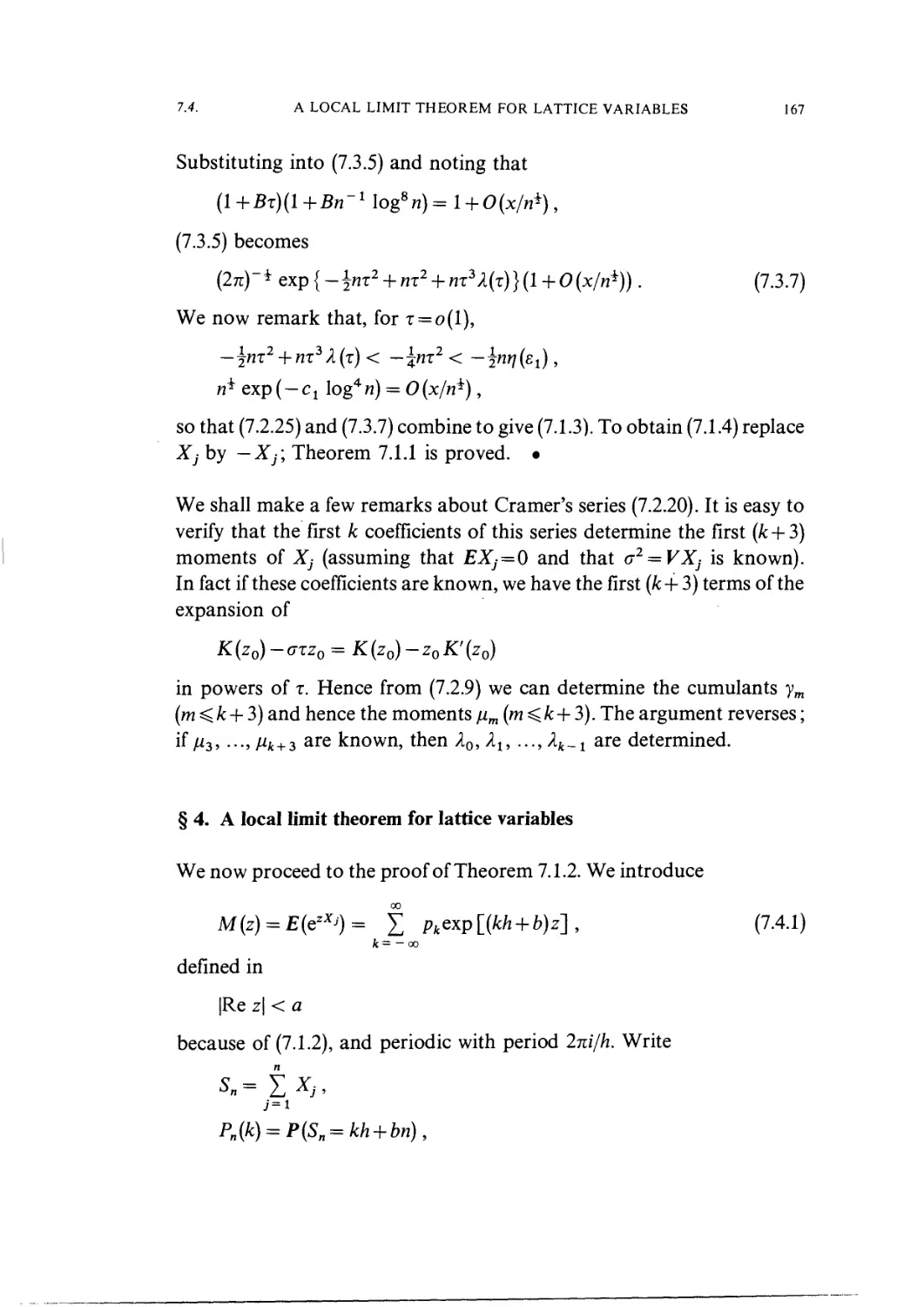
2. A local limit theorem for probability densities 161
3. Calculation of the integral near a saddle point 166
4. A local limit theorem for lattice variables 167
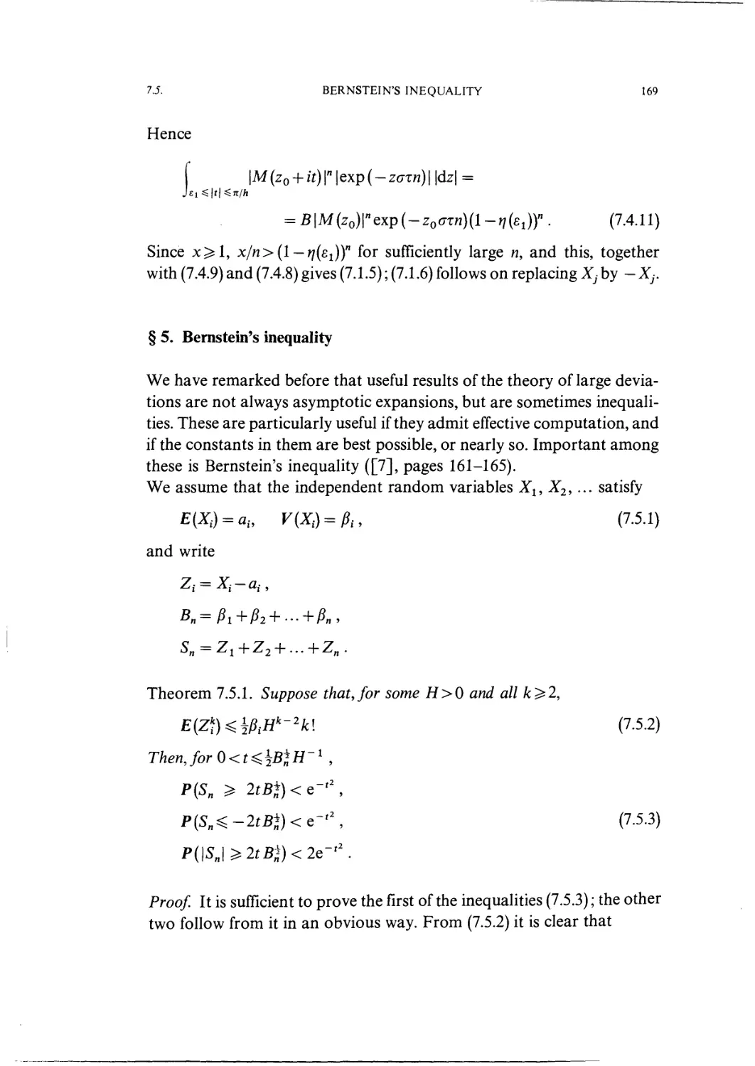
5. Bernstein's inequality 169
Chapter 8
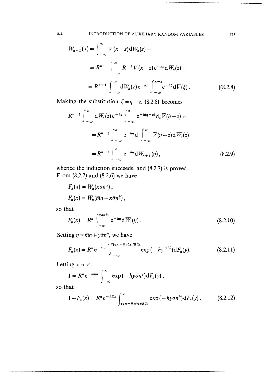
Cramer's integral theorem and its refinement by Petrov 171
1. Statement of the theorem 171
2. The introduction of auxiliary random variables 172
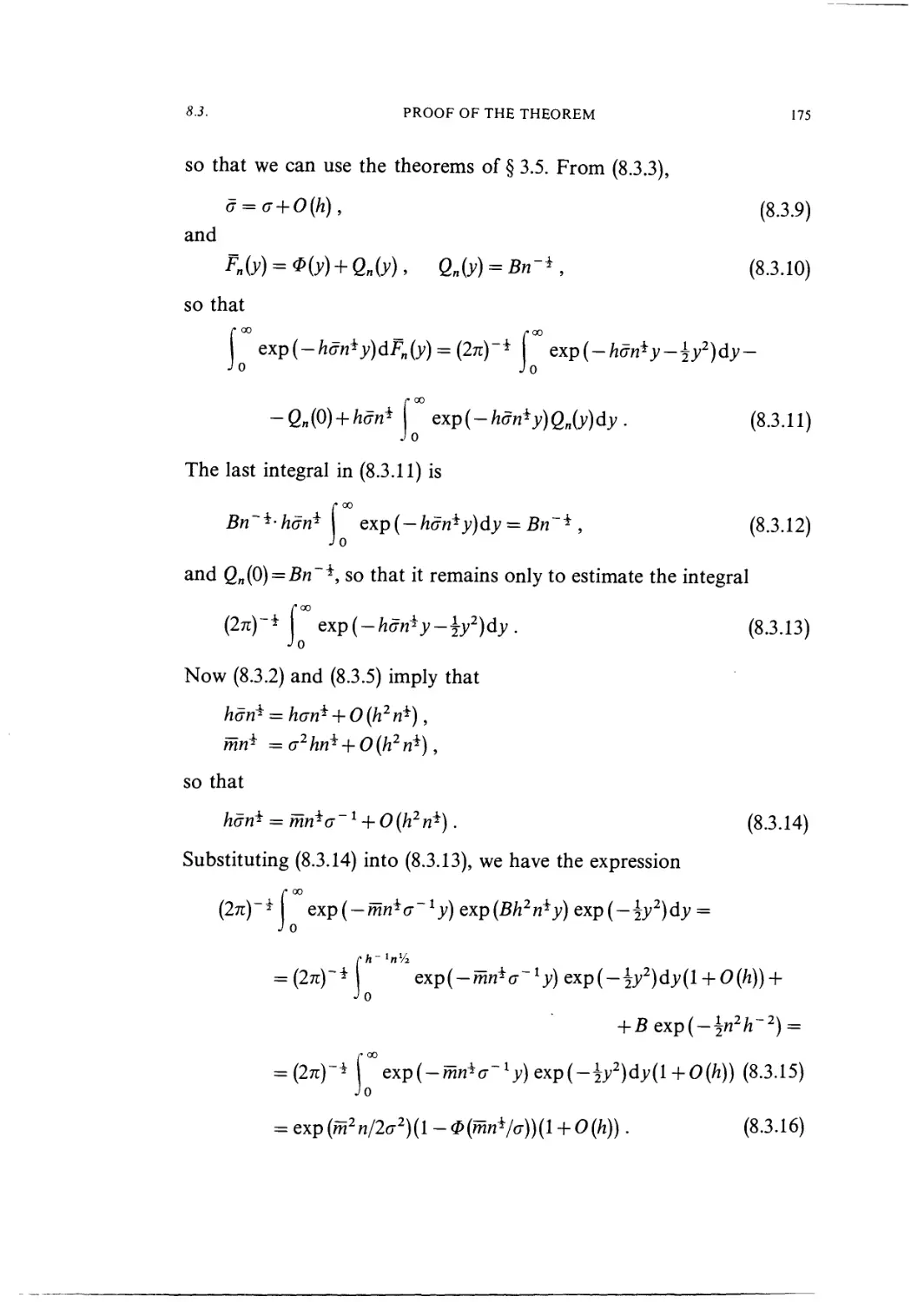
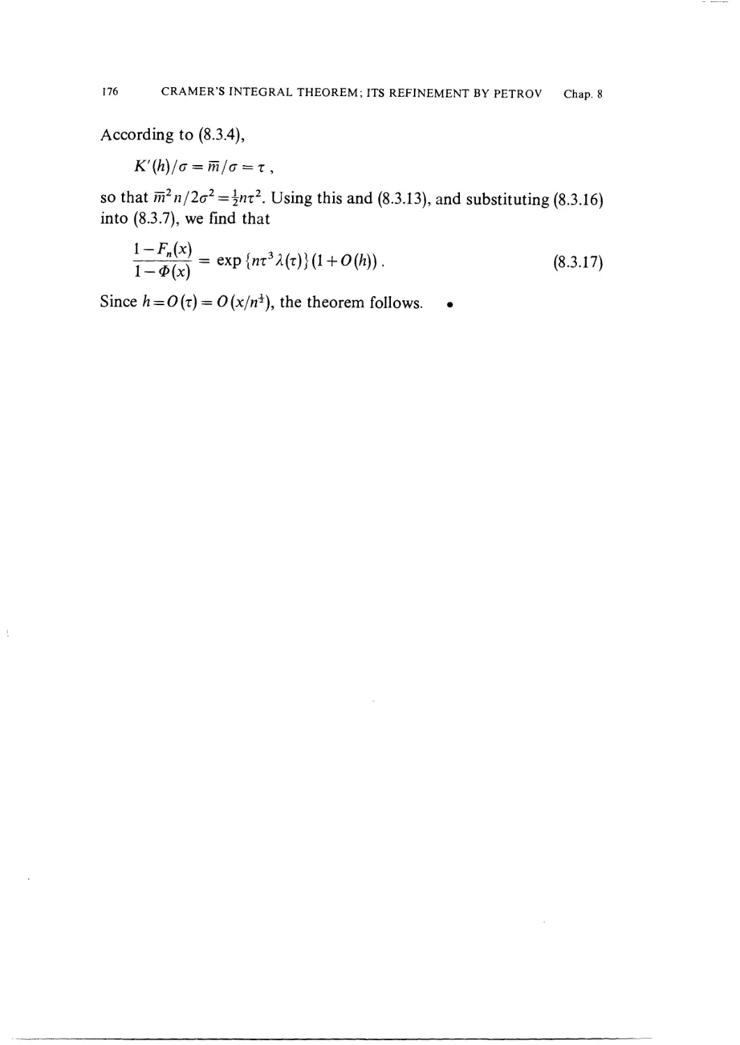
3. Proof of the theorem 174
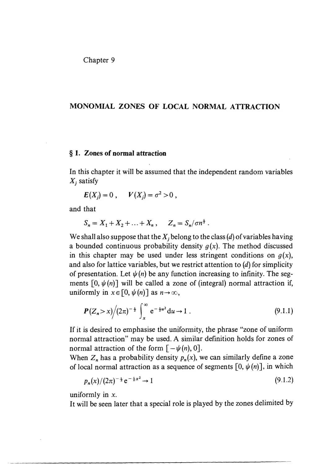
Chapter 9
Monomial zones of local normal attraction 177
1. Zones of normal attraction 177
2. The fundamental conditions 178
3. Fundamental theorems 180
4. Approximation of the characteristic function by a finite Taylor
series 182
5. Derivation of the basic integral 184
6. Completion of the proof 187
Chapter 10
Monomial zones of local attraction to Cramer's system of limiting tails 190
1. Formulation 190
2. On the condition A0.1.9) 192

CONTENTS
3. Derivation of the fundamental integral 192
4. Application of the method of steepest descents 194
5. Completion of the proof of Theorem 10.1.1 197
Chapter 11
Narrow zones of normal attraction 198
1. Classification of narrow zones by the function h 198
2. Statement of the theorems r- . . . 199
3. On the conditions imposed upon h(x) 200
4. The necessity of A1.2.2) for Class 1 200
5. The sufficiency of A1.2.2) for Class I 201
6. Investigation of the fundamental integral 203
7. More investigation of the fundamental integral 204
8. Investigation of K(t) 207
9. More investigation of K(t) 209
10. Completion of the proof of Theorem 11.2.1 211
11. The corresponding integral theorem 212
12. Calculation of the auxiliary limit distribution 214
13. More about the auxiliary limit distribution 215
14. Completion of the proof of Theorem 11.2.2 217
15. The general case of narrow zones 218
16. The transition to Theorems 11.2.3-5 220
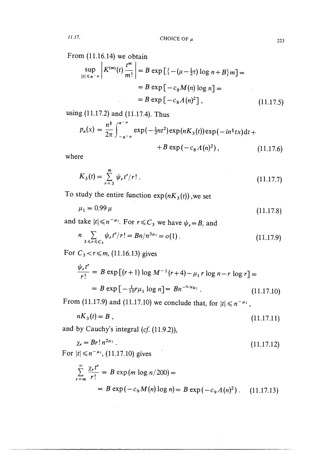
17. Choice of/i 222
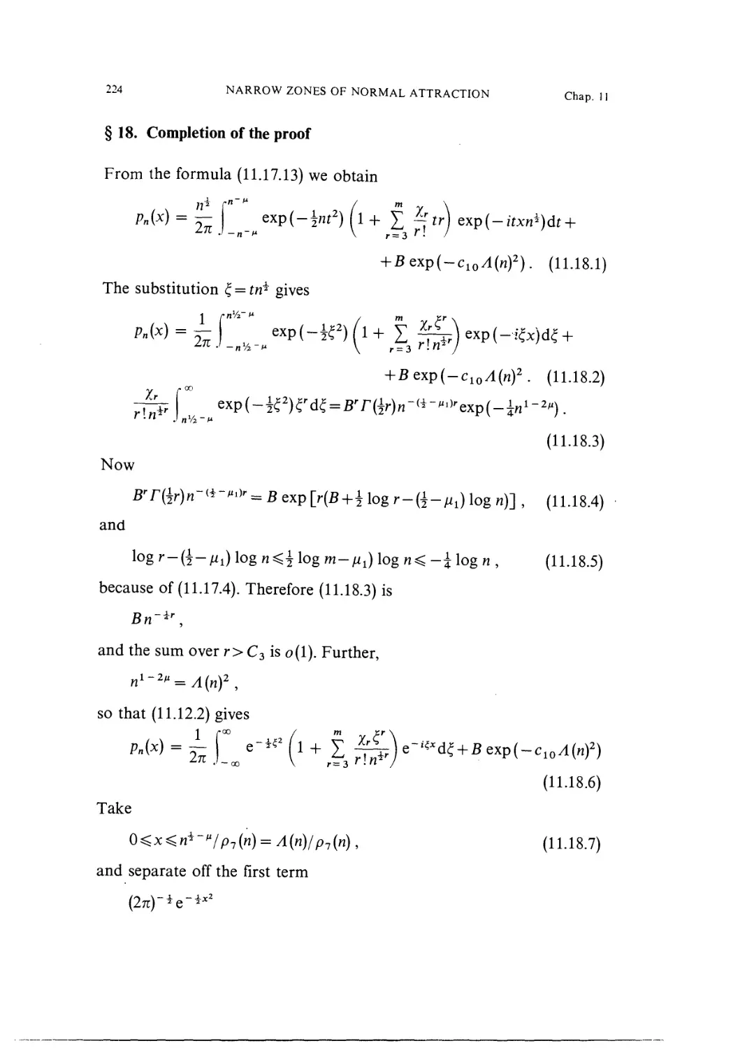
18. Completion of the proof 224
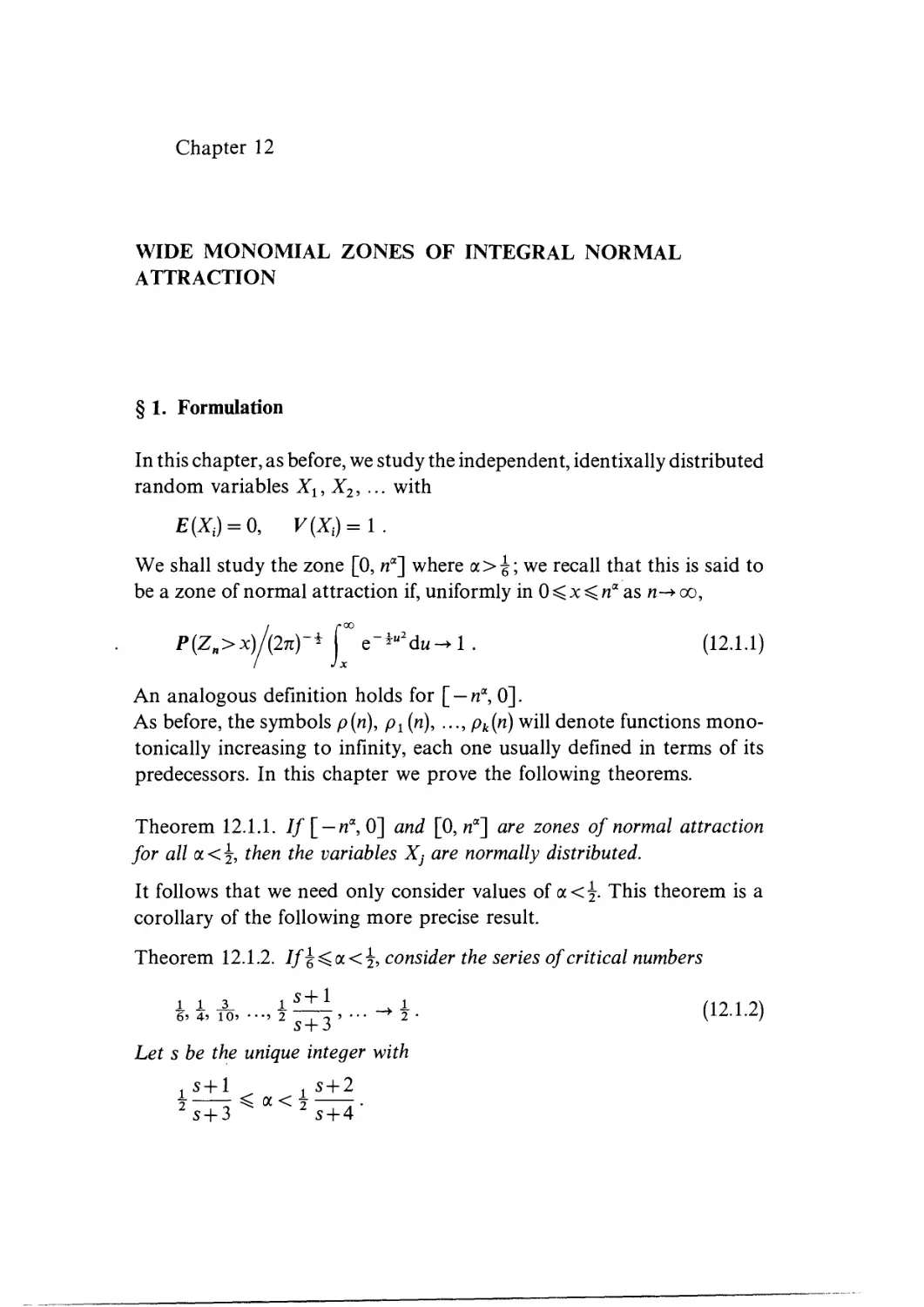
Chapter 12
Wide monomial zones of integral normal attraction 226
1. Formulation 226
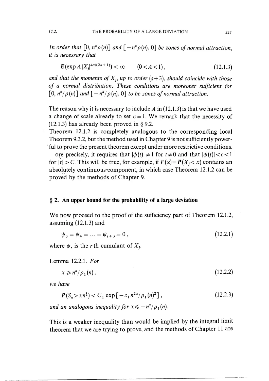
2. An upper bound for the probability of a large deviation . . . 227
3. Introduction of auxiliary variables 229
4. Study of the basic relation 231
5. Derivation of the fundamental formula 232

CONTENTS 9
6. The fundamental integral formula 234
7. Study of the auxiliary integral 235
8. Expansion of R as a Taylor series 236
9. Further transformations 238
10. Completion of the proof of sufficiency 240
11. Proof of the necessity 241
12. Completion of the proof 243
Chapter 13
Monomial zones of integral attraction to Cramer's system of limiting
tails 244
1. Formulation 244
2. An upper bound for the probability of a large derivation . . . 245
3. Investigation of the basic formula 251
4. Completion of the proof 253
Chapter 14
Integral theorems holding on the whole line 254
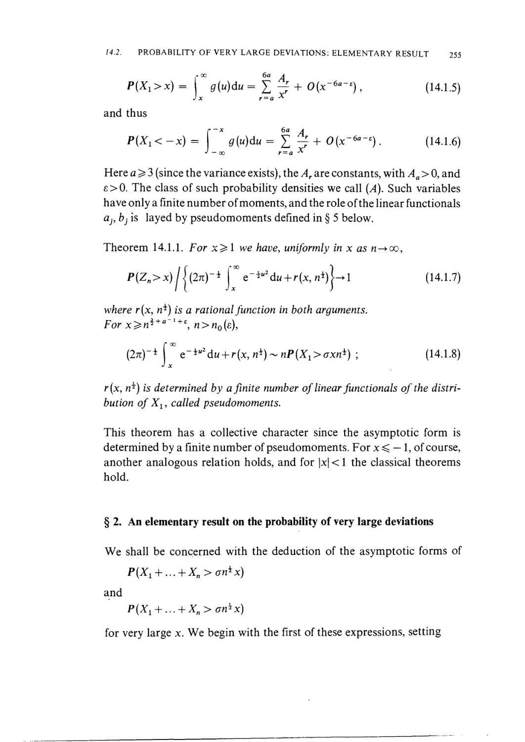
1. Formulation 254
2. An elementary result on the probability of very large deviations 255
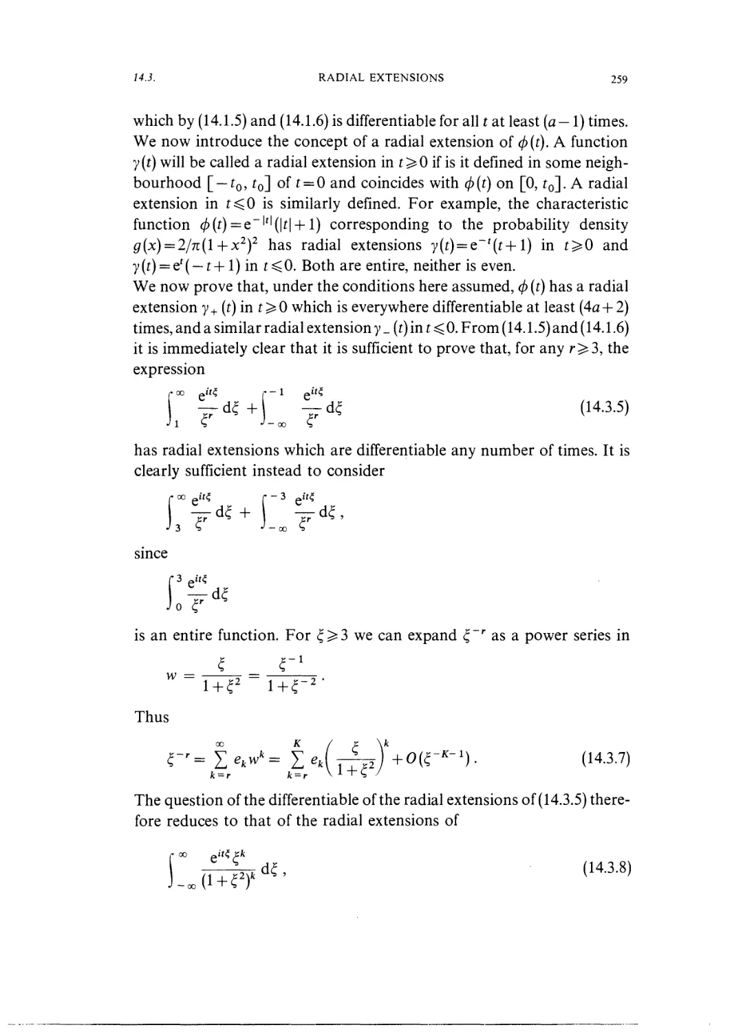
3. Radial extensions 258
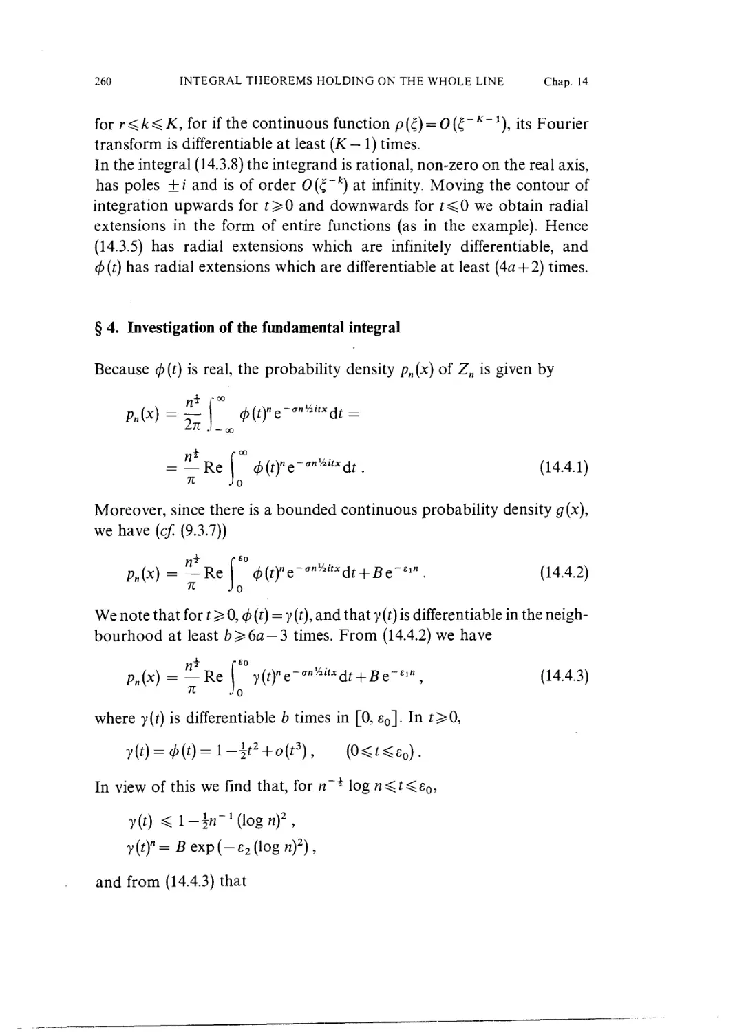
4. Investigation of the fundamental integral 260
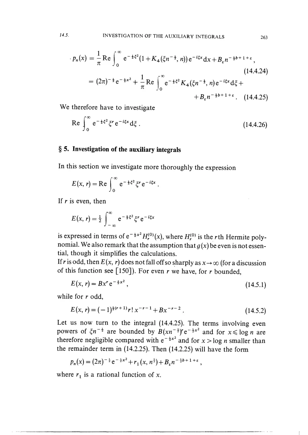
5. Investigation of the auxiliary integrals 263
6. An example 265
Chapter 15
Approximation of distributions of sums of independent components
by infinitely divisible distributions 267
1. Statement of the problem 267
2. Concentration functions 268

10 CONTENTS
3. Auxiliary propositions 273
4. Proof of Theorem 15.1.1 278
Chapter 16
Some results from the theory of stationary processes 284
1. Definition and general properties 284
2. Stationary processes and the associated measure-preserving
transformations 286
3. Hilbert spaces associated with a stationary process 288
4. Autocovariance and spectral functions of stationary processes 291
5. The spectral representation of stationary processes 292
6. The structure of L^ and linear transformations of stationary
processes 296
7. Existence theorems for the spectral density 298
Chapter 17
Conditions of weak dependence for stationary processes 301
1. Regularity 301
2. The strong mixing condition 305
3. Conditions of weak dependence for Gaussian sequences ... 310
Chapter 18
The central limit theorem for stationary processes 315
1. Statement of the problem 315
2. The variance of Xx +...+ Xn 321
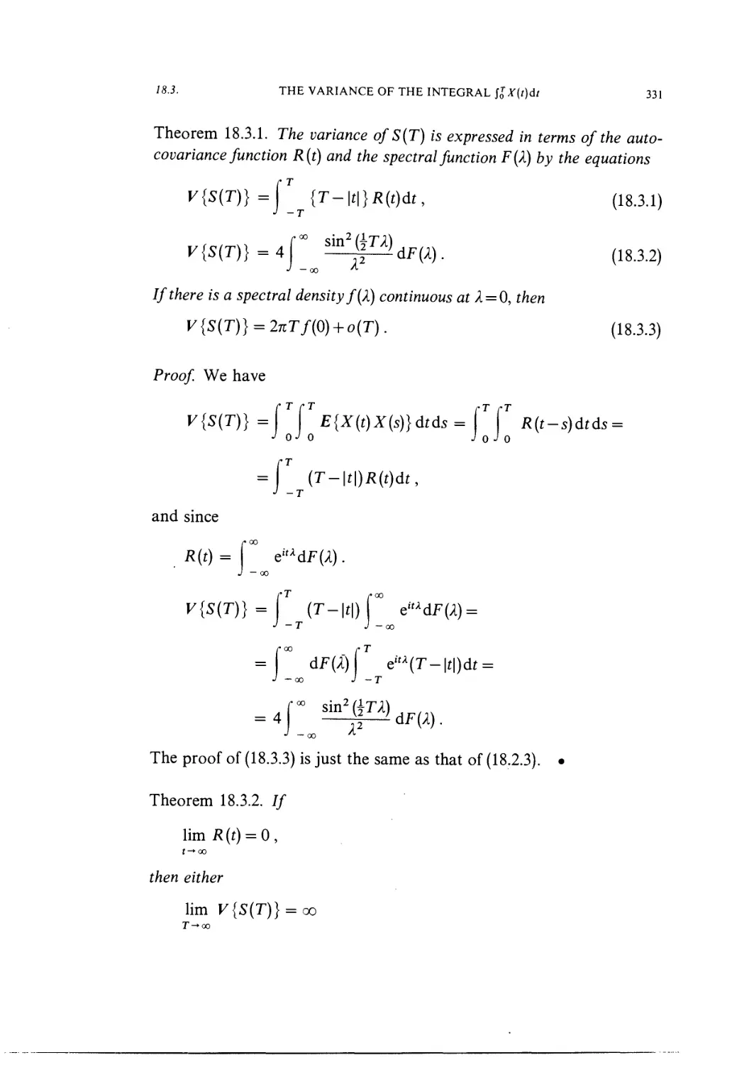
3. The variance of the integral ft X{t)dt 330
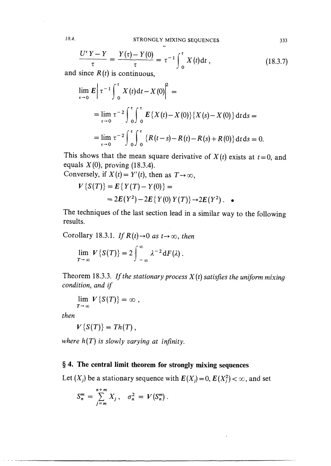
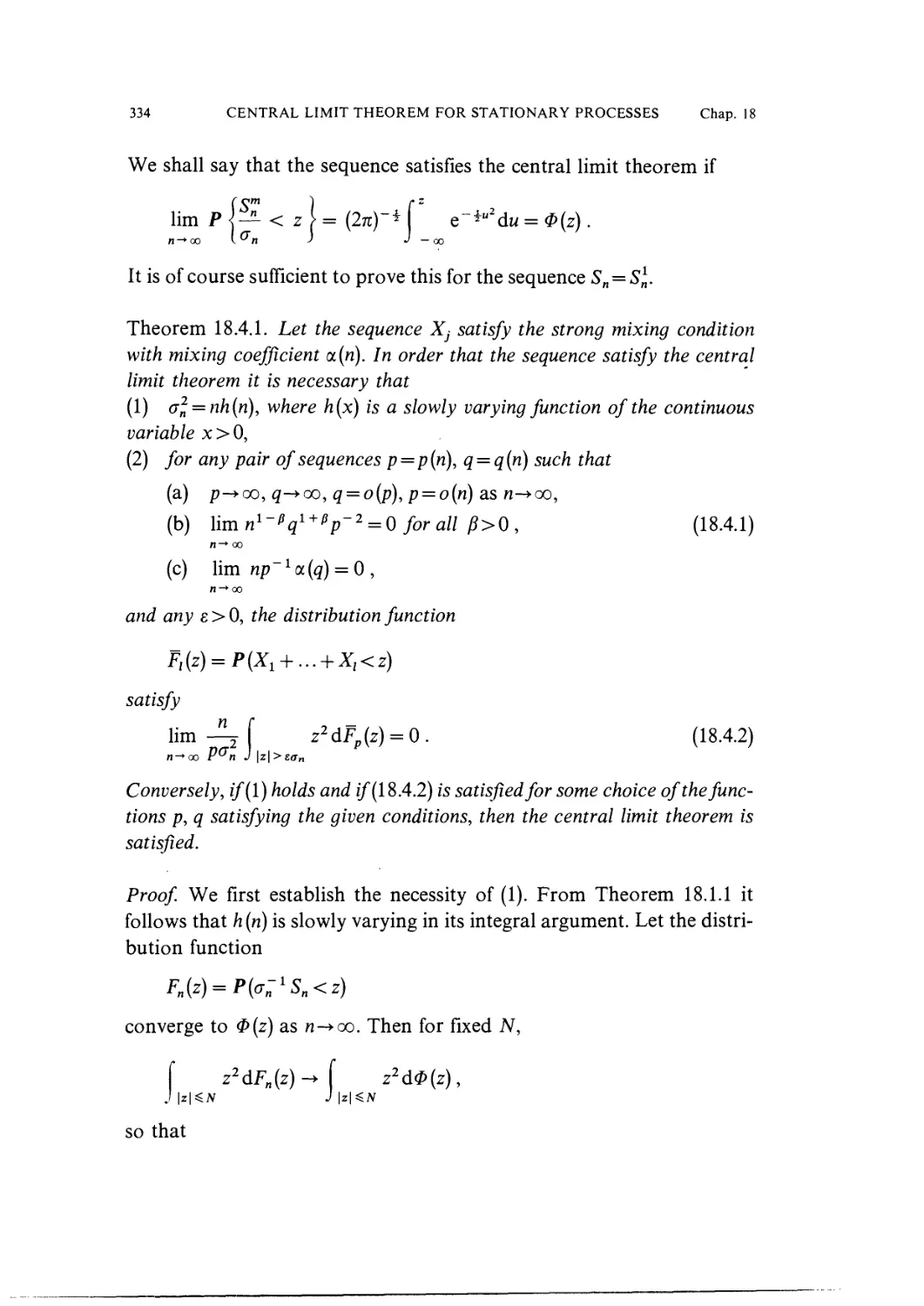
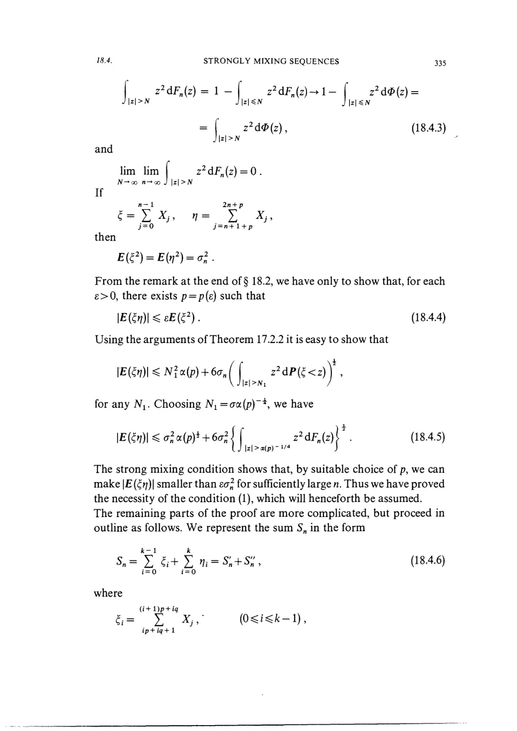
4. The central limit theorem for strongly mixing sequences . . . 333
5. Sufficient conditions for the central limit theorem 340

CONTENTS
6. The central limit theorem for functionals of mixing sequences 352
7. The central limit theorem in continuous time 362
Chapter 19
Examples and addenda 365
1. The central limit theorem for homogeneous Markov chains . . 365
2. m-dependent sequences 369
3. The distribution of values of sums of the form ~LfBkx). . . . 370
4. Application to the metric theory of continued fractions ... 374
5. Example of a sequence not satisfying the central limit theorem 384
Chapter 20
Some unsolved problems 390
Appendix 1
Sowly varying functions 394
Appendix 2
Theorems on Fourier transforms 398
Appendix 3
A theorem on convergence of conditional expectations 400
Notes 401
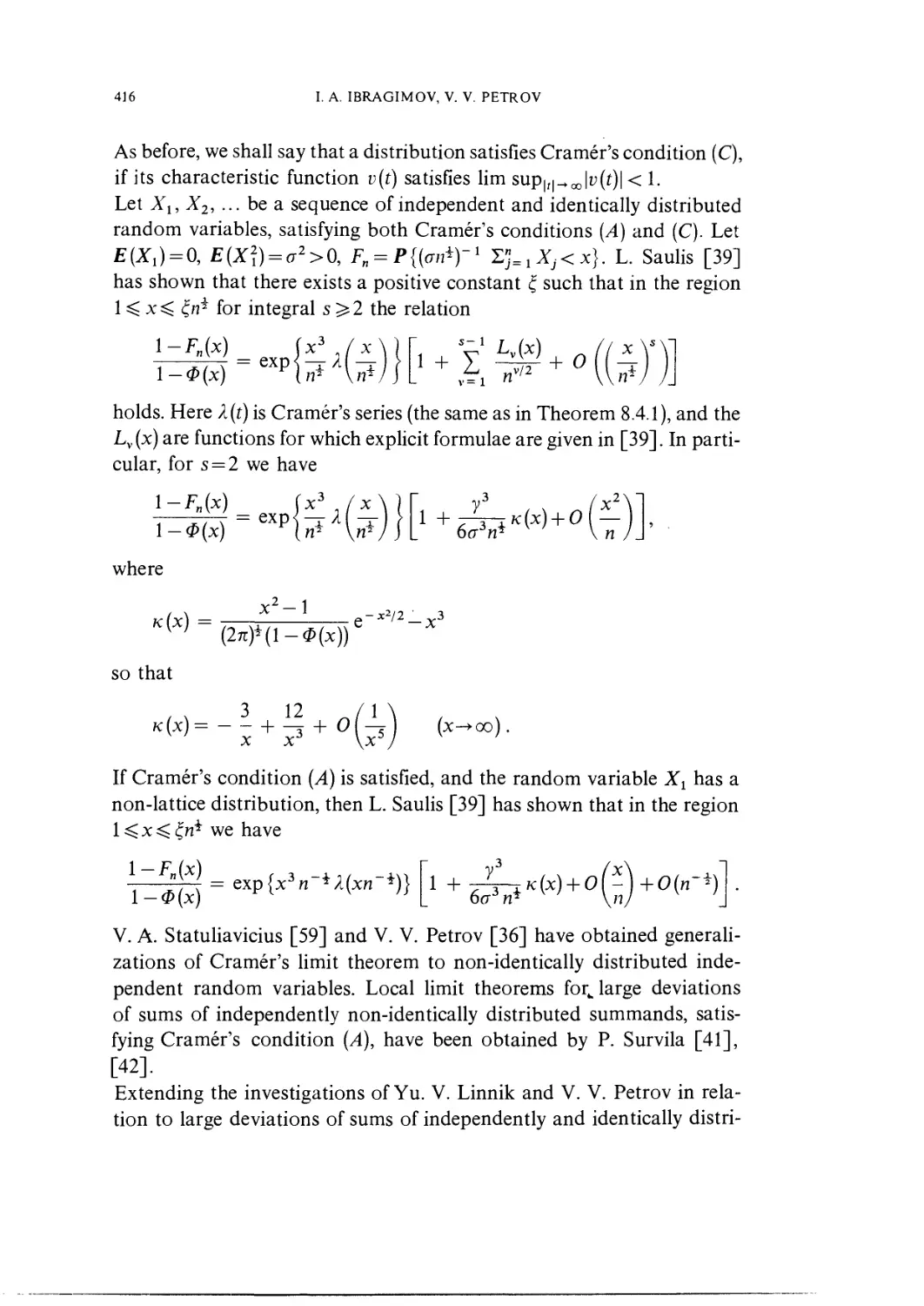
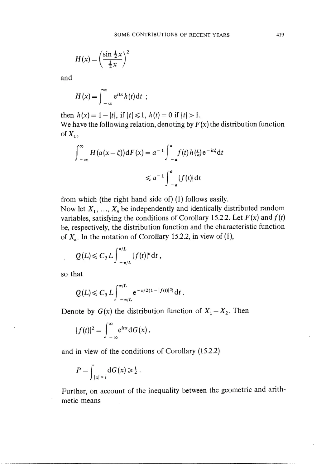
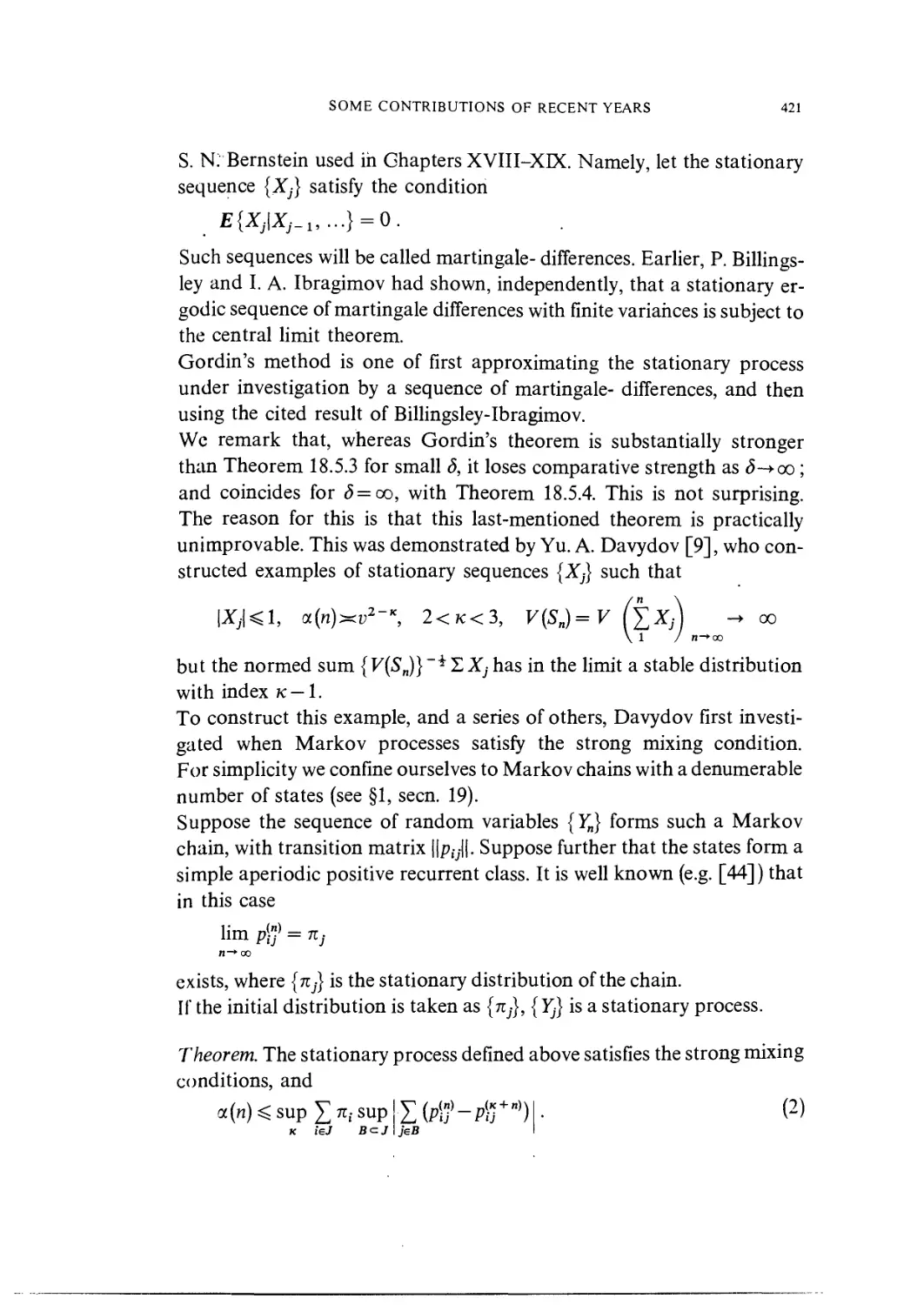
Some contributions of recent years 406
by I. A. Ibragimov, V. V. Petrov
Bibliography 429
Subject index 440

PREFACE
It is difficult to indicate in a short title the contents and methods of attack
of this book, and we seek therefore to do so in this preface. The problems
studied here concern sums of stationary sequences of random variables,
including sequences of independent and identically distributed variables.
More specifically, we are concerned with the distribution function Fn (x)
of the sum X1 + X2+ ... + Xn, where Xx, X2, ... is a stationary sequence.
In the independent case, asymptotic analysis of Fn (x) for large n is highly
developed, but in the general case much less is known.
Most of the methods expounded here can be extended, for example, to
problems in which the Xn are not identically distributed, but the results
are cumbersome and seem less final, and we therefore restrict ourselves
to the stationary case. As well as the problem of summation just outlined,
we include a discussion of some closely related problems of the analytical
structure of stable laws.
The book presupposes a knowledge of the monograph "Limit Distribu-
Distributions of Sums of Independent Random Variables" by B. V. Gnedenko and
A. N. Kolmogorov, whose publication in 1949 inspired much of the re-
research we describe.
Chapters 2-5 treat problems about sums of independent, identically
distributed random variables not connected with the theory of large
deviations, which occupies Chapters 6-14. In Chapter 15 the problem of
approximating Fn (x) by infinitely divisible distributions is studied. Chap-
Chapters 16-19 are devoted to limit theorems for weakly dependent stationary
sequences. In Chapter 20 some unsolved problems are formulated.

Chapter 1
PROBABILITY DISTRIBUTIONS ON THE REAL LINE:
INFINITELY DIVISIBLE LAWS
This chapter is of an introductory nature, its purpose being to indicate
some concepts and results from the theory of probability which are used
in later chapters. Most of these are contained in Chapters 1-9 of Gne-
denko [47], and will therefore be cited without proof.
The first section is somewhat isolated, and contains a series of results
from the foundations of the theory of probability. A detailed account
may be found in [76], or in Chapter I of [31]. Some of these will not be
needed in the first part of the book, in which attention is confined to
independent random variables.
§ 1. Probability spaces, conditional probabilities and expectations
A probability space is a triple (Q, 5, P), where Q is a set of elements co,
5 a cr-algebra of subsets of Q (called events), and P a measure on 5 with
P (Q) = 1. For E g g, P {E) is called the probability of the event E. A random
variable X is a real-valued measurable function on (Q, 5), and the measure
F defined on the Borel sets of the real line R by F(A) = P(X e A) is called
the distribution of X.
Several random variables X1,X2, ¦¦¦, Xn may be combined in a random
vector X = (XX, X2, ..., Xn), and the measure F(A) = P(XeA) defined on
the Borel sets of/?" is the distribution of X, or the joint distribution of the
variables Xl5 X2, ..., Xn.
More generally, if T is any set of real numbers, a family of random variables
X(t), tsT, defined on (Q, 5, P) is called a random process. Conditions
for the existence of random processes with prescribed joint distributions
are given by Kolmogorov's theorem [76].
A probability space is a special case of a measurable space, and it is there-

18 PROBABILITY DISTRIBUTIONS ON THE REAL LINE Chap. 1
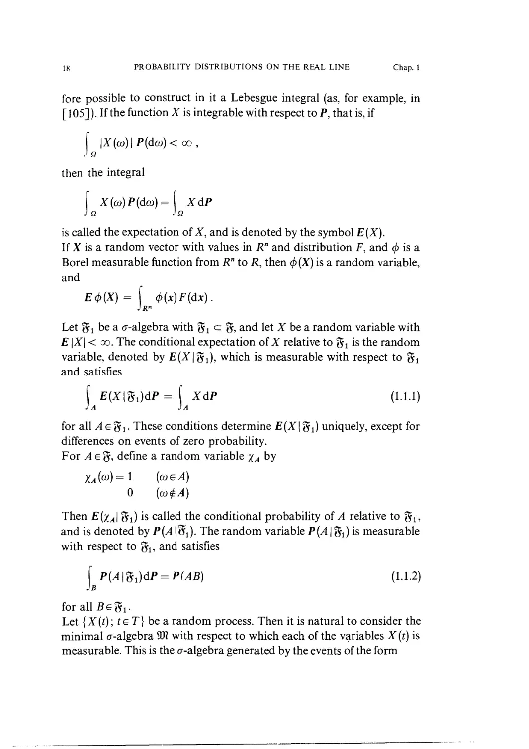
fore possible to construct in it a Lebesgue integral (as, for example, in
[105]). If the function X is integrable with respect to P, that is, if
\X(co)\P{dco)< oo,
.' n
then the integral
f X{co)P{dco)=[ XdP
is called the expectation of X, and is denoted by the symbol E(X).
If X is a random vector with values in R" and distribution F, and </> is a
Borel measurable function from R" to R, then <j> (X) is a random variable,
and
= f <t>(x)F(dx).
Let 5i be a cr-algebra with Si <= 3f, and let X be a random variable with
E \X\ < oo. The conditional expectation of X relative to 5i is the random
variable, denoted by E(X\%1), which is measurable with respect to 5i
and satisfies
E{X\%1)dP = ( *dP A.1.1)
a
for all >le5i- These conditions determine E(X\%1) uniquely, except for
differences on events of zero probability.
For A e 5, define a random variable Xa by
XaW=1 {coeA)
0 {co$A)
Then ?(^1 5i) is called the conditional probability of A relative to gl5
and is denoted by P(A l^). The random variable P(,415i) is measurable
with respect to 5l5 and satisfies
A.1.2)
B
for all Begj.
Let |X(t); te T] be a random process. Then it is natural to consider the
minimal cr-algebra 9lR with respect to which each of the variables X (t) is
measurable. This is the cr-algebra generated by the events of the form

1.2. DISTRIBUTIONS AND DISTRIBUTION FUNCTIONS 19
{(X(t1),X(t2),...,X(tn))cA}
for tl512, ..., tneT and Borel sets A in R". For any random variable Y,
we write
We shall state various properties of conditional expectations which will
be needed later (cf. [31], Chapter I). If Y and Z are random variables with
?|y| < oo and E\Z\ < oo, and if Z is measurable with respect to 5i> then
with probability one,
A.1.3)
If cr-algebras gl5 g2 satisfy ^ c g2 c g, then with probability one,
A.1.4)
§ 2. Distributions and distribution functions
If X is a random variable, its probability distribution is the measure
F{A) = P{XeA)
on the Borel subsets of the real line. It is well known that F is uniquely
determined by the corresponding distribution function F defined by
F(x) = F{{- oo, x)) = P{X<x).
In what follows, no distinction will be made between F and F, and we shall
speak, for instance, of a random variable X having distribution F(x).
A probability distribution F is called continuous if the measure F is ab-
absolutely continuous with respect to Lebesgue measure, i.e. if
F(A) = f p(x)dx
A
for some function p, which is necessarily given by p(x) = F'(x) outside a
set of Lebesgue measure zero. The function p is then called the density of
the distribution.
A probability distribution F is said to be discrete if it is concentrated on
some countable set {xh}. If ph = P(X = xh), then

20 PROBABILITY DISTRIBUTIONS ON THE REAL LINE Chap. 1
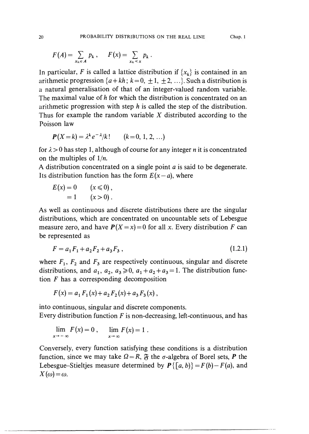
pk, F(x)= ? pk.
xk<x
In particular, F is called a lattice distribution if {xk} is contained in an
arithmetic progression {a + kh; /c = 0, +1, + 2, ...}. Such a distribution is
a natural generalisation of that of an integer-valued random variable.
The maximal value of h for which the distribution is concentrated on an
arithmetic progression with step h is called the step of the distribution.
Thus for example the random variable X distributed according to the
Poisson law
P{X = k) = Xke~x/k\ (fc = 0, 1,2, ...)
for X > 0 has step 1, although of course for any integer n it is concentrated
on the multiples of l/n.
A distribution concentrated on a single point a is said to be degenerate.
Its distribution function has the form E(x — a), where
?(x) = 0 (x<0),
= 1 (x > 0).
As well as continuous and discrete distributions there are the singular
distributions, which are concentrated on uncountable sets of Lebesgue
measure zero, and have P(X = x) = 0 for all x. Every distribution F can
be represented as
F = a1F1 + a2F2 + a3F3, A.2.1)
where F1, F2 and F3 are respectively continuous, singular and discrete
distributions, and al5 a2, a3^0, a1+a2 + a3 = l. The distribution func-
function F has a corresponding decomposition
F{x) = fl1F1(x) + a2F2(x) + fl3F3(x),
into continuous, singular and discrete components.
Every distribution function F is non-decreasing, left-continuous, and has
lim F(x) = 0, limF(x)=l .
x-* — oo
Conversely, every function satisfying these conditions is a distribution
function, since we may take Q — R, % the o--algebra of Borel sets, P the
Lebesgue-Stieltjes measure determined by P{[a, b)} =F(b) — F(a), and
X(co) = co.

1.3. CONVERGENCE OF DISTRIBUTIONS 21
Let X and Y be independent random variables with respective distribu-
distribution functions Fx and F2. The distribution function F of X+ Y is given by
F(x)=[ F1(x-y)dF2{y)=r F2(x-y)dF1(y). A.2.2)
J — CO J — 00
We say that F is the convolution of Fx and F2, and write
The convolution of n identical distributions will be denoted by
" = F*F*...*F .
If one of the distributions Fj, F2 is continuous, then so is F; in fact if Fj
admits a density pl5 then F has density
p1{x-y)dF2{y).
§ 3. Convergence of distributions
We here consider different types of convergence of probability distribu-
distributions on the real line, following Kolgomorov [82]. The ideas in that paper
will also be used in later chapters.
A) Convergence in variation. Define the distance px (F, G) between two
distributions F and G by
Pi(F, G) = sup \F{A)-G{A)\, A.3.1)
where the supremum is taken over all Borel sets A. A sequence of dis-
distributions Fn converges in variation to a distribution F if px (Fn, F)-»0. It is
clear that this mode of convergence can be expressed in terms of distri-
distribution functions: Pi(F, G) is one-half the total variation of F(x)—G(x).
For continuous distributions
|F'(x)-G'(x)|dx,
TO
while for discrete distributions

PROBABILITY DISTRIBUTIONS ON THE REAL LINE Chap. 1
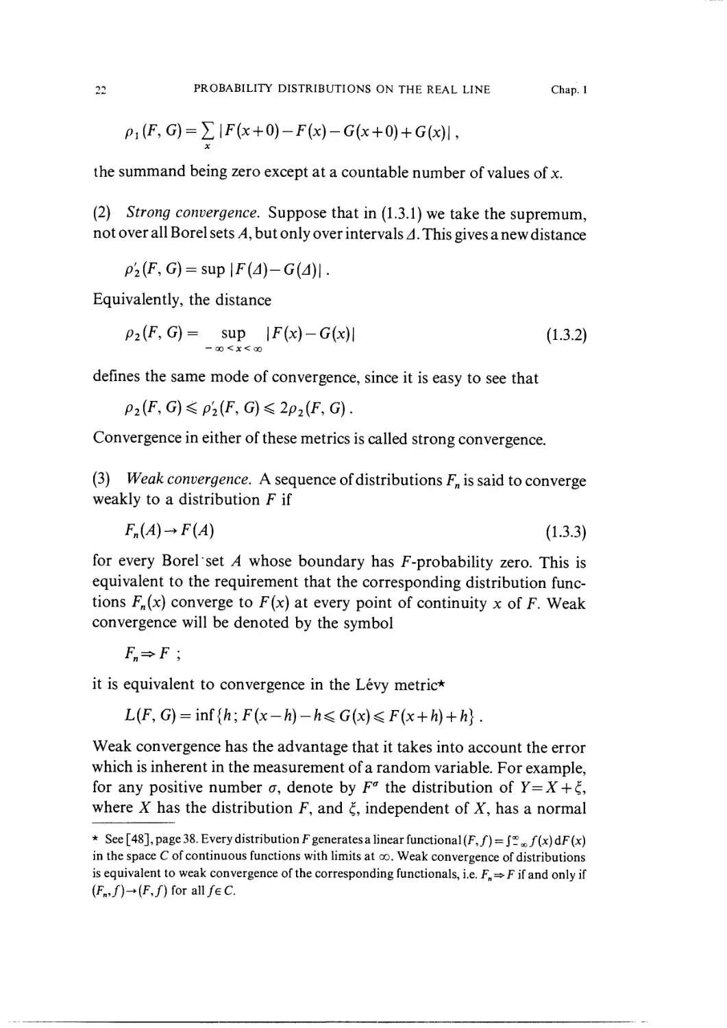
the summand being zero except at a countable number of values of x.
B) Strong convergence. Suppose that in A.3.1) we take the supremum,
not over all Borel sets A, but only over intervals A. This gives a new distance
p'2(F,G) = sup\F(A)-G(A)\.
Equivalently, the distance
P2(F,G) = sup \F(x)-G(x)\ A.3.2)
— oo <x< oo
defines the same mode of convergence, since it is easy to see that
p2(F,G)<p'2(F,G)<2p2(F,G).
Convergence in either of these metrics is called strong convergence.
C) Weak convergence. A sequence of distributions Fn is said to converge
weakly to a distribution F if
FH(A)-*FW A-3-3)
for every Borelset A whose boundary has F-probability zero. This is
equivalent to the requirement that the corresponding distribution func-
functions Fn(x) converge to F(x) at every point of continuity x of F. Weak
convergence will be denoted by the symbol
F =>F ¦
it is equivalent to convergence in the Levy metric*
L{F, G) = M{h; F{x-h)-h< G{x)^ F{x + h) + h].
Weak convergence has the advantage that it takes into account the error
which is inherent in the measurement of a random variable. For example,
for any positive number a, denote by Fa the distribution of Y=X + ?,
where X has the distribution F, and ?, independent of X, has a normal
* See [48], page 38. Every distribution F generates a linear functional (F,/) = J _ <«, f(x) dF (x)
in the space C of continuous functions with limits at oo. Weak convergence of distributions
is equivalent to weak convergence of the corresponding functionals, i.e. Fn=>F if and only if
(Fn,/H(F,/)forall/eC.

1.3.
CONVERGENCE OF DISTRIBUTIONS
23
distribution with mean zero and variance a2. Define a type of convergence
by saying that Fn-+F if, for all o > 0,
Pl
0 .
A,3.4)
Theorem 1.3.1. Convergence as defined by A.3.4) is equivalent to weak
convergence.
Proof. Denote by
(f)a{x) = B7r<T2)-*exp(-x2/2<72)
the density of the distribution of ?. Then for any distribution G, Ga is
a continuous distribution with density
g°(x)= <y{x-y)dG(y).
Therefore
dx
F(x-y)d{FH(y)-F(y)}
Suppose first that Fn=>F, and fix a positive number A. By the dominated
convergence theorem,
¦00
+ \ dx
-A
{Fn(y)-F(y)}-F(x-y)dy
\Fn(A)-F(A)\ f cj>°{x-A)dx +
J — 00
\Fn(y)-F(y)\dy
-A
dx . A.3.5)
One may assume that A is taken to be a point of continuity of F. Then the

24 PROBABILITY DISTRIBUTIONS ON THE REAL LINE Chap. 1
last three terms in A.3.5) tend to zero as n-+ oo. By choosing A sufficiently
large, the remaining terms may be made arbitrarily small. Hence, for all a.
Conversely, suppose that this holds. Then
{Fn(y)-F(y)}cf>°(x-y)dy -0. A.3.6)
J — oo
Suppose if possible that Fn=f>F. Then there exists x0, a point of continuity
of F, and 5 > 0 such that
\Fn(x0)-F(x0)\>6
for infinitely many n. There is no loss of generality in taking x0 = 0. If then
for instance Fn@) > F@) + S, there is an interval [0, a] in which F(x)<
F@)-|<5, and
Fn(x)-F(x) > FH@)~F(x) > S {F(x)-F@)} > \b .
But then
upP {Fn(y)-F(y)}<j>*&-y)dy=
a-+0 J — oo
= lim sup {Fn(y) — F(y)} (f)a{^a — y)dy >
a~*0 J 0
>jS lim sup (f)a(ja-y)dy = \b .
a~*0 JO 0
Hence there is a value of a for which
p2\tn,t )>4O, A.3.7)
and a similar conclusion holds in the other case Fn@)< F@) — d. Thus
A.3.7) holds for infinitely many n, which contradicts A.3.6), showing that
the supposition Fn=f>F must be false. •
§ 4. Moments and characteristic functions
T-ie moments av and absolute moments j5v of a random variable X with
distribution F are defined respectively by

1.4. MOMENTS AND CHARACTERISTIC FUNCTIONS 25
xvdF(x),
oo
/JV=E\X\V = P \x\vdF(x),
J - oo
so long as these expectations exist. The fiv satisfy the inequalities
#"<#", (r>s>0).
The characteristic function /(?) of X is defined by
eitxdF{x), A.4.1)
oo
and its connection with the moments is contained in the following
assertion.
If a random variable X has finite absolute moment fik (where k is a positive
integer), then f has derivatives up to order k, and
for s = 0, 1, 2, ..., k. As ?->0,
f(t)= I ~(ity+o(tk).
s = 0 S-
It is a most important fact that addition of independent random variables
corresponds to multiplication of characteristic functions. If the indepen-
independent variables Xt have respective characteristic functions f(t), then the
characteristic function of Xl + X2 +... + Xn is
f(t)=fi(t)f2(t)..Jn(t).
From A.4.1) the characteristic function is uniquely determined by the
distribution function. The converse is also true, and is expressed by the
relation
i rc eity — e~itx
F(x) = — lim lim I f{t)dt, A.4.2)
In y^n ^^ J_c it

26 PROBABILITY DISTRIBUTIONS ON THE REAL LINE Chap. 1
which holds at all points of continuity of F. Thus there is a one-to-one
correspondence between distribution functions and characteristic func-
functions.
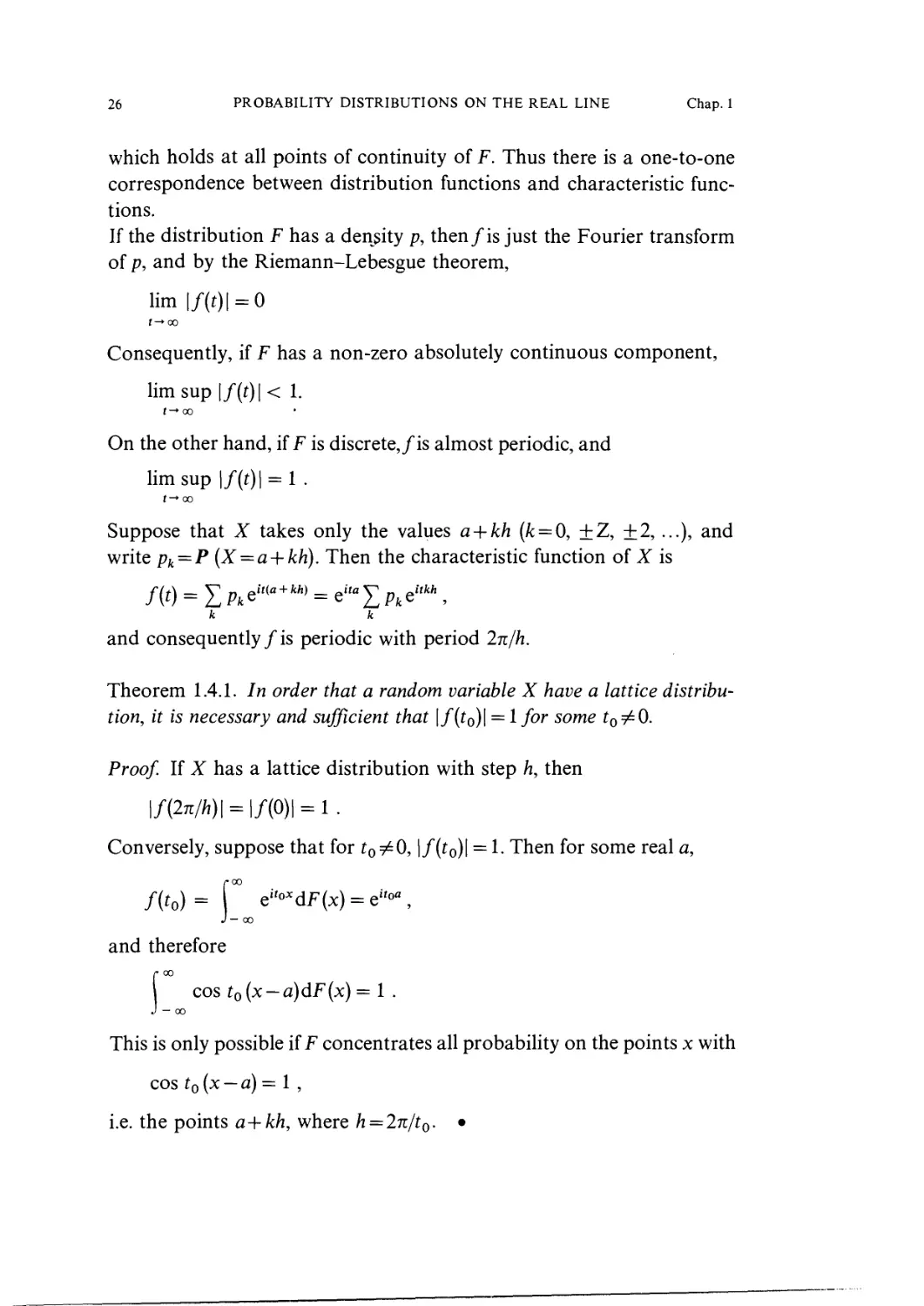
If the distribution F has a density p, then/is just the Fourier transform
of p, and by the Riemann-Lebesgue theorem,
lim
r->oo
Consequently, if F has a non-zero absolutely continuous component,
lim sup |/@| < 1.
t->oo
On the other hand, if F is discrete,/is almost periodic, and
lim sup |/@l = 1 •
t—ao
Suppose that X takes only the values a + kh (k = 0, ±Z, + 2, ...), and
write pk = P (X = a + kh). Then the characteristic function of X is
k k
and consequently / is periodic with period 2n/h.
Theorem 1.4.1. In order that a random variable X have a lattice distribu-
distribution, it is necessary and sufficient that \f(to)\ = lfor some ?0
Proof If X has a lattice distribution with step h, then
Conversely, suppose that for to^O, \f{to)\ = 1. Then for some real a,
r00
f(to)= e"°*dF(x) = e*,
J- oo
and therefore
• oo
Joo
cos to(x — a)dF(x) = 1 .
— oo
This is only possible if F concentrates all probability on the points x with
cos t0 (x — a) = 1 ,
i.e. the points a+kh, where h = 2n/t0. •

1.5. DISTRIBUTIONS AND CHARACTERISTIC FUNCTIONS 27
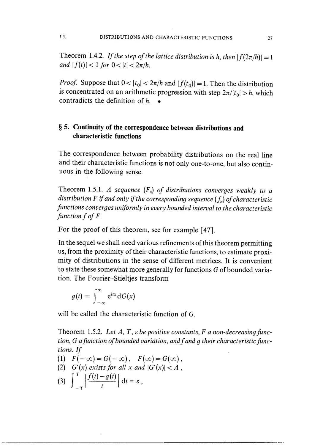
Theorem 1.4.2. If the step of the lattice distribution is h, then \fBn/h)\ = 1
and\f{t)\<lforO<\t\<2n/h.
Proof. Suppose that 0< \to\ < 2n/h and \f(to)\ = 1. Then the distribution
is concentrated on an arithmetic progression with step 2n/\to\ >h, which
contradicts the definition of h. •
§ 5. Continuity of the correspondence between distributions and
characteristic functions
The correspondence between probability distributions on the real line
and their characteristic functions is not only one-to-one, but also contin-
continuous in the following sense.
Theorem 1.5.1. A sequence (Fn) of distributions converges weakly to a
distribution F if and only if the corresponding sequence (/„) of characteristic
functions converges uniformly in every bounded interval to the characteristic
function f of F.
For the proof of this theorem, see for example [47].
In the sequel we shall need various refinements of this theorem permitting
us, from the proximity of their characteristic functions, to estimate proxi-
proximity of distributions in the sense of different metrices. It is convenient
to state these somewhat more generally for functions G of bounded varia-
variation. The Fourier-Stieltjes transform
g(t) = H e''MG(x)
•> - oo
will be called the characteristic function of G.
Theorem 1.5.2. Let A, T, e be positive constants, F a non-decreasing func-
function, G a function of bounded variation, and f and g their characteristic func-
functions. If
A) F(-oo) = G(-oo), F{od) = G(od),
B) G' (x) exists for all x and \G' {x)\ < A ,
C)
-r

28
PROBABILITY DISTRIBUTIONS ON THE REAL LINE
Chap. 1
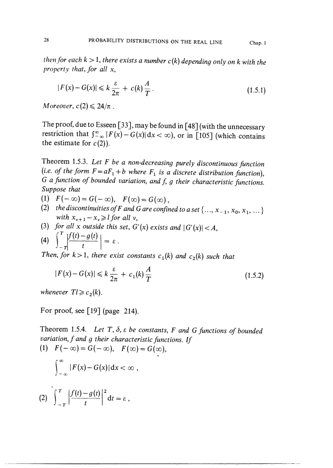
then for each k>l, there exists a number c(k) depending only on k with the
property that, for all x,
A.5.1)
Moreover, cB) < 24/n .
The proof, due to Esseen [33], may be found in [48] (with the unnecessary
restriction that $™M \F(x)-G{x)\dx< oo), or in [105] (which contains
the estimate for cB)).
Theorem 1.5.3. Let F be a non-decreasing purely discontinuous function
(i.e. of the form F = aFi+b where FY is a discrete distribution function),
G a function of bounded variation, and f g their characteristic functions.
Suppose that
A) F(-oo)=G(-oo), F(oo) = G(oo),
B) the discontinuities ofF and G are confined to a set {..., x_ 1; x0, x1; ...}
with xv+1—xv~^lfor all v,
C) for all x outside this set, G'(x) exists and \G'(x)\ <A,
¦ _r t
Then, for k>l, there exist constants c^k) and c2{k) such that
A.5.2)
whenever Tl^c2{k).
For proof, see [19] (page 214).
Theorem 1.5.4. Let T, 5, e be constants, F and G functions of bounded
variation, f and g their characteristic functions. If
A) F(-oo) = G(-oo), F(oo) = G(oo),
|F(x)-G(x)|dx< oo
B)
r
-r
f{t)-9(t)

1.5. DISTRIBUTIONS AND CHARACTERISTIC FUNCTIONS 29
-T
dt
then
00 c A 4
|F(x)-G(x)|dx<-(VarG + VarF)+- + -)
00 V 7 A.5.3)
w/iere c is an absolute constant.
(It is possible to show that c^47r.)
Proof. Denote by V the class of complex functions A (x) with bounded
variation
and by K the class of Fourier-Stieltjes transforms
a(t)= f°° QitxdA{x)
J - oo
of functions in V. It is clear that
INI = V(A)
is well-defined, and that
Lemma 1.5.1. Suppose that a(t) is absolutely continuous, and that both
a(t) and a'(t) belong to L2( —oo, oo). Then aeV, and
a'(t)\2dtV . A.5.4)
J
Proof. Use Plancherel's theorem (Appendix 2) to compare a and its
Fourier transform a(x). Then
d f00 „. eitx— 1
and

30
PROBABILITY DISTRIBUTIONS ON THE REAL LINE
Chap. 1
\a{t)\2dt= \a{x)\2dx. A.5.5)
GO •' — 00
If we can prove that 5eL(— oo, oo), then a will belong to V, since then
and moreover
Qitxa{x)dx,
\a(x)\dx.
A.5.6)
But the functions a and a' belong to L2(— oo, oo), and so by Theorem
A2.2 (Appendix 2), xa(x)eL2( — oo, oo) and
\a'{t)\2dt =
From A.5.5), A.5.6) and A.5.7), we have
A.5.7)
= T
a'(t)\2dt
Proof of theorem 1.5.4. Integrate by parts in the equation
(-00
f(t)-g(t)= etod{F(x)-G(x)},
J — oo
to obtain
n(t\ "Y°°
eif*{F(x)-G(x)}dx,
whence
|F(x)-G(x)|dx =
f(t)-g(t)
-it

1.5. DISTRIBUTIONS AND CHARACTERISTIC FUNCTIONS 31
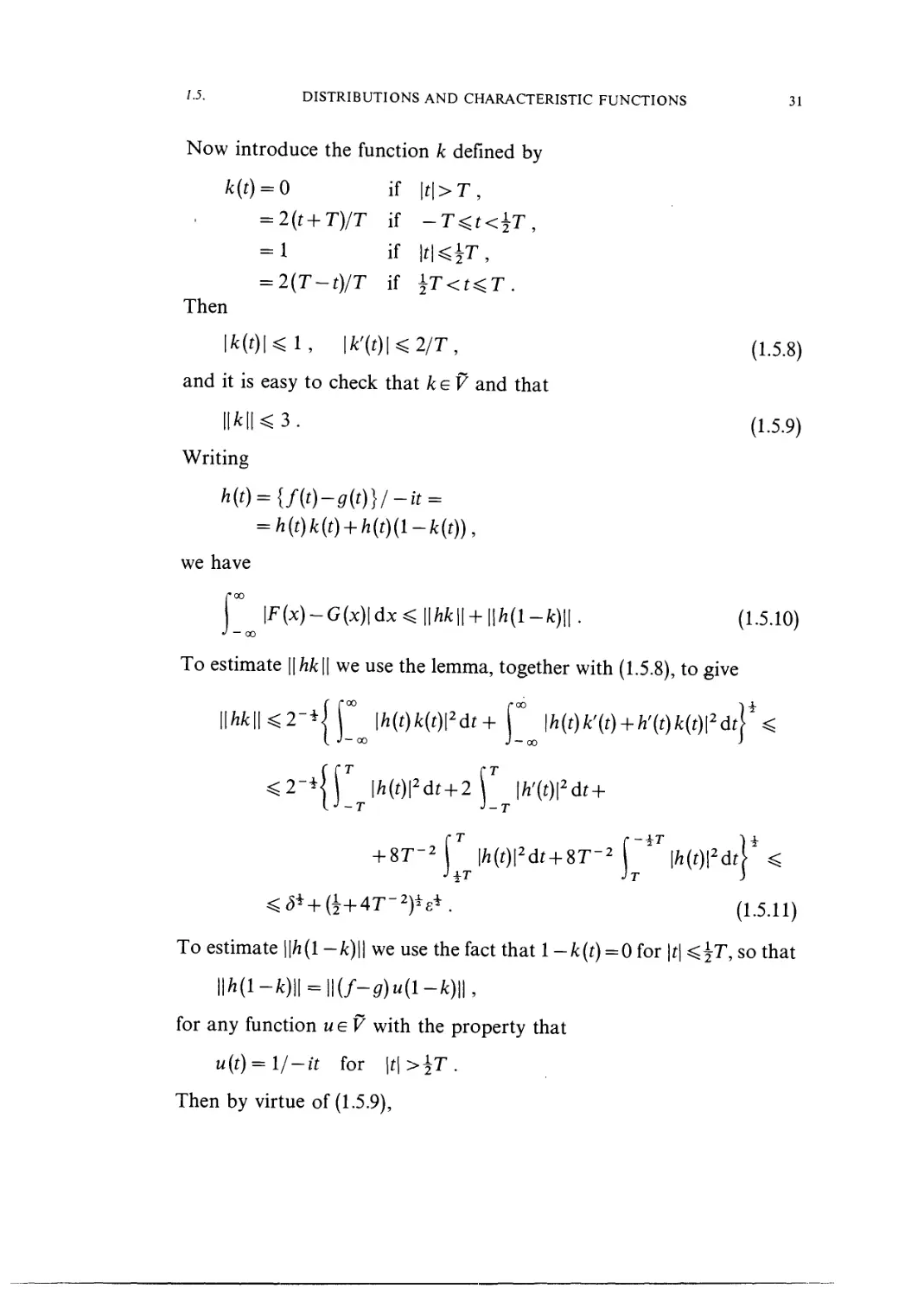
Now introduce the function k defined by
k(t) = O if |*|>7\
= 2(t+T)/T if -T^t<$T,
= 1 if
= 2{T~t)/T if ±
Then
|/c@l^l, \k'(t)\^2/T, A.5.8)
and it is easy to check that keV and that
II*IIO. A.5.9)
Writing
= h(t)k(t)
we have
TOO
\F(x)~G(x)\dx^\\hk\\ + \\h(l-k)\\. A.5.10)
J - oo
To estimate \\hk\\ we use the lemma, together with A.5.8), to give
{roo rco )
\h(t)k(t)\2dt+ \h(t)k'(t) + h'(t)k(t)\2dt\
J J
\h{t)\2dt + 2 J \h'{t)\2dt +
^ \h{t)\2dt\
T 3
2)M. A.5.11)
To estimate ||/i(l -k)\\ we use the fact that 1 -k(t)=O for \t\ ^jT, so that
for any function ueV with the property that
u(t)=l/-it for \t\>\T.
Then by virtue of A.5.9),

32 PROBABILITY DISTRIBUTIONS ON THE REAL LINE Chap. 1
\\h(l-k)\\^\\f-g\\\\u\\\\l-k\\^
< {11/11 + 11^11} INI {1 + 11*11} <
<4(VarF + VarG)||u||. A.5.12)
Taking in particular
u{t) = 4t/iT2, for |t|<±7\
= l/it, for \t\^T,
we have
roa r 00
sin txu(t)dt dx^c/T , A.5.13)
J-oo JO
where c is an absolute constant. Combining A.5.11), A.5.12), A.5.13)
proves the theorem. (It is shown in [165] that the smallest possible value
for ||w|| is n/T) •
§ 6. A special theorem about characteristic functions
The following theorem will be needed later.
Theorem 1.6.1. Let f(t) be any characteristic function, and v(t) = exp
(iat — ja2t2) the characteristic function of the normal distribution with
mean a and variance a2^0. Let (tk) be a sequence of points with tk^0,
lim tk = 0. If for all k,f(tk) = v(tk), then f{t) = v(t) for all t.
Proof Denote by F the distribution function corresponding to / Then
there are two cases.
A) <t2 = 0. Then
so that
Joo
{1-cos tk(x-a)}dF(x) = 0 .
— oo
This is possible only if F(x) = E(x — a).
B) a2 > 0. We shall need the theorem only for real characteristic func-
functions (corresponding to symmetric distributions) and the proof will
therefore be restricted to this case. Clearly then a = 0 and we may for

1.6. A SPECIAL THEOREM ABOUT CHARACTERISTIC FUNCTIONS 33
simplicity take a=l. We show that/has derivatives of all orders, and
that
/<2'>@) = i;B'>@) A.6.1)
for all r. (Derivatives of odd order all vanish at 0, by symmetry).
The proof proceeds by induction. To establish A.6.1) when r = 1, note that
= 2 f sm2&kx)dF(x)=l-v(tk) = O(t2). A.6.2)
J — CO
Consequently, the integrals
-A 1 hX J
are bounded uniformly in A, k. Letting ?fc->0, it follows that
•a
x2dF{x)
-A
is bounded in A. Letting A^oo, we have
( x2dF(x)<oo, A.6.3)
J - oo
from which it follows that / is twice differentiate, whence of course
/'@) = 0. Dividing A.6.2) by t2, and letting *fc->0, we have
Now suppose that, for all s<r,/Bs)@) exists and /Bs)(O) = yBs)(O). By
Rolle's theorem there is a sequence (rfc) with rfc^0, tfc->0 and
Then
SCO
x2(r-1)sin2(irfcx)dF(x) =
— oo
Arguing as before,
x2rdF(x)<oo
oo
and/Br) exists with/Br)(O) = i;Br)(O).

34 PROBABILITY DISTRIBUTIONS ON THE REAL LINE Chap. 1
Now v{t) is an entire function of t, and |/Br)@l ^ l/Br)@)l = |uBr)@)|.
Hence f(t) is also an entire function, and its derivatives at the origin agree
with those of v(t). Therefore /= v. •
§ 7. Infinitely divisible distributions
A distribution F is said to be infinitely divisible if, for each n, there exists a
distribution Fn with
Thus a random variable X with an infinitely divisible distribution can be
expressed, for every n, in the form
X = Xln + X2n + ¦¦¦ + Xnn,
where the Xjn (j= 1, 2, ..., n) are independent and identically distributed.
Theorem 1.7.1. In order that the function f(t) be the characteristic func-
function of an infinitely divisible distribution it is necessary and sufficient that
eiut-l -
), A.7.1)
where cr^O, — oo <y < oo, and M and N are non-decreasing functions with
M(-oo) = iV(oo)=0 and
0 re
re
u2dM{u) + u2dN{u)<oo
JO
for all e>0. The representation A.7.1) is unique.
The proof may be found in [48] (page 83) or in [47] (Chapter 9). Equation
A.7.1) is called Levy's formula. Simple examples of infinitely divisible
distributions are the normal and the Poisson distributions, but we shall
need also a generalised form of the latter.
The distribution F is called a compound Poisson distribution if it can
be represented in the form

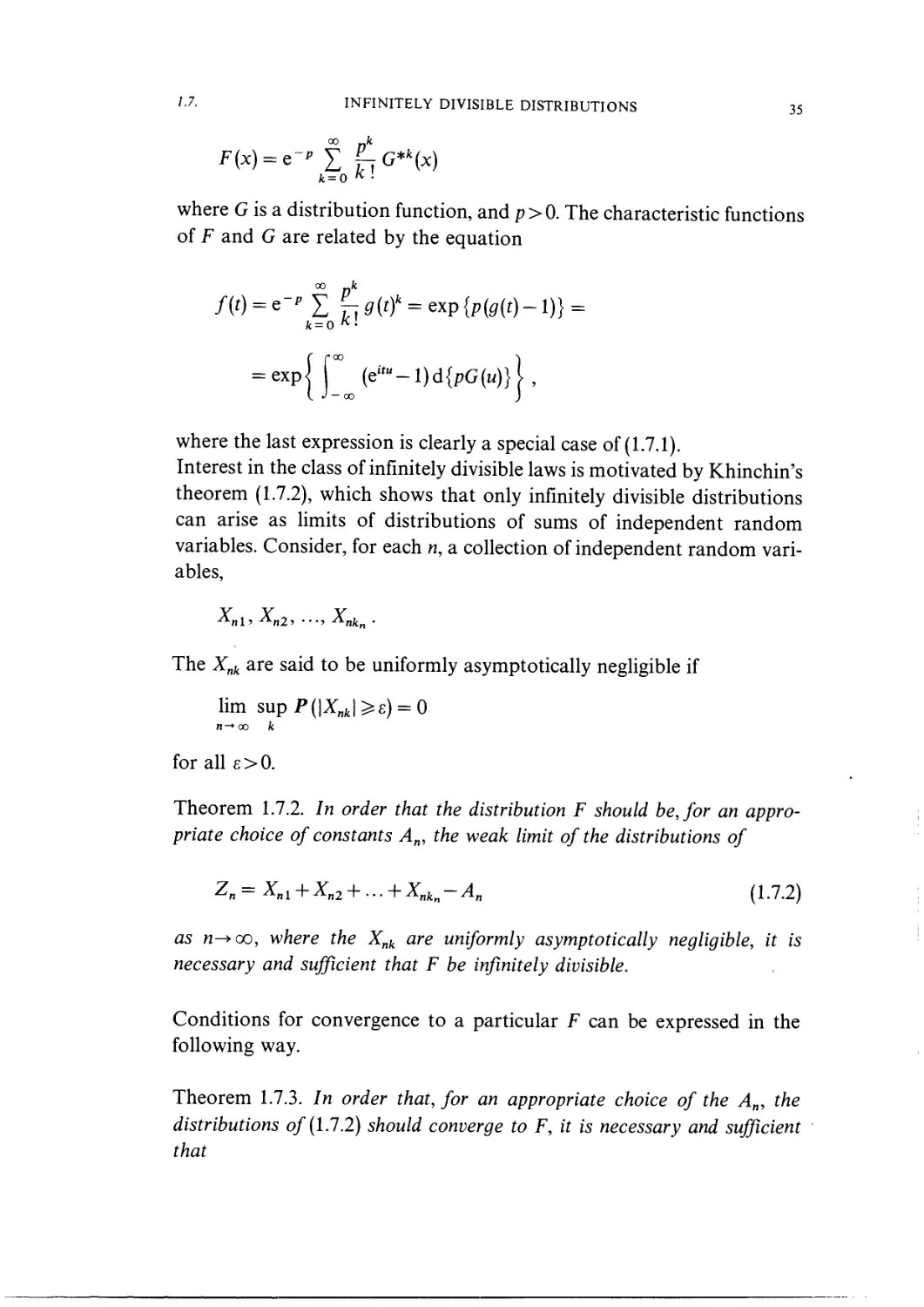
1.7. INFINITELY DIVISIBLE DISTRIBUTIONS 35
fc=0
where G is a distribution function, and p>0. The characteristic functions
of F and G are related by the equation
= exp||00 (J»-l)d{pG{u)}\,
where the last expression is clearly a special case of A.7.1).
Interest in the class of infinitely divisible laws is motivated by Khinchin's
theorem A.7.2), which shows that only infinitely divisible distributions
can arise as limits of distributions of sums of independent random
variables. Consider, for each n, a collection of independent random vari-
variables,
The Xnk are said to be uniformly asymptotically negligible if
lim supP(|Xnfc|^e) = 0
n—> oo k
for all ?>0.
Theorem 1.7.2. In order that the distribution F should be, for an appro-
appropriate choice of constants An, the weak limit of the distributions of
Zn = Xni + Xn2 + ...+Xnkn-An A.7.2)
as n->oo, where the Xnk are uniformly asymptotically negligible, it is
necessary and sufficient that F be infinitely divisible.
Conditions for convergence to a particular F can be expressed in the
following way.
Theorem 1.7.3. In order that, for an appropriate choice of the An, the
distributions of A-7.2) should converge to F, it is necessary and sufficient
that

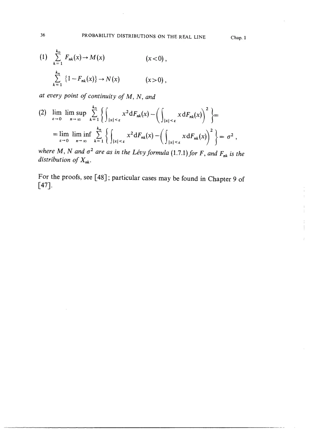
36 PROBABILITY DISTRIBUTIONS ON THE REAL LINE Chap. 1
A) ? Fnk(x)^M(x) (x<0),
point of continuity of M, N, and
B) limlimsup ? ( [ x2dFnfc(x)-f( xdFnfc(x)V 1=
?->0 n->oo fc=l|_J|x|<? \J|x|<? / J
= lim lim inf { f
where M, N and a2 are as in the Levy formula A.7.1) for F, and Fnk is the
distribution of Xnk.
For the proofs, see [48]; particular cases may be found in Chapter 9 of
[47].

Chapter 2
STABLE DISTRIBUTIONS; ANALYTICAL PROPERTIES AND
DOMAINS OF ATTRACTION
§ 1. Stable distributions
Definition. A distribution function F is called stable if, for any a1, a2 >0
and any bl,b2, there exist constants a>0 and b such that
bi)*F{a2x + b2) = F(ax + b). B.1.1)
It clearly suffices to take b1=b2=0. Then in terms of the characteristic
function / of F, B.1.1) becomes
f{tMf{t/a2)=f{t/a)e-a». B.1.2)
Interest in the stable distributions is motivated by the fact that, under
weak assumptions, they are the only possible limiting distributions of
normed sums
Zt.xl+x^...+x._Am BU)
of stationarily dependent random variables. In this section we establish
this result for independent random variables; the general case is dealt with
in Theorem 18.1.1.
Theorem 2.1.1. In order that a distribution function F be the weak limit
of the distribution of Znfor some sequence (Xi) of independent identically
distributed random variables, it is necessary and sufficient that F be stable.
If this is so, then unless F is degenerate, the constants Bn in B.1.3) must take
the form Bn = nll*h(n), where 0<a^2 and h(n) is a slowly varying function
in the sense of Karamata.

38
STABLE DISTRIBUTIONS
Chap. 2
Proof. Let/be the common characteristic function of the Xh and let 4>
be the characteristic function corresponding to the distribution F. Since
a degenerate distribution is trivially stable, we exclude this case, and prove
that necessarily
n = co, lim Bn+1/Bn= 1 .
B.1.4)
Suppose that the first condition in B.1.4) does not hold, so that there is a
subsequence (Bnk) with limit B^oo. Then
so that, for all t,
This is possible only if \f(t) \ = 1 for all t, which implies that F is degenerate.
Thus the first part of B.1.4) is proved, so that
lim \f(t/Bn+i)\ = l.
Thus
and
\f(t/Bn+1)\"+i =
Substituting Bnt/Bn+i for t in the former, and then Bn+ y t/Bn for t in the
latter, we deduce that, as n->oo,
lim
'n+ 1
= lim
'ifc')/
= 1 .
B.1.5)
If Bn+ !/?„-/> l,we can find a subsequence of either (Bn+ ^/B,) or (Bn/Bn+1)
converging to some B< 1. Going to the limit in B.1.5) we arrive at the
equation (j){t) = (j){Bt), from which
which is again impossible unless F is degenerate. Thus B.1.4) is proved.
Now let 0<a1 <a2 and by, b2 be constants. Because of B.1.4) we can
choose a sequence (m(n)) such that, as n->oo,

2.2. CANONICAL REPRESENTATION OF STABLE LAWS 39
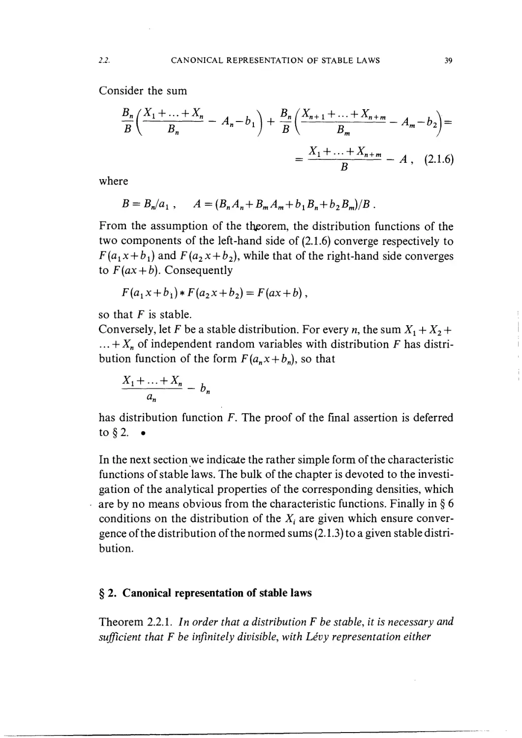
Consider the sum
) " T
B
where
-A, B.1.6)
= BJa
lt
From the assumption of the thjeorem, the distribution functions of the
two components of the left-hand side of B.1.6) converge respectively to
F(a1x + b1) and F(a2x + b2), while that of the right-hand side converges
to F(ax + b). Consequently
F(a1x + bi)*F(a2x + b2) =
so that F is stable.
Conversely, let F be a stable distribution. For every n, the sum X1 + X2 +
... + Xn of independent random variables with distribution F has distri-
distribution function of the form F(anx + bn), so that
has distribution function F. The proof of the final assertion is deferred
to §2. .
In the next section we indicate the rather simple form of the characteristic
functions of stable laws. The bulk of the chapter is devoted to the investi-
investigation of the analytical properties of the corresponding densities, which
are by no means obvious from the characteristic functions. Finally in § 6
conditions on the distribution of the Xt are given which ensure conver-
convergence of the distribution of the normed sums B.1.3) to a given stable distri-
distribution.
§ 2. Canonical representation of stable laws
Theorem 2.2.1. In order that a distribution F be stable, it is necessary and
sufficient that F be infinitely divisible, with Levy representation either

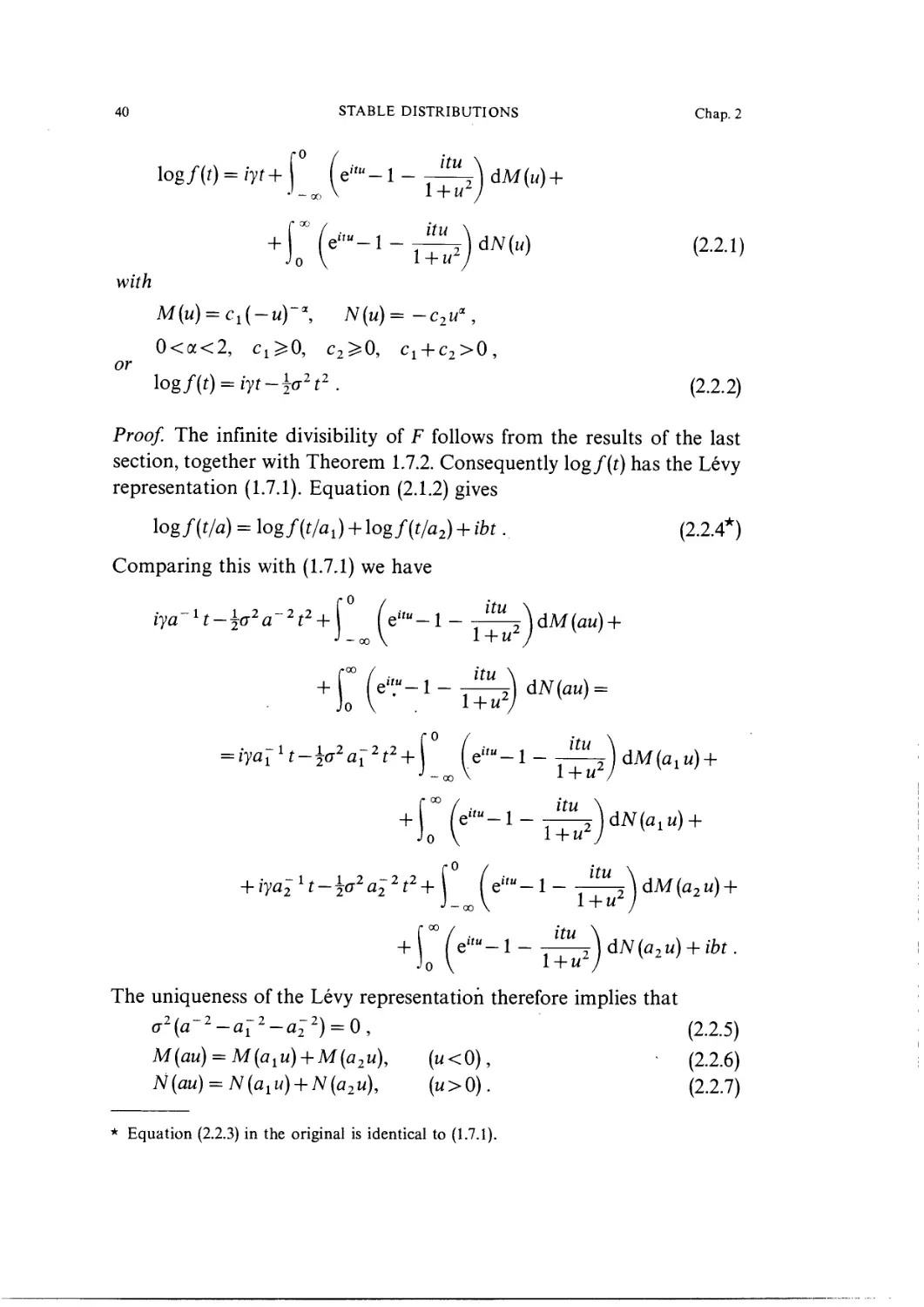
40 STABLE DISTRIBUTIONS Chap. 2
log/(f) = iyt+
M{u) = c,{-uY\ N(u)=-c2u\
0<a<2, c^O, c2^0, c1 + c2>0,
or
Iog/@ = i>f-ic72t2. B.2.2)
Proof. The infinite divisibility of F follows from the results of the last
section, together with Theorem 1.7.2. Consequently \ogf(t) has the Levy
representation A.7.1). Equation B.1.2) gives
log/(t/a) = log/(t/fll) + log f(t/a2) + ibt. B.2.4*)
Comparing this with A.7.1) we have
itu
dM(alU)
iya2~it-:2-(j2a2~2t2+
The uniqueness of the Levy representation therefore implies that
a2{a-2-a^2-a22) = 0, B.2.5)
) ) 2u), (u<0), • B.2.6)
u), (u>0). B.2.7)
* Equation B.2.3) in the original is identical to A.7.1).

2.2. CANONICAL REPRESENTATION OF STABLE LAWS 41
Suppose that M is not identically zero, and write
m(x) = M(e~x), ( —oo<x<oo).
From B.2.6) it follows that, for any Xx, X2, there exists 1 = 1A1, X2) such
that, for all x,
Thus more generally, for any Xx, X2, ..., Xn, there exists X such that
m(x + X) = m(x + XJ + ... +m(x + Xn). B.2.8)
Setting Xi =... =Xn = 0, there exists X = X(n) such that
m(x + X) = nm(x). B.2.9)
If p/q is any positive rational in its lowest terms, define
X(p/q) = X(p)-X(q);
then B.2.9) implies that
-m(x) = pm{x-X(q)} = m{x + X(p)-X(q)} =
H
= m{x + X(p/q)}.
Thus, for any rational r > 0,
m{x + X{r)} = rm{x). B.2.10)
Since M is non-decreasing, m is non-increasing, and so therefore is the
function X defined on the positive rationals. Consequently, X has right
and left limits X (s - 0) and X (s + 0) at all s > 0. From B.2.10) these are equal,
and X(s) is defined as a non-increasing continuous function on s>0,
satisfying
m{x + X{s)} = sm{x). B.2.11)
Moreover, it follows from this equation that
lim X(s) = oo , lim X(s) = — oo .
s->0
Since m is not identically zero, we may assume that m@)^0 (otherwise
shift the origin), and write m1(x)=m(x)/m@). Let xltx2 be arbitrary,
and choose s1? s2 so that

42 STABLE DISTRIBUTIONS Chap. 2
A(sl) = x1, X{s2) = x2.
Then
s1m@) = m(x1), s2m@) = m(x2), s2m(xl) = m(xl + x2),
so that
ml(xl+x2) = ml(xl)ml(x2). B.2.12)
Since m^ is non-negative, non-increasing and not identically zero,
B.2.12) shows that mi>0, and then m2 = log mi is monotonic and satisfies
m2(xl + x2) = m2(xl) + m2(x2). B.2.13)
It is known (see for example [50], page 106) that the only monotonic
functions satisfying this equation are of the form m2(x) = ax. Since
M( —oo)=0, this implies that
= c1(-u)-*, a>0,
As the integral
-1 ->0
must converge, we have a < 2. Thus finally
M(u) = cl(-u)~", 0<a<2, c^O. B.2.14)
In an exactly similar way,
N{u)= -c2u~p, 0<P<2, c2^0. B.2.15)
Taking ai=a2 = l in B.2.6) and B.2.7), we have
a-*=a-fi = 2, B.2.16)
whence a = /?. Moreover, B.2.5) becomes in this case
o2(a-2-2) = 0.
This is incompatible with B.2.16) unless o2=0, so that either g2 = 0 or
(u) = JV(u) = 0forallu. •
The integrals on the right-hand side of B.2.1) can be evaluated explicitly,
enabling the theorem to be reformulated in the following way.

2.2. CANONICAL REPRESENTATION OF STABLE LAWS 43
Theorem 2.2.2. In order that a distribution F be stable, it is necessary and
sufficient that its characteristic function be expressible in the form
\ogf(t) = iyt-c\t\' (l-iP^co(t, aj), B.2.17)
where a, ft, y, c are constants (c^O, 0<a^2, \f}\^ 1) and
co(t, a) = tan fact), a ^ 1 ,
= 2tt~1 log |*| , a=l.
(Note that a, which is called the index of F, has the same meaning as in
the previous theorem.)
Proof. We examine B.2.1) in three cases.
A) 0<a< 1. In this case the integrals
0 u du , f °° u du
yr^2 yir^ and 1 j—p- ^m
are finite and B.2.1) becomes, for some y',
f ° du c °° du
log f{t) = iy't + ac, (e'«- 1) -r^ + *c2 (e''"- 1) -^
¦> -oo IMI JO U
Therefore, in t>0,
du r00 dw
(-'-'lW J A"!)
L Jo u
The function
^ ()
u Jo u
is analytic in the complex plane cut along the positive half of the real axis.
Integrating it round a contour consisting of the line segment (r, R)
@< r< R), the circular arc (with centre 0) from R to iR, the line segment
(iR, ir), and the circular arc from ir to r, we obtain (on letting R^oo and
du
where

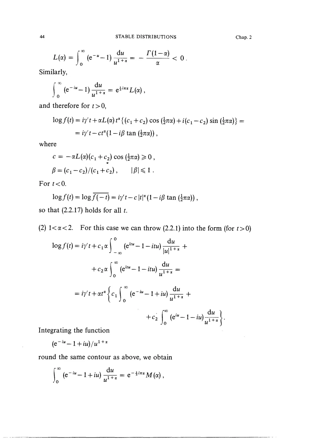
44 STABLE DISTRIBUTIONS Chap. 2
Similarly,
o u
and therefore for t > 0,
logf(t) = iy't + ocL{<x)tsl{{ci + c2) cos {{na) + i{cl-c2) sin
= iy't-ct*(l - ifi tan (^thx)),
where
c = —aL(a)(c1 + c2) cos (j7ra) ^ 0 ,
For
log/@ = log/(-0 = iyt-c\t\'(l-ip tan g
so that B.2.17) holds for all *.
B) l<a<2. For this case we can throw B.2.1) into the form (for t>0)
dw
u
Integrating the function
round the same contour as above, we obtain
' • v dw
o u

2.2. CANONICAL REPRESENTATION OF STABLE LAWS 45
o
where
Proceeding as before, we deduce that B.2.17) holds, with
c = —aM(a)(c1 + c2) cos (^7ca)^0 ,
P = (c1-c2)/(c1+c2), |?K1.
C) a= 1. Using the fact that
~°° 1-cosu
o u2
du = jn,
we have
u2) u2
f °°cos tu-l J f" / . ut \du
= du + i\ sin tu - —-=
Jo " Jo V l + u2)u2
,, ... ff°° sin to J f00 du
¦pit + it\im\\ —j—du-t
u(l+u2)J
"sinu . r°°/sinu 1
2
u
"du f00/sinu 1
— + it —-2 ^
Jo V " u(l+u2)
= —\nt — it log ? + itr , say .
Thus B.2.17) is satisfied with
c =jn{c1 +c2),

46
STABLE DISTRIBUTIONS
Chap. 2
This theorem allows us to establish the form of the normalising constants
Bn asserted in § 1. We shall prove the following result.
If a sequence X1,X2,... of independent, identically distributed random
variables is such that the distribution of the normed sum
Zn=(X1+X2+... + Xn-An)/Bn
converges to a stable law with index a, then
Bn = n1/ah(n), B.2.18)
where h is a slowly varying function in the sense of Karamata.
Using the notation of § 1, we have for all t,
„ ( t'
= exp(-C|t|-
For any fixed integer k,
„ / t N
Ikn
= exp(-c|tH(l+o(l)),
but at the same time
fkn GO
,B
kn,
Bn
= exp(-c|t|a;
B.2.19)
B.2.20)
the remainder term tending to zero uniformly in every finite ^-interval.
Suppose first that the sequence (BJBkn) is unbounded, so that there is a
subsequence (rij) with
Setting t = BknJ Bn. in B.2.20) and using B.2.19), we obtain the impossible
equation e~ck= 1. Hence {BJBkn) is bounded, and then B.2.19) and B.2.20)
yield
which is only possible if
lim B
This proves the assertion.

2.3. DENSITIES OF STABLE DISTRIBUTIONS; ANALYTIC STRUCTURE 47
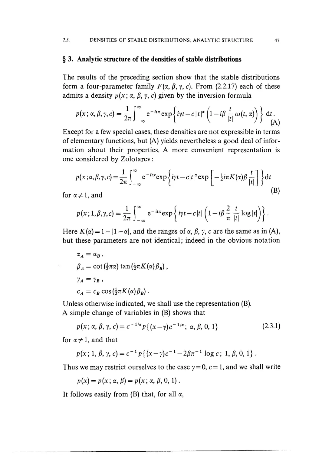
§ 3. Analytic structure of the densities of stable distributions
The results of the preceding section show that the stable distributions
form a four-parameter family F(<x, ft y, c). From B.2.17) each of these
admits a density p(x; a, ft y, c) given by the inversion formula
p{x;aj,y,c) = 2n\ e-Uxexpliyt-c\t\* (l-ifi -^ co{t,a)\\ dt.
Except for a few special cases, these densities are not expressible in terms
of elementary functions, but (A) yields nevertheless a good deal of infor-
information about their properties. A more convenient representation is
one considered by Zolotarev:
p(x;oc,fty,c) = — j e'^exp jiy?-c|t|aexp [-^(a)^! \dt
for a#l, and
Here K(a) = 1 —11 — a|, and the ranges of a, ft y, c are the same as in (A),
but these parameters are not identical; indeed in the obvious notation
PA = cot&za)
1a = 1b ,
cA =
Unless otherwise indicated, we shall use the representation (B).
A simple change of variables in (B) shows that
p(x;a,P,y,c) = c'llap{(x-y)c-lla; a, 0, 0,1} B-3.1)
for a#l, and that
Thus we may restrict ourselves to the case y = 0, c= 1, and we shall write
p(x) = p{x;a, 0) = p{x;a, ft 0, 1).
It follows easily from (B) that, for all a,

48 STABLE DISTRIBUTIONS Chap. 2
p(x;a, P) = p(-x;a, - P). B.3.2)
We may therefore restrict ourselves either to /?^0 or alternatively to
x ^ 0, a remark which will be of use later.
Another easy consequence of (B) is that p(x) has derivatives of all orders,
a statement which can be greatly strengthened as follows.
Theorem 2.3.1. The density p(x) of a stable law with a> 1, or with a= 1,
, is an entire function of x. Ifoc< 1, the density may be written
p(x) = x~14>1(x'a) , x>0,
= x-1<P2((-x)-«), -x<0,
where (P1 and <P2 are entire functions.
Proof We distinguish three cases.
A) a> 1. In this case the integral
converges uniformly for all complex z, and thus defines an entire func-
function of z coinciding with p on the real axis.
B) a=l. Write
nfyj j-i J Y| I *l I Y| I ,Z } } I
where
1 r00 r / ? \ ¦)
] dt. B.3.4)
For the sake of argument take /?>0. Suppose that it is permissible to
rotate the contour of integration through an angle — \n. Then
1 f°° f 2
-tx-C-
n
and as before this implies that p1} and so p, is entire.
It remains to justify the change of contour in B.3.4). To do this we integrate
the function - \
(p(t) = exp (— hx — T — iC-T log t j

2.3. DENSITIES OF STABLE DISTRIBUTIONS; ANALYTIC STRUCTURE 49
(taking the branch with log 1=0) around the contour consisting of the
line segment (r, R) @ < r < R), the circular arc CR (centre O) from R to
— iR, the line segment (— iR, — ir), and the arc cr from — ir to r. Clearly
lim
and
r <t>o C 2 )
ix ^ R\ exp< R |sin <f>x\— R cos (f> -\—JR(/>>d(/>-
Jo 1 n )
[in f 2 2 )
R exp IRsintyx + - jR(/> p sin <j> R log R \
J<t>o I n n )
\Rn exp R {(/>0(|x| + l) — cos ^>0} +
2 1 1
+ 0
exp R ||x| + 1 fi sin 0O log R
as JR->oo for (/>0 sufficiently small. This justifies the change of contour.
C) a < 1. It suffices to consider the case x>0. Substitute u for tx in the
equation
and rotate the contour of integration through an angle — jtt (the validity
of this operation being proved as in B)). Then
where
1- f °°
<P1(z)= - exp{-t-fzcosfrza(l+P))} x
x Jo
x sin {taz sin(^roc(l+/?))} dt
is clearly an entire function. •
Remark 1. The exclusion of the case a = l, /? = 0 is necessary, since
p(x; 1, 0) is the Cauchy distribution
which though analytic for x real has poles at x= ±i.

50
STABLE DISTRIBUTIONS
Chap. 2
Remark 2. For a<l, C=1 the arguments used in case C) above show
that, for all x < 0,
1 f
p{x; a, 1) = —Re/
7I.X 1 n
= 0.
Similarly, for a<l,
p(x; a, -l) = 0
for all x>0.
Theorem 2.3.2. For a^ 1, we may write
where
dsm c
forlpositive m.
When cc = p/q is rational, this is equivalent to the differential equation
s=l
of order max(p —1, g—1).
Proof. Write
and use
</>(*) =f{r)(x)
to denote the relation
(For integral r, this coincides with the usual notation for derivatives, see
[193].) For Re /i>0, it is clear that

2.3.
DENSITIES OF STABLE DISTRIBUTIONS; ANALYTIC STRUCTURE
51
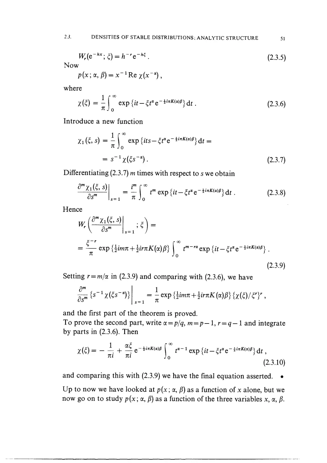
Now
p{x;a, P) = x~1
where
x{0 = - ( explit-
71J o
Introduce a new function
71
Differentiating B.3.7) m times with respect to s we obtain
ds
Hence
w.
s= 1
71
exp
r"raexp {it-
Setting r = m/a in B.3.9) and comparing with B.3.6), we have
= - exp {
ds"
s=l
B.3.5)
B.3.6)
B.3.7)
B.3.8)
B.3.9)
and the first part of the theorem is proved.
To prove the second part, write a=p/q, m=p—l,r = q—l and integrate
by parts in B.3.6). Then
z(f)= - - + ^e-*1"*""' P t'-'expiit-Zt'e-i^^dt,
ni ni J0
B.3.10)
and comparing this with B.3.9) we have the final equation asserted. •
Up to now we have looked at p(x; a, C) as a function of x alone, but we
now go on to study p(x; a, C) as a function of the three variables x, a, /?.

52 STABLE DISTRIBUTIONS Chap. 2
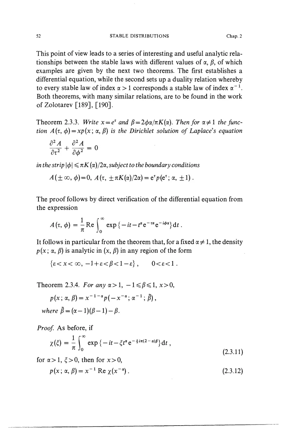
This point of view leads to a series of interesting and useful analytic rela-
relationships between the stable laws with different values of a, /?, of which
examples are given by the next two theorems. The first establishes a
differential equation, while the second sets up a duality relation whereby
to every stable law of index a > 1 corresponds a stable law of index a'1.
Both theorems, with many similar relations, are to be found in the work
ofZolotarev [189], [190].
Theorem 2.3.3. Write x = ex and P = 2<fxx/nK(a). Then for a#l the func-
function A(t, 4>) = xp(x; a, /?) is the Dirichlet solution of Laplace's equation
dx2 +
in the strip \4>\^ nK (a)/2a, subject to the boundary conditions
= eTp(eT;a, ±1).
The proof follows by direct verification of the differential equation from
the expression
A{t,<I>) = -Re ( Gxp{-it-
71 Jo
It follows in particular from the theorem that, for a fixed a # 1, the density
p(x; a, C) is analytic in (x, C) in any region of the form
{e<x< oo, — !+?</?<!— e} , 0<e<l.
Theorem 2.3.4. For any a>l, -l^^l, x>0,
p(x; a, C) = x~1~ap( — x~a; a; ft),
where fi = {a-1){C-1)-C.
Proof. As before, if
X{O = - \
71 Jo B.3.11)
for a>l, ?>0, then for x>0,
{x~a). B.3.12)

2.3.
DENSITIES OF STABLE DISTRIBUTIONS; ANALYTIC STRUCTURE
53
We show that the contour of integration in B.3.11) may be rotated through
the (negative) angle
The integrand \j/(t) of B.3.11) is analytic in the complex plane cut along
the negative half of the real axis. Let Fx be the line segment (p, R), F2 the
circular arc from R to R e^, F3 the line segment (R ei4>, p Qi<f>), and T4 the
circular arc from p el<t> to p. By Cauchy's theorem,
jf +f +f +f U(t)dt = O,
and it suffices therefore to show that the integrals along F2 and r4 tend
to zero as JR-> oo, p->0. For the first we have the estimate
\]/(t)dt
exp {- R cos %tt + 9) - ?Ra cos {9a - \n B - a) 0)} d91.
By breaking the interval into two parts @, ^J, (^>1; <j>) such that on @, <j)x)
the inequality cos@a— \nB — a)) >5 >0 is satisfied, we have
r2
as
Moreover,
ij/(t)dt = O(p)->0 as p->0.
Rotating the contour, substituting t for
obtain
= —\ exp {i?t-t1/a
and integrating by parts, we
'01'1 dt =
in n j 0
Now jn + 4>= —ftn/2a, so that taking real parts in B.3.13) we have
B.3.13)
so that

54 STABLE DISTRIBUTIONS Chap. 2
§ 4. Asymptotic formulae for the densities p(x; a, /?)•
It has already been remarked that the densities p(x; a, /?) may not in
general be expressed in terms of elementary functions or the common
"special functions". It is therefore of interest to represent the densities as
convergent or asymptotic series in the neighbourhood of particular points,
and to examine properties which are not at once obvious from the Fourier
expansions (A) and (B) with their oscillating integrands.
In this section we present a series of asymptotic formulae due to Linnik
[99], Skorokhod [174]. Bergstrom [16] and Pollard [135]. The special
case of the "extreme" stable laws p(x; a, ± 1) is due to Kolmogorov. The
method of proof is that of contour integration and, later, the technique of
steepest descent. Because of B.3.2) we can, and consistently will, restrict
attention to positive values of x.
Theorem 2.4.1. For a<l and x>0,
? () {fr(j)}
nx n=1 n\
B.4.1)
Proof. In proving Theorem 2.3.1 C) we established the equation
p{x;a,P)= - — Re if e"f exp{-tax-aQ~
TIX J o
and expanding the exponential formally we have
{C)
nx -0
nx n=Q nl
To justify this formal expansion it suffices to prove the last series absolu-
absolutely convergent, which is done by using Stirling's formula and noting
that the series is majorised by
f
»=o »'¦

2.4. ASYMPTOTIC FORMULAE FOR THE DENSITIES p(x; a, P) 55
A similar result holds for a > 1, but the series is now divergent and gives
an asymptotic expansion for p(x) as x->oo.
Theorem 2.4.2. For a> 1, the asymptotic expansion
as x—>oo.
The sign ~ denotes the asymptotic relation that, for all N,
p{x;a,P)=~ X
n\
The series B.4.3) does not converge; its terms do not even tend to zero.
Proof. In the equation
p(x\a,P) = — Re ( e~"exp{-ta;rae-*l'ltB~a)/'}dt,
nx J 0
rotate the contour of integration through an angle
justifying this as in the proof of Theorem 2.3.4. Then
p(x; <x,P) = — Re ei4> [ exp {-te?(*lt+*)}exp{itax-a}dt. B.4.4)
nx Jo
Taylor's formula implies that, for real s,
N (is)" \s\N+1
where |0| ^1. Hence
N ftiGt .y. net 'fi f(^' ~^ )^ v* ^
Combining B.4.4) and B.4.5) we have

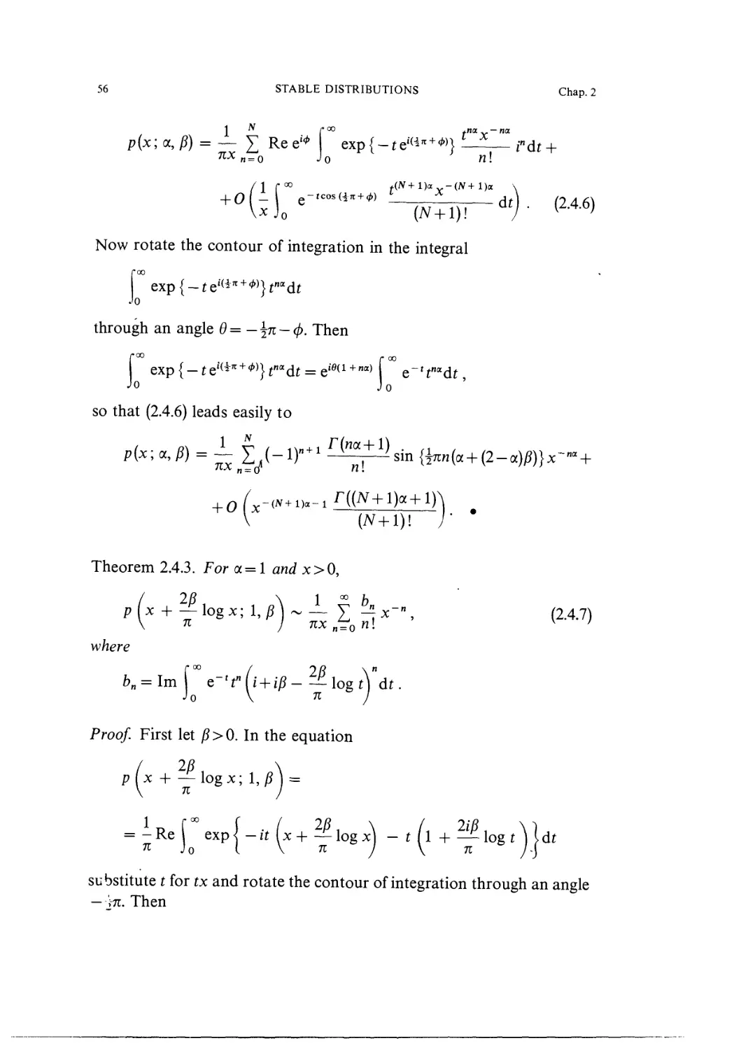
56 STABLE DISTRIBUTIONS Chap. 2
N /• oo j.na —na
n = 0
/I r oo ^(N+lJa -(^+l)a
(N+l)!
Now rotate the contour of integration in the integral
I Qxp{~tei(in+<t>)}tnadt
Jo
through an angle d=-\n-(j). Then
so that B.4.6) leads easily to
p(x; a,P) = — f, (-l
(N+l)
Theorem 2.4.3. For a = l and x>0,
28 \ 1
Mogx;l/n
x n%
where
= lm\ e-lf I i + iC- —log A dt
Proof. First let /?>0. In the equation
B.4.6)
X -ix-", B.4.7)
nx n%n\
If00 f ( 2B \ ( 2iB \ ~)
= - Re exp < - it [ x + — log x - t 11 H log M i dt
substitute t for tx and rotate the contour of integration through an angle
— -'m. Then

2.4. ASYMPTOTIC FORMULAE FOR THE DENSITIES p(x; a, 0) 57
( 2P i \ 1 f°° {it, 2B \
p\x-\ log x; 1, /? = — Im e ' exp < - A + p) tlogtrdt.
\ n / nx Jo tx nx )
B.4.8)
Expanding the exponential as a finite Taylor series with remainder,
B.4.8) becomes
Ttx.^n! V (N + l)! 7'
which is equivalent to B.4.7). To show that this also holds good for
expand the exponential in
(IB \ 1 f00 f lit )
p x H log x; 1, /? = — Re e"te~f/*exp <— — log t\ dt
\ n / nx Jo ( nx J
to deduce that v • • /
n
= —ReS f°°^( — logtj tne-H~tlxdt + O{x-N-2). B.4.10)
7CX n = o-'O n ¦ ^^
Now rotate the contour through — \k and expand eitlx, and the result
follows. •
We remark that for P= — 1 this theorem is of little interest, since it asserts
only that p(x; 1, — 1) decreases faster than any negative power of x. More
complete information for this case is given by the following theorem.
Theorem 2.4.4. As x-> + go,
where
an=
Jo
and cn((f>) is the coefficient ofy" in the power series expansion of the function

58
STABLE DISTRIBUTIONS
Chap. 2
Proof. In the equation
p(x; 1, —1) = -Re I exp
substitute t = zeinx and write ^ = e***. Then
-itx-t f 1 log t) >dt
p{x) = p{x; 1, -1) = -Re f exp[-z? A - -logzHdx B.4.11)
7C Jo (. V 7C / J
In the complex plane of z = u + iv with a cut along the negative real axis
the integrand is analytic, and we may deform the contour of integration
in B.4.11). For the choice of contour we use the method of steepest descents
[24].
It is easy to see that the saddle point is at z0 = — i/e, and the contour of
steepest descent is given by
Im \z (l --log zH =0.
Near the saddle point this is close to a circle of radius 1/e centred at the
origin, so that in B.4.11) we change the contour of integration to F =
F1 + r2 + r3, where F1 is the line segment (O, — i/e), F2 is the circular arc
(centre O) from — i/e to 1/e, and F3 the line segment A/e, oo). Thus
p{x)=
The first term is equal to
H (' - !
dz BA12)
-Re f exp{-z^(l--logzHdz =
n
ri
n
= -Rei(
n
_e-i \n
= 0, B.4.13)
and the third has
exp \-z? (l -logz ) idz
n
= e
B.4.14)
Finally, consider the integral around F2, which if z = e 1 exp {i(<j) — j
can be written as

2.4. ASYMPTOTIC FORMULAE FOR THE DENSITIES p(x;a,P) 59
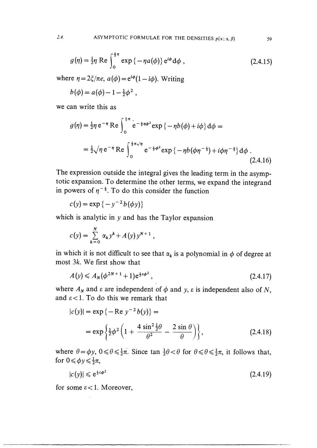
= in Re f \xp{-ria(<l>)}el+d<l>, B.4.15)
Jo
where rj = 2?/ne, a(<f)) = ei<t>(l-i(t)). Writing
we can write this as
e
o
B.4.16)
The expression outside the integral gives the leading term in the asymp-
asymptotic expansion. To determine the other terms, we expand the integrand
in powers of 77 ~*. To do this consider the function
c{y) = exp{-y-2b (<f>y)}
which is analytic in y and has the Taylor expansion
N
c(y)= V akyk + A(y)yN+1 ,
k = 0
in which it is not difficult to see that ock is a polynomial in <f> of degree at
most 3k. We first show that
A{y)^AN((fJN+1 + l)Qie't'2, B.4.17)
where AN and e are independent of <f> and y, s is independent also of N,
and e<l. To do this we remark that
4shr40 2sin0\] ,^1O,
+ —-^ — JJ, B.4.18)
where 9 = (py, O^O^n. Since tan ^9<9 for 9^9^^n, it follows that,
B-4-19)
for some e< 1. Moreover,

60
STABLE DISTRIBUTIONS
Chap. 2
B.4.20)
for
| A (y) | ^ max
jn , where C is a constant. Hence
Texp{-j; 2b{(f)y)}
oy
N +
= max|exp{-j; 2b((f)y)}1Z\ ,
where S is a sum of products of derivatives of y~2bD>y) which may be
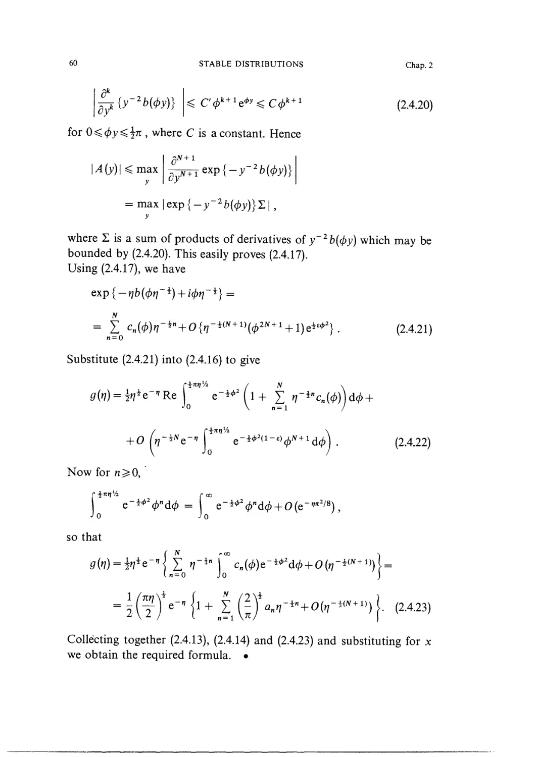
bounded by B.4.20). This easily proves B.4.17).
Using B.4.17), we have
Qxp{ — rjb((j)r] ^) + i(j)r]
N
= V cn((}))ri~2"-\-0 {n
n = 0
Substitute B.4.21) into B.4.16) to give
B.4.21)
N
n=l
+ 0
B.4.22)
Now for n
o
so that
n=0
. B.4.23)
Collecting together B.4.13), B.4.14) and B.4.23) and substituting for x
we obtain the required formula. •

2.4. ASYMPTOTIC FORMULAE FOR THE DENSITIES p(x; a, /?) 61
Theorem 2.4.5. For a<l, x>0, we have the asymptotic expansion
p(x; a, fi) ~ I Jo (-1)"r{("l1!)a}*n cos
For l<a<2 am* x>0,
B.4.25)
If a<l, then
1 r°°
p(x; a, j?) = -Re e-itxexp{-tae-?nap}dt.
71 Jo
Expand e~"* as a finite Taylor series with remainder, to give
i N ( — ixY1 r00
p(x;a,P) = - X RKL\
71 n = 0 n- Jo
f yN+l r oo
+ 01
To calculate the integrals in this expression we rotate the contours of inte-
integration through an angle \n$, to show that
Substituting this into B.4.26) we obtain
p{x;a,p)=- X t^
n\
(N

62 STABLE DISTRIBUTIONS Chap. 2
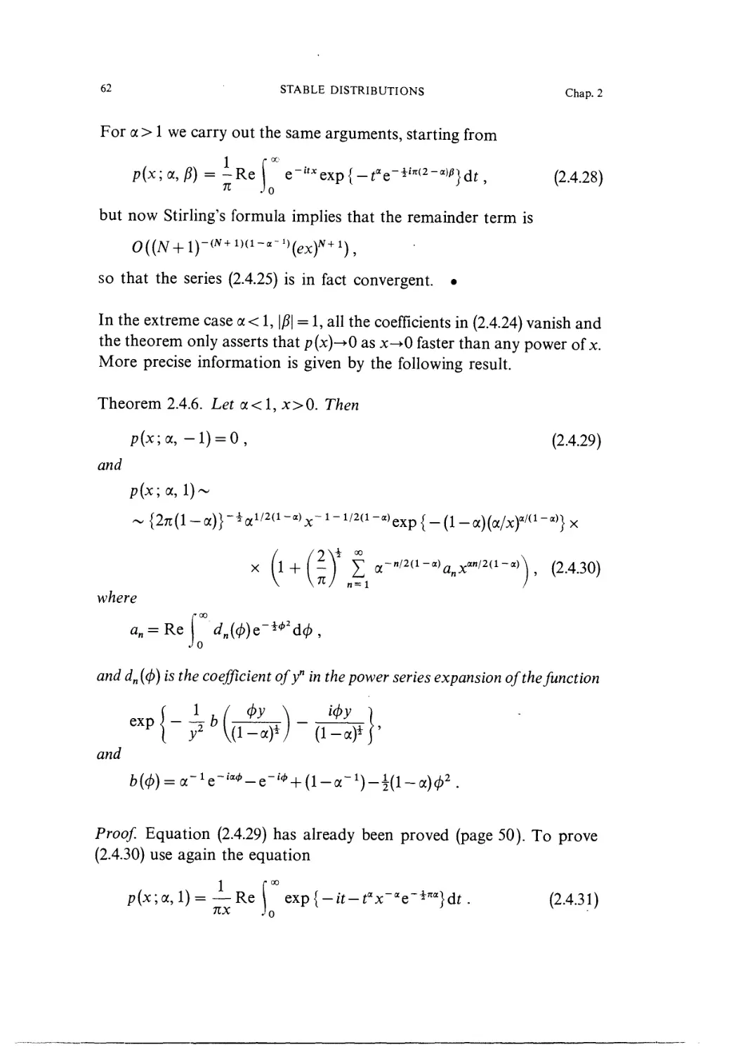
For a > 1 we carry out the same arguments, starting from
a)li}dt, B.4.28)
but now Stirling's formula implies that the remainder term is
[
71 Jo
so that the series B.4.25) is in fact convergent. •
In the extreme case a < 1, \f}\ = 1, all the coefficients in B.4.24) vanish and
the theorem only asserts that p(x)->0 as x->0 faster than any power of x.
More precise information is given by the following result.
Theorem 2.4.6. Let a<l, x>0. Then
p{x;a,-l) = 0, B.4.29)
and
p{x;a, 1)~
( (^T | ), B.4.30)
where
is the coefficient ofy" in the power series expansion of the function
exP I - -2 b G
and
Proof. Equation B.4.29) has already been proved (page 50). To prove
B.4.30) use again the equation
p(x;a,l)=—Re ( exp{-it-tax-ae~ina}dt. B.4.31)
nx .) 0

2.4. ASYMPTOTIC FORMULAE FOR THE DENSITIES p(.x; a, 0) 63
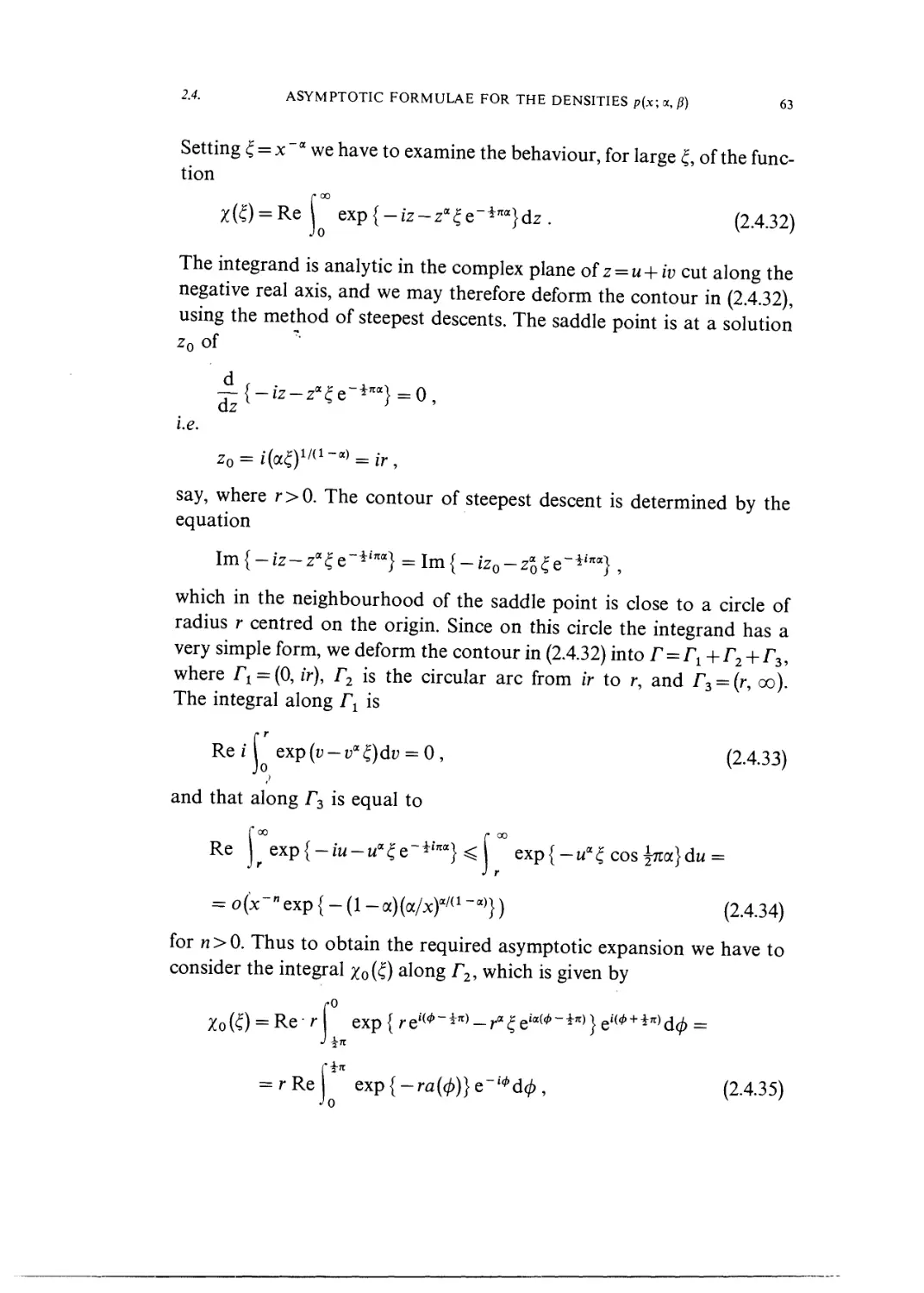
Setting ? = x~a we have to examine the behaviour, for large ?, of the func-
function
(°° -;z-za?e-*™}dz. B.4.32)
The integrand is analytic in the complex plane of z = u + iv cut along the
negative real axis, and we may therefore deform the contour in B.4.32),
using the method of steepest descents. The saddle point is at a solution
z0 of
~{-iz-zaZe~ina}=0,
dz
i.e.
say, where r>0. The contour of steepest descent is determined by the
equation
Im{-iz~za?e~iina} = Im{-izo-zao?e~?na} ,
which in the neighbourhood of the saddle point is close to a circle of
radius r centred on the origin. Since on this circle the integrand has a
very simple form, we deform the contour in B.4.32) into F = FX+F2 + F3,
where Fl = @, ir), F2 is the circular arc from ir to r, and F3 = (r, oo).
The integral along F1 is
Re i [' exp (v - va?)dv = 0 , B.4.33)
and that along F3 is equal to
= o(x~n exp {- A - a)(a/x)a/A ~a)}) B.4.34)
for n > 0. Thus to obtain the required asymptotic expansion we have to
consider the integral XoiO along F2, which is given by
f
Xo(O = ReH exp{re1(^ »*>-
B.4.35)

64 STABLE DISTRIBUTIONS Chap. 2
where a($)= -e~i<t> + a-1e~ia<t>.
Clearly a((p) has the convergent power series expansion
where
In B.4.35) substitute </>{r(l — a)}"* for </> to give
/4-TrMl-a)}*
ZoE) = (l-a)-*r*exp{-r(a-1-l)}Re x
Jo
B.4.36)
We now expand '
as a finite Taylor series in r~* with remainder. For the estimation of the
remainder term we need the inequality that, for 0^A— a)"*y(j)^\n ,
|exp{-};-2H(l-«)"i^]}Kexp(-i#2), B.4.37)
where 0<rj < 1 and v\ does not depend on y. This is proved by noting that
the absolute value of the left-hand side of B.4.37) is equal to
where
y(9)=l-(l-a)-1d-2(sin29-a-1sm2ad),
and6 =j(l—ot)~*(f)y^in. It is easily checked that sin20 — a sin2a0 is
increasing in 0<9^^n, and is thus strictly positive there. Hence y is
continuous and y(9)<l on 0^9^^n, so that there exists rj<l with
y(9)^rj<l. Thus B.4.37) is proved.
It is not difficult to see that, for all y,
<A\<f>\k+2t B.4.38)
where A depends only on k and a, and it follows that

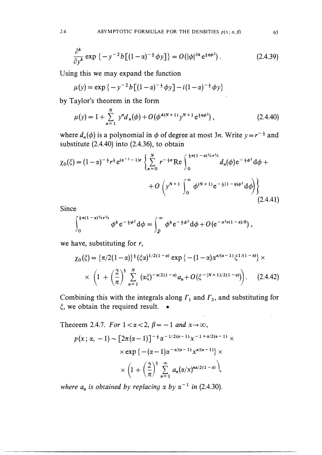
2.4. ASYMPTOTIC FORMULAE FOR THE DENSITIES p(.x; a, 0) 65
exp {-y-2b[(l-a)"*0j;]} = 0(|</>|3fce^2). B.4.39)
Using this we may expand the function
by Taylor's theorem in the form
fi{y)=l+ ? y"rfB@) + O@4<N+1)yw + 1e*^2), B.4.40)
n=l
where dn{4>) is a polynomial in <f) of degree at most 3n. Write 3; = r i and
substitute B.4.40) into B.4.36), to obtain
n = 0
0(yN+1 ^
B.4.41)
Since
p
we have, substituting for r,
x f1 + (U S (a^-"/2A-a)an + O(r|N+1)/2A~a))). B.4.42)
Combining this with the integrals along Fi and T3, and substituting for
?, we obtain the required result. •
Theorem 2.4.7. For l<a<2, C= — 1 and :*:->• 00,
p(x;a, -I)~[27r(a-l)]-*a-1/2(a-1)x-1+a/2(a-1)x
x exp { -(a- l)a~a/(a- "x"'14'} x
x(i + (-) f «>/^
\ \7T/ „= 1
where an is obtained by replacing a by a'1 in B.4.30).

66 STABLE DISTRIBUTIONS Chap. 2
Proof. It is unnecessary to work through the details because of the duality
Theorem 2.3.4. We merely substitute B.4.30) into the equation
p(x;a, -l) = x-1-ap{x-a;a-\ 1). •
Remark. All the asymptotic formulae of this section may be differentiat-
differentiated any number of times with respect to x, to give asymptotic expansions
for the derivatives p{k)(x; a, /?).
§ 5. Unimodality of stable laws
Definition. A distribution function F(x) is said to be unimodal if there
exists at least one a such that F(x) is convex inx<a and concave in x>a.
It follows from the theory of convex functions [130] that F is necessarily a
continuous distribution (except possibly at a), and that F'(x) is non-de-
non-decreasing in x < a and non-increasing in x > a. If F is any distribution for
which F" exists, it is unimodal if and only if F" (x) > 0 for x < a and F" (x) < 0
for x > a. The point a is called the mode of the distribution.
Theorem 2.5.1. If a sequence of unimodal distributions Fn converges weakly
to a distribution F, then F is unimodal.
Proof. Let an be a mode of Fn, and write
a = lim sup an .
n-»oo
Suppose first that \a\ < oo, and choose a subsequence ank converging to a.
Let xl5 x2 be points of continuity of F, with x1<a,x2<a. For sufficiently
large k, xx <ank, x2<ank, and since Fnk is unimodal,
Letting k-*co,
(^^j. B.5.1)

2-5- UNIMODALITY OF STABLE LAWS 67
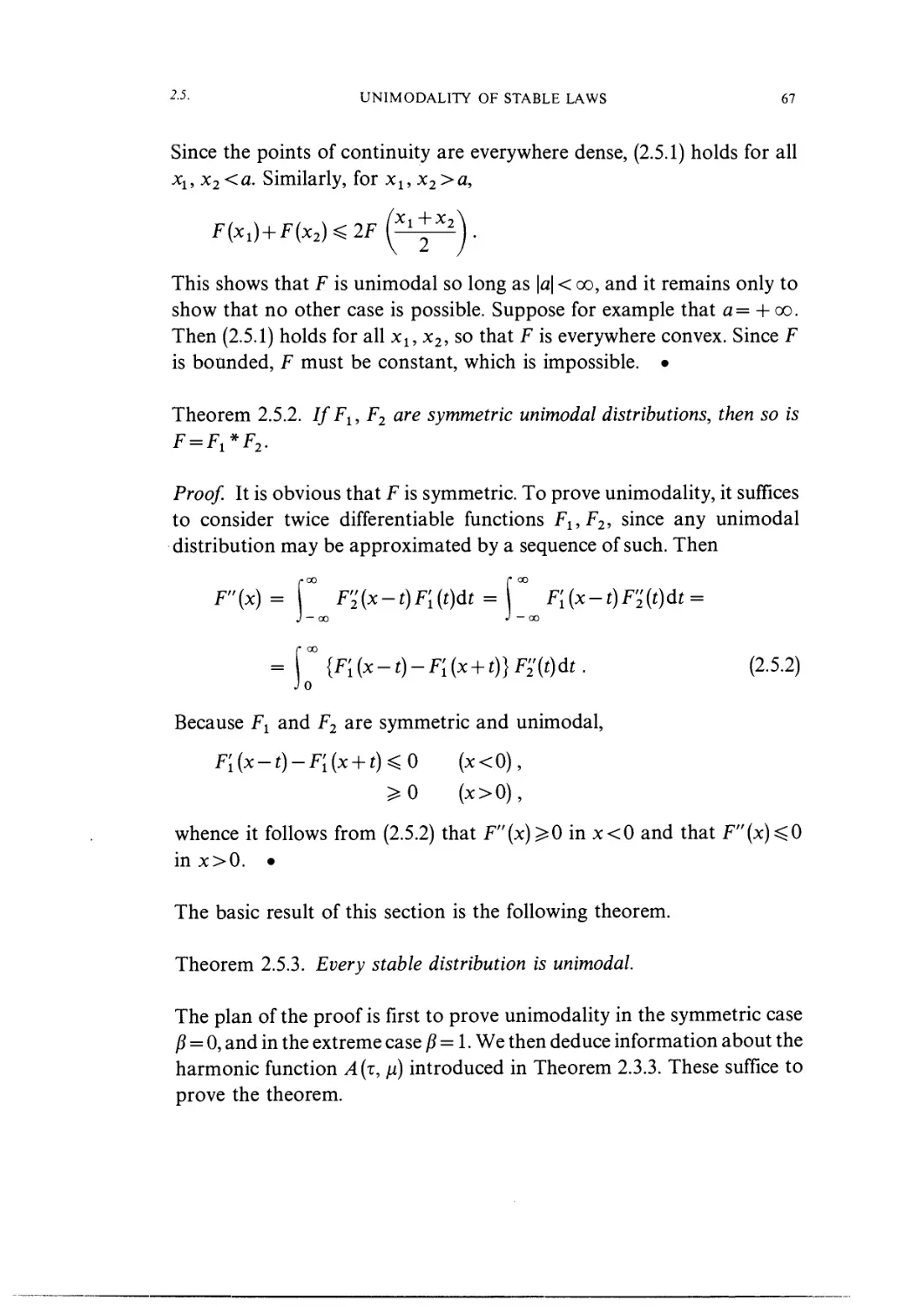
Since the points of continuity are everywhere dense, B.5.1) holds for all
xt, x2<a. Similarly, for x1? x2>a,
This shows that F is unimodal so long as \a\ < oo, and it remains only to
show that no other case is possible. Suppose for example that a = + oo.
Then B.5.1) holds for all x1? x2, so that F is everywhere convex. Since F
is bounded, F must be constant, which is impossible. •
Theorem 2.5.2. If Flt F2 are symmetric unimodal distributions, then so is
F = F1*F2.
Proof. It is obvious that F is symmetric. To prove unimodality, it suffices
to consider twice differentiate functions Fl,F2, since any unimodal
distribution may be approximated by a sequence of such. Then
F"(x)=C F2'(x-t)F[(t)dt = r F[(x-t)F'2'(t)dt =
J — oo J — oo
= H {F[(x-t)-F[(x + t)}F2'(t)dt . B.5.2)
Jo
Because Fl and F2 are symmetric and unimodal,
whence it follows from B.5.2) that F"(x)^0 in x<0 and that F"(x
in x>0. •
The basic result of this section is the following theorem.
Theorem 2.5.3. Every stable distribution is unimodal.
The plan of the proof is first to prove unimodality in the symmetric case
P = 0, and in the extreme case /? = 1. We then deduce information about the
harmonic function A(z, fi) introduced in Theorem 2.3.3. These suffice to
prove the theorem.

68 STABLE DISTRIBUTIONS Chap. 2
A) Some auxiliary results
Lemma 2.5.1. For ot< 1, x>0,
p'x(x; a, 1) = —- p(x; a, 1) =
B.5.3)
j o
where
"{<{>) = (^
and
cos <f> sin(la)<^
(l)i0
For x<0, a<l,
Jpi(x;a,l) = 0. B.5.4)
Proof. The function
of the complex variable z = pel<t> is analytic in the complex plane cut along
the negative real axis, and
r °°
p'x{x;oc, l) = Re y(z)dz. B.5.5)
Jo
Deform the contour into r = Fi+r2, where /~\ is the line segment @,
fa1/1"ax"a/1"a), and T2 is the curve
Supposing for the moment that this deformation is admissible, and noting
that
Re
we have, after a little calculation,

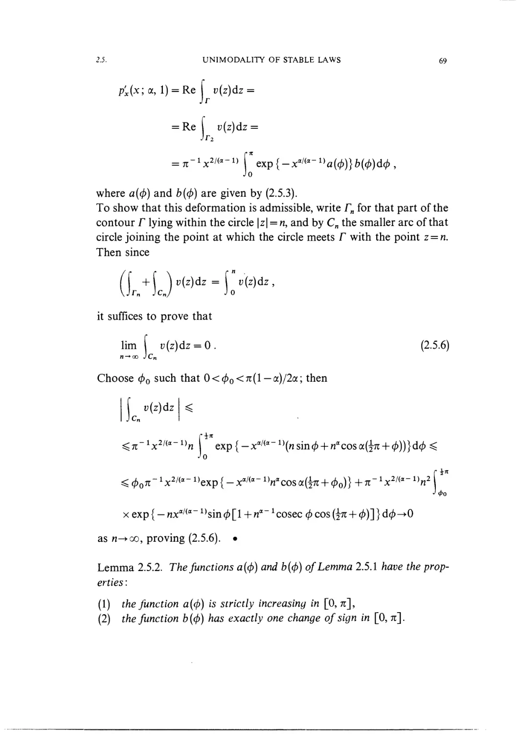
2.5. UNIMODALITY OF STABLE LAWS 69
p'x(x; a, 1) = Re v(z)dz =
Jr
= Re f v{z)dz =
Jr2
where a(<fi) and b(<fi) are given by B.5.3).
To show that this deformation is admissible, write Fn for that part of the
contour F lying within the circle \z\ = n, and by Cn the smaller arc of that
circle joining the point at which the circle meets F with the point z = n.
Then since
it suffices to prove that
lim ( v{z)dz = 0. B.5.6)
n-»oo JCn
Choose (fH such that 0<(f)o<iz(l— a)/2a; then
[ v{z)dz
o
ho
x exp {- nxal(a~ ^sin<f>[1 + na~ *cosec ^ cos (^tt + <?)]} d^^O
as n^-oo, proving B.5.6). •
Lemma 2.5.2. The functions a((f)) and b{4>) of Lemma 2.5.1 have the prop-
properties :
A) the function a((p) is strictly increasing in [0,7i],
B) the function b (cp) has exactly one change of sign in [0, tz\ .

70 STABLE DISTRIBUTIONS Chap. 2
Proof. Since sin cfx <\> in <\> > 0 we have
— (a cot tx(j) - cot </>) = i cosec2 acj) (sin 2a0 - 2a0) < 0 ,
so that the function
\jj (a) = a cot a0 — cot 0
is decreasing, and i//(l)=0, whence the inequality
a cot a(/> > cot cf)
holds for 0<a< 1, O<0<7r. Thus
— log aD>) = A -a)"x {a2 cota0 + A -aJ cot(l -a)^-cot $} >0,
and A) is proved.
To prove B) it is sufficient to show that
, . 2a cos 0 sin(l—aH _ 1 /a sinB — oc)(f) \
A — a)sina(/) 1—a\ sin a^ /
has just one change of sign. This is true since otherwise it has at least three,
and differentiating \J/((f)) = a sin B — olL> — sin occf) we obtain a contradic-
contradiction. •
Lemma 2.5.3. Suppose that l<a<2. Then for x>0,
p'x(x;a,l)<0, B.5.7)
and when x<0,
where
(a-1) sin (a-
/_s
ysi
y^/ sin txf)
is strictly increasing in [0, n/a], and
/ sin 4> \2/(a~ n /2a cos ^ sin (a-1H \
\sinacf)) \ (a — 1) sin a^
has exactly one change of sign in this interval.

2.5. UNIMODALITY OF STABLE LAWS 71
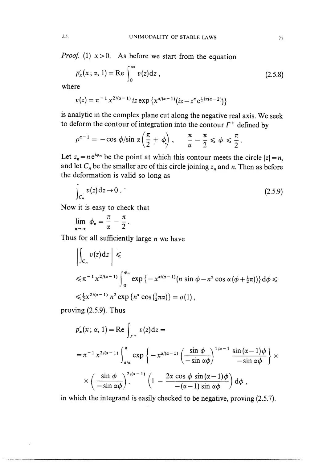
Proof. A) x>0. As before we start from the equation
p'x{x;a, l) = Re ( v{z)dz , B.5.8)
Jo
where
is analytic in the complex plane cut along the negative real axis. We seek
to deform the contour of integration into the contour F+ defined by
- . j 71 \ 71 71 71
p = — cos (p/sin a I —\- a>\ , ^ <p ^ — ¦
\2 ¦ y a 2 2
Let zn = nQl<t>n be the point at which this contour meets the circle \z\ =n,
and let Cn be the smaller arc of this circle joining zn and n. Then as before
the deformation is valid so long as
B.5.9)
Cn
Now it is easy to check that
lim cf)n= .
n-»oo CC Z
Thus for all sufficiently large n we have
y(z)dz
cn
<t>n
exp{ —xa/(a~1)(n sin cf) — na cos a((/>+^rr))}d(/>^
o
n2 exp {rf cos (^rra)} = o A),
proving B.5.9). Thus
p'x{x;oc, l) = Re I u(z)dz =
Jr+
n f u i\ { sin 6 \ 1/a~1 sin(a— \N )
exp { -Xat(*-y) r^-r) ^ ^- \ X
nla [ \ —Sin a(P/ —Sin a0 J
/ sin^ 1) / 2a cos
x —: . 1
j V
:. 1,rr.t
Y — smacpj V — (a — 1) sin acp
in which the integrand is easily checked to be negative, proving B.5.7).

72 STABLE DISTRIBUTIONS Chap. 2
B) x < 0. Write x = - y, so that
P'x{x;ol, l) = Re f u(z)dz, B.5.10)
f
Jo
where as always
v{z) = iT1 y2**-" iz exp {-//(a-
is analytic in the cut plane. We deform the contour to F~ =Tf + r2~,
where Ff is the line segment @, -ia1/A"a)) and F2~ the curve
p" = — cos 0/sin a((/)+^7r), — - ^ 4> < -.
The justification for this change is exactly as in the proof of Lemma 2.5.1,
and the proof is completed in the same way. •
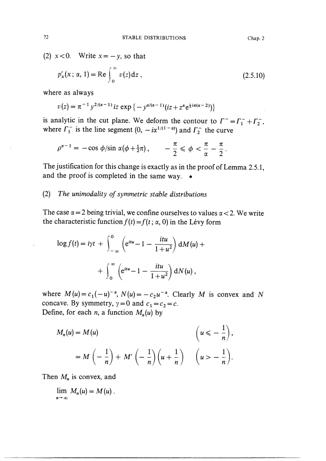
B) The unimodality of symmetric stable distributions
The case a = 2 being trivial, we confine ourselves to values a < 2. We write
the characteristic function/(t) =f(t; a, 0) in the Levy form
log/@ = iyt + \° (ete-1 - -^) dM(u)
where M{u) = ci{ — u) a, N(u)= —c2u a. Clearly M is convex and N
concave. By symmetry, y = 0 and c1=c2 = c.
Define, for each n, a function Mn(u) by
Mn(u) = M(u) {U^~l)'
Then Mn is convex, and
lim Mn{u) = M{u).

2.5. UNIMODALITY OF STABLE LAWS 73
Similarly
Nn(u)=-Mn(-u)
defines a concave function with
lim Nn{u) = N(u).
n —>oo
Let/n be the characteristic function of the infinitely divisible distribution
corresponding to Mn and Nn in the Levy formula. Since
\\mfn(t) = f(t)
n-»oo
it is suffices to prove that the corresponding distributions Fn are unimodal.
Now
eituLn{u)du\ , B.5.11)
k = 0 * '• I -I -oo J
where
5H=\° dM» + PdN»
J-oo JO
and
= N» («>0).
Now Ln(u) is positive, symmetric, and has a single maximum at the origin.
Thus
where /„ is a constant and !Pn a symmetric unimodal distribution function.
By Theorem 2.5.2, ?/n*fc is also symmetric and unimodal, and so therefore is
^ B.5.12)
From Theorem 2.5.1 it follows that F is also unimodal.

74 STABLE DISTRIBUTIONS Chap. 2
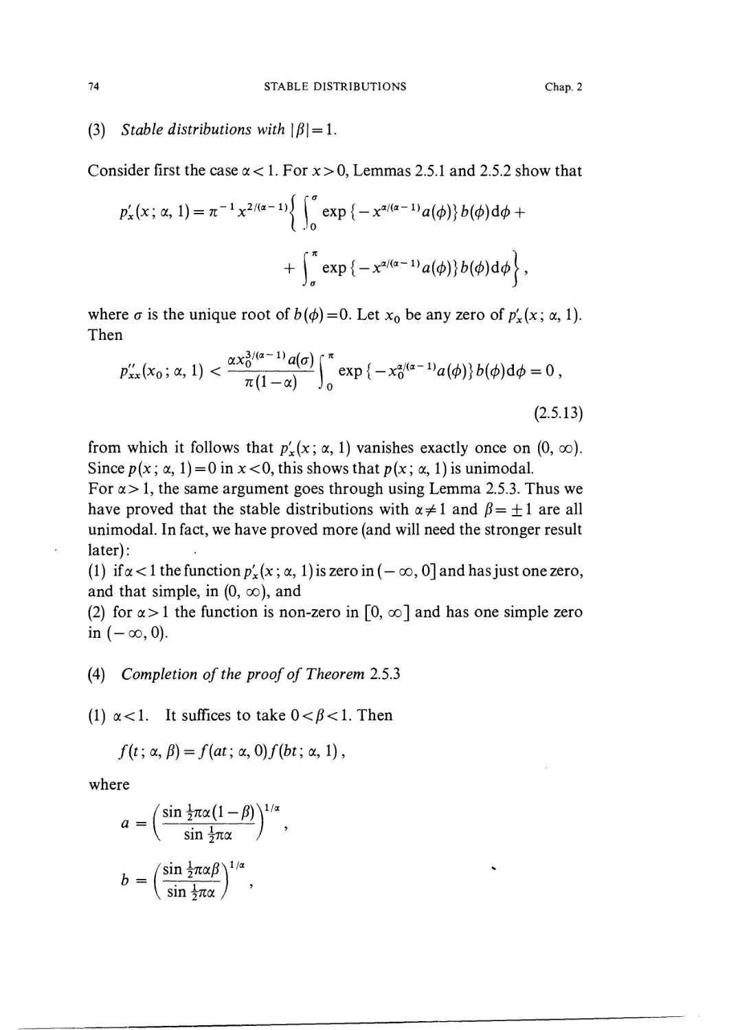
C) Stable distributions with |/?| = 1.
Consider first the case a < 1. For x>0, Lemmas 2.5.1 and 2.5.2 show that
p'x{x;ol, l) = 7r-1
where a is the unique root of &((/>) =0. Let x0 be any zero of p'x(x; a, 1).
Then
n
p'xX{x0; ot, 1) < — —1 exp{ — Xq a(<fi)}b[(fi)d(f) = 0 ,
n A -a) Jo
B.5.13)
from which it follows that p'x(x; a, 1) vanishes exactly once on @, oo).
Since p(x; a, l) = 0inx<0, this shows that p(x; a, 1) is unimodal.
For a> 1, the same argument goes through using Lemma 2.5.3. Thus we
have proved that the stable distributions with a#l and j8= ±1 are all
unimodal. In fact, we have proved more (and will need the stronger result
later):
A) ifa<l the function p^.(x; a, 1) is zero in (— oo, 0] and has just one zero,
and that simple, in @, oo), and
B) for a> 1 the function is non-zero in [0, oo] and has one simple zero
in (—oo,0).
D) Completion of the proof of Theorem 2.5.3
A) a<l. It suffices to take O</J<1. Then
f(t;a,P) = f{at;a,O)f{bt;a,l),
where
a =
sin
sin 1
sin

2.5. UNIMODALITY OF STABLE LAWS 75
so that by B.5.4),
r oo
p'x{x;cc,P) = a2b p'x{a{x-t); a, 0) p(bt; a, l)dt.
Jo
Because p(x; a, 0) is unimodal this implies that p'x(x; a, /?)>0 in x^O.
Denote by xo = xo(P) the smallest zero of p'x(x, a, /?), so that xo@)=0
andxo(j8)>0fbr 0>O.
We prove unimodality by showing that
D = {(x, P);x>xo{P), 0^1, p'x{x; a, /})>()}
is empty. Let D be the closure of D. From the asymptotic expansion of
p'x(x; a, /?) for large x it follows that D is bounded, and contains at most a
finite number of points of ft = 0 and none of of /? = 1.
It is not difficult to verify (cf. Theorem 2.3.3) that the function
A(T,fi) = x2p'x(x;a,P), B.5.14)
where x = e~\ P = 2/j,/tz, is harmonic in — oo<t<oo, 0<fi<^n. The
mapping (x, /?)->(t, fi) maps the compact set D into a compact set D in
this strip which meets the boundary at most a finite number of points.
On the boundary of D, A{z, /i)=0, which implies that A(t, h) = 0 in D,
since A is harmonic. In particular, if D is non-empty, a point of D is map-
mapped into a point with A (t, /x) = 0, which contradicts the definition of D.
This completes the proof for a < 1.
B) a>l. From the asymptotic expansion for x->0 it follows that, if
jg^O, p'x{0; a, /?)#0. Thus on the boundary of the domain 0<x<oo,
\P\ < 1, the function p'x{x; a, /?) vanishes only twice, at @, 0) and (x0, 1),
where x0 is the unique zero of p'x{x; a, — 1). The remainder of the argu-
argument goes through as in A), using the fact that B.5.14) defines a function
analytic in —oo<t<oo, — jn<fi<jn.
n
C). a= 1. Use the representation
{ro / itu \ c ol
iyt + ] (eitu-1 - j-^jj (T^pr d" +

76 STABLE DISTRIBUTIONS Chap. 2
to show that
f(t; l,cl,c2)= lim f{t; 1 -w, cl9 c2),
n-'oo
and use Theorem 2.5.1. •
§ 6. Domains of attraction
Let Xt, X2, ... be a sequence of independent random variables, with the
same distribution function F(x), and set
7 Xl+X2 + ...+Xn — An ,«,n
Zn = . B.6.1)
If, for a suitable choice of the constants An, Bn, the distribution of Zn
converges weakly to a non-degenerate distribution G(x), we say that
F(x) is attracted to G(x). The set of all distributions attracted to G(x)
is called the domain of attraction ofG(x), and Theorem 2.1.1 shows that
only stable laws have non-empty domains of attraction.
Theorem 2.6.1. In order that a distribution F(x) belong to the domain of
attraction of a stable law with exponent a @<a<2), it is necessary and
sufficient that, as |x|—>oo,
B.6.2)
where the function h (x) is slowly varying in the sense of Karamata (see
Appendix 1) and ct and c2 are constants with ct, c2 ^0, ct +c2>0 related
to the stable law by B.2.1).
Proof It follows from Theorems 1.7.3 and 2.2.1 that F will belong to the
domain of attraction of a stable law with index a @<a<2) if and only if
for some choice of the constants Bn,
), B.6.3)
), B.6.4)

2.6. DOMAINS OF ATTRACTION 77
lim lim sup n{( x2dF{Bnx) -( \ xdF{Bnx)) J = 0 .
B.6.5)
We first prove that these three conditions follow from B.6.3). For x>0
we write
and define Bn to be the smallest value of x for which
B.6.6)
Then
lim Bn = oo ,
n->oo
and so
«^-x-. B.6.7)
X(Bn)
It therefore follows from B.6.2) that
and this in turn implies that B.6.3) and B.6.4) are satisfied.
In order to verify B.6.5), we note that, since the expression there is non-
negative, it suffices to show that
lim lim sup n [ x2dF {Bn x) = 0 . B.6.8)
2-»0 n-»oo J |x| <e
Integrating by parts, we have
x2dF(Bnx) = 2B;2 \xX(x)dx-e2X(Bne). B.6.9)
\x\<e JO
We may clearly assume that sBn> 1; let s be the integer with
The results of Appendix 1 show that

78 STABLE DISTRIBUTIONS Chap. 2
hm sup bk 1
so that constants A{ can be found such that
B s f2k+1 h(x)
o fc=o hk *
s r 2k~
hBk)
J 2k
= i(c1+c2) + A4X(?Bn)Bn2?2. B.6.10)
Combining B.6.9) and B.6.10) we have
n [ x2dF(Bnx) ^C-
\x\<?
We have already shown that
lim
and by a property of slowly varying functions,
lim 2
'n
• oo
Thus, from B.6.11),
lim lim sup n [ x2 dF{Bnx) ^ lim A + 2AA) s2~a=0.
Conversely, we have to show that, if B.6.3), B.6.4) and B.6.5) are assumed,
then B.6.2) follows. It suffices to prove that

2.6. DOMAINS OF ATTRACTION 79
B) for every k>0,
lim 1&- = k°
x^^ i{kx)
Fix x>0 and, for large y>0, take n so that
Then
(n+l)F(-Bn+1x) n < F(-y) < nF(-Bnx)
((nx)) n + 1 l-F(y)(n + l)(l-F(B,,+ 1x)) n
and
{n+l)x{BH+1x) n < x(y) < nX{Bnx)
nX(Bnkx) n+1 ^ X(ky)" (n+l)X(Bn+1kx) n '
As ^^-oo, n-> oo, and B.6.3) and B.6.4) therefore imply that
F(-y) ct
and
lim A^r = k*.
Theorem 2.6.2. The distribution function F(x) belongs to the domain of
attraction of a normal law if it satisfies one of the following conditions:
A) F has finite variance,
{2)forx>0,
X(x)=l-F(x) + F(-x) = x-2h(x),
where h(x) is slowly varying.
Proof. From the results of § 1.7, F is attracted to a normal law if and only
if, for some choice of the constants Bn,
lim nX(Bnx) = 0 B.6.12)
n-»oo
for all x > 0, and

80 STABLE DISTRIBUTIONS Chap. 2
lim nB~2( I x2dF{x) -I f xdF(x)Y) = 1 B.6.13)
n-°o \J|x|<?Bn \J|x|<?Bn / /
for some ? > 0.
Suppose first that
00
.2,
x2dF(x)< oo ,
00
and set
a= p xdF(x), g2= [ {x-aJdF{x).
— oo
It is then easy to check that B.6.12) and B.6.13) are satisfied with Bn =
Suppose on the other hand that
00
2.
x2dF(x)=oo.
00
We first show that
([ xdF{x))=o([ x2dF{x)) B.6.14)
\}\X\<2 ) \)\X\<Z J
as z-* oo. To do this, choose a positive even function \[/ (x), increasing and
unbounded in x>0, such that
/= ( \j/{xJdF{x)< oo .
J— oo
Then
\ 2
xdF(x)| ^ \ \j/{xJdF(x) \ {x/\Js{x)JdF{x) =
showing that B.6.13) is equivalent to the condition
lim nB~2 f " x2dF{x)= 1 . B.6.15)
n-"oo J
If the function H is defined by
H(z)=[ x2dF(x),
J -2

2.6. DOMAINS OF ATTRACTION 81
then we prove that B.6.12) and B.6.13) imply that, for all /c>0,
r H(kz) i
It is sufficient to prove this for k> 1, and since
H(z)=- \Z x2dX(x),
Jo
it suffices to show that, as z->oo,
- J* x2dX(x) = o {- j* x2dX(z^j . B.6.16)
For any z, define n so that
Bn^z^Bn+1.
Then B.6.13) shows that, for large z,
o Jo--
From B.6.12) and the fact that Bn+l/Bn-+l, we have for large z,
kz rkBn+i
\ x
Bn
= o(n-1B2).
Thus H(z) is a slowly varying function.
Conversely, suppose that H(z) is slowly varying. Then
lim z
and we define Bn as the largest value of z for which
Then J3n->oo and
fBn
lim nB; 2 H (Bn) = nB; 2 T" x2 dX (x) = 1 . B.6.17)
n-oo J0

82 STABLE DISTRIBUTIONS Chap. 2
Since H is slowly varying,
^oo H(Bn)
so that
lim nB~2 \
Moreover,
nx{xBn) = n
0
r 00
dx
JxBn
00
s = 0
y-2R-2
dx)=l
H(xBn)
¦
J 2sxBn
I 2'2s-
s=0
Vdx(x)<
fBs+1xBn)
H(xBn)
HBs+1
B.6.18)
By Karamata's theorem (Appendix 1) H(z) has a representation
jj2^j B.6.19)
where A is a constant and e(u)->-0 as «-> 00. Thus for sufficiently large n,
H{2s+1xBn) „ (f2I+lrf» e(u) _, ) ,
-^ r^ < 2 exp { -^- dw J ^ 2is,
^W) PUxBn l+ii j^
and as n^-oo,
= 1+0A).
Hence from B.6.17) and B.6.18) it follows that, for all x,
lim nX{xBn) = 0.
n—* oo
Thus B.6.12) and B.6.13) are together equivalent to the statement that
H is slowly varying.
We now prove that if h(x) = x2x{x) is slowly varying, then so is H(z).

2.6. DOMAINS OF ATTRACTION 83
Integrating by parts, we find that
H(z) = - \ x2dX{x)= -h{z) + f^dx. B.6.20)
Jo J o x
From Karamata's theorem we can choose z1=z1(z)<z so that
lim
lim
2->00
Then
Jo
and so
sup
z
X
sup
— ou
<
h(x)
h(z)
z h(x
¦ 1 x
= 1,
^dx;
dx >ih(z) log (z/z,),
H(z)=\Z
Jo
For any k>0, as z^-oo,
^ 2 log kh(z) =
so that
Collecting these results together, the theorem is proved. •
It is clear that, when the variance is finite, H(z) will be slowly varying,
and thus the theorem may be expressed in the following way.
The distribution function F(x) belongs to the domain of attraction of a
normal law if and only if
2
H(z) = c2dF(x) B.6.21)
J -2
is a slowly varying function.

84 STABLE DISTRIBUTIONS Chap. 2
It may be shown in a similar way that the conditions of Theorem 2.6.1 are
satisfied if and only if the function
lim -^ = il. B.6.23)
z-»oo \ ( ,,\«Jr/,.\ 2
H{z) = \x\adF{x) B.6.22)
is slowly varying, and
xadF{x)
(-xfdF(x)
These conditions imply that
h(x) ~ -?--x(x) = o{H(x)} . B.6.24)
c1-\-c2
Conversely, the methods used in the proof of Theorem 2.6.2 can be used
to show that B.6.24) implies B.6.2), B.6.22) and B.6.23). This permits a
unification of Theorems 2.6.1 and 2.6.2.
Theorem 2.6.3. In order that a distribution function JF(x) belong to the
domain of attraction of a stable law with index a, it is necessary and sufficient
that
2-a
Theorem 2.6.4. IfF(x) belongs to the domain of attraction of a stable law
with index a, then for any d (O^d<oc),
\x\ddF(x)< oo.
Proof The result is obvious if the variance is finite. If it is infinite and a< 2,
then Theorem 2.6.1, together with the results of Appendix 1, shows that
for any e>0. Taking e sufficiently small, we have

2.6. DOMAINS OF ATTRACTION 85
\x\ddF(x) =
If rf = 2, use the formula B.6.21). •
Theorem 2.6.5. In order that the distribution with characteristic function
f(t) belong to the domain of attraction of the stable law whose characteristic
function has logarithm
where cc, /?, c, co(t, a) are as in Theorem 2.2.1, it is necessary and sufficient
that, in the neighbourhood of the origin,
log/@ = iyt-c\t\'R(t) (l " tf j*j «(t «)) ,
where y is a constant, and h(t) is slowly varying as t-*0.
Proof. To prove necessity, first note that, in the neighbourhood of the
origin,
where that branch of the function log is taken with log 1 =0. If, for
G1(x)=l-F(x), G2(x) = F(-x),
then
1-/@=
= r (eta- VdG^x) + {°° (e~ta- l)dG2(x). B.6.25)
Jo Jo
The asymptotic behaviour of Gx and G2 for large x is given by B.6.2); from
this we deduce the behaviour of their Fourier transforms, and thus that of
1 —f{t), as ?->0. Further calculations depend on the value of a; we distin-
distinguish four cases.
A) 0<a< 1. If suffices to examine the first integral on the right-hand
side of B.6.25).

86
STABLE DISTRIBUTIONS
Chap. 2
Integrating by parts, we have
(eitx-l)dGl(x)=it
o Jo
where, by Theorem 2.6.1 ,h1(x) is slowly varying as x-> go. (We are assum-
assuming, without loss of generality, that cx ^0.) The analysis of these integrals
requires the following lemma.
Lemma 2.6.1. If h(x) is a positive slowly varying function (as x->co),
and x~ah(x) is monotone decreasing, then as ?-*¦(),
v I v
X j X
a v '
j
v I va
X J X
B.6.26)
Proof of the lemma. Consider for example the integral involving sin x,
and split it into four parts:
+ +
d
+
A2t
By the second mean value theorem,
00 • h(x/t).
sin x - g - dx
= lim
¦ h(x/t).
sin x —^—- dx
since as t->0 for fixed A,
h(A/t) ^ {
B.6.27)

2.6.
DOMAINS OF ATTRACTION
87
From B.6.19), for all xe(<5, A2t),
h(x/t)
x
where s can, by suitable choice of A2, be made arbitrarily small. Therefore
sin x
6 Hx/t) .
—— sin xdx
dx^Sh(l/t). B.6.28)
If x<A2t, the function h(x/t) is bounded, so that
*2th{x/t) .
, sin xdx
B.6.29)
It is easy to see that bounds analogous to B.6.27)-B.6.29) hold also for
the integrals of sin x/xa. Finally,
uniformly in S < x < A x, so that
B.6.30)
We now take Al=Al(t)-^oo and S = S(t)-^O (t-^0) sufficiently slowly for
these bounds to remain true. Combining them, we have
00 . /j(x/t)
sin x
o *a
An exactly similar argument deals with the integral involving cos x.
Remark. By Euler's formula [12],
f00 fsin xl dx _ _,. , (cos^
J 0 | COS X j Xa
and consequently
" (sin x| fe(x/t) . _ , fcosl
I > ()^
o [cosxj xa v [sin
i unu\
v ' '
B.6.31)
Returning now to the proof of the theorem (case 1), we have from B.6.25)
and B.6.31),

88 STABLE DISTRIBUTIONS Chap. 2
l-/@ = r(l-a)cos(i7ra)(c1+c2)/2(|rr1)|?|ax
x\ lPW\
\ l ui
where /? = (c1—c2)/(c1 + c2).
B) l<a<2. In this case
f00 |x|dF(x)<oo,
J - oo
and there is no loss of generality in supposing that
xdF(x) = 0 .
— 00
Then
(l-eitx + itx)dF(x) =
= it r (e^-^G^dx-it ((e-I'xt-l)G2(x)dx.
Jo Jo
By the same method as before, one proves the following lemma.
Lemma 2.6.2. 7/1 <a<2 and the conditions of Lemma 2.6.1 are satisfied,
then as t->0,
oo glx_ 1 r oo e'X_ 1
h(A)dMiA) -3T-
0 x
= e"i't(a-1)r(l-a)/2(l/f). B.6.32)
Applying this result, we have
1 -f(t) =-chA/0111" (l + f/J ~ tan ftTra)) ,

2.6. DOMAINS OF ATTRACTION 89
where c = (c1 + c2) cos(jna)r(l—a),
P=(c1-c2)/(c1+c2).
C) a = 1. In this case 1 —f(t) differs by a term iy't from
B.6.33)
Integrating by parts and arguing as in the proof of Lemma 2.6.1, we have
for t>0,
itx
;t(l+x2)-2ix2A/i(x)
A + x2J / x
r °° eIX
it\ —h(x/t)dx+iy1t+O(t2) =
J t x
ith(l/t)\ —dx(l + o(l)) + iyit
J t x
iy1t, B.6.34)
Since
f °° sin x , , f00 cosx
dx = |yr, dx= -log ? + 0A).
Jo * Jr x
Carrying out similar computations for the second integral, and examining
in the same way the case t<0, we come to the result that
where
c = %k(c1 + c2), P = (cl-c2)/(cl

90 STABLE DISTRIBUTIONS Chap. 2
D) a = 2. If F(x) has finite variance a2, and if
xdF(x) = a ,
J— 00
then
= iat-±<r2t2(l + o(l)). B.6.35)
Suppose on the other hand that the variance is infinite, and write as be-
before
X(x)=l-F(x
H(x)=\Xu2dX(u).
Jo
It was shown in the proof of Theorem 2.6.2 that
h(x) = o(H(x)).
By the methods which have already been repeatedly used, it is easy to
show that
f00 (e<*-l-itx)dX(x)
Jt-1
B.6.36)
and therefore
c\t\~l
\ogf(t)= (eitx-l-itx+$t2x2)dG1(x)+
Jo
o
M-1
CM-1
-±t2 x2dX(x) + o(t2H(\t\-1)). B.6.37)
Jo
Moreover,
= O(t2h(\t\~1)) + it (
Jo

2.6. DOMAINS OF ATTRACTION 91
so that finally
This concludes the proof of the necessity; indeed we have proved some-
somewhat more, that when 0<a<2, then as ?-*¦(),
B.6.38)
and when a = 2,
|/(t)| -exp^tfdr1)}. B.6.39)
We now turn to the proof of the sufficiency. We write
A(t) = \t\*h(t),
and note that
lim l(t) = 0 .
The normalising constants Bn are chosen as follows,
; X{t) = c/n},
(this definition being meaningful for large n, since X(t) is continuous in a
neighbourhood of t = 0). Then
lim f(t/Bnf =
= exp | - c \t |- (l + ifi ~ co (t, a)^j |, B.6.40)
and the theorem is proved. •
It was shown in § 2.2 that the normalising constants Bn determining attrac-
attraction to a stable law of index a were necessarily of the form
Bn = nllah(n),
where h(n) is slowly varying. The classical theorems of probability (de
Moivre-Laplace-Levy) show that, for convergence to the normal law,
the most interesting case is that in which Bn = arv for a constant.

92 STABLE DISTRIBUTIONS Chap. 2
On the other hand, any stable law G of exponent a belongs to its own
domain of attraction, with Bn = an1/tx. This suggests the following defini-
definition.
A distribution belongs to the normal domain of attraction of a stable law
G with exponent a if it is in the domain of attraction ofG and if the normalising
constants are given by
Bn =
= an1/a,
where a is a constant.
Normal domains of attraction are characterised by the following theorems.
Theorem 2.6.6. In order that the distribution F(x) belong to the normal
domain of attraction of the normal distribution
it is necessary and sufficient that it have finite variance a2, and then Bn =
an*.
Proof The sufficiency follows from Levy's theorem. To prove the necessity
take Bn = an* and assume without loss of generality that
xdF(x) = O .
It then follows from Theorems 2.6.2, 2.6.5 and equation B.6.39) that
lim ^ H (w)" *'2 •
This is only possible if
H(oo)=— I x2dx(x) = x2dF(x) = a2 < oo ,
Jo ' J-oo
and a = a. •
Theorem 2.6.7. In order that the distribution F(x) belong to the normal
domain of attraction of the stable law G(x) with exponent a @<a<2) and
given constants cl5 c2, with Bn = ani, it is necessary and sufficient that

2.6. DOMAINS OF ATTRACTION 93
F(x) = (c1a« + a1(x))\xr\ (x<0),
F(x)=l-(c2aa + a2(x))x-\ (x>0), }
where a?(x)->0 as |x|->oo.
Proof. The sufficiency is immediate. To prove the necessity, note that
from B.6.35), for small t,
lim x(ani/a\t\- >~aUfn = |t|a,
t-0
which is only possible if B.6.41) holds.

Chapter 3
REFINEMENTS OF THE LIMIT THEOREMS FOR NORMAL
CONVERGENCE
§ 1. Introduction
In this chapter we consider a sequence XUX2, ... of independent, identi-
identically distributed random variables belonging to the domain of attraction
of the normal law. As shown in § 2.6, the X-} necessarily have a finite vari-
variance a2. We shall assume that E(Xj) = 0; then necessarily the distribution
Fnof
ZH=(X1+X2 + ... + XH)l<m* C.1.1)
converges to the normal distribution <P with zero mean and unit variance.
Indeed, with
we have
Rn(x) = Fn(x)-<P(x)^0
as n->oo, uniformly in x.
In § 3 we give an asymptotic formula for Rn(x) in terms of n~*. In the later
sections the behaviour of sup |-Rn(x)| for large n is the object of study.
The symbols//, and v will denote the characteristic functions correspond-
corresponding to the distributions F (the common distribution of the X,), Fn and <P
respectively (so that v(t) = e~*t2). We shall also write
a2 = E(Xf), a,= E(Xj), P,= E\Xj\.
§ 2. Some auxiliary theorems
This section is devoted to some important properties of the characteristic
functions fn(t).

3.2.
SOME AUXILIARY THEOREMS
95
Theorem 3.2.1. If /?3 is finite, then
A) for\t\^Tn = <73
l
6
C.2.1)
B)
where gn(t) = l+n~iP1(it),
and lim S(n) = 0,
C) for\t\^Tn3,
where lim dl(n) = 0
C.2.2)
C.2.3)
. A) Using the expression
exp(^)dF(x),
where |0| ^ 1, it is easy to show that, in \t\ ^ Tn, |/(t/crn})| >f|. Therefore
in this domain,
where by Lyapunov's inequality,
d3 . „,
Since
fn(t) = exp {n log (t/en*)},
it follows that
B4/25J

96
LIMIT THEOREMS FOR NORMAL CONVERGENCE REFINEMENTS Chap. 3
\Mt)-v(t)\
- J/2
exp
- 1
where we have used the obvious inequality
Finally, if \t\^Tn, then
+2 11 4. |3 o +2
2 6a3n> 4 '
and C.2.1) is proved.
B) Since
f{tlan^)-\=-~n
we have
o
\t\:
n-
In 6a5 n* Vn
Using C.2.4) again, we have, for 11\ ^ Tn3 ,
where
But
«3(ftK
6cr3 n^
(itK
C.2.4)
C.2.5)
C.2.6)
whence C.2.2) follows.
C) The proof of C.2.3) is exactly similar. •
By more intricate arguments (for which see, for example, [48] page 219),
the second part of the theorem may be strengthened as follows.

3.3. THE DEVIATION Rn(x) 97
Theorem 3.2.2. J/& is finite for some s ^ 3, then for \ 1| ^ Tns = n* <r3/8s&1/s,
s-2
. . . . i
+\t\^-"}e-*\ C.2.7)
where c(s) depends only on s, S(n) depends only on n and lim S(n) = 0, and
where the coefficients ckj are polynomials in the variables (ocjcf), r = 3, 4, ...,
k-j+3.
§ 3. The deviation Rn(x)
Under the assumptions made in this chapter,
In this section we investigate the asymptotic behaviour of Rn(x). The
character of the argument and its results depends on whether or not the
Xj have a lattice distribution. We first consider the non-lattice case.
Theorem 3.3.1. If the independent random variables Xj have the same non-
lattice distribution with finite third moment, then
Fn(x)-*(x) = n~* ^|^ A -x2)e-t*2 + o(n-t), C.3.1)
uniformly in x.
The proof follows on combining the expansion of/n presented in § 2 with
the following lemma.
Lemma 3.3.1. IfF is a non-lattice distribution, then for each co>0, there
exists a sequence X(n) with X(n)-^co as n->oo, such that
I = \fn(t)\r1dt = o(e-inV2). C.3.2)

98 LIMIT THEOREMS FOR NORMAL CONVERGENCE REFINEMENTS Chap. 3
Proof. If F satisfies Cramer's condition
(C) lim sup |/@l < 1 ,
r-*oo
(cf. § 1.4), then there is a positive constant c (depending on co) such that
| f(t) | < e ~c for all 111 ^ co. Choosing X (n) = n, we have
On the other hand, suppose that
lim sup |/@l = 1 •
Since the distribution is non-lattice, \f(t)\ < 1 for all t (see § 1.4), and hence
a(t)= {1— sup
defines a continuous, non-decreasing function, with
lim a(t)= oo .
t—* oo
For any X(n),
m . fA(n)l /. IV.
7=
If a(n)^n*, set X(n) = n, so that
I ^ A -n"*)" log(n/co) = o(Q-*n
If on the other hand a(n) >ni, then
Now a(t) takes every value larger than a(co), and hence for sufficiently
large n we can define X(n) by the equation a\_X(n)] = ni. Then X(n)< n
and
I ^ A -«-*)" log (n/co) = o{e
Proof of Theorem. We have to show that, uniformly in x,
where

3.3.
THE DEVIATION Rn(x)
99
G(x)=*(x)-n
a3
A-:
According to Theorem 1.5.2,
y
Mt)-g(t)
dt,
C.3.3)
where ^l = sup|G'(x)|, g(t) is the Fourier-Stieltjes transform of G, and
we take T=l(n)ni, where X(ri) is determined by the lemma. It therefore
suffices to prove that
fn(t)-g(t)
For sufficiently large n,
C.3.4) does not exceed Ii
) • C-3.4)
i = <T3n*/24/?3, and then the integral in
f3, where
\fn(t)-g(t)
~Tn3
fn(t)
9n(t)
dt,
dt,
dt.
Now
so that, by Theorem 3.2.1,
"
By Lemma 3.3.1,
\f"(t)\r1dt=o(n-±),
and clearly
C.3.5)
C.3.6)
C.3.7)

100 LIMIT THEOREMS FOR NORMAL CONVERGENCE REFINEMENTS Chap. 3
Combining C.3.5), C.3.6) and C.3.7) to obtain C.3.4), we complete the
proof. •
It is however easy to see that C.3.1) cannot apply to random variables
with a lattice distribution. Suppose for instance that Xj takes the values
+1 with probability j each, so that Xl-\-X2 + ... + Xn has a binomial
distribution. Then Fn(x) has a discontinuity at x = 0, whose magnitude
is by the de Moivre-Laplace theorem (cf. Theorem 4.2.1) asymptotically
B7rn)~i. Thus Fn(x) cannot be approximated by any continuous function
to an accuracy better than n~*. To obtain an analogue of C.3.1) we
introduce the discontinuous function
S(x)=[x]-x+|,
where [x] denotes the integer part of x. For the binomial example, it is
possible to compute the expression
*x2 + o(n-*). C.3.8)
This is a special case of the following general result.
Theorem 3.3.2. Let X1,X2,... be independent, identically distributed
lattice random variables, taking values in the arithmetic progression
{a + kh; k = 0, + 1, ...}, (h being maximal). Then, uniformly in x,
=>-+*->. <3-3.9»
Proof Denote the right-hand side of C.3.9), without the error term, by
G(x), and its Fourier-Stieltjes transform by g(t). If n is sufficiently large,
Theorem 1.5.3 applies to give
t
n
where ,4 = sup |G'(x)| < oo. We have therefore to show that

3.3. THE DEVIATION R,(x) 101
t = o(n~*). C.3.10)
We first compute the characteristic function dn(t) of
Expanding S(x) in a Fourier series, we have
S(x) = Yj — sm B7rvx),
V= 1 """
so that
h ^ 1 . x
-sin {Tv<m2x —
v=l V7r
with t = 2n/h. Therefore
dn(t)= rx Yj ~ exp(itx — jx2)sin(TV<mix — Tvan)dx =
oo p — izvan
where the symbol X' indicates that v = 0 is excluded from the range of
summation.
We now go on to evaluate the integral C.3.10), expressing it in the form
h + h + h' where /,- is the integral over the interval Aj, and
Ai = (-n, -^
^2 = (~^xo
A3 = fa<mi, n).
A) Consider first the integral I2, and suppose that Tn3<^xarv (if not,
the calculation is similar, but simpler). Since h is maximal, there exists a
constant c1>0 such that, in the interval Tn3^|t| ^jtott* ,
\fn(t)\ = \f(t/ani)\n = o(e-^). C.3.11)
In this interval,
for some c2>0. Finally, using C.3.2) we have

102 LIMIT THEOREMS FOR NORMAL CONVERGENCE REFINEMENTS Chap. 3
/,=
Tn3
-Tn,
Tn3
-Tn3
Mt)-g(t)
dn(t)
o(n~*) =
t
1 °° 1
i Z-i U.I
B)
'
— Tn,
C.3.12)
and simple calculations give
L =
fc=l
f*(t)-dH(<m*t)
where r=[<r xt 1ni — |] and
(k-i)t
dt =
dt
kxcn2
Because of C.3.1) and C.3.11),
Tn
Tn
C.3.13)
C.3.14)
= O(n-i). C.3.15)

3.3. THE DEVIATION Rn(x) 103
Moreover,
Therefore Jk = O(l/kn), and C3.13) gives
A similar argument shows that
so that C.3.10) is proved. •
If the random variables Xj have finite movements of order k>3, we can
extend the asymptotic expansions C.3.1) and C.3.9) down to terms of
order n~i{k~2).
Theorem 3.3.3. If the independent random variables Xj have /3k finite for
some /c>3, and satisfy Cramer's condition
r->oo
l, (C)
then, uniformly in x,
X n~iJ Pj(-<P) + o(n-*k-2)). C.3.17)
Here
JJ+2S
(ir2s4j)
s=l
= *(x)Qj(x),
where Qj(x) is a polynomial in x, and c{sj) is a polynomial in the moments
av. There is a connection between Pj( — $) and the function Pj(it) of § 2:
eitxdPj(-<P(x)).
00
We omit the proof, which is similar to that of Theorem 3.3.1 and uses
C.2.7) and Theorem 1.5.2, (see [48], page 235).

104 LIMIT THEOREMS FOR NORMAL CONVERGENCE REFINEMENTS Chap. 3
For lattice distributions the analogue of C.3.17) is considerably more
complicated, and involves the functions Sj defined by the Fourier series
S2j(x) =2 f B7rv)-2jcosB7ivx),
v= 1
S2J+i{x)=2
v= 1
Furthermore, write
v= 1
and
d= 1 if v=l or 2 (mod 4),
= -1 if v = 0or3 (mod 4).
Theorem 3.3.4. Let Xj be independent, with the same lattice distribution
taking values in the progression {a + kh; k = 0, + 1, ...}, h being maximal.
U Pk is finite for some k, then uniformly in x,
k~2 ( h y
a, I—r x
(<m*x _/na Vna
The proof of this theorem also will be omitted.
§ 4. Necessary and sufficient conditions
It follows from Theorems 3.3.1 and 3.3.2 that, whenever /?3<oo,
|Fn(x)-4>(x)| = 0(n~*) - C.4.0)
This raises the question of giving necessary and sufficient conditions for
C.4.0) to hold. In this direction we have the following result.
Theorem 3.4.1. In order that
\Fn(x)-<P(x)\ = O(n-id), @«5<l), C.4.1)

3.4. NECESSARY AND SUFFICIENT CONDITIONS 105
it is necessary and sufficient that
) = O{z-d). C.4.2)
Proof. Throughout this chapter the random variables X} have E(X,)=0
and E(Xf) = c1 < oo. Hence
C.4.3)
where
lim y(t) = O .
t-0
Near t = 0, the equation
has only a finite number of solutions (except in the trivial case when the
Xj have a normal distribution, which we exclude; see § 1.6), and therefore,
for some positive e,
y(f)#O, @<|t|<e). C.4.4)
We first prove the theorem for symmetric random variables, for which the
characteristic function f(t) is real.
Lemma 3.4.1. For symmetric random variables Xj, C.4.1) holds if and only if
t2\y{t)\dt = O{x3+d). C.4.5)
o
Proof. To prove the necessity of C.4.5), integrate by parts in the equation
etxd(Fn(x)-0(x)),
to obtain
—e~it2 f00
f00
= e^ {Fn(x) - 0(x)} dx .
-^ — 00
In other words, the functions

106 LIMIT THEOREMS FOR NORMAL CONVERGENCE REFINEMENTS Chap. 3
and
r(x) = Fn(x)-<P(x),
which belong to L2(— oo, oo), are Fourier transforms of one another. It
is easy to compute that
and
are also Fourier transforms of one another, and Parseval's theorem
therefore implies that
f ip{t)I{F)dt = i ?{x)J(xjdx. (*)
J — oo J — oo
Thus C.4.1) implies that
and therefore
logn
e ' {1— exp[ — jt2y(t/(jni)~]}dt = 0(n id).
-logn
Because of C.4.4), the integrand is of constant sign for sufficiently large n,
so that
o
As n->co, the integrand is equal to
uniformly in 0<f<l, so that
= O{n-iC+S)). C.4.7)
o
Now choose n so that

3.4. NECESSARY AND SUFFICIENT CONDITIONS 107
Then
\ r " /2 t2\y(t)\dt =
o
and C.4.5) is proved.
To prove the converse, note that Theorem 1.5.2 implies that
|F,,(x)-<P(x)| ^ i ^\fn(t)-e-*2\\t\-idt+ ^fj.. C-4.8)
We choose T = don*, where 5 > 0 is sufficiently small that
max \y(t)\^. C.4.9)
By C.2.4),
n*) | exp {-
and so for \t\^T, using C.4.9),
Therefore
t/an Vz
] u2y{u)du =
t-0 Jt Jo
t-0
\\ u2y{u)du \d{r 1e"i' }
t (. J 0 J
Combining this with C.4.8) proves the lemma.

108 LIMIT THEOREMS FOR NORMAL CONVERGENCE REFINEMENTS Chap. 3
To complete the proof for the special case of symmetric summands, we
have to express the condition C.4.5) in terms of F(x). Near t = 0 ,
f(t)-l=-Wt2(l+o(l)),
so that
= {f(t)-l}+O(t*). C.4.10)
It has been remarked that y has constant sign in @, e); suppose for in-
instance that y{t)<0 in this interval. Then from C.4.10),
a2
( ( {cos tu-1)dF{u)dt + O{x5) =
Jo J - oo
sin ux u2x2
1
dF{u) + 0(x5).
1 +
oq \ UX O
C.4.11)
Consequently, C.4.5) is equivalent to the condition
p.4.12)
Lemma 3.4.2. The conditions C.4.2) and C.4.12) are equivalent.
Proof. It is easily checked that, for all u,
sin u . u2
u 6 ^ '
so that C.4.12) implies that
MX 6
whence
'

3.4. NECESSARY AND SUFFICIENT CONDITIONS 109
u2dF{u) = O{xd),
J\u\>x
- 1
which implies C.4.2)
Conversely, suppose that C.4.2) holds, and write
R{z) = [ u2dF{u).
\u\>z
From the inequalities
.2
sin u
u
- 1
u
and the condition R(z) =O(z d), it follows that
00 fs'mux u2x2
1
fs
-oo V ux 6
x^
5!
^ 3x2K(x~1)+x4 f uR(u)du = O{x2+d). •
Jh<*-i
The theorem is therefore proved for the special case in which the Xj have
a symmetric distribution, and we now proceed to the general case.
To prove that C.4.2) is necessary, consider the independent, symmetric
random variables
where Xnl, Xn2 are independent with distribution F. Clearly the charac-
characteristic function of Yn is \f{t)\2, and the distribution function of
isGn(x) = Fn(x)*{l-Fn(-x)}.

110 LIMIT THEOREMS FOR NORMAL CONVERGENCE REFINEMENTS Chap. 3
Thus, if C.4.1) is fulfilled for Fn, then
<:
\{Fn(x)-<P(x)}*{l-Fn(-x)}\
Then by Lemma 3.4.1,
t2\Rey{t)\dt = C
and as before
Re log/(t)dt =
o
2x2
C.4.13)
Hence, exactly as in the symmetric case, the necessity of C.4.2) is proved.
To prove the sufficiency we need the following lemma whose proof, being
the same as that of lemma 3.4.1, will be omitted.
Lemma 3.4.3. //
= O(x3+d), C.4.14)
\
o
then
Because of this lemma it suffices to prove that C.4.14) follows from C.4.2).
We have already shown that C.4.2) implies that
[* t2\Rey{t)\dt=O{x3+3) ; C.4.15)
Jo
we now show that this remains true if Re y(t) is replaced by Im y(t).
Writing as before
R(z)=[ x2dF(x),
)\x\>z

MAXIMUM DEVIATION OF Fn FROM <P
and using C.4.2), we have
|Im!<72f2y(f)| = |Imlog/(f)| =
= |Im f(t)\+O(t*) =
(sin tu — tu)dF(u)
\u\3dF{u) +
o
R{u)du+O{tA)
o
so that
Jo
Combining this with C.4.15),
Remark. The reader will note that, in the symmetric case, the theorem is
also true for 5 = 1. In general this is not true, and one must add to C.4.2)
the additional condition
which is, of course, automatically satisfied for symmetric F.
§ 5. The maximum deviation of Fn from <JP.
Suppose that the random variables Xi have finite third moment. From
what has already been proved, we know that

112 LIMIT THEOREMS FOR NORMAL CONVERGENCE REFINEMENTS Chap. 2
but so far we have no information on the influence of F on the constant
implied by the 0 symbol. It is clear from Theorem 3.3.1 that this constant
must depend on F; the crucial parameter terms out to be the ratio /?3/cr3.
Theorem 3.5.1. If p3 = E\Xj\3<oo, then
max |F,,(x)-<P(x)| < Cp3/<r3n* , C.5.1)
X
where C is an absolute constant.
The proof is similar to that of Theorem 3.3.1. Using Theorem 1.5.2 we
have
Taking T=Tn = o3ni/5p3, and using Theorem 3.2.1 A), we have
Clearly the smallest constant C which one can put in C.5.1) is
d = sup {^ max |F,,(x)-<P(x)| 1,
n,F I A>3 x )
where the supremum is taken over all n and all distributions F with zero
mean and finite third moment. The exact value of the 'proper' constant
Cx is as yet unknown, but we shall calculate the 'asymptotically proper'
constant
C2 = lim sup sup max \ —— \Fn(x) — <P(x)\ } .
n-oo F x I H3 J
Theorem 3.5.2
Proof. The results of § 3 show that

3.5. MAXIMUM DEVIATION OF Fn FROM <P 113
llm max{^ |FH(x)<P(x)|} ^
n-oo x I P3 J A>3 OB7C)
for non-lattice distributions F, and that
lim max I^|F.(x)-*(x)|} -(&)"* (^ +
n-oo
for lattice distributions of step h. Thus the problem reduces to that of
finding a sharp upper bound for
ha2 | oc31
among lattice distributions of step h.
Lemma 3.5.1. For lattice distributions with step h,
\ha2 < inf E\X— c|3 . C.5.2)
c
Proof. There is no loss of generality in taking h=l, and in supposing that
the point c0 at which /?3(c) = E\X — c|3 attains its minimum is c0 = 0. Then
since /?'3(c0) = 0 we have
) = (°°x2dF(x). C.5.3)
Jo •
Moreover, since EX2 ^a2, it suffices to prove that
I" x2(|x|-|)dF(x)^0. C.5.4)
J — 00
Now this inequality is trivially satisfied unless there is a discontinuity x0
of F in the interval (— |, |); since h = 1 there can be at most one such dis-
discontinuity. Suppose without loss of generality that 0<x0<j. Then, be-
because the jumps of Fare at the points xo + k(k = 0, ±1, ...) and because of
C.5.3), we have
x2dF(x),
J — oo J—c
r x3dF(x) > x0 I" x r
Jo Jo

114 LIMIT THEOREMS FOR NORMAL CONVERGENCE REFINEMENTS Chap. 3
and adding these two equations,
x2dF{x). •
—oo
Lemma 3.5.2. For lattice distributions F the lower bound Ao of those A
for which
C.5.6)
is
Ao= {A0)*+ 3} /6. C.5.7)
Proof. There is no loss of generality in confining attention to those distri-
distributions for which h = l, 0^=0, a3>0. Then the inequality A^A0 is
equivalent to the assertion that, for all such distributions,
)>0. C.5.8)
Let us first remark that C.5.8) implies that A >?, since if A <? the function
Va\x) = -^ \x\ ~'6X~1
is negative in x> — a= — j{^+ A)~1 , and it is easy to find a distribution
with a!=0, a3>0 and h=l, concentrated on ( — a, oo], and C.5.8) is
contradicted.
If A>^, the function <\>A has two zeros, at Ax= — \{^+A)~l and at
A2 = \{A — %)~1; it is negative on(A1, A2) and positive outside this inter-
interval. If A2 — A1>1 we can find a distribution with h=l, oc1=O and a3>0
concentrated on the interval {Ax, A2), and C.5.8) is again contradicted.
It follows therefore that
so that
We have therefore proved that
and it remains to prove the reverse inequality.

3.5. MAXIMUM DEVIATION OF Fn FROM <P 115
We introduce the function
|x-r|3dF(x) + i(°° (x-rKdF(x) ,
where A = {A0)^ + 3} /6, and denote by t0 the point at which \j/ attains its
minimum. We may assume that
a3(T0)=
(otherwise replace F(x) by l—F( — x)). We distinguish two cases:
A) a3(T0) = 0. By Lemma 3.5.1,
r oo
Aj83 — i |a3| ^ ^(t0) = A \x-xo\3dF(x)^2AG2>^G2 ,
J - oo
which implies C.5.8)
B) a3(T0)>0. We have
^'(ro) = CA + i) p (x-roJdF(x)-CA-i) @°(x-ToJdF(x)=0
J - oo J to
C.5.9)
Taking for simplicity t0 = 0, we have
°° x3dF(x)>0,
- oo
and
^(to) = a(°0 |x|3dF(x)-i[°° xidF(x)^A/J3-±\a3\. C.5.10)
J — oo J — oo
In view of C.5.9) and C.5.10) it suffices to prove that
follows from
° x2dF(x) = (A-i)(°°x2dF(x). C.5.11)
-oo JO
Since 4>A ^ 0 outside (A j, A 2) and since A2 — A t = 1, it suffices to study the

116 LIMIT THEOREMS FOR NORMAL CONVERGENCE REFINEMENTS Chap. 3
case in which F has a discontinuity (it cannot have more than one) in
Suppose for instance that F has a discontinuity at —xoe(A1,O~\. Then
since <j>A decreases on (— co, 0) and increases on @, co), we have
x2cj)A(x)dF(x) > \
$)xo-$ f° x2dF(x) =
J - oo
using C.5.11). Similarly
°°2
x2dF(x)
o
Adding these two inequalities,
oo r oo
— oo J — oo
A similar argument works if xog [0, A2), showing that, for this particular
value of A, C.5.8) holds. •
In view of the earlier remarks this lemma proves the theorem.
Remark. It is easy to verify that equality holds in C.5.6) when, and only
when, F is the distribution of ±hY, where Y takes the values Ax =
2-?A0)* and A2 = ?A0)*-l with respective probabilities ?A0)*-1
and 2—?A0)*. Consequently, the upper bound C2 is attained.

3.6. DEPENDENCE OF THE REMAINDER TERM ON n AND x 117
§ 6. Dependence of the remainder term on n and x.
The estimates so far obtained for Rn(x)=Fn(x) — <P(x) are independent of
x, and are therefore of little value for large x. For instance, since Zn has
variance 1, it is a trivial consequence of Chebyshev's inequality that
\Fn(x)-0(x)\^2/x2. C.6.1)
A precise analysis of this remainder term for large values of x will be the
subject of Chapters 6-14, but we here prove a refinement of C.6.1) which
makes weaker assumptions (about existence of moments) than do
the more detailed results to be proved later.
Theorem 3.6.1. Let Xl,X2, ... be independent {but not necessarily identi-
identically distributed) random variables, with zero means and finite variances
a2 = E(X2). Let Fn be the distribution of the random variable
Zn = (X1 + X2 + ... + Xn)/sn,
where
and write
A = A(n) = sup \Fn{x)-<P(x)\.
If A (n)^ for all n>N, then for n>N,
\Fn(x)-<P(x)\ ^ min [j, C ^f#} , C-6.2)
where C is an absolute constant.
Proof. Let a ^ 1 be a real number, whose choice we defer, except to re-
require that each Fn be continuous at a and — a. Then
T x2dFn{x)= T x2d{Fn{x)-<P{x)} + " x2d<P{x) =
J—a J —a . —a
= a2{Fn(a)-^)}-a2{Fn(-a)-4>(-a)} +
-2V x{Fn{x)-<P{x)}dx+\ x2d0{x),
J —a J —a
so that

118 LIMIT THEOREMS FOR NORMAL CONVERGENCE REFINEMENTS Chap. 3
x2dFn{x)> -4a2A + T x2d<P(x).
—a '
Since
this implies that
x2 dFn (x) ^ 4a2 A + \ x2 d& (x)
It is clear that
, (x2{l-FJx)} if x^a,
x2dFn(x) >\ { "{ n ' ' C.6.4)
fx2{l-^(x)} if
>U(x) if
so that, for \x\^a ,
[ x2dFn{x)+
[ x2d<P{x).
)\x\2a
Thus for all \x\^a,
(l+x2)|Fn(x)-^(x)|^Da2 + l)zl+2( x2d^(x). C.6.6)
Now, writing c = B/tt)* ,
= c
a
oo

3.6. DEPENDENCE OF THE REMAINDER TERM ON n AND x 119
Substituting this into C.6.6) and taking
we obtain
where C is an absolute constant. •
A similar theorem is the following, whose proof may be found in [112].
Theorem 3.6.2. Under the conditions of Theorem 3.5.1,
where C is an absolute constant.

Chapter 4
LOCAL LIMIT THEOREMS
§ 1. Formulation of the problem
Suppose that the independent, identically distributed random variables
X1,X2,-.- have a lattice distribution with interval h, so that the sum
Zn = X1 + X2 + ... + Xn takes values in the arithmetic progression {na + kh;
/c = 0, ±1, ...}. The distribution of Zn is completely determined by the
numbers
Pn(k) = P{Zn=na + kh}.
A local limit theorem is an asymptotic expression for Pn(k) as n->oo.
If the distribution of the X-} belongs to the domain of attraction of a stable
law with density g(x), the natural way to obtain an asymptotic expres-
expression is to associate with the stable law a discrete distribution on the
lattice {khn}, where hn = h/Bn, and the Bn are the usual normalising con-
constants, assigning to khn the probability
Pn(k)= g(x)dx~hng(khn). ,
Uk~i)hn
The theorems of § 2 give conditions which ensure that
PH(k)~?H(k).
Another sort of local limit theorem arises when the distribution of the
Xj, belonging to the domain of attraction of a stable law with density
g(x), has a density p(x). The problem then is to give asymptotic expres-
expressions for the density pn(x) of the normalised sum
ard in particular to give conditions under which pn(x) converges (in some
sej se) to g(x). These problems are examined in § 3.

4.2. LOCAL LIMIT THEOREMS FOR LATTICE DISTRIBUTIONS 121
The first local limit theorem to emerge was that of de Moivre and Laplace.
In the last fifteen years local limit problems have been studied by many
authors, notably Gnedenko, whose work on the subject was motivated
by the work of Khinchin [74] on the analytic foundations of statistical
mechanics.
§ 2. Local limit theorems for lattice distributions
Let the independent random variables
XltX2, ...,Xn, ... D.2.1)
have the same distribution, concentrated on the arithmetic progression
{a + kh}, and write
zn = x1+x2+...+xn,
P(Zn=an + kh) = Pn(k).
Theorem 4.2.1. In order that, for some choice of constants An, Bn
lim sup
n-»oo k
h "v ' *V B
n
D.2.2)
where g(x) is the density of some stable distribution G with exponent a
@<a^2), it is necessary and sufficient that
A) the common distribution function F of the Xj should belong to the
domain of attraction of G, and
B) the interval h be maximal.
Proof. The transformation
Xj = (Xj-a)/h
permits us to confine attention, as we shall, to the case a = 0, h = 1.
(i) Necessity. If h = 1 is not maximal, there is some integer b > 1 such
that Pn(k) = 0 unless b divides k. Since this clearly contradicts D.2.2),
the necessity of B) is proved. Moreover, D.2.2) implies that

122 LOCAL LIMIT THEOREMS Chap. 4
as n->oo, so that A) is also necessary.
(ii) Sufficiency. Choose An, Bn so that Fn-+G. The characteristic func-
function of Zn is given by
where/is the characteristic function of the X}, and therefore
*Bn
where
z = znk=(k-An)/Bn.
If v is the characteristic function of the stable distribution G, then
D.2.4)
From D.2.3) and D.2.4), for any k,
'nPn{k)-gf^~) </1+/2 + /3+/4, D.2.5)
where
-A
-A
h=
h= f \f(t/Bn)\"dt,
JeBn^\t\$nBn
and A and e are constants, to be determined.
We turn now to the estimation of the integrals /,-.

4.2. LOCAL LIMIT THEOREMS FOR LATTICE DISTRIBUTIONS 123
A) Condition A) implies that, uniformly in \_ — A, A], the integrand in
1± converges to zero as n->oo. Hence
lim /i = 0 . D.2.6)
B) We remark that, for any 5<ct, there is a positive number c(d) (not
depending on n) such that in some neighbourhood of t = 0 (also indepen-
independent of n),
. D.2.7)
To prove this, use the results of § 2.6 to show that / satisfies
where c>0 and h is a slowly varying function with
\imnB;«h(Bn)=l.
By Karamata's theorem (Appendix 1) there exists a function e(u)->0
(«->co) such that, as n->co,
Bn u J
D.2.8)
If therefore n is sufficiently large,
for some c(S) >0.
Consequently, for sufficiently large n, s > 0 can be chosen so that
exp{-c(ia)|r|ia}d^O
as

124
LOCAL LIMIT THEOREMS
Chap. 4
C) Because h= 1 is the maximal interval, the results of § 1.4 show that
there is a positive constant c such that, for
1/@1 ^e'c.
Since Bn = o(e"c) (Theorem 2.1.1), we have
h=
as n->oo.
D.2.9)
D.2.10)
D) Finally, since v(t) is integrable on (— oo, oo), we have
lim 74 = 0. D.2.11)
A-* oo
Thus we have proved that each I} can be made arbitrarily small, and D.2.2)
follows.
Theorem 4.2.2. Let the conditions of Theorem 4.2.1 be fulfilled. Then,
with the same choice of normalising constants An, Bn,
lim
n-> oo k
Pn(k) -wg
= 0.
D.2.12)
Proof. Denote by Gn (x) the distribution on the lattice {(an + kh — An)/Bn}
obtained by grouping the distribution G in the manner described in § 1.
Denote by Fn(x) the distribution function of
Then D.2.12) asserts that the variation distance px(Fn, Gn) tends to zero
as n->co.
To prove this, restrict attention as before to the case h=l, a = 0. By
Theorem 4.2.1,
A (n) = A = sup
BnPn{k)-g(
¦k-A,
0
as n^co, and consequently
D.2.13)

4-3. A LIMIT THEOREM FOR DENSITIES
125
From the analytic properties of the density g(x) established in Chapter 2,
there exists a constant C such that
when \x\ ^ \y\. Consequently
I B^g{{k-An)/Bn- f /2 fl,(x)d
l\^BnA-1A J-A-V2
I
|fc-^n|<BnJ-% •/(fc-^n-i)/Bn V Bn
= 0(b;1),
and since
g(x)dx= l+O(Aia),
we have
Y, B~1g((k — An)/Bn)=l+O(Aia + B~1). D.2.14)
Similarly,
? B~1gf((fc-yln)/Bn) = O(zlia + B~1). D.2.15)
Finally, since the probabilities Pn(k) sum to unity, it follows from D.2.13)
and D.2.14) that
o(l). D.2.16)
\k-An\>BnA-lA
Combining D.2.13), D.2.15) and D.2.16) proves D.2.12). •
§ 3. A limit theorem for densities
In this section we shall assume that the common distribution of the Xj
has the property that, for some value N of n, the random variable
D.3.1)
has a density pn(x). This clearly implies the existence of pn{x) for all n^ N.

126 LOCAL LIMIT THEOREMS Chap. 4
Theorem 4.3.1. In order that for some choice of the constants An, Bn,
lim sup\Pn(x)-g(x)\^0, D.3.2)
n-*oo x
where g(x) is the density of some stable distribution with exponent a @<
a ^2), it is necessary and sufficient that the following conditions be fulfilled:
A) the common distribution function F(x) of the Xj should belong to the
domain of attraction of the stable law, and
B) there exists N with sup pN (x) < oo.
Proof Condition B) is clearly necessary, and implies that the densities
pn{x) (n ^ N) are uniformly bounded. To see that A) is necessary, note that
D.3.2) implies that, for x>y,
\{Fn(x)-Fn(y)}-{G(x)-G(y)}\ ^ \Pn(z)-g(z)\dz ^
Jy
^ sup \pn(z)-g(z)\(x-y)^0
z
as n->-oo, from which it follows easily that
lim Fn(x) = G(x).
n-* oo
Assume therefore that A) and B) are satisfied, and choose appropriate
constants An, Bn. Because of B) the density pN(x), and thus also its Fourier
transform, is square integrable, and
It follows that
is integrable for all n^2N, whence
()
T" T Q~itx~itAnlBnf{t/Bn)"dt
271 J_^

4.3.
A LIMIT THEOREM FOR DENSITIES
127
Denoting by v (t) the characteristic function of G, we have
Rn= sup\pn(x)-g(x)\ =
= sup
271 !_
- Q-itx{fn(t)-v(t)}dt
T \fn(t)-v(t)\dt<
D.3.3)
where
A
~A
I2=
\v(t)\dt,
L =
\fn(t)\dt,
and A and g are positive numbers to be determined.
Condition A) implies that/n->-t; uniformly in every bounded interval,
lim /x = 0 . D.3.4)
n-*oo
Since v is integrable,
lim T2 = 0.
A-*ao
The estimate D.2.7) shows that, for sufficiently small g, there exists c0 > 0
such that
<
as A-+CO. Since FN has a density,
D.3.5)
D.3.6)
and since fn is integrable for

128 LOCAL LIMIT THEOREMS Chap. 4
/4=f \fn(t)\dt =
'\t\2eB
f \f{t)\2Ndt-+0
\2cBn
.....
D.3./)
as 7j->co. Thus each of the integrals /,- can be made arbitrarily small, and
so therefore can Rn. •
Remark 1. It is not difficult to give examples of densities p(x) for Xj,
for which each pn(x) is unbounded. Such is the case for example [48] when
P(x)=\
({2|x|loglog|x|}-1, Ix^e,
a density belonging to the domain of attraction of the normal law.
Remark 2. Condition B) of the theorem will be satisfied if for some N,
the density pN(x) belongs to Lp for some p>l. Indeed, if l^p<2 and
\pN(x)\pdx<co ,
oo
then Titchmarsh's inequality (Appendix 2) shows that
showing that /„ is integrable, and pn therefore bounded, whenever
n>Np/(p-l).
§ 4. Limit theorem in the Lt metric
In the last section the discrepancy between p,,(x) and its limit g(x) was
measured by the uniform metric
sup\pn{x)-g{x)\.
X
However, pn(x) is determined only up to a set of measure zero, and it is
therefore more natural to use the Lx metric

4.4. LIMIT THEOREMS IN THE L, METRIC 129
roo
\\Pn-9\\l = \Pn(x)-g(x)\dx,
J -oo
or more generally the Lp metric
\\pn-g\\P={ ) IP.W-flr
for 1
It turns out to be unnatural to restrict attention to absolutely continuous
distributions F, and we shall accordingly describe the derivative F'(x) as
the density p(x), without presupposing that
F(x)= \ F'(y)dy.
J ~ oo
Each distribution function F may be represented in the form
F{x) = aR(x) + bS{x), D.4.1)
where a,b^0, a + b=l, R{x) is an absolutely continuous distribution
function
R(x) = j p(z)dz,
and S(x) is a singular distribution function (corresponding to a distribu-
distribution concentrated on a set of zero Lebesgue measure) with
S'(x) = 0
for almost all x. Then the density of x is
Now let Xx, X2, ¦¦¦ be a sequence of independent random variables with
distribution F, and denote as before by Fn(x) the distribution function of
the normalised sum
Zn=(X1 + X2 + ...+Xn-An)/Bn.
Then Fn has a similar decomposition
Sn(x) D-4-2)
into absolutely continuous and singular components, and pn(x) = F^(x) =
anR'n(x) will denote the corresponding density.

130 LOCAL LIMIT THEOREMS Chap. 4
Theorem 4.4.1. Let g(x) be the density of a stable law G. In order that, as
n-^oo,
llpn-0lli= I" \pn(x)-g(x)\dx^0 D.4.3)
J - oo
it is necessary and sufficient that
A) F belongs to the domain of attraction ofG, and
B) for some N, aN > 0.
Proof From D.4.3) it follows that
an= C anR'n(x)dx =
J- oo
r oo j-oo
pn(x)dx^ g(xNx=l D.4.4)
J— oo J — oo
as n-+co, whence B) is certainly necessary. Moreover, D.4.3) and D.4.4)
imply that, for each x,
\Fn(x)-G(x)\^
so that A) is also necessary.
Conversely, suppose that A) and B) are satisfied. To prove D.4.3) we re-
require a number of lemmas.
Lemma 4.4.1. For any a>0, b^O, a + b=l, /?>0,
(n)amb"~m=o{n-p). D.4.5)
n1/ilogn \mJ
m — na< — i
Proof Let <^l5 <^2, ... be independent and identically distributed random
variables taking only the values 0 and 1, with respective probabilities b
and a. Bernstein's inequality (cf § 7.5) shows that
X (n)amb"~m =
m-na<-nV2 logn V^f
D46)

4.4. LIMIT THEOREMS IN THE Ll METRIC 131
Lemma 4.4.2. IfN is the integer referred to in the statement of Theorem
4.4.1, then FN can be written in the form
FN(x) = aH1{x)+bH2{x),
where a>0, b^O, a + b=l, Hx and H2 are distribution functions, and H1
is absolutely continuous with bounded derivative:
ess sup H[ (x) < oo .
Proof Choose positive numbers k and K so that {x; k<pN(x)<K}
has positive measure, and define u(x) to be equal to pN{x) on this set and
zero elsewhere. Determine a and H, by
a= (°° u{x)dx>0, H1(x) = a~1[X u{x)dx. • D.4.7)
J J
We now proceed to the proof of the theorem. Any integer n ^ N can be
written n = mN + r, where m and r are integers and 0 ^ r < N. By Lemma
4.4.2,
+ AnBn-ANBN\
BN J z\ BN
*F*r(Bnx + AnBn) =
j=o\jJ V BN
z + z 1 G
j — ma < — mV4 log m j — ma > — mVi logm J \-' /
*H1*(m~j)*F*r =
, say.

132 LOCAL LIMIT THEOREMS Chap. 4
By Lemma 4.4.1,
I ( D.4.8)
j — ma< — mVilogm \J
By virtue of Lemma 4.4.2, the distribution
is absolutely continuous, with bounded density pmJ(x) (cf. § 1.2). If
hi{t), h2(t) and/(r) are the characteristic functions of Hu H2 and F, then
by Parseval's theorem and Lemma 4.4.2,
H \h1(t)\2dt= [°° \H[{x)\2dx^K [°° H'1{x)dx<oo. D.4.9)
J — oo J— oo J — oo
Therefore for all j^2 the function
h{ h^~jf
is absolutely integrable, and
rn(x) = rln(x)-g(x) =
I ("!)°'VH->pmJ(x)-g(x) =
j ~ ma < — m V4 log m \J /
(
-oo Vj-ma^mVilogm
D.4.10)
where v(t) is the characteristic function of G. We shall prove that
lim sup |rn(x)|=0. D.4.11)
n-» oo x
To prove this, write D.4.10) as

4.4.
LIMIT THEOREMS IN THE Lx METRIC
133
where
h =
\2A
I2=
L =
and A and 3 are to be determined.
A) If/n(t) denotes the characteristic function of Zn, then condition A)
implies that
\im fn(t) = v(t)
uniformly on ( — A, A). Thus Lemma 4.4.1 implies that
-A
-A
{ilsn(t)-fn(t)}e-itxdt
^ 2A sup \fn(t)-v(t)\ + 2A
= o(l).
j-ma<
— mVi logm V J/
D.4.12)
B) Since, for some s>0, \v(t)\ ^e ?|f|°", I2 can be made arbitrarily small
by choosing A sufficiently large, (cf. Theorem 2.2.2).
C) Since F belongs to the domain of attraction of a stable law with ex-
exponent a, there exist D.2.7) <5l5 s1>0 such that, for ItK^B,,,
D.4.13)
Choose <5<<52; then by Lemma 4.4.1,
fn(t)Q-itxdt-
AH\t\<dBn
dt + 25Bn
j — ma < — m lA log m \ J
D.4.14)

134 LOCAL LIMIT THEOREMS Chap. 4
In § 2.2 it was shown that Bn = nllah(n), where h is a slowly varying func-
function, and consequently
lim Bne~(logMJ = 0.
Therefore 73 can be made arbitrarily small by making A sufficiently large.
D) For all sufficiently large m,
ma — mi log m > \ma ,
so that
\t\>bBn
<my
j—ma> — mV4 logm \J
D.4.15)
Because /ii (t) is the characteristic function of an absolutely continuous dis-
distribution, there exist c>0 such that l/z^r)! < e~c for all \t\> 5BN, so that
D.4.15) implies that
f \h1(t)\2dt = o(l). D.4.16)
J-oo
Combining D.4.13), D.4.14), D.4.16) we obtain D.4.11). Since
r oo . r oo
Z'lB(x)dx<l= ^(x)dx,
J — oo J—oo
D.4.11) shows that, for any A,
so that
sup \rn(x)\ \
J\x\>A

4.5. A REFINEMENT OF THE LOCAL LIMIT THEOREMS 135
Remark. If the conditions of the theorem are satisfied, then
SOO roo
\pn(x)-g(x)\dx + (l-an) g{
— 00 J— 00
as n->00, so that Fn-+G in variation.
§ 5. A refinement of the local limit theorems for the case of normal
convergence
In this section we assume that the common distribution of the random
variables Xj has zero mean and finite variance a2. We write
for the density of the standard normal law. The theorems of this section
are rather similar to those of Chapter 3.
We first assume that, for n ^ n0, the normalised sum
Zn = (X1+X2 + ...+Xn)/<m± D.5.1)
has, for all n^n0, an absolutely continuous distribution with density
Pn(x).
Theorem 4.5.1. In order that
sup\pn(x)-(t)(x)\ = O(n-±d) D.5.2)
X
(O<S<1), it is necessary and sufficient that
A)
\x\2z
where F is the distribution function of the Xj, and
B) there exists N such that
sup pN(x) < oo .
Proof. The necessity of B) was proved in Theorem 4.3.1. In § 3 it was also
shown that, for n>N,

136 LOCAL LIMIT THEOREMS Chap. 4
-»@}dt. D.5.3)
Now v(t) = e~it2 has Fourier transform <?(*), so that, by Parseval's
theorem,
{fn{t)-v(t)}e-*2dt= f {pn(x)-0(x)}e-^2 =
J— oo
= O(n"**). D.5.4)
This equation is the same as that denoted by (*) in § 3.4, which was there
proved to imply A). Thus the conditions A) and B) are necessary for
D.5.2) to hold.
To prove their sufficiency, represent the right-hand side of D.5.3) as
the sum of the three integrals
i r tan Vi
~- Q~itx{fn(t)-v(t)}dt ,
Z7t J-fW/2
\t\>Eon1A
\\>ecrnV2
As in § 3.4, it is proved that
and as in § 3, that
for some c>0. Finally
Assuming that the X-} have finite moments of order /c^3, asymptotic
expansions for pn{x), similar to C.3.16), can be established.
Theorem 4.5.2. Suppose that the Xj have a finite moment of order k, and
that, for some N,

4.5. A REFINEMENT OF THE LOCAL LIMIT THEOREMS 137
sup pN(x) <
X
Then, uniformly
Pn{*) =</>{*
where
Pj(-(t>) = -
oo .
in x
trPj
as
(-
tt->oo,
n-*>P,
D.5.5)
Pj( — $) is defined as in Theorem 3.3.3.
In other words, the theorem shows that, whenever the left-hand side of
C.3.16) has a bounded derivative, that expansion may be formally
differentiated. We indicate the proof only for the case k = 3. If n>2N, then
iP1{-4>)=^T T Q-itx{fn(t)-g(t)}dt,
where
{cf § 3.3). Therefore, if
Tn3 = p3
then
\fn(t)\dt+ \ \g(t)\dt.
n3 \\>Tn3 J\t\>Tn3
D.5.6)
As we have seen, the last two integrals are o(n~*). By Theorem 3.2.1 B),
Similar results obtain for lattice distributions, like the following analogue
of Theorem 4.2.1.

138
LOCAL LIMIT THEOREMS
Chap. 4
Theorem 4.5.3. In order that
sup
an-
where 0 < 5 < 1, it is necessary and sufficient that the interval h be maximal
and that
Theorem 4.5.4. // the independent variables Xj have the same lattice
distribution with step h, and have E(Xj) = 0 and E\Xj\k<ccfor some
then
(znk)
Here Pj(— 4>) is obtained from Pj( — $) by substituting 4> for <P.
The proofs of these two theorems involve no new ideas beyond those of
§ 2, and will be omitted.

Chapter 5
LIMIT THEOREMS IN Lp SPACES
§ 1. Statement of the problem
Consider the sequence X1,X2,... of independent random variables
with the same distribution F. If F belongs to the domain of attraction of a
stable law Ga with exponent a, then the distribution functions Fn of the
normalised sums
Zn=(X1+X2 + ...+Xn-An)/Bn
satisfy
lim FH(x) = Ga(x)
n-»oo
for all x. In fact we can make the stronger assertion
lim sup\Fn(x)-Ga(x)\=0, E.1.1)
n —* oo x
because of the following simple lemma.
Lemma 5.1.1. If a sequence of distribution functions Gn(x) converges to a
continuous distribution function G(x), then
lim sup \Gn{x)-G(x)\=0.
n-* oo x
Proof For any positive number s, we can choose A so large that
and points cij with — A = a0<a1<... <as = A such that
Giaj-Giaj-J^e/e, (j=l, 2, ..., s).

140 LOCAL LIMIT THEOREMS Chap.5
There exists N such that, for all n>N and each j,
\G(aj)-Gn(aj)\<e/6.
If |x| < A, there exists j with cij < x < aj+1, and since G and Gn are monoto-
nic,
\Gn(x)-G(x)\ < IG^xJ-G^aJI + IG^
< {Gn(aj+1)-Gn(aj)} + \
+ \Gn(aj)-G(aj}\
BBSS
+ + +
Similarly, if x > A,
see
<6 + 3 + 6<8'
and the same argument deals with the case x< — A. Thus, for all x and
alln>JV,
\Gn(x)-G(x)\<8. .
If we denote by Lx the Banach space of bounded measurable functions
/on (—00, oo), with norm
= ess sup \f(x)\,
then E.1.1) asserts that, when F is in the domain of attraction of Ga, then
IIF.-GJI-O.
This chapter is devoted to a study of the analogous problem in the space

5.2. DOMAINS OF ATTRACTION OF STABLE LAWS 141
Lp of functions / for which the norm
\f(x)\pdx\llP
is finite. In § 2 it is shown that the domain of attraction of a stable law is
not reduced by replacing weak convergence by convergence in Lp, and
the remaining sections deal with the case of normal convergence.
§ 2. Domains of attraction of stable laws in the Lp metric
Let Xx, X2, ... be a sequence of independent random variables with the
same distribution F. If it is possible to select normalising constants An, Bn
in such a way that the distributions Fn of
Zn = {Xx+X2 + ...+Xn-An)IBn E.2.1)
converge weakly to a distribution function G, then it was shown in § 2.6
that G is necessarily stable. No change is necessary if weak convergence is
replaced by convergence in Lp.
Theorem 5.2.1. If the distribution G is a limit in Lp (p>0) of distributions
of normalised sums of the form E.2.1), then it is necessarily stable. Con-
Conversely, if the distributions Fn of E.2.1) converge weakly to a stable distri-
distribution G with exponent a, then
\\Fn-G\\p^0
as n->oo,for all p>a-1.
Proof Because of Lemma 5.1.1, we can restrict attention to p< oo. Sup-
Suppose therefore that 0 <p < oo and suppose that || Fn — G||p->0. The stability
of G follows from Theorem 2.1.1 and the following lemma.
Lemma 5.2.1. If\\Fn — G||p->-0, then Fn converges weakly to G.
Proof. If not, there is a point x0 and a sequence {n,} such that either
Fnj{x0)-G{x0)>5>0
or
FnjM-G(x0)< -<5<0

142 LOCAL LIMIT THEOREMS Chap.5
for all j. Suppose for instance that the former is true, and choose g>0 so
that G(xo + s) — G(xo)^j3. Then for xo^y^xo + e ,
so that
¦> x0
The contradiction proves the lemma. •
We now proceed to prove the second half of the theorem. Before doing
so, we remark that the condition p>a~1 is essential, since it is possible
(using Theorems 2.6.1 and 2.6.2) to give examples of distributions F in the
domain of attraction of G (of exponent a) such that, for all n and all p ^ a,
\Fn(x)-G(x)\*dx=oo.
oo
Suppose therefore that F is in the domain of attraction of a stable law G
of exponent a, and that pxx. By Theorem 2.6.4, Fn and G have finite
absolute moments of order 3 for any 3 <cc, and therefore, as x->oo,
Fn{-x) =o(x~d), G(-x) =o(x~d),
Taking 3 so that p>d~1>oc~1, we have
|F,,(x)-G(x)|'=0(|xr0,
so that (Fn — G) belongs to Lp.
Lemma 5.2.2. IfF belongs to the domain of attraction of a stable law G of
exponent a, then for all 3 < a the moments
Kn(S) =
are uniformly bounded in n.
Proof We distinguish two cases.
A) 0<a<l. We first show that the characteristic function fn(t) of Fn
satisfies the inequality

5.2. DOMAINS OF ATTRACTION OF STABLE LAWS 143
\l-fn(t)\^c(S)\t\6 E-2.2)
for <5<a, where cE) does not depend on n. To prove this, note that by
Theorem 2.6.4,
= ejp{iyt-c(t)\t\'h(\t\-1)} ,
where h is a slowly varying function with
n->oo
and
c(t) = co(l + i sgn tco(t, a)).
Then
and by Karamata's theorem (Appendix 1) there exists a function g(w)->-0
(«->()) such that
Moreover, it is clear that
ny-An
sup
< co,
and thus E.2.2) is proved.
Write
Wn(x) = Fn(x)-E(x),
where E(x) is the distribution function of the degenerate distribution
concentrated at x = 0. From E.2.2) the function
belongs to Lp so long as 1 <p<(l —a), and ||^J|P is bounded by a con-
constant independent of n. By Titchmarsh's theorem (Appendix 2), ij/n{t)
is the Fourier transform of some function ^n(x) in Lq (q=p/{p—l))
if l<p<min B,A-a)). But

144
LOCAL LIMIT THEOREMS
Chap.5
fn(t)-l =
whence it follows easily that *Pn{x)= Yn{x).
Integrating by parts, we find that
KnE)= T \x\*dF
n(x)=
J
\x\ddVn(x) =
x\d-1\Vn(x)\dx =
= 2 + 3 T Hd{x)?n{x)dx,
J - oo
E.2.3)
where
Setting
O
(|x|<l)
= Btc)-* f"
elementary calculations yield
If a<i let <5 <<5'<a, p = (l -<5')"x <2. Then «Pn
of Appendix 2 shows that
and Theorem A2.2
= r
J —
If, on the other hand,
E.2.4) as before.
E.2.4)
a^l, write p = (<5')~1, <5<<5'<a, and verify
B) l<a^2. Now E(Xj) is finite and we may clearly assume that
E(Xj) =0. As before we have, uniformly in n,
\l-fn(t)\<cE)\t\* E.2.5)
for <5<a, and as in E.2.3),

5.2. DOMAINS OF ATTRACTION OF STABLE LAWS 145
where Hd_1(x) = Hd_1 (x) sgn x.
Because of E.2.5) \j/n (t) is differentiate, with \]/'n e Lp for all 1 < p < B — a)~1.
From Theorem A2.3, it follows that \j/'n is the Fourier transform of xWn(x).
Arguing as before, we have
Hd_l(x)xWn(x)dx =
Thus we have proved that, for all values of a,
Kn{d) ^4 + K1{5) = K{d) < oo . .
It is now easy to complete the proof of the theorem. Since F belongs to
the domain of attraction of G, Lemma 5.1.1 shows that
X
~1>a
Hence if p>S i >a \ Lemma 5.2.2 gives
P \Fn(x)-G(x)\pdx + 2p\\ \WH(x)\p** +
+ P {1-G(x)}pdx+ [ {G(x)}pdx;
J T J - oo j
> 
|x|MG(x)
po — i I L-^-oo J
Taking T = A(n)~1/<5, we have
By analogy with the terminology of § 2.6 we could define the Lp domain of
attraction of G as the aggregate of distributions F with ||Fn-G||p->-0.
The theorem shows that, so long as p ><x~ \ the Lp domain of attraction
coincides with the domain of attraction as originally defined.

146 LOCAL LIMIT THEOREMS Chap.5
§ 3. Estimates for ||FB — <P|| p in the case of normal convergence
In this section we assume that the Xj have finite third moment, and write
E(Xj) = 0, E{Xj) = o\ E(X?) = a3, E\Xf=fl3.
As before, the distribution function and characteristic function of Xj, and
the distribution function and characteristic function of the normalised Zn,
are denoted respectively by F(x), f(t), Fn(x), fn(t); <P(x) is the distribu-
distribution function of the standard normal distribution.
In this section we estimate the rate at which cn = \\Fn — <P\\p converges to
zero. Theorem 5.3.1 can be considered as a generalisation of Theorem
3.5.1 in which Lp appears in place of L^. Theorems 5.3.2 and 5.3.3 are
analogues of Theorems 3.3.1 and 3.3.2.
Theorem 5.3.1. If the Xj have finite third moment, then for allp^l,
pp(Fn, <P) = \\FH-$\\p ^ cP-»l>c\»P3n-* , E.3.1)
where c, cx are absolute constants and p3 = jS3/<73.
Proof. Theorem 3.5.1 asserts that, under the conditions stated,
sup | Fn{x)-<P{x)\ ^cp3n-±, E.3.2)
which is E.3.1) with p=oo. Suppose we can also prove that E.3.1) is
true for p= 1, i.e. that
\\Fn-<P\\i= \FH{x)-${x)\dx^clP3n-*. E.3.3)
J - oo
Then it will follow that
\\Fn-<P\\pP=
sup\fn[x)-9[xn .
x J — oo
rP ~ 1 r r>P n ~ iP
/-co
1
•) —
proving E.3.1). Hence it remains only to prove E.3.3).
From Theorem 3.2.1 we have, for \t\^Tn = n*/5p3, the inequalities
E.3.4)

5.3.
ESTIMATES OF \\F,-4>\\,,
147
and
Now turn to Theorem 1.5.4, and set
A(x) = Fn(x), B(x) = <P(x), L
By virtue of E.3.4),
exp (-
n-1
E.3.5)
where cx x is a constant, and by E.3.4) and E.3.5),
e
so that
71 12 713
n2
In the next two theorems we describe the asymptotic behaviour of
c{np)=\\Fn-0\\p
as «-> oo; this depends on whether or not the Xj have a lattice distribution.
Theorem 5.3.2. IfF is not a lattice distribution then for
\\Fn-0\\p= Ap\a3\/a3ni + o(n--),
as n—>oo, where
oo,
E.3.6)
= 1/6B*)* ,
=A
(p<00)
Proof We have seen in § 3.3 that under the conditions stated,
E.3.7)
uniformly inxasn^co, where

148
LOCAL LIMIT THEOREMS
Chap. 5
Gn(x)=
This proves E.3.6) in case p = oo, since
sup \Bnn)~^Q1(x)e~ix \ = Bnn)~* |a3|/6<73 .
X
It is natural therefore to proceed by estimating ||Fn — Gn\\p. The next lem-
lemma deals with the case p= 1.
Lemma 5.3.1. Under the conditions of the theorem, as n->oo,
Proof. Use Theorem 1.5.4 with
A(x) = Fn(x), B(x)=Gn(x), T = X(n)n±,
where k{n)->oo (n-+ oo) is chosen in accordance with Lemma 3.3.1, to get
where
d =
Mt)-gn(t)
dt,
s =
-T
d L(t)-gn(t)
dt t
dt,
and
g.(f) =
Arguing as in the derivation of C.3.4), we have
E.3.8)
Moreover,
T
-T
dt + 2
-T
fM-^2dt = e1+s2, say.

5-3. ESTIMATES OF ||FB-*||P 149
The estimate
?i = o(n~1) E.3.9)
is proved in just the same way as E.3.8). To estimate e2 we split the inte-
integral je2 into three terms
[Tn rX(n)nV* ,--Tn
h=\ , h =\ , h = \
•> -Tn JTn J-X(n)nV2
where Tn = n*/5p3. It then follows from Theorem 3.2.1 C) that
I^oin'1). E.3.10)
It is clear that
I2=
ni fmi°\f(z)\2n-2
l/5p3<T
Now
and by Lemma 3.3.1 (if
X(n)/<r if(\,2n-2 r X(n)lo
l/5p3<T Z J l/5p3<T Z
Hence /2 = o(n~1), and similarly I3 = o(n~i), so that
e^e1 + e2 = o(«-1). E.3.11)
Combining these various inequalities, we have
/•oo
J -
Now suppose that 1 < p< oo. From Lemma 5.3.1 and equation E.3.7) we
infer
\\Fn-Gn\\pP=

150 LOCAL LIMIT THEOREMS Chap.5
Thus we have proved:
Lemma 5.3.2. Ifp^l then, as n->co,
\\Fn-Gn\\pp = o(n--p). E.3.12)
We are now in a position to complete the proof of the theorem. If
Rn(x) = Bnn)^Q1(x)e-^2 = Gn(x)~<P(x),
then by Minkowski's inequality,
Gn\\p + \\Rn\\p, . ,
lp-H^-GJIp. l '
Thus Lemma 5.3.2 implies that
and since
the theorem is proved. •
Remark. For integer values of p, Ap can be calculated explicitly; for
example,
A2=l/4{6)in*.
We now turn to the case of lattice distributions. Denote by Lh the class of
lattice distributions with maximal step h. For F in Lh let the values on
which F is concentrated be a + kh (k = 0, +1, ±2,...), write t = 2n/h and
define St (x) and dn(t) as in § 3.3.
Theorem 5.3.2. IfXl,X2, ... are independent random variables with the
same distribution F belonging to Lh and having finite third moment, then,
oo and n->oo,
where
Mp =

5.3. ESTIMATES OF ||F,-*|L 151
Proof. By Theorem 3.3.2,
as n->oo- uniformly in x, so that
= sup |Fn(x)-^(x)l =
x
It is not difficult to compute that, as n-> oo,
so that the theorem is proved in the special case p=oo. To discuss the
general case, we need the following analogue of Lemma 5.3.2.
Lemma 5.3.3. Under the conditions of the theorem, for all p^l,as «-> oo,
where
Proof. As before, it suffices to establish the case p=l. Again we use
Theorem 1.5.4, setting
A(x) = Fn(x), B(x) = Hn(x), T = n*.
to obtain
where
fn(t)-h(t)
6 =
-T
dt,

152
LOCAL LIMIT THEOREMS
Chap. 5
? =
-' -T
d L(t)-k(t)
dt t
J - T
2 rT
dt + 2\
and
hn(t)= eitxdHn(x) =
. — co
/•co /-co
4txdGH(x) + e''
J - co J - co
= gn(t) + dn{t).
Exactly as in the proof of Theorem 3.3.2, we have
To estimate ?x we split it into two parts,
and note that, again as in the proof of Theorem 3.3.2,
?12 = o{n~1).
To deal with ?ll5 note that
L(t)-gn(t)
V
dt +
1/2 14.@
-txanVi
dt. E.3.14)
The arguments used to estimate I2 in the proof of Theorem 3.3.2 show that
thefirstintegralinE.3.14)iso(n1). From
co _ — iTvan
it is easy to check that
<fB@) = 0, sup sup K
< oo
Tt^us, uniformly in n, and in some neighbourhood of t = 0 not depending
or n,

5-3. ESTIMATES OF ||FB-*||p 153
dn(t) = O(t2). E.3.15)
Moreover, for |f|^jr<7n^ ,
14,@1 < \t\ Q~?2o(e'nV2). E.3.16)
Therefore
I™ ^W2dt<|" o(i)dt+o(e-"%)( r^-^d^
so that
e^oin-*). E.3.17)
The proof of
is similar, it only being necessary to use B) rather than C) of Theorem
3.2.1, and to note that
d'n(t) = O(t)
in some neighbourhood not depending on n, and that
if \t\ ^jTcn^. Thus
and the lemma is proved. The rest of the proof is exactly analogous to
that of Theorem 5.3.1. •
For some values of p, Mp can be explicitly calculated; for instance,
M, =
p
h2 M
If a3 = 0, then for all p,
Mp = jha~1Bn)~{p

Chapter 6
LIMIT THEOREMS FOR LARGE DEVIATIONS
§ 1. Introduction and examples
In this and succeeding chapters we shall examine the simplest problems
in the theory of large deviations. Let Xi, X2,. • ¦ be independent, identically
distributed random variables, with
a2, F.1.1)
and let Zn denote the normalised sum
Then, for any x0,
P{Zn<x)-{2n)-> T e-*'2df^0 F.1.2)
J
as n->oo, uniformly in |x|^x0. If the Xj have a probability density p(x),
then the results of § 4.3 show that, under weak conditions, the density
pn{x) of Zn satisfies
pn(x)-Bn)-±e-±x2^0 F.1.3)
as x->oo, uniformly in |x|^x0.
In many problems encountered in such different branches of science as
mathematical statistics [18], [24], information theory [ 185], the statistical
physics of polymers [181] and even the analytic arithmetic of the hyper-
complex numbers [103], more precise information about the distribution
of Zn is required than is contained in the classical theorems. In particular,
such problems require the estimation of
P(Zn>x) F.1.4)

6.1. INTRODUCTION AND EXAMPLES 155
when both n and x are large. Such problems constitute the theory of large
deviations.
Since the probability F.1.4) will in general be small, the usual methods of
establishing limit theorems (via characteristic functions and partial dif-
differential equations) are too crude for the derivation of sufficiently general
results, and most of the theorems about large deviations are proved under
very stringent conditions. Before formulating the problem in general,
we consider some simple but characteristic special results.
Consider a Bernoulli scheme of n independent trials, with a probability
p > 0 of success. Write Y} = 1 if they th trial results in a success, and Y) = 0
otherwise. If
b(m,n,p) = p(fl Yj=rnJ,
then of course
where q = l—p. If Xj= Yj—p, then
E(Xj) = 0, V(Xj) = pq,
and Zn takes only the values
xm = (m-np)l(npqf
(m = 0, 1, 2, ..., n), with respective probabilities b(m, n,p). If we apply
Stirling's formula to F.1.5), we obtain the following local limit theorem:
if xm = o(rvt) as n->oo, then
b{m, n,p)~Bnnpq)-i exp {-jxl-<j)(xm)} , F.1.6)
where
00 nv~1
We remark that the asymptotic formula F.1.6) can be very useful, and is
often much easier to compute than the exact expression F.1.5).
Suppose that the random variables Xj introduced at the beginning of the
section satisfy Cramer's condition that, for some a>0,
(C) ?(expa|XJ|)< oo . F.1.8)
Then the following theorem will be proved later.

156 LIMIT THEOREMS FOR LARGE DEVIATIONS Chap. 6
Theorem 6.1.1. If x^O and x = o(n*) as n->oo, then
and
= exp
G(-x)
Here A (z) is a power series constructed by means of the cumulants of
the Xj, and converging in a neighbourhood of z=0, which conversely
determines the distribution of Xj, and
This theorem displays an important characteristic property. In it x is
only restricted to the range [0, o(n*)~\, but suppose we restrict it to the
narrower interval [0, na], where a < \. Then it is unnecessary to include in
F.1.9) the whole power series
1{z) = A0 + A1z+..., F.1.11)
since the truncated form
Xls\z) = A0 + Xxz+...+Xszs F.1.12)
gives the same asymptotic formula, where s is the integer satisfying
- F.1.13)
2 s + 2 2
Now it will be seen that the coefficients Xk (k^s) are determined by the
cumulants of Xj up to order (s+3). Thus if we have two sequences
{Xj} and {Xj}, both satisfying Cramer's condition, whose moments
agree up to order (s+3), and Zn and Z'n are the corresponding normalised
sums, then for |x|^na,
f(z;>x)
^r1- w^ru FU4)
as n->oo.
Thus the asymptotic behaviour of the tails of the distribution of Zn, in
the range |x|^na (a<y), is determined for distributions satisfying Cra-

6-1. INTRODUCTION AND EXAMPLES 157
mer's condition by a finite number of parameters, the first (s + 3) moments
of Xj. This situation is analogous to the classical case, in which a whole
class of distributions is attracted to the same stable law. It is however in
sharp contrast to the case a = |, in which the whole function X{z) enters,
since two different distributions have different functions l(z). Theorems
of the former type we will describe as having a "collective" character.
In the range x = o(ni) the asymptotic expressions F.1.9) and F.1.10) are
less valuable, since they are not collective. They only have a computational
value if it is easier to compute X{z) than to calculate the convolutions
directly. At the same time, these expressions can have a role in the ap-
approximate estimation of the probabilities of large deviations (cf. [18],
[185]). Sometimes it is necessary to give bounds for such probabilities in
wider ranges x = 0(ni), in which the case of the Bernoulli scheme shows
that we can have P(Zn>x) = 0. For such cases Bernstein's inequality
(§ 7.5) gives an upper bound of wide applicability.
Let us remark that the study of the very large deviations x = O (n*) gives
rise to an expression involving the entropy of a certain system of events
(Sanov [166]). We illustrate this by a simple example of the multinomial
distribution.
Suppose we require to test two alternative hypotheses Ho, H^ by means of
a series of n independent trials with possible outcomes A±, A2, -•-, Ar.
According to Ho the respective probabilities of these outcomes are pl5
p2, •••• pr', according to Hy they are all equal to 1/r. The likelihood ratio
test accepts Ho if
«
p?...p?'>Z, F-1.15)
where m,- is the number of trials resulting in the outcome Ah
n\
L(Ho)-m1!m2!...mr!Pl Vl '~
is the likelihood of Ho, and L^) is similarly defined. Now F.1.15) can
be thrown into the form
m1 Iogp1 + m2 logp2+... + m1 log pr>log <!;-« log r , F.1.16)
and the expectation of the left-hand side, under H0,isn times the entropy
of the scheme Au A2, •••, Ar under this hypothesis. Now suppose that
Hi is true, so that Ho is false, and the observations ml,m2, ...,mr represent

I5K LIMIT THEOREMS FOR LARGE DEVIATIONS Chap. 6
large deviations from npu np2, ..., npr. Were this not so, we could apply
the well-known Laplace approximation
L(H0)~Bnn)-*'-1\plP2...Pr)-t exp |-| ? g,.x?J, F.1.17)
where
qt=l-Pi, Xi = (m;-npi)/(npiqt)* .
Using this approximation, the likelihood ratio criterion would give a
quadratic rather than a linear form F.1.16). The reason for the discrepancy
is that F.1.17) does not hold when x{ is of order n*; the correct asymptotic
expression includes terms of entropy type.
§ 2. Statement of the problem
For the variables Xj introduced at the beginning of the chapter, we
examine the behaviour of the tail probabilities
P(Zn>x), P(Zn<-x) F.2.1)
as n-> oo for x in the range [0, \]/ (n)], \]/ (n) being a function tending mono-
tonically to infinity. We shall seek theorems which imply that, for all
xe[0, <A(n)], as n->oo,
P(Zn>x)/<P{x, au a2, ..., ak, n)-> 1 , F.2.2)
P{Zn< -x)/<P{-x, bu b2, ..., bh n)-, 1 , F.2.3)
where the parameters al5 ...,ak,bi, ...,bl are linear functions of the dis-
distribution F of the variables Xj. Such a limit theorem will have a collective
character, since it will show that all distributions for which these linear
functionals have given values have the same limiting behaviour. To put
it another way, we can speak of the "domain of attraction" of the "limiting
tails" <P. The problem of discovering the possible forms of the limiting
tails is closely analogous to the classical problem of characterising the
possible limit laws for centralised and normalised sums of independent
variables, i.e. the stable laws. And of course there is a corresponding
problem of local limit theorems.
In the following chapters, several systems of limiting tails are considered.
When the Xj have finite variance, the appropriate system is due to Cramer,

6.2. STATEMENT OF THE PROBLEM 159
the cij, bj are moments of Xj, and collective theorems hold for \\i (n) = rf
(a < j). If not all the moments of Xj exist, limit theorems may still be valid,
the aj, bj being "pseudo-moments" defined by analytic continuation.
In these theorems \\i (n) can be arbitrarily large.
There is one property of limit theorems for large deviations which should
be remarked; the local theorems are usually easier to prove than the
corresponding integral theorems. This is because, although the former
are stronger, they are naturally stated under stronger conditions, and
these considerably ease the proofs. Because of this, we begin with local
limit theorems.

Chapter 7
RICHTER'S LOCAL THEOREMS AND BERNSTEIN'S
INEQUALITY
§ 1. Statement of the theorems
The theorems of this chapter do not have a collective character, and are
related to Theorem 6.1.1. We shall consider a sequence of independent,
identically distributed random variables Xj with
E{Xj) = 0, V{Xj) = G2>0 G.1.1)
satisfying Cramer's condition
(C) ?{exp(a|XJ-|)<oo, G.1.2)
where a is a positive constant.
We shall call such variables those of class (C), and distinguish the subclass
(C, d) of variables with a bounded continuous probability density g(x),
and the subclass (C, e) of lattice variables, i.e. those taking only the values
b + kh (k = 0, +1, ...), h being maximal.
Assuming, as before, that
we remark that, for (C, d) variables, Zn has a probability density pn(x),
while for (C, e) variables, Zn takes only the values
The local theorems of Richter [147], [148] treat the asymptotic behaviour
of pn(x) and P(Zn = xnk) respectively. We shall consider only the simplest
formulation of these theorems, in order to make the proofs reasonably
simple (cf. §§ 4.2, 4.3).
Theorem 7.1.1. If the variables Xj belong to (C, d) then,forx^l,x = o(ni)
as n—>oo, we have

7.2.
A LOCAL LIMIT THEOREM FOR PROBABILITY DENSITIES
= exp
161
G.1.3)
G.1.4)
Here po(x) = Bn)
and
is Cramer's power series, convergent for \z\ < s(a), where s(a) depends only
on a (cf. F.1.11)). The construction of this power series will be detailed
later.
Theorem 7.1.2. If the variables Xj belong to (C, e), andx = xnk = (kh + bn)/
orfi, then for x^l, x = o(ni) as n->oo, we have
1+0
G.1.5)
For x^ — 1, x = o(n^), we have
an-
n = xnk) = p0(x)exp
The symbols po{x), k(z) have the same meanings as before. Theorems
G.1.1) and G.1.2) will be proved by the method of steepest descents.
§ 2. A local limit theorem for probability densities
Let the Xj belong to (C, d) and denote their characteristic function by
= Af(it) =
We remark that 4>(t)eL2( — co, co), i.e. that
\(P{t)\2dt<cjc
G.2.1)
Indeed, \4>{t)\2 is the characteristic function of Xx—X2, which has a
bounded continuous density ^(x). Then G.2.1) follows from the following

162 RICHTER'S LOCAL THEOREMS; BERNSTEIN'S INEQUALITY Chap. 7
lemma from the theory of Fourier transforms (for the proof of which see
[11], page 20).
Lemma 7.2.1. If a bounded continuous function g(x)eLi( — co, oo) has
a non-negative Fourier transform h(t), then h(t)eL1(—oo, oo).
The relation G.2.1) permits us to express pn{x) (n^2) by the inversion
formula
rlc0
M(z)" exp(-(Tii*xz)dz, G.2.2)
the integral being taken along the imaginary axis.
Since g is bounded and continuous, M(z)->0 as z-> + foo. Moreover,
\M(z)\< 1 for z^O. Hence for any e>0, n>2,
oo
"-2
\M(it)\"dt<{l-n(s)Y
\t\>? J-00
G.2.3)
Here B is bounded and rj(s) > 0. The right-hand side of G.2.3) can be writ-
written as B exp (— m/i(e)), where rj1(s)>0. Substituting into G.2.2) and using
the fact that, on the imaginary axis, |exp( — on*z)\ = 1, we have
G-2.4)
Because of condition (C) in G.1.2) M(z) has an analytic continuation to
the strip |Re z\ < a, which has a power series expansion about z = 0
convergent in \z\^\a = ax. The integrand in G.2.4) has the form
M (z)" exp (- on* zx). G.2.5)
We shall suppose that e is chosen so small that EKa^ and that |M(z)|>j
in |z|<e (this being possible since M is continuous and M@) = l). In
\z\ ^ e define K (z) as the branch of log M (z) with K @) = 0. Then G.2.5) may
be written as
exp{n(K(z)-c7ZT)}, G.2.6)
where x = x/ni; we assume that x ^ 1. Because |M(z)| ~^\ in \z\ ^ e, K(z)
is a regular function of z in this circle, and has a Taylor expansion
oo
K(z)= I ykzk/kl, G.2.7)
k=2

7.2. A LOCAL LIMIT THEOREM FOR PROBABILITY DENSITIES 163
where
etc. are the cumulants of Xj and ju,- are the moments of Xj.
Turning now to G.2.6), we assume that x = o(ni), so that t->0 as n->oo.
The saddle point equation (see for instance [24]) is
K'(z)-gt = 0 G.2.8)
or
z2 z3
ax = G2z+y3 — + y4 — + ... , G.2.9)
or
T = c7Z+Zlf!+^ + .... G.2.10)
2<7 6<7
If t is sufficiently small, and this will be true for large n, G.2.10) may be
inverted as a power series in t, converging for sufficiently small t. This
gives the position of the saddle point as
(by the rules for manipulating power series).
For sufficiently small t, z0 will lie inside the circle \z\ ^^e = el5 and from
G.2.11) will lie on the positive half of the real axis.
We consider the rectangular contour
Lt+Li + Li + Li, G.2.12)
where
Li = (iei, — iei),
L2 = (-ielt Zo-iEi),
L3 = (^o-^i. zo + i?i),
L4 = (zo + I?i, iEj) .
By Cauchy's theorem the function G.2.6) has zero integral around this
contour, so that, replacing e by et in G.2.4),
+\ +
Jz.3
G-2-13)

164
RICHTER'S LOCAL THEOREMS; BERNSTEIN'S INEQUALITY Chap. 7
Because
M(it) = exp K(it) = exp(-^2t2 + O(t3)),
we have, for ex sufficiently small,
Because M is continuous, when t is sufficiently small,
|M(z)|^exp(-|c72e2)
on L2 and L4. Moreover,
|exp( — an^z)\ = exp( — (m*Re z) < 1 ,
and therefore
¦>L2 ->L4
on L2 and L4. Moreover,
|exp (— an* z) | = exp (— en* Re z)
and therefore
l2
for f72(?i) >°- We therefore have, from G.2.13),
exp{n(i^(z)-c7Tz)}dz +
+ 0{exp(-ra7(?1))},
where f/(e1) = min[/71(e1), ^(fiJJ.If z = -
K (z) — axz = K (z0) — oxz0 +
G.2.14)
G.2.15)
G.2.16)
G.2.15)
G.2.16)
G.2.17)
and t is small, then
^. G.2.18)
J=2
Moreover,
K (Zo) - C7TZ0 = K (ZO) - Z0 X'o (ZO) =
Using G.2.11), we have
K(zo)-axzo= -%t
m~\
ml
G.2.19)

7.2. A LOCAL LIMIT THEOREM FOR PROBABILITY DENSITIES 165
where
is completely determined by K(z), converges for sufficiently small t,
and is called Cramer's series.
The series in G.2.18) is the Taylor expansion of K(z) about z0, and its
radius of convergence is at least %e=%e1. From G.2.11),
for sufficiently large n. For \t\ < st we have
n
= -inK"(z0)t2 + nO(t3). G.2.21)
j = 2 J-
Consider t in the range
n-"(lognJ<|f|^ei. G.2.22)
Because of G.2.21) we have in this range,
Re ^ ? " ^M'VJ < -.in/r(zo)r2 f , G2.23)
if Si is sufficiently small. Further
n)), G.2.24)
where cx is a positive constant. Inserting G.2.18) and G.2.24) into G.2.11),
we obtain
crn2
Pn(x)= -r-exp{n(K(zo)-(TXzo)} x
In
x[ expln
f; (o)^}
j=2 J- )
+ 0 ((^-expn{K(z0)-GTz0)exp(-c1 log4n)J +
G-2-25)

166 RICHTER'S LOCAL THEOREMS; BERNSTEIN'S INEQUALITY Chap. 7
§ 3. Calculation of the integral near a saddle point
From now on B will denote a bounded quantity, not necessarily the same
from one occurrence to another. If \t\ ^n~*(log nJ,
(itV
o)Kf- = -±nK"{z0)t2+inK'"(z0){itK + Bn~'(log n)\
j=2 ]•
and
inK'"(zo)(itK = Bn~i(log nN,
so that
expfn
V j=2
exp(-inK"(z0)t2)x
l/2(lognJ
x (l+^iX'"(zo)(irK + B«-1 log8n)df =
exp(-±nK"(zo)t2)x
n. G.3.1)
- oo
The integral is equal to
Bn/nK"{zo)f, G.3.2)
so that G.3.1) is equal to
Bn/nK"(zo))i(l+Bn'1 log8 n). G.3.3)
Thus the first term on the right-hand side of G.2.25) is equal to
<7BnK"(zo))-± exp{n(K(z0)-oTz0)}(l + Bn-x log8n), G.3.4)
or, because of G.2.19),
a{2nK"{z0)yiexp{-$nT2 + nT3A(T)}(l+Bn-1log8n). G.3.5)
Furthermore, G.2.7) gives
K"{z0) = G2 + Bz0 = <j2 + Bt. G.3.6)

7.4. A LOCAL LIMIT THEOREM FOR LATTICE VARIABLES 167
Substituting into G.3.5) and noting that
A +Bt)A +Bn~x log8n) =l + O(x/ni),
G.3.5) becomes
Bn)~* Qxp{-^nx2 + nx2 + nx3A{x)}{l + O(x/ni)). G.3.7)
We now remark that, for x = o(l),
~\nx2
n* exp( — cx log4n) = 0{x/ni),
so that G.2.25) and G.3.7) combine to give G.1.3). To obtain G.1.4) replace
Xj by — Xj-; Theorem 7.1.1 is proved. •
We shall make a few remarks about Cramer's series G.2.20). It is easy to
verify that the first k coefficients of this series determine the first (k + 3)
moments of Xj (assuming that EXj=0 and that a1 = VXi is known).
In fact if these coefficients are known, we have the first (k+ 3) terms of the
expansion of
K(z0)-<7xz0 = K(z0)-z0K'(z0)
in powers of x. Hence from G.2.9) we can determine the cumulants ym
(mKk + 3) and hence the moments /nm (m <k + 3). The argument reverses;
if jU3, ..., jUfc+3 are known, then Ao, A1? ...,Xk_x are determined.
§ 4. A local limit theorem for lattice variables
We now proceed to the proof of Theorem 7.1.2. We introduce
oo
], G.4.1)
Jt=-oo
defined in
|Re z\ < a
because of G.1.2), and periodic with period 2ni/h. Write
.7=1
Pn(k) = P(Sn=kh + bn),

168 RICHTER'S LOCAL THEOREMS; BERNSTEIN'S INEQUALITY Chap. 7
(these being the only values taken by Sn). Then, if |Re z\ <a,
M(zf= ? Pn(k)exp[z(kh + bn)-\. G.4.2)
k= — co
For any c in — \a ^ c < \a, multiply G.4.2) by exp [ — z(k0 h + bn)~\ to obtain
(after writing k for k0),
M{zf exp [-z{kh + bn)-]dz. G.4.3)
Writing x = xnk = (kh + bn)/an*, we have
fa r
Pn (k) = ~-\ M (zf exp (- zarv x) dz . G.4.4)
2nijc_in/h
We now remark, that, for \t\^n/h, t^O, the strict inequality
\M(c + it)\<M(c) G.4.5)
obtains. The weak inequality is obvious, and if there is equality we must
have
ekhit = 1 G.4.6)
whenever pfc#0, which contradicts the maximality of h.
Assuming that x^l, x = o(rfi) and keeping the notation of the previous
sections, we find that the saddle point is at z0, determined by G.2.10). For
sufficiently small eu we take c = z0 and study the integral
— [ ° ' M(z)n exp (- zaxn) dz . G.4.7)
This differs from G.2.17) only by a factor arv/h, and consequently,
according to G.3.7), is equal to
he'1 B7in)-± exp {-\nx2 + m3X(x)}A + 0(x/n*)). G.4.8)
Further, according to G.2.19),
M (zo)n exp (- z0 axn) = exp {- \m2 + m31 (t) } . G.4.9)
Because of G.4.5) and the continuity of M we have
\M(z0 + it)\<M(z0)(l + r](8i)) G.4.10)
for ?i ^ t^ n/h, where r\(ex) is a positive constant not depending on z0.

7.5. BERNSTEIN'S INEQUALITY 169
Hence
o + iY)|B|exp(-z<7T«)||dz| =
= B\M(zo)\"Qxp(-zo<7Tn)(l-r,(e1))n. G.4.11)
Since x^l, xjn>(l — n{ex))n for sufficiently large n, and this, together
with G.4.9) and G.4.8) gives G.1.5); G.1.6) follows on replacing Xj by - Xj.
§ 5. Bernstein's inequality
We have remarked before that useful results of the theory of large devia-
deviations are not always asymptotic expansions, but are sometimes inequali-
inequalities. These are particularly useful if they admit effective computation, and
if the constants in them are best possible, or nearly so. Important among
these is Bernstein's inequality ([7], pages 161-165).
We assume that the independent random variables Xx, X2, ... satisfy
= fl|, V(Xt)=0t, G.5.1)
and write
Theorem 7.5.1. Suppose that, for some H>0 and all
?(Zf)^t.#fc-2fc! G.5.2)
Then, for ^t
P(Sn
e-t2, G.5.3)
Proof. It is sufficient to prove the first of the inequalities G.5.3); the other
two follow from it in an obvious way. From G.5.2) it is clear that

170 RICHTER'S LOCAL THEOREMS; BERNSTEIN'S INEQUALITY Chap. 7
E exp (yZi) < oo G.5.4)
if \y\ < H~K Take 0<y<BH)'J. Then
I{y) = E exp [y(Z1+Z2 + ... + Zn)-\ = E exp(ySn).
Consider the inequality
2 G.5.5)
or
et2
exp(ySn)/I(y)>et2. G.5.6)
Since the left-hand side of G.5.6) has expectation 1, Chebyshev's inequality
shows that this inequality has probability at most e~'2, i.e.
>t2 + \ogI(y)}<e~t2, G.5.7)
But
oo k
k = 2 K-
5i), G-5.8)
so that
I (y)=f\E (#*')<
<exp(y2Bn). G.5.9)
Thus
P(Sn > t2 + y2Bn)<P(ySn > t2 + log I(y))e't2. G.5.10)
Now take y = tB~i, so that yH ^ by the condition assumed of t. Then
from G.5.10) we deduce that
)<e't2, G.5.11)
and G.5.3) is proved. •

Chapter 8
CRAMER'S INTEGRAL THEOREM AND ITS
REFINEMENT BY PETROV
§ 1. Statement of the theorem
The first general result in the theory of large deviations was the integral
theorem of Cramer [19], published in 1938, which has considerable
computational and analytical usefulness. It was refined and generalised
by Petrov [133] in 1954. In this chapter we discuss the work of Petrov,
keeping for simplicity to the case of identically distributed variables Xj.
It should be remarked that the most natural method for proving integral
theorems under Cramer's condition is the method of steepest descents,
whose use for local theorems was described in the last chapter. In the
case in which the distributions of the Xj are different such an approach
encounters, however, considerable difficulty.
Let the Xj satisfy G.1.1) and Cramer's condition G.1.2), and let X (z) denote
Cramer's series G.2.20). Write
Zn =
= P(Xj<y).
Then Petrov's refinement of Cramer's theorem, in the identically distri-
distributed case, has the following form.
Theorem 8.1.1. For x> 1, x = o(ni), we have
(8.1.1)
= exp -r X -r
n*.
fc^ = exp(Jig))|l + 0^)|. (8.1.2)

172 CRAMER'S INTEGRAL THEOREM; ITS REFINEMENT BY PETROV Chap. 8
§ 2. The introduction of auxiliary random variables
Since
?(exp a\Xj\)< oo ,
we may write, for \h\ <a,
R = R(h)= ehydV{y). (8.2.1)
J - oo
Let Xj be independent random variables with the distribution function
V(x) = R~1 (X ehydV(y), (8.2.2)
¦J — oo
and write
_ v_ _ (8.2.3)
Then
m = E{Xj) = R'1 r xehxdV(x) =
J - oo
R'lh\ d
= — log R ,
R(h) d/i
and
Write
FH(x)
Fn(x) = P(Xt + ... + Xn-mn<<mix). (8.2.6)
We prove by induction on n the fundamental relation
y). (8.2.7)
When n = l this follows trivially from (8.2.2). Suppose it is true for a
particular value of n. Then

8.2. INTRODUCTION OF AUXILIARY RANDOM VARIABLES 173
WH+l(x)= P V(x-z)dWn(z) =
— oo
OO
TOO
= Rn+1 R-1V(x-z)Q-hzdWn(z) =
J - oo
r f
= Rn+1 dWn(z)Q~hz e"*W(?). ((8.2.8)
J — oo •' — to
Making the substitution ^ = r\ — z, (8.2.8) becomes
whence the induction succeeds, and (8.2.7) is proved.
From (8.2.7) and (8.2.6) we have
(8.2.9)
Fn(x) = Wn
Fn (x) = Wn (mn +
so that
rxanVi
Fn(x) = R"\ e-^d^iy). (8.2.10)
J- oo
Setting ri = mn + ydrfi, we have
- r(ax-mnxA)laVi
Fn{x) = R"Q-hm Qxp(-hyffnlA)dFn{y)- (8-2.11)
^ - oo
Letting x->oo,
l=RnQ-hmn I Qxp(-hyan*)dFn(y),
J- oo
so that
/• go
1 _ Fn (x) = Rn e 'hmn exp (- /i^n") dFn (y). (8.2.12)

174 CRAMER'S INTEGRAL THEOREM; ITS REFINEMENT BY PETROV Chap. 8
§ 3. Proof of the theorem
Since
log ? = log ehydV(y)= ? ^/iv, (8.3.1)
- — oo v — 2 •
where yv are the cumulants of the Xj G.2.6), we have
" = dilogi?=|2G=T)T/lV' <8-3-2)
°2=di?logR=|2 j^j! hy~2 > ° • (8-3-3)
In the notation of § 7.2,
so that the factor multiplying the integral (8.2.12) is
exp{n(K(h)-hK'(h))}. (8.3.4)
We now choose h to be the solution of the saddle point equation
K'(h)-<n = 0, (8.3.5)
where x = x/ni = o{l). According to G.2.18) and G.2.19) there holds, for
sufficiently large n, the equation
K(h)-hK'(h) = K(h)-cx= -1t2 + t3A(t), (8.3.6)
where A(t) is Cramer's series G.2.20). Moreover, m = K'(h), so that by
(8.3.5), <7x-mni=Q. Substituting (8.3.6) into (8.2.12), we therefore have
_
exp(-hcn±y)dFn(y). (8.3.7)
o
We therefore have only to examine the integral in (8.3.7):
(8.3.8)
o
Now Fn is the distribution of the normalised sum

8.3. PROOF OF THE THEOREM 175
so that we can use the theorems of § 3.5. From (8.3.3),
& = c + O(h), (8.3.9)
and
Fn(y) = <p(y) + Qn(y), Qn(y) = Bn^ , (8.3.10)
so that
oo
o
r 00
n* exp{-hen±y)Qn{y)dy. (8.3.11)
Jo
The last integral in (8.3.11) is
Qxp{-hdniy)dy = Bn~i, (8.3.12)
and Qn@) = J5n~i, so that it remains only to estimate the integral
han^y — jy2)dy. (8.3.13)
'o
Now (8.3.2) and (8.3.5) imply that
mn* = a2hni+O(h2ni),
so that
hen* = mnia~1 + 0(h2ni). (8.3.14)
Substituting (8.3.14) into (8.3.13), we have the expression
r oo
{2k)~* exp( — mnia~1y)exp(Bh2niy)exp(—^y2)dy =
Jo
+ Bexp(-Wh~2) =
i>'2)d>'(l + O(/i)) (8.3.15)
exp(m2n/2<72)(l -$(mn*lo))(l + 0(h)). (8.3.16)
o

176 CRAMER'S INTEGRAL THEOREM; ITS REFINEMENT BY PETROV Chap. 8
According to (8.3.4),
so that m2n/la2 =jm2. Using this and (8.3.13), and substituting (8.3.16)
into (8.3.7), we find that
?& (8.3.17)
Since h = O (t) = O (x/n1), the theorem follows. •

Chapter 9
MONOMIAL ZONES OF LOCAL NORMAL ATTRACTION
§ 1. Zones of normal attraction
In this chapter it will be assumed that the independent random variables
Xj satisfy
E(Xj) = 0, FpQ = <t2 >0 ,
and that
Sn = Xx + X2 + ... + Xn, Zn = SJcn* .
We shall also suppose that the Xj belong to the class (d) of variables having
a bounded continuous probability density g(x). The method discussed
in this chapter may be used under less stringent conditions on g(x),
and also for lattice variables, but we restrict attention to (d) for simplicity
of presentation. Let \j/ (n) be any function increasing to infinity. The seg-
segments [0, \j/{n)~\ will be called a zone of (integral) normal attraction if,
uniformly in xe[0,ij/(n)~\ as n->oo,
P(Zn>x)/Bn)-* I e-*du->l. (9.1.1)
If it is desired to emphasise the uniformity, the phrase "zone of uniform
normal attraction" may be used. A similar definition holds for zones of
normal attraction of the form [ — \j/{n), 0].
When Zn has a probability density pn{x), we can similarly define a zone
of local normal attraction as a sequence of segments [0, \ff(n)~\, in which
pn(x)/Bn)-U-^2-+l (9.1.2)
uniformly in x.
It will be seen later that a special role is played by the zones delimited by

178 MONOMIAL ZONES OF LOCAL NORMAL ATTRACTION Chap. 9
yl,(n) = o(r&) ; (9.1.3)
such zones are said to be narrow. Zones of the form [0, ri*~\ (or [- na, 0])
are called monomial.
In what follows, Sx, S2, ... ; e1? e2, ... ; nx, n2, ... ; Co> Ci, C2> ••• are
small and positive, each one depending on its predecessors, c0, cx, ... ;
Co, Cx, ... ; Ko, Kx, ... are positive constants similarly chosen, B is
bounded and varies from one expression to the next, and p (n),px(n), p2(n)
are positive functions converging to oo as n->oo.
In this chapter we study monomial zones of local normal attraction, both
narrow and wide.
§ 2. The fundamental conditions
Theorem 9.2.1. Let 0<a<j. Then the condition
Eexp(\Xj\4a/{2a+1))< oo (9.2.1)
is necessary for [0, nap(n)~\, [ — nap(n), 0] to be zones of local normal
attraction.
Proof. Write jS=4a/Ba+l). Suppose that (9.2.1) does not hold. Then
there exists a sequence xm-+oo such that
P(Xx>xm)>Gxp{-2xpm) (9.2.2)
for all m, or
P(XX < ~xm) > exp(-2x?) (9.2.3)
for all m. Suppose that (9.2.2) holds. For sufficiently large m, choose n so
that
Since [0, nap(n)~\ is a zone of normal attraction,
P(Zn>2-n°p(n))<Qxp(-^n2ap(nJ). (9.2.4)
But the event {Zn > \na p (n)} will certainly occur if the independent
events {Xx>aniap{n) + d} and {\(X2 + X3+ ... + Xn)/<mi\< 1} both
occur. Hence, by the central limit theorem and (9.2.2),

9.2. THE FUNDAMENTAL CONDITIONS 179
P(Zn > frfp(n))> c0P{X, > xm)>c0 exp(-Cln2'p(rif). (9.2.5)
Since a < \, p < 1 and (9.2.5) contradicts (9.2.4). The case of (9.2.3) is treated
similarly. •
Theorem 9.2.2. For random variables of class (d) the condition (9.2.1) is
necessary in order that [0, nap(n)~\ and [ — nap(n), 0] should be zones of
local normal attraction.
We remark that this result is not an immediate consequence of the last
theorem since uniform convergence of densities does not at once imply
anything about P(Zn>x).
Proof. Suppose that (9.2.1) is not fulfilled. We show that there is either a
sequence xm->oo such that
f2%(x)dx>exp(-4x?), (9.2.6)
or one such that
f ^ 0(x)dx>exp(-4x?). (9.2.7)
J -2xm
Indeed, if there is no such sequence, then
Xg(x)dx = Bexp(-4xp) (9.2.8)
X
for x>0, and a similar condition for x<0. Hence
2x
exp (x^) g (x) dx = B exp (— xp)
X
in x >0. Taking x = l, 2, 4, ... and adding, we get
)dx < oo ,
and combining this with the corresponding argument we get (9.2.1).
Thus if (9.2.1) does not hold, either (9.2.6) or (9.2.7) does; suppose the
former, and write

180 MONOMIAL ZONES OF LOCAL NORMAL ATTRACTION Chap. 9
Since [0, nap(n)~\ is a zone of local normal attraction, we have
P{?nap(n)^Zn^^nap{n)} < exp{~n2ap(nJc3} . (9.2.9)
The event on the left-hand side certainly occurs if xm ^ Xx ^ 2xm and
\(X2 + ¦¦¦+Xn)/an'i\< I. The argument then proceeds as for the last
theorem. •
§ 3. Fundamental theorems
Theorem 9.3.1 //[0, na~\ and [ — na, 0] are zones of local normal attraction
for all a < j, then the Xj have a normal distribution.
In Chapters 10 and 12 analogous theorems will be proved for integral
normal attraction. Thus only bands with fixed a< \ are interesting. The
theorem is a corollary of the following more complex result.
Theorem 9.3.2. Let 0 < a < \, and let p (n) be any increasing function tending
to infinity and slowly varying as n-> oo. Ifa.<\, then the condition (9.2.1):
?{exp|X/a/Ba + 1)}< oo,
which is necessary for [0, nap(n)~\ and [ — nap(n),0~\ to be zones of local
normal attraction, is also sufficient for [0, na/p(n)~\ and [ — na/p(n),0] to
be zones of local normal attraction.
If on the other hand^^a<^, we consider a relative to the series of "critical
numbers"
6> 4> 10> ¦¦¦¦> 2 s , ^ ' ••• 2 • {y.3.1)
Let s be the unique integer with
,s+l ,s+2
2 s + 3 s + 4
Then for [ — nap(n), 0] and [0, nap(n)] fo ^e zones of local normal attrac-
attraction it is necessary that (9.2.1) holds and that the moments ofXj, up to order
(s+3), should coincide with those of a normal distribution. Conversely,
these two conditions suffice for [ — na/p(n), 0] and [0, na/p(n)~\ to be zones
of local normal attraction.

9.3. THE FUNDAMENTAL THEOREMS 181
Proof. In view of Theorem 9.2.2, it is sufficient to consider variables
satisfying (9.2.1), but we shall use only the weaker assumption that
E{exp(A\X/)}<co, (9.3.2)
where A < 1 is a constant, and /?=4a/Ba +1). From (9.3.2) all the moments
Hk = E Xf exist, and there is no loss of generality in taking g2 = 1. Suppose
that a<j is fixed and, if cl^\, take the integer s to satisfy
ii±I^a<i?±|. (9.3.3)
2 s+3 s + 4 v ;
If a>j(s+l)/(s + 3), we consider the moments jU3,jU4, ...,/ns+3 and the
cumulants k3=jU3, ka=ha — 3, ks=h5 — 10^3, ..., ks+3. If on the other
hand a = j(s+l)/(s + 3) we consider only ,u3, ...,ns+2, k3, ...,ks+2. For
the moment, however, we remain with the former case of strict inequality.
Assume that the first non-zero cumulant is Ka, so that
a,
Kr = 0 (r<a = so + 3), /ca#0. (9.3.4)
Suppose that so<s. (We must return later to the case in which
or in which there is equality in (9.3.3).)
Since the Xj belong to class (d), they have a bounded continuous prob-
probability density g (x), and their characteristic function is
4>(t)= P eitxg(x)dx.
•> — en
Then \<p(t)\2 is the characteristic function of (Xt — X2), which has a pro-
probability density, whence \4>{t)\2 has a non-negative Fourier transform.
From the lemma quoted in § 7.2, \<j)(tJELx(—<x>, oo), so that
\4>{t)\2dt< oo. (9.3.5)
oo
The normalised sum Zn = n~iSn(cr=l) has a probability density
Pn(x) = ^T <fi(t)n exp(-in±tx)dt. (9.3.6)
Moreover, 14>{t) \ < 1 for f#Oand(/)(f)->Oas|f|->oo. Thus, for any 0 < e0 < U
(9.3.5) implies that
1 , (9.3.7)

182 MONOMIAL ZONES OF LOCAL NORMAL ATTRACTION Chap. 9
where \R1\=Be~ElX. (9.3.8)
Because of (9.3.2). cf)(t) is infinitely differentiable for all t. For positive
integers T, p and \t\ ^ T,
tp~16{p~1)@) tp
t<f>'@) + ...+ JlV[) + -pRpif), (9.3.9)
where
2 sup \4^(t)\. (9.3.10)
Further, (p'@)=0, 0"(O) = -1, so that, for suitable e0 and \t\ ^e0, (9.3.9)
implies that
l-if2. (9.3.11)
If we write
and
\ ~ T^ < " (9-3.12)
(9-3.13)
then (9.3.11) shows that, for n" ^ |f|<e0,
r < A -i"'2)" = 5 exp(-c4n2ai). (9.3.14)
§ 4. Approximation of the characteristic function by a finite
Taylor series
The function 0 (t) is infinitely differentiable, but not in general analytic,
and to estimate the remainder in (9.3.9) we need bounds for (j)(q) for large
q. Now
f oo
\<t>(q)(t)) < |x|«0(x)dx • (9.4.1)
If
fc = (l+2a)/4a, (9.4.2)
then (9.3.2) implies that
)dx<oo. (9.4.3)

9.4. APPROXIMATING THE CHARACTERISTIC FUNCTION i83
Thus, for xM,
Too
exp(Ax1/k) g(u)du = B,
J x
and a similar condition holds for x^ — 1. It follows easily that
\(f){q)(t)\ = Bqr{kq). (9.4.4)
In \t\ ^n", write K{t) = log (f>(t), K@)=0 .
Then, from (9.3.7) and (9.3.14),
Pn{x)=T~\ Qxp(nK(t)~initx)dt + BQxp(-c4rn2'Xl), (9.4.5)
and from (9.3.11),
K(t) = B, ' (|t|<e0). (9.4.6)
Write
D) = ^(to) + t(/)/(to) + ...H p-^ . (9-4.7)
Then, since X(9)(f0) depends only on <p(p)(t0) for p^q, and since <p{p)(t0) =
0(P)(O), we have
o)rUo. (9-4.8)
For sufficiently small p, log <J>(t +10) is an analytic function of the complex
variable t in the disc bounded by Cp = {z; \z\=p), so that
From (9.4.4),
^^ = Bexp(Bp+(k-l)p log p). (9.4.10)
Choose
p = exp(-K0-(/c-l)logg), (9.4.11)
i<C0 being sufficiently large. Then
^_i^p = ? ? exp(Bp-X0p + (/c-l)p(logp-logg))
P! p=i (9.4.12)

184 MONOMIAL ZONES OF LOCAL NORMAL ATTRACTION Chap. 9
For sufficiently large Ko, the absolute value of this expression is less
than |, and (9.3.9) gives, for \t\ ^j?0,
(t0) = B exp(Bq + kq log q). (9.4.13)
Moreover, for \t\ ^n~fil,
where
, "^ = Bexpm^ + ^-lJlogm-^logn). (9.4.15)
We now take
(9.4.16)
where Kx is a large positive constant to be chosen later. Using the values
of k and fix, we have
? exp (Bm + (k~l)m log m~fj.x m log n) =
= J5 exp(J5m + (fc~l) m log m — (| — a^ m log n) =
{|~1 ^ —j ^
Bm + m — Ba log n-log Kx)~(^~txx) log n > =
L 4a J J
J5 — (a — a^logn —logjK^i. (9.4.17)
But a^a, 1 -2a>0, so that (9.4.17), and thus (9.4.15), are bounded by
Bexp(~exn2ai), (9.4.18)
if Kx is chosen sufficiently large (sx -sx(Kx)).
§ 5. Derivation of the basic integral
Write ^r = iC(r)@) = irK:r, so that \}/r=Q for 3^r<so + 3. Then
ilsr-+Bexp(~exn2a>). (9.5.1)

9.5. DERIVATION OF THE BASIC INTEGRAL 185
Now Re nK(t) ^0 for \t\ ^n"^1, and writing
m t.r
(9.5.2)
we have, from (9.4.5), (9.4.14) and (9.4.18),
+ Bexp(-e2n2ai). (9.5.3)
Now consider the entire function
where, from (9.5.2),
Z,o+3 = #so+3- (9-5.5)
From (9.4.13) with to = 0, we have for |
log r-^ log n"). (9.5.6)
For r^Cx, (9.5.6) is, for \t\ ^n~^1, equal to
fin"^1 , - (9.5.7)
and for r>Cl, if log r^sx log n, to
Bn~rdl . (9.5.8)
If log r>31 log n, then (9.4.17) and (9.4.18) show that (9.5.6) is equal to
Be~dir (ndl^r^m). (9.5.9)
Thus, in \t\ ^n'*1, we have
r = so + 3
) = 5) (9.5.10)
r = so + 3
using (9.3.13) and (9.3.12).
We may express xr as a Cauchy integral around \t\=n~^\ and then
(9.5.10) shows that

186 MONOMIAL ZONES OF LOCAL NORMAL ATTRACTION Chap. 9
r^ . (9.5.11)
We also remark that, because of (9.5.5), xSo+3 is of exact order n. Now let
IfK^iW", (9.5.12)
so that
If m is chosen in accordance with (9.4.16), then
Brft = B exp (n2^ !°JpA = B exp(-e2n2«<), (9.5.13)
where
e2 = \og(l/r]l)/K1. (9.5.14)
Now turn to (9.3.14) and to (9.4.5) with n~^ replaced by ^n"; (9.5.3)
gives
ni rim'*
Pn{x) = r- exp(-jnt2) exp(nKS0+3{t)) exp(- in±tx)dt +
+ 5exp(-c4^n2ai), (9.5.15)
or, taking into account (9.5.13) and (9.5.14),
\ (
n
pn(x) = — \ exp(->2) A+ J ^
(9.5.16)
where
i) + 5 exp(-?3n2ai), (9.5.17)
and
. (9.5.18)
Making the substitution ? = tri*, we find that
(9.5.19)
For

9.6. COMPLETION OF THE PROOF
i87
= Br exp(-i»7fn1-2'")r(ir)n-(*-'">r, (9.5.20)
and
= 5 exp(flr +jr log r-r^-^) log n) =
= B exp(Br + r(a1 log n-y log K1-a1 log «)) =
= 5 exp (Br-±r log ^) =
= 5e~C5r. (9.5.21)
Therefore, summing (9.5.20) over r^m, we get an expression equal to
ij2"*) ; (9.5.22)
a similar argument obtains for the integral over ( —oo, —t]1n*~fil).
Thus (9.5.16) may be written
^)e-&^ + R2, (9.5.23)
/
where i?2 satisfies the same equation (9.5.17) as Rx.
§ 6. Completion of the proof
In view of (9.5.23), we need to study the integrals
f 00
V )e-"*2, (9.6.1)
- 00
where H(ro)(x) = bHr(ax) for suitable constants a, b, and the Hr(r^ m) are
the Hermite polynomials [164]
Bx)q~2s
We suppose that
0<x<Cnai = Cni~ftl , (9.6.3)
and estimate (9.6.1) when C2<r^m. From (9.6.2), for x^0,

188 MONOMIAL ZONES OF LOCAL NORMAL ATTRACTION Chap. 9
f
. tf <°>(x) = B«q\ max f -, (9.6.4)
so that, writing s = pq @
-p log q-(l-2p)\og q + \og q-p log p +
-(l-2p)log(l-2p)] =
= 5 exp [tf E+1 -2p){?-/0 log n + log Q + P log g] .
Multiplying this by
* ^), (9.6.5)
and by
^ ), (9.6.6)
we obtain the expression
B exp 0E+ A -2p)(|-/f1) log n-(i-^) log
= 5 exp 0E +log C(l -2p)-p log KJ] . (9.6.7)
If p<$, |log C(l — 2p)| may be made arbitrarily large by taking ? small;
if p>\ and .K^ sufficiently large, p log iCj may be made arbitrarily large.
Thus, taking q = r, the sum of the terms in (9.5.23) for C2 < r < m is of order
Be~ix2e~C3. (9.6.8)
We now turn to the terms in (9.5.23) with
50 + 4^r^C2, (9.6.9)
whose sum is of order
Be-i*2 Y *?- = Be-ix2{xn~i+flif0+4. (9.6.10)
Moreover, the term with r = s0 + 3 is
Xsp + 3 tt@) (Y\p-ix2 -Hso+3) _
{<? 4- ^\ I "* ¦•A--/-* / v* ¦ ~\-// [y.o.LL)

9.6. COMPLETION OF THE PROOF 189
as n->oo, where a0 is a positive constant. Thus (9.5.23) becomes
R2 . (9.6.12)
Therefore, if
0<x<n*-'»/p1{n) = n"/p1{n), (9.6.13)
we have
and
Hence, from (9.6.12), the segments [0, nai/p1(n)'] form a zone of local
normal attraction.
Thus, if a = al5 50 + 3 = 5 + 3 and i{/s+3 = 0, we can infer from (9.6.13) that
[0,ri*/p1 («)] and, by a similar argument, [-na/p1(n),0'] are zones of
local normal attraction.
If on the other hand a > ax and i/^o+3 #0, then [0, rf~] cannot be a zone of
local normal attraction, since if it were so, because c^ <a, [0, nai] would
be such a zone. Then, if (>0 is sufficiently small, and
x = C«*~/fl =Cwai , (9.6.14)
(9.6.13) gives
(9.6.15)
where |yi|<y. Since 1/^+3 #0, this contradicts the assumption of local
normal attraction.
The case of equality in (9.3.3) and the case oc<i require only straight-
straightforward modifications of the arguments.
In order to complete the proof it suffices only to remark that, if k3 = k4 =
... = ks+3=0, then ^3, ^4, ..., pis+3 are equal to the moments of the normal
distribution with mean k1 and variance k2. Theorem 9.3.1 follows on
recalling that a distribution all of whose moments are the same as those of
a given normal distribution must be equal to that normal distribution. •

Chapter 10
MONOMIAL ZONES OF LOCAL ATTRACTION TO
CRAMER'S SYSTEM OF LIMITING TAILS
§ 1. Formulation
The theorems to be discussed in this chapter are important generalisations
of those of the last chapter. There only elementary theorems (Taylor's
theorem and elementary results in complex analysis) were used; here we
shall make use of the method of steepest descents.
Theorem 7.1.1 shows that, for variables of class (C, d) (i.e. (d) variables
satisfying the very stringent condition of Cramer), the limiting relations
G.1.3) and G.1.4) are satisfied in the ranges [0, i//{n)'] and [— i//(n), 0] so
long as ij/(ri) = o(ni). These relations involve the Cramer series ?.(z)
defined at G.2.20).
Now let
~~/~\ _r__i__.2| /1A11\
7T I zl ~~~ jTf\ —t— jT 4 7 —t— jTa 7 —4— III/ I II
be any given power series with real coefficients, with non-zero radius of
convergence. Let Xj be variables of class (d), and let Sn, Zn, a and pn(x)
be as in the last chapter. We shall be interested in the possibility of limiting
relations of the form
pB(x)/B*)-* exp (-W +^n (±yj -> 1 A0.1.2)
and
pH(-x)/Bn)-* exp(-W - ^n (- ^Y) -> 1 , A0.1.3)
in O^x^n". We shall see that, as before, it is sufficient to consider a<y.
We remark that, if

10.1. FORMULATION 191
so that relations like A0.1.2) and A0.1.3) imply local normal convergence.
In the last chapter the zones of local normal convergence were character-
characterised, so that we may take this case as having been dealt with.
Suppose therefore that
?<a<?. A0.1.4)
For 0<x^na,
^«^) = B-*?o»,ljr. A0.1.5)
Let 5 be the unique non-negative integer with
It is easily seen that
OO v'+3
v
I Ut-fr-Bn-', A0.1.7)
t~s+l n
where e=^(s + 2)—a(s + 4)>0, and thus n(z) may be replaced in A0.1.2)
and A0.1.3) by the truncated series
t *vz2, A0.1.8)
v=O
5 being determined by A0.1.6).
Theorem 10.1.1. Let ?^a<y, and define s by A0.1.6). Let p(n)-+oo as
n tends to infinity, and suppose that
?{exp|X/a/Ba+1)}<oo. A0.1.9)
Then uniformly in 0^x^na/p(n) as n-»oo,
pH(x)/Bn)-* exp (-ix2 + ^ A" ^ -> 1 , A0.1.10)
and
Pn{-x)l{2nf exp ^x2 - ^ A" {- ~Jj - 1 , A0.1.11)
where X{z) is Cramer's series.

192 CRAMER'S SYSTEM OF LIMITING TAILS Chap. 10
That A0.1.9) is to some extent necessary is shown by the following result.
Theorem 10.1.2. If, for all |x|^;7ap(;7) and all n^n0, we have
pn(x)^exp(-a0x2), A0.1.12)
where a0 is a positive constant, then A0.1.9) is satisfied (and then by the
previous theorem A0.1.10) and A0.1.11)/o//ow).
These theorems are, of course, of collective type in the sense of Chapter 7;
the moments of Xj (up to order 5 + 3) play the role of the linear functionals
ap by We see that, in the monomial zones, the only possible limiting tails
are those determined by the segments of Cramer's series k(z). Since s->-oo
as a-*j, the only possible series n (z) is the Cramer series, whose coefficients
are fixed polynomials of the underlying moments. Thus not every sequence
of numbers Xj can be the sequence of coefficients of a Cramer series.
§ 2. On the condition A0.1.9)
We first show that A0.1.9) follows from A0.1.12); the proof follows that
of Theorem 9.2.2 almost verbatim. If A0.1.9) does not hold, there exists a
sequence xm-»oo such that either (9.2.6) or (9.2.7) holds. Taking xm =
ani+ap{n) + 6 (|0| ^ 1) we see from A0.1.12) that, for sufficiently large m,
P(irfp(n) ^Zn^ hap(n)) < exp [-|a0n2*p("J] • A0.2.1)
The event whose probability is so bounded certainly occurs if both of the
independent events
\X2 + ... + Xn\/<m*<l, xm<X1<2xm,
occur, and this has probability greater than
)L A0.2.2)
if (9.2.6) holds. Thus (9.2.6) (and likewise (9.2.7)) contradicts A0.2.1),
since 4a/Ba +1) < 1. This proves Theorem 10.1.2. •
§ 3. Derivation of the fundamental integral
We now proceed to the proof of Theorem 10.1.1, assuming as we may that
<7 = 1 and replacing A0.1.9) by the weaker condition

10.3. DERIVATION OF THE FUNDAMENTAL INTEGRAL 193
))}<co A0.3.1)
for fixed A < 1. We shall begin along the lines of §§ 9.3,9.4. Note the basic
equation (9.3.6), and set
Following the arguments of the last chapter we arrive at an analogue of
(9.4.4):
yA r"~"
pn(x) = — exp(nK(t)-rijtitx)dt + Bexp(-c2nlct), A0.3.2)
where K(t) has its usual meaning.
According to (9.4.12), if ?0 is sufficiently small, and |?ol<i?o>
(t0) = B exp (Bq + kq log q), A0.3.3)
where
/c = (l + 2a)/4a. A0.3.4)
Moreover, (9.4.14) and (9.4.17) show that, if
m = [n2aIKl'\, A0.3.5)
and Ki is chosen sufficiently large, then
where, for \t\^n
tm+1Rm(t)
(m+1)!
Thus (as in (9.4.16) for
JB+ 1
(m+l)!
if Kx is chosen sufficiently large.
From A0.3.6),
and Re{nK{t))^0 for \t\ ^n~M. Write
= B exp [m(B + (k-1) log m-M log n)~\. A0.3.7)
= 5exp(-?1n2a), A0.3.8)
m jr
nK{t)= -\nt2 + n ? $, - + B exp(-?ln2a), A0.3.9)
r=3 r •

194 CRAMER'S SYSTEM OF LIMITING TAILS Chap. 10
r= 3 ' •
then from A0.3.9) we have (cf. (9.5.2))
ni
A0.3.10)
§ 4. Application of the method of steepest descents
The integrand of A0.3.10) is an entire function, since Km (t) is a polynomial.
Set
t = x/n*, l^x^n", T<na~*^n"", A0.4.1)
and z = it; then the integrand of A0.3.10) becomes
exp [n&2 + Km{~iz)-tz)] . A0.4.2)
Here Km (iz) = K(®] (z) is a polynomial in z with real coefficients. The
saddle point equation is
z + ~K«\z) = t, A0.4.3)
which for sufficiently large n will have a unique positive solution
z = zo = x-^x2 +?Cyi-y4)T3 + ... , A0.4.4)
in which the first (m — 2) coefficients will coincide with those of the Cramer
series G.2.20). Write p1(n) = p(n)i: and suppose that
Pi{n), A0.4.5)
so that
TVPifo)- A0.4.6)
The contour of integration z = ft, |?|^n~'/ may now be given a parallel
translation to the contour z = z0 + it, \t\ ^ rT11, so long as we can estimate
the integral over the horizontal segments z = ?±in~fl, 0^
have (c/ (9.5.5)) on these horizontal segments,

10.4. THE METHOD OF STEEPEST DESCENTS: ITS APPLICATION 195
\z\rK(r){0) n f / l-2a, \l
p^ = B exp \r (B + —— log r-/j. log n I . A0.4.7)
This may be estimated as in § 9.5; when r^Ci it is
Bn~r\ A0.4.8)
when Ci <r^e2 log n A0.4.7) it is
Bn~S4r, A0.4.9)
and when e2 log n ^ r ^ m it is
5e~?5r. A0.4.10)
Thus on the horizontal segments we have
n \K{^(z)\ =Bn1~3fl = Bn3^^ . A0.4.11)
Moreover, since z = ? + in ~fl,
^-i-n1-2^ -\n2\ A0.4.12)
since ^n~7Pi(«) and t^n~'l/p1(n)A0.4.6).
Moreover, 2a>3a — j, and comparing A0.4.11) with A0.4.12) we see that
A0.4.2) is, on the horizontal segments, equal to
5exp(-in2a). A0.4.13)
Thus A0.3.10) transforms into
pn{x) = —
A0.4.14)
From A0.4.3)
K^(z0), A0.4.15)
and, on z=zo + it,
0)-Tz0 + f; I -^ K^(zo)(ity . A0.4.16)
j=2 J• az
Using the estimates A0.4.8), A0.4.9) and A0.4.10) in A0.4.7), we have

196 CRAMER'S SYSTEM OF LIMITING TAILS Chap. 10
id^^O)(Zo)=2+jBT' A0A17)
(cf. (9.3.6)). We separate the contour of integration z=z0 + it, |r|<n~^into
two parts,
\t\ ^ /T* (log nf , «-* (log nf ^ \t\ ^ n'*1,
as in § 7.3.
According to A0.4.8), A0.4.9) and A0.4.10) we have, for
m 1 / d V
= B\t\3(
V3O$Cl C1<r<?2logn ?2logn<r )
= BW3- A0.4.18)
Thus
exp
= flexp[-(lognJ]. A0.4.19)
Inserting this into A0.4.14), we have
'o)-tzo)]x
x
exp n(i22 + KL0)B0)-T20) exp[-(log nK] +
+ 5exp(-?5n2a). A0.4.20)
From A0.4.18), for \t\ ^n*(log nJ,
m 1 jj
^ °*9 . A0.4.21)
j—3 J '
Inserting this into A0.4.20) and using the computations of § 3.3, we have

10.5. COMPLETION OF THE PROOF OF THEOREM 10.1.1 197
+ 5exp(-e5n2a) =
= Btc) - * exp [n &2 + K™ (z0) - xz0)] A + Bn " °-48) +
+ 5exp(-?5n2a). A0.4.22)
§ 5. Completion of the proof of Theorem 10.1.1
We now consider the expression whose exponential appears in A0.4.22).
Using A0.4.8), A0.4.9) and A0.4.10), we have
A0.1.1)
where KlC] denotes the sum of the first C terms of K. According to A0.2.18),
2), A0.5.2)
where Cx becomes arbitrarily large for large C. If Kx<n7Pi(n) and s
satisfies A0.1.6), then
nxzklCi]{x) = nxzkls]{x) + Bn-E. A0.5.3)
Substituting A0.5.1), A0.5.2) and A0.5.3) into A0.4.19) completes the
proof of the theorem for l^x^rf/p(n). The case —rix/p(ri)^x^ — l
follows on replacing Xj by — Xj, and the case \x\ < 1 is a consequence of
the classical theorem. •

Chapter 11
NARROW ZONES OF NORMAL ATTRACTION
§ 1. Classification of narrow zones by the function h
We retain the notation of the last two chapters, and record here some new
terminology. The narrow zones [0, A{n)\ and [-A(n), 0], where A(n)
is continuous and increasing and A(n) = o(ni), will be described in §2
by means of a function h(x), non-decreasing and continuous in x^2.
It will turn out to be natural to distinguish three classes of possible func-
function h.
Class I: This consists of functions h satisfying (for some Co > 0)>
(logxJ+c°<fc(x)^x*. A1.1.1)
If we write
/i(x) = exp{ff(logx)} ,
then H(z) is required to be monotonic and differentiate, with
H'(z)^l, H'(z)-*0 B-00), A1.1.2)
H'(z)expH(z)>Clz1+^. A1.1.3)
Class II: This consists of the non-decreasing continuous functions with
po(x) log x < fe(x) < (log xJ ,
fc(x) = M(x)logx = JV(logx)logx, A1.1.4)
JV'(z)-»0 (z-»oo).
(As.before, p with affixes denotes a function tending to infinity at infinity.)

11.2. STATEMENT OF THE THEOREMS 199
Class III: The functions h with
3 log x ^ h(x) ^ M log x ,
where M ^ 3 is a constant.
§ 2. Statement of the theorems
We shall investigate the narrow zones of local and integral normal con-
convergence for variables of the class (d) defined in Chapter 9. In terms of the
function h(x) we define A(n) by the equation
h{n*A{n)) = {A(n)}2 . A1.2.1)
We shall show that, in a weak sense, the condition for [0, A («)] to be a
zone of local normal attraction is related to the condition
?{expfc(|X;|)}< oo. A1.2.2)
Theorem 11.2.1. If h(x) belongs to Class I, then A1.2.2) is necessary for
[0, A(n)p(n)~\ , [ — A(n)p(n), 0] to be zones of local normal attraction and
sufficient for [0, A(n)/p(n)~\ and [ — A(n)/p(n), 0] to be zones of local nor-
normal attraction.
Theorem 11.2.2. The statement of Theorem 11.2.1 remains valid if the
word "local" is replaced by "integral" throughout.
If h belongs to Class II we define
A{n) = {h(n)}± = {M{n) log nf , A1.2.3)
since, under the conditions defining this class, this differs only by a slowly
varying function from that determined by A1.2.1).
Theorem 11.2.3. If h(x) belongs to Class II, the statement of Theorem
11.2.1 continues to hold.
Theorem 11.2.4. If h(x) belongs to Class II, the statement of Theorem
11.2.2 continues to hold.

200 NARROW ZONES OF NORMAL ATTRACTION Chap. 11
For h in Class III, we take
A(n)= {log n}*, A1.2.4)
thus delimiting "very narrow" zones.
Theorem 11.2.5. For h(x) in Class III and A(n) = {log np the statements
of Theorems 11.2.1 and 11.2.2 continue to hold.
§ 3. On the conditions imposed upon h(x)
We first comment on the conditions which the different classes, in parti-
particular Class I, impose on h(x). The inequality h(x)^(\og xJ+Co ensures
that the zone is not too narrow; it may be noted that, in the particular
case h(x) = (log xK, A1.2.2) simply says that the Xj have finite third mo-
moment. On the other hand, h (x) < xi implies that the zones are narrow in
the sense of Chapter 9. It should also be remarked that A (n) = na cor-
corresponds in A1.2.1) to h{x) = x4a/Ba+1), and 4a/Ba+l)<|for a<?. It is
natural to assume h to be monotonic and differentiate, so that H is
also. If we also assume that h' is monotonic, this leads to A1.1.2) and, in
view of the left-hand inequality of A1.1.1), to A1.1.3).
§ 4. The necessity of A1.2.2) for Class I
Suppose that [0, A(n)p(n)~] and [-A(n)p(n), 0] are zones of normal
attraction. Then for n > n0 we have
P(Zn > iA(n)p(n)) < exp(-M(nJp(nJ), A1.4.1)
since A(«)->¦ oo as n-»oo. Suppose that A1.2.2) is not satisfied. Then we
can find a sequence xm-^oo such that either
P(X1>xm)>Qxp(-2h(xm)), A1.4.2)
or
P(X, <-m)> exp{-2h(-xm)). A1.4.3)
Suppose for instance that A1.4.2) holds. For sufficiently large m choose
n so that
xm=an*A(n)p{n) + 0, \0\ ^ 1 .

11.5. THE SUFFICIENCY OF A1.2.2) FOR CLASS I 201
The event described in A1.4.1) occurs if both the independent events
occur, and thus by A1.4.2) and the central limit theorem,
P(Zn>±A(n)p(n)) > CoP&i >xm) >
= c0 exp [ - 2h (crn1 A (n) p (n) + 6)
>c0 exp[-2h{2oniA{n)p{n))'] . A1.4.4)
For sufficiently large ?, rj,
h{?ri) = exp [if(log ? + log >j)] ^exp \H(log ^)] + o(log n) =
= h^)rj0A), A1.4.5)
using A1.1.2). Setting ? = nM(n), rj = 2ap(n) we find that
2h{2aniA(n)p(n)} = 2A{nf p{nHA), A1.4.6)
so that A1.4.1) and A1.4.4) are contradictory. Similar arguments hold for
A1.4.3), and we have therefore proved the necessity of A1.2.2) in Theorem
11.2.2.
The corresponding local result for Theorem 11.2.1 is proved by a similar
argument as in § 9.2.
§ 5. The sufficiency of A1.2.2) for Class I
We now proceed to the proof that A1.2.2) is sufficient for [0, A(n)/p(n)~]
and [ — A(n)lp{n), 0] to be zones of local normal attraction. Indeed we
shall prove more generally the sufficiency of
for any positive constant a; for this slightly stronger result there is no
loss of generality in taking a=\.
For a given p(n), the function Ap(n) is defined implicitly by
h{Ap(n)nyP(n)} = {Ap(n)}2. A1.5.1)
It is then sufficient to prove that [0, Ap(n)~\ and \_-Ap(n), 0] are zones of

202 NARROW ZONES OF NORMAL ATTRACTION Chap. 11
local normal attraction, since [0, A(n)/p(n)~\ and [-A(n)/p(n), 0] are
narrower. Indeed, if we write Ap(n) = A(n)y(n), the arguments of § 4
applied to A1.5.1) and A1.2.2) show that
\p(n)J ""' ' '*"' Kp
Write
log Ap(n) = Xp{n), A1.5.2)
so that, from A1.5.1),
H{log Ap(n) + \og {n-/p{n))} = 2Xp(n). A1.5.3)
Setting
lp(n) = log (n*/p(n)) =
= ± log n-Pl(n), A1.5.4)
we have
H{Xp(n) + lp(n)} = 2Xp(n),
Xp(n)+lp(n) = H-iBXp(n)). A1.5.5)
We now choose a small positive number n so that
n1-2" = eBAp(nJ = cB exp {2Xp(n)}, A1.5.6)
B denoting as before a bounded quantity, not in general the same from
time to time. Then
A1.5.7)
A
- 2fx) log n =
so that
n
From
ullU.
n
log
A1.
log
1
2
n = 5 +
= B + 2Xp
ilogn-.
= B+lp(n)-Xp
= lP(n
5.5), we
n = H~
XP(n)
logn
) + Xp(n)-\
have
1{2Xp(n)}
1 B
logn
in),
Xp(») =
(«) + Pi(«) =
-p2(/i)-2Xp(/i).
+ p2(n)-2Xp(n),
¦
A1.5.8)

11.6. INVESTIGATION OF THE FUNDAMENTAL INTEGRAL 203
§ 6. Investigation of the fundamental integral
In the notation of Chapter 9, we have the equation (cf. (9.3.7), (9.4.5))
Pn(x) = y (/>WexP(~itxn^dt + B exp( — cle2Xp(n)). A1.6.1)
In order to use the method described in Chapter 9, we need to estimate
4>(q)(t) in |t| ^n~M. We have
. A1.6.2)
Moreover,
lim x/i'(x)=oo, A1.6.3)
x-> oo
since
x/i'(x).= exp [if (log x)] if'(log x).
The exponent in the integrand of A1.6.2) has derivative q/x — h'(x), and
we therefore consider the "saddle point equation"
xh'(x) = q. A1.6.4)
Because of A1.6.3) this has a unique positive solution x = Qo(q) for q>q0.
Lemma 11.6.1.
A1.6.5)
Proof. Choose Xj such that, for x>xa,
h{x) ¦? 2q log x ,
so that
h{x)-q log x^$h{x). A1.6.6)
Because of A1.1.1), this is true if
(logxJ+Co$s2g logx,
so that a possible choice of Xj is

204 NARROW ZONES OF NORMAL ATTRACTION Chap. 11
For x:
h (x) - q log x ^ \h (x) ^ 1 (log xJ +««,
so that
x«e~'1(*)dx = B. A1.6.7)
Moreover, the integrand has its maximum at Qo, so that
x«e-fc(x)(bc = 5 exp {B4 + 4 log Q0-h{Q0)} e
= Bexp{Bq + q\ogQ0-h{Q0)}, A1.6.8)
which proves the lemma. •
Substituting this result in A1.6.2), we have
6{q)(t)
BaLplq(B + \ogQ0qh(Q0))\ogq]. (J
Writing, as in Chapter 9,
^, (n.6.10,
we have
$ + t0)\t=o. A1-6.11)
§ 7. More investigation of the fundamental integral
The function
L(q)= log Q0(q)-q-ih(Q0(q))-log q A1.7.1)
can be shown to be non-decreasing, since the equation
Qo(q)h'(Qo(q)) = q (H.7.2)
implies that
l}. A1.7.3)

11.7.
MORE INVESTIGATION OF THE FUNDAMENTAL INTEGRAL
205
It therefore suffices to prove that
i.e. that
<
h(y) ^ y'
This is equivalent to
which we have assumed to be true.
Thus L(q) is non-decreasing in q. From A1.6.9) we have
(?~Y»tq=Bexp(B + qL(q))\t\q.
A1.7.4)
We consider this expression on the contour |t| = e v, where
. v = v(q) = Cl+L(q), A1.7.5)
and Cl is a suitable large constant. On this contour, A1.7.4) gives
— tq = B exp(B-Ciq-qLfa)
so that
and
= * exp(-iCi
tJ(t>U)(to)
i \
Hence, for |t0K" M>
2ni J|t| = e-v
= Bq\
dt
r+1
= B exp{Bq + q \og Qo{q)-h[Q0(q)]} .
A1.7.6)
A1.7.7)
A1.7.8)
A1.7.9)

206
NARROW ZONES OF NORMAL ATTRACTION
Chap. 11
Thus, for
sup
K{m)(t)
ml
= B exp {m[B + log Qo(m)-m h(Qo(m)) +
Now choose m to satisfy
Then
exp H {log Q0{m)} = h{Q0(m)} =
-logm-n logn]} . A1.7.10)
A1.7.11)
A1.7.12)
Substituting this in A1.17.10) and taking account of A1.5.8), we through
A1.7.10) into the form
B exp [m(B-p2 {n) + 2Xp{n)- log m-m'1 exp 2Xp(«))] =
= B exp [m (B - p2 (n) - exp 2XP (n) - log m) + 2Xp (n) - log m] .
A1.7.13)
We now show that
2Xp(n)-logm^oo A1.7.14)
as n-»-oo. First note that, by A1.7.2),
h'(Q0)
HQo)
exp[H(log Q0(m))] H'(log Q0(m)) = h(Q0)
so that
exp [H(log QoH)] #'(log QoH) = m .
Thus, from A1.7.11),
expBXp(n))H'(logBoH) = m,
expBXp(n))H'(Xp(n) + lp(n)) = m.
Thus, by A1.1.2),
2Xp (n) - log m = - log H' (Xp (n) + /p („)) _ oo ,
as n-»-oo, as asserted.
If we use A1.7.14) in A1.7.13), the latter becomes
?exp[-c2expBX»)].
A1.7.15)
A1.7.16)
A1.7.17)

11-8. INVESTIGATION OF K(t) 207
We remark that, because of A1.5.6),
§8. Investigation of K(t)
From A1.7.10),
sup
K{m)(t)
tm
= B exp[-c2 expBX»)] , A1.8.1)
so that, for |t|^n~M,
m j-
ik-y + B exp [-c2 expBXp(«))], A1.8.2)
r = 3 ' •
where
= B exp(Br + r log QoW-fcCQoW)) • A1.8.3)
Since
2X» > H(log n*/p(»)) = log h(n*/p(n)),
we have
expBXp(n)) > fc(n*/p(«)) > [log(«Vp(»))]2+Co,
so that
n exp( — c2 exp2Xp(n)) = B exp( —c3 exp 2Xp(n)).
Hence
nK(t) = nK2(t) + Bexp(-c4rn1-2'1), A1.8.4)
where
K2(t)=-$t2+ t
r= 3
Thus
-c4n1-2"), A1.8.6)
where

208 NARROW ZONES OF NORMAL ATTRACTION Chap. 11
l~r A1-8.7)
r=3 r ¦
We now consider the entire function
expK3(t). A1.8.8)
We write fii=fi — con, where
©n = ii, if exp BXp(n)) ^ m log n ,
, otherwise.
expBX»)
100 m log w
If |r| O~Ml and r^m, then
A1.8.9)
Since H(z) = o(z), Xp(n) = o(log n), and it follows from A1.5.7) that
Af = i + o(l), ^^0.49 + 0A). A1.8.10)
Therefore, for 3
il/ f
n o(l
n = o(l).
Now consider the values of r in
A1.8.11)
We prove that
Bo(r) = ?exp(r1/A+w). A1.8.12)
From A1.1.3) we have
so that, from A1.6.4),
proving A1.8.12). Thus A1.8.9) gives, in this range,

11.9. MORE INVESTIGATION OF K(t) 209
= B exp [r(? + r1/A+w-0.48 log n)~\ =
= B exp [(-0.47 log n)f[ = Bn'0Alr. A1.8.13)
Summing these expressions over C3<r^(log nI + Kl gives
Bn~2 . A1.8.14)
Finally, consider the range
Because L(q) is monotonic, A1.8.9) does not exceed
Bexp[r{B + \ogQ0(m)-m-1h(Q0(m))-\ogm-nl\ogn}-\. A1.8.15)
Comparing this with A1.7.10) and A1.7.13), this becomes
Bexp[r{B-Bm)-1expBX»)-p2(n) + conlogn}]. A1.8.16)
From the definition of con, this is
+ B exp
CO jT
we have
Xr = —-: exP
For
A1.8.17)
Summing over r in the given range, this gives
Bn~2 . A1.8.18)
Collecting together these various estimates we have, in \t\ ^n~Ml,
nK3(t) = B, exp[nK3(t)~\=B. A1.8.19)
§ 9. More investigation of K(t)
Writing

210 NARROW ZONES OF NORMAL ATTRACTION Chap. 11
Xrtr/r ! = Bnr(-") = B Qxp(-rcon log n). A1.9.3)
Each of the two cases of the definition of con leads to
' ! r = m+l V HUW1 /
)). A1.9.4)
m y f
Thus
y f
exp{nK3{t)} = l+ X ^- + Bexp(-c4exp2Xp{n)). A1.9.5)
and therefore
pH(x) ="-
Bexp{-c5 exp[2X»]} A1.9.6)
+ Bexp{-<;6 exp[2^(«)]} . A1.9.7)
For r^m we study the integral
A1.9.8)
for which the methods of § 9.5 give the estimate
B exp [-in1'2"] exp [r{B + ± log r-^-^) log «}] =
«}]. A1.9.9)
Since
expBXp(n)) = e^1^, Xp(n) = ({-pi) log n + B ,
we have
% log m-ft-^i) log n = i log m-ft-^) log n + (^! -fi) log n =
Thus the sum of A1.9.9) over 3 ^ r ^ m is
A1.9.10)

11.10. COMPLETION OF THE PROOF OF THEOREM 11.2.1 211
A similar analysis can be made of
so that A1.9.7) becomes
If00 f
Pn(x) = j- exp(-ia
+ Bexp{-c5expBX»)}. A1.9.11)
r=3 r. rc
§ 10. Completion of the proof of Theorem 11.2.1.
We now investigate, for 3^r^m, the integral
)e-**2 A1.10.1)
— oo
(cf § 10.6). The sum of the terms in A1.9.11) with 3 <r<C3 is
C3 |y I
'*-r' vr -±r {-I 1 1A ^\
—- x n , ^ii.iu.zj
which for
is
c3
Be~^2 X n^nii-^n-i'pj^-^Be-^p^nj-s, A1.10.4)
r = 3
Now let C3<r^m, and take r = q, s = pq@^p^j). Following §9.6 (cf.
A1.5.7)) we have, for C
= B sup exp {q[B-(l-2p) log Pl(n) + p log q +
P ogn + (/i1-Ai)logn]}. A1.10.5)
Further, expBXp(n))/m-»-oo, so that eBn1~2M/rn-»-oo, whence
log q < log m ^ B + A - 2jz) log n .
Thus we have
p log q- p(l-2n)logn = B-v(n),

212 NARROW ZONES OF NORMAL ATTRACTION Chap. 11
where v(n)^0. Therefore (see § 8), as w-»-oo,
(jji1-n)\ogn= -con log n^ - oo ,
so that A1.10.5) is of order
Bexp(-C4q). A1.10.6)
Summing these over p2(n)^q^.m we obtain
B/p3(n). A1.10.7)
Suppose that p2(n) is chosen so that
log q ^ i(l -2fi) log n = ft-//) log n. A1.10.8)
(remarking that A — 2/z) log «-»-oo). Then A1.10.5) has the estimate
sup {B exp[-q(l -2p) log pl(n)~\] + B exp [-gpft-//) log n] =
p
= B exp[-qp3(n)~\. A1.10.9)
Summing over 3^q^p2(n), we have the estimate
B/p4{n). A1.10.10)
This proves that [0, n*~'t/pl(n)~\ and \_ — ni~/t/pl(n)~\ are zones of local
normal attraction, and completes the proof of Theorem 11.2.1. •
§ 11. The corresponding integral theorem
Consider first the monomial zones [0, rf~\ and [ — na, 0], where a< ^ is a
constant. It is not difficult to go from this to the general narrow zone.
We introduce auxiliary normal variables Yn with zero mean and variance
n2a, which therefore have characteristic functions
i«2*f2), A1.11.1)
and set
Z'n = (Sn+Yn)n-±.
Let
; A1.11.2)

//.//. THE CORRESPONDING INTEGRAL THEOREM 213
we show that, if this is a zone of normal attraction for Z'n, then it is a zone
of normal attraction for Zn. We have
YncN@, rf), Ynn-±eN@, n3''), A1.11.3)
and
A1.11.4)
Because of A1.11.3),
[ e~*du A1.11.5)
as n-+co, if x satisfies A1.11.2). Thus
f e^^dw A1.11.6)
J X
assuming A1.11.2). Moreover,
and 2a-i<i-4<0.
Suppose that, under A1.11.2),
1
-±Y)
Then, from A1.11.6) and A1.11.7),
A1.11.8)
A1.11.9)
Writing y = n2lx~*, we have
fX+7 e-iu2du = By exp{-±x2) exp(xy)(l + o(l)). A1.11.10)
J X
Since a<^, xy<n3a'i= n~E*,
n~a<

214 NARROW ZONES OF NORMAL ATTRACTION Chap. 11
and so
T ' e->du = Bx-1 exp{-±x2)>rEs. A1.11.11)
In view of this, A1.11.9) gives
re-"dw. A1.11.12)
If in A1.11.7) we replace n2a~* by — nla~* and reverse the inequality, we
get
C e~±du. A1.11.13)
Similar arguments apply to [ — rf/p(n), — 1] and [— 1, 1], and thus we
have proved that A1.11.8) in \x\^na/p(n) implies that this is a zone of
normal convergence for Zn.
§ 12. Calculation of the auxiliary limit distribution
Take 1 ^xx ^na/p(n) and x2 = nK, where K is a positive constant to be
chosen later, and write
l-Fn(x) = P(Xl + ...+Xn+Yn>xn±). A1.12.1)
The event on the right-hand side implies that at least one of the events
X^^n'*, ^>ix2»~* occurs, and by (9.2.1), A1.11.3) and A1.11.9),
for sufficiently large K, its probability is bounded by
o(l) f°°e-*dw. A1.12.2)
We have
Fn(x2)-FH(Xl) = - <WiMt) dt.
271 J- t
oo
A1.12.3)
For|t|>e0,
tn(t) = exp(-Wat2) = B exp(-Waz2o), A1.12.4)
so that with this error we can restrict the integral A1.12.3) to the interval
[~eo> eo]-

11.13.
MORE ABOUT THE AUXILIARY LIMIT DISTRIBUTION
215
Moreover,
exp (— an* itx2) — exp (— an* i
A1.12.5)
Thus,
Fn(x2)-Fn(x1) =
n
x {exp (- a* itx2) - exp (- an* itx^} dt + B exp (- c6 n2a) A1.12.6)
Arguing as in §§ 9.5, 9.6 and keeping the same notation, we take
m = n2a/p0(n), A1.12.6)
where po(n) will be chosen later. Then
x t'1 {exp( — ari^itx^— exp ( —
Setting ?,=tr&, this becomes
exp( —c7n2a).
A1.12.7)
r=3
A1.12.8)
§ 13. More about the auxiliary limit distribution
If we set

2N NARROW ZONES OF NORMAL ATTRACTION Chap. 11
then
27TJ-oo V r=3
x v {exp(-/vx2(l + p))-exp(-h'x1(l+p))}di
+ Bexp(-c8n2a). A1.13.1)
We now take the summation sign outside the integral; the first term in the
resulting finite sum is equal to
JC2U+P)
JCl(l+p)
Now
rf
B n
so that this first term is
A1.13.2)
We therefore proceed to the estimation of the other terms, which can be
expressed in terms of Hermite polynomials. Consider first the values of
r in the range
3^r^C1. A1.13.3)
As in §§ 5.6, we must first estimate
H<0)(x)e-**2dx. A1.13.4)
X!
For 3 < r < Cx, this is of order
Bx'f^"**2. A1.13.5)
Since ir = Br\nr>l (cf. A1.9.2)) we have, under A1.11.2) and A1.3.3),
^"^(Xi «"-*)'. A1.13.6)

1114- COMPLETION OF THE PROOF OF THEOREM 11.2.2 217
But
ix.n^^K l/p(n), A1.13.7)
so that A1.13.6) is
P(n)
A1.13.8)
xi
Now consider the range
Qo-^m. A1.13.9)
We have
so that
A1.13.11)
For l
t = O
so that, with Q = r - 2s,
du = xeBr\ ? ? xe.
s«ir s\(r — 2s)! t = 0
A1.13.12)
§ 14. Completion of the proof of Theorem 11.2.2
Writing as in § 6,
r = q, s = pq@^p^), Q = r{l-2p),
the sum in A1.13.2) is, for l^x^na/p(n) and fixed t,
B exp[Bq + q(\ -2p)-2t-l)(a log n-log p(n)) +
-pq log q-pq log p-(l-2p) q log ^-^A -2p) log (l-2p) +
+ q logq + 2tlogq + 2tlog(l-2p)~\ . A1.14.1)

218 NARROW ZONES OF NORMAL ATTRACTION Chap. 11
This must be multiplied by
-^_ = Bexp(-aqlogn). A1.14.2)
The term corresponding to t is thus
B exp [t(log q-2a log n + 2 log p{n))] =
= B exp [t(log m-2a log n + 2 log p(n))] . A1.14.3)
In this
logm = 2a log n-log po(n) + 0 , |0| < 1 .
If we take po{n) so that
log Po(») > 2 log p(n),
then A1.4.3) is estimated as
Bipd")}-'* (H-14.4)
and when summed over t, taking account of the argument of § 9, gives
B{p2(n)}-«. A1.14.5)
Summing over q^Cu we obtain
B{p2(n)}~1.
Thus we have to add to A1.13.2) an error term of order
o(l) ("V^dM. A1.14.6)
A similar argument for [ — nap(n), —1] completes the proof of Theorem
11.2.2 in the special case of monomial zones. We now proceed to the
general case.
§ 15. The general case of narrow zones
We now follow the argument of §§ 11-14 to prove Theorem 11.2.2. Let
Xj be random variables with E{X}) = 0, V(X}) = 1, and suppose that A1.2.2)
is satisfied, where h(x) is a function of Class I. We begin by following § 3;
determine ft from A1.3.6) and set

11.15. THE GENERAL CASE OF NARROW ZONES 219
• a = i-iu. A1.15.1)
We shall prove that [0, rix/p5(n)~\ is a zone of normal attraction; similar
arguments will apply to [ — na/ ps(n), 0].
We shall follow the notations and arguments of §§ 11-14, noting only
significant differences. It is important to note that (cf A1.5.3))
n*-" =n« = eB exp(Xp{n))> (fc(n*/p(n))}* > (log nf +^ . A1.15.2)
As before, we introduce Yn and i//n(t) and deduce A1.12.3). We remark that
so that
nK+1 exp(-c6n2a) = exp(-c7n2a),
(cf A1.12.5)). In view of this the formulae A1.12.7), A1.12.8), A1.13.1)-
A1.13.5) all hold, the bound (9.5.11) for Xr being used.
We do, however, have to use somewhat more precise bounds. We have
s\(q — 2s)\ JXl
A1.15.3)
For l^:xl ^na/p6(n), Q = q — 2s = q(l — 2p), we easily find (for example
by the method of steepest descents) the estimate (Q^l),
C e~iu2uQdu = BQx^-' e~ix2 exp [iQ log % + 1 ] A1.15.4)
If xl^m^Q, xl^mi^Qi, this shows that A1.5.4) is
Bflxf-ie-**2. A1.15.5)
Arguing as in § 10, we deduce that [m1, na/p6(n)~\ is a zone of normal
attraction.
Now let Xj <m*. Then A1.5.4) is estimated as
BQxQ-lQ-WQWlo9Q A1.15.6)
We now set s = pq (O^p^j) and use A1.15.6) and the estimates
Xq/ql = B exp^tf log n),
n~*q = exp{-^q log n),

220 NARROW ZONES OF NORMAL ATTRACTION Chap. 11
to give an error term of
Bexp[q(B+l-2p)^ log m-p log g-(l-2p)log q +
+ log q-p log p-(l-2p) log(l-2p)—? log n + ni log n)] =
= B exp [^{B + (i-p) log m + p log g-p log p +
= B exp [^{B + i log m-^-Af) log n-con log n}] . A1.15.7)
Moreover, (as in § 10),
con log n -*¦ oo ,
so that A1.5.7) is
Bexp[-4p7(n)]. . A1.15.8)
Summing over 3 ^ q ^ m , we get
*/p8(n), A1.15.9)
which shows that [1, m*] is a zone of normal attraction. This completes
the proof of Theorem 11.2.2. •
§ 16. The transition to Theorems 11.2.3-5
The remaining theorems refer to the "very narrow" zones. Functions of
Class III satisfy
3 log* ^/i(x)^M log* , A1.16.1)
and A1.2.2) implies the existence of third moments, but not that of
moments of all orders. In this case it is possible [4] to establish by classi-
classical methods that [0, (log n)*/p(n)] and [ — (log n)* jp{n), 0] are zones of
local normal attraction for variables in (d), and of integral normal
attraction in general, and that [0, (log n)ip(n)~\ and [ — (log n)*p(n), 0]
will not be so unless all the moments exist. These assertions, which com-
comprise Theorem 11.2.5, can also be proved by the arguments described
below.
We shall, however, confine ourselves to functions h(x) of Class II, i.e.
those with

11.16. THE TRANSITION TO THEOREMS 11.2.3-5 221
po(x) log x ^ h(x) < (log xJ . A1.16.2)
We take
h(x) = M(x) \ogx = N (log x) log x , A1.16.3)
where
0 (z->oo), A1.16.4)
and
A{n) ={M(n) log n}*. A1.16.5)
If [0, A(n)p{n)~\ and [ — A(n)p(n), 0] are zones of local normal attraction
(it being understood that XjG(d)) or zones of normal attraction, then the
argument of § 4 shows that A1.2.2) must be satisfied. Conversely, suppose
that A1.2.2) is fulfilled, and that Xje(d);v/e prove that [0,A(n)/p{n)~\ is a
zone of local normal attraction. Let fi be a positive number to be fixed
later; then
p(x) = ?-[ (p(t)n Qxpi-itxn^dt + B Qxpi-csn1'2"). A1.16.6)
Following § 4, we have the estimate
4>(q){t) = B P° xqe~h{x)dx =
= B C exp(q \ogx-h(x))dx . A1.16.7)
Let Q(q) be the solution of the equation
h{x) = {q + 4)\ogx, A1.16.8)
M(x) =
Then
dx
r °° r °° dx
exp(^logx-/z(x))dx = B — = #. A1.16.9)
J<2(«) ^<2(«) x
and
oo
0
\ogx-h(x))dx = BQ{q) exp [4 log Q(q)~\ =
log fife)]. A1.16.10)

222
NARROW ZONES OF NORMAL ATTRACTION
Chap.
The resulting estimate for 4>(q)(t), through crude, is sufficient for our
purposes. From A1.16.8),
= M~1(q + 4), A1.16.11)
so that A1.16.10) gives
<^>@ = B exp[D + l) log M-
Following § 6, we find that
Kl9)@) = B exp [(q + 1) logM-1(g+4)] ,
A1.16.12)
A1.16.13)
and
sup
tm
ml
= Bexp[logM 1(m+4)-/jmlogn]. A1.16.14)
§ 17. Choice of ft
We choose pL so that
n1 ~2fl = A(nJ = M(n) log n,
so that
B
** 2 log n ' log n '
where
X(n) = log A(n) = O(log log n).
Let t= 10 ~6, and choose m by the condition
Thus
log
AT (log n) =
because of A1.16.4).
A1.17.1)
A1.17.2)
A1.17.3)
A1.17.4)

"-17- CHOICE OF n 223
From A1.16.14) we obtain
tm
sup
K(m){t)
ml
= B exp [{-(/J-ir) log n + B}m] =
= B exp [ — c8M(n) log n\ =
= Bexp[-c8A(nJ~\, A1.17.5)
using A1.17.2) and A1.17.4). Thus
Pn(x) = 5- Qxp{-^nt2)Qxp(nK3{t))exp(-initx)dt +
+ Bexp(-c8A{nJ), A1.17.6)
where
K3{t)= I il*rf/r\. A1.17.7)
r = 3
To study the entire function Qxp(nK3(t)) ,we set
^ = 0.99// A1.17.8)
and take |t|^n~Ml. For r^C3 we have i//r = B, and
3^ = o(l). A1.17.9)
For C3<r^m, A1.16.13) gives
il/ f
= Bexp[(r+l)logM~1(r + 4)-/^1rlogn-r log r] =
—^r//1 logn]= Bn1^1 . A1.17.10)
From A1.17.9) and A1.17.10) we conclude that, for |t| < n' ,
nK3(t) = B, A1.17.11)
and by Cauchy's integral (cf. A1.9.2)),
Xr = Br\n2ltl. A1.17.12)
For |t|</r"\ A1.17.10) gives
00 tr
Y IlL = b exp (m log n/200) =
r=m r!
= Bexp(-c9M(n)logn)=Bexp(-c9^l(nJ). A1.17.13)

224 NARROW ZONES OF NORMAL ATTRACTION Chap. 11
§ 18. Completion of the proof
From the formula A1.17.13) we obtain
f
n(x) = ^~ f exp(-±nr2) A + f ^tr) exp(-itxn>)dt +
+ Bexp(-c10A{nJ). A1.18.1)
The substitution ? = tn* gives
+ Bexp{-c10A(nJ . A1.18.2)
A1.18.3)
Now
BTftrJn-tt-"* = B exp [r(B + i log r-ft-^) log «)] , A1.18.4)
and
log r-^-/^) log n^ log m-^J log n< -? log n , A1.18.5)
because of A1.17.4). Therefore A1.18.3) is
Bn~ir,
and the sum over r> C3 is o(l). Further,
so that A1.12.2) gives
oo V r= 3 ' • '* /
A1.18.6)
Take
0<x<n*-Vp7(») = ^(n)/P7(n), A1.18.7)
and separate off the first term

11-18. COMPLETION OF THE PROOF 225
from A1.18.6); the sum of the remaining terms with 3 ^r< C3 will then be
o{l)e~ix2. A1.18.8)
For C^Kr^m, we follow § 10, and examine the expression
exp{r[B-(l-2p)logp7(n) +
+ p log r-p{\-2p) log n-^i-^) log n]}. A1.18.9)
Here log r^log m = B log log n (see (i 1.17.4)), so that A1.18.9) is
Brf^'^ . A1.18.10)
Summing over Ci<r^m gives an error
Bn~2 , A1.18.11)
so that A1.18.6) gives
pn(x) = Bn)-±e-^2(l + o(l)). A1.18.12)
This proves Theorem 11.2.3. •
The corresponding integral Theorem 11.2.4 is proved exactly as in § 15,
the rough estimates derived in §§ 16-18 being sufficient for the purpose.
It is important to note that, since
A(nJ = M(n) log n ^ po(n) log n ,
we have
-c12yl(nJ), A1.18.13)
and we can argue as in § 15.
Theorem 11.2.5 is derived by classical methods, the asymptotic expansions
of Chapter 3.

Chapter 12
WIDE MONOMIAL ZONES OF INTEGRAL NORMAL
ATTRACTION
§ 1. Formulation
In this chapter, as before, we study the independent, identixally distributed
random variables Xx, X2, ... with
We shall study the zone [0, rf] where a>?; we recall that this is said to
be a zone of normal attraction if, uniformly in 0<x<na as n->oo,
/ f
P(Zn >x)/B7r)-H e-*du-*l. A2.1.1)
An analogous definition holds for [ — rf, 0].
As before, the symbols p(n), px (n), ..., pk(n) will denote functions mono-
tonically increasing to infinity, each one usually defined in terms of its
predecessors. In this chapter we prove the following theorems.
Theorem 12.1.1. //[ — rf, 0] and [0, rf] are zones of normal attraction
for all ol<j, then the variables Xj are normally distributed.
It follows that we need only consider values of a < j. This theorem is a
corollary of the following more precise result.
Theorem 12.1.2. If ^^a<%, consider the series of critical numbers
,.••->*• A2-1.2)
Let s be the unique integer with
,s+1 ,s+2
2s+3 2s+4

12.2. THE PROBABILITY OF A LARGE DEVIATION 227
In order that [0, nap(n)~] and [-nap(n), 0] be zones of normal attraction,
it is necessary that
E{expA\Xj\4al{2a+i))< oo {Q<A<1), A2.1.3)
and that the moments of Xj, up to order (s + 3), should coincide with those
of a normal distribution. These conditions are moreover sufficient for
[0, na/p(n)~\ and [ — na/p(n), 0] to be zones of normal attraction.
The reason why it is necessary to include A in A2.1.3) is that we have used
a change of scale already to set a = l. We remark that the necessity of
A2.1.3) has already been proved in § 9.2.
Theorem 12.1.2 is completely analogous to the corresponding local
Theorem 9.3.2, but the method used in Chapter 9 is not sufficiently power-
powerful to prove the present theorem except under more restrictive conditions,
ore precisely, it requires that \4>(t)\^l for t^0 and that \4>(t)\<c<l
for \t\ > C. This will be true, for example, if F(x) = P(Xj< x) contains an
absolutely continuous-component, in which case Theorem 12.1.2 can be
proved by the methods of Chapter 9.
§ 2. An upper bound for the probability of a large deviation
We now proceed to the proof of the sufficiency part of Theorem 12.1.2,
assuming A2.1.3) and
^3 = ^4=...=^+3 = 0, A2.2.1)
where \j/r is the r th cumulant of X-y
Lemma 12.2.1. For
x>n*/Pl(n), A2.2.2)
we have
P(Sn>^)<C1exp[-Cln27p1(«J], A2.2.3)
and an analogous inequality for x^ — na/Pi(«)-
This is a weaker inequality than would be implied by the integral limit
theorem that we are trying to prove, and the methods of Chapter 11 are

228 INTEGRAL NORMAL ATTRACTION: WIDE MONOMIAL ZONES Chap. 12
appropriate. We shall indicate the necessary changes in §§ 11.11-13 which
are necessary to arrive at A2.2.3).
It is clearly sufficient to take
x = Xi = na/2p1(n) ;
as in § 11.11 we introduce an auxiliary normal variable YnEN@, rf),
with characteristic function
and write
Z'n = n-HSn+Yn).
Then
V(Z'n)=l + n2a~1 , A2.2.4)
and the other cumulants of Z'n coincide with those of Zn = n~iSn.
Suppose that we can prove that, for
rf rf
x
P(Z'n>x)<C2 exp[-c2n27Pi(nJ] ; A2.2.5)
we show that this implies A2.2.3). From A1.11.4)—A1.11.6) we conclude
that
A2.2.6)
From A2.2.5),
P(Z'n>x\n-i\Yn\n2*-i) = BQxp[-c2n2"/Pl(nJ]. A2.2.7)
Taking x = 3/178/0! (n) and following A1.11.7), we find that
P(Zn>x)^P{Z'n>x + n2a-i\n-±\Yn\^n2a-*). A2.2.8)
Since oc<j, 2a — j<a, so that for sufficiently large n,
2a~i< l.Olx,
and A2.2.5)-A2.2.7) combine to prove A2.2.3).
It therefore suffices to establish A2.2.5), and we do this by following closely
the argument of §§ 11.12, 13. The only difference is that now a 5^, so

12.3. INTRODUCTION OF AUXILIARY VARIABLES 229
that in the derivation of A1.13.2) we cannot use the inequality 3a-1 < 0.
However, since a<^, 3a-1 <a, and we can replace A1.13.2) by the esti-
estimate
-co
,-co
B e-±u2du = B exp[-c2n2a/Pl(nJ] . A2.2.9)
The later arguments of §§ 11.13, 14 go through unchanged, and we arrive
at A2.2.5), which proves A2.2.3). Replacing X-} by —X} we get the cor-
corresponding inequality for negative x. •
We need a slight strengthening of Lemma 12.2.1.
Lemma 12.2.2. Let n^ be an integer inl^n^n, and let x satisfy A2.2.2).
Then
P(Sni>xn*)<C3 exp[-C3«27Pi(*J] , A2.2.10)
with a similar result for negative x.
Proof Write Sn = Sni + Tni, where
Then
P(SH>±xn*)>P{Sni>xn*)P{\Tni\<$xn*)>cAP{Sni>xn*),
whence A2.2.10) follows from A2.2.3). •
§ 3. Introduction of auxiliary variables
We now write X[ = Xi + Ai, (i<n), where the A{ are independent, small
normal variables,
4-eiV@,n-10), A2.3.1)
and
S'n = Xl + X'2 + ...+X'n.
Then
V(S'n)=V(Sn) + n-'\
and the other cumulants of S'n coincide with those of Sn. It is easy to see

230 INTEGRAL NORMAL ATTRACTION: WIDE MONOMIAL ZONES Chap. 12
that if A2.1.1) is true with Sn replaced by S'n then it is true without this
substitution, so that we can work with the sequence S'n. This is conve-
convenient, since X\ has a continuous probability density p(x) with
0<p{x)^n10 (i<n). A2.3.2)
(It is to be noted that p(x) depends on n, but not on i ^ n.
We shall use a modification of Cramer's method ([156] and Chapter 8).
For functions p2{n), p3(«), ... to be specified later, take h in
n-±^h^n*-±/p2{n), A2.3.3)
and define
= 0 , (\Z\>n2*/p3(n)). A2.3.4)
Let Xt be independent random variables with probability density
), A2.3.5)
dx
where
oo
R=\ e^pidy). A2.3.6)
J — oo
For n1 ^n, write fni{x) for the probability density of
S'Hl = X[ + ...+XZl,
and/ni(x) for the probability density of
Sni = X1 + ...+Xnl.
For all ? we then have
/1(a=^1^i(^)/i(a- A2-3,7)
We shall seek estimates of the form
(Z) + 9pni, A2.3.8)
where |0|<1 (and 6; like B, may vary from place to place), and pni is
some error bound, attempting to establish these by induction 011^.

l2-4- STUDY OF THE BASIC RELATION 231
§ 4. Study of the basic relation
We have
f°°
fni + dt) = R-1 fni(Z-z)ei(hz)p(z)dz, A2.4.1)
J — oo
and supposing that A2.3.8) holds, this gives
OO
z))e1(hz)fnM-z)p(z)d
— oo
00
— oo
9pnie1(hz)p(z)dz. A2.4.2)
In view of A2.3.6), this may be rewritten as
e1(HZ-z))e1(hz)fni(Z-z)p(z)dz + epni.
A2.4.3)
We now compare the first term:
TOO
R~">~' el(h(Z-z))e1(hz)fni(Z~z)p(z)dz A2.4.4)
J — oo
with the integral
+ 1(?). A2.4.5)
We separate the domain of integration into two sets
K = {z;\z\^n° + yP4(n), |?-z|^n« + */p4(n)} A2.4.6)
and its complement 21. We first estimate
R*-1 I \e1(h(Z~z))ei(hz)~e1(h?)\fni(Z-z)p(z)dz, A2.4.7)
assuming that
p4(n)<{p3(n)}\ A2.4.8)
From A2.3.4),
ei(hu)<exp{n2*/p3{n))

232 INTEGRAL NORMAL ATTRACTION: WIDE MONOMIAL ZONES Chap. 12
for all u, so that
2alpM)- A2-4.9)
Moreover, as in A2.3.2),
0</ni(?-z)<rc10, A2.4.10)
so that A2.4.7) is bounded by
( ( i
I )\l;-z\>n«+V2/p4(n)
+ [ p{z)dz\. A2.4.11)
)\z\>n«+V2/p4(n) J
It is easy to see that Lemma 12.2.2 (with c3 replaced by jc3) applies to the
sums S'ni, so that the sum of the integrals in brackets does not exceed
2C3 exp(-c4n2Vp4(nJ) < 2C3 exp(-c4n2Vp3(»)f), A2.4.12)
using A2.4.8). Thus A2.4.11) does not exceed
2C3R--1 exp[-c5n27p3(/i)*] A2.4.13)
for sufficiently large n, with c5=jc4.
We now assume that in A2.3.3) p2(n) has been defined by
P2(»)={p3(«)}10. A2A14)
Then, for ze 21,
\hz\<n2«/p3(ny°, MZ-z)\<n2°/p3(nyo, A2.4.15)
so that A2.3.4) shows that
e1(h(Z-z))e1(hz)-e1(hQ = 0. A2.4.16)
Thus, A2.4.4) is
R-^-'exp[~c5n2Vp3(nn • A2.4.17)
§ 5. Derivation of the fundamental formula
We have shown in § 4 that A2.3.8) implies that
r0p,,1. A2.5.1)

12.5. DERIVATION OF THE FUNDAMENTAL FORMULA 233
We have therefore proved by induction on n the formula
ePnt A2.5.2)
where
n27p3(n)*]. A2.5.3)
Thus, for values of ? such that e^hty^Q,
m = R"e1(-K)W + 9R"e1(-h<;)pn. A2.5.4)
Since for all u,
A2.5.4) and 12.5.3) yield, when e
fS) = Rne,{~H)m) + eP'n, A2.5.5)
where
p; = 2(l + R+...+R")exp[C6n27p3(n)*]. A2.5.6)
If ei{hZ)*O, then \h?\^n2a/p3{n), so that by A2.3.3) and A2.4.14),
3{n)9^n2 A257)
Now consider the function
m)di , A2.5.8)
— 00
and write
From A2.5.5) and A2.5.7),
^ + en'p'^ A2.5.9)
1
2p'n, A2.5.10)
since the integrand vanishes on 41. We therefore estimate

234 INTEGRAL NORMAL ATTRACTION: WIDE MONOMIAL ZONES Chap. 12
'21
If ei(h?)=Q, then by A2.3.3) and A2.4.14),
l?l 2* A Pi(n) = «
Pi \n)
and thus by Lemma 12.2.2,
A2.5.12)
f /n(?)d?< C3 exp[-c3n2-/Pi(nJ] , A2.5.13)
for arbitrary Pl. We take p1(n)=p3(n), and then A2.5.13) can be seen, for
sufficiently large n, to be smaller than p'n. Thus we arrive at the equation
Wn(u) = f /„(?)<!?= R- [ ei(-^)/n(^)d^ + 20n2P;- A2-5.14)
§ 6. The fundamental integral formula
We consider the distribution function
The random variables Xt (i < n) have distribution function
V(x) = P(Xi<x) = R-1 T e1(hy)p(y)dy. A2.6.1)
•/ — oo
It is clear that for sufficiently large n, and i < n,
a2=V{Xt)>0, m = E(Xi)^oo. A2.6.2)
Writing
Fn{u)= Wn(mn + aun±),
A2.5.14) gives
C un lA
Fn(u) = R" ed-WdW^Q + Oprt, A2.6.3)
¦' — oo
where

12.7. STUDY OF THE AUXILIARY INTEGRAL 235
= 2n2p'n. A2.6.4)
In A2.6.3) we set w = co and u = x^l and subtract one expression from
the other, to get
xn Vz
A2.6.5)
If x^l, h?^0, then ei(-h?) = e K for h?<n2*/p3(n), and e1{-h?) = 0
for larger values. Thus
l-Fn(x) = R" f e-^dFFn(?) + 0pn3, A2.6.6)
JxnVi
where
Pn3 = 2pn2 + R" j°° e~«d^@ , A2.6.7)
and
From this
f e-*«d^B(^) ^ exp(-n2Vp3(«)), A2.6.8)
J xo
so that we can take
Pn3 = 2pn2 + R" exp [- n27p3 (n)] . A2.6.9)
n2*
§ 7. Study of the auxiliary integral
In A2.6.6) set ^ = mn^ + avn^, to obtain
_
e-w/2"dFn(i;) + 0pn3. A2.7.1)
We now turn to the quantity
R= e^htfpWdy, A2.7.2)
and approximate it by means of a truncated power series.
Set p5(n)=p3(n)^, yn = ri*+i/p5{n), so that Lemma 12.2.2 and A2.3.4)
give

236 INTEGRAL NORMAL ATTRACTION: WIDE MONOMIAL ZONES Chap. 12
R = I" ei(hy)p(y)dy + ePn4, A2.7.3)
where
pn4 = C4exp[-c7n27p3(n)*] . A2.7.4)
Because of A2.3.4) and A2.3.3), e1(hy) = ehy for |j>|^.yn, so that
R = j" e^p^dy + flp^. A2.7.5)
We need an upper bound for R;
R < c5 . A2.7.6)
To prove this, set
P{y)= C p{z)dz {y^O),
Jy
and use A2.1.3), A2.3.1 and the arguments of § 9.4 (following (9.4.3)) to
prove that
>). A2.7.7)
Use this and integrate A2.7.5) by parts, using the fact that, for Ky^y,,,
hy-c8y4*«2*+l) < -ic8/«/<2«+1>, A2.7.8)
to obtain A2.7.6). More generally, if 6(y) is continuous on [ — yn, yn], and
exp(hyd(y))p(y)dy<C5. A2.7.9)
§ 8. Expansion of R as a Taylor series
For a fixed positive integer K, expand A2.7.5) as a Taylor series of (K + 2)
terms:
K hp r hK+
K hp r hK+i r
R = I 1 yPP(y)dy + J^rW] exP(hye(y))p(y)dy +
k=0P- J\y\<yn [K+i-I J\y\<yn
+ dpn4. A2.8.1)

12.8. EXPANSION OF R AS A TAYLOR SERIES 237
We take
K = [10/(±-a)] + l A2.8.2)
and note that, for p < K,
ypp(y)dy <C6Qxp[~c9n2a/p5{nJ]<C6n-10 A2.8.3)
\y\>yn
for sufficiently large n. Thus A2.8.1) becomes, using A2.8.2), A2.8.3) and
A2.7.5),
K hp
R = l+ X olp— + 0C7n10, A2.8.4)
p=2 P-
where the ap are the moments of the Xt (i^n). Moreover,
yehyp(y)dy, A2.8.5)
oo
and the argument used to derive A2.7.5) and A2.7.6) gives
m = R~i f yJyp{y)dy + OPnS, A2.8.6)
JM^yn
where
pn5 = C4exp[-C9n2Vp3(»W • A2.8.7)
A2.8.8)
Hence, arguing as for A2.8.4),
K h"'1
We also need the variance
As in A2.8.8) we have
K hp-2
E(X2) = R~1 I ap-~~ + dC,n-\ A2.8.9)
so that a2 may be obtained from A2.8.8) and A2.8.9). This is most easily
done by remarking that, as far as their principal terms are concerned,
m and a2 may be obtained from R'JR^ and (R'[Rx -R\2)/R2 (cf. Chapter
8), where

238 INTEGRAL NORMAL ATTRACTION: WIDE MONOMIAL ZONES Chap. 12
ehyp{y)dy.
Thus
logR= ? yp^ + #C7n-9, A2.8.10)
p-2 P •
m= V yp— + dC7n-8 , A2.8.11)
P=2 PP!
pf2^7 n-7, A2.8.12)
where the yp are the cumulants of X{. Under the conditions A2.8.1) and
A2.3.1) we have
y2=l + n-20, yj = 0 (/=3,4, ..., s + 3), A2.8.13)
where s is the greatest integer with
! S+l
2 s + 3
Thus
and from A2.8.10), A2.8.11) and A2.3.3) we have
log R = ±y2h2 + eC8n-(s+4)l(s+3), A2.8.15)
m = y2h + eC8n-1/p2{n)s+3 . A2.8.16)
Thus A2.8.13) implies that
n-1p2{n)-s-3 . A2.8.17)
§ 9. Further transformations
Turning to A2.7.1) we now choose h so that
x = mni, A2.9.1)
where
^P2(nJ0. A2-9.2)

12.9. FURTHER TRANSFORMATIONS 239
From A2.8.17) this implies that
n-1p2{n)~s-3 , A2.9.3)
which in view of A2.9.2) is consistent with A2.3.3). Moreover,
R" e ' m" = exp [n (log R-hm)],
and from A2.8.15) and A2.8.16),
n(\ogR-hm)= -$nh2 + 9h= -^c2 + 0n~*x A2.9.4)
for sufficiently large n. From A2.7.1),
f e-h7lnViVdFH(v) + 0p3{n). A2.9.5)
Jo
For the calculation of the first term on the right-hand side we can follow
the argument of Cramer ([19]) and Chapter 8) almost verbatim. We have
dn±<v}, A2.9.6)
where
Moreover, we can prove as in A2.8.8) and A2.8.9) that
E\Xi-fn\3 < C9 (Kn). A2.9.7)
We remark that in A2.9.6) the normalisation is by rv rather than
(n + n~19)^, but this can be avoided by taking the factor (l + n~20)^ to
the other side, when the central limit theorem (Chapter 8) gives
Fn(v) = *(v) + Qn(v), \QH(v)\ < Clon~* log n , A2.9.8)
where <P is the standard normal distribution. Hence
exp{-haniy)dFn(y) =
o
/-co
= B71)"^ exp(-haniy-jy2)dy +
Jo
TOO
+ Qn @) + han* exp (- h&vfiy) Qn (y) dy =
Jo
. A2.9.9)

240 INTEGRAL NORMAL ATTRACTION: WIDE MONOMIAL ZONES Chap. 12
Moreover (see for example [22]),
-o
JhanVi
= Bnn)-±(ha)-1(l + 0CiO/hani). A2.9.10)
We now use A2.3.3), A2.9.3) and A2.8.12) to throw A2.9.10) into the form
B7r)-"x-1(l+0C11/i), A2.9.11)
which, substituted into A2.9.5), gives
A2.9.12)
§ 10. Completion of the proof of sufficiency
The expression just derived is valid for all x satisfying A2.9.2), but we
shall use it only in the range
n^x<«7p7(n), A2.10.1)
as for x<n* the integral limit theorem has already been proved in
§§ 7.11, 14. We can choose p7(n) to be equal to p2(nJ0 A2.4.14) and
Pi (n) = Pi («I0> but p3 (n) can increase arbitrarily slowly, so that the gener-
generality of A2.10.1) is not restricted. Thus if A2.10.1) is satisfied, we have
l-FH{x) = {2n)-* e-^duil + OC^n-^ + ep^, A2.10.2)
Jx
where /? = minG, j—oc).
It remains to estimate pn3, using A2.6.9) and A2.8.4). Consider first pn2,
which by A2.6.4), A2.8.10) and A2.5.6) satisfies
pn2 < 4n3 exp(n log R)
< C10nh2 < Cnx2< C11n

12.11. PROOF OF THE NECESSITY 241
so that
pn2 < C16 exp[-c12n27p3(«)*] • A2.10.3)
Similarly the last term in A2.6.9) has the bound
C16exp[-c12n27p3(»)L A2.10.4)
so that
pn3 < 2C16 exp[-c12n2Vp3(n)] . A2.10.5)
Substituting this into A2.10.2) we have the required integral theorem.
§ 11. Proof of the necessity
We now complete the proof of Theorem 12.1.2 by showing that, if
[0, nap(n)~\ and [ — rfp(n), 0] are zones of normal attraction, then A2.2.1)
must hold. Suppose to the contrary that, for same s0
+ 3- A2.11.1)
Writing
_i l _!
we introduce a further independent random variable
YneN@,na>), A2.11.2)
with characteristic function
A2.11.3)
The sum (X1 + X2 +... + Xn+Yn) has distribution function Fn(x) and
probability density
J — co
Using the notation of Chapter 9, and following the calculations which
there led to (9.5.2), we find that

242 INTEGRAL NORMAL ATTRACTION: WIDE MONOMIAL ZONES Chap. 12
+ Bexp(-?ln2a'). A2.11.4)
Following the computations of §§ 9.6, 6 that, for
l<x<na'C, A2.11.5)
where ? is a sufficiently small constant,
So + J A2.11.6)
where
^0. A2.11.7)
Take
x1 = K»ai5 x2=C«ai, A2.11.8)
and integrate over x, remembering that
we have
x n(n-ix)So + 3(l+yx)dx + Bexp(-fe1n2ai), A2.11.9)
where
lv,Ki. (i2.ii.io)
The ratio of the second and third terms to the first term on the right-hand
side of A2.11.9) is
>c13CS0+3 = Ci, A2.11.11)
if, as we shall assume, ( is sufficiently small compared with e1#

12.12. COMPLETION OF THE PROOF 243
§ 12. Completion of the proof
Now suppose that [0, nap(n)] and [-rfp(n), 0] are zones of normal
attraction, and consider the distribution function Fn(x) of n~k(Sn+ Yn).
Write gfjx) for the probability density of
Then
roo
Fn(x)= Fn(x-z)9i(z)dz, A2.12.1)
J - oo
and we shall consider the expression
Fn(x2)-FH(Xl). A2.12.2)
Suppose that e2>0; then
Fn(x-z)g1(z) = BQxp{-{n1~2E2). A2.12.3)
If x^x^x2, then for \z\<rfl~E\
Fn(x-z) = Bn)~i e~T" du[l+f/(x-z)], A2.12.4)
J -oo
where
to(x-z)|<e3, (x^x<x2), A2.12.5)
and e3 may be chosen arbitrarily small for large n. From A2.12.3) and
A2.12.4) we conclude that
[x
J — oo
A2.12.6)
where |0|< 1, and e4 can be made arbitrarily small for large n. In particular,
A2.12.7)
If ?4 is sufficiently small compared with the number Ci in A2.11.11), then
A2.12.7) contradicts A2.11.9). Thus A2.11.1) is impossible, and the proof
of the theorem is complete. •

Chapter 13
MONOMIAL ZONES OF INTEGRAL ATTRACTION TO
CRAMER'S SYSTEM OF LIMITING TAILS
§ 1. Formulation
This chapter is devoted to Petrov's theorems on integral convergence,
whose local analogues have been proved in Chapter 10. We keep the
notation of that chapter, but do not restrict the variables X} to belong to
the class (d). The basic results are the following analogues of Theorem
10.1.1.
Theorem 13.1.1. Let p(n)->oo be an arbitrary increasing function, and
suppose that, for some ot< j,
?{exp(|Xj|4a/Ba+1))}< oo . A3.1.1)
Then, uniformly in 0^x^na/p(n),
f)}» A3-1.2)
Here 2[s] (z) is the truncated Cramer series, and s in the integer defined by
A0.1.6).
Theorem 13.1.2. If, for all x in 0<x<nap(n), all n^nn, and positive con-
constants n0, a0 we have
P(Zn>x) ^ e-*0*2, P(Zn< -x) < e-*0*2, A3.1.4)
then A3.1.1) necessarily holds, and the conclusion of Theorem 13.1.1 applies.

13.2. THE PROBABILITY OF A LARGE DEVIATION 245
The deduction of A3.1.1) from A3.1.4) is exactly like that given in § 8.2.
Thus no truncated power series n[s](z) other than that of Cramer can
possibly appear in formulae of the type A3.1.2), A3.1.3). Further, in the
collective Theorem 13.1.1 the role of the linear functionals ah is played
by the moments of Xj.
§ 2. An upper bound for the probability of a large derivation
For the sequel, we shall need inequalities like A2.2.3) and A2.2.10) for
the probability of large deviations. We cannot however use the inequalities
already proved, since these depended on the vanishing of the first (s + 3)
cumulants, which is not here assumed.
Suppose then that Xx, X2, ... are independent and identically distributed,
with
and suppose that A3.1.1) is satisfied. We prove that, for any monotonic
function p(n)-+oo there exist positive constants cx and c2 such that
P(Sn>n°+i/p(n))< Cl exP[-C2n27p(nJ] A3.2.1)
for all sufficiently large n, where
To prove this assertion, we consider the normalised sum
Zn = SJanK A3.2.2)
and a modified random variable
Zn = Zn+YJan-, A3.2.3)
where Yn is a random variable, independent of the Xj, and having a normal
distribution with mean 0 and variance n2a. Thus
E(Zn) = 0, V(Zn)=l+a-2n2*-1. A3.2.4)
The distribution functions of Zn and Zn will be denoted by Fn(x) and Fn{x)
respectively, and their characteristic functions by fn{t) and/„(*:), so that
/H(t) =/,(,) exp {-^-j. A3.2.5)

246 CRAMER'S SYSTEM OF LIMITING TAILS Chap. 13
The random variable Zn has a continuous distribution, with density
which is everywhere continuous. Integrating from x1 to x2, (where x1 <x2
will be chosen later),
00 p-lfX2 a~itXl
I rco p-itx2_e
—it
-m
where v(u) is the common characteristic function of the variables Xj.
If g is a fixed positive number, then
i re p — iuan^hxi _
— IU
, A3.2.6)
where as usual sr denotes a positive constant. By virtue of B.6.35) there
exists si>0 such that
in |m|< ?i. Therefore (for any monotonic p x (n) -*¦ oo) we have, in the range
the inequality
Taking ? = ?! in A3.2.6), we therefore have
Fn(x2)-Fn(Xl) =
[
+ J3exp[-?2n27p1(nJ]. A3.2.7)
As in Chapters 9 and 10, we introduce the function
K{t) = log v{t),

13.2. THE PROBABILITY OF A LARGE DEVIATION 247
and obtain from A3.2.7),
X
lU
xexp \-±n2*u2 + n ? -f 1/
L r=2 ' •
A3.2.8)
where iJ/r = K{r){0) and m = [n2a/p1(nJ]. If
<rzr/r\, A3.2.9)
r=3
where
this becomes
1 i* ina~ Vi/pj(n) p — z<rn1/4x2 p
= ^ x
f " \1/ zr\
x exp (nKN (z)) exp I n ^ —L— Jdz
V N+l r' /
where JV is a large positive constant to be determined later.
We now apply the method of steepest descent, setting
na
<Tp(n) nT
so that r-+0 as n-*oo. Form the equation
A3.2.10)
A3.2.11)
±{RN(z)-ztG}=0. A3.2.12)
For sufficiently small t, this equation has a unique real root z0 with the
same sign as t and tending to zero as r-+0. In A3.2.10) we deform the con-
contour of integration to the three sides of a rectangle passing through z0,
to give
-83n2*/p1(nJ], A3.2.13)

248
CRAMER'S SYSTEM OF LIMITING TAILS
Chap. 13
where
2ni
En(z,t)dz,
zo-in*- Vilpi(n)
and
En{z,t) = exp[n{KN{z)-zt<j)'] exp in ^ Wr
Along the line z = zo + iv we have
z ' \ vTi r!
r= 2
and substituting w = v{nK'^(zo)}i we get
where
X
A3.2.14)
f
x exp n
dw, A3.2.15)
and Q is the interval
Now require that px (n) and N should satisfy
lim p(n)/pl = oo , Iimp1(n)=oo,
A3.2.16)

13.2.
THE PROBABILITY OF A LARGE DEVIATION
249
Then on Q,
for sufficiently large n (the positive constant C may be different in different
formulae), so that, for r^m = [n2a/pl(nJ] and weQ we have
\j/r ( iw
Cexp < r
l-2a
4a
log r-(?-a) log n-log
Hence
C
for sufficiently large n. It is not difficult to see that, under A3.2.17), a
similar bound obtains for
[logn]
r = N+l
so that for weQ and n sufficiently large, we have
with
Using this fact, we easily find that |
For the root z0 of A3.2.12) we have
Cri^ for all sufficiently large n.
where
6a3 2^
is a series converging for small t, in which, by taking N sufficiently large,
we can make arbitrarily many of its terms agree with those of the Cramer

250
CRAMER'S SYSTEM OF LIMITING TAILS
Chap. 13
series A(r). Hence from A3.2.14),
and thus for sufficiently large n, taking A3.2.11) into account,
, A3.2.18)
-n2a/4G2p(nJ]. A3.2.19)
The integrals I2 and 73 are estimated by the methods used for the similar
integrals in § 10.4, to give the bounds
|/,l<Cexp[-e5n27Pl(nJ], (s = 2,3).
Combining A3.2.13), A3.2.18) and A3.2.20), we obtain
for all finite x2>xi and all sufficiently large n.
We now set x2 = np, where
p>Ba+l)/4a + 3,
and
Sn=Sn+Yn. x
Then Sn > np implies that one of the events
A3.2.20)
A3.2.21)
occurs, and by A3.1.1)
P(Xj ^ nP~2) < C
and
so that
Adding A3.2.21) and A3.2.22), we therefore have
It remains only to replace Fn by Fn in A3.2.23). We have
A3.2.22)
A3.2.23)

/-*•-*• INVESTIGATION OF THE BASIC FORMULA 251
so that A3.2.23) gives
. l-Fn(Xl)^Cexp[-s6n2«/p(nJ].
Since x1 = rf/ap{n) this is the inequality A3.2.1) which we set out to prove.
Replacing Xj by — Xp we also have the inequality
P(Sn< -rf+*/p{n))<Cl exP[C2n27p(nJ] .
Moreover, the argument used in § 12.2 shows that, for any n
P(\Sni\ > rf+-lp{n) < c3 exp[-c4n27p(nJ] .
§ 3. Investigation of the basic formula
Having established the basic inequalities, we can now proceed as in
§§ 12.3-7. As in § 12.3, we write X/ = X; + zl,-, where At are independent
with
^eiV@,n-10). ' A3.3.1)
Keeping the notation of Chapter 12 and using A3.2.1) we proceed to the
formula (cf. A2.7.1))
, A3.3.2)
J (x-fhnV3.)lal/i
where
r oo
R= ei{hy)p{y)dy, A3.3.3)
and pn3 is defined in § 12.6.
Since the case a<? has already been investigated, we may suppose that
x>n^~s for any g>0. Thus we may take
<-±-2s=n-i-2s. A3.3.4)
From A2.8.10), A2.8.18) and A2.8.12) we have
Z
yP} 7 () 7n-g, A3.3.5)
p=2 V ¦
|2yP7^7+^C7n-8 = m^(^) + ^7n-8, A3.3.6)

252 CRAMER'S SYSTEM OF LIMITING TAILS Chap. 13
n-7 , A3.3.7)
where the superscript \K\ denotes a truncated power series in h, and the
yp are the cumulants of X-; in particular
Thus
d „.,
m[K]= —¦ nk](h) + dCin-g . A3.3.8)
dn v '
Following § 8.3, we take x = fhni, where
Kx<n7p7(n) A3.3.9)
(c/ A2.9.2), the notation of Chapter 12 being retained). From A3.3.2) we
have
Too
v) + 6pn3. A3.3.10)
In view of A3.3.5)—A3.3.8) the factor multiplying the integral in A3.3.10)
may be written
exp
_d_
dh
A3.3.11)
Now write x — n ix = m and choose h as the solution of the saddle point
equation
fh-x = ~ tiK](h)-x + dC7n-6 = 0. A3.3.12)
From A3.3.4),
If x' = x-dC7n-6, we easily find (cf. (8.3.6)),
^ -3 , A3.3.13)
where XliK] is a truncated Cramer series. By virtue of the definition of x',
tiK](h)-h~ HK](h)= -±x2 + x3A[iK](x) + Bn-3 . A3.3.14)

13.4. COMPLETION OF THE PROOF 253
Substituting this shows that A3.3.11) is equal to
2] . A3.3.15)
§ 4. Completion of the proof
Inserting A3.3.15) into A3.3.10), we have
+ 6pn3. A3.4.1)
For the computation of the integral we follow the argument of § 12.9 to
give
[h). A3.4.2)
Since z = n~ix, the substitution of A3.4.2) into A3.4.1) giveg
x
dpn3, A3.4.3)
or, because of A3.3.9) and A2.10.5),
1). A3.4.4)
But x>ni and /i = J5n~ix = J3na~i/p7(n), so that for the values of x
described in A3.3.9), A3.4.4) gives
Since X[ = Xl + Al, we find without difficulty that A3.4.5) holds for the
original variables also. In view of the definition of K, we can replace
\^K\ by (s], to obtain A3.1.2). Finally A3.1.3) is derived by replacing X}
by -Xj. .
The theorems of this chapter of course contain those of Chapter 12 on
normal attraction as a special case.

Chapter 14
INTEGRAL THEOREMS HOLDING ON THE WHOLE LINE
§ 1. Formulation
In the preceding chapters we have studied theorems of a collective type
concerning large deviations in zones of the form [0, \J/ (n)] and [ — \j/ (n), 0],
where \j/(n) = o(ni). The role of the linear functionals ap bj was played by
moments of the random variables Xj. In the case ij/(n) = nccp(n), the con-
condition
E{exp(,4|X/a/Ba+1))}< oo A4.1.1)
appears as a condition for normal attraction; this implies that all the
moments of Xj exist and the probability of a large deviation in Xj itself
falls off very sharply.
In this chapter we study theorems in which x is not restricted to any zone,
but allowed to range over the whole real line. Thus let XY,X2,... be
independent and identically distributed with
A4.1.2)
We shall seek classes of such variables for which collective limit theorems
hold which assert that, uniformly in x> 1 as n-+oo,
P{Zn>x)/${x, au .... ak, n)-> 1 A4.1.3)
and
P{Zn<x)/<p{-x, blt ..., bh n)-> 1 . A4.1.4)
Here the limiting tails <P depend on linear functionals ajy bj of F(x) =
P(Xl<x). We remark that the restriction x > 1 is harmless, since in |x| < 1
the classical theorems hold.
For simplicity we shall restrict attention to the case in which F is symme-
symmetric, having a bounded continuous density g(x) such that, for x ^ 1,

14.2. PROBABILITY OF VERY LARGE DEVIATIONS: ELEMENTARY RESULT 255
6a a
J- oo 6a a
, g(u)du= ? -r+0(x-6*-), A4.1.5)
x r = a -*
and thus
6a a
g(u)du = E -T + 0(x~6a-s). A4.1.6)
— oo r = a
Here a ^ 3 (since the variance exists), the Ar are constants, with Aa > 0, and
?>0. The class of such probability densities we call (A). Such variables
have only a finite number of moments, and the role of the linear functionals
dj, bj is layed by pseudomoments defined in § 5 below.
Theorem 14.1.1. For x^l we have, uniformly in x as n-+oo,
,n*)j^l A4.1.7)
where r(x, n*) is a rational function in both arguments.
For x^ni+a'1+s, n>no{s),
; A4.1.8)
r(x, n^) is determined by a finite number of linear functionals of the distri-
distribution of XY, called pseudomoments.
This theorem has a collective character since the asymptotic form is
determined by a finite number of pseudomoments. For x ^ — 1, of course,
another analogous relation holds, and for |x| < 1 the classical theorems
hold.
§ 2. An elementary result on the probability of very large deviations
We shall be concerned with the deduction of the asymptotic forms of
and
for very large x. We begin with the first of these expressions, setting

256 INTEGRAL THEOREMS HOLDING ON THE WHOLE LINE Chap. 14
Y = axnJl and supposing that y > n. Thus we consider the probability of the
event
Xl+X2+... + Xn>y. A4.2.1)
This can only occur if at least one of the events
Xt>yln (/=1,2, ...,n) A4.2.2)
occurs. These events overlap, but their intersections have small probability
if y is large. More precisely, we shall find values of j; for which the probab-
probability that two or more of the events A4.2.2) occur is of order
Bwy-% A4.2.3)
where rjn-+O as n-+oo. For each k^2 the probability that exactly k of the
events A4.2.2) occur is
ka
nk{2Aafn
k\yka
k Jka + k
k\yka '
The sum over k^2 is bounded by A4.2.3) if
A4-2.4)
nka + k . n
since BAa)k/kl=Be~k. This is equivalent to
y>11-l/(n-l)ankHk-l)+l/a (k^2), A4.2.6)
and is certainly satisfied if
y>f1n1n2+"-1. A4.2.7)
In particular, we may take
y>yn= n^-'Mog n , nn = (log n)~l . A4.2.8)
Let H1 be the event {Xi>y/n}. Then in view of the discussion,
P{SH>y) = nP{Hl)P{Sn>y\Hl) + Br,Hny-'. A4.2.9)
We now investigate the expression
, A4.2.10)

14.2. PROBABILITY OF VERY LARGE DEVIATIONS: ELEMENTARY RESULT 257
which if
L = yjnk log n
may be written
A4.2.11)
= P[Sn>y,
P\Sn>y,
an-
L
> L
hX A4.2.12)
For the first of these two expressions we have the inequalities
< L)P[Sn>y
an'
< L)P[Sn>y
A +o{l))P{X1 >y + Lan>\ H,), A4.2.13)
2 + ...+JCn
an'
< L
^A +o(l)) PiX^y- La^l HJ , A4.2.14)
by virtue of the central limit theorem. Further, under A4.2.7),
:1>y±L<mi\H1) = P{X1>y±Lani)/P{X1>y/n) =
A4.2.15)
because of A4.1.5), A4.2.8) and A4.2.11).
We now examine the second term in A4.2.12). The event
> L
an2
A4.2.16)
is independent of H1, and implies that for some i,
X(> yna/log n.
Arguing as before, and using A4.2.8) and A4.2.7), we have
> L ) < nP( X,
an-
\ogn
A4.2.18)

258 INTEGRAL THEOREMS HOLDING ON THE WHOLE LINE Chap. 14
We now use A4.2.14), A4.2.15) and A4.2.18) to rewrite A4.2.9) in the form
P(Sn>y) = n
= nP(X1>y)(l + o(l)). A4.2.19)
Thus, for y^yn,
A4.2.10)
where o(l) is uniform in y as n-*oo.
This simple result has an immediate probabilistic significance; it asserts
that if Sn takes a very large value this is most likely to be because exactly
one of the summands is very large; the probability of Sn being large as a
result of an accumulation of moderately large summands is comparatively
small.
Since the underlying distribution is symmetric, we also have
P(Sn< -y) = nP(X1 < -y)(l+o(l)) = Aany-"A +o(l)), A4.2.22)
where o(l) is uniform in
§ 3. Radial extensions
We now set
xn = n*+a~1+s, A4.3.1)
where s < 10 ~ 4 is a small positive constant. Because of the previous results
we have, for
P(Zn>x)~nP(X1>x<mi). A4.3.2)
Since the range x ^ 1 is dealt with by the central limit theorem, it is suffi-
sufficient now to examine the range
1 ^ x ^ xn. A4.3.3)
We shall do this with the help of the analytic method of Chapter 9. Con-
Consider the characteristic function
r oo
0(t)= eitxg(x)dx, A4.3.4)
J - oo

14.3. RADIAL EXTENSIONS 259
which by A4.1.5) and A4.1.6) is differentiable for all t at least [a—1) times.
We now introduce the concept of a radial extension of cf)(t). A function
y(t) will be called a radial extension in r^O if is it defined in some neigh-
neighbourhood [ —10, to~\ of t = 0 and coincides with </>(r) on [0, t0]. A radial
extension in r^O is similarly defined. For example, the characteristic
function </>(t)=e~l'l(|t| + l) corresponding to the probability density
g(x) = 2/n(l + x2J has radial extensions y(t) = e~t(t+l) in t^O and
y(t) = e'( — t+l) in r^O. Both are entire, neither is even.
We now prove that, under the conditions here assumed, </>(r) has a radial
extension y+ (t) in r^O which is everywhere differentiable at least Da+ 2)
times, and a similar radial extension y_(t) in t^O. From A4.1.5) and A4.1.6)
it is immediately clear that it is sufficient to prove that, for any r^3, the
expression
— d?+ — d? A4.3.5)
C •' — oo C
has radial extensions which are differentiable any number of times. It is
clearly sufficient instead to consider
3 o)-tc
since
•3
i
is an entire function. For ^3 we can expand ?~r as a power series in
Thus
oo K / c \k
JC). A4.3.7)
The question of the differentiable of the radial extensions of A4.3.5) there-
therefore reduces to that of the radial extensions of
A4.3.8)

260 INTEGRAL THEOREMS HOLDING ON THE WHOLE LINE Chap. 14
for r^k^K, for if the continuous function p(?) = O(?~K~1), its Fourier
transform is differentiable at least (K— 1) times.
In the integral A4.3.8) the integrand is rational, non-zero on the real axis,
has poles ±i and is of order O(?~k) at infinity. Moving the contour of
integration upwards for r^O and downwards for r^O we obtain radial
extensions in the form of entire functions (as in the example). Hence
A4.3.5) has radial extensions which are infinitely differentiable, and
</> (t) has radial extensions which are differentiable at least Da + 2) times.
§ 4. Investigation of the fundamental integral
Because </>(r) is real, the probability density pn{x) of Zn is given by
= —Re (j)(t)nQ-°nlAitx&t. A4.4.1)
n Jo
Moreover, since there is a bounded continuous probability density g(x),
we have (cf. (9.3.7))
pn(x) = — Re ^(t)"e-ff"%ftxdt + Be-81". A4.4.2)
7T J
We note that for t ^ 0, </> (t) = y (t), and that y (t) is differentiable in the neigh-
neighbourhood at least b>6a — 3 times. From A4.4.2) we have
( °
pn{x) = — Re ( y(tfe-anVtitxdt + Be~ein, A4.4.3)
7C J
o
where y(t) is differentiable b times in [0, s0]. In
In view of this we find that, for n~* log n
y{t) ^l-in-^lognJ,
y(r)"=J5exp(-g2(lognJ),
and from A4.4.3) that

14.4. INVESTIGATION OF THE FUNDAMENTAL INTEGRAL 261
nk .-n-l logn
pn{x) = — Re y{tfe-an1Aitxdt+B exp[-g2(log nJ] .
n Jo
A4.4.4)
If for r^n~* log n we write
K(t) = \ogy(t),
then
ni rn-*\ogn
Pn (*) = — Re exp [nK (t) - an* itx] dt +
7C Jo
+ B exp [- g2 (log nJ]. A4.4.5)
Note that y (t) is not necessarily even. Since it is b times differentiable,
4 t" + Btb A4.4.6)
in |t|<e0. If |t|<n"*logn,
6*M*+e, A4.4.7)
and since
we have, writing
yo(r)= 1-i-r2 +
that
K{t) = log 7o(t) + Bsn-*>+?, A4.4.9)
since in our interval Y<yo(t)<|.
For |t| ^n-i log n,
6-1 ^
log yo{t) = -it2 X 0, — + Bt», A4.4.10)
q = 3 y •
where
^=0. A4.4.11)
Moreover,
Bntb= Bsn-ib+1+\ A4.4.12)
and substituting into A4.4.5) we find that

262
INTEGRAL THEOREMS HOLDING ON THE WHOLE LINE Chap. 14
n
pn{x) = — Re
{¦H
exp n -^ + 1 0,-7 -
We write
6-1
j-q
and examine the entire function
exp[nK3{t)~\ .
For \t\<n~i log n,
and if we work to accuracy
we can ignore [nK3(t)~\b, and write
where
Substituting in A4.4.5) we obtain
• n ~ V2 log n
2
pn{x) = —Re
711 Jo
Substituting ? = tn* ,
1 r log n
pn(x) = — Re
7T Jo
and since
logn
o
for r^Cl7
= j3 exp(-i(log nf)
A4.4.13)
A4.4.14)
A4.4.15)
A4.4.16)
A4.4.17)
A4.4.18)
A4.4.19)
+1 + s. A4.4.20)
A4.4.21)
A4.4.22)

14.5. INVESTIGATION OF THE AUXILIARY INTEGRALS 263
• Pn (x) — -Kc I c I It i\.^,[cyi , n)) e dx -I- BF n
n Jo
A4.4.24)
_ _ , 2 1 f°°
= B7r) *e ix H—Re e~ii2KJ^n~i,n)e~^xd^ +
n Jo
+ J5?n-^+1+?. A4.4.25)
We therefore have to investigate
TOO
Re I e"« f e-'{xd^. A4.4.26)
Jo
§ 5. Investigation of the auxiliary integrals
In this section we investigate more thoroughly the expression
E{x, r) = Re f°° e-x2?e-& .
Jo
If r is even, then
is expressed in terms of e ix2H^0)(x), where H{r0) is the rth Hermite poly-
polynomial. We also remark that the assumption that g (x) be even is not essen-
essential, though it simplifies the calculations.
If r is odd, then E(x, r) does not fall off so sharply as x-+ oo (for a discussion
of this function see [150]). For even r we have, for r bounded,
E(x, r) = BxrQ~ix2, A4.5.1)
while for r odd,
E(x, r) = (- lp+ 1}r! x~r~ l + Bx-r~2 . A4.5.2)
Let us now turn to the integral A4.4.25). The terms involving even
powers of ?n~^ are bounded by B(xn~*)re~ix2 and for x^logn are
therefore negligible compared with e"**2 and for x >log n smaller than
the remainder term in A4.2.25). Then A4.2.25) will have the form
where rx is a rational function of x.

264 INTEGRAL THEOREMS HOLDING ON THE WHOLE LINE Chap. 14
Now let
A4.3.1). Then, from the last equation,
lb3 A4.5.3)
where r2 (x, n*) is a rational function, since rx (x, n*) can be represented,
up to accuracy Bsn~Jjrb+i+\ in the form of a power series in x ~ 1, beginning
with x~k (k^-2), which may be integrated term by term to give r2(x, n*).
For
[ pn{x)dx~nP{Xl>yon*)~nAJoay"n*a. A4.5.4)
Jy
In particular, taking y = xn,
nAJaaxania = Bsn~ib + 3+s, A4.5.5)
and so, combining A4.5.3) and A4.5.4),
TOO
pn{x)dx = P{Zn>x) =
Jx
~ib + 3+s, A4.5.6)
for x^xn. This formula is also true moreover for x^x^/r, and conse-
consequently, for such values of x,
r2(x, n*) - nAjaaxania . A4.5.7)
It is not difficult to see that A4.5.7) is also true for x > n , so that for x > 1,
P(Zn>x)^Bn)~i \ e"*" du + r(x, n±), A4.5.8)
.' X
where r is a rational function.
We notice that the coefficients of the rational function are expressed in
terms of a finite number of the derivatives at zero of the radial extension
y(t) of (f)(t). These derivatives are called the pseudomoments of Xj.
If </>(r) is differentiable h times at 0 (i.e. if h^ a— 1) then the first {h—1)
pseudomoments differ from the corresponding moments only by powers

14.5. INVESTIGATION OF THE AUXILIARY INTEGRALS 265
of i. The pseudomoments play the role of the linear functionals at, bi
described in Chapter 2.
We remark that similar conclusions may be drawn when the densities
have asymptotic expansions as x->oo;
P(Xl>X)= ^ g(u)du = j
a X
and similarly for x-> — oo, where G is of bounded variation (but not neces-
necessarily monotonic).
§ 6. An example
Suppose that
so that a = 1 and, for t ^ 0,
(/)(t) = e-t(t+l). A4.6.2)
Then
log <?(*)= -t + log(l + 0,
so that, in 0<t<l,
K(t) = -t + t-|t2+it3-it4 + ... A4.6.3)
= -±t2 + K3(t),
where
Thus K4@ will be a truncation of
Now
•¦QO
Re \
1 o

266 INTEGRAL THEOREMS HOLDING ON THE WHOLE LINE Chap. 14
so that
() B)-*-**22 B
P{Zn>x) ~ Btt)-* [ e-*dn+ 3 • A4.6.4)
3
3' A4.6.5)
which agrees with A4.6.4). Notice that in this case even the third moment
fails to exist, and the pseudomoment is needed.

Chapter 15
APPROXIMATION OF DISTRIBUTIONS OF SUMS OF
INDEPENDENT COMPONENTS BY INFINITELY
DIVISIBLE DISTRIBUTIONS
§ 1. Statement of the problem
We here consider the general problem of the limiting behaviour of the
distribution function Fn(x) of the sum
Sn = X1+X2 + ...+X,I A5.1.1)
of independent random variables with the same distribution F, when no
further assumptions are made about F. It follows from § 2.6 that it is not
in general possible to choose normalising constants An, Bn such that the
distribution of (Sn — An)/Bn converges to any non-degenerate distribution.
Even more is true, for there are distributions for which no subsequence
(Snk — Ank)/Bnk converges in distribution. One such example is the
(infinitely divisible) distribution with characteristic function [48]
/W-exp{J'(c«rx-l)d(
4 log |x|
-1
+ (cosoc-l)df
4 log x,
Although the sequence Fn (x) in general diverges, we can ask the question;
does there exist a sequence Dn(x) of infinitely divisible distributions such
that, in some sense, Fn and Dn are close for large n. The answer is affir-
affirmative, and is given by the following theorem.
Theorem 15.1.1. There exists an absolute constant C such that, for any
distribution F and any n there exists an infinitely divisible distribution Dn
with
Dn(x)-Fn(x)\^Cn-i . A5.1.2)

268 DISTRIBUTIONS OF SUMS OF INDEPENDENT COMPONENTS Chap. 15
This chapter is devoted to the proof of this theorem, which is completed
in § 4, §§ 2, 3 being devoted to some auxiliary propositions which are
necessary for the proof.
If F and G are distribution functions, we write
|F-G| = sup|F(x)-G(x)| A5.1.3)
X
for the distance used to define strong convergence in § 1.3. Then Theorem
15.1.1 is just the assertion that, for all F,
¦ M\Fn-D\^Cn-±, A5.1.4)
D
or since C does not depend on F,
sup M \Fn-D\ ^ Cn~> . ' A5.1.5)
F D
The left-hand side of A5.1.5) may be regarded as the greatest distance
(in the sense of A5.1.3)) of the set of n-fold convolutions Fn from the set of
infinitely divisible distributions.
Throughout this chapter, we shall write
-1° (x^°)'
11 (x>0) ;
Cu C2, ... will denote absolute constants.
§ 2. Concentration functions
The concentration function of a random variable X is the function
Qx{l) = 2@ = sup P{x^l
X
As a function of />0, this is non-decreasing and right-continuous.
If X, Y are independent random variables, the concentration function of
X + Y is not greater than that of either of them. In fact, for all u,

15.2. CONCENTRATION FUNCTIONS 269
and taking expectations,
We shall however need a more precise estimate for the decrease in the
concentration function of a sum of independent random variables.
Write
where the Xt are independent,
Qt(i) = QxM, G@ = Gs.@. s=
Theorem 15.2.1. There exists an absolute constant C± such that, for all
Q(L)^CYL/ls^ . A5.2.1)
The proof of this theorem requires a number of auxiliary results.
Lemma 15.2.1. Let S&be a set ofn elements, and K a class of subsets of SSL
such that no member ofK is contained in any other member. Then the num-
number v of members of K does not exceed ([!$.„]).
Proof. Among the classes K satisfying the conditions of the lemma, we
can choose one, Ko with the greatest possible size (number of elements).
Assume for the sake of argument that n is even (n = 2m); the argument for
odd n is similar. We show that all the subsets in Ko have the same size m.
Suppose if possible that Ko contains r ^ 1 sets of size k^m+l>j(n+l),
denoted by Al, A2, ..., Ar, and none of size >k. Each A{ has k subsets
An,Ai2,...,.Aik of size (k— 1), but the collection {A^; i=l, 2, ..., r;
7=1, 2, ..., k) may contain a given set more than once; enumerate the
distinct members of the collection as Bx, B2, ..., Bs. Each Ba can be a
subset of at most (n — k+l) of the Ah and so can appear at most (n — k+l)
times in the collection {AtJ). Thus
and since k>%(n+ 1), this implies that
s>r .

270 DISTRIBUTIONS OF SUMS OF INDEPENDENT COMPONENTS Chap. 15
Thus the class K' obtained from Ko by replacing Ay, ..., Ar by By, ..., Bs
is larger than Ko and satisfies the conditions of the lemma, and this con-
contradicts the assumption that Ko is maximal.
The contradiction shows that the members of Ko each have size ^ m.
An exactly similar argument shows that the members of Ko all have size
^ m. Thus the number of members of Ko cannot exceed the number of
subsets of 21 of size m, which is (?,). •
Lemma 15.2.2 If the random variables X{ in Theorem 15.2.1 have distribu-
distributions given by
where a,-^/, then
QBl-0)^(^J-. A5.2.2)
Proof. The probability of {x < Sn<x + 21} is equal to 2~n times the num-
number of sums of the form
falling in the interval (x, x + 2/). For any such sum, consider the subset of
{1, 2, ..., n] consisting of those k for which ek= 1. Then this collection of
subsets satisfies the conditions of Lemma 15.2.1, for if the subset corres-
corresponding to ?4ak is contained in that corresponding to Ze^'ak, we clearly
have
which gives a contradiction. Thus Lemma 15.2.1 shows that there can be
at most ([!„]) sums of the form Dekak lying in any interval (x, x + 21). •
Lemma 15.2.3. Under the conditions of the previous lemma,
Q{L)^C2L/ln*. A5.2.3)
Proof By Lemma 15.2.2,

15.2. CONCENTRATION FUNCTIONS 271
and by Stirling's formula,
Hence
X
IL/l]
Corollary 15.2.1. If
Proof. The concentration functions of Sn and Sn~Zj5? coincide.
Proof of Theorem 15.2.1. First suppose that the distribution functions
F,(x) of the X,- are continuous and strictly increasing, so that the inverse
functions F[~1 (?) are well-defined. The variable ?? = F?(X?) has
so that
where <^l5 <^2, ••-, <^n are independent and uniformly distributed on @, 1).
Write 1 -Qi(l) = 4e1, x[ = Ff1 (e-), x" = Fr1 A -e?), and note that
so thatx-' — xj>/. We consider the random subset {/l5 ..., im} of {1, 2, ...,
m} consisting of those / for which ^,-<?,- or ^> 1 — ?,-, and write, for such i,
Zt if &,,
-^ if ^>e...

272 DISTRIBUTIONS OF SUMS OF INDEPENDENT COMPONENTS Chap. 15
Probabilities conditional on fixed values of iu ..., im, Zn, ..., Zim will
be denoted by P. It is clear that, under P, the variables Xit, ..., Xim are
independent, with
P(Xk = ak + xk) = P(Xk = ak-xk) = ±,
where
As remarked above,
Q(L)^Qi(L), A5.2.4)
where Qi{L) is the concentration function, under P, of
m
This can be estimated using Corollary 15.2.1; for L^max xk^^l,
*. A5.2.5)
From this and A5.2.4) we have
Q{L)^EQ{L)^EQ1{L)^P{m^s)+4C2L/lsi. A5.2.6)
It remains to evaluate P (m^^s), which we do by noting that m can be re-
regarded as the number of successes in n trials, when the probability of
success at the kth trial is
Thus
E(m) = t 2*i = K
i= 1
n
V (m) = i_! 2e,- A — 2e,-) ^ js ,
i= 1
so that Chebyshev's inequality gives
Combining this with A5.2.4) we have
Q(L) ^ 8s +4C2L//s} ^ CiLlls* . A5.2.8)

15.3.
AUXILIARY PROPOSITIONS
273
The theorem is therefore proved for variables X{ whose distribution func-
functions are continuous and strictly increasing. The general case can easily
be deduced as follows. Replace X{ by X- = X{ + nh where n{ are independent
of each other and of the Xh having the normal distribution N@, a). The
distribution functions of the X[ are continuous and strictly increasing
(§ 1.2), and so
<2'(L)$SC1L/Zs'*,
where
A5.2.9)
As <r->0, Q'x^Qi and Q'^Q at points of continuity of Qt and Q which
form dense sets. Since C\ is absolute, it follows that
Corollary 15.2.2. If the distributions of the Xj satisfy
xk ~~ Xk
then
Q(L)^CAL/lnx> .
Proof. Under the condition stated, Q,(/)^|, so that
and
Q(L)
A5.2.10)
§ 3. Auxiliary propositions
Lemma 15.3.1. Ifa>0,ai>0, then
3-1
a1
A5.3.1)

274 DISTRIBUTIONS OF SUMS OF INDEPENDENT COMPONENTS Chap. 15
Proof Without loss of generality we can suppose that |(o"i/<r)—l|<i
and that a>a1,x>0. Then
<
<T
+
1 1
Lemma 15.3.2. //ttoe distribution function F(x) satisfies
/or
sup
A5.3.2)
Proof. If ? is a random variable with distribution F, then by Chebyshev's
inequality,
so that the sum in A5.3.2) is bounded by
Lemma 15.3.3. Let Xx, X2, ..., Xn be independent and identically distri-
distributed with

15.3.
AUXILIARY PROPOSITIONS
275
and let H be the distribution function
ari^, then
sup
r = - oo rh < x < (r +
...+Xn.If\Xk\^l,h*?
A5.3.3)
Proof If Hn (x) denotes the distribution function of
then by Theorem 3.6.2,
Since IXJ^/,
so that
and thus
+X2)
sup
= Z sup
r = - oo rhlan V2 < y < [(r +
^T Z
on* rJt
n
C
ori* ^n 1+r2
Lemma 15.3.4. For any integer n and
00
I
k=0
1,
A5.3.4)
A5.3.5)
Proof. This lemma is a strengthening of Poisson's well-known approxima-
approximation to the binomial distribution [47]. Let ?l5 ?2, ..., ?„ be independent

276 DISTRIBUTIONS OF SUMS OF INDEPENDENT COMPONENTS Chap. 15
variables taking only the two values 1 (with probability p) and 0 (with
probability q= 1 — p), and write
so that
Let r\x be a variable with a Poission distribution with parameter X, write
nx(k) = p(r1?=k) = ~e-\
and
nnp = ri, nnp{k) = n{k).
Then the left-hand side of A5.3.5) is equal to
f \pn(k)-n(k)\,
fc = O
the variation distance between the distributions of r\ and (.
We recall that
= np(l-p), A5.3.6)
and that
so that
np, E{n2) = {npf + np . A5.3.7)
There is no loss of generality in taking p^. We write xk = k — np, and
denote by ?' and Z" summation respectively over |xk| <^ and \xk\^r&.
Then
. (k) - n (k) | = z' ip. (k) - n (k) |+z" ip. (k) - n (k) \,
and we examine separately the two sums Z' and Z".
(I) Z". From A5.3.6) and A5.3.7) and Chebyshev's inequality,
X"\Pn{k)-n{k)\ ^ Z"Pw(/c) + Z"/7(/c)^ A5.3.8)

15.3.
AUXILIARY PROPOSITIONS
277
(II) S\ There is no loss of generality in assuming n ^4. Then
where d(k) = Pn(k)/n(k). It is easy to see that
d(k) = d1(k)d2(k),
where
d2{k)= {l-p)"-kenp .
We first show that d(k) = d(k, n, p) is bounded. We have
s=l
k-l co
s= 1 r= 1
r==1 rn
k-l
where Sr = ? s
s=l
Setting fr (x) = xr, we have
i,r+l
r+1
- s.
= kr+1
Y l
s = 0
= k
r+l
k-l r(s+l)lk
s = 0 J s/k
rkr
so that
In particular,
„ k2 k
A5.3.9)
Substituting into A5.3.9) and remembering that |/c|^|n, we have

278 DISTRIBUTIONS OF SUMS OF INDEPENDENT COMPONENTS Chap. 15
1V ' ^ r(r+l),f n
Moreover,
log^2(/c)=n[(l-p)log(l-p) + p]
A5.3.10)
7
It follows from A5.3.10) and A5.3.11) that
no, m=
By Taylor's theorem,
and therefore
3/c
— < 3. A5.3.12)
Using the inequality |ex-1| ^ |x| e|x|, together with A5.3.6) and A5.3.12),
we obtain
§ 4. Proof of theorem 15.1
In this section we conclude the proof of Theorem 15.1.1. The necessary
arguments are rather complicated, and we separate the proof into several
parts.
(I) Preliminary construction
Until part (IV) we shall assume that the distribution function F(x) of the
variables Xj is continuous and strictly increasing. As in § 2, X{ = F~1 (?,),
where (?,-) is a sequence of independent random variables, uniformly
distributed over @, 1).

15-4. PROOF OF THEOREM 15.1.1 279
We write
3 11 , otherwise ,
n
A* = Z A*j,
i
y = 0), B(x) = Pil
xdA(x), A5.4.1)
Clearly
) ). A5.4.2)
This construction expands F as a combination of two distributions. One of
them, A(x), is concentrated on the interval [x~, x+], where x~ =F~1 (jp),
x+ =F~1 A — jp), of length X. Consequently ^4(x) can be examined using
the results of § 3, notably Lemmas 15.3.2 and 15.3.3. The distribution B
on the other hand is concentrated on the half-lines ( — oo, x~]and[x+, oo),
each with probability j. For the powers BT=B*m (in this section powers of
distributions are always to be understood in the sense of convolution)
.we can use Corollary 15.2.2, which leads to the inequality (with X —
x+-x"),
QB«(X)^C4k-i, A5.4.3)
where QG denotes the concentration function of the distribution G.
There is no loss of generality in supposing that a = 0, since otherwise we
can replace X} by X- = Xj — a; if the distribution function of Z X] can be
approximated by the infinitely divisible distribution function D'(x), then
that ofLXj is approximated to the same accuracy by D (x) = D' (x — na).
We shall expand Fn as a sum
Fn=F"={pB + (l-p)} ? ()
j= i V1 /
and examine separately the two cases X ^ on* and X < an* .

280
DISTRIBUTIONS OF SUMS OF INDEPENDENT COMPONENTS Chap. 15
(II) The case / ^ oiv.
The compound Poisson distribution
fc=0
where B° = E, is infinitely divisible (§ 1.7). If
k=o
then Lemma 15.3.4 shows that
>-"P
^C9p = C9n-±. A5.4.4)
The variance of A"~k is equal to (n — k)a2 ^ no1 ^ A2, so that taking h = /l
in Lemma 15.3.2 and using A5.4.3) we have
\Bk*A"-k(x)-Bk(x)\ ^ r \An'k{x-z)-E(x-z)\dBk(z)^
J — 00
sup \A-k(y)-E(y)\
rX
dBk(x-y)
A5.4.5)
Hence
and splitting the sum into two parts corresponding to the ranges k^^r
and /c<^n*, we have
\F-F1\^C,C6n--+
Now
z
A5.4.6)
A5.4.7)

15.4.
PROOF OF THEOREM 15.1.1
281
and
so that Chebyshev's inequality gives
Hence A5.4.6) and A5.4.7) combine to give
\F-Fil ^ C4C6n"i + 4n-*^C10n"* ,
and so, from A5.4.4),
\F-D,\ ^ IF-FJ + I^-FJ ^ Clin~* ,
which is the assertion of the theorem.
(Ill) The case X<on*.
As the approximating infinitely divisible distribution, we use
A5.4.8)
. p. — np r>k. (f)
Write
and
From Lemma 15.3.4 we find, as above, that
np
T
= C9n~\ A5.4.9)
To estimate \F — F2\ we proceed as in the derivation of A5.4.5), but using
Lemma 15.3.3 instead of Lemma 15.3.2, and setting h = ani. Then
*) Z sup \A"~k(y)-4>in_k)a2(y)\
r y

282
DISTRIBUTIONS OF SUMS OF INDEPENDENT COMPONENTS Chap. 15
c
arv
(i5Aio)
Without loss of generality we can take n ^ 8; then the right-hand side of
A5.4.10) does not exceed
C4C7/r*(l -fn-*)"^
This is the analogue of A5.4.5) in (II), and as in (II) we deduce that
|F-F2|<2*C4C7n-*+ ("W
n~* . A5.4.11)
It therefore remains to estimate the deviation \F2 — F3\. By Lemma 15.3.1,
n — k
1 n(l-p)
Denoting by Z' a sum over those values of k with
n — k
n(l—p
and by Z" a sum over the remaining values of k, A5.4.2) gives
A5.4.12)
A5.4.13)
Using Chebyshev's inequality as in the derivation of A5.4.7) and A5.4.8),
A5.4.14)
= np{\-p)lni(\-pf
since we have assumed that n ^ 8.

15.4. PROOF OF THEOREM 15.1.1 283
Consequently
|F2-F3| ^ C5n-^ + C^n-* ^ C14n"* , A5.4.15)
and combining A5.4.9), A5.4.11) and A5.4.15) we obtain
|F-D2| ^ \F-F2\ + \F2-F3\ + \D2-F\ ^ C15n~* . A5.4.16)
Theorem 15.1.1 is therefore proved for the case of continuous, strictly
increasing distribution functions. We now deduce the general case by the
method of § 2.
(IV) The general case.
Define X/ = X[ + ^I-, where the rj( are independent normal variables with
mean 0 and variance 5. The distribution function of X[ is
F'(x) = f F(x-z)d4>d(z),
J — 00
which is continuous and strictly increasing. As 5-+0, F'n converges weakly
to Fn. By what has already been proved, there is an infinitely divisible
distribution D'n(x; 3) such that
sup \F;(x)-D'H{x; S)\ ^ ClW-* , A5.4.17)
where C1 = max(C11, C15).
By Helly's theorem, we can extract from the distributions D'n(x;3) a
convergent subsequence D'n(x; Sj) with dj->0, whose limit Dn(x), being the
limit of a sequence of infinitely divisible distributions, is itself infinitely
divisible. Setting S = Sj in A5.4.17) and passing to the limit, we have
\FH(x)-DH(x)\^Cin-* A5.4.18)
at all points of continuity of Fn — Dn. But this function is left-continuous
and its points of continuity are everywhere dense, so that A5.4.18) holds
for all x. •

Chapter 16
SOME RESULTS FROM THE THEORY OF STATIONARY
PROCESSES
In this chapter an account is given of those results from the theory of
stationary processes which will be required in the sequel. This chapter
has much in common with Chapter 1, but here the proofs will, as a rule,
be given in full, although the discussion will be rather condensed. For a
more complete and detailed account we refer to chapters X and XI of
[31], as well as [163].
§ 1. Definition and general properties
A random process Xt (t e T) is called stationary (in the strict sense) if the
distribution of the random vector
{Xtl+h, Xt2+h, ..., Xts+h)
does not depend on h, so long as the values tt + h belong to T (a subset of
the real line).
The random process is called stationary (in the wide sense) if E(Xf)< oo
for all t, and if E(XS) and E(XsXs+t) do not depend on s. Without loss of
generality we can (and will) take E(XS) = O (otherwise we can replace
Xt byXt — E (Xt)). If no confusion can be caused, the qualifying parentheses
(in the strict (or wide) sense) will be omitted.
The parameter set T will be taken to be either the whole line or the set of
integers (positive or negative), except when it is specifically stated that only
non-negative values of t are considered. We distinguish the two cases
as those of continuous time and discrete time; stationary processes with
a discrete time parameter are often called stationary sequences. It is nota-
tionally convenient to write continuous time processes as X(t) or X(s),
and discrete time processes as Xn or Xj; when both are considered together
we use the notation Xt or Xs.

16.1. DEFINITION AND GENERAL PROPERTIES 285
In the case of continuous time we assume that the process is stochastically
continuous in the sense that, for all s>0,
\imP{\X{t + s)-X{t)\>s}=0. A6.1.1)
s-*0
When dealing with wide-sense stationary processes, however, we shall
assume the stronger condition
lim E\X(t + s)-X{t)\2 = 0 . A6.1.2)
s-*0
These conditions are very weak; they are fulfilled in all cases of interest.
A random process X, is a function Xt(co) of two variables te T and coeQ,
where (Q, 5, P) is the underlying probability space (see § 1.1). We shall
assume that, as a function defined on (TxQ), Xt(co) is measurable with
respect to the product cr-algebra gr x g, where 5r is the cr-algebra of
Lebesgue sets in T. Every stochastically continuous process may be
modified to satisfy this condition without altering the finite-dimensional
distributions [31].
Example 1. The sequence of independent, identically distributed random
variables
..., X-i, Xq, Xi, X2, ...
forms a stationary process in the strict sense.
Example 2. Let ..., ?_l5 ?0, ?l5 ?2, ... be a sequence of independent,
identically distributed random variables with ?(?,•)=(), E(^j)=a2<co.
If the sequence a} is such that EJ1 _ x a] < oo, then the equations
oo oo
xj= Z ak?k+j= Z ak-jtk
fc= — oo k= — oo
determine a stationary sequence. If it is assumed that the ?,- are not in-
independent, but merely orthogonal in the sense that ?(?,-?,) =0 for i^j,
then the sequence Xj is stationary only in the wide sense. The verification
of these assertions is left to the reader.

286 THEORY OF STATIONARY PROCESSES: SOME RESULTS Chap. 16
§ 2. Stationary processes and the associated measure-preserving
transformations
With each random process Xt (— oo < t< go) we can associate cr-algebras
aR?(*) = a«S (- oo < a < fc < oo), where %% is the a-algebra generated by
the events of the form
A = {(Xtl,Xt2,...,Xts)eA} A6.2.1)
for a ^ t1 < t2 < ¦ ¦ ¦ < ts ^ b and s-dimensional Borel sets A. This o--algebra
can be regarded as the closure of the set of events A6.2.1) with respect
to the metric
B) = P{(A-B)u(B-A)}. A6.2.2)
A special role will be played by the o--algebras
arc.. A*1 < °o),
k— 00 5
clearly, for s>0,
"•— oo — *vvoo '
Every stationary process defines a family of mappings T% of Wx into itself
given by the following rule.
For events A of the form A6.2.1),
TA = T{(Xtl, ..., XJeA} = {(Xtl+t, ..., Xts+t)eA\ .
The set 21 of events of the form A6.2.1) is dense in 99?^ in the metric A6.2.2).
We can therefore extend V from 21 to ^Six as its unique continuous ex-
extension.
The family of mappings V has the following properties:
A) Tx is well-defined up to events of zero probability.
B) P(T'A) = P(A), AeWi^.
C) Up to events of probability zero,
r(f]Ak\= QT(Ak),

16.2. STATIONARY PROCESSES 287
V(A) =T(A),
ViT-'A) = T~t(TtA) = A.
D) Ttl+t2 = Ttl Tt2
i.e. T1+t2(A)=Ttl{Tt2{A)).
Transformations satisfying conditions (l)-C) are called measure-preserv-
measure-preserving transformations of WlK. Property D) indicates that the transforma-
transformations V form a group (a semigroup if only non-negative values of the
time parameter are considered).
Thus to any process Xt, stationary in the strict sense, there corresponds a
group (V) of measure-preserving transformations on the er-algebra SJd^.
In the discrete time case, (T{) is the cyclic group of powers of T= T1.
Conversely, every measure-preserving group of transformations, con-
continuous in the sense of A6.1.1), on a er-algebra 9ft <= ft, generates a family
of stationary processes Xt, and every stationary process is so generated.
To prove this, associate with Tl a transformation T[ on the class of random
variables measurable with respect to 9ft, defined by the conditions :
A1). T[ is well-defined up to differences on sets of zero probability.
BJ If x(A) is the indicator function of the event AeW, then
CJ The transformations T[ are linear; for random variables
measurable with respect to 9Ji, and constants a, /?,
DJ The transformations T[ are continuous; if ?„-><!; with probability 1,
then 77(<y-*77(?) with probability 1.
Since each random variable ?, measurable with respect to 9ft, is the limit
as n-»oo with probability 1, of the random variables
" k (k s ^ k+l\
there exists one and only one transformation T[ (up to events of probabili-
probability 0), satisfying the conditions A1)-D1).
If now ? is any random variable measurable with respect to 9ft, the ran-
random process defined by ?t=T[? will be stationary in the strict sense.
Moreover, if V is the group,of transformations defined by the stationary
* This assumes the process defined for both positive and negative values oft.

288 THEORY OF STATIONARY PROCESSES: SOME RESULTS Chap. 16
process Xt, then it is easy to see that
and in particular,
xt=rx0.
We note two properties of T{ which follow from C) and B1)-{4i):
m)n{n) A6.2.3)
and
A6.2.4)
It is always possible to work, not with the transformation Tx of WR^ into
itself, but with a one-to-one point transformation of Q itself. In fact, by
Kolmogorov's extension theorem for measures on product spaces, we
can always take Q to be the set of finite real-valued functions cot defined
on T, with Xt(co) = cot. We define transformations Tz of Q into itself by
the equation
Tz{co)t=cot + Z.
The stationarity implies that Tz preserves the measure of all sets in 21,
and thus of all in Wx. The transformations T{ are given by
An event AeWdx is called invariant if, for all t,
VA = A (mod 0),
i.e. p{T'A,A) = 0.
Clearly all events with probability 0 or 1 are invariant. If the group of
transformations Tl has no other invariant events it is said to be metrically
transitive. From a probabilistic point of view, the absence of metric trans-
sitivity implies a dependence between the distant past (ftft-oo) and the
future (901J.
§ 3. Hilbert spaces associated with a stationary process
On a given probability space (Q, g, P), consider the collection of all
complex random variables <!;, with ?|<^2| < oo. It is easy to check (cf. [2])
that

16.3. HILBERT SPACES 289
has all the properties of a scalar product, endowed with which the collec-
collection is a Hilbert space L2(Q).
Let Xt be a stationary process (in the strict sense) defined on this probability
space. Then the er-algebra 9Jt? determines the subspace Hba(X) consisting
of those ? e L2 (Q) which are measurable with respect to 9ft?. With the
obvious notation, for s > 0,
The restrictions U' of T[ to L2 (Q) form a group of unitary operators (if
only non-negative values of t are considered, a semigroup of isometric
operators). In the discrete time case, this is the cyclic group of powers of
the restriction U of T\. In fact, because of A6.2.3) and A6.2.4),
, Urf) = E(U? Un) = EU(?rj) = E(?rj) = (?, rj).
We remark that the space Hx is separable. In the discrete time case, the
set of indicators of events of the form A6.2.1), with A an s-dimensional
rectangle with rational vertices, forms a countable set which is contained
in no proper closed subspace of HK. In the continuous time case, we take
the indicators of A6.2.1) with A as before and the t-} rational.
If the time parameter is continuous, the group (V) is continuous in the
sense that, for all ?, rj, the scalar function
is continuous in t. To prove this, it is sufficient to show that, for all ?eHx,
-G^|| =lim{?|Gt+s^-G^|2}=0, A6.3.1)
and it is only necessary to prove this for a set of elements c, dense in Hm.
Because of A6.1.1) the indicators ? of events of the form A6.2.1) satisfy
A6.3.1).
If the process Xt is stationary only in the wide sense, we can define as
before the spaces Hl(X), but these are not very helpful because we cannot
define the measure-preserving transformation Uf. Instead we define the
smaller subspace L[(X), the closed subspace generated by the variables
Xu (s^u^t). It is clear that, for t>0,
r\ p — i

290 THEORY OF STATIONARY PROCESSES: SOME RESULTS Chap. 16
We define the group (U{) of unitary operators on L^ by
If the process is stationary in both the wide and strict senses, then U[ is the
restriction of U' to Lx; we shall use the symbol Ul for both operators.
A family of projection operators Ex (a ^ X ^ b) is called a partition of the
operator / if
A) Ea = 0, Eb=I,
C) EE = E
We state two theorems on the representation of groups of unitary oper-
operators as Fourier-Stieltjes transforms of partitions of the identity (the
proof of which can be found in [2]).
Theorem 16.3.1 (von Neumann-Wintner). To each unitary operator U
there corresponds a partition of the identity Ex( — n^X^;7t), such that
U"= f eUndEx. A6.3.2)
The integral is to be understood as the strong limit, as max (lj+1 —lj)-*0,
of the sums
Theorem 16.3.2 (Stone). Let U' be a group of unitary operators in the
Hilbert space H such that, for all ^,neH, (?/'?, n) is a continuous function
oft. Then there exists a partition of the identity Ek(—co<X<co) such that
oo
U'= QiodEx. A6.3.3)
If we apply these theorems to the operators U' on L00(X), we obtain the
representation
Ul= \eiadEx A6.3.4)
where the integration is over [ - n, it] in the discrete time case and over

16.4. AUTOCOVARIANCE AND SPECTRAL FUNCTIONS 291
(—go, go) in the continuous time case. We shall see in § 5 that this equa-
equation has an important probabilistic meaning.
§ 4. Autocovariance and spectral functions of stationary processes
Let Xt be a stationary process in the wide sense. By definition, E(XtXs)
depends only on (t — s):
The function Rt_s is called the autocovariance function of the process.
It has two properties, apart from the obvious fact that Rt = R_t:
(a) Rt is continuous,
(b) Rt is positive-definite [47].
In fact, by A6.1.2),
\Rt-Rs\ = \EXtX0-EXsX0\ ^ {E\Xo\2E\Xt-Xs\2}^0
as s-+t, and if zl5 ..., zn are arbitrary complex numbers, and t1, ..., tn
points of the parameter set T,
J,k=l
fc=l
These properties (a), (b) imply that Rt/R0 is the characteristic function of
some probability distribution. In the continuous time case, the Bochner-
Khinchin theorem shows that
Rt=
while in the discrete time case Herglotz's theorem asserts that
Rt=
where in either case F is bounded and non-decreasing.
The function F{X) is called the spectral function of the process Xt. If F(X) is
absolutely continuous, its derivative f(X) = F'(X) is called the spectral
density of the process. The relation between the autocovariance and
spectral functions is the same as that between the characteristic and distri-
distribution functions; in particular they determine one another uniquely.

292 THEORY OF STATIONARY PROCESSES: SOME RESULTS Chap. 16
It is a consequence of Kolmogorov's extension theorem that every posi-
positive-definite continuous function Rt defines a Gaussian process Xt
stationary in both senses (§ 17.3). Consequently, every continuous posi-
positive-definite function is the autocovariance function of some stationary
process, and every bounded non-decreasing function is the spectral func-
function of some stationary process.
§ 5. The spectral representation of stationary processes
In order to ascertain the probabilistic significance of the theorems of
§ 3 about the spectral expansion of the family U\ consider the random
process
= EXXO.
From A6.3.4),
Xt= UlX0 = je^dE^o = LiadZ{X). A6.5.1)
To understand A6.5.1) we must find an intrinsic description of the pro-
process Z, and to this end we construct stochastic integrals of which A6.5.1)
is a particular case. For a detailed account of such integrals see Chapter
DC of[31].
A random process Y (X) is said to have orthogonal increments if, for any
values X1<X2^X3<X4,
To each such process there corresponds a non-decreasing function
FY(X) = F{X) such that
E\Y{X2)-Y{X1)\2 = F{X2)-F{X1), {X2>X1).
It is convenient to write this relation in the symbolic form
E\dY{X)\2 = dF{X). A6.5.2)
In fact, one can set for example
f E\Y(X)-Y(X0)\2, (X^X0),
W \-E\Y(X)-Y(X0)\2, (X<X0),

16.5. THE SPECTRAL REPRESENTATION 293
where Xo is an arbitrary value of X. It is easy to see that A6.5.2) defines F
uniquely up to an additive constant.
Let Y(X) be a process with orthogonal increments, defined on some inter-
interval [a, b~\, and F(X) the function associated with it in A6.5.2). Denote by
L2 (dF) the complex Hilbert space of functions with
2 _
F
= f \f(X)\2dF(X)<crj.
•I a
We define the stochastic integral
f(X)dY(X)
for all/eL2(d.F) and all Borel sets A c [a, b~]. In fact it is sufficient to
define
/(/)= C f(X)dY(X),
J a
since we can then define
f(X)dY(X) =
We first define / (/) when/is a step function. Ifa<a1<a2<...<an<b and
CO, {X<ai),
f(X)=<Cj, (aj-^XKcij), A6.5.3)
to, {X>an),
then we define
= t Cj[Y(aj-0)- 7(^^-0)],
2
where Y(X±0) denotes the limit, in the metric of L2(Q) of Y(X+t) as
t^±0. (Clearly Y{X + 0)=Y{X)=Y{X-0) at points of continuity of
())
The integral / (/) defined in this way on the step function has immediately
the following properties.
A) For any complex numbers a, /? and any step functions/, g,
A6.5.4)

294 THEORY OF STATIONARY PROCESSES: SOME RESULTS Chap. 16
B) Iayl + pY2(f) = «Iyl(f) + PlY2(f). A6.5.5)
C) E{I(f)l^)}= \f{X)^(X)&F{X). A6.5.6)
D) If?
then ?{/(/)} = 0. A6.5.7)
It follows in particular that, for step functions / g,
E\I(f)-I(g)\2 = \\I(f)-I(g)\\2 =
= II/-0|If, A6.5.8)
so that / is an isometric mapping of the step functions (which are dense in
L2(dF)) into L2(Q). Thus / has a unique isometric extension to L2(dF),
obtained as follows. Every fe L2 (dF) is the limit of a sequence (/„) of step
functions. Because / is an isometry and L2 (Q) is complete, the elements
/(/„) will converge to some element of L2 (Q). This element is independent
of the choice of the sequence (/„), for if (gn) also converges to/ then
||lim /(/,)-lim I(gn)\\ = lim \\I(fn-gn)\\ = lim \\fn-gn\\F = 0 .
Thus /(/) is defined for all/eL2(.F), and / is an isometry of L2(F) into
L2(Q).
From the definition it follows that the stochastic integral /(/) satisfies
the equations A6.5.4)—A6.5.8). Moreover, /(/„) converges (in mean square)
to /(/) if and only if/, converges to/in L2(dF), i.e.
lim Cfn(X)dY(l) = \b(\imfn(X))dY(X). A6.5.9)
n J a J a\ n /
This is an easy consequence of A6.5.8).
Turning now to the representation A6.5.1) of the stationary process Xt,
we notice the following properties.
(a) The process Z(X) has orthogonal increments. In fact, if 2.1 < X2
2.4, then (EX2 — EXi) and {EX4 — EX3) are projections onto orthogonal sub-
spaces of LK. Therefore
((EX2-EXi)X0,(EX4-EX3)X0) =
= E{(Z(X2)-Z(Xl))(Z(X4)-Z(X3))} = 0.

16.5. THE SPECTRAL REPRESENTATION 295
(b) The function FZ(X) in the equation
E\dZ(X)\2 =
is just the spectral function of Xt. In fact, it has been shown that the spec-
spectral function F is uniquely determined by the equation
Rt=E(XtX0) =
But, from A6.5.1),
— piad \\F Y II2
whence
dF{X) = d\\ExX0\\2 = E\dZ{X)\2 .
Thus we have proved the following theorem.
Theorem 16.5.1. Every process Xt, stationary in the wide sense, with a
spectral function F(X), can be represented by the stochastic integral
fCO
Xt= eitXdZ{X), A6.5.10)
J - 00
if time is continuous, or by
eiadZ{l), A6.5.11)
if time is discrete, where Z(l) is a process with orthogonal increments, and
E\dZ{A)\2 = dF{X).
Conversely, it is easy to verify that A6.5.10) and A6.5.11) always define
stationary processes (in the wide sense).

29o THEORY OF STATIONARY PROCESSES: SOME RESULTS Chap. 16
§ 6. The structure of L^ and linear transformations of stationary
processes
Let Xt be a stationary process with spectral function F(a), having the
spectral expansion
Xt = eir/dZ(x).
Let Y be an arbitrary element of Lx (X); the smallest closed linear sub-
space containing X, for all t. We show that there corresponds to Y a
function </> (?) e L2 (dF) such that
Y = i (f>(X)dZ{l). A6.6.1)
In fact, Y is either a finite sum of the form
where
j
or a mean square limit of such sums. In the latter case
Y = lim X 4>fXtl* = lim D>n{X)dZ{X),
n j- j n J
where
j
By A6.5.9) the existence of
lim /(</>„)
entails that of
4> = lim (f>n,
and
Y = ^ (f)(X)dZ(X).
Conversely, a similar argument shows that every random variable of the
form A6.6.1) belongs to L^, so that we have proved the following result.

16.6. STRUCTURE OF ?„, AND LINEAR TRANSFORMATIONS 297
Theorem 16.6.1. The space L^ consists exactly of the random variables
of the form A6.6.1).
In fact, we can say more than this. Because of A6.5.8) the equation A6.6.1)
defines an isometric isomorphism between the Hilbert spaces L^ and
L2(dF), in which Xt corresponds to eitX, and the operator Ul in Lx to
multiplication by eitX in L2(dF).
Every random variable YeLx generates a stationary process Yt= UlY.
From the above argument it follows that, if Y is represented in the form
A6.6.1), then
Yt = j eacf>(X)dZx(X) = | e'adZyB), A6.6.2)
Zy{X) = \ c/){X)dZx{X).
The spectral function of the process Yt is
FY(X) = E\ZY(X)\2=E
HX)dZx(X)
= \ \cj>{X)\2dFx{X). A6.6.3)
One can say of the process Yt that it is the result of a linear transformation
of the process Xt. The function c/)(X) is called the kernel of the transforma-
transformation.
By Theorem 16.6.1 the linear transformation sending Xt into Yt necessarily
has the form
Yt = U{ Y , Y =
for 4>eL2(dF). But Y e Lx is a limit of sums of the form Z (j>jXtj, so that
every linear transformation of Xt is either given by a finite sum of the
form
or is a limit in mean square of such sums.
Example: differentiation.
Let X(t) be a continuous time process. If
X2dF(X)< oo ,
J — 00

298 THEORY OF STATIONARY PROCESSES: SOME RESULTS Chap. 16
the function il is in L2(dF), and is the kernel of a linear transformation
sending X (t) into
Y{t)={ ueiudZ{A).
Since in L2 (dF),
U= lim/T^e'^-l},
and since
h
we have, in L2(Q),
h->0
h
Consequently, Y(t) is the derivative in mean square of X(t), and exists if
and only if
X2dF(X)< oo .
§ 7. Existence theorems for the spectral density
Theorem 16.7.1. Let X} be a sequence stationary in the wide sense with
spectral function F{?). Then F{?) is absolutely continuous if and only if
Xj can be represented by the sum
00
Xj= I ck?k+J, A6.7.1)
fc=-oo
where
Z|cfc|2 < oo ,
and the random variables ?j are orthogonal, with E\?j\2 = 1.
Theorem 16.7.2. The spectral function F(X) of a continuous time process
X(t), stationary in the wide sense, is absolutely continuous if and only if
X(t) has a representation

16.7. EXISTENCE THEOREMS FOR THE SPECTRAL DENSITY 299
X{t) = C{t)d?{T + t), A6.7.2)
•> — oo
where CeL2{ — co, oo) and ?(t) is a process with orthogonal increments,
withE\d^{x)\2=dx.
Proof of Theorem 16.7.1. Suppose that Xj is of the form A6.7.1). Then the
sequence (?k) is stationary, and thus has a representation
where
Then
fc= — oo fc= — oo
where
Thus, by A6.6.3),
which is absolutely continuous, with derivative
Conversely, suppose that F(X) = FX(X) is absolutely continuous, with
F'(X)=f(X). Choose a measurable function c(X) such that/(/l) = |c(/l)|2;
then c(X)eL2{ — n, n), and has a Fourier series
c(x)~Y.^ikk A6-7-3)
with
Eic*i2< °° •
Now construct a process Zx B) with orthogonal increments and orthogo-
orthogonal to ZX(X), with

300 THEORY OF STATIONARY PROCESSES: SOME RESULTS Chap. 16
and set
• — n ^ r)
where
= 1 (c« = 0),
and l/c(X) is taken as 0 if c(X) = 0. It is easy to check that Z^X) is a process
with orthogonal increments and that ?|dZ^(/l)|2 =dl. Thus the sequence
consists of orthogonal variables with E\^k\2 = 1.
Hence
2) = B^ f
k= — oo
The proof of Theorem 16.7.2 is exactly similar, using Fourier integrals in
place of Fourier series. The process ?(t) is defined by
where \c(X}\2 =fx(X), so long as c(X) #0. If c(A) = 0, we need as before to
introduce the auxiliary process Z1 (X).

Chapter 17
CONDITIONS OF WEAK DEPENDENCE FOR STATIONARY
PROCESSES
The past history of the process Xt is described by the er-algebras 93?^ s, the
future by the a-algebras ^0l^+s. It may be that these a-algebras are inde-
independent, in the sense that, for all AeWVS^, ?eSR^s,
P{AB)-P{A)P{B) = 0.
In the general case, the magnitude of the left-hand side measures the de-
dependence between past and future, and it may be useful to assume this to
be small, in some sense. In this chapter we examine some of the possible
ways of limiting the dependence.
§ 1. Regularity
Definition 17.1.1. A stationary process Xt is said to be regular if the a-
algebra
is trivial in the sense that it contains only events of probability zero or one.
The famous zero-one law for independent random variables (see, for
example, [59], [31]) implies that, for instance, a sequence of independent,
identically distributed random variables is regular.
In the Hilbert space terminology of the last chapter, regularity simply
means that the subspace
(which consists of the random variables measurable with respect to
ftft-oo) contains only the constant functions.

302 WEAK DEPENDENCE FOR STATIONARY PROCESSES Chap. 17
Theorem 17.1.1. In order that a stationary process Xt be regular, it is
necessary and sufficient that, for all BeVR^,
lim sup \P{AB)-P{A)P{B)\ = 0. A7.1.1)
r->-oo
Proof. To prove the necessity of the condition, write xA for the indicator
function of an event A;
Xa(co)=\° (c°M)'
jl {coeA),
and set ? = %A — P(A), n = xB — PB, so that
P{AB)-P{A)P{B) = E{?n).
Since ? is measurable with respect to WIL^, equation A.1.3) gives
as t-> — oo, in virtue of the theorem of Appendix 3.
To prove the sufficiency, suppose to the contrary that A7.1.1) is satisfied,
but that Xt is not regular. Then there is an event A e 9Ji _ x with 0 < P{A) < 1,
and then
sup \P{AB)-P{A)P{B)\^\P{A)-P{AJ\>0,
which contradicts A7.1.1). •
Corollary 17.1.1. A regular process Xt is metrically transitive.
Proof. Let A be an invariant event. For any s > 0 we can find a finite t
and an event AEe'W_t such that
From A7.1.1),
lim \P{T-t-sAEnA)-P{AE)P{A)\ = O.
s-*co
But
= P{AEnTt+s A) = P{AEA),
so that

17.1. REGULARITY 303
P(AEA) = P(A)P(AE).
Letting g-»0, we have
P{A) = P{AJ , so that P(A) = 0 or 1.
From the proof of Theorem 17.1.1 it is clear that one can state it in the
apparently stronger form:
For the regularity of the process Xt it is necessary and sufficient that
lim sup|E(fr)-E(?)E(ij)|=0, A7.1.2)
t-*-<x> \
for alineHx, where the supremum is taken over all ^eH^^ with ?|?|2^1.
The condition of regularity can be described geometrically in the follow-
following way. Denote by Pt the projection operator onto the subspace Ht_x.
Then it is easy to see that Xt is regular if and only if, for all rjeHK,
lim ||P,»7|| = 0.
t-* — oo
Theorem 17.1.2. If the stationary process Xt is regular, and ifYeHx{Xt),
then the stationary process Yt=U{Y has an absolutely continuous spectral
function.
Proof. We call a stationary process Xt (in the wide sense) linearly regular if
Since E_fX c Hf_x, every regular process with E\X?\<co is linearly
regular. Moreover, if Xt is regular, and YeHlK(X) (s<oo), then the
process Yt=U'Y is linearly regular. In particular, the collection of
variables Y e Hx (X) for which Yt= U'Y is linearly regular is dense in
Hx. From this, we prove that all linearly regular processes (and hence
a fortiori all regular processes) have spectral densities. For simplicity, we
consider only the discrete time case.
Lemma 17.1.1 (Wold decomposition). A sequence Xj stationary in the
wide sense is linearly regular if and only if it is representable in the form
Xj= I akQk + j, A7.1.3)
k= — oo
where Z \ak\2 < oo, and ?j= U^qeU^^X) are orthogonal random variables.

304
WEAK DEPENDENCE FOR STATIONARY PROCESSES
Chap. 17
Proof. If the sequence Xj is represented in the form A7.1.3), then
so that Xj is linearly regular.
Conversely, let the sequence Xj be linearly regular. We denote by Lj the
orthogonal complement of UZl\X) in B_az(X), so that
The dimension of L{- clearly does not exceed 1. If it is zero, then
r/-i _ r/ _
which plainly contradicts the linear regularity. Hence
equal to 1.
We now show that
= Z ©4-
k= — oo
In fact, for all s <j,
has dimension
A7.1.4)
and because
the projection of any Y eLx pf) onto Ls_ ^(X) tends to zero as s-> — oo.
Because of A7.1.5), ^has a representation of the form
j
xj= I flk,^.
fc= — oo
where Hk\ak.\2<co, ?kjel}k, and the ?k. are orthonormal. Because I}k is
one-dimensional, <^fcj. does not depend on j (except by a factor of unit
modulus, which may be absorbed into akj). Since Xj= UJX0,
fc= — oo
Combining this lemma with the results of § 16.7 we see that the linearly
regular process Xj has a spectral density
A7.1.6)
0
V n eUk
— OC'
2
=

17.2. THE STRONG MIXING CONDITION 305
Remark. The results of § 16.7 show that, conversely, a stationary se-
sequence with a spectral density of the form A7.1.6) allows of the expansion
A7.1.3), and is thus linearly regular. But A7.1.6) means that f(X) =
\4>(ea)\2, where (/>(e1/l) is the value at z = ea of a function <ft(z) analytic
inside the unit disc \z\ < 1 and satisfying
u)\2dA< oo .
The theory of boundary values of such functions ([136], chapter II) shows
that such a representation for/(A) is possible if and only if
\ogf{X)dt> -oo. A7.1.7)
71
Thus A7.1.7) is a necessary and sufficient condition for linear regularity.
Returning to the proof of the theorem, let YeH^ (X). We show that the
spectral function of Y) = Uj Y is absolutely continuous. In fact, because of
the regularity, if e is any positive number, there exists N < oo such that, if
with yf'sMjX), Z(N) l^JI), then
?|Z(N)|2<8.
The spectral function FY (X) of Y, is the sum of the spectral function FYiN)(X)
of Y{N) and Fzifl)(X) of Z(N). The process Y}N} is linearly regular and FYlK)(X)
is absolutely continuous. Thus the total variation of the singular compo-
component of FY(X) does not exceed that oiFz(X) which since
is arbitrarily small. Thus F(X) is absolutely continuous and the theorem is
proved. •
§ 2. The strong mixing condition
If we strengthen A7.1.1) by requiring it to hold uniformly in B as well as A,
we arrive at the following definition.
Definition 17.2.1. A stationary process Xt is said to be strongly mixing
(or completely regular) if

306 WEAK DEPENDENCE FOR STATIONARY PROCESSES Chap. 17
<x(t)= sup \P{AB)-P{A)P{B)\^0 A7.2.1)
as t-> oc through positive values.
The non-increasing function a(t) will be called the mixing coefficient. It is
of course clear that a strongly mixing process is necessarily regular. A
sequence of independent random variables is strongly mixing; other
examples will appear in §§ 17.3, 19.1, 19.2, 19.4.
Theorem 17.2.1. Let the stationary process Xt satisfy the strong mixing
condition. If c, is measurable with respect to SCR'-^,, and r\ with respect to
(t>0), and if\?\^Cu \n\^C2, then
\E{?n)-E(t;)E(n)\ < 4ClC2a(r). A7.2.2)
Proof. We may clearly assume that t = 0. Using the properties of con-
conditional expectations stated in § 1.1, we have
O J-?(»7)]},
where
Clearly Ci is measurable with respect to 90?° ^ and therefore
Similarly, we may compare r\ with
to give
Introducing the events
the strong mixing condition A7.2.1) gives

17.2. THE STRONG MIXING CONDITION 307
P(AB)-P(AB)-P{AB)-P{A)P{B) +
-P(A)P(B) + P(A)P(B) + P(A)P(B)\^ 4a(t),
whence A7.2.2) follows. •
If the variables ?, r\ are complex, then separating the real and imaginary
parts, we again arrive at A7.2.2), with 4 replaced by 16.
Theorem 17.2.2. Let the random variables ?, r\ be measurable with respect
to SCR'-oo and 9lR^t respectively, and suppose that, for some 8>0,
?|?|2 + <5<Cl<oo, ?|^|2+<5<c2<oo. A7.2.3)
Then
where
Proof. As before, we take t = 0. Introduce the random variables
defined by
N to
and rjN, fjN similarly defined. Then
{ (\, A7.2.5)
and by Theorem 17.2.1,
|?(Mn)-?(U? Wi < 4N2a(t). A7.2.6)
Because of A7.2.3),

308 WEAK DEPENDENCE FOR STATIONARY PROCESSES Chap. 17
so that
Combining A7.2.5)-A7.2.7), we have
\E{?ri)-E{Z)E{ri)\
whence A7.2.4) follows on setting N = ol(t)~p. •
The left-hand side of A7.2.1) can be small either because P(B\A) is near
P{B), or because P(A) is small. This suggests that we should consider a
stronger mixing condition which requires the difference to be small com-
compared with P{A).
Definition 17.2.2. The stationary process Xt is said to satisfy the uniform
mixing condition if
sup
It is clear that 4> (t) is non-increasing, and that a uniformly mixing process
is strongly mixing (the converse is false; see § 3).
The essential supremum of a random variable ? (co) is the unique number
C ^ oo with the property that P (? > C) = 0 but P (? > C) > 0 for all C < C.
We remark that, if
<Mt) = sup esssup|P(B|9WLJ-P(B)|, A7.2.9)
then
0(t) = 0i(t). A7.2.10)
In fact,
\P(AB)-P(A)P{B)\ =
[P(B\W_J-P(B)]dP(co)
showing that ^(t)^^^!). Conversely, for any e>0, choose >l?e90lf_c
and B?g9lR,*t so that P(A,)>0 and for all coeAe,

17.2.
THE STRONG MIXING CONDITION
309
Without loss of generality we may suppose that, for all coeAe,
Integrating this inequality over Ae, we obtain
P(AEB?)-P(AEBE) > [f(r)-?]PD),
showing that <j){x)xj)l (t) — e. Since e > 0 is arbitrary, this proves A7.2.10).
Theorem 17.2.3. Let the stationary process Xt satisfy the uniform mixing
condition, and let ?, r\ be measurable with respect to SCRL^, and 90?
respectively. If
00
t + z
where p,q>l, p~l +q~l = l, then
A7.2.11)
Proof. Suppose first that ^ and rj are represented by finite sums
where the Aj are disjoint events in 90?'_ ^j and the Bt are disjoint events in
z. Then, using Holder's inequality,
\E(?ri)-E(Z)E(ri)\ =
I
I
^
<

310 WEAK DEPENDENCE FOR STATIONARY PROCESSES Chap. 17
j J
A7.2.13)
Denoting the summation over positive terms by D + , and over negative
terms by IT, we have
l\P(Bi\AJ)-P(Bi)\ =
. A7.2.14)
Substituting A7.2.14) into A7.2.13) proves the theorem for variables of
the form A7.2.13).
For the general case, it suffices to remark that
as ./V->oo, where ?N, r\N are random variables of the form A7.2.12), ?N
being defined by
_{k/N
and rjN similarly. •
All the concepts and theorems of §§ 1,2 apply equally to processes defined
only for t^O, so long as 90i'_^ is replaced throughout by 90?'o.
§ 3. Conditions of weak dependence for Gaussian sequences
The random vector X = (XU X2, ¦.., Xn) is said to be Gaussian if its charac-
characteristic function is of the form
lt 02, ..., 0n) = exp{ i X ajOj-t E RtjOtOj] , A7.3.1)
( J k,j )
where a} are arbitrary real numbers, and the matrix R = (RkJ) is positive-
semi-definite.

17.3. WEAK DEPENDENCE FOR GAUSSIAN SEQUENCES 311
It is easy to see that
aj = E(Xj), Rkj = E{(Xk-ak){Xj-a})} .
If the matrix R is non-singular, then X has the probability density (where
\R\ is the determinant of R),
p{xl,x
2,
where the matrix (rkj) is the inverse of R. Conversely, any positive-semi-
definite matrix R defines the distribution of a random vector with
characteristic function A7.3.1). The following properties are immediate
consequences of the definition.
A) The variables X^, X2, ..., Xn are independent if and only if Rkj = 0
for k # j, i.e. if and only if they are uncorrelated.
B) If Xj = {Xlj, X2j, ..., Xnj), and if the vector (Xl5 X2, .. .Xm) is Gaussian,
then ZJ=1 bjXj is Gaussian for all real by
C) If the sequence of Gaussian vectors Xj converges to a random vector X,
then X is Gaussian.
The random process Xt (te T) is said to be Gaussian if for any tu ...,
tn€T, the vector (Xti, Xt2, ..., XtJ is Gaussian.
It follows from what has been said that the finite-dimensional distributions
of a Gaussian process are determined by the two functions
at = E(Xt), Rts=E{(Xt-at)(Xs-as)} .
Conversely, Kolmogorov's theorem implies that there exists a Gaussian
process determined by these two functions, provided only that the func-
function Rts is such that, for any tj, the matrix (Rt r.) is symmetric and positive-
semi-definite.
In particular, if (Xj) is a stationary Gaussian sequence, then any condition
of weak dependence of the cr-algebras SCR/L00, SCR^+fc can, in principle, be
expressed in terms of the autocovariance function of the sequence, or of
the spectral function. Such expression may be far from simple, and raises
difficult and interesting analytical problems. These lie away from the
theme of this book, and we shall discuss them only in order to construct
examples of processes satisfying the conditions of §§ 1, 2.
Theorem 17.3.1. A Gaussian sequence Xj is regular if and only if it is linearly
regular.

312 WEAK DEPENDENCE FOR STATIONARY PROCESSES Chap. 17
Proof It suffices to show that every linearly regular Gaussian sequence is
regular. By Lemma 17.1.1 such a sequence has a representation of the
form A7.1.3). In this representation the variables Cj are limits in mean
square of linear combinations of the Xj, so thai the vector (<^l5 ..., ?„) is
Gaussian. Since the C/are orthogonal, they are independent. From A7.1.3),
and since Zj is regular by the zero-one law, Xj must be. •
Corollary 17.3.1. The Gaussian sequence Xj is regular if and only if it can
be represented in the form A7.1.3), where the tj are independent and nor-
normally distributed.
Corollary 17.3.2. The condition A7.1.7) is necessary and sufficient for the
regularity of a Gaussian sequence with spectral density f (A).
Theorem 17.3.2. A Gaussian sequence Xj satisfies the uniform mixing
condition of and only if the a-algebras <SMIL!X>, 9CR^°+n are independent for all
sufficiently large n.
Proof. The sufficiency of the condition is obvious. To prove its necessity
suppose that it is not satisfied, so that the autocovariance function Rj is
non-zero for infinitely many values of j. Without loss of generality, sup-
suppose that E(Xf) = 0, E{Xf)= 1.
Let j satisfy Rj?, and write Rj=p- Define events
A = {Xo ^ 2/p} , B = {XjE [0, 1]} .
If Xj is uniformly mixing, then
\P(AB)-P(A)P(B)\^<f>{j)P(A),
where $(/)->0, as j->co. But
P{AB)-P{A)P{B) =
x2 — 2pxy + y2 { dxdy
exp -
Up j 0 <-
f expj-
21 pJ 0 *-

17.3. WEAK DEPENDENCE FOR GAUSSIAN SEQUENCES 313
1 r f n2v2
exp - ?^
o
i-p2 2(i-p2)j rj-
It follows easily that
P(AB)-P(A)P(B)>{exp[3/2(l-p2)]-l-\Cj\}P(A),
where c,—> 0 asj-> oo, which contradicts the uniform mixing condition. •
The investigation of Gaussian sequences satisfying the strong mixing con-
condition is more complex. It rests upon a theorem of Kolmogorov and
Rozanov, whose proof [47] is rather long and will be omitted, but which
will be stated, since it is of central importance in the study of Gaussian
processes satisfying the strong mixing condition.
We set
where the supremum is taken over all
rjeL°n(X), E\r,\2 = l.
The Kolmogorov-Rozanov theorem is then as follows.
For stationary Gaussian sequences,
oc(n) ^ p(n) ^ 2ncc(n).
With the aid of this theorem we can construct an extensive class of Gaus-
Gaussian sequences satisfying the strong mixing condition.
Theorem 17.3.3. // the spectral density f(X) of a Gaussian sequence is
continuous, andf(X)^m>0, then it satisfies the strong mixing condition.
Proof. Clearly
X ? bkXk
where the supremum is taken over all finite sums Y = Itj^oajXj, Z =

314 WEAK DEPENDENCE FOR STATIONARY PROCESSES Chap. 17
ZjZnbjXj with E\Y\2=E\Z\2 = l. Hence, from the results of § 16.6,
p(n) =
where the supremum is taken over all trigonometric polynomials P and
Q of the form
&fce'» , A7.3.2)
with
By the Weierstrass approximation theorem, there exists, for any 8 > 0, a
trigonometric polynomial 7^ (X) such that, for all X,
If the order of 7?B) is N, then for k>N,
n
Hence, for n>N,
P,Q J ~n
= supf
P,<2 J -71
em-1 sup f"
P,<2 J -w
em"
= em
Remark. The continuity of /(A) has of course to be interpreted on the
unit circle; we must have/(ft) =/( — n).

Chapter 18
THE CENTRAL LIMIT THEOREM FOR STATIONARY
PROCESSES
§ 1. Statement of the problem
This chapter contains the main objective of the second part of the book,
the investigation of the limiting behaviour of the distributions of sums or
integrals of the form
T + a r-a+T
t = a
r-a+T
\ Xtdt-AT, A8.1.1)
J a
as 7"—>oo, where Xt is a stationary process.
If no assumptions except stationarity are made, it is not generally
possible to prove anything stronger than an ergodic theorem. Thus for
instance we may take Xt = X for all t, AT = 0, BT=T, and obtain any
distribution as the limiting distribution of A8.1.1). However, in this exam-
example, there is strong dependence between Xtl and Xt2 even for very large
values of 1^ —12\. This shows that, to obtain theorems of interest, we must
impose conditions of weak dependence between the past (90?° ^ and
future (9lRt°°) of the process. We shall therefore study processes satisfying
the strong or uniform mixing conditions, and functionals of such processes.
There is one other sort of trivial behaviour which must be excluded, which
arises when the sums Zf Xt do not grow as T increases. Suppose for exam-
example that (Zj) is a sequence of independent, identically distributed random
variables; then
defines a stationary process which is, in any reasonable sense, weakly
dependent. But
Xt — ST+ l~Sli
t= 1

316 CENTRAL LIMIT THEOREM FOR STATIONARY PROCESSES Chap. 18
so that A8.1.1) converges in distribution in a trivial way, taking BT= 1.
To exclude such behaviour, we always require that
lim BT = go .
With these restrictions, it is possible to find all the possible limit distribu-
distributions of A8.1.1).
Theorem 18.1.1. Let Fn(x) be the distribution function of
Bn1 tXj-AH, A8.1.2)
where Xj is a strongly mixing stationary sequence with mixing coefficient
oc(n), and
lim ?,,= oo. A8.1.3)
n—»oo
If Fn(x) converges weakly to a non-degenerate distribution function F(x),
then F(x) is necessarily stable. If the latter distribution has exponent a, then
where h(n) is slowly varying as n—>oo.
Before proving the theorem, we make a general remark about the methods
of proof of this and other limit theorems for dependent variables used in
this book. They are all based on a very fruitful idea introduced into
probability theory by Bernstein [8]. We represent the sum
in the form
j=0 j = 0
where
Any two random variables ?,-, ^ (i#j) are separated by at least one vari-
variable r\j containing q terms. If q is sufficiently large, the mixing condition

18.1. STATEMENT OF THE PROBLEM 317
will ensure that the ^ are almost independent, and the study of ? ^ may
be related to the well understood case of sums of independent random
variables. If, however, q is small compared with p, the sum ? r/j will be
small compared with Sn. Thus Bernstein's method permits us to reduce
the dependent case to the independent case.
Proof of theorem 18.1.1. From A8.1.3) we conclude, as in § 2.1, that
\imBn+1/Bn=l. A8.1.4)
n-> oo
Therefore, for any positive numbers al5 a2, there exists a sequence m(n)^>
oo such that
lim BJBn = aJa2.
n-> oo
We can also choose a sequence r(n) increasing so slowly that
in probability as n->oo.
Consider the sum
( n+r+m
n+r+m \
1 X Xj-Am-b2)
j=n+r+l /
(n+r+m \ n+r
(^i^) Z ^-Cj-^BJ-1 I X, A8.1.5)
j=i / j=«+i
By virtue of the strong mixing condition A7.2.2), the distribution function
of the left-hand side of A8.1.5) differs from
Fn{a1x + b1)*Fm(al -^
by at most o(l) as r^-oo. Because of the choice of r, the right-hand side
has the limiting distribution F(ax + b), where a>0 and b are constants.
Consequently,
F(alx + bl)*F(a2x + b2) = ^(a
and F(x) is stable.

318 CENTRAL LIMIT THEOREM FOR STATIONARY PROCESSES Chap. 18
To prove the second part of the theorem it suffices to show that, for all
positive integers k,
lim BJBn
n —* oo
We denote by fn@) the characteristic function of A8.1.2), so that as in § 2.2,
lim |/H@)| = e-c"l\ (c>0). A8.1.6)
n —* oo
Let r(n) be an unbounded increasing sequence, which will be chosen later,
and write
The variables ^ have the same distribution, so that
Let /"(«)-> oo so slowly that the limiting distribution of the sum
coincides with that of the sum
nk
A8.1.7)
Since r-> oo the random variables ^ are weakly dependent; precisely, by
Theorems 17.2.1,
j = 1
B
nk
? exp
'nk j=l
.Bnk j=l
B. ^s
'nk
as n—><X). Thus

18.1. STATEMENT OF THE PROBLEM 319
as n->oo, whence it follows from A8.1.6) that
lim (BjBnkYk=\. . A8.1.8)
n-*oo
Before formulating the analogous result for stationary processes with a
continuous time parameter, we must explain what is meant by an integral
of the form
b
X{t)dt.
a
For simplicity we assume that E\X(t)\ < oo .
Then
, E\X{t)\dt = \ dt\ \X{t,co)\P{dco) =
a J a J Ci
= {b-a)E\X{0)\< oo,
and since X (t, co) is measurable in (t, co), Fubini's theorem shows that
b
X{t,co)dt
a
exists for almost all co e Q, and that
-b r b
X{t)dt = f EX{t)dt.
a J a
Theorem 18.1.2. Let FT(x) be the distribution function of
Br1 i^ X{t)dt~AT, A8.1.9)
Jo
where X(t) is a stationary process satisfying the strong mixing condition,
and
lim BT = oo .
r-oo
IfFT(x) converges weakly to a non-degenerate distribution F(x) as T->co,
then F(x) is necessarily stable. If the exponent of this stable law is a, then
BT= T1/ah{T), A8.1.10)
where h(T) is slowly varying at infinity.

320 CENTRAL LIMIT THEOREM FOR STATIONARY PROCESSES Chap. 18
Proof. The stability of the limiting distribution is proved exactly as in the
discrete case. To prove A8.1.10) it suffices to prove that, for all t>0,
lim BTJBT = z11*. A8.1.11)
First, let z = k be an integer. Then the same arguments as were applied to
A8.1.8) in the discrete case yield
lim {BT/BTk)*k= 1 .
Thus A8.1.11) is proved for integral z.
If x = p/q is rational, then with T'=T/q , we have
lim (BTpiq/BT) = lim (^p |^ )= p«/q«.
T-*oo 7"-*oo V "r &T'q /
Thus A8.1.11) is proved for rational z.
Now let z be any positive number, and choose z' so that (t + t') is rational.
From what has already been proved,
lim {BT{z + zl)IBT) = {x + x'Yla. A8.1.12)
Writing
rT(r + r') + r r Tz rTz + r rT(r + z') + r
X{t)dt = X{t)dt + X{t)dt + X{t)dt,
JO J 0 J Tz J Tz + r
and using the arguments leading to A8.1.8), we see that
Hence, from A8.1.12),
T-oo L
Therefore
/ BTr\a
lim sup -^ ^ t
\ B I
and since t' can be chosen to be arbitrarily small,
lim sup l^A ^ t. A8.1.14)
V BT J

18.2. THE VARIANCE OF Xl + ... + Xn 321
This is true for all t > 0, and we may therefore replace t by t' and substitute
in A8.1.13) to give
(BT V
liminf/-^ I ^ t. A8.1.15)
The inequalities A8.1.14) and A8.1.15) complete the proof. •
Conditions are still not known for the convergence of the normed sums
of a stationary process to a given stable law with exponent a< 2. For the
remainder of the chapter we shall therefore consider only the conver-
convergence to a normal distribution of
Xtdt,
where we assume that E(Xt) = 0, E(Xt2) < oo, and BT is taken as
or
as the case may be. It is, of course, important then to ensure that BT^oo
(T-*co), and this condition is investigated in §§ 2,3. In § 4 necessary and
sufficient conditions for normal convergence, when Xt is strongly mixing,
are established, and in §§ 5,6 simpler sufficient conditions are deduced.
§ 2. The variance of Xx +... + Xn
Consider the stationary sequence
• -¦¦> X_ l5 Xo, a\, X2 • ¦ •
with autocovariance function R(n) and spectral function F(X) (and, as
remarked, ?^- = 0). If there is a spectral density, it will be denoted by
). We write
n = X1 + X2 + ¦ ¦ ¦ + Xn .

322
CENTRAL LIMIT THEOREM FOR STATIONARY PROCESSES Chap. 18
Theorem 18.2.1. The variance of Sn is given in terms of R(n) and F(X) by
the equations
n)= Z (n~\j
A8-2.1)
If the spectral density exists and is continuous at 2 = 0, then as n->oo,
+ o{n). A8.2.3)
Proof We have
V(Sn)= t E(XkXt)=
k,i=l k,i=l
1
\j\ i~k = j
R(k-i)= Z (n-\j\)R(j),
and A8.2.1) is proved. Since
*0") =
V(Sn) =
and since
-n
\j\)eijx = n + 2 Re( n
"
~ 2 Re
j=i
A8.2.2) is proved.
Now let/B) exist and be continuous at
A8.2.4)
n sin2 (t;
= 0. Integrating A8.2.4) we have
A8.2.5)
and hence
71 sin2(^

18.2. THE VARIANCE OF X.+...+ Xn 323
,.n-'/4
max |/B) -/@) I
sin2 (inA) |/B) -/@)|<U
max |/B)—/@)| +O(n~*) = o(n),
and the theorem is proved. •
Theorem 18.2.2. //
lim R(n) = 0,
n-» oo
then either
lim V(Sn) = cv
n-> oo
or
lim sup V(Sn) < oo ,
possibility holds if and only if
Xn=Yn+1-Yn, A8.2.6)
w/iere Yn=UnY, YeL^X).
Proof. We shall regard the sums Sn as elements of the Hilbert space
. Then the assertion that
liminf V(Sn)< oo
n-* oo
implies that there is a sequence (Sn.) with ||5nj.|| = V(Sn.)< C< oo. Since a
closed sphere in Hilbert space is weakly compact [2], there is a subse-
subsequence {rrij} of {nj} such that 5mj. converges weakly to some element — Y of
J, 0 = lim ?EMJ0 = - (Y, ?) = -
But then

324 CENTRAL LIMIT THEOREM FOR STATIONARY PROCESSES Chap. 18
and so, for all feL
= (Xu ^) -lim (Xmjt 0 = E(X1 ?) - lim fi
Every ^eL^X) is a limit in mean square of sums of the form
N
jj
j=-N
and since R(ri)-*0 we have
\imE(Xm.Z) = 0.
Thus, if
liminf V(Sn)< oo ,
then for all f e ?,„ ().
- y, a =
Taking, in particular, <^ = L/y— y — X1} we have with probability 1,
X1=UY-Y=Y1-Y0,
Xn = U"+1Y-U"Y=Yn+1~Yn.
In such a case, for all n,
c — y _ y
so that
Hence the theorem is proved. •
Remark. The theorem shows that, if R(n)-^-0, then V(Sn) necessarily
converges to a, possibly infinite, limit.
Corollary 18.2.1. Under the conditions of Theorem 18.2.2,
lim V{Sn) = if cosec2(^)dFB). A8.2.7)
J

18.2. THE VARIANCE OF Xx f... + Xn 325
Proof If lim F(Sn)<co, A8.2.6) shows that the spectral functions of Xn
and Yn are linked by the relation
{X) = \ea-l\2dFY{X), A8.2.8)
whence
lim V {Sn) = IE (Yl) = 2 [ * dFY (X) = \ f cosec2 {&) dF {X).
n-»oo J —n J —it
Conversely, suppose that J cosec2 (jl)dF(X) < oo.
Then, by Theorem 18.2.1,
oo ,
_K sin [2a)
and the argument just given gives A8.2.7).
Let (Xn) be a regular stationary sequence. We have proved that, for any
YeHv(X), the stationary sequence Yn=U"Y has a spectral density, and
thus by the Riemann-Lebesgue lemma,
lim RY{n)= lim [* einXfY{X)dX = 0 .
n-»oo n-» oo J —n
Thus the conditions of Theorem 18.2.2 are always satisfied for such se-
sequences. Assuming the uniform mixing condition, the theorem can be con-
considerably strengthened.
Theorem 18.2.3. If a stationary sequence Xn is uniformly mixing, and if
lim V(Sn) = oo ,
n-»oo
then
, A8.2.9)
where h(n) is a slowly varying function of the integral variable n. Moreover,
h (n) has an extension to the whole real line which is slowly varying.
The theorem therefore asserts that V(Sn) is either bounded or almost
linear.
Proof This is quite long, and will therefore be divided into several parts.

326 CENTRAL LIMIT THEOREM FOR STATIONARY PROCESSES Chap. 18
(I) Writing \j/(n)=V (Sn), we have first to prove that, for every integer k,
lim , . . = k .
We write
s=l
s=l
(fc-l)r
v-i
s=l
where r=[log t^(n)]. Since by Theorem 18.2.1,
1 n oi*-i2
_K sin ^/.j
we have r = 0(log n). Clearly
k k
snk=
and
= t Etf + 2 E ?^y
J=l
Since Xn is stationary,
^=F(Sn) = .A(n). A8.2.12)
Using Theorem 17.2.3 with p = q = 2,we have for i^j,
\E?iZj\ < 2*(|i-;|)*(?#)*(?#)* < 2^(r)*^(n), A8.2.13)
where (J)(t) is the uniform mixing coefficient. Finally, by A8.2.10),
A8.2.14)
and similarly

18.2. THE VARIANCE OF Xl + ... + Xn 327
j\ <^M = 0{\og ij/{n)J . A8.2.15)
Since r increases with n, 4>(r)=o(l) as n-»oo. The relations A8.2.11)—
A8.2.15) therefore show that
so that if/(n) is of the form A8.2.9), where h(n) is slowly varying.
(II) We now list the properties of h(n) which admit its extension to a
slowly varying function of a continuous variable.
Lemma 18.2.1. For fixed k,
lim h(n + k)/h{n)=l . A8.2.16)
n-»oo
Proof. Since ^(n)-»oo as n-»oo, the stationarity gives
( n+fc \2 / « n+fc
so that
h(n + k) n \j/(n + k) n
h(n) n + k \j/(n) n + k
Lemma 18.2.2. For all ?>0 ,
lim nE h (n) = oo ,
n-»oo
lim n-?h{n) = 0. A8.2.17)
Since
lim
and using A8.2.16), we have
log h(n) = X log {h{[2-'ri])/h{[2-'-l ri])} = o(\og n)

328 CENTRAL LIMIT THEOREM FOR STATIONARY PROCESSES Chap. 18
Lemma 18.2.3. Ifn is sufficiently large, then
sup ?^4. A8.2.18)
n\n)
Proof Fix a number m so large that 4> (m) ^ tV We examine the case r > §n,
the other case r ^ f n being similar. From the equation
r + m n n + m r + m
ZXj=ZXj+ I *j+ Z Xj,
j=1 j=l j=n+l j=n+m+l
we find that
where
Since
we have, for large n,
where #i>jf> d2>0. Consequently, for large n,
h(n) 3 h(n)
Lemma 18.2.4. For all sufficiently small c and all sufficiently large n,
W)<c~'- (I8-219)
(Of course, A8.2.19) only holds if en is an integer.)
Proof. From what has been proved about h(n),
U(rn\ [~logc/log2]
{log/i(cn)-log/i[2-tlogc/log2]n]}<ilogc-1 .

18.2. THE VARIANCE OF Xl + ... + Xn 17^
We remark that A8.2.19) holds for all c<c0, where c0 does not depend
on n.
(Ill) Using Theorem 18.2.1, we now extend the functions i//(n), h(n) to
the interval @, oo) by the equations
h{x)= x ¦
We have to prove that, for all real a > 0,
lim^ = a. A8.2.20)
As x-»oo,
tA(x) = «A([x])(l+0(l)),
so that when a = k is an integer,
using Lemma 18.2.1. Ua=p/q, where p, q are integers, then A8.2.21) gives
lim >T , 7 = lim
so that A8.2.20) is proved for rational values of a.
For any positive a, define
so that \j/^d) = xj/2{a) = a for rational a. It thus suffices to prove that
and \\i2 are continuous. But
I'* sin2(^?xA) , r sin(?xA)sin(ax/)

330 CENTRAL LIMIT THEOREM FOR STATIONARY PROCESSES Chap. 18
so that it suffices to establish the continuity of ij/1 and \\i2 at zero. Using
A8.2.19) we have, if a is sufficiently small, as x-»oo,
Consequently the functions t/^ and \\i2 are continuous and the theorem is
proved. •
The reader will notice that in the proof of theorem 18.2.3 we did not use
the full force of the uniform mixing condition, but only the inequality
n + m + p
I xj
i2 / m
E ? X,
J
i= 1 j=n + p
Thus the conclusion of the theorem remains true if one only assumes that
A) V(Sn) = if/{n)-+co (n->oo),
B) For any e>0, there exist numbers p, JV such that, for n,m>N,
/ n \ / n + m + p \
?(XX,) X X,-] ^ sij/{n)il/(m).
\i= 1 / \ j=n + p /
Using Karamata's theorem, we can throw the conclusion of the theorem
into the following form.
Corollary 18.2.2. Under the conditions of Theorem 18.2.3,
V{Sn)=Cn{l+o{l))expH" 8-^du\, A8.2.22)
where C>0 and ?(w)-»0 (w-»oo).
§ 3. The variance of the integral Jj X(t)dt
In this section we extend the results of § 2 to the continuous time case,
setting
S(T)=[ X{t)dt.
J o

18.3. THE VARIANCE OF THE INTEGRAL tfX(t)dt 331
Theorem 18.3.1. The variance of S(T) is expressed in terms of the auto-
covariance function R(t) and the spectral function F(X) by the equations
V{S(T)} =\ {T-\t\}R(t)dt, A8.3.1)
J
-T
V{S(T)} =4p SmfTA)dF(A). A8.3.2)
If there is a spectral density f(X) continuous at A = 0, then
V{S{T)} = 2nTf{0) + o(T). A8.3.3)
Proof We have
V{S(T)}=\ E{X(t)X(s)}dtds =\ R{t-s)dtds
•'O-'O J 0 J 0
(T-\t\)R(t)dt,
-T
and since
/• oo
R{t) = \ eiadF{X).
J - oo
V{S(T)} = \ (T-\t\)\
-/ -T J
_
dF(X)
-T
The proof of A8.3.3) is just the same as that of A8.2.3).
Theorem 18.3.2. If
t-»oo
then either
lim V{S(T)} = oo

332 CENTRAL LIMIT THEOREM FOR STATIONARY PROCESSES Chap. 18
or
limsup V{S{T)}< oo ,
r-»ao
the latter possibility occurring if and only ifX(t) is the mean square deri-
derivative
X{t) = ^^ = lim h-^Yit + Q-Yit)} , A8.3.4)
of a process Y{t)=Ut Y , where YeLx(X).
Proof. Suppose that V{S(T)} does not converge to oo. Then as in the
proof of Theorem 18.2.2 there exists a sequence Tn-»oo such that S(Tn)
converges weakly in Lx (X) to an element Y of Lx (X), so that for all
0 = (Y,0- A8.3-5)
n-»oo
We show that Y (t) = Ul Y is differentiable in mean square, and that
dt
Fix a number t, and note that, from A8.3.5), for any ? e L^ (X),
Z) = (U*Y,{;). A8.3.6)
Since R(t)->0,
for all ^l9 ^2eL00(X). Hence, using A8.3.6),
= (t I X{t)dt, n - lim t
/ n->oo V -I Tn
Since ^ is arbitrary,

18.4. STRONGLY MIXING SEQUENCES 333
UXY-Y 7(t)-7@) ,r
_ = __U U = T-i X{t)dt, A8.3.7)
T Jo
T
and since R(t) is continuous,
lim ?
T-»0
- 1
f E{X{t)-X{0)}{X{s)-X{0)}dtds =
t-»0 J OJ 0
( [
t-»0 J oJ 0
This shows that the mean square derivative of X(t) exists at t = 0, and
equals X@), proving A8.3.4).
Conversely, if X(t)= Y'(t), then as T-»oo,
V{S{T)} = E{Y(T)-Y{0)} =
= 2?G2)-2?{7@O(T)}->2?G2). •
The techniques of the last section lead in a similar way to the following
results.
Corollary 18.3.1. IfR(t)-+0 as r-»oo, then
/-co
lim V{S(T)} = 2\ X~2dF(X).
T-* oo J — oo
Theorem 18.3.3. 7/f/ie stationary process X(t) satisfies the uniform mixing
condition, and if
lim V{S{T)} = oo ,
V{S(T)} = Th{T),
where h(T) is slowly varying at infinity.
§ 4. The central limit theorem for strongly mixing sequences
Let (Xj) be a stationary sequence with E(Xj) =0, ?(X2) < oo, and set
n + m

334 CENTRAL LIMIT THEOREM FOR STATIONARY PROCESSES Chap. 18
We shall say that the sequence satisfies the central limit theorem if
lim P [^ < z I = Btc)-± I" e-"dw = <Z>(z).
n-»oo I ® n J J — oo
It is of course sufficient to prove this for the sequence Sn = S*.
Theorem 18.4.1. Let the sequence Xj satisfy the strong mixing condition
with mixing coefficient cc(n). In order that the sequence satisfy the central
limit theorem it is necessary that
A) a2 = nh(n), where h(x) is a slowly varying function of the continuous
variable x>0,
B) for any pair of sequences p = p(n), q = q{n) such that
(a) p-»oo, <?->oo, q = o(p), p = o(n) as n-»oo,
(b) \imn1-pq1 + pp-2 = Q forall ?>0, A8.4.1)
n-* oo
(c) lim np~icc(q) = O ,
n—* oo
and any s > 0, the distribution function
satisfy
lim -\ [ z2dFp{z) = 0. A8.4.2)
n-»oo P^n J |z|>?<rn
Conversely, if (I) holds and if(l 8.4.2) is satisfied for some choice of the func-
functions p, q satisfying the given conditions, then the central limit theorem is
satisfied.
Proof. We first establish the necessity of A). From Theorem 18.1.1 it
follows that h (n) is slowly varying in its integral argument. Let the distri-
distribution function
converge to &(z) as n-»oo. Then for fixed JV,
z2dFn(z)-> f z2d<P(z),
so that

18.4. STRONGLY MIXING SEQUENCES 335
and
If
z*dFn{z) =
J\z\>N
[
f
lim lim
N-»oo n-»oo J \z\ >!
n- 1
z2d
1 -jz<^z2dFn
I' z2d<Z>(z),
J|z|>N
FB(z) = O.
V Y
z2d<P(z) =
A8.4.3)
j = 0 j = n+1+ p
then
From the remark at the end of § 18.2, we have only to show that, for each
?>0, there exists p = p(e) such that
|?(&j)| ^ eE(?2) • A8.4.4)
Using the arguments of Theorem 17.2.2 it is easy to show that
for any A^. Choosing Ni=aa(p)~i, we have
J f z)V . A8.4.5)
J
The strong mixing condition shows that, by suitable choice of p, we can
make \E(^r\)\ smaller than ea2 for sufficiently large n. Thus we have proved
the necessity of the condition A), which will henceforth be assumed.
The remaining parts of the proof are more complicated, but proceed in
outline as follows. We represent the sum Sn in the form
i m = s'n+s:t A8.4.6)
i=0 i = 0
where
ip + iq + 1

336 CENTRAL LIMIT THEOREM FOR STATIONARY PROCESSES Chap. 18
Xj, @<i<*-1), A8.4.7)
kp + kq+ 1
where p and q satisfy B), and k=[n/(p + q)"\. This corresponds to the
decomposition
of the normalised sum Zn. Under the conditions imposed on p and q, we
show that SJ,' is negligible, and that the ^ are nearly independent.
We first have to verify that the conditions imposed on p and q can indeed
be satisfied; otherwise the theorem would be somewhat trivial. To do
this we set
k(n) = max {a[/r]*, (log n)} ,
jr»«(»*r
1L X{n) _
'LA(n).
9 = !>*] •
Then, all the conditions A8.4.1) are satisfied;
(a) p-»oo, q-*co, p = o(n), q = o(p) as n-»oo,
(b) n1-^1+^-2 = O(n-A + 3/?)/4) = o(l),i
(c) wp'^^^a^] ,. /.-> 0, as w->oo.
To show that Z^,' is negligible, we need the following lemma.
Lemma 18.4.1. If the distribution function Fn(x) of the random variable ?„
converges weakly as n-»oo to the distribution function F(x), and ifr\n con-
converges to zero in probability, i.e.
lim P(K|>?)-»0
n-»oo
for all ? > 0, then the distribution function of ?„ = ?„ + r\n converges weakly
to F(x).
Proof. Let f(t) be the characteristic function of F(x), so that
lim E(citin)=f(t).

STRONGLY MIXING SEQUENCES 337
Thus
lim sup \EQit(in+"n)-f{t)\
lim |? e"{" -f(t) \ + lim sup E \eitn" -11
n-»oo
^ lim sup I |e"x-11dP(r]n<x) + 2 lim P(rjn\ >e)
for any positive s.
To continue the proof along the lines suggested, we show that
lim ?|Z;'|2 = 0,
n-»oo
which, since
shows that Z|,'-»0 in probability. We have
E\Z':\2=a~2 E E(rjirjj) + 2<j;2 ? E^ + a;2 E(r,2k)^
S Jt 1 «
i, j =S Jt — 1
where q' = n — (p + q) [n/(p + q) ] ^ p + q is the number of terms in nk. From
the properties of h(n) (Lemma 18.2.4) and the requirements imposed on
k, p, q,
f(q\' h(nq/n)l ni+'ql~'
as n->oo, by A8.4.1). Similarly,
k{qh(q)q'h(q')}i = \ kqh{q)\^kqh{q)\
nh(n) 1 nh{n)) \ nh{n)\ "
< {Hq/np}*{kit/rip}*-+0, A8.4.10)
and
^4^-0. A8.4.11)

338
CENTRAL LIMIT THEOREM FOR STATIONARY PROCESSES Chap. 18
Combining A8.4.8)-A8.4.11), we see that
lim
n —* oo
as required.
From Lemma 18.4.1 it follows that the limiting distribution of Zn is the
same as that of Z'n, to the investigation of which we now turn. We denote
the characteristic function of c^ by (j)n(t), and prove that
\E(eitZ")-(j)n(t)k\-+O A8.4.12)
as n-»oo.
The variable
exp
it
is measurable with respect to 9ft(*001)p+(*~2k, and
~it
exp —
is measurable with respect to SQl(*_ i)ir+<ifc-d«+ i- By Remark 17.2.1,
k-l n r i* k-2
it
[it 1
?exp - X ^ -?exp
L^ J
and similarly, for / ^ k — 2,
7 I ^ ^exp —ft_J
16a(q),
E exp
Hence
— j] ^- - ? exp — J] ^.
L<7nJ = O J L^j^O J
? exp —
which tends to zero by A8.4.1), and proves A8.4.12).
Now consider a collection of independent random variables
ft,. (n=l,2, ... ;;=l,2,...,/c = /c(n)),
where ft,- has the same distribution as o~1 ?0. Then A8.4.12) asserts that
the limiting distribution of Z'n is the same as that of
(which has characteristic function (f)n{tf). The results of § 1.7 show that

18.4. STRONGLY MIXING SEQUENCES 339
this limiting distribution is <P(x) if and only if
0=lim ? ( z
n-»oo j= 1 J |z| >?
(
n-»oo J \z\ >E
But
k[ z2dP{o;^0<z) = /co--2f z2dP(Z0<z)
J|z|>? J
and the theorem is proved.
We remark that the only part of the proof in which A8.4.1(b)) was used
was in the proof that E\Z'^\2 =0.
The theorem simplifies if we assume that V(Sn) is asymptotically linear, as
it will be, for instance, if the spectral density/(A) exists and is continuous
at 1 = 0, with/@)#0.
Theorem 18.4.2. If Xj is strongly mixing, and V (Sn) = <r2n(l + o(l)) as
n-» oo (a > 0), then Xj satisfies the central limit theorem if and only if
limlimsupf z2dFn(z) = 0, A8.4.13)
N-»oo n-»oo J |z|>N
where Fn(z) is the distribution function of the normalised sum
Proof If Fn converges weakly to 0, then for fixed JV,
as n->oo. Since the variance of Fn is 1, this implies that
x2dFn(x)-»|' x2d$(x),
\x\>N )\x\>N
so that A8.4.13) is a necessary condition.

340 CENTRAL LIMIT THEOREM FOR STATIONARY PROCESSES Chap. 18
Conversely, if A8.4.13) is satisfied, and al = a2n(\+o{\)), we have
\z\>can °n J \z\>Lan\ap
= (l + o(l))[ z2dFp(z)-»0 A8.4.14)
J |z|>?fc(l+0(l))
as rc-»oo, since /c-»oo, p-»oo. •
§ 5. Sufficient conditions for the central limit theorem
In this section we investigate some conditions on the moments of X},
and on the mixing coefficients a (n), (f) (n), which guarantee that Xj satisfies
the central limit theorem.
Theorem 18.5.1. Let the uniformly mixing sequence Xj satisfy E |Xy|2 + 5 < oo
for some E>0. //
as n->oo, then Xj satisfies the central limit theorem.
Proof. We show that all the conditions of Theorem 18.4.1 are satisfied.
By Theorem 18.2.3,
so that condition A) is fulfilled. To verify condition B) we need the follow-
following lemmas.
Lemma 18.5.1. Under the conditions of the theorem, if 5 < 1, there exists a
constant a such that
n 2 + 5
Proof We denote constants by cl5 c2, ..., and write
n 2n + k
Sn= ? XJt Sn= X Xj, an=E\Sn\2+*.
j=l j=n+k+l

18.5. SUFFICIENT CONDITIONS 341
We show that, for any s1 >0, we can find cx and k such that
E\Sn + Sn\2+s ^ B + 81)an + c1G2+d • A8.5.1)
In fact,
\Sn\1+5. A8.5.2)
Because of the stationarity, Sn and Sn have the same distribution, and
E\Sf+*=E\Sn\2+d=an.
By Theorem 17.2.3 (with p=B + <5)/(l+<5)),
E\Sf+*\Sn\^2(l>(ky+^2+*an + E\Sn\1+*E\Sn\. A8.5.3)
Using the theorem again, but with p = 2 + d,
E[Sn\\Sn\l+d^2(t>(k)^2+^an + E\Sn\E\Sf+d A8.5.4)
By Lyapunov's inequality (§ 1.4),
E\Sn\^aHt ?|SJ1+^an1+5. A8.5.5)
Inserting the inequalities A8.5.3)-A8.5.5) into A8.5.2), we have
To prove A8.5.1) it suffices to take k so large that $<j)(kyi{2+d)^ &x.
We now show that, for any s2 > 0 there is a constant c2 for which
A8.5.6)
In fact, using Minkowski's inequality and A8.5.1), we have for large n,
a2n= E
2n
n + k 2n + k
sn+ X xj+sn-
j=2n+l
n + k
2 + 6
2n + k ) 2 + 5
~ [E\Xj\2+dyB+3)>
j=2n +

342 CENTRAL LIMIT THEOREM FOR STATIONARY PROCESSES Chap. 18
where since <7n->co,
8 "LP + ^K + c^H
as n->co. If we choose JV so large that, for n^JV,
then A8.5.6) holds for n ^ JV, with c2 = 2c ^ in place of c2. But we can choose
c2 so that A8.5.6) holds also for n<JV, and so A8.5.6) is proved.
Because of A8.5.6), for any integer r,
where
¦hBT-
V-
1 ~|1+*'
J
We show that, for sufficiently small s, yr is bounded, yr<c3.
The function h (n) is slowly varying so that, for any ?3 > 0, there exists JV
such that, for
^ l+e3.
For any integer / in 2^/^r— 1,
h{2r~l) (h{2r-2) h{2r-s) \//iB'-s-1) h{2r~l)
Here we choose s so that 2r~s~1<JV^2r~s, so that
r~l)
If ?3 and ? are chosen so small that
we obtain
Thus, for this choice of e,

18.5.
SUFFICIENT CONDITIONS
343
A8-5-7)
Now let 2r<n<2r+1, and write n in binary form n=vo2r + v12r~1 + ...
+ vr (vo = l> Vj=O or 1). We write Sn in the form
where the number of terms in thejth parenthesis is v}2r~K Using Min-
kowski's inequality and A8.5.7), and remembering that (AT,-) is stationary,
we have
4- -\-X
j=0
1\ Li a2r-J
\j=0
2+d
2+d
j=
But
j=0 "n j = 0
and since (Lemma 18.2.3),
h{2')
h(n)
SUp SUp
< GO ,
we have only to prove that
?
is bounded, which is true since the/th term is bounded by csp{ for some
Pi<l. Thus the lemma is proved. •
It is now not difficult to complete the proof of the theorem. We have to
prove that
lim
n
n-»oo f^n . z
z2dFp(z) = 0.
By Lemma 18.5.1,

344 CENTRAL LIMIT THEOREM FOR STATIONARY PROCESSES Chap. 18
0
, ?>; \h(n)J
as n->oo, by A8.4.1 (a) and Theorem 18.2.3. •
If the mixing coefficient (j)(n) is required to decrease reasonably fast, we
can remove the moment condition imposed on the Xj.
Theorem 18.5.2. Let the stationary sequence Xj satisfy the uniform mixing
condition, and let the mixing coefficient (f)(n) satisfy
Then the sum
oo
(J2 = E(X2O) + 2ZE(X0Xj) A8.5.9)
converges, and ifcr^O, as n-»oo,
(Z e-*dw. A8.5.10)
Proof By Theorem 17.2.3,
whence the convergence of A8.5.9) follows. As in A8.2.1),
so that, if <7#0, crn->oo. We deduce the validity of A8.5.10) from Theorem
18.5.1.
Since the sequence Xj is uniformly mixing, so is the sequence/N(X/), where
(x,(\x\^N),
JN\X) — } A /, .
@, (|x|

18.5. SUFFICIENT CONDITIONS 345
with a mixing coefficient < (f) (n). Clearly
so that we can apply Theorem 18.5.1.
As N-+CO,
E{fN(Xj)}-+0, E{fN(Xo)fN(Xj)}-+E{XoXj} .
Thus since a # 0 it follows that, for large N,
= E{fN(X0)-EfN(X0)}2 +
2 X E{fN(X0)-EfN(X0)} {fN(Xj)- EfN(Xj)}
>
For such N as n->oo,
Thus all the conditions of Theorem 18.5.1 are satisfied and consequently
lim pI^N)-1 t lfN(Xj)-EfN(Xj)-]<z\ =
n—>oo
We have to consider the normalised sum
7=1
where
y [/Nft)-?/N(x;
" _ 7=
7" _
an*
fN(x) = x-fN{x).

346 CENTRAL LIMIT THEOREM FOR STATIONARY PROCESSES Chap. 18
We first estimate
an
+ 2 X (n-j)E[fN(X0)-EfN(X0)-][fN(Xj)-EfN(Xj)-]
By Theorem 18.2.3, fory>0,
\E Un (*o) ~ EfN (Xo)-] [fN(Xj) - EfN(Xj)-] | ^
^ 20 (if E [fN (Xo) - EfN (X9)Y ^ rN(j> (jf
where 0@) = 1 and rN = 2E[fN(X0)']2. Thus, since rN-*0 (N->oo),
{
° I ;=i J
as N-+co.
For a given e>0, choose N so that
then the characteristic function /„ (t) of Zn satisfies
?e"z"-exp -
<T2{N) tf
a2 
1 -
a2(N)
and the theorem is proved. •
We now turn to sequences which are strongly mixing without necessarily
being uniformly mixing. Naturally, stronger conditions are necessary to
ensure normal convergence.
Theorem 18.5.3. Let the stationary sequence Xj satisfy the strong mixing
condition with mixing coefficient cc(n), and let E\Xj\2 + 3< oo/or some 5>0.If

18.5. SUFFICIENT CONDITIONS 347
oo, A8.5.11)
n= 1
then
<T2 = E{X20) + 2 ? E(X0X,-)<oo, A8.5.12)
7=1
and if ajkO, then
lim FJa-^-" f X,.<zl=#(z). A8.5.13)
Before proving this theorem, it is convenient to deal with the case of
bounded variables, to which (as in the proof of Theorem 18.5.2) the general
theorem may be reduced.
Theorem 18.5.4. Let the stationary sequence Xj be strongly mixing, with
oo
X a(n)< go ,
n= 1
and let Xj be bounded; P(\Xj\ < co) = 1. Then
00
G2 = E{X20) + 2 X E{X0Xj)<oo A8.5.14)
7=1
and, if a
lim plo-irT* ? Xj<z\=^(z). A8.5.15)
Proof The convergence of the series A8.5.14) follows from the inequality
|?(XoArJ)|^4coa(/) (see A7.2.2)). From this, as in the proof of Theorem
18.5.2, it follows that
Xj) =<72n(l+o(l)),
\7"=1 /
and that consequently
lim pl ——~ < z ) = lim P\ ——— < z ),
n^oo V on* J „_„,, V an
so long as either limit exists.

348 CENTRAL LIMIT THEOREM FOR STATIONARY PROCESSES Chap. 18
It is difficult to prove the theorem from the results of § 4, because the
system of functions p, q is too crude to make effective use of all the condi-
conditions assumed. It is easier to show how the arguments of § 4 can be refined
for our particular special case. We first estimate the moment ?(?"= i XtL.
Lemma 18.5.2. Under the conditions of Theorem 18.5.4,
=o(n3). A8.5.16)
Proof. We have
t xX = nE(Xt)+ I E(X?X}) + ? E(X?Xj)
7=1 / i*j ij
E(X?XjXk)+ ? EiXtXjXtXj). A8.5.17)
i*jkl
The number of terms in the second and third sums is 0(n2), so that it
suffices to estimate the fourth and fifth. By Theorem 17.2.1
E(X2XjXk)=o(jjJEX?XjXk\^ =
= ^(.<Zfc4oc(/c-;)Vo(n2M
and
= c(.<Z<i \exJjXm\~
= o( Z c$min(a(/-i),a(/-*))) =
= o(n2
But
n
V jcc(j) ^ n
7=1 7
L a(/) + n Z
=S n % 7 > n Vi
We have thus proved that
where
y (n) -> 0 and y (n) = sup y (/).

18.5. SUFFICIENT CONDITIONS 349
We return to the proof of Theorem 18.5.4, defining ?h r}t by the equations
A8.4.3), with
n
• "?¦ *"
n
p + q
where the minimum is taken over integers p. We show that p and q satisfy
A8.4.1 (a), (c)).
(a) Clearly, as n-»oo, p-*oo. By Lyapunov's inequality,
*( .? Xif > { E( i Xjjf = ^n2 (l+o(l)),
proving that
lim ny(n)>0 .
n—>oo
Thus for large n, p<n^(log nJ, so that p = o(n) and q-+oo. Since p-*oo,
q = o(n).
(b) Since a(n) is monotone and Za(n)<oo,
() < I
so that
The condition A8.4.1 (b)) is not in general satisfied. However, as remarked
at the end of the proof of Theorem 18.4.1, this condition was only used to
prove that
1 X *J=0, A8.5.18)
? = 0 /
and if we can find some other way of proving this, the rest of the argument
will go through unchanged. If then we can prove A8.5.18), it will suffice to
show that
^ \ t \ ¦ A8.5.19)
z2dp\ t Xj<z\=0,
for every e > 0.

350
CENTRAL LIMIT THEOREM FOR STATIONARY PROCESSES Chap. 18
We have
k \2
'."' I n.) -
i=o
n
(k-j)Er,or,j
and by Theorem 17.2.1,
h\^clq2a(p\i-j\),
n
i=0
Moreover,
so that
= O(p + q) = O(p)
Since a(n) is monotone,
fc-l fc-l jp-l
7=1 7=1 s = U-l)P
so that it follows from A8.5.20) that
7 = 0
- i
7=1
(k-j)Erjorjj
n 7=
,2 oo
7 = 0
as n->oo. Similarly,
7 = 0
Combining A8.5.21)-A8.5.23) we obtain A8.5.18).
Finally, by Lemma 18.5.2, as n-»oo,
oo / p
z4dP
_3 ?".
?2G41
and Theorem 18.5.4 is proved.
A8.5.20)
A8.5.21)
A8.5.22)
A8.5.23)

18.5. SUFFICIENT CONDITIONS 351
Proof of Theorem 18.5.3. The convergence of the series A8.5.12) follows
quickly from Theorem 17.2.2 and the convergence of ?oc(/)<5/B+<5). As in
the proof of Theorem 18.5.2, we introduce the functions fN,fN, and con-
consider the stationary sequence fN{Xj). Since Za(/) converges, this sequence
satisfies all the conditions of Theorem 18.5.4, and thus satisfies the central
limit theorem.
Now set
7=1
where
/ J=
7' —
7=1
z: =
n
a2(N) = E{fN(X0)-EfN(X0)}
+ 2 | E{fN(X0)-EfN(X0)}{fN(Xj)-EfN(Xj)} .
7=1
Using A7.2.4), we have
?|Z;f = a'2 {E[fN(X0)-EfN(X0J +
+ 2 ? (n-j)E[fN(X0)-EfN(X0)-][fN(XJ)-EfN(Xj)-]}
7=1
where C is a constant, and A ^ n an integer. This implies that
lim ?|Z;f = 0
n—> oo
uniformly in n. The proof is then completed in the same way as that of
Theorem 18.5.2. •

352 CENTRAL LIMIT THEOREM OF STATIONARY PROCESSES Chap. 18
§ 6. The central limit theorem for functional of mixing sequences
If Xj is a stationary sequence, then every YeH00(X) defines a stationary
sequence Y, = UJ Y. If Xj is strongly mixing, and Y e Hk_k (X) for some finite
k, then Yf is strongly mixing. For general YeH^X), this is not neces-
necessarily true (see below). If however, it is possible to approximate Y suffi-
sufficiently closely by variables in Hk_ k (X), then Y, might be expected to exhibit
the central limit behaviour typical of strongly mixing sequences. That this
is so under suitable conditions is shown by the theorems of this section.
In this section we do not impose moment conditions on the Xj, but the
Yj, since they belong to H^ (X), automatically have finite variance. We
assume always that ?(Y/) = 0.
Theorem 18.6.1. Let Xj be a stationary sequence satisfying the uniform
mixing condition, with mixing coefficient (j)(n), and consider the stationary
sequence Yj = UjY, where YeH^pQ. Suppose that
A) X \E{\Y-E(Y\mk_k)\2}\-<oo,
B)
7=1
Then
<72 = E(Y20) + 2 t E(Y0Yj) A8.6.1)
7=1
converges, and ifa^O, then
lim P (Yi + - + Y* <z)= Bjc)-
n-oo V <™* . /
Proof The stationary sequence {^f}, where
is uniformly mixing, since with the obvious notation,
and so, for AeW^^) Q
\P(AB)-P(A)P(B)\^4>a(n)P(A),

18.6. CENTRAL LIMIT THEOREM FOR FUNCTIONALS 353
where
rl, (n<2s),
(f>s(n) < \ A8.6.2)
UB) (n>2s). '
By the results of Appendix 3,
= ?(Y2)<oo,
so that (^f) satisfies the conditions of Theorem 18.5.2, and if
7=
then
lim P(gl +-^s" < z =Btt)-M e-^du. A8.6.3)
n -»op
Writing ^s) = Y, — ?{f\ we estimate the autocovariance functions of {Y,}
and {rif}. If
A8.6.2).gives,withi = [i/],
* + ^r@*]. A8.6.4)
Replacing Y by ^(os) = ^s ? HM (X), and noting that xp is thus replaced by
since (§ 1.1),
we have the analogue of A8.6.4),

354 ¦ CENTRAL LIMIT THEOREM OF STATIONARY PROCESSES Chap. 18
. A8.6.5)
The convergence of the series A8.6.1) now follows from conditions A)
and B), and A8.6.4). Writing
where
1 " 1 "
7' — V F(s) 7" — V
on j=i an j=1
we estimate ?|Z;'|2 by A8.6.5):
Choosing first N, and then s, sufficiently large, we can make E\Z'^\2
arbitrarily small for all n. Moreover, for s large, |1 — (<rs/cr)| can be made
arbitrarily small. Consequently, choosing N and s sufficiently large, and
then letting n-»oo, we can make the difference
arbitrarily small. •
If Y has moments of higher order than 2, we can weaken some of the condi-
conditions of the previous theorem.
Theorem 18.6.2. Let the stationary sequence X-} be strongly mixing, with
mixing coefficient cc(n), and consider the stationary sequence Yj=UjY,
where YeH^X). If
A) ?|7|2+<5<oo for some<5>0,
oo
B) I
k= 1
oo
C) I

18.6. CENTRAL LIMIT THEOREM FOR FUNCTIONALS 355
then
oo
a2 = E(Y20) + 2 ? E(Y0Yj) A8.6.6)
7=1
converges, and ifa^O, then
lim pGl + "i+7" <z)= Btt)-* fZ e-*du . A8.6.7)
n-»oo ^ ^^2 / J - oo
Proo/ Define ?f and ^f as before. By A),
(\Yj\2+d\WSj+j)} =
A8.6.8)
and by Minkowski's inequality,
E\rjf\2+i= E\Yj-?f\2+'^22+'E\Y\2 + ' . A8.6.9)
From A8.6.8) and Theorem 17.2.2,
|??<?>?f| = O[a(/"-2sM/B + 5)] , A8.6.10)
and, using Holder's inequality,
\E?f #1 < {?|^)|B + WA+5)}A+5)/B+5){?|^)|2 + 5}1/B + 5), A8.6.11)
and
By a similar argument to that used in the proof of the last theorem,
A8.6.10}-A8.6.12) give
where i = [37]. The proof is then completed as before. •
Remark 18.6.1. Condition B) of Theorem 18.6.2 is weaker than condi-
condition B) of Theorem 18.6.1, since for <5>0,

356 CENTRAL LIMIT THEOREM OF STATIONARY PROCESSES Chap. 18
Theorem 18.6.3. The conclusions of Theorem 18.6.2 remain valid if the
conditions (l)-C) we replaced by
A) P{\Y\<C) = l, C<oo,
B) X E\Y-E{Y\W!Lk)\<ao,
k= 1
C) ? a(/c)<co.
The proof is a straightforward modification of that of Theorem 18.6.2,
using Theorem 18.5.4 and the inequalities
CE\n
f\
Remark 18.6.2. It is easy to verify that all the theorems proved in this
section remain true for a rather wider class of sequences Yj which include
some cases of interest. Let $Ftj| (a ^ b) be a family of cr-algebras (not neces-
necessarily generated by a sequence (Xj)) such that $R* cz $Rj)', if [a, ?>] cz [a', i>'].
We say that this family is strongly mixing if
sup sup \P(AB)-P{A)P{B)\ = oi{n)-*O
1^
k
as n-»oo. The uniform mixing condition is similarly defined. Suppose
there is a measure-preserving transformation T on <$fl-00 for which
\; this generates a unitary operator U on the Hilbert space
of random variables with finite second moment measurable
with respect to 501* 00. Then the theorems apply to the stationary sequence
Yj= UjY, where YeH^Jl^^).
Returning now to the case in which Yj is generated by the mixing sequence
Xj, we investigate more closely the important special case in which Yj is
obtained by a linear transformation of Xj. For this to be meaningful we
assume without further comment that E(Xj)<oo. Then YeLo0(X), and
if Xj has the spectral decomposition
e^
— K
e^Z(dl),
then the results of § 16.7 show that

18.6. CENTRAL LIMIT THEOREM FOR FUNCTIONALS 357
where the kernel CY(X) satisfies
\CY{X)\2dF{X)<oo
if F(X) is the spectral function of Xy
The next two theorems show that, under wide conditions, the linear
transformation preserves the central limit property.
Theorem 18.6.4. Let Xj be stationary in the wide sense, and let
^ = ^(.1 XjJ->ao
as n-*co. Let the sequence Yj=UjY, YeL00(X) be generated by a contin-
continuous kernel CY(X). If
lim Pi a;1 Y X:<z) = $(z) = Btt)"* e~±" du ,
*-oo V j=l / J -oo
limP/V1 t Yj<z)=*(z/CY(O)).
n -»oo \ J=l /
Proo/ Suppose first that 7eLN_N(X), iV<oo, so that
N N
Y = Y c X Y = Y c
k=-N k=-N
and the kernel is
k=-N
Then
n n N N / n
a;1 Y Y^aZ1 Y Y c^+^a-1 Y ckl Y X: + 6n ),
j=\ j=lk=-N k=-N \j=l
where
N r - 1 N + n ~i
^ I N I \Xj\+ I \Xj\\.
k=-N Lj=-N j = n+l J

358 CENTRAL LIMIT THEOREM OF STATIONARY PROCESSES Chap. 18
Since on-* oo, I0J-+O in probability, and by Lemma 18.4.1,
lim Pie;1 ? Yj<z\= lim pja ? ckfdXj<z\ =
Proceeding to the general case, we use Weierstrass's theorem to select a
sequence of trigonometric polynomials CN (X) = Z^= _ N ckN eikX converging
uniformly to CY(X). Considering CN(X) as the kernel of a linear transfor-
transformation of Xj, we construct the stationary sequences
YjN=
and write
YjN •
7=1
From the special case already proved, we have for fixed N,
lim P{Z^<z) = <P{z/CN{0)). A8.6.13)
n-» oo
Write
j
7=1
where
n
7=1
By virtue of A8.6.13) it suffices to prove that
as N-*oo, uniformly in n. Now Yy'N has spectral decomposition
and spectral function

18.6. CENTRAL LIMIT THEOREM FOR FUNCTIONALS 359
By Theorem 18.2.1,
\j = n
where
d{N) = max \CY{X)-CY{0)\2 -> 0
as N-+00. Thus
and the theorem is proved. •
Theorem 18.6.5. Let (Xj) be a sequence of independent, identically distri-
distributed random variables, with E(Xo) = 0, E(Xl) < oo, and let
k= — oo
where
oo
Z d < °° •
as n-*oo, then
p/71 + ... + 7n < z\^^2nYi[ e"VdM
\ <*n J J -oo
Proo/ Clearly
oo
= Z
k— — oo
We prove that
{ ^(T.-Ml+K1)}1. A8.6.14)

360 CENTRAL LIMIT THEOREM OF STATIONARY PROCESSES Chap. 18
In fact,
cJ.H = W-1+cJ_ll_1) + 2(cj_1-cj_ll.1)cj-ll-lfll + cJ2.1.ll, A8.6.15)
and summing over j = k — /, k — l+i, ..., k gives
00 00
.2 z L ck *
-f- l.n
2-
+ —-—- + —~2— , A8.6.16)
in which we can choose / so that c2_,_lt,,/G2 is arbitrarily small, thus
yielding A8.6.14). -
Writing akn = ckn, we have
oo oo
0„ I Ii T ... T i.) = / Ou „ \u , / flt _ == 1 .
k= — oo fc = — oo
Let (Ej) be a sequence of positive numbers such that e7--*•(). Consider, for
each n, the sequence of independent random variables {?nj;j=l,2, ...,
2JV + 2}, where
2-,
\k\>N
and AT is chosen so that
Then
2N + 2
z2dP^nj<z)^\ z2dP(X0<z) + sn = o
7=1
The results of § 1.7 therefore show that
Example. We have remarked that there are functionals of strong mixing
sequences which do not generate strong mixing sequences, and we here
exhibit an example of this phenomenon. Let (e7-) be a sequence of inde-
independent random variables, with F(eJ=l) = F(ej=0)=^, and write

18.6. CENTRAL LIMIT THEOREM FOR FUNCTIONALS 361
%= i wir1* 0=1,2,...).
k = 0
It is not difficult to see that
E\Xl-E{Xl\el1e2i...tek)\2^2-k.
If it were true that (Xj) were strongly mixing, then so would the sequence
{f{Xj)) be, for any function/. It would then follow from Theorem 18.1.1
that, if Bn is such that
1 if(Xj)<z\->Bn)-*\S
j=l J J -
then Bl = nh (n) for some slowly varying function h. We choose for / the
function
k=l
where rk is the fe th Rademacher function
k
rk (x) = sgn sin Bk nx),
rk{Xl)= -l+2sk.
The random variables rk(Xi) are independent, since if il9 ..., fk are each
=is', s=l,2, ..., k) = P(ss=js; s=l,2,
s=l
Moreover, Erk(X1) = 0.
If Yj=f{Xj), then
so that
(t J "t1 (n-j)EY0Yj>nHl+o(l)).
The stationary sequence Gy) satisfies all the conditions of Theorem 18.6.5,
so that

362
CENTRAL LIMIT THEOREM OF STATIONARY PROCESSES
Chap. 18
However, o2n >ir(l + o(l)) cannot be represented in the form nh(n).
Consequently, Y, cannot be strongly mixing, and neither therefore, can
the sequence Xy
§ 7. The central limit theorem in continuous time
The extension of the results of this chapter to the case of stationary pro-
processes X (t) with a continuous time parameter t gives rise to no serious
difficulties. We shall therefore give only two theorems which are analogues
of results proved in §§ 5,6, leaving the extension of the other results of
§§ 4-6 to the reader.
Theorem 18.7.1. Let the stationary process X(t) be uniformly mixing, and
suppose that E\X(t)\2 + 3 <oo for some 5>0. If
(fT V
a\ = E[\ X{t)dt) -*oo
as T-+O0, then
1 I X{t)dt<z) =
Proof This could be carried out by the methods of § 5, but it is simplest
to derive it as a corollary of Theorem 18.5.1. We introduce the stationary
sequence
X(t)dt,
J 7-1
which is clearly uniformly mixing, and satisfies
as n-»oo. All the conditions of Theorem 18.5.1 are therefore fulfilled by
?j, which therefore satisfies the central limit theorem.
We have
2
7=1
<
T
\2
X(t)dt)
[T]
A8.7.1)

18.7. CENTRAL LIMIT THEOREM IN CONTINUOUS TIME 363
and as T-+00,
[T] ,T \2
X{t)dt+\ X{t)dt) =
0 J [T] /
( X{t)dt{ X{s)ds ) + e(( X{t)dt
0 Jrri J \J rn
Consequently, the right-hand side of A8.7.1) tends to zero as T-+00,
showing that the limiting distribution of
ST = a-l\ X(t)dt
J o
must be the same as that of
•m _ [T]
0 j=l
since
Theorem 18.7.2. Let the stationary process X(t) be uniformly mixing with
mixing coefficient </>(t), and consider the stationary process Y(t) = U'Y,
where Y eH^X)- If
A)
Jo
B) r
J o
then
r°° E{Y@)Y(t)}dt
0
converges, and if a # 0, then
as T-*co.

364 CENTRAL LIMIT THEOREM OF STATIONARY PROCESSES Chap. 18
Proof. Consider the stationary sequence
"' Y(t)dt,
so that ?j= Uj0;, where
= C Y(t)dt,
J o
and therefore
T
.)] [Y(t')-E(Y(t')Wk-k)-]}dtdt'
) J 0
2
o
Since
E{Y-E{Y\W_t)}2
is a non-increasing function of t, condition A) shows that
k= 1
From Theorem 18.6.1 and Remark 18.6.2 it follows that ?,- satisfies the
central limit theorem. Hence, as in the proof of the last theorem, we deduce
that X(t) satisfies the central limit theorem. •

Chapter 19
EXAMPLES AND ADDENDA
The separate sections of this chapter are not related to one another except
in so far as they illustrate or extend the results of Chapter 18.
§ 1. The central limit theorem for homogeneous Markov chains
Consider a homogeneous Markov chain with a finite number of states
(labelled 1, 2, ..., k) and transition matrix P = {Pij) (see, for instance,
Chapter III of [47]). If Xn is the state of the system at time n, we have the
sequence of random variables
XUX2, ...,Xn, .... A9.1.1)
We denote by p({f the probability of moving from state i to state; in n steps.
If for some s > 0, p^ > 0 for all i, j, then Markov's theorem [47] states that
the limits
Pj = lim pg>
n-*oo
exist for all i and j and do not depend on i, and that, for constants C, p
max |p|y-Pi|<Cp". A9.1.2)
The numbers p1, p2, ..., pk form a stationary probability distribution in
the sense that, if P(X1=j)=pj for all j, then the variables Xn form a
stationary sequence. It then follows from A9.1.2) that Xn is uniformly
mixing, since, if
A = {X1 = i1, X2 = i2,..., Xr = ir} ,
= in + r, ..., Xs = is} ,

366
EXAMPLES AND ADDENDA
Chap. 19
i
so that
\P(AB)-P(A)P(B)\ < P(A)\p\± + r-pin + r\ ^ P(A)Cp".
Let/(?) be any real function defined on the states of the chain. Application
of Theorem 18.5.2 shows that the central limit theorem applies to the
sequence f{Xj) whenever
o2 = E{f(X1)-Ef(X1)}2 +
+ 2 ? E{f{Xi+1)-Ef(Xi+1)){f(Xx)-Ef{Xx)}*0.
If 7r = G1^ n2, ..., nk) is any other initial distribution, we denote the cor-
corresponding probability and expectation by Pn and En.
Theorem 19.1.1. Assume that A9.1.2) holds, and that cr^O. Then,for any
initial distribution n,
t {f(Xj)-Ef(Xj)}<zl = Bk)
n-oo
Proof. The theorem is already proved for the case n=(p1,p2, ¦¦¦,Pk}-
Thus, denoting the normalised sum as usual by Zn, and setting r = [log n],
|e-i'2- En eitZ"\ < \e~it2-EeitZn\ + \En eitZ"-EeitZ"\ ^
[f(Xj)-Ef(xd -
)
j=\
U(Xj)-Ef(Xj)-]\-l
it
j=r+i
niPijr+i Pjr+l)Pjr+ lJr+2'--Pjn- ljn

19.1. HOMOGENEOUS MARKOV CHAINS 367
max
2Cpr + 2 |f| *°g " max |/(z)| + o(l) ->0 (n-»oo). ^ A9.1.3)
The results cited above extend to Markov chains on an arbitrary state
space, for the theory of which the reader is referred to Chapter V, § 5 of [31].
The transition matrix (p0-) is replaced by the transition function p(x, A),
defined for all points x of the state space X and all elements A of the o-
algebra $x of subsets of X. We choose an initial distribution n(A), a
probability measure on (X, ^x).
Using the Kolmogorov extension theorem, we can find a sequence of
random variables
XUX2,...,XH,... A9.1.4)
with values in X, such that
P(X1eA1,X2eA2,...,XneAn) =
ltdtH). A9.1.5)
f
A2
The n-step transition probabilities p{n)(?, A) are given by
and
n{A), (),
P(XneA) =^ ^A)nm (n>2)
Under reasonably weak conditions, there exists a stationary measure
p{A), such that
sup |pW (x, A) - p {A) | ^Cp", A9.1.7)
Z,A
where C, p are constants, 0< p < 1. This is true, for instance (see [23]) if
A) there is a finite measure m on %x with m(?)>0, an integer v and a
positive number e such that p(v) (?, ,4) < 1 — e whenever m D) ^ e (Doeblin's
condition), and
B) there is only one ergodic set.

368 EXAMPLES AND ADDENDA Chap. 19
If the measure p is taken as the initial distribution, then the sequence
A9.1.4) is stationary. Moreover, A9.1.7) implies the uniform mixing
condition, since
eA,, ..., XkeAk, Xn+k, ..., XseAs) +
-P(X1eA1,...,XkeAk)P(Xn+keAn+k,...,XseAs)\^
.eA,, ...,XkeAk)sup f \p(n)(Zn,
p{?n+k,d!;n+k+1)
^2Cp"P(X1eA1,...,XkeAk).
Thus the mixing coefficient satisfies
The reader will be able to show, conversely, that if A9.1.4) is uniformly
mixing, then A9.1.7) holds. Consequently the uniform mixing coefficient
of a Markov chain either does not tend to zero, or decreases exponentially
fast.
Theorem 19.1.2. Let A9.1.7) hold, and letf(?) be a real-valued measurable
function on X. If
and if
a2 = E{f(X1)-Ef(X1)}2
+ 2
then for any initial distribution n(A),
lim
n-*ao
Ja-'rT* ? [/(A})-?/(A})] < z } = B*)"* f'
I j = 1 J J-
Proof If the initial distribution n(A) is the stationary distribution p{A),
the stationary sequence f{Xj) is uniformly mixing, and the theorem is a

19.2. m-DEPENDENT SEQUENCES 369
special case of Theorem 18.5.2. For an arbitrary initial distribution we
proceed exactly as in the proof of Theorem 19.1.1, estimating the differ-
difference En — E. •
In a similar way we may use Theorem 18.6.1 to prove the following result.
Theorem 19.6.1. Let A9.1.7) hold, and letf=f(?u ?2, ...)bea real-valued
function on the infinite product XxXx ..., measurable with respect to the
product a-algebra %x x %x x ... . Write
IfE(tf)<oo,andif
o2 = E(fl-EflJ + 2
then for any initial distribution n, as n-> oo,
U ? (fj-EfJ)<z}=Bn)
J
-±\Z
§ 2. m-dependent sequences
A sequence of random variables
..., X_ !, Ao, A1} X2, •¦•
iJ to be m-dependent if the random vectors {Xa_p, ATa_p+1, ..., Xa),
(X6, Xb+1, ...,Xb+q) are independent whenever b — a>m, or equivalently
ifyjia_00 and t$flbx> are independent when b — a>m.
The latter form of the definition has an obvious extension to the case of a
process X(t) with continuous time parameter.
A simple method of constructing m-dependent sequences (see [25] for
examples occurring in statistics) is as follows. Let
• ••¦> Q-1-> Co> Ci> •••
be independent variables, and/(xl5 ..., xm) a function of m real variables.
Then
ZJ+l,...,Zj+m-l) A9-2.1)

370 EXAMPLES AND ADDENDA Chap. 19
defines an m-dependent sequence. The converse is false; there are m-
dependent sequences not expressible in the form A9.2.1).
Since Gaussian variables are independent if they are orthogonal, a sta-
stationary Gaussian process Xt is m-dependent if and only if its autocovari-
ance function Rt is identically zero in \t\ > m.
An m-dependent sequence is trivially uniformly mixing with </> (n) = 0 for
n>m. Hence the following result is a special case of Theorem 18.5.2.
Theorem 19.2.1. Let Xj be a stationary m-dependent sequence with EXq <
oo. Then
EX0Xj
converges, and if <r#0,
limP/V1^* fjXj<z\=<P{z).
n-*oo V j= 1 /
§ 3. The distribution of values of sums of the form
Let f(t) be a periodic function of the real argument t, with period 1, and
consider the distribution of the values of the sum
Sn(t) = t fBkt). A9.3.1)
Such sums are of considerable importance in the metric theory of numbers,
and as such have been studied by a number of authors. An important
special case is the function
At) = W,
the fractional part of t.
The reason for discussing the problem here is that it is a special case of
those discussed in § 18.6. Indeed, for 0^?<l,
Sn(t)= ?/({2kt})= ?/G*t),
where T is the mapping of [0, 1) into itself defined by
Tt={2t}.

19.3. SUMS OF THE FORM S/B*x) 371
This transformation preserves Lebesgue measure X; for A a [0,1),
X{T~1A) = X{A). A9.3.2)
(We leave this for the reader to verify.)
We now study the probability space formed by the segment [0,1), with
the Lebesgue measurable sets, and probability measure X. Then equation
A9.3.2) means that the sequence of random variables fk=fBkt) is
stationary. We shall see that much more can in fact be said.
Any te [0, 1) has an expansion of the form
where ek(t) = 0 or 1. If we neglect the rationals (which have measure zero),
the correspondence between t and the sequence [ek] is one-to-one, so that
the function f(t) may be written
f{t)=f{e1,e2,...).
It is clear that
so that el5 e2, ... is a stationary sequence. Moreover, the ek are indepen-
independent, since
P(s1 = ius2 = i2, ...,es = is) = X{t;s1{t) = i1, ..., es{t) = is} =
= 2-*=
k=l k=l
where ik = 0 or 1.
Consequently, the random variable f=f(t)=f {sl, e2, ¦¦¦) is measurable
with respect to the cr-algebra generated by the Ej, and
') —/(fik» fik+l» •••)
is obtained from the independent random variables Ej in the way discussed
in § 18.6. Theorem 18.6.1 therefore gives sufficient conditions for the
asymptotic normality of Sn(t), i.e. for the limit
. SH(t)-ESH(t) _} _ ^
to hold.

372 EXAMPLES AND ADDENDA Chap. 19
These conditions may be stated in a different, and more natural, form in
the present application. We must first, of course, require that / have a
finite variance, i.e.
f{tJdt<oo.
-' 0
Moreover, we need to compute
This is measurable with respect to {e1, ...,sk}, and must therefore be
constant on each of the intervals Ajk = [(j- \J'k,j2~k), (j= 1, 2, ..., 2k).
The definition of conditional expectation (§1.1) gives
f(t)dt,
AJk
so that
f(t)dt,
U-D2-k
for teAjk.
The special case of Theorem 18.6.1 can now be stated as follows.
Theorem 19.3.1. Letf(t) be a function in L2@, 1) and with period 1, and
let !hf(t)dt = O. If
!/@-[/L@i2^Y< cx), A9.3.3)
o /
then
? C f(t)fBkt)dt
0 k= W 0
converges, and if cr^O,
lim xlt-o'1^^
Remark 19.3.1. The condition A9.3.3) will be satisfied if either
A) f(t) is a function of bounded variation, or
B)
V / I I r/A fU i Ul2J*_ /W1 -2 —? _2 J p>0

>9-3-
SUMS OF THE FORM I/B*x)
373
Proof. A) If Var (/) < oo, then denoting the L2 norm by || • ||, we have
\
Ajk
[/(t)-/(«)] d«
(Var/)* (X 2k f dt f |/(t)-/(«)|d«)* =
\ j J Ajk JAjk /
(Var/J-*k,
so that
B) As above,
But
f dt [ [f(u)-f(t)Ydt =
JAJk JAjk
dt
A jk •> Ajk
+ 2 I dtf [/(tt)-/(tt +
•> Aik JAik
t-(j-lJ'k)-]x
x[/(«+t-(/-lJ"k)-/(t)]dtt
dt f [f(u + t-(j-lJ'k)-f(t)Ydu^
Ajk J Ajk
dtf [/(«)-/(«¦
0 J Ajk
-k
dt
[f(v +

374 EXAMPLES AND ADDENDA Chap. 19
Substituting condition B), we have
so that
f 11/- [All < oo . .
fc = l
§ 4. Application to the metric theory of continued fractions
Each real number t in the interval @, 1) has a unique continued fraction
expansion of the form
t = —k n—•••> A9AA)
where the an(t) are natural numbers, and every sequence {an(t)) corre-
corresponds to some real number t. We write A9.4.1) symbolically in the form
t = [ai(t),a2(t), ¦¦¦']¦ A9-4.2)
The metric theory of continued fractions is concerned with the problem
of computing the measures of sets of values of t defined by conditions on
the sequence an(t). We shall see that, if a suitable measure is placed on the
interval @, 1), then the sequence an(t) can be made stationary, and that it
then satisfies the uniform mixing condition. Many of the results of the
theory then follow from the known properties of mixing sequences.
Define then a probability space with @, 1) as the set of elementary events,
endowed with the cr-algebra of Lebesgue measurable sets. The appropriate
probability measure turns out to be that defined by the equation
-^-. A9.4.3)
It is evident that the an(t) are random variables, but the proof of the prop-
properties of the sequence (an) is quite complicated, and we need some simple
facts about continued fractions (which may be found in textbooks of
number theory, or in [68]).
If t >0, [f] = a0 we
t = [ao;a1,a2, ...

19.4. APPLICATION TO THE METRIC THEORY 375
where [al5 a2,...] is the expansion of {t}=t — a0. If
r i 1 !
[a0; a!,a2, ...,ak] = flo+ ——-••.+ —
is the terminating continued fraction corresponding to that of t, we write
[a0; au ..., ak]= pk/qk.
Then it is easy to prove by induction that, for all /c^ 2,
i+Pk-2, A9.4.4)
and from this it follows that, for all k ^ 2,
fc/>k-i-/Vk-i = (-!)*• A9A5)
If the continued fraction does not terminate, then
9k^2*(k-1), A9.4.6)
and either
- A9.4.7)
or
Pie ~T~ J)h — 1 Pie
Let t = [a0; a l5 a2,...], and define rn (not necessarily integral) recursively,
by
t = ao + \/rx ,
rn=an + l/rn+1, (n = l,2, ...).
Thent=[a0; a^^, ..., rn+1] and rn = [an; an+1,fln + 2, ...]. The number
rn is called the remainder of order n of the continued fraction expansion
oft.
From A9.4.4) it follows that, for all ki
r^ . -i Pk-lrk
["••«•¦•••¦<]-„_„
and thus for all n,
t = p"-ir" + P"~\ A9.4.8)
^^ + ^

376 EXAMPLES AND ADDENDA Chap. 19
We shall denote by A^fc\\fs the set of t e @, 1) for which
aki(t) = iu ...,aks{t) = is.
Lemma 19.4.1. The set A]J;2w"n is the interval with end-points
Pn Pn + Pn-l
where pn and qn are defined by
[i'i, i-2j •••' '«] = •
Proof. The set A}^2ynin consists of the numbers of the form
where l<rn + 1 <oo. Thus
t Pnrn+\+Pn-l
which varies on the interval with end-points
Qn Qn + Qn-1
as rn+1 varies on the interval [1, oo). •
The fundamental result is then the following theorem.
Theorem 19.4.1. With respect to the measure \x, the sequence an(t) is
stationary, and satisfies the uniform mixing condition with
where K and A are absolute constants.
We note that an cannot be stationary in the wide sense, since
1W
log 2 J o 1 +

19.4. APPLICATION TO THE METRIC THEORY 377
Proof. A) To prove that an(t) is stationary we have only to show that
We first show that
By Lemma 19.4.1, X^;;;"n is an interval with end-points pjqn and {pn + pn-i)l
{qn + Qn-i), where pjqn=[i1, i2, • ••, /„]. For the sake of argument suppose
that
1 Pn Pn ~^~ Pn - 1
Then
A 1 2 ... (n + 1) __ ) ' yl •< r < /I (
so that
oo i
2...(n+l)\_ V ___
log
Continuing in this way,
and more generally,
M<+s)::rs)) = M^::t)- A9.4.9)
Finally, the general case is obtained from A9.4.9) and the equation
and the stationarity is proved.
B) To prove the uniform mixing condition, it is sufficient to prove that
^:::w:)> A9-4.11)

378 EXAMPLES AND ADDENDA Chap. 19
since any sets A, B measurable with respect to (al5 ..., ak) and (ak+n, ...,
ak+n+s) respectively may be written as disjoint unions
A = U Ai, B = (J Bm,
I m
of sets A,, Bm of the type occurring in A9.4.11), and A9.4.11) will imply that
To prove A9.4.11) we need a theorem of Kyz'min, whose proof may be
found in [68].
Theorem (Kyz'min). Let (/„(*); n=l,2, ...) be a sequence of functions
on [0, 1] satisfying
If for O^x^l,
0</o(x)<m,
/„(*) = J
where
X is an absolute positive constant, and K depends only on M, m.
We set
Mn(x) = fi{t\a1 (t) = iu..., ak(t) = ak{t) = ik, zk+n{t)<x) ,
where zs(t) denotes the continued fraction
zs(t)=[as+1{t),as+2{t),...].
In order that al(t) = il, ..., ak(t)= ik, zk+n(t)<x, it is necessary and suffi-
sufficient that, for some integer r,

19.4. APPLICATION TO THE METRIC THEORY 379
a1(t) = i1,...,ak(t) = ik,— < w.iCX-.
r + x r
since
Therefore,
~ 1. A9.4.12)
It is easy to check that this equation may be differentiated term-by-term,
to give
A9.4.13)
for n^l.
We now introduce the functions
which satisfy
If the conditions of Kyz'min's theorem are satisfied, we can therefore con-
conclude that
0K~XnV^ \°\1 A9A14)
Now integrate this equation over A )k+n.'.\)k+n+s- Because of the stationarity,
the integral of the right-hand side is equal to
...k + n + s\ i Q is., I Ak + n .. .k + n+s\ _ — XnVz
To calculate the integral of the left-hand side, note that by Lemma 19.4.1,
Ajk+n/sjk+n+s is the interval (a, C) on which the first s coefficients of the
continued fraction of t arejk+n, ...,jk+n+s. The difference Mn(C) — Mn(cc)
is therefore the /z-measure of

380
EXAMPLES AND ADDENDA
Chap. 19
Thus
jk+ 1 ...jk + n
...k
...k + n ...k + n +s\
Hence the integrated version of A9.4.14) is equivalent to A9.4.11).
It remains to prove the admissibility of Kyz'min's theorem, so that we
have to show that
0<*o(x)<Cl, |%o(x)|<c2,
where cl5 c2 are constants. For teAj^y^ ,
where
— LZ1' ••' lk\
Thus
is the interval with end-points
Pk +
Therefore
The second equation gives
1
2 log 2
Pk
d«,
dt =
Differentiating A9.4.16), and using A9.4.5),
<194-16)
,194.17)

19.4. APPLICATION TO THE METRIC THEORY 381
Hence from A9.4.17) and the inequality qk^ 1 <qk, we have
The measure-preserving transformation T associated with the stationary
sequence {aj(t)) has the form
or equivalently,
Since the sequence is mixing, T is metrically transitive, so that the ergodic
theorem [47] has the following form.
Theorem 19.4.2. Let f(t) be an absolutely integrable function on @, 1).
Then for all points t of @, 1) except possibly for the elements of a set of
measure zero,
limn "j: f(TU) = (log!)-1 C {®-dt.
Corollary 19.4.1. Let f(r) be a function of the integral variable r, and let
f(r) = O{r1-5), <5>0. Then for almost all te@, 1),
Hm n-1 t f(ak) = f) f(r) log (l + -J—)/log 2 .
n-+oo &=i r=i \ ryr + z)/i
To prove this, it suffices to note that f(a1 (t)) takes the value f(r) on
In particular, taking/(r) = log r, we have, almost everywhere,
n co / 1 \ /
lim n 1 Y ak= Y log r log 1 + —.——. / log 2 ,
n-co fc=i r=i V r(r + 2)//
or equivalently,
co / 1 \logr/log2

382 EXAMPLES AND ADDENDA Chap. 19
Many similar results can be proved in the same way.
To formulate a central limit theorem for the sequence f{Tjt), we have to
be able to compute expressions of the form
t) = E(f\aua2,...,ak).
This is constant on A^y}^ and
so that, for
Theorem 19.4.3. Let the function f(t) satisfy
A) Af(tJdt<co1
Jo
B) f ( f \f(t)-UU)\2dty < oo , A9.4.18)
k=l\J0 /
and write
Then
a2= f {f(t)-a}2n(dt) + 2 ? f {f(t)-a}{f(Tkt)-a}»(dt)
JO k= 1 J 0
converges, and z/cr#O,
Km A< tier aT* X {/G*t-a)}<zf=tf>(z),
n^oo I k=0 )
where X denotes Lebesgue measure on @, 1).
Proof. It follows at once from Theorems 18.6.1 and 19.4.1 that
Km ^ to o--1*!"* X {f(Tkt)-a} < z> = $(z).
n->oo I k= 0 J
Hence we have only to show that jjl can be replaced by Lebesgue measure X.

19.4. APPLICATION TO THE METRIC THEORY 383
Lemma 19.4.2. //B c @, 1) belongs to the a-algebra 9K*+1 generated by
the functions aj(t) (/>n), then
\H{B)-A{B)\ ^ K^-^XiB), A9.4.20)
where Kx is a constant.
Proof. If in the second part of the proof of Theorem 19.4.1 we set
and carry through the same arguments, then instead of A9.4.11) we arrive
at the inequality
Summing over 1 ^i< oo, we find that
Since any set BeW^+1 can be approximated by unions of sets of the form
appearing in the last inequality, the lemma is proved. •
As well as the probability space considered throughout this section, we
construct another by replacing \x by X, distinguishing the corresponding
expectation operators as E^ and Ex, so that
Uf(t) is a bounded function measurable with respect to 9CR^+1, then Lemma
19.4.2 implies that
\E,{f)-Ex{f)\ ^ sup l/tolKe-** . A9.4.21)
t
In fact, it is sufficient to prove this inequality for/of the form
where the B, are disjoint sets in 9Pln°°+19 and for such/, A9.4.20) gives
\E,(f)-EAf)\ *
sup
t

384
EXAMPLES AND ADDENDA
Chap. 19
Now write
"
{f(Tkt)-a},
so that, by A9.4.19),
lim
n~* oo
Using A9.4.20), as n->oo, with r= [log n],
™* fc = 0
n- 1
(^-^)exp ^x
Hence the theorem is proved. •
Remark 19.4.1. Condition A9.4.18) is satisfied if either of the conditions
of Remark 19.3.1 is satisfied.
The proof is almost the same as before, using the fact that, for t,ue Ajt;; ;fk,
by A9.4.5) and A9.4.6),
\t-u\
Pk Pk + Pk-
§ 5. Example of a sequence not satisfying the central limit theorem
Let
•••) s-1) so' Ci) Qi-> •• •
be a sequence of independent normal variables with mean 0 and variance 1,

19.5. EXAMPLE OF A SEQUENCE 335
Yj= I \k\-aZk+j, A9.5.1)
k= — 00
where \ < a < f, and
Then Xj is a stationary sequence, which we shall prove not to satisfy the
central limit theorem. More precisely, if
Zn = SJV{Snf, SH=t Xj,
then the distribution of Zn does not converge to the normal distribution.
In view of the results of § 17.3, Yp and hence Xj, is regular. Thus we have
an example of a regular stationary process not conforming to the central
limit theorem. Moreover, X} is generated by independent random variables
in the sense of § 18.6. The reader will be able to verify without difficulty
that
which shows that the condition of Theorem 18.6.1 cannot be significantly
weakened.
We now go on to investigate the limiting distribution of Zn. In order not
to overload the argument, the justification for some of the analytical
operations is left to the reader.
From the results of § 16.7, it follows that the sequence Yj has spectral
density
k= 1
By partial summation,
fc=1 k=1 s=l
(e'"<k+1>*-l)[Vfl-(fc+l)-fl] . A9.5.2)
Since /c"a(/c + l)"a = O^) it follows that/(A) is bounded outside
any neighbourhood of 1 = 0. Indeed, a more precise analysis (using for
instance the Euler-Maclaurin formula [36]) shows that, as l->0,

386 EXAMPLES AND ADDENDA Chap. 19
k~a QikX ~ \k\a~ lT{\ -a) (sin (irra) + i sgn A cos fata)),
f(l)~\A\2la-»r(l-aJ. A9.5.3)
The investigation of the distribution of Zn is based on the following lemma.
Lemma 19.5.1. If (Yi, Y2, ..., Yn) is a non-degenerate Gaussian random
vector, then the characteristic function o/S"=1 Y-1 is
0@= fl \l-2itnj\-*,
where the fij are the eigenvectors of the matrix R = (EYjYk).
Proof. We denote by y the vector {yx, y2, ..., yn), by A the matrix (al7),
with inverse A'1 and determinant \A\, and associated quadratic form
The identity matrix is /.
If A is any complex matrix such that Re A = (Re au) is positive-definite,
then (see for example [22])
— oo ^ — oo
Therefore
= ?{exp(it
oo /•oo
— oo ^ — oo
oo
oo -^ — oo
i- = n ii -2i%r* • •
Remark 19.5.1. The function |1 -2iY|~* is the characteristic function of
?/2, where t]€N@, 1). Lemma 19.5.1 therefore asserts that 1.Y2 has the
same distribution as Zfiflj, where the ^are independent jV @, 1) variables.

19.5. EXAMPLE OF A SEQUENCE 387
Turning now to the stationary sequence X-}, Lemma 19.5.1 shows that
the characteristic function of Sn = Z"= x Xt is
E(eitS") = exp(-it f n{A f\ |l-2it/if I"*,
j=
where the /if are the eigenvalues of (#;_,; i,y'= 1,2, ..., n) and R, is the
autocovariance function of Yy Since R is positive-definite, nf)>0. We
suppose that they are indexed in descending order:
We also remark that
Lemma 19.5.2. There exist constants cx anrf c2 such that c1>0,c2<co and
ixf = max /if ^ Cln2A"a), A9.5.4)
(Tn<c2n2A-a). A9.5.5)
Proof. The autocovariance function R7- has the expression
n
By A9.5.3) there exists e>0 such that, in \X\ <e ,
Hence
= sup ? ykyjRk-j> \ ? Rk-j =
Sy2=l k,j=l n k,j=l
n) _n (^)
^ 2(W) di
In
and A9.5.4) is proved.
a)

388 EXAMPLES AND ADDENDA Chap. 19
To prove A9.5.5) note that, if (Uu U2, U3, t/4) is a Gaussian vector, its
characteristic function is
tUj) =exp{-iX htjE(UkUj)} ,
j k,j
and equating coefficients of tit2t3t4., we have
+ E(U1U4)E(U2U3).
Hence
( ) , A9.5.6)
and
so that
k= 1
Because of Lemmas 19.5.1 and 19.5.2, the characteristic function i]/n(t) of
Zn = SJ<Jn is
\-2itzi-
, A9.5.7)
where
0 < b = lim inf fc^ ^ lim sup bf = B < oo ,
n-*oo n-»oo
and ^n(r) is a characteristic function. If the distribution of Zn converges
to JV(O, 1) as ft-* oo, then we may go to infinity in A9.5.7) along a subse-
subsequence (fij) on which both b("j) and (fin. (t) converge, to arrive at the equation
2 A9.5.8)
where 0<bo< oo and (p(t) is a characteristic function.
It is however, a famous result of Cramer (see, for instance, [23] or [105]),
that if

19.5. EXAMPLE OF A SEQUENCE 389
where ^x and <f>2 are characteristic functions, then both </>! and <jJ must
be normal. This contradicts A9.5.8), and shows that Zn cannot converge
in distribution to N@, 1). In fact, more detailed analysis shows that
00
lim E{eitZ") = J] |1 -2itb
n-»oo j= 1
where
bj=]hn

Chapter 20
SOME UNSOLVED PROBLEMS
In this chapter we list various unsolved problems and possible lines of
further research, classified according to the chapters from which they
arise. They come from various sources, to which it would be difficult to
give exact credit.
Chapters 3-5
A) The problem of extending the results of § 3.4 to the case of conver-
convergence to a stable law of exponent a^2 (see [191], [21]). Thus we would
wish to find necessary conditions and sufficient conditions, not too far
apart, for the distribution function Fn(x) of the normalised sum of in-
independent, identically distributed random variables in the domain of
attraction of the stable law Ga (x) to satisfy
\Fn(x)-Ga(x)\ = O(n-y), y>0.
The method of § 3.4 does not work, since Theorem 1.6.1 is not applicable.
B) What is the multi-dimensional analogue of Theorem 3.4.1?
C) In the notation of § 3.5, write
Cn = sup sup — |FB(x) -$(x)\ .
F x P3
Theorem 3.5.2 says that Cn->[A0)* + 3]/6B7z:)* as n-+co It would of
course be interesting to know Cn explicitly, but failing that, to find esti-
estimates of Cn, perhaps the second term of an asymptotic expansion.
D) Along the same lines as the last problem, set
C*(x) = lim sup sup — \Fn(x)-<P(x)\ .
n-»oo F A>3
It has been conjectured by Kolmogorov [82] that, for symmetric distri-
distributions F,

Chap. 20 SOME UNSOLVED PROBLEMS 391
C*(x) = Bn)-^^x2. B0.1.1)
This has been proved under restrictive conditions by Linnik [98].
E) Find an analogue of Theorems 4.5.1 and 4.5.3 for the case of conver-
convergence to a stable law with exponent a =?2. It seems possible that this
problem is simpler than A).
F) How is Prohorov's theorem D.4.1) changed if convergence in
Lx(—oo, oo) is replaced by convergence in Lp(—oo, oo) (l<p<oo)?
G) Again in the spirit of A), extend the'results of § 5.3 to the case of
convergence to stable laws.
Chapters 6-14
A) In all the theorems of these chapters, the zones considered were of
width A(n)p(n) or A(n)/p(n), where p(n) is a function increasing arbi-
arbitrarily slowly to infinity. Can the function p (n) be replaced by a constant,
say 1? (Many results in this direction have been obtained by Nagaev.)
B) The problem of uniform normal convergence has been studied for
narrow zones of general form, and for wide monomial zones. The pro-
problem remains of studying wide zones which are not monomial.
C) The derivation of asymptotic expansions in different zones of normal
convergence.
D) The analogues of A )-C) for convergence to Cramer's system of limit-
limiting tails.
E) The discovery of systems of limiting tails other than that of Cramer,
and of their domains of attraction.
F) The establishment of sharp bounds for large deviations, and in
particular the computation of the best constant.
G) The discovery of wider classes of random variables, for which
integral theorems are valid on the whole line.
(8) As a particular case of G), study the random variables with contin-
continuous probability densities g(x) satisfying
for x^l and a similar condition for x< — 1. (Some results have been
obtained by B. Pergel of Budapest).
(9) The study of random variables for which

392 SOME UNSOLVED PROBLEMS Chap. 20
for x ^ 1, and a similar condition for x < — 1.
A0) Kolmogorov's problem. Let F1,F2 be two distributions, F\"\
F{2"] their n-fold convolutions, and suppose that F1(x) = F2(x) for \x\^a.
Under what conditions and in what zones is it true that as n->oo,
_—^ = 1? B0.1.4)
If
[ exp|x|4a/Bo(+1)dF1(x)< oo, B0.1.5)
J — CO
then for a > ?, B0.1.4) will not hold in general, in 0 ^ x < na, since the limit-
limiting tails of Cramer's system depend on the moments, and the moments of
i7! and F2 need not coincide. If a<?, then B0.1.4) depends on the equality
of the first two moments, and does not even need the condition that the
tails of Ft and F2 be identical. Thus Kolmogorov's problem is solved
under B0.1.5). In the absence of this condition the situation is obscure.
For variables of class (A) (§ 14.1) it is easy to check that B0.1.4) is implied
by the equality of the first two moments of Fx and F2 in [0, c (log n)*],
and also in \_n*+a~1+e, oo] if Fi(±x)~F2(±x). Between these two zones
it will not hold unless the pseudomoments of Fl, F2 coincide, which is a
condition on the distributions as a whole, and not merely on their tails.
A1) Extend the results of Chapters 9-14 to the case in which the variables
do not have the same distribution. (Much has been done in this respect
by Petrov [128], [129].)
A2) Deduce analogous results for Markov chains. (Some results have
been established by V A. Statylyavichyus.)
A3) Extend the results of Chapters 8-14 to random vectors.
A4) Investigate the large deviations of infinite-dimensional objects,
such as the whole history of Markov chains.
Chapter 15
A) Can Theorem 15.1.1 be proved in a neat analytical way using the
apparatus of characteristic functions? (Kolmogorov [85])
B) If in Theorem 15.1.1 the uniform distance \Fn — Dn\ is replaced by the
variational distance p(Fn, Dn) (§ 15.1), it is not known whether, as n-+cc,
sup inf p{Fn, DJ-+0.
F Dn

Chap. 20 SOME UNSOLVED PROBLEMS 393
Chapters 16-19
A) A vast field of research is presented by the problem of characterising
stationary processes satisfying one or other of the conditions of weak
dependence. (See for example [87], [55], [56], [184].) What conditions,
for example, are laid upon the moments of a stationary non-Gaussian
process by the strong mixing condition?
B) In Theorem 18.2.3, can the uniform mixing condition be replaced by
the strong mixing condition?
C) Conjecture: If a sequence Xj stationary in the strict sense is uniform-
uniformly mixing and satisfies
E{xfj< oo, lim
J = 1
then it satisfies the central limit theorem, (cf. Theorems 18.5.1, 18.5.2).
D) Can Theorem 18.5.3 be refined in the following way? Let a stationary
sequence Xj be strongly mixing with mixing coefficient tx(n), and let
E\Xj\2+d<co for some 8>0. Can one give a number a = a(8) such that
the central limit theorem holds whenever tx(n) = o(n~a), and for which an
example of a sequence not satisfying the central limit theorem can be
found for any tx(n) with lim sup a(n)na>0, it being always assumed of
course that F(S Xj) -> oo?
E) How far from the best possible condition is A) of Theorem 18.6.1?
For instance, suppose that Xj are independent variables taking two values
with constant probabilities p, q, and that
What is the precise order of magnitude of the quantity
y(n) = E{Y0-E(Y0\X.n,...,Xn)}2
which ensures that Y,- satisfies the central limit theorem? In the context of
§ 19.3, how can this condition be expressed in terms of/e L2@, 1).
F) How are the conditions for the central limit theorem to hold for
Markov chains related to the conditions of weak dependence? For example,
let/(Xj) be the stationary sequence derived from a homogeneous Markov
chain X/(§ 19.1). For this sequence to satisfy the central limit theorem, is
it enough that it be regular? If not, is it enough that it be strongly mixing?

Appendix 1
SLOWLY VARYING FUNCTIONS
A positive function h(x), defined for x^O, is said to be slowly varying if,
foralW>0,
A positive function q(x) (x^O) is said to be regularly varying with expo-
exponent a if for all t>0,
lim «& = f. (A1.2)
Clearly (A1.2) is equivalent to the assertion that
q(x) = xah(x),
where h(x) is a slowly varying function.
Theorem A 1.1. A slowly varying function h(x) which is integrable on
any finite interval may be represented in the form
h{x) = c{x) expj f ^ dt\ , (A1.3)
where
lim c(x) = c#0 ,
jc-»oo
lim e(x) = 0 ,
jc-»oo
and a>0.
This theorem is due to Karamata [62]. For its proof we require two
lemmas.

App. 1 SLOWLY VARYING FUNCTIONS 395
Lemma Al.l.
rx
lim h(t)dt= 00 .
x->oo J 0
Proof. By (Al.l), as x-^co,
[log x] + 1
logfc(x) = I {log/i(x2-fc)-log/i(x2-fc-1)}+O(l) =
k = 0
= o (log x),
so that, for large x,
= x-> •
limf^dr-flim^dr-l. (A1.4)
Lemma A1.2.
^dr-flim^
h(x)
Proof. By Fatou's lemma,
liminf -ALidt^l, (A1.5)
so that the function
Al\L (AL6)
is bounded. By l'Hopital's rule, it is easy to show from (Al.l) that, for all
r>0,
' h{t)dt
a(rx) rxh(rz) J 0
hm -)-f = lim ) / ~ = 1 ,
,_« a(x) ^^ xfi(x)
o
so that a(x) is also slowly varying. It is also bounded, so that
lim {a{rx)-a{x)}=0.
If H(x) = Jo h(t)dt, then (A1.6) may be written

396 SLOWLY VARYING FUNCTIONS App. 1
so that
H(x) = [ h(t)dt = c exp f ^ dt, (A1.8)
¦JO J a t
where c, a are constants. Thus
F a(t)
xh(x) = ca(x) exp —— dt,
and by (A1.7),
Crxa(t)A h(rx) a(x)
exp ^i dt = r-r^-y--> r
as X-+00, or equivalently,
lim
1 f
1
Since log r = f1 f1^, (A1.9) shows that, as
{a(x)-l}\ogr -
t
The integrand is bounded, and tends to zero as x -> oo for fixed t, so that
lim -^ — dt = 0 .
x-* qo -I 1 ^
Thus (A 1.10) shows that
lim a(x) = 1 . •
x-*oo
Proof of theorem. Set
as x-> oo, and
c(x) = ca(x)/a.
Then
xh(x) = ca(x) exp ^dt = xc(x)exp —dt. •
Ja t la t

App. 1 SLOWLY VARYING FUNCTIONS 397
The theorem has a number of simple consequences, of which the following
are useful.
B) Foralle>0,
lim xeh(x) = oo , lim x~eh(x) = 0 .
x-* oo x-* oo
C) lim sup -4 = 1 .
A positive function h(n) of an positive integral argument n is called slowly
varying if, for any positive integer k,
Generally speaking, a slowly varying function of an integer argument
does not have the properties, such as A), B) and C), which distinguish
the slowly varying functions of a continuous variable. In order to be able
to invoke such properties, it is necessary that h(n) be not merely slowly
varying, but also have a slowly varying extension h(x) defined for all
x^O.
An example of a slowly varying function h(x) which does not have such
an extension is
h(n) = (number of simple divisors of n) + (log n)* .

Appendix 2
THEOREMS ON FOURIER TRANSFORMS
For p > 0, we denote by Lp the collection of functions/^) for which
is finite, and write q = p/{p — l)..The following two theorems, due to
Titchmarsh, are extensions of those of Plancherel and Parseval for the
case p = 2. Their proofs may be found in Chapter 4 of [180].
Theorem A2.1. IffeLp, then
f(t)eixtdt
converges in Lq mean as a~+co to a function F(x) called the Fourier trans-
transform off which satisfies the inequality
(All)
For almost all x, we have the dual relations
eixt— 1
*,
- ixt
Theorem A2.2. 7/l<p<2,/(x), G(x)eLp, anrf F(x) anrf g(x) are their
Fourier transforms, then
r oo /"oo
F(x)G(x)dx= /(x)flf(x)dx. (A2.2)
J — oo J — oo

App. 2 THEOREMS ON FOURIER TRANSFORMS 399
Theorem A2.3. Let F(x) be the Fourier transform off(x)eLp A <p^2). //
also f(x)eLq andf'(x)GLp, then xF(x)gL2 and -ixF(x) is the Fourier
transform off'(x).
Proof. Since
— oo
the limit as x-+cc of
/(xJ-/@J = 2 \Xf(t)f'(t)dt
Jo
exists. Since |/(x)|2 is integrable, the limit of/(xJ cannot be non-zero, so
that
lim f(x) = 0 .
But
f f'(u)eixudu = {f{a)Jxa-f{-a)Q-ixa}-ix\a f(u)eixudu,
J -a J -a
and as a-* oo the left-hand side converges in Lp to the Fourier transform
of/'(x), and the right-hand side to — ixF(x). •
This theorem is a slight generalisation of Theorem 68 of [180].

Appendix 3
A THEOREM ON CONVERGENCE OF CONDITIONAL
EXPECTATIONS
Theorem A3.1. Let X be a random variable with E\X\p<co {p>l),
and let 9Cfln be a o-algebra of events for each integer n, with
mn^mn+1 (n=..., -1,0,1,2,...).
Let
and let 90?^ be the smallest a-algebra containing [j <H0ln. Then
n
lim E\E(X\<mn)-E(X\M_x)\p = 0,
n-* — oo
lim E\E{X\Wln)-E{X\moc)\p = 0.
n-* oo
In particular, ifX is measurable with respect to <H0loo, then
lim E\E{X\Wln)-X\p = 0. (A3.2)
n->oo
The proof may be found in § 7.1 of [31].
We note that the left-hand side of (A3.1) is finite for all n, since by Jensen's
inequality [31], for any cr-algebra 90?,
E\E{X\m)\p ^ E{E{\X\p\Wl)} = E\X\P .
In case p = 2, the point of view of § 16.3 gives (A3.1) a simple geometric
meaning. If Hn is the subspace of L2 (Q) consisting of the random variables
measurable with respect to 90ftn, and Pn is the projection operator onto
Hn, then it is easy to verify that

NOTES
Chapter 1
§§ 1-3: The development of probability theory on the basis of the con-
concepts of measure theory, including the definition of conditional expec-
expectation and conditional probability, comes from Kolmogorov [76].
Theorem 1.3.1 is cited without proof in [82].
§ 4: Characteristic functions were first used to prove limit theorems in
probability theory by Lyapunov [106]. Their basic properties were
studied by Levy [93].
§ 5: Theorem 1.5.1 comes from Levy [93]. The remaining theorems of
this section are due to Esseen [33], [34].
§ 6: Theorem 1.6.1 is well known. For much more general results, see
the book by Linnik [102], from which our proof is taken.
§ 7: Infinitely divisible distributions were first studied by de Finetti [38].
Formula A.7.1) was discovered by Levy [94], but in the case of finite vari-
variance had been earlier obtained by Kolmogorov [78]. Theorem 1.7.2
comes from Khinchin [70], Theorem 1.7.3 from Gnedenko [39].
Chapter 2
§§ 1-2: The results of these sections are due to Levy [93] and to Khinchin
and Levy [75].
§ 3: Theorem 2.3.1 for a > 1 was proved by Lapin, for a< 1 by Linnik
[99] and Skorokhod [174]. Theorem 2.3.2 is a combination of the results
of Linnik [99], Zolotarev [188] and Medygessy [109].
§ 4: Theorems 2.4.2 and 2.4.5 were proved by Bergstrom [6], Theorem
2.4.1 by Bergstrom [6] and Pollard [135], Theorem 2.4.3 by Skorokhod
[174]. The asymptotic expansions of Theorems 2.4.4 and 2.4.6 are new,
the leading terms having been obtained by Skorokhod [174] and Linnik
[99] respectively.

402 NOTES
§ 5: Unimodality was defined by Khinchin [72]; the unimodality of
stable distributions was proved by Ibragimov and Chernin [58], see
also Levy [97].
§ 6: The domain of attraction of the normal law was studied by Khinchin
[69] and Levy [95]. The domains of attraction of stable laws with ex-
exponent a#2 were investigated by Gnedenko [40] and Doeblin [30].
Theorems 2.6.1 and 2.6.2 are reformulations of the results of these authors.
Theorem 2.6.3 is due to Sakovich [165], Theorem 2.6.4 was proved for
a = 2 by Khinchin [69] and for a # 2 by Gnedenko. Theorem 2.6.5 is new.
Chapter 3
§3: Esseen [33]. For more restrictive conditions see Cramer [23].
The case of convergence to stable laws with a # 2 was investigated by
Cramer [21] and Zolotarev [191],
§ 4: A new result.
§ 5: The first estimate of Fn — <P, in the spirit of Theorem 3.5.1, was ob-
obtained by Lyapunov [101], the final result by Esseen [33]. Theorem 3.5.2
was proved by Esseen [35], the supplementary results by Rogozin [152].
§ 6: Esseen [33].
Chapter 4
§ 1: For earlier studies of local limit theorems, see von Mises [114] and
Bavli [4], [5].
§ 2: Gnedenko [42], [43], [45]. Local limit theorems for sums of vari-
variables with different distributions have been obtained by Prokhorov [139],
Rozanov [159] and Petrov [123].
§ 3: Gnedenko [44], [45]. Extensions to non-identical summands by
Smith [179] and Petrov [122].
§ 4: Prokhorov [138]. In the work of Sirazhdinov and Mamatov [172]
bounds were obtained for ||pn —</>|| for the case of normal convergence.
§ 5: Theorems 4.5.1 and 4.5.3 are new, Theorems 4.5.2 and 4.5.4 due to
Esseen [33]. For the non-identical case see-Petrov [125].
Chapter 5
§ 1: The first limit theorems in the Lp metric (in the case of normal con-
convergence) are due to Agnew [1], who described them as global variants
of the central limit theorem.
§ 2: A new result.
§ 3: Esseen [34].

NOTES 403
Chapter 6
§§1,2: Formulae analogous to F.1.6) and F.1.7) were obtained by
Smirnov [175] in 1933. More general local theorems were obtained in
1957 by Richter [147], [148] by using the method of steepest descents
and working under a condition introduced by Cramer [19], here cited in
a refined form due to Petrov [133]. Zolotarev [192] obtained the limit
theorems for large deviations for variables in the domain of attraction of a
non-normal stable law. For the role of large deviations in information
theory, see [28].
Chapter 7
§ 5: Bernstein [7] and Richter [149] introduced refinements of the in-
inequalities G.5.3). (In Richter's work there is an easily corrected error: in
formula A) the expression
should be
Chapter 8
Petrov [133].
Chapter 9
Linnik [100], [101], [104].
Chapter 10
Petrov [130]. Other local theorems for large deviations have been ob-
obtained by Richter [146] and Nagaev [120].
Chapters 11,12
These chapters largely describe the results of [101].
Chapter 13
Petrov [131].
Chapter 14
Linnik [104].
Chapter 15
§§ 1-4: The basic theorem of this chapter is due to Kolmogorov [85],
whose paper also describes the history of this problem. Concentration

404 NOTES
functions were introduced by Levy. Theorem 15.2.1 is an amplification
due to Rogozin [153] of a result of Kolmogorov [84]. Lemma 15.3.5
comes from Prokhorov [140]. Meshalkin [111] has shown that
inf sup |FB-D| ^ Or*(log n)~4 .
D F
In [85] there is an analogue of Theorem 15.1.1 for non-identical summands.
Chapter 16
§ 1: Processes stationary in the wide sense were first studied by Khin-
chin [65].
§ 2: An exposition of the theory of measure-preserving transformations
may be found in [154]. Recent achievements in this field have been the
result of the use of methods derived from probability theory, and especially
from the theory of stationary processes (see [156], [170] and [167]).
§ 3: The geometrical interpretation comes from Kolmogorov [79], [80].
§4: Khinchin [65].
§5: Theorem 16.5.1 was proved by Cramer [20], although equation
A6.5.1), without Z(X), was known to Kolmogorov [79]. For proofs of
Theorem 16.5.1 not using the spectral theory of unitary operators, see
[31], [187].
§§6,7: Kolmogorov [80].
Chapter 17
§ 1: Regular processes were studied by Vinokourov [183] ; Lemma 17.1.1
is due to Wold [185]. The idea of linear regularity, and condition A7.1.7),
come from Kolmogorov [80]. Theorem 17.1.2 is a very special case of
theorems on the spectrum of iC-systems and X-flows [86], [171].
§ 2: The strong mixing condition was introduced by Rosenblatt [158],
the uniform mixing condition by Ibragimov [152]. The results of this
section come from [184] and [57].
§ 3: Further information on the spectral densities of strongly mixing
processes may be found in [87], [55], [56], [163].
Chapter 18
§ 1: An alternative technique to that of Bernstein for proving limit
theorems is Markov's method of moments, which has been applied to
stationary processes by Leonov and Shiryaev [88], [89], [91], [92].
Theorems 18.1.1 and 18.1.2 are due to Ibragimov [184].

NOTES 405
§§ 2, 3: Theorems 18.2.2 and 18.3.2 are from Leonov [90]. Theorems
18.2.3 and 18.3.3 are new. Equation A8.2.7) comes from Robinson [151].
§§ 4-7: Mainly the results of Ibragimov [52], [51]. Related investiga-
investigations not confined to stationary processes may be found in the work of
Volkonskii and Rozanov [184] and in that of Rozanov [160], [161],
[162]. Theorem 18.4.2 comes from [184]. The first limit theorems for
strongly mixing processes were proved by Rosenblatt [158]. A variant
under a condition weaker than strong mixing has been proved by Sinai
[169]. Estimates for the rate of convergence may be found in [177].
The method for deducing the analogous results in continuous time is due
to Kolmogorov [77]. Results similar to those of § 5 were obtained by
Ciucu [14], [15], see also [16].
Chapter 19
§ 1: The central limit theorem for finite Markov chains was proved by
Markov himself [108]. Theorem 19.1.2 comes from Nagaev [117],
whose method of proof differs from ours. In [118] and [119] the condi-
conditions of that theorem are further relaxed. The most complete results on
inhomogeneous Markov chains were found by Dobrushin [27] and
Statulevicius [176]. In [110] Meshalkin has enumerated all possible
limit distributions for sums of random variables defined on a finite homo-
homogeneous Markov chain.
§ 2: m-dependent random variables were first studied by Hoeffding and
Robbins [51]. Theorem 19.2.1 is due to Diananda [25], [26].
§ 3: The results of this section, which are due to Ibragimov [53], are
amplifications of theorems of Kac [60]. Leonov [89] has investigated the
distribution of values of sums of the form ~Zf(Akt), where/is defined on
an n-dimensional cube, and the integral matrix A has no eigenvalues
which are roots of unity.
§ 4: These profound results in the metric theory of continued fractions
were obtained by Khinchin [66], [67]. The first part of Theorem 19.4.1 is
by Ryll-Nardzewski [164], the second by Ibragimov [53]. Theorem
19.4.2 is due to Ryll-Nardzewski [164], but weaker variants were known
to Khinchin. The central limit theorem for continued fractions was first
proved by Doeblin [29], Theorem 19.4.3 by Ibragimov [153]. In [54] a
central limit theorem was proved for the denominators qn(t).
The metric theory of more general number systems has been studied by
Renyi [144] and by Rokhlin [155].
§5: Rosenblatt [158].

SOME CONTRIBUTIONS OF RECENT YEARS
I. A. Ibragimov, V. V. Petrov
The present chapter is a review of contributions published in the years
between the appearance of the original (Russian language) version of this
book and the present translation A965-1970). Its authors have not
attempted to review all such contributions pertaining to the book's
subject matter; consideration is essentially given to those works which
to a certain extent extend or develop the results of preceding chapters,
such as those solving the problems of Chapter 20. Thus proofs are either
wholly omitted, or only touched on. The referencing of this chapter is
self-contained; all references given are to the complementary reference
list at the conclusion of the chapter.
On chapter 3
In recent years a great deal of work has been devoted to estimating the
remainder term of the central limit theorem. M. Katz [52] has obtained
the following generalization of the Berry-Esseen estimate (Theorem 3.5.1).
Let Xl,...,Xn be independently and identically distributed random
variables with zero mean and positive variance a2. Let E(X\g(Xl))< oo,
for a non-negative even function g(x) with the properties that g(x) and
x/g(x) are non-decreasing in the region x ^0 and lim g(x)= +oo. Put
j), <P (x) = Bn)
Then
sup\Fn(x)-<P(x)\ <
o2g{pn±)
where C is an absolute constant.
Substituting g(x) = \x\, we recover the Berry-Esseen estimate
sup\Fn(x)=$(x)\ ^

SOME CONTRIBUTIONS OF RECENT YEARS 407
V.M. Zolotarev [13] has noted that, in this last estimate, one may put
C = 0.82.
V.V. Petrov*[33], L.V. Osipov [25], L.V. Osipov and V.V.Petrov [26],
W. Feller [47], and others, have studied the generalization of the Berry-
Esseen estimate to non-identically distributed independent random
variables.
Considerable progress has been made in respect of the subject of non-
uniform estimates of the remainder term in the central limit theorem,
which appear as essential refinements of the uniform estimates. We first
note the following result of S. F. Kolodiazhniy [18], of interest beyond
the central limit theorem alone, and relevant to a theorem of Esseen
(Theorem 3.6.1). Let F(x) be an arbitrary distribution function, with finite
absolute moment of order p >0. Put A = sup\F(x) — <P(x)\.lfO< A^ e~*,
X
then there exists a constant c(p), depending on p, such that
for all x. Here
\x\pd<P(x)
As indicated in [18], this estimate is optimal in a certain sense.
The following important refinement of the Berry-Esseen estimate is due
to S.V. Nagaev [24]. Let Xy, X2, ¦¦¦, Xn be independent and identically
distributed random variables such that E(Xl) = 0, E(X\) = a2 > 0, E \X1 |3 =
/?3< oo. Then
CB
for all x. Here C is an absolute constant. A generalization of this result
to non-identically distributed random variables was obtained by A. Biki-
alis [1]. Non-uniform and uniform estimates of the remainder in the
central limit theorem without assumptions concerning the existence of
moments of the random variables under investigation may be found in
the paper of L. V. Osipov and V. V. Petrov [26].
We now pass onto an account of some recent results concerning asymp-
asymptotic expansions in the central limit theorem. Let Xx, X2, ¦¦¦ be a sequence

408
I. A. IBRAGIMOV, V. V. PETROV
of independent random variables with the same distribution function
V(x); suppose E(Xl) = 0, E{X\) = a2 >0, and let v(t)=E(eilXi),
U E\Xj_\K< oo for some integer k >3, then for all x and n
K~2 Pv( — $
F.(x)-*(x)-
v= 1
n
\y\KdV(y)
|-K- 1
Here 8 = azA2 E\X113) 1 and c(k) is a positive constant, depending only
on k. The function PV( — <P) is the same as in Theorem 3.3.3*). This result
is due to L. V. Osipov [28].
We note that under the assumption that lim sup^^^ \v(t)\ < 1 (condition
(C) of Cramer) we have sup|f| >a|y@l < 1 for any 8 >0, so that the factor
(sup|,| >a|y(t)| + l/2«)" decreases faster than n~p for any p >0. The follow-
following are then corollaries of Osipov's theorem.
If Cramer's condition (C) holds and E\Xx\r< oo for some r ^3, then there
exists a positive function e(u) such that limu_>ooe(u) = 0 and
Fn(x)-<P(x)-
v=l
,v/2
Also, if Cramer's condition (C) holds and ?|Z1|K< oo for some integer
k ^ 3, then
K — 2 n I rT\
1*1
v= 1
-v/2
uniformly with respect to x.
* n the paper of V.V. Petrov [31] there are explicit formulae for the functions PV(-<P).

SOME CONTRIBUTIONS OF RECENT YEARS
409
In the case k = 3, A. Bikialis [1] has shown that the preceding relation
still holds if Cramer's condition (C)is replaced by the weaker requirement
that the distribution of Xx be non-lattice.
Let us now consider a sequence of independent random variables
Xy, X2, ... having the same lattice distribution, on the possible values
a + mh (m = 0, +1, + 2, ...) where h is the (maximum) lattice distance for
the distribution. Let E(Xj)=0, E(Xf) = a2 >0, and E\Xx\r< oo for some
r ^ 3. Then, as shown by L. V. Osipov [27], there exists a positive function
e(u), such that lim,,-^ e(u)=0 and
M-2 / h \v
Fw(x)-77wr(x)- J] <5V — x
v=l WHV
xS,
fxari* an
'\~h~~~h
an
e(n*(\ + \x\))
Here
+ 1,
-1,
if
if
oo
[r]y2n(-<
v= 1 ^
v = 4m+l,
v = 4m+ 3,
cos 2nlx
*)
5
4m + 2
4m,
\2k
sin 2tt /x
Of some interest are upper and lower estimates of the remainder term
in asymptotic expansions, having the same order. Let Xu X2, ... be a
sequence of independent and identically distributed random variables
with E(Xl)=0, E(X\) = a2 >0 and ?|X1|K< oo for some integer k ^3.
We put
V(x) = P{X, < x),
x\
fdK(.x) (v =
-X <
(v=l,2,

410 I. A. IBRAGIMOV, V. V. PETROV
_jAnx+\LntK+1\+LnfK+2, if k even,
l^n,K-l+l^n.icl+^n,K+l , if K Odd .
The following result is contained in L. V. Osipov's [29] paper.
If ?|Z1|h'+1 = co and the distribution function V(x) satisfies Cramer's
condition (C), then
sup
X
k-2
*n(x)-*(x) - I
PA-*)
v=l
11
v/2
1,K
for odd k, and
sup
v/2
for even k*). Here
and the function FK _ 1 (— 0) is defined by the formal equation
The paper [29] also contains an analogous result for the case when
Xu X2, ... have identical lattice distributions.
Up to this point we have been concerned with estimates of remainder
terms in asymptotic expansions for distributions of sums of independent
random variables. We now pass onto a consideration of necessary con-
conditions for the representation of these distributions by similar asymptotic
expansions.
Let Xy, X2, ... be a sequence of independent random variables with the
same distribution function V(x), zero mean and finite positive variance
a2. Let ^!=0, /j,2 = g2, fi3, ^4, ... be a specified numerical sequence in
which the numbers /i3, jiA, ... may be arbitrarily chosen. Let QK(x),
k= 1, 2, ... be polynomials with coefficients expressed in terms of/i3, ...,
fiK + 2, in the same manner as the coefficients of the classical polynomials
QK(x) = Bn)iex2/2PK( — <P) are expressed in terms of the cumulants
73^ •••¦> Jk + 2 (see e-g- [31])-A sequence of numbers Pi,-fi2, ... is construct-
* an^d>n denotes that 0< lim inf ajbn^ lim sup ajbn< oo.

SOME CONTRIBUTIONS OF RECENT YEARS 4n
ed as follows: CK is defined in terms of nlf ..., fj,K in the same manner as
moments are expressed in terms of cumulants, i.e. Cl=/.il, ^2 = ^2 + ^1,
^3 + 3^^2 + ^15 •••• We then have the following theorem, due to I. A.
Ibragimov [15].
For the relation
nKl2j
k=1,2, ... to hold uniformly with respect to x, it is necessary (and for
distribution V(x) satisfying Cramer's condition (C), sufficient) that the
following conditions be satisfied:
1). the absolute moments up to order k + 1 of the distribution V(x) are
finite, and
) = Pm (m=l, ...
2). f \x\K+1dV(x) = o(z-1) (z->oo);
J
3) lim f xK+2dV(x) =
z-*tx> J —z
In recent years a number of papers have appeared in which the conver-
convergence rate in the central limit theorem is investigated by means of series
composed of weighted remainders [48], [49], [51]. Let Xl5 X2, ¦¦¦ be a
sequence of independent and identically distributed random variables
with E(X1)=0, 0<a2 = E(Xl)< 00, and Fn(x) the distribution function
of the normed sum
(en*)-1 j
Heyde [49] has shown that the series
n— 1 x
converges if and only if:
?|A'1|2 + a<oo,@<^<l); E{Xj log A+ |A\|)} < 00 , {3 = 0).
If Xlt ..., Xn are independent random variables each with the normal

412 I. A. IBRAGIMOV, V. V. PETROV
distribution function <P(x), then supx\Fn(x) — <P(x)\ = 0, although the
right hand side of the Berry-Esseen inequality differs from zero. Thus it is
of interest to consider estimates of the remainder in the central limit
theorem which do in fact become zero for normally distributed random
variables.
Let X1, X2, ¦.., Xn be independent random variables with the same distri-
distribution function V(x), with E(X1) = 0, E(Xj) = l. We introduce the pseu-
domoments
'oo
v,= \x\ld(V(x)-$(x))
— oo
(As far as is known, pseudomoments in connection with probabilistic
limit theorems were first utilized by Bergstrom [43].) Extending the in-
investigations of V. M. Zolotarev [10], V. Paulauskas [30] has shown that
sup
Pin-* Y,Xj<x)-<P(x)
Cn * max (v3, v|),
where C is an absolute constant.
On chapter 4
We consider a sequence of independent and identically distributed ran-
random variables Xx, X2, •••, with positive variance a2 and finite moment
* of some integral order k^3. Put
V. V. Petrov [32] has obtained the following refinements of Theorems
4.5.2 and 4.5.4- which are due respectively to B. V. Gnedenko and Esseen -
without auxiliary conditions.
If, for some n — n0 the random variable Zn has an absolutely continuous
distribution with bounded density pn(x), then there exists a function ?(n)
independent of x such that lim,,^^ ?(n) = 0 and
pn{x)-(f)(x) -
k-2
Mv/2
v= 1 "
"i
for all x.
If the random variable Xy may only take values of the form a + Nh

SOME CONTRIBUTIONS OF RECENT YEARS
413
(N=0, + 1, ±2, ...) where h is the maximal lattice distance, and a some
fixed number, then there exists a function 5 (n) independent of N such that
lim 8(n)=0 and
= 1
,v/2
for all N, where
In these theorems
<?(*) = B7r)^e-^2, Pv(-# = ~ Pv(-*).
Local limit theorems for sums of independent non-identically distributed
random variables have been investigated by: V. V. Petrov [35]; V. A.
Statuliavicius [40]; A. A. Mitalauskas and V. A. Statuliavicius [19];
N. G. Gamkrelidze [4], [5] ; D. A. Moskvin, L. P. Postnikova, and A. A.
Yudin [21]; and V. L. Pipiras and V. A. Statuliavicius [37].
On chapter 5
Let Xy, X2, ... be a sequence of independently and identically distributed
random variables with zero expectation and finite positive variance a2.
As before, put
j=
Further, let
/ r« \ i/p
\\Fn-<P\\P=[\ \Fn(x)-#(x)\>dx) , p>l.
I. A. Ibragimov [14] has shown that for the relationship
\\Fn-np=0(n-dl2)
to hold for any p ^ 1 and 8 @< 5 < 1), it is necessary and sufficient that as

414
I. A. IBRAGIMOV, V. V. PETROV
(In the case 8 = 1, it is necessary to supplement this condition by
z-+oo.)
Here V(x) is the distribution function of Xy.
Heyde [51] has shown that the series
n

n~ 1
converges if and only if ? {X\ log(l + |-X\ |)} < oo. Discarding the require-
requirement of finite variance of the random variable Xl5 Heyde has shown that
if the distribution function of Xl5 V(x), belongs to the domain of attraction
of the normal law, and further the condition
dx< oo
? n-'T p(B;liXj<x)-<P(x)
~ 1 J—co \ j=l /
is satisfied, where Bn is a sequence of constants such that
then it follows that ?(Xi) < oo, i.e. the distribution function V(x) be-
belongs to the domain of normal attraction of the normal law.
Estimates of the rate of convergence of Fn(x) to <P(x) in the metric of the
space Lp may be obtained from non-uniform estimates of the difference
Fn(x) — <P(x), which take into account the dependence of this difference
on n and x. For example, from the results of L. V. Osipov [28] and V. V.
Petrov [32] on asymptotic expansions in limit theorems, cited above, we
arrive at the following conclusions. Let Xx, X2, ... be a sequence of in-
independently and identically distributed random variables with zero mean
and finite moment ?|X1|K for some integer k^3. If the distribution of
the random variable Xx satisfies Cramer's condition (C), then
.5=1
PV(-<P)
,v/2
for arbitrary p^l. If the random variable (an*) 12,nj=1Xj, where a2 =

SOME CONTRIBUTIONS OF RECENT YEARS 415
E(X\), has for some n = n0 an absolutely continuous distribution with
bounded density pn{x), then
Ilfl,-*IL =
v= 1
iv/2
p
for any p^l. Here <f>(x) = B7r)-±e
-±e-*2/2
V. M. Zolotarev [11], [12] has investigated the topic of asymptotically
correct constants in relation to refinements of limit theorems in Lp spaces.
On chapters 6-14
A considerable amount of work in the literature of recent years has been
devoted to limit theorems for probabilities of large deviations of sums of
independent random variables, and to their application. We restrict our-
ourselves to mentioning several results which are pertinent to the contents of
Chapters 6-14.
Let F (x) be the distribution function of a random variable with zero
expectation, positive variance a2 and finite moments of all orders. Let
yK be the cumulant of order k of the distribution F(x). V. A. Statuliavicius
[59] has obtained relations of Cramer type for {1 — F(xa)}/{1 — <P(x)}
and {F( — xa)/<P( — x)} in the interval l
where
A = a inf
and H and 8 are certain positive constants. His results imply Theorem
8.4.1 (a refinement of Cramer's theorem), if for F(x) we take the distribu-
distribution function of the normed sums of independent random variables each
with the same distribution function V(x), satisfying the condition
ehxdV< oo, \h\< A, for some A >0 (Cramer's condition (A)).
•' — oo
The paper [59] also contains information on the estimation of constants
in remainder terms of Cramer-type relations.

416 I. A. IBRAGIMOV, V. V. PETROV
As before, we shall say that a distribution satisfies Cramer's condition (C),
if its characteristic function v(t) satisfies lim sup|,|_>oo|y(t)| < 1.
Let Xy, X2, ... be a sequence of independent and identically distributed
random variables, satisfying both Cramer's conditions (A) and (C). Let
E{Xl) = 0, E(Xi) = cr2>0, Fn = P{{aii^)-l H"j=lXj<x}. L. Saulis [39]
has shown that there exists a positive constant ? such that in the region
1 ^ x ^ ?n* for integral s ^ 2 the relation
holds. Here /l(t) is Cramer's series (the same as in Theorem 8.4.1), and the
Lv(x) are functions for which explicit formulae are given in [39]. In parti-
particular, for s = 2 we have
where
x2-\
'x2/2 ' x3
If Cramer's condition (A) is satisfied, and the random variable Xx has a
non-lattice distribution, then L. Saulis [39] has shown that in the region
1 ^ x ^ ?w* we have
6a5 n
V. A. Statuliavicius [59] and V. V. Petrov [36] have obtained generali-
generalizations of Cramer's limit theorem to non-identically distributed inde-
independent random variables. Local limit theorems forv large deviations
of sums of independently non-identically distributed summands, satis-
satisfying Cramer's condition (A), have been obtained by P. Survila [41],
[42].
Extending the investigations of Yu. V. Linnik and V. V. Petrov in rela-
relation to large deviations of sums of independently and identically distri-

SOME CONTRIBUTIONS OF RECENT YEARS 417
buted random variables when Cramer's condition (A) may not hold
(an account is given in Chapters 9-13), V. Wolff [2], [3] has obtained
very general results for sequences of independent non-identically distri-
distributed random variables. In the course of these he has obtained estimates
in the corresponding asymptotic expansions which appear to be new even
in the particular case of identically distributed variables. We mention a
corollary of Wolff's theorems. Let Xy, X2, ... be a sequence of indepen-
independently and identically distributed random variables, with E(Xj)=0,
E exp|X1|4ot/Bot+1)<oo for some positive a<\. Then
1 — <P(x)
as n->-oo in the region 0^x^rf/p(n), where p(n) is an arbitrary function
satisfying lim,,^ p(n) = + oo. Here s is a non-negative integer, defined by
the inequalities
s+1
< a ^
2(s + 2) ¦ 2(s + 3)'
and Xls] (t) is the truncation of Cramer's series X(t), consisting of the first
(s+1) members.
S. V. Nagaev [24] has related, to a substantial extent, the region in which
the condition ?exp|X1|^< oo @</?<l) is sufficient for the relation
\—Fn(x)~\—${x) and Fn(—x)~<P( — x) or for known relations per-
pertaining to truncations of Cramer's series, to the region in which this
condition is necessary for similar relations to hold. Recently L. V. Osipov
has obtained necessary and sufficient conditions for
«
as n-*oo uniformly with respect to x in the domain O^x^rf, where
We mention yet another result of A. V. Nagaev [24]: the condition
?|Ar1|m< oo is sufficient for
in the region O^x^ {{\m— l)log n}'1, and necessary for these same
relations in the region 0<x^ {(m+l)log n}~1.

418 I. A. IBRAGIMOV, V. V. PETROV
For some special classes of distributions, in relation to the asymptotic
behaviour of the probabilities of large deviations of sums of independent
random variables, A. V. Nagaev [22] [23] has obtained results without
restriction on the order of growth of x. In [23] the assumption made is
that the distribution of the random variables is absolutely continuous
with density p(x)^exp{ — \x\1~i} as |x|->-oo, where 0<?<l.
V. V. Petrov [34] and Rubin and Sethuraman [57] have obtained limit
theorems for the probabilities of large deviations when Cramer's condi-
condition (A) is replaced by less restrictive conditions of one-sided character.
For example, in [34] it is assumed that the moment generating function
E(ehXl) is finite in some non-degenerate interval, one of the ends of which
is h = 0.
Heyde [50] has investigated the asymptotic behaviour of probabilities
of large deviations of independently and identically distributed random
variables belonging to the domain of attraction of a non-normal stable
law.
On chapter 15
To date it is not clear to what extent the estimate A5.1.2) is conclusive.
A series of interesting estimates for the concentration function of a sum
of independent random variables has been obtained using purely ana-
analytic means, by Esseen [45], [46]. In particular, [45] contains an analytic
proof of Theorem 15.2.1. To demonstrate the approach of Esseen, we
confine ourselves to proving the inequality A5.2.10) for identically dis-
distributed random variables, on which the proof of Theorem 15.2.1 de-
depends.
Esseen's method depends on the following fundamental lemma [46].
Let X be a random variable with concentration function QX(L) and
characteristic function/(t). Then there exist absolute constants Cy and
C2 such that
rb/2 ra
\ \f(t)\2dt^Qx(LHC2a-1 \f(t)\dt, A)
J _b/2 J -a
where b is an arbitrary positive number, and a an arbitrary number satis-
satisfying the inequalities 0<aL<n.
We prove only the right hand inequality in A). Let

SOME CONTRIBUTIONS OF RECENT YEARS 419
and
H(x)= f eitxh{t)dt ;
J
then h(x)=l-\t\, if |t|^l, h{t) = 0 if |t| > 1.
We have the following relation, denoting by F(x) the distribution function
from which (the right hand side of) A) follows easily.
Now let Xy, ..., Xn be independently and identically distributed random
variables, satisfying the conditions of Corollary 15.2.2. Let F(x) and/(t)
be, respectively, the distribution function and the characteristic function
of XK. In the notation of Corollary 15.2.2, in view of A),
^ \f(t)\"dt,
-n/L
so that
-n/L
-n/L
Denote by G(x) the distribution function of Xx — X2. Then
— 00
\f(t)\2=
and in view of the conditions of Corollary A5.2.2)
J\x\>l
P=
Further, on account of the inequality between the geometric and arith-
arithmetic means

420 I. A. IBRAGIMOV, V. V. PETROV
exP{-in(l-|/(Ol2)}^exp{-n f sin2 ±txdG(x)} ^
J\x\>l
^ - exp {— np sin2 j tx\ dG (x).
PJ\x\>l
Thus
(¦nx/L
dG(x)x~1
\x]>l J -nx/L
C3 T
which coincides with A5.2.10).
Interesting inequalities for the concentration functions of sums of in-
independent variables are given by H. Kesten [53]. We mention also the
earlier work of Le Cam [54].
On chapter 17
The recent monograph of I. A. Ibragimov and Yu. A. Rozanov [17] con-
contains many results pertaining to conditions of regularity of stationary
Gaussian processes.
On chapters 18-19
M. I. Gordin [6] has obtained a substantial strengthening of Theorem
18.5.3; among his results is the following.
Theorem. Let the stationary sequence {X-\ satisfy the strong mixing con-
condition with coefficient cc(n). Suppose that for some E^0, E\Xj\2+s< oo. If
and as n->oo V(Sn)xn, then
< z
Gordin uses a new method of proof which differs from the methods of

SOME CONTRIBUTIONS OF RECENT YEARS 421
S. N: Bernstein used in Chapters XVIII-XDC. Namely, let the stationary
sequence {Xj} satisfy the condition
E{Xj\Xj.lt...} = 0.
Such sequences will be called martingale- differences. Earlier, P. Billings-
ley and I. A. Ibragimov had shown, independently, that a stationary er-
godic sequence of martingale differences with finite variances is subject to
the central limit theorem.
Gordin's method is one of first approximating the stationary process
under investigation by a sequence of martingale- differences, and then
using the cited result of Billingsley-Ibragimov.
We remark that, whereas Gordin's theorem is substantially stronger
than Theorem 18.5.3 for small 8, it loses comparative strength as E-»oo ;
and coincides for E=co, with Theorem 18.5.4. This is not surprising.
The reason for this is that this last-mentioned theorem is practically
unimprovable. This was demonstrated by Yu. A. Davydov [9], who con-
constructed examples of stationary sequences {Xj\ such that
2<k<3, V{SJ=v(?x]\ -oo
but the normed sum { V(Sn)} * X Xj has in the limit a stable distribution
with index k — 1.
To construct this example, and a series of others, Davydov first investi-
investigated when Markov processes satisfy the strong mixing condition.
For simplicity we confine ourselves to Markov chains with a denumerable
number of states (see §1, seen. 19).
Suppose the sequence of random variables {Yn} forms such a Markov
chain, with transition matrix ||/?,7||. Suppose further that the states form a
simple aperiodic positive recurrent class. It is well known (e.g. [44]) that
in this case
lim pg> = nj
n~* oo
exists, where {nj} is the stationary distribution of the chain.
If the initial distribution is taken as {nj}, {Yj} is a stationary process.
Theorem. The stationary process defined above satisfies the strong mixing
conditions, and
<x(n) ^ sup ? n; sup T (p-f- pi*+n)) . B)
K 16 J B<=J

422 I. A. IBRAGIMOV, V. V. PETROV
Even though the proof of this assertion is not very complex, we omit it.
On the basis of the inequality B), it is natural to use constructions for the
required examples similar to those used for analogous purposes in the
theory of Markov chains [44].
Specifically, let us consider a Markov chain whose state space consists of
all integers, the transition probabilities being defined by
Pu+i = P-i,-i-i =ai
Pio =P-io =l-a,-, i^O.
Here ao=\, and for i ^ 1,0< a{< 1. Denote by^n) the probability of first
return to state i at the n-th step. Then for n > 2
b0 =b1 = l, bn = a1,...,an_1, O2 .
Consequently if Xbn< oo, the states of the chain form a single positive
recurrent class, with stationary distribution.
o o
Now let us select numbers an such that
f(n) _ _?_ V f(n) _
/OO — ~H> 2-,J00 —
and define a stationary processes {Xj} by
Xj=f(Yj),
where the function / is defined on the integers as follows
= 0, (()i
With the aid of methods used in [44] it is possible to show that for the
process {Xj}, the sums X" Xj normed in an appropriate sense are asymp-
asymptotically distributed according to a stable law with index k— 1.
Finally, to see that cc(n)= O(n2~K), one needs to use the inequality B) in
conjunction with the following result: if a Markov chain consists of a
single positive recurrent class, then for s > 1

SOME CONTRIBUTIONS OF RECENT YEARS 423
if and only if
We omit the proof of this assertion.
The following examples may also be constructed, in an analogous manner :
a) A stationary process {Xj} such that E\Xj\r< oo, and the sums Sn=Z" X-}
are attracted to the stable law with index 2r/(r +1), but oc(n)x(n log log n) ~1
(here r is any number exceeding 2).
(b) A stationary process {Xj} such that \Xj\ < 2 and the sums Sn='Z" Xj
belong to the domain of partial attraction of all stable laws with indices
from the interval A+8, 2), e>0, and c/n^a(ri)^c/rf.
The results formulated above provide a partial solution to the problem of
Section 4.6 of Chapters XVIII-XDC (see Chapter XX).
In the theorems of Chapter XVIII, it is assumed that
-> oo .
The checking of whether this assumption holds is sometimes rather diffi-
difficult.
In the paper of M. I. Gordin [7] conditions are developed which imply
lim?(E" XjJ = oo. For example, one such condition is
P{AB}^cP{A}P{B}, oO.ylel^BelJ,
which are, in particular, satisfied for stationary processes generated by
the coefficients of decompositions into continued fractions (see §4 of
Chapter 19).
Diverse limit theorems for processes with mixing may be found in the
papers of M. H. Reznik [38], R. J. Serfling [58], and W. Phillipp [55], [56].
The last-mentioned paper contains estimates of the rate of convergence
to the limiting normal distribution in the spirit of Chapter III; it would
seem, however, that, as yet, these are far from precise. Better estimates,
but under more restrictive conditions (such as those applicable to the
situation of §3 in Chapter XDC) have been obtained by I. A. Ibragimov
[16]. D. Moskvin [20] has obtained theorems on large deviations for
processes of the kind considered in §3 of Chapter XDC.

424 I. A. IBRAGIMOV, V. V. PETROV
We remark that in §4 of Chapter XIX an example was given of the appli-
application of theoretico-probabilistic considerations in the investigation
of metric problems of number theory. Earlier examples of a similar sort
may be found in the work of Gordin [7] and M. Waterman [60], in which
other references are given. In particular, M. I. Gordin has shown that
stationary processes generated by a whole series of number-theoretic
endomorphisms (Riesz algorithms, ^-decompositions, Jacobi algorithms)
satisfy the condition of uniformly strong mixing with exponentially
decreasing mixing coefficient.
Bibliography for chapter 21
[1] Bikialis, A., Estimates of the remainder term in the central limit
theorem (Russian), Litovskiy matem. sbornik, 1966,6, No. 3,321-346.
[2] Wolff, V., Some limit theorems for large deviations (Russian),,
Doklady Akademii nauk SSSR, 1968, 178, No. 1, 21-23.
[3] —, Some limit theorems for large deviations of sums of independent
random variables (Russian), Doklady Akademii nauk SSSR, 1970,
191, No. 6, 1209-1211.
[4] Gamkrelidze, N. G., On the rate of convergence in the local theorem
for lattice distributions (Russian), Teoriya veroiatn. i ee primen.,
1966, 11, vyp. 1, 129-140.
[5] —, On the relation between the local and integral theorems for
lattice distributions (Russian), Teoriya veroiatn. i ee primen., 1968,
13, vyp. 1, 175-179.
[6] Gordin, M. I. On the central limit theorem for stationary processes
(Russian), Doklady AN S.S.S.R., 188, 4 A969).
[7] —, On random processes generated by number-theoretical endo-
endomorphisms (Russian), Doklady AN S.S.S.R., 182 5, A968).
[8] —, Yu. A. Davydov, I. A. Ibragimov, V. I. Solev, Stationary pro-
processes : limit theorems, regularity conditions (Russian), Sovietsko-
iaponskiy simposiyum po teorii veroiatnostey (Soviet-Japanese sym-
symposium on probability theory), Novosibirsk, 1969.
[9] Davydov, Yu. A., On the strong mixing property for Markov chains
with a denumerable number of states (Russian), Doklady AN
S.S.S.R., 187, No. 2 A969).
[10] Zolotarev, V. M., On the closeness of the distributions of two sums

SOME CONTRIBUTIONS OF RECENT YEARS 425
of independent random variables (Russian), Teoriya veroiatn. i ee
primenia, 1965, 10, vyp. 3, 519-526.
[11] —, On an extremal problem in limit theorems for sums of independ-
independent random variables (Russian), Litovskiy matem. sbornik, 1964, 4,
No. 3, 343-352.
[13] —, Some inequalities of probability theory and their application to
the refinement of A. M. Liapunov's theorem, (Russian), Doklady
Akademii nauk S.S.S.R., 1967, 177, No. 3, 501-504.
[14] Ibragimov, I. A., On the accuracy of approximation of the distribu-
distribution function of a sum of independent random variables by the
normal distribution (Russian), Teoriya veroiatn. i ee primen., 1966,
vyp. 4, 632-655.
[15] —, On the Chebyshev-Cramer asymptotic expansions (Russian),
Teoriya veroriatn. i ee primen., 1967, 12, vyp. 3, 506-519.
[16] —, The central limit theorem for sums of functions of independent
variables (Russian), Teoriya veroiatn. i ee primen., 12, 4, 1967.
[17] —, Yu. A. Rozanov, Stationary Gaussian Processes (Russian), M.,
1970.
[18] Kolodiazhniy, S. F., Generalization ofa theorem of Esseen (Russian).
Vestnik Leningradsk. univ., 1968, No. 13, 28-33.
[19] Mitalauskas, A. A., V. A. Statuliavicius, Local limit theorems and
asymptotic expansions for sums of independent lattice random
variables (Russian), Litovskiy matem. sbornik, 1966,6, No. 4,569-583.
[20] Moskvin, D. A., On the asymptotics of the probabilities of large
deviations of the sums E/(x2") (Russian), Teoriya veroiatn. i ee
primen., 15, 2 A970).
[21] —, L. P. Postnikova, A. A. Yudin, On an arithmetic method of
obtaining local limit theorems for lattice random variables (Russian),
Teoriya veroiatn. i ee primen., 1970, 15, vyp. 1, 86-96.
[22] Nagaev, A. V. Large deviations for a class of distributions (Russian),
In the sbornik: Limit theorems of probability theory, izd.-vo Aka-
Akademii nauk Uzbekskoy S.S.R., Tashkent, 1963, 56-68.
[23] —, Integral limit theorems allowing for large deviations, when
Cramer's condition does not hold, I, II (Russian), Teoriya veroiatn.
i ee primen., 1969, 14, vyp. 1, 51-63; vyp. 2, 203-216.
[24] —, Some limit theorems for large deviations (Russian), Teoriya
veroiatn. i ee primen., 1965, 10, vyp. 2, 231-254.
[25] Osipov, L. V., A refinement of Lindeberg's theorem (Russian),

426 I. A. IBRAGIMOV, V. V. PETROV
Teoriya veroiatn. i ee primen., 1966, 11, vyp. 2, 339-342.
[26] —, V. V. Petrov, On the estimation of the remainder term in the
central limit theorem (Russian), Teoriya veroiatn. i ee primen., 1967,
12, vyp. 2, 322-329.
[27] —, On asymptotic expansions of the distribution function of the
sum of independent lattice random variables (Russian), Teoriya
veroiatn. i ee primen., 1969, 14, vyp. 3, 468-^475.
[28] —, Asymptotic expansions in the central limit theorem (Russian),
Vestnik Leningrad, univ., 1967, No. 19, 45-62.
[29] —, On the accuracy of approximation of the distribution of the
sum of independent random variables by the normal distribution
(Russian), Doklady Akademii nauk S.S.S.R., 1968, 178, No. 5, 1013-
1016.
[30] Paulauskas, V., On a strengthening of Liapunov's theorem (Rus-
(Russian), Litovskiy matem. sbornik, 1969, 9, No. 2, 323-328.
[31] Petrov, V. V., On some polynomials occuring in probability theory
(Russian), Vestnik Leningradsk. univ., 1962, No. 19, 150-153.
[32] —, On local limit theorems for sums of independent random vari-
variables (Russian), Teoriya veroiatn. i ee primen., 1964, 9, vyp. 2, 343-
352.
[33] —, An estimate of the deviation of the distribution of the sum of
independent random variables from the normal law (Russian),
Doklady Akademii nauk S.S.S.R., 1965, 160, No. 5, 1013-1015.
[34] —, On the probabilities of large deviations of sums of independent
random variables (Russian), Teoriya veroiatn. i ee primen., 1965, 10,
vyp. 2, 310-322.
[35] —, Limit theorems for K-sequences of independent random variables
(Russian), Litovskiy matem. sbornik, 1965, 5, No. 3, 443-455.
[36] —, Asymptotic behaviour of probabilities of large deviations
(Russian), Teoriya veroiatn. i ee pnmen.,-4968, 13, vyp. 2, 432^44.
[37] Pipiras, V. L., V. A. Statuliavicius, Asymptotic expansions for sums
of independent random variables (Russian), Litovskiy matem. sbor-
sbornik, 1968, 8, No. 1, 137-151.
[38] Reznik, M. H., The law of the iterated logarithm for some classes
of stationary processes (Russian), Teoriyatn. i ee primen., 13,4, A968).
[39] Saulis, L., An asymptotic expansion for probabilities of large
deviations (Russian), Litovskiy matem. sbornik, 1969, 9, No. 3,
605-625.

SOME CONTRIBUTIONS OF RECENT YEARS 427
[40] Statuliavicius, V. A., Limit theorems for densities and asymptotic
expansions for distributions of sums of independent random vari-
variables (Russian), Teoriya veroiatn. i ee primen., 1965, 10, vyp. 4,
645-659.
[41] Survila, P., On large deviations for densities (Russian), Litovskiy
matem. sbornik, 1966, 6, No. 4, 591-600.
[42] —, On large deviations in the local theorem for lattice random
variables (Russian), Litovskiy matem. sbornik, 1968,8, No. 2,317-330.
[43] Bergstr6m, H., On distribution functions with a limiting stable dis-
distribution function, Arkiv Mat., 1953, 2, No. 5, 463-474.
[44] Chung, K. L., Markov Chains with Stationary Transition Probabili-
Probabilities, Springer, 1960.
[45] Esseen, C. G., On the Kolmogorov-Rogozin inequality for the con-
concentration function, Z. Wahrscheinlichkeitstheorie verw. Geb., 5,
210-216 A966).
[46] —, On the concentration function of a sum of independent random
variables, Z. Wahrscheinlichkeitstheorie verw. Geb., 9,290-308 A968).
[47] Feller, W. On the Berry-Esseen theorem, Z. Wahrscheinlichkeits-
Wahrscheinlichkeitstheorie verw. Geb., 1968, 10, No. 3, 261-268.
[48] Friedman, N. M. Katz, L. H. Koopmans, Convergence rates for the
central limit theorem, Proc. Nat. Acad. Sci. U.S.A., 1966, 56, No. 4,
1062-1065.
[49] Heyde, C. C, On the influence of moments on the rate of convergence
to the normal distribution, Z. Wahrscheinlichkeitstheorie verw. Geb.,
1967, 8, No. 1, 12-18.
[50] —, On large deviation probabilities in the case of attraction to a
non-normal stable law, Sankhya, 1968, A30 ,No. 3, 253-258.
[51] —, Some properties of metrics in a study on convergence to mor-
mality, Z. Wahrscheinlichkeitstheorie verw. Geb., 1969, II, No. 3,
181-192.
[52] Katz, M. L., Note on the Berry-Esseen theorem, Ann. Math. Statist.,
1963, 34, 1107-1108.
[53] Kesten, H., A sharper form of the Doblin-Levy-Kolmogorov-
Rogozin inequality for concentration function, Math. Scand., 25, 1,
A969) 133-143.
[54] Le Cam, L., On the distribution of sums of independent random
variables, Bernouilli-Bayes-Laplace Anniv. vol., Springer, 1965.
[55] Philipp, W., The central limit problem for mixing sequences of

428 I. A. IBRAGIMOV, V. V. PETROV
random variables, Z. Warsch. verw. Geb., 12, 155-171 A969).
[56] —, The remainder in the central limit theorem for mixing stochastic
processes, Ann. Math. Stat., 40, 2 A969).
[57] Rubin, H., F. Sethuraman, Probabilities,of moderate deviations,
Sankhya, All, 2-4 A965).
[58] Serfling, R. J. Contributions to central limit theory for dependent
variables, Ann. Math. Stat., 39, 1158-1195 A968).
[59] Statulivicius, V. A., On large deviations, Z. Warsch. verw. Geb., 6,
2 A966).
[60] Waterman, M., Some ergodic properties of multidimensional F-
expansions, Michigan State Univ., RM-227, M S-W, May 1969.

BIBLIOGRAPHY
[1] Agnew, R. P., Global versions of the central limit theorem,
Proc. Nat. Acad. ScL, 40 A954) 800-804.
[2] Akhiezer, N. I. and Glazman, I. M., The theory of linear operators
in Hilbert space, Gostekhizdat, 1950.
[3] Bahadur, R. R. and Ranga Rao, R., On deviations of the sample
mean, Ann. Math. Statist., 31 A960) 1015-1027.
[4] Bavli, G. M., On a local limit theorem in the theory of probability,
Sc. Ann. Sverdlovsk Univ., 2 A937) 7-24.
[5] —, Uber den lokalen Grenzwertsatz der Wahrscheinlichkeits-
rechnung, Rev. Fac. Sci. Univ. Istanbul, 2 A937) 79-92.
[6] Bergstrom, H., On some expansions of stable distribution func-
functions, Ark. Mat., 2 A952) 375-378.
[7] Bernstein, S. N., The theory of probability, Gostekhizdat 1946.
[8] —, Sur l'extension du theoreme limite du calcul des probabilites
aux sommes de quantites dependantes. Math. Ann., 97 A926) 1-59.
[9] Black well, D. and Hodges, J. L., The probability in the extreme
tail of a convolution. Ann. Math. Statist., 30 A959) 1113-1120.
[10] Blum, J. R. and Rosenblatt, M., A class of stationary processes
and a central limit theorem. Duke Math. J., 24 A957) 73-78.
[11] Bochner, S. and Chandrasekharan, K., Fourier transforms,
Princeton, 1949.
[12] Bochner, S., Lectures on Fourier integrals, Princeton, 1959.
[13] Bruijn, N. G. de, Asymptotic methods in analysis. North Holland,
1958.
[14] Ciucu, G. and Theodorescu, R. Procese cu Legaturi complete.
Bucarest, 1960.
[15] Ciucu, G. Proprietati ergodice ale unor lanturi cu legaturi com-
complete, Studii si cercetari matematice, 8 A957) 413-446.

430 BIBLIOGRAPHY
[16] —, Proprietes asymptotiques des chaines a liaisons completes.
Rend. Acad. Nat. Lince, 22 A957) 11-15.
[17] Cheng, T. T., On asymptotic expansions connected with the sums
of independent random variables. Acta Math. Sinica, 5 A955)
91-108.
[18] Chernoff, H., Large sample theory: parametric case. Ann. Math.
Statist., 27 A956) 1-22.
[19] Cramer, H. Sur un nouveau theoreme-limite de la theorie des
probabilites. Act. Sci. et Ind., 736 A938).
[20] —, On the theory of stationary random processes. Ann. Math.,
41 A940) 215-230.
[21] —, On the approximation to a stable probability distribution.
Studies in Mathematical Analysis and related topics (Stanford,
1962) 70-76.
[22] — , Mathematical methods of statistics. Princeton, 1946.
[23] —, Random variables and probability distributions. Cambridge,
1937.
[24] Daniels, H. E., Saddle-point approximations in statistics. Ann.
Math. Statist. 25 A954) 631-650.
[25] Diananda, P. H. Some probability limit theorems with statistical
applications. Proc. Camb. Phil. Soc, 49 A953) 239-246.
[26] —, The central limit theorem for m-dependent random variables
asymptotically stationary to second order. Proc. Camb. Phil.
Soc, 50 A954) 287-292.
[27] — , The central limit theorem for non-stationary Markov chains.
Teor. Veroyatnost. i Primenen 1,1 A956) 72-89; II, 1 A956) 365-^25.
[28] Dobrushin, R. L., Asymptotic bounds for error probability in
transmitting messages over a discrete channel without memory
with a symmetric transmission probability matrix. Teor. Veroya-
Veroyatnost. i Primenen, 7 A962) 283-311.
[29] Doeblin, W., Remarques sur la theorie metrique des fractions
continues. Comp. Math., 7 A940) 353-371.
[30] —, Sur l'ensemble des puissances d'une loi de probability. Studia
Math., 9 A940) 71-96.
[31] Doob, J. L., Stochastic processes. Wiley, 1953.
[32] Erdelyi, A., Higher transcendental functions, Vol. 2. McGraw-Hill,
1953.
[33] Esseen, C. G., Fourier analysis of distribution functions. A mathe-

BIBLIOGRAPHY 431
matical study of the Laplace-Gaussian law. Acta Math., 77 A945)
1-125.
[34] —, On mean central limit theorems. Trans. Roy. Inst. Tech.
Stockholm, 121 A958) 1-30.
[35] —, A moment inequality with an application to the central limit
theorem. Scand. Act., 3-4 A956) 160-170.
[36] Evgrafov, M. A., Asymptotic estimates and entire functions. Fiz-
matgiz, 1962.
[37] Feller, W., Generalization of a probability theorem of Cramer.
Trans. Amer. Math. Soc, 54 A943) 361-372.
[38] Finetti, B. de, Le funzioni caratterische di legge instantenea,
Rend. Lincei, 12 A930) 278-282.
[39] Gnedenko, B. V., On the theory of limit theorems for sums of
independent variables. Izv. Akad. Nayk USSR, A939) 181-232 and
643-647.
[40] —, On the theory of domains of attraction of stable laws. Uchenye
Zapiski Moskov. Gos. Univ., 30 A939) 61-72.
[41] —, On some properties of limit distributions for normed sums.
Ukrain. Mat. Z., 1 A949) 3-8.
[42] —, A local theorem for limiting stable distributions. Ukrain.
Mat. Z. 1 A949) 3-15.
[43] —, On domains of attraction of a normal law. Doklady Akad. Nayk
USSR, 71 A950) 425-428.
[44] —, A local limit theorem for densities. Dokl. Akad. Nayk USSR,
95 A954) 5-7.
[45] —, On a local limit theorem for identically distributed independent
terms. Wiss. Z. Humboldt Univ. Berlin, 3 A954) 287-293.
[46] —, On limit theorems of the theory of probability. Akad. Nayk.
Kiev, 1958.
[47] — , Course on the theory of probability. Gostekhizdat, 1949.
[48] Gnedenko, B. V. and Kolmogorov, A. N. Limit distributions for
sums of independent random variables. Addison-Wesley, 1954.
[49] Gnedenko, B. V. and Koroluk, V. S., Some remarks on the theory
of domains of attraction of stable distributions. Dopovidi Akad.
Nauk. Ukrain., 4 A950) 275-278.
[50] Hardy, G. H., Littlewood, J. E. and Polya, G., Inequalities,
Cambridge, 1934.
[51] Hoeffding, W. and Robbins, H., The central limit theorem for

432 BIBLIOGRAPHY
dependent random variables. Duke Math. J., 15 A948) 773-780.
[52] Ibragimov, I. A., Some limit theorems for stochastic processes
stationary in the strict sense. Dokl. Akad. Nayk USSR 125 A959)
711-714.
[53] —, The asymptotic distribution of values of certain sums. Vestnik
Leningrad Univ., 1 A960) 550-69.
[54] —, A theorem from the metric theory of continued fractions.
Vestnik Leningrad Univ., 1 A961) 13-24.
[55] — , On spectral functions of certain classes of stationary Gaussian
processes. Dokl. Akad. Nayk USSR, 137 A961) 1046-1048.
[56J — , On stationary Gaussian processes with a strong mixing prop-
property. Dokl. Akad. Nayk USSR, 147 A962) 1282-1284.
[57] — , Some limit theorems for stationary processes. Teor. Veroyat-
nost. i Primenen 7 A962) 361-392.
[58] Ibragimov, I. A. and Chernin, K. E. On the unimodality of stable
laws. Teor. Veroyatnost. i Primenen, 4 A959) 453-456.
[59] Ito, K., Stochastic Processes, Vol. 1. I.L. 1960.
[60] Kac, M., Probability methods in some problems of analysis and
number theory. Bull. Amer. Math. Soc. 55 A949) 641-665.
[61] Kallianpur, G., On a limit theorem for dependent random variables.
Dokl. Akad. Nayk USSR, 101 A955) 13-16.
[62] Karamata, J., Sur une mode de croissance reguliere; theoremes
fondamentaux. Bull. Soc. Math, de France, 61 A933) 55-62.
[63] Kendall, M. G., The advanced theory of statistics, Griffin, 1962.
[64] Khinchin, A. Ya., Uber einen neuen Grenzwertsatz der Wahr-
scheinlichkeitsrechnung. Math. Ann., 101 A929) 745-752.
[65] —, Korrelationstheorie der stationaren Stochastichen Prozesse.
Math. Ann., 109 A934) 631-637.
[66] —, Metrische Kettenbruchtheorie. Comp. Math., 3 A936) 276-285.
[67] —, Zur Metrische Kettenbruchtheorie, Comp. Math., 3 A936)
276-285.
[68] —, Continued fractions. Noordhoff, 1963.
[69] —, Sul dominio di attrazione della legge di Gauss. Giorn. Hal.
Attuari 6 A935) 371-393.
[70] —, Zur Theorie der unbeschrankt teilbaren Verteilunggesetze,
Mat. Sb., 2, 44 A937) 79-120.
[71] — , Limit laws for sums of independent random variables. GONTI,
1938.

BIBLIOGRAPHY 433
[72] —, On unimodal distributions. Izv. mat. mech. Tomsk Univ.,
2 A938) 1-7.
[73] —, The mathematical foundations of statistical mechanics. Dover,
1957.
[74] —, The mathematical foundations of quantum statistics. Gostek-
hizdat, 1951.
[75] Khinchin, A. Ya. and Levy, P., Sur les lois stables. C. R. Acad. Sci.
Paris, 202 A936).
[76] Kolmogorov, A. N., Foundations of the theory of probability.
Chelsea, New York, 1950.
[77] —, A simplification of the proof of the Birkhoff-Khinchin ergodic
theorem. Uspekhi Matern. Nayk, 5 A938) 52-56.
[78] —, Sulla forma generale di una processo stocastico omogeno
(Uno problema di Bruno di Finetti). Rund. Accord. Lincei, 15
A932) 805-808.
[79] —, Sur Interpolation et extrapolation des suites stationnaires.
C. R. Acad. Sci. Paris, 208 A939) 2043-2045.
[80] —, Stationary sequences in Hilbert space. Bull. Moscow Univ.
A 2 A941) 1-40.
[81] —, A local limit theorem for classical Markov chains. Isv. Akad.
Nayk USSR Math., 13 A949) 281-300.
[82] —, Some recent work in the field of limit theorems in probability
theory. Vestnik Leningrad Univ., 10 A953) 29-38.
[83] —, Two uniform limit theorems for sums of independent terms.
Teor. Veroyatnost. iPrimenen, 1 A956L26-436.
[84] —, Sur les proprietes des fonctions de concentration de M. P.
Levy. Ann. Inst. H. Poincare, 16 A958) 27-34.
[85] —, On the approximations of distributions of sums of independent
terms by infinitely divisible distributions. Trydi Moscow Math.,
12 A963) 437-451.
[86] —, A new metric invariant of transitive dynamical systems and of
automorphisms of Lebesgue spaces. Dokl. Akad. Nayk USSR,
119A958)861-865.
[87] Kolmogorov, A. N. and Rozanov, Yu. A., On the strong mixing
conditions of a stationary Gaussian process. Teor. Veroyatnost. i
Primenen, 5 A960) 222-227.
[88] Leonov, V. P., The use of the characteristic functional and semi-
invariants in the ergodic theorem for stationary processes. Dokl.

434 BIBLIOGRAPHY
Akad. Nayk USSR, 133, No. 3 A960).
[89] —, On the central limit theorem for ergodic endomorphisms of
compact commutative groups. Dokl. Akad. Nayk USSR, 135
A960) 258-261.
[90] —, On the dispersion of time averages of a stationary random
process. Teor. Veroyatnost i. Primenen, 6 A961) 93-101.
[91] Leonov, V. P. and Shiryaev, A. N., On the technique of calculating
semi-invariants. Teor. Veroyatnost. i Primenen, 4 A959) 342-355.
[92] —, Some problems in the spectral theory of principal moments.
Teor. Veroyatnost. i Primenen, 5 A960) 460-464.
[93] Levy, P., Calcul des probabilites, Paris, 1925.
[94] —, Sur les integrates dont les elements sont des variables aleatoires
independentes. Ann. Scuola Norm. Pisa B) 3 A934) 337-366.
[95] —, Proprietes asymptotiques des sommes de variables aleatoires
independentes ou enchainees. J. Math. Pures appl, G) 14 A935)
347-^02.
[96] — , Theorie de Vaddition des variables aleatoires, Paris, 1937.
[97] —, Remarques sur un probleme relatif aux lois stables. Studies in
mathematical analysis and related topics (Stanford, 1962) 211-218.
[98] Linnik, Yu. V., On the accuracy of approximation to a Gaussian
distribution of sums of independent random variables. Izv. Akad.
Nayk USSR Math., 11 A947) 111-138.
[99] —, On stable probability laws with exponent less than one.
Dokl. Akad. Nayk USSR, 94 A954) 619-621.
[100] —, New limit theorems for sums of random variables. Dokl.
Akad. Nayk USSR, 133 A960) 1291-1293.
[101] —, Limit theorems for sums of independent random variables,
I, II, III. Teor. Veroyatnost. i Primenen, 6 A961) 145-163, 6 A961)
377-391, 7 A962) 121-134.
[102] —, Decompositions of probability laws. Leningrad, 1960.
[103] —, Markov chains in the analytic arithmetic of quaternions and
matrices. Vestnik Leningrad Univ., 3 A956) 63-68.
[104] —, On the probability of large deviations for the sums of inde-
independent random variables. Proc. 6th Berkeley Symposium, 1960.
[105] Loeve, M., Probability theory. Van Nostrand, 1955.
[106] Lyapunov, A. M., Sur une proposition de la theorie des probabili-
probabilites, Bull. Acad. Sci. St. Petersbourg E) 13 A900) 359-386.
[107] —, Nouvelle forme du theoreme sur la limite de theorie des pro-

BIBLIOGRAPHY 435
babilites. Mem. Acad. St. Petersbourg, (8) 12 A901).
[108] Markov, A. A., Probability theory, 1924.
[109] Medygessy, P., Partial integro-differential equations for stable
density functions and their applications. Publ. Math., 5 A958)
' 288-293.
[110] Meshalkin, L. D., Limit theorems for Markov chains with a finite
number of states. Teor. Veroyatnost. i Primenen, 3 A958) 361-385.
[Ill] —, On the approximation of distributions of sums by infinitely
divisible laws. Teor. Veroyatnost. i Primenen, 6 A961) 257-275.
[112] Meshalkin, L. D., and Rogozin, B. A. Estimation of the distance
between distribution functions by the proximity of their characteristic
functions and application to the central limit theorem. Limit theorems
in probability theory (Tashkent 1963).
[113] Mitalauskas, A. A., On a local limit theorem for stable limit
distributions. Teor. Veroyatnost. i Primenen, 7 A962) 185-190.
[114] Mises, R. von, Vorlesungen aus dem Gebiete der angewandten
Mathematik; Wahrscheinlichkeitsrechnung und ihre Angewendung
in der Statistik und theoretischen Physik., Leipzig und Wien, 1931.
[115] Morgentaler, G. W., A central limit theorem for uniformly bound-
bounded orthonormal systems. Trans. Amer. Math. Soc, 79 A955) 281—
311.
[116] Nagaev, S. V., Large deviations for a class of distributions. Limit
theorems in probability theory (Tashkent, 1963) 56-68.
[117] —, Some limit theorems for homogeneous Markov chains. Teor.
Veroyatnost. i Primenen, 2 A957) 389-^16.
[118] —, Some problems in the theory of homogeneous Markov chains
in discrete time. Dokl. Akad. Nayk USSR, 139 A961).
[119] —, The central limit theorem for Markov processes in discrete
time. Izv. Akad. Nayk. Yz. S.S.R., 2 A962) 12-20.
[120] —, Local limit theorems for large deviations. Vestnik Leningrad
Univ., 1 A962) 80-88.
[121] —, The central limit theorem for large deviations. Izv. Akad.
Nayk Yz. S.S.R., 6 A962) 37-43.
[122] Petrov, V. V., A local theorem for the densities of sums of inde-
independent random variables. Teor. Veroyatnost. i Primenen, 1
A956) 349-357.
[123] —, A local theorem for lattice distributions. Dokl. Akad. Nayk
USSR 115A957L9-52.

436 BIBLIOGRAPHY
[124] —, An asymptotic expansion for the derivatives of distribution
functions of a sum of independent terms. Vestnik Leningrad
Univ., 19 A960) 9-18.
[125] —, A refinement of the local limit theorem for non-identical lat-
lattice distributions. Teor. Veroyatnost. i Primenen, 7 A962) 344-346.
[126] —, An asymptotic expansion for the derivatives of distribution
functions of a sum of independent random variables. Trydi VI
All-Union conference on the theory of probability and mathematical
statistics (Vil'nyns, 1962) 71-73.
[127] —, On local theorems for large deviations. Dokl. Akad. Nayk
USSR, 134 A960) 525-528.
[128] — , On integral theorems for large deviations. Dokl. Akad. Nayk
USSR, 138 A961O79-780.
[129] —, On large deviations of sums of random variables. Vestnik
Leningrad Univ., 1 A961) 25-37.
[130] —, Limit theorems for large deviations when Cramer's condition
is violated, I. Vestnik Leningrad Univ., 19 A963) 49-68.
[131] —, Limit theorems for large deviations when Cramer's condition
is violated, II. Vestnik Leningrad Univ., 1 A964).
[132] —, An extension of Cramer's limit theorem to non-identically
distributed independent variables. Vestnik Leningrad Univ. ,8 A953)
13-25.
[133] —, A generalisation of Cramer's limit theorem. Uspekhi Matem.
Nayk, 9 A954) 195-202.
[134] — , On the probability of large deviations of sums of independent
identically distributed random variables. Dokl. Akad. Nayk,
USSR, 154 A964).
[135] Pollard, H., The representation of e~x* as a Laplace integral.
Bull. Amer. Math. Soc, 52 A946) 908-910.
[136] Privalov, 1.1., Boundary properties of analytic functions. Gostekhiz-
dat, 1950.
[137] Prokhorov, Yu. V., Some refinements of a theorem of Lyapunov.
Izv. Akad. Nayk USSR Math., 16 A952) 281-292.
[138] —, A local theorem for densities. Dokl. Akad. Nayk. USSR, 83
A952) 797-780.
[139] —, On the local limit theorem for lattice distributions. Dokl.
Akad. Nayk USSR, 98 A954) 535-538.
[140] —, The asymptotic behaviour of the binomial distribution.

BIBLIOGRAPHY 437
Uspekhi Matem. Nayk, 8 A953) 135-142.
[141] —, On sums of identically distributed random variables. Dokl.
Akad. Nayk USSR, 105 A955) 645-647.
[142] —, A uniform limit theorem of A. N. Kolmogorov. Teor. Veroyat-
nost. i Primenen, 5 A960) 103-113.
[143] —, On a local limit theorem. Limit theorems in probability theory
(Tashkent, 1963) 75-80.
[144] Renyi, A., Representations for real numbers and their ergodic
properties. Acta Math. Acad. Sci. Hung., 8 A957) 477-^93.
[145] Richter, W., Zur Frage der Notwendigkeit der Cramerschen
Bedingung. Math. Nach., 20 A959) 231-238.
[146] —, Wahrscheinlichkeiten grosser Abweichungen in Nicht-
Cramerschen Fall. Wiss. Z. Techn. Hochsch. Dresden, 9 A959/60)
881-896.
[147] —, Local limit theorems for large deviations. Teor. Veroyatnost.i
Primenen, 2 A957) 214-229.
[148] —, Multi-dimensional local limit theorems for large deviations.
Teor. Veroyatnost. i Primenen, 3 A958) 107-114.
[149] —, Refinement of an inequality of S. N. Bernstein. Vestnik Lenin-
Leningrad Univ., 1 A959) 24-29.
[150] Rizhik, I. M., Tables of integrals and functions. GTTI, 1946.
[151] Robinson, E. A., Sums of stationary random variables. Proc.
Amer. Math. Soc, 11 A960) 77-79.
[152] Rogozin, B. A., A remark on the paper 'A moment inequality
with an application to the central limit theorem' by C. G. Esseen.
Teor. Veroyatnost. i Primenen, 5 A960) 125-127.
[153] —, An estimate of concentration functions. Teor. Veroyatnost. i
Primenen, 6 A961) 103-105.
[154] Rokhlin, V. A., Selected problems from the metric theory of
dynamical systems. Uspekhi Matem. Nayk, 4 A949) 57-128.
[155] —, Exact endomorphisms of a Lebesgue space. Izv. Akad. Nayk.
USSR Math., 25 A961) 499-530.
[156] —, New progress in the theory of transformations with invariant
measure. Uspekhi Matem. Nayk, 15 A960) 3-26.
[157] Rosenblatt, M., Independence and dependence. Proc. 4th Berkeley
symposium, 1961, 431-^443.
[158] — , A central limit theorem and a strong mixing condition. Proc.
Nat. Acad. Ad. USA, 42 A956) 43-^7.

438 BIBLIOGRAPHY
[159] Rozanov, Yu. A., On a local limit theorem for lattice distributions.
Teor. Veroyatnost. i Primenen, 2 A957) 275-281.
[160] —, On the central limit theorem for random functions, Teor.
Veroyatnost. i Primenen, 5 A960) 243-246.
[161] —, On the application of the central limit theorem. Proc. 4th
Berkeley Symposium, 1960.
[162] — , On the central limit theorem for weakly dependent variables.
Trydi VI All-Union conference on probability theory and mathe-
mathematical statistics (Vil'nyns, 1962 85-95.
[163] — , Stationary random processes. Holden-Day, 1967.
[164] Ryll-Nardzewski, C, On the ergodic theorems, II; Ergodic theory
of continued fractions. Studia Math., 12 I951) 74-79.
[165] Sakovich, G. N., A unique form of conditions of attraction to
stable laws. Teor. Veroyatnost. i. Primenen, 1 A956) 357-361.
[166] Sanov, I. N., On the probability of large deviations of random
variables. Mat. Sb., 42 A957) 11-14.
[167] Sinai, Ya. G., Dynamical systems and stationary Markov processes.
Teor. Veroyatnost. i Primenen, 5 A960) 335-338.
[168] —, The central limit theorem for geometric flows on manifolds
with constant positive curvature. Dokl. Akad. Nayk USSR, 133
A960) 1303-1306.
[169] —, On limit theorems for stationary processes. Teor. Veroyatnost.
i Primenen, 7 A962) 213-219.
[170] —, Probability notions in ergodic theory. Proc. Intern. Congr.
Math. Uppsala, 1963.
[171] —, Dynamical systems with a denumerable Lebesgue spectrum
of 1. Izv. Akad. Nayk USSR, 25 A961) 899-924.
[172] Sirazhdinov, S. Kh. and Mamtov, M., On convergence in mean
for densities. Teor. Veroyatnost. i Primenen, 7 A962) 433-437.
[173] Skorokhod, A. V., A theorem about stable distributions. Uspekhi
Matem. Nayk, 9 A954) 189-190.
[174] —, An asymptotic formula for stable distribution laws. Dokl.
Akad. Nayk USSR, 98 A954) 731-734.
[175] Smirnov, N. V., On the probabilities of large errors. Mat. Sb.
40 A933) 443-^54.
[176] Statulevicius, V. A., Limit theorems and their refinements for
inhomogeneous Markov chains. Litovsk. Mat. Sb., 1 A961J21-314.
[177] —, On refinements of limit theorems for weakly dependent vari-

BIBLIOGRAPHY 439
ables. Trydi VI Ail-Union conference on probability theory and
mathematical statistics (Vil'nyns, 1962) 113-119.
[178] Survila, P., Extremal properties of limit theorems. Teor. Veroyat-
nost. i Primenen, 8 A963) 25-126.
[179] Smith, W. L., A frequency-function form of the central limit theo-
theorem. Proc. Camb. Phil. Soc, 49 A953) 462-^72.
[180] Titchmarsh, E. C, Introduction to the theory of Fourier integrals,
Oxford, 1948.
[181] Treloar, L., Physics of rubber elasticity, Oxford, 1949.
[182] Vilkayskas, L., Zones of normal convergence in the multi-dimen-
multi-dimensional case. Litovsk. Mat. Sb., 1 A961) 25-39.
[183] Vinokurov, V. G., Conditions for the regularity of stochastic
processes. Dokl. Akad. Nauk USSR, 113 A957) 959-961.
[184] Volkonskii, V. A. and Rozanov, Yu. A., Some limit theorems for
random functions. Teor. Veroyatnost. i Primenen, 4 A959) 186-207.
[185] Wold, H., A study in the analysis of stationary time series. Uppsala,
1938.
[186] Wolfowitz, J., Information theory for mathematicians. Ann. Math.
Statist., 29 A958) 351-356.
[187] Yaglom, A. M., Introduction to the theory of stationary functions.
Uspekhi Matem. Nayk, 7 A952) 3-168.
[188] Zolotarev, V. M., An expression for the density of a stable law
with exponent a greater than one by means of a density with
exponent I/a. Dokl. Akad. Nayk USSR, 98 A954) 735-738.
[189] —, On the analytic properties of stable distribution laws. Vestnik
Leningrad Univ., 1 A956) 49-52.
[190] —, Mellin-Stieltjes transforms in probability theory. Teor.
Veroyatnost. i Primenen, 2 A957) 444-469.
[191] —, An analogue of the Cramer expansion in the case of attraction
to a stable law. Trydi VI All-Union conference on probability theory
and mathematical statistics (Vil'nyns, 1962).
[192] — ,On a new point of view on a limit theorem for large deviations.
Trydi VI All-Union conference on probability theory and mathe-
mathematical statistics (Vil'nyns, 1962) 43-^47.
[193] Zygmund, A. Trigonometric series. Cambridge, 1959.

SUBJECT INDEX
Agnew, 402
Autocovariance function, 291
Bavli, 402
Bergstrom, 54, 401
Bernstein, 316, 403, 404
— inequality, 130, 169
Binomial distribution, 100, 275
Cauchy distribution, 49
Central limit theorem, 315, 333, 340, 362,
384, 393
Chebyshev's inequality, 276
Chernim, 402
Cincer, 405
Collective, 157, 192
Compound Poisson distribution, 34
Concentration function, 268
Conditional expectation, 18, 400
— probability, 18
Continued fraction, 374
Continuous, 18
Convergence of distributions, 21
— in variation, 21
Convolution, 21
Cramer, 158, 171, 230, 244, 388, 402, 403
— condition, 98, 103, 155, 160
— series, 167, 174, 190,244
Degenerate, 20
Density, 19
Diananda, 405
Discrete, 19
Distribution function, 19
— probability, 19
Dobryshin, 405
Doeblin, 402, 405
Domain of attraction, 76, 79, 84, 120,
126, 141, 158
Domain of attraction, normal, 92
Entropy, 157
Ergodic theorem, 315
Esseen, 28, 401, 402
Expectation, 18
Finetti, 401
Fourier transform, 398
Functionals, 352
Gaussian, 310
— process, 292
Gnedenko, 401, 402
Hilbert space, 288 •
Ibragimov, 402, 404, 405
Index of stable law, 43
Infinitely divisible distribution, 34, 267
Inversion formula, 25
Kac, 405
Karamata, 37, 76, 123, 394
Khinchin, 401, 402, 404, 405
— theorem, 35
Kolmogorov, 54, 390, 392, 401, 403, 404,
405
— theorem, 17

442
SUBJECT INDEX
Kyz'min, 378
Laplace, 91, 100
Large deviations, 154, 227, 245, 255
Lattice distribution, 20, 26, 100, 120
Lebesque decomposition, 20
Lebesque - Stieltjes measure, 20
Leonov, 404, 405
Levy, 91,401,402, 404
— formula, 34
— representation," 39
Limiting tails, 158, 190, 244, 254, 391
Linnik, 54, 391, 401, 403
Local limit theorem, 120, 161
Lyapunov, 401, 402
M-dependant sequences, 369
Mamatov, 402
Markov, 404, 405
— chain, 365, 393
Medygessy, 401
Meshalkin, 404, 405
Method of steepest descents, 171,194
Metric, 128
Metrically transitive, 302
von Mises, 402
Mixing, 305
de Moivre, 91,100
Moments characteristic functions, 24
Monomial zones, 177,226
Multinomial distribution, 157
Nagaev, 391, 403, 405
Narrow zones, 198
von Neumann, 290
Parseval, 398
Pergel, 391
Petrov, 171, 244, 392, 402, 403
Plancherel, 398
Poisson law, 20
Pollard, 54
Probability, 17
— space, 17
Prohorov, 391
Radial extension, 258
Random process, 17
— variable, 17
— vector, 17
Regular, 301
Renyi, 405
Richter, 160,403
Robins, 405
Rogozin, 402, 404
Rokhlin, 405
Rosenblatt, 404, 405
Rozanov, 402, 405
Ryll-Nardzewsky, 405
Saddle point, 166
Sakovich, 402
Sanov, 157
Shirgaev, 404
Sinai, 405
Singular distributions, 20
Sirazhdinov, 402
Skorokhod, 54, 401
Slowly varying, 76
function, 37, 325, 394
Smirnov, 403
Smith, 402
Spectral density, 298
— function, 291
Stable distribution, 37
— law, 120,126, 319, 390
Stationary process, 284, 315
Statylyabichyus, 405
Step, 20
Stone, 290
Strong convergence, 22
— mixing, 305, 313, 316, 333, 354
Titchmarsh, 398
Uniform mixing, 308, 312, 325, 340, 352,
362
Uniformly asymptotically negligible, 35
Unimodal, 66, 72

SUBJECT INDEX
443
Vinokyrov, 404
Weak convergence, 22
Wintner, 290
Zero - one law, 301
Zolotarev, 52, 401, 402, 403
Zones of normal attraction, 177