/


Text
Longman Mathematical Texts
Integral equations
Longman Mathematical Texts
Edited by Alan Jeffrey and lain Adamson
Elementary mathematical analysis I. T. Adamson
Elasticity R. J. Atkin and N. Fox
Set theory and abstract algebra T. S. Blyth
The theory of ordinary differential equations J. C. Burkill
Random variables L. E. Clarke
Electricity C. A. Coulson and T. J. M. Boyd
Waves C. A. Coulson and A. Jeffrey
Optimization A. H. England and W. A. Green
Integral equations B. L. Moiseiwitsch
Functions of a complex variable E. G. Phillips
Continuum mechanics A. J. M. Spencer
Longman Mathematical Texts
Integral equations
B. L. Moiseiwitsch
Department of Applied Mathematics and Theoretical Physics,
The Queen's University of Belfast
[> r::J [>
[:][:J[:]
[:][:][:]
\ /
Longman
London and New York
Lonwnan Group Lmuted London
Associated companies, branches and representatives
throughout the world
Published in the United States of America
by Longman Inc., New York
@ Longman Group Limited 1977
All rights reserved. No part of this publication may be
reproduced, stored in a retrieval system, or transmitted
in any form or by. any means, electronic, mechanical,
photocopying, recording, or otherwise, without the
prior permission of the Copyright owner.
First published 1977
Library of Congress Cataloging in Publication Data
Moiseiwitsch, Benjamin Lawrence.
Integral equations.
(Longman mathematical texts)
1. Integral equations. 2. Hilbert space.
3. Linear operators. I. Title.
QA431.M57 515'.45 76-10282
ISBN 0-582-44288-5
Printed at The Pitman Press, Bath Ltd.
Preface
Many problems arising in mathematics, and in particular in applied
mathematics or mathematical physics, can be formulated in two
distinct but connected ways, namely as differential equations or as
integral equations. In the former approach the boundary conditions
have to be imposed externally, whereas in the case of integral
equations the boundary conditions are incorporated within the
formulation and this confers a valuable advantage to the latter
method. Moreover the integral equation approach leads quite natur-
ally to the solution of the problem as an infinite series, known as the
Neumann expansion, in which the successive terms arise from the
application of an iterative procedure. The proof of the convergence
of this series under appropriate conditions presents an interesting
exercise in elementary analysis.
Integral equations have been of considerable significance in the
history of mathematics. Thus Laplace and Fourier transforms are
examples of integral equations of the first kind, while another
interesting example is Abel's integral equation which is associated
with Huygens' tautochrone problem and has a singular kernel.
The Hilbert transform also possesses a singular kernel. It arises
from a boundary value problem in a plane and enables the solution
of the Hilbert type of singular integral equation to be derived.
Integral transforms in general often provide a convenient method for
finding the solution to the class of integral equations having kernels
of the difference, or convolution, type.
This book is mainly concerned with linear integral equations
although a brief discussion of a simple type of non-linear equation is
given at the end of the first chapter. The theory of linear integral
equations of the second kind was developed originally by Volterra
and Fredholm. In its more general form the analysis is carried out for
Lebesgue square integrable functions since they form a Hilbert space.
In this volume I have attempted to avoid unnecessary complications
wherever possible by proving results for square integrable functions
without usually specifying the sense in which the integration
vi Preface
is to be carried out. Thus the book can be followed, for the most
part, without distinguishing between Riemann and Lebesgue inte-
gration and this, I hope, will make it suitable for a wider range of
mathematics students.
I have devoted two chapters to Hilbert space and linear operators
in Hilbert space, the integral occurring in linear integral equations
being an example of a linear operator. Hilbert space is of fundamen-
tal importance in mathematical physics since it provides the founda-
tion for an axiomatic formulation of quantum mechanics. For this
reason I have thought it worthwhile to discuss, even if rather briefly,
some more general situations in which we are concerned with
elements or vectors in an abstract Hilbert space acted upon by
completely continuous linear operators, an example of which is the
linear integral operator with square inte rable kernel.
The final chapter is concerned with the theory of Hilbert and
Schmidt on Hermitian integral operators with square integrable
kernels. In this theory the solution of linear integral equations of the
second kind is expanded in terms of the characteristic functions and
values of the kernel. This is a common procedure in theoretical
physics although its mathematical justification is often disregarded.
The book concludes with a short discussion of variational principles
and methods.
The equations are numbered consecutively in each chapter.
When referring to an equation in another chapter, the number of
the chapter is inserted as a prefix but if the referenced equation is in
the same chapter the prefix is omitted.
The mathematical knowledge required to work through this
book, and to do the problems at the end of each c apter, is that
which an undergraduate student should possess as a result of
attending elementary courses in analysis, complex variable and
linear algebra. Thus the book should be suitable for students in their
final year of an honours mathematics or mathematical physics
course. The problems have been chosen so as to illuminate the
theory given in the main text. They are not too difficult and to gain
full advantage from the book the student is strongly advised to tackle
them.
Contents
Preface
1: Classification of integral equations
1.1 Historical introduction
1.2 Linear integral equations
1.3 Special types of kernel
1.3.1 Symmetric kernels
1.3.2 Kernels producing convolution integrals
1.3.3 Separable kernels
1.4 Square integrable functions and kernels
1.5 Singular integral equations
1.6 Non-linear equations
Problems
v
1
3
4
4
5
6
8
9
11
12
2: Connection with differential equations
2.1 Linear differential equations 14
2.2 Green's function 18
2.3 Influence function 20
Problems 22
3: Integral equations of the convolution type
3.1 Integral transforms 24
3.2 Fredholm equation of the second kind 26
3.3 Volterra equation of the second kind 31
3.4 Fredholm equation of the first kind 34
3.4.1 Stieltjes integral equation 34
3.5 Volterra equation of the first kind 36
3.5.1 Abel's integral equation 37
3.6 Fox's integral equation 39
Problems 40
4: Method of successive approximatioDS
4.1 Neumann series
4.2 Iterates and the resolvent kernel
Problems
43
46
51
Vlll Contents
s: Integral equations with singular kernels
5.1 Generalization to higher dimensions
5.2 Green's functions in two and three dimensions
5.3 Dirichlet's problem
5.3.1 Poisson's formula for the unit disc
5.3.2 Poisson's formula for the half plane
5.3.3 Hilbert kernel
5.3.4 Hilbert transforms
5.4 Singular integral equation of Hilbert type
Problems
53
54
55
59
60
61
63
65
67
6: HDbert space
6.1 Euclidean space
6.2 Hilbert space of sequences
6.3 Function space
6.3.1 Orthonormal system of functions
6.3.2 Gram-Schmidt orthogonalization
6.3.3 Mean square convergence
6.3.4 Riesz-Fischer theorem
6.4 Abstract Hilbert space
6.4.1 Dimension of Hilbert space
6.4.2 Complete orthonormal system
Problems
69
71
74
75
76
77
79
80
82
82
83
7: Linear operators in HUbert space
7.1 Linear integral operators 85
7.1.1 Norm of an integral operator 87
7.1.2 Hermitian adjoint 88
7.2 Bounded linear operatbrs 89
7.2.1 Matrix representation 91
7.3 Completely continuous operators 92
7.3.1 Integral operator with square integrable kernel 93
Problems 95
8: e resolvent
8.1 Resolvent equation
8.2 Uniqueness theorem
8.3 Characteristic values and functions
98
99
101
Contents ix
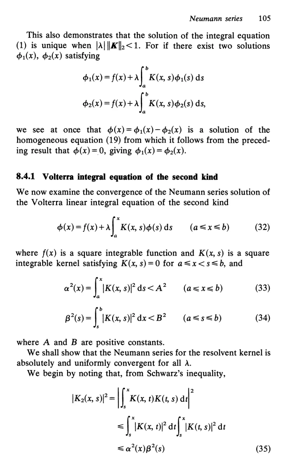
8.4 Neumann series 102
8.4.1 Volterra integral equation of the second kind 105
8.4.2 Bacher's example 109
8.5 Fredholm equation in abstract Hilbert space 109
Problems 111
9: Fredholm theory
9.1 Degenerate kernels 114
9.2 Approximation by degenerate kernels 120
9.3 Fredholm';, theorems 121
9.3.1 Fredholm theorems for completely continuous
operators . 125
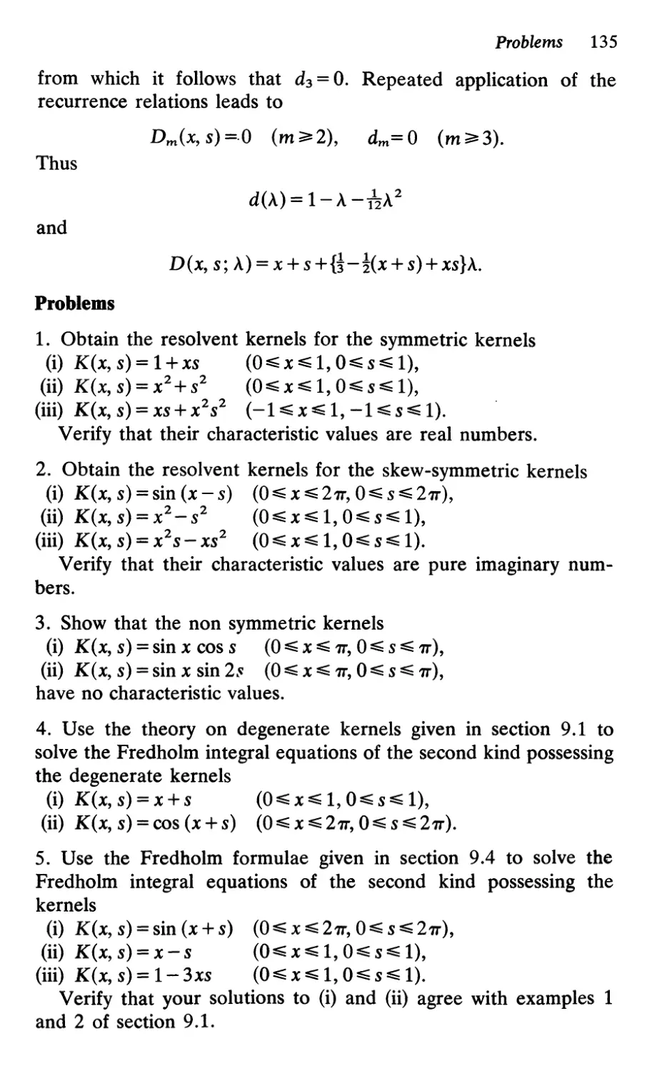
9.4 Fredholm formulae for continuous kernels 126
Problems 135
10: HUbert-Schmidt theory
10.1 Hermitian kernels
10.2 Spectrum of a Hilbert-Schmidt kernel
10 3 Expansion theorems
10.3.1 Hilbert-Schmidt theorem
10.3.2 Hilbert's formula
10.3.3 Expansion theorem for iterated kernels
10.4 Solution of Fredholm equation of second kind
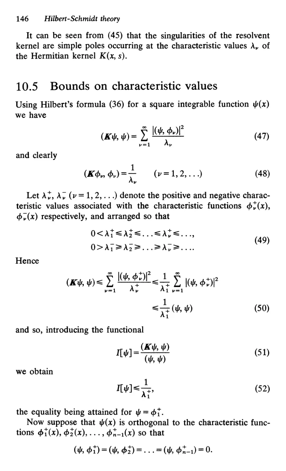
10.5 Bounds on characteristic values
10.6 Positive kernels
10.7 Mercer's theorem
10.8 Variational principles
10.8.1 Rayleigh-Ritz variational method.
Problems
Bibliography
Index
136
136
139
141
143
143
144
146
147
148
150
152
154
157
158
1
Classification
of integral equations
1.1 Historical introduction
The name integral equation for any equation involving the unknown
function cf>(x) under the integral sign was introduced by du Bois-
Reymond in 1888. However, the early history of integral equations
goes back a considerable time before that to Laplace who, in 1782,
used the integral transform
f( x) = {OO e -xs <I> (s) ds ( 1 )
to solve linear difference equations and differential equations.
In connection with the use of trigonometric series for the solution
of heat conduction problems, Fourier in 1822 found the reciprocal
formulae ,- 00
f(x) = \j { sin xs <I>(s) ds, (2)
<I>(s) = {OOSin xs f(x) dx (3)
and
f(x) = roo cos xs <I>(s) ds,
<I>(s) = roo cos xs f(x) dx
(4)
(5)
where the Fourier sine transform (3) and the cosine transform (5)
provide the solutions cf>(s) of the integral equations (2) and (4)
respectively in terms of the known function f(x).
In 1826 Abel solved the integral equation named after him
having the form
f(x) = f(x-s)-a<l>(s) ds (6)
where f(x) is a continuous function satisfying f(a) = 0, and 0 < a < 1.
2 Classification of integral equations
For a =! Abel's integral equation corresponds to the famous
tautochrone problem first solved by Huygens, namely the determi-
nation of the shape of the curve with a given end point along which
a particle slides under gravity in an interval of time which is
independent of the starting position on the curve. Huygens showed
that this curve is a cycloid.
An integral equation of the type
cf>(x) = f(x) + A r k'(x - s)cf>(s) ds (7)
in which the unknown function cf>(s) occurs outside as well as before
the integral sign and the variable x appears as one of the limits of
the integral, was obtained by Poisson in 1826 in a memoir on the
theory of magnetism. He solved the integral equation by expanding
cf>(s) in powers of the parameter A but without establishing the
convergence of this series. Proof of the convergence of such a series
was produced later by Liouville in 1837.
Dirichlet's problem, which is the determination of a function t/1
having prescribed values over a certain boundary surface Sand
satisfying Laplace's equation V 2 t/1 = 0 within the region enclosed by
S, was shown by Neumann in 1870 to be equivalent to the solution
of an integral equation. He solved the integral equation by an
expansion in powers of a certain parameter A. This is similar to the
procedure used earlier by Poisson and Liouville, and corresponds to
a method of successive approximations.
In 1896 Volterra gave the first general treatment of the solution
of the class of linear integral equations bearing his name and
characterized by the variable x appearing as the upper limit of the
integral.
A more general class of linear integral equations having the form
cf>(x) = f(x) + r K(x, s)cf>(s) ds (8)
which includes Volterra's class of integral equations as the special
case given by K(x, s) = 0 for s> x, was first discussed by Fredholm
in 1900 and subsequently, in a classic article by him, in 1903. He
employed a similar approach to that introduced by Volterra in 1884.
In this method the Fredholm equation (8) is regarded as the limiting
form as n 00 of a set of n linear algebraic equations
n
cf>(x r ) = f(x r ) + L K(x r , x s )cf>(x s )5n
s=1
(r = 1, . . . , n)
(9)
Linear integral equations 3
where 5n = (b - a)/n and X r = a + r5n. The solution of these equa-
tions can be readily obtained and Fredholm verified by direct
substitution in the integral equation (8) that his limiting formula for
n 00 gave the true solution.
1.2 Linear integral equations
Integral equations which are linear involve the integral operator
L = r K(x, s) ds (10)
having the kernel K(x, s). It satisfies the linearity condition
L [A 1 cP 1 (s ) + A 2 cP2 (s )] = AIL [ cP 1 (s ) ] + A 2 L [ cP2 (s ) ] ( 11 )
where
L[<f>(s)] = r K(x, s)<f>(s) ds
(12)
and Al and A2 are constants.
Linear integral equations are named after Volterra and Fredholm
as follows:
The Fredholm equation of the first kind has the form
f(x) = rK(X,S)<f>(S)dS (a x b) (13)
Examples are given by Laplace's integral (1) and the Fourier
integrals (2) and (4).
The Fredholm equation of the second kind has the form
<f>(x) = f(x) + r K(x, s)<f>(s) ds (a x b) (14)
while its corresponding homogeneous equation is
<f>(x) = r K(x, s)<f>(s) ds
(a x b)
(15)
The Volterra equation of the first kind has the form
f(x) = fK(X,S)<f>(S)dS (a x b) (16)
An example of such an equation is Abel's equation (6) which,
4 Classification of integral equations
however, has a special feature arising from the presence of a
singular kernel
K(x, s)=(x-s)-a
(0 < a < 1)
with a singularity at s = x.
The Volterra equation of the second kind has the form
<f>(x) = f(x) + r K(x, s)<f>(s) ds
(a x b)
(17)
We see that the Volterra equations can be obtained from the
corresponding Fredholm equations by setting K(x, s) = 0 for
a x < s b.
It can be readily seen also that the Volterra equation (16) of the
first kind can be transformed into one of the second kind by
differentiation, for we have
f x a
f'(x) = K(x, x)cf>(x) + - K(x, s)cf>(s) ds
a ax
so that provided K(x, x) does not vanish in a x b we obtain
f'(x) f X [ a ]
<f>(x) = K(x, x) a ax K(x, s)/ K(x, x) <f>(s) ds
1.3 Special types of kernel
1.3.1 Symmetric kernels
Integral equations with symmetric kernels satisfying
K(s, x) = K(x, s)
(18)
possess certain simplifying features. For this reason it is valuable to
know that the integral equation
o/(x) = g(x) + r P(x, s)/L(s)o/(s) ds
(19)
with the unsymmetrical kernel P(x, s)f.L(s), where however
P(s, x) = P(x, s), can be transformed into the integral equation (14)
with symmetric kernel
K(x, s) = f.L(x) P(x, s) f.L(s) (20)
Special types of kernel 5
by multiplying (19) across by .J I-L(x) and setting
cf>(x) = .J I-L(x) t/1(x) (21)
and
t(x) = .J I-L(x) g(x).
(22)
Real symmetric kernels are members of a more general class
known as Hermitian kernels which are not necessarily real and are
characterized by the relation
K(s, x) = K(x, s),
(23)
the bar denoting complex conjugate. We shall investigate the prop-
erties of integral equations with Hermitian kernels in chapter 10.
1.3.2 Kernels producing convolution integrals
A class of integral equation which is of particular interest has a
kernel of the form
K(x, s) = k(x - s)
(24)
depending only on the difference between the two coordinates x and
s. The type of integral which arises is
L: k(x - s )cf>(s) ds
(25)
called a convolution or folding. This nomenclature comes from the
situation which occurs in Volterra equations where the integral (25)
becomes
r k(x - s)cf>(s) ds
(26)
and the range of integration can be regarded as if it were folded at
s = x/2 so that the point s corresponds to the point x - s as shown in
Fig. 1.
o
:
s
:
);
x
x-s
Fig. 1. Convolution or folding
6 Classification of integral equations
Integral equations of the convolution type can be solved by using
various kinds of integral transform such as the Laplace and Fourier
transforms and will be discussed in detail in chapter 3.
1.3.3 Separable kernels
Another interesting type of integral equation has a kernel possessing
the separable form
K(x, s) = AU(X)V(s)
(27)
The Fredholm integral equation of the second kind (14) now
becomes
<f>(x) = f(x)+ AU(X) r v(s)<f> (s) ds
and can be readily solved exactly. Thus we have, on multiplying (28)
(28)
across by v(x) and integrating:
r v(x)<f> (x) dx = r v(x) f(x) dx + A r v(x) u(x) dx r v(s)<f> (s) ds
which gives
J b v(x) <f>(x) dx = S v x) dx
a 1- AS v(x)u(x) dx
(29)
so that
<f>(x) = f(x) + AU(X)J f(s) ds (30)
1- AS v(t)u(t) dt
We see that the solution (30) can be expressed in the form
<f>(x) = f(x) + A r R (x, s; A)f(s) ds (31)
where
R( . \ ) = u(x)v(s)
X,S,I\ -
1- AS v(t)u(t) dt
and is called the solving kernel or resolvent kernel.
(32)
Special types of kernel 7
The homogeneous equation (15) ,corresponding to (14) becomes
in the present case
cf>(X) = AU(X) r V(S ) cf>(S) ds.
The solution cP(x) of equation (33) must satisfy
(33)
r v(x) cf>(x) dx = A r v(x) u(x) dx r v(s)cf> (s) ds
The values of A for which the homogeneous equation has solutions
are called characteristic values. There exists just one value of A for
which (33) possesses a solution. This characteristic value Al is given
by
1 = Ai r v(x) u(x) dx,
the associated characteristic solution of (33) being cPl(X) = cu(x)
where c is an arbitrary constant.
The simple separable form (27) is a special case of the class of
degenerate kernels
(34)
n
K(x, s) = A L Ui(X) Vi(S)
i=l
(35)
gIvIng rise to integral equations which can be solved In closed
analytical form as we shall show in chapter 9.
Example 1. As a simple illustration of an integral equation with
separable kernel (27) we consider
cf>(x) = 1 + A r xscf>(s) ds (36)
Here f(x) = 1, K(x, s) = AXS and so u(x) = x and v(s) = s. It follows
that the resolvent kernel is
xs
R (x, s; A) = 1 _ A S5 t 2 d t
xs
(37)
1 - A/3
8 Classification of integral equations
and hence the solution to (36) is
AX [1
cf>(X) = 1 + 1 _ A/3 Jo s ds
=1+ 3h (A 3)
2(3 - A)
(38)
Example 2. Another example of an integral equation with a separ-
able kernel is
cf>(X) = eX + A r eia(x-s)cf>(s) ds
(39)
where f(x) = eX, K(x, s) = Aeia(x-s) so that u(x) = e iax and v(s) = e ias
Then the resolvent kernel is
e ia(x-s)
R(X,S;A)= I-A
(40)
and hence the solution of (39) is
Ae iax i 1 .
cf>(x) = eX + e(1-1a)s ds
I-A 0
AeiaX(el-ia -1)
=e x +
(1- A)(I- ia)
(41)
1.4 Square integrable functions and kernels
Functions cf>(x) which are square integrable in the interval a x b
satisfy the condition
flcf>(XW dx <00
(42)
where the integral is taken to be Riemann, or Lebesgue for greater
generality. In the former case it is said that cf>(x) is an R 2 function
and in the latter case that it is an L 2 function. Continuous functions
are square integrable over a finite interval since they are bounded.
However the converse is not necessarily true, that is square integra-
ble functions need not be continuous or bounded.
Kernels K(x, s) defined in a x b, a s b are said to be
square integrable if they satisfy.
r fIK(X, sW dx ds<oo (43)
Singular integral equations 9
together with
fIK(x, sW ds <00
(a x b)
(44)
and
fIK(x, sWdx<oo
(a s b)
(45)
where the integrals are taken to be Riemann or Lebesgue. The
kernel is then called R 2 or L 2 respectively.
Kernels of particular interest are those which are singular. Thus
consider a Volterra kernel of the form
F(x, s)
K(x,s)= (x-s)a
o (x < s)
where F(x, s) is a continuous function and 0< a < 1. Then IF(x, s)1 M
where M is a constant and so
(x> s)
(46)
f b f b 2 f b f x 1 F( x, s) 1 2
a a IK(x, s)1 dx ds = a dx a ds (X _ S)201
:so: M 2 f dx r ds(x - S)-201
M 2 f b
= dx(x - a)1-2a
1-2a a
M 2 (b _ a)2-2a
2(1- 2a)(1- a)
(a < !)
(47)
and so the double integral is finite if 0 < a <!. However if a ! the
singular kernel (46) is not square integrable.
1.5 Singular integral equations
An integral equation of the type
cf>(x) = f(x) + A r K(x, s )cf>(s) ds
(48)
is said to be singular if the range of definition is infinite e.g.,
0< x < 00 or -00 < x < 00, or if the kernel is not square integrable.
10 Classification of integral equations
Non-singular equations have a discrete spectrum, that IS the
associated homogeneous equation
cf>(X) = A r K(x, s )cf>(s) ds
(49)
has non-trivial solutions cPv(x) for a finite or at most a countable,
although infinite, set of characteristic values Av of the parameter A.
Also each characteristic value Av has a finite rank (or index), that is
it has a finite number of linearly independent characteristic func-
tions cP l)(X),..., cP )(x).
However if the integral equation is singular by virtue of having an
infinite range of definition, the spectrum of values of A may include
a continuous segment. For example it may be readily verified that
the homogeneous equation
cf>(x) = A L e-1x-s1cf>(s) ds
(50)
has solutions of the form
cP(x) = cle- v'1-2,\, X+ c2e v'1-2,\, X
(51)
for the continuous spectrum of values 0 < A < 00. Equation (50) is of
the convolution or difference type and will be discussed further in
section 3.2 of the chapter on integral equations of the convolution
type.
Also if the integral equation has an infinite range of definition the
characteristic values may have an infinite rank. Thus consider the
equation
cf>(x) = A [00 cos xs cf>(s) ds
(52)
with kernel
K(x, s) = cos xs
Using the Fourier cosine transform (5) and its reciprocal formula (4)
we have
(53)
Acf>(x) = [00 cos xs cf>(s) ds
and so
cf>(X) = A 2cf>(X)
Non-linear equations 11
giving A 2 = 1, or A = :f: 1 as characteristic values. Their ranks are
infinite since it can be shown without difficulty that
( ) 1'7T -ax a ( )
cf> x = -V 2 e :f: a 2 +x2 x >0
(54)
are characteristic functions corresponding to the characteristic val-
ues A = :f: 1 for all values of a> O. The kernel (53) belongs to a class
of singular kernels known as Weyl kernels.
1.6 Non-linear equations
In the case of non-linear equations, the spectrum of characteristic
values A may have the interesting property that the number of
solutions of the integral equation changes as we pass through
particular values of A known as bifurcation points.
As an example we consider the simple non-linear equation
cf>(x) - A[ s{ cf>(s)Y ds = 1
(55)
and investigate its real solutions cf>(x). We put
[S{cf>(S)}2 ds = a
(56)
in which case we have
cf>(x) = 1 + Aa
(57)
so that
a = (1 + Aa)2 [s ds = t(1 + Aa)2
This yields
A 2 a 2 +2(A-1)a + 1 = 0
(58)
which gives
1- A :f:v'(A -1)2- A 2
a= 2
A
(59)
Hence
1 :f: v' 1- 2A
cf>(x) = A .
(60)
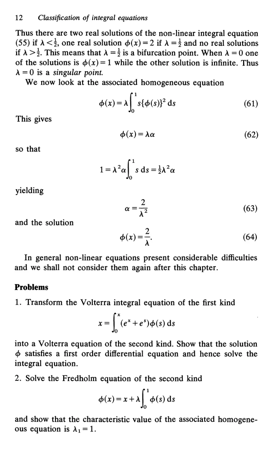
12 Classification of integral equations
Thus there are two real solutions of the non-linear integral equation
(55) if A <!, one real solution cP(x) = 2 if A =! and no real solutions
if A >!. This means that A =! is a bifurcation point. When A = 0 one
of the solutions is cP(x) = 1 while the other solution is infinite. Thus
A = 0 is a singular point.
We now look at the associated homogeneous equation
cp(x) = A[ s{cp(S)}2 ds
(61)
This gives
cP(x) = Aa
(62)
so that
1 = A 2 a {\ ds =!A 2a
yielding
2
a=-
A 2
(63)
and the solution
2
cP(x) =-.
A
(64)
In general non-linear equations present considerable difficulties
and we shall not consider them again after this chapter.
Problems
1. Transform the Volterra integral equation of the first kind
x= f(ex+eS)cp(S)dS
into a Volterra equation of the second kind. Show that the solution
cP satisfies a first order differential equation and hence solve the
integral equation.
2. Solve the Fredholm equation of the second kind
cp(x) = x + A[ cp(s) ds
and show that the characteristic value of the associated homogene-
ous equation is A 1 = 1.
Problems 13
3. Solve the Fredholm equation
cp(x) = 1 + A[ eX+scp(s) ds
and show that the characteristic value of the associated homogene-
ous equation is At = 2/( e 2 -1).
4. Solve the Fredholm equation
cp(x) = 1 + A[xnsmcp(s) ds
and show that the characteristic value of the associated homogene-
ous equation is At = m + n + 1.
5. Solve the Fredholm equation
cp(x) = x + AfT sin nx sin ns cp(s) ds
where n is an integer, and show that the characteristic value of the
associated homogeneous equation is At = 2/11'.
6. Show that the singular integral equation
cp(x) = A -J! rOSin xs cp(s) ds
has characteristic solutions
( ) r;. -ax X
cf> X = -V "2 e :f: a 2 + X2
associated with characteristic values A = :f: 1 for all a > O.
(X> 0)
7. Solve the non-linear equation
cp(x) = 1 + A[{cp(S)}2 ds
and show that A = * is a bifurcation point while A = 0 is a singular
point of the spectrum of characteristic values.
2
Connection with
differential equations
2.1 Linear differential equations
We first observe that the first order differential equation
dcf>
dx = F(x, cf»
(a x b)
(1)
can be written immediately as the Volterra integral equation of the
second kind
cp(x) = cp(a)+ r F[s, cp(s)] ds.
(2)
As an interesting but simple example of the above we consider
the following problem, solved by Johannes Bernoulli for the n = 3
case:
To find the equation y = cf>(x) of the curve joining a fixed origin
o to a point P such that the area under the curve is l/nth of the
area of the rectangle OXPY having OP as diagonal for all points P
on the curve (see Fig. 2).
Evidently this problem is equivalent to solving the homogeneous
V olterra integral equation of the second kind
I x 1
cf>(s) ds = - xcf>(x)
o n
(3)
for the unknown function cf>(x) where c/>(O) = O.
This equation can be solved by converting it into the differential
equation
1
<!>(x) = - {<!>(x) + x<!>'(x)}
n
Linear differential equations 15
y p
V
o
<P (x)
<P (s)
s
x
x
Fig. 2. Bernoulli's problem for n = 3; y = x 2 .
or more simply
n-1
cf>'(x) = cf>(x)
x
(4)
which has the solution
<f>(x) = Ax n - 1
(5)
For the case n = 3 solved by Bernoulli the curve is a parabola
y = Ax 2 .
We next consider the second order differential equation
d 2 <f>
dxz =F(x,cP) (a x b) (6)
16 Connection with differential equations
which can be expressed as
4>(x) = 4>(a) + (x - a)4>'(a) + r (x - s)F[s, 4>(s)] ds, (7)
this particular form being obtained on carrying out an integration by
parts.
Taking a = 0 and b - a = I this may be rewritten as
4>(x) = 4>(0) + 4>( I) - 4>(0) x
I
+ f(X - s)F[s, 4>(s)] ds +} r (s -l)F[s, 4>(s)] ds (8)
sInce
14>'(0)= 4>(1) - 4>(0) + r (s -1)F[s, 4>(s)] ds.
If the differential equation is linear and we write
F[x, cf>(x)] = r(x) - q(x)cP(x)
(9)
we obtain the Fredholm integral equation of the second kind
4>(x) = f(x)+ r K(x, s)q(s)4>(s) ds
(10)
where
cf> ( I) - cf> ( 0 ) i I
f(x) = 4>(0) + 1 x - 0 K(x, s)r(s) ds
(11)
and
K(x, s) =
s(l-x)
1
x(l- s)
I
(s x)
(s x)
(12)
In the particular case of a flexible string having mass p (x) per unit
length, stretched at tension T and vibrating with angular frequency
w, we have q(x) = w 2 p(x)/T and r(x) = O. If the string has fixed ends
at x = 0 and I, the transverse displacement cP(x) satisfies cP(O) = cP(l) = 0
so that f(x) = O. Thus we arrive at the homogeneous Fredholm
Linear differential equations 17
integral equation
cf>(x) = r K(x, s)q(s)cf>(s) ds
(13)
An important distinction between the differential equation and
the equivalent integral equation approach should be observed. In
the case of the differential equation formulation of a physical
problem the boundary conditions are imposed separately whereas
the integral equation formulation contains the boundary conditions
implicitly. Thus, for example, we see at once from (13) and (12) that
cf>(x) vanishes at x = 0 and x = I.
Let us now consider the second order linear differential equation
Lv(x) = r(x)
(0 x I)
(14)
where L is the linear differential operator given by
L= d {P(X) ddJ +q(x)
(15)
and p(x) has no zeros in the range of definition 0 x I.
We shall treat this equation somewhat differently from the previ-
ous equations by setting
dZv
cf> (x) = dx z .
(16)
Then we have
dv r x
dx = v'(O) + Jo cf>(s) ds
(17)
and
v (x) = v (0) + xv' (0) + r (x - s) cf> (s) ds,
from which it follows that the differential equation may be ex-
pressed as the Volterra integral equation of the second kind
(18)
cf>(x) = f(x) + r K(x, s)cf>(s) ds
(19)
where
f(x) = {p(x)}-l[r(x) - v'(O)p'(x) -{v(O) + xv'(O)}q(x)] (20)
18 Connection with differential equations
and
K(x, s) = {p(X)}-l[(S - X)q(X) - p'(X)].
(21)
2.2 Green's function
We consider the second order linear differential equation
Lv(x) = r(x)
(a x b),
(22)
where L is the linear differential operator (15), and suppose that its
solution v(x) satisfies homogeneous boundary conditions at x = a
and x = b, namely
av(a) + {3v'(a) = 0
av(b) + {3v'(b) = 0
(23)
where a and {3 are prescribed constants.
Let
LVi(X)=O
(i=1,2)
(24)
where Vl(X) and V2(X) are two linearly independent functions which
satisfy the boundary conditions (23) prescribed at x = a and b
respectively. We shall show that the solution of (22) may be
expressed in the form
v(x) = r G(x, s)r(s) ds
(25)
where
G(x, s) =
1
A Vl(X)V2(S)
1
A V2(X)Vl(S)
(x s)
(x s)
(26)
and A is a certain constant. G(x, s) is called the Green's function.
The method we shall use involves the Dirac delta function 8(x)
which vanishes for x 0 and satisfies
r 8(x-s)r(s) ds = r(x)
(27)
Clearly 5(x) is not a function as defined in the usual sense but
Green's function 19
belongs to a class known as generalized functions. A useful represen-
tation of the Dirac function is
8(x) = lim I(h, x)
h O
(28)
where I(h, x) is the impulse function defined as
1
I(h, x) = h
o
(O x h)
otherwise.
(29)
Thus the representation (28) vanishes for x ¥= 0 and has infinite
magnitude at x = O. Further
lim f oo I(h, x) dx = 1, (30)
h 0 -00
since the integral is unity for all values of h, and we write this as
L 8(x)dx=1
(31)
although care has to be exercised when interchanging the order of
the limiting operation and the integration.
Now (25) has to provide a solution of (22) and so
LG(x, s) = 8(x - s). (32)
It follows that
r S + B
! Js-e LG(x, s) dx = 1
(33)
which leads to
[ a ] X=S+B 1
lim - G(x, s) =-,
B O ax X=S-B p(s)
(34)
that is,
Vl(S)V (S)-V2(S)vHs) = p )
(35)
or
Vl (s)
V (s)
V2(S)
v (s )
A
-
p(s)
(36)
20 Connection with differential equations
where the determinant on the left-hand side is called the Wronskian.
For A to be non-vanishing it is evident that Vl and V2 must be
linearly independent.
As a simple example we consider the operator
d 2
L=-c- (O x l) (37)
dx 2
and the end conditions v(O):c v(l) = O. Then p(x) = -c and Vl(X) = x,
V2(X) = 1- x so that A = cl giving for the Green's function
x(l- s)
cl
G(x, s) =
(1- x)s
cl
(x s)
(x s)
(38)
2.3 Influence function
.
We consider a string of length 1 at tension T. The displacement
G(x, s) of the string at the point with coordinate x, resulting from
the application of a unit force perpendicular to the string at the
point with coordinate s, is called the influence function.
Now the displa ement G(s, s) of the string at the point s,
assumed to be small, satisfies the equilibrium equation (see Fig. 3):
TG(S,S) e + ,1S )=1
(39)
which yields
G( ) = s(l-s)
s, s Tl
and so it follows that the influence function is given by
x(l- s)
TI
s(l- x)
Tl
(40)
G(x, s) =
(x s)
(x s)
(41)
o s L
Fig. 3. Displaced string.
Influence function 21
Comparison with (38) shows that the influence function 'derived above
is just the Green's function for the linear differential operator
d 2
L=-T-
dx 2
(42)
Now suppose that we apply a loading force F(x) per unit length
to the string. Then the displacement of the string at the point with
coordinate x is given by
cf>(x) = r G(x, s)F(s) ds
(43)
using the principle of superposition. In the case of a horizontal wire
at tension T, possessing mass p(x) per unit length, the loading due
to the force of gravity is F(x) = -gp(x) and so the displacement of
the wire becomes
cf>(x) = - g r G(x, s )p(s) ds.
(44)
As a further example we consider a shaft of length I and mass
p(x) per unit length. If the loading at the point with coordinate s is
given by F(s) per unit length and G(x, s) is the influence function of
the shaft, then the displacement ck(x) at the point x is again given by
(43). Let us now suppose that the shaft is rotating with angular
velocity w. Then the loaqiag due to the rotation is given by the
centrifugal force
- F(s) = w 2 p(s)cp(s),
(45)
and so we obtain the following homogeneous integral equation for
the displacement of the shaft
cf>(x) = w 2 r G(x, s)p(s)cf>(s) ds
(46)
The balancing of the elastic and centrifugal forces can occur only
for certain discrete values of w known as the critical speeds which
correspond to values of w 2 for which the integral equation (46) has
non-vanishing solutions, that is its characteristic values.
22 Connection with differential equations
Problems
1. Solve the Volterra equations of the second kind
(i) cf>(x) = 1 + r cf>(s) ds
(ii) cf>(x) = 1 + 2 r scf>(s) ds
by finding the solutions of the equivalent differential equations.
2. Solve the Volterra equation
xcf>(x) = x n + r cf>(s) ds
3. Solve the Volterra equation
cf>(x) = f(x) +,\ r (x - s)cf>(s) ds
for (i) f(x) = 1, (ii) f(x) = x and A = :t: 1.
4. Solve the Volterra equation
cf>(x) = f(x) +,\ r sin (x - s)cf>(s) ds
for (i) f(x) = x and A = 1, (ii) f{x) = e- x and A = 2.
5. Show that the Volterra equation of the first kind
fX(x-s)n-l
f(x) = Jo (n -1)! cf>(s) ds
has the continuous solution cP(s) = f(n)(s) when f(x) has continuous
derivatives f'(x), f"(x),..., f(n)(x), and f(x) and its first n-1
derivatives vanish at x = o.
6. Show that the nth order linear differential equation
dny n dn-ry
d n -'\L a,.(x) d n-r - f(x)
X r=l X
where y(O) = y'(O) = · · · = y(n-l)(o) = 0, is equivalent to the Volterra
Problems 23
equation of the second kind
r x n a (x)(x-s)r-l
«f>(x) = f(x) + A Jo r l r (r-1)! «f>(s) ds
where cP(x) = dny/dx n .
7. Show that the solution of the differential equation
d2cP
+ W2cP = F[x, cP(x)] (O x l)
dx
obeying the end conditions cP(O) = cf>(l) = 0, satisfies the integral
equation
«f>(x) = r G(x, s)F[s, «f>(s)] ds
where
G( ) = { -(w sin wl)-l sin wx sin w.(l- s) (x s)
x, s -(w sin wl)-l sin w(l- x) sin ws (x s)
is the Green's function for the linear differential operator d 2 /dx 2 + w 2 .
3
Integral equations
of the convolution type
In the present chapter we shall be concerned with integral equations
whose kernels have the form
K(x,s)=k(x-s)
(1)
which is a function only of the difference between the two coordi-
nates x and s. The method of solution generally involves the use of
integral transforms. Hence before proceeding to consider the vari-
ous kinds of convolution type integral equations we shall briefly
discuss the more important forms of integral transform.
3.1 Integral transforms
We have already mentioned Laplace and Fourier transforms in the
historical introduction given in chapter 1.
The Laplace transform of a function cP(x) is given by
<I>(u) = l°Oe-uxq,(X)dX (2)
and the basic result which enables us to solve integral equations of
the convolution type is the convolution theorem which states that if
K(u) is the Laplace transform of k(x) then K(u)<I>(u) is the Laplace
transform of
r k(x - s)q,(s) ds (3)
To verify that this is correct, without any attempt at a rigorous
argument, we see that the Laplace transform of (3) is
1 00 e- UX dx r k(x - s)q,(s) ds = 1 00 e-utk(t) d{OO e-USq,(s) ds
= K(u)<I>(u)
on setting t = x - s and noting that we may take k(x) to vanish for
x<O.
Integral transforms 25
In addition to the sine and cosine transforms (2) and (4) referred
to in section 1.1, we have the exponential Fourier transform of a
function cP (x) defined as
<I>(u) = foo e iux 4>(x) dx' (4)
v2Tr -00
and the reciprocal formula
1 f oo .
cP(x) = r;:- e-1UX<I>(u) duo
v 2Tr -00
Then, if K(u) is the Fourier transform of k(x), the convolution
theorem for Fourier transforms states that .J2Tr K(u)<I>(u) is the
Fourier transform of
(5)
L k(x - s)4>(s) ds (6)
which can be easily verified as for the Laplace transform.
Another valuable integral transform is the Mellin transform
<1>( u) = [00 x U - l 4>(x) dx (7)
and the corresponding convolution theorem states that K(u)<I>(l- u)
is the Mellin transform of
[00 k(xs)4>(s) ds
where K(u) is the Mellin transform of k(x). In fact, again without
any attempt at rigour, we have that the Mellin transform of (8) is
[00 x u - 1 dx [00 k(xs)4>(s) ds = [00 t u - 1 k(t) d{OO s-u4>(s) ds
= K(u)<I>(l- u)
(8)
on setting t = xs.
Throughout the following sections we shall assume that all the
functions arising in the integral equations satisfy suitable conditions
which permit all the transformations to be performed with validity.*
* For details see E. C. Titchmarsh, Introduction to the Theory of Fourier
Integrals, 2nd ed., Oxford University Press, 1948.
26 Integral equations of the convolution type
3.2 Fredholm equation of the second kind
We consider firstly Fredholm equations of the type
cf>(x) = f(x)+ f k(x - s)cf>(s) ds (-00< X <00) (9)
A formal solution of this equation can be obtained by introducing
the Fourier transforms
1 f oo
<I>(u) = - eiUX<f>(x) dx,
J2; -00
1 f oo
F(u) = r:::- eiUXf(x) dx,
"2,,, -00
1 f oo
K(u) = r:::- eiUXk(x) dx.
"2,,, -00
Using the convolution theorem
(10)
(11)
(12)
1 f oo
K(u)<I>(u) = T r;:- k(x - s)c/>(s) ds
"2,,, -00
(13)
where T denotes the Fourier integral operator
1 f oo
T=- e iux dx
J2; -00 '
(14)
we obtain
<I>(u) = F(u) + 2", K(u)<I>(u)
(15)
as a result of operating with T on both sides of (9). This gives
<I>(u) = F(u)
1- ../2", K(u)
(16)
which provides the solution to the integral equation (9) in the form
<f>(x) = T- 1 [<I>(u)]
1 f oo e-iXUP(u)
= J2Tr -00 1- ../2Tr K(u) du
(17)
on using the reciprocal formula (5).
Fredholm equation of the second kind 27
Let us now consider the homogeneous equation
4>(x) = L k(x - s)4>(s) ds.
(18)
The solution to this can be written
n
cP(x) = L L cv,pxP-le-iwvX
v p=l
(19)
where the cv,p are constants, the W v are the zeros of 1- .J2'Tr K(u)
and n is the order of the multiplicity of the zero W v .
Thus we have that
1 = L k(t)eu"pt dt
(20)
on setting u = W v in (12), and
o = L k(t)tP-1ei"'pt dt
(p = 2, . . . , n)
(21)
on differentiating both sides of (12) p -1 times with respect to u and
setting u = W v . Hence
f 00 ( t ) P-l
1 = Lx> k(t) 1- x eu"pt dt
(22)
and so, setting t = x - s, we obtain
xp-1e-i"'px = L k(x - s)sP-1e-u"ps ds (23)
which shows that each term in the sum on the right-hand side of
(19) is a solution of (18).
Example 1.
As a first example we consider the case
f(x) = e- 1xl
k(x) = {,\ x
(x < 0)
(x >0)
(24)
(25)
Then
F(u) = fco e-lxl+iUX dx
J2; -00
12 1
=V ; 1+u 2
(26)
28 Integral equations of the convolution type
while
K(u) = r e X + iUX dx
5;, -r¥J
A 1
-
5;, 1 + iu
(27)
and so it follows that the solution is given by
1 f r¥J e-iXu du
4>(x) = 7T -co (1- iu)(1-'\ + iu)
Then if 0 < A < 1 we may apply Cauchy's residue theorem to
evaluate this integral obtaining the particular solution
(28)
2e- x
cP(x)= 2-'\
2e(l-A)X
2-A
(x > 0)
(x < 0)
(29)
Since there is just one zero, having order of multiplicity 1, of
1- v'21T K(u) = (1- A + iu)/(l + iu) at u = i(l- A), it follows
that the solution of the associated homogeneous equation
4>(x) = ,\ l co e x - s 4>(s) ds
(30)
is just
cP(x) = Ce(l-A)X
as can be readily verified by inspection.
Hence the general solution is given by
2e- x C (l-A)X
+ e
cP(x)= 2-A
( 2 + C ) e(l-A)X
2-A
(31)
(x > 0)
(x < 0)
(32)
where A is confined to the range of values 0 < A < 1.
Example 2. As a second example we discuss the Lalesco - Picard
equation for which
k(x) = Ae- ixi .
(33)
Fredholm equation of the second kind 29
We shall suppose that -f(x) and hence F(u) are unknown, in
which case it is convenient to rewrite the solution (17) in the form
cf>(x) = f(x)+ t: e-iXUP(u)M(u) du
(34)
where
M(u) = K(u)
1-fu K(u)
(35)
and
1 J oo .
f(x) = r:::- e-JXUP(u) duo
v 2", -00
(36)
For then we have, using the convolution theorem for Fourier
transforms
t: e-ixUP(u)M(u) du = t: f(u)m(x - u) du (37)
where
1 J oo .
m(x) = r;:- e-JXUM(u) du,
v 2", -00
(38)
that the solution (34) is given by
cf>(x) = f(x)+ t: f(u)m(x - u) duo
(39)
Now in the present example
K(u)= J'" Ae-lxl+iUX dx
fu -00
= 1:u 2 '
(40)
and so
-
2 A
M(u)= 1T1+u 2 -2A
(41)
30 Integral equations of the convolution type
from which it follows that
1 roo Ae -ixu
m(x) = 1T Lo 1 + u2-2'\ du
A - v'1-2A Ixl
- 1-2A e
(42)
provided A <! and using Cauchy's residue theorem. Hence a par-
ticular solution of the integral equation is
4>(x) = !(x) + ,\ foo !(u)e- v'1-2,\ lx-u l duo (43)
1-2A -00
Turning our attention to the homogeneous equation
4>(x) =,\ L e- 1x - sl 4>(s) ds
(44)
we note that there are two zeros, both having multiplicity of order 1,
of
1+u 2 -2A
1-.J2; K(u) = 1 2
+u
(45)
at u = :t:i l- 2A, so that the solution of (44) takes the form
cP(x) = Cl e - v'1-2A X + c2e v'1-2A X
(46)
where, fo r the i ntegral occurring in (44) to have a meaning, the real
part of 1 - 2A must satisfy
Re 1-2A< 1. (47)
Thus all values of A in the range 0 < A < 00 are allowed, but if A >!
the solution may be more suitably written as
cP(x) = alsin( 2A-1 x)+a2cos( 2A-1 x). (48)
However when A =!, 1- 2Tr K(u) has a single zero at u = 0 with
multiplicity of order 2 in which case the general solution of the
homogeneous equation is
cP(x) = Cl + C2 X .
(49)
V olte"a equation of the second kind 31
3 .3 Volterra equation of the second kind
If we set f(x)=O, k(x)=O, and cf>(x) =0 for x<O in the Fredholm
equation (9) of the second kind considered in section 3.2 we obtain
the integral equation
</>(x) = f(x)+ r k(x -s)</>(s) ds
(x > 0)
(50)
which is a V olterra equation of the second kind with a convolution
type integral.
Equation (50) can be solved most conveniently by introducing the
Laplace transforms
cI>(u) = ro e- UX </> (x) dx,
F( u) = {'" e -UXf( x) dx,
K(u) = r"" e-UXk(x) dx.
Jo .
(51)
(52)
(53)
Applying the convolution theorem for Laplace transforms
K(u)cI>(u) = L r k(x - s)</>(s) ds
. 0
. .
(54)
where L denotes the Laplace integral operator
L = L"" e- ux dx,
(55)
we find that
cI>(u) = F(u) + K(u)cI>(u)
(56)
which yields
F(u)
cI>(u) = 1- K(u)
= F(u)+ F(u)M(u)
(57)
where
M(u) = K(u)
1- K(u)"
(58)
32 Integral equations of the convolution type
Hence the solution of (50) can be written as
«(>(x) = f(x) + r m(x - s)f(s) ds
(59)
where
M(u) = I'O e-UXm(x) dx.
(60)
Example 1. We examine first the simple case where the kernel is
k(x) = { x
(x > 0)
(x < 0)
(61)
Then we have
1 00 A-
K(u)=A- e- ux xdx=2
o u
(62)
so that
A-
M(u)= 2 A-
u -
( 1 1 )
=2 u- -u+
(63)
and hence
( ) ( .J>...x - X )
mx=-e -e .
2
(64)
Thus the solution to the integral equation (50), as given by (59), is
«(>(x)=f(x)+ fXf(s){e (X-S)_e- (X-S)}ds (65)
2 Jo
Example 2. Our next example has the kernel
k(x) = {A X
(x >0)
(x < 0)
(66)
Then
1 00 A
K(u) = A- e(1-u)x dx =-
o u-l
(67)
Volterra equation of the second kind 33
so that
A
M ( u ) -
. u-(A+1)
(68)
and hence
m(x) = Ae(A+l)x. (69)
Thus, using (59) the solution of the integral equation (50) is
«(>(x) = f(x) + Af f(s)e(Hl)(X-S) ds (70)
Example 3. Our last example has the kernel
k(x) = { A s o in x (x > 0) (71)
(x < 0)
Then
1 00 A
K(u) = A e- ux sin x dx = 2 1
o u +
(72)
and so
A
M ( u ) -
- u 2 +1-A
(73)
which yields
A sin ( .J 1- A x)
.J 1-A (A < 1)
m(x) = AX (A = 1)
A
../ sinh ( ../ A -1 x) (A > 1)
A-I
(74)
on using the appropriate Laplace transform formulae. Hence the
solution of the integral equation (50) is given by
A J x
../ f(s) sin { ../ 1- A (x-s)} ds
I-A 0
«(>(x)-f(x)= ff(S)(X-S)dS
A J x
../A-1 0 f(s)sinh{ ../ A-1 (x-s)}ds
(A < 1)
(A = 1)
(A > 1)
(75)
34 Integral equations of the convolution type
3.4 Fredholm equation of the first kind
Here we are concerned with Fredholm equations of the form
f(x) = t: k(x - s )cf>(s) ds
(76)
with an integral of the convolution type on the right-hand side. To
solve this equation we take Fourier transforms. On applying the
convolution theorem (13) this yields
F(u) =.J2; K(u)cI>(u)
(77)
which leads to the formal solution of (76):
1 f oo .
cf>(x) = r;:- e -IXUcI>(u) du
"" 21T -(X)
= roo e- ixu F(u) duo
21T J-oo K(u)
(78)
3.4.1 Stieltjes integral equation
An interesting example of a Fredholm equation of the first kind
possessing a convolution type integral is obtained by applying
Laplace's integral operator
LOO e- xs ds
twice. Thus consider the equation
g(x) = A Loo e- xt d{OO e-tsl{I(s) ds.
(79)
Then, on reversing the order of the integrations, we see that
g(x) = A Loo l{I(s) ds Loo e -(x+s)t dt
= A L oo l{I(s) ds (80)
x+s
which is known as Stieltjes integral equation.
Now setting
x- = e- , s = eO", e1/2 g(e ) = f( ), el/2 t/J(e ) = cf>( ) (81)
Fredholm equation of the first kind 35
we obtain
A f oo cf>(u)
f( ) = 2 h .!( _ ) du.
-00 COS 2 U
(82)
This is a Fredholm equation of the first kind with kernel
A
k( )= 2 hl '
cos 2:
(83)
To solve (82) we require to find the Fourier transforn1 of k( )
which is given by
A f oo eiu
K(u)=- d
J2; -00 e 1/2 + e -1/2
A 1 00 Xiu-(1/2)
=- dx
J2; 0 l+x
(84)
on putting x = e . But it is well known that
1 00 a-1
X dx = '1T
o 1 + x sin '1Ta
(85)
and so we obtain
A ; A ; A ;
K(u) = = = (86)
sin {'1T(iu + !)} cos i'1TU cosh '1TU
Now, making use of the solution (78) to the equation (76), we see
that the solution of our integral equation (82) may be written as
4>( ) = f"" F(u) cosh 1TU e-il;u du
A'1T 2 '1T -00
= 1 f"" F(u){e-i(I;HJT)U + e-i(!;-i....)U} du (87)
2 '1T A J2; -00
where F(u) is the Fourier transform of f( ). Thus
1
cf>( ) = 2'1TA {f( + i'1T) + f( - i'1T)}
(88)
and hence the solution to Stieltjes integral equation (80) is
l . .
tfJ(x) = 2'1TA {g(xel'IT) - g(xe-I'IT)}.
(89)
36 Integral equations of the convolution type
Example. Suppose that
x
In-
a
g(x)= x-a
1
(x;e a)
(x = a)
(90)
a
Then (89) provides the solution
1
l(1(x) = '\'(x + a)
(91)
to Stieltjes equation (80).
3.5 Volterra equation of the first kind
We now discuss Volterra equations of the form
f(x) = f k(x - s )«(>(s) ds (x > 0), (92)
where f(O) = 0 and the integral on the right-hand side is of the
convolution type again. This can be obtained from the Fredholm
equation (76) of the first kind, examined in the previous section, by
taking f(x) = 0, k(x) = 0 and cf>(x) = 0 for x <0.
To solve equation (92) we introduce the Laplace transforms
F(u), K(u) and <I>(u) of f(x), k(x) and cf>(x). Then employing the
convolution theorem for Laplace transforms we obtain
F(u) = K(u)<I>(u)
(93)
and so
«(>(x) = L-l{ : : }
where L -1 denotes the inverse of the Laplace transform.
Example. Consider the integral equation
f(x) = fJo(X-S)«(>(S)dS
(94)
(95)
with a kernel of the convolution type given by
k(x) = Jo(x)
(96)
Volterra equation of the first kind 37
where Jo(x) is the zero order Bessel function satisfying 1 0 (0) = 1.
We can solve this equation by taking Laplace transforms. Since
1
L{Jo(x)} = .J 2
U +1
(97)
it follows that
cI>(u) = U2 + 1 F(u)
using (93). For the special case
f(x) = sin x
(98)
(99)
we have
1
F( u) = 2 1
u +
(100 )
and then
1
<1>( u) = / 2 ·
'\/u +1
We see at once from (97) that for this case
cP(x) = Jo(x) (102)
(101)
which produces the interesting formula
[Jo(X - s)Jo(s) ds = sin x. (103)
3.5.1 Abel's integral equation
The equation solved by Abel has the form
f(x) = [(x-s)-aq,(S)dS (0<a<1) (104)
with f(O) = 0, which is a Volterra integral equation of the first kind
with a singular kernel of the convolution type given by
k(x) = x-a.
(105)
This equation is of c<?nsiderable historical importance since for
a =! it describes the tautochroRe problem introduced briefly in
section 1.1.
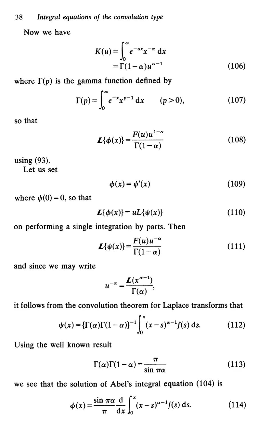
38 Integral equations of the convolution type
Now we have
K(u) = [00 e-uxx- a dx
= r(l- a)u a - 1
where r(p) is the gamma function defined by
f(p) = [00 e -xx p - 1 dx (p > 0),
(106)
(107)
so that
F(u)u 1 - a
L{«f>(x)}= r(1-a)
(108)
using (93).
Let us set
cf>(x) = t/J'(x)
(109)
where t/J(O) = 0, so that
L{ cf>(x)} = uL{ t/J(x)}
(110)
on performing a single integration by parts. Then
F(u)u- a
L{tf1(x)} = f(l-a)
(111)
and since we may write
-a L(x a - 1 )
u = r(a) ,
it follows from the convolution theorem for Laplace transforms that
tf1(x) = {f(a)r(I- a)}-l r (x - s)"'-lf(s) ds. (112)
U sing the well known result
'1T
r(a)r(l- a) = .
sIn '1Ta
(113)
we see that the solution of Abel's integral equation (104) is
«f>(x) = sin 'ITa r x (x _ s)"'-lf(s) ds. (114)
'1T dx Jo
Fox's integral equation 39
For the particular case a =! corresponding to the tautochrone
problem this solution simplifies to
1 d I x f(s)
cf>(x) = - - d ( )1/2 ds.
'1T X 0 x-s
(115)
3.6 Fox's integral equation
We seek the solution of the Fredholm integral equation of the
second kind having the form
<f>(x) = f(x) + L"" k(xs)<f>(s) ds
(O<x<oo)
(116)
named after Fox. This can be achieved by employing the Mellin
transforms <I>(u), F(u) and K(u) of cf>(x), f(x) and k(x) respectively
defined by (7).
Now we have shown in section 3.1 that K(u)<I>(l- u) is the
Mellin transform of
L"" k(xs)<f>(s) ds
and so we see that
<I>(u) = F(u) + K(u)<I>(l- u)
(11 7)
on taking the Mellin transforms of both sides of (116). Also,
replacing u by 1 - u, we have
<1>(1- u) = F(l- u) + K(l- u)<I>(u)
(118)
which enables us to write
cI>(u) = F(u) + K(u)F(l- u)
1- K(u)K(l- u)
(119)
Thus we have obtained a solution of Fox's integral equation (116)
provided we can derive cf>(x) from its Mellin transform <I>(u).
Example. Let us take as an example
k(x) = A .Jl: sin x
(120)
40 Integral equations of the convolution type
Then the Mellin transform of k(x) is given by
K(u) = A IX> x u - 1 sin x dx
= A f(u) sin u
(121)
and
2A 2 . u u
K(u)K(l- u) = --:;; f(u)f(l- u) SIn 2 cos 2
= A 2f(u)f(1- u) sIn u
=A 2
using (113). Hence, provided A 2 1, we see that
(122)
F(u) A /2 . u
<I>(u) = 1- A 2 + 1- A 2 -y f(u) SIn 2 F(l- u)
making use of (119). But by the convolution theorem for Mellin
transforms established in section 3.1 we know that f( u) sin u F( 1 - u)
is the Mellin transform of IX> sin xsf(s) ds, and so the solution of
Fox's integral equation with kernel given by (120) is
(123)
-
(x) A 2 00.
<fJ(x) = / 2 + 1 2 _ 1 SIn xsf(s) ds
-A -A 0
(O<x<oo)
(124 )
This result can be verified directly by using Fourier's reciprocal
sine formulae (1.2) and (1.3) in the form
2 1 00 1 00
f(x) = - sin xs ds sin stf(t) dt
0 0
Problems
(O<x<oo)
(125)
1. Solve the Lalesco- Picard equation
<fJ(x) = cas JLX + A L e-lx-sl<fJ(s) ds
(A <!)
Problems 41
2. Find the solutions to the Volterra equations of the second kind
<fJ(x) = f(x) =i: r (x - s)<fJ(s) ds
when (i) f(x) = 1, (ii) f(x) = x using the general solution (65), and
verify that they agree with the solutions obtained by solving the
equivalent differential equations (see problem 3 at the end of
chapter 2).
3. Find the solutions to the Volterra equation of the second kind
<fJ(x) = f(x) +,\ r sin (x - s)<fJ(s) ds
when (i) f(x) = x and A = 1,
(ii) f(x) = e- x and A = 2,
using the general solution (75) and verify that they agree with the
solutions obtained by solving the equivalent differential equations
(see problem 4 at the end of chapter 2).
4. If F(u) is the Fourier transform of f(x) show that the transform
of f"(x) is -u 2 F(u) provided f, f' 0 as x :t:oo. Hence show that
f(x) = f e-lx-sl<fJ(s)ds (-00< x <(0)
has the solution
cf>(x) = !{f(x) - f"(x)}
5. If F(u) is the Laplace transform of f(x) show that the transform
of f'(x) is uF(u)-f(O) for u>a provided f(x)e-ax o as x oo.
Hence find the solution of the Volterra equation of the first kind
f(x) = r e -s<fJ(s) ds
where f(O) = o.
6. Use Fourier's sine formulae to verify that the solution of Fox's
integral equation
<fJ(x) = f(x) + ,\ 1"" sin xs<fJ(s) ds
is given by (124).
(O<x<oo)
42 Integral equations of the convolution type
7. Use the method of Mellin transforms to solve Fox's integral
equation when the kernel is
k(X)=A cosx.
Verify the correctness of your solution by using Fourier's cosine
formulae.
4
Method of successive
approximations
4.1 Neumann series
A valuable method for solving integral equations of the second kind
is based on an iterative procedure which yields a sequence of
approximations leading to an infinite series solution associated with
the names of Liouville and Neumann. It is sometimes called the
Liouville-Neumann series but more often it is called the Neumann
.
serIes.
Let us first examine the Fredholm equation
<fJ(x) = f(x) + A r K(x, s)<fJ(s) ds
(a x b)
(1)
and consider the set of successive approximations to the solution
cf> (x) given by
cf>O(x) = cf> (O)(x)
cf>1 (x) = cf> (O)(x) + Acf> (1\X)
cf>2(X) = cf> (O\x) + Acf> (l)(x) + A 2 cf> (2)(X) (2)
and so on, the Nth approximation being the sum
N
cf>N(X) = L A ncf>(n)(x)
n=O
(N = 0, 1, 2, . . .)
(3)
where
cf> (O\x) = f(x),
<fJ(l)(X) = r K(x, s)<fJ(O)(s) ds,
<fJ(2)(X) = r K(x, S)<fJ(l)(S) ds,
(4)
and in general
<fJ(n)(x) = r K(x, s)<fJ(n-l)(s) ds
(n;?; 1).
(5)
44 Method of successive approximations
We see that the sequence of approximations is generated by an
iterative process of successive substitutions on the right-hand side of
(1).
Suppose that f(x) and K(x, s) are continuous functions in the
range of definition so that they are bounded and we may write
If(x)1 m
IK(x, s)I M
(a x b)
(a x b, a s b)
(6)
when m and M are positive constants. Then
1cf>(O)(x)1 = If(x)1 m,
IcfJ(l)(x)l:s;;; flcfJ(O)(s)IIK(X, s)1 ds:S;;; mM(b - a),
IcfJ(2)(x)l:s;;; flcfJ(l)(s)IIK(X, s)1 ds:S;;; mM2(b - a)2,
and in general
1cf>(n)(x)1 mMn(b - a)n.
(7)
Hence
N N 00
L A ncf>(n)(x) L IAlnlcf>(n)(x)1 m L IAlnMn(b - a)n (8)
n=O n=O n=O
and so L =o A ncf>(n\x) is absolutely and uniformly convergent in
a x b if p=IAIM(b-a)<l, that is if
1
IAI< M(b-a)
(9)
since then the series is dominated by the convergent geometric
serIes
f n m
mi.Jp = 1 .
n=O - P
(10)
When condition (9) is satisfied,
00
cf>(x) = LAn cf> (n)(x)
n=O
(11)
is a continuous solution of the integral equation (1).
Neumann series 45
The error made in replacing the exact solution cf> by the Nth
approximation cf>N is given by
00
rN(x) = cf>(x) - cf>N(X) = L A ncf>(n)(x). (12)
n=N+l
It is readily seen that
00
IrN(x)l m L pn_
n=N+l
N+l
mp
1-p
(13)
and so IrN(x)1 o as N oo if p<l.
Now let us turn our attention to the Volterra equation
cfJ(x) =f(x)+ A f K(x, s)cfJ(s) ds.
(14)
Then the previous analysis holds with K(x, s)=O for s>x. But we
have further that
1 cf> (O)(x)1 = If(x)1 m,
14>(1)(x)I";;;; flcfJ(O)(s)IIK(x, s)1 ds";;;; mMf ds = mM(x - a),
fX fX mM 2 (x - a)2
IcfJ (2)(x)I";;;; la IcfJ (l)(S )IIK(x, s)1 ds";;;; mM2la (s - a) ds = 2! '
fX mM 3 fX mM 3 (x - a)3
IcfJ(3)(x)l,,;;;; la IcfJ(2)(s)IIK(x, s)1 ds";;;; 2! la (s - a)2 ds = 3!
and in general, assuming that
IcfJ(n-1)(x)l,,;;;; mMn-l(x - at- 1
(n -I)!
and using the principle of induction, we have
IcfJ(n)(x)l,,;;;; (m , r x (s _ at --I ds = mMn( - at . (15)
n . Ja n.
Hence
f A ncfJ(n)(x) ,,;;;; m f IAlnMn(b - at (16)
n=O n=O n!
and so L =o A ncf>(n)(x) is absolutely and uniformly convergent in
a x b for all values of A since it is dominated by
00 IAlnMn(b _ a)n
m L , =mexp{IAIM(b-a)}. (17)
n=O n.
46 Method of successive approximations
Thus the Neumann series (11) converges for all values of A in the
case of the Volterra equation (14) whereas it converges only for
sufficiently small values of A in the case of the Fredholm equation
(1).
4.2 Iterates and the resolvent kernel
In the previous section we obtained solutions to the Fredholm and
Volterra equations of the second kind in the form of the infinite
series (11). It is convenient to express these solutions in terms of
iterated kernels defined by
K1(x, s) = K(x, s)
Kn(x, s) = r K(x, t)Kn-1(t, s) dt
(n 2)
(18)
(19)
so that
K 2 (x, s) = r K(x, t1)K(ti> s) dtl,
K 3 (x, s) = r K(x, tt)K 2 (tt, s) dt 1 (20)
= r r K(x, t1)K(ti> t 2 )K(t 2 , s) dt 1 dt 2 (21)
and in general
Kn(x, s) = r. · · r K(x, t1)K(tl, t 2 ) · · ·
K(t n -2, tn-1)K(t n - b s) dt 1 · · · dtn-l (22)
It follows at once that the iterated kernels satisfy
Kn(x, s) = r Kp(x, t)Kq(t, s) dt
for any p and q with p+q = n.
Now
(23)
</J(n)(x) = r Kn(x, s)[(s) ds
(24)
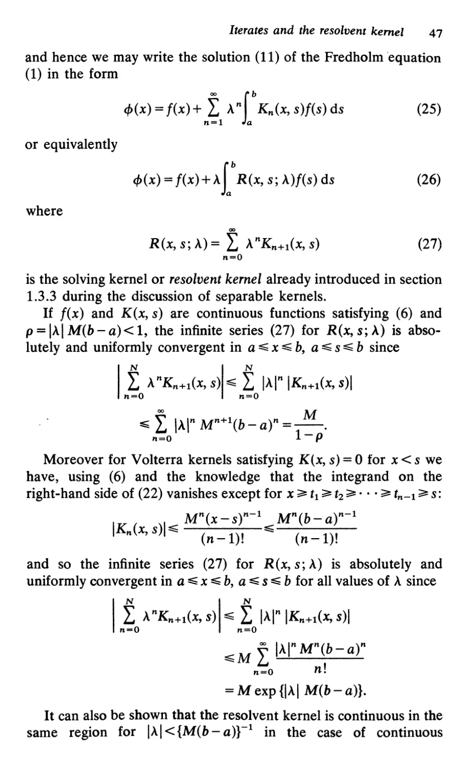
Iterates and the resolvent kernel 47
and hence we may write the solution (11) of the Fredholm 'equation
(1) in the form
00 f b
<fJ(X) = f(x)+ n l A n la Kn(x, s)f(s) ds
(25)
or equivalently
<fJ(x) = f(x) + A r R(x, s; A)f(s) ds
(26)
where
00
R(x, s; A) = L A nK n + 1 (x, s)
n=O
(27)
is the solving kernel or resolvent kernel already introduced in section
1.3.3 during the discussion of separable kernels.
If f(x) and K(x, s) are continuous functions satisfying (6) and
p = IAI M(b - a) < 1, the infinite series (27) for R(x, s;'\) is abso-
lutely and uniformly convergent in a x b, a s b since
N N
L A nK n + 1 (x, s) L lAin IKn+t(x, s)1
n=O n=O
f lAin M n +1(b-at= M .
n=O 1 - P
Moreover for Volterra kernels satisfying K(x, s) = 0 for x < s we
have, using (6) and the knowledge that the integrand on the
right-hand side of (22) vanishes except for x t 1 t 2 . · · tn-t s:
M n (x-s)n-1 Mn(b-a)n-1
IKn(x, s)1 (n -1)! (n -1)!
and so the infinite series (27) for R(x, s; A) is absolutely and
uniformly convergent in a x b, a s b for all values of A since
N N
L A nKn+t(x, s) L lAin IKn+t(x, s)1
n=O n=O
00 lAin Mn(b - a)n
ML
n=O n!
= M exp {IAI M(b - a)}.
It can also be shown that the resolvent kernel is continuous in the
same region for IAI<{M(b-a)}-1 in the case of continuous
48 Method of successive approximations
Fredholm kernels, and for all A in the case of continuous Volterra
kernels.
Example 1. As a first example of the Neumann series we consider
the Fredholm equation of the second kind
cf>(x) = f(x) + ,\ r u(x) v(s) cf>(s) ds
(28)
with separable kernel K(x, s) = u(x)v(s). This equation was dis-
cussed previously in section 1.3.3 where an exact solution (1.30)
in closed analytical form was obtained.
Now we have
K1(x, s) = K(x, s) = u(x)v(s)
K 2 (x, s) = r K1(x, t)K1(t, s) dt
b
= u(x) v(s) I v(t) u(t) dt
= au(x)v(s),
where
a = r v(t) u(t) dt,
and if we assume that
Kn(x, s) = an-1u(x) v(s)
then
Kn+i(x, s) = r K1(x, t)Kn(t, s) dt
= an-1u(x) V(S)f v(t)u (t) dt
= anu(x)v(s)
(29)
establishing the general form of the interated kernel Kn+1(x, s) by
the principle of induction.
Iterates and the resolvent kernel 49
Hence the resolvent kernel is
00
R(x,S;A)= L A n K n + 1 (x,S)
n=O
00
= U(X) V(S) L (Aa)n
n=O
(30)
u(x)V(S)
-
1-Aa
(31)
provided IAal < 1. This is in accordance with the exact solution
(1.32) derived previously for all A ¥= a-i.
The homogeneous equation corresponding to (28) is
cf>(x) = A r u(x) v(s) cf>(s) ds
It possesses one characteristic value Ai = a -1 and we see that the
Neumann expansion (30) converges to (31) for IAI<IAll.
Example 2. We now consider the Fredholm equation
cf>(x) = 1 + A r xscf>(s) ds (O::S:; x::S:; 1) (32)
with f(x) = 1 and separable kernel K(x, s) = xs. This was examined
earlier as example 1 of section 1.3.3.
We have
a= {\2dt=i
(33)
so that
xs
K n + 1 (x, s) = 3 n .
Hence the resolvent kernel is
(34)
00
R(x,S;A)= L A n K n + 1 (x,s)
. n=O
00 ( A ) n
= xs L -
n=O 3
xs
(35)
1 - A/3
50 Method of successive approximations
provided IA 1< 3, this being less severe that the condition given by
p < 1.
Thus, using (26) we see that
<fJ(x) = f(x)+ A r R(x, s; A)f(s) ds
= 1 + 1 : /3 r s ds
3Ax
-1+ 2(3-A) (36)
which is in accordance with the exact solution (1.38) derived previ-
ously for all A ¥= 3.
Example 3. Lastly we discuss the Volterra equation with kernel
K(x, s) = { e -s
(x>s)
(s > x)
(37)
This kernel is of the convolution type and was discussed before as
example 2 of section 3.3 where an exact solution in closed analytical
form was derived.
Now
K 2 (x, s) = f' K(x, t)K(t, s) dt
= IX e x - t . e t - s dt
= e X - S I Xd't
= eX-S(x - s) (x> s),
K 3 (x, s) = f'K(X, t)K 2 (t, s) dt
= IX e x - t . et-S(t - s) dt
= ex-sf'(t- s) dt
x-s (x - S )2 ( X > S )
:; e 2!
Problems 51
and in general, assuming that
(x - S)n-l
Kn(x, s) = e X -' (n -1)!
(x>s)
we have
K n + 1 (x, s) = r K(x, t)Kn(t, s) dt
I x ( ) n-l
_ x-t. t-s t - s d
- see (n -I)! t
_ x_srX (t-s)n-l
- e J. (n -1)! dt
( X -- S ) n
x-s
=e
n!
(x > s)
(38)
which establishes the general form of the iterated kernel by the
principle of induction.
Hence the resolvent kernel given' by (27) is
R( . \ ) = f ,\n(x-s)n x-s
x, S , 1\ i..J , e
n=O n.
= e(A+l)(x-s)
(x> s)
(39)
for all '\, which is in agreement with the solution (70) obtained in
section 3.3 since the resolvent kernel vanishes for x < s.
Problems
1. Use the method of successive approximations to solve
<f>(x) = 1 + A r eX+S <f>(s) ds
and verify that your solution agrees with the solution to problem 3
at the end of chapter 1 for ,\ < 2/(e 2 -1).
2. Use the method of successive approximations to solve
<f>(x) = x + A ["Sin nx sin ns<f>(s) ds
where n i . an integer, and verify that your solution agrees with the
solution to problem 5 at the end of chapter 1 for ,\ < 2/ 'IT.
52 Method of successive approximations
3. Obtain the solution in closed analytical form of
<f>(x) = f(x) + f1T K(x, s)<f>(s) ds
where
00
K(x, s) = L an SIn nx cos ns
n=l
and
00
L lanl<oo,
n=l
using the method of successive approximations.
4. Use the method of successive approximations to solve
<f>(x) = 1 + A r <f>(s) ds,
verifying that your solution for A = 1 agrees with that obtained to
problem l(i) at the end of chapter 2.
5. Use the method of successive approximations to obtain the
resolvent kernel for
<f>(x) = f(x) + A r (x - s)<f>(s) ds
Verify that this agrees with the solutions to problem 3 at the end of
chapter 2.
6. Use the method of successive approximations to show that the
resolvent kernel for
<f>(x) = 1 + A r xs<f>(s) ds
is given by
00 ( A ) n (X3 _ s3)n
R(X,S;A)=XSn o 3 n!
and hence solve the integral equation.
5
Integral equations
with singular kernels
5.1 Generalization to higher dimensions
So far in this book we have been concerned solely with integral
equations which involve an unknown function cf>(x) of a single real
variable x. However it is interesting to consider integral equations in
higher dimensions and to this end we suppose that V is a region of
an n-dimensional space and let M, N de-note points in the region V.
Then an integral equation of the second kind takes the form
cP(M) = f(M) + L K(M, N)cP(N) dUN
(1)
where K(M, N) is the kernel, f(M) is a given function, cf>(M) is the
function which we require to find, and the integration in (1) is over
all the points N of the n-dimensional region V.
Also an integral equation of the first kind takes the form
f(M) = L K(M, N)cP(N) dUN.
(2)
A common type of singular kernel is given by
K(M, N) = F( N) (3)
r
where F(M, N) is a bounded function and r is the distance between
the points M and N in the n-dimensional space. This type of kernel
is called polar and as r 0 it approaches an infinite value. It is said
to give rise to an integral equation with a weak singularity if
0< a < n. The polar kernel (3) is square integrable, Le.
L L IK(M, NW dUM dUN < co, (4)
when a is restricted further to the range 0 < a < n12, as we have
shown for the one-dimensional case (n = 1) in section 1.4.
54 Integral equations with singular kernels
5.2 Green's functions in two and three dimen-
.
stons
We now consider the linear second order partial differential equa-
tion
LtfJ = n (5)
and begin by investigating the two-dimensional case for which
iJ2 iJ2
L = + +q(x, y) (6)
iJx iJy
Then the corresponding Green's function G(x, y; s, t) satisfies
LG(x, y; s, t) = S(x - s )S(y - t).
(7)
Integrating over the interior of a circle l' of radius e centered at the
point with coordinates s, t we have
L LG(x, y; s, t) dx dy = 1
(8)
since the integral of the S functions amounts to unity. This leads to
lim f iJG du= 1
B O 'Y iJp
(9)
where du 'represents an .element of arc length and
p2 = (x - S)2 + (y - t)2.
(10)
We now see that
iJG
27Tp- 1
iJp
(11)
as p 0 and so
1
G (x, y; s, t) = 27T In p + g (x, y; s, t)
(12)
where
1
L g( x, y; s, t) = - 27T q (x, y) In p
(13)
and g is chosen so that G satisfies prescribed boundary conditions.
Dirichlet's problem 55
In the three-dimensional case
L = V 2 +q(r)
and the Green's function satisfies
(14)
LG(r, s) = 5(r-s)
(15)
where rand s are the position vectors of the points with coordinates
(x, y, z) and (s, t, u) respectively.
Integrating over the region contained by a sphere S of radius e
centered at the point with position vector s we obtain
Is LG(r, s) dr= 1
(16)
gIvIng
lim! aG dS = 1
8-+0 k aR
(17)
where the integration in (17) is over the surface of the sphere Sand
R 2 = Ir-sl 2 = (x - S)2+(y - t)2+ (z - U)2. (18)
It follows that
41TR 2 aG 1
aR
(19)
as R 0 and hence the Green's function has the form
1
G(r, s) = - 41TR + g(r, s)
(20)
where
q(r)
Lg(r, s) = 41TR
(21)
and we choose g so that G satisfies given boundary conditions.
5.3 Dirichlet's problem
The problem named after Dirichlet is concerned with determining a
function tf1 which has prescribed values f over the boundary r of a
certain simply connected region R and which is harmonic, Le.,
satisfies Laplace's equation, at all interior points of R.
56 Integral equations with singular kernels
We begin by considering the two-dimensional Dirichlet problem
in which we have a plane region R bounded by a closed contour l'
with a continuously turning tangent. Let us suppose that tf/(x, y) is
the harmonic function satisfying
a 2 tf/ a 2 tf/
Vitf/ = -+-= 0
ax 2 ay2
(22)
in R and having the prescribed values given by f(s, t) at all points
(s, t) of 1'. We now express tf/ as the real part of an analytic function
F(z) of the complex variable z = x + iy by putting
tf/(x, y) = Re F(z)
(23)
and look for a solution in the form of the Cauchy-type integral
F(Z)= f p,(C) dC
21Tl 'Y l- z
(24)
where the density IL«() is a real function of the complex variable ,
and the contour l' is directed in the anticlockwise sense. Next we
allow z to approach a point w on the boundary curve l' from the
interior of R. In the limit we obtain
F(w) =!IL(W)+ 2 1 · P f ;(C) dC
1Tl - W
'Y
(25)
where the integral occurring on the right-hand side of (25) is its
Cauchy principal value. (indicated by the prefix P):
'Urn f. p,(C) dC
B O 'Ye l- w
(26)
where I'B is the part of l' outside a circle of radius e centered at the
point w, and the term !IL(W) is the contribution arising from the
singularity at ,= w.
Now taking the real parts of (25) we find that
f(x, y) =tp,(x, y)+ 2 plp,(C) Im( C Cw ) (27)
where (x, y) are the coordinates of the point w on 1'.
Let us write ,- w = re i8 . Then the imaginary part of d'/(' - w)
Dirichlet's problem 57
becomes
Im ( d' ) =Im[d{ln(,-W)}]
'-w
= Im[d(In r+ i8)]
=d8
= a8 du
au
where du is an element of arc of 1'. Using one of the Cauchy-
R . . at/J ae/> at/J ae/> · h I d ..
Iemann equatIons - = -, - = -- connectIng t e rea an Imagl-
ax ay ay ax
nary parts t/J, e/> of an analytic function we get
(28)
a8 alar
-=- (In r) =--'
au an r an
where n is measured in the direction of the outward nQrmal to l'
(see Fig. 4).
Now
(29)
ar A A
-=r.R
an
(30)
here " denotes a unit vector, so that we obtain
1 f " "
1 f.n
f(X,y)=21L(x,y)+- 2 P lL(s,t)-du.
7T 'Y r
(31)
Since we can characterize the point , by its arc distance 00 along l'
from the point w, we may rewrite (31) in the one-dimensional form
1 f. ""
f.n
IL(U) = 2f(u) -- P IL(U) - du
7T 'Y r
which is a Fredholm integral equation of the second kind with a
polar kernel (3) for a = 1.
I
We next turn to the three-dimensional interior Dirichlet problem.
Let S be the boundary surface of the three-dimensional region R
and suppose that the solution t/J of Laplace's equation V 2 t/J = 0
possesses the prescribed values at the boundary surface given by the
function f.
If M is an interior point of R we may express the solution as the
potential of a double layer, which in electricity is a distribution of
(32)
58 Integral equations with singular kernels
w
Fig. 4. Dirichlet's problem.
electric dipoles spread over the surface S with their axes in the
directions of the normals. Thus we have
-f/(M)=- 4 1 f p,(N) r .2° dS N
1T Js r
(33)
where n is a unit vector along the outward normal at the poin N
of the surface S, IL(N) is the density of the double layer and r = MN.
Then allowing M to tend to a point of S from the interior of R
yields the two-dimensional Fredholm integral equation of the sec-
ond kind for IL:
IL(M) = 2f(M) -- 2 1 pf p,(N) r .2° dS N (34)
1T Js r
with a polar kernel (3) for a = 2.
Dirichlet's problem 59
5.3.1 Poisson's formula for the unit disc
We now search for the solution .p(r, 8) of Dirichlet's problem for a
unit circle 1', the polar coordinates (r, 8) being referred to the centre
of the circle. To this end we consider Laplace's equation in a.plane
vi.p = 0 (35)
where .p(r, 8) f( 8) as r 1- o.
If G(r, s) is the Green's function satisfying
ViG(r, s) = 5(r-s) (36)
with G(r, s) = 0 when s is on the boundary given by s = 1, it follows
from (12) that
1
G(r, s) = 2'1T {In Ir-sl-in (r Ir' -sl)}
(37)
where r' is the inverse point of r with respect to the unit circle l' so
that rr' = 1 and thus, using similar triangles (see Fig. 5), Ir - sl = r Ir' - sl
if s is on the boundary.
p'
o
'Y
Fig. 5. Poisson's formula: P' is the inverse point of P with respect to
the unit circle l' centered at 0 so that OP.OP' = OQ2 = 1, and OQP
and OP'Q are similar triangles.
60 Integral equations with singular kernels
Green's theorem states that
i 2 2 f ( a.p a cf»
(cf>V1.p- .pV1cf» dS = cf>--.p- dO"
R 'Y an an
where n is measured in the direction of the outward normal to the
boundary curve l' and so, setting cf> = G(r, s), we obtain
(38)
.p(r) = f l/1(s) G(r, s) duo
'Y an
(39)
Now
Ir -S12 = r 2 + S2 - 2rs cos (8 - x)
and
,2 Ir' - Sl2 = r 2 {,,2 + s 2 - 2,' s cos (8 - X)}
where (s, X) are the polar coordinates of the point s on the unit
circle 1'. But r' = r- 1 and so
r 2 lr' -S12 = 1 + ,2S2_ 2rs cos (8 - X).
Hence
1 f a
.p(r) =- 2 .p(s) - [! In {r 2 + s2-2rs cos (8- X)}
7T 'Y as
-! In {I +r 2 s 2 -2rs cos (8 - X)}] dO"
and since s = 1 and .p(s) = f(x) over the unit circle l' we find that
1 _,2 r 21T
l/1(r)= 2'7T Jo f(x)[1+r 2 -2rcos(O-X)]-ldX
(40)
which is Poisson's formula for the unit disc.
5.3.2 Poisson's formula for the half plane
We consider the half plane y > 0 bounded by the straight line y = 0
and suppose that .p(x, y) f(x) as y +0. Then the Green's func-
tion (12) which vanishes when the point s with coordinates (s, t) lies
on the boundary line t = 0, takes the form
1
G(r, s) = 2'7T {In Ir-sl-In Ir' -sl}
(41)
where the coordinates of rand r' are (x, y) and (x, -y) respectively.
Dirichlet's problem 61
Now using (39) we obtain
1 f oo a
tfJ(x, Y)=-- 2 f(s)-[!ln{(s-x)2+(t-y)2}
1T -00 at
-!In {(s - X)2 + (t + y)2}]t=ods
= ; L f(S)[(S-X)2+y2rldS (42)
which is Poisson's formula for the half plane.
5.3.3 Hilbert kernel
An integral equation with the singular kernel
( x - 8 )
cot 2
named after Hilbert can be obtained by using Poisson's formula (40)
for a unit disc and setting z = re iB and' = eix. Then d'/' = i dX and
(43)
, + z _ 1 + r cos ( 8 - X) + ir sin (8 - X)
, - z 1 - r cos (8 - X) - ir sin (8 - X)
gIvIng
( ' + Z ) 1 - r 2
Re = 2 ·
, - z 1 + r - 2 r cos (8 - X)
Hence
1 f ' + z d'
I/1(r, 0) = Re 27Ti ./(X) , - z T
where l' is the circle 1'1 = 1.
Let cf>(r,8) be the harmonic function which is conjugate to
tfJ(r, 8). Then cf>(r, 8) is determined apart from an additive arbitrary
constant which we choose so as to make cf>(r, 8) vanish at r = O. We
have then
(44)
. 1 I ' + z d'
I/1(r, 0) + 1<I>(r, 0) = 27Ti ./(X) , - z T'
Now .letting r 1- 0 so that z approaches a point of l' from the
interior of the unit disc, we obtain
(45)
tfJ(l, 8) + icf>(l, 8) = f( 8) + 2 1 . P I f(x) ,+ z d' .
1Tl y , - z ,
62 Integral equations with singular kernels
We already know that tf/(1, 8) = f(6). Putting cf>(1, 8) = g(8) we find
that
1 1 211 eix + e iO
g(8)=- 2 . P f(x) ix io dx
1Tl 0 e - e
i ,r 211 e i[(x- O )/2] + e -i[(x- O )/2]
= - 2'7T PJo f(x} e i [(x- IJ )/2]_ e- i [(x- IJ )/2] dX
and so
1 J 211 ( 8 )
g( O} = - 2'7T PJo f(x} cot X dX
(46)
which is an integral equation of the first kind for f(x) having the
Hilbert singular kernel (43).
Now we turn to the Poisson formula for the half plane and set
z = x + iy and ,= s + it. On the t = 0 axis we have
1m ( 1 ) = 1m ( 1 )
, - z s - x - iy
Y
-
(S-X)2+ y 2
and so
1 f tf/(,)
tf/(x, y) = Re --: y d'
1Tl 'Y - z
(47)
where l' is the straight line t = 0 together with the infinite semi-
circle in the upper half plane traced in the anticlockwise sense. We
let cf>(x, y) be the harmonic function conjugate to tf/(x, y). Then
. 1 f t/!(,)
I/1(x, y} + 1cf>(X, y} = -: , d'
1Tl - Z
'Y
(48)
and so, letting y + 0, we obtain
. 1 1 00 f(s)
tf/(x, +0) + lcf>(X, +0) = f(x) +--: P - ds
1Tl -00 S - x
. .
gIvIng
g(x} = -1. pf'" f(s} ds
1T J-oo s - x
(49)
Dirichlet's problem 63
where [(x) = t/1(x, +0), g(x) = cf>(x, +0) and the integral on the right-
hand side is the principal value defined by
lim [f x-e [(s) ds + 1 00 [(s) dS ] . (50)
e-+O -00 S - X x+e S - X
Equation (49) is an integral equation of the first kind having the
singular kernel (s - X)-I.
5.3.4 Hilbert transforms
Suppose that t/1(x, y), t/11 (x, y), t/12(X, y) are functions which are
harmonic in a plane region R bounded by a closed curve 1', and t/11
is conjugate to t/1 while t/12 is conjugate to t/11. Then using the
Cauchy- Riemann equations for the analytic functions t/1 + it/11 and
t/11 + it/12 respectively we obtain
at/1 _ at/11
- ,
ax ay
and
at/11 = at/12
ax ay'
so that
a
ax (t/1 + t/12) = 0,
Hence
at/1 _ at/11
-- -...--
ay ax
(51)
at/11 _ at/12
----
ay ax
(52)
a
-( t/1 + t/12) = 0
ay
(53)
t/1 = -t/12 + C
(54)
where C is a constant.
Let us now apply this result to the case of the unit disc for which
l' is the circle r = 1. We take the values of t/1, t/1b t/12 over l' to be
[(8), [1(8), [2(8) respectively and choose t/12 to vanish at r = 0 so that
C = t/1(r = 0). But Poisson's formula (40) for the unit disc informs us
that
1 r 21T
"'(r = 0) = 27T Jo f(x) dX
and so
(55)
1 i 21T
t/1 = -t/12 +- [(X) dX
27T 0
(56)
64 Integral equations with singular kernels
giving in particular
1 i 2'71"
f(8)=-fz(8)+ 27T 0 f(X)dX
(57)
Hence, if f( 8) and g( 8) are the real and imaginary parts of the
analytic function <1>( z) = t/J + icf> over the boundary circle r = 1, we
see that
1 1[2'71" ( 8 )
g(8) = - 27T PJo f(x) cot x dX
(58)
and
1 J 2'71" ( X 8 ) 1 i 21't
f(8)= 27T P Jo g(x) cot 2 dX+ 27T 0 f(X)dX
These are the reciprocal formulae deduced by Hilbert in 1904.
Equation (59) provides a solution of the integral equation (58) of
the first kind with the singular kernel (43). Combining (58) and (59)
together gives the Hilbert formula
1 i 2'71"
f(8)- 27T 0 f(X)dX
1 J2'71" ( X - 8 ) J2'71" ( , - )
= - (27T)2 PJo cot 2 dX · PJo f(x') cot X 2 X dX' (60)
(59)
For the case of the half plane, we have likewise
1 i oo f(s)
g(x)=--P -ds
1T -00 s - x
f(x) =1. P i 00 g(s) ds
1T -00 S - x
(61)
(62)
where f and g are the real and imaginary parts of the values
<I>(x + iO) of an analytic function <I>(z) = t/J + icf> over the boundary
line y = O. The function g(x) is the Hilbert transform of f(s).
Denoting the integral operator
-1. P I '" (63)
1T -00 s - x
by H we obtain
H{H[f]} = -f
(64)
Singular integral equation of Hilbert type 65
Whereas the reciprocal for ulae (61) and (62) involve integra-
tions over the infinite range -00 < s < 00, the range of integration in
the pair of formulae (58) and (59) is 0 X 27T and are conse-
quently referred to as finite Hilbert transforms.
5.4 Singular integral equation of Hilbert type
Let us now consider the singular integral equation
aq,(x) + 2 pf1T q,(s) cot (s 2 x) ds = f(x)
having a singular kernel of the Hilbert type (43). Operating on both
sides of (65) with
af1T s (s-X) dx+ 2 pf 1T cot e 2 x ) dx
(65)
and setting
b J21T ( s X )
F(x) = af(x)- 27T PJo f(s) cot 2 ds,
(66)
we obtain the simple result
b 2 i 21T
(a 2 + b 2 )q,(x) - 27T 0 q,(s) ds = F(x)
on using the Hilbert formula (60).
To solve this equation we note that
(a 2 + b 2 ) f1T q,(x) dx - b 2 f1T q,(s) ds = f1T F(x) dx
and hence
(67)
i 21T 1 i 21T 1 i 21T
<f>(x)dx=2 F(x)dx=- f(x)dx
o a 0 a 0
(68)
sInce
f 1T cot( s 2 x )dX=O.
Thus the solution of (65) is
F(x) b 2 r 21T
q,(x) = a 2 +b 2 + 27Ta(a 2 +b 2 ) Jo f(s)ds
(69)
66 Integral equations with singular kernels
If a = 0 (and we put b = 1) we obtain an integral equation of the
first kind having the form
1 f 2'71" ( s X )
f(x) = 27T P 0 q,(s) cot 2 ds.
(70)
Using (59) we arrive at the solution
1 1 2'71" 1 f 2'71" ( s X )
q,(X) = 27T 0 q,(S) ds - 27T P 0 f(s) cot 2 ds
(71)
If we now put
1 1 2'71"
27T 0 q,(S) ds = C
and substitute
1 f 2'71" ( s X )
q,(x) = C- 27T P 0 f(s) cot 2 ds
(72)
back into (70), we see that (72) provides a solution for any value of
the constant C if and only if
1 2'71"
o f(x)dx=O.
(73)
Finally we consider the singular integral equation of the second
kind
A 1 00 cf>(s)
cf>(x)--P -ds=f(x)
1T -00 s - X
(74)
Operating on both sides of this equation with
fOO A foo d
Lx> 8(x - s) dx + 7T PLoo x X s
and setting
A foo f(s)
F(x)=f(x)+ 1T P J-oo s_ xds
(75)
we find that
(1 + A 2)cf>(X) = F(x)
Problems 67
on using (64). Hence the solution of (74) is
cf>(x) = 1 2 {f(x)+ pr'" f(s) dS } (76)
1 + A 1T J-oo S - x
Problems
1. By taking f(21T-X)=f(x) and g(21T-X)=-g(X) in the pair of
finite Hilbert transforms (58) and (59), show that they may be
rewritten in the form
. 1 i 7T sin 0
(1) g( 0) = -- P f( cf> ) dcf>
1T 0 cos 0 - cos cf>
1 i 7T sin cf> 1 i 7T
(ii) f( 0) = - P g( cf» 0 dcf> + - f( cf> ) dcf>.
1T 0 COS - cos cf> 1T 0
[ . sin 0 ]
HInt: use !{cot !( 0 + cf» + cot !( 0 - cf»} =
cos cf> - cos 0
2. By putting x = cos 0, y = cos cf> and
-u(x) = f(O)/sin 0,
v(x) = g( O)/sin 0
show that the pair of reciprocal formulae (i) and (ii) in problem 1
may be rewritten as
(i) v(x)=_!pr l u(y) dy
1T J-1 X - Y
(ii) U(X)=!p f l v(y) dy+! 1 f l u(y)dy
1T -1 l-x 2 x-y 1T .J 1-x 2 -1
3. Find the solution of
pr l u(y) dy = 0
J-1 X - Y
4. Find the solution of Foppl's integral equation
! pr I :(t) 2 dt = f(s)
1T J-1 t - S
where cf>(t) and f(s) are even functions.
68 Integral equations with singular kernels
5. Find the solution of
1 f a
-p
1T -a
tg(t) d _ 2
2 2 t-s.
s -t
1 f 00 is
6. Evaluate - P ds using Cauchy's residue theorem and
'iT -00 S - x
hence find the solutions of
( . ) . 1 pf oo f(s) d
1 slnx=-- - s
1T -00 S - x
( .. ) 1 pf oo g(s) d
II COS X = - - S
1T -00 S - x
Verify that (i) and (ii) form a pair of reciprocal Hilbert trans-
forms.
7. Find the solution of
1
1+x2
p f oo f(s) ds.
1T -00 S - x
6
Hilbert space
In the remaInIng chapters of this book we shall be gIvIng an
introduction to the general theory of linear integral equations as
developed by Volterra, Fredholm, Hilbert, and Schmidt. For this
purpose we need to introduce the concept of a Hilbert space. This is
a suitable generalization of ordinary three-dimensional Euclidean
space to a linear vector space of infinite dimensions which, for the
subject of integral equations, is chosen to be a complete linear space
composed of square integrable functions having a distance property
defined in terms of an inner product.
To explain the meanings of these terms we consider Euclidean
space first and then the Hilbert space of sequences.
6.1 Euclidean space
In three-dimensional Euclidean space each point is specified by an
ordered set of three real numbers or coordinates (Xh X2, X3) forming
the components of the position vector x. The vector Ax has coordi-
nates (AXh AX2, AX3) and the vector sum x+y of two vectors x, y has
coordinates (Xl + Yh X2 +,Y2, X3 + Y3). These are properties of a linear
vector space.
The scalar product or inner product of two vectors x, y is defined
as
(x, y) = XIYI + X2Y2 + X3Y3 (1)
and the vectors are orthogonal, Le. at right angles, if (x, y) = o.
We have
(x, x) = xi + x + x 0,
where (x, x) = 0 if and only if x is the zero vector 0 with coordinates
(0, 0, 0).
The magnitude or norm Ilxll of a vector x is given by
Ilxll = (x, x) = xi+ x + x <00.
(2)
70 Hilbert space
The vector is said to be normalized if Ilx = 1 and then x is a unit
vector.
The distance between two points specified by the vectors x, y is
given by Ilx - yll. Evidently Ilxll is the distance of the point x from the
origin specified by the zero vector o.
Since the length of a side of a triangle is less than, or equal to
when the triangle collapses into a straight line, the sum of the
lengths of the other two sides, we have the triangle inequality
Ilx - yll Ilxll + Ilyli.
(3)
Suppose that x, y, z are linearly independent vectors so that
AX+#LY+VZ is not the zero vector 0 except when A=#L=V=O.
Then we can use them to construct an orthogonal and normalized,
Le. orthonormal set of three vectors e1, e2, e3. Thus let us put
e1 = x/llxli. This vector is clearly normalized. Then
y' = y - (y, e1)e1
is orthogonal to e1 and e2 = y'/lly'li is normalized.
Further
z' = z - (z, e1)e1 - (z, e2)e2
is orthogonal to e1' and e2 while e3 = z'/llz'll is also normalized.
The three mutually orthogonal unit vectors eb e2, e3 are said to
form a basis since any vector a of the three-dimensional space can
be expressed as the linear combination
a = (a, e1)e1 + (a, e2)e2 + (a, e3)e3.
The foregoing vector algebra can be extended to an n-
dimensional space whose points are specified by an ordered set of n
complex numbers (XI, X2, . . . , x n ) denoted by the vector x. The inner
product of two vectors x, y is now defined as
n
(x, y) = L xrYr = (y, x)
r=l
(4)
while the norm of the vector x is given by
..
IIxll = v'(x, x) = t IXrl2 < 00,
r=l
(5)
An orthonormal set of n vectors e1, e2, . . . , en form a basis of the
n-dimensional space, and an arbitrary vector a in the space can be
Hilbert space of sequences 71
expressed as the linear combination
n
a = L (a, er)e r
r=l
where the a r = (a, er)(r = 1, . . . , n) are the components of the vector
a with respect to the basis vectors. The only vector which is
orthogonal to every vector of the basis is clearly the zero vector 0
and so the orthonormal set eh e2,..., en is said to span the
n-dimensional space. If we take el = (1, 0, 0, . . . , 0), e2 =
(0, i, 0, . . . , 0), . . . , en = (0, 0, 0, . . . , 1) we see that a is the vector
specified by (ah a2, . . . , an).
6.2 Hilbert space of sequences
By a natural generalization of a finite dimensional space, we can
consider an infinite dimensional space whose points are represented
by vectors x having components, or coordinates, given by the infinite
sequence of complex numbers {xr} = (Xl, X2, . . . , X r , . . .) satisfying
00
L Ix r I 2 <00.
r=l
(6)
We now introduce the scalar product or inner product of two
vectors x and y given by
00
(x, y) = L xrYr= (Y, x)
r=l
(7)
Then we have 0 (x, x) < 00, where (x, x) = 0 if and only if x is the
zero vector 0 whose components all vanish.
Also we define the norm Ilxll of a vector x by the formula
Ilxll = v' (x, x) = rtl I X rI 2 .
Thus Ilxll = 0 if and only if x = o.
Further we let Ax be the vector with components {AX r } so that
IIAxl1 = IAlllxrl, and let the sum x+y of two vectors x, y be the vector
having components {x r + Yr} as in the case of a finite dimensional
space.
Now, by the Cauchy inequality
(8)
r lIXrIIYrl C 1IXrI2)C 1IYrI2)
(9)
72 Hilbert space
and the inequality
00 00
L XrYr L IXrIIYrl,
r=l r=l
(10)
we obtain Schwarz's inequality
I(x, y)1 Ilxllllyll.
(11)
This is the generalization to infinite sequences of the corresponding
result in three-dimensional Euclidean space which follows im-
mediately from (x, y) = Ilxllllyll cos a where a is the angle between
the vectors x and y.
Hence
00
Ilx+yI12= L I X r+YrI 2
r=l
00 00 00
= L IXrI 2 + L IYrI 2 + L (xrYr+xrYr)
r=l r=l r=l
(11xll + Ilyll)2 < 00.
This shows that the sum x + y satisfies the condition
00
L IX r +YrI 2 <00
r=l
(12)
and also yields the triangle inequality
Ilx + yll Ilxll + Ilyll
(13)
which can be rewritten in the form (3) by reversing the sign of y.
The real number
d(x,y)=llx-yll= rtlIXr-YrI2
(14)
represents the distance between two points characterized by vectors
x, y and is an obvious generalizatio of the idea of distance in
three-dimensional Euclidean space. Clearly Ilxll is the distance of the
point x from the origin given by the zero vector O.
A sequence of vectors {Xn} converges strongly to a limit vector x
if, given any B > 0, there exists N such that for n > N we have
Ilx n -xii < B. Strong convergence is denoted by X n x.
If X n x we have, using the triangle inequality,
Ilxn -xmll = Ilx n -x+x-xmll
llxn -xii + Ilxm -xll< B
Hilbert space of sequences 73
for sufficiently large nand m. A sequence {xn} satisfying Ilxn - xmll < B
for sufficiently large n, m is known as a Cauchy sequence.
We shall now demonstrate the converse of the above result,
namely that every Cauchy sequence has a limit vector x in the space.
Suppose that el = (1, 0, 0, . . .), e2 = (0, 1, 0, . . .), . .. are unit
vectors in the infinite dimensional space. They form a basis which
spans the space, and an arbitrary vector a = ah a2, . . . , a r , . . .) can
be expressed as
00
a = L are r
r=l
where a r = (a, e r ) and e r is the rth unit vector satisfying \\e r \\ = 1.
Then we have, using Schwarz's inequality,
I(x n , e r ) - (x m , e r )\ = I(x n -X m , er)1
\\Xn -xm\1 < B
for all sufficiently large nand m. It follows that the sequence of
numbers (x n , e r ) = x n) is a Cauchy sequence and approaches a
limiting value xr(r = 1, 2, . ..) as n' 00. But for sufficiently large
n, m we have
00
Ilxn-xm\\= L \x n)_x m)\2<B
r=l
and so for every k
k
L Ix n) - x m)\2 < B.
r=l
Hence, in the limit as m 00 we obtain
k
L \x n) - xrl 2 < B
r=l
and since this is true for every k we get
00
\\xn-x\\= L \x n)-XrI2<B.
r=l
But
r l I X rl 2 = IIxll = II(I -In) +Inll
Ilx-xnl\ + \\Xn\!
< B + IIXnl1
74 Hilbert space
and so
00
L Ix r I 2 <00.
r=l
Thus I = (Xl, X2, . . . , X r , . ..) belongs to the space and In I as
n 00.
A space in which In I when {Xn} is a Cauchy sequence is called
complete.
The space of sequences described above is an example of a
Hilbert space. We denote this space by 1 2 .
6.3 Function space
We consider the function space composed of all sectionally continu-
ous complex functions f(x) of a real variable x, defined in the
interval a x b, which are square integrable and thus satisfy the
condition
flf(XW dx <00.
Introducing the inner product of two such functions f(x) and g(x)
given by
(15)
(f, g) = r f(x) g(x) dx,
(16)
we define the norm of the function f(x) as
11111 = (f, f) .
(17)
Next we establish the important inequality named after Schwarz.
We have
f b (f) 2
f(x)- ( ,g) g(x) dx;;o:Q
a g, g
(18)
so that
(f, f) - 2 I(f, gW + I(f, g)1 2 ;;0: Q
(g, g) (g, g)
.
I.e.
({, f)(g, g) I(f, g)12
(19)
Function space 75
Hence
11111 Ilgll I({,. g)1
(20)
which is Schwarz's inequality for square integrable functions.
Also
(11111 + IIgll)2 = 11111 2 + IIgl12 + 21111111g11
({, f) + (g, g) + 21(f, g)1
by Schwarz's inequality. But
21(f, g)1 (f, g) + (f, g)
and so
(11fll + IIgI1)2 (f, f) + (g, g) + (f, g) + (g, f)
= (f + g, f + g).
Hence we have
11111 + II gll Ilf + gll
(21)
which is the triangle inequality for functions, sometimes known as
Minkowski's inequality.
6.3.1 Orthonormal system of functions
Two functions f(x) and g(x) belonging to the function space are said
to be orthogonal if .
(f, g) = r f(x) g(x) dx = 0
(22)
and the function f(x) is normalized if
11111 = 1.
(23)
We consider a set of sectionally continuous complex functions
cP1 (x), cP2(X),. . . , cPr(x), . . . satisfying the orthonormality condition
(<Pn <Ps) ':'" r <Pr(x) <ps(x) dx = 8rs
(24)
where 8rs is the Kronecker delta symbol
8rs = {
(r = s)
(r;es).
(25)
Such a set of functions is called orthonormal.
76 Hilbert space
An orthonormal system of functions is said to form a basis or a
complete system * if and only if the sole function which is orthogonal
to every member cPr(x) of the system is the null function which
vanishes throughout the interval a x b except at a finite number
of points.
It can be shown that every orthonormal system is either finite or
denumerably infinite, Le., the members of the system can be placed
in 1-1 correspondence with the natural numbers, and that an
incomplete system can always be completed to form a basis by
adding a finite or denumerable set of functions.
6.3.2 Gram-Schmidt orthogonalization
Now suppose that we have a finite or denumerable system of
functions Xl (x), X2(X), . . . , Xr(X), . . . which is not orthonormal. We
assume that the functions are linearly independent and that none of
them is null. Then if AIXI + A2X2 +. . . + AnXn is the null function we
must have Al = A2 = . . . = An = 0 and this holds for all n. We aim to
construct out of this system of functions, a new system which is
orthonormal, just as we were able to do in section 6.1 for three-
dimensional Euclidean space. We proceed by using the principle of
induction.
Clearlv
XI(X)
cf>l (x) = Ilxlll
(26)
is normalized. Further
tP2(X)
cf>2(X) = 111/1211 '
(27)
where
tP2(X) = X2(X) - (X2, cPI)cPI (x),
(28)
is normalized and also orthogonal to cP I (X).
Now let us suppose that we have constructed n such functions
cPI(X), cP2(X),..., cPn(x) which are normalized and mutually or-
thogonal. Then
( ) tP +I(X)
cf>n+l X = IIl/1n+111 '
(29)
* A complete system of functions should not be confused with a complete
space, discussed in section 6.3.4.
Function space 77
where
n
tfln+1(X) = Xn+1(X) - L (Xn+h cPr)cPr(X),
r=1
(30)
is normalized and orthogonal to all the functions cP1 (x), . . . , cPn (x).
Thus, using the principle of induction, we have shown that it is
possible to construct an orthonormal set of functions from the
original set.
The above process is called Gram-Schmidt orthogonalization.
6.3.3 Mean square convergence
Let f(x) be any function belonging to the function space and
suppose that we wish to obtain a best approximation to f(x) in the
form of the sum
n
L crcPr(X)
r=1
(31)
where the C r are parameters to be dete mined.
We can achieve this by requiring that
fb n 2
In = 1 f(x)- r l cr<p,(x) dx
(32)
be chosen as small as possible. This will then provide us with the
best mean square approximation to f(x).
We have that
n n
In = (f, f) - L {cr(f, cPr) + cr(f, cPr)} + L Ic r l 2
r=1 r=1
n n
=(f,f)+ L Ic r -a r I 2 - L 1a,12
r= 1 r= 1
(33)
where the a r = ([, cPr) are known as the Fourier coefficients of f(x).
Evidently In attains its least value when C r = ar(r = 1, . . . , n) and
then we have
n
In = (f,f)- L la r l 2 .
r=1
(34)
Since In 0 it follows at once that
n
(f, f) L la r l 2
r=1
(35)
for all n. This is called Bessel's inequality.
78 Hilbert space
If now
lim In = 0
(36)
n-+ oo
we say that f(x) is the mean square limit of the sequence of
functions {fn(x)} given by
n
fn (x) = L arcPr(x),
r=l
(37)
which we may write Ilf- fnll 0 as n 00, or that {fn(x)} is strongly
convergent to f(x), written fn(x) f(x) as n 00.
Then it follows that
00
IIfl1 2 = L I(f, cPr )1 2
r=l
(38)
which is known as Parseval's formula or the completeness relation. If
this formula holds, the orthonormal system of functions cPr(x) forms
a basis or a complete system. For suppose that, on the contrary,
there exists a function f(x) with non-vanishing norm in the function
space satisfying (f, cPr) = 0 for all values of r. Then it follows from
Parseval's formula that Ilfll = 0 which provides a contradiction.
Now consider two functions f(x) and g(x) belonging to the
function space. Then
00
Ilf + Agl1 2 = L I(f + Ag, cPr)12
r=l
supposing that the system of functions cPr forms a basis, and so
11111 2 + IA 1211g112 + X (f, g) + A (g, f)
00 00
= L I (f, cPr) 1 2 + I A 1 2 L I (g, cPr) 1 2
r=l r=l
00
+ L {X (f, cPr)( cPr' g) + A (g, cPr)( cPr' f)}.
r=l
Since A is an arbitrary parameter we see that
00
(f, g) = L (f, cPr)( cPr' g)
r=l
(39)
which is known as the generalized Parseval formula.
Function space 79
6.3.4 Riesz-Fischer theorem
A sequence of functions {fn(x)} is called a Cauchy sequence if
lim Ilfn - fmll = O.
(40)
n,m-+ oo
If a sequence {fn(x)} is mean sq are convergent to f(x) it is a
Cauchy sequence, for using the triangle inequality \\te see that
Ilfm - fnll = II(fm - f) + (f - fn)11
Ilfm - fll + Ilf - fnll
0 as m, n 00.
A function space is said to be complete if every Cauchy sequence
{fn(x)} is mean square convergent to a function f(x) belonging to the
space, i.e., fn(x) is strongly convergent to f(x) or fn(x) f(x).
Now, so far, we have assumed that our function space is com-
posed of sectionally continuous functions and such a space is not
complete. However a function space composed of functions that are
square integrable in the Lebesgue sense, i.e., L 2 functions, is
complete. This result is Fischer's form of the Riesz-Fischer theorem
which we assert without proof. It leads directly to Riesz's form of
the Riesz-Fischer theorem:
If cP1 (x), cP2(X), . . . , cPr(x), . .. is an orthonormal system of L 2
functions and {a r } is a sequence of complex numbers, then
n
L arcPr(x)
r=1
is mean square convergent to a L 2 function f(x) whose Fourier
coefficients are {a r } if and only if
00
L la r l 2 < 00.
r=1
The space of L 2 functions f(x) defined over the interval a x b
is another example of a Hilbert space, usually denoted by L 2 .
In this space f = g if the functions f and g are equal 'almost
everywhere', that is everywhere except at a finite number or a de-
numerable infinity of points of the interval a x b. Further f = 0
in this space if f vanishes 'almost everywhere'.
80 Hilbert space
6.4 Abstract Hilbert space H
We have described above two examples of Hilbert spaces, the space
of sequences 1 2 and the space of L 2 functions. We shall conclude this
chapter by abstracting the common axioms that all Hilbert spaces
must satisfy.
A Hilbert space H is a complete linear vector space possessing a
distance function or metric which is given by an inner product.
A linear vector space is a set of elements, sometimes called points
or vectors, f, g, h,... forming an Abelian group and permitting
multiplication by the field of complex numbers A.
An Abelian group has an internal law of" composition denoted
by the addition sign + satisfying the commutative law
{+g=g+f (41)
and the associative law
f+(g+h)=(f+g)+h,
(42)
,
having a zero element 0 such that
O+f= {+O= f,
(43)
and an inverse element - f corresponding to each element f of the
set such that
f+(-f) = (-f) + f= o.
(44)
The multiplication by the field of complex numbers satisfies
1 · f= f,
o . f = 0,
(AIL)f = A (lLf),
(45)
(46)
(47)
and satisfies the distributive law with respect to the elements f, g
A(f + g) = Af + Ag
and the distributive law with respect to the numbers A, IL
(48)
(A + lL)f = Af + ILf.
(49)
The inner product of two elements f, g is a complex number
denoted by ({, g) satisfying the conditions
(f, g) = (g, f),
(Af, g) = A (f, g),
({1 + {2, g) = ({1, g) + ({2, g).
(50)
(51)
(52)
Abstract Hilbert space H 81
It follows at once that (f, f) = (f, f) so that (f, f) is a real number. We
shall assume that
(f, f) o
and further that (f, f) = 0 if and only if f = O.
Then we have also that
(53)
(f, Ag) = (Ag, f) = X(g, f) = X(f, g)
(54)
and
(f, gl + g2) = (gl + g2, f) = (gt, f) + (g2, f)
= (f, gl) + (f, g2). (55)
The norm of the element f is defined as
Ilfll = (f, f) . (56)
We see that 11111 = 0 if and only if f = 0, and IIAfl1 = IA 111111.
Now
(f+ Ag, f+ Ag) 0
and so taking A = -(f, g)/(g, g) we obtain Schwarz's inequality
1II1111gli I(f, g)l.
(57)
Again following the proof given in section 6.3 we. arrive at the
triangle inequality
11111 + Ilgll Ilf + gll.
(58)
We now define a distance function d(f, g) in terms of the norm
according to the formula
d(f, g) = Ilf- gll.
(59)
This satisfies the conditions required of a distance between two
points f and g, namely
(i) d(f, g) = d(g, f),
(ii) d(f, g) 0,
(iii) d(f, g) = 0 if and only if f = g,
(iv) d(f, g) d(f, h) + d(h, g).
(60)
This last condition follows from the triangle inequality:
Ilf - gll = lI(f - h) + (h - g)1I IIf - hll + IIh - gll.
82 Hilbert space
A sequence of elements {fn} converges strongly to a limit element f
if, given any E > 0, there exists a N such that for n > N we have
Ilfn - fll < E. Strong convergence is denoted by fn f.
If fn f we have
Ilfn - fmll = II(fn - f) + (f - fm)11
llfn - fll+ Ilfm - fll< E
for sufficiently large n, m. A sequence {fn} of elements satisfying
Ilfn - fmll < E for sufficiently large n, m is known as a Cauchy se-
quence.
A Hilbert space is complete, that is every Cauchy sequence
converges to a limit vector in the space.
6.4.1 Dimension of HUbert space
To define the dimension of a space R we introduce the following
concepts. A subset T of R is said to be dense in R if, given any
E > 0 and any element fER, there exists an element gET such that
Ilf - gll < E. S is called a fundamental set in R if the set T of all linear
combinations L;=1 crfr with fr E S is dense in R. Then the dimension
of the space R is the least possible cardinal number of a fundamen-
tal set S in R.
The dimension of Hilbert space H is required to be denumerably
infinite.
6.4.2 Complete orthonormal system
Any set of linearly independent elements belonging to H can be
combined together to form an orthonormal system cPt, cP2, · · · ,
cP" · · · satisfying
(cPr' cPs) = 5rs
by applying the Gram-Schmidt orthogonalization process described
in section 6.3.2.
Because the dimension of H is denumerably infinite it follows
that any orthonormal system of elements belonging to H has not
more than a denumerable infinity of elements which we may denote
by cPt, cP2,. · · , cPr' · · ·
Given any element f E H and putting
n
fn = L (f, cPr)cPr
r=1
(61)
Abstract HHbert space H 83
where the (f, cPr) are the Fourier coefficients of f, we can show that
n
IIf - fnl1 2 = 11111 2 - L I(f, cPr)12
r=1
(62)
by following the analysis given in section 6.3.3. Since Ilf- fnll O, we
obtain Bessel's inequality
n
11111 2 L I(f, cPr)12,
r=1
(63)
valid fori all n, from which it follows that the series on the right-side
converges as n 00.
Hence, given any e > 0, we have
Ilfn - fml1 2 = 'r= +l (f, <Pr)<Pr 2 (n> m)
n
- L l(f,cPr)12<e
r=m+1
provided n, m are sufficiently large. Therefore {fn} is a Cauchy
sequence and so there exis s an element f' E H such that fn .....:; f' as
n 00, using the fact that H is complete. Thus
00
f' = L (f, cPr)cPr
r=1
(64)
and
11111 2 Ilf'11 2 . (65)
If the system cP1, cP2,. . . , cPr' . . . is a fundamental set in H then
f' = f and we have
00
IIfl1 2 = L I(f, cPr)12.
r=1
(66)
Then cP1, cP2, · · · , cPr' · . . is called a complete system or basis and (66)
is known as Parseval's formula or the completeness relation.
Following the analysis at the end of section 6.3.3 we can also
show that the generalized Parseval formula (39) holds for f, g E H.
Problems
1. Construct an orthonormal set of functions defined in the interval
-1 x 1 from 1, x, x 2 , x 3 using the Gram-Schmidt orthogonaliza-
tion process. Verify that the functions are proportional to the first
four Legendre polynomials.
2. Show that the set of orthogonal functions {cos nx} (n = 0, 1, 2,. . .)
do not form a basis spanning the space of continuous functions
defined over the interval - Tr X Tr. Likewise show that the set of
84 Hilbert space
orthogonal functions {sin nx} (n = 1, 2, . . .) do not form a basis of the
space.
3. Show that the sequence of functions {fn(X)} where
o (o x )
fn();)= C <x< )
o ( x 1 ),
converges to zero at all points of the interval 0 x 1 but that the
sequence is not mean square convergent to zero.
4. Establish that the space of continuous functions is not complete
by showing that the sequence of continuous functions {fn(x)} where
o
In(x) = !(nx + 1)
1
(-l X - )
( - < x < )
( X l),
converges strongly to the discontinuous function
o
I(x) = !
1
(-1 x <0)
(x=O)
(O<x l).
5. Show that if a Cauchy sequence {In} converges to an element I
then I is unique.
6. Verify that the space of infinite sequences 1 2 discussed in section
6.2 satisfies the axioms for abstract Hilbert space.
7. By considering the Cauchy sequence {xn} where
X n = (1, !, l, . . . , 1 / n, 0, 0, . . .),
show that the linear vector space of infinite sequences
(x h X2, · . . , x" . . .)
in which only a finite number of the coordinates x, do not vanish,
is not complete.
7
Linear operators
in Hilbert space
In an integral equation the unknown function occurs under the
integral sign and thus, if the functions involved belong to a Hilbert
space, it is clear that we have to deal with integral operators acting
on a Hilbert space of functions.
We pointed out in section 6.3.4 that square integrable functions in
the Lebesgue sense, that is L z functions, form a Hilbert space and
consequently the appropriate integral operators have L Z kernels
introduced in section 1.4. However, in order to avoid unduly
difficult concepts, we shall suppose that ou functions and kernels
are square integrable without usually specifying the sense in which
the integrals are to be performed.
It is worth while placing linear integral operators in a more
general context and so we shall conclude this chapter by giving an
introduction to the theory of linear operators in an abstract Hilbert
space.
7 .1 Linear integral operators
We consider the linear integral operator
K=fK(X,S)dS
where K(x, s) is a square integrable kernel, and write
tf1(x) = f K(x, s)cf>(s) ds,
(1)
(2)
where cP(s) is a square integrable function, in the symbolic form
t/J = K cP.
(3)
It is evident that the operator K is linear since
K(At cPt + AzcPz) = AtK cPt + AzK cPz
(4)
86 Linear operators in Hilbert space
where AI, A2 are constants and cf>I, cf>2 are square integrable func-
tions.
We also introduce the identity operator I satisfying
Icf> = cf>
(5)
for every square integrable function cf>(s), which may be expressed
in the form of the integral operator
1= f8(X-S)dS (6)
where 5 is the Dirac delta function defined in section 2.2.
If
L= fL(X,S)dS
(7)
is a second integral operator we have
x = LtfJ = L(Kcf> )
(8)
where
x(x) = f L(x, t) dtf K(t, s)<I>(s) ds
= f P(x, s)<I>(s) ds
(9)
and
P(x, s) = f L(x, t)K(t, s) dt,
(10)
that is
x = Pcf>
where P = LK is the integral operator with kernel P(x, s).
Integral operators satisfy the associative law
(11)
M(LK) = (ML}K
(12)
and the distributive laws
M(L+K)=ML+MK
(L + K)M = LM + KM
but, in general, do not satisfy the commutative law.
(13)
(14)
Linear integral operators 87
Using the associative law we see that
KmK n = K m + n
,
(Km)n = K mn
(m, n 1)
(15)
where
K n = f Kn(x, s) ds
(16)
and Kn(x, s) is the iterated kernel defined by (4.22).
7.1.1 Norm of an integral operator
If K(x, s) is a square integrable kernel its norm is defined by
[ r b r b ] 1/2
IIKIIz = Ja lIK(x, sW dx ds ·
(17)
Then if cP(s) is a square integrable function and tf/(x) is given by (2)
_ we have, using Schwarz's inequality (6.20), that
1t/1(xW..;; fIK(x, sW dsfl<P(SW ds
which yields
,fJt/1(XW dx";; f fIK(x, sW dx dsfl<p(sW ds
so that
Iitf/II::;; IIK11211ef>11 < 00
(18)
and thus tf/(x) is square integrable.
When IIKI12 = 0 then Iitf/il = 0 so that Kef> vanishes 'alm,ost.
everywhere' for all square integrable functions ef>, and K is called a
null operator.
Also if L(x, t) and K(t, s) are square integrable kernels, then
P(x, s) given by (10) is square integrable since, by Schwarz's in-
equality,
IP(x, sW..;; l"IL(X, tW dtfIK(t, sW dt
88 Linear operators in Hilbert space
so that
f fIP(x, sW dx ds f fIL(x, tW dx dtf fIK(t, sW dt ds
giving
IILK1b::;; IILlb IIKlb < 00.
(19)
Putting L = K we see that IIK 2 Ib::;; IIKII and in general
IIKnlb ::;; IIKII
(n = 1, 2, 3, . . .)
(20)
7.1.2 Hermitian adjoint
The Hermitian adjoint of a kernel K(x, s) is defined to be the kernel
K*(x, s) = K(s, x).
(21)
We see at once that
(AK)* = AK*,
K** = K.
(22)
Also
(LK)*(x, s) = LK(s, x)
= r L(s, t ) K(t, x ) dt
= f K*(x, t)L *(t, s) dt
= K*L *(x, s)
and so
(LK)* = K*L*.
(23)
Further, using the definition of the inner product given by (6.16), we
have
(K t/>, .,,) = r "'(x) dx f K (x, s )t/>(s) ds
= J: t/>(s) dSJ: K(x, s) "'(x) dx
= (cP, K*.p). (24)
If K* = K the kernel is called Hermitian or self adjoint.
Bounded linear operators 89
7.2 Bounded linear operators
So far we have been concerned with linear integral operators acting
on a space of square integrable functions which, if chosen to be all
the functions which are integrable in the Lebesgue sense, would
form a Hilbert space of functions L 2 .
We shall now turn our attention to the case of an abstract Hilbert
space, defined in section 6.4, acted on by bounded linear operators.
Consider a subset D of an abstract Hilbert space H such that if
f, g E D then Af + ILg E D where A, IL are arbitrary complex numbers.
Then D is called a linear manifold. We note that a linear manifold
must contain the zero element since f+(-l)f=O.
Suppose that corresponding to any element fED we assign an
element Kf E where is also a linear manifold. Then K maps D
onto and is called a linear operator with domain D and range if
K(Af+ ILg) = AKf+ ILKg
(25)
for f, g E D.
A linear operator K having the Hilbert space H as domain is
bounded if there exists a constant C 0 such that
IIKf1I C IIfll
for all IE H.
The norm IIKII of the bounded linear operator K is defined as the
smallest possible value of C. Thus IIKII is the least upper bound or
supremum of IIKf1I/IIf1I, that is
IIKf11
IIKII = E lfiI (26)
and so
IIKfll IIKIlIlf1I.
(27)
This is a generalization of the inequality (18) for the linear integral
operator (1) with square integrable kernel. Clearly (1) is a bounded
linear operator.
The linear operator K has an adjoint operator K* defined so that
(KI, .g) = (f, K*g)
(28)
for all I, g E H. This is in accordance with the definition (21) for linear
integral operators, as shown in section 7.1.2. If K* = K the
operator is self adjoint or Hermitian.
90 Linear operators in Hilbert space
Now by Schwarz's inequality (6.57), and (27), we have
I(Kf, g)1 IIKt1ll1gll IIKII I If II Ilgll
(29)
and so (Kf, g) is bounded. Likewise
I(f, K* g)1 IIK*lIlIfllllgll
(30)
so that
IIK*II = IIKII
(31)
and K* is also a bounded linear operator.
Further, any bounded operator K is a continuous linear operator
which transforms a strongly convergent sequence {fn} into a strongly
convergent sequence {Kfn}. For we have
IIKfn - Kt11 = IIK(fn - f)1I IIKllllfn - fll
so that if fn f as n 00 then
IIKfn - Kfll 0,
that is Kfn is strongly convergent to Kf
Actually every continuous linear operator K with domain H is
bounded. For otherwise there would exist a sequence {fn} such that
IIKfnll nllfnll so that IIKgnll 1, but gn = fnln IIfnll 0 as n 00,
which is contrary to the hypothesis that K is continuous.
We see that the linear integral operator (1), with a square
integrable kernel, is continuous.
If K and L are two bounded linear operators which map H onto
itself, then the product operator LK corresponds to
(LK)f = L(Kn.
Then
IILKfll ilL IIIIKt11 ilL II IIKII 1It11
so that
IILKII IILIIIIKIl
(32)
and therefore LK is a bounded operator.
Also
(LKf, g) = (Kf, L * g)
= (f, K*L*g)
Bounded linear operators 91
and hence
(LK)* = K*L*.
(33)
Lastly it is interesting to observe that the norms of bounded
linear operators K and L satisfy the triangle inequality. For, using
the triangle inequality (6.58) for the elements of Hilbert space, we
have
IIKf + Lf11 IIKf11 + IILf11
(11K11 + 1 11)11f11
so that
IlK + LII IIKII + IILII.
(34)
7.2.1 Matrix representation
Suppose that CPt, CP2, . . . , CPr' . . . is a complete orthonormal system
or basis in H. Then the matrix with elem nts
k rs = (K CPr, CPs)
(35)
is called the kernel matrix of the bounded operator K.
Introducing the Fourier coefficients
X r = (f, CPr),
Ys = (g, CPs)
(36)
where f, g E H, we have
00
f = 1 XrCPr,
r=1
00
g = 1 YsCPs
s=1
(37)
and
00 00 00
Kf = 1 xrK CPr = L 1 XrkrsCPs
r=1 r=1s=1
so that (Kf, g) has the bilinear form
00 00
(Kf, g) = 1 1 XrkrsYs.
r=ls=1
(38)
Since K is bounded it follows that
I(Kf, g)1 IIKIlIlf1lllgll
= IIKII Ctl I X rl 2 )Ctl IY s I2).
92 Linear operators in Hilbert space
Hence
r l S l xrkrsys .;;; IIKII C l I X rl 2 )C l IY s I2) (39)
and thus the bilinear form (38) is also bounded.
7.3 Completely continuous operators
We now introduce the concept of weak convergence. A sequence of
elements {fn} in Hilbert space is said to converge weakly to a limit
element f if (fn, g) (f, g) as n 00 for all g E H. Weak convergence
is written fn f as n 00.
If a sequence is strongly convergent it is also weakly convergent.
For, by Schwarz's inequality (6.57), we have
I(fn - f, g)1 IIfn - fll !tgll
and thus if IIfn - fll 0 as n 00 then (fn, g) (f, g) as n 00.
However, the converse need not be true. Thus we may have fn f
but fn f as n 00.
Let us suppose that K is a bounded linear operator in H. Then
I(Kln - Kf, g)1 IIK(ln - 1)11 IIgil
IIKII IIf n - fll II gll
and so if fn f as n 00 it follows that Kfn Kf, that is Kfn is
weakly convergent to Kf.
Now suppose that Kfn Kf when fn f as n 00. Then K is
called a completely continuous (or compact) linear operator in H.
Every completely continuous operator is bounded. For if fn f
as n 00 we have shown above that fn f and so Kfn Kf. Thus a
completely continuous operator is a continuous operator and this
means that it is bounded as shown in section 7.2.
However a continuous operator is not necessarily completely
continuous. For example the identity operator I is continuous but it
s not completely continuous for if fn f but fn f as n 00 then
obviously Ifn If but Ifn If.
If the kernel matrix (k rs ) of a bounded linear operator K satisfies
00 00
L L Ik rs l 2 <00
r=ls=l
(40)
Completely continuous operators 93
then K is completely continuous. For we have, using (38), that
00
(K(fn - f), cPs) = L (x n) - xr)k rs
r=1
(41)
where x n) and X r are the Fourier coefficients of fn and f respec-
tively, which gives
m
IIK(fn - f)II2 L I(K(fn - I), cPs)12
s=1
00 00
+ L L Ik rs l 2 IIfn - fll 2
s=m+1 r=1
(42)
using Cauchy's inequality.
On the right-hand side of (42) the second sum approaches zero as
m 00 uniformly in n since IIfn - fll is bounded and the operator K
satisfies the condition (40). The first sum approaches zero as n 00
since (K(fn - f), cPs) = (fn - f, K*cPs) 0 if'fn f. Thus Kfn Kf if
fn f as n 00 and thus K is completely continuous.
Any finite dimensional linear operator is co pletely continuous
since for this case the double sum on the left-hand side of (40)
contains a finite number of terms only.
7.3.1 Integral operator with square integrable kernel
As an example of a completely continuous operator we consider the
integral operator K over the space of square integrable functions
given by
g(x) = f K(x, s)f(s) ds
(a x b)
(43)
where the kernel is square integrable and satisfies
fIK(x, sW ds <00
(a x b),
fIK(x, sW dx <00
f fIK(X, sW dx ds <00.
(a s b),
(44)
94 Linear operators in Hilbert space
By Schwarz's inequality we have
Ig(xW.;:;; fIK(x, sW dSflf(sW ds
and so
flg(x W dx';:;; f fIK(x, sW ds dx flf(SW ds,
that is
Ilg112.;:;; f fIK(x, sW ds dx Ilf11 2 .
(45)
Hence
IIKII.;:;; f fIK(x, sW ds dx= IIKlb
(46)
since the norm of K is the least upper bound of Ilg"'"fll.
Now consider any complete orthonormal system
cPl(X), cP2(X), . . . , cPr(x), . .. in the Hilbert space of L 2 functions
defined over a x b. We let
krs = r r cf>s(x) K(x, t)cf>r(t) dxdt,
x r = r f(t) cf>r(t) dt
(47)
(48)
and
Ys = r g(x) cf>s(x) dx.
(49)
Then
Ys = r r K(x, t)f(t) cf>s(x) dx dt
(50)
But
f b 00
a K(x, t)cf>s(X) dx = r l k,.scf>r(t)
(51)
and
00
f(t) = L XrcPr(t)
r=l
(52)
Problems 95
for almost all values of t, that is except for a set of values of t of
Lebesgue measure zero, and hence
00
Ys = L xrkrs.
r=l
(53)
Also
r r K(x, t) <p.(x) dx 2 dt= rt 1 1k,.1 2
and, using Parseval's formula (6.66),
fIK(X, tW dx = ' l f K(x, t) <p.(x) dx 2,
(54)
(55)
Consequently
ffIK(x, tWdx dt= rt.J 1 1k,.1 2
(56)
and so the matrix representation of the integral operator K with
square integrable kernel satisfies the condition (40) which ensures
that K is completely continuous.
Problems
1. If 1 2 is the Hilbert space of infinite s quences
x = (Xh X2, . . . , X r , . . .)
and K is the operator defined by
Kx = (0, X2, X3, . . . , x,., . . .),
show that K is a linear operator in 1 2 having unit norm.
2. If K is the operator in 1 2 defined by
Kx=y
where Yr =x r +l/(r+ l)(r 1), show that K IS a bounded linear
operator and find IIKII.
3. Prove that the linear differential operator L = d/dx, acting on the
space of continuous functions f(x) defined in-the interval O x l,
is unbounded by showing that IILfnl1 = n7T where fn(x) = J2 sin n7TX.
96 Linear operators in HUbert space
4. Show that
(i) the integral operator
K 1 = i 1 sin xs ds
o S
(O x l)
is bounded, but that
(ii) the integral operator
i 1 sin xS d
K 2 = 2 S
o S
(O x 1)
is unbounded.
5. A normal operator K satisfies
KK* = K*K.
Show that the normal operator K also satisfies
IIKf11 = IIK fll
for every element f E H.
If M = (K + K*)/2,
N = (K - K*)/2i
show that the operator K is normal if and only if M and N commute,
that is MN = NM.
6. Find the kernel matrix (k rs ) for
K(x, t) = cos (x - t)
(-1T X 1T, -1T t 1T)
using the orthonormal basis composed of the trigonometric func-
tions
{ Ill. }
.[2;, ' .J; cos rx, .J; sIn rx
(r=1,2,...)
defined in the interval -1T X 1T.
Show that
t: t: IK(x, tW dx dt = 11<,.1 2 = 271"2.
7. Find the kernel matrix (k rs ) for
K(x,t)=X 2 +t 2 (-l x l,-l t l)
Problems 97
using the orthonormal basis composed of the functions
/2r+ 1
cPr(X) = V 2 Pr(X)
(r=O, 1,2,...)
where the Pr(x) are Legendre polynomials defined in the interval
-l x l.
Show that
i 1 i l 00 00 112
-1 -1 IK(x, tW dx dt = r o s o Ik,.l = 45 ·
8
The resolvent
We have already indicated in previous chapters that the solution of
an integral equation of the second kind can be expressed in terms of
a resolvent kernel. The purpose of the present chapter is to examine
the resolvent kernel and the resolvent operator in some detail and
to derive results of greater generality than before.
8.1 Resolvent equation
Let us turn our attention again to the Fredholm linear integral
equation of the second kind
cP(x) = f(x) + A r K(x, s)cP(s) ds
(a x b)
(1)
where A is a parameter. Introducing the integral operator
K= rK(X, s)ds (2)
we may rewrite this equation in the form
cP = f+ AKcP
(3)
or
(1 - AK)cP = f.
(4)
We now seek an integral operator R given by
R= r R(x, s; A) ds
(5)
such that
cP=f+ARf,
(6)
that is
cP = (1 + AR)f.
(7)
The operator R depends on the parameter A and since it provides
Uniqueness theorem 99
the solution to the integral equation (1), R is called the resolvent
and R(x, s; A) the resolvent kernel. We have seen in section 1.3.3
how the resolvent kernel arises in a natural way for integral equa-
tions possessing separable kernels.
Substituting (7) into (4) we find that, provided R exists, it must
satisfy
(I - AK)(I + AR)f = f
and so we anticipate that
(8)
R-K=AKR.
Likewise substituting (4) into (7) we find that
cP = (I + AR)(I - AK)cP
(9)
(10)
which yields
R-K=ARK.
(11)
The op rator equation
R- K = AKR = ARK
(12)
is called the resolvent equation.
If there exists an operator R with a square integrable kernel
R(x, s; A) satisfying the resolvent equation (12) for a given value of
A, then this value of A is said to be a regular value of the kernel
K(x, s). The set of all regular values of an operator K is known as
the resolvent set A.
The adjoint equation of (3) is defined as
t/J = g + AK*t/J (13)
where K* is the adjoint operator of K and g is a given square
integrable function while t/J is a square integrable solution.
Taking adjoints of the operators occurring in the resolvent equa-
tion (12) we obtain
R* - K* = AR* K* = AK* R* (14)
and so R* is the resolvent for the adjoint equation (13).
Evidently A is a regular value of K* if and only if A is a regular
value of K.
8.2 Uniqueness theorem
We shall show first in this section that if there exists a resolvent
kernel R(x, s; A) of the kernel K(x, s) for a given value of the
parameter A, then it is unique.
100 The resolvent
For suppose that there are two such kernels R 1 (x, s; A) and
R 2 (x, s; A). Then
R 1 - K = AR 1 K = AKR 1
R 2 -K=AR 2 K=AKR 2
and so, putting
r=R 1 -R 2 (15)
we see that
r = AKr. (16)
Hence
R 1 r = AR 1 Kr
= (R 1 -K)r
=R 1 r-Kr
yielding
Kr = o. (17)
It follows from (16) that r = 0 giving
R 1 = R 2 .
(18)
Next we show that if f(x) is a square integrable function and if A
is a regular value of the square integrable kernel K(x, s) possessing
the square integrable resolvent kernel R(x, s; A), then the integral
equation (3) has the unique square integrable solution (6).
Suppose that the function cP(x) is given by (6). Then we have
f+ AKcP = f+ AK(f+ ARt)
= f+AKf+A2KRf
= f+ AKf+ A(R- K)f
=f+ARf
=cP
and so cP is a solution of the integral equation (3).
Conversely, if the square integrable function cP satisfies (3) we
have
f = cP - AK cJ>
Characteristic values and functions 101
so that
f+ ARf= cp - AKcp + AR(cp - AKcp)
= cp+A(R-K-ARK)cp
=cp
using the resolvent equation (12), which proves the uniqueness of the
solution.
However it should be noted that there may exist other solutions
of (3) which are not square integrable.
8.3 Characteristic values and functions
We next consider the homogeneous linear integral equation of the
second kind
<I> (x) = Af K(x, S)<I>(S) ds
(19)
which we may rewrite in the form
cp = AKcp
(20)
where K is the linear integral operator (2).
This equation clearly has the solution cp = 0 for all values of A. In
addition to the solution cp = 0, the integral equation (20) may have
other square integrable solutions CPl (x), CP2(X), . . . , CPv(x), . .. for
certain values A b A2, . . . , Av, . . . respectively of the parameter A. We
shall call these values of A characteristic values. However they are
sometimes called eigenvalues although the term eigenvalue is usu-
ally reserved for the values of A -1. The corresponding solutions of
(20) are called characteristic functions or eigenfunctions.
A regular value A of a square integrable kernel cannot be a
characteristic value. For then we would have
cp = f+AKcp
with f = O. But for a regular value of A the integral equation has the
unique square integrable solution
cp=f+ARf
from which it follows immediately that cp = O.
The complement of the resolvent set A is called the spectrum L of
the operator K. Thus L contains the set of characteristic values of
K.
102 The resolvent
If cp(x) is a square integrable characteristic function of a continu-
ous kernel K(x, s) we have
I cfJ (x) - cfJ (x') I = IA I f {K (x, s) - K (x', s)}cfJ (s) ds
IAlllcfJl1 {fIK(X, s) - K(x', sW dSY'2
using Schwarz's inequality. Hence, given e > 0, there exists S > 0
such that I cp (x) - cp (x')1 < e if Ix - x'I < S by virtue of the continuity
of K(x, s), and thus cp(x) is also continuous. However if A-I = 0
corresponding to a zero eigenvalue the above argument breaks
down and the eigenfunction can be discontinuous (see problem 5, p.
112).
Now suppose that cp is a characteristic function of the kernel K
for the characteristic value A, and .p is a characteristic function of
the adjoint kernel K* for the characteristic value where IL A.
Then
(cp, .p) = (AK cp, .p) = A (K cp, .p)
and
(cp, .p) = (cp, iiK*.p) = IL (K cp, .p)
using (7.24), so that
(A -IL)(K cp, .p) = o.
Since IL A it .,follows that (K cp, .p) = 0 and hence
(cp, .p) = 0,
that is, cp and .p are orthogonal.
8 .4 Neumann series
We have already shown in chapter 4 that the method of successive
substitutions leads to the solution of the Fredholm linear integral
equation of the second kind (1) in the form of an infinite series,
named after Neumann, given by
cfJ(x) = f(x) + Af R(x, s; A)f(s) ds
(21)
Neumann series 103
where
ex>
R(x, s; A) = L A nK n + 1 (x, s)
n=O
(22)
is the resolvent kernel.
In terms of the integral operator (2) it can be readily seen that
the solution cp to the integral equation (1) can be written
ex>
cp = f + LAn Knf
n=l
(23)
while the resolvent R can be expressed in the form
ex>
R= L A n K n + 1 .
n=O
(24)
The Neumann series for the solution to the Fredholm equation
(1) and for the resolvent kernel (22) can be shown to be convergent
under considerably less stringent conditions than those derived in
sections 4.1 and 4.2. Thus let us suppose that f(x) is a square
integrable function and that K(x, s) is a square integrable kernel
satisfying
fiK(X, tW dt < A 2
(a x b)
(25)
where A is a finite positive constant. Since
K n +1(x, s) = f Kn(x, t)K(t, s) dt
where Kn(x, s) is the iterated kernel defined in section 4.2, we have
by Schwarz's inequality
IK n +1(x, sW.;;; fIKn(X, tW dtfIK(t, sW dt
(26)
so that, on integrating over s, we obtain
fI Kn +1(X, sW ds.;;; fIKn(X, tW dt"K" (27)
where IIKII2 is the norm of K(t, s) given by (7.17). Repeated
application of (27) gives
fIKn+1(X, sW ds.;;; A 2"KII n (28)
104 The resolvent
from which it follows that
f R(x, s; A)f(s) ds n o lAin f K n +1(x, s)f(s) ds
n o lAin Ilfll{fI Kn +1(X, sW dS} 1/2
ex>
A Ilfll L IAlnll II . (29)
n=O
Hence the Neumann series for cp(x) converges absolutely and
uniformly for IA IIIKII2 < 1.
If we assume further that
fIK(t, sW dt<B 2
(a s b)
(30)
where B is a finite positive constant, then
ex>
IR(x, s; A)-K(x, s)l L IAl n IK n + 1 (x, s)1
n=l
n l IAln{fIK(X, tW dtr21IKII -1{fIK(t, sW dtr2
ex>
AB L IAlnIlKII -l (31)
n=l
and so the Neumann series for the resolvent kernel converges
absolutely and uniformly if IA IIIKlb < 1.
We have shown in section 8.2 that the solution cp and the
resolvent R are unique. Hence if IA IIIKII2 < 1 the corresponding
homogeneous equation (19) has the unique solution cp = O. However
this can be verified directly for, by Schwarz's inequality, we have
IcP(xW IAI211cPI12 fIK(X, sW ds
giving, on performing an integration over x,
IIcpl12 IA 1211cp11211KII
I.e.
(1-1'\121IKII )lIcpI12 O.
But IA IIIKI12 < 1 and so it follows that Ilcpll = 0 which implies cp = O.
Neumann series 105
This also demonstrates that the solution of the integral equation
(1) is unique when IAIIIKII2 < 1. For if there exist two solutions
CPl (x), CP2(X) satisfying
<l>l(X) = f(x) + Af K(x, S)<I>l(S) ds
<l>2(X) = f(x) + Af K(x, S)<I>2(S) ds,
we see at once that cp(x) = CPl(X) - CP2(X) is a solution of the
homogeneous equation (19) from which it follows from the preced-
ing result that cp(x) =,0, giving CPl(X) = CP2(X).
8.4.1 V olterra integral equation of the second kind
We now examine the convergence of the Neumann series solution of
the Volterra linear integral equation of the second kind
<I> (x) = f(x)+ Af K(x, s)<I>(s) ds
(a x b)
(32)
where f(x) is a square integrable function and K(x, s) is a square
integrable kernel satisfying K(x, s) = 0 for a x < s b, and
a 2 (x) = fIK(x, sWds<A 2
2(S) = fIK(x, sW dx < B 2
(a x b)
(33)
(a s b)
(34)
where A and B are positive constants.
We shall show that the Neumann series for the resolvent kernel is
absolutely and uniformly convergent for all A.
We begin by noting that, from Schwarz's inequality,
IK 2 (x,sW= fK(X,t)K(t,S)dt 2
fIK(X, tW dtfIK(t, sW dt
a2(x) 2(s)
(35)
106 The resolvent
and
J x 2
IK 3 (x, sW = s K(x, t)K 2 (t, s) dt
fIK(X, tW dtfIK2(t, sW dt
a?(x) 2(s) f a 2 (t) dt,
I.e. ,
1 K 3 (x, s) 1 2 a 2 (x) {3 2 (s ) k 1 (x, s)
(36)
where
k 1 (x, s) = f a 2 (t) dt.
(37)
Next we use the principle of induction to establish the inequality
I K n+2(x, s)1 2 a 2 (x){32(s)k n (x, s)
(n = 1, 2, . . .)
(38)
where
kn(x, s) = f a 2 (t)k n _ 1 (t, s) dt
We have already proved that the inequality (38) holds for n = 1.
Now assuming the truth of the inequality for a positive integer n
and using Schwarz's inequality again, we see that
(n = 2, 3, . . .)
(39)
IK n + 3 (x, sW= fK(X, t)K n + 2 (t, s) dt 2
fIK(X, tW dtfIK n + 2 (t, sW dt
a2(x) 2(s) f a 2 (t)k n (t, s) dt
= a 2 (x){32(s )k n + 1 (x, s)
which establishes the inequality for integer n + 1.
Also, by using the principle of induction, we can show that
k ( ) = {k 1 (x, s)} n
n X, S ,.
n.
(40)
Neumann series 107
Obviously this holds for n = 1. Assuming its validity for a positive
integer n we have, using the definition (39), that
k n + 1 (x, s) = f Xa2(t){k1(t, sW dt
n. s
= J x { i. kl(t, S) } {k 1 (t, s)}n dt
n. s at
= 1- [ {k 1 (t, s)}n+l ] x
n! n+1 s
{ k 1 (x, s)} n + 1
(n + I)!
and so the formula (40) holds for integer n + 1.
Now
k 1 (x, s) = fdt{' IK(t, sW ds IIKII
(41)
and so, using (38), (33), (34), (40) and (41) we obtain
AB IIKII
IKn+2(x,s)l J;! ·
n!
(42)
Hence
ex>
IR(x, s; A)-K(x, s)l L IAln+lIK n + 2 (x, s)1
n=O
,c:: f I A In +1 AB IIKII
n=o
= IAI AB f IAlnIlKII (43)
n=O
which shows that the Neumann series for the resolvent kernel is
absolutely and uniformly convergent for all A since the infinite series
on the right-hand side of (43) is of the type L:=O zn rJn! which
converges for Izl < 00 by the ratio test. Thus every value of A is a
regular value for the Volterra equation of the second kind.
Since a regular value of A cannot be a characteristic value, it
108 The resolvent
follows that the homogeneous equation
cf>(x) = Af K(x, s)cf>(s) ds
(a x b)
(44)
has the unique square integrable solution cp = 0 for all A.
The Neumann series solution of the Volterra equation of the
second kind (32) takes the form
ex>
cp(x) = f(x) + A L A nfn+l(X)
n=O
(45)
where
fn(x) = f Kn(x, s)f(s) ds.
(46)
We have, by Schwarz's inequality, that
Ifl(XW fIK(X, sW dsflf(sW ds
A 211fll 2 (47)
and, using the inequalities (38) and (41) together with (33) and (40),
that
Ifn+l(xW,;; fIKn+1(X, sW ds{'lf(SW ds
A 21IKII (n-1) f x 13 2 (s) ds 11ft
(n-1)! a
A 211f1l211KII n
-.;:: .
(n -I)!
(48)
Hence
ex>
Icp(x)-f(x)I IAI L IAl n lfn+l(x)1
n==O
IAI A Ilfll { I + ! IAnKII; } (49)
n=l (n -I)!
and thus the Neumann series for cp(x) is absolutely and uniformly
convergent for IA 1< 00.
This demonstrates that the Volterra equation of the second kind
(32) has a unique square integrable solution cp(x) for any square
integrable function f(x) and all values of A.
Fredholm equation in abstract Hilbert space 109
8.4.2 Bocher's example
Although we have shown that the homogeneous Volterra equation
(44) with a square integrable kernel has the unique square integra-
ble solution cp = 0 for all values of the parameter A it may have
other solutions which are not square integrable. Thus consider the
homogeneous Volterra equation
cf>(x) = r sx-scf>(s) ds
(O x l)
(50)
with the bounded kernel
K(x, s) = { S -S
(0< s x 1)
(s = 0)
(51)
given by Bacher in 1909.
It can be readily verified that it has the discontinuous solution
{ cx x-I
cpo(x) = 0
(O<x l)
(x=O)
(52)
where c is an arbitrary constant. This solution is not square integra-
ble since
r cf> (x) dx
evidently diverges owing to the presence of the x- 2 singularity near
the origin.
We now see that if cp(x) is a solution of
cf>(x) = f(x) + r sx-scf>(s) ds
(0 x 1),
(53)
then cp(x) + CPo(x) is also a solution of (53). Thus the solution of (53)
is unique if and only if we restrict the solution to be square
integrable.
8.5
Fredholm
space
equation
.
In
abstract Hilbert
In the previous sections of this chapter we discussed Fredholm's
integral equation (1) in terms of the integral operator K given by
110 The resolvent
(2). However we may consider a more general form of Fredholm
equation
cp=f+AKcp
(54)
where K is a completely continuous linear operator which maps
abstract Hilbert space H onto itself, and the given element f and the
solution cp belong to H.
If there exists a continuous linear operator R called the resolvent
satisfying the resolvent equation
R-K=AKR=ARK
(55)
for a given value of A, this value is called a regular value. For such a
value of A the resolvent operator is unique as can be verified by
using the method described in section 8.2. Moreover (54) has the
unique solution
cp = f+ARf
(56)
as can be seen by direct substitution.
The adjoint equation of (54) is
.p = g + AK*.p
(57)
where K* is the adjoint of K, and g and .p belong to H. The
resolvent R* of (57) satisfies the resolvent equation
R*-K*=AR*K*=AK*R*. (58)
The homogeneous equation
cp = AKcp
(59)
possesses the trivial solution cp = 0 for all A. It may also have other
solutions belonging to H called characteristic vectors
CPb CP2, · · · , CPv, . .. for certain values AI, A2, . . . , Av, . . . of A called
characteristic values.
Following the analysis given in section 8.3 we can show that a
regular value of A cannot be a characteristic value. Also
(<f>,\fI)=O
(60)
where cp is a characteristic vector of K for the characteristic value A
and .p is a characteristic vector of K* for the characteristic value jl
where IL A.
We see from (55) that the resolvent is given by
R=K(I-AK)-l (61)
Problems 111
where the inverse L -1 of an operator L satisfies
L- 1 L=LL- 1 =1
,
(62)
I being the identity operator.
The resolvent operator may be expressed In the form of a
Neumann expansion
00
R= L A n K n + 1
n=O
(63)
where, using the triangle inequality (7.34) for bounded linear
operators, 00
IIRII L lAin IIK n + 1 11
n=O
00
L lAin IIKlln+1
n=O
since IIK n + 1 11 IIKlln+1 by successive application of (7.32). Hence R
is bounded if IA IIIKII < 1.
We also see that R is completely continuous if IAIIIKII < 1, for we
have
00
IIRfm - RfJl = L A nK n + 1 (fm - f)
n=O
00
L A nK n IIK(fm - f)11
n=O
o
as fm f SInce K IS completely continuous and L =o A n K n IS
bounded.
Problems
1. If R A , RIJ- are the resolvents for a given kernel K corresponding
to parameter values A, IL respectively, show that
R A - RIJ- = (A -IL)RARIJ-
2. If the linearly independent functions <Ph <P2, · · · , <Pn;
.ph .p2, · · · , .pn form a biorthogonal series so that
(<Pi, .pj) = 8 ij (i, j = 1, 2, . . . , n) ,
show that the kernel
n
K(x, s) = L Ui(X) Vi(S)
i=l
(a x b, a S b)
(1)
112 The resolvent
has the characteristic functions cf>i(X) with characteristic values ail
(i = 1, . . . ,n).
Further, use the Neumann expansion to show that the resolvent
kernel of K(x, s) converges to
R(x, s; A) = ! ai<f>;(x)t/1i(S)
i = I 1 - ai A
if laiAI < 1 for all i.
Verify that the relation obtained in problem 1 is satisfied.
3. Show that the kernel
00
K(x, s) = L a v cos vx cos vs
v=o
(0 x 7T, 0 S 7T),
where L:=o I a v 1< 00, has the characteristic functions 1/.[;,
-J2/7T COS vx (v = 1, 2, . ..) with characteristic values 1/7Tao,2/7Tav
respectively.
Use the Neumann expansion to show that for sufficiently small A
the resolvent kernel for K(x, s) is given by
00
R ( . ) - ao a v cos vx cos vs
x, s , A - + i..J .
1- 7TaoA v=l 1- 7T/2 avA
4. Show that the Poisson kernel
1 1- a 2
K(x, s) =- 2 (O X 27T, O S 27T),
27T 1 +a -2a cos (x-s)
where lal < 1, can be expressed as the Fourier series
11 00
-+- L a V cos v(x-s).
27T 7T v=l
Obtain the Neumann expansion for the resolvent kernel of
K(x, s) and show that it converges to
1 1 1 f a V
R(x, s; A)=- 2 1 A +- i..J 1 v cos v(x-s)
7T - 7T v=l - a A
if I A I < 1.
5. Show that the continuous kernel
K(x, s) = x{n -1- (2n -l)s}
(O x l, O s l)
Problems 113
has the discontinuous square integrable eigenfunction when n > 2:
{ -l/n
<f>(x) = X 0
(O<x l)
(x=O)
for the eigenvalue 0, that is
r K(x, s)<f>(s) ds = O.
6. Show that the discontinuous kernel
K(x, s) = {
(O x<!,O s l)
(! x l,O s l)
has the discontinuous characteristic function
<f>(x) = {
(O x <!)
(! x 1)
for the characteristic value 2.
Use the Neumann expansion to show that the resolvent kernel of
K(x, s) is given by
R(X,S;A)= { O 2
(! x 1)
2-A
(O x <!)
forIAI<2.
7. Show that the discontinuous kernel
{( S ) 1/2
K(x, s)=
(O<x l,O s l)
(x = 0, 0 S 1)
and all its iterates Kn (x, s) are not square integrable.
Establish that its resolvent kernel is given by
R ( . \ ) = K (x, s)
x, S, 1\ 1 _ A ·
Further show that K(x, s) has the discontinuous characteristic
function
{ -1/2
<f>(x)= Xo
for the characteristic value 1.
(0 < x 1)
(x=O)
9
Fredholm theory
We are now in a suitable position to discuss the theory originally
developed by Fredholm in 1903 and by Schmidt in 1907 concerning
the solution of linear integral equations. We shall approach this by
first considering degenerate kernels for which it is possible to
express the resolvent kernel in a closed analytical form. This will
enable us to use the method introduced by Schmidt to treat a
general square integrable kernel and to establish the Fredholm
theorems. We conclude this chapter by obtaining the Fredholm
solution for the case of a continuous kernel. This solution expresses
the resolvent kernel as the ratio of two power series which are
convergent for all values of the parameter A.
9.1 Degenerate kernels
Let us examine the special case of a degenerate kernel having the
separable form
n
K(x, s) = L Ui(X) Vi(S) (a x b, a s b) (1)
i=l
where Ul(X),. . . , un(x) and Vl(S), . . . , vn(s) are two sets of linearly
independent square integrable functions. The least integer n for
which a degenerate kernel can be expressed in the form (1) is called
the rank of the kernel. Thus a degenerate kernel is often called a
kernel of finite rank. Sometimes such a kernel (1) is referred to as a
Pincherle-Goursat kernel.
The corresponding Fredholm linear integral equation of the
second kind takes the form
n ! b
cp(x) = f(x)+ '\ 1 Ui(X) a Vi(S) CP(S) ds.
(2)
Degenerate kernels 115
To solve this equation we introduce the unknown constants
c; = f v;(s) <f>(s) ds (3)
depending on the solution 4>(x), so that we have
n
4>(x) = f(x) + A L CiUi(X).
i=1
(4)
On substituting back into (2) we obtain
.t U;(X) [ Ci - i :;(S) { f(S) + A .t CjUj(S) } dS ] = 0
l-l a J-l
and since the Ui(X) are linearly independent functions it follows that
Ci - r :;(S) { f(S) + A .! CjUj(S) } ds = O.
J a J = 1
(5)
Writing
a;j = f v;(s) Uj(s) ds
(6)
and
f; = r v;(s)f (s) ds
(7)
we obtain the system of linear algebraic equations
n
Ci - A L aijCj = fi (i = 1, . . . , n) (8)
j=l
characterized by the determinant
d(A) = det (1- AA)
1- Aal1 - Aa 12 - Aa ln
- Aa 21 1 - Aa22 - Aa2n
- (9)
-Aa n l - Aa n 2 1 - Aa nn
where A is the matrix with elements (aij) and 1 is the unit matrix.
The determinant d(A) is a polynomial of degree n in A. If
d(A) 0 for a given value of A, the system of equations (8) has the
116 Fredholm theory
unique solution given by Cramer's rule
1 n
c; = d(A) j l d;j(A}h
(i = 1, . . . , n)
(10)
where (d ij ) are the elements of the adjugate matrix D of 1- AA, that
is the transposed matrix of its cofactors.
Using (4) we see that
Ann
<f>(x) = f(x) + d(A) i l j l ui(x)dij(A}h
(11)
from which it follows that the resolvent kernel is given by
1 n n _
R(x, slA) = d(A) ; l j l u;(x)dij(A)Vj(s).
(12)
Further, the corresponding homogeneous equation
<f>(x) = Af K(x, s)<f>(s) ds
(13)
evidently has the unique solution 4>(x) = 0 if d(A) 0, that is if A is a
regular value of K(x, s).
Now suppose that d(A) = O. Then A must coincide with one of the
characteristic values Av of the homogeneous equation (13). If r is
the rank of the matrix 1- AA and p = n - r so that 1 P n -1, the
system of n homogeneous equations
n
Ci - A L aijCj = 0
j=l
(i = 1, . . . , n)
(14)
has p linearly independent solutions {c k)}(k = 1, . . . , p). Thus the
homogeneo,us equation (13) has the general solution
p
4>(x) = L ak4>(k)(x)
k=l
(15)
where p is called the rank (or sometimes the index to avoid
confusion with the previous terminology) of the characteristic value
A, and
n
4>(k)(X) = A L C k)Ui(X).
i=l
(16)
Degenerate kernels 117
Since 1- AA * = (1- AA)* it follows that the characteristic value A of
the adjoint homogeneous equation
t/1(x) = if K(s, x) «fi(s) ds
(17)
possesses the same rank p, and there.fore has the same number of
linearly independent solutions, as the homogeneous equation (13)..
We see also that if A is a characteristic .value for which the
inhomogeneous equation (2) has a particular square integrable
solution ef>o(x), then its general square integ able solution is
4>(x) = 4>o(x) + t Ctk4>(k)(X).
k=l
(18)
Lastly we shall show that there exists a square integrable solu-
tion ef>(x) of the inhomogeneous equation (2) for a given value of A
if and only if f(x) is orthogonal to every square integrable solution
of the adjoint homogeneous equation (17).
If A is a regular value of K (x, s) then «/1 = 0 and the result is
obvious.
However if A is a characteristic value of K(x, s), and writing the
inhomogeneous equation (2) in the operator form
<f> = f + AKef>,
(19)
we see that
(f, t/J) = (</>, «/1) - A (Kef>, «/1)
= (ef>, «/1 - AK* «/1) = 0
(20)
since the adjoint homogeneous equation (17) may be written
«/1 = AK* t/J
(21)
It follows that a necessary condition for <f> to be a solution of (19) is
that f should be orthogonal to every square integrable solution of
(21). .
This is also a sufficient condition. Thus if (f, t/J) = 0 for all the p
linearly independent solutions of the adjoint homogeneous equa-
tion, then the n equations (8) _can be reduced to r = n - p indepen-
dent equations possessing r independent solutions where 1 =s.; r n -1.
We now discuss two examples of degenerate kernels.
118 Fredholm theory
Example 1. Consider the degenerate kernel of rank 2
K(x, s) = sin (x + s) = sin x cos s + cos x sin s (22)
with 0 x 2'7T, 0 S 2'7T.
We have
Ul(X) = sin x,
Vt(s) = cos s,
U2(X) = cos x,
V2(S) = sin s,
(23)
and thus
r2
all= a22= Jo sin s cos s ds = 0,
i 2
a12= 0 cos 2 s ds = 7T,
(24)
i 2
a21 = 0 sin 2 s ds = 7T.
Hence
1
d(A) = -'7TA
-'7TA = 1- '7T 2 A 2
1
(25)
yielding the characteristic values Al = 1/1T, A 2 = -1/1T and the corre-
sponding orthonormalized characteristic functions
4>l(X) = / (sin x +cos x), 4>2(X) = / (sin x -cos x) (26)
V21T v2'7T
of the homogeneous Fredholm equation of the second kind. Sym-
metric real kernels such as (22), satisfying K(s, x) = K(x, s) always
have real characteristic values as we shall show in section 10.2.
The elements of the adjugate matrix Dare
d ll = d 22 = 1, d 12 = d 21 = 1TA
(27)
giving for the resolvent kernel
( . _ sin (x + s) + '7TA cos (x - s)
R x, s, A) - 1 _ '7T 2 A 2
(28)
Degenerate kernels 119
and for the unique solution to the Fredholm equation of the second
kind (2) when A =fi :f: 1/ 'Tr:
<f>(x) = I(x) + 1- z A Z {(It + 1TAfz) sin x + (1TA/ I + fz) cos x} (29)
where
r2 r2
II =.10 I(s) cos s ds, Iz = Jo I(s) sin s ds,
(30)
If f(s) = 1 we have {I = f2 = 0 and thus ({, 4>1) = ({, 4>2) = 0 so that
f(x) is orthogonal to the solutions 4>1(X), 4>2(X) of the adjoint
homogeneous equation (17) for the characteristic values Al = 1/'Tr,
A2 = -1/ 'Tr. Hence the inhomogeneous equation (2) has the general
solutions 4>(x) = 1 + a4>l(x), 1 + a4>2(x) corresponding to the charac-
teristic values A b A2 respectively.
If f(s) = s we have fl = 0, f2 = -2'Tr and thus (f, 4>1) = ({, 4>2) =
- .J2'Tr . Since the orthogonality condition is not satisfied in this case
the inhomogeneous equation (2) has no solutions for A = :i: 1/ 'Tr.
Example 2. Next we consider the degenerate kernel of rank 2
K(x,s)=x-s (O x l,O s l)
(31)
for which
Ul(X) = x, U2(X) = -1, Vl(S) = 1, V2(S) = s (32)
so that
i 1 1
all = -a22 = s ds =-
o 2
r 1 r 1 1
a12=- Jods=-1,azI= JoszdS= 3 '
(33)
Then
d(A) = i A 1 :!A = 1 + lz A z
and so the characteristic values given by d(A) = 0 are the pure
imaginary numbers :f:i2J3. Skew symmetric real kernels such as
(34)
120 Fredholm theory
(31), satisfying K(s, x) = - K(x, s), always have pure imaginary
characteristic values.
The elements of the adjugate matrix D of 1- AA are
d 11 = 1 +!A, d 22 = 1-!'\, d 12 = -A, d 21 = lA (35)
and so the resolvent kernel is
R ( · _ (l+!A)x-(l-!A)s-Axs-lA (36)
x, s , A) - 1 + l2 A 2
giving for the unique solution of (2)
<f>(x) == f(x) + I A 2 {(I +tA)x/t - (I-!A) f2 - hfz -tAfl}
+12
(37)
valid for all values of A :i: i2J3 and in particular for all real A.
9.2 Approximation by degenerate kernels
In this section our aim is to show that we can approximate a square
integrable kernel as closely as we please, in the mean square sense,
by a degenerate kernel of sufficiently high rank.
We suppose that K(x, s) is a square integrable kernel satisfying
fIK(x, s) 1 2 ds <00
DK(X,SWdX<oo (a s b),
II KII = r D K(x, s)1 2 dx ds <00,
(a x b),
(38)
and we shall prove that given any e > 0 there exists a degenerate
kernel P(x, s) such that
IIK-Plb E.
(39)
Let Vl(S), V2(S),. .., Vi(S)". . . be a complete orthonormal system
of square integrable functions and let
fK(X, S)Vi(S) ds = Uj(x).
a
(40)
Fredholm theorems 121
Using Parseval's formula we see that
00 I b
j l ' Uj(X) 1 2 = a' K(x, S) 1 2 ds
(41)
and so
i l fi U;(X) 1 2 dx = II KII
(42)
from which it follows that there exists a N such that for n > N
00 I b
j= +l a IUj(xWdx<e 2 .
(43)
Now, as a consequence of the completeness of the orthonormal
system {Vi(S)}, we have
fb n 00
L IK(x, s)- j l U;(X) Vi(SW ds = j= +l IUj(xW
and so
i b i b n 2
a a K(X,S)-i l Uj(X) Vj(S) dxds<e 2 ,
(44)
Hence taking
n
P(X, S) = L Ui(X) Vi(S)
i=l
(45)
where n > N, we obtain the desired result (39).
9.3 Fredholm theorems
We consider the Fredholm integral equation of the second kind
<I> (X) = f(x) + A r K(x, s)<I>(s) ds
(46)
where K(x, s) is a square integrable kernel and A is chosen so that
I A 1< w where w is a positive number. From the discussion given in
the previous section we know that there exists a square integrable
122 Fredholm theory
degenerate kernel (45) such that
K(x, s) = P(x, s) + Q(x, s)
(47)
and
1
IIQI\z<-.
w
(48)
Such a dissection of the kernel K(x, s) was introduced by Schmidt in
1907 and it enables us to write the integral equation (46) as
cf>(x) = fl(X;..\) +..\ r Q(x, s)cf>(s) ds
(49)
where
fl(X;..\) = f(x)+..\ fp(X, s)cf>(s) ds.
(50)
Since IAIIIQI\z< 1 it follows that the Neumann series for the
resolvent kernel RQ(x, s; A) of Q(x, s) is convergent, so that the
solution of the integral equation (49) can be expressed in the form
cf>(x ). fl(X;..\) +..\ f Ro(x, s; ..\)fl(S; ..\) ds. (51)
This may be rewritten
cf>(x) = fz(x; ..\) +..\ r T(x, s; ..\)cf>(s) ds
(52)
where
fz(x; ..\) = f(x) +..\ f Ro(x, s; ..\)f(s) ds
(53)
and
T(x, s; ..\) = P(x, s) +..\ f Ro(x, t; ..\)P(t, s) dt. (54)
Here T(x, s; A) is a degenerate kernel since it can be expressed in
the form
n
T (x, s; A) = L Y i (x) Vi (s )
i=l
(55)
Fredholm theorems 123
where
Yi(X) = Ui(X) +..\ r Ro(x, t; ..\)Ui(t) dt.
(56)
Thus we have converted our original integral equation (46) posses-
sing a general square integrable kernel K(x, s) into an integral
equation (52) with a degenerate kernel T(x, s; A). In particular we
note that if our original equation is homogeneous so that f(x) = 0,
the new equation with degenerate kernel T(x, s; A) is also
homogeneous since f2(X; A) = O. This means that the results obtained
in section 9.1 on degenerate kernels can now be applied to the
present case of a general kernel.
Using the expression (12) for the resolvent kernel corresponding
to a degenerate kernel we obtain
A i b n n _
cf>(x) = f2(x, ..\)+ d(..\) a i l j l Yi (x)dij(..\)Vj (s)f2(s; ..\) ds
(57)
w here d(A) = det (1- AA) and the matrix A has elements aij =
J Vi(S)Yj(s) ds while the dij(A) are the elements of the adjugate
matrix D of I-AA. Hence the resolvent kernel of K(x, s) can be
seen to have the form
1 n n
R(x, s;..\) = Ro(x, s; ..\)+ d(..\) i l j l Yi(x)dij(..\) zj(s)
(58)
where
Zj(s) = Vj(s) + A r vj(t) Ro(t, s; ..\) dt.
(59)
The resolvent kernel R(x, s; A) is therefore an analytic function of A
for IA 1< w except for poles occurring at the zeros of d(A). For a
given w these poles are finite in number and so as w 00 it is clear
that the number of poles becomes at most denumerably infinite with
no finite points of accumulation. This means that R (x, s; A) is a
meromorphic function of A whose poles coincide with the charac-
teristic values of K.
124 Fredholm theory
Our results can be expressed in the form of a set of theorems
known as the Fredholm alternatives:
Theorem 1. If K is an integral. operator with a square integrable
kernel K(x, s), and
cJ> = f + AK cf.>
(60)
is a Fredholm integral equation of the second kind, then A is either
a regular value or a characteristic value of K.
If A is a regular value of K, the integral equation (60) has the
unique square integrable solution
cf.> = f + ARf
(61)
for any square integrable function f, where the resolvent operator R
with kernel R(x, s; A) is a meromorphic function of A.
The characteristic values of K are at most denumerably' infinite
with no finite accumulation point. For each characteristic value A of
rank p, the homogeneous equation
cf.> = AK cf.>
(62)
has p linearly independent solutions cf.> (k) (k = 1, . . . , p).
Theorem 2. If A is a characteristic value of K then A is a
characteristic value of K*. The number of linearly independent
solutions of (62) and the adjoint homogeneous equation
tf/= AK* tf/
(63)
are the same.
Theorem 3. If A is a characteristic value of K and f is a square
integrable function, the integral equation (60) has a square integra-
ble. solution if and only if f is orthogonal to every square integrable
solution of the adjoint homogeneous equation (63). Then the gen-
eral square integrable solution of (60) is given by
p
cf.> = cf.>o L akcf.> (k)
k=l
(64)
where CPo is a particular square integrable solution of (60).
Fredholm theorems 125
9.3.1 Fredholm theorems for completely continuODs
operators
The Fredholm theorems stated above were generalized by Hilbert to
hold for completely continuous operators.
As for integral operators, the demonstration depends upon the
introduction of a degenerate, that is finite dimensional, linear
operator P.
Suppose K is a bounded linear operator and let Vb V2, . . . , Vi, . . .
be a complete orthonormal system in abstract Hilbert space H. Then
the kernel matrix of K has elements
k .. = (K v. v. )
IJ I' J
(65)
Putting
K Vi = Ui (i = 1, 2, . . .)
and expanding Ui in the form
(66)
00
_ (i)
Ui - x j Vj
j=l
(67)
where
00
IIudl 2 = L IxJi}12 < 00,
j=l
(68)
we have
00 00 00 00 00 00
L L Ik ij l 2 = L L I(ui, vj)1 2 = L L IxJi}12
i=l j=l i=l j=l i=l j=l
00
= L Iludl 2 .
i=l
(69)
Let us now assu.me that
00 00
L L Ik ij l 2 <00
i=lj=l
(70)
so that K is completely continuous as shown in section 7.3. Then it
follows from (69) that, given any e > 0, there exists N such that if
n>N
00
L Il u iI1 2 <e 2 .
i=n+l
(71)
126 Fredholm theory
Next we introduce a degenerate operator P such that
PVi = Ui
=0
(i = 1, . . . , n)
(i > n).
(72)
Suppose that v is any element in Hand
00
v = L YiVi
i=l
(73)
where
00
I/vII2 = L I yd 2 < 00.
i=l
(74)
Then we have
00
II(K - p)vll = L Yi(K - P)vdl
i=l
00
L IYd II(K - P)vdl
i=l
00
= L !Yi !lIud!
i=n+l
CJ+1 lyd 2 )CJ+l II U ill 2 ) (75)
< Ilvlle
using the triangle inequality and Cauchy's inequality together with
(71) and (74). Th f by choosing n sufficiently large, we can ensure
that IlK - PII < e /provided the kernel matrix of K satisfies (70) so
that K is completely continuous. This result allows us to approxi-
mate a completely continuous operator K as closely as we please by
a suitable degenerate operator P. Setting Q = K - P and choosing n
so large that IAIIIQII< 1, the resolvent operator R Q of Q is bounded
and given by a convergent Neumann series, as shown in section 8.5,
which enables us to carry through a similar analysis to that pre-
sented in section 9.3.
9.4 Fredholm formulae for continuous kernels
To conclude this chapter we shall derive the Fredholm solution of
the integral equation
cf>(x) = f(x) + A r K(x, s)cf>(s) ds (a x b) (76)
Fredholm formulae for continuous kernels 127
assuming that the kernel K{x, s) is continuous in the square domain
a x b, a s b, that f{x) is continuous in the interval a x b,
and that the integration is performed in the Riemann sense.
We first note the solution of (76) must be continuous for we have
{ f b } 1/2
Icf>(x) - cf>(x')J.s; If(x) - f(x')IIA J t JK(x, s) - K(x', sW ds
using the triangle and Schwarz inequalities, so that the continuity of
K{x, s) and f{x) ensures the continuity of the square integrable
solution cf.>{x).
We shall see that the solution obtained by Fredholm involves a
resolvent kernel given by the ratio of two power series in A which
are convergent for all A. The method introduced by Fredholm in
1903 to establish his formulae treats the integral equation (76) as the
limiting form of a finite system of linear algebraic equations. These
equations are obtained by choosing a net of n equal sub-intervals
having length 8n = (b - a)/n given by
a = Xo < Xl < X2 < . . . < X r < . . . < X n = b
(77)
where X r = a + r5n. Approximating the Riemann integral on the
right-hand side of (76) by the finite sum
n
8n L K{xr, xs)cf.>{xs)
s=l
where x = X r , we may replace the integral equation by the system of
n algebraic equations
n
cf.>{Xr) - A8n L K{xr, xs)cf.>{xs) = f{x r ).
s=l
(78)
Provided the matrix
1- A8nK=
1- A8nK{Xt, Xl) - A8 n K {Xt, X2)
-A8 n K{X2' Xl) 1- A8 n K{X2' X2)
. .. -A8 n K{xt, X n )
-A8 n K{X2' X n )
- A8 n K {xm Xl)
-A5 n K{x n , X2)
1- A8nK{xn, X n )
(79)
128 Fredholm theory
has the non-vanishing determinant dn(A) = det(l- A5nK), the system
of equations has the unique solution
1 n
cfJ(xr) = dn(A) S l Dn(x" xs)f(xs)
(80)
where Dn(x" xs) is the r, s element of the adjugate matrix of
1- A8nK, that is Dn(xr, xs) is the cofactor of the element involving
K(xs, x r ) in 1- A8nK.
Expanding dn(A) in powers of A we obtain
A8n A 28 (-l)n A n8:
d n (A)=I- lT S I +2!S2-".+ n! Sn (81)
where
n
51 = L K(x r , x r ),
r=l
n K(x rt , x rt ) K(x rt , x r2 )
5 2 = L
K (X r2 , X rt ) K (X r2 , X r2 ) ,
rJ, r 2=1
and generally
K (x rt , x rt ) K ( X rt , Xr'2) K(x rt , x rm )
K (x r2 , x rt ) K(x r2 , x r2 ) K(x r2 , x rm )
n
5m= L (82)
rJ,r2,...,rm = 1
K(x rm , X rt ) K(x rm , X r2 ) K(x rm , X rm )
Now letting n 00 and 8n 0 we obtain dn(A) d(A) where
d(A) = 1- A f b K(xl, Xl) dXI + A: f b f b K(Xl, Xl) K(Xl, X2) dXI dX2
a 2. a a K(X2' Xl) K(X2, X2)
A 3 f b f b f b I K(Xb Xl) K(Xb X2) K(Xb X3)
- 3! a a a K(X2' Xl) K(X2' X2) K(X2, X3) dXI dX2 dX3
K(X3, Xl) K(X3, X2) K(X3, X3)
+. . .
(83)
Fredholm formulae for continuous kernels 129
Introducing the notation
K ( Xh X2, · · . , Xm ) =
SI, S2, . . · , Sm
K(Xh S1) K(Xh S2)
K(X2, S1) K(X2, 82)
K(Xh Sm)
K(X2, Sm)
K(xm, S1) K(xm, S2)
K(x m , Sm)
(84)
we see that
00
d(A)= L dmAm
m=O
(85)
where do = 1 and
_(-l)m J b J b J b K( Xt,X2,...,Xm )d d d (86)
d m - . . . X 1 X2... Xm.
m! a a a Xl, X2, · · · , X m
d(A) is known as the Fredholm determinant.
Now, Dn(xr, xs) being the cofactor of the (s, r) element in dn(A),
we have for r S
[ f K(x" xs) K (x,., X St )
Dn (x" xs) = ABn K(x" xs) - ..\8 n K( ) K(x st , X St )
St=1 XS1,X S
A 2 8 2 n K(x r , xs) K (x r , X St ) K(x" X S2 -. . .]
+ n L K(x st , xs) K(x st , X St ) K(xst, X S2 )
2! St s2=1 K(x S2 , xs) K (X S2 , X St ) K (X S2 , X S2 )
(87)
and so, letting n 00 and X r x, Xs s, we see that
8 1 Dn(x" xs) AD(x, s; A) where
D(x,s;..\)=K(x,s)-..\ r b K(x,s) K(X,Sl) dS 1
J a K(st, s) K(sl, S1)
A 2 1 b I b K(x, s) K(x, S1) K(x, S2)
+ 2! a a K(st, s) K(st, Sl) K(st, S2) dS 1 ds 2 -. · ·
K(S2, s) K(S2, S1) K(S2, S2)
(88)
130 Fredholm theory
However for r = s, Dn has a similar expansion to dn(A) and in fact it
can be readily verified that Dn(x" x r ) d(A) as n 00. Hence in the
limit as n 00 we obtain
<f>(x) = f(x) + A r R(x, s; A)f(s) ds (89)
where the resolvent kernel R(x, s; A) is given by
D (x, s; A)
R(x, s; A) = d(A)
(90)
with
00
D(x, s; A) = L Dm(x, S)A m
m=O
(91)
and Do(x, s) = K(x, s) while generally
( l) m f b f b i b ( )
- X, Sl, S2, . . . , Sm
Dm (x, s) = . . . K dS l dS 2 . . . ds m .
m! a a a S,Sl, S 2,...,Sm
(92)
D(x,s; A) is known as the first Fredholm minor. To establish the
convergence of the series for d(A) and D(x, s; A) we employ
Hadamard's inequality
" "
Idet AI2 n L tars 1 2
r= 1 s = 1
(93)
where A is a n x n matrix whose (r, s) element is the complex
number a rs .
This inequality has a simple interpretation in three-dimensional
real Euclidean space. If 81 = (all, a12, a13), 82 = (a2l, a22, a23),
83 = (a3l, a32, a33) are three vectors determining the sides of a
parallelepiped, its volume is given by the scalar triple product
all a12 a13
.81 · (82 X 83) = a2l a22 a23.
a3l a32 a33
This is less than or equal to the volume of the corresponding
rectangular parallelepiped which is 118111118211118311 and thus (93)
follows for n = 3 and real numbers a rs .
If larsl M for all r, s we have
IdetAl2 n"M 2n . (94)
Since the kernel K(x, s) is continuous it is also bounded and so there
Fredholm formulae for continuous kernels 131
exists a positive number M such that IK(x, s)I M. Hence
mm/2M m (b-a)m
\dml , = am (95)
m.
and so
00 00
Id(A)I L IdmllAlm L amlAlm.
m=O m=O
(96)
Now
( 1 + ) m/2 M(b - a)
a m +1 m
am = (m + 1)1/2 0 (97)
as m oo since (l+l/m)m e and so L;=o amlAlm is convergent
for all A. Hence (96) implies the absolute convergence of d(A) for all
A.
Also, by the inequality (94), we have
(m + 1)(m+1)/2M m + 1 (b - a)m
IDm(x, s)1 , = b m (98)
m.
and so
00 00
ID(x, s; A)I L IDm(x, s)IIAlm L bmlAlm. (99)
m=O m=O
Now
b m (m + 1) 1/2 ( 1 ) m/2
-= 1+- M(b-a) O
b m - 1 m m
(100)
as m 00, from which it follows that I;=o b m IAlm is convergent so
that D(x, s; A) is absolutely and uniformly convergent for all A.
Our next step is to verify that the Fredholm solution (89) is
indeed correct by showing that the resolvent kernel (90) satisfies the
resolvent equation. To this end we note that
Dm(x, s) = dmK(x, s) + Qm(x, s)
(101)
where
(-l)m i b i b
Q m (x, s) = , . . .
m. a a
o K(x, S1)
K(S1, s) K(st, S1)
K(x, sm)
K(st, sm)
dS 1 . . . dS m (102)
K(sm, s) K(sm, S1)
K(sm, sm)
132 Fredholm theory
If we now expand in terms of the minors of the first column we
obtain
Om (X, s) = (-1 m f (-1 )i 1 b. . . i b J x, S h.. · · , Si- h Si + h.. · , Sm )
m. i = 1 a a A\ S h S2, . . . , St, Si + h . . . , Sm
XK(Sh S) d'St . . . dSm
= (_l)m-l J b.. . 1 b f b K ( x, Sh... ,.Sm-t ) K(t, S) ds 1 ... dS m - 1 dt
(m - 1)! a a a t, s 1, . . · , Sm-1
= fDm-t(X, t)K(t, s) dt (103)
which yields the recurrence relation
Dm(x, s) = dmK(x, s) + r Dm-t(x, t)K(t, s) dt. (104)
Hence
D(x, s; A) = d(A)K(x, s)+ AfD(X, t; A)K(t, s) dt. (105)
Similarly by expanding in terms of the minors of the first row of
(102), we can show that
Dm(x, s) = dmK(x,s) + l (X, t)Dm-t(t, s) dt (106)
and so we have also
D(x, s; A) = d(A)K(x, s)+ AJ:K(X' t)D(t, s; A) dt. (107)
It follows that the resolvent kernel (90) satisfies the resolvent
equation
R(x, s; A)- K(x, s) = Ai (X, t; A)K(t, s) dt
= AfK(X' t)R(t, s; ) dt (108)
and thus the Fredholm solution is verified.
Since
D ( ) ( -l)m-l i b 1 b ( x,St,...,Sm-t ) d
m -1 X, S = ( _ 1 ) ' · · .' K ds t . .. Sm-1
m . a a S, St, · · · , Sm-1
Fredholm formulae for continuous kernels 133
it follows that
f b D ( ) d = (-1) m-1 f b f b f b K( S, S 1 , · . . , Sm -1 ) d d
m-1 S, S S ,. · · S S1
a (m - 1). a a a S, S h . . . , Sm-1
. . . dS m - 1
and so we obtain the relation
1 f b
d m = -- D m - 1 (s, s) ds.
m a
(109)
Also, using (109), we have that
00
d'(A) = L mdmA m-1
m=1
00 f b
=- m o Am a Dm(s,s)ds
= -l (S' s; A) ds
(110)
and so
d'(A) f b
d(A) = - aR(s, s; A) ds
= - n o A n l n+1(S, s) ds (111)
employing the Neumann expansion (8.22) for the resolvent kernel.
The trace of the kernel K(x, s) is defined to be the quantity
Kl = fK(S, s) ds (112)
while the trace of the iterate Kn (x, s) is given by
Kn = r · · · r r K(s, t1)K(tt, tz). · .K(tn-t, s) dtl. · · dt n - 1 ds.
(113)
Hence we obtain the formula
d'(A) 00
d(A) = - n o K n +1 A n
(114)
134 Fredholm theory
from which it follows that the radius of convergence of the power
series on the right-hand side is IA11 where Al is the characteristic
value of the kernel K(x, s) having the least absolute magnitude.
Example. To illustrate the application of the Fredholm recurrence
formulae (104) and (109) obtained above we consider the kernel
K(x,s)=x+s (O x l,O s l). (115)
We have
do = 1, Do(x, s) = K(x, s) = x + s,
d 1 = - L o(S, s) ds = - f s ds =-1
and
D1(x, s) = -K(x, s)+ L o(X, t)K(t, s) dt
=-(x+s)+ fo<x+t)(t+S)dt
1 1
= 3 - 2 (x + s) + xs.
Hence
1 f 1
d 2 = - 2 Jo D1(s, s) ds.
1 1 1 1 2
= -- (3- s + s ) ds
2 0
1
= - 12 .
Further
D 2 (x, s) = - A K(x, s)+ L l(X, t)K(t, s) dt = 0
Problems 135
from which it follows that d 3 = O. Repeated application of the
recurrence relations leads to
Dm(x,s)=.O (m 2), dm=O (m 3).
Thus
d(A)=l-A- lz A Z
and
D(x, s; A) = x + s +{t-!(x + s) + XS}A.
Problems
1. Obtain the resolvent kernels for the symmetric kernels
(i) K(x, s) = 1 + xs (O:S:;; x:S:;; 1, O:s:;; s:S:;; 1),
(ii) K (x, s) = X z + s 2 (0 :s:;; x :s:;; 1, 0 :s:;; s :s:;; 1),
(iii) K (x, s) = xs + x 2 S 2 ( - 1 :s:;; x 1, - 1 :s:;; s :s:;; 1).
Verify that their characteristic values are real numbers.
2. Obtain the resolvent kernels for the skew-symmetric kernels
(i) K(x, s) = sin (x - s) (O:S:;; x :s:;; 27T, O:s:;; s :s:;; 27T),
(ii) K (x, s) = X 2 - S 2 (0 :s:;; x :s:;; 1, 0 :s:;; s :s:;; 1),
(iii) K (x, s) = x 2 S - xs 2 (O:S:;; X :s:;; 1, O:s:;; s :s:;; 1).
Verify that their characteristic values are pure imaginary num-
bers.
3. Show that the non symmetric kernels
(i) K (x, s) = sin x cos s (0 :s:;; x :s:;; 7T, O:s:;; s :s:;; 7T),
(ii) K (x, s) = sin x sin 2 s (0 :s:;; x :s:;; 7T, O:s:;; s :s:;; 7T),
have no characteristic values.
4. Use the theory on degenerate kernels given in section 9.1 to
solve the Fredholm integral equations of the second kind possessing
the degenerate kernels
( i) K (x, s) = x + s (0 :s:;; x :s:;; 1, O:s:;; s :s:;; 1),
(ii) K (x, s) = cos (x + s) (0 :s:;; x :s:;; 2 7T, 0 :s:;; s :s:;; 2 7T) .
5. Use the Fredholm formulae given in section 9.4 to solve the
Fredholm integral equations of the second kind possessing the
kernels
(i) K(x, s) = sin (x + s) (O:S:;; x:S:;; 27T, O:s:;; s:S:;; 27T),
(ii) K (x, s) = x - s (0 :s:;; x :s:;; 1, 0 :s:;; s :s:;; 1),
(iii) K (x, s) = 1 - 3 xs (0 :s:;; x :s:;; 1, 0 :s:;; s :s:;; 1).
Verify that your solutions to (i) and (ii) agree with examples 1
and 2 of section 9.1.
10
Hilbert-Schmidt theory
In this final chapter we shall direct our attention to self-adjoint or
Hermitian integral operators K satisfying
(K 4>, tfJ) = (4), KtfJ)
(1)
for all 4>, tfJ belonging to the Hilbert space of L 2 functions. Our
objective will be to develop the theory originated by Hilbert and
Schmidt, in which the resolvent kernel R(x, s; A) was expanded in
terms of the characteristic functions 4>v (x) and characteristic values
Av of the Hermitian kernel K(x, s).
10.1 Hermitian kernels
The original theory of Hilbert and Schmidt dealt with real symmet-
ric kernels satisfying the condition
K(s, x) = K(x, s)
but we shall be studying the more general case of Hermitian kernels
for which
K(s, x) = K(x, s)
(2)
where K(x, s) is not necessarily real. Then the integral operator
K= r K(x, s) ds (3)
is Hermitian since it satisfies the relation (1).
We see from (1) that (KtfJ, tfJ)=(tfJ,KtfJ)=(KtfJ, tfJ) and so (KtfJ, tfJ)
is real for all L 2 functions tfJ.
A Hermitian kernel which is square integrable is called a Hilbert-
Schmidt kernel.
10.2 Spectrum of a Hilbert-Schmidt kernel
Let us begin by investigating the properties of the set of characteris-
tic values or spectrum of a Hermitian square integrable kernel, that
is a Hilbert-Schmidt kernel K(x, s).
Spectrum of a Hilbert-Schmidt kernel 137
We shall show first that every non-null operator K possessing a
Hilbert-Schmidt kernel has at least one characteristic value A1. The
method of proof is due to Kneser.
Since K is Hermitian it follows from (1) that K n is also Hermi-
tian and hence, using the definition (9.112) of the trace of an
integral operator with kernel K(x, s), we have
K2n = trace (K n K n )
= f f Kn(x, s)Kn(s, x) ds dx
= r r Kn(x, s) Kn(x, s) ds dx
=IIKnll
(4)
and so K2n O. Also K2n< 00 SInce IIK n Il 2 :s:;; IIKII and K(x, s) IS
square integrable..
Using Schwarz's inequality for double integrals we have
K n = {trace (K n - 1 Kn+l)}2
= {f f K n - 1 (x, s)K n +1(s, x) ds dXY
{f fI Kn - 1 (X, sW ds dxHf fI Kn +1(x, sW ds dX}
(n 2).
=K2n-2 K 2n+2
(5)
Now IIK112> 0 since K is non-null and so K2>0. Further K4>O, for
if we were to suppose that K4 = 0 it would imply that K 2 (x, s) = 0
almost everywhere and in particular we would have K 2 (s, s) = 0 so
that K2 = O. Since K2 > 0 and K4 > 0 it follows from (5) that K2n > 0
for all nand
K2n+2 K2n K4
... -.
K2n K2n-2 K2
(6)
Putting Un = K2n IAl z n-1 we see that
U n +1 = IAl z K2n+2 IAI2 K4
Un K2n Kz
and hence I:=lUn is divergent if IAI> .J K2/K4. But I:=oK n +1 An is
convergent for sufficiently small IAI and indeed we showed at the
end of section 9.4 that the radius of convergence of this series is IAII
138 Hilbert-Schmidt theory
where Al is the characteristic value of K having least absolute
magnitude. Hence L:=l Un is also convergent for IAI<IAtl and si nce
we already know that this series is divergent for IA 1 > K2/ K4, it
follows that there exists at least one characteristic value A 1 and that
IA11:s:;; K2/ K4.
Next we shall show that all the characteristic values of a Hermi-
tian kernel K(x, s) are real. Thus let
AKcP = cP
where cP is a non-null characteristic function associated with the
characteristic value A. Then
(KcP, cP) = (A -lcP, cP) = A -l(cP, cP)
and since (KcP, cP) is real, and (cP, cP) is real and non-zero, it follows
that A is real.
We also see that the characteristic functions cP1, cP2 of a Hermi-
tian kernel K(x, s) for different characteristic values AI, A2 are
orthogonal. For we have
(cP1, cP2) = (A 1 K cPt, cP2) = Al (K cP1, cP2)
and
(cP1, cP2) = (cP1, A 2 K cP2) = A2(K cP1, cP2)
since K is Hermitian and A2 is real. This yields
(A}l- A2 1 )(cP1, cP2) = 0
and as Al '\2 it follows that (cPt, cP2)= o.
We proved above that every non-null Hermitian kernel K(x, s)
possesses at least one characteristic value Al and associated nor-
malized characteristic function cPl. Now consider the Hermitian
kernel
K (2) ( ) = K( ) _ cP1(X)cP1(S)
X, S x, s AI.
(7)
If K(2)(X, s) is non-null it also must have at least one characteristic
value A2 and associated characteristic function cP2.
Since
f b f b cP (x)
K(2)(x, S)«>1(S) ds = K(x, S)«>1(S) ds - = 0
a a 1
Expansion theorems 139
we see that CPl cannot be a characteristic function of K(2)(X, s) and
so CPl CP2 although Al may equal A2. Continuing this procedure we
shall find that either there exists an n such that
K(n+1)(x, s) = K(x, s)- ! <f>,,(x) <f>,,(s) ==0
v=l Av
in which case we have the bilinear formula
K(x, s) = ! <f>,,(x)<f>,,(s) . (8)
v=l Av
or there exists an infinite number of characteristic values Av and
their associated characteristic functions CPv.
By Bessel's inequality (6.35) applied to K(x, s) we have
fIK(x, sW ds;;. " 1 f K(x, s)<f>,,(s) ds 2
= ! 1<f>,,(;W (9)
v=l Av
so that, remembering that the CPv are normalized,
n 1
IIKII ;;. " 1 A; " (10)
Hence if IAvl < c for v = 1, . . . , n then n:S:;; c211KII and thus there are
only a finite number of characteristic values in the interval (-c, c).
Consequently the spectrum of characteristic values is countable
and has no finite point of accumulation.
We shall suppose that IAll:s:;; IA21:s:;; . . . and that if Av is a charac-
teristic value of rank p it will be repeated p times in this series and
that the associated p linearly independent characteristic functions
are orthogonal and normalized. We shall refer to these characteristic
functions CPl (x), CP2(X), . . . and their associated characteristic values
AI, A2,. . . as a full orthonormal system. We note however that this
system of functions need not be complete.
10.3 Expansion theorems
Although the series
Sn(x, s) = ! <f>,,(x)<f>,,(s)
v=l Av
(11)
140 Hilbert-Schmidt theory
need not converge as n 00, we can show that it is mean square
convergent to K(x, s), that is
! f fIK(X, s) - Sn(x, S W dx ds = O. (12)
Thus, by the Riesz form of the Riesz-Fischer theorem stated in
section 6.3.4, there exists a L 2 Hermitian kernel Q(x, s) such that
! fIQ(X, s)- Sn(x, sW ds = 0
(a x b)
(13)
and
f b cPv(x)
t Q(x, s)<I>v(s) ds = Av
(v= 1,2,.. .),
(14)
sInce
l l<1>v W fIK(x, sWds<oo
using (9) and that K (x, s) is square integrable.
Hence, setting
(15)
P(x, s) = K(x, s) - Q(x, s)
(16)
we see that
f P(x, s)<I>v(s) ds = 0
(v=1,2,...)
(17)
since Q(x, s) has the same Fourier coefficients as K(x, s).
In order to establish (12) we need to show that P(x, s) is null. Let
us suppose that, on the contrary, P(x, s) is non-null. Then there
exists a normalized characteristic function cPo( x) with characteristic
value Ao such that
AOPcPO = cPo
(18)
which gives
(cPo, cPv) = Ao(PcPo, cPv) = Ao( cPo, PcPv) = 0
since P is Hermitian and using (17).
Now for any positive integer n we have
f Q(x, s)<I>o(s) ds = f{ Q(x, s)- Sn(x, s) } <l>o(s) ds (20)
(v=1,2,...) (19)
Expansion theorems 141
since (c/>o, c/>v) = 0 for v = 1, 2, . . . and so, given any e > 0 there exists
N such that for n > N
IQc/>oI2 fIQ(X, s) - Sn(x, sW ds < e
(21)
using Schwarz's inequality and (13). As QC/>o is independent of n it
follows that QC/>o = 0 and so
AoK <Po = AoPc/>o = <Po (22)
which means that C/>O is a characteristic function of K but is
orthogonal to all the c/>v. This provides a contradiction since the C/>V
form a full orthonormal system. Hence P(x, s) must be a null kernel
and so
Q(x, s) = K(x, s)
(23)
which means that (13) holds with Q replaced by K, yielding the
result (12) we wished to establish.
10.3.1 Hilbert-Schmidt theorem
If f(x) is a square integrable function given by
f(x) = f K(x, s)g(s) ds
where K(x, s) is a Hilbert-Schmidt kernel and g(s) is a square
integrable function, then the Hilbert-Schmidt theorem states that
(24)
00
f(x) = L avc/>v(x)
v=l
(25)
where
1
a v = (f, c/>v) = Av (g, c/>v)
(26)
and c/>v(x), Av (v'= 1, 2, . ..) are the characteristic functions and
values of K(x, s).
The Hilbert-Schmidt series (25) for f(x) converges absolutely and
uniformly if, in addition, the kernel satisfies
fIK(x, s W ds < A 2 (27)
where A is a constant.
142 Hilbert-Schmidt theory
It is not difficult to establish (26) for we have
a v = (f, c/>v)
f b b
= a cf>,,(X) dx L K(x, s)g(s) ds
b b
= L g(s) ds 1 K(s, x) cf>,,(x) dx
= (g, K<pv)
1
= A" (g, cf>,,).
Hence
f b n <Pv (x) f b
f(x) = a {K(x, s) - Sn(x, s)}g(s) ds + " 1 A" a cf>,,(s) g(s) ds
f b n
= a {K(x, s) - Sn(x, s)}g(s) ds + " 1 a"cf>,,(x)
(28)
and so, employing Schwarz's inequality, we obtain
f(x)- " 1 a"cf>,,(x) 2 fIK(x, S)-Sn(X, sW ds flg(sW ds. (29)
Since the right-hand side of (29) can be made as small as we wish by
letting n become sufficiently large, the result (25) is proved.
Setting
b v = (g, cf>v)
(30)
we have
{ 00 } 2 { 00 b } 2
"- +1 1a"cf>,,(x)1 = "= +1 A: cf>,,(x)
L= +1Ib,,12}L= +1 Icf>,, W } (31)
using Cauchy's inequality (6.9). Now g(x) is square integrable and
so L':=1Ib v I 2 <oo. Hence, given any £ >0 there exists N such that for
n>N
00
L Ib v l 2 < £2.
v=n+l
(32)
Expansion theorems 143
Also (15) with the condition (27) gives
"= +1 Icp,, W fIK(X, sW ds < A 2. (33)
Thus for n > N we have
00
L lav<pv(x)1 < eA
v=n+l
(34)
from which it follows that the Hilbert-Schmidt series (25) is abso-
lutely and uniformly convergent.
10.3.2 Hllbert's formula
As a corollary to the Hilbert-Schmidt theorem proved above, we
have that if g(x) and h(x) are both square integrable functions then
00 1
(Kg, h) = " 1 A" (g, cp")(cp,,, h)
(35)
which is Hilbert's formula. It follows from the Hilbert-Schmidt
series (25) for f = Kg by taking the inner product with h. This can
be done term by term on the right-hand side since the series is
uniformly convergent.
For h = g Hilbert's formula reduces to
00 1
(Kg, g) = " 1 A" I(g, cp"W.
(36)
10.3.3 Expansion theorem for iterated kernels
Since the iterated kernel Kn(x, s) for n;=:: 2 is given by
.
Kn(x, s) = f K(x, t)K n - 1 (t, s) dt
and so is of the form (24) with g = Kn-b it follows from the
Hilbert-Schmidt theorem that if K(x, s) is a Hilbert-Schmidt kernel
then
00
Kn(x, s) = L av(s)q,v(x)
v=l
where
f b 1
av(s) = Kn(x, s)c/>v(x) dx = Pi c/>v(s).
a Av
144 Hilbert-Schmidt theory
Hence
Kn(x, s) = vt 1 CPv(xlt(s) (n 2)
(37)
where the series is absolutely and uniformly convergent if the kernel
K(x, s) satisfies the condition (27).
We deduce that
Kn=trace(K n )= fKn(X,X)dX
00 1
= L --;; (n, 2)
v=l Av
(38)
and in particular we have
00 1
K2=IIKI@= L 2<00.
v=1 A v
(39)
10.4 Solution of Fredholm equation of second
kind
Consider the Fredholm equation of the second kind
cp(x) - f(x) = A r K(x. s)cp(s) ds
(40)
where K(x, s) is a Hilbert-Schmidt kernel satisfying the condition
(27), the function f(x) is square integrable and A is a regular value.
If the solution c/>(x) of (40) is square integrable then the Hilbert-
Schmidt theorem gives
00
c/>(x) - f(x) = L avc/>v(x)
v=l
where
a v . (cf> - f, c/>v) = (c/>, c/>v) - (f, c/>v)
and also
Hence
A
a v = A(K cp, CPv) = Av (cp, CPv)
(cp, CPv) = AvA A (f, CPv)
Solution of Fredholm equation of second kind 145
and
A
a" = A" _ A (f, cf>,,).
Consequently the solution can be expressed as the absolutely and
uniformly convergent series
cf>(x) = f(x) + A f (f, cf>,,) cf>" (x )
v=l Av-A
= f(x) + A " 1 r cf>,, :>!. (s) f(s) ds (41)
and so the resolvent kernel takes the form
R(x, s; A) = f cf>,,(x)cf>,,(s)
v=l Av - A
(42)
if this series is uniformly convergent, for then it is permissible to
reverse the order of the integration and the summation in (41).
Now we have shown in section 10.3 that L;=11<Pv(x)1 2 /A; is
convergent, and since Av/(Av - A) -+ 1 as v -+ 00 it follows that
f Icf>,,(x W 2 < 00.
v=l (A v - A)
(43)
Hence, by the Riesz-Fischer theorem, the series (42) is mean square
convergent to a square integrable kernel R(x, s; A). Then using the
Hilbert-Schmidt theorem and the resolvent equation (8.12) written
in the form
R(x, s; A) = K(x, s)+ A r K(x, t)R(t, s; A) dt, (44)
we obtain the absolutely and uniformly convergent series for the
resolvent kernel
R ( · A ) = K ( x S ) + A f cf>v(x)cf>v(s)
x, s , , I..J \ ( \ _ \ )
v= 1 I\v I\v 1\
(45)
which enables us to express the solution of (40) as
cf>(x) = f(x) + A I b K(x, s)f(s) ds + A 2 f (f, cf>,,) cf>" (x) . (46)
a v=l Av(Av - A)
146 Hilbert - Schmidt theory
It can be seen from (45) that the singularities of the resolvent
kernel are simple poles occurring at the characteristic values Av of
the Hermitian kernel K(x, s).
10.5 Bounds on characteristic values
Using Hilbert's formula (36) for a square integrable function tfJ(x)
we have
(K t{1, t(1) = f I( t{1, <P" W
v=l '\V
(47)
and clearly
1
(K <p", <p,,) = A"
(v = 1, 2, . . .)
(48)
Let A , A (v = 1, 2, . . .) denote the positive and negative charac-
teristic values associated with the characteristic functions <p (x),
<p (x) respectively, and arranged so that
O< \+ \+ \+
1\ 1 1\2 · · · 1\ v · · .,
(49)
O>'\1";=:A2";=:.. .;=:A ;=:....
Hence
(Kt{1, t(1) f 1(t{1, W -; f 1(t{1, <P W
v=l Av Al v=l
1
At (t{1,t{1) (50)
and so, introducing the functional
I[ t{1 ] = (K t{1, t(1)
(tfJ, tfJ)
(51)
we obtain
1
I[ t{1 ] At'
(52)
the equality being attained for tfJ = cf> .
Now suppose that tfJ(x) is orthogonal to the characteristic func-
tions cf> (x), cf> (x), · · · , cf> -1 (x) so that
(t/1, cf> t) = (t/1, q, ) = · · · = (t/1, cf> -1) = o.
Positive kernels 147
Then
(K t/1, t/1).s;; f I (t/1, W .s;; f I (t/1, <f> w
v=n Av An v=n
1
.s;; A (t/1, t/1) (53)
which gives
1
I[ t/1 ].s;; A '
Similarly we can show that
(54)
1
I[ t/1 ];;;.: A 1"
and that if .p(x) is orthogonal to <PI, <P2, . . . , c/>;;-1 then
1
I[ t/1 ];;;.: A;; '
(55)
(56)
10.6 Positive kernels
A Hermitian kernel K(x, s) is said to be positive or non-negative
definite if
(K.p, .p) 0
(57)
for every square integrable function .p(x); and said to be positive
definite if
(K.p, .p»0
(58)
for every square integrable function satisfying 11.p11 > O.
We see at once from (47) and (48) that K(x, s) is a positive kernel
if and only if all its characteristic values are positive, that is
0<A1 A2 ....
Further K(x, s) is positive definite if and only if the full orthonor-
mal system of characteristic functions c/>v(x) (v = 1, 2, . ..) is also
complete. For (K.p, .p) = 0 if and only if (.p, <Pv) = 0 for all v.
Now let us suppose that the positive kernel K(x, s) is continuous.
Since K(x, s) is Hermitian it follows that K(x, x) is real. Then we
can show that K(x,x) O for a x b.
To this end we suppose that, on the contrary, there exists Xo with
a<xo<b such that K(xo,xo)=-e where e>O. We are given that
148 Hilbert-Schmidt theory
K(x, s) is continuous. Hence the real part of the kernel must also be
continuous and so we can find 5 > 0 such that for Xo - 5 x Xo + 5,
Xo- 5 s xo+ 5 we have Re {K(x, s)}< -!e.
Let
.po(x) = { I (xo- 5 x xo+ 5)
o elsewhere
and then, since (K .po, .po) is real, we see that
(Kt{1o, t{1o) = r r Re {K(x, s)}t{1o(s)t{1o(x) ds dx
= [ :8 [ :8Re{K( s)}ds dx
< -!e(25)2 < 0
which contradicts our supposition that the kernel K(x, s) is positive.
Hence K(x, x);=:: 0 for a < x < b and also at the end points since the
kernel is continuous.
10.7 Mercer's theorem
Mercer showed in 1909 that the expansion theorem given in section
10.3 can be strengthened if K(x, s) is a continuous positive kernel.
Thus, supposing that K(x, s) is such a kernel, we see that
K(n+1)(x, s) = K(x, s) - vt 1 cf>v(Xl v(S)
(59)
is also positive, and continuous for all n since the characteristic
functions c/>v(x) of a continuous kernel are continuous. Hence, using
the result proved in the previous section, we have
K(x, x) - ! cf>v (x)cf>v (x) = K(n+1)(x, x) 0 (60)
v=l Av
. .
gIvIng
! Icf>v(xW K(x, x)
v=l Av
(61)
for all n. Integrating we obtain
n 1 [b
V l Av Ja K(x, x) dx = trace K = Kl
(62)
Mercer's theorem 149
and so, as K(x, x) is continuous and therefore bounded, it follows
that
00 1
L -<00
v = 1 Av
(63)
which is a much stronger result than (39).
Now, by Cauchy's inequality (6.9), we have
L= +1 lcf>v(Xl v(S)r L= +1 lcf>v W } L= +1 lcf>v :W }. (64)
Al (61) . I . h oo l<Pv(x)1 2 . f .
so Imp Ies t at L,v=l IS convergent or all x. SInce
K(x, x) is bounded Av
f I cf>v (xW < C 2
v=n+l Av
(a x b)
(65)
where C is a positive constant, and given any e > 0 and a fixed value
of s there exists N such that
f I cf>v (sW < e 2
v=n+l Av
(66)
for n, m > N. Thus we have
f lcf>v(x)cf>v(s)1 < eC
v=n+l Av
(67)
and so we see that
f cf>v(x )cf>v(s)
v=l Av
(68)
is absolutely and uniformly convergent in x for each s. Similarly we
can show that (68) is absolutely and uniformly convergent in s for
each x.
Since we know that (68) is mean square convergent to K(x, s) it
follows that we must have
K(x, s) = f cf>v(x)cf>v(s)
v=l Av
(69)
In particular
K(x, x) = f lcf>v(xW
v=l Av
(70)
150 Hilbert-Schmidt theory
where the partial sums of the infinite series form a monotonic se-
quence of continuous functions which is convergent to a continuous
function.
Now Dini's theorem states that if a monotonic sequence of real
continuous functions is convergent in the closed interval a x b to
a continuous function, then the sequence converges uniformly in this
interval.
It follows that the series (70) is uniformly convergent in x and
hence, by Cauchy's inequality, that (69) is uniformly convergent in
x, s.
10.8 Variational principles
We showed in section 10.5 that if K is an integral operator
possessing a square integrable Hermitian kernel and .p is a square
integrable function, then the functional
I[ 1/1 ] = (K 1/1, 1/1)
(.p, .p)
(71)
has the maximum value 1/ A when .p = cP and the minimum value
l/Al when .p = q,1; and moreover if .p is orthogonal to the charac-
teristic functions <p , <p;,..., <P -1 then I[.p] has the maximum
value l/A when .p = <p , while if .p is orthogonal to CPl, c/>"2,. ..,
CP -l then I[.p] has the minimum value l/A when .p = cp . These
properties lead us to expect that I[.p] is stationary whenever .p is
one of the characteristic functions <Pv of K, thus giving rise to a
variational principle.
To establish that this is the case we examine the variation
5I[ <Pv] = I[ <Pv + 5<pv] - I[ <Pv]
(72)
arising from an arbitrary variation 5<pv in the characteristic function
cf>v. We have
I[ </> + l></> ] = (K </>" + K l></>", </>" + l></>,,)
v v ( <Pv + 8cpv, <Pv + 5<pv)
= I[ </> ] + (K </>'" l></>,,) + (K l></>", </>,,)
v (<Pv, <Pv)
_ (K </>'" </>,,){ (</>'" l></>,,) 2+ (l></>", </>,,)} + 0 {Il></>" 12}
(<Pv, c/>v)
= I[ c/>v] + O{15c/>vI 2 } (73)
Variational principles 151
since AvKcpv = CPv. Neglecting the quantity O{I«SCPvI 2 } of the second
order of smallness, we may write this result as the variational
principle
«SI[cpv] = 0
(74)
which establishes that I[ t/J] is stationary when t/J = CPv.
We can also derive a variational principle for ({, cp) where cp is
the solution of the inhomogeneous equation
cp = { + AK cf>
(75)
choosing A to be real so that
({, cf» = (cf>, cp) - A (K cp, cp) = (cf>, n
(76)
and thus is a real quantity also.
We introduce the functional
J[ t/J] = (f, t/J) + (t/J, n - (t/J, t/J) + A (K t/J, t/J) (77)
and so we have J[ cf> ] = ({, cf». Then
J[ cp + «Scp ] = ({, cf> + 8cp ) + ( cp + «Scf>, f) - ( cf> + «Scp, cf> + «Scf> )
+ A (K cf> + K «Scp, cp + «Scp)
= J[ cp ] + (f - cp + AK cf>, «Scf»
+ (<<Scf>, {- cp + AK cf» - ({1- AK} 8cf>, «Scf»
= J[ cf>] - ({1- AK} «Scf>, «Scp) (78)
since cp satisfies (75). Neglecting the second order quantity on the
right-hand side of (78) yields the variational principle
«SJ[cf>] = O.
(79)
Moreover if AK is a negative operator we see that
«SJ[cp] O
(80)
and this means that J[ t/J] attains a maximum value for t/J = cf> so that
J[ t/J] provides a lower bound to ({, cp).
An alternative expression for J[ t/J] may be obtained by setting
t/J = ax and optimizing with respect to the parameter a. We have
J[ax] = a({, X) + a (X, n - aa(x, X) + Aaa(Kx, X),
152 Hilbert-Schmidt theory
and taking
aJ _ aJ - 0
----
aa aa
we find that
(f, X)
a=
(X, X) - A (KX, X).
This results in the homogeneous formula
J[x] = (t, X)(X, f)
(X, X)-A(KX, X)
and clearly J[cp]=(f, cp) using (76).
(81)
10.8.1 Rayleigh-Ritz variational method
We may use the variational principle (74) to devise a method of
obtaining approximations to the characteristic values. This method
is associated with the original work of Rayleigh and Ritz in connec-
tion with the determination of the natural frequencies of vibration
of mechanical systems.
Let t/11, t/12, . . .., t/1n be a set of n linearly independent square
integrable functions and put
n
t/1 = L c r t/1r
r=1
(82)
where the C r (r = 1, . . . , n) are n adjustable parameters. Then we
have
1[t/1] = L:=l L =l cr .krs
r=1 s=1 crcsa rs
(83)
where k rs = (Kt/1r, t/1s) and a rs = (t/1r, t/1s). We now optimize with re-
spect to the parameters C r by taking
aI _ aI _ 0
----
a C r a c r
(r=l,...,n)
(84)
and these yield the set of n linear homogeneous equations
n n
A L krsc s - L arsc s = 0
s=1 s=1
(r= 1,..., n)
(85)
Variational principles 153
where 1/ A is the value of I[ tf1]. These equations have a non-trivial
solution if and only if the determinant of the coefficients vanishes:
Ak 11 - all Ak 12 - a12
Ak 21 - a21 Ak 22 - a22
Ak 1n - a1n
Ak 2n - a2n
= 0 (86)
Ak n1 -a n 1 Ak n2 -a n 2
Ak nn - ann
The n roots A (1), A (2), . . ., A (n) of this secular equation provide
variational approximations to the characteristic values of K. In
particular if K is positive and A (1) is the least of these roots then
o < A 1 A (1), thus giving an upper bound to the smallest characteris-
tic value.
Example. As a simple illustration of the Rayleigh-Ritz method we
consider a vibrating flexible string having uniform density p and
length I which is stretched at tension T and fixed at its two ends
x = 0, I.
Referring to section 2.1 we see that the homogeneous Fredholm
linear integral equation corresponding to this physical problem has
the positive symmetric kernel
s(l- x) (0 s x I)
I
K(x, s) = x(l- s) (87)
(O x s I)
I
Let us take
t/J(x) = C1X + C2 X2
(88)
as our trial function. Then
1 3
all = 3 '
1 4
a12 = a21 =4'
1 5
a22 = -
5
(89)
and
1 5
k 11 = 45 '
1 6
k 12 = k 21 = 72 '
1 7
k 22 = 112
(90)
154 Hilbert-Schmidt theory
The secular equation is
>..1 5 1 3
---
45 3
Al 6 1 4
---
72 4
>.. 1 6 1 4
---
72 4
AI? 1 5
---
112 5
=0
(91)
which gives the quadratic equation
5(AI 2 )2-432AI 2 +3780=0 (92)
whose least root is A (1) = 9.880/1 2 . Then the approximate least
angular frequency of vibration resulting from the application of the
Rayleigh-Ritz method to the function (88) is given by
{W(1)}2 = T A (1) = 9.880 (93)
p pi
which is only slightly greater than the exact value
2 2 T T
Wi = 17' pzZ = 9.870 p12 '
(94)
Problems
1. Show that the characteristic values of a skew-Hermitian kernel
(called skew-symmetric if real) satisfying
K(x,s)=-K(s,x)
are pure imaginary numbers.
2. Show that the Poisson kernel
1 1- a 2
K(x, s) = 217' 1 + a 2 - 2a CDS (x.- s)
where lal < 1, has the characteristic functions
1
.J27r '
1 .
J;. SIn vx,
(0 x 27r,0 s 27r)
1
J;. cos vx
(v = 1, 2, . . . )
with characteristic values 1, a -v, a -v respectively.
Use the expansion theorem (42) for the resolvent kernel to show
that it is given by the series obtained in problem 4 at the end of
chapter 8.
Problems 155
3. Show that the homogeneous equation
«J(x) = A r K(x, s)«J(s) ds
with the symmetric kernel
{ X(l- s)
K(x, s) = s(1- x)
(x s)
(x s)
is equivalent to the differential equation
cp" + Acp = 0
with cp(O) = cp(l) = O.
Hence show that the kernel has characteristic functions
J2 sin V'1TX (v = 1, 2, . ..) with characteristic values (V'1T)2 respec-
tively. Use the expansion theorem (69) to show that the kernel
K(x, s) is given by the uniformly convergent series
f sin V'1TX sin V'1TS
2 i.J 2
'1T v=l V
and also obtain an expansion for the resolvent kernel.
4. Show that the homogeneous equation with the symmetric kernel
{ X (O x s l)
K(x, s) =
s (O s x l)
is equivalent to the differential equation
cp" + Acp = 0
with cp(O) = cp'(l) = O.
Hence show that the kernel has characteristic functions
J2 sin {[(2v-1)/2]'1Tx} (v = 1, 2,...) with characteristic values
[(2v-1)/2]2'1T 2 . Use the expansion theorems to obtain uniformly
convergent series for K(x, s) and the resolvent kernel.
5. Use the Rayleigh-Ritz variational method together with the trial
function
t/1(x) = Cl + C2 X
to obtain an upper bound to the characteristic value for the separ-
able kernel
( ) x+s
K x,s =e
(O x 1, O s 1)
156 Hilbert-Schmidt theory
Verify that the result is slightly greater than the exact value ob-
tained in problem 3 at the end of chapter 1.
6. Use the Rayleigh-Ritz variational method and the trial function
t/J(x) = CIX + C2 X2
to obtain an upper bound to the least characteristic value for the
symmetric kernel in problem 4 and verify that it is slightly greater
than the exact value (7r/2)2.
7. By using the variational principle (79) together with the trial
function
00
t/J(x) = [(x) + L cvCPv(x),
v=l
where the CPv(x) are the characteristic functions of the square
integrable Hermitian kernel K(x, s) associated with the characteris-
tic values Av, show that
A([, CPv)
C v = Av - A
in agreement with the solution of the Fredholm equation of the
second kind obtained in section 10.4.
Show also that for real A
(t, ef» = (t, f) + A f (t, cf>v)( cf>", f) = (cf>, f).
v = 1 Av - ,\
Bibliography
Bocher, M., An Introduction to the Study of Integral Equations, Cambridge
Tracts in Mathematics and Mathematical Physics, No. 10, Cambridge
University Press, 1913.
Cochran, J. A., The Analysis of Linear Integral Equations, McGraw-Hill,
New York, 1972..
Courant, R. and Hilbert, D., Methods of Mathematical Physics, Vol. 1, Ch.
III, Interscience, New York, 1953.
Goursat, E., A Course in Mathematical Analysis, Vol. III, Part 2, Chs.
VIII-XI, Dover, New York, 1964.
Green, C. D., Integral Equation Methods, Nelson, London, 1969.
Hildebrand, F. B., Methods of Applied Mathematics, 2nd edn., Ch. 3,
Prentice-Hall, Englewood Cliffs, New Jersey, 1965.
Hochstadt, H., Integral Equations, Wiley, New York, 1973.
Hoheisel, G., Integral Equations, Nelson, London, 1967.
Kanwal, R.P., Linear Integral Equations, Academic Press, New York, 1971.
Lovitt, W. V., Linear Integral Equations, Dover, New York, 1950.
Mikhlin , S. G., Integral Equations, 2nd edn., Pergamon Press, London,
1964.
Morse, P. M. and Feshbach, H., Methods of Theoretical Physics, McGraw-
. Hill, New York, 1953.
Schmeidler, W., Linear Operators in Hilbert Space, Academic Press, New
York, 1965.
Smirnov, V. I., A Course of Higher Mathematics, Vol. IV, Integral
Equations and Partial Differential Equations, Pergamon Press, London,
1964.
Smithies, F., Integral Equations, Cambridge Tracts in Mathematics and
Mathematical Physics, No. 49, Cambridge University Press, London,
1958.
Titchmarsh, E. C., Introduction to the Theory of Fourier Integrals, 2nd edn.,
Ch. 11, Oxford University Press, 1948.
Tricomi, F. G., Integral Equations, Interscience, New York, 1957.
Whittaker, E. T. and Watson, G. N., A Course of Modern Analysis, 4th
edn., Ch. XI, Cambridge University Press, London, 1927.
Zabreyko, P. P., Koshelev, A. I., Krasnosel'skii, M. A., Mikhlin , S. G.,
Rakovshchik, L. S. and Stet'senko, V. Ya., Integral Equations - A Re-
ference Text, Noordhoff International Publishing, Leyden, 1975.
Index
Abel's integral equation, 1, 3, 37
Abelian group, 80
Abstract Hilbert space, 80, 109
Adjoint
equation, 99, 110
operator, 89, 99, 110
Adjugate matrix, 116
Associative law, 80, 86
Basis, 70, 73, 83
Bernoulli, 14
Bessel function, 37
Bessel's inequality, 77, 83
Best mean square approximation, 77
Bifurcation point, 11
Bilinear formula, 139
Biorthogonal series, 111
Bacher's example, 109
Bounded linear operator, 89
Bounds on characteristic values, 146
Cauchy inequality, 71
Cauchy principal value, 56, 63
Cauchy-Riemann equations, 57, 63
Cauchy sequence, 73, 79, 82
Cauchy-type integral, 56
Characteristic
functions, 101
values, 7, 21, 101, 110, 136
bounds on, 146
vectors, 110
Commutative law, 80, 86
Compact operator, 92
Completely continuous operators, 92,
111, 125
Completeness relation, 78, 83
Complete
linear vector space, 80
orthonormal system, 82
space, 74, 76, 79, 82
system, 76, 83
Continuous functions and kernels, 44,
102, 126
Convergence
of Neumann series, 2, 44
strong, 72, 78, 82
weak, 92
Convolution theorem
for Fourier transform, 25
for Laplace transform, 24
for Mellin transform, 25
Cramer's rule, 116
Critical speeds, 21
Degenerate kernels, 7, 114
approximation by, 120
Delta function, 18
Dense, 82
Difference kernel, 5
Differential equations
linear, 14
first order, 14
second order, 15, 17
Dimension of Hilbert space, 82
Dini's theorem, 150
Dirac, 18
Dirichlet's problem, 2, 55
Dissection, 122
Distance, 72
Distance function, 81
Distributive law, 80, 86
Domain, 89
Du Bois-Reymond, 1
Euclidean space
3-dimensional, 69
n-dimensional, 70
Expansion theorems, 139
for iterated kernels, 143
Field, 80
Finite Hilbert transform, 65, 67
Finite rank, 114
Flexible string, 16, 153
Foppl's integral equation, 67
Fourier
transforms, 1, 25, 26, 29, 35, 40
coefficients, 77, 91
Fox's integral equation, 39
Fredholm
alternatives, 124
determinant, 129
equations, 2
of first kind, 3, 34
of second kind, 3, 26, 43, 98, 102,
109, 144
formulae, 126
minor, 130
theorems, 121, 124, 125
Full orthonormal system, 139
Function space, 74, 79
L 2 , 79
Fundamental set, 82
Gamma function, 38
Generalized functions, 19
Gram-Schmidt orthogonalization, 76,
82
Green's function, 18, 54
in two dimensions, 54
in three dimensions, 55
Hadamard's inequality, 130
Hermitian adjoint, 88
Hermitian kernels, 5, 88, 136, 147
Higher dimensions, 53
Hilbert
formula, 143
integral operator, 64
kernel, 61
positive, 147
non-negative definite, 147
singular integral equation, 65
space, 69, 79
dimension of, 82
of sequences, 71
transform, 63, 64
Hilbert-Schmidt
kernel, 136
series, 141
theorem, 141
Homogeneous equation, 3
Huygens tautochrone problem, 2
Impulse function, 19
Index, 10, 116
Influence function, 20
Inner product, 69, 71, 74, 80
Integral equation
Abel's 1, 3, 37
Index 159
convolution type, 24
Foppl's, 67
Fox's, 39
Fredholm
first kind, 3, 34
second kind, 3, 26, 43, 98, 102,
109, 144
Homogeneous, 3
Lalesco-Picard, 28
singular, 9, 53
Stieltjes, 34
Volterra
first kind, 3, 4, 36
second kind, 4, 31, 45, 105
Integral transform, 24
Fourier, 1, 25, 26, 29, 35, 40
Hilbert, 63, 64
Laplace, 1, 24, 31, 34, 36, 38
Mellin, 25, 39, 40
Integral operators, 85
completely continuous, 92
continuous, 90, 92
norm of, 87
Iterated kernels, 46, 143
Inverse element, 80
Inverse point, 59
Kernel, 3
continuous, 102
convolution type, 5
degenerate, 7, 114, 120
difference, 5, 24
Hermitian, 5, 88, 136, 147
Hilbert, 61
Hilbert-Schmidt, 136
iterated, 46, 143
L 2 ,9
matrix, 91
Pincherle-Goursat, 114
polar kernel, 53
positive, 147
R2,9
regular value of, 99, 110
resolvent, 6, 47, 145
self-adjoint, 88
separable, 6
skew-Hermitian, 154
skew symmetric, 119, 154
singular, 4, 9, 53
square integrable, 8
symmetric, 4
Weyl, 11
Kneser, 137
160 Index
' 2 space, 74
L 2
function, 8, 79
kernel, 9
Lalesco-Picard equations, 28
Laplace
equation, 2, 55
uansfonn, 1, 24, 31, 34, 36, 38
Lebesgue, 8
Limit element, 82
Linear integral equation, 3
Linear manifold, 89
Linear operators, 85
bounded, 89
completely continuous, 92
continuous, 90, 92
in Hilbert space, 85
integral, 85
Linear vector space, 80
Liouville, 2, 43
Liouville-Neumann series, 43
Matrix representation, 91
Mean square
convergence, 77
limit, 78
Mellin uansform, 25, 39, 40
Mercer's theorem, 148
Metric, 80
Minkowski's inequality, 75
n-dimensional space, 70
Neumann, 2, 43
Neumann series, 43, 102
convergence of, 2, 44, 102
Non-linear equations, 11
Norm, 69, 70, 71, 74, 87, 89
Normal operator, 96
Null operator, 87
Operator,
adjoint, 89, 99, 110
bounded, 89
compact, 92
completely continuous, 92, 111, 125
continuous, 90, 92
Hermitian, 89
identity, 86
integral, 85
norm of, 87
normal, 96
null, 87
resolvent, 98, 110
self-adjoint, 89
Orthogonalization, Gram-Schmidt, 76
Orthonormal system, 70, 75, 82
Parseval's formula, 78
generalized, 78
Pincherle-Goursat kernel, 114
Poisson, 2
Poisson's formula,
for half plane, 60
for unit disc, 59
Polar kernel, 53
Positive Hermitian kernel, 147
R 2
function, 8
kernel, 9
Range, 89
Rank, 10, 114, 116
finite, 10, 114
infinite, 10
Rayleigh-Ritz variational method, 152
Regular value, 99, 110
Reimann, 8
Riesz-Fischer theorem, 79, 140
Ritz, 152
Resolvent
equation, 98, 110
kernel, 6, 47, 145
Joperator, 98, 110
\ set, 99
-......:
Scalar product, 69
Schwartz's inequality, 72, 74, 81
Self adjoint kernel, 88
Shaft, 21
Singular kernels, 4, 9, 53
Singular integral equations, 9, 53
of Hilbert type, 65
Singular point, 12
Space
complete, 76, 79, 82
Euclidean, 69
Hilbert, 69, 79
Spectrum, 10, 101, 136
Square integrable
functions, 8
kernels, 8
Stieltjes integral equation, 34
String, 16, 20, 153
Strong convergence, 72, 78, 82
Successive approximations, method of,
2,43
Symmetric kernel, 4
Index 161
Tautochrone, 2, 37
Trace, 133, 144
Transforms
Fourier, 1, 25, 26, 29, 35, 40
Hilbert, 63, 64
Laplace, 1, 24, 31, 34, 36, 38
Mellin, 25, 39, 40
Trial function, 153
Triangle inequality, 70, 72, 75, 81
Uniqueness theorem, 99, 105
Variational principles, 150
Volterra, 2
Volterra equation, 2
of first kind, 3, 4, 36
of second kind, 4, 31, 45, 105
Weak convergence, 92
Weyl kernel, 11
Wronskian, 20