/


Text
NUMERICAL MATHEMATICS
AND SCIENTIFIC COMPUTATION
Finite Element
Methods for Maxwell's
Equations
PETER MONK
NUMERICAL MATHEMATICS AND SCIENTIFIC
COMPUTATION
*P. Dierckx: Curve and surface fittings with splines
*H. Wilkinson: The algebraic eigenvalue problem
*I. Duff, A. Erisman, and J. Reid: Direct methods for sparse matrices
*M. J. Baines: Moving finite elements
*J. D. Pryce: Numerical solution of Sturm-Liouville problems
K. Burrage: Parallel and sequential methods for ordinary differential equations
Y. Censor and S. A. Zenios: Parallel optimization: theory, algorithms, and applications
M. Ainsworth, J. Levesley, M. Marietta, and W. Light: Wavelets, multilevel methods,
and elliptic PDEs
W. Freeden, T. Gervens, and M. Schreiner: Constructive approximation on the sphere:
theory and applications to geomathematics
Ch. Schwab: p- and hp- finite element methods: theory and applications to solid and
fluid mechanics
J. W. Jerome: Modelling and computation for applications in mathematics, science,
and engineering
Alfio Quarteroni and Alberto Valli: Domain decomposition methods for partial
differential equations
G. E. Karniadakis and S. J. Sherwin: Spectral/hp element methods for CFD
I. Babuska and T. Strouboulis: The finite element method and its reliability
B. Mohammadi and O. Pironneau: Applied shape optimization for fluids
S. Succi: The lattice Boltzmann equation for fluid dynamics and beyond
P. Monk: Finite element methods for Maxwell's equations
A. Bellen and M. Zennaro: Numerical methods for delay differential equations
Monographs marked with an asterisk (*) appeared in the series 'Monographs in
Numerical Analysis' which has been folded into, and is continued by, the current
series
Finite Element Methods
for Maxwell's Equations
Peter Monk
Department of Mathematical Sciences
University of Delaware
Newark, USA
CLARENDON PRESS • OXFORD
2003
OXFORD
UNIVERSITY PRESS
Great Clarendon Street, Oxford OX2 6DP
Oxford University Press is a department of the University of Oxford.
It furthers the University's objective of excellence in research, scholarship,
and education by publishing worldwide in
Oxford New York
Auckland Bangkok Buenos Aires Cape Town Chennai
Dar es Salaam Delhi Hong Kong Istanbul Karachi Kolkata
Kuala Lumpur Madrid Melbourne Mexico City Mumbai Nairobi
Sao Paulo Shanghai Taipei Tokyo Toronto
Oxford is a registered trade mark of Oxford University Press
in the UK and in certain other countries
Published in the United States
by Oxford University Press Inc., New York
© Oxford University Press, 2003
The moral rights of the author have been asserted
Database right Oxford University Press (maker)
First published 2003
Reprinted 2004
All rights reserved. No part of this publication may be reproduced,
stored in a retrieval system, or transmitted, in any form or by any means,
without the prior permission in writing of Oxford University Press,
or as expressly permitted by law, or under terms agreed with the appropriate
reprographics rights organisation. Enquiries concerning reproduction
outside the scope of the above should be sent to the Rights Deparament,
Oxford University Press, at the address above.
You must not circulate this book in any other binding or cover
and you must impose this same condition on any acquirer.
British Library Cataloguing in Publication Data
Data available
Library of Congress Cataloging in Publication Data
ISBN 0 19 850888 3
10 98765432
Typeset by the author using LATEX
Printed in Great Britain
on acid-free paper by
Biddies Ltd, King's Lynn, Norfolk
PREFACE
In writing a book on the mathematical foundations of the finite element method
for approximating Maxwell's equations I am well aware that I am on very
dangerous ground. In his recent textbook Functional Analysis, Lax [202] says that
"Two souls dwell in the bosom of scattering theory. One is mathematical and
handles the unitary equivalence of operators with continuous spectra. The other
is physics ...". This quotation seems to me to describe scattering theory
remarkably well, except that from the point of view of this book we need to substitute
"electrical engineering" for physics. There is currently an enormous effort in the
electrical engineering community to simulate electromagnetic phenomena using
a variety of numerical methods including finite elements, which are the subject
of this book. On the mathematical side there has recently been increased
interest in the understanding of the mathematical properties of Maxwell's equations
relevant to numerical analysis. The purpose of this book is to describe some of
the basic mathematical theory of Maxwell's equations as it pertains to finite
element methods, and hence to provide some mathematical underpinnings for
the finite element method in this context. Along the way I shall try to point out
some of the more obvious problems still remaining. Inevitably, such a book can
be criticized on the grounds of being insufficiently mathematical or insufficiently
practical (a more likely criticism), depending on the background of the reader
— which brings us back to Lax's quotation!
The book is intended to be self-contained from the point of view of finite
element theory. Therefore, there is a detailed discussion of convergence theory
for mixed finite element methods, basic definitions of finite elements, and error
estimates. However, it is much less detailed from the point of view of practical
implementation — for this aspect of the finite element method there are already
excellent sources in the electrical engineering literature including [177,272].
Inevitably, it is necessary to assume some mathematics background for the book.
Two subjects form the basis of the theory here: functional analysis and Sobolev
space theory. For these topics, the excellent book of McLean [215] covers more
than is necessary for this book. I have not assumed that the reader is familiar
with Sobolev spaces of vector functions. Thus, in Chapter 3, I have summarized
some more or less classical material on these spaces. The main source for this
chapter is the book of Girault and Raviart [143]. This is a lovely book and well
worth reading.
After the preparatory work in Chapters 2 (functional analysis and abstract
error estimates) and 3 (Sobolev spaces and vector function spaces) we move on,
in Chapter 4, to discuss a simple model problem for Maxwell's equations. This
is a cavity or interior problem, which is posed on a bounded domain, but with
v
VI
PREFACE
boundary conditions motivated by scattering applications (as first described in
Chapter 1). This chapter uses the spaces from Chapter 3 to write down and
analyze a standard variational formulation for the cavity problem. The analysis
motivates the function spaces involved and the analytical techniques used to
investigate such a problem.
At this stage we face a decision: what class of domains to allow for the
scatterer. On the one hand, the theory of partial differential equations is much
simplified if the domain has a smooth boundary. But this vastly complicates
the discussion of finite element methods and the effects of the approximation of
smooth boundaries is not well understood for Maxwell's equations. Therefore,
I have decided to focus my discussion on Lipschitz polyhedra. These allow the
use of standard tetrahedral meshes. In addition, some of the subtle problems
related to approximating Maxwell's equations (such as the non-convergence of
standard finite element methods in some cases [105]) appear in this situation.
Finally, some of the most interesting recent advances in finite element theory and
function space theory for Maxwell's equations has taken place in the context of
Lipschitz polyhedral domains (see, e.g. [63,106,12]).
Using the discussion of Chapter 4 as motivation, we sec that some special
finite elements — the edge elements of Nedelec [233] — are particularly well
suited to discretizing the Maxwell system. Therefore, in Chapters 5 and 6 we
present a detailed description of these spaces, together with an associated scalar
space for the electrostatic potential and other spaces needed to complete the
theory. These chapters are a central part of the book and, besides presenting the
original Nedelec finite element spaces, also emphasize some more recent
viewpoints, including in particular the discrete de Rham diagram which summarizes
the relationships between the relevant function spaces, their finite element
discretizations and interpolation operators.
Having obtained a suitable variational formulation of the cavity problem and
suitable finite element spaces, we then move to the finite element discretization of
the cavity problem in Chapter 7. I present in detail two proofs of convergence for
this method. To date, the first proof can only be applied in a special case, but has
the advantages of simplicity and of providing a very clean result. In addition, this
theory will be used later when we investigate the frequency dependence of the
error in finite element methods in Chapter 13 and when discussing an overlapping
Schwarz method for solving the associated matrix problem. The second proof uses
the theory of collectively compact operators to prove convergence in a rather
general case allowing spatially dependent electromagnetic parameters. Another
proof, due to Hiptmair [164], is not included but a similar technique is used later
in Chapter 10. A fourth proof, due to Boffl and Gastaldi [50], is also not included
since it rests on the theory of eigenvalue problems, which are not an emphasis of
this book (although we do provide some theory in Chapters 4 and 7). The three
chapters, 4, 5 and 7, form the core of the book and could be useful in a graduate
course on finite element methods. Together with some material from Chapter 13
and some from the engineering texts mentioned above, an entire course could be
PREFACE
VII
constructed -— and indeed this book is partially a result of such a course taught
at the University of Delaware. These chapters contain the principal technical
results used in all analyses of edge elements to date.
A central task of computational electromagnetism is the approximation of
scattering problems. In these problems a known incident field (e.g. from a radar
transmitter) interacts with an object (e.g. an aircraft) to create a scattered field.
The approximation of this scattered field (or the total field) is the goal of the
finite element method. In this book we shall only consider the case of a bounded
scatterer (like an aircraft). This reflects my interests, but of course there are many
very important applications of scattering from unbounded media. Examples
include the classical problem of computing scattering from an infinite periodic
structure (or diffraction grating) [25] or a periodic structure with defects [10].
Although we shall not be handling these problems here, the techniques presented
also appear in the analysis of more complex problems. For example the theory
of Chapter 10 has been used in the analysis of scattering from objects coated
by thin layers [11]. Our presentation of scattering problems starts with
classical scattering by a sphere in Chapter 9, where we derive the famous integral
representation of the solution to Maxwell's equations called the Stratton-Chu
formula. In addition, we derive classical series representations of the solution
of Maxwell's equations. These are used in Chapter 10 to derive a semi-discrete
method for the scattering problem utilizing the electromagnetic equivalent of the
Dirichlet to Neumann map. A fully discrete domain-decomposed version of this
algorithm is proposed and analyzed in Chapter 11. The methods in Chapters 10
and 11 have the disadvantage of needing a truncated domain with a spherical
truncation boundary. Obviously, using this method, high aspect ratio scatterers
would require a domain with a large volume and, hence, large computational
cost. Therefore, in Chapter 12 we turn to a coupled integral equation and finite
element method due to Hazard and Lenoir [159] and Cutzach and Hazard [111].
In this method the Stratton-Chu formula is used to represent the solution
outside the scatterer and simultaneously the finite element method is also used on a
truncated domain extending outside the scatterer. There is thus a region where
both methods represent the solution. It has to be admitted that this overlapping
scheme is not the standard one in widespread use. I prefer this method because
it avoids computing singular integrals and provides the basis for an
alternating Schwarz iterative scheme for solving the problem. Readers interested in the
more standard approach should consult the book of Jin [177] and the paper of
Hiptmair [163].
There are of course many more problems associated with the finite element
discretization of Maxwell's equations than those discussed in Chapters 7-12. In
particular, the matrix problem resulting from the discretization of the Maxwell
system is indefinite (regardless of the frequency of the radiation). Thus, the
solution of this linear system (which is large and sparse) presents a serious challenge.
Indeed, an efficient solution of this linear system is perhaps the main challenge
currently facing finite element analysis of scattering problems. We discuss this
Vlll
PREFACE
problem in Chapter 13. This chapter also contains shorter discussions of a
number of other practical aspects of the solution of Maxwell's equations. For example,
we discuss the sensitivity of the error in the calculation to the frequency of the
radiation and explain the need for a "sufficiently fine" grid compared to the
wavelength of the radiation. We also consider a posteriori error estimation and
the extraction of the far field pattern of the scattered wave from a knowledge of
the near field. In addition, we examine the domain truncation problem further
and, in particular, touch on the perfectly matched layer and infinite elements.
These topics are much less well understood from the theoretical point of view
than the error analysis presented earlier in the book.
The final chapter (Chapter 14) of the book hardly fits with the title, but since
inverse problems are my main reason for studying scattering theory I cannot
resist a brief introduction to inverse scattering. Besides its intrinsic interest, the
chapter provides an example of the application of some of the analytical results
derived earlier in the book.
There are a number of books that overlap to a greater or lesser extent with
this work. The electrical engineering books of Jin [177] and Silvester and
Ferrari [272] provide much more detail on coding finite element methods and, of
course, more details of engineering applications. Thus, they complement my book
rather well, with the book of Jin being most relevant because it focuses on edge
elements. From the point of view of scattering theory in a variational setting, the
book of Cessenat [73] is very useful but does not deal with numerical methods or
(in the main) Lipschitz domains. Similarly, the book of Colton and Kress [94],
although a vital source for much of the basic material in this book, uses a function
space setting different from the one used here. In addition, finite element methods
are not tackled. Perhaps closest to this book is the book of the founding father
of this area, Professor Nedelec [236]. However, the emphasis of Nedelec's book is
different in that he does not focus on finite element methods. Finally, although
not a book, the massive survey article of Hiptmair [164] deserves mention. This
article covers much of the material in Chapters 4-7 but at a more sophisticated
level using discrete differential forms. In the same way as the book of Jin
complements my book from the point of view of implementation, so does Hiptmair's
article complement my presentation of finite elements and cavity problems.
Some comment needs to be made about the bibliography and references. I
have roughly 300 references and have tried very hard to reference basic papers in
the field. One area where the references are somewhat scarce is to the practical
engineering literature. This does not represent a lack of enthusiasm for that
literature. In fact, the widespread and successful engineering use of finite element
methods and the need to buttress this success with a theoretical understanding
are the motivations for this book. Since most of the theoretical work on finite
elements has taken place in the mathematics literature, such papers appear in a
disproportionate way in the bibliography.
Inevitably, there is an enormous amount of interesting material left out of this
book. In essence, the contents are a reflection of my own research interests. In
PREFACE
IX
my defense, I can only quote Wittgenstein: "Whereof one cannot speak, thereof
one must be silent" [297].
Of course I have tried to rid the book of as many typos as possible. But I am
mindful that some bugs will have escaped detection. I plan to post any typos
reported to me on the web page
http://www.math.udel.edu/~monk/FEBook/index.html.
In addition I will record there any interesting suggestions regarding arguments
in the book (but I reserve the right to define what is "interesting"!).
Thanks are due to many people. My parents and the Falkland Island
government gave me an excellent school education. My PhD adviser Rick Falk
introduced me to finite elements, gave me tremendous encouragement as a graduate
student, and even suggested the University of Delaware for postgraduate
employment. In my professional life I have benefited tremendously from my
collaboration and friendship with David Colton, who encouraged me to write this book.
Outside the department, my family, and particularly my wife Ellen, have
supported me and provided a wonderful antidote to depression and self-absorption.
Particular thanks are also due to Pam Irwin, who cheerfully typed much of the
book from my execrable notes, and to David Colton and Fioralba Cakoni who
helped with the manuscript. Last, but by no means least, I would like to thank
Dr Arje Nachman and the Air Force Office of Scientific Research for grant
support which has made my research possible.
Newark
August 2002
P.M.
CONTENTS
Mathematical models of electromagnetism 1
1.1 Introduction 1
1.2 Maxwell's equations 2
1.2.1 Constitutive equations for linear media 5
1.2.2 Interface and boundary conditions 7
1.3 Scattering problems and the radiation condition 9
1.4 Boundary value problems 12
1.4.1 Time-harmonic problem in a cavity 12
1.4.2 Cavity resonator 13
1.4.3 Scattering from a bounded object 13
1.4.4 Scattering from a buried object 14
Functional analysis and abstract error estimates 15
2.1 Introduction 15
2.2 Basic functional analysis and the Fredholm alternative 15
2.2.1 Hilbert space 15
2.2.2 Linear operators and duality 18
2.2.3 Variational problems 19
2.2.4 Compactness and the Fredholm alternative 22
2.2.5 Hilbert-Schmidt theory of eigenvalues 24
2.3 Abstract finite element convergence theory 25
2.3.1 Cea's lemma 25
2.3.2 Discrete mixed problems 26
2.3.3 Convergence of collectively compact operators 32
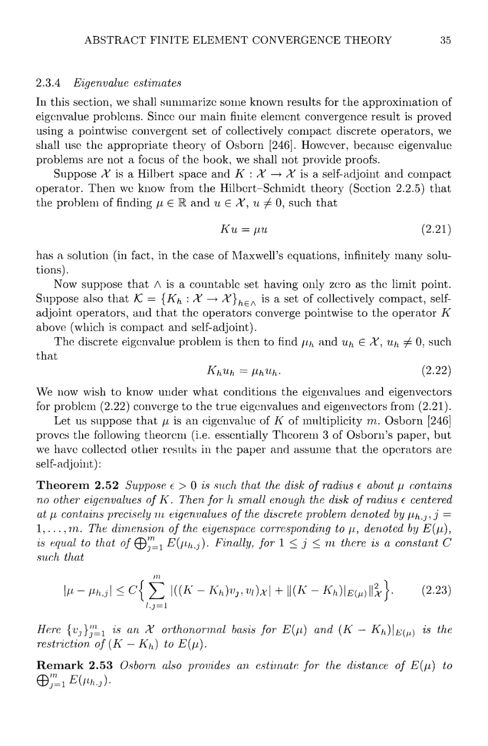
2.3.4 Eigenvalue estimates 35
Sobolev spaces, vector function spaces and regularity 36
3.1 Introduction 36
3.2 Standard Sobolev spaces 36
3.2.1 Trace spaces 42
3.3 Regularity results for elliptic equations 45
3.4 Differential operators on a surface 48
3.5 Vector functions with well-defined curl or divergence 49
3.5.1 Integral identities 50
3.5.2 Properties of tf(div; fi) 52
3.5.3 Properties of/f (curl; fi) 55
3.6 Scalar and vector potentials 61
3.7 The Helmholtz decomposition 65
3.8 A function space for the impedance problem 69
3.9 Curl or divergence conserving transformations 77
XI
Xll
CONTENTS
Variational theory for the cavity problem 81
4.1 Introduction 81
4.2 Assumptions on the coefficients and data 83
4.3 The space X and the nullspace of the curl 84
4.4 Helmholtz decomposition 86
4.4.1 Compactness properties of Xq 87
4.5 The variational problem as an operator equation 89
4.6 Uniqueness of the solution 92
4.7 Cavity eigenvalues and resonances 95
Finite elements on tetrahedra 99
5.1 Introduction 99
5.2 Introduction to finite elements 101
5.2.1 Sets of polynomials 108
5.3 Meshes and affine maps 112
5.4 Divergence conforming elements 118
5.5 The curl conforming edge elements of Nedelec 126
5.5.1 Linear edge element 139
5.5.2 Quadratic edge elements 140
5.6 H1^) conforming finite elements 143
5.6.1 The Clement interpolant 147
5.7 An L2(Q) conforming space 149
5.8 Boundary spaces 150
Finite elements on hexahedra 155
6.1 Introduction 155
6.2 Divergence conforming elements on hexahedra 155
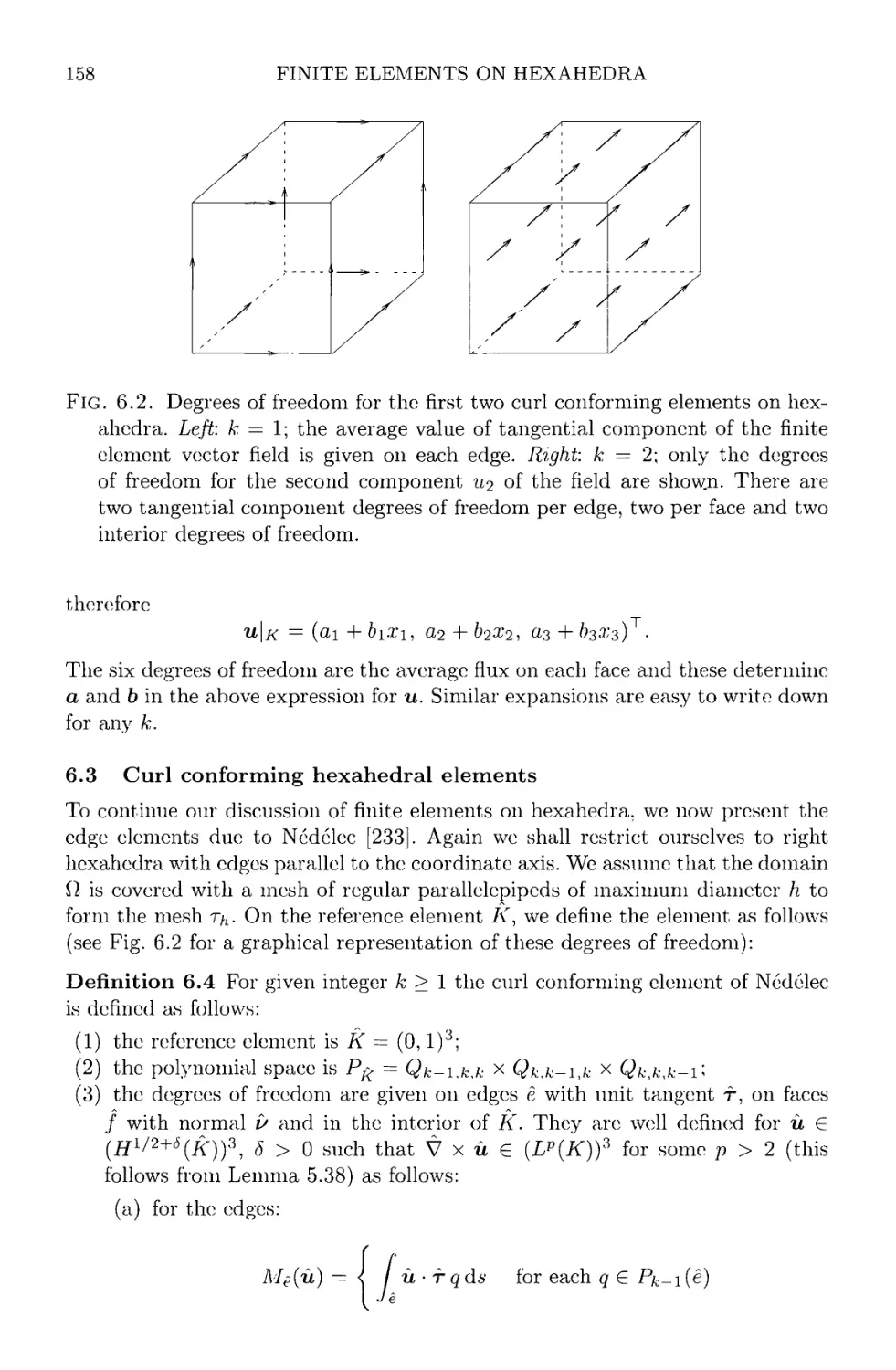
6.3 Curl conforming hexahedral elements 158
6.4 H1^) conforming elements on hexahedra 162
6.5 An L2{Q) conforming space and a boundary space 164
Finite element methods for the cavity problem 166
7.1 Introduction 166
7.2 Error analysis via duality 168
7.2.1 The discrete Helmholtz decomposition 170
7.2.2 Preliminary error analysis 171
7.2.3 Duality estimate 174
7.3 Error analysis via collective compactness 176
7.3.1 Point wise convergence 178
7.3.2 Collective compactness 180
7.3.3 Numerical results for the cavity problem 188
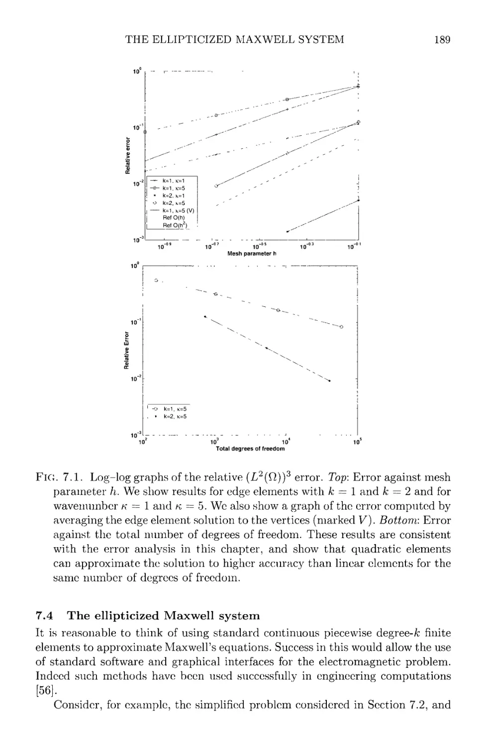
7.4 The ellipticized Maxwell system 189
7.4.1 Discrete ellipticized variational problem 191
7.5 The discrete eigenvalue problem 195
Topics concerning finite elements 199
8.1 Introduction 199
CONTENTS
xin
8.2 The second family of elements on tetrahedra 202
8.2.1 Divergence conforming element 202
8.2.2 Curl conforming element 205
8.2.3 Scalar functions and the de Rham diagram 209
8.3 Curved domains 209
8.3.1 Locally mapped tetrahedral meshes 210
8.3.2 Large-element fitting of domains 214
8.4 hp finite elements 217
8.4.1 i/1@) conforming hp element 218
8.4.2 hp curl conforming elements 219
8.4.3 hp divergence conforming space 221
8.4.4 de Rham diagram for hp elements 222
9 Classical scattering theory 225
9.1 Introduction 225
9.2 Basic integral identities 225
9.3 Scattering by a sphere 234
9.3.1 Spherical harmonics 236
9.3.2 Spherical Bessel functions 238
9.3.3 Series solution of the exterior Maxwell problem 241
9.4 Electromagnetic Calderon operators 248
9.4.1 The electric-to-magnetic Calderon operator 249
9.4.2 The magnetic-to-electric Calderon operator 252
9.5 Scattering of a plane wave by a sphere 254
9.5.1 Uniqueness and Rellich's lemma 254
9.5.2 Series solution 256
10 The scattering problem using Calderon maps 261
10.1 Introduction 261
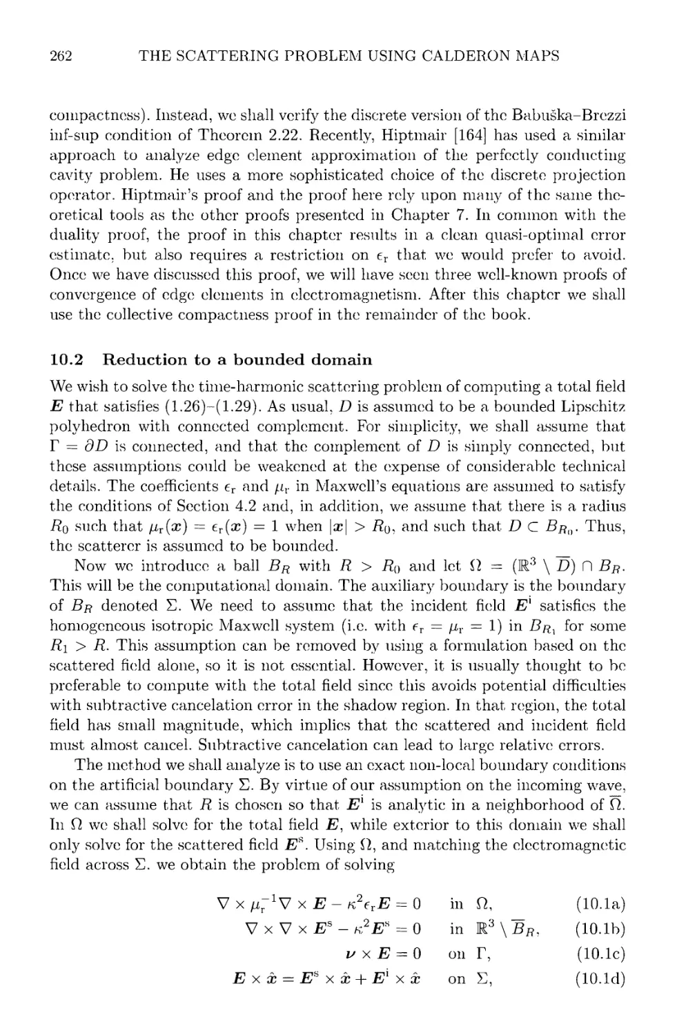
10.2 Reduction to a bounded domain 262
10.3 Analysis of the reduced problem 264
10.3.1 Extended Hclmholtz decomposition 267
10.3.2 An operator equation on Xq 269
10.4 The discrete problem 274
11 Scattering by a bounded inhomogeneity 280
11.1 Introduction 280
11.2 Derivation of the domain-decomposed problem 281
11.3 The finite-dimensional problem 289
11.4 Analysis of the interior finite element problem 290
11.5 Error estimates for the fully discrete problem 298
12 Scattering by a buried object 302
12.1 Introduction 302
12.2 Homogeneous isotropic background 303
12.2.1 Analysis of the scheme 308
12.2.2 The fully discrete problem 311
XIV
CONTENTS
12.2.3 Computational considerations 314
12.3 Perfectly conducting half space 315
12.4 Layered medium 318
12.4.1 Incident plane waves 318
12.4.2 The dyadic Green's function 321
12.4.3 Reduction to a bounded domain 328
13 Algorithmic development 332
13.1 Introduction 332
13.2 Solution of the linear system 333
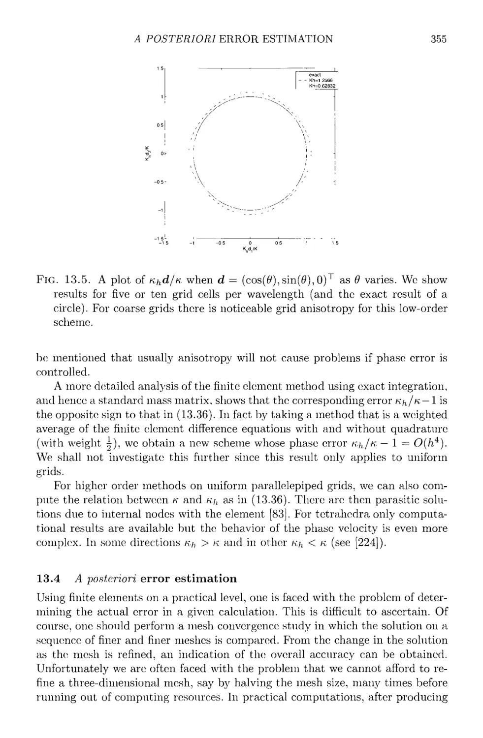
13.3 Phase error in finite element methods 344
13.3.1 Wavenumber dependent error estimates 345
13.3.2 Phase error in three dimensional edge elements 351
13.4 A posteriori error estimation 355
13.4.1 A residual-based error estimator 356
13.4.2 Numerical experiments 362
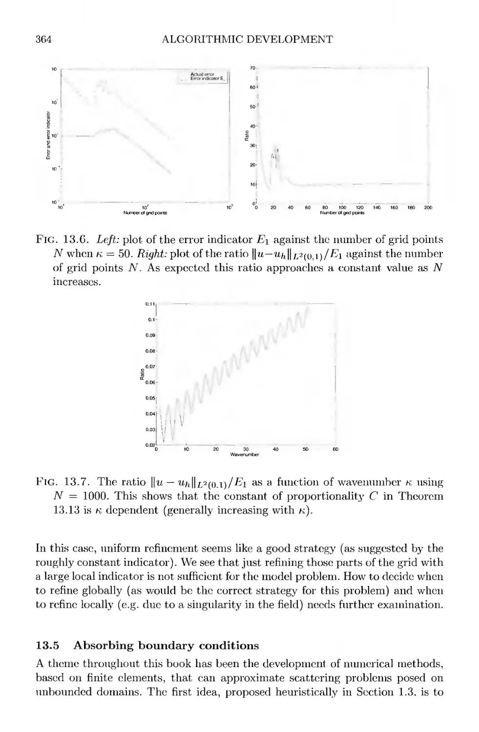
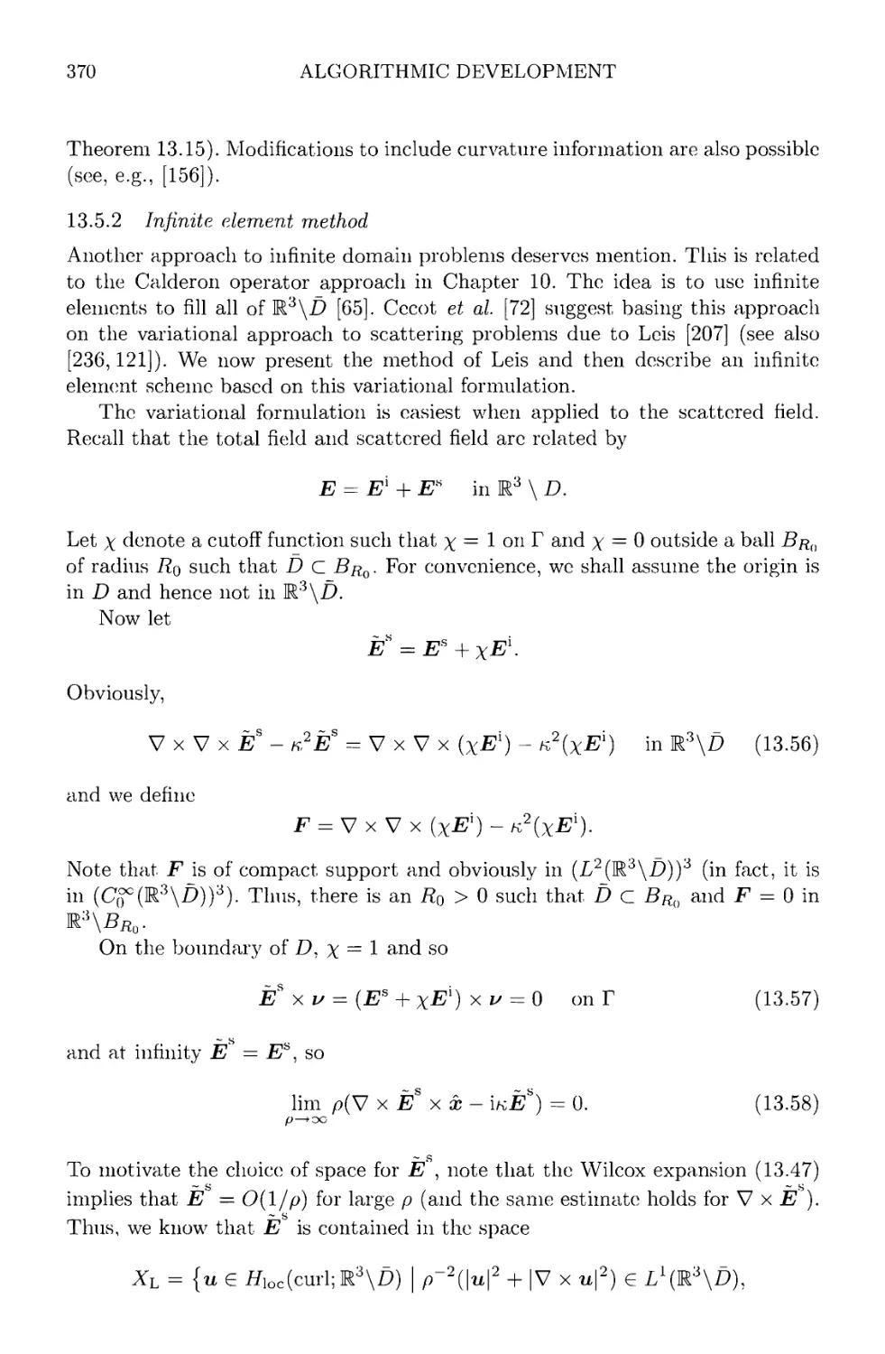
13.5 Absorbing boundary conditions 364
13.5.1 Silver-Miiller absorbing boundary condition 365
13.5.2 Infinite element method 370
13.5.3 The perfectly matched layer 375
13.6 Far field recovery 386
14 Inverse problems 394
14.1 Introduction 394
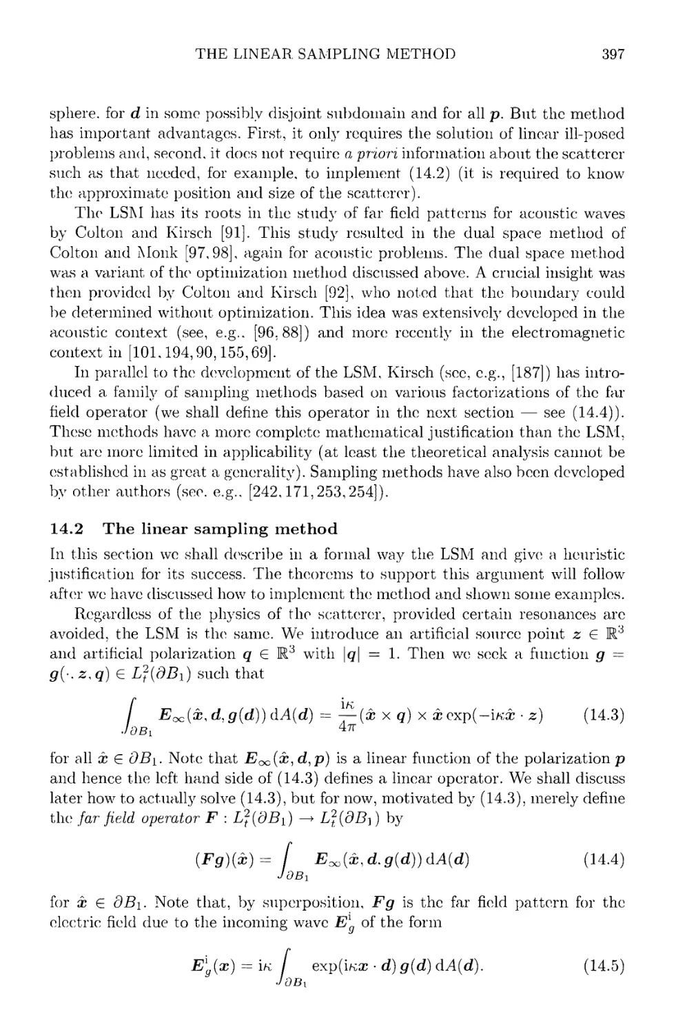
14.2 The linear sampling method 397
14.2.1 Implementing the LSM 399
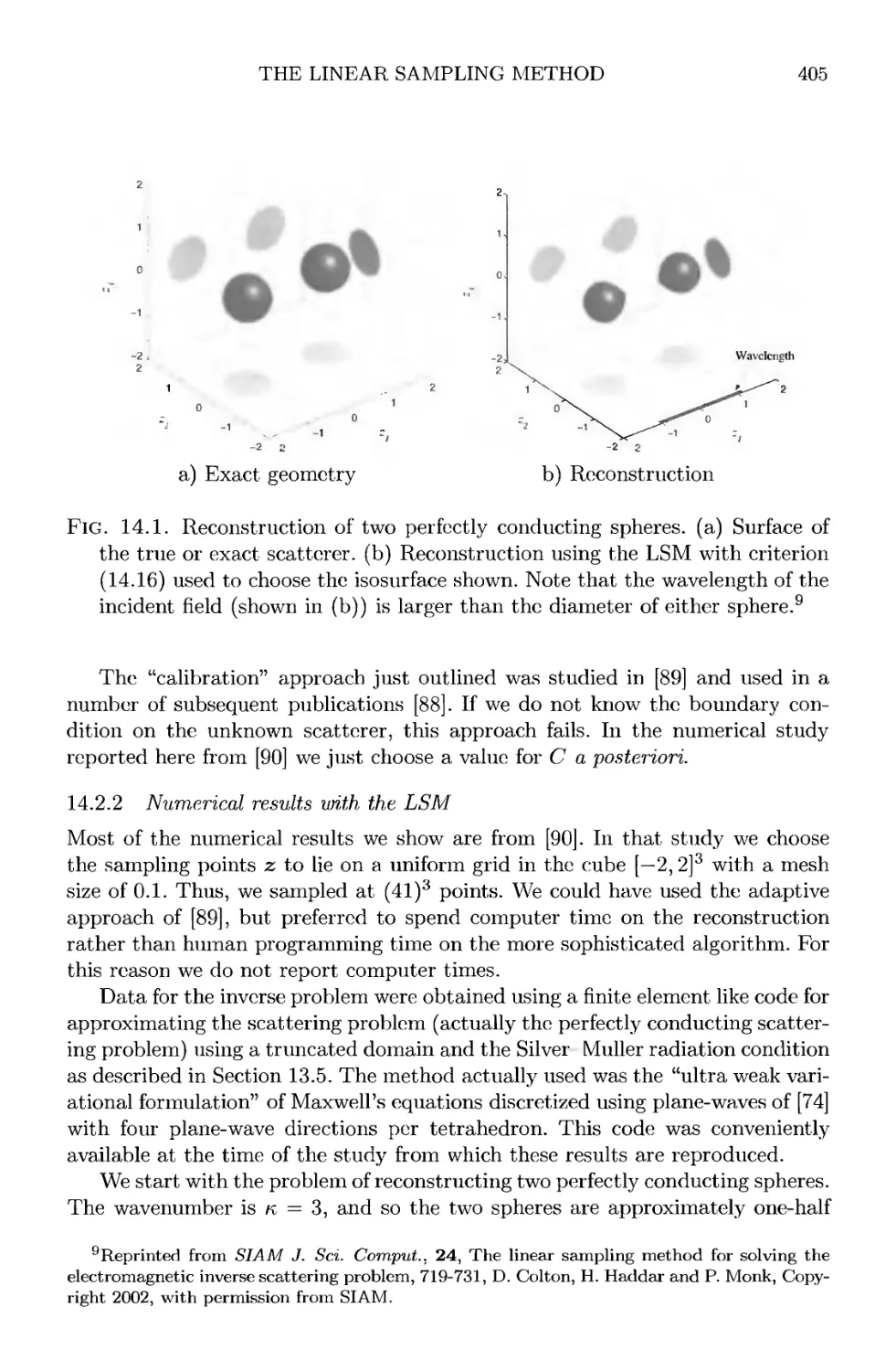
14.2.2 Numerical results with the LSM 405
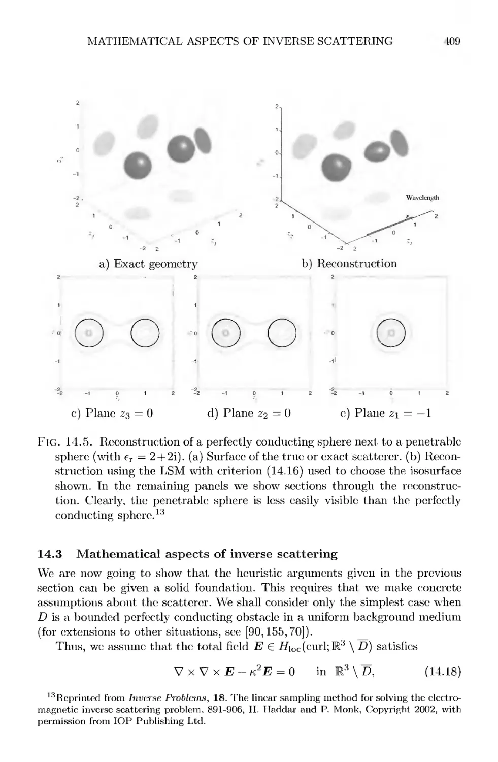
14.3 Mathematical aspects of inverse scattering 409
14.3.1 Uniqueness for the inverse problem 411
14.3.2 Herglotz wave functions 414
14.3.3 The far field operators F and B 417
14.3.4 Mathematical justification of the LSM 422
Appendices
A Coordinate systems 425
A.l Cartesian coordinates 425
A.2 Spherical coordinates 425
B Vector and differential identities 427
B.l Vector identities 427
B.2 Differential identities 427
B.3 Differential identities on a surface 427
References 428
Index
1
MATHEMATICAL MODELS OF ELECTROMAGNETISM
1.1 Introduction
In 1873 Maxwell founded the modern theory of electromagnetism with the
publication of his Treatise on Electricity and Magnetism, in which he formulated
the equations that now bear his name. These equations consist of two pairs
of coupled partial differential equations relating six fields, two of which model
sources of electromagnetism. It turns out that these equations are not sufficient
to uniquely determine the electromagnetic field and that additional constitutive
equations are needed to model the way in which the fields interact with
matter. There is considerable flexibility in the constitutive equations. Because of
this, we need to carefully state the problems to be analyzed in this book, and
we start this chapter by summarizing the classical Maxwell equations
governing an electromagnetic field in a linear medium. We then reduce this system
to its time-harmonic form by assuming propagation at a single frequency. The
time-harmonic Maxwell system will be the focus of this book. Besides Maxwell's
equations, it is also necessary to describe appropriate physical boundary
conditions. These include radiation conditions that select the outgoing field relevant
to scattering problems.
Once the basic boundary value problem is formulated, it is often expedient
to reduce the full Maxwell system to a simpler system relevant to the physical
problem at hand. For example, it is often reasonable to assume that the
electromagnetic field is time invariant or static. This reduces Maxwell's equations
to a potential problem. Simpler models can also be derived at long and short
wavelengths. We do not consider any of these reduced models here. We shall
be concerned with approximating the time-harmonic Maxwell system for linear
media in the "resonance region". By this we mean that the wavelength of the
radiation is commensurate with the dimensions of features of the scatterer.
We end this chapter with a summary of the relevant boundary value problems
from the point of view of this book. Our presentation, at this stage, is purely
formal (we simply assume the existence of appropriate solutions) and follows the
format of standard texts on electromagnetism, such as [274]. Later chapters will
give a careful variational formulation of the equations in this chapter, followed
by finite element methods.
First a word about notation: vectors are distinguished from scalars by the
use of bold typeface (but this convention does not, in general, carry over to
operators). Unless otherwise stated, vectors will all be three dimensional and
either real (in IR3) or complex (in C3). For example, a;Gi3 denotes position
1
2
MATHEMATICAL MODELS OF ELECTROMAGNETISM
in three-space and has components #i, ?2 and .T3 (x = B:1,0:2,3:3)T where T
denotes transpose). For two vectors a G CN and b G CN we define the dot
product on C^ by
N
a-b = J2a3bj-
3=1
The reason for not including complex conjugation in the dot product is that we
will need to write down expressions like v • E, where v is a real vector and E is
complex. In this case we do not want to conjugate E. Later, when we start to
write down variational formulations, it will be important to recall that the dot
product does not have complex conjugation built in. If a G CA' we define the
Euclidean norm of a by \a\ = y/a • a, where a = (ai,..., cij\t)T and a3 is the
complex conjugate of dj.
As usual in mathematics texts, i = \/—I, and j is just an integer variable.
In our error estimates we shall use a generic constant C everywhere different.
Apart from this, I have tried to avoid using the same symbol for two quantities
(at least on the same page!).
1.2 Maxwell's equations
The classical macroscopic electromagnetic field is described by four vector
functions of position xGl3 and time t G R denoted by ?, T>. Ji and 13. The
fundamental field vectors E and H are called the electric and magnetic field intensities,
respectively (we shall refer to them as the electric field and the magnetic field,
respectively). The vector functions T> and B, which will later be eliminated from
the description of the electromagnetic field via suitable constitutive relations,
are called the electric displacement and magnetic induction, respectively.
An electromagnetic field is created by a distribution of sources consisting of
static electric charges and the directed flow of electric charge, which is called
current. The distribution of charges is given by a scalar charge density
function p. while currents are described by the vector current density function J.
Maxwell's equations then state that the field variables and sources are related
by the following equations which apply throughout the region of space in M3
occupied by the electromagnetic field:
A.1a)
(Lib)
A.1c)
(l.ld)
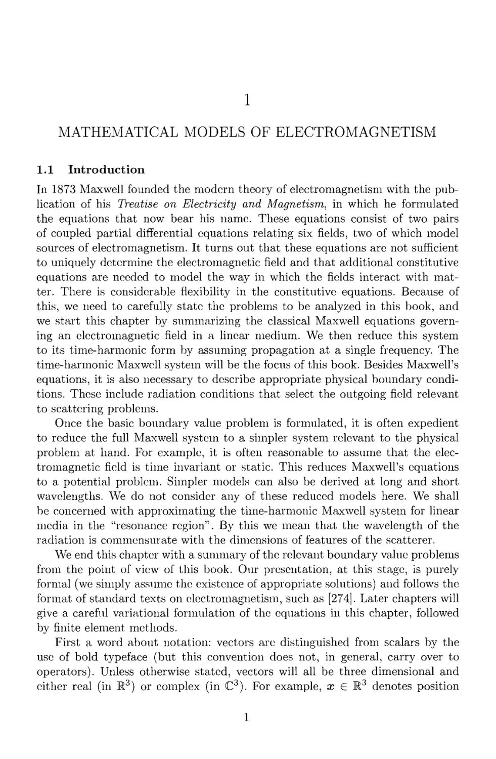
Equation A.1a) is called Faraday's law and gives the effect of a changing magnetic
field on the electric field. The divergence condition A.1b) is Gauss's law and gives
the effect of the charge density on the electric displacement. The next equation,
9B „ <.
-+Vx? =
vx> =
VB =
= 0,
= /».
---J
= 0.
MAXWELL'S EQUATIONS
3
A.1c), is Ampere's circuital law as modified by Maxwell. Finally, eqn (l.ld)
expresses the fact that the magnetic induction 3 is solenoidal. A table of SI
units relevant to electromagnetism is given in Table 1.1.
The divergence conditions A.1b) and (l.ld) arc consequences of the
fundamental field equations, A.1a) and A.1c), provided charge is conserved. Formally,
this is shown by taking the divergence of A.1a) and A.1c) and recalling that
V • (V x A) = 0 for any vector function A. Hence
„ d& n , ^ dV _ ^
V ¦ — = 0 and V • — = -V • J.
at at
But if charge is conserved, p and J are connected by the relation
V- J +
dp
dt
o,
A.2)
and hence
&¦>>¦¦
d_
dt
(V • V - p) = 0.
Thus if A.1b) and (l.ld) hold at one time, they hold for all time. However,
the fact that A.1b) and (l.ld) arc consequences of A.1a) and A.1c) for the
continuous electromagnetic field does not mean that these divergence conditions
can be entirely ignored when designing a numerical scheme to discretize A.1). A
successful scheme must produce a numerical approximation that in some sense
satisfies discrete analogs of A.1b) and (l.ld).
Either by using the Fourier transform in time, or because we wish to analyze
electromagnetic propagation at a single frequency (e.g. if the source currents
and charges vary sinusoidally in time), the time-dependent problem A.1) can be
reduced to the time-harmonic Maxwell system. If the radiation has a temporal
frequency uj > 0, then the electromagnetic field is said to be time-harmonic,
provided
?{xA) = ft (exp(-iujt)E{x)\ ,
T>(xA) = ft (exp{-iujt)b{x)) ,
U{xA) = ft (cxp{-iLJt)H(xj) ,
A.3a)
A.3b)
A.3c)
Quantity
Units
Electric field intensity ? Vm_1
Electric displacement T> Cm-2
Electric current density J Am-2
Quantity
Units
Magnetic field intensity 7i Am-1
Magnetic induction & T
Electric charge density p Cm-3
Table 1.1 A table giving the SI units appropriate for electromagnetic quantities.
4
MATHEMATICAL MODELS OF ELECTROMAGNETISM
B(x,t) = 5ft (cxp{-iut)B(x)) , A.3d)
where i = >/—1 and SR(.) denotes the real part of the expression in
parentheses. Note that E (and similarly other hat variables) are now complex-valued
vector functions of position but not time. Some authors instead choose a time
dependence of exp(kjt). Of course, the choice is arbitrary and, provided it is
used consistently, produces no difficulties. Our choice is fairly standard in the
mathematics literature.
For consistency we also need the current density and charge density to be
time-harmonic, so we assume
J(x,t) = 5ft (exp(-iujt)J(x)) ,
p(x, t) = K (exp(-iu)t)p(x)).
Substituting these relations into A.1) leads to the time-harmonic Maxwell
equations:
-\ujB + V x i? = 0, A.4a)
V-?> = p, A.4b)
-\u)D- V x H = -J, A.4c)
V • B = 0, A.4d)
where the time-harmonic charge density p is given via charge conservation A.2)
or by taking the divergence of A.4c) and using A.4b) as icop = V • J and hence
can be eliminated from the equations.
Equations A.4) give the time-harmonic Maxwell equations in differential
form. Frequently, particularly in the physics literature, they are stated in
integral form. As an example, consider A.4a) and let S be a smooth surface in R3
with boundary OS and unit normal i/. Then, using Stokes theorem, we find that
io; / B • vdA = I (V x E) • v&A = J E-rds, A.5)
JS 'Is JdS
T/ I rf -V.B.I//JE-T
/ B v E-t ^. '
Fig. 1.1. For a surface S with normal v the integrated flux of B normal to S
is given by the integral of the tangential component of E around the edges
shown. Here we show schematics for a triangle and rectangle, two important
surfaces from the point of view of numerical methods.
MAXWELL'S EQUATIONS
5
where r is the unit tangent to dS oriented by the right-hand rule relative to v.
In the integral formulation we see that E is naturally associated to line integrals,
whereas B is naturally associated to surface integrals. For example, in Fig. 1.1
we show this when S is a triangle or a rectangle, two important cases that will
appear later in the book.
Motivated by this integral formulation, finite difference schemes (in particular
the famous FDTD scheme of Yee [301,225]) usually associate the electric field
E with edges in a rectilinear mesh and the magnetic induction B with faces.
This is also the arrangement of discrete unknowns in a generalization of the
rectangular finite difference scheme to tetrahedral grids called the co-volume
scheme [214,240,241]. As we shall see in Chapter 5, we can also design finite
elements that have a similar arrangement of unknowns. Finally, we note that
A.5) is also a starting point for the description of Maxwell's equations in terms
of differential forms [164].
1.2.1 Constitutive equations for linear media
Equations A.4) must be augmented by two constitutive laws that relate E and
H to D and B, respectively. These laws depend on the properties of the matter
in the domain occupied by the electromagnetic field. We can distinguish three
cases:
A) Vacuum, or free space In free space the fields are related by the equations
t) = e0E and B = fi0H, A.6)
where the constants eo and jjlq are called, respectively, the electric permittivity
and magnetic permeability. The values of eo and Mo depend on the system of
units used. In the standard SI or MKS units
Mo = 4tt x 10 Hm~\
e0 ~ 8.854 x 10~12 Fm.
Furthermore the speed of light in a vacuum, denoted by c, is given by c =
v/e^o -1 (c « 2.998 x 10⁸ ms) [274].
B) Inhomogeneous, isotropic materials The most commonly occurring case in
practice is that various different materials (e.g. copper, air, etc.) occupy the
domain of the electromagnetic field. The medium is then called inhomoge-
neous. If the material properties do not depend on the direction of the field
and the material is linear, we have
D = eE and B = jjlH, A.7)
where e and jjl are positive, bounded, scalar functions of position (we shall
give a more careful description of these functions in Section 4.2).
C) Inhomogeneous, anisotropic materials In some materials the electric or
magnetic properties of the constituent materials depends on the direction of the
6
MATHEMATICAL MODELS OF ELECTROMAGNETISM
field (e.g. in the macroscopic description of a finely layered medium). In such
cases e and jj, in A.7) are 3x3 positive-definite matrix functions of
position. Usually, the finite element method is equally applicable to isotropic or
anisotropic materials in that programs can be written from the onset for
the anisotropic case. The theoretical justification of the convergence of the
method is more difficult in these cases. Of course, in the presence of extreme
anisotropy, special techniques may be necessary.
Although the methods in this book can be applied to anisotropic media, we
will not analyze methods with matrix-valued coefficients. This is mainly due to
the difficulty of verifying uniqueness of the solution of Maxwell's equations in
this case. Although uniqueness is known (see [287]), the proof is too complex for
this book.
One further constitutive relation needs to be discussed. In a conducting
material, the electromagnetic field itself gives rise to currents. If the field strengths
are not large, we can assume that Ohms law holds so that:
J = aE + J&, A.8)
where a is called the conductivity and is a non-negative function of position.
The vector function Ja describes the applied current density. Regions where a is
positive are called conductors. Where a = 0 and e ^ eo, the material is termed a
dielectric, and e is referred to as the dielectric constant In a vacuum (or air at low
field strengths) a = 0, e = eo and jjl = /xo- More generally, in anisotropic media,
the conductivity a can be a symmetric, positive semi-definite matrix function of
position. However, we shall not consider this case here.
Using the linear, inhomogeneous constitutive equations in A.7) and the
constitutive relation for the currents in A.8), we arrive at the following time-
harmonic Maxwell system:
-ujfiH + V x E = 0, A.9a)
V • {(E) = —V • (aE + Ja), A.9b)
io;
-liveE + 0-E-V x H = - Ja, A.9c)
V-(/zff) = 0, A.9d)
where we recall that Ja denotes a given applied current density.
There is one last reduction to perform on the equations. It is convenient to
work with relative parameter values. Following Colton and Kress [93], we define
E = el/2E and H = fil0/2H.
Using these definitions in A.9), and defining the relative permittivity and
permeability by
1 / icr\ . /i
er = — I e H and jiY = —,
eo V ^ / Mo
MAXWELL'S EQUATIONS
7
we obtain the final version of the first-order Maxwell system, where we note that
er = fir = 1 in vacuum:
-iKeTE - V x H = - —F,
A.10a)
A.10b)
1 /2 "
where F = i«//0 Ja and the wavenumber k = uj-^/e^jiQ. We also obtain the
divergence conditions (which follow from the differential equations when n > 0)
1
V • (erE) = -
V • (fjiTH) = 0.
rV-F,
A.11a)
A.11b)
Although it is possible to derive numerical schemes for the first-order system
A.10) A.11), it is more usual to eliminate the magnetic field H by solving
A.10a) for H and substituting into A.10b) to obtain the second-order Maxwell
system
V x (/x^V x E) - K2erE = F A.12)
together with A.11a). Of course, the choice of eliminating H, rather than F, is
arbitrary. We shall generally use A.12) in this book, rather than the first-order
system, since there are fewer dependent variables.
1.2.2 Interface and boundary conditions
Equations A.10) or A.12) are not a complete classical description of the
electromagnetic field since the equations do not hold at boundaries between different
materials where either /ir or er are discontinuous (e.g. at a copper-air interface).
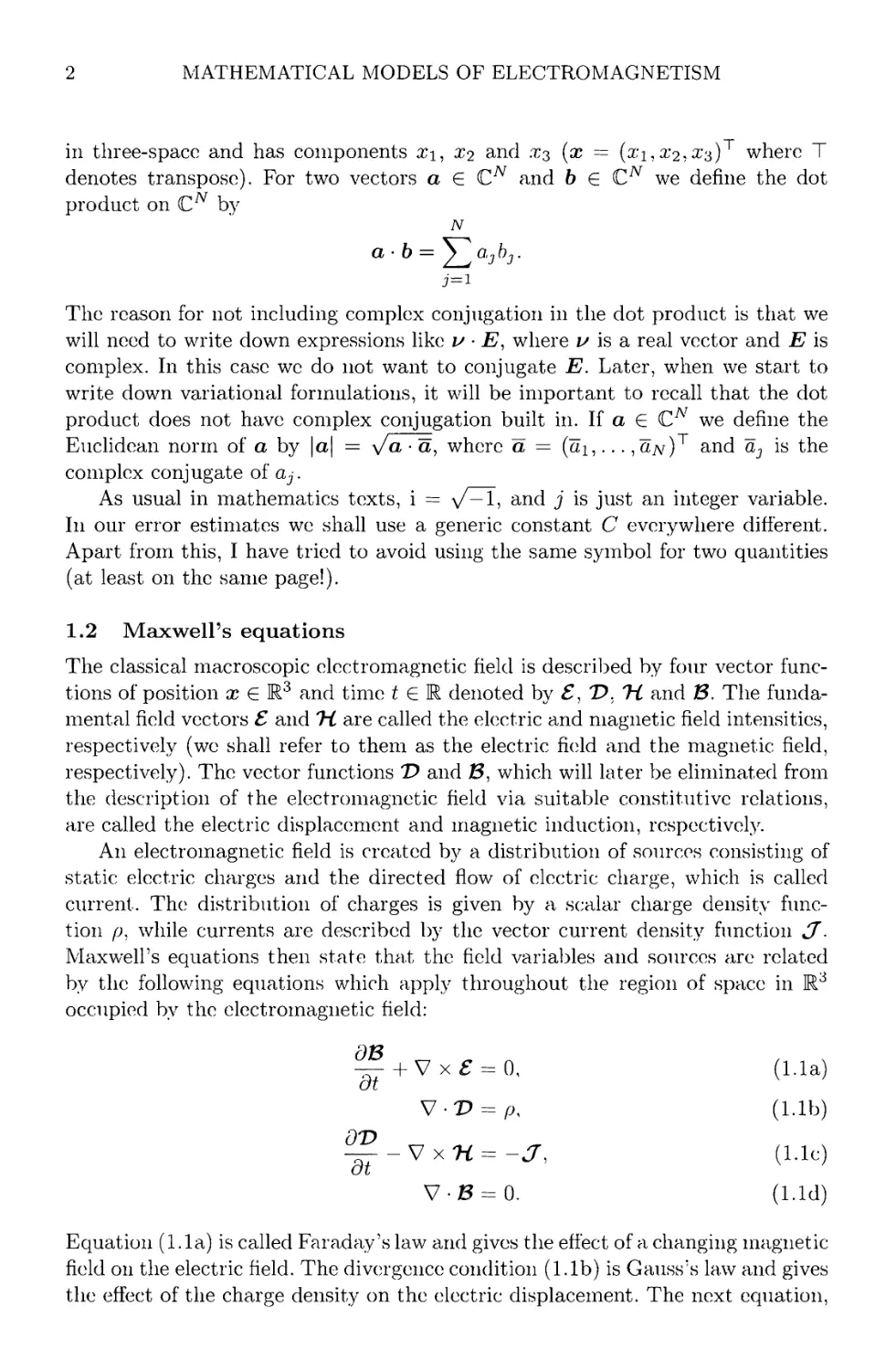
Let us consider the case of two media with differing electric and magnetic
properties separated by a surface S with unit normal u pointing from region 2 to
region 1 (see Fig. 1.2). As we shall see later in Lemma 5.3, for V x E in A.12) to
be well defined in a least-squares sense we must have the tangential component
Region 1
E,
8r..Hr.l
»,
V
/s
' r.2 ~ r,2
Region 2
E2 H2
Fig. 1.2. Geometry of the surface and subdomains in our discussion of interface
boundary conditions.
8 MATHEMATICAL MODELS OF ELECTROMAGNETISM
of the electric field to be continuous across S and so v x E is continuous across
S. Thus if Ei denotes the limiting value of the electric field as S is approached
from region 1 and E2 denotes the the limit of the field from the other region, we
must have
i/x(E1-E2) = 0 on S. A.13)
On the other hand, we shall see (Lemma 5.3 again) that for prH in A.11b) to
have a well defined divergence in the least-squares sense, the normal components
of jivH must be continuous across S so that
V • (/Xr.iff! - Mr,2i*2) =0 OU 5, A.14)
where, again, the subscripts denote limiting values of the coefficients and field
variables on either side of the surface S.
The continuity conditions A.13) and A.14) hold for any electromagnetic field.
However, we cannot assume that the analogue of A.13) holds for the magnetic
field. In general
vx{Hl-H2) = Js,
where this relation defines the tangential vector field Js termed the surface
current density on S. In most instances the magnetic field has continuous
tangential components (i.e. Js = 0). This is true unless the surface S models a thin
conductive layer giving rise to the conductive boundary condition (see [15]) or
singularities in F give rise to surface currents on 5. Thus we will also usually
assume that
i/x(H1-H2)=0 on S. A.15)
The presence of singularities in the charge density p may cause jumps in the
normal component of eTE. We write
v • (er,!^! - eu2E2) = ps on 5, A.16)
where ps is termed the surface charge density. From A.14) and A.16), even in
the case of a negligible surface charge and current density, we see that the electric
and magnetic field vectors are not continuous if er or jj,r are discontinuous across
S. Any numerical scheme for approximating Maxwell's equations in the presence
of material discontinuities must take into account that tangential components
of the field are continuous, but that normal components jump across a material
boundary. As we shall see, the variational or weak formulation of Maxwell's
equations used in this book automatically takes care of these jump conditions.
A particularly important case occurs when the material on one side of the
interface discussed above is a perfect conductor. From Ohm's law A.8), we see
heuristically that if the conductivity a —> oo and if the current density J is
to remain bounded then E —> 0. This suggests that in a perfect conductor the
electric field vanishes. If the side of the surface 5 labeled 2 in Fig. 1.2 is a
SCATTERING PROBLEMS AND THE RADIATION CONDITION 9
perfect conductor then E2 = 0 in A.13) and we arrive at the perfect conducting
boundary condition for Ei,
iyxE1=0 on 5, A.17)
where we can drop the index 1 since only the field outside the perfect conductor
needs to be modeled.
If the material on one side of the boundary is not a perfect conductor, but
allows the field to penetrate only a small distance, a more appropriate boundary
condition is the impedance or imperfectly conducting boundary condition.
Suppose again that the good conductor is in region 1 and that the normal v points
from region 2 into region 1. Then this boundary condition is
v x Hi - A(i/ x Ei) x v = 0, A.18)
where the impedance A is a positive function of position on the surface of the
material.
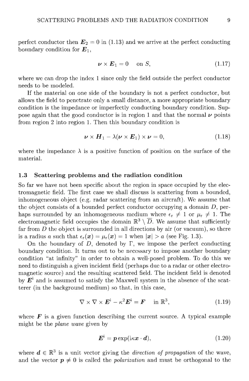
1.3 Scattering problems and the radiation condition
So far we have not been specific about the region in space occupied by the
electromagnetic field. The first case we shall discuss is scattering from a bounded,
inhomogeneous object (e.g. radar scattering from an aircraft). We assume that
the object consists of a bounded perfect conductor occupying a domain D,
perhaps surrounded by an inhomogeneous medium where er ^ 1 or jur ^ 1. The
electromagnetic field occupies the domain R3 \ D. We assume that sufficiently
far from D the object is surrounded in all directions by air (or vacuum), so there
is a radius a such that eT(x) = iav(x) — 1 when \x\ > a (see Fig. 1.3).
On the boundary of D, denoted by T, we impose the perfect conducting
boundary condition. It turns out to be necessary to impose another boundary
condition "at infinity" in order to obtain a well-posed problem. To do this we
need to distinguish a given incident field (perhaps due to a radar or other
electromagnetic source) and the resulting scattered field. The incident field is denoted
by El and is assumed to satisfy the Maxwell system in the absence of the scat-
terer (in the background medium) so that, in this case,
V x V x E'1 - k2E'1 = F in R3, A.19)
where F is a given function describing the current source. A typical example
might be the plane wave given by
El = pexp(i«as-d), A.20)
where d G R3 is a unit vector giving the direction of propagation of the wave,
and the vector p ^ 0 is called the polarization and must be orthogonal to the
10
MATHEMATICAL MODELS OF ELECTROMAGNETISM
er = 1
j-h = 1
Fig. 1.3. Geometry of the scatterer and boundaries for the scattering problem.
A bounded scatterer consisting of a perfectly conducting part and a
penetrable part where the electromagnetic properties differ from the background is
surrounded by air or vacuum.
direction of propagation so p • d = 0. In this case F = 0. The total field E
consists of the incident field El and the scattered field 22s, so
E = E[ + ES. A.21)
The scattered field is out-going (i.e. originates at the scatterer and propagates
outwards) and this is imposed by requiring the scattered field to satisfy the
Silver-Mtiller radiation condition [228]:
lim p ((V x Es) x x - mE*) = 0, A.22)
p—>oc
where p = \x\ and the limit is uniform in x = x/\x\.
The wavelength of the incident field in A.20) is 2tt/' k since \d\ = 1. If this
wavelength is much smaller than a typical length b of relevant features of the
scatterer (i.e. if Kb is large) or if this wavelength is much larger than b (i.e. if
nb is close to zero), it is possible to apply asymptotic methods to simplify the
scattering problem. For example, when Kb is small, a popular approximation is
the eddy-current model [272,165]. For large Kb one can use the geometric theory
of diffraction [181]. In this book we shall be concerned with computations in the
"resonance region", where Kb = O(l), so asymptotic methods are not applicable.
An obvious difficulty with approximating the scattering problem by a finite
element method is that the problem is posed on an infinite domain. One simple
way to avoid this difficulty is to approximate the scattering problem by imposing
the radiation condition A.22) on a surface E far from the scatterer (where /.ir = 1
and er = 1). Thus, in this approximation, the domain occupied by the
computational electromagnetic field, denoted by O, is the region between T and E, which
SCATTERING PROBLEMS AND THE RADIATION CONDITION 11
cr = 1
er 7^ 1 or \ir — 1
Fig. 1.4. Geometry of the scatterer and boundaries for the interior problem
with an absorbing boundary condition on the auxiliary boundary E.
are assumed to be disjoint surfaces (see Fig. 1.4), and Maxwell's equations are
satisfied in ft. On T we have the perfect conducting boundary condition, but on
E we impose a boundary condition inspired by the Silver-Miiller condition:
(VxE)xi/- \kEt = (V x E[) x v - \kE[t on E, A.23)
where v is the unit outward normal to E and Et = [y x E\y) x v (similarly for
ElT). This is just an impedance boundary condition of the form A.18) with a
special choice of the impedance. Equation A.23) is an example of an absorbing
boundary condition used to simulate the infinite domain outside ft. We shall
discuss some other possible choices in Section 13.5. Obviously, the solution of
the true scattering problem and the problem on a bounded domain are not
equal, but the difference can be made small by taking E far enough from the
scatterer.
One other interesting problem arises if the electromagnetic field is entirely
contained in a perfect conducting cavity. In this case ?1 is a bounded domain with
boundary T and Maxwell's equations are satisfied in Q. If there is no conductor
present (i.e. a = 0), there are values of the wave number k for which the Maxwell
system no longer has a unique solution. These values of k are resonant wave
numbers for cavity modes and mathematically are eigenvalues of the Maxwell
system.
The second scattering problem we wish to consider is a simple case when
the scatterer is unbounded. More complex ugratings" and "rough surfaces" will
not be considered in this book (see, e.g. [128]). The problem we shall consider
is a simple model for scattering from buried objects (arising, e.g., in simulating
ground penetrating radar). The background medium now consists of two regions.
The region .7:3 > 0 is assumed occupied by air and the region .7:3 < 0 is earth. The
relative permeability of air and earth is assumed to be unity, and the relative
permittivity of earth is assumed constant (with a possibly non-zero imaginary
part since the earth is usually a conductor).
At the air-earth interface, we impose the jump conditions discussed in the
previous section. We suppose the scatterer (consisting of perfect conductors,
MATHEMATICAL MODELS OF ELECTROMAGNETISM
Cr = 1
X > 0 Mr = 1
3 T
x3< ° er ^ 1 and fir = 1
n
M D
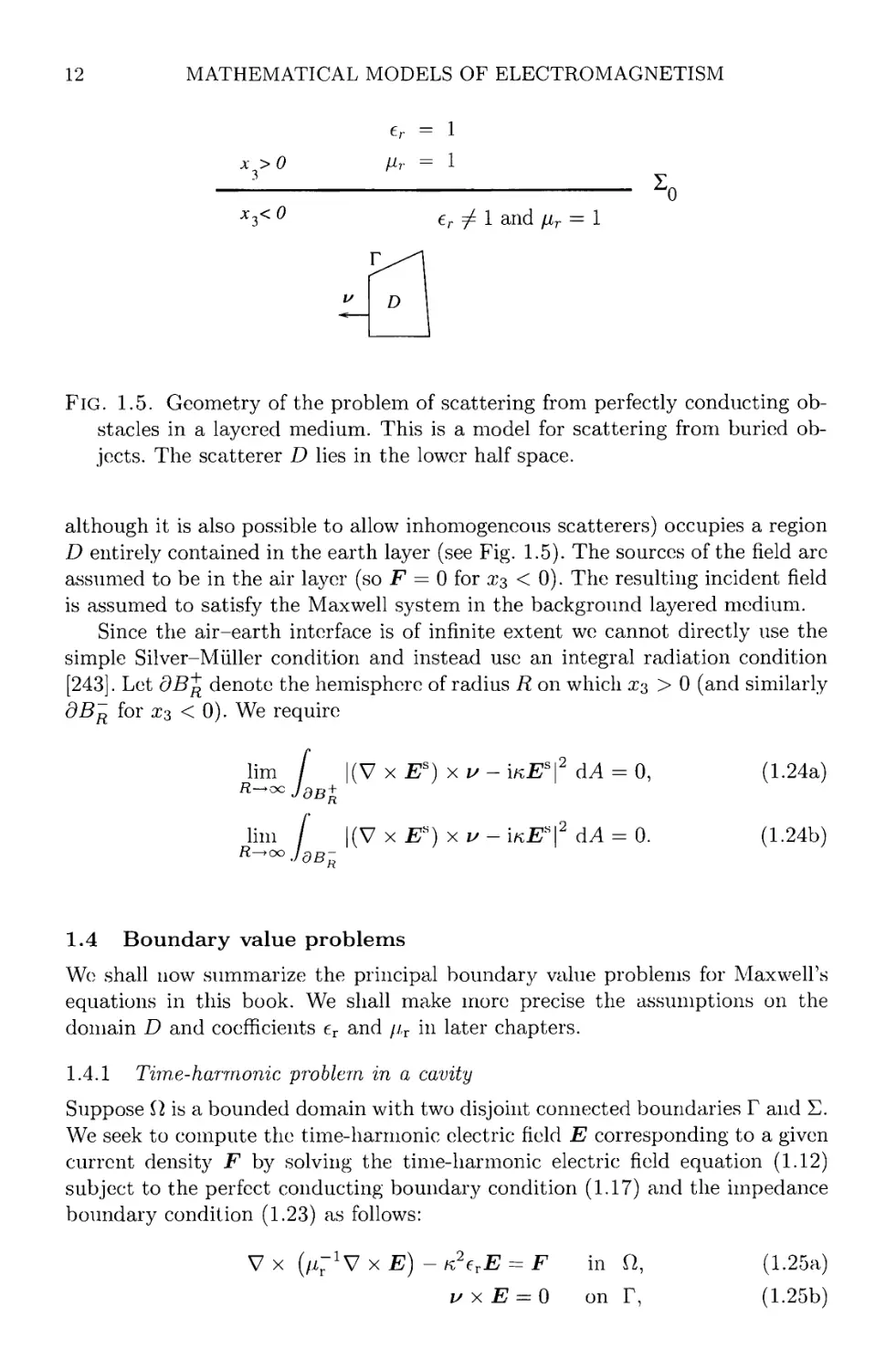
Fig. 1.5. Geometry of the problem of scattering from perfectly conducting
obstacles in a layered medium. This is a model for scattering from buried
objects. The scatterer D lies in the lower half space.
although it is also possible to allow inhomogencous scatterers) occupies a region
D entirely contained in the earth layer (see Fig. 1.5). The sources of the field are
assumed to be in the air layer (so F = 0 for x$ < 0). The resulting incident field
is assumed to satisfy the Maxwell system in the background layered medium.
Since the air-earth interface is of infinite extent we cannot directly use the
simple Silver-Muller condition and instead use an integral radiation condition
[243]. Let dBft denote the hemisphere of radius R on which x^ > 0 (and similarly
dB^ for x3 < 0). We require
lim / |(V x Es) x v-\kEs\2 <L4 = 0, A.24a)
^-^ JdB +
lim / |(V x E*)xv- ikE*\2 dA = 0. A.24b)
^^°° JdB~
1.4 Boundary value problems
We shall now summarize the principal boundary value problems for Maxwell's
equations in this book. We shall make more precise the assumptions on the
domain D and coefficients er and \iv in later chapters.
1.4.1 Time-harmonic problem in a cavity
Suppose il is a bounded domain with two disjoint connected boundaries T and E.
We seek to compute the time-harmonic electric field E corresponding to a given
current density F by solving the time-harmonic electric field equation A.12)
subject to the perfect conducting boundary condition A.17) and the impedance
boundary condition A.23) as follows:
V x (/ir_1 V x E) - K2erE = F in ?1, A.25a)
vxE = 0 on T, A.25b)
BOUNDARY VALUE PROBLEMS
13
p~l(S7 x E)xv-\k\Et =g on ?, A.25c)
where g is a given tangential vector field on ? (see A.23) for an example of g
computed from an incident field). We shall allow ? to be empty in which case
these equations model propagation in a cavity with a perfectly conducting wall.
For an absorbing boundary condition approximation of a scattering problem,
pr = 1 and A = 1 on ?, and er = /ir — 1 in a neighborhood of ?.
1.4.2 Cavity resonator
Given a bounded domain ft with boundary T, we seek scalars k and non-trivial
(i.e. not identically zero) electric fields E which satisfies eqn A.12) with F = 0,
so that
V x (/irV x E) - K2erE = 0 in ft,
isx E = 0 on T.
In addition, since there is no applied current, we require that E satisfy the
divergence condition A.11a) with p = 0, so that
V • (erJ5) =0 in ft.
The effect of this latter condition is to guarantee that there are at most finitely
many linearly independent solutions to this problem when k = 0.
1.4.3 Scattering from a bounded object
In this problem the domain of the electromagnetic field is the unbounded region
IR3 \ D, where D is a bounded domain with connected complement. Given a
known incoming electric field El satisfying A.19), we seek to compute the total
field E and scattered field Es such that the time-harmonic electric field equation
A.12) holds together with A.21), so that
V x (/i^V xE)- K2erE = F in M3 \ D, A.26)
E = El + Es in R3\D. A.27)
We assume that the scatterer is bounded so that D is bounded and er = /xr = 1
outside a sufficiently large ball. On the boundary T of the unbounded component
of R'3 \ D, we impose the perfect conducting boundary condition,
E x v = 0 on T. A.28)
In addition Es must satisfy the Silver-Miiller radiation condition A.22)
lim p ((V x Es) xx- ihlEs) =0 as r -> oo, A.29)
where p — \x\, uniformly in x = x/\x\.
14
MATHEMATICAL MODELS OF ELECTROMAGNETISM
1.4.4 Scattering from a buried object
Let
R+ = {x G M3 | x3 > 0} and Rs_ = {x e Rs \ xs < 0} .
We suppose that the scatterers are contained in a bounded region in the lower
half space. The interface between layers is denoted by Eo and is the plane X3 = 0
(see Fig. 1.5). For simplicity, we only consider a perfectly conducting scatterer
occupying a bounded domain D entirely contained in M?_ (so D C R?_), and we
assume that the complement of D is connected.
The electric field satisfies Maxwell's equations in M+ (with er = fj,r = 1, since
the domain is supposed to contain air) and the general Maxwell equation in
R?_ \ D with jiT = 1 and constant er = e°. The integral radiation condition is
imposed at infinity. Thus, for given F having support in M^_ (F = 0 is a possible
choice), the total field E satisfies
VxVxE- k2E = F in R^, A.30)
VxVxE- K2e*E = 0 inK3_\D. A.31)
Imposing the jump conditions A.13) and A.15) we have
[v x E] = 0 and [u x (V x E)] = 0 on E0, A.32)
where [•] denotes the jump in its argument across Eq. As usual, on the boundary
of D,
Exv = 0 on r.
We suppose that the scattered field is due to a given incident field E1 which
satisfies the background Maxwell system:
VxVxE1- k2E{ = F in M+,
V x V x El - K2e*E{ = 0 in Ri,
and the jump conditions A.32) on E0. Here F is the function of compact support
in IR^_ representing the source of the incident field appearing in A.30). Then we
have
E = E[ + Es in M3 \ D.
and the following integral radiation conditions on the scattered field Es
lim / |(V x E*) x v-inEs\2 dA = 0,
lim / |(VxEs)xi/- wEs\2 dA = 0.
2
FUNCTIONAL ANALYSIS AND ABSTRACT ERROR
ESTIMATES
2.1 Introduction
In our analysis of weak formulations of Maxwell's equations, we shall appeal
to certain basic theorems from functional analysis. The reader is presumed to
be familiar with these rudimentary concepts. As a result, the first part of this
chapter is simply a convenient summary of notation, definitions and theorems
with references to the literature. As a background source, a good book is that of
McLean [215].
In the second part of the chapter, we turn to some abstract finite element error
estimates that will be used later in our proofs of finite element convergence rates.
These results, although standard, are verified in detail due to their basic role in
the analysis of finite element methods. The notation here is fairly standard,
although we use calligraphic symbols like X to denote general Hilbert spaces.
This is to distinguish them from particular spaces appearing in later chapters.
2.2 Basic functional analysis and the Fredholm alternative
The material for this section is mainly taken from the books of Kress [193] and
McLean [215], which also contain proofs of the relevant results. In many cases
we have quoted theorems for Hilbert spaces even though the theorems hold for
more general spaces. Hilbert spaces will be enough for our needs.
2.2.1 Hilbert space
If X is a vector space over the complex numbers, then a scalar product on X is
a map (•, -)x ' X x X —> C such that
A) if u G X then (u, u)x — 0 if and only if u — 0;
B) for all u, v G X we have (u, v)x = (v, u)x\
C) for all u, v, iv G X and a, 0 G C we have
(au + (iv,w)x = a(u,w)x + 0(v,w)x-
The norm associated with {- ,-)x is
\\4>\\x = y/W^U fOT all 0G X.
This norm satisfies the usual triangle inequality
I|0 + ?||*<MU + ||?IU, for all?,0e*.
15
16 FUNCTIONAL ANALYSIS AND ABSTRACT ERROR ESTIMATES
Definition 2.1 Let X be a vector space with scalar product (•,•)*• If X is
complete with respect to the norm || • \\x it is called a Hilbert space.
A basic example of such a Hilbert space is L2(Q), the space of square-
integrable functions on an open domain ficM3, which has the scalar product
@,0= [ HdV,
Jn
where ? is the complex conjugate of ?. Here we have used the notation (•, •)
instead of the more correct (•, -)l2(Q)- In this case the L2 scalar product is so
important and used so frequently that it is worth immediately breaking our own
rules of notation!
Two elementary estimates are used over and over again in our error analysis.
The first is the Canchy-Schwarz inequality.
Lemma 2.2 (Cauchy-Schwarz inequality) For all uyv G X
|(«,tO*l<NUIMU- B.1)
This is easily proved (when u ^ 0) by expanding the inequality
(t(u, v)xu — v, t(u, v)xu — V J > 0.
with t = l/\\u\\%.
The second basic estimate follows from the Cauchy-Schwarz inequality using
the observation that for any S > 0, and real numbers a and C we have (S1^2a —
5~l/2CJ > 0. Expanding this inequality proves the basic arithmetic-geometric
mean inequality
Ml <!•? + ?/»".
Using this result and the Cauchy-Schwarz inequality proves the following lemma.
Lemma 2.3 (Arithmetic-geometric mean inequality) Let u,v G X and S > 0
then
\(u,v)x\<S-\\u\\2x + ±\\vfx. B.2)
A sequence {iin}™^ C X is said to be convergent to a function u G X if
lim ||it - un\\x = 0.
Sometimes we will emphasize this convergence in norm by speaking of strong
convergence. This is to distinguish from weak convergence. In particular, a
sequence {vn}^=l C X is said to converge weakly to a function v G X if for each
4> G X we have (vn, <j>)x —> {v, (j>)x as n —> co.
Unfortunately, bounded sets in a Hilbert space do not necessarily contain
a convergent subsequence. However, we shall make use of the following weaker
result.
BASIC FUNCTIONAL ANALYSIS AND THE FREDHOLM ALTERNATIVE 17
Lemma 2.4 Let {vn}^=1 C X be bounded. Then this sequence has a weakly
convergent subsequence.
We often work with subspaces of suitable vectors spaces. Indeed the finite
element method is just a method to construct useful subspaces of various function
spaces. An important class of subsets of X is defined next:
Definition 2.5 A subset U of a Hilbert space X is closed if it contains all limits
of convergent sequences in U.
We shall frequently encounter situations in which we know a subspace of a
Hilbert space which is not closed. We can then create a closed subspace from
this subspace as follows (the definition mentions subsets — we shall only use it
in the more restrictive case of subspaces).
Definition 2.6 Given a subset U C X, the closure of U in X (denoted by
closure(W)) is the set of all limits of convergent subsequences of U using the X
norm. Wc say a subset U C X is dense in X if closure(W) = X.
A particularly simple case will occur frequently throughout the book. If $} is
an open subset of M3, we denote by ?1 the closure of this subset.
A convenient property of Hilbert spaces is that there exists a best
approximation to a given function / G X from a closed subspace (Theorem 1.26 of [193]).
Theorem 2.7 Let U C X be a closed subspace of the Hilbert space X and let
f G X. Then there exists a unique g ? hi such thai
\\f-g\\X=m?\\f-v\\x.
This theorem has some important consequences, in particular the
decomposition of a Hilbert space into orthogonal subspaces. We shall use this decomposition
to write vector functions as a sum of a gradient and a curl (the Helmholtz
decomposition). In general, let U be a subspace of a Hilbert space X. We have the
following definition and theorem.
Definition 2.8 The orthogonal complement of U, denoted by UL, is the closed
subspace such that
UL = {v e X | (v, u)x = 0 for all ueU}.
Theorem 2.9 Let U be a closed subspace of a Hilbert space X. Then, if f 6 X,
there exist unique functions u eU and v 6 UL such that
f — u + v
and we write X =U QdU1-.
18 FUNCTIONAL ANALYSIS AND ABSTRACT ERROR ESTIMATES
2.2.2 Linear operators and duality
We now need to discuss operators mapping one Hilbert space to another such
space. Consider an operator A : X —» y, where X and y are Hilbert spaces. The
operators in this book are usually bounded and linear, by which we mean the
following:
Definition 2.10 An operator A : X —> y is said to be linear if
A(au + Cv) = aAu + CAv for all a, j3 G C, u, v G A.
and is bounded if there exists a constant C such that
\\A$\\y < CM* for all 0 6*,
where C is independent of <j>. In addition, A is said to be continuous if, for every
0 G A' and sequence {0n}^L1 converging to ^ in Af, we have ^40n —> A</> in ^ as
n —» oo.
A useful theorem is then the following (see, e.g. Theorem 2.5 of [193]).
Theorem 2.11 A linear operator is continuous if and only if it is bounded.
We can also define a norm for an operator to be the optimal boundedness
constant or more precisely as follows:
Definition 2.12 The natural norm of a bounded linear operator A : X —> y is
given by
\\A\\x^y = Slip -7— .
0#o. <f>ex \\<p\\x
The identity operator I : X —> A' is the operator such that J.r = .x for every
x G A. Obviously ||/||;r^;t = 1.
Standard spaces related to the operator A are as follows:
Definition 2.13 The range of the operator A : X —> y is denoted by A(A) and
given by
A(X) = {y ey \y = Ax for some x G A'} .
We denote by N(A) the null-space of A, so that
N(A) = {x G A' | Ax = 0} .
Let A : A' —> y be a bounded linear operator. We now wish to define some
useful operators related to A. There exists a unique linear operator A* : y —> X
called the adjoint operator such that
(At. y)y = (x, A*y)x for all x G A and y G J>. B.3)
Sometimes it is desirable to use the dual operator to A instead of the adjoint. To
define the dual operator we need first to define the dual space of a Hilbert space
X as follows:
BASIC FUNCTIONAL ANALYSIS AND THE FREDHOLM ALTERNATIVE 19
Definition 2.14 For a given Hilbert space X, the dual space Xf is the space of
bounded linear functionals on X. If / G X' then the norm of / is
||/||*,= sup JjgfH.
xex, z#o \\x\\x
We define the dual pairing <C •, • ^>x by
< 9, u *>x= g{u) for all u G X and g G #'.
Having defined the dual space and dual pairing, we can now define the dual
operator denoted by AT : yf —> X', where Xf and yf are the dual spaces of X
and y, respectively. If <^C •, • ^>y denotes the corresponding pairing for y then
AT is defined by
< Ax, y »;y=< x, ATy >^ for all x e X and y G Y.
Note that the dual pairing does not imply conjugation of the second argument
of <C •, • ^>x or <C •, • ^>y. We need one more concept. If V C y' then the
annihilator of V denoted by aV is defined by
&V= {uey\ <^g,u ^>y= 0 for all g G V} .
The following result is well-known (see, e.g. Theorem 4.6 of [94] and Theorem
2.10 of [215] and a density argument):
Theorem 2.15 Let A : X —> y be bounded and linear. Then
A{X)L = N(A*), NiA*I- = closure^*)) and
c\osme{A(X)) = a(Ar(AT)) .
Remark 2.16 The chief use of this result will be to prove "density" results. We
prove that either N(A*) = {0} or N{AT) = {0} and then can conclude that
A(X) is dense in y.
2.2.3 Variational problems
Wc shall be interested in approximating variational problems posed in Hilbert
spaces. Various theories exist that provide conditions on the underlying
variational problem to guarantee the existence and uniqueness of a solution. We start
by recalling the simplest of these: the Riesz representation theorem in the form
given by Theorem 2.30 of [215]. This theorem justifies the claim of the existence
of A* in B.3).
Theorem 2.17 Let X be a Hilbert space. For each g G Xf there exists a unique
u G X such that
(?/, v)x — g(v) for all v G X.
Furthermore, \\u\\x = 11.911X'¦
20 FUNCTIONAL ANALYSIS AND ABSTRACT ERROR ESTIMATES
Unfortunately, the Riesz representation theorem will not be sufficient for
our purposes. We need a famous generalization called the Lax-Milgram lemma.
Before stating this result, we need the following definitions.
Definition 2.18 Let X and y be a Hilbert spaces. A mapping a(-, •) : X x y —>
C is called a sesquilinear form if
a(a\u + Q'2^, 0) = a\a{u, 0) + a2a(v, 0)
for all ai, a2 G C, u, v, G X and 0 G y.
a{u, /?i0 + /?2X) = /?ia(u, 0) + [32a(u, \)
for all pufoeC, ueX and 0, x G ^.
As before, over-bar (e.g. /3) denotes complex conjugation.
An obvious example of a sesquilinear form is the L2(Q) scalar product
(?/,0) = / u0dV.
Jn
Definition 2.19 A sesquilinear form a(-, •) defined on Af x ^, where A' and y
are Hilbert spaces, is said to be bounded if there is a constant C independent of
u G X and 0 G J7 such that
|a(?i, 0)| < C||w|U 110b for all u G X and 0 G y.
Definition 2.20 The sesquilinear form a : X x A* —> C, where A' is a Hilbert
space, is said to be coercive if there is a constant a > 0 independent of u G X
such that
|a(-u,'u)| > a||u||* for all uE X.
Note that man}' books use the term "strictly coercive" for the form of coercivity
defined here.
Given a Hilbert space X and a bounded coercive sesquilinear form a(-, •) on
X x A\ we now consider the variational problem of finding u G X such that
a{u, 0) = /@) for all 0 G AT, B.4)
where / G A?' is a given linear functional. The following lemma summarizes the
existence and uniqueness theory for this problem.
Lemma 2.21 (Lax-Milgram) Suppose a : X x X —> C is a hounded and coercive
sesquilinear form. Then for each f G X' there exists a unique solution u G X to
B.4) and
\\u\\X<-\\f\\X>,
a
where C and a are the constants in the bounded/ness and coercivity definitions
above.
BASIC FUNCTIONAL ANALYSIS AND THE FREDHOLM ALTERNATIVE 21
In one case later in this chapter the Lax-Milgram lemma will not be
sufficient and we need a further generalization (see Theorem 1.4.3 of [244] and
also [24]). This generalization uses a sesquilinear form defined on the product of
two different spaces.
Theorem 2.22 (Generalized Lax-Milgram lemma) Let X and y be Hilbert
spaces and let a(-, •) denote a bounded sesquilinear form, on X xy which has the
following properties:
A) There is a constant a such that
inf sup |a(u,v)| > a > 0.
ueX, ||u||*=l v(Ey, \\V\\y<l
B) For every v G y, v ^ 0
sup \a(u,v)\ > 0.
u?X
Suppose g E yf, then there exists a unique u G X such that
a(u, (j)) — g{4>) for all 0 G y.
Moreover,
\\u\\X<%\\y>.
a
Condition (i) in this theorem is one form of the Babuska-Brezzi or inf-sup
condition and generalizes the coercivity property. The Babuska Brezzi condition
is often stated a little differently in the context of the variational theory of mixed
problems. In this theory we have two Hilbert spaces X and S and sesquilinear
forms,
a: X x X -^C and b : X x S ^ C.
These arc assumed to be bounded, so there is a constant C > 0 such that
|a(u,0)| <CH*||0|U for allu,0G*,
\b(u,0\<C\\u\\xU\\s for all ueX^e 5.
In order to develop an existence theory for the upcoming mixed variational
problem, we need to assume that a{-, •) is coercive, but not on all of X. To this
end, let
Z = {u G X | 6(u,f) = 0 for all ? G S} . B.5)
Definition 2.23 The sesquilinear form a(-, •) is said to be Z-coercive if there
exists a constant a > 0, such that
\a(u,u)\>a\\u\\% forallueZ B.6)
where a is independent of u.
22 FUNCTIONAL ANALYSIS AND ABSTRACT ERROR ESTIMATES
In addition, we need to assume an appropriate condition on &(•,¦)• It
follows from the inf-sup condition in Theorem 2.22 that the appropriate condition,
usually referred to as the Babuska-Brezzi condition, is the following.
Definition 2.24 The sesquilinear form &(•,•) is said to satisfy the Babuska-
Brezzi condition if there exists a constant C > 0 such that, for all pG5,
sup ^ > 0\\p\\s, B-7)
wex \\w\\x
where /3 is independent of p.
We can now state the following theorem, which is a consequence of the
generalized Lax-Milgram lemma and can be found in a special case in Section 10.2
of [60] and in more generality in Theorem 1.1, p. 42, of [61] (where we also use
Lemma 4.2 of [57]).
Theorem 2.25 Let X and S be Hilbert spaces and let a : X x X —> C and
b : X x S —> C be bounded sesquilinear forms that satisfy the Z-coercivity and
Babuska-Brezzi conditions given in B.6) and B.7), respectively. Suppose f G X'
and g G S' and consider the problem of finding u G X and p G S such that
a{u, (f>) + 6@, p) = /(</)) for all (j>eX, B.8a)
&(u, 0 = 0@ for all ?eS. B.8b)
Then there exists a unique solution (u,p) to B.8) and
\\u\\x + \\v\\s<C{\\!\\x, + \\g\\sl).
Remark 2.26 The system B.8) is often referred to as a "mixed" variational
problem because it first arose in studies of mixed variational problems in elasticity
theory. There are many excellent books devoted to the study of mixed methods
where the reader will find proofs and examples. Our presentation follows Brenner
and Scott [60] for the most part, with some material taken from Brezzi and
Fortin [61].
Lemma 4-2 of [57] shows that, ifb(-, •) satisfes the Babuska-Brezzi condition,
there is at least one function uq G X such that 6(iio,?) = <?(?) for all ? G S and
such that 11 Wo 11 A' < CII^IU7 where C is independent of g.
2.2.4 Compactness and the Fredholm alternative
Unfortunately, the theories outlined in the previous section, which are mainly
aimed at strictly coercive elliptic problems, do not settle the question of
existence for solutions of Maxwell's equations. For this we need to know how certain
perturbations of basic elliptic problems behave. In particular, if X is a Hilbert
space and T G X, we wish to solve the operator problem of finding u ? X, such
that
(/ + A)u = T,
where A : X —> X is bounded and linear. We need conditions under which
(/ + .A)-1 : X —> X exists and is bounded. Under very restrictive assumptions
BASIC FUNCTIONAL ANALYSIS AND THE FREDHOLM ALTERNATIVE 23
on the operator A, a simple extension of the binomial theorem can be used to
guarantee this. The proof is via a Neumann series and the result is summarized
in the following theorem (Theorem 2.8 of [193]):
Theorem 2.27 Let X be a Hilbert space and A : X —> X be a bounded linear
operator with \\A\\x-^x < 1- Then I + A has a bounded inverse given by the
Neumann series
oc
{I + A)-1 = ^(-l)Mn
and
Particularly for low-frequency problems, we can sometimes prove the
existence and uniqueness of solutions to scattering problems by the previous
theorem. However, for higher wavenumbers this is not sufficient. We remedy this by
restricting A to be in a special class of operators. To describe this class requires
some more definitions.
Definition 2.28 A subset U of a Hilbert space X is said to be compact if every
sequence of elements from U contains a subsequence converging to an element
ofW.
In fact, we have defined here the notion of sequential compactness. For a
Hilbert space this notion is equivalent to more general definitions (see Theorem
1.15 of [193]).
Definition 2.29 A subset hi of a Hilbert space X is relatively compact if its
closure is compact.
Now we can define a class of operators that plays a central role in scattering
theory.
Definition 2.30 A linear operator A : X —> y from a Hilbert space X to a
Hilbert space y is said to be compact if it maps bounded sets in X to relatively
compact sets in y.
Thus, to prove compactness of an operator A : X —> y, we need to show
that for every bounded sequence {<fin}%L0 in X, the sequence {A(f)n}™=0 in y
contains a convergent subsequence. An alternative approach is justified by the
next theorem, if we can decompose the operator into the product of a compact
and bounded operator (Theorem 2.15 of [193]).
Theorem 2.31 Let X, y, Z be Hilbert spaces and let A : X -> y and B : y -> Z
be bounded linear operators. Then the product BA : X —> Z is compact if one of
the operators A or B is compact.
Another useful result is the following (Theorem 2.19 of [193]).
Lemma 2.32 Let X be a Hilbert space. Then the identity map I : X —> X is
compact if and only if X is finite dimensional
24 FUNCTIONAL ANALYSIS AND ABSTRACT ERROR ESTIMATES
The method we shall adopt for proving that certain variational formulations
of Maxwell's equations have a solution is to appeal to Fredholm theory. This
theory can be stated in much more generality than we shall give here (see [193]).
The next theorem is a combination of Theorems 2.22 and 2.27 from [215].
Theorem 2.33 Let B : X —> X be a bounded linear operator where X is a
Hilbert space. Suppose B = I + A, where A is a compact operator and I is the
identity operator. Then either
A) The homogeneous equation Bu = 0 has only the trivial solution u = 0 in
X. In this case, for every f G X, the inhomogeneous equation Bu = / has
a unique solution depending continuously on f; or
B) The homogeneous equation Bu = 0 has exactly p linearly independent
solutions for some finite integer p > 0.
2.2.5 Hilbert-Schmidt theory of eigenvalues
If case B) of Theorem 2.33 holds, we have that Bu = 0 has at least one non-
trivial solution and thus there exists a u G X, u ^ 0, such that
Au = —u.
The function u is said to be an eigenfunction of A corresponding to the eigenvalue
( —1). More generally, we have the following definition.
Definition 2.34 A function u G X and a scalar 7 G C are respectively an
eigenfunction and corresponding eigenvalue of an operator A : X —> X if
Au = 711, and u ^ 0.
For a general compact operator A, we cannot conclude that there exist
eigenvalues and eigenvectors without further conditions on A. An important case in
electromagnetism occurs when A is self-adjoint, by which we mean:
Definition 2.35 An operator A : X —> X is self-adjoint if
(Au,v)x = {u,Av)x for all u,veX.
For self-adjoint and compact operators we have the classical Hilbert-Schmidt
theory. The following version of this theory is Theorem 2.36 from [215]
Theorem 2.36 // A : X —> X is a compact, self-adjoint, linear operator on
a Hilbert space X, then there exists a possibly finite sequence of eigenfunctions
ui, it2, • • • and real eigenvalues 71,72,••• such that
A) Auj = ijUj and Uj ^ 0, j = 1, 2,.. .;
B) ui is orthogonal to un if I ^ n;
C) |7il>M>--- >0;
D) if the sequence of eigenvalues is infinite Hindoo 7^ = 0;
E) Au = Y2j>i 7j(u> uj)^uj with convergence in X when the sum has infinitely
many terms;
F) let W = span{ui,t/2, • • •}, then X = closure(W) 0 A/"(A), where, as usual,
the null-space of A is N(A) = {u G X \ Au = 0}.
ABSTRACT FINITE ELEMENT CONVERGENCE THEORY 25
2.3 Abstract finite element convergence theory
Now we turn our attention to some standard convergence theories for abstract
finite element variational problems. Due to the central importance of these results
to our later error estimates, we provide detailed proofs of these theorems. Each
of the existence results quoted in the previous section (Lax Milgram, mixed
problem, Fredholm alternative) has a corresponding finite element convergence
theory.
We suppose that we have a sequence of finite-dimensional subspaces denoted
by Xh-> h > 0? of a Hilbert space X. These will actually be spaces of finite
element functions, and h will denote the maximum diameter of the elements in
the underlying mesh. However, at this stage it suffices to assume that the spaces
satisfy Xh C X, h > 0, and that they are finite dimensional. Since Xh C X
for each h, we say that the approximation is conforming. We can think that X\x
becomes larger (having an increasing dimension) as h —» 0, but we make no use
of that fact here.
In our error estimates, frequent use will be made of a generic constant C
everywhere different. This avoids the use of more and more subscripts to keep
track of constants in the estimates, and is entirely standard in publications on
error estimates. Rarely we shall be forced to keep track of constants and then
denote them by C\, C2,
2.3.1 Cea's lemma
The simplest convergence result is the finite-dimensional, or discrete, analogue
of the Lax-Milgram lemma [80] termed Cea's lemma.
Lemma 2.37 (Cea) Suppose Xh C X, h > 0, is a family of finite-dimensional
subspaces of a Hilbert space X. Suppose a : X x X —> C is a bounded, coercive
sesquilinear form and f G X'. Then the problem of finding Uh G Xh such that
a(uh, <t>h) = f((ph) for all (ph e Xh B.9)
has a unique solution. If u ? X is the exact solution solving B.4) then there is
a constant C independent of v, v,h and h such that
\\u-uh\\x<C inf \\u-xh\\x- B.10)
Remark 2.38 Estimate B.10) is said to be a quasi-optimal error estimate since,
up to the constant C, the actual error \\u — Uh\\x is bounded by the best
approximation error mfXhzxh \\'U — Xh\\x- An optimal estimate would have C — 1. Note
that a best-approximation function exists by Theorem 2.7, but it is not generally
the solution U}} of the variational problem B.9).
Proof of Lemma 2.37 Since Xh C X we can see that a : Xh x Xh —> C inherits
the boundedness and coercivity properties from the sesquilinear form on X x X
with the same constants. Hence, by the Lax-Milgram Lemma 2.21 applied to
26 FUNCTIONAL ANALYSIS AND ABSTRACT ERROR ESTIMATES
B.9), we know that a unique solution Uh G Xh exists. Now taking cf> = fa in
B.4) and subtracting B.9) from B.4) gives the Galerkin orthogonality relation,
a(u- uh,fa) = 0 for all fa G Xh.
But for any \h G X^, using this result,
a{u-uh,u- uh) = a(w -uh,u- \h) + a(u - uh,Xh - uh)
= a(w - itfc,w - x/i)-
Using this equality and the coercivity and boundedness properties of a(-, •),
a\\U ~ Uh\\% < W{U ~Uh,U- Uh)\
= \a{u -uh,u- Xh)\ < C\\u - uh\\x\\u - Xh\\x-
Hence
\\u-uh\\x < y — )\\u-Xh\\x for all*/* G <*/*.
D
2.3.2 Discrete mixed problems
We now need to perform an error analysis for discretizations of the mixed system
B.8). Here we no longer have a coercive bilinear form. Suppose we have finite-
dimensional subspaces X}x c X and Sh C S (again indexed by h > 0). The
discrete mixed problem is to find Uh G Xh and ph G Sh such that
afafc, </>/J + b{fa,ph) = f(fa) for all fa G A^, B.11a)
b(uh^h) = g{Zh) for all a G S*. B.11b)
As in the continuous mixed problem B.8), /GA" and g G Sf are given func-
tionals. It turns out that we need to assume that a(-, •) is coercive on a subset
of Xh x Xh and that &(•,•) satisfies the Babuska-Brezzi condition at the discrete
level. In particular, let us define the discrete analogue of the space 2 defined in
B.5) as follows:
Zh = {uh G Xh | b{u}uZh) = 0 for all & G Sh} . B.12)
We assume that a(-, •) is uniformly Zh-coercive so there is a constant a > 0 such
that
lafafc,^)! > a||w/i||Ar for a11 Wfe G Z&, B.13)
where a is independent of h and Uh G 2^.
ABSTRACT FINITE ELEMENT CONVERGENCE THEORY
27
Similarly, we also need a discrete Babuska-Brezzi condition, so we assume
there is a constant C > 0 independent of h and ph such that
sup ~iuTii—^Ms- B.14)
faeXh Wh\\x
In what follows it will also be useful to define
Zh(g) = {uh G Xh | b(uh,?h) = 9{€h) for all ^ G Sh} •
We can now state and prove a basic existence and uniqueness result for B.11)
[139,60,61]:
Theorem 2.39 Assume that a : X x X —»• C and 6 : A* x 5 —»• C are bounded
sesquilinear forms satisfying, respectively, the discrete coercivity condition B.13)
and the discrete Babuska Brezzi condition B.14)- Then, provided Zh(g) w not
empty, there exists a unique solution to B.11).
Remark 2.40 For this theorem, it suffices that B.13) and B.14) hold with
constants a = a(h) > 0 and C = C(h) > 0 for each h (i.e. they may depend on h).
But, to obtain quasi-optimal error estimates later in this section, we need a and
C to be positive independent of h, as was assumed above.
The proof of this theorem shows that, if Zh(g) ^ 0 and if a(-, •) is Zh-coercive f
a solution Uh to the discrete problem exists even though ph may not be uniquely
determined.
Proof of Theorem 2.39 This is a direct consequence of Theorem 2.25. We
provide a proof here to allow us to explain where the Z^-coercivity property
B.13) and the Babuska-Brezzi condition B.14) are used in analyzing B.11).
Since Z}x{g) is not empty, there is a function v/h ' G Z}x(g). Then we may write
Uh = u)x + ii,h , with uh G Z^. So, using B.11a),
a(u{^ + v?\<i>h) + b((bh,ph) = f(<j>h) for all (ph G Xh.
Choosing (ph G Zh, we sec that b(<ph,Vh) = 0, so that u\t G Zh satisfies
a(u^\oh) = f((ph) - a(u^\(l>h) for all 6h G Z,
h-
But a(-, •) is Zh-coercive and, of course, bounded, so by the Lax-Milgram lemma
there is a unique solution uh G Zh to this equation and the existence of Uh is
verified. Once we have found Uh, we can find ph G Sh by solving
b((j)h,Ph) = -a(uhj (ph) + f(M for all (ph G Xh<
This is a generalized variational problem. First note that if (ph ? Zh then
b(<Ph,Ph) = 0 and
28 FUNCTIONAL ANALYSIS AND ABSTRACT ERROR ESTIMATES
-a(uh, 4>h) + f{(j)h) = -a(uh, (j)h) - b((f)h,ph) + f((ph) = 0,
so the equation is trivial for (ph G 2^. But by the Projection Theorem 2.9 we
have Xh = Zh © 2^, so we need only analyze the problem of finding ph G Sh
such that
b(<t>h,ph) = -a{uh,(/>h) + /@fc) for all <f>h G 2,j. B.15)
Using the Babuska-Brezzi condition (we can replace Xh by Z^ since b((ph,Qh) = 0
for <f>h G 2/,),
SUP ~~iu~Ti ^aW<lh\\s
<phez? \\<Ph\\x
and, since (ph ? 2^", we must have
sup \b((ph,qh)\ > 0,
QhtSh
so by the generalized Lax-Milgram Lemma 2.22 a unique solution exists to B.15).
It remains to show that (uh,Ph) is unique. By linearity, we need only consider
equations B.11) with / = g = 0. Since g = 0, we see that Uh G Zh and, taking
<Ph — u>h and ?h = Ph in B.11) and subtracting the two equations, we see that
a(uh, Uh) = 0 so that the 2^-coercivity property implies Uh = 0. Hence we have
b{4>h,Ph) — 0 for all (ph ? Xh, and the Babuska-Brezzi condition implies that
Ph = 0. We have thus verified the uniqueness of the solution. ?
It might be helpful to see in a more concrete way how the discrete system
B.11) behaves at the matrix level. Let {(phj}™^ be a basis for 2^. Then, using
a basis in 2^, we can extend the basis for Zh to a basis {(ph.j)JLi °f ^/i» where
m is the dimension of Xh. Let {?/i,j}"=1 be a basis for Sh> Then
m n
uh = Y2 UJ^,j, Ph = y^^Pjth.j-
J=l 3=1
If u = (wi,t/2, • • •, wm)T and p = (j>i,P2, ¦ • ¦ >Pn)T then iT and p satisfy the
following matrix problem
,4?+5p = F,
?*u = G,
where 5* is the conjugate-transpose of B. The entries of the m x m matrix A
are given by
Aij =a((phj,(ph,i)> 1 < /,j < m
and of the m x n matrix B by
?j,j = btyhjithj), 1 <l < m, 1 < j < n.
ABSTRACT FINITE ELEMENT CONVERGENCE THEORY 29
The vectors F and G have entries Fi = f((f>h,i), 1 < ? ? ?n, &nd G^ = g{?h,j),
1 < j < ft- The construction of the basis implies that we may partition
Vu2'
where ^i G Cmi and ^2 ? Cm_mi are the coefficients of the components of u in
Zh and Zjt, respectively.
But since b((ph,Qh) = 0 for all (ph € ?/i and g^ G 5^, we see that
B=(±) and A =D^),
where B\ is an G71 — 7711) x n matrix. The discrete system is then
@|B*)(|)=G. B.17)
By the assumption that Zh{g) is not empty, there is a vector 4 such that
B*40) = G. Then from the top row of B.16)
Auui = Fi ->li240)»
and the Z^-coercivity property guarantees that the matrix An is non-singular.
Thus the above equation can be solved for u\. Now we have satisfied the top row
of B.16) and also B.17). The second row of B.16) reads
B1p = F2-A2lul-A22u^\
The Babuska-Brezzi condition guarantees B\ is of full rank so that pis uniquely
determined.
Now we wish to prove error estimates. We start with the following lemma
due to Falk and Osborn [139].
Lemma 2.41 Suppose the bounded sesquilinear form b : X x y —> C satisfies
the discrete Babuska-Brezzi condition B.14)- Then for any function v G X there
is a unique function Vh G Z^ such that
b(v - vh, <t>h) = 0 for all <j>h G Sh.
Furthermore,
C
\\vh\\x < —\\v\\x-
a
30 FUNCTIONAL ANALYSIS AND ABSTRACT ERROR ESTIMATES
Remark 2.42 By Remark 2.26 there is a function v G Z1- such that b(v,(j)) =
g{(j>) for all (j) G S. Thus, by Lemma 2.41, there is a Vh ? Z^ such that
b(vh,<l>h) = b(v,(/>h) = g{<t>h) for all (f>h e Sh- Hence Zh(g) ^ 0 whenever the
discrete and continuous Babuska-Brezzi conditions are satisfied.
The operator mapping v to Vh is sometimes termed the Fortin interpolation
operator.
Proof of Lemma 2.41 This is essentially a repeat of the last part of the proof
of existence for Theorem 2.39 using the generalized Lax-Milgram lemma. We do
not give it here. ?
Next we show that, even without the discrete Babuska-Brezzi condition, Uh
is a good approximation to u (see Theorem 10.3.7 of [60]). The problem with
the upcoming estimate is that it requires a knowledge of the approximation
properties of Zh(g), which is unlikely to be readily available.
Theorem 2.43 Suppose that the sesquilinear form a : X x X —> C is bounded
and Zh-coercive so that B.13) holds. In addition, suppose b : X x S —» C is
bounded. Let (u,p) G X x S satisfy B.8) and let (uh,Ph) ? %h x Sh satisfy
B.11). Then there is a constant C independent of h, (uh,Ph) arid (u,p) such
that
\\u-uh\\x<C< inf \\u-vh\\x + inf \\p-qh\\s\.
Proof This is essentially an application of the Strang lemma [80] but we
proceed from first principles. Note that Zh(g) ^ 0 (ph ? Zh{g)). If Vh e Z}x{g) then
Vh — Uh G Zh- So, for any Vh ? Zh(g), using the triangle inequality and the
Zh-coercivity of a(-, •) we have
\\u - uh\\x < \\u - vh\\x + \\vh - uh\\x
1 \a(vh -uh,vh -uh)\
<\\u-vh\\x +
a \\vh -uh\\x
^ I, I, , 1 \a(vh -Uh,Wh]
< \\u-vh\\x + - sup
<*whezh \\Wh\\X
. ii I, , 1 f \a(vh-u,wh)\ , \a(u-uh,wh)\
< \\u-vh\\x + - < sup n n + sup
kezh \\WhWx whzzh \\Wh\\x )
__ i^-, t ^^X,, I, . 1 \a{u-uh,wh)\
< A + — )\\u-Vh\\x + - sup n r , B.18)
where we have also used the continuity of a(-, •). However, using eqn B.8a) for
u, and the fact that Wh G Zh,
a(u - Uh,Wh) = a(u,Wh) - a(uh,Wh)
= a{u,wh) - f(wh)
ABSTRACT FINITE ELEMENT CONVERGENCE THEORY 31
= -b(wh,p) = -b(wh,p- qh) for all qh G Sh.
Hence, using the boundedness of b(-, •), we have \a(u — Uh, Wh)\ < C||t^||^||p —
Qh\\s- Use of this inequality in B.18) completes the estimate. ?
The next theorem shows that p — ph can be estimated provided that both the
Zh-coercivity condition and discrete Babuska Brezzi condition hold (see
Theorem 10.5.12 of [60])
Lemma 2.44 Suppose the conditions of Theorem 2.43 hold, and in addition that
the discrete Babuska-Brezzi condition given in B.14) holds. Then
\\P-Ph\\s < -z\\u-uh\\x + (l + -) inf \\p-qh\\s-
Proof Let <j> = <j)h in B.8a). Subtracting B.11a) from B.8a) we obtain
K^hiP - Ph) = -a(u - uh, (ph) for all (j)h G Xh.
Using this equality, the discrete Babuska-Brezzi condition and eqns B.8) and
B.11) we find that for any qh G Sh,
an II / \K<f>h,qh-Ph)\
P\\Qh-Ph\\s< sup
4>h?Xh II0/i Ik
= , \b(<l>h,p- Ph) + b((l)h: qh-p)\
<f>hexh \\<l>h\\x
_ | -a(u-uh,<ph) -\-b((j)h,qh - p)\
<f>hexh II <t>h || x
< C\\\u-Uh\\x + \\qh -P\\s),
where we have used the boundedness of a(-, •) and b{-, •) in deriving the last line.
Writing
\\P-Ph\\s < \\P-Qh\\s + kh-Phh
and using the above inequality provides the proof. ?
We can now state and prove our final error estimate for mixed methods (see
Corollary 10.5.18 of [60]). This result should be compared to that in Lemma
2.43. The important difference is that Zh(g) in the estimate of that lemma has
been replaced by X}t so we need only know about the approximation properties
of the full finite element space to understand convergence.
Theorem 2.45 Suppose that the discrete and continuous coercivity conditions
given by B.6) and B.13) and the discrete and continuous Babuska-Brezzi
conditions given by B.7) and B.14) are satisfied. Then there is a unique solution
(u,p) G XxS satisfying B.8) and a unique solution (iih,Ph) ? X^xSh satisfying
B.11). There is also a constant C independent ofh, (u,p) and (uh,Ph) suc^ ihat
\\u-uh\\x + \\p-ph\\s<c{ inf \\u-Xh\U+ inf ||p-(foils)-
32 FUNCTIONAL ANALYSIS AND ABSTRACT ERROR ESTIMATES
Remark 2.46 Often the discrete Babuska-Brezzi condition is difficult to prove,
and, for example, [61, 60] devote considerable space to methods for doing this.
For Maxwell's equations the continuous and discrete Babuska-Brezzi condition
are easily seen to be satisfied, but the Z or Z^-coercivity condition are a good
deal more difficult to verify.
Proof of Theorem 2.45 Existence and uniqueness of the solutions of prblems
B.8) and B.11) follows from Theorems 2.25 and 2.39, together with Remark
2.42. Combining Lemmas 2.43 and 2.44, we have
\\u-uh\\x + \\p-ph\\s < C\ m? \\u-Xh\\x+ inf. \\p-qh\\s\>
It remains to show that in the first term on the right-hand side we can replace
Zh(g) by Xh. For any vh e Xh let wh e Z^ satisfy b(wh,qh) = b(u - vh,qh)
for all qh G Sh- The existence and uniqueness of Wh is proved in Lemma 2.41.
Now, since b{u,qh) = g(qh), we have b(wh + vh,qh) = g(qh) for all qh e Sh so
Wh +ti/jG Zh(g)' Using the estimate for ||ttf/l||;r from Lemma 2.41,
\\u - (vh + wh)\\x < \\u - vh\\x + \\wh\\x <(l + -J \\u - vh\\x-
Hence
inf \\u-Xh\\x < A + -) inf \\u-vh\\x,
and the theorem is proved. ?
2.3.3 Convergence of collectively compact operators
This material is taken from Kress [193] (see [16] for the original work in this
area). First we define collective compactness. As usual, X denotes a general
Hilbcrt space.
Definition 2.47 A set /C = {Kn : X —> X, n = 0,1, 2,...} of bounded linear
operators is called collectively compact if, for each bounded set hi C X, the image
set
K,(U) = {Knu | for all u G W, and Kn e /C}
is relatively compact (i.e. its closure is compact).
Note that this definition implies that the operators {Kn}^=0 are uniformly
bounded. To see this we apply the definition choosing U — {u e X | ||w||^ = l}.
The image set K,(JA) is bounded (since it is relatively compact) and this implies
a uniform bound on ||Jirn||<Y^^> n = 0,1, 2, —
In our applications n will index a sequence of successively finer finite element
meshes (not necessarily nested). We want to estimate the error in the solution
as n tends to oo. Part of this process is to verify that the finite element solution
operators satisfy the following definition, which corresponds to the standard
notion of convergence for a finite element method.
ABSTRACT FINITE ELEMENT CONVERGENCE THEORY 33
Definition 2.48 The operators {Kn}^L0 are said to converge pointwise to an
operator K : X —> X if, for each f E X, Knf —> Kf in A? as n —> oo.
Recalling now that
||(#n - tf)tf|k->* = sup \\(Kn - K)Kf\\x,
fex, \\f\\x=i
with a similar definition for \\(Kn — K)Kn\\x^>x, we have our first result on
collectively compact operators (Theorem 10.6 of [193]).
Lemma 2.49 Suppose {Kn : X —> X}^L0 is a collectively compact set of
bounded linear operators and that the operators are pointwise convergent to a
compact operator K : X —» X. Then
\\(Kn - K)K\\x^x - 0 and \\(Kn - K)Kn\\x->x -> 0 as n — oo.
Before proving this lemma, we recall the following result that follows from
the uniform boundedness principle (Corollary 10.4 of [193], but stated for Hilbert
spaces).
Lemma 2.50 Let X and y be Hilbert spaces and let An : X —»• y, n = 1, 2,...
be a family of bounded linear and pointwise convergent operators with limit
operator A : X —> y. Then convergence is uniform on compact subsets U of X or,
equivalently,
sup \\An(j> — ^40||3; ^ 0 as n —> oo.
Using this lemma, the proof of Lemma 2.49 follows from the compactness of
A.
Proof of Lemma 2.49 We sketch the proof and direct the reader to Kress [193]
for details. Let
Q = {Knf\ ll/U* = 1, n = 0,l,...}.
Since {Kn}^L0 is collectively compact, Q is relatively compact. Since the family
of operators {Kn}™={) is uniformly bounded and Q is relatively compact, by
Lemma 2.50 the convergence of KnX ~^ &X as ft —> oo is uniform for x ? Q-
Thus, given e > 0, there exists TV > 0 such that \\Knx-Kx\\x < e for all n > TV
and all x ? Q- But X ? Q *s arbitrary, so we see that for every ^G/f such that
||f ||* = 1 we have \\(Kn - K)Km?\\x < e for all m, for all ? G X and for all
n > N. Taking m = n we get the required result. Using K in place of Kn in the
definition of Q (recalling that K is assumed to be compact), and proceeding as
above, proves the other case. ?
Now suppose K is such that for every T G X there is a unique solution u G X
of the equation
{I + K)u = Jr, B.19)
and || (I-\-K)~1\\x^x < oo. We wish to show that the discrete problem of finding
un G X such that
34 FUNCTIONAL ANALYSIS AND ABSTRACT ERROR ESTIMATES
(/ + Kn)un = Tn B.20)
for Tn G X has a unique solution, and derive an error estimate. This is done in
the following theorem.
Theorem 2.51 Let K : X —» X be a compact operator such that (I + K) is
invertible with bounded inverse and let u satisfy B.19). Suppose {Kn : X —>
X}^L0 is a collectively compact set of bounded linear operators that are pointwise
convergent to K. Then for all n large enough (I + Kn)~l exists and is uniformly
bounded independent of n as a map from X to X so that B.20) has a unique
solution un € X. In addition the following error estimate holds:
\\u - un\\x < C(\\F- Tn\\x + \\{K - Kn)u\\x).
Proof This theorem is from [119] and the proof is a slight modification of the
proof of Theorem 10.8 of [193]. We start by showing that (I + Kn)~l exists.
Since (I + K)~l is bounded, we may define Bn = I - (I + K)~lKn. Then
Bn(I + Kn) = I + (/ + K)~l{K - Kn)Kn.
Letting Sn = (J + K)~l{K - Kn)Kn, we know that
l|Sn||*-* < C\\(K - Kn)Kn\\x^x < 1
for it sufficiently large (by the previous lemma). Hence, using the Neumann series
(see Theorem 2.27), (I + Sn)~l exists and is bounded as follows
\\(I + Snr[\\x^<:
\Sn\\x-+
X-+X
Since / + Sn is invertible and Bn{I + Kn) — I + 5n, we see that (I + Kn) must
be injective. Using the fact that each operator Kn is compact (the entire set
is collectively compact) together with the Fredholm alternative (Theorem 2.33)
shows that (/ + A^)-i exists. Therefore, (I + Kn)~l = {I + Sn)~lB„, so that
l-\\(I + K)-i(Kn-K)Kn\\x^x'
and uniform boundedness of the inverse is verified. Using the equations for vn
and u, we can write
(/ + Kn)(u - Un) = (/ + Kn)u - Tn - (/ + K)u + {Kn - K)u - Tn
= {F - Fn) + {Kn - K)U.
Hence, by the uniform boundedness of (J + Kn)_1, we have ||?/ — un \\x < C\\{T—
Tn) + {Kn — K)u\\x and use of the triangle inequality proves the desired result.
?
Note that we have not proved the stronger result of norm convergence of
(I + Kn)~l to {I + K)~l as n —> oc. Under further restrictions on the operators
Kt) and their adjoints, it is possible to conclude this stronger result (see [285]).
ABSTRACT FINITE ELEMENT CONVERGENCE THEORY
35
2.3.4 Eigenvalue estimates
In this section, we shall summarize some known results for the approximation of
eigenvalue problems. Since our main finite element convergence result is proved
using a pointwise convergent set of collectively compact discrete operators, we
shall use the appropriate theory of Osborn [246]. However, because eigenvalue
problems are not a focus of the book, we shall not provide proofs.
Suppose X is a Hilbert space and K : X —> X is a self-adjoint and compact
operator. Then we know from the Hilbert-Schmidt theory (Section 2.2.5) that
the problem of finding \i G M and u G X, u ^ 0, such that
Ku = /jlu B.21)
has a solution (in fact, in the case of Maxwell's equations, infinitely many
solutions).
Now suppose that A is a countable set having only zero as the limit point.
Suppose also that JC = {K^ : X —> X}h(EA is a set of collectively compact, self-
adjoint operators, and that the operators converge pointwise to the operator K
above (which is compact and self-adjoint).
The discrete eigenvalue problem is then to find //,^ and U}X G X', Uh / 0, such
that
Khuh = tihuh. B.22)
We now wish to know under what conditions the eigenvalues and eigenvectors
for problem B.22) converge to the true eigenvalues and eigenvectors from B.21).
Let us suppose that fi is an eigenvalue of K of multiplicity ra. Osborn [246]
proves the following theorem (i.e. essentially Theorem 3 of Osborn's paper, but
we have collected other results in the paper and assume that the operators are
self-adjoint):
Theorem 2.52 Suppose e; > 0 is such that the disk of radius e about jj contains
no other eigenvalues of K. Then for h small enough the disk of radius e centered
at \i contains precisely in eigenvalues of the discrete problem denoted by fih.j,j —
1,...,???,. The dimension of the eigenspace corresponding to //, denoted by E(n),
is equal to that of ©'" l E(iifLj). Finally, for 1 < j < m there is a constant C
such that
I/* " MMl < C{ ]T |((tf - Kh)v3.v{)x\ + ||(A- - Kh)\eM\\1}' B-23)
Here {l,?}'^1 is an X orthononnal basis for E(f.i) and (K — Kft)\]?^ is the
restriction of (K — K}x) to ?"(//).
Remark 2.53 Osborn also provides an estimate for the distance of E(fi) to
3
SOBOLEV SPACES, VECTOR FUNCTION SPACES AND
REGULARITY
3.1 Introduction
The variational theory of Maxwell's equations is built on Sobolev spaces of scalar
and vector functions. In this chapter we shall summarize some basic results
concerning such function spaces. We start with Sobolev spaces of scalar functions.
The reader is assumed to be familiar with the basic concepts for these spaces, so
the first part of the chapter only serves to define some notation and collect some
standard results in a convenient place.
In the latter part of the chapter we discuss some Sobolev spaces of vector-
valued functions appropriate for analyzing Maxwell's equations. These spaces
are a little less standard, so we shall give more details. In particular, we note
that these spaces have rather delicate and surprising properties concerning the
density of smooth functions. We shall also discuss various decompositions of
vector fields (in particular, the Helmholtz decomposition of a vector function
into a curl-free and a divergence-free part) and prove a critical regularity result
for solutions of Maxwell's equations. Related to this, we discuss scalar and vector
potentials. The basic reference for this material is the excellent book of Girault
and Raviart [143].
3.2 Standard Sobolev spaces
We start by defining some standard spaces of functions (see, e.g. [215]). For any
open set ft C RN, N = 1, 2, 3 we define
Cfr(ft): the set of k times continuously differentiable functions on ft;
Cq (ft): the set of functions <p 6 Ck(Ct) having compact support in ft;
Ck(il): the set of functions in C/c(ft) which have bounded and uniformly
continuous derivatives up to order A; on ft (i.e. the restrictions of functions
mC^{RN) toft); and
Lp(ft), 1 < p < oo: the set of functions (f) on ft for which \<p\p is integrablo.
More exactly, functions (p such that
/ \4>\pdV <oo.
The most important case here is p = 2, which is the set of all square-
integrable functions on ft.
36
STANDARD SOBOLEV SPACES
37
We use the standard multi-index notation for derivatives. If
a = (ai,a2,...,a:jv)T ? Z+,
where Z+ is the set of non-negative integers, we set |a|i = ]Ci=i la*l anc* f°r
0GC|a|l(fi) we define
<3«0 #|a|i0
The space of distributions, denoted by Co°(fi)', is the dual space of C^{0)
in the sense that a linear functional T : Cq°(^1) —> C is contained in Co°(fi)',
provided that for every compact set K C Ct there exist constants C and fc such
that
\T(cf>)\<C ]T sup |i?«0|
|a|i<fc K
for all 0 G Co°(n) (see [298,215] for a more detailed discussion of distributions).
The standard definition of the distributional derivative of a function <j> G
Cq°(QY again uses the multi-index notation. The distributional derivative da(j) G
Co°(fi); of a function <j> G Co°(ft)' is the unique distribution that satisfies
\dxc
^) = (-l)Wl U ??) for all $ G Cg°(fi). C.1)
For functions </> G Cm(H), the distributional and standard (or strong) derivatives
of (j) agree provided |a|i < ra. Of course, for functions in L2(Q), the derivative
must, in general, be understood in the distributional sense.
An open, connected set in WN, N = 1,2,3, will be referred to as a domain.
The fundamental Sobolev spaces are denoted WS*P(Q), where s G Z+, 1 < p < oo
and ft is a domain in RN. These spaces are defined by
W8*p(n) = {(t>e LP(Q) | <9a0 G Lp(fi) for all |a|i < s} .
Associated with this space is the norm
W\\w-*w= ( E [ \da4>(x)\pdV(x)\ . C.2)
The corresponding semi-norm, used later in our interpolation analysis of finite
element methods, is
\4>\w^{n)= f ? [l^WdVix)) . C.3)
A particularly important case occurs when p = 2, and the majority of our use of
these spaces will be in this case.
38 SOBOLEV SPACES, VECTOR FUNCTION SPACES AND REGULARITY
An alternative definition of Sobolev spaces for p — 2 is to define the spaces
Hs(?l), s G Z+, using Fourier transforms. Rather than spending time to
introduce this concept, we note that for ft — RN, N — 2, 3, it can be shown that
H8(RN) = WS>2(MN) (see Theorem 3.16 of [215]). Then for a bounded domain
we define
Hs(fy = {u E C™(ny | u = U\q for some U e WS'2(RN)} .
The norm on this space is defined using an auxiliary space [215],
Hu»\n = {u^ W8>2(RN) | support(u) C RN \fi} .
Since this is a closed subspace of iy5,2^), the Projection Theorem 2.9
guarantees the existence of a projection P : WS,2(RN) —* H8-= and we can define
the #S(S1) inner product by
{u,v)Hs{n) = ((J- PI7, (I - P)V)Hb(RN)i where u = U\n and v = V\n.
As we shall see (Theorem 3.2), if the domain 0, has a sufficiently well-behaved
boundary we have HS(Q) = WS*2(Q), with ||u||#*(ft) = ||u||vps.2(Q)> so the two
spaces and their properties can be used interchangeably.
Functions in the Sobolev spaces discussed so far do not satisfy any
particular boundary condition. To define spaces of functions that satisfy a Dirichlet
boundary condition (i.e. vanish on the boundary) we proceed as follows. We use
the closure of Co°(fi) in the appropriate norm to define
W^p{n) = closure of Cg°(ft) in the WS>P{Q) norm . C.4)
Again, the special case p — 2 deserves its own notation, so we set
tf0s(ft) = W*-2(?l). C.5)
As we shall see, functions u in Hq(Q) satisfy the boundary condition u — 0 on
the boundary of Q, (denoted dfl) in an appropriate sense.
Most of our work concerns Maxwell's equations on bounded domains in R3
(unbounded domains will be reduced to bounded domains by a truncation
procedure). On bounded domains, the properties of Sobolev spaces are determined
by the smoothness or regularity of the boundary. We shall mainly consider one
case in this book: Lipschitz polyhedral domains. Because we wish to use this in
M2 and R3,we make the definition for a domain in RN, N = 2, 3.
Definition 3.1 The boundary dtt of a bounded domain ft in RN is Lipschitz
continuous if for every x ? dQ there is an open set O C R^ with x E O and
STANDARD SOBOLEV SPACES
39
Fig. 3.1. An example of a simple polyhedral domain that is not Lipschitz. At
the point marked • the surface is not the graph of a function.
an orthogonal coordinate system with coordinate ? = (Ci5--->C/v) having the
following properties. There is a vector a ? MN with
° = {C | -a>j < Cj < clj, 1<3<N}
and a Lipschitz continuous function </> defined on
O' = {Cf e R"-1 | - aj < ^ < aj9 l<j<N- 1}
with |0(C')| < aN/2 for all ?' e O' such that
fi fl O = {C | Cat < 0@. C e O'} and
This form of the definition is from [151]. We shall simply say that the domain
fl is Lipschitz when we mean that it has a Lipschitz continuous boundary.
The reason for using Lipschitz polyhedral domains is that they can be
covered by a mesh of tetrahedra. This makes the presentation of the finite element
method easier, but introduces difficulties with respect to the theoretical aspects
of existence, uniqueness and regularity of solutions of Maxwell's equations. In
particular, Lipschitz polyhedral domains can have reentrant edges and corners
that strongly influence the regularity of the solutions of Maxwell's equations.
Many common polyhedra are Lipschitz domains, but some rather simple looking
domains are not Lipschitz. For example, the crossed bricks shown in Fig. 3.1 is
a polyhedron that is not Lipschitz [215].
Sometimes we shall use boundaries in Cl by which we mean that Definition 3.1
holds with maps <fi e Cl(Of) for each O' in the definition. For example, we shall
consider a spherical domain which is, of course, smooth having a C°° boundary.
One key property of a Lipschitz domain is that it has a well-defined unit
outward normal v at almost every point on di\ [237]. By a unit normal, we
mean a normal vector v such that \v\ — 1. We can now state the following
theorem showing the equivalence of Hk(Q) and WS,2(Q).
40 SOBOLEV SPACES, VECTOR FUNCTION SPACES AND REGULARITY
Theorem 3.2 Let Q be a bounded Lipschitz domain in RN. Then the following
results hold:
A) C°°{tt) is dense in WS>P(Q) for se1+ andpeR, l<p< oo.
B) If s G Z+, «s > 1 and 1 < p < oo i/ien ?frere exists a continuous linear
extension operator II from, Ws"v{Vt) to WS,P(RJV) wt/i ifte property that
(IIu)|tt = w /ora^Grp(i]).
If p = 2, the operator exists for s > 0.
C) fP(fi) = Ws'2(ft); sGZ+, lyitft equivalent norms.
The proof of the first part of this theorem can be found in [237]. The second
part, called the Calderon extension theorem, is discussed extensively and proved
in [2] (see also Theorem A.4 of [215]). Note that since II is a continuous linear
operator, it is bounded, so there exists a constant C independent of u such that
l|niz||w..p(RN} < C\\u\\w^{il) for all u G WS>P(Q).
Theorem 3.2A) asserts the density ofC°°(Q) in Ws'p(ft). This is important
since it sometimes allows us to prove results for smooth functions and extend
them by limiting arguments to more general functions. It also allows us to
conclude the density of suitable finite element spaces in WS,P(Q). The next result
is a non-standard density result needed for the latter reason, and it is proved
in [35].
Lemma 3.3 Define the space
y={PeH1(n) \p\dneH\dn)}
with the graph norm \\p\\y = \\p\\2Him) + HpII#iCS2V Then C°°(Q) is dense in y.
In general, Cg°(ft) is not dense in W^p{ft) and then W^P(Q) is a proper
subset of l^s'p(ft). One useful case when Cq°(^) is dense is given in the following
lemma, which is proved in [298].
Lemma 3.4 If Q is a bounded Lipschitz domain, Cq°(Q) is dense in L2(Q).
The next results are of critical importance in the error analysis of finite
element methods. We say that WS,P(Q) is imbedded in a space X and write
Ws>p{fy --> X iiWs>p(Q) is a subset of X and if the identity map I from IV5'P(A)
to X is continuous. This is equivalent to saying that there exists a constant C
independent of u such that ||/u||x < C|Mlw»p(n) f°r an u ? Ws,p(ft).
If ft1 denotes the intersection of an /-dimensional hyper-plane with H, we
shall present conditions under which Wm+:?'p(f2) is imbedded in W7n,p(Ql). Here
the imbedding has to be interpreted carefully. By Theorem 3.2A), each element
u e Wm+j>p(n) is a limit of functions un e C°°(Ti), n = 1,2,.... These functions
have a well-defined restriction or trace on ft1. The imbedding result means that
the functions un\ctt converge to a function in Wm,p(Ql).
STANDARD SOBOLEV SPACES
41
The imbedding of Wrn+3'p{ft) in a space of continuous functions is understood
in the sense that there is a member of the equivalence class of functions u G
Wm+3,p(ft) with the required continuity. The following statement of the famous
Sobolev imbedding theorem is from [2].
Theorem 3.5 Let ft C 1^ be a bounded domain with Lipschitz continuous
boundary and suppose m,j are non-negative integers and 1 < I < N. Let pGl,
with 1 < p < oo. Then the following imbeddings hold:
A) Suppose mp < N and N — mp < I < N. Then
W"'+m'p(fi) --> Wj'q{Ql), P<q< lp/(N - mp).
B) Suppose mp = N then for 1 <l < N and p < q < oo. Then
W*+m*{Q) --> w^q{nl).
C) Suppose mp> N > (rn - l)p. Then W3+m-p(fl) ^ C3(ft).
This theorem holds in much greater generality than the above statement. For
a detailed discussion, and proof, see [2].
An imbedding is said to be compact if the imbedding operator / is compact.
The following theorem from [2] summarizes some results on when imbeddings
are compact.
Theorem 3.6 Let ft C M.N be a bounded Lipschitz domain and let fto be any
subdomain of ft (we allow fto = ft). Let ftl0 denote the intersection of fto with
an I-dimensional hyper-plane in RN. Let j,m be integers with m > 1 and j > 0
and let p GM with 1 < p < oo. Then the following imbeddings are compact:
A) Ifmp< N then
0 < N -mp <l < N and
\<q< lp/(N -mp), C.6)
mp = JV, 1 < I < N and
1 < q < oo, C.7)
B) Ifmp> N then W*+m*(n) <-> C3(ft0).
For a proof of this theorem, and a discussion of its history, see [2]. The special
case of C.6) when m = 1, p = 2, j = 0, I = N and fto = ft states that Hl(Q)
is compactly imbedded in L2(ft) for TV = 2,3. This observation underlies the
analysis of the Helmholtz equation.
Unfortunately, in the analysis of boundary values of functions, and in
discussing the regularity of solutions of Maxwell's equations, it is necessary to use
Sobolev spaces of fractional order. Following [237], we define the spaces Ws,p(ft),
1 < p < oc, ,s GM and s > 0 as follows. Let m G Z+ and suppose s — m + o,
W3+7n*p(ft) ^ Wj*q(SllQ),
w3+m>p(n) ^ wj-q(ftl0),
42 SOBOLEV SPACES, VECTOR FUNCTION SPACES AND REGULARITY
where a G M and 0 < a < 1. Then WS'P(Q) is defined to be the space of
distributions u G Cg°(fi)' such that w G Wm*{Q) and
//
ia°u(*) - *¦«(») I' dy(x) dv(tf) < ^ for all |a| = mm
hiJn \x-y\N+°P
The norm for this space is
i ii _ In up
\a\=m
\dau(x) - dau(y)\P ii/p
+ s Jjgr:;:rr^)^)}
r^n l«-y
With this norm, the space WS,P(Q) is a separable, reflexive Banach space for
1 < p < oo and s G M with s > 0 [237]. As in the case of integer values of <s,
we define WqP{Q) to be the closure of Cg°(fi) in Ws'p(fi). We still have have
fP(fi) = W^fi), s>0.
The imbedding theorems for fractional-order spaces are not as powerful as
for integer-order spaces. The following results will be needed for our treatment
of Maxwell's equations.
Theorem 3.7 Let Q be a bounded Lipschitz domain. Then, if 0 < t < s such
that s-3/p = t- 3/q, the imbedding W5'p(fi) ^ Wl'q{Q) holds. Furthermore,
if 0 < t < s < oc and p = q = 2 the imbedding is compact.
The imbedding result is proved in [237] in a special case and is stated this
way in Theorem 1.4.4.1 of [151]. The compact imbedding result is in [298] and
also in Theorem 3.27 of [215]. In addition, Theorem 3.2 holds for fractional-order
spaces (cf. [151] for a discussion of fractional-order Sobolcv spaces on Lipschitz
domains). We should point out that the results quoted for fractional-order spaces
are a very small selection of the known results (cf. [2]).
We shall denote by H~1(fl) the dual space of Hq(Q) with the usual dual
norm.
3.2.1 Trace spaces
We have one further topic in basic Sobolev space theory to discuss, in particular,
the way in which boundary values or traces of functions are handled. First we
have to define what we mean by Sobolev spaces on the boundary dQ of fi. We
follow [151] and recall from Definition 3.1 that the boundary 90 of O is such
that for every x G dVt there is a Lipschitz continuous map 0 : O' C IR^-1 —> E
such that
anno = K = (C',0(O)|C'eO/}
and thus locally dQ is an (N — l)-dimensional hyper-surface in RN. We define 0
via </>(C') — (C''0(O)- Then 0_1 exists and is Lipschitz continuous on (j)(Of).
This motivates the following definition:
STANDARD SOBOLEV SPACES
43
Definition 3.8 Let ft C RN be a bounded Lipschitz domain with boundary
dft. A distribution u on dft belongs to Ws'p(dft) for \s\ < 1 if the composition
u o 0 G Ws*p(Of fl cj)~l{dft n O)) for all possible O and 0 fulfilling the criteria
of Definition 3.1.
To define a norm on Ws*p(dft), we let {Oj,<pj)l=l be any atlas for dft such
that the pairs (Oj,<fij)j=1 satisfy the conditions of Definition 3.1. Then
i/p
\\u\\wr(dn) = [ J2\\uo $3\\w^(o>n<t>-\dnno>))
In the particular case s G [0,1) and ft G RN, this definition is equivalent to
\Jdn Jan Jdo. \x — V\ F J
where dA is the surface measure on dft. As usual, Hs(dft) = Ws,2(dft) for
0 < .s < 1.
The next theorem shows that, provided a function u is sufficiently smooth, it
is possible to define the boundary value of u on dft. This boundary value is called
the trace of u on dft. Of course, for any function u G C°°(ft), the evaluation of u
on dft is well-defined. Thus we define the trace operator 70 for such a function
by
7o(ti) = u\dn. C.8)
Theorem 3.9 (Trace theorem) Let ft be a bounded Lipschitz domain. Then,
provided 1/p < s < 1, the mapping 70 defined on C°°(?l) by C.8) has a unique
continuous extension as a linear operator from Ws'p(ft) onto Ws~1^P:P(dfl).
Moreover,
W*-p(Sl) = {u e Wl<p(n) I 7o(«) = 0} . C.9)
This theorem is proved for s = 1 in [237] and its extension to general s is
discussed in [151]. Note that C.9) implies that the space W^p(fl),p> 1, which
was defined by density in C.4) consists of functions that satisfy the homogeneous
Dirichlet boundary condition on dft. An alternative definition for W01,p(ffc), p > 1,
is
Wq'p(SI) = {u G Lp(n) I Vu G (Lp{n)K and 7o(w) - 0} ,
where V denotes the gradient, which is the operator from C^°(ft)f to (Co°(fty)N
defined by
/ du du \
\dxi'' " ' dxN )
44 SOBOLEV SPACES, VECTOR FUNCTION SPACES AND REGULARITY
The most important trace spaces for us will be Hl/2(dQ) = Wl^2'2(di1) and
its dual space H~l/2(dQ). The norm on this space is the usual dual norm. In
particular for any Lipschitz surface 5 we define
{f,9)s= f fgdA.
Js
The norm on H~l/2(dQ) can then be written
\\f\\H-uHsa) = sup i'y^0 , C-11)
where we have used the fact that H~l/2(dQ) can also be characterized as the
completion of L2(dQ) in a suitable norm to show that we may identify the duality
pairing with the L2(dQ) inner product (see page 98 of McLean [215] for details).
We shall also require, fortunately infrequently, to use trace spaces for s > 1.
In this case the definition is not as natural as the one given previously.
Keeping in mind our desire to study boundary value problems, we use the following
definition, which agrees with the previous one for 0 < s < 1 [12]. For s > 1 we
define the normed space
Hs(dQ) = {u G L2(dQ) | u = U\dn for some U G tfs+1/2(ft)} , C.12)
with norm given by
l|w|Us(^=C/e^v^),u=y|,J|C/||^+I/2^-
In particular, ||t/||/f»(an) = ||^r||//-+i/2(n), where U G Hs+l/2(i1) satisfies U\dn =
u and
(C/,0)H,+i/2(n) = 0 for all (p G Fs+1/2(Q)n^(l]).
This function exists by the Lax-Milgram Lemma 2.21. Thus we can see that
Hs(dO,) is complete since #S+1/2(Q) is complete, and is, in fact, a Hilbert space.
This definition has the advantage that we know any function in Hs(dQ), s >
1, can be extended to a function U G i7s+1//2(fJ), so it is well-suited to the study
of boundary value problems. In addition, the boundary data for electromagnetic
scattering problems is often given as the trace of a smooth vector field. The
main disadvantage of the definition is that it is difficult to determine when a
particular function g defined on dQ is in Hs(dQ), since no explicit norm is
available. Fortunately, for a Lipschitz polyhedron, we have the following result,
which is part of a much more general result in [41]. For a simple proof when OQ
is a cube, see [167].
Theorem 3.10 Let Q be a bounded Lipschitz polyhedron with boundary dQ.
Suppose dQ has faces dVtj, 1 < j < J, and suppose g G L2{0Q) is such that
REGULARITY RESULTS FOR ELLIPTIC EQUATIONS
45
• geH^dQj) forl<s< §;
• if two faces dftj and d?lj> meet at an edge ej^> then g\do.3 — g\dvt-, on ejj'.
Then g E Hs(dQ) (i.e. an extension to HsJrl/2(Q) exists).
We shall also need the following technical lemma from [143]. To state this
lemma we define
L2oc(Q) = {p E L2@) for all compact subdomains O (zVt) .
Lemma 3.11 Let Q be a bounded, Lipschitz and connected domain. Suppose
V e L2oc(tt) and Vp E JJ^K. Then p E L2(Q).
3.3 Regularity results for elliptic equations
This is a vastly technical subject. All we shall do is summarize some results
that will be used later in the analysis of finite element methods for Maxwell's
equations. Suppose Q is a bounded Lipschitz domain with boundary dft = Trj U
Tat, where Tn H r^> = 0. Let v denote the unit outward normal to T. We are
interested in conditions under which the problem of finding 0 such that
—A0 + ccj) = / in Q,
4> = jjld on rD,
— = jjln on Tyv,
ov
has a solution. Here c is a constant and //?>, /ijy and / are given functions whose
properties will be stated in the upcoming theorems. We say that <p E H1^}) is a
weak solution of this mixed boundary value problem if
(V0, VO + c@,0 = (/, 0 + (UN, 0rN and 0 - fiD on TD,
for all ? E H1^) with ? = 0 on Yd where we recall that {iin,?)tn = fr /xjv? dA
In fact, we will only consider several classical special cases of this problem.
The first result is a basic existence result for solutions of elliptic problems. It
follows directly from the Lax-Milgram Lemma 2.21 and the Trace Theorem 3.9.
Theorem 3.12 Let Q be a Lipschitz domain. Let /i E Hl/2(dQ) and f E
H~l(Q). Then there exists a unique weak solution 0 E i/1(Q) of
—Acf) + 0 = / in ?1 and 0 = fi on dQ,
Furthermore, there is a constant C such that
Il0l|tfi(a) < C {\\v\\m/Hdn) + ll/llif-i(fi)) •
We shall also need to know conditions under which the Dirichlet problem for
Poisson's equation has a solution. This is essentially the same result as in the
previous theorem, but requires a special inequality giving an alternative norm
for H1(Q). This is called the Poincare inequality and we give a general version
from Brenner and Scott [60]
46 SOBOLEV SPACES, VECTOR FUNCTION SPACES AND REGULARITY
Lemma 3.13 There exists a constant C > 0 such that for all u G H1(Q)
WuWhhq) <C,M|Vu||L2(n)+ / udA\\ .
Note that this result also holds if dft is replaced by a subset of <9?1 of positive
measure. In addition, the integral on the right-hand side can be replaced by an
integral over all Q.
Using this lemma, and proceeding as for the previous theorem, we can then
prove the next theorem.
Theorem 3.14 Let Q be a Lipschitz domain. Let /x G Hl/2(dQ) and f G
H~l(Q). Then there exists a unique weak solution 0 G H1^) of
—A(f) = / in Q and (p = jjl on dQ.
Furthermore, there is a constant C such that
UWh^q) < c (||mII//i/2(ot) + ll/llff-i(n)) •
We shall also need to know that the Neumann problem is well-defined.
Proceeding as before, we have the following result.
Theorem 3.15 Let ft be a Lipschitz domain with boundary dVt and unit outward
normal v. Let /x G H~l/2(dQ) and f G Hl(?l)f. Then there exists a unique weak
solution (f) G Hl(Q) of
—A0 -\- 6 — f in ft and —— = a on dQ
av
Furthermore, there is a constant C such that
UWhhq) < C (||mII//-i/2(^) + WfWn^ny) •
For the Neumann problem for Poisson's equation we need to introduce the
space
Hl(Sl)/R=lu?Hl{Q) / udA = o\.
Then, using the Poincare inequality, we have the following theorem, which differs
from the previous results in that a compatibility condition must be imposed on
the data.
Theorem 3.16 Let ft be a Lipschitz domain with boundary dft and unit outward
normal v. Let /i G H~1^2(dQ) and f G Hl(Q)f. Suppose
I fidA+ ( fdV = 0.
Jan. Jn
Then there exists a unique weak solution <j> G Hl(Q)/R of
REGULARITY RESULTS FOR ELLIPTIC EQUATIONS
47
— A0 = / in ft and —— — a on dft.
av
Furthermore, there is a constant C such that
UWh^q) < C (\\fJ.\\H-i/2(dn) + ll/lltfi(n)') •
The above theorems give the basic existence and uniqueness results we shall
need. However, we shall often be in a situation where the data are smoother than
assumed above. This can sometimes result in a smoother solution of Poisson's
equation. The actual regularity of the solution depends on the data and on the
smoothness of the boundary. For an arbitrary Lipschitz domain the following
theorem from [102,175,176] is known.
Theorem 3.17 Let ft be a Lipschitz domain. Suppose 0 G H1(ft) is the weak
solution of A0 = 0 on ft such that 0|d^ = fi G H1(dft). Then 0 G H3/2(fl) and
H0llij3/2(ft) <C\\(j,\\Hi(dn).
Suppose, instead, 0 G H1(ft) satisfies A0 = 0 on ft and d<j>/dv = /i G L2(dft)
with (/i, l)dn = 0. Then 0 G H3/2{ft) and
IHI//3/2(f2) < C\\fl\\L2{my
For a Lipschitz polyhedron the situation is improved due to the simpler
boundary. Here we use the definition of Hs(dft), s > 1, given in C.12). This
theorem is from [12].
Theorem 3.18 Let ft be a Lipschitz polyhedral domain. Then there is an
exponent sn > 0 such that if p G H1+S(dft), 0 < 6 < min(sn, 1/2), and f G L2(ft)
then the weak solution 0 G Hl(ft) of
—A0 = f in ft and 0 = \i on dft
is such that 0 G H3/2+6{ft).
For the Neumann problem, a similar result holds so that there is an sq, > 0
such that i//iG H6(dft), 0 < S < min(s?n,l/2), and f G L2{ft), together with
(/, 1) + (//, l)dtt = 0, then the weak solution 0 G H1(ft) of
<~\ ,
—A0 = / in ft and -7— — ii on dft
ov
is such that<PeH3/2+s(ft).
Since this theorem is important for our analysis and perhaps not very well-
known, we shall sketch a proof of the first part. By the definition of H1^~6(dft),
there is a function fi G H3/2+5(ft) such that /i = fi\on. Then define 0 = 0 — fi so
that 0 satisfies
— A0 = / + A/i in ft and 0 = 0 on dft.
The result then follows from Corollary 18.15 of [112].
48 SOBOLEV SPACES, VECTOR FUNCTION SPACES AND REGULARITY
3.4 Differential operators on a surface
Before starting our description of vector Sobolev spaces, we need to define some
differential operators related to tangential vector fields on dft. Suppose Q is a
bounded domain with C2 connected boundary dQ (i.e. the maps in Definition
3.1 are in C2). In fact, with some additional work of a very non-trivial nature,
much of what we present here can be extended to a Lipschitz domain [63]. Let
us define the space of surface tangential vector fields in L2(dft) by
L2(dft) = {ue (L2(dft)K | v - u = 0 a.e. on dft}, C.13)
where u is the unit outward normal to ft. The norm on this space is the standard
(L2(dft)f norm.
We start by defining two fundamental differential operators. For a function
p 6 ^(dfl) we define the surface gradient S/onP via a parametric representation
of dft. Suppose x ? dQ can be written as
x = (xi{ui,u2), x2{ui,u2), x3(u1,u2))T
for some surface patch of dft. Then, on this patch, V' onP ? Lj(dft) is defined by
v - Y^ 2? dp dx
where gli is the (z, j)th entry of the inverse of the matrix G given by
dx dx
du% du3
Gij = 1T~ ' 7T~> M = 1'2'
In particular, if dft = dB\ where Bi is the unit sphere centered at the origin (i.e.
dft is the surface of the unit sphere) and if we use spherical polar coordinates
(p, #, (j>) then
_ dp I dp
oO sm 6 o<j>
One useful observation is that the surface gradient and volume gradient are
related for functions p that are differentiable in the neighborhood of dft by
(Vp)|an = VanP+|^i>. C.14)
With this observation, we see that (y x Vp) x v — VenP on dft. This important
result holds for Lipschitz domains also.
Having defined the surface gradient, we can define the surface divergence
V^r : L2{dft) -> Hl{dfl)' by duality so that if v e L2(dft) then VdQ • v G
H^dtty satisfies
/ VdQ-vpdA= - j v-VdnpdA for all p e H^dtt).
Jan Jan
VECTOR FUNCTIONS WITH WELL-DEFINED CURL OR DIVERGENCE 49
This definition corresponds to the usual definition for the surface divergence given
by vector calculus, at least for smooth surfaces, so that if v G (H1(dQ)KnL2(dil)
and if v has the expansion
dx dx
GU\ OUi
then
V9Q-v = ^{^{VTm) + ir2{^V2)}>
where g = det(G).
In spherical polar coordinates, if v = vq eq + ?;^ e^, then on the surface of the
unit sphere
v? 1 d ( • <a\ \ , l dve
^ob1 - v = -— — (sm@)ve) + —^~wr-
sin 6 00 sin 0 ocp
The operator Adn : H^dtt) -> Hl(dQY defined for p G Hl{dn) by AanP -
Van • (Vanp) is called the surface Laplacian or Laplace-Beltrami operator.
The third fundamental operator is the surface vector curl denoted by Van x :
Hx(dn) -> L?E0) and defined by
Van x p = -v x VanP-
Thus Van x is just the rotated gradient.
One remaining operator, the surface scalar curl denoted by Van x : L2(dQ) —>
Hl(dil)'', can be defined via duality using Stokes theorem, so that if v G L2(di1)
then
/ VonxvpdA = V'VdnxpdA for all p G Hl(dtt).
Jon Jon
By using the duality definitions, we see that for v G Lf(dQ) we have
Van x v = -Van -{y xv) and Van ¦ v = Van x (i/ x v). C.15)
3.5 Vector functions with well-defined curl or divergence
The L2(Q) inner product extends trivially to vector functions. Suppose that
u = (ui.u2,uz)T G (L2(fi)K and v = (vi,v2,v3)T G (L2(fi)K. Then we write
the (L2(i1))s inner product as
(u,v) = / J^UjVjdV. C.16)
4,v) = / J2UJV3
50 SOBOLEV SPACES, VECTOR FUNCTION SPACES AND REGULARITY
Let us first define the curl and divergence. The curl operator is defined on a
three dimensional vector function v 6 (Cq0^)'K, where v = (vi,^2,^3)T by
Vxv=f—- — — - — — - —\ C 17)
\dx2 dx^' dxs dxi' dx\ 8x2)
where the derivatives are understood in the sense of distributions. In particular,
applying C.1) to each component of the curl we see that
(V x v,0) = (v, V x cj>) for all </> e (Cg°(ft)K. C.18)
To define the divergence operator, let v G (Cqc(^)/K then
i=l
Applying C.1) to each component of the divergence, we see that
(V -v,<l>) = -(v, V0) for all (/> e C0°°(^)- C.20)
Using the weak definition of derivative, we can then show that
V x (Vp) = 0 for all p e C^{n)f, C.21)
V - (V x v) = 0 for all v G (CjfWK- C.22)
For example, to prove C.21) we use C.18) with v = Vp to show that (V x
Vp, <f>) = (Vp, V x <f>) for all (j> e (Cg°(ft)K and by the distributional definition
of the gradient (Vp, V x 0) = -(p, V • (V x 0)) = 0 for all 0 6 (Cg°(f2)K,
where the last equality holds since V • (V x <p) = 0 for smooth functions. Now
that we have defined the curl and divergence, we can consider suitable function
spaces related to these operators. Indeed the goal of the rest of this chapter is to
define and investigate such spaces. We shall be particularly interested in density
results guaranteeing that functions in an appropriate space can be approximated
by smooth functions. This will allow us to establish certain trace theorems and
integral identities in the standard way. We start by considering classical integral
identities for differcntiable functions.
3.5.1 Integral identities
Here we recall some basic integral identities for vector functions with sufficiently
many classical derivatives. We start with the basic divergence theorem of Gauss,
which is proved for Lipschitz domains as Lemma 3.34 of [215].
Theorem 3.19 (Divergence Theorem) Let HcK3, with boundary dCl and unit
outward normal v, be a bounded Lipschitz domain. Let F : M3 —» M3 be a vector
field with F e (C1^)K. Then
( \7-FdV = [ F-i/dA C.23)
Jq Jon
This result also holds for a Lipschitz domain in R2 with suitable changes to the
integral measures.
VECTOR FUNCTIONS WITH WELL-DEFINED CURL OR DIVERGENCE 51
Using this theorem, we can easily prove various important identities.
Corollary 3.20 Let Q C M3 be a bounded Lipschitz domain with boundary dQ
and unit outward normal u.
A) If?e C1^) and u e (C1^)K then
I V-u?dV = - I u- V?dV+ J i/-u?dA C.24)
B) (Green's first identity) If ? e C:(H) and p e C2(H) then
I Ap?dV = - I Vp-VfdVr+ / $^dA C.25)
Jq Jn J on ov
C) (Green's second identity) If ? e C2(H) and p e C2(Q) then
I (Ap?-PA0dV= [ f^-^p) dA C.26)
in Jon \dv dv J
D) Suppose u and <fi are in (Cx(^)K. Then
J V x u-(j)dV= / u- V x 0dV+ / vxu-<f>dA. C.27)
For the first identity C.24), we choose F — f^u in C.23) and use the the
vector identity (B.3). Identity C.25) follows from C.24) by choosing u — Vp.
Subtracting C.25) with the roles of ? and p reversed gives C.26). Finally, C.27)
is proved by choosing F = u x <fi and using (B.7).
Comparing C.24) with C.20), and C.27) with C.18) reveals the link between
the definitions of the distributional derivative of the divergence and curl, and the
corresponding classical integral identities. We shall extend the identities C.24)
and C.27) to functions in suitable Sobolev spaces in the next two sections.
The last result of this section is a special case of the classical Stokes theorem.
Here we use the notation of Section 3.4. Let S denote a bounded Lipschitz domain
in the (xi,.x*2)-plane. Recall from Section 3.4 that, given a differentiable scalar
function 0 = <f>(xi<X2), we have the surface vector curl defined by
and for a vector function u = (ui (x\, X2), ^2(^1, ^'2))T we have the surface scalar
curl defined by
du2 dui
V5 x u= —-.
ax\ 0x2
Note that if the unit outward normal to dS in the (d'i,a;2) plane is up =
G-/i,z/2,0)T then the corresponding unit tangent vector is r = (—^2^i;0)T
(obviously assuming that the plane containing S is oriented with normal along the
positive X3-axis and the right-hand rule is in effect). The following can be proved
directly by integration by parts or by using C.23).
52 SOBOLEV SPACES, VECTOR FUNCTION SPACES AND REGULARITY
Corollary 3.21 (Stoke's theorem) Let S C IR2 be a bounded Lipschitz domain
with unit tangent r to dS. If u G (Cl(S)J and ? G Cl(S) then
\ Vs x u?dA = U'Vsx ?cL4+ / r-u^ds. C.28)
Js Js Jos
3.5.2 Properties of H(dlv; ft)
In this section we state and prove some results concerning the space of vector
functions with a square-integrable divergence. The results and proofs are mainly
from [143]. The space of functions with square-integrable divergence is denoted
by H(div: il) and defined by
//(div; fi) = {u G (L2(ft)K | V • u G L2(tt)} C.29)
with the associated graph norm
IMI//(,iiv:si) = {\Hf,.Hv.)f + IIv • «HL'(«))I/2 • C-30)
With the obvious inner product, H(div: il) is a Hilbert space.
The first result is a basic density result that will be used for the remainder
of the proofs.
Theorem 3.22 Let il be a bounded Lipschitz domain in IR3. Then
H{div:Q) = closure of{C^(tt)f in the H (div; ft) norm.
Remark 3.23 This theorem also holds when Q is unbounded provided Oil is
bounded. The following proof is from [115].
Proof of Theorem 3.22 The proof uses the projection theorem (Theorem
2.9). Wo prove that if u G H(dW:Q) is such that u is orthogonal to (C^{U)K
in the H(divAl) inner product then u = 0. This implies that the orthogonal
complement of the closure of (C^ (ft)K in /-/(div: ft) contains only the zero vector
and the desired result then follows from the projection theorem.
The assumption of orthogonality implies that.
(tx, 0) + (V • u, V ¦ 0) = 0 for all </> G ((^(ft)K. C.31)
Now we define Du = V ¦ u and define1 u and Du to be t he extensions of u and
Du to IR3 by zero outside ft. Obviously, it G (L2(R3)K and Du G L2(M3) and
by C.31)
(u,0)CA2(R3)K + {Du, V • 0)^G,3) - 0 for all 0 G (Cff (RA')K
where4 (•, -)(L2(R:i)K *s the (?2(^3)K inner product. But using C.20), this equality
implies that u — V'Du and, since u G (L2(IR3)K, wo conclude that Du G
VECTOR FUNCTIONS WITH WELL-DEFINED CURL OR DIVERGENCE 53
ii^IR3). Hence, by the definition of H1^}), wehave that Du G H1^). Now let
O denote a ball such that DcO. Then O \ ft is a bounded Lipschitz domain
and Du\0\jj — 0. Thus by the trace theorem (Theorem 3.9) applied to O \ fl
we see that Du = 0 on dft and hence Du G H^il). By definition, Cq°(Q) is
dense in H^(ft), so there is a sequence of functions {07i}^Li ^ QT(^) sucn tnat
0n —> Du in i/o(fi) as n —»• oo. Then, by C.31) with 0 = V0n, we conclude that
(ix, u) + (V • ti, V • ti) = (w, VDn) + (V • ti, Du)
= lim {(u,V0„L-(V-u,0n)} = O.
n,—+ oc
This shows that ||tx||H(div:U) = 0 and the theorem is proved. ?
The next theorem shows that functions in H(div; Q) have a well-defined
normal component on OCt. This fact turns out to have implications for the continuity
conditions imposed on the electromagnetic field across interfaces between
dissimilar materials, (see Section 1.2.2). For a function v G (C°°(Q)K the normal trace
operator 7n is defined almost everywhere in the classical way by
Iniy) = v\dn v. C.32)
Theorem 3.24 Let Q C M3 be a bounded Lipschitz domain in R3 with unit
outward normal v. Then
A) the mapping jn defined C.32) on (C°°(n)K can be extended by continuity
to a continuous linear map 7n from, H(div; Q) onto H~l/2{d?l);
B) the following Green's theorem, holds for functions v ? if (div; ft) and 0 G
H1^):
(w, V0) + (V • v,0) = @,7n(w))an- C.33)
Proof The proof is a standard application of the density result in Theorem
3.22. We start using C.24) so that for 0 G C°°(n) and v G (C00^)K
(v, V0) + (V • v,</>) = @,« • i/>an- C.34)
But since C°°(Q) is dense in ii1(H) (Theorem 3.2) this Green's theorem is also
valid for functions 0 in if1 (?2). Now using the Cauchy-Schwarz inequality on the
left-hand side of C.34) we conclude that
\((p.v ¦ i/)an| < ||v||//(div;S2)||^||//i(a) C.35)
for all 0 G ii^fi) and for all v G (C00^)K. Let ft G Hl/'2{diX) and define
0 G Hl(ft) to be the weak solution of
— A0 -f-0 = O in fi and 0 = /i on 9ffc.
By virtue of the regularity result for elliptic problems in Theorem 3.12,
||0||tfi(n) < C1|/x||tfi/2@n),
54 SOBOLEV SPACES, VECTOR FUNCTION SPACES AND REGULARITY
so we may rewrite C.35) as
for all fi G H1^2(di}) and for all v G (C°°(ft))s. This implies, using the definition
of the norm on H~1^2(dft) given in C.11), that
\\v ' v\\H-VHdn) < C\\v\\H{div.ny C.36)
Hence jn : v —> v ¦ u\qq, is a bounded, and therefore continuous, linear map from
the dense set (C00^)K C H(div;ft) to H~l/2(dft). Hence 7n can be extended
by continuity to a map (still denoted 7n) from H(div; ft) to H~1^2(dft).
It remains to show surjectivity. We accomplish this by showing that for any
f.i G H~l/2(dft) there is a v G if (div; ft) such that jn(v) = /i. Let 0 € Hx(ft) be
the solution of the Neumann problem (guaranteed by Theorem 3.14)
(V0, V^) + @,^) = (ft^)dn for all V G H\ft). C.37)
Let v = V0 G (L2(ft)K. Then taking V G Cg°(fi) in C.37) we see that
(v, V'0) + (<M-0 = 0 for all ^ G <T(^X
so by the distributional definition of the divergence V • v = 0 G L2(Q). Thus
v G if(div;0) and 7n(,w) = k' • V0 = yu, which establishes surjectivity. This
completes the proof of the theorem. ?
To solve problems in which the normal component of a vector field is specified
on <9Q, we shall need to consider the subspace of f/(div; ft) on which jn vanishes.
As in the case of Sobolev spaces, we define this subspace in a roundabout fashion
by density. In particular
#o(div; Q) = closure of (C™{ft)K in the tf(div; ft) norm. C.38)
The next theorem tells us that we have made the correct definition
Theorem 3.25 Let ft be a bounded Lipschitz domain in M3. Then
H0(div; (!) = {«? ff (div; ft) \ v - u\dn = 0}
Proof Again, we use the projection theorem (Theorem 2.9) to write
#(div;fi) = (closure (C™{ft)K) © (closure (^(ft)K)^ ,
where closure is with respect to the H(div; ft) norm. We then show that if
v e (closure (^(Q)K) and jn(v) = 0 C.39)
then v = 0. Suppose v satisfies C.39). Then
(w,u) + (V • v, V • u) = 0 for all u G (C^(^)K,
and hence if we define Dv = V • v the above equality shows that in the
distributional sense v — VDv. Since v G (L2(ft)K, we conclude that Dv G H^ft).
VECTOR FUNCTIONS WITH WELL-DEFINED CURL OR DIVERGENCE 55
Applying the Green's formula C.33) with v = u and <j> = Dv and using the
hypothesis that jn(v) = 0, we have that
(v, v) + (V - v, V • v) = (v: VDv) + (V • v, Dv) = Gn0), ^)afi = 0.
Hence v = 0 and we are done. ?
3.5.3 Properties of if (curl; 0)
We define the space of three-dimensional vector functions with curl in L? by
//(curl; ft) = {v G (L2(ft)K \V xve (L2(ft)K} C.40)
with the graph norm
IMIif(curl;«) = (||w||(L2(n)K + || V X V || (L2(n)K ) ^ . C.41)
From the point of view of Maxwell's equations the space //(curl; ft) is of central
importance since it corresponds to the space of finite-energy solutions.
Corresponding to the definition of higher-order scalar Sobolev spaces, it is
also convenient to define, for s > 0,
//s(curl;ft) = {u e (Hs(ft)f \Vxue (//s(ft)K}.
The space //q (curl; ft) is defined by density as follows:
ifo(curl; ft) = closure of (C0°°(n)K in ff (curl; ft). C.42)
As in the case of the divergence spaces, we start with a density result.
Theorem 3.26 Suppose ft is a bounded Lipschitz domain in Rs. Then the
closure of (C°°(ft)K in the //(curl; ft) norm is H(curl] ft).
To prove Theorem 3.26, we need the following lemma, which gives an
alternative characterization of functions in //q(curl; ft).
Lemma 3.27 Let ft be a bounded Lipschitz domain in R3 and let u G H(curl; ft)
be such that for every <fi G (C°°(ft)K
(V x u, <f>) - (w, V x c/>) = 0. C.43)
Then u G //0(curl: ft).
Remark 3.28 The Green's theorem in C.43) holds for u G //o (curl; ft) and
<p G //(curl; ft). This follows once we have proved the density of (C°°(ft)K in
//(curl; ft).
56 SOBOLEV SPACES, VECTOR FUNCTION SPACES AND REGULARITY
Proof of Lemma 3.27 The proof of this lemma is rather technical and is
from [143]. The idea of the proof is to use a convolution to construct a sequence
of functions in (Co°(ft)K that approach u in the 77(curl; ft) norm. In order to
do this, ft is first decomposed into a union of simpler subdomains. Then the
sequence is constructed on each subdomain. We shall give a complete proof,
except that we shall assume a number of properties related to the convolution
introduced below (see, e.g. [298] for a complete discussion of the convolution).
Since $1 is a bounded Lipschitz domain, there is a finite collection of open sets
{Oj}/=i such that ft C Uj=i Oj and such that each ftj = Oj Hft, 1 < j < J, is a
bounded, starlike, Lipschitz domain. By starlike we mean that for each j there is
a y- G ft3 such that for any x G ftj we have y3-\-9(x — y3) G ftj for all 9 G [0,1).
Relative to this open covering, there exists a partition of unity which is a set
of functions {aj}j=l such that at G Cq°(Oj), 1 > ctj(x) > 0, for 1 < j < ,7,
and 5^7=i aj(x) — 1 f°r an ^ ^ ft- For a discussion of such open coverings and
partitions of unity, see, e.g., [298].
Let u denote the extension of u by zero to all of IR3. From C.43) it is clear
that u e iJ(curl;R3). Then using the partition of unity
j
u = Na^ii in ft
and u3 = ajU G jfiT(curl;IR3) with supp(Wj) G ftj.
Now, for each ftj, we adopt a coordinate system with the origin at the point
y3 (the point about which ftj is starlike). Then the functions ue3 = iij (x/9)
defined for 9 G @,1) converge to u3 in J7(curl;M3) as 9 —* 1. Since the set ftj
is starlike, we also have that supp(w^) C ftj for 0 < 9 < 1. Next we construct a
sequence in (Co°(ftj)K converging to ue3.
Let p G C5°(M3) be such that
P>0, p(x) = 0 if \x\ > 1 and / pdV = l
(for the construction of such a function, see [298]). Then the family of functions
p€, e > 0 defined by pc(x) = p(x/e)/e3 is such that
pe > 0, pe(x) = 0 if \x\ > e and / pe dV = 1.
Now for any v G L2(R3), let the convolution p€ * v be defined by
pe*v(x)= / pe{x-y)v(y)dV(y).
J3R3
Then pe • v -^ v in L2(R3) as e -> 0, and p€ • v G C^(R3) [298], The
differentiability properties of the convolution imply that if v G (Co°(IR3)'K then
VECTOR FUNCTIONS WITH WELL-DEFINED CURL OR DIVERGENCE 57
V x (pc*v) = pf • (V x v) (where the convolution of a vector is defined element-
wise). Hence p€ * it® —> u°j as 6 —> 0 in //(curl; IR3). Furthermore, since ud- has
compact support in ftj, if e is small enough, supp(p€ • ii -) C ftj and hence
pe * u6j G (Co°(f^)K. As a result, we can find a sequence of values {9k,?k}kLi
such that @fc,fjt) —> A,0) as /c —> oo with 0 < 0k < 1 and 0 < ffc < 1 such that
/?e/. *u-k —> tij in i/(curl;fij). The function ix'^ defined by
is such that ix(fc) G (Co°(ft)K for each fc and ix(/c) -> it in if (curl; fi). Hence
ix G #o(curl; ft), and the proof is complete. ?
Proof of Theorem 3.26 The proof is from [115]. We use the projection theorem
(Theorem 2.9) and consider a function u G ii(curl; ft) that is orthogonal to all
vector functions in (C°°(n)K so that
(ix, <j>) + (V x ix, V x 0) = 0 for all 0 G (C°°(ft)K. C.44)
Now let v = V x it. Then the above equality and C.18) imply that u = — V x v.
Since ii G iJ(curl;0), this implies that V x v G (L2(Q)K and hence that v G
H(cur\;ft). Furthermore, C.44) implies that
(v, V x 0) - (V x v, cj>) = 0 for all <? G (C°°(fi)f.
So, Lemma 3.27 is applicable and we conclude that v G ifo(curl; f2). Now since
(C?° (ft)K is dense in ii0(curl;ft), there is a sequence {4>k}^=l C (C§°(J2)K such
that <pk —> v in the if (curl; fi) norm as k —* oo. Applying C.44) again, we see
that
(ix, tx) + (V x it, V x u) = lim -(n, V x 0fc) + (V x ix, </>k) = 0,
A:—>oc
so that ix = 0. Thus the orthogonal complement of the closure of (C°°(^)K is
trivial and the theorem is proved. D
Now we examine the trace properties of functions in if (curl; ft). Physically,
we know that Maxwell's equations need the tangential trace of the electric field
to be well-defined. Thus, if i/(curl:fi) is to be used as the energy space for
Maxwell's equations, we must verify that functions in this space have a well-
defined tangential trace [143,8,63]. This is accomplished next. First we define,
for a smooth vector function v G (C°°(fi)K, the two traces
7i(v) = v x v\dn, C.45)
7t(v) = {y x v\dn) x v, C.46)
where as usual u is the unit outward normal to ft.
58 SOBOLEV SPACES, VECTOR FUNCTION SPACES AND REGULARITY
Theorem 3.29 Let ft be a bounded Lipschitz domain in M3. Then the trace map
jt which is defined classically via C.45) on (C°°(ft)K can be extended by
continuity to a continuous linear map from H(curl; ft) into (if ~1//2(dft)K. Furthermore,
the following Green's theorem holds for any v G if (curl; ft) and </> G (H1(ft)K :
(V x v,4>) ~ KVx cf>) = Gt(v),0)sn. C.47)
Remark 3.30 The m,ap jt ' if (curl; ft) —> (H -1/2(<9ft)K is not surjective since
for any v, the trace map *yt(v) is tangential to dft, whereas (if _1/2(9ft)K
contains vectors that are not tangential to dft. The correct space for the trace is
examined in the next theorem and the remark following that theorem.
Proof of Theorem 3.29 The proof of this theorem closely resembles the proof
of Theorem 3.24 using the density result proved in Theorem 3.26. We start with
the standard integral identity C.27) so that for any v and <j> in (C°°(ft)K
(V x v, cj>) - (w, V x cj>) = {u x v, (P)dn. C.48)
Of course, the right-hand side may be written as {jt{v),<t>)dn-
Since (C°°(ft)K is dense in (if^ft)K, the identity C.48) holds for <t> G
(if1 (ft)K. Now using the Cauchy-Schwarz inequality on the left-hand side of
C.48) we obtain
|(i/ x v,(j))dn\ < \\v\\H{curhn)\\<i>\\iHim3 C.49)
for all v G ((^(ft)K and for all 0 G {H^ft)K. For given /lx G (if^^ft)K we
choose 4> to be the weak solution of — Acft + 0 = 0 in ft and <f> — \x on 9ft.
By Theorem 3.12 applied to each component of </>, we have that ||</>||(#i(n)K <
Cy||/LAll(//1/2(an)K and hence, from C.49),
|(i/ x v,fi)dQ\ < C\\v\\H{curl.n)\\fi\\Hu2{dn)
for all v G (C°°(ft)K and for all fi G {H^2(dft)K. It follows from the definition
of the -1/2 Sobolev norm in C.11) that \\v x v\\^H-i/2^d^y.i < C\\v\\H^cuvi.Qy
Hence jt, which is defined on ((^(ft)K, is continuous as a map from ii(curl; ft)
into (if~1/2(<9ft)K. Since (C°°(ft)K is dense in if (curl; ft), the map <yt can be
extended by continuity to a map from if (curl; ft) to (if _1/2(9ft)K. ?
We would like to prove a similar result about jt but this is not valid for
Lipschitz domains because, even if v G (if1 (ft)K, it is not necessarily true that
7t(v) G (ii1/2(9ft)K. For this reason we follow Chen et al. [77] and define the
trace space for Y(dft) as follows:
Y{dQ) = If G (ff/2(<9ft)K | there exists u G if (curl; ft)
with 7t(") = /}, C.50)
with norm
||/l|y(an) = „, mf . . Hltf(curi;n).
•uEif(curl;S2), yt(u) = f
With this norm, Y(dft) is a Banach space.
VECTOR FUNCTIONS WITH WELL-DEFINED CURL OR DIVERGENCE 59
Obviously, this characterization of the trace space is rather unappealing since
we have no intrinsic way to judge if a function is in Y(dft) other than by
constructing an extension to ft. Even for Lipschitz domains, it turns out that the
space can be characterized completely [63]. However, for our purposes the
following theorem is sufficient.
Theorem 3.31 The space Y(d$l) is a Hilbert space. The trace mapping jt :
H(curl; ft) —»• Y(dft) is surjective. The map 7t : #(curl; ft) —> Y(dfl)f is well-
defined. For any v E # (curl; ft) and cf) G i7(curl: ft)
(V x v, 0) - (u, V x cf>) = G«(w), 7T@))a«- C.51)
Remark 3.32 For a Lipschitz domain it is known that it is surjective (although
we do not prove that fact here) [63]. Later, in Chapter 14, we shall also consider
the case when we wish to define traces of functions in i7(curl; ft) on surfaces in
the interior of ft.
Of course, Y(dft) can be characterized precisely [63]. As a hint of what is
involved, let us define
H~1/2(dn) = |sG (H-l/2(dn))'s | s • i/ = 0 alm,ost everywhere on dft\ .
_ 1 /Q
Then we know that Y(dft) C Ht ^(dft). To see that jt(v) has additional
smoothness, note that if we choose <fi = V? for ? G iJ*(ft) then, according
to C.51), we have (^ft(v).^T(V?))on = (V x v, V?). Using C.14). we may write
this in terms of the surface gradient as (i/xv, VonQon = (Vxu, V?). Integrating
the right-hand side by parts using C.33) and using the fact that V • V x v = 0,
we obtain (is x v.VonOdn — (^ • V x v,^)on- The left-hand side is the weak
definition of the negative of the surface divergence and we have shown that for
any v 6 #(curl; ft)
Van • (v x v) = -v - (V x v)\m in H~xl2(dft). C.52)
Hence it turns out that the surface divergence of ^t(v) lies in H~l^2(dft). Thus
functions in Y(dft) have a well-defined surface divergence. For a smooth surface
it turns out that
Y(dil) = {ue H;l/2{dft) I Vdn ¦ u e H~^2(dft)\
usually denoted by H~1^2(D\v;dft). We shall use this space in Chapter 9 (only
for smooth domains). The dual space Y(dft)' is (again for smooth domains) given
by
tf-1/2(Curl;<9ft) = lue H~l/2(dQ) \ Von x u e tf/2(<9ft)} . C.53)
As remarked above, these spaces can also be defined for Lipschitz domains [63].
60 SOBOLEV SPACES, VECTOR FUNCTION SPACES AND REGULARITY
Proof of Theorem 3.31 We follow Chen et al. [77]. To prove that Y(dft) is a
Hilbert space we first note that, from C.47), if s G Y(dft) is such that s — jt{v)
for v G if (curl; ft) then, for any </> G (C°°(n)K,
(s, </>)«9Q = (V x v, 0) - (v, V x 0).
The right-hand side is well-defined for any v,(f> G if (curl; f?), and using C.47)
and the density of (C°°(ft)K in if (curl; Q) we conclude that the right-hand side
is independent of the choice of v provided s = jt(v). Thus, again using the
density of (C°°(n)K in if (curl; ft), we see that the right-hand side of C.51) is
well-defined for <p G H(curl; ft).
Now we see that for fixed s G Y(dil), the map L : if (curl; ft) —> R defined
by
1,@) = (s,7T@))r9Q = (V x v,0) - (v, V x 0).
is a linear functional on if (curl; ft): furthermore, L is bounded since \L((p)\ <
C\\v\\H{curi.n)\\(j>\\H(curin). Since L is independent of u (provided s = 7t(u))>
we may take the infimum and conclude that \L(cj))\ < ||s||y(dn)||0||//(Curi;$2)-
Hence, by the Riesz representation Theorem 2.17, we know there is a function
w G if (curl; ft) such that
(s, it{</>))dn = (V x w, V x </>) + (w, 0),
and using test functions 0 G (if^f^)K and then <fi G (ifx(n)K we see that w
satisfies
Vx(Vxu;)+w] = 0 in fi, C.54)
(V x w) x v — s on 9fi. C.55)
This implies that VxwG if (curl; ft) and, by the definition of the Y(dil) norm
and C.54),
l|s||y(an) < l|V x w\\H{curhn) < \\w\\H{cuvhny
Combining the above results we see that
Hell ;„f (*»7r@))aft
\\s \\Y(dn) = mt -rnrn
0Gif(curl:J2) ||</>||//(Curl;tt)
Now we can define an inner product on Y(dQ) denoted as usual by (•, -)y(#n).
Given Si,S2 G y(cft^) we know that there are functions it>i,it>2 G if (curl; fi)
such that C.54) and C.55) hold with s replaced with s\ and «2, respectively.
Then
(si,s2)Y(on) = (V x w1, V x w2) + (wi,«;2).
This verifies that Y(dft) is a Hilbert space. We now see, via C.51), that 7t@)
can be interpreted as a function in Y(dft)''. ?
The next theorem gives two alternative characterizations of ifo(curl; ft).
SCALAR AND VECTOR POTENTIALS
61
Theorem 3.33 Let Q be a bounded Lipschitz domain in R3. Then
#o(curl; ft) = {v G # (curl; ft) | -yt(v) = 0}
= iv G iJ(curl; ft) | (u, V x 0) = (V x u, <f>)
for all^e (C°°(ft)K}.
Proof This theorem follows from Lemma 3.27 and Theorem 3.29. Lemma 3.27
implies that the set
{v G tf (curl; ft) | (u, V x 0) = (V x u, <j>) for all 0 G (C°°(ft)K}
is a subset of #o(curl; ft), and the Green's formula in Theorem 3.31 (applied
with 7i(v) = 0) implies that
{v G tf(curl;ft) | 74(u) = 0} C
{veH(cwl\Q) | (w,Vx(/)) = (Vxw,(/)) for all 0 G (C°°(ft)K}.
Finally, since (Cg°(ft)K c{vG tf (curl; ft) | <yt(v) = 0} and the set on the right-
hand side of this inclusion is closed (because of the continuity of jt on H(curl; ft)),
we conclude that #o(curl; ft) C {v G //(curl; ft) | "yt(v) = 0} . These inclusions
prove the result. ?
We close with a theorem due to Chen et al [77] (see also [8]) concerning an
extension operator for if(curl;ft). This is stated without proof.
Theorem 3.34 Suppose ft is a bounded Lipschitz domain in M3 with boundary
9ft and suppose ft is compactly contained in another domain O. Then there exists
a bounded linear operator E : #(curl; ft) —> Jf(curl;IR3) such that Ev = v in ft
and the support of Ev is contained in O.
3.6 Scalar and vector potentials
We shall need to represent vector functions by a scalar potential, or by a vector
potential as appropriate. We need to know when this is possible, and we now
present some material mainly from [143] to accomplish this. Classically, it is
well-known that a function with vanishing curl can be represented by a scalar
potential. More precisely, we have the following theorem.
Theorem 3.35 Let ft C M3 and suppose u G (C:(ft)K and V x u = 0 in ft
then for every open rectangular parallelepiped Ocil there is a scalar function
(j) G C2(ft) such that u = V0 in O.
Remark 3.36 //ft is a simply connected Lipschitz domain then by taking a
union of parallelepipeds we can show that u = V0 in ft. If we require, for
example, that (j) has zero average value (i.e. (</>, 1) = 0) then </> is unique. This follows
from the Poincare inequality in Lemm,a 3.13.
62 SOBOLEV SPACES, VECTOR FUNCTION SPACES AND REGULARITY
Proof of Theorem 3.35 This theorem is proved in many classical texts for
example [174] and so we only sketch the proof here. The basis of the proof
is that one selects a point x = (xi)X2,xs)T ? O. Then for any other point
V — (z/i> 2/2,2/3 )T the function 0 is defined by
rvi rV2 ry3
(j){y)= / u1(r,x2,x3)dr + / u2{yi,s,x3) ds + / u3(y1,y2)t)dt.
In other words, 0 is defined by a path integral of u from x to y. From the this
definition it is clear that u$ = d(j)/dy^. But Stokes theorem, and the fact that
V x u = 0, shows that 0 does not depend on the path, thus 0 is unchanged if
the path from x to y first moves in the ^-direction, then in the ^-direction
and finally in the ^-direction. Then it is clear that u\ = d<j)/dy\. The second
component is derived in the same way. ?
Theorem 3.35 is extended to Sobolev spaces in [143] as follows.
Theorem 3.37 Let ft be a bounded, simply connected Lips chit z domain in R3
and suppose that u G (L2(ft)K. Then V x u = 0 in ft if and only if there exists a
scalar potential <fi G H1^) such that u = V0 and 0 is unique up to an additive
constant.
Proof Suppose V x u = 0, then using the proof from [143] we prove the
existence of a scalar potential 0 in two steps. First, using convolutions and a special
open covering of Q we prove the result on a sequence of strict subdomains of ft.
Then we show that this implies the result on Q.
To start, we extend u to all of M3 by zero, and denote the extension u. Now
we smooth u using convolution. Let pe be the smooth function introduced in the
proof of Lemma 3.27, and consider the convolution pe *u. Then, as in the proof
of Lemma 3.27, we have that for e > 0
pe*ii e (C0°°(IR3)K, C.56)
limpe*ii = u in (L2(ft)K C.57)
e—>0
V x pe*ii = /}e * V x ii. C.58)
Now we use pe * u to construct a scalar potential.
Since ft is a bounded, simply connected, Lipschitz domain there is a nested
sequence of bounded and simply connected Lipschitz domains {Oj}(^1 such that
0~ C ft, ft = U^Li Oj and Oj C 03+u 1 < j < 00. But V x u = V x u = 0
in Oj and, since pe * u(x) is determined by u in a ball of radius e about a?, we
have that for fixed j and e small enough V x (pe * it) = 0 in G3. Hence, by
Theorem 3.35 and the remark following that theorem, there is a continuously
differentiable function p{ such that
p€*ii = X7pi in Oj and / pi(x)dx
Jo,
0.
on
SCALAR AND VECTOR POTENTIALS
63
Fig. 3.2. A diagram of the geometry of Q including labeling of the boundaries.
For simplicity this is shown in two dimensions.
The latter integral equality simply fixes p{ unambiguously. But, by C.57), Vp{
is a convergent in (L2(Oj))s and hence, by the Poincare inequality in Lemma
3.13, p{ —> pi in Hl(Oj) as e —> 0. Thus, on Oj, wc have exhibited a function pp
such that u = Vp-7.
Now, since Oj C Oj+i, Vp-7 = Vp7'-1-1 on Oj. So by adjusting pi+l by a
constant, we have that pp = pi+l on C^. Since this is true for arbitrary j, we
know that there is a function p on Oj such that u = Vp on Oj and p G L2(Oj)
for all j. The latter inclusion shows that p G Lfoc(J]). The fact that p G L2(fJ) is
then assured by Lemma 3.11.
On the other hand, if u = V(/>, it is immediate that V x u = 0. ?
We shall need to use a vector potential to analyze the regularity of solutions
of Maxwell's equations. The next theorem gives conditions under which such
a potential exists. However, before stating this theorem we need to refine our
description of Q. Suppose Q is a bounded, connected, Lipschitz domain. We
denote by {dftj}j=0 the connected components of dCl. For definiteness, we define
di\) to denote the component of dVt that is the boundary of the unbounded
component of M3 \ ?1. For j = 0,..., J let Qj denote the domain in M3 \ il, having
boundary dQj (so Qq is unbounded). Let O C M3 denote a bounded Lipschitz
domain containing Q in its interior. See Fig. 3.2 for a caricature of Q in a special
case.
Theorem 3.38 For any function u ? H(div; Q) such that
V - u = 0 in ft and (u - v, \)di\3 =0, 0 < j < J,
there exists a vector potential A G (Hl(Q)) such that u = V x A in O and
Remark 3.39 The proof uses Fourier transforms (see e.g. [215]). Essentially,
the proof is to extend u to a function u G i/(div;M3) having compact support.
Then A can be written formally as
A = -A_1Vxu mIR3.
64 SOBOLEV SPACES, VECTOR FUNCTION SPACES AND REGULARITY
Proof of Theorem 3.38 This proof is from [143,12]. We first note that since
u G H(div; Q), the appropriate trace theorem (Theorem 3.9) implies that uv e
H~l/2(dQ). We can thus explicitly extend u to IR3 via a scalar potential as
follows. On each ftj, 1 < j < J, we define pj E H1(Qj)/R to be the solution (see
Theorem 3.15) of
—Apj = 0 in fij,
—i = u ¦ v on ail-.
ov J
By virtue of the condition {u-v, l)diij = 0, this problem is well-defined and has
a unique solution. On Qo H O, we define p0 ? Hl@ C\ n0)/M by
0 inOfl^o,
u ¦ v on <9?lo?
0 on dO.
This solution also exists by Theorem 3.15 since (dp/dis, l)d(Onctu) = ^- Now we
can define u G (L2(R3)K by
{u in fi,
Vpj in fij-nq, j = o,..., j,
0 in R3\C>.
Note that V • u = 0 in M3 because V ¦ it = 0 on Q0 H 0, M3 \ 0, fi1?..., ftj, and
SI and the normal component of it is continuous across common boundaries; see
Theorem 5.3. Thus u e #(div;R3).
Now let ui denote the Fourier transform of the Zth component of u. If the
transform variable is ?, let A have components
1_ |^|2 > 2- |€|2 , A3- |?|2 .
Then it is easy to check, using the fact that u is divergence free so ?,\u-[ + ?2^2 +
?3^3 = 0, that
ill = 6-^3 - 6^2, u2 = ?3^1 - Ci-^3, ?3 = ?ii2 - 6^1-
The function A in the theorem is the inverse Fourier transform of A. We need
to show that A e (H1^)K. Since
3
M<l<?lfi<l'
Z=l
Parseval's identity shows that VAt e (L2(M3)K , / = 1, 2,3. Now let \ € C^°(M3)
be such that \ — 1 m a neighborhood of the origin. Then writing A(?) =
-Ap0 =
dpo =
9po =
dv ~
THE HELMHOLTZ DECOMPOSITION
65
x(?) A(?) + A — x{€)) A(?) we see that \A 1S of compact support and hence the
inverse transform is analytic on M3, and its restriction to ft is in (L2(fi)K. The
second term A — x)A vanishes near ? = 0 and belongs to (L2(IR3)K and since
the Fourier transform preserves the (L2(IR)K norm, we know the inverse Fourier
transform of A - \)A is in (L2(M3)K (see Corollary 3.13 of [215]). ?
3.7 The Helmholtz decomposition
Frequently, we shall need to write a vector field (e.g. the electric field E) in
terms of vector and scalar potentials. This decomposition will be termed the
Helmholtz decomposition. In this section we shall present, without proofs, the
related de Rham diagram. As we shall see. this concept is useful when describing
interpolation properties of finite element spaces. Because this decomposition is
central to our discussion of Maxwell's equations, but we shall not use the full
power of the general theory, we delay detailed proofs until we actually use the
results.
Before starting our discussion, we need to define more notation related to
the domain Q. In this section we do not assume that ft is simply connected, but
instead assume that there exist L open connected surfaces E/, / = 1,2, L
called interior cuts contained in ft such that, for 1 < I < L,
A) Each surface E/ is an open part of a smooth surface;
B) <9E, C 0fi;
C) E/ H Em = 0 if / ^ m;
D) the set 12° = ft\ (J,=1 E, is simply- connected, and pseudo-Lipschitz by
which we mean that for any point x G Oft there is an integer rx equal to
1 or 2 and a positive number p0 such that for all p with 0 < p < po the
intersection of ft with the ball with center x and radius p has rx connected
components, each one being a Lipschitz domain.
This definition is from [12]. For a graphical caricature of this geometry see
Fig. 3.3.
It is easy to see that if ;; G Hl(ft) then Vp G //(curl: ft) since V x Vp =
0 G (L2(ft)K and V/; G (l2(fi)K. Similarly, if u G ff(ciirl:U), then V x u G
H(div; Q). These results, and the corresponding result for the divergence applied
to functions in H(div: Q), can be summarized in the following de Rham diagram:
H\n)/R ^^ if (curl; fi) -^-> iJ(div: ft) ^-^ L2(ft). C.59)
A similar result, with boundary conditions, is
H^{Q) —^— ff0(curl:fi) -^- H0{div:tt) -^—» L2(ft)/M. C-60)
Less obvious is that V/f1(Q)/R is a closed subspace of iJ(curl; 12). We have
argued before that VJf1(fi)/R is contained in the kernel of the curl operator
and, moreover, as we shall see, the codimension of VH1(ft)/R in this kernel
66 SOBOLEV SPACES, VECTOR FUNCTION SPACES AND REGULARITY
Fig. 3.3. Example of an interior cut that creates a simply connected
pseudo-Lipschitz domain out of a torus. The surface of the torus has
partially removed to show the cut Ei (marked by darker shading).
is finite dimensional (the codimension of a closed subspace of a Hilbert space
is the dimension of it's orthogonal complement). Similar results hold for the
other spaces and operators in the sequence and are summarized in the following
theorem (Theorem 7 of [73]).
Theorem 3.40 The diagrams C.59) and C.60) have the property that the range
of one operator is contained in the kernel of the one following it m the sequence
(for example V x (Vi/^ft)) = 0). The range space of each operator is a closed
subspace of the appropriate kernel with finite codimension.
Let us now understand the final part of this theorem, and with our
applications in mind let us consider diagram C.60) with boundary conditions. Since
VHq(?1) is a closed subspace of the kernel of the curl operator in #q(curl: ft),
we may use the projection theorem (Theorem 2.9) to write the null-space of the
curl as
N(curl) =VJff01(")®(Vi?o("))"L»
with orthogonality in the H(cuv\: ft) inner product. Now suppose u E N(curl) C
#o(curl:ft) and u E (Ytf^ft))-1. Then V x u = 0 in ft and v x u = 0 on <9ft,
and
u V?dV = 0
for all ? E Hq(Q). Thus V • u = 0 in ft. This argument may also be reversed so
that we conclude that
(VHb(Sl))± = {u E iJ0(curl: ft) | V x u = 0. V • u = 0 in ft}
The above space is sufficiently important to have its own name. We denote the
normal cohorttology space by /ijy(ft) defined by
KN{iX) = {u E #o(curl; ft) | V x u = 0, V • u = 0 in ft} .
/
THE HELMHOLTZ DECOMPOSITION
67
A similar analysis shows that the orthogonal complement of V x Hq(cut\; ft) in
the kernel of the divergence is given by the tangential cohomology space Kr(ft)
defined by
KT{ft) = {we tf0(div; ft) | V • w = 0, V x w = 0 in ft}.
The previous theorem shows that dim^jv^)) < oo and dim (Kt(ft)) < oo.
Note that Kw(ft) and Kx(ft) arise naturally in electrostatics or magnetostat-
ics, respectively Suppose we seek a solution of the Maxwell system in a perfectly
conducting cavity ft that is independent of time (i.e. a steady state or static
solution) when e = 1, a = 0 and J = 0 (i.e. in a vacuum with no source). Then
V x E = 0 in ft (static field),
V • E = 0 in ft (no sources),
v x E = 0 on dft (perfect conductivity).
Thus E G Kj\(ft). Similarly, a source free magnetostatic field lies in Kr(ft)< It
is thus desirable to obtain a characterization of these spaces that is amenable to
computation. Before doing this, we pause to summarize the situation so far:
Theorem 3.41 (Theorem 8 of [73])
A) Ifu G i/o(curl;fJ) is such that V x u = 0 in ft then there exists a unique
scalar potential p E Ho(ft) arid function fN G Kj\r(ft) such that
u = Vp + fN.
B) If w ? Ho(div: ft) is such that V w =0 in ft then there is a vector potential
A e Ho(cmkft) and a function fT G Kr(ft) such that
w = V x A-\- fT.
The vector potential is unique if we require in addition that V • A = 0 in ft and
(i/-AA)r, =0, j = 0.1 J.
Now let us characterize K\(ft) using the argument from [12]. Let u G K^{ft)
and define
Go = {g G Hl(ft) | g\on0 = 0 and g\m}j = constant, 1 < j < J) .
Then obviously VGo C A'.v(^) and we may define p G Bo by requiring that
/ Vp • VldV = I u- v^dA for all ^ G G0. C.61)
Jn Jon
This problem has a unique solution by the Lax-Milgram Lemma 2.21 and the
Poincare inequality in Lemma 3.13. Now consider u = u — Vp. Then clearly
68 SOBOLEV SPACES, VECTOR FUNCTION SPACES AND REGULARITY
V x it = 0 in Q and choosing ? = 1 on dfti and ? = 0 on dQj, j ^ I, in C.61)
we have
= (u-i/,Oan-(Vp,VO=0.
(ti-I/,0^ - (-^yOdtt
Hence, via Theorem 3.38. there is a vector potential A e (i/1^)K such that
ii — V x A. Using the volume Stokes theorem C.51) we have
(it, u) = (u, V x A) = (V x ii. A) — {v x it, A)on = 0
Thus i/, = Vp for some p 6 #d(^) and Ap = 0. Examination of this proof shows
that we have proved:
Theorem 3.42 The dimension of K^(i1) is J and K^(ft) is spanned by
functions S/pj. 1 < j < J, where pj G H[(Q) satisfies
Apj = 0 in Q. and p3 — Sj,s on 90.s, 0 < s < J.
Remark 3.43 In addition {dp3/du. l)ons — $js< 1 < J' < J * and
(dpj/di/A)dn0 = _L
A similar, but more1 involved, proof gives the following result (recall that
«° = "\(U,i,?,))[12]:
Theorem 3.44 The dimension of AY A2) is L (the number of interior cuts).
AV(O) is spanned by Vp/, 1 < / < L. where pi G Hl(Q{)) and satisfies
Ap, = 0
[p/]v = constant .
0}
d
dpi'
= 0,
) =*/,,.
™ n°,
on rH,
1 < .s < L,
1 < .s < L,
1 < s < L.
The function pi is unique up to a constant.
From our point of view, the important lesson of this theory is the following
Helmholt.z or Hodge decomposition (henceforth referred to as the Helmholtz
decomposition) of (L2(^))' . This will be fully proved later, after Theorem 4.5,
in the form we need for the analysis of Maxwell's equations.
A FUNCTION SPACE FOR THE IMPEDANCE PROBLEM 69
Theorem 3.45 Every u E (L2(ft)) has the decomposition
u = Vp + fN + V x A
for unique p E H^ft), fN E K^{ft) and
A E {w E H(cm\; ft) | V • w = 0 in ft, v - w = 0 on <9ft,
and (u; • i/, l)Ei =0 1 < / < L).
Remark 3.46 A similar decomposition holds with p E Hl{it),f E Kr{ft) and
AEH0(cm\;ft).
To simplify the presentation in the remainder of the book we are going to
assume that ft is simply connected, so L = 0, and that dft consists of two
components dfto = E and dfti = T. Thus J = 1. At the expense of more
complex notation and spaces,, we could easily include the case J > 1 in our
discussion. More complicated is the case L > 0. For a discussion of these aspects,
see [12,73,71,164].
3.8 A function space for the impedance problem
When solving problems involving the impedance boundary condition, we need
to use a subspace of if(curl; ft). This is the space iJjmp(curl; ft) defined by
i?imP(curl;fi) = {uE tf (curl; ft) | u x v E L2t{dfl)}
with the graph norm (recall that Li {dft) is defined in C.13))
llMllffimp(curi;n) = IMI(W»K + l|V x u||^L2(n)K 4- ||u x i/||??(an).
The choice of boundary data in Li {dft) is justified in [265].
Our next goal is to prove that {C°°{ft)K is dense in this space. To do that we
need to establish some more properties of functions in this space. We start with
a basic regularity estimate for functions in #jmp(curl; ft) due to Costabel [102].
For a more complete description of the regularity of the solutions of Maxwell's
equations see [44,106].
Theorem 3.47 Let ft be a bounded Lipschitz domain in M3. Suppose that u E
tf (curl; ft) H H{div;Q), and u x v E {L2{dft)f ¦ Then u E {Hl/2{fl)f and the
following norm estimate holds:
\\u>\\(HV*(n)K < C{\\u\\{L2{n)K + ||V x ix||(L2(n)K
+ ||V • u\\L2{Q) + ||u x i/||(L2(an)K). C.62)
Similarly, suppose u E H(curl; ft) D H{div;ft), and uvE {L2{dft)K. Then
u E {Hl/2{ft)K and the following norm estimate holds:
IMI(/p/2(n)K < C{\\u\\{L2{n)K + ||V x ix||(L2(n)K
+ ||V.u||L2(n) + ||u.i/||(L2(an)K). C.63)
70 SOBOLEV SPACES, VECTOR FUNCTION SPACES AND REGULARITY
Remark 3.48 Note that on a convex or smooth domain with u x v = 0 on the
boundary, we can conclude (by the same argument) that u G (Hl(Q)K [266],
but on general domains this inclusion does not hold. The difficulty with using
(H1^)K elements on general domains is that solutions of Maxwell's equations
cannot always be approximated by functions in (Hl(Q)K (see [105,114]).
Proof of Theorem 3.47 The proof is from [143] as modified by [102]. As
noted in [207,12], it suffices to prove the result in the case when fi is simply
connected with connected boundary. The general case can be reduced to this
case by noting that a general Q, can be covered by a finite union of open sets
Ok, k = 1,... ,X, such that Q^ = O^flfi is Lipschitz and starlike. Then we
can introduce a partition of unity {Xk)k=i sucn that the support 0f \k is in
Ok (see [215] pp. 83-85). Proving the result for each \kU on Clk (now a simply
connected Lipschitz domain with connected boundary) and adding the results
proves the general case. We shall now prove this result. For simplicity, we shall
drop the subscripts on f^ and Xfcw- Thus we assume that Q is bounded and
simply connected with connected boundary dQ.
The method of proof is to factor u into terms with well-understood regularity.
Let / = V x u G (L2(fi)K. Then V • / = 0 in fi and so, by Theorem 3.38 (there
is now no constraint on the boundary since wc have reduced to a connected
boundary), there is a vector potential w G (i/1(H)K such that V x w = /
and V • w = 0 in Q. The construction of w implies that ||iy||(//i(Q)K < C||V x
WII(L2(J2)K.
Now let z = u — w. Then V x z — 0 and z G (L2(ft)K. Hence, since we
have reduced to the case of a simply connected domain, Theorem 3.37 implies
that there is a scalar potential p G H1^) such that z = Vp, and p satisfies
Ap = V • z in Q. Since V • z G L2(CL), we can construct a function q G H2(i},)
such that Aq = V • z in CI. Such a function can be constructed by convolution
of V • z (extended by zero to IR3) with the fundamental solution of Laplace's
equation on all M3 in the same way as the existence of a vector potential was
proved in Lemma 3.38. Then p = q + r, where Ar = 0 in Ct and z = V(q + r).
Let us now consider the first estimate of the theorem, so we assume is x u e
(L2(dn)K. By the definition of z,
z x v = (u — w) X V.
Since w G (Jf1(fi)K, the trace theorem shows that w\qh G (Hl^2(di1)K and
so V(q + r)xv = zxve (L2(dQ)K. Hence Vr x v e (L2(dQ)K and we see
that r G ^(dtt). By the regularity result in Theorem 3.17, r G #3/2(ft), and
recalling that u = w -\-Vq -hVr we have
IMIff3/2(n) < C||Vr X I/||(L2@J2)K
< C (||u x v\\{L2{dn)K + ||w; x i/||(L2(ot)K + ||Vg x v\\{L2{m)K)
< C (||u x i/||(L2(an)K + ||«;||(ifi/2(sj2)K + \\q\\m{dn))
A FUNCTION SPACE FOR THE IMPEDANCE PROBLEM
71
<C(\\ux i/||(L2(dn)K + ||V x u\\(L2{n))s + ||V • u||L2(n)) . C.64)
Thus, ue (Hl/2(ft)K and
llMll(/fl/2(«)K < C (\\w\\{HW2{n))S + ||Vg||(ffl/2(n)K + ||Vr||(//l/2(n)K)
< C (||V x u||(L2(tt)K + ||V • u||L2(n) + ||Vr||(/fi/2(a)K) ,
and the term in Vr is estimated using C.64).
In the case is - u e L2(9ft), we sec that z - is = u - is — w is e L2(<9ft) and
-^(q + r) = z-iseL2(dQ).
Since q G i/2(ft), we know that dq/dis G L2(<9ft) and can conclude, via Theorem
3.17, that 7* G #3/2(ft). The proof continues as before, replacing is x u by is u
in the appropriate places. ?
The following spaces will be useful for our analysis of i/;mp(curl; ft):
XN = {u G tf (curl; ft) n H(div: ft) | is x u = 0 on <9ft} , C.65)
X/v,0 = {u G Xyv | V • u = 0 in ft} , C.66)
W/N = {u e #(curl; ft) fl #(div; ft) | V • u = 0 in ft and
isxueL2(dtt)}, C.67)
IT = {wG if (curl; ft) H tf (div; fi) | i/ • ti = 0 on <9ft} , C.68)
XTH = {ia G XT | V • u = 0 in fi} , C.69)
WT = {u G J? (curl; ft) fl tf(div; ft) | V • u = 0 in ft and
is>ueL2(dQ)}, C.70)
with the obvious graph norms in each case. Now we can prove the next lemma
via the previous theorem and the compact
(see the Sobolev Imbedding Theorem 3.5).
via the previous theorem and the compact imbedding of (H1^2{ft)K in (L2(ft)K
Corollary 3.49 If Q is a bounded Lipschitz domain, the spaces Xt, Xn, Wn
and Wt ore all compactly imbedded in (L2(ft)K.
For a Lipschitz polyhedron ft, and with homogeneous boundary data,
Theorem 3.47 can be improved. The following result is Proposition 3.7 of [12].
Theorem 3.50 Let ft be a bounded Lipschitz polyhedron. Suppo se u G Xn ot
u G Xt then there is a 6 > 0 such that for all s with 0 < s < 8, the function
u G (/f1/2+5(ft)K and the following a priori estimate holds:
l|u||(tfi/2+*(H)K < C {||V x u||(L2(n)K + ||V • u||L2(n) + H|(L*(n)K} •
72 SOBOLEV SPACES, VECTOR FUNCTION SPACES AND REGULARITY
Proof The proof proceeds as in the proof of Theorem 3.47 by first reducing
to a simply connected Lipschitz domain with connected (actually polyhedral)
boundary. We then introduce a bounded, connected and simply connected
Lipschitz domain O containing ft. Given u G X/v, let z denote the extension ofVxw
by zero to O. Because u G Xn, we know that z G H(div\ O) and V • z = 0 in O.
Hence, via Theorem 3.38, we know there exists a vector potential w G {Hl{0))'3t
such that z = V x w and V • w — 0 in O. Clearly V x (u — w) = 0 in O so that
by Theorem 3.37 there is a scalar p G Hl@) such that u — w = Vp in ft and
—w = Vp in 0 \ ft. In ft the potential p satisfies
Ap — V • u in ft,
v x Vp — —v x w on <9ft.
Since w G (i/1^)K, we know that p G H2(G \ ft) and, taking the trace of p
from the exterior of ft, we see that for 0 < s < 1/2 we have p G H1+s(dQ). Via
Theorem 3.18, we conclude p G #3/2+s(ft) for 0 < s < sq. Thus u — w + Vp G
(ff1/2-^^)K, 0 < s < sQ < 1/2.
The same argument is made for u G Xt, except now p satisfies a Neumann
problem and the use of Theorem 3.18 shows that p G i/3/2+s(ft) for 0 < s < sq.
Taking S with 0 < 5 < min(sn, sq) proves the result. ?
The next result shows that, under suitable conditions, the norm ||ii||(L2(^)K of
a function in Wn or Wt can be estimated from its curl and boundary values. For
similar results, see [266,197,198] and [143]. For extensions to mixed boundary
conditions, see [195]. Results of this type are usually referred to as Friedrichs
inequalities.
Corollary 3.51 Suppose that ft is a bounded Lipschitz domain. If ft is simply
connected, and has a connected boundary, there is a constant C > 0 such that
for every u G Wn
l|w||(L2(n)K < C (||V x ix||(L2(n)K + ||i/ x u\\{L2{dn))s) .
The same inequality holds for Wt with v x u replaced by v • u.
Remark 3.52 Using this result and Theorem 3.50, we see that i/ft is a bounded
Lipschitz polyhedron and if ft is simply connected with a connected boundary then
there is a 5 with 0 < 5 < 1/2 such that for u G Xn,o or u e Xr.o, we have
u G (#,s+1/2(ft)K for 0 < s < S and we have
IMI(//*+i/2(^)K < C||V x n||(L2(a)K.
Proof of Corollary 3.51 We start with the proof for Wn- Suppose the result
is false. Then there exists a sequence of function {un}^=0 C Wn such that
l|V x un\\{L2{Q)K + ||i/ x un\\{L2{dn)ys < 1/n
and ||MTi||(?2(n)K = 1 for all n. By the compactness of the imbedding of Wn in
(L2(ft)K (Corollary 3.49) there is a subsequence, still denoted {un}^=0, such
A FUNCTION SPACE FOR THE IMPEDANCE PROBLEM
73
that un —> u in (L2(^)K as n —> oo (and weakly in Wat) for some u G Wat. But
since ||wn||(L2(n)K —> 1 as n —> oo, this implies that u ^ 0. On the other hand,
|| V x u||(?2(Q)K = 0. And so, since V x u = 0 in Q, wc conclude by Theorem 4.3
that u = Vp for some p G if1 (ft). However, since V • u = 0 in ft, this implies
that Ap = 0 in ft. The fact that v x i/, = 0 then shows that V^np = 0 and
since there is only one component to dft this implies, perhaps shifting p by a
constant, that p = 0 on dft. The uniqueness of the solution of the the Dirichlet
problem for Laplace's equation then shows p = 0 in ft and hence u — 0. This is
a contradiction.
The proof for Wt proceeds similarly. We need only show that if V x u = 0 in
ft and u G Wt then u = 0. Proceeding as before, we see that u = Vp for some
p G if1 (ft) that satisfies Ap = 0 in ft and dpjdv — 0 on dft. The uniqueness of
the solution of the Neumann problem for Laplace's equation then shows that p
is constant, and we may select p = 0. Hence u = 0 in this case also. ?
We need one more auxiliary result from [35], Let us consider the following
subspace of i7imp(curl; ft):
#imP(curl; ft) = {u e #imp(curl; ft) | (V x u) • v = 0 on <9ft} .
Note that since V x u G H(div; ft), Theorem 3.24 shows that the trace (Vxu)-i/
on <9ft is well-defined.
Lemma 3.53 27ie space (C°°(ft)K is den.sr m #imp(curl; ft).
Proof The proof is from [35]. As in the proof of Theorem 3.47, we may assume
that ft is simply connected with connected boundary. Suppose u G ifimp(curl; ft).
Let A G Xt,o satisfy
[ V x A-V xcj)dV = [ ix • V x </> - V x u • 0dl/ C.71)
for all 0 G Xj\o- Using the Friedrichs inequality in Corollary 3.51 and the Lax-
Milgram Lemma 2.21 we see that this problem has a unique solution.
Because any function in <fi G Xt may be written as <p = {<j> — V?) + V?,
where ? G H} (ft) satisfies
A? = V • (j> in ft and -^ = 0 on ft,
ov
we sec that </> = <? + V?, where 0 G Xt,o and ? G H1(ft). Using the test
function </> = V? in both sides of C.71), we see that the equation also holds for
this function. Thus C.71) holds for all 0 G Xt, and hence holds for any test
function in (Co°(ft)K. Indeed, using such a test function we easily verify that
V x (V x A) = 0 in ft. In addition, using the definition of Xt in C.68) together
with C.51) we conclude that
A ¦ v = 0 and v x (V x A) = v x u on dft. C.72)
74 SOBOLEV SPACES, VECTOR FUNCTION SPACES AND REGULARITY
Now let us write u = (u - V x A) + V x A. Since V x (V x A) = 0 and the
boundary of the domain is connected we see, via Theorem 3.38, that V x A = Vp
for some p G H1^). But since
VanP = {y x Vp) x i/ = (i/ x (V x A)) xi/ = (i/xw)xi/G Lf(fl),
we conclude that p G H1(dft). Hence, via the density result in Lemma 3.3, we
know that p may be approximated to arbitrary accuracy by functions in C°°(fl),
and so V x A can be approximated by functions in (C°°(ft)K.
Now consider u - V x A. Note that by C.72), v x (u - V x A) = 0 so that
v — V x A G jff"o(curl; f2), and C.42) guarantees that it can be approximated to
arbitrary accuracy by functions in (C°°(ft)K. ?
Now, at last, we can state and prove the main result of this section
Theorem 3.54 The space (C°°(^)K is dense in iJimp(curl; fl).
Proof This proof is from [35]. Again, we can assume that ft is simply connected
with a connected boundary (see the start of the proof of Theorem 3.47). Let
u G i?imp(curl; ft) and define p G Hl(tt)/R by
/ Vj>- V?dV= f V xu-V^dV C.73)
for all ? G Hl(ft)/R. By the Poincare inequality in Lemma 3.13, and the Lax-
Milgram Lemma 2.21 this problem has a unique solution.
Since V • (Vp) = 0, using Theorem 3.38, there is a function A G (iJ1^)K
such that V • A = 0 and Vp = V x A in Q. But A can be approximated in
(Hl(fl)K to arbitrary accuracy using functions in (C°°(ft)K (see Theorem 3.2)
and hence can be approximated by the same functions in iJimp(curl;fi).
Now we write u = A + (u — A). We see that for any ? G Hl{ft), using C.33)
and the definition of p in C.73),
/ w Vx (u-A)?dA = / Vx (u- A)-V?dF
(V xix- Vp) • VfdV = 0.
a
Thus v ¦ V x (u — A) = 0 on 9fi, and so it — A G #imp(curl; O). Use of Lemma
3.53 completes the proof. ?
The space Xpj defined in C.65) is the appropriate space for the "cllipticized"
Maxwell's equations in a metallic (or perfectly conducting) cavity (see Section
7.4 for more on this approach). This space is, however, rather dangerous. The
norm on Xn is
IMlL = llv x wll(L2(n)K + llv ' u\\h(n) + Mfmn))^
and if we are to use Xj\r we need to know that smooth functions are dense in
this space using this norm.
A FUNCTION SPACE FOR THE IMPEDANCE PROBLEM 75
For a smooth function u ? (C°°(Q,)K satisfying the boundary conditions
characterizing Xn, integration by parts shows that
l|Vw||fL2(n)K = ||V x w||fL2(n)K + ||V • ii||i2(n).
Of course, this is not true for arbitrary u G Xn- However, with this observation
the following lemma is plausible (although the proof is quite difficult, and can
be found in [105,51,103] — we do not give it here because it is not central to
our study).
Lemma 3.55 Let Q be a bounded Lipschitz polyhedral domain and define C^ =
(C°°(n)K H XN. Then C^ is dense in (H1^)K nXN-
The difficulty with using Xn occurs when (if1(fi)K fl Xn ?" X^.
Unfortunately, this occurs whenever fl is non-convex. To be more precise we follow [112]
and define
2>(ADir) = {0 6 H%(n) | A</> e L2{n)}.
It is easy to see that V2>(ADlr) is a closed subset of Xn- But when there are
re-entrant corners or edges on dil this space contains singular functions that are
not in H2(Q) and hence which have gradients that are not in (H1^)K. This
would not be a problem if such functions could be approximated by functions
in (Hl(i1)K fl Xn, but this is not the case. We consider the decomposition of
?>(ADir) defined by
2>(ADir) = (H2{Q) n H%(n)) © /CDir.
Thus we decompose a function in X>(ADir) into a smooth part in H2(?l) and a
singular part in /Coir &s is usual when analyzing solutions of Poisson's problem
on a polyhedral domain. The functions in \7(H2(Q) D Hq(H,)) are contained in
(^(fiJfnXjv and in fact the following lemma holds [103].
Lemma 3.56 Let Ct be a bounded Lipschitz polyhedron then
xN = ((^(fi)K n xN) © v/cDir.
But /Coir is an infinite-dimensional space of singular functions associated with
the re-entrant corners and edges of dft. Thus, on a non-convex domain, Cjy is
not dense in Xn and neither is (H1^)K fl Xn- It follows that the use of finite
element functions in (Jf1(fi)K fl Xn with convergence in the Xn norm will fail
on a non-convex domain (in particular, care must be taken when using standard
vector continuous piecewise polynomial elements). This is discussed further in
Section 7.4, where we note that Costabel et al. [114] have proposed a remedy
using appropriate weighted spaces (i.e. using a weaker norm than the Xn norm).
To show that this is a concrete concern, we consider the following example
from Leis [207]. Consider the L-shaped domain in R2 given by C = (—10,10J \
([0,10) x (—10, 0]), see Fig. 3.4 (similar examples can be constructed in M3 using
76 SOBOLEV SPACES, VECTOR FUNCTION SPACES AND REGULARITY
10
8
6
4
2 ,
0
-2
-4
-6
-8
f\
I
V '
0.7
<j0.6
;0.5
0.4
H0.3
J0.2
]0A
Fig. 3.4. The L-shapcd domain for the example of singular solutions of
Maxwell's equations. We plot \u\ so that the singularity is at the origin and
the edges of the domain are parallel to the coordinate axes (of course, we
have truncated the solution which is infinite at @,0) for graphical purposes).
the exterior of a cone). The domain for the electromagnetic field is il = C x 1R.
We seek solutions of Maxwell's equations independent of x% lying in the (xi,x2)
plane. Hence, if u = (Ei,E2)T, we see that Maxwell's equations imply that
V? x Vc x u - k2u = 0
in ?,
where the differential operators are the planar scalar and vector curl defined
in Section 3.4. Let us assume that u satisfies the perfect conducting
boundary condition on edges meeting at the origin @,0), and allow general non-
homogeneous boundary data on the remaining edges of ?. Choosing appropriate
non-homogeneous boundary data, we can see that one solution of this boundary
value problem is
where (p, d>) are the cylindrical coordinates of (x\,X2) and U is a solution of the
scalar Helmholtz equation AU + k2U = 0 in C satisfying zero Neumann data
on the edges of the L-shapcd domain meeting at @,0) and non-homogeneous
Neumann boundary data elsewhere. Leis [207] shows that for a = | one such
solution is given by U = JQ(p)cos(a</>), where Ja is the Bessel function of first
kind and order a.
A plot of \u\ for this choice of U is shown in Fig. 3.4, where the singularity
(of course truncated for graphical purposes) at the origin is clearly visible. Note
that an asymptotic expansion of u near p = 0 shows that u — 0(p-1/3) near
p = 0 and hence, since |Vw| = 0(p~4/3), we see that u & (Hl{C)f. This
provides an example, which can be generalized to domains exterior to cones in
CURL OR DIVERGENCE CONSERVING TRANSFORMATIONS 77
three dimensions, of the fact that solutions of Maxwell's equation can be rather
singular near the boundary.
3.9 Curl or divergence conserving transformations
In finite element theory we often wish to transform between different geometric
domains. We need to ensure that the transformed function has a well-defined
gradient, curl or divergence, as appropriate. Suppose that K and K are two
bounded domains in M3 (e.g. the reference tetrahedron and a tetrahedron in the
mesh). Suppose Fk ' K —» K is a continuously differentiable, one-to-one and
onto map, and det(dF^) is one sign on K.
A scalar function p G Hl(K) is transformed to a scalar function p on K by
poFK=p, C.74)
where o denotes composition of functions. It is then obvious that p G HX(K)
since the chain rule implies that
Vp=(dFx)-TVp, C.75)
where V denotes the gradient with respect to the coordinate system for K. We
shall adopt the same convention for V- and Vx. The equality C.75) is proved
in [80].
Vector functions must be transformed in a more careful way to conserve their
properties. Suppose it 6 if (curl; K) and we wish to associate with it a function
u defined on K in if (curl; if). Since Vp e if (curl; AT) and Vp G if (curl; K)
(when p and p are related by C.74)) we see that we must transform it to u via
the transformation C.75) so that
uoFK = (dFK)~Tu, C.76)
where <1Fk is the Jacobian matrix defined by
(dF^m = ^^, l</,m<3.
dxrn
Then we have the following result found in the notes of Dubois [133] and
Appendix A of [82].
Lemma 3.57 Suppose u and ii are related by C.76) where Fk : K —> K is a
continuously differentiable, invertible and surjective mapping. Let [V x u] denote
the 3x3 matrix with
[v x u]- = ? - ?¦
dui dui
Then
[V x u] o FK = dF^ ' [V x ii] dF}
t rrz ^ ^1^17-1
Hence if it € if (curl; K) then u E ii(curl; K).
78 SOBOLEV SPACES, VECTOR FUNCTION SPACES AND REGULARITY
Proof Note that the change of variables can be written
dxk .
ui = ^2 ~^~Uk-
k=i dx*
With this expansion
duj _ _d__ /y^ 9xfc . | _ V^ ( d<2^k - y^ dxk dxi duk\
dxj dxj y?^ dxi kJ ^ ydxtdxj k ^ dx% dxj dxt J '
Similarly,
duj _ y^ / d2xk . y^ dxk dxi duk \
®Xi k^i \dxidxj f^{ dxj ®xi &xi J
Subtracting these expressions gives
dxi \ dxi dxk J dx3
^sr^dxk fduk dui\
ik=i z=i i x i K/
3 3
= EE(drl)'^x^'(drl)u'
fc=ii=i
This verifies the change of variable for the curl considered as a matrix and
completes the proof. ?
It is now possible, using for example MAPLE, to show that for any skew
symmetric matrix C of the form
/ 0 ci c2
C = -ci 0 c3
\-C2 -C3 0
and any invert ible matrix B, if
dct(B)
A = B~TCB~l and d= , ^^B ( -c2
ci
then ^2,3 = di, A1.3 = —c?2 and ^2 = ^3- We have thus verified the following
corollary.
Corollary 3.58 Under the conditions of Lemma 3.57, suppose ii ? H(cur\;K)
and that u and ii are related by C.76). Then u G H(curhK) and
(V x u) o FK = dFK Vxii.
det(dFKJ
CURL OR DIVERGENCE CONSERVING TRANSFORMATIONS 79
Now we wish to prove a similar result for the divergence. In view of the fact
that if u G if (curl; K) then V x u G if (div; K) we see that we must transform
a function in w G H(div; K) to w G if (div; K) via
To verify that this is a good transformation we prove the following lemma:
Lemma 3.59 Suppose w and w are differentiable functions related by C.77),
where Fk : K —> K is a continuously differentiable, invertible and surjective
mapping. Then
V • w = -———^— V • w.
det(dFK)
Hence if w G if (div; K) then w G ii(div; K).
Proof Suppose w G if (div; K) and w G if (div; K) are related by C.77). Then
transforming the following integral from K to K using Fk, for p G C^°(K) we
obtain, using C.74) and C.20),
/ V • wpdV = - w- VpdV
Jk Jk
= -sign(det(dFK)) / w • \7pdV
Jk
= sign(det(dFx)) / V-wpdV,
Jk
where sign(det(dFx)) = det(dF^)/| det(dF#)|. Now we transform back to K
treating V • w as a scalar function using C.74) to obtain
/ V-wpdV= [ (V-w)p ] dV. C.78)
Jk Jk det(dF^)
Since this holds for all p G Cq°(K), we have the desired result. ?
Some further useful facts that can help in the implementation of a finite
element method are as follows. First, let is be the unit outward normal to K.
Then if x G OK and v is defined by
»{Fk(x)) = ^fe(*)> C-79)
\dFK v\
we know that v is a unit normal to K. Second, let f is any unit vector tangent
to dK at x. Then if r is given by
\afKT\
we know that r is a unit vector tangent to dK at Fk{x) (see p. 265 of [143]).
80 SOBOLEV SPACES, VECTOR FUNCTION SPACES AND REGULARITY
It is also necessary to know how surface and line integrals transform under
Fk- For example, if we define the surface Jacobian by
Jt(x) = \dct{dFK)\\(dFK)-Ti>\,
then, if p and p are related by C.74), we have [61]
/ pdA = / pJydA.
JdK Jok
Here 0 is the unit outward normal to K. In addition for v and v related by
C.77) and <p and <p related by C.74) we have
/ v -i/(f>dA = sign(det(dFK)) / v-v^dA. C.81)
JdK Jok
This relationship is used to conclude that mapped divergence conforming
elements are still divergence conforming on the mapped element (see Chapter 5).
Similarly if u and ii are related by C.76), and if v and v related in the same
way then
/ v x u • wt dA = sign(det(d,FV)) / i/ x ii • wt dA. C.82)
Jok Jok
This latter result follows from Theorem 3.29. Using that theorem, if u, w G
H(curl; K) and if C.76) is used together with the conclusion of Corollary 3.58,
we have
/ is x u- wrdA = / (V x u - w — u • V x w) dV
JdK Jk
-/,'^1((^-*)-(^T*>
-{dF^Tii) • (dFKV x w)} dV
= sign(det(dF^)) / (Vxii-w-u-S/xw) dV
= sign(det(dF/c)) / 0 x it • wrdA,
Jdk
which completes the derivation of the desired equality.
4
VARIATIONAL THEORY FOR THE CAVITY PROBLEM
4.1 Introduction
Finite element methods are based on variational or weak formulations of
boundary value problems. Before proceeding to discretizc the Maxwell system, we,
therefore, need to establish a reliable variational formulation. In this chapter we
shall develop a standard variational formulation of the cavity problem A.25) and
show that it has a unique solution. Of course, there are many possible variational
formulations for this problem, including those based on the first-order Maxwell
system A.10). but the one we shall develop is commonly used as the basis of finite
element methods. In order to perform the analysis of this variational problem we
will have to expand on the discussion of appropriate function spaces presented
in the previous chapter. First we formally derive a variational formulation of the
cavity problem using the Galerkin method.
We assume that the domain ft C M3 occupied by the electromagnetic field
is bounded and simply connected. In addition, we assume that ft is a Lipschitz
polyhedron (see Definition 3.1). In fact, for this section we could drop the
assumption that ft is a polyhedron (that assumption comes into play when we
discuss finite element methods). The boundary of ft is assumed to consist of at
most, two connected components, denoted E and T (either of these may be the
empty set if there is only one component to the boundary). For a schematic of
the domain, see Fig. 4.1.
Using the Galerkin method. wTe can find a variational formulation for the
cavity problem as follows. Taking the dot product, of (J.25a) by the complex
conjugate of a smooth vector function </> (called the test function) and integrating
over ft, and then using the integration by parts formula C.51) we obtain
/ [(fi~lV x E) • V x^-k2 {erE) • 0] dV + / v x (fi~]V x E) -fodA
Jii Jon
= / F -4>dV, D.1)
¦hi
where (9ft denotes the boundary of ft, (p is the complex conjugate of <f> and
4>T = [y x 0) x v on 9ft. Recalling our assumption that 9ft = EUT. we now
need to take account of the boundary conditions. On T the perfect conducting
boundary condition A.25b) gives no information about v x (//~1V x J5), so
we eliminate this portion of the integral by choosing <j> such that (pT = 0 or,
equivalent!}', v x <fi — 0 on V. On E the impedance boundary condition A.25c)
81
82
VARIATIONAL THEORY FOR THE CAVITY PROBLEM
Q7
Qd
^
Fig. 4.1. Geometry of the cavity. The impenetrable scatterer occupies the
domain D with boundary T and is surrounded, in this case, by a medium made
up of materials of differing electromagnetic properties occupying subdomains
ilj, j = 1,. .. ,4. These subdomains are Lipschitz, and on these subdomains
the functions //r and er are also suitably smooth (see the text). The impedance
boundary condition is applied on the boundary component ?.
gives //r X(V x E) x v — \k\Et + g- Using this in D.1) we obtain (taking data
terms to the right-hand side)
/ [ (/j V xE)-\7 xcj>- k2 (eTE) • </>] dV - i« / XET • </>T dA
Jn Jt,
= [ F-$dV + I g-fadA.
D.2)
From this we can see that in order for all the integrals to be well defined, we
should use the space X defined by
X = {ue H(cm\: il) | v x u = 0 on T and uT e (?2(?)K on ?} . D.3)
Thus, we can state the variational or weak cavity problem as follows. Given
F e (L2(J2)K and g e L?(E), we wish to find E e X such that D.2) is satisfied
for all 0 e X.
In order to simplify notation, we recall the following inner products. For any
u,ve (L2(ft)K,
(u.v) = / u - vdV
Jq
and for any u,v G (L2(?)K
(u, v) = (u,v)t = / w-vdA
Using this notation the variational cavity problem is to find E E X such that
(//-1 V x ?, V x 0) - k2 (ertf, 0) - m(\ET, <j>T) = (F, 0) + (g, cf>T) D.4)
ASSUMPTIONS ON THE COEFFICIENTS AND DATA
83
for all 0gX. For future reference we define the sesquilinear form a : X x X —> C
as follows.
a(u, v) — (/i^1^7 x u,V x v) - k2 (erw, v) - \k{\ut, vt) D.5)
for all w, i; G I.
The remainder of this chapter is devoted to showing that, under appropriate
assumptions on the coefficients and domain, problem D.4) has a unique solution.
There are two aspects of Maxwell's equations that make this theory interesting.
First, the curl operator has a large null space (the curl of the gradient of a
function is zero) and this null space, which is related to the divergence condition
A.11a), must be removed from X using the Helmholtz decomposition. This will
require an understanding of some of the properties of the space X, which we
present in Section 4.3. Second, the presence of the term — k2 (erE, </>) on the left-
hand side of D.4) means that the left-hand side is not a coercive sesquilinear form.
To counter this problem, we can use the Fredholm alternative (Theorem B.33))
to provide conditions under which we are guaranteed the existence of a solution.
This in turn requires a separate proof that D.4) has at most one solution. The
result of this analysis will be a well-understood variational problem suitable for
discretization by the finite element method.
4.2 Assumptions on the coefficients and data
So far we have been rather lax in specifying our assumptions on the coefficients
and data in D.4). We correct that in this section. Remember our standing
assumption that H is a bounded, simply connected, Lipschitz polyhedral domain
with boundary Oft consisting of two disjoint connected components ? and I\
The coefficients er and jix in D.4) are assumed to be piecewise smooth. In
particular, we assume that ft may be decomposed into P subdomains denoted
ftp, p = 1,..., P, (see Fig. 4.1) such that
A) f2 = |Jp=i ^p where ft denotes the closure of il;
B) ilp D ilq = Hi, if p^q\
C) each subdomain flp, p = 1,..., P, is connected and has a Lipschitz
boundary;
D) the coefficient f.ir is constant on each subdomain (of course, a different
constant is allowed from subdomain to subdomain);
E) the coefficient ev is assumed to have the following properties:
• the restriction of er to flp is a function in Hs(ftp),
• there is a constant c > 0 such that for each p, p — 1,...,P, either
S(er) > c on ftp or ^(er) = 0 on ilp.
The unusual assumption that er|^p ? Hs(ilp) requires some comment! Using the
Sobolev Imbedding Theorem 3.5, we can see that this implies er G Cl(ftp). In
addition, we shall need to extend such functions outside ilp while maintaining
smoothness. Thanks to the Calderon Extension Theorem 3.2, this is possible.
84 VARIATIONAL THEORY FOR THE CAVITY PROBLEM
The assumption that (.ir is piecewise constant is used to simplify the proof of
uniqueness for the solution of D.4) and can be avoided as we shall comment in
Section 4.6.
The impedance function A is assumed to be a strictly-positive real-valued
function of position on the boundary E with A G L°°(Yi). Physically, we expect
A > 0, but the case A = 0 is useful for imposing a symmetry boundary condition
on the field and will be handled later in Chapter 11.
The data functions F and g are assumed to be such that g G L'f(Yl) and
F G (L2A2)K. Of course in specific applications we may have more smoothness.
In particular, for scattering problems we often have that F = 0 and g G (iP(E)K
for any s > 0. We could allow F to be more general, so that all the arguments
of this section are valid if F G X', wdiere Xf is the dual space of X. This allows,
for example, surface delta functions (i.e. sheets of charge) but not line delta
functions (crude models of wires) [73]. However, the presentation of the finite
element method would be more complex, and so we generally stick with the
easier assumption of square hitegrability.
4.3 The space X and the nullspace of the curl
The space X was introduced in the previous section as the natural space for
posing problem D.4). Here we will give some of its relevant properties which
follow from the properties of #o(curl; Q) and iijmp (curl; Q) introduced in Sections
3.5.3 and 3.8, respectively. Then we continue by identifying the null-space of the
curl operator, so we can rewrite D.4) by removing this null-space.
Theorem 4.1 The space X defined in D-3) when equipped with the inner
product (u,v)x defined, for each u,v G X, by
(w, v)x = {u, v) + (V x u, V x v) + (uT, Vt)
is a Hilbert space. The following space is dense in X:
X = {u | u - w\n for some w G C^{R3 \ D)} ,
where D is the domain exterior to F viewed from Q.
Remark 4.2 Of course, the inner product defined in this theorem gives rise to
the norm || • \\x defined for every u G X by
IMIx = IMllr(curl;n) + I|ut||(L2(E)K.
Proof of Theorem 4.1 To see that the set X is well-defined, we need only note
that, by Theorem 3.29, for any u G if (curl; Q), the trace v x u makes sense as
a function in (ii_1/2(E)K, hence ut is defined.
To see that X is a Hilbert space, we need to show that it is complete. Note that
for any u,v G X, (ut,vt) = (^xu,i/xv),so we can use \\vxu\\(L2^yi in place
of the corresponding norm on ut in the definition of X. Now suppose we have
THE SPACE X AND THE NULLSPACE OF THE CURL 85
a Cauchy sequence {un}^=1 in X. Then this is certainly a Cauchy sequence in
H(curl; fi) and {u x ur}}^==1 is a Cauchy sequence in (L2(E)K, so there are
functions u G //(curl; Q) and v G (L2(E)K such that un —> it in if (curl; fi) and 1/ x
un —> v in (L2(E)K. On the other hand, in (ii""i/2(E)K, 1/ x wn —> 1/ x w since
the trace operator is continuous on ii(curl;f2). Thus v x u = v and we have
verified the desired completeness.
To prove the density result, let 0 G Q^M3) be such that (j) = 1 in the
neighborhood of T, (p = 0 in the neighborhood of E and 0 < q < 1. If u G
X then (j)u G iifo(curl; Q). and so by Theorem 3.26, given e > 0, there is a
function u[1] G {C^°(tt)K such that \\&u - u{sl)\\x < e/2. On the other hand,
(l — d))u G iJimp(curl: Q.) Hence by Lemma 3.54, for any S > 0, there is a function
i42) G (^(fi)K such that ||A - 0)u - u?]\\x < 6. Now let oA G C°°(R3) be
such that 0i = 0 in the neighborhood of T and 0i = 1 in the support of A — <p).
Then ui^ + (piuf] G X and
< \\tiu-u^\\x + \\{l-Q)u-
= \\<tm-uM\\x + \\(l-<t>)u-
< \\0u-u^\\x + \\(l-4>)u-
x\\u^-(l-d>)u\\x
<e/2 + 6+\\l-0i\\Wi^{nN
Picking 6 such that S + ||1 — ^i||wlw(n)^ < e/2 completes the proof. ?
Next we need to characterize the functions in X which have vanishing curl,
since we will have to handle them carefully in analyzing the variational problem.
So far we have not needed to use the strong assumptions about the domain Q.
For the next result we need to invoke these standing assumptions.
Theorem 4.3 Suppose Q is simply connected Lipschitz domain and has a
boundary consisting of two disconnected components E and T (each of which are
connected). In addition, suppose u G X is such that ur = 0 on E and V x u = 0 in
Q. Then there is a scalar potential p G S such that u = Vp, where S is defined
by
S = {p g Hl(Q) | p = 0 07?. E and p is constant on E} . D.6)
Remark 4.4 An equivalent way to state the theorem is that any u G iio(curl; Q)
such that Vxw = 0 can be represented as the gradient of a scalar potential in
S. Note VS = KN{il) 0 Vi^Q) (see Theorem 341).
If the boundary of SI consists of N + 1 connected components, then the above
result holds except that the scalar potential is defined up to N constant boundary
values on N of the surfaces. The proof is obvious.
If the domain il is not simply connected, the same conclusion holds because
of the assumed perfect conducting boundary condition. In this case we must first
«i2)||.Y + ||(l-0l)t42))IU
«?2>ll.v + ||A - <&,) («?2> - A - 0)«) ||.v
t42)||.Y + l|l-0l||wi=c(H)
86
VARIATIONAL THEORY FOR THE CAVITY PROBLEM
reduce to a simply connected domain using "cuts", and then show that in fact
the potential p is continuous across the cuts. For a detailed discussion of cuts in
this context, see [12] and Section 3.7.
Proof of Theorem 4.3 By Theorem 3.37 we know that u = Vp for some
p G if1(fi). The perfect conducting boundary condition implies that on each
component of the boundary ut — (y x u) x v = 0. But ut = (Vp)^ = Vsp,
where Vsp is the surface gradient on S = T or S = E. Thus p is constant on each
component of the boundary, and we can choose the value on one component (in
particular, on T) to vanish. D
4.4 Helmholtz decomposition
Now that we have characterized the null space of the curl operator we can remove,
or factor out, this component from X. The following lemma, which we prove in
detail, is essentially a special case of Theorem 3.45 (however, we allow er ^ 1).
Lemma 4.5 (Helmholtz decomposition) The space VS is a closed subspace of
X, and we may write
X = X0 © VS, D.7)
where
X0 = {weX | (eYw, VO = 0 for all ? e 5} . D.8)
Remark 4.6 This is just the Helmholtz decomposition. By the lemma, any u ?
X can be written uniquely as u = u$ 4- Vp for some Uy G Xy and p G S. But
from the definition of Xq we see thai if ? G HI (Q) then
(V-(eru0),0 = -(frWo,VO=0,
so V-(erWo) = 0, and we can now conclude that the normal trace V'{erU[}) is well
defined. Using this fact, together with the choice of a test function (gS such
that ? = 1 onYj, we see that (is • (erWo), 1) = 0. Since the divergence vanishes in
n,
0=(V.(ertio),l) = (i/-(fruo),l>^.
We conclude that (y • (eriio), l)r = 0 and hence, by Theorem 3.38, there is a
vector function ip G (Hl (Q))'s such that €tuq = V x ip. Therefore, we can write
u = e~lV x ip + Vp,
which reduces to the classical Helmholtz decomposition in Theorem 3.45 when
er = l.
Proof of Lemma 4.5 This lemma is proved in [190]. It is entirely classical when
er is real since then the bilinear form (eTu,v) is an inner product on (L2(f?)K,
so the result follows from the projection theorem.
HELMHOLTZ DECOMPOSITION
87
The space \7S is closed in X since 5 is closed in Hl(Q). Now we have to
make sense of the decomposition of X. Let us define the sesquilinear form a :
IxI^Cby
a(u,v) = (Vxu,Vxd) + (eru,v) + (ut-vt), for u, v G X.
Since er is complex symmetric with strictly uniformly positive and bounded real
part, the sesquilinear form a( •, •) has the following properties:
(i) There exists a constant c > 0 independent of u such that
|a(u,i/,)| > c||u||^- for all u e X.
This follows from taking the real part of a(u, u).
(ii) There exists C > 0 independent of u and v such that
\a{u,v)\ < C\\u\\x\\v\\x for all v,u G X.
Hence, for each u G X, the Lax-Milgram Lemma 2.21 assures us that there
exists a unique function Pu G VS such that
a(Pu,v) = (eru,v) for all v G V5.
It follows that P is a bounded operator from X into V5 and obviously Pu = u
if u G VS, so P is a projection. Thus we may write any function u G X as
n = Pu + (/ - P)u. But (J - P)u G X0 since for any f G 5
(er(J - P)w, VO = a(G - i>, VO = 0.
This completes the proof. ?
4.4.1 Compactness properties of Xq
Next we shall prove two useful properties of the space Xq defined in D.8). The
first, due to Weber [292], is the compact imbedding of Xq into (L2(Q)K (see
also [207]). The second result, which follows from the compactness property, is a
"Friedrichs inequality" [266,196] showing that on Xq, the curl-curl bilinear form
is coercive.
Using Theorem 3.47, and a trick from [71], we can prove the following general
compactness result (of course, the Sobolev norm estimate in Theorem 3.47 does
not hold since, in general, the fields in Xq are discontinuous). A similar trick is
also used in [159].
Theorem 4.7 Suppose the domain ft and the coefficient er satisfy the conditions
given in Section 4-2. Then Xq is compactly imbedded in (L2(Q)K.
88 VARIATIONAL THEORY FOR THE CAVITY PROBLEM
Proof The proof follows closely the proof of Proposition 2.28 in [71]. For this
proof we need to distinguish between the space Xo when er = 1 and the
corresponding space for general er. Thus we define
X^ = {ueX I (u, V?) = 0 for all (gS},
X^r) = {u e X | (f ru, VO = 0 for all (gS}.
Consider a bounded sequence {wn}^Ll C Xq . Using the Helmholtz
decomposition (see Lemma 4.5) when er = 1 we may write wn — Wh,' + Vp\7 . for
some w)h' e Xq and jrn G S. Because (wn, Vpn ) = (VpTl , ^Pn ),we know
that HV/A^llx < Hnllx and thus ||w;^0)||x < C||u;n||x. Then by the
compactness property when er = 1 implied by Theorem 3.47 since X^ C Wx (see also
Corollary 3.49), there is a function w^ ? Xq ' and a subsequence, still denoted
{wn }^_1 such that
i^0) -> w{i) strongly in {L2(n)f as n — oo. D.9)
But using the Helmholtz decomposition of X^1' (i.e. with e = er) we have w^ =
iu(er) + Vp^trK for some w(e,,) e ^Q€r). and p(fr) G S. We shall now show that
wn —» w(e^ in (L2@)K as ??, —> oo. Using the fact that {tuAi}^1 and w^fr^ are
in Xq we have
= (er(™(e'} - wn), (w^ + Vp(rr) - tw„ + Vp^))
= (fr(«;^-ii;nI(ii;W-ii;^0))).
Hence, due to D.9), ||«;^) - wn\\{L2m* < C|kA) - w{nU0)\\{L2m:> - 0 as
77 -> 0. ?
The next result verifies that we have indeed removed the null-space of the
curl from X. It is very similar to Corollary 3.5 L and is referred to as Friedrichs
inequality.
Corollary 4.8 Suppose that it is a bounded, simply connected, Lipschitz domain
with boundary consisting of two disjoint connected components S and T. In
addition, suppose that the function ev satisfies the conditions given in Section 4.2.
Then there is a constant C such thai for every u G Xq
IM|(L*(n)K < C (||V x u\\{L2{n)), + ||i/ x u||(L2(E)K) .
Proof We proceed as in the proof of Corollary 3.51. This requires us to verify
that if u e Xq and
||V X 1X||(L2(J2)K + \\l/ X W||(L2(E)).3 = 0
then u — 0. Since V x u = 0 in ?2, v x u = 0 on ? and u G Xo, we conclude
by Theorem 4.3 that u = Vp for some p e S. Thus u e (VS) n (VS)-1 and so
u = 0. ?
THE VARIATIONAL PROBLEM AS AN OPERATOR EQUATION 89
4.5 The variational problem as an operator equation
Now that we know X = Xq 0 V5 (see Lemma 4.5) wc can write any solution
F of D.4) as E = F() + Vp for some F0 G X0 and p G S. Substituting this
decomposition into D.4) and using the fact that V x Vp = 0. and (Vp) xi/ = 0
on c)Q. we find that
(Air_1 V x F0, V x 0) - k2 (er (F0 + Vp). </>) - ^(AF0(t, 4>T)
= (F, 0) + (flf, 0T> for all 0 G X. D.10)
Now if we choose <fi = V? for some (gS and use the fact that V? G Hq(cx\y\\ il)
we obtain -^2 (er (F0 + Vp) , V?) = (F. V?)- But since F() G X0 we see that
p G 5 satisfies
-k2 (frVp, VO = (F5 VO for all ? G 5. D.11)
Given our assumptions on er, we can easily show that this variational problem
has a unique solution.
Lemma 4.9 Assume that k > 0 and that Q, and er satisfy the conditions given
in Section 4-2. Then there exists a unique solution p G S to D-11) and there is
a constant C independent of F such that
||Vp||(L2(n)K<C||F||(L*(n)K. D.12)
Proof This is an easy application of the Lax-Milgram Lemma 2.21. Let b :
5 x S —> C be defined by 6(p, ?) = — k2 (frVp, V?). Then we can easily verify
that b is a bounded sesquilinear form on S x S using the boundedness of er.
On the other hand, taking ? = p and using the fact that the real part of er is
uniformly positive, we can show that b is coercive. ?
Using Lemma 4.9 we can see that determining E or Fo is equivalent and so
we will study the problem of determining F0 G Xq such that
(ij-1 V x F0, V x 0) - k2 (frF0, 0) - iK(AF0.T, <f>T)
= (F. <j>) + <<?, cf>T) + k2 (f rVp, 0), D.13)
for all (j> G Xq. The restriction to test functions in Xq is justified since Xq is a
subset of X.
We shall have to work a good deal harder to analyze D.13) compared to
D.11). We start by writing D.13) as an operator equation and then show that the
resulting equation is of Fredholm type. Application of the Fredholm alternative
then reduces the analysis to proving that D.13) has at most one solution. The
obvious space in which to write the operator equation is Xq, but because our
finite clement space will not be a subspa.ee of Xq (it will be a subspace of X) we
instead work in (L2(^)K.
We define the sesquilinear form a+ : X x X —> C by
a+{u,v) = (/i^V x u, V x v) + k2 (eru,v) — \h(\u,vt) D.14)
for all it, v G X. This form is coercive as the following lemma shows.
90
VARIATIONAL THEORY FOR THE CAVITY PROBLEM
Lemma 4.10 There exists a constant a > 0 depending on jir, cr, A and k such
that
|a+(u, u)\ > ot\\u\\'x for all u G X,
where a is independent of u.
Proof This lemma is obvious if er is real valued. From the definition of a+ we
have
|a+(w,«)|2 = (||Mr-1/2V x u||2LW +K2P(erI/2u||^wJ
+ («2||3(erI/2«||fl2(n)K - kIIA^utII2^^J •
Expanding this expression and using the arithmetic-geometric mean inequality
we see that, for any 5 > 0,
\a+(u,u)\2 > II^V x «||^(fi)K +«4||»(frI/2«||^(n)K
+k4 (l - i) ||3(erI/2«||^(n)K +«2A -S)\\X^2uT\\{LHJ:)):,
By the assumptions on the coefficients, there are constants er.i > 0 and er^ > 0
such that 5R(er) > erj and ^(er) < er,2 m ^- Then, if we choose E < 1, we may
estimate
P(^rI/2ti||fLa(n))s + (l " J) P(^rI/2li||^(n)K
> K?,l + ^,2 - j<?2J IM|*L2(n)K.
Thus if we choose S such that 1 > S > e22/(f2.i + <>,2) wc obtain the desired
inequality. ?
Now that we know a+ is coercive, we can define the map K : (L2(?2)K —>
(L2(^)K such that if f e (L2{Q)K then #/ e X0 C (L2(fi)K satisfies
a+(AT/, 0) = -2k2 / er/ • 0dV for all 0 G X0. D.15)
We have the following result.
Theorem 4.11 The operator K is a bounded and compact map from (L2@)K
into (L2(?2)K. In addition,
\\Kf\\x<C\\f\\(L.m*.
THE VARIATIONAL PROBLEM AS AN OPERATOR EQUATION 91
Proof We start by showing that K is well defined by checking that a+(u,v)
satisfies the conditions of the Lax-Milgram Lemma 2.21. First we check bound-
edncss. Using the Cauchy-Schwarz inequality and the boundedness of /jr, fr, and
A, we see that
\a+(u.v)\ < C (||V x u||(L2(h)K||V x v\\{L*m* + \\u\\{L2{n)r\\v\\{L2{m*
+ ||WT||(L2(E)K,||vr||(L2(E)K) ,
where C depends on k and the upper and lower bounds on /ir, er and A. Hence
\a+(u,v)\ <C||w||a"||v||x- Coercivity was proved in Lemma 4.10. Thus a+( •, •)
satisfies the conditions of the Lax-Milgram Lemma 2.21, so Kf is well defined
and||A7llx<C||/||(LWJ.
Now we need to show that K is compact. Suppose {/n}^L0 *s a "bounded
sequence in (L2(H)K. Then by the above inequality {Kfn}^L0 is a bounded
sequence in Xq. Hence by the Theorem 4.7 there is a subsequence converging
strongly in (L2(?l)K. This implies that K is compact and we are done. ?
Next we define a vector T G (L2(fi)K by requiring T G Xq satisfies
a+(J\ 4>) = (F, 0) + (g. <j>T) + «2(erVp, (f>) for all 0 G X0. D.16)
Again using the Lax-Milgram Lemma 2.21 exactly as before, we have that T is
well defined and
WHx < C (||F||(La(n)K + \\g\\{L*vw + l|Vp||(z.»(n)H •
By Lemma 4.9 this can be rewritten as
imU<C(||F||(ia(„)K + ||»||(i2(E)K). D.17)
Using the operator A" we can then see that problem D.13) is equivalent to finding
E{) G (?2(ft)K such that
{I + K)E0 = F. D.18)
Furthermore, since K is compact, the Fredholm alternative (Theorem 2.33) is
applicable. Thus, if we can show that this equation has at most one solution, we
will have proved our desired existence result. The proof of the uniqueness of any
solution of D.18) requires a careful analysis and will be undertaken in the next
section. Note that, if we can solve D.18), then we shall have the norm estimate
\\Eo\\{LHn)V<C\\T\\{LHil)K. D.19)
However, rearranging D.18), we have Eq = T — KEq, so Eq G Xq and, by the
a priori estimate for A', we have
Po||A-<C(||^||(La(n)K + ||?;o||(L3(n)K)
and, using the estimate D.19) and the a priori estimate for T in D.17) provides
an estimate for Eq in X.
92
VARIATIONAL THEORY FOR THE CAVITY PROBLEM
4.6 Uniqueness of the solution
In this section we shall prove that the variational formulation of Maxwell's
equations D.4) has at most one weak solution under the assumptions in Section 4.2
and provided that either (or both) of the following conditions hold:
• The imaginary part of er is strictly positive on some open subdomain of Q.
• The boundary E is non-empty.
Let us suppose there are two solutions E^E-? G X to D.4). Let e = Ey —E2.
Then using the linearity of the system we can subtract D.4) with E = E2 from
D.4) with E = Ej to show that the difference e e X satisfies the homogeneous
problem
(fi~l V x e, V x 0) - k2 (ere, <j>) - \ti{\eT, </>T) = 0 for all </> e X. D.20)
Thus, to prove uniqueness of the solution, it suffices to prove that e = 0 is the
only solution of the above homogeneous problem. In fact, we shall prove the
following theorem.
Theorem 4.12 Under the assumption that the data for D-4) satisfies the
conditions in Section 4-2 and, in addition, that either the imaginary part of eT is
strictly positive on some non-empty subdomain of ft or that E is non-empty,
there is at most one solution E to D-4)-
The proof proceeds in two steps. First, using the above assumptions on the
coefficient er or boundary E, we prove that the solution is unique on either the
region where the imaginary part of er is positive, or on E. We then appeal to a
unique continuation result to show that the solution is unique everywhere.
We prepare to prove Theorem 4.12 by first proving the unique continuation
result. Unfortunately, this result does not seem to follow easily from the
variational formulation for Maxwell's equations. Instead, it is proved by using a
differential inequality. We state and prove the basic unique continuation result
next. This is essentially Theorem 9.3 from Colton and Kress [94].
Theorem 4.13 Suppose Qq is an open, connected subdomain of ft. Suppose that
u, v e H(c\ir\\flo) satisfy
1K€YU + V X V = 0] . ~
— _ > in il0
lKfaV — V x u = 0 J
and that u vanishes in a ball of non-zero radius contained in fio. Suppose, in
addition, that eT is a real, continuously differentiable function in CIq and /ir is
real and constant in ilo • Then u = 0 and v = 0 in flo.
Remark 4.14 This theorem holds in more generality. Vogelsang [287] proves
unique continuation under the assumption that er and f.ir are symmetric, real
valued, uniformly positive-definite and bounded matrix functions of position in
(L°°(fio)) • However, the proof, although similar in spirit, is much more
complicated than the one given here. An even m,ore general case has recently been
analyzed in [245].
UNIQUENESS OF THE SOLUTION
93
The proof of this theorem uses a result on differential inequalities. The proof
we give is from Colton and Kress [94] who in turn follow Leis [207] and Miiller
[228].
Lemma 4.15 Let Qi be a connected domain in M3 and suppose v G (Hl(Q,i)K
where v = {vi,V2<v-s)T is a real-valued function that satisfies
3
\Av\<C^2(\vq\ + \Vvq\)
q=l
almost everywhere in Qi, where C is a constant. If v vanishes identically in a
neighborhood of a point xo G i2i, then v is identically zero in tti.
Remark 4.16 This result is essentially Lemma 8.5 of [94], although our result
is stated for v G (i/2($li))^ . The proof in Colton and Kress is for v G (C2(Oi))
but only relies on the fact that Av is well defined in L2(Qi). For the proof of
this lemm,a, see Colton and Kress [94]-
Using this differential inequality we can prove the unique continuation result
for Maxwell's equations stated in Theorem 4.13.
Proof of Theorem 4.13 Using the fact that V x v — mevu we have
V x f~lV xv- K2firv = 0 in O0.
In addition, since /xr is constant on f^o, taking the divergence of this equation
shows that V-u = 0 in ft0. But Vxfr_1Vxv = ^VxfVxvj + fV^xVxi;
and using the fact that V x V x v = —Av 4- VV • v we have
Av = er(Ve~1) x V x v - K2\i^v.
Hence Av G L2(Qo) and, by standard interior elliptic regularity results (see,
e.g. Theorem 2.7 of [207]), we have that for any Cti compactly contained in
?2q, v G (H2(Qi)) . Thus we may apply the previous lemma to the real and
imaginary parts of v separately and conclude v = 0 in ?li. But the subdomain
Qi was arbitrary and hence v = 0 in Qq. D
Now that we have prepared the ground, we can prove the desired uniqueness
theorem.
Proof of Theorem 4.12 Consider the solution e G X of D.20). We now select
<p = e in D.20) and take the imaginary part of the resulting equation to show
that
k2 (9?(fr)e, e) + K(AeT, eT) = 0. D.21)
Since A is real and positive, this implies ex = 0 on E and e = 0 on any subdomain
of ft on which S(er) is strictly positive.
Suppose first that 9(er) is strictly positive on some subdomain Slp of Q. If
Qp = Q then we are done. If not, then we can only conclude that e = 0 on all
94 VARIATIONAL THEORY FOR THE CAVITY PROBLEM
FlG. 4.2. Geometry of the domains in the continuation proof of uniqueness.
The ball Bri(xo) is centered at xo (indicated by the • in the diagram) on
the common boundary between Qp and ilq. The solution e is zero on ?2p and
hence in a small ball (dotted line) inside Bri(xo).
subdomains such that S(er) ^ 0. Let ftq be a subdomain on which S(er) = 0 and
that shares a boundary containing an open set with a subdomain ftp on which
we have verified that e = 0. The pair of domains has the following properties:
• Qq n Qp is a Lipschitz surface with non-empty interior;
• er is real on Qq, and continuously differentiable there.
Now we extend er on Qq across the boundary flq n Qp into Qp such that the
extended function er is continuously differentiable (this is possible by the Calderon
Extension Theorem 3.2 since our assumption is that er G H3(Qq)). Also //r
restricted to Qq is trivially extended as a constant to obtain /2r defined on ftp U Qq.
Let Brj(xo) be a ball of sufficiently small radius r\ centered on a point xq in
i1q H i\p such that Bri (xq) C Clq U Qp and er is strictly positive in ttq U 5ri (a?o)
(see Fig. 4.2).
Since e vanishes on ftp we have that e also satisfies
V x jl~l V x e - ft2ere = 0 in 12g U Bri (x0)
and e vanishes on Bri(xo) 0 Qp and in particular on a ball in this set. Hence,
since er and fiv are real valued, we conclude by the unique continuation result in
Theorem 4.13 that e = 0 in QqUBri(xo) and hence in QpU$lq. We can continue
in this way jumping from subdomain to subdomain until all the subdomains on
which er is real have been reached and we conclude that e = 0 on ft.
If 6r is real in all O, we must invoke the assumption on E which is not empty.
Using D.21) we know that er = 0 on E. Let ?29 be a subdomain such that
Qq n E contains a non-trivial subdomain of E and such that er is continuously
differentiable on ?}q. As before, we can extend er on Qq to a function er defined
on R3 such that er is continuously differentiable. Since er is positive on fi9, we
may then choose a ball Bri(xo) centered at a point xq on Qq D E such that er
is positive on ftq U Bri(xq) and Bri(xq) Oil C Qg. Now if we extend e by zero
from Qq to Bri (xq) \ ?lq we have that
CAVITY EIGENVALUES AND RESONANCES
95
/ fi~lV x e • V x </> - K2eYe • 4>dV = 0
JnquBri{X{))
for all <p G Ho(c\irh Qq U Z?ri(a?o)) so that e is a weak solution of Maxwell's
equations there and, furthermore, e vanishes on Bri(xo) \ i},q. Hence, again by
the unique continuation result of Theorem 4.13, e vanishes on ftq U Bri (xq) and
hence on ftp U ftq. Now we can proceed as before to show that e = 0 on ft by
jumping across boundaries between the subdomains on which er is differentiable.
?
We can now summarize our existence and uniqueness result for the interior
problem D.4).
Theorem 4.17 Suppose the coefficients, domain and data for problem, D-4)
satisfy all the conditions outlined in Section 4-2. Suppose, in addition, that either
(or both) of the following conditions hold:
• The imaginary part of ev is strictly positive on som,e subdomain of ft
containing a ball of non-zero radius.
• The boundary E is non-empty.
Then problem D-4) possesses a unique solution E G X for any value of k > 0.
Furthermore, there is a constant C > 0 independent of E,F and g but depending
on k such that
\\E\\x<C(\\F\\{L2m3 + \\g\\(LHS))>).
Proof According to Theorem 4.5 we may write E — E^+Vp for some Eq G Xq,
and p G S. In addition, by Lemma 4.9, p is uniquely determined and estimate
D.12) holds. By Theorem 4.12, there is at most one solution to D.4) and hence,
by the fact that D.18) is a Fredholm equation, the Fredholm alternative
(Theorem 2.33) implies that D.18) has a unique solution and D.19) holds.
Since T G X0 and AE0 G X0, we have that E0 = -KE0 + T G X0 and
using D.19)
\\E0\\x < ll^ollx + m\x < C (||25o||(L'(n)K + WHx) < C\\F\\x- D.22)
The norm bound then follows by combining D.12) and D.22) and using D.17).
?
4.7 Cavity eigenvalues and resonances
Theorem 4.17 proves the existence and uniqueness of the solution of D.4)
provided $(er) is strictly positive on some region or A is strictly positive on E^C.
Suppose now that E = 0 and S(er) = 0. We are thus trying to solve the problem
of finding E G Ho(c\irl; ft) such that
(/y-1 V x F, V x </>) - K2{erE, 0) = (F, 0) for all 0 G tf0(curl; Q). D.23)
The term (g, (pT) in D.4) does not appear since E = 0. As before, /ir and er satisfy
the assumptions in Section 4.2 with the additional assumption that 9(er) = 0.
96
VARIATIONAL THEORY FOR THE CAVITY PROBLEM
In this case, as we shall see, there are values of k for which we cannot, in general,
conclude the existence of a unique solution to D.23) (existence can be concluded
for special choices of F). The values of k for which D.23) fails to have a unique
solution are called cavity eigenvalues or resonances of Q. A knowledge of these
resonances is useful in the design of microwave devices [271].
Since 3(/ir) = ^(er) = 0, we can take real and imaginary parts of E and
conclude that it suffices to analyze D.23) when E, /ir and er are all real-valued
functions and H0(cuy\; ft) is a real Hilbert space. Thus for the rest of this section
we shall be dealing with real-valued functions and all constants will be real.
To compute the resonances of O, we consider the problem of finding non-
trivial pairs E G iifo(curl; ft) and n G R such that
{jj,-1 V x E,V xcj>) = K2(eTE, 0) for all 0 G H0(cmh ft). D.24)
Note that both k and E are unknown, as is usual for eigenvalue problems.
To analyze this problem, we can invoke the Helmholtz decomposition (Lemma
4.5) to write any solution as
E = E0 + Vp, where E0 G X0, p G S.
Then we see that p satisfies (taking </> = V? in D.24) for some FS)
*2(erVp,V0 = 0 for all ^G 5.
Thus either k; = 0 or (erVp, V?) = 0. If k ^ 0 then choosing ? = p, we have
Vp = 0 and hence from the vanishing Dirichlet data on T we have that p = 0.
When k = 0, we have from D.24) that E0 G X0 satisfies
(erV x E0, V x (j>) = 0 for all (p G X0.
Since Eq G Xq, the Friedrichs inequality (Corollary 4.8) implies that Eq = 0.
Thus k = 0 is an eigenvalue of infinite multiplicity of D.24) and the
corresponding eigenfunctions are E = Vp, for p G S. These eigenfunctions are not
usually considered to be physically relevant since we also need V - (^YE) = 0
because no sources are present. In this case, we see that V • (erVp) = 0 in Q
and we again conclude that p = 0. Thus any scheme for using D.24) to compute
resonances must be able to identify the eigenfunctions corresponding to k = 0
and either only compute those for k ^ 0 or else compute all eigenpairs for D.24)
and reject those for k = 0.
Now we can assume that k ^ 0 and we see that D.24) may be written as the
problem of finding Eo G X0, (E0 ^ 0), and kgI, such that
(/V1 V x ?0, V x 0) = K2{erE0, cf>) for all 0 G X0. D.25)
By choosing <p = E$ we see from the Friedrichs inequality (Corollary 4.8) that
^2 = hi-1? x Ep,v x Ep) > Q
(eTE0,Eo)
We may choose k > 0.
CAVITY EIGENVALUES AND RESONANCES
97
To conclude the existence of eigenvalues and eigenfunctions we apply the
Hilbert-Schmidt theory (Theorem 2.36). To this end, we rewrite D.25) as the
problem of finding Eo G Xq such that
(//-1 V xE0,Vx(/)) + (erE0, 4>) = (k2 + l)(erJE0, 4>) for all </> G X0.
Now we define the operator K : (L2(H)) —> (L2(H)) by requiring that if
/ G (L2(fi)K. then A7 G X0 satisfies
O^ V x Kf, V x 0) + (ertf/, 0) = (er/, </>) for all 0 G X0. D.26)
The proof of Theorem 4.11 shows that K is compact. In addition, K is self-
adjoint, but not in the usual (L2(Q)) inner product. We actually need to
introduce a new space L2r(Q) defined by L2r(Q) = (L2(f2)) but with the inner
product (and corresponding norm) given by
(ti, v)L2r(n) = (tru,v) for all u,v G L2?r(Q).
Obviously, the norm on L2r{Q) is equivalent to the standard (L2(fi)) norm and
so K : L2ti(Q) —> L2y(Q.) is well defined and compact. To see that iT is self-adjoint
in this space, for any u,v G L2 (fl) we have, using the definition of if,
(u,Kv)L2 (H) = (eYu,Kv) = (/xIT1V x Ku,V x j^v) + (etlw, Kv)
= (/V1 V X tfv, V X Xw) + (er#U, #u)
= (evv,Ku) = (Ku,v)L2^ny
Here we have used the fact that er and /ir are real, and hence (-,-)l2 (ft) *s a
symmetric bilinear form.
Since K is compact and self-adjoint as a map from L2v{iT) to itself, we can
apply the Hilbert-Schmidt theory to the operator equation
KE0 = nE0, D.27)
where \x — 1/A + ft2). We summarize our discussion (actually a little more work
will be needed!) as follows:
Theorem 4.18 The solutions of the eigenvalue problem D.24) have the
following properties:
A) Corresponding to the eigenvalue k = 0 there is an infinite family of eigen-
functions E = Vp for any p G S.
B) There is an infinite discrete set of eigenvalues k3 > 0, j = 1,2,... and
corresponding eigenf unctions Ej e Xo, Ej ^ 0, such that
(a) equation D-24) is satisfied,
(b) 0 < «i < k2 < • -,
98
VARIATIONAL THEORY FOR THE CAVITY PROBLEM
(c) linij-^oo Kj = oo,
(d) Ej is orthogonal to Ei in the (•, -)l'2 ^ inner product if j ^ I.
Proof In our discussion preceding the theorem we have already constructed the
eigenfunctions corresponding to k = 0. We have also verified that the Hilbert
Schmidt theory is applicable, so we know the existence of a possibly finite set of
7j. j = 1,... and Ej ^ 0 such that
KE3=l3E3, j = l,2,....
The increasing property of kj = l/j3 — 1 then follows from the fact that |7j|
decreases.
We now need only verify that the set of eigenvalues is unbounded to complete
the verification of the theorem. By the definition of K and recalling that N(K)
denotes the null-space of K, we see that u G N(A') if and only if
(/z^1 V x Ku. V x <j>) + (eTKu< </>) = 0 for all <f> G Xih
and choosing <fi — u we see that this requires (eYu. u) = 0 so u = 0. Hence
N(K) = {0}. so by Theorem 2.36 we see that
X0 = closure (span {Ei,E-2 })
and, since Xq is infinite dimensional, so is {E\, E2 }. ?
Since the set of Maxwell eigenvalues is discrete, we can solve D.23) for almost,
every value of k > 0. Wlien k is not an eigenvalue we can apply the arguments
of Section 4.5 and the Fredholm alternative to deduce* the following result that
is essentially a corollary to the previous theorem.
Corollary 4.19 Suppose <s(eY) = 0 and ? = 0 and that the conditions on the
data, domain and, coefficients in Section 4-2 hold. Then, if k is not a Maxwell
eigenvalue (i.e. k2 ^ k'2 for any j where k7 is the jth Maxwell eigenvalue
guaranteed by Theorem 4-18. and h > 0), problem D-23) has a unique solution for
any F G (L2(Q))' and the norm estimate of Theorem 4-17 holds.
5
FINITE ELEMENTS ON TETRAHEDRA
5.1 Introduction
The previous chapter shows that the Sobolev space H(curl; Q) plays a central role
in the variational theory of Maxwell's equations. Thus we need to derive finite
elements in this space to obtain a class of finite element spaces suitable for dis-
cretizing the Maxwell system. The choice of this class of elements — termed edge
elements — is motivated by the desire to design a robust finite element method
for the Maxwell system. Edge elements can be used in the presence of
geometric complexity (and its inevitable consequences on the regularity of the solution
of Maxwell's equations) and in the presence of "discontinuous electromagnetic
properties which occur when electromagnetic waves propagate through
different materials. Besides this practical justification, edge elements possess many
fascinating mathematical properties and challenges.
The chapter starts (see Section 5.2) by discussing some general aspects of
finite element methods and a characterization of the continuity requirements of
the various spaces. Next, in Section 5.3. we describe the first step in a practical
finite element computation: mesh generation. The design of efficient and reliable
mesh generators is a research area outside the scope of this book (see, e.g. [278,
140,134]). We shall simply discuss some basic requirements of a suitable mesh. In
reality, mesh generation must be linked, either by the experience of the user or,
better still, by automatic adaptive software, to the desired solution. Nevertheless,
it is convenient to discuss the mesh first in isolation.
After we have described the mesh, we then discuss finite elements built on
this mesh, assuming the mesh to consist of tetrahedra (elements on hexahedral
grids are discussed in the next chapter). From the previous chapter we know
that it would be best to use finite elements that lie in the space Xo (see D.8)).
Unfortunately, as we shall see. there is currently no good finite element subspace
of this space. This is because any finite element subspace must consist of
continuous piecewise polynomials (see the remark following Lemma 5.3) and hence
be a subspace of (i/](^)K. Use of standard continuous piecewise linear finite
elements, which are in (/^(Q)K, cannot generally be successful without special
modification due to the fact that (Hl(Q)K D X0 is a proper subset of Xo when
i} has re-entrant corners (see Lemma 3.56). Hence the resulting finite element
space is not dense as the mesh size goes to zero [19,20,104,113]. We are thus
driven to use subspaces of X that are not subspaces of Xq. This non-conformity
results in complications for the analysis and implementation of finite element
methods for Maxwell's equations.
99
100
FINITE ELEMENTS ON TETRAHEDRA
It turns out to be necessary to present four different finite element spaces! The
most obvious requirement is for finite elements suitable for discretizing the basic
energy space for electromagnetics: X or more generally if (curl; ft). This leads
us to the edge elements of Nedelec [233]. The analysis presented in the previous
chapter also requires the use of a scalar potential in the space S C if1 (ft), so
we also need to discuss standard spaces of continuous scalar finite elements.
To analyze Nedelec's elements in if (curl; ft), we shall also need to present his
family of elements suitable for discretizing if (div; ft), and for completeness we
shall present a related finite element family in L2(ft). Note that the relevant
function spaces are related by the famous de Rliam diagram [54] discussed in
Section 3.7:
Hl(Sl) —^—> if (curl; ft) -^-> if (div; ft) —^-> L2(ft),
which summarizes, for example, the fact that if p 6 /f1(ft) then Vp G if (curl; ft).
Furthermore, the range of the gradient operator is closed and contained in the
kernel of the curl operator, or more simply V x (Vp) = 0 (similarly, V- (V x A) =
0). We shall construct finite element spaces Ufh C if1 (ft), Vh C if (curl; ft),
Wh C if (div; ft) and Z\t C L2(ft) (and from these suitable spaces for discretizing
the Maxwell system) which have the same relationship as the continuous spaces.
We shall also describe interpolation operators 7^, r^, Wh and Po,/i that map from
suitable subspaces U C if1 (ft), V C if (curl; ft), W C if (div; ft) and the space
L2(ft) into the appropriate finite element spaces (these operators are used in
finite element error analysis and also in implementing boundary conditions). Of
central importance to the analysis is that the spaces and interpolation operators
are linked by the following commuting diagram called the discrete de Rham
diagram:
H1^) —^—> if (curl; ft) ^^ if (div; ft) —^—> L2(ft)
U U U
U V w
^ rh wh p0l/,
uh —^ vh ^^ wh —^^ zh.
This diagram implies, for example, that if p is smooth enough (i.e. in U) then
\7nhp = rhVp.
The interrelationship of the various spaces will be key to our error analysis. It
has practical significance in the way that charge conservation is approximated,
and in the way that edge finite element methods can be stabilized. One
implication of the commuting diagram is the existence of an approximate Helmholtz
decomposition of a vector field into the gradient of a scalar potential and an
INTRODUCTION TO FINITE ELEMENTS
101
almost divergence-free vector. This will be made more explicit in Sections 7.2.1
and 7.3.
Although the interrelationship of operators and spaces was implicit in the
papers of Nedelec [233,235], Girault [142] was the the first to detail the actual
operator iTh involved. The relationship to the de Rhain diagram and the central
importance of this structure was first noted by Bossavit [53,54]. Building on
this idea, Hiptmair [164] has presented a theory of finite elements for Maxwell's
equations from the point of view of differential forms. There is no doubt that this
is extremely elegant, and explains some of the rather obscure choices we shall
make during the rest of this chapter.1
The analysis in this and subsequent chapters is based on the idea that a
finite element space is used on a sequence of meshes. Accuracy is obtained by
taking a sufficiently fine and well-designed mesh. This is the classical h-version of
the finite element method. Later, in Chapter 8, we will make some observations
regarding the hp-version in which the mesh is refined and the finite element space
is also modified to accelerate convergence (see, e.g. [275,286]).
In Section 5.4 we describe and analyze the finite element spaces of Nedelec
in H(div;Q) [233,235] which will be used to discretize the magnetic induction.
A corresponding analysis for elements in i7(curl; Q) is performed in Section 5.5.
These elements will be used to discretize the electric field. We complete our
analysis of tetrahedral elements by constructing subspaces of scalar functions in
Hl (Q.) (Section 5.6) and in L2(Q) (Section 5.7). Finally, we also need to comment
on the trace of finite element functions on the boundary, and we do this in Section
5.8.
Rather than provide every detail of the more complex estimates in this
section, full proofs are not provided for all results. For example, some of the
approximation results for non-integer-order Sobolev space are not proved, despite
the importance of these estimates in later chapters. Instead, the main ideas of
such proofs are provided by proving the result for integer-order spaces, and the
reader is directed to the appropriate references for the remaining cases. The aim
is to make the presentation more readable without sacrificing too much
understanding.
5.2 Introduction to finite elements
Finite elements are built using piccewise polynomial functions on simple
geometrical domains (e.g. piecewise linear functions on tetrahedra). The presentation
of the finite element spaces and the interpolation error analysis in this chapter
follows the classical approach of Ciarlet [80]. In this classical approach, a finite
element is a triple (K. Pk- ?a')< where
• A' is a geometric domain (e.g. a tetrahedron, hexahedron or prism),
ll have elected not to follow this theory because to do so would restrict the potential
readership. However. I do think that Hiptmair's approach will ultimately be the "standard"
way to work with finite elements for Maxwell's equations and is a very powerful tool in the
right hands.
102
FINITE ELEMENTS ON TETRAHEDRA
• Pk is a space of functions (usually polynomials) on K\ and
• Hk is a set of linear functional on Pk. These linear functional are called
the degrees of freedom of the finite element.
For example, in the rather trivial case of quadratic finite elements in one
dimension, we could define
K = (a, b), E.1a)
Pk = Polynomials in one variable of degree at most two, E.1b)
2* = {l*, 1 <«<3 | Ji(?z) = u(a), Z2(u) = u((a + 6)/2),
l3(u) = u{b)\. E.1c)
For the purpose of analysis and computation it is necessary to chose a particular
reference element This element is usually chosen to be a simple shape and unit
size and in this book the reference element will always be denoted K. In one
dimension, K — @,1). We can obtain a finite element on a general geometric
element simply by mapping from the reference element to a general element. Let
us again consider quadratic finite elements in one dimension. If p G P^, then
we can obtain a corresponding quadratic polynomial on the general element by
p(a+(b—a)x) — p[x) for each x 6 K. In this case the degrees of freedom on K are
given by the set E^ in E.1c) with a = 0 and 6=1, which we write in shorthand
as {{/-@),?i(l/2),u(l)}. Using the change of variables, they map directly to the
degrees of freedom on K given by the set {u(a),u((a + b)/2),u(b)}. Note that
we shall often write the degrees of freedom in this shorthand form, where each
element of the set defines a functional. We shall usually define operations (e.g.
numerical quadrature) on the reference element, and then obtain general results
by mapping to a given element. This is also how we prefer to program finite
elements.
Of course, the three components of the finite element (K,Pk,^k) cannot
be chosen at random. The geometric element must be chosen so that K is non-
degenerate (in our simple example, b > a), and Pk must be a finite-dimensional
vector space of functions that are convenient to implement (e.g. polynomials).
The degrees of freedom E# must be chosen so that if a value is given for each
of the degrees of freedom, it uniquely determines a function in Pk- In this case
the finite element is said to be unisolvent.
Definition 5.1 The finite element (K, Pk, Y>k) is said to be unisolvent if
specifying a value for each the degrees of freedom in E^ uniquely determines a
function in Pk>
In the case of our simple example E.1), we know that specifying the value
of a quadratic polynomial at three distinct points uniquely determines the
polynomial, and thus E.1) is unisolvent. Once the unisolvence of a finite element
has been established, we can use the degrees of freedom to construct a basis
INTRODUCTION TO FINITE ELEMENTS
103
for Pk- The basis functions are often referred to as shape functions in the
engineering literature. If we have a general finite element with degrees of freedom
^k — {^n, 1 < n < ™} for some rn > 1 then unisolvence requires that Pk have
dimension rn. We can then define the basis consistent with ?#- to be {(pj}™=1,
where, for 1 < n < rn.
^ePK and U^) = Sn<3 = [lll^ E.2)
The fact that the finite element is unisolvent implies that the set {4>j}™=l is
well-defined and is a basis for Pk- Any function p G Pk can be written as
m
P(x) = ^2lj(P)(l)j(X)
3 = 1
so that the degrees of freedom give the expansion coefficients for writing a general
finite element function in terms of a convenient basis.
Applying this general philosophy to E.1), we can compute the standard
Lagrange basis for quadratic polynomials. From the definition of Pk in E.1) we
know that on K (when a — 0 and 6=1)
<j)j{z) — cij + bjX + c3x2, 1 < j < 3,
and by the definition of ?#- in E.1) we have that
hD)j) = (Lj,
/2@j) = a3 +bj/2 + Cj/4,
h(<t>j) = cij + b3 + c3.
Thus, to construct 0i we must solve the matrix problem
(iii) (=)-(:)
Unisolvence is equivalent to the unique invertability of this linear system for
an arbitrary right-hand side (and, in particular, the one given here). A simple
calculation shows that a\ = 1, b\ = —3 and c\ = 2, so that we get the expected
basis function
0i=2(x-l/2)(.r-l).
A similar calculation, using the right-hand side @,1,0)T yields <p2(x) — 4A —
x2)/3 and, with @,0,1)T, we obtain (j)-s(x) = 2x(x — |). Of course, all we have
done is compute the standard Lagrange basis for quadratic polynomials on the
unit interval.
104
FINITE ELEMENTS ON TETRAHEDRA
Note that the degrees of freedom are not unique. We might, for example,
use the following alternative finite element, which differs from E.1) only by the
degrees of freedom:
K = (a, 6), E.3a)
Pk — Polynomials of degree at most two. E.3b)
^k = \ U, 1 < i < 3 I li(u) = u(a). h{u) — \ u(s) ds\
h(u) = u(b)}. E.3c)
A quick calculation shows that this finite element is also unisolvent and we can
compute a basis corresponding to these degrees of freedom as before. In fact,
the basis is exactly the same as for the element given by E.1)! This does not
always happen, but occurs here because Simpson's quadrature rule is exact for
quadratic polynomials and the degrees of freedom for E.1) are at the quadrature
points of Simpson's rule.
Associated with the finite element (K, Pk* ^k) is an interpolant. For a
suitably smooth function u (in the case of E.1), a continuous function), we define
the interpolant on the interval K to be the unique function ttku 6 Pk such that
1(ttku — u) = 0 for all / G Y>k-
The operator ttk ' C(K) —>• Pk is referred to as the interpolation operator.
Different degrees of freedom give rise to different interpolation operators.
Using the definition of the nodal basis we see that
rn
7TKu(x) = y^l3(u)(t)j(x).
J = l
In the case of E.1) on K, we have just used an elaborate method to arrive at
the standard quadratic Lagrange interpolant since on the reference element
7vku{x) = u{0J(x - l)(x - 1/2) + 6A/2LA - x2)/3 + u(lJx(x - 1/2).
The interpolant for E.3) is different. Now (still representing the interpolation
operator by tt^I) we have
7Tku(x) = u@J(x - l)(x - 1/2) +( f u(s) ds j 4A - x2)/3
+u{lJx(x - 1/2).
Generally, interpolants involving integral degree of freedom have better
approximation properties than those involving point values alone, as we shall see shortly.
This is important from the theoretical point of view since the error in a suitable
INTRODUCTION TO FINITE ELEMENTS
105
interpolant can often be used to estimate the error in the solution obtained by
the finite element method. The interpolant is also useful in practice, for example,
to set boundary conditions.
The next step is to use the element-wise defined finite elements to build a
space of functions on the desired domain. Suppose we want to use the finite
element E.1) to approximate functions defined on [0,L]. We first "mesh" the
interval by decomposing [0, L] into a finite union of non-overlapping intervals
so that [0.L] — U^=i[r/^^d where at < 6;, aL = bl-i. 2 < i < m, rii = 0
and 6jv = L. By applying E.1) on each interval (a?,^), we obtain a function
that is piecewise quadratic on [0,L]. However, the finite element space is not all
piecewise quadratics. The properties of the global finite element are governed
by the degrees of freedom. By taking the union of all the element degrees of
freedom, we obtain a set of global degrees of freedom E given by E = \JKeTh E/^.
By specifying values for all the degrees of freedom in E, we in turn specify the
degrees of freedom on each element; thus on each element K we specify a unique
function in Pk (since E# is unisolvent). In computing a global finite element
function (e.g. when we approximate a partial differential equation using the finite
element method), we must compute values for these degrees of freedom.
In the case of E.1) or E.3), the value of the finite element function at the
end point of each interval is in E and so the global finite element function is
continuous (the piecewise quadratic is continuous in each subinterval and the
fact that the quadratics agree across inter-element boundaries means that the
global function is continuous: see Fig. 5.1). Thus the elements E.1) or E.3) give
rise to the finite element space consisting of all continuous piecewise quadratics on
the given mesh. We define the maximum element size by h = maxi<^<A^ |6? —ai\.
Then we can write the finite element space as
Sh = {uh ? C@, L) | Uh\x ? -Pk" for every element K in the mesh} .
This definition does not mention the degrees of freedom explicitly, and shows
that the global finite element function space corresponding to E.1) or E.3) is
the same. This means that if Sh is used in a numerical algorithm, the accuracy
properties will be independent of the interpolant used (provided the interpolant
is not used explicitly in the algorithm). However, it is often the case that one set
of degrees of freedom is computationally preferable compared to another, since
the choice of degrees of freedom effects the conditioning of the matrices occurring
in the finite element method [14].
From our definition of Sh it is obvious that Sh C C@,1), and this implies
(by virtue of Theorem 5.3 below) that Sh C H1^, 1). The key here is that the
degrees of freedom line up to guarantee the needed global smoothness. We say
that the degrees of freedom E# are Hl conforming or more generally:
Definition 5.2 Let W be a space of functions. The finite element (K, Pk, E#)
is said to be W conforming if the corresponding global finite element space is a
subspace of W.
106
FINITE ELEMENTS ON TETRAHEDRA
/
Ql hl=a2 bfa3 h3
Fig. 5.1. The degrees of freedom govern global continuity. Between the vertical
dashed lines (marking the nodes of the mesh) the function is quadratic on each
subinterval. Since the degree of freedom at b\ is also at a<2, the corresponding
function values must agree, so the piecewise quadratic is continuous there and
at other mesh points marked •. The degrees of freedom marked o are at the
mid-point of each subinterval (not at nodes in the mesh) and the polynomial
is always continuous within each subinterval.
At this stage we can go ahead and analyze the approximation properties of
S}t by estimating the error in the interpolant. By using the interpolant ttk'u on
each element K, we can build a global interpolant ix^u G S\t of a suitably smooth
function u (in this case, continuous is sufficient). It is possible to prove that for
the interpolant given by E.1) there is a constant C independent of h and u such
that
\\u - -Khu\\H^L) < Cti-s\u\w^L) for 0 < .s < 1 < t < 3. E.4)
This result is typical of the estimates we shall derive later in this chapter.
Assuming u 6 if *@, L). t > 1, this inequality gives the rate at which the interpolation
error decreases as the mesh is refined (in other words, as h is decreased). The
exponent of h is optimal (no higher rate of convergence is possible in the global
norms used here). Unfortunately, the constant C is usually difficult to estimate
with any precision. Note that, if the interpolant E.3) is used instead of E.1), we
obtain the same estimate as above but in addition if u 6 Hq @, L) fl if?@, L) we
have
||u - *hu\\H-x(fi>L) < Chl+t\\u\\W@.L) for 1 < f < 3,
so that the maximum rate of convergence is thus 0(h4) in the i/_1@, L) norm
provided u G Hs@, L) n ^@, L).
This simple example has been used to show how locally defined finite
elements can be used to build global finite element spaces. When designing a finite
element, we need to specify a polynomial space and degrees of freedom that
guarantee conformance in a suitable function space. For example, for a subspace
of Hl(Q), it is necessary that the global finite element function be continuous.
The only lemma of this section details, in addition, the continuity requirements
for subspaces of if (curl; fi) and H (div; fi) (see [80,233]).
INTRODUCTION TO FINITE ELEMENTS
107
Lemma 5.3 Suppose K\ and K2 are two non-overlapping Lipschitz domains
meeting at a common surface E (with non-zero measure) so that K\ DK2 = E.
A) Suppose thatpi G Hl(Ki) andp2 G Hl(K2) and define pe L2(ifiUif2UE)
by
pi on K\*
1 p2 on K2.
Then, if pi = p2 on E, we have p G Hl(K\ U K2 U E).
B) Suppose that u\ G H(cmt\,K{) and u2 G iJ(curl, K2) and define u G
(L^U^UE)K ty
I u2 on K2. K }
Then, if u\ x v = u2 x 1/ on E, where v is a unit normal to ?. ?i;e have
u G tf(curl,A:i UX2UE).
C) Suppose that u\ G H(div:K1) and u2 G tf(div,K2). Define u G (L2(K1 U
if 2 U E)K fry f5.5j. Then, if ui u ~ u2 - u on E7 tuft ere z^ is a ?mz? norm,al
to E, we /lave u G *f(div, A\ U^US).
Remark 5.4 If we wish to use a finite element space in X$ we would need to
impose the continuity across E of parts 2. and 3. above. Hence both u • v and
u x v would need to be continuous there. For piecewise polynomials on K\ and
K2, this would imply the continuity of u across E and hence the resulting finite
element space would be a subspace of {Hl(Ki U K2 U E)K.
Proof of Lemma 5.3 The first result is standard for finite element methods
(see Theorem 2.1.1 of [80]). We shall only provide a proof of the second part of
this lemma (from [235]), since the last part is proved similarly. We shall prove
that V x u G {L2(K1 U E U K2)K and
Vxn= n Jr '
[v x u2 on K2.
Let <\> G (Cff(Ki U K2 U E)K. Then, using the definition of u followed by
integration by parts (in fact, C.51)),
/ u-Vx(/>dV= ui-Vx0dV+/ u2-Vx(j)dV
Jk1uk2uy, jkx Jk2
L
V x m ¦ (pdV + / V x u2 ¦ cj)dV
+ / (ui x ui + u2 x i/2) • (j)dA,
where v\ is the unit outward normal to K1 and v2 is the unit outward normal
to K2. Using the distributional definition of the curl, the relationship 1/1 = —v2
on E and the assumed continuity requirement that u\ x v\ = u2 x v\, we have
108
FINITE ELEMENTS ON TETRAHEDRA
/ V xu-(f)dV = u-V x <j>dV
JK1UK2W ./A'iUK2US
= / V x m • (pdV + / V x u2 • 0dV.
which completes the proof. ?
5.2.1 Sets of polynomials
Finite element spaces are built using piecewise polynomial functions. In this
section we define some notation and summarize some results for polynomial
spaces used throughout the book. Let,
A- = {polynomials of maximum total degree k in x\.j'2-Xs} , E-6)
Pk — {homogeneous polynomials of total degree exactly k in .Ti,.'1*2, ?3} (.5.7)
More precisely, let the multi-index ex = {a[.a2.a^)T ? Z+ (so that a? > 0).
Then let x0" — r^x^x^* anc^ lali = ai + a'2 + °3- A polynomial p G 7\. if and
only if it can be written as
|a|!<fc
for some choice of coefficients aa G C. Similarly, p 6 ft if and only if
p(x) = ^ a^x0
|a|1=A:
for some choice of coefficients a>oc E C
We shall also need to use polynomial spaces defined on planes and lines. We
shall write Pfc(S). where S is a portion of a plane or line, to denote the space
of polynomials of total degree at most k in two variables (for a plane) or one
variable (for a line) using an orthogonal coordinate system in the plane or arc
length along the line. Thus, if c is a segment of a line and / is a subdomain of
plane in M3. then
Pfc(e) = {polynomials of maximum total degree k in arc length on e} ,
Pfc(/) = {polynomials of maximum total degree k in ?1,^2 on /} ,
where (?1,^2) is an orthogonal coordinate system in the plane containing /. In
particular,
Pk(e) = {p\e I p e Pk} and P,(/) = {p\f | p e Pk) .
Note that in RN
dim(Pfc) = (N + k\ E.8)
INTRODUCTION TO FINITE ELEMENTS
109
where dim(P/c) is the dimension of P&. In IR*3
dim(Pit) = 5(fc + 2)(fc + l). E.9)
A particularly important polynomial in Pi is the barycentric coordinate
function or linear shape function. Let aTl, n = 1,...,4, be the vertices of a non-
degenerate tetrahedron (i.e. having non-zero volume, or, equivalently, in which
the vertices do not lie in a plane). The nt\\ baryccntric coordinate function
is the polynomial denoted by Xn(x) which is the unique function in Pi such
that \rt(a3) — ?nj, 1 < j < 4. The functions {Xn}fl=1 have the property that
X^77=i ^n = 1- A proof of the existence and uniqueness of An can be found
in [80] and proceeds as follows. Suppose the vertices of the tetrahedra are atli
n = 1,..., 4. Then An = 0^ + p{2n)Xl + /^n).r2 + $l)xz and the coefficients
(arranged as a vector C^ = (p[n\ &n\ &n\ P^V) satisfy AC{n) = f{nl where
the 4x4 matrix A and vector pn> are given block-wise by
1
ai
1
a2
1
a3
a4
T
1 * and /<">
where en is the nth column of the 4x4 identity matrix. The assumption that
the elements are non-degenerate implies that A is non-singular, so the above
equation for /3^n> has a unique solution.
In order to discuss finite elements built on hexahedra, we also need the
following "tensor product'5 polynomial space:
Qi.rn,7} = {polynomials of maximum degree / in x\. m in .T2, and n in ?3} ,
and with obvious notation Q/,m for polynomials of degree at most / in x\ and
m in X2> Similar to the definition of P/, we define Qi,m(f) m terms of surface
coordinates. Note that
dim(Q,,m,w) = (/ 4- l)(m + l)(rc + 1).
Other more exotic spaces of polynomials will be introduced as we discuss the
various finite element spaces.
We shall need the following result concerning the approximation of a function
by polynomials in Sobolev spaces sometimes called the Deny-Lions theorem.
Recall that || • \\h*{i<) denotes the full Sobolev norm on HS(K), whereas | • \h»{K)
denotes the semi-norm involving only derivatives of degree exactly s.
Theorem 5.5 Suppose K is a Lipschitz domain. Let k > 0 be an integer. Then
their, exists a constant C such that
A) ifpe HS(K) for som,e s with 0 < .s < k + 1 then
inf \\p + 4>\\h*{k)<c\p\h*{k); E.10)
110
FINITE ELEMENTS ON TETRAHEDRA
B) ifve (HS{K)K for0<s<k + l then
inf \\v + 0||(//,(K)K < C\v\{H,{K)ys; E.11)
C) i/ v e {Hs(K)f and V x v e (HS(K)K for 0<s<k then
. ,Wf ,, (llv + ^ll(^(^)K + HVx (v + (^)ll(^(/0K)
< C (|v|(h»(k)K + |V x v|(h«(a:)K + |V x v|(jffM wK) , E.12)
where [s] is the integer part of s (see eqn E.12) of [9]).
In all these estimates, C is independent of p or v but depends on K and s.
Remark 5.6 To understand this theorem suppose a function p is smooth enough
to have a Taylor series up to derivatives of order s (integer). Then by choosing
(j) to equal the polynomial formed by the terms up to derivatives of order order
s — 1 in the Taylor series, and using the remainder term, we have E.10). This
approach can be generalized to the Sobolev space setting [60].
In order to prove this theorem, we need to know that the dual space of
Pk is finite-dimensional. This follows by showing that the unisolvence of the
barycentric functions has an analogue for higher-degree polynomials. This lemma
is from [239].
Lemma 5.7 Let K be a tetrahedron with vertices {aj}^=l. Then for any k > 1
a polynomial p G Pk is uniquely determined by its values on the principal lattice
{4 4
x e M3 | x = 2_] ^jaj, where Y^ A^ = 1
j = l 3 = 1
and X3; e { 0, -, ~,..., v 1 }, 1 \ , 1 < j < 4 } .
Remark 5.8 The points in a unisolvent set for Pk do not have to be exactly on
the principal lattice, hi some cases it is helpful to perturb them, while keeping the
unique determination property [160]. This can help improve conditioning.
Proof of Lemma 5.7 We provide only a sketch of the proof. Since dim(Pjt) and
the number of points in Lk(K) are identical, we only need show that if p(x) — 0
for all x G Lk(K) then p = 0.
We start by considering the edges of K. On each edge the polynomial p is of
degree k — 1 in arc length and vanishes at A: + 1 points. Hence p = 0 on each
edge.
Now consider a face / which we can assume has vertices ai, a^ and 0,3. We
know that, if /c = 1, then p = 0 on / since it vanishes at the four vertices of
the tetrahedron and the argument before Theorem 5.5 shows that these uniquely
INTRODUCTION TO FINITE ELEMENTS
111
determine p. For k > 1 we proceed by induction and assume that the degrees
of freedom uniquely determine the polynomial for polynomials of degree I with
I < &-linIR2.Then since p = 0 on each edge of / we know p may be represented
as p = A1A2A3P, where Xj is the barycentric function for node a3, 1 < j < 3, and
p is of degree (k — 3) (if k = 2 we readily have p = 0). Then p = 0 at the points
in Lk{K) interior to /' and hence by the induction hypothesis we have p — 0, so
p = 0 on /.
Now turning to the tetrahedron K, we can adopt the same proof by factoring
four linear factors from p corresponding to the four faces of K. Induction again
shows that p = 0 for any k. This completes the proof of the lemma. ?
Having proved Lemma 5.7, we can now prove the Deny-Lions theorem.
Proof of Theorem 5.5 We follow the proof of Theorem 3.1.1 of [80]. Note that
if k denotes the largest integer strictly less than ,s then
inf Wv + Hh^k) < inf \\p +<I>\\h*{K)-
Then, if N is the dimension of P^, let {fi)^=l denote a basis for the dual space of
Pj,. For example, {fi}^ could consist of point evaluation operators applied at
the points in the fundamental lattice in Lemma 5.7. Then by the Hahn-Banach
theorem these functional may be extended to HS(K), such that for 0 E P^(K),
fi{</>) = 0 for all I if and only if 0 = 0.
Now we prove that there is a constant C such that, for all p G HS(K),
\\p\\HHK)<Chp\H^K)+}^\Mp)\j ¦ E-13)
If not, there exists a sequence {pn}^=l such that ||pn||/**(#") = 1 for all n and
N 1
\Vn\H»{K) +Yl\fl(Pn)\ < -•
1=1
Since {pn}J?=i is bounded on HS(K) and Theorem 3.7 shows that HS(K) is
compactly embedded in Hk(K), we know there is a subsequence still denoted
{Pn}?Li such that pn —> p G Hk(K) strongly as n —» 00. Since HS(K) is
complete, the fact that \pn\H*(K) < Vn and that the series converges in Hk(K)
allows us to conclude that it converges in HS{K). Since \pn\H^{K) —> 0, it follows
that \p\h*(K) — 0 and so we know p is a polynomial of degree less than or equal
to k. The fact that fi(p) = 0, 1 < I < TV, then implies p = 0, which contradicts
\\p\\h-«(k) = 1.
Next, we apply E.13) to p + 0 for 0 6 P~k,
\\P + <P\\h°{k) < C l\p\H,{K) + ? \ft{p + 0)| J ,
112
FINITE ELEMENTS ON TETRAHEDRA
where we have used the fact that \(f>\H*{K) — 0- Choosing 0 so that fi(p + cp) =
0, 1 < I < N, completes the proof of part 1 of the theorem. To prove part 2 we
just apply part 1 to every component of v. Part 3 is proved in the same way as
part 1. ?
5.3 Meshes and affine maps
The first step in using most finite element software is to generate a finite element
mesh covering the domain Q (recall that ?1 is assumed to be a Lipschitz
polyhedron and hence can be meshed by tetrahedra [134] — we shall discuss curved
boundaries later in Chapter 8). Abstractly, this means that we find a finite set
Th — {K} of subdomains (referred to as elements) such that
A) 12 = UKerh K, where O denotes the closure of il\
B) for each K G r^, K is an open set with positive volume;
C) if K\ and K2 are distinct elements in r/t then K\ Pi K2 = 0:
D) each K G r/? is a Lipschitz domain.
For each element K, we define the parameters Kk and px such that
Hk = diameter of K (diameter of the smallest sphere containing K).
pK = diameter of largest sphere contained in A\
then h = maxxeT/j /?/<-so that the index h denotes the maximum diameter of
the elements K ? r^.
For the purpose of theory, we suppose that there is a family of meshes
{Vi I h > 0} and we analyze the error as h decreases. This is the standard
/?.-version of the finite element method where we attempt to obtain convergence
by refining the mesh. To be a well-defined finite element mesh we need more
geometric constraints. These are simplest to state if every element K G r/4 is
a tetrahedron or a hexahedron. Thus we now assume that the mesh consists of
tetrahedra or hexahedra. It is necessary that the mesh satisfy the standard finite
element geometric constraints, so that if Kj G T}x and K2 G r/,, and if K\ nK2 7^ 0
then the elements meet in one of the following ways:
• the elements meet at a single point that is a vertex for both elements:
• the elements meet along a common edge and the endpoints of the edge are
vertices of the the two elements:
• the elements meet at a common face and the vertices of the face are vertices
of both elements.
We shall later discuss prismatic elements and curvilinear elements. The
generalization of the above geometric constraints to these elements is obvious.
From the point of view of implementation (but not necessarily analysis) the
simplest mesh to generate is a tetrahedral mesh of a polyhedral domain. Thus
each K G th is a tetrahedron. The reference element is also a tetrahedron and, in
this book, it is defined to be the tetrahedron K with vertices di,.. ., 64 given by
di - @, 0, 0)T, d2 = A, 0, 0)T, d3 = @,1, 0)T, and d4 = @, 0,1)T. Any K G rh
MESHES AND AFFINE MAPS
113
can be obtained by mapping K using an affine map. By this we mean that for
any K G T}x there is a map Fk : K —> K such that Fk{K) — K and
FKx = BKx + bK, E.14)
where Bk is a non-singular 3 x 3 matrix, and hi< is a vector. The non-singularity
of Bk is a result of the fact that we assumed that K has a non-empty interior
since the volume of K is | det(JBx)|/6 (the factor 1/6 comes from the fact that
the volume of the reference element is 1/6). In practice, it is easy to compute
Bk and 6^, since if K has vertices e&i,... ,a.\ and if we choose Fk to satisfy
Fk{ch) = «2 for 1 < i < 4 then 6/c = ai and Bk is the matrix with jth column
given by aJ+\ — a\.
We shall be concerned with mapping between functions defined on the
reference tetrahedron K and the target tetrahedron K. For a simple scalar function,
we need only change variable in the usual way as discussed in Section 3.9. Thus,
if p is a scalar function defined on A', we obtain a corresponding function p on
K by
p(FK(x))=p(x) E.15)
or, equivalently, po Fk = p, where o denotes composition of functions. A simple
calculation using the chain rule shows that the gradient transforms as follows:
{Vp)oFK = Bj<TVp, E.16)
where V is the gradient with respect to sc. It is clear from these relations that
properties of Bk will determine the effects of the affine map. In particular,
keeping track of the change of variables, it is possible to prove the following
result (c.f. [80]).
Lemma 5.9 For' each m > 0 and real p with 1 < p < oc the mapping v —>
v = vo Fftl is an isomorphism from Wm%p(K) onto Wm>p(K) and the following
bounds hold:
\v\Wm.P{K) < Ci\BK\m\ det(BK)\-l/P\v\w„„„(K) for all v € Wm*{K),
\v\w~-hk) < Ci|^1r|det(B/f)|1/P|f)|Wm,p(^) for all v e Wm*{K),
where \Bk\ denotes the spectral norm of Bk-
Proof For a full proof, see [80]. We shall prove the result in the case m = 1.
Using E.16) we see that
/ \Vv\pdV= I \BxTVv\p\det(BK)\dV and
Jk Jk
Hence
/ \Vv\pdV < |detEK)||^T|p / \Vv\pdV and
Jk Jk
114
FINITE ELEMENTS ON TETRAHEDRA
Fig. 5.2. Geometry of the estimate of \Bk\. For simplicity, we show the
two-dimensional case. Suppose two points x and y are on the circle of
diameter p^. They are mapped into the triangle K and hence the mapped
points are at most Hk apart.
Jf< ' ~ \d?X{BK)\]K\ '
Taking the pt\\ root of both sides completes the proof. Repeated use of E.16)
proves the general case. ?
The previous lemma shows that we must understand how the norm of Bk
and By/ depends upon K.
Lemma 5.10 Let K and K be affine equivalent (by which we mean that there
is an invertible affine map Fk such that Fk(K) = K). Then
\BK\<— and \B~l\ < ^.
Pk PK
In addition, there are constants C\ > 0 and C>i independent of Uk and pK such
that
Clp3K<\det(BK)\<C2hsK.
Proof By the definition of the spectral norm norm,
\BK\ = sup \BK?\ = — sup \BK(Pf<?)\.
I?l=i Pk l€l=i
Hence
\BK\ = — sup \BK?\.
Pk \Z\=Pk
However, since a ball of radius p^ is contained in AT, if |?| = p^ then there are
vectors x<y e K such that x — y = ? (see Fig. 5.2). Upon applying the affine
MESHES AND AFFINE MAPS
?He fieomeity Mesh Yiew Refinement Help
+
PotntJ.. 7324 Elements: 35841 Surf Elements- 5034
?fle Seometiy Mesh yiew ReRnsmtnt Help
Prices: J314 Ft n&,3S64J Surf 5034
Fig. 5.3. An example of a tctrahedral mesh computed by the mesh generator
NETGEN [269]. This mesh generator allows the user to define simple surfaces,
and then attempts to fill the resulting volume with tetrahedra. Top: half of
the domain cut by a plane. The domain ft is interior to a parallelepiped and
exterior to one of the two cubes, and includes the interior of the other. One
cube is a perfect conductor and the other contains a penetrable medium.
Bottom: a mesh generated by NETGEN showing the tetrahedra. The penetrable
cube has been filled with tetrahedra. Some experimentation with meshing
parameters such as the desired mesh size and rapidity of change of mesh size
within the grid (or granularity of the mesh) is usually required to generate
an acceptable mesh.
map Bk?> = Bk{x — y) = Fkx — Fkjj. By the definition of the affine map.
Fkx — FkJJ G K and hence |#k?| < \Fkx — Fxy\ < hx (again see Fig. 5.2).
This completes the proof of the first inequality. The second inequality in the
theorem is proved in a similar way by considering the map from K to K.
116
FINITE ELEMENTS ON TETRAHEDRA
To prove the estimate for det(Bx), we n°te that | det(Bx)\ = vo\(K)/vo\(K).
D
From this theorem, it is clear that it is important to quantify the relationship
between hx and px- To do this we shall restrict our attention to meshes that
form a regular family. By this we mean the following:
Definition 5.11 Let
ctk — hxIPx and &h — max ax-
Kerh
We say that a family of meshes is regular as h —» 0 if there is are constants
0"mm > 0 and ho > 0 such that
&h > cTmiii for all h with 0 < h < ho.
In essence, a family of meshes is regular if the tetrahedra do not flatten out
during mesh refinement. We note that irregular meshes in which <7min « 0 usually
result in ill-conditioned matrix problems and can result in poor approximation
compared to more regular meshes. Nevertheless, it is sometimes desirable to use
rather irregular meshes if the solution is known a priori to change more rapidly
in one direction than another.
Mesh generators usually require a geometric model of the surface of il. In
practice, this is usually supplied from a CAD package, although most academic
mesh generators will allow the user to input a description of the geometry using
simple primitives such as spheres, cubes, etc. See, for example, Fig. 5.3. Once
the user has supplied a geometric description, the mesh generator will attempt
to mesh the domain to the desired value of h (possibly also refining in selected
regions). Output from the mesh generator will at least consist of a list of
coordinates of the vertices in the mesh, as well as a list, by tetrahedron, of the
vertices belonging to each tetrahedron. There will also be some method for
flagging nodes on the boundary of O arid indicating if the tetrahedra are in different
subdomains (e.g. each subdomain may represent a different material so that the
subdomain label can be used to set different electrical parameters on the
various tetrahedra). Mesh generators usually succeed in producing a non-degenerate
mesh (although this should be checked before using the mesh!).
Tetrahedral meshes are generally referred to as "unstructured" since the
arrangement of elements (see Fig. 5.3), and, in particular, the index of the vertices
and neighboring elements cannot be predicted to follow a fixed pattern ahead
of mesh generation. By contrast, a "structured'' mesh is akin to a finite
difference grid, in that it is easy to determine element vertices and neighbors. The
unstructured grid imposes a programming overhead, and performance penalty,
compared to structured grids, but has the advantage that it can fit a more general
geometry.
The most common structured grid is one composed of parallelepipeds (with
edges parallel to the coordinate axes). In such a mesh the arrangement of
unknowns is (apart from at the boundaries) translation invariant throughout the
MESHES AND AFFINE MAPS
117
mesh and problems such as node numbering and matrix assembly are much
easier than for an unstructured mesh. Obviously, structured meshes made of
parallelepipeds are only able to cover simple domains, but this disadvantage is
often outweighed by easier implementation and greater efficiency compared to
unstructured codes.
To improve the ability of hexahedral meshes to fit the domain of calculation,
it is usual to form grids from general curvilinear hexahedra. In this case the grid
Tfc, h > 0, consists of elements K (of maximum diameter h) such that each K
can be obtained by an invertible mapping Fk '¦ K —> K* where K = @, lK is
the reference element.
A typical example of such a mapping is to use a trilinear map (so edges of K
map to linear edges in K, but, of course, in general the faces of K are curvilinear).
If K has vertices di,. .., as (see Fig. 5.4) and K has vertices a\,..., ag we can
take the map to be
8
FK(x) = ^2 am0m(?),
m=1
where 0m ? Qi.i,i and (t>m(di) = <5m./, 1 < l.rn < 8 (we shall prove these
functions are well defined in Section 6.4). We need to make sure that the points
ai,.... ag have the same connectivity with respect to edges as d\,..., dg in K
so that the mapped element does not collapse (see Fig. 5.4). In particular, we
need that det(dF/<-) is strictly positive or strictly negative on K. The trilinear
map has the advantage (since Qu.i with vertex values specified results in a
continuous piecewise trilinear function on the mapped mesh see Section 6.4)
that if adjacent elements are obtained in this way, then their common face agrees
and no gaps open up between faces of adjacent elements.
8 8
5
¦7
7
6
; 6 6r -<
5
A
12 12
Fig. 5.4. The reference hexahedron and its image under a trilinear map. Left:
the reference element and node; numbering. Center: a mapped element in
which the numbering of the vertices in the image is such that the correct
connectivity of the vertices is maintained and the result is a curvilinear
element. Right: the vertices are connected in the wrong way, and the resulting
element is singular.
a
118
FINITE ELEMENTS ON TETRAHEDRA
In high-order codes, particularly the hp method code of [286], more exotic
maps arc used to obtain curvilinear hexahedra such that selected faces fit
boundaries occurring in the problem (e.g. the surface of a curvilinear scatterer, or
a curvilinear boundary between materials of different types). Away from such
boundaries, the trilinear map is usually used to save time.
In this book wc will generally not discuss the use of arbitrary hexahedra.
This is because the theory is not well developed for this general case (but see
Section 8.3 for more details on curvilinear elements). In the next chapter, when
we discuss hexahedral elements, we shall assume that Fk(x) = BKX + hx, where
Bk is a diagonal matrix so that all elements in the mesh are parallelepipeds with
edges parallel to the coordinate axes.
It should not be thought that mapped hexahedral grids obtained by using
the trilinear map are less flexible than tetrahedra for filling space. It is true that
tetrahedral mesh generating software appears better developed than hexahedral
grid software at the current time. However, Gary Cohen has pointed out that
any tetrahedral grid can be converted to a mapped hexahedral grid by the
simple expedient of decomposing each tetrahedron into four hexahedra using the
centroid of the tetrahedron, the centroid of each face and the mid point of each
edge of the tetrahedron as new vertices for the hexahedral mesh (see Fig. 5.5).
In this case the hexahedral grid will be unstructured since the arrangement of
hexahedra does not follow a simple finite difference lattice. Of course, a mapped
hexahedral grid can also be decomposed into curvilinear tetrahedra in the usual
way by decomposing each hexahedron using five tetrahedra (preferable) or six
tetrahedra (easier, but possibly less accurate for low-order edge elements).
5.4 Divergence conforming elements
We start our study of finite element spaces by describing in detail a basic family of
elements in #(div; ft) due to Nedelec [233]. This family extends to three
dimensions the classical divergence conforming elements of Raviart and Thomas [261]
(in two dimensions elements are often known in the electromagnetics literature as
FlG. 5.5. Decomposition of a tetrahedral element into four hexahedra by adding
new vertices at the centroid of each geometric part (edge, face and volume)
of the tetrahedron.
DIVERGENCE CONFORMING ELEMENTS
119
the Rao-Wilton Glisson elements [258]). The three-dimensional family of
divergence conforming elements is used in some time-dependent codes for Maxwell's
equations, and is a theoretical tool for our later error analysis. At lowest order
the degrees of freedom for this element are associated with faces in the mesh (just
the average flux across the face) and so these elements are sometimes referred to
as "face elements".
In order to define these elements we shall need to use a special space of vector
polynomials. For each k > 0 we define
Dk = (Pk-iK®Pk-iX. E.17)
Obviously, u G Di if and only if u = a + 6x, where a G C3 and b G C.
This implies that D\ will need four degrees of freedom in order to be specified
uniquely. In general, using E.8) and E.9) we have the following result.
Lemma 5.12 The dimension of Dk is \{k + 3)(/c + l)k.
We shall also need to know the space containing the divergence of the
functions in Dk and in this regard wc have the following lemma:
Lemma 5.13 Let Dk be as defined in E.17), then V • Dk = Pk-i-
Proof If u G Dk then u(x) = p(x) + q(x)x and since q G Pk-i we can easily
show by direct computation that V • (q(x)x) = (k + 2)q(x). But V • (Pk-iK —
Pk-2 and we have proved the desired result. ?
Next we give the definition of the divergence conforming element on the
reference tetrahedron K. Before doing this we need one more remark about
notation. In the definition, / will denote a general face of K with outward unit
normal z>.
Definition 5.14 (Divergence conforming finite element) Sec Fig. 5.6. The
element is defined as follows:
• K is the reference tetrahedron;
• Pk = Dk\
• the degrees of freedom E^ = M^(u) U MAil), where the sets of moments
Mpr(u) and MAu) are defined for any sufficiently smooth u as follows:
Mf(u) = i /u • vqAA for all q G Pk-i(f) for each face f\ , E.18)
Mk{u) = J / u • qdV for all q G {Pk-2?\ ¦ E.19)
We shall need to know when these degrees of freedom are well defined. Ideally,
we would like to require only that u G H(div; K) but this is not possible since
the trace of such a function is not sufficiently smooth for the degrees of freedom
E.18) to be well defined. Instead, we shall use a much more stringent criterion:
120
FINITE ELEMENTS ON TETRAHEDRA
@.0,1)
@,0,0)
@.1,0)
@,0.1)
@,1,0)
A.0,0) @,0,0)
A.0.0)
Lowest order k = 1
Quadratic k — 2
Fig. 5.6. A graphical representation of the degrees of freedom for the first two
divergence conforming elements. Left k = 1; the average value of normal
component of the finite element vector field is given on each face. Right k — 2:
there are three normal component degrees of freedom per face (represented
by the bold face normal vectors on each face), and, in addition, three interior
degrees of freedom represented by the three vectors (not bold face) at the
centroid of the tetrahedron.
Lemma 5.15 The degrees of freedom E.18) and E.19) are well defined for any
ue(HV2+6{K))'6,S>0.
Remark 5.16 This is not an optimal result. In [61] it is shown that the degrees
of freedom are well defined if u G (Lq(K))[K q > 2 and V-mG L2{K).
the degrees of freedom M^ are de-
Proof of Lemma 5.15 Since it e [L2{K)f
fined and bounded (via the Cauehy-Schwarz inequality). By the Trace Theorem
3.9, u\f e (H5(f)K C (L2(/)K and hence the degrees of freedom in Mf are also
defined and bounded. ?
We need to extend the divergence conforming element to a general
tetrahedron K. This is done by relating the finite element function on tetrahedron K to
a function on the reference element K. Since the elements are vectorial and we
wish to map divergences to divergences, we can no longer use the simple change
of variable E.15). Instead, following Section 3.9, we relate u(x) on an arbitrary
tetrahedron K to u(x) on the reference element K by C.77) which for the affine
map F/v is written as
u o Fk —
1
det(?A-
-DKu.
E.20)
Note that if is is the unit outward normal to K then the vector v on K given by
I
voFK = T-— {B~L) ' v
E.21)
is a unit normal to K (it may be inward or outward depending on the sign of
determinant of Bk)- This can be checked by a tedious manipulation or by noting
DIVERGENCE CONFORMING ELEMENTS
121
that the normal is a gradient of a suitable linear function and hence transforms
like a gradient.
We now wish to show that the transformed element is well defined. First we
show that the space Dfc is invariant under the transformation E.20).
Lemma 5.17 Dk is invariant under the transformation E.20).
Proof If it e Dk then u = p + qx, where p G (P^-iK and q G P/,. Hence
Bku = BKp + (]BKx = BKp - qbK + qx,
where we have used E.14). But B^p ° F^1 -f go F^1 G (P;._iK and since q is
homogeneous of degree A\ r/oF = q + q\. where q G Pk-i aiid q\ G Pk-2- This
completes the verification of the claim once we have written u = Bku o F^1 —
{BKp o F^1 + q o F/c + </i 05) + qx. ?
Next we need to relate the degrees of freedom on K and K and show that
they are invariant under the transformation E.20).
Lemma 5.18 Suppose det(/?/<') > 0 and that the normals v on K and is on K
are related by E.21). Suppose also that the degrees of freedom of a function u
on K are given by
Mf{u) — < u-vqdA for all q G Pk-i(f) for each face
f ofK}, E.22)
u • qdV for all q such thai q o Fk = BK q,
E.23)
Then the degrees of freedom for ii on K and for u on K (transformed by E.20))
are identical.
Remark 5.19 7/'detEx) < 0, the degrees of freedom are again identical modulo
suitable sign changes.
Proof of Lemma 5.18 Using E.20) and the assumed transformation for q (and
canceling the factor dct(Bx)),
/ u-qdV= f ii>(BTK)(Bj^q)dV = f uqdV. E.24)
Jk Jk J k
Thus the degrees of freedom in Mk(u) are invariant. In the same way, using E.20)
and transforming the normal vector by E.21) we can transform the degrees of
freedom in E.22) to obtain
122
FINITE ELEMENTS ON TETRAHEDRA
1 „ „ arca(/)
/ det(BK)\BKTis\U ' "aiea.(f)
u.vqdA= J , i/n "^_T ^u ¦ O*-^^ dA. E.25)
Using an orthogonal coordinate system with one axis along i>, we can then sec
that
area(/)
detEx)|?KTi>|area(/)
1,
which shows that the degrees of freedom Mf(u) are also invariant (for a more
general result see C.81) which can be used to prove this lemma even for general
smooth transformations). ?
Next we prove a lemma that implies (as we shall see soon) that the
elements are globally divergence conforming. It will also be used in the proof of
unisolvence.
Lemma 5.20 If u G Dk and if all the degrees of freedom, of type E.22) on a
face f vanish then u • v — 0 on that face.
Proof of Lemma 5.20 Since u G Dk, u = p + qx for some p G (Pk-iK and
q G Pk-i- Thus, if /' contains the vertex a then for all x G /,
uv = pv + qxv = pv + qai/e Pk-i(f).
The choice of q = u • v in the degrees of freedom of type E.22) shows that
uv = 0. ?
Next we show that the element in Definition 5.14 is unisolvent. We first note
that there are
dimfiV! (/)) + 3dim(Pfc_2) = \k{k + 1) + \{k + l)fe(fc - 1)
= I(fc + 3)(k + l)fc
degrees of freedom which is equal to the dimension of L^. So unisolvence can be
proved by either proving the existence of a function u G Dk corresponding to
an arbitraiy choice of the degrees of freedom, or by showing that any function
consistent with an arbitrary choice of degrees of freedom is unique. We choose
to prove uniqueness, and from the linearity of the degrees of freedom, this is
equivalent to proving that the only function in u G Dk having all degrees of
freedom vanish is the function u = 0. This is proved in the following lemma.
Lemma 5.21 If all the degrees of freedom, E.22) and E.23) of a function u G
Dk vanish then u = 0.
Proof First we transform to the reference element and use the invariance of
the degrees of freedom (Lemma 5.18) to conclude that all degrees of freedom
vanish for it. By Lemma 5.20, u • i> — 0 on dK. Using the divergence theorem
DIVERGENCE CONFORMING ELEMENTS
123
(in the form of C.24)) and the fact that the degrees of freedom E.23) vanish,
shows that for every q G Pk-i,
V-itqdV = - / U'X7qdV = 0.
Hence choosing q = V • ii shows that V • ii = 0.
But, using the fact that ii G Dk, we have that ii = p + qx for p G (P^-iK
and q G i\--i- So V • it = V • p + (k + 2)q (this is a consequence of the fact
that q is homogeneous of degree k). Since V • u — 0, we conclude that g =
-V • p/(k + 2) G Pk-2: which implies that <? = 0 and u = p G (Pfc-iK- Thus
it = (f;i0i,x202,^3^3)T, where 0 = (<?i,02,03)T ^ (P/c-2K. If A: = 1 this ends
the proof since 0 = 0. If k > 1, the choice of q — (ft in the degrees of freedom
E.23) shows that (ft = 0 and hence ii = 0. Mapping back to K shows that u = 0
as claimed. D
The unisolvencc of the element on a given tetrahedron K implies that there is
a well-defined interpolation operator on K denoted wk- By this we mean that if
u G (H1/2+6(K)K, 5 > 0 (see Lemma 5.15), then there is a unique finite element
function Wku G Dfc such that
Mf(u — wku) = {0} and Mk(u — wj<u) = {0},
where Mf and Mk arc' the sets of degrees of freedom in E.22) and E.23).
Obviously this is the same as requiring that for all faces / of K
[u - wKu) • uqdA = 0 for all q G Pk-i{f)* E.26)
and
/ (u - wKu) • qdV = 0 for q o FK = B~Tq for all g G (Pfc-2K. E.27)
To prove error estimates, we need to prove that the interpolant on a general
element K and interpolation on the reference element K are related.
Lemma 5.22 Using the transformation E.20), provided u is sufficiently smooth
that wku is well defined, we have wjpu = w^ii.
Proof By the definition of wku, all degrees of freedom of u — w^u vanish
on K. Hence by Lemma 5.18 all degrees of freedom for w]pu — it vanish on K.
This implies that all degrees of freedom of w^(w]^u — it) vanish on K and,
by the unisolvence of the degrees of freedom guaranteed by Lemma 5.21, we
know that w^{wku — u) = 0. But Dk is invariant under interpolation and so
WfrWjpu = wku and the lemma is proved. ?
124
FINITE ELEMENTS ON TETRAHEDRA
Now we can state a theorem summarizing the unisolvence and conformance
of this family of elements. We assume that there is a regular family of meshes
of Q denoted {rfb}h>o- The global set of degrees of freedom is the union of all
element degrees
Kerh
where E^ is given by Definition 5.14 (of course, the directions of the normals at
the faces must be taken consistently).
Theorem 5.23 A vector function u G Dk defined on tetrahedron K is uniquely
determined by the degrees of freedom E.22) and E.23). Moreover, the space
Wh of finite elements on the mesh r^ defined element-wise by Definition 5.14 is
divergence conforming, so that Wh C H{<X\v:Q).
Remark 5.24 This theorem gives us an alternative characterization ofWh that
is independent of the degrees of freedom:
Wh = {uh e if (div; ft) I uh\K e Dk for all K e rh) . E.28)
Proof of Theorem 5.23 The first part of the theorem just states unisolvence,
which is proved in Lemma 5.21. The second part follows from Lemma 5.20,
since if two tetrahedra K\ and K<i meet on a common face / with normal v
pointing into Ko, then since the degrees of freedom on / of type E.22) agree
across the face (taking into account orientation of the normal), we know that
the degrees of freedom E.22) of u\ky — u\k2 vanish on / and hence by Lemma
5.20 (u|ki — u\k2) ' u — 0. By the characterization result in Theorem 5.3, this
implies that u has a well-defined divergence in L2(Ki U A'2) ^nd hence since K]
and Ko are arbitrary, u G H(div; il). ?
Now that we know the element is well-defined and divergence conforming,
we can define a global interpolation operator Wh : (i/1/2+<5(ft)K —> W/,, S > 0,
which is defined element-wise in terms of the element interpolant by
WhulK = Wku for each K G T}X.
The following theorem proves an error estimate for this interpolant.
Theorem 5.25 Suppose {rh}h>o ?-<s a regular family of meshes on ft andO < S <
1/2. Then if u G (Hs(ft)K, 1/2 + S < s < k, there is a constant C independent
of h and u such that
\\u - whu\\{L*m* < Chs\\u\\{H>m^ 1/2 + S < s < k. E.29)
Remark 5.26 It is also possible to estimate
||V • [u - whu)\\L2{n) < Chs\\V • u\\Ha{a) for-+6< s < k:
see E.60).
DIVERGENCE CONFORMING ELEMENTS
125
Proof of Theorem 5.25 Wo shall only prove the result for integer s. For
intermediate values of s the estimate can then be obtained by interpolation
(see [60] for this type of argument). For 1/2 + 5 < s < 1 the result is proved
using the integral characterization of the fractional order Sobolev norm, and
essentially the same mapping procedure we shall use. For details the reader can
consult [9].
By the definition of the norm and interpolant, we may write
\\u-Whu\\2{L2{n)K= Yl \\U-WI<UW2(Li(K))*-
Kerh
Mapping to the reference element K using E.20), we find that
\\u-wKu\\2{L-2{K)K = / \u-wKu\2dV
J K
dV
/ \Bk{u-wku
J k
|2
*' "v " \det(BK)\
$^WI|U-W'(u|l(#r
But by Lemma 5.10, we have
K
\\u - wKu\\{L2{K)K < C dvt(BK^1/2 ll& - wKu\\{L2{k)K.
Now we use Lemma 5.22, and the fact that (I — w k)p = 0 for all p 6 (P^-iK
to write
\\u-w?u\\{L2{k)K = \\u-wku\\(L2{k)K
= \\(I-wf<)(u + p)\\{L2{k)K E.30)
for all p e (I-\-iK. By the Sobolev Imbedding Theorem 3.5, the value of each
of the degrees of freedom of u on K can be estimated by the (HS{K)K norm of
u for 1/2 + S < s < k. Furthermore, Pk is a finite-dimensional vector space, so
all norms are equivalent and hence
Nx(^ + ^)ll(L2(/oK <c\\u + p\\{Hb{f<)K.
Using the previous equality, equation E.30) and Theorem 5.5, we have
\\u-wku\\{L2{R)K <C^mJ ^\\u + p\\{H.,{k)K <C\u\{Hs{k)K.
Hence, combining the above estimates we obtain
ChK
Idet(^)!1/2
u-wKu\\{LHK)y, < |H.rR^|1/2N(if.(^.
126
FINITE ELEMENTS ON TETRAHEDRA
Mapping back to the reference element (using E.20)) in the same way as in the
proof of Lemma 5.9 we obtain
ChK [det(^)l1/2
Idet(^)!1/2 PK
\u-wKu\\{L2{K)K < M^p^|1/2 — hK\u\{Hs{K)K.
Squaring and adding this estimate over all K G r^ and using the regularity of
the mesh to conclude that hx /Pk is bounded independent of h completes the
proof of E.29). ?
To complete our discussion of divergence conforming elements, let us consider
in detail the important case k = 1. In this case, considering the reference element
X, if we label the face opposite vertex d^ as face fz with unit outward normal
i>i then the associated facial element ij)l G D\ satisfies
/ ip7 -i>jdA = 5i,j.
Jf,
This implies that ipi = 2(x — a.L). Then using E.20), we see that
A direct calculation shows that if det(I?A-) > 0
Jf, det(BK)
Thus, when dct(BK) > 0,
/ ipt* vdA= / i/>i-i>dA = 67j<
and so the degrees of freedom are invariant under the affine map as we verified
in general.
When k = 1, the dimension of the space W}x is exactly the number of faces
in the mesh, and the interpolant satisfies the error estimate
||u - whu\\{L2{n)y, < Ch8\\u\\(H.m3, 1/2 + 6 < s < 1,
so the maximum rate of convergence is 0(h).
5.5 The curl conforming edge elements of Nedelec
The elements we shall define and analyze in this section will be used later to
discretize the electric field in Maxwell's equations and are due to Nedelec [233].
The lowest-order space (later k = 1) has also been discovered independently by a
number of authors [295,42,26,206,3] (and maybe others!). In particular, Whitney
THE CURL CONFORMING EDGE ELEMENTS OF NEDELEC 127
[295] seems to have been the first to use the basic polynomial space for the
lowest-order element. This explains why the lowest-order element is sometimes
termed the Whitney element (although Whitney discovered the element in a
different context). More generally, elements of the type discussed in this chapter
arc termed edge elements because, at lowest-order (again when k = 1), the
degrees of freedom are associated with edges of the mesh (see Fig. 5.7).
We shall present and analyze the elements in the manner of [143], which
in turn follows Nedelec [233]. Of key importance is a relatively recent paper
by Amrouche et al. [12] that provides the best characterization to date of the
space of vector fields on which the classical edge interpolant is well defined.
An alternative construction of edge elements (and the associated scalar spaces)
which emphasizes a hierarchical and explicit description of the basis functions is
given in [290,13,5] and a factorization is given in [149]. This family of elements
includes the ones described in this section as well as the second family of edge
elements due to Nedelec which we describe in Section 8.2. Higher order elements
can also be constructed using differential forms [162,164].
In order to define this family of edge elements, we need to define a special
space of polynomials. We start by defining a subspacc Sk of homogeneous vector
polynomials of degree k by
Sk = {pe(Pk)s \x-p = 0}. E.31)
We note that if p G (PkYJ< then x • p 6 Pk+i and any polynomial in Pk+\ may
be written in this way. Thus, using E.8) and E.9),
dim(Sfc) = 3 dim Pk — dimP^+i
= \{k + 2)(k + 1) - i(fc + 3)(fc + 2) = k(k + 2).
Lowest-order k = 1 Quadratic k = 2
Fig. 5.7. A graphical representation of the degrees of freedom for the first two
curl conforming elements. Left: k = 1; degrees of freedom are the average
value of tangential component of the vector field on each edge. Right: k = 2;
there are two degrees of freedom per edge (represented by the bold face
vectors on each edge) and, in addition, two degrees on each face.
128
FINITE ELEMENTS ON TETRAHEDRA
Having defined Sk, we can now define the important space Rk by
Rk = (Pk-i)*®Sk. E.32)
The dimension of Rk can be calculated from the dimension of Sk given above
and E.8) as follows:
dim(iJfc) = 3dim(iV!) + dimEfc)
= ?(fc + 3)(fc + 2)fc.
In fact, Rk is quite a natural space of polynomials being part of a Helmholtz
decomposition of (i^K, as is shown in the following lemma:
Lemma 5.27 The following algebraic decomposition holds:
(PfcK = tf*©VPfc+i-
Proof Suppose u G Rk D VPfc+i- Then u = Vp for some p G P/,+1- But, since
p G Pfc+i, it is easy to show that p = (fc + 2) a? • Vp, and hence x • it = x • Vp ^ 0
unless p = 0. Thus ^nVft+1 = {0}. But dim(i?fc+i) + dim(VPfc+i) = dim(PA?).
This proves the lemma. ?
Edge finite element spaces depend on the use of the vector polynomial space
Rk defined in E.32). Before defining and analyzing the elements, we need to
prove a further auxiliary result concerning a discrete Helmholtz decomposition
Ofiifc.
Lemma 5.28 If u e Rk satisfi.es Vxu = 0 then u = Vp for som,e p G P^.
Remark 5.29 There is an analogue of Rk for two-dimensional domains, or
surfaces. In this case we define, for a triangle f in the (xi, X2)-plane,
$k(f) = \ P ? P? I P(x) 'X = 0 where x = (.ri, x2)T > .
and Rk(f) — (Pfc-i(/)J ©«5jfc(/). The above lemma remains true for this space,
provided we interpret the curl as the scalar surface curl on f defined by V/ x u =
du2/dxi — du\/dx2.
Proof of Lemma 5.28 Since V x u = 0, we know that u = Vp for some
p G Hl(K) (see Theorem 3.37). But u G (PfcK^ so we know that p G Pfc+i, and
we can write p = p\ + p2, where pi G P/c and P2 G P/c+i- However, i/, G P/c
so x • Vp2 = 0 and since p2 is homogeneous # • Vp<2 = A:p2^ which implies that
p2 = 0. ?
Our analysis of this element follows the same pattern as our analysis of the
divergence conforming elements in the previous section. In particular, we make use
of the reference element K and transform between reference and target elements.
We first define the curl conforming elements on the reference element:
THE CURL CONFORMING EDGE ELEMENTS OF NEDELEC 129
Definition 5.30 (Curl conforming element) The curl conforming finite element
is defined by
• K is the reference tetrahedron,
• Pk = Rk,
• The degrees of freedom are of three types associated with edges e of K, faces
/ of K and K itself. We denote by r a unit vector in the direction of e. We
define three different degrees of freedom as follows (see Fig. 5.7):
A) the first set is associated with edges of the element:
Mi{u) = s ii • rqds for all q G Pk-i(e) for each edge e of K > ,
B) the second set is associated with faces of the element:
Mf(u) = < — / u • qdA for each face / of K.
{ area(/) .//
ge(Pfr-2(/)Kandg.i> = oL
C) the last set of degrees of freedom are associated with the volume:
Mf<{u) = Uu-qdV for all q e (Pk-3(K)A .
Then E^ = M^{u) U Mf(u) U Mk(u).
Remark 5.31 The degrees of freedom M ? need some comment since they appear
to differ from those in [233]. If q G (P/c_2(/)K and q 0 = 0 then q = (i>xq)xv,
so
I it • q dA — I it x 0 • q x is dA.
But q x 0 — r e (P/c-2(/)J; where (P/J_2(/)J denotes the set of vector fields
tangential to f with each component in Pk-2(f)- S° ^e new degrees of freedom
and the original ones from [233] are equivalent. However, we find the new set
easier to manipulate from the point of view of proving affine equivalence.
Because we are working in H(curl; K), the general results of Section 3.9 show
that vectors in R^ must be transformed in a special way. If ii ? Rk on K, we
define u on K by the transformation C.76), which, in the special case of an affine
map, becomes
uoFK = (Bjc)-1u. E.33)
An important consequence of this formula is that the curl of u is related in an
easy way to the curl of u (see Corollary 3.58), i.e.
130
FINITE ELEMENTS ON TETRAHEDRA
det B? at)
Wo shall also need to show how tangent vectors transform under the affine map.
Let r be a unit vector in the direction of an edge e of the tetrahedron A'. Then
the vector r given by
E.35)
BKf
\BKr\
is a unit tangent vector to the edge e of K that is the image of e under Fj<.
Our next lemma shows that Rk is indeed invariant under the transformation
E.33). This is the first step in proving the affine invariance of the finite element
space.
Lemma 5.32 Rk is invariant under E.33).
Proof If u G Rk* then u — p[ + p2, where p[ G (P/0_iK and p2 G Sk- Then
u(x) = [(Bl.)-'Pi + (^)P2] (F^(x))
= [(^)Pi] (F^(x)) + (BTK)-lp2(B^x - B^bK).
Since p2 G (A-K- wc seo that P2{Bj<ix — B^bx) — Po^Bj^x) +p:i(x)* where
p3 G (Pfc-iK. Hence
u{x) = [(B^y^iF^ix^+p^x)] + (Blr'p^B-'x).
and {Bj<)~lp1 o F~l + p3 G (Pjt-i);J. Furthermore,
and we conclude that u G Rk- ?
Now we can define the curl conforming element on a general tetrahedron K.
Definition 5.33 The curl conforming finite element on an element A' is defined
by
• A' is a tetrahedron,
® The degrees of freedom are of three types associated with edges c of A\ faces
/ of A' and A' itself. We denote by r a unit vector in the direction of c. There
are three different degrees of freedom as follows:
A) the set is associated with edges of the element:
Mc(u) = < / u • rqds for all q G Pk-i((-')
for each edge e of K >; E.36)
THE CURL CONFORMING EDGE ELEMENTS OF NEDELEC 131
B) the second set is associated with faces of the element.
Mf(u) = < —— / u • qdA for each face / of K, and for all
iarea(/O/
q = BKq, q G (P*_2(/)K, q ¦ i> = o|; E.37)
C) the last set is associated with the volume:
Mk(u) = < / u - qdV for all q obtained by mapping q G (PksK
hyqoFK = (l/dct{BK))BKq\. E.38)
Then EA- = Me(u) U Mf{u) U MK(u).
These degrees of freedom are affine invariant under the transformation from
A' to A'.
Lemma 5.34 Suppose dct(Bk) > 0 and the tangent vectors r on the edges of K
are related to those on K by E.35). Then each of the sets of degrees of freedom
E.36)- E.38) for u on K are 'identical to the degrees of freedom for u on K
(provided E.33) is used).
Proof Using the change of variables E.33). and canceling the determinant
terms gives
/ u-qdV= I (Bjc1u)-{BKq)dV= [ ii-qdV.
Next we consider facial degrees of freedom E.37). Then using the change of
variables E.33) we can write
^- / u -qdA = —i_ f{Blu) • (B-'q)'^^dA
area(/).// area(.f) ,// A /v*'area(/)
= ttt / u-qdA.
area(,/) Jf
To prove the result for edge degrees of freedom E.36). we use E.35) to show
that, provided E.33) is used,
f i /'/d-Tm . Jength(e) r l length^)
urq ds = / (BK u) ¦ rq- —-- d.s = u- (BK r) q- -—- d.s.
Je Jv lcngth(e) J0 length(e)
Now r = (b — a)/length(rj), where a and h are the end points of e. Hence
B-i = (a - b) length(e)
K T length(e) length(e))'
132
FINITE ELEMENTS ON TETRAHEDRA
Thus
I u - rqds = it ¦ rqds.
D
We need to establish that the element is curl conforming. Using Theorem 5.3
we know that it suffices to prove that across every face separating two elements
in the mesh th the tangential trace u x v of a finite element is continuous across
the face. Since the degrees of freedom of type E.37) agree across the common
face, and for each edge of the face the degrees of freedom of type E.36) also
agree, we know that the degrees of freedom for the difference of the functions on
each element all vanish. Thus it suffices to prove the following lemma (see the
proof of Theorem 5.23 for more details of this type of argument in the context of
divergence conforming elements). We shall prove the lemma for general fc > 3.
For k < 3 the proof terminates at an earlier stage.
Lemma 5.35 Ifu€ Rk is such that the degrees of freedom of type E.37) vanish
on a given face f and such that the degrees of freedom of type E.36) vanish for
each edge of f then wxi/ = 0 on f.
Proof It is convenient to prove this result on the reference element, which is
possible since Lemma 5.34 guarantees that all degrees of freedom associated with
/ (including edges) vanish simultaneously with those associated with /. We can
also assume that / is the face of K in the plane ?3 = 0. Then the tangential
component of u is
iir = (Hi(xi,;?'2,0),f/2(^i,^2,0),0)T
and by Stokes Theorem 3.21, for every q G Pk-i(f),
/ V j x iiTqdA = uT • Vj x qdA+ iiT ¦ r q ds.
Since q G Pk-\ (/), we have V; x q G (Pfc_2(/)J. so the fact that the degrees of
freedom of type E.37) and E.36) vanish on / and Of implies that V p x iiT =
0 on /. Then since iir G Rk{f) (using the analogue of Rk in two dimensions;
see R,emark 5.29). the analogue of Lemma 5.28 in two dimensions shows that
iiT = Vfp for some p G P/., where V? is the surface gradient on /. But for each
q G Pf?-\(e), using the vanishing of degrees of type E.36) on each edge e,
0 = iir - rqds = / —qds.
Je Je ds
Choosing q = dp/ds shows that dp/ds = 0 on each edge e of / and we can choose
p = 0 on Of. Then using the geometry of /' we see that, p = ?1X2A — x± — X2)?'
THE CURL CONFORMING EDGE ELEMENTS OF NEDELEC 133
for some r G Pk-z(f), and so integration by parts shows that, for a fixed tangent
vector f\
IVfp-rqdA = - pf -VjCJdA.
We now select q to satisfy r • V ?q — v and, since r is constant, we can assume
that q G Pk-i(f). Thns. using the face degrees of freedom,
fi?'2(l — xi — xo)r" dA = 0
if
and we can conclude that r = 0, which completes the proof. ?
Since the number of degrees of freedom and the dimension of Rk are the
same, the next result proves unisolvence of the element.
Lemma 5.36 Suppose u G Rk is such that all its degrees of freedom, E.36)
E.38) vanish. Then u — 0.
Proof We first map to the reference element, where all degrees of freedom also
vanish. By the previous lemma, u x 0 = 0 on dK. Then the integration by parts
result C.51) together with the vanishing of the moments E.38) show that
/ V x u ¦ q dV = / ii ¦ V x q dV - 0 for all q G (Pk-
Jk Jk
E.39)
Using Corollary 3.21 (Stokes theorem in the plane) on each face / of K together
with the vanishing of the moments E.37) shows that
/ Vj x iiTqdA = / uT ¦ Vj x qdA = 0 for all q G Pk-i(f).
Hence V;XWr = (Vxw)-/) = 0 on / and hence on OK.
Since V x ii G (P/c-iK. we know that
V x u = (i:i^,i,.f2V-;2i^3^3)T,
where ip = (?/>i, 02^^)T ^ {^k-2)s and so picking q = ^ in E.39) shows that
V x it — 0 in K. By Lemma 5.28, u — Vp for some p G TV But the fact that
ii x is — 0 on OK implies that we can take p = 0 on dK and so
p = xiXoT's'r for some r G P/
fc-3-
The fact that the degrees of freedom E.38) vanish implies that p — 0, and the
lemma is proved. ?
To summarize the situation so far, we have proved the following theorem:
134
FINITE ELEMENTS ON TETRAHEDRA
Theorem 5.37 The finite element defined in Definition 5.33 is iif (curl; Q)
conforming and unisolvent.
As a result of this theorem, we can characterize the global finite element
space on a mesh T}x by
Vh = {u G tf (curl; ft) | u\K G Rk for all K G rh) . E.40)
Using the degrees of freedom E.36)-E.38), we can define an interpolant for V^.
Assuming that u has the necessary smoothness, the element-wise interpolant
denoted by r/cii. G i?fc, where K G r^. is characterized by the vanishing of the
degrees of freedom on u — r^u.
Me{u - rKu) = Mf(u - rKu) = Mk(u - rKu) = {()}. E.41)
The global interpolant r^u G Vh is then defined element by element using
^h^\i< — tku for all K ^r\x.
Unfortunately, because of the degrees of freedom E.36) the interpolant is not
defined for a general function in iJ(curl: Ct). To date, the best characterization of
the functions for which the interpolant is defined is from [12]. We give a slightly
simplified version.
Lemma 5.38 Suppose there are constants S > 0 and p > 2 such that u G
(iji/2+5(#)K and such that v x it G (Lp(iOK for each K in rh. Then rhu is
well-defined and bounded.
Remark 5.39 In fact, [12] gives an even weaker characterization requiring only
that V x u G (LP(Sl))'s, u e(Lp(K)f and u x v G {lP{dK)f for some p > 2.
This is implied by the result above, which is what we need for oar analysis.
Proof of Lemma 5.38 We can assume that 0 < 6 < 3/2. It is clear that E.37)
and E.38) are well defined since u G {L2{K)f and, by the Trace Theorem 3.9,
we have u G (H6(dK)f C (Lp{dK)K for any 2 < p < 6/C - 26) (here we have
also used Theorem 3.7).
It remains to show that E.36) is well defined. We select p such that 2 <
p < 6/C — 25). Let p' be such that l/p + l/pf = 1. Given a polynomial q G
Pfc-i(e) we extend it by zero to a function, still denoted by q on df\ where / is
a face containing e on its boundary. Such a function is in Wl~l/p 'p (df) since
1 - l/p' < 1/2.
Now using the right inverse of the trace map (see Theorem 3.9), we see that
q is the trace of a function (again denoted q\) in Wl>v (/). Then (see Corollary
3.21, using a density argument and noting that since u G #(curl; A") we know
V/Xu = Vxii-zvG H~Y/2{dK)), we conclude that
u • t qds = / V/ x uqdA — / u • V/ x q&A.
THE CURL CONFORMING EDGE ELEMENTS OF NEDELEC 135
Extending q by zero to all of dK and finally extending q G Wl 1//p ,p {dK) to a
function in q G Wl,p (K), and using C.23) extended by density to functions in
WUp'{K), we have
u - rqds = / V x u • VqdV - / u • V/ x gdA
Thus, using the boundedness of the extension operator in each step, we have
/ u-rqdsl < C(j|V x u\\{Lp{K)y4Vq\\{LP>{K)K
+ IMI(lp(9*:)K||V/ x g||(LP/(aK)K
< C (||V x u\\{LP{K)K + ||w||(ifi/2+A(/0K) IMIvri-i/p'.P'(e)-
This proves the boundedness of the edge degrees of freedom for functions with
the stated smoothness and completes the proof. ?
We can now proceed to analyze the properties of the interpolant. Our first
result establishes a link between the curl conforming elements of this section and
the divergence conforming element of first type defined in Definition 5.14.
Lemma 5.40 Suppose Wh is the divergence conforming finite element space in
E.28) and Vh is the curl conforming space given by E.40). Then Vxl^C Wh,
and if u is a function such that both the interpolants r^u and Wh(V x u) are
defined, then Wh(V x u) = V x r^u.
Proof Let uh G Vh. Then V x Uh\K ? (Pk-iK for each K G Tfh. Furthermore,
V • (V x Uh) = 0. Thus V x Uh G H(div\ Q) and so by characterization E.28)
we see that V x ujx G Wh- It follows that V x rhU G W/l5 and so it suffices to
prove that the divergence element degrees of freedom for Wh V x u and V x r^it
agree element by element. But, on a given element K G r^ with face /, for every
q G Pk-i(f), first using the face degrees of freedom E.22) for the divergence
element, and then using the edge and face degrees of freedom for the curl element,
we derive
/ (V x rhU — Wf-,V x u) - vqdA
Jf
= / (V x rhU - V x it) • i/qdA
= / u-rqds+ / \ut • V/ x q — (V x u) ¦ v
JOf Jf L
= / (V x u - V x u) • v q dA = 0.
In deriving the above equality, we have used the integration by parts result C.28).
136
FINITE ELEMENTS ON TETRAHEDRA
For the internal degrees of freedom E.23), we see that for every q G (Pk-2K*
using the internal divergence element degrees of freedom, followed by the surface
and internal degrees of freedom E.37) and E.38) for the curl conforming element,
that
L
[V x r^u — WhV x u] - qdV
= / rhu • V x qdV + / (y x rhu) • q<\A - / V x u • qdV
J K JdK Jk
u • V x g dV + / v x u- qdA- / V x u- qdV
K JdK JK
L
V x u • q dV - / V x u • q dV = 0.
k Jk
Here we have used the integral identity C.27). D
It follows from the previous lemma that we can expect good approximation
properties for the curl of the interpolant since we have already proved good error
estimates for the divergence conforming interpolant it>/?.
Our next result provides error estimates for the interpolant.
Theorem 5.41 Let T}x be a 'regular mesh on Q. Then
A) Ifue {H*{tt)f and V x u e (#s(ft)K for 1/2 + 5 < s < k for S > 0 then
\\u - rhu\\(L2{il)y + ||V x (u - rhu)\\{L2(Q))»
< Ch» {\\u\\{H.{il)Y + ||V x u\\{H*{il)V) . E.42)
B) Ifue {H^'2^5(K))'A, 0 < S < 1/2 and V x u\K e Dk, where Dk is defined
in E.17), then
\\u-rhu\\{L2{K)K < C(hY2+S\\u\\{Hi/2+5{K)yi
+hK\\Vxu\\{L2(K)),). E.43)
Remark 5.42 The first estimate holds tetrahedron by tetrahedron (i.e. with {}
replaced by K and h replaced by Hk)- This is because it is proved element by
element. Estimate E.42) was proved in its current form by Alonso and Valti
[9, 77]. Previous estimates along this line include the original paper of Nedelec
[233], Dubois [132] and myself [216]. Estimate E.43) is a generalization of the
estimate B.4) in [18] and is proved in [167] for Lipschitz polyhedral domains.
This estimate is vital to our later proofs of convergence of the finite element
method.
Note that a result of the proof of this theorem is the estimate
||V x (u- rhu)\\{L2{n)YA < Chs\\V x u\\(H,{n))^
for 1/2 + S < s < k and 6 > 0.
THE CURL CONFORMING EDGE ELEMENTS OF NEDELEC 137
Before we can prove this estimate, we summarize how Sobolev norms of curl
conforming functions (i.e. those transformed by E.33)) change as the functions
are mapped.
Lemma 5.43 Suppose the meshr^ is regular and s > 0. Then there is a constant
C independent of v such that if v is transformed by E.33) to obtain v then
\v\(H>(K))* <ChKi/2
|Vx6|(^(A.)K<C^+1/2|Vxf;
*>l(/r(/0K<
Proof For non integer s, the proof is given in [9]. We shall confine ourselves to
proving the first result in the case of integer s. Using the fact that v — BJ^voFk
we see that for any multi-index a.
dx~^
Bl^{voFK).
>K
dxc
Thus the only difference between this and the classical mapping result in Lemma
5.9 is the presence of the matrix Bk- Using Lemma 5.9 we see that if |a|i = s
then
dav
dxc
<C\BK\\BK\s\det(BK)\
-1/2
(L*(K)K
d<*v
dxc
(LHK))*
< Ch
.s-1/2
K
dav
0xc
(LHK)y
and adding over all multi-indices |a|i = s proves the result. For the curl
estimates, we use transformation E.34) in the same way. ?
Proof of Theorem 5.41 We shall only prove the result for integer .s\ to avoid
technical complications. Thus we assume s is an integer with 1 < s < k and
the proof reduces to that in [233]. See [9] for more details particularly when
1/2 + 5 < s < 1. We start by estimating the (L2@)K portion of E.42) by
decomposing the desired estimate into element-wise contributions:
\\U-rhU\\2(L2{n)K= ^ WU-rhU\\2{L2{K)K.
Kerh
Next, for each element A", we transform to the reference element K using E.33):
\\u-rhu\\{L2{K)yA < \det(BK)\l/2\B-l\\\it - r^\\{L2{AlK
< Ch]B\\u - f^u\\{L2{k)K.
But, because of Lemmas 5.32 and 5.34, we have that rjpu — r}<u. So, using the
fact that (Pk-iK C Rk*
138
FINITE ELEMENTS ON TETRAHEDRA
for every <j> 6 (Pfc_iK. But the degrees of freedom of u, given by E.36)-E.38),
may be estimated using Lemma 5.38 so that:
||(J - rk){u + 0I1(^(^K < C (\\ii + 4>\\{Ha{k))* + ||V x (ii + 0)||(//,(A-)K) •
Now, using Theorem 5.5, we have (using the fact that s is an integer)
0e(Sf_o3|l(/"r^)(ii + 0)ll^3^»3
< C (lAl(tf*(*)K + IV x u\{h,{k)}s) • E.45)
Mapping back to the reference element (using Lemma 5.43) shows that, for
any integer s > 1/2, \u\{H.(k))s < ChsKl/2\u\{H,{K)K and |V x u\{h»{k))» ^
ChSft '"|V x tt|(//«(K")K- Using this estimate in E.45) and then using E.45) in
E.44) shows that
\\u ~ rKu\\{L2{K)K < ChsK (\u\{Hs{K)K + |V x u\{H,{K)K) . E.46)
In fact, for integer s > 1 this estimate can be proved without the need for the
curl term.
To prove the curl estimate, we can use Lemma 5.40 and Theorem 5.25:
||V x(u- rhu)\\(L2{n)y3 < \\(I - wh)V x u\\{L2(n)yi < Chs\\V x u\\{H»mK.
Combining this with E.46) proves the iJ(curl; ii) estimate.
The proof of E.43) follows the same pattern. Mapping to the reference
element and using Lemma 5.38, we see that all the degrees of freedom of r^ii can
be estimated by ||ii||(//1/2+(^)K + ||V x u\\(L/>(K)yh V > 2- But, since Vxw e Dk,
the equivalence of norms on a finite-dimensional vector space shows that rkii
can be estimated by IMI (#1/2+6 (?)K + ||V x u\\(L2(k\\3- Thus we have
II" - rkil\\(LHk)r ^ CJ?r()K (HA + ^H(HV2+A(^)K + ||V x u||(^(^)K) ,
where (p vanishes from the curl part of the estimate because it is a constant
function. Thus, by Theorem 5.5, we have
II6 " rK™kL*{K))» ^ C (l"l(ifi/*f*(*))* + H^7 X ^(LHKir) •
Now mapping back to the reference element using Lemma 5.43 completes the
estimate. ?
We have seen how to construct subspaces V/? C if (curl: il) but we also need
to construct subspaces of X. Fortunately, this is easy, as the following lemma
shows.
THE CURL CONFORMING EDGE ELEMENTS OF NEDELEC 139
Lemma 5.44 Suppose u G X and r^u is well defined. Then r^u G X.
Remark 5.45 This implies that it is sufficient to set the degrees of freedom
associated with edges and face on F to zero in order to construct finite element
functions in X. Our proof uses the fact that T and ? are disjoint and covered
completely by tria,ngulations. Thus we can define
Xh = {uh G H(cm\; Vt) | Uh\K ? Rk for a^ K e Thj Uh x v = 0 on F]
and for any suitably smooth function u in X we know that r^u G Xh so the
error estimates of Theorem 5.41 hold for interpolation in X as well.
Proof of Lemma 5.44 Let / be a face of the mesh on I\ The degrees of freedom
E.36) and E.37) associated with / only depend on the tangential components
of u on / which vanish. Hence all degrees of freedom associated with / vanish
and so, by Lemma 5.35. r^u x v = 0 on /. ?
5.5.1 Linear edge element
Because of their importance in practice, let us consider the linear elements (A; =
1) in more detail. For k = 1, Nedelec [233] shows that
i?i = {u(x) = a + b x x, where a, b G C3} .
The six constants (the components of a and 6) are determined from the moments
j u • rds on the six edges, e, of an element K. It is for this reason that such
elements (and by extension the entire family) are called edge elements (see Fig.
5.7).
Direct computation shows that the basis function with unit integral on the
edge joining vertices i and j is given by
r/>Lj = X.VXj -AjVA7;, E.47)
where A^ is the barycentric coordinate function corresponding to node a?. The
function ^ also arises in the work of Whitney [295] and so the k = 1 element
is sometimes called the Whitney element (see [53.54,164] for a more extensive
discussion of this aspect of edge elements). It is easy to see, using mid-point
quadrature on the edge joining vertices i and j and the fact that this quadrature
is exact for quadratic polynomials, fe ^i- • rds = 1. We also remark that
V x %l)l3 =2VA, x VAj. E.48)
The Whitney representation of the basis function is a convenient way of
programming the lowest-order edge element.
Note that, on each element K G r^. a simple calculation shows that V •
WVjIk) — 0- But this does not imply that ipt • is globally divergence free. Since
the normal component of -07- • is not continuous across faces in the mesh there
is a singular contribution to the divergence at the faces in the mesh.
140
FINITE ELEMENTS ON TETRAHEDRA
5.5.2 Quadratic edge elements
Now we shall give details of how to compute a basis for quadratic edge elements
k — 2 on a tetrahedron. The problem is to find a basis that is easily constructed
and which yields conformity of the global finite element space without elaborate
modifications. This is relatively easy because of the degrees of freedom defined
previously in this chapter, once we have agreed on a global orientation for the
various geometric elements (edges and faces) in the mesh.
A straightforward computation using MAPLE (or similar algebraic software
— or even by hand!) shows that if we define the vectors Py j = 1, 2. 3, as follows
Pi = -Z3 * P2 = U h PS
then /?2 is spanned by the following twenty vectors:
V{ = B\, V'2 — e2« ^3 = 63. ?4 = .T\.e\
65 = xie2, #g = #163, 67 = T2ei, v& = X2&2*
69 = .r2e3. ?10 = i'sei, vn = x-se2, 612 = ?363,
Vl3=^lPi, VM=^2Pi- *i5=X3P]. VlG = ^lP2'
#17 = -K2P2' ^18 = aKP2. *19 = ?lP3, ^20=^2P3,
where e?-. j = 1,2,3, are the usual Cartesian unit vectors. Thus any u 6 R2
can be written as it = $^=1 w^. We now wish to compute the basis functions
corresponding to the affine invariant degrees of freedom in Definition 5.30. As
usual our reference tetrahedron has vertices
and we label the edges and faces as in Fig. 5.8.
To each edge [&;, d-,], i < j we assign a unit tangent vector
\a>j -aA\
The edge degrees of freedom on the reference element are thus
/ u-fijqds
for q G Pi([d?.dj]). Since u • fi3q G P2{e), we can compute the above integral
by Gaussian quadrature
THE CURL CONFORMING EDGE ELEMENTS OF NEDELEC
141
Fig. 5.8. Labeling of the edges on the reference tetrahedron with the
direction of the edge (the direction of the associated tangent vector) marked.
Vertex numbers are surrounded by a dashed circle. Faces are triangles with
oriented via the right-hand rule: face 1 is the triangle [1,2,3] (i.e. the
triangle with vertices numbered 1,2 and 3) with normal vector in the direction
(a2 — ai) x (a.3 - a-[), face 2 is the triangle [1.2,4], face 3 is the triangle [1,3.4]
and face 4 is the triangle [2,3,4].
where s[y and s^ are the two Gaussian quadrature points in arc length along
[dt.dj} with sio closest to at and ?)?% / = 1,2, are the corresponding three-
dimensional coordinate of the Gauss point on [dt, dj\. Now we choose the linear
polynomial q so that q{s\ ) = 1, q{sn ) = 0 (and vice versa), so the
corresponding degrees of freedom are just
H^) '{P>3 ~^)
and u(Cri}) '{d3 -ax)
E.49)
For each face / with vertices {d?,d7,d/0} . i < j < k, we choose (note these
are not unit tangent vectors)
_(/)
.(/)
aj — a,;) and t2 = (d/r — d?). Then the
degrees of freedom associated with / are
^ / u ¦ t{/\\A and l—^ I u ¦ f{/] di.
area(/) .// area(/) Jf
For the purpose of computing the basis elements, it is convenient to compute
these integrals by quadrature at the midpoints of the edges of the tetrahedron,
so since it is at most quadratic.
-Lrf
area(/) Ji
u • f\f) di
a1 + a7
\ . /at + afc\
.(f)
I = 1,2.
E.50)
Using these degrees of freedom, we can now compute the basis functions for i?2-
For example, we could compute the basis function that has degree of freedom
142
FINITE ELEMENTS ON TETRAHEDRA
Fig. 5.9. The choice of degrees of freedom and affine mapping guarantees that
the direction of the tangent vectors agree across element boundaries.
1 at the first Gauss point on the edge [di,d2] but zero at all other degrees of
freedom by using the expansion u = X]7=i llj^j m the following equations:
^(?1,2) ¦ (d2 - di) = 1,
-B)
^(?1,2) ' (&2 -di) = 0,
?(*!,«) ' (&m ~ at) = 0, / < m, (/,m) ^ A,2), 1 < /,?n < 4,
L^ / u.r^fc)di = 0, l<fc<4, l</<2,
arca(/fe) J/,
where we use the discrete equations E.50) to actually implement the area
integral. Here fk is the fcth face of the reference tetrahedron as defined in the caption
to Fig. 5.8. Using this procedure, we can successively compute the coefficients of
the 20 basis functions for K in terms of V\ ?20 once and for all. To obtain
basis functions on any other element K, we need only transform to that element.
Our careful choice of tangent vector directions and degrees of freedom makes
it possible to ensure that tangent directions are always followed consistently on
the target elements provided we follow the following simple rule. Suppose the
vertices in the mesh are enumerated and the set of vertices is written {al}l=l,
where Nh is the total number of the vertices in the mesh. Then a tetrahedron K
in the mesh will have vertices a%1, a^2, a^3, au and we assume that the vertices
are ordered so that i\ < %2 < ?3 < i±. We choose the affine map so as to map d/
to av, 1 < / < 4. Thus, the component matrix and vector of the affine map are
given by
bK = aix and BK = (al2 - a^ , ai3 - ah, au - aix).
In Fig. 5.9 we indicate how this forces the tangent directions to be consistent
between the orientation of edges on the reference element K and the global
orientation on K. To see this, suppose tetrahedra K\ and K^ meet at face /
if1 (ft) CONFORMING FINITE ELEMENTS
143
with vertices a^, a,j2, a33, j\ < J2 < J3. Then, for example, the tangent vector
will point from a3l to aj2 along the appropriate edge, regardless of whether K\
or K2 is the target element. This trick is due to Paul Wesson.
Obviously, this procedure for computing basis functions can be extended (at
the cost of some considerable labor) to higher-order edge elements. The key point
is that our choice of vertex order for edges, faces and tetrahedra establishes an
intrinsic orientation for each geometric quantity which unambiguously forces the
degrees of freedom to agree.
5.6 i/x(Q) conforming finite elements
We continue our description of the spaces of functions needed for Maxwell's
equations by discussing the scalar space suitable for discretizing the potential p
(or the space 5 given by D.6)). This material is entirely classical, so we shall
mainly give references to the appropriate literature. We start by defining the H1
conforming element:
Definition 5.46 (Scalar finite element space) On a general tetrahedron K,
• K = tetrahedron;
• PK = Pk;
• the degrees of freedom E^ fall into four classes (depending upon /c, some may
not be needed):
A) vertex degrees of freedom: Let a2, 1 < i < 4 be the vertices of K, then
Mv(p) = {p(at), 1<*<4}, E.51)
B) edge degrees of freedom:
\^He).l/qdS
MM = {^m.Lpqds for a11 q e Pfc-2(e)'
for all edges e >, E.52)
C) face degrees of freedom:
Mf(p) = I —^jjr I pqdA for all q e P*-3(/),
[ aieaUJ Jf
for all faces / >, E.53)
D) volume degrees of freedom:
144
FINITE ELEMENTS ON TETRAHEDRA
Then EK = Me(p) U Mv(p) U Mf(p) U MK(p).
Of course, if k < 4 then Mk(p) is not used, if k < 3 then Mf(p) is not used,
and if k < 2 then Me(p) is not used. We note that the total number of degrees
of freedom is
4 + 6dim(Pfc_2(e)) + 4dini(Pfc_3(/)) + dim(Pfc_4(IO)
= i(fc + 3)(fc + 2)(fc + l),
so that there axe the same number of degrees of freedom as the dimensions of
P*-
Lemma 5.47 The clement defined above is Hl(Q) conforming and unisolvent.
Proof First we prove conformance in the general case k > 4 (for k < 4 the
proof terminates early). Using Lemma 5.3 this reduces to showing that if all
vertex, edge and face degrees of freedom of p G Pk vanish for a particular face /'
of the tetrahedron, then p = 0 on that face. Since the vertex degrees of freedom
for p vanish, for each e G Of we may write
f Op f Oq
for any q G P^-i(e). Choosing q = dp/ds shows that dp/ds = 0 along this
edge and hence p = 0 along each edge. Since p — 0 on 0}\ p = A^/Vr. where
A1.A2.A3 are the area barycentric coordinate functions for /. Then using the
facts that r G P^-^(f) and that the face degrees of freedom vanish, we have
0= f prdA= I AiA2A3?;2dA
Hence 7* = 0, and we have proved that p — 0 on /.
Now we prove unisolvence. This reduces to showing that if all degrees of
freedom of the polynomial p G Pk vanish, then p = 0. But from the previous
conformance calculation, we know that the vanishing degrees imply p = 0 on
OK. Thus, p = Ai A2A3A4?' for some r G Pfc-4> where Ai A4 are the volume
barycentric coordinate functions for K. Using the volume degrees of freedom
(that vanish)
0= / prdV= I AiA2A3A4/-2dK
Hence r = 0. and we have proved that p = 0, as desired. ?
For any p G Hs/'2+6(K). 5 > 0, we can now define an interpolation operator
i\k bv requiring that
Mv(p - 7TKP) = Mc{p - 7TKp) = Mf(p - 7TKp) = MK(p ~ 7lK.p) = {0}.
For piecewise linear functions, this just says that n^p interpolates p at the
vertices, but for A: > 2 the interpolation is via the moments or weighted integrals
Hl(tt) CONFORMING FINITE ELEMENTS
145
along the edges, over face and volumes (besides the usual vertex interpolation).
The restriction on the regularity of p allows us to use the Sobolev Embedding
Theorem 3.5 to show that that H3/2+6(K) C C{K) and hence to ensure vertex
values are well defined.
The conformance lemma above also allows us to define the space
Uh = {ph e H\Q) | ph\K e Pk for all K e rh) , E.55)
which is just the standard space of piecewise A>degree, continuous piecewise
polynomials. Via the local interpolation operators, we then define the global
interpolation operator nh : H3/2+s(tt) -> Uh, S > 0, by
{^hp)\k = kkP, iovdllKerh. E.56)
The following theorem summarizes the accuracy properties of the interpolant.
Theorem 5.48 Let t/7 be a regular family of meshes of ft. Then there exists a
constant C independent of h and p such that
\\p ~ 7Thp\\Hi{i}) < CTi^lMl^n), | + S < s < k + 1.
Proof For 2 < s < k + 1, this theorem is entirely classical and may be found
in [80]. For ^ +5 < s < 2 it may be proved, for example, by using the techniques
from [9]. We shall not provide the proof here, but the usual technique of mapping
to the reference element and using Theorem 5.5 suffices. ?
Now we show that the scalar space Uh and curl conforming space Vh are
connected in an intimate way.
Theorem 5.49 Suppose Uh is defined by E.55) and Vh is defined by E.40),
then VUh C Vh and if p is sufficiently smooth that both TVhP and r^Vp are well
defined (e.g. p G H's/2+6(Q), S > 0), we have
VnhP = rhVp.
Proof This result is proved in [233]. First we see that if ph ? Uh, then Vp/t G
H(curl; it) and on each tetrahedron K, {S/ph)\i< ? (-Pfc-iK C Rk- Hence VUh C
Vh-
To show that S/n^p = r/jVp, it then suffices to show that all the degrees of
freedom for S/nhP and r/tVp agree tetrahedron by tetrahedron. We start with
the edge degrees. For q e Pk-i(e),
J(ynhp - rhVp) ¦ rqds = - /'(^f - ^)qds, E.57)
where we have used the edge degrees E.36) for r^Vp. Now for q — 1, and if
e = [a, 6],
146
FINITE ELEMENTS ON TETRAHEDRA
/
(dJ^ ~ °?)qds = («hP(t>) -P(b)) - (*hP(a) -p(a) = 0,
where we have used the vertex interpolation property of p from E.52). For general
q G Pk-i(e)< integrating the right hand side of E.57) by parts and using the
vertex interpolation property and the degrees of freedom E.52) of 7r^, we obtain
/ (Vtt/,p - rhVp) ' rqds = - (irhp - p) — d.s = 0
since dq/ds G Pfc_2(e). For the face degrees of freedom, using a constant tangent
vector r and q G P^-^if) we have
/ (Vtt/,p - rhVp) -rqdA = / ^-{nhp - p)qdA,
where we have used the face degrees of freedom E.37) for r}h to remove this
operator. Using a general unit tangent vector r, we conclude that
/ (ViThp - rhVp) • rqdA = 0
Jf
if and only if
J V/Grhp - v) ¦ i dA = 0 for all ? e (P;>._2(/)J.
Using the Divergence Theorem 3.19 in the plane containing /, we conclude that
Vf{nbp-p)-?dA=- (Trhp-p)Vf?dA+ / {nhp-p)vr ?ds.
Jf Jf Jdf
where v j is the outward normal to / in the plane of /. But V/ • ? G Pfc_:$(/)
and Vf ¦? e P/,._9(e) for each edge, so the right-hand side vanishes using the face
and edge degrees of freedom E.53) and E.52) for H}x. We have thus proved that
the face degrees of freedom E.37) for Vtt/j? and r^Vp agree.
Finally, for the volume degrees of freedom we use the degrees of freedom in
E.38) together with the integral identity C.24) to show that if q G (ft-3K then
/ (\/7Thp-rh\/p)-qdV
J K
= / V(nhp-p) -qdV
Jk
/ (tt/iP - p) V • q dV + / GThp -p)q-v dA
Jk Jc)k
But V q G Pk-i and q • v G Pk-zif) for each face /'. so the right-hand side
vanishes, using the face and volume degrees of freedom for ir^. This completes
the proof. ?
if1 (ft) CONFORMING FINITE ELEMENTS
147
5.6.1 The Clement interpolant
In some situations, it is useful to have an interpolant defined on discontinuous
functions. In particular, in Section 13.4, we shall need to interpolate a function
p E if1 (ft), where ft C M3 is a bounded Lipschitz polyhedron. Functions in
if1 (ft) are not necessarily continuous and so the standard interpolant 7rh,p is not
well defined on this space (hence the restriction p G iiF(ft), s > § in Theorem
5.48). In this section we shall define a generalized interpolant called the Clement
interpolant [81] as generalized by Bernardi [40]. Other generalized interpolants
are also available with many of the same properties (see, e.g. Chapter 4.8 of [60])
so our choice of this interpolant is, to some extent, arbitrary. These generalized
interpolants have the desirable property of interpolating less smooth functions
than the standard interpolant but have obvious defects which make them less
desirable for general use. For example, the generalized interpolants all use average
values of the function to be interpolated, and hence the value of the interpolant
on one tetrahedron may depend on values of the function on other tetrahedra.
This non-local behavior complicates the theory and implies that the generalized
interpolant of a finite element function does not necessarily reproduce the finite
element function exactly.
We start by following [143] and describe the Clement interpolant without
regard for boundary conditions. Let r^ denote a regular tetrahedral mesh of ft
using elements of maximum diameter h. Let Uh denote the space of continuous
piecewise-linear finite element functions on r^ given by E.55) with k = 1 (higher-
order generalizations are possible but we shall not require them here — see [40]).
The standard set of global degrees of freedom E/, of Uh is given by function
values at the vertices of the mesh. Let e&i,..., a^h denote the Nh vertices of r^.
By the unisolvence property (Lemma 5.47), for each a?; there is a unique finite
element function 0,- G Uh such that
ei{aJ) = Sl,J: l<j<Nk,
and the functions 0?, 1 < i < Njt, are a standard Lagrange basis for Uh-
For each i we then define the macro-element A, by
A? = [j{K e rh I support @?) fl A' / 0}
= (J{A e rh | a,i e /?}.
Since the mesh T}x is regular, the interior angles of the tetrahedra arc bounded
away from zero, independent of h and so there is a maximum number M of
tetrahedra that meet at any vertex (the number M depends on the regularity
constant for the mesh but is independent of/?.). In addition, the number of
macroelements containing a given element K is also bounded independently of h. Using
these facts, Bernardi [40] proves the following lemma, which makes critical use
of the regularity of the mesh.
Lemma 5.50 If K and K' are contained in a macro-element A^ we have Hk <
CKk' where C is independent of h and i.
148
FINITE ELEMENTS ON TETRAHEDRA
With this lemma, Bernardi argues that it is possible to construct a finite
number of reference domains Aj, 1 < / < L (L independent of /i), consisting of
unions of at most M tetrahedra such that each macro-element A? is the image
of some A[. By this we mean that each tetrahedron in A/ is mapped by an affine
map to a distinct element in A^ and that the union of mapped elements is all
of A*. The domains Ai play the role of the reference domain K in the theory
of the previous sections of this chapter. In particular, because there are finitely
many reference configurations Aj independent of h, the various interpolation
and continuity constants appearing in the theory for these domains arc bounded
independently of h.
We can now define the Clement interpolation operator Ilcicm : HX(Q) —> Uh-
Let Aj be a macro-element with Ai its reference configuration. Then let p G
i71(fi) and define pj G P\ to be the unique function such that
/ {pj-p)idV = 0 for all | G Pl(A<)
J kt
where, for each K G Aj. we obtain p by the usual mapping. Thus p = p o F^ K,
where F}y K is the affine map between the appropriate K G A; and A" 6 A^.
Then, if a3 e A/ maps to a3 e A3, we have
Tlc^uP = ^2pj(aJ)ej. E.58)
3 = 1
This defines Ilcicm on H1^!) (i.e. when no boundary conditions are present),
but because of the averaging procedure, even if p = 0 on <9?2, it is possible that
IlcieniP ^ 0 Oil d?l.
We have already encountered in Chapter 4 the situation where il is a
connected domain with disconnected boundary consisting of two connected
components T and E. Recall that
S = {p 6 Hl(Q) I p = 0 on r and p = constant on E} .
Note that T is exactly covered by a union of faces of the mesh (if T is just a
portion of one component of <9Q, it would be necessary that the mesh be chosen
to exactly cover T — see [40]). In this case, for p e S, we can define a conforming
Clement interpolant, still denoted IIcicniT in the same way as E.58) but omitting
from the sum terms corresponding to vertices on T and enforcing the interpolant
to be constant on E. In this case IlciemP € Sh = S DU^. Theorem 5.1 of [40]
then gives the following estimates for any p ? S and K G T}x:
lb - nCicmP||L2(A') < ChK\\p\\Hi{DK) and
||p-nClemP||tfi(A') < C\\p\\ni{DK),
where Dk is the union of all macro-elements Aj containing K.
AN L2(Q) CONFORMING SPACE
149
Using the interpolation estimate that for any u G Hl(K)
\Hhm) < C (h^\\u\\lHK) + hK\\Vu\\lLHK)K)
with constant C independent of A" (this result is proved in two dimensions in [226]
and the same proof, with obvious modifications, proves it in three dimensions)
allows us to obtain the following theorem.
Theorem 5.51 Let r^ be a regular mesh of Q. Then the modified Clement
operator with boundary data (i.e. respecting the boundary conditions on T and EJ
denoted by Ilciem : S —> 5/i satisfies
Yl ( 77^-H^ — rTC71orxi^||^2Cjr^) -K 7;—11^> — T^Clorx^^11^-^(^>jr^) J < C||p||tfi (n),
I<erh \nK tll< /
where C is independent of h and p.
5.7 An L2(Q) conforming space
We will now define a finite element space in L2{i1) to complete the discrete de
Rham complex. Let Zh denote the space of piecewise (k — l)-degree discontinuous
scalar elements on r/n so
Zh = {qh e L2(n) | qh\K G P/c_! for all K G rh) .
It is easy to see that the L2(iX) projection Pojh : L2{Vt) —» Z}x is related to W\x.
In fact, for all sufficiently smooth functions,
V • wi,u = Po.^V • u
since, for all q G Pu-\, using the definition of Pq,/i followed by the integral
identity C.33). we obtain
./
{V-whu - P0JlV -u)qdV
K
L
(V • whu — V • u)qdV
K
= — {whU — u) -VqdV + / (wfhu — u) ¦ uqdA.
JK JOK
Here, both integrals on the right-hand side vanish, owing to the face and volume
degrees of freedom defining Wh-, so the commuting property of wjt and Po,/7 is
established. Thus, if we define, for S > 0.
U = ff3/2+*(fl),
V = {vG (tf 1/2+E(tt)K | V x v G (tf 1/2+<5(ft)K},
W ={we (tf 1/2+<5(ft)K | V • w G L2{n)},
then the above result and Theorems 5.40 and 5.49 show that the following
discrete dc Rham complex commutes:
150
FINITE ELEMENTS ON TETRAHEDRA
H1^) —^-> if (curl; fi) ^^ H(div;$J) —^— L2(fi)
u u u
U V W E-59)
**i r4 Whl M
% -^- Vh ^^ Wh -^ Zh.
Here C4 is given by E.55), Vh by E.40), W^ by E.28) and Zh as above.
We have established error estimates for 7^, Vh and Wh- We could also easily
establish such results for Pq,^ (this is standard finite element theory) and hence
establish the following result for W}t:
||V-(ti;fcw-u)||(L2(n)K = ||Po,/iV-u-V-u||(L2(n)K <Ch8\\V-u\\Hs{Q) E.60)
for 0 < s < k— 1, provided u is sufficiently smooth such that V u G HS(Q), and
10/^1/, is well defined (u ? W is enough). This proves the estimate in the remark
following Theorem 5.25.
We see that by establishing convergence in L2(Q) for 7^, in (L2(tt)K for V}x
and Wh, and in L2(Q) for Po,/i, we can establish higher norm convergence by
using the commuting diagram. For example, using the estimates for r^, we have
||VGr/lp-p)||(L2(n)K < \\rhVp- Vp||(L2(n)K
<C/*s||Vp||„,(n) for i+(J<s<fc_l.
5.8 Boundary spaces
A tetrahedral mesh r^ of Q induces a triangular mesh on dQ in the sense that the
faces of the elements in t\x that lie on 9Q cover the boundary and obey the usual
finite element meshing constraints (see Section 5.3). Furthermore if the mesh on
i\ is regular, then so is the mesh on the boundary (interpreting regularity in
terms of the inscribed and circumscribed circles in the same way as in Definition
5.11).
Let us denote the mesh induced by Th on dft as Th{dil). For a suitably smooth
function it, we shall need to estimate the error in
||7t(u - rhu)\\L2{dn) = ||A/ x(u- rhu)\dn) x i/||L?(an), E.61)
where jt is the trace operator defined in C.46). This estimate can be performed
in two ways. We could estimate the error in terms of boundary norms of jt(u)
noting that ^t^hu) lies in the appropriate two-dimensional analogue of the set
Rk (this is just the rotated Raviart Thomas space). However, we wish to relate
the convergence rate to volume norms of the function u. We, therefore, prove
the following (most likely suboptimal) result.
BOUNDARY SPACES
151
Lemma 5.52 Suppose u e (Hs(ft)K and VxitG (HS(Q)K for some \ < s <
k. Then
||7r(u - rhu)\\L2{dn) < Chs~1/2 {\\u\\H,{n) + ||V x u\\H,{n)) .
Proof Using E.61) we have
||7tO - rhu)\\2L2(dn) < \\u - rhu\\2{L2{m)yi = ]T ||w - rhu\\2{L2{f)K.
ferh{da)
If we now map to the reference element using the usual volume change of variables
E.33) we can ensure that the face / maps to the face of the reference element
in the (x\,X2)-plane. This is exactly the standard two-dimensional reference
element. We obtain
\\u ~ rhu\\2L2U)yi = f \B«T(u - rku)\2'^^&A.
Jf area(/)
Thus we see that
\\u ~ rhu\\lmf))* < C\B7<T\2 |area(/)| \\u - r^n||^2(/)K
<C\\u-rku\\2L2{f)K.
Now, using Theorem 3.9 on K, we obtain
We may now proceed as in the proof of Theorem 5.41 (following E.45)) by using
the Deny-Lions theorem 5.5 and mapping back to the element K having /' as a
face using Lemma 5.43. ?
Putting together this lemma and Theorem 5.41 provides the following
estimate for the error in X. This result is not optimal, since we obtain at best an
estimate of 0(h1/2) for linear edge elements. At the expense of a higher norm
on the right-hand side, we could improve the result, but this would not fit with
our later theory.
Lemma 5.53 Suppose u G (HS(Q)K andVxu e {Hs(Q))z for some \ < s < k
then
\\u - rhu\\x < Chs~l/2 (M|(/f*(n)K + ||V x u\\{Hs{n))s) .
Sometimes, we shall also need to assume that on boundaries where the
impedance boundary condition is applied (denoted ?), the mesh has an
additional uniformity. For a given face / we define the diameter of /, denoted /i/,
to be the diameter of the largest circle in the plane of / containing / in its
interior. Now we say that a mesh r^, h > 0, is quasi-uniform on E if the following
holds.
152
FINITE ELEMENTS ON TETRAHEDRA
Definition 5.54 A family of meshes r/?,. h > 0, is said to be quasi-uniform on
E if there are constants r > 0 and ho > 0 independent of h such that
rh < hf for all / G rh{E) and h0 > h > 0.
Effectively, this definition rules out an unbounded disparity in the diameter
of the elements in the mesh on E as // —> 0. Usually, we would like the flexibility
of allowing very small tetrahedra in some parts of the mesh (but maintaining a
regular mesh of course), so we prefer to assume quasi-uniformity only when all
else fails! However, in our problem E is an auxiliary boundary and we expect the
solution to be smooth near E. Thus the restriction of quasi-uniformity on E is
less significant than assuming the entire mesh th is quasi-uniform. Nevertheless,
it would be desirable to do away with this assumption.
We shall use the inverse assumption to bound certain norms of discrete
functions as follows.
Lemma 5.55 Suppose p^ G P}< for fixed k on a triangle T G r/t(E). Then there
is a constant C independent of h such that
Hp/i||l~(t) < Ch^WphW^p) and \\ph\\H'(T) < Ch^\\ph\\L2{T).
Remark 5.56 Results such as this are classical and more general cases can be
found in [80].
Proof of Lemma 5.55 Both estimates are proved the same way. We only
provide details for the first estimate. By mapping to the reference domain T
using an affine map, we have
\\ph II L-on = IIjpIIl-(t)-
On the reference domain, since P^ is a finite-dimensional vector space, the
equivalence of norms on this space shows that there is a constant C such that
IIpIIl-(t) ^ c\\P\\mf)-
Now mapping back to the element T, we have
Uplift) < i „ \\ph\\mT)<
y/\det(BT)\
where Bt is the matrix in the affine map that maps T to T, where T is the two-
dimensional reference element in the same plane as T. Using the two-dimensional
analogue of Theorem 5.10, we have
|det(BT)| >Ch\
and use of this estimate, together with the quasi-uniformity assumption, proves
the desired result. ?
The assumption of quasi-uniformity allows us to prove the following more
technical inverse estimate from [58].
BOUNDARY SPACES
153
Lemma 5.57 Suppose 77,, (E), h > 0 is a regular and quasi-uniform family of
meshes on E. Let pk be a piecewise k-degree polynomial on r/4(E). Then for any
S with 0 < 5 < | there is a constant C such that
\\p»\\H.H?)<Cir6\\ph\\L2m.
Remark 5.58 Note that this lemma shows that piecewise polynomials are in
HS(Y.) provided 0 < S < \. Of course, by applying the estimate to each
component of a piecewise polynomial vector function we see that quasi-uniformity
implies an inverse inequality for vector piecewise polynomials. In particular,
W" X U/i||(tf»(E)K < Ch~5\\u X Uh\\{L2cv))**
when Uh ? Vh •
Proof of Lemma 5.57 The proof is from [58] and uses the interpolation theory
of Sobolev spaces which we have not discussed in this book. A good reference
for an introduction to this theory is [60]. The difficulty with the proof is that
the upper limit s = \ is not included in the range of validity of the estimate. In
addition the fractional Sobolev norm involves a double integral over the boundary
E. This complicates the use of a mapping approach to the proof. Instead, we give
the proof from [58] which proceeds directly via function space interpolation. The
fractional Sobolev norm is equivalent to the following norm:
WIW)= r K{ph.tfr2S-ldt, E.62)
Jo
where
K(ph,tJ = inf (\\ph-v\\lHE)+t2\\vfHH^) . E.63)
Here v can depend on t.
For h < t < 1 we choose v — 0 and obtain
r K(VhAJr2&-'dt < B6)-lh-2S\\ph\\l^). E.64)
•/ h
The choice for 0 < t < h is much more complex. We want to approximate p/7 on
each triangle, but not up to the boundary of the triangle where the discontinuity
of ph occurs. Suppose the faces of E arc /i, /2,..., fi\ih- We use a non-negative
cutoff function 0i G C(E) such that 0i ? C^(fi) and with the following
properties:
{!
»i(*) = rn ^^ and dist^,?/,)>*, E.65)
I) II X ? JU
154
FINITE ELEMENTS ON TETRAHEDRA
\VfM < ct~l for all x, E.66)
where dist(sc, 9//) is the distance of x from the boundary dfi. On // such a
function is just a standard cutoff function since each face is planar. The function
v in E.63) is taken to be
Mh
V = ^2<l>lPh-
1=1
Of course, v is a smooth function and using the arithmetic geometric mean
inequality we have
\H2HHfl) < C (\\Pk\\2HHfl) + l|Pfc|licc(//)||V/|^||fL2(/l)K) .
Note that V/,0/ is only non-zero in a strip of width t around the edge of the
triangle (hence having an area 0(ht)). Using this fact and the estimate E.66)
we obtain
\\v\\h(fl)<c(\\ph\\lHfl)+ht^\\ph\\l^fi)). .
The same idea is used in the following estimate:
lb" - v\\hu,) = IK1 - <i>i)Ph\\hui) ^ Cht\\ph\\l~itly
Now using the above two estimates, and the inverse estimates in Lemma 5.55,
we have
K(PhAJ<Cth-l\\ph\\lHfi).
Hence
/ Kfatftr2*-1 At < Cir2S\\ph\\lHf-
JO
Using this estimate and E.64) in E.62) proves the result. ?
Finally, let us remark that if Uh 6 Vh is an edge finite element function then
ItiVh) ? #(Div; E) where
i/(Div; E) = {v G (L2(E)K | VE • v e L2(E), v ¦ v = 0 a.e. on E} .
Similarly, 7t(^/0 ? i/(Curl;E), where
if (Curl; E) = {v e (L2(E)K | VE x v e L2(E), vv = 0 a.e. on E} .
6
FINITE ELEMENTS ON HEXAHEDRA
6.1 Introduction
In this chapter we shall discuss the definition and properties of Nedelec's first
family of finite elements on hexahedra [233]. The presentation follows his work
closely, but, as in the previous chapter, we emphasize the connections between
the various spaces. The outline of the chapter is roughly the same as the previous
chapter, and. in particular, it is necessary to read Sections 5.2 (last part) and
5.3 before this chapter.
We assume a regular finite element mesh r^, h > 0 (see Section 5.3), of
hexahedra of maximum diameter h with the very strong assumption that all
elements are parallelepipeds with edges parallel to the coordinate axes. This
implies that each element K ? T>t can be obtained from the reference element
K = @, lK via a diagonal affine map Fk(x) = Bkx + 6^, where Bk is an
invertible diagonal matrix. In this case the conclusions of Lemma 5.9 concerning
the change of norms under F& still holds and the estimate for the norm of Bk,
B^1, and its determinant in Lemma 5.10 also still hold.
Because of the simplicity of the mapping, it is usual to work directly with basis
functions on the mapped element and not work via the reference element and
affine map as in the previous chapter, where we considered tetrahedral elements.
Although we actually define the various elements on the reference domain K, the
same definitions can be used on a target element K in the mesh. Our analysis
of hexahedral elements is a little less thorough than for tetrahedra, but having
seen the analysis for tetrahedra, the reader can fill in the details!
Hexahedral elements are popular in engineering and are the basis of a number
of successful codes. The elements we shall describe here are due to Nedelec [233]
(in this case of divergence elements they are a straightforward generalization to
three dimensions of the Raviart Thomas mixed finite element [260]).
6.2 Divergence conforming elements on hexahedra
On the reference element K we define the clement as follows (see Fig. 6.1 for a
graphical representation of these degrees of freedom):
Definition 6.1 For given integer k > 1 the divergence conforming element of
Nedelec is defined as follows.
A) The reference element is K = @, lK.
B) The polynomial space is Pf< = Qk.k-i,k-i x Qk-i.k.k-i x Qfc-i,&-i,fc.
155
156
FINITE ELEMENTS ON HEXAHEDRA
Fig. 6.1. The degrees of freedom for the first two divergence conforming
elements on hexahedra. For simplicity we only show the degrees of freedom for
the x\-component. Left: k = 1; the average value of the normal component of
the finite element vector field is given on each face (represented by the bold
face normal vectors on each face). Right: k = 2; there are four normal
component degrees of freedom per face (denoted by thick arrows) and, in addition,
four interior degrees of freedom represented by non-bold-face vectors.
C) The degrees of freedom are given on faces / with normal is and in the
interior of K (they are well defined for u e (tf 1/2+E(i\")K, S > 0, by Lemma
5.15):
(a) for the faces
MAu) = < I u-vq
&A for each q e Qk-i.k-\(f)
and each face / >, F.1)
(b) for the volume
Mk{u) = <j / u-qdV for all
qtQ
xQk
k-'2,k-l.k-l x Wk-ljc-'2.k-l
X Qk-
¦l.k-l.k-2
.F.2)
Then T,k - Mf(u) U Mk(u).
Using the transformation E.20), a basis function on K can be mapped to a basis
function on a general element K. Since the mapping is a diagonal affinc map (Bk
is diagonal), this simply scales each component of it and so we do not define the
element on a general hexahedron K (but see the tetrahedral degrees of freedom
in Definition 5.18 for how q on K must be mapped).
DIVERGENCE CONFORMING ELEMENTS ON HEXAHEDRA 157
Wo start our analysis of this element by showing that the element is
divergence conforming and unisolvent.
Theorem 6.2 A vector function u G Qk.k-i.k-i x Qk-itk.k-i x Qk-i.k-uk
defined on the reference hexahedron K — @, lK is uniquely determined by the
degrees of freedom F.1) and F.2). Moreover, the space W}x of finite elements
on the mesh T}x defined by mapping the element in Definition 6.1 from the
reference element using E.20) is divergence conforming, so that Wh C H(div:Q). In
particular,
Wh = {uh G H(div;Q) \ uh\K G
Qk.k-i,k-i x Qfc-i,fe,fc-i x Qk-uk-i.k for all K G rh}. F.3)
Proof First we show conformity. Using Theorem 5.3 (as in the proof of Lemma
5.20), we need to prove that if all the degrees of freedom of type F.1) of u G P%
vanish on a particular face, then u • is — 0 on that face. But, using the fact
that the element has faces parallel to the coordinate planes, on / the normal
component of u is such that u • 0 G Qk-i,k-i, and so we may choose q = ii • v
in F.1) and hence conclude the desired result.
To prove imisolvence, we first note that the dimension of P^ is 3k2 (k + 1),
and this is also the number of degrees of freedom in E^. Hence it suffices to
prove that if all degrees of freedom vanish for u G P^ then u = 0. But by the
conformity proof, we know7 that it • u = 0 on each face of K and hence (again
using the fact that the faces are parallel to the coordinate axes) we have
u = (xi(l - xi)ru x2(l - x2)r2, x3(l - x3)r3)T,
for some r G Q*-2,fc-i,fc-i x Qk-1.k-2.k-1 x Qk-i.k-i,k-2- Hence choosing q = r
in F.2) proves that r = 0 and we are done. ?
Now that we have a well-defined finite element, we can define a global
interpolation operator W}x using the element-wise interpolation operator (see E.26)
and E.27)). We have the following error estimate using the same argument as
for Theorem 5.25 (but substantially simpler — owing to the fact that Bk is
diagonal).
Theorem 6.3 Suppose 7>t is a regular family of hexahedral meshes on ft with
edges parallel to the coordinate axes. Assume 0 < S < \. Then if u G {HS(Q)K,
1/2 + S < s < k, there is a constant C independent of h and u such that
\\u - whu\\{L2{n)yi < Chs\\u\\{H,{n))s, ± + 5 <s <k. F.4)
Let us close by remarking that the simplest element in this family, when
k - 1 (see Fig. 6.1) has
u\k ? Qi,o,o x Qo,i,o x Qo,o,i;
158
FINITE ELEMENTS ON HEXAHEDRA
Fig. 6.2. Degrees of freedom for the first two curl conforming elements on hex-
ahcdra. Left: k = 1; the average value of tangential component of the finite
element vector field is given on each edge. Right: k = 2; only the degrees
of freedom for the second component n<2 of the field are shown. There are
two tangential component degrees of freedom per edge, two per face and two
interior degrees of freedom.
therefore
u\K = (ai + bixu a2 + b2x2, a3 + &3^3)T-
The six degrees of freedom are the average flux on each face and these determine
a and h in the above expression for u. Similar expansions are easy to write down
for any k.
6.3 Curl conforming hexahedral elements
To continue our discussion of finite elements on hexahedra, we now present the
edge elements due to Nedelec [233]. Again we shall restrict ourselves to right
hexahedra with edges parallel to the coordinate axis. We assume that the domain
12 is covered with a mesh of regular parallelepipeds of maximum diameter h to
form the mesh 77,,. On the reference element A", we define the element as follows
(see Fig. 6.2 for a graphical representation of these degrees of freedom):
Definition 6.4 For given integer k > 1 the curl conforming element of Nedelec
is defined as follows:
A) the reference element is K = @, lK;
B) the polynomial space is Pk = Qk-i.k* x QkM-i,k x Qk,k,k-i<
C) the degrees of freedom are given on edges e with unit tangent r, on faces
/ with normal v and in the interior of K. They are well defined for it ?
{Hl/2+6{K)K, S > 0 such that V x u e {LP(K)K for some p > 2 (this
follows from Lemma 5.38) as follows:
(a) for the edges:
Mi(u) =
f qds for each q 6 Pk-i (e)
CURL CONFORMING HEXAHEDRAL ELEMENTS
159
and each edge e >; F.5)
(b) for the faces:
Mi
[Ail) = < / u x v • qdA for each q G
Qjb-2,fe-i(/) x Qk-i,k-2{f) and each face / L F.6)
where we note that n x i> is a vector in the plane of / and hence can be
interpreted as a two dimensional vector;
(c) for the volume:
(«) = {/.-
Mk(u) = < J iiq&V for all q G Qfc-i,fc-2,fc-2 x
Qfc-2.fc-l,fc-2 X Qfc-2.fc-2.fe-l f • F.7)
Then E^ = Me(u) U Mf(u) U M^{u).
Using the transformation E.33) the basis function on K can be mapped to
the basis function on a general element K. Since the mapping is a diagonal affine
map (Bk is diagonal), this simply scales each component of u and so we do not
define the element on a general hexahedron K.
We start our analysis of this element by showing that the element is curl
conforming and unisolvent.
Theorem 6.5 A vector function u G Qk-i,k,k x QkM-i.k x Qfc.fc.fc-i, k > 1,
defined on the reference hexahedron K is uniquely determined by the degrees
of freedom F.5) F.7). Moreover, the space Vfx of finite elements on the mesh
Th defined by mapping the element in Definition 6.4 from the reference element
using E.33) is curl conforming, so that V/x C H(c\ir\\iX). In addition,
Vh = {uh G H(cmhtt) I uh\K G Qfc_i,fc,fc x QkM-i,k x Qk.k.k-i
for all K erh}. F.8)
Proof First we show conformity. Using Theorem 5.3 (as in the proof of Lemma
5.35), we need to prove that if all the degrees of freedom of type F.5) and F.1)
of it G Pfr vanish on a particular face, then it x 1/ = 0 on that face. Suppose
we consider the face ?3 = 0. Then on this face the tangential components of it
are u\ G Qk-i.k and vo ? Qk,k-i- On each edge of this face, u • r G Pfc_i, and
160
FINITE ELEMENTS ON HEXAHEDRA
hence choosing q = ii • f in the degrees of freedom in F.5) shows that u • r = 0
on each edge of this face.
Now consider the face / with ?3 = 0. Because u • r = 0 on the edges of
thus face, we know that the tangential components of ii on this face have the
factorization
iii = ?2A - x2)vi for some ?>i G Qk-i.k-2,
u2 = .tiA - Xi)v2 for some ?2 G Qk-2,k-i-
Choosing gi = ?2 and 42 = —#i in the degrees of freedom F.6) shows that
vj = V2 = 0 on this face and hence it x 1/ vanishes on this face, and we have
verified conformity.
To prove unisolvence, we first note that the dimension of P^ is 3k(k + lJ,
and this is also the number of degrees of freedom in E^. Hence,-it suffices to
prove that if all degrees of freedom vanish for u G P^ then it = 0. But by the
conformity proof, we know that u x 1/ — 0 on each face of K and hence (using
the fact that the faces are parallel to the coordinate axes) we have
u = (x2(l - x2)x3(l - x3Hi, ?i(l - i:i)x3(l - ?3)^2, ?i(l - *i).x2(l - x2)i3)T
for some 0 G Qk-i,k-2M-2 xQk-2M-i,k-2 xQk-2.k-2.k-i- Hence, choosing q = cj)
in F.7) proves that <p — 0 and we are done. ?
Now that we have a well-defined finite element, we can define a global in-
terpolant using the element-wise interpolation operator as in E.41). As in the
previous chapter, we denote this operator by r^. We have the following error
estimate using the same argument as for Theorem 5.41.
Theorem 6.6 Suppose th is a regular family of hexahedral meshes on Q with
edges parallel to the coordinate axis. Provided u G (Hs(ft)K, and V x u G
(HS(Q))S for ^ + S < s < k, 0 < S < \, there is a constant C independent of h
and u such that
\\u ~ rhu\\{L2{n)K + ||V x (u - rhu)\\(L2{n))*
< Chs {\\u\\{H,ms + ||V x u\\{H>m*) F.9)
for ±+6 <s<k. In addition, if\7 xue Qk.k-i.k-i x Qk-iM.k-\ x Qk-i.k-Uc
on an element K then
\\u - rhu\\{L*{K))* < C (h){2+6\\u\\{Hi/2+HK)K + hK\\V x u\\(L2{K)).^ . F.10)
Our final result of is section links the space presented above with the
divergence conforming space Wh from F.3).
Theorem 6.7 Let Wh be the space given by F.S) and V/t be the space given by
F.8). Then V x V/t C W^. Furthermore, using the degrees of freedom in this
chapter, if u is smooth enough such that r}tu and itf^V x u are defined, then
V X ThU — WhS x u.
CURL CONFORMING HEXAHEDRAL ELEMENTS
161
Proof The first part is clear since VxI4 c if (div; ft), and, if Uh G V^, a direct
calculation shows that V x uh\K e Qfc,fc-ijfe-i x Qk-i,k*-i x Qfc-i,fc-i,ft.
The second part of the theorem is proved by verifying that the degrees of
freedom given in F.1) and F.2) vanish for V x r^u — WhS x u. The result then
follows from the unisolvencc of the element proved in Theorem 6.2. We perform
the analysis on the reference element. For degrees of the type given in F.1) we
let / be a face of K with normal i>, and let q 6 Qk-i,k-i(f)- Then using the
degrees of freedom for w^V x ii from F.1), C.52), C.15) and integration by
parts, we have
/ (V x r^ii - WfrV x it) • OqdA
= / (V x r^ii - V x ii) • OqdA
— — I V? • @ x (r^it - it))qdA
Jf '
= / 0 x {rp.ii — it) • V fqdA — I 0 ? • @ x (r^ii — ii)) gds,
7/ 7a/
where i> ? is the unit outward normal to / in the plane of /. The first term on
the right-hand side vanishes by using the degrees of freedom F.6) for r^u since
Vpq G Qk-2,k-i(f) x Qfc-i,fc-2(/)- The second term vanishes using the degrees
in F.5) since 0 x @ ?q) = ±rg and q G Pfc-i(e) for each edge e of /.
For the volume degrees of freedom in F.2), if
q € Qk-2.k-l,k-l x Qh-l.k-2.k-l x Qk-l.k-l,k-2
we have, using the degrees of freedom F.2) for w and integration by parts,
/ (V x r^ii - u^V x ii) • qdV
Jk
IK
(V x r^ii - V x ii) • qdV
K
= / (r^u — it) • V x qdVr + / (Ox (r^ii - ii)) • qdA.
Jk Jdk
Use of the degrees of freedom F.7) and F.6) shows that the right-hand side
vanishes, and this completes the proof. ?
Let us close by remarking that the simplest element in this family, when
k = 1 (see Fig. 6.2) has u\k G Qo,i,i x Qi,o.i x Qi,i,o, so that
(ai + biX2 + C1X3 + dix2X's'
a2 + 62^1 + C2X3 + (I2X1X3
a 3 + b3xi + C3X2 + ^3X1X2
162
FINITE ELEMENTS ON HEXAHEDRA
The twelve degrees of freedom are given by the average of the tangential
component on each edge and these determine the coefficients in the above expression
for u. Similar expansions are easy to write down for any k.
6.4 H1^}) conforming elements on hexahedra
Now we continue our study of finite elements on parallelepipeds with edges
parallel to the coordinate axes by describing a standard family of scalar finite
elements in Hi(Q). In keeping with our previous discussions of curl and divergence
conforming elements, we shall not provide a great deal of detail about these
elements.
Definition 6.8 Let k > 1. On the reference element the gradient conforming
element is defined as follows.
(i) A' = (o,iK.
B) Pk = QkM^
C) Let e be a general edge of K and / a general face. Let p G H3/'2+s(K) for
some S > 0. There are four families of degrees of freedom as follows:
(a) vertex degrees:
Mv('f)) = \p{a) for the eight vertices a of A' > ; F.11)
(b) edge degrees:
Mc(p) = < pqds for all edges e of K and all q G P/,-2(^) [ ; (G.12)
(c) face degrees:
p q dA for all faces / of K and all
'I
F.13)
(d) volume degrees:
MK(p) - ( / pqdA for all q e Qk-2.h-2.k-2}- F-14)
k •/ K )
Then Y>k = Mv{p) U Me{p) U Mf(p) U AIK(P)-
Our first lemma proves that the element is H1^'!) conforming using Lemma
5.3 in the usual way.
Lemma 6.9 // all the degrees of freedom of a function p G Qk.k.k associated
with a face f of K vanish (including vertices, and edges of the face) then p = 0
on f.
Hl(ty CONFORMING ELEMENTS ON HEXAHEDRA 163
Proof We use the fact that the vertex degrees of freedom vanish on each edge
e of /. For example, on the edge xi — x2 = 0 we have p — x^{\ — x%)r for some
r G Pfc_2(e). Choosing q — r in the degrees of freedom F.12) for this edge shows
that r = 0.
Now using the fact that p = 0 on each edge of /'. which we assume to be the
face ?3 = 0, we have
p = ?i(l - xi)x2(l - x2)r
for some r G Qk-2,k-2{f)- Choosing q = r in the degrees of freedom F.13) shows
that r = 0 and hence p = 0 on /, as required. D
Next we prove unisolvence of the element. The number of degrees of freedom
and the dimension of Qk,k,k arc both (k + lK and thus it suffices to show the
following result:
Lemma 6.10 If p G Qk,k k and all the degrees of freedom off) vanish, then
p = o.
Proof From the previous lemma we know that p = 0 on OK. Hence
p = ;f;i(l - ?1)^2A - ^2)^3A - xs)r.
where 7' G Qk-2.k-2,k-2- Choosing q = r in F.14) proves r = 0, as required.
?
The finite element on a general element K can be obtained by mapping using
the diagonal affine map Fk via p o FjK- = p in the usual way.
Using the degrees of freedom E.51)-E.54) transformed on K we can define
an interpolant
nK : H3/'2+6(K) - Qk.k.k
by requiring the degrees of freedom of n^p — p vanish. The global interpolant
717, p is then defined element-wise by 7Thp\i< = kkP for all elements in the mesh.
Using the same proof as for Theorem 5.48, we have the following result:
Theorem 6.11 The estimate of Theorem 5.48 holds for the element of this see-
lion.
We can summarize the space as follows:
Uh = {Ph G Hl(Q) I ph\T< G Qk.k.k for all K G rh) . F.15)
We have the following relation with Vh defined in F.8).
Theorem 6.12 If Uh is defined by F.15) and Vh by F.8) then VUh C Vh. In
addition, if p is such that r/4Vp and tt/j; are defined then Vtt^p = ThVp.
Proof Clearly, if p/? G Uh then Vph G //(curl; ft): we see directly that Vph ?
Qk-LkM X QkJ?-l.k X Qk,kM-U so Vplh G Vh.
164
FINITE ELEMENTS ON HEXAHEDRA
To prove the commuting property, we map to the reference element and show
that all degrees of freedom of type F.5)-F.7) vanish for S/n^p — r^Vp. Then,
via Lemma 6.10, we conclude that W^p — r^Vp = 0.
For the edge degrees of freedom F.5), if r is tangent to e = [d, b] and if
q G Pk-i(e) then using F.5) and integration by parts we have
I
(V7rA.;) - rkVp) ¦ f q d.s
Vn^p— Vp) • rqds
rp - v) (&) - (*kP - p) (a) - / <J (nf<P - p) A*
= Y*kP
Since dq/ds G P/J_2(<5) using F.11) and F.12) we conclude that the right-hand
side above vanishes.
The face degrees F.6) and volume degrees F.7) are treated in the same way.
We do not give the details. ?
Finally, by mapping to the reference cube and using the Deny Lions Theorem
5.5 we can verify the following theorem.
Theorem 6.13 Assume that the mesh r^. h > 0, is regular and the elements
in the mesh are parallelepipeds with edges parallel to the coordinate axes. Then
the error estimates of Theorem 5.1^8 hold for the hexahedral elements discussed
in this section.
6.5 An L2(Q) conforming space and a boundary space
As for the elements on tetrahedra considered in the previous chapter we can
complete the de Rham diagram by defining
Zh = {'Ph. € L2(tt) | ph\K e Qfc-i,fc_ijfc-i for all K 6 rh] ,
and define Po./i to be the L2(ft) orthogonal projection into Z^. It is then clear,
using the same argument as in Section 5.7, that V • Wh,u — Po,^V • u for any u
for which both sides are well defined.
Using this result and Theorems 6.7 and 6.12 proves that the discrete de Rham
diagram in E.59) also holds for the finite elements on hexahedra in this chapter.
Also, the same error estimates hold, so the accuracy properties of both spaces
are asymptotically the same.
In the same way as in Section 5.8, the volume mesh induces a regular mesh,
denoted by Tj^dil), on the boundary of Q. In this case the edges of the mesh are
parallel to the coordinate axes. Hence the same mapping argument shows that
Lemma 5.53 holds in this case.
AN L2(ft) CONFORMING SPACE AND A BOUNDARY SPACE 165
If the boundary mesh is quasi-uniform on some component ? of the boundary,
the same arguments show that Lemmas 5.55 and 5.57 also hold.
7
FINITE ELEMENT METHODS FOR THE CAVITY PROBLEM
7.1 Introduction
In Chapter 4 we showed that a standard Galerkin formulation for the Maxwell
problem in a cavity has a unique solution. In performing this analysis, we
encountered various function spaces (in particular, the spaces X and 5 defined
in D.3) and D.6)). Then in Chapters 5 and 6 we saw how these spaces can
be discretized using finite elements. In this chapter we shall see how these two
themes can be combined to produce a finite element approximation of Maxwell's
equations posed on a bounded domain. As we saw in Chapter 4, there are two
possibilities: for a given wavcnuinber k > 0 there may be exactly one solution
to the cavity problem or there may be non-trivial solutions to the homogeneous
problem. We shall analyze both cases.
The obvious choice of using vector continuous piecewisc-linear elements is
dangerous since, if the domain has re-entrant corners, it is possible to compute
finite element solutions that converge to a field that is not a solution of Maxwell's
equations [105]. For this model problem, modifications to the bilinear form to
restore convergence are given in [113,114], but further modifications are needed
to handle, for example, discontinuous coefficients. We prefer to use the edge
finite elements of Nedelec [233]. These avoid the problem of spurious solutions at
the cost of increased complexity. Furthermore, these elements can be applied to
problems involving discontinuous coefficients (modeling different media)
without modification. Indeed shortly after the publication of Nedelcc's paper, these
elements started to be used in engineering codes [55].
In presenting the analysis there seem to be two possible paths. Either one
can use a special theory of mixed methods developed by Daniele Boffi and his
co-workers [48,47,46,50] to handle Maxwell's equations, or one can use discrete
analogs of compactness arguments to derive the theory. The latter approach,
which we shall follow, fits better with our approach in Chapter 4 of using
compactness to analyze the continuous system. In fact, Boffi [46] has shown that
the approach we shall follow here, using the discrete compactness concept of
Kikuchi [183-185], is equivalent to his approach.
Within the general approach of discrete analogs of compactness, we shall
present two convergence proofs. The first proof from [222] uses duality theory
along the lines of [267] and is rather specialized, in that we need to simplify the
cavity problem in order to apply the proof (it is likely that this proof can be
extended to more general cases, but that would require a better understanding
of Maxwell's equations). The advantage of the approach is that the argument
166
INTRODUCTION
167
is relatively simple, and the results are rather precise. The proof is based on
early work in [217], convergence is proved using duality via the ideas of Schatz
[267] concerning the compact perturbation of coercive bilinear forms. Due to
limitations on the understanding of edge elements and the regularity theory for
Maxwell's equations at that time, Q was assumed to be convex, and the mesh
was quasi-uniform. Here we lift these restrictions.
The second approach uses the theory of collectively compact operators to
produce a general convergence theory applicable for a general class of coefficients
and the general domain considered in Section 4. This approach was implicit in the
work of Kikuchi [185] and first explicitly suggested in [38,178] for the analysis of
waveguide problems. In [119], Demkowicz and I applied the theory of collectively
compact operators to prove convergence on general Lipschitz polyhedra. We
assumed quasi-uniformity of the mesh to provide a certain inverse inequality
which, as we shall see, is not necessary. Moreover, using the results of [71], our
proof extends to include rather general spatially dependent coefficients in the
equations (e.g. piecewise-constant coefficients). The drawback of this approach
is its complexity.
A third compactness-based proof due to Hiptmair [164] will not be considered
in this section. Instead, we shall use a similar approach when we prove the
convergence of edge element methods for the full scattering problem in Chapter
10.
A fourth and different approach is due to Boffi and Gastaldi [50]. They use
the general convergence theory of Rappaz [123], together with their estimates of
Maxwell eigenvalue convergence, to prove convergence on general regular meshes.
This is the approach also suggested in [122], where it is shown that the
convergence of the discrete eigenvalues is equivalent to the convergence of the source
problem considered here (the proof can then be completed using the results
in [49]).
Let us now discuss the finite element method for the discretization of the
general problem D.4). We suppose that the interior problem has a unique solution
because either
A) E^D, and A strictly positive, or
B) S(fr) is strictly positive definite on a a ball contained in Q, or
C) 3(fr) = 0 and A = 0 but k is not a resonance or Maxwell eigenvalue for ft.
In any of these cases, we know that the variational problem D.4) has a unique
solution depending continuously on the data, and thus is suitable for finite element
discretization (see Chapter 4).
From the previous two chapters, we know that edge finite elements on tetra-
hedral or rectilinear hexahedral meshes satisfy the discrete de Rham diagram
E.59) and have the same interpolation error estimates. Thus, from the point of
view of analysis, the choice of elements is immaterial. However, for the sake of
clarity we shall assume the use of a tetrahedral mesh. In particular, we suppose
Q has been covered by a regular mesh of tetrahedra, and that the elements pre-
168 FINITE ELEMENT METHODS FOR THE CAVITY PROBLEM
sented in Chapter 5.5 are used. Thus we define the finite element subspace of X
consisting of degree-k edge elements by
X}} = [uh G #(curl; ft) | U}}\jx- G Rk for all K G r/t
and tx/? x 1/ = 0 on r}, G.1)
where fc > 0 is an integer. We assume that the mesh is consistent with the
coefficients jiv and er, by which we mean that any surfaces where fiY or er are
discontinuous are also unions of faces of the mesh. On each tetrahedron K the
coefficient //r is constant and the coefficient er is an H3(K) function of position,
so it is continuous (more precisely, it satisfies the conditions in Section 4.2).
Given F G (L2(ft)K and g G I^(?), we seek to approximate the solution
E G X of D.4) by finding Eh G Xh such that
(fi-;lV x 4Vx <t>h) - K2(eTEh,<t>h) -\n{\EKT,<j>KT)
= (F, 0/J + (^, <^.T) for all <f>h G X/,. G.2)
This variational problem should be compared with D.4). Now we want to prove
that G.2) has a unique solution which approximates the solution E of D.4) in a
quasi-optimal way.
7.2 Error analysis via duality
In this section we give a simple proof of convergence of edge finite element
approximations to the cavity problem for Maxwell's equations. This analysis is
from [222] and is motivated by the work of Gopalakrishnan and Pasciak [147],
who use similar estimates in their analysis of Schwarz methods for Maxwell's
equations. It is based on the use of solutions to the dual variational problem.
Unfortunately, in order to use the duality theory, we need to simplify G.2).
In particular, for this section, we assume er = /ir = 1 in ft, and, in addition,
the boundary of Q is assumed to have just one component T (thus, the
boundary condition is perfectly conducting). With these simplifications, we wish to
approximate the electric field E that satisfies the Maxwell equations
Vx(VxE)- k2E = F in ft, G.3a)
v x E = 0 on T = Oil G.3b)
As usual, F is a given function related to the imposed current sources and the
parameter k, is the wavenumber assumed to be real and positive. Equation G.3b)
specifies a standard perfectly conducting boundary condition on the boundary
of ft.
In this case, the space X given in D.3) simplifies to X = i/0(curl; ft) and 5
given in D.6) simplifies to S = i/()(ft).
ERROR ANALYSIS VIA DUALITY
169
With the above simplifications, problem D.4) becomes the problem of finding
E e iJ0(curl; Q) such that
(VxE.Vx(/))- k2(E, 0) = (F, 0) for all </> G i/0(curl; fi). G.4)
Because k is real, we can assume that any solution of this problem is real, so all
spaces and functions in this section are real. From Chapter 4 we know that this
problem has a unique solution unless k is an interior Maxwell eigenvalue for Q.
We assume this is not the case in this section.
The problem of approximating E by finite elements then reduces to using
the finite element space Xh defined in G.1) and computing Eh ? X}-, such that
the following simplified version of G.2) is satisfied:
(Vx?»,Vx 4>h) - K2{Eh,c(>h) = (F,4>h) for all 0„ G Xh. G.5)
The remainder of this section is devoted to proving the following theorem.
Theorem 7.1 Let Q be a simply connected Lipschitz polyhedron with connected
boundary T. Let T}% be a regular mesh and suppose Xh is given by G.1). In
addition, suppose k, is not a Maxwell eigenvalue for Q.. Then if E satisfies G.4)
and Eh 6 Xh satisfi.es G.5). there is a constant C independent of h. E and Eh
and a constant ho > 0 independent of E and Eh such that, for all 0 < h < ho,
\\E - Eh\\ H(curhn) < 1 _ Chl/2+6 ^lfY, 11^ " VhWmcurhQ). G-6)
Here 5 > 0 is the exponent in Lemma 7.6.
Remark 7.2 Choosing h small enough that (for example) Ch}/2+6 < r? proves
quasi-optimal convergence of the edge element approximation. Furthermore, the
constant 1/A — Chl^2+S) can be made arbitrarily close to unity. Note that we do
not use k-dependent norms, but of course the constant C depends on k via the
a priori estimate for the dual problem. Later, in Section 13.3, we shall see how
this K dependence can be included in the estimate.
Ifue Hs(cur\;Q) for some s with \ < s < k, then Theorems 5.41 and
7.1 show that for all sufficiently small h there 'is a constant C such that \\E —
^hili7(curi;Q) ^ Chs. In general, the polyhedral boundary T causes singularities
in the solution that prevent high global regularity [44,106]. Nevertheless, as we
have seen, we can expect sufficient regularity to guarantee a convergence rate of
better than 0(h1/2). The mesh only needs to be regular so that it can be refined
strongly near boundary singularities in E. Nicaise has shown in detail how to
this near an edge [238].
Assuming Theorem 7.1 is proved, we then have the following corollary.
Corollary 7.3 For any F e (L2(Q)K, there is an ho > 0 such that, for all
h < ho, eqn G.5) has a unique solution.
170 FINITE ELEMENT METHODS FOR THE CAVITY PROBLEM
Proof It suffices to prove uniqueness. Let F = 0. Then, since k is not a Maxwell
eigenvalue, E = 0 in G.4) and Eh = 0 is one solution of the discrete problem.
By the error estimate G.6), for any solution Eh of the discrete problem, we have
the estimate \\Eh\\Hicurl.n) < CinfVhexh ll^l|//(curi;Q) = 0- Hence Eh = 0, and
uniqueness is proved. ?
7.2.1 The discrete Helrnholtz decomposition
For the simplified problem considered in this section (see G.5)), we have already
commented that S = Hq(?1) and so we take
Sh = {Ph e H?{il) | PhW e Pk for all K G 77J . G.7)
It follows from E.59) that VSh C Xh. Thus VSh provides a large subspace of
test functions in X}x> Using this space, we say a function u G (L2(Q)) is discrete
divergence-free if
(u,V&) =0 foralUfc e Sh.
We then have the following discrete Helrnholtz decomposition analogous to D.7)
Xh=Xo,h(BVSh., G.8)
where X$jL is the space of discrete divergence-free finite elements. In other
words,
*o,/i = {uh G Xh | (ufc. Vfr) = 0 for all & G 5/,} , G.9)
Now let Yh denote the following space of degree-A; divergence conforming
finite elements (see Section 5.4):
Yh = {zh G ff0(div;n) | zh\K G Dk} C Wh.
First, we note that via E.59) and taking into account the boundary conditions
we have V x Xh C Y/t. Thus, as in [18], we can regard the curl as a bounded
operator from Xh into Yh. We denote the null-space of the curl operator in Xh
by Nh(curl). Let Uh G iV^curl). Since the domain Q, is simply connected and
the boundary Y is connected, the fact that V x Uh = 0 in il implies U}x = Vp
for some p G Hq(Q). In addition since Uh € Xh, we know that p € Sh. Hence in
Xh the null-space of the curl is given by Nh (curl) = VSVi-
The discrete divergence-free space Xq,/,, is thus given by Xqjx — Ar^(curl)-L,
where iV^curl)-1- is the orthogonal complement of A^ (curl) C Xh in the (L2(f2)K
inner product. Now, following [18], let V^x denote the discrete adjoint operator
for the curl by which we mean that for each Zh ? Yh, the function V/? x Z}h G Xh
is the unique function such that
(Vh x zh, tj>h) = (zh, V x tf>h) for all ij)h € xh-
By a standard theorem from functional analysis, Theorem 2.15, we know that
Nhicml^ = Vh x (V x Xh),
so that we have the following result.
ERROR ANALYSIS VIA DUALITY
171
Lemma 7.4 For each Vh G X0jt there is a function Zh G V x Xh C Yh such
that Vh = Vh x Zh, in the sense that
(vh, <j)h) = (zh, V x (ph) for all </>h G Xh.
This lemma was first given in [18] where it is pointed out that an alternative
way to write the discrete Helmholtz decomposition is as follows. Any function
Vh G Xh may be written as
vh = V^ x zh + Vpfc
for some z^ G V x X& C Yh and p^ G S^.
Next we need to define the ii/o(ciirl; Q) orthogonal projection. This is denoted
Ph : iifo(curl;fi) —> X^, and is such that if w G #o(curl;f2) then PhU G X^
satisfies
(V x (u - Phu\ VX0J + ((u - Pfcii), 0J = 0 for all ^ G Xh. G.10)
Cca's Lemma 2.37 shows that this projection satisfies the optimal error estimate
||U - PhU\\H(curVS1) = inf \\U - Vh\\H(cur\;n)'
vh?Xh
If u G iP(curl;n), s > ?, Theorem 5.41 can then be used to provide order
estimates for the right-hand side of the above equality.
Using the test function <j>h = V?/t, for some ?/7. G S^, in G.10) shows that
u — P}xu is discrete divergence-free since
{{u - Phu\ V60 = 0 for all & G S*. G.11)
7.2.2 Preliminary error analysis
This section is devoted to proving two lemmas that will be used in the proof of
the our main theorem (Theorem 7.1).
Under the assumptions of this section, the general sesquilinear form rz(-, •)
defined in D.5) reduces to
a(u, 0) = (V x u, V x </}) - k2(u, </>).
At this stage, we do not know that Eh exists, but if it does exist we define
eh = E — Eh. Then, by subtracting G.5) from G.4), we obtain the Galerkin
error equation,
a(eh, iph) = 0 for all $h G Xh. G.12)
In particular, choosing i\)h — V?h for some fyt G Sh shows that e^ is discrete
divergence-free.
In [217] the problem of estimating \\E — Eh\\H{cur\-,n) was approached via a
classical Garding inequality. Our first lemma is a weaker form of the Garding
inequality as used in [147],
172 FINITE ELEMENT METHODS FOR THE CAVITY PROBLEM
Lemma 7.5 There is a constant C independent of h, E and Eh such that
\\eh\\H(curm)<\\E-PhE\\H{cnr^)+C SUP ^^ ', G.13)
v,,eXh \\Vh\\H{curhn)
Proof Using a very slight modification of the proof of Lemma 4.4 of [147] we
see that by the definition of the curl norm and the definition of a(-, •) we have
lle/i||//(curl:fi) = a(eh'eh) + A + K2)(eh,eh)
= a{eh.E - PhE) + a(eh,PhE - Eh) + A + K2){eh,eh).
Now using the Galerkin condition G.12), the definition of the curl norm, and the
definition of || • ||//(CUii;n) we have
KllH(eu,i:n) = <eh- E - PhE) + A + K2){eh, eh)
= (V x e/l, Vx(E- PhE)) + {eh, {E - PhE))
+ A + k2) {(eh. eh) - (e;i, (E - PhE))}
= (V x e/l, Vx(E- PhE)) + (eh,(E - PhE))
+ {l + K2){eh,PhE-Eh).
Hence, using the Cauchy-Schwar/ inequality and the boundedness of the
projection Ph : #(curl; B) -> Xh.
Ile/Jlff(curl;n) ^ 11^ ~ ^^ll//(curl;n) || ^h || tf(curl;tt)
+ A + k2) sup l(^/?)l \\PhE - Eh\\H{cnrhn)
vheXh \\vh\\H(curhil)
= \\E - PhE\\ff(cur\:Q) ||e/, ||//(curi;J2)
+ A + *2) sup 1^-^I \\Pheh\\H{cnrm)
vheXh \\Vh\\H(curhil)
< \\E - PhE\\H(curi.ty \\eh\\H(cnrhQ) +
(l+«) SUp n \\eh\\H{cuvhil).
vheXh \\Vh\\H(cnT\;Q)
This proves the desired estimate with C = 1 -\- h2. ?
Our error estimate will be completed if we can estimate the supremum on
the right-hand side of G.13). This is done in Lemma 7.7. Before we prove this
lemma, we need to investigate discrete divergence-free functions in more detail.
For such functions we can construct a nearby exactly divergence-free function.
This construction was used, for example, by Girault [142] and myself [217] with
an ad hoc analysis. The solution operator for G.14) which maps a discrete
divergence free vector to its divergence free component is called the Hodge operator by
Hiptmair [164]. Building on the work of Hiptmair, the clearest analysis is from
Arnold et al [18].
ERROR ANALYSIS VIA DUALITY
173
For a given discrete divergence-free function Vh G ^o,/i> let us define vh G
#o (curl: ft) by
V x v* = V x vh in 12, G.14a)
V V =0 in a G.14b)
Note that vh is the divergence-free component of V}t in the Helmholtz
decomposition.
In [18] it is suggested to view the solution vh of G.14) as part of the solution
of the mixed problem of finding vb G ifo(curl; 12) and zh G V x Hq(cuyI: 12) such
that
(v'\ 0) + (V x 0, **) - 0 for all (ft G tf0(curl: 17), G.15a)
(V x vf\?) = (V x v,?,|) for all ? G V x tf0(curl: 12). G.15b)
Both the coercivity condition and Babuska-Brezzi condition for mixed methods
are obviously satisfied and so (t/\ zh) exists. Thus we have the following lemma:
Lemma 7.6 Let vjh G Xq^. Suppose vh G #o(curl;12) satisfies G.14)- Then
there are constants C and S > 0 independent of h and V}x and vh. such that
\\vh - vh\\(L2myt < Ch^2+s\\V x vh\\(LHii)K.
Proof The proof follows [18]. From the characterization of vh we see that
vh G Xy and hence, by Theorem 3.50. there is an exponent S > 0 such that vh G
(tf1/2+*(S3)),\ and since V x vh = V x v,n we see that Vxvh e Wh C (LpA2)K
for p > 2. Hence, using Lemma 5.38, the edge finite element interpolant r^v11 is
well defined. But then, using the commuting diagram property of edge elements
E.59), \iwh is the divergence conforming element interpolation operator,
V x rhvh = WftV x vb = WhV x Vh = V x V}h. G-16)
Since Vh is discrete divergence-free, by Lemma 7.4 there is a function z^ G Vx/Y/j
such that
(vh. (fth) + (V x <f>h. zh) = 0 for all <fth G Xh, G.17a)
(V x vh^h) = (V x V/l,^) for all {fceVx X*. G.17b)
Of course the second equation above is trivially satisfied! Thus (v/M z/t) is nothing
else than the mixed finite element approximation to (vh,zh) defined by G.15).
Now, selecting (ft = r}zvh — Vjx in G.15a) and <fth = VhVh — vjx in G.17a) and
using the fact that V x (fth = 0 (see G.16)) we have (vh — Vh,rhVh — Vh) = 0.
Thus
(vk -vh:vh-vh) = (vh -vh.vh -rhvh) + {vh -vh,rhvh -vh).
Hence \\vh — ^h||(L2(n)K < \\vh — ^h^h\\(L2(n)):i anc^ using Lemma 5.38, we have
174 FINITE ELEMENT METHODS FOR THE CAVITY PROBLEM
\\vh - vh\\{L2{il))s < C {li1/M\\vh\\(H1/2+sms + ft||V x vh\\{L2m^ .
The a priori estimate \\vh\\<Hi/2+5m\\3 — ^11^ x vh\\(L2{Q)K completes the proof.
?
7.2.3 Duality estimate
Now we can estimate the troublesome term in G.13).
Lemma 7.7 For all h small enough, there exist constants C and 5 with 0 < 8 <
\ such that
sup n < Ch0±1/-\\eh\\H{curl.n).
vh?Xh \\Vh\\H(cur\;il)
Proof This lemma is proved by a duality argument similar to the one in
the proof of Lemma 4.3 of [147] and the duality argument in [217]. Using the
continuous Helmholtz decomposition, there is a divergence-free function ej G
#o(curl; Q) and a scalar ph G H&(Sl) such that eh = e? + Vp\ Here ph G Hft(il)
satisfies
(Vp\ VO = (efc, VO for all ? G H^Cl).
Thus, by choosing f = p}\ we see that \\Vph\\{L-2{n)y, < ||e^||(L2(n)K.
Using the discrete Helmholtz decomposition, we also can write V}t = vq,/i +
V?/i for some Vojt G Xqjl and ^ G 5/?. Since we have already shown that €h is
discrete divergence-free, we have
(eh,vh) = {eh,v0M) = (e?, v0,fc) + (Vp\ v0,h). G.18)
The first term on the right-hand side is estimated by
l(eo-«o,/i)| < l|eoll(L2(n)K ||i><m||(L*(«)K < C||eoll(L2(Q)K IKII(L2(n)K, G.19)
where we have made use of the fact that llV^H^^p < ||^/i||(l2(^)K- Thus we
can estimate this term by estimating ||eo ||(l2(Q)K> which we do next.
We define the adjoint variable z G ii/o(curl;fi) (unrelated to z/? and zh in
the previous section!) such that
a@, z) = (eff, </>) for all (j> G #0(curl; fi). G.20)
Clearly, z is the weak solution in Hq(cuy\:Q) of
V x V x z - n2z = efQ in H,
and the assumption that k is not an interior Maxwell eigenvalue implies that z
is well defined and there is a constant C such that ||z||ij(Curi:fi) < ^lleo ll(L2(ft)):^
(see Corollary 4.19).
ERROR ANALYSIS VIA DUALITY
175
Since eft is divergence-free, it follows that z is also divergence-free (to see
this, take 0 = V? for f G H^(Q) in eqn G.20)). Thus we have
V x z e (L2(!2))'\ V-z = 0inf2 and zv x z = 0 on I\
Hence z G Xm and, by Theorem 3.50 and the remark after Corollary 3.51,
we have z G (Hll2+6(i1)) for some 8 with 0 < S < 1/2 together with the
norm bound ||z||(//i/2+*(q)K < C||eoll(?2(n)K- I11 addition, we see that V x z G
(L2(fi)K is the weak solution of
V x (V x z) = k2z + eg in (L2(ft)K,
V • (V x z) = 0 in fi,
i/ • (V x z) = 0 on r.
Thus VxzG X^ and again, by Theorem 3.50, we know that
VxzG (Hl'2+S(n)K
with the norm bound ||V x z|| (#1/2+5 (q)K < C'||eo||(L2(J2)K- We conclude that
z G i/1/2+5(curl;Q). Hence, by Lemma 5.38, the interpolant r^z is well defined,
and we can use Theorem 5.41 to obtain the error estimate
\\z - Phz\\H{cnrhn) < \\z - rhz\\H{cnrhn) < Ch1/2+6\\e%\\{L2m3.
Now using G.20) and the fact that z is divergence-free, we have
llcoll(L*(n)K = <*(eo>*) = a(eo + Vp\z) = a(efc,z).
Then, by the Galerkin condition G.12), and the above estimate for z — PhZ,
lleo ll(L*(n)K =a(eh,z-Phz)
< C\\eh\\H(cuT\:il)\\z ~ PhZ\\H(cxirhQ)
We have thus proved that
HeolltLW* < C/i,/2+*||eh||H(curl;Jl). G.21)
Now we estimate the term (Vph, vo.fc) hi G.18). Since, by construction, vq,/i
is discrete divergence-free, Lemma 7.6 implies that there is a divergence-free
function Vq G if (curl; Q) with
Iko - fo./,||(L2(„)K < ChV2+s\\V x w0,fc||(L=(n))=»
= C/i1/2+5||VxV/l||(L,(Si));i.
Now using the fact that Vq is divergence-free, and using the error estimate above,
we have
176 FINITE ELEMENT METHODS FOR THE CAVITY PROBLEM
< Cft1/2+5||Vp"||(L2(n)).J ||V x vh\\(LHQ)K. G.22)
Using G.21) in G.19) and using the resulting estimate together with G.22) in
G.18) proves the desired result. ?
We now prove our main theorem.
Proof of Theorem 7.1 Lemma 7.7 shows that
(e/i- vh)\ . ^j l/2+<S|i II
sup n < Ch i + \\eh\\H(CUThn).
vheXh \\Vh\\H{cur\;n)
Putting this together with G.13) shows that
||e/i||/f(curM}) < \\E - Pfcl?||//(curl:fi) + Ch ,1/2+E \\eh || H(c\iT\\i\) •
Choosing h small enough that 1 — CJi1^2+s > 0 proves the result. ?
Our proof rests critically on regularity results for the dual problem and on
the estimate in Lemma 7.4 for the approximation of a discrete divergence-free
function by a divergence-free function. For smooth coefficients these results still
hold. For general coefficients er and //,r, both results might be difficult to obtain,
However, it is possible that using arguments like those in [71], the explicit
estimates used here could be replaced by uniform convergence estimates based on
the compactness arguments of the type used by Schatz and Wang [268]. Indeed,
this is essentially the approach taken in the next section.
7.3 Error analysis via collective compactness
In this section we shall apply the theory of convergence of collectively compact
operators to prove convergence of the solution of the general problem G.2) to the
solution of D.4). This allows us to return to the full generality of the problem
discussed in Section 7.1. However, we shall need to restrict the class of finite
element meshes. In particular, we need to assume that the mesh th is quasi-
uniform on E.
We start by developing a discrete Helmholtz decomposition to reduce the
problem to an operator equation suitable for analysis. Then we prove point-
wise convergence of the appropriate operators and finally apply the theory of
collectively compact operators to prove convergence.
From the properties of scalar finite element spaces in Section 5.6 and the
commuting diagram E.59), we know that if
Sh = {p ? Uh | p = 0 on T, p is constant on E} G.23)
then Sh. C S and VSh C V}x. In fact. V5/t C X}t. To check this we need only check
that the boundary conditions in the definition of X^ are satisfied. But these hold
because any pn ? Sh is constant on Y and E, and hence has vanishing surface
ERROR ANALYSIS VIA COLLECTIVE COMPACTNESS
177
gradient there. Thus we can write the following discrete Hclmholtz decomposition
as
Xh — X0jt © VS/n
where
X0.k = {uh G Xh | (eruh. V&) = 0 for all & e Sh} .
Obviously, if Uh G Xojh it is not necessarily the case that V • (eriz/t) = 0, so
Xojt <jL Xq. This causes difficulties for analysis. However, the discrete functions
in X{),h are orthogonal to the gradient of all scalar finite element functions in SO
Now we write
Eh = E0,h + Vph for some E0,h G X0jL and ph G Sk.
Substituting into G.2), selecting cj)h = V?h for some ?h G Sh and using the
definition of Xq,^, we find the discrete analogue of D.11):
-«2(frV^, V&) = (*\ V&) for all ^ G 5fc. G.24)
Because er has a positive real part, we can apply the Lax Milgram Lemma 2.21
to guarantee that G.24) has a unique solution. Then Cea's Lemma 2.37 implies
a quasi-optimal error estimate and we have proved the next lemma.
Lemma 7.8 Let p G 5 satisfy D.11). There is a unique solution p\t G S\t of
G.24) and
\\p-Ph\\m{ii) <c 'm{ \\p-th\\Hi(si)-
Remark 7.9 If p is a smooth solution of D-10) then we can give explicit bounds
3
2
on the error. For example ifp G iiP(?l), | +8 < s < A: + 1. we have, by Theorem
5.48, that
\\p-Ph\\Hi(n) < Ch^WpWH^ny
Now that ph is in hand, we may focus on the problem of finding Eqj,, G Xq^
such that
(/ir-1V x JS?0,/t,V x 00 - H2(erE0Jl,(f)h) -m(\EoMtT,<l>h,T)
= (F, 00 + (g< 0/l>T) + «2(erVph> 00 G.25)
for all <fih ? Xq.ji- Paralleling the analysis of D.13) in Chapter 4, we recall
the sesquilinear form a+ given by D.14) and define the discrete operator K}x '
(L2@)K -> (L2{n)K and vector Th G (?2(ft)K by requiring, for any / G
(L2(fi)K, that Khf G X0Jl C (L2{n))'3 satisfies
a + (/i,,/, 00 = -2K2(er/5 00 for all 0/t G X0,ft, G.26)
and the function Th G Xq^ satisfies
a+(^, 00 = (F. 00 + (<?, 0hjT> + *2(erVp/7., 00 for all 0,7, G X0;/l. G.27)
where a+(-,-) is given by D.14). As in the proof of Theorem 4.11, using the
Lax-Milgram Lemma 2.21 now applied with Xoh m place of Xq, we know that
178 FINITE ELEMENT METHODS FOR THE CAVITY PROBLEM
KfL and Th are well defined. We can write the discrete problem G.25) as the
problem of finding E0jh G (L2(ft)K such that
E0A + KhE0mh =Th. G.28)
Of course, a solution Eqjz of this problem will satisfy
Eo,h — Fh — KhEo.h G Xo,h,
so we are effectively computing the same solution as before and have not changed
the problem by posing the problem in (L2(Q)K. The way ahead is now clear.
From Section 4.5 we know that E0 G (L2(i2)K satisfies D.18) and by the
above argument E$jx G (L2(Q))'S satisfies G.28). We shall apply the theory
of collectively compact operators (see [16,193]) and Section 2.3.3 to prove that
ll^o - ?u/i||(L2(n)K —> 0, as h —> 0.
7.3.1 Pointwise convergence
The first step in applying the theory of collectively compact operators given in
Section 2.3.3 is to verify the pointwise convergence of Khf to Kf in (L2 (Q.)N.
As a preliminary before doing this, wTe need to verify that the finite element
spaces are dense in the appropriate way, which we do next.
Lemma 7.10 The space X^ is dense in X. in the sense that for any u G X
lim inf \\u-Xh\\x =0.
Similarly Sh is dense in S.
Proof Since the space X defined in Theorem 4.1 is dense in X, we can
approximate any u G X to arbitrary accuracy by a smooth function x G Af. This
function can be approximated to arbitrary accuracy by its interpolant in X}h if
h is taken to be sufficiently small (see Theorem 5.53).
Similarly, writing p G 5 as p — po +Pi> where po G Hq(Q) and p\ is a smooth
function, taking the constant value of p on S and vanishing on T and then using
the density of C?°(fi) in i/<5(ft), we can verify the density of 5 n C°°(Tl) in 5.
Then the error estimates in Theorem 5.48 provide the desired result. ?
Theorem 7.11 Given a function f G (L2(fi)K, we have \\{K - I<h)f\\x -> 0
as ft —> 0. Furthermore, if f G Xq,
\\(K-Kh)f\\x<C inf ||A7-X,JLy.
Proof We use the theory of mixed finite element methods given in Sections 2.2.3
and 2.3.2 to rewrite the variational problems for K and Kh- For the operator K
ERROR ANALYSIS VIA COLLECTIVE COMPACTNESS
179
this is done as follows. Given / G (L2(f2)K, we seek Kf G X and q G S such
that
a+{Kf,<j>) + (er<?, V<?) = -(«2 + l)(er/,0) for all 0 G X,
(er#X VO = 0 for all ? G S. U }
To see that this is wellposed. we apply the Babuska-Brezzi theory of mixed
methods given in Section 2.2. We note that Lemma 4.10 shows that a+(-,-)
is coercive on X. Furthermore, V5 C X, thus the inf-sup condition is easily
verified, since taking (f> = \7q we have (using the positive definiteness of the real
part of er)
\(evcj> • V9)| = \((erVq) • V«?)| > C\\Vq\\2{L,{ii))a > C\\q\\2H1{il),
where we have used the Poincare inequality (Theorem 3.13) to bound the norm
of q in i/1(n) in terms of the semi-norm. Thus, G.29) has a unique solution
agreeing with the previous definition of Kf in D.15), as we can see if we select
<t> G X0 in G.29).
Similarly, the finite element operator Kh can be defined as the solution of
the mixed finite element problem of finding K^f G Xh and qh G Sh such that
a+(Khf, 4>h) + (cT<f>h, Vqh) = -{k2 + l)(fr/, cf>h) for all </>h G Xh,
(cr^h/,Va) = 0 for all ^eS^.
Again a+(-,-) is coercive and, since VS/t C JO,, the same argument as above
verifies the Babuska-Brezzi condition for this discrete mixed problem. Choosing
4>h G Xo./i shows that the problem reduces to the previous definition of K}-, given
in G.26).
Hence, using Theorem 2.45, we have to estimate
\\(K-Kh)f\\x + \\V(q-qh)\\{LHn)y,
<c\ inf. ||A'/ - Xl,\\x + inf. ||V(g - &)||(Jra(J!)K)} • G-30)
But, by Lemma 7.10, S^ is dense in S, and X^ is dense in X as h —» 0. Hence
the right-hand side converges to zero as h decreases, and pointwise convergence
is proved.
Now if / G Xq% choosing <fi = Vg in G.29) we obtain (using also that Kf G
Xq) that (erVq, S/q) = 0 and hence q = 0. The estimate then follows from G.30).
?
Since we need to perform a similar analysis to estimate T — Th, wc do this
next.
Lemma 7.12 Let T be defined by D.16) and Th by G.27). Then
||^-^||x<c( inf \\T-Xh\\x+ vti ||V(p-a)ll(^(^)K},
where p G S satisfies D.11).
180 FINITE ELEMENT METHODS FOR THE CAVITY PROBLEM
Proof We write the definition of T as the mixed problem of finding T G X,
and r G S such that
a+{F, <f>) + (fr0, Vr) = (F, 0) + (.9, 4>T) + «2(frVp, 0) for all </> G X,
(frJ-.V0 = 0 forall^GS.
Selecting 0 = Vr, and using the definition of p, we see that the right-hand side
vanishes, so that (eT Vr, Vr) = 0 and so r = 0.
Next we define a new function T}x G X^ and r^ G 5/, to satisfy
a+{Fh, 0/J + (fr^fc, Vrh) = (F, <f>h) + <0« 0h.T> + *2(<*. V/>. </>/?)
for all 0^ G X^,
(erA,V^) = 0 for all fr G 5/,.
Exactly the same argument, choosing 0^ = VrvM shows that r/z = 0. Performing
the mixed method analysis as in the proof of the previous theorem shows that
WP-ThWx < C'miXh€Xh \\F - Xh\\x. But fh G X0M satisfies
a+{Fh, <f>h) = (J7, <j)h) + (flf, 0^>T) + K2(erVp, 0/J for all 0^ G Xq,/,,
so subtracting G.27) from this equation gives a+(Th — JF^.^J = K2(erV(p —
Ph). 0/J and selecting <ph = jT/7 — j^ shows that
C\\?h -Fhfx < HTh-Th,Th-Th)\ = \K2(erV(p-Ph),fh-Fh)\
< C\\V(p - Ph)\\{LHn)y4^ - ^k\\x-
Then the triangle inequality implies that 11T—T\x \\ x < | | T — J~h \\ x +11 fh ~ Fh I\x,
and the estimate follows from the estimate of ||V(p — Ph)\\(L2(Q)):i m Lemma 7.8.
D
7.3.2 Collective compactness
Let A denote a countable set of mesh sizes whose only accumulation point is
zero. So A = {hn}^Ll and hn —>• 0 as n —> 0. This set is a sequence of decreasing
mesh sizes.
We need to show that {KfL}heA is a collectively compact set of operators.
This will follow once we have proved that the finite element space has a discrete
compactness property which was first described by Kikuchi for the lowest-order
Nedelec element [185]. Using more recent regularity theory, Leszek Demkowicz
and myself were able to extend the discrete compactness property to all orders
of Nedelec elements on a reasonably large class of domains, but only if eT =
1 [119]. To complete the picture Caorsi et al. [71] have shown that, once the
discrete compactness property is proved for er = 1, it holds for a general class of
coefficients including the ones in this book. Thus we shall now state and prove
the discrete compactness property and show that this implies that {Kh}heA is
collectively compact.
ERROR ANALYSIS VIA COLLECTIVE COMPACTNESS
181
Definition 7.13 We say Xo./i, h ? A, has the discrete compactness property if
for every sequence {uh}heA such that
• Uh G Xo,/i for each h G A;
• there is a constant C independent of iz/, such that ||w/i||a' < C independent
of /i G A,
there exists a subsequence, still denoted {uh}* and a function u G Xq such that
Uh ^ u strongly in (Z/2(ft)K as /i —> 0 in A .
Supposing for the moment that Xq^ has the discrete compactness property,
we can easily prove the collective compactness of {Kh}heA-
Theorem 7.14 // Xojl7 h G A, has the discrete compactness property then
{Kh}heA is collectively compact as a set of maps from (L2(^)K to (L2(U)K.
Proof Let U be a bounded set in (L2(f?)K. We need to show that JC(U) is
relatively compact in (L2(fi))**. Let {wn}™=1 C JC(U) be a sequence. Then for
each n there is an hn G A and un G U such that wn — Khn(un). Hence wn G
X()jln and ||il>„||a' < C\\un\\{L2(ii)K < Ci. Without loss of generality, we can
assume /in —» 0 as n —>• oo (otherwise, we are in a finite-dimensional space and
the convergence of a subsequence in {wn}'^L[ is guaranteed). But {wn}<?=l is
exactly as in the definition of discrete compactness and so the existence of a
convergent subsequence is assured. ?
Now it remains to prove the discrete compactness property. Unfortunately,
we can only do this using regularity theory for Maxwell's equations. It would be
highly desirable to obtain a proof without this constraint. The proof progresses
in two steps. First we prove discrete compactness when er = /zr = 1 and then,
using an argument of Caorsi et al. [71] we extend the result to general er.
We start with a regularity result from [167].
Lemma 7.15 Suppose il is a bounded, simply connected Lipschitz polyhedron
with boundary OQ consisting of two connected components E and T. Let r^ be a
regular mesh that is also quasi-uniform on E. Let Uft G Xqjl a,nd suppose u G Xq
satisfies
V x u = V x Uh in Q,
v x u = v x Uh on dtt.
Then there is a 5 > 0 with S < 1/2 such that u G {H^2+3{n))*, for 0 < s < 6
and
\W\(H^2 + Hn)yA < C (||V X u\\{L2{n)y, + \\f X ti||(^(E)H •
Remark 7.16 In Theorem 3.47 this result is proved for s = 0. The result is
proved for v x Ufh = 0 in [12]. The result here is possible since v x U}t is smoother
than just square integrohle. The proof combines features of [102] and [12], and is
from, [167].
182 FINITE ELEMENT METHODS FOR THE CAVITY PROBLEM
Proof of Lemma 7.15 In this proof we shall use the spaces Hl(dfL), I > 1
defined in C.12). Let O denote a smooth bounded and simply connected domain
with connected boundary containing fj in its interior. First we construct a vector
potential w G (/f1@)K such that Vxiu = Vxw/linfi and V • w = 0 in Q.
This is done as follows.
Let z be defined on O by
@ in D,
z = < V x u in 11,
[V? in 0\(TTuD).
Here ? G Hl@\(Q U D))/R solves the boundary value problem
A? = 0 in 0\(fKJD),
v • V x uh on E,
^ = 0 on dO.
ov
Note that v • V x uh G #~1/2(E) since V x uh G i?(div;fi), and the fact
that V • (V x Uh) = 0 implies the necessary compatibility condition (of course,
v • V x Uh = 0 on T since v x Uh — 0 there). Thus z has continuous normal
component across E and T and V • z = 0 in O. Hence, by Theorem 3.38, there
is a function w G (H1^)K with the desired properties.
Since ft is simply connected and V x (u — w) = 0 in Q, there is, by Theorem
3.37, a scalar potential p G H1 (il) such that u — w = Vp. But since V • (u — w) =
V • u — V • w = 0 in O we have Ap = 0 in Q. Now we follow [12] to show
p G H3/2+s(Q) where a- is the index in the statement of the theorem. Inside D
we have V x w = 0, so since w G (H1(D)):\ there is a scalar potential rj G H2(D)
with ii; = Vr/. On T
(y x (u — «;)) x i/ = (y x Vp) xi/ = VrP,
where Vr denotes the surface gradient. But (yxw)xv = Vr??. Thus Vr?? = Vr?>
and so, possibly adjusting r; by a constant, rj = p and we have p G HK^2(T).
In the case of E, clearly p|E G #1/2(E) and w|E G (//^(E)K. Furthermore,
(y x (tx — iu)) x i/ = — VEp (again VE is the surface gradient of p). Hence on E
we have ut — wt — Vsp. In addition, ut = UhT. Now for each face F of E, the
normal vector v is constant and U}x is piecewise polynomial, so via Lemma 5.57,
ukt\f € (#-s0F)K5 0<3<i.
Thus Vsp G (Hs(F)f and so p G H1+S{F), 0 < s < |.
Since p G iif1+s(F), it is continuous on F and so must be continuous on
E, otherwise we would not have p|s G H 1//2(E). But by the characterization of
traces for polyhedral domains in Theorem 3.10, we have p G i71+s(E). Thus p
dv
ERROR ANALYSIS VIA COLLECTIVE COMPACTNESS
183
is the trace of a function p G H3/2+s(Q). Now considering the function p — p we
see that
A(p — p) = —Ap on fi,
p — p = 0 on d?l.
By Theorem 3.18, there is a 6 > 0 such that p - p G H3/2+s(Q) for 0 < s < 6
and we are done. ?
Now we can prove the discrete compactness property for Xoth when er = /xr =
1. Note that in this theorem the boundary inverse property applies to ? only.
Theorem 7.17 Suppose eY = /xr = 1 and jr/J^eA ^ regular and possesses
the boundary inverse property on S (".see Section 5.8). Then Xq^ possesses the
discrete compactness property.
Proof of Theorem 7.17 Let wn G Xo,hn, n = 15 2 and suppose hn —» 0
and Hiw^ ||x < C < oo, for all n. Let pn G S satisfy (Vpn, Vf) = (wn, Vf) for
all ?e S. Then let wn = wn - Vpn. Clearly, wn satisfies
V x wn = \7 x wn and V • wn = 0 in 0,
i/ x iun = v x wn on dft.
Hence wn G Xo and ||iun||x < C. So, by the continuous compactness result in
Theorem 4.7, there is a subsequence, still denoted by {wn}n<L1^ and a function
w G Xo such that wn —> u; as ?i —> oo strongly in (L2(i2)K. Since, by our
previous lemma, u?n G (#1/2+s(^)K, s > 0, and V x wn = V x wn G W^, we
know by Theorem 5.41 that the interpolant rh„wn is well defined. Using the
fact that rhnwn = wn, the interpolant of X7pn is well defined and so, using the
commuting diagram E.59), we have rh„wn = Wn — V7r/lnpn. Hence, using the
fact that w G Xo and it>n G ^o,hr),
w;n) • {rhnwn -wn)dV
Wn)'(-S77Thnpn)dV
Thus ||iu - wn||(L2(n)K < ||«> - r/lniyn||(L2(^)K. But
||w; - r^niyn||(L2(j2)K < \\w - wn\\{L2{n))s + ||wn - rhnwn\\{L2{n)r.
Now we expand the second term and use the error estimate E.43) to obtain
\\wn-rhnwn\\2(L2m*= ]T \\wn-rhnwnf{L2{K))s
K?rh
(w - wn) • (w - Wn) dV
Jil
= (w — wn) • (w - rh„wn) dV + (w ¦
Jii Jn
= I (w — wn) • (w — rhnwn) dV + / (w
Jii ' Jn
< \\W - Wn\\rL2{n)ys\\w - rhnWn\\{L2{n)K.
184 FINITE ELEMENT METHODS FOR THE CAVITY PROBLEM
Kern
Using the triangle inequality
\\wtl - rhnwn\\{L2{n)K
< C (hl/2^\\w^(Hl/^m^ + ftn||V X Wn\\{L>{n))*) .
But, from the previous lemma,
ll™"ll(tfl/2T-(H)K < C (||V X Wn\\{L2{m* + \\U X W„||(ifs(E)K) .
Using the boundary quasi-uniformity assumption, the inverse estimate for
fractional order spaces from Lemma 5.57 and the remark following that lemma, we
have
||i/ x wn\\{H,{z)y < Ch~s\\i/ x ii>„||(L2(E)K.
Thus
\\w-wr)\\{L2{n)K < ||w;-ti;n||(L2(tt)K+Cfty2||Ti;n|LY.
The first term on the right-hand side converges to zero by construction and the
second because lin —> 0 and ||w;„||x < C as n —> oo. Hence we have proved that
10,1, —» it> in (L2(fJ)K as n —> oc and we are done. ?
We now prove the discrete compactness property for general er.
Theorem 7.18 Let il be a bounded simply connected Lipschitz domain with
boundary dtt consisting of two connected components E and T. Suppose eY
satisfies the assumptions in Section 4-/2, and that the mesh is regular and quasi-
uniform on ?. Then {Xo^jheA has the discrete compactness property.
Remark 7.19 The proof is due to Caorsi et al. [71], who also investigate the
connection between various properties of discrete spaces to clarify the relationship
between the various convergence theories.
Proof of Theorem 7.18 We again use the notation of Theorem 4.7, where the
dependence on eY is explicitly recognized by a superscript. In particular, let
Xoi = iuhe Xh | (eiifc, V?n) = 0 for all fr G Sh)
for e = 1 or e = eY. We have the Helmholtz decomposition with respect to the
standard (L2(Q))S inner product,
Xh = x?l®VSh. G.31)
and using the bilinear form (u,v)L2 ^2) = {evu,v) from Section 4.7, we have the
Helmholtz decomposition
Xh = x?rh)®VSh, G.32)
where U}x G X^ if and only if Ufh G X}h and (erUh, V?h) = 0 f°r all ?/,, G Sh-
Now suppose we have a sequence {wn}^Ll such that
ERROR ANALYSTS VIA COLLECTIVE COMPACTNESS
185
• wn G Xq^ for each n,
• ||^?i 11 A' < C for all 77.,
and /?„ ^ 0 as ?? —> oc. Using the decomposition G.31) we have
w7) = w?W + Vp^K where i^U)) e X{0])hn and pW e Shn.
and ||*w7/4.' ||x < CHijU/JIa"; s° there exists a convergent subsequence (using
Theorem 7.17) such that {w{n'0)}™=]i converges in (L2{n)K to ™(i-0) e X^].
Now let
^A.0) = ^(er.O) + Vj;Fr)^ where w{Cr.O) G ^Cr) and p(cr) e ?
We shall now show that wn —> iy(fr,°) in (L2(Q)K as n —> oc. Using the
orthogonality of ii;(er-0) and u>n to gradients of functions in S/ln we have
(er(™<<"°> -™n),(™^-™n))
= (ev(w^ - iun), (u/c"°> - w^ - Vp^))
= (fr(«,<c"°> - wn), (w^» _ W{U0) + v^})
for all ?rl G Sh „ • Hence
iiw('-0)-t«n||(La(!I)).,
<C||t0(<--o>-ii;^(,) + VU<LW
< C(||u><'-°> -^l,1'0' + Vp^\\(LHii)K + ||VF, -*>M)||(tW)
= C(||t0<u)) -«#-°Vw + ||V&, -;/">)||(LW).
The first term on the right hand side converges to zero by the convergence of
{wn ' }^=i to u^1-0) and the second by the density of 5/ln in S as n —^ oc.
?
Now that we have verified the discrete compactness property, we can prove
the following result that guarantees that the low-frequency limit of Maxwell's
equations is well approximated by edge elements. This is the discrete version of
the Friedrichs inequality in Corollary 4.8.
Lemma 7.20 Under the assumptions of Theorem 7.18, there exists a positive
constant C independent of h ? A such that if u^ ? Xq^. for h G A small enough
then
\\Uh\\{L*{l\))* < C(||V X Uh\\{L2{n)y + \\U X lXft||(L2(E))-0 •
Remark 7.21 It would be better to have a proof of this directly from the
definition of the space. This is possible in some cases [233].
Proof of Lemma 7.20 Note that since Vxu/, =0 in Q and v x U}x = 0 on Oil
implies U}h — Vph for some p}x G Sh- Hence U}x — 0. we know that this estimate
holds for any h > 0, but with C = C(h).
186 FINITE ELEMENT METHODS FOR THE CAVITY PROBLEM
The proof that C is independent of h is by contradiction. Suppose the result
does not hold. Then there is a sequence of mesh sizes hn G A, n — 1,2,... and
functions uhn G X0lh„ such that \\uhri \\(l2(H)K = 1 and IIV x uhn ||(L->(ft)p + \\v x
uh7l ||(L2(E)p < \jn. But by discrete compactness, a subsequence, still denoted by
{rifrrf}$?L0, converges in (L2(fJ)K to a function u G Xq. Clearly, ||u||(L2(n)K = 1?
but
l|V x u||(L2(n)K + ||i/ x u||(L2(E)K = 0.
Since Vxu = 0infi, i/xu = 0on dQ and wElo, we know that u = 0. But
this is a contradiction and the proof is complete. ?
Before continuing with our analysis of the finite element problem G.2), we
state and prove a result that will be useful later when we analyze Schwarz
iterative methods. Note that in this result we take er to be a symmetric matrix.
Corollary 7.22 Suppose the discrete Friedrichs inequality in Lemma 7.20 holds
when er = 1 with constant C\. Now suppose that ev is a real, symmetric, positive-
definite and continuous matrix-valued function of position on il. Let
xom = {*>h e Xh | (ervhi Vfr) = 0 for all ?h G Sh}
then, for all Vh G XqH, we have
(?TVh,vh) < C2maxp(er) (||V x vh\\{L2{n)ys + ||i/ x vh\\iL2{^)ys) , G.33)
where p(er) is the spectral radius of er.
Remark 7.23 This also holds for complex valued and discontinuous er, but since
we shall not need this case we do not prove it here.
Proof of Lemma 7.22 Let Vh G X^ h . Then using the standard discrete
Helmholtz decomposition with er = 1
Vh = Vh + Vpfe for some unique vh G X0Jl and ph G Sh.
Using the fact that eTVh is discrete divergence-free and using the Cauchy- Schwarz
inequality, we have
{crVh,vh) = (ervh,vh -Vph) = {evvh,vh)
<lkr1/2^||(L2(S2)K||er1/2i;/l||(L2mK. G.34)
But
\\^/2Vh\\2{L2{Q)ys = (eTvh)vh) < / p(cr)\vh\2dV < rnaxp{er)\\vh\\2L2{n)ys.
Thus, using this estimate in G.34) and then using the estimate from Lemma
7.20 on V}X, we obtain
{ervh,vh) < \\el/2vh\\(L*(n)y*
ERROR ANALYSIS VIA COLLECTIVE COMPACTNESS
187
< Ci maxp(erI/2 (||V x vh\\{L*{n))* + ||i/ x t)/l||(L2(E)K) .
Since V x ^ = V x u/t in Q and u x i)^ = v x u^ on E, the estimate is proved.
D
Now we continue with the analysis of G.2). Having verified the discrete
compactness, and hence the collective compactness of {Kh}he/\-> we have, by
Theorem B.51), that the discrete finite element equations have a unique solution and
convergence occurs in (L2(Q)K.
Theorem 7.24 Let r^ be a regular mesh which is, in addition, quasi-uniform on
E. Then under the standard assumptions on the domain and data from, Section
4.2 arid for It G A sufficiently small, (J+A'h)-1 exists and is uniformly bounded as
a map from (L2(Q)K to (L2(J2)K, thus G.28) has a unique solution Eqjl G Xq^.
Furthermore, the following error estimate holds:
\\E0,h - Eo||(L*(n)K < C(||.F - ^||(L2(n)K + \\(K- Kh)E0\\{L2{Q)K).
Now, given the special properties of the finite element problem, wre can
actually prove the desired theorem on convergence in X.
Theorem 7.25 Under the assumptions for Theorem 7.24, and provided h 6 A
is small enough, the finite element discretization of Maxwell's equations given by
G.2) has a unique solution Eh G X}h. Furthermore,
\\Eh-E\\x<c( inf |j^-0j|x+ inf \\KEv-r,h\\x
+ inf Wp-OiWhhq) K
where Eq G X satisfies D-13) and p satisfies D.11).
Proof Recall that we wrote Eh = Eq^ + ^Ph- We know by the previous
theorem that Eq^ ? Xqjl exists. In addition, Lemma 7.8 shows that ph converges
quasi-optimally. But, using the equations for Eq^ and Eq we have
\\Eh - E\\x
< \\EQth-E0\\x + \\p-Ph\\HHn)
< \\KhE0.h ~ KE0\\x + \\Fh ~ Hx + \\p ~ Ph\\H^n)
< \\Kh(Eo,h - EQ)\\x + \\(Kh - K)E0\\X + \\Fh - F\\x
+ \\p-Ph\\Hi(Q)'
The uniform continuity of Kh implies
\\Kh(Eo,h - Eo)\\x < C\\Eoth - ^o||(L2(n)K
and this can now be estimated by the previous theorem. The remaining terms on
the right-hand side can be estimated using the pointwise estimates of Theorem
188 FINITE ELEMENT METHODS FOR THE CAVITY PROBLEM
7.11 and Lemmas 7.12 and 7.8. Note that Eq ? Xq, so we can use the estimate
of Theorems 7.11 and 7.12. ?
7.3.3 Numerical results for the cavity problem
Now we present some very simple numerical results that suggest that the error
analysis we have given reflects the convergence rate seen in practice. We solve
G.2) with F — 0 and g = V x E1 - mElT^ where El — pexp(itid • x). and
d = d/\d\, where d = A1,1,5)T and p = @,-5,1)T/10. The domain Q =
[0, l]3 and T = 0. The boundary ? is the surface of the unit cube. Thus the
exact solution is E1 and is an analytic function of position. Hence we should
see the optimal approximation rate in the error (for k = 1 edge elements this
is 0(h). and for k = 2 we should sec 0(h2)). Starting with a coarse mesh of
96 tetrahedra, we subdivide the mesh by bisecting each edge in the mesh to
provide successively finer meshes. On each mesh, we solve G.2) with k = 1 or
k = 2. For small numbers of degrees of freedom we use GMRES and incomplete
LU (ILU) preconditioning [146]. Since this is a memory intensive algorithm, for
the finer grids we use a symmetric successive over relaxation preconditioned bi-
conjugate gradient scheme. In general, the low wavenumber computation when
k — \ requires more fill-in in the ILU preconditioner than when k = 5. It is often
observed that for small k the discrete problem becomes less well conditioned
(most likely due to a diminishing weight on the discrete divergence condition).
We shall comment more on this conditioning problem in the next section.
Having computed the solution, the error is computed by fifth order numerical
quadrature on each element. The result for wavenumber k = 1 and k = 5, and for
degrees k = 1 and k = 2 is shown in Figure 7.1. In the left panel of Fig. 7.1, we see
that, when k = 1, the relative (L2(Q)K norm error is decreasing consistent with
a convergence rate of approximately 0(h). Similarly for k = 2 we observe 0(ti2)*
regardless of k. However, when k = 5 the error is now much larger than when
k = 1. We shall examine in detail the k dependence of the error in Section 13.3.
One further graph in Fig. 7.1 (left panel) shows the result of computing the error
at the vertices in the triangulation when k — 1 and k — \. We simply average the
value of the finite element solution on each element meeting at each vertex. This
graph suggests quadratic convergence @(h2)) even though k — 1. and may be
evidence of ilsuper-convergcnce". Often, particularly for highly refined meshes,
there are positions in the mesh at which the solution converges at a faster rate
than is expected globally. This is known to occur for edge elements on hexahedral
grids [219,211], and for two-dimensional edge elements [59]. However for edge
elements on tetrahedra the problem is open.
The right-hand panel of Fig. 7.1 shows the global relative (L2(Q)K error
as a function of the total number of degrees of freedom (or unknowns) in the
problem for k = 1 and 2 when k = 1. Obviously the second order (k = 2)
method attains any given accuracy with fewer unknowns that the first order
(k = 1) method. This indicates the superiority of higher order schemes when the
solution is smooth, as is the case for this model problem.
THE ELLIPTICIZED MAXWELL SYSTEM
189
ilT
k=l. k=5
k=2. k=i
o k=2, k=5
k=1,K=5(V)
| Ref 0(h)
'| Ret 0(h2)
Mesh parameter h
-o k=l. k-=5
Total degrees of freedom
Fig. 7.1. Log-log graphs of the relative (L2@)K error. Top: Error against mesh
parameter h. We show results for edge elements with k = 1 and k = 2 and for
wavenumber k = 1 and k = 5. We also show a graph of the error computed by
averaging the edge element solution to the vertices (marked V). Bottom: Error
against the total number of degrees of freedom. These results are consistent
with the error analysis in this chapter, and show that quadratic elements
can approximate the solution to higher accuracy than linear elements for the
same number of degrees of freedom.
7.4 The ellipticized Maxwell system
It is reasonable to think of using standard continuous piecewise degree-fc finite
elements to approximate Maxwell's equations. Success in this would allow the use
of standard software and graphical interfaces for the electromagnetic problem.
Indeed such methods have been used successfully in engineering computations
[56].
Consider, for example, the simplified problem considered in Section 7.2, and
190 FINITE ELEMENT METHODS FOR THE CAVITY PROBLEM
suppose again, for simplicity, that the right-hand side F G H(div; ft) is such that
V • F = 0, so that E eX (see D.3) for the definition of X) satisfies
VxVxE- k2E = F in ft, G.35)
V • E = 0 in ft, G.36)
v x E = 0 on T. G.37)
We assume that k, is not a Maxwell eigenvalue for ft so this problem has a
unique solution in Ho(cuv\: ft). Multiplying G.35) by a test function <p G X and
integrating by parts results in the usual problem of seeking E G X such that
(VxE,Vx(/))- k2(E, 0) = (F, 4>) for all 0 G X. G.38)
As usual, for this simplified problem, we can assume that the fields are real.
One problem is that the sesquilinear form (V x E, V x <fi) in G.38) is not
coercive. It is thus often suggested to "ellipticize" the variational problem by
adding a "penalty term" that helps to control the divergence of the field. In
particular, we introduce a parameter 7 > 0 such that E G Xn (see C.65))
satisfies
(VxE,Vx(/)) + 7(V • E, V • (p) - k2{E, 0) = (F, <f>) for all 4>eXN. G.39)
Here we have now restricted to X^ since we need V • E G L2(ft).
Our first observation is that if 7 is large enough then the solution of G.35)-
G.37) and of the solution of G.39) are identical. Of course, we have already
shown that G.35) G.37) have a unique solution in Xn,o (see Corollary 4.19)
and this is also a solution of G.39). We need only show that this is the only
solution.
To show uniqueness of the solution of G.39), we start by using the Helmholtz
decomposition to write the solution E G Xn as E = Eq + Vp for some p G G =
{q G Hjj(ft) I Ap G L2(ft)} and E0 G (VG)-1. Then choosing 0 = V? for some
(GG, we have
7(V • (E0 + Vp), AO - k2(E0 + Vp, VO = (F, V?).
Using the fact that V • ?0 = V • F = 0 we see that 7(Ap, A?) - K2(Vp, V?) = 0
for all ? G G. Integrating by parts we obtain (Ap + («2/7)p, A?) = 0. Hence, we
conclude that p satisfies
Ap+ (k2/7)p = 0 in ft,
p = 0 on r.
Then, if 7 is chosen so that «2/7 is less than the first Dirichlet eigenvalue of ft,
the only solution of the above system is p = 0. It would also suffice to assume
that «2/7 is not a Dirichlet eigenvalue for ft. but this would be difficult to ensure
in practice. We have proved that E — Eq, which satisfies G.38) and we see that
THE ELLIPTICIZED MAXWELL SYSTEM
191
the addition of the term 7(V • E,V • <p) does not change the solution of G.38),
but only provides a stabilization of the variational formulation. In particular via
Theorem 3.50 and Corollary 3.51 and using the simple geometry of Q, wc have
that there is a constant C > 0 such that, for all u ? Xn,
H|(L2(tt)K < C {||V x u||(L2(n)K + ||V • u||L2(n)} .
Hence the differential operator in G.39) is coercive. However, we need to be
mindful of the warnings in Section 3.8 regarding the use of finite elements in
Xn-
Now suppose wc wish to discretize G.39) using finite elements. Since Xn C
ifo(curl;fi) and Xn C i7(div;Q), Theorem 5.3 implies that any piecewise
polynomial subspace must be continuous across faces between elements. Thus the
resulting piecewise polynomial subspace must be a subset of (i/1 (O)K. For
example, we could take
XN,h = (UhY n xN,
where Uh is given by E.55). We could then try to compute the function Eh ?
XNfr that satisfies
(V x Eh, V x <j>h) + 7(V • Eh, V • 0h) - K\Eh> <Ph) = (F, cj>h)
for all <fi G Xnj}. Unfortunately, if ft has re-entrant corners, we know that
(Hl(tt)K n Xn is a closed proper subspace of Xn (see Lemma 3.56). Thus, if
we compute a sequence of fields Eh ? Xnm for h > 0, we will find that
Eh -> E in (H1^)K H XN as h -+ 0.
However, E ^ E\ [105]. Thus we have the terrible situation that we compute a
convergent solution (we can check this "in practice" by examining the solution
on successively finer meshes) but the numerical solution converges to the wrong
answer.
This bad state of affairs can be corrected either by adding suitable singular
functions to the finite element space Xn,h (at least in two dimensions, see [51])
or by modifying the term (V • Eft,V • <f)h) using weight functions that vanish
sufficiently fast approaching re-entrant corners or edges on T [114]. This implies
that we are no longer working in (Hx(^)K r^JV5 and corrects the difficulty. Use
of the method in [114] seems to be the best "fix" if continuous finite elements
are to be used.
7.4.1 Discrete ellipticized variational problem
In this section we continue with our assumption that E = 0, but now allow a
general F G (L2(Q)K and general er and /jlt. We also assume that the wavenum-
ber Av is not a Maxwell eigenvalue for Q. Given that the addition of the term
7(V • erE,V - eT<p) in G.39) restores the coercivity of the differential operator
for Maxwell's equations (at least if 7 is large enough and er = 1), it is natural
192 FINITE ELEMENT METHODS FOR THE CAVITY PROBLEM
to ask if such a stabilization is possible with edge elements. The straightforward
answer is 'no', because functions in Xh do not have a well-defined divergence.
However, we can define a discrete divergence via the discrete Helmholtz
decomposition. For any u G (L2{{1)) we define V^ • u G Sh by
(Vfc • u, &) = -(u, V&) for all ^ G S*. G.40)
The Lax Milgram lemma guarantees that V/j, • u is well defined. Now using the
test function <j>h = V?,h in G.2) we see that -K?(erEh, V?/J = (F, V&). Thus,
(Vh.(er^),a) = ^(F,V6J,
and the solution Eh G X^ of G.2) satisfies
(m V x Eh, V x 0fc) + 7(Vh • frJB/t. Vfc • et<f>h)
-K2(erEh,<t>h) = (F,cf>h) G.41)
for all <fih G X^. Naturally, we may be concerned that the stabilization term has
ruined uniqueness or otherwise perturbed the solution. However, we have the
following result:
Lemma 7.26 Provided h is sufficiently small and 7 is sufficiently large
(independent of h), then G.41) has a unique solution that is also a solution of G.2).
Proof We need only prove uniqueness since we already know that the solution
of G.2) is also a solution of G.41). Thus, we assume F — 0. Using the discrete
Helmholtz decomposition we can write Eh = Eh,o + Vp/t for some ph G Sh, and
Eh.o € X0.h where (eTEh%0, V^) = 0 for all & G Sh and hence Vh • {eTEhlo) = 0.
Choosing cj)h = V?/i, for some ?/t G 5^, in G.41) shows that
7(Vfc • erVpfc, Vh • 6rVO0 " «2(erVpft, V&) = 0.
Now let </h = V/z • erVp/i. Then using the definition of the discrete divergence
V/r to modify the second term on the left-hand side above, we obtain
7(<//n Vfc • er V&) + «2(<//i, a) = 0 for all & G Sh.
Hence, again using the definition of the discrete divergence,
{erS/qh, V&) - —(qh<Zh) = 0 for all ?h G 5ft. G.42)
7
The Poincare inequality applied to the first term above shows that
Here C depends on the lower bound on 3J(er) assumed in Section 4.2 but is
independent of h. So if k2/j < C we conclude that G.42) shows that qh — 0.
But, by the definition of qh and the discrete divergence,
THE ELLIPTICIZED MAXWELL SYSTEM
193
0 = {qh,Ph) = (Vfc • trVph*Ph) = -(erVp^, S7ph),
and another application of the Poincare inequality shows that ph = 0. Hence .E^o
satisfies G.2) with zero data and so Eh,o — 0. This completes the uniqueness
proof. ?
One advantage of the formulation in G.41) is that it stabilizes the edge
element method for low frequency. In the standard edge element method given by
G.2), control over the discrete divergence of erEh is via the lower-order term
— K2(eTEh, <f)h). As k decreases this term becomes less significant and the
conditioning of the discrete problem deteriorates [220]. With the stabilization term,
the problem may be solved down to k = 0 (at least in a special case).
Lemma 7.27 Suppose E = 0 and so dfl consists of one connected component
r. Then for all Eh G Xh there exists a constant C > 0 independent of h and Eh
such that
||V x Eh\\(L2{Q^s + ||Vfc • eri2fc||(L2(n)K > C\\Eh\\(L2(fi)y^
Remark 7.28 This result shows that for all k small enough (i.e. forO < k2 < C,
where C is the constant in the above lemma) and if E = 0 we know that G.41)
is uniquely solvable (i.e. down to k = 0).
Proof of Lemma 7.27 Using the discrete Helmholtz decomposition Eh =
Eh,o + Vph for some ph G Sh, and Eh,o G X0,h and Vh • CrEh,o = 0. By the
discrete Friedrichs inequality (Lemma 7.20) there is a constant C > 0 such that
||V x ??M||(L2(n)K > CH^ft.ollcL^n^. But
{Vh ¦ €rEh,?h) = {Vh • trVph,th) = -{tr^Ph, V&)-
Thus, if ^ =ph,
(Vh ¦ evEh,Ph) = -(erVpfc, Vph).
Via this equality, the bounds on er and the Poincare inequality,
l|Vpft||?L2(n)K < C\\Vh • erEh\\{L2{n)K\\ph\\L2{n)
<C\\Vh'eTEh\\L2(n)\\Vph\\{L2WK.
Hence ||Vph||(L2(^)P < C\\Vh • 6rEh\\L*(tt)- Then, using the orthogonality of the
Helmholtz decomposition in L2^ (fi), we have
\\Eh\\{L2m* < C(\\Eh,Q\\{L2mz + ||Vph||(L2(n)K),
and using the above inequalities completes the proof. ?
One obvious problem with the previous formulation in G.41) is that V^- is
defined via G.40) and so the evaluation of V/L • erEh would require to invert
the mass matrix. This can be avoided by using mass lumping (for a detailed
discussion of mass lumping see [82]).
194 FINITE ELEMENT METHODS FOR THE CAVITY PROBLEM
It is easier to do this if the data for the problem are divergence-free. Thus, we
assume that pj-, G Sh has been computed via G.24) and we now wish to compute
Eq^ G Xoji that satisfies G.25). Since V^ • er?u/i = 0, we can approximate it
in the following way. Suppose we are using linear edge elements (i.e. k = 1) on
tetrahedra. Then we can approximate the L2(iV) inner product for functions in
Sh by quadrature as follows:
A'Gr,, Jk Ken, .7 = 1
G.43)
where {a^}^=1 are the vertices of element K in the mesh r/l? and vol (AT) is the
volume of K. This quadrature is exact if ph and ?h are piecewise constant. In
any case, it defines an inner product (-,•)/»< on Sh x Sh- We can then define a new
discrete divergence denoted V/? • using this quadrature. Thus, for u G L2(Q), the
function Vjj • u G Sh satisfies
(V? • u. U)h = -(u, V&) for all fr G Sh.
Since (•.•)/? is an inner product, the Lax-Milgram lemma proves that V^ • u
is well defined. However, since the quadrature points in G.43) are also at the
degrees of freedom for the piecewise linear basis functions for Sh, we see that
the mass matrix corresponding to this inner product is diagonal. Thus, we can
compute the degrees of freedom of Vjf • u by simply inverting a diagonal matrix.
We can then compute Eojt ? Xft by solving the following modified stabilized
problem:
(fi-'V x E0Jl, V x <f>h) + 7(V? • erS(,.ft. V? • eT<t>h)h - K2(evE{]J),cf)h)
-iK{\E0Jl.T,<t>h.T = (F,<t>h) + (s,^,t) + ^2(frV;;/,,0/?) G.44)
for all (/>/, G X/7. In [220]. Shangyou Zhang and myself showed how this problem
(with k — 0. E = 0) could be solved by a multigrid method provided hexahedral
elements with edges parallel to the coordinate axes are used.
Other methods of stabilizing the edge element method G.2) are also possible.
Demkowicz e.t id. [122,286] have advocated the use of a stabilized problem in
which the divergence constraint is explicitly enforced via a Lagrange multiplier.
For example, in order to solve G.44) we can compute E^m G XfL and qh G Sh
such that
{tx~lV x Eo.h.V x </>,,) - K2(evE0.h,(t>h) - ui(\E0J^T.(ph} + (e^,,, W//,)
= {F.4>h) + {g.<f>hT) +K2(<rVph,<t>h): G.45)
(er^(),,,VO0=0, G.46)
for all (ph G Xh and ?h ? Sh- Choosing <j>h = S/qh and using the definition of
Ph shows that qh = 0. Thus the solution of the above mixed system is exactly
THE DISCRETE EIGENVALUE PROBLEM
195
the solution of G.25). Given that qn = 0, we can further modify the system
by replacing G.46) by (er??0./i» V?h) = b(qh,?h)* where b(-, •) is a positive-semi-
definite bilinear form defined on Sh x Sh (i.e. b(qh,qh) > 0 for all q^ G S/J.
Possible choices are
b(qh,?h) = {qh^h) or b(qh^h) = (V(?h, V&).
The choice of &(•,•) is usually motivated by a desire to improve the
conditioning of the problem to speed suitable iterative solvers. No definitive conclusion
concerning the best choice seems to have been reached so far.
7.5 The discrete eigenvalue problem
We now wish to show that we can approximate the cavity resonator problem of
Section 4.7. Our presentation will barely scratch the surface of this important
and interesting subject. Until recently, there has been a good deal of confusion
surrounding finite element methods for this problem. In particular, standard
piecewise-linear continuous finite elements methods usually produce spurious
modes by which we mean that the computed eigenvalues, or the multiplicity of
the eigenvalues, is incorrect regardless of the size of the mesh parameter h. The
situation was clarified by the work of Boffi et al. [48,46,49], who showed that
point wise convergence of the solution of the discrete source problem is not
sufficient to guarantee good convergence of eigenvalues. They proposed an extension
to mixed method theory that provides a sufficient condition for eigenvalue
convergence. In particular, the work in [49] provides a complete picture of why edge
elements are successful for eigenvalue calculations.
Our approach to the cavity problem in the preceding sections has been based
on discrete compactness to allow us to treat general coefficients. Thus, rather
than take the mixed method approach to the eigenvalue problem, it is natural
for us to invoke the theory of Section 2.3.4. Indeed Boffi [47] has shown that his
new FortID property of mixed methods is equivalent, to discrete compactness.
The problem we wish to approximate is given in Section 4.7. Thus, as in
that section, we assume ? = 0 and 5(er) = 0, together with the standard
assumptions from Section 4.2. It follows from Theorem 4.18 that there are non-
trivial eigenfunction E G X = H^(cuy\:Q) and eigenvalues k G JR. such that
D.24) is satisfied.
Now let X}h C X denote the edge finite element space given by G.1). This is
an edge element space of degree-A; piecewise polynomials on a regular tetrahedral
mesh. Of course, we could also use edge elements on a mesh of hexahedra with
edges parallel to the coordinate axes as described in Chapter 6.
The discrete eigenvalue problem is to find Eh G Xh* Eh / 0 and Kh G K
such that
(//-1 V x Eh, V x oh) = N?h(eTEh, d>h), Vdh G Xh. G'.47)
We immediately see that Eh = Vph / 0 for any ph G Sh, is an eigenfunction
corresponding to the eigenvalue h'h = 0. Under the assumption that ft has a
196 FINITE ELEMENT METHODS FOR THE CAVITY PROBLEM
boundary T consisting of just one component, the discrete Priedrichs inequality
from Lemma 7.20 shows that the only eigenfunctions corresponding to Kh = 0
lie in VSh (recall Sh is given by G.7)).
If tih 7^ 0 then choosing <ph — V?h for any & G Sh in G.47) shows that
— ix\{evEh, V?/J = 0, for all ^ G Sh- Thus, evEh is discrete divergence-free and
so Eh lies in Xq^ (see G.9)). For the purposes of analyzing the physically relevant
eigenfunctions corresponding to Kh > 0, it suffices to analyze the problem of
finding Eh G Xojz,Eh ^ 0, and nh G M, Kh > 0, such that
O^1 V x Eh< V x <f>h) = K2h{evEh,cj)h) for all <f>h G X{)mh.
As in Section 4.7, we rewrite this variational problem as the problem of finding
Eh ? Xo^h, Kh > 0, such that
(/x^V x ?,, Vx0h) + {eTEh,4>h) = D + l)(erJBh,0fc)
for all 0,, G Xo./i.
Now we can define the operator Kh : 1/^@) —> L^ (?1) analogously to K in
D.26), so that if / G l?(fi) then Khf G X0./i satisfies
(Mr-:V x Khf< V x </>J + (er #*/, <^) = (Cr/, </>h) for all </>„ G X0,h. G.48)
As is the case for K (using essentially the same proof), we can see that Kh
is self-adjoint using the L2 (Q) inner product. Furthermore, since Kh is related
via a constant to the operator Kjt defined in G.26), Lemma 7.11 shows that
{Kh}heA is pointwise convergent. In addition, Theorems 7.14 and 7.18 show
that {Kh}heA is collectively compact (recall A is the discrete set of mesh sizes
defined in Section 7.3.2). Thus, if we define fih = 1/A + «|) then the discrete
eigenvalue problem is equivalent to finding \ih and Eh G Xqju Eh ^ 0 such that
KhEh = iihEh. G.49)
We can now apply Theorem 2.52 to prove the following result:
Theorem 7.29 Suppose jjl is an eigenvalue of K of multiplicity in. Then,
under the conditions on the data given in Section 4-2 and, in addition, under the
restrictions rioted in this section there are exactly m discrete eigenvalues f^h.j,
.7 = 1,..., m of G48) such that
\fl — fth.j I —* 0> 1 < J < m, as h —> 0-
Remark 7.30 Using the error estimate for pointwise convergence in Theorem,
7.11, we could derive the order of convergence estimates, depending on the
regularity of the eigenfunctions. For example, if linear (k = 1) edge elements are
used and if all the eigenfunctions lie in (H2(Q)K, as occurs for a cube, we know
that the error in the eigenvalues is 0(h2). For a much more detailed analysis of
eigenvalue problems see [49].
THE DISCRETE EIGENVALUE PROBLEM
197
Proof of Theorem 7.29 Using D.7) and G.48) we may write
{{K-Kh)vhv3) = (Vx (K - Kh)vhV x Kvj)
= (V x (K - Kh)vhVx (K - Kh)v3).
Hence, since E{n) is finite-dimensional, B.23) may be rewritten as
Hh, \<C< max || V x (K - Kh)v{\
W>)K + mfx II{K - ?/i)w/||(L3(n)K1 •
The pointwise convergence of Kh to K in if (curl; ft) shown in Lemma 7.11
proves that both terms on the right-hand side above vanish as h —> 0. ?
In Fig. 7.2 we show a convergence study for computing eigenvalues using a
tetrahedral finite element code base on edge elements with k = 1 (from the Mod-
ulef library). The domain is f? = [0, l]3 and it is then known analytically that
the first three non-zero eigenvalues are as follows:
Group index I
1
2
3
Eigenvalue ki
2BttJ
3BttJ
5BttJ
Multiplicity mi
3
2
6
Having computed the first few (at least 11) non-zero eigenvalues, we plot the
error
1
771,
l = 1,2.3,
G.50)
where the m\ discrete eigenvalues Kjj,h* 1 < j < ^/, converge to k,[. We see
that, since the eigenfunctions are smooth functions of position in this case, the
weighted average of discrete eigenvalues converges at a rate 0(h2). This is
consistent with our theoretical prediction. For further numerical results, and details
of implementation, see e.g. [205].
The result in Fig. 7.2 is from [289] where the h version of the finite element
method (as described in this chapter) was compared to the p-version (see
Section 8.4 for an introduction to the more general hp version of the finite element
method). Unfortunately the theory in that paper was based on [210] which
contains an error. Therefore the proof in [289] is not correct and convergence of the
p-version is an open problem to date. For recent results on hp methods for the
eigenvalue problem see [4].
This section has shown that edge elements may be used successfully to
compute solutions of eigenvalue problems in electromagnetic applications. One area
of considerable practical importance is the computation of modes in a waveguide.
This problem reduces to a two-dimensional eigenvalue problem but with
modified operators. Edge elements have proved to be a useful discretization tool (see,
198 FINITE ELEMENT METHODS FOR THE CAVITY PROBLEM
1.0000
8 0.1000
0.0100
Group 1
0.0010 Group 2
Group 3
Reference 0(hA2);
0.0001
0
Mesh Parameter h
Fig. 7.2. Error in approximating the first three normalized eigenvalues for the
Maxwell eigenvalue problem on the unit cube. We show the error defined by
G.50) as a function of mesh size. Convergence with a rate 0(h'2) is observed
as expected for k = 1 edge elements.2
e.g. [38,178,39]). A second area that is currently very popular is the computation
of modes in periodic structures. These structures have important applications in
optical switching [108,127].
2Reprinted from IEEE Trans. Mag.. 32, Computing cavity modes using the p-version of
the finite element method, 1934-40, Y. Wang, P. Monk and B. Szabo, Copyright 1996 IEEE,
with permission from IEEE.
8
TOPICS CONCERNING FINITE ELEMENTS
8.1 Introduction
The basic finite elements presented in Chapters 5 and 6 can be considerably
elaborated to try to improve their performance. Of course, the edge elements
presented in these chapters are not the only possible family of elements obeying
the discrete de Rham diagram. In this section, we start by quickly reviewing
another family of elements (termed here the "second family") also due to Nedelec
[235]. These elements are defined for a tetrahedral mesh and have been used
extensively by Mur [231] for time domain electromagnetic modeling. Indeed, Mur
independently discovered the lowest-order element of this type. These elements
have the attractive property of offering superior approximation properties in the
(L2(?}))' norm compared to the first family (see Theorems 8.15 and 5.41). On
the other hand, for a given grid, the second family uses more degrees of freedom
than the first family (for k = 1 the second family on tetrahedra uses twice as
many degrees of freedom as the first family). Having never directly compared the
two families in the frequency domain, I cannot recommend one over the other.
Continuing our development of edge elements, we then discuss the
approximation of curved boundaries. Our goal is very limited. In Chapters 10 and 11,
we shall need to approximate Maxwell's equations on a domain with a spherical
outer boundary. We need to have a method that will provide optimal
convergence in this simple case. As we shall see, the results for more general curved
boundaries are by no means complete.
We end this chapter with a brief introduction to hp finite element methods
for Maxwell's equations. The elements we shall discuss (from [120]) underlie the
hp code of Demkowicz and co-workers [286,255,257]. There are many subtleties
involved in writing code for an hp finite element method [270] and this book,
which focuses mainly on the h version, is not the place for discussing such details.
We note that it is currently an open problem to prove error estimates for general
hp methods for Maxwell's equations (sec [218] for a start in this direction).
There are many more generalizations and modifications of edge elements in
the literature. All are useful in certain circumstances, but are too specialized for
this book. Examples include
A) Enhanced elements Various enhancements of edge elements have been
proposed to obtain special properties. For example, the edge element of [135,136]
has additional basis functions designed to allow mass lumping for time
dependent computations.
199
200
TOPICS CONCERNING FINITE ELEMENTS
B) Non-conforming elements It is worth pointing out that standard
nonconforming finite elements like those in [109] result in an inconsistent method
when applied to Maxwell's equations [223]. A new family of non-conforming
methods suitable for Maxwell's equations has been proposed in [131]. So far
this has only been analyzed for low-frequency problems, but deserves to be
looked at for the general Maxwell problem.
C) Prism elements These elements are due to Nedelec [235] (see also [247,
150]) and have been used by Nicaise [238] for building refined meshes near
singularities in the solution along edges of the domain. For these elements
the reference domain is a product domain formed by the reference triangle
f with vertices @,0)T, A,0)T, @,1)T and the unit interval I = @,1) so
K = Tx I. The elements on this domain are also tensor products. Let Rk{T)
denote the set of edge basis functions on T of degree at most k (see Remark
E.29)). For example, if k = 1 and the first family is used, then u G i?i(T) if
and only if
for some constants a, /; and c. Then the finite element functions on K are
drawn from
PK = (b4,\t) ® pk{i)) x (pk(f) ® pfc_i(/)).
Degrees of freedom may then be specified as suitable line and surface
integrals motivated by the product structure of the element. We shall now give
two examples.
The lowest order element has k = 1. In this case, we have it G Pk provided
/ (ai + a2x3) + (as + aAx:i)x2 \
u= (a5 + a6x3) - (a3 + a±S:$)xi .
\ a7 + a$xi + 0,9X2 J
This gives nine degrees of freedom that are uniquely specified by the nine
edge degrees of freedom
Me(K) = < / u • t ds for the nine edges e of K with unit tangent f > .
If k = 2. there are 36 basis functions in Pk with the usual degrees of freedom
for R2{T) on the upper and lower triangular faces of the prism and on the
surface ?3 = \ (this gives a total of 3 x 8 = 24 degrees of freedom). In
additional there are 12 degrees of freedom along lines parallel to the i:3-axis.
More precisely, there are two integral degrees of freedom along each of 12
lines positioned at the Lagrange interpolation points for P2{T) (see Fig. 8.1).
Provided every prismatic element K ? T}x is a right prism (the triangular base
is at right angles to the rectangular faces) a combination of the techniques
INTRODUCTION
201
Fig. 8.1. Degrees of freedom for the two lowest order prism elements. Left:
k = 1. Right: k — 2. The integral degrees of freedom are marked by arrows
on the appropriate edges or faces. For the k = 2 element, only the degrees
of freedom on the visible faces of the prism are shown, and multiple degrees
per edge are shown with bold arrows.
in Chapters 5 and 6 can be used to verify the existence of an interpolant
with the usual approximation properties.
D) Pyramidal elements Gradinaru and Hiptmair [148] have shown that it is
possible to derive edge elements on pyramids (here the reference domain
is the pyramid with vertices @,0, 0)T, A,0,0)T, @,1,0)T, A,1,0)T and
(^,7^1)T)- Such elements might be useful for combining tetrahedral and
hexahedral elements in one computation.
E) Super-convergence The global convergence rate of a finite element method
depends on the norm used for measuring the convergence rate and is limited
by the smoothness of the solution and the maximum degree of the polynomial
space contained in the element-wise basis. In general, when interpolating
smooth functions, if the finite element space contains all polynomials of
degree I on each element, the interpolation error in the Hs norm is 0(hl+1~s)
(this is a rule of thumb and not a theorem — but the statement can be made
rigorous using the Bramblc-Hilbert lemma, see [60]). For example, for edge
elements with k = 1 and for a smooth function it, Theorem 5.41 implies
that we have ||ii - rhu\\^L2^y.i = O(h) since (P0K C Pi but (PiK {?
i?i. Similarly for k = 2 we have (PjK C P2 but (P2K ? P2. so ||u -
r/iwll(L2(J2))-j — 0(h2) is the best possible rate. Frequently, however, there
are certain points in the mesh at which the solution is "super-convergent",
or convergent to higher order than the global rate. In [219] (see also [211] for
an improvement on this result), it was shown that edge elements of the first
kind on cubes can be super-convergent on special surfaces within the element.
Whether this holds for the time harmonic Maxwell system is not known. In
addition, although super-convergence is known for triangular edge elements
in two dimensions [59], there is no proof of super-convergence in IR3 for
tetrahedra. It is also not agreed if super-convergence is seen in computations,
although Fig. 7.2 suggests that super-convergence may be observed at the
202
TOPICS CONCERNING FINITE ELEMENTS
vertices of the mesh provided averaged values of the fields are used.
8.2 The second family of elements on tetrahedra
A potential disadvantage of the first-type elements presented in Chapters 5 and
6 is that using the degree-fc elements, it is only possible to obtain an 0(hh)
error estimate for the interpolant in the (L2(ft)K norm for the divergence or
curl conforming elements. By analogy to error estimates for scalar piecewise k
degree, continuous, finite elements, we might hope for 0(/ifc+1). This can be
obtained with the second family of curl or divergence conforming elements as
described by Nedelec [235]. We shall denote the relevant finite element spaces
by Ul2) C tf^ft), V^ C tf(curl;ft) and W^] C H{div: ft) to distinguish them
from the first family spaces.
In keeping with our description of edge elements on hexahedra in Chapter
6, the presentation here is less detailed than for the first family of elements on
tetrahedra presented in Chapter 5. It would be a good idea to be familiar with
the material in Sections 5.2 (last part) and 5.3 before starting this chapter.
We assume a regular finite element mesh r^, h > 0, (see Section 5.3) of
tetrahedra of maximum diameter h. As usual each element K G th can be obtained
from the reference element K via an affine map Fkx = Bkx + hj< where Bk is
an invertible matrix.
8.2.1 Divergence conforming element
Now we define the second family of divergence conforming finite elements.
Definition 8.1 The second family of divergence conforming elements is defined
as follows:
• K is a tetrahedron;
• PK = (PkK;
• the degrees of freedom Ex is composed of two sets. For a vector function u
on K such that u G (Hl/2+s(K)K, S > 0, we define
Mf(u) = < (p'is)qdA for all q G Pk(f) for each
face /of K L (8.1)
MK(u) = < u-qdV for all q G Rk-i
where v is the unit normal to /.
As in the case of the first-type family analyzed previously, we shall use the
standard reference tetrahedron K and transform between K and K using E.20).
We next prove the analogue of Lemma 5.18 for type 2 elements.
THE SECOND FAMILY OF ELEMENTS ON TETRAHEDRA 203
Lemma 8.2 The degrees of freedom (8.1) and (8.2) for u on K vanish if and
only if the degrees of freedom for u on K vanish.
Proof If we change variables in the degrees of freedom E.23) using E.20), we
obtain, assuming that det (Bk) > 0,
f uqdV= [ (BKu)-(qoFK)dV = [ ii ¦ {BJKq) o FK dV.
Jk Jk Jk
Then using Lemma 5.32, we know that if q G Rk on K, then B^qo Fk G Rk on
K. So we can be sure that if all the degrees of freedom (8.2) vanish on K, they
also vanish on K (and, of course, vice versa).
The proof of the invariance of the degrees of freedom (8.1) follows using the
same argument as used to prove Lemma 5.18. ?
Next we prove that the elements in Definition 8.1 are divergence conforming
by proving the analogue of Lemma 5.20.
Lemma 8.3 If u G (ftK and all the degrees of freedom of type (8.1) for u
associated with a given face f vanish, then u • v = 0 on f.
Proof Since u • v G ft(/), picking q — u ¦ v in (8.1) proves the result. ?
The remaining result we need in order to know that the finite elements are
well-defined is that the degrees of freedom are unisolvent. As in the case of
the first family of divergence conforming elements (see Section 5.4), the number
of degrees of freedom and the dimension of Pk = (ftK are the same and so
it suffices to prove that the degrees of freedom uniquely determine a vector
polynomial in Pk-
Lemma 8.4 If u G (ftK is such that all the degrees of freedom (8.1) and (8.2)
vanish, then u = 0.
Proof We have already shown (in Lemma 8.3) that u • u = 0 on each face /
of K. As in the proof of Lemma 5.21, we can then use Green's formula to show
that V • u = 0 in K. More precisely, using C.24) and the vanishing of the normal
trace of u on OK, we obtain
/ V -uqdV = - / u • VqdV = 0 for all q G Pk-
Jk Jk
i?
so V • u = 0. Hence the last equality above holds for any polynomial q and in
particular for q G ft. Now using Lemma 5.27 to write (Pk-i)'6 = Rk-i + Vft
we sec that this implies (using also the the degrees of freedom (8.2)) that
[uqdV = 0 for all q G (ft-iK. (8.3)
Jk
Mapping to the reference element and using the same argument as in proof of
Lemma 5.21, the fact that it — 0 on the faces of K now implies that u —
(rr10i,x202,^303)T with @i,4>2,</>3)T G (ft-iK- Choosing q = {fa.faifaV m
(8.3) proves that u = 0. ?
204
TOPICS CONCERNING FINITE ELEMENTS
The previous lemmas show that the second family of elements in Definition
8.1 is divergence conforming and unisolvent as we summarize in the next theorem.
Theorem 8.5 A vector field u G (PkK is entirely determined by the degrees of
freedom (8.1) and (8.2). Moreover, the space W^ of finite element functions
on a mesh r/t of Q defined by Definition 8.1 is divergence conforming so that
\<lf] cff(div;S2).
Remark 8.6 We can summarize the definition of the second family divergence
conforming space without reference to degrees of freedom by
Wf} = {uh G H(div:U) | uh\K G (PkK for all K G rh } . (8.4)
Having proved the unisolvence and divergence conforming properties of
second kind divergence conforming elements, we can define a local interpolant
using the degrees of freedom (8.1) and (8.2). Thus, if u 6 iJ(div;J2), we define
WkU G {PkK by requiring that
/ (u — wku) - isqdA — 0 for all q G Pk(f)> for each face /,
Jf
/ (u — WfK-u) • qdV = 0 for all q G Rk-i>
J K
Then we can define a global interpolant w^ from
(ffi/2+*(ft)K. s > 0, onto V\f]
by
{whu)\K = wjxu for all K G tj}.
We have not used notation to distinguish between the interpolants for the two
families of curl conforming finite element space, since in practice it will always
be quite clear which space we use.
We have the following error estimate proved in the same way as for Lemma
5.25.
Theorem 8.7 Let r/t be a regular mesh. Then there is a constant C independent
of h and u such that
\\u - whu\\{Tj-2{n)yi < Chs\\u\\{H,{n)yi.
for ±+S<s<k + 1.6>0.
Remark 8.8 The case k = 1 is of practical interest. In this case, assuming u
is sufficiently regular.
\\u - Whu\\{L2{n)K < Ch2\\u\\{H2{i})yA.
This compares to a best case of 0A1) for first kind elements in E.25). On the
other hand, this element has three times as m,any degrees of freedom as the first
family on the same mesh.
THE SECOND FAMILY OF ELEMENTS ON TETRAHEDRA 205
Proof of Theorem 8.7 The proof of this result follows the same outline as the
proof of Theorem 5.25. We note that the invariance of the degrees of freedom
in Lemma 8.2, and the invariance of {Pk)s under the map E.20), shows that
wku = wfrii. Mapping to the reference element as before and using Theorem
5.5 proves the estimate. ?
8.2.2 Curl conforming element
The lowest order space of the second family of curl conforming elements was
discovered independently by Mur [231] and Nedelec [233]. Mur has used the
elements extensively in electromagnetic computations (see. e.g. [230]). Nedelec
[235] provides an analysis of the interpolation error and extends the construction
to arbitrary order. It is his analysis we follow here.
As in the case of the divergence conforming elements in the previous section,
it is possible to construct a space of curl conforming functions using vector
polynomials of degree exactly k.
Definition 8.9 This second family of curl conforming finite elements is defined
as follows:
A) Each element K is a tetrahedron.
B) Pk = {Pk)* fc*r some positive integer k.
C) If e denotes an edge of K with unit tangent vector r and / denotes a face
of K with unit normal v. we define, for u e (H1/2+6(K))'s, S > 0, and
Vx ue (L(i(K))\ q>2,
Me(u) = | (w r)qds for all q e Pk(e) and all edges e of k\, (8.5)
Mf(u) = | uT • qdA for all q e Dk-i(f) and all
faces / of kV (8.6)
MK(u) = { J u ¦ qdV for all q G D/r_2(/v)}. (8.7)
Then
EA- = Me{u) U Mf{u) U Mk(u).
Here Dk-i(f) is the analogue of D^-i in two dimensions given by Dk-i(f) =
(Pk-2(f)J S Pk-i(f) ^ of vector functions tangential to /, and ut (in (8.6))
is interpreted as a vector with two components in the plane of /.
As in the case of the first family of edge elements, we establish conformance
and unisolvence first, and later turn to the error estimates. Of course, the basis
functions in (PkK are invariant under the transformation E.33). Furthermore,
the number of basis functions is
dim(F-?) = i(fc + l)(fc + 2)(fc + 3).
206
TOPICS CONCERNING FINITE ELEMENTS
and this is exactly the number of degrees of freedom in (8.9). Curl conformance
and unisolvence are established by a series of results. First we show that even
though the elements are not affine invariant it is still possible to handle the
elements via affine maps.
Lemma 8.10 The degrees of freedom, (8.5)-(8.7) for a function u on K vanish
if and only if they vanish for it on K.
Proof Using the change of variables E.33) and E.35), we have
u • rq &s — 7e it rq d,§,
where 7e = ±1 is the constant resulting from the change of variables (see Chapter
5). Thus, the degrees of freedom (8.5) vanish on K and K simultaneously.
Next we consider facial degrees of freedom of type (8.6). In this case we must
use the fact that functions in Dk-i(f) must be transformed using E.20). Hence,
up to a constant factor 7/ depending on / only,
/ u • q &A = 7/ / it B^}Bkq dA = 7/ / it • q dA
Jf Jf Jf
where / is the usual two dimensional reference element in the same plane as /.
From this, we see that the degrees of freedom (8.6) vanish simultaneously. The
proof that the degrees of freedom (8.7) satisfy the lemma proceeds analogously.
?
The next lemma establishes curl conformance, via Theorem 5.3, by showing
that the tangential component of the finite element on a face is entirely
determined by values of the degrees of freedom on the same face.
Lemma 8.11 Suppose u G (PkK is such that all degrees of freedom associated
with a face f and the edges of f vanish. Then u x v = 0 on f.
Proof This proof is similar to the proof of Lemma 5.35 and we shall only sketch
the argument. The degrees of freedom (8.5) imply that u • r = 0 on Of. Then
Green's theorem for the two-dimensional curl and the degrees of freedom (8.6)
imply that if ut is the tangential component of u on /', then
V/ x uT = 0 on /,
where V/ x is the surface curl defined in Section 3.4. This implies that ut = V/p
where V/ is the surface gradient on / and p G Pfc+i(/). Since ut has vanishing
tangential component on df\ we may choose p = 0 on df and so
p= AiA2A3r,
where A;, 1 < i < 3, are the barycentric functions for / and r ? Pk-2(f)- Then
the degrees of freedom (8.6) and the Divergence Theorem 3.19 in the plane imply
that
THE SECOND FAMILY OF ELEMENTS ON TETRAHEDRA 207
/ AiA2A3r V • qdA = 0 for all q e Z>fc-i(/).
But, by Lemma 5.13, V • Dk-i = Pk-2 and so choosing V • q — r we obtain
r = 0. This proves the lemma. ?
Now we establish unisolvence.
Lemma 8.12 If u e {PkK and all the degrees of freedom of type (8.5)-(8.7)
vanish, then u = 0.
Proof This proof is similar to the proof of Lemma 5.21. By the previous lemma,
u x v — 0 on OK. Using the three dimensional Stokes formula C.51) and the
volume degrees of freedom
/ V x u • qdV = / u • V x qdV = 0 for all q e {Pk-i)\
Jk Jk
since VxgG Dk_2(K). Selecting q = V x u implies that V x u = 0. Now
we invoke Lemma 8.10 to conclude that all degrees of freedom vanish on K and
hence V x u — 0 in K and ii x is — 0. The proof now follows the proof of Lemma
5.36 to show that u — 0 and hence u = 0. ?
As in the case of first type elements, the preceding lemmas imply that we
can define a finite element subspace of H(curl; U) as follows:
Vh2) = {u G #(curl; ft) | u\K e Pi for all K e rh) . (8.8)
The associated interpolation operator defined using the degrees of freedom (8.5)-
(8.7) is still denoted by r^(!). The second-family divergence conforming space
from the previous section and the space V^ above arc linked as before.
Lemma 8.13 Let Wh he defined by E.28) and Vfl be defined by (8.8) with
B)
their associated interpolation operators WfX and rk- Then V x V^ C Wh and if
u is smooth enough that r^u is defined, then
WhV x u — V x rhU.
Remark 8.14 This result holds if Wh and Wh are taken to be the second-kind
spaces from this chapter (i.e. W^" from Section 8.2.1). For divergence-free
functions, the interpolant is identical for these divergence conforming spaces.
Proof of Lemma 8.13 The assertion that V x V^ C Wh is proved in exactly
the same way as in the proof of Lemma 5.40. For the facial degrees of freedom,
using the two dimensional Stokes formula C.28) on a given face /',
/ V/ x (u — Vhu) q dA = (u — rhu) • rq ds + I (u — r^n) -Vxq dA
Jf Jdf Jf
208
TOPICS CONCERNING FINITE ELEMENTS
for all q G Pk-i(f) where V/ x (u — r^u) = v - V x (u — r^u). Thus, using the
definition of r^, the face and edge degrees of freedom imply that the right-hand
side vanishes, so that
/ V x (u - rhu) • uqdA — 0 for all q G Pjt(/).
Jf
But by the Stokes theorem C.51), for all q G (P/.-2K*
/ V x (u - rhu) ¦ qdV = / (u — rhu) • V x q dV
J K JK
+ / (u — rhu) x v • q dA = 0.
JdK
Hence, using the face and volume degrees of freedom, Wh V x (u — r^u) = 0 and
SO WhV X U = Wk\7 X r}xU = V X VhU. ?
Finally, we can state an error estimate for this element.
Theorem 8.15 Letrh be a regular mesh of it. Then ifu G (H"(Sl)K} 1 < .s < k,
\\u-rhu\\{L2{Q)K + /i||V x (u-rhu)\\(L2{n)K < Chs+1\u\{H,+Hn)yi.
In addition, both estimates of Theorem 5.41 hold.
Remark 8.16 Note that if k = 1. the first error estimate of the theorem shows
that the (L2(l})K norm of the interpolation error for a smooth function is 0(h?)
instead of 0(h) for the first family of elements.
Proof of Theorem 8.15 The proof of this theorem follows the same lines as
the proof of Theorem 5.41. Here we have that E.44) is replaced by
• rii\\{L2my - ||G - rh)(ii + 0)||(L2(J2)K for all 0 G P/
and this allows us to obtain an 0(ft/s+1) error bound in the (L'2(il))s norm.
?
Let us again consider the case A' = 1 in more detail. There are now two
degrees of freedom on each edge and the two basis functions associated with the
edge from vertex / to vertex j are A?VA? and — X3VX7. Thus on a tetrahedron
K the function u G (PiK may be written as
u= Y2 A,AVAj - 0jj\3V\l,
1<'<J<4
and
1<2<J<4
These expressions should be compared to those given for the first family of edge
elements given in E.47) E.48). Note that the second family here differs from the
CURVED DOMAINS
209
first family only by the addition of gradients to the space (in particular VA^A^).
On a given mesh, when k = 1, the second family of elements has twice as many
degrees of freedom as the first family, but the error in the (L2(ft)K norm is 0(h2)
rather than 0(h).
8.2.3 Scalar functions and the de Rham diagram
We now need to discuss the appropriate scalar finite element space to complete
the relevant parts of the de Rham diagram for second-type elements. This is
easy since the spaces are the same as in Section 5.6. The difference now is that
the curl conforming space consists of piecewise (PkK polynomials, so the scalar
space must consist, at least, of piecewise Pk+i polynomials. The appropriate
scalar space turns out to be
U™ = {Ph e H1^) | Ph\K e Pk+1 for all K e rh] .
B)
With this choice of scalar space, and using the second-family edge space V?
defined above and the face space Wh defined in Section 5.4, we have the following
discrete de Rham diagram:
Hl(yt) —^ tf (curl; ft) -^-> tf(div;ft) —^—> L2(ft)
u u u
U V W (8-9)
jj{2) V . yB) Vx
\l.
wh
V-
*>•* \
- z„
where we use the first-type edge space for Wh and for Z^. Of course, 7^ and r}x
are the U^ and Vf[ interpolants, respectively.
A final remark is necessary concerning the second-family. It is possible to
define second family edge elements on hexahedra [235]. However, for this family,
the discrete de Rham diagram does not hold and hence these elements do not fit
the theory of this book. Despite this, elements of this type can be used (for an
application in elasticity and a modification to mixed method theory to handle
such elements, see [29,30]). They have also been used in time domain Maxwell
simulations [84] with considerable success, but there exists the possibility of
spurious modes appearing in the computed solution.
8.3 Curved domains
In the majority of this book, we assume that the computational domain Q is
a Lipschitz polyhedron. This is mainly so that we can assert that ft is exactly
covered by a tetrahedral mesh. However, in Chapters 10 and 11 we wish to
use an auxiliary boundary E that is a sphere. Thus, we need to discuss how to
approximate a simple curved domain of this type.
210
TOPICS CONCERNING FINITE ELEMENTS
For Laplace's equation and first-order scalar elements, the usual way to
approximate a curved domain il is to approximate the domain by a polyhedron
ilh consisting of a union of regular tetrahedra with vertices in fj. This mesh
is chosen so that the skin (f^^) U (f^Q) has small volume. In the case of
Laplace's equation, it is then possible to show that the "variational crime" of
not using the exact computational domain does not affect the order of accuracy
of the method. Of course, for higher-order elements this crude boundary
approximation adversely impacts the convergence rate. An analysis of this type has
not been carried out for Maxwell's equations. It would be interesting because
of the perturbation of the tangential boundary condition, the non-coercive
nature of the Maxwell problem, and the perturbation of the divergence condition
introduced by the approximation.
In view of the fact that the analysis is unavailable for edge element
approximation on a perturbed domain, we now outline a strategy for dealing with a
smooth curved boundary. This is certainly sufficient for the problems in this
book where we only consider a spherical curved boundary. For piecewise smooth
Lipschitz domains, a more advanced strategy would be needed (cf. Bernardi [40]
for a start in this direction).
We start by presenting a method due to Dubois [132] for fitting smooth
boundaries exactly. Error estimates are only proved for first-order edge elements
of the first kind, and we shall summarize the known results in this area. However,
we shall not use Dubois' method in the way he advocates, so we shall only sketch
his theory. Instead, we make an essentially trivial observation that allows us to
map the curvilinear domain, using Dubois methods, to a polyhedral domain (and
a perturbed Maxwell system) and hence apply our theory of edge elements on
polyhedral domains. It would be interesting, and of practical interest, to examine
isoparametric type mapping methods for edge elements. In this regard, we should
note a warning. The method we advocate will work for tetrahedral elements. In
addition, if the polyhedral domain obtained by mapping the curvilinear domain
can be meshed by rectilinear hexahedral elements as discussed in Chapter 6, these
elements may also be used. However, if hexahedral elements are mapped to target
elements that are not parallelepipeds, recent results of [17] suggest that there are
situations under which non-optimal convergence rates (or even non-convergence)
may be observed. Thus, mapped hexahedral elements are safest if used in the
manner we shall outline in Section 8.3.2. Nevertheless, curvilinear hexahedral
elements are in common use in engineering codes [110,272,177]. As we shall see,
the theory of edge elements on curvilinear domains is not well developed. For
example, the Dubois method, which is akin to an isoparametric technique, is
only justified for smooth boundaries and the lowest-order vertex, edge and face
elements described in Chapter 5.
8.3.1 Locally mapped tetrahedral meshes
In this section we follow Dubois [132]. We suppose that the simply connected
domain 12 has a boundary consisting of two disjoint connected components, one
CURVED DOMAINS
211
of which is denoted by F and is the boundary of a Lipschitz polyhedron and the
other denoted by E which is C2 regular. By this we mean that E is such that
the maps in Definition 3.1 are assumed to be C2 rather than just Lipschitz. We
suppose Q, is covered by a family of curvilinear meshes r^, h > 0, of disjoint
elements K G T}x of maximum diameter h such that
A) if K is interior to ?1 or K shares at most one point with E or K D F ^ 0,
then K is a tetrahedron (we assume that h is small enough that no element
intersects both F and E);
B) if K shares a face or an edge with E, then it is the image of the reference
tetrahedron under an invertible C2 map Fk ' K —> K-, which we shall give
shortly;
C) the elements satisfy the usual finite element mesh geometric constraints
given in Section 5.3.
We can summarize these properties by saying that Th is a tetrahedral mesh except
for elements sharing an edge or face with E which are allowed to be curvilinear
tetrahedra. Provided the mesh is refined appropriately, we can assume that every
curvilinear element satisfying condition B) above has at most one face or one
edge on E.
In order to specify the map Fk in part B), we make use of a projection P^
which projects points close to E onto E. More precisely it is possible to show
that there is a neighborhood ?1% C ft of E such that if x G f^s, then there is a
unique point y G E depending on x such that x — y is normal to E at y. Then we
define P^x = y, so p? just projects points normally onto E. If E is the sphere
of radius R (as will be the case for our applications), then
P^x = Rx/\x\ (8.10)
is well defined provided x ^ 0. In general, the use of P^ rules out piecewise
smooth boundaries and this deficiency needs to be addressed in the future. We
also need to assume that h is chosen sufficiently small so that all elements
intersecting E lie in Os, and define r/tjs = {K ? Vi | K H E ^ 0}. Then we
suppose that each K G r^.s ^ such that K C O^. Since O^ is open, this is
always possible.
Now assume that K ? r^ has one edge on E and that the vertices a\ and ao,
of K lie on E. This edge must be chosen to be Ps([ai, a<i\) where [a±, 02] is the
straight line from a\ to 0,2- Thus,
Px([Q>i,a2]) = {x G E I x = PE(iax + A - t)a2) for 0 < t < l} .
In the the same way, if K G th shares a face with E, this face is also described
using the projection P^. Suppose the face has vertices ai,a,2 and a$ all on E.
Then the curvilinear face is given by
Ps ([ai,a2,a3]) = {x G E | x = P^{\\a\ + A2a2 + A3a3),
212
TOPICS CONCERNING FINITE ELEMENTS
Xj > 0,1 < j < 3 and Ai + A2 + A3 = 1} .
The reason for these specific assumptions is to provide a concrete method for
constructing Fk that ensures that elements do not overlap or leave some part of
Q, or E uncovered.
Using the notions just described, we can give Dubois' definition of Fk :
K —> K for a curvilinear tetrahedron (see also [208]). Let K be the reference
tetrahedron with barycentric coordinate functions \3, 1 < j < 4. Then:
A) if K has a single curved edge between a\ and a2 (obtained by mapping the
vertices di and a2 of the reference element), we define
FK(x) = A - A3 - A4)ft ( Aiai+A2a'2 1 + A3a3 + A4a4: (8.11)
V Ai + A2 /
B) if K shares a single curvilinear face having vertices ai,a2 and a3 with E.
then
ew^ /i \ nd Miax + A2a2 + A3a3 \ -
FA-(x) = A - A4)PS , , . + A4a4. (8.12)
^ Ax + A2 + A3 J
Now that we have this careful definition of Fk , we can show that r^ does cover
12 and that the edges and faces are defined without needing to explicitly use the
tetrahcdra that contain them.
Lemma 8.17 The edges and faces of r^ on E are defined without explicit
reference to the tetrahedra containing them,.
Proof Suppose elements K± and J<~2 meet at a face / and that one edge of /
lies on E. If the end points of this edge are a\ and a2, then the edge is given by
Pj:(tai -f A — ?)a2) which does not depend on the choice of element. D
This is all of Dubois' theory that we need. But for completeness we outline his
construction of edge elements on the curvilinear grid and give the main results
of his theory. Recall from Section 3.9 that dF/<- denotes the Jacobian matrix for
Fk- Then using the definition of Dx in E.17) and R\ in E.32), the appropriate
local subspaces for an element K e th are obtained using the mappings C.77)
and C.76) to obtain
DAK) — \ w \ w o Fk = -;—,, ^ N (IFkw for some w e D\ k (8.13)
I I det(dF^) J '
RY(K) = tv I voFK = (dFK)-Tv for some v G Ri\. (8.14)
Note that it is vital to use the appropriate transformations here. With these
subspaces in hand, the obvious generalization of the first kind spaces W}x and Vh
defined in E.28) and E.40) to curvilinear domains is
Vh = {vh G tf (curl; fi) | vh\K E Ri(K) for all K G rh), (8.15)
CURVED DOMAINS
213
Reference
Element
Affine Map
Kh
Curvilinear1
Element
Fig. 8.2. A summary of the various maps used in this section. For simplicity,
we show the elements as triangles. The map Fq,k maps the reference triangle
to a standard triangle K with two vertices on the curvilinear boundary (the
boundary ? is shown as a dashed line). The map Ff, maps the triangle K to
the curvilinear triangle K. The map Fk maps K to K directly.
Wh = {wh € tf(div;ft) | vh\K e D^K) for all K G rh}. (8.16)
In addition, we have the usual mapped scalar space
Uh = {ph eH\n) \ph\K o FK = p for somcp e Pi}. (8.17)
Because we have used the appropriate transformations, the results of Section 3.9
show that the discrete de Rham diagram E.59) still holds.
Now we need to define the interpolant in each case. For Uh C Hl(iT) we
simply use standard point values at the vertices in the mesh. For Vh and Wh, we
use the obvious degrees of freedom so that the degrees of freedom for Vh are
?\/ = < / v • r ds for each edge e of the mesh
where r is the unit tangent to e, and the degrees of freedom for Wh are
Svr = \ w - is dA for each face / of the mesh > ,
where is is a normal to /. Because of the use of the mappings to define D\ (K) and
jRi(A'), and taking into account that is and r are related to is and r by C.79)
and C.80), we see that these degrees of freedom are mapped (up to sign) to the
corresponding degrees of freedom on the reference element K. Thus, unisolvence
and conformance follow using the same arguments as used in Sections 3.9, 5.4
and 5.5 (using eqns C.81) and C.82)). Furthermore, the same arguments show
the commuting properties of the interpolants relative to the above degrees of
freedom. Hence, we see that the discrete de Rham diagram E.59) holds with the
obvious definition for Zh using the mapping C.78).
To analyze the approximation properties of these spaces we need to analyze
how the Jacobian dF^ and Hessian (<9/3x/)dF^(x), 1 < I < 3, depend on h. This
can be done by first defining F$%k to be the affine map given by Fqhk(x) = Bk&-\-
214
TOPICS CONCERNING FINITE ELEMENTS
\>k such that Fq^k maps the vertices of K to those of K. Then Fq%k(K) — K is
a true tetrahedron and \Bk\ and det(?/f) can be estimated using Lemma 5.10.
We define F^ = Fk ° Fqk, so Fk — F^ o Fo,k- See Fig. 8.2 for a graphical
summary of this notation.
For a true tetrahedron K the map Fj> = I. For a curvilinear tetrahedron, if
the mesh is regular and quasi-uniform (i.e. hx < (?Pk and ft < 7ft #- for fixed a
and 7 and all K € r^, ft > 0), Dubois proves the following lemma.
Lemma 8.18 The following estimates hold with constants independent of ft: if
d^KAj *6' ^e {i">J) e^rV of AFfr then
sup \{dFk)UJ - Sid\ < Ch, 1 < ij < 3,
sup
sbGK
1;"**'
<C, l<i,j,/<3.
This lemma allows the use of |??^| in place of \dFK\ in the scaling estimates
and allows Dubois to prove the following optimal approximation theorem (most
likely the results of Theorems 5.41 and 5.25 also hold but this has not been
verified).
Theorem 8.19 Assume that the mesh is regular and quasi-uniform,. Then for
all h small enough
\\u - rhu\\{L2{n))s + ||V x(u- rhu)\\{L2{n)K
< Ch(\\u\\{Him3 + ||V x u||(jffi(tt)K),
\\U~ Whu\\ {L2{n)K < C7l||ll||(tfl(fi)K,
where r^ and w^ are the interpolation operators for the curvilinear spaces V^
and Wht respectively.
The problem with this approach is that only the lowest-order edge elements
are covered by the theory. Since the mapping Fk depends on h, it is likely
that the mapping procedure we have outlined would pollute error estimates for
higher-order elements (see Ciarlet [80] for isoparametric element error estimates
in the scalar case up to cubic elements).
Note also that this analysis is restricted to tetrahedra. For hexahedra, the
corresponding mapping procedure (even if Fk is restricted to be trilinear) can
destroy the optimal convergence properties of the element in //"(curl; ft) (see [17]
for the two-dimensional case). This problem occurs because local mappings Fk,
dependent on ft, are used. Since we wish to approximate Maxwell's equations
in the interior of a sphere, we can use a mapping independent of ft and hence
maintain accuracy. This is done in the next section.
8.3.2 Large-element fitting of domains
We now discuss a method for exactly meshing a smooth curvilinear boundary
which preserves the approximation properties of any finite element method.
Suppose ? is a smooth C2 curvilinear boundary (we have in mind the sphere) and
CURVED DOMAINS
215
Fig. 8.3. Figure showing the steps in creating a curvilinear grid. First, the
domain is covered by large curvilinear elements (top left) obtained by mapping
standard elements on a crude approximation of the domain (top right). Then
the crude approximate polygonal is meshed (bottom left) and the resulting
grid mapped back to the curvilinear domain (bottom right).
T is a polyhedral boundary for the domain Q. We first construct a curvilinear
tetrahedral grid for Q of elements of diameter at most H. This can be done by
Dubois' method from the previous section, provided Ps is known (see (8.10) for
the case of a sphere).
Each curvilinear tetrahedron K G th is the image of a true tetrahedron K
having the same vertices via F^. The element K is in turn obtained from the
reference element by a standard affine map denoted by Fq;x as in the previous
section (see Fig. 8.2). Let f#- denote the mesh of tetrahedra K covering the
domain Qh = ^kefH Thus, ilu is a crude tetrahedral mesh of ft that can
be mapped by a piecewise smooth mapping element by element to cover f? with
"large" elements. We now cover the polyhedral domain Qh by regular elements
on a finer mesh T}x such that each element K^ G f}x is entirely contained in some
K G th- Mapping K to K transforms each Kh C^toa curvilinear element
K}t on Q and the union of these elements gives a curvilinear mesh of 1] in which
216 TOPICS CONCERNING FINITE ELEMENTS
curvilinear elements are used even away from the boundary.
Fig. 8.3 shows the idea in the two-dimensional context. In this example, the
annular domain is first meshed by a few curvilinear triangles as shown in the top
left panel. These fit the boundary E exactly, thanks to the use of P^ and the
two-dimensional version of the construction oiFfr given in (8.11) and (8.12). The
curvilinear triangles in ra are the image under F^ of the true triangles in fa
forming ?la and shown in the right-hand panel. The domain Qa is then meshed
as usual using a regular triangulation shown in the bottom left panel. Finally,
the maps F^ are used to map back to ft and obtain a curvilinear triangulation of
Q as shown in the bottom right panel. We may also form a quasi-uniform mesh
of E by using a quasi-uniform mesh on the boundary of Qa that is mapped to
E (see Fig. 8.2).
For notational convenience, we can define Fa : 0,h —> 0 to be the continuous
piecewise smooth map such that if x G K G f#, then Fa(x) = Fj^(x). Then the
curvilinear mesh 77, is defined by
rh -\Kh\K = FH{Kh) for some Kh efh\ .
Recalling that Qjj is a polyhedral domain, we may then define standard edge
finite element spaces Uh (vertex elements in if^Q//)), Vh (edge finite elements
in if (curl: fin)) and Wh (face finite elements in H(div: ft a)) in the usual way as
in Chapter 5 using the fine grid f/?,. The corresponding space on il is obtained
by the usual mappings as follows:
Uh = \ph € Hl(tt) J ph o Fh = Ph for some ph G Uh\ ,
Vh = \vh G if (curl; Ji) | vh o FH = (dFH)~Tvh for some vh eVh\,
Wh = <wh e if (div; Q) I wh o FH = —^—dFHwh for some wh G Wh
I det(dF/f)
Because we used the continuous piecewise smooth map Fa in the way discussed in
Section 3.9, we automatically have Vf//t C Vh and VxV/j C Wh- The appropriate
continuity conditions are also satisfied as in the case of a simple affine map
analyzed in Chapter 5.
To obtain error estimates we note that if v G if (curl; 12) there is a function
v G H (curl; ft a) such that v o Fa = (dFa)'Tv, and since Fa is piecewise
smooth, v inherits the smoothness of v element by element. Thus, using the
invariance of the degrees of freedom for Vh (see Lemma 5.34 for the affine case),
we have r^v = (dF#)-T r}tv provided v is smooth enough that r^ is well defined.
This implies that
\\v ~ rhv\\{L2{n)K - ||det (dFHI/2(dFHT){v - fhv)\\{L*{nH)K
< C\\v-fhv\\{L2{nH)K.
The inequality holds since dFa is independent of h. A similar result holds for
the curl of v. Thus Vh (and in a corresponding way Uh and Wh) on Q inherit all
HP FINITE ELEMENTS
217
the approximation properties from the corresponding space Vh (Uh or Wft) on
ilfj. We may summarize this as follows.
Theorem 8.20 Theorems 5.25, 5.41 and 5.48 hold for the spaces UfL.Vh a,nd
W}x on the curvilinear grid Th of ft.
Of course, this construction requires us to evaluate various integrals of
curvilinear finite element functions on ft. This can be done by mapping back to flu-
So for example if ii/7. Vh ? Vh, then
(evuh,vh) = / eruh -vhdV
Jn
= I [(dFH)-hT(dFH)-TUh]-vh\dct (dFn)\dV
= / eruh • vh dV
where er = |det (dF//)|dF^1(er o F#)dF^T is defined element by element, and
on each clement inherits the smoothness of er. In general, these integrals must
be done numerically. Unfortunately, the analysis of integration rule accuracy
needed to maintain the order of the approximation in the numerical scheme (i.e.
0(h) when A: = 1, etc.) has yet to be performed for edge elements. We presume
that an integration rule that computes the integrals of polynomials of degree
2k — 1 exactly on each element is sufficient (see Ciarlet [80]). This is the second
variational crime (the first being the isoparametric approximation of iY) that
needs to be investigated for the Maxwell system.
Let. us remark that this technique is probably not of practical interest in
general but does cover the case of spherical ? considered in later chapters. In
addition, we could also use hexahedral elements if r# consists of curvilinear
hexahedra and these can be mapped onto right hexahedra with edges parallel to
the coordinate axis whose union forms Qh (a limitation for sure!).
8.4 hp finite elements
In the hp version of the finite element method [275], a finite element grid T}x
is used, and in addition the degree of the polynomial approximation on each
element is varied to produce a good approximation of the solution. Typically,
where the solution is smooth (e.g. in Maxwell's equations away from boundaries,
interfaces or regions of non-smooth er or /xr), large elements can be used and
high-degree piecewise polynomial basis functions ensure accuracy. In particular,
analytic functions can be well approximated by high-order polynomials. In
regions where the solution is less smooth (e.g. in the neighborhood of a re-entrant
corner or edge of the domain), the mesh needs to be refined and the
polynomial degree decreased (see [238] for an analysis of mesh refinement towards an
edge singularity). The programming of an hp scheme is rather complex (see
Demkowicz [255,257]), but is rendered tractable by an appropriate definition of
218
TOPICS CONCERNING FINITE ELEMENTS
the degrees of freedom for hp finite elements. These have to be chosen so that
it is convenient to allow the degree of the piecewise polynomial to change from
element to element. Here we give a construction of hp finite elements from [120],
for another construction see [149,7,6]. Unfortunately, while we can analyze the
interpolation error in these elements for fixed polynomial degree as the mesh is
refined (h —> 0), there is no analysis yet that provides error estimates like part (b)
of Theorem 5.41 that includes the influence of the polynomial degree, and hence
there is, as yet, no hp error analysis available for the time-harmonic Maxwell's
equations. We start with the simplest case of elements in Hl(fl) and proceed to
if (curl; Q) and H(div:Q). As usual, we consider a Lipschitz polyhedral domain
Q covered by a regular tetrahedral mesh r^, h > 0, where h is the maximum
diameter of the elements in the mesh. Furthermore, we recall that K denotes the
standard reference element.
8.4.1 Hl(Q) conforming hp element
This element is quite standard being essentially the element defined in Section
5.6 but modified to allow p to vary from element to element. The basis functions
in the space Pk are defined by 11 integer parameters for each element K: kx,
kf for each face /, and ke for each edge e, as follows:
Pk = {q? PkK {K) | q\f G Pkf if) for each face / and
q\e G Pke(e) for each edge e}. (8.18)
We can now define the parameter p in the name "hp method": p = mm Kerh kx>
We choose the polynomial degree indices to satisfy kf < k^ and ke < &#. We
also require ke < kf for every edge e of a face /. Demkowicz et al. [255,257]
use the following minimum rule to assign the appropriate indices. First, the
elemental polynomial degree kx is assigned for each KEr/i, then if / is a face of
two tetrahedrons K\ and K2, the index kf is assigned to be the minimum of kxx
and kx2 (for boundary faces kf = fc/r). The edge degrees ke are then assigned
to be the minimum of the face degrees kf for faces adjacent to this edge.
Now we can define the hp degrees of freedom for q 6 Hl(K), I > |, on a
tetrahedral element K by using the following four sets of degrees of freedom
corresponding to those in Definition 5.46:
• Vertex degrees: Let a2, 1 < i < 4, be the vertices of K. Then
Mv{q) = {q(at) | 1 < i < 4}.
• Edge degrees: Let s denote arc length along e. Then
Me{q) — \ / w~~^~ ds for all </> 6 PkSe) sucn ^nat ^ vanishes at
the end points of e for all edges e \.
HP FINITE ELEMENTS
219
• Face degrees:
Mf(q) = { / V/g • VfOdA for all <f> G Pkf(f) such that
<t> — 0 on df for all faces / >.
• Volume degrees:
MK(q) = | / Vg - V0dF for all 0 G PfeK. {K) such that d> = 0 on 0k\.
Then the element degrees of freedom are
Y>K = Mv{q) U Me(q) U Mf(q) U MK(<?).
Note that MK{q) = 0 if &*: < 4, M/(g) = 0 if kf < 3 and Me(g) = 0 if ke < 2.
Using these degrees of freedom, we can prove unisolvence and H1 conformance
as in the proof of Lemma 5.47. Suppose all degrees of freedom of a discrete
function qh G Pk associated with vertices and edges of a face / vanish. The
degrees Mv(qh) = {0} imply that we can select (j) = qn in the degrees of freedom
hfe(qh) so that fe(dqf2/dsJ ds = 0 and thus qh = 0 on eacli edge of /. But then
we may choose (p — qh in the degrees for Mf(qh), so Jf \X7fqh\2dA — 0. Using
the fact that qh — 0 on d}\ we have qh — 0 on / as required for unisolvence.
Using these degrees of freedom we may define an hp interpolant ^h,p,K ¦
HS(K) —> Pk, s > ^, as in Chapter 5 and hence a global interpolant irh.p via
E.56). The error estimates for this interpolant are technically challenging. It is
possible to prove that if q G HS(Q). s > 2, and if a uniform degree p is used on
all elements (i.e. p = Uk = kf = kc for all K, f and e), then
\\q-*h.Pq\\HH<l) < Ch<"h^+1-^y-s\\q\\HHil),
as h —>• 0 and p —> oo [227]. More complex estimates near singularities and for
variable degree are also known [270]. The set of all finite element functions of
the type outlined in this section on a mesh T}x with maximum h and minimum
polynomial degree is denoted by UhiP.
8.4.2 hp curl conforming elements
Now we need to define a finite element subspace Vh,p of Jf (curl; iX) such that
Vf/^.p C Vh.p and such that the appropriate part of the discrete de Rharn
diagram commutes. Recall that ut denotes the tangential component of u on an
appropriate surface. We define the space of basis functions Pk on an element K
by
Pv = {ue (PfcA._i(/0K | uT G {Pkf-iU)f for each face / and
u • r G Pfce_i(e) for each edge e with unit tanjent r >.
Here, as before, kf < k<K and ke < kf for all edges e of / and each /. Of course,
we use here the same indices fc#. kf and ke as were used in (8.18).
220
TOPICS CONCERNING FINITE ELEMENTS
Note that if fc# = fc + 1 and kf = ke = k + 1, then Py = (PkK, ^nd we are
thus dealing with a generalization of the second family of edge elements defined
in Section 8.2. In general,
VhiP-i = {uh G Jf (curl; il) \ uh\K G Py for all K G rh) .
Now we can define degrees of freedom for this space. As in Section 5.5 this
involves edge, face and volume degrees in general. Let u G (i/1/2+E(A')K. 6 > 0,
and V x u G (Lq(K))'6, q > 2. Then the following degrees of freedom are well-
defined.
• Edge degrees (recall that r is the unit tanjent to edge e):
Me(u) = < / u • Tcpds for all q> G i\ _i for each edge e > .
• Face degrees of freedom:
Mf(u) = U Vf x Mt)V/ x 0dA for all 0 G (Pfc/_i(/)K
with 0 • r = 0 on Of and / uT • V/f (L4 for all ? G Pfcf (/)
such that ? = 0 on dK >.
• Volume degrees of freedom:
MK(u) = < / V x u • V x <?dV for all 0 G (PfcK-iK such that
0T = 0 on <9i^, and / u ¦ V? dV for all f G PkK such that
$ = oona/rl.
Then, as usual, the total degrees of freedom on K are
Sk = Mc(ti) U Mf(u) U MK{u).
Here MK(u) = 0 if fcK < 4 and Mf(u) = 0 if /c/ < 3.
The degrees of freedom Mf(u) and MK{u) look unusual and perhaps might
appear overdetermined. This is not the case. When we compute the local edge
interpolant rh,p-i of it, we need (e.g. using the degrees of freedom in Mk(u))
that
/ V x (u - r^p-xu) ¦ V x (j)dV = 0 for all 0 G (PfcK.-iK n #0(curl; K),
JK
HP FINITE ELEMENTS
221
/ (ti-r/l>p_iu)-V^dV = 0 foralUGPfc^nffo1^).
If we introduce a Lagrange multiplier, we see that this is equivalent to finding
rt^p-iu G Pk and A G PkK H H^(K) such that
/ Vx(w-%p-iu)-Vx0d7+ / 0-VAdV = O
Va- ./a'
for all 0 G (P/ck-iK H iJ0(curl; K),
[ (u- rh,p_iu) • V?dV = 0 for all ? G Pfcl, n H%(K).
Choosing <p — VA shows that A = 0 so the above two problems are equivalent and
the stated degrees of freedom do not overdetermine r^.p-iu. Again unisolvence
and conformance are easy to prove using arguments like those verifying Lemmas
5.36 and 5.37. However, nothing is proved about the approximation properties of
this operator when p varies. Computational evidence [256] suggests that optimal
convergence rates are obtained.
8.4.3 hp divergence conforming space
The next space needed to complete the de Rham diagram is much simpler than
the previous spaces. Let
Wh.p-2 = {v>h e //(div:fi) | 117*1* G (PkK-2(K)f and
ff • wh\f G (Pfc/_2(/)J for each face
/ in the mesh where Vf is a unit normal to /}.
As in the case of the curl conforming space, the indices fc/<- and kf are those for
the Hl(Q) conforming space Uh,P and kf < k^- By using this choice, it is clear
that V x Vh.p-i C Wh,P-2- To complete the definition of this space, we need to
define the degrees of freedom. These are analogous to those for the second family
face space W^ ' in Section 8.2. In particular, we have, for u G {Hl^2Jr5{K))z,
5 > 0, the following degrees:
• Face degrees of freedom:
Mf(u) = < / vf • u(j)dA for all 4> G Pkf-2{f) and each face / of K > .
• Volume degrees of freedom:
MK{u) = { I V .uV-0dK for all 0 G (PkK-2{K)y such that
vf - 4> = 0 on all faces of K and
/ u • V x ? dV for all ? G Pkl<^1{K) such that
Jk
222
TOPICS CONCERNING FINITE ELEMENTS
Vf x ? = 0 on each face of / >.
The element degrees of freedom are then S^ = Mf(u) U Mk{u). As in the
case of the curl conforming elements, the degrees of freedom Mk{u) are unusual
and might appear to overdetermine a function Uh G Wh,P-2- However, using the
appropriate mixed problem, we see that this is not the case. The interpolant
Wh,p-2U can now be defined using these degrees of freedom in the usual way.
This definition only makes sense for kx > 2. Note that Mk(u) — 0, if kx < 3.
For completeness, we shall also define
'h.p-3
{zh G L2(tt) I zh\K G PkK-<s(K) for all K G rh)
which is well defined for kj<c > 3 and denote by Po.h.p-3 the L2(ft) orthogonal
projection into Z^p-3-
8.4.4 de Rham diagram for hp elements
Suppose Uk > 3 for all K G r/7 (it is possible using first-type edge elements to
extend this construction below Rk = 3). Then we have the following theorem.
Theorem 8.21 Provided kx > 3 for all K G r\h (i.e. p > 3), the following
discrete de Rham diagram, commutes:
H\Q) —^-> if (curl; J2) -^-> JJ(div: $2) —^—> L2{Q)
U U U
U V W (8.19)
Uh.p > Vh,p-l > Wh.p-2 > Zli.p-3
where U, V and W are subspaces on which the appropriate interpolation operators
are defined.
Proof We have already seen that the bottom row of the diagram is satisfied by
the design of the spaces. The remainder of the proof mirrors that of Theorems
5.49 and 5.40 (see [120] for details). For example to prove that
V7Tfupq = r^p-iVg
for all q G if3/2+<5(fi), S > 0, we proceed to check that the degrees of freedom
rh,p-i^q agree with those of Vnh,PQ element by element. We start with edge
degrees. Let e be an edge of K G r^, with unit tangent r. Then using the edge
degrees for r^p-iVg, we have that for all d) G Pkc-i
I (V7vh,pq - rhtP-iVq) • rcpds = / — (tt^ - q)(t>ds. (8.20)
HP FINITE ELEMENTS
223
Choosing 0 = 1 we have, if a and b are the end points of e,
Q-^h,Pq - q) ds = (irhmPq(b) - q(b)) - (nh,pq(a) - q(a)) = 0
where we have used the vertex degrees of freedom for irtL.pq.
Now we write 0 = &q + </>i where 0o ? ^o and Je <pds = Je (po ds. We have
0i = d^/Os for some ? ? P/^ and we may choose ?(a) = 0. Then the fact that
j <pi ds — 0 shows that ?F) = 0. Using 0 = d^/ds in (8.20) and the edge degrees
of freedom for 717,, p<? shows that the edge degrees of freedom for r^.p-i^q and
Virh%pq agree.
Now we proceed to the face degrees of freedom for r/i.p_iVg. Using the
degrees of freedom for r^p-iVg, for (j) ? (Pkf-i(f)J with vanishing tangential
component on df, we have
/ V/ x (Vtt/1;P<7 - r^p-iVg) -V/x^di
/,
V/ x (Vtt^ pqf - Vg) -V/x^di^O.
/
Next, we use the face degrees of freedom for r/l>p_iVg and the face degrees of
freedom of 7Th,Pq to show that for ? ? P/C/ with ? = 0, we have
/
= [{Virh.pq-Vq)-VfZdA
(Vfnh.pq - Vfq) ¦ Vjq) ¦ V/?dA = 0.
/<
Finally, we need to check the volume degrees of freedom. At this stage we know,
from the curl conforming condition for l4iP_i, that
(Vtt/^ - r^p-tVq) x v = 0 on fltf, (8.21)
where u is the unit outward normal to K. In the same was as for the face degrees,
using the degrees of freedom for rh,p-i, for all <p G {PkK (K))S niiTo(curl; A') we
have
/.
V x {V7rh:Pq - r^.p-iV^) • V x </>dV
K
V x (ViT}upq - Vq) • V x <j)dV = 0.
/,
Indeed, choosing 0 — Vii}Upq—rh,p-i V<? we see that Vx (V7r^.pg — rh,p-i
in /C, so there is a function ? e PkK(K) with ? = 0 on diiT such that V? =
224
TOPICS CONCERNING FINITE ELEMENTS
^^h,pQ — rh,p-i^Q (the boundary condition on ? is necessary for (8.21) to hold).
Hence, using the volume degrees for r/l)P_i and nh,p, we have
\\Vnh,pq-rh,p-iVq\\2{L2{K)K= / (Vtt/^ - rh,pVq) ¦ V?dV
= [ (Vnh.pq-Vq)-V^dV = 0.
JK
This completes the proof that V 717^*7 = r^p_iVg. The proof that V x r/liP_iit =
wh.p-2^ x w is similar. ?
9
CLASSICAL SCATTERING THEORY
9.1 Introduction
In this chapter wc shall present some material from classical scattering theory.
The first part of the chapter is devoted to establishing an integral
representation, called the Stratton -Chu formula, for the scattered field in a homogeneous
isotropic exterior domain. For us this has three uses. First, we use it in Section
9.3.3 to prove that a separation-of-variables solution of Maxwell's equations
converges. Second, in the same section, it will be used to derive a representation
for the electromagnetic held at large distance from the scatterer. In radar
applications this is often the desired output from a numerical simulation. Finally, it
will be used in Chapter 12.2 as the basis for another integral representation of
the scattered field that can be coupled to a finite element code. This material
is entirely classical (except that the formula needs to be verified for a Lipschitz
domain), and can be found in many books. Our presentation roughly follows [94],
After deriving the Stratton-Chu formula, we will analyze a scattering
problem. In this case the scatterer is a sphere. We shall develop a standard separation-
of-variables solution using vector spherical harmonics. Again, this material is
standard in most textbooks, and we broadly follow [94]. Having established the
separation-of-variables solution, we can then use it to verify mapping properties
of the exterior Calderon operator which maps electric boundary data to
magnetic boundary data. In particular, we verify the mapping properties in Sobolev
spaces. This presentation follows [190,192]. For a more general discussion of the
exterior Calderon operator, see, for example, [73]. Finally, we derive the famous
Mei series solution for the scattered field due to the interaction of a plane wave
with a perfectly conducting sphere.
9.2 Basic integral identities
We start by deriving a classical representation formula for solutions of the
Maxwell system in a uniform, homogeneous and isotropic medium called the
Stratton-Chu formula. Our presentation follows loosely that of Colton and Kress
[94], which is a good reference for more details about proving these results. Note
that in this section, in anticipation of later applications, we are dealing with
general Lipschitz domains.
Before starting our analysis, we recall that the fundamental solution of the
Helmholtz equation is given by
expfidx — y\) . , .
<$>(x,y) = —^ p, x^y. (9.1)
225
226
CLASSICAL SCATTERING THEORY
This function satisfies the Hclmholtz equation
A?y$ + «2$ = -6X in R3, (9.2)
where Ay is the Laplacian with respect to y and 8X is the Dirac-delta function
concentrated at x, so that for any u G C(^(IR3)
Sxu dV = u(x)
Jr:
(in other words, 5X G (CS°(R3)) )• Thi«
can be extended to continuous
functions by a density argument. In addition. $ satisfies the Somrnerfeld radiation
condition, the appropriate radiation condition for the Helmholtz equation, as
follows:
lim py(- iK$) =0, (9.3)
Pt,-*oc ¦ \apy J
where py = \y\ and the limit is uniform in y = y/\y\ for x in a compact subset of
R3. This can be derived using the asymptotic estimates in the proof of Corollary
9.5. In general, we shall use the notation Vy, Vy- and Vyx to denote gradient,
divergence and curl with respect to y, and dA(y) and dV(y) to remind the
reader that the appropriate integrals are with respect to y.
Clearly, V^ = — Vy$ if x ^ y. In addition, using asymptotic estimates
(see [94] or the proof of Corollary 9.5), we can show that
Vtf*xy = o(-^) as py — oc. (9.4)
We start with a simple representation theorem for a suitably smooth vector
function on a bounded Lipschitz domain G (see, e.g. Theorem G.l of [94]). For
this theorem the vector functions do not need to satisfy Maxwell's equations.
Theorem 9.1 Let G be a bounded Lipschitz domain in R'3 with boundary DG.
Let v denote the unit outward normal on OG. If E.H G C(G) f)C1(G) we have,
for a,ny x ? G,
E(x) = -Vxl (vxE){y)${x,y)dA{y) + V I {y ¦ E)(y)Q{x, y) dA{y)
Jog jog
-in f {ux H)(y)$(x. y) dA(y) - V / (V • E)(y)$(x, y) dV(y)
JOG JG
+V x I (V xE~ iKH)(y)$(x, y) dV(y) (9.5)
JG
+k/(VxH + inE)(y)$(x, y) dV(y).
JG
BASIC INTEGRAL IDENTITIES 227
Proof Lot e G M3 be a constant vector. Then, using the properties of the
fundamental solution for the Helmholtz equation in (9.1)
-e • E(x) = / (Ay$ + k2<S>)(x, y)(e • E)(y) dV(y).
Jg
But, using (B.6), A^(e$) = -Vy x (vy x (e$)) + V7Yvy • (e$)V so, using the
Green's formulae C.27) and C.24), we have
-e ¦ E(x) = [ {-Vy x (e*)(*,y) • (V x ?)(y) - V„ • (e$)(a;,y)(V ¦ E)(y)
Jg
+ K2e-E(y)$(x,y)}dV(y)
- j (i/(y) x (v„ x (e*)) (x, y)) ¦ E(y) dA(y) (9.6)
+ / Vy(e*){x,y)(vE)(y)dA(y).
JOG
But regrouping terms and applying the integration by parts formula C.27) we
have
j {n2e ¦ B(y)*(s,y) - (v„ x (e*))(aj,y)(V x E)(y)} dV(y)
= / {K2e ¦ E(y)$(x.y) - i«V„ x (e*)(*,y) • ff(y)} dV(y)
+ / {i«Vv x (eO)(x,y)H(y) - Vy x (e$)(x,y)(V x E)(y)} dV(y)
Jg
= -in I ${x,y)e ¦ (V x H + iKE){y)dV(y)
¦la
+ j V„ x (e*)(s, y) ¦ (inH - V x E)(y) dV(y)
iKu{y) x (e4>(x.y)) -H(y)dA(y).
Using this in (9.6), together with the fact that for any continuously differentiable
vector function ? on G we have
Vy x (e$(x. ?/)) • ?(y) = e • V* x ($(as, y)?(y))
and
V?y • (e*)(x,y) - -e • (V^X^y),
we obtain
e • ?(x) = -e • < V x / $(as, 2/)(i*ff - V x e)(y) dV(y)
228
CLASSICAL SCATTERING THEORY
+V / <S>(x,y)V-E(y)dV(y)
-in f $(a;, y)(V xH + mE)(y) dV{y)
Jg
-\k / <f>(x,y)H(y) x u{y)dA{y)
JdG
-Vx / &{x,y)E{y)xv{y)dA(y)
JdG
-V / $(x,y)vE{y)dA(y)\.
JdG J
Since this holds for any e, we can remove e from the above equation and
reordering the triple products gives the conclusion of this theorem. ?
Now we assume that E and H satisfy the homogeneous isotropic Maxwell
system
V x E - mH = 0, (9.7a)
V x H + inE = 0, (9.7b)
in the sense of distributions in a Lipschitz domain G. At first, G is assumed to
be bounded, but later we shall generalize to the unbounded complement of a
bounded domain.
Under the assumption that E, H satisfy the Maxwell system (9.7), we obtain
the following simplification of the previous theorem, which states the famous
Stratton-Chu formula on a bounded domain.
Theorem 9.2 Let G be a bounded Lipschitz domain with unit outward normal
v. Let E.H e //(curl; G) be solutions of (9.7) in G. Then, for any x 6 G,
E(x) = -Vx I (vxE)(y)$(x,y)dV{y)
Jog
+ -VxVx / (uxH){y)$(x,y)dV(y). (9.8)
1K Jog
Remark 9.3 A similar formula holds for H:
H(x) = -Vx [ (uxH)(y)$(x7y)dA(y)
Jog
- —V x V x / u{y) x E(y)$(x,y)dA(y)
l« JdG
(see [94] for a derivation).
BASIC INTEGRAL IDENTITIES
229
Proof of Theorem 9.2 If we eliminate H from (9.7), we obtain
V x (V x E) - k2E = 0 in G. (9.9)
Taking the divergence of this equation, we see that V • E = 0 in G. Now using
(B.6) we obtain
Vx(VxE)- k2E = -AE - k?E, (9.10)
so that each component of E satisfies the Helmholtz equation on compact
subsets of G. Hence using interior regularity estimates for solutions of second-order
elliptic problems (see, e.g. Theorem 4.16 of McLean [215]) we see that the
components of E are smooth functions of position away from the boundary (i.e. on
compact subsets of G).
Let {Gn}^Li be a sequence of Lipschitz domains that are compactly
contained in G and expand to fill G as n —> oo. The previous theorem holds on each
Gn, and since Maxwell's equations hold in the classical sense in Grl, we can take
the divergence of each equation to show that V • H = V • E = 0 in Gn. Using
this fact and the fact that E,H satisfy (9.7), we have
E{x) = -V x / u{y) x E(y)$(x,y)dA(y)
JdGn
+V / i/(y) • E(y) $(x, y) dA(y) (9.11)
JdG„
-i« / {v{y) x H(y)) $(x, y) dA(y).
JdGn
Using the fact that x ^ dGn for n large enough, together with (9.2) and (9.10),
we have
-iK / v{y) x H(y)$(x,y)dA(y)
JdGn
= -- / (i/ x H)(y)Ax<S>(x,y)dA(y)
^ JdG„
= -V x V x / (u{y) x H(yj)$(x.y)dA(y)
-IVV. / (vxH)(y)*(x.y)dA(y). (9.12)
!* J0Gu
By integration by parts using C.27) and using Maxwell's equations (9.7) together
with the fact that E is divergence free, we have
V • / [y x H)(y)$(x, y) dA(y) = - [ {v x H){y) ¦ V„*(a:, y) dA(y)
JdG„ JdG„
230
CLASSICAL SCATTERING THEORY
= - / VxH(y)-Vv$(x,y)dV(y)
= i« / E(y).Vy${x,y)dV(y)
= in f $(x,y)(vE)(y)dA(y). (9.13)
JdGri
Using (9.13) in (9.12) and the result in (9.11) proves the desired identity on Gn.
Another application of Greens formula and the Lebesgue dominated convergence
theorem shows that
Vx / {vxE){y)${x,y)dA{y)->V x / (y x E)(y)$(xy) dA(y)
JdG„ -Jog
as n —¦» oo, with a similar convergence result for the other term. Hence, we have
proved the desired result on G. ?
Now we wish to extend this result to unbounded domains. This involves a
limiting argument in which the outer boundary of G tends to infinity. The
radiation condition can then be used to show that the contribution of this boundary
vanishes in the limit.
Let D be a bounded Lipschitz domain in R3 whose complement is connected.
A solution E, H of the Maxwell system (9.7) in R3 \ D is said to be radiating if
it satisfies the Silver-Muller radiation condition.
lim p(H xx-E) = Q, (9.14)
p—>oo
where p = \x\ and the limit holds uniformly in all directions x = x/p.
Let #ioc(curl;R3 \ D) denote the space of functions u G H(curl; Br \ D)
for every ball Br containing D in its interior. The following theorem gives the
Stratton-Chu formula for an unbounded domain.
Theorem 9.4 Let v denote the exterior normal to D (i.e. interior to R3 \ D),
where D is the domain defined prior to this theorem. Let E,H e #ioc(curl:R3 \
D) satisfy the Maxwell system (9.7) in R3 \ D and. in addition, suppose E.H
are radiating. Then for each x E R3 \ D
E{x) = V x / (i/ x E)(y)${x. y) dA{y)
JOD
- —VxVx / {vxH){y)${x*y)dA{y). (9.15)
lK JOD
Proof Let Qr denote ft fl Br, where Br is the ball of radius R centered at the
origin. We choose R sufficiently large that D C Qr. The normal v is chosen to
point into Qr on Oil and out of Q,r on 8Br. Using the previous two theorems,
taking into account the direction of the normal, for each x G ?Ir,
E(x) = Vx [ {vxE){y)$(x,y)dA(y)
J'dD
BASIC INTEGRAL IDENTITIES 231
--VxVx / (v x H)(y)$(x,y)dA(y)
1K> JdD
-Vx / (vxE)(y)$(x,y)dA{y)
JdBR
+V / (v.E){y)$(x,y)dA(y)
<ldBR
-m I {vx H )(yMx, y) <L4(y), (9.16)
JdBR
where we have used the transformed boundary terms of Theorem 9.2 on d?l
and the boundary term of Theorem 9.1 on OBr. We shall now show that the
boundary terms on 8Br vanish as R —> oo.
First we show that
/ \E(y)\2 dA(y) = 0A) as R -+ oc. (9.17)
JdBR
From the radiation condition (9.14) we have
f \H x u\2 + \E\2 - 2K(i/ x E ¦ H) dA = f \H x v - E\2 dA -> 0
Jc)BR JdBR
as i? —> oo. But (recalling the choice of the direction of the normal vectors) using
C.27) and the Maxwell system (9.7)
/ uxE-HdA- [ vxE-HdA
JdBR JdD
V x E-H-E-V xHdV (9.18)
Ik [ \H\2-\E\2dV,
JnR
so we obtain the conservation of energy result,
/ vxE-HdA = ?R I vxE-HdA, (9.19)
JdBR JdD
and thus we conclude that
lim / \H xv\2 + \E\2dA = m [ (vxE)-HdA.
R^^ JdBR JdD
[ |JIxi/|2<L4 = 0(l) and / \E\2 dA = 0{1)
JdBn JdBR
ldBR JdB
as R —> oo.
232
CLASSICAL SCATTERING THEORY
Now using this result and the Cauchy-Schwarz inequality, we have that
Vx / (y x E)(y)$(x,y)dA{y)\
I JdBn I
= / A/ x E)(y) x Vx<S>{x,y)dA{y)\
\JdBn I
< \\E\\{L2{Br))*\\Vx$ x i/||(L2(Br)K -* 0 (9.20)
as R —> oc, where we have also used the asymptotic estimate (9.4).
The remaining terms on ODr in (9.16) are estimated by expanding as follows:
-V / {vE){y)${x,y)&A{y) + \K [ (y x H){y)$(x,y)dA{y)
Jdbr Jobr
= -V / (i/ • JE)(y)*(*i y) dA{y) - / i«?(y)*(x, y) dA(y)
+i« / (i/ x ff + ?)(y)$(a;, 2/) <L4(y). (9.21)
The last term on the right-hand side of this expansion tends to zero as R —» oc
since |$(x,y)| = 0A/R), and the radiation condition (9.14) estimates the term
\v x jFf + jE"| = o(l/R). The remaining terms in this expansion need even more
manipulation using standard vector identities,
-V f (v ¦ E)(yWx, y) dA{y) - I mE(y)*(x< y) dA{y)
JDBn JdBn
= f A/ - E)(y)Vy<S>(x, y) - iKE(y)$(x, y) dA(y)
JdBR
= I "(V) x ((V^(xl2/)) x E(y)) dA(y)
JdBB V J
+ / E{y). (i/(y) • Vy$(x, y) - m<S>(x, y)) dA(y). (9.22)
The first term on the right-hand side above tends to zero as R —> 00 as can
be seen by using the estimates (9.4), (9.17) and the Cauchy-Schwarz inequality
as in the proof of (9.20). The second term also vanishes using the Cauchy
Schwarz inequality, (9.17) and the Sommerfeld radiation condition for 3> in (9.3).
Combining (9.20)-(9.22) shows that the integrals over ODr in (9.16) vanish as
R, —> oc and we have proved the desired result. ?
Let us note that we could equally well have used the integral radiation
condition
/ I if x v - E\2 dA -» 0 as R -> oc.
JdBR
Note also that the result on conservation of energy (9.19), has a physical
interpretation. Reordering the triple products, we have
BASIC INTEGRAL IDENTITIES
233
5ft
/ v-ExHdA = $l[ v-ExHdA.
Jc)BR JdD
The quantity $l(E x H) is the classical Poynting vector and JR(i/ • E x H) gives
the flux density of encrgv transport through a surface normal to v (see p. 79
of [73]).
As a corollary of the previous result, we have the following asymptotic
representation for E at great distances from the scatterer. This result expresses
the intuitive fact that, far from a scatterer. the scattered field is an expanding
spherical wave with amplitude modulated in different directions.
Corollary 9.5 Every radiating solution of Maxwell's equations (9.7) in R3 \ D
has the asymptotic behavior
g(g) = CXy) |iMa)+o(j^)} as\x\^oo (9.23)
'uniformly in x = x/\x\. Furthermore,
E^(x) = ^-x x / ((i/ x E)(y)
47r JdD v
+ (i/ x H)(y) x x) exp(-kx • y) dA(y). (9.24)
Remark 9.6 Their, is a corresponding expansion for the magnetic field in terms
of H^x). However, there is no 'need to compute both Ex and H^ since Hoc =
x x E^. Note that E^ is tangential to the unit sphere, that is x • E^x) = 0.
Definition 9.7 The vector function E^x) is called the electric far field pattern
or the far field pattern of the electric field.
Frequently, particularly for radar computations, it is the far field pattern
that is the desired output from a Maxwell solver. We shall discuss this more in
Chapter 13.
Proof of Corollary 9.5 Using the asymptotic expansion
\x-y\ = ^\x\2 -2x.y+\y\2 = \x\ - x • y + 0(—),
VI as | /
we can derive the following estimates. For any constant vector a,
and
^ „ ( ^, n\ 9exp(iK,|x|) f , . .
Vx x Vx x \a&{x,y)) = *r v \ \ \ exp(-i«x ¦ y) x x (a x x)
234
CLASSICAL SCATTERING THEORY
+°o
(9.25)
as \x\ —> oo uniformly for all y G dQ. Using these formulae in (9.15) and taking
limits we obtain the desired result. ?
9.3 Scattering by a sphere
We start our discussion of electromagnetic scattering problems by restricting
ourselves to a particularly simple geometry: scattering by a sphere. Besides the
fact that we shall need results for this problem in order to provide a truncation
scheme for one of the finite element methods discussed in a later chapter, we can
also use this problem to prove some preliminary theorems concerning uniqueness
for the general scattering problem.
Let D = Br, i.e. the scatterer is a sphere of radius R centered at the
origin. Then, given an incident field El that satisfies the homogeneous isotropic
Maxwell's equations in all of M3. we seek to find a total electric field E and
scattered field E* such that
Vx(VxE)- n2E = 0 in R3 \ BR, (9.26a)
xx E = 0 on dBR, (9.26b)
E = E[ + EH in R3\Z?r, (9.26c)
lim p(V x Es xx- ikE*) = 0. (9.26d)
p—»OC
Here x = x/\x\ and p = \x\. The limit in (9.26d) is uniform in x.
In this case it will be convenient to solve for Es, so we eliminate E using
(9.26c) so that Es satisfies
V x (V x Es) - k2E* = 0
x x E* = g := -x x El
lim p(V x E* xx- ikEs) = 0.
p—>oc
We shall use separation of variables to solve this problem in a classical way. Our
presentation is taken from [94], but the material is very well known and can be
found, for example, in [236,284]. It turns out that the appropriate functions to
use in our solution are spherical harmonics and spherical Bessel functions. For
complete details, see [203].
The idea is to use solutions of the simpler Helmholtz equation to build
solutions of Maxwell's equations. In particular, let ubea classical solution of the
Helmholtz equation
Au + k2u = Q inRs\BR. (9.28)
in M3\5R,
on dBfi,
(9.27a)
(9.27b)
(9.27c)
Then the function u given by
SCATTERING BY A SPHERE
235
u = V x (ux) (9.29)
is a solution of (9.27a). The function u is called a Debye potential. To see that u in
(9.29) is a solution of Maxwell's equations, we rewrite (9.29), using the expression
for the curl in spherical polar coordinates (p, 0, </>), noting that xu = puep, where
ep is a unit vector in the x direction (see Section A.2) to obtain
du 1 du
u = -^e4> + —-a-zrree, (9.30)
80 sm# d(p
where e$ and e^ are unit vectors for spherical polar coordinates. Then, using
the expression for the curl in these coordinates given by (A.l)
1 ,A x 1 d ( du\
psm0 pdp \ 80 J
eo, (9-31)
p sin 6 dp \ dej)
where the Laplace-Beltrami operator Aqbi for the surface of the unit sphere is
given bv
1 8 { . ndu\ 1 82u
^8^=-— — S1110— +
sin 0 80 V 90 J sin2 0 d(j>2'
Hence, again using the formula for curl in spherical coordinates,
Vx(Vxu) = -JL|(AU)e, + |(Aa)e,
and, using this expansion in Maxwell's equations, we obtain
V x (V x u) - k2u = —-—- — (Au + K2u)ee + tttAAu + /^uW.
sin 0 aq> 00
Thus, u satisfies Maxwell's equations if u satisfies the Helmholtz equation. We
have not discussed the radiation condition, but later it will turn out that if u
satisfies the Sommerfcld radiation condition (9.3) then u will satisfy the Silver-
Miiller radiation condition (9.27c).
In order to use separation of variables to solve (9.28), we use spherical
coordinates (/?,#,</>) and rewrite (9.28) as
I 8 { 08u\ 1 . n
p28p\ dp) p2
If u = ui(p)u2{0, </>), it follows that
1 ( 8 f 2du\ N 22 \ 1
Ui \8p Op J U2
Thus, we need to solve Aqb^2 = ^2 on e?jBi, for S constant, or, equivalently,
find the eigenvalues and eigenfunctions of the Laplace-Beltrami operator on 8B\.
236
CLASSICAL SCATTERING THEORY
These turn out to be the elassieal spherical harmonics, and we present a summary
of their properties in the next section. Once a2 is known, we have
^(^)+«V«,+*«i = 0. (9.32)
Introducing t = hip, this can be rewritten as
For appropriate choices of S. this is the spherical Bessel differential equation.
Solutions of this equation are the spherical Bessel functions, and these are studied
in Section 9.3.2. Using these functions we shall obtain a series solution of (9.27b)
and (9.27c) in Section 9.3.3. The properties of this solution are studied in the
remainder of the chapter.
9.3.1 Spherical harmonics
On the surface of a sphere, the eigenfunctions of the Laplace-Beltrami operator
turn out to be the classical spherical harmonics which we define next. This
section provides no proofs, since the results are rather standard. Good references
are [94,236]. Recall that Pn denotes the space of homogeneous polynomials of
degree n in .?;i, X2 and ?3.
Definition 9.8 The trace on dB^ of a function a G Pn such that Ati = 0 in M3 is
called a spherical harmonic of order n (recall that P71 is the space of homogeneous
polynomials of degree exactly n, see E.7)).
It turns out that there are exactly 2rc + 1 linearly independent spherical
harmonics of order n. Now we seek to write down explicit formulae for the
spherical harmonics using spherical polar coordinates {p. 0,<p) (see Section A.2).
In this coordinate system, any polynomial u G Pn must have the form u —
pnYn(O.0). Using the standard expansion for the Laplacian in spherical polar
coordinates, we see that Au = 0 implies
sin 9 aO \ 30 J snr 0 o02
or, using the Laplace-Beltrami operator for the surface of the unit sphere,
&ob, Yn + n{n + l)Yn = 0 on dBy.
This tells us that the eigenvalues of A^s1 on OBi are —n(n. + 1). Since A^
is a self-adjoint compact operator from L2(OBi) to L2{dB\), wre can apply the
Hilbert-Schmidt theory (Theorem 2.36) to conclude that
/ YnYm &A - 0 for r? ^ m.
Alternatively, this can be proved directly via Green's theorem [94].
SCATTERING BY A SPHERE
237
The easiest spherical harmonics to obtain explicitly are those that do not
depend on the angle 0. In this case, using the substitution t — cos 9, and denoting
the ^-independent spherical harmonic by Pn(t)< we see that (9.33) becomes the
Legendre differential equation
^A - t2)^Pn+n(n + l)Pn = 0. (9.34)
The solutions of this equation that are polynomials of degree n in /. are called
Legendre polynomials. We summarize the relevant results concerning these
polynomials next. The proof of this theorem can be found in [94] except for Rodrigues'
formula (9.35). This is proved in Lebedev [203].
Theorem 9.9 A family of solutions of (9.34) is provided by the Legendre
polynomials denoted Pn(t) and given by Rodrigues' formula
(—~\)n rjn
Pn(t) = ±—L(l-t2)n, n = 0.1,2,... . (9.35)
v ; 2nn\ dtnK '
These polynomials satisfy the recurrence relation
{n + l)Pn(t) - B?i + l)tPn(t) + nPn_i(t) =0, n = 1, 2,...
a,nd have the orthogonality property
j Pn(t)Pm(t)dt = ^-^Snni.
Finally for -1 < t < 1, \Pn(t)\ < 1, n = 0,1. 2
Remark 9.10 Rodrigues' formula implies that
Po(t) = h Pi(t)=t, P2(t) = ±Ct2-l).
In fact, for n odd, Pn{t) is a polynomial of odd powers oft and, for n even, is a
polynomial of even powers.
Using the Legendre polynomials we can now seek solutions of (9.33) that
depend on 0 and <b. Using separation of variables in (9.33) we see that the mth
spherical harmonic of order //, denoted Y„m(#,o), must have the form
Y™(e.4>) = f(cos9)cxp(im<t>)
for some function /. Setting t = cos 6 in (9.33) we see that /' must satisfy the
associated Legendre differential equation
A - t?)f" - 2tf'(t) +
n(n+ 1)
\~i?
fit) = o.
(9.36)
238
CLASSICAL SCATTERING THEORY
By writing f(t) = A — t2)n/2g(t),we can prove (see [94] for details) that the
solutions of (9.36) are given by / = P™(?), where P™(t) denotes the mth
associated Legendre function of order n given by the following extension of Rodrigues
formula
Pnm@ = (l-<2)m/2f^J Pn(t), m = 0,1,2,...,m.
Note that there does not seem to be a unique normalization for P™ in the
literature and we have adopted the one used in [94]. Thus, the corresponding
spherical harmonic is
ynm(^, d>) = 7™P™(cos 0) cxp(im0) n = 0,1, 2,... , m = 0,1, 2,..., n,
where 7™ is a normalization constant given in the next theorem.
Theorem 9.11 The spherical harmonics
*™*>=y^l^ilel(cos0)exp(im0)
(9.37)
for rn = —?i...., n and n = 0,1, 2,... form a complete orthonormal system in
L2(dB{).
Remark 9.12 It might appear that this theorem is a consequence of the Hilbert-
Schmidt theory. However, this would, only be a complete argument if we could,
show that (9.37) gives all eigenfunctions of Aobx ¦ A direct verification of the
theorem, is given in [94]-
Using spherical polar coordinates, we have denoted by Y™@, (/)) the m,th
spherical harmonic of order n. We will find it convenient to also use the notation
Y™(x), where x is the unit vector with spherical polar coordinates @,0).
A useful expansion using spherical harmonics is given by the addition theorem,:
J2 Y^(x)Yr^(y) = ^^Pn(cosO,
m= — n
m= — n
where ? denotes the angle between the unit vectors x and y.
9.3.2 Spherical Bess el functions
Having determined that the spherical harmonics are the cigerifunctions of the
Laplace-Beltrami operator on the unit sphere we can now determine the radial
dependence of solutions of the Helmholtz equation (i.e. the function m in (9.32)).
Using the fact that S = —n(n + 1) we can rewrite equation (9.32) as
T9 {p2l^) + k2(?Ui ~ n{n + 1)U1 = °' (9'38)
SCATTERING BY A SPHERE
239
Using the change of variable t = Kp, this can be rewritten as the spherical Bessel
differential equation
*(t^)+(,'-„(„ + l))Ul=0.
The direct series solution of this differential equation gives two families of
solutions:
3n{t) = ^ 2^!1.3...Bn + 2Z + l) (9*39)
and
,,) = _Bn)!f (-l)'t*—1 (940)
The function jn is called the spherical Bessel function of order n and is analytic
for all teM. The function yn is the spherical Neumann function and is analytic
for t G @,oc). The corresponding spherical Hankel functions hiP and hi? are
defined by
hn] = in + iyn, and /^2) = jn - \yn.
In fact, jn and '</„ can be expressed in terms of trigonometric functions. In
particular,
. , N sin(t) , N cos(t)
JoW = —^, yo(t) = f1,
and we see that
We have the following theorem summarizing the asymptotic properties of the
spherical Hankel functions. The proof may be found in [94,203].
Theorem 9.13 // fn = jn, fn = yn> fn = h^P or fn = /^2), the following
recurrence relations hold
/„ + l@ + /n-l = ^j^fn(t). n= 1,2,... , (9.41)
/„+i(t) = -<"^{rn/n(«)}, n = 0,l,2,..., (9.42)
/;(<) =/n-iW-^AW, n=l,2,.... (9.43)
.For /zxed n, ?/ie following asymptotic expansions hold:
/#>(*) = j exp(i(i - nw/2 - tt/2)) |l + O (jj j , (9.44)
240
CLASSICAL SCATTERING THEORY
/#>'(*) = \ cxp(i(t - nTT/2)) |l + O (j) } . (9.45)
as ? —> oc. The folio-wing asymptotic relations hold for large n:
*"<.>-^HG)).
(W)'{z) = -^hW(z) + h^iz), (9.47)
z
^ = ^TT)«A + 0G))' (9-49)
Cin)'W = »^TI)n(i + o(i)), (^0)
where Bn — 1)!! = 1 • 3 • 5 • * • Bn — 1). W^e a/50 feave ?/ie tWr.m.s&za?i identity:
2i
Finally,
'27 A"
/'J.1)(*) = o(^) - n-00
uniformly for t on compact subsets of @, 00).
Note that the asymptotic expansions show that
0
l(h?HKr))-iKh?H«r)-„ , 2r2
O
Hence ?/(?¦) = ft„ ;(kt) satisfies the Sommerfeld radiation condition,
lim r (^ - mu) = 0. (9.52)
r->oc yc^r /
As we have seen, this is the radiation condition for the Helmholtz equation
corresponding to the Silver -Mhller condition for Maxwell's equations.
We can now summarize our discussion of spherical harmonics and Bessel
functions by the following theorem.
Theorem 9.14 The function v™(x) = jn(K,\x\)Y™(x) satisfies the Helmholtz
equation Av + k2v — 0 in allM3. The function v"Ll(x) = hn ' (k\x\)Y™ (x) satisfies
the Helrnholtz equation in M?\{0} and the Sommerfeld radiation condition (9.52).
SCATTERING BY A SPHERE
241
Filially, we note two standard expansions. The first is for plane waves and is
termed the Jacobi-Anger expansion:
cxp(mpcos9) = ^i'lBn + l)jn(Kp)P„(cos0). (9.53)
77=0
For a proof of this result, see [94]. The second is the Funk-Hecke formula
/ exp(-i«px • z)Y™(z) dA(z) = %jn{Kp)Y^{x) (9.54)
for x G 3B\, p > 0 and all n > 0, —n <m< n.
9.3.3 Series solution of the exterior Maxwell problem
In this section we shall use the separation-of-variables solutions of the Helmholtz
equation developed in the previous two sections to solve Maxwell's equations in
the exterior of the ball of radius R, i.e. in M3 \ Br. The material parallels the
presentation in [94], but with the emphasis on Sobolev spaces.
In particular, we want to solve the problem of finding E* such that
V x V x E* - k2E* = 0 in R3 \ BR, (9.55a)
v x Es = A on dBR, (9.55b)
p (V x Es x x - ikEs) ^0 as p -> oo, (9.55c)
where A is a suitable given tangential vector field on 8Br. Choosing X = g
provides the solution of (9.27a)~(9.27c).
We start by expanding the boundary data in terms of suitable vector basis
functions on OBr. Let Y™(x), m = — n,..., ?i, a = 0,1,... , denote an orthonor-
mal sequence of spherical harmonics on the unit sphere normalized so that
/ Y™(x)Y<>(x)dA - <W<W-
JdBx
We have in mind the explicit spherical harmonics given in Theorem 9.11. The
basis functions for tangential fields on OB ft are then the vector spherical harmonics
of order n given by
U™ - rTl—V^r- and V™ = x x U™ (9.56)
y/n{n+l)
for n = 1,2 and m = —n...., n. Here, as usual, Va^i denotes the surface
gradient on the surface of the unit sphere dB\ (see Section 3.4). That these
vector spherical harmonics are a good choice is shown next.
Lemma 9.15 The vector spherical harmonics defined in (9.56) are a complete
orthonormal basis for L\ {dB\).
242
CLASSICAL SCATTERING THEORY
Proof From the fact that Aqb^Y™ = —n(n + l)y™, we see, using integration
by parts, that
/ V9Biy„m • VdBlYp&A = n(n + 1) / Y™YpdA
JDBl JdB^
= n(n+ lNn.n'Sm.m',
so {U™} is an orthonormal set in L^(OBi). In addition, again using integration
by parts,
/ U%V$dA=-r \ I VdBlY?.(VdBlxW)M
JdBl \/n(n + l)ri(ri + 1) JdBl
= 0.
where we have used the fact that V'qbi ' (Vas1 x p) = 0 for any sufficiently
smooth function p.
Finally,
/ V$VfdA = f -==t===VdBl x y- • VMl x ^fdA
JaBi Jasj y/n(n + l)n'(n' + 1)
= / i, A« ^itv°bi x (^ x y»l) • ^dA
Job, yjn(n + l)n'(??/ + 1) v y
= 0,
since V0Bl x (V^ x y™) = A^y™ = -n(r? + l)y™. Thus, we have verified
that the vector spherical harmonics are orthonormal.
Now we want to show that if a G L^(dBi) we can expand a using the
orthonormal set in (9.56). We do this by proving a Hclmholtz decomposition for
a. First define a G ^(dB^/R as the solution of
/ V^rx • Vr)B^dA = J a- VdBl?dA for all ? G #](<9?i
This lias a unique solution by the Lax-Milgram Lemma 2.21. We may expand a
as
«(*) = E E «n.my„m(*).
n = l 77?.=—n
where a[] = 0 since a has vanishing average value on dB\. Furthermore, since
JdBi
V0B,O'VdBladA=Y^ Y, n(n + 1)K,m|2 <
we mav be sure that
oo n
/ . x , .9
OC
n=lm=—n
SCATTERING BY A SPHERE
243
oc n
n=l m=—n
Similarly, we define ft e H^dB^/R by
/ VdBl x ft - VdBl x ?dA = / a • VdBl x ? <L4
for all ? G Hl(dBi)/R. Again this has a unique solution by the Lax-Milgram
lemma. We may write
oo n
/*(*) = E E Pn.mY^ix)
n=l m= — n
and
oo n
(Vm x /3)(x) = E E &.™* x VaB^rC*)-
n=l m= — n
Then, since V^ x (a- V^Bi x /? — V^a] = 0, we see that a - V^ x ft -
V^o = V^Bt^ for some 0 G H1@Bi)/R and, since
V^Bi • (a - VoBi X /? - VaBia) = A0Bl0 = 0,
we see that a — V^ x ft — VgBla = 0, which completes the proof. ?
By the preceding lemma we can expand any function A G L2(dBB) by
oo n
* = E E an,mCC + &n,mV™, (9.57)
7i=l m=—n
and Parseval's theorem shows that we can define (this differs by a constant factor
R2 from the definition using integrals, and is thus strictly just equivalent to the
usual definition)
oc n
\\X\\%(SBn) = H E (K.m\2 + K,m\2).
Furthermore, if H}\dBR) = L2{0BR) n (Hl{dBR))'\ it follows that the norm
on the space H}(dBR) can be characterized, equivalently, by
oc n
\\x\\li}{dBn) = 5Z 51 n(n + 1) (K.m|2 + \bn.m\2) .
n=l 7n= — 7?
Still more generally, if
244
CLASSICAL SCATTERING THEORY
Hts(dBR) = iu e {Hs{dBR)f | u ¦ v = 0 on dZ?^}
then
oc 7?
WxWh@BR) = J2 E (»(n + i))8(K«.l2 + K™l2)-
r? = l m = —n
For our purposes, we shall find that the correct space for the tangential vector
field A is #-1/2(Div; OBr), which is the completion of L'f(8BR) in the norm
ll^ll/f-V'^Div^Bw) = H^II(H-1/2(9Bi?)K + ||Vas^ ' ^llj/-i/2((9B/?)-
As we shall see, for a smooth boundary, in particular for 8BR, we have
Y{dBR) =-- H-1/2(Div:DBE)
where Y(dBR) is the trace space defined in C.50) and
Y(dBR)' = H(Cml;dBR).
If A = ?~ i E™=-« *n,n,CC + bn.mV™ and
^ ex; n
r?,= l 7n=—n
we may equivalently express this norm (again ignoring factors of R) as
oc n 1
llAll*-^(Div-c9B«) = E E >/n(n + l)|an>m|2+ , . , l^f- (9.58)
n=lm=_n y/n[n + 1)
Notice we use Div in place of div to indicate a surface divergence. Although it will
turn out that suitable traces of functions in H(curl; Br) lie in i/-1/2(Div; dBR),
we can go further and define Hs(Div,dBR) for any «s as follows:
Hs(Dw:dBR) = {ue (Hs(dBR)K | u • u = 0 and
VdBR-ueHs(dBR)} (9.59)
with norm
\\M\h°(DW-MBr) = \\^\\(H°{dBR))* + W^dBR ' MIh^OBr)
or, equivalently, if A is expanded as in (9.57),
co n
l|A||k(Div;aBfl) = E E «n(n + 1))S+1 l««-l2 + ("(" + !))S I6"-!2}'
71=1 771=—71
Now that we have an explicit representation for A, as well as for norms on dBR,
we need to develop a corresponding series solution for the radiating solutions of
SCATTERING BY A SPHERE
245
Maxwell's equations (i.e. those satisfying (9.55a) and (9.55c)). Motivated by the
discussion of Debye potentials in Section 9.3, we define the vector wave functions
AC = V x {xhW{*\x\)Y™{x)} and Nr7[l = -V x AC, (9.60)
IK
for n = 1, 2,... and m = —?i, ...,??, where hn is the spherical Hankel function of
first kind and order n presented in Section 9.3.2 (note that this notation differs
from that in [94]).
Theorem 9.16 The functions M™ and N™ defined in (9.60) are radiating
solutions of Maxwell's equations in M3 \ {0} (i.e. they satisfy (9.27a) except at
x = 0 and (9.27c)).
Proof The argument in the introduction of this chapter, together with the
fact that hn (k\x\)Y™ (x) satisfies the Helmholtz equation in M3 \ {0} shows
that AC satisfies Maxwell's equations in IR3 \ {0}. Taking the curl of Maxwell's
equations shows that N™ is also a solution.
Using (B.4), we may compute AC = h?\K\x\)S7dBlY™(x) x x, so
(V x AC) x x = J^L/^)(kM) + KhW'(K\x\)} VdBlY™(x) x x.
Hence
(VxM^xi-iKMr^^WasI)
+kh^'(K\x\) - iKh,V)(K|a5|))VaBiy,r'(x) x x. (9.61)
The Silver -Miiller radiation condition follows from the decay of hn '(k\x\) for
large |x| and the fact that hn (k]x\) satisfies the Sommerfeld radiation condition
(see Theorem 9.14 and the discussion in Section 9.3.2). A similar computation
verifies this for N^L by taking the curl of (9.61). ?
Before we state and prove the main theorem of this section, we need to recall
another well-known result for vector spherical harmonics. Let use define
M"' = V x {xjn(K\x\)Y™(x)} and iv" = i-V x M™. (9.62)
IKj
These are the interior vector spherical harmonics used to expand a solution of
Maxwell's equations inside the sphere. We also need suitable solutions of the
Helmholtz equation as defined in Theorem 9.14. Now recalling that <? is the
fundamental solution of the Helmholtz equation (see (9.1)), and letting p be
any fixed vector, we have the following formula, usually referred to as the vector
addition theorem
oo . n
^x,y)p=Yl^T) ? NZ(x)N'"(y)-p
246
CLASSICAL SCATTERING THEORY
- E ^i) E M« (*) M»^) • p (9-63)
n=l m= —n
oc ?i
+iE E V<(»)V^(y)-p
n=l m= — n
convergent either with respect to y for fixed x or with respect to x for fixed y
provided \x\ > \y\. In addition this series and its term by term derivatives in x or
y are uniformly and absolutely convergent on compact subsets of \x\ > \y\ [194].
Theorem 9.17 Let E* be a radiating solution of Maxwell's equations for \x\ >
R > 0. Then Es has the representation
oo n
Es(x) = J2 E {an,mM™(x)+Cn.mN':(x)}. (9.64)
n=lm=—n
The series converges uniformly (together with its derivatives) on compact subsets
of \x\ > R. Conversely, if the tangential component of the series converges in
Lf(dDfi) then the series converges uniformly on compact subsets ofRs \Br a,nd
represents a radiating solution of Maxwell fs equations.
Remark 9.18 The corresponding series for H* = (l/i«)V x Es is
oo n
H*(X) = E E {«n.mKn - /Jn.mM™}.
There is also an analogue of this theorem for interior problems. In this case,
for any Lipschitz domain D, a solution of the interior Maxwell system can be
— m
represented on a ball D contained in D by (9.64) with M7n replaced by Mn
—m
and N7n replaced by Nn . Convergence is uniform on compact subsets of B.
This expansion is useful for representing incident electromagnetic fields in the
neighborhood of the scatterer (see Section 9.5.2) or for computing a series solution
of scattering from a dielectric sphere [284]-
Proof of Theorem 9.17 This proof follows Kress [194], Suppose Es is a
radiating solution of Maxwell's equations, and let Hs — (l/i/s:)V x Es. Using
these functions, and substituting the expansion (9.63) for $ in the Stratton-Chu
formula (9.15) proves the expansion.
The converse of the theorem is proved by showing that the convergence of
the series L^(dBfi) implies the uniform convergence of tangential components of
the series on any sphere of strictly larger radius. Applying the first part of the
theorem to the solution outside the sphere of radius R\ > R proves the result
(see the proof of Theorem 6.25 in [94] for more details). ?
Now let us suppose the boundary data A G i/_1//2(Div; dBft) has the
representation (9.57). We want to compute the scattered field satisfying (9.55) in
SCATTERING BY A SPHERE
247
terms of the coefficients of this expansion. Theorem 9.17 shows that any radiating
solution of Maxwell's equations can be written (for \x\ > R) in the form
oo n
E^x) = E E K.mAO*) + 0n.mN^(x)}, (9.65)
n=l m= — n
with uniform convergence on compact subsets of \x\ > R. The corresponding
magnetic field Hs is given by
.j oc n
ff-VxE5^ Y, K.m*C - /?„,m2VC}.
n=l m= — n
We need to express x x Es and x x ?fs on |as| = R, in terms of the coefficients
of the expansion for E*. Using (9.65), we have
oo n
xxEs = J2 E ian,mxx Mnn\x) + Cn.m x x N%{x)},
n=l ?n= —n
and using the definition of M™ in (9.60) and the fact that for a suitably smooth
vector function u and scalar function (j> the identity V x (<j>u) = (V0) x it+0 V x i/,
holds, we obtain
* x M]\'(x) = xx (s7{h^(K\x\)Y™(x)} x x)
= VdBl{til\K\x\)Ynm(x)}.
It follows from the definition of C7™ in (9.56) that
x x M%(x) = h\l]{KR)^n{n + 1) U%(x) on \x\ = R. (9.66)
Next we want to compute x x AT™ on |x| = R. Using the vector identity (B.8),
the definition of iV™, the fact that x and x are parallel, and C.14), we obtain
x x AC(*) = ^ x v j/#>(«M)ynm(A) + M^^Wl)^*)]}
= -^ {^("l*!) + M^/^M*!)} (& x VdBRY™{x)).
Using the definition of V™, we have shown that
A x N?(x) = ± {*#>(k|*|) + mJU^kIsI)} v^+1)V-(x). (9.67)
Using this equality and (9.66), shows that, on \x\ = R,
co n
&x?;s = ^ Y, an,mhM(KR)y/n(n+l)UZ
71 = 1 m= — n
248
CLASSICAL SCATTERING THEORY
?7 = 1 rn= — u
KR(h^)'(KR)}y/n(n+l)V^. (9.68)
We also need to obtain the scries for x x Hs on \x\ = R. But Hs has the same
form as 22s. where now a7lj7n plays the role of /3rl<7?7 and —/in,m the role of t*n,m-
This yields
«JJs = ^ ? a„.m {/#>M) + KR(hW)'(KR)} y/n(n + l)V%
n = l m= —n
-EE A,.m/^1)(Ki?)v/^+l)^'- (9-69)
?i=l rn= — n
Now we can solve the the boundary value problem (9.55) for arbitrary tangential
boundary data A. For given A G H-l/2(Div;dBR), let (E\H*) satisfy
mEs + VxHs=0 in M3 \ BR, (9.70a)
i«ff8 -VxF = 0 in M3 \ 5*, (9.70b)
xxEs = A on dBR. (9.70c)
lim p (Hs x ? - #s) = 0. (9.70d)
p—>oc
Equating terms in (9.57) and (9.68), we obtain a series for each field which
converges in iifioc(curl;M3 \ Br) as follows.
Lemma 9.19 For A 6 i/_1/2(Div; dBR) given by (9.57), the unique solution
E\ H* e Hloc(cm\;R3\BR) of (9.70) is given by
n=lm=-n ^ («#) y/n{jl + 1)
[/?i1}(^) + kJ?^ )'(«**)] 07,G1 + 1;
^s = y^ y^ I"
a TV™
K,R)y/n(n
iKRbr,,mM™
n(n+iy
[h\r(KR) + ^(ft^'fai?)] v/n(n+l)
9.4 Electromagnetic Calderon operators
We now wish to define analogs of the famous Dirichlet-to-Neumann (DtN) map
for Maxwell's equations. These maps are referred to as Calderon operators by
Cessenat [73] and as boundary component maps (either electric-to-magnetic, or
magnetic-to-electric) by Colton and Kress [94].
ELECTROMAGNETIC CALDERON OPERATORS 249
9.4.1 The electric-to-magnetic Calderon operator
The electric-to-magnetic Calderon operator takes electric field boundary data to
magnetic field boundary data. In particular, for a given tangential vector field A
on OBr we define GCX = x x ffs, where Es and Hs satisfy (9.70). We can use
(9.69) to obtain an explicit representation for the map Ge from A to x x JFfs.
For A e H-[/'2(Div;dBR) given by (9.57) and using (9.68), (9.69) and Lemma
9.19, we have
CeA = ix/T = f; ? |_iKi?^t/;r + ^iv-|. (9.71)
n = l m=-n ^ n )
where
We now proceed to analyze Ge in a fashion similar to that followed by Mas-
moudi [213] in his analysis of series solutions of the Helmholtz equation. First
we prove bounds for the coefficients Sn defined in (9.72) which appear in the
expansion (9.71) of Gc\.
Lemma 9.20 There exist positive constants c\ and c.2 such that, for all n,
cy n < \5n\ < C211.
Proof This lemma is proved in [94]. Set z = k,R. From the recurrence relation
(9.43) with fn = h{n\ we see that
dn + n = ttt + n + 1 = —— .
h?\z) h?\z)
Now we use the formula for the asymptotic behavior of the Hankel function,
given by (9.46) for large values of n, and obtain
_zh<;lUz)_ 2A.3---Bn-3)/iz»)(l + 0(^))
on 1 n
hil)(z) (l-3---Bu-l)/i^+i)(l+0(I))
2n - 1 V \ ™
For small ?& we note that hn (z) and zfon*)'^) + hnl)(z) have no real roots.
This completes the proof. ?
Our next result shows that Ge is continuous as a map
Ge : H-l/2(DW;dBR) -> H-^2{DW;dBR).
250
CLASSICAL SCATTERING THEORY
Theorem 9.21 There exists a constant C such that the following inequality
holds:
||GeA||H-,/I(Div.aBjj) < C||A||/f-1/2(Div;aBn) for all A € ff"^(Div; 8BR).
Proof By (9.58), (9.71) and Lemma 9.20,
— — ' \K,Rbn.m\z
\Ge\\\2H-uHDW.,dBR) = Y, ? {y/l + n(n+iy- |<JJ2
n=\ m,= — 7i
J- Q-7X.7T). On
, ^71,771 wn I
}
y/1 + n(n + 1) «2#2
|<5n|2 v/l+n(n+l)|an, '2 ¦
l+n(n+l) k2R2
oo n 1
<cy y { ; =|6wt,
- ^menVl + n(n+l)' '
+ N/l + n(?z + l)|an,m|2},
}
where C depends on kR, c.\ and C2, from Lemma 9.20. ?
Next we wish to analyze the operator Gc for a purely imaginary wavcnumbcr.
We start by analyzing Sn for k = i.
Lemma 9.22 Let
Sn = m{'fj{iR)+l. (9.73)
Then Sn is real and strictly negative for all n.
Proof In the proof of Lemma 9.20, we have derived the representation (now
for k = i)
- JRhj'Um)
on+n= 7- .
h{n\iR)
But hn (iR) = jn{iR) + i?/n(^) ancl using the expansions for jn and yn in (9.39)
and (9.40), respectively, we see that P/i^LR) e R. But inh\}](i\x\)Y^(x) is
a non-trivial solution of the Helmholtz equation Ait — u — 0 in IR3 \ Br with
appropriate decay at infinity and hence can have no real zeros as a function of
r. Thus \nh\i (iR) has one sign as a function of R for each n. But then
. (\Rh™AR)\ .. . (irh(nlUb-)\
S18n m = lim slSn —m •
ELECTROMAGNETIC CALDERON OPERATORS
251
From the large-r, asymptotics of the Hankel function given by (9.44) we obtain
Thus. Sn + 7? < 0 for each n, as claimed. ?
Now we analyze the operator Ge for purely imaginary wavenumbors. Let
Gc : ff-1/2(Div;aSjj) -> ff/2(Div;9Sfl)
be defined by (9.71) with k — i, so that if A is given by (9.57) then
n—1 m— — n \
where Sn is given by (9.73).
Lemma 9.23 The operator Ge is negative definite in the sense that
(GeA,A x x) < 0
for any A G H~l/2(Div:dBn) with A^O. Furthermore,
|<GCA, A x x)\ > c\\X\\2H.i/HTyiv.0BK) for all A e H^2(Div;dBR).
Proof Recall that if A is given by (9.57) then
^A = E ? i J^ptC - ^KT | - 0-74)
oc n
n=l m= — n
= ? ? {-««.-^n+Vmt7'nn}.
Thus,
n—l r7i — — n
//y \ \ ~\ V^ \~^ f 7-> "", . \an.m\ 0n \
(GeA,Axx) = 2^ 2^ (^"i + r )<0'
Now, using the fact that Su = —n + 0(l/n) and using the characterization of the
norm on H~l^2{D'iv\dBR) given in (9.58) we can prove the coercivity estimate
of the lemma. ?
Our final lemma of this section shows that a suitable combination of Gc and
Ge is compact on a suitable set of functions on OB^. Let
HD?J2(Div;dBR)
252
CLASSICAL SCATTERING THEORY
Lemma 9.24 Then the following operator is well defined and bounded:
Gc + iKGe\H-i/2{Dlv:0BR)
,3/2
-1/2
3/2,
: HvZ'{DW;dBR) — H?'{dBR),
where H;'-{dBR) = {u e {Hzl2(dBR))'6 \ u ¦ v = 0}. Hence
G0 +i«Ge : H-^2(Dw;dBR) -> //"^(Div:^)
is compact.
Proof From the series expansion of Gc and Ge we know that if
00 n
A = E E K.mV^+Vmt/;"}
71 = 1 771= — Ti
then
(Gc + iKG0)A = ? J2 [(|-iK*»)?lfV™
6J- 7-?7?
n=l ni= — n
+ikR
1 1
From the asymptotics of Sn and Sn we obtain
(in fact Sn'
-1/2
r ~ f = 0A/n2)
0A / 713) but we do not need this improved estimate).
If A ? HDJ (Div; OBr), then an,m = 0 for all ?i, ?n and
|(Ge + iKGe)A||^3/
OO 71
= ^ E E
2(r/0
1
n—\ rn= — n ' "'
OO 71
l
s
un
|6u.m|2(l+r7(»+l)K/2
= «2ij2v y , l \bnr.
1 1
(l + n(n + l)J
< c||A||^3/2(dS/i).
This ends the proof.
D
9.4.2 77?,e magnetic-to-electric Calderon operator
The magnetic-to-electric Calderon operator is the analogue of the Neumann-to-
Dirichlet (NtD) map. The properties of the exterior operator of this type follow
ELECTROMAGNETIC CALDERON OPERATORS
253
directly from Theorem 9.21, given the symmetry between electric and magnetic
fields for Maxwell's equations. However, we provide a direct proof since we need
some slightly different properties when we apply this operator. We also analyze
the interior magnetic-to-electric Calderon operator.
Proceeding formally, suppose that A G 7/_1/2(Div; 8BR) is a tangential
vector field on 0BR. then we define the exterior Calderon operator Qe by
QCX = x x u\dBn< (9.75)
where u is the solution of
VxVxw-k2w = 0 in M3 \ ~B^, (9.76a)
x x —V x u = A on dBR, (9.76b)
lim p ((V x u) x x — \ku) — 0 . (9.76c)
p—>oc
The interior Calderon operator is defined in a similar way by
GiX = xx w\dBR (9.77)
where w is the solution of
V x fi'1 V xw- K2evw = 0 in BR , (9.78a)
x x — V xw = X on 0BR . (9.78b)
We have the following lemma summarizing the basic mapping properties of
Lemma 9.25 If X ? Hs(Div;dBn), s € R, is given by (9.57) then the solution
u of (9.76a) -(9.76c) is given by
U~ h Jr?_n h?\KR) + kR (hiPyinR) x/n(n+l)
TV -^ 7^—. (9.79)
and ifte exterior Calderon operator has the representation
~b
w = EE
n=l m = — n
where
-r-Un -6nanVn
(9.80)
In particular, Qc : iJs(Div; 9S/j) —> Hs(Div;dBn) and Ge is invertible.
254
CLASSICAL SCATTERING THEORY
Proof The representation of u in (9.79) in terms of M™ and N™ is proved
in Theorem 9.19. The representation of u and QeX in terms of the coefficients
of A then follows using the basis functions in (9.66) and (9.67). Finally, the
mapping properties follow from the definition of the norm on Hs(D'w, dBn) and
the estimate for Sn from Lemma 9.20. ?
Now let Gi denote the interior Calderon operator in the case when er = /ir = 1.
We have the following lemma:
Lemma 9.26 Let
1 f1 + KRUn)'{KR)
ikR \ jn(hiR)
and suppose R is chosen so that 0 < \Sn\ < oo. When eY = //r = 1 we have
ft* = E E
77.= 1 777,=
rjm _ s am Vm
0n
The operator Q\ : Hs(Div:dBR) —> Hs(Div;dBfi) is bounded linear operator for
any s.
Remark 9.27 The condition that 0 < \Sn\ < oo implies a restriction on R.
which can be checked a priori from a knowledge of the spherical Bessel functions.
Proof of Lemma 9.26 The proof is the same as for Lemma 9.25 once the
conditions on Sn are satisfied. ?
9.5 Scattering of a plane wave by a sphere
In this section we shall derive a series solution for a particular scattering problem
to illustrate the techniques used in the preceding sections of this chapter. In
particular, we shall solve the problem of scattering of a plane wave from a perfectly
conducting sphere of radius R. The equations are given by (9.27a) (9.27c), with
g = —x x E1 on 8Br, where El = e\ exp(mx:i). (9.81)
In the first part of this section we shall prove that this scattering problem has
at most one solution by proving a uniqueness theorem for scattering by a sphere.
This will be used in later sections to prove uniqueness of solutions of general
scattering problems. Then, in Section 9.5.2, we will actually derive the famous
Mei series solution for this problem. For us, it is valuable as a test problem for
finite element scattering codes.
9.5.1 Uniqueness and Rellich's lemma
Our first result, termed Rellich's lemma, is a tool used to prove that scattering
problems involving a bounded scatterer have a unique solution.
SCATTERING OF A PLANE WAVE BY A SPHERE
255
Lemma 9.28 (Rellich's lemma) Suppose that E* is a solution of Maxwell's
equations (9.27a) in the exterior of a sphere of radius R subject to the
radiation condition (9.27c). Let H* = (l/i«)V x Es. If
3fM / (x xE*)-WdA\ <0
( / (x x E*) • H*
\JdBf>
for all p> R, then E* = Hs = 0 in RS\BR.
Proof Using the scries for x x E* in (9.68) and computing (x x ffs) x x using
(9.69) and (9.56) on a sphere of radius /?, we obtain
/ {xxE*)-HsdA
n=l 7n= —n *-
\Kp I J J
Now,taking the real part of both sides, we obtain
n f (x x B«) • WdA = p2 e E [ia—i2 + i^-i2] ^^
where the Wronskian VF is given by
From (9.51) we know that W = -2i/(K,pJ, so that
K/ (zx^-iTd^-V V ^+l)[|a,.m|2 + |/?n,m|2].
Hence, under the assumption of this lemma,
0 oc n
2J2Y1 n(n+1){K,m\2 + \Pn,n\2} <0
n—1 ??i= —?i
and thus a1um = ftn,m = 0 f°r ail appropriate n and m. ?
We also have the following result that follows from this proof.
Corollary 9.29 Let E be a radiating solution of Maxwell's equations in the
complement of BR.IfEoo=0 then E = 0 in R3\BR.
256
CLASSICAL SCATTERING THEORY
With the aid of the Lemma 9.28 we can show that (9.27a)-(9.27c) have a
unique solution.
Corollary 9.30 Given g e g/2(Div;9Bfi), problem (9.27a)-(9.27c) has at
most one solution Es G iJioc(curl;R3 \ Br).
Proof By the linearity of the problem we only need prove that there is a unique
solution to (9.27a)- (9.27c) when g = 0. Multiplying (9.27a) by W and
integrating over the annulus Qr,r! — Brx \ Br, R\ > R. and using C.27), we obtain
0 = / (VxVxF- k2Es) • WdV
= [ |Vx Es\2 - k2\Es\2 dV + I (i/x Vx?s).FdA
where v is the unit outward normal to SIr^ry . Using the vanishing boundary
condition on OBr and the definition of Hs, we obtain
/ |V x Es\2 - k2\Es\2 dV + in f (y x Hs) . W dA - 0.
Taking the imaginary part of this equation (using the fact that k is real) shows
that
Hence
3?
z I (v xHs)-EsdA) = 0.
JdBRl J
¦ I (vxH*)'WdA) = 0.
JdBRl J
Taking complex conjugates, we see that the condition of Lemma 9.28 is satisfied
for all R < R\ < oo and hence Es — 0. This completes the proof. D
9.5.2 Series solution
In this subsection we shall derive the Mei series solution of (9.27a)-(9.27c) using
g given by (9.81). We follow Ishimaru [172]. For the more general case of a
dielectric sphere, see [172,283]. For a more sophisticated treatment, see [194].
Our first goal is to determine a series representation for the incident field that
is suitable for matching to the series for JET given in (9.64) on OBr. In this case
we seek a representation in the same form as (9.64) but using basis functions
appropriate for the interior problem (see remark 9.18) since El is an analytic
function of position in the neighborhood of Br. Thus, we write
oo n
• ^—^ ^—^ ( -— m ~ ?n ^l
E =2^ 2L. {&n.mMn(x) + 0n,mNn(x)j,
n=l m= — n
SCATTERING OF A PLANE WAVE BY A SPHERE
257
where an^rn and j3n.m are coefficients to be determined, and Mn and Nn are
-—- m -—-771
given by (9.62). Using the definition of Mn and Nn , we may write this as
E[ = Vx (xl{l\p,x)) I^VxVx {xl{2\p,x)), (9.82)
IK
where p = \x\ and
oo n
n=l m= — n
oc n
n=l ra= —n
Using the definition of Y™ in (9.37), we obtain
OO 71
I{2\p,x) = E E in(«A>)P™(cosd)G^i,cosM) + 7i2L«in(m^»)),
n=l m=0
where 7n,m, j = 1,2, are coefficients related to the /?n>m. A similar expansion
can also be obtained for I^l\
A direct computation of the curl in spherical coordinates given by (9.31)
shows that the radial component of E\ denoted Elp, is given by
--J
^.-E^ + ^^ta*)).
where we have used the fact that 1^ is a solution of the Helmholtz equation.
Using equation (9.38) we see that
d2 9 n(n + l)
dpz /?-
2 + K" ^ I (PJri(Kp)) = 0,
4 = EE !^^Jn(^)Pr(cos^)G^cos(m0) +7$lsin(m0)). (9.83)
n=lm=0 r
Now we turn to the given incident field E1 = ei exp(iKX3). Note that
ei = sin 6 cos 0 ep + cos 0 cos (free — sin 0 e^.
Thus, using the Jacobi-Anger expansion (9.53), we obtain
Exn = cos 0 sin 6 exp(i«p cos 0) = —: 7— exp(i^p cos 6)
258
CLASSICAL SCATTERING THEORY
= "^ ? iUBn + lKn{KP)-Pn (cosd ).
Noting that (d/d0)(Po(cos0)) = 0 and (d/d0)(Pn(cos0)) = -P7](cos0), we
obtain
OC
4 = — ? i"_1Bn + l)j„MP,l(cos6>).
Comparing this equation with (9.83), we sec that 7n,m = 0 for j = 1, 2 provided
m 7^ 1 and 7^{ = 0 for all ??. Finally,
(D_i^2n+l)
°~-1_ n(n + l) ' n-1-2"---
This provides the expansion for I^2K The expansion for 1^ can be derived
similarly. We thus obtain the following lemma.
Lemma 9.31 If E1 = eiexpfax^) then El has the series expansion (9.82),
with
lW(p, x) = f; j„ (MP,! (cos 6) ^"^ «).s <*, (9.84)
n=l
(n+l)
i"Bn+l) . ,
7<2» (p, *) = ? jn («p)P,t (cos 6») V. 7~ ; sin ^. (9.85)
?i=l v y
Now that wo have a suitable expansion for the incident field, we can match
it to the scattered field. Using the expression for E* given in (9.64) outside Br.
we write
co n
^S = ? ? {c*n.mM™{x) + (in.mN™{x)},
?7,= 1 ???,= — n
where an,m and ,3n;m are constants depending on n and m. As before, using the
definition of JVfJ" and iV™, we may write this as
E* = V x (xl{i)<s(p,x)) + i-V x V x {xl{2)*(p,x)), (9.8G)
IK
where
oo n
/(^(p,*) = ? ? h^(H,p)P;»(cos9)Elllcos(,n<t>) + 6^m sm(m<p)) (9.87)
n = l r/i=0
and Er; m, j — 1,2, are coefficients to be determined (they are related to a*„.m). A
similar expansion can also be obtained for jB)'s. The boundary condition (9.27c)
can be written as (E* + E1) x cc = 0 on OBr and this reduces to
J(D'° + /CD =0,
SCATTERING OF A PLANE WAVE BY A SPHERE
259
Fig. 9.1. A plot of \E^\ against 0 for 6 = 0 and 0 < 6 < n (converted to
degrees) when R = 1. The dashed line shows the result for k = 4.1 and the
solid line shows the result when k, = 1.1. This should be compared to Fig.
11.10 of [284] allowing for differences in the angles.
d_
dp
(p(/^'s + /^)) = 0
B)
for p = R, and all x. Comparing (9.84) and (9.87) we thus obtain
I™*(p,:
EJr,
jr,(KR) i»Bfl+l)
^h(nl){K,R) n(n+l)
and a similar calculation shows that
^/i^MP^cosffJcos^,
I^(p,x) = -Y:
^[ hP{KR) + H,Rh{nY(KR) ri(n + 1)
h{fp(np)P7\{cose)sm(j).
These formulae, when used in (9.86), give the famous Mei series for the scattered
field. Although it may appear complicated, the series can be implemented in a
few lines of MAPLE (a symbolic mathematics program) and so, by truncating
the series, an approximation to Es can be computed at any desired point in
space.
The Mei series can also be used to approximate the far held pattern of the
scattered field. Using the asymptotic estimates (9.44) and (9.45), it can be shown
that (see [284])
260
CLASSICAL SCATTERING THEORY
jn(nR) + kRj'(kR) _ . , „, . ...I
- -7JT " nv eP x VM cos<^P^(cosfl) } ,
where VV^ is the surface gradient on the surface of the unit sphere in spherical
coordinates. As an example, we show a graph of |2?oc| for k — 1.1 and k, = 4.1
when R = 1 for 0 < 6 < tt and 6 = 0. This should be compared with Fig. 11.10
of [284] allowing for the difference in the choice of angles. In this case we used a
sum up to n = 6.
10
THE SCATTERING PROBLEM USING CALDERON MAPS
10.1 Introduction
In this chapter we shall present a variational formulation for the full
scattering problem summarized in Section 1.4.3. In particular we shall allow both
an inhomogeneous medium and a perfect conducting scatterer to be present.
The formulation uses the electromagnetic analogue of the DtN map called the
electric-to-magnetic Calderon operator described in Section 9.4.1. The method
we shall describe is a generalization to Maxwell's equations of the variational
formulation for the Helmholtz equation underlying the DtN absorbing
boundary conditions in [182,153,154]. Understanding this method will provide a
general existence result for weak solutions of the scattering problem which will be
used later in Section 14. In addition, the variational formulation is suitable for
applying finite elements to discretize Maxwell's equations, as well as being a
starting point for understanding infinite elements [121] and absorbing boundary
conditions [291,154,152]. Concerning the finite element approximation of this
problem, we shall only give a partial convergence result assuming the use of an
exact Calderon operator. For a discussion of the discretization of the Calderon
operator via series truncation, see [121], where an analysis of this aspect of the
discretization is carried out. We shall consider an alternative approach in the
next chapter. The contents of this chapter are based on [190] (and the
corrigendum [191]) together with [121].
The general idea of using boundary operators to truncate infinite domain
problems has been used for sometime. My work with Andreas Kirsch on a
similar method for the Helmholtz equation [188,189] was motivated by the paper of
Masmoudi [213], who carried out a program of analysis for the Helmholtz
equation in M2. In the case of Maxwell's equations, Abboud and Nedelec [1] proved
the existence and uniqueness for the continuous problem discussed here. They
used the standard Sobolev space Hl(Q) as a basis for their variational problem,
and so had to use a considerably more complex variational formulation than
we shall need. For reasons discussed in Section 3.8, it seems desirable to avoid
(Hl(ti,)K. Lcvillain [209] has analyzed the coupling of integral equations and
variational methods for the problem we study. He shows that his formulation is
equivalent to the formulation of Abboud and Nedelec.
Once we have analyzed the continuous problem to show that the variational
formulation provides a solution of the scattering problem we shall prove the
convergence of a finite element discretization. At the risk of annoying the reader, we
do not use either of the techniques detailed in Chapter 7 (duality and collective
261
262 THE SCATTERING PROBLEM USING CALDERON MAPS
compactness). Instead, we shall verify the discrete version of the Babuska-Brczzi
inf-sup condition of Theorem 2.22. Recently, Hiptmair [164] has used a similar
approach to analyze edge element approximation of the perfectly conducting
cavity problem. He uses a more sophisticated choice of the discrete projection
operator. Hiptmair's proof and the proof here rely upon many of the same
theoretical tools as the other proofs presented in Chapter 7. In common with the
duality proof, the proof in this chapter results in a clean quasi-optimal error
estimate, but also requires a restriction on er that we would prefer to avoid.
Once we have discussed this proof, we will have seen three well-known proofs of
convergence of edge elements in electromagnetism. After this chapter we shall
use the collective compactness proof in the remainder of the book.
10.2 Reduction to a bounded domain
We wish to solve the time-harmonic scattering problem of computing a total field
E that satisfies A.26)-A.29). As usual, D is assumed to be a bounded Lipschitz
polyhedron with connected complement. For simplicity, we shall assume that
T = dD is connected, and that the complement of D is simply connected, but
these assumptions could be weakened at the expense of considerable technical
details. The coefficients er and f.iv in Maxwell's equations are assumed to satisfy
the conditions of Section 4.2 and, in addition, we assume that there is a radius
Ro such that jjlt(x) = er(x) — 1 when \x\ > Ro, and such that D C Br0. Thus,
the scatterer is assumed to be bounded.
Now we introduce a ball BR with R > R{) and let ft = (M3 \D)nBR.
This will be the computational domain. The auxiliary boundary is the boundary
of Br denoted E. We need to assume that the incident field El satisfies the
homogeneous isotropic Maxwell system (i.e. with eT = /xr = 1) in Brx for some
Ri > R. This assumption can be removed by using a formulation based on the
scattered field alone, so it is not essential. However, it is usually thought to be
preferable to compute with the total field since this avoids potential difficulties
with subtractive cancelation error in the shadow region. In that region, the total
field has small magnitude, which implies that the scattered and incident field
must almost cancel. Subtractive cancelation can lead to large relative errors.
The method we shall analyze is to use an exact non-local boundary conditions
on the artificial boundary E. By virtue of our assumption on the incoming wave,
we can assume that R, is chosen so that El is analytic in a neighborhood of ft.
In ft we shall solve for the total field E, while exterior to this domain we shall
only solve for the scattered field E*. Using ft, and matching the electromagnetic
field across E. we obtain the problem of solving
V x /x^V x E- K2erE = 0
V x V x Es - k2E* = 0
v x E = 0
Exx = E*xx + E[xx
in
in
on
on
a
M3\S*,
r,
s,
A0.1a)
A0.1b)
A0.1c)
(lO.ld)
REDUCTION TO A BOUNDED DOMAIN
263
— (V x E) xx= —X7 x(Es + E[)xx on E, (lO.le)
lim p ((V x Es)xx- \kEs) = 0. (lO.lf)
Here we have used the facts that jjlt = ev = 1 for \x\ > Ro and that x = x/\x\.
We derive the Galerkin formulation of this problem as follows. If we multiply
A0.1a) by a smooth test function (ft, integrate over fi and formally use integration
by parts, C.51), wc obtain
(/j-1 V x E, V x (ft) - K2(eTE, (ft)
+ / xx (^T1 V x E) • (& x 0) x & dA = 0,
Jdn
where (-, •) is the usual (L2@)K inner product.
Now using A0. le) on E and requiring that v x (ft = 0 on I\ we may write
(/xr_1V x E,V xcj>) ~ K2{erE, (ft)
+i« (x x —V x (#s + ?*), {x x (ft) x x) = 0,
l/"v
where, as usual, (•, •) is the (L2(E)K inner product.
To complete the derivation of the variational problem, we need to make
precise how x x (l/i«;)V x (E^ + E1) depends onxxE. We use the Calderon operator
Gc defined in Section 9.4.1. Choosing A = x x (E — E1) we see that the definition
of Gc implies that on E we have x x (l/irc)(V x Es) = Ge(x x (E - E1)). Our
variational problem now becomes the problem of finding E such that v x E = 0
on T and
(fi~l V x E, V x (ft) - K2{eTE, (ft)
-hi*; (Ge{x x (E - E[)) + x x — V x E\ (ftT) = 0
for all smooth test functions (ft such that v x (ft = 0 on T.
From this discussion, we can sec that the appropriate space for the solution
E on ft is
X = {ue //(curl; O) | v x u = 0 on T}
equipped with the usual if (curl; ?1) norm. Note that this space contains the space
X defined in D.3). Now we can state precisely the variational problem we shall
analyze in this paper: find the vector field E G X such that
(//r_1V x E,V x eft) - K2(erE,cft) + ik(Gc{x x E),cftT)
= (k Gc(x x E'1) - x x V x E\ cftT) A0.2)
for all (ft e X.
We shall show that this problem has a unique solution by applying an
argument that generalizes our analysis of cavity problems in Chapter 4. This provides
a simple proof of the existence of solutions of the scattering problem. The
variational formulation is suitable for discretization using edge elements. In the last
section we perform an error analysis by verifying a discrete inf-sup condition.
264 THE SCATTERING PROBLEM USING CALDERON MAPS
10.3 Analysis of the reduced problem
In order to provide a rigorously justified variational formulation for the
scattering problem, we must analyze in some detail the variational problem A0.2).
In particular, we shall prove the existence of a unique solution to this problem.
First we show that the scattering problem has at most one solution.
Theorem 10.1 Under the standing assumptions for this chapter, there is at
most one solution
E E Hloc{cml:Rs \D)
of the scattering problem A.26) A.29).
Proof By linearity, we need only consider the case E1 = 0 whence E = Es and
thus E is a radiating solution of Maxwell's equations in the exterior of D. By
taking the dot product of Maxwell's equations with E and integrating over Q,
(defined in the previous section), and then integrating by parts using C.51) we
obtain
lux fj-1^ x E-EdA + (fj,-lV x E,V x E) - K2(erE,E) = 0.
J on
Using the fact that v x E — 0 on F and recalling that H = (l/i^/^V x E, we
obtain
m / v x H • EdA + (tt~l V x E,V x E) - K2(erE, E) = 0.
Taking the complex conjugate of both sides, we obtain that
Vl( I vxE- HdAj = -k I %eY)E • EdV < 0.
Hence, by the Rellich Lemma 9.28, we conclude E = 0 on M3 \ Br. We can
now apply the unique continuation principle in Lemma 4.13 as in the proof of
Theorem 4.12 to show that E = 0 on Q. This completes the proof. ?
Now suppose that the reduced problem A0.2) has a solution. The series
solution constructed in Section 9.3.3 then provides an extension of this solution
from the bounded domain ?1 to R3\Br. Due to the use of the Calderon map Ge,
this extended solution satisfies the Maxwell system A0.1a) in the weak sense in
#ioc(curl;R3 \D) together with the radiation condition. The general uniqueness
result in Theorem 10.1 then implies that this extension is the only solution of
A0.2). Hence, once we have proved the existence of a solution of A0.2), we shall
also have verified that A.26) A.29) has a unique weak solution in #ioc(curl; M3 \
D).
ANALYSIS OF THE REDUCED PROBLEM
265
Now we shall start the analysis of the truncated problem. First, we write
A0.2) as the problem of finding E G X such that
A(E, 0) - B{(P) for all0 e X, A0.3)
where
A(E,4>) = Qu^V x JB,V X(/))-K2(frE»
+'w (Ge(x x E), {x x </>) x aj), A0.4)
5@) = (k Cc(x x E{) - x x V x E\ (x x 0) x x). A0.5)
The sesquilinear form A(-, •) is a generalization of the form a(>, •) encountered
in D.5).
We now follow a path similar to that in Section 4.5, where we analyzed the
cavity problem. We use a Helmholtz decomposition to factor out the null-space
of the curl operator. This is given by the gradient of the following scalar space:
S = {peH1^) |p = 0onr}.
If there is no perfect conductor present, so D = 0, we use
S= IqeH^n) \ f qdA = o\.
{ ' J\x\ = R J
Then we seek p ? S such that
A{Vp, VO = B(V0 for all ? e S. A0.6)
This equation can be rewritten as
aifr.O + h('P^) = B(V0 for all ? G S, A0.7)
where we define (using Gc defined in (9.74))
aiM = -^2(erVi;,V0 + K2(Ge(^ x VpMVE?>-
MM) = i«((Ge + i«Gc)(i x Vrf. Vs0, P,? ^ 5.
Here we have used C.14) to write the tangential component of the gradient of ?
in terms of the tangential gradient on E. From Lemma 9.23 we know that Ge is
negative definite and thus ai(p.?) is a coercive sesquilinear form on S x S.
To analyze A0.7), we introduce the operator JC\ : S —> S defined by
Gi (/Cip, 0 = ^i (P? 0 f°r aU P*?, ? s.
and the function 6e5 defined by
aiF,0 = ^(V0 for all Ce 5.
Given the previous observation concerning the positive definiteness of a\ and
the fact that Ge is bounded from #_1/2(Div; E) to #/2(Div: E), we can show
266 THE SCATTERING PROBLEM USING CALDERON MAPS
that a\ is continuous on S x 5 and apply the Lax Milgram Lemma 2.21. We
conclude that /Ci and b are well defined. Furthermore, p G 5 satisfies
(I + ld)p = b. A0.8)
By Lemma 9.24, Gc + kGe: tf "^(Div; E) -> JHr/2(Div;E) is compact, and
— 1/9
since x x Vp G i/Div (Div; E) for all p G 5. so we see that /Ci is compact. Thus,
we have a Fredholm equation.
We now need to prove uniqueness of any solution of A0.8). By linearity it
suffices to consider the case when b = 0. Then p satisfies
-«2(erVp, VO + m(Gc(x x Vp), VE?) = 0 for all f G 5.
Choosing ? = p, we have
i«(Gc(i x Vp). VEp) = K2(erVp, Vp).
But by the definition of Gc, if ii G H]oc(curh Ws\Br) is the weak solution (whose
existence is verified by Theorem 9.17) of
VxVxu-k2u = 0 in M3\SjR, A0.9)
jr x u = ? x Vp on E, A0.10)
together with the Silver-Miiller radiation condition, then
Gc(x x Vp) = x x v on E,
where v = (l/i«)V x i/, (i.e. the magnetic field corresponding to the electric field
u). The integral appearing in the R.ellich uniqueness lemma 9.28 is given by
x x u • vdA = -(Vsp, ? x u) = —(VeP, Gc(x x Vp))
./s
= -(Gc(i x Vp), Vsp) = --(^-Vp, Vp).
i
Thus,
$l( I xxu- vdAj = -«(S(er)Vp, Vp) < 0,
and by the Rellich lemma, u — 0 in IR3 \ Br. From A0.10), this implies that
Vsp = 0 on E and thus (f rVp, Vp) = 0. We conclude via the Poincare inequality
in Lemma 3.13 that p = 0.
Since A0.8) has at most one solution and is a Fredholm equation, the Fred-
holm alternative in Theorem 2.33 completes the proof of the following result.
Theorem 10.2 Under the conditions on the coefficients and data outlined in
Section 10.2 and assuming that eY = //r = 1 in a neighborhood o/E, the following
hold:
ANALYSIS OF THE REDUCED PROBLEM
267
• The sesquilinear form a\ is bounded and coercive on S x S. There exists
a compact operator /Ci from S into itself with &i(p*?) = ai(JC\p, ?) for all
• The operator I -\- JC\ is an isomorphism from S onto itself. The variational
problem, of finding p G S such that yl(Vp, V?) = 7?(V?) for all ? G S is
uniquely solvable in S and the solution is given by p = G + /Ci)-16, where
beS satisfies aiF,?) = ?(Vf) for all (gS.
We are now in a position to factor out VS from X by using an extension of
the Helmholtz decomposition. This is done in the next section.
10.3.1 Extended Helmholtz decomposition
We use an extended Helmholtz decomposition (described in Lemma 10.3) using
the space Xq defined by
X0 = [ueX\ - K2(evu, VO + ik(Gc(x x u). Vs?) = 0 for all f G s\
= < u G X | V • (erw) = 0 in O, and x u =
--VE • Ge(& x u) on EJ . A0.11)
This space plays the role that Xq played in the variational theory of the cavity
problem in Section 4. We then have the following Helmholtz decomposition for
these spaces.
Lemma 10.3 The spaces VS and Xo are closed subspaces of X. The space X
is the direct sum of the spaces VS and Xq, that is,
X = X0 © VS.
Furthermore, the projections onto the subspaces are bounded, that is there exist
constants Ci, C2 > 0 with
Ci||t« + Vp||
H(cuv\-tt) - \\W\\H{cur\;il)
<C2\\w + VP\\2H{cur].n)
for all w ? Xo and p G S.
Proof The closedness of VS is obvious. The subspace Xo is closed since, for
fixed ?, ? Sy the linear functional u 1—> (eru, V?) and u h-> (Gc(x x ix), Vr?) are
bounded on H(cur\;Q) (the latter by the boundedness of the trace operator jt
from 7f (curl; Q) into iJ-^Divj ?) j.
To show that X = X0 0 VS, let u G I be fixed. Define p G S to be the
solution of
4(Vp,V0 = i4(u.VO for all ?gS.
268 THE SCATTERING PROBLEM USING CALDERON MAPS
Theorem 10.2 shows that this problem is wellposed and that there exists C > 0
(independent of u) with
l|Vp||(L2(ft)K < C\\u\\H{curl:{l).
Furthermore, if w = u — Vp then w G Xq as is seen directly from the variational
equation. Finally, we have to show that VS D Xq consists of the trivial function
only. Suppose u = Vp e VS n X0. Then
0 = A(u,V0 = A(Vp,V?) for allies',
which implies (again by Theorem 10.2) that p = 0. This completes the proof.
?
As a consequence of the compact imbedding theorem (Theorem 4.7), we have:
Lemma 10.4 The space Xq is compactly imbedded in (L2(Q)K.
Proof Consider a bounded set of functions {uj}^L^ C Xq. Each function u3 G
Xq can be extended to all of IR3 by solving the exterior Maxwell problem
V x (V x vj) - k2v7 = 0 in M3 \ 7?^,
x x Vj — x x Uj on E,
together with the Silver Miiller radiation condition at infinity. The function ue-
defined by
c J Uj on il,
Ui = \vj onR3\%
is in Jfioc(curl; M3 \ D) since the tangential components are continuous across
E (see Theorem 5.3). Furthermore, since Uj G Xq, we have the constraint that
k2x • Uj = — i^Vs • Gc(x x u3). But
Ge(x x tx?) = —x x V x v;
IK
and so using Maxwell's equations and C.52) we have that x • Uj — x • Vj on
E. Thus, the normal component of vZ is continuous and this extended function
has a well-defined divergence. The divergence free conditions inside il and in the
complement of Br then show that V • {evuc3) = 0 in IR3 \ D.
Now we choose a cutoff function x ? Cq^IR3) such that \ = 1 in Q. We can
apply the general compactness Theorem 4.7 to the sequence {xuCj} and extract
a subsequence converging strongly in (L2(l])K. This completes the proof. ?
ANALYSIS OF THE REDUCED PROBLEM
269
10.3.2 An operator equation on Xq
In order to complete our proof of the existence of a solution of A0.2) we now use
the Helmholtz decomposition from the previous section to decompose E = w +
Vp for uniquely determined w e Xq and p 6 S. We observe that A(w, V?) = 0
for all ? ? S by the definition of Xq. Therefore, we can decompose the variational
equation A0.3) as
4(Vp,Vf) + A(Vp^) + A{w,il)) = B{Vi) + B(i/>) A0.12)
for all t/> G Xq and (GS.
Choosing -0 = 0 we see that p satisfies A0.6), and so Theorem 10.2 shows
that p is well defined and continuously dependent on the data. It thus remains
to show that w ? Xq, which satisfies the equation
A{w,il>) = Bty) - A(S7p,*l>) forall^eXo, A0.13)
exists and is continuously dependent on the data. This will be done by
decomposing the sesquilinear form into a coercive and compact part. Define
B(ip) = B{i/j) - A(Vp,^) forallV>eX0.
At this point, we need to examine Gc> in more detail. Suppose that A G
i/_1/2(Div; E) has the expansion
OC 77
ti = l m= — n
Using the sequence {5tl} defined in Lemma 9.22 and the expansion for Gc in
(9.71) we can write
GeX
= EE
n=l m= — n
dr,
+ ^EE an7Jnv»;
7i—l m— — n
= Gl\ + G
c2A,
^71,111
t r m
where the two sums in the above expression define G* and G2 respectively. Next
we show that the first series on the right-hand side above defines a compact
operator from Xq into #-1/2(Div; E).
Lemma 10.5 Let 7t : Jf (curl; ft) —> i7_i/2(Div: E) be the trace operator defined
in C.45). The operator G* o7t, that is the mapping u h-> G\(x x u), is compact
from X0 into Jf/2(Div; E).
270 THE SCATTERING PROBLEM USING CALDERON MAPS
Proof We split G\ into two parts:
n
Sn
OO Tl ,
n=l m= — n
oc n
e ~ Z^ 2-^ -mf> n -
n=l m=—n
Using the expansion for Sn in the proof of Lemma 9.20 and for 5n in the proof
of Lemma 9.22, the asymptotic behavior of Sn — 5n is given by
Sn-5n = o(^-Y n>l.
Thus G\'V is certainly compact from i7-1/2(Div; E) into itself. Therefore, from
the boundedness of the trace operator -yt : i/(curl;fi) —> i/_1/2(Div; E), we
conclude that G\'V o 7t is compact from Xq into H_1/2(Div; E).
From the definitions of the norm on H-1/2(Div; E) in (9.58) and the definition
of Gl'u, we see that, for u € Xo,
||(G^o7t)«||H_I/a(Div:E) = \\Gl<u(x x «)||„-i/a{Div;E)
Now using the boundary condition satisfied by functions in Xq on E and the
trace theorem in H(div; Q) (Theorem 3.24) we have that
ll(Gc^°7tHI//-i/2(Div;E) = C\\x-u\\H-i/2{E)
< c^J\\u\\hm> + \\v - (tru)\\l2{n)
= C||^ll(L2(a)K.
The compactness of Xq in (L2(il)K (Lemma 10.4) yields the assertion. ?
This lemma suggests to split the sesquilinear form A(-. •) into A = a 2 + ^2
where
a2(w,'0) = (m^V x u, V x -0) + K,2(frii,^) + k(Gc2(a;xu)^T),
b2(u.if;) = —2k2 (ertx, ^7) -|- k(Gj(x x u),^T).
From the expansion for G2 we obtain
1 OO 71
iK{G^(ixA),AT) = -^E E lfenm|25n > 0.
n;
=0 m= — n
Hence we conclude that 0,2 is coercive (see also Lemma 4.10); in addition, we shall
show that 62 is compact. This gives rise to the compact operator /C2 : Xq —> ^0
defined by
b2(u,xp) = (i2(JC2U)ift) for all ia,-0 G Xo •
We have the following result.
ANALYSIS OF THE REDUCED PROBLEM
271
Theorem 10.6 Under the same hypotheses as Theorem 10.2 the following hold:
• The sesquilinear form 02 is bounded and coercive on Xq x Xq . There exists
a compact operator IC2 from Xq into itself with 62(F, (ft) = 0,2 (A^i*1, (ft) for all
F,(fteX0.
• The operator I -\- JC2 is an isomorphism from Xq onto itself. The variational
equation A(w,(ft) — B(<ft) for all eft G Xq is uniquely solvable in Xq and the
solution is given by w = G + /C2)-1B, where B satisfies a2{B, (ft) = B(cft) for
all (ft ? Xq.
Proof The sesquilinear form 02 is obviously bounded. By Lemma 9.23 and
using the same argument as in the proof of Lemma 4.10 we can verify that
\a2{u,u)\ > C|M|^(ciirl.n) for all u G X.
The Lax-Milgram Lemma 2.21 yields the existence of the operator /C2 and the
element B. Now we have to show that /C2 is compact and that I -\- JC2 is one-to-
one.
To prove compactness, let {Fn} C Xq be a sequence converging to zero
weakly in X. Then the trace x x Fn converges to zero weakly in 7T_1/2(Drv: E)
and, by Lemma 10.5, \\iK.Gl(x x i77n)||H-1/2(Div:i!) converges to zero. Also, by
Lemma 10.4, ||^n||(L2(a)K —* 0- Altogether we estimate
\b2(Fn,(ft)\ < \\ikGI(x x Fn)llm/2(Div;S)||0T||//-i/2(curl;S)
+ C||Fn||(L2(n)K||0||(L2(n)K
< Cn ||0||iJ(curl;n)>
with Cn —» 0 as ??, —> 00. Then
C||/C2Fa||//(curl;n) < a2iJC2Fn,JC2Fn)
= b2(Fn,JC'2Fn) < Cn ||/C2-Fn||fJ(curl;ft).
which shows that ||/C2-Fn||/f(curi:n) -> 0. This proves that /C2 is compact.
It remains to prove that (I + K,2)w = 0 has only the trivial solution w = 0.
If G + K,2)w = 0 then w satisfies
A(w, (ft) = a2(w + /C2W;, (ft) = 0 for all (ft E Xq.
But since w 6 Xq, we have, for any p ? 5,
A(w, (ft + Vp) = A(w, Vp) + A(w, (ft) = 0,
so that w (extended to Rs \ Br as a solution of Maxwell's equations) is a weak
solution of the exterior scattering problem with vanishing incoming wave and
hence w — 0 (see Theorem 10.1).
The Fredholm alternative now shows the existence of w for general data and
completes the proof of the theorem. ?
272
THE SCATTERING PROBLEM USING CALDERON MAPS
Wc now combine these results in the following main theorem of this section:
Theorem 10.7 Under the same hypotheses as Theorem, 10.2 the variational
equation A0.2) is uniquely solvable in X for every incident field El that is a
regular solution of the background Maxwell system in Bp>.
It will be useful later in this chapter, and in Chapter 14, to have a
generalization of this theorem. Let A G Y(T) (Y(T) is defined in C.50)) and suppose
that we wish to find E\ G #ioc(curl; IR3 \D) such that
V x fjL-1^ x Ex - K2erEx = 0 in R3 \ ?>, A0.14)
uxEx = \ on I\ A0.15)
and E\ satisfies the Silver Miiller radiation condition. We have the following
theorem.
Theorem 10.8 Problem A0.14)-A0.15), together with the Silver Miiller
radiation condition, has a unique solution Ex G H\oc(cm\:M?\D) for any A G Y(T).
For any R > 0 sufficiently large there is a constant C depending on R such that
\\E>\\H(cxiTh(ve\D)nBR) ^ ClWIycr-)-
Proof Let R be large enough that the scatterer is contained in Br (i.e. R, > Rq
where R0 is defined in Section 10.2) and let Q = (M?\D)r\BR. By the definition
of A G Y(T) there is an F G iJ(curl;ft) such that v x F = A on T. Now let
E = Ex - F G X. which satisfies
A(E. (p) = -A(F, c/>) for all </> G X.
The argument proving the previous theorem now yields the existence of E G X
and
||-E||//(curl;tt) < C\\F\\H(CUY].ny
Hence ^A exists and ||^A||tf(curi:n) < C\\F\\H{cur].n) with C independent of F.
Taking the infimum over all F G H(curl;Q) such that v x F — A proves the
desired result (taking into account the definition of the norm on y(r)). ?
To motivate our proof of convergence of the finite element approximation to
this problem, we next note that the results we have obtained so far enable us to
verify the Babuska-Brezzi condition of Theorem 2.22. It will be useful here and
in the next section to define
A\ = I + /Ci : S -> S and A2 = I + /C2 : X0 -> X{). A0.16)
Lemma 10.9 Under the assumptions of Theorem 10.2. there exists a > 0 such
that
A(u.d))
sup ——— > a||ti||//(curi;n) for all u G X.
^eX II 011//(curl ;fi)
The constant a is independent of u.
ANALYSIS OF THE REDUCED PROBLEM
273
Proof Let u ? X and use the generalized Helmholtz decomposition of Lemma
10.3 to write u = w + Vp for unique w G Xq and p G S. Now we take, for
arbitrary C > 0 independent of i/,,
cj) = A2w - jSV^ip,
where A3, j = 1,2, are defined in A0.16). We shall shortly make a particular
choice for C.
Using the fact that A(w, V?) = 0 for all ? G S, we obtain
^(ti,0) = i4(w,^2^) - /?A(Vp,Wlip) + A(Vp,^2^). A0.17)
For the first term on the right-hand side of A0.17) we use the definition of A2
and the results of Theorem 10.6 to obtain
A(<W,A2w) = CL2{A2W,A2w) > Ci||^2™|ltf(curl;n) ^ ^IIHItffcurl-.H)
for some positive constants C\ and C2. For the second term on the right-hand
side of A0.17) we use the definition of A\ and recall that a\{p,p) is non-positive
for any p G 5 to arrive at
-A(Vp, VAip) = -o^A^Aip) > C3\\Aip\\2Hi{n) > C4p\\2HHn)
> C4||Vi>||^2(n)K
for some positive constants C3 and C4. The last term on the right hand side of
A0.17) is estimated by using the continuity of A on X x X, and the continuity
of A2 as a map from Xo to Xo '¦
\A(Vp,A2w)\ < C5||Vp||//(curl;n)||^l2^||H(curl;n)
< CG||Vp||(L2(n)):3ll'U;llH(curl;^)-
Putting these estimates in A0.17) gives
(curl;S2) + 0^4 || Vp|| (L2(Q));> ~~ ^0 ||HI//(curl ;Q) || Vp|| (L2(ft)K •
Using the arithmetic geometric mean inequality, we arrive at
A(u,<t>) > (c2-g)|MI2w(curiin) + (/?C4-C6|)||Vp||fL2@)K,
where 7 is another arbitrary positive parameter. We now choose 7 = Cq/C2 and
[3 = C|/BC2C4) + I and conclude that
AM) > imin(C2,C4) (lM&(curl;n) + l|Vp||^)K) . A0.18)
Using Lemma 10.3 to write (\\w\\H{curi.Q) + ||Vp||(L2(a)K) > C||ti||H(curi;n) an^
using, in addition, the fact that A3, j = 1,2, are invertible we obtain
(HHIi*(curl;<2) + II Vp||(L2(n)K )
>C{\\A2w\\H{curl,n) + MlVp||(jL3(tt)K) > Cll^ll^curi;^)
and hence from A0.18) we have A(u, (p) > ®\\u\\H(cul.\.ty ||<?||//(Curi;n) • This ends
the proof. ?
274 THE SCATTERING PROBLEM USING CALDERON MAPS
10.4 The discrete problem
To prove convergence by the method used in this chapter, we need now to make
a severe restriction on the function er. We assume er G C1(R3 \ D). This will be
a standing assumption for the remainder of this chapter. A slight generalization
of this assumption is used by Hiptmair [164] (in particular, he assumes that er is
uniformly Lipschitz continuous) in his analysis of cavity problems. It would be
desirable to show that the necessary properties of the finite element spaces can
be obtained for less smooth refractive index er.
We shall discretize A0.3) using the usual family of edge finite element sub-
spaces Xh C X, where the parameter h measures the maximum diameter of the
elements in the associated finite element mesh. We assume that the mesh T}x is
regular. We can use edge elements on tctrahedra (see Chapters 5 and 8) or on
hexahedra (see Chapter 6). However, for definiteness, we shall assume the use of
tetrahedra. Since the outer boundary of Vt is not a polyhedron, we assume that
the method of Section 8.3.2 has been used to obtain an exact curvilinear finite
element covering of it. As usual, associated with Xh is a scalar space Sh C S
such that VSh C Xh- The most important implication of these assumptions is
that the commuting diagram E.59) holds. Note that apart from the mapping
used to fit the curved boundary E, the spaces Xh and Sh are exactly the same
as those used in Chapter 7.
As we have seen in Chapter 7, it is important to understand the Helmholtz
decomposition of discrete functions. We need to discuss this further since Xo
is not the same space as Xq used in Chapter 7. B}~ virtue of Lemma 10.3, any
vector Uh € Xh can be written as
uh = wh + Vph A0.19)
for unique wh G Xq and ph G 5.
Since V x uh = V x wh and A(wh. V?) = 0 for all f G 5, the function
wh G Xq is a weak solution of
Vx/ = Vx uh in fi, A0.20)
V • (eYwh) = 0 in ft, A0.21)
v x wh = 0 on T, A0.22)
x • wh = --VE ¦ Gc(x x it;'1) on E. A0.23)
hi
In Lemma 10.14 below, we shall show that wh G (#1/2+<5(ft)K for some S > 0
provided er G CX(E3 \ D). With this regularity, Lemma 5.38 implies that the
edge finite element interpolant VhWfl is well defined and Lemma 5.41 (or the
equivalent lemma for other element types) shows that
Ik'1 - rhwh\\{LHQ)), < Ch^2+"\\uh\\H(cur[.M) A0.24)
for some S > 0.
THE DISCRETE PROBLEM
275
We shall need one more operator. We recall the projection operator Ph defined
in G.10). From the density of Xh in X we obtain the following result.
Lemma 10.10 For any 0 G X,
lim ||P^-0||//(curl;a) =0. A0.25)
Proof By Cea's lemma applied to G.10), if 0 G (i/2(fi)K n X then
\\Ph<l> - 0||tf(curl;Q) < Ci\\rh(f) - 0|| H(curl ;H)
< C2 h ||0||(if2(n)K ^ 0 as h -+ 0, A0.26)
where rh is the edge element interpolation operator.
Furthermore, since Ph is an orthogonal projection, it is uniformly bounded
in h. From the definition of Ph it follows that
(P/>0, Ph4>)H(cuT\fr) = @, -Ri0)if(curl;J2) for all 0 G X
and thus ||^0||//(CUri;?2) < C ||0||f/(curi;S2) for all 0 G iJ(curl;12) where C does
not depend on h. The density of (Qf (M3 \ D)f in X, which follows from the
extension Theorem 3.34 and the use of a cutoff function, implies that any given
0 G X can be approximated to arbitrary accuracy by a smooth function, which
can in turn be approximated to arbitrary accuracy by a finite element function.
This completes the proof. ?
The finite element approximation of the solution E ? X of A0.2) is Eh G Xh,
which satisfies
A(Eh, 4>h) = B{<j>h) for all 0, G Xh. A0.27)
We need to show that Eh is well defined and has good approximation
properties. In order to prove this result, we now prove the following basic Babuska-
Brezzi condition:
Lemma 10.11 Under the assumption that eT G C^M3 \ D) and the
assumptions of Theorem, 10.2, there exists a > 0 such that, for all h sufficiently small
independent of Uh ,
A(uh,4>h)
SUP lETl - a\\uh\\H{cur\:Q) for al1 uh € Xh.
<PheXh WhllH(curl ;Q)
Proof Given Uh G Xh we first decompose Uh using the continuous Helmholtz
decomposition in Lemma 10.3. Thus we write U}x = wh + Vph with ph G S and
wh G Xq. Let Ph : X —> X^ be the orthogonal projection analyzed in Lemma
10.10. We set
<f>h = Ph(A2wh-pVAiph)
with C > 0 independent of it^ taking the value chosen in the proof of Lemma
10.9.
276 THE SCATTERING PROBLEM USING CALDERON MAPS
Let <p = A2wh — fiVAiph, which would be the appropriate choice for proving
the continuous Babuska-Brezzi condition. From the definition of <f>,
A{uh,4>h) = A{uh,<j>) + A(uh,(Ph-I)(A2wh-6VAiph)). A0.28)
From the proof of Lemma 10.9 and the fact that Ph is uniformly bounded (see
the proof of Lemma 10.10)
A(uh,<f>) > a\\uh\\ H (curl ;il)\\<t>\\H(cur\:n) > <*l \\uh || //(curl ;fi) || <$>h II tf(curl :fi) •
Now we turn to the second term on the right-hand side of A0.28). We start
by using the definition of A\ and A2 hi A0.16). Then using the fact that
wh - ftVph = A + P)wh - puh
and that {Ph — I)vn = 0 for any Vh ? Xh, we can expand A2 and A\ to obtain
A(uh% {Ph - I){A2wh - pVAlPh)) = A{uh} {Ph - I){wh - f3VPh))
+ A(uh. (Ph - I){JC2wh - pVK,ph))
= A + 3) A(uh, {Ph - I){wh - rhwh))
+ A(uh,{Ph-I){lC2Wh-j3VlC1ph)). A0.29)
The first term on the right-hand side of this equation is estimated by continuity
and the boundedness of Ph
|A(«,„ (Ph - I)(wh - rhwh))\ < C||«/l||H(curl:n)||t«ft - rhwh\\H(cml,a).
But, using the same argument as in the proof of equation G.16) of Lemma
7.6, we have V x r}hwh = V x wh and hence \\wh — r}tw/l||//(Curi;r2) = IIwh —
rhWh\\(L2{n)):i- Thus, using A0.24), we complete the estimation of the first term
on the right-hand side of A0.29):
\A(uh, (wh - rhwh))\ < Chl/2+6\\uh\\2H{cnrUil). A0.30)
To estimate the second term on the right-hand side of A0.29), we note that
the operators JC2 and /Ci are compact in Xq and 5, respectively. Therefore, V/Ci
is compact from 5 into if(curl;fi). Since \\Ph<P — 0||//(Curi;Q) converges to zero
for every 0 G if (curl; ft) (see A0.25)), the convergence of {Ph ~ I)JC2 —> 0 in the
operator norm of maps from Xq into ff(curl;0) and {Ph — i)V/Ci —> 0 in the
operator norm of maps from 5 to H{curl; ft) follows (see Lemma 2.50).
Estimate A0.30) together with the above considerations shows that from
A0.29) we have
\A{uh,{Ph - I){A2wh - CVAlVh))\
< Ch\\Uh\\H (curl :Q) (|| ^ || //(curl ;ft) + || Vph || //(curl :Q) )
THE DISCRETE PROBLEM
277
< ch\\uh\\2H{cur];n) with Ch -> 0 as h -> 0.
Altogether we have proved an estimate of the following form (where Ch —»• 0 as
h ->0)
\A(Eh,<f>h)\ > C\\uh\\2H{cnrUQ) -Cb\\uh\\l(cm,sl) > C\\uh\\2H{cnr].ny
where the last inequality follows if h is small enough.
From the definition of <f>h and the boundedness of Aj (j = 1, 2) and Ph, we
conclude that
\\<t>h\\H{cxir\-M) < C (\\wh\\H{cuvl.n) + 11^11//^)) ^ C| Wl//(curl *2)-
This finally proves that
\A(uh,<j>h)\ > C||^||//(curl;Q)||(/)/J|/f(curl;^),
from which the lemma follows. ?
Using the above Babuska-Brezzi condition, we can prove the following error
estimate
Theorem 10.12 The discrete solution Eh G Xh is well defined provided h is
small enough and satisfies the error estimate
\\E - Eh\\H{cuvl.n) <C inf \\E -uh\\H(cud:n)-
Remark 10.13 If E is smooth enough, this theorem, gives an optimal error
estimate. For example, if Nedelec 's first-type or second-type finite elements of
lowest order are used [233. 234]- and provided the solution is smooth enough, we
can prove that
\\E - ?fc||W(curi:«) < Ch (\\E\\{inm3 + ||V x E\\{HHQ)),).
Higher-order elements will give rise to higher-order convergence rates in the
obvious way. provided the solution E is smooth.
In practice, the infinite sum in (9.71) would need to be truncated. This would
produce an extra error in the computed solution. The error analysis for the
corresponding problem for the Helmholtz equation may be found in [188], and, an
error analysis for truncation in Gc but not using finite elements is in [121]. In
the next chapter, we shall analyze a similar method with discretization using
finite elements and a truncation of Gc.
This theorem is just the beginning for a practical use of finite elements to
approximate the scattering problem. The theorem, guarantees that, up to the
constant C. the computed solution Eh will optimally approximate the true solution
E. But. of course, the actual error will depend critically on the mesh. Thus, the
mesh will need to be refined towards edges and vertices of the domain D. For
re-entrant edges, the design of such meshes, and, the necessary estimates to
accompany the analysis of refined meshes, can be found in [238]. As far as I am
aware, there are no corresponding results for re-entrant vertices.
278 THE SCATTERING PROBLEM USING CALDERON MAPS
Proof of Theorem 10.12 Suppose that A0.27) has a solution Eh G Xh. Let
Uh G Xh and </>h G Xh- Prom A{Eh,(j>h) = ^D>h) = A(E,<fih) and Lemma
10.11, we conclude that
a 11^ -^||H(curi;n) < sup L
^eXh\{0} ll<Phlltf(curl;ft)
IA(?-^,</)Jl
SUP L < cll^-lX^ll^curi.fi).
0hGXh\{O} ||<P/ill//(curl;«)
The triangle inequality yields
II-E - ^/i||//(curl;Q) < \\E ~ Uh\\ H (curl ;Q) + \\uh ~ Eh\\ H (curl ;Q)
- A + ^) ll^-^H^curl^).
Now we prove that there is at most one solution to A0.27). It suffices to show
that Eh = 0 is the only solution when B(-) = 0. But, when B(-) = 0, the
only solution of the continuous problem A0.3) is E = 0. Using the previously
established a priori estimate, for any Uh G Xh,
\\Eh\\H {curl ¦&) < [l + — J \\uh\\H (curl ;Q),
which implies Eh = 0. Hence, uniqueness is verified. Since A0.27) is a linear
system with as many equations as unknowns, this also implies the existence of
Eh for a general ?(•,•) and completes the proof. ?
It remains to prove the auxiliary lemma concerning the smoothness of wh.
Lemma 10.14 Under the assumptions of this section, wh G (//1/2+E@)K for
some 6 > 0, and
\\wh\\(W/*+*{n))* < CIIV x Uh\\(L2{n))s.
Proof Let W G #ioc(curl; M3 \ ~Br) satisfy
VxVx^- k2W = 0 on M3 \ B^,
v x W = v x wh on E,
together with the Silver- Miiller radiation condition. Now let we be defined by
e _ J wh on f?,
W = { W on R3 \ B^.
Then, because of the continuity of the tangential component across E, we have
we G 7/ioC(curl; IR3 \D). In addition, using exactly the same argument as in the
proof of Lemma 10.4, we see that the normal component of wc is continuous
THE DISCRETE PROBLEM
279
across E. Since erwh is divergence free in D and W is divergence free in R3 \ D,
we can be sure that V-erit;c = 0 in M3\75. Now take a cutoff function \ ? Cq°(R3)
that is unity on Q. Let Brx be a ball of radius R\ large enough to contain the
support of X- The function \wG ? Hq(cut\; B^) n H(d\v; Brx) and so, by the
regularity result in Theorem 3.50, we know that \wG ? (Hl^2^6(Bfil)K for some
S > 0. Using the fact that eY V • iuG + (Ver) • we = V • (eTwe) = 0, and the a priori
estimate for solutions of the scattering problem in Theorem 10.8 we have, using
also Theorem 3.50,
ll^ll(ifi/^(tt)K < C (||V x wh\\{L*m* + \\wh\\{L2mz) . A0.31)
But using Theorem 10.2, we see that the problem A0.20)-A0.23) has at most
one solution and since, by Lemma 10.4, Xo is compactly imbedded in (L2(S7)K,
the proof of Corollary 3.51 shows that there is a constant C such that for all
vex0
IMI(L*(ft)K <C||V X V\\{L2{Q)K.
Use of this estimate in A0.31) proves the desired a priori estimate and completes
the proof of the lemma. ?
11
SCATTERING BY A BOUNDED INHOMOGENEITY
11.1 Introduction
In the previous chapter we reduced the scattering problem to a problem posed on
a bounded domain using an appropriate Caldcron operator. The resulting finite
element problem is not completely discrete, since we assume that the exterior
Calderon operator is computed exactly. Here we shall show how to avoid this
by decoupling the problem into discrete interior and exterior problems using
a Lagrange multiplier to enforce the desired continuity of the solution on the
artificial boundary. The problem we shall solve is that given in A.26) A.29),
with the important modification that there is no perfect conductor present (so
D = 0). This very much simplifies the presentation of the analysis. Of course,
in practice the numerical method we shall describe can be used when a perfect
conductor is present. This chapter is mainly derived from [90].
The motivation for this problem is to compute the interaction of microwave
radiation with a dispersive medium (such as biological tissue). In this case we
can assume that the scatterer is a bounded inhomogeneous conductor with a
potentially complicated distribution of permittivity and conductivity (the
permeability is usually constant in this application, but we shall allow it to vary).
The scatterer is assumed to be illuminated by a time-harmonic microwave source
(e.g. from a cell-phone antenna). The microwave source produces an incident
electromagnetic field that interacts with the scatterer and produces a scattered
time-harmonic electromagnetic field.
Using a domain decomposition approach, we employ finite elements to dis-
cretize in the vicinity of the scatterer and an approximate Calderon
operator, expressed as a truncated series, to discretize the exterior domain. The
idea of using a truncated special function expansion to approximately model
the exterior domain has been used effectively for the Helmholtz equation (see,
e.g. [182.144,168,153]). A similar approach to obtaining artificial boundary
conditions for Maxwell's equations has been proposed by Grote and Keller [154]
using the special function expansion of the solution that we use in this
chapter. They show how to implement the method efficiently for the time-dependent
problem. For more recent results in this direction (again for the time domain
problem), see [152]. Our results show that, for the time-harmonic problem, the
use of truncated spherical harmonic expansions on the artificial boundary
produces a well-posed discrete problem (under the conditions of Theorem 11.17)
that converges to the exact solution.
Of course, we already know, from the previous chapter, that the problem
280
DERIVATION OF THE DOMAIN-DECOMPOSED PROBLEM 281
A.26)—A.29) has a unique variational solution provided the coefficients satisfy
the conditions in Section 4.2. The theory presented here will produce an
alternative proof of this fact.
The layout of the chapter is as follows. In Section 11.2, we formulate the
domain decomposition scheme for the continuous problem. Then we show that
the domain-decomposed problem possesses a unique solution. To do this, we view
the scattering problem as a compact perturbation of the free-space problem in
a suitable sense. We also show that, despite the fact that we do not explicitly
handle the divergence condition explicitly, the solution is unique.
Section 11.3 is devoted to describing the finite-dimensional discrete problem
based on using the edge finite elements from Chapter 5 in the interior and a
truncated Fourier series on the surface of the sphere. In Section 11.4, we analyze
the interior finite element problem and derive an error estimate for the interior
scheme. Finally, in Section 11.5, we analyze the overall discrete problem, prove
that it possesses a unique solution and derive an error estimate. The analysis of
this problem is complicated by the fact that we have been unable to write the
boundary Calderon operator as a compact perturbation of a coercive operator
(see also [116]). Thus, we have to adopt a more general splitting, writing the
operator as an invertible operator plus a compact perturbation. This is possible
because of the very special boundary space that we use on the artificial boundary.
11.2 Derivation of the domain-decomposed problem
Before we show how to reduce the scattering problem to a problem posed on a
bounded domain, we shall make explicit the assumptions on the coefficients er
and j.iv. Later, in the section on numerical analysis, we shall further restrict the
class of coefficients to enable us to prove error estimates. The basic assumptions
are given in Section 4.2. Here we make one more assumption that is reasonable
in the biological context. We assume that S(fr) ^ 0 on some subdomain in the
scatterer. This is used to guarantee that a suitable interior problem has a unique
solution.
Let Br be a ball of radius R containing the scatterer in its interior (i.e. there
exists a < R such that er(x) = Mr(^) = 1 for \x\ > a). The computational
domain U = Br. The artificial boundary is ? = OBr and F = 0. Inside H, the
electric field satisfies the Maxwell system
V x ^V xE - K?erE = 0.
Outside Q, in R3 \ H, the scattered field E* satisfies the following constant
coefficient Maxwell system together with the Silver Miiller radiation condition:
VxVxF - k2E* = 0 in R3 \ H,
lini p((V x Es) xx- \kE") = 0.
p-+oc
As iii the previous chapter, across the artificial boundary, these problems are
linked by enforcing the continuity of the tangential components of the electric
and magnetic fields:
282
SCATTERING BY A BOUNDED INHOMOGENEITY
1 1 1
x x —V x E = x x —V x Es + xx — V xE1 on E, A1.1)
IK IK IK
xx E = x x E* + x x E[ on E. A1.2)
Here we view E as defined on O, and E* and E1 as defined on R3 \ fi.
Next, we want to explicitly decouple the two fields and pose the problem as
an operator equation on E. We use the interior and exterior Calderon operators
denoted G\ and Qe defined, respectively, by (9.77) and (9.75). Using the two
Calderon operators, we see that if A = x x A/ik)V xEonE then, using the
boundary relations A1.1) and A1.2), we have
GA - Gc (\-x x — V x E1) = xxE%.
Now we can state the problem we wish to solve precisely. Given a function
/ e tf-V^Div; E), we wish to find A 6 //"^(Div; E) such that
(Gi-Ge)\ = f. (H.3)
As we have seen, in applications to the scattering problem,
/ - x x El - Go (x x i-V x E'1 J . A1.4)
Once we have computed A via A1.3), we can compute E on Q by solving (9.78a)
and (9.78b). Similarly, we can compute Es in R3 \U by solving (9.76a)-(9.76c),
with A replaced by A - x x (l/i«)V x E\
Next, we shall establish the following theorem concerning the continuous
Calderon operators for the coupled problem. It is the cornerstone of our later
analysis of the numerical method.
Theorem 11.1 Suppose the coefficients eY and \xv satisfy the conditions outlined
at the beginning of this section and that fi is chosen such that k is not an
eigenvalue for the interior magnetic Maxwell eigenvalue problem when eY — /xr = 1.
Then,
Gi-Ge = T + K,
where T is a bounded invertible operator from i/s(Div;E) onto i7s(Div;E)? for
any s, and K is a compact perturbation.
Remark 11.2 The interior magnetic Maxwell eigenvalue problem is to find E ^
0 and k such that
V x V x E = k2E in Q
i/x(VxJE)=0 on T.
It seems odd that, when jjlv — er = 1, the interior Maxwell eigenvalues enter the
picture. They do so because of the use of an interior problem as a stepping stone
in the analysis. By perturbing this problem, we could avoid this restriction so in
fact this theorem holds for all k > 0.
DERIVATION OF THE DOMAIN-DECOMPOSED PROBLEM 283
The outline of the proof is as follows. First, we establish the theorem in the
case when er ~ pr — 1. Then we show how the result can be extended to the
general case. We denote by Q\ the interior Calderon operator when er = pT =
1 and use a suitable series solution to establish the result. Some preliminary
properties for G\, including its series representation, are given in Lemma 9.26.
Theorem 11.3 Under the conditions on E in Lemma 9.26, if er — pr = 1, then
where T : Hs(Div\ E) —» Hs(Div\ E) is bounded and invertible and A'i is compact
for any s.
Proof By Lemmas 9.25 and9.26, if A is given by (9.57) then
oo n r , .. - v
~lm~„L \5- 6nJ V '
Using the asymptotic relations for spherical Hankel and Bessel functions (9.46)
(9.50) and the Wronskian identity (9.51), we can derive the following estimates
i i 2«a/1 + on
Sn ~ Sn = \n (l + o(-
Hence, if we define the operator T by
2\kR 2^
n n n kR
A1.5)
u=l m—n
we have derived the desired decomposition. ?
The next step is to extend the above result to the case of a general medium.
To do this, we state the following regularity result. In this result we choose p so
that a < p < R. Then the scatterer is contained in the interior of the ball of
radius p. Let flp.R denote the annulus {x \ p < \x\ < R} having boundaries E
and Tp where Tp is the surface of the sphere of radius p centered at the origin.
We use the space of functions on E defined in (9.59).
Theorem 11.4 Assume that p is chosen so that k is not a Maxwell eigenvalue
for the annulus ?Ip,r (i.e. the following interior problem possesses a unique
solution). Let the operator L : 7 —> x x E\^ be defined by
V x E
V x H
- ikH = 0
+ \kE = 0
x x E = 7
x x H = 0
in Qp.R.
in Q,pM,
on Ep,
on E.
Then L is bounded from H 1//2(Div;Ep) into Hs(Div;T) for any s.
284
SCATTERING BY A BOUNDED INHOMOGENEITY
Proof Recall the tangential fields U™ and V1^1 defined in (9.56). Using the
vector basis functions defined in (9.62) and (9.60), we know that
?7 = 1 771.= —tl
for suitable constants {a™, a™,/?™, /?™}. For convenience we define
hn(z)=hW(z) + zhW'(z). H>0,
with a similar expression for jn Then, using the relationships between the
boundary and volume basis in (9.66) (9.67) with similar relationships for the interior
fields we obtain that
oc n
X X
* = EE
n=l rri = — n
<h^\Kv)url + h4^3]:v:
+
IfXI
where r = p or r = R, depending upon which boundary is under consideration.
Furthermore, since H — (l/i«)V x E, we have
ex: 7i
n=lm=—n
and hence
oc n
X X
"-EE
71=1 771= —71
+
a^w^^ + ^^/^v™
lrCT
where r = R or r = p, depending upon if we are at the inner or outer boundary
of the annular region.
We determine the coefficients a™, /^n, a™ and /3™, m = —iu.
n = 1, 2,... from the boundary conditions. Suppose
, n and
OC ?l
a = EE Ktc + cm-
n=l 7U= —n
Using the boundary condition on r = p, we have
cC^>(M + d;riu(M = <C/xAK+T)
DERIVATION OF THE DOMAIN-DECOMPOSED PROBLEM 285
3™hn{kp) + WJn(kp) = iKpbZ/y/n(n + l).
On the boundary r = R. we have the vanishing tangential component of the
magnetic field. Hence
a^hn(KR) + a™j„(KR) = 0,
(%hl»{KR) + fcjn(kp)=0.
These two systems can be solved for the unknown coefficients to yield
Di y/n(n + 1) ' " Di ^(n + 1) '
jm= 1 JKPbZJn(KR) ~ 1 XKPb™h?\K.R)
'" D-2 y/n(n +1) ' " D2 y/n(n +1)
where
D1=h^(kp)jn(KR) - hn(nR) jn(kp),
D-2 = hn(kp) Ju(kR) - jn{kp)h<P(KR).
Now using the asymptotic estimates (9.46)-(9.50), we can easily show that
L\ = Y, E K /l»(«/?) + «'" J'»(««)] ^n
oc /?
+ E E ^ M««) + C3'"M)] V-
= E E [(?f u + ^K'tc + (|)"+2(i+^)cnrt
where \n.iin = 0(l/n). The fact that p < R then implies the necessary decay
in the coefficients in this expansion. ?
Now we consider the interior problem with general coefficients. It might
appear that this case is covered by the theory of Chapter 4, but this is ruled out by
our assumption that A > 0. Our results here extend the previous theory to the
case where A is identically zero (at least in the case D = 0, but this assumption
can be removed). The approach to proving existence is very like the one used in
Chapter 4 and we only sketch it here.
Given A ? iif-1/2(Div; E), we recall that we can define the operator
Gi : tf-1/2(Div:E) -> tf-1/2(Div;E)
by g{\ = x x iu|E, where w e H(curl; ft) satisfies (9.78a) and (9.78b). To
obtain a variational formulation of this problem suitable for later finite element
286
SCATTERING BY A BOUNDED INHOMOGENEITY
discretization, we can multiply (9.78a) by a test function <fi G i7(curl; ft) and
integrate by parts (using (9.78b) for the boundary term) to obtain
(/ir_1Vxu,Vx^) - K2(eru.(p) + i«(A,0) = 0 A1.6)
for all (j) G i/(curl; ft). In order to show that Q\\ is well defined and maps
#-1/2(Div; E) into jy_1/2(Div; ?) it suffices to show that a unique solution of
A1.6) in i/(curl;ft) exists. As usual for problems of this type we do this in two
steps. First we show uniqueness and then use the Fredholm alternative to obtain
existence.
Lemma 11.5 Assume that er and {jlv satisfy the conditions of Section 4-2 and,
in addition, that 5(er) ^ 0 in some subdomain of CI. Then problem A1-6) has at
most one solution.
Proof By linearity, it suffices to consider the case when A = 0 and choose
0 = u hi A1.6). Then
(/i^V x it, V x u) - hi2(evu.u) = 0
and hence (since fir is real symmetric) S(erit, u) = 0. This implies that u = 0
in every subdomain in which Q:(er) 7^ 0 (at least one such subdomain exists by
assumption). Now using the unique continuation result of Theorem 4.13 as in
the proof of Theorem 4.12, we conclude that u = 0 in ft. ?
Next we prove that u exists, using the Fredholm alternative. To do this, we
first have to prove a compact imbedding result. We know that Vi71A2)/IR is a
closed subspace of H(curl; ft). Hence, if we define S = H1(ft)/R, we have the
Helmholtz decomposition
ff(curl;ft) = AToOVS, A1.7)
where
X0 = {v G tf (curl; ft) | (erv, Vq) = 0 for all qtS}. A1.8)
This space plays the role that X$ played in Chapter 4. The following result is
well known (see, e.g. [207]).
Theorem 11.6 The divergence free space Xq defined in A1.8) is compactly
imbedded in (L2(ft))' .
Proof When et = fiT = 1, this result follows from the second part of Costabel's
regularity result in Theorem 3.47. For general er and /*r satisfying the conditions
of Section 4.2, a slight modification of the proof of Theorem 4.7 proves the result.
We do not provide the details (for another proof of this result, see [159]). ?
Now suppose that u e Xq and V x u — 0 in ft. Since u is curl free, there is
a function p G S such that u = Vp and, since u G Ao, we have (erVp, Vp) = 0.
The positive defmiteness of the real part of er now implies p = 0. Combining
this uniqueness result with the above compactness result implies the following
corollarv:
DERIVATION OF THE DOMAIN-DECOMPOSED PROBLEM 287
Corollary 11.7 There exists a constant C > 0 such that, for all u G Xo,
IMI(L2(n)K < C||V x ix||(L2(n)K.
Using these results, we can prove the promised existence result.
Theorem 11.8 There exists a unique solution u G H(curl; CI) to the interior
boundary value problem A1.6) arid hence Q\ : H~l/2(Div: E) —> H~l/2(Div\ E)
is well defined and bounded.
Proof For given A G i/_1/2(Div; E), we define p G S by
K2(erVp,Vg) = i«(A,Vg) for all ^G 5. A1.9)
For this problem, existence and uniqueness follow from the Lax -Milgram lemma,
since 5R(er) is uniformly positive definite. Now we make the ansatz
u = z + Vp, A1.10)
where z G Jf (curl; Q) satisfies
(^Vxz.Vx^) - K2(erz,0) = -iK(A,0) + K2(erVp,0) A1.11)
for all 0 G i/(curl; fi). By choosing <fi — Vg for an arbitrary g G 5, we see that
(erz, V<?) = 0 and thus z G Xo- Since i7(curl;fi) is the direct sum of Xo and
V5, we can rewrite A1.11) as the problem of finding z G Xo such that
(/i^V x s,V x 0) - *2(erz,0) = -i«(A,0) + K2(erVp, (/>) A1.12)
for all 0 G Xo. By Corollary 11.7, the first term on the left-hand side of A1.12)
defines a bounded and coercive sesquilinear form on Xq. Hence we can define
the operator B : (L2{Ct)jS -> (L2(Ct)K such that for / G (L2(Cl)K we require
Bf G X0 C (L2(^)K to be the solution of
(/^VxB/.Vx^) = -«2(fr/,0) A1.13)
for all <p e Xq. The operator B is compact since it is continuous from (L2(Cl))
into Xq and Xo is compactly embedded in (L2@))' (see Theorem 11.6).
We now define T G Xo C [L2(Cl)) to be the solution of
(//r_1V x^,V x cj>) = -i/s(A,0) + K2(eYVp,<t>) (H-14)
for all 0 G Xq. Then the original problem is equivalent to finding z G (L2(Ct))
such that
(J + B)z = T
and the existence of a solution to this problem (and hence to the original
problem) follows from the Fredholm alternative (Theorem 2.33) and the uniqueness
result proved in Lemma 11.5. Using the same argument as in the discussion
following the proof of Theorem 4.11, we can then conclude that z G Xq with an
appropriate a priori estimate. ?
288
SCATTERING BY A BOUNDED INHOMOGENEITY
Now that we have verified the existence of the operator G\, we can prove
Theorem 11.1.
Proof of Theorem 11.1 Using Theorem 11.3 and the definition of G\ and G\,
we can write
ge\-G\\ = (Ge-G\)\ + (Gi-Gi)\ = TX + Kx\ + xx{u-u),
where u solves A1.6) and u solves A1.6) with er = /.ir = 1. Now if we define
w = u — u then w ? if (curl; Q) satisfies
(fj,-1Vxw,Vx<l>) - K2(erw,</>) = ((//^-lJVx^Vx^) - K2((fr-l)i2.0)
for all 0 6 if (curl; Q). Using exactly the same argument as in the previous
theorem (but with a different right-hand side), we can see that w is the unique
solution of the above variational problem. Now let us choose p < R such that Bp
contains the support of (//,r — 1) and (eT — 1) in its interior. Then, by the trace
theorem for iif(curl;fl), the function x x w\^ 6 H~ll2(Div; ?p) is bounded
in terms of the curl norm of u and hence, by Theorem 11.8, in terms of the
ii_1//2(Div; E) norm of A. Then, using Theorem 11.4, we conclude that x x w G
ifs(Div; E) for any s. Hence G\ — G\ is a compact map from if-1/2(Div; E) into
i//2(Div; E). We have thus proved Theor em 11.1 since
Qz-Q, = T + (Kt + Qi-gi).
and K = K\ + G\ — G\ is compact. ?
Theorem 11.1 can be used to prove the existence of a weak solution of the
original scattering problem (of course, this is already known from the previous
chapter). To do this, it is necessary to prove that A1.3) has a unique solution.
Lemma 11.9 Under the conditions of Theorem, 11.1, problem A1.3) has at most
one solution.
Proof By linearity it suffices to consider the case / = 0. For a given solution A
we define Ui to satisfy (9.76a)-(9.76c) and define u<i to satisfy (9.78a)-(9.78b).
Existence and uniqueness of u\ is given by Lemma 9.25 and we have proved the
existence and uniqueness of a weak solution of (9.78a)-(9.78b) in Theorem 11.8.
Then eqn A1.3) ensures that if we define the function u by
{ui inIR3\fL
|^ U2 in SI.
then u is a solution of the Maxwell system A.26)-A.29) with vanishing incident
field (and D — 0). The classical uniqueness result in Theorem 10.1 for the solution
of the Maxwell system then shows that u = 0. Hence A = 0. ?
Using Theorem 11.1 and the above uniqueness lemma, by the application of
the Fredholm alternative (Theorem 2.33), we can prove the following result:
THE FINITE-DIMENSIONAL PROBLEM
289
Theorem 11.10 For every f E H 1//2(Div;E) there exists a unique solution
A e tf-^DivjE) to A1.3) and
ll^ll/Z-i/^DiviS) < CII/lltf-^CDivjE)-
11.3 The finite-dimensional problem
In this section wc describe the discrete problem derived from A1.3). The idea is
to seek an approximation of A on E using the space Sn defined as follows
with an.m,pnirn e C
N
U=H E [<*n,mUZ + Pn.mVZ]
n=l \m\<n
In other words, we seek to approximate A by a finite Fourier series. We define
Pn : #-1/2(Div;E) —> 5jv to be the orthogonal projection onto Sn in the
i/_1/2(Div; E) inner product. Due to the orthogonality properties of the basis
functions, this is nothing more than the truncation operator (see Section 9.3.3).
Of course, for any A e if-^Div; E)
PNX —> A in?r1/2(Div;E) as TV -> oc .
We also have the following error estimate
HI - PN)\\\H-^iDiv;S) < CN-"-^2\\X\\H,{Div.x) A1.15)
for any o > — \. This is seen by using the series definition of the norm and
elementary manipulations as follows.
||(/-P^)A||2H_1/a(Div;E)<C^ J2
n>N m= — n
n\aW + -K
ml 2
C^n-2' ^
02+2ct \„m\2
2o |Lmi21
in=—n
cr + ^|K
<
<
n>N
c
n>N m=~n
[n
2+2CT|am|2
2cr |Lmi21
+ n-|C
C
llAiii
jVl+2<7»/1llH<'(Div;S).
where A = ?~=1 ??n=_„ « ^n + bn vn)- Wc als0 note that Sn satisfies the
following inverse estimate, for any A at G Sat,
|Ajv||.ffi/2(Div;?) - C^I|AA'||//-i/2(Div;S) •
A1.16)
290
SCATTERING BY A BOUNDED INHOMOGENEITY
This is again seen by using the series representation of X^:
N n
AHtfi/2(Div;E) - Gl_^ Z^ F
7i—1 m = — n
N n
<^2E E
n=lm=—n
= CN2\\XNfH^r2
K\2+nK\2]
nK\2 + lK\2
(Div;E) •
Since T, defined by A1.5), is a diagonal operator when restricted to SV, it
is easy to see that T and P/v commute:
PNT = TPN.
For any function A G Sjv, the function GcXjy is easy to calculate using the
truncation of (9.80).
The interior operator Q\ also needs to be discretized. For this, we apply the
finite element method using the edge elements of Nedelec [233] from Chapter 5
as modified for a spherical domain in Section 8.3.2. We shall limit ourselves to
the lowest-order edge space in the remainder of this chapter, so that the Dubois
locally mapped elements (see Section 8.3.1) can also be used. If the construction
in Section 8.3.2 is used, there is no reason in principle not to use higher-order
elements.
Let T}t be a regular curvilinear mesh for Q and let Vh denote the corresponding
space of degree k — 1 edge elements (defined in Section 8.3.2). Of course, Vh C
H(c\w\\{1). We now wish to discretize Q\. For any function A G H~1^2{T>yv\ E),
we define Q\jx\ = xxu^, where U}x ? Vh satisfies the discrete analogue of A1.6):
(//^V x uh, V x <j)h) - K2(tYuh,<j)h) + i«(A,0ft) = 0
for all </}h G Vh. A1.17)
In Section 11.4 we shall show that this problem has a unique solution, and derive
some error estimates.
Now that we have a discrete analogue of Q\. we define the discrete analogue
of A1.3) to be the problem of finding Xnm ? S/v such that
{PnGui-Gc)Xnm = PNf. A1.18)
The remainder of the chapter is devoted to showing that this problem has a
unique solution that converges at an optimal rate to the exact solution.
11.4 Analysis of the interior finite element problem
We wish to allow the coefficients er and /xr to be piecewise smooth. At the
interfaces where er is discontinuous, we know that E is generally discontinuous.
ANALYSIS OF THE INTERIOR FINITE ELEMENT PROBLEM 291
Similarly, where //r is discontinuous, we know that V x E will generally be
discontinuous (irrespective of the smoothness of the interfaces). So we want to
extend the function spaces to allow for such discontinuities. Let
PH^cml-M) = lue (L2(fi)K | u\nnnn e (jf1^ n ft)K and
Vxti|nnnnG (^(ft^nft)K, n = 0,l,...,iv}s
where the domains ftn, n = 0,1, N were introduced in Section 4.2. The norm
on this space is
N
IMIptf^curiifi) = llwll(L2(a)K + 2^ |_llwll[Hi(a,nn)K + llv x uW(Hl(nnnn)K\ •
111 addition, we define, for sGN,
PH»(Q) = {Pe (L2(H)K | p|„nn„ e (Hs(nn nfi)K}
with the norm
N
\\p\\ph*(Q) = IIPll(L2(n)K + 5Z [llPllH-(nnnn)] •
n=0
We must assume that the interfaces where er or /ir are discontinuous (i.e. between
the domains i1n, n = 0 AT) lie along the faces of the mesh. Of course, this
means that either the interfaces are polyhedral, or we have used the methods of
Section 8.3.2 to develop a curvilinear mesh in each ftr7.
Using Lemma 5.38, we know that the interpolation operator r^ corresponding
to the k = 1 edge space V}h is well defined for functions in PHl (curl; ft) and the
following estimate holds for the curvilinear interpolant:
\\U - r,?.li||(L2(n)K + ||V X (U- rhu)\\{L2{n)K < CJl ||lx||ptfi(Curl;$2)- A1-19)
Of course, the interpolation operator is well defined for much less regular
functions but we wish to prove optimal error estimates for which the above
smoothness is sufficient.
Let Sh — Uh/^ where ?//,. is the mapped curvilinear space of continuous
piecewise-linear scalar functions defined in Section 8.3.2. We can then define the
space of discrete divergence-free fields to be
X0.h = luh e Vh | {evuh,Vph) = 0 for all ph e Shj .
Now suppose we have a sequence of refinements of the mesh indexed by mesh
sizes hi > h-2 > • • •. We assume /i„ —» 0 as n —> oo and set
A = {hn | 77 = 1,2,...}. A1.20)
We want to show convergence of Gi,h„ to Q\ as n increases. In order to prove this,
we proceed as in [119] using a discrete compactness argument. First we give the
292
SCATTERING BY A BOUNDED INHOMOGENEITY
discrete compactness result for this case (a generalization of the original result
of Kikuchi [185] to variable er [71]).
Theorem 11.11 Suppose {un}n<L1 C H(curl; il) is a bounded sequence such
that for each n there is an in — m(n) such that un G X}lm and hm —> 0 as
ii —> 0. Then there is a subsequence, also denoted by {un}^!=l; which converges
weakly in if (curl; ?1) to a function u G Xo, that is,
(eru,\7p) = 0 for allpeHl(Q),
and un —> u strongly in (L2(ft))' .
Proof The proof follows the same outline as the proof of Theorem 7.18. First
we prove discrete compactness when er = 1. For each n we define un ? Xo by
V x utl = V x un in il,,
V -un = 0 in H.
un • x = 0 on ?.
Hence, by Theorem 3.47, we know that there is a subsequence of {un}, still
denoted by {utl}, and a function u e Xq such that un —» u strongly in (L2(?2)K
(and weakly in if (curl; Q)). But since O is smooth, un e (ii1//2+E(^)K for some
S > 0 by Theorem 3.50. In this case rhmun is defined (see Lemma 5.38) and in
Theorem 8.20 we note that the second estimate of Theorem 5.41 holds for the
curvilinear elements.
Now we may write, using the Helmholtz decomposition A1.7),
un = un + Vpn
for some p" G S and un G X$. Using the commuting diagram for the curvilinear
space un = rhmun + Vpn for some pn E S^, and using the fact that u G Xo and
Un ? Xhin, we may write
(u-un,u- un) = (u- un,u-rhrnun)
= (u — un,u — un) + (u — un,un — rhjnun).
Hence
\\u - un\\{L2{Q)K < \\u - un\\{L2{n)ys + \\un - rhmun\\{L2{n)K -> 0 as n -> oo.
Hence the discrete compactness result is proved when er = 1.
Now we follow [71] as in the proof of Theorem 7.18, allowing for the fact that
er is complex to complete the proof. ?
Using this result as in the proof of Lemma 7.20 we have the following result
which generalizes Lemma 11.7 to the finite element context. We do not give the
proof because it is so similar.
ANALYSIS OF THE INTERIOR FINITE ELEMENT PROBLEM 293
Corollary 11.12 Provided h is sufficiently small, there is a constant C
independent of h and ujh such that
l|u/i||(L2(tt)K < C||V x uh\\{L2{n))i for alluh G X0,h-
Now we show that G\m is well defined by showing that A1.17) has a unique
solution. We proceed along the same lines as in the proof of Theorem 7.25. Let
Ph ? Sh satisfy the discrete analogue of A1.9),
«2(frVpfc,V&) = i«(A,V&) for all & e Sh . A1.21)
Since the real part of eT is positive definite and the average value of p^ is zero,
this problem has a unique solution by the Lax -Milgram lemma.
Next we make the ansatz
uh = zh + Vpft, A1.22)
where z\h G Xq^ satisfies
(/i^Vx^Vx^) - K2{eYzh^h) = -k(A,0) + K2{erVph,4>h) (n-23)
for all 4>h G Xo.h- To convert this to an operator equation, we define B\x :
(L2(Q))' —> (L2(ft)) by Bhf = Wfh G X0,/M where tu,, satisfies
(ij-1 V x i^, Vx(/)ft) = -K2(evf. (j)h) for all 0/t G I0./t •
Note that S^ is actually a bounded map from (L2(?2))' into X0j}. We also define
Th, € X0Jl C (L2(Q))'^ as the solution of
(/^VxaVx^) = -iK<A,0) + K2(frVpfc,^) A1.24)
for all <ph G Xo,/i- By Corollary 11.12 and the Lax Milgram lemma, these
problems have a unique solution. Thus, we consider the operator equation for finding
v G (L2(fi)K such that
(I + Bh)v = Th. A1.25)
Note that if we can uniquely solve this problem then v = —B^v + Th ? ^o.h«
so that v G ATo,fr. In addition,
(/^VxfnM^x^) = (//1T1V xTfl.yx<t>h) for all 0ft G X0./i •
Now, using the definition of Bh and J7/,, we see that v satisfies A1.23) and so.
in fact, Zh = v. We have the following result:
Theorem 11.13 The collection of operators {Bh}he/\, where the discrete set A
is given by A1.20), converges pointwise to the operator B defined in A1.13) in
(L2(?2)) . In addition, the set of operators {Bh]he/\ IS collectively compact when
considered as maps from (L2{i1)) to (L2(il)) .
294
SCATTERING BY A BOUNDED INHOMOGENEITY
Proof This proof parallels the proof of similar results in Chapter 7, in particular
Theorems 7.11 and 7.14. Thus, to prove pointwise convergence we rewrite the
definition of Bf as a mixed problem. For / G (L2(^)K we see that Bf G if (curl; U)
and q G S satisfy
(/ir_1V x B/.V x cj>) + ((t<f>.Vq) = -K2(er/,0)
for all 0 e Jf (curl; fi), A1.26)
(frB/,V^)=0 foralUeS. A1.27)
The second equation ensures that Bf S Xq. Similarly, we can see that Bhf € Vh
and (jh ? Sh satisfy
(/i^V x Bft/5Vx <j>h) + {eT^Vqk) = -n2{evf\<f>h)
for all <j)h G Vh, A1.28)
(crS/,/. V&) = 0 for all & G 5/L. A1.29)
The last equation ensures Bhf G Xo.fc.
Now Corollary 11.12 shows that the bilinear form (/ir_1Vx •, V x •) is coercive
on Xqj} and the fact that VSh C V^. can be used to verify the Babuska Brezzi
condition (as in the proof of Theorem 7.11). Thus, we know that
\\Bf ~ B/i/||if(curl;fi) < C{ inf \\Bf - Xh\\H(curl:n)
+ inf \Wq-Zh)\\{mn))>}- A1-30)
Then the density of Vh in ii(curl; Q) and of S^ in ii1(n)/IR completes the proof
(actually we have proved pointwise convergence in i/(curl;?l), which is more
than sufficient).
Next we show that the set of operators is collectively compact. Let U C
(L2@)) be a bounded set. Then, if u G ?/, we know that BhU G Xqjl satisfies
(fi~lV x Bhu, V x cf)h) = -K2Fru, 0/t) for all </>h G X0^ .
It follows from Corollary 11.12 that ||V x Bhu\\^L2^y.i < C\\u\\^L2^yi. But
using the discrete Friedrichs inequality in Corollary 11.12, we have
\\Bhu\\{L2{Q)K + ||V x Bhu\\{L2{n)yA < C\\u\\{L2{n)y*.
Then, by the discrete compactness property, we can extract a convergent
subsequence from Bh(U). Thus, Bh{U) is pre-compact in (L2(Q)) , as required. ?
We have written the finite element problem as an operator equation (see
A1.25)) so that we can now prove the basic existence and convergence theorem
for Qix-
ANALYSIS OF THE INTERIOR FINITE ELEMENT PROBLEM 295
Theorem 11.14 For sufficiently sm.aU h, the operator Q\^ is well defined and
|| (ft - ?i,/i)A||tf-i/2(Div;E) -> °
as h -> 0.
Proof First we show that z\x (see A1.22)) is well defined, using Theorem 2.51.
Via the collective compactness and pointwise convergence of Bh, we know that,
provided h is small enough, (I + Bh) is invertiblc with uniformly bounded inverse
as a map from (L2(fi)) into itself. Hence zn and ph in A1.22) are well defined.
Furthermore, the following error estimate holds:
||^-^||(L2(J2)K < C[\\(Bh~B)z\\{L2{il)K + 11^-^11(^(^K).
We estimate the first term on the right-hand side using A1.30) and the fact that
q = 0 because z G Xq. The same arguments as in the proof of Lemma 7.12 show
that
\\f-fh\\(L^n)y*<C^\\T-rih\\H{cur].ci) + \\p-<j>h\\m(n)j
for any rfh G Vh and <ph € Sh> We have thus proved that
\\z - zh\\{L2{n)K < C {\\p-iph\\m(n) + ll^-^hll/f(curi;a)
+ \\Bz - il>h\H(curun)}' A1.31)
It remains to derive an error estimate in the H(curl; Q) norm. This is done as in
the proof of Theorem 7.25. We obtain
\\Z~ Zh\\H(cur\*l) < C {\\p-1ph\\Hi(n) + \\^-Vh\\H(cur\-n)
+ \\Bz-<iPh\\H{curhn)}. A1.32)
To obtain an estimate for u — u^, we use A1.22) to write
\\u-uh\\H{QnvX.n) < C\\\z - zh\\H{curhil) + \\V{p-ph)\\{L2{n)):^. A1.33)
But ph converges to p in 5 and Zh converges to z by the density of S}X in S
and of Xh in if (curl; J2), respectively. Using the trace theorem for if (curl; il) on
smooth surfaces, we have
IKft-ft^Alln-i/^Div^) < C,||u-w/l||H(curi;n)->0aa/i^0. A1.34)
We have proved the desired result. ?
The above estimate shows that the G\,h converges to Qi with very general
assumptions on the smoothness of the data (er, pr and Q) to the problem but
with no rate of convergence. To obtain optimal error estimates for the coupled
problem, we need to establish a convergence rate. Hence, for the remainder of the
Chapter, we shall assume that the coefficients er and /ir are sufficiently smooth
that the following a priori estimates hold.
296
SCATTERING BY A BOUNDED INHOMOGENEITY
A) For every p ? S satisfying V • (erVp) = 0 in 17, we have
A1.35)
/f1/2(S)
This is a, typical elliptic regularity estimate for p for smooth data.
B) Suppose / e {L2(tt)K is such that V • (/*r/) = 0 in ft. Let u e tf (curl; ft)
satisfy
V x u = f.irf in ft .
V • (eTu) = 0 in ft ,
x • u = 0 on ? .
Then uePH1^) and
\\u\\Pm{n) < C\\f\\{LHn)K. A1.36)
C) Let / e (?2(ft)K and g G H^2(Div; E) satisfy the compatibility condition
that
(fr/,V^) + (p,VO = 0 for all? e//1 (ft). A1.37)
Let v e //(curl; ft) satisfy
V x v = fz/
V • (/irV) = 0
x x v = g
Then v e Pi?1 (ft) and
N|p/P(n) < C[||/||(L2(n)).i + ||^||ifi/2(Div;E)] • A1-38)
Obviously, these assumptions rule out rough boundaries between the domains
ftn where ev and //r are smooth (see Section 4.2 for details on the assumptions
on the data). Note that all the above estimates hold if eT and //,r are continuously
differentiable in ft. For a discussion of regularity of Maxwell's equations in the
presence of piecewise smooth functions with smooth interfaces, see [293], and for
the case of piecewise constant coefficients with non-smooth interfaces see [107].
Using A1.36) and A1.38), if / and g satisfy the compatibility condition
A1.37) and if u G Xq satisfies
V x /i,?1 V x u = erf in ft ,
x x V x u = g on ? ,
then
IM|ptfi(curl;U) < C'[||/||(L2($2)K + ||^||/fi/2(Div;E)] • A1.39)
The goal of the remainder of this section is to prove the following error
estimate.
l|Vp||
PH1 {cxivhi})
< c
dp
dx
in ft,
in ft.
on ? .
ANALYSIS OF THE INTERIOR FINITE ELEMENT PROBLEM 297
Theorem 11.15 Assume that A1.35) A1.38) hold. Then there exists a
constant C such that
\\(Qi-Qi.h)MH-u2{Diy.x) < Cft||A||ffl/2(Div:S:), he a.
for all Xe i/^DivjE).
Before starting the proof of this theorem, note that if the functions p and Bf
are smooth, we also have an error estimate for Bh as the next theorem shows
(this follows from A1.30) and the approximation properties of V/, and 5/J.
Theorem 11.16 If Bf e PH1 (c\ir\;Q) and p e PH2(n) then
\\Bf-Bhf\\ < Ch(\\Bf\\pm{c.url:n) + \\p\\ph*m) •
Proof of Theorem 11.15 We can simply use estimate A1.32) followed by
A1.33) and A1.34). First we estimate p - <j>h. Note that p e S is defined by
A1.9) and so satisfies
V • (erVp) = 0 in SI,
$ = -^VE.A onE.
OX K-
Using assumption A1.35) and choosing d>/7 to be the S projection of p, we have
\\p-d>h\\H\n) < Ch\\p\\PH2{n) < C/i||A||ffi/a(Div.E).
Now we estimate H^-^/JI by choosing r)h = rhT. Then \\T-Vh\\H(cm±n) <
C/ill^llp/fMcuri^)- Using A1.39), we have
W^WpH ^cuv\:il) < C [\\ Vp|| (L*{i1))» + II M\ tfi/2(Div;E) J
and thus
W^ - VhW(LHn))* <C7i(||Vp||(L2(n)K+ 1^11^1/2(^.2)]
< C/i||A||i/i/2(Div:S) .
It remains only to estimate z — r^ and Bz — i/>h. We choose r^ = r^z and
ij)h = r^Bz and. proceeding as for the other estimates, we can show that
\\Z - KhZ\\H{cnv\-n) < Cf^||z||pjF/i(curl;J2) < C^ll^ll Hl/2(D\v;E).
\\Bz-rhBz\\H{curhn) < Ch\\Bz\\PHi{cnr[.n) < Ch\\X\\Hi/2{DW:i:y
Combining all the estimates in A1.32), A1.33) and A1.34) proves the theorem.
?
298
SCATTERING BY A BOUNDED INHOMOGENEITY
11.5 Error estimates for the fully discrete problem
In this section we shall analyze the fully discrete problem. In particular, we shall
prove the following theorem.
Theorem 11.17 Assume that A1.35) A1.38) hold. Then there is a S > 0 such
that, for N sufficiently large and hN < S, there is unique solution Xn.h ? Sn of
A1.18) satisfying
\\XNM - A||H-i/2(Div:E) < C (A||/||i/i/2(Div:E) + (h + 1/AOIIA||^/2(Div;E)) •
Remark 11.18 We can obtain a higher power of N in this estimate (at the
expense of a higher norm of X). For the Helmholtz equation in two dimensions,
using a similar method, Andreas Kirsch and I were able to prove optimal
estimates without a stability relation between h and N [188]. Grote and Keller [153]
proved the same result for the Helmholtz equation in three dimensions.
Unfortunately, we have been unable to prove this for Maxwell's equations, and instead
must require that the mesh size be sufficiently small compared to the number of
modes used on the boundary.
Proof of Theorem 11.17 Note first that by operating on A1.3) by Pn and
using the fact that Qc and Pn commute we have
pNGiX-gcpNx = pNf. (n.40)
Let us define e^ji = Xnm — PNX. Then using A1.40) and A1.18) we have
(PnG\m - PnQq^n.Ii = Pn(G[ - Gc)eNji + PhT{Gi.h - G\)eN.h
= PN(Gi - Gu,)PnX - PnGi(PnX - A),
where we have used the fact that PnGc(PnX — A) = GcPn(PnX — A) = 0.
Using Theorem 11.1 we have the decomposition G\—G* = T + K, where T, K :
i7_1/2(Div; E) —» ?T-1/2(Div; E), T is an isomorphism and K is compact. Using
the fact that Pn and T commute, we obtain our fundamental error equation:
TeNJl + PNKeN,h + Pn(G\m - G\)eN.h
= PN(Gi - Guh)PnX - PNGi(PNX - A).
First we need to show that this equation has a solution. The operator on the
left-hand side is
T + PNK + PN{G-hh - GO = {T + K) + (PNK - K) + Pn(Glh ~ &).
The operator T + K is invertible due to Theorem 11.10. We now apply Theorem
2.27 by showing that PnK —> K and Pn(G[Ji — G\) —» 0 considered as operators
from ff-1/2(Div; E) to //"^(Div; ?).
Since Pn is the orthogonal projection for i/-1/2(Div; E) into Sn and K
is compact in this space, we know that PnK —> K in the operator norm of
ERROR ESTIMATES FOR THE FULLY DISCRETE PROBLEM 299
#-1/2(Div; 5]) (see Lemma 2.50). For the other term on the left-hand side above,
we can use the error estimate for the finite element solution in Theorem 11.15,
together with the inverse estimate A1.16), to show that
\\PN(G\,h - ?iW,h||//-V2(Div;s)) < \\(QiM - ?iW,h||//-i/2(Div;?)
< C7i||e7V,h||/fi/2(Div;S)
< CA/"h||ejv,/i||#-i/2(Div:S).
Thus, for sufficiently large N and small Nh, the operator T'+PnK + PN{Qi,h — Q\)
is invertible with uniformly bounded inverse. This implies that eyv^, and hence
XnMi 'ls weU defined and we can obtain an error estimate simply by estimating
the right-hand side using Theorem A1.15) and the estimate A1.15):
\\Pn(G[ - &i./i)^P/vA||/f-i/2(Div.E) < C'h||PwA||Hi/2(Div.E),
\\PnQ\(Pn>^ - A)||//-i/2(Div;E) < C\\PNX - A||H-i/2(Div;S)
C
< ^yl|A||tf-i/2(Div;E).
Putting these estimates together, we obtain the estimate
HeiV.h||ff-i/2(Div;?) < C (/ill/ll//V2(Div;S) + 0 + l/N) || A|| ffi/2(Div;E)) .
The use of the triangle equality then proves the estimate of the theorem. ?
Our final result gives an error estimate for the field in the scatterer and near
it. It follows from the previous result.
Corollary 11.19 Assume that A1.35)-AL38) hold. Let E e #ioc(curl; IR3)
satisfy A.26) A.29) with D = %. Define Eh e Vh to satisfy
{^~l V x Eh, V x 0/J - K2{erEh, </>) + \n{\h^N, <ph) = 0 for all </>h G Vh,
where Xnm ? Sn satisfies A1.18). Then, for h sufficiently small Eh is well
defined and
\\E - Eh\\H{cm,.Q) < C (/i||/||Hi/a(DiviE) + (h + l/^)||A||wi/a(Div:S)).
Looking through the proofs we have given in this chapter, we see that we
have made almost no use of the fact that we used the lowest-order edge element
space. This choice was made to simplify the assumptions on regularity for proving
convergence to obtain an optimal convergence rate. We could use higher-order
curvilinear edge elements and gain higher-order convergence for smooth
solutions.
We now need to comment on how to compute with this scheme. The simplest
implementation (attractive in two dimensions) is to compute the matrix
representing PnQ\,h — Gc on Sn- To do this, we must solve the interior finite element
problem A1.17) with right-hand side A taken to be each basis function in S^
300 SCATTERING BY A BOUNDED INHOMOGENEITY
(i.e. U™ and V™, 1 < n < N and — n < in < n). For each basis function, after
expressing the result as a series in Sn, we obtain from this series the coefficients
of one column of a matrix C called the capacitance matrix. Once C has been
determined, it is only necessary to project / onto Sn and solve a matrix problem
to solve A1.18). Despite the fact that C is a dense matrix, this can be an efficient
strategy in two dimensions particularly if the problem is to be solved for many
right hand sides (i.e. many incident waves). In three dimensions this becomes
memory and time consuming.
Another approach is to write the equation A1.18) as
(G-'PnGim - I)XNth = G~lPKf> A1.41)
Now we can apply an iterative method to this equation, for example the bi-
conjugate gradient scheme (or the conjugate gradient scheme for the normal
equations for A1.41)). In these iterative schemes, there is no need to compute
and store the matrix representing Gui- Instead, we must be able to compute
the action of G~1PnGuH on a vector /x G S'jv, which can be done by solving
just one interior Maxwell problem A1.17). We also need to compute the
adjoint of this operator (i.e. the conjugate transpose of the corresponding matrix)
applied to a general vector \± G SV. We now show how to compute G*h[i :
ff-^CurljE) -> ^-^(CurhE). By definition, for any A G H~^2(D\y- E)
and fj, G iJ-^CurLE), we have
(A.^M) = (^A,M).
But Giji^ = xxwh* where Wh G V/? satisfies A1.17) and so, taking into account
conjugation in the definition of (•,•),
{\,Gthv) = {wh,fi x x) = (Ji x x.wh).
Now let Vh G Vh satisfy
(/ir_1Vxvh, \/xcj)h)-K2(eTvh.(f)h) = -\K(jixx.<t)h) for all <j>h G Vh. A1.42)
This has a unique solution (at least if h is small enough), by Theorem 11.14.
Thus,
(\,Qthn) = (-l/i«) ((Mr1^ x vh< V x wh) - K2(ervh,wh))
= (-l/i«) (({i~lV x u>h. V x vh) - K2(fTwh,vh)) = (X.Vh).
We see that G*^ — Vh.T- Hence we can compute G*hfJ> at the cost of solving
a second interior Maxwell problem like A1.17). For a two dimensional example
including numerical results, see [189].
Of course, the method we presented in this chapter is not the only possible
way to solve the problem Since there is no perfect conductor, one way is by using
suitable volume integral equations (see, e.g. [94,177]). This method handles the
ERROR ESTIMATES FOR THE FULLY DISCRETE PROBLEM 301
infinite domain precisely, but requires the evaluation of singular integrals and
the approximate inversion of a large dense system (of course, using a suitable
iterative method).
There are many other possible methods for approximating this scattering-
problem. For example, the interior finite element method can be coupled to a
boundary element method that effectively computes the Calderon operator (and
allows a rather general artificial boundary) [177]. This method is very often used
in practice and has been analyzed by Hiptmair [163]. Other methods include
the use of a perfectly matched layer of (see [36] and Section 13.5.3) and infinite
elements (see Section 13.5) to terminate the finite element region.
In the method presented here, the scattering problem is decomposed into
two parts, one on the bounded domain inside the artificial boundary and the
other on its infinite complement. Matching is done on the artificial boundary.
As a result, the method is said to be a non-overlapping domain decomposition
scheme. An alternative scheme proposed in [159] is to use an overlapping method.
This introduces a coupling between the solution at some interior points and the
solution at some points on the artificial boundary. The method allows a very
general artificial boundary, whereas the method we describe here is restricted to
a spherical outer boundary. More general boundaries are possible ( e.g. ellipsoidal
boundaries), at the expense of working with suitable basis functions in more
general coordinate systems. We shall discuss the overlapping method in the next
chapter.
12
SCATTERING BY A BURIED OBJECT
12.1 Introduction
In this chapter we describe a method for approximating the electromagnetic
field scattered from objects embedded in a non-uniform background medium.
Wc have in mind scattering from buried objects. In the simple model for this
problem presented in Chapter 1 and considered later in this chapter, the space
IR3 is divided into two half spaces by the plane ?3 = 0. In the lower half space
is a uniform conducting medium modeling the earth. In the upper half space
is a non-conducting medium modeling the air. This two-layered medium is the
background medium. Buried objects are perturbations of the lower layer in this
background (see Section 1.3).
The method we are going to describe uses an integral representation of the
field away from the scattcrer. In particular, this requires a knowledge of the
Green's function for the background medium. Although complex, this is well
known for the layered earth model just mentioned. Within the scatterers if
necessary, and in a domain containing them, we represent the field by finite elements.
Thus, there is an overlapping region in which both the finite element method
and integral representation give an approximation to the electromagnetic field.
The overlapping method is due to Hazard and Lenoir [159] for a homogeneous
isotropic background and to Cutzach and Hazard [111] in the case of a
layered background medium. The work has its roots in the paper of J ami and
Lenoir [173].
In fact, this overlapping scheme is not the standard method for problems of
this type. Instead it is usual to use an integral formulation on the boundary of
the scatterer to take care of the infinite region. This requires the use of an
integral equation with a singular kernel which complicates the implementation of
the scheme, since a special quadrature scheme is needed to take care of the
singular integral. In the overlapping method no singular integrals are encountered.
Of course, the overlapping method requires to mesh a larger domain than for
the non-overlapping scheme (although not much larger) and the resulting linear
system is less structured. However, Liu and Jin [212] have shown that an
overlapping scheme may have advantages from the point of view of implementation
and we shall return to this point later in the chapter.
The plan for this chapter is as follows. In the first section, we apply the
overlapping scheme to our model scattering problem of scattering by a bounded
perfectly conducting object in a homogeneous uniform background medium. It
turns out that a direct application of the Hazard and Lenoir approach leads to
302
HOMOGENEOUS ISOTROPIC BACKGROUND
303
unwieldy matrices. Thus, we apply flux-recovery procedures [294,21-23] in the
discretization of the method resulting in a fully discrete problem that is better
suited to implementation. We prove convergence using the technique from [167]
and comment on implementation and on the relationship to Liu and Jin's scheme.
In Section 12.3 we comment on how the method must be modified when
there is an infinite perfectly conducting ground plane present. Finally in the last
section, we formulate the problem for a buried perfectly conducting scatterer.
12.2 Homogeneous isotropic background
To describe the overlapping method as simply as possible, we first consider our
standard model problem consisting of a perfectly conducting scatterer which
occupies a bounded, Lipschitz, polyhedral region D in M3 with connected
complement. In this case the background medium is isotropic and homogeneous.
Thus, we wish to approximate the total field E G i/ioc(curl;]R3 \ D) such that
A.26)—A.29) are satisfied in the special case er — jjly = 1.
We shall now derive an integral representation of the scattered field away from
the scatterer in free space. It turns out that the Stratton-Chu formula given in
Theorem 9.4 is not suitable for our purposes, since we need a formula that we
can relate to the finite element variational problem. As we shall see, by rewriting
the Stratton-Chu formula, we can achieve a better formula. In preparation for
this, we define the matrix function
G(*, y) = $(x, y)I + -^VyX?yQ(x< y), x + y, A2.1)
K
where I is the 3x3 identity matrix and Vy\7y$(x,y) is the Hessian matrix for
$ defined by
(vyVy$(a?,y)) = - Q , 1 < i,m < 3.
V /u dyidy7rl
Definition 12.1 The matrix G in A2.1) is called the dyadic Green's function
for Maxwell's equations.
We shall shortly see that the dyadic Green's function arises naturally. We denote
by gt{x,y) the lih. column of G(x,y) and define V x G to be the matrix with
/th column V x gt.
The dyadic Green's function is related to Maxwell's equations in the following
way. A simple calculation shows that each column satisfies the homogeneous
Maxwell system when x ^ y and we shall see that in fact each column satisfies
Vy x Vy x gt - K2gt = e{ Sx in IR3
together with the Silvcr-Miiller radiation condition (9.14) where e\ is the /th
unit vector. Using the extension of curl to matrices defined above, we can write
this as
304
SCATTERING BY A BURIED OBJECT
X7y xVyxG- k2G = ISX in M3.
The representation of G in A2.1) can be derived directly from Maxwell's
equations using properties of $ (see Theorem 5.2.1 of [236]), but we only use the
result of the next corollary so we have adopted a more round about approach of
using the Stratton Chu formula.
Theorem 12.2 Under the conditions of Theorem 9.4, for any x G M3 \ D,
E(x) = I {GT(x,y)(v x (V x ?))(*,)
+ (V„ x G)T(x,y)(v x E)(y)}dA(y), A2.2)
where v is the unit outward normal to D. T = dD, and GT(x, y)(v x (V x E))(y)
and (Vy x G)T(cc, y)(v x E)(y) are understood as matrix-vector multiplications.
Remark 12.3 Note that we assume that er = /*r = 1 in R*\D. If either er ^ 1
or /ir ^ 1, we would need to replace T in this theorem with another Lipschitz
smooth surface S containing the scatterer (i.e. both D and the region where eY
or jiT are not unity) in its interior.
Proof of Theorem 12.2 Using Theorem 9.4, we need to rewrite the
expressions on the right-hand side of (9.15). First, using the fact, that $ is the
fundamental solution of the Hclmholtz equation and x ^ y, we have
V x V x / (y x H)(y)$(x.y)dA(y)
\tx
= I(A-VV.)/ (vxH)(yL>{x.y)dA{y)
lK' JdD
x H){y)$(x<y)
IK Jr I
+V.X [(i/ x H)(y) • V.T*(a?, y)] } dA(y). A2.3)
But the Ith entry of the gradient term is
(V, \{u x H)(y) ¦ Vx*(*,v)\)i = ^ X> x H^y)^(X-V)
rn=l
A d2<&
= V(" x H)m{y)-z—z—(x,y).
^i dT<dx-
Using this fact in A2.3) and the fact that H = A/1k)V x E shows that
- —VxVx / (vxH)(y)$(x,y)dA{y)
lK JdD
HOMOGENEOUS ISOTROPIC BACKGROUND
305
a
*H + -V,Vy$ (ar, y){u x (V x ?))(y) dA(y)
r \ «
as required. For the other term, using the fact that Vx$ = —Vy$,
Vx|(./x ?)(i/)$(a:, y) dl/(y) = / A/ x ?)(y) x V„*(», y) dV(y)
= / (V„ x (I$))T (x, y){u x ?J)(y) dV(y)
= I (S7yxG)T(x,y)(i,xE)(y)dV(y),
and wo are done. ?
The scattering problem we wish to solve is the standard model problem of
finding E and Es such that
Vx(VxE)- k2E = F in M3 \ ~D, A2.4a)
i/ x E = 0 on T, A2.4b)
E = El + E* in M3\D, A2.4c)
lim p((V xF)xx- m?s>) = 0. A2.4d)
Note that i?s can then be represented using the results of Theorem 12.2 and this
was our reason for deriving the result.
As usual for the model scattering problem, we suppose there is a known
incident field E1 that satisfies the homogeneous, isotropic Maxwell's equations
in the neighborhood of D and in D. It is thus an analytic function of x in a
neighborhood of D. In particular, we have in mind two standard cases.
A) Point source We suppose the incident field is due to a point dipole source
located at xp € ft with polarization p, \p\ = 1. In this case we take
E\x) = G(xp,x)p.
Clearly
V x V x E\x) - k2E\x) = p6Xp in M3,
so that F =pSXp in A2.4a).
B) Plane Wave An incident plane wave with polarization p and direction of
propagation d is given by A.20). In this case, A2.4a) is satisfied with F — 0.
The scattering problem is posed on an infinite region R3 \ D. In order to
apply a finite element method, we truncate the domain. Following Hazard and
Lenoir, we introduce a connected, Lipschitz, polyhedral surface E, with interior
De, such that D C D^. The outward unit normal on E is again denoted by v.
We define the truncated computational domain 0 = D^ \ D, and we assume
that Dz and D are such that ft is simply connected and that the boundary of
ft consists of two disjoint, connected components E and T.
306
SCATTERING BY A BURIED OBJECT
The goal is to use finite elements in ?1 to approximate E, but we need a
boundary condition on E. This is provided by using the version of the Stratton-
Chu formula given in Theorem 12.2. For x G M3 \ D, we define
I(E*) = J {GT(*, y) {v x (V x E8)) (y)
+ (Vy x G)T(x,y)(u x Ea)(y)}dA(y). A2.5)
Using the fact that E1 and the columns of G are regular solutions of Maxwell's
equations inside D (since x is outside D), we have X{El) = 0 in Q and thus
E = El+X(E) inH,
provided i? is regular enough for 2(E), defined in A2.5), to be well defined.
Unfortunately, the regularity requirement implicit in A2.5) is not met by
functions in H(curl; ?1), since the term u x V x u is not defined if u is a general
function in this space. We therefore need to extend the definition of X to allow
for less regular arguments.
Let x ? Cq°(Dj:) denote a cutoff function such that x = 1 on T and define
G(as, •) G tf (curl; ft) by
G(x,y) = X(y)G(x,y). A2.6)
We can now define the regularized integral operator
2R(ES)= [ ((VvxG)T(x,y)VxEs(y)
-K2GT(x,y)Es(y))dV(y) A2.7)
+ /(Vy x G)T(x,y) (i/ x E*){y)&A{y),
where the curl is again with respect to y and the integral is evaluated for x
outside the support of the cutoff function x (hi particular for x in a neighborhood
of E). Using integration by parts, we can verify that for a smooth solution Es
of A2.4) we have JR(?S) = I{ES). and thus
E = El+XR(E). A2.8)
Note also that, since XR(E) is evaluated outside the support of x, a further
integration by parts, and the use of the perfectly conducting boundary condition
on F, shows that
XR{E) = I (Vy x (Vy x G) - k2g) T (x, y) E(y) dV(y). A2.9)
This is the form of XR we shall use for the first part of the upcoming analysis.
HOMOGENEOUS ISOTROPIC BACKGROUND
307
Before stating the variational problem for Maxwell's equations, we define one
further operator. For a sufficiently smooth field it, we can define a tangential
impedance boundary condition operator on E as follows:
T(u) = (V x ix)|E x u-\kut on E. A2.10)
Now we can apply the Galerkin method to obtain a variational formulation of
A2.4) as we did in the introduction to Chapter 4. In particular we need to
recall the subspace of i/(curl;?2) denoted by X and defined in D.3). Then the
truncated version of problem A2.4) is to find E G X such that
(V x E, V x 0) - k2(E, (P) - \n{ET> 0t> - (T(IR(E)), <t>r)
= (T(?T), (pT) for all 0 G X. A2.11)
Hazard and Lenoir [159] show that problem A2.11) has a unique solution for
every k > 0, and given incident field El. We shall shortly give a modified version
of this proof suitable for our later numerical analysis. First we define the finite
element approximation of the above equation.
We suppose that 12 has been covered by a regular mesh r^ consisting of
tetrahedra of maximum diameter h. In addition, as in Section 7.3, we need to
assume that th is quasi-uniform on E. On this mesh we have the standard space
of fcth-order edge elements denoted by Xh and defined in G.1) that is derived
from the space Vh of edge elements defined in E.40).
For later use we need to discretize the operator 1R defined in A2.7). Recall
that we will only evaluate XR(E) in a neighborhood of E.
Definition 12.4 Let G/t(as, •) denote the matrix function for which ghj(x, •) is
the Zth column of G/L(x,-). Then G^ is an admissible discrete dyadic Green's
function if the following hold (where gt(x, •) is the mth column of G(sc, •)) for
1 < I < 3:
A) ghA(x,-)eVh;
B) {ghl(x,-))T interpolates (g^x.-^r on T (using edge and face degrees of
freedom E.36) and E.37));
C) ghl(x, •) = 0 on all tetrahedra having a vertex, face or edge on E.
Obviously, this discretization of G(x,y) is not uniquely determined by the
above requirements. For computational convenience, we use ghh I = 1, 2, 3, that
decay to zero rapidly away from T. This minimizes the support of Gh and is the
reason for discretizing G.
We can now define the discretized version of the integral operator defined in
A2.7) for u G if (curl $2) and x outside the support of Gh (in particular, for
x e E) by
lh{u)(x)= J ({V xGh)T{x,y)V xu(y)
308
SCATTERING BY A BURIED OBJECT
-«2G^(aj,yHy))dV(y). A2.12)
As long as x is on S. Xh{u) is a smooth function of x. Hence, T(Xh{u)) is a well
defined and smooth (tangential) vector field on each face on ?.
The fully discrete finite clement analogue of A2.11) is to find Eh 6 Xh such
that
(V x Eh,V x cj>h) - K2(Eh,<t>h) - (iKEh.T + T(Ih{Eh)),(l>h,T)
= (T(El), cj>fuT) for all </>h 6 Xh. A2.13)
Unfortunately, we have been unable to prove directly that Eh converges to E.
Instead, we first analyze the convergence of the solution of the following
intermediate problem of finding Eh G Xh such that
(V x ^,Vx 4>h - n2{Eh,<j>h) - (iKEh,T + T(XR{Eh)),<l>h,T)
= (T(E?), (f>h,T) for all cj>h e Xh. A2.14)
Here the operator XR is not discretized.
In the next section we shall show that Eh is well defined and converges to
the true solution E. In principle, we could implement A2.14) but the integral
operator XR would become increasingly more expensive to evaluate as the mesh
size decreases since a volume integral over a fixed volume must be evaluated.
Hence we prefer to compute with A2.13), since Xh can be constructed to only
involve a skin of tetrahedra that share an edge with T.
12.2.1 Analysis of the scheme
We will prove that as the mesh size h decreases, the solutions of the discrete
problem A2.14) approach the exact solution of A2.11). The approach follows
very closely that of Section 7.3 and is from [167]. In order to use the Fred-
holm alternative in the analysis of the finite element formulation, we rewrite the
continuous variational problem A2.11) and the discrete finite element problem
A2.13) as operator equations. We recall the bilinear form a+ defined in D.14)
with er = fiv = 1 and A = 1. Thus for u, v G X we have
a+(u*v) = (Vxw,Vxu) + k2(u,v) — \k{ut->vt). A2.15)
Note that \a+{u, u)\1/'2 is a norm on X equivalent to ||tx||x-
Now recall the space Xq of divergence-free fields in X defined by D.8). Define
the operator A : (L2(ft)K — (L2(Q)K such that for all / e (?2(^)j3, Af e X0 C
(L2(ft)K satisfies
a+(A/, 0) = -2H2(f, 0) - (T(XR(f))^T) for all 0 e X0. A2.16)
By the Lax-Milgram lemma, this problem is well posed. In particular, using the
expression for XR in A2.9) shows that ||T(JR(i/,))||(L2(S)K < C||ix||(z,2(f^)K which
HOMOGENEOUS ISOTROPIC BACKGROUND
309
allows us to prove the continuity of a+(«, •). The operator A plays the part of the
operator K in D.15) for the theory here.
Similarly, we define T G X0 by
a+(T, <f>) = (T(??), (P) for all </> G X0. A2.17)
We proceed to show that the operator problem of finding E G (L2(fi)K such
that
E + AE = .F A2.18)
is exactly equivalent to solving the Hazard Lenoir equation A2.11). Any solution
of A2.11) is divergence-free and thus if we pick a test function <p G X$, we can
recast A2.11) as the problem of finding E G Xq such that
a+(E + AE-T,</>) = 0 for all <\> G X0.
Hence, in Ar, E + AE - T = 0 and this certainly implies equality in (L2(ft))'s.
Conversely, if we have a solution E G (L2(H)K of
E + AE = T,
then, since E — T— AE, we know that E e Xq. Therefore, E satisfies
a+(E + AE-T,?)=0 for all ? G X
which is the Hazard-Lenoir equation A2.11). This shows the equivalence of the
operator equation A2.18) and the Hazard-Lenoir equation A2.11).
Hazard and Lenoir prove the compactness of A as an operator from „Yo to
Xq. We need to perform the analysis in (L2(Q)K, since X{)^ (?_ X0. In fact, A is
compact as a map from (L2(il))'s to (L2(Q))S as the next lemma shows.
Lemma 12.5 The map A : (L2(ft)K -> (L2(ft)K is compact
Proof By the Lax-Milgram lemma, A is well defined and bounded as a map
from (L2(ft)K into Xq. Theorem 4.7 shows that Xq is compactly embedded in
(L2(Q)K. This proves the compactness of A. ?
Using this lemma we can see that A2.18) is a Fredholm equation on (L2(Q)K.
Theorem 10.1 implies that there is at most one solution and hence A2.18) has
a unique solution E in X (this is a third proof of the existence of a solution to
the exterior scattering problem in this book!).
Now we write the discrete problem A2.14) as an operator equation. We define
the operator Ah : (L2(il))'s —» (L2(?})K as the straightforward discrete analogue
of A. By this we mean that for a given / G (L2(Q)K, the function A^f G Xo,h
satisfies
a + {Ahf.?h) = -2k2(/,0 - <r(JR(/)),^,T> for all ?h € X0.h. A2.19)
We can also define Th G Xqjl by
a+(Th^h) = (T(Ei),^T) for alU,, e X„,h. A2.20)
The operator Ah and vector Th are well defined by the Lax-Milgram lemma.
310
SCATTERING BY A BURIED OBJECT
We can now pose the problem of finding Eh G (L2(Q)K such that
Eh + AhEh = Th. A2.21)
Assuming that such a solution can be found, Eh = Th — AhEh G X{)jx. As a first
step in our analysis of this problem, we need to demonstrate that as the mesh
size h decreases, the discrete operator Ah converges pointwise to A. This is the
content of the next lemma, the proof of which is rather classical (see [179]).
Lemma 12.6 For fixed f G (L2(Q))'S, Ahf -> Af in X as h -> 0.
Proof This follows by the same argument used to prove Theorem 7.11. ?
As we saw in Section 7.3, the pointwise convergence of Ah to A is not sufficient
to conclude that the operator (I+Ah) is invertible. We use collective compactness
to provide the missing ingredient in the convergence proof (as in Section 7.3.2).
Let A be a countable set of positive real numbers whose only accumulation
point is at zero. We assume that the mesh size h G A and hence that there is a
sequence of mesh sizes hn —> 0 as n —> oo.
Lemma 12.7 Assuming that the mesh is regular and quasi-uniform on ?, the set
of operators {Ah} he a is collectively compact considered as m,aps from (L2(Q)K
to (L2@)K.
Proof The proof is essentially that of Theorem 7.14 using Theorem 7.18. ?
We can now analyze the operator-based problems A2.18) and A2.21) which
are to find E G {L2(Q)K and Eh G (?2(^)K such that
(/ + A)E = T and (/ + Ah)Eh = Th,
for h G A. We have the following theorem.
Theorem 12.8 Let Th be a regular triangulation of Q that is quasi-uniform on
S. Under the conditions on the domain in Section 4-2, and assuming er = //,r = 1,
we have the following result. For h G A sufficiently small, (I + A}x)~l exists and
is uniformly bounded as a map from (L2(Q)K to (L2(f2)K. The following error
estimate
\\Eh - E\\{L2{Q}y, < C (||.F - Th\\{LHm, + \\(A - Ah)E\\{L,m3)
holds, with C independent of h, E and T.
Proof This follows the proof of Theorem 7.24. ?
Theorem 12.9 Under the conditions of Theorem 12.8 and provided h G A is
small enough, the discrete variational problem A2.14) has a unique solution Eh G
Xh- Furthermore ,
\\Eh-E\\x<c( inf ||^-X/J|X+ inf \\AE-il>h\\x) .
In general, Eh —> E in X as h —>• 0.
HOMOGENEOUS ISOTROPIC BACKGROUND
311
Proof From the previous theorem, Eh is proved to exist uniquely. It remains
to estimate the error in X. The proof then follows that of Theorem 7.25. In this
case, because of the special right-hand side, the function p appearing in Theorem
7.25 vanishes. ?
This result can be made more specific provided the solution is regular enough.
Let
JJfl(curl;fi) = {u e {Hs(n)f | V x u G (i/5(fi)K, ^xixG (Hs(f)f
for each face / of ?}
for some ,s > 0 with norm
IMIWurl; ft) := WU\\hs(Q) + ||V X u\\2Htt(n) + ^ \\t/ X li||^(/).
Then the error estimate of Theorem A2.9) can be written as shown below.
Corollary 12.10 If F,AE e #5(curl; ft) for some s > \, then
\\E-Eh\\x <chm[n^k\
Remark 12.11 For a Lipschitz polyhedral domain, the best we can generally
expect is that the above regularity requirements hold for some s with \ < s but
possibly with s less than 1.
12.2.2 The fully discrete problem
The discretization we have considered to this point is not optimal for
implementation, since JR is expensive to compute. We prefer to use A2.13) in place of
A2.14). Let us define Ah : (L2(ft)K -> (L2(ft)K such that if / e (?2(ft)K, then
Ahf ? Xo^h satisfies
a+(Ahf,Sh) = -2K2(f,th)-(T(Ih(f)),tKT) for all Zh e XQ,h. A2.22)
Then A2.13) is equivalent to solving
{I + Ah)Eh=Fh. A2.23)
In order to prove convergence, we make a specific choice of G^. We choose G^
to interpolate G on Q (as a function of y). Using this choice, we can prove the
following lemma.
Lemma 12.12 There is a constant C such that for any u G X,
\\(Ah-Ah)u\\x<Chk\\u\\x,
where k is the order of the edge finite elements used to build Xh-
312
SCATTERING BY A BURIED OBJECT
Proof By the definition of Ah and Ah,
a+((Ah - Ah)u, (Ah - Ah)u) = - / T(lh(u) - IR(u)) ¦ {Ah-Ah)udA.
Thus, \\{Ah-Ah)u\\x < C\\T(lh{u)-lH(u))\\{L2{z))*- However, for any
derivative Dx with respect to x, for any a?GE,
\Dx{Ih(u)-Iu{u))\ = /(V xDx(Gh -G))TV xu-n2Dr(Gh-G)TudV
\Jii
<C\\Dx(Gh--G)\\x\\u\\x-
But since DX.G is smooth when x ^ y, and G/t interpolates G, we may use the
first interpolation estimate in Theorem 5.41 to show that \\Dx(Gh.— G)\\x < C7/fc
and we are done. ?
Next we verify that (/ + Ah) is invertible as a map from X to X.
Lemma 12.13 For a// /? sufficiently small, the operator (I + A^) is invertible
with a uniformly bounded inverse as a map from X to X.
Proof We have already seen that this lemma holds with (L2(Q))S in place of
X. Now let u e (L2(tt)K solve u + Ahu = J^ for some T e X. Then, since
u = T' — Ah,u G X, we may estimate
\\u\\x < \\T\\x + Ili^Hx < II^ILv + C*H|(LW < \\F\\X + C||^||(LW.
Thus, ||(i + AhY^TWx < CII^Ha', and we are done. ?
Now we can prove that A2.23) has a unique solution that is close to the
solution Eh of A2.14).
Theorem 12.14 Under the conditions on the domain, mesh and data in
Theorem 12.9 and provided h is sufficiently small, eqn A2.23) (or, equivalently,
A2.13)) has a unique solution Eh 6 Xh. and if Eh is the solution of A2.14)
with Gh chosen to interpolate G, then
\Eh-Eh\\x<Chk\\E
MIA'-
Remark 12.15 As a result of this theorem, we can conclude that Eh satisfies
the error estimates in Theorem 12.9 and Corollary 12.10.
Proof of Theorem 12.14 In Lemma 12.13 we have already verified that (I+Ah)
is invertible as a map from X to X and the inverse is uniformly bounded. Since
Eh + AhEh + {Ah - Ah)Eh = Th,
we have (/ + Ch)Eh = (/ + Ah)~AFh. where Ch = (I + Ah)~l{Ah - Ah) and
hence using Lemma 12.12 HC/Jlx—x < Chk < 1 for h sufficiently small. This
HOMOGENEOUS ISOTROPIC BACKGROUND 313
implies, via Theorem 2.27. that (I-\-Ch) is invertible with bounded inverse in X
and hence Eh exists.
We have
(/ + Ah)(Eh - Eh) = (Ak - Ak)Eh
so that, using Lemma 12.12 and the boundedness of (/ + Ah)~l. we have
\\Eh - Eh\\x < C\\(Ah - Ah)Eh\\x < Chk\\Eh\\x.
Thus, we can conclude that Theorem 12.9 holds for E}h. ?
We now show that Ejx is the unique solution of the discrete problem regardless
of how the discrete Green's dyadic is chosen, providing it is admissible according
to Definition 12.4.
Lemma 12.16 Suppose G/t is admissible according to Definition 12.4- Then,
under the conditions of Theorem 12.9 and provided h is small enough, eqn A2.13)
has a unique solution.
Proof Suppose Eh is the solution of A2.13) corresponding to the special choice
of G/i that interpolates G (shown to be the unique solution of A2.13) with this
discrete Green's dyadic by Theorem 12.14). We denote this choice of discrete
Green's dyadic by G}t . Suppose that Gh is another admissible discrete Green's
dyadic. Let Th . ? = 1.2, denote the operator in A2.12) using Gh . We first show
that X^\Eh) = T{h]{Eh). By definition
(llP(Eh)-lil)(Eh))T = jf {(V x Eh)TV x (Gf - Gl1})
-K2El(G™-G™)}dV(y).
Now the /th column of G^2) - G^1} is (Gh2) - g?°)z = gh2] ~ g$, and since
g)t\, j = 1,2. interpolates gt on I\ the tangential component of the difference
vanishes there. Hence, g)~\ —gh \ ? Xjx, and so since {g\x ¦j — gh\)r = 0, / = 1, 2, 3,
on E we have from the definition of EfX in A2.13) and using the test function
jf {(V x Eh) • V x (g™-g$) - *2Eh • (g™ - g^)} dV = 0,
and xol{h2)(Eh) = ^(Eh). Thus, Eh satisfies A2.13) withlh = T{2). Reversing
the argument, we see that if Eh ' satisfies A2.13) with Th = Th \ then it also
satisfies A2.13) with Th = Th \ Hence by the uniqueness of the solution of A2.13)
B)
in this case, E) — Efly and we are done. ?
314
SCATTERING BY A BURIED OBJECT
12.2.3 Computational considerations
Now we shall show why A2.13) helps in the discretization of this problem. Let
{€i}iL\ be a basis for Xh- Usually this basis would be constructed using the
degrees of freedom E.33), but other choices are possible [234]. Then we can
express Eh G Xh as
Nh
Eh = / jEiZh
and we may write the variational equation A2.13) as a matrix equation. Let
E = (Ei,.... ENh)T and let S and L be Nh x Nn matrices with
SLm = (V X ?m, V X k) - «2(?m,?) - iK(?mtT,tl,T),
Lltm = -(T(Ih(?m)Ml),
for 1 < l,m < Nh. Let F be the vector with Ft = (T^),^) for 1 < I < Nh.
Then
(S + L)E = F. A2.24)
Our analysis guarantees that S + L is invertible for /i sufficiently small, but
S + L is not particularly well structured from the point of view of numerical
linear algebra. It is non-definite and non-symmetric.
The matrix S is somewhat better behaved than L. It is sparse and symmetric
(but not Hermitian). It corresponds to the standard discretization of the interior
problem studied in Chapter 7 and is also invertible for h sufficiently small. In
general, S has O(Nh) non-zero entries.
If we choose G^ to interpolate zero away from T, then Zh(?j) vanishes when
€3 is zero on all tetrahedra sharing an edge with I\ Thus, L^m ^ 0 only if ?; is
associated with an edge or face on E and ?m is associated with a tetrahedron
touching r. For a quasi-uniform mesh, we expect 0(Nh' ) edges and faces on
E and 0(Nh' ) tetrahedra to touch I\ Hence, L has 0(Nh' ) non-zero entries
which is far more than 5. Thus, L is very expensive to compute and store. This
suggests that A2.24) should be solved by an iterative technique (e.g. GMRES)
and then only the action of L needs to be computed. We expect that this can be
computed rapidly using the fast multipole method [263] to yield a fast overall
solver. In fact, Liu and Jin [212] have done this using a method that is closely
related to the one outlined in this section. Liu and Jin divide the computational
domain into two subdomains separated by a surface C containing the scatterer
D in its interior. Then they use a variational formulation computing E inside
C and H outside C. The integral representation A2.2) is used on C to obtain
the boundary condition on the artificial boundary E. Since E has a tangential
trace from inside C and H has a tangential trace from outside C, enough data
are available on C to apply A2.2) directly. They then solve the coupled problem
PERFECTLY CONDUCTING HALF SPACE
315
by an iterative scheme. Applied to our case, this iterative scheme would require
to guess E^ and then compute, for some 7 with 0 < 7 < 1, and n = 0,1,2 ...,
^(n+l) _ g(n)
{I + A-lL)EW -A~lF
At each step of this iterative scheme, the term LE^ can be evaluated using the
fast multipole method (without the need for evaluating near interactions in the
fast multipole method). Then A~1(F — LE^) is evaluated by solving the interior
finite element problem (in Liu and Jin's case using a multi-frontal solver). At
least for Liu and Jin's formulation, fast convergence is observed.
12.3 Perfectly conducting half space
Next we consider the case where the electromagnetic field is confined to the
upper half space denoted by
R3. = {x G R3 I x3 > 0}.
The lower half space is assumed to be occupied by a perfect conductor and that
the scattered electric field E* in the upper half space satisfies the boundary
condition
v x Es = 0 on E0, A2.25)
where So = {a; G M3 | ^3 = 0}. We denote the lower half space by R:i — {x ?
R3 I x3 < 0}.
The choice of boundary condition in A2.25) requires some comment. We shall
use an incident field E1 that satisfies the perfect conducting boundary condition
on S0. Thus E'1 x v = 0 on E0 and so if the total field E = E[ + Es, then
E* x v = (Ei + ,ES) x v = E x v = 0.
Our goal is to obtain an integral representation of the electric field in R+
outside any scatterers present there. Let D C R^ be a bounded Lipschitz domain
with connected complement such that D C M.\. We suppose that Es satisfies
Maxwell's equations in Q = K+\D so that
VxVxF- k2Es = 0 in M3. \ D, A2.26)
with the perfectly conducting boundary condition A2.25) on Sq and the Silver-
Miiller radiation condition (9.14) holding uniformly for all directions in di^nM^
(i.e. the upper half of the unit sphere).
This field can be represented by an integral of the form A2.2) provided we
obtain a suitable dyadic Green's function for the half space problem. In particular
we seek a 3 x 3 matrix function Gpec(sc,2/) such that for each fixed x G M+,
Vy x (Vy x Gpec) - k2Gpcc - <U for y e R^_. A2.27)
Here Vy x Gpec is understood column by column as in the previous section. In
addition, again defining the indicated quantity column by column
v x Gpcc = 0 on E0, A2.28)
316
SCATTERING BY A BURIED OBJECT
lim pv((V x Gpcc) xy- mGpec) = 0, A2.29)
where the limit holds uniformly for x in a compact subset, of R'j. and for all
directions y in the upper half of the unit sphere.
This problem is considered by Sommerfeld in [273] where equations A2.27)
A2.29) are suggested as a model of a dipole antenna over sea water (obviously
a calm day!). Following Sommerfeld, we can construct Gpec from our existing
Green's dyadic G. To do this, we shall need to use mirror image points reflected
by the plane Eo so that
if x = (.?;!,x2,x3)T G R+ we define x' = {xux2. -*3)T. A2.30)
Suppose Gpec has columns gpec>1. 9pec:2 and flfpeCj3 then
9VecAx<y) =9i(x.y)-gl{x',y), A2.31a)
9PecAx> y) = 9i(xi y) - 92(x^ V)< A2.31b)
9pCcAx< y) = 9?AX, y) + g3{x\ y). A2.31c)
!Pec(aM/) = G(a;,y)- 0 1 0 G(x'.y
Thus,
To verify that this Green's dyadic actually solves A2.27)-A2.29), we note that
both G(sc, •) and G(x\ •) satisfy A2.27) for y ^ x, and G(x\ •) is smooth for all
y G R+ so only G(x, •) contributes to the singularity at y = x in A2.27). Also
each term of Gpec satisfies the radiation condition A2.29). Finally, to show that
A2.28) is satisfied, we can perform a direct calculation (by MAPLE preferably)
or use the diagram in Fig. 12.1 (similar to Fig. 27 from [273]).
Now using essentially the proof of Theorem 12.2 (and using an argument like
that in the proof of Theorem 9.1), we can obtain the following result.
Theorem 12.17 Suppose Es G iJioc(curl: R3 \ D) is a radiating solution of the
homogeneous Maxwell's equations in R+ \ D satisfying the perfectly conducting
boundary condition on Eq. Then for each x G R^_\D, the representation formula
A2.2) holds with G replaced by Gpcc and R3 \ D replaced by M'j. \ D.
Now we describe two commonly used incident waves. The incident waves
must satisfy Maxwell's equations in the background medium (i.e. in the upper
half plane) and obey the perfectly conducting boundary condition on Eq.
A) Point Source We suppose that a dipole point source with polarization p G
R3, |p| ^ 0, is located at xp G R+ \ D. The field due to this dipole point
source is given by
E'i(x) = Gpec(xp,x)p. A2.32)
Clearly, this field satisfies
Vx(VxF)- k2E{ = p5Xp, in R^., A2.33)
PERFECTLY CONDUCTING HALF SPACE
317
..^%.
^ r/
t
Air
x=0
Perfect Conductor .
Fig. 12.1. How the dipole source and its mirror image sum to produce a field
satisfying the perfect conducting boundary condition on Eo (i.e. where x-j = 0).
Two cases arc shown: a vertically polarized dipole, and a horizontally
polarized dipole. The vector construction indicates how the fields due to the dipole
at x' and its mirror point cancel on Eo- This explains why the sign change is
needed comparing the expressions for </pecj in A2.31a) and </peCj3in A2.31c).
v x E[ = 0 on E0, A2.34)
lim p((V x E'1) x x - mE1) = 0. A2.35)
Thus, El satisfies the homogeneous Maxwell's equations in D and in a
neighborhood of D and the perfectly conducting boundary condition on Eq. It
is important thai the incident field satisfies Maxwell's equations and the
boundary condition on E0 for the method we shall describe to work. The
Silver Miiller radiation condition is specified just to allow a unique
identification of E1 in terms of Gpec. Of course, by adding or integrating incident
fields from point sources, we can also handle multiple sources or even a
distributed current density.
B) Plane Wave If the source point xp is very far from the scatterer D, the
incident waves are approximately plane waves. The basic plane wave A.20)
has to be modified to allow for reflection at Eq to satisfy A2.34). In this
case, we have the incident wave
E\x) = pexp(iKX • d) — p'exp(i«a? • d'). A2.36)
Here the polarization p and direction of propagation d satisfy |d| = l,p^0
and p • d = 0. It is easy to see that
VxfVxE1)- k2E[ = 0 in R%.
If X's = 0, taking into account that v = @,0,1)T,
v x El = v x (p — p')expf ift(xidi -F ?2^2)) = 0-
318
SCATTERING BY A BURIED OBJECT
Thus, the incident field given in A2.36) satisfies Maxwell's equations in a
neighborhood of D together with the perfectly conducting boundary
condition on Eq as required for our integral representation.
Now given an incident field E{ defined by A2.32) or A2.36) the total field E
and scattered field Es satisfy
Vx(VxE)- k2E = F
v x E = 0
E = E[+ES
lim pf(V x EH) x x
where F = p5X(), x0 ? D, if A2.32) is used and F = 0 if A2.36) is used. Note
that on So
0 = v x E = v x (El + Es) = v x Es,
so E* also satisfies the perfectly conducting boundary condition on E0. Thus, E*
can be represented by the integral formula in Theorem 12.17 which is our goal.
We could now proceed to verify uniqueness of the solution of A2.37). Truncating
the problem as in the previous section with G replaced by Gpec (see A2.11)),
and then applying the Fredholm theory as in the previous section, we could
verify existence of a solution to this problem. The finite element method given
by A2.13) can then be used (and proved to converge), provided the finite element
mesh is contained in R+ and G is replaced by Gpec.
12.4 Layered medium
In this section, we study scattering from objects in a layered background medium.
For simplicity (it also corresponds to our research interests), we will only study
a medium with two layers. For multiple layers, see [288,248,67]. We start by
deriving a special solution of Maxwell's equations in a layered medium (without
scatterers). This will later be used as an incident or incoming wave for the
scattering calculation. Next we derive the dyadic Green's function for the layered
medium. As in the previous sections of this chapter, each column of the dyadic
Green's function is the solution of Maxwell's equations due to a dipole point
source. Finally, we use the dyadic Green's function in a representation theorem
as in Corollary 12.2.
12.4.1 Incident plane waves
We are going to calculate how a plane waves interact with the layered medium.
This solution will serve as an incident field for the scattering problem. We
emphasize that we must always use incident fields that satisfy the Maxwell's equations
for the background medium. The scattered field is then the perturbation of the
incident field due to the scatterer alone (some authors differ on the splitting
of incident and scattered fields). The geometry of the problem is shown in Fig.
inR^.\D, A2.37a)
on T = T and on E0, A2.37b)
inM^\D, A2.37c)
wE") = 0, A2.37d)
LAYERED MEDIUM
319
Incident wave
Reflected wave
Fig. 12.2. The directions and geometry of scattering of plane waves from the
interface between two different media in the upper and lower half space.
12.2. A plane wave propagating with direction vector d (\d\ = 1) is incident
from above (so d% < 0). It gives rise to a reflected wave with direction df and a
transmitted wave with direction d' \
For now we assume that d x e3 ^ 0. Then we can define vectors I and m by
I
d x es
\d x e-A
and m = d x I.
The three-tuple (d.l,m) forms an orthonormal coordinate system in M3. In
the absence of the layered medium, the incident field (which must be
polarized orthogonal to d) can be written as (oqI + Pom)exp(\KX • d), where k is
the wavenumber in the region x$ > 0 (assumed real and positive). With the
layer present, this field will be reflected and transmitted at the interface a>s — 0
and we want to compute this field in M3. By linearity we can consider the two
polarizations I and m separately.
Parallel incidence In this case gq = 0 and Cq ^ 0. Again, in the absence of
the layer, the incident magnetic field is given by
H
1
V x 10omexp(iK,x • d) J = f5$d x mcxp(iKX • d) = — /%l exp(iKX • d).
Thus, the polarization of the incident magnetic field is parallel to the plane
x*3 = 0 (hence the term "parallel incidence") and it turns out to be easier to
work in terms of the magnetic field. In the presence of the layer, the magnetic
field H\ now including reflected and transmitted components, is given by
H\x)
-Pol exp(iftsc • d) — falcxp(mx • d') if x$ > 0,
-fol cxp(mnx • d^~') if ?3 < 0.
A2.38)
Here d = (di,d2:d^)T and, as usual, the image point d! — {d\,d2,—d'i))T. The
index of refraction of the lower half plane is n = v/ef with S (v^?) — 0- The
vector d^ G C3 satisfies d^~' ¦ d^ = 1. The unknown coefficients C\ and #2
measure the magnitude of the reflected and transmitted waves respectively.
320
SCATTERING BY A BURIED OBJECT
To determine j3\, 02 and S ^, we impose the continuity conditions.
Continuity of e-s x Hl on Eq implies
[Pqz x I exp(iK,x • d) + [i\z x / exp(ittx • d')) \x =Q
= /?2^ x Zexp(iK?7,a? • d^)| r =Q.
Since this must hold for all xi and X2 we need
kd1 = knd[~] and kd2 = knd{~]. A2.39)
From this we can compute dr~\ since
(->v-,-<'iV,.^.^-/',_r\.,!S
Hence, d3~ is determined by requiring that $s(y/efd3~~ ) > 0 and that the sign
of ^(dg ) and ^(^3) agree so that the transmitted wave propagates downwards
and does not grow as 3:3 tends to —00.
In addition, we need
A> + A =&. A2-40)
Next we impose the boundary condition on E1 = — (l/i«er)V x H (where er = 1
if X3 > 0). Using A2.39), the continuity of es x E1 at .T3 = 0 implies
fJoC's x (d x I) + /Jxes x (d' x i) = — e3 x (d(_) x Z).
Taking the dot product, with I and using the fact that e-s • I — 0 gives
/?0e3 • d + fte3 • d! = — e3 • d(~}. A2.41)
??
Solving A2.40) and A2.41) for ft and ft gives
ft = d^-d^/n ft = 2d3
^0 ^3+4'V^' /3° d3+4~V»'
This completes our determination of .H1 (and hence El) under parallel incidence.
Perpendicular Incidence: Now we consider the case when ft — 0 and cto 7^ 0.
In the absence of the layer the full incident electric field is given by olqI exp(mx ¦
d). Then in the presence of the layer the full incident field, including transmitted
and reflected waves, is given by
i _ f a0l exp(i«x • d) + aj exp(itix ¦ d1) if x3 > 0 , .
\ ail exp(\Knx • d^ ') if a;3 < 0,
with the same notation as in the previous section. Continuity of e-s x E at .7; 3 = 0
implies that
(aoe3 x Z exp(iftx • d) 4- 0'ie3 x I exp(mx • d')) | , __Q
LAYERED MEDIUM
321
= Q2G3 X lexp(\K1lX • (T ')| _
Hence, as before, A2.39) holds and we are correct in using the same notation
<r-' in both cases. In addition, similarly to A2.40), we have
a0 + Qi = Q'2.
But H1 = (l/i/c)V x E\ so continuity of e3 x H at x3 = 0 implies
a^es x (d x I) + aie3 x (d' x !) = 0:2^3 x (cr ^ x Z).
Proceeding as in the previous section we compute
ai dz — ndij Q'2 2^3
This completes our determination of plane wave scattering by a plane
interface. The incident field including transmitted and reflected components is
considered to be the "incident wave" for this formulation.
12.4.2 The dyadic Green's function
Next we turn our attention to computing the dyadic Green's function for the
layered medium. First we need to understand the free space Green's dyadic G
a little more. Suppose u is any locally smooth solution of the vector Helmholtz
equation so that Au + k2u = 0 component-wise. Then if we define
v = u H—~VV • u
and use the fact that V x V x v = — Av + VV • v, we can easily verify that v is
a divergence free solution of Maxwell's equations V x (V x v) — k2v = 0. The
vector u is called a Hertz vector. For free space, the Green's dyadic is G, and we
see that the first column gx is given by
gx = n + 4vv n,
where the Hertz vector II is given by II = ($(sc, y),0, 0)T. A similar
representation can be given for the other two columns of G.
Thus, the columns of the free space dyadic Green's function can be
constructed from solutions of the vector Helmholtz equation which simplifies
computing the expressions for this dyadic. Of course, this is essentially a formal
process and once the Green's dyadic has been computed, it is then necessary to
check its properties to ensure that the formal approach has computed the desired
matrix. This is the approach followed by Sommerfeld [273] in the case we are
considering, and generalized in [288] for multiple stratifications.
322
SCATTERING BY A BURIED OBJECT
Let us denote by Gl the Green's dyadic for the layered medium with the Zth
column denoted by <7l,/> 1 < / < 3. We consider two cases: the first is a vertically
polarized dipole source (I = 3) and the second more complex case is horizontally
polarized (/ = 1,2). We follow [273] but modify the result in order to obtain the
dyadic.
First we wish to compute the third column of the dyadic Green's function
Gl, denoted by <?l,3> which satisfies
lim
Vy x (Vy x gL3) - K~nzgL3 = e36x. A2.43)
/ \(VyX9w,)xy-^ngLJ2dA(y) = (\ A2.44)
JBv,
where y = y/\y\< and n(y) = n(ys), is the index of refraction given by
n{y) = {^ if*
V?> < 0 (positive imaginary part).
Here we are using y as the independent variable, since, by tradition, x denotes
the position of the source (vertically polarized since it is in the direction en).
Because the source is normal to the interface E0, symmetry considerations
suggest that the Hertz vector II for gLS will be II = @, 0, n3)T. Near the source,
we wish II to have the singular behavior of $(x, y), but this needs to be corrected
by a ''secondary field'' to allow for reflections from the interface at y$ = 0. So
we write
11+(y) if y, > 0.
and U.^(y) = $(x. y) + nj (?/), where fit is a smooth solution of the Helmholtz
equation
AII++K2n+ =0 iiiK*..
Similarly, n^ is a smooth solution of
AU^ + K2n2U^ =0 inIR:i.
Using cylindrical polar coordinates with origin at (xi, x-2* 0)T having coordinates
denoted by (/), 0. jt/3), where
p= \/{x\ -y\J + {x2 -2/2J<
we see that IlJ and U^ must satisfy
IU%)+m-^"> *¦*¦
p— I + tt-2 - k2 J fit = 0 in K^, A2.45a)
LAYERED MEDIUM
323
;lD)+lr*v)n*=0 *«"- ,1245b)
Here we have used symmetry to conclude that IIJ = H-s(p,2/3) and II3" =
II^(/?, 7/3) (i.e. there is no dependence on the angle 9 of the polar coordinates).
If we define
//+ = v A2 — ft2 and //_ = y A2 — rc2n2,
with real part of /x± positive (take care: /i± is not magnetic permeability!), we
see that the equations in A2.45) have linearly independent solutions,
exp(/i±2/3)J0(Ap), exp(-/i±2/3)Jb(Ap),
cxp(ii±y3)Y0{\p), exp(-fjL±y3)Yo(Xp),
where Jo and Yq are cylindrical Bessel functions of order zero (see [93]). Because
the functions nj and II3" are bounded at p = 0, we reject the solution involving
Yq. Furthermore, for II3" to be bounded as 2/3 —» 00, we must choose the negative
exponential solution and write by superposition (a similar argument picks the
function for U^)
n+ = <P(x,y) + / a(A).70(A/j)cxp(-/i+(.T3 +t/3))ciA, A2.46a)
n3 = / 6(A)J(,(Ap)cxp(/i_2/3-M+a;3)dA. A2.46b)
Here we have introduced a convenient factor exp(—//+X3) independent of y in
both integrals. To complete our determination of gL 3 when x-j > 0, we need to
express ${x,y) as an integral (Fourier-Bessel expansion). From Sommerfeld [273]
(see Sections 21B and 31B),
exp(iK|x — y\) 1 f°° T ,, x . . IX A 1X
V ' U- ' J0(Ap)cxp(-/i+|a;3-j/3|)—dA,
4?r|x - y| 4tt ,/0 /*+
where, as before, /? = ^/(^'i — 2/iJ + (x'2 — 2/2J and /i+ = \/A2 — k2 (positive
real part). Thus, for y:i > 0,
Hj = / ( — cxp(-^+|x-3 - 2/31) —
+a(A)exp(-/y + (a:3 + 2/3)))jo(A/j)dA. A2.47)
Next, we determine a (A) and b(X) from the transmission conditions at 7/3 = 0.
Recalling that
gL3 = n + -^VV • n if 7/3 > 0, A2.48a)
324
SCATTERING BY A BURIED OBJECT
gL.s = n + -^VV n if ys < 0, A2.48b)
K*f*i
and using the fact that IT has only a third component depending on p and 2/3,
we see that the continuity of e3 x gL3 and e3 x (V x gL:s) is implied by the
conditions
JL_^__9_ + _ 1 d d
K2dpdy3 3 ~ K2e°dpdy3XX3
nJ = -^^^-n^ aty3 = o,
d „. d
-n| = -n3- at ,3 = 0
Integrating with respect to p, we see that these conditions are satisfied if
—IlJ = _ —-IK" and nj = II3 at y3 = 0.
02/3 3 e*dy3 3 3 3
Hence, using A2.46) and A2.47), we require
-^— + a(A) - 6(A) = 0 and —A - fi+a(*) ~ —bM = 0.
47T //+ 47T f ?
These equations can be solved to obtain
a+(A) = -*- (i - , 2^~ ) and 6(A) = "?A
47r/i+ \ e$fi+ + ju_ / 27r(e^+ + //_)
Hence,
f00 ( A A
nj = / <^ exp(-//+|x3 - 2/31) + i exp(-/i+(.T3 + 2/3))
-^ / f~ , r exp(-/z+(ar3 + 2/3)) f </o(Ap) dA
and this can be rewritten, for ?3 > 0, 7/3 > 0, as
H+ = $(a>,2/)+*(x',y)
-¦?- I ./o(Ap)exp(-/x+(a;3 +3/3)) ( T^T ) ~ dA'
As we might expect, gL 3 is a perturbation of the third column of the Green's
dyadic Gpec for a perfectly conducting half space problem.
For x-s > 0 and 2/3 < 0,
1 f°° eeA
n^ = — / -—5- J0(Ap) exp(/i_2/3 - M+^3) dA.
2tt Jq e°/x+ + /x_
A similar calculation gives gL 3 for X3 < 0 and any 2/3. We obtain
A
1 T00 A
nj = — / J0(A^)exp(-/x+2/3 + M-^3) : dA for 2/3 > 0,
LAYERED MEDIUM
325
exp(iK7i\x — y\) oxp(i^?z|x/ — y\
Hi ~ ] 1 1 "i"
4.k\x — y\ Att\x' — y\
where we recall n = 1/eJ for 7/3 < 0.
Now we want to compute the field due to a horizontal dipole. With no loss
of generality, we can assume that the dipole is directed along the ei-axis. The
other case, directed along the e2-axis, is obtained by rotation. Thus, we want to
compute gL1 which satisfies
Vy x (Vy x gLfl) - n2n gul = ei6x in R\ A2.49a)
lim / \(Vxgul)xy-mngLA\2dA(y)=Q, A2.49b)
J*-00 JdBR
where gLA is considered as a function of y and x G R+, is fixed. In this case, we
cannot simply assume that the Hertz vector II has one component as we did in
the previous section. Instead, it turns out that II = (IIi,0,n3)T. As before, we
separate into primary (singular fields) and secondary fields. We write
fn+ = $(x,i/) + n| if ?y3>0,
1 \n- if?y3<o.
Here we have again used the fundamental solution of the Helmholtz equation to
provide the necessary singularity. In addition
n _/n+ if y,
Ih ' \ II3 if y.
>o.
<0.
The functions f[+, Ui and 11^ are non-singular solutions of the Helmholtz
equations AII+ + K2n+ = 0 in M^, AITJf + n2n2TV[ = 0 in R:i and so on (the
solutions are smooth away from the plane 7/3 = 0). The components IIi and 11%
are only coupled at the interface and as before boundary conditions are provided
by requiring that tangential components ofc/L<1 given by the analogue of A2.48)
are continuous. By requiring continuity of the first component of gLA, we have.
at y-s = 0,
and by enforcing continuity of the second component,
k2 dy2 txleer dy2
Tliese conditions are satisfied if, at 7/3 = 0, we have
11+ = n", A2.50)
326
SCATTERING BY A BURIED OBJECT
v-n+ - —v-rr. A2.51)
In addition, continuity of tangential components of V?y x gL1 requires
out _ an3-
d'ij2 dy2 '
dy\ dy3 J \ dyi dy3
These are satisfied if, at y% — 0,
n+ = n^ (i2.52)
<9I1+ OTf
dy-d dy:
A2.53)
The boundary conditions A2.50)-A2.53) are such that we can solve for xl^ and
then compute 11^. Furthermore, it turns out that we can assume that 11^ is
independent of the angular coordinate 9.
As in our derivation of II3 in the case of a vertical dipole. we can write, for
2/3 > 0,
Ut = ( ^ exp(-/i+|^3 - 2/31)— + n+(A) exp(-^+(.T3 + y3)) J Jo (A/?) dA,
and, for 7/3 < 0,
/»OC
njf = / 6(A) Jo(Xp) cxp(/i_2/3 - /i+x3) dA.
</o
The transmission conditions A2.50) and A2.53) are satisfied if
h a(A) = 6(A) and — A - /i+a+(A) = /x_6(A).
47T //+ 47T
Solving for a+(A) and 6(A), we obtain
11+ = *(*, y) - *(»', „) + 1- r MXPfXP{-^+X-i))XdX for y3 > 0,
2tt J0 //+ + M-
rif = — / Jo(A/o)cxp(/A_y3 - /X+.T3) ; dA for y3 < 0.
27T 7 /X+ + /i-
Again we see that 111 is a perturbation of the corresponding Hertz vector for the
perfectly conducting half space.
LAYERED MEDIUM
327
Wc now wish to determine 11*. The boundary condition A2.51) yields
<9n+ i 91I3- _ 1 anjf sn+
dyz e? dys e? dyi dy±
at 2/3 = 0.
But we are trying to solve A2.49) using cylindrical polar coordinates, so we need
to express d/dyi in that coordinate system:
d _ dr d _ d
dyi dyi dr 8r'
where 6 is the angle coordinate (i.e. angle between e\ and y). So
^Ui-^^cosol(^--Ut). A2.54)
dy3 3 e? %3 dr\6* 'J V }
We thus cannot assume that II3 has no angular dependence. Instead, we build
the angular dependence by using J\(Xp) cos 9 exp(—/LM/3) as the basic solution of
the Helmholtz equations satisfied by II3 . Hence,
/»OC
n| = / c(X)Ji(Xp)cos9 exp(-fi+(ys-\-xs))dX,
Jo
rOC
I[- = / d(X)Ji (Xp) cos 0 cxp(/i_y3 - /i+.T3) dA.
Jo
Here c(A),d(A) are coefficients to be determined. Condition A2.52) yields c(X) =
d(X) and condition A2.54) yields
—/i+Ji( Ap )cos#c(A) fi-Ji(Xp)cos9d(X)
cos 9 XJ^(Xp) X l
,2tt(/i+ +/x_) e?27r(/x+ -f-/i_)
Since J/, = -Ji [203], we have
A2(^-l)
c(X)
27r(e?/x++^_)(/x++/x-)'
Multiplying top and bottom by /i+ — /x_ and using the definition of /i+ and p,-,
we have
1 A2 (/i+ -/i_)
d(X) = c(X)
2tt k,2 (e°/x_ + /i_
This completes our determination of gLj for x3 > 0 (and by rotation gL2 for
X3 > 0). The case of ghl and gL2 for X3 < 0 is left to the reader!
328
SCATTERING BY A BURIED OBJECT
12.4.3 Reduction to a bounded domain
We now wish to use a representation theorem like that used in the previous
sections to reduce the scattering problem to a problem posed on a bounded
domain. We assume, as discussed in Section 1.3, that the background medium has
two regions. In the upper half space M^_. the medium is air. while the lower half
space is occupied by earth, which is modeled as a uniform conducting medium.
We assume that the air and earth have the same magnetic properties, so that
fiY = 1 [273].
Let the refractive index n be defined by
„2_R if *3<0,
\ 1 if x-3 > 0,
with 3(h) > 0. Then we seek to compute a total field E E #ioc(curl; IR3) such
that
VxVxE- k2ti2E = F in M3 \ D. A2.55)
Here F is a function of compact support in IR+. In general, we could allow a
distributed source, but we have in mind either F = 0 (plane wave) or F — pSXo
for some pGl3, p/ 0 and Xq ? R+ (point source). The scatterer D C R'l
is a bounded, simply connected domain such that R3 \ D is simply connected.
Extensions to more general topological settings are possible. On the surface of
the scatter V, we impose the perfect conducting boundary condition
vxE = 0 on T. A2.56)
The total field E is the sum of the incident and scattered field (El and E*
respectively)
E = E[ + E\ A2.57)
where E1 is a smooth solution of Maxwell's equations in a neighborhood of D
and satisfies
VxVxE1- K?n2E{ = F in IR3.
Note that the usual transmission conditions are satisfied on Sq. In the case F = 0.
we have E[ given by A2.38) or A2.42). whereas if F = pSXll, we have E[ =
&~[(x,X())p where Gl is the dyadic Green's function for the layered medium.
Finally. E* satisfies the integral radiation condition
lim / |V x Es x x-iKnEii\2dA = 0. A2.58)
R^ocJdBR
To reduce this problem to a variational problem posed on a bounded domain
we introduce a Lipschitz smooth and connected surface E containing D in its
LAYERED MEDIUM
329
interior. We assume the added restrictions that E C IR'i and that the domain Q
inside E and outside D is simply connected.
We now need to derive a boundary condition on E. For this we follow Cutzach
and Hazard [111] and use the integral representation proposed previously in
Section 12.2. Using T = 3D as the surface for the integral representation A2.2),
we obtain, for x G IR3 \ D,
E*(x) = I (GTT(x. y) (i/ x V x ??H) (y)
+ (Vy x GL)T(cc,y) (i/ x ?s) B/)) dA(y).
Now, since both the columns of Gl and the function E1 are smooth solutions of
the homogeneous Maxwell system in D we have
J Gl(x< y) (i/ x V x Ex) (y) + (V, x GL)T (aj, 2/) (i/ x ^) (y) dA(y) = 0
./r
and so
E = E] + #s
= & + J (GTT(«,y)(i/xVx??)(y)
+ (Vy x GL)T(x, y) (i/ x ?) (y)) cL4(y).
But, using the perfectly conducting boundary condition, the last term in the
integral vanishes, so we have
E = El+ ! Gl{x,y){y x V x E)(y)dA(y). A2.59)
This representation is not sufficient for deriving a finite element method, since we
need to allow more general fields E in i7(curl; il). Hence, as in Section 12.2, we
extend the domain of the integral operator in A2.59). To this end let \ G Co°(IR3)
be such that \ = 0 in a neighborhood of E and outside E and suppose x — 1 on
r. Then
Gj(aj,y)(i/x VxE)(y)dA(y)
= J x(y)Gl(x.y) (uxVxE) (y)dA(y)
r X(y)Gl(x,y)(VxVxE)(y)
+ (Vy x (X(y)GTj)T (a,y)V x E(y)dA(y).
I
Here we have used the integration-by-parts formula C.51) and have taken into
account that v points out of D. As in Section 12.2, let Gj^x^y) — x{y)Gh(x,y)
330
SCATTERING BY A BURIED OBJECT
where x ? Co°(M3) is such that x = 1 m a neighborhood of T and \ — 0 in
a neighborhood of E. Then using the fact that E satisfies the Maxwell system
A2.55) with F — 0 in Q, we have
E(x) = E\x) + f (Vyx Gl(x,y) V x E(y) - K2e^l{x.,y)E{y)) dV(y).
As before, we define, for u G H(cur\: Q) and x outside the support of x-
I{u){x) = J (Vyx Gl{x,y)V x u{y)
-K2e*Gl{x,y)u{y))&V{y). A2.60)
We have proved the following lemma.
Lemma 12.18 Let E e #i0c(curl;R3 \ D) satisfy A2.55)- A2.58). Then, for x
outside the support of x, w? have
E{x) - E\x) + l(E){x). A2.61)
In order to apply the arguments developed in Section 12.2, we need to extend
the operator J to functions in (L2@)) . We note that Gl(#,2/) is smooth when
x is not in the support of X- Hence, using integration by parts, for u G if (curl; Q)
such that v x u — 0 on T, we obtain the regularized operator JR defined by
IR(u)= I (vyxVyxGL(x,y)-K2n2Gh{x,y)^ u(y)dV(y).
Using this identity we see that XR(u) is well defined and continuous for u G
(L2@)K and agrees with 2R{u) defined in A2.60) when u e i/(curl;fi).
Now using the space X defined in D.3), and using the representation for E
given by A2.61), we see that we need to compute E G X such that
V x\7 xE- K2n2E = F in i\ A2.62)
v x E = 0 on T. A2.63)
(V x E x v - iktiEt) = (V x El x v - mnElT)
+(V xlR{E)xu- mnlK{E)T) on E, A2.64)
where F = pSXo in the case of a point source (in the upper half space) and F — 0
for a plane wave. Here we have imposed the impedance boundary condition on E.
Thus, the XR operator gives a perturbation of the absorbing boundary condition
considered in Section 13.5.
Using the standard Galerkin strategy of multiplying A2.62) by the complex
conjugate of 0 G X and integrating by parts, then using A2.63) and A2.64), we
obtain the problem of finding E G X such that
(V xE,V xcj>) - K2{n2E, 0) - \k(Et, (pT) ~ (Tn (ZR(E)) < <t>T)
LAYERED MEDIUM
331
= (Tn{E[), 0T) for all (p e X, A2.65)
where the impedance operator Tn is given by
Tn{u) = (V x u) x v — ikuut on E.
This is essentially the operator T from A2.10) but allowing for the fact that
e^ / 1. Note that, if F = pSXo, then E\x) = Gl(xq,x)p, and if E1 is a plane
wave as constructed in Section 12.4.1 then F = 0. In either case El satisfies the
background layered medium Maxwell system.
We could now proceed to analyze this variational problem as we did for
the simpler problem in Section 12.2. Using asymptotic methods, Cutzach and
Hazard [111] show that any solution E of A2.65), extended to M3\ft by A2.61),
satisfies the radiation condition A2.58). Hence, a solution of A2.65) is a weak
solution of the scattering problem. As in Section 12.2, eqn A2.65) can then be
expressed as a Predholm equation on Xq. The uniqueness result of [111] then
allows us to conclude the existence of a solution to A2.65). The finite element
error analysis can be applied to the discretization of A2.65) obtained by replacing
X by Xh (see G.1)), and we can conclude that Theorem 12.9 holds provided ft
is covered by a regular mesh of elements that are quasi-uniform on E.
13
ALGORITHMIC DEVELOPMENT
13.1 Introduction
The intention of this rather ambitious chapter is to discuss some issues related to
practical aspects of solving Maxwell's equations. We start with a very important
problem: how to solve the linear system resulting from an edge finite element
discretization of Maxwell's equations (see Section 13.2). This is a major problem
since the matrix for this linear system is complex and sparse (and often
symmetric) but not Hermitian or definite. Hence many of the standard approaches are
not applicable. We discuss the use of an overlapping Schwarz algorithm. Multi-
grid methods have also been tried [118]. Nevertheless, much remains to be done
to arrive at a fast solver.
After discussing the solution of the linear system, we consider the problem
of the wavenumber dependence of error estimates. This forces us to confront the
problem of "phase error1' which is, perhaps, the dominant cause of error in the
computed solution for coarse grids. In particular, the wavelength of the wave in
a numerical simulation will not be precisely correct. Thus, the numerical wave
will become out of phase with the true solution as the wave transits a region (see
Section 13.3).
Related to phase error is the difficulty of assessing the error in a numerical
solution. There are many schemes for providing an a posteriori error estimate for
finite element methods for parabolic and uniformly elliptic problems. These tend
not to work so well for time-harmonic problems on coarse grids, since constants in
the a posteriori estimates depend on the wavenumber k. In addition, local error
indicators do not necessarily show where to refine a mesh, since phase error can
build up slowly across a domain. In Section 13.4 we derive a residual-based error
estimator and discuss the problem further.
In Section 13.5 we return to the problem of how to approximate the solution
of an exterior scattering problem via a boundary value problem posed on a
bounded domain. In Chapters 10 -12 this was done by using elaborate schemes for
approximating the Calderon operator. Here we consider three other approaches.
In particular, we examine further the standard absorbing boundary condition, a
less standard infinite element approach and finally the justly celebrated Berenger
perfectly matched layer (PML).
Lastly, in Section 13.6 we describe a special post-processing issue related
to Maxwell's equations. Often the desired output from a Maxwell solver is an
estimate of the far field pattern of the scattered wave. We show how to apply
flux recovery techniques to extract a high order approximation to the far field
332
SOLUTION OF THE LINEAR SYSTEM
333
pattern.
Necessarily a great deal of important work has been neglected in this section.
I have tried to put the issues examined here into perspective, but there is much
less analysis here, and much that remains to be done.
13.2 Solution of the linear system
We now want to discuss how to solve the linear system derived from the finite
element approximation of Maxwell's equations. Unlike the situation for uniformly
elliptic problems where methods such as multigrid [282] are available, the
problem of solving our linear system is less well understood.
For simplicity we shall not discuss the full scattering problem here. The
principal difficulty is visible on a simple model problem. Thus, let us consider the
perfect conducting cavity problem of finding E on a bounded domain ft such
that
VxVxE- k2E = F in ft,
v x E = 0 on T = <9ft.
As usual, this is cast into variational form as the problem of finding E G
#o (curl: ft) such that
(Vx?,Vx(/))- k2{E, </>) = (F, 0) for all <j> e if o (curl; ft).
For this section we have no impedance boundary condition, and eY = /ir =
1. Hence the general sesquilinear form a defined in D.5) reduces to a(u,v) =
(V x u, V x v) — k2(u,v). Iii Chapter 4 we presented a detailed existence and
uniqueness study of this problem. In this chapter we assume that k is not an
interior Maxwell eigenvalue and ft is a simply connected Lipschitz polyhedron
writh connected boundary T — 9ft.
As we have seen in Chapter 7 the problem of finding a finite element
approximation is developed as follows. We suppose that we have a family of finite
element meshes 77,./* > 0, of regular geometric elements. For concreteness we
assume that they are regular tetrahedra, but hexahedra with edges parallel to
the coordinate axis are also permissible. Let Xh C ifo(curkft) be the degree-A:
edge space on these elements given by cqn G.1). We then want to find Eh ? Xjt
such that
(V x Eh.Vx 4>h) - K2(Eh,(P) = (F,4>h) for all <f>h e Xh. A3.1)
From Chapter 7 we know that this problem is well posed provided h is small
enough, and Eh -* E as h —> 0 in if (curl; ft).
Now let us expand Eh using the edge finite element space basis functions for
Xh defined via the degrees of freedom for the element (having first introduced a
numbering of those degrees of freedom). Then we can write
334
ALGORITHMIC DEVELOPMENT
Nh
Eh{x) = YtElXl{x)i A3.2)
1=1
where Nh is the number of degrees of freedom for functions in X}u and {Xi}iL\
are the basis functions. For example when k = 1, the degrees of freedom are
associated with the edges in the mesh and hence Nh is given by the number of
interior edges in the mesh. Using A3.2) in A3.1), we see that the problem of
solving A3.1) is equivalent to solving the matrix problem
AhEh = Fh, A3.3)
where Ah is the Nh x Nh matrix with
{Ah)i,m = (V x %n7,Vx Xi)-K2(Xm>Xi), 1 <l,rn<Nh.
The vector Fh has Zth entry FL = (F, Xi), 1 < h < Nh, and
Eh = (E\, E2,..., Exh) .
From Corollary 7.3, we know that Ah is invertible if h is small enough but
although, in this case, Ah is symmetric it is not positive definitive due to the
presence of the term —K2(xrn, Xi) m its definition. Usually, for scattering problems,
Ah is sparse, complex, but neither symmetric nor Hermitian. For the Helmholtz
equation, the corresponding bilinear form is positive definite for k sufficiently
small and only loses definiteness as k increases beyond the first Dirichlet
eigenvalue of the domain. For Maxwell's equations, due to the fact that the curl of
the gradient of a function vanishes, the bilinear form is indefinite for any k > 0,
no matter how small.
One approach is to solve A3.3) using, for example, sparse LU factorization
[146]. However, as Nh grows, the amount of work and memory (usually memory is
the deciding factor) needed for the factorization renders this approach infeasible.
We are thus motivated to consider using an iterative solver. We could hope to
use the simple Richardson scheme of generating a sequence of vectors Ehn ,
n = 0,1, 2,..., from an initial guess Eh using the iteration
where an > 0 is a parameter to be chosen. The iteration matrix for this procedure
is M = I — (y.nAh, and since Ah is indefinite there is no reason to suppose it
is possible to choose an so that the spectral radius of I — anAh, denoted by
p(I — anAh), satisfies the necessary condition for convergence that p(I — anAh) <
1. Even if such a choice is possible, we need to choose an = 0(h2), since the
largest eigenvalues of Ah are 0(l//i2), as is suggested by Gerschgorin's theorem.
Thus, convergence will be extremely slow.
SOLUTION OF THE LINEAR SYSTEM
335
One way around this is to construct a matrix Bh, called a prcconditioner,
and use the iteration
E{hn+1) = E™ + Bh(Fh - AhE[n)). A3.4)
We want to choose By, such that B^Ah ~ / or, more precisely, such that p(I —
BhAh) < 1 uniformly in h, so that the iterative method converges at roughly
the same rate regardless of h. In order to be useful, Bh must also be easy to
compute so that each step of the iteration is relatively efficient. For example, it
would be desirable to have the number of floating point operations expended to
compute AhX be roughly the same as the number needed to compute B)xy for
general vectors x and y.
One easy method to construct B^ is the incomplete LU (ILU)
decomposition. It is necessary to allow for considerable fill in for this approach to work
(in particular, the level-zero ILU decomposition is often singular), but such a
prcconditioner can be effective. Of course, for large problems, this approach also
becomes prohibitively expensive. For standard uniformly elliptic problems like
Laplace's equation, typical methods for constructing Bh include the multigrid
method and the Schwarz methods.
Multigrid methods have been derived and analyzed for finite element sub-
spaces in #(div;0) and iJ(curl;fi), by Hiptmair [161] and Arnold et al. [18].
The analysis of these methods, which uses tools like those found in Chapter 7,
shows that for the coercive problem of finding E G #o(curl; Q) such that
VxVxE + 7E = F, 7>0, A3.5)
these multigrid methods can be very effective. There is also ample computational
evidence to this effect [262]. We should point out that, although A3.5) does not
arise in time-harmonic scattering theory, it arises as part of an implicit method
for solving the time domain Maxwell equations.
For the non-coercive Helmholtz and Maxwell equations, a new problem
appears. Due to the indefiniteness of the problem there is a coarse level mesh below
which the discrete equations lose the necessary properties for convergence of the
iterative scheme (we know they also lose accuracy if the number of grid points
per wavelength drops too low - see Section 13.3). Thus, the multigrid mesh
coarsening strategy must stop at a grid that is still fine enough to resolve the
wave and this has an adverse impact on multigrid efficiency. Non-standard
methods have been suggested for avoiding this problem (see [204] for an interesting
suggestion applied to the Helmholtz equation).
The same problem also afflicts the Schwarz methods for Maxwell's
equations [68,280,281,147]. In these methods, a global coarse grid (but not too
coarse) is needed to obtain a convergent iteration. Here we choose to describe
the overlapping Schwarz method rather than the multigrid method, because one
of the few general codes to use either technique uses a Schwarz procedure [256].
In fact the one we shall present here is a little simpler than the one used in that
336
ALGORITHMIC DEVELOPMENT
code. In particular, we present the method of Gopalkrishnan and Pasciak [147]
and follow directly their proofs with the exception that we check that they are
applicable for a general Lipschitz polyhedron (rather than a convex polyhedron
assumed in [147] ).3
The overlapping Schwarz algorithm is based on two levels of partitioning of
ft (at least in the variant proposed in [147]). The first level is based on a coarse
mesh th of regular elements of maximum diameter H with elements denoted
K\, Kmh. Next, each coarse-level tetrahedron Km is partitioned into fine
level tetrahedra K™,1 = l,...,Lm, where K\n C Km, \ <l < Lm. This is
obviously a fairly practical setup in which a coarse grid is generated first, and is
then refined to try to obtain a more accurate solution.
We denote by Xh the subspace of #o(curl:fi) constructed using edge
elements of degree k on t#. To form the overlapping grid, each K\ is enlarged to
form K[ by adding fine-level tetrahedra in such a way that dK[ is a union of faces
of the level h mesh. Obviously, each K[ is covered by a mesh of level h tetrahedra,
and if Xh denotes the global edge element space of elements of degree k on the
h level grid we may define
XhJ = {uh G Xh | uh{x) = 0 for x ? K[) , 1 < / < MH.
We can think of this edge finite element subspace as the intersection of X/? with
#o(curl; K[) where functions in i/o(curl; K[) are extended to ft by zero. It is also
convenient to introduce the corresponding space of scalar
Sh.i = {ph e Sh | ph{x) = 0 for all x <? K[)
so that roughly Sh.i = H$ (Kf)r\Sh, where Sh is the usual scalar space associated
with X}-,.
Of course, this overlapping grid has to obey some rules, and we make the
following assumptions [147]:
A) Generous overlap There exists 5 > 0 such that dist (OK[(M\ dKiDfl) > 5H
for/ = l,2,...,A/tf.
B) Finite covering Every point of ft belongs to at most p subdomains K\
independent of h and H.
C) H-independent uniformity There are a fixed number of Lipschitz polyhedral
reference domains {Km} such that each subdomain Kft is the image under
an affine transformation Fmj : Kvl —>• K[ of the form Fmj(x) — Bmjx-\-bmj
where Bmj is an invertiblc matrix and bmj 6 IR3. The transformations are
assumed to be such that there are constants cq and c\ independent of H
such that
('®H < \BmA ^ c\H. ( where | • | = matrix spectral norm),
cQH <\fet{BmJ)\V* <dH.
3While proof reading tliis text. I found that a theory of Schwarz methods for general polyhc-
dra has also been developed by Pasciak and Zhao. Their report "Overlapping Schwarz methods
in H(curl) on nonconvex domains" is available at http//www.math.tamu.edu/~joe.pasciak).
SOLUTION OF THE LINEAR SYSTEM
337
Remark 13.1 It appears that the first two assumptions are rather standard in
the Schwarz literature [14?, 280]. The third, assumption is a generalization of
the one in [147], although it has to be admitted that the generalization is not
particularly useful and that it is difficult to satisfy this assumption (or the one
in [147]) except for very special uniform meshes.
Now we define the two-level multiplicative Schwarz preconditioner. During
the course of the iterative algorithm to compute E}™ * from Ej] via A3.4), we
first compute the residual vector on the fine grid
In the two-level multiplicative Schwarz method, we apply the preconditioner Bh
to rj, in the following way. The vector 7^ corresponds, using the basis func-
tions, to a function rh G X}x. We then solve the discrete Maxwell's equations
on the coarse grid to find t>#- G Xh such that
a(vH, <f>H) = {r{h\<l>H) for a11 Qh ? XH.
Of course, this requires inverting the coarse grid matrix Ah (or, more precisely,
solving a linear system involving Ah) and this in itself is expensive. We could do
this, for example, using an incomplete LU preconditioned Richardson procedure
on the coarse grid space Xh-
Now, for each / = 1,..., Mh we solve the local fine grid problem of finding
Vh.i ? X}tj such that
a{vhA, ({)Kl) = (r;G7?'\ <j)hJ) - a{vH, (j)hd) for all <j>Kl G Xhd.
This corresponds to solving Mh standard discrete Maxwell problems on each of
the overlapping subdomains K\ using the fine level grid. If these subdomains are
small (within the generous overlap assumption), each of these problems should
be much more rapid to solve than the global problem.
Let Vh.i and Vh be the coefficients of Vhj and Vh in the usual basis function
expansion, then we define
Mh
1=1
As we can see from this discussion, it is easier to think of this algorithm in
terms of functions and operators. In this view the residual f^ is thought of
as a functional in the dual space Xfh. More precisely, for <fi G Xfl) we define
4'° : Xh - R by
<n)W>) = (rT,0).
Since R^ is obviously bounded and linear, R\^ G Xfh. Then the preconditioner
Bh is a map from X'h —> Xh- To compute Bh(Rh) f°r some Rh G X'h, we carry
out the following three steps (equivalent to the previously presented algorithm):
338
ALGORITHMIC DEVELOPMENT
1. Solve for vh G Xh,
a(vH, 4>h) = RhD>H) for all cj)H G XH.
2. For I = 1, Mh define Vh.i G Xh,i by
a{vh,u<t>hd) = Rh(<l>h,i) ~ a(vH, </>hj) for all 4>hii G Xh^.
3.SetBh(Rh) = vH+aZtLH1vhj.
We shall prove the following theorem from [147] (but now extended to hold
on Lipschitz polyhedral domains), which shows that Bh is a good preconditioner.
Theorem 13.2 There exists a$ > 0 such that for all a < oq, there is a constant
H2 > 0, H2 = H2{a), such that if H < H2 then
\\(I - BhAh)uh\\H{curhi}) < -y\\uh\\H{cur\&)
for all Uh G Xh with 7 < 1 independent of h and H. Here Ah : Xh —> X'h is the
operator such that (Ah<j)h)(?h) = o{4>h->?>h) for all <ph G Xh, and ?h G Xh (i.e.
the operator corresponding to the matrix Ah introduced previously).
To prove this theorem, we shall first prove a number of lemmas. Following
[147] we define the operators TH : H (curl; ft) -> XH and Thj : if (curl; ft) -> Xhj
such that Tijw G Xh satisfies
a(THw, 4>H) — a(w, <fiH) for all </>H G Xh A3.6)
and that Th.iw G Xh,i satisfies
a(Thjw. 4>hyl) = a{w, (f)hl) for all </>hil G Xhd A3.7)
for / = 1,2,..., Mh- From our study in Chapter 7, Theorem 7.1, we know that
since k is not an interior Maxwell eigenvalue for Q, A3.6) can be uniquely solved
provided H is small enough. We shall show later that TV/, / = 1,... ,Mh, are
also well defined for H small enough and derive a stability bound.
Assuming for the moment that these operators are well defined, we have the
following lemma.
Lemma 13.3 Using the operators defined in (IS.6) and A3.7), we have
(I-BhAh) = (I-afh)(I-TH),
where
mh
Th = / ^Thj.
SOLUTION OF THE LINEAR SYSTEM
339
Proof Take u^ G X^ and let Rh{(t>) = a(uh,4>), for all 0 G X. We shall
compute (/ — BhAf^Uh. In step B) of the algorithm, Vh,i G X^j satisfies
a(vhd, (phl) = a(uh, (phJ) - a(vH, <t>h,i) for a11 4>hj ^ xh,i,
so vhil = Th.i{uh - vH). Hence, (/ - BhAh)(uh) = (I - a J^tl" Thj)(uh - vH).
But vh G Xh satisfies a(v#, 4>h) — a(uh, 4>h) f°r a^ 0h ^ ^h so ^h — T^h^k
and we are done. ?
One of the main components of the analysis in [147] is to prove that the
discrete Friedrichs inequality holds on each subdomain K[ and estimate the
constant. We use the same approach but allow more general transformations;
hence our proof uses different estimates on the local domain.
Lemma 13.4 For I = 1,..., Mh there is a constant C independent of h and H
such that, provided H is small enough,
\\vhA\\{LHK;)r < CH\\V x vhJ\\{L2{Ki)K, 1<1<MH A3.8)
for all Vh.i G Xo^d, where Xq^,i is the space of discrete divergence-free functions
in Xhj- More precisely,
X(]jhj = < Uhj G Xhi
/ uhji • V?h.i dV = 0 for all ?hj G Shj \ •
Ji<; J
Proof As in [147] this is proved by mapping, but we adopt a slightly different
approach to the one in that paper. By the ^-independent uniformity assumption,
there is a reference domain Kni and as affine map Fm^ : Krn —»• K[. Scalar
functions in ? G H^{K[) are identified as usual with scalar in H^Km) by ? =
? ° Fmj, and according to E.16) we have V? = i?J^V?. Here V denotes the
gradient, on Km and Fmj(x) = Bmjx + brnj. Similarly, a vector function uq G
#o(curl; K[) is identified with u G #o(curl ; Kni) by
^(^,i)T^4/, A3.9)
and, via Corollary 3.58, we have
V x u = det(Bmj)(^mj)V x u. A3.10)
Now suppose Vhj G Xq^j is discrete divergence free and is mapped to v on Km.
For all & G Hl(K[) fl S^ (mapped to ? on ifm), we have
0 = / t*., • V&dV = / (B-fS) • (B"IV0| det(Bm.OI dV.
JK[ J Km
Thus, v is discrete divergence free on Krn but with the weight matrix
340
ALGORITHMIC DEVELOPMENT
i=\det(BmU)\B-1AB-Jr
This matrix is symmetric and positive definite so, provided h is small enough.
Corollary 7.22 shows that
j (ev) vAV< Cp(e)]\V x v\\2{Li{km))a,
where p(e) is the spectral radius of e. Using A3.9) and A3.10) to map back to
the domain K[, we obtain
\\vhA2(L*(K>{))* < Cp(?)\det{Bmj)\ |Bm,/r2||V x vhA\\2L2{K,)K.
From the bounds in the definition of ./^-independent uniformity, we have
p(e)\det(BniA)\\Bmd\-2<CH2
and hence the lemma is proved. ?
Using the previous lemma in the same way as in [147], we can then prove the
following a priori estimate for T^.i-
Lemma 13.5 For all H sufficiently small, the operators X^,/, / = 1 Mh,
are well defined and
\\ThjUh\\H(cuY\ ;K'}) < C\\uh\\H(cnri .Kj)
for all Uh G X}x and C independent of h, H, I and U}lA.
Remark 13.6 This lemma is not surprising. If H is small enough, we expect
that k will become sm,aller than the smallest positive Maxwell eigenvalue of K[
for each I. In this case the Maxwell operator is coercive provided gradients are
factored out of the function space.
Proof of Lemma 13.5 Using the discrete Helmholtz decomposition G.8), we
have
Th%luh = whA + Vph,z, A3.11)
where Wkj G Xqjlj and pfhi G S}hi- By multiplying the above equation by Vphj
and integrating over tt, we see that phj satisfies (^/ph.i^Phd) — (uh^Phd)-
Hence,
\\VPhA\(L*(K>))» < ||^||(L2(A-)K. A3.12)
To estimate the other function in A3.11). we choose 4>hl — Wfhi in A3.7) so that
(V x whj<V x whJ) - K2(whj,whj) = (V x uh< V x wh,i) - K2{uh.wh,i).
Using the previous lemma, we obtain
SOLUTION OF THE LINEAR SYSTEM
341
A - C#2)||V X WhA\\{L2{K,)y, < Cilltifcll^curijK^llw^H^curi.K:/). A3.13)
Choosing H small enough shows that
IIV x whJ\\2{L2{Kl)K < C\\uh\\H{cuvlJ<i)\\whd\\H{curhKD A3.14)
and using A3.8) wo obtain
\\whJ\\{L2{K;)y < C||V X WhA\\{L2{K!)K. A3.15)
Putting together A3.13)-A3.15) proves that \\whj\\H(curi.K>) < C\\uh\\H{curhKi).
Note that \\Thduh\\H{curhn) < C(\\whd\\H{curhn) + \\Vph,i\\(LHn))^)- Using A3.12)
and the above estimate for the norm of Whj completes the proof. ?
Lemma 13.7 For H sufficiently small, we have
(uh -THuh,vH) < CHl/2Jr6\\uh -THuh\\H{QUvX.K/i)
x||v/f||/f(curl;A:/)? A3.16)
(uh -Th.iUhiVh,i) < CH\\uh -Ti/n^||//(curl;X/)||'y/l,z||i/(curi.X/) A3.17)
for all vjj G Xjj and Vh,i G X^i, 1 < / < Mfj. Here S is a constant depending
on the domain with \ > S > 0 (see Lemma 7.7).
Proof Estimate A3.16) is the result of Lemma 7.7. Estimate A3.17) follows
from Lemma 13.4 in the following way. We use the discrete Helmholtz
decomposition G.8) to write Vhj = Whj + ^Ph.i for some w^j G Xq^.i and p/7j G Shj-
Then using the test function cf)hl = V?/u for some ^.i ? Sh,i hi A3.7) shows
that (uh - Thduh, S/^h.i) = 0 so that
(uh - ThAuh,vhj) = (uh - Thduh,whj)
< \\uh - r/lj/ti/l||(L2(K'/)K||w;/li/||(L2(^//)K.
and use of the Friedrichs inequality A3.8) completes the proof. ?
Recall that the H(curl; SI) inner product is defined by
(u. v)H{cm±n) = (Vxw,Vxu) + (ix, v),
and that the #o(curl: f2) orthogonal projection Ph ' Jf (curl; il) —>• Xh by
(PllUh ~ Uh, </)H)H{cur\:Q) = 0 for a11 4>H ^ XH-
Similarly, Phj : //(curl; Q) —» Xh.i is defined by
{PhjUh ~ uh, (j>hj)h(curl-n) = 0 for all cj>hd G Xhj.
We now state the following theorem from Toselli [281] concerning the relationship
between the H(curl; ft) norm of u^ G X}x and its projections into the local
subspaces. This is quite elaborate to prove, and we direct the interested reader
to Toselli's work.
342
ALGORITHMIC DEVELOPMENT
Lemma 13.8 There exists a constant C, independent of h and H, such that for
all Uh E Xh,
/Mh \
(U}u UH)h(curhQ) < C I ^(Pfi.jlX/i, Uh)H(CUTi.Q) + (PtfU/i, ^)//(curl;^) ] •
The filial lemma is related to the additive version of the Schwarz precondi-
tioner in [147], and will be used in the proof of our main result.
Lemma 13.9 Let iih ? Xh be such that TnUh = 0. Then there is a constant C,
independent of H, such that
Proof Using Lemma 13.8, the definition of Th.i and of a(-, •), and rearranging
terms we obtain
C{ilh,Uh)H(cur\;Q) < ^(^/i,^, U/Jtf (curi;n) + {PliUh, Uh) H(curlSl)
1=1
MH
= Y^ {a(Th,iuh, PhjUh) + A + K2)(uh,PhiiuhJ)}
i=i
+a{THuh, PHUh) + A + K2){uH,PHuh).
Using the assumption on iih, and rewriting a(-,-) in terms of the (•, -)if(curi:n)
inner product, this may be rewritten as
1 = 1
+ A + K2)(uh -Thtuh,Phiiuh)}
+A + K2)(uh - THiih, PHuh).
Using Lemma 13.7 and the definition of the projection P^j, we obtain
MH
C(uh,Uh)H(cur\;tt) < / ^{Th,lUh,Uh)Hjcurhil)
1 = 1
(MH
+dH1/2+6 < ^ \\uh - T/l.iii/l||H(curi;K/)||Ph|,ii/l||//(curi.jft:/)
+ \\uh - THUhWHicuThK^WPHUhWHicurUKD ?,
where S > 0 is the parameter in Lemma 13.7. Then by Lemma 13.5 and
Theorem 7.1, we can estimate iih — T^iUh and iih — TnUh- In particular, using the
SOLUTION OF THE LINEAR SYSTEM
343
boundedness of the projection we obtain, via the finite covering property, the
following estimate holds.
Mh
2_^\\uh - Th,lUh\\H(c\ir\\K[)\\Ph,lUh\\H{cuT\\K\)
1=1
+ \\uh - THUh\\H(curl.fy\\PHUh\\H{curhn) < ^2 {Uh, U>h) H{c\iv\-?l) •
So there is a constant C3 such that
C(iLh<Uh)H(curhn) < ^(^^^//(curl;^) +^3^1/2+ (Uk,Uh)H(curUn)-
1=1
If H is chosen so that C — C3Hx/2+<5 is positive, we get the desired result. ?
Now we can prove the main result of this section.
Proof of Theorem 13.2 For uh e Xhj set uh = G - TH)uh. Then
\\iih - <xfhuh\\2H{cuTl.a) = \\uh\\2H{curl.n) - 2a(uh,fhuh)H{curl.Q)
W\\fhuhfH{curhQ). A3.18)
By Lemma 13.5 and the finite covering property, there is a constant C\ such that
Mh
Il^i^i||#(curl;f2) - /^ C\\lih || H{c\it\\K[) - ^1 W^h II H(curl;n) *
Z=l
Lemma 13.7 estimates the second term in A3.18). We obtain
\\uh - fhuh\\2H{cnrl.n) < A - 2aC2 + CiOL2){uh, Uh)H(curhn)-
Now we choose a small enough that 1 — 2aC2 + &ia2 = J2 < 1. Then using the
boundedness of 7 — Th guaranteed by Theorem 7.1, we have
\\u>h - Thuh\\2H{cxirVil) < 7i||G - TH)uh\\H{cuTl.Q)
- 1 _ CJjl/2+6\\Uh\\H(™W)>
where S > 0 is the exponent in Lemma 7.6. Choosing H small enough shows that
7i/(l - CT/1/2^) = 7 < 1. This completes the proof. ?
We have now verified that 7 — B^Ah has norm less than one independent
of h and thus the iteration scheme A3.4) will converge at a rate independent
of h. Of course, the Richardson scheme is not the preferred method for solving
this type, but was presented for ease of exposition. Many researchers use instead
the GMRES method. In [147] it is pointed out that the multiplicative precon-
ditioner (and an additive Schwarz preconditioner also analyzed in that paper)
344
ALGORITHMIC DEVELOPMENT
can be used in conjunction with GMRES. In their numerical tests of the above
theory. Gopalkrishnan and Pasciak [147] found that the multiplicative method
performed slightly better than the additive method (hence why we present only
the multiplicative method). These numerical experiments also reveal that the
constraint that H be "small enough" is necessary. An obvious question is just
how small must H be chosen. A glance at the proof of the main theorem suggests
that H has to be small enough to provide a quasi-optimal error estimate for the
Maxwell problem on the coarse mesh with a constant sufficiently close to one.
Thus, the coarse mesh must already be fine enough to provide some
approximation to the solution of the scattering problem. In the next section we shall
examine the question of how fine the mesh must be for this to happen in more
detail. Concluding this section, we see that an important open problem is how to
avoid the '"coarse" grid and still maintain optimal convergence rates (if, indeed,
this is possible).
13.3 Phase error in finite element methods
The error estimates we have proved so far guarantee quasi-optimal accuracy for
a given problem provided all data are fixed and the mesh size //, is sufficiently
small (e.g. Theorem 7.1). In practice, we often want to solve scattering problems
for a given geometry and incoming wave, but a variety of wavenumbers k. Our
error estimates do not include the effect of changing wavenumber. Generally, as
the wavenumber increases, using a fixed grid, the error in the computed field
increases [28,249]. There seems to be very few papers that rigorously analyze
the effect of changing wavenumber on error. In this section we shall provide some
analysis motivated by the work of Ihlenburg and Babuska [169,170] for a special
model problem. For a more detailed discussion, see the book of Ihlenburg [168].
Another goal for this section is to provide some heuristics for choosing the mesh
size in a time-harmonic electromagnetic computation.
Let us first recall that the Maxwell system
VxVxE- k2E = 0 in M3
has the following plane wave solution E = pexp(iK,x • d), where \d\ — \p\ = 1
and d • p = 1. The wavelength of this plane wave is denoted by A and given by
A = 2n/K. Considerations of approximating sinusoidal waveforms by piecewise
linear functions suggests that in order to approximate a plane wave the mesh
must be sufficiently fine compared to the wavelength. Typical engineering rules
of thumb suggest that for piecewise linear functions, h should be chosen so that
A ~ 10/i or Iik ~ 27r/10 to provide "reasonable" accuracy. In Fig. 13.1 we show
a graph of the piecewise linear interpolant of sin(Kx), 0 < x < 1, for k = IOtt
using equally spaced interpolation points for X/h = 1,4,10. It turns out that,
at least for oscillatory functions such as this, choosing h such that Kh is a fixed
value provides a roughly uniformly accurate interpolant as k changes. Thus as k,
increases, h must correspondingly decrease, and h = 0A/k).
PHASE ERROR IN FINITE ELEMENT METHODS 345
Fig. 13.1. The interpolant of/(a:) = sin(«ar), k = 107r using A/ft = 1, 4 and 10.
When X/h = 1 the approximation is very poor A00% error — see the dotted
line), while for X/h = 10 the error is barely visible.
Of course for higher-order methods, we expect to be able to use a larger
value of h and if we have a degree-p polynomial space, then it is only necessary
to control hn/p in order to obtain satisfactory accuracy from the interpolant.
Unfortunately the approximation of Maxwell's equations by finite elements
does not compute the interpolant. It turns out that in order to control the error
in the finite element solution as k, increases, it is necessary to decrease h faster
than 0A/k). Simply keeping nh fixed as k increases does not give a sequence of
solutions of fixed accuracy. We examine this in detail in the next section using
a one dimensional model problem. The second section provides some further
insight into multidimensional problems.
13.3.1 Wavenumber dependent error estimates
To understand the wavenumber dependence of the error in the finite element
solution, Ihlenburg and Babuska [169, 170] have examined a one-dimensional
time-harmonic problem. We shall follow their lead by analyzing the problem of
computing u ? Hl@.1) such that
u" + n2u = 0 on @,1), A3.19a)
u@) = 1, A3.19b)
u'(l) - \kuA) = 0, A3.19c)
This problem has the advantage that the solution is easy to compute (just u =
exp(iKx)) and there are no singularities due to the geometry of the domain.
Thus, the accuracy of the finite element method is only due to approximating
the smooth time-harmonic wave u. As part of the analysis we shall present, we
also need to consider the solution z ? i/1@,1) of an adjoint problem given by
z" + K2z = f on @,1),
A3.20a)
346
ALGORITHMIC DEVELOPMENT
2@) = 0, A3.20b)
z'(l) + wz(l) = 0, A3.20c)
for a special choice of / G L2@,1). The solution of this problem can be written
using a Green's function [169] and it is possible to show that
l|2|U'(o,i)<«ll/llt2(o.i), A3.21a)
l*|ff*«u) <A + k)||/IU*(o,i), A3.21b)
w
JO
here we recall that | • |jj2(o,i) is the semi-norm of order 2 on H @,1).
Using the usual Galerkin strategy, we can derive a variational problem
associated to A3.19). If 0 is a smooth test function such that 0@) = 0, then
0= / (u" + K2uL>dx= / (k2u0-u^') dx + u AHA).
Jo Jo
Hence using the boundary condition A3.19c),
(u'(j)f - K2ucp) dx - iKu(l)(p(l) = 0.
/o
So if clid(Ui 0) denotes the left-hand side of this equation and
5={0G^1(O,1)|0(O) = O},
we can see that u G i^1@,1) satisfies u@) = 1 and
a1D(u, 0) = 0 for all 0 G S. A3.22)
To construct the usual piecewise linear approximation to u, we introduce a mesh
0 = Xq < xi < ... < xn = 1.
where \xi — x/_i| = h, I = 1,..., N. Then let
Sh = {uh G Hl@,1) | uh\[xi_uXl] G Pi for 1 < I < TV} . A3.23)
and define
<Sb,/i = {uh G Sh | uh@) = 0} . A3.24)
Thus, the standard continuous piecewise linear approximation Uh G Sh satisfies
Uh@) = 1 and
aid(%, <t>h) = 0 for all </>h G S0,/i. A3.25)
A unique solution to A3.25) exists. This follows from the same argument as in
the proof of Theorem 7.1 and Corollary 7.3, and was shown by Babuska and
Ihlenburg [169]. Furthermore, by the one-dimensional analogue of Theorem 7.1,
\\u-Uh\\Hi@ti) < Ch\\u\\H2{{)jy
111 Fig. 13.2 we plot the relative error \\u—uh\\ h1 (o,i) / \\u\\ h1 {o,i) against k keeping
nh roughly fixed. Of course, keeping fxh fixed is not possible precisely, since 1/h
PHASE ERROR IN FINITE ELEMENT METHODS 347
08l ;'
0 7- .A " 1
06i • .¦"-" ' I
04 / I
0 3|- <
0 2 . -•'
0,d _^ ^_ ._ _ !
10 15 20 25 30 35 40 45 50
Waven umber
Fig. 13.2. Plot of relative Hx@,1) norm error against wavenumber k, using a
mesh such that tt/kH > 4 (i.e. at least eight grid calls per wavelength). The
error grows even though nh is essentially fixed.
must be an integer. We choose the largest h such that there are at least least
eight grid intervals per wavelength (thus kK < tt/4). Clearly the error is not
controlled by keeping nh bounded from above.
Heuristically, we can understand this effect as follows. At the left end of the
interval @,1), we have Uh@) = u@) = 1, but the wavelength of the numerical
solution Uh(x) differs from the exact wavelength 2tt/k,. In fact, it is slightly
too short. Thus, after one oscillation, the peak of the wave is displaced. After
one more oscillation the peak is further displaced (almost double the previous
displacement) and so on. So with each oscillation of the solution, the waves
become progressively more and more out of phase and the error grows with x.
This can be seen in Fig. 13.3. The phase error buildup depends on the number
of wavelengths in the domain which increases as k increases. Hence, h must be
decreased faster than 0A/k) to control this error.
Mathematically, this error buildup is proved in the following theorem [169].
We derive the error in the following ^-dependent norm:
H2 = 11^11^@.1)+«2Hw|li2(o.i)- A3-26)
Theorem 13.10 Let uh e Sh satisfy (IS.25) and u e S satisfy A3.22). Then,
provided h2K? is small enough, and k > «o > 0 for some constant k,q there is a
constant C independent of h, «, u and Uh (out depending on kq) such that
h-uhl <C(k/i + /iV) A3.27)
Remark 13.11 In A3.27) the term fiK, corresponds to polynomial interpolation
error and gives the asymptotic O(h) rate of convergence. The term h2K3 must
also be controlled and this accounts for phase error. For fixed Hk, if k is increased,
this term will eventually cause a blowup in the error. We need
(JikYk « 1 and Iik « 1.
348
ALGORITHMIC DEVELOPMENT
Exact
Computed
Position Position
Fig. 13.3. The real part of the exact solution a and the approximate solution Uh
of the one-dimensional problem {left panel) and pointwise error (right panel).
Here there are eight grid points per wavelength and k = 50. Clearly the error
grows from left to right as the numerical solution becomes progressively more
and more out of phase with the exact solution.
So the number of grid points per wavelength needed to control phase error
increases 0(yfR) as k —» oo.
Phase error causes linear finite element methods to become extremely
expensive (particularly in three dimensions) when the domain of calculation spans
many wavelengths.
For a fixed «, as h is decreased, the error is first dominated by phase error
governed by the term h2K3. In this "pre-asymptotic" phase, the convergence
rate can be quite different (here 0(h2)) compared to the asymptotic convergence
rate (here O(h)). As h is decreased still further the dominant term in the error
becomes 0(h), and we see the true asymptotic rate of convergence.
Proof of Theorem 13.10 The proof is similar to that of the convergence of
edge finite elements for Maxwell's equations in Section 7.2. First we derive a
Garding inequality:
\\u-uhf = ll^-^^'ll^^^ + ^IKw-^OIIi^o.i)
< a1D(u - uh,u - uh) + 2k2\\u - u/?.|||2(oa)
< a1D(u - uh. u - 7rhu) + 2k2\\u - uh\\2L-2@A),
where 7r/7.?/ ? Sh is the interpolant of u. Here we have used the definition of
aio(u,<p) and the fact that if A3.25) is subtracted from A3.22), then
<i\d{u - uh, 4>h) = 0 for all c/>h e S0,/i- A3.28)
Using the interpolant irhU of u in Sh removes the boundary term at x = 1 from
^id(*, u ~ flTiw) and using the Cauchy-Schwarz inequality, we have
PHASE ERROR IN FINITE ELEMENT METHODS
349
1?/ - uftI2 < ||7/ - uh\l \\u - 7Thu\\ + 2k2\\u - uh\\2L2{0tly A3.29)
It now remains to estimate \\v — ?//i||l2(o.i) using a duality argument. Let z G
tf1 @,1) satisfy
z" + k2z = w-t/ft in @,1).
z(Q) = 0,
z'(l)+i/^(l) = 0.
This solution also exists and satisfies the a priori bound A3.21b) so that
\z\hhq,i) <(*+ l)\\u - uh\\L2{0A). A3.30)
Now using Zs integration by parts and the boundary conditions on z, we have
\\u-uh\\h{0A)= / {u-uh){z" + K2z)dx
Jo
= -a1D(u- uh,z)
= ~aiD(u - uh, z - 7rhz), A3.31)
where we have used the Galcrkin orthogonality condition A3.28).
To obtain the correct estimate it is now necessary to use a trick from page
127 of [168] that relies on the fact that we are working in one dimension. By the
definition of ai?>(-, •) and using integration by parts we may write
UlD^hU - Uh, Z - 7Thz) =22 {{^hU ~ UhY(z - 1thz)'
; -, J Xl
1=1 JX'
K2{7VhU ~ Uh)(z - 7Thz)) d
Z
N~l rxl + 1
^ {7ThU ~ Uh)'{z - 7Thz)\*lt + 1 ~ / {{7VhU - Uh)"{z ~ 7Thz)
;_i J Xi
l = l
+K2(irhu - Uh)(z - 7Thz)) dz
.2
(nhu - uh)(z - 7Thz)dx,
where we have used the fact that, since we are using a piecewise linear finite
element space, (n^u — Uh)n = 0 on each element, and, since n^z interpolates z
we also have G17^ — Uk)f(x — tt^z)]^1 = 0 for each I.
Now using using the above equality we have
CLiD(u - Uh< Z - 7Thz) = CliD(u - 7ThU. Z - 7Thz) + diDGrhU - Uh, Z - 7Thz)
rl
((u - 7rhu)'(z - TThzY - K2('U - Uh)(z - 7Thz)) dx
350
ALGORITHMIC DEVELOPMENT
<\\(u- nhuy\\L2{Qyl)\\(z - 7Thz)f\\L2{0X)
+ K2\\U - Uh\\L2@A)\\z - 7T/^||L2((hl). A3.32)
The usual error estimate for piccewise linear interpolation E.4) and the a priori
estimate A3.30) now implies that
H* - 7i7iz||L2(o,i) < Ch2\z\H2{QA) < Ch2(K + l)||u - uh\\L*{{hl).
Using this estimate in A3.32) shows that
\a(u-Uh,Z-7Thz)\ < \\{U - 7ThuY\\L2{0A)\\(z - 7ThzY\\L2{0A)
+ Ch2K2(K+l)\\u-Uh\\l2{{)l).
Note that C is just the constant from the interpolation estimate and therefore
independent of «, h and u. Provided h is small enough that Cti2K2(K + 1) < 1/2
we have, using equality A3.31),
\\u - ?^lli2(o,i) ^ 2\\(u - nhuy\\L*(od)\\(z - ^hzyw^iOA)-
Using this estimate in A3.31) we have
\\u~uhf<\\u-uh\\\\u-nhu\\
+ Ck2\\(u - 7lhUy\\L2{0A)\\(z - 7ThZy\\L2{0A).
Again using the standard estimate for the error in piecewise linear interpolation
and A3.30) this estimate may be written as
\iu-uhf<j\u-uh\i\iu-nhu\j
+CK2h(K + l)||(w - 7r/zW)'||L2@.1)lk - ^lk2(o.i)-
Via the arithmetic geometric mean inequality, and using the definition of the
triple-bar norm, we obtain that there is a constant C independent of h: k and u
such that
I* - Uhf < C (|« - lThuf + K2h\K + 1J\\(V - Wll^O.l)) .
Once more using error estimates for the piecewise linear interpolant and A3.21b)
(this applies to u once the boundary condition is lifted to @,1) and the problem
is rewritten as a source problem with homogeneous boundary data), we obtain
for all k bounded away from zero,
|w ~ uhf < C (ftV + ftV + h4n6)
which completes the proof. ?
One way of controlling phase error is to use a higher order method. This
is well recognized in the engineering community [149]. If continuous degree p
PHASE ERROR IN FINITE ELEMENT METHODS
351
elements are used to approximate the one-dimensional problem A3.19), and if u
is smooth, Ihlenburg and Babuska [170] prove that if Iik < a < it
I"- W/iHifi(o.l
) < cm (i+c2« (y)) (^y it*i^+i(o.i)-
where Ci = (^)P (^pI/4 and C2 is independent of h,K and p. Hence for
oscillatory solutions, by which we mean that |'u|jj/'+i(o.i) < C{\ + «)pII/IIl2(o,i)> wc
have
^^r ^fhKY < ^ f^Y+1
h-Uh\\Hi@A)<Ci(p)l—J +C2(P)«I 2" I
It is thus clear that for higher-order methods the phase error term can be reduced
both due to a larger p in (hn/2p) and due to a higher power of (hn/2p). Note,
however, that we still cannot decrease below a small integer number of
interpolation points per wavelength (including interior nodes). For example, figures
of four to five degrees of freedom per wavelength are mentioned for very high
order methods. The goal of reducing the number of grid points per wavelength is
one motivation for developing hp finite element codes [122,286], spectral element
methods in the time-domain [300, 34] and for using higher-order fixed degree
edge elements in engineering codes (e.g. [149]).
13.3.2 Phase error in three dimensional edge elements
The previous discussion focussed in detail on continuous piecewise linear elements
in one dimension, so the results are just suggestive of what happens to edge
elements in three dimensions. Nevertheless, wc do see phase error in finite element
calculations for Maxwell's equations. This error is more serious for linear elements
than quadratic elements. To my knowledge there has been little or no study of
phase error for edge finite elements applied to time-harmonic problems. For time-
dependent problems there has been more progress, and some of these results can
be reinterpreted in the context of time-harmonic problems. Numerical evidence
suggests that the phase error is 0(li2) for linear tetrahedral edge elements, and
similarly for linear hexahedral edge elements (see [83,84,299]). Interestingly it
seems that a uniform grid of cubes converted to a tetrahedral grid by subdividing
into six tetrahedra is particularly poor from the point of view of dispersion
error [299,224]. For right hexahedral elements, it is possible to analyze the phase
error for any order of polynomial subspace by relating the three-dimensional
phase error to phase error for appropriate one-dimensional problems such as the
one analyzed previously [83].
To illuminate this discussion further, let us now derive the phase error for
linear hexahedral elements. For a more complete discussion, see [83]. We consider
V x V x E- k2E = 0 inM3,
and in particular the plane wave solution E = pexp(i«sc • d), for \d\ = |p| = 1
and d • p = 0. Suppose R3 is covered by an infinite mesh of cubes with sides of
352
ALGORITHMIC DEVELOPMENT
length h and with edges parallel to the coordinate axes as in Chapter 6. Denote
the mesh by r^, and let
Xh = {uh G 7/ioc(curl;]R3) | uh\K G Q0,i,i x Qi.o.i x Qi,i,o
for all elements K G r^}.
In other words Xh is the standard linear edge finite element space on R3. We
seek Eh G Xh such that
/ V x Eh ¦ V x 4>h - k2^ • 0,, dV = 0 for a11 0h ^ *ft- A3-33)
./R3
In particular we are interested in discrete solutions that interpolate a plane wave.
In general, the numerical wavenumber Kh is such that K,h ^ k and so the
wavelength of the numerical wave, denoted by A^, is such that A^ = 2it/Kh ^
2nJ'k — A. This accounts for phase error in the solution. We define a measure of
phase error to be \kh — k\ and note that kh depends on d. Thus, the numerical
wavenumber is anisotropic in that it depends on the direction of propagation of
the wave. Waves propagating in different directions on the mesh have slightly
different wavelengths further complicating the phase error problem in three
dimensions.
To simplify the presentation, we are going to analyze phase error for a mass-
lumped approximation to A3.33). For an analysis of A3.33) with a full mass
matrix, see [83]. In this mass-lumped approximation we replace the integral over M3
by a quadrature. Let af, ..., a% denote the eight vertices of the parallelepiped
K. For any sufficiently smooth function of compact support (continuous on each
element), we write
/ f(x)dV= Y, [ /(*)<"^ E <?*(/)>
•/r3 Ken, Jk i<erh
where Qi< is given by the three-dimensional trapezoidal rule
Q*-(/) = ^ ?/(<")¦
This quadrature has the effect that the mass matrix corresponding to the term
— k2 J Eft - 0/tdF is diagonal and certain couplings in the curl-curl matrix are
also absent. In fact, evaluating the integrals in A3.33) by this quadrature results
in the standard Yee finite difference scheme for this problem [301].
By choosing <f)h in A3.33) to be a basis function for Xh with degrees of
freedom that vanish except on one edge, we can write down the finite difference
equation satisfied by the degrees of freedom of Eh- We suppose the grid to be a,
tensor product of grids xu = Ih, I G rL,X2.n — m/i, in G Z and xs,n = nh>* n G Z.
Thus, nodes in the grid have coordinates (#i,z, x*2,m, ?'3.n) f°r some integer L m, n
PHASE ERROR IN FINITE ELEMENT METHODS
353
?,,,,,„+
Fig. 13.4. Labeling of the vertices and degrees of freedom for elements
surrounding the edge connecting node a?/>min = (zi,z,#2,m-?3,n) to
&i.mji = (^ij5^2,m^3.n+i)- Here the bold arrow marks the position of the
degree of freedom for each edge, and wc have marked some of the labels for
the degrees of freedom (some are left off so as not to overly clutter the figure).
and we can index this node by (Z,ra,7?,). Edges in the mesh can be indexed by
the midpoint of the edge (I + 1/2, m, n) for edges in the .Ti-direction (oriented in
the positive x direction), (/, m + 1/2, n) in the ^-direction and (/, m, n + 1/2) in
the ^-direction. With each edge is associated a degree of freedom which we take
to be the value of the tangential component of the field at the midpoint of the
edge (i.e. not scaled by the edge length although this is possible). So ?/+i/2,m,n
denotes the value of (Eh)i at (xij+i/2J/m52n)- See Fig. 13.4 for a summary of
this convection for the edge connecting (x'i,/,^,™?^,™) to (?i,/,#2,mj #3,71+1)-
Choosing cj)h to interpolate 1 on this edge and zero elsewhere gives an equation
relating ?'.7n,7i+i/2 to surrounding values.
Tedious calculation then shows that the degrees of freedom satisfy the
following difference equation:
D — K h )?/,m,n+l/2 + ?/,m+l/2,n+l + ?/-l/2,m,n + ?{+l/2,m,n+l
+ ?7,m-l/2,n+1 ~ ?7,m+l,n+l/2 — ?/,m+1/2,n. — ?«-l/2,m,n+l ~ ?/-l,7n,n+l/2
-?i
1,771-1/2,71+1
E,
7,771-
-1,77+1/2 _ ?/+l.771,71+1/2 _ ?/ + l/2/
0.
A3.34)
Similar equations hold for the .xi-directed edge between (xij,X2,mi%3,n) and
(#i,z+i)#2,m,#3,7i) relating ?/+i/2,m.n to degrees on surrounding edges and on
the edge connecting (.xu, .T2,m,x3,ri) to (.xi,/>«T2,m+i^3,n) relating ?/..m+i/2,n
to degrees on surrounding edges. Since the mesh is translation invariant in the
#i —, X2— and ^-directions, these equations describe the entire, infinite, set of
equations satisfied by the degrees of freedom.
354
ALGORITHMIC DEVELOPMENT
We now seek plane wave solutions by substituting for the degrees of freedom
using A3.34) such that
El+l/2,m,n = Pi exP {iKh(xu + l/2dl + ^2,^2 + ^3,nd3)) ,
?z.m + l/2.7i = Vl exP (lK/i(a;i,ZCfl + ^2^+1/2^2 + ^3.77^3)) « A3.35)
^.m.n + 1/2 = P3 exp (lKh(xiAdi + X2,m^2 + ^n + 1/2^3)) •
We repeat this for the equation on the other two edges and obtain a 3 x 3 matrix
problem in which the coefficient matrix A depends on Kh, «, ft, d and there is an
unknown vector ph = (pi,h,P2A<P3.h)T related by
A(hih,K.h,d)ph = 0.
In order to have non-trivial solutions, A must have zero as an eigenvalue and
MAPLE tells us that this implies
2,2 A ( • 2 (Khdih\ . 2 (Khd2h\ . 2fKhd3h\\
Letting /i = Kh we obtain
2 A( . 2(KhV>di\ . 2fKhfJ-d2\ . 2fKh^d:A\ ntior\
which emphasizes the role played by the product Kh. Consider the case d =
A, 0, 0)T corresponding to one dimensional wave propagation along the edges in
the mesh. Then
2 a - 2 (l*nh \
If fi2 > 4, we see that Kh must be complex. This corresponds to exponential
decay (or growth) of the discrete plane wave given by A3.35) and shows that
the discrete scheme has become a very poor approximation to the true solution.
This occurs when nh > 2 or A/ft < 7i\ so we need at least four grid points
per wavelength to maintain an oscillatory solution. This gives some idea of the
number of grid cells per wavelength needed for the finite element method to
maintain a realistic wave solution (and hence the size of "ft sufficiently small" in
our error estimates).
A Taylor series expansion of A3.36) shows that A3.34) implies
— = 1 + ±-(d\ + d\ + ^)(^ftJ + 0((ft^L). A3.37)
K LZ
Thus, the numerical wavenumber Kh is larger than the true number and so the
numerical wavelength is smaller. The numerical wave will slightly lag the true
solution in phase. Fig. 13.5 shows a plot of Kh as a function of d for X/h =
5 and A/ft = 10. The propagation anisotropy is obvious. However, it should
A POSTERIORI ERROR ESTIMATION 355
exact
Kh=1 2566
Kh=0.62832
-15- ' ' ' -
-15 -1 -0 5 0 0 5 1 15
Khdi/K
FlG. 13.5. A plot of k^A/k when d = (cos(#),sin(#),0)T as 9 varies. We show
results for five or ten grid cells per wavelength (and the exact result of a
circle). For coarse grids there is noticeable grid anisotropy for this low-order
scheme.
be mentioned that usually anisotropy will not cause problems if phase error is
controlled.
A more detailed analysis of the finite element method using exact integration,
and hence a standard mass matrix, shows that the corresponding error k^Jk — 1 is
the opposite sign to that in A3.36). In fact by taking a method that is a weighted
average of the finite element difference equations with and without quadrature
(with weight |), we obtain a new scheme whose phase error k^jk — 1 = 0(h4).
We shall not investigate this further since this result only applies to uniform
grids.
For higher order methods on uniform parallelepiped grids, we can also
compute the relation between k and Kft as in A3.36). There are then parasitic
solutions due to internal nodes with the element [83]. For tetrahedra only
computational results are available but the behavior of the phase velocity is even more
complex. In some directions k^ > k and in other KfL < k, (see [224]).
13.4 A posteriori error estimation
Using finite elements on a practical level, one is faced with the problem of
determining the actual error in a given calculation. This is difficult to ascertain. Of
course, one should perforin a mesh convergence study in which the solution on a
sequence of finer and finer meshes is compared. From the change in the solution
as the mesh is refined, an indication of the overall accuracy can be obtained.
Unfortunately we are often faced with the problem that we cannot afford to
refine a three-dimensional mesh, say by halving the mesh size, many times before
running out of computing resources. In practical computations, after producing
356
ALGORITHMIC DEVELOPMENT
a grid, I usually check the phase accuracy of the solution by adjusting boundary
conditions until a plane wave is the exact solution. The accuracy of the finite
element method for approximating this problem is then easy to assess. If necessary
the grid can be refined to produce a good approximation to a variety of plane
waves in different directions. It is then likely that phase error is under control.
If we want to improve a solution computed on a given mesh, it would also be
useful to refine the mesh in selected areas, or non-uniformly, to decrease the error
by refining in those parts of the domain that are currently causing the majority
of the error.
In attempting to solve problems of the type raised in the previous paragraphs,
we are led to questions of a posteriori error analysis (estimation of the error in a
given solution after computing the solution) and adaptivity (mesh modification
to produce a more accurate solution). Obviously the goal is to adapt the mesh
to produce a solution of a desired accuracy with close to minimum work. We are
still far from the goal for Maxwell's equations.
This area is not very well developed for computational electromagnetics for
high frequencies, although there have been some notable successes in the work of
Demkowicz and co-workers [256]. This work uses a different a posteriori indicator
to the one proposed here. It has been particularly important in pointing out
that singularities do crop up in electromagnetic problems, and they can have a
profound effect on the solution in the near field. The effect on the far field is not
so clear. For low frequency problems, the error estimation problem is relatively
well studied [31,33,32].
The fact that, due to limits on computing resources, many computational
electromagnetic calculations are performed on a coarse grid in the pre-asymptotic
convergence regime, where the error is dominated by phase error (see Section
13.3), implies that adaptive methods based on asymptotic estimates may be
unreliable. In fact, the wavenumber dependence of a posteriori error estimates
is an unsolved problem. In the next subsection we shall derive a residual based
error estimator, and then perform a few numerical experiments to illuminate the
problem.
13.4.1 A residual-based error estimator
In this section we derive an a posteriori estimator of Eriksson-Johnson type based
on local residuals [138]. For simplicity, we restrict ourselves to the model problem
from Chapter 4 rather than the full scattering problem in Chapter 12. The reader
interested in a posteriori error indication for the full scattering problem can
consult [256,221]. The material for this section is essentially from [221].
The variational problem to be approximated is D.4) where the coefficients
satisfy the conditions of Section 4.2. The discrete edge element approximation
to this problem is given by problem G.2) using edge finite elements. We recall
that the mesh is regular and that discontinuities of the coefficients fall on faces
of the mesh only. It is useful to recall the bilinear form a(-, •) defined in D.5) and
to define the linear functional
A POSTERIORI ERROR ESTIMATION
357
F{v) = (F,v) + (g,<l>T).
In contrast to Chapter 7, in this section wc shall assume that F G H(d\v: ft). We
wish to estimate the (L2(H)K norm of e^ = E — Eh where Eh G Xh satisfies
G.2) and E G X satisfies D.4). An estimate for the error in the i/(curl; il) norm
is then possible via the Garding inequality.
We start by deriving a general lemma concerning the (L2(f2))' error. To this
end, we define the function z G X by
a@, z) = {eT<p. eh) for all 0 G X.
where X is given in D.3). This solution exists since it is the weak solution of the
adjoint problem
Vx/ir_1Vx2;- K2erz = eYeh in Q,
v x z = 0 on T,
(V x z) x v + \k\zt = 0 on E.
This problem can be analyzed via the Fredholm theory in exactly the same way
as the standard problem for Maxwell's equations analyzed in Chapter 4 (or note
that ~z satisfies D.4) with a suitable choice of data functions). Thus, z G X exists
uniquely since we have assumed that E ^ 0, and
||^||//(curl;Q) < C||^r^ || (L2(Q)K .
Using the Helmholtz decomposition D.7) we have
z = zq + Vp. for some zq G Xq and p G 5 A3.38)
where Xo is defined in D.8) and S in D.6). Of course,
l|Vp||(La(n)):. < C\\z\\^m)> < C||efc||(i2(n)K. A3.39)
Choosing </> = e^ we have a(e/l? zq) +a(e^, Vp) = (ereh, e/?,). Using the Galcrkin
property that a(eh*4>h) = 0 for all <j)h G X^, we obtain
a(eh,z0 - 4>k) + a(efc, V(p-&)) = (^e/Me^)
for all & G S^ and </>/? G Xh, A3.40)
where 5/,, and Xh are defined in G.23) and G.1), respectively.
Now using the notation that for an element K and face /,
(u,v)k = / u-vdV and {ut*vt)/ = / ^r • vt dA
Jk Jf
we have, after integrating by parts over each tetrahedron K in the mesh r^,
a(e/,.z - cj)h)
358
ALGORITHMIC DEVELOPMENT
= Yl {^ ly x eh' V x (z° ~~ ^h))K ~ K2{eTeh,zo - <f>h)K}
Kerh
-iK,{\eh%T, (zq - <J>h)t)
= Yl UV x f1*1^ x e^z° ~ ^h)K - K2{ereh,zo - <j>h)k}
Kerh
+ Y (f1*1 V x e/l'VK x (z° ~ ^))^ ~ iK(Ae^> (zo - 0/Jt),
where vk is the outward normal to K.
For a piecewise smooth function v, we now define the jump in the yL/,~i(V x
v) x 1/ across a face / as follows. Suppose / is a face between two tetrahedra
K\ and K2 in the mesh. Let v\kx = v± and v\k2 — v2- Similarly, let //r>/ = |x,,
I = 1,2. In addition, let the outward normal to K\ be denoted by v\, I = 1,2.
Then
[V X v]T = M^i (V X Vi) X ^! + jU~2(V X V2) X l/2.
For the true solution E of D.4), [V x E]t — 0, and thus, using, in addition, the
fact that Vx/ir_1VxE- K2erE = F in 0, we have
a(eh, z0-4>h)= Y (F ~ V x ^ V x ^ + K2tvEh* z0 - cf>h)K
K?rh
+ ^([Vx^]T, (zo-0/Jt)/
+ ^ (/ir-1 V xehxu- iK\ehTl (z0 - </v)t),
feF*
where Fj is the set of all faces in the interior of ft and Fs is the set of all faces
of the mesh on E. We have also used the fact that v x (z — <ph) = 0 on T to
eliminate these faces.
Using the fact that on E, the impedance trace /x^(V x E) x v — ikE? = g,
we obtain, having also used the Cauchy-Schwarz inequality,
a(eh,z0 - </>h)
= Y \\F~ Vx^V x Eh + K2eYEh\\{L2{n)),\\z0-(t)h\\{L2{n)K
Kerh
+ ]T IIIV x Eh}T\\Lnf)\\(z0 - <j>h)T\\L*u) A3.41)
f?Fj
+ J2 \\9-V7lVxEh xiz + i/cA^rll^^lKajo-^Tll^CE)-
The second term on the left-hand side of A3.40) is estimated similarly, using the
fact that -k2V • (erE) = V • F,
a(eh.y{p-?h))
A POSTERIORI ERROR ESTIMATION
359
K?rh
= - ^ (V • F + «2V ¦ (crEh), (p - ?h))K + *2(ere,7. • vK, {p - ?h))dK.
Kerh
We now define, for a face / separating K\ and A'2 and a piece wise smooth
function v, the normal jump as follows
[v]n = er,l^i • I/l + ^r,2^2 ' ^2,
where frj = 6rU'/7 I = 1,2. Obviously [er^]Ar = 0 on each face interior to Q, and
we may choose ^h = P on ? since both functions are constants there. Hence,
a(eh,V(p-?h))< \ X^ llV-F + «2V-(er^)||L2W||^-^||L2(l0
+k2 ? ||[^]iv||L2(/)||p-aiU2(/)l A3-42)
feFT )
Using A3.41) and A3.42) in A3.40), we have proved the following basic lemma.
Lemma 13.12 Assume that jumps in eT or /ir lie on faces of the regular mesh
Th- Then for any <j>h G X^ and ?^ G Sh with ?,h = P onTj, we have
\{ereh,eh)\ < J^ \\F ~ v x /^V x Eh + K2evEh\\{L2{K)y,\\zQ - (/)h\\{L2{K)K
i<erh
+ Y, \\V-F + K2V.(evEh)\\LHK)\\p-Zh\\LHK)
Kerh
+ J2 {II[Vx^]t||l?(/)||(z0-(/),Jt||l?(/)
feFj
+K2\\[Eh}N\\L.2{f)\\p-zh\\mf)}
+ Y Wd-f^1^ xEh X V + lK\EhT\\L2{f)\\(z0 - <l>h)T\\L>(f)-
ftFx
Here zq and p are given by the Helmholtz decomposition of the solution z of the
adjoint problem, in A3.38).
This estimate can be used directly. For example an approximation to zq
and p could be computed on a finer mesh, and the estimate evaluated directly
(see [141]).
To derive a classical residual based error estimator, we now need to make
some specific choices of ^ and <ph. The choice of ^ is easiest. In general, we
cannot expect p to be smoother than p ? Hl{Q) and so we choose ^ = Ilcicm^
where Ilcicm is the Clement interpolant defined in Section 5.6.1. Recalling that
360
ALGORITHMIC DEVELOPMENT
/?/v- denotes the diameter of an element K and letting Kf denote the element of
largest diameter having / as a face, we obtain
Y ||V • F + k2V ¦ {€TEh)\\L2{K)\\p - Uclcmp\\i:2{K)
Kerh
+ E H[^]^llL2(/)||p-nClcmP||L2(/)
1/2
< ( E /4l|V-F + K2V-(fr^)||i2(K))
x E Trllp-ncicmpHi2(^)
1/2
E/^||[^]iV||i2(/)
E l ll^-nClcmP||ia(/)
But because of the regularity of the mesh, there is a constant C such that
0-
feFj *i K?rh
Thus, using estimate E.51) for the Clement iiiterpolant, and the a 'priori estimate
for p in A3.39), we have
Y II V • F + K,2V • (er^)||L2(/q|b - nciemPllL^/v)
Kerh
+ E H[^]Arll^(/)||p-nClemP||L2(/)
<^( E /?Kl|V-F + ^V-(er^)|ri2w
2("))a
feFj
+ X)/^/li[^wii»(/))V2ii^H(^
The estimation of the terms involving zq — (ph is a little more tricky. It depends
on the regularity of z (because we do not currently have an analogue of the
Clement interpolant for edge elements). Let S& > 0 and Sf > 0 be exponents
associated with edges and faces to be given shortly. Then, proceeding as before,
Y \\F - V XMr^ X Eh - K2fvEh\\{L2{K)y*\\z0 - (f>h\\{L2{K)y3
Kerh
A POSTERIORI ERROR ESTIMATION
361
+ J2 IHV X Eh]T\\L?(f)\\(Zt> ~ 0/i)t||l?(/)
f?Fr
+ E H# " V X Eh X V + ^A^HIl?(/)I|(>0 - 0fc)r||L?(/)
/E*V
^ C| E hKK llF - V x /^r1 V x ^ - H2erEh
^ll(L2(A')K
zT},
+ E/^;ii[Vx^wii?(/)
1/2
+ Eh*; ii^ - v x ^h x 1/+i^A^Tn2L?(/) I
/€FE J
x| E ^A'II^0-^||^WK
x 1/2
+ E^25kik*o -^)tii^(^)L ¦
/Grh J
Away from boundaries and jumps in the coefficients eT and /xr we expect ?q to
be smooth, but near singularities caused by the boundary or by jumps in the
coefficients it will be less smooth [106,107]. To simplify the presentation, we
suppose eT and jur are smooth enough (continuously differentiable is enough!)
that zq G iJ,s(curl; A"), for some s with \ < s < 1. for all K G r^. Then using the
estimates in Theorem 5.41 and Lemma 5.53 for the interpolant r^ and choosing
8k = A" and 5/ = .s — \ we have
E ftA'2l*o - ^0||2L2(K)K + /i^2(s/2)||2o - rhz0\\2iL2{K)y,
K<Erh
- ^ E llZ°ll//fl(ciirl;A-)>
and we also need to assume that the following a priori estimate holds
E HZo||Wurl:Ar) - ^H^IIC^2^)K-
Kerh
Note that this estimate holds (with s = 1), if Q is convex and the coefficients
are smooth for example.
We thus we have the following theorem.
Theorem 13.13 Assume that T}x is a regular mesh and that Vt, er and jir satisfy
the conditions of Section J^.2. In addition suppose that the mesh is such that ev
and /zr are differentiable functions on each tetrahedron (jumps occur at faces of
362
ALGORITHMIC DEVELOPMENT
the mesh) and that F ? _?T(div; f?). Assume that there is an exponent s with
| < s < 1 such that zq ? if5(curl; K) for all K G r\x. In addition, we assume
KErh
Then there is a constant C independent of E, Eh and h such thai
\\E - Eh\\{LHa)K <C{J2 (l%\\F - V x /tr-lV x Eh + K2etEh\\lL2{K))>
Kerh
+ hl\\V-F-V-(?TEh)\\l2{K))
+ e (^r1/2)ii[vx^^ni?(/)+/^/ii^]^ii'2(/))
feF,
-i try
+ Y, ^;/2)ii^-vx^hxi/ + i«A^riii?(/)} .
Remark 13.14 If ev and fir are sm,ooth7 and ft is convex, the estimate holds
with s = 1.
The above estimate can be criticized for three things:
• First of course is the appearance of s. It seems likely that even for non-convex
domains s — 1 is the correct choice, but without a better interpolant (i.e. one
defined on function with less regularity) this is as much as we can say without
a detailed analysis of the singularities of E.
• Second, the constant C is dependent on the wavenumber k. It is expected
(from experience in two dimensions) that C will grow with h,. Better results
might be obtained using the dimensionless quantity h,K in place of h throughout
the estimate. Of course, C is not known even for a posteriori estimates of this
type for simpler problems like the Dirichlet problem, for Poisson\s equation, but
in that case C is at least constant.
• Third, the constant C will depend on the size of jumps in the coefficients.
A more detailed analysis would include weights to take care of regions 'where
the coefficients are poorly behaved (see, e.g., [76] for the case of the Laplace
equation with discontinuous coefficients).
All these improvements have yet to be performed, and significant work would be
needed to make them possible.
13.4.2 Numerical experiments
To get some ideas of the issues involved with error estimation for time-harmonic
problems, we can consider a simple one-dimensional model problem. This
problem has no singularities so that we can focus on the problem that distinguishes
the boundary value problems for time-harmonic waves from simple uniformly
elliptic problems namely propagation error. We seek u 6 #:@,1) such that
u" + k2u = 0 in @,1),
A POSTERIORI ERROR ESTIMATION
363
Jo
u@) = 1,
u'(l) - \kuA) = 0.
The solution to this problem is u(x) — exp(i/ec). Now we seek a numerical
approximation Uh G Sh where Sh is the standard space of piecewise linear
functions on a uniform mesh of size h given by A3.23) (thus the mesh points are
Xj = (j - 1)/?,, j = 1.2, ...,7V + L where TV = l/h). The discrete solution
Uh G Sh satisfies
u'htfh ~ K2uh(t)h da; - muh{lHh{^) = 0 for all (ph G S0M
/o
and Uh@) = 1, where <So,h is given by A3.24).
Applying the error estimation philosophy developed in the proof of the
previous theorem to this problem shows that we should define z by
z" + k2z = u — Uh in @,1),
*@) = 0,
z'(l) + i«z(l) = 0.
Here z G H2@,l) and ||^||//2(o.i) < C^ti — w/i||l2(cu)- The a posteriori error
estimator derived by taking z^ = 7r^z (i.e. the piecewise linear interpolant) is
\ V2
rAr-l
,D<ci x)«4/i4 r+i\Uh\2dx
Figure 13.6 shows that for fixed k = 50, the indicator
¦ V2
Ei = I U *4ft4 /x'+1 \u»\2dx
parallels \u — ^/i||l2(o,i) as N increases. This is the result claimed in Theorem
13.13.
As we have commented previously, the constant of proportionality in
Theorem 13.13 depends on the wavenumber k. Figure 13.7 shows how the approximate
constant of proportionality changes with k. We choose a very fine discretization,
N = 1000, and compute the ratio ||?/, — w/i||l2(o,i)/^i- On average, the constant
of proportionality increases with k.
Figure 13.8 (a) shows the pointwise error \(u — Uh)(x)\ against x for k = 50
and N = 1000. As is to be expected, the error grows from left to right due to
the accumulation of phase error, across the domain. A plot of the local error
indicator
hAKA j J+1 \uh\2dx A3.43)
at (xj+i -\-Xj)/2 is shown in Fig. 13.8 (b). The error indicator is roughly constant
across the domain and does not have any relation to the local error in the method.
364
ALGORITHMIC DEVELOPMENT
Numoer of grid points
Fig. 13.6. Left: plot of the error indicator E\ against the number of grid points
N when k — 50. Right: plot of the ratio \\u—Uh\\r^{0A)/^i against the number
of grid points N. As expected this ratio approaches a constant value as N
increases.
0.06-
0.05:
Wavenumber
Fig. 13.7. The ratio \\u — Uh\\L'2(QA)/Ei as a function of wavenumber k using
Ar = 1000. This shows that the constant of proportionality C in Theorem
13.13 is k, dependent (generally increasing with k).
In this case, uniform refinement seems like a good strategy (as suggested by the
roughly constant indicator). We see that just refining those parts of the grid with
a large local indicator is not sufficient for the model problem. How to decide when
to refine globally (as would be the correct strategy for this problem) and when
to refine locally (e.g. due to a singularity in the field) needs further examination.
13.5 Absorbing boundary conditions
A theme throughout this book has been the development of numerical methods,
based on finite elements, that can approximate scattering problems posed on
unbounded domains. The first idea, proposed heuristically in Section 1.3. is to
ABSORBING BOUNDARY CONDITIONS
365
0.27- —¦- — -
0 0.1 0.2 0.3 0.4 0.5 0.6 0.7 0.8 0.9 1
Position
(a) (b)
Fig. 13.8. Left: pointwise error \(u — Uh)(x)\ plotted against x for n = 50 and
N = 1000. Due to the accumulation of phase error this increases from left
to right. Right: the local error indicator E\ in A3.43) against x. This is
approximately constant, and is consistent with the fact that uniform refinement
would be a good strategy for this problem.
observe that the scattered wave satisfies the Silver Muller radiation condition
to progressively better accuracy moving away from the scatterer (as p —> oo
in A.22)). Thus, if an auxiliary boundary ? is introduced sufficiently far from
the scatterer, we expect that solving a boundary value problem on a bounded
domain using the Silver-Muller radiation condition as a boundary condition on
E will give rise to an approximate electromagnetic field that is close to the true
solution. Furthermore, moving the boundary ? further from the scatterer should
result in an improved, or more accurate, solution.
We start this section by justifying this approach, but only for a special choice
of auxiliary boundary ?. The second part of this section is devoted to a
description and some preliminary analysis of the infinite element method [72]. The final
part of this section introduces the famous Berenger PML.
13.5.1 Silver-Muller absorbing boundary condition
In this section we assume that E = E# = 8BR, that is the surface of a sphere of
radius R centered at the origin (here we include a subscript R to underline that
E will change as R. changes). Let Rq be chosen big enough such that D C BR{).
Then we assume R, > Ro and let CtR denote the region exterior to D and interior
to BR(SlR = BR\D).
Let E e ifioc(curl; R3\D) denote the weak solution of A2.4) when F = 0 (e.g.
using a plane-wave as the incoming wave). We denote by ER the approximation
to E obtained by finding the weak solution of ER e X of the following problem
(recall X is given by D.3)):
Vx VxEr-k2Er = 0\ .
ER = E? + ETR | m a« A3'44)
366
ALGORITHMIC DEVELOPMENT
ERxv = 0 on r, A3.45)
V x ESR x x - \K E*RT = 0 on XR. A3.46)
Here E1 is a given incident field, assumed to be an analytic solution of Maxwell's
equations in R3, (e.g. A.20)). As proved in Chapter 4, this problem has a unique
solution in #(curl; ?1). We have the following estimate.
Theorem 13.15 Let B be a fixed bounded domain contained in Qr0. Then there
exists a constant C independent of R such that for all R large enough
\\E - l?rt||iJ(curl;B) < C'R~ .
The constant C depends on B.
Remark 13.16 The rather slow convergence in R shown in the above theorem
accounts for the fact that, if high accuracy is needed, it is necessary to take Y,r
far from the scatterer. Since Q,r must be filled with finite elements, this makes
the method time consuming.
Note that if Er^ is a finite element approximation of Er, then we have
\\E - Er^H{cut\\B) < \\E ~ ^K||/f(curl;B) + \\F R - E rjx ||tf(cllrl;J3) •
The first term on the right-hand side converges to zero as R —> oo? while the
second term converges as h —> 0. For a fixed mesh size h, increasing R, can
actually cause the total error on the left-hand, side to increase if the increase in
phase error in the second term offsets the decrease due to larger R in the first
term,. In general, when increasing R it is necessary to decrease h in order to keep
the error \\Er — #K,h||#(curi:B) from growing (see our discussion of phase error
in Section 13.3 of this chapter).
The theorem is proved by an argument due to Goldstein [145], who analyzed
the corresponding method for the Helmholtz equation. Our proof follows his with
the necessary modifications for handling Maxwell's equations. First we need a
lemma concerning the radial dependence of solutions of Maxwell's equations.
Lemma 13.17 Suppose E satisfies A24) with F = 0 and let Es = E - E[.
Define u = e-xp{—\K\x\)E* for p = \x\ > i?0. Then for all p > Rq,
(^)Q«<cP-1-Q||?;s||w(curl;n„(i),
\(V x u) x x\ < cP-3\\Es\\H{curl,QRo).
A3.47)
A3.48)
A3.49)
Remark 13.18 A direct computation shows that V x u = exp(—i/s|sc|)V x Es —
iK,exp(—iK,\x\)x x E*, so |(V x u) x x\ — |V x Es x x — ik.Et\ where as usual x is
a unit radial vector. Hence, A3.49) is an estimate of how well the Silver-Miiller
absorbing boundary condition is satisfied by the solution of the problem A2.4).
ABSORBING BOUNDARY CONDITIONS
367
Proof of Lemma 13.17 Estimate A3.47) follows from the well-known Wilcox
expansion of the solution [296]. A simple but indirect proof is given in Theorem
4.8 of [93]. A direct proof is possible by using the Stratton-Chu formula (9.15),
and expanding the fundamental solution <? of the Helmholtz equation as a series
in |as| as in the proof of Corollary 9.5.
The second estimate A3.48) also follows from the Stratton-Chu formula
(9.15), using the regularized form in A2.8). Again we use a series approximation
of $ valid for large p.
To prove the last inequality we again use the Stratton-Chu formula together
with the boundary condition to obtain
Es(x) = V x V x \ v x H • $(x<y) dA(y)
and the asymptotic estimate (9.25) shows that
*~.s/ \ • f exp(idxl) I , . „ x - /, TTN .x
Es(x) = m / Ay , , < exp(-mx • y) x x ((i/ x H) x x)
Jt 4tt|x| y
+0 (\^1) ) cL4(y). A3.50)
We see that the first term above is just the far field pattern. Hence, using the
notation of A3.47), we have
exp(-iK\x\)E%x) = ^^ + o(\
P \P2
where a>i(x) is the far field pattern and is thus tangential to the unit sphere (i.e.
x - a,i(x) = 0). Hence, a direct calculation in spherical polar coordinates shows
that
and so
|(V x u) x x\ = O I -3 j as p —> 00.
The norm estimate follows by an examination of the remainder term in A3.50)
via the regularized Stratton-Chu formula A2.8). ?
Now we can prove our main theorem. As usual, a fundamental tool is a
suitable adjoint problem. Let <p G (Cq°(B)K and extend <p by zero to M3. Then
we define z G #ioc(curl; R3\D) to be the weak solution of the adjoint problem
V x V x z - k2z = cf> in M3VD, A3.51)
v x z = 0 on T, A3.52)
368
ALGORITHMIC DEVELOPMENT
lim p(V x z x x + ikz) = 0. A3.53)
Using the methods of Chapter 12, it is easy to see that this problem has a unique
solution. Furthermore, there is a constant C such that
11*11 ^(curl;^) < C'||0||(L2(fi)K.
Proof of Theorem 13.15 The proof follows the proof of Theorem 3.1 of [145].
Let e = E — Ep. Then, using Lemma 3.4, we have
I e||(L3(B)):* = sup —
</>e(c-(/?)K Hto2(B)K
where (e, </>) = jn e • <fidV. Hence, using A3.51)
ii ii (e,V x V xz-h2z) M,r.
c (L2(B)K = sup — . A3.54)
0€(CO~(B)K \\<I>\\{L*{B))*
Using integration by parts C.51), we have
(e. V x V x z - h?z) = (V x e, V x z) - n2{e, z) + (e,^xVx z),
where we have used the boundary condition that e x v — 0 on T. Expanding the
above expression gives
(e. V x V x z - k2z) = (V x e, V x z) - at (e, z)
— iK,(eT, zt) + (er, v x V x z - ikzt)-
Integrating by parts once more, and using the fact that e satisfies the
homogeneous Maxwells equations in Qr,
(e, V x V x z - k2z) = ((V x e) x u — mer, zT) - (e^, (V x z) x v + \kzt).
Using A3.54), this implies that
l|e||(L2(B))» < ||(V x e) x v - \KeT\Li^R)\zT\L'iipR)
+ l|er||L?(E„)ll(V x z) x u + \kzt\\lHEh). A3.55)
The first term on the left-hand side is estimated by Lemma 13.17, parts A3.48)
and A3.49). We see that z satisfies a standard scattering problem, so the
estimates of Lemma 13.17 also apply to z. Hence,
II*t||l?(e) < C\\z\\H{QUYX,nR()) < C||0||(L2(B)P
and
||(V x e) x v - iKeT||L?(E) - ||(V x Es) x u - i^r||L?(S)
< C R~ ||^S||//(curl;QR())-
Similarly, the second term on the left-hand side of A3.55) can be estimated.
Using these estimates in A3.55) proves the theorem. ?
ABSORBING BOUNDARY CONDITIONS
369
An obvious question which has received considerable attention in the
mathematics and engineering literature is whether it is possible to obtain better
absorbing boundary conditions than the Silver-Muller condition on E#. In particular,
boundary operators B are sought such that
B(E*) = O (J-") for a > 3.
Using the Wilcox expansion A3.47), Webb and Kanellopoulos [291] have derived
a family of operators of increasing order. For their family, denoted by B^, N =
1,2,..., the following estimate holds
B»(ES) = ° (j^m
The lowest-order operator is exactly the Silver -Miiller condition. Higher-order
operators require extra regularity for the finite element space on E#. This can
be achieved for some edge spaces by modifying the degrees of freedom on E, but
seems difficult in general. Nevertheless, a computational test of this boundary
condition [180,75] shows that it can provide considerable improvement.
An alternative approach, first proposed by Mur [229], is to recall that each
component of E* satisfies the Holmholtz equation in free space. Furthermore,
from the Stratton-Chu formula (9.15) we see that each component also satisfies
the radiation condition appropriate for the Helmholtz equation. Hence, it is
possible to use absorbing boundary conditions appropriate for the Helmholtz
equation on each component of the scattered field. This is difficult to implement
for general edge finite element spaces.
Rather than pursue these approaches here we instead point out that the
method used in Chapter 10 gives a natural way to implement progressively
higher-order absorbing boundary conditions. Truncating the series expansion
(9.71) to N terms results in a boundary operator that annihilates the first N
terms of the Fourier series for Es. Using this fact it should be possible to derive
an estimate like the one in estimate A3.49) of Lemma 13.17. Hence we might
prove a convergence result for fixed N as R —> oo. This is essentially the approach
of Grote and Keller [152,154]. They construct absorbing boundary conditions of
arbitrary order for the time domain problem by a careful analysis of the series
expansion (9.71).
The major criticism of the approach of Webb and Kanellopoulos [291], Grote
and Keller [154] or our suggestion in the previous paragraph is that the
auxiliary boundary E must be spherical. Of course in the lowest-order case, we can
apply the Silver-Muller absorbing boundary condition A.22) on non-spherical
boundaries by interpreting x as the unit outward normal to E. Typical auxiliary
boundaries in practice include parallelepipeds and ellipsoids. Again if the
auxiliary boundary is sufficiently far from the scatterer, we can expect reasonable
accuracy (although not necessarily a convergence rate of R~2 as guaranteed in
AT = 1,2,
370
ALGORITHMIC DEVELOPMENT
Theorem 13.15). Modifications to include curvature information are also possible
(see, e.g., [156]).
13.5.2 Infinite element method
Another approach to infinite domain problems deserves mention. This is related
to the Calderon operator approach in Chapter 10. The idea is to use infinite
elements to fill all of M3\jD [65]. Cecot et aL [72] suggest basing this approach
on the variational approach to scattering problems due to Leis [207] (see also
[236,121]). We now present the method of Leis and then describe an infinite
element scheme based on this variational formulation.
The variational formulation is easiest when applied to the scattered field.
Recall that the total field and scattered field are related by
E = E{ + E* in M3 \ D.
Let x denote a cutoff function such that \ — 1 on T and x — 0 outside a ball Br()
of radius Rq such that D C Br0 . For convenience, we shall assume the origin is
in D and hence not in R3\D.
Now let
Obviously,
VxVxE8- k2Es = V x V x (XEl) - ti2(xE'1) in R3\D A3.56)
and we define
F = V x V x (XE[) - k2{xE[).
Note that F is of compact support and obviously in (L2(R3\D))S (in fact, it is
in (C§°(M3\?>)K). Thus, there is an R0 > 0 such that D C BRo and F = 0 in
R3\SHo.
On the boundary of D, x — 1 and so
ES x is = (Es + xEl) x i/ = 0 onT A3.57)
and at infinity & = Es, so
lim p(V x Es xx- mES) = 0. A3.58)
p—>OG
To motivate the choice of space for E", note that the Wilcox expansion A3.47)
implies that E = 0A/p) for large p (and the same estimate holds for V x E ).
Thus, we know that E is contained in the space
XL = {u e Hloc{cm\;R3\D) \ p~2{\u\2 + |V x u\2) e Ll(R6\D),
ABSORBING BOUNDARY CONDITIONS
371
v x u = 0 on T and \7 x u x x - iku e L2(R6\D)} . A3.59)
Note that by A3.49) this space contains E . Furthermore, this space is a Hilbert
space when equipped with the norm
IMIk = IIp~1^II^(r3\jd)K + IIpv X UW2(LHR3\D)r
+ ||V X U X X — 1K,''M||(?2(]r3\2))K-
The space includes the radiation condition in its definition in an integral sense.
Now we wish to provide a variational characterization of E' G Xl-
Multiplying A3.56) by a test function 0 G (Cq°(R3\D)) and integrating by parts, we
arrive at the equation
/ V x ?s • V x 0 - n2E* • 0dV = f F . 0dV.
Jr3\d Jr*\d
3\
We note that
/
V x E • V x <j)-KzE -4>dV
R3\D
< \\ES\\Xl (\\p<f>\\2{L2{W\D)K + ||PV X 0||^2(R3X5)K)
1/2
Let ||</>||2Y* - ll/°0ll(L2(R3\i))K + IIpv x ^II^(r2\d)K- Theu a suitable space for
test functions is
XI = closure of (C(^AR3\L>)K in the norm || • ||X?.
Thus, a possible variational characterization of E G X^ is
VxEs-Vx0- K2^s-0dy
/
F-$dV for all 0 G X?. A3.60)
7]R
K3\?>
We know that this problem has a variational solution, since we know the original
infinite domain problem has a solution (see Chapter 12). All that remains is to
show that A3.60) has only one solution.
Lemma 13.19 Problem A3.60) has at most one solution.
Proof The proof mimics the proof of Theorem 4.22 of [207]. Let F = 0, and
let 0 = XrF where \R 1<S a cutoff function such that x — 1 hi &R and X — 0
outside B2R. In proving this theorem we use the fact that E" satisfies the weak
homogeneous Maxwell system outside Br{) and hence E is a classical solution
372
ALGORITHMIC DEVELOPMENT
(this follows from the Stratton-Chu formula, see [94]). Thus, the necessary
integration by parts and trace results hold. In particular, considering A3.60) with
F = 0 and using the integration by parts result in C.51), we sec that
= / V x if • V x (xrE3) - K2Ef • (\rES) dl
JR3\D V J
= / \VxE\2-K2\lf\2dV
Jbr\d
+ / V x if • V x (Xr?) - K2Xn\ES\2dV
J^3\BR
= [ \VxEs\2-K2\Es\2dV
Jbr\d
[ XR (V
JR2\BR v
^S O CK
+ / x/?(VxVxEL'- k2E' )-E"dV
3\Br
V x if • x x Es c\A.
dBR
Thus, taking imaginary parts
0 = 3 ( ( V x if • (x x JE?S) dA j for i?. > i?0
where Br0 contains D. Hence Rellich's Lemma 9.28 and the unique continuation
principle (Theorem 4.13) imply that have E = 0. ?
Now that we have a good variational formulation for the exterior Maxwell
system, we can discretize it using suitable elements. Cecot et al. [72] suggest
constructing the elements using mapped hexahedral hp elements. We shall suggest
the analogue for /i-version tetrahedral elements in the following way.
We fix a radius R > R0 and divide R3\D into R*\BR and BR\D. We mesh
Br\D in the normal way using a tetrahedral mesh except near 0BR where we
use mapped tetrahedra (see also Section 8.3). The mesh on BR\D induces a
curvilinear triangular mesh on dBR. The domain M?\Br is then meshed by
infinite radial prismatic elements by extending mesh lines radially outward from
each node on 3BR (see Fig. 13.9 for a two-dimensional example). On elements
in Br\D, we can use standard edge elements, with the appropriate mapping on
curvilinear tetrahedra. On an infinite prismatic element K, we obtain the infinite
element basic functions via mapping. In particular let
#oc = {(?, 7/, p) G M3 | (?, rj)ef and R < p < ooj .
Here T is the standard two-dimensional triangular reference element with vertices
@,0), @,1) and A,0). Then K can be obtained by a map of the form, for x —
ABSORBING BOUNDARY CONDITIONS
373
Is
?
I:
Fig. 13.9. A sketch of two-dimensional infinite radial elements. The scatterer
occupies the darker region containing the origin. In the lighter shaded region
standard finite elements are used (with curved boundaries near the circle).
Outside the circle are infinite radial elements (their infinite extent is denoted
by a dashed line).
F{x) = ?-FT(Z,v), A3-61)
where Fr^.r/) is a parametric representation of 8Br mapping T onto the base
of the prism on 8 Br (see Section 8.3 for a discussion of how the triangulation
on 8Br is obtained). Now using the usual curl conforming transformation, we
can obtain finite element functions on K from functions defined on the reference
element K.
We shall now construct a subspace X\^h C Xl- Let us assume for completeness
that we are using mapped linear (k — 1) curvilinear elements as in Section 8.3.
Then the basis functions on an infinite element K are obtained by mapping the
following functions on K^ to an infinite element Koc using A3.61):
N 3 N 3
(p)a.»)+EE
(p)Am(S,f7)ep,
71=0 771=1 71=0 771=1
where ep is a unit radial vector in the direction of increasing p > R and
— j cxp(ift(p — R)) for n = 0,
Xn(p) = { / /jiy^1 /R\\
¦ ) - ( - ) cxp(i«(p - R)) for n > 0,
n+2
an(p) = ( —¦ ) cxp(i«(/9 — a)) for n > 0.
374
ALGORITHMIC DEVELOPMENT
Here the vector functions 4>m are the tangential basis functions obtained for
the two-dimensional curl conforming edge finite element space. These functions
are defined on the reference triangle and are just the tangential trace of edge
finite clement functions defined on the three-dimensional reference element (see
Section 5.8). In addition, the functions Am are the usual barycentric coordinate
functions for piecewise linear scalar finite elements in two dimensions.
Some comments are needed on the choice of basis functions which follows the
philosophy of [72]. The lowest-order O (l/p) term in the expansion is a tangential
vector field. This is suggested by the expansion in A3.47), where a® is the far field
pattern and hence a tangential vector field. This ensures (see A3.49)) that the
resulting expansion satisfies the Silver-Muller radiation condition. The choice of
functions for Xn{p), n > 0, is motivated by the need to provide continuity of the
tangential component of the discrete field across OBr.
A corresponding basis for a subspace X? is also needed. We denote this
subspace by X? h. Again following Cecot et al. [72], we choose the elements in
Br\D to be standard edge finite element functions (in our discussion k = 1
edge elements). On an infinite element K, the basic functions are obtained using
mapping from the functions (of course, using curl conforming mapping)
TV 3 TV 3
HZ,ViP) = Y Y An.m(t>n(p)^m(^V) + Y Y Bn,mPn(p)kn{?,, Tf)ep.
Here
Mp) = {
p
Pn(p) = {P<t>n)'-
exp(ift(/9 - R)) n = 0,
cxp(ift(p — R)) n > 0,
This choice of functions satisfies the decay conditions for functions in X?
(functions in Xl* differ from those in Xl by a factor p~2) and is chosen so that the
transformed gradient of a scalar function given on Koc by
N 3
P = Yl Yl CnmP<t>n(p)><m(€,ri)
n=0 m—1
is contained in X? h. This allows a large set of gradient test functions in the
discrete analogue of A3.60), namely to find Eh ? X\jfl such that
/ V x tfh-V xfa- K2E*h.fadV = [ F-^~hdV for all <j>h e Xlh.
Jr3\d Jr3\d
This is not a standard Galerkin method since X? h ^ X^. An error analysis
has yet to be performed, but computational results given in [72] show good
ABSORBING BOUNDARY CONDITIONS
375
performance for the hp method on practical problems. The tetrahedral /i-version
we have outlined here has not been tried in practice yet!
Let us remark that the basic idea behind the infinite element method is to
use a truncated Wilcox expansion
^Ubh - E°n(i) (l) with a°1.x = 0.
71=1 ^'
The functions a^(x) are then discretized by finite elements that depend on x.
Thus, the infinite element method is similar to the method from Chapter 10
which consists in using an expansion of E in terms of the spherical Bessel
functions. However, the infinite element method computes the coefficients a^(x)
rather than using a spherical harmonic expansion. Hence, an indication of the
likely error behavior as a function of h and N can be found in Corollary 11.19.
Indeed, this is roughly the viewpoint of Demkowicz and Pal [121].
One potential advantage of the infinite element is that it can be used with
more general coordinate systems than simple spherical coordinates. For example
if ellipsoidal coordinates are used, we can take the outer boundary of the finite
element region to be the surface of an ellipsoid. The requirement from the point
of view of theory is to prove a Wilcox-like expansion in the ellipsoidal coordinate
system and adequately characterizes the first few terms in the expansion so that
the radiation condition is satisfied. The infinite element scheme is then applicable
without the use of ellipsoidal special functions [66].
13.5.3 The perfectly matched layer
As we have seen above and in Chapters 10-12, the truncation of the infinite
domain of a scattering problem to obtain a finite computational domain requires
some suitable boundary condition be imposed on the artificial boundary. We
have, to a greater or lesser degree, examined the use of artificial boundary
conditions, the Calderon operator, Lagrange multiplier methods, infinite element
methods and the overlapping Schwarz method of Hazard and Lenoir. In this
section, we discuss another truncation procedure motivated from considerations of
the scattering problem in the time domain. In this method we view the scattered
wave as propagating out from the scatterer (the incident field hits the scatterer
creating a scattered field). If a convex auxiliary boundary is used, the scattered
field must leave the computational domain and, in the time domain, there should
be no reflection of the scattered wave at the auxiliary boundary. Thus, the
auxiliary boundary should "absorb" the scattered wave. One way to obtain such
an absorber is to surround the computational domain by an artificial "sponge"
layer in which an artificial conducting medium is placed. Figure 13.10 shows a
schematic of the situation. The problem with this classical approach is that the
conducting sponge layer will produce a significant reflected wave at the interface
between vacuum and conductor unless the conductivity is small at the interface.
The need to limit reflection, while at the same time increasing the conductivity
376
ALGORITHMIC DEVELOPMENT
PEC scatterer
Maxwell's equations satisfied here
Fig. 13.10. Geometry of a typical sponge layer. The concave (viewed from the
scatterer) sponge layer "absorbs" waves scattered by the perfect conductor.
into the layer to provide sufficient absorption, implies that the classical sponge
layer must be thick compared to the wavelength of the radiation and hence
inefficient (for a sophisticated version of the sponge layer, see, e.g., [259]).
In 1994 Berenger suggested a revolutionary approach to sponge layers [36,37].
He suggested modifying the Maxwell system in the sponge layer so that the
resulting Berenger-Maxwell system has the following properties before
discretization:
A) exponential absorption of the scattered wave into the sponge layer;
B) no reflection at any wavenumber k, > 0 and any angle of incidence of the
scattered wave at the vacuum/sponge layer interface.
The second property explains the usual name for the Berenger layer: the
Perfectly Matched Layer or PML. These properties are carried over approximately to
the discrete Berenger-Maxwell system and provide a very attractive method for
implementing a sponge layer. Not surprisingly, this pioneering work has spawned
an enormous number of papers investigating various aspects of the layer,
modifications and alternative derivations (e.g. [264,276,277]). Although originally
intended for time domain problems, the layer can be applied in the frequency
domain. In order to do this with edge elements it is important that the resulting
equations still fit into the curl-curl framework we have used throughout this
book.
We shall now provide a formal derivation of the Berenger-Maxwell system
in the form suggested by Zhao and Cangellaris [302]. In this derivation we use
the idea that the Berenger layer can be viewed as a continuation of the solution
of the Maxwell system into the upper half complex plane. This view is due to
Chew and Wheadon [79] (see also [86]).
The problem we wish to approximate is the model scattering problem of
computing the electromagnetic field scattered from a bounded perfectly conducting
scatterer in an infinite homogeneous background. Let the scatterer occupy a
bounded domain Del3 with a Lipschitz polyhedral boundary and connected
complement. It is easiest to describe the PML if we work with the scattered
ABSORBING BOUNDARY CONDITIONS 377
field. The scattered electric field Es satisfies the time harmonic Maxwell
system in K3 \ D together with an inhomogeiieous perfectly conducting boundary
condition on T = V:
VxVxf- h2Eh = 0 in E3 \ 15. A3.62)
vxE* = -vx El on I\ A3.63)
where v is the unit outward normal to D and El is a given incident field. In
addition, the scattered field must satisfy the usual Silver Muller radiation
condition.
As we have seen in Theorem 10.8, this problem has a unique solution Es G
H\oc{cui'h Q). We wish to derive a truncated problem on a bounded domain with
the goal that, the solution of this modified problem approximates E well near D.
As a first step we now derive the equations that hold in the sponge layer when
the PML is used (see Fig. 13.10).
13.5.3.1 The PML in rectilinear coordinates We start by using the change
of variables approach to derive the Maxwell-Berenger equations in Cartesian
coordinates (i.e. the inner boundary of the sponge layer is along coordinate planes
as shown in Fig. 13.10). We allow for general coordinate stretching in the x-[-,
j*2- and .r;j-direction. Let x = (;?q. xo. x^)T and define, for i = 1,2,3,
J:, = fX' + ~jai a'^'h lf •'¦'>"- A3.64)
I x-i otherwise .
Here, for each ?. at is the point at which the PML begins and o% is the function
that governs the absorption in the PML such that (Ti(s) > 0 for s > a,;. Of course,
we also stretch in negative coordinate directions as well to provide a PML in those
directions. Oilier changes of variables could also be considered in place of A3.64).
However, the one in A3.64) gives a PML like the original Berenger layer [86].
For low-frequency work it may be that i/k should be replaced by 1/@ — ik) for
some 3 > 0 on the right-hand side above [252].
To obtain the Maxwell- Berenger equations in the layer, let us suppose that
E can be continued into the upper half of the complex plane in each of «zq, x^
and x% as a solution of Maxwell's equations so that
V xV x E^ k2E = 0. A3.65)
where Vx denotes the? curl with respect to the complex vector variable x =
(.Ti,.I'2,^3)T. We now wish to change variables back to real coordinates using
the expressions for x from A3.64). We define d7(xj) = 1 + \cfj(xj)/k. j = 1,2,3,
and obtain by direct calculation that
378
ALGORITHMIC DEVELOPMENT
/ 1 dE3 1 3E2 \
VxE =
d2 dx2
(l dE3
\yd^ dxi
1 dE2
dz dx-i
_ 1 dEi
d'i dx3
1 dEi
\
J
di dx\ d2 dx2
Rearranging this expression using the fact that dj — d3 (xj), j
( 1 (d{d3E3) d(d2E2)\ \
1, 2, 3, we obtain
V x E =
3X2
(d{d3E3)
{ dXl
d(d2E2)
y did2 y dxi
Thus, if we define the matrices A and B by
d2d3 \
1
d\d3
1 /
dx3 J
_d{d1E}y
dx3
9(digi)\
9x2 I
/.
1
d2d3
0
0 \
V
0
did3
0
0
1
d^d2)
B =
(di 0 0
0 d,2 0
V 0 0 d3
we may write Vxti = AV x (Bit). Returning to A3.65), we can now use the
above expression to write the Maxwell-Bcrenger equation A3.65) for the field E
in x-coordinates in terms of x as follows:
AV x (BA)V xBE- k2E = 0.
Defining /_?# = €b — B~1A~1 and defining a new variable E = BE. we conclude
that E satisfies
V x /i^V x E- K2eBE = 0,
where
/** 0 n ^
A3.66)
Mb = ^b
0
V
^2
0
0
d\d2
~dVJ
13.5.3.2 The PML in spherical coordinates We now repeat the derivation of
the previous section in spherical coordinates (see Section A.2). The Maxwell-
Berenger system is again obtained by continuing the standard solution into the
ABSORBING BOUNDARY CONDITIONS
379
upper half plane, this time as a function of radius. To define the continuation
variables, let Ro > 0 be the radius of a sphere containing the scatterer in its
interior. We choose R > Rq and a real valued absorption function a = a(p)
parametrized by p and satisfying <j(p) — 0 for p < R and a(p) > 0 for p > R.
Then
P=\ Jr «
if p > ii,
if p < R.
Note that
, a(s)ds if p > R, -z \<j
p JR and d = 1 H
K
dP \l ** \tp<R.
It will prove convenient to define a and d by
1 rp
P
0 if p < R
Then p and p are related by d as follows
p = p(l + ^J =pd. A3.67)
Now suppose that i? satisfies Maxwell's equations A3.65) using spherical polar
coordinates (p. 0,0). We wish to rewrite A3.65) using standard spherical
coordinates. If
E = Epep + EeeB + E^e^
we can write
psmO \o9 o4> ) p \sva.0 o<j> op )
l{lp^-fo
— {pEe)-^EEp)e4>.
Then changing back to the real coordinate p using the fact that p — dp and
d/dp = (l/d)d/dp, we obtain
1 / 0
VxE= -2 — (sinO dE*) - irr{dE0) ep
d psin0 \w 0<p '
ddp \sm0d<p dp
380
ALGORITHMIC DEVELOPMENT
We define the operators A : M3 -> IR3 and ? : M3 -> R3 so that, if v =
vpep + U0e$ + w^e^, then
1 1 1
Av = zj7vPep + -=ivoee + -=?^e^,
d dd ad
Bv = cfopep + r/?;^ + dv^e^.
The curl relation above can be written as V x E = AV x (BE). Using this
expression in A3.65), we obtain
V x BAV x (BE) - k;2^-1^-1^ = 0.
Hence, if we define e# = pb = A~lB_1 and E = ??!?, we can write the above
equations as
V x (/i-LV x jB) - K2eBi? = 0, A3.68)
where
d2
?bv = /i^u = -jvpep + r/?^e^ + dv^e^. A3.69)
Note that in spherical coordinates it is easy to see how the Berenger PML
absorbs outgoing waves using the coordinate stretching derivation. From
Theorem 9.17, outgoing solutions of A3.65) can be expressed as a series involving
the spherical Hankel function hn («p). This function decays exponentially as the
imaginary part of p increases (see the asymptotic estimate (9.44)).
13.5.3.3 A bounded Berenger medium, We now return to the problem of
approximating the solution E of A3.62) and A3.63) subject to the Silver-Muller
radiation condition. This will be easiest to describe in polar coordinates. Having
seen this case, the reader can write down the appropriate problem in the
rectilinear case (in addition, the rectilinear case is standard in the literature, whereas
the spherical case is less well known).
Let Bb be a ball of radius b > R containing D in its interior and let the
computational domain be denoted by Q = Bb \ D. In the sponge layer (b >
p > R), the Maxwell-Bcrenger equation A3.68) is satisfied. In the remainder of
O, the standard Maxwell system is satisfied. Define fir and er as follows, using
A3.69):
{ pB(x) \i\x\ > R, ,. _ j eE
\l otherwise, €r[ } " \ 1
- ( \ _ ) ro\~j " i-i - ^> - ( \ _ j eB(&) if \x\ > R,
MX) - <j 1 „fw™„ eT{x) - <j , otherwise.
Let Eb denote the solution of the PML truncated problem (both in the PML
and standard medium). Then using the above definition, we see that
V x p-lV x Eb -ti2evEb = 0 in fi. A3.70)
On the surface of the scatterer we just require that Eb satisfy A3.63).
ABSORBING BOUNDARY CONDITIONS
381
It remains to give a boundary condition on Fb. Most authors advocate the use
of a simple perfectly conducting boundary condition there [251]. However in [86]
we showed that there is an advantage in using a simple absorbing boundary
condition (ABC). We now derive a Silver-Miiller type ABC suitable for the
outer boundary. The standard Silver-Miiller ABC is (assuming er = p,r = 1 near
this boundary)
is x V x E + \kEt = 0 on dBb,
where v is the unit outward normal to Bb and Et denotes the tangential
component of E on the boundary. If we now apply this equation to E using p as the
radial variable we obtain
v x V x E + \kEt = 0 on 8Bb
and changing variables back to the real radius p we obtain
i/xAVx BE + \kB-1BEt = 0 on dBb.
Now replacing BE with Eb, we have v x A\7 x Eb + \kB~1Eb^t — 0 on 8Bb.
But B~1Eb,t involves only tangential components of E, so v x AV x Eb +
\nd Eb,t = 0 on 0Bb. Hence, multiplying through by d and using the definition
of /ib, we obtain the modified Silver-Miiller condition
v x ji^V x EB + ik.Eb%t = 0 on 0Bb. A3.71)
Now we can derive the weak form of the problem. We multiply eqn A3.70)
by a. function (f) G X (see D.3) for the definition of X) and proceed as in the
derivation of D.4). This results in the problem of finding Eb ? i/(curl; fi) such
that Eb.t e L~(Tb) and
v x EB = -v x E[ on T, A3.72a)
(p-l\7 x?B!Vx^)- k2 (erEB,(i>) - \k(Eb^4>t) = 0 A3.72b)
for all (j>eX. A3.72c)
Superficially this problem is very close to the standard cavity problem D.4), but
because the coefficients jlr and eT are derived from the PML, they do not obey
the conditions for our theorems regarding existence and uniqueness of the
solution of D.4). In particular, Q:(er) is not semi-definite. Thus, even the existence of
a unique solution of the variational problem A3.72) is not known. For the related
problem of time-harmonic acoustic scattering modeled by the Helmholtz
equation in curvilinear coordinates, Lassas and Sommersalo [201,200] have verified
existence and uniqueness. In addition, they prove convergence of the continuous
Helmholtz-Berenger solution to the solution of the scattering problem as the
total absorption in the layer increases. We do not give their proof here, since
it does not pertain directly to the Maxwell equations and is rather technical. A
382
ALGORITHMIC DEVELOPMENT
proof of convergence of the discrete finite element solution to the solution of the
scattering problem is an open problem, as is any result about A3.72).
Assuming that the Lassas and Sommersalo result holds for Maxwell's
equations, we would expect that Eb approachs E in the H(curl; Q) norm
exponentially fast as JR ads increases. This suggests that either a can be taken large or
b large. Taking a large cuts down the volume of the PML to be meshed, but care
must be taken as we shall discuss next. Note that Teixeira et al. [277] argue that
any PML must be concave as viewed from inside the computational domain.
Problem A3.72) can be approximated by standard edge finite elements as
discussed in Chapter 7. Indeed one attraction of the PML approach to truncation
is that, once a finite element code is written for general matrix-valued er and //r,
implementation of the PML just involves a careful definition of these coefficients.
Care must be taken, however, in the following ways:
A) Linear system, solver The Maxwell-Berenger /xr and er do not satisfy
standard assumptions on the coefficients for Maxwell's equations, and hence may
adversely affect matrix conditioning or the performance of the iterative solver
used to solve the linear system.
B) Choice of a It is critical to choose the layer function a and the thickness of
the layer correctly. In particular, for the discrete problem, there will be some
reflection at the layer interface p = R with magnitude depending on the size
of of ha(R+), where cr(jR+) denotes the limiting value of a at R from the
layer (see [85] for more details in the case of the Helmholtz equation). Thus,
it is usual to choose cr(R+) small (perhaps even zero) and increase a into the
layer. Many functional forms for a have been suggested (see, e.g., [36,37]).
In [85], we used a numerical approach to predict optimal absorption functions
a for the Helmholtz equation. This approach has been extended to Maxwell's
equations by Petropoulis [250].
13.5.3.4 Numerical results in two dimensions The purpose of this section is to
show that the Berengcr PML layers can be used to compute near-field solutions
of Maxwell's equations in two dimensions. Suppose that the solution of A3.62) is
independent of x% and that the magnetic field can be written as H = @, 0, H)T.
This implies that E = (E\, ?, 0)T. The function H then satisfies the Helmholtz
equation,
AH + k2H = 0,
outside the scatterer which is now a two-dimensional Lipschitz polygon, still
denoted by D. The perfectly conducting boundary condition reduces to a
Neumann boundary condition for H on T. Thus, the scattering problem becomes the
problem of computing the weak solution H G ^^(R2 \ D) of
AH + k2H = 0 in R2\D,
dH _ DIP
dv dv
on T = dD,
ABSORBING BOUNDARY CONDITIONS 383
Fig. 13.11. The mesh used in the numerical experiments reported on the
time-harmonic wave equation (Helmholtz equation) with PML. 4
limpi^^.^ =0,
where the last equation is the Sommerfeld radiation condition. We take the
incident field to be H% = exp(i«Xi).
We can now apply the coordinate stretching philosophy to the Helmholtz
equation to obtain a PML (see [86]). Using the same notation as the previous
section, we see that, within the PML, the Helmholtz Berenger solution Hb
satisfies
_d_ fchdHs\ + d_ (chdHB\ + ^^^ = Q
dx\ \d\ dxi J dx2 \ch dx2 )
which is a generalized Helmholtz equation.
We shall now present examples of the use of the PML in the frequency
domain [86]. We consider two cases: the rectilinear PML just described and a
cylindrical PML derived by change of variables in the same way. For this test,
we compute the field scattered from a perfectly conducting metal obstacle in
transverse polarization. As we discussed above, this corresponds to solving the
Helmholtz equation with Neumann data imposed on the metal wall. The scat-
terer is contained in a 4.2 x 1.4 box and k = 6.2832. The grid used is shown in Fig.
13.11, where the outer radius of the circle is p = 5 and the maximum diameter of
elements in the mesh is h = 0.279. Note that the grid is not aligned with either
the Cartesian or radial coordinate system. Cubic isoparametric H1 conforming
finite elements are used to discretizc the problem [80]. For the Cartesian case
we use a simple Neumann boundary condition on the outer boundary. For the
4Reprinted from SI AM J. Sci. Comput., 19. The perfectly matched layer in curvilinear
coordinates, 2061-2090, F. Collino and P. Monk, Copyright 1998, with permission from SIAM
Publications.
384 ALGORITHMIC DEVELOPMENT
Fig. 13.12. Contours of the the real part of the scattered field computed using
the two PMLs outlined in the text. Upper left: the field is computed using a
capacitance matrix code that handles the infinite domain exactly. Upper right:
The real part of the field computed using the Cartesian PML. Bottom: The
cylindrical PML is used. Near the scatterer the fields are similar, decaying
away to zero in both PML layers.5
cylindrical PML, we use a modified Sonimerfeld radiation condition analogous
to A3.71).
We choose parameters for the Berenger layer along the lines of those discussed
in [37]. In particular, we use a parabolic layer, a(s.a) = tf"o(N — aJ for N > a
and a = 0 for |s\ < a. In all cases we choose <j0 = 5. In the Cartesian case, we
use
di(xi) = 1 + -cr(xi - 5,2.5) and d2(x2) = 1 + -o~{x2,1.2).
This implies that the layer is 0.5 units from the scatterer. For the cylindrical
layer, we use
° Reprinted from SI AM J. Sci. Compute 19. The perfectly matched layer in curvilinear
coordinates, 2061-2090, F. Collino and P. Monk; Copyright 1998, with permission from SIAM
Publications.
ABSORBING BOUNDARY CONDITIONS
385
Matched Hi/Nystrom
Berenger. Cartesian PML
Berenger, Curvilinear PML
Fig. 13.13. The real part of the scattered field along the line x<2 = 0 for the three
solutions in Fig. 13.12. Note that in these plots the point X\ = 0 corresponds
to the left edge of the computational domain. The break in the solution is
due to the perfectly conducting scatterer. In the top left panel, we use the
capacitance matrix approach. In the top right panel, we use the Cartesian
PML. In the bottom panel, we plot the solution for the cylindrical Berenger
medium.6
d(p) = l+-a(p,2.5).
K
The upper left panel of Fig. 13.12 shows contours of the real part of the scattered
field H computed by a capacitance matrix technique that matches the finite
element solution to an integral equation solution outside the grid (thus handling
the infinite domain accurately) [189]. In Fig. 13.12, the upper right panel shows
the real part of the Helmholtz-Berenger solution Hb using the Cartesian layer,
and the bottom panel shows the real part of the Helmholtz-Berenger solution
Hb using the cylindrical layer. Clearly, the near field (e.g. in the mouth of the
scatterer) computed using both Berenger layers is similar to the capacitance
matrix solution. But, as expected, the Berenger solution dies away rapidly in the
absorbing layer. Furthermore, in both cases, the contours of the solution show
that no abrupt curvature changes when the Berenger layer is entered which
indicate that the layer is "perfectly matched". In this case the layer is too large,
since Hb has vanished well before the outer boundary.
6Reprinted from SIAM J. Set. Comput., 19, The perfectly matched layer in curvilinear
coordinates, 2061-2090, F. Collino and P. Monk, Copyright 1998, with permission from SIAM
Publications.
386
ALGORITHMIC DEVELOPMENT
Figure 13.13 shows the real part of the scattered field along the xi-axis
computed using the different schemes. In the top left panel, we use the capacitance
matrix approach. The remainder of Fig. 13.13 shows the corresponding result
for the Cartesian and cylindrical Hehnholtz Berenger media. The solutions are
similar for \x — 5| < 2.5, but the Helmholtz Berenger result dies away quickly
once the PML is reached. These results give numerical support to the claim that
the PML can be used to compute time-harmonic solutions.
13.6 Far field recovery
Frequently, the goal of solving Maxwell's equations is to compute the electric
far field pattern of the scattered field (a similar problem arises in computing the
field at points outside the computational domain). For the methods of Chapters
10-12, the truncation scheme allows a direct computation of the far field pattern
via the series or integral equation used in the truncation procedure. However, if
the field has been computed using an absorbing boundary condition or perfectly
matched layer to truncate the domain (as discussed in Sections 13.5 and 13.5.3),
we need a procedure to compute the far field pattern from the near field. Here
we present the method used in [224] which is an extension of the method in [226]
to Maxwell's equations.
To fix ideas, suppose we want to compute an approximation to the far field
pattern due to a perfectly conducting scatterer occupying a bounded Lipschitz
smooth polyhedral domain Dei3. As we have seen in Chapter 1, this implies
computing an approximation to the solution E of
VxVxE- k2E = 0 in R3\Z), A3.73a)
E = E[ + ES in R3\D, A3.73b)
v x E = 0 on T, A3.73c)
lim p{\7 x Es xx- wE*) = 0, A3.73d)
where E1 is a given incident wave, and the unit outward normal to D is denoted
by v. We then have, according to Theorem 9.5,
Es(x) = ex*>(™\*\) fEix(&) + o (±-) } as \x\ - oc, A3.74)
\x\ I \ \x\
where x = x/\x\ and
E.oc(x) = ^x x / \uy x E(y)
VxE
+ I Vy X —"
: j exp(-i*;x • y) c\A(y). A3.75)
In our model problem v x E = 0 on T so this term can be dropped from A3.75),
but in general for a penetrable scatterer or a surface away from T we will need
to include this term.
FAR FIELD RECOVERY
387
The first step in computing E^ is to truncate the scattering problem. Here
we assume the use of the simplest absorbing boundary condition as described in
Chapter 1 and Section 13.5. Of course, for methods like those in Chapters 10-12
there is no need to use the approach here, since the field in the exterior domain
is explicitly modeled. We introduce an artificial boundary E far enough from
T such that E1 is smooth inside ?. The solution E of the truncated problem
satisfies
V x V x E - ti2E = 0 in H,
v x E = 0 on T,
V x E x v - \kEt = (V x E[) x v - mE{T on E,
where il is the region exterior to T and interior to E. We define g = V x E1 x
v — \kExt on E.
On E the normal v is oriented outward to CI. Hence, E G X satisfies
(V x E, V x 0) - k2(E, 0) - ik(Et, (pT) = {g, </>T) A3.76)
for all 0 G X. Existence and uniqueness for this problem is verified in Chapter
4. If E is far enough from I\ Theorem 13.15 assures us that we can assume that
E is a good approximation of E (actually verifying the accuracy for a given
computation is not easy!).
In practice, we compute Eh G Xjx where X^ is defined in G.1) such that
(V x Eh,V x cph) - K2(Eh,</>h) - w(EhiT,<l>h.T) = (9,4>kt)
for all 4>h G Xh. A3.77)
In Section 7.3 we studied the convergence of Eh to E. The main problem in
using A3.75) with E replaced by Eh is that v x (V x Eh) is not well defined
since V x Eh ? #(curl;ft).
Thus, we must extend A3.75) so that we can apply it to finite element
functions. To do this, we recall a(-, •) defined in D.5) with the choice er = jjly — A = 1
so that
a(u.w) = (V x n, V x w) — k2(u,w) — ik(ut,wt).
Now let v G if (curl; Q) be any function of y such that,
vT G Lt2(E), A3.78a)
vr(y) = {(& x e) x x)Texp(—inx • y) on Y, A3.78b)
where e is any unit vector. Then
e-Eoc = — f(vxV xE)-vTdA. A3.79)
For each choice of x and e, there is a different function v satisfying A3.78).
Taking e to be each of the orthogonal unit vectors ei, e2 and e;3 in A3.79), we
388
ALGORITHMIC DEVELOPMENT
can compute the three components of E^. In fact since E^ • x = 0, we need
only use two tangential unit vectors for each x.
We see that for a fixed x, the desired quantity e • E^ is a functional of the
field E. Thus, we can use the ideas of super-convergent flux recovery [294,21-23]
in the same way as was used in [226] for the Helmholtz equation to approximate
e • E^o (see also Chapter 12). To start we use the definition of v and integration
by parts to obtain
6-^00 = -— / (v xV x E) -vT dA + — / [y x (V x E)) ¦ vT dA
^ Jan 47r ./s
= (VxVxE-v-VxE-Vxv)dV
+ T~ / {y x v x E) -vTdA
hfa^-fc
„,., (V x E x v - \kEt) • vT dA
47T I ./E
where u is the unit outward normal to Q and we recall that the definition of
a(-, •) includes complex conjugation of its second argument.
Replacing E by E in the above equality, we define E^ by
e ¦ JBoo = -^ U(E,v) - f g vT dA j A3.80)
for any unit vector e. This allows us to use the solution of the truncated
problem E ? X to approximate the far field pattern. A partial justification of this
approach is that the far field pattern E^ does not depend on the choice of v,
provided A3.78) is satisfied. To see this, suppose v^ and v^ satisfy A3.78)
and give rise to far field patterns E^ and E^ . Then
e-E™-e.E™ = ±lf(E^
But v^ - v^ G A", so that using A3.76) we have e • E(^ - e • E™ = 0.
We can now define the approximate far field pattern for Eh based on A3.80).
One possible approach, used in [220], is to simply substitute Eh for E in A3.80).
However, it is then necessary to integrate over ?2 which is a fixed volume
independent of mesh size to evaluate ci(Eh,v). This gets very time consuming for
small h [220]. In addition, using A3.80) directly, the discrete far field pattern
depends on the choice of v which is undesirable.
Again using the ideas of super-convergent flux recovery, we instead use the
method of Chapter 12 and define V}x G Vh as follows (recall 14 is the subspace
of if (curl; 12) used to construct Xh in Chapter 7):
(vh)T(y) interpolates ((x x e) x x)Texp(—\kx • y) on Y. A3.81)
FAR FIELD RECOVERY
389
Then we define the approximate far field pattern Eh%00 by
e-Eht00{x) = — la(Eh,vK)~ / g < vh.T dA\ . A3.82)
This definition is also independent of the choice of Vh provided Vh satisfies
A3.81). The proof is exactly the same as for the independence of E^ on v
but using A3.77) in place of A3.76).
In practice, we choose Vh G Vh to interpolate ((x x e) x x)Texp( —inx-y) on
r, and to interpolate zero elsewhere in Q. Thus, Vh is only non-zero on elements
sharing a face or edge with T. To evaluate a(Eh,Vh) requires integration only
over the elements in this "skin", and the integrals can be computed precisely
since Vh is a finite element function. On the other hand, in our analysis of the
error, we shall choose Vh as a suitable interpolant of a function defined on 12.
To start our analysis of this procedure, note that
e • E^ — e • E^oo = e • Eoo ~ e ' ^oc + e • E^ — e • E^^oc-
Our assumption is that E is chosen far enough from T to ensure that the error
due to the absorbing boundary condition e • E^ — e • E^ is sufficiently small.
It remains to estimate the term e • E^ — e • E^^oo- To do that we define two
auxiliary functions. First let ? G if (curl; Q) be such that
?T G L?(E), A3.83a)
?T = (v- vh)T on T, A3.83b)
a@,O=O forall^GX A3.83c)
Then let z G #(curl: ft) be such that
zT G L?(E),
zT = vT on T, A3.84a)
a@, z) = 0 for all <j> G X. A3.84b)
In both cases existence of the solution is shown by the use of the Fredholm
alternative and unique continuation as in the analysis of A3.76) given in Chapter
4. Of course, ? is the weak solution of
V x V x ? - k2? = 0 in ft,
i/x? = i/x(v — Vh) on r,
V x ? x v — ift?T = 0 on E.
The function z satisfies the same problem but with Vh omitted. We then have
the following basic error estimate.
Lemma 13.20 Suppose E satisfies A3.76) and Eh satisfies A3.77). If E^ is
given by A3.80) and Eh^ by A3.82), then
e-Ex-e- Eh%00 = — I a(E - Eh,vh - z) - / g • ?TdA I,
where ? satisfies A3.83) and z satisfies A3.84)-
390
ALGORITHMIC DEVELOPMENT
Proof Let v = Vh + ?, then
e-E^-e- EKoc = — i a{E - Eh,vK) + a(E^) - / # • ?T dA I
But, since I^Gl, eqn A3.83) implies
i- ja(? - Eh<vK) - f 9'tTdA.
47T
Since .E — E^ ? X, A3.84) implies that we may subtract z, and we are done.
?
Using the estimate in the previous lemma, we can estimate the error in the
computed far field pattern as follows.
Corollary 13.21 Under the conditions of the previous lemma, for any unit
vector e,
|e • jBoo - e - EhiOQ\ <c{\\E- Eh\\x\\rhz - z\\x + \\u x (rhv - v)||y(r)} ,
where Vh is the interpolation operator into the edge finite element space Vh-
Remark 13.22 The regularity of E and z is in general the same. Thus, if
\\E — Eh\\x = 0(hs), then \\rh,z — z\\x = 0(hs) so that the first term on the
right hand side of this estimate converges at twice the rate of convergence of
the finite element solution. This is the "super-convergence" referred to in super-
convergent flux recovery. Since
||i/ x (rhv - v)\\Y(r) < C\\v x (rhv - v)llff(niv:r)
and since v is constant on each triangle, we have
||i/ x {rhv-v)\\H{D[v:T) < Chk,
where k is the degree of the edge finite element space used to compute Efx. Hence,
we obtain
le-tfoo-e-^ool <C(/i2* + /ifc),
which suggests only 0(hk) as a maximum rate of convergence. However, the error
\\v x (rhv — v)||j/(DiV;r) can be controlled a priori since v is a known function
on T. Hence, the error from, this term can be controlled by suitably refining the
surface grid on T. Moreover, for smooth domains, it may well be possible to use
negative norm estimates of the error v x [r^v — v) as was done for the Helmholtz
equation in two dimensions in [226]. It is likely that this would provide a better
estimate only for quadratic or higher order edge elements and has yet to be done.
FAR FIELD RECOVERY
391
Fig. 13.14. A slice through the tetrahedral mesh used in this study indicating
the geometric resolution of the two meshes: left, mesh 1; right, mesh 2. The
maximum element diameter is roughly comparable in the two cases, but mesh
2 approximates the boundary of the sphere better.7
Proof of Corollary 13.21 We select v^ = r^z and use the continuity of a(-, •)
and the Cauchy Schwarz inequality to obtain
|e - ?oo - e ¦ Eh.acl < C\\E - Eh\\x \\rhz - z\\x
+ ll^llLf(E)ll€rllL?(E)- A3-85)
Now wc need to relate the norm ||?tIIl2(x;) to boundary data on T. Considering
A3.83) we see that v x (v — Vh) € Y(T). Furthermore, using a cutoff function,
we know that there is a function ?0 G if (curl; ft) such that i/ x ?0 = i/ x (v — Vh)
on r and ?0 T = 0 on E. Thus if u = ? — ?0 Gl, we see that u satisfies
a((f},u) = a@,?o) for all (fi ? X.
Using the a priori estimate obtained by applying the Fredholm alternative to
A3.83), we obtain
IKIIa- < Nl* + HUx < CU0\\H(cmm) < C||i/ x {vh - v)\\Y(T).
Using this estimate in A3.85) completes the proof. ?
Now we present the result of a numerical experiment to test this approach to
computing the far field pattern taken from [224]. We use linear first kind edge
elements (k = 1) on a tetrahedral mesh to approximate backscattering by a
sphere. The domain D is a sphere of radius 0.25 and E is taken to be the surface
of the cube [— 1, l]3. Of course, the sphere is not a Lipschitz polyhedron, but we
7Reprinted from Journal of Computational Physics, 170, Phase-accuracy comparisons and
improved far-field estimates for 3-D edge elements on tetrahedral meshes, 614-641, P. Monk
and A.K. Parrot, Copyright 2001, with permission from Elsevier Science.
392
ALGORITHMIC DEVELOPMENT
can expect that a surface triangulation will adequately approximate the sphere
to the accuracy of linear elements (this has not been proved).
The incoming wave is a plane wave in the direction d = A,0.0)T with p =
@,1, 0)T. For an incoming plane wave E\ the radar cross section in the direction
x is denoted by RCS(x) and given by
RCS(*) = ^^M.
For a sphere of radius a, we then define the 'normalized echo area by
NEA= ArRCS(-d).
ixaz
Here RCS( — d), the backscattered RCS, is measured in the direction from which
the plane wave is incident (i.e. —d). Using the MIE series from Section 9.5.2,
it is possible to compute the exact RCS and hence the NEA for a range of
wavenumbers k.
Using two meshes of tetrahedra with different surface approximate properties
(mesh 1 has « 70000 elements and mesh 2 has « 110000 elements, see Fig. 13.14),
we can find the time-harmonic linear (k = 1) edge element solution to A3.77). In
fact, in the example presented here, the solution is computed using a broadband
excitation in the time domain. The time-harmonic solution is then extracted
using the Fourier transform (see [224]). Using this field, we can compute an
approximation to the NEA either by using our proposed method in A3.82) or
using A3.79) directly by simply substituting Eh for E.
Figure 13.15 shows the results for mesh 1 and mesh 2. In both cases our
proposed method A3.82) improves the accuracy of the NEA. Ultimately for high
h the computed echo area becomes inaccurate most likely due to a breakdown
in accuracy of the finite element method as the wavelength of the radiation
decreases (see Section 13.3). The improved resolution of the sphere in mesh 2
explains the improved results for that mesh.
FAR FIELD RECOVERY
393
On surface RCS for the "mesM '
On surface RCS for the "mesh2"
\ /
\ /
Sphere radius in wavelengths
Sphere radius in wavelengths
Fig. 13.15. Comparison of the computed NEA as a function of sphere radius
in wavelengths (a/A = Ka/2-K). hi both panels, the solid line indicates the
exact solution computed via the MIE series. The dashed line is computed via
A3.79) and the improved dashed dot line is computed via A3.82). On the
left is the result for mesh 1, on the right for mesh 2.8
8Reprinted from Journal of Computational Physics, 170. Phase-accuracy comparisons and
improved far-field estimates for 3-D edge elements on tetrahedral meshes, 614 641, P. Monk
and A.K. Parrot, Copyright 2001, with permission from Elsevier Science.
14
INVERSE PROBLEMS
14.1 Introduction
So far, in this book we have studied the direct scattering problem of computing
the interaction of incident electromagnetic fields with a known target. In this
final chapter, we shall discuss the inverse scattering problem of determining the
shape of a scatterer from a knowledge of the incident field and the corresponding
far field pattern. On the one hand, we shall not use finite element methods except
to obtain data for testing the inverse algorithm. On the other hand, much of our
previous theoretical work can be used to investigate the inverse algorithm. In
addition, my own study of direct scattering has been largely motivated by work
on inverse problems.
We shall limit ourselves to the inverse scattering problem for time-harmonic
waves in the resonance region. By "resonance region" we mean that the
wavelength of the electromagnetic waves B7t/k) is the same order of magnitude as the
size of features we wish to detect (e.g. the diameter of the scatterer). Of course,
this is exactly the frequency range we have been discussing in the preceding
chapters.
Contrasting the direct and inverse scattering problems, we can summarize
the situation as follows:
Direct Problem We assume that we know the relevant details of the
scatterer such as its shape, electromagnetic parameters e, a and ^, and its
position. We then seek to approximate the scattered field due to a given
incident field. One example of this type of problem, as we have seen, is to
predict the radar cross section of a given aircraft. This involves finding the
far field pattern of the scattered field. The direct problem is also sometimes
referred to as the "forward problem".
Inverse Problem By contrast, the model inverse scattering problem
presented in this chapter assumes that measurements of the far field pattern
due to a variety of incoming waves are available (typically at a number
of different frequencies although we shall only consider the single
frequency case here). From these scattering data, it is desired to determine
information about the scatterer.
As an example of an inverse problem, we could seek to determine the shape of a
scatterer or perhaps the presence of undesirable flaws inside the scatterer. The
best known inverse problem is most likely the radar problem [52]. In this problem
we seek to determine the velocity and position of an object from measurements
394
INTRODUCTION
395
of the far field pattern at the same position as the source of the incident field
(termed backscattering data). Other applications include non-destructive testing
of objects by microwave interrogation [199], microwave medical imaging [99,100]
and mine detection [27]. In these latter applications it is possible, in principle, to
gather more than just backscattered data. It may also be desirable to obtain more
than just positional information. For example, in the non-destructive testing
application it might be desirable to image flaws to determine if they threaten
the integrity of the object under investigation.
The inverse scattering problem we shall investigate is a model problem in
that we have simplified certain practical aspects. In particular, we have chosen
an inverse problem that fits into the basic theoretical framework established in
the foregoing chapters. Considerable elaboration of the basic method is possible.
The problem we wish to discuss assumes that a bounded scatterer in a
homogeneous, isotropic and infinite background medium is illuminated by plane
waves with direction dGM3 and polarization p 6 C3 given by
E\x) = i«(d x p) x d exp(iftx • d), A4.1)
where \d\ = 1. This rather elaborate version of the plane wave (compared to
A.20)) allows us to use an arbitrary polarization p and still have El as a solution
of the background homogeneous Maxwell system. This incident field reduces to
the standard one if p is perpendicular to d. The incident field E1 is scattered
by an unknown bounded object, and we assume that the far field pattern of
the scattered electric field E^x.d^p) is known for all observation directions
x E dB\, all directions of incident field d G dB\ and all polarizations p G C3.
In reality, only measurements of E^ would be available, and so Eqq cannot be
assumed exactly known. We shall deal with this problem later.
We have assumed the knowledge of a tremendous amount of data. In fact,
we shall only use a discrete set of x and d. In addition, E^ is linear in p
and orthogonal to x, so for each d two measurements corresponding to linearly
independent polarizations orthogonal to d suffice to determine Eoc for all p.
Note that we assume that both the amplitude and phase of the components of
2?oo are known. From this data, we wish to determine the shape of the unknown
scatterer.
There are a variety of methods that can be used to attack this inverse
problem. A good survey can be found in Colton [87]. A very flexible option is to use an
optimization approach. Let S denote a scatterer of the type to be reconstructed.
For example, S could denote the surface of a perfect conducting scatterer. Then
we denote by E^x, d,p, S) the far field pattern of the scattered field due to S
when the incident field A4.1) is used. Then we seek an optimal 5* that gives the
best fit to the data by solving, for example,
inf/ / \\Ex(;d,p,S)-Ex(;d,p)\\2(L2{dBi)KdA(d)dA(p). A4.2)
396
INVERSE PROBLEMS
The reader will have noted that my description of 5 is rather imprecise, and that
this approach begs the question whether 5* actually exists. The first of these
difficulties is a drawback of the optimization approach. We need specific a priori
information about the unknown scatterer to make the formulation precise. For
example, we might assume that we are reconstructing a perfectly conducting
scatterer that is star like with respect to the origin. Then S denotes the unknown
boundary parametrized by a suitable function of angular polar coordinates. If in
fact there are two scatterers present, or the boundary of the scatter is imperfectly
conducting, this approach might fail.
It is also necessary to establish conditions under which A4.2) has a mini-
mizer S*. Often this requires modifying the basic least-squares term in A4.2) to
regularize the problem or limit the search for a minimizer to some compact set
(see, e.g., [43]).
Numerically, it is necessary to establish that a suitable gradient of the
functional in A4.2) with respect to the parameters defining a discrete approximation
to S can be computed in an efficient way (see, e.g., [126]). Then large-scale
optimization methods are needed to actually compute an approximation to S* (see,
e.g., [166] in the acoustic context). Efficient and special purpose optimization
algorithms have been proposed in [129,130] in the context of electromagnetics.
The advantage of this method is that it is rather general. The functional can
be modified to incorporate incomplete data (e.g. measurements only on a portion
of dBy), and even allow for measurements of the magnitude of ^oo alone. The
general applicability of the method, and the fact that it is possible to reconstruct
details of the scatterer (e.g. the function er if the scatterer is a dielectric and er
is included as an unknown in the optimization scheme) are advantages of this
approach. For more details, see, e.g., [130].
Another fruitful approach is to linearize the map from the scattering data S
to the far field pattern i?oo(*5 d,p, S) about a reference configuration, and then
predict S* by solving the linearized problem. For example, a linearization valid
at low frequency and low contrast (er close to unity) is given by the Born
approximation (see, e.g., [45,78,124]). When the Born approximation is applicable,
extremely fast algorithms can be constructed (for example [45,117]). However,
if the approximation is applied outside its domain of applicability, poor
reconstructions can result. Of course, it is possible to iterate the linearization
technique about successively improving estimates of the scatterer to obtain a Newton
method for the inverse scattering problem (see, e.g., [254]). This method has a
similar complexity to the optimization technique outline in the previous
paragraphs.
The linear sampling method (LSM), which is the subject of this chapter,
attempts to provide the speed and simplicity of linearization methods without
making any special assumptions or approximations. The LSM only reconstructs
the boundary of the scatterer, so it does not immediately produce information
about the nature of the scatterer such as the conductivity of the material. The
LSM requires, at the least, data for x in some open subdomain of the unit
THE LINEAR SAMPLING METHOD
397
sphere, for d in some possibly disjoint subdomain and for all p. But the method
has important advantages. First, it only requires the solution of linear ill-posed
problems and, second, it does not require a prion information about the scattcrer
such as that needed, for example, to implement A4.2) (it is required to know
the approximate position and size of the scattcrer).
The LSM has its roots in the study of far field patterns for acoustic waves
by Colton and Kirsch [91]. This study resulted in the dual space method of
Colton and Monk [97,98], again for acoustic problems. The dual space method
was a variant of the optimization method discussed above. A crucial insight was
then provided by Colton and Kirsch [92], who noted that the boundary could
be determined without optimization. This idea was extensively developed in the
acoustic context (see, e.g.. [96.88]) and more recently in the electromagnetic
context in [101,194,90,155,69].
In parallel to the development of the LSM, Kirsch (see, e.g., [187]) has
introduced a family of sampling methods based on various factorizations of the far
field operator (we shall define this operator in the next section — see A4.4)).
These methods have a more complete mathematical justification than the LSM,
but are more limited in applicability (at least the theoretical analysis cannot be
established in as great a generality). Sampling methods have also been developed
by other authors (see. e.g.. [242,171,253,254]).
14.2 The linear sampling method
In this section we shall describe in a formal way the LSM and give a heuristic
justification for its success. The theorems to support this argument will follow
after we have discussed how to implement the method and shown some examples.
Regardless of the physics of the scattcrer, provided certain resonances arc
avoided, the LSM is the same. We introduce an artificial source point z G M'3
and artificial polarization q G IR3 with \q\ = 1. Then we seek a function g =
g(-.z,q) G Lf{dB{) such that
/ Eoc(x, d, g(d)) dA(d) = —(x x q) x xexp(—\kx • z) A4.3)
JdB1 47r
for all x G OB^. Note that E^x, d,p) is a linear function of the polarization p
and hence the left hand side of A4.3) defines a linear operator. We shall discuss
later how to actually solve A4.3), but for now, motivated by A4.3), merely define
the far field operator F : L2t{dBi) -> tf{dB}) by
{Fg)(x)= [ EQO{x,d.g(d))dA(d) A4.4)
JdBx
for x G dBi. Note that, by superposition, Fg is the far field pattern for the
electric field due to the incoming wave Elg of the form
E[{x) = in / exp(inx-d)g{d)dA(d). A4.5)
398
INVERSE PROBLEMS
This is an example of an electric Herglotz wave function with kernel ing. We shall
study such functions more in Section 14.3.2. Let us denote the corresponding
scattered field by Eg so that Fg = Esgoc.
Turning now to the right-hand side of A4.3), we see that this is the far field
pattern of an electric dipole at z with polarization q so that if we define
Ee,oc(x, z,q) — -r{& x g) x x exp(—i/ttfc • z) A4.6)
47T
then Ee<x is the far field pattern of Ee given by
Ee(x) = ^-V x V x (q$(x,z)),
where $ is the fundamental solution to the Helmholtz equation given by (9.1).
We can thus rewrite A4.3) as
E>9i00{x) = Ee^(x, z, q) for all x G dBx. A4.7)
Now let us assume that z G D where D denotes the unknown support of the
scatterer (i.e. we want to reconstruct T = OD). Suppose also that A4.3) is
solvable so that A4.7) holds. Since the two far field patterns agree, Corollary
9.29 of Rellich's lemma and the unique continuation result in Theorem 4.13
show that
E*g(x) = Ee(x, z, q) for x e R3\D.
Now let x e r and let z G D approach x. Due to the singularity in $ at
x = z, the norm of the right-hand side blows up in the i7ioc(curl, R3 \ D). On
the left-hand side, we have a weighted integral of scattered fields, and due to our
assumption that dD is a Lipschitz polyhedron, the fields are in #ioc(curl, M3\D).
The only way for the left-hand side to become unbounded is for \\g{-, z, q)\\iJ2(dBl)
to become unbounded as z —> x. We see that the boundary of D is indicated
by the growth of ||g(-, z, q)\\L2(dBi)- L^ter, after we have discussed how to solve
A4.3) in more detail, we shall show that if z ? Z), the procedure for computing
g will also result in a function with large norm. Thus, we can say that D is
indicated by the region of z ? M3 where ||#(-, z, q)\\L2(dBi) < °°-
Note that nowhere have we used any a priori information about the boundary
conditions on T or the scattering mechanism in D (e.g. D could be a penetrable
scatterer where er ^ 1 or jitr ^ 1). This makes clear that the implementation of
the method is independent (within some limitations we shall mention later in
this chapter) of a priori information on the scatterer.
The general scheme for finding T is now clear. We solve A4.3) for many z
in the region of IR3 where we expect D to lie. These sample points z must have
sufficient density that some will lie in D (hence the need for a priori data on
the size and approximate position of the scatterer). Regions where g has small
norm establish an outline of D (this can then be refined by using further sample
points in the neighborhood of this approximate reconstruction, see [89]). Note
THE LINEAR SAMPLING METHOD
399
that A4.3) is a linear first kind integral equation. The combination of sampling
and linearity gives rise to the name "linear sampling method" or LSM (clearly
a major drawback of the scheme compared to other algorithms such as ART
(cf. [232]) or MUSIC (cf. [125]) is a poor acronym).
Health Warning The preceding paragraphs are the only place in this book where
I have knowingly made a false argument! The heuristic argument supporting the
LSM fails in general because for most scatterers A4-3) does not have a solution!
There are some scatterers (e.g. a perfectly conducting sphere) where g does exist,
but in general we cannot be sure of existence.
In Section 14.3, we shall remedy this failing by giving a theoretical
justification of the LSM. Next, however, we show how to implement the method assuming
certain properties for F that will be proved later.
14.2.1 Implementing the LSM
In view of our upcoming discussion we make the following definition.
Definition 14.1 Let A : U C X ^ V C y be sm operator from a subset hi of
a Hilbert space X into a subset V of a Hilbert space y. The problem of finding
4> eU such that
A<f> = f
where / G V is wellposed if A : U —> V is bijective and the inverse operator
A~l : V —> U is continuous. Otherwise the equation is illposed.
We wish to compute solutions of A4.3) (in fact, in view of the Health
Warning, only approximate solutions). But the far field operator F is compact, since
Eqq is a smooth (even analytic) function of its arguments. The next lemma shows
that this compactness implies that F~ , even if it exists, cannot be bounded and
hence A4.3) is illposed.
Lemma 14.2 The far field operator F : L?@?i) -> L^dBi) given by A4-4) ^s
compact and the far field equation A4-3) is illposed.
Proof The fact that F is compact follows from the smoothness of the kernel
Eoo and Theorem 3.6. Suppose F_1 exists, and is bounded. Then F_1F = 1"
and so J is compact (since F~l is bounded and F is compact, see Theorem 2.31).
Hence, by Lemma 2.32, L^(dBi) is finite dimensional. This is a contradiction,
so A4.3) is illposed. ?
Since F_1, if it exists, cannot be bounded, we must seek approximate but
stable solutions by modifying A4.3) (shortly we shall show that F is injective
and so has an inverse on its range). This process is termed regularization and
has been studied in great detail for many years (see, e.g., [137,186]). Next, we
shall outline enough of this theory to understand the approach we have adopted.
The method we shall use to regularize A4.3), the Tikhonov regularization
with Morozov's discrepancy principle, is but one of many possible regularization
400
INVERSE PROBLEMS
techniques. It has the virtue of giving reasonable reconstructions in practice. To
understand the method, we first need to generalize the matrix singular value
decomposition to operators in the standard way. Let F* denote the Lf(dBi)
adjoint of F so that
{Fg,h)L2{dBl) = {g,F*h)L2{dBl) for all Kg e L2t{dBx).
Then F* is bounded and so F*F is bounded and self-adjoint. In addition, F*F is
compact, since F is compact. Hence by the Hilbert-Schmidt theory (see Theorem
2.36), we know that F*F has an orthonormal sequence of eigenfunctions 077 G
L't(dBi) and eigenvalues /^ such that jjl\ > fi2 > • • • > iiu —> 0 as n —> oc, and
F*F<j>n = &<!>„ n = l,2,....
We can define a second sequence of vectors ?,t = (l/fin)F(j>n so that
F0n =/*„?„. F*?„=/*n0„, ?01,7 = 1.2 A4.8)
The set {(/in, 0n,?n)}?Li *s called a singular system for i<\ Using this
singular system, we have the following theorem (for a more general version and a
discussion of the result, see Theorems 4.7 and 4.8 of [94]).
Theorem 14.3 Assuming F is injective and compact, any g ? Lf(OBi) can be
written as
oo oc
The generalized far field equation of finding g G Lf(dB\) such that Fg — f
where f 6 Lf(dBi) is solvable if and only if f G N(F*)-L and satisfies
°° 1
71 = 1 f n
In this case, the solution is given by
oc 1
n = l V"
Remark 14.4 In Lemma 14-14 we shall show that for at least one class of
scattering problems. F is injective. In our application, f = Ee.oc- The filial
equation of the theorem, shows that the solution is very sensitive to perturbations
of f in the higher Fourier modes, since fxn —> 0 as ?? —» 0.
Now we can describe the first part of the regularization strategy for A4.3). As
mentioned before, we choose to apply the Tikhonov regularization [137,186,279].
THE LINEAR SAMPLING METHOD
401
Lemma 14.5 The operator (aI + F*F) : L2t{dBi) -> L2{dBi), a > 0, ft as a
bounded inverse.
Proof Let c(#, Ji) = a{gM)L2{dBl) + (Fg,Fh)L2{dBl). Then c(-, •) satisfies
the conditions of the Lax-Milgram Lemma 2.21 and the assertion of the lemma
follows. ?
Now we define the regularized solution of A4.3) by
gCi = (aI + F*F)-1F*EetX.
Using the singular system A4.8)
oc
71=1 'l
(^.oc,€„)L2(eBl)^n. A4.9)
If a is chosen appropriately we can have fj,n/(a + /i^) — /in1 for the first few
modes (i.e. small n), but, since yu„ —» 0 as ?? —> oo, we have
~ — for n large enough
a + //- a
so that the growth of the higher-order modes in expansion A4.9) are controlled.
Clearly the choice of a is of critical importance to the method. If a is too large ga
will be inaccurate, but if a is too small stability will be compromised. We should
note that the Tikhonov regularization is a valid regularization in the sense that
if a solution g to A4.3) exists then in the limit as a —> 0, we have, from A4.9),
ga -*g in L2t{dBA).
Since we shall be solving the regularized version of A4.3) for many z with
a wide range of norms expected for ga, we need an automatic way to pick a in
a reasonable way. We do this using the Morozov discrepancy principle [137,279,
157]. Let us define the norm of the residual,
R(a) = \\Fga-Ee,00\\L-f{dBly
If a is small we expect R(a) to be small, since many terms in the expansion
A4.9) will be close to those for F~lE€tOQ (but the norm of ga may be large due
to instability). More precisely,
and
Thus,
oo
1=1
oc
11
2
a + 14
f\J-Je,oc)
-{Ee,
?tJl
»iSn)sn
?(dBi)?n-
402
INVERSE PROBLEMS
a2
R^ = 12 ( ¦ 9x2l(ge.oo,ew)L?(agl)l2- A4'1Q)
This is a continuous and monotone increasing function of a. In fact, R(a) —>
||^e,oo||L2(dBi) as a —> oo and jR(a) —> 0 as a —> 0. On the other hand,
11^111?^) = E^f^jK^o-f-)^^)!2 (i4.il)
is monotone decreasing as a —»• oo. The idea of the Morozov discrepancy principle
is to balance i?(a:) and ||flra||i,2(dBi)> taking into account possible errors in F and
2?e,oo (the former come from measurement errors in Ex, while the latter are
needed for our upcoming theory). Suppose we have available only measurements
Fs of F (via its kernel) and an approximation Eeeoo to Ee%00 such that
\\F ~ FshudB1)^LUdBl) < $ and ||^@0 - ^oollLfOBO < f-
The magnitude of the residual generated by actually computing with Fs and
i?g ^ can be estimated formally as follows. Suppose ge s solves exactly F$g€ s =
^U-Then
Fg(i5 = (F- Fs)g€i6 + i^<M = (F - Fs)g?y6 + (*?oc " #e,oc) + 4oc
So ll^e,5 ~ Ecoc\\L2t(dB!) < ShcshudB!) + e. It thus makes sense to choose a
so that R(a) = tfHfl^slli/^dBi) + e. Of course, geE is not available. In addition,
in our applications, e is small compared to S\\gej6\\L2(dB1)^ so we actually choose
a to satisfy the following equality
R(a) = S\\ga\\L2{dBly
Squaring both sides and using the expansions for R(a) and ga in A4.10) and
A4.11), we see that this implies finding the zero of
Ma) = X,,„2 , ^\(Ee,^u\
The function //(a) is obviously monotone increasing and so there is at most one
zero (in fact, fi(a) is negative for a small enough and positive if a > <5/xo, and
there is one zero). Despite this nice property, solving fi(a) = 0 for all sample
points z significantly slows the inverse algorithm. In addition, //(a) is rather flat,
so the magnitude of the zero can vary over many orders of magnitude in a single
inverse problem. We usually work with In (a) rather than a itself. Of course, we
do not need a very accurate solution of this problem. For noisy data, F is not
known and we must work with the singular system for Fs rather than jF.
Now we discuss one method for solving A4.3) from [90]. The left-hand side
of A4.3) is convenient for theory, but obscures the dependence of the far field
THE LINEAR SAMPLING METHOD
403
operator on g. We first derive an equivalent form. Let (ei(sc), e2(&),&) denote
an orthonormal basis for R3. Since the far field pattern E^ is radial, we know-
that x • E^x.d.p) = 0 (see Corollary 9.5). Hence, A4.3) is equivalent to the
two scalar equations,
/ e3\x) - Eoc(x,d,g(d))dA(d) = e3(x) • Eej00(x,z,q) A4.12)
JdBx
for all x G 0B± and j = 1,2. Now we assume that the far field pattern satisfies
the reciprocity relation: s • E^x, d,r) = r • E^—d, —x, s) for all x, d G dB\
and r, s G C3. We shall prove this shortly in Theorem 14.15 for a particular class
of scatterers. Using the reciprocity relation, we may rewrite A4.12) as
/ Eoc(-d.-xiej(x)) -g(d)dA(d) = e3\x) • Ee%00(x,z. d) A4.13)
JdBi
for all x G dB\ and j — 1,2. This clarifies the fact that the far field operator is
linear in g.
For the numerical study we shall present shortly, we now replace the integral
in A4.13) by a sum using a quadrature approximation. We first approximate the
surface dBi using a triangulation. Each triangle T of this mesh corresponds, by
radial projection, to a segment 5 of the unit sphere. Suppose T has vertices aj,
j = 1, 2, 3. Then for any smooth function / on 0B\, we approximate
r 1 3
/ /dA^-area(T)^/(a,).
If the triangulation has Nh vertices given by d777, in = 1,..., iV#, we obtain
fdA^ ^u;m/(dm),
m=1
where the quadrature weights are ujrn, m = 1,..., Nh- In our numerical
experiments, Nh = 42 and we choose the evaluation points for Eoo to agree with
the incident directions so that successively x = dm, 1 < m < Nh- In view of
the fact that d3 • g(dj) = 0, wre may write g = gi^3e\(d3) + g2,3e2(dj) where
9i.ji92.j ? C. Thus, the fully discrete problem corresponding to A4.3) is to find
gi.j*92,j* 1 < j < N#, such that
W// 2
^^o;j^cx:(-rfj1-rfm)e?(dm)) • en(d3)gn,3 = eL(dm) ¦ Ee^oc(dm, z.q)
j = l n=l
for / = 1,2 and ???, = 1, 2,..., A/"//. This gives rise to 2A/# linear equations in
2A/# unknowns. By enumerating the equations and unknowns in this problem,
it may be written as
Job
404
INVERSE PROBLEMS
Aco9 = f, A4.14)
where /' is a vector given by the right hand side above and A^ is a 2Ath x 2Nh
matrix.
In our forthcoming numerical study, we shall show results where E^ is
computed numerically. The use of computed data for the inverse problem can give
rise to unwitting "inverse crimes". This phrase, coined in [94], refers to the
possibility that the computed data for an inverse algorithm can be especially well
suited to the inversion scheme under investigation. To avoid such crimes and also
to simulate measurement error, we actually replace A^ by Ae^ given by
(l+e(Ri)Lin+ie(R2)un) 1 < Lm < 2NH,
where e > 0 is an error parameter and Ri and R2 are BNh) x BNh) matrices
of random numbers uniformly distributed in [—1,1]. Of course, for a physical
measurement device, the error is unlikely to be uniform, but this suffices to
investigate the numerical scheme. We chose e = 0.01 in the results shown later.
Now we apply the Tikhonov regularization to A4.14) with A^ replaced by
^4^ so that the regularized solution, still denoted by g. satisfies
(a/+(A^)M|c).9 = (A|0)*/,
where a > 0 is the regularization parameter. Using the singular value
decomposition of A^, we can easily solve this equation for g. We then use the Morozov
discrepancy principle described earlier in this section to find an appropriate a for
each z and q by taking the Morozov parameter corresponding to the noise level
5 = |Aoc — A^l (the spectral matrix norm). Note that this choice of S ignores
errors due to the numerical scheme for computing the data A^.
Once we have computed g for a given z and q. we can compute \\qWh given
by
We expect that the boundary 3D will be indicated by large values of ||<;||h,
and that \\g\\n will also be large outside D. Of course, this statement begs the
question of what is "large".
In practice, this is a difficult question to answer. One approach is to first
reconstruct a sphere or other known target with similar size and boundary
conditions as the unknown scatterer. A parameter C is then chosen so that the
boundary of the object is indicated by the surface of points z such that Q(z) — C
where
G(z) = \{\\g{q = ei)\\-Hl + \\g(q = e2)\\-f{1 + \\g(q = e3)\tf). A4.15)
Note that here we have combined data for each polarization q in a single function
G{z), since e3, j = 1, 2, 3, are the three standard unit vectors.
THE LINEAR SAMPLING METHOD
405
2
2
1 2
0 ' 1
Z 0
-' •- -1
-2 2
a) Exact geometry
Fig. 14.1. Reconstruction of two perfectly conducting spheres, (a) Surface of
the true or exact scatterer. (b) Reconstruction using the LSM with criterion
A4.16) used to choose the isosurface shown. Note that the wavelength of the
incident field (shown in (b)) is larger than the diameter of either sphere.9
The "calibration" approach just outlined was studied in [89] and used in a
number of subsequent publications [88]. If we do not know the boundary
condition on the unknown scatterer, this approach fails. In the numerical study
reported here from [90] we just choose a value for C a posteriori.
14.2.2 Numerical results with the LSM
Most of the numerical results we show are from [90]. In that study we choose
the sampling points z to lie on a uniform grid in the cube [—2,2]3 with a mesh
size of 0.1. Thus, we sampled at D1 K points. We could have used the adaptive
approach of [89], but preferred to spend computer time on the reconstruction
rather than human programming time on the more sophisticated algorithm. For
this reason we do not report computer times.
Data for the inverse problem were obtained using a finite element like code for
approximating the scattering problem (actually the perfectly conducting
scattering problem) using a truncated domain and the Silver- Muller radiation condition
as described in Section 13.5. The method actually used was the "ultra weak
variational formulation" of Maxwell's equations discretized using plane-waves of [74]
with four plane-wave directions per tetrahedron. This code was conveniently
available at the time of the study from which these results are reproduced.
We start with the problem of reconstructing two perfectly conducting spheres.
The wavenumber is k = 3, and so the two spheres are approximately one-half
9Reprinted from SI AM J. Sci. Comput., 24, The linear sampling method for solving the
electromagnetic inverse scattering problem, 719-731, D. Colton, H. Haddar and P. Monk,
Copyright 2002, with permission from SI AM.
©*
b) Reconstruction
406
INVERSE PROBLEMS
O O "O o ¦- o
a) Plane z3 = 0 b) Plane z2 = 0 c) Plane z\
= -1
Fig. 14.2. To provide more details of the reconstruction shown in Fig. 14.1 we
show here contour maps of Q[z) on three planes through the scatterer. We
also superimpose the exact scatter for comparison. Clearly, the outlines of
the scatterers are visible, but there is a slight pinching of the reconstruction
towards one another.10
wavelength in diameter and their centers are separated by approximately one
wavelength. This choice of k was dictated by limitations on the forward code,
but results in a difficult inverse problem since the scatterers are less than a
wavelength in diameter. Generally, the fidelity of a reconstruction improves as
k increases and the wavelength of the incident field becomes smaller than the
scatterers. However, the reconstruction shown in Fig. 14.1 is acceptable. These
plots show the isosurface of ||#||// given by
6{z) = 0.2max<?(jz). A4.16)
where Q{z) is given by A4.15) and includes information from all polarizations
q. Figure 14.2 shows 20 contours oiQ(z) on different cross-sections through the
scatterer. These reveal that the reconstruction is slightly pinched towards each
other. This is typical of reconstructions of objects that are close together. If
the balls were still closer together the pinching could become more obvious, even
closer and the balls would be reconstructed as an elongated "dumbbell". In these
computations, the error parameter e was set to 0.01.
It is reasonable to ask if it is helpful to use all polarization data (by this we
mean different q). Next we show the reconstruction of a U-shaped scatterer in
Fig. 14.3. Parameters are as in the previous problem. Clearly, it is possible for
the LSM to reconstruct non-convex scatterers. Of course the indentation of the
U is smoothed, but the indentation, which is much less than a wavelength deep
and so is difficult to reconstruct, is evident. In Fig. 14.3 we used Q(z) given by
A4.15), including data for all polarizations q. The contour level drawn is
10Reprintcd from SI AM J. Sci. Compute 24. The linear sampling method for solving the
electromagnetic inverse scattering problem, 719-731, D. Colton, H. Haddar and P. Monk,
Copyright 2002, with permission from SI AM.
THE LINEAR SAMPLING METHOD
407
+
a) Exact geometry
Wavelength
-2 2
b) Reconstruction
c) Plane z<s = —0.1
d) Plane z2 = 0
e) Plane z\ — 0
Fig. 14.3. (a) The exact U-shaped scatterer and (b) its reconstruction using
criterion A4.17). In the remaining panels we show contour maps of Q(z) on
surfaces through the scatterer. In this case, all polarization data are used (Q is
given by A4.15)). Clearly, it is possible to reconstruct non-convex objects.11
G(z) = 0.3max?(z). A4.17)
Figure 14.4 shows contour plots of \\g(q = e^Hf/1 for j = 1,2,3 on various
sections through the scatterer. These individual components of Q each emphasize
different aspects of the scatterer. For example, \\g(q = ^H^1 provides resolution
of the vertical parts of U and so on. It is clearly important to combine all these
polarization data in order to get an accurate reconstruction.
We have commented a number of times that the LSM does not require a
priori knowledge concerning the boundary data on the unknown scatterer. Of
course, the fidelity of the construction will depend on the properties of the
actual scatterers present (and so on boundary data), but the method need not be
11 Reprinted from SI AM J. Sci. Comput.. 24. The linear sampling method for solving the
electromagnetic inverse scattering problem, 719-731, D. Colton, H. Haddar and P. Monk,
Copyright 2002, with permission from SI AM.
408
INVERSE PROBLEMS
1\
o ,.
n /
' ..»
0
L
J
1 2 -2
n_r
n n
a) Plane 2:3 = —0.1 b) Plane z<z = 0
c) Plane z\ = 0
Fig. 14.4. To investigate the influence of the polarization q on the
reconstruction, we show the individual components of Q. The top row of figures shows
\\g(q — ei)ll^21/(9B n, etc. Combining the results for all three choices of q (see
Figure 14.3) results in a better reconstruction than for any single choice of
12
(indeed cannot be!) adjusted for this. In the next and last example, we show
the reconstruction of two balls. One is perfectly conducting, but the other is
penetrable conducting with eT — 2 + 2i. In this case, k = 3. The reconstruction
is shown in Fig. 14.5. The penetrable sphere is reconstructed almost as well as
the perfectly conducting ball. Criterion A4.16) (the same as for two perfectly
conducting balls) is used to draw the three-dimensional pictures. This case is not
covered by the theory presented in the next section. For further details
concerning this example, see [155].
12 Reprinted from SI AM J. Sci. Compute 24, The linear sampling method for solving the
electromagnetic inverse scattering problem, 719-731, D. Colton, H. Haddar and P. Monk,
Copyright 2002, with permission from SI AM.
MATHEMATICAL ASPECTS OF INVERSE SCATTERING
109
2
-2.
2
1
0 1
0
¦
-2 2
a) Exact geometry
2 ' 2
:o o :o o - o
-1 -V -11
-2 -2 -2
-2-1 0 1 2-2-1 0 1 2-2-1 0 1 2
c) Plane z3 = 0 d) Plane z^ = 0 e) Plane z\ = —1
Fig. 14.5. Reconstruction of a perfectly conducting sphere next, to a penetrable
sphere (with er = 2 + 2i). (a) Surface of the true or exact scatterer. (b)
Reconstruction using the LSM with criterion A4.16) used to choose the isosurface
shown. In the remaining panels we show sections through the
reconstruction. Clearly, the penetrable sphere is less easily visible than the perfectly
conducting sphere.13
14.3 Mathematical aspects of inverse scattering
We are now going to show that the heuristic arguments given in the previous
section can be given a solid foundation. This requires that we make concrete
assumptions about the scatterer. We shall consider only the simplest case when
D is a bounded perfectly conducting obstacle in a uniform background medium
(for extensions to other situations, see [90,155,70]).
Thus, we assume that the total field E G i/ioc(ciirl;R3 \ D) satisfies
Vx\7xE-k2E = Q in M3\5, A4.18)
^Reprinted from Inverse Problems, 18. The linear sampling method for solving the
electromagnetic inverse scattering problem, 891-906, II. Haddar and P. Monk. Copyright 2002, with
permission from IOP Publishing Ltd.
*,
Wavelength
2
b) Reconstruction
410
INVERSE PROBLEMS
E = E* + E'1 in M3\D, A4.19)
v x E = 0 on T = dD, A4.20)
lim p ((V x Es)xx- mEs) = 0, A4.21)
where El is given by A4.1) and D is a Lipschitz polyhedral domain with simply
connected complement.
Before we start our analysis we need to re-examine the space Y(T) where T =
3D defined in C.50). In particular, we need to revert to the original definition
of Chen et al. [77], since we need to consider traces on T of functions on D and
on M3\D. We define
Y{T) = {/ G (tf-1/2(r)K| there is a function u G H0(cm±BR) with
v x u = f onT}, A4.22)
where R is large enough, so that T C Br.
Note that the choice / G (tf_1/2(r)K follows from Theorem 3.29. The space
Y(T) is equipped with the norm
||/||y(r) = inf \\u\\h(cutUbr)-
U6H()(iurl,Br)
vxu=f
It is possible to show that ^(r) is a Banach space. Using the extension result for
H{c\u\\D) functions in Theorem 3.34, we can prove that || • ||y(r) is equivalent
to the norm
lllilll ;„f ((/,<ft))i
l/|y(r),i = mf fTm ,
</>GH(curi,D) \\(p\\H (curhD)
i/X<f>=f on r
where
((/,0))i= /(Vxu.^-u.Vx0)dK
Jd
and w G i7(curl; Z)) is any function such that uxu = / on T. Using the extension
theorem again, this time applied to i/(curl; Br\D), shows that ||/||y(r) is also
equivalent to
l/lv<r>,= inf ((/'0)J
where
^(crLDpSD) ll^llff(curl;BB\D)
uxcf>=f on r, i/x0=() on dBj?
((/, 0)J = / _(V x u ¦ <j) - u • V x 0)dV.
and w G i/(curl; 2?^ \ D) is any function such that zv x u = / on T and i/ x
ii = 0 on 8Br Thus, traces of functions defined on either side of T suffice to
characterize Y(T). In addition, Y(T) is in fact a Hilbert space. These facts are
MATHEMATICAL ASPECTS OF INVERSE SCATTERING 411
not surprising, since Y(T) can be given an intrinsic characterization. It is in fact
the appropriate generalization (non-trivial indeed!) to Lipschitz boundaries of
the space i?-1/2(Div;r). Detailed results can be found in [63]. We do not give
the results here, because the indirect characterization in A4.22) suffices for us.
The plan of this section is now as follows. First, we show that the data used
for the inverse problem uniquely determine the scatterer. Then, in Section 14.3.2
we examine in detail properties of the Herglotz wave functions defined in A4.5).
Using these functions, we then verify various properties of the far field operator
F defined in A4.4) that justify the use of regularization to solve A4.3) and
our particular numerical implementation. Finally, we prove the desired results
justifying the LSM in Section 14.3.4. Our presentation follows [94,95,70].
14.3.1 Uniqueness for the inverse problem
Our next result shows that an exact knowledge of the far field pattern for all
measurement points x, all directions d and all polarizations p uniquely
determines D. Thus, at least in theory, there is sufficient information in the data to
determine the boundary of D. This is a comforting result, if we are about to try
to solve the inverse scattering problem (but, of course, the result says nothing
about the stability of the reconstruction with respect to measurement error).
This version of the theorem is taken from [194].
Theorem 14.6 Let Di and D2 be two perfectly conducting Lipschitz
polyhedral scatterers such that at a fixed wavenumber k the far field patterns for both
scatterers coincide for all directions d and polarizations p. Then D\ = D<i-
This theorem is proved most easily using a remarkable reciprocity result first
proved by Potthast [254], termed a "mixed reciprocity"' result since it gives an
equality between solutions of A4.18) A4.21), and a solution of the same problem
except that the incident wave is due to an incident field from a dipole source. Let
Edp and Esdp be the total field and scattered field solutions of A4.18) A4.21)
when
Kp(x) = --V, x Vx x (g *(*,*)), x + z, A4.23)
where <?> is, as usual, the fundamental solution of the Helmholtz equation (see
(9.1)) and q G C3, q ^ 0. is the polarization of the dipole source located at
z e M3.
We may write Edp = Edp(x,z,q) (or Esd — Esdp(x, z, q)). Similarly, we
denote by E(x,d,p) or E*(x,d,pj the solutions of A4.18)-A4.21) with the
incident plane wave given by A4.1).
Theorem 14.7 Suppose D is a perfect conductor, then
p-Edp^{x,z,q) = -—q- Es(z,-x,p)
for all xedBi, ze M.3\D and p,q e C3.
412
INVERSE PROBLEMS
Remark 14.8 In proving this theorem, it is useful to use the magnetic fields
H = (l/i«)V x E and Hl = (l/i«;)V x E\ both for point source and plane wave
solutions.
Proof of Theorem 14.7 The proof uses the representation theorem for the
far field pattern and C.51). By the Stratton-Chu formula in Theorem 9.4, we
have
E*(z,-x,p) = Vz x lux Es(y,-x.p)$(y,z)dA(y)
- —V, x V~ x / v x H*(y,-x,p)$(z.y)dA(y)
IK Jr
= V~ x / v x E(y, -x.p)$(z,y)dA(y)
Vr x V~ x / v x H(y. —x,p)®(z.y)dA(y)
i« Jr
V5 x / vxEl(y)$(z,y)dA(y)
- —Vz x V., x / v x H\y)${z,y)dA(y) j . A4.24)
The term in parentheses on the last lines of the above equation evaluates to zero,
since z ^ D so that Ex satisfies Maxwell's equations in D and <&(z.y) satisfies
the Helmholtz equation in D (see the proof of the first Stratton-Chu formula in
Theorem 9.1). Furthermore, v x E — 0 on I\ so A4.24) may be written as
q • E*(z, -x,p) = -—q • V. x V2 x / i^ x U(y, -x,p)$(z.y) cL4(y)
** ./r
= y v x tf (y, -x,p) • E)lp(y) dA(y),
where we have used the fact that for constant vectors r, s G C3, we have
r • V~ x V~ x (s$(z< i/)) = s • V~ x V~ x (r$(z* y))
and i^ is given by A4.23). Again using the boundary condition on I\ we have
q Es{z.-x<p) = / i/ x H(y.-x.p) • Edp(y.z<q)dA{y)
- / v x H{y,-x.p) • E*dp{y.z,q)dA(y)
= - / i/x H(y.-x.p) • E*lp{y,z,q)dA{y)
= - {vxH(y.-x.p).Esdp{y,z,q)
MATHEMATICAL ASPECTS OF INVERSE SCATTERING
413
+1/ x Hsdp{y,z,q) • E(y,-x,p)} dA{y)
= J {vxE*dp{y,z,q)-H\y)
+vxH*dp(y.z,q)-E[(y)}dA(y)
+ / {1/ x E*ip(y,z,q) • H*(y,-x,p)
+v x Hsdp(y,z,q) • tfH(y,-&,p)} <W(y). A4.25)
The last integral here vanishes, because both (i^p, ?^p) anc^ (ES,HS) are
solutions of Maxwell's equations in M3\l) satisfying the radiation condition (see the
proof of the Stratton-Chu formula in Theorem 9.1 for example). Hence, using
the definition of El and Hl and comparing the first integral on the right hand
side to the representation for Edp,oc given in Corollary 9.5 shows that
/ {u x Esdp(y,z,q) ¦ H\y) + vx Hdp(y.z.q) • E^y)}^)
= 4np- Edp^(x,z,q).
Use of this in A4.25) proves the result. ?
We are now in a position to prove the uniqueness theorem. Besides the
previously proved result on mixed reciprocity, this proof also makes use of the well-
posedness of the forward problem in the exterior of D guaranteed by Theorem
10.8. In particular, let X be the space defined in D.3). We know that ||2?||a' is
bounded in terms of the data for the scattering problem. We use the spaces Xi
where the domain is ?li exterior to D\, and X2 where Q2 is exterior to D2 chosen
large enough that ill 0^2 contains a neighborhood of D\ and D2.
Proof of Theorem 14.6 By Relliclf s lemma in the form of Corollary 9.29
and unique continuation (see Theorem 4.13), the equality of the far field patterns
implies that the scattered field due to Dj, denoted by E\, equals the scattered
field E\ cnic to D2 in G which denotes the unbounded component of M3\(Z)i U
D2). This holds for all directions d and all polarizations. Hence, via the mixed
reciprocity result of Lemma 14.7, we see that Ei^p.-yc (the far field pattern due
to a dipole point source at z G G scattered from D\) equals the far field pattern
^2,rfp,oc (hie to the same source and domain D2. Again, by Rellich's lemma and
unique continuation, we conclude that E\ d = E\ d in G, for all source points
zeG.
Now suppose D\ ^ D2. Then (perhaps after renumbering the domains!) there
is a point x* 6 dDi,x* ? D2. Since D\ is a Lipschitz polyhedron, we can also
choose x* to lie in the interior of a face of dD\, which then has a well-defined
normal v(x*). Let
Zn = X* + TXV{X*)
for n > 7V(), such that zn G G. Denoting by E\^dp(x,z) the scattered field due
to a point source at z and D2, we have
414
INVERSE PROBLEMS
||2^dp(,^-?2,rfp(^*)^^
The right-hand side tends to zero as n —»• oo due to the well-posedness of the
forward problem for scattering from D2 in the X2 norm (see Theorem 10.8 and
recall x* ^ ZJ? so the boundary data on D2 converges in Y(dD'2))-
On the other hand, because of the boundary condition
" x ^ldp(-) zn) = ~vx Eldp(.< zn) on <9D,
where Edp is the dipole source at zn and the fact that Exdp{^ x*) ? H(cmh fii H
^2) wc have
lim ll^l,^(^Zn)||//(curl:^1n^2) ~> CO.
This is a contraction. Thus, it must be impossible to find such a point x* and
we conclude that D\ — D2 as required. ?
14.3.2 Herglotz wave functions
A principal tool of the analysis of the LSM is the Herglotz wave function. Let us
recall the definition.
Definition 14.9 A field Eg is an electric Herglotz wave function if there is a
function g G Lf(dBi) such that
Eg(x) = / g(d) exp(\KX • d) &A(d) for all s G R3.
JdBl
Surprisingly such functions appear frequently in scattering applications. Note
that Eg is defined (and analytic) for any x. In fact, Eg is characterized by the
following lemma due to Hartmann and Wilcox [158].
Lemma 14.10 A function E is a solution of Maxwell's equation A4-18) in all
o/IR3 subject to the growth condition \\E\\h^cxxv\.Br^ = 0(i?1/2) if and only if E
is an electric Herglotz wave function.
Proof Suppose E9 is an electric Herglotz wave function. Then
V • Eg = i/c / expose • d) d • g(d) dA(d) = 0 in M3,
JdBi
where we have used the fact that g is a tangential vector field. Hence,
V x V x Eg - H2Eg = -AEg - k2E9 = 0 iii Rs.
The fact that Eg satisfies the growth condition is obvious. For the proof of the
reverse implication of the lemma, see Theorem 6.30 of [94]. ?
Lemma 14.11 Suppose Eg is an electric Herglotz wave function. Then Eg = 0
for all x if and only if g = 0.
MATHEMATICAL ASPECTS OF INVERSE SCATTERING 415
Proof Following Colton and Kress [94], wc note that each component of Eg
satisfies the Helmholtz equation and
(Eg)i= I gi(d)exp(iKX'd)dA(d), Z = 1,2,3.
JdBi
Using the Funk-Hecke formula (9.54), we obtain
/ gi{d)Y™(d)dA{d) = 0, m = -n,...,n, n = 0,1,2,... ,
and the completeness of the spherical harmonics in L2{dB\) guaranteed by
Lemma 9.11 shows that gi = 0. ?
We now state and prove a critical result for our upcoming theory. Indeed,
this result is usually the most difficult result to prove when verifying the LSM
in a particular situation. Our proof is taken from [95] with slight modifications
to apply to Lipschitz domains.
Theorem 14.12 Let D be a bounded Lipschitz domain with connected
complement. Then any function E G i7(curl; D) satisfying VxVxE- k2E = 0 in D
(in the sense of distributions) can be approximated by an electric Herglotz wave
function Eg to arbitrary accuracy in the H(cuvl\D) norm.
Remark 14.13 The assumption that D has connected complement is essential.
Indeed it is possible to show, via simple examples, that the theorem does not hold
on domains for which the complement is disconnected. On the other hand, we
allow the scatterer to be disconnected. Note also that the theorem, holds even if h,
is a Maxwell eigenvalue.
Proof of Theorem 14.12 Let
M{D) = {E e #(curl; D)|VxVxE- k2E = 0 in D) .
We consider the map HD : L2{dBi) -> M(D) defined, for g e L2@BA): by
(HDg){x) = / cxp(iKX • d)g(d) dA(d).
JdBl
We want to show that Hr}(L2(dBi)) is dense in M(D). This is done by
characterizing a suitable adjoint operator Hp and showing Hp is injective. Once we
have shown that Hp is injective, the result follows by Lemma 2.15.
In particular, H^ : M{D) —> L2(dBi) is defined by requiring that, if h ?
M{D), then
(HD{g).h)H{curl.D) = (g,Hb(h))L2{0Bl)
for all g G L2@Bi). We start by characterizing H*D. Using the definition of the
//(curl; D) inner product and the integration by parts identity C.51), we obtain
{HD(g),h)H{cUTlD)= / / (exp(i^x • d) g • h
416
INVERSE PROBLEMS
+VT x (exp(iKX • d) g(d)) • V x h(x)) dA(d) dV(x)
/ g(d) • <^ / exp(-'mx • d) (h(x) + V x V x h(x)) dV (x)
JdB1 [Jd
+ / exp(-i/<cx • d) (v(x) x <j(d)) • V
hdA(x)\
dA(d).
Here we have used the fact that V x V x h = K2h G (L2(D))^ to justify the
integration by parts. Since V x V x h — K2h = 0 in D in the usual weak sense,
we have
(Hh(h)){g)
-I
exp(—\kx - d)(l + n2)hdV(x)
exp(—\kx • d) v x V x hdA(x)
x <i.
Now from the proof of Corollary 9.5, we see that this is the far field pattern of
<$>(y,x)h{x)dV{x) A4.26)
V(y) = L^JVy x V, x
— Vy X VV X
K JdD
§(y,x)v x (V x h)dA(x)
Using the fact that h satisfies Maxwell's equations in D and that Vr ¦ [y x V x
h) = -k2l> ¦ h for h G M(D) (note that v ¦ h is well defined in #_1/2(r), since
V • h = 0 in D), we obtain
V(j/) = A + ^2) / $(?/, x)h dV(x) - f $(y, x) v(x) x (V x h) dA(x)
Jd Jr
—-V / $(y,x)v-hdA(x).
k Jr
This formula defines V for any y ? IR3\D. Then, using the fact that $ is the
fundamental solution of the Helmholtz equation (proceeding along the lines of
the proof of Theorem 9.1), we see that the same formula defines V for y G D.
Then, if V+ = V"|R3yp and V_ = V\jj, we have
VxVxy+- k/V+O in R3\D,
V x V x V_ - k2V- = A + «2)fe in D.
As y —> r = dD, the integrand on T in the definition of V becomes singular. This
results in the classical jump properties relating traces of V+ to V- on I\ Since
this is the only place we shall use such properties we have not discussed them
in detail. However, they are well known (see, e.g., [94]) for smooth boundaries
MATHEMATICAL ASPECTS OF INVERSE SCATTERING 417
and the same relations also hold for Lipschitz boundaries (see [215,62,64]). In
particular, it can be shown that
v x V+ = v x V-. 1
k on 1 .
I
i^xVx V+ = v x V x V - — v x V x h,
Now suppose Hph = 0. Since Hph is the far field pattern of V+, this implies, by
Corollary 9.29 of Rellich's lemma and the unique continuation result in Theorem
4.13, that V+ = 0. But using the equations satisfied by h and V_ and the
integration by parts result C.51), we have
MmcvrLD) = [ (Vxh-Vxh + h-h)dV
JD
= / (V x V x Ji • 7i + h • 7i) dV + I V xhv x hdA
Jd Jr
= A + k2) / hhdV- fh'UxVxhdA
(VxVxy_-K2y_)-/i(iy- I huxv xhdA
y Jr
= I (W xV-'V xh- k2V- ¦ h) dV + / h • v x V x V+ dA
Jd Jr
= fy_-(VxVxS- k2H) dV+ I v x V+ • V x hdA = 0,
where we have used the fact that v x V+ = 0 and v x V x V + — 0 on T.
Thus, /i = 0 and so Hp is injective. By Lemma 2.15 we have thus proved
HD(L2(dBi)) = M(D). This completes the proof. D
14.3.3 The far field operators F and B
Now we study the far field operator F and a related operator B which we shall
define shortly. Of course, F is defined by A4.4). Our first task is to verify that the
far field operator is injective with dense range. This implies that the Tikhonov
regularization is an appropriate procedure for solving A4.3). Again the fact that
D has connected complement is a critical assumption.
Theorem 14.14 Suppose k is not an interior Maxwell eigenvalue for D. Then
the far field operator F : L2(dBi) —> L2(dBi) is injective with dense range.
Proof Suppose Fg = 0, then
/.
E00{x,d,g{d))dA{d) -0 for all x e dB,
where E^ is the far field pattern of the solution E G i7ioc(curl;R3\D) satisfying
A4.18)-A4.21). The left-hand side is the far field pattern of the scattered field
due to the incoming wave given by the Herglotz wave function
418
INVERSE PROBLEMS
K
/ E\x,d,g(d))&A(d) = m / g(d)exp(mx • d) dA(d).
JdB1 JdB1
This follows by superposition of the solutions of the scattering problem. Since
the far field vanishes, we conclude that, due to Corollary 9.29 of Rellich's lemma
and the unique continuation result in Theorem 4.13, the scattered field due to
this incident field vanishes identically outside D. Hence Eg satisfies
V x V x Eg - K2Eg = 0 in D,
v x Eg = 0 on T.
The second equation follows from the perfect conducting boundary condition on
r. Since k, is not an interior Maxwell eigenvalue, Eg = 0. Hence, by Lemma
14.11, g = 0 and injectivity is proved.
Now we prove that F has dense range. Let F* : L^(dBi) —> Lj(dBi) denote
the adjoint to F. By definition,
(Fg. h)L2{dBl) = / exp(i«x • d)g(d) • h{x) dA(d) dA(x)
= I g(d)- ( J cxp(-wx ¦ d)h(x) dA(x)) dA{d).
JdBi \ Jc)B1 J
Thus, (F*h)(d) = (Fh)(-d), where h(x) = h{-x). Since F is injective, it
follows that F* is injective, so that Lemma 2.15 shows that F(L%(dBi)) is dense
in L^(dBi). ?
In fact, the proof has shown a slightly stronger result than that stated in
the theorem. We see that F is injective with dense range unless k is a Maxwell
eigenvalue of D and the corresponding eigenfunction is a Herglotz wave function.
We next show that the reciprocity result used in the formulation of the
numerical scheme (see the derivation of A4.13)) is valid.
Theorem 14.15 The electric far field pattern due to the scattering of plane
'wave of the form A4-1) by a, perfect conductor satisfies the reciprocity relation
q< Ex(x,d,p) = p • jEoo(-d, -x,q)
for all x. d G OBi and all q,pG M3.
Remark 14.16 Colton and, Kress [94] point out that this result holds for
imperfect conductors as well.
Proof of Theorem 14.15 From Corollary 9.5, we see that
47rg-Foc(?,d,p) = / (i/ x Es{y,d,p) • H\y,-x,q)
+v x Hs(y,d)P) .E\y,-x,q))dA{y)
where H[ = (l/i«)V x E[ and Hs = (l/i«)V x Fs.
MATHEMATICAL ASPECTS OF INVERSE SCATTERING
419
Similarly,
Anp-Eoci-d, -x,q) = / (y x Es(y,-x,q) H\y,d.p)
+v x Jf 8(y, -i, g) • ?%, d, p)) <L4(y).
Subtracting these expressions and adding and subtracting suitable combinations
of incident fields, we obtain
47r(q • E^x.d.p) -p- E^-d.-x.q))
= J(u x E(y,d,p)-Hi(y,-x,q)+vx H(y,d,p) - El(y,-x,q))dA(y)
- ( A/ x E\y, d, p) • JT(y, -x, q) + 1/ x if ^y, d, p) • ^(y. -x, g)) <L4(y)
- j (y x E\y,-x,q) ¦ H{y)d,p)+vx H°(y,-x,q) ¦ E[(y,d,p))aA{y)
+ / (" x ?s(y, -x, <?) • 2Js(y, d,p) +1/ x ?s(y, -x, <?) ¦ ff8(y, d, p)) d4(y).
The second and fourth integral vanish. To see that the second integral vanishes,
we can use C.51) and the fact that both El and Hl are smooth solutions of
Maxwell's equations in D. A similar argument in R3\D shows that the fourth
integral vanishes. In this case, it is necessary to use an argument like that in
the proof of Theorem 9.2 (via the radiation condition) to show that there is no
contribution from infinity.
Combining the remaining integrals shows that
4tt(<7 • E^x.d.p) -p Eoo{-d,-x,q))
= / {i/ x E{y,d,p) ¦ Jf(y,-x,g) + v x Jf(y,d,p) • E{y,-x.q)} dA(y).
The fact that v x E — 0 on F and hence Et = 0 on F shows that the right hand
side of this equation vanishes and completes the proof. ?
Now we need some results concerning the far field operator B which we define
next. For A E Y(T) let Ex e #ioc(curl; R3\Z)) satisfy
VxVxEA- k2Ex = 0 in R3\D, A4.27)
uxEx = \ on T, A4.28)
lim p(V x Ex x x - mEx) = 0. A4.29)
Then we define B : Y{T) -> tf(dBx) by B\ = Ex,oo- Thus, B maps boundary
data to the corresponding far field pattern.
Lemma 14.17 The operator B is a bounded, compact and linear m,ap.
420
INVERSE PROBLEMS
Proof The operator 3 is the composition of two operators. The first is the
operator mapping A to the solution E in the neighborhood of T (bounded as
a map from Y(T) into X by Theorem 10.8). The second operator maps this
data to the far field using the integral representation in A3.80) (choosing v = 0
in a neighborhood of E). This is clearly bounded and compact and hence the
composition of these two functions yields the conclusion of this lemma. ?
Lemma 14.18 The operator 3 is injective with dense range.
Proof The injectivity of 3 is implied by Corollary 9.29 of Rellich's lemma and
the unique continuation result in Theorem 4.13.
To prove density, we will show that the dual operator 3T : Lf(OBi) —» Y(T)'
is injective. The dual is defined by
((B(\),g))dBl = {(\,BT(g))}r A4.30)
for all g G L2t(8B\) and A G Y@D) where ((•, -))oai represents the bilinear form
on L*(dBi) x Ljf@J3i) given by
((A,/i))flBl = / X-fidA
and ((•, -))r is the corresponding duality pairing on I\
From the representation for Ex in Corollary 9.5, we have
3(X) = — x x
47T ./r
v x E\ H [y x V x E\) x x
in
.exp{-iKX-y)dA{y), A4.31)
where E\ solves the scattering problem A4.27)-( 14.29). Because E\ satisfies
Maxwell's equations in the exterior of D, we know that v x V x E\ is well
defined in ^(r).
Interchanging order of integration in A4.31), we have
(C(X).g))dBl = ^ / / Gxp{-iKX • y) g(x
47r Jy JdBi
r JdBi
x x (i/ x Ex) + — (x x [y x V x Ex) x x > dA(x) dA(y). A4.32)
IK \
Now let us define a Herglotz wave function Eg by
Eg{y)"= / g(x)exp(-iKX-y)dA(x)
JdBx
and note that, since
V x Eg = m {g(&) x x) exp(-itx.x • y) dA(x),
JdBi
MATHEMATICAL ASPECTS OF INVERSE SCATTERING
421
have
/ oxp(—iKX ¦ y)g(x) • x x [y x E\) dA(x) = — (V x Eg) • v x Ex-
Job, 1K
JOBy
Also, since g(x) - x = 0.
/ cxp(—i«x • y)g(x) • (i; x A/ x V x ^a)) x x dA(x) = Eg ¦ u x V x J5A.
Putting these equations in A4.32), we obtain the formula
((B(\),g))dBl = -1 / [(i/ x V x EX) • Eg - (i/ x V x tfff) • ?A] dA
47T Jp
Now define 22 6 #ioc(curl; M3\D) to satisfy
V x V x E - k2E = 0 in M?\D,
v x E = v x Eg on T,
lim p(V x E x x — \kE) = 0.
Then we may write
((B(\).g})dBl = -?- I (v x V x Ex) ¦ E - (is x X7 x E9) • Ex dA
47T ,/r
Using Green's formula C.51) and arguments similar to those used to prove the
Stratton Chu formula in Theorem 9.2, we can show that since E\ and E are
both radiating solutions of Maxwell's equations, we have
v x V x Ex) • E - {y x V x E) • Ex dA = 0.
r
Hence,
((B(A),fl)Hi,1 = -^ |(i/ x ?A) • (V x ?, - V x ?)<L4
= -^- /A'(Vx?,-VxB)cL4.
and we have shown that
47rBT(g) = (V x Eg - V x E)T G Y(r)'.
Now suppose JBT(^) = 0. Then
v x Ea = v x E 1 ^
y - ^ on r.
i/ x (V x Ey) = v x (V x E)
Since E^ is a solution of Maxwell's equation in D and E is a solution in R3 \ D,
these relations imply that E can be extended by Eg into D and the extended
422
INVERSE PROBLEMS
function satisfies the homogeneous Maxwell's equation in all of M3 together with
the radiation condition. Hence, by Corollary 9.29 of Rellich's lemma and the
unique continuation result in Theorem 4.13, we have E = 0 and so Eg = 0. This
implies, by Lemma 14.11, that g = 0. Hence, we have proved that B is injective.
The density result of this theorem now follows from Lemma 2.15. ?
It will be useful in the next section to note that we may rewrite the far field
equation A4.3) as
B{^'tEg) = —22e<oc,
IK
where ltEg = v x Eg on T.
14.3.4 Mathematical justification of the LSM
Here we prove our main theorem justifying the LSM.
Theorem 14.19 Assume that k is not a Maxwell eigenvalue for D. Then if F is
the far- field operator A4-4) corresponding to the perfectly conducting scattering
problem A4-18)-A4.21), we have:
A) If z G D, then for every e > 0 there exists a solution ge(-,z,p) G L%{dB\)
satisfying the inequality
\\F9e(-,Z,P) - Ee.oc{',Z,p)\\L*(dBi) < ?'
Moreover, this solution satisfies
^r\\E9e(-^P)\\H(cur\;D) =00, and hm ||flfc(., z, p) \\L2{dBl) =00.
where Eg (.^ is the electric Herglotz wave function with kernel g€.
B) If z G M3 \ D, then for every e > 0 and S > 0 there exists a solution
g6e(-,z,p) e Lt(dBi) such that
\\Fg5t€{',z,p) - ^cocC-,*,?)!!/,?^) < e + <5,
and, in addition,
]™ ll^,(..z.p)lltf(curi:D) = oo, and lhn ||^6(-,z,p)||L2(aBl) = oc,
where Egs f(..z,p) is the electric field of the electromagnetic Herglotz pair with
kernel gs<F.
Remark 14.20 It is important to verify that both the norm,s of g and Eg blow
up as z approaches the boundary.
Proof of Theorem 14.19 First, let z e D. In this case E(%00(-,z,p) is in
the range of 13 since it is the far field pattern of the electric dipole Ee(x,z.p)
which is the solution of the exterior mixed boundary problem A4.18) A4.21)
MATHEMATICAL ASPECTS OF INVERSE SCATTERING
423
with incoming wave El = Ee\r- Let E G //(curl; D) be the weak solution of the
interior boundary value problem
VxVxE- k2E = 0 in D,
v x E = v x Ee on T.
From Theorem 14.12 and the definition of Y(T) for every e > 0 there is a
<je(-,z,p) G Lj(dBi) such that the corresponding electric Herglotz function
Ege{-,z.P) satisfies
ll7t(^-^fle(,*,P))l|y(r) <*¦
The continuity of the operator B (see Theorem 14.17) and the fact that *ytE —
7tEe implies that
B(*ytEgA.,XiP)) - -^e,oo(.,z,p) < Ce A4.33)
for some positive constant C. Furthermore, if z —> T then
ll^e(-,^,p)||//(curl;(R3\^)nBR) — 00.
The well-posedness of the exterior perfectly conducting boundary value problem
implies
Jim ||7tJEe||y(r) -> oo, arid so Jim ||7i^f(-,2,p))l|y(r) -> oo.
Hence the kernel and the corresponding electric Herglotz function blow up in
norm as z —>• V.
Now let zeR3\D. For these points 2SeiOC(-, z, p) is not in the range of B. To
see this, suppose it is in the range of B. Then, due to R,ellich's lemma and unique
continuation, the field due to electric dipole Ee(x, z,p) has to be a solution to
Maxwell's equation in R3 \ D which is not possible since it has a singularity at
z.
However from Theorem 14.18, using Tikhonov regularization, we can
construct a regularized solution to the far field equation A4.3). In particular, if
f^eY(T)is the regularized solution of
B(fz) = --Ee,OQ(<,z,p)
corresponding to the regularization parameter a chosen by the Morozov
discrepancy principle we may choose a small enough so that
i(f^--Ee^(,z,p)
<s.
??CBi
A4.34)
for an arbitrary small 5 > 0. In addition, because Ee<00 is not in the range of B,
424
INVERSE PROBLEMS
U™ ll/*llv(r) =00.
A4.35)
Using Theorem 14.18 and the continuity of the operator B. we can find an electric
Herglotz function Eg (.^z.p) with gae(-.z<p) ? L2t{dB\) such that
l|BGt^,e(..z,))-B(/2)llL?(OB1)<f-
Now combining A4.34) and A4.36), we obtain
A4.3G)
< e + ?.
Lj(dBi
m-ytEg f(,z.P)) " —Ee.^i'.z.pM
Furthermore, since 7tEg (..z.p) approximates f* in ^(r), A4.35) implies that
a—>U
|y(r) = oc, and so Hm ||flfa.e(-, z,p)\\Lf{0Bl)
ex.
?
APPENDIX A
COORDINATE SYSTEMS
A.l Cartesian coordinates
A) Unit vectors:
ei = (l.(),0)T,e2 = @;L0)T,e3 = @,0,1I
B) x = (xi,x2.xs)T = xie^ -fx2e2 + x^e-*.
C) Gradient:
_ dp dp dp
vp = -—ei + 7^^e2 + -—e3.
a.ri ox-? ox-s
D) Divergence:
a.ri a:r2 cAr^
E) Curl:
V - [ — - — ^ - f — - —^1 + f — - —
dx2 8x:\) \8xi 8x3 J \8xi 8x2
F) Laplacian:
(92P ^ a2P
3X1 &*2 ^3
A.2 Spherical coordinates
A) Unit vectors:
ep = sin 0 cos 6 ey + sin 0 sin d> e2 + cos 6 e3 ,
e$ — cos 0 cos 0 e\ + cos 0 sin 0 e2 — sin 0 63,
e^ = — sin d> e\ + cos 0 e2.
B) x = p sin 0 cos 0 e\ + psin 0 sin <p e2 + /) cos 0 e^.
C) Gradient:
_ dp 1<9p 1 dp
VP = ^ep + ~"^e^ + —^^
dp p 80 p sm 0 oq
D) Divergence:
/92 6>p p Sill 0 G0 /? Sill 0 #0
425
426
COORDINATE SYSTEMS
E) Curl:
_ 1 ( d . dve\
V x v = —— —(singly) - —-
psmd \ov od> J
1/1 dvp d \
p \dp" ' 86
F) Laplacian:
. i d ( 2dP\ , i d f . fQ,dP\ , i d2P
p2 dp V dp J p2 sin e oe V K 'do) p Sm2 e 84>2
APPENDIX B
VECTOR AND DIFFERENTIAL IDENTITIES
B.l Vector identities
A) a x h = —b x a.
B) a • (b x c) = (a x b) • c = (c x a) • 6.
B.2 Differential identities
These differential identities are valid for smooth functions/vector functions:
V x (Vp) = 0, (B.l)
V-(V xv) = 0, (B.2)
V • @v) = V<p ¦ v + 0V • v, (B.3)
V x @v) =iVxv + (V0) x v, (B.4)
V x (it x v) = u(V • v) - {u • V)v + (v • V)u - v(V • ti), (B.5)
V x (V x u) = V(V • u) - Au, (B.6)
V-(uxv) = V'Vxu-u-Vxv, (B.7)
V x V x {asu(as)} = -xAu(x) + V <^ u{x) + P^-(x) \ . (B.8)
(*)+/>g(*)}
In the (B.6) and (B.8), Au = (Ai/i, Av,2* Aus) in Cartesian coordinates only.
B.3 Differential identities on a surface
Let 5 be a smooth surface with unit normal v and let v and p be smooth
functions defined a neighborhood of S. The following identities hold:
Vsp= {v x Vp|5) x i/,
Vs x p = -v x Vsp,
Vs x v = -Vs • (i/ x v),
Vs • v = Vs x A/ x v),
Vs • {y x v) = —v ¦ (V x v)\s-
The differential equalities in this and the previous subsection can be extended
to less smooth functions as discussed in the text.
427
REFERENCES
Abboud, T. and Nedelec, J.C. A992). Electromagnetic waves in an inho-
mogeneous medium. J. Math. Anal. Appl., 164, 40-58.
Adams, R.A. A975). Sobolev Spaces, Volume 65 of Pure and Applied
Mathematics. Academic Press, New York.
Ahagon, A.. Fujiwara, K., and Nakata. T. A996). Comparison of various
kinds of edge elements for electromagnetic field analysis. IEEE Trans.
Mag., 32, 898-901.
Ainsworth, M. and Coyle, J. B001). Computation of Maxwell eigenvalues
on curvilinear domains using hp-version nedelec elements. To appear in
Proceedings of ENUMATH 2001.
Ainsworth, M. and Coyle, J. B001). Hierarchic hp-edge clement families for
Maxwell's equations on hybrid quadrilateral/triangular meshes. Comput.
Meth. Appl. Mech, Eng., 190, 6709 733.
Ainsworth, M. and Coyle. J. B002). Conditioning of hierarchic ^-version
nedelec elements on meshes of curvilinear quadrilaterals and hexahedra.
Accepted for publication in SIAM J. Numer. Anal.
Ainsworth, M. and Coyle, J. B002). Hierarchic finite element bases on
unstructured tetrahedral meshes. In press.
Alonso, A. and Valli, A. A996). Some remarks on the characterization
of the space of tangential traces of H(rot;Ct) and the construction of an
extension operator. Manuscript a Mathematical 89, 159 178.
Alonso, A. and Valli, A. A999). An optimal domain decomposition pro-
conditioner for low-frequency time-harmonic Maxwell equations. Math.
Comput, 68, 607 31.
Amman, H. and Bao, G. B002). Maxwell's equations in a perturbed
periodic structure. Adv. Comput. Math., 16, 99-112.
Ammari, H. and Nedelec, J.C. A999). Generalized impedance boundary
conditions for the Maxwell equations as singular perturbations problems.
Communi. Partial Dtff. Eqns, 24, 821-49.
Amrouche, C, Bernardi, C, Dauge, M., and Girault, V. A998). Vector
potentials in three-dimensional nonsmooth domains. Math. Meth. Appl.
Set., 21, 823-64.
Andersen, L.S. and Volakis, J.L. A998). Hierarchical tangential vector
finite elements for tetrahedra. IEEE Microwave and Guided Wave
Letters, 8, 127- 9.
Andersen, L.S. and Volakis, J.L. A999). Condition nubers of various FEM
matrices. Journal of Electromagnetic Waves and Applications, 13, 1663
79.
428
REFERENCES 429
[15] Angell, T.S. and Kirsch, A. A992). The conductive boundary condition
for Maxwell's equations. SI AM J. Appl. Math., 52, 1597-610.
[16] Anselone, P.M. A971). Collectively Compact Operator Approximation
Theory. Prentice-Hall, Englewood Cliffs.
[17] Arnold, D., Boffi, D., Falk, R.S., and Gastaldi, L. B001). Finite element
approximation on quadrilateral meshes. Comrnun. Numer. Meth. Eng., 17,
805-12.
[18] Arnold, D.N.. Falk, R.S., and Winthur, R. B000). Multigrid in H(div)
and H(curl). Numer. Math., 85, 197-217.
[19] Assous, F. and Ciarlet Jr., P. A997). Une characterisation de Forthogonal
de A(H2(n) DH^tt)) dans L2(ft). C R. Acad. Sci. Paris, Serie 1, 325,
605-10.
[20] Assous, F., Ciarlet Jr., P., Raviart, P.A., and Sonnendriicker, E. A999).
Characterization of the singular part of the solution of Maxwell's equations
in a polyhedral domain. Math. Meth. Appl. Sci., 22, 485-99.
[21] Babuska, I. and Miller, A. A984). The post-processing approach in the
finite element method - Part 1: Calculation of displacements, stresses
and other higher derivatives of the displacements. Int. J. Numer. Meth.
Eng., 20, 1085-109.
[22] Babuska. I. and Miller, A. A984). The post-processing approach in the
finite element method Part 2: The calculation of stress intensity factors.
Int. J. Numer. Meth. Eng., 20, 1110 29.
[23] Babuska, I. and Miller, A. A984). The post-processing approach in the
finite element method - Part 3: A posteriori error estimates and adaptive
mesh selection. Int. J. Numer. Meth. Eng.. 20, 2311 24.
[24] Babuska, I. and Aziz, A.K. A972). Survey lectures on the mathematical
foundations of the finite element method. In The Mathematical
Foundations of the Finite Element Method with Applications to Partial Differential
Equations (ed. A. Aziz), pp. 5-359. Academic Press, New York.
[25] Bao, G. and Dobson, D.C. B000). On the scattering by a biperiodic
structure. Proc. Am. Math. Soc, 128, 2715 23.
[26] Barton, M.L. and Ccndes, Z.J. A987). New vector finite elements for
three-dimensional magnetic computation. J. Appl. Phys., 61, 3919-21.
[27] Baum, C. A999). Detection and Identification of Visually Obscured
Targets. Taylor and Francis, Philadelphia.
[28] Bayliss, A., Goldstein, C.I., and Turkel, E. A985). On accuracy conditions
for the numerical computation of waves. J. Comput. Phys., 59, 396-404.
[29] Becache, E., Joly, P., and Tsogka. C. B001). An analysis of new mixed
finite elements for the approximation of wave propagation problems. SIAM
J. Numer. Anal, 37, 1053-84.
[30] Becache, E., Joly, P., and Tsogka, C. B002). A new family of mixed finite
elements for the linear elastodynamic problem. SIAM J. Numer. Anal., 39,
2109-32.
[31] Beck, R., Deufmard, P., Hiptmair, R., Hoppe, R., and Wohlmuth, B.
430
REFERENCES
A998). Adaptive multilevel methods for edge element discretizations of
Maxwell's equations. Surveys of Mathematics in Industry, 8, 271-312.
Beck, R., Hiptmair, R., Hoppe, R., and Wolilmuth, B. B000). Residual
based a-psoteriori error estimators for eddy current computation. RAIRO
- Math. Model. Numer. Anal, 34, 159 -82.
Beck, R., Hiptmair, R., and Wohlmuth, B. B000). A hierarchical error
estimater for eddy current computation. In ENUMATH99: Proceedings
of the 3rd European Conference on Numerical Mathematics and Advanced
Applications (ed. P. Neittaanmaki and T. Tiihonen), pp. 110-20. World
Scientific, Singapore.
Ben Belgacem, F. and Bernardi, C. A999). Spectral element discretization
of the Maxwell equations. Math. Comput., 68, 1497 520.
Ben Belgacem, F., Bernardi, C, Costabel, M., and Dauge, M. A997). Un
resultat de densitc pour les equations de Maxwell. C. R. Acad. Sci. Paris,
Serie 7, 324, 731-36.
Berenger, J.P. A994). A perfectly matched layer for the absorption of
electromagnetics waves. ,7. Comput. Phys., 114, 185 200.
Berenger, J.P. A996). Perfectly matched layer for the FDTD solution of
wave-structure interaction problems. IEEE Trans. Antennas Propagat., 44,
110-7.
Bermudez, A. and Pedreira, D.G. A992). Mathematical analysis of a finite
element method without spurious solutions for computation of dielectric
waveguides. Numer. Math., 61, 39-57.
Bermudez, A., Pedreira, D.G., and Joly, P. B002). A hybrid approach
for the computation of guided modes in integrated optics. Adv. Comput.
Math., 16, 229-61.
Bernardi, C. A989). Optimal finite element interpolation on curved
domains. SIAM J. Numer. Anal, 26, 1212 40.
Bernardi, C, Dauge, M., and Maday, Y. B000). Compatibilite de traces
aux aretes et coins d'un polyedrc. C. R. Acad. Sci. Paris, Serie 1, 331,
679 84.
Bespalov, A.N. A988). Finite element method for the eigenmode problem
of a RF cavity. Sov. J. Numer. Anal. Math. Modell, 3, 163-78.
Biegler, L.T., Coleman, T.F., Conn, A.R., and Santosa, F.N. (ed.) A997).
Large-scale Optimization and Applications. Part I: Optimization in Inverse
Problems and Design. Springer, New York.
Birman, M. and Solomyak, M. A987). L'2 theory of the Maxwell operator
in arbitrary domains. Russ. Math. Surv., 42, 75-96.
Bleistein, N., Cohen, J.K., and Stockwell Jr, J.W. B001). Mathematics
of Multidimensional Seismic Imaging, Migration, and Inversion. Springer,
New York.
Bom, D. B000). Fortin operators and discrete compactness for edge
elements. Numer. Math., 87, 229-46.
REFERENCES 431
[47] Boffi, D. B001). A note on the de Rhain complex and a discrete
compactness property. Appl Math. Lett., 14, 33-8.
[48] Boffi, D., Brezzi, F., and Gastaldi, L. B000). On the problem of spurious
eigenvalues in the approximation of linear elliptic problems in mixed form.
Math. Comput., 69, 121-40.
[49] Boffi, D., Fernandez, P., and Perugia, I. A999). Computational models of
electromagnetic resonators: Analysis of edge element approximation. SIAM
J. Numer. Anal, 36, 1264-90.
[50] Boffi, D. and Gastaldi, L. B002). Edge finite elements for the
approximation of Maxwell resolvent operator. RAIRO - Math. Model. Numer.
Anal, 36, 293-305.
[51] Bonnet Ben-Dhia, A.S., Hazard, C, and Lohrengel, S. A999). A singular
field method for the solution of Maxwell's equations in polyhedral domains.
SIAM J. Appl. Math., 59, 2028 44.
[52] Borden, B. A999). Radar Imaging of Airborne Targets. Institute of Physics,
Bristol.
[53] Bossavit, A. A988). Mixed finite elements and the complex of Whitney
forms. In The Mathematics of Finite Elements and Applications VI (ed.
J. Whiteman), pp. 137-44. Academic Press, London.
[54] Bossavit, A. A998). Computational Electromagnetism. Academic Press,
San Diego.
[55] Bossavit, A. and Verite, J.C. A982). A mixed FEM-BEM method to solve
3-D eddy current problems. IEEE Trans. Mag., 18, 431-5.
[56] Boyse, W.E., Lynch, D.R., Paulsen, K.D., and Minerbo, G.N. A992). Node
based finite element modelling of Maxwell's equations. IEEE Trans.
Antennas Propagat., 40, 642-51.
[57] Braess, D. B001). Finite Elements Bnd edn). Cambridge University Press,
Cambridge.
[58] Bramble, J.H., Pasciak, .I.E., and Xu, J. A991). The analysis of multigrid
algorithms with non-nested spaces or non-inherited quadratic forms. Math.
Comput., 56, 1 34.
[59] Brandts, J.H. A994). Superconvergence and a posteriori error estimation
for triangular mixed finite element methods. Numer. Math., 68, 311-24.
[60] Brenner, S.C. and Scott, L.R, A994). The Mathematical Theorey of Finite
Element Methods. Springer, New York.
[61] Brezzi, F. and Fortin, M. A991). Mixed and Hybrid Finite Element
Methods. Springer, New York.
[62] Buffa, A., Costabel, M., and Schwab, C. B001). Boundary element
methods for Maxwell's equations on non-smooth domains. To appear in Numer.
Math.
[63] Buffa, A., Costabel, M., and Sheen, D. B003). On the traces of H(curl, ft)
in Lipschitz domains. Preprint.
[64] Buffa, A., Hiptmair, R., von Petersdorff, T., and Schwab, C. B002).
Boundary element methods for Maxwell equations in Lipschitz domains, to ap-
432
REFERENCES
pear in Numer. Math.
Burnett, D.S. A994). A three-dimensional acoustic infinite element based
on a prolate spheroidal multipole expansion. J. Acoust. Soc. Am., 96,
2798-816.
Burnett, D.S. and Holford, R.L. A998). Multipole-based 3-D infinite
elements: an ellipsoidal acoustic element and a spherical electromagnetic
element. In Computational Methods for' Unbounded Domains (ed. T. Geers),
pp. 52-62. IUTAM.
Cai, W. and Yu, T. B000). Fast calculation of dyadic Green's
functions for electromagnetic scattering in a multilayered medium. J. Comput.
Phys., 165, 1-21.
Cai, X.C. and Widlund, O.B. A993). Multiplicative Schwarz algorithms for
some nonsymmetric and indefinite problems. SI AM J. Numer. Anal., 30,
936-52.
Cakoni, F. and Colton, D. B002). Combined far field operators in elec-
tromagentic inverse scattering theory. To appear in Math. Meth. Appl.
Sci.
Cakoni, F., Colton, D., and Monk, P. B003). The direct and inverse
scattering problems for partially coated obstacles. Submitted for publication.
Caorsi, S., Fernandes, P., and Raffetto, M B000). On the convergence of
Galerkin finite element approximations of electromagnetic eigenproblems.
SIAM J. Numer. Anal., 38, 580-607.
Cecot, W., Demkowicz, L., and Rachowicz, W. B000). A three-dimensional
infinite element for Maxwell's equations. TICAM Report 00-20, TICAM,
University of Texas at Austin, USA.
Cessenat, M. A996). Mathematical Methods in Electromagnetism. World
Scientific, Singapore.
Cessenat, O. A996). Application d'une nouvelle formulation variation-
nelle aux equations d'ondes harmoniques. Problemes de Helmholtz 2D et
de Maxwell 3D. Ph. D. thesis, Universite Paris IX Dauphine.
Chatterjee, A., Jin, J.M., and Volakis, J.L. A993). Edge-based finite
elements and vector ABC's applied to 3D scattering. IEEE Trans. Antennas
Propagat, 41, 221-26.
Chen, Z. and Dai, S. B002). On the efficiency of adaptive finite element
methods for elliptic problems with discontinous coefficients. SIAM J. Sci.
Comput. (to appear).
Chen, Z., Du, Q., and Zou, J. B000). Finite element methods with
matching and nonmatching meshes for Maxwell equations with discontinuous
coefficients. SIAM J. Numer. Anal, 37, 1542-70.
Chew, W. A990). Waves and Fields in Inhomogeneous Media. Van Nos-
trand Reinhold, New York.
Chew, W. C. and Weedon, W. H. A994). A 3D perfectly matched medium
from modified Maxwell's equations with stretched coordinates. Microwave
Opt Technol. Lett, 7A3), 599-604.
REFERENCES 433
[80] Ciarlet, P.G. A978). The Finite Element Method for Elliptic Problems,
Volume 4 of Studies In Mathematics and Its Applications. North-Holland,
New York.
[81] Clement, P. A975). Approximation by finite element functions using local
regularization. RAIRO Anal Numer., 9, 77-84.
[82] Cohen, G.C. B002). Higher-order numerical methods for transient wave
equations. Springer, Berlin.
[83] Cohen, G. and Monk, P. A998). Gauss point mass lumping schemes for
Maxwell's equations. Numer. Meth. Partial Diff. Eqns., 14, 63-88.
[84] Cohen, G. and Monk, P. A999). Mur-Nedelec finite element schemes for
Maxwell's equations. Comput. Meth. Appl. Mech. Eng., 169, 197-217.
[85] Collino, F. and Monk, P. A998). Optimizing the perfectly matched layer.
Comput. Meth. Appl. Mech. Eng., 164, 157-71.
[86] Collino, F. and Monk, P. A998). The perfectly matched layer in curvilinear
coordinates. SIAM J. Sci. Comput, 19, 2061-90.
[87] Colton, D.L. B002). Inverse acoustic and electromagnetic scattering
theory. To appear in Proceedings of the MSRI Conference on Inverse
Problems, G. Uhlmann, ed., Cambridge University Press, Cambridge.
[88] Colton, D., Coyle, J., and Monk, P. B000). Recent developments in inverse
acoustic scattering theory. SIAM Rev., 42, 369-414.
[89] Colton, D., Giebcrmann, K., and Monk, P. B000). A regularized sampling
method for solving three dimensional inverse scattering problems. SIAM
J. Sci. Comput, 21, 2316-30.
[90] Colton, D., Haddar, H., and Monk, P. B002). The linear sampling method
for solving the electromagnetic inverse scattering problem. SIAM Journal
on Computing, 14, 719-31.
[91] Colton, D. and Kirsch, A. A984). Dense sets and far field patterns in
acoustic wave propagation. SIAM J. Math. Anal, 15, 996-1006.
[92] Colton, D. and Kirsch, A. A996). A simple method for solving inverse
scattering problems in the resonance region. Inv. Prob., 12, 383-93.
[93] Colton, D. and Kress, R. A983). Integral Equation Methods in Scattering
Theory. Wiley, New York.
[94] Colton, D. and Kress, R. A998). Inverse Acoustic and Electromagnetic
Scattering Theory Bnd edn). Number 93 in Applied Mathematical
Sciences. Springer, New York.
[95] Colton, D. and Kress, R. B001). On the denseness of Herglotz wave
functions and electromagnetic Herglotz pairs in Sobolev spaces. Math. Meth.
Appl. Sci., 24, 1289-303.
[96] Colton, D., Kress, R., and Monk, P. A997). Inverse scattering from an
orthotropic medium. J. Comput. Appl. Math., 81, 269-98.
[97] Colton, D. and Monk, P. A985). A novel method for solving the inverse
scattering problem for time-harmonic acoustic waves in the resonance
region. SIAM J. Appl Math., 45, 1039-53.
[98] Colton, D. and Monk, P. A986). A novel method for solving the inverse
434
REFERENCES
scattering problem for time-harmonic acoustic waves in the resonance
region II. SI AM J. Appl. Math., 46, 506-23.
[99] Colton. D. and Monk, P. A994). The detection and monitoring of leukemia
using electromagnetic waves: mathematical theory. Inv. Prob., 10, 1235-
51.
100] Colton. D. and Monk, P. A995). The detection and monitoring of leukemia
using electromagnetic waves: Numerical analysis. Inv. Prob., 11, 329-42.
101] Colton, D. and Potthast, R. A999). The inverse electromagnetic scattering
problem for an anisotropic medium. Quart. J. Mech. Appl. Math., 52, 349-
72.
102] Costabel, M. A990). A remark on the regularity of solutions of Maxwell's
equations on Lipschitz domains. Math. Meth. Appl. Sci., 12, 365-8.
103] Costabel, M. and Dauge, M. A998). Espaces fonctionnels Maxwell:
Les gentils, les mechants et les singular it cs. Report available at
http://www.maths.univ-rennesl .fr/~dauge/.
104] Costabel, M. and Dauge, M. A998). Un resultat de densite pour les
equations de Maxwell regular isees dans un domaine Lipschitzien.
Technical report, IRMAR, Universite de Rennes 1, France. Report available at
http://www.maths.univ-rennesl.fr/~costabel/.
105] Costabel, M. and Dauge, M. A999). Maxwell and Lame eigenvalues on
polyhedra. Math. Meth. Appl. Set., 22, 243-58.
106] Costabel, M. and Dauge, M. B000). Singularities of electromagnetic fields
in polyhedral domains. Arch. Rat. Mech. Anal, 151, 221-76.
107] Costabel, M., Dauge, M., and Nicaise, S. A999). Singularities of Maxwell
interface problems. RAIRO - Math. Model. Number. Anal., 33, 627 49.
108] Cox, S.J. and Dobson, D.C. A999). Maximizing band gaps in two-
dimensional photonic crystals. SIAM J. Appl Math., 59, 2108-20.
109] Crouzeix, M. and Raviart, P.-A. A973). Conforming and non-conforming
finite element methods for solving the stationary Stokes problem. RAIRO
Anal Numer., 7,R-3, 33 76.
110] Crowley, C.W., Silvester, P.P., and Hurwitz. H. A988). Covariant
projection elements for 3D vector field problems. IEEE Trans. Mag., 24.
397-400.
Ill] Cutzach, P.-M. and Hazard, C. A998). Existence, uniqueness and ana-
lyticity properties for electromagnetic scattering in a two-layered medium.
Math. Meth. Appl Sci, 21, 433-61.
112] Dauge, M. A988). Elliptic Boundary Value Problems on Corner Domains.
Volume 1341 of Lecture Notes in Mathematics. Springer, Berlin.
113] Dauge, M., Costabel, M., and Martin, D. A999). Numerical investigation of
a, boundary penalization method for Maxwell equations. Report available
at http://www.maths.univ-rennesl.fr/~dauge/.
114] Dauge, M., Costabel, M., and Martin, D. B001). Weighted regulariza-
tion of Maxwell equations in polyhedral domains. Report available at
http://www.maths.univ-rennesl.fr/~dauge/.
REFERENCES 435
Dautray, R. and Lions, J.-L. A990). Spectral Theory and Applications,
Volume 3 of Mathematical Analysis and Numerical Methods for Science
and Technology. Springer, Berlin.
de La Bourdonnaye, A. A995). Some formulations coupling finite element
and integral equation methods for Helmholtz equation and
electromagnet ism. Nurner. Math., 69, 257-68.
Deming, R.W. and Devaney, A.J. A997). Diffraction tomography for multi-
monostatic ground penetrating radar imaging. Inv. Prob., 13, 29-45.
Demkowicz. L., Gopalakrishnan, J., and Pasciak, J.E. B002). Analysis of
a multigrid algorithm for time harmonic Maxwell equations. In press.
Demkowicz, L. and Monk, P. B001). Discrete compactness and the
approximation of Maxwell's equations in R3. Math. Compute 70, 507 23.
Demkowicz, L., Monk, P., and Vardapctyan, L. B000). de Rham diagram
for hp finite element spaces. Comput. Math. Appl, 39, 29-38.
Demkowicz, L. and Pal, M. A998). An infinite element for Maxwell's
equations. Comput. Meth. Appl Mech. Eng., 164, 77-94.
Demkowicz, L. and Vardapctyan, L. A998). Modelling electromagnetic
absorbtion/scattering problems using ftp-adaptive finite elements. Comput.
Methods Appl. Mech. Engrg., 152, 103-24.
Descloux, J., Nassif, N.. and Rappaz, J. A978). On spectral approximation.
I. The problem of convergence. RAIRO Anal Nurner., 12, 97-112.
Devaney, A.J. A984). Acoustic tomography. In Inverse Problems in
Acoustic and Elastic Waves (ed. F. Santosa, et al), pp. 250-73. SIAM,
Philadelphia.
Devaney, A.J. B003). Super-resolution processing of multi-static data
using time-reversal and MUSIC, to appear in J. Opt. Soc. Am.
Dierkes, T., Dorn, O., Natterer, F.. Palamodov, V., and Sielschot, H.
B002). Frechet derivatives for some bilinear inverse problems. SIAM J.
Appl Math., 62, 2092-113.
Dobson, D.C., Gopalakrishnan. J., and Pasciak, J.E. B000). An efficient
method for band structure calculations in 3D photonic crystals. J. Com,put.
Phys., 161, 668-79.
Dobson, D.C. and Pasciak, J.E. B001). Analysis of an algorithm for
computing electromagnetic Bloch modes using Nedelec spaces. Comput Meth.
Appl. Math., 1, 138-53.
Dorn, O., Bertete-Aguirre, H., Berryman, J.G., and Papanicolaou, G.C.
A999). A nonlinear inversion method for 3D-electromagnetic imaging using
adjoint fields. Inv. Prob., 15, 1523 -58.
Dorn, O., Miller, E., and Rappaport, C. B000). A shape reconstruction
method for electromagnetic tomography using adjoint fields and level sets.
Inv. Prob., 16, 1119-56.
Douglas Jr., J., Santos, J.E., and Sheen, D. B000). A nonconforming mixed
finite element method for maxwell's equations. Math. Meth. Appl. Sci., 10,
593-613.
436
REFERENCES
[132] Dubois, F. A990). Discrete vector potential representation of a divergence
free vector field in three dimensional domains: Numerical analysis of a
model problem. SIAM J. Numer. Anal, 27, 1103-42.
133
134^
135
136
137;
138
139
140
141
142
143
144
145
146
147;
148
149
150
Dubois, F. B000). Du tourbillon au champ de vitessc. Lecture notes.
Edelsbrunner, H. B001). Geometry and Topology for Mesh Generation.
Cambridge University Press, Cambridge.
Elmkies, A. and Joly, P. A996). Elements finis et condensation de masse
pour les equations de Maxwell: le cas 2D. Technical Report 3035, INRIA,
France.
Elmkies, A. and Joly, P. A997). Elements finis d'arete et condensation de
masse pour les equations de Maxwell: le cas 3D. C. R. Acad. Set. Paris,
Serie 1, 325, 1217-22.
Engl, H.W., Hanke, M., and A.Neubauer A996). Regularization of Inverse
Problems. Kluwer, Dordrecht.
Eriksson, K. and Johnson, C. A987). Error estimates and automatic
time step control for nonlinear parabolic problems, I. SIAM J. Numer.
Anal, 24, 12-23.
Falk, R.S. and Osborn, J.E. A980). Error estimates for mixed methods.
RAIRO Anal Numer., 14, 269-77.
George, P.-L. and Borouchaki, H. A998). Delaunay Triangulation and
meshing. Editions Hermes, Paris.
Giles, M.B. and Suli, E. B002). Adjoint methods for PDEs: a posteriori
error analysis and postprocessing. Acta Numerica, 11, 145-236.
Girault, V. A988). Incompressible finite element methods for Navier-
Stokes equations with nonstandard boundary conditions in M3. Math.
Compute 51, 53-8.
Girault, V. and Raviart, P.A. A986). Finite Element Methods for Navier-
Stokes Equations. Springer, New York.
Givoli, D. A991). Non reflecting boundary conditions. J. Comput.
Phys., 94, 1-29.
Goldstein, C.I. A981). The finite element method with non-uniform mesh
sizes applied to the exterior Helmholtz problem. Numer. Math., 38, 61-82.
Golub, G.H. and Van Loan, C.F. A996). Matrix computations Crd edn).
Johns Hopkins University, Baltimore.
Gopalakrishnan, J. and Pasciak, J.E. B003). Overlapping Schwarz pre-
conditioners for indefinite time harmonic Maxwell equations. Math. Corn-
put, 72, 1-15.
Gradinaru, V. and Hiptmair, R. A999). Whitney elements on pyramids.
ETNA, 8, 154-68.
Graglia, R.D., Wilton, D.R., and Peterson, A.F. A997). Higher order
interpolator}' vector bases for computational electromagnetics. IEEE Trans.
Antennas Propagat., 45, 329-342.
Graglia, R.D., Wilton, D.R., Peterson, A.F., and Gheorma, I.L. A998).
Higher order interpolatory vector bases on prism elements. IEEE Tra,ns.
REFERENCES
437
Antennas Propagat., 46, 442-50.
Grisvard, P. A985). Elliptic Problems in Nonsmooth Domains. Pitman,
London.
Grote, M.J. B000). Non-reflecting boundary conditions for electromagnetic
scattering. Int. J. Numer. Modeli, 13, 397-416.
Grote, M.J. and Keller, J.B. A995). On nonrefiecting boundary conditions.
J. Comput. Phys., 122, 231-43.
Grote, M.J. and Keller, J.B. A998). Nonrefiecting boundary conditions for
Maxwell's equations. J. Comput. Phys., 139, 327-42.
Haddar, H. and Monk, P. B002). The linear sampling method for solving
the electromagnetic inverse medium problem. Inv. Prob., 18, 891-906.
Hanouzet, B. and Sesques, M. A990). Influnce des termes de courbure
dans les conditions aux limitcs artificielles pour les equations de Maxwell.
C.R. Acad. Sci. Paris, 311 Serie I, 561-4.
Hansen, P.C. A998). Rank-Deficient and Discrete Ill-posed Problems.
SIAM, Philadelphia.
Hart man, P. and Wilcox, C. A961). On solutions of the Helmholtz equation
in exterior domains. Math. Zeit.* 75, 228-55.
Hazard, C. and Lenoir, M. A996). On the solution of time-harmonic
scattering problems for Maxwell's equations. SIAM J. Math. Anal, 27, 1597-
630.
Hesthaven, J.S. and Warburton, T. B002). Nodal high-order methods on
unstructured grids. I. Time-domain solution of Maxwell's equations. J.
Comput. Phys., 181, 186 221.
Hiptmair, R. A998). Multigrid method for Maxwell's equations. SIAM J.
Num,er. Anal, 36, 204-25.
Hiptmair, R. B001). Higher order Whitney forms. Progress in
Electromagnetics Research, 32, 271 99.
Hiptmair, R. B002). Coupling of finite elements and boundary elements
in electromagnetic scattering. In press.
Hiptmair, R. B002). Finite elements in computational electromagnetism.
Acta Numerica, 11, 237-339.
Hiptmair, R. B002). Symmetric coupling for eddy current problems. SIAM
J. Numer. Anal, 40, 41 65.
Hohage, T. B001). On the numerical solution of a three-dimensional
inverse medium scattering problem. Inv. Prob., 17, 1743-63.
Hsiao, G., Monk, P., and Nigam, N. B002). Error analysis of a finite
element-integral equation scheme for approximating the time-harmonic
Maxwell system. SIAM J. Numer. Anal, 40, 198-219.
Ihlenburg, F. A998). Finite Element Analysis of Acoustic Scattering,
Volume 132 of Applied Mathematical Sciences. Springer, Berlin.
Ihlenburg, F. and Babuska, I. A995). Finite element solution of the
Helmholtz equation with high wavenumber Part I: The h-version of the
FEM. Computers Math. Applic, 30, 9-37.
438 REFERENCES
[170] Ihlenburg, F. and Babuska, I. A997). Finite element solution of the
Helmholtz equation with high wave number Part II: the hp version of
the FEM. SIAM J. Numer. Anal, 34, 315-58.
[171] Ikehata, M. A998). Reconstruction of an obstacle from the scattering
amplitude at a fixed frequency. Inv. Prob., 14, 949 54.
[172] Ishimaru, A. A991). Electromagnetic wave propagation, radiation, and
scattering. Prentice-Hall, Englewood Cliffs.
[173] J ami, A. and Lenoir, M. A978). A variational formulation for exterior
problems in linear hydrodynamics. Comput. Meth. Appl. Mech. Eng., 16,
341-59.
[174] Jeffreys, H. and Jeffreys, B.S. A972). Methods of Mathematical Physics
Crd edn). Cambridge University Press, Cambridge.
[175] Jerison, D.S. and Kenig, C.E. A981). The Neumann problem on Lipschitz
domains. Bull. Amer. Math. Soc, 4, 203-7.
[176] Jerison, D.S. and Kenig, C.E. A982). Boundary value problems on lipschitz
domains. In Studies in Partial Differential Equations (ed. W. Littmann).
pp. 1-68. Math. Assoc. America, Washington DC. MAA Studies in
Mathematics No. 23.
[177] Jin, Jian-Ming A993). The Finite Element Method in Electromagnetics.
Wiley, New York.
[178] Joly, P., Poirier, C, Roberts, J.E., and Trouve, P. A996). A new
nonconforming finite element method for the computation of electromagnetic
guided waves I: mathematical analysis. SIAM J. Numer. Anal, 33, 1494-
525.
[179] Joly, P., Poirier, C, Roberts, J.-E., and Trouve, P. A991). A new
nonconforming finite element method for computation of electromagnetic
guided waves. In Computing methods in applied science and engineering
(ed. R. Glowinski), pp. 433 44. Nova Science Publishers.
[180] Kanellopoulos, V.N. and Webb, J.P. A991). A numerical study of vector
absorbing boundary conditions for the finite-element solution of Maxwell's
equations. IEEE Microwave and Guided Wave Lett., 1, 325-7.
[181] Keller, J.B. A962). Geometrical theory of diffraction. J. Opt. Soc. Am., 52,
116-30.
[182] Keller, J.B. and Givoli, D. A989). Exact non-reflecting boundary
conditions. J. Comput. Phys., 82, 172 92.
[183] Kikuchi, F. A986). An isomorphic property of two Hilbert spaces appearing
in electromagnetism: analysis by the mixed formulation. Japan. J. Appl.
Math., 3, 53-8.
[184] Kikuchi, F. A987). Mixed and penalty formulations for finite element
analysis of an eigenvalue problem in electromagnetism. Comput. Meth.
Appl. Mech. Eng., 64, 509-21.
[185] Kikuchi, F. A989). On a discrete compactness property for the Nedclec
finite elements. J. Fac. Sci. Univ. Tokyo, Sect. 1A Math., 36, 479-90.
[186] Kirsch, A. A996). An Introduction to the Mathematical Theory of Inverse
REFERENCES
439
Problems. Springer, New York.
187] Kirsch, A. A998). Characterization of the shape of a scattering obstacle
using the spectral data of the far field operator. Inv. Prob., 14, 1489-512.
1881 Kirsch, A. and Monk, P. A990). Convergence analysis of a coupled
finite element and spectral method in acoustic scattering. IMA J. Numer.
Anal, 9, 425-47.
1891 Kirsch, A. and Monk, P. A994). An analysis of the coupling of finite
element and Nystrom methods in acoustic scattering. IMA J. Numer.
Anal, 14, 523-44.
1901 Kirsch, A. and Monk, P. A995). A finite element/spectral method for
approximating the time harmonic Maxwell system in M3. SI AM J. Appi
Math., 55, 1324-44.
1911 Kirsch, A. and Monk, P. A998). Corrigendum to "A finite element/spectral
method for approximating the time-harmonic Maxwell system in M3 (SIAM
J. Appl. Math., 55 A995) pp. 1324-44). SIAM J. Appi Math., 58, 2024 8.
192] Kirsch, A. and Monk, P. B002). A finite element method for approximating
electromagnetic scattering from a conducting object. Numer. Math., 92,
501-34.
193] Kress, R. A999). Linear Integral Equations Bnd edn). Springer, Berlin.
1941 Kress, R. B002). Specific theoretical tools. In Scattering (ed. R. Pike and
P. Sabatier), pp. 37 210. Academic Press, San Diego.
1951 Kfizek, M. and Neittaanmaki, P. A984). Finite element approximation
for div-rot system with mixed boundary conditions in non-smooth plane
domains. Apl. Mat., 29, 272-85.
1961 Kfizek, M. and Neittaanmaki, P. A984). On the validity of Friedrichs'
inequalities. Math. Scand., 54, 17-26.
1971 Kfizek, M. and Neittaanmaki, P. A985). Solvability of a first order system
in three-dimensional non-smooth domains. Apl. Mat., 30, 307-15.
1981 Kfizek, M. and Neittaanmaki, P. A989). On time-harmonic Maxwell
equations with nonhomogeneous conductivities: solvability and FE-
approximation. Apl. Mat., 34, 480-99.
1991 Langenberg, K.J. A987). Applied inverse problems for acoustic,
electromagnetic and elastic wave scattering. In Basic Methods of Tomography and
Inverse Problems (ed. P. Sabatier), pp. 124-467. Adam Hilger, Bristol.
2001 Lassas, M. and Somersalo, E. B001). Analysis of the PML equations in
general convex geometry. Proc. Roy. Soc. Edinburgh Sect. A, 131, 1183-
207.
201] Lassas, M. and Sommersalo. E. A998). On the existence and convergence
of the solution of pml equations. Computing, 60, 229-42.
202] Lax, P. B002). Functional Analysis. Wiley, New York.
203] Lebedev, N.N. A972). Special Functions and Their Applications. Dover,
New York.
[204] Lee, B., Manteuffel, T.A., McCormick, S.F., and Ruge, J. B000). First-
order system least-squares for the Helmholtz equation. SIAM J. Sci. Com-
440 REFERENCES
put, 21, 1927-49.
[205] Lee, J.F. and Mittra, R. A992). A note on the application of edge-elements
for modeling 3-dimensional inhomogeiicously-filled cavities. IEEE Trans.
Microwave Theory Tech., 40, 1767 -73.
[206] Lee, J.F., Sun, D.K., and Cendes, Z.J. A991). Tangential vector finite
elements for electromagnetic field computing. IEEE Trans. Mag., 27, 4032-
5.
[207] Leis, R. A988). Initial Boundary Value Problems in Mathematical Physics.
Wiley, New York.
[208] Lenoir, M. A986). Optimal isoparametric finite elements and error
estimates for domains involving curved boundaries. SI AM J. Numer.
Anal, 23, 562-80.
[209] Levillain, V. A990). Coupling integral equation methods and finite
volume elements for the resolution of time harmonic Maxwell's equations in
three dimensional heterogeneous medium. Technical Report 222, Centre
de Mathematiques Appliquees, Ecole Poly technique.
[210] Levillain, V. A992). Eigenvalue appoximation by mixed methods for
resonant inhomogenous cavities with metallic boundaries. Math. Cornput., 58,
11-20.
[211] Lin, Q. and Yan, N. B000). Global superconvergence for Maxwell's
equations. Math. Compute 229, 159-76.
[212] Liu, J. and Jin, J.M. B001). A novel hybridization of higher order finite
element and boundary integral methods for electromagnetic scattering and
radiation problems. IEEE Trans. Antennas Propagat., 49, 1794-806.
[213] Masmoudi, M. A987). Numerical solution for exterior problems. Numer.
Math., 51, 87-101.
[214] McCartin, B.J. and Dicello, J.F. A989). Three dimensional finite
difference frequency domain scattering computation using the control region
approximation. IEEE Trans. Mag., 25, 3092-94.
[215] McLean, W. B000). Strongly Elliptic Systems and Boundary Integral
Equations. Cambridge University Press. Cambridge.
[216] Monk, P. A992). Analysis of a finite element method for Maxwell's
equations. SIAM J. Numer. Anal, 29, 714-29.
[217] Monk, P. A992). A finite element method for approximating the time-
harmonic Maxwell equations. Num,er. Math., 63, 243-61.
[218] Monk, P. A994). On the p and hp extension of Nedelecs curl conforming
elements. J. Com/put. Appl. Math., 53, 117-37.
[219] Monk, P. A994). Superconvergence of finite element approximations to
Maxwell's equations. Numer. Meth. Partial Diff. Eqns., 10, 793-812.
[220] Monk, P. A995). The near field to far field transformation. COMPEL, 14,
41-56.
[221] Monk, P. A998). A posteriori error indicators for Maxwell's equations. J.
Comput. Appl Math., 100. 173-90.
[222] Monk, P. B003). A simple proof of convergence for an edge element dis-
REFERENCES
441
cretization of Maxwell's equations. To appear in Computational
Electromagnetics. Proc. GAMM Workshop, Kiel (Germany), January 26-28,
2001 (C. Carstensen, S. Funken, W. Hackbusch, R.H.W. Hoppe, P. Monk;
cds.), Lecture Notes in Computational Science and Engineering, Vol. 28,
Springer, Berlin-Heidclberg-New York, 2003.
Monk, P. and Parrott, A.K. A994). A dispersion analysis of finite element
methods for Maxwell's equations. SIAM J. Set. Compute 15, 916-37.
Monk, P. and Parrott, A.K. B001). Phase-accuracy comparisons and
improved far-field estimates for 3-D edge elements on tetrahedral meshes. J.
Coinput Phys., 170, 614-41.
Monk, P. and Siili, E. A994). A convergence analysis of Yee's scheme on
non-uniform grids. SIAM J. Numer. Anal, 31, 393-412.
Monk, P. and Siili, E. A998). The adaptive computation of far field
patterns by a posteriori error estimation of linear functionals. SIAM J. Numer.
Anal, 36, 251-74.
Muhoz-Sola, R. A997). Polynomial liftings on a tetrahedron and
applications to the hp version of the finite clement method in three dimensions.
SIAM J. Numer. Anal, 34, 282-314.
Miiller, C. A969). Foundations of the Mathematical Theory of
Electromagnetic Waves. Springer, Berlin.
Mur, G. A981). Absorbing boundary conditions for the finite-difference
approximation of the time-domain electromagnetic-field equations. IEEE
Trans. Electromag. Compatibility, 23, 377-82.
Mur, G. A992). The finite-element modeling of three-dimensional time-
domain electromagnetic fields in strongly inhomogeneous media. IEEE
Trans. Mag., 28, 1130-3.
Mur, G. and de Hoop, A.T. A985). A finite-element method for computing
three-dimensional electromagnetic fields in inhomogeneous media. IEEE
Trans. Mag., 21, 2188-91.
Natterer, F. and Wubbeling, F. B001). Mathematical Methods in Image
Reconstruction. SIAM, Philadelphia.
Nedelec, J.C. A980). Mixed finite elements in R3. Numer. Math., 35,
315-41.
Nedelec, J.C. A982). Elements finis mixtes incompressibles pour Inequation
de Stokes dans IR3. Numer. Math., 39, 97 112.
Nedelec, J.C. A986). A new family of mixed finite elements in R3. Numer.
Math., 50, 57-81.
Nedelec, J.-C. B001). Acoustic and Electromagnetic Equations. Number
144 in Applied Mathematical Sciences. Springer, New York.
Necas, J. A967). Les Methodes Directes en Theorie Equations Elliptiques.
Masson, France.
Nicaise, S. B001). Edge elements on anisotropic meshes and approximation
of the Maxwell equations. SIAM J. Numer. Anal, 39, 784-816.
Nicolaides, R.A. A972). On a class of finite elements generated by Lagrange
442 REFERENCES
interpolation. SIAM J. Numer. Anal, 9, 435-45.
Nicolaides, R.A. A992). Direct discretization of planar div-curl problems.
SIAM J. Numer. Anal, 29, 32-56.
Nicolaides, R.A and D.Q.Wang A998). Convergence analysis of a covolunie
scheme for Maxwell's equations in three dimensions. Math. Compute 67,
947-63.
Norris, A. A998). A direct inverse scattering method for imaging obstacles
with unknown surface conditions. IMA J. Appl. Math., 61, 267-90.
Odeh, F. A963). Uniqueness theorems for the Helmholtz equation in
domains with finite boundaries. J. Math. Mech., 12, 857 -67.
Oden, J.T. and Carey, G.F. A983). Finite Elements: Mathematical Aspects,
Volume IV. Prentice-Hall, Englewood-Cliffs.
Okaji, T. B002). Strong unique continuation property for the time
harmonic Maxwell equations. J. Math. Soc. Japan, 54, 89-122.
Osborn, J.E. A975). Spectral approximation for compact operators. Math.
Comput, 29, 712-25.
Ozdemir, T. and Volakis, J.L. A997). Triangular prisms for edge-based
vector finite element analysis of conformal antennas. IEEE Trans.
Antennas PropagaL, 45, 788-97.
Paulus, M., Gay-Balmaz, P., and Martin, O.J.F. B000). Accurate and
efficient computation of the Green's tensor for stratified media. Phy. Rev.
E, 62, 5797-807.
Peterson, A.F. and Baca, R.J. A991). Error in the finite element
discretization of the scalar Helmholtz equation over electrically large regions. IEEE
Microwave and Guided Wave Letters, 1, 219-21.
Petropoulis, P. B002). An analytical study of the discrete perfectly
matched layer for the time-domain Maxwell equations in cylindrical
coordinate. To appear.
Petropoulos, P.G. A998). On the termination of the perfectly matched
layer with local absorbing boundary conditions. J. Comput. Phys., 143,
665-73.
Petropoulos, P.G. B000). Reflectionless sponge layers as absorbing
boundary conditions for the numerical solution of Maxwells equations in
rectangular, cylindrical and spherical coordinates. SIAM J. Appl. Math., 60,
1037 -58.
Potthast, R. B000). Stability estimates and reconstructions in inverse
scattering using a singular source. J. Comput. Appl. Math., 114, 247-74.
Potthast, R. B001). Point Sources and Multipoles in Inverse Scattering
Theory. Chapman and Hall/CRC, London.
Rachowicz, W. and Demkowicz, L. B000). An hp-adaptive finite element
method for electromagnetics part I: aata structure and constrained
approximation. Comput. Meth. Appl. Mech. Eng., 187, 307-35.
Rachowicz, W. and Demkowicz, L. B000). A three-dimensional ftp-
adaptive finite element package for electromagnetics. Technical Report
REFERENCES 443
00-04, TICAM, University of Texas.
[257] Rachowicz, W. and Demkowicz, L. B002). An fop-adaptive finite element
method for electromagnetics - part II: a 3D implementation. Int. J. Num,er.
Meth. Eng., 53, 147-80.
[258] Rao, S.M., Wilton, D.R., and Glisson, A.W. A982). Electromagnetic
scattering by surfaces of arbitrary shap. IEEE Trans. Antennas Propagat., 30,
409-18.'
[259] Rappaport, CM. A995). Reducing the computational domain for FDTD
scattering simulation using the sawtooth ancchoic chamber ABC. IEEE
Trans. Mag., 31, 1546-9.
[260] Raviart, P.A. and Thomas, J.M. A977). A mixed finite element method
for 2nd order elliptic problems. In Mathematical Aspects of the Finite
Element Method (ed. A. Dold and B. Eckmann), Lecture Notes 606. Springer,
London.
[261] Raviart, P.A. and Thomas, J.M. A977). Primal hybrid finite element
methods for 2nd order elliptic equations. Math. CompuL, 31, 391-413.
[262] Reitzinger, S. and Schoberl, J. B002). An algebraic multigrid method for
finite element discretizations with edge elements. Numer. Linear Algebra
with Appl, 9, 223-8.
[263] R,okhlin, V. A990). Rapid solution of integral equations of scattering
theory in two dimensions. J. Com,put. Phys., 86, 414-39.
[264] Sacks, Z.S., Kingsland, D.M., Lee, R., and Lee, J.F. A995). A perfectly
matched anisotropic absorber for use as an absorbing boundary condition.
IEEE Trans. Antennas Propagat, 43, 1460-3.
[265] Santos, J.E. and Sheen, D. B000). On the existence and uniqueness of
Maxwell's equations in bounded domains with application to magnetotel-
lurics. Math. Meth. Appl. Sci., 10, 615-28.
[266] Saranen, J. A982). On an inequality of Friedrichs'. Math. Scand.. 51,
310-22.
[267] Schatz, A.H. A974). An observation concerning Ritz-Galerkin methods
with indefinite bilinear forms. Math. Compute 28, 959-62.
[268] Schatz, A.H. and Wang, J. A996). Some new error estimates for Ritz-
Galerkin methods with minimal regularity assumptions. Math. Corn-
put., 65, 19.
[269] Schoberl, J. A997). NETGEN - An advancing front 2D/3D-mesh generator
based on abstract rules. Coniput. Visual. Sci., 1, 41-52.
[270] Schwab, C. B000). p- and hp-finite Element Methods. Theory and
Applications in Solid and Fluid Mechanics. Oxford University Press, Oxford.
[271] Schwartz, M. A972). Principles of Electrodynamics. Dover, New York.
[272] Silvester, R.P. and Ferrari, R.L. A996). Finite element methods for
electrical engineers Crd cdn). Cambridge University Press, Cambridge.
[273] Sommerfeld, A. A949). Partial Differential Equations in Physics.
Academic Press, New York.
[274] Stratton, J.A. A941). Electromagnetic Theory. McGraw-Hill, New York.
444 REFERENCES
[275] Szabo, B. and Babuska, I. A991). Finite Element Analysis. Wiley, New
York.
[276] Teixeira, F.L. and Chew. W.C. B000). Complex space approach to
perfectly matched layers: a review and some new developments. Int. J. Numer.
Modelling-Electronic, Network Devices and Fields, 13, 441-55.
[277] Teixeira. F.L., Hwang, K.P., WC, W.C. Chew, and Jin, J.M. B001). Con-
formal PML-FDTD schemes for electromagnetic field simulations: A
dynamic stability study. IEEE Trans. Antennas Propagate 49, 902-7.
[278] Thompson, J.F., Warsi, Z.U.A., and Martin, C.W. A985). Numerical Grid
Generation. North-Holland, New York.
[279] Tikhonov, A.N., Goncharsky, A.V., Stepanov. V.V.. and Yagola. A.G.
A995). Numerical Methods for the Solution of Illposed Problems. Kluwer,
Dordrecht.
[280] Toselli, A. B000). Overlapping Schwarz methods for Maxwell's equations
in three dimensions. Num,er. Math., 86, 733-52.
[281] Toselli, A. B001). An iterative substructuring method for Maxwell's
equations in two dimensions. Math. Comput, 70, 935-49.
[282] Trottenberg, U. B001). Multignd. Academic Press, San Diego.
[283] Van BladeL J. A961). Some remarks on Green's dyadic for infinite space.
IRE Transactions on Antennas and Propagation. 9, 563-6.
[284] Van Bladel, J. A985). Electromagnetic Fields. Hemisphere, New York.
[285] Vardapetyan, L. A999). hp Adaptive finite element method for
electromagnetics with applications to waveguiding structures. Ph. D. thesis, Graduate
School of the University of Texas at Austin.
[286] Vardapetyan, L. and Demkowicz, L. A999). ftp-Adaptive finite elements
in electromagnetics. Comput. Meth. Appl. Mech. Eng.< 169, 331-44.
[287] Vogelsang, V. A991). On the strong unique continuation principle for
inequalities of Maxwell type. Math. Ann., 289, 285-95.
[288] Wait, J.R. A962). Electromagnetic Waves in Stratified Media. Macmillian,
New York.
[289] Wang, Y., Monk, P., and Szabo, B.A. A996). Computing cavity mods
using the p-version of the finite element method. IEEE Trans. Mag., 32,
1934-40.
[290] Webb, J.P. and Forghani, B. A993). Hierarchal scalar arid vector tetrahe-
dra. IEEE Trans. Mag., 29, 1495-8.
[291] Webb, J.P. and Kanellopoulos. V.N. A989). Absorbing boundary
conditions for the finite element solution of the vector wave equation. IEEE
Microwave and Opt. Technol. Lett., 2, 370-2.
[292] Weber, C. A980). A local compactness theorem for Maxwell's equations.
Math. Meth. Appl Sci, 2, 12 25.
[293] Weber, C. A981). Regularity theorems for Maxwell's equations. Math.
Meth. Appl. Sci, 3, 523-6.
[294] Wheeler, J.A. A978). Permafrost thermal design for the trans-Alaska
pipeline. In Moving Boundary Problems (ed. D. Wilson, A. Solomon, and
REFERENCES
445
P. Boggs), pp. 267 84. Academic Preys, New York.
[295] Whitney. H. A957). Geometric Integration Theory. Princeton University
Press, Princeton.
[296] Wilcox, C. A956). An expansion theorem for electromagnetic fields.
Comm. Pure Appl. Math., 9, 115 34.
[297] Wittgenstein. Ludwig A961). Tractatus Logico-Philosophicus. Humanities
Press, New York.
[298] Wloka, J. A987). Partial Differential Equations. Cambridge University
Press, Canibridge.
[299] Wu, J.Y. and Lee, R. A997). The* advantages of triangular and tetrahe-
dral edge elements for electromagnetic modeling with the finite-element
method. IEEE Trans. Antennas Propagate 45, 1431-7.
[300] Yang, B. and Hesthaven, J. S. B000). Mull idomain pseudospectral
computation of Maxwell's equations in 3-D general curvilinear coordinates. Appl.
Numer. Math., 33, 281-89.
[301] Yee, K.S. A966). Numerical solution of initial boundary value problems
involving Maxwell's equations in isotropic media. IEEE Trans. Antennas
Propagal, 16, 302-7.
[302] Zhao, L. and Cangellaris, A.C. A996). A general approach for developing
unsplit-field time-domain implementations of perfectly matched layers for
FDTD grid truncation. IEEE Trans. Microwave Theory Tech., 44, 2555-
63.
INDEX
a posteriori error estimate , 355
duality estimate , 359
numerical results . 363
residual estimate , 361
ABC , see absorbing boundary condition
absorbing boundary condition , 11 , 365
error estimate , 366
annihilator , 19
arithmetic geometric mean inequality . 16
assumptions on data
coefficients , 83
domain , 83
impedance , 84
source fields , 84
asymptotic expansion of 3> , 233
Babuska-Brezzi condition
continuous , 22
discrete , 27
backscattered RCS , 392
barycentric coordinate , 109
Bessel differential equation , 236
spherical , 239
boundary component map , . see Calderon
operator
boundary condition
impedance , 9
perfectly conducting , 9
boundary inverse estimate , 152
boundary projection P^ , 211
boundary spaces , 150
boundary to far field map 23 , 419
buried object , . see scattering problem ,
layered medium
Calderon Extension , 40
Calderon operator
elcctric-to-magnetic , 249
exterior coercive Gc , 251
exterior elcctric-to-magnetic Gc , 249
exterior magnetic-to-electric Ge , 253
interior magnetic-to-clectric ?; , 253
interior magnetic-to-clectric ? , , 254
magnetic-to-clectric . 252
Cartesian coordinates , 425
Cauchy-Schwarz inequality . 16
cavity problem , 12
collective compactness , 180
discrete , 168
eigenvalues
continuous , 13 . 96
discrete , 195
ellipticized , 189
discrete , 191
error analysis via collective
compactness , 176
error analysis via duality , 168
error estimate , 169 , 187
existence , 95
numerical results , 188
scalar potential , 89
uniqueness , 92
variational , 83
cavity resonances , see cavity problem ,
eigenvalues
Cea's lemma , 25
Clement interpolant , 147
Clement macro-element , 147
closed Hilbert space , 17
closure , 17
collectively compact , 32
compact imbedding
X0 into (L2(S2)K , 286
X0 into (L2(Q)K , 268
X0 into (L2(f2)K , 87
conditioning for small « , 193
conductivity , 6
conforming finite element , 105
constitutive equations , 5
continuity required of elements , 107
continuous elements , danger , 191
curl , 50
curved domains , 209 , 213
large elements , 214
method of Dubois , 210
de Rham diagram
continuous , 65
discrete , 149
Debye potential , 235
degrees of freedom
Hl(Q) conforming
hcxahedra . 162
hp , 219
tctrahedra , 143 , 209
curl conforming
hcxahedra , 158
hp , 220
446
INDEX
tetrahcdra , 129 , 205
definition . 102
divergence conforming
hexahedra , 156
hp , 222
tetrahcdra , 119 . 202
shorthand , 102
dense subspacc , 17
density , X^ in X . 178
Deny-Lions Theorem . 109
dielectric , 6
dipolc source
explicit formula , 411
free space , 305
half space , 316
horizontal polarization , 325
vertical polarization , 322
discrete compactness , 181 , 292
ofXo , fe , 183 , 184
discrete divergence , 192
discrete divergence-free , 170
approximation by divergence-free , 173
discrete Helmholtz decomposition , 170 ,
177
dispersion error , see phase error
distributional derivative , 37
divergence , 50
divergence theorem , 50
domain , 37
dot product , 2
DtN map , see Calderon operator
dual pairing , 19
dual space , 19
duality estimate , 174
dyadic Green's function , see Green's
dyadic
edge clement , 127 , 158 , 219
linear , 139
quadratic , 140
eigenfunction , 24
eigenvalue , 24
clement size parameters: hx and pjK- . 112
enhanced elements , 199
Euclidean norm , 2
far field equation , 397
far field operator F , 397
far field pattern , 233
far field recovery , 386
finite covering , 336
finite element spaces
on curved domains , 216
Shj , 336
Uh , 145 , 163
U{h2\ 209
IVp , 219
Vh , 134 , 159
V^\ 207
VLP-1-220
Wh , 124 , 157
W^\ 204
W^p-2 , 221
Xhl 168
Xh . h 336
Zh , 149 . 164
Zh , p-3? 222
finite element , general definition ,
finite elements
H1^) conforming
hp , 218
hexahedra , 162
tetrahedra , 143 , 209
curl conforming
hp< 219
hexahedra , 158
tetrahcdra , 126 , 205
divergence conforming
hexahedra , 155
hp , 221
tetrahedra , 118 , 202
L2@) conforming
hexahedra , 164
tetrahedra , 149
one dimensional , 101
estimates , 106
first family of elements
hexahedra , 155
tetrahedra , 99
Eourier space
error estimate , 289
inverse estimate , 290
on E , 289
Fredholm alternative , 24
Friedrichs inequality , 72 , 88 , 185
function spaces
classical
Ck(tt) , 36
C#(ft) , 36
Ck(U) , 36
LP{Q) , 36
polynomial
Di(K) , fii(/0 , 212
Dkl 119
Pk , Pk , 108
Pfc(e) , Pfc(/) , 108
h> . 108
Ql , rn , n , 109
tffc , 128
Ski 128
448
INDEX
Sobolev
Z/*1/2^) , 44
H-](Q) , 42
IIs (tt) . 38
H*(n) . 38
L?oc(fi) , 45
5 , 85
5 , 286
5 , 265
Ws'P(ft) , 37
W^'p(ft) , 38
M/5>P(dft) . 43
vector
//0(curl; ft) , 55
//()(div;tt) . 54
//(curl; ?2) . 55
//(div:Q) , 52
//imp(curl;tt) , 69
//loc(curl;R3 \ D) . 230
//-^(CurljT) . 59
//-^(DivjT) , 59
//-V^DivjT) , 244
//s(curl;Q) , 55
//6(Div;r) , 244
/v . /v(n) , 67
KT(tt) , 67
L2(#ft) , 48
A . 82
A'o , 86
A0 , 286
Wy . \?t- A/v , A . v^) . Xrj , A^q , 71
X , 263
A0 , 267
y(r) , 58 . 410
fundamental solution <I> . 225
Funk Hccko formula , 241
generalized Lax-Milgram lemma . 21
generous overlap , 336
geometric constraints on elements , 112
gradient , 43
Green's dyadic , 303
discrete , admissible , 307
layered medium , 321
first column , 325
third column , 322
perfectly conducting half space , 316
Carding inequality , 171
health warning , 399
Helmholtz decomposition . 65 . 69 . 86 . 267 ,
286
Herglotz wave function . 398 , 414
approximation property . 415
characterization , 414
uniqueness , 414
Hertz vector , 321
Hilbert space , 16
compact . 23
relatively compact , 23
Hilbert-Schmidt theorem , 24
//-independent uniformity , 336
Hodge operator , 172
/?p-finite elements , 217
ill-posed/well-posed , 399
imbedding , 40
incident field . 9
infinite element method . 370
discrete problem , 374
inner product
boundary
<¦ . •>< , " , 44
<•-•> . 82
volume
(• , •) . 49
integral identities . 50
interface condition , 8
interior cut , 65
inlerpolant
definition
new™ , 148
7rhj 145 , 163
^ . p . 219
r/ , . 134 , 160 , 207
rh . P-i* 220
wh , 124 , 157 , 204
tu/ , , 7 , _2< 222
error estimate
7Th , 163
nri , rn . 149
nh . 145 , 164
rh . 136 . 160 , 208
wh , 124 , 157 . 204
inverse problem , 394
linear sampling method , 397
uniqueness , 411
Jacobi-Anger expansion , 241
jump across a face [-]/v , 359
jump across a face [•]-/- . 358
Laplace-Beltrami operator A#q . 49
Lax-Milgram lemma , 20
Legendrc differential equation , 237
associated . 237
Legendre function , associated , 238
Legendre polynomials , 237
Lois1 variational method . 371
linear sampling method , 397
INDEX
449
implementation , 402
mathematics . 422
numerical results , 405
Lipschitz domain , 38
LSM , see linear sampling method
matrix problem , 334
Maxwell's equations
time dependent . 2
time harmonic , 7
Mei series , 256 , 259
mesh parameter h . 112
minimum rule . 218
mixed problem , 22
mixed reciprocity , 411
Morozov discrepancy principle , 402
NEA , see normalized echo area
Neumann series , 23
non-conforming elements , 200
normal vector , 39
normalized echo area , 392
NtD map , see Calderon operator
Ohm's law , 6
operator
adjoint , 18
bounded , 18
collectively compact , 32
compact , 23
continuous , 18
dual . 19
linear , 18
norm . 18
nullspace , 18
pointwise convergent , 33
range , 18
self-adjoint . 24
orthogonal complement , 17
perfectly matched layer , 375
numerical results , 382
rectilinear , 377
spherical , 378
truncated domain , 380
permeability , 5
permeability , relative /ir , 6
permittivity , 5
permittivity , relative ft , 6
phase error , 344
k dependence , 347
three dimensional edge elements , 351 ,
354
plane wave , 9
polarization , 9
PML , . see perfectly matched layer
Poincare inequality , 46
pointwise convergence , 178
Poisson problem
Dirichlet boundary condition , 45
Neumann boundary condition . 46
Poynting vector , 233
preasymptotic convergence , 348
preconditioned iteration . 335
prismatic elements , 200
projection Ph , 171 , 275
projection theorem , 17
properties of //(curl;f2) , 55
properties of J7(div , f2) , 52
pyramidal elements , 201
quasi-uniform mesh on S . 152
radar cross section , 392
radiating solution , 230
radiation condition
integral for layered medium , 12
Silver Mtiller , 10
Sommerfcld , 226 , 240
RCS , see radar cross section
reciprocity , 418
regular mesh , 116
regularity
divergence-free projection , 182
elliptic problems , 45
Maxwell's equations , 69 . 71 , 283
rcgularization , 399
Rellich's lemma , 255
Rellich's uniqueness theorem , 255
residual based error estimator , 356
resonance region . 1 , 10
Richardson iteration , 334
Riesz theorem , 19
Rodrigues' formula , 237
scalar potential , 61
Scalar product , 15
scattered field , 9
scattering problem
Babuska-Brezzi condition , 273
bounded scatterer , 13
convergence , 277
discrete , 275
discrete Babuska-Brezzi condition , 275
domain decomposition , 281
existence , 272 , 289
half space , 315
layered medium , 14 , 318
non-homogeneous , 272
overlapping scheme , 307
450
INDEX
overlapping , discrete , 308
uniqueness , 256 , 264 , 288
variational , 263
Schwarz iteration , 337
second family of elements , tetrahedra , 202
series expansion for I2b , 246 , 248
sesquilinear form
bounded , 20
coercive , 20
definition , 20
A , 265
a , 83
ai , 6i , 265
a2 , b2 , 270
a+ , 89
a , 87
6 , 89
singular system . 400
Sobolev imbedding theorem , 41
solution of the linear system , 333
speed of light , 5
spherical Bessel function
asymptotics , 239 , 240
spherical Bessel functions , 239
spherical coordinates , 425
spherical harmonic , 236 , 238
starlike . 56
Stoke's theorem . 52
Stratton-Chu formula , 228 , 230 , 304
strong convergence , 16
super-convergence , 188 , 201
surface divergence V#q- , 48
surface gradient V^q , 48
surface scalar curl Vqq x , 49
surface vector curl V^x , 49
Tikhonov regularization , 400
time harmonic field , 3
total field , 10
trace
70 for H1^) , 43
7i« IT f°r #(curl ; ) , 57
7n for //(div;Q) , 53
transformation
affine , 113
curl preserving . 77
divergence preserving , 79
for scalar functions , 77
unique continuation , 92
unisolvent element , 102
vector addition theorem , 245
vector potential , 63
vector spherical harmonics , 241
vector wave functions
exterior , 245
interior . 245
wavelength , 10 , 344
wavenumber , 7
wavenumbcr dependence of error , 345
weak convergence , 16
Wesson's trick for orienting edges , 143
Whitney clement , 139
Wilcox expansion , 366
Wronskian identity , 240
2-cocrcivity , 21
2/ , -coercivity , 26
NUMERICAL MATHEMATICS AND SCIENTIFIC COMPUTATION is
a series designed to provide texts and monographs for graduate students
and researchers on a wide range of mathematical topics at the interface
of computational science and numerical analysis.
Finite Element Methods for Maxwell's Equations
Peter Monk
Since the middle of the last century, computing power has increased sufficiently
that the direct numerical approximation of Maxwell's equations is now an
increasingly important tool in science and engineering. Parallel to the increasing
use of numerical methods in computational electromagnetism there has also
been considerable progress in the mathematical understanding of the properties
of Maxwell's equations relevant to numerical analysis. The aim of this book is
to provide an up-to-date and sound theoretical foundation for finite element
methods in computational electromagnetism. The emphasis is on finite element
methods for scattering problems that involve the solution of Maxwell's equations
on infinite domains. Suitable variational formulations are developed and justified
mathematically. An error analysis of edge finite element methods that are
particularly well suited to Maxwell's equations is the main focus of the book.
The methods are justified for Lipschitz polyhedral domains that can cause
strong singularities in the solution. The book finishes with a short introduction
to inverse problems in electromagnetism.
ALSO PUBLISHED BY OXFORD UNIVERSITY PRESS
The lattice Boltzmann equation: for fluid dynamics and beyond
Sauro Succi
Finite element and boundary element applications in quantum mechanics
L. Ramdas Ram-Mohan
Numerical analysis: a mathematical introduction
Michelle Schatzman
Applied shape optimization for fluids
Bijan Mohammadi and Olivier Pironneau
OXFORD
UNIVERSITY PRESS
www.oup.com